Design of Intelligent Auction Agents for Mobile AGent-based ...

Design and Implementation of Auction

Agents for Mobile AGent-based Internet

Commerce System (MAGICS)

by Jie Zhang

A Thesis submitted in Partial Fulfillment of the Requirements for the

Degree of Master of Philosophy

Jie Zhang

Department of Computing

The Hong Kong Polytechnic University

January 2004

ABSTRACT

Abstract of thesis entitled “Design and implementation of intelligent

auction agents for Mobile AGent-based Internet Commerce System (MAGICS)”

submitted by Jie Zhang for the degree of Master of Philosophy at The Hong

Kong Polytechnic University in January 2004.

Auction-based electronic commerce (e-commerce) has become very

popular in the past few years. Numerous Web-based auction sites have been set

up to support both consumer-oriented and business-oriented transactions. To

complement the existing Internet auction services, software agents (or simply

agents) are expected to become more commonly used to provide sophisticated

and fully automated auction services. To achieve this goal, many agent-based

auction systems are being developed worldwide. In this thesis, we investigate the

design of auction agents for a mobile agent-based auction system called the

Consumer-to-Consumer (C2C) Mobile AGent-based Internet Commerce System

(MAGICS). Our focus is to design auction agents with different bidding

strategies to facilitate e-commerce and mobile commerce (m-commerce). In C2C

MAGICS, a bidder can create a mobile auction agent through a proxy server.

Equipped with a certain bidding strategy, the mobile auction agent can then

move to the required server(s) to carry out the bidding tasks.

Based on the commonly used proxy bidding service, we first investigate a

deterministic bidding strategy. Essentially, an agent keeps bidding unless the

specified maximum bidding price is exceeded. To analyze the bidding strategy, a

general mathematical model is set up to evaluate the bidding results. Furthermore,

2

we have studied two types of distributions for the maximum bidding price

namely: linear and normal distributions. Some simulations have been conducted

to validate the correctness of the mathematical model and to study the behavior

of the system.

As an extension of the deterministic bidding strategy, we propose a

probabilistic bidding strategy. In essence, a generic willingness function is used

to specify the bidding probability for each price. In fact, it can be used to cover

the deterministic bidding strategy as well. Based on the willingness function, we

have developed a mathematical model to compute the bidding results for both of

the popular English and Dutch auctions. In particular, close form mathematical

expressions have been obtained for some cases for analysis purposes.

Furthermore, four willingness functions are defined to cover some possible

bidding approaches. Simulation and experimental results are presented to

validate the analytical results and to analyze the bidding results.

Finally, we propose a Backward InDuction Strategy (BIDS) for enabling an

agent to bid effectively in multiple, concurrent auctions. Based on the concept of

an auction chain, BIDS seeks to maximize the value of a utility function by

solving a backward induction equation recursively. By doing so, an agent can

determine whether to bid in the next available auction. Note that it may be better

to stop bidding if the current utility (i.e., the utility associated with the current

bid price) is less than the expected utility of all of the subsequent auctions.

Simulation results demonstrate the advantages of BIDS over other strategies,

particularly in the ability of BIDS to achieve a higher winning probability and a

greater expected utility.

3

Some research results of this thesis have been published/presented as follows:

Jie Zhang and Henry C. B. Chan, "Analysis of a bidding strategy for mobile

agent-based auction systems", poster paper for Fifth International Conference on

Electronic Commerce (ICEC’2003), Pittsburgh, USA, September 2003.

Jie Zhang and Henry C. B. Chan, “A mathematical model for analyzing the

proxy bidding method for mobile agent-based auction services”, in Proceedings

of the 18th International Conference on Advanced Information Networking and

Applications (AINA’2004), Fukuoka, Japan, March 2004.

Jie Zhang, Raymond S. T. Lee and Henry C. B. Chan, "Backward InDuction

Strategy (BIDS) for Bidding in Multiple Auctions", in Proceedings of IEEE

International Conference on Systems, Man & Cybernetics (SMC’2003), pp.

4322-4327, Washington D. C., USA, October 2003.

4

ACKNOWLEDGEMENTS

The thesis could not have been written without the invaluable guidance of

my supervisor Dr. Henry C.B. Chan of the Department of Computing at the

Hong Kong Polytechnic University. Some ideas in this thesis originated from

him. During my Master’s study, Dr. Chan has been consistently kind and

supportive, and has encouraged me to develop both academically and

intellectually. He read this thesis very carefully, and his insightful comments

have been invaluable to me. My development over last two years of graduate

work has been in large part due to the unfading help and support of Dr. Chan. I

would also like to thank my co-supervisor, Dr. Raymond Lee for his invaluable

comments and suggestions on this project.

The project has been supported by the Department of Computing, The

Hong Kong Polytechnic University, under account number 4-Z006. The research

project on business-to-consumer MAGICS is supported by a Competitive

Earmarked Research Grant from the Research Grants Council of the Hong Kong

Special Administrative Region, China, under account number PolyU 5078/01E. I

would like to thank Irene Ho for her contributions in the C2C MAGICS project,

which have established the basis for my work.

I would like to thank all teachers and colleagues of the Department of

Computing. In particular, I would like to thank my boy friend, Chen Hui for his

discussion on formulating the analytical model in chapter 5. One of the most

fulfilling and joyful aspects of my graduate school experience has been the

friendship and support of a group of talented graduate students in the Department

5

of Computing. I wish all my classmates a brilliant future.

I have been very fortunate to have a family that supports my academic

endeavors. My parents have always provided me with support and

encouragement whenever I needed it.

6

TABLE OF CONTENTS

ABSTRACT........................................................................................................................ 2

ACKNOWLEDGEMENTS ................................................................................................ 5

TABLE OF CONTENTS.................................................................................................... 7

LIST OF FIGURES .......................................................................................................... 10

LIST OF TABLES ............................................................................................................ 14

CHAPTER 1 INTRODUCTION ..................................................................................... 15

1.1 Introduction to Auctions ................................................................................... 15

1.2 Auction Types ................................................................................................... 16

1.2.1 Several classic auctions............................................................................. 17

1.2.2 Single-item auction and multi-item auction.............................................. 19

1.3 Auctions Characteristics.................................................................................... 21

1.3.1 Auction theorems ...................................................................................... 21

1.3.2 Tricks in auctions ...................................................................................... 23

1.3.3 Auction bidders ......................................................................................... 24

1.4 Online auctions.................................................................................................. 25

1.4.1 Advantages of online auctions .................................................................. 25

1.4.2 Challenges of online auctions ................................................................... 27

1.5 Scope and Objectives ........................................................................................ 28

1.6 Organization of the Thesis ................................................................................ 29

CHAPTER 2 LITERATURE REVIEW ......................................................................... 31

2.1 Introduction ....................................................................................................... 31

2.2 Agent-based online auction............................................................................... 32

7

2.3 Several agent-based online auction systems ..................................................... 33

2.4 Agent Bidding Strategies .................................................................................. 40

2.5 Summary ........................................................................................................... 53

CHAPTER 3 DETERMINISTIC BIDDING STRATEGY AND WINNING

PRICE PREDICTION....................................................................................................... 54

3.1 Introduction ....................................................................................................... 54

3.2 System Architecture .......................................................................................... 56

3.3 Market Analysis ................................................................................................ 58

3.3.1 Mathematical model.................................................................................. 58

3.3.2 Experimental Results ................................................................................ 63

3.4 Prediction of winning probability ..................................................................... 70

3.4.1 Several prediction schemes ....................................................................... 70

3.4.2 Method of Moments and Maximum Likelihood Estimation .................... 74

3.4.3 Evaluation of the prediction methods ....................................................... 81

3.5 Summary ........................................................................................................... 88

CHAPTER 4 PROBABILISIC BIDDING STRATEGY ............................................... 90

4.1 Introduction ....................................................................................................... 90

4.2 System Architecture .......................................................................................... 92

4.3 Willingness Function and Bidding Strategy ..................................................... 95

4.4 Mathematical Model ....................................................................................... 100

4.4.1 English Auction....................................................................................... 100

4.4.2 Dutch Auction ......................................................................................... 103

4.5 Results and Discussions .................................................................................. 105

4.6 Conclusion ...................................................................................................... 113

CHAPTER 5 BACKWARD INDUCTION BIDDING STRATEGY (BIDS) ............. 115

8

5.1 Introduction ..................................................................................................... 115

5.2 System model .................................................................................................. 116

5.3 Concept of auction chain................................................................................. 118

5.4 BIDS................................................................................................................ 120

5.4.1 Bidding in pure English auctions ............................................................ 120

5.4.2 Bidding in pure FPSB auctions............................................................... 125

5.4.3 Bidding in pure Vickrey auctions ........................................................... 127

5.5 Experimental results........................................................................................ 128

5.6 Summary ......................................................................................................... 137

CHAPTER 6 CONCLUSIONS .................................................................................... 139

REFERENCES................................................................................................................ 141

LIST OF SYMBOLS ...................................................................................................... 146

APPENDICES ................................................................................................................ 151

9

LIST OF FIGURES

Figure 1.1 Tree graphs of auction types

Figure 1.2 Organizations of this thesis

Figure 2.1 Structure of AuctionBot

Figure 2.2 Kasbah Strategy

Figure 2.3 BiddingBot

Figure 2.4 Negotiation process

Figure 2.5 Match figure

Figure 3.1 System architectures

Figure 3.2 System interfaces

Figure 3.3 Linear distribution

Figure 3.6 Probability of stopping at a particular price for an English auction

(n=10)

Figure 3.7 Probability of stopping at a particular price for a Dutch auction

(n=10)


with a uniform distribution for the reserve price


with a linear increasing distribution for the reserve price


with a linear decreasing distribution for the reserve price


with normal distribution for the reserve price

10









Figure 3.16 Comparison of the average winning price for English and Dutch

auctions

Figure 4.1 System overview and key modules

Figure 4.2 Bidding process

Figure 4.3 Demonstration of the auction process

Figure 4.4 The constant willingness bidding strategy

Figure 4.5 The linearly decreasing willingness approach

Figure 4.6 The aggressive bidding approach

Figure 4.7 The conservative bidding approach

Figure 4.8 Model of the English auction

Figure 4.9 Model of the Dutch auction

Figure 4.10 Comparison of the experimental, simulation and analytical results

of English auction

Figure 4.11 Comparison of the experimental, simulation and analytical results

of Dutch auction

Figure 4.12 Average winning price of the English auction with different

degree of aggressiveness values

11


degree of aggressiveness values


degree of conservativeness values


bidding probabilities

Figure 4.16 Average winning price of the Dutch auction with different bidding

strategies

Figure 4.17 Average winning price of the Dutch auction with different degree

of aggressiveness values

Figure 4.18 Average winning price of the Dutch auction with different degree

of conservativeness values

Figure 4.19 Average winning price of the Dutch auction with different bidding

probabilities

Figure 4.20 Comparison of the average winning price of the English/Dutch

auction

Figure 5.1 Structure of the auction site

Figure 5.2 Auction chains

Figure 5.3 Winning probability of the BIDS agent at different maximum bids

Figure 5.4 Average utility of the BIDS agent when the maximum bid

changes

Figure 5.5 Variation of the maximum bid

Figure 5.6 Winning probability for different auction durations

Figure 5.7 Expected utility for different auction durations

Figure 5.8 Winning probability of the agent in markets with FPSB auctions

12

Figure 5.9 Expected utility of the agent in markets with FPSB auctions

Figure 5.10 Winning probability of the agent in markets with Vickrey auctions

Figure 5.11 Average utility of the agent in markets with Vickrey auctions

Figure 5.12 Winning probability of the agent in markets with various auctions

Figure 5.13 Expected utility of the agent in markets with various auctions

Figure 5.14 Winning Probability of the agent in markets with different utility

functions

13

LIST OF TABLES

Table 3.1 Estimated result of the prediction schemes for English/Vickrey

auction

Table 3.2 Winning probability errors of different prediction schemes in

English/Vickrey auctions

Table 3.3 Square distances of different prediction schemes in

English/Vickrey auction

Table 3.4 Estimated result of the prediction schemes for Dutch/FPSB

auction


Dutch/FPSB auction

Table 3.6 Square distance of different prediction schemes in Dutch/FPSB

auction

Table 4.1 Probability of an auction stopping at different bidding prices

Table 4.2 Probability of auction stopping at different bidding prices

Table 5.1 Available auctions

14

CHAPTER 1

INTRODUCTION

1.1 Introduction to Auctions

Auctions have been used as a mechanism to match buyers and sellers for a

very long time. For example, in Rome, auctions were used by sellers to market

their goods. The first book about auction was written in Britain in the 1600’s [11].

The most general auction method, “first-price open price auction”, is also called

the English auction. Simply stated, an auction is a method of allocating goods

that are either scarce or difficult to evaluate based on competition [35]. In a

market, a seller wants to sell an item at the highest possible price and the buyers

wish to obtain the item at the lowest possible price. An auction helps the seller to

identify the buyer who is willing to pay the highest price. Furthermore, the

buying price of the item can be determined by the buyers instead of the sellers.

This means that sellers can push the burden of pricing to the market. However,

sellers may also control prices by choosing an appropriate auction type and by

setting a lowest (or “reserve”) selling price.

There are various types of auctions. The bidding prices in an auction can be

either ascending or descending and they can be either public or private [17]. An

auction can also be classified based on the number of items sold (single-item

auctions or multi-item auctions). Different auctions have their own

characteristics and the most suitable type of auction for selling something

15

depends on many factors. Among them are time to sell the item, the cost of the

item and the characteristics of the buyers.

With the advent of the Internet, auctions are nowadays widely used for

electronic commerce [22]. With online auctions, users could buy/sell items in

various regions of the world. Compared to traditional auctions, online auctions

bring greater convenience while dramatically decreasing the transaction cost.

However, they have some shortcomings that do not exist in traditional auction

markets.

The organization of the rest of this chapter is as follows. Section 1.2

describes different types of auctions and 1.3 describes their characteristics.

Section 1.4 introduces the online auctions and some famous online auction

services. Section 1.5 concludes this chapter.

1.2 Types of Auction

There are many ways to classify auctions. According to the bidding

information, auctions can be divided into open-auctions and closed auctions.

Based on the variation of prices, we have ascending price auctions and

descending price auctions. The difference between single-item auction and multi-

item auction is the quantity of items to be sold. Auctions can also be classified

into one-sided auctions and double auctions. Figure 1.1 shows the different types

of auctions [9].

Auction-based electronic commerce has become very popular in the past

few years [30]. Numerous auction sites have been set up to carry out different

kinds of auctions. We describe several common types of auctions in detail as

follows. For simplicity, we assume that the seller also acts as the auctioneer.

16

Auctions

Open Auction Closed Auction

Increasing Bid DecreasingBid

DoubleAuction

Sealed BidAuction

EnglishAuction

YankeeAuction

DutchAuction

Sealed-bidMulti-units

Auction

1st PriceSealed Bid

Auction

2nd PriceSealed-bid

Auction

Figure 1.1: Tree graph of auction types

1.2.1 Several classic auctions

English auction

In an English auction, there are one seller and many buyers [35]. The seller

sets a reserve price and deadline that are disclosed to buyers and a lowest

acceptable price that is known only to the seller and auctioneer. The price is

successively raised from the reserve price until only one bidder remains. That

bidder wins the item at the final price provided that the final price is not less than

the lowest acceptable price and deadline has not been reached. The auction can

be run by having the seller announcing prices, the bidders calling out prices, or

bids submitted electronically with the best current bid posted.

Dutch auction

A Dutch auction works in the opposite way. First the seller sets a reserved

price, a decremental price and a private lowest acceptable price [30]. The

auctioneer starts at the reserved price, and then lowers the price continuously.

17

The first bidder who accepts the current price wins the item provided that it is not

less than the lowest acceptable price.

First-price sealed-bid auction (FPSB)

This auction has a deadline and each bidder independently submits a single

bid before the deadline without seeing others’ bids. The item is sold to the bidder

who places the highest bid [30]. Same as the above, the winning price must be

equal to or larger than the lowest acceptable price.

Vickrey auction

Vickrey auction is a famous type of auction that is similar to FPSB [30].

The only difference between them is that the bidder who makes the highest bid

gets the item at the second-highest bid, or the “second price”. The Vickrey

auction has a so-called “truth-telling” characteristic. That is, bidders tend to

submit bids based on their own value of the item.

Yankee auction

A Yankee auction can be viewed as a generalized type of the English

auction because it works in a similar manner but caters for the bidding for

multiple items [9]. Basically, the seller allocates items to the buyers according to

the descending order of their bid prices until all items are sold out. Bidders with a

higher bid will be served first. Each bidder pays what they bid plus the number of

items to be bought.

Double auction

All the classic auctions we have introduced above are one-sided, in that a

single seller (or buyer) accepts bids from multiple buyers (or sellers) to bid to

exchange a designated commodity. The continuous double auction (CDA)

18

matches buyers and sellers immediately on detection of compatible bids whereas

a periodic version of the double auction, which is also termed a call market or

clearinghouse, collects bids over a specified interval of time and then clears the

market at the expiration of the bidding interval [35]. The most common rules are

ks-th-price and (ks+1)-th-price rules. Consider a set of ktotal single-item bids, of

which ks are selling offers and the remaining kb=ktotal-ks are buying offers. The ks-

th-price auction clearing rule sets the price at the ks-th highest among all the ktotal

bids while (ks+1)-th-price rule chooses the price of the (ks+1)-th bid. The sellers

whose bids are lower than the price will transact with buyers outbidding the

price.

1.2.2 Single-item auction and multi-item auction

Auctions can also be classified into single-item auctions and multi-item

auctions, according to the number of items sold. All auction rules described

above only apply to selling one item. Rules for multi-item auctions are more

complicated since the quantity requirement of each bidder may be different [35].

The English auction, Dutch auction and sealed-bid auction also support the

selling of multi-items as described below.

In English and sealed-bid auctions, a bidder is asked to submit k bids,

where , to indicate how much he/she is willing to pay for each

additional item. Thus b is the amount that the bidder is i willing to pay for one

item, is the amount he/she is willing to pay for two items and so on.

Given that there are j items to sell in an auction, they will be sold to the buyers

with the highest j bids. As an example, consider a situation in which there are six

items to be sold to three bidders and the submitted bid vectors are:

ik

ii bbb ≥≥≥ ...21

ii bb 21 +

i1

19

Bidder 1: (50,47,40,32,15,5)

Bidder 2: (42,28,20,12,7,3)

Bidder 3: (45,35,24,14,9,6)

In this case, the six highest bids are

( ) ( )35,40,42,45,47,50,,,,, 32

13

21

31

12

11 =bbbbbb

Consequently bidder 1 is awarded three items, bidder 2 is awarded one item, and

bidder 3 is awarded two items. However, the price that the bidders pay for each

item depends on the pricing rules. The most common pricing rules are the

discriminatory and uniform-price rules. In a discriminatory auction, each bidder

pays an amount equal to the sum of his bids that are deemed to be winning—that

is, the sum of his bids that are among the j highest of all bids submitted in all.

Formally, if exactly of the i-th bidder’s j bids b are among the j highest of all

bids received, then i pays

ik ik

∑=

ik

k

ikb

1

In a uniform-price auction, all j items are sold at a “market-clearing” price

such that the total amount demanded is equal to the total amount supplied, where

all items are sold at the lowest winning price. That is, j items will be sold at the j-

th highest price. This scheme encourages bidders to bid more.

In multi-item Dutch auction, the auctioneer announces the price

decreasingly and an item is sold to a bidder who agrees to accept the current

price. The auction is over when all items are sold.

20

1.3 Auctions Characteristics

1.3.1 Auction theorems

As introduced above, there exist various auctions in the market. However,

the key differences among different auctions are related to the following [22]:

Anonymity: Different information is disclosed during the auction process.

For example, sealed-bid auctions are more anonymous than other types of

auctions. In sealed-bid auction, only the identity of the final winner is

disclosed and all the bids are kept secret. In Dutch auctions, we can know

the bids of winners and their identities. In English auctions all bids are

public.

Rules for ending an auction: English auction may end at a predefined

closing time. Alternatively, they may also end on the condition that no

new bids are submitted within a certain time period. Dutch auctions

always end by a new bid or when the price decreases to a predefined price.

Sealed-bid auctions have a definite deadline.

Payment amount: When an auction is over, the winner must pay for the

item. However, the payment amount is not always equal to the winner’s

bid. In Discriminative Auctions (i.e., Yankee auctions), a winner always

pays what he/she bids. In Non Discriminative Auctions, however, each

winner pays the lowest bid among all winners. In Vickrey auction, the

winner pays the second highest bid rather than the highest bid.

Restrictions on bid amount: In all auctions, the seller can specify the

bidding parameters. In English auction, the seller typically sets the

21

minimum bidding and the minimum incremental price. In Dutch auctions,

the maximum price and the decreasing price are set. A private reserve

price can also be specified. Of course, it is confidential to the bidders.

Although these auction protocols are somewhat different, Vickrey

discovers the following theorems that can basically be applied to most auctions

[35]:

Revenue-Equivalence Theorem

(1) English auctions, Dutch auctions and sealed-bid auction achieve the

same expected revenue, if all bidders are risk-neutral, their valuation of

the item follows the same distributions and they all evaluate the item

independently. All bidders only know their own value and the distribution

of other bidder’s valuation.

(2) In Vickrey auctions, it is a weakly dominant strategy for the bidder to bid

based on its own valuation, i.e., all bidders tend to bid based on their real

valuation of the item.

Because of their particular characteristics, each auction may preponderate

over all others in different situations. Vickrey auctions encourage bidders to bid

based on the true value of the item. In Dutch auctions, the seller could change the

decreasing price at any moment so that they could control the pace of the auction

process. This is especially applicable for selling perishable items such as

vegetables, meats. Dutch auctions were first used in the Dutch fish markets.

Dutch auctions also discourage the formation of “rings” (see later explanation).

In Dutch auction, a ring member still obtains benefits if he/she breaks away from

the ring. However, if a ring member leaves the ring in an English auction, it will

22

not get any benefit and the operation of ring will not be influenced. Thus the

English auction encourages the formation of rings. In comparison with other

auctions, English auctions are more transparent and are usually favored by

governments. Since Internet auctions do not suffer from constraints of time and

location, English auctions are also preferred because of their transparency. For

Dutch auctions, it is necessary that the bidders should gather at a common

location at the same time. For English auctions, as a bidder should submit more

than one bid, he/she should check the bidding status frequently. However, it is

not convenient when the bidder is busy or the network is congested. Sealed-bid

auctions, where a bidder submits one bid before the deadline, overcome these

drawbacks. There is no need to keep track of the auction status.

In practice, open cry auctions are usually used for selling one item. If

multiple items are to be sold, they are sold one at a time. This is acceptable in the

physical world because each item sells fast, and it is impractical to take multiple

bids for the items simultaneously. On the Internet, one can sell multiple items

simultaneously. This is also necessary in some cases because an auction may

take a longer time. Therefore, we expect to see an increase in the use of auctions

for multiple items for facilitating e-commerce.

1.3.2 Tricks in auctions

Auctions are actually a zero-sum game between bidders and auctioneers.

Some dishonest bidders may commit frauds to maximize their chance of winning

an auction [22].

23

Bidding collusion

In an English auction, a set of bidders may collude to form a ring, where

the members of the ring agree not to outbid each other. At the end of the auction,

if the item is won by a ring member, it is resold among the ring members in a

separate auction, or through some other allocation procedure. The surplus created

in the second sale is a loss inflicted on the seller, which is divided among ring

members. The Internet makes the formation of rings much easier.

Shills

The auctioneer may also commit frauds to increase its profit. It may

estimate the reserve price of the highest bidder and pretend to be one of the

bidders. That bidder will submit bids increasingly until the highest bidder reaches

its reserve price. That spurious bidder is called a “shill”.

In general, bidder collusions and shills are illegal in commerce. However,

there is no “cyber law” to punish these behaviors.

Winner’s curse

“Winner’s curse” means that the winning bid is always greater than the

product’s market valuation. It is especially serious when the item is of private-

valuation.

1.3.3 Auction bidders

Risk-averse and risk-neutral bidders

In an auction, each bidder may have a different objective. As we know, the

winning probability should increase as the benefit to the bidder decreases.

According to the tradeoff between winning probability and benefit, the bidders

24

can be divided into two categories: Risk-neutral and Risk-averse [35]. Risk-

neutrality bidders always seek to maximize their expected profits while risk-

averse bidders prefer to optimize the winning probability. Compared to risk-

neutral bidders, the risk-averse bidders may submit a higher bid to increase their

chance of the winning.

Private value and common value

Let us consider the following. Given an auction with one item to sell, and

there are N potential bidders. Bidder i assigns a value of Xi to the object—the

maximum amount a bidder is willing to pay for the object. If each Xi is

independently valuated by the bidders, the valuation of the item is called private

value. If the valuation of the item can be influenced by other factors, such as the

valuation of other bidders, the number of items in the current market, the

valuation is called common value. For example, the valuation of stocks is usually

based on common value, which may fluctuate with the market situation and the

amount of stocks held by other people.

If all the valuations of the item are of private value and they are identically

distributed within the interval [0, ω] according to an increasing distribution

function F, this auction is symmetric and all bidders are symmetric bidders.

Otherwise, the auction is asymmetric.

1.4 Online auctions

1.4.1 Advantages of online auctions

With the advent of the Internet, more and more auction sites are appearing,

such as www.ebay.com and www.onsale.com. The popularity of online auctions

25

http://www.ebay.com/

http://www.onsale.com/

continues to rise. EBay is one of several commercial sites that run user-created

auctions. It claims to be transacting nearly $2 million a week. You can buy

nearly everything you want on this C2C website. Onsale is the first and most

prominent of the seller-oriented online auctions. It reported a gross revenue for

the second quarter of 1997 of $18.6 million—a 50% increase over the previous

quarter [30]. It is estimated that, up until now there are about four million people

participating in online auctions among the 400 hundred auction web sites. Online

auctions have been viewed as one of the most important Internet applications,

like e-mail.

Generally speaking, online auctions have the following advantages over

traditional auctions:

Online auctions are more economical than traditional auctions. In a

traditional market, an auctioneer has to pay considerable overhead

costs to run the auctions. However, the cost of running online

auctions is relatively negligible.

Online auctions are not constrained by geographical distance. Users

can easily go to each auction site. Furthermore, auction information

can be updated instantly.

Online auctions can operate 24 hours a day [22], while the traditional

market cannot.

26

1.4.2 Challenges of online auctions

As mentioned above, the Internet greatly facilitates trading between people,

especially those distributed in different areas. However, there are also some

problems that do not exist in the physical market [22].

In order to protect online auctions from being disturbed, auction sites

should provide an access control mechanism. For example, a seller could specify

that the auction is only for registered buyers. Furthermore, some security

measures should be taken to ensure that an auction site can not be attacked by

hackers. These include preventing unauthorized postings as well as denial-of-

service attacks. In physical auctions, bidders can notify the auctioneers of their

bids directly such that no one can interfere with them. However, bidding

information may be intercepted and modified by other people when biddings

takes place on the Internet. Thus cryptographic mechanisms are needed to ensure

that a bid submitted is not tampered with, or disclosed to other bidders such that

the auction rules are violated.

In English auctions, some spurious bids may be created by the seller or

auctioneer to prompt the bidders to further increase their bids. Technically,

someone who does this is called a “shill”. Such false bid may occur frequently if

the auctioneer knows the highest bidder’s reserve price. While false bids also

exist in physical auctions, the problem is greatly aggravated because the bidders

in online auctions are usually geographically dispersed and the cyber identities

can be created easily. The possible solution to this problem is called caveat

emptor, which requires mechanisms to let bidders determine the identity of other

27

bidders. For example an independent third party trust rating system can be used

to assign a trustworthiness rating to the participants.

When an auction is over, the seller and buyer should complete the deal. To

ensure the execution of the contract, a trusted third party service is needed for

authentication and validation purposes.

1.5 Scope and Objectives

With so many advantages, it is expected that online auctions will become

even more popular in the future. To facilitate users to place bids in auctions,

agent technology has been employed in many auction sites. A number of agent-

based systems have also been developed to help users to place bids automatically

and effectively. As a prevalent bidding strategy, the Proxy Bidding Service is

provided by many auction sites (i.e., eBay). It allows users to specify their

maximum bidding prices so that the proxy can keep bidding unless the specified

maximum bidding prices are exceeded. As the popularity of this deterministic

proxy bidding strategy in online auction systems, there is a need to analyze its

behavior. In Chapter 3, we analyze the proxy bidding strategy accordingly. In

particular, we investigate two prediction schemes to estimate the distribution of

the user reserve prices. This allows an agent to predict the winning probability in

an auction, which is a very important issue related to the design of bidding

strategies.

In the real world, sometimes users may not be certain whether to submit a

bid. They may just have a certain degree of willingness to bid at a certain price.

However, the proxy bidding strategy cannot be used to handle this situation.

Therefore, we propose a probabilistic bidding strategy (i.e., bidding based on a

28

willingness function). Bidders can use different willingness functions to instruct

their auction agents to bid based on their preferences. In fact, the proxy

(deterministic) bidding strategy can be considered as a special case of the

probabilistic bidding strategy. In particular, it can be used to effectively support

mobile auctions.

The above two strategies deal with biddings in a single auction. However,

with the development of online auctions, it is common to find many auctions

selling the same item concurrently. Consequently, it is of interest to develop

bidding strategies for multiple auctions. To achieve this goal, we propose a

backward induction bidding strategy (BIDS) for users to bid in multiple

concurrent heterogeneous auctions.

1.6 Organization of the Thesis

The organization of the rest of this thesis is as follows:

Chapter 2 describes some agent-based online systems and the research on

various bidding strategies

Chapter 3 analyzes the general proxy bidding strategy and introduces

some prediction schemes. A generic mathematical model is formulated to

analyze the proxy bidding strategy. Based on the mathematical model,

two prediction schemes have been put forward. With the previous auction

records, they can estimate the winning probability in an auction based on

certain parameters.

Chapter 4 presents the probabilistic bidding strategy. The probabilistic

bidding strategy is based on a willingness function. A mathematical

29

model has been formulated to analyze the bidding results for both the

English and Dutch auction methods.

Chapter 5 investigates BIDS, a bidding strategy, for supporting multiple

concurrent auctions. A series of experiments have been conducted to

evaluate the performance of BIDS in comparison with some other

schemes.

Chapter 6 concludes the thesis.

The organization of this thesis is shown in Fig. 1.2.

Single-site Multi-site

Probabilistic BiddingStrategy

Deterministic BiddingStrategy BIDS

Bidding Strategy

Figure 1.2: Organizations of this thesis

30

CHAPTER 2

LITERATURE REVIEW

2.1 Introduction

Chapter 1 described the background of the project. Although existing

online auctions provide many advantages, they also have some shortcomings.

Agent technologies can be used to solve some of these problems and they could

greatly facilitate online auctions. With the development of agent-mediated

electronic commerce, many agent-enabled auction sites have been set up and are

expected to be popular in the future. One of the vital problems in agent-mediated

online auctions is the design of the agent’s bidding strategy, which could greatly

affect the performance of an agent-based system. At present, only a few auction

sites support intelligent agents, which are implemented by means of simple

bidding strategies. The design of bidding strategies is a complicated problem and

they need to be adapted to different system environments and user requirements.

In the past several years, many researchers are working on this issue.

The organization of this chapter is as follows. Section 2.2 briefly describes

the basics of agents and their advantages for online auctions. Several famous

agent-based online auction systems are also introduced in section 2.3. In section

2.4, we give an overview of some bidding strategies proposed by various

researchers. Section 2.5 summarizes this chapter.

31

2.2 Agent-based online auction

Software agent technologies have been developing rapidly in the past

several years. As said by Guilfoyle (1995), in ten years time, most new IT

development will be affected, and many consumer products will contain

embedded agent-based systems [24]. What is a software agent? An agent is a

program that can delegate a task. The difference between “traditional software”

and an agent is that an agent is personalized, continuously running and semi-

autonomous [30]. These features make agents useful for a wide variety of

information and process management tasks.

The first idea to develop machine independent executable messages could

be traced back to the early days of AI work. Carl Hewitt has put forward a

concurrent actor model in 1977, in which the concept of a self-contained,

interactive and concurrently executing object called an actor was proposed.

Nowadays agents have many more characteristics. Autonomy, learning and

cooperation are the basic attributes. Autonomy means that agents can operate on

their owns without the need of human guidance. An agent is cooperative because

it can work with other agents to complete a task. Some agents can even

automatically learn information from the outside environment to enhance their

performance. Agents with all of the above three characteristics are considered to

be intelligent [36]. There are also several other attributes to classify agents. One

of them is mobility. After initiation, some agents only work in the original server,

whereas other agents can move across computers over a network. These agents

are called mobile agents [13].

32

The agent technology is quite useful in online auctions [30]. Currently,

most popular auction sites only provide a human interface. To bid for an item,

users have to search on the Internet, find the items they want and send the bid

message themselves. Unlike auctions in physical world which only lasts for a

short time and bidders can know the auction result quickly, online auctions

usually last for a longer time, from 2-3 days to even several weeks. It is quite

inconvenient for users to monitor the bidding situation and respond quickly.

Agent technology is a good way to facilitate online auctions. Agents can stay

alive in an auction site, observing the fluctuation of prices and providing

responses in a timely manner. Other than bidding in just one auction, mobile

agents could even automatically wander on the Internet to search for appropriate

auctions to participate. With the learning ability, intelligent agents can even

perform better than humans in the aspect of negotiation. Intelligent agents can

collect the records of all previous auctions and analyze them quickly. With good

bidding strategies and rich history information, agents can perform better than

human beings. Furthermore, with high computation power, intelligent agents can

give much faster responses than human beings.

2.3 Several agent-based online auction systems

Development of the Internet has spurred a number of attempts to create

virtual marketplaces. However, only human’s interfaces are provided by

concurrent online marketplaces. With the development of agent technology,

auction sites with agent interfaces have been available. Some of the famous

auction sites are described as follows:

33

eBay and Onsale

Besides a user interface, eBay and Onsale also provide some simple agent-

like interfaces [30]. For example, Onsale provides a proxy agent called

BidWatcher, which can automatically bid on the user’s behalf. Before bidding in

an English auction, the user tells the agent the maximum price he/she is willing

to pay and the BidWatcher will automatically bid the minimum price possible to

win the auction without exceeding the user’s assigned price ceiling. Given an

English auction with current price c, minimum incremental price d and the user’s

maximum bidding price l, the agent will always bid the price c+d if it is no

higher than l. Otherwise, it will not submit any bid. However, proxy agents

provided by the auction sites are not secure and trustful. The maximum bidding

price may be disclosed to the auction site and a shill bidder can be created.

AuctionBot

Michigan AuctionBot (http://auction.eecs.umich.edu/) was developed by

the Artificial Intelligence Laboratory at University of Michigan. It has been

available for public use at the University of Michigan since September 1996 and

to the entire Internet since January 1997 [27]. In particular, it has been used for

selling used textbooks. AuctionBot can handle many auctions simultaneously and

all its auctions are organized in a hierarchical structure. Sellers can choose the

catalog in a systematic manner and create an auction at whatever layer he/she

wants. One of the most significant features of AuctionBot is the parameterization

of auctions. After analyzing the characteristics of all auctions, they decompose

the auction design space into a set of orthogonal parameters such as “Bidding

restrictions”, “Auction Event”, “Information Revelation” and “Allocation

Policies”. With these parameters, many classic auction types can be supported by

34

http://auction.eecs.umich.edu/

setting the appropriate parameters. Furthermore, this kind of parameterization is

so flexible that it can support auctions that do not exist at present. This

parameterization method greatly enhances the scalability of the auction site.

Figure 2.1 shows the structure of AuctionBot. Besides user interface, AuctionBot

also provides agent interface. The database stored parameters of all auctions,

which be accessed by users and agents through interfaces by certain rules. The

agent interface provided by AuctionBot is a TCP/IP-level message protocol that

allows agents to access all the features of the AuctionBot present in the web

systems. Agents can place bids, create auctions, request auction information or

review their accounts. The API provided by AuctionBot is self-contained such

that developers can use it to build their own front end to AuctionBot. A backend

decision program runs cyclically, which is up to conclude imminent auctions and

make final decisions. When the auction is over, results will be notified to users

through emails. However, AuctionBot provides only an information service. It

collects bids, determines the results of the auction by using a well-defined set of

auction rules, and notifies the participants. No actual money exchange is

executed.

HTTPServer CGI

TCP Server

User interface

Agent interface

DatabaseDecision

Agent

User

Email server

Result notification

Figure 2.1: Structure of AuctionBot

35

Kasbah

Kasbah is a Web-based multi-agent system where users can create buying

agents and selling agents to trade goods [2]. Generally these agents automate the

Merchant Brokering and Negotiation stages of the consumer buying process.

That is, agents can find all potential agents and negotiate with them

automatically. Agents in Kasbah are not smart because no AI or machine

learning techniques are used. However, the most interesting feature of Kasbah is

its multi-agent aspect, that is, agents in Kasbah can interact and compete with

each other. There are totally three kinds of agents in Kasbah: market agents,

selling agents and buying agents. In Kasbah, there is a market agent, which is

responsible for managing the selling agents and buying agents. All other agents

are grouped according to their interests, that is, the items they would like to

buy/sell. Once a buying/selling agent joins Kasbah, the market agent will add the

agent into the corresponding group and other agents in the group will receive a

notification message simultaneously. After receiving the message, the

buying/selling agents will treat this new agent as a potential trader. Similarly,

departure messages are sent by the market agent once an agent leaves the market.

Each agent is allowed to perform its action in one “slice” of execution time in

each market place “cycle”. During an execution time, an agent can negotiate with

other agents. However, only one agent can be contacted within a time slice. If all

potential agents have been inquired, the seller/buyer agent decreases/increases its

offer with a certain strategy. Three strategies are available: linear, quadratic and

cubic as shown in Figure 1.3. They represent three types of agent behavior. After

changing the offer, a selling/buying agent first inquires the buying/selling agent

with the highest/lowest price in the previous round.

36

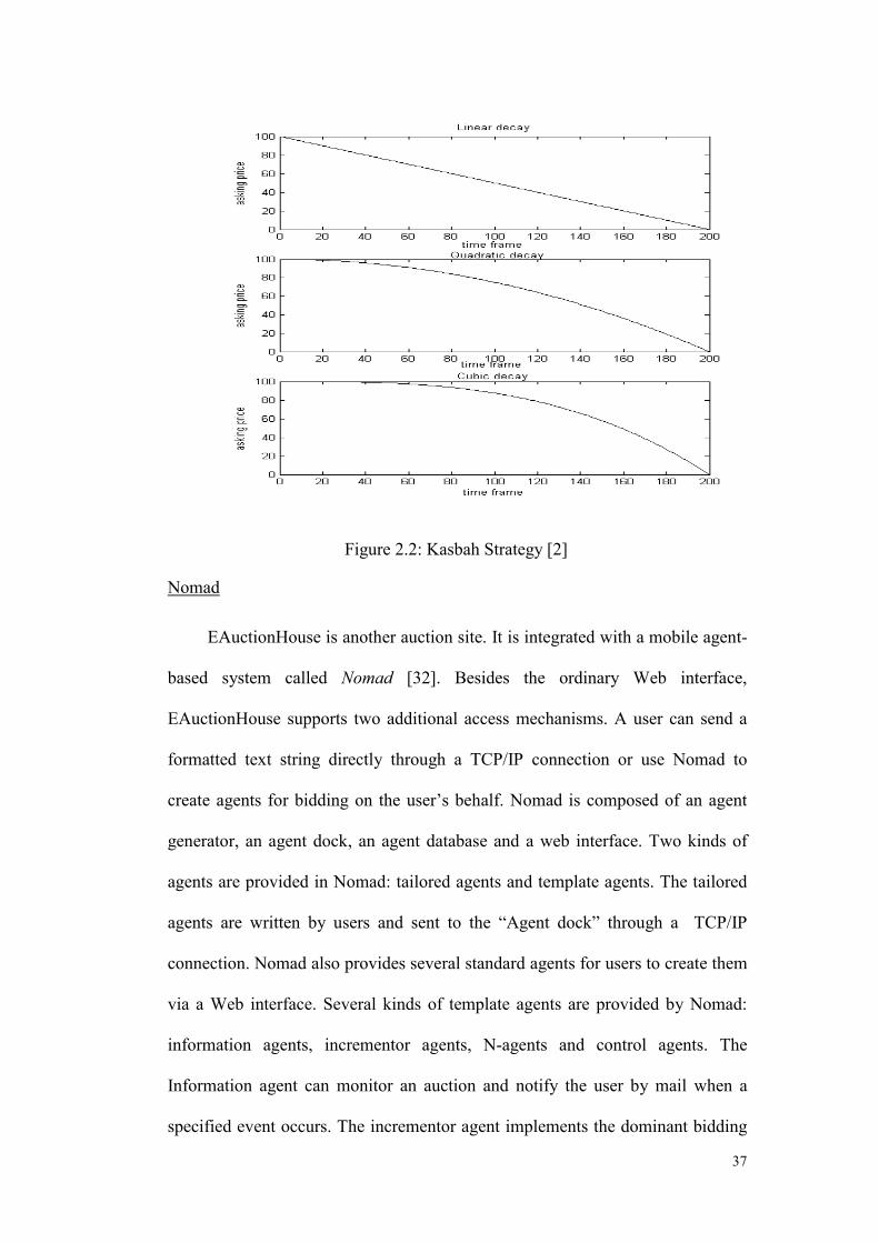
Figure 2.2: Kasbah Strategy [2]

Nomad

EAuctionHouse is another auction site. It is integrated with a mobile agent-

based system called Nomad [32]. Besides the ordinary Web interface,

EAuctionHouse supports two additional access mechanisms. A user can send a

formatted text string directly through a TCP/IP connection or use Nomad to

create agents for bidding on the user’s behalf. Nomad is composed of an agent

generator, an agent dock, an agent database and a web interface. Two kinds of

agents are provided in Nomad: tailored agents and template agents. The tailored

agents are written by users and sent to the “Agent dock” through a TCP/IP

connection. Nomad also provides several standard agents for users to create them

via a Web interface. Several kinds of template agents are provided by Nomad:

information agents, incrementor agents, N-agents and control agents. The

Information agent can monitor an auction and notify the user by mail when a

specified event occurs. The incrementor agent implements the dominant bidding

37

strategy in single English auctions. The N-agents is designed for FPSB auctions,

which implements the Nash equilibrium strategy given the distribution of the

agent valuation. Both user-written agents and standard agents are available in the

agent dock. They can communicate with eAuctionHouse through TCP/IP

connections using a predefined protocol.

MAGMA

The above auction sites only focus on the Brokering and Negotiation steps

of the buying process. MAGMA is an auction site, which focuses on the whole

buying process, covering also the purchase step [23].

In MAGMA, agents are not necessarily situated at the same location. They

can be local, functionally independent and communicate with each other through

socket connections. In other words, they can communicate using a common

communication layer and transmit messages using a packet that is something like

an IP packet consisting of a header and a body. A relay server is used to facilitate

communications between the agents. It maintains all socket connections and

routes messages between agents based on the agent names. There is also an

advertising server that stores information of items in the market and can reply to

requests generated from the trader agents. Another component of the market is

the bank, which contains accounts of all trader agents. It can handle money

transfer and check deposit. In MAGMA, a “trader agent” has two different states:

buying and selling. Each agent is associated with a wallet, an inventory, an ad

manager and a negotiator. The wallet stores the monetary information including

the banking accounts, check, tokens and so on. In the purchase step, the wallet

sends a payment request to the bank and receives the corresponding check. The

inventory stores the information of items to be sold and the ad manager is

38

responsible for advertising issues. The negotiator is to negotiate with the counter-

agent. It has two modes: manual mode and automatic mode. Using these two

modes, it integrates with the user-interface and the agent interface. MAGMA is

designed to be an open standard, allowing platform and language independent

agents that conform to the MAGMA messaging API to connect to the system,

register with the relay server, and conduct businesses over the MAGMA

infrastructure.

BiddingBot

Bidding agent

Bidding agentLeading agent

Bidding agent

Auctionsite

Auctionsite

Auctionsite

User

Figure 2.3: BiddingBot

Different from the above auction sites, BiddingBot is a multi-agent system

that supports users in attending, monitoring, and bidding in multiple auctions

[27]. Since there exists multiple auctions selling the same item simultaneously, it

is more beneficial to bid in multiple auctions and select the one with the lowest

price. However, it may result in “accidental purchase” (i.e., two or more auction

agents win). In BiddingBot, agents can communicate with each other so as to

avoid “accidental purchase”. BiddingBot is composed of a leader agent and

39

several bidder agents. Each bidder agent can bid in an auction site and the leader

agent is for monitoring the behavior of the bidder agents. Before submitting a bid,

the bidder agent sends a request message to the leader agent. The leader agent

accepts the bid if there are no agents holding an active bid or the active bids can

be withdrawn. In BiddingBot, users always buy the item with the lowest price

through BiddingBot and thus the “Winner’s curse” issue can be avoided.

2.4 Agent Bidding Strategies

The design of bidding strategies is related to game theory, where each

bidder only knows partial information and tries to win the game with minimum

loss. A strategy could depend on various factors, such as other bidders’ strategies,

the seller’s minimum accepting price, the number of auctions in the future.

However, the information that an agent knows is incomplete while it is required

to make a decision within a short time [38].

Many auction sites now provide agent-like services, which are

implemented with predefined and non-adaptive negotiation strategies. When

bidding in an English auction in eBay, a user can create a simple agent by

inputting its maximum bidding price [30]. The agent can automatically submit

the bid, which is equal to the sum of the current price and the minimum

incremental price. In Kasbah, three bidding strategies can be chosen as shown in

Figure 1.3 to bid in a continuous double auction: anxious, cool-headed and

frugal. They respectively correspond to linear, quadratic and exponential

functions for generating proposals/counter-proposals. The above strategies are

quite simple and straightforward. However, they are non-adaptive. In other

40

words, they do not make use of any available information and do not adapt to

change in the market situation.

K. M. Wong and E. Wong proposed a bidding strategy for continuous

double auctions [18]. Unlike the above non-adaptive bidding strategies, this

strategy is “market-driven”, that is, the strategy is changed when the market

situation varies. Before bidding in the market, the user should notify the agent of

its preference, the threshold of each attribute, the maximum bidding price M and

the user’s eagerness to trade G. After entering the market, the agent firstly

searches for all counter-offers and evaluates them. The agent only negotiates

with the count-offer with the maximum valuation. In the negotiation process, the

market situation is evaluated before making an offer. For example, a seller agent

considers the market situation at time t as the following four factors:

i. the number of seller agents St;

ii. the number of buyer agents Bt

iii. the number of agents interested in the agent’s current offer It;

iv. closing time of the marketplace T.

Using the above value, the agent could get the “remaining market time”

T(t), “competitions” C(t) and “attractiveness” A(t), which is calculated as:

( )T

tTtT −= (2.1)

( )tt

t

SBB

tC+

= (2.2)

( )t

t

BI

tA = (2.3)

41

The market situation at time t, which is denoted as M(t) is:

( ) ( ) ( ) ( )3

1 tAtCtTtM ++−= (2.4)

Therefore, the price that the buyer agent should submit at time t+1, bt+1is

( ) MEtMbt ×+

=+ 21 (2.5)

Using this strategy, bids submitted by sellers is dependent on the market

situation. With long remaining time, more buyer agents may be interested in the

offer, so the seller agent tends to give a higher offer and vice versa.

Another negotiation strategy in continuous double auctions has been put

forward by W. Y. Wong et al. [38]. This strategy applies the Case-Based

Reasoning (CBR) techniques to capture and reuse the previously successful

negotiation experiences. Given a counter agent, the strategy divides the

negotiation process into a number of decisions making episodes for evaluating an

offer, determining strategies and generating a counter-offer as shown in Figure

2.4:

Time

offer

counteroffer

Seller agent

Buyer agent

Episode 1 Episode 2 Episode 3 Episode 4 Episode 5

Figure 2.4: Negotiation process [38]

The offer in each episode is created by an episode strategy, which can be

changed from one to another. An episode strategy is represented by a concession

42

scheme. Given a series of offers: (O1, O2, O3, O4, O5), the concession in i+1-th

episode C(i+1) is represented as follows:

( ) %1001 1 ×−

=+ +

i

ii

OOOiC (2.6)

Thus a bidding process can be represented as a series of concession ratio.

The agent would store the concession series of successful negotiation experience.

In the agent’s database, the past auction records are firstly classified into

three categories according to the user’s objective: “Must-buy”, “Good-deal”,

“Best-price”. The second level records some attributes of the items. When

negotiating, the agent searches for all past negotiation records with the same

objective and similar item attributes, and matches the concession series with

those of the past records (see Figure 2.5). The one with the maximum similarity

is selected and its corresponding concession ratio is used as the concession ratio

of the current episode.

Buyer: (B1, B2, B3, B4, B5, B6, B7)Seller: (S1, S2, S3, S4, S5, S6, S7)

(b1, b2, b3)(s1, s2, s3)

Match

Match

Previous negotiation recordRecent concession list of

current negotiation

Figure 2.5: Match figure [38]

With the development of electronic commerce, it is often possible to find

auctions selling similar goods on the Web. However, the above strategies only

consider a single auction, which may be inefficient in two aspects:

i. For a buyer, it may pay more for an item than its real value, which is

called the “winner’s curse”.

43

ii. A seller may fail to make a deal in an auction site.

The above issues can be addressed by considering multiple simultaneous

auctions. By bidding in simultaneous auctions, buying agents can compare the

price of different auctions and then bid in the best auction. Selling agents could

also find the buyer with a higher offer thus achieving higher profits and higher

success transaction ratio. Furthermore, with more participants employing

multiple bidding strategies, the market can be more efficient and the equilibrium

price can be achieved.

Because of the above advantages, many researchers also investigate

bidding strategies for multiple auctions. The design of multiple-site bidding

strategies is more complicated than single-site bidding strategies because of the

complicated environment. Besides the bidding price, a multiple-site bidding

strategy should also select the appropriate auctions to participate. It is even more

complicated if the agent needs to buy multiple items, because the number of bids

should also be decided.

P. Anthony et al. proposed a multiple bidding strategy, which can be

applied for English, Dutch and Vickrey auctions simultaneously [26]. Before

bidding in the market, four parameters are assigned to the agent: the user’s

maximum bidding price, the latest time to obtain an item, the desire indicator etc.

In a bidding process, the agent decides the current maximum bidding price based

on the above parameters and other market attributes. Four tactics can be used in

this strategy, namely “the remaining time tactic”, “the remaining auctions tactic”,

“the desire for bargain tactic” and “the desperateness tactic”. For instance, the

remaining time tactic determines the recommended bid value based on the length

44

of residual time for the auction. The bid value at time t, frt is calculated by the

following expression:

( ) Mtf rtrt ×= α (2.7)

where αrt(t) is a polynomial of the form:

( ) ( ) βα

1

1

−+=

Ttkkt rtrtrt (2.8)

In (2.8), krt and β are constant values, M is the maximum bidding price set by the

user and T is the deadline to obtain the item.

The remaining time tactic reflects the current maximum bidding price of

the agent, taking into consideration of the remaining trading time. The other three

tactics respectively calculate the maximum bidding price based on the remaining

number of auctions in the market, the user’s desire and the user’s desperateness.

The final maximum bidding price is a combination of the four prices with a

certain weight assigned by the user. Given a maximum bidding price bt at time t,

the agent only considers the opening auctions that satisfy the following

conditions:

i. English auctions with imminent deadlines and minimum bidding prices

higher than bt

ii. Dutch auctions with current price no higher than bt

iii. Vickrey auctions with imminent deadlines

Among all the potential auctions, the agent calculates the expected utility of

each auction and bids in the auction with the maximum utility value. For an

English auction, the agent will bid up to bt; For a Dutch auction, the agent will

45

submit a bid once the price decreases to bt. For a Vickrey auction, the agent will

submit a bid at bt.

The performance of this strategy depends on ten parameters: four user

parameters, four weights, krt and β. A genetic algorithm has been applied to find

the optimum set of parameters under different market situations and bidding

objectives [25]. The algorithm is summarized as follows (see [25] for details):

Randomly create initial bidder populations; While not (Stopping Criterion) do

Calculate fitness of each individual by running the market place 2000 times;

Create new population Select the fittest individuals (HP); Create a “mating pool” for the remaining population;

Perform crossover and mutation in the mating pool to create new generation (SF);

New generation is HP+SF;

End While

After running for 2,000 times, a set of stable parameters were obtained,

which is the optimum set of parameters in the given bidding situation. The paper

inspected four market situations: short bidding time and a small number of active

auctions in the marketplace (STLA); short bidding time and large number of

active auctions (STMA); long bidding time and small number of active auctions

in the marketplace (LTLA); long bidding time and large number of active

auctions in the marketplace (LTMA). Three different utility functions are used,

which represent the preference of users. Having classified the market situation

into multiple categories, the optimum parameters of each situation could be

determined [25]. The intelligent agent could always assign the appropriate

parameters according to the suitable market situations.

46

Another bidding strategy based on dynamic programming has been

proposed by A. Byde [1]. The strategy applies for English auctions for one item.

The price is increased by a fixed amount and one of the bidding agents is

randomly selected to be the highest bidder. If there are no agents submitting bids

in a given time step, the item should be awarded to the agent with the highest bid

and the auction closes. Three bidding algorithms namely “GREEDY”,

“HISTORIAN” and “OPTIMAL” are put forward. Agents using the “GREEDY”

algorithm always bid with the lowest current price without taking other issues

into consideration. For the “HISTORIAN” algorithm, an agent bids with the

highest expected utility. For the “OPTIMAL” algorithm, an agent is assigned a

market state according to the current auctions in the market. Since each auction

may change to another state with a certain transitional probability, the market

situation transitional probability takes into account the corresponding transitional

probabilities of each auction. A reward is assigned to the transition from state A

to state B, which is calculated to be the total value minus the payment for the

items bought for the transition and the expected payments on active bids in state

B. Since the state space is finite and a-cyclic, the value of each state can be

determined by an inductive computation process and the agent should bid in the

auction that maximizes the value. Experiments showed that the “OPTIMAL”

algorithm outperform the others while the simple “GREEDY” algorithm gives

the worst performance.

Some researchers also investigate a bidding strategy for agents to bid

multiple items in multiple simultaneous English auctions [4], [5]. The strategy is

composed of two sub-algorithms, which are respectively used to decide how to

allocate multiple bids in the current active auctions and whether to leave the

47

current bidding auction for another auction with a lower bidding price. All

auctions in the market are discriminatory multi-item English auctions, that is,

winner should buy the item with what he/she bid. Given an English auction

selling j items, the optimum strategy for the agent is to outbid the j-th highest

price in order to achieve the highest utility. If an agent bids k items in an j-item

English auction, the corresponding optimum strategy is to outbid the (j-k+1)-th

price for k times. If an agent holds one or more active bids in Na auctions and it

wants to get a total of NT items, the first rule gives out the best allocation of the

other (NT-Na) bids. For each auction, a beatable-j list is calculated, where

. The beatable-j list consists of the lowest j active bids excluding the

agent’s own k bids. To bid j items in the auctions, the optimum strategy is to

submit the bid which is equal to the sum of the j-th price in the beatable-j list and

the incremental price for j+k times. Using a depth-first searching method, the

agent can easily find out the best allocation of the N

TNj ≤≤1

T-Na bids.

The above mechanism is optimum when all English auctions end

simultaneously. However, auctions may also terminate at different times. Given

two auctions, one with a higher price and imminent deadline and the other one

with a lower price and longer deadline, the agent needs to choose which auction

to participate. The mechanism proposed in the paper combines a simple learning

algorithm with the utility theory. That is, it firstly works out a winning

probability function B(x,q) based on several learning techniques. B(x,q) indicates

the probability that x bidders value the good with a valuation greater than q in a

given auction. With a bid price q, an agent can win with probability 1-B(j,q) in

the auction with j items to sell. Based on the winning probability, the utility in

both auctions can be easily worked out. For the auction with imminent deadline,

48

the utility is U1 = M-q, where M is maximum bidding price and q is the agent’s

bidding price. For the auction with a longer deadline, its utility is represented as

follows:

( ) ( )( )∑=

−×−−=v

qqMqjBqjBU

02 ,1, ( ) (2.9)

Given U1>U2, the agent should bid the first auction up to price M-U2.

Otherwise, it should move jump to the second auction. Using this strategy, the

agent can achieve optimal or near-optimal purchase decisions.

Marlon Dumas et al. proposed a bidding strategy to buy a single item in

heterogeneous auctions including English auction, FPSB auction and Vickrey

auction [19], [20]. All English auctions in the market have predefined deadlines.

Before an agent entering the market, it is assigned the maximum bidding price M,

the deadline to leave the market T and the minimum expected probability of

obtaining the item G. It is assumed that it takes L time units to execute a

transaction so two auctions can be participated by the agent sequentially only if

their deadlines are separated by at least L time units. In the bidding phase, the

bidding agent selects a set of auctions As and a bidding price bt, where bt ≤ M.

The following conditions should also be satisfied:

• The deadlines of auctions in As are non-conflicting. That is, the agent

could sequentially participate in all auctions in As.

• Denote the probability that at least one of the selected bids succeeds

as P(As, bt), P(As, bt) should be no lower than the expected winning

probability G. That is:

( ) ( )( ) GbPbAPsAa

tats ≥−−= ∏∈

11, (2.10)

49

where Pa(bt) is the probability of winning auction a with a maximum

bidding price bt.

• The bidding price bt is the lowest one among all possible prices that

satisfy the above two conditions.

Given the optimum auction set and the bidding price bt, the agent

successively places bids in each of the selected auctions until one of them is

successful. In case of sealed-bid auctions, the agent places a bid at price bt. For

English auctions, the agent bids at bt just before the auction closes since last-

minute bidding works best for English auctions.

Several prediction methods

In the previous bidding strategies, the winning probability function has

been widely used and several schemes to predict the winning probability have

been put forward. The histogram method and the normal method are the most

popular methods [20].

The histogram method assumes that the winning probability with price z in

a given FPSB auction or English auction with current price zero is the same as

the ratio of number of the times that an agent can win with price z in the past

auctions to the number of all past auctions. Denote P(x) as the probability that

the past auction price is x. Thus P(x) is equal to the number of previous auctions

with final price x, divided by the number of all past auctions. For example, if the

sequence of observed final prices is (22, 20, 25), the winning probability with

price z in auction a with zero current price is:

50

( )

<<≤<≤

≥

=

200222033.0252266.0

251

zifzifzif

zif

zPa (2.11)

If it is known that the winning price of the auction is no lower than price q,

the corresponding winning probability should be revised to:

( )( )

( )∑∑

≥

≤≤

=

==

qx a

zxq aa xfpP

xfpPzP (2.12)

where . Otherwise, Pqz ≥ a(z) = 0.

The histogram method is straightforward. However, it has two

disadvantages. First, the computation of winning probability is dependent on the

size of the set of past auctions. Second, if the minimum winning price is higher

than all final prices of the past auctions, the winning probability cannot be found.

Compared to the histogram method, the normal method addresses the above two

drawbacks.

The normal method assumes that the distribution of winning price follows a

normal distribution with mean µ and variance σ. Thus the winning probability

with price z in an auction a with zero minimum price is:

( ) ∫−

∞−

−= σ

µ

σπ

z x

a dxezP 2

2

21

(2.13)

The winning probability of auction a with minimum price q is:

( )∫

∫∞

−

−

−

−

−

=

σµ

σµ

σµ

q

x

z

q

x

a

dxe

dxezP

2

2

2

2

(2.14)

51

However, the winning price in English auctions and Vickrey auctions

reflects the maximum bidding price of the second highest bidder instead of the

maximum bidding price of the winner. A simulation algorithm can be used to

produce the maximum bidding price of the highest bidder. It first examines all

the maximum bidding price of the failed bidders and then figures out the

distribution of the maximum bidding price. For each previous auction, a series of

numbers are produced according to this distribution and the first one that equals

to or higher than the final price of that auction is assigned as the maximum

bidding price of winner. After processing all auction records, the right

distribution can be worked out easily.

Another prediction method based on machine learning has been put

forward by R. E. Schapire [29]. The learning problem can be viewed as a

conditional-density-estimation problem: given current conditions, estimate the

conditional distribution of prices. A boosting-based algorithm is proposed.

Abstractly, given pairs (x1, y1), (x2, y2), …, (xn, yn), where each xi belongs to a

space X and each yi is in R. The xi’s are the auction-specific feature vectors for

some n, X⊆(R∪{⊥})n. Each target quantity yi is the difference between the

closing price and the current price. Given a new x, the goal of the algorithm is to

estimate the conditional distribution of y given x. The algorithm first divides the

value of y into equal-length bins:

[ ) [ ) [ ) [ )1322110 ,,......,,,,,, +kk bbbbbbbb

where 1210 ... +<<<<< kk bbbbb

The purpose of the algorithm is to estimate the probability that a new y

(given x) will be at least bj. Given the estimate pi for each bj, the probability that

52

y is in the bin [ )1, +jj bb

} R→

is pj+1-pj. A logistic regression algorithm based on

boosting techniques is applied to calculate pi. First a real-valued function

is set up with the interpretation that { kXf × ,...,2,1:

( )( )jxf ,exp11−+

(2.15)

This is the estimate of the probability that y , given x. The boosting-like

algorithm is used to find out the function f that minimizes

jb≥

( ) ( )( )∑∑= =

−+m

i

k

j

jxfys iije1 1

,1ln (2.16)

where ( )

<−≥+

=j

jj byif

byifys

11

2.5 Summary

In this chapter, we have given an overview of agent-based auction systems.

The use of agent technology in online auctions not only save user’s time but also

can enhance the bidding efficiency. The key issue in designing an agent-based

auction system is the development of bidding strategies. Several bidding

strategies for agent-based online auctions have been introduced in the chapter.

Generally, the bidding strategies can be divided into two categories: single-site

bidding strategies and multiple-site bidding strategies. Unlike single-site bidding

strategies, the multiple-site bidding strategies can be used in handling multiple

heterogeneous auctions. As many bidding strategies rely on the prediction of

winning probabilities, several simple prediction schemes have also been

described.

53

CHAPTER 3

DETERMINISTIC BIDDING STRATEGY AND WINNING PRICE PREDICTION

3.1 Introduction

As mentioned previously that one of the fundamental issues in designing

agent-based auction services is to develop an effective bidding strategy; in other

words, how to instruct an agent to place bids on behalf of the user. Kasbah

allows users to specify a negotiation strategy in terms of a price-time function [2].

AuctionBot provides an application programming interface for users to develop

customized agents [27]. In addition, there are also bidding strategies for handling

auctions at multiple sites; e.g., [26], [1].

Many auction sites such as eBay provide a proxy bidding service, which

can be viewed as a simple bidding strategy [30]. This proxy bidding strategy

allows a user to specify a maximum bid price called the maximum bidding price,

such that the user can keep bidding automatically unless the specified maximum

bidding price is exceeded. This popular proxy bidding strategy can also be

extended to mobile agent-based auction systems. In this case, an agent is

instructed to continue bidding up to a certain price. In fact, the mobile agent-

based approach has an advantage over the traditional proxy bidding service

because the maximum bidding price can be kept secret (i.e., the auctioneer

cannot know the maximum bidding price). Due to the popularity of the proxy

bidding strategy, there is a need to analyze its behavior.

54

In this chapter, we first analyze the general proxy bidding strategy for an

auction system called C2C MAGICS. The analysis provides valuable insights

into the design of auction services in general and the agent-based auction systems

in particular. Based on the distribution of the maximum bidding price or the

reserve price, the model can be used to determine the probability of stopping at a

particular price and the expected winning price. Simulation and analytical results

are presented to evaluate the system's behavior. To perform the analysis, it is

important to obtain the winning probability in an auction for a certain maximum

bidding price. For the proxy bidding strategy, two prediction schemes are used to

estimate the distribution of maximum bidding prices from the distribution of

winning prices. These two schemes are the method of moments and the

maximum likelihood estimation. Some experiments have been done to evaluate

the performance of the two schemes and compare them with other prediction

schemes. Experimental results indicate that the method of moment and maximum

likelihood estimator work more effectively than other schemes.

The organization of the remaining sections of this chapter is as follows.

Section 3.2 describes the system architecture of the mobile agent-based auction

system. Section 3.3 formulates the mathematical model to evaluate the bidding

results and discusses the simulation and analytical results. Section 3.4 presents

the prediction methods and evaluates its performance. Section 3.5 concludes this

chapter.

55

3.2 System Architecture

User terminals

Proxy server

Internet

Access moduleAuction protocol moduleBackend system moduleAdministration moduleOther module(s)

Mobile agent

Auction server

Figure 3.1: System architectures

Figure 3.1 shows the architecture of the mobile agent-based auction system

as presented in [9]. There are five sub-systems: The access module is for

processing incoming mobile agents. The auction protocol module contains the

auction rules to support different types of auctions. The backend system stores

the necessary information (e.g., user information). The administrative sub-

system is for management purposes. Finally, there are other supporting systems,

such as payment gateways to handle payment functions. The above auction

system is called C2C MAGICS, which is part of the Mobile Agent-based Internet

Commerce System (MAGICS). The aim is to facilitate C2C e-commerce by

using mobile agents to complement the current Web-based e-commerce system.

Unlike other auction sites, the task of bidding can be delegated completely to a

mobile agent. Users can instruct their agents to bid using a particular bidding

strategy.

56

Figure 3.2: System interfaces

As many user terminals may not be able to support mobile agents, a proxy

server is provided for users to create the required agents. In fact, the proxy server

can be used to create other mobile agents for different purposes (e.g., to create

some agents to search for a desirable product or to compare the prices of a

product). Users can access the proxy server through a Web or WAP interface. To

create an agent, a user needs to input the bidding information including the

reserve price (i.e., the maximum bidding price). The agent searches for the

respective auction server and moves to the respective “auction space” to bid for

the item with other agents. The aforementioned bidding strategy is used in which

each agent keeps bidding up to the specified reserve price. In the following

analysis, we consider using either the English or Dutch auction method to buy

and sell one item.

57

3.3 Market Analysis

3.3.1 Mathematical model

In this section, an analytical model is formulated to evaluate the bidding

results for both the English and Dutch auctions. These include computing the

distribution of the winning price and, hence, the average winning price. The

model is summarized as follows.

There are a total of n agents participating in an English/Dutch auction. The

possible prices are b0, b1, b2, … bd. The incremental/decremental price for the

English/Dutch auction is h, so we have bi=bi-1+h (i=1,2,3,…,d). Note that for the

English and Dutch auctions, the bidding prices are: (b0, b1, b2, …) and (bd, bd-1,

bd-2, …), respectively. Note that the price b0 and b1 are so low that each agent is

able to bid and the initial price bd in Dutch auction is so high that no agents could

accept it. Each agent is provided with a maximum bidding price, which follows a

distribution R. In other words, the probability that the winning price does not

exceed bi is R(bi). In general, each agent always gives a bid, provided that the

bidding price does not exceed its maximum bidding price. Denote F(bi) as the

probability that the winning price does not exceed bi. Note that in the later

analysis, an appropriate subscript will be added to identify the auction type:

English (E) or Dutch (D). Based on R(bi) and n, the objective of the following

analysis is to determine F(bi) as well as the average winning price. A number of

distributions for the maximum bidding prices will be considered.

English auction

For the English auction, the bidding prices keep rising until no one submits

a higher bid. Each submitted bid should be the current highest price, plus the

58

incremental price h. Finally, the item is sold to the bidder who submits the

highest bid. Given the distribution of the reserve price and the number of agents,

we can compute the distribution of the final price and the expected winning price

AE as follows.

As we know, if more than one agent has a reserve price higher than bi, no

matter which agent bid price bi, at least one agent would outbid it. And the final

winning price must be larger than bi. Two possible cases with winning price bi

are considered here:

Case 1: The reserve price of all n agents does not exceed bi, so no one will bid

higher than bi. This case occurs with probability Rn(bi).

Case 2: If there is an agent t with reserve price larger than bi, it will certainly be

the winner. In the case that there are i (i=0,1,…n-1) agent(s) with reserve

price bi, the final price does not exceed bi only when t is the winner. This

case occurs with probability

( )( ) ( ) ( ) ( ) ( )( )∑−

=−−

−−− −×+

−1

011

11

111

n

i

iiii

innii bRbRbR

ibRn .

Integrating the above cases, we get the distribution of the winning price F(bi) as

follows:

( ) ( ) ( )( ) ( ) ( ) ( ) ( )( )

( ) ( )( ) ( ) ( ) ( )( )1

1

1

011

11

11

11

−−

−

=−−

−−−

−−

−+=

−×+

−+= ∑

in

in

ii

ii

n

n

i

iiii

inniii

niE

bRbRbRbR

bRbR

bRbRbRi

bRnbRbF (3.1)

It is not difficult to see that with probability FE(bi)- FE(bi-1), the winning price

will stop at bi. Thus we could get the auction’s average winning price AE as:

59

( ) ( )( ) ( ) ( )(∑∑+∞

=−

+∞

=− −+=−×=

110

11

iiEiE

iiEiEiE bFbFihbbFbFbA ( )) (3.2)

If the reserve prices of the agents have upper limit bd, the average winning price

can be transferred as follows:

( ) ( ) ( )( ) ( ) ( )∑∑∑−

=

−

==− −=−+=−+=

1

0

1

00

110

d

iiEd

d

iiE

d

iiEiEE bFhbbFhhdbbFbFihbA

(3.3)

Dutch auction

A Dutch auction works in the opposite way from English auction. Here we

consider that only one item is sold. First the auctioneer announces a very high

price bd and then decreases the price gradually by h each time. The first bidder

who accepts the price becomes the winner and the item is sold at the accepted

price. Given the distribution of the reserve price and the number of agents, we

can compute the distribution of the final price and the expected winning price AD

as follows

The analysis for a Dutch auction is simpler than that for an English auction.

According to the strategy, the winning price in a Dutch auction is equal to the

highest reserve price among all agents. If the winning price is equal to or lower

than bi, the reserve price of all n buyers must not exceed bi. Thus, we can easily

get the distribution of the winning price as

( ) ( )in

iD bRbF = (3.4)

Similar to above, the average winning price can be computed as follows:

( ) ( )( ) ( ) ( )( ) ( )∑∑∑−

==−

=− −=−×=−×=

1

001

01

d

ii

nd

d

ii

ni

ni

d

iiDiDiD bRhbbRbRbbFbFbA

(3.5)

60

In the following sub-sections, we will use the above model to evaluate the

bidding results for several linear distributions for the reserve price. More

specifically, the distribution of the winning price and the expected winning price

will be computed.

Probability

Reserve pricec1

c2

brbl

Probability

Reserve pricebl br

c1

c2

Probability

Reserve pricebl br

c1 c2

Figure 3.3: Linear distribution

Here we assume that the reserve price set by a user follows a linear

distribution between bl and br. The density functions of several linear

distributions H(b) are shown in Figure 3.3, where br should be larger than bl.

Assume the H(bl) and H(br) is c1 and c2, respectively. According to the property

of density function, we could easily get that lr bb

c−

=+2

21c . Therefore, the

linear distribution can be modified as uniform distribution and linear increasing

distribution and linear decreasing distribution by adjusting the value of c1.

Thus, the density function of the reserve price is:

61

( )( )

( )

>

≤≤+−

−−

−

<

=

r

rlllrlr

l

bbif

bbbifcbbbb

cbb

bbif

bH

1

220

11

2 (3.6)

We can easily get the distribution of the reserve price as follows:

( ) ( )( )

( )( )

>

≤≤−

−−+

−

−<

=

r

rllr

rl

lr

l

l

bbif

bbbifbb

bbbbcbbbb

bbif

bR

1

01

2

2

(3.7)

Based on (3.1), the distribution of the winning price in an English auction is:

( ) ( )( )

( )( ) ( ) ( ) ( )( )(( ) ( )(

))

( )( )

( )( ) ( )( )

( )( )

−+−−−

+−

−−−

−−−

+−

−

−++−+−−−−−−−−−

+

−−−

+−

−=

n

lr

irli

lr

li

n

lr

irli

lr

li

ilrlrli

irlilrlilr

n

lr

irli

lr

liiE

bbhbbbhbc

bbbhb

bbbbbbc

bbbb

bbbhbbhchbbhbbbbbbcbbbb

bbbbbbc

bbbb

bF

12

21

2

2

12

122

12

2

22

(3.8)

where b ril bb ≤≤

Note that when b or , we haveli b< γbbi > ( ) 0=ibF and ( ) 1=ibF , respectively.

This applies to the following cases as well.

The average winning price in English auction is

( ) ( )∑∑−

=

−

=

−=−+=1

0

1

00

r

ii

nEr

r

ii

nEE bFhbbFhhrbA (3.9)

For a Dutch auction, the distribution of the winning price is

( ) ( )( )

( )( ) n

lr

rl

lr

liD bb

bbbbcbbbb

bF

−−−

+−

−= 1

2

2

(3.10)

where b ril bb ≤≤

Hence, the average winning price is

62

( )( )

( )( )∑−

=

−−−

+−

−−=

lr

i

n

lr

irli

lr

lirD bb

bbbbcbbbb

hbA1

12

2

(3.11)

3.3.2 Experimental Results

100 120 140 160 180 200 220 240 260 280 3000

0.01

0.02

0.03

0.04

0.05

0.06

0.07

0.08

Winning price

Pro

babi

lity

English Auction

Uniform distribution (Analytical)Normal distribution (Analytical)Uniform distribution (Simulation)Normal distribution (Simulation)

Figure 3.6: Probability of stopping at a particular price for an English

auction with ten bidders

100 120 140 160 180 200 220 240 260 280 3000

0.02

0.04

0.06

0.08

0.1

0.12

0.14

0.16

0.18

0.2

Winning price

Pro

babi

lity

Dutch Auction

Uniform distribution (Analytical)Normal distribution (Analytical)Uniform distribution (Simulation)Normal distribution (Simulation)

Figure 3.7: Probability of stopping at a particular price for a Dutch auction

with ten bidders

We have applied the above model to carry out some analysis. Furthermore,

63

we have also validated the analytical results by means of simulations. For the

simulations, a Java program has been written to simulate the auction process.

Each simulation was repeated 100,000 times to obtain the steady state results.

Figure 3.6 and Figure 3.7 show the probability of stopping at a particular

price for English and Dutch auctions, respectively with n=10. As shown in the

previous section, the probability can be found as F(bi)-F(bi-1). For the linear

distribution, we set c1= c2 so that it is actually a uniform distribution with

minimum and maximum reserve prices set at $150 and $250, respectively. The

mean and variance of the normal distribution are $150 and $50, respectively.

Figure 3.6 shows the distribution of the winning price when ten agents

participated in an English auction. The analytical and simulation results are

almost the same, thus indicating the correctness of both models. Figure 3.7

shows the distribution of the winning price for the Dutch auction with the same

set of simulation parameters as the English auction. It can be seen that the Dutch

auction method tends to give a higher winning price.

150 155 160 165 170 175 180 185 190 195 2000

0.1

0.2

0.3

0.4

0.5

0.6

0.7

0.8

0.9

Winning price

Pro

babi

lity

Linear distribution with k=0.5

n=10 (Analytical)n=20 (Analytical)n=40 (Analytical)n=80 (Analytical)n=160 (Analytical)n=10 (Simulation)n=20 (Simulation)n=40 (Simulation)n=80 (Simulation)n=160 (Simulation)

Figure 3.8: Probability of stopping at a particular price for an English

auction with a uniform distribution for the reserve price

64

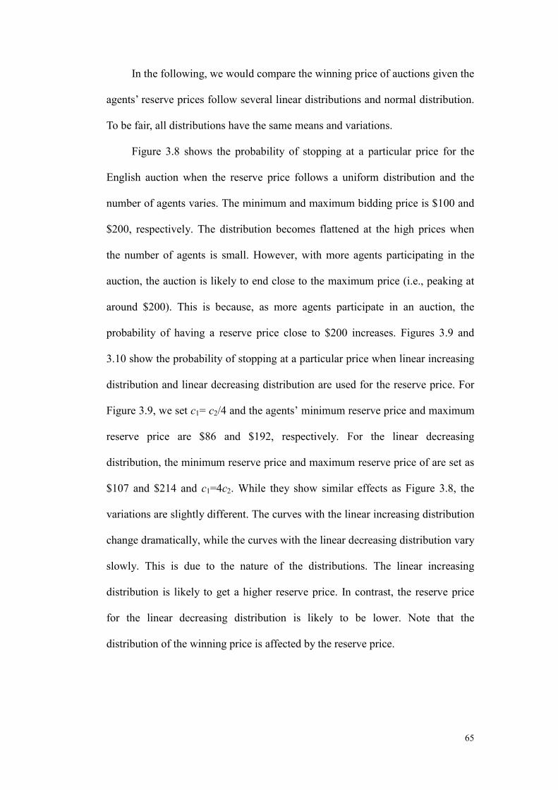
In the following, we would compare the winning price of auctions given the

agents’ reserve prices follow several linear distributions and normal distribution.

To be fair, all distributions have the same means and variations.

Figure 3.8 shows the probability of stopping at a particular price for the

English auction when the reserve price follows a uniform distribution and the

number of agents varies. The minimum and maximum bidding price is $100 and

$200, respectively. The distribution becomes flattened at the high prices when

the number of agents is small. However, with more agents participating in the

auction, the auction is likely to end close to the maximum price (i.e., peaking at

around $200). This is because, as more agents participate in an auction, the

probability of having a reserve price close to $200 increases. Figures 3.9 and

3.10 show the probability of stopping at a particular price when linear increasing

distribution and linear decreasing distribution are used for the reserve price. For

Figure 3.9, we set c1= c2/4 and the agents’ minimum reserve price and maximum

reserve price are $86 and $192, respectively. For the linear decreasing

distribution, the minimum reserve price and maximum reserve price of are set as

$107 and $214 and c1=4c2. While they show similar effects as Figure 3.8, the

variations are slightly different. The curves with the linear increasing distribution

change dramatically, while the curves with the linear decreasing distribution vary

slowly. This is due to the nature of the distributions. The linear increasing

distribution is likely to get a higher reserve price. In contrast, the reserve price

for the linear decreasing distribution is likely to be lower. Note that the

distribution of the winning price is affected by the reserve price.

65

150 155 160 165 170 175 180 185 190 1950

0.1

0.2

0.3

0.4

0.5

0.6

0.7

0.8

0.9

Winning price

Pro

babi

lity



Figure 3.9: Probability of stopping at a particular price for an English auction


150 160 170 180 190 200 2100

0.1

0.2

0.3

0.4

0.5

0.6

0.7

Winning price

Pro

babi

lity





66

120 140 160 180 200 220 240 2600

0.01

0.02

0.03

0.04

0.05

0.06

0.07

0.08

0.09

Winning price

Pro

babi

lity

Normal distribution




150 155 160 165 170 175 180 185 190 195 2000

0.1

0.2

0.3

0.4

0.5

0.6

0.7

0.8

0.9

Winning price

Pro

babi

lity



Figure 3.12: Probability of stopping at a particular price for a Dutch auction


Figures 3.11 show the probability of stopping at a particular price when the

agents’ reserve price follows a normal distribution, with mean and variance of

$150 and $28.87, respectively. It can be seen that the winning probability follows

67

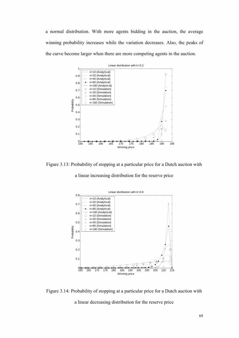
a normal distribution. With more agents bidding in the auction, the average

winning probability increases while the variation decreases. Also, the peaks of

the curve become larger when there are more competing agents in the auction.

150 155 160 165 170 175 180 185 190 1950

0.1

0.2

0.3

0.4

0.5

0.6

0.7

0.8

0.9

1

Winning price

Pro

babi

lity



Figure 3.13: Probability of stopping at a particular price for a Dutch auction with

a linear increasing distribution for the reserve price

160 165 170 175 180 185 190 195 200 205 210 2150

0.1

0.2

0.3

0.4

0.5

0.6

0.7

0.8

Winning price

Pro

babi

lity




a linear decreasing distribution for the reserve price

68

140 160 180 200 220 240 260 2800

0.01

0.02

0.03

0.04

0.05

0.06

0.07

0.08

Winning price

Pro

babi

lity

Normal distribution



normal distribution for the reserve price

Figures 3.12, 3.13, 3.14 and 3.15 show the probability of stopping at a

particular price for a Dutch auction when the reserve price follows the uniform,

linear increasing, linear decreasing and normal distributions, respectively. The

parameters are the same with those for English auctions. In general, they are

similar to the graphs for an English auction.

Next, we analyze the relationship between the average winning price and

the distribution of the reserve price. Figure 3.16 shows the average winning price

for English and Dutch auctions when the number of agents varies. From the

graphs, it can be seen that the average winning price increases towards the

maximum price as more agents participate in the auctions. It can be seen that the

average winning price for the four distributions are close to each other. However,

with more agents participate in the auction, the average winning price for the

normal distribution is the highest and the average winning price for the linear

increasing distribution tends to be the lowest.

69

Furthermore, we compare the average winning price in English and Dutch

auctions. As shown in Figure 3.16, the average winning price for an English

auction is generally lower than that for a Dutch auction. This is because for

English auctions, the winning price is the second highest reserve price or the

second highest reserve price plus the incremental price. For Dutch auctions, the

winning price is always the highest reserve price. However, the difference is

greatly reduced as more agents participate in the auction.

10 20 30 40 50 60 70 80 90 100175

180

185

190

195

200

205

210

215

220

225

Number of agents

Ave

rage

win

ning

pric

e

Comparison

k=0.2 (English)k=0.5 (English)k=0.8 (English)Normal distribution (English)k=0.2 (Dutch)k=0.5 (Dutch)k=0.8 (Dutch)Normal distribution (Dutch)

Figure 3.16: Comparison of the average winning price for English and Dutch

auctions

3.4 Prediction of winning probability

3.4.1 Several prediction schemes

In the above section, we have analyzed the general proxy bidding strategy

and computed the distribution of winning prices. A related issue is how to get the

winning probability for a certain maximum bidding price. To calculate the

probability, we must have the distribution of maximum bidding prices.

70

Unfortunately, it is unknown in the real world. So, for the proxy bidding strategy,

two prediction schemes are used to predict the distribution of maximum bidding

prices from the distribution of winning prices. They are the method of moments

and the maximum likelihood estimation.

To perform the analysis, we define the notations as follows:

A is the set of previous auction records.

|A| is the number of auction records.

ai is the i-th auction in the auction set A.

x(a) indicates the winning price of auction a.

N(a) gives the number of agents participating in auction a.

Ai is the set of auction records with i agents participating in the

auction.

Fc(bz) gives the winning probability of the current auction c with

reserve price bz.

The aim of a prediction scheme is to compute Fc(bz) for each reserve price bz.

Histogram method

The histogram method can deal with FPSB auction or English auction. The

key assumption of the method is that the distribution of the winning price

depends on the historical frequencies. It means that the winning probability with

price z in an initial auction is the same as the ratio of number of the times that the

agent could win with price z in the past auctions to the number of all past

auctions.

71

Thus Fc(bz) is equal to the number of previous auctions with final price no

higher than bz, divided by the number of all past auctions. Mathematically the

winning probability is represented as:

( ) ( ) ( )

||,)(

AAabaxPbF zi bax

zzc

∑ ≤=∈≤= (3.12)

If it is known that the winning price of the auction must be no lower than q,

the winning probability should be revised to

( ) ( )( )

( )( )

( )

( )∑∑

<

≤

−=

∈<−∈≤

=∈≥∈≤

=qax

baxzzzc

i

zi

AAaqaxPAabaxP

AaqaxPAabaxPbF

||,)(1,)(

,)(,)(

(3.13)

where b . Otherwise, Fqz ≥ c(bz) = 0.

Similar to above, if it is known that the winning price of the auction must

be no higher than q, the winning probability should be revised to

( ) ( )( )

( )

( )∑∑

≤

≤=∈≤∈≤

=qax

baxzzc

i

zi

AaqaxPAabaxP

bF,)(,)( (3.14)

where b . Otherwise, Fqz ≤ c(bz) = 0.

The histogram method is simple to understand. However, it has two

disadvantages:

• Winning probability is computationally intensive. That is, each time the

prediction is needed, the whole database that stores the historical records

must be re-processed to calculate the corresponding winning probability.

• If the minimum bidding price q is higher than the winning prices of all

the past auctions, the histogram method is generally not applicable. It is

72

because that the denominator of the above formula is equal to zero. In

other words, the histogram method is unable to give a prediction if the

current quote has never been observed in the past.

Normal method

The normal method assumes that the distribution of winning price follows a

normal distribution with mean µ and variation σ [19]. Thus the winning

probability with price bz can be calculated as:

( ) ( ) ∫−

∞−

−=≤= σ

µ

σπ

zb t

zzc dtebaxPbF 2

2

21)( (3.15)

The winning probability of an auction with minimum price q is:

( ) ( ) ( )( ) ( )( )( )( )

∫

∫∞

−

−

−

−

−

=≥

≤≤=≥≤=

σµ

σµ

σµ

q

t

b

q

t

zzzc

dte

dte

qaxPbaxqPqaxbaxPbP

z

2

2

2

2

| (3.16)

Similar to above, given that the winning price of auction is no higher than q, the

winning probability with maximum bidding price bz can be calculated as:

( ) ( ) ( )( ) ( )( )( )( )

∫

∫−

∞−

−

−

∞−

−

=≤≤

=≤≤=σ

µ

σµ

q t

b t

zzzc

dte

dte

qaxPbaxPqaxbaxPbP

z

2

2

2

2

| (3.17)

Since the winning price in English auctions and Vickrey auctions reflect the

maximum bidding price of the second highest bidder instead of the maximum

bidding price of the winner, a simulation program is used to find the maximum

bidding price of the highest bidder. It firstly inspects all the maximum bidding

prices of the failed bidders and figures out the distribution of the maximum

73

bidding price. For each auction, a series of numbers are produced according to

the distribution and the first one that equals to or higher than the final price of

that auction is assigned as the maximum bidding price of the winner. After

considering all the auction records, the appropriate distribution can be worked

out.

Compared to the histogram method, the normal method addresses the above

two drawbacks. It only needs to store the number of records, the mean and the

variation. The normal method is able to compute a probability of winning an

auction with a given bid, even if the value of the specific quote in that auction is

greater than that of all the final prices of the past auctions. In fact, the normal

distribution considers the whole set of real numbers. This is unlike the histogram

method which only considers the winning prices that have occurred.

3.4.2 Method of Moments and Maximum Likelihood Estimation

In fact, the above prediction schemes both consider that the winning prices

have a consistent distribution. They employ the winning prices of previous

auction records and predict the distribution (in Histogram method the distribution

consists of historical frequencies of the winning prices; in Normal method the

distribution is normal, and the mean and variation are determined by the

historical records). However, the distribution is influenced by other important

factors such as the number of agents that participate in an auction. From the

analysis of the popular auction market in previous sections, we can get that the

distribution of the winning price depends on the number of agents. While the

Normal method is grounded on an assumption that the distribution of winning

price follows a normal distribution, it is more reasonable to assume that the

74

distribution of the maximum bidding price of each agent follows a normal

distribution. The method of Moments and the Maximum likelihood estimators

are based on this assumption and make use of both the winning price and the

number of agents in the auction records to perform the prediction [16].

Method of Moments

Let X be a random variable having the probability density function f(x;

Q1,Q2,…,Qk), where Q1,Q2,…,Qk are parameters that characterize the distribution.

The r-th moment about the origin, ur(Q1,Q2,…,Qk) is defined as

( ) [ ]rkr xEQQQu =,....,, 21 (3.18)

If the distribution is continuous, the expected value is

[ ] ( )∫∞

∞−== dxxxfxEu1 (3.19)

and

[ ] ( )∫∞

∞−== dxxfxxEu 22

2 (3.20)

There is another kind of moments, called the moments for center. It can be

calculated as follows:

( ) ( )( )[ ]rkr xExEQQQv −=,....,, 21 (3.21)

If the distribution is continuous, we get

( )[ ] 01 =−= xExEv (3.22)

and

( )( )[ ] ( ) ( ) ( ) ( )( ) (∫∞

∞−−==−=−= dxxfxExxDxExExExEv 2222

2 ) (3.23)

75

Equation (3.23) is the variation of the distribution.

Consider a random sample, X1,X2,…, Xn from the distribution having

density function f(x; Q1,Q2,…,Qk). Then the j-th sample moment is

∑=

=n

i

jij X

nM

1

1 (3.24)

where j=1, 2, ….., k

These statistic moments can be used to estimate the parameters Q1, Q2, …,

Qk. Thus we can have the following equation set:

( )kjj QQQuM ,...,, 21= (3.25)

where j=1, 2, ….., k

A solution of the equation set, say ( )kQQQ)))

,...,, 21 is called the estimator of

. ( )kQQQ ,...,, 21

In our problem, we need to figure out the distribution of the winning price.

The analysis of auction model in section 3.2.1 provides the winning price

distribution, given the distribution of agents’ reserve prices and the number of

agents. Since the reserve price is assumed to follow a normal distribution, we

only need to get the mean and variation of the distribution and the number of

agents participating in the auction. Here we set the average number of agents in

previous auctions as the number of agents in current auction c. Since the number

of agents should be an integer, we adopt its rounded value, which is denoted as

nr(c). Here we use the 1st moment for origin and 2nd moment for center to

determine the mean and variation of the reserve price distribution R(bz).

76

As shown in section 3.2.1, the distribution of the winning price in English

auction is

( ) ( ) ( )( ) ( ) ( ) ( ) ( )( )

( ) ( )( ) ( ) ( ) ( )( )1

1

1

011

11

11

11

−−

−

=−−

−−−

−−

−+=

−×+

−+= ∑

in

in

ii

ii

n

n

i

iiii

inniii

ni

bRbRbRbR

bRbR

bRbRbRi

bRnbRbF (3.26)

The mean E(b) and variation D(b) are

( ) ( ) ( )( ) ( ) ( )( )∑∑+∞

=−

+∞

=− −+=−×=

110

11

iii

iiii bFbFihbbFbFbbE ( ) (3.27)

( ) ( ) ( )bEbEbD 22 −= (3.28)

The distribution for Dutch auction is

( ) ( )in

i bRbF = (3.29)

The corresponding mean and variation are

( ) ( ) ( )( ) ( ) ( )( ) ( )∑∑∑−

==−

=− −=−×=−×=

1

001

01

d

ii

nd

d

ii

ni

ni

d

iiii bRhbbRbRbbFbFbbE

(3.30)

( ) ( ) ( )bEbEbD 22 −= (3.31)

For the past auction records, its 1-st moments for origin and 2-nd moments for

center can be calculated as

( ) ( )∑=

==A

iiax

AxEu

11

1 (3.32)

The calculation of 2-nd moments for center is a little different:

( ) ( ) ( ) ( )( )∑=

−==A

iani xEax

AxEv

i1

22

1 (3.33)

77

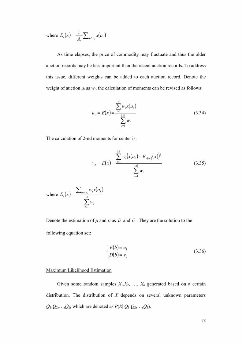
where ( ) ( )∑ ∈=

ti Aa it

t axA

xE 1

As time elapses, the price of commodity may fluctuate and thus the older

auction records may be less important than the recent auction records. To address

this issue, different weights can be added to each auction record. Denote the

weight of auction ai as wi, the calculation of moments can be revised as follows:

( )( )

∑

∑

=

===A

ii

A

iii

w

axwxEu

1

11 (3.34)

The calculation of 2-nd moments for center is:

( )( ) ( ) ( )( )

∑

∑

=

=

−==

A

ii

A

ianii

w

xEaxwxEv

i

1

1

2

2 (3.35)

where ( )( )

∑

∑

=

∈=A

ii

Aa ii

t

w

axwxE ti

1

Denote the estimation of µ and σ as µ) and σ) . They are the solution to the

following equation set:

( )( )

==

2

1

vbDubE

(3.36)

Maximum Likelihood Estimation

Given some random samples X1,X2, …, Xn generated based on a certain

distribution. The distribution of X depends on several unknown parameters

Q1,Q2,…,Qk, which are denoted as P(X| Q1,Q2,…,Qk).

78

The following likelihood function S is defined as the function that indicates

the probability of generating a series of random numbers. If the distribution is

discrete, the function S is represented as [21]:

( ) (∏=

==n

ikikn QQQXXPQQQXXXS

1212121 ,....,,|,....,,|,....,, ) (3.37)

If the distribution of X is continuous with density function denoted as

f(x|Q1,Q2,…,Qk), the likelihood function is represented as:

( ) ( )∏=

=n

ikikn QQQXfQQQXXXS

1212121 ,....,,,....,,|,....,, (3.38)

The maximum likelihood estimation assumes that the best estimation of Q1,

Q2,…,Qk is the set that maximizes the probability to generate the samples X1,

X2, …, Xn. Thus they are the solutions to the equation set:

( )

( )

( )

=

=

=

0,....,,|,....,,

......

0,....,,|,....,,

0,....,,|,....,,

,....,,

2121

,....,,2

2121

,....,,1

2121

21

21

21

k

k

k

QQQn

kn

QQQ

kn

QQQ

kn

dQQQQXXXdS

dQQQQXXXdS

dQQQQXXXdS

)))

)))

)))

(3.39)

For this problem, the maximum likelihood function can be calculated as

( ) ( )∏=

=n

iin XfXXXS

121 ,,|,....,, σµσµ (3.40)

The estimation of µ and σ, µ) and σ) are the solutions to the following equations:

( )

( )

=

=

0,|,....,,

0,|,....,,

,

21

,

21

1

1

kd

XXXdSd

XXXdS

n

n

σµ

σµ

σσµ

µσµ

))

))

(3.41)

79

Having got the distribution of the agents’ reserve prices, we can get the winning

probability for a reserve price bz, Fc(bz) as follows:

( ) ( ) ( )zcn

zc bRbP r= (3.42)

where R is the distribution of ( )σµ )),Φ .

However, the winning probability should be revised slightly according to

different bidding states. For an English auction with a current price q, the

winning probability should be revised as:

( )

( ) ( )( )

( ) ( )( )

−≤−

−

≤−−

−−

=

otherwiseif

bidhighestholdnotandhbqifqF

qFbF

bidhighestholdandbqifhqF

hqFbF

bP zz

zz

zc

01

1

(3.43)

The method of moments and the maximum likelihood estimators both

employ the information on the number of agents in the previous auction records.

This enhances the accuracy of prediction. As shown in the following section,

these two schemes perform better than the histogram method and normal method.

The maximum likelihood estimator is well suited to predict goods with high price

fluctuation particularly, when limited historical records are available. Compared

to the maximum likelihood estimators, the computation of method of moments is

almost independent on the size of the number of past auctions. When the number

of auction records increases, the new value of moments can be calculated by

considering the previous moment values and the number of new auction records.

The complexity of calculating the method of moments is generally lower than

that of the maximum likelihood estimators. Furthermore, considering the effect

of the price fluctuation of the commodity, appropriate weights can be added to

80

each auction record according to its time of occurrence. However, the accuracy

of the method of moments is not as good as that of the maximum likelihood

estimators (see the next section).

3.4.3 Evaluation of the prediction methods

In this section, a series of experiments are carried out to evaluate the

performance of the moment method and maximum likelihood estimators.

Moreover, we also compare the performance of these two estimation methods

with the histogram method and normal method.

( )σµ )), (µ,σ)=(250,10) n=[10, 20] (µ,σ)=(250,20) n=[10, 20]

Record number 50 100 200 500 50 100 200 500

Method of Moments

248.4 10.4

249.6 10.4

249.0 10.6

250.0 9.2

255.2 14.4

248.8 20.6

249.5 19.9 249.6 19.8


247.5

11.0 248.2 11.0

248.3

10.5

248.9

10.2

247.0

21.5

248.8

20.5

248.5

20.7

248.5

20.8

( )σµ )), (µ,σ)=(250,50) n=[10, 20] (µ,σ)=(250,100) n=[10, 20]

Record number 50 100 200 500 50 100 200 500

Method of Moments

245.0 54.8

253.3

46.9 253.3 47.9

252.7 47.5

255.0

90.0 255.0 95.1

247.0 103.5 250.0 99.9


253.5 47.2

251.6 48.7

248.8 51.1

249.0 50.8

248.2 102.7

255.0 98.8

250.2

98.3

250.0

100.9

Table 3.1. Estimated results of the prediction schemes for English/Vickrey

auction

As we know, the proxy bidding strategy is a popular strategy, which has

been widely used many auction sites (i.e., eBay). As shown in the analytical

results, the final winning price depends largely on the number of agents

participating in an auction. Although there are many auction records provided in

eBay, they only provide the final winning price of the auctions without

disclosing the number of bidders involved. Therefore, we adopt the auction

81

records in a simulated MAGICS environment to estimate the winning

probabilities. Based on the assumption that the reservation price of the agents

follows a certain normal distribution φ(µ,σ), a great deal of auctions has been

carried out in MAGICS (as described above) to generate a series of

English/Vickrey and Dutch/FPSB auction records. The auction records are

divided into a training set and a testing set, which are used to generate the

prediction function by using several prediction schemes. The aim is to verify the

performance of the prediction methods. In the experiment, the number of agents

participating in an auction submits a bid according to a uniform distribution

between $10 and $20. The mean of the agent’s reserve price is $250. Totally

eight sets of auction records have been generated: English/Vickrey and

Dutch/FPSB auction records with variation of reserve prices $10, $20, $50 and

$100. Based on the above data, different prediction schemes were set up. The

results are shown in Table 3.1.

Table 3.1 shows the estimation results of the method of moments and the

maximum likelihood estimation for English/Vickrey auctions. We can see that

the results of these two schemes are close to the actual parameters and thus the

performance of the two schemes are good. For each auction record, we also

conducted the experiment based on different number of records: 50, 100, 200 and

500. It is obvious that with more auction records, the performance is better.

After evaluating the estimation results of the two schemes, the prediction

functions were set up to estimate the winning probability of an agent with a

certain reserve price. To analyze the prediction schemes, we employed the

following method:

82

Given that the winning probability of an agent with reserve price bz in an

auction c is Pc(bz) and the actual winning probability is Oc(bz), the error of the

prediction εc(bz) is defined as

( ) ( ) ( )( )zc

zczczc bO

bObPb

−=ε (3.44)

Moreover, to evaluate the prediction function, the square distance ε is

defined as follows:

( ) ( )( )∑ ∈−=

Ni ii bObP 2ε (3.45)

Table 3.2 shows the error of the four prediction schemes with different

reserve prices. The number of past auction records is 500 for all cases. It is

obvious that the errors of the method of moments and maximum likelihood

estimation are close and the errors are much smaller than those of the other two

schemes, especially when the variation of the agent’s reserve price is large. The

histogram method gives the worst performance. In the table, the errors for low

reserve price are usually larger because of the smaller denominator Oc(bz). It can

also be seen that the method of moments performs better when the variance of

the normal distribution is large.

Error εb(p) (µ,σ)=(250,10) n=[10, 20] (µ,σ)=(250,20) n=[10, 20]

Reserve Price 270 275 280 285 290 300 310 320

Histogram method 0.408358 0.097683 0.020449 0.003494 0.360474 0.097683 0.020449 0.003494

Normal method 0.222384 0.097683 0.020071 0.003494 0.170248 0.076535 0.020257 0.003493

Method of Moments 0.128615 0.045014 0.012001 0.002426 0.074121 0.011413 0.000660 0.000660


0.054479 0.014560 0.003036 0.000480 0.004072 0.006550 0.003072 0.000914

83

Error εb(p) (µ,σ)=(250,50) n=[10, 20] (µ,σ)=(250,100) n=[10, 20]

Reserve Price 350 375 400 425 450 475 500 550


Normal method 0.163403 0.081850 0.020025 0.003332 0.135021 0.129130 0.079647 0.019953



0.009931 0.005328 0.001913 0.000495 0.014990 0.009861 0.006048 0.001856

Table 3.2. Winning probability errors of different prediction schemes for

English/Vickrey auctions

Table 3.3 shows the square distance of the four prediction schemes with

different number of auction records: 50, 100, 200 and 500. Generally, the square

distance of the prediction function becomes smaller when there are more auction

records. It is obvious that the square distance of the method of moments and the

maximum likelihood estimation are much lower than that of the histogram

method and normal method. Thus the former methods achieve a better

performance. When the reserve price varies more significantly, the square

distance of the histogram method and normal method becomes quite large while

that of the moment method and maximum likelihood estimation only increases

slightly. Also, when the number of auction records is small, the performance of

the maximum likelihood scheme is better than that of the moment method.

error (µ,σ)=(250,10) n=[10, 20] (µ,σ)=(250,20) n=[10, 20]

Record number N=50 n=100 n=200 n=500 n=50 n=100 n=200 n=500


Normal method 0.735076 0.544424 0.497218 0.333425 0.658226 0.629831 0.513279 0.507945


Maximum Likelihood

0.016333 0.007502 0.017258 0.015787 0.009116 0.005220 0.005178 0.004389

84

Estimation

error (µ,σ)=(250,50) n=[10, 20] (µ,σ)=(250,100) n=[10, 20]

Record number N=50 n=100 n=200 n=500 n=50 n=100 n=200 n=500


Normal method 0.659307 0.654040 0.590018 0.491330 1.823992 1.085582 0.936870 0.931147



0.017910 0.008446 0.008372 0.005050 0.021656 0.019489 0.019870 0.011200

Table 3.3 Square distance of different prediction schemes for English/Vickrey

auctions

After analyzing the performance of the prediction methods for

English/Vickrey auctions, we discuss the experimental result for Dutch/FPSB

auctions. Unlike the English/Vickrey auctions, the winning price is the highest

reserve price among all agents. Table 3.4 gives the estimation results of the

method of moments and the maximum likelihood estimation in Dutch/FPSB

auctions with various numbers of records: 50, 100, 200 and 500. It can be seen

that the more the auction record, the better the estimation of the two prediction

schemes.

( )σµ )), (µ,σ)=(250,10) n=[10, 20] (µ,σ)=(250,20) n=[10, 20]

Number of records 50 100 200 500 50 100 200 500

Method of Moments

251.6

8.4

249.6

10.2

249.7

10.0

249.5

10.1

259.5

13.8

253.9

16.6

248.8

20.5

248.9

20.2


247.7

11.9

250.3

9.9

249.4

10.1

248.8

10.2

251.8

18.0

251.5

18.6

248.4

20.8

249.6

19.9

( )σµ )), (µ,σ)=(250,50) n=[10, 20] (µ,σ)=(250,100) n=[10, 20]

Number of records 50 100 200 500 50 100 200 500

Method of Moments

269.0

37.7

268.6

38.3

262.2

40.6

253.0

46.0

275.0

72.7

261.5

84.1

246.7

97.1

257.2

94.9

85


255.1

42.8

259.9

40.5

250.5

46.8

247.0

50.5

249.5

98.7

247.7

95.6

243.2

100.6

246.6

100.6

Table 3.4. Estimation result of the prediction schemes for Dutch/FPSB auction

Table 3.5 shows the winning probability error of the four prediction

schemes with different reserve prices. The number of past auction records of all

schemes is 500. We can see that the errors of the method of moments and the

maximum likelihood estimation are close to each other. In fact, they are much

smaller than those of the other two schemes. The winning probability error of the

histogram method and the normal method in Dutch/FPSB auctions is much

closer than that in English/Vickrey auction. It is because the winning probability

of English/Vickrey auction is determined by the second highest of agents’

reserve price. An enhancement has been made by the normal method to simulate

the highest price of the auction records while the histogram method has not.

The square distance of the four prediction schemes based on various

number of auction records is shown in table 3.6. It is obvious that the minimum

square error of the method of moments and the maximum likelihood estimation

are much lower than that of the histogram method and normal method. Thus the

former schemes give better performances. Similar to above, the square distance

of the histogram method and the normal method in Dutch/FPSB auctions is

smaller than that in English/Vickrey auctions.

Error εb(p) (µ,σ)=(250,10) n=[10, 20] (µ,σ)=(250,20) n=[10, 20]

Reserve Price 270 275 280 285 290 300 310 320


Normal method 0.077984 0.035787 0.013440 0.003456 0.008834 0.017685 0.010862 0.003281

86



0.061869 0.016801 0.003592 0.000589 0.024492 0.008314 0.002219 0.000461

Error εb(p) (µ,σ)=(250,50) n=[10, 20] (µ,σ)=(250,100) n=[10, 20]

Reserve Price 350 375 400 425 450 475 500 550


Normal method 0.034544 0.031686 0.014097 0.003601 0.012099 0.002744 0.011701 0.009944



0.032032 0.008804 0.001893 0.000310 0.017829 0.009608 0.004870 0.001034


Dutch/FPSB auctions

Error (µ,σ)=(250,10) n=[10, 20] (µ,σ)=(250,20) n=[10, 20]

Record number n=50 n=100 n=200 n=500 N=50 n=100 n=200 n=500


Normal method 0.262619 0.176886 0.292299 0.105926 0.255754 0.131406 0.113048 0.089655



0.013914 0.002692 0.008973 0.017901 0.030137 0.017562 0.004902 0.008786

Error (µ,σ)=(250,50) n=[10, 20] (µ,σ)=(250,100) n=[10, 20]

Record number n=50 n=100 n=200 n=500 n=50 n=100 n=200 n=500


Normal method 0.774698 0.472748 0.304987 0.258457 0.204137 0.605121 0.300031 0.175048



0.082169 0.080185 0.052375 0.020062 0.070732 0.038593 0.019526 0.015685

Table 3.6. Square distance of different prediction schemes in Dutch/FPSB

auction

87

3.5 Summary

In this chapter, we have presented a mobile agent-based auction system,

which can be accessed via a Web/WAP interface. Based on the bidding

information, the agent will bid for the user up to the specified reserve price. A

general mathematical model has been set up to analyze the bidding results.

Furthermore, we have studied two distributions for the reserve price namely:

linear and normal distribution. Some simulations were conducted to validate the

correctness of the mathematical model. The simulation and analytical results

indicate that Dutch auctions result in a higher average winning price in general,

particularly when the number of agents is small. However, when more agents

participate in an auction, the difference between the average winning price for

English and Dutch auctions becomes negligible. The generic model can also be

applied to analyze the bidding results for other distributions of the reserve price.

An important issue is to compute the winning probability for a certain maximum

bidding price. This is essential in determining the maximum bidding prices. We

have investigated two prediction schemes called “method of moment” and

“maximum likelihood estimator” for the proxy bidding strategy. With the

previous auction records, the two prediction schemes can be used to estimate the

winning probability in an auction given a certain maximum bidding price. Some

experiments have been done to evaluate the performance of the two schemes and

compare the estimation schemes with two other prediction schemes proposed by

[20]. Experimental results indicate that the method of moment and maximum

likelihood estimator perform much better than the other two schemes, especially

in English/Vickrey auctions. As expected, with more auction records, the

estimation schemes achieve a better accuracy.

88

In this chapter, we assume that the reserve prices of all agents follow the

same distribution. As a future work, the analysis can also be extended to consider

agents with different reserve price distributions. Furthermore, for the prediction

schemes, we only consider the case that the reserve prices of the agents follow a

normal distribution. More analysis can be done to evaluate the performance of

the prediction schemes by using other distributions (e.g., power-law

distributions).

89

CHAPTER 4

PROBABILISIC BIDDING STRATEGY

4.1 Introduction

In chapter 3, we have discussed a proxy bidding strategy. It is based on the

popularly used proxy bidding service. Basically, an agent keeps renewing a bid

for a user provided that the bidding price is not greater than the user’s price

ceiling. Essentially, the agent will bid the price with certainty given it is lower

than the specified price. However, sometimes users may not be certain whether

to place a bid. They just have a certain degree of willingness to submit a bid at a

certain price. The proxy bidding strategy can not address this requirement. In this

chapter, we introduce a probabilistic bidding strategy, where each agent submits

bids according to a willingness function. In essence, a willingness function

specifies the willingness (or technically the bidding probability) to bid at a

certain price. Bidders can use different willingness functions to instruct their

auction agents to bid based on their preferences. By using an appropriate

willingness function, the required bidding strategy can be conveyed to the agent

effectively. For example, as shown later, we can convey the following

instructions to a bidding agent by using a suitable willingness function:

“Always bid up to $10 for me.”

“… I am a bit uncertain so bid for me with a probability of 0.8 between

$10 and $20.”

90

“For the first two minutes and the residual time, keep bidding if the price

is below $20 and $30, respectively.”

In fact the proxy bidding strategy can be considered as a probabilistic

bidding strategy with a constant willingness function: the willingness stays at

one between certain price values.

As an example, we consider the application of the probabilistic bidding

strategy for supporting mobile commerce (m-commerce) in general and mobile

auction (m-auction) services in particular. M-commerce is the extension of e-

commerce, enabled by wireless networking and mobile computing [3, 34]. M-

auction services allow users to buy or sell something by using a dynamic pricing

mechanism through their mobile terminals. Compared to the Web-based auction

services, m-auction services are generally time-critical and location-dependent

[33]. For example, a hotel may provide an auction-based reservation service for

some of its rooms. Mobile consumers or travelers around the hotel can bid for

the rooms within a short period of time. Because of the characteristics of m-

commerce, bidding strategies should be simple and efficient in terms of

computation so that agents can make decisions quickly.

To support m-auctions, we define a number of bidding strategies by using

some willingness functions and formulate a mathematical model to analyze the

bidding results for both the English and Dutch auction methods. In some cases,

close-form mathematical expressions have been derived. Furthermore, we make

use of the mathematical model to study the system behavior. In particular, all the

analytical results are validated by simulation results to ensure the correctness.

91

The model, analysis and results provide valuable insights into the design of

agent-based m/e-auction services.

The organization of the rest of this chapter is as follows. Section 4.2 gives

the system architecture. Section 4.3 presents the bidding strategies. Section 4.4

formulates a mathematical model for computing the average winning price for

the English and Dutch auctions. Section 4.5 discusses the simulation results.

Section 4.6 concludes the chapter.

4.2 System Architecture

Web Browser

Sellers/Buyers

Proxy server(Agent server)

InternetMobile terminal

AuctionsiteDirectory Server

⋯

Auctionsite

Auctionsite

Auction site

Access

Auctionprotocol

Supporting system

Admin.system Backend

system

⋯

Figure 4.1: System overview and key modules

Figure 4.1 shows the basic architecture of the mobile agent-based auction

system, which is also part of the Mobile AGent-based Internet Commerce

Systems (MAGICS) research project. Actually it is the extension of the system

described in chapter 3, where the mobile agent could automatically search for the

auction sites based on certain location requirements and then bid sequentially. To

92

find out the location information, the proxy server is connected to a directory

server, which can be co-located.

(2) Find auction sites

3) Return the localauction sites

(6) Send an agent

(8) Bidding Result

r Directory Server TargetAuction Site

AnotherAuction Site

(7) If failed, move toanother auction site

y the failure results

Time

User

(1) Request to bid

Figure 4.2: Bidding process

((4) Return local auctionsites

(5) Confirm to bid

(9) Notify the results(e.g. through SMS)

Proxy Serve

(7) Notif

Figure 4.2 shows the basic operation of the system. To participate in an

auction, bidders need to access the proxy server through their mobile terminals

and provide the bidding information, such as the minimum and maximum

bidding prices, and choose one of the four bidding strategies: constant, linearly

decreasing, aggressive and conservative. Of course, additional bidding strategies

can be supported by using the corresponding willingness functions as explained

in the next section. After submitting the bidding information, a mobile agent is

created, and then it moves to the corresponding auction server to bid for the

required products. The proxy server searches for the auction server(s) with the

assistance of a directory server. In an m-auction environment, the auction server

can be location-based. As an example, let us consider that a user wants to book a

room at the nearest hotel by means of m-auction. Having received the request,

the proxy server identifies the potential hotels ranked according to the ascending

order of the distance to the user. If required, the proxy server can also send the

93

list to the user for confirmation before sending off the mobile auction agents.

After confirmation, the proxy server sends a mobile agent to bid for a hotel room

with other agents. In this chapter, we assume that the mobile auction agent bid in

a sequential manner (e.g., try to find the closest hotel within the affordable price

range). We are also investigating a parallel bidding scenario, which is outside the

scope of this chapter. At each auction server, a seller agent is set up to control the

bidding process. Upon arrival, an auction agent registers with the seller agent.

The seller agent announces the new price to the auction agents whenever there is

an update. Each auction agent submits bids to the seller agent based on its

willingness function (see the next section) as defined by its owner. All messages

exchanged are XML-based. To ensure the non-repudiation requirement, all

messages can be digitally signed with the user’s private key, which is carried by

the corresponding agent. To verify the messages, each mobile auction agent can

provide a digital certificate to the selling agent for authentication purposes.

Finally, if the bidding result is unsuccessful, the mobile agent moves to the next

hotel to continue the bidding. If successful, the mobile agent reserves the room

accordingly and notifies the user (e.g., through Short Messaging Service).

( 1 ) I n p u t t h e b i d d i n g i n f o r m a t i o n ( 2 ) C r e a t e a b i d d i n g a g e n t

( 4 ) N o t i f y t h e b i d d i n g r e s u l t ( 3 ) B i d w i t h o t h e r a g e n t s

Figure 4.3: Demonstration of the auction process

94

A prototype system has been built to show the basic function of the mobile

auction system (see Figure 4.3). Basically a user accesses the system through a

WAP phone. A mobile agent is then created and sent to the required auction

server. The mobile agent then participates in the auction with other agents by

using a predefined bidding strategy. Finally, the auction result is returned to the

user.

4.3 Willingness Function and Bidding Strategy

As mentioned before, to support agent-based auction services, it is essential

to develop an effective mechanism to convey the bidding strategies to the agents.

We propose using a willingness function for this purpose. Basically a willingness

function reflects the degree of willingness to submit a bid at a certain price.

Bidders can use different willingness functions to instruct their auction agents to

bid based on their preferences. For instance, the popular proxy bidding service

can be represented by a willingness function with a value of one within a certain

price range. This means that the agent will bid with certainty (i.e., with a

probability of one) within the specified prices. Sometimes, a user may not be so

certain whether he/she will bid at a certain price. In this case, he/she can specify

a willingness value of less than one to reflect the “fuzzy or uncertain nature”. For

example, a willingness of 0.5 tells the agent to bid at the specified price with

probability 0.5. In general, the willingness function can be time-dependent too.

This can then be used to model the price-time function used in Kasbah [2]. For

instance, before and after 12:00 pm, the willingness value for a buying agent

remains at one up to $10 and $12, respectively. This means that the buying agent

will accept a selling price not exceeding $10 and $12 before and after 12:00 pm,

95

respectively. Compared to the price-time function used in Kasbah, the

willingness function is more flexible and general because it can also be used to

model some “fuzzy situations” (i.e., the user wants to tell the agent to bid with a

certain probability rather than with certainty). However, to facilitate the

explanation, we focus on a non-time dependent willingness function in this

chapter.

In this section, we introduce four bidding strategies or willingness functions

for the mobile auction service, namely the constant, linear, aggressive,

conservative bidding strategies. Before explaining the strategies in details, the

following assumptions and notations are defined:

• b1 is the minimum bidding price set by a bidder

• bz is the maximum bidding price set by a bidder

• h is the incremental bidding price or the difference between bj and bj+1.

Hence, we have bj = b1 + (j-1) h.

• W(bj) is the willingness value (i.e., bidding probability) at the bidding

price bj, where 0 ≤ W(bj) ≤ 1 and b1 ≤ bj ≤ bz

Constant Willingness Function

b1 bz

W(b)

0

1

p

Price

Figure 4.4: The constant willingness bidding strategy

96

The proxy bidding service can be represented by a constant willingness

function, as shown in Figure 4.4. In this case, if the current bidding price is no

higher than a user’s minimum bidding price (b1), the agent will always submit a

bid. If the current bidding price is between the user’s minimum bidding price

(b1) and maximum bidding price (bz), user will always bid with probability p.

Note that for the proxy bidding strategy, p is set to one. If the current bidding

price is higher than the user’s maximum bidding price, user won’t bid it at all.

Mathematically, the willingness function is as shown in (4.1).

( )

>≤<

≤=

z

z

bbifbbbifp

bbifbW

0

1

1

1

(4.1)

Linearly Decreasing Willingness Function

b1 bz

W(b)

0

1

p

Price

Figure 4.5: The linearly decreasing willingness approach

In general, a user may be less willing to submit a bid as the bidding price

increases. To model this situation, the linearly decreasing willingness bidding

strategy is introduced. As shown in Figure 4.5, the degree of willingness to bid

for an item decreases linearly as the bidding price increases. Mathematically, the

willingness function is shown in (4.2).

97

( )

>

≤<−−

≤

=

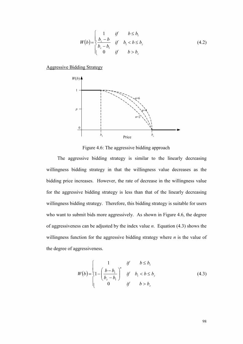
z

zz

z

bbif

bbbifbbbb

bbif

bW

0

1

11

1

(4.2)

Aggressive Bidding Strategy

b1 bz

W(b)

0

1

p

Price

n=2

n=6

n=4

Figure 4.6: The aggressive bidding approach

The aggressive bidding strategy is similar to the linearly decreasing

willingness bidding strategy in that the willingness value decreases as the

bidding price increases. However, the rate of decrease in the willingness value

for the aggressive bidding strategy is less than that of the linearly decreasing

willingness bidding strategy. Therefore, this bidding strategy is suitable for users

who want to submit bids more aggressively. As shown in Figure 4.6, the degree

of aggressiveness can be adjusted by the index value n. Equation (4.3) shows the

willingness function for the aggressive bidding strategy where n is the value of

the degree of aggressiveness.

( )

>

≤<

−−

−

≤

=

z

z

n

z

bbif

bbbifbbbb

bbif

b

0

1

1

11

1

1

W (4.3)

98

It can be seen from Figure 4.6 that when the value of n increases, the slope

of the curve becomes flattened. By using a higher index value, a user can

participate more actively in an auction.

Conservative Bidding Strategy

b1 bz

W(b)

0

1

p

Price

n=2

n=6 n=4

Figure 4.7: The conservative bidding approach

In contrast to the aggressive bidding strategy, the conservative bidding

strategy is for users with a conservative attitude. In this case, the willingness

value decreases sharply as the bidding price increases. Mathematically, the

willingness function is defined as follows:

( )

>

≤<

−−

−

≤

=

z

z

n

z

bbif

bbbifbbbb

bbif

bW

0

1

1

11

1

1

(4.4)

Similar to the aggressive bidding strategy, the index n controls the degree

of conservativeness. When n increases, the slope of the curve is steeper,

indicating that the bidder is less willing to place a bid as the price increases (see

Figure 4.7).

Of course, other bidding strategies can be defined as well by specifying the

corresponding willingness function. In the following section, we will analyze the

99

bidding results of the English and Dutch auctions for the above bidding strategies

(i.e., willingness functions).

4.4 Mathematical Model

In the previous sections, we discussed different bidding strategies and the

implementation of the auction system. In this section, we present a mathematical

model to compute the average winning price of an auction. First we define the

following notations:

• bj is the bidding price of the item where b1 ≤ bj ≤ bz

• mj is the probability that at least one bidder bids at bj

• x is the number of bidders

• P(bk) is the probability that the price will stop at bk

• E(b) is the expectation of the winning price

4.4.1 English Auction

b1 b2 bj bj+1 bz

Stop at b1

Stop at b2

Stop at bj

Stop at bj+1

Stop at bz

m2 mj+1

1 - m2 1 - m3 1 - mj+1 1 - mj+2 1

Figure 4.8: Model of the English auction

Figure 4.8 shows the model for computing the average winning price for

the English auction. Consider that the highest bid price at the present moment is

bj. If any agent bids at bj+1, the highest bid price will obviously increase to bj+1.

100

This situation occurs with probability mj+1. In other words, if no agent bids at

bj+1, the auction will stop at bj with a probability of 1-mj+1. Note that the bid

price will not increase above bz.

Hence, mj+1 is the probability that the bid price will change from bj to bj+1.

It depends on the bidding strategies of the bidders. Assuming that all bidding

agents use the same bidding strategy (i.e., have the same willingness function),

is the probability that no bid is received at b11 )](1[ −

+− xjbW j+1. Note that the

current winning agent does not bid. Hence, 1 is the probability

that at least one agent places a bid at b

11 )](1[ −

+−− xjbW

j+1. As a result, the bid price increases to

bj+1 with probability

111 )](1[1 −

++ −−= xjj bWm (4.5)

Table 4.1: Probability of an auction stopping at different bidding prices

Stop at Probability

b1 1 – m2

b2 m2 × (1 – m3)

bj m2 × m3× m4 ……× mj × (1-mj+1)

bz m2 × m3 × m4 …. × mz-1 × mz ×1

Based on the above discussion, Table 4.1 gives the probability that an auction

stops at bj.

Thus we can easily get the distribution of the winning price as:

( ) ( )( ) (( ))( )∏=

−−+ −−−=

k

i

xi

xkk bWbWbP

2

111 111 (4.6)

In other words, (4.6) gives the probability that the winning price is bk. According

to (4.6), we can compute the average winning price of the English auction as

follows:

101

( ) ( )( ) (( ))( )∑ ∏= =

−−+ −−−×+=

z

k

k

i

xi

xk bWbWkhbbE

1 2

1110 111 (4.7)

where b0=b1 – h.

We now evaluate (4.6), (4.7) based on the different willingness functions (or

bidding approaches) as follows.


Substituting (4.1) into (4.6), we get:

( ) ( ) ( )( )( )( )

=−−

<≤−−−= −−

−−−

zkifpzkifppbP zx

kxx

k 11

111

111111 (4.8)

Putting (4.1) into (4.7), the average winning price can be found to be:

( ) ( ) ( )( ) ( ) ( )( )( )

( )( ) 111

1121

0 111

1121111 −−−

−−−−

−−×+−

−−−+−−−−+=

zxx

zxzx

phzp

pzpzhbbE

(4.9)

Detailed calculation of (4.9) is shown in Appendix I.

Linear Willingness Function

Similarly, substituting (4.2) into (4.6), we have:

( )

=

−−

−

<≤

−−

−

−=

∏

∏

=

−

=

−−

zkifzi

zkifzi

zk

bPz

i

x

k

i

xx

k

2

1

2

11

111

1111

1 (4.10)

Also, the average winning price can be found to be:

( ) ∏∑ ∏=

−−

= =

−−

−−

−×+

−−

−

−×+=

z

i

xz

k

k

i

xx

zihz

zi

zkkhbbE

2

11

1 2

11

0 111

111

1

(4.11)

102

4.4.2 Dutch Auction

bz bz-1 bj bj-1 b1

Stopat bz

Stopat

bz-1

Stopat bj

Stopat bj-

1

Stopat b1

1 - mz 1-mj

mz mz-1 mj mj-1 1

Figure 4.9: Model of the Dutch auction

Figure 4.9 shows the mathematical model of the Dutch auction. In this

case, bj moves to bj-1 with probability 1- mj (i.e., no agent wants to submit a bid at

the price bj). If one of the agents bids at bj, which occurs with probability mj, the

auction ends. Note that the bid price will not decrease below b1 (i.e., m1 =1). For

the Dutch auction, mj can be found as follows:

xjj bWm )](1[1 −−= (4.12)

Table 4.2: Probability of auction stopping at different bidding prices

Stop at Probability

bz mz

bz-1 (1 – mz) × mz-1

bj (1 - mz) × (1 – mz-1) ×….. × (1-mj+1) × mj

b1 (1 - mz) × (1 – mz-1) × ….. × (1 – m2) × 1

Note that there are x bidding agents. According to Table 4.2, we can easily

compute the distribution of the winning price to be:

103

( ) ( )( )( ) ( )(∏+=

−×−−=z

ki

xi

xkk bWbWbP

1

111 ) (4.13)

The average winning price can then be worked out as:

( ) ( )( )( ) ( )(∑ ∏= +=

−×−−×+=z

k

z

ki

xi

xk bWbWkhbbE

1 10 111 ) (4.14)

where b0=b1 – h.

We now evaluate (4.13), (4.14) by using different willingness functions.


Substituting (4.1) into (4.13), we obtain:

( ) ∏+=

−−

×

−−

−=z

ki

xx

k zi

zkbP

1 11

111 (4.15)

The average winning price can be determined as follows:

( ) ( )( ) ( )( ) ( )( )x

xzxx

pppzpzhbbE

−−−+−−−−−

+=11

11112 32

0 (4.16)

Detailed calculation of (4.16) is shown in Appendix II.

Linear Willingness Function

According to formula (4.2), distribution of auction winning price given all x

agents apply linear willingness approach is given out as follows:

( ) ∏+=

−−

×

−−

−=z

ki

xx

k zi

zkbP

1 11

111 (4.17)

The average winning price is

( ) ∑ ∏= +=

−−

×

−−

−×+=z

k

z

ki

xx

zi

zkkhbbE

1 10 1

1111 (4.18)

104

4.5 Results and Discussions

100

101

102

103

380

400

420

440

460

480

500

Number of agents

Ave

rage

win

ning

pric

e

English auction

AnalyticalSimulationExperimental

Figure 4.10: Comparison of the experimental, simulation and analytical results of English auction

Based on the above bidding strategies, we present some simulation,

analytical and experimental results in this section. As an example, the minimum

and maximum bidding prices are set to be $300 and $500, respectively. For the

analytical results, they were calculated by the respective equations given in the

last section. The simulation model was written in Java to simulate a bidding

process. Each simulation is repeated 10,000 times to obtain the average results.

To validate the simulation/analytical models, we have also run some experiments

using the aforementioned prototype system (i.e., using IBM Aglet). In each

experiment, the auction process was repeated 50 times to compute the average

winning price. Two representative examples of the experiments for the linearly

decreasing willingness approach are shown in Figures 4.10 and 4.11. Figure 4.10

shows the average winning price for the English auction when different numbers

of agents are used. It can be seen that the experimental, simulation and analytical

results are almost the same. Figure 4.11 shows the simulation, experimental and

105

analytical results for the Dutch auction. Again, the average winning price as

found by the three approaches are almost the same, thus confirming the

correctness of simulation/analytical/experimental models. Unfortunately, the

experimental approach was time consuming because many agents were created in

each auction. Having validated the simulation and analytical models, we will use

them to obtain the results in the following sub-sections.

100

101

102

103

492

493

494

495

496

497

498

499

Number of agents

Ave

rage

win

ning

pric

e

Dutch auction

AnalyticalSimulationExperimental

Figure 4.11: Comparison of the experimental, simulation and analytical results of

Dutch auction

Results for the English Auction

In this sub-section, we present the results for the English auction method.

First, we evaluate the relationship between the average winning price and

different bidding strategies. As shown in Figure 4.12, we can see that the average

winning price is higher if the aggressive bidding strategy is used. This is because

the agents bid more actively, so the average winning price becomes higher. In

contrast, if the conservative bidding strategy is used, the average winning price

becomes lower. Figure 4.12 also shows that when the number of agents

106

increases, the average winning price also increases slightly. This is because the

overall chance for submitting a bid is higher when the number of agents is larger.

100

101

102

103

320

340

360

380

400

420

440

460

480

500

Number of agents

Ave

rage

win

ning

pric

e

English auction

Linear approach (Analytical)Aggressive approach (n=4,Analytical)Conservative approach (n=4,Analytical)Linear approach (Simulation)Aggressive approach (n=4,Simulation)Conservative approach (n=4,Simulation)

Figure 4.12: Average winning price of the English auction with different bidding strategies

100

101

102

103

430

440

450

460

470

480

490

500

Number of agents

Ave

rage

win

ning

pric

e

English auction with aggressive bidding strategy

n=2 (Analytical)n=4 (Analytical)n=6 (Analytical)n=2 (Simulation)n=4 (Simulation)n=6 (Simulation)

Figure 4.13: Average winning price of the English auction with different degree

of aggressiveness values

107

100

101

102

103

320

340

360

380

400

420

440

460

480

500

Number of agents

Ave

rage

win

ning

pric

e

English auction with conservative bidding strategy


Figure 4.14: Average winning price of the English auction with different degree

of conserveness values

101

102

103

300

320

340

360

380

400

420

440

460

480

500

Number of agents

Ave

rage

win

ning

pric

e

English auction with constant bidding strategy

p=0.1 (Analytical)p=0.2 (Analytical)p=0.3 (Analytical)p=0.5 (Analytical)p=0.1 (Simulation)p=0.2 (Simulation)p=0.3 (Simulation)p=0.5 (Simulation)

Figure 4.15: Average winning price of the English auction with different bidding

probabilities

Figure 4.13 shows that when the number of agents is small, the average

winning price is more sensitive to the change in the aggressiveness value.

108

However when the number of agents is large, the effect is much smaller. Figure

4.14 shows a similar trend with the conservativeness bidding approach (i.e., the

conservative values have a larger effect when the number of agents is small).

Figure 4.15 shows the average winning price for the constant willingness

function with different values of p. It can be seen that for each curve, the average

winning price increases dramatically when the number of agents reaches a

certain threshold. The threshold value is smaller when p is larger.

Results for the Dutch Auction

In this sub-section, we present the results for the Dutch auction. Similar to

above, we first evaluate the average winning price of different bidding strategies,

namely the aggressive, conservative and linearly decreasing bidding strategies.

Then, we discuss the effect on the average winning price if the degree of

aggressiveness and conservativeness are varied.

100

101

102

103

470

475

480

485

490

495

500

Number of agents

Ave

rage

win

ning

pric

e

Dutch auction

Linear approach (Analytical)Aggressive approach (n=2,Analytical)Conservative approach (n=2,Analytical)Linear approach (Simulation)Aggressive approach (n=2,Simulation)Conservative approach (n=2,Simulation)

Figure 4.16: Average winning price of the Dutch auction with different bidding strategies

109

100 101 102 103494

494.5

495

495.5

496

496.5

497

497.5

498

498.5

499

Number of agents

Ave

rage

win

ning

pric

e

Dutch auction with aggressive bidding strategy


Figure 4.17: Average winning price of the Dutch auction with different degree of aggressiveness values

100

101

102

103

400

410

420

430

440

450

460

470

480

490

500

Number of agents

Ave

rage

win

ning

pric

e

Dutch auction with conservative bidding strategy


Figure 4.18: Average winning price of the Dutch auction with different degree of conservativeness values

110

101

102

103

494

495

496

497

498

499

500

Number of agents

Ave

rage

win

ning

pric

e

Dutch auction with constant bidding strategy

p=0.1 (Analytical)p=0.2 (Analytical)p=0.3 (Analytical)p=0.5 (Analytical)p=0.1 (Simulation)p=0.2 (Simulation)p=0.3 (Simulation)p=0.5 (Simulation)

Figure 4.19: Average winning price of the Dutch auction with different bidding probabilities

Figure 4.16 shows the average winning price when the number of bidding

agents is varied. As expected, the average winning price for the aggressive

bidding strategy is higher than that of the other bidding strategies. Furthermore,

the average winning price for the conservative bidding strategy is the lowest.

This is because the bidding probability of the aggressive bidding approach is

higher than that of the other bidding strategies, especially the conservative

bidding strategy. Due to the use of a higher bidding probability, the auction

stops at a higher price. As a result, the average winning price for the aggressive

bidding strategy is higher than that of the conservative or linearly decreasing

strategy. Furthermore, as the number of agents increases, the average winning

price increases as expected. This is because as more agents participate in an

auction, the chance for having a higher bid is larger. Hence the auction is likely

to stop at a higher price. Referring to (4.3), it can be seen that as n increases, the

degree of aggressiveness increases (i.e., the probability that an agent places a bid

111

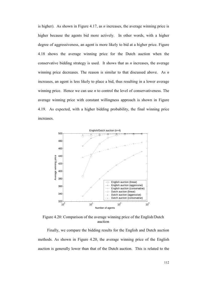
is higher). As shown in Figure 4.17, as n increases, the average winning price is

higher because the agents bid more actively. In other words, with a higher

degree of aggressiveness, an agent is more likely to bid at a higher price. Figure

4.18 shows the average winning price for the Dutch auction when the

conservative bidding strategy is used. It shows that as n increases, the average

winning price decreases. The reason is similar to that discussed above. As n

increases, an agent is less likely to place a bid, thus resulting in a lower average

winning price. Hence we can use n to control the level of conservativeness. The

average winning price with constant willingness approach is shown in Figure

4.19. As expected, with a higher bidding probability, the final winning price

increases.

100

101

102

103

320

340

360

380

400

420

440

460

480

500

Number of agents

Ave

rage

win

ning

pric

e

English/Dutch auction (n=4)

English auction (linear)English auction (aggressive)English auction (conservative)Dutch auction (linear)Dutch auction (aggressive)Dutch auction (conservative)

Figure 4.20: Comparison of the average winning price of the English/Dutch auction

Finally, we compare the bidding results for the English and Dutch auction

methods. As shown in Figure 4.20, the average winning price of the English

auction is generally lower than that of the Dutch auction. This is related to the

112

auction protocol as shown in Figure 4.8 and Figure 4.9. From Figure 4.20, it can

be seen that the average winning price of the Dutch auction is higher than that of

the English auction if the conservative or linearly decreasing bidding strategy is

used. However, if the aggressive bidding strategy is adopted or the number of

agents is large, the average winning prices for the English and Dutch auctions are

close to each other.

4.6 Summary

In conclusion, we have presented an auction system based on mobile

agents. The system can be accessed via a mobile terminal. A user can generate a

mobile auction agent that uses one of four different bidding strategies: constant,

linearly decreasing, aggressive and conservative. For each bidding strategy, a

willingness function is used to define the bidding probability at a particular price.

According to the specified bidding strategy (or willingness function) and other

necessary information, each mobile agent moves to the respective auction server

to bid with other agents. In the context of m-commerce, the auction server can be

location-based (e.g., closest to the user) and the bidding results can be conveyed

to the user through SMS. A mathematical model has been presented to evaluate

the bidding results for both the English and Dutch auction methods. In particular,

some close form mathematical expressions have been derived for analysis

purposes. Simulation and analytical results have been presented to study the

bidding strategies. As shown above, all the simulation results match closely with

the analytical results, thus validating the correctness of both the simulation and

analytical models. In general, the analytical model can be applied and extended

to analyze other bidding strategies. The study indicates that the Dutch auction

113

results in a higher average winning price in general, particularly if the number of

agents is small. However, if the number of agents is large, the average winning

price of the English auction is close to that of the Dutch auction in many cases.

Furthermore, as expected, the average winning price is generally higher if a more

aggressive bidding strategy is adopted.

114

CHAPTER 5

BACKWARD INDUCTION BIDDING STRATEGY (BIDS)

5.1 Introduction

The above two chapters have analyzed several bidding strategies for single-

site auctions. However, with the development of online auctions, it is possible for

agents to participate in many concurrent auctions selling the same item. For

example, when a user wants to buy a certain digital camera, he/she may find that

there are many auctions selling the same camera, probably using different

auction types. In general, we can achieve better results by participating in

multiple auctions rather than a single auction. To enable an agent to participate in

multiple auctions, we need to develop a special bidding strategy. In this chapter,

we introduce a backward induction strategy for users to bid in multiple

concurrent heterogeneous auctions. In particular, two contributions are made

namely: the auction chain concept, and the backward induction auction

algorithm. In general, basic concept of the backward induction bidding strategy

is given as follows:

Given that it is not possible to participate in all auctions due to

overlapping deadlines, we first identify all the possible sets of auctions (the

auction chains) in which an agent can bid. The “attractiveness” of each auction

chain is determined by a utility function based on the past winning probability.

115

After getting the expected utility of all the auction chains, we can easily

select the right auctions to participate and determine the corresponding bidding

prices. Compared with the two bidding strategies discussed in Chapters 3 and 4,

BIDS is more adaptive as it can change the bidding behaviour based on the

market situation.

Details of BIDS and the performance analysis are illustrated in the

following sections. Section 3.2 describes the system model and the bidding

strategy. Section 3.3 explains the concept of auction chains. Section 3.4 presents

the operation of BIDS. Section 3.5 discusses the experimental results. Section 3.6

summaries this chapter.

5.2 System model

EnglishAuctions

FPSBAuctions

VickreyAuctions

Market

Access ControlMechanism

Agent Interface

WEB Interface

WAP Interface

User Agent

User

Auction Site

Figure 5.1. Structure of the auction site

Before presenting the bidding strategy, we present the system model first.

As shown in Figure 5.1, there are totally three kinds of auctions in the market:

English auction, FPSB auction and Vickrey auction. Essential information for

running the auctions is stored in the database and an access control mechanism is

116

employed to ensure that only appropriate information can be accessed. The

auction site provides two kinds of interfaces for the users: user interface and

agent interface. A user can access the system through the user interface. The

agent interface provides several methods, based on which, users could create

their own agents. For simplicity, we assume that all auctions in the market sell

the same item and only one item is on sale in each auction. Each auction may

begin and end at different times and the active period of English auctions and

sealed-bid auctions are announced before the closing time. The number of

bidders in each auction and its current price (if any) is available by sending an

inquiry message to the access control subsystem. The system elements are

described as follows:

Agent

Before bidding, the agent is assigned two parameters:

M is the maximum price that the agent can bid.

T denotes the latest time to obtain the item.

Auction

Here we denote A as the set of auctions that were presently active or have

not started and the agent should bid in set A. Set A includes various kinds of

auctions, specifically Ae, Af and Av denote the set of English auctions, FPSB

auctions and Vickrey auctions in A, respectively. Therefore, we have

Φ=∩=∩=∩ vfvefe AAAAAA

and . AAAA vfe =∪∪

117

For an auction c, its beginning time and ending time are denoted as B(c)

and D(c), respectively. Given that the present system time is t, we can easily get

that ( ){ }tcDcA ≥= . Let h(c) be the minimum incremental price for an auction c

and its present highest bid be x(c), we have v(c)=x(c)+h(c), where v(c) indicates

the minimum bidding price of auction c. Furthermore, we assume that in the

market, it takes L time units to process a bid so the smallest time gap between

two consecutive bids is L.

For each bid in an auction, it should be either active or inactive. In an

English auction, a bid remains “active” after it is submitted until a higher bid

outbids it. When the auction ends, all bids become the “inactive”. All bids in

FPSB or Vickrey auctions are active until the auction is over.

After the agent finishes the bidding, the bidding result will be evaluated

based on a utility function U(x) as defined by the user. The utility function may

be different according to the user requirements. In this section, we adopt the

commonly used utility function as given in (5.1) for the later analysis [8]. Note

that other utility functions can also be used for BIDS.

( ) −

=otherwise

xpriceatwincanagenttheifxMxU

0 (5.1)

Given the above system model, our objective is to design a bidding strategy,

with such that an agent can maximize the utility value as computed by (5.1).

5.3 Concept of auction chain

In this section, we first introduce the concept of the auction chain. An

auction chain is actually an auction sequence where an agent could bid one by

118

one. We assume that the auction agent only requires one item so that it should

stop bidding before the previous bidding result is known. Otherwise, if the agent

participates in two active auctions and happens to be the winner in both auctions,

it would obtain two items, which is called “accidental purchase”. The agent

should avoid the occurrence of such accidental purchase. Before calculating the

future expected utility, we should first find out all the possible auction chains

between the system time t and the ending time T. Denote an auction chain

between t and T as Ct,T and suppose that Ct,T comprises n auctions: c1,

c2,...,ci,…,cn. We should fulfill the following conditions:

All the auctions in Ct,T should not be closed at time t, i.e., c , where

.

Ai ∈

ni ≤≤1

The respective auctions should be listed according to their deadlines. The

deadline of two consecutive auctions should be separated by at least L, i.e.,

( ) ( ) LcDcD ii ≥−+1 (5.2)

where 1 1−≤≤ ni

The deadline of auction cn should not be later than T-L, i.e., . ( ) LTcD n −≤

Figure 5.2 shows which auctions the agent can participate in. They are

represented by the short lines with length L. As shown in the figure, an auction

chain is defined by a set of non-overlapping lines.

119

Figure 5.2. Auction chains

5.4 BIDS

In this section, we present the Backward InDuction bidding Strategy

(BIDS) for the aforementioned multi-auction scenario. Using BIDS, an auction

agent can decide whether to submit a bid and to decide the appropriate bidding

price. Basically, BIDS is based on the following:

It is better to stop bidding in an auction if the utility value of the current

bid is lower than the expected utility value of all the subsequent

auctions.

If not, the auction agent should bid at a specific price.

In section 5.4.1 to 5.4.3, we introduce the bidding strategy for a single type

of auctions.

5.4.1 Bidding in pure English auctions

The operation of BIDS in English auctions is as follows:

After the deadline ( t ) or the agent is waiting for the previous bidding

results, it should stop bidding.

T>

120

If bidding is allowed, the agent should first find out all the auction chains and

compute the respective expected utility.

Let c be the first auction in the auction sequence with the maximum expected

utility and r(c) be the maximum bidding price of the auction c. If r ,

the agent should bid in auction c with price v

( ) ( )cvc t≥

t(c). If not, the agent should wait

because it is better to participate in the upcoming auctions.

Calculation of future expected utility U

Before calculating the future expected utility, we should first find out all

auction chains between the current system time t and the deadline T. For each

auction chain, the expected utility is computed. Here we adopt the backward

induction method to recursively compute the expected utility value of an auction

chain. Given an auction chain C with n auctions listed in the ascending order of

their deadlines: c1, c2,...,ci,…,cn. In order to compute the expected utility value of

an auction chain C, we first determine whether an agent should bid in an auction.

However, the action for ci depends on the expected utility between ci+1 and cn.

Denote the expected utility between ci and cn as Ui and the expected utility value

of auction ci as ui. It can be seen that Ui is dependent on Ui+1. Hence the expected

utility of the auction chain can be calculated recursively as follows:

Step 1: Calculate Un

The agent should only bid in the final auction cn if the minimum bidding

price is less than its maximum bidding price M. Note that if the agent submits a

bid and wins, the final utility value will be greater than zero. However, if the

bidding agent does not bid, the utility value will be zero. Denote the maximum

bidding price in auction ci as r(ci), We have r(cn) =M. Because the bidding agent

121

(with the maximum bidding price r(cn)) may not buy the item at price r(cn), two

outcomes are possible:

1. The bidding agent bids at price y, where ( )ncry ≤ and where the other agents

do not submit a higher bid. In this case, the bidding agent wins at price x and

the resultant utility value is M-y.

2. The bidding agent bids up to r(cn) but some agents submit a higher bid. The

bidding agent loses.

Let the expected utility value of auction ci be ui and the conditional winning

probability for a bidding price y in the i-th auction ci be ( )yicF on the condition

that the winning price will be lower than y. The expected utility of auction ci can

be computed as follows:

( ) (( )∫ −=

)( n

iti

cr

cv ci ydFyMu )

)

(5.3)

For auction cn, we can get

( ) (( )∫ −==

M

cv cnnnt

nydFyMuU (5.4)

Step 2: Calculate Ui based on Ui+1

Assume that if Ui+1 is known, the maximum bidding price for auction ci

can be calculated as:

( ) 1+−= ii UMcr (5.5)

When the auction agent submits a bid y (y > M-Ui+1) and wins, the utility value is

M-y, which is lower than Ui+1. In this case, the agent should not bid in auction ci.

122

Based on (5.3) and the value of r(ci), we can compute ui. The average

utility value that is obtained from auction ci is ui. If the agent fails, it will keep on

bidding in the subsequent auctions. In this case, the expected utility value is Ui+1.

Hence, the bidding agent with a maximum bidding price r(ci) will win the

auction ci with probability ( )( )ic crFi

. The average utility value between ci and cn

can be computed as follows:

( )( )( ) 11 +×−+= iicii UcrFuUi

(5.6)

The expected utility value for the auction chain C can then be determined

using the recursive equation (5.6).

A Simple Example

In this subsection, we present a simple example to explain how BIDS

works. Given an agent uses BIDS with a maximum bidding price (M) of $100.

Before the deadline T, there are a total of five available English auctions as

shown in the following table:

Table 5.1. Available auctions

Auction Current

price

Minimum

incremental

price

Deadline

A $20 $1 50

B $40 $1 60

C $40 $1 75

D $50 $1 80

E $60 $1 110

Assume that the minimum bidding interval between two consecutive bids is

20 and the winning probability is as follows:

123

( )

>

≤<−

≤

=

1001

1002080

20200

x

xxx

xF (5.7)

Before making decision, the agent first finds out all the auction chains in the

market. It is obvious that there are three auction chains as follows:

Chain I: [A C E]

Chain II: [A D E]

Chain III: [B D E]

The expected utility of each auction chain should then be computed. For

Chain I, we get r(E) = M =100. Since the current price of auction E is $60, the

conditional winning probability is:

( )

>

≤<−

≤

=

1001

1006040

60600

x

xxx

xFE (5.8)

Therefore, the expected utility of auction E is:

( ) ( ) 01.19100

6133 =−== ∫ xdFxMuU E (5.9)

The maximum bidding price that the agent should use for auction C is r(C) = M -

U3 = 100 – 19.01 =80.99. The expected utility for auction C is:

( ) ( ) 00.2699.80

412 =−= ∫ xdFxMu C (5.10)

Thus we get

( )( ) 02.321 3222 =×−+= UrFuU C (5.11)

124

Also, we have r(A) = M –U2 = 100 – 32.02 =67.98. Hence the expected utility for

auction A is:

( ) ( ) 60.3298.67

211 =−= ∫ xdFxMu A (5.12)

Thus

( )( )( ) 42.451 211 =×−+= UArFuU A (5.13)

Therefore, the expected utility for Chain I is $45.42. Similarly we can

compute the expected utility of Chain II is $43.78 and that of Chain III is $35.37.

As a result, Chain I has the highest expected utility. Since the current price of

auction A is $20, much lower than $67.98, the agent should submit a bid for

auction A at a price of $21.

5.4.2 Bidding in pure FPSB auctions

The operation of BIDS for FPSB auctions is similar to that for English

auctions and the operation is as follows:

After the deadline ( t ) or the agent is waiting for the previous bidding

results, it should stop bidding.

T>

If bidding is allowed, the agent should first find out all the auction chains and

compute the respective expected utility.

Let c be the first auction in the auction sequence with the maximum expected

utility and r(c) be the bidding price of the auction c. The agent should submit

a bid at price r r(c) for the auction c.

125

Calculation of future expected utility U

The expected utility of the FPSB auction chain is similar to the English

auction chain. However, each auction in the auction chain is assigned a bidding

price instead of the highest bidding price because of the nature of the sealed-bid

auction. Assume that an auction chain C has n auctions, which are listed in

ascending order of their deadlines: c1, c2,...,ci,…,cn. In order to compute the

expected utility value of the auction chain C, we first determine the bidding price

in each auction. Denote the bidding price of auction ci as xi, we can see that xi

depends on the expected utility between ci+1 and cn. Denote the expected utility

between ci and cn as Ui and the expected utility value of auction ci as ui. It can be

seen that Ui is dependent on Ui+1. Hence the expected utility of the auction chain

can be calculated recursively as follows:


In FPSB auction, a risk-neutral agent only submits a bid that can maximize

the expected utility. Given that the agent submits a bid with price y, it will win

the auction with probability ( )yncF and the corresponding utility is M-y.

Otherwise, the agent should leave the market with utility zero. Thus the expected

utility of the last auction with bidding price y is ( ) ( )yMync −×F . Therefore, the

expected utility of auction cn should be:

( ) ( )yMyFMaxUncMyn −×=

≤≤0 (5.14)

Also, r(cn) should be the corresponding bidding price of Un.


126

Assume that if Ui+1 is known, Ui can be worked out easily. If the agent

submits a bid with price y in auction ci, it will win the auction with

probability ( )yicF with utility M-y. Otherwise, it should bid in future auctions with

utility Ui+1. Thus Ui should be

( ) ( ) ( )( ) 101 +≤≤

×−+−×= iccMyi UyFyMyFMaxUii

(5.15)

and r(ci) is the corresponding bidding price of Ui.

As mentioned above, the expected utility value for the auction chain C can

be determined using the above recursive equation.

5.4.3 Bidding in pure Vickrey auctions

The operation of BIDS for Vickrey auctions can be worked out in a similar

manner. The only difference is the calculation of the expected utility. In Vickrey

auctions, the buying price is the second highest price instead of the highest price

as in FPSB. Therefore, the calculation of the auction chain C should be revised as

follows:


In Vickrey auctions, a risk-neutral agent only submits the bid that can

maximize the expected utility. Given that the agent submits a bid with price y, it

can win the auction with probability ( )yncF . However it should buy the item with

the second highest price. Denote E(y) as the expectation of the second highest

price given the highest price y, we can get the expected utility of auction cn as

( ) ( )( )yEMyFMaxUncMyn −×=

≤≤0 (5.16)

rn should be the corresponding bidding price of Un.

127


If the agent submits a bid with price y in auction ci, it can win the auction

with probability and the expected utility is M-E(y). Otherwise, it should bid

in future auctions with utility U

( )yFic

i+1. Thus Ui should be

( ) ( )( ) ( )( ) 101 +≤≤

×−+−×= iccMyi UyFyEMyFMaxUii

(5.17)

r(ci) is the corresponding bidding price of Ui.

The expected utility value for the auction chain C can then be determined

using the recursive equation.

5.5 Experimental results

In this section, we set up a simulation model to evaluate the performance of

BIDS. The simulations assume multiple English auctions with randomly chosen

start and end times. For comparison purposes, we use five different types of

bidding agents:

A Simple agent: Participates in a randomly chosen auction using a simple

proxy bidding strategy, that is, keeps bidding within a maximum bidding

price

A BIDS agent: Submits bids using BIDS.

A Greedy agent: Uses the Greedy strategy as described in [1].

A Historian agent: Uses the Historian strategy as described in [1].

128

An Ideal agent: Bids based on the ideal scenario that it knows the winning

price of each auction. This is not realistic but it can provide the best

performance for comparison purposes. Note that even though the ideal agent

knows all the final winning prices, it may still lose if its maximum bidding

price is lower.

Each of the following simulations was repeated 1,000 times to obtain the average

result.

Firstly, we have conducted a simulation with 50 English auctions and 600

background agents. Each English auction lasted for 55 time units. The

background agents are all simple agents with the maximum bids randomly

selected between $50 and $100. For each simulation, a BIDS, ideal, Greedy,

Historian or simple agent was generated. The agent competed with the

background agents using a particular maximum bidding price. To ensure a fair

comparison between the different bidding agents, the same simulation

environment was used on each occasion.

60 65 70 75 80 85 90 95 1000

0.1

0.2

0.3

0.4

0.5

0.6

0.7

0.8

0.9

1

Maximum bidding price

Win

ning

pro

babi

lity

Ideal agentsBIDS agentsGreedy agentsHistorian agentsSimple agents

Figure 5.3. Winning probability of the BIDS agent at different maximum bids

129

60 65 70 75 80 85 90 95 1000

5

10

15

20

25

30

35


Ave

rage

util

ity


Figure 5.4. Average utility of the BIDS agent when the maximum bid changes

Figures 5.3 and Figure 5.4 compare the winning probability and the

average utility value of the different agents. The figures show that the BIDS

agents perform much better than the simple agents. It can be seen in Figure 5.3

that the BIDS are more likely to win than the Greedy or Historian agents. When

the maximum bidding price is $100, which is the maximum possible bidding

price for all agents, the winning probability converges to 1 since no agent can

submit a higher bid. Note that the aim of BIDS is not to maximize the winning

probability but to maximize the expected utility.

Figure 5.4 shows the expected utility of the agents with different bidding

strategies. It is obvious that the average utility of the agent increases with larger

maximum bidding prices. Note that, the ideal agents achieve the highest average

utility as expected. Among the other four strategies, BIDS agents outperform the

others. The simple agents achieve the lowest expected utility. The expected

utility of the Greedy and Historian agents are very close.

130

0 100 200 300 400 500 60065

70

75

80

85

90

Simulation time

Max

imum

bid

ding

pric

e

BIDS (1)BIDS (2)

Figure 5.5. Variation of the maximum bidding price

Figure 5.5 shows the variation of the maximum bidding price of the BIDS

agents when there are 800 agents in the market, participating in 70 auctions. The

two curves on the graph correspond to two different simulations. Both of them

indicate the maximum bidding price at a specific system time. It can be seen that

the maximum bid responds to the market situation, which involves factors such

as remaining time, number of remaining auctions and the bidding prices of all the

active auctions. It can be seen that the current reserve price of the agent is

generally increasing and the value will reach M at time T. However, sometimes

the current reserve price may decrease slightly in response to the market

condition (i.e,. how the other agents bid).

Furthermore, we have also conducted several simulations with different

market sizes: 30 auctions and 400 background agents; 70 auctions and 900

background agents and 100 auctions and 1,100 background agents. Although

these markets have different number of auctions and agents, the ratios of number

of agents to number of auctions are quite close. Other simulation parameters

remain the same and the maximum bidding price for the BIDS agents is $80.

131

Figure 5.6 and Figure 5.7 show the winning probability and the expected utility

of the BIDS agent with different market sizes, respectively. It can be seen that

both the winning probability and the average utility of the agent increase with the

market size.

100 150 200 250 300 350 400 450 5000.1

0.2

0.3

0.4

0.5

0.6

0.7

0.8

0.9

T

Win

ning

pro

babi

lity

30 auctions, 400 agents70 auctions, 900 agents100 auctions, 1100 agents

Figure 5.6 Winning probability for different auction durations

100 150 200 250 300 350 400 450 5000

2

4

6

8

10

12

T

Ave

rage

util

ity

30 auctions, 400 agents70 auctions, 900 agents100 auctions, 1100 agents

Figure 5.7 Expected utility for different auction durations

All the above figures consider a market with pure English auctions. In the

following, we consider other types of auctions. FPSB auctions and Vickrey

auctions is shown as follows, respectively. Figure 5.8 and Figure 5.9 show the

132

winning probability and the expected utility of agents in a market with 80 FPSB

auctions and 1200 simple agents. It can be seen that the BIDS agents outperform

the Historian agents and simple agents in both the winning price and expected

utility. Note that the winning probabilities of the BIDS agents and Historian

agents are lower than those of the simple agents when the maximum bidding

price is $100. It is because the simple agents always bid at the maximum bidding

prices and therefore always win when the maximum bidding price exceeds the

bids of all other agents. However, the goal of the other two agents is to maximize

the expected utility, thus they may submit a lower bid even if their maximum

bidding price is very large.

60 65 70 75 80 85 90 95 1000

0.1

0.2

0.3

0.4

0.5

0.6

0.7

0.8

0.9

1


Win

ning

Pro

babi

lity

Ideal agentsBIDS agentsHistorian agentsSimple agents

Figure 5.8 Winning probabilities of the agents in a market with FPSB auctions

133

60 65 70 75 80 85 90 95 1000

5

10

15

20

25

30


Exp

ecte

d U

tility


Figure 5.9 Expected utilities of the agents in a market with FPSB auctions

Figure 5.10 and Figure 5.11 show the winning probability and the expected

utility of the agents in a market with 80 Vickrey auctions and 1200 simple

agents. Like the market with FPSB auctions, the BIDS agents outperform the

Historian agents and simple agents in both the winning price and expected utility.

60 65 70 75 80 85 90 95 1000

0.1

0.2

0.3

0.4

0.5

0.6

0.7

0.8

0.9

1


Win

ning

Pro

babi

lity


Figure 5.10 Winning probabilities of the agents in a market with Vickrey auctions

134

60 65 70 75 80 85 90 95 1000

5

10

15

20

25

30


Exp

ecte

d U

tility


Figure 5.11 Average utilities of the agents in a market with Vickrey auctions

Figure 5.12 and Figure 5.13 show the winning probability and expected

utility of agents in a market with three kinds of auctions. These include 30

English auctions, 30 FPSB auctions and 30 Vickrey auctions. There are totally

1200 agents in the market. Again, the BIDS agents outperform the Historian

agents and simple agents in both the winning price and expected utility.

60 65 70 75 80 85 90 95 1000

0.1

0.2

0.3

0.4

0.5

0.6

0.7

0.8

0.9

1


Win

ning

Pro

babi

lity


Figure 5.12 Winning probabilities of the agents in a market with various auctions

135

60 65 70 75 80 85 90 95 1000

5

10

15

20

25

30

35

40


Exp

ecte

d U

tility


Figure 5.13 Expected utilities of the agents in a market with various auctions

As mentioned above, the behavior of the agents can be changed according

to various user preferences, which can be represented by different utility

functions. Here we define a new utility function as follows:

( )

−=

otherwise

xpriceatwincanagenttheifMx

xU0

11β

(5.18)

When β=1, the utility function is

( )

−=

otherwise

xpriceatwincanagenttheifMx

xU0

1 (5.19)

Since the maximum bidding price is fixed, the agent is essentially risk-

neutral. When β>1, the value of the final buying price x has a smaller impact on

the final utility value. The agent is essentially risk-averse, which tends to achieve

a higher winning probability. The larger the β, the larger the degree to try

winning the auction. When β<1, the final buying price x has a larger impact on

the final utility value and the agent tends to achieve a lower buying price rather

than a higher winning probability. Figure 5.14 shows the winning probability of

136

the agents with different utility functions. It can be seen that the winning

probability of the agent increases with larger values of β. Moreover, BIDS is so

flexible that a user can even change the evaluation utilities when the agent is in

the bidding process. After receiving the new utility function, the agent can

automatically adjust its bidding behavior according to the new user preferences.

65 70 75 80 85 900.3

0.4

0.5

0.6

0.7

0.8

0.9

1


Win

ning

Pro

babi

lity

β=2.0β=1.2β=0.8β=0.5

Figure 5.14 Winning Probability of the agents in a market with different utility functions

5.6 Summary

In this chapter, we have proposed a novel bidding strategy called Backward

InDuction bidding Strategy (BIDS), which enables agents to bid in markets with

multiple heterogeneous auctions: English auctions, FPSB auctions and Vickrey

auctions. BIDS seeks to maximize the value of a utility function by solving a

backward induction equation recursively according to different utility functions.

The key concept of BIDS is the following: Given that it is not possible to

participate in all auctions due to overlapping deadlines, we first identify all

possible sets of auctions (the auction chains) in which an agent can bid. The

“attractiveness” of each auction chain is then determined by a utility function

137

based on the past winning probability. Compared with other bidding strategies,

BIDS is very flexible that the agent can automatically change its behaviours

according to user requirements, which can be represented by various utility

functions. Furthermore, the utility functions can even be changed during the

bidding process.

A series of experiments/simulations have been conducted to evaluate the

performance of BIDS. The results demonstrate that the advantages of BIDS over

other strategies, particularly in the ability of BIDS to achieve a higher winning

probability and greater expected utility. The bidding behavior of agents can be

changed by using a different utility function. We have also done some

experiments to compare the bidding results with different user preferences. The

results show that risk-averse agents always achieve higher winning probabilities

than risk-neutral agents.

138

CHAPTER 6

CONCLUSIONS

In this thesis, we have contributed to the development of a mobile-agent-

based auction systems with a focus on investigating different bidding strategies

to facilitate the design of auction agents. In chapter 1, we have introduced the

background of this project. Compared to physical auctions, online auctions are

more economical and flexible. In particular, the transaction cost for online

auctions is negligible for they are not constrained by the geographical distance. It

is generally expected that agents will be used to complement the existing online

auction systems.

In chapter 2, we have described several bidding strategies for agent-based

online auctions. Generally, the bidding strategies can be divided into two

categories: single-site bidding strategies and multiple-site bidding strategies.

Unlike single-site bidding strategies, the multiple-site bidding strategies can be

used to handle multiple heterogeneous auctions. Since many bidding strategies

rely on the prediction of winning probabilities, several simple prediction schemes

have also been described.

In chapter 3, we have investigated a deterministic bidding strategy. In

essence, it is based on the popularly used proxy bidding services. A general

mathematical model has been set up to evaluate the bidding results. Two

distributions for the reserve price have been considered, namely: linear and

normal distribution. Some simulations have been conducted to validate the

139

correctness of the mathematical model. In general, the generic model can also be

applied to analyze the bidding results for other distributions of the reserve price.

Furthermore, two prediction schemes called “method of moment” and

“maximum likelihood estimator” have also been investigated. According to the

previous auction records, they can estimate the winning probability in an auction

given a certain maximum bidding price. Some experiments have been conducted

to evaluate the performance of the two schemes and to verify their effectiveness.

In chapter 4, we have proposed a probabilistic bidding strategy. For

example, it can be used to support m-auction services. A series of bidding

strategies have been introduced. For each bidding strategy, a willingness function

is used to define the bidding probability at a particular price. A mathematical

model has been presented to evaluate the bidding results for both the English and

Dutch auction methods. Some simulation results have been presented to validate

the analytical results and to analyze the system behavior.

In chapter 5, we have proposed a bidding strategy called BIDS to handle

multiple heterogeneous auctions. Based on an auction chain concept and by

solving a backward induction equation recursively, BIDS can be used to

determine the auctions to participate and the respective bidding prices.

Simulation results demonstrate the advantages of BIDS over other strategies,

particularly in the ability of BIDS to achieve a higher winning probability and

greater expected utility.

140

REFERENCES

[1] A. Byde, “A Dynamic Programming Model for Algorithm Design in

Simultaneous Auctions”, in Proceedings of WELCOM'01, pp. 152-163,

Spring 2001.

[2] A. Chavez, P. Maes, “Kasbah: an agent marketplace for buying and

selling goods”, in Proceedings of the First International Conference on

the Practical Application of Intelligent Agents and Multi-agent

Technology (PAAM'96), pp. 75-90, April 1996.

[3] A. Tsalgatidou and J. Veijalainen, “Mobile electronic commerce:

Emerging issues”, in Proceedings of the 1st International Conference on

E-commerce and Web technologies, pp. 447-486, September 2000.

[4] C. Preist, A. Byde, and C. Bartolini, “Economic dynamics of agents in

multiple auctions”, in Proceedings of 4th International Conference on

Autonomous Agents, pp. 545-551, May 2001.

[5] C. Preist, C. Bartolini, and I. Philips, “Algorithm design for agents which

participate in multiple simultaneous auctions”, Agent Mediated Electronic

Commerce III, pp. 139-154, 2001.

[6] D. B. Lange and M. Oshima, Programming and Deploying Java Mobile

Agents with Aglets, Addison Wesley Longman Press, August 1998.

[7] D. L. Reiley, “Auctions on the Internet: what’s being auctioned, and

how?”, Journal of Industrial Economics, Vol. 48, No. 3, pp. 227-252,

September 2000.

141

[8] H. Benameur, B. Chaib-draa, P. Kropf, “Multi-item auctions for

automatic negotiation”, Information and Software Technology, Vol. 44,

pp. 291-301, July 2002.

[9] H. C. B. Chan, I. S. K. Ho and R. S. T. Lee, “Design and implementation

of a mobile agent-based auction system”, in Proceedings of IEEE Pacific

Rim Conference on Communications, Computers and signal Processing

(PACRIM), 2001. Vol. 2, pp. 740 -743, August 2001.

[10] H. C. B. Chan, R. S. T. Lee, T. S. Dillon and E. Chang, E-commerce:

Fundamentals and Applications, John Wiley and Sons, 2001.

[11] http://learntoauction.com/auctionlist.htm

[12] I. S. K. Ho and H. C. B. Chan, “On the design of auction agents with

different bidding strategies”, in Proceedings of International Conference

on E-Commerce (ICEC'02), October 2002.

[13] J. Baumann, “Mobile agents: control algorithms”, Springer Press, 2000.

[14] J. Zhang and H. C. B. Chan, “Analysis of a bidding strategy in mobile

agent-based auction systems”, Poster paper in International Conference

on Electronic Commerce (ICEC’03), September 2003.

[15] J. Zhang, R. S. T. Lee and H. C. B. Chan, "Backward InDuction Strategy

(BIDS) for Bidding in Multiple Auctions", in Proceedings of IEEE

International Conference on Systems, Man & Cybernetics (SMC2003),

pp. 4322-4327, October 2003.

[16] J. Zhang, H. C. B. Chan, “A mathematical model for analyzing the proxy

bidding method for mobile agent-based auction services”, in Proceedings

of the 18th International Conference on Advanced Information

Networking and Applications (AINA’2004), March 2004.

142

http://learntoauction.com/auctionlist.htm

[17] K. Reynolds, “Going…Going…Gone! ”, Agorics, Inc., 1996.

[18] K. M. Sim and E. Wong, “Toward market-driven agents for electronic

auction”, IEEE Transactions on Systems, man, and Cybernetics-Part A:

systems and humans, Vol. 31, No. 6, pp. 474-484, November 2001.

[19] M. Dumas, G. Governatori, A. T. Hofstede, N. Russell, “An architecture

for assembling agents that participate in alternative heterogeneous

auctions”, in Proceedings of 12th International Workshop on Research

Issues in Data Engineering: Engineering E-Commerce/E-Business

Systems (RIDE'02), pp. 75-83, February 2002.

[20] M. Dumas, L. Aldred, G. Governatori, A. T. Hofstede, N. Russell, “A

Probabilistic Approach to Automated Bidding in Alternative Auctions”,

in Proceedings of the 11th international conference on World Wide Web,

pp. 99-108, May 2002.

[21] M. Fogiel, “The Statistics Problem Solver”, Research and Education

Association, ISBN: 0-87891-515-x, New York, N. Y.

[22] M. Kumar, S. I. Feldman, “Internet auctions”, in Proceedings of the 3rd

USENIX Workshop on Electronic Commerce, pp. 49-60, 1998.

[23] M. Tsvetovatyy, M. Gini, B. Mobasher, Z. Wieckowski, “MAGMA: an

agent-based virtual market for electronic commerce”, Journal of Applied

Artificial Intelligence, Vol. 11, No. 6, pp. 501-523, September 1997.

[24] N. R. Jennings, M. J. Wooldridge, “Agent technology: foundations,

applications, and markets”, Springer Press, 1998.

[25] P. Anthony, N. R. Jennings, “Evolving Bidding Strategies for Multiple

Auctions”, in Proceedings of 15th European Conference on AI (ECAI-

2002), pp. 178-182, 2002.

143

[26] P. Anthony, W. Hall, V. D. Dang, N. R. Jennings, “Autonomous Agents

For Participating In Multiple Online Auctions”, in Proceedings of the

IJCAI Workshop on E-Business and the Intelligent Web, pp. 54-64, July

2001.

[27] P. R. Wurman, M. P. Wellman, W. E. Walsh, “The Michigan Internet

AuctionBot: a configurable auction server for human and software

agents”, in Proceedings of the Second International Conference on

Autonomous Agents (Agents-98), pp. 301-308, May 1998.

[28] R. Baldwin, “Online Auctions: Just Another Fad?”, IEEE Multimedia

Journal, Vol. 6, No. 3, pp. 12-13, July-September 1999.

[29] R. E. Schapire, P. Stone, D. McAllester, M. L. Littman and J. A. Csirik,

“Modeling Auction Price Uncertainty Using Boosting-based Conditional

Density Estimation”, in Proceedings of the 19th International Conference

in Machine Learning, pp. 546-553, 2002.

[30] R. H. Guttman, A. G. Moukas and P. Maes, “Agent-mediated electronic

commerce: a survey”, Knowledge Engineering Review, Vol. 13, No. 2,

pp. 143-152, June 1998.

[31] T. Ito, N. Fukuta, T. Shintani, and K. Sycara, “BiddingBot: A multiagent

support system for cooperative bidding in multiple auctions”, in

Proceedings of 4th Internet Conference on Multi-Agent Systems, pp. 182-

189, 2000.

[32] T. Sandholm, Q. Huai, “Nomad: mobile agent system for an Internet-

based auction house”, IEEE Internet Computing, pp. 80-86, March/April

2000.

144

[33] U. Varshney, “Location management for mobile commerce applications

in wireless internet environment”, ACM Transactions on Internet

Technology (TOIT), Vol. 3, No. 3, pp. 236-255, August 2003.

[34] U. Varshney and R. Vetter, “Mobile commerce: framework, applications

and networking support”, Mobile Networks and Applications, Vol. 7, No.

3, pp. 185-198, June 2002.

[35] V. Krishna, “Auction theory”, Academic Press, San Diego, 2002.

[36] W. Brenner, R. Zarnekow and H. Wittig, “Intelligent software agents:

foundations and applications”, Springer Press, 1998.

[37] W. Y. Wong, D. M. Zhang, M. Kara-Ali, “Negotiating with experience”,

in AAAI Knowledge-Based Electronic Markets, Technical Report WS-00-

04, pp. 85-90, 2000.

[38] Y. A. Tung, R. D. Gopal and A. B. Whinston, “Multiple Online

Auctions”, Computer Journal, Vol. 36, No. 2, pp. 100-102, February

2003.

145

LIST OF SYMBOLS

Chapter 2

M Maximum bidding price of the user

G User’s eagerness to trade, expected probability of

obtaining the item

St Number of seller agents at time t

Bt Number of buyer agents at time t

It Number of agents interested in the agent’s current offer at

time t

T The deadline of obtaining the item

T(t) Remaining market time ratio at time t

C(t) Competition measurement at time t

A(t) Attractiveness of the agent

bt Prices that the agent submits at time t

Oi i-th bidding price of the agent

C(i+1) Concession in i+1-th episode

frt Bidding price of the remaining time tactic

αrt(t) Remaining time ratio parameter

krt A parameter of the remaining time ratio function

β A parameter of the remaining time ratio function

NT Number of items that the agent wants to buy

Na Number of active bids that the agent has submitted

146

B(x,q) Probability that x bidders value the good with a valuation

greater than q in a given auction

L Time for the market to process a bid

As Set of auctions that could be participated sequentially

Pa(z) Winning probability in an auction a with maximum

bidding price z

(xi, yi) Previous auction record, where each xi belongs to a space

X and each yi is in R. The xi’s are the auction-specific

feature vectors and for some n, X⊆(R∪{⊥})n

pi Probability that winning price is no higher than bi

Chapter 3

bi Sequence of bidding prices in an auction

h Incremental price in English auctions or decremental price

in Dutch auction

R(bi) Distribution of bidders’ reserve prices

FE(bi) Distribution of winning prices in English auction

FD(bi) Distribution of winning prices in Dutch auction

AE Average winning price in English auction

AD Average winning price in Dutch auction

n Number of agents participating in the auction

c An auction c

n(c) Number of agents in the auction c

bl Lower bound of the reserve prices

br Upper bound of the reserve prices

147

H(b) Density function of the reserve prices

c1 Density value of bl, H(bl)

c2 Density value of br, H(br)

A Set of previous auction records

|A| Number of auction records

Ai Set of auction records with i agents participating in the

auction

ai i-th auction in A

x A function that indicates the winning prices in an auction,

x: A->NR

N A function that indicates number of agents in an auction, N:

A->NR

Fc(bz) Winning probability in auction c with reserve price bz

D(b) Deviation of the winning price

q Current price of an auction

Et(x) Average prices of previous auction records with t agents

u1 Average prices of the previous auction records

v2 Deviation of previous auction records

f(x; Q1,Q2,…,Qk) Function on x, with parameters Q1, Q2, …, Qk

ur(Q1,Q2,…,Qk) r-th origin moment of function f(x; Q1,Q2,…,Qk)

vr(Q1,Q2,…,Qk) r-th center moment of function f(x; Q1,Q2,…,Qk)

S Likelihood function

Mj j-th sample moment of the previous auction records

Oc(bz) Actual winning probability in auction c with reserve price

bz

148

εc(bz) Errors of the prediction method in auction c with reserve

price bz.

ε Square error, used to evaluate the correctness of a

prediction function

Chapter 4

b1 Minimum bidding price

bz Maximum bidding price set by a bidder

h Incremental bidding price/decremental bidding price

W(bj) Willingness value at the bidding price bj

mj Probability that at least one bidder bids at bj

x Number of bidders in the auction

P(bk) Probability that the price will stop at bk

Chapter 5

M Maximum bidding price of the user

T Deadline to obtain the item

A Set of auctions in the market that have not ended

Ae Set of English auctions in the market that have not ended.

Af Set of FPSB auctions in the market that have not ended.

Av Set of Vickrey auctions in the market that have not ended.

B(c) Beginning time of auction c

D(c) Deadline of auction c

h(c) Minimum incremental price for auction c

x(c) Present highest bid for auction c

v(c) Minimum bidding price for auction c

149

L Time for the market to process a bid

U(x) Utility function with final buying price x

t Current system time

Ct,T An auction chain between t and T

n Number of auctions in the auction chain C

ci i-th auction in the auction chain

c First auction in an auction sequence

r(c) Maximum bidding price of auction c

Ui Expected utility between ci and cn

ui Expected utility value of auction ci

E(y) Expectation of second highest price given the highest price

y

150

APPENDICES

Appendix I

According to the W(bk) and P(bk), the average winning price can then be

found as follows:

( ) ( )( ) ( )( )( )

( )( ) ( )( )( ) ( )( ) (( )( )

( ) ( )( ) ( )( )

( ) ( )( ) ( )( ) 111

1

1110

111

1

1110

2

111

1

1 2

1110

1 2

1110

11111

11111

111111

111

−−−

=

−−−

−−−

=

−−−

=

−−+

−

= =

−−+

= =

−−+

−−×+−−×−+=

−−×+−−×−+=

−−−×+−−−×+=

−−−×+=

∑

∑

∏∑ ∏

∑ ∏

zxz

k

kxx

zxz

k

kxx

z

i

xi

xz

z

k

k

i

xi

xk

z

k

k

i

xi

xk

pazpkpab

pazpkpab

bWbWazbWbWkab

bWbWkabbE

)

If , we get 1<p

( ) ( ) ( )( ) ( ) ( )( )( )

( )( )

( ) ( )( ) ( ) ( )( )( )

( )( ) 111

1121

0

111

1121

0

111

1121111

111

1121111

−−−

−−−−

−−−

−−−−

−−×+−

−−−+−−−−+=

−−×+−

−−−+−−−−+=

zxx

zxzx

zxx

zxzx

pazp

pzpzab

pazp

pzpzabbE

If , . 1=p ( ) zbbE =

Appendix II

According to the bidding strategy defined in section 4.3 and formula 4.20,

we get the average winning price as follows:

151

( ) ( )( )( ) ( )( )

( )( )( ) ( )( ) ( ) ( )

( )( ) ( ) ( ) ( ) ( )1

20

1

20

1 10

1111

1111

111

−−

=

−−

=

= +=

−+−×−−+=

−+−−−×+=

−×−−×+=

∑

∑

∑ ∏

zxkzxz

k

x

zxkzxxz

k

z

k

z

ki

xi

xk

papkpab

pappkab

bWbWkabbE

If , we get 0>p

( ) ( )( )( ) ( )( ) ( ) ( ) ( ) ( )

( )( ) ( ) ( )

( )( ) ( )( ) ( )( )x

xzxx

zx

x

zxzxxx

pppzpzab

pap

pppzzpabbE

−−−+−−−−−

+=

−+−−

−+−−−−−−−−+= −

−−

1111112

111

12111211

32

0

12

23

0

If , we get . 0=p ( ) 1bbE =

152

Design of Intelligent Auction Agents for Mobile AGent-based ...

Documents

Transcript of Design of Intelligent Auction Agents for Mobile AGent-based ...