Control of Heavy-Duty Trucks: Environmental and

Fuel Economy Considerations

by

Jianlong Zhang

Petros Ioannou

Center for Advanced Transportation Technologies

University of Southern California

EE-Systems, EEB200, MC2562

Los Angeles, CA 90089

i

Abstract In this project we investigate the effect of heavy-duty trucks, equipped with different Adaptive Cruise Control (ACC) systems, operating in mixed traffic with manually driven passenger vehicles, on the environment and traffic flow characteristics. The sluggish dynamics of trucks whether manual or ACC that is due to their limited acceleration capabilities filters speed disturbances caused by leading vehicles and lead to beneficial effects on the environment and traffic flow characteristics. This response however may lead to higher travel times in certain situations as well as invite cut-ins from neighboring lanes causing additional disturbances. A new ACC design that is developed and experimentally tested reduces some of the negative effects of trucks in mixed traffic. Keywords: heavy-duty truck, vehicle following control, adaptive cruise control, fuel economy, emission, traffic flow characteristics

ii

Executive Summary This is the Final Report for TO4203. In this project we investigated the effect of trucks, manually driven as well as with different Adaptive Cruise Control (ACC) systems in mixed traffic on the environment and traffic flow characteristics. We used driver models to simulate human driving and validated truck dynamical models for simulations and ACC design. Experiments involving actual vehicles are carried out in order to validate the models used. Emissions models for passenger vehicles and trucks developed by the group of Professor Matthew Barth of the University of California at Riverside are used to study the effect of trucks in mixed traffic on the fuel economy and pollution. A new ACC design for trucks is developed that has better properties than existing ones with respect to impact on the environment and performance. The main findings of this project are as follows: 1. The sluggish dynamics of trucks whether manual or ACC due to limited acceleration and speed capabilities make their response to disturbances caused by lead passenger vehicles smooth. The vehicles following the truck are therefore presented with a smoother speed trajectory to track. This filtering effect of trucks is shown to have beneficial effects on fuel economy and pollution. The quantity of these benefits depends very much on the level of the disturbance and scenario of maneuvers. For example if the response of the truck is too sluggish relative to the speed of the lead vehicle then a large intervehicle spacing may be created inviting cut ins from neighboring lanes. These cut-ins create additional disturbances with negative effects on fuel economy and pollution. Situations can be easily constructed where the benefits obtained due to the filtering effect of trucks are eliminated due to disturbances caused by possible cut-ins. Furthermore cut-ins are shown to increase travel time for the vehicles in the original traffic stream. 2. The ACC trucks improve performance as they are designed to respond smoothly during vehicle following while maintaining safe intervehicle spacings. The spacing rule adopted influences the performance and response of the ACC truck. For the same spacing rule however different ACC designs behave in a very similar manner. The new ACC design developed, analyzed and tested under this project is shown to have better filtering properties than existing ones leading to improved benefits for fuel economy and pollution during traffic disturbances. Furthermore the new ACC design provides a smooth response and filters oscillations that may appear in the speed response of the lead vehicle. 3. The behavior of trucks in mixed traffic on the macroscopic level is analyzed and found to depend on a particular number that characterizes the ratio of the time headway used by trucks versus that of the passenger vehicles. For relatively low ratios the presence of trucks appears to improve the traffic flow characteristics whereas for high ratios the traffic flow of mixed traffic becomes unstable at lower traffic densities and at lower traffic flows compared with traffic with no trucks. In practice for safety reasons and due to limited acceleration and speed capabilities of trucks this ratio is large most of the time leading to the conclusion that trucks will tend to make traffic flow more unstable at lower

iii

traffic densities and at lower traffic flows. The use of ACC however will reduce this ratio and improve the traffic flow characteristics. 4. The limited experiments performed validated our simulation models at least on the microscopic level. In addition they demonstrated that our new ACC design works in real time and under actual driving conditions in a satisfactory manner. Additional experiments of larger scale are essential in order to validate the results of the emission models as well as some of the macroscopic phenomena predicted by simulations and the fundamental diagram.

iv

TABLE OF CONTENTS

LIST OF FIGURES ........................................................................................................... V LIST OF TABLES......................................................................................................... VIII 1 INTRODUCTION ............................................................................................................ I 2 VEHICLE MODELS....................................................................................................... 4

2.1 Truck Dynamics........................................................................................................ 4 2.2 Human Driver Models .............................................................................................. 4

2.2.1 Human driver model for passenger vehicles ..................................................... 4 2.2.2 Human driver model for heavy trucks ............................................................... 6 2.2.3 String Stability ................................................................................................... 8

3 ADAPTIVE CRUISE CONTROL DESIGNS FOR HEAVY TRUCKS...................... 11 3.1 Simplified Model for Control Design..................................................................... 11 3.2 ACC Design ............................................................................................................ 12

3.2.1 Control Design for Speed Tracking ................................................................. 12 3.2.1 Control Design for Vehicle Following............................................................. 14

3.3 Modified ACC Design for Heavy Trucks............................................................... 20 3.3.1 Modifications in Speed Tracking Control........................................................ 20 3.3.2 Modifications in Vehicle Following Control ................................................... 21

3.4 Simulations ............................................................................................................. 27 3.4.1 Low Acceleration Maneuvers .......................................................................... 28 3.4.2 High Acceleration Maneuvers ......................................................................... 34 3.4.3 High Acceleration Maneuvers with Oscillations ............................................. 40

3.5 Experimental Testing .............................................................................................. 44 3.5.1 Low Acceleration Maneuvers .......................................................................... 44 3.5.2 High Acceleration Maneuvers ......................................................................... 49 3.5.3 Model Validation ............................................................................................. 54

4 IMPACT OF HEAVY TRUCKS ON MIXED TRAFFIC ............................................ 57 4.1 Emission and Fuel Consumption ............................................................................ 57

4.1.1 Emission Models for Passenger Vehicles and Heavy Trucks .......................... 57 4.1.2 Vehicle Following Disturbances...................................................................... 58 4.1.3 Lane Change Effect.......................................................................................... 62

4.2 Macroscopic Traffic Flow Analysis........................................................................ 64 4.2.1 Fundamental Flow-Density Diagram.............................................................. 64

4.2.1.1 Manual/ACC Traffic without Heavy Trucks ............................................ 65 4.2.1.2 Manual/ACC Traffic with Heavy Trucks ................................................. 69

4.2.2 Shock Waves Analysis ...................................................................................... 81 5 CONCLUSIONS............................................................................................................ 84 ACKNOWLEDGMENT................................................................................................... 85 APPENDIX : TRUCK LONGITUDINAL MODEL........................................................ 86 REFERENCES ................................................................................................................. 89

v

LIST OF FIGURES Figure 1. Interconnected system of vehicles following each other in a single lane............ 5 Figure 2. Block diagram of the Pipes’ model ..................................................................... 5 Figure 3. Block diagram of the Bando’s model.................................................................. 6 Figure 4. Diagram of the truck following mode ............................................................... 15 Figure 5. The nonlinear filter used in the speed tracking mode........................................ 20 Figure 6. Region 1 and Region 2 in the rv−δ plane ....................................................... 21 Figure 7. The nonlinear filter used in the vehicle following mode................................... 22 Figure 8. Block diagram of the new ACC system ............................................................ 25 Figure 9. Flow diagram of the new ACC system.............................................................. 26 Figure 10. Low acceleration: (a) speed responses and (b) separation error responses of the

vehicles in string 1 (all the vehicles are manually driven passenger vehicles)......... 29 Figure 11. Low acceleration: (a) speed responses and (b) separation error responses of the

vehicles in string 2 (the second vehicle is a manually driven heavy truck).............. 29 Figure 12. Low acceleration: (a) speed responses and (b) separation error responses of the

vehicles in string 3 (the second vehicle is an ACC truck with the nonlinear spacing rule), (c) fuel response and (d) engine torque response of the ACC truck ............... 30

Figure 13. Low acceleration: (a) speed responses and (b) separation error responses of the vehicles in string 4 (the second vehicle is an ACC truck with the quadratic spacing rule), (c) fuel response and (d) engine torque response of the ACC truck ............... 31

Figure 14. Low acceleration: (a) speed responses and (b) separation error responses of the vehicles in string 5 (the second vehicle is an ACC truck with the constant time headway spacing rule), (c) fuel response and (d) engine torque response of the ACC truck .......................................................................................................................... 32

Figure 15. Low acceleration: (a) speed and separation error responses of the vehicles in string 6 (the second vehicle is an ACC truck with the new controller), (c) fuel response and (d) engine torque response of the ACC truck...................................... 33

Figure 16. High acceleration: (a) speed responses and (b) separation error responses of the vehicles in string 1 (all the vehicles are manually driven passenger vehicles)... 35

Figure 17. High acceleration: (a) speed responses and (b) separation error responses of the vehicles in string 2 (the second vehicle is a manually driven heavy truck)........ 35

Figure 18. High acceleration: (a) speed responses and (b) separation error responses of the vehicles in string 3 (the second vehicle is an ACC truck with the nonlinear spacing rule), (c) fuel response and (d) engine torque response of the ACC truck .. 36

Figure 19. High acceleration: (a) speed responses and (b) separation error responses of the vehicles in string 4 (the second vehicle is an ACC truck with the quadratic spacing rule), (c) fuel response and (d) engine torque response of the ACC truck .. 37

Figure 20. High acceleration: (a) speed responses and (b) separation error responses of the vehicles in string 5 (the second vehicle is an ACC truck with the constant time headway spacing rule), (c) fuel response and (d) engine torque response of the ACC truck .......................................................................................................................... 38

Figure 21. High acceleration: (a) speed responses and separation error responses of the vehicles in string 6 (the second vehicle is an ACC truck with the new controller), (c) fuel response and (d) engine torque response of the ACC truck .............................. 39

vi

Figure 22. High acceleration with oscillations: (a) speed responses and (b) separation error responses of the vehicles in string 1 (all the vehicles are manually driven passenger vehicles) ................................................................................................... 41

Figure 23. High acceleration with oscillations: (a) speed responses and (b) separation error responses of the vehicles in string 2 (the second vehicle is a manually driven heavy truck) .............................................................................................................. 41

Figure 24. High acceleration with oscillations: (a) speed responses and (b) separation error responses of the vehicles in string 3 (the second vehicle is an ACC truck with the nonlinear spacing rule)........................................................................................ 42

Figure 25. High acceleration with oscillations: (a) speed responses and (b) separation error responses of the vehicles in string 4 (the second vehicle is an ACC truck with the quadratic spacing rule) ........................................................................................ 42

Figure 26. High acceleration with oscillations: (a) speed responses and (b) separation error responses of the vehicles in string 5 (the second vehicle is an ACC truck with the constant time headway spacing rule) .................................................................. 43

Figure 27. High acceleration with oscillations: (a) speed responses and separation error responses of the vehicles in string 6 (the second vehicle is an ACC truck with the new controller) .......................................................................................................... 43

Figure 28. Low acceleration (experiment data): (a) speeds of the three vehicles, (b) separation error and (c) engine torque responses of the ACC truck with the nonlinear spacing rule ............................................................................................................... 45

Figure 29. Low acceleration (experiment data): (a) speeds of the three vehicles, (b) separation error and (c) engine torque responses of the ACC truck with the quadratic spacing rule ............................................................................................................... 46

Figure 30. Low acceleration (experiment data): (a) speeds of the three vehicles, (b) separation error and (c) engine torque responses of the ACC truck with the constant time headway spacing rule........................................................................................ 47

Figure 31. Low acceleration (experiment data): (a) speeds of the three vehicles, (b) separation error and (c) engine torque responses of the ACC truck with the new controller ................................................................................................................... 48

Figure 32. High acceleration (experiment data): (a) speeds of the three vehicles, (b) separation error and (c) engine torque responses of the ACC truck with the nonlinear spacing rule ............................................................................................................... 50

Figure 33. High acceleration (experiment data): (a) speeds of the three vehicles, (b) separation error and (c) engine torque responses of the ACC truck with the quadratic spacing rule ............................................................................................................... 51

Figure 34. High acceleration (experiment data): (a) speeds of the three vehicles, (b) separation error and (c) engine torque responses of the ACC truck with the constant time headway spacing rule........................................................................................ 52

Figure 35. High acceleration (experiment data): (a) speeds of the three vehicles, (b) separation error and (c) engine torque responses of the ACC truck with the new controller ................................................................................................................... 53

Figure 36. Model validation: (a) speed responses of the three vehicles (the second is ACC_C) and (b) engine torque responses of ACC_C in experiment and simulation................................................................................................................................... 55

vii

Figure 37. Model validation: (a) speed responses of the three vehicles (the second is ACC_N) and (b) engine torque responses of ACC_N in experiment and simulation................................................................................................................................... 56

Figure 38. Diagram of the CMEM model......................................................................... 57 Figure 39. Responses of the vehicles in string 6 in high acceleration maneuvers with three

cut-in vehicles: (a) speed responses and (b) separation error responses.................. 63 Figure 40. Fundamental flow-density diagrams of the manual traffic and the ACC traffic

................................................................................................................................... 67 Figure 41. Mixed traffic with passenger vehicles and heavy trucks................................. 69 Figure 42. Fundamental flow-density diagrams of the manual traffics with/without heavy

trucks ( Lhm rr = ) ........................................................................................................ 74 Figure 43. Fundamental flow-density diagrams of the manual traffics with/without heavy

trucks ( Lhm rr < ) ........................................................................................................ 75 Figure 44. Fundamental flow-density diagrams of the manual traffics with/without heavy

trucks (one truck is treated as Lr passenger vehicles, Lhm rr < )................................ 76 Figure 45. Fundamental flow-density diagrams of the manual traffics with/without heavy

trucks ( Lhm rr > ) ........................................................................................................ 77 Figure 46. Fundamental flow-density diagrams of the manual traffics with/without heavy

trucks (one truck is treated as Lr passenger vehicles, Lhm rr > )................................ 78 Figure 47. Fundamental flow-density diagrams of the ACC traffic with/without heavy

trucks ( Lha rr < ) ......................................................................................................... 80 Figure 48. Illustration of shock wave in transportation traffic ......................................... 82

viii

LIST OF TABLES Table 1. Travel time, fuel and emission benefits of the 8 passenger vehicles following the

truck in a string of 10 vehicles for low acceleration maneuvers of the lead vehicle (no cut-ins) ................................................................................................................ 59

Table 2. Fuel and emission benefits of the heavy truck during low acceleration maneuvers of the lead vehicle (no cut-ins).................................................................................. 59

Table 3. Travel time, fuel and emission benefits of the 8 passenger vehicles following the truck in a string of 10 vehicles for high acceleration maneuvers of the lead vehicle (no cut-ins) ................................................................................................................ 60

Table 4. Fuel and emission benefits of the heavy trucks in high acceleration maneuvers (no cut-ins) ................................................................................................................ 61

Table 5. Travel time, fuel and emission benefits of the 8 passenger vehicles following the truck in a string of 10 vehicles for high acceleration maneuvers with oscillations of the lead vehicle (no cut-ins)...................................................................................... 61

Table 6. Fuel and emission benefits of the trucks in high acceleration maneuvers with oscillations (no cut-ins)............................................................................................. 62

Table 7. Travel time, fuel and emission data of the 8 passenger vehicles following ACC_NEW in high acceleration maneuvers, without cut-in(s) and with three cut-ins................................................................................................................................... 64

i

1 INTRODUCTION During the last decade, extensive studies related to vehicle automation have been done to improve safety and efficiency of vehicle following. In addition to California’s Intelligent Transportation System (ITS) program led by Partners for Advanced Transit and Highways (PATH), the US DOT National Automated Highway System Consortium (NAHSC) and the Intelligent Vehicle Initiative (IVI), almost every major automobile company has developed or is currently developing automatic controllers for passenger vehicles and trucks, which is the first significant step towards vehicle automation. In most countries such as USA, Europe and Japan, the Intelligent Cruise Control (ICC) or adaptive cruise control (ACC) or active control system where a vehicle can follow the vehicle in front in a single lane automatically is already available for some passenger vehicles.

It is envisioned that automation in heavy trucks is more of a near term reality than in its counterpart passenger vehicles. A number of truck companies experimented with heavy truck automation. DiamlerChrysler has already developed automatic vehicle following control systems for heavy trucks, “electronic draw bar” system, based on electronic sensors used for things such as brake-by-wire and collision avoidance systems [19]. Others include the Eaton-VORAD Collision Avoidance System which allows a truck to perform automatic vehicle following maintaining a safe time headway in traffic flow [16]. Lateral controllers like the Rapidly Adapting Lateral Position Handler (RAPLH) are used to steer buses/trucks along winding roads and change lanes to pass slower vehicles [16]. Another system for detecting lane departure developed by Odetics ITS of Anaheim, California has been announced as an option on the Mercedes-Benz Actros truck/tractor in Europe, and is about to be introduced as an option by Mercedes’ North American counterpart, Freightliner [16]. Furthermore, THOMSON-SCF DETEXIS, a company formed by an alliance between THOMSON-SCF and DASSAULT Electronique is currently engaged in developing onboard electronics for advanced automotive products such as Adaptive Cruise Control (ACC) [32]. At PATH, there have been several research efforts on truck automation. A number of different longitudinal controllers, proposed and tested in [28, 29] with either linear or nonlinear spacing policies, allow automatic vehicle following in the longitudinal direction. It has been shown that the control strategies satisfy individual stability and string stability for a platoon of trucks. In the case of lateral control of heavy trucks, classical loop-shaping, H-infinity loop-shaping and sliding mode control methods have been tested and verified by experiments in [10].

The environmental performance of these automatic control systems as they begin to penetrate into the transportation system is very important. The expected benefits and positive effects once validated by analysis and experiments will help accelerate the deployment of automated heavy trucks as well as other intelligent vehicles and concepts of Automated Highway Systems (AHS). In [4, 5] it has been shown that the smooth response of the ACC vehicles, designed for passenger comfort, significantly reduces fuel consumption and levels of pollutants during the presence of traffic disturbances. It has

ii

been shown that the presence of 10% ICC vehicles in the highway traffic lowers the fuel consumption and pollution levels by as much as 8% and 3.8% to 47.3% respectively during traffic disturbance scenarios [4, 5]. Other studies have been done that indicate the potential impact of Advanced Public Transportation Systems (APTS) on air quality and fuel economy, which conclude that transit buses produce less hydrocarbon (HC) and carbon monoxide (CO) emissions than autos on a passenger-mile basis [15]. In [12] different Intelligent Transportation Technologies (ITS) have been discussed that have the potential to improve air quality, including reduction of unnecessary “stop and go” type of traffic.

In this report, we evaluated the performance of different vehicle following

controllers (ACC) currently available for heavy trucks using microscopic simulations. A new ACC controller is designed to provide better performance on the microscopic level with beneficial effects on fuel economy and pollution. The current and new ACC controllers are evaluated using extensive simulations. Experiments with actual vehicles are used to demonstrate the operation of the new ACC controller in real time and to validate our simulation models. Microscopic as well as macroscopic analyses coupled with simulations are used to investigate the impact of trucks in mixed traffic with passenger vehicles. The emission models for passenger vehicles and trucks developed by Professor’s Matthew Barth of the university of California at Riverside are used to evaluate the impact of trucks on emissions and fuel economy. Our main findings are the following:

1. The sluggish dynamics of trucks whether manual or ACC due to limited acceleration and speed capabilities make their response to disturbances caused by lead passenger vehicles smooth. The vehicles following the truck are therefore presented with a smoother speed trajectory to track. This filtering effect of trucks is shown to have beneficial effects on fuel economy and pollution. The quantity of these benefits depends very much on the level of the disturbance and scenario of maneuvers. For example if the response of the truck is too sluggish relative to the speed of the lead vehicle then a large intervehicle spacing may be created inviting cut-ins from neighboring lanes. These cut-ins create additional disturbances with negative effects on fuel economy and pollution. Situations can be easily constructed where the benefits obtained due to the filtering effect of trucks are eliminated due to disturbances caused by possible cut-ins. Furthermore cut-ins are shown to increase travel time for the vehicles in the original traffic stream. 2. The ACC trucks improve performance as they are designed to respond smoothly during vehicle following while maintaining safe intervehicle spacings. The spacing rule adopted influences the performance and response of the ACC truck. For the same spacing rule however different ACC designs behave in a very similar manner. The new ACC design developed, analyzed and tested under this project is shown to have better filtering properties than existing ones leading to improved benefits for fuel economy and pollution during traffic disturbances. Furthermore the new ACC design provides a smooth response and filters oscillations that may appear in the speed response of the lead vehicle.

iii

3. The behavior of trucks in mixed traffic on the macroscopic level is analyzed and found to depend on a particular number that characterizes the ratio of the time headway used by trucks versus that of the passenger vehicles. For relatively low ratios the presence of trucks appears to improve the traffic flow characteristics whereas for high ratios the traffic flow of mixed traffic becomes unstable at lower traffic densities and at lower traffic flows compared with traffic with no trucks. In practice for safety reasons and due to limited acceleration and speed capabilities of trucks this ratio is large most of the time leading to the conclusion that trucks will tend to make traffic flow more unstable at lower traffic densities and at lower traffic flows. The use of ACC however will reduce this ratio and improve the traffic flow characteristics. 4. The limited experiments performed validated our simulation models at least on the microscopic level. In addition they demonstrated that our new ACC design works in real time and under actual driving conditions in a satisfactory manner. Additional experiments of larger scale are essential in order to validate the results of the emission models as well as some of the macroscopic phenomena predicted by simulations and the fundamental diagram.

4

2 VEHICLE MODELS 2.1 Truck Dynamics The longitudinal dynamics of a heavy truck can be characterized by a set of differential equations, algebraic relations and look-up tables. In this report, the truck model used for simulations is taken from [29, 30] and is described for completeness in the Appendix. This model contains six states and is detailed enough to capture all the important longitudinal dynamics of a truck. Among the six states, the dominant state is the one associated with the truck longitudinal speed v ∗, which is determined by

m

FFFv rat −−= (2-1)

where m is the vehicle mass, tF is the tractive tire force, aF is the aerodynamic drag force, and rF is the rolling friction force. In (2-1), aF is equal to 2vca , where ac is the aerodynamic drag coefficient, and rF is equal to wr hmgc , where rc is the rolling friction coefficient, wh is the radius of the front wheels, g is the gravity constant. The brake/fuel commands are incorporated in the differential and algebraic equations that determine the tire force tF . As in practice, in our analysis and simulations the fuel and brake commands are applied during separate time intervals. 2.2 Human Driver Models

2.2.1 Human driver model for passenger vehicles In our study, the Pipes’ vehicle following model is chosen among several other vehicle following models as it simulates slinky type effects that are often observed in actual vehicle following. Therefore, as in previous studies [4, 5], we find it to be the most appropriate human driver model for the type of simulations and experiments we performed. The Pipes’ model was first proposed by Pipes [20] and later validated by Chandler [7]. It is a linear follow-the-leader model based on the vehicle following theory that pertains to the single lane dense traffic with no passing and assumes that each driver reacts to the stimulus from the vehicle ahead.

Suppose that the ith vehicle among the vehicle string shown in Figure 1 is

manually driven. The driver adjusts the speed of the ith vehicle in a way described as

∗ In this report, “speed” always represents “longitudinal speed”.

5

( ) ])()([11 cii

cmi Ltxtx

htv −−−−= − ττ (2-2)

where 0>cmh is the time headway used by the driver, cL is the passenger vehicle length, ( )txi and ( )tvi are the position and speed of the ith vehicle at time t, respectively, and τ

is the driver’s response time. By differentiating both sides of (2-2), the Pipes’ model can be rewritten as ( ) )]()([ 1 ττ −−−= − tvtvKta iii (2-3) where 1−iv and iv are the speeds of the i-1th and ith vehicles, respectively, ia is the

acceleration of the ith vehicle and cmh

K 1= is the sensitivity factor.

Figure 1. Interconnected system of vehicles following each other in a single lane

The transfer function of the Pipes’ model, shown in Figure 2, is given by

s

s

i

ip Kes

KevvsG τ

τ

−

−

− +==

1

)( (2-4)

with sec5.1=τ and 1sec37.0 −=K .

Figure 2. Block diagram of the Pipes’ model

Time Delay τ = 1.5sec Acceleration

Command

+ - vi-1 vi Gain

K = 0.37sec-1 ∫

HUMAN DRIVER

VEHICLE DYNAMICS

veh i+1 veh i veh i-1 veh i-2

6

2.2.2 Human driver model for heavy trucks The human driver model for heavy trucks used in our study is proposed by Bando et al [1]. In this model, the driver of the vehicle controls the acceleration in such a way that he/she maintains an optimal safe speed according to the following distance to the preceding vehicle. The model has the following form: ( ) ( ) ( ) ( )))(( 1 txtxtxVKtx ititiai −−−−= − ττ (2-5) where tτ is a time delay, aK is a positive gain, ( )txi 1− and ( )txi are the positions of the i-1th vehicle and the ith vehicle in a vehicle string, and )(•V is the desired speed as a function of the vehicle separation distance. The diagram of the Bando’s model is shown in Figure 3. In our subsequent analysis and in Figure 3, ( ) ( ) ( )txtxtx iii −=∆ −1 denotes the separation distance between the i-1th and the ith vehicles.

Figure 3. Block diagram of the Bando’s model

The desired speed chosen by the driver is modeled as a non-decreasing function of the intervehicle spacing, such that for small following distances it becomes small, and gradually increases with a growing distance, but does not exceed some maximum value assessed as safe by the driver. Therefore, the desired speed ( )ixV ∆ has the following properties [1]: (i) ( ) 0=∆ ixV for 0sxi <∆ , where 0s is the intervehicle spacing corresponding to the jam density, (ii) ( )ixV ∆ is an increasing function, and (iii)

( ) ∞∞→∆=∆ VxV ixi

lim where ∞V is some maximum safe speed that the driver maintains in a

free moving traffic. According to this model, for any intervehicle spacing, there exists a safe speed that the driver tries to achieve.

If we assume that the truck driver attempts to maintain a constant time headway

during driving, then the desired speed is set by

( )

−∆

=∆tm

ii h

sxxV 0,0max (2-6)

Time Delay τt Acceleration

Command

vi-1 vi V ∫

HUMAN DRIVER

VEHICLE DYNAMICS

+-Gain

Ka ∫ + -

∆xi vd

7

where tmh is the time headway used by the truck driver. If we take a further look at the truck driver model described by (2-5) and (2-6), we can see that it is closely related to the Pipes’ model. Without confusion, we use τ to substitute tτ in the Bando’s model. From

( ) ( ) ( )( ) 00 1 sdvvtxt

iii +−=∆ ∫ − λλλ (2-7)

and (2-5), we get

( ) ( )

−+−=− −

−

itmii

s

aii vhsvvs

eKvsv 010τ

(2-8)

If we consider the desired speed (2-6) as ( )tm

ii h

sxxV 0−∆=∆ , then

( ) ( )[ ]01012 ii

sas

atmai svsveK

eKshKsv ++

++= −

−−

ττ (2-9)

With ∞→aK , (2-9) becomes

( )011

1

sves

ev is

h

sh

itm

tm ++

= −−

−

τ

τ

(2-10)

Comparing (2-10) with (2-4), it becomes clear that the Pipes’ model is a special case of the Bando’s model.

In our model, the acceleration for the manually driven truck is given by

( )( ) ( )( ) ( )

( ) ( )

−−−−>−−−−<−−−−

=

−

−

−

otherwise ),)(())(( if ,))(( if ,

1

max1max

min1min

iiia

iiia

iiia

i

xtxtxVKAxtxtxVKAAxtxtxVKA

txττ

ττττ

(2-11)

where minA and maxA are the minimum acceleration (i.e. maximum deceleration) and maximum acceleration respectively the truck is capable to achieve, and V is taken as in (2-6). In our simulations, we take 1sec8.0 −=aK , which is recommended in [18]. The time delay tτ is taken as 1.0 second, which is shorter than the delay in the Pipes’ model. The reason is that the truck driver sits high, views traffic far ahead and makes a decision faster than drivers in passenger vehicles. The time headway tmh is set as 3.0 seconds, which is larger than that used in the Pipes’ model for passenger vehicles. The reason being that the truck has lower braking acceleration capabilities than passenger vehicles

8

and truck drivers need to maintain longer headways for safety considerations. We put ms 0.60 = to account for the intervehicle spacing at zero or very low speeds.

2.2.3 String Stability One important issue involved in vehicle following control is string stability [4, 5, 21, 24]. String stability in a platoon or string of vehicles implies that the intervehicle spacing, speed and acceleration errors of an individual vehicle in the vehicle string does not get amplified as it propagates upstream [4]. A platoon composed of M vehicles, in Figure 1, can be modeled as 1)( −= iii vsGv (2-12) where Mi ≤≤2 , vi is the speed of the ith vehicle and G si ( ) is a proper stable transfer function that represents the input-output behavior of the ith vehicle. The speed error rv , acceleration error ra and separation error δ for the ith vehicle are defined as

−=−=−=

−

−

idrii

iiri

iiri

sxaaavvv

δ1

1

(2-13)

where rix is the separation distance and dis is the desired separation distance between the i-1th and the ith vehicles. Definition 2.1 [4]: A platoon is said to be string stable if

[ ] Miipaa

vv

pipi

pripri

pripri

≤≤∀∞+∈∀

≤

≤

≤

−

−

−

2 with , ,1 ,

1

1

1

δδ

(2-14)

Theorem 2.1 (String Stability) [4]: The class of interconnected systems of vehicles following each other in a single lane without passing is string stable if and only if the impulse response g ti ( ) of the error propagation transfer function for each individual vehicle in this class satisfies Mii ≤≤∀≤ 2 with 1g

1i (2-15)

9

Theorem 2.2: Suppose the error propagation transfer function ( )sGi is proper and stable with 1)0( ≤iG . The interconnected system is string stable if ( )sGi has the pole-zero interlacing property [8]. Proof: Suppose ( )sGi is a proper stable transfer function with the pole-zero interlacing property. It can be expressed as

( )( )

( )∏

∏

=

−

=

−

−= n

kk

n

jj

i

ps

zsKsG

1

1

1 (2-16)

with 011211 <<<<<<< −−− pzzpzp nnnn . Hence we can express ( )sG as

( ) ( )∑= −

=n

k k

ki ps

KsG1

(2-17)

where 1K , 2K … nK have the same sign. This implies the impulse response of ( )sGi , ( )tgi , doesn’t change sign. Hence,

∫∫∞

−∞

≤===0

0

01 1|)0(||)(||)(||||| Gdtetgdttgg t (2-18)

Theorem 2.1 implies that the interconnected system is string stable.

Generally speaking, it is difficult to judge whether an interconnected system is string stable or not unless we are given the numerical form of the error transfer functions. In this study, we will pay more attention to a special case of string stability: L2 string stability. L2 string stability can be defined similarly to (2-14) with the only difference:

2=p . It means that the energy (represented by the L2 norm) of the output error is not larger than the energy of the input error. If the error transfer function in an interconnected system is ( )sGe , L2 string stability is equivalent to 1)( ≤

∞ωjGe [4],

where ∞

)( ωjGe is defined as |)(|sup ωω

jGe . Since we know [8]

1eg)( ≤∞

ωjGe (2-19) the condition to judge L2 string stability, 1)( ≤

∞ωjGe , is conservative compared to (2-

15).

10

We investigate the string stability of a string of manual vehicles closely following each other in a single lane using the human driver models that have been presented. The string stability theorem is used to examine whether the driver models considered belong to the class of systems that guarantee string stability. We assume that all vehicles in the string have identical input/output characteristics. It is easy to see that

)()(1111

sGsGvv

aa

vv

iei

i

ri

ri

ri

ri

i

i =====−−−−δ

δ (2-20)

For the Pipes’ model given in (2-4) with 5.1=τ and 37.0=K , we obtain

( ) s

s

pi esesGsG 5.1

5.1

37.037.0)( −

−

+== (2-21)

As shown in [4], 1)( >ωjGi , for some small frequencies (for example,

025.1)3.0( ≈jGi ). This means 1)( >∞

ωjGe , and the Pipes’ model does not guarantee L2 string stability. String stability as defined in Definition 2.1 cannot be satisfied, either. Pipes’ model was validated in practice in numerous experiments. It was shown that, among other examined vehicle following models, this model shows the closest resemblance to actual human driving that is characterized by an oscillatory behavior and ‘slinky-type’ effects (string instability), which are often observed in practice [4].

For the Bando’s model given in (2-11), if there is no acceleration or speed limits, we have

s

s

i

ii ess

evvsG −

−

− ++==

8.04.28.0)( 2

1

(2-22)

It can be shown that 1)( <ωjGi for any finite ω , 1)( =

∞ωjGi but 1g

1i > , which means it can only guarantee L2 string stability. If we consider acceleration limits for a heavy truck, we expect the slinky effect to be more serious than that of a passenger vehicle, since the truck cannot regulate its speed fast enough due to limited acceleration. We use the above human driver models to simulate manual driving in the subsequent sections of the report.

11

3 ADAPTIVE CRUISE CONTROL DESIGNS FOR HEAVY TRUCKS The Adaptive Cruise Control (ACC) system is an extension of the conventional Cruise Control (CC) system. In addition to the autonomous speed regulation provided by the conventional CC systems, the ACC system provides the intelligent function that enables the ACC vehicle to adjust its speed automatically in order to maintain a desired intervehicle spacing between itself and a moving preceding vehicle or obstacle in the same lane. In this section, we present the ACC designs and modifications based on fuel economy and emission considerations for heavy trucks. Simulations and experiments are carried out to compare the behaviors of heavy trucks with different ACC controllers.

An ACC vehicle operates in the mode of speed tracking or vehicle following. The speed tracking mode is active when the lane is clear, i.e. no object is detected by the forward-looking sensor installed on the vehicle. Otherwise, the vehicle following mode is active and the ACC system adjusts the vehicle speed to maintain a desired spacing from the vehicle or obstacle ahead. The control objectives in these two modes are different, which indicates the controllers employed in the two modes should be considered separately. However, the control constraints are the same in these two modes. The control objectives should be achieved under the following two constraints [14]: C1. maxmin ava ≤≤ , where mina and maxa are specified. C2. The absolute value of jerk defined as | v | should be small. The first constraint arises from the inability of the truck to generate high accelerations and from driver comfort and safety considerations. For example, in most ACC designs emergency braking is a task given to the driver. This means that the ACC system will activate braking up to a certain deceleration and the driver is expected to take over and complete the emergency stopping. The second constraint is for driver comfort. While this constraint is more crucial in passenger vehicles it would be desirable to have in trucks too. 3.1 Simplified Model for Control Design The longitudinal model discussed in the previous section is sixth-order and highly nonlinear, thus not suitable for control design. Since the mode associated with the longitudinal speed is much slower than those associated with the other five states, the longitudinal truck model can be approximated as a first-order nonlinear system: ( )τ,,uvfv = (3-1) where v is the longitudinal speed, u is the fuel/brake command and τ represents the negligible fast dynamics. This nonlinear model can be linearized around operating points corresponding to steady state, i.e.

12

( ) ( ) duubvvav dd +−+−−= (3-2) where dv is the desired steady state speed, du is the corresponding steady state fuel command, d is the modeling uncertainty, and a and b are constant parameters that depend on the operating point, i.e. the steady state values of the vehicle speed and load torque. If there is no shift of gears, a and b are positive. In our analysis, we always assume a and b are positive since gear shift is a short time transient activity. For a given vehicle, the relation between dv and du can be described by a look-up table, or by a 1-1 mapping continuous function ( )dud ufv = (3-3) In our analysis, we assume ( )du uf is differentiable and

( ) udud

u Mufdudm ≤≤ (3-4)

Hence, the simplified truck model used for ACC design is described by (3-2) - (3-4). 3.2 ACC Design

3.2.1 Control Design for Speed Tracking In the speed tracking mode, the ACC system should always regulate the vehicle speed v close to the desired speed dv set by the driver or by the roadway in an advanced vehicle highway system [27]. The control objective can be expressed as ( ) 0lim =

∞→tevt

(3-5)

where ( ) ( ) ( )tvtvte dv −= . Lemma 3.1: For the system represented in (3-2), (3-3) and (3-4), the following controller

vN

dvivp esske

skeku

11

1 +++= (3-6)

where pk , ik , dk and N are some positive parameters, can stabilize the closed-loop system and guarantee that ( )tev converges exponentially fast to the residual set

13

( ) ( ) ∞∞

⋅+⋅≤∈= tdCtvCeReE dvvv 21 (3-7)

where 0, 21 >CC are some constants. Furthermore, if dv and d are constant, then ( )tev converges to zero exponentially fast. Proof: Using (3-6), the closed-loop system is

( ) ( )( ) ( ) ( ) ( ) ( )[ ]

( )ssbusdNsssv

sNssse d

dv ∆−+

−∆+

=2

(3-8)

where ( ) ( )[ ] ( )[ ] ipidp NbksbkaNbksbkNbkass ++++++++=∆ 23 1 . The initial conditions are ignored since they do not affect stability and steady state performance. Recall that a and b are positive and pk , ik , dk and N are also designed to be positive, thus all the coefficients in ( )s∆ are positive. From Routh’s stability criterion, ( )s∆ is Hurwitz if and only if ( )[ ] ( )[ ] ipidp NbkbkaNbkbkNbka >++⋅+++ 1 (3-9) or equivalently, [ ] ( )[ ] ( ) 02 >++++⋅++ ppidp bkaNbkaNbkNbkbka (3-10) Since (3-10) always holds, the closed-loop system is always stable. Rewrite the closed-loop system as ( ) ( ) ( ) ( ) ( ) ( )[ ] ( )sRsdsubsGsvsGse ddv +−+= 21 (3-11) where ( )svd , ( )sud and ( )sd denotes the Laplace transforms of ( )tvd , ( )tud and ( )td , respectively, and ( )sR denotes the terms related to initial conditions ignored in (3-8). Hence

( ) ( ) ( ) ( ) ( ) ( )[ ] ( )trdtdtubgdtvgtet

d

t

dv +−−−+−= ∫∫ 0 20 1 τττττττ (3-12)

where ( )tg1 , ( )tg2 and ( )tr are the inverse Laplace transforms of ( )sG1 , ( )sG2 and ( )sR , respectively, and ( )tr consists of terms that converge to zero exponentially fast. Since the system is stable, ( ) ( ) 121 , Ltgtg ∈ [8]. It follows from (3-12) that ( ) ( ) ( ) ( ) ( ) ( ) ( ) ( )trtdtgtutgbtvtgte ddv +++≤

∞∞∞ 121211 (3-13)

14

Using the assumption in (3-4) and taking ( ) ( )12111 tg

mbtgC

u

+= and ( )122 tgC = , it

follows that ( )tev converges exponentially fast to the residual set given by (3-7). Furthermore, if dv and d are constants, it follows from (3-7) that ( )tev converges to zero exponentially fast.

According to (3-6), a fuel command is issued when u is positive, while the brake is activated when 0uu −< ( 00 >u is a constant). If 00 ≤≤− uu , the brake system is inactive and the fuel system is operating as in idle speed. This is a simple switch logic that prevents frequent chattering between the fuel and brake actuators. In [29], an alternative approach is used to deal with the same problem. In the work of [29] the control effort u is multiplied by a fixed gain whenever u is negative in order to deal with the different actuator limits.

In the previous ACC or CC designs no effort has been made to meet the control constraints C1, C2 directly and prevent saturation. The reason is that in these designs it has been assumed that the desired speed is a constant or a slowly increasing signal set by the driver. Hence the constraints will not be violated. However, if the desired speed is set by the roadside control system in a future architecture [27], then dv may differ much from v at some points in time and the constraints may be violated. We will address this issue in a subsequent section on modifications of the ACC controller.

3.2.1 Control Design for Vehicle Following In the vehicle following mode, the ACC system regulates the vehicle speed so that it follows the preceding vehicle by maintaining a desired intervehicle spacing and a steady state speed that doesn’t exceed the allowable speed limit maxV . The control objective is to regulate the vehicle speed fv to track the speed of the preceding vehicle lv , as long as

maxVvl ≤ while maintaining a vehicle separation rx as close to the desired spacing ds as possible, as shown in Figure 4. With the time headway policy, the desired intervehicle spacing is given by fd hvss += 0 (3-14) where 0s is a fixed safety intervehicle spacing to avoid vehicle contact at low or zero speeds and h is the time headway. In most applications, h is a positive constant. The control objective in the vehicle following mode can be expressed as ∞→→→ tvr as 0 ,0 δ (3-15)

15

where flr vvv −= is the relative speed and dr sx −=δ is the separation error. In practice, this control objective may not be met exactly when lv varies considerably, or in the presence of sensor noise, modeling errors, delays and other imperfections. The ACC system should be designed to be robust with respect to these imperfections so that δ remains non-negative most of the time. If δ becomes negative, it means the intervehicle spacing rx is less than the desired ds and the vehicle may be violating the vehicle following safety separation. The safety separation can be chosen to account for possible imperfections so that small negative values for δ do not violate safety.

Figure 4. Diagram of the truck following mode

The simplified longitudinal model similar to that shown in (3-2) is used for the control design for the vehicle following mode. However, in this mode, the desired steady state speed is equal to lv , the speed of the lead vehicle. Hence the longitudinal model in (3-1) can be linearized along the lead vehicle’s speed trajectory lv and the corresponding steady state fuel command du when lv is a constant or varies slowly. The simplified linear model is ( ) ( ) duubvvav dlff +−+−−= (3-16) where ( )lud vfu 1−= . The explanations for a, b and d are the same as before. Lemma 3.2: For the system represented in (3-16), (3-3) and (3-4), the following controller

( ) ( ) ( )δδδ kvsskkv

skkvku r

Ndrirp +

+++++=

11

1 (3-17)

where 0>k , can stabilize the closed-loop system if the positive control parameters pk ,

ik , dk and N are chosen properly. Furthermore rv and δ converge exponentially fast to the residual set

xr

sd δ

vf vl

16

( ) ( )

( ) ( ) ∞∞

∞∞

⋅+⋅≤

⋅+⋅≤∈∈=

tdCtvC

tdCtvCvRRvE

l

lrrv

43

21

and

,

δ

δδ (3-18)

for some finite constants 0>iC , i = 1, 2, 3, 4. Furthermore, if lv and d are constants, then 0→rv and 0→δ exponentially fast. Proof: Using (3-17), we obtain

( ) ( ) ( )( ) ( ) ( ) ( ) ( ) ( ) ( )( )sbusd

ssssv

sssssv dlf −

Γ−Γ+

Γ−ΓΓ−Γ

= *

2

*

*11 (3-19)

where ( ) ( )[ ] ( )[ ] ( )[ ] iippdd bkkskhbkbkkskhbkbkkaskhbks ++++++++++=Γ 1111 23 ,

( ) ( )[ ]Ns

skskhbks d

+++

=Γ3

* 1 , ( ) ( ) ( ) ipipdd bkksbkkbksbkbkkasbks ++++++=Γ 231 , and

( ) ( )Ns

sksbks d

++

=Γ3

*1 . We have assumed ( ) 00 sxr = and ignored all the other initial states

since they will not affect stability and system performance at steady state. The system in (3-19) is stable if ( )sΓ is Hurwitz and

( )( ) ) ,0[ ,1

*

∞+∈∀<ΓΓ

=

ωωjss

s (3-20)

Express ( )sΓ as ( )sΓ = 01

22

33 asasasa +++ . The four coefficients in ( )sΓ are all

positive, since pk , ik , dk and k are positive constants. From Routh’s stability criterion, ( )sΓ is Hurwitz if and only if

3021 aaaa > (3-21) or equivalently ( )[ ] ( )[ ] 011 2 >−+++⋅++ ipdpip kkkkbkkkkhkkhbka (3-22) Obviously, there always exist constants pk , ik and dk satisfying (3-22). For example, if

we fix ik and dk , (3-22) is satisfied by choosing pk large. If we rewrite ( )( )s

sΓΓ*

as

Nss

asasasasbsb

+⋅

++++

012

23

3

22

33 , then (3-20) is equivalent to

17

( ) ( ) ( )( ) 02

22220

2220

221

220

431

222

220

21

62231

22

23

2823

23

>+−+

−+−+−−++−

aNaaNaNa

aaNaNaaabaaaaNba

ω

ωωω (3-23)

for all [ )∞∈ ,0ω . Since 02

323 >− ba , one sufficient condition for (3-23) to be satisfied is

that 02 20

21 ≥− aaa and 02 2

23122 ≥−− baaa (3-24)

It is trivial to see that (3-24) is satisfied by choosing pk large for any fixed values of dk and ik . It follows that if the controller parameters pk , ik , dk and N are chosen to satisfy (2-21) and (2-23), the closed-loop system is stable.

With (3-19) and ( ) ( ) ( )svs

svs

hss lf11

++

−=δ ( 0s is canceled by ( )0rx ), we can

show that rv and δ converge exponentially fast to the residual set δvE by following the same approach used in the proof of Lemma 3.1. If lv are d are constants, (3-18) implies that 0→rv and 0→δ exponentially fast.

If we assume that a vehicle string contains only trucks and all of them have identical input/output characteristics, then from (2-20), we can show that all the error transfer functions are the same as the speed transfer function ( )sGv . If the lead vehicle speed varies slowly around some point, the values of a and b in (3-16) can be viewed as constants, and the speed transfer function inside the string is described by

( ) ( ) ( )( ) ( )ss

sssGvv

vl

f*

*11

Γ−ΓΓ−Γ

== (3-25)

We rewrite this transfer function as

( )01

22

33

401

22

33

asasasasbsbsbsbsGv ++++

+++= (3-26)

where

pd bkaNbkb ++=3 ( ) ( )pipd bkkbkbkbkkaNb ++++=2 ( ) ipi bkkbkkbkNb ++=1

iNbkkb =0 ( )[ ] ( )[ ]khbkakhbkNa pd +++++= 1113

18

( )[ ] ( )[ ]pipd bkkkhbkkhbkbkkaNa ++++++= 112 ( )[ ] ipi bkkbkkkhbkNa +++= 11 iNbkka =0 Lemma 3.3: The system represented by (3-3), (3-4), (3-16) and (3-17) can be made L2 string stable if the controller parameters pk , ik , dk and N are properly chosen. Proof: The system is L2 string stable if and only if 1)( ≤

∞ωjGv , or equivalently

( ) ( )

( ) ( ) ) ,0[ ,120

22

421

33

20

22

21

33 ∞+∈∀≤

+−++−

+−++−ω

ωωωω

ωωω

aaaabbbb (3-27)

After some algebraic calculations, we can show (3-27) is equivalent to

( ) ( )( ) 022

2222

20202

12

1

203131

22

22

42

23

23

6

≥+−−+

++−−+−−+

bbaaba

abbaabaaba ωωω (3-28)

for all ) ,0[ ∞+∈ω . It is easy to show that 022 020

21

21 >+−− bbaaba . Hence one

sufficient condition for (3-28) to hold is 02 2

23

23 ≥−− aba and 0222 03131

22

22 ≥++−− abbaaba (3-29)

Any set of parameters that provides system stability and satisfies (3-29) can guarantee L2 string stability. One can verify that if ik and dk are fixed, then (3-29) holds for large pk and N. Therefore the truck platoon is L2 string stable.

In the above analysis, h and k are both constants. In [6], the desired intervehicle spacing is taken as 2

210 ffd vhvhss ++= (3-30) where 1h and 2h are positive constants. We refer to (3-30) as the quadratic spacing policy. In fact, the time headway employed in the quadratic spacing policy is fvhh 21 + . Suppose the lead vehicle operates around a nominal speed 0lv . Then the time headway used by the following vehicle can be approximated by 021 lvhh + . Hence the above analysis for stability and string stability is applicable to the quadratic spacing policy for small perturbations around the nominal speed 0lv . In [28], the time headway h and the control parameter k are chosen as

19

( )( )

−+=

−=− 2

0

0

σδeckck

vchsath

kk

rh (3-31)

where 0h , hc , 0k , kc and σ are positive constants to be designed (with 0kck < ) and the saturation function ( )•sat has an upper bound 1 and a lower bound 0. If we set hc and σ to be zero, then 0hh = and 0kk = , which implies the linear spacing policy involving the constant h and k is a special case of the nonlinear spacing policy with variable h and k in (3-31). With linearization, we can repeat the previous analysis for local stability and string stability for the nonlinear spacing policy. Detailed information can be found in [28, 31]. Other choices of spacing rules based on traffic flow characteristics can be found in [23].

In this report, we will present the simulation results with the PID type controller (3-17) for different spacing policies. Other control methodologies, such as sliding mode control and adaptive control, can be easily designed based on the linearized model in (3-16). Simulation results indicate that for a given heavy truck, its transient speed response characteristics depend on the spacing rule used, i.e. how the time headway h and the control parameter k are chosen. In other words, for the same spacing rule, different controllers exhibit similar behavior as long as they are designed properly. There are several practical issues associated with the application of the controller (3-17). To guarantee that the constraints C1, C2 are not violated, we should avoid the generation of high or fast varying control signals. Such high or fast varying control signals can be generated by the control law (3-17) if the lead vehicle accelerates rapidly or changes lanes creating a large spacing error or the truck switches to a new target with large initial spacing error. In [28], these practical situations have not all been addressed as the emphasis was on following another lead truck whose acceleration profiles are also limited. The control parameter k shown in (3-31) is proposed in [28] to eliminate the adverse effect of large separation error. However, in the mixed traffic case considered in our research, the lead vehicle may be a passenger vehicle and we must consider how to deal with the situation in which the lead vehicle speeds up with acceleration not attainable by the following truck. In [14], a nonlinear filter is used to smooth the speed trajectory of the lead vehicle, and ( )δsat is used instead of δ to eliminate the adverse effect of large separation error. These modifications worked well for the passenger vehicle case. However, in the heavy truck case, fast increasing lv may also lead to fast increasing δ since the heavy truck can only accelerate slowly. This indicates that δ should also be smoothed before being passed into the control system. Furthermore, in this situation, the temporary separation error could be very large, and it may take long time for the truck to catch the preceding vehicle. If we simply use ( )δsat for the controller (3-17), any changes in lv will affect the control signal when ( )δδ sat> , while some changes in lv may be ignored. In the following section we modify the ACC controller to address these issues in addition to others.

20

3.3 Modified ACC Design for Heavy Trucks High accelerations are not achievable by heavy trucks due to the inherent low actuation-to-weight ratio and fuel system saturation. This means heavy trucks cannot tightly track a rapidly increasing speed or follow a rapidly accelerating passenger vehicle especially when their loads are heavy. The ACC control system discussed in the previous subsection must be modified to take this fact into account.

3.3.1 Modifications in Speed Tracking Control For the speed tracking case, the reference speed trajectory must be modified to correspond to accelerations achievable by the heavy trucks in order to avoid saturation of the fuel system. This point can be realized by passing the desired speed trajectory through the nonlinear filter shown in Figure 5 to generate a smooth reference signal refv , and forcing the truck to track refv . In the nonlinear filter, p is a positive constant, and the saturation function is used to limit the varying rate of refv . The upper and lower bounds of the saturation function, maxa and mina , are chosen in a way the driver feels comfortable and the fuel and brake saturations are avoided when the heavy truck tightly follows refv . These two bounds can be selected according to vehicle dynamics or experimental results, and they are functions of the reference speed refv and load weight. This nonlinear filter was first used in [14] for the design of ACC systems for passenger vehicles. The controller for speed tracking used in the new ACC system has the same form as (3-6) with dv replaced by refv , and Lemma 3.1 can be applied with the same substitution. If dv is a constant, then ( ) dreft

vtv =∞→

lim and the control objective in (3-5)

can still be achieved. In our simulations, dk is set to be zero since refv will only vary in a smooth way and the approximated differential term is no longer important for performance.

Figure 5. The nonlinear filter used in the speed tracking mode

amax

amin

vd vref

21

3.3.2 Modifications in Vehicle Following Control In the vehicle following case, the controller should be modified so that the control objective in (3-15) is still achievable and the truck satisfies the constraints C1, C2. With constant h and k, it is easy to show that ∞→→+⇔∞→→→ tkvtv rr as 0 as 0 ,0 δδ (3-32) The control objective in (3-15) can therefore be stated as 0→+ δkvr . This objective is equivalent to ∞→+→ tkvv lf as δ (3-33) This indicates that the vehicle following mode can be viewed as a special speed tracking mode, in which the desired speed dv is equal to δkvl + .

Since dv may vary faster than a truck can track, we can employ a nonlinear filter similar to that in Figure 5 to generate a smooth signal refv to be tracked. By regulating the truck’s speed towards refv , the ACC system forces the truck to follow the preceding vehicle in a safe and comfortable way, and the control objective in (3-33) is still achievable. As shown in Figure 6, the dashed line represents 0=+ δkvr , where the control objective in (3-33) is achieved. All the trajectories in this plane should be regulated towards this line and finally reach the original point if the speed of the lead vehicle is a constant. The solid line in Figure 6 represents Bkvr −=+ δ , where B is a positive constant. The whole plane is split into two regions by this solid line: the area above represents the safe region (region 1), while the area below represents the unsafe region (region 2). The reference speed refv is generated depending on which region rv and δ are located.

Figure 6. Region 1 and Region 2 in the rv−δ plane

δ

vr

vr + kδ = 0

vr + kδ = -B

Region 1

Region 2

22

In region 1, Bkvr −>+ δ means the vehicle separation distance is safe for the truck. If the truck tries to tightly track the desired speed δkvv ld += , its speed may be regulated much higher than lv and its fuel system may be saturated. In this case the nonlinear filter shown in Figure 7 is used to generate a smooth reference speed, refv , to be tracked instead of dv . This nonlinear filter limits refv between maxa and mina , and prevents regulating refv higher than maxV or too higher than lv . In some situations, when δ is large, it can ignore some changes in lv and generate constant reference speed. These points are realized with the use of the saturation function and the following function

( )

+>

≥+≤≤+<

≥+≤=

<+≤≤+<

+<<

<+≤=

=

vlref

vlrefvlref

vlrefref

vlrefvlref

vlrefref

vlrefref

lref

MvvazMvvmvVv

zMvvVvzMvvmvVv

mvvVvzMvvVvz

vvzf

if ,;0 and ,or

;0 and , if ,00 and ,or

; and or ;0 and , if ,

,,

min

max

max

max

max

max

(3-34)

where z is the signal after the acceleration limiter (the saturation function in Figure 7), and vm and vM are design parameters with vv Mm <<0 . Obviously, with (3-34), the nonlinear filter will never generate a reference speed over maxV . Let’s assume that there is no speed limit ( maxV is infinite). When vlref mvv +< , which means the reference speed for the following vehicle is not too large, refv can vary with any rate that lies between

maxa and mina . If lv increases and stays at some constant value, then from (3-34), it can be seen that refv will never exceed vl mv + , which means the follower’s speed could hardly exceed vl mv + . If for some reason (the preceding vehicle slows down later or there is a cutting-in vehicle), vlrefvl Mvvmv +≤≤+ is satisfied, then refv decreases when δkvv lref +> , or remains constant when δkvv lref +≤ . In the last case, when

vlref Mvv +> , refv decreases with the deceleration mina to avoid large relative speed.

Figure 7. The nonlinear filter used in the vehicle following mode.

amax

amin

vd vref vl

δ

z

23

In region 2, Bkvr −≤+ δ indicates that the truck is too close to the preceding vehicle and it is in the unsafe region. The same nonlinear filter as used in region 1 is employed to generate a smooth reference speed. However, in this region the absolute values used for mina are larger than those used in region 1. In other words, refv is allowed to decrease faster in order to guarantee safety.

The key idea of the new ACC system is to generate smooth reference speed trajectory refv with the nonlinear filters shown in Figure 5 and 7, and regulate the truck’s speed towards it. The acceleration filter function in (3-34) is employed to prevent refv from being regulated to a value higher than maxV or much higher than lv , and reject some changes in lv when δ is large (see simulations in Section 3.4.3). The ACC controller employed here is

( ) ( )vvs

kvvku refirefp −+−=1 (3-35)

refv used in (3-35) is generated from either the nonlinear filter in Figure 5 or the

nonlinear filter in Figure 7 depending on the mode of operation. We no longer use the approximated derivative term in the controller since refv always changes smoothly. Lemma 3.4: For the system represented in (3-16), (3-3) and (3-4), the controller (3-35) can locally stabilize the closed-loop system if the control parameters pk , ik and p are

chosen properly. If lv and d are constants with maxVvl < , then [ ]Tex 0,0,0,0= is

uniformly asymptotically stable, where the state vector [ ]Txxxxx 4321 ,,,= is defined as

fl vvx −=1 , δ=2x , fref vvx −=3 and ( )ii

dt

fref bkd

kudvvx +−−= ∫04 τ .

Proof: (a) Suppose the acceleration limiter and the function (3-34) are removed from the nonlinear filter in Figure 7. We have

( ) ( ) ( )( )sksvps

psv lref δ++

= (3-36)

From (3-16) and (3-36), we obtain

( ) ( ) ( )( ) ( ) ( ) ( ) ( ) ( ) ( )( )sbusd

ssssv

sssssv dlf −

Ω−Ω+

Ω−ΩΩ−Ω

= *

2

*

*11 (3-37)

where ( ) ( )[ ] ( )[ ] iipp bkkskhbkbkkskhbkass +++++++=Ω 11 23 is the same as ( )sΓ in

(3-19) with 0=dk , ( ) ( ) ( ) ipip bkksbkkbksbkas ++++=Ω 21 is the same as ( )s1Γ in (3-

24

19) with 0=dk , ( ) ( )( )ps

skkhskskbs ip

+

++=Ω* and ( ) ( )( )

psskskskb

s ip

+

++=Ω*

1 . The

system in (3-37) is stable if ( )sΩ is Hurwitz and

( )( ) ) ,0[ ,1

*

∞+∈∀<ΩΩ

=

ωωjss

s (3-38)

Similar to the proof for Lemma 3.2, ( )sΩ is Hurwitz if and only if ( )[ ] ( )[ ] 011 >−++⋅++ ipip kkkkkhkkhbka (3-39) Obviously, there always exist constants pk and ik satisfying (3-39). After we have chosen pk and ik based on (3-39), we need to check the condition (3-38). It is true that

( )( )( ) ∞<

Ω

++

= ωjs

ip

skkhskskb

and 1<+ = ωjspss for all [ )∞∈ ,0ω , and

( )( )( ) 0lim =

Ω

++∞→ s

kkhskskb ip

ω. Hence, for large p, (3-38) holds and the closed-loop system

is stable. If lv and d are constants, it is easy to show that [ ]Tex 0,0,0,0= is uniformly asymptotically stable in the large [13].

(b) Using the controller with the nonlinear filter described in Figure 7, the closed-loop system is described by ( )xffAxx 10 ++= (3-40) where

( ) ( ) ( )[ ]Tlref xkxxpvvzfxf 0,,,,0,0 3211 −+−= ( ( )( )321 xkxxpsatz −+= ),

[ ]Tlvf 0,0,0,0 = , and

−−−−−−−−−−

=

0100

010

ip

ip

ip

bkpbkkpaphbkhbkah

bkbka

A

( ) [ ]Txf 0,0,0,01 = leads to the case discussed in part (a). In the proof for part (a) we have

shown that A is stable when pk , ik and p are chosen properly. It is easy to verify that

( ) 01 =xf when x is sufficiently small. Hence the closed-loop system is locally stable when the control parameters are properly chosen. If lv and d are constants with maxVvl < ,

25

then it can be verified that [ ]Tex 0,0,0,0= is the only equilibrium point of (3-40), and it is uniformly asymptotically stable according to Theorem 3.4.5 in [13].

Remark: Even though we can only show uniform asymptotic stability, our simulation results indicate that [ ]Tex 0,0,0,0= is asymptotically stable in the large (when maxVvl < ).

In the ACC system, the two sub-systems for fuel and brake cannot be active at the same time. Since only one control effort u is used to generate two inputs for the two sub-systems, we design the logic that dictates the switching between the brake and fuel systems in a way that prevents chattering. The following switching rules are incorporated in the ACC system: In the vehicle following mode:

S1. If the separation distance rx is larger than maxx ( 0max >x is a design constant), then the fuel system is on.

S2. If the separation distance rx is smaller than minx ( 0min >x is a design constant), then the brake system is on.

S3. If maxmin xxx r ≤≤ , then the fuel system is on when 0>u , while the brake system is on when 0uu −< ( 00 >u is a positive constant). When

00 ≤≤− uu , the brake is off and the fuel system is operating as in idle speed. In the speed tracking mode:

S4. The fuel system is on when 0>u , while the brake system is on when 0uu −< . When 00 ≤≤− uu , the brake is off and the fuel system is operating as

in idle speed. S1 and S2 in the vehicle following mode are used to avoid unnecessary activities of the brake or fuel systems when the vehicle separation is large or small enough. They are similar to those used in [14]. When the controller is switched from speed tracking to vehicle following, the reference speed refv should also be properly set to avoid large control effort jumps.

Figure 8. Block diagram of the new ACC system

Reference Speed

Generator Controller

(3-35) Switch Logic Truck +-

vref vf fuel

brake

vl

xr

vd

u

26

Figures 8 and 9 show the block diagram and flow diagram of the new ACC system, respectively.

Figure 9. Flow diagram of the new ACC system

Initialization

Start

End

Read data from sensors

Switch logic

Output data to actuators

Filter raw data

Calculate brake output

Calculate throttle output

Brake output is zero

Throttle output is zero

Brake onBrake off

Every 20ms

Calculate control output

Generate reference speed

27

3.4 Simulations Simulations are carried out with Matlab/Simulink to study the effects of heavy trucks on mixed traffic. We use simulation results to investigate how a heavy truck would affect the speed and separation responses of the following passenger vehicles. In the next section, these simulation results are used to analyze the effects of these responses on fuel consumption and emissions.

We use simulations to investigate and compare the behavior of six vehicle strings, each containing ten vehicles. In vehicle string 1, all the ten vehicles are passenger vehicles (modeled using the Pipes’ model (2-4)). Vehicle strings 2, 3, 4, 5 and 6 are almost the same as vehicle string 1, but their second vehicle is replaced by a manually driven truck (modeled using the modified Bando’s model in (2-11), an ACC truck with the nonlinear spacing policy in (3-31), an ACC truck with the quadratic spacing policy, an ACC truck with the constant time headway policy and an ACC truck with the newly developed controller, respectively. The truck dynamics used in the simulations are described in the Appendix. For easy reference, we will use ACC_N, ACC_Q, ACC_C and ACC_NEW to represent ACC trucks with nonlinear spacing rule, quadratic spacing rule, constant time headway rule and the newly developed controller, respectively.

In each set of simulations, the lead passenger vehicle operates with the same

speed trajectory and all the other vehicles are following their preceding ones. The simulation parameters for manual vehicles are the same as those presented in Section 2, and the parameters for ACC trucks are chosen as:

ACC_N: 0h =1.6s, 0k =1s-1, hc =0.2s, kc =0.5s-1, σ =0.1m-2 and 0s =6.0m ACC_Q: 1h =0.8s, 2h =0.03s2/m, k =0.2s-1 and 0s =6.0m ACC_C: h=1.6s, k =0.2s-1 and 0s =6.0m ACC_NEW: h=1.6s, k =0.2s-1, 0s =6.0m, p=10s-1, vm =2.0m/s, vM =8.0m/s, and

maxa and mina are acceleration limits chosen based on the capabilities of the truck and desired driver comfort considerations.

In the simulations, the truck weight is fixed at 20 tons, and the parameters for the ACC controllers are tuned for each truck to achieve good performance. A low-pass filter is placed after each ACC controller to limit the change rate of control effort. In ACC_N, ACC_Q and ACC_C, the velocity of the preceding vehicle, lv , is not fed into the ACC systems directly. It is processed with the nonlinear filter shown in Figure 5, and the acceleration bounds in the nonlinear filter are chosen to be 1.0m/s2 and –2.0m/s2. These two bounds are chosen based on driving comfort. The filtered velocity is fed into the ACC systems. We also use ( )δsat instead of and δ in ACC_Q and ACC_C to eliminate the adverse effect of large separation errors. These techniques were used in [14] for the ACC passenger vehicle. In our simulations, we assume that the ranging sensor installed on ACC trucks to measure inter vehicle distance and relative speed has a maximum operating range of 120 meters. If the vehicle separation distance is larger than 120

28

meters, the ACC system will switch from the vehicle following mode to the speed tracking mode.

3.4.1 Low Acceleration Maneuvers In these simulations, the lead passenger vehicle accelerates from 8m/s to 20m/s with a constant acceleration of 0.8m/s2, and then cruises at a constant speed. The 0.8m/s2 acceleration is easily achievable by passenger vehicles but it is larger than the maximum acceleration a heavy truck could achieve with the particular trailer mass used in the simulations. When the lead passenger vehicle increases its speed with accelerations much smaller than 0.8m/s2, a heavy truck can easily follow the preceding vehicle. The five different trucks will behave similarly to a passenger vehicle. However, if the lead passenger vehicle increases its speed faster than 0.8m/s2, the responses of the five trucks with different ACC systems are different. Figures 10(a) and (b) show the speed and separation error responses in vehicle string 1 (all manually driven passenger vehicles), and Figures 11(a) and (b) show the speed and separation error responses in vehicle string 2 (manually driven passenger vehicles with the second vehicle in the string being a manually driven truck). The response labeled by “vi” corresponds to the ith vehicle in the string. These figures indicate that the manually driven truck behavior is similar to that of the second passenger vehicle in vehicle string 1. The truck however has to reach its maximum acceleration limit in order to follow the preceding vehicle, leading to a slightly larger overshot in the speed response. Furthermore, the maximum transient separation error of the truck is slightly larger than that of the second passenger vehicle in vehicle string 1, Figures 12, 13, 14 and 15 show the speed, separation error and truck fuel and engine torque responses in vehicle string 3, 4, 5 and 6, respectively. The vehicle following controllers in ACC_N, ACC_Q and ACC_C tend to generate large control efforts in the presence of large speed and separation errors, which easily leads to fuel system saturation. This point can be seen from the fuel responses in Figures 12, 13 and 14. Within the three controller, the one in ACC_N behaviors the most aggressively, due to its variable time headway. However, the newly developed ACC controller regulates the truck’s speed towards a smooth reference speed generated by the nonlinear filter in Figure 7. Therefore, its fuel system and engine torque response in a smooth way. The fuel saturation is avoided in Figure 15(c) and the truck’s acceleration is kept within the desired acceleration limits maxa and mina . The adverse effect caused by the new ACC controller is that it makes the heavy truck more sluggish, and the separation error is larger than those of the other ACC trucks until the truck catches up with the lead vehicle.

29

Figure 10. Low acceleration: (a) speed responses and (b) separation error responses of the vehicles in

string 1 (all the vehicles are manually driven passenger vehicles)

Figure 11. Low acceleration: (a) speed responses and (b) separation error responses of the vehicles in

string 2 (the second vehicle is a manually driven heavy truck)

(a) (b)

(a) (b)

30

Figure 12. Low acceleration: (a) speed responses and (b) separation error responses of the vehicles in

string 3 (the second vehicle is an ACC truck with the nonlinear spacing rule), (c) fuel response and (d) engine torque response of the ACC truck

(a) (b)

(c) (d)

31

Figure 13. Low acceleration: (a) speed responses and (b) separation error responses of the vehicles in string 4 (the second vehicle is an ACC truck with the quadratic spacing rule), (c) fuel response and

(d) engine torque response of the ACC truck

(a) (b)

(c) (d)

32

Figure 14. Low acceleration: (a) speed responses and (b) separation error responses of the vehicles in

string 5 (the second vehicle is an ACC truck with the constant time headway spacing rule), (c) fuel response and (d) engine torque response of the ACC truck

(a) (b)

(c) (d)

33

Figure 15. Low acceleration: (a) speed and separation error responses of the vehicles in string 6 (the

second vehicle is an ACC truck with the new controller), (c) fuel response and (d) engine torque response of the ACC truck

(a) (b)

(c) (d)

34

3.4.2 High Acceleration Maneuvers In this case, we want to investigate how heavy trucks would affect the responses of the following passenger vehicles when the lead vehicle accelerates rapidly. In the simulations, the lead passenger vehicle accelerates from 8m/s to 20m/s with a constant acceleration of 2m/s2, and then cruises at a constant speed. Figures 16 and 17 show the speed and separation error responses in vehicle string 1 and 2, respectively. The separation error for the manual truck is temporarily large due to its inability to accelerate as fast as the lead passenger vehicle. The truck driver regulates the vehicle speed to be higher than that of the lead vehicle in order to close in and maintain the desired separation distance. This leads to a peak in the speed response as shown in Figure 17(a). It indicates the slinky effect of a manually driven heavy truck is more serious than that of a passenger vehicle. Figures 18, 19, 20 and 21 show the speed, separation error and truck fuel and engine torque responses in vehicle string 3, 4, 5 and 6, respectively. Figures 18(c), 19(c) and 20(c) indicate that the traditional ACC controllers lead to fuel system saturation very soon in order to track the speed of the lead vehicle and maintain the desired separation. The new ACC controller regulates the truck’s speed in a smooth way without having to saturate the fuel system, and the control objective in (3-15) can be achieved eventually.

35

Figure 16. High acceleration: (a) speed responses and (b) separation error responses of the vehicles in

string 1 (all the vehicles are manually driven passenger vehicles)

Figure 17. High acceleration: (a) speed responses and (b) separation error responses of the vehicles in

string 2 (the second vehicle is a manually driven heavy truck)

(a) (b)

(a) (b)

36

Figure 18. High acceleration: (a) speed responses and (b) separation error responses of the vehicles in

string 3 (the second vehicle is an ACC truck with the nonlinear spacing rule), (c) fuel response and (d) engine torque response of the ACC truck

(a) (b)

(c) (d)

37

Figure 19. High acceleration: (a) speed responses and (b) separation error responses of the vehicles in

string 4 (the second vehicle is an ACC truck with the quadratic spacing rule), (c) fuel response and (d) engine torque response of the ACC truck

(a) (b)

(c) (d)

38

Figure 20. High acceleration: (a) speed responses and (b) separation error responses of the vehicles in

string 5 (the second vehicle is an ACC truck with the constant time headway spacing rule), (c) fuel response and (d) engine torque response of the ACC truck

(a) (b)

(c) (d)

39

Figure 21. High acceleration: (a) speed responses and separation error responses of the vehicles in string 6 (the second vehicle is an ACC truck with the new controller), (c) fuel response and (d) engine

torque response of the ACC truck

(a) (b)

(c) (d)

40

3.4.3 High Acceleration Maneuvers with Oscillations In this subsection we simulated the situation where the lead passenger vehicle accelerates from 8m/s to 16m/s with a constant acceleration of 2.0m/s2, and its speed oscillates around 16m/s before settling to the constant speed of 16m/s. This situation may arise in today’s traffic where traffic disturbances downstream create a situation where the driver speeds up and then slows down in an oscillatory fashion before reaching steady state. The speed oscillations may also arise due to lane change behaviors before the lead vehicle. In this situation, the temporary separation distance between the first and second vehicles will be very large, and we would like to investigate how the vehicles in the various strings of vehicles considered will behave with respect to the speed oscillations of the lead vehicle.

Figures 22, 23, 24, 25 and 26 show the speed and separation error responses in vehicle string 1, 2, 3, 4 and 5, respectively. In Figures 22 and 23, the speed disturbance introduced by the lead vehicle is transferred upstream unattenuated due to the aggressive behavior of human drivers. Figure 24 shows that the responses of ACC_N are similar to those of the manually driven truck. ACC_Q behaves better than ACC_N. However, when its speed is larger than that the lead vehicle, the speed disturbance is transferred upstream unattenuated. This is due to the use of ( )δsat . The control effort generated by (3-17) will be directly affected by lv , since ( )δsat is always a constant when δ is large. The same is true for ACC_C.

Figure 27 shows the speed and separation error responses in vehicle string 6. In

this case due to the new ACC truck controller, the speed disturbance is attenuated. This attenuation is due to the use of (3-34). Note, the speed disturbance can only be attenuated when the separation error is positive. When the separation error is negative, the ACC truck’s response will be to reduce the separation error for safety reasons rather than reduce the oscillations.

41

Figure 22. High acceleration with oscillations: (a) speed responses and (b) separation error responses

of the vehicles in string 1 (all the vehicles are manually driven passenger vehicles)

Figure 23. High acceleration with oscillations: (a) speed responses and (b) separation error responses

of the vehicles in string 2 (the second vehicle is a manually driven heavy truck)

(a) (b)

(a) (b)

42

Figure 24. High acceleration with oscillations: (a) speed responses and (b) separation error responses

of the vehicles in string 3 (the second vehicle is an ACC truck with the nonlinear spacing rule)

Figure 25. High acceleration with oscillations: (a) speed responses and (b) separation error responses of the vehicles in string 4 (the second vehicle is an ACC truck with the quadratic spacing rule)

(a) (b)

(a) (b)

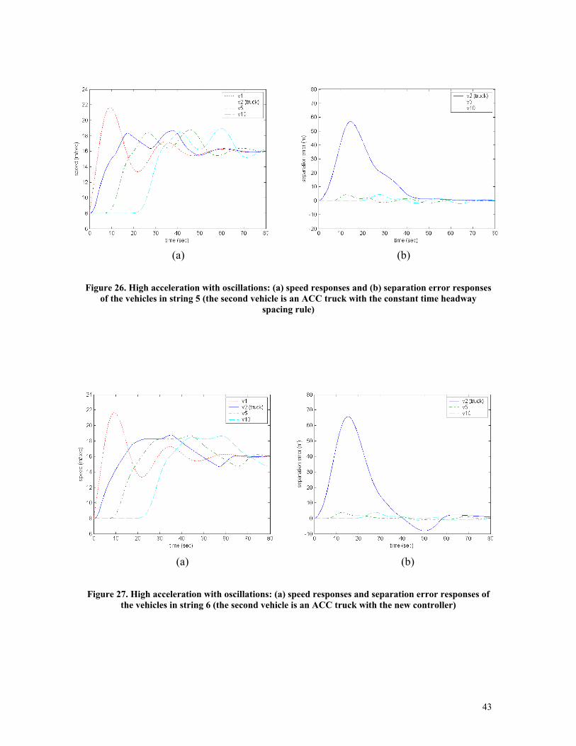
43

Figure 26. High acceleration with oscillations: (a) speed responses and (b) separation error responses

of the vehicles in string 5 (the second vehicle is an ACC truck with the constant time headway spacing rule)

Figure 27. High acceleration with oscillations: (a) speed responses and separation error responses of

the vehicles in string 6 (the second vehicle is an ACC truck with the new controller)

(a) (b)

(a) (b)

44

3.5 Experimental Testing Experiments are conducted at Crows Landing test field on December 5th, 2003 to verify the theoretical and simulation results. Due to time limitation and limited number of passenger vehicles, we only tested how the four different ACC systems affect the response of a heavy truck in a string consisting of three vehicles. The lead vehicle was a Buick LeSabre with an automatic speed tracking system. The second vehicle was the heavy truck with different ACC systems. The tractor mass was about eight tons and the trailer mass was about seven tons. The third vehicle was a Buick LeSabre driven by a human driver, following the truck as in normal traffic. The lidar system installed on the truck was used as the ranging sensor providing separation distance and relative speed between the preceding vehicle and the truck. More detailed information about the hardware and software configurations can be found in [26]. Each vehicle was equipped with a Data Acquisition System recording useful experimental data. In the experiments, the parameters for ACC trucks were chosen as:

ACC_N: 0h =1.6s, 0k =1s-1, hc =0.2s, kc =0.5s-1, σ =0.1m-2 and 0s =6.0m ACC_Q: 1h =0.8s, 2h =0.03s2/m, k =0.2s-1 and 0s =6.0m ACC_C: h=1.6s, k =0.2s-1 and 0s =6.0m ACC_NEW: h=1.6s, k =0.2s-1, 0s =6.0m, p=10s-1, vm =2.0m/s, vM =8.0m/s, and

maxa and mina are acceleration limits chosen based on the capabilities of the truck and desired driver comfort considerations.

A low-pass filter is placed after each ACC controller to limit the rate of change of the control effort. In ACC_N, ACC_Q and ACC_C, the velocity of the preceding vehicle is passed through the nonlinear filter (the same way as in the simulations).

3.5.1 Low Acceleration Maneuvers The lead passenger vehicle accelerates from 13.4m/s (about 30 miles per hour) to 20.1m/s (about 45 miles per hour) with a constant acceleration of 0.6m/s2, and then cruises at a constant speed. Figures 28, 29, 30 and 31 show the speed responses of the three vehicles (labeled as v1 v2 and v3), and the separation error and engine torque responses for the heavy truck with controllers ACC_N, ACC_Q, ACC_C and ACC_NEW respectively. The controllers ACC_N, ACC_Q and ACC_C behave aggressively in regulating the engine torque in order to follow the lead vehicle tightly. The engine torque is close to the maximum value (about 1966 N-m) for short periods of time. As shown in Figure 31, the new ACC system regulates the engine torque in a smooth way at the expense of a larger separation error.

45

Figure 28. Low acceleration (experiment data): (a) speeds of the three vehicles, (b) separation error

and (c) engine torque responses of the ACC truck with the nonlinear spacing rule

(a) (b)

(c)

46

Figure 29. Low acceleration (experiment data): (a) speeds of the three vehicles, (b) separation error

and (c) engine torque responses of the ACC truck with the quadratic spacing rule

(a) (b)

(c)

47

Figure 30. Low acceleration (experiment data): (a) speeds of the three vehicles, (b) separation error and (c) engine torque responses of the ACC truck with the constant time headway spacing rule

(a) (b)

(c)

48

Figure 31. Low acceleration (experiment data): (a) speeds of the three vehicles, (b) separation error

and (c) engine torque responses of the ACC truck with the new controller

(a) (b)

(c)

49

3.5.2 High Acceleration Maneuvers The lead passenger vehicle accelerates from 13.4m/s (about 30 miles per hour) to 20.1m/s (about 45 miles per hour) with acceleration around 1.2m/s2, and then cruises at a constant speed. Figures 32, 33, 34 and 35 show the speed responses of the three vehicles, and separation error and engine torque responses for the heavy truck with controllers ACC_N, ACC_Q, ACC_C and ACC_NEW respectively. As before, the controllers ACC_N, ACC_Q and ACC_C behave aggressively in regulating the engine torque, while the new ACC system regulates the engine torque in a smooth way at the expense of creating a larger separation error. It should be noted that in this experiment, the acceleration bounds, maxa and mina , used for the nonlinear filter in the ACC_NEW controller are different from those used in the previous experiment, and the response of the ACC_NEW is not as sluggish as before.

50

Figure 32. High acceleration (experiment data): (a) speeds of the three vehicles, (b) separation error

and (c) engine torque responses of the ACC truck with the nonlinear spacing rule

(a) (b)

(c)

51

Figure 33. High acceleration (experiment data): (a) speeds of the three vehicles, (b) separation error

and (c) engine torque responses of the ACC truck with the quadratic spacing rule

(a) (b)

(c)

52

Figure 34. High acceleration (experiment data): (a) speeds of the three vehicles, (b) separation error

and (c) engine torque responses of the ACC truck with the constant time headway spacing rule

(a) (b)

(c)

53

Figure 35. High acceleration (experiment data): (a) speeds of the three vehicles, (b) separation error

and (c) engine torque responses of the ACC truck with the new controller

(a) (b)

(c)

54

3.5.3 Model Validation The experiments demonstrated that all the ACC controllers are working on an actual truck in a vehicle following and cruising driving environment. They all have similar responses except for the new ACC controller that is designed to give a smoother response. Even though the number of experiments was limited, the experimental results are valuable in validating our simulation models for the ACC truck and human driver. Our model validation approach is described below.

We simulated the same scenarios as in the experiments using our simulation models. In particular we consider a string of three vehicles where the first and third are manually driven vehicles and the second one is the ACC truck. The first vehicle is made to generate the same speed trajectories as in the experiments. The second vehicle is a heavy truck modeled in the Appendix with one of the ACC systems and the third vehicle is modeled using the Pipes’ model.

In the first validation test, the first vehicle generates the speed trajectory with low acceleration that was used in the experiments, which is plotted with the red dotted line in Figure 36(a), labeled as “1st vehicle”. The speed responses of the ACC truck (with the constant time headway policy) and the passenger vehicle are plotted in Figure 36(a) with broken lines and labeled as “2nd vehicle (ACC truck), simulation” and “3rd vehicle (Pipes’ model), simulation”, respectively. The corresponding experimental data are also plotted in Figure 36(a) with solid lines and labeled as “2nd vehicle (ACC truck), experiment” and “3rd vehicle, experiment”, respectively. It can be seen that the speed responses in the simulation are very close to those in the experiment, which indicates the validation of the used models. The engine torque responses in the simulation and experiment are plotted in Figure 36(b), and they are very similar to each other.

In the second validation test we use the speed trajectory with high acceleration for

the first vehicle and the ACC control with the nonlinear spacing rule in (3-31) for the heavy truck. As shown in Figure 37, the similarity between the simulation and experimental results strongly supports that the nonlinear model used for trucks and the Pipes’ model are valid.

Additional validation tests supported the same conclusion: the nonlinear model

used for heavy trucks and the Pipes’ model used to model human driver response in the longitudinal direction are valid models to be used for studying vehicle following in a mixed traffic situation. Consequently our simulation models and results can be used with confidence in studying vehicle following characteristics and effects involving more vehicles in a mixed traffic situation.

55

Figure 36. Model validation: (a) speed responses of the three vehicles (the second is ACC_C) and (b)

engine torque responses of ACC_C in experiment and simulation

(a)

(b)

56

Figure 37. Model validation: (a) speed responses of the three vehicles (the second is ACC_N) and (b)

engine torque responses of ACC_N in experiment and simulation

(a)

(b)

57

4 IMPACT OF HEAVY TRUCKS ON MIXED TRAFFIC 4.1 Emission and Fuel Consumption In this section we investigate the impact of heavy trucks on mixed traffic in terms of emission and fuel consumption using the simulation results discussed in the previous section. The emission levels and fuel consumption of an individual vehicle are determined by vehicle parameters such as second-by-second speed, acceleration, road grade, wind gust, and variables associated with vehicle accessories. In the emission analysis, the quantities measured are the tailpipe emissions of unburned hydrocarbons (HC), oxides of carbon (CO, CO2), oxides of nitrogen (NO, NO2, denoted by NOx) and fuel consumption.

4.1.1 Emission Models for Passenger Vehicles and Heavy Trucks For passenger vehicles, the Comprehensive Modal Emissions Model (CMEM) developed at UC Riverside is used to analyze the vehicle data and calculate the air pollution and fuel consumption [3]. It calculates vehicle emissions and fuel consumption as a function of the vehicle operating mode, i.e. idle, steady state cruise, various levels of acceleration/deceleration, and other variables associated with road and vehicles characters. A simple diagram for the CMEM model is shown in Figure 38. In our simulations, we selected the vehicle category to be 5, which is the most common vehicle type in California: high-mileage, high power-to-weight. The inputs for the CMEM model are vehicle longitudinal speed and acceleration data, while road grade is taken to be zero and no wind gust is considered. Other variables associated with vehicle accessories like air-conditioning are also neglected. The outputs generated by the CMEM models include second-by-second tailpipe emissions of HC, CO, CO2 and NOx, and fuel consumption.

Figure 38. Diagram of the CMEM model

The emission prediction model used for heavy trucks is developed by the same

research group at UC Riverside, under PATH TO 4215. Similarly to the CMEM model for passenger vehicles, this model takes as its input the operating parameters such as the vehicle’s speed and acceleration data, wind speed, road grade and accessory power.

CO2

CO

HC

vehicle acceleration

vehicle speed

CMEM model

NOx

Fuel consumption

other variables associated with road and vehicle parameters

58

Vehicle parameters such as vehicle weight, maximum horsepower, gear ratios are pre-set for one specific truck. The output results are instantaneous values of tailpipe pollutant emissions of HC, CO, CO2 and NOx, and fuel consumption. More detailed information about the emission models can be found in [2, 3].

4.1.2 Vehicle Following Disturbances We investigate how the heavy trucks affect the travel time, fuel efficiency and emissions of the passenger vehicles in traffic using the emission models presented in Section 4.1.1 and the simulation results presented in Section 3.4. At the same time, we investigate how different ACC systems affect the fuel efficiency and emissions of the heavy trucks in the presence of different vehicle following disturbances. In this subsection, we assume that no lane changes take place despite the creation of possible large intervehicle spacings during vehicle maneuvers. The effect of lane changes is considered in a separate subsection.

We investigate and compare the behavior of six vehicle strings, each containing ten vehicles using the simulation tests we completed in section 3.4. In vehicle string 1, all the ten vehicles are passenger vehicles (modeled using the Pipes’ model (2-4)). Vehicle strings 2, 3, 4, 5 and 6 are almost the same as vehicle string 1, but their second vehicle is replaced by a manually driven truck (modeled using the modified Bando’s model in (2-11), an ACC truck with the nonlinear spacing policy in (3-31), an ACC truck with the quadratic spacing policy, an ACC truck with the constant time headway policy and an ACC truck with the newly developed controller, respectively. The same as before, we use ACC_N, ACC_Q, ACC_C and ACC_NEW to represent ACC trucks with nonlinear spacing rule, quadratic spacing rule, constant time headway rule and the newly developed controller, respectively. Test 1: Low Acceleration Maneuvers The purpose of this test is to examine the effect of the truck (2nd in the string) on the behavior of the following 8 passenger vehicles when the lead vehicle performs a low acceleration maneuver creating a disturbance that propagates upstream.

The lead passenger vehicle accelerates from 8m/s to 20m/s with a constant acceleration of 0.8m/s2, and then cruises at a constant speed. We calculate the fuel consumption and emissions of each vehicle from the time the lead vehicle begins to accelerate, until the string covers a distance of 1.2km. The travel time is recorded over a distance of 1.2km as this is the distance taken by the vehicles to reach a steady state speed after completing the acceleration maneuver.

Table 1 shows the travel time, fuel and emission benefits for the last eight

passenger vehicles in each vehicle string in the presence of different truck in the 2nd position in the string of the 10 vehicles. The data in the second column are for vehicle

59

string 1 (all manually driven passenger vehicles), and the fuel and emission benefits are denoted by 0% and this case is used as the basis for comparison. The data in columns 3-7 are for vehicle strings 2-6, respectively. For the fuel and emission data, a positive number means improvement while a negative number means deterioration. The notation “≈ 0” in the table represents benefits between –4% and 4%, and is considered to be negligible due to inaccuracies in the emission model. As we can see, the presence of different trucks in the 2nd position in the string will not affect the travel time of the following passenger vehicles. Due to the aggressive response of the manual truck, the fuel and emission benefits are minor except for NOx as shown in column 3 of Table 1. The smooth response of the ACC trucks filters the disturbance created by the lead vehicle presenting a smoother speed response to be tracked by the passenger vehicles following the truck. As a result some benefits with respect to fuel and emissions are shown in Table 1. These benefits are small due to the fact that the disturbance created was a rather smooth one (low acceleration).

We also evaluate the fuel consumption and emission results for heavy trucks in these simulations and the data are presented in Table 2. The ACC trucks lead to better fuel consumption and emission results compared to the manually driven truck. However, there is little difference among the four different ACC trucks. The benefits are small however due to low level of disturbance.

String of 10 vehicles

Manual Passenger Vehicle in the 2nd

position

Manual truck in the 2nd position

ACC_N in the 2nd position

ACC_Q in the 2nd position

ACC_C in the 2nd position

ACC_NEW in the 2nd position

Travel Time (sec)

73.7 73.9 73.3 73.3 73.3 73.3

Fuel (g) 0% (617.8) ≈ 0 ≈ 0 ≈ 0 ≈ 0 4.2% CO2 (g) 0% (1924) ≈ 0 ≈ 0 ≈ 0 ≈ 0 4.2% CO (g) 0% (20.6) ≈ 0 7.3% 6.4% 6.0% 9.2% HC (g) 0% (0.93) ≈ 0 7.1% 6.3% 5.9% 9.0% NOx (g) 0% (1.51) 9.1% 10.0% 0 12.1% 10.7% 24.0%

Table 1. Travel time, fuel and emission benefits of the 8 passenger vehicles following the truck in a

string of 10 vehicles for low acceleration maneuvers of the lead vehicle (no cut-ins)

Manual Truck ACC_N ACC_Q ACC_C ACC_NEW Fuel (g) 0% (594.8) 5.8% 6.0% 5.4% 6.6% CO2 (g) 0% (1901) 5.9% 6.0% 5.4% 6.5% CO (g) 0% (5.27) 5.3% 5.3% 5.1% 6.0% HC (g) 0% (0.26) ≈ 0 ≈ 0 ≈ 0 ≈ 0 NOx (g) 0% (12.42) 4.8% 4.8% 4.2% 5.4%

Table 2. Fuel and emission benefits of the heavy truck during low acceleration maneuvers of the lead

vehicle (no cut-ins).

60

Test 2: High Acceleration Maneuvers The purpose of this test is to examine the effect of the truck (2nd in the string) on the behavior of the following 8 passenger vehicles when the lead vehicle performs a high acceleration maneuver creating a disturbance that propagates upstream.

The lead passenger vehicle accelerates from 8m/s to 20m/s with a constant acceleration of 2.0m/s2, and then cruises at a constant speed. As in test 1, we consider the same six strings of vehicles with 10 vehicles in each string. The travel time is recorded over a distance of 1.7km as this is the distance taken by the vehicles to reach a steady state speed after completing the acceleration maneuver.

Table 3 shows the travel time, fuel consumption and emission results for the last eight passenger vehicles in the simulations with high acceleration maneuvers. The presence of different trucks in the 2nd position in the string of 10 vehicles does not affect travel time as despite the sluggish response of the truck and the creation of a large intervehicle spacing, the truck eventually closes in by using a higher speed than the lead vehicle. The strings with heavy trucks significantly increase the fuel efficiency and decrease emissions of the following passenger vehicles. The trucks act as low-pass filters presenting a much smoother speed response to be tracked by the vehicles following the trucks in the string. Furthermore, it is observed that all the ACC trucks lead to better fuel consumption and emissions compared with the manual truck. The new ACC system has the best improvements.

String of 10 vehicles

Manual Passenger Vehicle in the 2nd

position

Manual truck in the 2nd position

ACC_N in the 2nd position

ACC_Q in the 2nd position

ACC_C in the 2nd position

ACC_NEW in the 2nd position

Travel Time (sec)

96.0 96.2 95.4 95.4 95.4 95.4

Fuel (g) 0% (1020) 15.5% 21.5% 22.7% 22.4% 23.9% CO2 (g) 0% (2828) 5.5% 12.1% 13.4% 13.1% 14.5% CO (g) 0% (251.2) 87.9% 89.4% 89.9% 89.9% 90.4% HC (g) 0% (4.02) 65.1% 68.4% 71.5% 71.4% 73.1% NOx (g) 0% (4.21) 52.1% 56.0% 60.6% 60.3% 67.7%

Table 3. Travel time, fuel and emission benefits of the 8 passenger vehicles following the truck in a

string of 10 vehicles for high acceleration maneuvers of the lead vehicle (no cut-ins)

Table 4 shows the fuel consumption and emission results for different trucks. All the ACC trucks have better results in terms of fuel efficiency and emissions compared with the manually driven truck. This is due to the smoother response of the ACC trucks compared with the more aggressive manually driven truck. However, there is little difference among the four different ACC trucks.

61

Manual Truck ACC_N ACC_Q ACC_C ACC_NEW

Fuel (g) 0% (802.0) 10.6% 12.7% 12.6% 12.6% CO2 (g) 0% (2564) 10.4% 12.6% 12.5% 12.5% CO (g) 0% (7.09) 9.2% 11.1% 11.0% 10.9% HC (g) 0% (0.34) 4.4% 5.2% 5.1% 5.1% NOx (g) 0% (18.14) 7.6% 9.5% 9.5% 10.2%

Table 4. Fuel and emission benefits of the heavy trucks in high acceleration maneuvers (no cut-ins)

Test 3: High Acceleration Maneuvers with Oscillations The purpose of this test is to examine the effect of the truck (2nd in the string) on the behavior of the following 8 passenger vehicles when the lead vehicle performs a high acceleration oscillatory maneuver creating a disturbance that propagates upstream.

The lead passenger vehicle accelerates from 8m/s to 16m/s with a constant acceleration of 2.0m/s2, and its speed oscillates around 16m/s before settling to the constant speed of 16m/s. The travel time is recorded over a distance of 1.3km as this is the distance taken by the vehicles to reach a steady state speed after completing the acceleration maneuver.

Table 5 shows the travel time, fuel consumption and emission results for the last eight passenger vehicles in each vehicle string. The travel time of the following passenger vehicles is little affected by the trucks. It follows from Table 5, that the presence of heavy trucks can significantly improve the fuel efficiency and decrease most of the emissions. This is due to the fact that the inherent sluggish characteristics of the heavy trucks can attenuate the high frequency components in the speed of the lead vehicle. Among the ACC trucks, the ACC_NEW leads to the best results in all aspects, since it filters the oscillations in the lead vehicle’s speed more effectively than the others.

String of 10 vehicles

Manual Passenger Vehicle in the 2nd

position

Manual truck in the 2nd position

ACC_N in the 2nd position

ACC_Q in the 2nd position

ACC_C in the 2nd position

ACC_NEW in the 2nd position

Travel Time (sec)

88.0 88.1 87.5 87.5 87.6 87.6

Fuel (g) 0% (860.3) 23.9% 29.7% 34.2% 34.0% 36.3% CO2 (g) 0% (2245) 9.8% 16.0% 21.3% 21.0% 23.6% CO (g) 0% (298.3) 90.2% 93.5% 94.5% 94.5% 95.1% HC (g) 0% (4.45) 73.7% 79.3% 82.4% 82.8% 84.2% NOx (g) 0% (4.87) 59.4% 65.0% 68.8 69.0% 78.7%

Table 5. Travel time, fuel and emission benefits of the 8 passenger vehicles following the truck in a

string of 10 vehicles for high acceleration maneuvers with oscillations of the lead vehicle (no cut-ins)

62

Table 6 shows the fuel consumption and emissions results for different trucks. All the ACC trucks lead to better fuel consumption and emissions results compared with the manually driven truck, and the performance of the new ACC system is the best.

Manual Truck ACC_N ACC_Q ACC_C ACC_NEW Fuel (g) 0% (618.2) 12.0% 23.1% 22.9% 27.4% CO2 (g) 0% (1976) 12.0% 23.0% 22.8% 27.4% CO (g) 0% (5.55) 10.6% 20.0% 20.0% 23.6% HC (g) 0% (0.28) 4.8% 8.5% 8.5% 12.4% NOx (g) 0% (13.2) 9.1% 17.0% 17.2% 21.5%

Table 6. Fuel and emission benefits of the trucks in high acceleration maneuvers with oscillations (no

cut-ins)

From the data presented in Tables 1, 3 and 5, we can see that the presence of heavy trucks in the mixed traffic can improve fuel consumption and emissions of the passenger vehicles, especially in the presence of disturbances due to high acceleration maneuvers. The heavy trucks act as filters due to their sluggish response and present to the following vehicles upstream smoother speed responses to be tracked. Furthermore, the ACC trucks lead to better fuel and emissions results than the manually driven trucks due to their smoother response. In the case of high acceleration maneuvers with oscillations, the heavy truck with the newly developed ACC controller (ACC_NEW) filters the oscillations more effectively leading to better fuel and emission results than the other ACC trucks.

The results obtained raised several questions that require further investigation. First the validity of the emission models and their accuracy needs to be revisited in collaboration with the UC Riverside researchers that developed the emission models for passenger vehicles and trucks. While most of the benefits obtained make sense qualitatively a quantitative validation is necessary by using actual experiments and measuring fuel and pollutants in real time. In our approach we assume that the lead vehicle reaches a steady state giving time for the truck to close in by using a higher speed leading to a travel time that is not affected by the presence of the truck. We can also create scenarios where the travel time will be affected when the truck does not speed up to close in with the lead vehicle especially when the truck cannot achieve a higher speed due to load and speed limits. In such situations another effect takes place as the sluggish response of the truck creates large inter vehicle gaps inviting vehicles from neighboring lanes to cut in front of the truck. This effect is investigated in the next subsection.

4.1.3 Lane Change Effect The motivation for studying lane change effects in mixed traffic with heavy trucks and passenger vehicles is based mostly on the fact that the sluggish response of the heavy truck results in a large temporary gap between the truck and the accelerating passenger

63

vehicle in front, giving rise to multiple cut-ins from the neighboring lanes. In this subsection, we consider various cut-in situations, and study the effects of lane changes using microscopic simulations. It is assumed that when the spacing between the truck and its preceding vehicle is large enough (larger than tvs 8.20 + , where tv is the truck speed), one or more passenger vehicles from the neighboring lane cut in between the two vehicles and position themselves with safe intervehicle spacings. In this simulation, the truck is considered to be equipped with the new ACC system, followed by eight passenger vehicles. We like to investigate how the disturbance created by the cut-ins will affect the response of the truck and that of the passenger vehicles following the truck.

We consider the situation where the passenger vehicle leading the ACC truck accelerates from 8m/s to 20m/s with a constant acceleration of 2m/s2, and then cruises with a constant speed creating a large inter vehicle spacing. We assume that three vehicles cut in at 5, 10.6 and 17.5 seconds, respectively, and with the speeds of 12.2, 18.0 and 21.0m/s, respectively. These cut-ins are shown in Figure 39. We consider the travel time, fuel consumption and emissions for the last eight passenger vehicles after they have traveled 1.7km, and present them in the right column of Table 7. For comparison purpose, the corresponding data for the situation without cut-in vehicles are also presented in Table 7. From Table 7, we can see that the disturbance created by the cut-ins has a small negative effect on fuel consumption and emissions. However, the travel time is increased by about 4 seconds due to the cut-ins.

Figure 39. Responses of the vehicles in string 6 in high acceleration maneuvers with three cut-in

vehicles: (a) speed responses and (b) separation error responses

(a) (b)

64

Without Cut-in(s) With Cut-in(s)

Travel Time (sec) 95.4 99.5 Fuel (g) 776 811 (-4.5%) CO2 (g) 2418 2531 (-4.5%) CO (g) 24.2 24.3 (-0.4%) HC (g) 1.08 1.11 (-2.8%) NOx (g) 1.36 1.40 (-2.9%)

Table 7. Travel time, fuel and emission data of the 8 passenger vehicles following ACC_NEW in high

acceleration maneuvers, without cut-in(s) and with three cut-ins

Note that the above simulation results are based on the cut-in situations considered. If we consider more aggressive cut-ins for example, a passenger vehicle at a low speed cuts in just a few meters ahead of the heavy truck forcing the truck to decelerate and then speed up, different results may be obtained as the disturbance created in such scenario may have a more adverse effect on fuel economy and pollution. Furthermore cut-ins will create disturbances in the neighboring lane too with adverse effects on fuel economy and pollution for the vehicles in those lanes. Our conclusion is that while the heavy trucks with ACC or not have smooth responses and filter traffic disturbances their sluggish behavior will create large gaps inviting cut-ins which may take away any benefits their filtering response will have for the vehicles in their lane. Furthermore, the cut-ins will create additional disturbances in the neighboring lanes that will also have a negative effect on fuel economy and pollution. 4.2 Macroscopic Traffic Flow Analysis In this section we investigate the effect of heavy trucks manually driven and with ACC on traffic flow characteristics in mixed traffic on the macroscopic level using the fundamental flow-density diagram. A fundamental flow-density diagram defines the steady-state relation between the traffic flow rate and the traffic density [17]. We outline flow-density diagrams for 100% manual and 100% ACC vehicles traffic, and discuss the impact on the flow-density curves caused by heavy trucks. The manual traffic flow-density curve discussed in this report is constructed using the linear relationship between speed and density hypothesized by Greenshields [9]. The 100% ACC traffic flow-density curve is constructed using the ACC design with the constant time headway policy. The effect of heavy trucks mixed with passenger vehicles in the presence of traffic flow disturbances is also analyzed.

4.2.1 Fundamental Flow-Density Diagram The fundamental flow-density diagram defines the steady-state relation between the traffic flow rate q and the traffic density ρ . The precise definitions of these two traffic

65

variables and the means of measuring them are explained in [17]. In this subsection we focus on the flow-density diagrams for 100% manual and 100% ACC traffic and the impact of heavy trucks on these flow-density diagrams. 4.2.1.1 Manual/ACC Traffic without Heavy Trucks In this subsection, we assume all the vehicles in the traffic stream are passenger vehicles. The presence of heavy trucks will be considered in the next subsection. In constructing the fundamental flow-density diagram for the 100% manual vehicles traffic, we consider the hypothesis in [9] that

fvv

−=

max

1ρρ (4-1)

where v is the vehicles’ mean speed (or traffic flow speed), fv is the free speed corresponding to negligible traffic density when there is no interaction among vehicles, and maxρ is the density corresponding to the jam condition when all the vehicles are in standstill due to congestion. The maximum value of maxρ is equal to 1/L where L is the average length of vehicles and corresponds to the case where vehicles are bumper to bumper. In practice, the bumper-to-bumper situation will never happen. Hence we add some intervehicle spacing to L. In the following analysis, L is larger than the average length of a vehicle.

The traffic flow rate q at steady state measures the number of vehicles moving in a specified direction on the road per unit time and is given by vq ρ= (4-2) With (4-1), the manual traffic flow-density relationship at steady state is given by

fvq

−=

max

1ρρρ (4-3)

The fundamental ρ−q diagram labeled as “100% manual” in Figure 40 is generated using (4-3). It follows from (4.3) that the traffic flow rate achieves its maximum value

4max f

mm

vq

ρ= when the traffic density is

2maxρ

ρ =cm .

While the behavior of human drivers is random and at best we can develop a

manual traffic flow-density model that is qualitatively valid, the response of ACC vehicles is more deterministic due to the use of a specific spacing policy. In this report we consider the ACC designs that use a constant time headway policy. For simplicity we assume that all ACC vehicles have the same length L and use the same time headway ha .

66

When the traffic density is low, we can assume no vehicle interaction and all the ACC vehicles operate close to the free speed v f . As the traffic density increases, and reaches the value

Lvh fa

ca +=

1ρ (4-4)

the ACC vehicles begin to interact with each other. The total spacing, s, occupied by an ACC vehicle using a constant time headway ha at a speed v is given by s h v La= + (4-5) Note, the safe distance term 0s in the spacing policy (3-14) has been incorporated into L. Since s is the reciprocal of ρ , from (4-5), we can get

−= L

hv

a ρ11 (4-6)

According to (4-6), the steady-state speed of the ACC vehicles decreases with increasing ρ until ρ reaches its maximum value L1max =ρ . The fundamental flow-density diagram for the traffic with 100% ACC vehicles is given by

( )

≤<−

≤≤=

max 10

ρρρρ

ρρρ

caa

caf

hLv

q (4-7)

Equation (4-7) does not capture effects that are due to individual vehicle responses but describes the average steady state traffic flow characteristics. The relationship described by (4-7) can be graphically viewed as the curve labeled as “100% ACC” in Figure 40.

The maximum traffic flow rate for the 100% ACC traffic, mcq , is equal to Lvh

v

fa

f

+.

67

Figure 40. Fundamental flow-density diagrams of the manual traffic and the ACC traffic

If the traffic is dense enough to be viewed as a fluid, then from the conversation of mass equation, we have

0=∂∂

+∂∂

xq

tρ (4-8)

Further assuming that the human driver or the ACC system can adjust the vehicle’s speed instantaneously to the steady state value based on the current traffic density, we can treat q as a function that depends only on ρ , and (4-8) can be rewritten as

0=∂∂

+∂∂

xc

tρρ (4-9)

where

ρ

ρρ ∂

∂+==

vvddqc (4-10)

When the traffic density on any road section is close to a constant 0ρ , c can be

approximated as a constant equal to ( )0

00ρρρ

ρρ=∂

∂+

vv , which can be interpreted as the

slope of the tangent to the ρ−q curve at 0ρρ = . When c is a constant, the solution of (4-9) is a traveling wave

flow rate q (veh/hr)

flow density ρ (veh/km)

100% ACC

100% manual

qma

qmm

ρcm ρca ρmax

68

( ) ( )ctxFtx −=,ρ (4-11) where F is an arbitrary differentiable function. If v is a non-increasing function of ρ , which is true in practice, we can see that vc ≤ always holds. This means the traveling wave always propagates backwards relative to the traffic flow. If 0>c , then any density disturbance propagates as a forward traveling wave. If 0<c , then the density disturbance propagates as a backward traveling wave, which indicates that any density disturbance is traveling upstream in the space without any attenuation. Using the flow-density relationship of manual traffic described by (4-3), it can be shown that

ff vvvc −=

−= 221

maxρρ (4-12)

It follows that c is a strictly decreasing function of ρ and

[ ]

( ]

∈<∈≥

max if ,00 if ,0

, ρρρc, ρρc

cm

cm (4-13)

In the 100% manual traffic, the ρ−q curve has a stationary point that corresponds to a critical density cmρ that gives the maximum traffic flow rate qmm or the capacity on that section of the road. The point ),( cmmmq ρ has been empirically observed to be unstable, i.e. it leads to a breakdown in traffic flow [5]. When the traffic flow conditions exist at or near this point, the traffic flow rate and the average speed decrease as the traffic density increases, and the operating point moves towards the jam density maxρ on the ρ−q curve. This observation is explained in [33]. As capacity is approached, the flow tends to become unstable as the number of available gaps reduces. Traffic flow at capacity means that there are no usable gaps left. A disturbance in such a condition due to lane changing or vehicle merging is not ‘effectively damped’ or ‘dissipated’. As indicated by (4-11) and (4-13), any disturbance propagates upstream without attenuation. This leads to a breakdown in traffic flow and ‘formation of upstream queues’. As pointed out in [33], this is the reason why all facilities are designed to operate at lower than the maximum traffic flow conditions.

For the ACC traffic described by (4-7), it follows that

[ ]

( ]

∈−

∈=

max if ,

0 if ,

, ρρρhL

, ρρvc

caa

caf

(4-14)

where caρ is the critical density given in (4-4). From (4-13), it follows that the speed of the traveling wave is the same as the average speed of all the ACC vehicles when the

69

traffic density is lower than caρ . When the traffic density is higher than caρ , any disturbance in the traffic will propagate upstream with a constant speed ahL . As we can see, selecting large ah can slow the speed of traveling waves, but decrease the maximum traffic flow rate.

Let us consider the stability of the point ),( camaq ρ , which corresponds to the point ),( cmmmq ρ in the manual traffic. It is not possible to empirically determine the stability of ),( camaq ρ . However, it is expected that the point ),( camaq ρ will also be unstable, i.e. at this operating point there will be a breakdown in traffic flow [5]. As in the manual traffic, flow will tend to become unstable as capacity is approached and the number of available gaps reduces. At critical density there will be no usable gaps left. Any disturbance generated at this condition is expected to lead to the formation of upstream queues and a breakdown in traffic flow, as observed in the manual traffic [5]. From (4-14), it can be shown that when ( ]max, ρρρ ca∈ , the traffic is unstable in the sense that disturbances propagate upstream unattenuated [22]. 4.2.1.2 Manual/ACC Traffic with Heavy Trucks In the previous subsection, we have developed a flow-density model that qualitatively describes manual traffic flow characteristics, and a deterministic flow-density model for ACC traffic. We have assumed that all the vehicles in the traffic stream are passenger vehicles of the same size and use the same spacing rule. In this subsection, we consider how the heavy trucks affect the fundamental flow-density diagrams and the traveling waves, i.e. the traffic disturbances. To simplify the analysis, we consider the case where the vehicles are all manually driven or ACC operated. In either situation (manual or ACC), there are only two classes of vehicles, passenger vehicles and heavy trucks. The vehicles of the same class have the same size and use the same spacing rule. Hence, at steady state conditions, vehicles of the same class use identical intervehicle spacings. For the ACC case, the intervehicle spacing is equal to the designed value for the ACC controller considered. For the manual case, the inter vehicle spacing is taken to be equal to the average value observed in manual traffic.

Figure 41. Mixed traffic with passenger vehicles and heavy trucks

Lt

sc st

st0

Lc

sc0

sc

70

Consider the mixed traffic flow shown in Figure 41, where tL and cL are the average lengths of heavy trucks and passenger vehicles, respectively, and ts and cs are the average intervehicle spacings used by trucks and passenger vehicles, respectively. Note, the safety distances at the congestion conditions ( 0ts and 0cs ) are incorporated in

tL and cL , as done in the previous analysis. The average intervehicle spacing at steady state , s , is given by ct sppss )1( −+= (4-15) where p is the penetration of heavy trucks in traffic. The average traffic density, mixρ , is given by

ct

mix sppss )1(11−+

==ρ (4-16)

Due to the lack of studies for truck driver behavior, we have no data as to how

truck drivers adjust the intervehicle spacing as a function of the traffic density or traffic speed. We assume that the average time headway kept by truck drivers is hmr times of that kept by passenger vehicle drivers, and hmr is a constant for all speeds. In our analysis, we assume 1>hmr since trucks have lower braking capabilities than passenger vehicles and tend to maintain larger intervehicle spacings for safety reasons. From (4-1), we can see that the average time headway used by passenger vehicles is given as:

vv

Lhf

ccm −= (4-17)

where cL is the average length of a passenger vehicle. Equation (4-17) indicates that drivers decrease the time headway as the traffic density increases. Based on our assumption, the average time headway used by truck drivers, tmh , is

vv

Lrrhrh

f

t

L

hmcmhmtm −

⋅== (4-18)

where ctL LLr = , and 1>Lr . From (4-15) and (4-16), we get

cLcmh

mix Lpvhp +=

1ρ (4-19)

71

where )1( pprp hmh −+= , ( )pprp LL −+= 1 and v is the traffic speed. In (4-19), cL Lp and cmhhp represent the average vehicle length and time headway, respectively. With (4-17), it follows that

fp

pf

p

vLrL

Lrv

LrLLv

+−−=

+−−

=ρρ

ρρρ

ρ1

11

1 (4-20)

where cL LpL = and Lhp ppr = . Here, ρ is used to represent mixρ , and in the following analysis, we will always use ρ . When 0=p , (4-20) is the same as (4-1), and the corresponding fundamental flow-density diagram is labeled as the “0% trucks” in Figures 42, 43, 44, 45 and 46. With (4-2) and (4-20), the traffic flow rate q is given by

fp

p vLrL

Lrq ρ

ρρρ

+−−=

11 (4-21)

From (4-21), it follows that

( )( ) f

p

p vLrL

LrLddq

2

222

1

1

ρρ

ρρρ +−

−−= (4-22)

and

( ) fp

p vLrL

Lrd

qd32

2

1

2

ρρρ +−−= (4-23)

[ ]L1,0∈ρ indicates ( ) 01 >+− ρρ LrL p , and then 02

2

<ρd

qd . Hence, q is a strictly

concave function of ρ on [ ]L1,0 , and ρd

dqc = is a strictly decreasing function of ρ on

[ ]L1,0 . The maximum traffic flow rate, mmq , is achieved at cmρ , where mmq and cmρ are given as

( )Lrpcm

+=

11ρ (4-24a)

( ) Lr

vq

p

fmm 2

1+= (4-24b)

From (4-22), it follows that the speed of the traveling waves, c, is given by

72

( )( ) f

p

p vLrL

LrLddqc 2

222

1

1

ρρ

ρρρ +−

−−== (4-25)

At the same time, from (4-20), we get

( )vrvvLvv

pf

f

+−

−=ρ (4-26)

Substituting (4-28) into (4-27), we get

( )

fp

f

f vrvv

vvc

22 −−= (4-27)

Using the above equations we examine how the presence of trucks affect the traffic flow characteristics. If the truck is counted as a single vehicle it is trivial to see that the traffic flow rate will decrease because a heavy truck occupies more space than a single passenger vehicle due to its larger length and bigger spacing used ( 1>hmr and 1>Lr ). Furthermore, it is easy to verify that cmcm ρρ < and mmmm qq < . However, if we treat one truck as Lr passenger vehicles, how does the appearance of trucks affect the traffic throughput? Another question is how it affects the speed with which a traveling wave generated by a density disturbance travels upstream. These answers depend on the value of pr . When p is nonzero, Lhmp rrr >⇔>1 , Lhmp rrr =⇔=1 and Lhmp rrr <⇔<1 . When we treat one heavy truck as equivalent to Lr passenger size vehicles, each of

which has the length of cL and uses a time headway cmL

hmcm h

rrh =′ , and the penetration of

heavy trucks is p means the equivalent penetration in passenger size vehicles is

( )prprp

L

L

11 −+=′ . It can be seen that the previous analysis for the traffic including heavy

trucks based on (4-21) can also be applied to the analysis for the traffic where trucks are treated as equivalent to Lr passenger size vehicles with proper replacement of variables. In the following analysis, we denote the traffic density and flow rate for the traffic including trucks as ρ′ and q′ , respectively, when one truck is treated as Lr passenger size vehicles. The maximum density, critical density and maximum traffic flow rate are denoted as maxρ′ , cmρ′ and mmq′ , respectively.

We consider the following cases:

73

Case 1: Lhm rr = In this case, we consider Lhm rr = , i.e. the time headway ratio of truck versus passenger vehicle is equal to the length ratio of truck versus passenger vehicle, or equivalently,

1=pr for all p. The assumed average time headway used by truck drivers is

cmc

ttm h

LLh = (4-28)

Hence, (4-20) can be rewritten as

fvv

−=

max

1ρρ (4-29)

where L1max =ρ . Using the similarity of (4-29) with (4-1), we can conclude that the previous analysis based on (4-1) can be applied to (4-29) by simply taking maxmax ρρ = and LL = . The fundamental flow-density diagram based on (4-29) is labeled as the “100p% trucks” in Figure 42. Due to the presence of heavy trucks, the maximum traffic flow rate mmq and the corresponding critical density cmρ are less than mmq and cmρ , respectively. If the mixed traffic has the same speed as the “0% trucks” traffic, the traveling waves in the two traffic flows have the same speed, as indicated by (4-12). This point can be graphically viewed in Figure 42. Suppose A0 is an arbitrary point on the curve labeled as “0% trucks”, and the line connecting O and A0 intersects the curve “100p% trucks” at point Ap. At Ap and A0, the two traffic streams have the same speed, which is equal to the slope of the line passing through O and A0. The slopes of the two tangents at Ap and A0, which correspond to the speeds of the traveling waves in the two traffic flows, are the same for all 10 ≤≤ p . This means the presence of heavy trucks does not affect the speed of the traveling waves, provided the speeds of the two different traffic flows are the same.

In this case, when one heavy truck is treated as Lr passenger size vehicles, each of

these vehicles uses the same average time headway as the passenger vehicles in the manual traffic. Hence the ρ′−′q curve is the same as the curve labeled as “0% trucks” in Figure 42, for 10 ≤≤ p . This means the presence of heavy trucks doesn’t affect the traffic flow-density diagram. In practice this case is possible to occur but it is not a frequent one as trucks tend to use much higher headways on the average than passenger vehicles for safety reasons and also due to their limited acceleration capabilities.

74

Figure 42. Fundamental flow-density diagrams of the manual traffics with/without heavy trucks

( Lhm rr = )

Case 2: Lhm rr <

In this case, Lhm rr < , i.e. the time headway ratio of truck versus passenger vehicle is smaller than the length ratio of truck versus passenger vehicle. Equivalently, 1=pr if

0=p , and 10 << pr otherwise. The fundamental flow-density diagram is labeled as

“100p% trucks” shown in Figure 43. From (4-24a) and (4-24b), we know that Lcm 21

>ρ

and L

vq f

mm 4> . It is obvious that for two traffic flows at the same speed, the one with

100p% of trucks will have traveling waves propagating upstream faster, based on (4-27). This point can be graphically viewed as in Figure 43: the slope of the tangent at point Ap is smaller (more negative) than that at point A0. Following the same analysis, we conclude that for two traffic flows at the same speed, the one with more percentages of trucks will have traveling waves transferring upstream faster.

In this case, when one heavy truck is treated as Lr passenger size vehicles, each of

these vehicles uses the time headway cmL

hm hrr

, which is smaller than cmh . The

fundamental flow-density diagram is labeled as “100p% trucks” shown in Figure 44. It is easy to verify that this curve can be achieved by scaling the curved labeled as “100p% trucks” in Figure 43 with Lp in both q and ρ axes. Now we can see that

flow rate q (veh/hr)

flow density ρ (veh/km)

0% trucks qmm

ρcm cmρ ρmax maxρ

mmq

100p% trucks

O

A0

Ap

75

cL1

maxmax ==′ ρρ , c

cm L21

>′ρ and c

fmm L

vq

4>′ . This indicates the presence of heavy

trucks increases the critical density and traffic throughput if we treat each of them as Lr passenger size vehicles. This is due to the fact that in this case the drivers of heavy trucks use relatively small time headway. As case 1, this case is unlikely to take place frequently in practice as trucks will employ high headways on the average for safety reasons but also due to their inability to accelerate as fast and maintain as high speeds as passenger vehicles.

Figure 43. Fundamental flow-density diagrams of the manual traffics with/without heavy trucks ( Lhm rr < )

flow rate q (veh/hr)

flow density ρ (veh/km)

0% trucks qmm

ρcm cmρ ρmax maxρ

mmq

100p% trucks

O

A0

Ap

76

Figure 44. Fundamental flow-density diagrams of the manual traffics with/without heavy trucks (one truck is treated as Lr passenger vehicles, Lhm rr < )

Case 3: Lhm rr > In this case, Lhm rr > , i.e. the time headway ratio of truck versus passenger vehicle is larger than the length ratio of truck versus passenger vehicle. Equivalently, 1=pr if

0=p , and 1>pr otherwise. In practice it is more likely that Lhm rr > . This is due to the fact that trucks are more likely to maintain higher headways due to safety reasons as well as due to their sluggish response. The fundamental flow-density diagram is labeled as

“100p% trucks” shown in Figure 45. From (4-24a) and (4-24b), we know that Lcm 21

<ρ

and L

vq f

mm 4< . For two traffic flows at the same speed, the one with trucks will have

traveling waves propagating upstream slower, based on (4-27). This point can be graphically viewed as in Figure 44: the slope of the tangent at point Ap is larger (less negative) than that at point A0. Following the same analysis, we conclude that for two traffic flows at the same speed, the one with more percentages of trucks will have traveling waves transferring upstream slower.

flow rate q (veh/hr)

flow density ρ (veh/km)

0% trucks qmm

ρcm cmρ ′ ρ’max (ρmax)

mmq′ 100p% trucks

O

77

Figure 45. Fundamental flow-density diagrams of the manual traffics with/without heavy trucks

( Lhm rr > )

In this case, when one heavy truck is treated as Lr passenger size vehicles, each of

these vehicles uses the time headway cmL

hm hrr

, which is larger than cmh . The fundamental

flow-density diagram is labeled as “100p% trucks” shown in Figure 46. It is developed by scaling the curved labeled as “100p% trucks” in Figure 45 with Lp in both q and ρ

axes. Now we can see that cL

1maxmax ==′ ρρ ,

ccm L2

1<′ρ and

c

fmm L

vq

4<′ . This indicates

that the presence of heavy trucks decreases the critical density and traffic throughput if we treat each of them as Lr passenger size vehicles. This is due to the drivers of heavy trucks using larger time headways relative to that of passenger vehicles. Furthermore a density disturbance will travel upstream slower in the case of mixed traffic with trucks taking longer time to dissipate. We believe that this case is the most dominant one in practice as trucks due to their limited acceleration and speed capabilities will average high time headways with negative effects on traffic flow characteristics predicted in this case.

flow rate q (veh/hr)

flow density ρ (veh/km)

0% trucks qmm

ρcm cmρ ρmax maxρ

mmq

100p% trucks

O

A0

Ap

78

Figure 46. Fundamental flow-density diagrams of the manual traffics with/without heavy trucks (one

truck is treated as Lr passenger vehicles, Lhm rr > )

In the ACC traffic, the fundamental flow density diagram is easy to construct since all the vehicles in the traffic stream are guided by the designed ACC systems. Let us assume that the trucks use the spacing rule ttata Lvhs += (4-30) where tas is the spacing occupied by one ACC truck and tah is the time headway. We also assume that the passenger vehicles use the spacing rule ccaca Lvhs += (4-31) where cas is the spacing occupied by one ACC passenger vehicle and cah is the time headway. From (4-15), it is derived that at speed v, the average intervehicle spacing is given as Lvhs aa += (4-32) where ( ) cataa sppss −+= 1 , ( ) cataa hpphh −+= 1 and ( ) ct LppLL −+= 1 . If the traffic

density is lower than Lvh fa

ca +=

1ρ , then there is no vehicle interaction and all vehicles

flow rate q (veh/hr)

flow density ρ (veh/km)

0% trucks qmm

ρcm cmρ ′

mmq′

100p% trucks

O ρ’max (ρmax)

79

travel at the free speed fv . When the traffic density reaches or exceeds caρ , (4-32) leads to

Lvha +

=1ρ (4-33)

or equivalently

−= L

hv

a ρ11 (4-34)

The steady-state speed of the ACC vehicles decreases with increasing ρ until ρ reaches its maximum value L1max =ρ . The steady-state flow-density relationship is given by

( )

>−

≤=

caa

caf

hL

vq

ρρρ

ρρρ

1

(4-35)

The flow-density relationship in (4-35) is similar to that in (4-7), and the previous analysis for the ACC traffic with passenger vehicles can be applied to the mixed ACC traffic with proper replacement of variables. If the truck is counted as a single vehicle it is trivial to see that the traffic throughput will decrease because a heavy truck occupies more space than a single passenger vehicle. However, if we treat one truck as Lr passenger size vehicles, how does the appearance of trucks affect the traffic throughput? How do heavy trucks affect the speed of traveling waves? When the traffic density is extremely low, the appearance of heavy trucks will not affect throughput since there is no interaction among vehicles and all vehicles move at the free speed. If we assume the traffic density is relatively high, then all the traffic disturbances will be propagated upstream at the speed ahL− . Let’s define cataha hhr = ,

)1( pprp hah −+= , and keep the definitions for Lp , Lr and pr as used for the manual

traffic. It can be verified that pa rhL 1= . Again, we can see how heavy trucks affect the traveling waves depends on the value of pr , and the conclusions to be presented are the same as those for the manual traffic. Case 1: Lha rr = In this case, the time headway ratio of truck versus passenger vehicle is equal to the length ratio of truck versus passenger vehicle, i.e. 1=pr for all possible values of p. This means the presence of heavy trucks does not affect the speed of the traveling waves. If

80

we treat one heavy truck as Lr passenger size vehicles, the flow density curve for the mixed traffic is the same as that of the traffic without trucks. Case 2: Lha rr <

In this case, the time headway ratio of truck versus passenger vehicle is smaller than the length ratio of truck versus passenger vehicle. Equivalently, 1=pr if 0=p , and

10 << pr otherwise. The fundamental flow-density diagram is given in Figure 47, labeled as “100p% trucks”. For comparison purposes, the fundamental flow-density diagram for the ACC traffic without trucks is also given in Figure 47, labeled as “0% trucks”. It is easy to see that for high traffic densities, the appearance of heavy trucks will make traveling waves propagate upstream faster. It can also be shown that for two traffic flows with the same speed, the one with higher percentage of trucks will have traveling waves propagating upstream faster.

If one heavy truck is treated as Lr passenger size vehicles, the flow density curve can be developed by scaling the curve labeled as “100p% trucks” in Figure 47 with Lp in both q and ρ axes. In this case, this appearance of heavy trucks increases the critical density and traffic throughput.

Figure 47. Fundamental flow-density diagrams of the ACC traffic with/without heavy trucks ( Lha rr < )

flow rate q (veh/hr)

flow density ρ (veh/km)

0% trucks

100p% trucks

qma

ρcm ρmax cmρ maxρ

mmq

81

Case 3: Lha rr >

In this case, the time headway ratio of truck versus passenger vehicle is smaller than the length ratio of truck versus passenger vehicle. Equivalently, 1=pr if 0=p , and 1>pr otherwise. Following (3-35), we know that the appearance of heavy trucks will make traveling waves propagate upstream slower. It can also be shown that for two traffic flows with the same speed, the one with higher percentage of trucks will have traveling waves propagating upstream slower.

If one heavy truck is treated as Lr passenger size vehicles, the appearance of heavy trucks decreases the critical density and traffic throughput. The conclusion is the same as that in Case 3 of the manual traffic: the traffic is more susceptible to instability due to the presence of heavy trucks.

The three cases above related to ACC vehicles indicate very similar conclusions as in the corresponding cases of manually driven vehicles. In the manually driven vehicles we argue that the limited acceleration and speed capabilities of trucks will create large intervehicle gaps frequently raising the average headway used to be much greater than that of passenger vehicles therefore in manual traffic case 3 will dominate. For the ACC traffic however it is more likely that cases 1, 2 will be dominant as ACC trucks will use lower average headways than in case 3 leading to a more stable traffic characteristics than those in manual traffic.

4.2.2 Shock Waves Analysis Shock waves are discontinuous waves that occur when traffic on a section of a road is denser downstream than upstream. The waves on the less dense section travel faster than those in the dense section ahead and catch up with them. Then the continuous waves coalesce into a discontinuous wave or a “shock wave” [17]. It can be shown that shock waves travel at a speed given by [17]

12

12

ρρ −−

=qqu (4-36)

where ( 1q , 1ρ ) and ( 2q , 2ρ ) are the traffic flow rates and traffic densities on the two sections, respectively. In the fundamental diagram, this is given by the slope of the chord connecting the two points that represent conditions ahead and behind the shock wave at a and b, respectively (see Figure 48). In this report, we use (4-21) and (4-36) to analyze shock waves. Suppose the traffic speeds ahead and after the shock wave are 1v and 2v , respectively. The speed of shock waves given by (4-36) is

82

( ) ( )

( )( )( )

pf

ff

f

fff rv

vvvvvvv

vvvvvvvu 112

21

22

112

2 ⋅−−

−−

−−−+= (4-37)

Given pr , we can estimate how heavy trucks affect the shock waves.

Figure 48. Illustration of shock wave in transportation traffic

Case 1: Lhm rr =

1=pr for all possible values of p means the presence of heavy trucks does not affect the speed of shock waves. Case 2: Lhm rr <

1=pr if 0=p , and 10 << pr otherwise. This indicates the shock waves are propagated upstream faster in the case of mixed traffic with heavy trucks. Case 3: Lhm rr >

1=pr if 0=p , and 1>pr otherwise. This indicates the shock waves are propagated upstream slower in mixed traffic with heavy trucks.

flow rate q (veh/hr)

flow density ρ (veh/km)

ρmax

a

b

ρ2 ρ1

q1

q2

83

The question that should be raised is that which one of these cases corresponds to real traffic. Based on our microscopic studies and simulations we claim that for manual traffic case 3 will be more dominant case while for ACC mixed traffic cases 1, 2 will be more dominant. Therefore the presence of ACC vehicles both passenger and trucks will improve the traffic characteristics on the macroscopic level as due to ACC, smaller headways could be used and the frequency of traffic disturbances would be reduced due to the smooth response of ACC vehicles.

84

5 CONCLUSIONS The sluggish dynamics of trucks whether manual or ACC due to limited acceleration and speed capabilities make their response to disturbances caused by lead passenger vehicles smooth. The vehicles following the truck are therefore presented with a smoother speed trajectory to track. This filtering effect of trucks is shown to have beneficial effects on fuel economy and pollution. The quantity of these benefits depends very much on the level of the disturbance and scenario of maneuvers. For example if the response of the truck is too sluggish relative to the speed of the lead vehicle then a large intervehicle spacing may be created inviting cut-ins from neighboring lanes. These cut-ins create additional disturbances with negative effects on fuel economy and pollution. Situations can be easily constructed where the benefits obtained due to the filtering effect of trucks are eliminated due to disturbances caused by possible cut-ins. Furthermore cut-ins are shown to increase travel time for the vehicles in the original traffic stream.

The ACC trucks improve performance as they are designed to respond smoothly during vehicle following while maintaining safe intervehicle spacings. The spacing rule adopted influences the performance and response of the ACC truck. For the same spacing rule however different ACC designs behave in a very similar manner. The new ACC design developed, analyzed and tested under this project is shown to have better filtering properties than existing ones leading to improved benefits for fuel economy and pollution during traffic disturbances. Furthermore the new ACC design provides a smooth response and filters oscillations that may appear in the speed response of the lead vehicle.

The behavior of trucks in mixed traffic on the macroscopic level is analyzed and found to depend on a particular number that characterizes the ratio of the time headway used by trucks versus that of the passenger vehicles. For relatively low ratios the presence of trucks appears to improve the traffic flow characteristics whereas for high ratios the traffic flow of mixed traffic becomes unstable at lower traffic densities and at lower traffic flows compared with traffic with no trucks. In practice for safety reasons and due to limited acceleration and speed capabilities of trucks this ratio is large most of the time leading to the conclusion that trucks will tend to make traffic flow more unstable at lower traffic densities and at lower traffic flows. The use of ACC however will reduce this ratio and improve the traffic flow characteristics.

The limited experiments performed validated our simulation models at least on the microscopic level. In addition they demonstrated that our new ACC design works in real time and under actual driving conditions in a satisfactory manner. Additional experiments of larger scale are essential in order to validate the results of the emission models as well as some of the macroscopic phenomena predicted by simulations and the fundamental diagram.

85

ACKNOWLEDGMENT The authors would like to thank Ms. Margareta Stefanovic for numerous discussions on truck dynamics and vehicle control.

86

Appendix : TRUCK LONGITUDINAL MODEL The nonlinear longitudinal truck model involving the diesel engine, automatic transmission and drivetrain developed in [29, 30] is highly detailed and complicated. The input to this model is fuel/brake command, and the output is the longitudinal acceleration and speed. In the following, we present the basic equations and dynamics of the truck model used in this report for control design and simulation purposes. The following notation is used: m – vehicle mass v - longitudinal speed u - control input (fuel or brake) τ - variable indicating dynamics Fa = cav2 - aerodynamic drag force Fr - rolling resistance force Ft - tractive force (force that accelerates or decelerates the vehicle) id, ib – tire slips hw - the driving wheels radius ωw - angular speed of the wheels Jw - total inertia of the wheels Rtotal - total reduction gear ratio Mb - applied brake torque Mbc - commanded brake torque MT - driving torque (from torque converter turbine part) αi - constants fitted from experimental data ωp - angular speed of the pump of torque converter ωt - angular speed of the turbine of torque converter Je - effective inertia of the engine Mf - friction torque of the engine Mload - load torque produced in the transmission subsystem. Mind - indicated torque (developed in the cylinders) ηind - indicated efficiency mfi - quantity of the fuel injected into cylinders Qlhv - lower heating value of the fuel kf - constant of proportionality Y - fuel index, scaled value of the actual fuel command u uf – output signal of the fuel (or brake) actuator

The dominant state of the longitudinal model is the one associated with the truck longitudinal speed. The longitudinal dynamics associated with the longitudinal speed v are described by the equation:

mFFFv rat −−

=

87

where

=

=

w

rr

aa

hmgcF

vcF 2

The reactive aerodynamic drag and rolling resistance forces are counteracted by the tractive tire force Ft to produce the force that accelerates or decelerates the vehicle. The tractive force depends linearly on the tire slip (up to ~ 15% slip) as

dit ikF = or bit ikF −= The plus or minus sign depends on whether the tire is under the driving or braking torque. The tire longitudinal slip is determined by the non-negative one of

WWd h

viω

−= 1 and v

hi WW

bω

−= 1

The dynamics of the angular speed of the wheels ωw are determined by

bWttotal

TWW MhF

RMJ −−=ω

The variable in the above equation that depends on the control input (which is the applied throttle angle - translated into the amount of fuel injected into the cylinders) is the converter turbine torque MT. This torque is modeled, under the assumption of instantaneous gear shift and no torsion in the driveline, as a static relation

221

20 TTPPTM ωαωωαωα ++=

The angular speed of the pump ωP is in fact the angular speed of the engine crankshaft ωe, and its dynamics are

)()()( tMtMtMJ loadfiindee −−−= τω Here, Mind (indicated torque, generated in the cylinders) is calculated as

LHVfiindind QmM η= where mfi, the quantity of the fuel injected into cylinders, is determined as

Ykm ffi =

88

where Y is the fuel index (defined as the position of the fuel pump rack, which determines the amount of fuel provided for combustion). It is a scaled version of the actual fuel command, u. The dynamics of the fuel pump and the actuators that issue the fuel command to the injectors are modeled as a 1st order system

)(1 uuu ff

f +−=τ

The above equations also include dependence on the brake torque Mb, which plays a role if a brake command is issued. The following first order system models the dynamics of the brake actuator

b

bbcb

MMM

τ−

=

The equations stated above concisely describe the vehicle dynamics. The complete model of the diesel engine, transmission and drive-train consists of a series of differential equations, algebraic relations and look-up maps, compiled from experimental data and can be found in [29, 30].

89

REFERENCES [1] Bando M., Hasebe K., Nakayama A., Shibata A. and Sugiyama Y., “Dynamical Model of Traffic Congestion and Numerical Simulation”, Phys. Rev., E 51, pp. 1035-1042, 1995. [2] Barth M.J., et al, “Development of a heavy-duty diesel modal emissions and fuel consumption module for SmartAHS”, California PATH Project, TO 4215. [3] Barth M.J., et al, “User’s Guide: Comprehensive Modal Emissions Model, Version 2.0”, University of California, Riverside, 2001. [4] Bose A., Ioannou P., “Analysis of Traffic Flow With Mixed Manual and Intelligent Cruise Control Vehicles: Theory and Experiments”, California PATH Research Report, UCB-ITS-PRR-2001-13, 2001. [5] Bose A., Ioannou P., “Mixed Manual/Semi-Automated Traffic: A Macroscopic Analysis”, California PATH Research Report, UCB-ITS-PRR-2001-14, 2001. [6] Broqua F., Lerner G., Mauro V., and Morello E., “Cooperative driving: Basic concepts and a first assessment of “intelligent cruise control” strategies” in Advanced Telemat-ics in Road Guidance. Proceedings of the DRIVE Conference, pp. 908-929, Elsevier, February 4-9 1991. [7] Chandler P.E., Herman R. and Montroll E., “Traffic Dynamics: Studies in Car Following”, Operations Research, vol. 6, pp. 165-184, 1958. [8] Desoer C.A. and Vidyasagar M., “Feedback Systems: Input-Output Properties”, Academic Press Inc., New York, 1975. [9] Greenshilds B.D., “A study in Highway Capacity”, Highway Res. Board Proc, vol. 14, p. 468, 1934. [10] Hingwe P., Wang J., Tai M. and Tomizuka M., “Lateral Control of Heavy Duty Vehicles for Automated Highway System: Experimental Study on a Tractor Semi-trailer”, California PATH Program, UCB-ITS-PWP-2000-01, 2000. [11] Hopper S., “Modifications of Bando’s car following model with explicit delay”, M.Sc. Thesis, University of Bristol, 2000. [12] Horan T.A., Hempel L.C., Jordan D.R. and Alm E. A., “ITS and the Environment: Issues and Recommendations for ITS Deployment in California”, California PATH Research Report, UCB-ITS-PRR-96-18. [13] Ioannou P. and Sun J., “Robust Adaptive Control”, Prentice Hall, 1996.

90

[14] Ioannou P. and Xu T., “Throttle and Brake Control”, IVHS Journal, vol. 1(4), pp. 345-377, 1994. [15] Jolibois S.C. and Kanafani A., “An Assessment of IVHS-APTS Technology Impacts on Energy Consumption and Vehicle Emissions of Transit Bus Fleets”, California PATH Research Report, UCB-ITS-PRR-94-19, 1994. [16] Kelly T., “Keeping Trucks on Track”, ITS World, pp. 20-21, July/August 1999. [17] Lighthill M.J. and Whitham G.B., “On Kinematic Waves II. A Theory of Traffic Flow on Long Crowded Roads”, Proceedings of the Royal Society of London, Series A 229, pp. 317-345, 1955. [18] Mason A. and Woods A., “Car-following model of multi-species systems of road traffic”, Phys. Rev., E 55, pp. 2203-2214, 1997. [19] Parker J.G., “Trucks in a Row”, Traffic World, pp. 23, July 12, 1999. [20] Pipes L.A., “An Operational Analysis of Traffic Dynamics”, Journal of Applied Physics, vol. 24, pp. 271-281, 1953. [21] Sheikholeslam S. and Desoer C.A., “Longitudinal Control of a Platoon of Vehicles with no Communication of Lead Vehicle Information”, Proceedings of the American Control Conference, Boston, MA, pp. 3102-3106, 1991. [22] Swaroop D. and Rajagopal K.R., “Intelligent Cruise Control Systems and Traffic Flow Stability”, Transportation Research, Part C: Emerging Technologies, 7(6), pp. 329-352, 1999. [23] Swaroop D. and Huandra R., “Intelligent Cruise Control System Design Based on a Traffic Flow Specification”, California PATH Research Report UCB-ITS-PRR-99-5, 1999. [24] Swaroop D. and Hedrick J.K., “String Stability of Interconnected Systems”, IEEE Trans. on Automatic Control, vol. 41, No. 3, pp. 349-357, 1996. [25] Swaroop D., Hedrick J.K., Chien C.C. and Ioannou P., “A Comparison of Spacing and Headway Control Laws for Automatically Controlled Vehicles”, Vehicle System Dynamics, vol.23, No.8, pp.597-625, 1994. [26] Tan Y. and Kanellakopoulos I., “longitudinal Control of Commercial Heavy Vehicles: Experimental Implementation”, California PATH Research Report, UCB-ITS-PRR-2002-25, 2002.

91

[27] Palmquist, U, “Intelligent Cruise Control and Roadside Information”, IEEE Micro, pp.20-28, 1993. [28] Yanakiev D., Eyre J. and Kanellakopoulos I., “Analysis, Design and Evaluation of AVCS for Heavy-Duty Vehicles with Actuator Delay: Final report for MOU 240”, California PATH Research Report, UCB-ITS-PRR-98-18, 1998. [29] Yanakiev D., Eyre J. and Kanellakopoulos I., “Analysis, Design, and Evaluation of AVCS for Heavy-Duty Vehicles: Phase 1 Report”, California PATH Research Report, UCB-ITS-PWP-95-12, 1995. [30] Yanakiev D. and Kanellakopoulos I., “Engine and Transmission Modeling for Heavy-Duty Vehicles”, California PATH Research Report, Tech Note 95-06, 1995. [31] Zhang J., Ioannou P. and Chassiakos A., “Automated Container Transport System between Inland Port and Terminals”, Final Report for METRANS, Dec. 2002. [32] ERTICO-ITS Europe, 1999. [33] 1985 Highway Capacity Manual.