deeper groundwater flow and chemistry in the arsenic affected ...

University of Kentucky University of Kentucky

UKnowledge UKnowledge

University of Kentucky Doctoral Dissertations Graduate School

2006

DEEPER GROUNDWATER FLOW AND CHEMISTRY IN THE DEEPER GROUNDWATER FLOW AND CHEMISTRY IN THE

ARSENIC AFFECTED WESTERN BENGAL BASIN, WEST BENGAL, ARSENIC AFFECTED WESTERN BENGAL BASIN, WEST BENGAL,

INDIA INDIA

Abhijit Mukherjee University of Kentucky, [email protected]

Right click to open a feedback form in a new tab to let us know how this document benefits you. Right click to open a feedback form in a new tab to let us know how this document benefits you.

Recommended Citation Recommended Citation Mukherjee, Abhijit, "DEEPER GROUNDWATER FLOW AND CHEMISTRY IN THE ARSENIC AFFECTED WESTERN BENGAL BASIN, WEST BENGAL, INDIA" (2006). University of Kentucky Doctoral Dissertations. 368. https://uknowledge.uky.edu/gradschool_diss/368

This Dissertation is brought to you for free and open access by the Graduate School at UKnowledge. It has been accepted for inclusion in University of Kentucky Doctoral Dissertations by an authorized administrator of UKnowledge. For more information, please contact [email protected].

http://uknowledge.uky.edu/

http://uknowledge.uky.edu/

https://uknowledge.uky.edu/

https://uknowledge.uky.edu/gradschool_diss

https://uknowledge.uky.edu/gradschool

https://uky.az1.qualtrics.com/jfe/form/SV_9mq8fx2GnONRfz7

mailto:[email protected]

ABSTRACT OF DISSERTATION

Abhijit Mukherjee

The Graduate School

University of Kentucky

2006

i

DEEPER GROUNDWATER FLOW AND CHEMISTRY IN THE ARSENIC AFFECTED

WESTERN BENGAL BASIN, WEST BENGAL, INDIA

______________________________________________________


______________________________________________________

A dissertation submitted in partial fulfillment of the requirements for the degree of Doctor of Philosophy in the

College of Arts and Sciences at the University of Kentucky

By Abhijit Mukherjee

Lexington, Kentucky

Director: Dr. Alan E. Fryar, Associate Professor of Earth and Environmental Sciences

Lexington, Kentucky

2006

Copyright © Abhijit Mukherjee 2006

ii


DEEPER GROUNDWATER FLOW AND CHEMISTRY IN THE ARSENIC AFFECTED WESTERN BENGAL BASIN, WEST BENGAL, INDIA

A regional-scale hydrogeologic study was conducted in a ~21,000-km2 area of West Bengal (Murshidabad, Nadia, North and South 24 Parganas districts), India, with severe, natural arsenic contamination of shallow groundwater jeopardizing ~13.5 million inhabitants. The study evaluated the suitability of deeper water as an alternate drinking water source.

A hydrostratigraphic model (resolution: 1000 m × 1000 m × 2 m, ≤ 300 m below MSL) indicates a continuous, semi-confined sand aquifer (main aquifer) underlain by a thick clay aquitard. The aquifer deepens toward the east and south. In the south, there are several deeper, laterally connected, confined aquifers. Based on observed hydrostratigraphy, eight seasonal groundwater models (resolution: 1000 m × 1000 m × 15 m) were developed with presence of pumping (2001), absence of pumping (pre-1970s) and projected irrigational pumping (2011 and 2021). Simulations indicate topographically controlled, seasonally variable regional groundwater flow, which has been severely distorted by pumping.

Samples of deep groundwater, river water and rainwater were collected for major and minor solutes, dissolved gases and stable isotopes. A δ18O-δ2H bivariate plot of groundwater falls subparallel to the constructed local meteoric water line (δ2H = 7.24 δ18O + 7.73), suggesting a predominance of meteoric recharge (from monsoonal rainfall of present-day composition) with some evaporation. A trend of δ18O depletion of groundwater was observed northward and westward from the Bay of Bengal, indicating a continental effect. Major solutes indicate the presence of hydrochemically distinct water bodies in the main and deeper isolated aquifers. Spatial trends of major and redox-sensitive solutes and geochemical modeling indicate that carbonate dissolution, silicate weathering, and cation exchange along with seawater and connate-water mixing control the major-ion chemistry. The suboxic main aquifer water exhibits partial redox equilibrium, with the possibility of oxidation in micro-scale environments. The redox processes are depth-dependent and hydrostratigraphically variable.

Deeper water was found unsafe with elevated (≥10 μg/L) As in ~60% of samples. The presence of As is related to coupled Fe-S redox cycles. Deeper water is probably polluted by groundwater flow though interconnected aquifers with reduced sediments. Deep irrigational pumping has potentially attracted shallower, polluted water to greater depths.

iii

KEYWORDS: Arsenic Contamination, Hydrostratigraphy, Groundwater Flow Modeling, Hydrogeochemistry, West Bengal, India

Abhijit Mukherjee

3 July 2006

iv


By

Abhijit Mukherjee

Alan E. Fryar Director of Dissertation

Susan M. Rimmer Director of Graduate Studies

3 July 2006

i

RULES FOR THE USE OF DISSERTATION

Unpublished dissertations submitted for the Doctor’s degree and deposited in the University of

Kentucky Library are as a rule open for inspection, but are to be used only with due regard to the

rights of the authors. Bibliographical references may be noted, but quotations or summaries of

parts may be published only with the permission of the author, and with the usual scholarly

acknowledgements.

Extensive copying or publication of the thesis in whole or in part also requires the consent of the

Dean of the Graduate School of the University of Kentucky.

ii

DISSERTATION

Abhijit Mukherjee

The Graduate School

University of Kentucky

2006

iii


_______________________________________________________

DISSERTATION

_______________________________________________________

A dissertation submitted in partial fulfillment of the requirements for the degree of Doctor of Philosophy in the

College of Arts and Sciences at the University of Kentucky

By

Abhijit Mukherjee

Lexington, Kentucky

Director: Dr. Alan E. Fryar, Associate Professor of Earth and Environmental Sciences

Lexington, Kentucky

2006

Copyright © Abhijit Mukherjee 2006

iv

This dissertation is dedicated to my parents Kajali and Barindra Lal Mukherjee, my loving wife

Abira, and my friend, philosopher, and guide Dr. Alan E. Fryar, without whose inspiration this

work would not have been possible.

v

Acknowledgements First of all, I would like to show my earnest gratitude and appreciation to my teacher and

advisor Dr. Alan Fryar, through whom executing this research work and writing this dissertation

has become possible. His endless support during laboratory analysis, computer modeling, and his

travel to India for fieldwork in 2004 were invaluable assets for doing this work. My stay as his

student at the University of Kentucky will remain as an unforgettable memory to me throughout

my life.

I would also like to show my sincere gratitude to my advisory committee members Dr.

William Thomas, Dr. Paul Howell (Earth and Environmental Sciences), and Dr. Steve Workman

(Agricultural and Biosystems Engineering), and external examiner Dr. David Atwood

(Chemistry), for their advice on various occasions.

This project could not have been executed without the cooperation of the Public Health

Engineering Directorate (PHED), and State Water Investigation Directorate (SWID),

Government of West Bengal. However, the ideas presented in this dissertation are those of the

author and have not been officially endorsed by the Government of West Bengal or any other

person or organization. Special thanks to P.K. De, A. Banerjee, A. Bhattacharya, and G.

RoyChowdhury (PHED) for helping me with selection of sampling sites; Dr. S.P. SinhaRoy

(Arsenic Core Committee) and the late Prof. A. Chakraborty (Indian Institute of Technology-

Kharagpur) for their advice; and B.M. Engineering (KrishnaNagar) for supplying lithologs. I

should especially mention the extensive help and cooperation that I received from Animesh

Bhattacharya (PHED).

I also gratefully acknowledge the immense assistance provided by T. Datta and B. Hazra

(PHED), Sudipta Rakshit (UK Agronomy), Basanmoy Moitra (Shantipur), and my "man Friday"

Murali Singh (Calcutta) in sample collection; Trish Coakley, Bob King, John May (UK ERTL),

Millie Hamilton (UK Forestry), Dr. Elisa D’Angelo (UK Plant and Soil Sciences), Jason Backus

(KGS) and Dr. Chris Eastoe (University of Arizona) with sample analyses; Dr. Helena

Truszczynska (UK SSTARS) with statistical analyses; Dr. Terry Lahm, Dr. Maura Metheny and

Martin VanOort with groundwater modeling; Tom Sparks and Mark Thompson (KGS) for help

iii

with GIS; and to Dr. Kevin Henke (UK CAER), Dr. Steve Fisher (KGS) and Dr. Sunil Mehta

(Framatome ANP) for reviewing the manuscript. I would also like to show my special thanks to

my colleagues Tao Sun, James Ward, Josh Sexton, Todd Aseltyne, Matt Surles and Niladri

Gupta for their help on various occasions.

The project was financially supported by the University of Kentucky (Department of

Earth and Environmental Sciences, College of Arts & Sciences, and the Graduate School), the

Kentucky NSF-EPSCoR program, and the Geological Society of America. Thanks also to Pam

Stephens and Rebecca Hisel for providing me help with the official procedures.

I wish to show my heartiest gratitude to my parents, brother and other family members

and friends in India, and also my aunt, uncle and cousins in Pennsylvania, and the Ruthven-Fryar

family for their constant emotional support and good wishes during my long stay for higher

studies in the USA. Especially, I should mention the immense support provided by my father

Barindra Lal Mukherjee during extremely strenuous fieldwork in 2005. Finally, I would like to

thank my beloved wife Abira for her everlasting patience, inspiration, help and trust in me.

Last but not least, I am sincerely grateful to the inhabitants of West Bengal for their

tremendous hospitality and cooperation during the fieldwork.

iv

Table of Contents

Acknowledgements................................................................................................................iii

List of Tables .........................................................................................................................ix

List of Figures ........................................................................................................................xi

List of Files ............................................................................................................................xvi

Chapter 1: Introduction ..........................................................................................................1

1.1 Prelude .................................................................................................................1

1.2 Importance and objective of work .......................................................................2

1.3 The study area ......................................................................................................3

1.4 Geologic overview of the Bengal basin ..............................................................4

1.4.1 Boundaries of the basin..................................................................................4

1.4.2 Geologic framework and history ...................................................................5

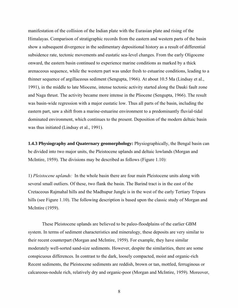
1.4.3 Physiography and Quaternary geomorphology .............................................8

1.4.4 Age dating......................................................................................................13

1.4.5 Holocene landform evolution ........................................................................14

1.4.6 Mineralogy, sedimentology and elemental distribution.................................16

1.4.7 Hydrogeology ................................................................................................19

1.5 Geochemistry of arsenic ......................................................................................21

1.5.1 Arsenic sorption kinetics................................................................................22

1.5.2 General mechanisms of arsenic mobilization in aqueous solution ................23

1.6 Background..........................................................................................................25

1.6.1 The contamination problem ...........................................................................25

1.6.2 Bengal basin hydrogeochemistry...................................................................27

1.6.3 Similar studies in North America ..................................................................28

Chapter 2: Regional hydrostratigraphy..................................................................................56

2.1 Introduction and study area..................................................................................56

2.1.1 Extent .............................................................................................................56

2.1.2 Elevation ........................................................................................................56

2.1.3 Coordinate system..........................................................................................56

v

2.2 Previous studies ...................................................................................................57

2.3 Data acquisition and sediment classification .......................................................57

2.4 Conceptual interpolation......................................................................................58

2.5 Lithologic modeling.............................................................................................58

2.6 Discussion ............................................................................................................59

2.7 Proposition of hydrostratigraphic nomenclature..................................................61

Chapter 3: Regional groundwater flow modeling..................................................................80

3.1 Introduction..........................................................................................................80

3.2 Previous modeling efforts ....................................................................................80

3.3 Conceptual model ................................................................................................81

3.4 Discretization and design.....................................................................................81

3.4.1 Horizontal discretization................................................................................82

3.4.2 Vertical discretization and aquifer parameters ..............................................82

3.4.3 Surface topography ........................................................................................83

3.4.4 Specified head boundaries .............................................................................83

3.4.5 Constant head boundaries ..............................................................................83

3.4.6 Rationale of seasonal models.........................................................................83

3.4.7 Recharge ........................................................................................................84

3.4.8 Groundwater abstraction................................................................................86

3.4.9 Calibration and sensitivity analyses...............................................................88

3.5 Simplifications and limitations ............................................................................89

3.6 Results and discussion .........................................................................................90

Chapter 4: Regional stable isotopic (δ18O-δ2H) signature of recharge and deeper

groundwater .........................................................................................................107

4.1 Introduction and background ...............................................................................107

4.1.1 Previous studies from Bengal basin groundwater..........................................107

4.1.2 Climate...........................................................................................................110

4.1.3 Hydrostratigraphic framework of study area .................................................110

4.2 Methods................................................................................................................111

4.2.1 Sampling ........................................................................................................111

4.2.2 Laboratory methods .......................................................................................112

vi

4.2.3 Data grouping and statistical clustering.........................................................112

4.3 Results..................................................................................................................113

4.3.1 Rainwater .......................................................................................................113

4.3.2 River water.....................................................................................................114

4.3.3 Groundwater ..................................................................................................114

4.4 Factors influencing δ18O and δ2 H composition of recharge and groundwater ...115

4.4.1 Precipitation ...................................................................................................115

4.4.2 Distance from sea (continental effect) ...........................................................116

4.4.3 River water.....................................................................................................117

4.4.4 Spatial distribution and depth ........................................................................119

4.5 Implications for groundwater recharge................................................................120

4.6 Conclusion ...........................................................................................................121

Chapter 5: Deeper groundwater chemistry and geochemical modeling ................................139

5.1 Introduction and background ...............................................................................139

5.1.1 Hydrostratigraphic framework.......................................................................139

5.1.2 Controls on hydrogeochemistry of Bengal basin...........................................139

5.2 Methodology........................................................................................................141

5.2.1 Sampling and field analyses...........................................................................141

5.2.2 Laboratory analyses .......................................................................................143

5.2.3 Statistical analyses .........................................................................................144

5.2.4 Geochemical modeling ..................................................................................145

5.3 Groundwater quality ............................................................................................146

5.3.1 Hydrochemical facies.....................................................................................146

5.3.2 Process controlling major solute distribution in groundwater .......................148

5.4 Redox conditions in groundwater ........................................................................152

5.4.1 Results............................................................................................................152

5.4.2 Environment...................................................................................................153

5.4.3 Governing Processes......................................................................................154

5.4.3.1 Iron dissolution ........................................................................................154

5.4.3.2 Sulfur cycling...........................................................................................155

5.4.3.3 Carbon cycling.........................................................................................156

vii

5.4.4 Summary ........................................................................................................159

5.5 Arsenic in deeper groundwater ............................................................................159

5.6 River water-groundwater interaction ...................................................................162

5.6.1 River water chemistry ....................................................................................162

5.6.2 Arsenic in river water.....................................................................................163

5.7 Geochemical modeling ........................................................................................163

5.7.1 Saturation indices...........................................................................................163

5.7.2 Inverse modeling of groundwater evolution along flow paths ......................164

5.8 Conclusion ...........................................................................................................168

Chapter 6: Suitability of deeper groundwater as an alternate drinking water source ............200

6.1 Introduction and finding ......................................................................................200

6.2 Probable causes....................................................................................................201

6.3 Implications for future water-resource development and management...............204

References..............................................................................................................................220

Vita.........................................................................................................................................224

viii

List of Tables

Table 1.1 Population details of arsenic-affected areas within the study area ........................30

Table 1.2 Geographical extent of the study area....................................................................32

Table 2.1 Location of lithologs used for this study ...............................................................64

Table 3.1 Distribution of rainfall and calculated potential recharge (PR) data from Global

Historic Climatology Network (GHCN v. 2) stations in and around the study

area..........................................................................................................................94

Table 3.2 Monthly temperature (1811 to 2005) and precipitation (1829 to 2005) data for

Calcutta along with calculated (ET) and potential recharge from GHCN v. 2.......96

Table 3.3a Seasonal details of irrigation pumps (DTWs) for each district and public

water-supply wells (PDTWs) for Calcutta with the study area ..............................97

Table 3.3b Projected details of irrigation pumps (DTWs) for each district and public

water-supply wells (PDTWs) for Calcutta with the study area ..............................97

Table 3.4 Results of sensitivity analyses on premonsoon with pumping (PREM-p) for

uncertain aquifer parameters...................................................................................98

Table 3.5 Results of model calibration with the best-fitted parameter values from Table

3.4 ...........................................................................................................................99

Table 3.6 Comparison of annual modeled submarine discharge (SGD), inflow and

pumping volumes between 2001 and pre-1970s ....................................................100

Table 4.1 Stable isotopic sample locations for groundwater, river water and rainwater

from Gangetic West Bengal....................................................................................123

Table 5.1 Location and details of the groundwater and river water samples from the

western Bengal basin ..............................................................................................170

Table 5.2a Field measurements and major solute composition of the water samples ...........173

Table 5.2b Minor solute, dissolved gas and stable isotopic compositions of the water

samples....................................................................................................................176

Table 5.3 Details of the first six components (showing 90% of the variance) obtained

from the principal component analyses (PCA) for 15 parameters..........................179

Table 5.4 List of selected minerals documented in the sediments of the Bengal basin by

previous workers.....................................................................................................180

ix

List of Tables (continued)

Table 5.5: Summary of saturation indices (SI) calculated by PHREEQC for some phases

possibly in contact with western Bengal groundwater and river water samples ....181

Table 5.6 Details of the reaction path models........................................................................183

Table 6.1 Details of unfiltered arsenic concentrations detected in the public water supply

wells used in the present study................................................................................205

x

List of Figures Figure 1.1 Map of West Bengal showing the arsenic-affected areas.....................................33

Figure 1.2a Montage of photographs taken (2003-2005) of patients suffering from arsenic

contamination in the study area ...........................................................................34

Figure 1.2b Photo of one of the first known victims of As contamination............................35

Figure 1.2c Reported cases of malignancy (1983-1998) caused by arsenicosis in

West Bengal .........................................................................................................36

Figure 1.3a Plot showing cumulative growth percentage of deep public water supply

wells in West Bengal ...........................................................................................36

Figure 1.3b Map showing extent of arsenic poisoning in the Bangladesh part of the

Bengal basin.........................................................................................................37

Figure 1.4a Map of Murshidabad showing the administrative blocks within the study area 38

Figure 1.4b Map of Nadia showing the administrative blocks within the study area............39

Figure 1.4c Map of North 24 Parganas showing the administrative blocks within the

study area .............................................................................................................40

Figure 1.4d Map of South 24 Parganas showing the administrative blocks within the

study area............................................................................................................41

Figure 1.5 Geological map of Bengal basin and its surroundings .........................................42

Figure 1.6 Map showing the tectonic elements of the Bengal basin .....................................43

Figure 1.7 A cross-section of the Bengal basin from west to east boundary through the

submarine canyon in the Bay of Bengal ..............................................................44

Figure 1.8 General stratigraphic succession of the eastern part of the Bengal basin.............45

Figure 1.9 Lithostratigraphic succession of the western part of the basin with sequence

boundaries and phases of the delta formation......................................................46

Figure 1.10 Physiographic map of the Bengal basin .............................................................47

Figure 1.11 Fence diagram of lithology of the Bengal basin.................................................48

Figure 1.12 Major stages of Holocene landform evolution in the Bengal basin ...................49

Figure 1.13 Eustatic sea level curve of the Bengal basin based on a study in the central

GBM plain. ..........................................................................................................50

xi

List of Figures (continued)

Figure 1.14 Plot showing the relation between a) mean grain size and organic carbon and

b) organic carbon and total nitrogen in the Bengal basin ....................................51

Figure 1.15 Eh-pH diagram for aqueous As in the system As-O2-H2O at 25oC and 1 bar

total pressure ........................................................................................................52

Figure 1.16 Plot showing (a) arsenite and (b) arsenate speciation as a function of pH and

ionic strength of about 0.01 M.............................................................................53

Figure 1.17 Adsorption isotherms and relationship of adsorbed As with net OH- release

during the reaction with arsenite and arsenate with ferrihydrite at pH 4.6 and

pH 9.2...................................................................................................................54

Figure 1.18 Calculated increase in As concentration when the pH of a sediment

(containing 1g/kg Fe as HFO) is increased from its initial value of pH 7 under

closed-system conditions .....................................................................................54

Figure 1.19 Calculated increase in As concentration when the specific surface area of

HFO in a sediment (containing 1g/kg Fe as HFO) is reduced from initial value

of 600 m2/g under closed-system conditions .......................................................55

Figure 2.1 Location map of the study area showing the districts and important rivers.........70

Figure 2.2 Elevation map of the study area prepared from SRTM-90 DEM along with

locations of important towns................................................................................71

Figure 2.3 Map showing location of the 143 lithologs used for lithologic interpolation and

orientation of the 11 cross-sections shown in Figures 2.4 and 2.5 ......................72

Figure 2.4a Modeled cross-section along transect AA’ in Figure 2.3 ...................................73

Figure 2.4b Modeled cross-section along transect BB’ in Figure 2.3 ...................................74

Figure 2.4c Modeled cross-section along transect CC’ in Figure 2.3....................................75

Figure 2.4d Modeled cross-section along transect DD’ in Figure 2.3 ...................................76

Figure 2.5 Modeled cross-sections along transect EE’, FF’, GG’, HH’, II’, JJ’, KK’ in

Figure 2.3 .............................................................................................................77

Figure 2.6 Modeled plan maps of the study area showing the subsurface distribution of

lithologic units at definite depths.........................................................................78

Figure 2.7 Conceptual block model showing the proposed hydrostratigraphic units............79

xii


Figure 3.1a Modeled groundwater level maps obtained from PREM, PREM-p, M, and M-

p............................................................................................................................101

Figure 3.1b Modeled groundwater level maps obtained from POSTM, POSTM-p, 2011-p,

and 2021-p ...........................................................................................................102

Figure 3.2 CGWB map of waterlogged areas within the study area .....................................103

Figure 3.3 Images of flooding in the study area during monsoon seasons (2001-2003) .......104

Figure 3.4 Plot of mass balance of the eight flow models shown in Figures 3.1 and 3.2......105

Figure 3.5 Plot of mass balance for each layer for PREM-p .................................................106

Figure 4.1 Map of the study area showing the stable isotopic sample locations for

groundwater, river water and rainwater ...............................................................128

Figure 4.2 Composite δ18O−δ2H bivariate plot showing the findings of previous workers

in the Bengal basin...............................................................................................129

Figure 4.3 Map of the study area showing (a) contour plot of mean annual rainfall (in

mm), and (b) contours of average daily summer air temperature........................130

Figure 4.4 Simplified hydrostratigraphic diagram of the study area .....................................131

Figure 4.5 Double-axis plot of monthly rainfall (in mm) and air temperature (in oC) for

Calcutta in 2004 ...................................................................................................132

Figure 4.6 δ18O-δ2H bivariate plot of the rainwater collected during the present study .......133

Figure 4.7 δ18O-δ2H bivariate plot of deeper groundwater and river water from the study

area.......................................................................................................................134

Figure 4.8 Bivariate plots of latitudinal locations and δ18O ..................................................135

Figure 4.9 Plot of δ18O of the rainwater samples along latitude............................................135

Figure 4.10 δ18O compositions of river water and groundwater plotted versus latitude (a)

Ganges-Bhagirathi-Hoogly, (b) Jalangi, and (c) Ichamati...................................136

Figure 4.11 Map of the distribution of the groundwater data points classified on the basis

of the statistical (HCA) groups 1, 2 and 3 ...........................................................137

Figure 4.12 Depth profile of the δ18O of groundwater samples in the study area classified

based on aquifer type and statistical groups ........................................................138

xiii


Figure 5.1 Map of the study area showing the 53 groundwater (hydrostratigraphically

classified) and 7 river water-sampling locations .................................................186

Figure 5.2 Generalized hydrostratigraphic framework along a north-south transect and

plot of the maximum tapped depth ......................................................................187

Figure 5.3 Piper plot of the hydrochemical facies distribution of groundwater and river

water samples by aquifer type and district...........................................................188

Figure 5.4 Bivariate plot of the three clusters obtained from hierarchical cluster analyses

(HCA) with the first and second principal component (PC) axes .......................189

Figure 5.5 Molar ratio bivariate plots of a) Na-normalized Ca and HCO3-, b) Na-

normalized Ca and Mg, c) Ca+Mg versus HCO3-, and d) Si and Cl-normalized

(Na+K) .................................................................................................................190

Figure 5.6 Stability field of a) Ca-Al silicate phases b) Na-Al silicate phases, and c) K-Al

silicate phases relative to groundwater and river water samples .........................191

Figure 5.7 Depth-profiles of water quality parameters: a) pH, b) Si, c) Ca+Mg, and d)

Na+K....................................................................................................................192

Figure 5.8 Distance (with latitude) plots of water quality parameters: a) Ca+Mg, b)

Na+K, c) HCO3-, and d) Si ..................................................................................193

Figure 5.9 Plot of Br-/Cl- mass ratio versus Cl- concentration for groundwater, river

water, and seawater..............................................................................................194

Figure 5.10 Comparison of observed EH of the groundwater and river water samples with

calculated EH of redox couples present in the waters ..........................................195

Figure 5.11 Depth-profiles of redox-sensitive parameters: a) EH, b) Fe(total), c) Fe(II), d)

As(total), e) As(III), f) percentage of As(III) in main-aquifer samples with

detectable (≥ 0.005 mg/L) As(III), g) Mn, h) SO42-, and i) CH4..........................196

Figure 5.12 Distance (with latitude) plots of redox-sensitive parameters: a) Cl--

normalized SO42-, b) Mn, c) Fe (total), d) As (total), e) CH4...............................197

Figure 5.13 Bivariate plots showing relations between a) Fe(total) and Mn, b) As(total)

and Fe(total), and c) As(III) and Fe(II). ...............................................................198

Figure 5.14 Plots of δ34SSO4 versus Cl-normalized SO42- concentrations ..............................198

xiv


Figure 5.15 Plot of δ13CDIC with depth ..................................................................................199

Figure 6.1 Flow chart showing the probable causal factors and processes that could have

led to pollution of the deeper groundwater of the western Bengal basin.............209

Figure 6.2 Map of unfiltered arsenic concentrations of deeper water within the study area.210

Figure 6.3 Comparison of percentage of arsenic concentrations between unfiltered

samples collected during this study and data collected from PHED ...................211

Figure 6.4 Map showing plot of arsenic concentrations of deeper wells of BGS/DPHE

(2001) (≥ 50 m bgl) in Bangladesh and the data collected for the wells during

this study (ours and PHED’s) ..............................................................................212

Figure 6.5 Comparison of arsenic concentrations as a function of depth for deeper wells

of BGS/DPHE (2001) (≥50 m bgl) in Bangladesh and the data collected for

the wells during this study (ours and PHED’s)....................................................213

Figure 6.6 Map showing the discretization of the 12-km2 area in and around Kamagachi

(Ranaghat-I) that was used for particle-tracking modeling. ................................214

Figure 6.7a Cross-section showing the results of particle-tracking modeling in absence of

pumping at Kamagachi (pre-1970s).....................................................................215

Figure 6.7b Cross-section showing the results of particle-tracking modeling in presence

of irrigation and water-supply pumping at Kamagachi (present day) .................216

Figure 6.8a Cross-section along section AA’ showing sediment color data and wells

where As concentration data were available........................................................217

Figure 6.8b Cross-section along section BB’ showing sediment color data and wells


Figure 6.8c Cross-section along section CC’ showing sediment color data and wells


xv

List of Files

abmdissertation.pdf

xvi

Chapter 1: Introduction

1.1 Prelude

More than 2% (120 million) of the total population (6 billion) of this planet lives in an

area of ~200,000 km2 covering the eastern part of the state of West Bengal (India) and most of

Bangladesh. This area, popularly known as the Bengal basin, is the world’s largest fluvio-deltaic

system (Coleman, 1981; Alam et al., 2003). The basin is drained jointly by the River Ganges,

River Brahmaputra (also known as River Jamuna in Bangladesh), River Meghna and their

numerous tributaries and distributaries, and hence is also known as the Ganges-Brahmaputra-

Meghna (GBM) delta or basin.

Indiscriminate use of the rivers and streams as pathways of sewage and industrial waste

by the Bengal basin inhabitants has made the surface water impotable. Moreover, the

introduction of high-yielding dry-season rice (Boro) (Harvey et al., 2005) accelerated the

demand for irrigation. This led to the shift of water policy from surface water to groundwater in

both West Bengal and Bangladesh during the early 1970s. As a consequence, several million

wells (ranging from low yielding hand-pumped to heavy-duty motor driven) were installed in

order to meet drinking, irrigation, and industrial water demands (Smith et al., 2000; BGS/DPHE,

2001; Harvey et al., 2005; Horneman et al., 2004).

Unfortunately, arsenic concentrations exceeding the US Environmental Protection

Agency (USEPA) maximum contaminant level of 50 μg/L were discovered in 1978 (Guha

Mazumder et al., 1998) in some wells in the North 24 Parganas district of West Bengal, followed

by detection of arsenicosis by 1984 (Garai et al., 1984). Arsenic, cited as the most hazardous

contaminant by the U.S. Agency for Toxic Substance and Disease Registry (ATSDR, 2005), is a

ubiquitous metalloid which, when ingested for extended periods, may cause severe health

effects, including arsenical dermatitis, deformation of limbs, circulatory and respiratory

problems, and various cancers, leading to untimely death. Soon, groundwater in other parts of

West Bengal (mostly east of the River Bhagirathi-Hoogly [Figure 1.1], the main distributary of

the Ganges in India) and, Bangladesh in 1993 (Swartz et al., 2004), were found to have

groundwater with As concentrations exceeding the World Health Organization (WHO, 1993,

1

2001) drinking water safe limit of 10 μg/L. More than 50 million people may be at potential risk

from As exposure in the Bengal basin (Figures 1.2a, b and c). Of these, at least 1 million are

likely to be affected by arsenicosis, as calculated by Yu et al. (2003) based on dose-response data

from Guha Mazumder et al. (1998). The contamination has been termed as the greatest mass

poisoning in human history (Smith et al., 2000). Estimates show that at present about 25%

(McArthur et al., 2004) to 33% (Horneman et al., 2004) of the wells have been identified to be

contaminated by As. Since 1990, numerous studies by governmental and non-governmental

agencies and researchers have tried to understand the causes and effects of this contamination.

These studies have led to a detailed understanding of the water-sediment chemistry and

proposition of several hypotheses on the occurrence and fate of arsenic in groundwater on both

sides of the Indo-Bangladesh border (e.g. Saha, 1991; AIP/PHED, 1991, 1995; Mallick and

Rajgopal, 1995; Das et al., 1995, 1996; Bhattacharya et al., 1997; CGWB, 1997; Mandal et al.,

1998; Nickson et al., 1998, 2000; Ray, 1999; Acharyya et al., 1999, 2000; BGS/DPHE, 2001;

McArthur et al., 2001, 2004; Ravenscroft et al., 2001, 2005; Harvey et al., 2002, 2005, 2006;

Ghosh and Mukherjee, 2002; JICA, 2002; Smedley and Kinniburgh, 2002; Dowling et al., 2003;

Stüben et al., 2003; van Geen et al., 2003, 2004; Horneman et al., 2004; Swartz et al., 2004;

Polizzato et al., 2005).

1.2 Importance and objective of work

It has been hypothesized that the non-point source, geogenic As mostly occurs in the

Holocene shallow aquifers of the Bengal basin and probably has been mobilized from the

sediments by redox reactions. Various workers (e.g. BGS/DPHE, 2001; McArthur et al., 2001;

JICA, 2002; van Geen et al., 2003; Ravenscroft et al., 2005, Zheng et al., 2005a) have suggested

that deeper groundwater could be an alternate, safe drinking water source. Consequently, water-

supply authorities have installed numerous deep community wells (Figure 1.3a) to provide As-

free water to the huge urban and rural population, although the deeper water chemistry has

received relatively little attention.

Because Bangladesh occupies most of the Bengal basin, it has received more attention

than the part of the basin in West Bengal. Several comprehensive studies (e.g.

BGS/DPHE/MML, 1999; BGS/DPHE, 2001; JICA, 2000, 2002) have examined the

2

contamination extent (Figure 1.3b), detailed regional hydrogeology and hydrogeochemistry of

much of the eastern part of the basin. In West Bengal, however, in spite of district-level surveys

of groundwater resources by the Central Ground Water Board (CGWB) (1994a, b, c, d, and e)

and State Water Investigation Directorate (SWID) (1998), the regional hydrologic framework

and detailed deeper hydrochemistry remain largely unrevealed. In most of the studies so far, the

As concentration of the groundwater has been described in terms of absolute depth. However, for

a proper understanding of the subsurface spatial distribution of As, geochemical processes, and

possible future extent of the pollution, a detailed composite approach needs to be formulated.

This study is intended to characterize the deeper hydrogeology of the arsenic affected

parts of the western Bengal basin (parts of four districts of West Bengal) with an estimated 13.5

million people at risk (Table 1.1). Of these at least 4 million rural residents are drinking deep

water supplied from public water-supply schemes within the study area.

In the second chapter, a hydrostratigraphic model for the arsenic-contaminated areas of

the western Bengal basin has been proposed with block-scale descriptions of the inferred aquifer-

aquitard framework. In the third chapter, numerical simulations of regional-scale, seasonal

groundwater flows through the proposed hydrostratigraphic framework have been described. The

fourth chapter illustrates the stable isotopic composition of rainwater and regional trends in

groundwater. The fifth chapter focuses on detailed characterization and geochemical modeling of

the deeper water chemistry of the study area. The sixth and final chapter summarizes the extent

of arsenic pollution in deeper water along with possible reasons for such pollution.

1.3 The study area

The study area (Table 1.2) consists of an area of about 21,000 km2 in the western Bengal

basin, including the districts of Murshidabad (eastern part) (Figure 1.4a), Nadia (Figure 1.4b),

North 24 Parganas (Figure 1.4c) and South 24 Parganas (Figure 1.4d). The area is bounded in the

north by the River Ganges, in the west by the River Bhagirathi-Hoogly (distributary of the River

Ganges), in the east by the international border between India and Bangladesh and in the south

by the Bay of Bengal. The study area includes the city of Kolkata (Calcutta) as well as a number

3

of smaller municipalities, including Behrampur, Krishna Nagar, Kalyani, Naihati, Barasat and

Bashirhat.

1.4 Geologic overview of the Bengal basin

The Bengal basin represents world’s largest sediment dispersal system (Kuehl et al.,

1989; Milliman et al., 1995, Goodbred et al., 2003), with passage of an estimated 1060 million

tons of sediments per year to the Bay of Bengal through a delta front of 380 km (Allison, 1998),

thereby forming the world’s biggest submarine fan, the Bengal fan (Kuehl et al., 1989; Rea,

1992), with an area of 3 × 106 km2. Water discharge through the Bengal basin to the ocean is

fourth largest in the world (Milliman and Meade, 1983). The total area of the GBM basin has

been estimated to be about 200,000 km2 (Alam et al., 2003). The maximum flow estimated for

the River Ganges during the past century was on the order of 43,000 m3/s, while the maximum

flow for the Brahmaputra was on the order of 57,000 m2/s (Chatterjee, 1949).

The Ganges enters the basin from the northwest after draining the Himalayas and most of

north India for about 2500 km (Figure 1.5). The Ganges then divides into two distributaries. The

main stream (River Padma) flows southeast toward the confluence with the River Brahmaputra

in Bangladesh. The other part flows due south through West Bengal as the River Bhagirathi-

Hoogly. For simplicity, both these distributaries are termed as the original stream, i.e., Ganges.

The Ganges flows through a meandering course with very few braided reaches and occasional

tributaries. It has been avulsing toward the northwest for the last 250 years (Brammer, 1996).

The Brahmaputra enters the basin from the northeast (Figure 1.5) after draining Tibet and

northeast India for about 2900 km. It has a palaeo-channel bifurcated along the east of the

Madhupur forest. In general, the Brahmaputra is a braided stream characterized by multiple

thalwegs, mid-channel bars and vegetated river islands. The channel belt shows a rapid lateral

migration of up to 800 m/year (Allison, 1998). The Meghna drains the Sylhet basin and part of

the Tripura hills before flowing into the Brahmaputra (Figure 1.6).

1.4.1 Boundaries of the basin: The Bengal basin is bounded (Figure 1.5) on the north and

northwest by the Rajmahal Hills, which are composed of lower Jurassic to Cretaceous trap

basalts of the Upper Gondowana system (Ball, 1877). From west to east they are known as the

4

Garo, Khasi and Jayantia hills, which stretch for about 97 km from north to south and 240 km

from east to west (Morgan and McIntire, 1959). In the northeast the Shillong or Assam plateau

acts as a boundary. The hills and the plateaus are composed of intensely stressed Precambrian

quartzite and schist overlain by the Eocene Nummilitic limestone (Wadia, 1949). The Bengal

basin’s eastern limit is marked by the Tripura hills to the north and Chittagong hills to the south,

which are composed of Paleocene-Pliocene age sediments of the Siwalik system (the Himalayan

foredeep basin sediment system) (West, 1949). The Tripura hills include a series of plunging

anticlines, which die out under overlapping recent sediments of the Sylhet basin (Morgan and

McIntire, 1959). The Bangladesh-India border follows the base of the hills.

1.4.2 Geologic framework and history: The Bengal basin was initiated as a subsiding foredeep

basin of the uprising Himalayan front and the Indo-Burma range formed by the collision of the

Eurasian and Indian continental plates. By the mid-Miocene (Curray et al., 1982), the basin had

become a huge sink of the sediments eroded from the rising mountain range (Allison, 1998). The

basin has a complex evolutionary history. About 1 to 8 km of Permian to Recent clastic

sediments rest on the stable shelf in the western part of the basin (Imam and Shaw, 1985) and up

to 16 km of Tertiary to Quaternary alluvial sediment cover is present in the foredeep of the basin,

which at present lies at the mouth of the Ganges and Brahmaputra rivers (Allison, 1998) (Figure

1.7). The ongoing Himalayan orogeny has kept the basin tectonically active, with most of its

activity now focused in the foredeep region, as manifested by a number of vertical faults and

folds. This has caused vertically displaced regional sedimentary blocks, which have divided the

basin into numerous poorly connected sub-basins, which in turn caused conspicuous differences

in sedimentary environment and lithology (Goodbred et al., 2003). On a larger scale, the basin is

supposed to be divided into eastern and western portions, which are separated by a hinge zone

marked by high magnetic and gravity anomalies (Sengupta, 1966).

Geologically, the basin is bounded in the west by the Peninsular shield of India, which

has a Precambrian basement of metasediments with granitic, granophyric and doleritic

intrusions. These are followed upward by scattered, east-west trending intracratonic Gondwana

deposits like the Damodar basin with the Raniganj and Jharia coal basins and some Tertiary

deposits like the Baripada and Durgapur beds, as well as the Mesozoic volcanics of the Rajmahal

5

trap. In the east the Naga-Lushai orogenic belt bound the basin. This belt consists of highly

deformed Cretaceous-Tertiary sediments and is bordered in the north and northeast by the Dauki

fault zone (Evans, 1964) and the Naga thrust (Sengupta, 1966), with a general movement

direction of north-northeast. The Shillong Plateau, which borders the basin in the northeast, is

most probably the continuation of the Indian shield through the Garo-Rajmahal gap (Sengupta,

1966).

Stratigraphic study of the Bengal basin shows that from the Cretaceous through the mid-

Eocene, sedimentation was similar throughout the basin (Figures 1.8 and 1.9). The succession

starts with the Gondwana sediments and volcanics, followed by a thick sequence of shallow

marine clastics and carbonates in both the eastern and the western sub-basins. Arenaceous

sediments dominate the clastics in both areas. The carbonate deposit, known as the Nummilitic

Sylhet limestone, is found extensively throughout the basin. As a result of the basin

configuration and nature of the submergence, the sequence is thinner in the western sub-basin.

After the deposition of the Sylhet limestone, the sedimentation pattern of the basin changed to

become more argillaceous, as marked by the Kopili Formation. After the Kopili, there occurred

some significant movement of the basin-basement and -margin fault systems, which led to a

completely different depositional environment and stratigraphic sequence in the two sub-basins.

While thick marine sediments continued to be deposited in the deeper eastern sub-basin,

successively resulting in the Bogra Formation, Barail Formation, Surma Group and Tipam

Group, in the western sub-basin the Bhagirathi Group (consisting of the Memari-Burdwan,

Pandua-Matla and Debagram-Ranaghat formations; Biswas, 1963), were deposited in a more

near-shore environment. From the advent of the Pliocene, a similar style of sedimentation

resumed throughout the basin, thereby depositing the voluminous and extensive Bengal alluvium

over all the previous lithotypes.

Sequence-stratigraphic and seismic studies have established that there is a zone of flexure

above the Sylhet limestone in the southeastern portion of the western part of the basin. This zone

acts as a seismic reflector and has been interpreted as a hinge zone or a zone of faulting, which

may be a shallow manifestation of a much more intense fault zone in the basement (Sengupta,

1966). The unconsolidated sediments deposited over it, because of bed instability and adjustment

6

of movement, have suffered from flexure, which gave the post-Sylhet deposits of the Bengal

basin a broad synformal shape. The zone is not very wide, but it passes from east Calcutta to the

town of Mymensinhga in northern Bangladesh. Thus the zone has been named as the Calcutta-

Mymensinhga hinge zone (CMHZ) (Figure 1.6). The zone can be traced to its truncation by the

Dauki fault zone in the Naga Hills of Assam (Sengupta, 1966). It occurs at a depth of about 4700

m below Calcutta, with a trend of N 30o E. The presence of the CMHZ has been confirmed by

the finding of a series of low-magnitude magnetic highs in northwest Calcutta and a steep gravity

gradient in the west. Calcutta has been flanked by broad gravity highs to the east, indicating the

presence of a gravity divide in-between (Sengupta, 1966).

The formation of the Bengal basin started with the break-up of Gondwanaland in the late

Mesozoic, at about 126 Ma (Lindsay et al., 1991). Extrusion of basalt both in the Rajmahal areas

and the south Shillong plateau (Banerjee, 1981) some time in the late Jurassic to early

Cretaceous initiated the process of basin development. This was followed by the slow subsidence

of the Bengal shelf in the late Cretaceous, leading to restricted marine transgression from the

southeast in the proto-basin. The western part of the basin (mostly in West Bengal) records

deposition of lagoonal argillaceous and arenaceous sediments, whereas the Assam front in the

eastern and northeastern part was occupied by an open neritic sea (Sengupta, 1966). The proto-

GBM delta started forming by sediments deposited by repeated submergence and transgression

over a planar erosional surface, which exists at about 2200 m depth in the central part of the

basin, with a dip toward the southeast (Lindsay et al., 1991).

During the middle to late Eocene, basin-wide subsidence initiated by movement along

basin-margin faults caused an extensive marine transgression in the basin, which resulted in the

deposition of the Sylhet limestone. Basement movement probably caused the formation of the

CMHZ on top of this limestone (Sengupta, 1966). Subsequently, the sea began receding from the

Bengal basin. At about 49.5 Ma, a major shift in the sedimentation pattern began. The carbonate-

clastic platform sedimentary sequence was replaced by a predominantly clastic deposit (Lindsay

et al., 1991). The process became conspicuous at about 40 Ma, when the basin became

dominated by fluvial clastic sediments and the transitional delta prograded rapidly with frequent

lobe switching. The sudden change in deltaic sedimentation and morphology was probably a

7

manifestation of the collision of the Indian plate with the Eurasian plate and rising of the

Himalayas. Comparison of stratigraphic records from the eastern and western parts of the basin

show a subsequent divergence in the sedimentary depositional history as a result of differential

subsidence rate, tectonic movements and eustatic sea-level changes. From the early Oligocene

onward, the eastern basin continued to experience marine conditions as marked by a thick

arenaceous sequence, while the western part was under fresh to estuarine conditions, leading to a

thinner sequence of argillaceous sediment (Sengupta, 1966). At about 10.5 Ma (Lindsay et al.,

1991), in the middle to late Miocene, intense tectonic activity started along the Dauki fault zone

and Naga thrust. The activity became more intense in the Pliocene (Sengupta, 1966). The result

was basin-wide regression with a major eustatic low. Thus all parts of the basin, including the

eastern part, saw a shift from a marine-estuarine environment to a predominantly fluvial-tidal

dominated environment, which continues to the present. Deposition of the modern deltaic basin

was thus initiated (Lindsay et al., 1991).

1.4.3 Physiography and Quaternary geomorphology: Physiographically, the Bengal basin can

be divided into two major units, the Pleistocene uplands and deltaic lowlands (Morgan and

McIntire, 1959). The divisions may be described as follows (Figure 1.10):

1) Pleistocene uplands: In the whole basin there are four main Pleistocene units along with

several small outliers. Of these, two flank the basin. The Barind tract is in the east of the

Cretaceous Rajmahal hills and the Madhupur Jungle is in the west of the early Tertiary Tripura

hills (see Figure 1.10). The following description is based upon the classic study of Morgan and

McIntire (1959).

These Pleistocene uplands are believed to be paleo-floodplains of the earlier GBM

system. In terms of sediment characteristics and mineralogy, these deposits are very similar to

their recent counterpart (Morgan and McIntire, 1959). For example, they have similar

moderately well-sorted sand-size sediments. However, despite the similarities, there are some

conspicuous differences. In contrast to the dark, loosely compacted, moist and organic-rich

Recent sediments, the Pleistocene sediments are reddish, brown or tan, mottled, ferruginous or

calcareous-nodule rich, relatively dry and organic-poor (Morgan and McIntire, 1959). Moreover,

8

there is a conspicuous difference in the landform features formed by the Pleistocene and the

Recent sediments. The Pleistocene sediments form highlands, which are the manifestation of

differential structural movements between the two units and also seaward subsidence with higher

terrace formation during Pleistocene glaciations. Four such terraces have been identified

(Morgan and McIntire, 1959). Also, the upland is characterized by only few prominent drainage

systems, which also flow through deeply scoured, well-defined meanders.

The Barind is the largest Pleistocene unit in the Bengal basin, with an aerial extent of

about 9400 km2. It has been dissected into four separate units by recent fluvial systems, which

include the north Bengal tributaries of the Ganges and Brahmaputra, namely the Mahananda,

Karatoya, Atrai, Jamuna and Purnabhaba. The area is actively affected by orogenic movements,

which are indicated by earthquakes, tilting of its eastern part, river course switching and visible

major fault planes.

The 4100 km2 of the Madhupur Jungle north of the city of Dhaka is the other important

Pleistocene landform of the Bengal basin. The elevation of the upland increases from 6 m above

mean sea level (MSL) in the south to more than 30 m above MSL in the north. The western side

has a higher average elevation, while the whole upland dips toward the east, where ultimately it

gets concealed under the thick Recent alluvium. The western margin marks an abrupt separation

between the low-lying, flat, Recent flood plain in the east and the highly dissected older upland.

The margin is bounded by six en-echelon faults ranging from 10 to 21 km in length and with the

eastern side up-thrown by at least 6 to 18 m. It is believed by some workers that at least part of

the uplift of the Madhupur forest took place during the 1762 catastrophic earthquake (Fergusson,

1863). The diversion of the Brahmaputra from its old course can be possibly attributed to the

sudden uplift of the Madhupur Jungle and its gradual tilting toward the east and also the sudden

diversion of the Tista from being a tributary of the Ganges to that of the Brahmaputra in 1787.

Moreover, the presence of the lowland between the en-echelon fault system of the Madhupur and

the Karatoya River fault system of the northeast Barind indicates ongoing subsidence/uplift.

2) Recent Sediments: The other main physiographic division is the Recent alluvial plain and delta

of the GBM system (Morgan and McIntire, 1959), also known as the Recent alluvial lowland of

9

Bengal (Umitsu, 1987, 1993). These alluvial deposits are the most extensive part of the Bengal

basin and cover almost the whole of the basin except the Pleistocene highlands.

Different workers have tried to classify this huge sedimentary basin in various ways. The

classification described here is a combination of the two proposed by Morgan and McIntire

(1959) and Umitsu (1987). According to this joint scheme, there are four physiographic

subdivisions as described below:

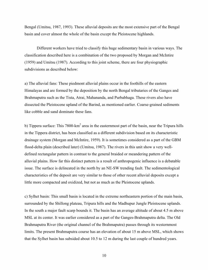
a) The alluvial fans: These piedmont alluvial plains occur in the foothills of the eastern

Himalayas and are formed by the deposition by the north Bengal tributaries of the Ganges and

Brahmaputra such as the Tista, Atrai, Mahananda, and Purbabhaga. These rivers also have

dissected the Pleistocene upland of the Barind, as mentioned earlier. Coarse-grained sediments

like cobble and sand dominate these fans.

b) Tippera surface: This 7800-km2 area in the easternmost part of the basin, near the Tripura hills

in the Tippera district, has been classified as a different subdivision based on its characteristic

drainage system (Morgan and McIntire, 1959). It is sometimes considered as a part of the GBM

flood-delta plain (described later) (Umitsu, 1987). The rivers in this unit show a very well-

defined rectangular pattern in contrast to the general braided or meandering pattern of the

alluvial plains. How far this distinct pattern is a result of anthropogenic influence is a debatable

issue. The surface is delineated in the north by an NE-SW trending fault. The sedimentological

characteristics of the deposit are very similar to those of other recent alluvial deposits except a

little more compacted and oxidized, but not as much as the Pleistocene uplands.

c) Sylhet basin: This small basin is located in the extreme northeastern portion of the main basin,

surrounded by the Shillong plateau, Tripura hills and the Madhupur Jungle Pleistocene uplands.

In the south a major fault scarp bounds it. The basin has an average altitude of about 4.5 m above

MSL at its center. It was earlier considered as a part of the Ganges-Brahmaputra delta. The Old

Brahmaputra River (the original channel of the Brahmaputra) passes through its westernmost

limits. The present Brahmaputra course has an elevation of about 15 m above MSL, which shows

that the Sylhet basin has subsided about 10.5 to 12 m during the last couple of hundred years.

10

The cause is certainly tectonic, associated with movements of the fault systems. Recent fossil

wood fragments have been found at depths of 15 to 18 m below surface. The surface is inundated

every year during monsoon season. The basin can be classified geomorphologically as having

natural levees with dendritic drainage and continuously meandering levees (Umitsu, 1985). The

sediment composition of the basin ranges from sandy to silty near the surface, grading to fine

sand at a depth of about 12 m.

d) Ganges-Brahmaputra-Meghna flood and delta plain: This is the principal unit of the Bengal

basin. This unit is so vast that many studies including the present work refer the Bengal basin as

almost synonymous with the plain. It covers more than 105 km2 of the alluvial plain in both

Bangladesh and West Bengal, India, excluding the units that have already been mentioned.

The plain is bounded by the Pleistocene terraces in the west, the Barind and Madhupur

Jungle in the north, the Tippera surface in the east (Morgan and McIntire, 1959) and the Bay of

Bengal in the south. It is formed by two of the largest river systems of the world and thus is

considered one of the best and most complex examples of fluvio-deltaic geomorphology. Like

many of the large alluvial systems of the world, the GBM plain is also formed by overlapping of

a number of sub-deltas (Morgan and McIntire, 1959) and alluvial flood plains. Moreover,

avulsion of the major streams in the area, which are either tributaries or distributaries of the

Ganges or Brahmaputra, within a time scale of 100 years, has resulted in a Recent sediment

sequence of about 100 m of overbank silts and clays incised by channel sands (Coleman, 1969;

Umitsu, 1987; Goodbred and Kuehl, 2000, Allison et al., 2003). The active delta area in the

southernmost part of the plain, which supports the largest mangrove forest in the world, the

Sunderban, can be demarcated from the flood plain by the furthest inland extent of ocean water

from the Bay of Bengal during the dry season of October to April (Allison et al., 2003).

The GBM alluvial plain has an altitude of about 15 to 20 m in the northwest, which

decreases to 1 to 2 m in the south near the coast. According to physiographic characteristics the

plain can be divided into five distinct regions (Umitsu, 1987). These include a) the area in and

around the city of Calcutta, b) the area of broad and indistinct natural levees (Umitsu, 1985) in

the northwest part, also known as the moribund delta (Bagchi, 1944), c) the central part of the

11

plain, which includes areas with natural levees with dendritic distributary channels near the city

of Khulna city (Umitsu, 1985) along with meandering and distinct natural levees, d) the

Sunderban and e) the mouth of the Meghna with its active delta (Umitsu, 1987).

The oldest surface sediments in the GBM flood plain are recorded near the cities of

Calcutta and Commila in northeastern Bangladesh, very near the Tippera surface, whereas the

youngest sediments are all located in the active floodplain and the delta. The sediments in all the

other places are of Holocene age. The Ganges alluvial deposits are divided into an upper silty or

clayey part and a lower sandy part to a depth of about 50 m. In the northwestern part, near the

Tippera surface, the sediments in the upper horizons are slightly oxidized and light gray in color.

In the central and southern parts of the plain, organic and peaty materials are occasionally visible

in near surface horizons. In the southernmost part, in and near the active delta region, alternating

silt and sand are present with an upward fining sequence (Umitsu, 1987). The Brahmaputra-

dominated alluvial plain is present in the area between the Barind and the Madhupur Jungle. This

plain has a distinct basal gravel horizon overlain by a sequence of sandy sediments.

Umitsu (1987, 1993) classified the vertical sequence of the recent formations of the GBM

plain into five units (lowest, lower, middle, upper, and uppermost). Each of these units is

separated from its succeeding units by a difference in grain size, which is certainly a

manifestation of depositional environment. The descriptions of the individual units are as

follows, after Umitsu (1987). The lowest unit, which has a thickness of about 10 m, is composed

predominantly of gravel. Near the northern portion of the plain, the bed occurs at a depth of more

than 70 m below the surface, indicating that the sea level of the Bay of Bengal at the time of its

deposition must have been about 100 m below the present level. The lower member is dominated

by sand-sized sediments with few gravels. The unit contains two horizons near the middle and

the top with a coarser grain size, probably resulting from a change in sediment size deposited by

the rivers. An unconformity, probably caused by temporary marine regression, exists between

the lower and the middle members. This is indicated by the presence of weathered and oxidized

horizons at the top of the lower unit. The lower horizon in certain locations, mostly in the central

plain, has sediments with occasional peat and organic material, indicating a swampy

environment of deposition. The middle unit shows a coarsening upward sequence. The upper

12

member has a coarse-grained middle portion, sandwiched between fine-grained upper and lower

portions. This oscillation of sedimentation pattern is believed to be caused by eustatic sea level

change. Clay- and silt-sized sediments are characteristic of almost the entire uppermost horizon,

with occasional peaty sediments.

The peaty materials in all these units are interpreted to have been deposited in mangrove

swamps, which developed in the prograding delta over time (Vishnu-Mittre and Gupute, 1979;

Umitsu, 1987; Islam and Tooley, 1999).

1.4.4 Age dating: Because of the presence of a large amount of organic material in the Recent

sediments, radiometric age (mostly radiocarbon) dating of the sediments has been done by

several workers. The lower unit organic remains of the central GBM plain near the city of

Khulna (Bangladesh) at a depth of 46 m below MSL yield an age of 12,320 ± 240 years before

present (BP) (Umitsu, 1993). Ages from shell fragments and wood remains from the middle unit

at depths of 25 to 33 m below MSL range from 8910 ± 150 to 7640 ± 100 years BP (Umitsu,

1993). Peat layer ages determined from the upper unit are 7060 ± 120 years BP at 18 m below

MSL and 6490 ± 130 year BP at 14 m below MSL (Umitsu, 1993).

Peat layers from the far western GBM plain (West Bengal, India) have been dated ~7100

to 9100 years BP at depths of 20 to 50 m in the coastal area (Hait et al., 1996) and, in inland

areas, 6500 to 7500 years BP at depths of 6 to 12 m and 2000 to 5000 years BP at depths <5 m in

inland areas (Banerjee and Sen, 1987). Mangrove remains from Calcutta have been dated at

~7000 years BP (Sen and Banerjee, 1990). The sediments from a location near Calcutta have

been dated as 2615 ± 100 years BP at 1.37 m below surface to 5810 ± 120 years BP at 6.25 m

below surface level (Vishnu-Mittre and Gupute, 1979).

Sediments from the Brahmaputra plain basal gravel at a depth of 101 m below sea level,

in the south of the Barind, yield an approximate age of 28,320 ± 1550 years BP (Umitsu, 1987).

Sylhet basin organics at depths of 36.6 m to 55 m below MSL yield ages of 6320 ± 70 years BP

and 9390 ± 60 years BP respectively (Goodbred and Kuehl, 2000).

13

Radiocarbon dating of sediments from a depth of 25 to 30 m below surface at the active

delta area near the main mouth of the GBM, records an age of 8400 years BP (Goodbred and

Kuehl, 2000). Muddy sand about 50 m west of the aforementioned location and at a depth of 35

m below surface, yields an age in the range of 7500-8000 years BP (Goodbred and Kuehl, 2000).

1.4.5 Holocene landform evolution: As noted in section 1.4.3, the main lithostratigraphic and

geomorphic units of the Bengal basin are mostly of Holocene age (Figure 1.11). Hence

understanding the Holocene fluvio-dynamic processes along with the effects of eustatic sea level

changes and tectonic impacts in this basin is critical for any further study. In the northwestern

part of the basin, where tectonic processes are most active, fine-grained sediments dominate the

stratigraphy. In the western part of the basin, near the stable shelf, the strong fluvio-dynamic

processes have resulted in formation of extensive flood plains with a dominance of coarser

grained sediments. The coastal region in the south has a mixture of fine-grained sand and mud

deposits with peat layers, which have resulted from eustatic influence (Goodbred et al., 2003).

Deposition of the lowest unit of the GBM delta began at the onset of the Pleistocene

glacial maximum in this part of the world (Islam and Tooley, 1999) (Figure 1.12). This is

documented by the fact that the lowest unit was deposited at a depth of about 70 m below the

present land surface, indicating that the glacial maximum sea level and the base level of land

erosion must have been at least 100 m below the present MSL. Thus the rivers draining the plain

during that time must have scoured through the earlier plains and deposited the basal gravel at a

depth analogous to the sea level at that time (Umitsu, 1993). At that time the “Swatch of no

ground” submarine canyon now in the center of the Bay of Bengal most probably was the estuary

of the GBM plain (Chowdhury et al., 1985). If this hypothesis is true then most of the northern

part of the Bay of Bengal during the Pleistocene glaciation was dry land (Islam and Tooley,

1999). The sediment supply at this time was low compared to the present (Milliman et al., 1995)

and sediment inflow was low until the late Pleistocene, about 15,000 years BP (Weber et al.,

1997).

Around 12,000 to 11,500 years BP, at the onset of the Holocene, the southwest monsoon,

which determines the climate-controlled processes in southeast Asia, became stronger than at

14

present (Gasse et al., 1991), which led to a simultaneous increase in discharge and fluvial

sedimentation. The sediment discharge has been estimated to be on the order of 2.5 × 109 t/yr

(Goodbred and Kuehl, 2000). The lower unit of the GBM plain was probably deposited at this

time as an extensive flood plain in the central region (Umitsu, 1993). As mentioned earlier, this

unit coarsens upward, which may be correlated with increased discharge and aggravated erosion

along the upper reaches of the main rivers.

The conditions of sedimentation and eustatic sea level rise that took place at about 10,500

years BP are a matter of debate because of the presence of apparently contradictory evidence.

The sedimentary record at this time contains both dissected flood plains (Umitsu, 1993) caused

by fluvial erosion and also drastic fining of sediments (Goodbred and Kuehl, 2000) further

inland. It has been hypothesized that either there was a temporary (Umitsu, 1993) and most

probably major (Lindsay et al., 1991) marine regression or the eustatic sea level rose to about –

45 m MSL from the previous sea level (Fairbanks, 1989; Blanchon and Shaw, 1995), which

caused extensive back-flooding and sedimentation. However, both these theories claim that the

present GBM delta started forming and prograding into the bay at this time (Lindsay et al., 1991;

Goodbred and Kuehl, 2000). The sharp decrease of sediment input to the submarine fan at this

time (Weber et al., 1997) could be a manifestation of enhanced sediment trapping in the delta

plain system. The fine sediment thus deposited would constitute the middle unit of the GBM

plain (Umitsu, 1993). Hence, most probably there was a short-lived but effective marine

regression followed by a marine transgression, which cumulatively initiated the modern delta-

forming processes.

From about 10,000 years BP to about 7,000 years BP, in the mid-Holocene, a major and

rapid transgression (Umitsu, 1993; Islam and Tooley, 1999; Goodbred and Kuehl, 2000) took

place probably as a cause of glacial ice melting, which resulted in the deposition of fine

sediments (the upper unit of the GBM plain) even in the north-central part of the basin. The

coastline at that time transgressed up to the central delta, in the north of Khulna city (Umitsu,

1993). This continued transgression might also have had some short-lived regression cycles, for

example, at about 9000 years BP. These are indicated by increased fluvial activity (Islam and

Tooley, 1999). During the latter part of this transgression, the coastline probably receded slightly

15

toward the south causing the coarsening of the upper horizons of the upper unit. At this time

mangrove vegetation (Vishnu-Mittre and Gupte, 1979) spread all over the central GBM plain and

caused extensive deposition of peat. After ∼7000 years BP, the gradient of the marine

transgression curve decreased (Umitsu, 1993; Islam and Tooley, 1999; Goodbred and Kuehl,

2000). Nonetheless, the general trend of the eustatic sea-level curve shows continued

transgression from the mid-Holocene onward (Figure 1.13). The decreased rate of transgression

since 7000 years BP led to the deposition of the uppermost unit of the GBM plain, which

contains clay, silt, and organic-rich layers throughout the southern Bengal basin. The

continuation of these processes is the active delta formation and the mangrove vegetation in the

Sunderban region.

Bengal Peat: These are extensive peat layers in the upper and uppermost units throughout the

southern Bengal basin. These layers have been reported by various workers, including Vishnu-

Mittre and Gupte (1979), Sen and Banerjee (1990), Barui and Chanda (1992), Umitsu (1987,

1993), and Islam and Tooley (1999), who have referred to the layers as the Bengal peat. Civil

construction in Calcutta in recent past, even at shallow depths, have yielded remnants of peaty

material. The above-mentioned authors have claimed the peat as in-situ in origin and mostly

formed from mangrove (or mangal) vegetation. Studies near the city of Khulna have yielded five

well-developed and generally thick layers of peat, each separated by inorganic layers (Islam and

Tooley, 1999). The lowermost peat layer has been dated at 7000 to 6650 years old and contains

remains of mangrove plants like Acrostichum aureum, Heritiera spp., and Avicennia spp. Parts

of the uppermost layer have been dated at 5000 to 2000 years old and contain abundant remains

of freshwater peat-forming plants. The intercalation of mangrove and fresh water plant with

mineral-rich layers have been interpreted to indicate deposition in a basin that was inundated by

marine transgression with intermediate temporary regressions (Islam and Tooley, 1999).

1.4.6 Mineralogy, sedimentology and elemental distribution: The mineralogy and

sedimentology of the Bengal basin are to a large extent dependent on the type of sediments

eroded and transported by the Ganges, the Brahmaputra and their northern tributaries like the

Tista, Meghna, Rangeet and Mahananda. Because of differences in sediment provenance, the two

river systems have quite distinctive mineralogies (Heroy et al., 2002). The Brahmaputra flows

16

through various rock types, including Precambrian metamorphics (high grade schist, gneiss,

quartzite, and marble), felsic intrusives, Paleozoic-Mesozoic sandstones, shales and limestones

(Huizing, 1971). The Ganges drains terrains with similar kinds of lithologies, but also receives

lower course and lowland tributaries which drain Mesozoic and Tertiary mafic extrusives and

Precambrian-Cambrian shield (Huizing, 1971). The lowland tributaries also produce a kind of

saline and alkaline soil, which contains calcareous concretions called "kankar" (Sarin et al.,

1989). The sediments of the floodplains and the streambeds of all three river systems have been

found to be very similar in sedimentary properties and mineralogy (Morgan and McIntire, 1959;

Umitsu, 1993). Therefore the bank and floodplain sediments have been designated as major

short-term river sediment sources (Meade and Parker, 1985).

More than 76% of bed sediments from the GBM river system are fine to very fine sand,

with a mean grain size of 2.5 to 4 Φ (1/6 to 1/16 mm) (Datta and Subramanian, 1997). The grain

size decreases from upper to lower reaches, and 66% of the sediments are moderately to well

sorted according to the scale of Folk and Ward (1957) (Datta and Subramanian, 1997). All bed

sediments are positively skewed (Goswami, 1985; Datta and Subramanian, 1997), and 95% of

the suspended sediments are above 6 Φ (0.01 mm) and are well sorted (Datta and Subramanian,

1997).

The Bengal basin sediment mineralogy is dominated by detrital quartz and feldspar grains

(Datta and Subramanian, 1997). The higher quartz content relative to feldspar is indicative of

low-relief tropical weathering in the basin (Potter, 1978). The presence of very low amounts of

carbonates is possibly an indication of differential deposition along the fluvial flow path (Datta

and Subramanian, 1997).

Among the clay minerals, illite and kaolinite are profuse and occur in nearly equal

proportions, while chlorite and montmorillonite are insignificant (Datta and Subramanian, 1997).

The presence of high illite and low chlorite indicates the ongoing neotectonic activity that the

basin is experiencing (Morgan and McIntire, 1959) and the enrichment of the parent rocks in

muscovite mica (Griffin et al., 1968). The presence of a large amount of kaolinite signifies the

intense kaolinization of the parent minerals (e.g. feldspars). The Ganges system has a higher

17

amount of smectite and a lower amount of kaolinite in comparison to the Brahmaputra (Sarin et

al., 1989). Several studies have concluded that the smectite-kaolinite assemblage has been

derived from the low-temperature alteration of the high-grade crystalline sediments of the

Himalayas by pedogenic processes within the Bengal basin, while the illite-chlorite suite has

been derived from direct erosion of the Himalayas. The amount of these assemblages derived

from the cratonic part of the Indian subcontinent is insignificant (France-Lanord et al., 1993;

Heroy et al, 2003).

The heavy mineral assemblages in all three river systems of the Bengal basin are similar

(Datta and Subramanian, 1997). Among the heavy minerals, amphibole is most prominent,

followed by garnet and epidote. There is a little enrichment of pyrope garnet in the Ganges

system, while epidote is slightly higher in the Brahmaputra system (Huizing, 1971; Datta and

Subramanian, 1997). Unstable minerals in general dominate the heavy mineral assemblage (e.g.

hornblende, garnet, magnetite, and ilmenite), followed by semistable minerals like apatite,

epidote, staurolite, and kyanite. There is a dearth of stable and ultrastable heavy minerals (Datta

and Subramanian, 1997). The predominance of unstable heavy minerals is possibly a

manifestation of lack of significant chemical alteration during their transport (Kumar and Singh,

1978). The high-grade metamorphic terrains are the provenance of 40 to 46% of the heavy

minerals, followed by the igneous terrains with 21 to 29% (Huizing, 1971; Datta and

Subramanian, 1997). There is a slight enrichment of amphibole in the Brahmaputra relative to

the Ganges (Huizing, 1971; Datta and Subramanian, 1997), while the alluvium of the latter has

more calcareous matter (Wadia, 1981). Pyrite is seldom found in the basin (BGS/DPHE, 2001).

This range of heavy minerals is comparable to that of Miocene and younger sediments eroded

from various orogenic sources, including the ophiolite suites of the Himalayas (Uddin and

Lundberg, 1998).

The distributions of nitrogen and phosphorus in the basins of the Ganges, Brahmaputra

and Meghna are similar and vary within a narrow range. The average total nitrogen (TN) of the

three basins ranges from 0.1 mg/g to 0.6 mg/g (Datta et al., 1999). The average total phosphorus

(TP) is about 0.7 ± 0.1 mg/g in the Meghna basin, 0.9 ± 0.2 mg/g in the Brahmaputra and 1.0 ±

0.4 mg/g in the Ganges (Datta et al., 1999). The total carbon (TC) content appreciably increases

18

from the Meghna basin to the Ganges. The values are 1.8 ± 0.5 mg/g in the Meghna, 2.0 ± 1.7

mg/g in the Brahmaputra and 8.2 ± 2.8 mg/g in the Ganges (Datta et al., 1999). While in the

Meghna basin the total carbon consists primarily of total organic carbon (TOC) and there is little

or no total inorganic carbon (TIC), the Ganges basin contains appreciable amounts of both TIC

and TOC. In general, in the Bengal basin there is a very good correlation between TN and TOC

and between TOC and grain size of the sediments (Figure 1.14). TN in the basin may be

controlled by the organic sources and biogeochemical processes (Datta et al., 1999). The Ganges

river sediments show higher concentrations of Na+, HCO3- and Cl- than the Brahmaputra (Sarin

et al., 1989). The Ganges sediments are rich in Ca2+, Mg2+ and HCO3- but poor in N and P. The

Brahmaputra and Meghna sediments are typically characterized by noncalcareous, acidic soil

(Saheed, 1995).

Common naturally-occuring trace metal contaminants reported in the Bengal basin

include lead, arsenic, cadmium, mercury, and selenium (Aswathanarayana, 1995). The

concentrations of trace elements like lead, arsenic and mercury are less in the Bengal basin than

in standard shale and clay (Datta and Subrmanian, 1997). The index of geoaccumulation (Muller,

1979) is negative for lead, arsenic and mercury in the GBM system but is positive for cadmium

in the Brahmaputra plains (Datta and Subrmanian, 1997).

1.4.7 Hydrogeology: The Bengal basin groundwater system is strongly influenced by the

monsoonal rainfall caused by the southeast monsoon wind. It receives heavy rainfall during the

monsoon period, which stretches from mid-June to mid-October. Annual rainfall varies from

about 125 cm in the west-central part to more than 500 cm in the northeast part near the Shillong

plateau and the Himalayas in the north. The average temperature is about 30o in the summer and

about 15o in the winter. Everywhere on the delta plain precipitation exceeds annual potential

evapotranspiration (Allison, 1998). The heavy rainfalls during the monsoon period together with

the water from Himalayan snowmelt brought down by the Ganges and Brahmaputra cause

extensive, damaging floods in the Bengal lowlands. There are distinct dry and wet seasons.

During the dry months, severe groundwater exploitation for irrigation and other purposes

becomes a necessity.

19

There have been various attempts to define the groundwater flow regimes in the basin. A

common practice is to differentiate the aquifer materials between the older and more oxidized

red-brown sediments and the younger gray sediments. On this basis five major aquifer systems

have been identified in the Bengal basin (BGS/DPHE, 2001). These are:

a) late Pleistocene to Holocene Tista mega-fanglomerate and Brahmaputra channel basal

gravel aquifers composed of coarse sand, gravels and cobbles;

b) late Pleistocene to Holocene Ganges, lower Brahmaputra and Meghna main-channel

shallow aquifers composed of braided and meandering river sediments;

c) early to middle Pleistocene coastal and moribund Ganges delta deep aquifers composed

of stacked, main-channel medium to coarse sands at depths more than 130 m;

d) early to middle Pleistocene Old Brahmaputra and Chandina deep aquifers composed of

red-brown medium to fine sands underlying Holocene gray medium to fine sands;

e) early to middle Pleistocene Madhupur Jungle and Barind aquifers composed of coarse to

fine fluvial sands of the Dupi Tila Formation, confined by near surface clay residuum.

Many workers have characterized the shallow aquifers but the deep aquifers have yet to

be studied in detail. The estimate of average groundwater recharge made by 3H-3He isotope

dating is in the range of 0.6 ± 0.2 m/year. The groundwater flux thus determined to the Bay of

Bengal is on the order of 0.2 × 1015 liter/year, which is equal to about 19% of the total surface

water flux (1.07 × 1015 liter/year) (Basu et al., 2002). However, these estimates are controversial

because the high groundwater flux is implausible in a flat terrain like the GBM plain, where in a

distance of 100 km, the land surface elevation only decreases by about 10 m (Harvey, 2002). The

hydraulic conductivity (K) of the young gray sediments has been estimated in the range of 0.4 to

100 m/day. The older red-brown sediments have K in the order of 0.2 to 50 m/day (BGS/DPHE,

2001).

20

In general, the regional groundwater flow is from north to south with local variations in

vicinity of the river systems, which are mostly effluent. However, the regional flow path has not

previously been studied in detail. Locally, the high pumping rate through the shallow tubewells

has a conspicuous effect on the shallow aquifer parameters. The hydraulic gradient in the

northern part of the basin is about 1 m/km, which decreases in the southern Bengal basin to about

0.01 m/km (BGS/DPHE, 2001). This low gradient has led to a very slow flushing rate, which has

had a significant effect on the hydrogeochemistry of the groundwater basin. Estimates show that

Brahmaputra and Ganges basin sediments may have been flushed only once, if at all, since they

have been deposited (BGS/DPHE, 2001).

1.5 Geochemistry of arsenic

Arsenic (As) is a ubiquitous element found in soils, rocks, natural waters, the atmosphere

and organisms, mostly as a trace element. Its presence in the environment in abnormal amounts

results mostly from natural conditions (Smedley and Kinniburgh, 2002), although As

concentrations are sometimes aggravated by anthropogenic activities (Acharyya et al., 2000).

Arsenic is a member of the fourth group and fifth period (VB). It has an atomic number

of 33 and atomic weight of 74.92. It is unique among the heavy metalloids in terms of its

sensitivity to mobilization in groundwater at pH 6.5 to 8.5 under both oxidizing and reducing

conditions (Smedley and Kinniburgh, 2002). Arsenic occurs in four oxidation states: arsenate

(As[V]), arsenite (As[III]), arsenic (As[0]) and arsinic (As[-III]). The most common states of As

in nature are As(V) and As(III), both as solids and in aqueous solution. As(III) is more mobile

and stable than As(V) in aqueous solution, especially at pH >7. Stability of As(III) increases

significantly in reducing conditions and it is about 100 times more toxic and hazardous than

As(V) in solution (Ray, 1999). Arsenic is a sidero-chalcophile, i.e., it has a strong affinity for

iron and sulfur. In nature it occurs mostly as sulfides, often being associated with Cu, Zn, Ni, and

Ag. The major primary minerals of As are realgar (AsS), orpiment (As2S3) and arsenopyrite

(FeAsS). These primary As minerals crystallize from hydrothermal solution formed in the last

stage of magmatic crystallization, i.e., in the epithermal and mesothermal ranges and with

volcanic emanation. Under oxidation they occasionally alter to secondary minerals like scorolite

(FeAsS.2H2O), leucopyrite (Fe3As4), and pitticite (complex hydrated mixture of arsenate and

21

sulphate). Among all these minerals arsenopyrite is most abundant in nature and is regarded as

the primary source of groundwater contamination. Derived from primary and secondary

minerals, As also occurs as ionic sorbed phases on the surface of metal (Fe, Mg, Al) oxides in

colloidal solutions and sometimes in geothermal springs (Ray, 1999)

1.5.1 Arsenic sorption kinetics: Redox reactions of major elements like Fe and Mn have a

strong control on the behavior, concentration and speciation of trace elements like As in aqueous

systems. One of the principal processes by which groundwater is enriched in As is reductive

dissolution of hydrous Fe oxides [HFO (e.g. FeOOH)] along with release of sorbed As. The

sequence begins with consumption of O2 and reduction of SO42-, being accelerated by

accumulation of CO2 derived from oxidation of organic matter. The liberated Fe and SO42- will

react with each other, ultimately forming pyrite (FeS2) under reducing conditions. Excess Fe

present in the system may be precipitated as authigenic magnetite (Fe3O4). However, under

strongly reducing conditions, in the presence of H2S, magnetite will transform into pyrite.

Because the release or sorption of small amounts of As can have a major effect on the overall As

concentration in the aquifer, understanding the coupled Fe-As-SO42- reactions is of immense

importance (Smedley and Kinniburgh, 2002).

Oxidation of As(III) and reduction of As(V) are other reactions that may influence the

speciation behavior. The redox processes are slowest at a slightly acidic pH (around 5) and are

catalyzed by microbial activities. This redox reactions lead to the release of adsorbed As(III) in

groundwater (Masscheleyen et al., 1991). The reduction of As(V) takes place at a redox potential

intermediate between those for Fe(III) and SO42- reduction.

Equilibrium thermodynamics indicate that As(V) (as H2AsO4- and HAsO4

2-) should

predominate over As(III) (as H3As3O30 and H2AsO3

-) under all conditions except where strong

SO42- reduction is taking place (Masscheleyen et al., 1991). However, under natural conditions,

due to the interaction of multiple redox couples, the speciation process may be much more

complex (Seyler and Martin, 1989), so that As(III) may predominate in less reducing

environments (Seyler and Martin, 1989; Eary and Schramke, 1990; Kuhn and Sigg, 1993) or

even oxidizing environments (Abdullah et al., 1995). Incubation studies of sediment from

22

Bangladesh showed that reductive dissolution of As can take place even in mildly oxic

conditions (van Geen et al., 2004). The presence of naturally occurring organics (NOM) can

have a profound effect on As movement as they can effectively hinder As(III) from reaching

sorption equilibrium (Redman et al., 2001). This discussion shows that reduction of As will

probably be the most effective mechanism of As mobilization in the subsurface of large fluvio-

deltaic systems with reducing groundwater and large amounts of NOM (Smedley and

Kinniburgh, 2002).

As(V) and As(III) have different adsorption isotherms, which implies that they travel

through the aquifer with different velocities and increased separation along the flow path.

Experiments show that As(III) moves five to six times faster than As(V) in acidic and mildly

oxidizing conditions. At near neutral to neutral pH, As(V) moves faster than before but is still

superseded by As(III). Under alkaline and reducing conditions both of them move rapidly (Gulen

et al., 1979). Under similar conditions, in most natural systems, As(V) reacts much more rapidly

with Fe oxides than As(III) does (Pierce and Moore, 1980). As(V) thus is preferentially adsorbed

on Fe oxide and hydroxide (e.g., ferrihydrite [Figure 1.17]) surfaces (Ferguson and Anderson,

1974; Gulen et al., 1979, Pierce and Moore, 1980; Jain et al., 1999) and Mn oxide (Manning et

al., 2002; Foster et al., 2003) at low concentrations. Alternately, As(III) can be scavenged by iron

sulfides (Korte and Fernando, 1991; Rittle et al., 1995). Arsenic adsorption is more dependent on

its oxidation state than on pH at near-neutral pH values. Oxidation of As(III) may lead to

lowering of mobility and the oxidation rate can be radically increased by the presence of Mn

oxides (Oscarson et al., 1981; Scott and Morgan, 1995). The rate of oxidation is independent of

the concentration of dissolved O2 (Scott and Morgan, 1995).

1.5.2 General mechanisms of arsenic mobilization in aqueous solution: Among aqueous

systems, As is found in maximum concentration in groundwater, and also in the most varied

concentration ranges. High-As groundwater is not common or typical in most aquifers but occurs

only under very special biogeochemical conditions. Understanding the reason for As

accumulation in hazardous amounts in groundwater systems requires a good understanding of the

hydrodynamics, hydrogeochemistry and water-solid interaction potential of the aquifer. In most

studied areas it has been seen that high-As groundwater is not related to areas of high As

23

concentration in the source rock. Two key factors have been identified. First, there should be

very specific biogeochemical triggers, which lead to the mobilization of As from the solid/sorbed

phase to groundwater, and second, the mobilized As should have sufficient time to accumulate

and not be flushed away, i.e., it should be retained in the aquifer (Smedley and Kinniburgh,

2002). In other words, As release from the source should be quick, relative to the rate of

groundwater flushing. Commonly five different mechanisms are identified for mobilization of As

in groundwater. Each of them is described in brief as follows (after Smedley and Kinniburgh,

2002).

1) Mineral dissolution: The primary process by which As is introduced into the aqueous system

is by dissolution of primary and secondary minerals (mentioned earlier) under extreme Eh-pH

conditions. Fe-Mn oxides tend to dissolve at acidic pH values. The associated minor/trace

elements like As that occur as adsorbed (labile) or bound (non-labile) phases tend to be released

during the host mineral’s dissolution. Similarly the sulfide minerals dissolve when oxidized,

liberating As. This is the probable mechanism by which As is effectively mobilized from

arsenopyrite/pyrite to many surface water and shallow groundwater systems.

2) Desorption of As under alkaline and oxidizing conditions: As tends to be strongly adsorbed by

oxide minerals as arsenate under near-neutral to acidic conditions. However, as the pH becomes

alkaline, As starts to rapidly desorb (Figure 1.18), increasing its concentration in groundwater

along with other oxyanions like phosphate, vanadate, molybdenate and uranyl. The presence of

HCO3- and (PO4)3- may significantly modify the strongly non-linear adsorption isotherm of As,

thereby affecting its mobilization in groundwater to some extent. Among the processes that may

result from this change of pH are uptakes of protons by mineral weathering and ion-exchange

reactions.

3) Desorption and dissolution of As under reducing conditions: The most widespread As

contamination probably results from reduction of ferromagnesian oxides/hydroxides and SO42-

under anoxic aqueous conditions. Simultaneous with Fe(III) reduction to Fe(II), As(V) is reduced

to more mobile and hazardous As(III), thereby increasing As concentrations in groundwater. The

most common cause of this is rapid sediment accumulation and burial. This condition is ideal in

fluvial systems with large meandering channels, where huge amounts of sediment are rapidly

24

deposited in the stream bed and in back-channel fills. The presence of a large quantity of NOM,

which is very common in fluvial ecosystems, accelerates the reduction and mobilization cycle.

The reductive dissolution of FeOOH is enhanced by microbial activity of dissimilatory

(respiratory) bacteria strains like Shewanella Br Y (Cumming et al., 1999). Microcosm studies

by Islam et al. (2004) showed that anaerobic metal-reducing bacteria could play a catalytic role

in mobilization of As from Bengal sediments. van Geen et al. (2004) suggested that the

dissimilatory microbial reduction is stimulated by addition of substrate, possibly by the class of

organisms responsible for sulfur reduction (Inskeep et al., 2002; Oremland et al., 2002).

4) Reduction of oxide mineral surface area: In the early stages of weathering and sedimentation,

HFOs are generally deposited as fine-grained crystals of diameter ~5 nm and specific surface

area of ~600 m2/g (Smedley and Kinniburgh, 2002). As the age of the deposited sediments

increases, the HFOs recrystallize to more ordered and large-grained minerals like hematite and

goethite with specific surface areas of ~150 m2/g. The result is significant surface-area reduction.

Assuming that the total mass and volume of As remain constant in the system, this could lead to

considerable mobilization of adsorbed species due to sorption-site deficiency (Figure 1.19).

5) Reduction in bond strength between As and host mineral surface: Under strong reducing

conditions, the surfaces of HFOs are reduced to form Fe(II) from Fe(III). This, in addition to the

above-described effects, will result in a significant decrease of net surface positive charge,

thereby reducing the electrostatic attraction between the mineral surface and adsorbed species.

This could result in substantial mobilization and enrichment of As in groundwater (BGS/DPHE,

2001).

1.6 Background

1.6.1 The contamination problem: As concentrations in groundwater of the Bengal basin vary

widely, generally ranging from less than 0.005 mg/l to 3.2 mg/l (CGWB, 1999; BGS/DPHE,

2001), but in certain areas concentrations up to 4.1 mg/l have been identified (Ghosh and

Mukherjee, 2002). The contaminated aquifers are of Quaternary age and are comprised of

micaceous sand, silt and clay derived from the Himalayas and basement complexes of eastern

India. They are sharply bounded by the River Bhagirathi-Hoogly (distriburtary of River Ganges)

25

in the west, the Rivers Ganges and Padma in the north, the flood plain of the River Meghna

(tributary of the River Padma), and the River Jamuna in the northeast (Acharyya et al., 2000).

There has been much speculation about the primary source of As in this basin. The total

amount of solid-phase As in the soil and sediment is not significant, ranging from 1 to 30 mg/kg

(McArthur et al., 2001; Harvey, 2002). Several workers have confirmed that the contamination is

natural and is intensified by anthropogenic interferences (Acharyya et al., 1999, 2000; Ray,

1999). Of the several hypotheses about the sources of As, the most convincing are as follows:

1) As is transported by the River Ganges and its tributaries from the Gondwana coal seams in the

Rajmahal trap area, which are located to the west of the basin. As concentration of the coal can

reach up to 200 ppm (Saha, 1991).

2) As is transported by the north Bengal tributaries of the River Bhagirathi and the River Padma

from near the Gorubathan base-metal deposits in the eastern Himalayas (Ray, 1999).

3) As is a biogenic deposit in the paleo-channels of the River Bhagirathi and the River Padma

under euxinic conditions (P. Chakrabarty, West Bengal State Remote Sensing Board, 1999,

personal communication).

4) As is transported with the fluvial sediments from the Himalayas (e.g., McArthur et al., 2004).

This is the most accepted hypothesis at present.

Four main mechanisms have been identified by various workers to explain the

mechanism of As mobilization in groundwater of the Bengal basin. These are:

1) As is released by oxidation of As-bearing pyrite in the alluvial sediments (Mallick and

Rajgopal, 1995; Das et al., 1996; Mandal et al., 1998). However, a general low concentration of

SO42- in the groundwater may not support this idea (McArthur et al., 2001).

26

2) Arsenic anions sorbed to aquifer material are displaced into solution by competitive exchange

of PO43− available from fertilizers of surface soils (Acharyya et al., 2000). Other workers have

argued that dissolved PO43− is contributed primarily by sources other than fertilizer (e.g.,

reductive dissolution of iron oxyhydroxide [FeOOH], degradation of human waste, and oxidation

of peat) and that competitive exchange may be minor (McArthur et al., 2001).

3) As sorbed to FeOOH is released by reduction of peat under anoxic conditions during sediment

burial (Bhattacharya et al., 1997; Nickson et al., 1998, 2000; McArthur et al., 2001, 2004;

Ravenscroft et al., 2001) or by oxidation of NOM (Harvey et al., 2002, 2005).

4) As is released from HFOs or other sediment phases by complex redox reactions related to Fe

and S cycling (Zheng et al., 2004) and is retained in the solution by partial redox equilibrium

(see Chapter 5).

Many of the workers have agreed that one of the main mechanisms of transport of As

across contaminated aquifers is indiscriminate agricultural and industrial pumpage.

1.6.2 Bengal basin hydrogeochemistry: The groundwater of the GBM floodplain is mostly

dominated by Ca2+ and HCO3- with some Na+, Cl- and negligible SO4

2- (BGS/DPHE, 2001;

Dowling et al., 2002). Elevated concentrations of Sr and Ba are seven to nine times those of the

local surface-water concentrations. Other trace metals like V, Ni, Mo, Ag, Cd, and Pb are at or

near the detection limit (1–100 nmol/L) with detectable concentrations of U (Dowling et al.,

2002). A distinct SW-NE divide of the hardness of the waters has been observed, with high Mg

and Ca waters being particularly associated with Ganges sediments to the southwest

(BGS/DPHE, 2001). In most places the ratios of V, Mn, Fe, Ni, Zn, As, Sr, Mo, Ag, Cd, Ba, Pb,

and U to chloride are much greater than the seawater ratios, indicating that the dissolved trace

metals in the groundwater may have been derived from the weathering of aquifer protoliths

(Dowling et al., 2002). Positive correlations between Sr and Ca and between Sr and HCO3-

suggest that the Sr in the groundwater may have been derived from the weathering of carbonates

(Dowling et al., 2002). Most Bangladesh groundwater has high concentrations of Fe and As,

which are often (though not always) found to be strongly correlated (BGS/DPHE, 2001). Strong

27

correlations (r2 = 0.6 – 0.9) were observed between dissolved As and CH4, Fe, and NH4+

(Dowling et al., 2002).

87Sr/86Sr of Bengal groundwater (0.717– 0.735) indicates that the sediment source is

mainly from the Ganges drainage basin (Dowling et al., 2002). The shallow groundwater (< 70 m

bgl) has δ18O values between –3.5 and –5.5 ‰ (VSMOW). This range is similar to that of the

present precipitation in Bangladesh. Samples from deeper groundwater are scattered along the

Global Meteoric Water Line (GMWL), but are either low (-6 ‰) or high (-3 ‰), suggesting

recharge from precipitation in a different climatic regime from about 3,000 to 30,000 years ago

(Aggarwal et al., 2000). δ13C values range from –10 to –15 ‰ (VPDB). Tritium content of

groundwater varies from 0 to 7 TU. Deeper wells have values of ~0.4 TU or less. Present-day

rain and river water in Bangladesh has tritium concentrations of level of 5-10 TU (Aggarwal et

al., 2000). 14C ranges from 7.6 to 113.5 pmc, with deeper water having values less than 60 pmc.

Water with 14C values in the range of 7 to 60 pmc has been estimated to have an age of about

3000 to 15,000 years (Aggarwal et al., 2000).

1.6.3 Similar studies in North America: Several previous studies in North America have

examined at regional hydrogeochemical evolution. These studies used various techniques in

addition to traditional chemical analyses. The hydrogeochemical facies concept was introduced

by Back and Hanshaw (1970) to study the mixing of groundwaters and water-sediment

interaction along a flow path. Stable isotopes (e.g., 2H, 13C, 18O, 34S) and 87Sr/86Sr have been

extensively used as tracers to identify groundwater sources and geochemical processes (Clark

and Fritz, 1997). Radioisotopes (3H, 14C, 36Cl) have been used to estimate residence time or age

of groundwater as well as for investigation of recharge and discharge rates (Bentley et al., 1986;

Lehmann et al., 1993; Johnson et al., 2000; Roback et al., 2001; Alley et al., 2002). Occasionally

dissolved noble gases have also been used to understand paleo-recharge conditions (e.g.,

Andrews et al., 1991). Finally, modeling of flow and geochemistry has been used in many

studies to assess the regional scale hydrogeochemistry (Plummer et al., 1990; Aravena et al.,

1995a; Parkhurst et al., 1996; Plummer and Sprinkle, 2001).

28

The studies that are relevant to the present work have been undertaken in alluvial basins

such as those of the Atlantic Coastal Plain, the High Plains, the Gulf Coastal Plain, and the

Alberta basin in North America. One of the first regional studies of groundwater chemistry was

conducted by the USGS in the Mississippi valley in 1957 to assess sustainability of the regional

aquifer system (Boswell, 1996). Hendry et al. (1991) observed systematic patterns in Na+, Cl-,

HCO3- + CO3

2-, SO42-, δ18O, δ2H and pH along the groundwater flow path in the Milk River

aquifer from Montana to Alberta. For a regional flow path ~100 km long in the Black Creek

aquifer in South Carolina, Chapelle and McMahon (1991) concluded that SO42- reduction

appeared to be sustained by SO42- diffusion from an adjoining aquitard, while S2- concentrations

are probably limited by pyrite precipitation at the aquifer-aquitard boundary. Fryar et al. (2001)

used chemical analyses of precipitation, groundwater, soils, soil gas, and stable isotopes (δ13C,

δ18O and δ2H), along with speciation calculations and groundwater flow modeling, to investigate

sources of recharge and controls on regional-scale hydrochemical evolution of the Ogallala

aquifer of the Texas High Plains. Reactions during recharge were inferred to include oxidation of

organic matter, dissolution and exsolution of CO2, dissolution of CaCO3, silicate weathering, and

cation exchange. Penny et al. (2003) noticed sequential peaks of Ca2+, Mg2+, K+, and Na+ along

regional groundwater flow paths in Alabama, indicating separation of ions, possibly driven by

cation exchange. Several discrete zones of Fe2+, Mn2+, Sr2+, and SO42- rich groundwater have

formed along these flow paths, possibly related to microbial reduction of Fe and Mn. The

modeled groundwater flow pattern indicates mixing of meteoric water, carbonate groundwater

and saline basinal brines.

The present study selectively follows methodologies of the above-mentioned studies.

However, it is distinct in that it tries to characterize the detailed hydrogeology of the Bengal

basin in terms of aquifer-aquitard relationships, groundwater flow, regional hydrochemical

patterns and chemical evolution to delineate the controls on nonpoint-source As contamination.

29

Table 1.1 Population details of arsenic-affected areas (by districts and administrative blocks) within the study area, excluding arsenic-affected parts of Calcutta (Kolkata) (Source: PHED, unpublished data).

District As affected Based on 2001 Census

Administrative

Blocks Total Population in each Block

Murshidabad Raninagar-I 155000 Raninagar-II 156000 Domkal 312000 Nawda 196000 Jalangi 216000 Hariharpara 222000 Beldanga-I 259000 Suti-I 139000 Suti-II 213000 Bhagwangola-I 163000 Bhagwangola-II 130000 Berhampur 379000 Raghunathganj-II 193000 Murshidabad-Jiaganj 200000 Farakka 220000 Lalgola 268000 Beldanga-II 210000 Raghunathganj-I 154000 Sub-Total: 3785000 Nadia Karimpur-I 167000 Karimpur-II 192000 Tehatta-I 218000 Tehatta-II 134000 Kaliganj 291000 Nakashipara 335000 Nabadwip 122000 Hanskhali 261000 Krishnaganj 133000 Haringhata 208000 Chakdaha 363000 Santipur 216000 Chapra 272000 Ranaghat-I 207000 Ranaghat-II 330000 Krishnanagar-I 280000 Krishnanagar-II 124000 Sub-Total: 3853000

30

Table 1.1 (continued) District Blocks Population in each

block North 24 Parganas Habra-I 188000 Habra-II 150000 Barasat-I 238000 Barasat-II 169000 Deganga 276000 Basirhat-I 147000 Basirhat-II 194000 Swarupnagar 226000 Sandeshkhali-II 136000 Baduria 248000 Gaighata 300000 Rajarhat 145000 Amdanga 166000 Bagda 274000 Bongaon 344000 Haroa 182000 Hasnabad 177000 Barrackpore-II 159000 Barrackpore-I 157000 Sub-Total: 3876000 South 24 Parganas Baruipur 352000 Sonarpur 167000 Bhangar-I 204000 Bhangar-II 207000 Budge Budge-II 173000 Bishnupur-I 206000 Bishnupur-II 191000 Joynagar-I 219000 Mograhat-II 262000 Sub-Total: 1981000 Grand Total: 13495000

31

Table 1.2: Geographical extent of the study area

End

point

Decimal degrees

Latitude Longitude

Projection: Transverse Mercator

(UTM 45, Central Meridian 87),

Spheroid: WGS 84

Northing Easting

NW 24.66 88.01 2,725,439 600,000

SW 21.64 88.04 2,393,130 606,432

NE 24.30 88.71 2,690,042 675,641

SE 89.09 21.62 2,392,602 716,850

32

1000

Figure 1.1: Map of West Bengal showing the arsenic-affected areas (red) (PHED, 2004).

33

Figure 1.2a: Montage of photographs taken (2003-2005) of patients suffering from arsenic

contamination in the study area.

34

Figure 1.2b: Photo of one of the first known victims of As contamination (residing near our sample location at Kankphul, block Habra-II, North 24 Parganas).

35

0

50

100

150

200

250

300

1982 1984 1986 1988 1990 1992 1994 1996 1998 2000

Tota

l Mal

igna

ncy

y

Figure 1.2c: Reported cases of malignancy (1983-1998) caused by arsenicosis in West

Bengal (unspecified source).

0

5

10

15

20

25

30

35

1977 1980 1985 1990 2000 2001 2002 2003 2004

%

Figure 1.3a: Plot showing cumulative growth percentage of deep public water supply wells in

West Bengal (PHED, unpublished data).

36

Figure 1.3b: Map (smoothed) showing extent of arsenic poisoning in the Bangladesh part of the Bengal basin (BGS/DPHE, 2001).

37

Figure 1.4a: Map of Murshidabad (eastern) showing the administrative blocks within the study area (PHED, unpublished map, as of 2004).

38

Figure 1.4b: Map of Nadia showing the administrative blocks within the study area (PHED, unpublished map, as of 2004).

39

Figure 1.4c: Map of North 24 Parganas showing the administrative blocks within the study area. The red outline shows area with some surface water supply (PHED, unpublished map, as of 2004).

40

Figure 1.4d: Map of South 24 Parganas showing the administrative blocks within the

study area. The red outline shows area with some surface water supply (PHED, unpublished map, as of 2004).

41

Figure 1.5: Geological map of Bengal basin and its surroundings (Segall and Kuehl, 1992).

42

Figure 1.6: Map showing the tectonic elements of the Bengal basin

(BGS/DPHE, 2001).

43

44

Figure 1.7: A cross-section of the Bengal basin from west to east boundary through the submarine canyon in the Bay of Bengal (Imam and Shaw, 1985).

Figu

re 1

.8: G

ener

al st

ratig

raph

ic su

cces

sion

of t

he e

aste

rn p

art o

f the

Ben

gal b

asin

(Ala

m e

t al.,

199

0).

45

45

Figure 1.9: Lithostratigraphic succession of the western part of the basin with sequence boundaries and phases of delta formation (Lindsay et al., 1991).

46

Figure 1.10: Physiographic map of the Bengal basin (Goodbred and Kuehl, 2000).

47

Figure 1.11: Fence diagram of lithology of the Bengal basin (Goodbred et al., 2003).

48

Figure 1.12: Major stages of Holocene landform evolution in the Bengal basin (Umitsu, 1993).

49

Figure 1.13: Eustatic sea level curve of the Bengal basin based on a study in the central GBM plain. The dashed boundary of the curve indicates limit of error (Islam and Tooley, 1999).

50

Figure 1.14: Plot showing the relation between a) mean grain size and organic carbon and b) organic carbon and total nitrogen in the Bengal basin (Datta et al., 1999).

51

Figure 1.15: Eh-pH diagram for aqueous As in the system As-O2-H2O at 25oC and 1 bar total pressure (Smedley and Kinniburgh, 2002).

52

(a)

(b)

Figure 1.16: Plot showing (a) arsenite and (b) arsenate speciation as a function of pH and ionic strength of about 0.01 M (Smedley and Kinniburgh, 2002).

53

Figure 1.17: Adsorption isotherms and relationship of adsorbed As with net OH- release during the reaction with arsenite and arsenate with ferrihydrite at pH 4.6 and pH 9.2 (Jain et al., 1999).

Figure 1.18: Calculated increase in As(V) concentration when the pH of a sediment (containing 1g/kg Fe as HFO) is increased from its initial value of pH 7 under closed-system conditions (Smedley and Kinniburgh, 2002).

54

Figure 1.19: Calculated increase in As(V) concentration when the specific surface area of HFO in a sediment (containing 1g/kg Fe as HFO) is reduced from initial value of 600 m2/g under closed-system condition (Smedley and Kinniburgh, 2002).

55

Chapter 2: Regional hydrostratigraphy 2.1 Introduction and study area

In this chapter, a hydrostratigraphic model for the arsenic contaminated areas of the

western Bengal basin has been proposed with block-scale descriptions of the possible aquifer-

aquitard framework.

2.1.1 Extent: The study area represents an interfluvial delta plain, bounded by the main channel

of the River Ganges in the North, the River Bhagirathi-Hoogly in the west, the rivers Jalangi,

Bhairav, Ichamati, Raimangal and Kalindi in the east, flowing almost along the Indo-Bangladesh

border, and the Bay of Bengal in the south (Figure 2.1). In addition, the River Churni bifurcates

from the Ichamati and flows toward the Bhagirathi-Hoogly, and the River Matla drains the

southern parts of South 24 Parganas (Survey of India, 1971).

2.1.2 Elevation: In general the topography of the area is very flat (maximum elevation of about

35 m above mean sea level (MSL) near Jangipur, Murshidabad, sloping toward the Bay of

Bengal in the south), with a gradient of about 0.1 m/km from north to south. In order to obtain

detailed elevations, a digital elevation model (DEM) was acquired from the Shuttle Radar

Topography Mission (SRTM 90) of NASA (horizontal resolution of 3 arc-sec/90 m; vertical

resolution of 1 m) and processed for the study area. The color-coded DEM is shown in Figure

2.2. This DEM was imported into gridding/contouring software (Surfer ® version 8, Golden

Software, Golden, CO, USA) and saved in Surfer grid (.grd) format. This resulted in enhanced

compatibility of the DEM grid with the other modeling software that has been used in this

project.

2.1.3 Coordinate system: The locations of the reference points within the study area were

measured in the field by a Trimble® hand-held GPS using a spherical coordinate system of

latitude and longitude (datum WGS84). To minimize the distortion for discretization of the grids

for the lithologic and groundwater models, the location data were projected to Universal

Transverse Mercator (UTM 1983), Zone 45 (central meridian 87, spheroid GRS 80, reference

56

latitude 0, scale factor of 0.9996, false easting 500,000, false northing 0). The coordinates of

origin of the modeled area for both type of modeling were easting 600,000, northing 2,380,000.

2.2 Previous studies

AIP/PHED (1991, 1995), CGWB (1994a, b, c, d, e, 1997), SWID (1998), Acharyya et al.

(2000), Goodbred and Kuehl (2000) and Goodbred et al. (2003) are the only detailed

publications on the sedimentary framework of the entire study area, although some restricted

government reports may also exist. All of these reports tend to provide brief descriptions of the

lithology without specifying the relations between the individual aquifers at the local or regional

scale.

2.3 Data acquisition and sediment classification

Lithologic data for this study were collected from 143 lithologs of drinking water,

irrigation and observation wells drilled in and around the study area as shown in Table 2.1. These

lithologs exist in the databases of the PHED and SWID, Government of West Bengal; B.M.

Engineering (KrishnaNagar, West Bengal); and the Central Ground Water Board (CGWB),

Government of India (CGWB, 1994d; SWID, 1998; PHED, 2003a, b, c, d). The depth of the

lithologs ranges from 50 m to 612 m below ground level (bgl) with a mean of 243.4 m. In

general the depth of the logs increases from Murshidabad to South 24 Parganas. They are

distributed throughout the area except for some areas near the active delta front and near the

eastern border of central Nadia district. To fill the data gap in this latter area, five logs were

collected from the Bangladesh part of the basin from the Japan International Cooperation

Agency (JICA, 2002).

The lithology in the logs has been generally recorded at sub-meter vertical resolution and

consists of four major types of unconsolidated sediment: gravel, sand, sandy clay and clay. A

number of lithologs from various localities have recorded further subdivision of sands in terms of

grain size (very coarse, coarse, medium, fine) and color (white, yellow, gray, dark) along with

documentation of the presence of mica, calcareous concretions and fossil fragments (mostly in

South 24 Parganas). The clays have also sometimes been described in terms of color (black,

gray, yellow/brown etc.) and cohesiveness (sticky, pasty, etc.). However, because in this study,

57

effort was made only to characterize the regional-scale hydrostratigraphy, only the major types

of the sediments were used for conceptualization and modeling. Though this method has

excluded more detailed quantitative description of the aquifer materials, it has successfully been

able to produce a general regional model without ambitious interpolations. Also, a relatively thin

soil horizon with a general thickness of 2 to 4 m covers the study area. The soil varieties are

Entisols (Udifluvents) (north of Calcutta), Alfisols (Tropaqualfs) (in most of South 24 Parganas)

and Aridisols (in the delta front) (CGWB, 1994e). These soils have not been included in the

modeling or the description of the hydrostratigraphy.

From hydrogeologic points of view, these sediments have been categorized as aquifer

(sand and gravel) and aquitard (clay). The position of the sandy clay is ambiguous: it can act as

either less permeable aquifer or higher permeability aquitard. Its exact category will vary from

locality to locality based on the sand/clay ratio and permeability. Although the less permeable

sediments like clay transmit some groundwater, they separate the overlying aquifer(s) from

lower aquifer(s) by hydraulic conductivity (K) contrast. In the study area, the extent, thickness

and K of these clay or aquitard layers are very important as they govern the three-dimensional

flow of groundwater at local and regional scales (Tóth, 1963).

2.4 Conceptual interpolation

Four north-south and 25 east-west transects connecting all of the lithologs were laid out

on the map of the study area, 11 of which are shown in Figure 2.3. Cross-sections were

developed for each of these transects by manual interpolation.

2.5 Lithologic modeling

Based on the acquired lithologs, a lithologic model was developed with RockWorks

(RW) version 2004® (RockWare, Golden, CO, USA). RockWorks is multipurpose geologic

software that can develop a lithologic solid model in a block-centric finite-difference grid. The

gridding was done by eight nearest-neighbor methodology. Initially all the nodes of the solid

model were assigned an “undefined” value. Then, based on the presence of the nearest defined

nodes, the model can do 3-D interpolation by average minimum distance, and the number of

nodes to be included within this distance can be user-defined.

58

The location (in UTM), elevation (in m), vertical extent (in m) and lithology (above-

mentioned sediment types) of each of the lithologs were entered into the RockWorks project

database. A solid model was developed to a depth of 300 m below MSL and was assigned an

initial land-surface elevation of 30 m above MSL. The resolution of the model was 1000 m (x) ×

1000 m (y) × 2 m (z). The resulting discretization consisted of 135 x nodes × 335 y nodes × 165

z nodes, thus having 7,462,125 solid model nodes, each with a voxel volume of 2,000,000 m3.

For interpolation, four nodes were assigned between each defined-undefined node. The SRTM

90-DEM grid was imported into the model to define the topographic elevation.

From the constructed solid model, a number of profile sections and fence diagrams were

developed (Figures 2.4 and 2.5), including the transects planned for conceptual interpolation.

The output of each of these modeled sections was visually compared with manual interpolation

and corrected for any obvious error or noise. It should be remembered that because the modeling

has been performed at a regional scale and the interpolations are based on nearest neighbor

algorithms, the results are not free of uncertainties and do not represent local-scale variations.

Thus the interpretations should be considered as among the most probable scenarios of the

lithologic/hydrostratigraphic conditions existing in the study area. It was observed that the

modeled transects were closely comparable to the manually interpolated transects, except that the

computer-generated ones seemed to demonstrate/simulate the 3-D extent of the lithologic bodies

to a greater extent. Some volumetric analyses were also performed for each sediment type at the

model resolution in order to understand the volume of aquifer and aquitard sediments within the

study area. Several plan-view maps have also been developed for specific depths in order to

visualize the nature of the aquifers and aquitards at those depths.

2.6 Discussion

The lithologic modeling suggests the presence of a very complex 3-D hydrostratigraphic

framework in the subsurface of the western Bengal basin. A detailed description of the study area

at the block scale is provided here to illustrate the general spatial trends in aquifer thickness and

spatial variability. This is important because without understanding the subsurface framework in

at least the block scale, it is very difficult to ascertain the nature of flow in a particular area and

59

hence an understanding of the As contaminated areas. The cross-sections in Figures 2.4 and 2.5

and depth-plan maps in Figure 2.6 provide detailed depictions. The names of the localities

mentioned henceforth represent the respective blocks (not shown on the map) or towns. These

names are followed by numbers in parentheses corresponding to the locations of lithologs listed

in Table 2.1. These numbers are also shown in the cross-sections. At a depth of ~300 m from

MSL (the base of the model), a thick clay deposit covers the whole area. In the northernmost part

of Murshidabad (from west to east, the blocks are Raghunathganj-II, Lalgola, Bhagawangola-I

and -II and Raninagar-II), the topmost sand layer extends from near the surface to a depth of

about 65 - 75 m (locations 73, 79 in Table 2.1). Below this unconfined aquifer is a basal clay

aquitard extending from ~80 m to more than 300 m in the west (73, 74, 75), and dividing into

multiple layers toward the east (80, 89). Near Raninagar-II, the upper clay layer is very thin and

is mostly replaced by a sandy clay horizon, which lies between thick sand layers. In the west, this

thick aquitard extends to near Beldanga (86) and Kaliganj (45), while it diminishes to form a

extensive sand layer toward Karimpur-I and -II in the east to a depth of 110 m (58, 59, 60) and

gradually increasing to about 190 m (61, 62). The most noteworthy thing about this area is the

presence of isolated aquifers at depths of ~200 to 230 m and ~240 to 265 m extending from

Bhagawangola (76, 77) to Behrampur (84) through Murshidabad-Jiaganj, with the possibility of

southward extension. These isolated aquifers have water chemistry distinct from the shallower

aquifer (see Chapter 5). Toward the south, the unconfined sand aquifer thickens to a depth of

about 190 m in Nakashipara (near Bethuadahari in the west, 47) and to a depth of about 230 m in

Tehatta (67, 70). The basal aquitard exists from ~230 m to more than 300 m depth. There are

also some isolated aquifers in Tehatta from a depth of ~120 to 160 m (42, 43).

The unconfined aquifer changes to a confined/semiconfined aquifer south of Shantipur

because of thick clay layers from near surface to a maximum depth of 60 m. These layers thin to

the east, toward Ranaghat-II (52), and ultimately vanish toward the Bangladesh border (137,

138). In the west, near the town of Kalyani (123), this surficial aquitard extends to about 65 m

bgl, extending south to the north-northeast of Calcutta, where it is thin (12 to 25 m bgl) near

Dumdum (129) and BidhanNagar (130), and continues toward Diamond Harbour (100, 102). In

the east, toward Ranaghat (51, 52) and eastern Chakdah (56), this aquitard thins to about 10-12

m before it disappears near the western border of Bagdah (1). Near the India-Bangladesh border,

60

two gravel horizons exist at depths of about 110 to 120 m and 160 to 180 m, as observed in

Krishnachandrapur (136). These gravel horizons, probably indicating paleo-channels, thin

toward the west, and only the top horizon is observable at a depth of about 75 to 100 m at

Palashipara, Tehatta (68). The basal aquitard exists at 170 to 200 m depth in south Nadia (51, 52,

and 123). In the western part of North 24 Parganas, the extensive basal clay layer splits to form a

sandwiched confined aquifer, which continues to the Bay of Bengal. This aquifer starts in the

north of Calcutta and is prominently visible in BudgeBudge (111) at a depth of 212 to 280 m.

Some gravel horizons are visible near the Bangladesh border of northern North 24 Parganas at a

depth of 138 m to 148 m (3) and in Jessore (115 m-120 m, 185 m-190 m, and 260 m-280 m)

(137, 138).

Two thick clay lenses occur farther south of Calcutta, toward Budge Budge (111) (52 m

to 151 m) in the west and Swarupnagar block (82 m to 204 m) in the east (4, 31), continuing

toward south-central South 24 Parganas. The hydrostratigraphy of southern South 24 Parganas is

dominated by multiple aquitards (100, 118, 119, 121). Many of these clay layers contain

fragments of invertebrate fossils, indicating a marine origin. These clay layers separate a

succession of fresh-brackish-fresh aquifers. The brackish aquifers exist at depths of 22 m to 168

m in southern South 24 Parganas (CGWB, 1994d). Around Kariberia, Diamond Harbour (114)

area, a gravel horizon is visible at a depth of 98 m to 150 m. This gravel bed is a marker horizon

between the overlying brackish aquifer and fresh water below (CGWB, 1994e).

The volumetric analyses of the lithologic model indicate about 2.26 × 1012 m3 of sand and

about 2.85 × 1012 m3 of clay within the study area. The amount of sandy clay is an order of

magnitude lower than these two main lithotypes. Assuming that all the sand layers are saturated

and have 20% porosity (n) (Harvey, 2002; JICA, 2002), about 4.52 × 1011 m3 of water is

estimated to reside at steady state in aquifers of the study area.

2.7 Proposition of hydrostratigraphic nomenclature

Hydrostratigraphic units have been defined as bodies of rock with considerable lateral

extent that compose a geologic framework for distinct hydrologic systems (Maxey, 1964). Based

61

on the hydraulic properties of rocks/sediments, they were supposed to be practical mappable

fundamental units for describing hydrologic systems in the field (Seaber, 1988).

Several workers have discussed the general nature of the aquifer system in the basin,

focusing mostly on Bangladesh (UNDP, 1982; Barker et al., 1989; EPC/MMP, 1991;

BGS/DPHE, 2001, Stüben et al., 2003; Ravenscroft et al., 2005). However, for the western

Bengal basin there is a scarcity of published regional-scale hydrologic studies. Thus, based on

the discussion so far, a hydrostratigraphic nomenclature for our study area is proposed. Seaber

(1988) commented that because of the lack of physical material in Maxey’s (1964) definition of

hydrostratigraphic units (dynamics of hydrologic regime), hydrostratigraphic units have not been

formally adopted by North American Commission on Stratigraphic Nomenclature. Hence the

proposed nomenclatures in this study are also intended to be informal.

In summary, the study area is dominated by a major single-aquifer system, which is

mostly unconfined/semiconfined except in the southernmost part. In several localities, this main

aquifer has been locally divided into multiple layers by the presence of discontinuous aquitards,

but except in the southernmost part (south portion of North 24 Parganas and South 24 Parganas),

the nature of the groundwater flow and chemistry is generally similar throughout (see Chapter 5),

supporting our interpretation of a single hydrostratigraphic unit. The deeper, isolated aquifers are

differentiable from the semiconfined portions of this main aquifer on the basis of groundwater

chemistry (see Chapter 5). The name Golden Bengal or Sonar Bangla (in Bengali) aquifer is

proposed for the main aquifer in the study area as shown in Figure 2.7, after the poetic

description of Bengal by Tagore (1905). The thick, extensive, basal clay layer that marks a

definite division between the Golden Bengal aquifer and any other aquifer present below -300 m

MSL is named as the Murshidabad aquitard due to its best development in the Murshidabad area

(Figure 2.7). The Golden Bengal aquifer probably formed over the Murshidabad aquitard as a

major shift in the delta building process of the Rivers Ganges-Brahmaputra. The Murshidabad

aquitard thins toward the east and south, but it can be vertically traced to a depth of at least 300

m. In the southernmost part of the study area, distinct intermediate-depth aquitards extend

northward from the active delta front in the south and pinch out northward around the middle of

North 24 Parganas. These aquitards have divided the main aquifer into multiple layers, which

62

63

have differences in chemistry and flow patterns. While the upper and lower portions of the

aquifer in this area contain fresh water, the intermediate portion contains of brackish water

(CGWB, 1994e), as a result of seawater intrusion from the Bay of Bengal. These aquitards have

confined a part of the Golden Bengal aquifer from near a line between Calcutta and Bashirhat,

and thicken toward the south. They are named as the Ichamati-Bhagirathi-Hoogly aquitard

system, after the major rivers that drain the area (Figure 2.7).

Tab

le 2

.1: L

ocat

ion

of li

thol

ogs u

sed

for t

his s

tudy

.

Loca

tion

No.

Loc

atio

n N

ame

Blo

ck/T

own

(Dis

trict

a ) D

istri

ct (C

ount

ryb )

Latit

ude

Long

itude

D

epth

c (m)

1 K

urul

ia

Bag

da

NP

23.1

7 88

.88

345

2 Pa

nchi

ta

Bon

gaon

N

P 23

.11

88.7

9 22

9 3

Icha

pur

Gai

ghat

a N

P 22

.91

88.7

4 23

4 4

Bar

aban

kra

Swar

upna

gar

NP

22.7

6 88

.86

371

5 K

ankp

ul

Hab

ra-I

I N

P 22

.87

88.6

5 20

9 6

Sadp

ur

Hab

ra-I

N

P 22

.86

88.7

6 27

8 7

Koy

adan

ga

Hab

ra-I

N

P 22

.87

88.6

8 20

7 8

Mad

habp

ur

Am

dang

a N

P 22

.77

88.5

3 23

2 9

Hum

aipu

r B

aras

at-I

I N

P 22

.68

88.5

4 17

7 10

B

aman

gach

i B

aras

at-I

N

P 22

.76

88.5

7 16

8

11

Ber

acha

mpa

(A

min

pur)

D

egan

ga

NP

22.6

9 88

.67

177

12

Ars

ula

Bad

uria

N

P 22

.75

88.7

6 16

8

13

Ban

sjha

ri

Mul

lickp

ur

Bas

hirh

at-I

N

P 22

.58

88.8

8 31

3 14

C

ham

pali

Min

akha

n N

P 22

.57

88.8

0 31

1 15

Sa

hebk

hali

Hin

dalg

anj

NP

22.3

5 88

.93

234

16

Sita

liya

Sand

eshk

hali-

II

NP

22.3

5 88

.90

380

17

Har

oa

Har

oa

NP

22.6

0 88

.70

371

18

Bis

hnup

ur

Raj

arha

t N

P 22

.62

88.5

6 22

1 19

D

ebho

g B

ashi

rhat

-I

NP

22.6

1 88

.83

154

20

Sank

chur

a B

ashi

rhat

-I

NP

22.6

1 88

.88

157

21

Raj

endr

apur

B

ashi

rhat

-II

NP

22.6

3 88

.80

207

22

Kal

upur

B

onga

on

NP

23.0

1 88

.78

198

23

Cha

ndra

para

G

aigh

ata

NP

22.9

7 88

.76

212

64

64

Tab

le 2

.1 (c

ontin

ued)

Lo

catio

n N

o. L

ocat

ion

Nam

e B

lock

/Tow

n (D

istri

cta )

Dis

trict

(Cou

ntry

b ) La

titud

e Lo

ngitu

de

Dep

thc (m

) 24

B

arun

hat-P

atlik

hanH

asna

bad

NP

22.5

3 88

.92

78

25

Mur

aris

ha

Has

naba

d N

P 22

.59

88.8

1 33

6 26

N

urpu

r M

inak

han

NP

22.5

6 88

.78

287

27

Path

argh

ata

Raj

arha

t N

P 22

.59

88.5

6 12

4 28

R

eckj

wan

i R

ajar

hat

NP

22.6

2 88

.53

143

29

Thak

dari

Raj

arha

t N

P 22

.60

88.5

2 14

7 30

K

alin

agar

Sa

ndes

hkha

li-I

NP

22.4

4 88

.83

169

31

Gob

inda

pur

Swar

upna

gar

NP

22.8

7 88

.86

240

32

Ber

acha

mpa

(D

eulia

) D

egan

ga

NP

22.7

0 88

.68

199

33

Eojh

naga

r B

ashi

rhat

-II

NP

22.7

1 88

.72

168

34

Dal

alpa

ra

Bas

hirh

at T

own

NP

22.6

9 88

.85

256

35

Ram

pur

Gai

ghat

a N

P 22

.95

88.7

5 39

0 36

B

anip

ur

Hab

ra T

own

NP

22.8

3 88

.65

250

37

Jana

poll

Hab

ra-I

N

P 22

.87

88.6

9 25

3 38

C

hika

npar

a G

aigh

ata

NP

22.9

3 88

.77

435

39

And

hark

oth

Kar

impu

r-I

Nd

24.0

5 88

.72

336

40

Kar

impu

r-Ja

lang

i K

arim

pur-

II

Nd

23.9

3 88

.58

330

41

Teha

tta

Teha

tta-I

N

d 23

.72

88.5

3 11

7 42

H

ansp

ukur

ia

Teha

tta-I

I N

d 23

.74

88.4

8 26

5 43

Is

war

chan

drap

ur

Teha

tta-I

I N

d 23

.76

88.5

0 20

2 44

K

alig

anj

Kal

igan

j N

d 23

.74

88.2

7 27

7 45

Ju

ranp

ur

Kal

igan

j N

d 23

.72

88.2

2 10

3 46

Ju

mpu

kur

Kal

igan

j N

d 23

.72

88.3

8 27

6 47

B

irpur

N

akas

hipa

ra

Nd

23.6

2 88

.48

231

48

Bet

huad

ahar

i N

akas

hipa

ra

Nd

23.6

1 88

.43

106

65

65

66

Tab

le 2

.1 (c

ontin

ued)

Lo

catio

n N

o. L

ocat

ion

Nam

e B

lock

/Tow

n (D

istri

cta )

Dis

trict

(Cou

ntry

b ) La

titud

e Lo

ngitu

de

Dep

thc (m

) 49

B

ara

And

ulia

C

hapr

a N

d 23

.64

88.5

4 32

0 50

M

amjo

ani

Han

skha

li N

d 23

.81

88.5

9 14

0 51

K

amag

achi

R

anag

hat-I

N

d 23

.22

88.5

6 33

2 52

G

agna

pur

Ran

agha

t-II

Nd

23.1

4 88

.64

228

53

Shan

tipur

Sh

antip

ur

Nd

23.2

5 88

.43

177

54

Bha

luka

K

rishn

aNag

ar-I

N

d 23

.35

88.4

1 28

8 55

G

obra

pota

K

rishn

aNag

ar-I

N

d 23

.42

88.5

5 13

0 56

G

hent

ugac

hia

Cha

kdah

N

d 23

.03

88.5

9 14

9 57

D

ebag

ram

K

alig

anj

Nd

23.6

9 88

.33

308

58

Kar

impu

r K

arim

pur-

I N

d 23

.98

88.6

5 11

0 59

D

orad

aha

Kar

impu

r-II

N

d 24

.00

88.6

1 10

4 60

D

ogac

hi

Kar

impu

r-II

N

d 24

.03

88.5

8 10

5 61

M

ahis

bath

an

Kar

impu

r-II

N

d 23

.95

88.6

1 14

4 62

N

aray

anpu

r K

arim

pur-

II

Nd

23.9

0 88

.53

112

63

Dig

naga

r K

rishn

aNag

ar-I

N

d 23

.34

88.4

4 12

2 64

So

nata

la

Kris

hnaN

agar

-II

Nd

23.5

3 88

.51

146

65

Dhu

bulia

K

rishn

aNag

ar-I

I N

d 23

.52

88.4

5 13

6 66

N

azirp

ur

Teha

tta-I

N

d 23

.88

88.5

6 11

5 67

B

etai

Te

hatta

-I

Nd

23.8

0 88

.59

186

68

Pala

ship

ara

Teha

tta-I

I N

d 23

.79

88.4

5 10

0 69

Sh

yam

naga

r Te

hatta

-I

Nd

23.7

8 88

.50

173

70

Bar

eya

Teha

tta-I

I N

d 23

.75

88.3

8 19

1 71

G

opin

athp

ur

Teha

tta-I

I N

d 23

.84

88.4

6 13

7 72

Pa

lsun

da

Teha

tta-I

I N

d 23

.78

88.4

0 17

2 73

R

amak

anth

apur

Su

ti-I

Md

24.5

4 88

.06

88

74

Seke

ndra

R

aghu

nath

ganj

-II

Md

24.5

0 88

.08

330

66

67

Tab

le 2

.1 (c

ontin

ued)

Lo

catio

n N

o. L

ocat

ion

Nam

e B

lock

/Tow

n (D

istri

cta )

Dis

trict

(Cou

ntry

b ) La

titud

e Lo

ngitu

de

Dep

thc (m

) 75

M

ithip

ur

Rag

huna

thga

nj-I

I M

d 24

.50

88.0

5 99

76

K

anta

naga

r B

hagw

ango

la-I

M

d 24

.34

88.3

1 31

7 77

H

abas

pur

Bha

gwan

gola

-I

Md

24.3

9 88

.37

300

78

Mah

isha

stha

li B

hagw

ango

la-I

M

d 24

.34

88.3

2 32

5 79

La

lgol

a La

lgol

a M

d 24

.42

88.2

5 15

0 80

Ja

lang

i-Kar

impu

r Ja

lang

i M

d 24

.13

88.7

2 30

5 81

La

lbag

M

ursh

idab

ad-J

iaga

nj

Md

24.1

8 88

.28

50

82

Jiag

anj

Mur

shid

abad

-Jia

ganj

M

d 24

.23

88.2

7 15

4 83

B

ehra

mpu

r B

ehra

mpu

r Tow

n M

d 24

.09

88.2

6 91

84

C

haig

hari

Beh

ram

pur

Md

24.1

6 88

.41

330

85

Mah

ula

Bel

dang

a-I

Md

24.0

0 88

.24

334

86

Taki

pur

Bel

dang

a-I

Md

23.8

7 88

.25

120

87

Mah

imap

ur

Md

Md

24.2

1 88

.26

96

88

Isla

mpu

r R

aniN

agar

-I

Md

24.1

5 88

.47

50

89

Nab

ipur

R

aniN

agar

-II

Md

24.2

5 88

.60

90

90

Edra

kpur

N

awda

M

d 23

.91

88.4

6 28

7 91

K

atak

opra

D

omka

l M

d 24

.08

88.6

3 77

92

Sh

aktip

ur

Bel

dang

a-II

M

d 23

.86

88.2

0 14

6 93

G

hasi

ara

Sona

rpur

SP

22

.44

88.4

6 25

4 94

K

alik

apor

e So

narp

ur

SP

22.4

0 88

.48

283

95

Can

ing

Tow

n C

anin

g-I

SP

22.3

2 88

.65

299

96

Dih

ikal

as

Mog

raha

t-II

SP

22.2

8 88

.37

299

97

Sona

khal

i B

asan

ti SP

22

.30

88.7

4 40

0 98

So

naga

-Gos

aba

Gos

aba

SP

22.2

5 88

.80

421

99

Deb

ipur

M

athu

rapu

r-I

SP

22.2

0 88

.47

365

100

Dia

mon

d H

arbo

ur D

iam

ond

Har

bour

SP

22

.22

88.2

3 30

6

67

68

Tab

le 2

.1 (c

ontin

ued)

Lo

catio

n N

o. L

ocat

ion

Nam

e B

lock

/Tow

n (D

istri

cta )

Dis

trict

(Cou

ntry

b ) La

titud

e Lo

ngitu

de

Dep

thc (m

) 10

1 G

anga

Sag

ar

Saga

r SP

21

.86

88.1

8 30

0 10

2 Sa

risha

D

H-I

I SP

22

.28

88.2

1 30

1 10

3 A

khay

Nag

ar

Kak

dwip

SP

21

.98

88.2

7 30

9 10

4 B

haga

nkha

li B

asan

ti SP

22

.32

88.7

8 32

3 10

5 B

ahar

u Jo

ynag

ar-I

SP

22

.24

88.4

6 32

0 10

6 B

elia

ghat

a B

arui

pur

SP

22.3

0 88

.53

300

107

Dak

hin

Bar

asat

Jo

ynag

ar-I

SP

22

.26

88.4

8 29

5 10

8 M

ogra

hat

Mog

raha

t-II

SP

22.2

6 88

.42

303

109

Sout

h G

aria

B

arui

pur

SP

22.3

6 88

.50

305

110

Bis

hnup

ur

Bis

hnup

ur

SP

22.3

6 88

.30

304

111

Bud

geB

udge

B

udge

Bud

ge

SP

22.4

1 88

.19

550

112

Falta

Fa

lta

SP

22.3

0 88

.14

304

113

Kak

dwip

K

akdw

ip

SP

21.9

8 88

.25

440

114

Kar

aiba

ria

Dia

mon

d H

arbo

ur-I

I SP

22

.25

88.1

4 43

4 11

5 K

urul

ia

Bar

uipu

r SP

22

.33

88.5

6 60

1 11

6 N

amkh

ana

Nam

khan

a SP

21

.88

88.2

7 43

2 11

7 R

ajpu

r So

narp

ur

SP

22.4

5 88

.43

612

118

Sita

ram

pur

Kul

pi

SP

22.1

6 88

.29

414

119

Jala

beria

K

ulta

li SP

22

.19

88.5

7 40

0 12

0 A

ncha

na

Man

dirb

azar

SP

22

.22

88.3

5 40

1 12

1 Je

lerH

at

Bar

uipu

r SP

22

.30

88.5

6 41

2 12

2 D

akhi

n D

urga

pur

Path

ar P

ratim

a SP

22

.06

88.3

9 40

1 12

3 K

alya

ni

Kal

yani

Tow

n N

d 22

.98

88.4

7 17

4 12

4 N

aiha

ti N

aiha

ti To

wn

NP

22.8

9 88

.41

148

125

Pani

hati

Pani

hati

Tow

n N

P 22

.70

88.3

7 14

2 12

6 B

arra

ckpo

re

Bar

rack

pore

Tow

n N

P 22

.79

88.3

6 15

4

68

69

Tab

le 2

.1 (c

ontin

ued)

Lo

catio

n N

o. L

ocat

ion

Nam

e B

lock

/Tow

n (D

istri

cta )

Dis

trict

(Cou

ntry

b ) La

titud

e Lo

ngitu

de

Dep

thc (m

) 12

7 K

amar

hati

Kam

arha

ti To

wn

NP

22.6

5 88

.40

142

128

Raj

arha

t-New

tow

nR

ajar

hat

NP

22.6

0 88

.44

137

129

Sout

h D

umD

um

Dum

Dum

Tow

n C

CU

22

.58

88.4

1 20

0 13

0 B

idha

nnag

ar

Salt

Lake

Tow

n C

CU

22

.56

88.4

2 15

2 13

1 B

hatja

ngla

K

rishn

aNag

ar-I

N

d 23

.38

88.5

0 30

5 13

2 N

eulia

R

anag

hat-I

I N

d 23

.12

88.6

3 16

8 13

3 Ju

gpur

N

akas

hipa

ra

Nd

23.6

0 88

.39

152

134

Chu

adan

ga

(Chu

adan

gaa )

(Bde

shb )

23.6

3 88

.85

300

135

Bar

a D

udhp

atal

ia

(Chu

adan

ga)

(Bde

shb )

23.5

5 88

.82

300

136

Kris

hnac

hand

rapu

r(Jh

enai

daha )

(Bde

shb )

23.2

9 88

.91

300

137

Jess

ore

(Jes

sore

a ) (B

desh

b ) 23

.15

89.2

2 30

0 13

8 B

anka

basi

(J

esso

rea )

(Bde

shb )

22.9

2 89

.27

300

139

Bhi

mpu

r K

rishn

aNag

ar-I

N

d 23

.43

88.6

2 22

9 14

0 B

onga

on

Bon

gaon

N

P 23

.05

88.8

2 22

3 14

1 C

hua

Har

ihar

para

M

d 24

.03

88.4

5 84

14

2 K

ism

at-I

mad

pur

Har

ihar

para

M

d 24

.03

88.3

5 71

14

3 Su

rang

apur

N

awda

M

d 23

.93

88.4

6 96

Md:

Mur

shid

abad

, Nd:

Nad

ia, N

P: N

orth

24

Parg

anas

, SP:

Sou

th 2

4 Pa

rgan

as, C

CU

: Cal

cutta

Bde

sh: B

angl

ades

h

a Nam

es o

f dis

trict

s in

Ban

glad

esh

b N

ame

of c

ount

ry o

ther

than

Indi

a

c

Dep

th to

nea

rest

met

er

69

Figure 2.1: Location map of the study area showing the districts and important rivers (district boundaries are in dashed lines). UTM values (in parentheses) are listed beside respective latitude and longitude values.

70

Figure 2.2: Elevation map of the study area prepared from SRTM-90 DEM along with

locations of important towns (the stars): #1 Jangipur, #2 Behrampur, #3 Karimpur, #4 Tehatta, #5 Debagram, #6 KrishnaNagar, #7 Ranaghat, #8 Bongaon, #9 Barasat, #10 Bashirhat, #11 Calcutta (Kolkata), #12 Diamond Harbour.

71

72

Figure 2.3: Map showing location of the 143 lithologs in Table 2.1 used for lithologic interpolation and orientation of the 11 cross-sections shown in Figures 2.4 and 2.5.

73

Fi

gure

2.4

a: M

odel

ed c

ross

-sec

tion

alon

g tra

nsec

t AA

’ in

Figu

re 2

.3 (v

ertic

al e

xagg

erat

ion

= 27

5×).

73

74

Figu

re 2

.4b:

Mod

eled

cro

ss-s

ectio

n al

ong

trans

ect B

B’ i

n Fi

gure

2.3

(ver

tical

exa

gger

atio

n =

265×

).

74

75

Figu

re 2

.4c:

Mod

eled

cro

ss-s

ectio

n al

ong

trans

ect C

C’ i

n Fi

gure

2.3

(ver

tical

exa

gger

atio

n =

265×

).

75

76

15

Fi

gure

2.4

d: M

odel

ed c

ross

-sec

tion

alon

g tra

nsec

t DD

’ in

Figu

re 2

.3 (v

ertic

al e

xagg

erat

ion

= 26

5×).

76

77

Figu

re 2

.5: M

odel

ed c

ross

-sec

tions

alo

ng tr

anse

ct E

E’, F

F’, G

G’,

HH

’, II

’, JJ

’, K

K’ i

n Fi

gure

2.3

.

77

Figure 2.6: Modeled plan maps of the study area showing the subsurface distribution of lithologic units at definite depths.

78

Figure 2.7: Conceptual block model showing the proposed hydrostratigraphic units (not to scale).

79

Chapter 3: Regional groundwater flow modeling 3.1 Introduction

In this chapter, numerical simulations of regional-scale, seasonal groundwater flows through the

proposed hydrostratigraphic framework have been described. The objectives for the groundwater

flow modeling were to:

i) understand the groundwater flow pattern at a regional scale in the western Bengal

basin;

ii) understand the interactions between shallow and deep groundwater flow and hence

the possibility of cross contamination of arsenic across the vertical extent of the

aquifers;

iii) calculate the relative magnitude of flow in the shallower and deeper parts of the

aquifers;

iv) analyze the effects of pumping at present and projected future rates on the flow

patterns and predict the future status of the groundwater resource for the study area.

The rivers (see Figure 2.1) are the most important geomorphic features in the study area.

The complete Holocene stratigraphic sequence has been formed by the channel-interchannel-

deltaic sedimentation of these rivers. Herein, it is hypothesized that they provide a strong control

on the nature of groundwater flow in the area. One rationale for selecting this area is that it can

be considered to be a hydrologically closed system for purpose of groundwater flow modeling,

considering the major hydrologic boundaries on all four sides.

3.2 Previous modeling efforts

Groundwater flow models for the Bengal basin have been developed for Faridpur and

Chapai Nawabganj (BGS/DPHE, 2001) and Jennaidah and Jessore (JICA, 2002) in Bangladesh.

These models included 2-D cross-sectional models and a 3-D regional model. No comprehensive

modeling study was found to have been done for our study area, although local-scale modeling

has been performed for the Yamuna subbasin in North 24 Parganas (Ghosh et al., 1999;

Mukherjee, 2004).

80

3.3 Conceptual model

Before planning the details of the model design, a conceptual model was conceived.

Being a tropical fluvio-deltaic system with monsoonal rainfall, groundwater flow in the western

Bengal basin is complicated to conceptualize, even without considering extensive anthropogenic

impacts. Therefore, in this modeling effort, only the parameters that were thought to have

significant control on the groundwater flow were incorporated. The model design is based on the

observed hydrostratigraphy, including an upper aquifer and a basal confining unit. Recharge is

primarily meteoric, while discharge occurs both through outflow to surface water bodies and

pumping for irrigation. The modeled area is bounded in the north, west, and east by the

specified-head-boundary Rivers Ganges, Bhagirathi-Hoogly and Jalangi/Ichamati, and to the

south by the Bay of Bengal, a constant head boundary.

3.4 Discretization and design

The 3-D groundwater flow in the study area is modeled by MODFLOW (McDonald and

Harbaugh, 1988). Groundwater flow in heterogeneous, anisotropic media can be expressed by

the following equation:

thSsW

zhK

zyhK

yxhK

x zzyyxx ∂∂

=−∂∂

∂∂

+∂∂

∂∂

+∂∂

∂∂ )()()(

where

Kxx, Kyy and Kzz are hydraulic conductivity values in x, y, and z directions, which are assumed to

be parallel to the major axes of K (L/T)

h is the hydraulic head (L)

W is volumetric flux per unit volume and represents sources and/or sinks of water (T-1)

Ss is the specific storage of the porous material (L-1)

t is time (T)

Microsoft Windows® based Groundwater Vistas® (GV) version 4 (Environmental

Simulations International, Reinshold, PA, USA) was used as a pre-processor (for design and

discretization) and post-processor (for viewing results and mass balance). The modeled study

area is 335 km in length and 110 km in width. It coincides almost with the study area except

81

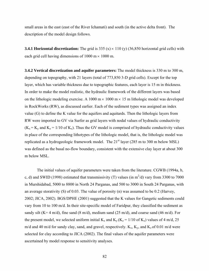
small areas in the east (east of the River Ichamati) and south (in the active delta front). The

description of the model design follows.

3.4.1 Horizontal discretization: The grid is 335 (x) × 110 (y) (36,850 horizontal grid cells) with

each grid cell having dimensions of 1000 m × 1000 m.

3.4.2 Vertical discretization and aquifer parameters: The model thickness is 330 m to 300 m,

depending on topography, with 21 layers (total of 773,850 3-D grid cells). Except for the top

layer, which has variable thickness due to topographic features, each layer is 15 m in thickness.

In order to make the model realistic, the hydraulic framework of the different layers was based

on the lithologic modeling exercise. A 1000 m × 1000 m × 15 m lithologic model was developed

in RockWorks (RW), as discussed earlier. Each of the sediment types was assigned an index

value (G) to define the K value for the aquifers and aquitards. Then the lithologic layers from

RW were imported to GV via Surfer as grid layers with nodal values of hydraulic conductivity

(Kx = Ky and Kz = 1/10 of Kx). Thus the GV model is comprised of hydraulic conductivity values

in place of the corresponding lithotypes of the lithologic model, that is, the lithologic model was

replicated as a hydrogeologic framework model. The 21st layer (285 m to 300 m below MSL)

was defined as the basal no-flow boundary, consistent with the extensive clay layer at about 300

m below MSL.

The initial values of aquifer parameters were taken from the literature. CGWB (1994a, b,

c, d) and SWID (1998) estimated that transmissivity (T) values (in m2/d) vary from 3300 to 7000

in Murshidabad, 5000 to 8800 in North 24 Parganas, and 500 to 3000 in South 24 Parganas, with

an average storativity (S) of 0.03. The value of porosity (n) was assumed to be 0.2 (Harvey,

2002; JICA, 2002). BGS/DPHE (2001) suggested that the K values for Gangetic sediments could

vary from 10 to 100 m/d. In their site-specific model of Faridpur, they classified the sediment as

sandy silt (K= 4 m/d), fine sand (8 m/d), medium sand (25 m/d), and coarse sand (46 m/d). For

the present model, we selected uniform initial Kx and Ky (Kz = 1/10 of Kx) values of 4 m/d, 25

m/d and 40 m/d for sandy clay, sand, and gravel, respectively. Kx, Ky, and Kz of 0.01 m/d were

selected for clay according to JICA (2002). The final values of the aquifer parameters were

ascertained by model response to sensitivity analyses.

82

3.4.3 Surface topography: The initial thickness of the topmost layer was set as 30 m. The

SRTM DEM was imported into GV for the surface elevation/upper bound of the topmost layer.

3.4.4 Specified head boundaries: According to the conceptual model, ArcGIS® (ESRI,

Redlands, CA, USA) shape files were developed for each river and then imported into GV as

specified-head-boundary river objects. To resemble reality, all of the rivers shown in Figure 2.1

have been included. The rivers were divided into 11 reaches according to geometric similarities

along each reach. For each of the stream reaches, the starting and ending cells were specified

with attributes like channel width, stream stage, channel bed elevation, and K of the bed

sediments. Depending on the reach length and surrounding topography, GV automatically

interpolated the attribute values for the cells lying between the starting and ending cells of each

reach. The width of each of the reach was specified according to measurements from the base

map. In Bangladesh, the stage of the rivers varies from approximately 5 to 13 m above the

streambed (Dowling et al., 2003). For this model the stage values for each reach were selected

from field experience and the topographic values specified for the cells in the vicinity, assuming

that the stage of the river is near the land surface. The other attributes were specified according

to estimation, field experience and local information.

3.4.5 Constant head boundaries: Constant head boundaries with a value of 0 m representing

the Bay of Bengal were assigned to the southernmost rows of the top four layers of the model.

Though not exact, the depth and extent of the constant head boundaries for each layer were

guided by the original bathymetric data (Survey of India, 1971). The extreme southern boundary

was marked at the southernmost tip of the study area (the active delta front).

3.4.6 Rationale of seasonal models: The study area has distinct wet (monsoon) and dry seasons.

On average (1901 to 1970), the seasonal rainfall can be considered as pre-monsoon (January to

May) equaling 16.23% of annual rainfall, monsoon (June to October) 82.21% and post-monsoon

(November-December) 1.57%. Increased pumping lowers the water level in the dry seasons. The

aquifer is mostly full during the monsoon season as an effect of increased precipitation and lower

rates of pumping. Hence any excess potential recharge is rejected (BGS/DPHE, 2001), thereby

83

causing regular, widespread runoff and flooding. The division of seasons for this study was done

in the context of irrigation schedules. The seasons have different daily recharge rates and

pumping rates for irrigation.

In West Bengal, rice cultivation is dominated by boro (mainly dependent on groundwater

irrigation) during the pre-monsoon (January to April/May), followed by kharif (mainly

rainwater-fed) during the monsoon (July to October/November). Rabi (post-monsoon)

cultivation is also mostly groundwater fed. The high-yielding boro cultivation caught momentum

with the onset of groundwater pumping for irrigation in the early 1970s. In Bangladesh, the

cultivation increased from less than 0.05% of the total area in the early 1970s to more than 20%

(more than 45% of total cultivable area) around 2000 (Hossain et al., 2003; Harvey et al., 2005).

Boro requires from about 1 m (Harvey et al., 2005) to about 3 m (AIP/PHED, 1995) of annual

irrigation, while kharif requires only about 0.3 m (S.P. SinhaRoy, Arsenic Task Force,

Government of West Bengal, personal communication, 2004).

In spite of having some localities with an overdraft problem (where the groundwater is

not replenished annually), groundwater levels at the beginning of each irrigation season tend to

be similar from year to year, which suggests that the groundwater levels are controlled by local

river stages (BGS/DPHE, 2001). This observation and the lack of detailed storativity data for the

different hydrologic units led to construction of three separate models for different annual

irrigation seasons, instead of a single transient model with three seasons (stress periods). A single

transient model would have been preferable, but the disproportionate precipitation (and hence

recharge) during the monsoon adversely affects the water levels during other seasons of a

transient model, resulting in poorly constrained values of the volume of water in storage.

Moreover, calibration of the pre-monsoon model with pumping (at the beginning of the irrigation

season) indicates a reasonable fit, as noted below, supporting the rationale of separate seasonal

models.

3.4.7 Recharge: The exact recharge values in the study area were not available. Previous studies

have estimated 0.3 to 5.5 mm/d (BGS/DPHE, 2001) and 1.6 mm/d (annual average) (Basu et al.,

2002; Dowling et al., 2003) for the Bangladesh part of the basin. For the West Bengal part,

84

SWID (1998) estimated that recharge is up to 15% of total precipitation. Because recharge rate is

one of the primary controlling factors for groundwater flow in a low-topographic-gradient study

area, a detailed approach for estimating the potential recharge (PR) was developed. The term

“potential recharge” is used in place of “recharge” because the rainwater available for recharge

will also run off, and there is no record or simple method available for estimating either the

recharge or run-off in an area crowded by numerous ponds, ox-bow lakes, small streams and

larger rivers. Harvey et al. (2005) noted that the pond/lake bottoms and streambeds can provide

significant areas for infiltration of recharge, and irrigation water applied to cultivated fields can

also re-infiltrate, resulting in a very complex cycle of recharge and discharge. Actual recharge

values can be obtained by the difference in groundwater levels between wet and dry seasons.

However, no such data were available except for general values obtained for some small

localities. Moreover the daily oscillation of water levels due to irrigation pumping can be more

than 0.2 m, thus presenting a very difficult scenario for estimating recharge and groundwater

flow directions (Harvey et al., 2005).

Seasonal mean rainfall data, as shown in Table 3.1, were calculated for 25 locations

within and near the study area based on multiple years’ data obtained from the National Climatic

Data Center (http://www.ncdc.noaa.gov/oa/pub/data/ghcn/v2/ghcnftp.html). Table 3.2 shows the

monthly mean temperature data for Calcutta from 1811 to 2005. Based on these data, potential

evapotranspiration (PET) values were estimated for each location according to Malmstrom

(1969):

)(*9.40)/( TemonthmmPET ×=

where

)3.237

3.17exp(611.0*+

××=

TTe

T is average monthly temperature (°C).

Evapotranspiration (ET) values were calculated (Pike, 1964) for each of these 25 locations as:

2/12 ])(1[)/(

PETRRmonthmmET

+=

85

where

R = average precipitation (mm/month)

PET = potential evapotranspiration (mm/month)

Potential recharge (PR) was then calculated as:

PR (mm/month) = R – ET

The monthly PR values were aggregated according to the previously described seasons. These

values were then used to form 2-D daily PR grids of the study area by kriging in Surfer, where

daily PR (mm/day) = s

s

dR

where

Rs = cumulative mean monthly rainfall for that season (in mm)

ds = number of days in that season

The daily PR grid files were then imported into GV to form the different zones of recharge in the

top layer of each model.

3.4.8 Groundwater abstraction: In the study area, generally four types of pumping wells are

used for abstraction of groundwater. Similar to the description of BGS/DPHE (2001) for

Bangladesh, they are:

- Low yielding hand-pump tubewells (HTW): These are generally screened at a shallow

depth (generally 10 to 50 m depending on their location). They are privately owned or are

installed by the PHED and are mostly used for drinking and domestic purposes in villages

and towns. They are pumped discontinuously throughout the day and because of their

very low yield, they are thought to have minimal stress on groundwater.

- Public-water-supply deep tubewells (PDTW): They are generally owned by PHED or

town municipalities. They are operated by electric motorized pumps and have high

abstraction rates (50-100 m3/h). Generally they are used for 6 hours each day. The

pumped water is piped to communities for domestic use. Due to their limited numbers

and restricted hours of operation, they were not considered in this modeling exercise,

except in and around Calcutta, where the main abstraction takes place by a dense network

of PDTWs as shown in Table 3.3a.

86

- Irrigation shallow tubewells (STW): These privately owned tubewells use relatively small

diesel-motorized 4.5 h.p. centrifugal or submersible pumps to abstract groundwater from

relatively shallow depths (30-75 m). They are generally fitted with 75-mm diameter

galvanized iron pipes and have an average yield of 26 m3/hr (CGWB, 1994e). Because in

many instances they are installed privately, their hours and rates of operation are not

exactly known, although MID (2001) provided an estimated number of wells for each

district (Murshidabad: 66,664, Nadia: 94,789, North 24 Parganas: 63,202, and South 24

Parganas: 9,452). They should have a widespread effect on groundwater flow, at least at

shallow depths. However, due to the attached uncertainty, they were not included in the

model design, with the understanding that this makes the model incomplete. Thus these

provide a possibility of future refinement of the model.

- Irrigation deep tubewells (DTW): These wells are owned by the Government of West

Bengal Irrigation Department. Groundwater is withdrawn by 18-20 h.p. electric motors

coupled with turbine or submersible pumps, which can yield up to 200 m3/hr. They are

generally 60 to 180 m in depth (average 130 m) with 355- or 305-mm diameter steel pipe

for about the upper 30 m and then 216-mm diameter pipe for the rest (CGWB, 1994e).

They are one of the main sources of irrigation water in the study area and were included

in the model design as pumping nodes. The number of DTWs currently present in the

modeled area as shown in Table 3.3a was complied from MID (2001). Their hours of

operation vary widely for cultivation seasons, but some generalized estimates of hours of

operation and rate (Table 3.3a) were obtained for each district (M.K. Sinha, SWID,

Government of West Bengal, personal communication, 2004). These values were used to

determine the pumpage for each grid cell following the equation:

aA

trNQ ×××

= )(

where

Q = the assigned total pumpage (outflow) value to each grid cell for a specified time [L3]

A = area of each district within the model boundary [L2]

N = number of pumps

r = pumpage rate [L3/T]

t = hours of operation per day [T]

87

a = area of each grid cell.

The exact depths at which the wells are operating were not available. Hence, the pumping

nodes were assigned to model layers closest in depth to the PDTWs (data available from the

lithologs) in the area. As it was also not possible to ascertain the lengths of the screened

intervals for these pumps, the whole thicknesses of the layers (i.e. 15 m) were used.

Three sets of models were developed:

i) with pumping: pre-monsoon (PREM-p), monsoon (M-p), post-monsoon (POSTM-p), based

on numbers of DTWs and PDTWs in 2001;

ii) without pumping: pre-monsoon (PREM), monsoon (M) and post-monsoon (POSTM),

assuming no DTWs or PDTWs (pre-1970s conditions);

iii) projected pumping: average population growth of West Bengal for 1991-2001 was 18.15%;

rates by district are tabulated in Table 3.3b (Census, 2001). Assuming the same rate of

population growth in the next two decades, projected number of pumps and pumping rates

for 2011 (2011-p) and 2021 (2021-p) for each district were calculated according to the

following equation:

PN ×= η

where

N = projected number of pumps

η = number of pumps per capita in 2001

P = projected population in the year of interest.

Based on these estimated data, two pre-monsoon models (assuming same pumping rates, hours

of operation and tapped depths as at present) were simulated.

3.4.9 Calibration and sensitivity analyses: Ideally, the models should have been calibrated for

all three seasons for steady-state simulations without any pumping. However, because water-

level data were only available for the study area for the pre-monsoon in presence of pumping, the

PREM-p model was calibrated at steady state against known head values from 26 locations.

88

These water-level values for April and May were obtained from various sources (our field

measurements, CGWB [1994d, e], and SWID [1998]). Sensitivity analyses were performed on

this calibrated model (PREM-p) by sequentially varying the Kx-y of sand and clay, S and n

values. Model response due to sensitivity analyses are listed in Table 3.4. The model was found

to be most sensitive to the Kx values of sand and clay. Using the selected values from the

analyses, the final model was recalibrated and found to have good agreement with present water-

level contours as shown in Table 3.5. The differences between the observed and computed values

were probably a cumulative manifestation of a specified head boundary in the vicinity,

discrepancy in topographic elevations, exclusion of STWs, and uncertain aquifer parameters. The

finalized values obtained from the sensitivity analyses were then used for defining the aquifer

properties of the other seven models (PREM, M, POSTM, M-p, POSTM-p, 2011-p, and 2021-p).

3.5 Simplifications and limitations

As discussed earlier, the complexities of the western Bengal aquifers are so great that it is

very difficult to construct a groundwater model that reflects local-scale variations of aquifer

properties. Hence, based on the similarity to other data from the study area or previous studies,

several generalizations and assumptions were involved in order to construct the model. As a

consequence there are several limitations. Thus the modeling exercises for this study should be

considered as a guideline or template on which future workers may modify and elaborate,

although our results reasonably resemble current conditions. The simplifications are listed below.

i) Values for potential recharge at each cell are based on the interpolated values from the 25

monitoring stations. Calculation of PET was based on the temperature values that were

available for Calcutta only. Moreover, as mentioned earlier, there may be differences

between the potential recharge and absolute recharge. Hence the amount of water that is

actually percolating into the system is not well constrained.

ii) In order to make the numerical flow model executable within the present constraints of

time and computational resources, a 15-m vertical resolution was used. This leads to a

broad generalization for the hydrostratigraphic layers, so smaller-scale variations in the

lithology may be over- or under-emphasized.

iii) Precise aquifer property (Kx-y-z and S) values for each locality were not obtained. Hence

generalized aquifer property values for the different hydrogeologic units were used

89

throughout the model and the ranges of observed values obtained from the literature were

used for sensitivity analyses.

iv) Most of the specified head values were estimated based on previous literature, field

experience, local information and topography, except the stream widths, which were

known for each reach.

v) The smaller water bodies (such as small streams, ponds, and lakes), which are present

throughout the modeled area, were not built into the model because they were thought to

have insignificant effects on the regional flow.

vi) No comprehensive data were found for the DTW pumps (location, rate of pumping, hours

of operation or screen depth and length). Hence a number of generalizations were

undertaken as explained earlier.

vii) The STWs, which would probably have significant control on the groundwater flow, were

not included in the model because of insufficiency of data.

3.6 Results and discussion

Figures 3.1a and 3.1b shows the final simulation results of the eight models as contour

maps of groundwater levels in the area. The effects of seasonality due to variable PR rates are

distinctly visible in all the models.

The models without pumping (PREM, M and POSTM) suggest that there is a

topographically controlled, natural regional flow from the northern boundary of the study area

toward the south-southeast. The rivers in the system are in general effluent. The PREM contours

indicate lateral flows in the vicinity of the Ganges in the north and northwest and along the

Bhagirathi-Hoogly north of Calcutta. Flows also converge in the vicinity of the Jalangi, whereas

contours meet the Bhairab and upper part of the Ichamati at high angles. PREM also indicates

the development of a few groundwater mounds above the land surface, illustrating aquifer

saturation in those localities, with radially outward flow for excess water. Two such prominent

localities can be noted near the western part of North 24 Parganas (near Bashirhat) and northern

Murshidabad (near Jangipur). These locations match with present-day waterlogged areas

(CGWB, 1994e) (Figure 3.2). The reason for this waterlogging is a conjunctive effect of the

presence of a shallow aquitard, thickening of clay layers (Figure 2.5) and very flat topography.

90

The possible result is flow stagnation and groundwater accumulation in these areas. Near the

active delta front, contours become more broadly spaced, which is consistent with tidal

fluctuations, although the models did not include those. The groundwater flow in M is not

conspicuously visible on the map. Because of the large amount of water available for recharge

during monsoonal rainfall, aquifer saturation and excess water ponding take place leading to

recurrent wide floods and increased runoff to the streams. These are in agreement with Harvey et

al. (2005), who observed in Munshiganj (Bangladesh) that groundwater flow ceases as stream

stages rise and hydraulic head becomes uniform in flooded areas. BGS/DPHE (2001) reported up

to 56.9% of the total area of Bangladesh flooded annually between 1954 and 1988 (based on

Miah [1988] and Brammer [1990a, b]). Although no such historical data were available for the

study area, a devastating flood in September 2000 affected 18.3 million people (with demise of

1187 people) in 6177 villages of nine districts of West Bengal, including Calcutta

(http://www.bapscare.org/services/disaster/2000/2000floods.htm). In Jumpukur (Table 2.1,

location 46), Nadia, floodwater marks of 2000 were observed during fieldwork at 1.98 m above

land surface (Figure 3.3). Of the 65 blocks within the study area, 75% have flood hazard

potential of medium to very high (Sanyal and Lu, 2003). The POSTM model demonstrates north-

to-south flow with perpendicular to semi-perpendicular intersection of contour lines with the

boundary rivers.

The “with pumping” models (PREM-p, POSTM-p, 2011-p and 2021-p) indicate that in

all of the districts, except the southern half of South 24 Parganas, the natural flow paths have

been thoroughly disrupted by the formation of cones of depression due to pumping. In vertical

sections, local-scale convective flow cells are found to have developed corresponding to these

depressions. In southern South 24 Parganas, flow reversal has developed along with increased

inflow from the constant-head boundary of the Bay of Bengal. This phenomenon can be easily

explained by the large salt-water intrusion that has been documented in these areas (CGWB,

1994d, e; SWID, 1998, Allison et al., 2003). PREM-p demonstrates the effects of abstraction all

over the study area, with prominent pumping centers in the blocks of Murshidabad-Jiaganj,

Behrampur, Hariharpara and Domkal in central Murshidabad; Kaliganj and Nakashipara in

northern Nadia; Shantipur, KrishnaNagar-I and Ranaghat-I in south-central Nadia; Chakdah,

Haringhat, Habra-II and Amdanga in southern Nadia; and northern North 24 Parganas and

91

Calcutta. Of these, the depression around Calcutta (CGWB, 1994e; Sikdar et al., 2001) is most

acute due to the huge amount of pumping for municipal water supply through PDTWs. The

groundwater mounds near Jangipur and Bashirhat, though still observable, have become

substantially reduced in size and extent. In the 2011-p and 2021-p models, the cones have

become more pronounced. In 2021-p some dry cells corresponding to deep cones of depression

have formed in central Murshidabad, northern North 24 Parganas, and south-southeast Calcutta.

These dry cells imply severe overdraft. In the POSTM-p model, in addition to the effects of the

PREM-p models, a huge cone of depression has developed in north and central North 24

Parganas with centers at Calcutta, Rajarhat, Barasat-I and II, and Deganga. However, in reality,

the cone of depression may not be so large because of the availability of monsoonal water in

storage that has not been accounted for in the model design. The effect of pumping is not at all

conspicuous in the monsoon model (M-p), indicating that the saturated aquifers are not stressed

in spite of pumping.

Table 3.6 and Figure 3.4 show the groundwater mass (inflow-outflow) balance of these

models. The mass balance error ranges between 0.02% (PREM-p) and -0.06% (POSTM-p). It

indicates that at present the submarine groundwater discharge (SGD) through the delta front of

South 24 Parganas seems to have decreased by 6% annually since the onset of pumping, while

the annual salt-water intrusion has increased by 98%. The inflow of river water into the system

has increased by 92% in the last three decades, but the rivers are still effluent mostly because of

the monsoonal groundwater discharge. The model demonstrates that the rivers have changed

from slightly effluent to influent for the post-monsoon season. This estimation is probably not

viable because of the monsoonal water in storage, as mentioned above.

Dowling et al. (2003) estimated annual SGD as about 1.5 ± 0.5 × 1011 m3 of water for the

entire delta front (500 km wide). Considering that the delta front in the present study area is 110

km, the present estimates for SGD of 5.37 × 106 m3 are negligible. The probable reason for the

difference is that Dowling et al. (2003) considered that all the recharge water reaching below 30

m (first 2 layers of the model) is discharged to the Bay of Bengal. However, the present model

shows that a considerable amount of water upwells from the aquifer deeper than 30 m to the

rivers. The estimation of abstracted water (only by DTWs and PDTWs) from the modeled area is

92

93

about 8 × 108 m3 annually. On the basis of estimation of resident groundwater (4.52 × 1011 m3)

from the lithologic model, it seems that the total volume of groundwater resource is as yet

underutilized. Dowling et al. (2003) suggested an average actual recharge rate of 0.6 m/year.

Using that estimation, the total annual recharge in the study area (recharge rate × rechargeable

surface area) would be about 9 × 109 m3, which shows that the groundwater abstraction by DTW

and PDTW is only about 9%. This value is similar to Dowling et al.’s estimate of 12 ± 4%.

However, the composite cone of depression around Calcutta (as visible in PREM-p and POSTM-

p) is perennial and formed by overdraft pumping, which has superseded any recharge in that

area. The cause may be exponential metropolitan growth (which is directly proportional to

increases in groundwater demand for drinking and industrial use) and the lack of recharge due to

impervious urban cover and the near-surface shallow aquitard (Figure 2.4a). The aquifers near

Calcutta have not completely dried up probably because of the recharge that takes place in the

north (near northern North 24 Parganas and southern Nadia) and subsurface inflow from the

Bhagirathi-Hoogly.

Figure 3.5 illustrates the layer-by-layer mass balance calculation for the PREM-p model.

The bulk of the groundwater flow in the system takes place between layers 2 and 6

(approximately 15 m to 105 m bgl). This indicates that the local flow systems predominate,

which agrees with the conclusion of Harvey et al. (2005) regarding flow in Bangladesh.

Although lesser in extent, the medium to regional-scale flow to a depth of about 200 m (layer no.

13) is not insignificant. Below that depth, to the base of the model, there is minimal recharge and

groundwater has relatively long residence times. These results indicate that the Golden Bengal

aquifer is continuously being recharged and there is substantial flow even in the deeper part of

the aquifer, apart from the isolated aquifers mentioned above.

In conclusion, natural groundwater flow in the study area is dependent on the amount

and timing of precipitation, and is controlled by the relatively flat topography and locations of

major streams, but has been heavily distorted by pumping. This finding is in agreement with the

results of 3-D regional modeling in western Bangladesh (JICA, 2002).

94

Tabl

e 3.

1: D

istri

butio

n of

rain

fall

and

calc

ulat

ed p

oten

tial r

echa

rge

(PR

) dat

a fr

om G

loba

l His

toric

Clim

atol

ogy

Net

wor

k (G

HC

N v

. 2

[GH

CN

, 200

5]) s

tatio

ns in

and

aro

und

the

stud

y ar

ea.

D

ata

cove

rage

Pr

e-m

onso

on (J

an.-M

ay)

Mon

soon

(Jun

.-Oct

.) Po

st-m

onso

on (N

ov.-D

ec.)

Loca

tion

From

To

R

ain

(mm

/d)

PR (m

m/d

)R

ain

(mm

/d)

PR (m

m/d

)R

ain

(mm

/d)

PR (m

m/d

) B

ehra

mpo

re

1901

19

70

1.40

0.

14

7.57

3.

30

0.31

0.

00

Ara

mba

gh

1901

19

68

1.51

0.

13

7.24

3.

10

0.39

0.

00

Bon

gaon

19

01

1967

2.

09

0.31

8.

34

3.96

0.

35

0.00

K

rishn

aNag

ar

1901

19

70

1.77

0.

21

7.55

3.

26

0.38

0.

00

Ran

agha

t 19

01

1967

1.

73

0.20

6.

80

2.73

0.

28

0.00

K

alya

ngan

j 19

06

1954

1.

31

0.12

6.

98

2.86

0.

30

0.00

H

arin

ghat

a 19

08

1966

1.

35

0.10

6.

43

2.41

0.

30

0.00

C

alcu

tta

1829

20

05

1.67

0.

19

8.92

4.

42

0.47

0.

01

Bud

geB

udge

19

01

1970

1.

64

0.16

9.

27

4.74

0.

39

0.00

D

umD

um

1947

19

80

1.47

0.

14

8.58

4.

13

0.43

0.

01

Bar

rack

pore

19

01

1965

1.

52

0.14

8.

01

3.74

0.

49

0.01

B

aras

at

1901

19

59

1.62

0.

16

8.11

3.

75

0.39

0.

00

Bas

hirh

at

1901

19

70

1.67

0.

20

8.54

4.

16

0.47

0.

01

Dia

mon

d H

arbo

ur

1901

19

67

1.46

0.

13

8.93

4.

49

0.37

0.

00

Gos

aba

1921

19

56

1.39

0.

15

9.41

4.

86

0.64

0.

02

Saga

r Isl

and

1975

19

84

1.46

0.

11

9.23

4.

78

0.31

0.

00

Potk

abar

i 19

01

1956

1.

68

0.24

6.

88

2.78

0.

39

0.01

H

oogl

y 19

01

1962

1.

83

0.22

7.

52

3.30

0.

40

0.00

K

alna

19

01

1963

1.

61

0.16

6.

78

2.73

0.

33

0.00

H

owra

h 19

01

1948

1.

59

0.15

8.

32

3.95

0.

35

0.00

Se

ram

pore

19

01

1962

1.

73

0.20

8.

24

3.88

0.

39

0.00

A

zim

ganj

19

01

1961

1.

41

0.14

7.

26

3.09

0.

25

0.00

94

Tabl

e 3.

1 (c

ontin

ued)

Lo

catio

n Fr

om

To

Rai

n (m

m/d

)PR

(mm

/d)

Rai

n (m

m/d

) PR

(mm

/d)

Rai

n (m

m/d

) PR

(mm

/d)

Boi

nche

e 19

32

1962

1.

63

0.17

7.

92

3.63

0.

42

0.01

K

atw

a 19

01

1966

1.

44

0.13

7.

37

3.17

0.

32

0.00

U

lube

ia

1901

19

68

1.83

0.

22

8.90

4.

47

0.38

0.

00

95

95

Tabl

e 3.

2: M

onth

ly te

mpe

ratu

re (1

811

to 2

005)

and

pre

cipi

tatio

n (1

829

to 2

005)

dat

a fo

r Cal

cutta

alo

ng w

ith c

alcu

late

d ev

apot

rans

pira

tion

(ET)

and

pot

entia

l rec

harg

e fr

om G

HC

N v

.2 (G

HC

N, 2

005)

.

Tem

pera

ture

(o C)

Prec

ipita

tion

(mm

/mon

th)

Mon

th

Mea

n M

ax

Min

M

ean

Max

M

in

ET

(mm

/mon

th)

PR

(mm

/mon

th)

Janu

ary

19.6

822

.70

15.0

011

.53

73.7

00.

0011

.45

0.08

Fe

brua

ry

22.6

525

.40

18.8

024

.25

202.

200.

0023

.70

0.54

M

arch

27

.52

30.2

023

.60

32.6

115

9.30

0.00

31.8

7 0.

74

Apr

il 30

.34

33.1

026

.80

52.5

919

6.20

0.00

50.4

3 2.

17

May

30

.80

33.2

028

.40

130.

6443

4.60

2.00

106.

19

24.4

5 Ju

ne

30.0

132

.20

27.7

029

2.36

946.

0040

.60

149.

71

142.

66

July

29

.10

30.8

027

.20

333.

5587

9.00

109.

0014

8.14

18

5.41

A

ugus

t 28

.98

31.0

027

.70

337.

2668

3.50

122.

4014

7.69

18

9.57

Se

ptem

ber

29.0

130

.60

27.7

026

4.65

944.

7056

.10

139.

73

124.

92

Oct

ober

27

.87

31.2

026

.50

136.

2347

4.00

0.00

102.

02

34.2

1 N

ovem

ber

24.0

027

.10

21.8

022

.37

238.

500.

0022

.01

0.36

D

ecem

ber

20.1

423

.40

17.8

06.

4714

6.00

0.00

6.46

0.

01

96

96

Popu

latio

n Pr

e-m

onso

on 2

011

Pre-

mon

soon

202

1

Dis

trict

G

row

th ra

te

(199

1-20

01)

No.

of p

umps

c Pu

mpi

ng (m

3 /m2 /d

) N

o. o

f pum

psc

Pum

ping

(m

3 /m2 /d

) M

ursh

idab

ad

23.7

6 55

1 4.

92E-

04

682

6.09

E-04

N

adia

19

.54

905

6.70

E-04

10

82

8.01

E-04

N

orth

24

Parg

anas

22

.69

398

1.82

E-04

48

8 2.

23E-

04

Sout

h 24

Par

gana

s 20

.85

35

4.69

E-06

42

5.

67E-

06

Cal

cutta

3.

93

520

1.46

E-03

54

0 1.

52E-

03

Pum

p de

tails

Pr

e-m

onso

on

Mon

soon

Po

st-m

onso

on

Dis

trict

N

umbe

r R

ate(

m3 /h

r)a

Ope

ratio

n ho

urs(

/d)

Pum

ping

(m

3 /m2 /d

) O

pera

tion

hour

s(/d

) Pu

mpi

ng

(m3 /m

2 /d)

Ope

ratio

n ho

urs(

/d)

Pum

ping

(m

3 /m2 /d

) M

ursh

idab

ad

445

150

18

3.98

E-04

8

1.77

E-04

10

2.

21E-

04

Nad

ia

757

150

18

5.60

E-04

8

2.49

E-04

10

3.

11E-

04

Nor

th 2

4 Pa

rgan

as

324

100

18

1.48

E-04

8

6.58

E-05

10

8.

23E-

05

Sout

h 24

Pa

rgan

as

29

75

18

3.88

E-06

8

1.72

E-06

10

2.

16E-

06

Cal

cutta

50

0b 10

0 6

1.41

E-03

6

1.41

E-03

6

1.41

E-03

97

Tab

le 3

.3a:

Sea

sona

l det

ails

of i

rrig

atio

n pu

mps

(DTW

s) fo

r eac

h di

stric

t and

PD

TWs f

or C

alcu

tta w

ithin

the

stud

y ar

ea.

Tab

le 3

.3b:

Pro

ject

ed d

etai

ls o

f irr

igat

ion

pum

ps (D

TWs)

for e

ach

dist

rict a

nd P

DTW

s for

Cal

cutta

with

in th

e st

udy

area

.

a M

.K. S

inha

, Sta

te W

ater

Inve

stig

atio

n D

irect

orat

e, G

over

nmen

t of W

est B

enga

l, pe

rson

al c

omm

unic

atio

n, 2

004

b nu

mbe

r of P

DTW

s est

imat

ed fr

om T

he S

tate

sman

, Cal

cutta

, 6 Ju

ne 2

004,

loca

l sec

tion,

pag

e 6

c cal

cula

ted

base

d on

Cen

sus (

2001

)

97

Table 3.4: Results of sensitivity analyses on PREM-p for uncertain aquifer parameter values. Sand (Kx) m/d RSS Comment

25 78.9 formation of large dry cells 37.5 34.4 used model parameter value 50 21.9 formation of small dry cells in Nd and NP

70 21.7 formation of large dry cells all over the study area

Sand (Ky) m/d 25 34.4 used model parameter value

37.5 31.2 formation of dry cells near CCU and SP 15 39.5 formation of dry cells near CCU and Md

Clay (Kx-y) m/d 0.1 34.4 used model parameter value 0.5 47.7 not much effect, long time to converge 1 49.1 not much effect, long time to converge

0.01 42.2 distorted contours and flow toward River Ganges

S 0.03 34.4 used model parameter value 0.015 34.4 no effect 0.06 34.4 no effect 0.3 34.4 no effect

n 0.2 34.4 used model parameter value 0.1 34.4 no effect 0.4 34.4 no effect

bold: initial values, italicized: used values, RSS = residual sum of squares Md: Murshidabad, Nd: Nadia, NP: North 24 Parganas, SP: South 24 Parganas, CCU: Calcutta

98

99

Table 3.5: Results of model calibration with the best-fitted parameter values from Table 3.4.

Calibration locations Latitude Longitude Layer

Observed (hydraulic head in m

above MSL)

Computed (hydraulic head in m

above MSL) ResidualRaghunathganj 24.5 88.08 4 22 21.32 0.68 Lalgola 24.42 88.25 4 20.7 20.40 0.30 Bhagawangola 24.34 88.32 4 19.9 18.38 1.52 Raninagar-II 24.25 88.6 4 16.5 15.27 1.23 Jiaganj 24.23 88.27 4 17.2 18.55 -1.35 Lalbagh 24.18 88.27 4 18.6 17.52 1.08 Raninagar-I 24.15 88.47 4 14.5 11.75 2.75 Behrampur 24.09 88.26 4 17.5 16.34 1.16 Nawda 23.91 88.46 4 14.3 14.09 0.21 Potkabari 23.86 88.52 6 13.5 13.36 0.14 Debagram 23.69 88.33 6 11.3 11.05 0.25 Chapra 23.61 88.56 6 11.9 11.03 0.87 Nakashipara 23.6 88.35 6 12.4 10.98 1.42 Banguin 23.33 88.66 6 8.2 8.24 -0.04 Bongaon 23.05 88.83 7 7.1 6.75 0.35 Amdanga 22.77 88.53 10 4.5 3.64 0.86 Baduria 22.76 88.79 7 7.8 7.19 0.61 DumDum 22.73 88.38 9 3 1.77 1.23 Haroa 22.61 88.68 12 4 6.50 -2.50 East Calcutta 22.56 88.42 9 0 -0.18 0.18 Rajpur-Sonarpur 22.45 88.43 12 5 4.19 0.81 Baruipur 22.4 88.48 12 5 3.43 1.57 Jalerhat 22.3 88.56 12 3.5 2.74 0.76 Sonakhali 22.3 88.74 12 2.8 3.04 -0.24 Kulpi 22.16 88.29 12 2.2 1.38 0.82 Dakhin Durgapur 22.06 88.39 12 2.2 0.89 1.31 residual mean: 0.61 residual standard deviation: 0.97 sum of squares: 34.35 absolute residual mean: 0.93 minimum residual: -2.50 maximum residual: 2.75

100

Tabl

e 3.

6: C

ompa

rison

of a

nnua

l mod

eled

subm

arin

e gr

ound

wat

er d

isch

arge

(SG

D),

inflo

w a

nd p

umpi

ng v

olum

es b

etw

een

2001

an

d pr

e-19

70s.

Attr

ibut

e PR

EM-p

M

-p

POST

M-p

A

nnua

l (P

rese

nt)

PREM

M

PO

STM

Ann

ual

(pre

- 19

70s)

% c

hang

ew

ith

resp

ect t

o pr

e-19

70s

Ann

ual S

GD

ou

tflow

to

Bay

of B

enga

l 1.

37E+

06

3.41

E+06

5.82

E+05

5.

37E+

06

1.61

E+06

3.

49E+

066.

22E+

05

5.72

E+06

-6.1

1 A

nnua

l inf

low

fr

om

Bay

of B

enga

l 1.

28E+

04

1.04

E+02

5.57

E+03

1.

85E+

04

0.00

E+00

0.

00E+

003.

53E+

02

3.53

E+02

98.0

9 A

nnua

l ou

tflow

to

river

s 3.

89E+

08

1.29

E+10

3.96

E+06

1.

33E+

10

7.30

E+08

1.

31E+

102.

04E+

07

1.39

E+10

-4.2

1 A

nnua

l inf

low

fr

om ri

ver

1.18

E+08

3.

37E+

051.

09E+

08

2.28

E+08

1.

64E+

06

3.33

E+05

1.62

E+07

1.

82E+

0792

.03

Ann

ual

pum

ping

4.

58E+

08

2.27

E+08

1.10

E+08

7.

95E+

08

0.00

E+00

0.

00E+

000.

00E+

00

0.00

E+00

100.

00

10

0

101

10

1

Figu

re 3

.1a:

Mod

eled

gro

undw

ater

leve

l map

s obt

aine

d fr

om P

REM

, PR

EM-p

, M, a

nd M

-p. T

he b

old

blue

line

s ind

icat

ed

the

maj

or ri

vers

in th

e ar

ea. T

he b

lack

are

as in

dica

te c

lose

ly sp

aced

dec

reas

ing

cont

our l

ines

.

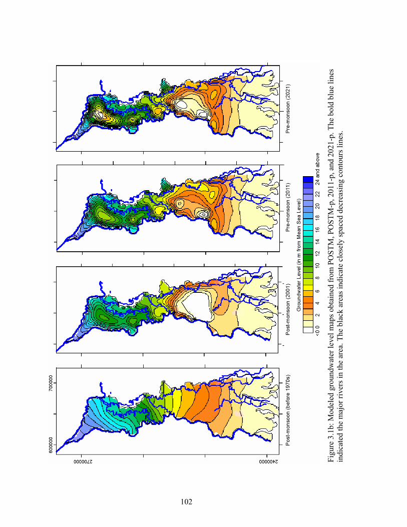
102

Fi

gure

3.1

b: M

odel

ed g

roun

dwat

er le

vel m

aps o

btai

ned

from

PO

STM

, PO

STM

-p, 2

011-

p, a

nd 2

021-

p. T

he b

old

blue

line

s in

dica

ted

the

maj

or ri

vers

in th

e ar

ea. T

he b

lack

are

as in

dica

te c

lose

ly sp

aced

dec

reas

ing

cont

ours

line

s.

102

Figure 3.2: Map of water logged areas (marked red) within the study area of western Bengal basin (CGWB, 1994e).

103

104

Error!

(e)

Figure 3.3: Collection of images of monsoon flooding in the study area during 2001-2006 (Source: local newspapers [a-d] and field photo [e]).

(a) (b)

(c) (d)

2001 flood water mark(Loc. 46, table 2.1)

105

1.0E

+00

1.0E

+01

1.0E

+02

1.0E

+03

1.0E

+04

1.0E

+05

1.0E

+06

1.0E

+07

1.0E

+08

Inflow

Outflow

Inflow

Outflow

Inflow

Outflow

Inflow

Outflow

Inflow

Outflow

Inflow

Outflow

Inflow

Outflow

Inflow

Outflow

PR

EM

PR

EM

-pM

M-P

PO

STM

PO

STM

-p20

11-p

2021

-p

m3/d

Rec

harg

e

Con

stan

t Hea

d

Rive

r

Wel

l

Fig

ure

3.4:

Plo

t of m

ass b

alan

ce o

f the

eig

ht fl

ow m

odel

s sho

wn

in F

igur

es 3

.1 a

nd 3

.2.

10

5

106

0.E+

00

1.E+

06

2.E+

06

3.E+

06

4.E+

06

5.E+

06

6.E+

06

7.E+

06

8.E+

06

0.E+

00

1.E+

06

2.E+

06

3.E+

06

Laye

r Bot

tom

Laye

r Bot

tom

Laye

rTop

Rech

arge

Laye

rTop

Rive

rW

ell

Rive

r

>MSL

MSL

-15

-30

-45

-60

-75

-90

-105

-120

-135

-150

-165

-180

-195

-210

-225

-240

-255

-270

4.E+

06

5.E+

06

6.E+

06

7.E+

06

8.E+

06

>MSL

MSL

-15

-30

-45

-60

-75

-90

-105

-120

-135

-150

-165

-180

-195

-210

-225

-240

-255

-270

Eleva

tion o

f top

of la

yer (

in m

from

MSL

)

Inflow (m3/d)

Outflow (m

3/d)

Figu

re 3

.5: P

lot o

f mas

s bal

ance

for e

ach

laye

r for

PR

EM-p

(pre

-mon

soon

with

pum

ping

[200

1]).

106

Chapter 4: Regional-scale stable isotopic (δ18O-δ2H) signature of recharge and deeper groundwater

4.1 Introduction and background

During the last two decades, several international institutions and organizations have

studied the hydrogeochemistry and groundwater dynamics of the Bengal basin by using a variety

of hydrogeologic techniques. Previous studies (e.g. Aggarwal et al., 2000; Basu et al., 2002;

Stüben et al., 2003; Harvey et al., 2005; Klump et al., 2006) have applied stable isotopic

techniques to understand hydrogeochemical processes in the region. This chapter documents and

discusses stable isotopic results of the deeper groundwater of the western Bengal basin. The

study area is about ~ 22,000 km2, including the previously described area (eastern Murshidabad,

Nadia, North 24 Parganas and northern and central South 24 Parganas) along with the

southernmost part of Maldah, (Figure 4.1). The area lies ~ 200 km south of the eastern

(Darjeeling) Himalayas. No previous basinal-scale isotopic study has been done in West Bengal.

The objective is to delineate the source and recharge of deeper groundwater in Gangetic West

Bengal by identifying regional trends in the 18O and 2H compositions of groundwater, surface

water and rainwater.

4.1.1 Previous stable isotopic studies of Bengal basin groundwater: Published studies on δ18O

and δ2H distributions in the Bengal basin have been limited. The earliest work relevant to the

present study was done by Dray (1983), who demonstrated that significant isotopic differences

exist between groundwater and the River Ganges in Bangladesh, indicating a lack of rapid

interaction between the two.

Krishnamurthy and Bhattacharya (1991) collected 55 shallow groundwater samples (<10

m below ground) along a ~1400 km transect between Calcutta and Delhi. Of these, only three of

the samples were collected from or near the present study area. The samples from Calcutta and

North 24 Parganas had δ18O values of ~ -4.3 and ~ -4‰ (VSMOW) respectively (values

estimated from figure), while a sample about 20 km west of Calcutta was found to have δ18O of

~ -4.5‰. The authors showed that as the Indian southwestern monsoon wind moves from the

Bay of Bengal west-northwest toward central India (Ananthakrishnan, 1977; Rao, 1981), there is

107

a clear continental effect (Dansgaard, 1964), so that the δ18O of groundwater becomes more

depleted.

Ramesh and Sarin (1992) documented that the Ganges headwaters, which originate at

>3500 m in northern India, are isotopically highly depleted (δ18O: -7.8‰ to -14.4‰ and δ2H: -

51‰ to -103‰), defining a slope that is similar to the global meteoric water line (GMWL). The

Ganges mainstream was found to be enriched downstream by evaporation.

Shivanna et al. (1999) reported stable isotopic results for water samples collected from

various depths in selected areas of Murshidabad and South 24 Parganas districts of West Bengal.

They inferred that the aquifers in Murshidabad are connected, while there is limited connectivity

between deeper and shallower groundwater in South 24 Parganas. They also showed that isotopic

compositions of both the shallow groundwater and rivers are seasonally dependent, with

maximum depletion occurring in December (Murshidabad groundwater δ18O: -3.00‰ to -

8.00‰; River Bhagirathi: -8.50‰; River Bhairavi: -5.50‰) and maximum enrichment in May (-

3.00‰ to -7.50‰; -6.78‰; and -3.53‰, respectively), probably because of enrichment by

enhanced evaporation. Furthermore, they suggested that the depleted stable isotope values of

some shallow groundwater compared to local precipitation in Murshidabad is an artifact of

interaction with the depleted Ganges water, while most of the other localities have recharge from

precipitation.

Aggarwal et al. (2000) provided a detailed and systematic basin-scale study of

Bangladesh, in which they attempted to delineate As-contaminated and uncontaminated aquifers

and discussed the mechanisms of As mobilization based on stable isotopic signatures. They also

evaluated the effect of geomorphic and sea level changes on atmospheric isotope composition

and hence recharge. They grouped waters based on isotopic composition and depth and assigned

them to different climatic regimes. They concluded that the older, deeper groundwaters are

generally uncontaminated.

Stüben et al. (2003) concluded that the shallow groundwater of their study area (in the

vicinity of Behrampur, Murshidabad district) is of meteoric origin, whereas more depleted River

108

Bhagirathi water (δ18O: -7.91‰ to -8.01‰) indicates a contribution of snowmelt water from the

Himalayas and precipitation further up in the Ganges valley.

Harvey et al. (2005) and Klump et al. (2006) concluded from their study site in

Bangladesh (Munshiganj) that there is a difference in δ18O values between groundwaters above

and below ~ 30 m from ground surface, suggesting mixing of chemically and isotopically

distinct groundwater bodies at that depth. Values of δ18O are relatively depleted (< -3‰) above ~

30 m depth, become abruptly enriched (~ -1‰) at ~ 30 m depth, and then decrease slightly

downward to a depth of ~ 100 m.

Zheng et al. (2005a) studied the annual variation in stable isotopic compositions of

rainwater, surface water and shallow groundwater at Araihazar, Bangladesh. They concluded that

the composition of precipitation falls on the GMWL and that the surface water bodies are

significantly evaporated, resulting in a δ18O enrichment of up to 10‰ in the dry season. The

groundwater suggests recharge both from direct precipitation and from moderately evaporated

surface water during the wet season and at the beginning of the dry season. The authors did not

find evidence of recharge from strongly evaporated irrigational water in paddy fields. Figure 4.2

combines results from some of the previous stable isotopic studies in the Bengal basin.

Literature on the isotopic composition of precipitation in the study area is scarce. The

nearest monitoring points of the International Atomic Energy Agency and World Meteorological

Organization (Global Network of Isotopes in Precipitation) are located in New Delhi, Allahabad,

Shillong and Yangon (Myanmar). The average δ18O compositions for rainfall in these locations

are: New Delhi (dry season [ds]: -1.53‰; monsoon [m]: -5.85‰), Yangon (ds: -3.92‰; m: -

4.54‰), Allahabad (annual mean [am]: -7.36‰) and Shillong (am: -3.67‰) (Araguas-Aruguas

et al., 1998). Considering these values, Aggarwal et al. (2000) suggested the isotopic

composition of recharge in their Bangladesh study area to be ~ -4.5‰ for δ18O and ~ -30‰ for

δ2H. They also suggested an average δ18O value of -4.5‰ for rains in Calcutta based on shallow

groundwater results from Krishnamurthy and Bhattacharya (1991).

109

4.1.2 Climate: Due to its proximity to the Bay of Bengal and its low latitude position (the Tropic

of Cancer passes through the study area), Gangetic West Bengal experiences a warm and humid

climate with distinct dry and wet seasons. These may be termed as pre-monsoon (January to

May), monsoon (June to October) and post-monsoon (November-December). The bulk of the

precipitation takes place as a result of moisture-laden monsoon winds from the Bay of Bengal.

Local convectional storms contribute to some pre-monsoonal rainfall. On average (based on

Global Historic Climatology Network [GHCN] version 2 data from 1901 to 1970 [GHCN,

2005]), pre-monsoon rainfall contributes 16.23% of the annual rainfall, monsoon 82.21% and

post-monsoon 1.57%. It is hypothesized that most of the groundwater in the study area is

recharged from monsoonal precipitation. Aggarwal et al. (2000) concluded from their study in

Bangladesh that the stable isotopic signature of deeper water (at depths of 100-150 m and ~ 300

m) is different from that of the shallower aquifers, suggesting that recharge of the deeper water

took place following rainfall 3 to 30 ka ago.

Monthly precipitation results from 35 monitoring stations in and around the study area

have been acquired. Figure 4.3 shows the contour plots of the annual rainfall in these stations

(computed from GHCN version 2 data) along with average daily summer temperature to

illustrate the present climatic regime of Gangetic West Bengal.

4.1.3 Hydrostratigraphic framework: The hydrostratigraphic characterization of the study area

(up to a depth of 300 m below mean sea level [MSL], and excluding the part of the study area in

Maldah) has resulted in the delineation of several types of aquifers (Figure 4.4) (Chapter 2). The

first is a continuous, semiconfined sand aquifer (termed hereafter as the main aquifer) underlain

by a thick clay aquitard. The names “Sonar Bangla aquifer” for this main aquifer and

“Murshidabad aquitard” for the basal clay aquitard have been proposed in Chapter 2. The main

aquifer deepens from a maximum of ~ 50-80 m below land surface in the north to ~ 180 to >200

m in the south. In the southern half of the study area, discontinuous clay layers locally divide the

near-surface aquifer to form several deeper, confined aquifers. Several smaller, isolated aquifers

at greater depths than the main aquifers (~200-300 m) contain groundwater with considerably

different solute compositions (Chapter 5). Finally, some deep parts of the main aquifer are not

isolated but appear to demonstrate restricted conditions (intermediate between the main and

110

isolated aquifers). The hydrostratigraphic positions of the two sampled wells that are screened

below 300 m and of the four sampled wells in Maldah are not known.

4.2 Methods

4.2.1 Sampling: Sixty-four groundwater, seven river-water and fourteen rain-water samples

were collected from Gangetic West Bengal during the months of May to August of 2003−2005

(Figure 4.1, Table 4.1). The latitude and longitude of each of the sampling points were recorded

in the field using a handheld Global Positioning System (datum WGS84).

A number of deep, community water supply wells with single intake zones (single

strainers) were selected. These wells (except the ones in Calcutta) are owned and operated by the

Public Health Engineering Directorate (PHED), Government of West Bengal. Detailed

information about the well completion and tapped aquifer was obtained from the PHED database

and a local drilling agency (B.M. Engineering, KrishnaNagar). Similar information was not

available for the four wells in the district of Maldah, but they were ascertained to have single

strainers (personal communication with PHED officers). Groundwater is withdrawn from all of

these wells by 15-20 h.p. electric motors powering turbine or submersible pumps with general

yields of 50 to 100 m3/hr, which can go up to 200 m3/hr. They are typically operated for 6 hours

(2−3 hours at a time) each day. The wells are generally screened at depths of 50 to 409 m, with

the overall trend of increasing well depth toward the south and east of the study area.

During 2004 and 2005, groundwater samples were collected according to standard

sampling protocols (Wood, 1981). The wells were purged for 40 to 75 minutes until the EH, pH,

temperature (T) and electrical conductivity (EC) of the out-flowing water were stable, thereby

indicating that the sampled water was representative of the aquifer. Each sample was then

collected by pumping water through a disposable 0.45-μm plastic capsule filter. River water

samples were collected using a hand-filtration unit with the same kind of filter. All of the

samples for δ18O and δ2H were collected in 40-mL amber glass vials with solid caps. Care was

taken to exclude air bubbles. During 2003, the samples were not filtered and were collected after

~20-30 minutes of purging. The field parameters (EH, pH, T and EC) were also not measured for

these samples. One-liter HDPE bottles were used to collect rainwater samples for δ18O and δ2H.

111

As much as possible, each rain sample was collected during an entire storm to capture an average

composition. Later, some of these waters were sub-sampled and transferred to 10-mL glass vials

with solid caps.

4.2.2 Laboratory methods: Isotope analyses of 2003 and 2004 samples were performed at the

University of Kentucky Environmental Research and Training Laboratory (UK ERTL) on a

ThermoFinnigan Delta Plus XP isotope ratio mass spectrometer (IRMS) using a Gas Bench II

peripheral unit equipped with a GC-autosampler. The analyses were standardized against the

international references Vienna-Standard Mean Ocean Water (VSMOW), Greenland Ice Sheet

Project (GISP), and Standard Light Antarctic Precipitation (SLAP), as well as internal standards,

with three standard gas injections followed by seven sample gas measurements. Precision was

determined with duplicate and triplicate samples. For δ18O analyses, 0.5 mL of each standard and

sample were transferred into individual exetainers and then flushed for one minute with 0.5%

CO2 in He at 40 mL/min. They were then left to equilibrate at room temperature on a Gas Bench

II for 48 hours before being analyzed. For δ2H, 0.5 mL of each standard and sample were

transferred into individual exetainers containing platinum rods and flushed for three minutes with

2% H2 in He at 90 mL/min. The samples were then left to equilibrate in a hot block in the gas

bench for 16 hours at 22o C before analysis. Precision was ± 0.1‰ for δ18O and ± 1.0‰ for δ2H.

Analyses of 2005 isotope samples were performed at the University of Arizona Isotope

Geochemistry Laboratory on a gas-source IRMS (Finnigan Delta S) standardized with VSMOW,

SLAP, and internal standards. The δ18O samples were equilibrated with CO2 at ~15oC in an

automated equilibration device coupled to the IRMS. For δ2H, samples were reacted with Cr at

750oC using a Finnigan H device coupled to the spectrometer. Precision was ± 0.08‰ for δ18O

and ± 0.9‰ for δ2H.

4.2.3 Data grouping and statistical clustering: The stable isotopic compositions of the sample

locations with known well-completion details were grouped hydrostratigraphically into main

(containing all the locations that were thought to be pumping water from the main aquifer) and

isolated (consisting of the wells drawing water from the isolated aquifers and from depths >300

112

m). The rationale for grouping >300-m and isolated aquifer samples together is that a clay

aquitard underlies the study area south of Maldah at a depth of ~300 m (Chapter 2).

For all the wells, δ18O and δ2H values were evaluated by hierarchical cluster analysis

(HCA) to investigate statistical relationships between hydrochemical and spatial parameters

(Drever, 1997). Statistical associations do not necessarily demonstrate a causal relationship but

do represent data in a condensed version for better visualization. Cluster analysis was used to

determine if the samples could be grouped into distinct hydrochemical populations (Güler et al.,

2002). The HCA was done on the original data set (without any weighting or standardization)

following Davis (1986), Güler et al. (2002), and Dreher (2003). The clustering was done by

importing the r×c data matrix (r samples with c variables) into the statistical software package

SPSS version 14 (SPSS Inc., Chicago, IL). For best grouping, the dendogram was constructed by

Ward’s method of linkage (Ward, 1963) with squared Euclidean distance (Güler et al., 2002).

Ward’s method uses an analysis of variance (ANOVA) approach to evaluate the distances

between clusters. See Table 4.1 for the cluster number corresponding to each location.

4.3 Results

4.3.1 Rainwater: Because of the small number of samples (n = 14), rainwater samples were not

used for statistical analyses or calculating mean weighted annual composition, but were used to

generate a local meteoric water line (LMWL) for Gangetic West Bengal. As noted in Table 4.1,

11 of the 14 samples were collected during 2004; the remaining three were collected in 2005.

The samples represent May to August; 10 samples were from the monsoon season and four from

the pre-monsoon. In 2004, the monsoon season in West Bengal began on 12 June (news release

from Regional Meteorological Office, Alipur, Calcutta; Anandabazar Patrika, Calcutta, 12 June

2004, page 1). Calcutta received 156 mm of rainfall (9.39% of total 1661 mm for 2004) during

the pre-monsoon (January to May) and 1505 mm (90.61%) during the monsoon (June to

October) (Figure 4.5). No rainfall occurred in November and December. Thus assuming that the

rest of the study area had similar pattern and proportion of precipitation (as evident from the

seasonal means stated in section 4.1.2), it can be assumed that our rainfall dataset fairly

represents the isotopic composition of the precipitation available for groundwater recharge in

Gangetic West Bengal.

113

The LMWL plotted from our data in Figure 4.6 compares well to the global meteoric

water line (GMWL) (Craig, 1961). The LMWL with a relation of

δ2H = 7.24 δ18O + 7.73 (r2 = 0.93)

is quite similar to the line developed by Bhattacharya et al. (1985) for a limited number of

precipitation samples from New Delhi, Ahmedabad and Shillong:

δ2H = (7.2 ± 0.1) δ18O + (5.1 ± 0.1).

Krishnamurthy and Bhattacharya (1991) suggested a δ2H-δ18O slope of ~7.2 for average Indian

monsoonal precipitation. Our data agree well with this suggestion. Figure 4.6 also distinguishes

between the monsoon and pre-monsoon rains. Except for samples rain-water R1 and R8, the

monsoon samples have δ18O values (-4.74‰ to -9.34‰) that are more isotopically depleted than

those of the pre-monsoon rains (1.45‰ to 0.32‰). This suggests that the pre-monsoon rains may

originate from isotopically enriched local moisture sources (such as evaporated surface water

bodies), whereas the monsoon rain clouds have traveled a greater distance and had multiple

fractionations before precipitation. An explanation for the higher δ18O and δ2H values of samples

R1 and R8 is that they represent moisture sources that are relatively close to the sampling

locations. The six samples for Calcutta plotted against month (June to August) do not

demonstrate any seasonal trend (Figure 4.5).

4.3.2 River water: All of the river water samples plot below the LMWL (Figure 4.7), suggesting

evaporation. The Bhagirathi-Hoogly samples (river sample numbers 1, 2 and 3), with δ18O

values of -5.57‰ to -5.74‰, are more depleted than the Jalangi and Ichamati samples, with δ18O

of -3.15‰ to -0.37‰. The Bhagirathi-Hoogly values are more enriched than other reported

values for that river (Shivanna et al., 1999; Stüben et al., 2003). No data from other studies

appear to exist for the Jalangi and Ichamati. One of the Ichamati samples (river water location

[RW] # 7 [see Table 4.1 for location details]) was significantly more enriched than the other

samples from this group and represents the composition of the tidally influenced southern rivers.

4.3.3 Groundwater: Figure 4.7 differentiates the isotopic composition of samples between the

main and the isolated aquifers. With the exception of one sample (groundwater location # 64 [see

Table 4.1 for location details]), the δ18O values of the samples range from -3.12‰ to -6.12‰. Of

the 64 samples, 40 have δ18O values more depleted than the mean (-4.80‰) of all samples. Five

114

of six isolated aquifer samples and 19 of the 54 main aquifer samples were more enriched than

the mean, which indicates that the isolated groundwaters are relatively isotopically heavier than

the main aquifer samples. Kalinagar (#64) (δ18O of -0.48‰) is located in the southernmost part

of the study area (near the delta front [Sunderbans]) and is suspected of being influenced by

seawater intrusion from the Bay of Bengal or brackish water intrusion from one of the numerous

tidal channels in the vicinity

.

Statistical grouping of the data by HCA suggests three distinct groups (Table 4.1, Figure

4.7). Most samples fall in group 1 (n = 49), while 7 samples fall in group 2 and 8 fall in group 3.

All of the groups contain samples from both main and isolated aquifers.

4.4 Factors influencing δ18O and δ2 H composition of recharge and groundwater:

In general, the isotopic composition of groundwater is similar to the mean weighted

annual precipitation composition, although variations may result depending on types of soils and

vegetation, unsaturated flow through heterogeneous porous media, evapotranspiration, seasonal

variations, long-term climatic variations, and residence time in the recharge zone (Clark and

Fritz, 1997). For the study area, the effect of evaporation before or during infiltration, seawater

influence toward the south, and seasonal variability may be important. As noted earlier, Bengal

basin recharge is dominated by monsoonal precipitation, although in certain areas and years there

might be a significant contribution from the pre-monsoonal rainfall. The effect of seasonal

variation would be most dominant in the shallow groundwaters. Clark and Fritz (1997) noted that

in a system lacking preferential flow, the seasonal effects generally disappear below a critical

depth. Hence, considering the depth from which groundwater samples were collected for this

study, the isotopic composition of the groundwater should be similar to the weighted annual

mean composition of precipitation after accounting for evaporation. However, it should be noted

that because all the groundwater and river water samples were collected at the same time of the

year, no study of seasonal trends was undertaken.

4.4.1 Precipitation: Most of the groundwater samples plot slightly below the LMWL (Figure

4.7). A linear fit relation of all groundwater samples

δ2H = 5.8 δ18 O – 2.96 (n = 64, r2 = 0.82)

115

has a lower slope than both the LMWL and GMWL, indicating that the isotopic composition of

the study area is influenced by some additional factors (e.g. evaporation, sea water intrusion)

besides precipitation. This relationship is similar to the one determined by Krishnamurthy and

Bhattacharya (1991) for shallow groundwater for their study area from Calcutta to Delhi:

δ2H = 6.4 δ18 O – 1.0 (n = 55, r2 = 0.95),

but somewhat different from Bhattacharya et al. (1985):

δ2H = (6.8 ± 0.1) δ18 O + (2.2 ± 0.4)

for groundwater samples from several other stations in addition to those of Krishnamurthy and

Bhattacharya (1991). Our relationship is also different from that of Aggarwal et al. (2000) for

Bangladesh (reconstructed from reported values for both <100 and >100 m samples):

δ2H = 6.9 δ18 O + 1.0 (n = 53, r2 = 0.91)

However, when only the main aquifer samples are considered (excluding the tidal/sea-water

influenced #64), the relationship

δ2H = 6.7 δ18 O + 1.44 (n = 53, r2 = 0.84)

is very similar to those of Bhattacharya et al. (1985) and Aggarwal et al. (2000). The

groundwater δ18O range (except for #64) is within the range of monsoon precipitation

composition during 2004-2005. This indicates that groundwater of the study area is probably

recharged primarily from precipitation with similar isotopic composition to the present. The

slight deviation of the samples from the LMWL suggests that some evaporation of rainfall occurs

prior to or during infiltration, or there might be some mixing of the infiltrating water with

preexisting soil moisture that has undergone several cycles of evaporation and wetting (Allison,

1982). Harvey et al. (2005) concluded that the recharge in their study area in Bangladesh is very

complex: in addition to direct infiltration from precipitation, recharge may also take place from

the bottom of ponds, ox-bow lakes, rivers, and re-infiltration of groundwater withdrawn for

irrigation. Such a scenario is probably also true for our study area.

4.4.2 Distance from sea (continental effect): Comparison of the δ18O and δ2H compositions of

groundwater with distance from the Bay of Bengal (monsoonal moisture source) (Figure 4.8)

shows a prominent continental effect. Because of the north-south orientation of the study area,

latitude was used as a proxy for distance from the sea. The δ18O value decreased from about -

3.2‰ (excluding #64) from near the southernmost part of the study area to about -6‰ in the

116

northernmost part (r2 = 0.31 and P = 0.01). This pattern is consistent with recharge from the

southwest monsoon, which moves from the Bay of Bengal toward the north with a Rayleigh-type

distillation, where the air moisture becomes progressively depleted with successive phases of

precipitation (Dansgaard, 1964). Krishnamurthy and Bhattacharya (1991) and Bhattacharya et al.

(2003) documented similar subcontinent-scale depletion from the southwest monsoon.

Krishnamurthy and Bhattacharya (1991) also concluded that the continental effect from Calcutta

to Delhi cannot be solely explained by Rayleigh distillation, but must also account for re-entry of

enriched vapor into the air from evapotranspiration (with an efficiency of ~40%). The inland

gradient of δ18O depletion for our samples (~ -0.84‰ per 100 km) is much higher than the

reported gradients of -2‰ per 1,000 km by Krishnamurthy and Bhattacharya (1991) for Calcutta

to Delhi and -6‰ per 1,000 km by Bhattacharya et al. (1985) for Ahmedabad (western India) to

Delhi. A decrease in the inland gradient can be caused by significant recycling of water vapor

within the basin by evapotranspiration, as noted by Salati et al. (1979) for the Amazon basin and

by Krishnamurthy and Bhattacharya (1991). However, estimation for Calcutta (see Chapter 3)

indicates up to 50% evapotranspiration occurs during the summer, suggesting sufficient vapor

mass recycling. Therefore, the cause of the high gradient in our study area is unresolved. It

should also be noted that the calculations and conclusions by Krishnamurthy and Bhattacharya

(1991) were based on the assumption of insignificant isotopic variation normal to the west-

northwest movement of the monsoon (i.e. along the long axis of our study area). In our study,

plotting the δ18O values with longitude, a prominent trend of depletion (from ~ -3‰ to ~ -6‰)

parallel to the westward component of the southwest monsoon (similar to the observation of

Krishnamurthy and Bhattacharya [1991]) can also be seen. Thus the isotopic composition of

monsoon precipitation in Gangetic West Bengal appears to show a continental effect both

northward and westward. This hypothesis could have been confirmed more robustly with a more

detailed precipitation data set across the study area, but except for Behrampur (n = 3) and

Calcutta (n = 6), our sample set lacks multiple samples from individual locations. The measured

δ18O ranges for monsoon rainfall in Behrampur (-6.72‰ to -9.34‰) and Calcutta (-0.46‰ to -

8.15‰) fail to show any trend (Figure 4.9).

4.4.3 River water: In order to understand the influences of the individual major streams within

the study area on the isotopic composition of recharge, the groundwater samples are grouped by

117

proximity to the rivers and plotted against distance from the sea (latitude). These sample sets are

(a) River Ganges-Bhagirathi-Hoogly (n = 32), (b) River Jalangi (n = 14), and (c) River Ichamati

(n = 11). Some of the samples co-exist in both the Ganges and Jalangi groups. Distinct spatial

trends are observed between these three groups, which might indicate some causal relationship.

(a) River Ganges-Bhagirathi-Hoogly (Figure 4.10a): The composition of the river water samples

from the Bhagirathi-Hoogly is almost the same over a distance of about 300 km, indicating a

minimal latitudinal effect on the river water composition. The river water is generally more

depleted than the groundwater, perhaps because of the highly depleted snow melt from the

Himalayas (source of the Ganges) (Ramesh and Sarin, 1992; Stüben et al., 2003). The

groundwater isotope values trend more positive toward the south, in contrast to the river water.

In the northern to central portion of the study area (up to central Nadia), the river water and

groundwater values are similar, indicating the possibility of recharge from the inflow of the river.

Some of the samples deviating from the Ganges-Bhagirathi-Hoogly river water can also be

grouped with the River Jalangi, indicating the possibility of influence from both the rivers. The

maximum deviation from the linear trend in this area is Jumpukur (#24), which is suspected to

have restricted recharge because of hydrostratigraphic heterogeneity. In the south, the

groundwater-river water dissimilarity increases. The two most dissimilar groundwater samples,

from Ghasiara (#34) and Canning (#36), are thought to have influences of restricted recharge

(due to depth) and sea-water intrusion, respectively. The value from Calcutta (#4) is very similar

to river water of Belur (RW #3), suggesting that recharge of groundwater in Calcutta is

influenced by the Bhagirathi-Hoogly. This also agrees with the prediction of a groundwater

model developed for the area (see Chapter 3) that high urban pumpage of groundwater attracts

inflow of water from the river.

(b) Jalangi (Figure 4.10b): The river is highly meandering (in contrast to the Ganges-Bhagirathi-

Hoogly and the Ichamati) and covers relatively little latitudinal distance. The two isotopic values

of the river water are similar to each other, but they are far more enriched than groundwater in

this group. The enrichment can be attributed to high evaporation from the relatively narrow

stream channel and surface runoff influences. The groundwater locations in this group do not

show any spatial trend. The greatest deviation from the linear trend was shown by the isolated

aquifer sample from Iswarchandrapur (#45) and restricted main aquifer in Bhaluka (#49). Thus

the Jalangi may not have much influence on groundwater recharge.

118

(c) Ichamati (Figure 4.10c): Both the groundwater and the river water become highly enriched

toward the south. The trends of groundwater and river water are sub-parallel to each other. The

isotopic values of the river water are enriched than the groundwater. While the reason for

enrichment of the Ichamati at Bongaon (RW #6) is probably evaporation and surface runoff

influence, at Taki (RW #7), where the stream channel is very wide, the enrichment is consistent

with tidal inflow from the Bay of Bengal. The maximum deviation of groundwater from the

linear trend is demonstrated by Kalinagar (#64) near the delta front, reflecting seawater intrusion.

4.4.4 Spatial distribution and depth: It is evident from the discussion so far that the isotopic

composition of Gangetic West Bengal groundwater shows a prominent spatial pattern. A plot of

the statistical groups on a map of the study area helps to better visualize this pattern (Figure

4.11). The reason for this pattern, while not definitive, can be a composite or cumulative

influence of precipitation, latitudinal effect, temperature, river inflow, seawater intrusion,

hydrostratigraphy and (or) depth. Many of these points have already been individually discussed.

Figure 4.11 shows that most of the areas except south-central North 24 Parganas and eastern

South 24 Parganas are represented by HCA group 1, succeeded southeastward by groups 2 and 3.

Of the two outliers in the north, the one in Murshidabad is represented by the isolated aquifer at

Chaighari (#17). The outlier in Nadia has two points: group 3 is represented by the restricted

main aquifer at Jumpukur (#24), and group 2 represents Debagram (#20). The reasons for these

outliers are not certain.

The influences of depth and seawater intrusion for the observed pattern require

evaluation. A δ18O-depth plot (Figure 4.12) illustrates that no apparent relation exists, and the

distributions of the statistical groups are not dependent on the absolute depth. However, most of

the isolated aquifer samples have been assigned in the higher order HCA groups, suggesting

some hydrostratigraphic control. A lack of correlation between δ18O and Cl- concentration (see

Chapter 5) negates the idea that the southward existence of the higher-order groups reflects a

seawater influence from the Bay of Bengal.

119

4.5 Implications for groundwater recharge

The isotopic compositions of deep groundwater (both in the main aquifer and isolated

aquifers) are similar to modern-day precipitation values from the study area. This observation

indicates that the deeper parts of the aquifers of Gangetic West Bengal have been recharged by

rainfall under a climatic regime similar to the present, with a moisture source in the south (Bay

of Bengal) and progressive depletion of monsoonal rainfall as it moves toward the north.

Aggarwal et al. (2000) concluded that the samples with δ18O values heavier than -3‰ or lighter

than -6‰ probably indicate recharge from older rainwater from a different climatic regime,

although this water plots on the present day meteoric water line. In our study area, only a few

samples had δ18O values close to older water range of Aggarwal et al. (2000). The samples with

δ18O values close to or < -6‰ are from Sujapur (#7), Islampur (#3), Nabipur (#2), Habaspur

(#37) and Kamagachi (#54). All of these samples (except Sujapur, which is undefined) are from

the main aquifer. Four of the six isolated aquifers (Chaighari [#17], Chikanpara [#29], Bansjhari

Mullickpur [#31], and Murarisha [#63]) and a few main aquifer samples (Berachampa [#27],

Dalapara [#30], and Kalinagar [#64]) have δ18O values close to -3‰, which do not vary

systematically with depth. It can be noted that the northernmost wells #2, #3, #7, and #37 (as

mentioned above) are more depleted and the southwestern wells #27, #30, and #64 are less

depleted, probably as a result of the continental effect as described in section 4.4.2. Hence

simply being enriched or depleted relative to a critical value may not solely indicate climatic

differences, and several other factors need to be carefully evaluated. It is possible that because of

hydrostratigraphic heterogeneities, the deeper samples of Aggarwal et al. (2000) are older than

ours, but in the absence of radioisotope data for our samples, we were not able to evaluate this

possibility.

Based on similarities in isotope data from 1979 and 1999 from Bangladesh, Basu et al.

(2002) concluded that extensive irrigational pumping has not disturbed regional groundwater

flow in the Bengal basin. The authors inferred that such pumping would have resulted in mixing

of groundwater from various depths, assuming that isotopic composition with depth would

reflect a difference between 1979 (pre-pumping era) and 1999 (present pumping conditions). Our

data show no significant difference in isotopic composition between the shallower water

(Shivanna et al., 1999; Stüben et al., 2003) and the deeper water of the main aquifer system.

120

Moreover, no direct relation was observed between depth and isotopic composition for our

groundwater samples from the main aquifer. There are several possible reasons for this

homogeneous distribution, including similarities in hydrostratigraphy, climate and land use

within the study area.

Flow-model simulations of the study area (see Chapter 3) indicate that pumping could

have caused vertical mixing of groundwater in the main aquifer, thus homogenizing the chemical

and isotopic compositions locally. Therefore, the lack of a significant vertical trend in isotopic

compositions with depth in the study area could in part be an artifact of pumping. However, the

persistence of a lateral isotopic trend consistent with depletion of rainfall with distance from the

Bay of Bengal and similarity in isotopic compositions between water from the isolated aquifers

and the main aquifer indicate that pumping has not completely homogenized groundwater.

Hence, there should not be a notable difference between regional-scale isotope distributions in

1979 (before extensive pumping) and 1999 as suggested by Basu et al. (2002). Therefore

conclusions regarding groundwater mixing cannot be solely based on isotopic signatures.

4.6 Conclusion

Stable oxygen and hydrogen isotopic compositions of rainwater samples collected

during this study show that the monsoonal precipitation is generally more isotopically depleted

than the pre-monsoon rainfall in Gangetic West Bengal, India. The isotopic composition of

deeper water from the main aquifer of the study area suggests recharge under current climatic

conditions with the prevailing southwest monsoon originating from the Bay of Bengal in the

south and moving to the north (toward the eastern Himalayas) and west-northwest (toward north-

central India), indicating a continental effect caused by precipitation with a Rayleigh-type

distillation. Effects of evaporation are observable in the recharged water. The depletion gradient

determined in the present study is more than any previous values documented from India.

Depletion or enrichment with depth, as proposed by some previous workers, was not observed.

Comparison with previous studies suggests that the isotopic compositions of the deeper and

shallower parts of the main aquifer are similar, and inferences about groundwater mixing from

various depths cannot be drawn based exclusively upon stable isotopic data at the regional scale.

Moreover, the lack of prominent differences between the isolated and main aquifer samples

121

122

makes it impossible to distinguish between the climatic regimes during which they were

recharged. The sample from the active delta front indicates seawater or brackish water intrusion,

while those from locations near the north-central part of the study area and from Calcutta

indicate recharge influenced by the River Ganges-Bhagirathi-Hoogly. The snow-fed Ganges-

Bhagirathi-Hoogly river samples are distinctly more depleted than those of the other major rivers

of the area (Jalangi and Ichamati), which are affected by evaporation, surface runoff and tidal

influences.

123

Tabl

e 4.

1: S

tabl

e is

otop

ic sa

mpl

e lo

catio

ns fo

r gro

undw

ater

, riv

er w

ater

and

rain

wat

er fr

om G

ange

tic W

est B

enga

l. L

oc.

No.

C

olle

ctio

n D

ate

Loc

atio

n A

dmin

istr

ativ

eB

lock

/Tow

n D

istr

ict1

Lat

itude

Lon

gitu

de D

epth

2A

quife

r3δ18

O

(‰)

δ2 H

(‰)

HC

A

Clu

ster

4

1 17

/5/0

3 B

anip

ur

Hab

ra to

wn

NP

22.8

2 88

.69

150

M

-4.5

4 -2

3.92

2 2

27/5

/03

Nab

ipur

R

aniN

agar

-II

MD

24

.25

88.6

0 24

3 M

-6

.00

-36.

481

3 27

/5/0

3 Is

lam

pur

Ran

iNag

ar-I

M

D

24.1

5 88

.47

88

M

-5.8

7 -3

6.65

1 4

18/6

/03

Kal

igha

t C

alcu

tta

SP

22.5

2 88

.34

120

M

-5.5

5 -3

5.56

1 5

3/7/

03

Dat

tapa

ra

Shan

tipur

tow

n N

D

23.2

5 88

.43

128

M

-5.2

3 -3

4.56

1

6 16

/5/0

3 B

erac

ham

pa

(Deu

lia)

Deg

anga

N

P 22

.70

88.6

8

M

-5.0

1 -3

0.70

1

7 23

/5/0

3 Su

japu

r (B

akha

rpur

) K

alia

chak

-I

MA

24

.92

88.0

9

U

-6.1

2 -3

8.13

1

8 23

/5/0

3 B

aish

nabn

agar

(D

aria

pur)

K

alia

chak

-III

M

A

24.8

2 87

.99

U

-5

.73

-34.

451

9 23

/5/0

3 M

otha

bari

Kal

iach

ak-I

I M

A

24.9

4 88

.06

U

-5

.84

-36.

641

10

23/5

/03

Saha

pur

Old

Mal

dah

tow

n M

A

25.0

1 88

.15

U

-5

.63

-33.

381

11

24/5

/03

Aur

anga

bad

Suti-

II

MD

24

.62

88.0

3

M

-5.5

6 -3

3.81

1 12

20

/5/0

4 La

lgol

a La

lgol

a M

D

24.4

2 88

.25

66

M

-5.6

8 -3

6.55

1

13

21/5

/04

Lalb

ag M

orgu

e M

ursh

idab

ad

tow

n M

D

24.2

3 88

.27

32

M

-4.6

0 -2

9.61

1

14

21/5

/04

Kan

tana

gar

Bha

gwan

gola

-I

MD

24

.34

88.3

1 66

M

-5

.73

-36.

531

15

22/5

/04

Edra

kpur

N

awda

M

D

23.9

1 88

.46

82

M

-5.1

8 -3

0.73

1 16

22

/5/0

4 Ta

kipu

r B

elda

nga-

I M

D

23.8

7 88

.25

55

M

-5.1

1 -3

1.27

1 17

23

/5/0

4 C

haig

hari

Beh

ram

pur

MD

24

.16

88.4

1 22

8 I

-3.9

7 -2

4.35

2

18

24/5

/04

Seke

ndra

R

aghu

nath

ganj

-I

MD

24

.50

88.0

8 37

M

-5

.22

-36.

271

19

25/5

/04

Beh

ram

pur

Girl

s' C

olle

ge

Beh

ram

pur

tow

n M

D

24.0

9 88

.26

74

M

-5.1

3 -3

2.10

1

12

3

124

Tabl

e 4.

1 (c

ontin

ued)

L

oc.

No.

C

olle

ctio

n D

ate

Loc

atio

n A

dmin

istr

ativ

eB

lock

/Tow

n D

istr

ict1

Lat

itude

Lon

gitu

de D

epth

2A

quife

r3δ18

O

(‰)

δ2 H

(‰)

HC

A

Clu

ster

4

20

25/5

/04

Deb

agra

m

Kal

igan

j N

D

23.6

9 88

.33

78

M

-4.1

5 -2

7.04

2 21

26

/5/0

4 Ju

ranp

ur

Kal

igan

j N

D

23.7

2 88

.22

155

M

-5.3

7 -3

5.10

1 22

26

/5/0

4 B

irpur

N

akas

hipa

ra

ND

23

.63

88.4

8 18

5 M

-5

.84

-36.

801

23

27/5

/04

Bet

huad

ahar

i N

akas

hipa

ra

ND

23

.61

88.4

3 89

M

-5

.62

-33.

161

24

27/5

/04

Jum

puku

r K

alig

anj

ND

23

.72

88.3

8 26

9 M

-3

.61

-20.

513

25

28/5

/04

Han

spuk

uria

Te

hatta

-II

ND

23

.74

88.4

8 23

0 I

-5.1

1 -3

2.50

1 26

29

/5/0

4 G

agna

pur

Ran

agha

t-II

ND

23

.14

88.6

4 17

6 M

-5

.01

-31.

541

27

1/6/

04

Ber

acha

mpa

(A

min

pur)

D

egan

ga

NP

22.6

9 88

.67

298

M

-3.3

5 -1

9.77

3

28

2/6/

04

Jana

poll

Hab

ra-I

N

P 22

.87

88.6

9 15

1 M

-3

.83

-26.

152

29

2/6/

04

Chi

kanp

ara

Gai

ghat

a N

P 22

.93

88.7

7 40

9 >3

00

-3.6

5 -2

1.53

2 30

3/

6/04

D

alal

para

B

ashi

rhat

tow

n N

P 22

.69

88.8

5 23

0 M

-3

.36

-18.

893

31

3/6/

04

Ban

sjha

ri M

ullic

kpur

B

ashi

rhat

-I

NP

22.5

8 88

.88

273

I -3

.12

-17.

133

32

4/6/

04

Ber

acha

mpa

D

egan

ga

NP

22.7

0 88

.68

155

M

-5.1

8 -3

2.62

1 33

4/

6/04

Eo

jhna

gar

Bas

hirh

at-I

I N

P 22

.71

88.7

2 15

1 M

-4

.50

-27.

772

34

5/6/

04

Gha

siar

a So

narp

ur

SP

22.4

4 88

.46

240

M

-3.5

3 -1

9.17

3 35

5/

6/04

K

alik

apor

e So

narp

ur

SP

22.4

0 88

.48

240

M

-4.7

9 -2

9.39

1 36

7/

6/04

C

anni

ng

Can

ning

-I

SP

22.3

2 88

.65

189

M

-3.5

6 -1

8.70

3 37

16

/5/0

5 H

abas

pur

Bha

gaw

ango

la-I

MD

24

.32

88.3

4 76

M

-6

.07

-40.

531

38

17/5

/05

Chu

a H

arih

arpa

ra

MD

24

.03

88.4

5 84

M

-4

.68

-35.

631

39

17/5

/05

Sura

ngap

ur

Naw

da

MD

23

.93

88.4

6 96

M

-5

.16

-32.

781

40

18/5

/05

Mah

imap

ur

Pala

ce

Mur

shid

abad

M

D

24.2

1 88

.26

32

M

-4.9

5 -3

1.39

1

41

18/5

/05

Kis

mat

-Im

adpu

r Har

ihar

para

M

D

24.0

3 88

.35

71

M

-4.6

8 -3

0.58

1 42

19

/5/0

5 N

azirp

ur

Teha

tta-I

N

D

23.8

6 88

.54

110

M

-5.0

6 -3

3.60

1 43

19

/5/0

5 N

aray

anpu

r K

arim

pur-

II

ND

23

.92

88.5

5 10

8 M

-5

.14

-33.

801

12

4

125

Tabl

e 4.

1 (c

ontin

ued)

L

oc.

No.

C

olle

ctio

n D

ate

Loc

atio

n A

dmin

istr

ativ

eB

lock

/Tow

n D

istr

ict1

Lat

itude

Lon

gitu

de D

epth

2A

quife

r3δ18

O

(‰)

δ2 H

(‰)

HC

A

Clu

ster

4

44

20/5

/05

Pala

ship

ara

Teha

tta-I

I N

D

23.7

9 88

.46

95

M

-5.0

5 -3

5.32

1

45

20/5

/05

Isw

arch

andr

a pu

r Te

hatta

-I

ND

23

.76

88.4

6 21

7 I

-4.4

6 -3

0.22

1

46

21/5

/05

Dhu

bulia

K

rishn

aNag

ar-I

IN

D

23.5

0 88

.45

132

M

-5.4

1 -3

5.88

1 47

21

/5/0

5 So

nata

la

Kris

hnaN

agar

-II

ND

23

.52

88.5

1 14

0 M

-5

.11

-34.

421

48

22/5

/05

Gob

rapo

ta

Kris

hnaN

agar

-IN

D

23.4

2 88

.55

120

M

-5.1

7 -3

0.14

1 49

22

/5/0

5 B

halu

ka

Kris

hnaN

agar

-IN

D

23.3

5 88

.41

279

M

-4.3

4 -2

9.55

1 50

23

/5/0

5 B

him

pur

Kris

hnan

aga-

I N

D

23.4

3 88

.62

211

M

-5.3

6 -3

6.00

1 51

26

/5/0

5 N

ewto

wn

Raj

arha

t N

P 22

.58

88.4

5 13

2 M

-5

.10

-33.

521

52

26/5

/05

Path

argh

ata

Raj

arha

t N

P 22

.58

88.5

1 12

0 M

-4

.44

-30.

061

53

27/5

/05

Ghe

ntug

achi

a C

hakd

ah

ND

23

.03

88.5

9 12

9 M

-3

.57

-29.

521

54

27/5

/05

Kam

agac

hi

Ran

agha

t-I

ND

23

.22

88.5

6 15

2 M

-5

.83

-42.

811

55

28/5

/05

Panc

hita

B

onga

on

NP

23.1

1 88

.80

193

M

-5.3

5 -3

4.10

1

56

28/5

/05

Bon

gaon

H

ospi

tal

Bon

gaon

tow

n N

P 23

.05

88.8

2 20

2 M

-4

.92

-30.

551

57

29/5

/05

Ram

pur

Gai

ghat

a N

P 22

.95

88.7

5 20

0 M

-4

.91

-31.

301

58

29/5

/05

Kan

kphu

l H

abra

-II

NP

22.8

6 88

.62

190

M

-3.6

4 -2

2.81

2 59

30

/5/0

5 B

aman

gach

i B

aras

at-I

N

P 22

.75

88.5

1 15

8 M

-5

.00

-32.

341

60

30/5

/05

Hum

aipu

r B

aras

at-I

I N

P 22

.68

88.4

7 15

9 M

-4

.49

-29.

561

61

31/5

/05

Har

oa

Har

oa

NP

22.6

0 88

.68

167

M

-4.8

8 -3

2.01

1 62

31

/5/0

5 A

rsul

a B

adur

ia

NP

22.7

4 88

.77

148

M

-5.0

8 -3

3.50

1 63

1/

6/05

M

urar

isha

H

asna

bad

NP

22.5

9 88

.84

362

>300

-3

.57

-19.

723

64

1/6/

05

Kal

inag

ar

Sand

eshk

hali-

I N

P 22

.45

88.8

7 16

5 M

-0

.48

-14.

803

Riv

ers

Riv

er

1 28

/5/0

4 M

ayap

ur

Bha

gira

thi-

Hoo

gly

ND

23

.42

88.3

9

-5

.74

-38.

75

12

5

126

Tabl

e 4.

1 (c

ontin

ued)

L

oc.

No.

C

olle

ctio

n D

ate

Loc

atio

n R

iver

D

istr

ict1

Lat

itude

Lon

gitu

de D

epth

2A

quife

r3δ18

O

(‰)

δ2 H

(‰)

HC

A

Clu

ster

4

2 23

/5/0

4 B

ehra

mpu

r to

wn

Bha

gira

thi-

Hoo

gly

MD

24

.09

88.2

6

-5

.67

-39.

88

3 11

/6/0

4 B

elur

tow

n B

hagi

rath

i-H

oogl

y H

W

22.6

3 88

.36

-5.5

7 -3

6.36

4 17

/5/0

5 A

mta

la

Jala

ngi

ND

23

.93

88.4

6

-2

.95

-29.

60

5 21

/5/0

5 So

nata

la

Jala

ngi

ND

23

.52

88.5

1

-3

.15

-24.

22

6 28

/5/0

5 B

onga

on to

wn

Icha

mat

i N

P 23

.05

88.8

3

-3

.00

-21.

32

7 31

/5/0

5 Ta

ki

Icha

mat

i N

P 22

.59

88.9

4

-0

.37

-6.6

7

Rai

ns

Seas

on

1 21

/5/0

4 B

ehra

mpu

r to

wn

Pre-

mon

soon

M

D

24.0

9 88

.26

4.39

23

.95

2 25

/5/0

4 D

ebag

ram

Pr

e-m

onso

on

ND

23

.69

88.3

3

1.

45

22.2

7

3 6/

6/04

B

aras

at to

wn

Pre-

mon

soon

N

P 22

.76

88.5

9

0.

32

14.3

1

4 12

/6/0

4 C

alcu

tta

Mon

soon

SP

22

.52

88.3

4

-7

.34

-48.

96

5 15

/6/0

4 B

ehra

mpu

r to

wn

M

onso

on

MD

24

.09

88.2

6

-9

.34

-64.

54

6 19

/6/0

4 C

alcu

tta

Mon

soon

SP

22

.52

88.3

4

-8

.15

-52.

23

7 4/

7/04

B

ehra

mpu

r to

wn

Mon

soon

M

D

24.0

9 88

.26

-6.7

2 -4

5.61

8 12

/7/0

4 C

alcu

tta

Mon

soon

SP

22

.52

88.3

4

-0

.46

8.34

9 15

/7/0

4 Sh

antip

ur to

wn

Mon

soon

N

D

23.2

5 88

.43

-6.3

8 -3

7.06

10

14

/7/0

4 B

aras

at to

wn

Mon

soon

N

P 22

.76

88.5

9

-4

.74

-13.

81

11

2/8/

04

Cal

cutta

M

onso

on

SP

22.5

2 88

.34

-5.4

9 -4

0.55

12

19

/5/0

5 B

etai

Pr

e-m

onso

on

ND

23

.75

88.3

8

1.

23

18.8

3

13

1/7/

05

Cal

cutta

M

onso

on

SP

22.5

2 88

.34

-4.9

3 -9

.41

14

2/

8/05

C

alcu

tta

Mon

soon

SP

22

.52

88.3

4

-7

.08

-52.

54

12

6

127

1 Dis

trict

nam

e: M

D: M

ursh

idab

ad, N

D: N

adia

, NP:

Nor

th 2

4 Pa

rgan

as, S

P: S

outh

24

Parg

anas

, HW

: How

rah

2 Dep

th o

f bot

tom

of s

train

er

3 Aqu

ifer t

ype:

M: m

ain,

I: is

olat

ed, U

: und

efin

ed, >

300:

gre

ater

than

300

m.

4 Hie

rarc

hica

l Clu

ster

Ana

lyse

s (H

CA

) res

ults

127

Figure 4.1: Map of the study area showing the sampling locations for groundwater, river water and rainwater.

128

Figure 4.2: Composite δ18O−δ2H bivariate plot showing the findings of previous workers in Bengal basin. 1: Aggarwal et al. (2000); 2: Stüben et al. (2003); 3: Shivanna et al. (1999). Note that the values from Shivanna et al. (1999) are only the maximum and minimum ranges; detailed values were not available. SP denotes South 24 Parganas.

129

Figure 4.3: Map of the study area showing (a) contour plot of mean annual rainfall (in mm). The + symbol indicates the location of the monitoring stations whose data were used for drawing the contours. Maximum data range: 1821 to 2005, although most of the stations have data ranging from 1901−1970. The arrows show the approximate direction of movement of the southwest monsoon wind from the Bay of Bengal; (b) contours of average daily summer air temperature (in oC) redrawn after CGWB (1994e).

130

Figure 4.4: Simplified hydrostratigraphic diagram of the study area (not to scale) showing the different type of aquifers discussed in this article (see Chapter 2 for details). Note that no data were available for the part of the study area in Maldah and below 300 m from mean sea level, so those areas have been marked as undefined (U).

131

Figure 4.5: Double-axis plot of monthly rainfall (in mm) and air temperature (in oC) for Calcutta in 2004. The bars indicate the maximum and minimum rainfall in each month between 1821 and 2005 (based on GHCN v. 2). The higher values of rain from June to October indicate the monsoon in 2004. The δ18O compositions of the six samples collected from Calcutta during the 2004 and 2005 monsoons are also plotted.

132

Figure 4.6: δ18O−δ2H bivariate plot of the rainwater samples collected during the present study. The linear regression fit for these data indicates the local meteoric water line (LMWL) for the study area. The global meteoric water line (GMWL) of Craig (1961) and the expected isotope composition of the Bay of Bengal (0, 0) are also plotted for reference.

133

Figure 4.7: δ18O−δ2H bivariate plot of deeper groundwater and river water from the study area. The groundwater samples have been grouped by (a) aquifer types (main and isolated) and (b) statistical groups (1, 2 and 3, see Table 4.1). The LMWL represents the linear fit line defined in figure 4.6. The dashed line represents the linear fit of all the groundwater samples. The location no. 64 represents the marine influence on the groundwater in the southern part of the study area. The expected value of the isotopic composition of the Bay of Bengal (0, 0) is also plotted for reference.

134

Figure 4.8: Bivariate plots of latitudinal locations and δ18O. The solid lines represent the trend lines obtained from linear regression fit of the data. The location no. 64 represents the marine influence on the groundwater in the southern part of the study area. The expected value of the isotopic composition of the Bay of Bengal (0, 0) is also plotted for reference.

Figure 4.9: Plot of δ18O of the rainwater samples along latitude.

135

Figure 4.10: δ18O composition of river water and groundwater plotted versus latitude. The groundwater data have been grouped based on proximity to the rivers (a) Ganges-Bhagirathi-Hoogly, (b) Jalangi, and (c) Ichamati. The solid line represents the trend-line obtained from the linear regression fit of the data. The approximate latitude and δ18O value of the Bay of Bengal (21.4oΝ, 0) are also plotted for reference.

(c)

136

Figure 4.11: Map of the distribution of the groundwater data points classified on the basis of the statistical (HCA) groups 1, 2 and 3.

137

Figure 4.12: Depth profile of the δ18O of groundwater samples in the study area classified based on aquifer type and statistical groups. The location no. 64 represents the marine influence on the groundwater in the southern part of the study area.

138

Chapter 5: Deeper groundwater chemistry and geochemical modeling

5.1 Introduction and background

This chapter documents the first detailed characterization and geochemical modeling of

the deeper water chemistry of the study area in the western Bengal basin (Figure 5.1).

5.1.1 Hydrostratigraphic framework: The hydrostratigraphic characterization of the study area

(up to a depth of 300 m below mean sea level [MSL]) has resulted in delineation of two major

types of aquifers (Figure 5.2) (see Chapter 2). The first is a continuous, semiconfined sand

aquifer (termed henceforth as the main aquifer) underlain by a thick clay aquitard. This main

aquifer or Golden Bengal aquifer (as proposed in Chapter 2), deepens from a maximum of ~ 50-

80 m below ground level [bgl] in the north to ~180 to >200 m bgl in the south. In the southern

half of the study area, discontinuous clay layers locally divide the near-surface aquifer to form

several deeper, confined aquifers. Second, in some localities there are several smaller, isolated

aquifers present at greater depths (~200-300 m) containing groundwater with considerably

different chemistry from the main aquifer (termed henceforth as isolated aquifers). For this

study, the term “deeper” is used to connote either the deeper portions of the main aquifer or the

isolated aquifers, and the absolute depth varies spatially depending on the local

hydrostratigraphy. There are also some deep parts of the main aquifer that are partially isolated

and have chemical characters between those of the upper main and the isolated aquifers. A study-

area wide aquitard has been observed at a depth of ~300 m MSL (which also forms the base of

the hydrostratigraphic model [Figure 5.2]).

5.1.2 Controls on hydrogeochemistry of the Bengal basin: Galy and France-Lanord (1999)

concluded that the water chemistry of the Ganges-Brahmaputra drainage system is controlled by

the presence of carbonates, the composition of silicates and the oxidation of sulfides, and, despite

heavy monsoonal rainfall, chemical weathering is limited in the Ganges flood plains and lower

elevations than in the Himalayas. The authors suggested that weathering in the basins is

dominated by H2CO3 liberated by degradation of organic matter in the soil, with an estimated 6-

9% of the weathering of the Ganges caused by H2SO4 action derived from the oxidation of

sulfides. About 60% of the Gangetic clay has been inferred to be smectite + kaolinite (Galy and

139

France-Lanord, 1999). Dowling et al. (2003) suggested that Ganges-Brahmaputra floodplains

have been dominated by carbonate weathering, according to the following generalized reaction:

carbonates + H+ cations (Ca2+ or Mg2+) + HCO3-.

However, some authors have argued that the development of the foreland basin, in front of the

Himalayas (Burbank, 1992), has resulted in deposition of silt-dominated sediments in the

Ganges-Brahmaputra flood plain, favoring silicate weathering (Derry and France-Lanord, 1996;

Galy and France-Lanord, 1999). Following Appelo and Postma (1994) and Faure (1998), this can

be generalized as:

feldspars (orthoclase and plagioclase) + CO2 + H2O clay minerals (e.g., kaolinite) + cations

(Na+ or K+) + HCO3- + SiO2;

mica/pyroxene + CO2 + O2 + H2O clay minerals (e.g. kaolinite) + Fe-hydroxides + cations

(Ca2+, K+ or Mg2+) + HCO3- + SiO2.

Hence, Na+ and K+ may enter the Bengal basin groundwater from incongruent dissolution of

feldspars, micas and pyroxenes, whereas Ca2+ and Mg2+ can be derived both from silicate and

carbonate weathering. Other than carbonate and silicate weathering, HCO3- in groundwater can

originate from the vadose zone or biogenic CO2 gas dissolution (Garrels, 1967).

Galy and France-Lanord (1999) suggested that Na+ and K+ are the dominant cations

released by the weathering of the alkaline Himalayan silicates because of lower abundance of

Ca-plagioclase in the Himalayas. Mg2+ may be introduced from weathering of biotite, and to a

lesser extent from pyroxenes, chlorites and garnets (Galy and France-Lanord, 1999), to form

hydrobiotite, vermiculite or smectite, which are found in the Himalaya-derived sediments

(Baumler and Zech, 1994; Grout, 1995). Thus Ca2+ in the Bengal basin groundwater will most

probably be introduced from carbonate dissolution, while Mg2+ will probably have mixed

contributions.

It should also be noted that the sediments in the study area may not have been derived

solely from the Himalayas. Alam et al. (2003) suggested that during different stages of the

development of the Bengal basin, sediments were derived from two major depocenters: the

Himalayas in the north and cratonic India in the west. Hence mineralogy and sediment

chemistry of the western Bengal basin may have been influenced by erosion of the Precambrian

140

gneiss, schist and Chotonagpur basalts from the Indian craton by the west-bank tributary systems

of the River Bhagirathi-Hoogly (e.g. River Damodar). This contribution would be more subdued

moving toward the central part of the basin in Bangladesh.

Most of the recent studies of groundwater chemistry in the Bengal basin have strongly

advocated that the redox processes in the aquifer at various depths are largely controlled by

FeOOH reduction as an effect of microbially mediated oxidation of natural organic matter

(Bhattacharya et al., 1997; Nickson et al., 1998, 2000; McArthur et al., 2001, 2004; Harvey et al.,

2002, 2005; Zheng et al., 2004), which may occur as dissolved organic carbon or peat layers

(McArthur et al., 2001; 2004, Ravenscroft et al., 2001, 2005) leading to production of high

concentrations of HCO3-. The groundwater has been found to be anoxic (Harvey et al., 2002;

Swartz et al., 2004, Mehta and Bhattacharya, c. 2000), with frequent presence of sulfide and CH4

(e.g. Ahmed et al., 1998; Gavrieli et al., 2000; Nickson et al., 2000; McArthur et al., 2001, 2004)

and very little dissolved O2.

5.2 Methodology

5.2.1 Sampling and field analyses: Fifty-three deep groundwater and seven river-water samples

(three from the River Bhagirathi-Hoogly and two each from the River Jalangi and River

Ichamati) were collected from the study area (Table 5.1, Figure 5.1) during the summers (May to

early July) of 2004 and 2005. The groundwater samples were located approximately along the

original (pre-1970s) regional groundwater flow path (see Chapter 3). The sample locations were

recorded by a hand-held GPS unit using a spherical coordinate system of latitude and longitude

(datum WGS84). The groundwater samples were collected from single-strainer, public supply

wells installed and maintained by the Public Health Engineering Directorate (PHED),

Government of West Bengal. Water is withdrawn from these wells by 15-20 h.p. electric motors

coupled with a turbine or submersible pumps with general yield of 50 to 200 m3/hr. They are

generally pumped daily for 6 hours in two or three shifts. Well completion data were obtained

from PHED archives and a local driller (B.M. Engineering, KrishnaNagar, Nadia). Generally, the

tapped depth deepens from the north (Murshidabad) toward the south and east. Among the 53

groundwater samples, 47 samples have been collected from the main aquifer and four from

isolated aquifers. The remaining two sampled wells are screened below the regional basal

141

aquitard, so their hydrostratigraphic position is uncertain. They are termed as >300 m. For

hydrochemical discussion, the isolated aquifer samples and the >300-m samples are grouped

together as “isolated”, because both of these types of samples are hydrostratigraphically

separated from the main aquifer.

The groundwater samples were collected according to standard methods (Wood, 1981).

An in-line flow cell was fitted with an Orion® pH electrode (model no. 8165BN), platinum

redox electrode (model no. 9678BN) and temperature probe (model no. 917005) such that the

outflowing water had minimal contact with the atmosphere. Specific conductance (EC) was also

measured simultaneously by an Orion® conductivity meter (model no. 130). Before sampling at

each location, the pH electrode was calibrated using standard pH 4, 7 and 10 buffer solutions

(Wood, 1981) and the redox electrode was referenced to ZoBell’s solution (ZoBell, 1946).

Before sample collection, the wells were extensively purged (40 minutes to more than an hour)

in order to obtain stable EH, pH and temperature (T) values, which were considered to be

representative of in-situ conditions. After the starting of the pump, EH and pH were recorded

every 10 minutes, whereas T and EC were noted every 5 minutes until stabilization (EC was not

measured for some 2005 samples due to instrument malfunction). Groundwater samples were

collected through high capacity in-line 0.45-μm filters after purging. Redox-sensitive parameters

were measured by CHEMets® (Chemetrics, Calverton, VA, USA) medium-to-low range field

kits: NO3-N (Cd reduction/azo dye formation method [APHA, 1995a]), NO2--N (azo dye

formation method [APHA, 1995b]), NH4+-N (nesslerization method [APHA, 1992]), total Fe and

Fe(II) (1.10-phenanthroline method [Tetlow and Wilson, 1958]) and S2- (only 2005) (methylene

blue method [EPA, 1979; APHA, 1995c]). Sulfide was also qualitatively determined by odor and

taste (both years) (Ross et al., 1999; Varner et al., 2004). Dissolved oxygen (O2) samples were

collected in 300-mL biological oxygen demand (BOD) bottles (Wheaton) and were measured

immediately with a Orion® electrode (model no. 970899). Samples for cations (except NH4+)

were collected in separate 125-mL white high-density polyethylene (HDPE) bottles and were

acidified in the field with 1.5 mL 6N HNO3 to buffer the sample to pH ~ 2. Samples for As(III)

were collected in amber HDPE bottles after adding 1 mL of 0.250 M EDTA to ~30 mL sample

and subsequently extracted through a disposable Supelco® (Supelco/Sigma-Aldrich, Bellefonte,

PA, USA) anion-exchange resin cartridge (model LC-SAX). EDTA was added to preserve the

142

As species distribution by chelating metal cations, buffering the sample pH, and reducing

microbial activity (Gallagher et al., 2001; Bednar et al., 2002). Samples for analyses of N species

(NH4+, NO3

+ and NO3-) and other anions were collected in separate 125-mL white HDPE bottles.

Nitrogen species were preserved by adding 1.5 mL CHCl3 in the field (Böttcher et al., 1990).

Dissolved organic carbon (DOC) samples were collected in 40-mL amber glass vials with solid

caps to which 1.5 mL of 50% H2SO4 were added in order to eliminate inorganic carbon. CH4

samples were collected without air bubbles in separate 40-mL amber glass vials with septa to

exclude headspace. Carbon-13 samples were collected in solid-capped 40-mL amber glass vials

poisoned in the field with five drops of HgCl2. Samples for sulfur-34 were collected in 1-L

HDPE bottles to which ~15 g of BaCl2 were added in order to precipitate BaSO4. The samples

were allowed to sit overnight and the supernatant was siphoned off, after which the precipitates

were transferred and stored in 125-mL white HDPE bottles. Samples for alkalinity were

collected in BOD bottles without headspace and analyzed within 2 days by a digital titrator

(Hach Company, Loveland, CO, USA) and magnetic stirrer by titrating a 100-mL sample with

1.600 N H2SO4 to pH < 4.5 (Wood, 1981). The titration data were used to obtain HCO3- and CO2

concentrations via the U.S. Geological Survey (USGS) alkalinity calculator

(http://or.water.usgs.gov/alk).

River-water samples were generally collected in the same fashion as groundwater

samples. However, EH, pH, and T were not measured in a flow cell, and samples were collected

using a hand-filtration unit. Analyses were limited to major and minor solutes.

5.2.2 Laboratory analyses: The samples (except for 13C and 34S) were analyzed in the

laboratories of the University of Kentucky (UK). Analyses of cations and anions were done in

the Environmental Research and Teaching Laboratory at UK (ERTL). Total As and As(III) were

measured using an atomic absorption spectrophotometer with a graphite furnace (Varian AAS

880 with Zeeman GF). Other major cations (except NH4+) and trace metals were measured by

multi-element scans using an inductively coupled plasma-optical emission spectrometer

(VarianVista Pro ICP-OES). Accuracy of analyses was assessed by method blanks, laboratory

controlled standards and spiked samples, and precision was determined by duplicate and

143

http://or.water.usgs.gov/alk

triplicate analyses. For 2005 samples, Y was used as an internal standard to account for

instrumental error. The precision of analyses was generally better than 5%.

Anions (preserved and unpreserved) and N species were measured at ERTL using an ion

chromatograph (IC) (Dionex ICS-2500) with AS18 column for 2004 samples and by an IC

(Dionex ICS-2000) and an autoanalyzer (Bran-Luebbe AAIII) (for N species) for 2005 samples

at the UK Department of Forestry. The error was generally <6 % for the IC and <3% for the

autoanalyzer. The CH4 samples were analyzed using a gas chromatograph with flame ionization

detector (Shimadzu GC-14A with Chromatopac C-R5A) at the UK Department of Agronomy.

DOC was measured using a Phoenix 8000 UV-Persulfate TOC Analyzer at the Kentucky

Geological Survey. Stable isotope analyses were performed at the Isotope Geochemistry

Laboratory at the University of Arizona using a continuous-flow isotope-ratio mass spectrometer

(IRMS) (ThermoQuest Finnigan DeltaPlusXL). Before analyses of 34S, the BaSO4 precipitates of

the samples were filtered with a vacuum filter. Only samples with sufficient precipitate (~ 2 mg)

were able to be analyzed. The IRMS was standardized against international standards OGS-1 and

NBS123 as well as several other sulfide and sulfate materials. Precision (1σ) of the analyses was

± 0.15‰. Samples for 13C of dissolved inorganic carbon (DIC) were reacted for >1 hour with

H3PO4 at room temperature in exetainer vials previously flushed with He gas. Standardization

was done using NBS-19 and NBS-18, and precision (1σ) was ±0.25‰.

5.2.3 Statistical analyses: Multivariate statistics (hierarchical cluster analyses [HCA] and

principal component analyses [PCA]) were used to investigate relationships among the samples

(Drever, 1997). Both HCA and PCA were performed on the concentrations of As(total), B, Ba,

Ca, Fe(total), K, Mg, Mn, Na, NH4+, Sr, Cl-, SO4

2-, HCO3-, and CO3

- for each location. Below-

detection-level (bdl) concentrations were replaced by bdl × 0.55 (Sanford et al., 1993). While

cluster analyses were used to determine if the samples could be grouped into distinct

hydrochemical populations, PCA was used to reduce the dimension of the data (Güler et al.,

2002) in order to understand relations among different chemical parameters. The multivariate

statistical analyses were done on the original data set (without any weighting or standardization)

following theories and methodologies stated in Davis (1986), Güler et al. (2002) and Dreher

(2003), by importing the r×c data matrix (r samples with c variables) into the statistical software

144

package SPSS version 14 (SPSS Inc., Chicago, IL). For best grouping in HCA, the dendogram

was constructed by Ward’s method of linkage (Ward, 1963) with squared Euclidean distance

(Güler et al., 2002). PCA was done without restricting the component numbers, but it was found

that the first six components were able to account for 90% of the variance of all variables. The

component axes were rotated using a varimax algorithm for simplified visualization.

5.2.4 Geochemical modeling: Saturation indices (SI = log[IAP KT-1], where IAP is the ion

activity product and KT is the equilibrium solubility constant of a phase at ambient temperature)

were calculated for groundwater and river water samples using PHREEQC version 2.8

(Parkhurst and Appelo, 1999) with thermodynamic values of phases from the MINTEQ database

(Allison et al., 1990) except for CH4, for which the PHREEQC database was used.

Concentrations of As and Fe were entered according to their redox states. The Fe(II)/Fe(III)

couple was assigned for calculation of pe for groundwaters and O(-II)/O(0) was assigned for

river waters. However, as the dissolved oxygen values of river waters were not measured, a value

of O2 = 7 mg/L was assigned for all of the river locations. Natural surface waters generally have

an O2 concentration of ~ 8 mg/L (Langmuir, 1997). SI > 0 (supersaturation) indicates

precipitation of phases is thermodynamically favorable (although slow rates of reactions can

inhibit precipitation), while SI <0 (undersaturation) suggests dissolution (Drever, 1997).

Minimal reaction-path models (in inverse mode) were developed using PHREEQC for

pairs of wells located along 60 possible flowpaths as predicted by a regional groundwater flow

model with pumping at quasi-current (2001) rates (see Chapter 3). The mass-balance models

were developed for reactions with and without mixing. However, because of a lack of

thermodynamic constraints in the program algorithm, these models can lead to

thermodynamically impossible results (Sracek et al., 2004b). The models were designed to

evaluate the amounts of exchangeable cations (CaX2, KX, MgX2, and NaX, where X is an

anion), carbonates (calcite, dolomite, siderite), other carbon phases (CO2, CH2O, CH4) and pyrite

that could react along each flow path in order to explain the gross hydrochemistry of the western

Bengal aquifers. Trace elements (e.g. As, Mn, and V) were not included in the mass balance

calculations because of lack of information about the solid phases in which they reside. Halite

was used as a proxy for mixing with connate seawater along flowpaths, as suspected from an

145

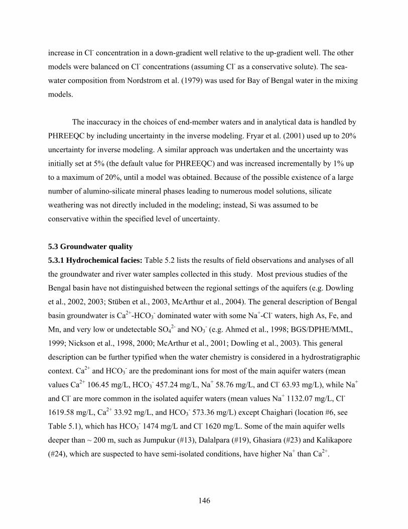
increase in Cl- concentration in a down-gradient well relative to the up-gradient well. The other

models were balanced on Cl- concentrations (assuming Cl- as a conservative solute). The sea-

water composition from Nordstrom et al. (1979) was used for Bay of Bengal water in the mixing

models.

The inaccuracy in the choices of end-member waters and in analytical data is handled by

PHREEQC by including uncertainty in the inverse modeling. Fryar et al. (2001) used up to 20%

uncertainty for inverse modeling. A similar approach was undertaken and the uncertainty was

initially set at 5% (the default value for PHREEQC) and was increased incrementally by 1% up

to a maximum of 20%, until a model was obtained. Because of the possible existence of a large

number of alumino-silicate mineral phases leading to numerous model solutions, silicate

weathering was not directly included in the modeling; instead, Si was assumed to be

conservative within the specified level of uncertainty.

5.3 Groundwater quality

5.3.1 Hydrochemical facies: Table 5.2 lists the results of field observations and analyses of all

the groundwater and river water samples collected in this study. Most previous studies of the

Bengal basin have not distinguished between the regional settings of the aquifers (e.g. Dowling

et al., 2002, 2003; Stüben et al., 2003, McArthur et al., 2004). The general description of Bengal

basin groundwater is Ca2+-HCO3- dominated water with some Na+-Cl- waters, high As, Fe, and

Mn, and very low or undetectable SO42- and NO3

- (e.g. Ahmed et al., 1998; BGS/DPHE/MML,

1999; Nickson et al., 1998, 2000; McArthur et al., 2001; Dowling et al., 2003). This general

description can be further typified when the water chemistry is considered in a hydrostratigraphic

context. Ca2+ and HCO3- are the predominant ions for most of the main aquifer waters (mean

values Ca2+ 106.45 mg/L, HCO3- 457.24 mg/L, Na+ 58.76 mg/L, and Cl- 63.93 mg/L), while Na+

and Cl- are more common in the isolated aquifer waters (mean values Na+ 1132.07 mg/L, Cl-

1619.58 mg/L, Ca2+ 33.92 mg/L, and HCO3- 573.36 mg/L) except Chaighari (location #6, see

Table 5.1), which has HCO3- 1474 mg/L and Cl- 1620 mg/L. Some of the main aquifer wells

deeper than ~ 200 m, such as Jumpukur (#13), Dalalpara (#19), Ghasiara (#23) and Kalikapore

(#24), which are suspected to have semi-isolated conditions, have higher Na+ than Ca2+.

146

The charge-balance computation shows that the main aquifer samples have higher error

(below +10%, except #1 and #26) than the isolated aquifer samples (-3.22 to +0.65%, except

#34). These errors are within the ranges of some of the previous studies in the Bengal basin (e.g.

Aggarwal et al., 2000; Dowling et al., 2003; Stüben et al., 2003). The positive errors for the main

aquifer indicate that there are more anions in the waters than have been accounted for. A possible

explanation is that some of the Cl- has co-precipitated with Fe (oxidized to Fe(III) during

sampling) in the anion samples (D. Chakraborty, Jadavpur University, Calcutta, personal

communication, 2003). No reason was found for the higher errors for #1 and #26, which were

confirmed even after running duplicate analyses of the samples in different laboratories.

However, it should be noted that #1 and #26 were the first samples collected for 2004 and 2005,

respectively, which may indicate a sluggish response of the pH electrode during alkalinity

titrations.

A Piper plot (Piper, 1944) (Figure 5.3) suggests that deeper groundwater in the western

Bengal basin can be broadly divided into seven hydrochemical facies (following Morgan and

Winner, 1962, and Back, 1966): 1) Ca2+-HCO3-; 2) Ca2+-Na+-HCO3

-; 3) Na+-Ca2+-HCO3-; 4)

Ca2+-Na+-HCO3--Cl-; 5) Na+-Cl--HCO3

-; 6) Na+-Cl-; and 7) Ca2+-Cl-. Thirty-eight of the 47 main

aquifer samples and the river water samples (except the tidally influenced Ichamati [RW #7]) fall

in facies 1, while the isolated aquifer samples are divided into facies 5 and 6. The plot also

illustrates that when the locations are grouped by districts (which is similar to grouping

according to distance from the Bay of Bengal because of the north-south orientation of the study

area), all of the main aquifer samples from Murshidabad (n = 12) and 14 of 16 Nadia samples

belong to facies 1. A Piper plot of shallow groundwaters from the Behrampur area of

Murshidabad constructed by Stüben et al. (2003) agrees with this observation. For 24 Parganas

(North and South combined), only 12 of 19 samples belong to facies 1, indicating the presence of

chemically distinctive water bodies nearer to the Bay of Bengal. The presence of these brackish

waters can be attributed to cation exchange and/or mixing with more saline water bodies; their

evolution is discussed in more detail in the geochemical modeling section (5.7). Sikdar et al.

(2001) and Chatterjee et al. (2004) identified hydrochemical facies similar to our samples for

North and South 24 Parganas in and around Calcutta.

147

The hierarchical cluster analysis (HCA) of the groundwater data by locations illustrates

the presence of three distinct clusters. All of the main aquifer samples aggregate within Group 1,

while Group 2 contains the isolated aquifer (<300-m) samples and Group 3 contains >300-m

samples (Table 5.1). The plot of the HCA groups corresponding to the 1st (PC1, 36.46% of total

variance, Table 5.3) and 2nd (PC2, 20.41% of total variance) principal component axes (Figure

5.4) illustrates this finding in more detail. All the main aquifer locations except Kalikapore (#24)

have much lower PC1 values than the other two groups. The isolated aquifers (<300-m) except

Chaighari (#6) have higher PC2 than the >300-m wells. While Kalikapore (#24) has PC2 values

similar to isolated aquifer wells, Chaighari (#6) is distinct from all other wells in terms of its PC1

composition. HCA by chemical constituents does not show any prominent clustering, although

Stüben et al. (2003) and Sracek et al. (2004a) observed such clusters in their local-scale study

areas.

5.3.2 Processes controlling major solute distributions in groundwater: Minerals that have

been documented by previous authors from Bengal basin sediments are listed in Table 5.4. A Na-

normalized Ca versus HCO3- plot (Figure 5.5a, following Gaillardet et al., 1999) shows that the

main aquifer samples range from being influenced by silicate weathering to carbonate

dissolution. The molar Ca/Na ratio for average crustal continental source rock is 0.6 (Taylor and

McLennan, 1985). The other wells show mixed contributions of both silicate and carbonate

reactions. A Ca versus Mg bivariate plot (not shown) shows a somewhat linear relationship for

the main aquifer (r2 = 0.38) and more so for the isolated aquifers (r2 = 0.69). The same plot

normalized by Na (Figure 5.5b) shows some samples in the range of silicate weathering,

indicating that although most of the Mg may have been derived from carbonate dissolution, some

has a silicate source. A bivariate plot (Figure 5.5c) of Ca+Mg versus HCO3- shows some scatter.

Dowling et al. (2003) noted that average (Ca+Mg)/HCO3- is ~0.9 for their study area, with

depths of 10 to 400 m. However, the results from the present study have an average value of only

0.53 for the main aquifer. Stallard and Edmond (1983, 1987) suggested that a molar ratio of (Na

+ K)/Cl > 1 may indicate silicate weathering. Only four of the 47 main aquifer samples of this

study have (Na+K)/Cl < 1. Dowling et al. (2003) also showed that Sr was correlated well with

HCO3- and inversely related to (Na+K)excess (= [Na+K]-Cl). For the main aquifer samples for the

present study, a Sr versus HCO3- plot (not shown) yielded r2 = 0.02, and no relation is apparent

148

between (Na+K)excess and Sr, although a Na- normalized Ca versus Sr plot yielded r2 = 0.77 and

0.95 for main and isolated aquifers, respectively. Although Sr and Ca have probably been

contributed by carbonate dissolution, not all HCO3- has originated from carbonate dissolution,

and it is not the predominant chemical reaction influencing deeper groundwater in the western

Bengal basin, as suggested by Dowling et al. (2003) for Bangladesh.

Al3+ tends to be conserved in the solid phase (Freeze and Cherry, 1979). Because of its

low solubility and tendency to occur as a colloidal hydroxide (Stumm and Morgan, 1996),

measured Al concentrations are viewed as semi-quantitative and are not reported and discussed

here. Stability diagrams (Figure 5.6) illustrate the relationship between feldspars, mica

(muscovite) and clay minerals. The diagrams were generated assuming end-member

compositions using the equilibrium relationships of Tardy (1971) and Drever (1997) for standard

temperature (25 oC) and pressure (1 atm) and by plotting log ([Ca2+]/[H+]2) or log ([Na2+]/[H+]),

log ([K2+]/[H+]), versus log [H4SiO40], where [ ] denotes solute activity calculated by PHREEQC

using the MINTEQ database. The plots indicate that the groundwater of the study area is in

equilibrium with kaolinite, with some samples close to Na-smectite and muscovite, and feldspars

(anorthite, albite and orthoclase) are unstable, suggesting weathering. These observations match

very well with the observed mineralogy of the Bengal basin. The plots show that most of the

samples are close to equilibrium with quartz than with amorphous silica, discussed in section 5.7.

This observation agrees well with Hem (1992), who mentioned that natural waters are typically

supersaturated with respect to quartz but undersaturated with respect to amorphous silica.

Some interesting patterns are notable when pH, Ca+Mg, Na+K and Si are plotted against

depth and along distance from the Bay of Bengal (latitude) (Figures 5.7 and 5.8). The values of

pH are circumneutral, but at depths >200 m, the waters become more alkaline. The concentration

of Ca+Mg decreases with increasing depth and with nearness to the sea. Na+K is higher in the

deeper wells (generally more than 200 m bgl) and the isolated aquifer wells than the shallower

and northern wells. Ahmed et al. (2004) mentioned without any elaboration that Ca, Mg, Na and

K vary significantly with depth and region in Bangladesh. Si increases to a depth of ~150 m,

when it starts to scatter and decrease. Si increases toward the south and then starts decreasing,

probably as a function of depth. The isolated aquifer wells have relatively low Si concentrations.

149

The decrease of Ca+Mg in comparison to Na+K along the regional hydraulic gradient in

the North and South 24 Parganas suggests cation exchange according to the following general

reaction (after Schwartz and Zhang, 2002):

bivalent cation (Ca2+ or Mg2+) + Na-clay Na+ + Bivalent cation (Ca2+ and/or Mg2+)-clay.

A (Na+K)/Cl versus Si bivariate plot (Figure 5.5d) suggests that (Na+K)/Cl increases as Si

becomes more than ~500 μmole/L, suggesting some threshold value as an indicator of significant

silicate weathering. The Cl- ratio helps to normalize the samples affected by saltwater intrusion

or mixing with connate water. HCO3- does not vary regionally either with distance (Figure 5.8c)

or depth in the main aquifer, indicating that the processes consuming and liberating the anion are

approximately in overall equilibrium.

The brackish groundwaters encountered in the isolated aquifers and some deeper portions

of the main aquifer (e.g. locations #16, #23, #24, #38) differ considerably from those in the main

aquifer, suggesting different pathways of chemical evolution. Brackish water (e.g. #40, #53) in

the main aquifer in the southernmost part of the study area probably results from mixing with

intruded seawater in this region, as documented by CGWB (1994d, e). A plot of Cl-normalized

Br- concentrations (Figure 5.9) following Whittemore (2004) shows a definite trend of mixing of

fresh groundwater with water with present-day seawater composition.

The existence of brackish water and brines in sedimentary basins can be caused by a)

dissolution of evaporites, b) retention of formation waters buried with the sediments and c)

membrane filtration (Schwartz and Zhang, 2002). Fresh groundwater becoming more saline with

flow downdip from the recharge area has been documented in the Williston Basin, USA

(Downey, 1984; Butler, 1984), the Dakota Sandstone in South Dakota, USA (Peter, 1984), and

the Milk River aquifer in the USA and Canada (Hendry et al., 1991). Ranganathan and Hanor

(1987) showed that diffusion can cause salinization of fresh water overlying formational brines

at depth. In the present study area, some parts of the deeper main aquifer are relatively fresh in

contrast to adjoining areas with higher Cl- concentrations (e.g. location #39). This fresh water

“nose” (Schwartz and Zhang, 2002), reflecting insufficient mixing and flushing, is similar to that

seen in Ohio, USA (Lahm et al., 1998).

150

The isolated aquifers probably contain formation water trapped within lower permeability

sediments and may be similar to modified-connate water pockets reported from South 24

Parganas (Handa, 1972; Sikdar et al., 2001) and several places in Bangladesh (Ahmed, 1994;

Bhattacharya et al., 2002). This is consistent with the isolated aquifers falling close to the

evaporite range in the Ca/Na versus HCO3-/Na plot (Figure 5.5a; note that three isolated samples

are not shown in the plot because of very low values [Ca/Na < 0.01]). The depth of these isolated

aquifers generally increases toward the south, probably in congruence with the delta-building

process and recession of the proto-Bay of Bengal. The marine origin is further supported by the

fact that, except for Chaighari (#6), the isolated aquifer wells are dominated by Na+ and Cl-.

Moreover, they contain lower concentrations of Si and much higher B (Si mean [except #34,

which has a relatively higher concentration]: 8.12 mg/L, B mean: 3.14 mg/L) than the main

aquifer wells (Si: 16.21 mg/L; B: 0.10 mg/L). Seawater contains 0.02 to 4 mg/L Si and 4.5 mg/L

B on average (Mance et al., 1988). Nordstrom et al. (1979) documented a Si value of 4.28 mg/L

for seawater.

Formation waters can be modified by meteoric diagenesis prior to burial. Land and

Prezbindowski (1981) showed that connate water of the Edwards Formation (Texas, USA) was

altered by mixing with several pore volumes of meteoric recharge. This might explain the

similarity between δ18O of the main aquifer waters of this study (~ -3 to -6‰ VSMOW) and that

of isolated aquifer waters and restricted main aquifer waters (~ -3 to -5‰) (see Chapter 4).

Alternatively, as suggested by Sikdar et al. (2001), there may still be some mixing between the

main aquifer and isolated aquifers through higher permeability “windows” within the confining

beds.

The Na+-Cl--HCO3- type water at Chaighari (#6) is distinct from any other well sampled

in the study area. Schwartz and Zhang (2002) noted Na+-HCO3- type water can evolve along

with relatively high F- concentrations as a result of continuous availability of CO2 in the system.

The major source of CO2 in deeper aquifers may be bacterially-mediated oxidation of organic

matter (Chapelle, 1993). Exchange of Ca 2+ in the evolving water for Na+ on marine-originated

clays in the aquifer can also enhance carbonate dissolution and introduction of more Na+ and

151

HCO3- into solution (Plummer et al., 1994). A combination of these processes has produced

sodium-bicarbonate water in the Atlantic Coastal Plain, USA (Foster, 1950), Eocene aquifers of

the east Texas basin, USA (Fogg and Kreitler, 1982), and the Milk River aquifer, USA and

Canada (Hendry and Schwartz, 1990). Interestingly, Chaighari has the highest F- and B

concentrations in the study area (F- of Chaighari is ~10 times of the mean of all other wells [0.14

mg/L] and B is ~3 times the mean of other isolated aquifers).

5.4 Redox conditions in groundwater

5.4.1 Results: Sampling of existing public supply wells can result in aeration of water through

the pump-head or plumbing (Parkhurst et al., 1996; Nickson et al., 2000). McArthur et al. (2004)

did not tabulate O2 data from their study site in North 24 Parganas because they suspected

sample aeration. It is possible that samples in this present study were aerated during collection.

Notwithstanding these concerns, samples in the present study had very little O2, with a mean of

1.04 mg/L. Only six of 53 samples had O2 of more than 1.5 mg/L, and 17 samples had 1 to 1.5

mg/L. The EH measurements by platinum electrodes fell mostly in a range of +15 mV to +120

mV with a mean of +80.8 mV. A few samples had much higher (n = 5, maximum +311.4 mV) or

lower (n = 4, minimum -40.2 mV) values. The general range also agrees with observations of

Swartz et al. (2004) of +20 to +100 mV. Excluding the two isolated aquifer wells in Nadia

(locations #14 and #34), in general the deeper wells have lower EH along with higher pH values.

Consistent with the low O2 and EH values, only two samples had NO3--N greater than the

detection level (DL) of 0.12 mg/L. NO2- and PO4

3- were not detected at any location (DL: 0.1

and 0.12 mg/L, respectively). NH4+ was detected at 36 locations (mean: 0.36 mg/L, maximum:

1.59 mg/L). SO42- was detected in a number of wells in both the main and isolated aquifers,

mostly in the northern part of the study area, with a mean of 7.1 mg/L and maximum of 39.6

mg/L. H2S was not detected either by smell or taste in any sample (DL: 0.05 to 0.5 mg/L [Ross et

al., 1999; Varner et al., 2004]) or by CHEMets in 2005 samples (DL: 0.05 mg/L). CH4

concentrations were greater than room-air concentration (measured during analyses: ~250 μM)

in 15 samples; 13 of these 15 samples had concentrations more than 1000 μM. The maximum

was 68 × 103 μM at Iswarchandrapur (#34), followed by 32 × 103 μM at Hanspukuria (#14). It

should be noted that due to the volatility of CH4, and relatively long lead time between sampling

152

and analyses due to travel and shipping, these reported values might underestimate actual

concentrations. Fe(II) and As(III) were the predominant Fe and As species in all sampled waters

with detectable concentrations. Dissolved Fe(II) was almost indistinguishable from total

dissolved Fe (Fe[II]/Fe mean: 97%), while As(III) averaged 72% of the total dissolved As

measured from locations with concentrations above detection level (0.005 mg/L).

5.4.2 Environment: Oxidation-reduction processes, as defined by the activities of aqueous redox

couples, generally tend to segregate into discrete zones in the aquifer following a predictable

pattern (Chapelle, 1993). Berner (1981) classified the redox environments of sedimentary

aquifers as oxic and anoxic (postoxic, sulfidic, and methanic) (Parkhurst et al., 1996). The oxic

system is defined by the presence of measurable O2. Parkhurst et al. (1996) used 1 mg/L as the

arbitrary boundary between oxic and anoxic environments, while Chapelle et al. (1995)

suggested 0.5 mg/L as the boundary. Systematic geochemical trends of redox zones depend on

the nature of metabolic pathways of bacterial decomposition and the nature of organic matter

(Martens and Goldhaber, 1978). Some trace elements (e.g. As, Cr) may change their redox state

in the postoxic zone (Parkhurst et al., 1996). The redox zones can be demarcated by calculating

the negative log of activity of electrons (pe) in aqueous solutions, where

pe = 16.9EH at 25oC.

The pe values of the various redox couples were calculated for the sample waters using

PHREEQC with the MINTEQ thermodynamic database (Allison et al., 1990) for As, Fe, O and

N species and the PHREEQC database (Parkhurst and Appelo, 1999) for C species. Following

Parkhurst et al. (1996), a distribution plot of the observed platinum electrode potential (EH) to

calculated EH of redox couples (computed from pe) shows that the waters from both the main and

isolated aquifers (Figure 5.10) lie in the postoxic environment of Berner (1981), while the river

waters exist near the oxic-postoxic boundary. The observed values cluster mostly in the data

range of Fe(II)/Fe(III) with some values in the range of As(III)/As(V) and approaching sulfidic.

This suggests that in the western Bengal basin, notwithstanding the presence of several redox-

sensitive couples, Fe(II)/Fe(III) is the dominant redox couple in deep groundwater. This

observation agrees well with the finding of Barcelona et al. (1989) that average observed EH

agreed with values calculated using the Fe(II)/Fe(III) couple in a suboxic system and suggestions

153

of previous workers that Fe(III) reduction may be controlling the redox state of Bengal basin

sediments (e.g. Bhattacharya et al., 1997; McArthur et al., 2004; Zheng et al., 2004). Sracek et al.

(2004a) found that for Bangladesh water, EH values calculated using As(III)/As(V) were lower

than field measurements and suggested that this may be attributed to dominance of another redox

couple.

Vanadium exists mostly in its oxidized state (V[V]) in hydrologic systems because of the

low solubility of the reduced form (V[III]) (Parkhurst et al., 1996). V was detectable in all

samples, with a mean of 0.09 mg/L. The highest V concentrations were detected in some of the

deepest wells of the main aquifer (e.g. Kalikapore [#24]: 0.34 mg/L). V(V) is generally reduced

to V(III) in the postoxic to sulfidic range at circumneutral pH, which suggests that deeper water

of the western Bengal basin is not sufficiently reduced to immobilize V.

5.4.3 Governing processes: Similar to other regional studies in the Bengal basin (e.g. Aggarwal

et al., 2000; Dowling et al., 2002, 2003), this study is limited by the number of sample locations

and may not be sufficient to understand the processes operating at the local scale (centimeters to

meters vertically and tens to hundreds of meters laterally). However, in spite of these constraints,

redox-sensitive parameters show broad patterns with depth and distance from the Bay of Bengal

(Figures 5.11 and 5.12). A depth versus EH plot (Figure 5.11a) demonstrates a weak inverse

relation (r2 = 0.28), with relatively lower values from >200 m depth. Similar spatial trends of EH

and pH have been reported by Jackson and Peterson (1982). Mn, Fe (total and Fe[II]), As (total

and As[III]), and SO42- generally decrease with depth, while CH4 and As(III)% seem to increase

with depth (with some scatter). Similarly, when plotted against distance, Mn and SO42- are higher

in the northern part of the study area and tend to decrease southward (SO42- outliers in South 24

Parganas may have been caused by modern or unflushed paleo-seawater [evident from a Cl--

normalized SO42- plot to account for marine influence]). Fe and As may decrease southward, but

the trends are not very prominent. These observations indicate that the redox processes operating

in the western Bengal basin are depth-dependent.

5.4.3.1 Iron dissolution: Fe is ubiquitous in Bengal basin groundwater, and has been found to be

correlatable with HCO3-. This correlation is suggested to have been caused by reductive

154

dissolution of Fe (oxyhydr)oxides by oxidation of organic matter (e.g. Nickson et al., 1998,

2000; McArthur et al., 2001; Ahmed et al., 2004). However, no such correlation was observed

between Fe and HCO3- in samples of this study (r2 < 0.001 for main aquifer), probably because

other processes besides organic matter oxidation (e.g. weathering) also produce HCO3-. Some of

the samples have Fe concentrations correlatable with Mn (Figure 5.13a), but the other locations

have wide scatter, suggesting that some but not all of the Fe and Mn dissolution is causally

related with overlapping redox zones. Fe and Mn should be more concentrated in the shallower

depths (Farmer and Lovell, 1986; Stumm and Morgan, 1996) in response to post-depositional

diagenetic remobilization, with peak Fe concentrations at shallower depths than Mn (Anwar et

al., 2002). McArthur et al. (2004) noted that reduction of FeOOH is more dominant than

reduction of Mn oxides toward the top and base of the aquifer at their study site. These

observations do not hold well for samples in the present study, as Mn concentrations decrease

strongly with depth.

5.4.3.2 Sulfur cycling: The decrease of SO42- southward from Murshidabad indicates that 1)

either the aquifer water becomes sulfidic as depth increases and results in deposition of

authigenic sulfide or 2) the input of SO42- in deeper groundwater of Nadia and North 24 Parganas

was originally low. Zheng et al. (2004) opined that the very low SO42-/Cl- ratios in their study

area suggest SO42- reduction rather than low original SO4

2- concentrations. H2S was not detected

in any of the samples in the present study and thus there is no direct proof of SO42- reduction.

However, H2S has been reported from shallow groundwater from some locations of Murshidabad

and South 24 Parganas of West Bengal (Mehta and Bhattacharya, c. 2000) and some areas in

Bangladesh (Ahmed et al., 2004). It is possible that the high level of Fe(II) in most locations

scavenged all of the reduced S species present in the water. High levels of authigenic sulfide

deposition can take place even in a low-SO42- system with high organic carbon content

(Neumann et al., 2005). Pyrite and other authigenic sulfides have been documented from

sediments in various locations within the Bengal basin (e.g. Das et al., 1996; Chowdhury et al.,

1999; Chakraborti et al., 2001; Pal et al., 2002). McArthur et al. (2004) commented that

diagenetic Fe sulfides in the sands of North 24 Parganas may have formed during the onset of

anoxia as a result of SO42 -reduction in connate water.

155

The δ34SSO4 elucidates the S redox cycling in more detail. Incomplete SO42- reduction

causes 34S to be depleted in the precipitating pyrite and progressively enriched in the residual

SO42-. Conversely, oxidation of this authigenic pyrite could introduce SO4

2- depleted in 34S

(Faure, 1998). Hence, in a SO42--reducing system, the concentration of SO4

2- should be inversely

related to δ34SSO4. Jacks et al. (1994) documented a δ34S composition of ~10 ‰ for the

monsoonal rainwater. Groundwater in a closed system without mixing and having δ34SSO4

composition >10 ‰ can thus be suspected to have undergone extensive reduction (Zheng et al.,

2004), while lower values may indicate oxidation. Results from this study show that δ34SSO4

ranges from 5.7 to 45.8‰ VCDT, which suggests, given the predominance of monsoonal

recharge (Stüben et al., 2003; see also Chapter 4), that both oxidation and reduction of sulfur

have taken place. A plot of SO42-/Cl- versus δ34SSO4 (Figure 5.14) shows an inverse trend in

agreement with SO42- reduction, but this trend bifurcates, which suggests that some of the SO4

2-

might have gone through repeated phases of reduction and reoxidation, as hypothesized by

Zheng et al. (2004).

5.4.3.3 Carbon cycling: Zheng et al. (2004) showed that their few deeper groundwater samples

from Araihazar in Bangladesh are generally low in HCO3- (<4000 μM), suggesting that this

water is less evolved (McArthur et al., 2001). Zheng et al. (2004) also argued that deeper

groundwater has relatively high O2 concentrations due to lack of oxygen demand or limited

availability of labile organic matter. However, in the present study, HCO3- concentrations in the

deeper water of the main aquifer were relatively uniform, with a mean of 457 mg/L (7131 μM).

A distance-O2 plot (Figure 5.12f) qualitatively shows (relative to a concentration of 0.8 mg/L [50

μM], between the threshold concentrations of Chapelle et al. [1995] and Parkhurst et al. [1996])

that the oxygen content may decrease southward (equivalent to increasing depth), suggesting the

progressive consumption of oxygen along the flow path. Dissolved organic carbon (DOC)

concentrations were low but detectable at most locations. Chatterjee et al. (2004) reported values

of DOC up to 12.9 mg/L from the Baruipur area of South 24 Parganas (depth not specified). The

mean DOC concentration of the main aquifer (0.92 mg/L) from this study was lower than that of

the isolated aquifers (1.65 mg/L). The persistence of DOC can reflect limited microbial activity

or the presence of relatively refractory organic matter (Chapelle, 1993). The chemical nature and

156

source of the organic carbon can limit the amount of reductive bacterial activity (Beck et al.,

1974; Martens and Goldhaber, 1978).

CH4 concentrations >250 μM (room-air concentration during sample analyses) indicate

highly reducing conditions (Berner, 1981; Zheng et al., 2004). Very high CH4 concentrations

(>2500 µM) were generally found in southern Nadia and North 24 Parganas. CH4 in Bengal

basin groundwater has also been documented by Ahmed et al. (1998), Harvey et al. (2002), and

McArthur et al. (2004). CH4 is a common product of decomposition of natural organic matter

(NOM) in aquifer systems (Barker and Fritz, 1981; Coleman et al., 1988; Leuchs, 1988,

Grossman et al., 1989; Simpkins and Parkin, 1993; Aravena et al., 1995b; Zhang et al., 1998) by

pathways of acetate fermentation and CO2 reduction by H2 (Oremland, 1988). In the Bengal

basin, possible sources of NOM include human wastes (Harvey et al., 2002, 2005; McArthur et

al., 2004) and peat. Peat fragments in southern Bengal basin sediments are expected because of

the geomorphic evolution of the delta (Umitsu, 1987, 1993; Islam and Tooley, 1999; Allison et

al., 2003). Peat was formed as waterlogged back-channel deposits of the paleo-rivers in this area

at about 5,000 years before present during late Quaternary sea-level change (Umitsu, 1993) when

the erosional base levels of the paleo-rivers were much lower than present (Ravenscroft et al.,

2001). Peat fragments have been recovered from Calcutta (Barui and Chanda, 1992; A.

Mukherjee, University of Kentucky, unpublished data), North and South 24 Parganas (Umitsu,

1987, 1993; Banerjee and Sen, 1987; CGWB, 1994d; Pal et al., 2002; McArthur et al., 2004),

and at various locations in Bangladesh (e.g. Reimann, 1993; Brammer, 1996; Ahmed et al.,

1998; Safiullah, 1998; BGS/DPHE/MML, 1999; Islam and Tooley, 1999; AAN, 2000; Ishiga et

al., 2000; Tareq et al., 2003; Swartz et al., 2004). Elevated CH4 concentrations in the study area

may be related to the existence of peat layers in the vicinity, although no peat was identified in

the lithologic logs of the wells. However, CH4 concentrations >500 µM were also observed at

shallower depths in several locations in Murshidabad and Nadia. The detection of CH4 and other

reduced solutes in these wells probably cannot be explained by the presence of peat, as the

author is not aware of any report of peat occurrence in these areas. Harvey et al. (2002)

documented a similar situation in their study area in Munshiganj, Bangladesh, and commented

that CH4 in the shallow waters was derived from the dissolved inorganic carbon (DIC) pool and

was probably formed by carbonate reduction. However, McArthur et al. (2004) argued that peat

157

could have been missed during drilling. Methanogenesis at shallow depths (2-3 m below the

water table) has been reported (≥ 400 µM) in the sandy aquifer of Rømø, Denmark and has been

attributed primarily to CO2 reduction along with subordinate acetate fermentation, occurring

predominantly in microenvironments with higher H2 concentrations (Hansen et al., 2001).

Understanding the δ13C composition of dissolved inorganic carbon (DIC), which is

mostly HCO3-, might give some insight to C cycling within the system. Zheng et al. (2004)

commented that depleted values of δ13CDIC probably confirm that CO2 from oxidation of organic

matter contributes a portion of DIC in Bengal basin groundwater. BGS/DPHE/MML (1999)

recorded δ13CDIC up to +10‰, which is common for methanogenic CO2 (Whiticar, 1999;

McArthur et al., 2001). McArthur et al. (2004) showed that the δ13CDIC content at two of three

locations studied in North 24 Parganas becomes enriched with depth (range 0 to -10 ‰ VPDB).

At one of these locations, peat fragments were identified in the aquifer, which may have

supported methanogenesis. The location where an opposite trend was observed had a peat layer

embedded in an overlying thick aquitard, which may have limited the CH4 mixing. McArthur et

al. (2001) mentioned that at their study location in Bangladesh (Faridpur), δ13C became depleted

with increasing Ca, suggesting the dissolution and equilibration of depleted calcite (0 to -6‰

[Quade et al., 1997; Singh et al., 1998]) or pedogenic carbonates (lower Himalayan carbonates:

~-12 ‰ [Quade et al., 1997]) by enriched methanogenic CO2 (+5 to +10‰). The depleted DIC in

groundwater can form from oxidation of CH4 (McArthur et al., 2001; Zheng et al., 2004).

In the present study, the δ13CDIC in the shallower part of the main aquifer (~ -8 ‰ VPDB)

is generally more depleted than the deeper part (~ 0‰ VPDB), but this trend has a number of

outliers, suggesting that multiple processes are involved (Figure 5.15). No trend was observed

between δ13CDIC and Ca or HCO3-. Enrichment of δ13CDIC with depth may take place as a result

of lessened biological activity in the deeper part of the main aquifer; incomplete CO2 reduction

to form highly 13C-depleted CH4, thereby progressively enriching the residual CO2 (consistent

with Harvey et al. [2002] and the existence of higher concentration of CH4 at depth [Figure

5.11i]); lessened dissolution of depleted carbonates at depth; and/or mixing with δ13C-enriched

connate water (δ13CDIC ~ 0 ‰ for seawater). Alternatively, depleted DIC (at shallower depths as

158

well as in some of the deep water) could have formed from some CH4 oxidation. Most of the

wells appear to reflect one or more of these trends, but Chaighari (#6) was probably influenced

more by organic matter oxidation, as evident from the most depleted δ13CDIC (-8.2‰ VPDB).

5.4.4 Summary: The finding from this study that Fe(III) reduction is the dominant redox process

in deeper groundwater of the western Bengal basin is consistent with other studies of

groundwater in the Bengal basin. However, the co-existence of O2, NH4+, Fe(II), As(III), V,

SO42-, and CH4 in various wells indicates that the aquifer volumes sampled by these wells are not

in redox equilibrium. Similar partial equilibrium systems have been observed in other studies,

e.g. Fe(III) reduction and methanogenesis (Berner, 1981), SO42--reduction and methanogenesis

(Kuivila et al., 1989; Parkes et al., 1990), SO42- and Fe(III) reduction (Canfield et al., 1993;

Wersin et al., 1993; Postma and Jakobsen, 1996), and Fe(III) reduction, SO42--reduction and

methanogenesis (Jakobsen and Postma, 1999).

5.5 Arsenic in deeper groundwater

Elevated arsenic (>10 µg/L) has been observed in a majority of the deep groundwater

samples from this study, with concentrations reaching > 137 µg/L. Arsenic concentrations in

Bengal basin sediments are close to the average crustal concentration (Swartz et al., 2004). Most

of the recent studies from the Bengal basin have hypothesized the release of sorbed As phases by

reductive dissolution of FeOOH (e.g. Bhattacharya et al., 1997; Nickson et al., 2000; McArthur

et al., 2001, 2004; Harvey et al., 2002, 2005; Dowling et al., 2002; Stüben et al., 2003), although

some authors have also suggested As liberation by oxidation of As-enriched pyrite (e.g. Mallick

et al., 1995; Das et al., 1996; Mandal et al., 1998).

Reductive dissolution and mobilization of As(III) can happen in less reducing

environments (Seyler and Martin, 1989; Eary and Scramke, 1990; Kuhn and Sigg, 1993) or even

oxidizing environments (Abdullah et al., 1995). Van Geen et al. (2004) showed that reductive

dissolution of As can take place even in mildly oxic conditions. Anaerobic metal-reducing

bacteria could play a catalytic role in mobilization of As from Bengal basin sediments (Islam et

al., 2004). Such dissimilatory microbial reduction may be stimulated by addition of a substrate

159

(van Geen et al., 2004) and may be performed by SO42--reducing bacteria (Inskeep et al., 2002;

Oremland et al., 2002).

Several studies of Bengal basin groundwater have observed a moderate to strong

correlation between As and Fe, as expected from reductive dissolution of FeOOH onto which As

is adsorbed (e.g. Nickson et al., 1998, 2000; McArthur et al., 2001; Dowling et al., 2002 [locally

up to r2 = 0.8 to 0.9]; Stüben et al., 2003). In the samples of this study, Fe correlates weakly with

As (r2 = 0.26, p = 0.01, Figure 5.13b), although Fe(II) yields a better correlation with As(III) (r2

= 0.32, Figure 5.13c). Swartz et al. (2004) showed that As in sediments of the deeper aquifer in

Munshiganj, Bangladesh (~165 m), does not co-vary well with Fe. Such weak correlations

suggest that reduction of As and Fe may not be simultaneous. Islam et al. (2004) showed that As

is released from sediments after Fe(III) reduction. McArthur et al. (2004) suggested that some of

the As released by reductive dissolution can be re-sorbed to the residual or partially reduced

FeOOH. Complex cycles of oxidation and reoxidation of Fe and S species can cause preferential

immobilization of As (Zheng et al., 2004). At a regional scale, the As concentrations in our

samples do not have significant correlations with Mn (r2 = 0.12), NH4+ (r2 = 0.02), CH4 (r2 =

0.03), DOC (r2 <0.01), O2 (r2 <0.01), HCO3-(r2 = 0.03), or chalcophile elements (e.g. Zn [r2

<0.01]), as have been suggested by previous workers (e.g. Mn [Stüben et al., 2003], NH4+

[Dowling et al., 2002; Ahmed et al., 2004], CH4 [Ravenscroft et al., 2001; McArthur et al., 2001,

2004; Dowling et al., 2002], DOC [Ahmed et al., 2004], and Zn [Stüben et al., 2003]). The lack

of these correlations suggests that As is mobilized by multiple processes, perhaps by reactions

having occurred in the shallow subsurface, above the sampling depths of this study. Moreover,

the lack of correlation of As with pH (r2 = 0.12) indicates that pH-dependent sorption reactions

probably do not play a significant role in regulating As mobility in deeper groundwater of the

western Bengal Basin.

Although the presence of peat layers in certain areas can act as the redox driver for

mobilization of As, as argued by McArthur et al. (2004), this explanation does not appear to

apply to areas such as Murshidabad and northern Nadia, where the existence of peat in the

aquifer framework up to 300 m depth is highly improbable in light of the Ganges-Brahmaputra

delta-building history. Harvey et al. (2002, 2005, 2006) proposed that anthropogenic organic

160

matter (human waste) or natural organic matter (NOM) can infiltrate through the bottoms of

rivers, lakes and ponds, and thus influence groundwater redox chemistry. Although this

explanation is plausible in light of the large population of the study area, infiltration of dissolved

organic matter (DOM) cannot solely explain the existence of the As in deeper groundwater, as

most of the DOM should be oxidized at shallower depths under normal vertical hydraulic

gradients.

The authors envision a scenario whereby As liberated by metal (oxyhydr)oxide reduction

remains mobile except to the extent that it is sequestered in authigenic sulfides. McArthur et al.

(2004) commented that As desorbed during reduction of Mn oxides can be re-sorbed onto

residual FeOOH phases. Results from the present study indicate that Mn is reduced at a

shallower depth than Fe, so As that is resorbed onto residual FeOOH phases will be remobilized

by subsequent Fe(III)-reduction. Although McArthur et al. (2004) commented that SO42-

reduction is improbable at present because of the dominance of Fe(III) reducing bacteria over

SO42- reducing bacteria (Chapelle and Lovely, 1992), the δ34SSO4 results from this study suggest

that SO42--reduction is occurring but probably overlapping with other redox zones. This process

might result in deposition of authigenic Fe sulfides, which could partially scavenge the As,

depending on the initial SO42- concentrations. The reason that As still exists in solution in

sulfidic and even methanogenic zones is because of the partial redox equilibrium and the

possibility of limited SO42- availability in deeper groundwater. Zheng et al. (2004) mentioned

that the introduction of small amounts of oxygen into a SO42--reducing environment with high

As/Fe ratios can result in re-oxidation of Fe(II). This process may also contribute to

remobilization of some previously immobilized As in sulfides. Furthermore, the recirculation of

water by extensive pumping (Chapter 3) may cause homogenization of the aquifer and

availability of more aerated water from shallower depths. Although such reoxidation is highly

unlikely at the regional scale in a large, reduced aquifer like the main aquifer of the study area, it

could happen at smaller scales, as suggested by the occurrence of lower As(III)% values at depth

(Figure 5.11f). Moreover, oxidation of As(III) to As(V) can take place even in anoxic

environments by activity of autotrophic microorganisms (Rhine et al., 2006).

161

5.6 River water-groundwater interaction

5.6.1 River water chemistry: The rivers in the study area and their possible interactions with

the main aquifer can be classified into three groups: the Ganges (G), Jalangi-upper Ichamati (JI),

and the tidal rivers (T). Group G consists of the three samples from the Bhagirathi-Hoogly (R1,

R2, and R3). As the main Indian distributary of the Ganges, the Bhagirathi-Hoogly reflects the

weathering of upstream terrains, including the Himalayas. The JI are relatively smaller rivers and

probably reflect more local recharge (R4, R5, R6), while T (R7), the sample from the lower

reach of the Ichamati, represents the chemistry of southern tidal rivers.

The hydrochemical facies distribution (Figure 5.3) shows that while T is of Na-Cl type,

consistent with diluted sea water, G and JI are of Ca2+-HCO3- type, and almost indistinguishable

from the main aquifer samples in this facies. All the river samples were slightly alkaline (pH 7.5

to 8.3) and had high EH (266 to 408 mV), suggesting oxidizing conditions. Of these, the pH

ranges of the samples from the Bhagirathi-Hoogly and Jalangi (which discharges to the

Bhagirathi-Hoogly and has a tributary from the Ganges main channel) are higher than the

Ichamati samples. G and JI generally have major ion concentrations in the lower range of main

aquifer groundwater and relatively low Si and HCO3-. The carbonate units in the provenance of

the Gangetic sediments dominate the ionic distribution of the river water from north to south in

the basin (Galy and France-Lanord, 1999). The G and JI samples fall on the carbonate

dissolution trend of the Na-normalized Ca versus HCO3- plot (not shown), in agreement with this

idea. The JI samples generally are more dominated by carbonate dissolution and more enriched

with other major ions than the G samples, probably as a result of enhanced evaporation. This

idea is further reinforced by the higher SO42-/Cl- ratio (G: 3.8 to 2.9; JI: 1.1 to 0.4) and more

depleted δ18O (-5.6 to -5.7 ‰ versus -2.9 to -3.1 ‰) of G relative to JI (see Chapter 4). Galy and

France-Lanord (1999) concluded that river water originating in the Himalayas has depleted

δ34SSO4 values in response to the higher input of SO42- by oxidation of pyrite. G samples have

higher concentrations of SO42- than JI, but the δ34SSO4 of those samples were not determined.

Based on the similarity in δ18O data (see Chapter 4), there may be some inflow of the G

water to the thinner portions of the main aquifer in the vicinity of Murshidabad and near

Calcutta. Conversely, there is probably groundwater discharge to JI. These claims are also

162

supported by the regional groundwater flow model developed in Chapter 3, showing that during

present-day summers (the sampling season), there should be natural groundwater inflow from the

Bhagirathi-Hoogly in northern Murshidabad and outflow to the Jalangi and upper reaches of the

Ichamati. Irrigational/urban overdraft pumping can cause inflow from the Bhagirathi-Hoogly in

west-central Murshidabad and near Calcutta. If this is true, then the chemical differences

between the river water and groundwater in these localities may reflect groundwater evolution by

reactions within the aquifer sediments and the hyporheic zones. Groundwater discharge along the

Jalangi and upper Ichamati probably explains the higher concentrations of solutes in those

streams relative to the Bhagirathi-Hoogly. The interaction of group T with groundwater could

not be evaluated because of strong seawater influence.

5.6.2 Arsenic in river water: One very interesting observation was the occurrence of elevated

As concentrations for all three samples of the JI group. The samples were re-analyzed three times

from splits to validate this observation. Elevated As has not been reported in most studies of

surface water in the Bengal basin, although Stüben et al. (2003) noted As in water of a small

stream (River Gobra) in Murshidabad. They suggested that the As in this stream has been

mobilized by reduction of Mn in the alluvial sediments because of the low oxygen content of the

stream water relative to the Bhagirathi-Hoogly. However, given the observed EH values of the

present study, groundwater discharge is a more plausible explanation for occurrence of As in

stream water. Elevated As was detected in groundwater samples (locations #27, #28, #30, #31,

#32, #36, #44, and #45) near the JI sample locations. The differences in As concentrations

between the river water and deeper groundwater could be caused by enrichment by evaporation,

outflow from shallower, more As-enriched groundwater (not analyzed in this study), and (or)

oxidation of As-bearing pyrite in river bank and bed sediments. Although the valence state of the

As was not determined, it was probably As(V) because of the elevated EH values and lack of Fe

and Mn.

5.7 Geochemical modeling

5.7.1 Saturation indices: Table 5.5 lists the ranges of SI values for some of the important phases

that are thought to affect the chemistry of the deeper groundwater and major rivers in the study

area. SI values for phosphate and sulfide phases were not calculated because those solutes were

163

below detection level. Previous literature on SI values for Bengal basin groundwater is very

limited (e.g. Ahmed et al., 2004; Sracek et al., 2004a; Swartz et al., 2004). Groundwater is highly

undersaturated with respect to oxygen but has higher-than-atmospheric PCO2, consistent with DIC

inputs from organic matter oxidation and carbonate dissolution. Sracek et al. (2004a) reported

similar values of PCO2 for Bangladesh. SI for methane for most wells is slightly undersaturated or

near equilibrium. Groundwater is undersaturated with respect to the major As phases (e.g.

arsenolite, As2O5, and FeAsO4·2H2O) and Mn oxide phases (e.g. birnessite, bixbyite, manganite,

nsutite, and pyrolusite), indicating that once As and Mn enter into solution, they do not

precipitate. Groundwater is highly to moderately supersaturated with respect to Fe(III)

(oxyhydr)oxide phases like magnetite, hematite, goethite, lepidocrosite, maghemite, Mg-ferrite,

and ferrihydrite, but near equilibrium or undersaturated with respect to Fe(II) minerals like

siderite and mixed Fe oxides like Fe3(OH)8. Swartz et al. (2004) commented that the Fe(II) in

pore water of the Bengal basin may have been derived from Fe(II) minerals like siderite,

vivianite (Fe3(PO4)2), and mixed Fe (oxyhydr)oxides (e.g. green rust), which form from biogenic

reduction of FeOOH (Zachara et al., 1998; Nickson et al., 2000). Groundwater is supersaturated

with respect to carbonate phases except for rhodochrosite. Ahmed et al. (2004) suggested that the

near-equilibrium SI values for carbonates indicate that the high HCO3- values in Bengal basin

groundwater cannot be totally attributed to carbonate dissolution and may have a significant

input from organic carbon oxidation. Sracek et al. (2004a) calculated siderite supersaturation for

Bangladesh groundwater. Groundwater and river water are supersaturated with respect to quartz

and undersaturated with respect to amorphous SiO2, in agreement with the stability diagrams

(Figure 5.6).

5.7.2 Inverse modeling of groundwater evolution along flow paths: Reaction-path models

have been used in various studies worldwide to elucidate hydrochemical evolution along regional

(tens to hundreds of kilometers) flow paths, as reviewed by Nordstrom (2004) and Glynn and

Plummer (2005). However, no reaction-path modeling has been reported for the western Bengal

basin. The Piper plot (Figure 5.3) indicates some major-ion evolution along groundwater flow

paths. Intense irrigational pumping beginning around 1970 may have disrupted the regional

groundwater flow path in the western Bengal basin, resulting in local flow paths towards centers

of pumping (see Chapter 3). However, the earlier discussion of groundwater quality (Section 5.3)

164

indicated that some major solute trends along depth and distance can still be discerned, and

hence chemical evolution of groundwater at the regional scale can still be evaluated.

Sixty reaction-path (inverse) models, converging within the specified maximum

uncertainty range, were developed for the study area (Table 5.6). Six models developed for

evolution of Chaighari groundwater (#6) by mixing with Bay of Bengal water failed to converge

and are not included in Table 5.6. Of the 60 models, 37 models involved flow with both mixing

and reactions, and 23 involved flow with reactions but not mixing. The models were broadly

used to investigate:

i) evolution of isolated aquifer water (locations #6, #14, #18, #20, #34, #52) by mixing with

connate water (paleo-Bay of Bengal) or modern Bay of Bengal seawater;

ii) evolution of the main aquifer water with relatively high Cl- concentrations in the northern part

of the study area (Murshidabad and Nadia, e.g. #38) by mixing with connate water or diffusion

from isolated aquifers at depth (models 30 and 31) (following Ranganathan and Hanor, 1987);

iii) evolution of the main aquifer water with relatively high Cl- concentrations in the southern

part of the study area (North and South 24 Parganas, e.g. #16, #19, #23, #24) by mixing with

connate water via diffusion from isolated aquifers (models 32 and 38), or by seawater intrusion

or tidal water infiltration (e.g. #25, #53);

iv) river water-groundwater interaction: mixing of infiltrating river water (whether through

natural inflow or induced infiltration by pumping) with up-gradient groundwater to evolve down-

gradient groundwater (e.g. #2, #11, #35, #37); mixing of discharging groundwater with upstream

river water to evolve downstream river water (R2, R4); and tidal influence on river water

chemistry (R7).

Because of the similarities of major solute chemistry for most parts of the individual

aquifers, mass balance models were only developed for pair of wells/river locations that were

thought to represent two distinct end-member waters or for mixing of two waters followed by

reactions to produce a third water. For many locations (particularly the isolated wells), present-

day hydraulic connections between the respective wells have not been established by physical

means; the flow paths are intended to test hypotheses of the possible hydrochemical evolution

processes from similar up-gradient water in the recent geologic past, during delta progradation.

165

Similarly, the mixing with Bay of Bengal water for the isolated aquifers and deeper main aquifer

water (e.g. #16, #23, #24) was meant to be a proxy of the past seawater intrusion from the proto-

Bay of Bengal and interaction with the paleo-groundwater. Mixing with Bay of Bengal water for

shallower main aquifer wells (e.g. #25, #53) in North and South 24 Parganas was used to

evaluate present-day seawater intrusion.

The mass balance processes in the models included carbonate weathering (calcite,

dolomite, and siderite dissolution and precipitation), cation exchange (Ca2+/Mg2+, Ca2+/Na+,

Ca2+/K+, Na+/Mg2+, Mg2+/K+and Na+/K+), carbon cycling (CO2 and CH4 dissolution and

exsolution; CH2O [organic carbon] oxidation), and sulfur cycling (pyrite dissolution and

precipitation). Halite dissolution was used for 23 models as a proxy for mixing with connate

water from the proto-Bay of Bengal. All but six models (models 51-55) relating to the mixing of

river water with groundwater were balanced for Cl- (Cl- balance is not shown in Table 5.6). The

unbalanced, questionable models depict very high (up to 100%) mixing of river water with

groundwater, which is probably an unrealistic scenario. Si balance was used to evaluate the role

of silicate weathering processes. While the balance would indicate minimal Si influx from

weathering within the specified uncertainty, a failure suggests the presence of processes that

have not been accounted by the mechanisms included in the models. Models for isolated aquifers

(locations #6 [except model 3], #18, #20, and #52) and the deeper main aquifer (locations #16,

#19 [except model 38], and #38) indicated some Si cycling. All of these wells are suspected to

have water with long residence times (as suggested in Chapter 3), which favors silicate

weathering because of the slow dissolution kinetics (Langmuir, 1997). The reason for the

imbalance of location #53 (models 47-48) is unclear, but it could have been caused by

inaccuracy in the choice of the up-gradient water.

In general, the convergence of the reaction-path models (except evolution of location #6

from Bay of Bengal water and the mixing models of groundwater-river water interaction)

indicates that various processes could control chemical evolution of groundwater in the western

Bengal basin. Within the constraints of the present study, no definite reaction pathways can be

identified. Conservative stable isotopes (δ18O and δ2H), which can indicate distinct sources of

water, are relatively homogeneous with depth and between different aquifers, and dependent on

166

distance from the sea (see Chapter 4). In addition, the selection of acceptable mass-balance

models is difficult in light of the simplifications undertaken for model design, particularly the

selection of end members, the program’s requirement that mixing precede reactions, and the

assumption of one-dimensional flow without dispersion.

All of the models (except models 57 and 58 for evolution of R4, which did not include

cation exchange) involved a combination of cation exchange and carbonate weathering. Siderite

dissolution was observed for all flow paths involving groundwater and sea water mixing. Pyrite

was found to precipitate along all groundwater flow paths (except models 41, 43, 44, 45),

supporting our previous inference about the redox environment. Models 43 and 44, which

involve pyrite dissolution as water of location #23 evolves to #24, are suspect because δ34S for

#23 is much more enriched than for #24. Many of the models also indicate exsolution of CO2

along flow paths. While this seems to be possible in light of the higher-than-atmospheric PCO2

values, such CO2 outgassing is not expected to happen within deeper groundwater, which is

isolated from the atmosphere. However, gas bubbles were observed while collecting many of

groundwater samples in this study, which may indicate CO2 exsolution as a result of aeration and

depressurization during pumping.

All of the isolated aquifers except Chaighari (#6) could have evolved as a result of

mixing of main aquifer water with paleo-seawater. Chaighari may evolved from a groundwater

similar to any of the selected upgradient wells that underwent cation exchange (+K+, +Na+, -

Ca2+, -Mg2+), carbonate dissolution (mostly dolomite and siderite), consumption of CH4 and

CH2O, and precipitation of pyrite. The evolution of the brackish main aquifer waters through

diffusion from more saline isolated aquifers seems to be possible for locations #16 and #38, but

is improbable for #19, because mixing of >75% of isolated aquifer water (with composition of

#52) would be required.

River sample R2, representing the Bhagirathi-Hoogly water, though spatially separated

from R4 (the northernmost River Jalangi location), was assigned as the upstream end-member

for models 57 and 58 with the rationale that both rivers are distributaries of the Ganges, and R2

should more closely resemble the Ganges. Those models suggest that R4 and R5 (the two As-

167

contaminated river locations) have significant inflow from groundwater with composition of #28

and #32 (up to 24% for R4) and #36 (up to 12% for R5). Locations #28, #32, and #36 all have

elevated As concentrations, thus reinforcing the inference in section 5.6.2 about discharge of As-

contaminated groundwater to smaller rivers in summer. The composition of upstream Ichamati

water (R6) can evolve to the downstream composition (R7) by mixing with a large amount (up to

47%) of Bay of Bengal water (model 60).

5.8 Conclusion

This study has delineated patterns of, and inferred the controls on, deeper groundwater

and stream-water quality in the western Bengal basin. The importance of the study lies in

assessing the groundwater quality of the deeper, semiconfined regional aquifer, whose shallower

parts have been reported to be contaminated by As. Like studies of regional aquifers elsewhere,

this study entailed sampling from public water-supply wells, which are screened over depths of a

few meters to tens of meters. While sampling from such wells results in depth-integrated data, it

can also mask smaller-scale geochemical heterogeneities (Ronen et al., 1987; Parkhurst et al.,

1996; Fryar et al., 2001). However, for most of the wells (except a few in Murshidabad), the

thickness of the screened intervals is probably small relative to the total depth of the aquifer

considered at those locations. Notwithstanding this constraint of large screened intervals,

groundwater analyses show distinct spatial (along depth and distance) and chemical trends

indicative of various hydrochemical processes. The depths of the sampled wells for the main

aquifers generally increase towards the south, consistent with the hydrostratigraphy.

In general, the groundwater of the main aquifer is chemically distinctive from that of the

isolated aquifers, indicating different recharge sources and (or) pathways of evolution. The

major-ion composition of water in the main aquifer in the northern part of the basin is a Ca2+-

HCO3- type, which evolves to six other facies toward the south in response to mixing with

intruded seawater from the Bay of Bengal or connate waters as well as reactions. Carbonate

dissolution and cation exchange may be the dominant processes influencing the major-ion

composition, but silicate weathering also plays an important role. The predominant anion (HCO3-

) in the main aquifer appears to be introduced as a combination of oxidation of NOM and

mineral weathering. The Na+-Cl- waters of the isolated aquifers are believed to be connate water

168

169

from the proto-Bay of Bengal, which has been significantly modified by diagenetic processes

and recharge from the overlying aquifer.

Multiple mechanisms control the redox chemistry of the aquifers. Average EH of the sub-

oxic water is mostly similar to the values calculated using the Fe(II)/Fe(III) redox couple and

extends into the As(III)/As(V) range. The redox processes are depth-dependent and

hydrostratigraphically variable. The water contains little or no NO3-, with no detectable PO4

3-

and H2S. A partial redox equilibrium model with overlapping redox zones is proposed.

Concentrations of SO42- and Mn decrease with increasing depth below the surface and with

distance from north to south. Highest concentrations of total and reduced species of Fe and As

generally occur at depths ~100 m bgl, with an increase in the As(III)/Astotal ratio and in CH4

concentrations with depth.

Arsenic mobilization may be controlled by microbially mediated Fe(III) reduction, but

such mobilization probably involves multiple processes, as indicated by the weak correlation

between Fe and As and by the lack of correlation with several other parameters suggested by

previous workers. Once mobilized from the sediments, As is likely to persist unless sequestered

by authigenic pyrite. However, δ34S data suggest that such pyrite can be reoxidized, probably in

micro-environments.

The chemistry of the River Bhagirathi-Hoogly is somewhat different from that of the

other, smaller streams in the area (e.g. the River Jalangi and upper reaches of the Ichamati). The

northern parts of the deeper main aquifer may receive some recharge from the Bhagirathi-

Hoogly, but subsequently undergo moderate to extensive chemical evolution. Groundwater

discharge into the Jalangi and Ichamati in summer (supported by groundwater modeling by

[Chapter 3] and geochemical modeling) appears to cause elevated concentrations of As in these

streams.

170

Tabl

e 5.

1: L

ocat

ion

and

deta

ils o

f the

gro

undw

ater

and

rive

r wat

er sa

mpl

es fr

om th

e w

este

rn B

enga

l bas

in.

No.

W

ell l

ocat

ion

Blo

ck/T

own

Dis

tric

t a L

atitu

de

Lon

gitu

deSc

reen

top

(m b

gl) b

Scre

en

bott

om

(m b

gl) b

Aqu

ifer

Typ

e c

Sam

plin

g da

te

(d/m

/y)

HC

A

Gro

up d

1 La

lgol

a La

lgol

a M

D

24.4

2 88

.25

42

66

Mai

n 20

/5/0

4 1

2 La

lbag

Mor

gue

Mur

shid

abad

M

D

24.2

3 88

.27

20

32

Mai

n 21

/5/0

4 1

3 K

anta

naga

r B

hagw

ango

la-I

M

D

24.3

4 88

.31

48

66

Mai

n 21

/5/0

4 1

4 Ed

rakp

ur

Naw

da

MD

23

.91

88.4

6 52

82

M

ain

22/5

/04

1 5

Taki

pur

Bel

dang

a-I

MD

23

.87

88.2

5 31

55

M

ain

22/5

/04

1 6

Cha

igha

ri B

ehra

mpu

r M

D

24.1

6 88

.41

209

228

Isol

ated

(<30

0 m

)23

/5/0

4 2

7 Se

kend

ra

Rag

huna

thga

nj-I

M

D

24.5

0 88

.08

21

37

Mai

n 24

/5/0

4 1

8 B

ehra

mpu

r B

ehra

mpu

r tow

n M

D

24.0

9 88

.26

47

74

Mai

n 25

/5/0

4 1

9 D

ebag

ram

K

alig

anj

ND

23

.69

88.3

3 48

78

M

ain

25/5

/04

1 10

Ju

ranp

ur

Kal

igan

j N

D

23.7

2 88

.22

43

64

Mai

n 26

/5/0

4 1

11

Birp

ur

Nak

ashi

para

N

D

23.6

3 88

.48

164

185

Mai

n 26

/5/0

4 1

12

Bet

huad

ahar

i N

akas

hipa

ra

ND

23

.61

88.4

3 72

89

M

ain

27/5

/04

1 13

Ju

mpu

kur

Kal

igan

j N

D

23.7

2 88

.38

246

269

Mai

n 27

/5/0

4 1

14

Han

spuk

uria

Te

hatta

-II

ND

23

.74

88.4

8 21

5 23

0 Is

olat

ed (<

300

m)

28/5

/04

2 15

G

agna

pur

Ran

agha

t-II

ND

23

.14

88.6

4 14

5 17

6 M

ain

29/5

/04

1

16

Ber

acha

mpa

(A

min

pur)

D

egan

ga

NP

22.6

9 88

.67

274

293

Mai

n 1/

6/04

1

17

Jana

poll

Hab

ra-I

N

P 22

.87

88.6

9 12

2 15

1 M

ain

2/6/

04

1 18

C

hika

npar

a G

aigh

ata

NP

22.9

3 88

.77

400

409

Isol

ated

(>30

0 m

)2/

6/04

3

19

Dal

alpa

ra

Bas

hirh

at to

wn

NP

22.6

9 88

.85

206

230

Mai

n 3/

6/04

1

20

Ban

sjha

ri M

ullic

kpur

Bas

hirh

at-I

N

P 22

.58

88.8

8 26

2 27

3 Is

olat

ed (<

300

m)

3/6/

04

2 21

B

erac

ham

pa

Deg

anga

N

P 22

.70

88.6

8 14

0 15

5 M

ain

4/6/

04

1 22

Eo

jhna

gar

Bas

hirh

at-I

I N

P 22

.71

88.7

2 12

1 15

1 M

ain

4/6/

04

1 23

G

hasi

ara

Sona

rpur

SP

22

.44

88.4

6 21

6 24

0 M

ain

5/6/

04

1

170

Tab

le 5

.1 (c

ontin

ued)

N

o.

Wel

l loc

atio

n B

lock

/Tow

n D

istr

ict a

Lat

itude

L

ongi

tude

Top

B

otto

m

Aqu

ifer

date

H

CA

24

K

alik

apor

e So

narp

ur

SP

22.4

0 88

.48

220

240

Mai

n 5/

6/04

1

25

Can

ning

Tow

n C

anni

ng-I

SP

22

.32

88.6

5 17

0 18

9 M

ain

7/6/

04

1 26

H

abas

pur

Bha

gaw

ango

la-I

M

D

24.3

2 88

.34

61

76

Mai

n 16

/5/0

5 1

27

Chu

a H

arih

arpa

ra

MD

24

.03

88.4

5 70

84

M

ain

17/5

/05

1 28

Su

rang

apur

N

awda

M

D

23.9

3 88

.46

81

96

Mai

n 17

/5/0

5 1

29

Mah

imap

ur P

alac

e M

ursh

idab

ad

MD

24

.21

88.2

6 20

32

M

ain

18/5

/05

1 30

K

ism

at-I

mad

pur

Har

ihar

para

M

D

24.0

3 88

.35

56

71

Mai

n 18

/5/0

5 1

31

Naz

irpur

Te

hatta

-1

ND

23

.86

88.5

4 85

11

0 M

ain

19/5

/05

1 32

N

aray

anpu

r K

arim

pur-

II

ND

23

.92

88.5

5 79

10

8 M

ain

19/5

/05

1 33

Pa

lash

ipar

a Te

hatta

-II

ND

23

.79

88.4

6 71

95

M

ain

20/5

/05

1 34

Is

war

chan

drap

ur

Teha

tta-I

N

D

23.7

6 88

.46

211

217

Isol

ated

(<30

0 m

)20

/5/0

5 2

35

Dhu

bulia

K

rishn

aNag

ar-I

I N

D

23.5

0 88

.45

103

132

Mai

n 21

/5/0

5 1

36

Sona

tala

K

rishn

aNag

ar-I

I N

D

23.5

2 88

.51

110

140

Mai

n 21

/5/0

5 1

37

Gob

rapo

ta

Kris

hnaN

agar

-I

ND

23

.42

88.5

5 10

1 12

0 M

ain

22/5

/05

1 38

B

halu

ka

Kris

hnaN

agar

-I

ND

23

.35

88.4

1 26

1 27

9 M

ain

22/5

/05

1 39

B

him

pur

Kris

hnan

aga-

I N

D

23.4

3 88

.62

182

211

Mai

n 23

/5/0

5 1

40

New

tow

n R

ajar

hat

NP

22.5

8 88

.45

91

120

Mai

n 26

/5/0

5 1

41

Path

argh

ata

Raj

arha

t N

P 22

.58

88.5

1 96

12

0 M

ain

26/5

/05

1 42

G

hent

ugac

hia

Cha

kdah

N

D

23.0

3 88

.59

100

129

Mai

n 27

/5/0

5 1

43

Kam

agac

hi

Ran

agha

t-I

ND

23

.22

88.5

6 12

2 15

2 M

ain

27/5

/05

1 44

Pa

nchi

ta

Bon

gaon

N

P 23

.11

88.8

0 16

2 19

3 M

ain

28/5

/05

1 45

B

onga

on H

ospi

tal

Bon

gaon

tow

n N

P 23

.05

88.8

2 17

7 20

2 M

ain

28/5

/05

1 46

R

ampu

r G

aigh

ata

NP

22.9

5 88

.75

181

199

Mai

n 29

/5/0

5 1

47

Kan

kphu

l H

abra

-II

NP

22.8

6 88

.62

159

190

Mai

n 29

/5/0

5 1

48

Bam

anga

chi

Bar

asat

-I

NP

22.7

5 88

.51

127

158

Mai

n 30

/5/0

5 1

49

Hum

aipu

r B

aras

at-I

I N

P 22

.68

88.4

7 12

8 15

9 M

ain

30/5

/05

1 50

H

aroa

H

aroa

N

P 22

.60

88.6

8 13

7 16

7 M

ain

31/5

/05

1 51

A

rsul

a B

adur

ia

NP

22.7

4 88

.77

117

148

Mai

n 31

/5/0

5 1

17

1

171

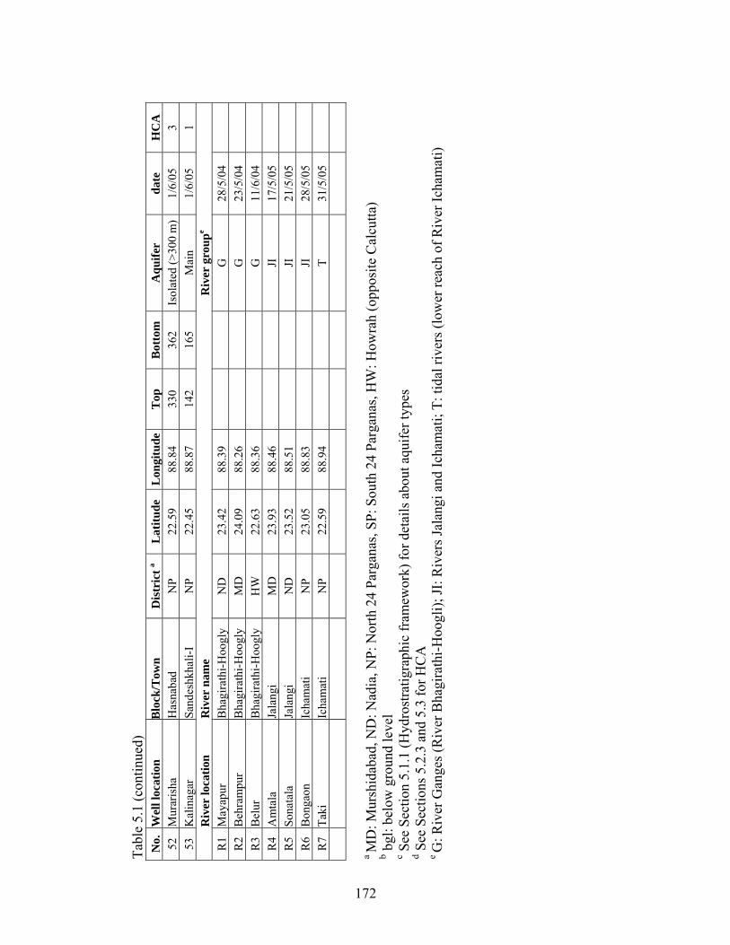
172

Tabl

e 5.

1 (c

ontin

ued)

N

o.

Wel

l loc

atio

n B

lock

/Tow

n D

istr

ict a

Lat

itude

L

ongi

tude

Top

B

otto

m

Aqu

ifer

date

H

CA

52

M

urar

isha

H

asna

bad

NP

22.5

9 88

.84

330

362

Isol

ated

(>30

0 m

)1/

6/05

3

53

Kal

inag

ar

Sand

eshk

hali-

I N

P 22

.45

88.8

7 14

2 16

5 M

ain

1/6/

05

1

Riv

er lo

catio

n R

iver

nam

e

Riv

er g

roup

e

R

1 M

ayap

ur

Bha

gira

thi-H

oogl

y N

D

23.4

2 88

.39

G

28/5

/04

R

2 B

ehra

mpu

r B

hagi

rath

i-Hoo

gly

MD

24

.09

88.2

6

G

23

/5/0

4

R3

Bel

ur

Bha

gira

thi-H

oogl

y H

W

22.6

3 88

.36

G

11/6

/04

R

4 A

mta

la

Jala

ngi

MD

23

.93

88.4

6

JI

17

/5/0

5

R5

Sona

tala

Ja

lang

i N

D

23.5

2 88

.51

JI

21/5

/05

R

6 B

onga

on

Icha

mat

i N

P 23

.05

88.8

3

JI

28

/5/0

5

R7

Taki

Ic

ham

ati

NP

22.5

9 88

.94

T 31

/5/0

5

a M

D: M

ursh

idab

ad, N

D: N

adia

, NP:

Nor

th 2

4 Pa

rgan

as, S

P: S

outh

24

Parg

anas

, HW

: How

rah

(opp

osite

Cal

cutta

) b b

gl: b

elow

gro

und

leve

l c S

ee S

ectio

n 5.

1.1

(Hyd

rost

ratig

raph

ic fr

amew

ork)

for d

etai

ls a

bout

aqu

ifer t

ypes

d S

ee S

ectio

ns 5

.2.3

and

5.3

for H

CA

e G

: Riv

er G

ange

s (R

iver

Bha

gira

thi-H

oogl

i); JI

: Riv

ers J

alan

gi a

nd Ic

ham

ati;

T: ti

dal r

iver

s (lo

wer

reac

h of

Riv

er Ic

ham

ati)

17

2

173

Tabl

e 5.

2a: F

ield

mea

sure

men

ts a

nd m

ajor

solu

te c

ompo

sitio

n of

the

wat

er sa

mpl

es. L

oc. c

orre

spon

ds to

no.

in ta

ble

5.1.

All

units

are

in

mg/

L ex

cept

whe

re m

entio

ned.

Bla

nk fi

elds

indi

cate

no

mea

sure

men

t. L

oc.

T (o C

) pH

E

h (m

V)

SC (μ

S)O

2 C

aa K

M

g N

a Si

C

l SO

42- b

H

CO

3- 1

29.1

7.

10

15.0

8 89

4 0.

94

136.

67

4.08

36

.85

38.1

6 13

.46

50.1

0 13

.45

368.

00

2 28

.4

6.92

31

1.42

10

61

1.50

15

4.06

7.

78

44.8

7 53

.13

12.7

3 56

.75

31.0

0 59

0.70

3

28.1

7.

02

79.8

4 64

3 1.

10

117.

35

2.95

26

.13

13.2

2 15

.24

3.07

bd

l 43

6.00

4

28.0

6.

91

120.

72

736

0.83

13

2.50

2.

59

30.1

9 18

.74

17.0

8 3.

19

11.4

0 49

0.00

5

28.3

6.

92

83.7

9 76

8 0.

86

130.

76

2.65

34

.22

23.2

6 16

.18

10.3

7 3.

44

481.

80

6 32

.8

8.09

17

.87

6490

1.

29

bdl

8.28

1.

23

1557

.54

7.80

16

20.0

0 bd

l 14

74.2

0 7

27.8

6.

94

81.5

7 87

3 1.

23

152.

73

3.17

36

.80

20.4

3 14

.12

35.5

0 21

.45

502.

50

8 28

.5

6.91

11

8.34

70

5 0.

49

110.

21

2.42

27

.65

23.8

3 16

.44

37.9

5 13

.95

395.

30

9 28

.2

6.88

70

.07

751

1.08

13

2.22

6.

25

33.9

6 24

.10

14.0

3 35

.20

2.70

48

8.90

10

28

.5

7.11

12

6.94

61

9 0.

96

115.

49

2.71

29

.44

15.7

5 14

.69

23.0

5 9.

41

414.

30

11

28.3

6.

83

106.

69

760

1.30

13

6.03

3.

43

34.1

3 16

.10

18.5

3 4.

62

0.25

52

5.50

12

31

.8

7.12

16

3.33

94

3 1.

51

155.

49

3.64

32

.82

35.7

2 12

.60

73.7

0 36

.20

481.

30

13

31.4

7.

48

83.3

4 71

4 1.

25

41.2

0 2.

83

21.5

8 97

.38

14.5

8 41

.70

1.17

47

2.40

14

29

.9

7.44

99

.38

5280

0.

75

36.1

6 6.

73

37.7

1 10

96.0

2 10

.66

1610

.00

bdl

482.

40

15

28.5

7.

00

100.

64

689

1.40

11

3.55

2.

63

28.2

8 18

.23

16.4

5 6.

78

bdl

452.

10

16

33.0

7.

67

30.1

2 10

32

0.65

16

.73

4.15

26

.95

180.

20

9.73

13

3.50

bd

l 44

0.80

17

28

.3

6.87

87

.69

632

0.82

10

3.59

2.

15

27.3

9 14

.40

18.8

8 3.

55

bdl

409.

20

18

34.5

7.

73

-16.

32

3960

1.

31

16.1

9 4.

90

21.6

9 84

4.07

7.

57

1085

.00

bdl

597.

60

19

32.4

7.

91

18.0

8 18

07

0.79

13

.20

2.99

13

.34

373.

83

7.02

40

1.00

bd

l 44

6.70

20

32

.2

7.69

19

.73

6100

1.

44

20.4

0 11

.19

53.9

0 13

47.8

5 7.

38

1870

.00

bdl

643.

80

21

29.8

7.

14

66.8

5 80

2 2.

32

107.

34

3.22

39

.37

44.1

2 20

.51

12.9

5 bd

l 54

4.80

22

29

.2

7.06

10

8.31

77

5 1.

37

111.

32

3.09

38

.81

33.7

1 20

.90

8.20

bd

l 50

2.40

23

32

.5

7.05

64

.60

1510

0.

89

88.3

6 4.

79

47.1

5 19

0.78

16

.03

286.

00

24.3

0 44

0.70

24

32

.7

6.98

10

9.75

22

30

0.72

20

0.04

6.

99

79.7

5 20

0.20

17

.73

665.

50

22.8

0 40

0.90

25

30

.2

7.45

44

.75

1115

0.

92

73.1

1 4.

15

47.8

3 10

7.97

12

.76

162.

00

18.3

5 40

6.00

173

Tabl

e 5.

2a (c

ontin

ued)

L

oc.

T (o C

) pH

E

h (m

V)

SC (μ

S)O

2 C

aa K

M

g N

a Si

C

l SO

42- b

H

CO

3- 26

29

.1

7.09

74

.28

618

1.30

12

1.99

4.

54

26.6

1 24

.20

12.9

0 29

.74

11.8

4 33

0.30

27

29

.3

7.16

44

.43

750

1.21

11

3.39

3.

00

26.2

0 27

.55

14.3

4 27

.84

18.2

3 41

0.10

28

28

.2

6.78

81

.97

850

1.51

14

5.01

3.

09

31.5

5 25

.68

17.2

3 5.

29

5.14

54

2.20

29

27

.8

7.07

14

4.37

10

59

2.50

12

9.41

7.

40

37.3

0 48

.20

11.1

3 53

.40

39.6

4 52

7.30

30

28

.6

7.13

11

7.26

78

6 1.

82

104.

55

2.81

25

.85

23.8

3 15

.12

24.2

3 15

.71

446.

30

31

30.8

7.

09

91.9

9 56

6 0.

63

86.2

6 2.

42

17.5

5 12

.23

15.4

9 2.

49

2.20

35

6.30

32

29

.1

7.04

75

.18

745

1.67

10

5.48

2.

80

24.4

4 17

.57

15.3

6 7.

26

4.32

46

6.90

33

29

.1

6.76

77

.18

876

1.62

13

3.10

4.

41

28.9

5 24

.78

15.4

6 35

.61

30.5

7 45

6.50

34

27

.9

7.23

47

.90

7860

0.

29

124.

14

12.1

8 72

.21

1298

.20

14.3

3 0.

00

bdl

385.

30

35

28.1

6.

84

201.

44

695

1.19

11

0.44

2.

48

23.3

3 16

.88

17.4

7 2.

32

bdl

447.

40

36

28.0

7.

01

77.8

2 78

7 0.

67

130.

11

3.27

31

.80

31.9

3 18

.21

23.5

5 17

.98

510.

90

37

29.4

7.

01

69.0

6 61

2 0.

89

92.9

0 2.

52

20.7

8 12

.36

16.1

3 1.

99

bdl

380.

90

38

30.5

7.

51

6.42

89

2 0.

76

19.8

1 2.

12

12.7

7 18

7.83

9.

41

110.

25

bdl

417.

20

39

28.3

6.

99

96.8

9 62

7 0.

13

103.

01

2.57

23

.30

12.4

8 19

.11

0.82

bd

l 42

1.00

40

32

.2

7.06

10

3.73

74

7 1.

36

117.

92

4.10

41

.99

149.

16

17.5

8 26

0.25

12

.98

477.

50

41

28.4

6.

85

99.6

2

0.71

12

0.37

2.

67

27.6

8 59

.96

18.4

9 82

.36

4.55

46

6.30

42

31

.4

7.07

79

.74

0.

90

100.

99

2.45

26

.39

17.6

0 19

.07

3.24

bd

l 44

4.00

43

29

.2

7.03

71

.41

0.

37

97.7

9 2.

64

22.2

4 15

.44

18.9

9 1.

48

bdl

401.

90

44

30.8

7.

28

51.2

9

0.53

77

.92

3.23

27

.61

104.

39

16.3

7 48

.68

bdl2

55

3.30

45

28

.8

6.92

45

.01

0.

25

110.

77

1.96

25

.81

24.9

3 16

.56

26.6

0 3.

41

437.

60

46

30.0

7.

04

60.9

0

0.17

10

1.94

2.

97

24.0

4 17

.89

20.2

8 6.

10

bdl

443.

80

47

30.4

6.

98

101.

50

0.

85

112.

94

2.42

31

.62

21.7

7 20

.83

3.77

bd

l 49

3.80

48

29

.9

7.08

11

9.08

0.49

10

8.47

2.

80

32.3

0 31

.16

20.4

7 17

.32

bdl

480.

50

49

29.2

6.

73

110.

51

0.

48

107.

69

3.70

29

.20

25.4

1 26

.32

9.22

bd

l 47

9.40

50

31

.2

7.19

11

2.39

0.54

83

.98

3.33

32

.03

62.9

0 19

.93

32.9

7 bd

l 48

2.90

51

29

.4

7.24

77

.56

3.

50

93.8

5 3.

04

30.5

5 52

.56

19.7

4 24

.64

bdl

490.

50

52

34.6

8.

19

-29.

70

4370

0.

35

6.65

3.

50

9.47

64

8.75

7.

18

673.

91

bdl

757.

70

53

29.3

7.

67

-40.

17

0.

55

31.0

0 4.

42

19.0

5 16

9.62

10

.18

108.

72

bdl

435.

10

17

4

174

175

Tabl

e 5.

2a (c

ontin

ued)

R

iver

s

Loc

. T

(o C)

pH

Eh

(mV

) SC

(μS)

O2

Caa

K

Mg

Na

Si

Cl

SO42-

b

HC

O3-

R1

38.1

8.

20

407.

55

266

26

.49

3.06

10

.90

14.2

2 5.

27

8.62

13

.00

137.

10

R2

28.8

8.

30

269.

81

322

29

.37

3.14

14

.42

17.4

2 6.

03

11.4

5 15

.00

145.

20

R3

29.5

7.

92

368.

08

281

27

.50

2.85

9.

42

13.4

5 4.

49

12.7

0 14

.50

149.

20

R4

34.4

8.

01

297.

96

561

80

.66

3.10

23

.06

18.3

5 9.

63

15.6

7 2.

89

344.

30

R5

32.8

8.

30

266.

37

392

43

.36

5.36

21

.66

18.9

5 12

.59

19.5

1 3.

98

260.

60

R6

32.9

7.

56

309.

20

69.7

7 1.

93

21.7

5 23

.69

12.2

3 15

.94

6.85

31

3.30

R

7 31

.5

7.70

32

2.06

23

7.35

29

.41

667.

78

4986

.36

1.99

69

69.7

0 bd

l 12

8.60

bd

l = b

elow

det

ectio

n le

vel

a D

etec

tion

leve

l (D

L) =

10

mg/

L b D

L =

0.12

mg/

L

17

5

176

Tabl

e 5.

2b: M

inor

solu

te, d

isso

lved

gas

and

stab

le is

otop

ic c

ompo

sitio

ns o

f the

wat

er sa

mpl

es. L

oc. c

orre

spon

ds to

no.

in ta

ble

5.1.

All

units

are

in m

g/L

exce

pt w

here

men

tione

d. B

lank

fiel

ds in

dica

te n

o m

easu

rem

ent.

DL:

det

ectio

n le

vel,

bdl:

belo

w d

etec

tion

leve

l. C

once

ntra

tions

of A

l, B

e, C

o, C

r, C

u, N

i, Pb

, Sb,

Se,

Tl,

U, N

O2- -N

, and

PO

43- fo

r all

sam

ples

wer

e be

low

det

ectio

n le

vel.

L

oc.

As(

tot.)

As(

III)

B

B

a Fe

(tot

.)M

nN

H4+

Sr

V

Zn

Br

F N

O3-N

CO

32-C

H4 (μ

M)

DO

C

δ13C

(‰

) Fe

(II)

δ34S

(‰)

DL

0.00

5 0.

005

0.01

0.

10

0.02

0.

10

0.01

0.05

0.10

0.01

0.01

0.10

0.

12

0.12

0.

50

1 0.

060

0.04

2 0.

09

0.21

2.

62

2.00

0.

480.

440.

340.

13bd

l bd

l 0.

27

bdl

0.80

4.

187E

+00

1.30

2

0.01

6 0.

013

0.06

0.

27

bdl

bdl

0.57

bdl

0.34

0.17

0.03

bdl

0.50

0.

54

0.80

6.

316E

+00

1.20

12.1

03

0.09

2 0.

064

0.03

0.

13

2.09

2.

00

0.41

0.93

0.23

0.09

0.01

bdl

bdl

bdl

0.70

1.

241E

+03

1.10

4

0.02

0 0.

018

0.01

0.

17

3.24

3.

00

0.17

0.18

0.20

0.10

0.03

bdl

0.13

bd

l 0.

60

6.69

8E+0

0 1.

10

8.

20

5 0.

137

0.08

2 0.

01

0.13

0.

92

0.90

0.

540.

730.

310.

120.

10bd

l 0.

12

bdl

0.40

4.

689E

+00

1.20

6

bdl

bdl

10.2

8 bd

l 0.

41

0.20

bd

l bd

l 0.

61bd

l 0.

035.

56

1.07

bd

l 20

.50

2.96

0E+0

0 1.

90

-8.1

6

7 0.

074

0.05

7 0.

17

0.15

3.

79

3.80

0.

620.

310.

310.

140.

08bd

l 0.

17

bdl

0.50

8.

390E

+00

1.00

18.4

08

0.04

4 0.

040

0.18

bd

l 0.

75

0.70

0.

060.

270.

310.

100.

03bd

l 0.

29

bdl

0.30

6.

407E

+00

1.20

14.3

09

0.12

3 0.

071

0.08

0.

20

5.23

5.

20

0.27

1.59

0.25

0.12

0.03

bdl

0.36

bd

l 0.

50

7.90

1E+0

2 1.

80

10

0.00

8 0.

005

0.06

0.

36

0.40

0.

40

0.47

0.39

0.24

0.10

0.02

bdl

0.33

bd

l 0.

50

6.42

2E+0

0 1.

20

7.

40

11

0.03

9 0.

013

0.05

0.

21

0.33

0.

30

0.06

0.53

0.40

0.12

bdl

bdl

bdl

bdl

0.50

5.

228E

+01

1.00

12

0.

052

0.03

5 0.

05

0.14

0.

44

0.40

0.

59bd

l 0.

190.

11bd

l bd

l 0.

56

bdl

0.60

7.

992E

+00

0.90

21.6

013

bd

l bd

l 0.

17

bdl

0.33

0.

30

bdl

0.34

0.28

0.07

0.02

bdl

0.43

bd

l 1.

30

1.07

1E+0

1 0.

70

14

bdl

bdl

2.09

bd

l 0.

20

0.20

bd

l bd

l 0.

800.

100.

025.

30

bdl

bdl

1.90

3.

227E

+04

0.70

-2

.17

15

0.

080

0.05

4 0.

06

0.12

1.

26

1.20

0.

090.

660.

230.

10bd

l bd

l bd

l bd

l 0.

40

1.58

9E+0

3 1.

00

16

bdl

bdl

0.20

bd

l 0.

15

0.10

bd

l 0.

470.

220.

080.

03bd

l 0.

77

bdl

2.00

3.

276E

+03

0.80

17

0.

088

0.05

7 0.

04

0.16

1.

61

1.60

0.

070.

910.

250.

090.

01bd

l bd

l bd

l 0.

30

8.94

7E+0

0 1.

30

18

0.02

8 0.

021

2.68

bd

l 0.

11

0.20

0.

02bd

l 0.

350.

06bd

l 3.

95

bdl

bdl

4.60

8.

229E

+00

2.60

-2

.57

19

bd

l bd

l 0.

46

bdl

0.04

bd

l 0.

010.

760.

180.

04bd

l 1.

23

bdl

bdl

2.70

1.

397E

+04

3.70

-5

.27

20

0.

008

0.00

3 1.

33

bdl

0.14

0.

10

bdl

bdl

0.33

0.15

0.03

6.16

bd

l bd

l 7.

60

2.02

6E+0

1 4.

70

-0.5

3

21

bdl

bdl

0.06

0.

21

0.66

0.

60

0.08

0.49

0.39

0.13

bdl

bdl

0.23

bd

l 0.

80

5.20

5E+0

0 1.

20

22

bdl

bdl

0.05

0.

22

0.84

0.

80

0.11

0.38

0.38

0.14

bdl

bdl

0.22

bd

l 0.

90

7.16

6E+0

0 0.

90

23

bdl

bdl

0.14

0.

28

0.53

0.

50

0.04

bdl

0.44

0.15

bdl

0.84

bd

l bd

l 0.

80

1.38

5E+0

1 0.

90

45

.80

17

6

177

Tabl

e 5.

2b (c

ontin

ued)

Loc

. A

s(to

t.)

As(

III)

B

B

a Fe

(tot

.)Fe

(II)

Mn

NH

4+ Sr

V

Z

n B

r F

NO

3-NC

O32-

CH

4 (μ

M)

DO

C

δ13C

(‰

) δ34

S (‰

) 24

bd

l bd

l 0.

08

0.31

0.

65

0.60

0.

19bd

l 0.

860.

340.

041.

94bd

l bd

l 0.

50

2.60

4E+0

1 0.

50

11

.50

25

bdl

bdl

0.09

0.

10

0.24

0.

20

0.03

0.60

0.

490.

160.

020.

52bd

l bd

l 1.

00

1.49

3E+0

1 0.

80

26

0.03

2 0.

021

0.29

0.

22

1.47

1.

00

0.29

bdl

0.45

0.04

0.02

bdl

bdl

bdl

0.30

8.

172E

+01

1.00

-8

.29

27

0.

055

0.05

4 0.

18

0.23

2.

10

2.10

0.

52bd

l 0.

340.

07bd

l 0.

54bd

l bd

l 0.

40

9.84

0E+0

1 1.

00

-7.3

616

.40

28

0.01

5 0.

013

0.13

0.

30

3.56

3.

56

0.08

bdl

0.30

0.08

bdl

bdl

bdl

bdl

0.40

8.

554E

+01

1.30

-2

.00

29

bd

l bd

l 0.

15

0.22

0.

40

0.40

0.

680.

17

0.39

0.10

0.03

1.33

bdl

0.14

0.

40

1.07

3E+0

2 0.

90

-6.1

011

.10

30

0.02

4 0.

020

0.09

0.

14

1.03

1.

00

0.31

0.63

0.

270.

080.

010.

58bd

l bd

l 0.

20

2.01

0E+0

3 1.

00

-4.8

211

.70

31

0.02

7 0.

027

0.06

0.

12

0.61

0.

60

0.11

bdl

0.21

0.04

0.05

bdl

bdl

bdl

0.30

2.

716E

+02

0.70

-3

.73

32

0.

099

0.04

9 0.

06

0.17

1.

80

1.80

0.

10bd

l 0.

250.

07bd

l bd

l bd

l bd

l 0.

40

8.27

8E+0

1 0.

80

-4.7

3

33

0.01

1 0.

011

0.06

0.

31

2.29

2.

00

0.22

bdl

0.31

0.08

0.01

1.04

bdl

bdl

0.40

1.

149E

+02

0.80

-3

.51

5.70

34

bd

l bd

l 4.

05

0.21

1.

26

1.20

0.

033.

29

3.78

0.18

0.05

7.36

bdl

bdl

0.80

6.

822E

+04

0.70

-2

.38

35

bd

l bd

l 0.

11

0.10

bd

l bd

l 0.

510.

16

0.33

0.06

bdl

0.69

0.12

bd

l 0.

60

1.23

6E+0

2 0.

70

-3.1

015

.80

36

0.02

0 0.

020

0.11

0.

78

1.12

1.

00

0.11

0.12

0.

370.

090.

011.

330.

13

bdl

0.60

8.

584E

+01

0.80

-2

.10

37

0.

049

0.04

9 0.

06

0.21

1.

65

1.65

0.

160.

17

0.23

0.05

0.05

bdl

bdl

bdl

0.30

4.

549E

+02

0.80

-3

.94

38

bd

l bd

l 0.

39

bdl

0.04

bd

l 0.

020.

26

0.37

0.03

0.03

1.20

bdl

bdl

1.50

1.

255E

+04

1.40

-5

.07

39

0.

018

0.01

1 0.

03

0.12

0.

70

0.70

0.

030.

29

0.31

0.06

0.02

bdl

bdl

bdl

0.30

1.

282E

+02

0.70

-1

.12

40

bd

l bd

l 0.

09

0.26

0.

94

0.90

0.

23bd

l 0.

750.

120.

041.

900.

24

bdl

0.30

1.

069E

+02

0.50

-4

.16

41

0.

029

0.02

9 0.

06

0.18

1.

38

1.30

0.

190.

13

0.42

0.07

0.01

0.80

bdl

bdl

0.30

9.

725E

+01

bdl

-6.0

9

42

0.05

5 0.

055

0.02

0.

15

1.31

1.

30

0.09

0.87

0.

420.

070.

01bd

l 0.

12

bdl

0.50

1.

880E

+04

bdl

-2.5

5

43

0.04

9 0.

048

0.01

0.

11

1.21

1.

20

0.06

0.21

0.

350.

050.

01bd

l bd

l bd

l 0.

30

4.17

9E+0

3 bd

l -1

.28

44

0.

010

0.01

0 0.

35

bdl

0.50

0.

50

0.07

1.12

0.

820.

060.

111.

75bd

l bd

l 0.

60

9.61

1E+0

1 1.

3

45

0.

028

0.02

7 0.

01

0.30

5.

10

5.00

0.

070.

94

0.28

0.06

bdl

1.33

0.14

bd

l 0.

30

7.85

9E+0

1 0.

50

-5.0

9

46

0.05

4 0.

053

0.01

0.

28

3.53

3.

50

0.09

bdl

0.30

0.08

bdl

bdl

bdl

bdl

0.20

1.

000E

+02

bdl

-0.7

6

47

bdl

bdl

0.01

0.

20

0.51

0.

50

0.09

0.17

0.

510.

09bd

l bd

l bd

l bd

l 0.

50

1.44

7E+0

4 1.

2 -5

.15

48

bd

l bd

l 0.

01

0.16

1.

02

1.00

0.

060.

10

0.60

0.08

0.12

1.29

0.23

bd

l 0.

40

1.63

4E+0

4 1.

4 -2

.03

49

0.

019

0.01

9 0.

01

0.22

1.

25

1.20

0.

26bd

l 0.

360.

100.

041.

520.

14

bdl

0.30

8.

221E

+01

1.0

-2.4

6

50

bdl

bdl

0.05

0.

13

0.43

0.

40

0.08

0.69

0.

450.

08bd

l 0.

98bd

l bd

l 0.

70

4.81

1E+0

1 1.

70

-4.2

0

17

7

178

Tabl

e 5.

2b (c

ontin

ued)

Loc

. A

s(to

t.)

As(

III)

B

B

a Fe

(tot

.)Fe

(II)

Mn

NH

4+ Sr

V

Z

n B

r F

NO

3-NC

O32-

CH

4 (μ

M)

DO

C

δ13C

(‰

) δ34

S (‰

) 51

bd

l bd

l 0.

04 0

.13

0.82

0.

80

0.13

0.19

0.

450.

07bd

l1.

70

0.20

bd

l 1.

40

2.97

5E+0

3 0.

50

-5.6

0

52

bdl

bdl

1.37

bd

l bd

l bd

l 0.

011.

24

0.13

0.03

0.07

3.69

0.

49

bdl

12.5

01.

351E

+02

0.50

-2

.08

53

bd

l bd

l 0.

18 0

.10

bdl

bdl

0.01

0.53

0.

310.

030.

010.

15

0.12

bd

l 1.

80

6.59

8E+0

1 0.

50

-5.5

3

Riv

ers

R

1 bd

l

0.01

bd

l bd

l

0.00

bdl

0.12

0.05

0.04

bdl

0.20

0.

20

0.70

R

2 bd

l

0.02

0.1

0 0.

23

0.

00bd

l 0.

130.

060.

04bd

l 0.

17

bdl

0.65

R

3 bd

l

bdl

bdl

0.03

0.02

bdl

0.10

0.05

0.02

bdl

0.20

0.

22

0.60

R

4 0.

055

0.

01 0

.18

bdl

0.

03bd

l 0.

280.

040.

000.

46

bdl

bdl

2.40

R

5 0.

101

0.

00

bdl

bdl

0.

01bd

l 0.

200.

050.

011.

35

0.16

bd

l 2.

70

R6

0.03

7

0.01

0.1

5 bd

l

0.03

0.05

0.

240.

040.

000.

40

bdl

bdl

1.40

R

7 bd

l

2.33

0.1

8 bd

l

0.00

bdl

3.67

1.86

0.04

26.9

7bd

l bd

l 0.

70

178

Table 5.3: Details of the first six components (showing 90% of the variance) obtained from the principal component analyses (PCA) for 15 parameters. Rotation method: Varimax with Kaiser normalization. Rotation converged in six iterations. Principal Component 1 2 3 4 5 6 % Variance 36.461 20.405 12.466 10.508 6.291 3.770

HCO3- 0.951 -0.001 -0.008 -0.055 -0.088 -0.017

CO32- 0.925 0.067 -0.150 -0.109 -0.069 -0.186

B 0.894 0.265 -0.107 -0.055 0.176 -0.086 Na 0.664 0.616 -0.263 -0.135 0.110 -0.214 K 0.373 0.850 0.132 -0.091 0.136 -0.009 Mg -0.366 0.783 0.233 -0.046 0.128 0.265 Cl 0.464 0.767 -0.211 -0.115 0.276 -0.132 Mn -0.101 -0.085 0.907 0.214 -0.020 -0.017

SO42- -0.075 0.167 0.804 -0.124 -0.241 0.259

Ca -0.428 0.066 0.571 0.322 0.085 0.485 As(tot.) -0.131 -0.142 0.190 0.867 0.048 -0.231 Fe(tot.) -0.072 -0.079 -0.018 0.815 0.057 0.417

NH4+ -0.018 0.162 -0.136 0.164 0.910 -0.083

Sr 0.039 0.603 -0.053 -0.144 0.717 0.120 Ba -0.165 0.037 0.175 0.019 -0.048 0.899

179

180

Table 5.4: List of selected minerals (in no definite order) documented in the sediments of the Bengal basin by previous workers. Name of the individual member of group minerals is mentioned wherever available, otherwise mentioned as group name.

Author Site Mineral phases FAO (1971) Across Bangladesh Clays, quartz, calcite, dolomite, mica Das et al. (1995)

Maldah, North 24 Parganas (West Bengal)

FeSO4, hematite, magnetite, quartz, pyrite

Datta et al. (1997)

Across Bangladesh Quartz, feldspar, carbonate (unspecified, very low), illite, kaolinite, amphibole

Chowdhury et al. (1999)

Bangladesh and West Bengal

Pyrite, rozenite (FeSO4.H2O), FeOOH, hematite,

magnetite, quartz, calcite Nickson et al. (2000)

Tungipara, Gopalganj (Bangladesh)

Fe-oxyhydroxide, authigenic pyrite

Breit et al. (2001)

Brahmanberia (Bangladesh)

Biotite, siderite, vivianite

Chakraborti et al. (2001)

Murshidabad, Nadia, North and South 24 Parganas (West Bengal)

Pyrite, Fe-oxide, Fe-oxyhydroxide, gypsum, calcite, quartz, goethite, mica, feldspar, Ca3(PO4)2, rozenite

BGS/DPHE (2001)

Chapai Nawabganj, Laxmipur, Faridpur (Bangladesh)

Quartz, mica (including altered biotite), feldspars, pyroxene, Fe2O3, apatite, smectite, illite, kaolinite, chlorite, authigenic pyrite, calcite

Anwar et al. (2002)

Narayanganj (Bangladesh)

Kaolinite, illite, montmorillonite, goethite, amorphous Fe-oxide, mica, feldspar, amphibole

Dowling et al. (2002)

Laxmipur (Bangladesh) Quartz, biotite, altered vermiculite, Fe-oxyhydroxide

Pal et al. (2002)

Nadia, South 24 Parganas (West Bengal)

Quartz, feldspar, calcareous concretion, Fe-oxide, Fe-oxyhydroxide, siderite, hornblende, muscovite, biotite, kaolinite, illite, montmorillonite

Allison et al. (2003)

Gangetic delta front (Bangladesh)

Smectite, kaolinite

Heroy et al. (2003)

Gangetic flood plain (Bangladesh)

Dolomite, calcareous concretion, smectite, kaolinite

Ahmed et al. (2004)

14 locations across Bangladesh

Quartz, muscovite, biotite, feldspar (fresh and altered), chlorite, hornblende

McArthur et al. (2004)

North 24 Parganas (West Bengal)

Fe-oxyhydroxide, calcite

Swartz et al. (2004)

Munshiganj (Bangladesh) Quartz, plagioclase, orthoclase, muscovite, biotite, magnetite, hornblende, chlorite, apatite, pyrite

Tabl

e 5.

5: S

umm

ary

of s

atur

atio

n in

dice

s (S

I) c

alcu

late

d by

PH

REE

QC

for

som

e ph

ases

pos

sibl

y in

con

tact

with

wes

tern

Ben

gal

grou

ndw

ater

and

rive

r wat

er sa

mpl

es. B

lank

fiel

ds in

dica

te v

alue

s not

ava

ilabl

e. S

I < 0

: und

ersa

tura

tion;

SI >

0: s

uper

satu

ratio

n.

Phas

es

Mai

n aq

uife

r (n

= 4

7)

Isol

ated

aqu

ifers

(n =

6)

Riv

er (G

gro

up, n

= 3

) R

iver

(JI g

roup

, n =

3)

Riv

er (T

) N

ame

Form

ula

Mea

n M

ax

Min

M

ean

Max

M

in

Mea

n M

ax

Min

M

ean

Max

M

in

(n =

1)

Ars

enol

ite

As 4

O6

-22.

13

-20.

26-2

5.22

-24.

39

-22.

91-2

5.87

-1

34.3

-1

32.2

-1

36.2

As 2

O5

-31.

31

-28.

70-3

4.05

-33.

84

-33.

60-3

4.08

-3

2.74

-3

1.18

-3

3.81

B

irnes

site

M

nO2

-16.

14

-11.

57-1

8.27

-16.

82

-15.

63-1

7.66

5.72

5.

72

5.72

4.

79

4.97

4.

44

B

ixby

ite

Mn 2

O3

-14.

84

-9.8

8 -1

7.56

-15.

64

-13.

68-1

6.85

7.93

7.

93

7.93

6.

81

7.33

6.

03

Ca 3

(AsO

4)2. 6H

2O

-13.

33

-11.

01-1

5.78

-14.

38

-14.

12-1

4.64

-9

.92

-9.1

7 -1

1.03

C

alci

te

CaC

O3

0.27

0.

54

-0.0

1 0.

21

0.37

0.

07

0.41

0.

54

0.18

0.

87

1.08

0.

54

0.31

Log

P CO

2 -1

.41

-1.0

3 -2

.23

-1.9

2 -1

.69

-2.3

0 -2

.94

-2.7

1 -3

.12

-2.4

4 -2

.02

-2.8

5 -2

.74

Dol

omite

C

aMg(

CO

3) 2

0.32

1.

04

-0.2

8 0.

83

1.20

0.

47

0.75

1.

07

0.20

1.

60

1.98

0.

88

1.40

Fe(O

H)2

.7C

lO3

5.66

7.

75

0.65

6.

48

7.83

6.

06

6.98

7.

50

6.46

Fe3(

OH

) 8

0.48

4.

74

-3.0

0 1.

62

5.44

0.

52

-5.8

1 -4

.61

-7.0

1

FeA

sO4. 2H

2O

-6.8

4 -4

.55

-8.3

5 -8

.04

-7.9

1 -8

.16

Fe

rrih

ydrit

e Fe

(OH

) 3

0.95

2.

82

0.39

1.

30

2.76

0.

78

2.36

2.

76

1.95

G

oeth

ite

FeO

OH

5.

50

7.35

4.

93

5.94

7.

42

5.28

6.

90

7.29

6.

50

Gre

enal

ite

Fe3S

i 2O5(O

H) 4

-1.3

2 0.

93

-8.9

3 -0

.52

2.09

-1

.98

-29.

62

-28.

34-3

0.90

Hem

atite

Fe

2O3

16.0

3 19

.73

14.8

8 16

.92

19.8

9 15

.58

18.8

2 19

.60

18.0

3

Le

pido

cros

ite

FeO

OH

4.

47

6.34

3.

91

4.83

6.

28

4.31

5.

88

6.28

5.

47

Mag

hem

ite

Fe2O

3 5.

29

9.03

4.

17

6.01

8.

92

4.97

8.

11

8.92

7.

30

Mag

netit

e Fe

3O4

17.5

2 21

.73

13.8

6 18

.96

22.8

8 17

.44

11.1

8 12

.34

10.0

2

M

anga

nite

M

nOO

H

-7.5

6 -5

.07

-8.9

6 -8

.01

-7.0

8 -8

.55

3.82

3.

82

3.82

3.

18

3.43

2.

80

M

etha

ne

CH

4 -1

.02

1.19

-2

.48

-0.7

2 1.

73

-2.6

0

Mg-

Ferr

ite

MgF

e 2O

4 6.

68

10.4

8 4.

81

8.73

11

.26

6.62

11

.17

12.3

9 9.

94

M

n 3(A

sO4) 2

. 8H2O

-1

2.51

-8

.84

-15.

41-1

3.86

-1

3.86

-13.

86

-11.

75

-10.

88

-12.

42

Nsu

tite

MnO

2 -1

5.55

-1

0.98

-17.

68-1

6.23

-1

5.04

-17.

076.

31

6.31

6.

31

5.37

5.

56

5.03

O

2 -4

2.68

-3

4.56

-46.

73-4

2.45

-4

0.07

-45.

31-0

.72

-0.7

1 -0

.73

-0.7

2 -0

.72

-0.7

2 -0

.68

Pyro

lusi

te

MnO

2 -1

3.59

-9

.10

-15.

68-1

4.11

-1

2.73

-15.

228.

27

8.27

8.

27

7.60

7.

83

7.22

Qua

rtz

SiO

2 0.

15

0.38

-0

.24

-0.1

3 0.

15

-0.2

7 -0

.38

-0.2

7 -0

.46

-0.0

5 -0

.01

-0.1

4 -0

.74

Rho

doch

rosi

te M

nCO

3 -0

.80

0.94

-2

.00

-1.4

9 -0

.99

-2.1

5 -1

.30

-1.3

0 -1

.30

-1.1

0 -0

.71

-1.4

5

18

1

181

Phas

es

Form

ula

Mea

n M

ax

Min

M

ean

Max

M

in

Mea

n M

ax

Min

M

ean

Max

M

in

Si

derit

e Fe

CO

3 0.

08

0.79

-2

.29

0.02

0.

93

-0.7

4 -1

0.56

-1

0.38

-10.

73-1

.38

-1.3

8 -1

.38

SiO

2 (am

orph

.) -1

.12

-0.8

9 -1

.50

-1.3

9 -1

.13

-1.5

2 -1

.63

-1.5

4 -1

.69

-1.2

6 -1

.26

-1.2

6 -2

.00

Tabl

e5.

5(c

ontin

ued)

182

18

2

Tabl

e 5.

6: D

etai

ls o

f the

reac

tion

path

mod

els.

Res

ults

indi

cate

: cat

ion

exch

ange

(a: C

aX2,

b: K

X, c

: MgX

2, d:

NaX

), su

lfur c

yclin

g (m

: pyr

ite),

carb

on c

yclin

g (n

: CO

2, o:

CH

4, p:

org

anic

car

bon

[CH

2O])

and

car

bona

te w

eath

erin

g (x

= c

alci

te, y

= d

olom

ite, z

=

side

rite)

.

Flow

path

(wel

ls/r

iver

) R

esul

t (ph

ases

) M

odel

N

o.

To

From

M

ixin

g

with

1

Mix

ing

(ran

ge

%)

No.

of

min

imal

m

odel

s U

ncer

tain

ty%

(5 to

20)

Hal

ite

Dis

solu

tion

2 Si

bal

ance

3D

isso

lutio

n (+

) 4 Pr

ecip

itatio

n (-

) 5

E

volu

tion

of is

olat

ed g

roun

dwat

er

1 6

26

9 11

us

ed

faile

d b,

d,y,

o,p,

x a,

c,m

,o

2 6

8

9

6 us

ed

faile

d b,

d,z,

y,n,

o,p,

x x/

a,c,

m

3 6

29

9 18

us

ed

wor

ked

d,z,

y,n,

o,p,

x a,

c,m

,o,x

4

6 30

6

8 us

ed

faile

d b,

d,z,

y,n/

p,x

a,c,

m,o

5

6 2

9 6

used

fa

iled

d,z,

y,n,

o,p,

x a,

c,m

6

6 27

9

8 us

ed

faile

d b,

d,z,

y,n,

o/p,

x a,

c,m

7

14

33

6 19

us

ed

wor

ked

b,d,

y,z,

o/p

a,m

,n

8 14

33

B

oB

9.3

2 15

no

t use

d w

orke

d d,

z,o/

p x,

b,c,

m,n

9

14

13

13

17

used

w

orke

d b,

c,d,

z,o/

p,y,

n d,

m,a

,x

10

14

13

BoB

6.

3 5

15

not u

sed

wor

ked

d,z,

o,n/

p a,

m,b

,c,n

11

34

33

4

13

used

w

orke

d a,

b,c,

z,o/

p,y

x,d,

m,n

12

34

33

B

oB

15

2 13

no

t use

d w

orke

d a,

z,o/

p x,

b,c,

m,n

13

34

13

6

15

used

w

orke

d a,

b,c,

z,o/

p,n,

y d,

m,x

,n

14

34

13

BoB

11

.0-1

2.0

2 16

no

t use

d w

orke

d a,

z,o/

p x,

b,c,

m,n

15

20

19

10

6

used

w

orke

d b,

c,x/

y,z,

n/p

x/a,

o,d

16

20

19

BoB

7.

6-8.

1 4

6 no

t use

d w

orke

d d,

z,n/

p,y

x/a,

b,c,

m,o

17

20

51

6

5 us

ed

faile

d b,

d,y/

x,n/

p,c

x/a,

z,o,

c 18

20

51

B

oB

8.4-

9.7

4 6

not u

sed

faile

d d,

z,n/

p,y

a,b,

c,m

,o,x

19

20

19

R

7 19

6

19

not u

sed

wor

ked

d,y/

x,z,

n/p

a/x,

c,o

20

18

17

3 6

used

fa

iled

d,b,

y/x

a/x,

c,z,

o 21

18

17

B

oB

5.1-

5.2

6 5

not u

sed

faile

d d,

z,y/

x,o/

p a/

x,b,

c,m

22

18

46

6

6 us

ed

faile

d b,

d,y/

x,n

a,c,

z,o,

x 23

18

46

B

oB

4.7-

5.8

6 7

not u

sed

faile

d d,

z,o/

p,y/

x a,

b,c,

,m,n

,x

18

3

183

184

Tabl

e5.

6(c

ontin

ued)

No.

T

o Fr

om

Mix

ing

%

Min

imal

no.

U

ncer

tain

tyH

alite

Si

D

isso

lutio

n (+

) 4 Pr

ecip

itatio

n (-

) 5

24

52

51

6 8

used

fa

iled

d,y,

x,n/

p a,

z,c,

o,x

25

52

51

BoB

3

6 8

not u

sed

faile

d d,

z,y/

x,p,

n a,

b,c,

m,o

,x

26

52

22

6 8

used

fa

iled

d,y/

x,o/

p a,

c,z

27

52

22

BoB

2.

8-3.

1 6

8 no

t use

d fa

iled

d,z,

y/x,

p/o

a,b,

c,m

Evo

lutio

n of

mai

n aq

uife

r bra

ckis

h w

ater

in n

orth

ern

stud

y ar

ea (N

adia

)

28

38

35

4 6

used

fa

iled

d,z,

o/p,

y x,

a,b,

c,n

29

38

36

4 6

used

fa

iled

d,z,

o/p,

,y

x,a,

b,c,

m,n

30

38

35

14

6.

6 4

6 no

t use

d fa

iled

d,z,

o/p,

y x,

a,c,

n,b

31

38

35

34

3.6

4 14

no

t use

d fa

iled

d,o/

p,y

a,b,

c,n

E

volu

tion

of m

ain

aqui

fer b

rack

ish

wat

er in

sout

hern

stud

y ar

ea (2

4 Pa

rgan

as)

32

16

21

20

6

4 7

not u

sed

faile

d b,

d,o/

p,y

x,c,

a,z,

n 33

16

21

4

7 us

ed

faile

d b,

d,o/

p,y

x,a,

c,z

34

16

21

BoB

0.

5 4

7 no

t use

d fa

iled

d,z,

o/p,

y x,

a,c,

b,m

,n

35

16

22

4 7

used

fa

iled

d,o/

p,b,

y x,

a,c,

n,b

36

16

22

BoB

0.

6 4

7 no

t use

d fa

iled

d,z,

o/p,

b,y

x,c,

a,m

,n

37

19

51

BoB

1.

7-1.

8 4

6 no

t use

d fa

iled

d,y,

o/p

x,a,

c,b,

n,m

38

19

51

52

77

2

18

not u

sed

wor

ked

a,o/

p x,

d,z,

n 39

19

51

4

6 us

ed

faile

d d,

y,o/

p x,

a,c,

z,n

40

23

41

BoB

0.

9-1

13

8 no

t use

d w

orke

d c,

d,z,

y a,

m,n

,b,x

,o

41

23

41

4 8

used

w

orke

d b,

m,y

/c

d,x,

a,o,

n,z

42

24

23

BoB

1.

8-1.

9 2

6 no

t use

d w

orke

d a,

z,o/

p x,

b,d,

m

43

24

23

R7

3.4-

4.7

3 18

no

t use

d w

orke

d a,

o/p,

m

d,n

44

24

23

10

6 us

ed

wor

ked

a,b,

y,m

,o/p

,c

x,d

45

25

41

R7

1.2-

1 3

18

not u

sed

wor

ked

c/d,

m

a/x,

z,n,

o 46

25

41

B

oB

0.4-

0.6

9 19

no

t use

d w

orke

d d/

c,z

a,m

,o,n

,z,x

47

53

50

B

oB

0.3

4 6

not u

sed

faile

d d,

z,o/

p,y

x,a,

c,m

,n

48

53

50

R7

0.8-

0.9

5 18

no

t use

d fa

iled

d,y,

x,

a,c,

z,x

18

4

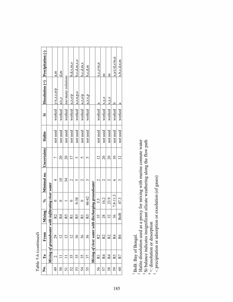
185

No.

T

o Fr

om

Mix

ing

%

Min

imal

no.

U

ncer

tain

tyH

alite

Si

D

isso

lutio

n (+

) Pr

ecip

itatio

n (-

)

M

ixin

g of

gro

undw

ater

with

infil

trat

ing

rive

r wat

er

49

2

29

R2

0 4

7 no

t use

d w

orke

d y/

x,z,

c,n/

p a,

m

50

11

12

R4

0 10

20

no

t use

d w

orke

d a/

c,z

d,m

51

11

12

R

5 1

34

20

not u

sed

wor

ked

too

man

y so

lutio

ns

52

35

12

R1

0 2

17

not u

sed

wor

ked

a,z,

o/p

b,d,

x,m

,o

53

35

36

R5

0-38

5

5 no

t use

d w

orke

d a,

z,n,

p,o

b,c,

d,m

,x,o

54

35

36

R

1 0

2 5

not u

sed

wor

ked

a,z,

o/p

b,c,

d,m

,x

55

37

36

R5

46-6

2 3

5 no

t use

d w

orke

d a,

z,x,

p b,

c,d,

m

M

ixin

g of

rive

r wat

er w

ith d

isch

argi

ng g

roun

dwat

er

56

R

1 R

2 35

5.

5 2

12

not u

sed

wor

ked

a x,

c,z/

m,n

57

R

4 R

2 28

16

.2

2 20

no

t use

d w

orke

d x,

y,z

m

58

R4

R2

32

23.9

2

20

not u

sed

wor

ked

x,y,

z m

59

R

5 R

4 36

7.

8-11

.5

6 10

no

t use

d w

orke

d b

x,a/

c/d,

z/m

,n

60

R7

R6

BoB

47

.3

3 12

no

t use

d w

orke

d a

x,b,

c,d,

n,m

1 B

oB: B

ay o

f Ben

gal.

2 Hal

ite d

isso

lutio

n us

ed a

s a p

roxy

for m

ixin

g w

ith m

arin

e co

nnat

e w

ater

3 Si

bal

ance

indi

cate

s ins

igni

fican

t sili

cate

wea

ther

ing

alon

g th

e flo

w p

ath

4 +:

dis

solu

tion

or d

esor

ptio

n 5 -:

prec

ipita

tion

or a

dsor

ptio

n or

exs

olut

ion

(of g

ases

)

Tabl

e5.

6(c

ontin

ued)

185

Figure 5.1: Map of the study area showing the 53 groundwater (hydrostratigraphically classified) and 7 river water-sampling locations; bmsl: below mean sea level. The thin black solid lines within the map (b) indicate the district boundaries.

186

Figure 5.2: (a) Generalized hydrostratigraphic framework along a north-south transect, parallel to the River Bhagirathi-Hoogly, redrawn for each district (not to scale). (b) Plot of the maximum tapped depth (bgl: below ground level) of the sampled wells.

187

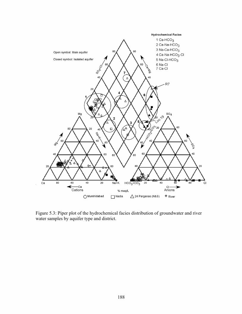
Figure 5.3: Piper plot of the hydrochemical facies distribution of groundwater and river water samples by aquifer type and district.

188

Figure 5.4: Bivariate plot of the three clusters obtained from hierarchical cluster analyses (HCA) with the first and second principal component (PC) axes. The data points are further classified according to aquifer type.

189

Figure 5.5: Molar ratio bivariate plots (plotted after Gaillardet et al. [1999]) of a) Na-normalized Ca and HCO3

-, b) Na-normalized Ca and Mg, c) Ca+Mg versus HCO3-, and

d) Si and Cl-normalized (Na+K). The dashed boxes in plots (a) and (b) represent the ranges of approximate compositions of the three main source end members (evaporites, silicates, and carbonates) without any mixing. Only three isolated aquifer samples can be seen in (a) and (b), as the other three have very low molar Ca/Na ratios. Bivariate plots between.

190

Figure 5.6: Stability field of a) Ca-Al silicate phases, b) Na-Al silicate phases, and c) K-Al silicate phases relative to groundwater and river water samples from the western Bengal basin. The phase boundaries are plotted using thermodynamic data of Tardy (1971) for (a) and (b), and Drever (1997) for (c).

191

Figure 5.7: Depth-profiles of water quality parameters: a) pH, b) Si, c) Ca+Mg, and d) Na+K; bgl: below ground level.

192

Figure 5.8: Distance (with latitude) plots of water quality parameters: a) Ca+Mg, b) Na+K, c) HCO3

-, and d) Si.

193

Figure 5.9: Plot of Br-/Cl- mass ratio versus Cl- concentration (following Whittemore [2004]) for groundwater, river water, and seawater (from Drever [1997]). Only the main aquifer and river water samples with Cl- concentrations > 10 mg/L and detectable Br concentrations are shown in the plot. The area between the dashed lines indicates the mixing zone of freshwater with seawater composition. The numbers beside the data points represent sample locations.

194

Figure 5.10: Comparison of observed EH of the groundwater and river water samples with calculated EH (converted from pe) of redox couples present in the waters. The plot has been classified into the redox system of oxic and anoxic (postoxic, sulfidic, and methanic) after Berner (1981). The sulfidic zone has been marked with (?) because of lack of S2- detection. GW: groundwater, R: river.

195

196

Figure 5.11: Depth-profiles of redox-sensitive parameters: a) EH, b) Fe(total), c) Fe(II), d) As(total), e) As(III), f) percentage of As(III) in the main aquifer samples with detectable (≥ 0.005 mg/L) As(III), g) Mn, h) SO4

2-, and i) CH4; bgl: below ground level.

Figure 5.12: Distance (with latitude) plots of redox-sensitive parameters: a) Cl--normalized SO4

2-, b) Mn, c) Fe (total), d) As (total), e) CH4. The very high CH4 concentrations are present in southern Nadia and northern North 24 Parganas. (f) shows the number of samples with O2 concentrations higher than 50 μmole/L (0.8 mg/L) is generally higher in the northern part of the flow path (north of ~23.5oN latitude).

197

Figure 5.13: Bivariate plots showing relations between a) Fe(total) and Mn, b) As(total) and Fe(total), and c) As(III) and Fe(II).

Figure 5.14: Plots of δ34SSO4 versus Cl-normalized SO4

2- concentrations. Location 4 with very high SO4

2- /Cl- is not shown. The solid lines represent visual trend lines; line (A) has a much higher gradient than (B), suggesting (B) possibly has undergone some reoxidation.

198

Figure 5.15: Plot of δ13CDIC with depth (bgl: below ground level).

199

Chapter 6: Suitability of deeper groundwater as an alternate drinking water source

6.1 Introduction and findings

Natural, non-point source, elevated concentrations of arsenic (As) in groundwater of the

Bengal basin (Bangladesh and West Bengal, India) have put an estimated 50 million people at

risk. This pollution has been regarded as the greatest mass poisoning in human history (Smith et

al., 2000). Polluted groundwater is believed to reside mostly at depths <100 m, and the deeper

groundwater has been considered a safe alternate water source in Bangladesh by various workers

(BGS/DPHE, 2001; van Geen et al., 2003; Ravenscroft et al., 2005).

In order to provide safer water, the decision-making authorities of West Bengal began

drilling deep community water-supply wells around the mid-1970s. As of 2004 about 35% of the

total West Bengal population of 80 million is being supplied water from such wells (Figure

1.3a). The main objective of the present study has been to evaluate the suitability of the deep

water-supply wells in the study area with acutely As-contaminated shallow groundwater. In this

area, an estimated 13.5 million people are at risk (Table 1.1). The number of reported

malignancies from this area has grown to an estimated 300 at the turn of the century (Figure

1.2c). This study has shown that deeper groundwater commonly has As concentrations exceeding

the World Health Organization safe limit of 10 μg/L (WHO, 1993, 2001) and has explored the

possible causes of such contamination. Figure 6.1 provides a flow chart of such causes

(described afterward) that could have lead to the deeper water contamination.

Unfiltered arsenic concentration data collected during this study and compiled from

PHED (as of 2004) (Table 6.1) show that ~60% of the sampled community water-supply wells

(well depths 31 m to 400 m below ground level [bgl]), supplying water to ~ 5 million people,

have As concentrations >10 μg/L, while ~20% of sampled wells have As concentrations > 50

μg/L (Government of West Bengal safety standard) (Figure 6.2). Samples collected during this

study have a higher percentage of wells having As >50 μg/L than the PHED data (Figure 6.3).

Some of the reasons for this may include spatial variation between sampling locations and

analytical protocols. Comparison of results of this study with previously reported As results from

adjoining, relatively deep (>50 m bgl) Bangladesh groundwater (BGS/DPHE, 2001) suggests

200

that the study area may have a greater proportion of contaminated deep wells (except areas south

of ~23.5oN latitude) than in Bangladesh (Figures 6.4 and 6.5).

6.2 Probable causes

To investigate the finding of elevated As in deeper groundwater in this study, which

contravenes existing hypotheses (BGS/DPHE, 2001; van Geen et al., 2003; Ravenscroft et al.,

2005), aquifers in the study area were delineated (see Chapter 2), realizing that the presence of

extensive confining layers (aquitards) between shallower and deeper aquifers would limit

groundwater mixing. Construction of regional aquifer-aquitard models, based on 143 drillers'

logs at a 2-m vertical resolution and up to 300 m depth below MSL, indicate the presence of a

single (main) aquifer devoid of significant confining layers from the north of the study area

down to ~23.7oN latitude. This absence suggests the possibility of mixing of contaminated and

uncontaminated waters at various depths along natural groundwater flow paths by advection and

dispersion, as well as mixing by flow induced by pumping. The aquifer deepens southward

(toward the Bay of Bengal) and eastward (toward the basin center in Bangladesh) from about

~50 m depth in northern Murshidabad, in correspondence with the delta-building architecture of

the River Ganges and its distributaries.

Potable deeper groundwater is available to a maximum depth of ~200 m in most central

and southern parts of the study area, while such water is available only to ~80 m depth in most

parts of Murshidabad and northern Nadia because of the existence of thick basal aquitards.

Isolated aquifers at greater depths have high chloride and boron (a potential contaminant)

concentrations (Cl- mean: 1619.6 mg/L, B mean: 3.6 mg/L), rendering them undrinkable. The

presence of intermediate-depth confining layers in the southern portions of the study area and

locally present elsewhere have not resulted in distinct differences in overlying and underlying

groundwater chemistry, although these aquitards have limited groundwater mixing via local-

scale (102 to 103 m laterally) cross-formational flow. Lower As concentrations in the southern

parts of the Bengal basin (Figure 6.4) may be an artifact of the presence of these intermediate-

depth aquitards. Some studies from Bangladesh (Aggarwal et al., 2000; Basu et al., 2001) have

proposed a distinction between As-contaminated and uncontaminated water by depth, as

illustrated by 18O composition. However, compositions of major solutes (n = 53, Chapter 5) and

201

stable isotopes (2H and 18O) (n = 64, δ18O range: -3 to -6 ‰ VSMOW, depending on distance

from the Bay of Bengal; Chapter 4) in groundwater are similar at various depths in the main

aquifer (except seawater-intruded southern parts [CGWB, 1994d, e]), suggesting similarity in

sources of recharge, pathways of geochemical evolution and the presence of interconnected

aquifers.

To understand groundwater flow patterns in the study area, regional-scale numerical flow

models were developed for various seasons with and without pumping. The models suggested

the occurrence of pre-pumping flow cells extending laterally ~2 to 10 km and vertically across

almost the entire depth of the main aquifer. With the introduction of deep irrigational pumping,

the models developed widespread, deep centers of depression with radial inflows from shallower

depths.

Recent studies in Bangladesh (Harvey et al., 2002; Zheng et al., 2005b have suggested

that land use (e.g. irrigational pumping from deeper water) may have an important control on the

As distribution with depth. Deeper irrigational pumping (>100 m) is much more common in

West Bengal (MID, 2001; see Chapter 3) than in Bangladesh (BGS/DPHE, 2001), which could

explain greater As concentrations in deeper groundwater of the study area.

To investigate this in more detail, groundwater flow was modeled in a 12-km2 area

around a contaminated well at Kamagachi (23.22oN, 88.56oE, block Ranaghat-I, Nadia,

maximum tapped depth 150.5, As: 0.049 mg/L, Figure 6.6). Within this area, a <10-m thick layer

of clayey surficial sediment is underlain by the main aquifer sand (medium to fine), which

extends continuously to 201 m bgl and is underlain by sandy clay (64 m) and clay to at least 300

m bgl. Particle-tracking simulations based on flow modeling without (Figure 6.7a) and with

pumping (Figure 6.7b) showed that dissolved As at shallow depths (50 m bgl) and up to ~75 m

horizontal distance, as well as As at depths ≥ 60 m and located 100 m away horizontally, could

have reached the target well (150 m bgl) within 30 years (deep irrigational pumping started in the

1970s). The results suggest that deeper irrigational and drinking water pumping could have

caused As movement to deep wells.

202

Recent studies from the Bengal basin (e.g. Horneman et al., 2004; McArthur et al., 2004;

Bhattacharya et al., 2005) have suggested that the gray color of aquifer sediments can be an

indicator of chemically reduced conditions leading to the existence of As in solution, rather

adsorbed onto orange/yellow (oxidized) iron-rich sediments. Such orange sediments have been

reported to exist at depths of ~150 m in Bangladesh and have been attributed as one of the major

causes for As contamination of groundwater there (Zheng et al., 2004). Compilation and manual

extrapolation of sediment color data (Figure 6.8) from lithologs in the hydrostratigraphic model

shows that with few exceptions (mostly at shallower depths), the sands are mostly grey up to a

depth of 300 m, suggesting that reduction is the dominant chemical process with depth. This

observation was supported by the general decrease of SO42- and Mn and increase of CH4 and

As(III)% with depth (Chapter 5). δ13CDIC enrichment with depth suggests that some CH4 has

probably been derived from CO2 reduction than totally originating from peat, a suggested redox

driver for arsenic mobilization in the Bengal basin (McArthur et al., 2001, 2004; Ravenscroft et

al., 2001). Peat has been encountered in many places in the paleo-delta front in the southern part

of the study area, but not in the north. Although Fe(III) reduction is likely the dominant redox

process (e.g. Bhattacharya et al., 1997; Harvey et al., 2002; McArthur et al., 2001, 2004;

Ravenscroft et al., 2001), outliers in SO42- and As(III)% trends with depth and distance suggest

localized re-oxidation at scales less than the lateral spacing of deep wells (10 to 102 m). δ34SSO4

results (Zheng et al, 2004; Chapter 5, this study) support this observation, as does the presence of

yellow/orange sediment lenses in Figure 6.8. These observations lead to the inference infer that

As fate depends on the interplay among Fe, S, and C cycles: As is mobilized from host sediment

under reducing conditions, but can also be partially scavenged by precipitation of pyrite (limited

by the availability of S), which in turn may be locally re-oxidized to re-liberate As. The

oxidation may be caused by circulation of more oxygenated water from the shallow subsurface

during intensive deeper groundwater abstraction or by complex interaction among redox-

sensitive solutes.

The occurrence of elevated As concentrations in deeper groundwater of the western

Bengal basin is not solely dependent on any one of the above-mentioned causes, but is probably

a cumulative effect of sediment architecture, deep pumping and subsurface redox conditions.

Arsenic can be liberated from deeper sediments (depending on the original solid-phase

203

204

concentration) by Fe(III) reduction, and is being retained in solution except as sequestered by

authigenic pyrite. The contaminated water is then circulated, with acceleration via pumping, to

previously uncontaminated depths through interconnected sand bodies.

6.3 Implications for future water-resource development and management

This study concludes that extensive deeper water exploitation may not be a sustainable

alternative for drinking water supply for most of the study area (at least from Murshidabad to

central North 24 Parganas). Switching to treated surface water could be an alternative (as has

been done in parts of Maldah, North and South 24 Parganas, and Calcutta), but the associated

costs and logistical difficulties of supplying to distant locations have limited its applicability.

Thus pragmatically, deep drinking water wells would probably have to be installed, but would

need very careful pre-installation site characterization, including local hydrostratigraphy (~10

km2). Also, the newly installed wells need to be regularly monitored, realizing that safe wells can

become contaminated with time. Arsenic treatment technologies are widely available, but when

such technologies are used (e.g. pump and treat), their performance also needs to be monitored

regularly.

Deeper irrigational pumping should be strongly discouraged, as it appears to spread As to

previously uncontaminated zones of the main aquifer. The reason that deeper water of

Bangladesh is still relatively As-free is probably because of less extensive deep pumping.

Development of such pumping in future poses a serious threat and should be a focus of future

studies. It is also important to understand the vertical and lateral extent and rate of contaminant

transport at the local scale between contaminated and as-yet uncontaminated areas.

Tabl

e 6.

1: D

etai

ls o

f unf

ilter

ed a

rsen

ic c

once

ntra

tions

det

ecte

d in

the

publ

ic w

ater

supp

ly w

ells

use

d in

the

pres

ent s

tudy

. Bol

d te

xt

for

As c

once

ntra

tion:

sam

pled

dur

ing

this

stud

y; p

lain

text

: dat

a co

llect

ed fr

om P

HED

dat

abas

e.

L

ocat

iona

Blo

ck (T

own)

D

istr

ictb

Lat

itude

L

ongi

tude

D

epth

(m)c

As (

mg/

L)d

Popu

latio

ne

Kal

igha

t C

alcu

tta

CC

U

22.5

2 88

.34

~120

<0

.005

na

R

amak

anth

apur

Su

ti-I

MD

24

.54

88.0

6 39

.4

<0.0

05

15,5

53

Mith

ipur

R

aghu

nath

ganj

-II

MD

24

.50

88.0

5 37

.8

0.04

0 10

,885

M

ahis

hast

hali

Bha

gwan

gola

-I

MD

24

.34

88.3

2 76

.1

0.08

0 na

Ja

lang

i-Kar

impu

r Ja

lang

i M

D

24.1

3 88

.72

115.

9 <0

.005

31

,169

Ji

agan

j M

ursh

idab

ad

MD

24

.23

88.2

7 84

.9

<0.0

05

na

Mah

ula

Bel

dang

a-I

MD

24

.00

88.2

4 26

6.8

0.01

0 10

,869

K

atak

opra

D

omka

l M

D

24.0

8 88

.63

73.5

<0

.005

23

,803

Sh

aktip

ur

Bel

dang

a-II

M

D

23.8

6 88

.20

143.

3 0.

010

26,6

50

Lalg

ola

Lalg

ola

MD

24

.42

88.2

5 66

.0

0.06

0 38

,267

La

lbag

M

ursh

idab

ad

MD

24

.23

88.2

7 31

.65

0.01

6 na

K

anta

naga

r B

hagw

ango

la-I

M

D

24.3

4 88

.31

65.9

0.

092

12,7

75

Edra

kpur

N

awda

M

D

23.9

1 88

.46

82.1

0.

020

10,9

51

Taki

pur

Bel

dang

a-I

MD

23

.87

88.2

5 54

.8

0.13

7 37

,881

C

haig

hari

Beh

ram

pur

MD

24

.16

88.4

1 22

8.0

<0.0

05

10,4

79

Seke

ndra

R

aghu

nath

ganj

-I

MD

24

.50

88.0

8 37

.1

0.07

4 16

,348

G

irl's

Col

lege

B

ehra

mpu

r Tow

n M

D

24.0

9 88

.26

74.2

0.

044

na

Hab

aspu

r B

haga

wan

gola

-I

MD

24

.32

88.3

4 75

.8

0.03

2 14

,379

C

hua

Har

ihar

para

M

D

24.0

3 88

.45

83.8

0.

055

15,4

96

Sura

ngap

ur

Naw

da

MD

23

.93

88.4

6 96

.0

0.01

5 37

,936

M

ahim

apur

Pal

ace

Mur

shid

abad

M

D

24.2

1 88

.26

31.6

<0

.005

na

K

ism

at-I

mad

pur

Har

ihar

para

M

D

24.0

3 88

.35

70.6

0.

024

35,9

77

Naz

irpur

Te

hatta

-1

MD

23

.86

88.5

4 11

0.6

0.02

7 10

,303

N

aray

anpu

r K

arim

pur-

II

MD

23

.92

88.5

5 10

8.4

0.09

9 12

,091

N

abip

ur

Ran

iNag

ar-I

I M

D

24.2

5 88

.60

243.

0 <0

.005

11

,420

Is

lam

pur

Ran

iNag

ar-I

M

D

24.1

5 88

.47

88.0

0.

041

26,9

81

And

hark

oth

Kar

impu

r-I

ND

24

.05

88.7

2 18

3.4

<0.0

05

12,7

80

Teha

tta

Teha

tta-I

N

D

23.7

2 88

.53

111.

0 0.

019

18,0

31

20

5

205

206

Tabl

e6.

1(c

ontin

ued)

Loc

atio

na B

lock

(Tow

n)

Dis

tric

tb L

atitu

de

Lon

gitu

de

Dep

th (m

)c A

s (m

g/L

)d Po

pula

tione

Kal

igan

j K

alig

anj

ND

23

.74

88.2

7 10

5.7

0.03

0 16

,152

B

ara

And

ulia

C

hapr

a N

D

23.6

4 88

.54

145.

3 0.

021

36,1

74

Kar

impu

r K

arim

pur-

I N

D

23.9

8 88

.65

106.

7 0.

030

29,6

34

Dor

adah

a K

arim

pur-

II

ND

24

.00

88.6

1 10

0.4

0.02

5 12

,506

D

ogac

hi

Kar

impu

r-II

N

D

24.0

3 88

.58

100.

4 <0

.005

18

,313

M

ahis

bath

an

Kar

impu

r-II

N

D

23.9

5 88

.61

140.

2 0.

017

14,6

16

Dig

naga

r K

rishn

aNag

ar-I

N

D

23.3

4 88

.44

118.

1 0.

030

24,1

93

Shya

mna

gar

Teha

tta-I

N

D

23.7

8 88

.50

167.

8 0.

030

na

Bar

eya

Teha

tta-I

I N

D

23.7

5 88

.38

187.

7 0.

010

12,8

76

Gop

inat

hpur

Te

hatta

-II

ND

23

.84

88.4

6 13

4.0

0.06

0 14

,093

Pa

lsun

da

Teha

tta-I

I N

D

23.7

8 88

.40

167.

3 0.

030

na

Deb

agra

m

Kal

igan

j N

D

23.6

9 88

.33

78.3

0.

123

27,4

77

Jura

npur

K

alig

anj

ND

23

.72

88.2

2 15

4.7

0.00

8 12

,896

B

irpur

N

akas

hipa

ra

ND

23

.63

88.4

8 18

5.4

0.03

9 12

,719

B

ethu

adah

ari

Nak

ashi

para

N

D

23.6

1 88

.43

88.9

0.

052

4,45

1 Ju

mpu

kur

Kal

igan

j N

D

23.7

2 88

.38

268.

9 <0

.005

31

,000

H

ansp

ukur

ia

Teha

tta-I

I N

D

23.7

4 88

.48

230.

0 <0

.005

13

,591

G

agna

pur

Ran

agha

t-II

ND

23

.14

88.6

4 17

6.0

0.08

0 13

,562

Pa

lash

ipar

a Te

hatta

-II

ND

23

.79

88.4

6 95

.0

0.01

1 15

,884

Is

war

chan

drap

ur

Teha

tta-I

N

D

23.7

6 88

.46

217.

0 <0

.005

2,

463

Dhu

bulia

K

rishn

aNag

ar-I

I N

D

23.5

0 88

.45

132.

0 <0

.005

37

,175

So

nata

la

Kris

hnaN

agar

-II

ND

23

.52

88.5

1 14

0.0

0.02

0 15

,322

G

obra

pota

K

rishn

aNag

ar-I

N

D

23.4

2 88

.55

119.

6 0.

049

2,88

0 B

halu

ka

Kris

hnaN

agar

-I

ND

23

.35

88.4

1 27

8.6

<0.0

05

18,2

02

Bhi

mpu

r K

rishn

anag

a-I

ND

23

.43

88.6

2 21

1.0

0.01

8 19

,982

G

hent

ugac

hia

Cha

kdah

N

D

23.0

3 88

.59

129.

0 0.

055

8,68

3 K

amag

achi

R

anag

hat-I

N

D

23.2

2 88

.56

151.

6 0.

049

34,2

45

Dat

ta P

ara

Shan

tipur

Tow

n N

D

23.2

5 88

.43

128.

2 0.

212

na

Kur

ulia

B

agda

N

P 23

.17

88.8

8 24

0.0

0.04

4 20

,963

Ic

hapu

r G

aigh

ata

NP

22.9

1 88

.74

222.

0 0.

033

14,0

09

Bar

aban

kra

Swar

upna

gar

NP

22.7

6 88

.86

319.

0 <0

.005

22

,378

20

6

207

Loc

atio

na B

lock

(Tow

n)

Dis

tric

tb L

atitu

de

Lon

gitu

de

Dep

th (m

)c A

s (m

g/L

)d Po

pula

tione

Sadp

ur

Hab

ra-I

N

P 22

.86

88.7

6 23

8.0

<0.0

05

7,14

6 K

oyad

anga

H

abra

-I

NP

22.8

7 88

.68

198.

0 0.

054

6,81

2 C

ham

pali

Min

akha

n N

P 22

.57

88.8

0 28

9.9

<0.0

05

4,64

3 Sa

hebk

hali

Hin

dalg

anj

NP

22.3

5 88

.93

208.

0 <0

.005

10

,550

B

ishn

upur

R

ajar

hat

NP

22.6

2 88

.56

151.

0 0.

060

18,2

14

Deb

hog

Bas

hirh

at-I

N

P 22

.61

88.8

3 26

9.0

0.01

0 7,

738

Sank

chur

a B

ashi

rhat

-I

NP

22.6

1 88

.88

150.

0 <0

.005

12

,925

R

ajen

drap

ur

Bas

hirh

at-I

I N

P 22

.63

88.8

0 20

5.0

0.02

8 9,

926

Kal

upur

B

onga

on

NP

23.0

1 88

.78

196.

1 0.

020

9,21

0 C

hand

rapa

ra

Gai

ghat

a N

P 22

.97

88.7

6 20

7.8

0.02

2 16

,347

B

arun

hat-P

atlik

han

Has

naba

d N

P 22

.53

88.9

2 73

.0

<0.0

05

19,9

92

Nur

pur

Min

akha

n N

P 22

.56

88.7

8 28

3.5

<0.0

05

6,23

8 R

eckj

wan

i R

ajar

hat

NP

22.6

2 88

.53

137.

1 0.

036

27,3

78

Thak

dari

Raj

arha

t N

P 22

.60

88.5

2 14

1.0

0.01

0 9,

724

Gob

inda

pur

Swar

upna

gar

NP

22.8

7 88

.86

234.

7 <0

.005

13

,993

K

alya

ni

Kal

yani

Tow

n N

P 22

.98

88.4

7 14

5.70

0.

010

na

Nai

hati

Nai

hati

Tow

n N

P 22

.89

88.4

1 14

4.9

0.05

0 na

Pa

niha

ti Pa

niha

ti To

wn

NP

22.7

0 88

.37

139.

0 0.

010

na

Bar

rack

pore

B

arra

ckpo

re T

own

NP

22.7

9 88

.36

150.

7 0.

010

na

Kam

arha

ti K

amar

hati

Tow

n N

P 22

.65

88.4

0 13

9.2

0.01

0 na

So

uth

Dum

Dum

D

um D

um

NP

22.5

8 88

.41

152.

0 <0

.005

na

B

idha

nnag

ar

Salt

Lake

N

P 22

.56

88.4

2 14

6.1

0.01

0 na

Ja

napo

ll H

abra

-I

NP

22.8

7 88

.69

151.

0 0.

088

8,68

3 C

hika

npar

a G

aigh

ata

NP

22.9

3 88

.77

408.

7 0.

028

19,8

21

Dal

alpa

ra

Bas

hirh

at T

own

NP

22.6

9 88

.85

230.

2 <0

.005

na

B

ansj

hari

Mul

lickp

ur

Bas

hirh

at-I

N

P 22

.58

88.8

8 27

2.9

0.00

8 6,

974

Ber

acha

mpa

D

egan

ga

NP

22.7

0 88

.68

298.

0 <0

.005

33

,203

B

erac

ham

pa

(Am

inpu

r)

Deg

anga

N

P 22

.69

88.6

7 15

5.0

<0.0

05

sam

e B

erac

ham

pa (D

eulia

) D

egan

ga

NP

22.7

0 88

.68

293.

0 <0

.005

sa

me

Eojh

naga

r B

ashi

rhat

-II

NP

22.7

1 88

.72

151.

2 <0

.005

11

,804

Tabl

e6.

1(c

ontin

ued)

20

7

208

Loc

atio

na B

lock

(Tow

n)

Dis

tric

tb L

atitu

de

Lon

gitu

de

Dep

th (m

)c A

s (m

g/L

)d Po

pula

tione

New

tow

n R

ajar

hat

NP

22.5

8 88

.45

132.

0 <0

.005

na

Pa

thar

ghat

a R

ajar

hat

NP

22.5

8 88

.51

120.

3 0.

029

10,6

68

Panc

hita

B

onga

on

NP

23.1

1 88

.80

192.

9 0.

010

10,2

23

Bon

gaon

Hos

pita

l B

onga

on T

own

NP

23.0

5 88

.82

201.

6 0.

028

na

Ram

pur

Gai

ghat

a N

P 22

.95

88.7

5 20

0.0

0.05

4 14

,634

K

ankp

hul

Hab

ra-I

I N

P 22

.86

88.6

2 19

0.1

<0.0

05

9,11

1 B

aman

gach

i B

aras

at-I

N

P 22

.75

88.5

1 15

7.7

<0.0

05

8,70

0 H

umai

pur

Bar

asat

-II

NP

22.6

8 88

.47

158.

5 0.

019

19,1

92

Har

oa

Har

oa

NP

22.6

0 88

.68

167.

6 <0

.005

16

,861

A

rsul

a B

adur

ia

NP

22.7

4 88

.77

147.

6 <0

.005

19

,768

M

urar

isha

H

asna

bad

NP

22.5

9 88

.84

362.

3 <0

.005

9,

854

Kal

inag

ar

Sand

eshk

hali-

I N

P 22

.45

88.8

7 16

5.0

<0.0

05

15,2

65

Ban

ipur

H

abra

Tow

n N

P 22

.82

88.6

9 15

0.0

0.32

0 na

D

ihik

alas

M

ogra

hat-I

I SP

22

.28

88.3

7 26

7.0

<0.0

05

na

Bah

aru

Joyn

agar

-I

SP

22.2

4 88

.46

272.

9 <0

.005

15

,657

B

elia

ghat

a B

arui

pur

SP

22.3

0 88

.53

278.

0 <0

.005

22

,696

D

akhi

n B

aras

at

Joyn

agar

-I

SP

22.2

6 88

.48

278.

0 <0

.005

15

803

Mog

raha

t M

ogra

hat-I

I SP

22

.26

88.4

2 25

2.0

<0.0

05

32,6

04

Sout

h G

aria

B

arui

pur

SP

22.3

6 88

.50

256.

8 <0

.005

18

,202

G

hasi

ara

Sona

rpur

SP

22

.44

88.4

6 24

0.0

<0.0

05

2781

6 K

alik

apor

e So

narp

ur

SP

22.4

0 88

.48

240.

0 <0

.005

32

,719

C

anin

g C

anin

g To

wn

SP

22.3

2 88

.65

188.

7 <0

.005

11

,719

a Lo

catio

n: T

wo

or m

ore

publ

ic su

pply

wel

ls p

rese

nt in

eac

h lo

catio

n (a

lso

calle

d sc

hem

e)

b Dis

trict

: CC

U: C

alcu

tta, M

D: M

ursh

idab

ad, N

D: N

adia

, NP:

Nor

th 2

4 Pa

rgan

as, S

P: S

outh

24

Parg

anas

c D

epth

: Max

imum

tapp

ed d

epth

from

gro

und

leve

l d A

s: U

nfilt

ered

As c

once

ntra

tions

mea

sure

d fr

om o

ne w

ell o

f eac

h lo

catio

n (s

chem

e)

e Popu

latio

n: P

opul

atio

n (b

ased

on

Cen

sus,

2001

) ser

ved

by a

ll th

e w

ells

in e

ach

loca

tion

(sch

eme)

Ta

ble

6.1

(con

tinue

d)

208

Figure 6.1: Flow chart showing the probable causal factors and processes that could have led to pollution of the deeper groundwater of the western Bengal basin.

209

As 10 to 49 μg/L (40.6%)As ≥ 50 μg/L (16.6%)

As < 10 μg/L (42.8%)

PHED database (52)

Our samples (59)

As 10 to 49 μg/L (40.6%)As ≥ 50 μg/L (16.6%)

As < 10 μg/L (42.8%)

PHED database (52)

Our samples (59)

As ≥ 50 μg/L (16.6%)

As < 10 μg/L (42.8%)

PHED database (52)

Our samples (59)

Figure 6.2: Map of unfiltered arsenic concentrations of deeper water within the study area. The dashed box indicates the area used for particle tracking modeling (Figure 6.7)

210

41.5

49.1

9.4

44.1

32.2

23.7

0

10

20

30

40

50

60

less than 10 10 to 49.9 50 or moreμg/L

%PHEDThis study

Figure 6.3: Comparison of percentage of arsenic concentrations between unfiltered samples collected during this study and data collected from PHED.

211

As 10 to 49 μg/LAs ≥ 50 μg/L

As < 10 μg/L

PHED database (52)

Our samples (59)

BGS (2001) (1111)


As < 10 μg/L

PHED database (52)

Our samples (59)


As < 10 μg/L

PHED database (52)

Our samples (59)

As ≥ 50 μg/L

As < 10 μg/L

PHED database (52)

Our samples (59)

BGS (2001) (1111)

Figure 6.4: Map showing plot of arsenic concentrations of deeper wells of BGS/DPHE (2001) (≥50 m bgl) in Bangladesh and the data collected for the wells during this study and from PHED.

212

Figure 6.5: Comparison of arsenic concentrations as a function of depth for deeper wells of BGS/DPHE (2001) (≥50 m bgl) in Bangladesh and the data collected for the wells during this study and from PHED.

213

3 km

4 km

IW-2

IW-4

IW-1

IW-3

TW

River Churni

Figure 6.6: Map showing the discretization of the 12-km2 area in and around Kamagachi (Ranaghat-I) that was used for particle tracking modeling. Horizontal grid spacing: 100 m × 100 m, vertical layers: 10 m (31 layers). The topography was defined by the SRTM-90 DEM. The irrigation wells (IW) were placed in arbitrary positions. The number of IWs was calculated per unit area from MID (2001). They were screened at 120 m bgl. The public supply well at Kamagachi (TW) was used as the target well and was placed in according to its global coordinates and screened at a depth of 150 m bgl. The rates of pumping are tabulated in Table 3.3a. The pumping rate inferred for the public TW was the same as those in Calcutta. The thin blue lines on the map indicate the simulated water-level contours with irrigational and public water-supply pumping (present-day conditions).

214

Sand

Sandy clay

Clay

Figure 6.7a: Cross-section showing the results of particle-tracking modeling in the absence of pumping at Kamagachi (pre-1970s). The particles were placed horizontally at a depth of 50 m bgl. The numbers beside the flow paths indicate the numbers of years required to reach specific distances.

215

216

50 m 60 m 80 m 100

120

10 m

10 0m

500 m

1000 m

1500 m

Sand

Sandy clay

Clay

100 m

TW

Figure 6.7b: Cross-section showing the results of particle-tracking modeling in presence of irrigation and water-supply pumping at Kamagachi (present day). The particles were placed horizontally at a depth of 50 m bgl, and vertically at every 10 m from 50 m to 120 m bgl. TW indicates the target well. The numbers beside the flow paths indicate the numbers of years required to reach specific distances.

217

Figu

re 6

.8a:

Cro

ss-s

ectio

n al

ong

sect

ion

AA

’ (se

e fig

ure

2.3)

show

ing

sedi

men

t col

or d

ata

and

wel

ls w

here

As

conc

entra

tion

data

wer

e av

aila

ble

(with

box

es).

The

boxe

s ind

icat

e th

e ap

prox

imat

e ta

pped

dep

th. W

ells

with

red

boxe

s ha

d A

s ≥10

μg/

L, a

nd g

reen

box

es w

ere

≤10

μg/L

.

21

7

218

Figu

re 6

.8b:

Cro

ss-s

ectio

n al

ong

sect

ion

BB

’ (se

e fig

ure

2.3)

show

ing

sedi

men

t col

or d

ata

and

wel

ls w

here

As

conc

entra

tion

data

wer

e av

aila

ble

(with

box

es).

The

boxe

s ind

icat

e th

e ap

prox

imat

e ta

pped

dep

ths.

Wel

ls w

ith re

d bo

xes

had

As ≥

10 μ

g/L,

and

gre

en b

oxes

wer

e ≤1

0 μg

/L.

21

8

219

Figu

re 6

.8c:

Cro

ss-s

ectio

n al

ong

sect

ion

CC

’ (se

e fig

ure

2.3)

show

ing

sedi

men

t col

or d

ata

and

wel

ls w

here

As

conc

entra

tion

data

wer

e av

aila

ble

(with

box

es).

The

boxe

s ind

icat

e th

e ap

prox

imat

e ta

pped

dep

ths.

Wel

ls w

ith re

d bo

xes

had

As ≥

10 μ

g/L,

and

gre

en b

oxes

wer

e ≤1

0 μg

/L.

219

References AAN, 2000. Arsenic contamination in groundwater and hydrogeology, Samta village, western Bangladesh. Asian Arsenic Network, report July 2000. Abdullah, M.I., Shiyu, Z., Mosgren, K., 1995. Arsenic and selenium species in the oxic and anoxic waters of the Oslo-fjord, Norway. Mar. Pollut. Bull. 31, 116−126. Acharyya, S.K., Lahiri, S., Raymahashay, B.C., Bhowmik, A., 1999. Arsenic poisoning in the Ganges delta. Nature 401, 545. Acharyya, S.K., Lahiri, S., Raymahashay, B.C., Bhowmik, A., 2000. Arsenic toxicity of groundwater in parts of the Bengal basin in India and Bangladesh: the role of Quaternary stratigraphy and Holocene sea-level fluctuation. Environ. Geol. 39, 1127−1137. Aggarwal, P.K., Basu, A.R., Kulkarni, K.M., Froehlich, K., Tarafdar, S.A., Ali, M., Hussain, A., 2000. A report on isotope hydrology of groundwater in Bangladesh: Implications for characterization and mitigation of arsenic in groundwater. International Atomic Energy Agency-TC Project BGD/8/016, 64 p. Ahmed, K.M., 1994. Hydrogeology of the Dupi Tila Aquifer of the Barind Tract, NW Bangladesh. Unpublished Ph.D. thesis, Univ. London, London. Ahmed, K.M., Hoque, M., Hasan, M.K., Ravenscroft, P., Chowdhury, L.R., 1998. Occurrence and origin of water well CH4 gas in Bangladesh. J. Geol. Soc. India 51, 697–708. Ahmed, K.M., Bhattacharya, K.M., Hasan, M.A., Akhter, S.H., Alam, M., Bhuyian, M.A.H., Imam, M.B., Khan, A.A., Sracek, O., 2004. Arsenic enrichment in groundwater of the alluvial aquifers in Bangladesh: an overview. Appl. Geochem. 19, 181−200. AIP/PHED, 1991. National drinking water mission submission project on arsenic pollution in groundwater in West Bengal. Final report, Steering Committee, Arsenic Investigation Project (AIP) and Public Health Engineering Directorate, Government of West Bengal, India, 58 p. AIP/PHED, 1995. Prospective plan for arsenic affected districts of West Bengal. Arsenic Investigation Project (AIP) and Public Health Engineering Directorate (PHED), Government of West Bengal, Calcutta, India. Alam, M.K., Hassan, A.K.M.S., Khan, M.R., Whitney, J.W., 1990. Geological map of Bangladesh. Geological Survey of Bangladesh. Alam, M., Alam, M.M., Curray, J.R., Chowdhury, M.L.R., Gani, M.R., 2003. An overview of the sedimentary geology of the Bengal basin in relation to the regional tectonic framework and basin-fill history. Sed. Geol. 155, 179−208.

220

Alley, W.M., Healy, R., LaBaugh, J.W., and Reilly, T.E., 2002. Flow and storage in groundwater systems. Science 296, 1985-1990. Allison, G.B., 1982. The relationship between 18O and deuterium in water and sand columns undergoing evaporation. J. Hydrol. 55, 163−176. Allison, J.D., Brown, D.S., Novo-Gradac, K.J., 1990. MINTEQA2/PRODEFA2−A geochemical assessment model for environmental systems−version 3.0 user's manual. Environmental Research Laboratory, Office of Research and Development, U.S. Environmental Protection Agency, Athens, Georgia, 106 p. Allison, M.A., 1998. Geologic framework and environmental status of the Ganges-Brahmaputra Delta. J. Coastal Res. 14(3), 826−836. Allison, M.A., Khan, S.R., Goodbred, S.L., Kuehl, S.A., 2003. Stratigraphic evolution of the late Holocene Ganges-Brahmaputra lower delta plain. Sed. Geol. 155, 317−342. Ananthakrishnan, R., 1977. Some aspects of the monsoon circulation and monsoon rainfall. In: Krishnamurti, T.N. (Ed.), Monsoon Dynamics. Birkhauses-Verlag, Basel and Stuttgart. Andrews, J.N., Drimmie, R.J., Loosli, H.H., Hendry, M.J., 1991. Dissolved gases in the Milk River aquifer, Alberta, Canada. Appl. Geochem. 6(4), 393−403. Anwar, H.M., Komaki, K., Akai, J., Takada, J., Ishizuka, T., Takahasi, T., Yoshioka, T., Kato, K., 2002. Diagenetic control on arsenic partitioning in sediments of the Meghna River delta, Bangladesh. Environ. Geol. 41, 816−825. American Public Health Association, 1992. Standard Methods for the Examination of Water and Wastewater, 18th edition, method 4500-NH3 C, pp. 4−78. American Public Health Association, 1995a. Standard Methods for the Examination of Water and Wastewater, 19th edition, method 4500-NO3-E, pp. 4−87. American Public Health Association, 1995b. Standard Methods for the Examination of Water and Wastewater, 19th edition, method 4500-NO2 B, pp. 4−85. American Public Health Association, 1995c. Standard Methods for the Examination of Water and Wastewater, 19th edition, method 4500-S2- D, pp. 4−124. Appelo, C.A.J., Postma, D., 1994. Geochemistry, groundwater and pollution. A.A. Balkema, Rotterdam, 536 p. Araguas-Araguas, L., Froehlich, K., Rozanski, K., 1998. Stable isotope composition of precipitation over Southeast Asia. J. Geophys. Res. 103, 721−742.

221

Aravena, R., Wassenaar, L.I., Plummer, L.N., 1995a. Estimating 14C groundwater ages in a methanogenic aquifer. Water Resour. Res. 31, 2307−2317. Aravena, R., Wassenaar, L. I., Barker, J. F., 1995b. Distribution and isotopic characterization of methane in a confined aquifer in southern Ontario, Canada. Canadian J. Hydrol. 173, 51–70. Aswathanarayana, U., 1995. Geoenvironment: an introduction. A.A. Balkema, Rotterdam, 270 p. ATSDR, 2005. CERCLA priority list of hazardous substances. Agency for Toxic Substance and Disease Registry, U.S. Department of Health and Human Services. Back, W., 1966. Hydrochemical facies and groundwater flow patterns in the northern part of Atlantic Coastal Plain. U.S. Geol. Surv. Prof. Paper 498-C, 16 p. Back, W., Hanshaw, B.B., 1970. Comparison of chemical hydrogeology of the carbonate peninsulas of Florida and Yucatan. J. Hydrol. 10, 330–368. Bagchi, K., 1944. The Ganges Delta. University of Calcutta Press, Calcutta, 157 p. Ball, F., 1877. Geology of the Rajmahal hills. Geol. Surv. Ind. Memoir 13, 1−94. Banerjee, R.K., 1981. Cretaceous-Eocene sedimentation, tectonism and biofacies in the Bengal Basin, India. Palaeogeog. Palaeoclimat. Palaeoecol. 34, 57−85. Banerjee, M., Sen, P.K., 1987. Palaeobiology in understanding the change in sea level and the coast line in Bengal basin during Holocene period. Ind. J. Earth Sci. 14, 307−320. Barcelona, M.J., Holm, T.R., Schock, M.R., George, G.K., 1989. Spatial and temporal gradients in aquifer oxidation-reduction conditions. Water Resour. Res. 25, 991−1003. Barker, J.A., Davies, J., Herbert, R., 1989. The pilot study into optimum well design: IDA 4000 Deep Tubewell II Project, vol. 4: Well and aquifer modeling: Part 1. A multi-layer model for long term pumping tests. British Geological Survey technical report WD/89/11. Barker, J. F., Fritz, P., 1981. The occurrence and origin of methane in some groundwater flow systems. Canadian J. Earth Sci. 18, 1802–1816. Barui, N.C., Chanda, S., 1992. Late Quaternary pollen analysis in relation to palaeoecology, biostratigraphy and dating of Calcutta peat. Proc. Ind. Nat. Sci. Acad. B54(4), 191−200. Basu, A.R., Jacobsen, S.B., Poreda, R.J., Dowling, C.B., Aggarwal, P.K., 2001. Large groundwater strontium flux to the oceans from the Bengal Basin and marine strontium isotope record. Science 293, 1470−1473. Basu, A.R., Jacobsen, S.B., Poreda, R.J., Dowling, C.B., Aggarwal, P.K., 2002. Response to Harvey, 2002: Groundwater flow in the Ganges delta. Science 296, 1563.

222

Baumler, R., Zech, W., 1994. Soils of the high mountain region of Eastern Nepal: classification, distribution and soil forming processes. Catena 22, 85–103. Beck, K.C., Reuter, J.H., Perdue, E.M., 1974. Organic and inorganic geochemistry of some coastal plain rivers of the southeastern United States. Geochim. Cosmochim. Acta 38, 341−364. Bednar, A.J., Garbarino, J.R., Ranville, J.F., Wildeman, T.R., 2002. Preserving the distribution of inorganic arsenic species in groundwater and acid mine drainage samples. Environ. Sci. Technol. 36, 2213–2218. Bentley, H. W., Phillips, F.M., Davis, S.N., Habermehl, M., Airey, P.L., Calf, G.E., Elmore, D., Gove, H.E., Torgersen, T., 1986. Chlorine-36 dating of very old groundwater: 1. The Great Artesian basin, Australia. Water Resour. Res. 22, 1991–2001. Berner, R.A., 1981. A new geochemical classification of sedimentary environments. J. Sed. Petrol. 51, 359−365. BGS/DPHE, 2001. Arsenic contamination of groundwater in Bangladesh, vol. 2: final report. Kinniburgh, D.G., Smedley, P.L. (Eds.), British Geological Survey (BGS) Technical Report WC/00/19, Keyworth, 255 p. BGS/DPHE/MML, 1999. Groundwater studies for arsenic contamination in Bangladesh, Phase I: Rapid investigation phase. Department of Public Health Engineering, Govt. of Bangladesh, British Geological Survey and Mott MacDonald Ltd., UK. Bhattacharya, P., Chatterjee, D., Jacks, G., 1997. Occurrence of arsenic-contaminated groundwater in alluvial aquifers from the Bengal Delta Plain, Eastern India: options for a safe drinking water supply. Water Resour. Dev. 13, 79−92. Bhattacharya, P., Jacks, G., Ahmed, K.M., Khan, A.A., Routh, J., 2002. Arsenic in groundwater of the Bengal Delta Plain aquifers in Bangladesh. Bull. Environ. Contam. Toxicol. 69, 538−545. Bhattacharya, P., Von Bromssen, M., Jakariya, M., Ahmed, K.M., Jacks, G., 2005. Redox characteristics of sedimentary aquifers as a tool for targeting arsenic safe groundwater in Bangladesh. Geol. Soc. Am. Abstracts with Programs 37(7), 170. Bhattacharya, S.K., Gupta, S.K., and Krishnamurthy, R.V., 1985. Oxygen and hydrogen isotope ratios in groundwaters and rivers from India. Proc. Ind. Acad. Sci. (Earth and Planetary Science) 94, 283−295. Bhattacharya, S.K., Froehlich, K., Aggarwal, P.K., Kulkarni, K.M., 2003. Isotopic variation in Indian monsoon precipitation: records from Bombay and New Delhi. Geophys. Res. Let. 30, 2285−2288.

223

Biswas, B., 1963. Results of exploration for petroleum in the western part of Bengal basin, India. Proc. Symposium on Development of Petrology. Res., Mineral Resource Division, Service 18(1), 241−250. Blanchon, P., and Shaw, J., 1995. Reef drowning during the last deglaciation: evidence from catastrophic sea level rise and ice sheet collapse. Geology, 23(1), 4-8. Boswell, E.H., 1996. Hydrogeology of the Lower Mississippi Valley as related to the work of Harold N. Fisk. Eng. Geol. 45, 205−217. Böttcher, J., Strebel, O., Voerkelius, S., Schmidt, H.L., 1990. Using isotope fractionation of nitrate-nitrogen and nitrate-oxygen for evaluation of microbial denitrification in sandy aquifer. J. Hydrol. 114, 413−424. Brammer, H., 1990a. Floods in Bangladesh. I. Geographical background to the 1987 and 1988 floods. Geograph. J. 156, 12−22. Brammer, H., 1990b. Floods in Bangladesh. II. Flood mitigation and environmental aspects. Geograph. J. 156, 158−165. Brammer, H., 1996. The geography of soils of Bangladesh. University Press Ltd., Dhaka, 287 p. Breit, G.N., Foster, A.L., Sanzalone, R.F., Yount, J.C., Whitney, J.W., Welch, A.H., Islam, M.K., Islam, M.N., 2001. Arsenic cycling in eastern Bangladesh: the role of phyllosilicates. Geol. Soc. Am. Abstracts with Programs 32(7), A192. Burbank, D.W., 1992. Causes of recent Himalayan uplift deduced from deposited patterns in the Ganges basin. Nature 357, 680–683. Butler, R.D., 1984. Hydrogeology of the Dakota aquifer system, Williston Basin, North Dakota. In: Jorgensen, D.G., Signor, D.N. (Eds.), Proc. Geohydrology of Dakota Aquifer Symposium. Water Well Journal Pub. Co., Worthington, Ohio, pp. 12−23. Canfield, D.E., Thamdrup, B., Hansen, J.W., 1993. The anaerobic degradation of organic matter in Danish coastal sediments: Iron reduction, manganese reduction and sulfate reduction. Geochim. Cosmochim. Acta 57, 3867–3883. Census, 2001. Provisional population totals. Census of India, chapter 3, series 1. Government of India, 16 p. CGWB, 1994a. Hydrogeology and groundwater resource of Murshidabad district, West Bengal. Technical report, series D, Central Ground Water Board (CGWB), Eastern Region, Government of India.

224

CGWB, 1994b. Hydrogeology and groundwater resource of Nadia district, West Bengal. Technical report, series D, Central Ground Water Board (CGWB), Eastern Region, Government of India. CGWB, 1994c. Hydrogeology and groundwater resource of North 24 Parganas district, West Bengal. Technical report, series D, Central Ground Water Board (CGWB), Eastern Region, Government of India. CGWB, 1994d. Hydrogeology and groundwater resource of South 24 Parganas, West Bengal. Technical report, series D, Central Ground Water Board (CGWB), Eastern Region, Government of India. CGWB, 1994e. Hydrogeological atlas of West Bengal, Scale 1:2,000,000. Central Ground Water Board (CGWB), Eastern Region, Government of India. CGWB, 1997. High arsenic groundwater in West Bengal. Technical Report, series D, Central Ground Water Board (CGWB), Eastern Region, Calcutta, Government of India. CGWB, 1999. High incidence of arsenic in groundwater in West Bengal. Central Ground Water Board, Ministry of Water Resources, Government of India. Chakraborti, D., Basu, G.K., Biswas, B.K., Chowdhury, U.K., Rahman, M.M., Paul, K., Chowdhury, T.R., Chanda, C.R., Lodh, D., Ray, S.L., 2001. Characterization of arsenic-bearing sediments in the Gangetic delta of West Bengal, India. In: Chappell, W.R., Abernathy, C.O., Calderon, R.L. (Eds.), Arsenic Exposure and Health Effects IV. Elsevier Science Ltd., Oxford, pp. 27−52. Chapelle, F.H., 1993. Ground Water Microbiology and Geochemistry. John Wiley & Sons, Inc., New York, 424 p. Chapelle, F.H., McMahon, P.B., 1991. Geochemistry of dissolved inorganic carbon in a coastal plain aquifer: 1. Sulfate from confining beds as an oxidant in microbial CO2 production. J. Hydrol. 127, 85−108. Chapelle, F.H., Lovley, D.R., 1992. Competitive-exclusion of sulphate reduction by Fe(III)-reducing bacteria−a mechanism for producing discrete zones of high-iron groundwater. Ground Water 30, 29–36. Chapelle, F.H., McMahon, P.B., Dubrovsky, N.M., Fujii, R.F., Oaksford, E.T., Vroblesky, D.A., 1995. Deducing the distribution of terminal electron-accepting processes in hydrologically diverse groundwater systems. Water Resour. Res. 31, 359−371. Chatterjee, D., Jana, J., Jacks, G., Bhattacharya, P., 2004. Natural arsenic in groundwaters of West Bengal, India: Examples from the districts of Nadia and South 24 Parganas. Proc. 32nd IGC, Florence, Italy, BWO 06-42.

225

Chatterjee, S.P., 1949. Bengal in Maps. Oriental Longmans Ltd., Calcutta, 105 p. Chowdhury, M.I., Hoque, M., Pramanik, A.H., 1985. Morphology and origin of Swatch of No Ground, Bay of Bengal. J. Nat. Oceanographic Marine Inst. 2, 19−29. Chowdhury, T.R., Basu, G.K., Mandal, B.K., Biswas, B.K., Samanta, G., Chowdhury, U.K., Chanda, C.R., Lodh, D., Roy, S.L., Saha, K.C., Roy, S., Kabir, S., Quamrazzaman, Q., Chakraborti, D., 1999. Arsenic poisoning in the Ganges Delta. Nature 401, 545−546. Clark, I.D., Fritz, P., 1997. Environmental Isotopes in Hydrogeology. Lewis Publishers, Boca Raton, Florida, 328 p. Coleman, J.M., 1969. Brahmaputra river: channel processes and sedimentation. Sed. Geol. 3, 129−139. Coleman, J.M., 1981. Deltas: Processes of Deposition and Models of Exploration, 2nd edition. Burgess, Minneapolis. Coleman, D.D., Liu, D.L., Riley, K.M., 1988. Microbial methane in the shallow paleozoic sediments and glacial deposits of Illinois, USA. Chem. Geol. 71, 23–40. Craig, H., 1961. Isotopic variations in meteoric water. Science 133, 1702−1703. Cumming, D.E., Caccavo, F., Fendorf, S., Rosenzweig, R.F., 1999. Arsenic mobilization by the dissimilatory Fe(III) reducing bacterium Shewanella alga BrY. Environ. Sci. Technol. 33, 723−729. Curray, J.R., Emmel, F.J., Moore, D.G., Raitt, R.W., 1982. Structure, tectonics and geological history of northern Indian Ocean. In: Nairn, A.E., Stehli, F.G. (Eds.), The Ocean Basins and Margins. New York, Plenum, 107−112. Dansgaard, W., 1964. Stable isotopes in precipitation. Tellus 16, 436−467. Das, D., Chatterjee, A., Mandal, B.K., Samanta, G., Chakraborti, D., Chanda, B., 1995. Arsenic in groundwater in 6 districts of West Bengal, India. Environ. Geochem. Health 18, 5−15. Das, D., Chatterjee, A., Mandal, B.K., Samanta, G., Chakraborti, D., Chanda, B., 1996. Arsenic in groundwater in 6 districts of West Bengal, India: the biggest arsenic calamity in the world. Part 2: Arsenic concentration in drinking water, hair, nails, urine, skin-scale and liver tissue (biopsy) of the affected people. Analyst 120, 917−924. Datta, D.K., Subramanian, V., 1997. Textures and mineralogy of sediments from the Ganges-Brahmaputra-Meghna river system in the Bengal basin, Bangladesh and their environmental implications. Environ. Geol. 30(3), 181−188.

226

Datta, D.K., Gupta, L.P., Subramanian, V., 1999. Distribution of C, N, and P in the sediments of the Ganges-Brahmaputra-Meghna river system in the Bengal basin. Org. Geochem. 30, 75−82. Davis, J.C., 1986. Statistics and Data Analysis in Geology. John Wiley and Sons, New York, 550 p. Derry, L.A., France-Lanord, C., 1996. Neogene Himalayan weathering history and river 87Sr/86Sr: impact on the marine Sr record. Earth Planet. Sci. Let. 142, 59–74. Dowling, C.B., Poreda, R.J., Basu, A.R., Peters, S.L., 2002. Geochemical study of arsenic release mechanisms in the Bengal basin groundwater. Water Resour. Res. 38(9), 1173−1191. Dowling, C.B., Poreda, R.J., Basu, A.R., 2003. The groundwater geochemistry of the Bengal basin: weathering, chemosorption, and trace metal flux to the oceans. Geochim. Cosmochim. Acta 67, 2117−2136. Downey, J.S., 1984. Geology and hydrology of the Madison limestone and associated rocks in parts of Montana, Nebraska, North Dakota, South Dakota, and Wyoming. U.S. Geol. Surv. Prof. Paper 1273-G, 152 p. Dray, M., 1983. Contribution of isotopic techniques in the determination of the relationship of surface water/groundwater in Bangladesh (Ganges and Brahmaputra area). Proc. National Symposium on River Basin Development. Dacca, Bangladesh, 158−170. Dreher, T., 2003. Comment on Güler et al., 2002, Evaluation of graphical and multivariate methods for classification of water chemistry data. Hydrogeol. J. 11, 605−606. Drever, J.I., 1997. The Geochemistry of Natural Waters, 3rd edition. Prentice-Hall, Upper Saddle River, New Jersey, 388 p. Eary, L.E., Schramke, J.A., 1990. Rates of inorganic oxidation reaction involving dissolved oxygen. In: Melchior, D.C., Bassett, R.L. (Eds.), Chemical Modeling of Aqueous Systems II. Am. Chem. Soc. Symp. Ser. 416, pp. 379−396. EPA, 1979. Methods for Chemical Analysis of Water and Wastes, method 376.2, U.S. Environmental Protection Agency. EPC/MMP, 1991. Dhaka region groundwater and subsidence study, Final report. Engineering and Planning Consultants, Dhaka, and Sir Mott MacDonald and Partners, UK. Evans, P., 1964. The tectonic framework of Assam. J. Geol. Soc. Ind. 5, 80−96. Fairbanks, R.G., 1989. A 17,000 glacio-eustatic sea level record: influence of glacial melting rates on the Younger Dryas event and deep ocean circulation. Nature 342, 637−642.

227

FAO, 1971. Soil survey project, Bangladesh. Food and Agricultural Organization (FAO), AGL:SF/PAK 6, Tech. Rep. 3, Rome. Farmer, J.G., Lovell, M.A., 1986. Natural enrichment of arsenic in Loch Lomond sediments. Geochim. Cosmochim. Acta 50, 2059−2067. Faure, G., 1998. Principles and Applications of Geochemistry, 2nd edition. Prentice Hall, Upper Saddle River, New Jersey, 600 p. Ferguson, J.F., Anderson, M.A., 1974. Chemical form of arsenic in water supplies and their removal. In: Rubin, A.J. (Ed.), Chemistry of Water Supply, Treatment and Distribution. Ann Arbor Science, Ann Arbor, Michigan, pp. 137−158. Fergusson, J., 1863. On recent changes in the delta of the Ganges. Quarterly J. Geol. Soc. London, 19, 321−354. Fogg, G.E., Kreitler, C.W., 1982. Ground-water hydraulics and hydrochemical facies in Eocene aquifers of the East Texas basin. Rep. Invest. No. 127, Bureau of Economic Geology, Univ. Texas at Austin, 75 p. Folk, R.L., Ward, W.C., 1957. Brazos river bar: a study in the significance of grain size parameters. J. Sed. Petrol. 22, 125−145. Foster, A.L., Brown, G.E., Parks, G.A., 2003. X-ray absorption fine structure study of As(V) and Se(IV) sorption complexes on hydrous Mn oxides. Geochim. Cosmochim. Acta 67, 1937–1953. Foster, M.D., 1950. The origin of high sodium bicarbonate waters in the Atlantic and Gulf Coastal Plains. Geochim. Cosmochim. Acta 1, 33−48. France-Lanord, C., Derry, L., Michard, A., 1993. Evolution of the Himalayas since Miocene time: isotopic and sedimentological evidence from the Bengal Fan. In: Treloar, P.J., Searle, M.P. (Eds.), Himalayan Tectonics. Geological Society Special Publication 74, 603−621. Freeze, R.A., Cherry, J.A., 1979. Groundwater. Prentice Hall, Englewood Cliffs, New Jersey, 604 p. Fryar, A.E., Mullican III, W.F., Macko, S.A., 2001. Groundwater recharge and chemical evolution in the southern High Plains of Texas, USA. Hydrogeol. J. 9, 522−542. Gaillardet, J., Dupre, B., Louvat, P., Allegre, C.J., 1999. Global silicate weathering and CO2 consumption rates deduced from the chemistry of large rivers. Chem. Geol. 159, 3−30. Gallagher, P.A., Schegel, C.A., Wei, X., Creed, J.T., 2001. Speciation and preservation of inorganic arsenic in drinking water sources using EDTA with IC separation and ICP-MS detection. J. Environ. Monitor. 3, 371–376.

228

Galy, A., France-Lanord, C., 1999. Weathering processes in the Ganges-Brahmaputra basin and the riverine alkalinity budget. Chem. Geol. 159, 31−60. Garai, R., Chakraborty, A.K., Dey, S.B., Saha, K.C., 1984. Chronic arsenic poisoning from tube-well water. J. Indian Med. Assoc. 82, 32−35. Garrels, R.M., 1967. Genesis of some ground waters from igneous rocks. In: Abelson, P.H. (Ed.), Researches in Geochemistry. John Wiley & Sons, New York, pp. 405−421. Gasse, F., Arnold, M., Fontes, J.C., Fort, M., Bingyan, L., Quinsang, Z., 1991. A 13,000 year record from western Tibet. Nature 353, 742−745. Gavrieli, I., Zheng, Y., van Geen, A., Stute, M., Dhar, R., Ahmed, K.M., Simpson, J., Goldstein, S.L., 2000. Hydrogeochemical study of arsenic contamination in Bangladesh groundwater−role of redox condition. J. Conf. Abstract 5, 435. GHCN, 2005. The Global Historical Climatology Network version 2, accessed December, 2005. URL: http://www.ncdc.noaa.gov/oa/climate/research/ghcn/ghcn.html. Ghosh, A.R., and Mukherjee, A., 2002. Arsenic contamination of groundwater and human health impacts in Burdwan District, West Bengal, India. Geol. Soc. Am. Abstracts with Programs 34(2), 107. Ghosh, N.C., Chakraborty, B., and Mazumder, P.K., 1999. Groundwater flow model of Yamuna sub-basin. Proc. Workshop on Groundwater and Its Protection with Special Reference to Arsenic Contamination, CGWB, Calcutta, India. Glynn, P.D., Plummer, L.N., 2005. Geochemistry and the understanding of ground-water systems. Hydrogeol. J. 13(1), 263–287. Goodbred, S.L., Kuehl, S.A., 2000. The significance of large sediment supply, active tectonism, and eustasy of margin sequence development: Late Quaternary stratigraphy and evolution of the Ganges-Brahmaputra delta. Sed. Geol. 133, 227−248. Goodbred, S.L., Kuehl, S.A., Steckler, M.S., Sarkar, M.H., 2003. Controls on facies distribution and stratigraphic preservation in the Ganges-Brahmaputra delta sequence. Sed. Geol. 155, 301−316. Goswami, D.C., 1985. Brahmaputra river, Assam, India: physiography. Basin denudation and channel aggradation. Water Resour. Res. 21(7), 959−978. Griffin, J.J., Windhom, H., Goldberg, E.D., 1968. The distribution of clay minerals in the world ocean. Deep Sea Research 15, 433−459.

229

Grossman, E.L., Coffman, B. K., Fritz, S.J., Wada, H., 1989. Bacterial production of methane and its influence on ground-water chemistry in east-central Texas aquifers. Geology 17, 495–499. Grout, H., 1995. Characterisation physique, mineralogique, chimique et signification de la charge particulaire et colloýdale derivieres de la zone subtropicale. Unpublished PhD thesis, Aix-Marseille, France. Guha Mazumder, D.N., Haque, R., Ghosh, N., De, B.K., Santra, A., Chakraborty, D., Smith, A.H., 1998. Arsenic level in drinking water and the prevalence of skin lesions in West Bengal, India. Int. J. Epidem. 27, 871−877. Gulen, J., Champ, D.R., Jackson, R.E., 1979. Influence of redox environments on the mobility of arsenic in groundwater. In: Jenne, E.A. (Ed.), Chemical Modeling in Aqueous Systems. Am. Chem. Soc. Symp. Ser. 81, pp. 95. Güler, C., Thyne, G.D., McCray, J.E., Turner, A.K., 2002. Evaluation of graphical and multivariate statistical methods for classification of water chemistry data. Hydrogeol. J. 10, 455−474. Hait, A.K., Das, J.K., Ghosh, S., Ray, A.K., Saha, A.K., Chanda, S., 1996. New dates of Pleisto-Holocene subcrop samples from South Bengal, India. Indian J. Earth Sci. 23(2), 79−82. Handa, B.K., 1972, Geochemical characteristics and quality of groundwater in Gangetic West Bengal. Proc. Geohydrology and Geotechniques of the Lower Ganga Basin, IIT Kharagpur, West Bengal, B65−B81. Hansen, L.K., Jakobsen, R., Postma, D., 2001. Methanogenesis in a shallow sandy aquifer, Rømø, Denmark. Geochim. Cosmochim. Acta 65, 2925−2935. Harvey, C.F., 2002. Groundwater flow in the Ganges delta. Science 296, 1563. Harvey, C.F., Swartz, C.H., Badruzzaman, A.B.M., Keon-Blute, N., Yu, W., Ali, M.A., Jay, J., Beckie, R., Niedan, V., Brabander, D., Oates, P.M., Ashfaque, K.N., Islam, S., Hemond, H.F., Ahmed, M.F., 2002. Arsenic mobility and groundwater extraction in Bangladesh. Science 298, 1602−1606. Harvey, C.F., Swartz, C.H., Badruzzaman, A.B.M., Keon-Blute, N., Yu, W., Ali, M.A., Jay, J., Beckie, R., Niedan, V., Brabander, D., Oates, P.M., Ashfaque, K.N., Islam, S., Hemond, H.F., Ahmed, M.F., 2005. Groundwater arsenic contamination on the Ganges Delta: biogeochemistry, hydrology, human perturbations, and human suffering on a large scale. Compt. Rend. Geosci. 337, 285−296. Harvey, C.F., Ashfaque, K.N., Yu, W., Badruzzaman, A.B.M., Ali, M.A., Oates, P.M., Michael, H.A., Neumann, R.B., Beckie, R., Islam, S., Ahmed, M.F., 2006. Groundwater dynamics and arsenic contamination in Bangladesh. Chem. Geol. 228, 112–136.

230

Hem, J.D., 1992. Study and interpretation of the chemical characteristics of natural water. U.S. Geol. Surv. Water-Supply Paper 2254, 264 p. Hendry, M.J., Schwartz, F.W., 1990. The chemical evolution of ground water in the Milk River aquifer, Canada. Ground Water 28, 253−261. Hendry, M.J., Schwartz, F.W., Robertson, C., 1991. Hydrogeology and hydrogeochemistry of the Milk River aquifer system, Alberta, Canada: a review. Appl. Geochem. 6(4), 369−380. Heroy, D.C., Kuehl, S.A., Goodbred, S.L., 2003. Mineralogy of the Ganges and Brahmaputra Rivers: implications for river switching and Late Quaternary climate change. Sed. Geol. 155, 343−359. Horneman, A., van Geen, A., Kent, D.V., Mathe, P.E., Zheng, Y., Dhar, R.K., O’Connell, S., Hoque, M.A., Aziz, Z., Shamsudduha, M., 2004. Decoupling of As and Fe release to Bangladesh groundwater under reducing conditions. Part I: Evidence from sediment profiles. Geochim. Cosmochim. Acta 68(17), 3459−3473. Hossain, M., D. Lewis, M. Bose, A. Chowdhury, 2003. Rice research: Technological progress and impacts on the poor: The Bangladesh case (Summary Report), International Food Policy Research Institute (IFPRI). Huizing, H.G.J., 1971. A reconnaissance study of the mineralogy of sand fractions from East Pakistan sediments and soils. Geoderma 6, 109−133. Imam, M.B., Shaw, H.F., 1985. The diagenesis of Neogene clastic sediments from Bengal basin, Bangladesh. J. Sed. Petrol. 55, 665−671. Inskeep, W.P., McDermott, T.R., Fendorf, S., 2002. Arsenic(V)/(III) cycling in soils and natural waters: Chemical and microbiological processes. In: Frankenberger Jr., W.T. (Ed.), Environmental Chemistry of Arsenic, Marcel Dekker, pp. 183–215. Ishiga, H., Dozen, K., Yamazaki, C., Ahmed, F., Islam, M.B., Rahman, M.H., Sattar, M.A., Yamamoto, H., Itoh, K., 2000. Geological constraints on arsenic contamination of groundwater in Bangladesh. Abstracts of 5th Forum on Asian Arsenic Contamination, Yokohama, Japan. RGAG, Saitama, pp. 53–62. Islam, M.S., Tooley, M.J., 1999. Coastal and sea level changes during the Holocene in Bangladesh. Quat. Int. 55, 61−75. Islam, F.S., Gault, A.G., Boothman, C., Polya, D.A., Charnock, J.M., Chatterjee, D., Lloyd, J.R., 2004. Role of metal-reducing bacteria in arsenic release from Bengal delta sediments. Nature 430, 68−71.

231

Jacks, G., Sharma, V.P., Trossander, P., Aberg, G., 1994. Origin of sulfur in soil and water in a Precambrian terrain, South India. Geochem. J. 28, 351−358. Jackson, R.E., Patterson, R.J., 1982. Interpretation of pH and Eh trends in a fluvial-sand aquifer system. Water Resour. Res. 18, 1255−1268. Jakobsen, R., Postma, D., 1999. Redox zoning, rates of sulfate reduction and interactions with Fe-reduction and methanogenesis in a shallow sandy aquifer, Rømø, Denmark. Geochim. Cosmochim. Acta 63, 137−151. JICA, 2000. The study on the ground water development of deep aquifers for safe drinking water supply to arsenic affected areas in western Bangladesh. Progress report, book 1-3. Japan International Cooperation Agency, Kokusai Kogyo Co. Ltd. and Mitsui Mineral Development Engineering Co. Ltd. JICA, 2002. The study on the ground water development of deep aquifers for safe drinking water supply to arsenic affected areas in western Bangladesh. Draft final report, book 1-3. Japan International Cooperation Agency, Kokusai Kogyo Co. Ltd. and Mitsui Mineral Development Engineering Co. Ltd. Johnson, T.M., Roback, R.C., McLing, T.L., Bullen, T.D., DePaolo, D.J., Doughty, C., Hunt, R.J., Murrell, M.T., Smith, R.W., 2000. Groundwater ‘‘fast paths’’ in the Snake River Plain aquifer: Radiogenic isotope ratios as natural groundwater tracers. Geology, 28, 871−874. Jain, A., Klaus, R.P., Loeppert, R.H., 1999. Arsenite and arsenate adsorption on ferrihydrite: surface charge reduction and net OH-release stoichiometry. Environ. Sci. Technol. 33, 1179−1184. Klump, S., Kipfer, R., Olaf, A.C., Harvey, C.F., Brennwald, M.S., Khandkar, N.A., Badruzzaman, A.B.M., Hug, S., Imboden, D.M., 2006. Groundwater dynamics and arsenic mobilization in Bangladesh assessed using noble gases and tritium. Environ. Sci. Technol. 40, 243−250. Korte, N.E., Fernando, Q., 1991. A review of arsenic(III) in groundwater. Crit. Rev. Environ. Contr. 21, 1–39. Krishnamurthy, R.V., Bhattacharya, S.K., 1991. Stable oxygen and hydrogen isotope ratios in shallow groundwater from India and a study of the role of evapotranspiration in the Indian monsoon. In: Taylor, H.P., O’Neil, J.R., Kaplan, I.R. (Eds.), Stable Isotope Geochemistry. A Tribute to Samuel Epstein. Special Publication No. 3, The Geochemical Society, San Antonio, Texas, pp. 187−194. Kuehl, S.A., Hairu, T.M., Moore, W.S., 1989. Shelf sedimentation off the Ganges-Brahmaputra river system: evidence of sediment bypassing to the Bengal fan. Geology 17, 1132−1135.

232

Kuhn, A., Sigg, L., 1993. Arsenic cycling in eutrophic Lake Greifen, Switzerland-influence of seasonal redox processes. Limnol. Oceanog. 38, 1052−1059. Kuivila, K.M., Murray J.W., Devol A.H., Novelli, P.C., 1989. Methane production, sulfate reduction and competition for substrates in the sediments of Lake Washington. Geochim. Cosmochim. Acta 53, 409–416. Kumar, S., Singh, I.B., 1978. Sedimentological study of Gomti river sediments, Uttar Pradesh, India: example of a river in alluvial plain. Senckenb Marit 10(6), 145−211. Lahm, T.D., Bair, E.S., Vanderkwaak, J., 1998. Role of salinity-derived variable-density flow in the displacement of brine from a shallow, regionally extensive aquifer. Water Resour. Res. 34, 1469−1480. Land, L.S., Prezbindowski, D., 1981. The origin and evolution of saline formation waters, Lower Cretaceous carbonates, south-central Texas, USA. J. Hydrol. 54, 51−74. Langmuir, D., 1997. Aqueous Environmental Geochemistry. Prentice Hall, Upper Saddle River, New Jersey, 600 p. Lehmann, B.E., Davis, S.N., Fabryka-Martin, J., 1993. Atmospheric and subsurface sources of stable and radioactive nuclides used for groundwater dating, Water Resour. Res. 29, 2027−2040. Leuchs, W., 1988. Vorkommen, Abfolge und Auswirkungen anoxischerredoxreaktionen in einem Pleistozänen Porengrundwasserleiter. Bes. Mitt. Dtsch. Gewass. Jahrbuch (Dusseldorf) 52, 106 p. Lindsay, J.F., Holiday, D.W., Hulbert, A.G., 1991. Sequence stratigraphy and the evolution of the Ganges-Brahmaputra complex. Am. Assoc. Petrol. Geol. Bull. 75, 1233−1254. Mallick, S., Rajgopal, N.R., 1995. Groundwater development in the arsenic affected alluvial belt of West Bengal–some questions. Curr. Sci. 70, 956−958. Malmstrom, V.H., 1969. A new approach to classification of climate. J. Geog. 68, 351−357. Mance, G., O'Donnell, A.R., Smith, P.R., 1988. Proposed environmental quality standards for List II substances in water: Boron. Water Res. Center, Tech. Rep. no. 256. Mandal, B.K., Chowdhury, T.R., Samanta, G., Mukherjee, D., Chanda, C.R., Saha, K.C., Chakraborti, D., 1998. Impact of safe water for drinking on five families for 2 years in West Bengal, India. Sci. Tot. Environ. 218, 185−201. Manning, B.A., Fendorf, S.E., Bostick, B., Suarez, D.L., 2002. Arsenic(III) oxidation and arsenic(V) adsorption reactions on synthetic birnessite. Environ. Sci. Technol. 36, 976–981.

233

Martens, C.S., Goldhaber, M.B., 1978. Early diagenesis in transitional sedimentary environments of the White Oak Estuary, North Carolina. Limnol. Oceanogr. 23, 428−441. Masscheleyen, P.H., DeLaune, R.D., Patrick, W.H., 1991. Effect of redox potential and pH on arsenic speciation and solubility in a contaminated soil. Environ. Sci. Technol. 25, 1414−1419. Maxey, G.B., 1964. Hydrostratigraphic units. J. Hydrol. 2, 124−129. McArthur, J.M., Ravenscroft, P., Safiullah, S., Thirlwall, M.F., 2001. Arsenic in groundwater: testing pollution mechanisms for aquifers in Bangladesh. Water Resour. Res. 37, 109−117. McArthur, J.M., Banerjee, D.M., Hudson-Edwards, K.A., Mishra, R., Purohit, R., Ravenscroft, P., Cronin, A., Howarth, R.J., Chatterjee, A., Talukder, T., Lowry, D., Houghton, S., Chadha, D., 2004. Natural organic matter in sedimentary basins and its relation to arsenic in anoxic groundwater: the example of West Bengal and its worldwide implications. Appl. Geochem. 19, 1255−1293. McDonald, M.G., Harbaugh, A.W., 1988. A modular three-dimensional finite-difference ground-water flow model. U.S. Geol. Surv. Techniques Water-Resour. Invest., Book 6, Chap. A1, 586 p. Meade, R.H., and Parker, R.S., 1985. Sediments in rivers of the United States. National Water Summary, 1984. U.S. Geol. Surv. Water Sup. Paper 2275, 49−60. Mehta, B.C., Bhattacharya, M., c. 2000. Hydrogeochemistry of mobilization of arsenic in groundwater of West Bengal, India. Central Ground Water Board, Calcutta. Miah, M.M., 1988. Flood in Bangladesh: A hydromorphological study of the 1987 flood. Academic Publishers, Dhaka. MID, 2001. Report of 3rd Minor Irrigation Census in West Bengal 2000-2001. Minor Irrigation Department, Government of West Bengal, India. Milliman, J.D., Meade, R.H., 1983. World-wide delivery of river sediments to the oceans. J. Geol. 91, 1−22. Milliman, J.D., Rutkowski, C., Meybeck, M., 1995. River discharge to sea: a global river index (GLORI). Texel, NIOZ, 125 p. Morgan, C.O., Winner Jr., M.D., 1962. Hydrochemical facies in the 400 foot and 600 foot sands of Baton Rouge area, Louisiana. U. S. Geol. Surv. Prof. Paper 450-B, B120-121. Morgan, J.P., McIntire, W.G., 1959. Quaternary geology of Bengal Basin, East Pakistan and India. Geol. Soc. Am. Bull. 70, 319−342.

234

Mukherjee, S., 2004, Prerequisite studies for numerical flow modeling to locate safe drinking water wells in the zone of arsenic polluted groundwater in the Yamuna sub-basin, West Bengal, India. Proc. 32nd IGC, Florence, Italy, BWO 06-42. Muller, G., 1979. Schermetalle in den sedimenten des Rhines. Varenderungen seit 1971, Umaschau 79, 778−785. Neumann, T., Raush, N., Leipe, T., Dellwig, O., Berner, Z., Bottcher, M.E., 2005. Intense pyrite formation under low-sulfate conditions in the Achterwasser lagoon, SW Baltic Sea. Geochim. Cosmochim. Acta 14, 3619−3630. Nickson, R., McArthur, J.M., Ravenscroft, P., Burgess, W.G., Rahman, M., 1998. Arsenic poisoning of groundwater in Bangladesh. Nature 395, 338. Nickson, R., McArthur, J.M., Ravenscroft, P., Burgess, W.G., Ahmed, M., 2000. Mechanism of arsenic release to groundwater, Bangladesh and West Bengal. Appl. Geochem. 15, 403−411. Nordstrom, D.K., 2004. Modeling low-temperature geochemical processes. In: Drever, J.I., Holland, H.D., Turekian, K.K. (Eds.), Treatise on Geochemistry, vol. 5, Surface and Groundwater, Weathering and Soils. Elsevier Ltd., pp. 37−72. Nordstrom, D.K., Plummer, L.N., Wigley, T.M.L., Wolery, T.J., Ball, J.W., Jenne, E.A., Bassett, R.L., Crerar, D.A., Florence, T.M., Fritz, B., Hoffman, M., Holdren, G.R., Jr., Lafon, G.M., Mattigod, S.V., McDuff, R.E., Morel, F., Reddy, M.M., Sposito, G., Thrailkill, J., 1979, A comparison of computerized chemical models for equilibrium calculations in aqueous systems. In: Jenne, E.A. (Ed.), Chemical Modeling in Aqueous Systems, Speciation, Sorption, Solubility, and Kinetics, Am. Chem. Soc. Symp. Ser. 93, pp. 857−892. Oremland, R.S., 1988. Biogeochemistry of methanogenic bacteria. In: Zehnder, A.J.B. (Ed.), Biology of Anaerobic Microorganisms. John Wiley & Sons, New York, pp. 641–706. Oremland, R.S., Newman, D.K., Kail, B.W., Stolz, J.F., 2002. Bacterial respiration of arsenate and its significance in the environment. In: Frankenberger Jr, W.T. (Ed.), Environmental Chemistry of Arsenic. Marcel Dekker, pp. 273–295. Oscarson, D.W., Huang, P.M., Defosse, D., Herbillion, A., 1981. Oxidative power of Mn(IV) and Fe(III) oxides with respect to As(III) in terrestrial and aquatic environments. Nature 291, 50−51. Pal, T., Mukherjee, P.K., Sengupta, S., Bhattacharya, A.K., Shome, S., 2002. Arsenic pollution in groundwater of West Bengal, India−An insight into the problem by subsurface sediment analysis. Gondwana Res. 5, 501−502.

235

Parkes, R.J., Cragg, B.A., Fry, J.C., Herbert, R.A., Wimpenny, J.W.T., 1990. Bacterial biomass and activity in deep sediment layers from the Peru margin. Phil. Trans. R. Soc. Lond. A331, 139–153. Parkhurst, D.L., Appelo, C.A.J., 1999. User's guide to PHREEQC (version 2): A computer program for speciation, batch-reaction, one-dimensional transport, and inverse geochemical calculations. U.S. Geol. Surv. Water Resour. Invest. Rep. 99-4259, 312 p. Parkhurst, D.L., Christenson, S., Breit, G.N., 1996. Ground-water quality assessment of the Central Oklahoma aquifer, Oklahoma−geochemical and geohydrologic investigations. U.S. Geol. Surv. Water-Supply Paper 2357-C, 101 p. Penny, E., Lee, M.K., Morton, C., 2003. Groundwater and microbial processes of Alabama coastal plain aquifers. Water Resour. Res. 39(11), 1320, doi:10.1029/2003WR001963. Peter, K.L., 1984. Hydrogeochemistry of lower Cretaceous sandstone aquifers, Northern Great Plains. In: Jorgensen, D.G., Signor, D.N. (Eds.), Proc. Geohydrology of Dakota Aquifer Symp. Water Well J. Pub. Co., Worthington, Ohio, pp. 163−174. PHED, 2003a. Tubewell particulars of water supply schemes, district Murshidabad. Public Health Engineering Directorate, Government of West Bengal, India. PHED, 2003b. Tubewell particulars of water supply schemes, district Nadia. Public Health Engineering Directorate, Government of West Bengal, India. PHED, 2003c. Tubewell particulars of water supply schemes, district North 24 Parganas. Public Health Engineering Directorate, Government of West Bengal, India. PHED, 2003d. Tubewell particulars of water supply schemes, district South 24 Parganas. Public Health Engineering Directorate, Government of West Bengal, India. PHED, 2004. Map showing arsenic affected blocks in West Bengal. Public Health Engineering Directorate, Government of West Bengal, India. Pierce, M.L., Moore, C.B., 1980. Adsorption of arsenite on amorphous iron hydroxide from dilute aqueous solution. Environ. Sci. Technol. 14, 214−216. Pike, J.G., 1964. The estimation of annual runoff from meteorological data in a tropical climate, J. Hydrol. 2, 116–123. Piper, A.M., 1944. A graphic procedure in the geochemical interpretations of water analyses. Trans. Amer. Geophys. Union 25, 914−923. Plummer, L.N., Busby, J.F., Lee, R.W., Hanshaw, B.B., 1990. Geochemical modeling of the Madison aquifer in parts of Montana, Wyoming, and South Dakota. Water Resour. Res. 26(9), 1981−2014.

236

Plummer, L.N., Prestemon, E.C., Parkhurst, D.L., 1994. An interactive code (NETPATH) for modeling net geochemical reactions along a flow path, version 2.0. U.S. Geol. Surv. Water-Resour. Invest. Rep. 94-4169, 130 p. Plummer, L.N., Sprinkle, C.L., 2001. Radiocarbon dating of dissolved inorganic carbon in groundwater from confined parts of the Upper Floridan aquifer, Florida, USA. Hydrogeol. J. 9, 127–150. Polizzotto, M.L., Harvey, C.F., Sutton, S.R., Fendorf, S., 2005. Processes conducive to the release and transport of arsenic into aquifers of Bangladesh. Proc. Nat. Acad. Sci. 102(52), 18819-18823 Postma, D., Jakobsen, R., 1996. Redox zonation: Equilibrium constraints on the Fe(III)/SO4

2-

reduction interface. Geochim. Cosmochim. Acta 60, 3169−3175. Potter, P.E., 1978. Petrology and chemistry of modern big river sands. J. Geol. 86, 423−449. Quade, J., Roe, L., DeCelles, P.G., Ojha, T.P., 1997. The late Neogene 87Sr/86Sr record of lowland Himalayan rivers. Science 276, 1828−1831. Ramesh, R., and Sarin, M.M., 1992. Stable isotope study of the Ganga (Ganges) river system. J. Hydrol. 139, 49−62. Ranganathan, V., Hanor, J.S., 1987. A numerical model for the formation of saline waters due to diffusion of dissolved NaCl in subsiding sedimentary basins with evaporates. J. Hydrol. 92, 97−120. Rao, K.N., 1981. Tropical cyclones of the Indian Seas. In: Arakawa, H., Takahasi, K. (Eds.), World Survey of Climatology 9, Elsevier, Amsterdam, pp. 257−281. Ravenscroft, P., McArthur, J.M., Hoque, B., 2001. Geochemical and palaeohydrological controls on pollution of groundwater by arsenic. In: Chappell, W.R., Abernathy, C.O., Calderon, R.L. (Eds.), Arsenic Exposure and Health Effects IV. Elsevier Science, Oxford, pp. 53−77. Ravenscroft, P., Burgess, W.G., Ahmed, K.M., Burren, M., Perrin, J., 2005. Arsenic in groundwater of the Bengal basin, Bangladesh: Distribution, field relations, and hydrogeologic setting. Hydrogeol. J. 13, 727−751. Ray, A.K., 1999. Chemistry of arsenic and arsenic minerals relevant to contamination of groundwater and soil from subterranean source. Everyman’s Science 35(1). Rea, D.K., 1992. Delivery of the Himalayan sediments to the Northern Indian Ocean and its relation to global climate, sea level, uplift and sea water strontium. In: Duncan, R.A. et al. (Eds.), Synthesis of Results from Scientific Drilling in the Indian Ocean. Am. Geophys. Un. Geophysical Monograph 70, pp. 387−402.

237

Redman, A.D., Macalady, D.L., Ahmann, D., 2001. Influence of natural organic matter on sorption of arsenic oxyanions onto metal oxides. Geol. Soc. Am. Abstracts with Programs 33(6). Reimann, K.U., 1993. The Geology of Bangladesh. Gebruder Borntraeger, Berlin. Rhine, E.D., Phelps, C.D., Young, L.Y., 2006. Anaerobic arsenite oxidation by novel denitrifying isolates. Environ. Microbiol. 8, 899–908. Rittle, K.A., Drever, J.I., Colberg, P.J.S., 1995. Precipitation of arsenic during bacterial sulphate reduction. Geomicrobiol. J. 13, 1–11. Roback, R.C., Johnson, T.M., McLing, T.L., Murrell, M.T., Luo, S., Ku, T.L., 2001. Uranium isotopic evidence for groundwater chemical evolution and flow patterns in the eastern Snake River Plain aquifer, Idaho. Geol. Soc. Am. Bull. 113, 1133−1141. Ronen, D., Magaritz, M., Almon, E., Amiel, A.J., 1987. Anthropogenic anoxification (“eutrophication”) of water table region of a phreatic aquifer. Water Resour. Res. 23, 1554−1560. Ross, B., Parrott, K., Woodard, J., 1999. Household water quality: hydrogen sulfide in household water. Virginia Polytechnic Institute and State University, Virginia Cooperative Extension pub. no. 356-488, 2 p. Safiullah, S., 1998. CIDA arsenic project report: monitoring and mitigation of arsenic in the groundwater of Faridpur Municipality. Jahangirnagar University, Dhaka, Bangladesh, 96 p. Saha, A.K., 1991. Genesis of arsenic in groundwater in parts of West Bengal. Center for Studies on Man and Environment, Calcutta, annual volume. Saheed, S.M., 1995. Bangladesh. In: Zink, J.A. (Ed.), Soil Survey: Perspective and Strategies of 21st century FAO, Rome, 51−56. Salati, E., Oall’Olio, A., Matsui, E., Gat, J.R., 1979. Recycling of water in the Amazon basin, an isotope study. Water Resour. Res. 15, 1250−1258. Sanford, R.F., Pierson, C.T., Crovelli, R.A., 1993. An objective replacement method for censored geochemical data. Math. Geol. 25, 59–80. Sanyal, J., Lu, X.X., 2003. Application of GIS in flood hazard mapping: a case study of Gangetic West Bengal, India. Map Asia Conference, GIS development.net, 8 pp. Sarin, M.M., Krisnaswami, S., Dilli, K., Somayajulu, B.L.K., Moore, W.S., 1989. Major ion chemistry of the Ganges-Brahmaputra river system: weathering processes and fluxes to the Bay of Bengal. Geochim. Cosmochim. Acta 54, 1387−1396.

238

Schwartz, F.W., Zhang, H., 2002. Fundamentals of Ground Water. John Wiley & Sons, Inc., New York, 582 p. Scott, M.J., Morgan, J.J., 1995. Reactions at oxide surfaces. 1. Oxidation of As(III) by synthetic birnessite. Environ. Sci. Technol. 29, 1898−1905. Seaber, P.R., 1988. Hydrostratigraphic units. In: Back, W., Rosenshein, J.S., Seaber, P.R. (Eds.), The Geology of North America, vol. O-2, Hydrogeology. The Geological Society of America, Boulder, Colorado, pp. 9−14.. Segall, M.P., Kuehl, S.A., 1992. Sedimentary processes of the Bengal continental shelf as revealed by clay size mineralogy. Cont. Shelf Res. 12(4), 517−541. Sen, P.K., Banerjee, M., 1990. Palyno-plankton stratigraphy and environmental changes during the Holocene in the Bengal Basin, India. Rev. Palaeobot. Palynol. 65, 25−35. Sengupta, S., 1966. Geological and geophysical studies in the western part of the Bengal Basin, India. Am. Assoc. Petrol. Geol. Bull. 50, 1001−1017. Seyler, P., Martin, J.M., 1989. Biogeochemical processes affecting arsenic species distribution in a permanently stratified lake. Environ. Sci. Technol. 23, 1258−1263. Shivanna, K., Sharma, S., Sinha, U.K., Nair, A.R., Navada, S.V., Ray, A., Talukdar, T., Mehta, B.C., Ghosh, A.K., 1999. Arsenic pollution in ground water of West Bengal. Proc. Workshop on Groundwater Pollution and Its Protection with Special Reference to Arsenic Contamination. CGWB, Calcutta. Sikdar, P.K., Sarkar, S.S., Palchoudhury, S., 2001. Geochemical evolution of groundwater in the Quaternary aquifer of Calcutta and Howrah, India. J. Asian Earth Sci. 19, 579−594. Simpkins, W.W., Parkin, T.B., 1993. Hydrogeology and redox geochemistry of CH4 in a late Wisconsinan till and loess sequence in central Iowa. Water Resour. Res. 29, 3643–3657. Singh, S.K., Trivedi, K.P., Ramesh, R., Krishnaswami, K., 1998. Chemical and strontium, oxygen and carbon isotopic compositions of carbonates from the lesser Himalaya: Implications to the strontium isotopic composition of the source waters of the Ganga, Ghagra, and Indus rivers. Geochim. Cosmochim. Acta 62, 743−755. Smedley, P.L., Kinniburgh, D.G., 2002. A review of the source, behaviour and distribution of arsenic in natural waters. Appl. Geochem. 17, 517−568. Smith, A.H., Lingas, E.O., Rahman, M., 2000. Contamination of drinking-water by arsenic in Bangladesh: a public health emergency. Bull. WHO 78(9), 1093−1103.

239

Sracek, O., Bhattacharya, P., Ahmed, K.M., Bromsen, M.V., 2004a. Geochemistry of arsenic-enriched groundwater of Brahmanbaria district, Bangladesh: speciation modeling and multivariate statistics. In: Proc. 32nd IGC, Florence, Italy, BWO 06−24. Sracek, O., Bhattacharya, P., Jacks, G., Gustafsson, J., Bromsen, M.V., 2004b. Behavior of arsenic and geochemical modeling of arsenic enrichment in aqueous environment. Appl. Geochem. 19, 169−180. Stallard, R.F., Edmond, J.M., 1983. Geochemistry of Amazon 2. The influence of geology and weathering environment on the dissolved load. J. Geophys. Res. 88, 9671−9688. Stallard, R.F., Edmond, J.M., 1987. Geochemistry of Amazon 3. Weathering chemistry and limits to dissolved load. J. Geophys. Res. 92, 8293−8302. Stüben, D., Berner, Z., Chandrashekharam, D., Karmakar, J., 2003. Arsenic enrichment in groundwater of West Bengal, India: geochemical evidence for mobilization of As under reducing conditions. Appl. Geochem. 18(9), 1417−1434. Stumm, W., Morgan, J.J., 1996. Aquatic Chemistry, 3rd edition. John Wiley and Sons, New York, 1022 p. Survey of India, 1971. Map of West Bengal, scale 1:1,000,000. Publishing Group of Survey of India, Government of India. Swartz, C.H., Blute, N.K., Badruzzaman, B., Ali, A., Brabander, D., Jay, J., Besancon, J., Islam, S., Hemond, H.F., Harvey, C.F., 2004. Mobility of arsenic in a Bangladesh aquifer: Inferences from geochemical profiles, leaching data, and mineralogical characterization. Geochim. Cosmochim. Acta 66, 4539−4557. SWID, 1998. A comprehensive hydrogeological information of Murshidabad district. Geologic Division No. III, State Water Investigation Directorate (SWID), Government of West Bengal, 43 p. Tagore, R., 1905. Amar Sonar Bangla (My Golden Bengal). Baul (Folk Singer), Visva-Bharati Publications, Calcutta, India. Tardy, Y., 1971. Characterization of the principal weathering types by the geochemistry of waters from some European and African crystalline massifs. Chem. Geol. 7, 253–271. Tareq, S.M., Safiullah, S., Anwar, H.M., Rahman, M.M., Ishazuka, T., 2003. Arsenic pollution in groundwater: a self organizing complex geochemical process in the deltaic sedimentary environment, Bangladesh. Sci. Tot. Environ. 313, 213–226. Taylor, S.R., McLennan, S.M., 1985. The Continental Crust: Its Composition and Evolution. Blackwell, London, 312 p.

240

Tetlow, J.A., Wilson, A.L., 1958. Determination of iron in boiler feedwater. Analyst. Tóth, J., 1963. A theoretical analysis of groundwater flow in small drainage basins. J. Geophys. Res. 68, 4795−4812. Uddin, A., Lundberg, N., 1998. Unroofing history of the eastern Himalayas and the Indo-Burma ranges: heavy mineral study of Cenozoic sediments from the Bengal Basin, Bangladesh. J. Sed. Res. 68(3), 465-472. Umitsu, M., 1985. Natural levees and landform evolution in the Bengal lowland. Geograph. Rev. Jap. 58(2), 149−164. Umitsu, M., 1987. Late Quaternary sedimentary environment and landform evolution in the Bengal Lowland. Geograph. Rev. Jap. Series B 60, 164−178. Umitsu, M., 1993. Late Quaternary sedimentary environments and landforms in the Ganges Delta. Sed. Geol. 83, 177−186. UNDP, 1982. Groundwater survey: The hydrogeological conditions of Bangladesh. UNDP technical report DP/UN/BGD-74-009/1, 113 p. van Geen, A., Ahmed, K.M., Seddique, A.A., Shamsudduha, M., 2003. Community wells to mitigate the arsenic crisis in Bangladesh. Bull. WHO 81, 632–638. van Geen, A., Rose, J., Thoral, S., Garnier, J.M., Zheng, Y., Bottero, A., 2004. Decoupling of As and Fe release to Bangladesh groundwater under reducing conditions. Part II: Evidence from sediment incubations. Geochim. Cosmochim. Acta 68, 3475−3486. Varner, D., Skipton, S., Jasa, P., Dvorak, B., 2004. Drinking water: Sulfates and hydrogen sulfide. University of Nebraska-Lincoln Extension Webguide pub. no. G1275, 3 p. Vishnu-Mittre, S., Guputa, H. P., 1979. Pollen analytical study of Quaternary deposits in the Bengal Basin. Paleobotanist 19, 297−306. Wadia, D.N., 1949. Geology of India, 2nd edition. MacMillan and Co., Ltd., London, 460 p. Wadia, D.N., 1981. Geology of India. Tata McGraw-Hill, New Delhi, 508 p. Ward, J.H., 1963. Hierarchical grouping to optimize an objective function. J. Am. Stat. Assoc. 69, 236–244. Weber, M.E., Wiedicke, M.H., Kudgrass, H.R., Hubsher, C., Erienkeuser, H., 1997. Active growth of Bengal Fan during sea level rise and highstand. Geology 25, 315−318. Wersin, P., Hohener, P., Giovanoli, R., Stumm, W., 1991. Early diagenetic influences on iron transformations in a freshwater lake sediment. Chem. Geol. 90, 233–252.

241

West, W.D., 1949. Geological map of India. Geol. Surv. India records, vol. 81, pt. 1, 222 p. Whiticar, M.J., 1999. Carbon and hydrogen isotope systematics of bacterial formations and oxidation of methane. Chem. Geol. 161, 291−314. Whittemore, D.O., 2004. Geochemical identification of the saltwater source affecting surface and ground waters near the Washita River, Garvin County, Oklahoma. Kansas Geol. Surv. Open File Rep. 2004-58. Wood, W.W., 1981, Guidelines for collection and field analysis of ground-water samples for selected unstable constituents: U.S. Geol. Surv. Techniques Water-Resources Investigations, Book 1, Chap. D2, 11 p. WHO, 1993. Guidelines for Drinking-Water Quality. Vol. 1 Recommendations, 2nd edn. World Health Organization, Geneva. WHO, 2001. WHO Guidelines for Drinking-Water Quality: Arsenic in Drinking Water. Fact Sheet No. 210. World Health Organization, Geneva. Yu, W., Harvey, C.M., Harvey, C.F., 2003. Arsenic in groundwater in Bangladesh: A geostatistical and epidemiological framework for evaluating health effects and potential remedies. Water Resour. Res. 39, 1146. Zachara, J.M., Fredrickson, J.K., Li, S.M., Kennedy, D.W., Smith, S.C., Gassman, P.L., 1998. Bacterial reduction of crystalline Fe(III) oxides in single phase suspensions and subsurface materials. Am. Mineral. 83, 1426−1443. Zhang, C., Grossman, E.L., Ammerman, J.W., 1998. Factors influencing methane distribution in Texas ground water. Ground Water 36, 58–66. Zheng, Y., Stute, M., van Geen, A., Gavrieli, I., Dhar, R., Simpson, H.J., Schlosser, P., Ahmed, K.M., 2004. Redox control of arsenic mobilization in Bangladesh groundwater. Appl. Geochem. 19, 201−214. Zheng, Y., Datta, S., Stute, M., Dhar, R., Hoque, M.A., Rahman, M.W., Ahmed, K.M., Schlosser, P., van Geen, A., 2005a. Stable isotopes (18O, 2H) and arsenic distribution in the shallow aquifers in Araihazar, Bangladesh. Eos Trans. AGU, 86(52), Fall Meeting Supplement, Abstract H31B-1305. Zheng, Y., van Geen, A., Stute, M., Dhar, R., Mo, Z., Cheng, Z., Horneman, A., Gavrieli, A., Simpson, H.J., Versteeg, R., Steckler, M., Grazioli-Venier, A., Goodbred, S., Shanewaz, M., Shamsudduha, M., Hoque, M., Ahmed, K.M., 2005b. Geochemical and hydrogeological contrasts between shallow and deeper aquifers in two villages of Araihazar, Bangladesh:

242

243

Implications for deeper aquifers as drinking water sources. Geochim. Cosmochim. Acta 69, 5203−5218. ZoBell, C.E., 1946. Studies on redox potential of marine sediments. Am. Assoc. Petrol. Geol. Bull. 30, 477−513.

244

Vita

Personal Details Date of Birth: 23 February 1976 Place of Birth: Calcutta, India Education o Master of Science (M.S.) in Geology, University of Kentucky, USA, 2003 Thesis title: Identification of natural attenuation of trichloroethene and technetium-99 along Little Bayou Creek, McCracken County, Kentucky. Advisor: Dr. Alan E. Fryar o Post Graduate Diploma in Software Engineering, National Institute of Information

Technology, India, 2000 o Master of Science (M.Sc.) in Geology, University of Calcutta, India, 1999 Thesis title: Geotechnical study of landslides in and around the approach road to Kalimpang, Darjeeling district, West Bengal. Advisor: Prof. Arup K. Mitra o Bachelor of Science with Honors (B.Sc.[Hons]) in Geology, University of Calcutta,

India, 1997 Special/Short Courses o MODFLOW, International Ground Water Modeling Center, Colorado School of

Mines, November 2004 o Quaternary Geology, remote sensing and GIS, International Union of Quaternary

Research (INQUA), Indian Chapter, January 1999 o Basic computer applications, Indian Institute of Computer Engineers, Asutosh

College, 1994-1995 o Petrographic slide preparation and ore polishing, Asutosh College, 1994 Research Experience o Regional hydrogeology and groundwater quality in the western Bengal basin, India by

computer-generated simulations, and chemical and stable isotopic characterizations (for ongoing Ph.D.)

o Groundwater/surface-water interactions and fate of organic and radioactive contaminants by conservative and non-conservative tracer tests and simulations at a U.S. Department of Energy nuclear enrichment facility in the northern Gulf Coastal Plain, USA (for M.S., 2001-2003)

o Environmental geotechnical studies of lower Ganges river, India (for post-masters research at the University of Calcutta, 1999-2001)

o Geotechnical studies on causes, effects and remediation of landslides in Eastern Himalayas, India (for M.Sc., 1997-1999)

Honors/Grants o Selected as Earth Institute Fellow at the Columbia University, 2006 o Dissertation Enhancement Award, University of Kentucky, 2005 ($3000) o Ferm Grant for field research, Department of Geological Sciences, University of

Kentucky, 2005 ($600)

245

o Graduate Student Research Grant Award, Hydrogeology Division, Geological Society of America, 2004 ($2815)

o Pirtle Fellowship, Department of Geological Sciences, University of Kentucky, 2004-2006 ($3000 each year)

o Departmental nominee, Outstanding Master's Thesis Award in Physical Sciences and Engineering, Council of Southern Graduate Schools, 2003

o Student research grant, Geological Society of America, Southeastern Section, 2002 ($600), 2005 ($900)

o Student research grant, Graduate School, University of Kentucky, 2002 ($400), 2004 ($400)

o Brown-McFarlan Grant for research, Department of Geological Sciences, University of Kentucky, 2002 ($400)

o Nominated for “International Man of the Year” by International Biographical Center, Cambridge, UK, 2001

o Selected as “One of the 2000 Outstanding Scientists and Intellectuals” by International Biographical Center, Cambridge, UK, 2001

o Nominated for “Young Scientist Award” by Indian Science Congress Association, 2001

o All India Rank 20th in Graduate Aptitude Test in Engineering (GATE), Government of India, 2001

o National Scholarship from Government of India for excellence in graduate studies, 1999

o Total Freedom Scholarship from National Institute of Information Technology (NIIT), India, for software engineering study, 1997

Professional Affiliations o American Association of Petroleum Geologists o Geological Society of America o Indian Science Congress Association Professional Services o Co-Chair (with Prosun Bhattacharya, KTH, Stockholm, Sweden, Kaye Savage,

Vanderbilt University, and Andrea Foster, U.S. Geological Survey) topical session on "Arsenic and metalloids in groundwater and surface water systems" Geological Society of America Annual Meeting, Philadelphia, PA, 2006

o Co-Chair (with Alan E. Fryar, University of Kentucky, and Alan Welch, U.S. Geological Survey) of “Arsenic occurrence and fate in hydrogeologic systems” topical session (3 sessions), Geological Society of America Annual Meeting, Salt Lake City, Utah, 2005

o Co-convener, Graduate and undergraduate research symposium, Department of Geological Sciences, University of Kentucky, 2003

o Convener, Green Circle of India (a non-governmental environmental research organization), 1999-2001

246

List of Publications Refereed Journal Articles Mukherjee, A., Fryar, A.E., and Howell, P. (in review). Regional hydrostratigraphy and

groundwater flow modeling of the arsenic contaminated aquifers of the western Bengal basin, West Bengal, India. Hydrogeology Journal.

Mukherjee, A., Fryar, A.E., and Rowe, H.D. (in review). Characterizing the regional scale stable isotopic (δ18O-δ2H) signature and recharge of the deeper water of the arsenic affected areas of the Gangetic West Bengal, India. Journal of Hydrology.

Mukherjee, A., and Fryar, A.E. (in review). Deeper groundwater chemistry and geochemical modeling of the arsenic affected western Bengal basin, West Bengal, India. Applied Geochemistry.

Mukherjee, A., Fryar, A.E., and LaSage, D.M., 2005. Using tracer tests to assess natural attenuation of contaminants along a channelized Coastal Plain stream. Environmental & Engineering Geoscience, vol. 11, no. 4, 371-381.

Mukherjee, A., and Mitra, A.K., 2001. Geotechnical study of mass movements along the Kalimpong approach road in the eastern Himalayas. Indian Journal of Geology, vol. 73, no. 4, 271-279.

Ghosh, D., Deb, A., Fryar, A.E., Mukherjee, A., Patra, K., and Sengupta, R., (in revision). Deeper groundwater alpha radioactivity and related chemistry of the arsenic polluted areas of West Bengal, India. Journal of Environmental Radiation.

Mukherjee, A., Fryar, A.E., and Bhattacharya, A. (in preparation). Arsenic contamination of western Bengal basin: Is deeper groundwater an alternate safe drinking-water source?

LaSage, D.M., Fryar, A.E., and Mukherjee, A. (in preparation). Contaminated ground-water discharge along a channelized Coastal Plain stream. To be submitted to Journal of Contaminant Hydrology

Book Chapter Mukherjee, A., Fryar, A.E. (in preparation). Arsenic in hydrologic systems. In Henke,

K., Atwood, D., Blue, L. (eds): Chemistry, Geology and Biology of Arsenic. John Wiley & Sons, Ltd (UK)

Unpublished Theses Mukherjee, A., 2003. Identification of natural attenuation of trichloroethene and

technetium-99 along Little Bayou Creek, McCracken County, Kentucky. University of Kentucky, Lexington, 177 p. (M.S. thesis)

Mukherjee, A., 2001. Geotechnical study of landslides in and around the approach road to Kalimpang, Darjeeling district, West Bengal. University of Calcutta, Kolkata, 126 p. (M.Sc. thesis)

Conference Papers Fryar, A.E., and Mukherjee, A., 2006. Arsenic pollution in western Bengal basin: Is

deeper water an alternate safe source? In Proceedings of the International Congress on Integrated Water Resources Management and Challenges of the Sustainable Development (GIRE3D), Marrakech, Morocco.

Mukherjee, A., Fryar, A.E., and Chakraborti A., 2004. Regional groundwater chemistry and its relation to arsenic contamination in the western Bengal basin. In Proceedings

247

XXXIII Congress IAH & 7o Congress ALHSUD, International Association of Hydrogeologists, Zacatecas, Mexico, paper WS-AS-04, 4 p.

Abstracts Mukherjee, A., and Fryar, A.E., 2006. Arsenic mobilization and retention caused by

partial redox equilibrium in deeper groundwater of the western Bengal basin, West Bengal, India. Geological Society of America, Abstracts with Programs, in press.

Mukherjee, A., Von Brömssen, M, Jacks, G, Ahmed, K.M., Fryar, A.E., Hasan, M.A., Bhattacharya, P., 2006. Hydrochemical contrast between two arsenic affected areas near the eastern and western margins of Bengal basin: some preliminary results. Geological Society of America, Abstracts with Programs, in press.

Gupta, N.N., Mukherjee, A., White, E. R., Fryar, A.E., Atwood, D.A., 2006. Use of water insoluble thiols for arsenic remediation—a field Study. Geological Society of America, Abstracts with Programs, in press.

Mukherjee, A., and Fryar, A.E., 2005. A composite approach to characterize the deeper aquifer of the arsenic contaminated western Bengal basin, India. Geological Society of America, Abstracts with Programs, vol. 37, no. 7, p. 170.

Mukherjee, A., and Fryar, A.E., 2005. Status of arsenic contamination and hydrogeochemistry of deeper groundwater in eastern part of River Bhagirathi, West Bengal, India. In Proceedings of the National Conference on Arsenic Pollution in West Bengal, Srikrishna College, Bagula, West Bengal, India.

Mukherjee, A., and Fryar, A.E., 2005. Arsenic in deeper groundwater of the western Bengal basin, India: a contradiction of conventional belief. In Proceedings of the Kentucky Water Resources Annual Symposium, Kentucky Water Resources Research Institute, 29-30.

Mukherjee, A., and Fryar, A.E., 2005. Understanding the regional scale groundwater flow and chemistry in the arsenic affected western Bengal basin, India. In Proceedings, 92nd Session, Indian Science Congress. Earth System Sciences, Indian Science Congress Association.

Ghosh, D., Deb, A., Patra, K.K., Sengupta, R., Mukherjee, A., and Fryar, A.E., 2005. Double health risk in arsenic contaminated drinking water—evidence of enhanced alpha radioactivity: Geological Society of America Abstracts with Programs, v. 37, no. 7, p. 170.

Mukherjee, A., and Fryar, A.E., 2004. Regional-scale hydrostratigraphy and groundwater chemistry in the western Bengal basin, India. Geological Society of America Abstracts with Programs, vol. 36, no. 5, p. 566.

Mukherjee, A., and Fryar, A.E, 2004. Trends in arsenic and other solutes in deep groundwater along a topographic gradient within the western Bengal basin, India. In Proceedings of the Kentucky Water Resources Annual Symposium, Kentucky Water Resources Research Institute, 9-10.

Mukherjee, A., Fryar, A.E., and Chakrabarti, A., 2004. Study on spatial distribution of arsenic in Bengal groundwater as a function of regional groundwater flow and palaeogeomorphology: A curtain raiser. In Proceedings, 91st Session, Indian Science Congress. Earth System Sciences, Indian Science Congress Association.

Mukherjee, A., 2003. An overview of probable mechanism of arsenic mobilization in Bengal basin groundwater. In Proceedings, 90th Session, Indian Science Congress. Earth System Sciences, Indian Science Congress Association.

248

Mukherjee, A., and Fryar, A.E., 2003. Evaluating natural attenuation of contaminants along a first order coastal plain stream. Geological Society of America Abstracts with Programs, vol. 35, no. 6, p. 375.

Mukherjee, A. and Fryar, A.E., 2003. Identification of natural attenuation of trichloroethene and technetium along Little Bayou Creek, Kentucky, by tracer tests. Geological Society of America Abstracts with Programs, vol. 35, no. 1, p. 73.

Mukherjee, A., and Fryar, A.E., 2003. Natural attenuation of trichloroethene and technetium along Little Bayou Creek, Kentucky by tracer tests. In Proceedings of the Kentucky Water Resources Annual Symposium, Kentucky Water Resources Research Institute.

Mukherjee, A., 2002. Hydrogeological study on causes and effects and remediation of arsenic contamination of Bengal basin ground water. In Proceedings, 89th Session, Indian Science Congress. Earth System Sciences, Indian Science Congress Association.

Ghosh, A.R., and Mukherjee, A., 2002. Arsenic contamination and human health impacts in Burdwan district, West Bengal, India. Geological Society of America Abstracts with Programs, vol. 34, no. 2, p. 107.

Mukherjee, A., 2001. Assessment of causal factors and suggested remedial measures for the landslides of the west slope of Kalimpong hills. In Proceedings, 88th Session, Indian Science Congress, Earth System Sciences.

Popular Science Articles Mukherjee, A., 1999. Triggering the ages of ice. Breakthrough, vol. 8, no. 2. Mukherjee, A., 1995. March toward extinction. Scan, vol. 8. Invited Lectures o Rast-Holbrook Lecture Series, Department of Earth and Environmental Sciences,

University of Kentucky, February 2006: Hydrologic characterization of the arsenic contaminated western Bengal basin, India.

o Kentucky Geological Survey, November 2004: Regional Quaternary hydrostratigraphy, groundwater flow, hydrochemistry and arsenic contamination of the Indian part of the Bengal basin: interim results.

o Arsenic Core Committee, Government of West Bengal, October 2004: Study of hydrogeochemical evolution of groundwater and fate of arsenic along regional flow path in the western Bengal basin, India.

Extracurricular Activities o Chairman, University of Kentucky Graduate and Family Housing Resident Council,

2005-2006 o Vice-Chairman, University of Kentucky Graduate and Family Housing Resident

Council, 2004-2005 o Committee member, Student Activity Board, University of Kentucky, 2002-2003 o Publicity Secretary, Jubamaitry (a social organization), Calcutta, India, 1994-2001

deeper groundwater flow and chemistry in the arsenic affected ...

Documents

Transcript of deeper groundwater flow and chemistry in the arsenic affected ...