Debunking Four Long-Standing Misconceptions of Time ...

Debunking Four Long-Standing Misconceptionsof Time-Series Distance Measures

John PaparrizosUniversity of Chicago

[email protected]

Chunwei LiuUniversity of [email protected]

Aaron J. ElmoreUniversity of [email protected]

Michael J. FranklinUniversity of [email protected]

ABSTRACTDistance measures are core building blocks in time-seriesanalysis and the subject of active research for decades. Unfor-tunately, the most detailed experimental study in this area isoutdated (over a decade old) and, naturally, does not reflectrecent progress. Importantly, this study (i) omitted multipledistance measures, including a classic measure in the time-series literature; (ii) considered only a single time-series nor-malization method; and (iii) reported only raw classificationerror rates without statistically validating the findings, re-sulting in or fueling four misconceptions in the time-seriesliterature. Motivated by the aforementioned drawbacks andour curiosity to shed some light on these misconceptions, wecomprehensively evaluate 71 time-series distance measures.Specifically, our study includes (i) 8 normalization methods;(ii) 52 lock-step measures; (iii) 4 sliding measures; (iv) 7 elas-tic measures; (v) 4 kernel functions; and (vi) 4 embeddingmeasures. We extensively evaluate these measures across128 time-series datasets using rigorous statistical analysis.Our findings debunk four long-standing misconceptions thatsignificantly alter the landscape of what is known about ex-isting distance measures. With the new foundations in place,we discuss open challenges and promising directions.ACM Reference Format:John Paparrizos, Chunwei Liu, Aaron J. Elmore, and Michael J.Franklin. 2020. Debunking Four Long-Standing Misconceptions ofTime-Series Distance Measures. In Proceedings of the 2020 ACMSIGMOD International Conference on Management of Data (SIG-MOD’20), June 14–19, 2020, Portland, OR, USA. ACM, New York, NY,USA, 19 pages. https://doi.org/10.1145/3318464.3389760

1 INTRODUCTIONThe understanding of a multitude of natural or human-madeprocesses involves the analysis of observations over time.

Permission to make digital or hard copies of part or all of this work forpersonal or classroom use is granted without fee provided that copies arenot made or distributed for profit or commercial advantage and that copiesbear this notice and the full citation on the first page. Copyrights for third-party components of this work must be honored. For all other uses, contactthe owner/author(s).SIGMOD’20, June 14–19, 2020, Portland, OR, USA© 2020 Copyright held by the owner/author(s).ACM ISBN 978-1-4503-6735-6/20/06.https://doi.org/10.1145/3318464.3389760

MeasureCategory

CategoryCardinality

ScalingMethods [45]

Lock-step 52 8 4 (1)Sliding 4 8 ✘

Elastic 7 1 5 (1)Kernel 4 1 ✘

Embedding 4 1 ✘

Table 1: Summary of our comprehensive experimental eval-uation across 128 datasets. Last column shows summary ofcategory cardinality and scaling methods (in parentheses)evaluated previously in [45] across 38 datasets.

The recording of such time-varying measurements leads inan ordered sequence of data points called time series or, moregenerally, data series, to include sequences ordered on dimen-sions other than time [105, 106]. In the last decades, time-series analysis has become increasingly prevalent, affectingvirtually all scientific disciplines and their correspondingindustries [41], including astronomy [4, 67, 142], biology[13–15, 49], economics [22, 56, 89, 91, 125, 134, 138], energysciences [6, 9, 94], engineering [70, 97, 121, 139, 150], envi-ronmental sciences [58, 61, 64, 65, 99, 124, 148], medicine[36, 113, 123], neuroscience [19, 77], and social sciences[22, 95]. With sensors and devices becoming increasinglynetworked and with the explosion of Internet-of-Things (IoT)applications, the volume of produced time series is expectedto continue to rise [90]. This unprecedented growth andubiquity of time series generates tremendous interest in theextraction of meaningful knowledge from time series.The basis for most analytics over time series involves

the detection of similarities between time series. The mea-surement of similarity, through a distance or similarity mea-sure, is the most fundamental building block in time-seriesdata mining, fueling tasks such as querying [2, 33, 45, 71,76, 78, 84, 96, 107, 118, 136, 143], indexing [24, 25, 29, 48,51, 72, 73, 75, 86, 117, 129, 135, 140, 146, 164], clustering[5, 12, 46, 69, 74, 85, 110, 116, 145, 147, 153, 161], classifi-cation [11, 63, 66, 87, 101, 109, 120, 156], motif discovery[17, 31, 86, 102, 157, 158], and anomaly detection [21, 40, 88,133, 155, 157]. In contrast to other data types where distancemeasures often process observations independently, for timeseries, distance measures consider sequences of observationstogether [48]. This characteristic complicates the definitionof distance measures for time series and, therefore, it is desir-able to study the factors that determine their effectiveness.

https://doi.org/10.1145/3318464.3389760

https://doi.org/10.1145/3318464.3389760

The difficulty in formalizing accurate distance measuresstems from the inability to express precisely the notion ofsimilarity. As humans we easily recognize perceptually simi-lar time series, by ignoring a variety of distortions, such asfluctuations, misalignments, and stretching of observations.However, it is challenging to derive definitions to reflect thesimilarity for mathematically non-identical time series [50].Due to that difficulty and the need to handle the variety ofdistortions that are characteristic of the time series, dozens ofdistancemeasures have been proposed in the time-series liter-ature [8, 18, 27, 28, 30, 45, 51, 53, 100, 109, 110, 127, 137, 141].Despite this abundance of time-series distance measures

and their implications in the effectiveness for a multitudeof time-series tasks, less attention has been given in theircomprehensive experimental validation. Specifically, in thepast two decades, only a single comprehensive experimentalevaluation has been dedicated to studying the accuracy of9 influential time-series distance measures over 38 datasets[45]. Unfortunately, this study suffers from three main draw-backs: (i) this study omitted multiple distance measures, in-cluding one of the most classic measures in the time-seriesliterature, namely, the cross-correlation measure [20, 112];(ii) this study considered only a single time-series normaliza-tion method; and (iii) this study reported raw classificationerror rates without performing any rigorous statistical anal-ysis to assess the significance of the findings. Therefore, theanalysis is incomplete, and, the findings might not be conclu-sive. Importantly, this study is now outdated (more than adecade old), and, naturally, it does not reflect recent progress.Considering the previous drawbacks as well as the remark-able interest in time-series analysis during the last decade,we believe it is critical to revisit this subject in more detail.

However, our effort is not only motivated by the neces-sity to address the aforementioned issues or to extend theprevious study with newer datasets and distance measures.Instead, the thorough experimental evaluation of time-seriesdistance measures that we present in this paper is the byprod-uct of our attempt to challenge four long-standing miscon-ceptions (seeM1−M4 in Section 2) that have appeared in thetime-series literature. These misconceptions are concernedwith the (i) normalization of time series; (ii) identification ofthe state-of-the-art distance measure in every category ofmeasures; (iii) performance of the omitted measures againststate-of-the-art measures; and (iv) detection of the most pow-erful category of measures. Such misconceptions originatedfrom several influential papers [2, 18, 51, 59, 135], some ofwhich date back a quarter of a century, and are fueled by re-cent inconclusive findings [46] as well as successive claims inthe literature that we discuss later. Considering how widelycited and impactful these papers are, we believe it is riskynot to challenge such persistent misconceptions that mightdisorientate newcomer researchers and practitioners.

Motivated by the aforementioned issues and our curiosityto shed some light on these misconceptions, we conduct acomprehensive experimental evaluation to validate the effec-tiveness of 71 time-series distance measures. These distancemeasures belong to five categories: (i) 52 lock-step measures,which compare the ith point of one time series with theith point of another; (ii) 4 sliding measures, which are thesliding versions of lock-step measures when comparing onetime series with all shifted versions of the other; (iii) 7 elasticmeasures, which create a non-linear mapping between timeseries by comparing one-to-many points in order to align orstretch points; (iv) 4 kernel measures, which use a function(with lock-step, sliding, or elastic properties) to implicitlymap data into a high-dimensional space; and (v) 4 embeddingmeasures, which exploit distance or kernel measures indi-rectly for constructing new representations for time series.In addition, we consider 8 normalization methods for time se-ries, which serve as preprocessing steps. Table 1, summarizesour comprehensive evaluation and compares some statisticsagainst the decade-old influential study [45].

We perform an extensive evaluation of these distance mea-sures across 128 datasets [41] and compare their classificationaccuracy obtained from one-nearest-neighbor classifiers (1-NN) under both supervised and unsupervised settings. Weconduct a rigorous statistical validation of our findings byemploying two statistical tests to assess the significance ofthe differences in classification accuracy when comparingpairs of measures or multiple measures together. In summary,our study identifies (i) normalization methods leading to sig-nificant improvements in a number of distance measures; (ii)new lock-step measures that significantly outperform thecurrent state of the art; (iii) an omitted baseline that mosthighly popular elastic measures do not outperform; and (iv)new elastic and new kernel measures that significantly out-perform the current state of the art. These findings debunkthe four long-standing misconceptions and, therefore, alterthe landscape of what is known about existing measures.We start with the description of the four misconceptions

in the literature (Section 2) and we review the relevant back-ground (Section 3). Then, we present our contributions:• We explore for the first time 8 normalization methods inconjunction with 56 distance measures (Section 4).

• We study 52 lock-step distance measures (Section 5).• We investigate 4 classic sliding measures omitted fromvirtually every previous evaluation (Section 6).

• We validate the accuracy of 7 elastic measures under bothsupervised and unsupervised settings (Section 7).

• We compare for the first time 4 kernel functions (Section8) and 4 embedding distance measures (Section 9).

• We present an accuracy-to-runtime analysis (Section 10).Finally, we conclude with the implications of our work anda discussion of new directions and challenges (Section 11).

2 THE FOUR MISCONCEPTIONSIn this section, we describe four misconceptions that haveappeared in the time-series data mining literature.These misconceptions have originated in part from sev-

eral influential papers [2, 18, 51, 59, 135]. Subsequently, thesemisconceptions were fueled by a comprehensive study oftime-series distance measures [45] as well as dozens of sub-sequent papers in the literature trusting its findings. Eventhough an extension of this study appeared five years later[144], this newer version focused on elaborating on the pre-vious results. Recent studies that have focused on time-seriesclassification [11, 87] performed a statistical analysis of sev-eral classifiers, including the distance measures in [45, 144].Unfortunately, these studies only considered supervised tun-ing of necessary parameters, which does not reflect the useof distance measures for similarity search [48]. Importantly,some results in [11] contradict other results in [87], which, inturn, validated claims that there is no significant differencebetween the evaluated elastic measures [45, 144]. Interest-ingly, the improved accuracy found for some measures wasattributed to the evaluation framework used while otherwiseit was claimed to be undetectable [11]. Considering such ap-parent difficulties in providing conclusive evidence for thisimportant subject, it is not surprising that the followingmisconceptions have persisted for so long.

Before we dive into the details, we emphasize that we donot believe or imply that any of these misconceptions werecreated on purpose. On the contrary, we believe that theyare based on evidence, trends, and resources available at thegiven point in time. We describe the four misconceptions inthe form of answers to questions a newcomer researcher orpractitioner would likely identify by studying the literature.M1: How to normalize time series? The consensus is touse the z-score or z-normalization method. Starting with thework of Goldin and Kanellakis [59], a follow-up of the twoseminal papers for sequence [2] and subsequence [51] searchin time-series databases, that suggested first to normalizethe time series to address issues with scaling and translation,z-normalization became the prevalent method to preprocesstime series. Despite the proposal of alternative methods thesame year [3], the z-normalization was subsequently pre-ferred as the suggested transformations are also applicable tothe widely popular Fourier representation [2, 51, 117]. Dueto the ubiquity of z-normalization, a valuable resource fortime series, the UCR Archive [41], offered until recently thedatasets in their z-normalized form. To the best of our knowl-edge, no study has ever extensively evaluated normalizationmethods for time series. We review 8 relevant approaches inSection 4 and study their performance in Sections 5 and 6.M2: Which lock-step measure to use? The consensus isto use the Euclidean distance (ED). ED was the method of

choice in the first paper for sequence search in time series [2]due to its usefulness in many cases and its applicability overfeature vectors. Considering that ED is straightforward toimplement, parameter-free, efficient, as well as tightly con-nected with the Fourier representation and widely supportedby indexing mechanisms (in contrast to other Lp -norm vari-ants [160]), there is no surprise about its popularity. Besides,evidence that with increased dataset sizes, the classificationerror of ED converges to the error of more accurate measures[135], justified its use from virtually all current time-seriesindexing methods [48]. (Our results in Section 10 suggestthat classification error of ED may not always converge tothe error of more accurate measures, at least not always withthe same speed of convergence.) In Section 5, we evaluate52 lock-step measures to determine the state of the art.M3: Are elastic better than sliding measures? The an-swer is currently unknown. Despite the wide popularityof the cross-correlation measure, also known as sliding Eu-clidean or dot product distance, in the signal and imageprocessing literature [23], cross-correlation has largely beenomitted from distance measure evaluations. We believe twofactors are responsible for that. First, cross-correlation wasconsidered in the seminal paper [2] as a typical similaritymeasure, but ED was preferred instead because (i) cross-correlation reduces to ED; and (ii) for the aforementionedreasons inM2. Second, in the introduction of Dynamic TimeWarping (DTW) [18], an elastic measure, as an alternativeto ED a year later, no comparison was performed againstcross-correlation, an obvious baseline. Subsequently, vir-tually all research on that subject focused either on lock-step or elastic measures [48, 50], with a few exceptions[83, 110, 128]. Interestingly, cross-correlation was not con-sidered as a baseline method in any of the proposed elasticmeasures [27, 28, 30, 100, 137, 141], neither in any of theexperimental evaluations of distance measures discussedpreviously [11, 45, 87, 144]. Strangely, cross-correlation wasalso omitted frommany popular surveys [50, 119]. Therefore,it remains unknown if elastic measures outperform slidingmeasures. We study 4 sliding measures in Section 6 and anal-yse their performance against elastic measures in Section 7.M4: Is DTW the best elastic measure? The general con-sensus that has emerged is yes. Since the introduction ofDTW as a distance measure for time series [18], DTW hasinspired the exploration of edit-based distances and it iswidely used as the baseline method for this problem [11, 27,28, 30, 87, 100, 110, 137, 141]. It is not uncommon to identifystatements even in the abstracts of papers that 1-NN withDTW is exceptionally difficult to outperform [114–116, 152].Such statements have been backed over the years by theaforementioned extensive evaluations, which conclude that(i) the accuracy of other elastic measures is very close tothat of DTW [45, 144]; (ii) there is no significant difference

in the accuracy of elastic measures [87]; and (iii) that it is“a little embarrassing” that most classifiers do not outper-form 1-NN with DTW [11]. Therefore, there is little space todoubt that DTW is the best elastic measure. To study thatmisconception, we validate 7 elastic measures in Section 7.

To complete the analysis and capture recent progress, wealso include kernel measures and embedding measures in ourevaluation (Sections 8 and 9). With the detailed presentationof the four misconceptions, we believe we have now con-vinced the reader that these misconceptions are not based onany personal biases but, instead, have originated naturallyalong with the evolution of this area. However, it is risky tonot challenge their validity, which may result in confusionfor newcomer researchers and practitioners and discouragethem from tackling problems in that area. Importantly, itis surprising to consider that half a century of scientificprogress has not resulted in any significant improvementsover ED or the 50-year-old DTW [126].

Next, we review the relevant background required to vali-date the accuracy of the normalization methods and distancemeasures. Even though the efficiency of measures is anotherimportant factor of their effectiveness, there are many waysto accelerate each measure, ranging from hardware-awareimplementations to algorithmic solutions such as the use ofindexing or comparison pruning. We refer the reader to anexcellent recent study of data-series similarity search [48],which shows the level of detail required to only evaluate ED.Therefore, we leave such detailed study for future work butwe present an accuracy-to-runtime analysis in Section 10. e

3 PRELIMINARIES AND BACKGROUNDIn this section, we review the necessary background for ourexperimental evaluation of time-series distance measures.Terminology and definitions: We consider a time-seriesdataset as a set of n real-valued vectors X = [®x1, . . . , ®xn]

⊤ ∈

Rn×m , where each time series, ®xi ∈Rm , is anm-dimensionalordered sequence of data points. From this definition, it be-comes clear that we consider univariate time series of equallength, where each of these points is a scalar. Following theprevious evaluations [11, 45, 144], we consider that the sam-pling rates of all time series are the same and, therefore, wecan omit the discrete time stamps. In addition, time seriesinto consideration do not track errors as in the case of un-certain time series [39, 40, 159].1Datasets: To conduct our extensive evaluation, we use oneof the most valuable public resources in the time-series datamining literature, the UCR Time-Series Archive [41]. Thisarchive contains the largest collection of class-labeled time-series datasets. Currently, the archive consists of 128 datasets1Most of the measures we consider can be extended with some effort foruncertain time series ormultivariate time series where each point representsa vector [10], but we leave such exploration for future work.

and includes time series from sensor readings, image outlines,motion capture, spectrographs, medical signals, electric de-vices, as well as simulated time series. Each dataset containsfrom 40 to 24, 000 time series, the lengths vary from 15 to2, 844, and each time series is annotated with a single label.The majority of the datasets are already z-normalized and,therefore, we apply the same normalization to all datasets.The latest version of the archive has deliberately left a

small number of datasets containing time series with vary-ing lengths and missing values to reflect the real world. Fol-lowing the recommendation of the authors of the archive,who performed similar steps to report classification accu-racy numbers on the UCR archive website [41], we resampleshorter time series to reach the longest time series in eachdataset and we fill missing values using linear interpolation.Through these steps, we make the new datasets compatiblewith previous versions of the archive as well as with all dis-tance measures that we consider in this study [108].Evaluation framework: Following the previous studies[11, 45], we also employ the 1-NN classifier in our evaluationframework, with important differences. 1-NN classifiers aresuitable methods for distance measure evaluation for severalreasons [45]. Specifically, 1-NN classifiers: (i) resemble theproblem solved in time-series similarity search [48]; (ii) areparameter-free and easy to implement; (iii) dependent onthe choice of distance measure; and (iv) provide an easy-to-interpret (classification) accuracy measure, which captures ifthe query and the nearest neighbor belong to the same class.A critical step for the effectiveness of classifiers is the

splitting of a dataset into training and test sets. Previousstudies [11, 45, 144] used the k-cross-validation resamplingprocedure, which produces k groups of time series, tunesnecessary parameters on the k − 1 groups, and evaluatesthe distance measures using the group of time series left.Strangely, [45, 144] tuned parameters only on a single groupand evaluated the distance measures using the k − 1 groups,which contradicts the common practice. In [11], the improvedaccuracy of some measures is attributed to such a resamplingprocedure, while otherwise, it was claimed to be undetectable.Therefore, to eliminate biases from resampling, we respectthe split of training and test sets provided by the UCR archiveas well as the class distribution in the datasets (i.e., somedatasets contain the same number of time series in eachclass while other datasets contain imbalanced classes). Thisdecision makes our evaluation framework as close to deter-ministic as possible and enables reproducibility.More formally, given a matrix F = [ ®f1, . . . , ®fp ]

⊤ ∈ Rp×m

with the p time series in the training set, a matrix G =[®д1, . . . , ®дr ]

⊤ ∈ Rr×m with the r time series in the test set,and any choice of distance measure, d(·,·), our 1-NN classi-fier relies on two dissimilarity matrixes to produce the final

Algorithm 1: 1-Nearest-Neighbor (1-NN) ClassifierInput :E is an r -by-p dissimilarity matrix

GL is a 1-by-r vector with the class labels of time series in GFL is a 1-by-p vector with the class labels of time series in F

Output :acc is a scalar storing the classification accuracy1 function acc = OneNNWITHDM(E ,GL, FL):2 acc = 03 for i = 1 to r do4 best_dist = ∞

5 for j = 1 to p do6 dist = E(i , j)7 if dist < best_dist then8 class = FL(j)9 best_dist = dist

10 if GL(i) == class then11 acc = acc + 1

12 acc = accr

classification accuracy. Specifically, matrixW ∈ Rp×p con-tains the dissimilarity values between all pairs of time seriesin the training set, withWi j = d( ®fi , ®fj ) ∀ ®fi , ®fj ∈ F , whereasmatrix E ∈ Rr×p contains the dissimilarity values betweeneach time series in the test set with each time series in thetraining set, with Ei j = d(®дi , ®fj ) ∀ ®дi ∈G, ®fj ∈F .

Algorithm 1 shows the pseudocode of our 1-NN classifierthat evaluates the test accuracy given a matrix E (as wellas vectors FL and GL containing the class labels of F andG, respectively). By providing as input, a matrixW (as wellas two times the vector FL containing the class labels ofF ), the same algorithm computes the leave-one-out trainingaccuracy, which enables parameter tuning. With this setup,we decouple the processes of distance matrix computation,parameter tuning, and distance measure evaluation. Impor-tantly, it facilitates easy distribution of the computation ofthe dissimilarity matrixes for different parameters and avoidsthe need to find the appropriate k value to perform k-cross-validation, which is another factor that might have affectedthe findings in the previous studies [11, 45].Statistical analysis: To assess the significance of the differ-ences in accuracy, we employ two statistical tests to validatethe pairwise comparisons of measures and the comparisonsof multiple measures together. Specifically, following thehighly influential [42], we use the Wilcoxon test [149] witha 95% confidence level to evaluate pairs of measures overmultiple datasets, which is more appropriate than the t-test[122]. Aswith pairwise tests we cannot reason aboutmultiplemeasures together and following [42], we also use the Fried-man test [54] followed by the post-hoc Nemenyi test [104]to compare multiple measures over multiple datasets andreport statistical significant results with 90% confidence level(because these tests require more evidence than Wilcoxon).Availability of code and results: We implemented theevaluation framework in Matlab, with imported C and Java

codes for several distance measures. To ensure the repro-ducibility of our findings, we make the code available andwe provide the results in a website to ease exploration.2Environment: We ran our experiments on 15 identicalservers: Dual Intel(R) Xeon(R) Silver 4116 CPU @ 2.10GHzand 196GB RAM. Each server has 24 physical cores (12 perCPU), which provided us with 360 cores for four months.

Next, we start with the study of normalization methods.

4 TIME-SERIES NORMALIZATIONSIn this section, we review 8 normalization methods usuallyperformed as a preprocessing step before any comparison.As we discussed earlier, a critical issue when comparing

time series is how to handle a number of distortions thatare characteristic of the time series. For complex distortions,sophisticated distance measures are required as offering in-variances to such distortions is not trivial, which explains theproliferation of distance measures in the literature. However,in several cases, a simple preprocessing step is generallysufficient to eliminate particular distortions, as we see next.

Consider the following two examples [59]: (i) two productswith similar sales patterns but different sales volume; and(ii) temperatures of two days starting at different values butexhibiting the exact same pattern. The first is an example ofthe difference in scale between two time series, whereas thesecond is an example of the difference in translation. Despitesuch differences, in many cases, it is useful to recognize thesimilarity between time series. Formally, for any constantsa (scale) and b (translation), linear transformations in timeseries of the form a®x + b should not affect their similarity.

Several methods have been proposed to handle these pop-ular distortions. Normalization methods transform the datato become normally distributed, whereas standardizationmethods place different data ranges on a common scale. Inthe machine-learning literature, feature scaling is also usedto refer to such methods. In practice, all terms are used in-terchangeably to refer to some data transformation.Z -score normalization: The most popular normalizationmethod in the time-series literature is by far the z-score (seeSection 2). Z -score transforms data such that the resultingdistribution has zero-mean and unit-variance:

®x ′ =®x − averaдe(®x)

std(®x)(1)

where averaдe(·) is the mean of ®x and std(·) is its standarddeviation. Z -score is also widely used in many machine-learning algorithms, which might explain its popularity [62].Min-max normalization (MinMax): An alternative ap-proach is to scale time-series values in the [0,1] range:

®x ′ =®x −min(®x)

max(®x) −min(®x)(2)

2http://benchmarks.timeseries.org

http://benchmarks.timeseries.org

0 20 40 60 80 100 120 140

-6

-4

-2

0

2

4

6

(a) z-score0 20 40 60 80 100 120 140

0

0.2

0.4

0.6

0.8

1.0

(b) MinMax0 20 40 60 80 100 120 140

-0.6

-0.4

-0.2

0

0.2

0.4

0.6

(c) UnitLength0 20 40 60 80 100 120 140

-0.8

-0.6

-0.4

-0.2

0

0.2

0.4

0.6

(d) MeanNorm

0 20 40 60 80 100 120 140-600

-400

-200

0

200

400

600

800

(e) MedianNorm0 20 40 60 80 100 120 140

-8

-6

-4

-2

0

2

4

6

(f) AdaptiveScaling0 20 40 60 80 100 120 140

-200

-100

0

100

200

300

400

500

(g) Logistic0 20 40 60 80 100 120 140

-1.0

-0.8

-0.6

-0.4

-0.2

(h) Tanh

Figure 1: Example of how each of the 8 normalization methods transforms two time series of the ECGFiveDays dataset [41].

However, many distance measures cannot deal with zero val-ues and, therefore, scaling time series between an arbitraryset of values [a,b] is often preferred:

®x ′ = a +®x −min(®x) · (b − a)


The selection of the range is data-dependent and might re-quire tuning to maximize its effectiveness.Mean normalization (MeanNorm): Another option tonormalize time series is to combine the previous methods:

®x ′ =®x − averaдe(®x)


such that numerator is based on z-score and the denominatoris based on MinMax normalization.Median normalization (MedianNorm): Another methodis to divide the data points by the median (or mean):

®x ′ =®x

median(®x)(5)

which is less popular due to numerical issues that may arise.Unit length normalization (UnitLength): A commonway to normalize time series is to scale the data points suchthat the whole time series has length one:

®x ′ =®x

| | ®x | |(6)

where | | · | | denotes the Euclidean norm.Adaptive scaling (AdaptiveScaling)) [32, 154]: In con-trast to all previous normalization methods, this approachcomputes the scaling factor between pairs of time series:

a =®xi · ®x j

T

®xi · ®x jT (7)

which is used in each pairwise comparison (e.g., ED( ®xi ,a · ®x j ).Recently, several activation functions for neural networks

gained popularity [81]. We explore two such functions.Logistic or sigmoid normalization (Logistic)): The lo-gistic function uses the formula below to activate time series:

®x ′ =1

1 + e−®x(8)

Hyperbolic tangent normalization (Tanh)): Thismethoduses the formula below to activate time-series values:

®x ′ =e2®x − 1e2®x + 1

(9)

Figure 1, shows an example of how each one of the previ-ously described normalization methods transforms a pair oftime series from the ECGFiveDays dataset [41]. We observethat in some cases, the differences are only visible in therange of values (e.g., z-score vs. UnitLength), but, in others,the visual effect is more distinct (e.g., MinMax, MeanNorm,and AdaptiveScaling). The most unexpected visual effectscome from the two non-linear transformations (i.e., Logisticand Tanh). We evaluate the accuracy of these 8 methodsalong with the 52 lock-step measures in the next section.

5 TIME-SERIES LOCK-STEP DISTANCESIn this section, we study 52 lock-step measures that havebeen proposed across different scientific disciplines.

Distance measures provide a numerical value to quantifyhow distant are pairs of objects represented as points, vec-tors, or matrixes. Due to the difficulty in formalizing thenotion of similarity, as well as the need to handle a variety ofdistortions and applications, hundreds of distance measureshave been proposed in the literature. This proliferation of dis-tance measures across different scientific areas has resultedin multi-year efforts to organize this knowledge into dictio-naries [43] and encyclopedias [44] of distance measures.As it is understandable, not all of these measures are ap-

plicable to time-series data. Thankfully, different endeavorshave already been conducted to identify appropriate mea-sures for a variety of tasks across different fields [55, 162]. Aninfluential study [26] identified 50 lock-step distance mea-sures that we adapt in our evaluation of time-series distancemeasures. We note that a previous study [57] evaluated a sub-set of these measures (45) using 1-NN over 42 datasets fromthe UCR archive and concluded that there is no significantdifferences between these lock-step distance measures.

Unfortunately, we identified issues with this study. First,several of the evaluated measures are known to be equivalentto each other and, therefore, they should provide identicalclassification accuracy results. For example, this is the casefor the Euclidean distance and the inner product (or Pear-son’s correlation), which under z-normalization, they shouldprovide the same accuracy numbers. Second, several distancemeasures were not properly implemented, resulting in usingas distance values either the real part of complex numbersor the first value of a normalized vector of the input timeseries. Therefore, the analysis of these lock-step measures isincomplete, and the findings of the study are inconclusive.In our study, we have carefully re-implemented all 50

distance measures from [26]. The distance measures belongto 7 different families of measures: (1) 4 measures belong tothe Lp Minkowski family; (2) 6 measures belong to the L1family; (3) 7 measures belong to the Intersection family; (4) 6measures belong to the Inner Product family; (5) 5 measuresbelong to the Fidelity family; (6) 8 measures belong to the L2family; and (7) 6measures belong to the Entropy family. Apartfrom these 42measures, we also consider the 3measures thatutilize ideas from multiple other measures (Combinations) aswell as 5 measures proposed in the survey but not reportedin the literature (until that point), overall 50 measures.Besides these measures, we also include two measures

that have substantial differences from the previous lock-stepmeasures. Specifically, DISSIM [53] defines the distance as adefinite integral of the function of time of the ED in orderto take into consideration different sampling rates of timeseries. This computationally expensive operation can be ap-proximated by a modified version of ED that considers in thedistance of the ith points the i+1th points, which is a form ofa smoothing operation. Finally, the adaptive scaling distance(ASD), embeds internally the AdaptiveScaling normaliza-tion described previously with an inner product measureto compare time series under optimal scaling [32, 154]. Weexclude from our analysis and leave for future study threerecently proposed correlation-aware measures [98] that aremore complex in nature than those we consider here.Evaluation of lock-step measures: In lieu of includingseveral pages with formulas and tables with raw classifica-tion accuracy numbers, we created a website to ease theexploration of our results, as noted earlier. For all mathe-matical formulas, we refer the reader to the previous survey[26]. Below, we only report the summary of raw results andfindings from our rigorous statistical analysis. Specifically,we evaluate 52 distance measures and their combinationswith 8 normalization methods using our 1-NN classifier over128 datasets (see Section 3). Table 4 contains all distance mea-sures requiring parameter tuning along with the evaluatedparameters. From the lock-step measures, only one measure,the Minkowski distance, requires tuning.

DistanceMeasure

ScalingMethod Better Average

Accuracy > = <

Minkowski(Lp -norm)

z-score ✔ 0.7083 79 13 36MinMax ✔ 0.7041 70 12 46

UnitLength ✔ 0.7083 79 13 36MeanNorm ✔ 0.7082 81 10 37

Tanh ✘ 0.6941 60 7 61

Lorentzian

z-score ✔ 0.7022 71 8 49MinMax ✔ 0.7010 66 7 55


Tanh ✘ 0.6950 63 9 56

Manhattan(L1-norm)

z-score ✔ 0.7017 76 11 41MinMax ✔ 0.7017 66 11 51


Tanh ✘ 0.6913 63 11 54

Avg L1/L∞

z-score ✔ 0.7012 75 10 43MinMax ✔ 0.7013 68 5 55


Tanh ✘ 0.6911 60 13 55

DISSIM

z-score ✔ 0.7013 78 6 44MinMax ✔ 0.7016 66 8 54


Tanh ✘ 0.6917 64 10 54

Jaccard MinMax ✘ 0.6955 66 12 50MeanNorm ✔ 0.6939 76 19 33

ED(L2-norm)

MinMax ✘ 0.6947 69 13 46MeanNorm ✘ 0.6896 67 11 50

Emanon4 MinMax ✔ 0.7034 72 6 50Soergel MinMax ✔ 0.7011 73 4 51Clark MinMax ✘ 0.6986 73 4 51Topsoe MinMax ✘ 0.6962 71 4 53Chord MinMax ✘ 0.6934 64 8 56ASD MinMax ✘ 0.6884 56 13 59

Canberra MinMax ✘ 0.6933 56 4 68ED z-score - 0.6863 - - -

Table 2: Comparison of lock-step distance measures. “Scal-ing Method” column indicates the underlying time-seriesnormalization. “Better” column denotes that the distancemeasure outperforms the baseline with statistical signifi-cance. “AverageAccuracy” column shows themean accuracyachieved across 128 datasets. The last three columns indicatethe number of datasets over which a distancemeasure is bet-ter (“>”), equal (“=”), or worse (“<”) than the baseline.

Table 2 reports the performance of lock-step measuresagainst the baseline listed in the last row. Following the con-vention [52], we also report the average accuracy acrossdatasets but we note that this number is meaningless whennot accompanied by rigorous statistical analysis. Specifically,

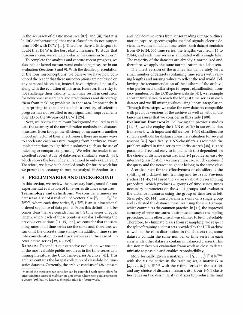
1 2 3 4 5 6

MinkowskiLorentzianManhattan

EDDISSIM

Avg L1/L∞

Figure 2: Ranking of lock-stepmeasures under z-score basedon the average of their ranks across datasets.

1 2 3 4 5

UnitLengthMeanNorm

ED-z-scoreMinMaxz-score

Figure 3: Ranking of normalizationmethods in combinationwith the Lorentzian distance based on the average of theirranks across datasets. ED uses z-score normalization.

from all combinations of distance measures and normaliza-tion methods (52 · 8 = 416 in total), we only report those re-sulting in an average accuracy higher than the one achievedby ED with z-score, the current state-of-the-art lock-stepmeasure. We omit measures achieving the same or worseaverage accuracy than ED. We observe 14 measures withsome improvement in their average accuracy in contrast toED and overall 36 combinations with different normalizationmethods. However, only about half of these combinationsresult in statistically significant differences according to theWilcoxon test. (We perform all pairwise comparisons withWilcoxon to ensure we did not miss any accurate measure.)

In particular, Minkowski distance performs better in termsof average accuracy than all other distance measures, but itis also the only measure that requires tuning, which is notalways desirable. Interestingly, several measures of the L1family, namely, the Lorentzian (i.e., the natural logarithm ofL1), the Manhattan, and the Avg L1/L∞, outperform ED withstatistically significant differences. DISSIM, a measure thatintegrates some form of smoothing of time series, also outper-forms ED significantly. In all of these measures, we observe asimilar trend: all combinations with z-score, UnitLength, andMeanNorm normalizations lead to significant improvements.However, our extensive experimentation reveals three un-knownmeasures in the time-series literature that achieve sta-tistically significant improvement over ED, namely, the Jac-card distance with MeanNorm, the Emanon4 distance withMinMax, and the Soergel distance with MinMax. Interest-ingly, all three distance measures do not show improvementsunder z-score, which shows the importance of consideringdifferent normalizations. Among all methods, MeanNormseems to perform the best. However, the Wilcoxon test sug-gests no statistically significant differences between any ofthe 17 combinations that outperform ED with z-score.To better understand the performance of lock-step mea-

sures, we also evaluate the significance of their differencesin accuracy when considering several distance measurestogether, using the Friedman test followed by a post-hoc

Nemenyi test. Specifically, we perform two analyses: (i) weevaluate different distance measures under the same normal-ization; and (ii) we evaluate standalone distance measuresunder different normalizations; Figure 2 shows the averagerank across all datasets of the distance measures, which un-der z-score normalization, outperformed previously ED. Thethick line connects measures that do not perform statisticallysignificantly better. We observe that Lorentzian is rankedfirst (once we ignore the supervised Minkowski), meaningthat it performed best in the majority of the datasets. All 5measures significantly outperform ED, but we observe nodifference between them. Figure 3 evaluates a standalonedistance measure, the Lorentzian measure that performedthe best previously, with different normalization methodsagainst ED with z-score. We observe that the 3 out of the 4combinations that were better than ED under the Wilcoxontest remain better under this statistical analysis, and there isno difference between them. We omit similar figures for theother measures as we observe the similar trends.Debunking M1 and M2: Our evaluation shows clear ev-idence that normalization methods other than z-score canlead to significant improvements, which debunks M1. Eventhough for standalone measures, we did not observe signif-icant improvements (e.g., ED with MeanNorm vs. ED withz-score), that does not reject our hypothesis. We note thatthe majority of the UCR datasets are in their z-normalizedform and, therefore, for fairness, we z-normalized all datasets,which may have limited this analysis. Despite that, we iden-tified two new distance measures, unknown until now, thatonly under MinMax andMeanNormmethods outperform EDwith z-score and, importantly, z-score is not suitable for them.Normalizations such as MeanNorm, which combines z-scoreand MinMax methods, seems to perform the best for severalmeasures. Similarly, our analysis shows that distance mea-sures other than ED can lead to significant improvements,which debunksM2. We identified 7 distance measures thatsignificantly outperform ED. We emphasize that no previousstudy considered different normalization methods in orderto challengeM1, and our findings contradict both previousstudies [45, 57], which concluded that there is no significantdifference in the accuracy of lock-step measures.

Next, we focus on sliding versions of lock-step measures.

6 TIME-SERIES SLIDING DISTANCESWe study 4 variants of cross-correlation, a measure that haslargely been omitted from distance measure evaluations.Starting with the concurrent introduction of lock-step

and elastic measures for the problem of time-series similar-ity search [2, 18, 51], the vast majority of research focusedon these two categories of measures (see M3 in Section2). Cross-correlation, which is similar to convolution, datesback in the 1700s [47] but received practical popularity only

DistanceMeasure

ScalingMethod Better Average

Accuracy > = <

NCCc(SBD)

z-score ✔ 0.7309 86 9 33MinMax ✔ 0.7186 72 8 48

UnitLength ✔ 0.7309 86 9 33MeanNorm ✔ 0.7309 86 9 33MedianNorm ✘ 0.7050 63 7 58Adaptive ✘ 0.7072 72 8 48Tanh ✘ 0.7077 58 8 62

NCCbz-score ✔ 0.7309 86 9 33

UnitLength ✔ 0.7309 86 9 33

NCC z-score ✔ 0.7309 86 9 33UnitLength ✔ 0.7309 86 9 33

Lorentzian UnitLength - 0.7024 - - -Table 3: Comparison of sliding distance measures. “Scal-ing Method” column indicates the underlying time-seriesnormalization. “Better” column denotes that the distancemeasure outperforms the baseline with statistical signifi-cance. “AverageAccuracy” column shows themean accuracyachieved across 128 datasets. The last three columns indicatethe number of datasets over which a distancemeasure is bet-ter (“>”), equal (“=”), or worse (“<”) than the baseline.

after the invention of Fast Fourier Transform (FFT) [34],which dramatically reduced its computational cost. Cross-correlation is one of the most fundamental operations insignal processing [23] and, lately, in deep neural networks[79, 80]. Recently, research focusing on time-series clusteringused cross-correlation and achieved state-of-the-art perfor-mance for this task [110, 111]. However, this work assumedz-normalized time series and performed evaluations onlyagainst ED and DTW. Next, we present cross-correlation fol-lowing the notation used in [110] in an attempt to establishconsistent terminology with the recent literature.

In simple terms, the cross-correlation measure maximizesthe correlation (or, equivalently, minimizes the ED [103]) be-tween a time-series ®x and all shifted versions of another timeseries ®y. By shifting (or sliding), we refer to an operation,®x(s), that rearranges the data points by moving all points by|s | positions to the right, for s ≥ 0, or left, for s < 0. For ex-ample, ®x(1) moves all data points by one position to the rightand brings the final entry to the first position (or differentlypads the empty positions with zeros; both approaches lead tosimilar measures). When we consider all shifts, s ∈ [−m,m],wherem is the length of both time series (the measure canalso operate with unequal lengths), we produce the cross-correlation sequence,CCw (®x, ®y), withw ∈ {1, 2, . . . , 2m− 1},of length (2m − 1), containing the inner product of the twotime series in every possible shift.

Unfortunately, the computation of CCw (®x, ®y) is expensive,O(m2), but, thankfully, with the use of FFT (F (·)) and its

inverse version (F −1(·)), the cost reduces to O(m · log(m)):

CCw (®x, ®y) = F −1{F (®x) ∗ F (®y)} (10)

Having introduced the necessary notation and consideringpopular normalizations, we can derive the following 4 vari-ants of cross-correlation similarity measures [110]:

NCCq(®x, ®y) =

max(CCw ( ®x , ®y)

m

), q = “b” (NCCb )

max(CCw ( ®x , ®y)m−|w−m |

), q = “u” (NCCu )

max(CCw ( ®x , ®y)| | ®x | | · | | ®y | |

), q = “c” (NCCc )

max(CCw (®x, ®y)), q = “ · ” (NCC)

(11)

known as the normalized cross-correlation (because it as-sumes some underlying time-series normalization), NCC ,the biased estimator, NCCb , the unbiased estimator, NCCu ,and the coefficient normalization or SBD [110], NCCc .Evaluation of sliding measures: Due to the resemblanceof cross-correlation to the sliding version of Pearson’s cor-relation, when time series are z-normalized, the majority ofthe literature assumes this underlying data normalization[110]. To the best of our knowledge, the performance ofcross-correlation as a measure to compare time series underdifferent normalization methods is not well explored. Ta-ble 3 reports the performance of the combinations of cross-correlation variants with normalization methods. Specifi-cally, from 32 such combinations (i.e., 4 measures × 8 nor-malizations), we report only those resulted in an averageaccuracy higher than the one achieved by Lorentzian (withz-score followed by UnitLength, the last row of the Table 3),the new state-of-the-art lock-step distance measure basedon our previous analysis (Section 5). As before, we performall pairwise comparisons using the Wilcoxon statistical testto ensure we did not miss any accurate combination.

We observe that from all 4 cross-correlation measures, theunbiased estimator, NCCu , performs worse than all othervariants. Specifically, no combination of NCCu with any ofthe normalization methods outperforms the Lorentzian dis-tance. In contrast, the remaining 3 variants, NCC , NCCb ,and NCCc , all include combinations that outperform thebaseline. In particular, combinations of NCC and NCCb withz-score and UnitLength normalizations significantly outper-form the baseline. We observe negligible differences betweenthese combinations (i.e., only one dataset is slightly affected).Interestingly, the coefficient normalization variant, NCCc ,outperforms the baseline with 6 combinations of normal-ization methods. However, only half of these combinationsoutperform the Lorentzian distance with a statistically signif-icant difference. In all of these measures, we observe a similartrend: all combinations with z-score and UnitLength normal-ization methods lead to significant improvements. However,for NCCc , another normalization, namely, MeanNorm, also

1 2 3 4 5

NCCc -z-scoreNCCc -UnitLength

Lorentzian-UnitLengthNCCc -MinMax

NCCc -MeanNorm

Figure 4: Ranking of different normalization methods forNCCc based on the average of their ranks across datasets, us-ing Lorentzian with UnitLength as the baseline method.

achieves similar improvement, which is not the case whencombined with NCC and NCCb . Even though NCC , NCCb ,and NCCc perform similarly in terms of average accuracy,NCCc appears to be the most robust cross-correlation mea-sure as it leads to improvement over the baseline with morenormalization methods than the other variants and for threesuch combinations the improvement is statistically signifi-cant. Among all combinations that outperform the baseline,Wilcoxon suggests no statistically significant differences.

In addition to these pairwise comparisons, we also evalu-ate the significance of the differences when considered alltogether. Figure 4 shows the average rank across datasets offive combinations of NCCc with normalization methods (weexcluded Tanh normalization as from Table 3 we observethat, despite the increase in average accuracy, the Lorentziandistance still outperforms this combination in more datasets).Similarly to the pairwise analysis, we observe that combi-nations with z-score, MeanNorm, and UnitLength normal-izations lead to significant improvements according to theFriedman test followed by a post-hoc Nemenyi test to assessthe significance of the differences in the ranking. Combi-nations of NCCc with AdaptiveScaling or MinMax do notachieve significant improvement. We observe that both sta-tistical evaluation approaches lead to similar conclusions.We omit figures for NCC and NCCb with similar findings.

For completeness, we report another analysis using ED asthe baseline instead of the Lorentzian distance (we omit thefigure due to space limitation). NCCc in combination withz-score, UnitLength, and MeanNorm normalization methodsoutperform ED but, in contrast to Figure 4, now combinationswith AdaptiveScaling and MinMax are also significantly bet-ter than ED. This analysis confirms our results in Section5 that the Lorentzian distance (and other L1 variants) aremore powerful than ED. In addition, our analysis indicatesthat NCCc outperforms all lock-step measures with all dif-ferent normalizations, making it a strong baseline methodfor time-series comparison.We now turn our focus to elastic measures and, particu-

larly, to their performance against sliding measures.

7 TIME-SERIES ELASTIC MEASURESIn this section, we study 7 elastic measures, a popular cate-gory of measures for time-series comparison.

DistanceMeasure Parameters

MSM c ∈ {0.01, 0.1, 1, 10, 100, 0.05, 0.5, 5, 50, 500}

DTW δ ∈ {0, 1, 2, 3, 4, 5, 6, 7, 8, 9, 10, 11, 12, 13, 14, 15, 16,17, 18, 19, 20, 100}

EDR ϵ ∈ {0.001, 0.003, 0.005, 0.007, 0.009, 0.01, 0.03, 0.05,0.07, 0.09, 0.1, 0.2, 0.3, 0.4, 0.5, 0.6, 0.7, 0.8, 0.9, 1}

LCSSδ ∈ {5, 10}ϵ ∈ {0.001, 0.003, 0.005, 0.007, 0.009, 0.01, 0.03, 0.05,0.07, 0.09, 0.1, 0.2, 0.3, 0.4, 0.5, 0.6, 0.7, 0.8, 0.9, 1}

TWE λ ∈ {0, 0.25, 0.5, 0.75, 1.0}ν ∈ {0.00001, 0.0001, 0.001, 0.01, 0.1, 1}

Swale ϵ ∈ {0.01, 0.03, 0.05, 0.07, 0.09, 0.1, 0.2, 0.3, 0.4, 0.5,0.6, 0.7, 0.8, 0.9, 1},p ∈ {5}, r ∈ {1}

Minkowski p ∈ {0.1, 0.3, 0.5, 0.7, 0.9, 1, 1.3, 1.5, 1.7, 1.9,2, 3, 5, 7, 9, 11, 13, 15, 17, 20}

KDTW γ ∈ {2−15, 2−14, 2−13, 2−12, 2−11, 2−10, 2−9, 2−8,2−7, 2−6, 2−5, 2−4, 2−3, 2−2, 2−1, 20}

GAK γ ∈ {0.01, 0.05, 0.1, 0.25, 0.5, 0.75, 1, 2, 3, 4,5, 6, 7, 8, 9, 10, 11, 12, 13, 14, 15, 16, 17, 18, 19, 20}

SINK γ ∈ {1, 2, 3, 4, 5, 6, 7, 8, 9, 10, 11, 12, 13, 14, 15, 16,17, 18, 19, 20}

RBF γ ∈ {2−15, 2−14, 2−13, 2−12, 2−11, 2−10, 2−9, 2−8, 2−7,2−6, 2−5, 2−4, 2−3, 2−2, 2−1, 20}

GRAIL γ ∈ {1, 2, 3, 4, 5, 6, 7, 8, 9, 10, 11, 12, 13, 14, 15, 16,17, 18, 19, 20}

RWSγ ∈ {10−3, 3 · 10−3, 10−2, 3 · 10−2, 0.1, 0.14, 0.19,0.28, 0.39, 0.56, 0.79, 1.12, 1.58, 2.23, 3.16, 4.46, 6.30,8.91, 10, 31.62, 102, 3 · 102, 103}, Dmax = 25

SIDL λ ∈ {0.1, 1, 10}, r ∈ {0.1, 0.25, 0.5}Table 4: Parameter choices for distance measures..

As discussed earlier, sliding measures find a global align-ment by sliding one time series against the other. In contrast,elastic measures create a non-linear mapping between time-series data points to support flexible alignment of differentregions. Through this mapping, elastic measures permit timeseries to “stretch” or “shrink” their observations to improvetime-series matching. Most elastic measures rely on dynamicprogramming to find this mapping efficiently by definingrecursive formulas over am-by-m matrixM that contains ineach cell the ED (or some other lock-step measure) betweenevery point of one time series against every point of anothertime series. In general, the goal of different elastic measuresin the literature is to employ different strategies to find awarping path,W = {w1, . . . ,wk }, with k ≥ m, a contiguousset of matrix cells that shows the mapping of every pointof one time series to one, more, or none of the points of theother time series. To improve the efficiency and the accuracyof elastic measures, it is a common practice to introduceconstraints (in the form of parameters) to guide the warpingpath to visit only a subset of cells inM or to determine abovewhich distance threshold two points should match.

DistanceMeasure

ParameterTuning Better Average

Accuracy > = <

MSM LOOCCV ✔ 0.7628 86 3 39c = 0.5 ✔ 0.7627 89 2 37

TWE LOOCCV ✔ 0.7632 85 4 39λ=1,ν =0.0001 ✔ 0.7622 89 4 35

DTWLOOC ✔ 0.7519 75 16 37δ = 100 ✘ 0.7248 54 10 64δ = 10 ✘ 0.7372 64 6 58

EDR LOOCCV ✔ 0.7485 74 8 46ϵ = 0.1 ✘ 0.7202 62 5 61

Swale LOOCCV ✔ 0.7499 72 8 48ϵ = 0.2 ✘ 0.7229 63 4 61

ERP - ✔ 0.7488 77 5 46

LCSS LOOCCV ✘ 0.7398 66 6 56δ = 5, ϵ = 0.2 ✘ 0.7160 63 2 63

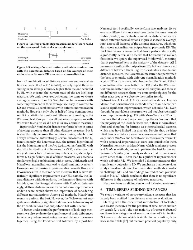
NCCc - - 0.7309 - - -Table 5: Comparison of elastic measures against NCCc . “Pa-rameter Tuning” indicates supervised or unsupervised tun-ing. “Better” denotes that themeasure outperforms the base-line with statistical significance. “Average Accuracy” showsthe mean accuracy achieved across 128 datasets. The lastthree columns indicate the datasets over which a measureis better (“>”), equal (“=”), or worse (“<”) than the baseline.

The first elastic measure, DTW [126, 127], was proposed asa speech recognition tool and, later, it was introduced in thetime-series literature as a suitable approach for time-seriescomparison [18]. DTW finds the warping path that mini-mizes the distances between all data points. In the originalform, DTW is parameter-free, however, many approacheshave been proposed to define bands (i.e., the shape of thesubset cells of matrixM that the warping path is permitted tovisit) and the width or window (i.e., size) of the bands. We usethe Sakoe-Chiba band [127], which is the most frequentlyused in practice [45], and we tune the window δ using pa-rameters shown in Table 4. For example, a value δ = 10indicates a window size 10% of the time-series length.

The Longest Common Subsequence (LCSS) distance is an-other type of elastic measure that was derived from the ideaof edit-distances for characters. Specifically, LCSS introducesa parameter ϵ that serves as a threshold to determine whentwo points of time series should match [7, 141]. Similarlyto DTW, LCSS also constrains the warping window by in-troducing an additional parameter δ [141]. Edit Distance onReal sequence (EDR) distance [28] is another edit-distance-based measure that similarly to LCSS, uses a parameter ϵ toquantify the distance of points as 0 or 1. EDR also introducespenalties for gaps between matched subsequences. Edit Dis-tance with Real Penalty (ERP) distance [27] is a measure thatbridges DTW and EDR distance measures by more carefullycomputing the distance between gaps of time series.

Differently than the previous approaches, the SequenceWeighted Alignment model (Swale) [100] proposes a modelto compute the similarity of time series using rewards formatching points and penalties for gaps. Apart from a thresh-old ϵ parameter, Swale also requires parameters for the re-ward r and the penalty p. The Move–split–merge (MSM) dis-tance [137] is another elastic measure based on edit-distancebut in contrast to DTW, LCSS, and EDR, MSM is a metric.MSM uses a set of operations to replace, insert, or delete val-ues in time series to improve their matching. Finally, TimeWarp Edit (TWE) distance [92] is a measure that combinesmerits from LCSS and DTW. TWE introduces a stiffness pa-rameter ν to control the warping but at the same point italso penalizes matched points (parameter λ).

For each one of these 7 elastic measures, several variantsand extensions have been proposed in the literature. For ex-ample, Derivative DTW (DDTW) [60] combines raw timeseries with their first-order differences (derivatives). Com-plexity Invariant distance (CID) [16] is a weighting schemeto compensate for differences in the complexity of two timeseries. Finally, Weighted DTW (WDTW) [68] adds a penaltyto the warping path of DTW. All of these approaches describeextensions that can potentially be used in combination withall previously described elastic measures. Importantly, eachof these extensions often introduces additional parametersthat require tuning. To avoid an explosion of evaluated ap-proaches, we do not include such variants in our analysis.An excellent recent study [11] focusing on time-series classi-fication has evaluated several of these approaches (and didnot identify significant improvements from their use).Evaluation of elastic vs. sliding measures: With the in-troduction of the 7 elastic measures we are now in posi-tion to evaluate their performance against sliding measures,an experiment that has been omitted in all previous stud-ies [11, 45]. Table 5 compares the classification accuracy ofelastic measures against the accuracy of NCCc , the state-of-the-art sliding measure based on our previous experimentin Section 6. As we did not observe significant differencesfrom using different normalization methods for NCCc , for allsubsequent experiments we always use z-normalized timeseries. We also do that so that our results are closely compa-rable to those reported previously [45, 144]. Table 5 includestwo experimental settings, one supervised and one unsuper-vised. In the supervised setting, the necessary parametersof the elastic measures are tuned on the training set usingcross-validation with a leave-one-out-classifier (LOOCCV),as noted in Section 3. In the unsupervised setting, we con-sult the parameters selected through LOOCCV to identifya set of parameters that perform well on average across alldatasets. This step involves several trial-and-error attemptsand a post-hoc analysis of the results (i.e., we observe the

1 2 3 4 5 6 7 8

MSMTWEDTWEDR

NCCcLCSSERPSwale

Figure 5: Ranking of elastic and sliding distance measuresbased on the average of their ranks across datasets, usingsupervised tuning for their parameters.

1 2 3 4 5 6 7 8 9

MSMTWEERP

DTW-10

EDRLCSS

DTW-100NCCcSwale

Figure 6: Ranking of elastic and sliding distance measuresbased on the average of their ranks across datasets, usingunsupervised tuning for their parameters.

accuracy on the test sets). Even though this is an unfair ad-vantage against parameter-free approaches, such as NCCc ,we perform this post-hoc analysis to ensure that elastic mea-sures are not misrepresented in such unsupervised scenarioand that a domain expert could potentially identify suchparameters without supervised tuning. For some measures,such as DTW, that was an easy step, however, for others, wehad to perform multiple attempts to identify parameters thatachieve a competitive accuracy on average.From Table 5, we observe that when parameters are se-

lected under supervised settings (lines with LOOCCV tuning)all elastic measures significantly outperform NCCc with oneexception, the LCSS measure, which marginally outperformsNCCc but the difference is not statistically significant ac-cording to Wilcoxon. However, the picture is different forthe unsupervised scenario. Specifically, we observe that 4out of the 7 elastic measures do not outperform NCCc . In-terestingly, LCSS, EDR, and DTW (with δ = 100, whichresembles an equivalent parameter-free measure to NCCc )are slightly worse. MSM, TWE, and ERP on the other side sig-nificantly outperform NCCc in the unsupervised setting aswell. Among all elastic measures, ERP is the only parameter-free measure that achieves significantly better accuracy thanNCCc in both supervised and unsupervised settings.

To better understand the performance of elastic measuresagainst NCCc , in addition to all previous pairwise statisticalcomparisons, we also evaluate the significance of the dif-ferences when considered all together. Specifically, Figure 5shows the average ranks of the elastic measures in the su-pervised setting and Figure 6 shows the average ranks in theunsupervised setting. The ranking of measures in Figure 5contradicts some of the pairwise results observed in Table 5.

Specifically, we observe that even under supervised settings,4 out of the 7 elastic measures, namely, LCSS, ERP, EDR, andSwale, do not achieve significantly better performance thanNCCc . The results for MSM, TWE, and DTW, are consistentin both statistical evaluations. For the unsupervised setting,both statistical evaluation approaches agree to an extent. Inparticular, Figure 6 shows clearly that MSM and TWE out-perform NCCc . However, the remaining 5 elastic measuresperform similarity to NCCc . Interestingly, as we observed inTable 5, NCCc slightly outperforms 3 elastic measures.

To validate our findings, we repeat the analysis (we omitfigures due to space limitation) and evaluate the significanceof the differences when we consider all elastic measures to-gether (i.e., excluding NCCc ). Specifically, we observe thatSwale, ERP, EDR, and LCSS do not outperform DTW-10 withstatistically significant difference. Interestingly, the super-vised LCSS is slightly worse than the unsupervised DTW-10.ERP, which under pairwise evaluation appears to signifi-cantly outperform DTW-10, when all measures are consid-ered together, both appear to achieve comparable perfor-mance. MSM, TWE, and DTW also perform similarly andall three supervised measures outperform DTW-10. How-ever, under unsupervised settings, we observe that MSMand TWE significantly outperform all other elastic measures.Debunking M3 and M4: Our comprehensive evaluationshows clear evidence that sliding measures are strong base-lines that most elastic measures do notmanage to outperformeither in supervised or unsupervised settings, which debunksM3. Specifically, from all 5 elastic measures evaluated in thedecade-old study [45], namely, LCSS, Swale, EDR, ERP, andDTW, only DTW significantly outperforms cross-correlationunder the supervised scenario. In the unsupervised setting,none of the 5 measures outperforms cross-correlation and,interestingly, several of them perform slightly worse. Thisis a remarkable finding, showing that the simplest type ofalignment between time series is very effective and it shouldhave served as a baseline method for elastic measures. OnlyMSM and TWE, two measures that appeared after [45] showpromising results and outperform cross-correlation with sta-tistically significant differences in both supervised and unsu-pervised settings. Importantly, MSM is the only method thatsignificantly outperforms DTW under supervised settings(according to Wilcoxon) and, under unsupervised settings,both MSM and TWE significantly outperform DTW (withboth statistical tests validating this result). Therefore, thereis clear evidence that the widely popular DTW is no longerthe best elastic distance measure, which debunks M4.

8 TIME-SERIES KERNEL MEASURESUntil now, our analysis focused on three categories of dis-tance measures, namely, lock-step, sliding, and elastic mea-sures, with the goal to provide answers to the four-long

DistanceMeasure


Accuracy > = <

KDTW LOOCCV ✔ 0.7668 89 7 32γ = 0.125 ✔ 0.7501 85 7 36

GAK LOOCCV ✔ 0.7474 79 9 40γ =0.1 ✔ 0.7387 72 10 46

SINK LOOCCV ✔ 0.7469 69 13 46γ = 5 ✘ 0.7396 58 11 59

RBF LOOCCV ✪ 0.6869 20 29 79γ = 2 ✪ 0.6613 13 29 86

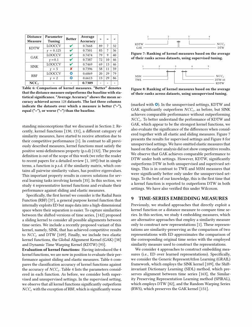
NCCc - - 0.7309 - - -Table 6: Comparison of kernel measures. “Better” denotesthat the distancemeasure outperforms the baselinewith sta-tistical significance. “Average Accuracy” shows the mean ac-curacy achieved across 128 datasets. The last three columnsindicate the datasets over which a measure is better (“>”),equal (“=”), or worse (“<”) than the baseline.

standing misconceptions that we discussed in Section 2. Re-cently, kernel functions [130, 131], a different category ofsimilarity measures, have started to receive attention due totheir competitive performance [1]. In contrast to all previ-ously described measures, kernel functions must satisfy thepositive semi-definiteness property (p.s.d) [132]. The precisedefinition is out of the scope of this work (we refer the readerto recent papers for a detailed review [1, 109]) but in simpleterms, a function is p.s.d. if the similarity matrix, which con-tains all pairwise similarity values, has positive eigenvalues.This important property results in convex solutions for sev-eral learning tasks involving kernels [35]. In this section, westudy 4 representative kernel functions and evaluate theirperformance against sliding and elastic measures.

Specifically, the first kernel we consider is the Radial BasisFunction (RBF) [37], a general purpose kernel function thatinternally exploits ED but maps data into a high-dimensionalspace where their separation is easier. To capture similaritiesbetween the shifted versions of time series, [142] proposeda sliding kernel to consider all possible alignments betweentime-series. We include a recently proposed variant of thiskernel, namely, SINK, that has achieved competitive resultsto NCCc and DTW [109]. Finally, we include two elastickernel functions, the Global Alignment Kernel (GAK) [38]and Dynamic Time Warping Kernel (KDTW) [93].Evaluation of kernel functions: Having introduced the 4kernel functions, we are now in position to evaluate their per-formance against sliding and elastic measures. Table 6 com-pares the classification accuracy of kernel functions againstthe accuracy of NCCc . Table 4 lists the parameters consid-ered in each function. As before, we consider both super-vised and unsupervised settings. In the supervised setting,we observe that all kernel functions significantly outperformNCCc with the exception of RBF, which is significantly worse

1 2 3 4

KDTWGAK

NCCcDTW

Figure 7: Ranking of kernel measures based on the averageof their ranks across datasets, using supervised tuning.

1 2 3 4 5

MSMTWE

NCCcDTW-10KDTW

Figure 8: Ranking of kernel measures based on the averageof their ranks across datasets, using unsupervised tuning.

(marked with ✪). In the unsupervised settings, KDTW andGAK significantly outperform NCCc , as before, but SINKachieves comparable performance without outperformingNCCc . To better understand the performance of KDTW andGAK, which appear to be the strongest kernel functions, wealso evaluate the significance of the differences when consid-ered together with all elastic and sliding measures. Figure 7presents the results for supervised settings and Figure 8 forunsupervised settings.We have omitted elastic measures thatbased on the earlier analysis did not show competitive results.We observe that GAK achieves comparable performance toDTW under both settings. However, KDTW, significantlyoutperforms DTW in both unsupervised and superivsed set-tings. This is in contrast to TWE and MSM measures thatwere significantly better only under the unsupervised set-tings. To the best of our knowledge, this is the first time thata kernel function is reported to outperform DTW in bothsettings. We have also verified this under Wilcoxon.

9 TIME-SERIES EMBEDDING MEASURESPreviously, we studied approaches that directly exploit akernel function or a distance measure to compare time se-ries. In this section, we study 4 embedding measures, whichare alternative approaches that employ a similarity measureonly to construct new representations [1]. These represen-tations are similarity-preserving as the comparison of tworepresentations with ED approximates the comparison ofthe corresponding original time series with the employedsimilarity measure used to construct the representations.We consider 4 approaches to construct embedding mea-

sures (i.e., ED over learned representations). Specifically,we consider the Generic RepresentAtIon Learning (GRAIL)framework, which employs the SINK kernel [109], the Shift-invariant Dictionary Learning (SIDL) method, which pre-serves alignment between time series [163], the Similar-ity Preserving Representation Learning method (SPIRAL),which employs DTW [82], and the Random Warping Series(RWS), which preserves the GAK kernel [151].

DistanceMeasure


Accuracy > = <

GRAIL LOOCCV ✘ 0.7407 56 8 64RWS LOOCCV ✪ 0.7128 45 3 80

SPIRAL - ✪ 0.6494 26 4 98SIDL LOOCCV ✪ 0.5759 12 1 115NCCc - - 0.7309 - - -

Table 7: Comparison of embedding measures. “Better” de-notes that the distance measure outperforms the baselinewith statistical significance. “Average Accuracy” shows themean accuracy achieved across 128 datasets. The last threecolumns indicate the datasets over which a measure is bet-ter (“>”), equal (“=”), or worse (“<”) than the baseline.

Evaluation of embedding measures: For all approaches,we follow [109] and tune required parameters using therecommended values from their corresponding papers. Weconstruct representations of same length (100) for fairness.Table 7 presents the results against NCCc . We observe thatGRAIL, is the only framework that constructs robust repre-sentations that when ED is used for comparison (under the1-NN settings), it achieves similar performance to NCCc , butwithout significant difference. All other embedding measuresperform significantly worse (marked with ✪) and none ofthe embedding measures outperform DTW. We note, how-ever, that embedding measures (as well as kernel methods),achieve much higher accuracy under different evaluationframeworks (e.g., with SVM classifiers), as shown in [109].We leave such extensive analysis for future work.

10 ACCURACY-TO-RUNTIME ANALYSISUntil now, we performed an extensive evaluation of distancemeasures based on their accuracy results. However, it is alsoimportant to understand the cost associated with each oneof these distance measures. In Figure 9, we summarize theaccuracy-to-runtime performance of the most prominentmeasures. The runtime performance includes only inferencetime (i.e., evaluation on the testing sets). We observe thatED, and all lock-step measures (omitted), are the fastest, butachieve relatively low accuracy (all these measures haveO(m) runtime cost). NCCc and SINK, two methods that relyon the classic cross-correlation measure, provide a goodtrade-off between runtime and accuracy in comparison to ED(these measures have O(m logm) runtime cost). We observethat all other elastic or kernel methods require substantiallyhigher runtime cost to achieve comparable accuracy resultsto NCCc (these measures have O(m2) runtime cost). We alsoobserve that embedding measures show promise as they canbe both efficient and accurate. We note that for elastic mea-sures, the runtime cost can be substantially improved withthe use of lower bounding measures (i.e., efficient measuresto prune the expensive pairwise comparisons). To the best

103 104 105 106

Cumulative inference runtime cost (in seconds) for 128 datasets

0.60

0.65

0.70

0.75

Ave

rage

accu

racy

acro

ss12

8da

tase

ts

ED

NCCc

MSMEDRERP

Swale

LCSS

TWEDTW KDTW

GAKSINK

GRAIL

RWS

SPIRAL

SIDL

Lock-step

Sliding

Elastic

Kernel

Embedding

Figure 9: Accuracy-to-runtime comparison.

0 500 1000 1500 2000 2500 3000 3500

Training instances on FordA

0.0

0.2

0.4

0.6

0.8

1.0

Err

orra

te(1

-NN

clas

sifie

r)

0 200 400 600 800 1000

Training instances on StarLightCurves

ED

NCCc

DTW

MSM

EDR

ERP

LCSS

TWE

Swale

SINK

GAK

KDTW

0 500 1000 1500 2000

Training instances on CBF

0.0

0.2

0.4

0.6

0.8

1.0

Err

orra

te(1

-NN

clas

sifie

r)

0 2000 4000 6000 8000

Training instances on ElectricDevices

Figure 10: Error rates with increasingly larger datasets.

of our knowledge, for NCCc and the kernel methods, nolower bounding measures exist and, therefore, we leave suchextensive runtime analysis for future work. Finally, Figure10 suggests that with increasingly larger dataset sizes theclassification error of ED may not always converge to theerror of more accurate measures, at least not always with thesame speed of convergence, which highlights the importanceof considering measures other than ED (see Section 2).

11 CONCLUSIONWe presented a comprehensive evaluation to validate theperformance of 71 distance measures. Our study not only de-bunked four long-standing misconceptions in the time-seriesliterature but also established new state-of-the-art results forlock-step, sliding, elastic, kernel, and embedding measures.Our findings prepare the ground to facilitate further devel-opment of distance measures with implications to virtuallyevery task. With the new knowledge in place, several newchallenges open that we hope to sparkle new research direc-tions. For example, identifying more accurate normalizationswill result in substantial improvement for many tasks. Thereis a lack of methods for unsupervised tuning of parameters.Finally, embedding measures might show the most promiseconsidering their runtime-to-accuracy trade-off.Acknowledgments: We thank the anonymous reviewers whose comments havegreatly improved thismanuscript.We also thank Themis Palpanas and EamonnKeoghfor useful discussions after acceptance. This research was supported in part by aGoogle DAPA Research Award, gifts from NetApp, Cisco Systems, and Exelon Util-ities, and an NSF Award CCF-1139158. Results presented in this paper were obtainedusing the Chameleon testbed supported by the National Science Foundation.

REFERENCES[1] Amaia Abanda, Usue Mori, and Jose A Lozano. 2019. A review on

distance based time series classification. Data Mining and KnowledgeDiscovery 33, 2 (2019), 378–412.

[2] Rakesh Agrawal, Christos Faloutsos, and Arun N. Swami. 1993. Effi-cient Similarity Search In Sequence Databases. In FODO. 69–84.

[3] Rakesh Agrawal, King-Ip Lin, Harpreet S. Sawhney, and KyuseokShim. 1995. Fast similarity search in the presence of noise, scaling,and translation in time-series databases. In Proceeding of the 21thInternational Conference on Very Large Data Bases. Citeseer, 490–501.

[4] Shadab Alam, Franco D Albareti, Carlos Allende Prieto, FriedrichAnders, Scott F Anderson, Timothy Anderton, Brett H Andrews, EricArmengaud, Éric Aubourg, Stephen Bailey, et al. 2015. The eleventhand twelfth data releases of the Sloan Digital Sky Survey: final datafrom SDSS-III. The Astrophysical Journal Supplement Series 219, 1(2015), 12.

[5] Jonathan Alon, Stan Sclaroff, George Kollios, and Vladimir Pavlovic.2003. Discovering clusters in motion time-series data. In CVPR. 375–381.

[6] Francisco Martinez Alvarez, Alicia Troncoso, Jose C Riquelme, andJesus S Aguilar Ruiz. 2010. Energy time series forecasting based onpattern sequence similarity. IEEE Transactions on Knowledge and DataEngineering 23, 8 (2010), 1230–1243.

[7] Henrik André-Jönsson and Dushan Z Badal. 1997. Using signaturefiles for querying time-series data. In European Symposium on Princi-ples of Data Mining and Knowledge Discovery. Springer, 211–220.

[8] Johannes Aßfalg, Hans-Peter Kriegel, Peer Kröger, Peter Kunath,Alexey Pryakhin, and Matthias Renz. 2006. Similarity search ontime series based on threshold queries. In International Conference onExtending Database Technology. Springer, 276–294.

[9] Martin Bach-Andersen, Bo Rømer-Odgaard, and Ole Winther. 2017.Flexible non-linear predictive models for large-scale wind turbinediagnostics. Wind Energy 20, 5 (2017), 753–764.

[10] Anthony Bagnall, Hoang Anh Dau, Jason Lines, Michael Flynn, JamesLarge, Aaron Bostrom, Paul Southam, and Eamonn Keogh. 2018.The UEA multivariate time series classification archive, 2018. arXivpreprint arXiv:1811.00075 (2018).

[11] Anthony Bagnall, Jason Lines, Aaron Bostrom, James Large, andEamonn Keogh. 2017. The great time series classification bake off: areview and experimental evaluation of recent algorithmic advances.Data Mining and Knowledge Discovery 31, 3 (2017), 606–660.

[12] Anthony J Bagnall and Gareth J Janacek. 2004. Clustering time seriesfrom ARMA models with clipped data. In KDD. 49–58.

[13] Ziv Bar-Joseph. 2004. Analyzing time series gene expression data.Bioinformatics 20, 16 (2004), 2493–2503.

[14] Ziv Bar-Joseph, Georg K Gerber, David K Gifford, Tommi S Jaakkola,and Itamar Simon. 2003. Continuous representations of time-seriesgene expression data. Journal of Computational Biology 10, 3-4 (2003),341–356.

[15] Ziv Bar-Joseph, Anthony Gitter, and Itamar Simon. 2012. Studyingand modelling dynamic biological processes using time-series geneexpression data. Nature Reviews Genetics 13, 8 (2012), 552.

[16] Gustavo EAPA Batista, Eamonn J Keogh, Oben Moses Tataw, andVinicius MA De Souza. 2014. CID: an efficient complexity-invariantdistance for time series. Data Mining and Knowledge Discovery 28, 3(2014), 634–669.

[17] Nurjahan Begum and Eamonn Keogh. 2014. Rare time series motif dis-covery from unbounded streams. Proceedings of the VLDB Endowment8, 2 (2014), 149–160.

[18] Donald J Berndt and James Clifford. 1994. Using Dynamic TimeWarping to Find Patterns in Time Series.. In AAAI Workshop on KDD.359–370.

[19] Bharat B Biswal, Maarten Mennes, Xi-Nian Zuo, Suril Gohel, ClareKelly, Steve M Smith, Christian F Beckmann, Jonathan S Adelstein,Randy L Buckner, Stan Colcombe, et al. 2010. Toward discoveryscience of human brain function. Proceedings of the National Academyof Sciences 107, 10 (2010), 4734–4739.

[20] R Bracewell. 1965. Pentagram notation for cross correlation. TheFourier transform and its applications. New York: McGraw-Hill 46(1965), 243.

[21] Markus M Breunig, Hans-Peter Kriegel, Raymond T Ng, and JörgSander. 2000. LOF: identifying density-based local outliers. In ACMsigmod record, Vol. 29. ACM, 93–104.

[22] Peter J Brockwell and Richard A Davis. 2016. Introduction to timeseries and forecasting. springer.

[23] Lisa Gottesfeld Brown. 1992. A survey of image registration tech-niques. ACM computing surveys (CSUR) 24, 4 (1992), 325–376.

[24] Yuhan Cai and Raymond Ng. 2004. Indexing spatio-temporal trajec-tories with Chebyshev polynomials. In SIGMOD. 599–610.

[25] Alessandro Camerra, Themis Palpanas, Jin Shieh, and Eamonn Keogh.2010. iSAX 2.0: Indexing and mining one billion time series. In 2010IEEE International Conference on Data Mining. IEEE, 58–67.

[26] Sung-Hyuk Cha. 2007. Comprehensive survey on distance/similaritymeasures between probability density functions. City 1, 2 (2007), 1.

[27] Lei Chen and Raymond Ng. 2004. On the marriage of Lp-norms andedit distance. In VLDB. 792–803.

[28] Lei Chen, M Tamer Özsu, and Vincent Oria. 2005. Robust and fastsimilarity search for moving object trajectories. In SIGMOD. 491–502.

[29] Qiuxia Chen, Lei Chen, Xiang Lian, Yunhao Liu, and Jeffrey Xu Yu.2007. Indexable PLA for efficient similarity search. In VLDB. 435–446.

[30] Yueguo Chen, Mario A Nascimento, Beng Chin Ooi, and Anthony KHTung. 2007. Spade: On shape-based pattern detection in streamingtime series. In ICDE. 786–795.

[31] Bill Chiu, Eamonn Keogh, and Stefano Lonardi. 2003. Probabilisticdiscovery of time series motifs. In Proceedings of the ninth ACMSIGKDD international conference on Knowledge discovery and datamining. ACM, 493–498.

[32] Kelvin Kam Wing Chu and Man Hon Wong. 1999. Fast time-seriessearching with scaling and shifting. In Proceedings of the eighteenthACM SIGMOD-SIGACT-SIGART symposium on Principles of databasesystems. Citeseer, 237–248.

[33] Richard Cole, Dennis Shasha, and Xiaojian Zhao. 2005. Fast windowcorrelations over uncooperative time series. In Proceedings of theeleventh ACM SIGKDD international conference on Knowledge discov-ery in data mining. ACM, 743–749.

[34] James W Cooley and John W Tukey. 1965. An algorithm for themachine calculation of complex Fourier series. Math. Comp. 19, 90(1965), 297–301.

[35] Corinna Cortes and Vladimir Vapnik. 1995. Support-vector networks.Machine learning 20, 3 (1995), 273–297.

[36] Madalena Costa, Ary L Goldberger, and C-K Peng. 2002. Multiscaleentropy analysis of complex physiologic time series. Physical reviewletters 89, 6 (2002), 068102.

[37] Nello Cristianini and John Shawe-Taylor. 2000. An introduction tosupport vector machines and other kernel-based learning methods. Cam-bridge university press.

[38] Marco Cuturi. 2011. Fast global alignment kernels. In Proceedingsof the 28th international conference on machine learning (ICML-11).929–936.

[39] Michele Dallachiesa, Besmira Nushi, Katsiaryna Mirylenka, andThemis Palpanas. 2012. Uncertain time-series similarity: Return to thebasics. Proceedings of the VLDB Endowment 5, 11 (2012), 1662–1673.

[40] Michele Dallachiesa, Themis Palpanas, and Ihab F Ilyas. 2014. Top-knearest neighbor search in uncertain data series. Proceedings of the

VLDB Endowment 8, 1 (2014), 13–24.[41] Hoang Anh Dau, Eamonn Keogh, Kaveh Kamgar, Chin-Chia Michael

Yeh, Yan Zhu, Shaghayegh Gharghabi, Chotirat Ann Ratanamahatana,Yanping, Bing Hu, Nurjahan Begum, Anthony Bagnall, AbdullahMueen, Gustavo Batista, and Hexagon-ML. 2018. The UCR TimeSeries Classification Archive. https://www.cs.ucr.edu/~eamonn/time_series_data_2018/.

[42] Janez Demšar. 2006. Statistical comparisons of classifiers over mul-tiple data sets. The Journal of Machine Learning Research 7 (2006),1–30.

[43] Michel-Marie Deza and Elena Deza. 2006. Dictionary of distances.Elsevier.

[44] Michel Marie Deza and Elena Deza. 2009. Encyclopedia of distances.In Encyclopedia of distances. Springer, 1–583.

[45] Hui Ding, Goce Trajcevski, Peter Scheuermann, Xiaoyue Wang, andEamonn Keogh. 2008. Querying and mining of time series data:experimental comparison of representations and distance measures.Proceedings of the VLDB Endowment 1, 2 (2008), 1542–1552.

[46] Rui Ding, Qiang Wang, Yingnong Dang, Qiang Fu, Haidong Zhang,and Dongmei Zhang. 2015. Yading: Fast clustering of large-scale timeseries data. Proceedings of the VLDB Endowment 8, 5 (2015), 473–484.

[47] Alejandro Domínguez. 2015. A history of the convolution operation[Retrospectroscope]. IEEE pulse 6, 1 (2015), 38–49.

[48] Karima Echihabi, Kostas Zoumpatianos, Themis Palpanas, and HoudaBenbrahim. 2018. The lernaean hydra of data series similarity search:An experimental evaluation of the state of the art. Proceedings of theVLDB Endowment 12, 2 (2018), 112–127.

[49] Jason Ernst and Ziv Bar-Joseph. 2006. STEM: a tool for the analysisof short time series gene expression data. BMC bioinformatics 7, 1(2006), 191.

[50] Philippe Esling and Carlos Agon. 2012. Time-series data mining.ACM Computing Surveys (CSUR) 45, 1 (2012), 12.

[51] Christos Faloutsos, M. Ranganathan, and Yannis Manolopoulos. 1994.Fast Subsequence Matching in Time-series Databases. In SIGMOD.419–429.

[52] Manuel Fernández-Delgado, Eva Cernadas, Senén Barro, and DinaniAmorim. 2014. Do we need hundreds of classifiers to solve real worldclassification problems? The journal of machine learning research 15,1 (2014), 3133–3181.

[53] Elias Frentzos, Kostas Gratsias, and Yannis Theodoridis. 2007. Index-based most similar trajectory search. In ICDE. 816–825.

[54] Milton Friedman. 1937. The use of ranks to avoid the assumption ofnormality implicit in the analysis of variance. J. Amer. Statist. Assoc.32 (1937), 675–701.

[55] Daniel G Gavin, W Wyatt Oswald, Eugene R Wahl, and John WWilliams. 2003. A statistical approach to evaluating distance metricsand analog assignments for pollen records. Quaternary Research 60,3 (2003), 356–367.

[56] Martin Gavrilov, Dragomir Anguelov, Piotr Indyk, and Rajeev Mot-wani. 2000. Mining the stock market: Which measure is best. In Proc.of the 6th ACM SIGKDD. 487–496.

[57] Rafael Giusti and Gustavo EAPA Batista. 2013. An Empirical Com-parison of Dissimilarity Measures for Time Series Classification. InBRACIS. 82–88.

[58] Steve Goddard, Sherri K Harms, Stephen E Reichenbach, TsegayeTadesse, and William J Waltman. 2003. Geospatial decision supportfor drought risk management. Commun. ACM 46, 1 (2003), 35–37.

[59] Dina Q Goldin and Paris C Kanellakis. 1995. On similarity queriesfor time-series data: constraint specification and implementation.In International Conference on Principles and Practice of ConstraintProgramming. Springer, 137–153.

[60] Tomasz Górecki and Maciej Łuczak. 2013. Using derivatives in timeseries classification. Data Mining and Knowledge Discovery 26, 2

(2013), 310–331.[61] Aditya Grover, Ashish Kapoor, and Eric Horvitz. 2015. A deep hybrid

model for weather forecasting. In Proceedings of the 21th ACM SIGKDDInternational Conference on Knowledge Discovery and Data Mining.ACM, 379–386.

[62] Joel Grus. 2019. Data science from scratch: first principles with python.O’Reilly Media.

[63] Jon Hills, Jason Lines, Edgaras Baranauskas, James Mapp, and An-thony Bagnall. 2014. Classification of time series by shapelet transfor-mation. Data Mining and Knowledge Discovery 28, 4 (2014), 851–881.

[64] Ove Hoegh-Guldberg, Peter J Mumby, Anthony J Hooten, Robert SSteneck, Paul Greenfield, Edgardo Gomez, C Drew Harvell, Peter FSale, Alasdair J Edwards, Ken Caldeira, et al. 2007. Coral reefs underrapid climate change and ocean acidification. science 318, 5857 (2007),1737–1742.

[65] Rie Honda, Shuai Wang, Tokio Kikuchi, and Osamu Konishi. 2002.Mining of moving objects from time-series images and its applicationto satellite weather imagery. Journal of Intelligent Information Systems19, 1 (2002), 79–93.

[66] Bing Hu, Yanping Chen, and Eamonn Keogh. 2013. Time SeriesClassification under More Realistic Assumptions. In SDM. 578–586.

[67] Pablo Huijse, Pablo A Estevez, Pavlos Protopapas, Jose C Principe,and Pablo Zegers. 2014. Computational intelligence challenges andapplications on large-scale astronomical time series databases. IEEEComputational Intelligence Magazine 9, 3 (2014), 27–39.

[68] Young-Seon Jeong, Myong K Jeong, and Olufemi A Omitaomu. 2011.Weighted dynamic time warping for time series classification. PatternRecognition 44, 9 (2011), 2231–2240.

[69] Konstantinos Kalpakis, Dhiral Gada, and Vasundhara Puttagunta.2001. Distance measures for effective clustering of ARIMA time-series. In ICDM. 273–280.

[70] Kunio Kashino, Gavin Smith, and Hiroshi Murase. 1999. Time-seriesactive search for quick retrieval of audio and video. In 1999 IEEEInternational Conference on Acoustics, Speech, and Signal Processing.Proceedings. ICASSP99 (Cat. No. 99CH36258), Vol. 6. IEEE, 2993–2996.

[71] Shrikant Kashyap and Panagiotis Karras. 2011. Scalable knn search onvertically stored time series. In Proceedings of the 17th ACM SIGKDDinternational conference on Knowledge discovery and data mining.ACM, 1334–1342.

[72] Eamonn Keogh. 2006. A decade of progress in indexing and mininglarge time series databases. In VLDB. 1268–1268.

[73] Eamonn Keogh, Kaushik Chakrabarti, Michael Pazzani, and SharadMehrotra. 2001. Locally Adaptive Dimensionality Reduction forIndexing Large Time Series Databases. In SIGMOD. 151–162.

[74] Eamonn Keogh and Jessica Lin. 2005. Clustering of time-series subse-quences is meaningless: Implications for previous and future research.Knowledge and Information Systems 8, 2 (2005), 154–177.

[75] Eamonn Keogh and Chotirat Ann Ratanamahatana. 2005. Exact in-dexing of dynamic time warping. Knowledge and Information Systems7, 3 (2005), 358–386.

[76] Chan Kin-pong and Fu Ada. 1999. Efficient Time Series Matching byWavelets. In ICDE. 126–133.

[77] S Knieling, J Niediek, E Kutter, J Bostroem, CE Elger, and F Mormann.2017. An online adaptive screening procedure for selective neuronalresponses. Journal of neuroscience methods 291 (2017), 36–42.

[78] Flip Korn, H. V. Jagadish, and Christos Faloutsos. 1997. EfficientlySupporting Ad Hoc Queries in Large Datasets of Time Sequences. InSIGMOD. 289–300.

[79] Yann LeCun, Yoshua Bengio, et al. 1995. Convolutional networks forimages, speech, and time series. The handbook of brain theory andneural networks 3361, 10 (1995), 1995.

https://www.cs.ucr.edu/~eamonn/time_series_data_2018/

https://www.cs.ucr.edu/~eamonn/time_series_data_2018/

[80] Yann LeCun, Yoshua Bengio, and Geoffrey Hinton. 2015. Deep learn-ing. nature 521, 7553 (2015), 436.

[81] Yann A LeCun, Léon Bottou, Genevieve B Orr, and Klaus-RobertMüller. 2012. Efficient backprop. In Neural networks: Tricks of thetrade. Springer, 9–48.

[82] Qi Lei, Jinfeng Yi, Roman Vaculin, Lingfei Wu, and Inderjit S Dhillon.2017. Similarity preserving representation learning for time seriesanalysis. arXiv preprint arXiv:1702.03584 (2017).

[83] Chung-Sheng Li, Philip S. Yu, and Vittorio Castelli. 1996. Hierar-chyscan: A hierarchical similarity search algorithm for databases oflong sequences. In ICDE. IEEE, 546–553.

[84] Xiang Lian, Lei Chen, Jeffrey Xu Yu, Guoren Wang, and Ge Yu. 2007.Similarity match over high speed time-series streams. In ICDE. 1086–1095.

[85] Jessica Lin, Michail Vlachos, Eamonn Keogh, and Dimitrios Gunop-ulos. 2004. Iterative incremental clustering of time series. In EDBT.106–122.

[86] Michele Linardi and Themis Palpanas. 2018. Scalable, variable-lengthsimilarity search in data series: The ULISSE approach. Proceedings ofthe VLDB Endowment 11, 13 (2018), 2236–2248.

[87] Jason Lines andAnthony Bagnall. 2015. Time series classificationwithensembles of elastic distance measures. Data Mining and KnowledgeDiscovery 29, 3 (2015), 565–592.

[88] Fei Tony Liu, Kai Ming Ting, and Zhi-Hua Zhou. 2008. Isolationforest. In 2008 Eighth IEEE International Conference on Data Mining.IEEE, 413–422.

[89] Helmut Lütkepohl, Markus Krätzig, and Peter CB Phillips. 2004. Ap-plied time series econometrics. Cambridge university press.

[90] Mohammad Saeid Mahdavinejad, Mohammadreza Rezvan, Moham-madamin Barekatain, Peyman Adibi, Payam Barnaghi, and Amit PSheth. 2017. Machine learning for Internet of Things data analysis: Asurvey. Digital Communications and Networks (2017).

[91] Rosario N Mantegna. 1999. Hierarchical structure in financial mar-kets. The European Physical Journal B-Condensed Matter and ComplexSystems 11, 1 (1999), 193–197.

[92] Pierre-François Marteau. 2008. Time warp edit distance with stiffnessadjustment for time series matching. IEEE Transactions on PatternAnalysis and Machine Intelligence 31, 2 (2008), 306–318.

[93] Pierre-François Marteau and Sylvie Gibet. 2014. On recursive editdistance kernels with application to time series classification. IEEEtransactions on neural networks and learning systems 26, 6 (2014),1121–1133.

[94] Francisco Martínez-Álvarez, Alicia Troncoso, Gualberto Asencio-Cortés, and José Riquelme. 2015. A survey on data mining techniquesapplied to electricity-related time series forecasting. Energies 8, 11(2015), 13162–13193.

[95] Richard McCleary, Richard A Hay, Erroll E Meidinger, and DavidMcDowall. 1980. Applied time series analysis for the social sciences.Sage Publications Beverly Hills, CA.

[96] Vasileios Megalooikonomou, Qiang Wang, Guo Li, and ChristosFaloutsos. 2005. A multiresolution symbolic representation of timeseries. In Data Engineering, 2005. ICDE 2005. Proceedings. 21st Interna-tional Conference on. IEEE, 668–679.

[97] Katsiaryna Mirylenka, Vassilis Christophides, Themis Palpanas, Ioan-nis Pefkianakis, and Martin May. 2016. Characterizing home deviceusage from wireless traffic time series.

[98] Katsiaryna Mirylenka, Michele Dallachiesa, and Themis Palpanas.2017. Data series similarity using correlation-aware measures. InProceedings of the 29th International Conference on Scientific and Sta-tistical Database Management. 1–12.

[99] AMorales-Esteban, Francisco Martínez-Álvarez, A Troncoso, JL Justo,and Cristina Rubio-Escudero. 2010. Pattern recognition to forecast

seismic time series. Expert Systems with Applications 37, 12 (2010),8333–8342.

[100] Michael D Morse and Jignesh M Patel. 2007. An efficient and accuratemethod for evaluating time series similarity. In SIGMOD. 569–580.

[101] Abdullah Mueen, Eamonn Keogh, and Neal Young. 2011. Logical-shapelets: An expressive primitive for time series classification. InKDD. 1154–1162.

[102] Abdullah Mueen, Eamonn Keogh, Qiang Zhu, Sydney Cash, andBrandon Westover. 2009. Exact discovery of time series motifs. InProceedings of the 2009 SIAM international conference on data mining.SIAM, 473–484.

[103] Abdullah Mueen, Yan Zhu, Michael Yeh, Kaveh Kamgar, Krishna-murthy Viswanathan, Chetan Gupta, and Eamonn Keogh. 2017.The Fastest Similarity Search Algorithm for Time Series Subse-quences under Euclidean Distance. http://www.cs.unm.edu/~mueen/FastestSimilaritySearch.html.

[104] Peter Nemenyi. 1963. Distribution-free Multiple Comparisons. Ph.D.Dissertation. Princeton University.

[105] Themis Palpanas. 2015. Data series management: the road to bigsequence analytics. ACM SIGMOD Record 44, 2 (2015), 47–52.

[106] Themis Palpanas. 2016. Big sequence management: A glimpse ofthe past, the present, and the future. In International Conference onCurrent Trends in Theory and Practice of Informatics. Springer, 63–80.

[107] Panagiotis Papapetrou, Vassilis Athitsos, Michalis Potamias, GeorgeKollios, and Dimitrios Gunopulos. 2011. Embedding-based subse-quence matching in time-series databases. TODS 36, 3 (2011), 17.

[108] John Paparrizos. 2019. 2018 UCR Time-Series Archive: BackwardCompatibility, Missing Values, and Varying Lengths. https://github.com/johnpaparrizos/UCRArchiveFixes.

[109] John Paparrizos and Michael J Franklin. 2019. GRAIL: efficient time-series representation learning. Proceedings of the VLDB Endowment12, 11 (2019), 1762–1777.

[110] John Paparrizos and Luis Gravano. 2015. k-shape: Efficient and accu-rate clustering of time series. In Proceedings of the 2015 ACM SIGMODInternational Conference on Management of Data. ACM, 1855–1870.

[111] John Paparrizos and Luis Gravano. 2017. Fast and Accurate Time-Series Clustering. ACM Transactions on Database Systems (TODS) 42,2 (2017), 8.

[112] Athanasios Papoulis. 1962. The Fourier integral and its applications.McGraw-Hill.

[113] C-K Peng, Shlomo Havlin, H Eugene Stanley, and Ary L Goldberger.1995. Quantification of scaling exponents and crossover phenomenain nonstationary heartbeat time series. Chaos: An InterdisciplinaryJournal of Nonlinear Science 5, 1 (1995), 82–87.

[114] François Petitjean, Germain Forestier, Geoffrey I Webb, Ann E Nichol-son, Yanping Chen, and Eamonn Keogh. 2014. Dynamic time warpingaveraging of time series allows faster and more accurate classification.In 2014 IEEE international conference on data mining. IEEE, 470–479.

[115] François Petitjean, Germain Forestier, Geoffrey I Webb, Ann E Nichol-son, Yanping Chen, and Eamonn Keogh. 2016. Faster and more accu-rate classification of time series by exploiting a novel dynamic timewarping averaging algorithm. Knowledge and Information Systems47, 1 (2016), 1–26.

[116] François Petitjean, Alain Ketterlin, and Pierre Gançarski. 2011. Aglobal averagingmethod for dynamic time warping, with applicationsto clustering. Pattern Recognition 44, 3 (2011), 678–693.

[117] Davood Rafiei and Alberto Mendelzon. 1997. Similarity-based queriesfor time series data. In ACM SIGMOD Record, Vol. 26. ACM, 13–25.

[118] Thanawin Rakthanmanon, Bilson Campana, Abdullah Mueen, Gus-tavo Batista, Brandon Westover, Qiang Zhu, Jesin Zakaria, and Ea-monn Keogh. 2012. Searching and mining trillions of time seriessubsequences under dynamic time warping. In KDD. 262–270.

http://www.cs.unm.edu/~mueen/FastestSimilaritySearch.html

http://www.cs.unm.edu/~mueen/FastestSimilaritySearch.html

https://github.com/johnpaparrizos/UCRArchiveFixes

https://github.com/johnpaparrizos/UCRArchiveFixes

[119] Chotirat Ann Ralanamahatana, Jessica Lin, Dimitrios Gunopulos,Eamonn Keogh, Michail Vlachos, and Gautam Das. 2005. Miningtime series data. In Data mining and knowledge discovery handbook.Springer, 1069–1103.

[120] Chotirat Ann Ratanamahatana and Eamonn Keogh. 2004. Makingtime-series classification more accurate using learned constraints. InSDM. 11–22.

[121] Usman Raza, Alessandro Camerra, Amy L Murphy, Themis Palpanas,and Gian Pietro Picco. 2015. Practical data prediction for real-worldwireless sensor networks. IEEE Transactions on Knowledge and DataEngineering 27, 8 (2015), 2231–2244.

[122] John Rice. 2006. Mathematical statistics and data analysis. CengageLearning.

[123] Joshua S Richman and J Randall Moorman. 2000. Physiological time-series analysis using approximate entropy and sample entropy. Amer-ican Journal of Physiology-Heart and Circulatory Physiology 278, 6(2000), H2039–H2049.

[124] Kexin Rong, Clara E Yoon, Karianne J Bergen, Hashem Elezabi, PeterBailis, Philip Levis, and Gregory C Beroza. 2018. Locality-sensitivehashing for earthquake detection: A case study of scaling data-drivenscience. Proceedings of the VLDB Endowment 11, 11 (2018), 1674–1687.

[125] Eduardo J Ruiz, Vagelis Hristidis, Carlos Castillo, Aristides Gionis,and Alejandro Jaimes. 2012. Correlating financial time series withmicro-blogging activity. In Proceedings of the fifth ACM internationalconference on Web search and data mining. ACM, 513–522.

[126] Hiroaki Sakoe and Seibi Chiba. 1971. A dynamic programming ap-proach to continuous speech recognition. In ICA. 65–69.

[127] Hiroaki Sakoe and Seibi Chiba. 1978. Dynamic programming algo-rithm optimization for spoken word recognition. IEEE transactionson acoustics, speech, and signal processing 26, 1 (1978), 43–49.

[128] Yasushi Sakurai, Spiros Papadimitriou, and Christos Faloutsos. 2005.Braid: Stream mining through group lag correlations. In SIGMOD.ACM, 599–610.

[129] Patrick Schäfer and Mikael Högqvist. 2012. SFA: a symbolic fourierapproximation and index for similarity search in high dimensionaldatasets. In Proceedings of the 15th International Conference on Extend-ing Database Technology. ACM, 516–527.

[130] Bernhard Schölkopf, Alexander Smola, and Klaus-Robert Müller. 1997.Kernel principal component analysis. In International Conference onArtificial Neural Networks. Springer, 583–588.

[131] Bernhard Schölkopf, Alexander Smola, and Klaus-Robert Müller. 1998.Nonlinear component analysis as a kernel eigenvalue problem. Neuralcomputation 10, 5 (1998), 1299–1319.

[132] Bernhard Schölkopf and Alexander J Smola. 2002. Learning withkernels: support vector machines, regularization, optimization, andbeyond. MIT press.

[133] Pavel Senin, Jessica Lin, Xing Wang, Tim Oates, Sunil Gandhi,Arnold P Boedihardjo, Crystal Chen, and Susan Frankenstein. 2015.Time series anomaly discovery with grammar-based compression..In Edbt. 481–492.

[134] Dennis Shasha. 1999. Tuning time series queries in finance: Casestudies and recommendations. IEEE Data Eng. Bull. 22, 2 (1999),40–46.

[135] Jin Shieh and Eamonn Keogh. 2008. i SAX: indexing and miningterabyte sized time series. In Proceedings of the 14th ACM SIGKDDinternational conference on Knowledge discovery and data mining.ACM, 623–631.

[136] Yutao Shou, Nikos Mamoulis, and David Cheung. 2005. Fast and exactwarping of time series using adaptive segmental approximations.Machine Learning 58, 2-3 (2005), 231–267.

[137] Alexandra Stefan, Vassilis Athitsos, and Gautam Das. 2013. The move-split-merge metric for time series. TKDE 25, 6 (2013), 1425–1438.

[138] Ruey S Tsay. 2014. Financial Time Series. Wiley StatsRef: StatisticsReference Online (2014), 1–23.

[139] Kuniaki Uehara and Mitsuomi Shimada. 2002. Extraction of primitivemotion and discovery of association rules from human motion data.In Progress in Discovery Science. Springer, 338–348.

[140] Michail Vlachos, Marios Hadjieleftheriou, Dimitrios Gunopulos, andEamonn Keogh. 2006. Indexing multidimensional time-series. TheVLDB Journal 15, 1 (2006), 1–20.

[141] Michail Vlachos, George Kollios, and Dimitrios Gunopulos. 2002.Discovering similar multidimensional trajectories. In Proceedings 18thinternational conference on data engineering. IEEE, 673–684.

[142] Gabriel Wachman, Roni Khardon, Pavlos Protopapas, and Charles RAlcock. 2009. Kernels for periodic time series arising in astronomy.In Joint European Conference on Machine Learning and KnowledgeDiscovery in Databases. Springer, 489–505.

[143] HaoWang, Yilun Cai, Yin Yang, Shiming Zhang, and Nikos Mamoulis.2014. Durable Queries over Historical Time Series. TKDE 26, 3 (2014),595–607.

[144] Xiaoyue Wang, Abdullah Mueen, Hui Ding, Goce Trajcevski, PeterScheuermann, and Eamonn Keogh. 2013. Experimental comparisonof representation methods and distance measures for time series data.Data Mining and Knowledge Discovery (2013), 1–35.

[145] Xiaozhe Wang, Kate Smith, and Rob Hyndman. 2006. Characteristic-based clustering for time series data. Data mining and knowledgeDiscovery 13, 3 (2006), 335–364.

[146] Yang Wang, Peng Wang, Jian Pei, Wei Wang, and Sheng Huang. 2013.A data-adaptive and dynamic segmentation index for whole matchingon time series. Proceedings of the VLDB Endowment 6, 10 (2013), 793–804.

[147] T Warren Liao. 2005. Clustering of time series data - a survey. PatternRecognition 38, 11 (2005), 1857–1874.

[148] Peter J Webster, Greg J Holland, Judith A Curry, and H-R Chang.2005. Changes in tropical cyclone number, duration, and intensity ina warming environment. Science 309, 5742 (2005), 1844–1846.

[149] Frank Wilcoxon. 1945. Individual comparisons by ranking methods.Biometrics Bulletin (1945), 80–83.

[150] Billy M Williams and Lester A Hoel. 2003. Modeling and forecastingvehicular traffic flow as a seasonal ARIMA process: Theoretical basisand empirical results. Journal of transportation engineering 129, 6(2003), 664–672.

[151] Lingfei Wu, Ian En-Hsu Yen, Jinfeng Yi, Fangli Xu, Qi Lei, andMichaelWitbrock. 2018. RandomWarping Series: A Random Features Methodfor Time-Series Embedding. In AISTATS. 793–802.

[152] Xiaopeng Xi, Eamonn Keogh, Christian Shelton, Li Wei, and Choti-rat Ann Ratanamahatana. 2006. Fast time series classification usingnumerosity reduction. In Proceedings of the 23rd international confer-ence on Machine learning. ACM, 1033–1040.

[153] Yimin Xiong and Dit-Yan Yeung. 2002. Mixtures of ARMA modelsfor model-based time series clustering. In ICDM. 717–720.

[154] Jaewon Yang and Jure Leskovec. 2011. Patterns of temporal variationin online media. InWSDM. 177–186.

[155] Dragomir Yankov, Eamonn Keogh, and Umaa Rebbapragada. 2008.Disk aware discord discovery: Finding unusual time series in terabytesized datasets. Knowledge and Information Systems 17, 2 (2008), 241–262.

[156] Lexiang Ye and Eamonn Keogh. 2009. Time series shapelets: a newprimitive for data mining. In Proceedings of the 15th ACM SIGKDDinternational conference on Knowledge discovery and data mining.ACM, 947–956.

[157] Chin-ChiaMichael Yeh, Yan Zhu, Liudmila Ulanova, Nurjahan Begum,Yifei Ding, Hoang Anh Dau, Diego Furtado Silva, Abdullah Mueen,and Eamonn Keogh. 2016. Matrix profile I: all pairs similarity joins

for time series: a unifying view that includes motifs, discords andshapelets. In 2016 IEEE 16th international conference on data mining(ICDM). IEEE, 1317–1322.

[158] Chin-ChiaMichael Yeh, Yan Zhu, Liudmila Ulanova, Nurjahan Begum,Yifei Ding, Hoang Anh Dau, Zachary Zimmerman, Diego FurtadoSilva, Abdullah Mueen, and Eamonn Keogh. 2018. Time series joins,motifs, discords and shapelets: a unifying view that exploits thematrixprofile. Data Mining and Knowledge Discovery 32, 1 (2018), 83–123.

[159] Mi-Yen Yeh, Kun-Lung Wu, Philip S Yu, and Ming-Syan Chen. 2009.PROUD: a probabilistic approach to processing similarity queriesover uncertain data streams. In Proceedings of the 12th InternationalConference on Extending Database Technology: Advances in DatabaseTechnology. ACM, 684–695.

[160] Byoung-Kee Yi and Christos Faloutsos. 2000. Fast time sequenceindexing for arbitrary Lp norms. VLDB.

[161] Jesin Zakaria, Abdullah Mueen, and Eamonn Keogh. 2012. ClusteringTime Series Using Unsupervised-Shapelets. In ICDM. 785–794.

[162] Pavel Zezula, Giuseppe Amato, Vlastislav Dohnal, and Michal Batko.2006. Similarity search: the metric space approach. Vol. 32. SpringerScience & Business Media.

[163] Guoqing Zheng, Yiming Yang, and Jaime Carbonell. 2016. Efficientshift-invariant dictionary learning. In SIGKDD. ACM, 2095–2104.

[164] Kostas Zoumpatianos, Stratos Idreos, and Themis Palpanas. 2016.ADS: the adaptive data series index. The VLDB Journal—The Interna-tional Journal on Very Large Data Bases 25, 6 (2016), 843–866.

Debunking Four Long-Standing Misconceptions of Time ...

Documents

Transcript of Debunking Four Long-Standing Misconceptions of Time ...