Simulations of Galactic Disks Including a Dark Baryonic Component
Upload
khangminh22Category
view
0download
0
HAL Id: tel-02124578https://tel.archives-ouvertes.fr/tel-02124578v2
Submitted on 20 Jun 2019
HAL is a multi-disciplinary open accessarchive for the deposit and dissemination of sci-entific research documents, whether they are pub-lished or not. The documents may come fromteaching and research institutions in France orabroad, or from public or private research centers.
L’archive ouverte pluridisciplinaire HAL, estdestinée au dépôt et à la diffusion de documentsscientifiques de niveau recherche, publiés ou non,émanant des établissements d’enseignement et derecherche français ou étrangers, des laboratoirespublics ou privés.
Dark Matter on the Galactic Scale : from ParticlePhysics and Cosmology to Local Properties
Martin Stref
To cite this version:Martin Stref. Dark Matter on the Galactic Scale : from Particle Physics and Cosmology to LocalProperties. Physics [physics]. Université Montpellier, 2018. English. NNT : 2018MONTS077. tel-02124578v2

THÈSE POUR OBTENIR LE GRADE DE DOCTEUR
DE L’UNIVERSITÉ DE MONTPELLIER
En physique théorique
École doctorale : Information, Structures, Systèmes
Unité de recherche Laboratoire Univers et Particules de Montpellier
Dark Matter on the Galactic Scale:From Particle Physics and Cosmology to Local Properties
Présentée par Martin StrefLe 11 septembre 2018
Sous la direction de Julien Lavalle
Devant le jury composé de
Pierre Salati, Professeur, Laboratoire de physique théorique d’Annecy-Le-Vieux Président du jury
Julien Lavalle, Chargé de recherche, Laboratoire Univers et Particules de Montpellier Directeur de thèse
Anne Green, Professor, University of Nottingham Rapporteuse
Torsten Bringmann, Professor, University of Oslo Rapporteur
Malcolm Fairbairn, Professor, King’s College London Examinateur
Joseph Silk, Professeur, Institut d’Astrophysique de Paris Examinateur
Benoit Famaey, Chargé de recherche, Observatoire Astronomique de Strasbourg Examinateur
Emmanuel Nezri, Chargé de recherche, Laboratoire d’Astrophysique de Marseille Examinateur


”If I have seen further it is by standing in between the shoulders of dwarfs”Sidney Coleman


v
Remerciements
Je tiens a remercier Julien Lavalle pour avoir ete mon directeur de these. Tu m’as appris de tresnombreuses choses au cours de ces trois annees de travail, tant sur le plan scientifique que sur leplan humain. Tu m’as transmis un modele du chercheur qui me donne aujourd’hui envie de fairede la recherche un metier. Merci de m’avoir communique tes connaissances et ton enthousiasme,tu es la principale raison pour laquelle je garderai un excellent souvenir de cette these. J’espereque nous continuerons a travailler ensemble a l’avenir!
Je remercie egalement Thomas Lacroix. J’ai beaucoup apprecie travailler avec toi au cours deces deux annees passees ensemble. Merci d’avoir relu mon manuscrit! J’en profite pour remerciertous les jeunes du LUPM et du L2C avec qui j’ai passe beaucoup de bons moments. Merci donc aRonan, Justine, Michelle, Rupert, Valentin, Camille, Thibault, Duncan, Julien, Grazia, Quentin,Loann, Nishita, Manal et Marco!
Merci aux ”marseillais” Emmanuel et Arturo pour le bon temps passe ensemble, au travail eten dehors!
Je remercie tous les membres permanents du LUPM, en particulier Denis Puy et Agnes Lebrepour leur aide et leur soutient. Je remercie tous les permanents de l’equipe IFAC avec qui j’ai puinteragir: Michele, Nicolas, Felix, Karsten, Cyril, Gilbert, Jean-Loıc et Sacha.
Merci aux responsables des enseignements que j’ai effectue au cours de ma these: BertrandPlez, Coralie Weigel, Jerome Dorignac, Simon Modeste et Didier Laux.
Merci au Labex OCEVU pour avoir finance ma these et m’avoir permis de voyager a traversle monde!
I thank Professor Anne Green and Professor Torsten Bringmann for accepting to review thismanuscript and be part of my defence committee. I would also like to thank the other membersof the committee: Professor Silk, Professor Fairbairn, Professeur Salati and Benoıt Famaey.
Enfin merci papa, maman et soeurette pour votre soutien et votre amour. And thank youLisa. I told you these caramels you sent me would earn you a spot here, so there you go! I amreally glad I met you, you have changed my life these past few months.


vii
Contents
1 Introduction 1
1.1 The missing mass problem on the scale of individual structure . . . . . . . . . . . 1
1.1.1 Galactic rotation curves . . . . . . . . . . . . . . . . . . . . . . . . . . . . 2
1.1.2 Galaxy clusters . . . . . . . . . . . . . . . . . . . . . . . . . . . . . . . . . 2
1.2 The missing mass problem on cosmological scales . . . . . . . . . . . . . . . . . . 3
1.2.1 The Cosmic Microwave Background . . . . . . . . . . . . . . . . . . . . . 3
1.2.2 The Big Bang Nucleosynthesis . . . . . . . . . . . . . . . . . . . . . . . . 6
1.2.3 Large-scale structures . . . . . . . . . . . . . . . . . . . . . . . . . . . . . 6
1.3 Theoretical approaches to the missing mass problem . . . . . . . . . . . . . . . . 7
1.3.1 Modification of the theory of gravity . . . . . . . . . . . . . . . . . . . . . 7
1.3.2 Particle dark matter . . . . . . . . . . . . . . . . . . . . . . . . . . . . . . 8
1.4 ΛCDM on small scales . . . . . . . . . . . . . . . . . . . . . . . . . . . . . . . . . 11
1.4.1 Issues . . . . . . . . . . . . . . . . . . . . . . . . . . . . . . . . . . . . . . 12
1.4.2 Possible solutions . . . . . . . . . . . . . . . . . . . . . . . . . . . . . . . . 12
1.5 Experimental searches for particle dark matter . . . . . . . . . . . . . . . . . . . 14
1.5.1 Particle colliders . . . . . . . . . . . . . . . . . . . . . . . . . . . . . . . . 14
1.5.2 Direct searches . . . . . . . . . . . . . . . . . . . . . . . . . . . . . . . . . 14
1.5.3 Indirect searches . . . . . . . . . . . . . . . . . . . . . . . . . . . . . . . . 16
2 Thermal history of weakly interacting massive particles 21
2.1 Thermodynamics in an expanding universe . . . . . . . . . . . . . . . . . . . . . 21
2.1.1 Friedmann-Lemaitre-Robertson-Walker cosmological model . . . . . . . . 21
2.1.2 Matter content and time evolution . . . . . . . . . . . . . . . . . . . . . . 22
2.1.3 Statistical mechanics in an expanding universe . . . . . . . . . . . . . . . 25
2.2 A simplified WIMP model . . . . . . . . . . . . . . . . . . . . . . . . . . . . . . . 28
2.2.1 Lagrangian . . . . . . . . . . . . . . . . . . . . . . . . . . . . . . . . . . . 28
2.2.2 Tree-level amplitude . . . . . . . . . . . . . . . . . . . . . . . . . . . . . . 29
2.2.3 Cross-sections . . . . . . . . . . . . . . . . . . . . . . . . . . . . . . . . . . 30
2.3 Chemical decoupling . . . . . . . . . . . . . . . . . . . . . . . . . . . . . . . . . . 30
2.3.1 The Boltzmann equation . . . . . . . . . . . . . . . . . . . . . . . . . . . 31
2.3.2 Freeze-out and freeze-in . . . . . . . . . . . . . . . . . . . . . . . . . . . . 33
2.4 Kinetic decoupling and primordial structures . . . . . . . . . . . . . . . . . . . . 38
2.4.1 Boltzmann equation and decoupling temperature . . . . . . . . . . . . . . 39
2.4.2 Minimal mass of dark matter halos . . . . . . . . . . . . . . . . . . . . . . 40
3 Dark matter halos and subhalos in the Universe 45
3.1 The formation of dark matter structures . . . . . . . . . . . . . . . . . . . . . . . 45
3.1.1 Evolution of cosmological perturbations . . . . . . . . . . . . . . . . . . . 45
3.1.2 The halo mass function . . . . . . . . . . . . . . . . . . . . . . . . . . . . 52
3.1.3 The internal structure of dark matter halos . . . . . . . . . . . . . . . . . 57
3.2 Subhalos and their evolution . . . . . . . . . . . . . . . . . . . . . . . . . . . . . 63

viii Contents
3.2.1 Tidal stripping . . . . . . . . . . . . . . . . . . . . . . . . . . . . . . . . . 64
3.2.2 Tidal shocking . . . . . . . . . . . . . . . . . . . . . . . . . . . . . . . . . 67
3.2.3 Disruption of subhalos . . . . . . . . . . . . . . . . . . . . . . . . . . . . . 73
3.3 A constrained model of Galactic subhalos . . . . . . . . . . . . . . . . . . . . . . 74
3.3.1 Outline of the model . . . . . . . . . . . . . . . . . . . . . . . . . . . . . . 76
3.3.2 Initial subhalo PDFs . . . . . . . . . . . . . . . . . . . . . . . . . . . . . . 76
3.3.3 Calibrating the subhalo mass fraction . . . . . . . . . . . . . . . . . . . . 80
3.3.4 Post-tides parameter space . . . . . . . . . . . . . . . . . . . . . . . . . . 84
4 Impact of dark matter subhalos on indirect searches 91
4.1 Boost factor . . . . . . . . . . . . . . . . . . . . . . . . . . . . . . . . . . . . . . . 91
4.2 Indirect searches with gamma rays . . . . . . . . . . . . . . . . . . . . . . . . . . 94
4.3 Indirect searches with antimatter cosmic rays . . . . . . . . . . . . . . . . . . . . 97
4.3.1 Origin and acceleration of cosmic rays . . . . . . . . . . . . . . . . . . . . 99
4.3.2 The master equation . . . . . . . . . . . . . . . . . . . . . . . . . . . . . . 102
4.3.3 Propagation parameters and dark matter searches . . . . . . . . . . . . . 106
4.3.4 Boost factor for cosmic-rays . . . . . . . . . . . . . . . . . . . . . . . . . . 106
4.3.5 Impact of subhalos on searches with antiprotons . . . . . . . . . . . . . . 108
4.3.6 Antiproton analysis . . . . . . . . . . . . . . . . . . . . . . . . . . . . . . 108
5 The dark matter phase space of the Galaxy 115
5.1 Milky Way mass models . . . . . . . . . . . . . . . . . . . . . . . . . . . . . . . . 115
5.2 Statistical mechanics of gravitational systems . . . . . . . . . . . . . . . . . . . . 117
5.2.1 The Liouville theorem and the Boltzmann equation . . . . . . . . . . . . 117
5.2.2 Relaxation time . . . . . . . . . . . . . . . . . . . . . . . . . . . . . . . . . 120
5.2.3 Thermodynamic equilibrium? . . . . . . . . . . . . . . . . . . . . . . . . . 121
5.2.4 The Jeans equations . . . . . . . . . . . . . . . . . . . . . . . . . . . . . . 122
5.3 The Eddington formalism . . . . . . . . . . . . . . . . . . . . . . . . . . . . . . . 123
5.3.1 Jeans Theorem . . . . . . . . . . . . . . . . . . . . . . . . . . . . . . . . . 123
5.3.2 Isotropic velocity distributions . . . . . . . . . . . . . . . . . . . . . . . . 124
5.3.3 Anisotropic extensions . . . . . . . . . . . . . . . . . . . . . . . . . . . . . 127
5.4 Theoretical issues and limitations . . . . . . . . . . . . . . . . . . . . . . . . . . . 132
5.4.1 Finite-size systems instability . . . . . . . . . . . . . . . . . . . . . . . . . 132
5.4.2 Positivity . . . . . . . . . . . . . . . . . . . . . . . . . . . . . . . . . . . . 140
5.4.3 Stability . . . . . . . . . . . . . . . . . . . . . . . . . . . . . . . . . . . . . 143
5.5 Test of the Eddington formalism on hydrodynamic cosmological simulations . . . 147
5.5.1 Cosmological simulations . . . . . . . . . . . . . . . . . . . . . . . . . . . 149
5.5.2 Fitting the galactic components . . . . . . . . . . . . . . . . . . . . . . . . 150
5.5.3 Radial boundary and escape speed . . . . . . . . . . . . . . . . . . . . . . 152
5.5.4 Velocity distributions . . . . . . . . . . . . . . . . . . . . . . . . . . . . . 154
5.5.5 Moments of the velocity distributions . . . . . . . . . . . . . . . . . . . . 155
6 Impact of the phase space on dark matter searches 159
6.1 Direct-searches-like observables . . . . . . . . . . . . . . . . . . . . . . . . . . . . 159
6.1.1 Direct searches . . . . . . . . . . . . . . . . . . . . . . . . . . . . . . . . . 159
6.1.2 Capture by compact objects, microlensing . . . . . . . . . . . . . . . . . . 161
6.2 Indirect-searches-like observables . . . . . . . . . . . . . . . . . . . . . . . . . . . 164
6.3 New bounds on p-wave annihilating dark matter . . . . . . . . . . . . . . . . . . 166
6.3.1 Bounds on s-wave annihilation . . . . . . . . . . . . . . . . . . . . . . . . 168
6.3.2 Bounds on p-wave annihilation . . . . . . . . . . . . . . . . . . . . . . . . 168

Contents ix
Appendices 175
A Mathematical functions and identities 177A.1 Error function . . . . . . . . . . . . . . . . . . . . . . . . . . . . . . . . . . . . . . 177A.2 Gamma and beta functions . . . . . . . . . . . . . . . . . . . . . . . . . . . . . . 177A.3 Riemann zeta function . . . . . . . . . . . . . . . . . . . . . . . . . . . . . . . . . 178A.4 Bessel functions . . . . . . . . . . . . . . . . . . . . . . . . . . . . . . . . . . . . . 178
A.4.1 Bessel function of the first kind . . . . . . . . . . . . . . . . . . . . . . . . 178A.4.2 Modified Bessel functions of the second kind . . . . . . . . . . . . . . . . 179
A.5 Fourier transform . . . . . . . . . . . . . . . . . . . . . . . . . . . . . . . . . . . . 179
B The WIMP template 181B.1 Thermodynamics . . . . . . . . . . . . . . . . . . . . . . . . . . . . . . . . . . . . 181B.2 Particle physics . . . . . . . . . . . . . . . . . . . . . . . . . . . . . . . . . . . . . 182
B.2.1 Conventions and Diracology . . . . . . . . . . . . . . . . . . . . . . . . . . 182B.2.2 Amplitudes . . . . . . . . . . . . . . . . . . . . . . . . . . . . . . . . . . . 183B.2.3 Invariant phase space and cross-sections . . . . . . . . . . . . . . . . . . . 184B.2.4 Thermally-averaged cross-section . . . . . . . . . . . . . . . . . . . . . . . 186
B.3 The Boltzmann equation in an expanding Universe . . . . . . . . . . . . . . . . . 186B.3.1 Liouville operator in the flat FLRW metric . . . . . . . . . . . . . . . . . 187B.3.2 Liouville operator for the number density . . . . . . . . . . . . . . . . . . 187B.3.3 Collision operator for two-body annihilation processes . . . . . . . . . . . 188B.3.4 Liouville operator for the temperature . . . . . . . . . . . . . . . . . . . . 189B.3.5 Kinetic decoupling temperature . . . . . . . . . . . . . . . . . . . . . . . . 190
C Impact of subhalos on indirect dark matter searches 191C.1 Indirect searches with gamma rays . . . . . . . . . . . . . . . . . . . . . . . . . . 191C.2 Indirect searches with cosmic rays . . . . . . . . . . . . . . . . . . . . . . . . . . 191
C.2.1 Effect of propagation parameters . . . . . . . . . . . . . . . . . . . . . . . 191C.2.2 Moving clumps . . . . . . . . . . . . . . . . . . . . . . . . . . . . . . . . . 191C.2.3 Fluxes and exclusion curves . . . . . . . . . . . . . . . . . . . . . . . . . . 192C.2.4 Variance . . . . . . . . . . . . . . . . . . . . . . . . . . . . . . . . . . . . . 192
D The dark matter phase space of the Galaxy 195D.1 Mass models of McMillan (2017) . . . . . . . . . . . . . . . . . . . . . . . . . . . 195D.2 Anisotropy in the Cuddeford models . . . . . . . . . . . . . . . . . . . . . . . . . 196D.3 Numerical simulations . . . . . . . . . . . . . . . . . . . . . . . . . . . . . . . . . 197
D.3.1 Fitting the simulated galaxies . . . . . . . . . . . . . . . . . . . . . . . . . 197D.3.2 Escape speed . . . . . . . . . . . . . . . . . . . . . . . . . . . . . . . . . . 197D.3.3 Velocity distributions . . . . . . . . . . . . . . . . . . . . . . . . . . . . . 197D.3.4 Moments of the velocity distributions . . . . . . . . . . . . . . . . . . . . 197
E Impact of the phase space on dark matter searches 209E.1 Relative velocity distribution . . . . . . . . . . . . . . . . . . . . . . . . . . . . . 209
E.1.1 Isotropic case . . . . . . . . . . . . . . . . . . . . . . . . . . . . . . . . . . 209E.1.2 Anisotropic case . . . . . . . . . . . . . . . . . . . . . . . . . . . . . . . . 210
E.2 Bounds on p-wave annihilating dark matter . . . . . . . . . . . . . . . . . . . . . 210
F Resume en francais 213F.1 Introduction . . . . . . . . . . . . . . . . . . . . . . . . . . . . . . . . . . . . . . . 213
F.1.1 Le probleme de la masse manquante: preuves observationnelles . . . . . . 213F.1.2 Le modele ΛCDM aux petites echelles . . . . . . . . . . . . . . . . . . . . 213F.1.3 Approches theoriques du problemes de la matiere sombre . . . . . . . . . 214

x Contents
F.1.4 Recherches experimentales des particules de matiere sombre . . . . . . . . 214F.2 Histoire thermique des particules massives interagissant faiblement . . . . . . . . 214
F.2.1 Decouplage chimique . . . . . . . . . . . . . . . . . . . . . . . . . . . . . . 214F.2.2 Decouplage cinetique . . . . . . . . . . . . . . . . . . . . . . . . . . . . . . 215
F.3 Halos et sous-halos de matiere sombre dans l’Univers . . . . . . . . . . . . . . . . 215F.3.1 Formation des structures . . . . . . . . . . . . . . . . . . . . . . . . . . . 215F.3.2 Evolution des sous-halos . . . . . . . . . . . . . . . . . . . . . . . . . . . . 215F.3.3 Modele contraint des sous-halos Galactiques . . . . . . . . . . . . . . . . . 215
F.4 Impact des sous-halos sur les recherches indirectes de matiere sombre . . . . . . . 216F.4.1 Impact sur les recherches avec les rayons gamma . . . . . . . . . . . . . . 216F.4.2 Impact sur les recherches avec les antiprotons . . . . . . . . . . . . . . . . 216
F.5 L’espace des phases de la matiere sombre Galactique . . . . . . . . . . . . . . . . 216F.5.1 Le formalisme d’Eddington . . . . . . . . . . . . . . . . . . . . . . . . . . 216F.5.2 Problemes et limitations du formalisme d’Eddington . . . . . . . . . . . . 216
F.6 Impact de l’espace des phases sur les recherches de matieres sombre . . . . . . . 217F.6.1 Impact generique sur les observables . . . . . . . . . . . . . . . . . . . . . 217F.6.2 Application aux positrons cosmiques . . . . . . . . . . . . . . . . . . . . . 217
F.7 Conclusion . . . . . . . . . . . . . . . . . . . . . . . . . . . . . . . . . . . . . . . 217
Bibliography 219

1
Chapter 1
Introduction
Physicists today are confronted with a wealth of astrophysical and cosmological evidence that alarge fraction of the mass content of the Universe is invisible. Though theorists have come up withnumerous possible explanations for that missing mass, there is at the moment no experimentaldata supporting one explanation over the others. This missing mass problem has been resistinginvestigations for decades and is considered one of the most important problem of modern physics.For a historical review on the missing mass problem, we refer to Bertone & Hooper (2016).
Interestingly, this is not the first time physicists have faced an observational missing massproblem. Back in 1846, French astronomer Le Verrier and English astronomer John Couch Adamswere trying to explain some anomalies observed in the trajectory of Uranus [see e.g., Weinberg(1972)]. The trajectory seemed to be in contradiction with the Universal law of gravitationand Newtonian dynamics. To account for this discrepancy, Le Verrier and Adams assumed,independently, that the trajectory is perturbed by another orbiting body. They computed thetheoretical position this object should have to explain the anomaly and Le Verrier sent hisresult to astronomer Johann Gottfried Galle in Berlin. Galle, upon receiving Le Verrier’s letter,immediately looked for the object and discovered Neptune. This discovery remains one of themost astonishing successes of Newton’s theory. In that particular case, the missing mass problemwas really a missing matter problem since theory and observations were reconciled thanks to anobject unseen at the time. A few years later, another missing problem appeared in astronomy. Itwas Le Verrier, again, who showed that the rate of precession of the perihelion of Mercury’s orbitwas anomalous with respect to Newton’s theory. In light of its past success with Uranus, LeVerrier suggested that Mercury’s anomaly could be explained by another yet undiscovered planethe called Vulcan. However, this time, all observational efforts to observe the hypothetical planetfailed. Mercury’s anomaly remained unexplained for decades before being finally accountedfor by the general theory of relativity of Albert Einstein (1915). This new theory of gravityperfectly accounts for the effect without introducing any unobserved matter, hence in that case,the missing mass problem was an indication that the theory had to be revised in depth. Thesehistorical examples point toward two ways of solving the current missing mass problem. Eitherwe have to revise the established theory of gravity (i.e. general relativity), or the Universe isfilled with a new form of matter whose properties are unknown.
We begin by reviewing the astrophysical and cosmological evidence for the missing massproblem. We then discuss the theoretical approaches currently under investigation, and finallywe present the experimental searches for particle dark matter.
1.1 The missing mass problem on the scale of individual struc-ture
In this section, we present the astrophysical evidence for a missing mass. We discuss observationsof galaxies and galaxy clusters.

2 1.1. The missing mass problem on the scale of individual structure
Figure 1.1 – Rotation curve for the M33 galaxy, by Stefania Deluca for Wikipedia. The data are takenfrom Corbelli & Salucci (2000).
1.1.1 Galactic rotation curves
Perhaps the most striking observation leading to the missing mass problem is the rotation curvesof galaxies, i.e. the circular velocity profile of stars as a function of their distance to the centre ofgalaxies. The first measurements of rotation curves were performed in the 1930s and the 1940sbut were limited to the innermost regions of galaxies. The birth of radio astronomy with thefirst observation of the 21 cm line of neutral hydrogen (Ewen & Purcell, 1951; van de Hulst,1951) allowed astronomers to explore the outer parts of galaxies. The realization that rotationcurve data were in apparent disagreement with the observed distribution of matter took place inthe 1970s. Observations showed that the rotation curve of most spiral galaxies flatten at highradius (Freeman, 1970; Rogstad & Shostak, 1972; Roberts & Rots, 1973; Bosma, 1978; Rubinet al., 1978). A modern measurement of the rotation curve of M33 is shown in Fig. 1.1. Ifthe luminosity is a good tracer of the mass density of matter in galaxies, we expect the discdensity to be exponentially falling with radius. We show in Fig. 1.1 the rotation curve of thegalaxy M33. One can see by eye that the luminous matter does not extend much beyond 104 ly.Such a distribution leads to a prediction for the rotation curve which is shown as a dashed line.This curve strongly differs from the measured rotation curve, shown by the data points. Theseanomalies motivated authors to suggest the presence of a large quantity of unobserved matter ingalaxies (Einasto et al., 1974; Ostriker et al., 1974).
While rotation curves are a spectacular observational proof of the missing mass problem, thisproblem is not limited to spiral galaxies. The measured velocity dispersion of stars combinedwith the virial theorem allows one to predict the mass of any type of galaxy. It is found that alltypes of galaxies, irrespective of their morphology (spiral or elliptical) or their size, contain alarge amount of missing mass. Our own galaxy, the Milky Way, is no exception.
The rotation curves of the Milky Way point toward an invisible mass [see e.g., Fich et al.(1989); Dehnen & Binney (1998); Catena & Ullio (2010); McMillan (2011); Binney & Piffl (2015)].Measures of the velocity dispersion of nearby stars also lead to a non-zero invisible matter density[see for instance the pioneering work of Oort (1932) and the review of Read (2014)].
1.1.2 Galaxy clusters
Though galactic rotation curves provide the most striking astrophysical evidence for a missingmass, it was not in galaxies that the problem first became quantitatively worrying. The firstevidence for an invisible mass on extragalactic scales came from the analysis of the observations

Chapter 1. Introduction 3
of the Coma Cluster by Zwicky (1933). Zwicky found an unusually large velocity dispersionfor several galaxies within the galaxy cluster. He applied the virial theorem to the structure inorder to estimate its mass, assuming an average mass of 109 M⊙ for galaxies, and found thatthe large velocity scatter led to a total mass far above the ”luminous” mass. He concluded thatmost of the mass in the Coma Cluster had to be made of dark matter. He later returned to hisanalysis of the Coma Cluster, this time with the aim of estimating the average mass of galaxieswithin the cluster (Zwicky, 1937). This led him to find an average mass-to-light ratio of order500 for galaxies. It later turned out that this estimate was based on a poorly measured Hubbleparameter. More modern measurements lead to a mass-to-light ratio roughly ten times lower.This does not change Zwicky’s conclusion that most of the mass in galaxies is dark. Severalmethods exist to measure the mass of galaxy clusters. Apart from the measure of the velocitydispersion of galaxies and the use of the virial theorem, one can study the large amount of gaswhich is observable in X-ray. Assuming hydrostatic equilibrium, one can link the gas temperatureprofile to its mass profile. Temperatures inferred through this method are approximately anorder of magnitude lower than the temperature measured in X-ray. Theory and observations canbe reconciled if a large fraction of the mass is dark. Finally, a third probe of the mass in galaxyclusters is gravitational lensing (already suggested by Zwicky (1937), see Massey et al. (2010) fora review). This method relies on the deflection of light by massive bodies as predicted by thegeneral theory of relativity. Two distinct regimes are used to study galaxy clusters. In the stronggravitational lensing regime, photons are significantly deflected and the presence of a massiveobject in the foreground (a “lens”) leads to multiple images of background light sources (likegalaxies or quasars). Many strong lensing arcs have been detected by the Hubble space telescopesuch as those observed in the Abell 2218 galaxy cluster, see Fig. 1.2. The study of these arcsallows one to estimate the total mass within the cluster and again a large discrepancy is foundwith respect to the luminous mass. Another interesting regime is weak gravitational lensingwhich occurs when light rays pass too far from the lens for the distorsion and magnification of theindividual background objects to be detectable. However, two nearby sources are approximatelydistorted by the same amount, which enables a statistical treatment of background sources [seee.g., Hoekstra et al. (2013)]. Strong lensing probes the inner parts of a cluster, while weaklensing probes the more external parts (also better suited to study). These methods allow oneto reconstruct the mass distribution in galaxy clusters and lead to results consistent with theprevious methods. By combining with spectrometric/photometric-redshift measurements, onecan also use weak lensing to make a tomography of structures in the universe.
1.2 The missing mass problem on cosmological scales
This section focuses on the missing mass problem on cosmological scales. Two pillars of moderncosmology, the Cosmic Microwave Background (CMB) and Big Bang Nucleosynthesis (BBN),are briefly reviewed. We also say a few words about the use of large-scale structures (LSS).
1.2.1 The Cosmic Microwave Background
The CMB is fossil radiation emitted approximately 300,000 years after the Big Bang. Itsexistence was predicted in the 1940s (Gamow, 1948a,b; Alpher & Herman, 1948a,b). It wasdiscovered accidentally by Penzias & Wilson (1965) and immediately interpreted as the primordialbackground radiation (Dicke et al., 1965). In the hot Big Bang model, this radiation is interpretedas a remnant of the time of recombination, when the first hydrogen atoms were formed and thephoton temperature decreased below their binding energy. It is of paramount importance forcosmology because the matter perturbations that later gave rise to cosmological structures left animprint on the radiation (Zeldovich & Sunyaev, 1969; Peebles, 1982a,b). These imprints manifestthemselves as small temperature anisotropies on an otherwise perfectly isotropic background

4 1.2. The missing mass problem on cosmological scales
Figure 1.2 – Lensing arcs in the Abell 2218 galaxy cluster as observed by the Hubble space telescope.Credit: NASA, ESA, and Johan Richard (Caltech, USA).
radiation. The CMB anisotropies were first observed by the COBE satellite (Smoot et al., 1992)and found to be in agreement with theoretical predictions. The discovery of the CMB, theobserved low degree of anisotropy and the measured spectrum all provided strong arguments infavour of the hot Big Bang model (Peebles, 1965; Peebles & Dicke, 1966; Peebles et al., 1991).
A variety of effects contribute to shape the CMB as we observe it today. Reviews on thesubject are for instance Hu (1995); Durrer (2001). The most striking feature found in theanisotropies is the presence of acoustic peaks, which were predicted long before their discoveryin the 1990s (Silk, 1968; Peebles & Yu, 1970; Sunyaev & Zeldovich, 1970). These peaks appearbecause baryons fall into the potential wells created by the primordial perturbations. Becausebaryons are tightly coupled to photons, they experience a radiation pressure which drives thesebaryons outward from the perturbation. At recombination, baryons stop interacting with photonsand are therefore frozen in a shell surrounding the dark matter perturbation. The radius of thisshell is given by the sound horizon at the time of recombination and leads to a characteristicangular scale in the CMB. The temperature fluctuation correlation function measured by Planckis shown in Fig. 1.3 as a function of the multipole l (a multipole is related to an inverse angularsize on the CMB). Acoustic peaks are clearly visible in the figure. The existence of baryonicacoustic oscillations in the CMB is a robust indication that the Universe contains a form ofnon-interacting matter. Without this dark matter, perturbations would be washed out byradiation pressure. This effect is called Silk damping (Silk, 1968) or diffusion damping. It occursbecause of the departure of the baryon-photon plasma from a perfect fluid. This departuretakes place because photons have a non-zero free-streaming length which allows them to escapepotential wells. Their subsequent collisions with baryons damp the baryon perturbations belowa given scale. If all matter were interacting with photons, high-l peaks in the CMB would becompletely suppressed. Since these peaks are observed, we conclude that a fraction of matterdoes not interact with photons.
Baryonic acoustic oscillations and Silk damping are the two main effects shaping primordialperturbations in the CMB. Also contributing to anisotropies are late-time effects such as theinteraction of CMB photons with electrons in galaxy clusters (Sunyaev & Zeldovich, 1970), or theblueshifting/redshifting of photons due to the presence of potential wells along the line-of-sight(Sachs & Wolfe, 1967).
Taking into account all these effects allows one to fit the CMB data to an exquisite precision.Only six independent parameters are needed to account for all CMB-related observations. These

Chapter 1. Introduction 5
parameters constitute the basis of the ΛCDM standard model of cosmology, and include thebaryons abundance relative to the critical density Ωbh2 (the factor h2 allows one to factorize theuncertainty associated to the Hubble parameter H0 = 100 h km/s/Mpc), the cold dark matterabundance Ωch
2, the optical depth τ , the amplitude of primordial perturbations (As or σ8),the primordial spectral index ns and the value of the cosmological constant.1 The parametersobtained with Planck are shown in Table. 1.1. One sees that the fraction of ordinary matter inthe model is
Ωbh2
Ωbh2 + Ωch2= 15.8% , (1.1)
hence a bit more than 84% of all matter in the Universe is non-interacting around the time ofrecombination. The properties of dark matter in the ΛCDM model are the following: it is anon-interacting (pressureless), non-relativistic fluid (hence the word “cold”) characterized by itsabundance only.
0
1000
2000
3000
4000
5000
6000
DTT
ℓ[µK
2]
30 500 1000 1500 2000 2500
ℓ
-60
-30
0
30
60
∆D
TT
ℓ
2 10
-600
-300
0
300
600
Figure 1.3 – Temperature power spectrum of the CMB as obtained by Ade et al. (2016).
Ωbh2 Ωch2 τ σ8 ns h
Planck 2015 0.02226 0.1186 0.066 0.8149 0.9677 0.6781
Planck 2018 0.02237 0.1200 0.0544 0.8111 0.9649 0.6736
Table 1.1 – Parameters of the ΛCDM model as measured by Ade et al. (2016) and Aghanimet al. (2018).
1It is also implicitly assumed that the Standard Model of particle physics is valid at all times.

6 1.2. The missing mass problem on cosmological scales
1.2.2 The Big Bang Nucleosynthesis
Another major part of the current standard model of cosmology is Big Bang Nucleosynthesis(BBN). This is the theory that describes the formation of light elements (D, 3He, 4He, 7Li).The foundations of the theory were laid down in the 1940s and 1950s (Gamow, 1946; Alpheret al., 1948, 1953). Reviews can be found in Sarkar (1996); Olive et al. (2000). Though initiallydesigned as a theory explaining the formation of all elements, it was soon realized that BBNcould not account for elements heavier than lithium. This is because these elements are producedthrough 3-body and 4-body processes which are very unlikely at the time of BBN due to thesmall baryon-to-photon ratio. Heavier elements are actually formed much later inside stars,see Fig. 1.4. As stated, predictions of BBN for the abundances of 3He and 4He depend on thebaryon-to-photon ratio (Peebles, 1966; Wagoner et al., 1967; Reeves et al., 1973). This ratio canbe independently measured from the CMB, and this value leads to good agreement betweenpredictions of BBN and observations. Hence the primordial formation of elements also pointstoward a Universe dominated by a form of non-interacting matter.
Figure 1.4 – The periodic table of elements with their cosmological or astrophysical origin. By Cmgleefor Wikipedia, based on work by Jennifer Johnson at Ohio University.
1.2.3 Large-scale structures
After recombination, the growth and formation of large-scale structures is dominated by darkmatter (Blumenthal et al., 1984). Galaxy surveys such as CfA (de Lapparent et al., 1986; Geller& Huchra, 1989), 2dFGRS (Colless et al., 2001), SDSS (York et al., 2000) and BOSS (Andersonet al., 2014) also lead to results in full agreement with the primordial probes that are theCMB and BBN. In particular, observations of large-scale structure are recovered in numericalsimulations starting with CMB-like initial conditions (see e.g.Springel et al. (2005); Klypin et al.(2011)). The observation of baryonic acoustic oscillations in the matter power spectrum is anotherstrong argument in favour of dark matter (Percival et al., 2010). The consistency of large-scalestructures with CMB and BBN data shows that ΛCDM is a robust cosmological model, at leastfor all times in between BBN and today and on super-galactic scales.
We would like to mention a tension that appears when the value of the Hubble parameter H0
as inferred from the CMB is compared to the value obtained from local, low redshift measurements(Bernal et al., 2016). Using Cepheid variables as distance rulers, Riess et al. (2016); Riess et al.(2018); Riess et al. (2018) measured the Hubble parameter to a value H0 = 73.48±1.66 km/s/Mpc,which is in disagreement at the 3.6σ level with the CMB value H0 = 67.4±0.5 km/s/Mpc. Minimalextensions of ΛCDM are not able to resolve the tension on H0 without introducing new tensionson other cosmological parameters (Ade et al., 2016; Aghanim et al., 2018). Alternatively, the

Chapter 1. Introduction 7
discrepancy could be due to a systematic uncertainty on the local measurement as proposed byRigault et al. (2015). A clear solution to this issue is yet to be found.
1.3 Theoretical approaches to the missing mass problem
We have presented the astrophysical and cosmological evidence for missing mass in the Universe.We have discussed how the ΛCDM model accounts for observations by introducing a non-interacting, non-relativistic matter fluid that makes up most of the mass in the Universe. Wenow turn to theories attempting to describe the physics of the dark matter itself. We first discusstheories of modified gravity and then turn to particle dark matter which is the main focus of thiswork.
1.3.1 Modification of the theory of gravity
The general theory of relativity is very well tested on scales from a few centimeters to the size ofthe solar system, essentially in the weak-field regime (Will, 2014). A wide variety of phenomenapredicted by the theory have been observed, such as gravitational lensing (Dyson et al., 1920) orgravitational waves (Hulse & Taylor, 1975; LIGO Scientific Collaboration & Virgo Collaboration,2016). However, the overwhelming amount of anomalous observations, to which we can addthe discovery of the accelerated expansion (Riess et al., 1998; Perlmutter et al., 1999), mightcast some doubts on the validity of the theory on large scales. This motivates the search foran alternative theory of gravity which could explain these anomalies while still accounting forobservations consistent with general relativity, just like Einstein’s theory explains Mercury’sanomaly and reproduces Newton’s gravity in the non-relativistic weak-scale regime. We notethat there are other reasons that might motivate revisions of general relativity, whether it is onrather philosophical grounds (Brans & Dicke, 1961) or in the perspective of building a theory ofquantum gravity [see e.g., Rovelli (1998)].
In the context of the galactic rotation curve issue, an empirical formulation of modifiedgravity was developed by Milgrom (1983) as an alternative to Newtonian gravity, that wouldprovide an explanation to the flatness of rotation curves without resorting to dark matter. Thistheory is known as Modified Newtonian Dynamics (MOND). We refer to Famaey & McGaugh(2012) for a review. In MOND, the Newtonian acceleration is given by
þaN = µ
(
a
a0
)
þa , (1.2)
where a0 is a constant acceleration and µ is an interpolating function which satisfies
µ(x) →
1 for x ≫ 1x for x ≪ 1 .
(1.3)
This modification of Newton’s law is motivated by the flattening of galactic rotation curves. Atest particle on a circular orbit, in the deep-MOND regime a ≪ a0, around a point-mass M hasa velocity solution of
(v2/r)2
a0=
GNM
r2, (1.4)
which leads
v = (GN M a0)1/4 , (1.5)
therefore the speed is independent of the radius, in agreement with the observation of flat rotationcurves. MOND is very successful at explaining galactic dynamics without relying on any invisible

8 1.3. Theoretical approaches to the missing mass problem
form of matter. In particular, as seen in Eq. (1.5) where M is the baryonic mass, it naturallyaccounts for correlations between dark matter and baryons such as the baryonic Tully-Fisherrelation (Tully & Fisher, 1977) or the mass discrepancy-acceleration relation (McGaugh et al.,2016), while explaining these relations in the framework of ΛCDM is challenging. However,MOND has difficulties accounting for the dynamics observed on larger scales. For instance,in its simplest version, it is not compatible with the inner dynamics of galaxy clusters (The& White, 1988; Sanders, 1999, 2003; Pointecouteau & Silk, 2005). MOND has also difficultieswith cosmology. In order to get cosmological predictions for MOND, one must first construct arelativistic extension of MOND. There is no generic way of constructing such a theory, thereforeseveral examples exist e.g., Bekenstein & Milgrom (1984); Bekenstein (2004); Zlosnik et al. (2007);Blanchet (2007); Skordis (2008); Milgrom (2009). Since there is no unique theory, there is nounique prediction for cosmology. It seems difficult for known theories of modified gravity toaccount for all observations, especially CMB anisotropies (McGaugh, 1999; Slosar et al., 2005).This obviously does not rule out modified gravity as an idea.
We would like to mention an interesting observation put forward as a strong case in favour ofparticle dark matter over modified gravity. This is the observation of the so-called Bullet cluster(Clowe et al., 2006). The name actually refers to a pair of clusters having experienced a collision.Combined lensing and X-ray observations show that the mass distributions and the gas are notoverlapping, see Fig. 1.5. This observation is easy to interpret in the ΛCDM framework. As thetwo clusters collided, the dark matter halos passed through each other thanks to the collisionlessnature of the dark matter fluid. In contrast, the two gas clouds originally sitting at the centresof the two clusters did collide and remained where the collision took place. Note however thatsuch a high-speed collision might actually be quite rare in a ΛCDM universe (Kraljic & Sarkar,2015). The situation is more surprising in a modified gravity context since one has to explainwhy the centre of mass is not overlapping with the gas cloud. A detailed study of the Bulletcluster (Angus et al., 2007) showed that to reproduce the observations, MOND typically needsan amount of collisionless, invisible matter e.g., in the form of neutrinos with mass 2 eV. One ofthe biggest challenges of the MOND class of approaches is to come up with predictions that canhelp distinguish them from the particle dark matter scenarios.
Figure 1.5 – Segregation of the centres of mass and gas in the Bullet Cluster, as observedby the Hubble space telescope (the coloration has been added artificially). Credit: X-ray:NASA/CXC/CfA/M.Markevitch, Optical and lensing map: NASA/STScI, Magellan/U.Arizona/D.Clowe,Lensing map: ESO WFI .
1.3.2 Particle dark matter
We now turn to the Uranus-like approach to the missing mass problem, i.e. particle dark matter.In contrast to modified gravity, particle dark matter provides a consistent picture for the dark

Chapter 1. Introduction 9
matter from the early universe to the local universe, and is the pillar of our understanding ofstructure formation which copes with almost all observed phenomena: CMB, Ly-α, large-scalestructures, rotation curves, galaxy properties (pending ongoing work on baryonic effects). Itis somewhat impressive that starting from initial conditions set by the CMB, we can get theUniverse we observe simply by assuming an extra pressureless cold dark matter component. Wequickly present the main particle candidates and refer to Bertone et al. (2005) and Bergstrom(2009) for detailed reviews on the subject.
1.3.2.1 Baryonic dark matter
Let us first examine the possibility that dark matter is actually made of ordinary matter. Therequirement that dark matter particles be neutral and stable rules out all known particles withthe exception of neutrinos. Neutrinos are also excluded because of their mass (
∑
mν 6 0.23 eV(Ade et al., 2016)) which implies these particles decoupled while they were relativistic, henceneutrinos are hot dark matter. Hot dark matter particles have too large a free-streaming scale toform galaxies at early times, instead they form first much larger structures like super-clusters.Forming galaxies in that scenario is only possible through fragmentation of large structures,however this is not compatible with observations which show that older structures are smaller onaverage.
An alternative scenario where dark matter is made of ordinary matter is Massive AstrophysicalCompact Halo Objects (MACHOs) such as planets, neutron stars, brown dwarfs or black holes(Petrou, 1981; Paczynski, 1986). The amount of observed baryonic matter in galaxies only makesup a fraction of the total baryonic abundance constrained by BBN and the CMB. Thereforethere is room for a large fraction of invisible baryonic matter in galaxies. However, MACHOshave been ruled out as the main components of the Milky Way halo through microlensing studies(Tisserand et al., 2007). Black holes are still alive as dark matter candidates if they are primordiali.e. they formed during the radiation era (Hawking, 1971) and are consequently seen as part ofthe dark matter at the time of the CMB (see Carr et al. (2016) for a review). Numerous boundsfrom cosmology and astrophysics are currently available (from lensing, dynamics, gravitationalwaves, etc.) yet a couple of mass windows are still open for primordial black holes to make upnearly all of dark matter. The recent discovery of black hole binaries through their gravitationalradiation (LIGO Scientific Collaboration & Virgo Collaboration, 2016) has renewed interest infew-solar-mass black holes as dark matter (Bird et al., 2016; Clesse & Garcıa-Bellido, 2017).
1.3.2.2 Weakly Interacting Massive Particles
The most popular class of beyond-the-Standard-Model dark matter candidates are WeaklyInteracting Massive Particles (WIMPs). This term refers to particles being neutral, stable(or at least very long-lived), interacting weakly (though not necessarily through the SM weakinteraction) and having a mass in the GeV-TeV range (the MeV range is also accessible to scalars(Boehm & Fayet, 2004)). The main motivation for these particles to be the dark matter is theirvery simple production mechanism in the early Universe (Lee & Weinberg, 1977) and the factthat they are cold dark matter candidates. The next chapter is devoted to the presentation ofthe WIMP’s thermal history, therefore we do not enter into these details here. The GeV-TeVmass range is currently being deeply probed by observations and experiments. The sub-GeV andmulti-TeV ranges are still to be explored.
Supersymmetry Supersymmetry was developed in the early 1970s as an extension of gaugetheories for a variety of reasons, including purely aesthetic ones (Ramond, 1971; Neveu & Schwarz,1971; Gervais & Sakita, 1971; Golfand & Likhtman, 1971; Wess & Zumino, 1974; Volkov &Akulov, 1973). It was soon realized however that this framework offers a solution to the gaugehierarchy problem (Gildener, 1976; ’t Hooft, 1980). Supersymmetry also helps unifying all gauge

10 1.3. Theoretical approaches to the missing mass problem
interactions into a grand unified theory (Marciano & Senjanovic, 1982). Moreover, promotingsupersymmetry to a gauge symmetry (i.e. a local one) rather than a global one leads to thetheory of supergravity (Nath & Arnowitt, 1975; Freedman et al., 1976) which can be interpretedas a low-energy effective theory of superstrings, thus linking supersymmetry to the unificationof all interactions including gravity. On top of this, supersymmetry provides a number of darkmatter candidates (Ellis et al., 1984). The most promising one is the neutralino, which is amixing of the superpartners of the gauge and Higgs fields. If the neutralino is the lightestsupersymmetric particle, R-parity ensures its stability. The neutralino is by far the most studieddark matter candidate in the literature. We refer to Jungman et al. (1996) for a classic reviewon supersymmetric dark matter and to Martin (1997) for a review on supersymmetry and theassociated formalism.
Extra dimensions Extra dimensions of space were first considered in the 1920s (Kaluza,1921; Klein, 1926) in the context of unification of electromagnetism and gravity. They regainedattention in the 1980s when it was demonstrated that string theory is not viable with only threedimensions of space. Since then, a number of models with extra dimensions has been proposed,such as new dimensions at a millimetre (Arkani-Hamed et al., 1998; Antoniadis et al., 1998;Arkani-Hamed et al., 1999), Randall-Sundrum models (Randall & Sundrum, 1999) and UniversalExtra Dimensions (UED). UED provide a dark matter candidate in the form of the lightestKaluza-Klein particle, whose stability is protected by the conservation of momentum in theextra-dimensions (Servant & Tait, 2003; Agashe & Servant, 2004). The most promising darkmatter candidate is the Kaluza-Klein photon B(1), see Hooper & Profumo (2007) for a review.
Simple models Supersymmetry and extra-dimensions are consistent frameworks that areprimarily motivated as solutions to problems other than dark matter, like the hierarchy problem,but provide a dark matter candidate as a bonus. The absence of discovery of a dark matterparticle (or any new particle) at LEP and LHC renders these framework more and more contrived.Supersymmetry, for instance, is now less and less favoured as a solution to the hierarchy problem,due to the lack of ”naturalness” (’t Hooft, 1980) of the supersymmetric models that have notbeen excluded yet [although the measure of naturalness and its meaning are still under debate(Anderson & Castano, 1995; Wells, 2018)]. In light of this situation, physicists have startedpaying attention to simpler models aiming only at providing a dark matter candidate. Tostudy simple models while still being relevant to more sophisticated theories, one can work onsimplified dark matter models (Abdallah et al., 2015). The dark matter is then assumed tobe a fermion or a scalar interacting with Standard-Model-particles through a single mediator(scalar or vector). This considerably simplifies the phenomenology and allows one to study awide variety of constraints, from theoretical consistency (Kahlhoefer et al., 2016) to experimentalsearches. Another guiding principle that can be used to build a dark matter model is minimality,i.e. the requirement that dark matter be explained with a minimum number of extra particlesadded to the Standard Model. This leads to the minimal dark matter model (Chardonnet et al.,1993; Cirelli et al., 2006, 2007, 2015) where dark matter is part of a SU(2) multiplet and has amass at the TeV scale.
1.3.2.3 Axions and axion-like particles
QCD axion The axion is a light boson first introduced to solve the CP problem of stronginteractions (Peccei & Quinn, 1977; Weinberg, 1978; Wilczek, 1978). The original “StandardModel” axion was very quickly excluded but alternative models of a so-called “invisible” axionwere built. Two main axion models are currently considered: the KSVZ axion (Kim, 1979;Shifman et al., 1980) and the DFSZ axion (Zhitnitsky, 1980; Dine et al., 1981), which both relyon new physics above some very high energy scale. It was quickly realised that axions are darkmatter candidates, which can be produced non-thermally in the early Universe (Preskill et al.,

Chapter 1. Introduction 11
1983). The QCD axion has a mass in the range 10−12 eV 6 ma 6 10−3 eV (Abbott & Sikivie,1983) and very feeble interactions with ordinary matter. Its mechanism of production makesit extremely cold, hence it behaves like any other cold dark matter candidate on cosmologicalscales. For a review on the cosmology of axions, we refer to Marsh (2016). The QCD axion asdark matter is being looked for in resonant microwave cavities (Sikivie, 1983) such as the oneused in the ADMX experiment.
Axion-like-particles One can study light bosons without trying to solve the strong-CPproblem. Such particles are referred to as axion-like particles (ALPs). These particles have aninteresting phenomenology on cosmological and astrophysical scales due to their large de Brogliewavelength, see Hui et al. (2017) for a review. If ALPs have a mass of order 10−22 eV, their deBroglie wavelength is λ ∼ 1 kpc and such particles can solve the small-scale issues discussed inSec. 1.4 (Hu et al., 2000). However, such a low mass may be in conflict with observations of theLyman-α forest (Irsic et al., 2017; Armengaud et al., 2017).
1.3.2.4 Other candidates
There are many dark matter candidates other than WIMPs and axions. We very briefly mentionsome of them.
Sterile neutrinos Sterile neutrinos are right-handed neutrinos that are not charged underSU(2) and have therefore suppressed couplings to other SM particles.. They are very wellmotivated as explanations for such phenomena as neutrino oscillations and the matter-antimatterasymmetry. Their feeble interactions make sterile neutrinos with a mass of a few keV viabledark matter candidates. Unlike WIMPs and axions, sterile neutrinos are unstable particles buttheir lifetime can be longer than the age of the Universe, see e.g.Dodelson & Widrow (1994).Their dominant decay channel is through a photon and an active neutrino, giving rise to a verynice astrophysical signature: an X-ray line at half the sterile neutrino mass (for a decay atrest). Another major difference is that sterile neutrinos behave as warm dark matter i.e. theirfree-streaming scale is near the scale of observed dwarf galaxies. For a review on sterile neutrinosas dark matter, we refer to Boyarsky et al. (2009); Drewes et al. (2017).
Asymmetric dark matter Asymmetric dark matter is motivated by the observation thatdark matter and baryons have similar cosmological abundances Ωc ≃ 5 Ωb. Since the observedabundance of baryons is due to a baryon-antibaryon asymmetry in the early Universe, it isnatural to assume a similar asymmetry in the dark sector. Therefore, asymmetric models assumethat dark matter is not its own antiparticle (while this is the case in most WIMPs models). Thevalue of the dark matter relic abundance sets its mass to a few GeV (Gu et al., 2011). There aremany different models of asymmetric dark matter, all with a very rich phenomenology. For adetailed discussion of these models, we refer to Petraki & Volkas (2013).
1.4 ΛCDM on small scales
The ΛCDM model is extremely successful at describing all cosmological observations on large-scaleand at any redshift currently accessible to observation. It predicts the statistical properties ofgalaxies and galaxy clusters starting from the initial conditions given by the CMB. On sub-galactic scales however, it is not clear yet if ΛCDM gives a good description of observations.A series of apparent mismatches between observations and ΛCDM numerical simulations havebeen identified. We refer to Bullock & Boylan-Kolchin (2017) for a review on these small-scalechallenges.

12 1.4. ΛCDM on small scales
1.4.1 Issues
Core versus cusp The absence of pressure in the dark matter fluid leads to the formation ofdark matter halos with very cuspy density profiles in numerical simulations (Navarro et al., 1996;Navarro et al., 1997; Diemand et al., 2008; Springel et al., 2008). However, many observationspoint toward the presence of a central core in DM halos across all scales, from galaxy clustersto dwarf spheroidal galaxies, see e.g., Flores & Primack (1994); Moore (1994); de Blok et al.(2001); Oh et al. (2011). This difference between CDM numerical simulations and observations iscalled the core-cusp problem and it has been a source of much debate ever since its identification.It is not clear that observations unambiguously imply the existence of dark matter cores. Theonly way to infer the shape of the dark matter profile at the centres of galaxies is to study thedynamics of luminous matter. However, the central gravitational potential of Milky-Way-likegalaxies is dominated by baryons hence it is difficult to make robust statements about the darkmatter distribution at the centres of galaxies. An alternative is to study dark-matter-dominatedsystems such as dwarf galaxies, however these systems contain few stars and analyses are limitedby statistics. The core-cusp problem is actually divided into two different problems: there is anapparent discrepancy between the density slopes found in simulations and the slopes inferredfrom observations, but there is also an excess of dark matter mass at the centres of galaxiesi.e. a problem of normalisation (Bullock & Boylan-Kolchin, 2017). Another related issue is theso-called ”diversity problem”, the fact that galaxies with the same halo mass can have widelydifferent rotation curves (Oman et al., 2015).
Missing satellites Another issue concerns the number count of satellite galaxies in the MilkyWay. While we observe a handful of galaxies orbiting the Milky Way (Drlica-Wagner et al., 2015),cold dark matter numerical simulations predict thousands of objects with similar mass (Mooreet al., 1999). However, dozens of dwarfs are now discovered every year thanks to new surveysand the discrepancy is getting smaller and smaller.
Too big to fail A third issue, related to the missing satellites problem, is the “too big tofail” problem (Boylan-Kolchin et al., 2011, 2012). Not only does our Galaxy seem to be missingsatellites, it seems to be missing the most massive ones. Another way of stating the problem isthat the observed satellites are not as massive as we expect them to be on the basis of cold darkmatter simulations. A mismatch appears when comparing the rotation curves of dwarfs to therotation curves of the most massive satellites in simulations, the former being generically lowerthan the latter. Note that this issue is not restricted to satellite galaxies, as it is also observed infield dwarfs.
1.4.2 Possible solutions
The small-scale issues have been identified for a long time now (nearly twenty years for thecusp-core and missing satellites problems) but there is still no consensus on the solution. Twodifferent approaches are currently explored.
Baryonic physics A possible solution to the small-scale problem might be baryonic feedback,which should anyway be at play whatever the dark matter scenario. The idea is that a strongepisode of star formation can lead to supernovae-driven winds that expel baryonic matter frompotential wells at the centres of galaxies. This decreases the depth of the potential wells andremoves dark matter from the centre (Navarro et al., 1996). Also, ultraviolet pressure in the earlyUniverse prevents baryons from cooling in the smallest objects. It has be shown on the basisof numerical simulations that this process is efficient at depleting the central regions of CDMhalos and turning their initial cusp into cores (Mashchenko et al., 2008; Pontzen & Governato,2012; Mollitor et al., 2015; Onorbe et al., 2015; Read et al., 2016). It is also efficient at removing

Chapter 1. Introduction 13
baryons and dark matter out of satellites which helps solving the too big to fail and missingsatellites problems. However, one has to keep in mind that baryonic physics is not fully undercontrol in cosmological simulations. Since the numerical resolution is far too limited to resolve thescales relevant to star formation, baryonic feedback is modelled using simplified recipes. Thereis no consensus yet on which recipe is the most accurate to describe baryonic processes, hencethe resolution of the small-scale problems through baryonic physics is still a matter of debate(Renaud et al., 2013; Rosdahl et al., 2017). However, this solution is rather elegant since it onlyinvolves interactions that are known to exist and does not require an extension of the unknowndark matter sector. Moreover, the state of the art has been very successful in reproducing mostof the observed properties of galaxies and galaxy clusters (Pillepich et al., 2018; Springel et al.,2018).
Departure from ΛCDM One can assume these problems point toward a failure of the CDMparadigm on small scales, and require a revision of the properties of the dark matter sector.A way to address these issues from the dark matter sector is to modify the behaviour of darkmatter on small scales, to keep the virtue of CDM on large scales while suppressing some poweron small scales. Two mechanisms are used to suppress formation below a given scale: either darkmatter particles have a free-streaming length much larger than CDM candidates, or a pressure isintroduced to offset gravity.
A way of suppressing power on small scales is to depart from the “cold” regime and assumethe dark matter particle is close to relativistic when structures start to form efficiently. Thisis the so-called Warm Dark Matter (WDM) scenario. We refer to Colombi et al. (1996); Bodeet al. (2001); Schneider (2015); Vogelsberger et al. (2016) for numerical studies and e.g., Bondet al. (1982); Peebles (1982a); Dodelson & Widrow (1994) for analytical studies and models.If produced thermally, the dark matter particle must have a mass in the keV range to lead toa suppression scale right below the scale of dwarf galaxies. WDM has become popular withthe advent of a scenario where a sterile neutrino is a viable dark matter candidate, allowingto incorporate several issues (e.g., neutrino masses, leptogenesis, etc.) in the same framework.Reviews on particle-physics models can be found in Boyarsky et al. (2009) and in Drewes et al.(2017). The WDM scenario is constrained by cosmological observations of the Lyman-α forestand the CMB anisotropies (Viel et al., 2005). The observed number of DM dominated satelliteof the Milky Way also leads to a lower bound on the WDM mass (Polisensky & Ricotti, 2011;Lovell et al., 2014). In fact, it has been shown that the WDM scenario cannot solve both thecore-cusp and missing satellites problem (Maccio et al., 2012). All these constraints push theWDM scenario to colder and colder regions of the parameter space, making it less and lessappealing solution per se of the small-scale problems (while still an appealing realization ofparticle physics scenarios in the form of sterile neutrinos, bearing in mind that these small-scaleissues could be solved by baryonic physics).
Among the second class of solutions, we find self-interacting dark matter (SIDM) as originallyproposed in the context of dark matter by Carlson et al. (1992) and put forward by Spergel& Steinhardt (2000) as a solution to the small-scale issues. We refer to Tulin & Yu (2018)for a review on the subject. In SIDM, dark matter particles are assumed to have a sizeableself-scattering cross-section. This naturally induces a pressure in high-density regions and turnscusps into cores. The lower concentration of SIDM halos with respect to CDM halos also helpsto address the too big to fail issue as well as the missing satellite problem (subhalos are moresensitive to tidal stripping and subject to evaporation). On large scales, SIDM behaves just likecold dark matter (van den Aarssen et al., 2012). Observations of the Bullet Cluster (Markevitchet al., 2004) give an upper limit of σ/m . 1 cm2/g on the scattering cross-section divided bythe dark matter mass. Another interesting scenario is fuzzy dark matter (Sin, 1994; Hu et al.,2000; Arbey et al., 2001). In this case, the DM particle is a boson with an extremely small massm ∼ 10−22 eV. Such a small mass implies a de Broglie wavelength λ ∼ 1 kpc which has observable

14 1.5. Experimental searches for particle dark matter
consequences on the small-scale structuring of dark matter, see Marsh (2016); Hui et al. (2017)for reviews. A lower bound on the fuzzy dark matter mass can be set using Lyman-α data (Irsicet al., 2017; Armengaud et al., 2017) which make this scenario a very contrived solution to thesmall-scale issues.
1.5 Experimental searches for particle dark matter
In this section, we review searches for particle dark matter, with an emphasis on WIMP searches.
1.5.1 Particle colliders
Dark matter can be searched for in particle colliders such as the Large Hadron Collider (LHC),see e.g., Fairbairn et al. (2007). The overwhelming amount of data recorded by the ATLAS (Aadet al., 2008) and CMS (Chatrchyan et al., 2008) experiments at CERN makes it a necessity tolook into specific directions in order to obtain any valuable information. Three main approachesare currently used to look for dark matter at the LHC: effective field theories, simplified modelsand complete theories (Abercrombie et al., 2015). Since dark matter is stable and very weaklyinteracting, it escapes the detector if produced. The creation of a dark matter particle in acollision manifests itself through missing transverse energy /ET and missing transverse momentum
/pT. Since the LHC is a proton collider, the typical event being looked for is pp → χχX, where
χ is the dark matter particle and X is a Standard Model contribution (jets from quarks orgluons, electroweak bosons, Higgs, etc.). LHC constraints on dark matter models can be foundin Goodman et al. (2010, 2011); Askew et al. (2014). It is standard to translate constraintsfrom the LHC into direct-detection-like constraints in order to compare the two approaches,generally in terms of effective operators (Fitzpatrick et al., 2013). Collider constraints exhibitsmore model-dependence than direct searches in general, which induces the need for specificanalyses. Other older colliders such as the Large Electron-Positron (LEP) collider can also beused to put complementary constraints on dark matter (Fox et al., 2011). For an overview ofcollider searches, we refer to Kahlhoefer (2017); Penning (2018).
1.5.2 Direct searches
1.5.2.1 WIMPs
Direct dark matter searches are based on the assumption that the dark matter particle caninteract with atomic nuclei. Direct detection experiments are designed to observe the nuclearrecoil caused by interactions with dark matter particles from the Galactic halo. This idea wasfirst proposed for the detection of neutrinos (Drukier & Stodolsky, 1984) then applied to darkmatter (Goodman & Witten, 1985). It was then extended by taking into account the dark matterdistribution in the Galaxy as well as the rotation of the Earth around the Sun which lead to thevery distinct feature of annual modulation (Drukier et al., 1986). A review on annual modulationcan be found in Freese et al. (2013). General reviews on direct searches can be found in Jungmanet al. (1996); Lewin & Smith (1996); Cerdeno & Green (2010); Baudis (2012). There are anumber of direct detection experiments currently probing the WIMP parameter space. Sinceno recoil signal unambiguously attributed to dark matter has been detected yet (at the notableexception of the modulated signal observed in the DAMA experiment, see Bernabei et al. (2018)),experimental efforts are summarized through upper bounds on the WIMP-nucleon scatteringcross-section. A compilation of exclusion limits is shown in Fig. 1.6.
The main ingredient necessary to make predictions for direct searches is the expected eventrate
R =n⊙mA
⟨
v′σ(v′)⟩
, (1.6)

Chapter 1. Introduction 15
Figure 1.6 – Compilation of direct detection limits taken from various experiments. Also shown is theexpected background from coherent neutrino scattering. This figure was taken from Cooley (2014).
where n⊙ is the local dark matter number density, mA is the mass of the atomic nucleus used inthe experiment, σ is the WIMP-nucleus scattering cross-section and the average is over the localWIMP velocity distribution. The event rate can also be written
R =n⊙mA
⟨
v′∫ Emax(v′)
ET
dErdσ
dEr(Er, v′)
⟩
, (1.7)
where the integral is performed over the recoil energy Er. The lower bound on the integral isthe threshold energy ET of the detector. The upper bound is the maximal recoil energy, whichdepends on the WIMP velocity. This expression can be transformed into
R =
∫ ∞
ET
dErdR
dEr(Er) , (1.8)
with the differential event rate
dR
dEr(Er) =
n⊙mA
∫
v′>vmin(Er)d3þv′ v′ fþv′
(þv′)dσ
dEr(Er, v′) , (1.9)
where vmin(Er) is the minimal speed needed for a WIMP to create a recoil Er. The function fþv′is
the WIMP velocity distribution in the rest frame of the Earth. The expression in Eq. (1.9) is veryintricate as it mixes elements from particle physics (masses and cross-section) with elements fromastrophysics (number density and velocity distribution). For elastic scattering, the expressioncan be simplified by writing the differential cross-section as
dσ
dEr(Er, v) =
σ0mA
2 µ2v2F 2(Er) , (1.10)

16 1.5. Experimental searches for particle dark matter
where σ0 is a standard cross-section at zero momentum transfer, µ is the reduced dark matter-nucleus mass
µ ≡ m mA
m + mA, (1.11)
and F is a form factor associated to the nucleus. More precisely, the cross-section can be dividedinto a spin-independent (relevant for scalar interactions) and a spin-dependent (relevant foraxial-vector interactions) part
dσ
dEr(Er, v) =
mA
2 µ2v2
[
σSI F 2SI(Er) + σSD F 2
SD(Er)]
. (1.12)
These two possibilities are usually considered separately. Note that a more general expressioncan be written in the language of effective field theories (Fitzpatrick et al., 2013). For a givenchannel channel (spin-independent or spin-dependent), the differential event rate can be writtenas
dR
dEr(Er) =
ρ⊙σ0
2 mχµ2F 2(Er) η(Er) , (1.13)
with σ0 = σSI or σ0 = σSD depending on the channel, and
η(Er) ≡∫
v′>vmin(Er)d3þv′ 1
v′ fþv′(þv′) . (1.14)
This shows that the particle physics and astrophysics contributions can be completely factorizedand therefore treated independently. This is not true if the mediator has a mass m ≪ q, where qis the exchanged momentum, see e.g., Schwetz & Zupan (2011).
1.5.2.2 Axions
Axions are also being looked for through direct detection techniques. Most experiments lookingdirectly for axions rely on the Primakoff effect (Primakoff, 1951) which predicts a conversionof axions into photons in a magnetic field. For instance, the Axion Dark Matter Experiment(ADMX) (Du et al., 2018) uses a microwave cavity placed in strong magnets to probe the axionparameter space. For a review on microwave cavity searches, we refer to Shokair et al. (2014).For a general review on the experimental searches for axions, we refer to Graham et al. (2015).
1.5.3 Indirect searches
Indirect searches rely on the assumption that dark matter can annihilate or decay into StandardModel particles. One could also include other classes of signatures in this category, for instance:gravitational signals (dynamics of stellar systems, lensing, or waves), impact on stellar evolution,etc. In this section, we will focus on the indirect searches for WIMPs. Particles originating forWIMP annihilation or decay, after having propagated through the Galactic or extra-galacticmedium, could be detected in the Solar System. The main difficulty of these types of searches isto disentangle a potential dark matter signature from an “ordinary” astrophysical contribution.For reviews on the subject, we refer to Profumo & Ullio (2010); Lavalle & Salati (2012); Cirelli(2015).
1.5.3.1 Gamma rays
Indirect detection of annihilating dark matter through gamma rays has been investigated fora long time (Gunn et al., 1978; Stecker, 1978; Silk & Bloemen, 1987; Bergstrom & Snellman,1988; Bouquet et al., 1989; Jungman & Kamionkowski, 1995; Bergstrom et al., 1998). We refer

Chapter 1. Introduction 17
to Bringmann & Weniger (2012) for a review on this topic. There are several reasons whygamma rays are extremely appealing for dark matter searches. First of all, photons propagate instraight lines, which is a considerable advantage with respect to charged cosmic rays. Second,photons are a generically expected product of dark matter annihilation into Standard Modelparticles, irrespective of the annihilation final state (leptons, quarks, gauge bosons,etc).2 Theγ-ray emission from these processes is called prompt emission and it has the very nice featureof directly tracing the morphology of the underlying dark matter density profile in addition toproviding information on the WIMP mass and its self-annihilation branching ratio. Hence anunambiguous detection of dark matter annihilation through gamma rays would allow one toreconstruct the dark matter distribution in our Galaxy (and possibly in others galaxies as well).Finally, gamma-ray emission from dark matter annihilation may present spectral features thatcould enable one to distinguish it from conventional astrophysical sources. In particular, thedetection of a gamma-ray line in the GeV-TeV range would be extremely hard to explain in termsof known astrophysical phenomena (atomic lines are X-rays and nuclear lines are in the MeVrange).
A number of experiments are currently probing gamma-rays in a range relevant for WIMPsearches, including satellite-based experiments like Fermi-LAT (Atwood et al., 2009) and ground-based experiments like the High Energy Stereoscopic System (H.E.S.S.), the Major AtmosphericGamma-ray Imaging Cherenkov (MAGIC) and the Very Energetic Radiation Imaging TelescopeArray System (VERITAS). For a review of the history and techniques of ground-based telescopes,we refer to Hillas (2013).
Privileged targets for dark matter annihilation are regions of high density, and ideally oflow signal-to-noise ratio. These include the Galactic centre (see the discussion below) andsatellites like dwarf spheroidal galaxies (Ackermann et al., 2015; Albert et al., 2017). Darkmatter contributions can also be searched for in the diffuse emission (Ackermann et al., 2012b)which leads to very competitive constraints, see Chang et al. (2018) for a recent study. Finally,extragalactic contributions are also expected (Ullio et al., 2002; Serpico et al., 2012; Sefusattiet al., 2014; Hutten et al., 2018). While we have only discussed WIMP annihilation, all thesearches actually extend to any dark matter candidate which can annihilate into gamma rays.These searches also apply to decaying dark matter (Cirelli et al., 2012).
GeV gamma-ray emission at the Galactic centre Let us briefly discuss a gamma-rayobservation which has been put forward as a potential signature of annihilating dark matter.A number of studies have found that the gamma-ray emission at the centre of the Galaxy asmeasured with Fermi exceeds expectations from supposedly known astrophysical backgrounds(Goodenough & Hooper, 2009; Vitale et al., 2009; Hooper & Goodenough, 2011; Hooper & Linden,2011; Abazajian & Kaplinghat, 2012; Macias & Gordon, 2014; Abazajian et al., 2014; Daylanet al., 2016; Calore et al., 2015,?; Ajello et al., 2016). The Galactic centre has always been a primetarget because the dark matter density is expected to be very high there (Silk & Bloemen, 1987;Stecker, 1988; Bouquet et al., 1989; Berezinsky et al., 1992; Berezinsky et al., 1994; Bergstromet al., 1998). The observation of a gamma-ray emission, which, after subtraction of a backgroundstrongly extrapolated from observations in the disc (where cosmic-ray models are constrained),points to a morphology that resembles that expected from dark matter annihilation (Daylan et al.,2016) and the fact that it can be explained by a WIMP with a thermal cross-section has raised alot of excitement in the community. It has been realized however that less exotic interpretationsof the gamma-ray excess are possible, such as injection of cosmic rays (Carlson & Profumo, 2014;Petrovic et al., 2014; Gaggero et al., 2015) or a population of unresolved millisecond pulsars(Abazajian, 2011; Abazajian et al., 2014; Mirabal, 2013). Evidence for a large contribution fromunresolved point-sources (Bartels et al., 2016; Lee et al., 2016) seems to disfavour the dark matterinterpretation (Clark et al., 2016) and favour instead the pulsar scenario, but the debate remains
2A notable exception is the annihilation into neutrino pairs.

18 1.5. Experimental searches for particle dark matter
open. However, it should not come as a surprise that unexpected emissions are found in regionswhere the astrophysical background is very difficult to predict. The Galactic center is indeed aregion expected to host a plethora of high-energy phenomena and sources (some of them yet tobe discovered), which will take a lot of time to be fully understood. In such difficult regions,clean signals like gamma-ray lines are likely to be the most reliable smoking gun of dark matterannihilation or decay (a previous tentative identification in Weniger (2012) looked promisingfrom this perspective, even though it turned out to be a statistical fluke).
1.5.3.2 Neutrinos
Neutrinos share with photons the appealing property of propagating in straight lines through theGalactic and intergalactic medium. This makes them an interesting probe of annihilating anddecaying dark matter. Their very feeble interaction with matter also makes them very difficultto detect. Experiments rely on the Cerenkov light emitted as neutrinos pass though a mediumto infer there momentum and trajectory. Examples of such experiments are IceCube (Ahrenset al., 2003), Super-Kamiokande (Fukuda et al., 2003) and ANTARES (Aslanides et al., 1999).Apart from the targets also interesting for gamma-ray searches such as the dark matter halo andthe Galactic centre, neutrino telescopes also look for WIMP annihilation inside the Sun and theEarth. Indeed, WIMPs can in principle be gravitationally captured by the Sun (Press & Spergel,1985; Silk et al., 1985; Hagelin et al., 1986; Srednicki et al., 1987; Bouquet et al., 1987) or theEarth (Krauss et al., 1986; Sivertsson & Edsjo, 2012) and subsequently annihilate at their core.
1.5.3.3 Cosmic rays
The last main detection channel often considered is antimatter charged cosmic rays. A majordifference between cosmic rays and gamma rays or neutrinos is their propagation in the Galaxy.While photons and neutrinos propagate in straight lines, charged particles are scattered off theinhomogeneities of the interstellar magnetic field. Therefore, their trajectory is a random walkand the detection of a charged particle on Earth does not allow one to infer their spatial origin ingeneral. We leave the details of the propagation of cosmic rays aside for now, it will be reviewedin Chap. 4. Dark matter being neutral, its annihilation should create an equal number of particlesand antiparticles. Since the overwhelming majority of cosmic rays received on Earth are particlesowing to the matter-antimatter asymmetry of the universe, dark matter contributions are beinglooked for in antiparticle channels, for which the background is expected to be not only muchsmaller, but also predictable.
Antiprotons Antiprotons are particularly interesting as a probe of dark matter (Silk &Srednicki, 1984; Stecker et al., 1985; Hagelin & Kane, 1986; Jungman & Kamionkowski, 1994;Bergstrom et al., 1999). Antiprotons are appealing because there are no known sources ofprimary antiprotons (in contrast to positrons). Their propagation is a bit simpler than that ofpositrons because energy losses are negligible in the GeV-TeV range, which makes them havinga larger diffusion horizon with respect to positrons with the same energy (Maurin et al., 2002;Donato et al., 2004; Barrau et al., 2005; Bringmann & Salati, 2007; Lavalle et al., 2008; Lavalle,2010; Cerdeno et al., 2012; Boudaud et al., 2015). This makes them a good probe of the darkmatter halo and its substructures, as we will see in Chap. 4. Recently, features above idealizedbackground models have been reported in the latest antiprotons flux measurements performedby the AMS-02 collaboration (Aguilar et al., 2016). It has been suggested that this excesscould be due to dark matter annihilation (Cuoco et al., 2017; Cui et al., 2017, 2018) though animprovement of background models significantly reduces the excess (Giesen et al., 2015; Winkler,2017; Reinert & Winkler, 2018).

Chapter 1. Introduction 19
Positrons Another interesting channel is cosmic-ray positrons. Unlike antiprotons and othernuclei, the propagation of positrons at high energies is dominated by energy losses. Thismakes 0.1-1 TeV positrons a very local probe, complementary to antiprotons. An excess in thepositron fraction e+/(e+ + e−), first hinted by Barwick et al. (1997), has been reported by thePAMELA collaboration (Aguilar et al., 2007; Adriani et al., 2009, 2013) and then confirmed bythe Fermi (Ackermann et al., 2012a) and AMS-02 collaborations (Aguilar et al., 2013). While aninterpretation of the excess in terms of dark matter is possible in principle (Bergstrom et al.,2008), it requires a clumpiness enhancement which is very unlikely in the ΛCDM model (Lavalleet al., 2007; Lavalle et al., 2008; Pieri et al., 2011). An alternative explanation would be acontribution from nearby pulsars (Hooper et al., 2009; Delahaye et al., 2010; Profumo, 2011;Linden & Profumo, 2013) which have been known for a long time to be able to efficiently produceelectron-positron pairs and accelerate them to GeV-TeV energies in the surrounding nebulae(Rees & Gunn, 1974; Gaensler & Slane, 2006). It has been claimed, on the basis of gamma-rayobservations of nearby pulsars by the HAWC collaboration, that these objects cannot account forthe observed excess (Abeysekara et al., 2017) though this conclusion has been contested (Hooper& Linden, 2017). Questions regarding the origin of the positron excess are still very much opentoday, though it is likely that these positrons originate from conventional astrophysical processes.
Cosmic-ray positrons actually turn out to be an excellent probe of MeV WIMPs thanks tothe satellite experiment Voyager I. The latter, launched in 1977, has crossed the heliopause inthe early 2010’s (today at a distance of 140 AU from the Earth) and makes it possible to detectcosmic rays which are no longer deflected by solar modulation. Voyager I can detect electronsand positrons in the 10-50 MeV range, the flux of which provides a very strong constraint onMeV DM annihilation (slightly below the CMB constraints for s-wave annihilation, but muchmore stringent for p-wave annihilation), see Boudaud et al. (2017) and Boudaud et al., 2018 (inpreparation).
1.5.3.4 Cosmological probes
While all the probes we have discussed so far are based on the detection of dark matter annihilationproducts today, it is actually possible to use cosmology to probe annihilation in the past. Inparticular, the CMB is a cosmological probe that is very sensitive to energy injections, whichcan affect temperature anisotropies, distort the CMB spectrum and change its polarization. Thisallows one to constrain annihilation and decay at the time of recombination but also duringthe dark ages (Salati, 1985; Hu & Silk, 1993; Chen & Kamionkowski, 2004; Padmanabhan &Finkbeiner, 2005; Slatyer et al., 2009; Slatyer, 2016a,b; Slatyer & Wu, 2017; Poulin et al., 2016).Complementary to CMB constraints, BBN can also be used to place constraints on earlier decayor annihilation (Jedamzik, 2004, 2006). Finally, the absorption of 21 cm CMB photons byhydrogen atoms right before the formation of the first stars can be used as a probe of dark matterat redshifts unexplored so far (Loeb & Zaldarriaga, 2004; Lopez-Honorez et al., 2016).

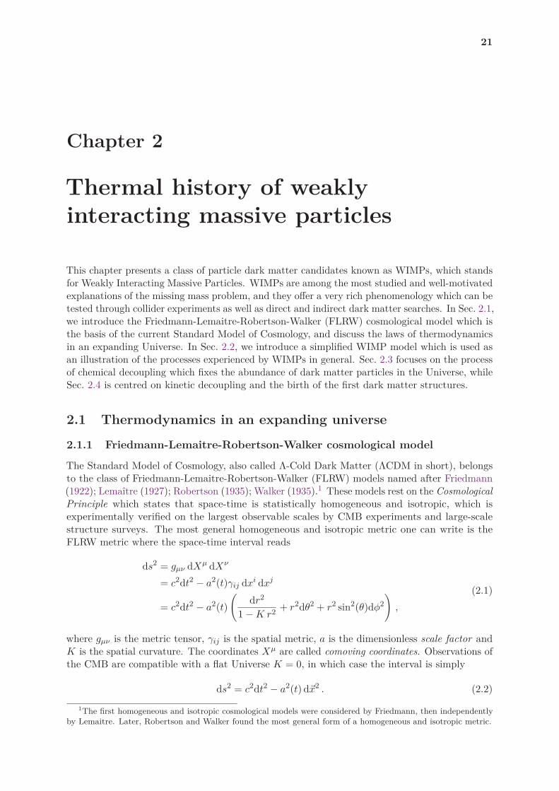
21
Chapter 2
Thermal history of weaklyinteracting massive particles
This chapter presents a class of particle dark matter candidates known as WIMPs, which standsfor Weakly Interacting Massive Particles. WIMPs are among the most studied and well-motivatedexplanations of the missing mass problem, and they offer a very rich phenomenology which can betested through collider experiments as well as direct and indirect dark matter searches. In Sec. 2.1,we introduce the Friedmann-Lemaitre-Robertson-Walker (FLRW) cosmological model which isthe basis of the current Standard Model of Cosmology, and discuss the laws of thermodynamicsin an expanding Universe. In Sec. 2.2, we introduce a simplified WIMP model which is used asan illustration of the processes experienced by WIMPs in general. Sec. 2.3 focuses on the processof chemical decoupling which fixes the abundance of dark matter particles in the Universe, whileSec. 2.4 is centred on kinetic decoupling and the birth of the first dark matter structures.
2.1 Thermodynamics in an expanding universe
2.1.1 Friedmann-Lemaitre-Robertson-Walker cosmological model
The Standard Model of Cosmology, also called Λ-Cold Dark Matter (ΛCDM in short), belongsto the class of Friedmann-Lemaitre-Robertson-Walker (FLRW) models named after Friedmann(1922); Lemaıtre (1927); Robertson (1935); Walker (1935).1 These models rest on the CosmologicalPrinciple which states that space-time is statistically homogeneous and isotropic, which isexperimentally verified on the largest observable scales by CMB experiments and large-scalestructure surveys. The most general homogeneous and isotropic metric one can write is theFLRW metric where the space-time interval reads
ds2 = gµν dXµ dXν
= c2dt2 − a2(t)γij dxi dxj
= c2dt2 − a2(t)
(
dr2
1 − K r2+ r2dθ2 + r2 sin2(θ)dφ2
)
,
(2.1)
where gµν is the metric tensor, γij is the spatial metric, a is the dimensionless scale factor andK is the spatial curvature. The coordinates Xµ are called comoving coordinates. Observations ofthe CMB are compatible with a flat Universe K = 0, in which case the interval is simply
ds2 = c2dt2 − a2(t) dþx2 . (2.2)
1The first homogeneous and isotropic cosmological models were considered by Friedmann, then independentlyby Lemaitre. Later, Robertson and Walker found the most general form of a homogeneous and isotropic metric.

22 2.1. Thermodynamics in an expanding universe
It is standard to introduce the physical coordinates Y µ which follow the space-time dynamics andare related to the comoving coordinates through Y 0 = X0 and þy = a(t) þx. The metric measuredby a physical observer is simply the Minkowski metric
ds2 = c2dt2 − dþy2
= ηµν dY µ dY ν .(2.3)
The energy-momentum tensor T µν is severely constrained by the symmetries of the metric tensorgµν . It can be shown, see e.g. Weinberg (1972), that the most general energy-momentum tensorcompatible with the cosmological principle is
Tµν =
(
ρ +p
c2
)
UµUν − p gµν , (2.4)
where U is a 4-velocity. This is the energy-momentum tensor of an ideal fluid with energy densityρ(t) and pressure p(t). This is also the energy-momentum tensor of a collection of ideal fluidssuch that
ρ =∑
ρi
p =∑
pi .(2.5)
The space-time dynamics is related to the matter content through Einstein’s equations
Gµν + Λgµν =8πGN
3Tµν , (2.6)
where Gµν is the Einstein tensor and Λ is the cosmological constant. The(
µ=0ν=0
)
and(
µ=iν=i
)
components lead to
(
a
a
)2
=8πGN
3ρ +
Λc2
3− K c2
a2(2.7)
a
a= −4πGN
3
(
ρ + 3p
c2
)
+Λc2
3, (2.8)
which are called the Friedmann equations. The Hubble parameter is defined as H ≡ a/a and itsvalue today H0 ≡ H(t0) is the Hubble constant. It is conventional to fix the value of the scalefactor today a(t0) = 1. Another set of useful equations is given by the covariant conservation ofT µν :
∇µT µν = 0 , (2.9)
which leads to
ρ = −3H
(
ρ +p
c2
)
. (2.10)
This last equation actually holds separately for each ideal fluid, under the assumption thesefluids are not interacting with each other.
2.1.2 Matter content and time evolution
For a given fluid, it is standard to defined its equation of state as
w(t) =p(t)
ρ(t)c2. (2.11)

Chapter 2. Thermal history of weakly interacting massive particles 23
Studies of the CMB point toward a Universe containing radiation (photons), pressureless matter(cold dark matter, and baryons after recombination) and a cosmological constant, see Ade et al.(2016). The equation of state of each of these components can be computed, see e.g. Weinberg(1972), and we get
wrad =1
3(2.12)
wmat = 0 (2.13)
wΛ = −1 , (2.14)
hence all the equations of state of the known components of the Universe are time-independentin first approximation. Note that the radiation pressure is purely relativistic in origin and doesnot stem from interactions within the radiation fluid. The cosmological constant has its energydensity defined through Eq. (2.7) which leads to ρΛ = Λc2/(8πGN), hence ρΛ is positive and thecosmological constant has a negative pressure. In General Relativity, the cosmological constant isoften interpreted as a property of space-time itself rather than a fluid. It could also be interpretedas a new dark energy component with its own dynamics, which the subject of intense researchin cosmology. For more details on the cosmological constant, we refer to the classic review byWeinberg (1989) and to Martin (2012). For a time-independent equation of state, Eq. (2.10)leads to
ρ(t) = ρ0 a(t)−3(1+w) , (2.15)
where we set a(t0) = 1 for the value of the scale factor today (with t0 the age of the Universe).Consequently, we have
ρrad(t) = ρrad,0 a(t)−4 (2.16)
ρmat(t) = ρmat,0 a(t)−3 (2.17)
ρΛ(t) = ρΛ,0 , (2.18)
From these equations, we can already identify three main epochs in an expanding universe wherea goes from zero to one. The universe is initially dominated by the radiation component, hencethe qualification of ”hot Big Bang”. What happens next depends on the relative abundancebetween the three species. If ρΛ > ρ4
m,0ρ−3r,0 , the universe switches from a radiation-dominated
epoch to an epoch dominated by the cosmological constant. Alternatively, if ρΛ < ρ4m,0ρ−3
r,0 whichis effectively the case in our Universe, the radiation epoch is followed by a period of matterdomination before eventually entering the cosmological constant epoch.
We would like to derive the evolution of the scale factor as a function of the cosmic time. Usingthe first Friedmann equation (2.7), and assuming the Universe is flat (K = 0) and dominated bya single component with equation of state w > −1, we can derive an expression for a(t)
a(t) =
1 − 3(1 + w)
2
√
8πGN
3ρ0(t0 − t)
23(1+w)
. (2.19)
This solution describes an expanding Universe. Note that Eq. (2.7) has an alternative, contracting,solution which we reject on the basis of observations. If we set the origin of time througha(t = 0) = 0, we get the age of the universe
t0 =1
1 + w
√
1
6πGNρ0, (2.20)
and a very simple expression for the scale factor
a(t) =
(
t
t0
)2
3(1+w)
. (2.21)

24 2.1. Thermodynamics in an expanding universe
We see that the FLRW models predict a power-law dilation of space in the absence of acosmological constant. The Hubble parameter is then
H(t) =2
3(1 + w)t. (2.22)
From this last equality, the age of the Universe can be estimated using the value of the Hubbleconstant since we have t0 ≃ H−1
0 up to a factor of order unity. This leads to t0 ≃ 14.4 Gyr, nottoo far from the CMB estimate of 13.8 Gyr. The previous time evolutions were derived assumingw > −1, it is worth doing the analysis for w = −1 i.e. when the Universe is dominated by acosmological constant. In that case, the first Friedmann equation leads to the expanding solution
a(t) = exp [H(t − t0)] , (2.23)
with H = c√
Λ/3 the Hubble parameter which is time-independent. In this case, the Universeundergoes an exponential growth.
In cosmology, it is standard to use the cosmological redshift rather than the cosmic time. Letus consider a photon emitted at time t with frequency νem and observed by a comoving observerat time t0, then we have
νem
νobs=
1
a(t)≡ 1 + z , (2.24)
where z is the redshift. The abundance of a given species in the Universe is usually expressed as
Ωi =ρi
ρc, (2.25)
where ρc is the critical density, defined as the total density of a FLRW Universe without curvature(K = 0). According to Eq. (2.7), we have
ρc =3 H2
8πGN, (2.26)
and Eq. (2.7) can be written in the very simple form
1 = ΩK(t) +∑
i
Ωi(t) , (2.27)
where ΩK is the curvature density. The curvature abundance today is compatible with ΩK = 0,see Ade et al. (2016), therefore our Universe is flat and the total energy density is equal to thecritical density. The Hubble parameter can be expressed as a function of the cosmic abundancesand the redshift as
H(z) = H0
√
Ωm,0(1 + z)3 + Ωr,0(1 + z)4 + ΩΛ,0 , (2.28)
where Ωm,0, Ωr,0 and ΩΛ,0 are today’s matter, radiation and cosmological constant abundances.The values inferred from the CMB are Ωm,0 ≃ 0.3 with a small baryonic fraction Ωbar,0 ≃ 0.05,and ΩΛ ≃ 0.7. Hence the energetic content of the Universe is essentially made of CDM and Λ,with ordinary matter only contributing 5%.
The redshift dependency of each cosmic abundance is
Ωm(z) = Ωm,0(1 + z)3(
H0
H(z)
)2
(2.29)
Ωr(z) = Ωr,0(1 + z)4(
H0
H(z)
)2
(2.30)
ΩΛ(z) = ΩΛ,0
(
H0
H(z)
)2
. (2.31)

Chapter 2. Thermal history of weakly interacting massive particles 25
Figure 2.1 – Left panel: Redshift evolution of the cosmic abundances of cold dark matter (blue),radiation (red) and cosmological constant (green). The epochs of matter-radiation equality (dashedpurple), recombination (dashed cyan) and reionization (dashed orange) are also shown. Right panel:cosmic time as a function of the redshift.
The evolution of the abundances as a function of z is shown on the left panel in Fig. 2.1. Onenotices that the radiation-to-matter ratio is (1 + z) Ωr,0/Ωm,0 so, even though today’s ratioΩr,0/Ωm,0 is very small, there is a redshift zeq at which this ratio is equal to one. This transition,when the Universe leaves the radiation-dominated era and enters the matter-dominated era, iscalled the matter-radiation equality and is a crucial epoch for structure formation, as we willsee in Sec. 3.1. CMB studies point toward a value for the redshift at equality zeq = 3365. Sincecosmic time is a more intuitive quantity than redshift, it is useful to relate t to z. We have
dt =da
a
= − dz
(1 + z)H(z),
(2.32)
hence
t0 − t =1
H0
∫ z
0
dz′
(1 + z′)√
Ωm(1 + z′)3 + Ωr(1 + z′)4 + ΩΛ
. (2.33)
The quantity t0 − t is shown on the right panel in Fig. 2.1. As one can see, t0 − t saturates forz > 10 and most of the major events of the cosmological history such as the matter-radiationequality, the formation of the first hydrogen atoms and the formation of the first stars happensat least 13 billion years ago.
2.1.3 Statistical mechanics in an expanding universe
We now focus on the radiation-dominated era and assume some species were in thermodynamicequilibrium. This must be true for photons, electrons and positrons at least, since the interactionrate of photons with charged particles was much larger than the Hubble rate. The number ofparticles in an elementary phase-space volume is
dN = f(þx, þp, t) d3þx d3þp
= f(þx, þp, t) dx1dx2dx3dp1dp2dp3 .(2.34)

26 2.1. Thermodynamics in an expanding universe
We have, from the i component of the geodesic equation (B.55), pi ∝ a−2 and the modulus of
the momentum is given by p =√
−a2δijpipj hence p ∝ 1/a. The elementary phase-space volume
d3þx d3þp is invariant under the expansion. This implies that the phase-space distribution is ascalar under coordinate transformations, which means we do not have to worry about the choiceof coordinates (comoving or physical for instance) when giving the expression of the phase-spacedistribution. The equilibrium phase-space occupation number of particles of species A is
f eqA (þp) =
1
exp[
EkBT
]
+ ǫ, (2.35)
where ǫ = +1/ − 1 if A is a fermion/boson (Fermi-Dirac/Bose-Einstein statistics). For simplicity,we use from now on the natural units ~ = c = kB = 1. The number density, energy density andpressure are defined by
nA(t) = gA
∫
d3þp
(2π)3fA(þp, t) (2.36)
ρA(t) = gA
∫
d3þp
(2π)3fA(þp, t) E (2.37)
pA(t) = gA
∫
d3þp
(2π)3fA(þp, t)
þp.þv
3, (2.38)
where gA is the number of spin/helicity degrees of freedom of A. These definitions are alsovalid out of equilibrium. Alternatively, these quantities can be computed directly from theenergy-momentum tensor Tµν . Note that in the convention we adopt henceforth, the integrationis over the physical momentum such that nA, ρA and pA decrease as the Universe expands.Equilibrium quantities can be expressed in term of the temperature T rather than time. Wehave the explicit expressions
neqA (T ) =
gA
2π2T 3
∫ ∞
0
u2
e√
u2+x2 + ǫdu (2.39)
ρeqA (T ) =
gA
2π2T 4
∫ ∞
0
u2
e√
u2+x2 + ǫ
√
u2 + x2 du (2.40)
peqA (T ) =
gA
2π2T 4
∫ ∞
0
u2
e√
u2+x2 + ǫ
u2
3√
u2 + x2du , (2.41)
where
x ≡ mA/T (2.42)
and mA is the mass of the species under consideration. In the relativistic limit x ≪ 1, weimmediately get ρA = 3 pA hence the equation of state of radiation is w = 1/3. Using the integralexpression of the Riemann zeta function in Appendix A.3, the number density and energy densityin the relativistic limit can be expressed as
neqA (T ) =
ζ(3)
π2gA T 3
1 if A is a boson3/4 if A is a fermion
(2.43)
ρeqA (T ) =
π2
30gA T 4
1 if A is a boson7/8 if A is a fermion
(2.44)
peqA (T ) =
π2
90gA T 4
1 if A is a boson7/8 if A is a fermion
(2.45)

Chapter 2. Thermal history of weakly interacting massive particles 27
In the non-relativistic limit x ≫ 1, if the energy is approximated with E ≃ m + p2/(2m)there is no distinction between bosons and fermions any more (the statistics follows the Maxwell-Boltzmann law) and we have
neqA (T ) =
gA m3A
(2π mA/T )3/2e−mA/T (2.46)
ρeqA (T ) = mA nA(T ) =
gA m4A
(2π mA/T )3/2e−mA/T (2.47)
peqA (T ) = ρeq
A (T )/x . (2.48)
The equation of state of non-relativistic matter is then w = 1/x ≃ 0.
Entropy Assuming adiabatic expansion and no entropy production, the entropy in a comovingvolume is conserved therefore we have
s(T ) a3(t) = cst (2.49)
where s is the entropy density. The second law of thermodynamics reads
d(ρa3) = T d(sa3) − p d(a3) , (2.50)
which gives the relation
s(T ) =ρ + p
T. (2.51)
In the relativistic limit, we can use p = ρ/3 and Eq. (2.44) to get
seqA (T ) =
2π2
45gA T 3
1 if A is a boson7/8 if A is a fermion
(2.52)
Therefore, the entropy density goes like T 3. Since the entropy is conserved in a comoving volume,it immediately follows that the temperature of a relativistic component goes like
T ∝ 1
a(t), (2.53)
i.e. the temperature decreases like the inverse of the scale factor as the Universe expands. Thismakes the temperature of the photon bath yet another alternative time variable along with thescale factor and the redshift. Note that the relation between the temperature and the scale factordepends on the species at equilibrium in the thermal bath.
Effective degrees of freedom Since photons are always part of the thermal bath, it isconventional to express the total energy and entropy densities in units of the photon energy andentropy densities by introducing the effective degrees of freedom geff and heff defined by
ρ(T ) =π2
30geff(T ) T 4
s(T ) =2π2
45heff(T ) T 3 .
(2.54)
Another more formal definition can be extracted from the equation above
geff ≡∑
i
gγρi(Ti)
ργ(T )(2.55)
heff ≡∑
i
gγsi(Ti)
sγ(T )(2.56)

28 2.2. A simplified WIMP model
For relativistic species, the effective degrees of freedom can be written explicitly
geff(T ) ≡∑
boson i
gi
(
Ti
T
)4
+7
8
∑
fermion j
gj
(
Tj
T
)4
(2.57)
heff(T ) ≡∑
boson i
gi
(
Ti
T
)3
+7
8
∑
fermion j
gj
(
Tj
T
)3
. (2.58)
We introduced specific temperatures Ti and Tj to account for species which are not in thermalequilibrium with the thermal bath.2 For particles in equilibrium with the bath, we have geff = heff .The effective degrees of freedom of a particular species A can be expressed using Eqs. (2.40) and(2.41). We find
geff,A(T ) = gA15
π4
∫ ∞
0
u2
e√
u2+x2 + ǫ
√
u2 + x2 du (2.59)
heff,A(T ) = gA45
4π4
∫ ∞
0
u2
e√
u2+x2 + ǫ
(
√
u2 + x2 +u2
3√
u2 + x2
)
du . (2.60)
Using the definition and recurrence property of the modified Bessel functions, one can expressgeff,A and heff,A in term of rapidly converging series
geff,A(T ) = gA15
π4
∞∑
n=1
(−ǫ)n+1
(
6x
n3+
x3
n
)
K1(nx) +3x2
n2K0(nx)
(2.61)
heff,A(T ) = gA45
4π4
∞∑
n=1
(−ǫ)n+1
(
8x
n3+
x3
n
)
K1(nx) +4x2
n2K0(nx)
(2.62)
These expressions are established in App. B.1. The quantity geff is shown in Fig. 2.2. One noticesan important decrease of geff around T ≃ 150 MeV: this is the QCD phase transition, when thetemperature is low enough so that quarks are confined into hadrons (see e.g., Borsanyi et al.(2016) for a detailed study of the transition using lattice simulations).
2.2 A simplified WIMP model
2.2.1 Lagrangian
We introduce a very simple model of WIMP dark matter. Our goal is to use this model asillustration of the typical thermal history of WIMPs. In this spirit, we do not try to address anypotential issues, e.g.consistency with respect to quantum field theory, that this model might have.We will not try to address questions related to the generation of the dark mass or the impact onthe hierarchy problem. We are considering a simplified model, in the sense of Abdallah et al.(2015) rather than a fully consistent theory like supersymmetry. We consider a fermion χ as thedark matter particle. This fermion can be either a Dirac or a Majorana fermion. Dark mattercan interact with SM fermions through a real scalar field φ or a real pseudo-scalar field a. Thescalar/pseudo-scalar particle is massive and the scalar particle is assumed to be different fromthe Higgs field. Our working Lagrangian is the following
L = LSM + Lkin + Lint , (2.63)
where Lsm is the SM Lagrangian, Lkin contains the kinetic terms for χ, φ and a, and Lint containsthe mass terms and the interactions terms. The interaction part in the case of Majorana dark
2In the standard cosmological evolution, species that decouple from the thermal bath never maintain thermalequilibrium on their own and the temperature is not rigorously defined, therefore Ti and Tj should be thought ofas effective temperature instead.

Chapter 2. Thermal history of weakly interacting massive particles 29
Figure 2.2 – Effective degrees of freedom geff (blue) and g∗ (red) as functions of the temperature.
matter can be written
Lint = − 1
2mχ χχ − 1
2m2
φ φ2 − 1
2ma a2
− λφ
2χχ φ − λa
2χ γ5 χ a
− λ′φ ff φ − λ′
a f γ5 f a .
(2.64)
If dark matter is a Dirac field, there is no 1/2 factor in front of the dark matter mass term andcoupling term. In Eq. (2.64), f refers to a SM fermion. The scalar and pseudo-scalar particlescan in principle interact with several SM fermions, in which case there are couplings λ′
φ and λ′a
for each fermion. Free parameters in our model are the masses mχ, mφ, ma, and the couplingsλφ, λa, λ′
φ, λ′a. Note that such a simplified model is already constrained by several experiments
(e.g., LHC, Xenon, indirect searches).
2.2.2 Tree-level amplitude
Two types of reactions are especially relevant during the thermal history of our dark matter can-didate: annihilation and elastic scattering. The tree-level Feynman diagrams for the annihilationare shown in Fig. 2.3. The dark matter particle, whether a Majorana or a Dirac fermion, canannihilate through the scalar or the pseudo-scalar into a pair of SM fermions. Note that thesediagrams, up to a time-reversal transformation, also control the production of dark matter fromthe annihilation of SM fermions. The squared amplitude for the annihilation processes, averagedover initial spins and summed over final spins, is given by
|Mann|2 = Nc(λmedλ′
med)2
(
s − m2med
)2
(
s − 4 m2χ
)
(
s − 4 m2f
)
scalar
s2 pseudoscalar(2.65)
This result is demonstrated in App. B. In Eq. (2.65), Nc is the number of non-spin degrees offreedom of the SM fermion (for instance the number of colors if f is a quark). If p1 and p2 are the4-momenta of the incoming dark matter particles, and k3 and k4 the 4-momenta of the outgoingSM fermions, s is the Lorentz-invariant Mandelstam variable accounting for centre-of-mass energys = (p1 + p2)2 = (k3 + k4)2.

30 2.3. Chemical decoupling
φ
χ (p2)
χ (p1)
f (k4)
f (k3)
(a)
a
χ (p2)
χ (p1)
f (k4)
f (k3)
(b)
Figure 2.3 – Pair annihilation of the dark matter particle into SM fermions through the scalar portal(a) or the pseudo-scalar portal (b).
Tree-level diagrams for the elastic scattering of a dark matter particle off a SM fermion areshown in Fig. 2.4. These diagrams are simply obtained by rotating the annihilation diagrams inFig. 2.3. For the amplitude, this translates into a change s → t, where t = (p1 − p2)2 = (k3 − k4)2
and this time p1 (p2) is the 4-momentum of the incoming (outgoing) dark matter particle and k3
(k4) is the 4-momentum of the incoming (outgoing) SM fermion. The amplitude for the process is
|Mscat|2 = Nc(λmedλ′
med)2
(
t − m2med
)2
(
t − 4 m2χ
)
(
t − 4 m2f
)
scalar
t2 pseudoscalar(2.66)
φ
f (k3)
χ (p1)
f (k4)
χ (p2)
(a)
a
f (k3)
χ (p1)
f (k4)
χ (p2)
(b)
Figure 2.4 – Elastic scattering of a dark matter particle off a SM fermion through the exchange of ascalar (a) or a pseudo-scalar (b).
2.2.3 Cross-sections
As shown in the appendix, the Lorentz-invariant annihilation cross-section is given by
σann =1
16π
(λmedλ′med)2
(
s − m2med
)2+ m2
medΓ2med
(s − 4 m2)1/2(s − 4 m2f )3/2 s−1 scalar
(
s−4 m2f
s−4 m2
)1/2
s pseudoscalar(2.67)
The cross-sections are shown for both mediators in Fig. 2.5. As one can see, the two cross-sectionshave a similar behaviour at high energies. A difference appears at low energies: while the scalarcross-section is suppressed when the WIMPs annihilate at rest (
√s = 2 m), the pseudoscalar
cross-section diverges.
2.3 Chemical decoupling
A fundamental element for any dark matter candidate is its production mechanism in theearly Universe. The case of the WIMP was first discussed by Lee & Weinberg (1977) (see alsoVysotsky et al. (1977); Sato & Kobayashi (1977); Hut (1977); Dicus et al. (1977)). In this seminalpaper, Lee and Weinberg established the evolution equation for the number density of a weaklyinteracting particle (having in mind a heavy neutrino) and set a lower bound on its mass by

Chapter 2. Thermal history of weakly interacting massive particles 31
Figure 2.5 – Annihilation cross-sections as functions of the centre-of-mass energy√
s (normalized tothe sum of the masses of the incoming particles).
requiring that its energy density does not overclose the Universe. This original calculation hassince then been revisited many times, see for instance Bernstein et al. (1985); Kolb & Olive(1986); Srednicki et al. (1988); Griest & Seckel (1991); Gondolo & Gelmini (1991); Edsjo &Gondolo (1997); Steigman et al. (2012), and the astrophysical and cosmological phenomenologyof WIMPs have been investigated in details (Gunn et al., 1978; Tremaine & Gunn, 1979).
In this section, we review the standard calculation of the WIMP relic density. We show thatthe number density of WIMPs today is set by the chemical decoupling of the dark matter particle.Using our toy model, we illustrate the freeze-out and freeze-in scenarios.
2.3.1 The Boltzmann equation
Evolution of the number density In this section, we establish the master equation for thetime evolution of the WIMP number density, following the standard treatment of Gondolo &Gelmini (1991). We assume that dark matter particles can annihilate into SM particles througha reaction
1 + 2 → 3 + 4 , (2.68)
where 1 and 2 are dark matter particles, and 3 and 4 are SM particles. In our simplified model,these SM particles are fermions, however the following treatment holds regardless of the natureof the outgoing particles. The phase-space number density of 1 obeys the Boltzmann equation
L[f1] = C[f1] (2.69)
where L and C are the Liouville and collision operators, respectively. As shown in App. B.3,taking the zeroth-order moment of the Boltzmann equation leads to the evolution equation ofthe number density
dn1
dt+ 3 H n1 = − 〈σannv〉 (n1n2 − n1,eqn2,eq) . (2.70)
Note the equilibrium number densities neq1 and neq
2 actually represent the plasma productionterm. It can be conveniently expressed in terms of the WIMPs equilibrium density thanks to the

32 2.3. Chemical decoupling
principle of detailed balance. In this equation, 〈σannv〉 is the thermally-averaged cross-sectiondefined as
〈σannv〉 ≡∫
d3þp1 d3þp2 f1(þp1) f2(þp2) σann vm∫
d3þp1 d3þp2 f1(þp1) f2(þp2), (2.71)
where fi is the phase-space number density of i, σann is the cross-section of the reaction inEq. (2.68), and vm is the Møller velocity
vm ≡
√
(p1.p2)2 − m21m2
2
E1 E2(2.72)
=√
|þv1 − þv2|2 − |þv1 × þv2|2 . (2.73)
The Moller velocity is such that vm n1 n2 is Lorentz-invariant. Note that the averaged cross-section depends on the temperature in the dark matter bath through the phase-space distributionfunction (DF).
The standard treatment of chemical decoupling assumes thermal equilibrium between darkmatter particles and the thermal bath is maintained during decoupling. For a study of the fullout-of-equilibrium decoupling, see Binder et al. (2017). Two cases are usually considered for 1and 2: either these particles are identical and the dark matter number density is n = n1 = n2
(which is the case if dark matter is a Majorana fermion), or 1 and 2 are different (which is thecase if dark matter is a Dirac fermion) and we further assume n1 = n2 to get n = n1 + n2 = 2 n1.In the following, we focus on the case of identical particles where the Boltzmann equation is
dn
dt+ 3 H n = − 〈σannv〉
(
n2 − n2eq
)
. (2.74)
For non-identical particles, the evolution equation for n is the same with the replacement〈σannv〉 → 〈σannv〉 /2. In Eq. (2.74), the first term on the right-hand side accounts for thedepletion of the dark matter density by annihilation of dark matter particles. The second termaccounts for the creation of dark matter particles by annihilation of particles in the thermalbath. The second term on the left-hand side of the equation is a friction term accounting for theexpansion of the Universe. We know that a constant number of dark matter particles inside acomoving volume yields a number density n(t) ∝ a−3(t), hence it is useful to introduce a quantitythat remains constant during the expansion. If the total entropy of the Universe is conserved,the entropy density verifies s ∝ a−3(t) (see Eq. (2.49)), therefore we define a comoving numberdensity3
Y ≡ n
s. (2.75)
Plugging the definition of the comoving density in Boltzmann equation (2.74), we get
dY
dt= −s 〈σannv〉
(
Y 2 − Y 2eq
)
. (2.76)
Note that the Hubble friction term is gone, as expected. We make use of x = m/T as a timevariable, where m is the dark matter mass and T is the temperature of the thermal bath. Withthe substitution
d
dt=
ds
dt
dx
ds
d
dx
= −3Hsdx
ds
d
dx,
(2.77)
3Note that the term comoving density is abusive since Y has units of inverse entropy.

Chapter 2. Thermal history of weakly interacting massive particles 33
we get
dY
dx=
1
3H
ds
dx〈σannv〉
(
Y 2 − Y 2eq
)
. (2.78)
We can go further by using the effective degrees of freedom introduced in Eq. (2.54) and theexpression of the Hubble parameter H2 = 8πGNρ/3. We finally get
dY
dx= −
(
π
45 GN
)1/2 m g1/2∗
x2〈σannv〉
(
Y 2 − Y 2eq
)
, (2.79)
with
g1/2∗ ≡ heff
g1/2eff
(
1 +1
3
d ln heff
d ln T
)
. (2.80)
The behaviour of g∗ with the temperature closely follows that of geff , as shown on the left panelin Fig. (2.2). Equation (2.79) is the most practical form of the Boltzmann equation when itcomes to numerical calculations.
Thermally-averaged annihilation cross-section Let us comment on the averaged cross-section defined in Eq. (2.71). If the WIMP has a Maxwell-Boltzmann phase-space distribution,Gondolo & Gelmini (1991) showed that it can be expressed as a single integral
〈σannv〉 =1
8m4TK22 (m/T )
∫ ∞
4m2σann(s)
(
s − 4m2) √
sK1(√
s/T ) ds . (2.81)
This result is exact and valid if the temperature is low enough for the Maxwell-Boltzmannapproximation to hold. Numerically, it is a very good approximation if T < 3m.
As the temperature gets lower and x ≫ 1, 〈σannv〉 can be expanded in powers of x−1
〈σannv〉 ≃ a +b
x+
c
x2+
d
x3+ . . . (2.82)
The first, temperature-independent term is referred to as the s-wave contribution, while thesecond term is referred to as p-wave. The relation between the cross-section σann and coefficientsa, b, c and d is explicitly given by Srednicki et al. (1988). The coefficients are expressed in termsof the Lorentz-invariant function
w(s) ≡ E1E2 σann vm
= σann(s)√
(p1.p2)2 − m21m2
2
= σann(s)
√s
2
√
s +(m2
1 − m22)2
s− 2(m2
1 + m22) ,
(2.83)
and its derivatives. Expressions for a and b in our simplified model are given in App. B.2.4. Thethermal cross-sections are shown in Fig. (2.6). The behaviour as a function of the temperature isvery different depending on the nature of the mediator: while the pseudo-scalar cross-sectionkeeps a constant value at low temperature, the scalar one is falling like T .
2.3.2 Freeze-out and freeze-in
Freeze-out The Boltzmann equation (2.79) cannot be solved analytically but we can guessthe qualitative behaviour of the solution. Let us suppose the WIMP is in thermal and chemicalequilibrium with the plasma at a given x. When the temperature of the plasma drops well below

34 2.3. Chemical decoupling
Figure 2.6 – Thermally-averaged annihilation cross-sections as functions of the temperature. Weshow the scalar (red) and pseudo-scalar (blue) channels, for both the exact solution (solid) and the 1/xexpansion (dashed).
the WIMP mass, i.e. when x ≫ 1, conservation of energy forbids the creation of WIMPs fromcollisions in the plasma. The Boltzmann equation then reduces to
dY
dx= −
(
π
45 GN
)1/2 m g1/2∗
x2〈σannv〉 Y 2 , (2.84)
which shows that dark matter self-annihilation depletes the comoving density. At some point, asthe number of dark matter particles drops and the Universe expands, self-annihilation becomesinefficient and the comoving density remains roughly constant. At this point the dark matter ischemically decoupled from the thermal bath. Chemical decoupling happens when the annihilationrate drops below the expansion rate
Γann(xcd) ≃ H(xcd) , (2.85)
where Γann = n 〈σannv〉. We assume the decoupling occurs when WIMPs are well into the non-relativistic regime, hence we can use Eq. (2.46) for the WIMP number density. The annihilationand Hubble rates are shown on the left panel in Fig. 2.7. The value of xcd at the intersectionbetween the two rates is solution of
x1/2cd e−xcd ≃
(
π5
45geff
)1/21
mp m 〈σannv〉 , (2.86)
where mp ≡ (8πGN)−1/2 is the reduced Planck mass. For a WIMP with mass m = 100 GeVand a cross-section at the electroweak scale 〈σannv〉 ∼ 10−8 GeV−2, we get xcd ≃ 30. Note thatxcd depends only logarithmically on the mass and the cross-section. We evaluate xcd in our toymodel using the Boltzmann equation as done by Gondolo & Gelmini (1991). The result is shownin the right panel on Fig. 2.7. The value of xcd changes by ten units over two decades in darkmatter mass. Note that this change is partly due to resonant annihilation at 2 m = mφ/a, whichis clearly visible in the figure.
We now integrate Eq. (2.84) between xcd and x0 (T0 is the temperature of the photon bathtoday) to get
1
Y0− 1
Ycd=
(
π
45 GN
)1/2
m
∫ x0
xcd
g1/2∗x2
〈σannv〉 dx . (2.87)

Chapter 2. Thermal history of weakly interacting massive particles 35
If enough particles annihilate right after xcd, we can neglect 1/Ycd in Eq. (2.87). If we further
assume 〈σannv〉 to be temperature-independent and take an average value for g1/2∗ , we get an
expression for today’s relic abundance
Ωcdm =m s0 Y0
ρc. (2.88)
Using
ρc =3
8πGNH2
0
=3
8πGN(100 h km/s/Mpc)2 ,
(2.89)
we get
Ωcdmh2 =(
5πG3N
)1/2 s0
g1/2∗
xcd
〈σannv〉 (100 km/s/Mpc)−2 . (2.90)
The dark matter abundance does not depend explicitly on the dark matter mass. There is actuallya hidden dependency in xcd but as we have seen before, it is very weak. The evolution of thedark matter density is shown in the left panel of Fig. 2.8 for a constant annihilation cross-section.An important feature of the freeze-out scenario is the dependence of the relic abundance on theinverse of the cross-section: the higher the cross-section, the later the decoupling and the lowerthe abundance. In a given model, the cross-section obviously depends on the dark matter mass.We show the evolution of the dark matter density in our toy model in the right panel on Fig. 2.8for different values of the dark matter mass.
Figure 2.7 – Left panel: Hubble rate (black curve) compared to the annihilation rate for a scalar(solid curve) or a pseudoscalar channel (dashed curve) with a dark matter mass m = 100/300/500 GeV(red/green/blue). Right panel: xcd = m/Tcd with Tcd the temperature of chemical decoupling, as afunction of the dark matter mass. Are shown the scalar (red) and pseudoscalar channels (blue).
The dark matter relic abundance is almost entirely fixed by the annihilation cross-section.We can turn the expression around and compute the cross-section that leads to the observeddark matter abundance. We get
〈σannv〉 ≃ 3 × 10⁻²⁶ cm3s−1 ≃ 10−8 GeV−2 , (2.91)

36 2.3. Chemical decoupling
which turns out to be the order of magnitude of an electroweak cross-section. The fact thata massive particle with electroweak scale interactions leads to the correct order of magnitudefor the dark matter relic abundance is dubbed the “WIMP miracle” and is one of the mainreasons why WIMP models have been extensively studied in the literature. The value of theconstant/s-wave annihilation cross-section that leads to the correct relic abundance is shown inthe left panel on Fig. 2.9. The cross-section varies from 4.5 × 10⁻²⁶ cm3/s to 2 × 10⁻²⁶ cm3/sover four orders of magnitude of the dark matter mass. This dependence on the dark mattermass is also shown in Steigman et al. (2012). The dark matter relic abundance today is shownas a function of the dark matter mass in the right panel in Fig. 2.9. We can constrain our modelby fixing, for a given dark matter and mediator mass, the product of the coupling constants λλ′
by requiring that the relic abundance matches the value measured by Ade et al. (2016).Our very simple WIMP model captures the essential features of the freeze-out mechanism. In
more complicated models, such as those coming from supersymmetric theories, the phenomenologyof freeze-out can be significantly modified by the presence of other non-standard particles in thespectrum. A typical example is coannihilation (Binetruy et al., 1984; Edsjo & Gondolo, 1997).This occurs when a particle has a mass right above the dark matter mass. In that case, the darkmatter particle can coannihilate with that particle, which opens a new channel changing the darkmatter relic abundance. Interestingly, the Boltzmann equation governing the number density ofnon-standard particles in the presence of coannihilation can be written
dn
dt+ 3 H n = − 〈σeffv〉
(
n2 − n2eq
)
, (2.92)
i.e. it is exactly the same equation as Eq. (2.74) with an effective annihilation cross-section〈σeffv〉 whose expression is given in Edsjo & Gondolo (1997). This equation is valid if all thenon-standard particles are in equilibrium. Note that in the non-relativistic limit, we have
neq2
neq1
=g2
g1
(
m2
m1
)3/2
e−∆m/T , (2.93)
with ∆m = m2 −m1. Consequently, the impact of coannihilation of 1 with 2 on the calculation ofthe relic density crucially depends on ∆m > 0, and is more important for a small mass difference.
Figure 2.8 – Left panel: chemical decoupling in the freeze-out regime, in the case of a constantannihilation cross-section (s-wave) 〈σannv〉. Right panel: chemical decoupling for the scalar (solid curve)and pseudoscalar channel (dashed curve), for a dark matter mass m = 100/300/500 GeV (red/green/blue).

Chapter 2. Thermal history of weakly interacting massive particles 37
Figure 2.9 – Left panel: s-wave value of the annihilation cross-section to get the observed relicabundance (red), compared to the “canonical” value (dashed black). Right panel: Final relic abundancefor the scalar (red) and pseudoscalar channel (blue), compared to the observed abundance from the Planckcollaboration (dashed black).
Freeze-in The main assumption behind the freeze-out scenario is that dark matter has reachedchemical and thermal equilibrium at some temperature T > m. This assumption can be relaxed.We can instead assume that dark matter is produced by collisions within the plasma through acontinuous process. This can happen in the inflationary scenario: after inflation, the inflatondecays into Standard Model particles during what is called the reheating epoch (Turner, 1983;Traschen & Brandenberger, 1990; Kofman et al., 1997). If we assume dark matter is not directlyproduced by the inflaton or in negligible proportions, then our initial condition is n(Trh) = 0where Trh is the reheating temperature. Dark matter is then produced by annihilation of StandardModel particles and its comoving density follows Eq. (2.79). There are then two possibilities.Either the production/annihilation cross-section is large enough for the dark matter to reachchemical and thermal equilibrium before decoupling, in which case we are back to the freeze-out scenario, or the cross-section is too small for dark matter to ever reach equilibrium. Thelatter case is an example of freeze-in scenario, when dark matter chemical decoupling occursout-of-equilibrium. Hall et al. (2010) showed that the freeze-in scenario leads to predictions thatare independent of the reheating temperature so long as Trh ≫ Tcd, so the freeze-in scenariois independent of the high-energy physics just like the freeze-out scenario. Hall et al. (2010)considered dark matter produced through the decay of some heavier particle, however theirconclusions also holds for dark matter produced through annihilation. We show the chemicaldecoupling in the freeze-in regime in Fig. 2.10 for different value of the s-wave cross-section (notethe very low values 〈σannv〉 with respect to the freeze-out scenario). A major difference betweenfreeze-out and freeze-in is visible in the figure: while the asymptotic value at x ≫ xcd is roughlyproportional to 1/ 〈σannv〉 in the freeze-out case, it goes like 〈σannv〉 in the freeze-in scenario.This can bee seen from the Boltzmann equation (2.79) where we can assume Y ≪ Yeq. TheBoltzmann equation is then simply
dY
dx=
(
π
45 GN
)1/2 m g1/2∗
x2〈σannv〉 Y 2
eq , (2.94)

38 2.4. Kinetic decoupling and primordial structures
which can be directly integrated between xrh and x0 to get
Y0 =
(
π
45 GN
)1/2
m 〈σannv〉∫ x0
xrh
g1/2∗
Y 2eq
x2dx . (2.95)
This shows that the relic abundance in the freeze-in scenario is indeed proportional to the s-waveannihilation cross-section. Note that the integral in Eq. (2.95) diverges if xrh → 0 therefore itstrongly depends on xrh, which seems to be in contradiction with what we have stated earlier.This is because we assumed temperature independent cross-section, which cannot be the case atlow x. In a simple scenario where dark matter is linked to the Standard Model through a singlemediator with mass mmed, the cross-section is suppressed for x ≪ m/mmed, which regularisesthe integral if the reheating temperature is such that Trh ≫ mmed. WIMPs which experience afreeze-in are sometimes referred to as FIMPs for Feebly Interacting Massive Particles i.e. veryweakly interacting massive particles.
Figure 2.10 – Chemical decoupling in the freeze-in regime. The initial condition is Y (xrh) = 0 withxrh = 0.1. The ”step” features at low x are due to numerical issues.
2.4 Kinetic decoupling and primordial structures
Immediately after dark matter annihilation stops being efficient, elastic scattering between darkmatter and Standard Model particles maintains the two in kinetic equilibrium. Let us showthat kinetic decoupling generically happens after chemical decoupling. We recall that freeze-outhappens roughly when the annihilation rate becomes lower than the Hubble rate
Γann = n 〈σannv〉 < H . (2.96)
and we typically get xcd = m/Tcd ≃ 25 as seen in the previous section. To obtain a preciseestimate of the kinetic decoupling temperature, one must solve the Boltzmann equation
L0[f ] = C0[f ] . (2.97)
with
L0[f ] =∂f
∂t− H|þp|2
E
∂f
∂E. (2.98)

Chapter 2. Thermal history of weakly interacting massive particles 39
Let us first try to find a simple estimate. A naive approach would be to compare the scatteringrate to the Hubble rate
Γscat =∑
i
neqi 〈σχiv〉 < H , (2.99)
where the sum is over the different targets the dark matter particle can scatter off. We can assumethese targets to be in thermal equilibrium with the photon bath. Comparing the scattering rateto the Hubble rate is not correct however. Many interactions are actually needed to maintainlocal thermal equilibrium. When the WIMP is in equilibrium with the thermal bath, it has anaverage momentum p =
√3mT while the momentum exchange during a single encounter with a
particle from the bath is δp ≃ T hence
δp
p=
√
T
3 m≪ 1 , (2.100)
since the WIMP is non-relativistic. What should really be compared to the typical expansiontime is the relaxation time (Hofmann et al., 2001; Bringmann & Hofmann, 2007), i.e. the timeneeded to maintain local equilibrium. We assume Ncoll collisions are needed for the change inmomentum to be comparable to the momentum of the dark matter particle. Since scattering is arandom process, this leads to
p = δp√
Ncoll , (2.101)
i.e.
Ncoll =
(
p
δp
)2
=3 m
T. (2.102)
The relaxation time can be written
τrel =Ncoll
Γscat≃ Ncoll
neq 〈σscatv〉 . (2.103)
Assuming the Standard Model scattering partners are relativistic and the scattering cross-sectionis σscat = G2
FT 2 with GF the Fermi constant, we get by comparing τrel to H−1
Tkd ≃ 10 MeV
(
m
100 GeV
)1/4
. (2.104)
This is indeed lower than the typical freeze-out temperature
Tfo ≃ 4 GeV
(
m
100 GeV
)
. (2.105)
While chemical decoupling takes place at temperatures in the GeV range for a dark matter massof 10 − 100 GeV, Tkd is in the MeV range (Schmid et al., 1999; Boehm et al., 2001; Chen et al.,2001). The scaling of Tkd with respect to the dark matter mass is not necessarily in m1/4 as itdepends on the mass scaling of the scattering cross-section. Note that in some models, kineticdecoupling happens close enough to chemical decoupling to affect the prediction of the relicdensity (Binder et al., 2017).
2.4.1 Boltzmann equation and decoupling temperature
Let us now go back to the Boltzmann equation. In practice, the evolution of the full phase-spacedensity is not needed if we are only interested in the evolution of the temperature. It is enough

40 2.4. Kinetic decoupling and primordial structures
for our purpose to compute the second-order moment of the Boltzmann equation. FollowingBringmann & Hofmann (2007), we define a dark matter temperature parameter as
Tdm ≡ 2
3
1
n
∫
d3þp
(2π)3
þp2
2 mf(þp) . (2.106)
Note that Tdm is strictly speaking a temperature only when dark matter is still in equilibrium withthe thermal bath (and we have Tdm = T ). After kinetic decoupling, local thermal equilibriumcannot be maintained and the temperature is ill-defined. The average kinetic energy in Eq. (2.106)is however well defined at any time, hence we can use it to define a temperature-like parameterfor the out-of-equilibrium WIMP bath. Taking the second moment of the Boltzmann equationleads to (Bertschinger, 2006; Bringmann & Hofmann, 2007; Bringmann, 2009; Gondolo et al.,2012)
adTdm
da+ 2 Tdm = −2
γ(T )
H(T )(Tdm − T ) , (2.107)
where
γ(T ) =∑
i
gi
6 m T
∫ ∞
0
d3þp
(2π)3fi(1 ± fi)
p√
p2 + m2i
∫ 0
−4 p2dt (−t)
dσχi
dt(2.108)
is the momentum relaxation rate as given in Gondolo et al. (2012). This equation has thefollowing boundary conditions: at early times, the dark matter is in thermal equilibrium withthe photon bath and we have Tdm ∝ a−1. Inserting this into Eq. (2.107) leads to
T − Tdm =Tdm
2
H
γ, (2.109)
and since at high temperature γ ≫ H, we have Tdm ≃ T . At late times, after kinetic decoupling,the momenta of dark matter particles redshift as p ∝ a−1 and according to the definition of thetemperature parameter in Eq. (2.106), we have Tdm ∝ a−2. Solving the Boltzmann equation inthe general case requires numerical integration, however analytical expressions are available insome cases (Bertschinger, 2006; Bringmann & Hofmann, 2007; Visinelli & Gondolo, 2015). Thekinetic decoupling temperature can be defined at the intersection between these two asymptoticregimes (Bringmann & Hofmann, 2007). Alternatively, it can be defined through γ(Tkd) = H(Tkd)(Visinelli & Gondolo, 2015). Using the former definition and using a zero-momentum transferapproximation for the collision term leads to a very simple expression for the kinetic decouplingtemperature (Bringmann & Hofmann, 2007)
m
Tkd=
(
a
n + 2
)1/(n+2)
Γ
[
n + 1
n + 2
]
(2.110)
The expressions of n and a are given in App. B.3.5. The derivation of this expression relieson the zero-momentum transfer approximation which cannot be applied to the case of thepseudoscalar portal (this is because in that particular case a = 0 according to the expressiongiven in the appendix). We limit our analysis to the scalar channel and therefore to the p-waveannihilation case, assuming the dark matter couples to the three generations of leptons. Theresulting decoupling temperature is shown in the left panel in Fig. 2.11.
2.4.2 Minimal mass of dark matter halos
Kinetic decoupling is of great importance for WIMPs as it sets the size of the first dark matterstructures to be formed in the Universe (Boehm et al., 2001; Hofmann et al., 2001; Berezinskyet al., 2003; Green et al., 2004; Boehm & Schaeffer, 2005; Loeb & Zaldarriaga, 2005; Green et al.,

Chapter 2. Thermal history of weakly interacting massive particles 41
Figure 2.11 – Left panel: kinetic decoupling temperature as a function of the dark matter mass m,assuming the dark matter-SM mediator is a scalar particle. Right panel: comoving free-streaming lengthas a function of the scale factor.
2005; Profumo et al., 2006; Bertschinger, 2006; Bringmann & Hofmann, 2007; Bringmann, 2009).These primordial structures are the smallest bound dark matter structures and their mass is ofgreat importance for dark matter searches. The damping scale in the CDM power spectrum isset by several mechanisms. Before kinetic decoupling, collisions between plasma particles anddark matter induce a pressure that counteracts the effect of gravity. During kinetic decoupling, aremaining viscous coupling between baryons and dark matter also suppresses power below somescale. Finally, once dark matter is kinetically decoupled it enters the free-streaming regime whichfurther damps matter perturbations. The collisional and free-streaming damping mechanismsare discussed below.
2.4.2.1 Collisional damping
In the next chapter, we establish the evolution equation for the overdensity δ(t, k) of a givenmode k
∂2δ
∂t2+ 2H
∂δ
∂t+
(
c2s
k2
a2− 4πGNρ
)
δ = 0 . (2.111)
In this equation, c2s = dp/dρ is the sound speed in the plasma and ρ the average matter density
of the Universe. Solutions of this equation have a very different behaviour depending on the signof the term between brackets. If this term is positive, solutions have an oscillatory behaviourdamped by the Hubble expansion. If this term is negative, solutions are growing like the scalefactor. The transition between these two regimes sets the Jeans scale
kJ ≡ 2πa
cs
√
GNρ
π, (2.112)
which can also be expressed as a length
λJ ≡ 2πa
kJ= cs
√
π
GNρ. (2.113)

42 2.4. Kinetic decoupling and primordial structures
This length defines the scale at which pressure and gravity compensate each other, and belowwhich the overdensity is damped because of pressure. In the radiation era, the sound speedis c/
√3, such that the Jeans scale is almost equal to the horizon scale. The pressure term
characterized by the sound speed is only relevant when WIMPs are kinetically coupled to theplasma, therefore this damping mechanism is collisional in nature. The minimal mass needed fora dark matter perturbation to overcome pressure forces is
Mao ≡ 4
3π ρcdm(tkd)
(
λJ
2
)3
. (2.114)
In this expression, “ao” stands for acoustic oscillations. In a relativistic fluid ρ is given inEq. (2.54). Conservation of number density and entropy yields the dark matter mass density asa function of the photon bath temperature:
ρcdm(T ) = ρcdm(T0)s(T )
s(T0)= ρc Ωcdm
heff(T )
heff(T0)
(
T
T0
)3
, (2.115)
where T0 is the CMB temperature today. Putting this together, we get Mao ∝ T −3. We showMao as function of the kinetic decoupling temperature in the left panel in Fig. 2.12. We obtainvery small masses, ranging from 10−11 M⊙ to 10−5 M⊙. Note that Mao only depends on the darkmatter mass through the decoupling temperature Tkd.
2.4.2.2 Collisionless damping
After dark matter gets kinetically decoupled, it enters the free-streaming regime, which inducesan additional damping of perturbations. This damping occurs because structures only startgrowing efficiently after matter-radiation equality. Before equality, the growth is suppressedby the Meszaros effect (Meszaros, 1974). Between the time of decoupling and the time whenstructures start growing, dark matter particles can free-stream away from perturbations and thuswash out the small-scale power spectrum. Unlike the previous damping mechanism we discussed,this damping is collisionless in nature. The physical distance travelled by a dark matter particlefrom the time of decoupling tkd to some later time t is (see e.g., Berezinsky et al. (2003))
λfs(t) = a(t)
∫ t
tkd
vcdm(t′)
a(t′)dt′ , (2.116)
where vdm is the dark matter particle speed. This speed can be estimated from the pseudo-temperature of the dark matter bath. We have, after decoupling
Tcdm(t) = Tkd
(
a(tkd)
a(t)
)2
, (2.117)
and
vcdm(t) ≃√
〈v2〉 =
√
3 Tcdm(t)
m. (2.118)
Changing variable from t to a(t) in Eq. (2.116) and using the expression of the Hubble rate inEq. (2.28) we get
λfs(t) =a(t) a(tkd)
H0
√
3 Tkd
m
∫ a(t)
a(tkd)
da
a3√
Ωm a−3 + Ωr a−4 + ΩΛ
. (2.119)
It is not very clear at what time t this free-streaming length should be evaluated. In principle,we should take t = t0 but after matter-radiation equality structures start to grow efficiently

Chapter 2. Thermal history of weakly interacting massive particles 43
and WIMPs can get captured by the potential wells and stop free-streaming. Fortunately, thecomoving length λfs(t)/a(t) saturates at matter-radiation equality, see right panel in Fig. 2.11,therefore we evaluate it there. The free-streaming mass at equality is then defined as
Mfs ≡ 4
3π ρcdm(teq)
(
λfs
2
)3
. (2.120)
This quantity is shown in the left panel in Fig. 2.12. Unlike the acoustic oscillation mass, itdepends explicitly on the dark matter mass and it gets lower as the mass gets higher. This isbecause, at a given Tkd, the speed of high-mass dark matter particles is lower at matter-radiationequality. Also, for a given xkd, heavier particles have more time to decrease their speed beforeequality. Since the smallest dark matter objects observed in the Universe are dwarf spheroidalgalaxies with masses around 107 − 108 M⊙, a lower limit can be set on the dark matter mass byrequiring Mfs . 107 M⊙. This leads to a limit m & keV, which corresponds to the typical massof warm dark matter candidates. Note that this bound only applies to thermally produced darkmatter.
The mass under which all perturbations are erased is given by the maximum of Mao and Mfs
Mmin ≡ Max[Mao, Mfs] . (2.121)
It is the typical mass of the first dark matter structures to form and, since structure formation is ahierarchical process, the core mass of the smallest dark matter halos. Using the mass dependenceof the decoupling temperature given in Eq. (2.110), we can express the minimal mass Mmin as afunction of the dark matter mass m. This is shown in the right panel in Fig. 2.12. We see that theminimal mass is a decreasing function of the dark matter mass: heavier dark matter candidateslead to smaller structures. This correlation is also recovered in more complicated model such assupersymmetry (Bringmann, 2009). This provides a direct link between astrophysics and themicroscopic properties of the dark matter particle. This allows one to put generic constraintson the dark matter interaction properties using structure formation (Boehm & Schaeffer, 2005;Cyr-Racine et al., 2016).
Figure 2.12 – Left panel: cut-off mass as a function of the kinetic decoupling temperature, forcollisional damping (red curve) and collisionless damping (blue curve). Right panel: minimal halo massas a function of the dark matter mass.
As stated above, the smallest dark matter structures observed today are dwarf spheroidalgalaxies with masses 107 − 108 M⊙. This mass range is orders of magnitude higher than the

44 2.4. Kinetic decoupling and primordial structures
masses we have just computed. There is no contradiction here because halos with masses smallerthan those of ultra-faint dwarf galaxies are too light to efficiently accrete baryons and formstars, therefore they remain dark and not directly observable. This does not mean these smallstructures are impossible to probe. In particular, the presence of such structures in our Galaxycould impact on dark matter searches. In the next chapter, we explore the formation of darkmatter halos and study their distribution in our Galaxy.

45
Chapter 3
Dark matter halos and subhalos inthe Universe
This chapter is devoted to the study of dark matter structures in the Universe. The firstsection focuses on the formation of dark matter halos, starting from the theory of cosmologicalperturbations in a Newtonian framework. We investigate the statistics of the perturbations anduse the Press-Schechter theory to derive the halo mass function. The internal structure of CDMhalos is discussed based on the results of numerical simulations and theoretical arguments. Thesecond section focuses on halos within halos, which are called subhalos. The interactions ofthese subhalos with their host is studied in details, including the effect of baryonic matter onthese substructures. Finally, we elaborate a semi-analytical model to predict the distribution ofsubhalos in our own Galaxy, and we obtain the first kinematically consistent Milky Way halomodel including a self-consistent subhalo population.
3.1 The formation of dark matter structures
3.1.1 Evolution of cosmological perturbations
3.1.1.1 Newtonian perturbation theory
We wish to give a brief description of the theory of cosmological structure formation, followingMo et al. (2010) and Knobel (2012). We study a non-relativistic ideal fluid with density ρ(þr, t),pressure p(þx, t) and velocity field þv(þr, t) where t is the cosmic time and þr the physical positionvector. We restrict ourselves to a Newtonian analysis, which is a valid approximation for modesmuch smaller than the horizon. The fundamental hydrodynamical equations of Newtonian gravityare:
∂tρ + þ∇.(ρþv) = 0 (continuity)
∂tþv + (þv.þ∇)þv = −(þ∇p)/ρ − þ∇φ (Euler)∆φ = 4πGNρ (Poisson) ,
(3.1)
where φ is the gravitational potential. This is not a closed system since we have five equationsfor six unknowns (ρ, p, þv and φ). We must add an equation of state for the fluid
p = p(ρ, s) (state) , (3.2)
where s is the entropy per unit mass of the fluid. Finally, we add a conservation equation for theentropy
∂s
∂t+ þ∇.(sþv) = 0 (entropy conservation) . (3.3)

46 3.1. The formation of dark matter structures
Since we only consider the case of a single fluid, entropy is indeed conserved. The hydrodynamicaltreatment is valid if the mean free path of the particles constituting the fluid is much smallerthan the scale of interest. In the case of a collisionless fluid like dark matter, the treatment holdsas long as we are considering scales larger than the free streaming scale (which means dissipativeprocesses can be neglected). A fully consistent treatment of the growth of perturbations mustrely on the relativistic Boltzmann equation, which we do not discuss here. The generic effectof free streaming is the damping of perturbations below the free streaming scale, as discussedin the previous chapter (see e.g., Bertschinger (2006) for a fully consistent treatment of darkmatter perturbations). Note that we only wish to describe the evolution of a non-relativisticfluid (v ≪ c and p ≪ ρc2) and we ignore the effect of relativistic components (like neutrinos)and the cosmological constant. The inclusion of such components would introduce relativisticpressure and also affect the expansion rate. The modern formalism of relativistic perturbationtheory was developed by Bardeen (1980).
We wish to study the growth of perturbations under the effect of gravity, therefore we perturbour system of equation by defining
ρ(þr, t) = ρ(t) + δρ(þr, t) (3.4)
p(þr, t) = p(t) + δp(þr, t) (3.5)
þv(þr, t) = þv(t, þr) + δþv(þr, t) (3.6)
φ(þr, t) = φ(t, þr) + δφ(þr, t) (3.7)
The over-lined symbols refer to the (homogeneous and isotropic) background quantities. Theperturbation of the velocity field δþv is called the peculiar velocity field. Note that we do notperturb the entropy, i.e. we are only considering isentropic perturbations (also called curvatureperturbations in a relativistic context). Again, this is because we only consider a single fluid atall times. Using Eq. (3.2), we express the pressure perturbation as
δp =
(
∂p
∂ρ
)
S
δρ ≡ c2s δρ , (3.8)
where cs is the speed of sound in the fluid (assumed independent of the density in the following).It is convenient to perform calculations in comoving coordinates þx = þr/a(t) where þx is time-independent in a FRW background. The average velocity field is then
þv(t) ≡ þr = H(t)þr , (3.9)
where H = a/a is the Hubble parameter and Eq. (3.9) is simply the Hubble law. Derivativestransform as
þ∇r =1
aþ∇x
∂
∂t
∣
∣
∣
∣
r=
∂
∂t
∣
∣
∣
∣
x− Hþx.þ∇x
(3.10)
The hydrodynamical equations can be written, at first order in perturbation theory, as
∂tδρ|x + 3Hδρ + ρ(þ∇x.δþv)/a = 0
∂tδþv|x + Hδþv = −c2s (þ∇x δρ)/(aρ) − (þ∇x)/a δφ
∆x δφ = 4πGNa2δρ .
(3.11)
Since the equations above are all linear in the perturbed quantities, it is convenient to move toFourier space by defining
δρ(þk, t) ≡ 1
V
∫
δρ(þx, t) e−iþk.þx d3þx
δρ(þx, t) ≡ V
(2π)3
∫
δρ(þk, t) eiþk.þx d3þk(3.12)

Chapter 3. Dark matter halos and subhalos in the Universe 47
where þk is the comoving wave vector. The volume V in Eq. (3.12) is introduced to ensure thatδρ(þx) and δρ(þk) have the same dimensions. We similarly define δþv(þk, t). Note that the spatialintegral is performed over a large volume V ∝ L3 with L larger than any scale under study here.In Fourier space, we now get
∂tδρ|k + 3Hδρ + ρ iþk.δþv/a = 0
∂tδþv∣
∣
∣
k+ Hδþv = −c2
s iþk δρ/(aρ) − iþk δφ/a
−k2δφ = 4πGNa2δρ .
(3.13)
We introduce the relative density perturbation, or overdensity, as
δ(þk, t) ≡ ρ(þk, t) − ρ(t)
ρ(t)=
δρ
ρ. (3.14)
Combining Eqs. (3.13) leads to
∂2δ
∂t2
∣
∣
∣
∣
∣
k
+ 2H∂δ
∂t
∣
∣
∣
∣
∣
k
+
(
c2s
k2
a2− 4πGNρ
)
δ = 0 . (3.15)
This is the evolution equation for the fluid overdensity δ(þk, t) in an expanding Universe. It isa second-order differential equation, thereby it has two independent solutions for each Fouriermode þk.
3.1.1.2 Jeans instability
To understand the behaviour of the overdensity, we first consider the case of a static Universe.We have H = 0 and ρ is a constant, Eq. (3.15) then simply becomes
∂2δ
∂t2
∣
∣
∣
∣
∣
k
+
(
c2s
k2
a2− 4πGNρ
)
δ = 0 . (3.16)
The form of the solution depends on the sign of the quantity in front of δ. If this quantity isnegative, then there is an exponentially growing solution and an exponentially decaying one.If the quantity is positive, we get two independent oscillating solutions. This behaviour is theresult of a competition between pressure and gravity. Thus the time evolution of a perturbationdepends critically on its size, which must be compared to the Jeans length
λJ ≡ 2πa
kJ= cs
√
π
GNρ. (3.17)
A perturbation at a (physical) scale larger than λJ either grows and enters the non-linear regimeδ > 1, or decays (depending on the initial condition on δ). Smaller perturbations however arenot able to overcome the pressure and keep oscillating. The criterion is often expressed in termsof mass rather than length, by defining the Jeans mass
MJ ≡ 4
3πρ
(
λJ
2
)3
=c3
s
6
√
π5
G3Nρ
. (3.18)
This is simply the mass within a sphere of diameter λJ. We can estimate the Jeans length in thebaryonic matter fluid right after recombination. The fluid is then made of hydrogen atoms whichare decoupled from radiation. If the fluid is modelled as an ideal monoatomic gas, the speed ofsound is
cs =
(
γkBTrec
mp
)1/2
, (3.19)

48 3.1. The formation of dark matter structures
with γ the adiabatic index (γ = 5/3 for a monoatomic gas), Trec ≃ 2.7 × (1 + 1100) K is thetemperature at recombination and mp is the proton mass. We get cs ≃ 193 m/s and this leads tothe comoving Jeans Length
λJ ≃ 0.01(
Ωb,0h2)−1/2
Mpc , (3.20)
and the corresponding Jeans mass
MJ ≃ 1.5 × 10⁵(
Ωb,0h2)−1/2
M⊙ . (3.21)
This is roughly the mass of a globular cluster, therefore after recombination all baryons startfalling efficiently into perturbations the size of globular clusters and beyond. Before recombination,the tight coupling between matter and radiation induces a large pressure and increases the Jeansmass by roughly ten orders of magnitude (Mo et al., 2010) which corresponds to the scaleof a super-cluster. The formation of baryonic structures therefore begins only at the end ofrecombination.
We neglected the effect of the expansion in the analysis above. The expansion enters througha friction term in Eq. (3.15). This friction damps the oscillatory modes and slows down thegrowth (decay) of the growing (decaying) modes. We can still find solutions in some special cases.A useful example is a matter-dominated Universe, which is a valid approximation when z ≪ zeq
and the cosmological constant is still negligible. We focus on modes much larger than the Jeanslength, in which case the overdensity is solution of
∂2δ
∂t2
∣
∣
∣
∣
∣
k
+ 2H∂δ
∂t
∣
∣
∣
∣
k− 4πGNρ δ = 0 . (3.22)
This equation is also valid for all modes of perturbations in the CDM fluid since it is pressureless(and therefore has a vanishing speed of sound). In the case of a pressureless fluid, the solutionsof Eq. (3.22) can be found, see e.g., Mo et al. (2010), and they read
δdecay(t) ∝ H(t) ,
δgrowth(t) ∝ H(t)
∫ t
0
dt′
a2(t′)H2(t′).
(3.23)
In the case of a matter-dominated universe, it is straightforward to show δdecay ∝ t−1 (also validin a radiation-dominated universe) and δgrowth ∝ t2/3. While perturbations grow exponentiallyfast in a static Universe, the growth follows a power law in the case of an expanding Universe.Note that the growing mode has the same time evolution as the scale factor, i.e. δgrowth ∝ a, inthe matter dominated case. The general solution of Eq. (3.22) can be written
δ(þk, t) = δ−(þk)D−(t) + δ+(þk)D+(t) . (3.24)
where δ− and δ+ are set by the initial conditions. We only focus on the growing part. Wesimply have δ(þk, t) = δ+(þk)D+(t) with D+ the linear growth function, or linear growth factor(Heath, 1977). An approximate formula for the growth function is given by Carroll et al. (1992);Hamilton (2001)
D+(z) =1
1 + z
g(z)
g(0), (3.25)
where
g(z) =Ωm(z)
Ω4/7m (z) − ΩΛ(z) +
(
1 + Ωm(z)2
) (
1 + ΩΛ(z)70
) . (3.26)
The growth function is shown in Fig. 3.1.

Chapter 3. Dark matter halos and subhalos in the Universe 49
Figure 3.1 – Linear growth factor as given in Eq. (3.25), for the cosmology of Ade et al. (2016).
3.1.1.3 Non-linear evolution: the spherical collapse case
Derivation We would like to gain further insights on the evolution of overdensities in thenon-linear regime. Unfortunately, there are no known solutions of the hydrodynamical equation inthe general case. The standard way of investigating the non-linear growth of structures is to relyon cosmological numerical simulations. It is possible however to derive useful analytical results byconsidering simple, highly symmetric cases. Here we focus on the growth of an isolated, sphericalperturbation over a homogeneous and isotropic background, following the treatment given inKnobel (2012). We consider the matter as being homogeneously distributed in the sphericalperturbed region, with a density ρ = ρ + δρ where ρ is the background density and δρ > 0. Byvirtue of the Birkhoff theorem (Weinberg, 1972), the background and the perturbation evolveindependently. The scale factor a(t) of the background obeys the Friedmann equation with zerocurvature (we further assume no cosmological constant)
(
a
a
)2
=8πGN
3ρ . (3.27)
The background density evolves as
ρ(t) =1
6πGNt2. (3.28)
The “universe” defined by the perturbation, however, has a curvature K = 1 since it is acollapsing, closed region. The corresponding scale factor A ≡ R(t)/R0 then obeys
(
AA
)2
=8πGN
3ρ − c2
R20
, (3.29)
where R0 = R(t0) is the radius of the perturbation at the present day. We perform the followingchange of variable
dt =AR0
cdτ =
R
cdτ , (3.30)
where τ is a (dimensionless) conformal time. Introducing the (constant) mass within theperturbation M = 4/3 πρ0R3
0, Eq. (3.29) can be written(
dAdτ
)2
= 2GNM
c2R0A − A2 . (3.31)

50 3.1. The formation of dark matter structures
This equation has the following solution for the growing mode
A(τ) =GNM
c2R0(1 − cos(τ)) (3.32)
We can now express the cosmic time as a function of the conformal time by using Eq. (3.30)
t(τ) =GNM
c3(τ − sin(τ)) , (3.33)
and inject this into the expression of the background density in Eq. (3.28) to get
ρ(τ) =1
6πGN
[
GNM
c3(τ − sin(τ))
]−2
. (3.34)
The time evolution of the overdensity is then
δ(τ) =ρ
ρ− 1 =
9
2
(τ − sin(τ))2
(1 − cos(τ))3− 1 . (3.35)
This expression is valid for the entire lifetime of the overdensity, even when it enters the non-linearregime. Note that it does not explicitly depend on the mass of the perturbation.
Time evolution Let us analyse in detail the evolution of the overdensity. At early times wehave τ ≪ 1 and
δ(τ) =3
20τ2 =
3
20
(
6 c3
GNMt
)2/3
, (3.36)
which is obtained by using Eq. (3.33). The δ ∝ t2/3 behaviour is precisely the one predicted bylinear theory for a matter-dominated universe. The evolution quickly departs from the predictionof linear theory however, as can be seen on the left panel in Fig. 3.2. While the linear overdensityremains finite at all times, the spherical model prediction diverges as τ → 2π. On the right panelin Fig. 3.2, we show the evolution of the scale factor A. At first, A follows the evolution of thebackground A ∝ τ2 then quickly decouples and starts collapsing at τ = π.
Virialization The spherical model predicts a collapse of the overdense region to a singularity.However, a realistic perturbation is not perfectly spherical and the system is expected to reach asteady state. The equilibrium of a self-gravitating structure can be characterized via the scalarvirial theorem, see e.g., Binney & Tremaine (1987), which states that a system in a steady statesatisfies
2K + W = 0 . (3.37)
In this equation, K is the total kinetic energy and W the potential energy of the system. Wecan ask what is the radius at which the spherical perturbation reaches its virial equilibrium.First, let us compute the potential energy of a homogeneous sphere of mass M and radius R.We consider a radial shell of thickness dr at radius r, its potential energy is
dW = −GN mshell (4/3 π r3ρ)
r, (3.38)
where mshell = 4πr2dr. Integrating over all radial shells, we get
W = −3
5
GNM2
R. (3.39)

Chapter 3. Dark matter halos and subhalos in the Universe 51
Figure 3.2 – Left panel: Evolution of the overdensity δ as a function of the dimensionless conformaltime τ . Are shown the prediction of the spherical collapse model (red curve) and the linear theory (bluecurve) Right panel: Evolution of the scale factor (with arbitrary normalization) within the perturbationas a function of the conformal time.
The radius of the spherical density has no choice but to follow the evolution of the scale factor, asdisplayed on the right panel of Fig. 3.2. Consequently the scale factor, and therefore the radius,reaches its maximum at τ = π. At this point we have dR/dτ = 0 and therefore the kinetic energyis K = 0. Consequently the total energy of the structure is Etot(Rmax) = W (Rmax). Now let uscompute the kinetic energy when the radius is R = Rmax/2:
K(Rmax/2) = Etot − W (Rmax/2)
= W (Rmax) − W (Rmax/2)
= −1
2W (Rmax/2) ,
(3.40)
which gives the virial relation in Eq. (3.37). Therefore we can assume the structure reachesequilibrium when its radius has decreased to a value equal to half its maximum Rvir = Rmax/2.This corresponds to a conformal time τvir = 3π/2. However, simulations show that virialequilibrium is reached later so τvir = 2π is usually assumed. The corresponding cosmic time iscomputed using Eq. (3.33)
tvir = 2πGNM
c3. (3.41)
The spherical collapse model predicts an infinite density at this time, which is not of great use.The prediction of the linear theory, however, remains finite. If the linear overdensity δlin(t) isdefined using Eq. (3.36), we get at the time of virial equilibrium
δlin(tvir) =3
20
(
6 c3
GNMtvir
)2/3
=3
20(12π)2/3 ≃ 1.686 . (3.42)
This value is independent of the perturbation’s mass or its time of collapse and is thereforeuniversal. Note this value does not reflect in any way the actual overdensity of the structure sinceit has fully entered the non-linear regime by then. It is a very useful result nonetheless becauseit allows to define a threshold for the virialization of a non-linear structure through linear theory.This remarkable result is the starting point to compute the mass function of dark matter halos.
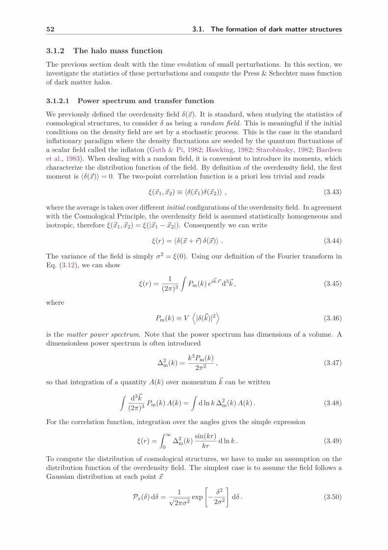
52 3.1. The formation of dark matter structures
3.1.2 The halo mass function
The previous section dealt with the time evolution of small perturbations. In this section, weinvestigate the statistics of these perturbations and compute the Press & Schechter mass functionof dark matter halos.
3.1.2.1 Power spectrum and transfer function
We previously defined the overdensity field δ(þx). It is standard, when studying the statistics ofcosmological structures, to consider δ as being a random field. This is meaningful if the initialconditions on the density field are set by a stochastic process. This is the case in the standardinflationary paradigm where the density fluctuations are seeded by the quantum fluctuations ofa scalar field called the inflaton (Guth & Pi, 1982; Hawking, 1982; Starobinsky, 1982; Bardeenet al., 1983). When dealing with a random field, it is convenient to introduce its moments, whichcharacterize the distribution function of the field. By definition of the overdensity field, the firstmoment is 〈δ(þx)〉 = 0. The two-point correlation function is a priori less trivial and reads
ξ(þx1, þx2) ≡ 〈δ(þx1)δ(þx2)〉 , (3.43)
where the average is taken over different initial configurations of the overdensity field. In agreementwith the Cosmological Principle, the overdensity field is assumed statistically homogeneous andisotropic, therefore ξ(þx1, þx2) = ξ(|þx1 − þx2|). Consequently we can write
ξ(r) = 〈δ(þx + þr) δ(þx)〉 . (3.44)
The variance of the field is simply σ2 = ξ(0). Using our definition of the Fourier transform inEq. (3.12), we can show
ξ(r) =1
(2π)3
∫
Pm(k) eiþk.þr d3þk , (3.45)
where
Pm(k) ≡ V⟨
|δ(þk)|2⟩
(3.46)
is the matter power spectrum. Note that the power spectrum has dimensions of a volume. Adimensionless power spectrum is often introduced
∆2m(k) =
k3Pm(k)
2π2, (3.47)
so that integration of a quantity A(k) over momentum þk can be written
∫
d3þk
(2π)3Pm(k) A(k) =
∫
d ln k ∆2m(k) A(k) . (3.48)
For the correlation function, integration over the angles gives the simple expression
ξ(r) =
∫ ∞
0∆2
m(k)sin(kr)
krd ln k . (3.49)
To compute the distribution of cosmological structures, we have to make an assumption on thedistribution function of the overdensity field. The simplest case is to assume the field follows aGaussian distribution at each point þx
Px(δ) dδ =1√
2πσ2exp
[
− δ2
2σ2
]
dδ . (3.50)

Chapter 3. Dark matter halos and subhalos in the Universe 53
Since the variance is independent of þx, so is the distribution. The real and imaginary partof δ(þk) are also distributed according to a Gaussian distribution. Additionally, all modes þkare independent of each other. A Gaussian distribution is conveniently entirely determined byits second moment, therefore the power spectrum alone is enough to characterize the wholedistribution. This is a very nice and practical feature, and it is standard to assume a Gaussiandistribution for the overdensity field for this reason. This simple case is also a standard predictionof many models of inflation (Martin et al., 2014). Furthermore, observations so far do not showany sign of non-gaussianity. We do not expect the Gaussian assumption to hold in the non-linearδ & 1 regime however. One reason is that the non-linear evolution mixes the modes, it is thereforeunlikely that their distribution remain independent. Another simpler reason is that by definitionof the overdensity in Eq. (3.14) we have δ > −1, while the Gaussian distribution is even andextends to arbitrary low values of δ.
Inflationary models predict the power spectrum of primordial fluctuations, which is usuallycalled the primordial power spectrum. What is needed to compute the mass function of darkmatter halos is the power spectrum today. Perturbation modes today are related to their initialcondition through the transfer function T (k). Parametric fitting formulas for T (k) are givenby Eisenstein & Hu (1998); Eisenstein & Hu (1999). The transfer function is shown on the leftpanel in Fig. 3.3. We show T (k) when only CDM is taken into account (blue curve) and whenbaryonic features are included (red curve). There is little difference between the two, though onenotes the presence of wiggles in the transfer function accounting for baryonic effects. This is asignature of baryonic acoustic oscillations. The asymptotic behaviour of the transfer function isthe following:
T (k) =
1 for k ≪ keqln(k)
k2 for k ≫ keq(3.51)
where keq is the mode entering the horizon at equivalence. The suppression of power on small scalesin due to the suppression of growth during the radiative era [the Meszaros effect (Meszaros, 1974)]:small-scale modes entering the horizon before matter-radiation equality grow logarithmicallyuntil equality, while mode entering during the matter-dominated era grow efficiently right away.
The power spectrum today is related to the primordial spectrum Pm,0 through
Pm(k) = |T (k)|2 Pm,0(k) . (3.52)
The primordial power spectrum inferred from observations of the Cosmic Microwave Backgroundhas a power-law behaviour Pi(k) ∝ kns with ns = 0.9677 ± 0.0060 according to Ade et al. (2016).A spectrum with index ns = 1 is called scale-invariant or Harrison-Zel’dovich spectrum (Harrison,1970; Zel’dovich & Novikov, 1970; Peebles & Yu, 1970), therefore the power spectrum of theCMB is nearly scale-invariant. The term scale-invariant can be understood by looking at thegravitational potential power spectrum Pφ ∝
⟨
|δφ|2⟩
. The potential fluctuation is related to thedensity fluctuation through Poisson’s equation (3.13) which gives
δφ(k) = −3
2
H20 Ωm,0
k2 aδ(k) . (3.53)
Consequently, we have Pφ ∝ k−4 Pm(k) ∝ kns−4 and the dimensionless power spectrum ∆2φ ∝
k3 Pφ ∝ kns−1. For a value ns = 1, we see that the dimensionless gravitational potential powerspectrum is independent of k. This is not true for the dimensionless matter power spectrumhowever, which has the scaling ∆2
m ∝ kns+3.The ΛCDM transfer function as shown in the left panel on Fig. 3.3 assumes a perfectly cold
dark matter fluid. If the dark matter particle is a WIMP, the collisional and collisionless dampingmechanisms discussed in Sec. 2.4 leave an imprint on the dark matter transfer function. Thistranslates into a strongly suppressed transfer function above a comoving mode given by the

54 3.1. The formation of dark matter structures
Figure 3.3 – Left panel: CDM transfer function (blue) and matter transfer function (red) fromEisenstein & Hu (1998). Right panel: linear matter power spectrum in the cosmology of Ade et al.(2016).
kinetic decoupling of the dark matter particle (Loeb & Zaldarriaga, 2005). Consequently, thedark matter power spectrum is also suppressed below that scale and strongly departs from thescale-invariant spectrum (Green et al., 2005).
3.1.2.2 Filtering
Our goal is to derive the halo mass function, that is the number density of dark matter halos perunit of mass. In order to do this, we need to assign a mass M, or a scale length R, to a region ofspace from the overdensity field δ(þx). This is achieved by defining a smoothed density field
δR(þx) =
∫
δ(þx′) W (þx − þx′, R) d3þx′ , (3.54)
where W is a window function (with units of inverse volume). In Fourier space, we have simply
δR(þk) = W (kR) δ(þk) . (3.55)
A common choice for the window function is the real-space top-hat
W (þx − þx′, R) =
3/(4πR3) if |þx − þx′| 6 R0 if |þx − þx′| > R .
(3.56)
The associated Fourier transform is
W (kR) =3
(kR)3[sin(kR) − kR cos(kR)] . (3.57)
Another popular choice is the Gaussian window function
W (þx − þx′, R) =
(
1
2πR2
)3/2
exp
[
−|þx − þx′|22 R2
]
, (3.58)
with Fourier transform
W (kR) = exp
[
−(kR)2
2
]
. (3.59)

Chapter 3. Dark matter halos and subhalos in the Universe 55
A third useful choice is the Fourier-space top-hat window
W (kR) = Θ(1 − kR) , (3.60)
where Θ is the Heaviside step function. This window does not have a well-defined volume in realspace. A volume can be assigned in a formal way by requiring that W (0, R)V (R) = 1, whichleads V (R) = 6π2R3. Note that the windows are all normalized
∫
W (þx, R) d3þx = 1 . (3.61)
Furthermore, their Fourier transform is defined through
W (kR) =
∫
W (þx, R) e−iþk.þx d3þx , (3.62)
which differs by a factor 1/V from our definition of the Fourier transform given in Eq. (3.12)(this factor is actually included in the definition of W ). A variance can be straightforwardlydefined for the smoothed density field
σ2R ≡
⟨
δ2R(þx)
⟩
=1
(2π)3
∫
Pm(k) |W (kR)|2 d3þk
=
∫
∆2m(k) |W (kR)|2 d ln k .
(3.63)
The smoothing on a length scale R can be translated into a smoothing on a mass scale M throughthe volume of the window in real space. This volume can be generically written V (R) = γ R3,with γ a constant equal to 4π/3 for the top-hat filter, (2π)3/2 for the Gaussian filter and 6π2 forthe k-space top-hat. The mass is then
M = ρ V (R) . (3.64)
with ρ the background density (which is time-dependent in general). For a power-law spectrumP (k) ∝ kn, we get the scaling of the variance σ2
R ∝ R−(3+n) ∝ M−(3+n)/3. Since the smootheddensity field δR is linearly related to the density field, it also follows a Gaussian statistics, andits variance is simply σ2
R. The mass root mean square σM is shown in the left panel on Fig. 3.4.
3.1.2.3 The Press-Schechter mass function
We now arrive at the actual computation of the mass function. The original derivation wasperformed by Press & Schechter (1974). Though the derivation has some important shortcomings,which we briefly discuss later on, it leads to a very simple and powerful expression for the massfunction. A nice review on the Press-Schechter mass function and its extensions can be found inZentner (2007). The main assumption of Press and Schechter relies on the spherical collapsemodel. The idea is that a smoothed fluctuation δM (t) equating some critical overdensity δc
collapses into a halo of mass M . If a region of scale R (mass M) has a density fluctuation δ > δc,then we can reasonably conceive that a more extended region of scale R′ > R (mass M ′ > M)would be less contrasted with δ′ < δ, while still with δ′ > δc. This leads to the assumtion that ifδR > δc, there is a region of size R′ > R that crosses the threshold δR′ = δc. This means thatfor a given scale R (M), probing δ > δc upward translates into probing more and more massivecollapsed objects of mass M ′ > M . The value of δc is usually set to be δc = 1.69, as predicted bythe spherical collapse model in Eq. (3.42). If we assume the probability distribution of δM is theGaussian distribution with variance σ2
M , the fraction of dark matter collapsed into halos of massM or higher is
F (M) =
∫ ∞
δc
(
1
2πσ2M
)3/2
exp
[
− δ2
2σ2M
]
dδ
=1
2erfc
(
ν√2
)
.
(3.65)

56 3.1. The formation of dark matter structures
Here erfc is the complementary error function and ν ≡ δc/σM is the peak height. The numberdensity of objects with mass between M and M + dM is then
dn
dMdM =
ρ
M
∣
∣
∣
∣
dF
dM
∣
∣
∣
∣
dM
=ρ
M2
∣
∣
∣
∣
d ln σM
d ln M
∣
∣
∣
∣
ν
√
2
πexp
[
−ν2
2
]
dM .
(3.66)
A factor of two has been added by hand to the formula to get the correct estimate. This is relatedto the cloud-in-cloud problem which we discuss below. Note that if σM has a weak dependencewith respect to M , which is the case if the power spectrum is scale-invariant, then the massfunction has a power-law behaviour dn/dM ∝ M−2 at small masses and is exponentially cutoff at large masses. The typical mass M∗ at which the transition happens is set by σ(M∗) = δc.The Press-Schechter mass function multiplied by M2 is shown in the right panel in Fig. 3.4. Thequantity M2 dn/dM spans less than two orders of magnitude over 23 orders of magnitude inM , which shows the goodness of the approximation dn/dM ∝ M−2 below the galactic scaleM ∼ 1012 M⊙. The mass function falls sharply above M ∼ 1014 M⊙.
3.1.2.4 Beyond the Press-Schechter theory
The Press-Schechter mass function is surprisingly successful at capturing the behaviour of darkmatter halos found in cosmological simulations. The derivation of the formula suffers howeverfrom the multiplication by a factor of two with little justification. There is actually alreadya problem in the expression of the halo fraction in Eq. (3.65). This can be understood from
the scaling σ2 ∝ M−(3+n)/3, which implies that σM→0−→ ∞, and hence that ν
M→0−→ 0. Hence thefraction of mass contained in collapsed objects of arbitrary small mass is F (0) = 1/2, i.e. themodel predicts that only half of the dark matter can collapse into halos. This issue was alreadynoted by the original authors who argued that the discrepant factor of two is linked to thecloud-in-cloud problem. The idea is that an under-dense region δM (þx) < δc can be embedded inan over-dense region δM ′(þx) = δc and will eventually collapse into a halo of mass M ′, thereforeunder-dense regions should also be included in the halo fraction (3.65). Including these clouds-in-cloud certainly increases F (M), however it is not clear that this leads to an exact factor oftwo.
The cloud-in-cloud problem was solved by Bond et al. (1991) who used the excursion settheory to consistently derive the mass function. Amazingly, they recovered the Press-Schechtermass function in Eq. (3.66) with the factor of two lacking in the original derivation. The formalismthey used is therefore often referred to as the extended Press-Schechter formalism. This techniqueis not only a tool to derive mass functions, it can also be used to study the formation history ofdark matter halos. In particular, it can be used to simulate merger trees as it was first shown byLacey & Cole (1993). The extended Press-Schechter theory motivates the study of generalizedmass functions of the form
dn
dM=
ρ
M2
∣
∣
∣
∣
d ln σM
d ln M
∣
∣
∣
∣
ν f(ν) , (3.67)
where f(ν) = dF/dν, and for the Press-Schechter mass function f(ν) =√
2/π exp(−ν2/2). Thederivation of Bond et al. (1991) was extended beyond the spherical collapse approximation bySheth & Tormen (1999), see also Sheth et al. (2001), to include ellipsoidal collapse. This leads toa simple form of the mass function
ν f(ν) = 2A
(
1 +1
ν ′2q
)
(
ν ′2
2π
)1/2
exp
(
−ν ′2
2
)
, (3.68)

Chapter 3. Dark matter halos and subhalos in the Universe 57
where ν ′ =√
aν, a = 0.707, q = 0.3, and A ≃ 0.322. The original Press-Schechter mass functionin Eq. (3.66) is recovered with a = 1, q = 0 and A = 1/2. The Sheth-Tormen mass function iscompared to the Press-Schechter mass function in the right panel on Fig. 3.4. The Sheth-Tormenmass function predicts more structures at very high masses where the function is sharply falling,less structures below down to M ∼ 106 M⊙, and more structures even below. The latter regime isnot probed by observations nor cosmological simulations, hence the robustness of the Seth-Tormenand Press-Schechter mass functions in that region is unknown.
Figure 3.4 – Left panel: Root mean square of the smoothed overdensity field as a function of themass. Right panel: Press-Schechter mass function (solid line) and Seth-Tormen mass function (dashedline). We used the cosmology of Planck 2015 (Ade et al., 2016).
3.1.3 The internal structure of dark matter halos
In this section, we describe the internal structure of dark matter halos. Since the evolution of avirialized dark matter structure is a non-linear process, the prime tool to study it is numericalsimulation. The shape of the density profile of dark matter structure is the result of severalphysical processes. Some, such as phase-mixing and violent relaxation (Lynden-Bell, 1967; Binney& Tremaine, 1987), are internal to the structure and may drive it to its equilibrium state. Otherscome from the interaction of the halo with its environment, such as accretion and mergers. Anaive expectation would be that the internal shape of a halo depends on its particular historyand its environment. Quite remarkably, N-body cosmological simulations where all these effectsare accounted for have shown that this is not the case. Indeed, if the effect of baryonic matter isignored, virialized dark matter halos have a universal shape. This fundamental result was firstestablished by Navarro et al. (1996); Navarro et al. (1997) and recently probed further down tothe origin of the first peaks by Angulo et al. (2016). Another investigation based on simulationswas done here Ogiya & Hahn (2018). It was shown by Navarro et al. (1996); Navarro et al. (1997)that CDM halos are spherical and their density profile is very well fitted by what is now calledthe Navarro-Frenk-White (NFW) profile
ρ(r) = ρs1
x
1
(1 + x)2 (3.69)
x ≡ r
rs(3.70)

58 3.1. The formation of dark matter structures
Fitting parameters ρs and rs are called scale density and scale radius, respectively, and theydepend on the mass and the size of the dark matter halo. The NFW profile exhibits a steepr−1 diverging behaviour as r ≪ rs and a steeper r−3 tail when r ≫ rs. However, if dark matterself-annihilates, then a core should appear at the very center of a halo around the radius at whichthe dynamical time exceeds the annihilation time
tdyn ≃ [GNρ(rcore)]−1/2 > tann ≃ m
〈σannv〉 ρ(rcore). (3.71)
While the emergence of this profile is reproduced by most simulations, it is still not clear what arethe physical mechanisms setting this power-law scaling. The mass can be expressed analytically
m(r) = 4π
∫ r
0dr′ r′2 ρ(r′)
= 4πρsr3s
[
ln (1 + x) − x
x + 1
]
,(3.72)
hence it has a logarithmic divergence at large radii. This is not an issue in practice since onecan always associate to a halo a virial radius and compute a finite mass within that radius. Ageneralized version of the NFW profile is often used in the literature
ρ(r) = ρs x−γ [1 + xα](γ−β)/α (3.73)
The index γ measures the inner slope of the dark matter profile while β controls the outerslope, and α sets the transition between the two regimes. The NFW profile is recovered for(α, β, γ) = (1, 3, 1). Since the original work of Navarro, Frenk and White, it has been found thatthe Einasto profile (Einasto, 1965, 1968) actually provides a better fit to CDM halos found insimulations (Navarro et al., 2004; Merritt et al., 2005; Graham et al., 2006; Gao et al., 2008;Springel et al., 2008). The Einasto profile takes the following form
ρ(r) = ρs exp
− 2
α[xα − 1]
. (3.74)
While the NFW profile has a central cusp, the Einasto profile has a core.1 It involves a freeparameter α which sets the transition between the inner core and the exponential behaviour inthe outskirts, hence it takes the same role as the α parameter in Eq. (3.73). The α parameter inthe Einasto profile is found in simulations to be very small, typically of order α ∼ 0.1, hence thecore is very small. This is a general property of CDM halos: they present little to no core andexhibit instead a cuspy behaviour in their central regions. Some (α, β, γ) and Einasto profilesare shown in the left panel of Fig. 3.5, normalised to their scale density ρs.
It has been found in dedicated simulations that near the free-streaming scale, the profile ofhalos is significantly cuspier than the NFW profile, exhibiting instead a ρ ∝ r−1.5 behaviour(Ishiyama et al., 2010; Anderhalden & Diemand, 2013; Ishiyama, 2014; Ogiya & Hahn, 2018). Wedo not account for this effect in the following but note that it might have interesting consequenceson indirect searches for instance.
3.1.3.1 The concentration parameter
The shape of a dark matter halo with a given virial mass mvir is often described with a singleparameter called the concentration
cvir =rvir
r−2, (3.75)
1Note however that the central region of dark matter halos in simulations suffer from resolution loss, hence theobservation of a core might not reflect the true physical behaviour of the profile.

Chapter 3. Dark matter halos and subhalos in the Universe 59
Figure 3.5 – Left panel: a variety of density profiles often used to describe CDM halos, including theNFW profile (α, β, γ) = (1, 3, 1) and several Einasto profiles. Right panel: density contrast ∆ for theparametrisation of Bryan & Norman (1998) (red), the value in a matter dominated universe (green) and∆ = 200 (blue).
where rvir is the virial radius of the halo and r−2 is defined as
d ln ρ
d ln r
∣
∣
∣
∣
r=r−2
= −2 . (3.76)
The virial radius is set through the relation
m(rvir)43 π r3
vir
≡ ∆vir ρc , (3.77)
where ρc is the critical density and ∆vir is the density contrast defined by
∆vir ≡ δvir + 1 , (3.78)
with δvir the overdensity at the epoch of virialization. This density contrast can be evaluatedthrough the spherical collapse model, see Sec. 3.1.1.3, and it depends on redshift and cosmology.Fitting formulae are provided by Bryan & Norman (1998) in terms of the parameter x = Ωm(z)−1where Ωm(z) is the matter abundance given in Eq. (2.29). The formulae in the absence of curvature(ΩK = 0) is
∆vir = 18π2 + 82 x − 39 x2 . (3.79)
Note that ∆ = 18π2 is the value of the density contrast in a matter dominated universe. Toavoid the dependence over the cosmological parameters, it is conventional to fix the value of thedensity contrast to ∆ = 200. This is a conservative choice in that it underestimates the virialradius, as one can see on the right panel in Fig. 3.5. From now on, we fix the virial contrast to∆ = 200 and consider the virial quantities r200, m200 and c200. The radius r−2 is proportional tothe scale radius rs up to a numerical factor that depends on the profile. For the αβγ profile inEq. (3.73), we have
r−2 = rs
(
2 − γ
β − 2
)1/α
. (3.80)

60 3.1. The formation of dark matter structures
hence r−2 = rs for the NFW profile. Similarly, we also have r−2 = rs for the Einasto profile.Note that r−2 is ill-defined for β = 2, which happens in the case of the cored isothermal sphere(α, β, γ) = (2, 2, 0) for instance
ρ(r) =ρs
1 + r2
r2s
. (3.81)
In that case, one can simply choose r−2 ≡ rs.
The concentration parameter is directly related to the scale density ρs. Given the virial massand concentration m200 and c200, one can compute the scale parameters ρs and rs. As shownbefore, we have
m(r200)43 π r3
200
= 200 ρc . (3.82)
For a given density profile, we introduce a dimensionless mass profile m such that
m(r) = 4πρs r3s m
(
r
rs
)
, (3.83)
hence Eq. (3.82) becomes
4πρs m(
r200rs
)
43 π
(
r200rs
)3 = 200 ρc . (3.84)
The ratio r200/rs is related to the concentration up to profile-dependent numerical factor thereforewe write
r200
rs= η c200 , (3.85)
with η = [(β − 2)/(2 − γ)]1/α for αβγ profiles according to Eq. (3.80). We get the scale densityas a function of the concentration only
ρs =200 ρc
3
(η c200)3
m (η c200). (3.86)
The virial mass is simply
m200 ≡ m(r200) =4
3π r3
200 200 ρc
=4
3π (η c200 rs)
3 200 ρc
(3.87)
therefore
rs =1
η c200
(
3 m200
4π 200 ρc
)1/3
. (3.88)
This shows that the mass and the concentration together completely determine the density profileof a dark matter halo.

Chapter 3. Dark matter halos and subhalos in the Universe 61
3.1.3.2 The mass-concentration relation
Though mass and concentration are independent parameters, a correlation between the two isfound in cosmological simulations as already noticed by Navarro et al. (1996). This is quitenatural in the context of hierarchical clustering since smaller structures are more likely to collapseearlier, when the Universe was denser. A variety of studies have proposed semi-analytical modelsof this mass-concentration relation, see e.g., Navarro et al. (1996); Bullock et al. (2001); Maccioet al. (2008); Prada et al. (2012); Dutton & Maccio (2014); Ludlow et al. (2014); Diemer &Kravtsov (2015); Ludlow et al. (2016); Diemer & Joyce (2018). A fit of the relation for fieldhalos is provided by Sanchez-Conde & Prada (2014), and by Moline et al. (2017) for subhalos insimulated Milky-Way-like galaxies – we will further investigate the later case based on theoreticalgrounds.
We review the model of Bullock et al. (2001) as modified by Maccio et al. (2008) that helpsunderstand and predict this relation. The first step is to relate the mass of a halo at the redshiftof collapse zc to its virial mass at redshift z < zc
m∗(zc) = F m200(z) , (3.89)
where F is a free parameter to be determined, assumed to be independent of the redshift ofcollapse, and m200 is the virial mass
m200 =4
3π r3
200 200 ρc(z) . (3.90)
The spherical collapse model prediction in Eq. (3.42) defines the characteristic mass as the onecrossing the non-linear threshold at the collapse redshift zc
σ(m∗, zc) = 1.686 . (3.91)
Note that
σ(m∗, z) = σ(m∗, 0) D+(z) , (3.92)
where D+ is the linear growth factor already introduced in Eq. (3.25). The redshift of collapseis shown as a function of the mass in the left panel on Fig. 3.6. The redshift is a decreasingfunction of the mass i.e. more massive halos collapse later as expected in the hierarchical scenarioof structure formation. All structures collapse at a much lower redshift than matter-radiationequality which takes place at zeq ≃ 3300 (Ade et al., 2016). The choice of the window functiondefining σ(M) introduces a small uncertainty on the redshift. In the right panel, we comparethe redshift of collapse to the redshift when structures enter the non-linear regime, defined for agiven mass m by
σ(m, znl) = 1 . (3.93)
Obviously, this redshift is always superior to the redshift of collapse zc. We note that the redshiftsof collapse we obtain are significantly smaller than those found in other studies (Diemand et al.,2005; Green et al., 2005). This might be due to differences in the cosmological parameters sincewe used the cosmology of Ade et al. (2016) while older studies relied on the results from WMAP.
Let us go back to the concentration model. We introduce a characteristic density ρs definedas
ρs(z) =m200(z)43 π r3
s (z)
=
(
r200(z)
rs(z)
)3
200 ρc(z)
= [η c200(z)]3 200 ρc(z) ,
(3.94)

62 3.1. The formation of dark matter structures
Figure 3.6 – Left panel: redshift of collapse as defined by σ(F m200, zc) = 1.686, with F = 0.01 andfor various choices of the window function. Right panel: redshift of collapse and redshift of non-linearevolution, defined by σ(F m200, zc) = 1.686 and σ(F m200, znl) = 1 respectively. We used the real spacetop-hat window function, and show the results for two values of the F parameter: F = 0.01 (solid line)and F = 1 (dashed line).
with the η parameter introduced in Eq. (3.85). Note that ρs is a priori different from the scaledensity ρs. In the model of Maccio et al. (2008), the characteristic density is assumed to beindependent of the redshift, which implicitly entails that further evolution of the halo aftervirialization does not strongly affect its very internal structure. If we further assume that thedensity contrast ρs/(200 ρc) is universal at any collapse redshift zc, and set to a constant K3 tobe determined, then we get2
c200(z) = K
[
ρc(zc)
ρc(z)
]1/3
= K
[
H(zc)
H(z)
]2/3
. (3.95)
The concentration is therefore related to the mass m200 through the redshift of collapse zc. Themodel has two independent free parameters F and K that must be calibrated on cosmologicalsimulations. For the cosmology of Planck 2013 (Ade et al., 2014), it is found by Dutton & Maccio(2014) that F = 0.01 and K = 4.2 provide a good fit to their simulations. Even though thismodel is tested over five decades of mass from dwarf galaxies to galaxy clusters, it is shown bySanchez-Conde & Prada (2014) that it also agrees with simulations of Earth-mass halos withm200 ∼ 10−6 M⊙ (Diemand et al., 2005; Ishiyama et al., 2010). We show the mass-concentrationrelation in the Planck cosmology in the left panel on Fig. 3.7. We show the model of Pradaet al. (2012), using the fitting function provided by Sanchez-Conde & Prada (2014) (P12 in thelegend), as well as the concentration from the Bullock et al. (2001); Maccio et al. (2008) modelwe discussed above (P01/B08 in the legend). Both models give a close prediction over eighteendecades in mass, with a predicted concentration of around 10 for Milky-Way-like halos andaround 60 for Earth-mass halos. Since the scale density of a halo is uniquely determined by itsconcentration, we can compute ρs as a function of the mass using a model for the concentration.The result is shown in the right panel on Fig. 3.7. Unlike the concentration, the scale densitydepends on the functional form of the density profile. This leads to large differences as we showby comparing ρs for an NFW and an Einasto profile.
2This assumes that halos are isolated, or do not experience major mergers after their formation (accretion ofmuch smaller objects only).

Chapter 3. Dark matter halos and subhalos in the Universe 63
In the following, we use the fitting formulae for c200(m200) provided by Sanchez-Conde &Prada (2014) of the model of Prada et al. (2012) and do not consider the Bullock et al. (2001);Maccio et al. (2008) model.
Figure 3.7 – Left panel: concentration c200 at z = 0 for the model of Prada et al. (2012) with thefitting function given in Sanchez-Conde & Prada (2014) (red line), and the model of Bullock et al. (2001)revised by Maccio et al. (2008); Dutton & Maccio (2014) (green, blue and magenta lines). Right panel:scale density ρs in units of the local density, for the concentration models shown in the left panel, and twoinner profiles (NFW and Einasto).
3.2 Subhalos and their evolution
The previous section describes the formation of dark matter halos and their statistics froma cosmological point of view. The hierarchical scenario of structure formation predicts thatlarge dark matter halos are formed by the collapse of a collection of smaller, already formedhalos. We can wonder whether these small objects survive the collapse of their larger hoststructure and are still present in galactic halos today. This is a crucial question for particledark matter searches as these subhalos can strongly impact predictions for direct and indirectsearches as well as gravitational searches, as discussed in Chap. 4. The evolution of a subhaloinside a galactic halo is a priori very complex as it experiences a variety of gravitational effectsfrom the host galaxy: tidal stripping, shocking, heating, dynamical friction, interactions withbaryons (shocking by the disc, encounter with stars), etc. To account for all these effects ina self-consistent way, study of subhalos often rely on numerical cosmological simulations likeVia Lactea II Diemand et al. (2008) or Aquarius Springel et al. (2008) for dark matter-onlysimulations. For numerical studies of subhalos in simulations including baryons, see e.g., Zhuet al. (2015); Garrison-Kimmel et al. (2017); Rodriguez-Puebla et al. (2016). These simulationsallow to self-consistently follow the evolution of subhalos from their collapse to z = 0. A majordrawback is the very high computational cost of numerical simulations, which strongly limitstheir resolution. As an example, the best mass resolution achieved in the Aquarius simulation isMres ≃ 103 M⊙ which is orders of magnitude higher than the lowest mass achievable in typicalWIMP models mmin ≃ 10−6 M⊙, see Sec. 2.4. Some simulations focus on the smallest scales, seee.g., Diemand et al. (2005); Ishiyama et al. (2010); Anderhalden & Diemand (2013); Ishiyama(2014), but can only do so at very high redshifts and therefore cannot investigate subhalos ingalactic halos today. Moreover, it has recently be pointed out that cosmological simulations

64 3.2. Subhalos and their evolution
are very likely to strongly overestimate the tidal disruption of subhalos due to resolution limit(van den Bosch et al., 2018; van den Bosch & Ogiya, 2018). It is therefore important to questionthis survival issue on first-principle grounds.
An alternative approach to the subhalo problem is semi-analytic modelling, see e.g., Berezinskyet al. (2003); Green & Goodwin (2007); Kamionkowski et al. (2010); Gan et al. (2010); Bartels& Ando (2015); Han et al. (2016); Stref & Lavalle (2017); Hiroshima et al. (2018), see alsoBerezinsky et al. (2014) for a review. Given the complexity of the issue, analytic calculationsare possible only at the cost of approximations and therefore partial loss of consistency. Amajor benefit of this approach is the possibility of investigating all scales at play in one unifiedframework. It also provides ways to account for known cosmological and dynamical constraints.This is especially appealing for dark matter searches which is why we focus on this approach inthe following. We still keep an eye on the results of numerical simulations to qualitatively checkthe validity of our calculations.
In what follows we present semi-analytic methods to model tidal effects, including thecontribution of the host halo, the galactic disc and the stars. Before going into the details, letus give a rough estimate of the typical number of subhalos in a Milky-Way-like galaxy. Anestimation of this number can be obtained from cosmological simulations. For instance, in theAquarius simulation of Springel et al. (2008) the number of subhalos found in the best resolvedMilky-Way-sized halo is ∼ 300 000, with the mass resolution Mres ≃ 105 M⊙. Extrapolating theM−2 behaviour of the halo mass function to subhalo masses down to mmin = 10−6 M⊙, we get atotal number of subhalos Nsub ≃ 3 × 10¹⁶! Such a gigantic number suggests that subhalos donot ”see” the clumpy nature of the galactic halo and essentially behave as if they were movingthrough a smooth potential. This simplifies our study of tidal effects.
3.2.1 Tidal stripping
The first effect we investigate is tidal stripping. When a subhalo orbits a host potential, part ofits material is stripped away by the host galaxy. This effect has long been known to be relevantin Galactic dynamics as it explains for instance the observed finite extensions of globular clusters(King, 1962).
3.2.1.1 Tidal radius for point masses
Let us consider two point masses m and M orbiting each other at a fixed separation R, withM ≫ m, such that the rotation angular frequency about the center of mass is given by
ω =
√
GN(m + M)
R3. (3.96)
Placing ourselves in the co-rotating frame, we now investigate the motion of a vanishinglylight test-mass particle in the joint potential induced by the two bodies, assuming it is initiallypositioned at a distance x ≪ R from the lightest one. This can be thought of as a WIMP orbitinga point-like subhalo embedded in the potential generated by a point-like host halo. This is calledthe restricted three-body problem (Spitzer, 1987; Binney & Tremaine, 1987). We consider amassless test particle confined to the axis linking the masses m and M , and call x its distance tothe mass m. The equations of motion for the test particle are
x =GN m
x2− GN M
(R − x)2+
GN(M + m)
R3
(
M
M + mR − x
)
, (3.97)
where the last term accounts for the centrifugal force in the co-rotating frame. We look for astationary point x = 0. To get a close expression for x, we assume M ≫ m, hence M representsa galactic halo and m a satellite subhalo. This implies x ≪ R and we get the solution
x ≃ R
(
m
3M
)1/3
. (3.98)

Chapter 3. Dark matter halos and subhalos in the Universe 65
This stationary solution is actually the approximate position of a Lagrange point. It also definesthe radius of the Hill sphere, or Roche sphere (named after astronomers George William Hilland Edouard Roche) which is the region of influence of a celestial body. More precisely, it is theregion inside which a particle is bound to the satellite rather than the host halo, therefore itgives the maximal spatial extent of the satellite. This spatial boundary is referred to as the tidalradius.
A very rough estimation of the tidal radius is obtained by assuming a point-like structure forthe Galaxy. Using Eq. (3.98), we get
rt,point1 ≡ R
(
mint(rt,point1)
3 Mtot
)1/3
, (3.99)
where Mtot = Mdm + Mbar is the total mass of the Galaxy, including both dark matter andbaryons. From now on, we refer to this definition as the first point-like Jacobi radius. This is animplicit definition since the tidal radius appears on both sides of the equation. In practice wesolve this equation numerically to get the radius.
Assuming the Galaxy has a point-like structure is of course a very bad approximation, exceptfor subhalos orbiting in the outskirts of the dark halo. For a subhalo on a circular orbit of radiusR, we can instead define its tidal radius by replacing the total mass Mtot in Eq. (3.99) withthe mass M(R) within the orbit. We refer to this new definition as the second point-like Jacobiradius
rt,point2 ≡ R
(
mint(rt,point2)
3 M(R)
)1/3
. (3.100)
Note that M(R) also includes both dark matter and baryons. As we go to very large radii, weexpect the value of rt,point1 and rt,point2 to coincide. We can rewrite Eq. (3.100) as
3 mint(rt,point2)
4π r3t,point2
= 3 × 3 M(R)
4π R3, (3.101)
which is
ρsub(rt,point2) = 3 ρhost(R) , (3.102)
where ρsub and ρhost(R) are the mean density of the subhalo and the host, respectively. Notethat the definition of the tidal radius in Eq. (3.100) is not considered in Stref & Lavalle (2017).
What is the mass and concentration dependence of the Jacobi radii? We saw in Sec. 3.1.3that the scale density ρs is determined by the concentration parameter c200 alone, ρs = ρs(c200),and is independent of the cosmological mass m200. The mass profile can be expressed
mint(r) = 4π
∫ r
0r′2 ρ(r′) dr′ = 4πρsr
3s mint(r/rs) , (3.103)
with mint a dimensionless function. For both point-like radii, we have
mint(rt,point/rs)
(rt,point/rs)3=
3
ρs(c200)
M
R3, (3.104)
where ρs and rs are the scale density and radius of the subhalo, and M refers to Mtot or M(R)depending on the definition of the tidal radius. This shows that the ratio rt,point/rs only dependson the concentration c200 and the radius of the orbit R, and is independent of the cosmological
mass m200. Consequently, rt,point depends on m200 like rs does, so rt,point ∝ m1/3200.

66 3.2. Subhalos and their evolution
3.2.1.2 Tidal radius for a smooth mass distribution
The case where the host has an extended mass distribution can be treated in a consistent way,although the computation is more involved (Binney & Tremaine, 1987; Tollet et al., 2017). Itcan be shown that the Jacobi radius is modified to
rt,smooth ≡ R
mint(rt,smooth)
3M(R)(
1 − 13
d ln Md ln R (R)
)
1/3
. (3.105)
We refer to this definition as the smooth Jacobi radius. As for the point-like case, the ratiort,smooth/rs is independent of m200. Indeed the ratio is solution of the equation
mint(rt,smooth/rs)
(rt,smooth/rs)3=
3
ρs(c200)
M(R)
R3
(
1 − 1
3
d ln M
d ln R(R)
)
, (3.106)
It has therefore the scaling with the cosmological mass rt,smooth ∝ m1/3200, similar to the point-like
radius. We note that if the host halo has a constant density d ln M/d ln R = 3, the right-handside of Eq. (3.105) diverges and the definition of the tidal radius breaks down. This is becausea subhalo evolving in a constant-density field experiences tidal compression which prevents itsmass from being transferred to its host, see Dekel et al. (2003) for a detailed discussion.
For the sake of comparison, we introduce another tidal radius rt,dens based on a simplecriterion involving only the density of the satellite and the host:
ρint(rt,dens) ≡ ρhost(R) . (3.107)
Unlike the Jacobi radii, this radius is not motivated by first principles. It is a rather phenomeno-logical definition, as the radial boundary of a halo is defined as the point where its density reachesthe background density. Like in the case of the Jacobi radii, the ratio rt,dens/rs is independent ofm200 since the mass density profile is ρint(r) = ρs ρint(r/rs) with ρint a dimensionless function.Consequently, rt,dens/rs is solution of
ρint
(
rt,dens
rs
)
=ρ(R)
ρs(c200), (3.108)
and only depends on c200 and R.The tidal radii defined above assume a circular orbit for the satellite. However, we do not
expect subhalos to have circular orbits in general. A more realistic description should involveelliptical orbits. Despite this approximation, it is found that a simple prescription such asEq. (3.105) gives a radius which is tightly correlated to the observed radius of subhalos in N-bodysimulations, see e.g., Fig. 15 in Springel et al. (2008).
The different definitions of the tidal stripping radius rt are compared in Fig. 3.8. The positiondependence of the ratio rt/rs is shown for two Milky Way mass models from McMillan (2017):the NFW model (left panel) and the (α, β, γ) = (1, 3, 0) model (right panel). Irrespective of thedefinition, the tidal radius gets smaller and smaller as the subhalo orbits closer and closer tothe center of the Galaxy. The only exception is the smooth Jacobi radius in the cored darkmatter-only mass model, but as we discussed above, this definition of the tidal radius breaksdown when the density is too flat. This potential problem disappears when the baryons areadded to the mass model, hence it does not have any consequences in a realistic framework. Weobserve that the point-like approximation leads to the strongest tides, while the smooth anddensity-based models give rather close predictions. Interestingly, the exact shape of the Galacticdark matter profile has no impact on the calculation when baryons are also included. This canbe seen by comparing the left and right panels of Fig. 3.8. The red curves (NFW+baryons)and green curves (core+baryons) are nearly identical, hence the calculation of the tidal radius

Chapter 3. Dark matter halos and subhalos in the Universe 67
is robust and insensitive to the largely unknown inner shape of the dark halo profile. Fig. 3.9shows the concentration dependence of the tidal radius for subhalos at the position of the Sun(R⊙ = 8.21 kpc for the mass model considered here). This shows that tides have a stronger effecton less concentrated structures. We compare subhalos with two different density profiles: eitheran NFW profile, or an Einasto profile with αE = 0.17, see Eq. (3.74). The difference between thetwo profiles is small over most of the relevant concentration range.
Both Fig. 3.8 and Fig. 3.9 show that the first Jacobi radius is smaller than all the other radii,at all position in the host Galaxy and for all concentrations. The other radii, i.e. the secondand smooth Jacobi radii as well as the density-based radius, lead to comparable values. This isan indication that the first Jacobi radius probably overestimates the effect of tides on subhalos.Consequently, we do not consider this tidal radius in the following. From now on, each time atidal radius is referred to as ”point-like”, it actually refers to the second Jacobi radius defined inEq. (3.100). We stress that this is different from Stref & Lavalle (2017), where the only point-likeradius considered was the one defined in Eq. (3.99).
Figure 3.8 – Left panel: tidal radius to scale radius ratio as a function of the position inside theGalaxy, for the NFW mass model of McMillan (2017). The subhalo internal profile is an NFW withconcentration c200 = 60. Right panel: same as left panel for the cored mass model of McMillan (2017).
3.2.2 Tidal shocking
We described tidal stripping which is the effect on a satellite of a constant or slowly-varyinggravitational potential. We now discuss the opposite situation where the gravitational potentialrapidly varies in time: this is called tidal shocking. The physical effect is very simple tounderstand: as a subhalo passes by or passes trough a dense object (a dark matter cusp, a stellardisc, a star,etc.), it experiences a strong gravitational field which strips away some particlespreviously bounded to the subhalo. In the following, we investigate in details the shocking effectinduced by the Galactic disc.
3.2.2.1 Shocking by the Galactic disc
A very important effect is the shocking induced by the Galactic disc. This effect was firstdiscussed, in the context of star clusters affected by the passing of a nearby cloud, by Spitzer(1958). This paper makes use of the impulsive approximation which consists in ignoring the

68 3.2. Subhalos and their evolution
Figure 3.9 – Tidal radius to scale radius ratio as a function of the concentration, at the position of theSun R⊙ = 8.21 kpc. We show the ratio for the first Jacobi radius (red), the second Jacobi radius (green),the smooth Jacobi radius (blue) and the density-based radius (magenta). We compare the prediction fortwo different internal density profiles: NFW (solid lines) and Einasto (dashed lines).
inner dynamics of the cluster when evaluating the effect of the shock. Tidal shocking was theninvestigated by Ostriker et al. (1972) to evaluate the impact of the Galactic disc on globularclusters, again using the impulsive approximation. The importance of adiabatic invariance waspointed out by Weinberg (1994b,a) and the shocking calculation was revised and generalized byGnedin et al. (1999); Gnedin & Ostriker (1999). The impact of disc shocking on subhalos hasbeen numerically studied in a cosmological context by D’Onghia et al. (2010); Yurin & Springel(2015); Errani et al. (2017) and generically found to be a major source of stripping in the innerpart of the host halo. Here we provide several semi-analytic methods to evaluate the impact ofthe disc on subhalos.
First, we reproduce the original computation of Ostriker et al. (1972). We consider an object(subhalo, globular cluster) crossing the galactic disc. We work in the rest frame of the disc anddefine the z-axis as perpendicular to the disc. The object is on a circular orbit of radius R.Let zc and zp be the z-coordinate of the object’s center and of a particle orbiting in the object,respectively. We define ∆z ≡ zp − zc, vz ≡ d∆z/dt and the equation of motion is
dvz
dt= gd(R, zp) − gd(R, zc)
≃ ∆z∂gd
∂z(R, zc) ,
(3.109)
where gd is the gravitational acceleration caused by the disc. If the disc has a mass density ρd,the modulus of the acceleration is given by
|gd(R, z)| = 4πGN zd ρd(R, z) . (3.110)
Integrating Eq. (3.109) over time, we get the net velocity change
∆vz =
∫
dt ∆z(t)∂gd
∂z[zc(t)] . (3.111)
We now make the impulsive approximation: the dynamics within the object is considered veryslow compared to the crossing of the disc, hence ∆z is roughly time-independent. Changing the

Chapter 3. Dark matter halos and subhalos in the Universe 69
integration variable from t to zc we get
∆vz =∆z
Vz2 gd(R, 0) , (3.112)
where Vz is the z-velocity of the object’s center and the factor of two comes from the odd-parityof gd. Consequently, the kinetic-energy gain per unit of particle mass in the rest frame of theobject is
δǫ =1
2(∆vz)2 =
2 g2d
V 2z
(∆z)2
=2 g2
d
V 2z
r2 cos2(θ) ,
(3.113)
where r is the distance between the particle and the object’s center, and θ is the angle betweenthe radial and vertical directions. This result holds if Tcross(R) ≪ τsub(r) where Tcross is theobject crossing time and τsub(r) the orbital period of the particle within the object. This is thecontent of the impulsive approximation. This approximation might break down for particles nearthe center of the object which have a very short period. These particles are then protected byadiabatic invariance, which can be accounted for by multiplying the right-hand side of Eq. (3.113)by a corrective factor A(η) (Weinberg, 1994b,a). Using analytical and numerical studies, Gnedinet al. (1999); Gnedin & Ostriker (1999) proposed a parametric form for this factor
A(η) = (1 + η2)−3/2 , (3.114)
where η is the adiabatic parameter defined as
η ≡ ωint(r)Tcross , (3.115)
with ωint the orbital frequency of particles within the clump. The energy gain is modified to
δǫ(r, θ) =2 g2
d
V 2z
r2 cos2(θ) A(η) . (3.116)
If η ≫ 1 i.e. the orbital time of a test particle in the subhalo is much smaller than the disk-crossingtime, then the impulsive approximation breaks down and A(η) → 0: particles are adiabaticallyprotected against tidal shocking. Let us estimate the importance of adiabatic invariance insubhalos. With zd the length scale of the disk along the z-axis, the typical crossing-time isTcross(R) = zd/Vz(R). The z-component of the velocity should be close to the velocity dispersionalong z, i.e. Vz ≃ σz. Assuming an isotropic velocity distribution of subhalos, we have σ2
z = σ2/3where σ is the total velocity dispersion. To evaluate this velocity dispersion, we may assume aMaxwell-Boltzmann velocity distribution for subhalos in the Galaxy. As we will see in Chap. 5,this is equivalent to assuming a singular isothermal sphere for the subhalo spatial distribution.In that case, the velocity dispersion is simply related to the circular velocity
σ2(R) =1
2v2
c (R) , (3.117)
where
vc(R) =
√
GN m(R)
R(3.118)
with m(R) the Galactic mass within R. This should give the right order of magnitude of Vz evenif the subhalo distribution does not strictly follow the isothermal profile. The crossing time is

70 3.2. Subhalos and their evolution
then
Tcross(R) =√
2zd
vc(R)= zd
√
2R
GN m(R)
≃ 0.45 Myr
(
zd
100 pc
) (
200 km/s
Vz
)
.
(3.119)
Assuming the internal density profile of subhalos is also not too far from the singular isothermalsphere, we can express the internal velocity dispersion as
σ2int =
3
2
GN mint(r)
r(3.120)
and the orbital frequency
ωint(r) =σint
r
=
√
3 GN mint(r)
2 r3
= 2.4 × 10⁻² Myr−1(
mint(r)
10−6 M⊙
)1/2(
3.5 × 10⁻³ pc
r
)3/2
(3.121)
Note that ωint, expressed as a function of r/rs, depends only on the concentration c200 andnot on the mass m200. We find that the adiabatic correction becomes relevant only whenr < 10−3 rs i.e. subhalos are stripped down to their very center. This only happens for themost extreme stripping and shocking models discussed in this section [like the first point-likeJacobi radius in Eq. (3.99)], and only in the inner parts of the Galaxy. This means that theimpulsive approximation is a good approximation in most cases. Nevertheless, we performed ourcalculations including the corrective factor regardless of the modelling of tidal effects.
Shocking radius: differential method What is the tidal radius induced by disc shocking?There is no prescription available in the literature to compute this radius, therefore we proposeseveral definitions. One way to identify a maximal radius is to compare the kinetic energy gainin Eq. (3.116) to the potential energy of a dark matter particle in the subhalo. Let us consider asubhalo with pre-crossing radial extension r0, and a dark matter particle on a circular orbit atr < r0 in that subhalo. Assuming a hard truncation of the subhalo at radius r0, the potentialenergy (per unit of particle mass) is given by
φint(r) − φint(r0) (3.122)
where
φint(r) = −GN
∫ ∞
r
mint(r′)
r′2 dr′ , (3.123)
is the solution of Poisson’s equation cancelling at infinity. If the kinetic energy gain by a particleinside a subhalo during the crossing of the disc exceeds its potential energy, this particle becomesunbound to the subhalo. The new radius r1 after a single crossing of the disc can be evaluatedby equating the kinetic energy gain and the potential energy:
δǫ(r1) ≡ φint(r0) − φint(r1) . (3.124)
This definition is meaningful because |φint(r) − φint(r0)| is a decreasing function of r, hence thedark matter particles removed by that procedure are in the outskirts of the clump, see the left

Chapter 3. Dark matter halos and subhalos in the Universe 71
panel in Fig. 3.10. Note that the energy gain given in Eq. (3.116) has an angular dependence,hence we use instead the energy gain averaged on the sphere of radius r:
〈δǫ〉 (r) ≡ 1
4π
∫ 2π
0dφ
∫ π
0d(cos θ)δǫ(r, θ)
=2 g2
d
3 V 2z
r2 A(η) ,
(3.125)
and the radius r1 after disc shocking is really defined by
〈δǫ〉 (r1) ≡ φint(r0) − φint(r1) . (3.126)
This definition of the tidal shocking radius depends on the radial extension r0 before crossing.This means that the radius of the clump has to be computed after each crossing of the stellardisc. We call the final radius obtained via this procedure the differential radius rt,diff . The ratiort,diff/rs is independent of m200. Indeed the adiabatic correction A(η) only depends on ρs(c200),the energy gain scales like r2
s and the potential energy like ρsr2s hence the ratio only depends on
the scale density ρs(c200), the position of the subhalo R and its radius before crossing r0. Theangle-averaged energy gain and the potential energy for a single crossing, for a clump at theposition of the Solar System R = R⊙, are shown on the left panel in Fig. 3.10. The ratio rt,diff/rs
is the x-axis value of the intersection between the red curve (energy gain) and the blue curve(potential). The radius before crossing is chosen to be the cosmological radius r200 such thatr200/rs = c200.
Shocking radius: integral method We consider an alternative definition of the shockingradius based on integrated quantities. The idea is to compute the total energy gain of a subhaloand compare it to its binding energy. The total energy gain is computed from Eq. (3.116)
∆E(< r0) =
∫
δǫ ρint(þr) d3þr
= 2π
∫ r0
0dr r2
∫ 1
−1d cos θ δǫ(r, θ) ρint(r)
(3.127)
If the adiabatic correction is neglected and the subhalo has an NFW profile, the total energygain is analytical
∆E(< r0) ≃ 8π
3
g2d
V 2z
ρsr5s
[
(x0 − 3)x20 − 6x0
2(x0 + 1)+ 3 ln (1 + x0)
]
, (3.128)
where x0 = r0/rs. This energy has to be compared with the binding energy of the subhalo, whichis defined by
U(< r0) = GN
∫
mint(þr)
|þr| ρint(þr) d3þr . (3.129)
This is also an analytical function for the NFW profile
U(< r0) = 16π2GNρ2s r5
s
[
1
2
(
1 − 1
(1 + x0)2
)
− ln(1 + x0)
1 + x0
]
. (3.130)
Having computed the total energy gain and the total binding energy of a subhalo, we can defineits extension rt,int after disc shocking as follow
∆E(< rt,int) = U(< rt,int) . (3.131)

72 3.2. Subhalos and their evolution
Beyond rt,int, the total energy gain is larger than the binding energy of the clump as shown inthe right panel on Fig. 3.10. This gives the shocking radius after one single crossing. For theradius after Ncross crossing, we prescribe
Ncross∆E(< rt,int) = U(< rt,int) . (3.132)
The ratio rt,int/rs is, again, independent of m200 which can be seen from Eqs. (3.128)(3.130).We have ∆E ∝ ρsr
5s and U ∝ ρ2
s r5s therefore rt,int/rs only depends on ρs(c200) and R. The total
energy gain for a single crossing, at the position of the Sun R = R⊙, is compared to the bindingenergy and the total potential energy on the right panel in Fig. 3.10. The ratio rt,int/rs is definedby the x-axis value of the intersection between the green curve and the blue curve. Fixing theintegral radius with the potential energy (red curve) rather than the binding energy leads to asimilar, though slightly lower, numerical value.
Shocking radius: simulation-based estimate We finally consider a third definition of theshocking radius based on a numerical study by D’Onghia et al. (2010). This study focuses onthe effect of a Galactic disc on subhalos and shows that it is very efficient at disrupting thesestructures. The authors propose an empirical criterion to model the effect of disc shocking. Theypropose an expression for the total energy gain in units of the binding energy
∆E
U=
(1.84 r1/2)2g2d
3 σ2V 2z
, (3.133)
where r1/2 is the radius containing half the subhalo’s mass and σ is an estimate of the internalvelocity dispersion of the clump
σ2 = 0.4GNmtot
sub
r1/2, (3.134)
where mtotsub is the total subhalo mass. The dynamical grounds for this expression are taken
from Binney & Tremaine (1987). The authors argue that a subhalo is destroyed when the totalenergy after Ncross crossing of the galactic disc is comparable to the binding energy. Whetherclumps are actually destroyed in numerical simulations or disappear due to limited resolution isa difficult question which has very likely not fully been addressed in the past. Indeed, recentwork has shown that criteria based on the binding energy strongly overestimate the disruptionefficiency (van den Bosch et al., 2018; van den Bosch & Ogiya, 2018). This can be understoodfrom the adiabatic invariance argument stated before, which makes the dense cores of subhalosvery resilient to tidal effects. For the sake of comparison, we define a disc shocking radius through
Ncross∆E
U(rt,sim) = 1 , (3.135)
This radius is similar to our integral definition, with a different expression for the total energygain. This simulation-based definition also leads to a ratio rt,sim/rs independent of m200 becausethe total energy gain has the scaling ∆E ∝ ρsr
5s just like our integral definition. The energy ∆E
is shown on the right panel in Fig. 3.10. We see that for c200 < 10, we have ∆E > ∆E hence thesimulation-based estimate is more efficient at stripping subhalos. Note that the simulations ofD’Onghia et al. (2010) focuses on massive subhalos m & 106 M⊙ hence their results might notapply to smaller, more concentrated structures.
3.2.2.2 Encounter with stars
Another effect quite similar to disc shocking is the effect of individual stars on subhalos passingclose by. This effect has been investigated in several studies (Berezinsky et al., 2006; Angus

Chapter 3. Dark matter halos and subhalos in the Universe 73
Figure 3.10 – Left panel: angle-averaged energy gain (red) compared to the potential energy (blue)of a dark matter particle at a radius r within a subhalo orbiting at R = R⊙. Two possible values of theconcentration are shown c200 = 60 and c200 = 30. Right panel: integrated energy gain following thedefinition in Eq. (3.127) (green) and in Eq. (3.133) (purple), for c200 = 60 and c200 = 30. Are shown thebinding energy (blue) and the total potential energy (red).
& Zhao, 2007; Zhao et al., 2007; Green & Goodwin, 2007; Schneider et al., 2010), using bothanalytical and numerical estimates. It can be shown that for subhalos, the effect of disc shockingdominates over the shocking from each star (Berezinsky et al., 2014). Encounters with starsmight be more important for ultracompact minihalos which are halos having collapsed duringthe radiation-dominated era (Berezinsky et al., 2010). These structures are dense enough to bepractically immune against regular tidal effects, in which case stellar encounters might be theonly potential source of disruption.
3.2.3 Disruption of subhalos
All the tidal radii we have introduced to model the effects of halo stripping and disc shockingare compared in Fig. 3.11. The ratio rt/rs where rt is the tidal radius is shown for a particularconcentration c200 (we recall that this ratio is independent of the subhalo’s mass). The colouredcurves show the tidal radii for the stripping methods discussed in Sec. 3.2.1 and the black curvesshow the tidal radii for the disc shocking methods discussed in Sec. 3.2.2. Irrespective of theparticular methods chosen for stripping and shocking, the effect of disc shocking is sub-dominantat large radius R ≫ 10 kpc with respect to halo stripping. This is not a surprise since theGalactic disc extends to Rdisc ∼ 15 kpc and we assumed subhalos are on circular orbits. Forsubhalos on radial orbits, we expect disc shocking to play a role even at distances R > Rdisc butwe do not take this possibility into account. More interesting is the hierarchy below 10 kpc: discshocking is generically more important than halo stripping in that region. However, the choice ofthe shocking radius definition leads to important differences in that region: while the differentialand integral methods lead to similar results, the simulation-based method is much more efficientat stripping subhalos. We recall however that this criterion has only been probed on massivesubhalos which tend to be less concentrated due to their late collapse, see Sec. 3.1.3.
We now discuss the possible disruption of subhalos by tidal effects. We have seen that tidaleffects are very efficient at stripping subhalos down to their scale radius and below, the questionis then: can a structure survive after having lost most of its mass? This is crucial for indirect

74 3.3. A constrained model of Galactic subhalos
dark matter searches for instance, as the impact of a clump on these searches depends on itsluminosity ∝
∫
ρ2d3þr rather than its mass, and most of the luminosity comes from the structure’score, see e.g., Berezinsky et al. (2008). The question of survival under tidal effects also concernsluminous structures. Star clusters in particular have been under investigation for a long time, seee.g., Spitzer (1958). However these stellar systems are subject to phenomena like relaxation andevaporation which facilitate their disruption but are not relevant for the particle dark matterscenario (at the notable exception of primordial black hole dark matter). The question of thesurvival of dark matter subhalos is a more recent one. It has been investigated numerically,in dedicated studies Tormen et al. (1998); Hayashi et al. (2003) or within general studies onsubhalos Diemand et al. (2004, 2008); Springel et al. (2008); van den Bosch (2017). Cosmologicalsimulations seem to agree on the fact that subhalos are very efficiently disrupted by the tidal fieldof the host galaxy. Hayashi et al. (2003) find that subhalos are disrupted when their tidal radiibecome similar to their scale radii rt ∼ rs. The numerical study of disruption is unfortunatelycomplicated by the resolution limit inherent to simulations. A recent detailed analytical andnumerical investigation van den Bosch et al. (2018); van den Bosch & Ogiya (2018) point towarda resilience of subhalos against tidal effects. It is shown by the authors that the disruptionobserved in simulations could be almost entirely explained by numerical artefacts and thereforevastly overestimated. This very recent result needs confirmation and calls for more dedicatedstudies of artificial disruption in simulations.
In order to account for all possible scenarios (disruption when rt ∼ rs, complete resilience,and everything in between) we model subhalo disruption in a flexible way. Concretely, we assumea subhalo is fully disrupted if its tidal radius verifies
rt
rs6 ǫt , (3.136)
where ǫt is a free parameter we refer to as the disruption parameter. To get results in agreementwith Hayashi et al. (2003), we can fix ǫt = 1 while a value compatible with van den Bosch et al.(2018) would be much lower, for instance ǫt = 10−2. We recall that, incidentally, the ratio rt/rs
is mass-independent for all the tidal radius definitions considered here, and only depends on c200
and R. Hence Eq. (3.136) can be rewritten as a condition on the concentration c200
c200 > cmin(R) , (3.137)
where cmin(R) is the minimal concentration a subhalo needs to survive tidal effects at a positionR. This concentration is the solution of
rt
rs(cmin, R) ≡ ǫt . (3.138)
and therefore it is a function of the position R only. The minimal concentration is shown inFig. 3.12 for ǫt = 1 (left panel) and ǫt = 10−2 (right panel). The value of cmin(R) is very roughlyten times lower in the ǫt = 10−2 case compared to the ǫt = 1 case. The hierarchy between thedifferent definitions of the tidal radius is left essentially unaffected by the choice of ǫt. Therelative position of the coloured and black curves shows, again, that disc shocking dominates inthe inner parts of the Galaxy (R < 10 kpc) while halo stripping dominates outside. Note that,unlike Fig. 3.11 which shows rt/rs(R) for only one particular value of the concentration c200,the entire information on rt/rs is contained in Fig. 3.12. Hence the minimal concentration is avery convenient tool to compare the different definitions of the tidal radius, irrespective of thesurvival of subhalos under tidal effects and the realistic value of ǫt.
3.3 A constrained model of Galactic subhalos
In this section, we use our knowledge of tidal effects to build a semi-analytic model of Galacticsubhalos. This is essentially the content of Stref & Lavalle (2017), though we also discuss

Chapter 3. Dark matter halos and subhalos in the Universe 75
Figure 3.11 – Tidal-to-scale radius ratio rt/rs as a function of the position R in the Galaxy, for thedifferent definitions of the stripping and shocking radii given in Secs. 3.2.1 and 3.2.2. The concentration isfixed to c200 = 60.
Figure 3.12 – Minimal concentration cmin for the survival of a subhalo as a function of the position Rin the Galaxy, for two values of the disruption parameter: ǫt = 1 (left panel) and ǫt = 10−2 (right panel).
here cases that are not considered in the original paper. Let us first discuss the other subhalomodels available in the literature. The small-scale structuring of CDM is of great interestfor essentially two distinct communities: cosmologists working on structure formation, andastroparticle physicists interested in dark matter searches. Models built by cosmologists tend tofocus on a consistent modelling of the formation, mergers and evolution of dark matter structureswith redshift, see e.g., Taylor & Babul (2004); Penarrubia & Benson (2005); Van Den Boschet al. (2005); Zentner et al. (2005); Gan et al. (2010); Pullen et al. (2014); Han et al. (2016).Astroparticle physicists, on the other hand, are, for instance, interested in computing the boostfactor for indirect searches for annihilating dark matter. Hence all is needed is the subhalo

76 3.3. A constrained model of Galactic subhalos
distribution today and the full modelling of the redshift evolution is not required. Semi-analyticmodels are in general calibrated on N-body simulations, see e.g., Lavalle et al. (2007); Lavalleet al. (2008); Kamionkowski et al. (2010); Pieri et al. (2011); Bartels & Ando (2015); Hiroshimaet al. (2018) though some rely only on first principles e.g., Berezinsky et al. (2003). Our modelbelongs to the dark matter-searches-oriented category. Its originality with respect to other modelsresides in the implementation of dynamical constraints: the model is built in such a way that itis, by construction, consistent with existing observations of our own Galaxy. This is of crucialimportance for dark matter searches as observations of the Milky Way have become more andmore precise, peaking with the recent results of the Gaia mission, see Gaia Collaboration et al.(2018).
3.3.1 Outline of the model
Before going into the details of the modelling, we give a general outline of the method. Asubhalo in our Galaxy is characterized by three quantities: its mass m, its concentration c andits position within the Galaxy þr – we further assume spherical symmetry, so we will consider theradial position |þr| = R. We have knowledge of the cosmological mass and concentration PDFsof isolated dark matter halos, as we have seen in Secs. 3.1.2 and 3.1.3. The main assumptionof our model is that the mass, concentration and position PDFs of subhalos is only affectedby the tidal effects experienced by these subhalos. The construction of the model is as follows.We start from a virtual configuration where the dark matter halo of the Galaxy is made ofsmoothly distributed dark matter and non-interacting subhalos. By non-interacting, we meanthat subhalos in this initial configuration do not ”feel” the tides from the host. The subhalos areconsidered as test particles and initially follow the dark matter distribution as inferred by studiesof the Galactic dynamics, for instance the dynamically constrained NFW profile constructed byMcMillan (2017). Their mass and concentration PDFs are the cosmological ones. We then plugin tidal effects, considering stripping by the Galactic potential and shocking by the Galacticdisc. Tidal effects remove matter from subhalos, which is transferred to the smooth dark mattercomponent. Since tides affect subhalos according to their mass, concentration and position, theinitial (cosmological) PDFs are all modified by stripping and shocking. The posterior PDFs arecomputable and constitute outputs of our model. These modified PDFs completely determinethe subhalo population in the Galaxy today and therefore allow us to compute all the quantitiesrelevant for dark matter searches such as the boost factor, the subhalo number density, etc.
3.3.2 Initial subhalo PDFs
Mass function Let us start by describing the initial (pre-tides) PDFs. We assume the massPDF to be the cosmological mass function given by the Press-Schechter theory in Eq. (3.66). Onscales far smaller than that of galaxy clusters, the Press-Schechter mass function behaves as apower law
dP
dm200(m200) =
1
Km
(
m200
M⊙
)−αm
, (3.139)
with αm ≃ 2. The factor Km is set by requiring that the mass PDF be normalized to one overthe range of mass m200 explored by subhalos. If we impose m200 ∈ [mmin, mmax], the factor isgiven by
Km =
∫ mmax
mmin
(
m
M⊙
)−αm
dm =M⊙
αm − 1
[
(
mmin
M⊙
)1−αm
−(
mmax
M⊙
)1−αm]
. (3.140)
The minimal cosmological mass mmin is set by the free-streaming scale of the dark matter particle,see Sec. 2.4 for details. Assuming dark matter is thermally produced in the early Universe, the

Chapter 3. Dark matter halos and subhalos in the Universe 77
epoch of free streaming follows kinetic decoupling and therefore depends on the microscopicinteractions of the dark matter particle. To be as general as possible, we take mmin as a freeparameter, keeping in mind its very low value in typical WIMPs models mmin ∼ 10−6 M⊙, seee.g., Green et al. (2004, 2005); Bringmann & Hofmann (2007); Bringmann (2009). The maximalmass is set to mmax = 10−2 Mhalo where Mhalo is the total (virial) mass of the Galactic darkmatter halo. This value of the maximal mass is set by the pre-infall mass scale of satellite galaxieslike Draco (Read et al., 2018). Note the smallness of mmin implies
Km ≃ M⊙αm − 1
(
mmin
M⊙
)1−αm
, (3.141)
hence the normalization is not sensitive to the value of mmax. Note that we account forthe suppression of power below the free-streaming scale through a sharp cutoff in the massfunction. A more realistic description could be obtained by multiplying the power law by a factor1 − exp (−(m200/mmin)n) with an index n controlling the sharpness of the mass cutoff. Finally,a fully consistent treatment would require the computation of the power spectrum including thefree-streaming (and collisional) damping, and the computation of the mass function using thePress-Schechter formalism as done in e.g., Schneider et al. (2013).
Concentration PDF The cosmological concentration PDF is given by a log-normal distribu-tion
dP
dc200(c200, m200) =
1
Kc
1
c200
√2π σc
exp
[
−(
ln c200 − ln c(m200)√2σc
)2]
, (3.142)
with a scatter σc, and a mass-dependent median concentration c(m200). This mass dependenceinduces a correlation between c200 and m200. We recall that this correlation has a cosmologicalorigin: dark matter halos of low mass are more likely to collapse earlier, in a denser Universe,and are therefore more concentrated on average. For the median mass-concentration relation,we use the relation given by Sanchez-Conde & Prada (2014), which is obtained by fitting therelation found in CDM numerical simulations
c(m200) =5
∑
n=0
cn
[
ln
(
m200
h−1M⊙
)]n
, (3.143)
where h is the scaled Hubble parameter and cn = [37.5153, −1.5093, 1.636 × 10⁻², 3.66 ×10⁻⁴, −2.89237 × 10⁻⁵, 5.32 × 10⁻⁷]. The scatter σc is found to be mass independent in CDMnumerical simulations, see Maccio et al. (2008). We fix its value to σc = 0.14 dex = 0.14 ln(10),as in Maccio et al. (2008); Sanchez-Conde & Prada (2014); Dutton & Maccio (2014). Note thatthe concentration PDF differs from the usual log-normal PDF by a factor 1/Kc. This is becausec200 > 1 by definition, hence we have
Kc =
∫ +∞
1dc
1√2πσcc
exp
[
−(
ln c − ln c√2σc
)2]
=1
2erfc
(
− ln c√2σc
)
.
(3.144)
In practice however, we find that Kc is equal to one over the entire range of m200. The n-thmoment of the concentration PDF takes the following form
〈cn〉 =cn
2Kcen2σ2
c /2 erfc
[
− 1√2
(
nσc +ln c
σc
)]
. (3.145)
The average concentration 〈c200〉 is compared to the median concentration c on the left panelin Fig. 3.13. The average is close to the median for all masses though it is systematicallyhigher. The concentration PDF is shown on the right panel in Fig. 3.13 for three subhalo massesm200 = 10−6/100/106 M⊙.

78 3.3. A constrained model of Galactic subhalos
Figure 3.13 – Left panel: median concentration (red curve) and average concentration (bluecurve) as functions of the mass m200. Right panel: concentration PDF for m200 = 10−6/100/106 M⊙
(red/blue/green curve, respectively).
Spatial distribution In our initial, virtual set-up, subhalos are test particles thus their spatialdistribution is given by the global dark matter density profile
dP
dV(R) =
ρDM(R)
MDM, (3.146)
where MDM is the virial mass of the dark matter halo, so that the spatial distribution is normalizedto one over the virialized halo. As a reference, we use the dynamically constrained NFW profileof McMillan (2017) for ρDM. We insist on the fact that this spatial distribution corresponds toa virtual configuration since tides are ignored. Indeed, while the NFW profile is in general agood fit to the global dark matter profiles (smooth dark matter and subhalos together) foundin N-body simulations, it is not a good description of the subhalo spatial distribution. Whilegalactic halos have a cuspy profile, the subhalo distribution is in general cored, which meansmost of the dark matter at the center of galaxies is smooth. We will see that this feature canbe entirely explained in our model, even when starting from test particles spatially tracing thesmooth potential. Once these effects are plugged in, the initial spatial PDF in Eq. (3.146) isstrongly modified and a core naturally emerges, as we show in the following.
Phase-space number density Having characterized the PDFs of our three parametersc200, m200 and R, we can define a subhalo phase-space number density d3N/dw3 where dw3 =4πR2dR dc200 dm200.3 To slightly simplify the notation, we introduce
F0(c200, m200, R) ≡ d3N
dw3, (3.147)
and we have
F0(c200, m200, R) =Nsub,0
K0
dP
dc200(c200, m200) × dP
dm200(m200) × dP
dV(R) . (3.148)
3What is referred to as the phase space here is the parameter space with coordinates (c200, m200, R). In chapters5 and 6, the notion of phase space is also used but it refers to the usual statistical-physics space with coordinates(þr,þv) where þr is the position and þv is the velocity.

Chapter 3. Dark matter halos and subhalos in the Universe 79
The quantity Nsub,0 is the total number of subhalos in the absence of tidal effects, which is notthe real number of subhalos in the Galaxy. The factor K0 ensures the normalization of F0 toNsub,0 over the entire phase-space. Since all the individual PDFs are normalized to one, weimmediately have
K0 =
∫
dVdP
dV
∫
dm200dP
dm200
∫
dc200dP
dc200= 1 . (3.149)
We stress here that in the initial, virtual configuration all the PDFs factorize. This will not bethe case when we will plug in tidal effects. Note that in many subhalo models, this separabilityof the PDFs is often assumed [see e.g., Charbonnier et al. (2012)].
We would like to define a mass density profile ρsub(R) associated with the subhalo population.This density profile has to verify
4π
∫ R200
0dR R2 ρsub(R) = Msub , (3.150)
where Msub is total dark matter mass within subhalos in the virialized Galactic halo. This massis also given by
Msub = 4π
∫ R200
0dR R2
∫
dm200
∫
dc200 F0(c200, m200, R) m200 , (3.151)
hence the definition of the subhalo mass density
ρsub(R) ≡∫
dm200
∫
dc200 F0(c200, m200, R) m200 . (3.152)
Without tidal effect, the integration over c200 is trivial and the subhalo mass density simplifies to
ρsub(R) = Nsub,0dP
dV(R)
∫ mmax
mmin
dm200dP
dm200m200
=Nsub,0 〈m200〉
MDMρDM(R)
(3.153)
We introduce the subhalo mass fraction
fsub,200 ≡ Nsub,0 〈m200〉MDM
=Msub
MDM(3.154)
which is the proportion of dark matter mass inside subhalos. If the dark halo of the Galaxywas initially entirely made of subhalos, i.e. there was no smooth component, we would havefsub,200 = 1 and consequently ρsub = fsub,200ρDM = ρDM. The number of subhalos would then be
Nsub,0 =MDM
〈m200〉 . (3.155)
For a mass index αm = 2, and using the approximation in Eq. (3.141), we get
Nsub,0 =MDM
mmin ln(mmax/mmin)≃ 3.5 × 10¹⁶ , (3.156)
for MDM = 1.3 × 10¹² M⊙, mmax = 10−2MDM and mmin = 10−6 M⊙. Note that this is a roughapproximation since we expect some dark matter to be smoothly accreted to the Galactic haloduring its lifetime.
In general, we assume that the Galactic halo is partly made of subhalos and partly madeof smoothly distributed dark matter. The consistency with respect to dynamical constraints isensured by the definition of the smooth density:
ρsmooth(R) = ρDM(R) − ρsub(R) . (3.157)
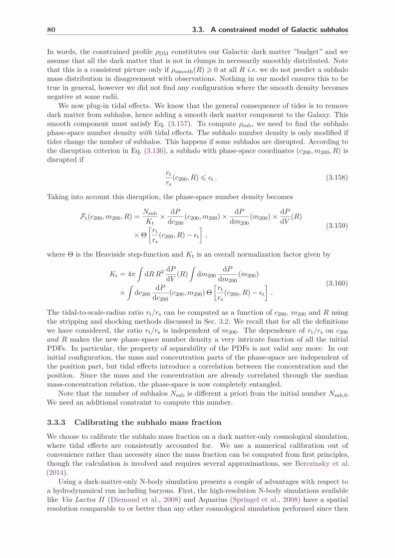
80 3.3. A constrained model of Galactic subhalos
In words, the constrained profile ρDM constitutes our Galactic dark matter ”budget” and weassume that all the dark matter that is not in clumps in necessarily smoothly distributed. Notethat this is a consistent picture only if ρsmooth(R) > 0 at all R i.e. we do not predict a subhalomass distribution in disagreement with observations. Nothing in our model ensures this to betrue in general, however we did not find any configuration where the smooth density becomesnegative at some radii.
We now plug-in tidal effects. We know that the general consequence of tides is to removedark matter from subhalos, hence adding a smooth dark matter component to the Galaxy. Thissmooth component must satisfy Eq. (3.157). To compute ρsub, we need to find the subhalophase-space number density with tidal effects. The subhalo number density is only modified iftides change the number of subhalos. This happens if some subhalos are disrupted. According tothe disruption criterion in Eq. (3.136), a subhalo with phase-space coordinates (c200, m200, R) isdisrupted if
rt
rs(c200, R) 6 ǫt . (3.158)
Taking into account this disruption, the phase-space number density becomes
Ft(c200, m200, R) =Nsub
Kt× dP
dc200(c200, m200) × dP
dm200(m200) × dP
dV(R)
× Θ
[
rt
rs(c200, R) − ǫt
]
,
(3.159)
where Θ is the Heaviside step-function and Kt is an overall normalization factor given by
Kt = 4π
∫
dR R2 dP
dV(R)
∫
dm200dP
dm200(m200)
×∫
dc200dP
dc200(c200, m200) Θ
[
rt
rs(c200, R) − ǫt
]
.
(3.160)
The tidal-to-scale-radius ratio rt/rs can be computed as a function of c200, m200 and R usingthe stripping and shocking methods discussed in Sec. 3.2. We recall that for all the definitionswe have considered, the ratio rt/rs is independent of m200. The dependence of rt/rs on c200
and R makes the new phase-space number density a very intricate function of all the initialPDFs. In particular, the property of separability of the PDFs is not valid any more. In ourinitial configuration, the mass and concentration parts of the phase-space are independent ofthe position part, but tidal effects introduce a correlation between the concentration and theposition. Since the mass and the concentration are already correlated through the medianmass-concentration relation, the phase-space is now completely entangled.
Note that the number of subhalos Nsub is different a priori from the initial number Nsub,0.We need an additional constraint to compute this number.
3.3.3 Calibrating the subhalo mass fraction
We choose to calibrate the subhalo mass fraction on a dark matter-only cosmological simulation,where tidal effects are consistently accounted for. We use a numerical calibration out ofconvenience rather than necessity since the mass fraction can be computed from first principles,though the calculation is involved and requires several approximations, see Berezinsky et al.(2014).
Using a dark-matter-only N-body simulation presents a couple of advantages with respect toa hydrodynamical run including baryons. First, the high-resolution N-body simulations availablelike Via Lactea II (Diemand et al., 2008) and Aquarius (Springel et al., 2008) have a spatialresolution comparable to or better than any other cosmological simulation performed since then

Chapter 3. Dark matter halos and subhalos in the Universe 81
[see e.g., Springel et al. (2018)].4 Second, the properties of baryons in simulations differ fromthe observed properties of baryons in the Milky Way. The point is that galaxies in simulationsare identified as ”Milky-Way-like” on the criteria such as the dark matter mass, the baryonicmass, the dark-matter-to-baryons mass ratio, the presence of a disc, etc. However the detailedkinematics of the Milky Way is in general not recovered by simulated Milky-Way-like galaxies.Since we want our model to be predictive regarding the effect of tides in general, and the impactof the disc in particular, we calibrate on a CDM simulation.
We calibrate on the VL2 simulation of Diemand et al. (2008). One has to keep in mindthat a cosmological simulation is run for a particular set of cosmological parameters. Threeparameters are especially important for the formation and evolution of dark matter halos: thematter abundance Ωm, the normalization of the power spectrum σ8 and the spectral index ns.The most recent estimates for these parameters are provided by Ade et al. (2016) who findΩm ≃ 0.31, σ8 ≃ 0.82 and ns ≃ 0.97. The matter abundance Ωm and the normalization σ8
impact the concentrations of halos on all scales with larger values leading to more concentratedstructures, while ns controls the amount of power on small scales, see Guo et al. (2013). Thecosmological parameters used in VL2 are Ωm = 0.24, σ8 = 0.74 and ns = 0.951, based on theWMAP-3 cosmology Spergel et al. (2007). This makes VL2 a rather conservative simulationin terms of subhalo abundance and concentration. For comparison, the Aquarius simulation ofSpringel et al. (2008) was run with Ωm = 0.25, σ8 = 0.9 and ns = 1 with a spatial resolutionsimilar to VL2.
The authors of VL2 provide the cumulative number of subhalos above a given maximalvelocity NVL2(> vmax), see Fig. 3 in Diemand et al. (2008). The velocity vmax is the peak heightof the subhalo circular velocity
vmax = Max
√
GN mint(r)
r
=
√
GN mint(rvmax)
rvmax
. (3.161)
Assuming subhalos have an NFW profile and they follow the mass-concentration relation givenin Eq. (11) of Pieri et al. (2011) (which is fitted over the VL2 subhalos) we can associate, ina unique way, a value of m200 to a maximal velocity vmax. This association is possible if thesubhalo internal profiles are not strongly modified by tidal effects, i.e. their scale parameters ρs
and rs remain roughly unchanged. The subhalo mass fraction between vmax,1 and vmax,2 is givenby
fVL2sub,200 =
1
M200,VL2
∫ vmax,2
vmax,1
dvmaxdNVL2
dvmaxm200(vmax) . (3.162)
Note that fsub,200 is an effective mass fraction in terms of m200 rather than the actual massfraction fsub. The latter cannot be estimated however since we do not know the actual mass ofstripped subhalos in VL2. A fit of NVL2 is provided in Diemand et al. (2008)
NVL2(> vmax) = 0.036
(
vmax
201 km/s
)−3
, (3.163)
which is very accurate for vmax ∈ [3 km/s, 20 km/s]. Using this fit and the virial mass of thegalactic halo in VL2 M200,VL2 = 1.42 × 10¹² M⊙, we get the subhalo mass fraction
fVL2sub,200 = 0.116 for vmax ∈ [3 km/s, 20 km/s] . (3.164)
4The reason why simulations performed ten years ago have a resolution comparable to simulations beingperformed now is a change of focus in the numerical simulation community. Now that CDM physics is undercontrol on sub-galactic scales and the small-scale issues have been clearly identified, the challenge is to incorporaterealistic baryonic physics in the picture or explore departures from ΛCDM (Bullock & Boylan-Kolchin, 2017).

82 3.3. A constrained model of Galactic subhalos
Using the relation between vmax and m200, we convert it into a fraction on a mass interval
fVL2sub,200 = 0.116 for m200 ∈ [3.14 × 10⁶ M⊙, 1.25 × 10⁹ M⊙] . (3.165)
Dividing by the total dark matter mass, we get
fVL2sub,200 ≃ 11% for
m200
M200∈ [2.2 × 10⁻⁶, 8.8 × 10⁻⁴] . (3.166)
We use this last equation to calibrate the mass fraction in our subhalo model, replacing M200
by the total dark matter mass in the particular mass model we use. We note that the use of adifferent N-body simulation like Aquarius leads to a similar mass fraction.
Having estimated the mass fraction in VL2, we must now express the same mass fractionin our subhalo model. By definition, the mass fraction in subhalos with cosmological massesbetween m1 and m2 is
fsub,200 =1
MDM
∫
dV
∫ m2
m1
dm200
∫ ∞
1dc200 F sim
t (c200, m200, R) m200 , (3.167)
where F simt is the subhalo phase-space density as defined in Eq. (3.159). There are some subtleties
associated with the computation of tidal effects while doing the calibration. The calibration isdone on a dark matter-only simulation, hence the baryonic effects (stripping by the baryonicpotential and shocking by the Galactic disc) should not be included in F sim
t . The only effect thatshould be included when doing the calibration is tidal stripping by the dark matter halo. Anotherimportant point concerns the relevant value of the disruption parameter ǫt. As discussed inSec. 3.2.3, the value of this parameter has been found in simulation to be ǫsim
t ≃ 1 (Hayashi et al.,2003). However, subhalo disruption in simulations might be entirely explained by numericalartefacts as argued by van den Bosch et al. (2018), hence the realistic value of this parametermight be much lower, possibly ǫt ≃ 0 if subhalos are never completely disrupted (they should bestrongly resilient to tidal shocks in the regime of very large inner density and when the innerorbital timescale is small with respect to the timescale of gravitational encounter).
Irrespective of the realistic value of ǫt, the artificial disruption discussed by van den Bosch etal. should be present in VL2 or any other N-body simulation used for the calibration. Therefore,when computing the mass fraction in Eq. (3.167) to perform the calibration, one should fix thedisruption parameter to ǫt = ǫsim
t = 1 for consistency. The masses m1 and m2 in Eq. (3.167) areset to the VL2 values in Eq. (3.166)
m1 = 2.2 × 10⁻⁶ MDM
m2 = 8.8 × 10⁻⁴ MDM .(3.168)
Using the definition of the minimal concentration (3.138), we have
fsub,200 =4πN sim
sub
MDMKsimt
×∫ R200
0dR R2 dP
dV(R)
∫ m2
m1
dmdP
dm200(m) m
∫ ∞
csimmin(R)
dcdP
dc200(c, m) .
(3.169)
Equating the mass fraction in Eq. (3.169) with the value found for VL2, we can deduce thenumber of subhalos N sim
sub in our model. We stress that this is the number of subhalos in thesimulation-like configuration, i.e. without baryons and with ǫt = ǫsim
t = 1.Since the calibration is only performed on the CDM part only, our model is predictive
regarding the effect of the baryonic distribution on subhalos. However, before doing predictionswe must compute the total number of subhalo Nsub beyond the simulation-like configuration.Starting from N sim
sub , we want to add the effects of tidal stripping by the full baryonic potential

Chapter 3. Dark matter halos and subhalos in the Universe 83
and disc shocking. We also want to investigate situations where the disruption parameter ismuch smaller than the simulation value. A simple way to compute the number of subhalos inthese cases is to assume the subhalo density profile ρsub in the outer region of the dark halo isleft unchanged compared to the simulation-like case (dark-matter-only and ǫt = 1). This is areasonable assumption since subhalos near the virial radius of the Galactic halo experience nearlyno tidal effects and behave as field halos. The asymptotic preservation of ρsub at R ≃ R200 canbe written using Eq. (3.152)
N simsub
Ksimt
∫ mmax
mmin
dm200
∫ +∞
csimmin(R)
dc200 Ft m200 =Nsub
Kt
∫ mmax
mmin
dm200
∫ +∞
cmin(R)dc200 Ft m200 , (3.170)
where N simsub (Nsub) and Ksim
t (Kt) are the number of subhalos and normalization factor inthe simulation-like case (”realistic” case, respectively). According to Fig. 3.12, the minimalconcentration in the outer region of the halo is cmin ≃ 1, irrespective of the value of ǫt or theinclusion of baryonic effects. This just means subhalos are not affected by tidal effects when theyorbit far from the Galactic center. We have cmin(R200) ≃ csim
min(R) = 1, hence the simple relation
N simsub
Ksimt
=Nsub
Kt. (3.171)
This relation allows us to compute Nsub regardless of the presence of baryons or the value ofǫt. We computed the number of subhalos for several values of αm and mmin, the results arefeatured in Tab. 3.1. The upper (lower) panel shows values obtained for ǫt = 1 (ǫt = 0). Wefirst note the high sensitivity of Nsub to the mass index αm. Going from an index of αm = 2to αm = 1.9, Nsub drops by a factor of more than fifty for Mmin = 10−10 M⊙ and more thantwenty for Mmin = 10−6 M⊙. This points toward the crucial importance of the small-scale powerspectrum when dealing with subhalos. The fact that this spectrum is almost completely unprobedat these scales (see however constraints from ultracompact mini-halos considerations Bringmannet al. (2012); Aslanyan et al. (2015)) makes the actual number of subhalos greatly uncertain.The value of the mass cutoff is also crucial, as it changes the number of subhalos by orders ofmagnitude. The impact of Mmin is more important for high values of the mass index αm. Notehowever that the mass cutoff can be determined in principle from the interaction properties ofthe dark matter particle (Green et al., 2005; Bringmann & Hofmann, 2007; Bringmann, 2009),hence it is calculable in the framework of a specific dark matter model. The disruption parameterhas a much smaller impact than the mass functions parameters, as a change from ǫt = 0 to ǫt = 1only increases Nsub by roughly 3%. The main reason why this number is not very sensitive to ǫt
is that most subhalos reside in the outer regions of the Galaxy, where tidal effects are ineffective.Another reason is that the subhalos most exposed to disruption are the less concentrated ones.Since subhalos with low concentration are among the most massive on average, their number islow and their survival does not impact the total number of structures.
Nsub (ǫt = 1) Mmin = 10−10 M⊙ Mmin = 10−6 M⊙αm = 1.9 4.79 × 10¹⁸ 1.20 × 10¹⁵
αm = 2 2.60 × 10²⁰ 2.59 × 10¹⁶
Nsub (ǫt = 0) Mmin = 10−10 M⊙ Mmin = 10−6 M⊙αm = 1.9 4.97 × 10¹⁸ 1.25 × 10¹⁵
αm = 2 2.70 × 10²⁰ 2.70 × 10¹⁶
Table 3.1 – Number of subhalos for several value of αm and mmin, and two values of the disruptionparameter: ǫt = 1 (Upper panel) and ǫt = 0 (Lower panel). The computation is done for the NFWmass model of McMillan (2017), with the smooth stripping radius and the differential shocking methodintroduced in Sec. 3.2

84 3.3. A constrained model of Galactic subhalos
3.3.4 Post-tides parameter space
3.3.4.1 Mass density profiles
In the previous section, we showed how to compute the number of subhalos Nsub for all typesof tidal effects and for any value of the disruption parameter ǫt. We can now evaluate anysubhalo-related quantity, starting with the global mass density profile of the subhalo population
ρsub(R) =Nsub
Kt
∫ mmax
mmin
dm200
∫ ∞
cmin(R)dc200 Ft(c200, m200, R) mt . (3.172)
Note that we integrate the tidal mass mt, and not the cosmological mass m200, to get the truesubhalo population mass density profile. For a subhalo with internal mass density ρint, the tidalmass is simply defined through
mt(c200, m200, R) ≡ 4π
∫ rt(c200,m200,R)
0dr r2 ρint(r) , (3.173)
where rt(c200, m200, R) is the tidal radius. Hence the tidal mass depends on all our parametersin a non-trivial way. We can exploit the m200-independence of rt/rs to rewrite the tidal mass
mt = 4πρsr3s
∫ rt/rs
0dx x2 ρint(x) . (3.174)
Moreover ρs only depends on c200, and r3s ∝ m200, hence mt/m200 only depends on c200 and R.
The tidal mass mt is simply proportional to the cosmological mass m200.We investigate the impact of tidal effects on the subhalo mass density profile. We compare
the different tidal radius recipes introduced in Sec. 3.2 on the left panel in Fig. 3.14. The resultsare consistent with the hierarchy observed through the minimal concentration in Fig. 3.12: thepoint-like stripping method is the most destructive while the smooth and density-based ones leadto similar results. Disc shocking has a dramatic impact on the subhalo distribution regardless ofthe method used, although the simulation-based one is by far the most destructive. Note thathere disc shocking is added on top of halo stripping, which was not the case when we discussedthe minimal concentration for instance. This is done by computing the stripping radius firstand then using it as the initial radius before subhalos experience disc shocking. The impact ofthe disruption parameter is shown on the right panel in Fig. 3.14. The value of this parameterhas very important consequences on the subhalo distribution. Lowering its value from ǫt = 1 toǫt = 0.1 increases the subhalo density at R = 0.1 kpc by more than five orders of magnitude!Further dividing ǫt by ten only increases ρsub by less than an order of magnitude though.
Another source of uncertainty on the subhalo mass distribution is the global dark matterdistribution in our Galaxy. For instance, McMillan (2017) fits a set of kinematic data withan NFW dark matter profile and a cored profile (α, β, γ) = (1, 3, 0). Both these models are inagreement with the data used by McMillan though they lead to a very different dark matterabundance in the inner region of the Milky Way. The subhalo mass density profile for thesetwo mass models is shown on the left panel of Fig. 3.15. Note that assuming as we did at thebeginning that subhalos initially behave as test particles in a global potential allows us to remainagnostic as for the possible origin of a cored halo profile, which should affect identically thesmooth and subhalo components. The subhalo density in the cored model (red dashed line) islower than in the NFW model (red solid line) by roughly the same factor as the total dark matterdensity (black lines). Note that a lower total density implies a lower subhalo number densitybecause we define the initial spatial distribution as
dP
dV(R) =
ρDM(R)
MDM. (3.175)
Note that a lower total dark matter density also leads to weaker tidal effects, however tides fromdark matter are subdominant compared to baryonic contributions in the inner region of the

Chapter 3. Dark matter halos and subhalos in the Universe 85
Galaxy. This leads to a prediction for the local mass fraction inside subhalos which is independentof the global dark matter density profile in the Galaxy. This has strong consequences on darkmatter searches with cosmic rays, as we will see in the next chapter. We look at the impactof the mass function parameters αm and mmin on the right panel in Fig. 3.15. Changing themass cutoff from mmin = 10−6 M⊙ to mmin = 10−10 M⊙ increases the subhalo central density byroughly an order of magnitude, while changing from αm = 1.9 to αm = 2 leads to a comparable,somewhat bigger increase.
Figure 3.14 – For both panels, we use the NFW model of McMillan (2017) and the mass functionparameters αm = 2 and mmin = 10−6 M⊙. Left panel: subhalo mass density profile for the different tidaleffect recipes discussed in Sec. 3.2. Are shown the stripping by the total potential through the point-like(red), smooth (green) and density-based (blue) methods. Disc shocking is added to tidal stripping withthe integral (dashed), differential (dotted-dashed) and simulation-based (dotted) methods. Right panel:.For the smooth halo stripping and differential disc shocking, we show the subhalo mass density fordifferent value of the disruption parameter ǫt = 1/0.5/10−1/10−2 (solid/dashed/dotted-dashed/dottedline, respectively).
3.3.4.2 Number density profiles
A quantity complementary to the mass density is the subhalo number density profile, defined as
nsub(R) =
∫ mmax
mmin
dm200
∫ ∞
1dc200 Ft(c200, m200, R)
=Nsub
Kt
dP
dV
∫ mmax
mmin
dm200dP
dm200
∫ ∞
cmin(R)dc200
dP
dc200.
(3.176)
Note that the number density is related to the spatial distribution through
nsub(R) = NsubdP
dV
∣
∣
∣
∣
t(R) . (3.177)
The function dP/dV |t is the subhalo spatial distribution when tidal effects are accounted for.According to Eq. (3.176), it is given by
dP
dV
∣
∣
∣
∣
t(R) =
1
Kt
dP
dV
∫ mmax
mmin
dm200
∫ ∞
cmin(R)dc200
dP
dm200
dP
dc200(3.178)

86 3.3. A constrained model of Galactic subhalos
Figure 3.15 – For both panels, we use the smooth halo stripping and differential disc shocking, andthe disruption parameter is fixed to ǫt = 1 Left panel: total dark matter (black) and subhalo (red) massdensity profiles for the NFW (solid line) and cored (dashed line) models of McMillan (2017). Rightpanel: subhalo mass density profile in the NFW model of McMillan (2017), for different values of themass function power index αm and mass cutoff mmin.
It is a priori different from the initial subhalo distribution dP/dV . The number density is shownon the left panel in Fig. 3.16 for different values of αm and mmin. As for the mass densityprofile, tidal effects strongly impact the number density in the central region of the Galaxy.When all effects are included, the number density is depleted for radii smaller than R ≃ 10 kpc.Depending on the values of αm and mmin, nsub(10 kpc) varies between 8 pc−3 (for αm = 1.9 andmmin = 10−6 M⊙) and 2 × 10⁶ pc−3 (for αm = 2 and mmin = 10−10 M⊙). The number of subhalosat the position of the Sun R ≃ 8.2 kpc depends crucially on the careful modelling of disc shocking.Indeed, if the only effect considered is stripping by the Galactic potential the subhalo numberdensity peaks at R ≃ 4 kpc instead of 10 kpc. The disruption parameter ǫt has also a stronginfluence on nsub as shown on the right panel in Fig. 3.16. The lower ǫt, the closer nsub is to thenumber density without tidal effects (dashed black line). For a parameter ǫt = 10−2, the numberdensity profiles with and without tides are almost indistinguishable, which means ǫt = 10−2 islow enough for nearly all subhalos to survive tidal effects. These subhalos still lose most of theirmass, which can be seen by looking at the subhalo mass density on Fig. 3.14. For ǫt = 10−2, themass density is significantly depleted at the center of the Galaxy and strongly differs from theoverall dark matter profile.
3.3.4.3 Concentration
In our initial set-up, there is no correlation between concentration and position in the halo. Ifsubhalo can be disrupted by tidal effects, this introduces a correlation. Indeed, low-concentrationhalos are more susceptible to tides than more concentrated ones, consequently they are morelikely to be disrupted. By a selection effect, the tidally-stripped subhalo population is moreconcentrated than the same population without tides. This can be seen by computing the averagecosmological concentration at a position R, for a given cosmological mass m200
〈c200〉 (m200, R) =
∫ +∞cmin(R) dc200
dPdc200
c200∫ +∞
cmin(R) dc200dP
dc200
. (3.179)

Chapter 3. Dark matter halos and subhalos in the Universe 87
Figure 3.16 – The NFW mass model of McMillan (2017) is used for both panels. Left panel: subhalonumber density without tides (dashed lines), with stripping (dotted-dashed lines) and with strippingand shocking (solid lines). The number density is shown for different values of αm and mmin. Rightpanel: subhalo number density for different values of the disruption parameter ǫt = 1/0.5/10−1/10−2
(solid/dashed/dotted-dashed/dotted lines, respectively).
We recall that the mass dependence is coming from the cosmological correlation between c200
and m200 which is implemented in dP/dc200. The average concentration in Eq. (3.179) shouldbe compared to the average for field halos given in Eq. (3.145). Both are shown on Fig. 3.17.One can see that in the presence of tides, 〈c200〉 rises at the center of the Galaxy. The lowerthe disruption parameter gets, the closer the average concentration is from the cosmological,radius-independent value. When ǫt = 0, the minimal concentration is cmin = 1 everywhere andthere is no selection any more, hence the average concentration is given by Eq. (3.145).
We recall that we assume the internal profile of subhalos is not modified by tidal effects, inparticular the scale parameters ρs and rs remain constant. In principle, these parameters canchange as the dark matter rearranges within the subhalo after part of it has been stripped. It wasshown by Penarrubia et al. (2008), based on a numerical study, that the maximal velocity vmax
and the associated radius rmax change as functions of the mass stripped from the subhalo only.The radius rmax decreases as the subhalo lose mass, hence the structure gets artificially moreconcentrated as some of its mass is stripped away. This increase in concentration is artificial inthe sense that is does not mean the subhalo gets denser as some of the matter is stripped away.In fact, the density in the inner parts of the subhalo decreases with the mass loss. Scaling lawsfor the evolution of vmax and rmax are given by Penarrubia et al. (2008); Errani et al. (2018),although it is not completely clear whether the numerical artefacts pointed out by van den Boschet al. could also be at play here. An analytic study of the phase space of tidally stripped halosleads to similar conclusions, see Drakos et al. (2017); Lacroix et al. (2018).
3.3.4.4 Mass function modification
The mass function is also affected by tides. To see how tides affect the mass function, it is moremeaningful to look at the physical mass mt rather than the cosmological mass m200. Thereforewe would like to compute a mass function dn/dmt with respect to the physical mass. We notedearlier that the tidal mass is related to the cosmological mass through a scaling relation
mt = m200 ∆(c200, R) , (3.180)

88 3.3. A constrained model of Galactic subhalos
Figure 3.17 – Average cosmological concentration as a function of the position in the Galaxy, fordifferent values of ǫt.
where ∆ is an integral depending on the tidal radius. We can define a new phase-space numberdensity where m200 is replaced by mt by performing the following operation
Ft(c200, m200, R) =
∫ mmax
mmin
dm200 Ft(c200, m200, R) δ [mt − m200∆(c200, R) ] (3.181)
=
∫ mmax
mmin
dm200
m200Ft(c200, m200, R) δ
[
mt
m200− ∆(c200, R)
]
, (3.182)
Further integration over the cosmological concentration c200 leads to the number density dn/dmt
per unit of physical mass
dn
dmt(mt, R) =
Nsub
Kt
dP
dV
∫ mmax
mmin
dm200
m200
dP
dm200
∫ ∞
cmin(R)dc200
dP
dc200δ
[
mt
m200− ∆(c200, R)
]
(3.183)
This quantity, multiplied by the mass squared, is shown in Fig. 3.18. We show the mass functioninside the disc (R = 8 kpc), at the very end of the disc (R = 20 kpc) and far from the disc(R = 100 kpc). The initial mass function, when tides are unplugged, is shown as the dotted curves.It is perfectly flat i.e. it goes like m2
200. The mass function with respect to the cosmologicalmass m200 when tides are plugged in is shown as the dashed curves. There is a significantdeparture from the m2
200 regime, especially at high masses. The departure is stronger in thecentral region of the halo. This is easily understood in terms of stripping: the most massivehalos are also the less concentrated and therefore the most likely to be disrupted by tidal effects.If the disruption parameter was set to zero, the slope would not be affected because all subhaloswould survive tidal effects. Finally, we look at the ”true” mass function dn/dmt, defined withrespect to the physical mass as in Eq. (3.183). The slope of the mass function is also modified,in more or less the same way as it was for dn/dm200. The normalization of the mass function ismuch different however, with dn/dmt being much lower than dn/dm200 at a value of the massm = mt = m200 > mmin. Below the cosmological mass cutoff mmin, the situation is reversed.While dn/dm200 is zero, we have dn/dmt Ó= 0. This happens because some subhalos with acosmological mass m200 > mmin get stripped to a mass mt < mmin hence the power spectrumextends below the cutoff scale. This analysis shows the cosmological information imprinted inthe mass function is partly lost in the local Galaxy due to tidal effects. The mass index αm
differs significantly from the Press-Schechter prediction of αm ≃ 2 and the mass cutoff mmin,related to the kinetic decoupling of the dark matter particle, is significantly lowered.

Chapter 3. Dark matter halos and subhalos in the Universe 89
Figure 3.18 – Left panel: mass-differential number density dn/dm in terms of both the cosmo-logical mass (dotted/dashed curves for tidal effects unplugged/plugged) and the real tidal mass (solidcurves), assuming a cutoff mass mmin = 10−6 M⊙, and calculated at 3 positions (R = 8/20/100 kpc inblue/red/black), as a function of the relevant mass (a scaling of m2 is applied as αm = 2 is chosen here).Right panel: same as in the left panel but with mmin = 10−10 M⊙.

91
Chapter 4
Impact of dark matter subhalos onindirect searches
The WIMP miracle has motivated several avenues of research based on the interaction betweendark and ordinary matter through means other than gravitation. These include particle acceleratorsearches, direct and indirect searches. The latter are the focus of this chapter. Indirect searchesaim at identifying the dark matter particle(s) by detecting the products of its annihilation ordecay, assuming these interactions are possible. Dark matter is being looked for in a numberof channels, including gamma rays, neutrinos and charged cosmic rays such as antiprotons andpositrons. The observability of dark matter through its annihilation or decay depends on itsdetailed microscopic interactions and on its clustering properties. In this chapter, we aim atevaluating the uncertainty coming from the sub-galactic scale clustering, focusing on the case ofannihilating dark matter. We first work out the generic impact of subhalos on indirect searchesin Sec. 4.1. We investigate two detection channels to illustrate the effect of clustering. We firstlook at gamma rays in Sec. 4.2. After describing the propagation of charged cosmic rays in theGalaxy in Sec. 4.3, we investigate the case of cosmic-ray antiprotons in Sec. 4.3.
4.1 Boost factor
The impact of clustering on indirect searches for annihilating dark matter was first pointed outby Silk & Stebbins (1993). The idea is quite simple: since subhalos are overdense regions withrespect to the smooth dark matter distribution, the annihilation rate is locally enhanced insubhalos. This means that a clustered dark matter halo should yield a higher overall annihilationrate than a perfectly smooth one. Since we expect CDM to structure on small-scales, the size ofthis effect should be estimated and its impact on indirect searches evaluated.
Given a halo with internal mass density profile ρint and radial extension rt, we define itsluminosity as
Lt ≡ 4π
∫ rt
0dr r2 ρ2
int(r) . (4.1)
The luminosity of a structure is directly related to its average annihilation rate
Γann =〈σannv〉
2 m2Lt . (4.2)
The luminosity is a function of the cosmological mass m200 and concentration c200 through theinternal profile, and a function of the spatial extension rt. Using the links between m200, c200, ρs
and rs, one can show that
Lt =200 ρc
3m200c3
200
∫ xt0 dx x2 ρ2(x)
[
∫ c200r−2/rs
0 dx x2 ρ(x)]2 , (4.3)

92 4.1. Boost factor
with xt = rt/rs and ρ = ρ/ρs as already introduced in Eq. (3.108). This shows that the luminosityis proportional to the cosmological mass and goes roughly like c3
200. As shown in Fig. 4.1, mostof the luminosity of a dark matter halo comes from its inner region: more than 80% of theluminosity originates from the core of the structure (r < rs), regardless of its density profile.
Figure 4.1 – Ratio of the truncated luminosity to the cosmological luminosity as a function of thetruncation radius, for the NFW profile (red) and the cored isothermal sphere (blue).
For a tidally stripped subhalo, the radial extension is given by the tidal radius rt =rt(c200, m200, R) where R is the distance from the Galactic centre. This makes Lt a func-tion of c200, m200 and R. The luminosity of the whole Galactic subhalo population is obtainedby summing the contribution from each individual subhalo
Lsub =∑
subhalo i
Lt(c200,i, m200,i, Ri) . (4.4)
In our statistical description of the subhalo population in the previous chapter, we introducedand computed the parameter-space subhalo number density Ft(c200, m200, R) (see Sec. 3.3.2).Using this density, the luminosity can be written as
Lsub =
∫
dV
∫
dm200
∫
dc200 Ft(c200, m200, R) Lt(c200, m200, R) . (4.5)
The luminosity Lsub is a single number characterising the entire subhalo population. It isconvenient to introduce a luminosity density Lsub(R) such that
Lsub ≡∫
dV Lsub . (4.6)
With Eq. (4.5), the subhalo luminosity density can be written
Lsub(R) =
∫
dm200
∫
dc200 Ft(c200, m200, R) Lt(c200, m200, R)
=Nsub
Kt
dP
dV
∫ mmax
mmin
dm200
∫ ∞
cmin(R)dc200
dP
dm200
dP
dc200Lt(c200, m200, R) .
(4.7)
Of course, annihilation in the Galaxy is not sourced only by subhalos. Two other contributionsshould be taken into account: annihilation between dark matter particles in the smooth halo,

Chapter 4. Impact of dark matter subhalos on indirect searches 93
and annihilation of subhalo particles onto dark matter particles in the smooth halo. Let us workout all these contributions in a consistent way. The luminosity of the whole Galaxy, includingthe subhalo and the smooth contribution, is given by
Ltot =
∫
dV
[
ρsmooth(þR) +∑
i
ρint,i
(∣
∣
∣
þR − þri
∣
∣
∣
)
]2
, (4.8)
where we used the exact contribution of subhalos by summing over all the objects. Thedevelopment of Ltot leads to three terms
Ltot =
∫
dV ρ2smooth + 2
∫
dV
[
ρsmooth
∑
i
ρint,i
]
+
∫
dV
[
∑
i
ρint,i
]2
, (4.9)
namely the smooth, cross (subhalo particles on smooth particles) and subhalo contributions. Weneglect the possible overlap between subhalos which simplifies the subhalo contribution into
∫
dV
[
∑
i
ρint,i
]2
≃∑
i
∫
vol. sub.dV ρ2
int,i
=∑
i
Lt,i .
(4.10)
Using our statistical description of the subhalo population, the average value of this sum leadsprecisely to the expression of Lsub in Eq. (4.5). Likewise, the cross term simplifies to
2
∫
dV
[
ρsmooth
∑
i
ρint,i
]
= 2∑
i
∫
vol. sub.dV ρsmooth ρint,i . (4.11)
Assuming the smooth background is constant within the volume of a subhalo, we get theluminosity of the ”cross” contribution
Lcross ≃ 2∑
i
ρsmooth,i mt,i . (4.12)
where ρsmooth,i is the value of the smooth density in subhalo i and mt,i the mass of that subhalo.In our statistical description, this is
Lcross = 2
∫
dV ρsmooth
∫
dm200
∫
dc200 Ft mt
= 2
∫
dV ρsmooth ρsub ,(4.13)
where we used the definition of ρsub in Eq. (3.152). Putting everything together, we get
Ltot = Lsmooth + Lcross + Lsub
=
∫
dV (Lsmooth + Lcross + Lsub) ,(4.14)
with the expressions of the luminosity densities:
Lsmooth = ρ2smooth (4.15)
Lcross = 2 ρsmooth ρsub (4.16)
Lsub =
∫
dm200
∫
dc200 Ft Lt . (4.17)
These luminosity density profiles serve as the basis to compute the annihilation signal in indirectsearches, irrespective of the particular messenger used (gamma rays, antiprotons, positrons, etc.).

94 4.2. Indirect searches with gamma rays
As realized by Silk & Stebbins (1993), a clumpy halo generically leads to a stronger annihilationsignal than a smooth halo. A convenient way to quantify this enhancement is through a boostfactor. The integrated boost factor is defined as the ratio of the luminosity of a clumpy halo tothe luminosity of the same halo if all the dark matter was smoothly distributed. In other words,the boost factor is
B ≡∫
dV (Lsmooth + Lcross + Lsub)∫
dV ρ2DM
, (4.18)
where Lsmooth, Lcross and Lsub are given in Eqs. (4.15) to (4.17). By definition, the boost factoris an annihilation signal multiplier equal to 1 in the absence of small-scale clustering.1 Theintegrated boost factor is a single number characterizing the clumpiness enhancement withina given volume. A local information on the impact of clumps on the annihilation rate can beobtained with the differential boost factor
B(R) ≡ Lsmooth(R) + Lcross(R) + Lsub(R)
ρ2DM(R)
. (4.19)
Using the luminosity density rather than the integrated luminosity allows us to identify regionsin the host halo where the enhancement is stronger and thus point toward potentially interestingtargets for indirect searches. So far, our definitions are not specific to any detection channel. Wewill see in the following that our definition of the boost has to be modified when looking at aparticular channel. For now, our definition in Eq. (4.19) is enough to find the regions in theGalaxy most affected by the clustering of CDM.
The luminosity densities are shown in Fig. 4.2. The left panel shows the impact of theminimal mass mmin and the right panel shows the impact of the mass index αm. The bottompanels show the associated differential boost. We see that the boost is 1 for radii smaller thanR ∼ 5 kpc and it grows to very high values at large radii. This difference is entirely due to tidaleffects which, as we have seen in the previous chapter, deplete of subhalos the central regionof the Galaxy while leaving the outer part unchanged. Both mmin and αm have a high impacton the luminosity and the boost. The impact of the disruption parameter is shown in Fig. 4.3.While the luminosity of the subhalo contribution alone is strongly affected by the value of ǫt,especially within R . 10 kpc, the overall luminosity is not very sensitive to this value. Thereason is that enough dark matter in the inner region (R < 4 kpc) is in the smooth component ofthe halo for this contribution to dominate the luminosity. The subhalo contribution dominatesat large radii but the value of ǫt is unimportant there because tides have little effects in thatregion. On the bottom panel in Fig. 4.3, we see that a small difference appears in the transitionregion 4 kpc< R <10 kpc. This surely is of interest because this is precisely where the Solarsystem is located.
4.2 Indirect searches with gamma rays
The impact of dark matter clumpiness on gamma-ray searches has been investigated in numerousstudies, see e.g. Bergstrom et al. (1999); Ullio et al. (2002); Berezinsky et al. (2003); Kamionkowskiet al. (2010); Pieri et al. (2011); Blanchet & Lavalle (2012); Serpico et al. (2012); Bartels & Ando(2015); Hiroshima et al. (2018). Subhalos could affect gamma-ray searches in a number of ways.The individual detection of subhalos is a possibility (Tasitsiomi & Olinto, 2002; Koushiappas,2006; Moore et al., 2005; Pieri et al., 2008; Ando et al., 2008; Kuhlen et al., 2008; Hutten et al.,2016; Calore et al., 2017). Observed satellites like dwarf spheroidal galaxies constitute privilegedtargets in this context (Ackermann et al., 2015; Albert et al., 2017). The vast majority of subhaloshave masses much too small to allow their individual detection unless they are very close to
1Note that an alternative definition can be found in the literature where the boost is shifted by one so that it iszero if there is no enhancement. We will not use this definition in the following.

Chapter 4. Impact of dark matter subhalos on indirect searches 95
Figure 4.2 – Left, upper panel: luminosity density profile for subhalos (dotted lines), smoothdark matter (dashed lines) and the cross contribution (dotted-dashed lines), as well as the sum of allcontributions (solid lines), for two values of the minimal mass mmin. Left, lower panel: differentialboost factor, as defined in Eq. (4.19). Right panel: same as left panel, with mmin = 10−6 M⊙ andαm = 2 or αm = 1.9.
Figure 4.3 – Upper panel: luminosity density profile for subhalos (dotted lines), smooth dark matter(dashed lines) and the cross contribution (dotted-dashed lines), as well as the sum of all contributions(solid lines), for different values of the disruption parameter ǫt. Lower panel: differential boost factor,as defined in Eq. (4.19).
the Earth. However, these structures should contribute significantly to the diffuse gamma-raybackground (Ackermann et al., 2012b).
In order to estimate the contribution of dark matter clumps to the annihilation signal, let usfirst express the gamma-ray flux for a smooth galactic halo. The energy-differential flux per unit

96 4.2. Indirect searches with gamma rays
of solid angle is given by
dφ
dE dΩ
∣
∣
∣
∣
l.o.s.=
1
4π
〈σannv〉2 m2
dNγ
dE
∫
l.o.s.ds ρ2(s) , (4.20)
where dNγ/dE is the gamma-ray spectrum emitted at annihilation.2 Interpolation functions forall possible spectra are given in Cirelli et al. (2011). In this expression, l.o.s. stands for line ofsight. The line of sight is usually characterized by two angles: the latitude b and the longitudel, with −90 6 b 6 90 and 0 6 l 6 360. Relations between these coordinates and Cartesiancoordinates are given in App. C. The differential flux is obtained by integrating over the solidangle (defined by the region of interest or the angular resolution of the detector)
dφ
dE
∣
∣
∣
∣
l.o.s.=
1
4π
〈σannv〉2 m2
dNγ
dE
∫
∆ΩdΩ
∫
l.o.s.ds ρ2(s) . (4.21)
Much like the expression of the event rate in direct detection experiments, the particle physicsand astrophysical of the expression can be factorized. The astrophysical part is referred to as theJ-factor
J(∆Ω) ≡∫
∆ΩdΩ
∫
l.o.s.ds ρ2(s) . (4.22)
When looking at targets within the Milky Way, a different definition of the J-factor is sometimesused
J⊙(∆Ω) ≡∫
∆ΩdΩ
∫
l.o.s.ds
(
ρ(s)
ρ⊙
)2
, (4.23)
where ρ⊙ is the local dark matter density. The J-factor is highly sensitive to the shape of thedark matter density profile. Since the profile is poorly known at the centre of the Galaxy, thisis a major source of uncertainty for gamma-ray searches. This uncertainty is illustrated in theright panel on Fig. 4.4 where we show the J-factor as a function of the longitude, for a latitudeb = 0 (so that for l = 0, the line of sight points toward the Galactic centre). While there islittle difference above l = 60, predictions at the centre varies by several orders of magnitudedepending on the central slope.
It is straightforward to express the J-factor including the contribution from substructuresgiven our discussion in the previous section. One simply has to replace in Eq. (4.22) or Eq. (4.23)the density ρ2 by the luminosity densities defined in Eqs. (4.15) to (4.17). Hence the J-factoralong any line of sight can be separated into three contributions: annihilation in subhalos, in thesmooth halo and the ”cross” contribution
J(∆Ω) =
∫
∆ΩdΩ
∫
l.o.s.ds [Lsub + Lsmooth + Lcross] . (4.24)
These contributions are shown in the right panel on Fig. 4.4, for the mass function parametersαm = 2 and mmin = 10−6 M⊙ and a disruption parameter ǫt = 1. The inclusion of substructuressignificantly affects the J-factor, which is increased by a factor of more than two with respect tothe no-subhalo configuration for longitudes l > 50. We note that the contribution from subhalosis nearly independent of the latitude, which is a consequence of their spatial distribution whichis mainly shaped by tidal effects. The cross contribution is always at least an order of magnitudebelow the other contributions, which is why it is often neglected in the literature.
Since subhalos can have a sizeable contribution to the gamma-ray flux, it is worth defining aboost factor. Its definition is straightforward given our discussion in the previous section:
BJ =
∫
∆Ω dΩ∫
l.o.s. ds [Lsub + Lsmooth + Lcross]∫
∆Ω dΩ∫
l.o.s. ds ρ2(s), (4.25)
2This expression is valid for dark matter particles which are there own antiparticle. If that is not the case, theflux should be multiplied by a factor of 1/2.

Chapter 4. Impact of dark matter subhalos on indirect searches 97
i.e. it is simply the ratio between the J-factor including subhalos to the J-factor assuming allthe dark matter is smoothly distributed. Unlike our definition of the differential boost in theprevious section, see Eq. (4.19), this boost factor depends on the direction of the line of sightand not on the distance to the Galactic centre. The ”J-factor boost factor” is very sensitive tothe parameters characterizing the clump distribution. In particular, the disruption parameter ǫt
can significantly affect the boost, as shown in Fig. 4.5. For αm = 2 and mmin = 10−6 M⊙ (topleft panel), and for very low values of ǫt, motivated by the recent results of van den Bosch et al.(2018), we get a boost of BJ = 2 at l = 40 and more than BJ = 4 at l = 90, to nearly 6 at theanti-centre at l = 180. Such high values should strongly impact dark matter searches usingthe diffusive gamma-ray background, see for instance the recent analysis of Chang et al. (2018).However, the impact of subhalos is strongly sensitive to the mass index αm and the mass cutoffmmin, as shown in the top right panel and the bottom panel in Fig. 4.5. For a value of αm = 1.9,as found in the simulation of Springel et al. (2008), the boost is greatly suppressed and staysbelow 2 at all longitudes.
Figure 4.4 – Left panel: J-factor has defined in Eq. (4.22) as a function of the longitude, for a latitudel = 0. We used the mass models of McMillan (2017) and the angular resolution is 0.5. Right panel:J-factor including the contribution of substructures (red) compared to the no-subhalos case (black). Themass function parameters are αm = 2 and mmin = 10−6 M⊙, and the disruption parameter is ǫt = 1.
4.3 Indirect searches with antimatter cosmic rays
Since their discovery by Hess in 1912 (F. Hess, 1912), cosmic rays have been collected by a widevariety of ground-based and spatial experiments. Cosmic rays are relativistic charged particleswandering in the interstellar medium. They are composed primarily of nuclei (99%) and leptons(1%). Among the nuclei, around 90% are protons, 9% are helium nuclei and 1% heavier nuclei.Leptons are composed essentially of electrons 90% and positrons 10%. The cosmic-ray spectrumis measured over several decades in energy and behaves approximately as a power-law, see Fig. 4.6(Blasi, 2013; Aloisio et al., 2018). Measurements are precise enough to show features in thespectrum, which depart from a perfect power-law. Below 10 GeV, cosmic rays received at theEarth are affected by solar modulation which we discuss below. Between 10 GeV and 3 PeV, thedata are well-fitted by a power law with an index of γ ≃ 2.7. At 3 PeV, there is a first breakingof the power-law called the ”first knee”. Between 3 PeV and 300 PeV, the spectrum softens toγ ≃ 3.1. At 300 PeV, another feature called the ”second knee” marks the transition between an

98 4.3. Indirect searches with antimatter cosmic rays
Figure 4.5 – Top panel: J-factor has a function of the longitude for different values of the disruptionparameter ǫt (coloured lines). We also show the J-factor for a smooth halo (black line). The bottompanel shows the boost factor for each ǫt. The mass function index is αm = 2 and the mass cutoff ismmin = 10−6 M⊙ (left panel) or mmin = 10−10 M⊙ (right panel). Bottom panel: same figure as the toppanel, for αm = 1.9.
index γ ≃ 3.1 and γ ≃ 3.3. This regime holds up to the ”ankle” at 1 EeV (= 1018 eV), whereit hardens to γ ≃ 2.6. At 50 EeV, cosmic rays have enough energy to efficiently interact withCMB photons which strongly limit their propagation in the intergalactic medium. The effect isreferred to as the GZK effect after Greizen, Zatsepin and Kuzmin (Greisen, 1966; Zatsepin &Kuz’min, 1966).3
The two knees in the cosmic-ray spectrum are thought to mark the transition betweenGalactic cosmic rays and extragalactic cosmic rays. The radius of gyration of a charged specieswith momentum p and charge number Z, interacting with a constant magnetic field þB is
rg ≃ 1 pc
(
p
PeV
) (
B
µG
)−1
Z−1 , (4.26)
3Note that the limit of 50 EeV is only valid for protons. Heavier elements can violate this limit, which explainswhy some cosmic rays have been detected at much higher energies.

Chapter 4. Impact of dark matter subhalos on indirect searches 99
therefore in the 1-100 PeV range the radius is comparable to the size of the Milky Way. Belowthis energy range, we expect cosmic rays to have mainly a Galactic origin, while cosmic rayswith higher energies are expected to come from extragalactic sources.
10-10
10-8
10-6
10-4
10-2
100
100
102
104
106
108
1010
1012
E2dN
/dE
(
GeV
cm
-2sr-1
s-1
)
Ekin (GeV / particle)
Energies and rates of the cosmic-ray particles
protons only
all-particle
electrons
positrons
antiprotons
CAPRICEAMS
BESS98Ryan et al.
GrigorovJACEEAkeno
Tien ShanMSU
KASCADECASA-BLANCA
DICEHEGRA
CasaMiaTibet
Fly EyeHaverahYakutskAGASA
HiRes
Figure 4.6 – Observed cosmic-ray spectrum as a function of the kinetic energy. Figure taken fromHillas (2006).
4.3.1 Origin and acceleration of cosmic rays
4.3.1.1 Acceleration mechanisms
To accelerate a charged particle, one needs a non-zero electric field. Large scale electric fields arerare in astrophysics because astrophysical plasmas are highly conductive. However, stochasticacceleration can be achieved by small-scale electric fields. We very briefly present the two mainmechanisms of acceleration of cosmic rays. For reviews, we refer to Drury (1983); Blandford &Eichler (1987); Malkov & Drury (2001).
Second-order Fermi acceleration A mechanism to accelerate cosmic rays was originallyproposed by Fermi (1949). The idea is that cosmic rays can be deflected by molecular clouds,which contain magnetic fields stronger than those found in the interstellar medium. The randommotion of molecular clouds in the Galaxy tend to increase the average energy of cosmic rays. A

100 4.3. Indirect searches with antimatter cosmic rays
calculation shows that the average relative energy gain is given by⟨
∆E
E
⟩
≃ 4
3β2 , (4.27)
where β = V/c and V is the average speed of molecular clouds in the Galactic referential(typically a few hundred of km/s). The dependence on the square of β justifies the designationof second-order for this acceleration mechanism. Though this mechanism does play a role inaccelerating cosmic rays, its suppression in β2 limits its importance.
First-order Fermi acceleration The dominant process in the acceleration of cosmic rays isbelieved to be the so-called first-order Fermi mechanism (Axford et al., 1977; Bell, 1978a,b).The principle is the same as the second-order mechanism except the interaction is between acosmic ray and a shock wave rather than a molecular cloud. A shock can be described as afrontier between two mediums with different thermodynamic variables (temperature, pressure,density): the upstream medium (interstellar medium) and the downstream medium (the insideof the shell). Charged particles can diffuse on magnetic inhomogeneities and cross the shockfront back and forth, as represented in the lower right bubble in Fig. 4.9. The average relativeenergy gain can be computed to get
⟨
∆E
E
⟩
=4
3
∆v
c=
4
3β , (4.28)
where ∆v = v2 − v1 is the difference between the upstream medium velocity and the downstreammedium velocity (typically more than a thousand km/s). Unlike the previous accelerationmechanism, here the relative energy gain is linear in β hence it is referred to as a first-orderFermi acceleration mechanism. It is much more efficient at accelerating cosmic rays than thesecond-order mechanism and is actually thought to be the dominant acceleration mechanism upto the ankle.
4.3.1.2 Interactions with the interstellar medium
Energy losses Cosmic rays lose energy by interacting with the interstellar medium. Theseinteractions are the following:
• ionization of the interstellar atomic gas
• Coulomb interaction with electrons and protons in an ionized plasma
• Bremmsstrahlung: photon emission from interactions between electrons and the gas nuclei
• inverse Compton: scattering of a relativistic electrons on a photon
• synchrotron: photon emission when an electron propagates in a magnetic field
These interactions are relevant for all charged species. However, the relative importance of theloss mechanism depends on the particle’s mass. Consequently, nuclei are mostly affected by thefirst two processes, while all interactions are important for leptons. As a result, the propagationof high-energy leptons is dominated by energy losses, while losses can often be neglected forhigh-energy nuclei.
Destruction Cosmic-ray nuclei can be destroyed by inelastic interactions with other atoms orions in the interstellar gas. Nuclear reactions of spallation split nuclei into smaller products. Fora nucleus N interacting with a nucleus C from the gas to create a product P , the interactionrate can be expressed
ΓN+C→P = nC vN σN+C→P , (4.29)

Chapter 4. Impact of dark matter subhalos on indirect searches 101
where nC is the number density of C, vN is the speed of N and σN+C→P the cross-section.
Destruction is also relevant for antimatter which can annihilate with the interstellar matter(this concerns positrons and antiprotons, but is relevant mostly close to or in the non-relativisticregime).
4.3.1.3 Sources of cosmic rays
Cosmic rays below a few tens of MeV come from the Solar wind while ultra-high energy ones(T > 1018 eV) have an extragalactic origin. In between, cosmic rays must have a Galactic origin.We will focus on Galactic cosmic rays below.
Galactic primary cosmic rays A primary cosmic ray is a cosmic ray directly accelerated atits source. Major contributors to the injection and acceleration of cosmic rays in the Galaxy aresupernovae. A supernova is the explosion of a star at the end of its life. As the star explodes, allthe elements synthesized in its core are injected into the interstellar medium (Baade & Zwicky,1934; Sekido et al., 1951). A shock wave is also created which expands at high speed away fromthe supernova. The most famous and spectacular example of supernova remnant (SNR) is theCrab nebula, see Fig. 4.7. Supernovae explosions occur at a rate of three per century in ourGalaxy. While supernovae inject heavy nuclei in the interstellar medium, they also accelerateparticles with their shock wave through the first-order Fermi mechanism. This acceleration ispowerful enough to explain cosmic rays with energies up to the ankle and it is therefore thoughtto be the main source of acceleration in the Galaxy. Another major source of primary cosmicrays are Pulsar Wind Nebulae (PWNe) which are the by-products of core-collapse supernovae(ending with a rotating and magnetized neutron star). Each PWN is in principle associated to aSNR but contributes to the acceleration of cosmic rays at relativistic shocks (a large fraction ofcosmic rays accelerated by PWNe are electron/positron pairs).
Figure 4.7 – The Crab nebula. The associated supernova exploded in 1024 and was observed at thetime by Chinese and Japanese astronomers. Picture taken by the Hubble space telescope.

102 4.3. Indirect searches with antimatter cosmic rays
Galactic secondary cosmic rays In opposition to primary sources, a secondary origin forcosmic rays is spallation. Spallation is a nuclear process where a nucleus is hit by another particleor a gamma-ray and subsequently split into a lighter nucleus and other particles (neutrons,protons, antiprotons, etc.). The process occurs when cosmic rays interact with atoms in theinterstellar medium, mostly hydrogen and helium but also carbon, nitrogen and oxygen. Thus,spallation is a process that converts primary cosmic rays into secondary cosmic rays (Berezhkoet al., 2003). Light nuclei like beryllium and boron are entirely created by spallation, see Fig. 1.4.Secondary cosmic rays provide a powerful test of the cosmic-ray transport properties, sincethe source acceleration properties may somewhat factorize in the ratio of secondary-to-primarycosmic-ray fluxes. Note that secondaries, if produced in the acceleration zone at a source, mayalso be accelerated themselves, gaining the status of primaries. Finally, note that secondariescan also experience inelastic processes, and be either destroyed or inelastically driven to lowerenergies: in the latter case, we talk about ”tertiaries” (this happens for instance to antiprotonsat low energy).
4.3.1.4 Solar modulation
For cosmic rays to reach the Earth, they have to enter the zone of magnetic influence of the Sun(Potgieter, 2013). This zone is called the heliosphere and is created by the Solar wind, a flowof magnetized plasma ejected from the Sun. The heliosphere ends at the heliopause which isdetermined by the equilibrium between the pressure from the Solar wind and the pressure ofthe interstellar medium. The properties of the Solar wind strongly depend on the Solar activitywhich is known to have periodicity of 11 years. This period corresponds to the time between twoinversions of the Sun’s magnetic poles.
Cosmic rays lose energy due to their interaction with the Solar wind. This strongly affectsthe cosmic-ray flux below 10-20 GeV, with a periodicity of 11 years. The equation governing thepropagation of cosmic rays in the heliosphere is complex and getting solutions requires numericalcalculations. An alternative is to use the effective descrition of Gleeson & Axford (1968) in termsof force-field. Let ΦIS and ΦTOA be the interstellar and top-of-atmosphere fluxes, respectively.We consider a nucleus with atomic number A and Z, then the top-of-atmosphere flux is given by
ΦTOA(TTOA) = ΦIS(TIS)p2
TOA
p2IS
(4.30)
TIS = TTOA +Z e φF
A(4.31)
where pTOA and pIS are the top-of-atmosphere and interstellar momentum per nucleon, i.e.
p2TOA = (TTOA + mp)2 − m2
p (4.32)
p2IS = (TIS + mp)2 − m2
p , (4.33)
where mp is the proton mass. The parameter φF is called the Fisk potential and it has to beinferred from experimental measurements. This parameter depends on time, it is periodic with aperiod of 11 years. The effect of solar modulation in this simple parametric model is shown for aprimary antiproton flux in Fig. 4.8.
4.3.2 The master equation
Let us know introduce the phenomenological model of cosmic-ray propagation. For classictextbooks on cosmic rays, we refer to Ginzburg & Syrovatskii (1964); Berezinsky et al. (1990).The magnetic halo is approximated to a cylinder of radius Rgal = 20 kpc and half-height Lbetween 1 and 15 kpc. All the matter is concentrated in the Galactic disc, which is itself identifiedto a cylinder with radius Rgal and half-height h ∼ 100 pc. This model is referred to as a 2D

Chapter 4. Impact of dark matter subhalos on indirect searches 103
Figure 4.8 – Effect of solar modulation of the antiproton flux using the Fisk potential. We show theflux for a smooth NFW profile and a thermal annihilation cross-section 〈σannv〉 = 3.10−26 cm3/s. We usedthe propagation model of Kappl et al. (2015), see Tab. 4.1.
model because the cosmic-ray density only depends on the cylindrical radius R and the altitudez.
We denote Ψ the cosmic-ray density per unit energy
Ψ(E, t, þx) ≡ dn
dE. (4.34)
The evolution of Ψ follows a Fokker-Planck equation (Blandford & Eichler, 1987). Instead ofderiving the transport equation from first principles, we simply sketch the main physical processescoming into play. For a detailed review on cosmic-ray propagation, we refer to Strong et al.(2007). The cosmic-ray density obeys a continuity equation
∂tΨ + þ∇. þJ + ∂EJE = Q − S , (4.35)
where Q and S are the source and sink term, respectively. The spatial current can be written
þJ = þVc Ψ − K þ∇Ψ , (4.36)
where þVc encodes the convection due to the Galactic wind and K is the coefficient of spatialdiffusion. The structure of the Galactic wind is widely unknown (Cox, 2005). From now on, wemake the very simplistic assumption that the wind is perpendicular to the disc and goes awayfrom it i.e.
þVc = sign(z) Vc þez . (4.37)
The diffusion coefficient is assumed homogeneous and isotropic. The non-linear diffusion theory(Shalchi, 2009) and numerical simulations (Casse et al., 2002) show that it has a power-lawdependence on the rigidity
K(E) = K0 β
( R1 GV
)δ
, (4.38)
where β = v/c and R = p/q is the rigidity. In the particular case of Kolmogorov magneticturbulence, we have δ = 1/3 (Kolmogorov, 1941). Note that since we expect different sources of

104 4.3. Indirect searches with antimatter cosmic rays
turbulence on different scales, the diffusion coefficient should somewhat reflect these features.This is actually observed as breaks in the spectra of nuclei and in the B/C ratio, and can beinterpreted as breaks in the diffusion coefficient (Panov et al., 2009; Ahn et al., 2010; Adrianiet al., 2011; Aguilar et al., 2015b,a; Aguilar et al., 2016). For theoretical studies, we refer toGenolini et al. (2017); Evoli et al. (2018).
The energy current is given by
JE = −b Ψ − D ∂EΨ , (4.39)
where b = bloss + badia with
bloss = −⟨
dE
dt
⟩
(4.40)
is the average energy loss rate (from synchrotron, inverse Compton, etc...) and
badia = −þ∇.þVc
3T
(
2 m c2 + T
m c2 + T
)
(4.41)
is the adiabatic loss rate due to the convective wind (Maurin et al., 2001). Cosmic rays diffuse onthe inhomogeneities of the magnetic halo which themselves are moving at the Alfven speed Va.At the encounter with inhomogeneities, cosmic rays are reaccelerated following the second-orderFermi mechanism. The energy diffusion coefficient is linked to the Alfven speed and the spatialdiffusion through
D(E) =2
9V 2
a
E2β2
K. (4.42)
If reacceleration is intimately linked to spatial diffusion, it should occur all over the magnetichalo. However, we could think about cases where reacceleration is more efficient where sourcesare confined, in the disc. This assumption notably helps in solving the transport equationanalytically. Formally, the reacceleration region can however be rescaled to an arbitrary size byrescaling the Alfven speed Va, which should be thought about as an effective speed.
A term of energy gain should in principle be added to the transport equation as in Strong &Moskalenko (1998), however it is not necessary to account for experimental results hence we donot consider it in the following. To summarize, the transport equation is
∂tΨ + þ∇.[
þVcΨ − K þ∇Ψ]
− ∂E [b Ψ + D∂EΨ] = Q − S . (4.43)
The sink term can in general be written
S = ΓtotΨ , (4.44)
where Γtot is the total destruction rate taking into account all processes that can remove thespecies under study, at a given position, time, and/or energy. (including decay if the species isunstable). Since the half-height of the disc is much smaller than the half-height of the magnetichalo in most propagation models, we can assume the disc to be infinitely thin. In that case, allprocesses that occur only in the disc come with a pre-factor 2hδ(z), hence we get
∂tΨ + þ∇.[
þVcΨ − K þ∇Ψ]
− ∂E [b Ψ + 2hδ(z) D∂EΨ] + ΓtotΨ = Q . (4.45)
All processes of acceleration and diffusion included in the equation are schematically representedin Fig. 4.9.
A cosmic-ray proton spends millions of years diffusing in the Galactic disc, and hundredsof millions of years diffusing in the whole halo, while the rate of supernovae explosions is a few

Chapter 4. Impact of dark matter subhalos on indirect searches 105
R
R=20 kpc
h=0.1 kpcr
L=3-10 kpc
=8.0 kpc
z
(axial symmetry around z)
R0.6
( B )
β+
β-
R-2.2
0 0
0 0
0 0
0 0
0 0
0 0
0 0
0 0
0 0
1 1
1 1
1 1
1 1
1 1
1 1
1 1
1 1
1 1
(H+He+...) ISM
(p,He)
Spallation
V1 V2
p1 p2
Þ1 Þ2
(Halo+Disc) (Disc)
(Disc)(Halo+Disc)
Diffusion on magnetic inhomogeneitiesAcceleration by shock waves
ß disintegration
Energy losses
Reacceleration : Va
Nj
Nl
Nk
Z,A
Z’,A’(A,Z) (A,Z+1)
(A,Z-1)
Vc
Vc
Ec/n
Ec/n
(Disc)
(Disc)
Figure 4.9 – Schematic edge-on view of the Milky Way diffusive halo. The stellar and gaseous diskis sandwiched between two thick layers which contain turbulent magnetic fields. After having beenaccelerated by supernova driven shock waves or produced by dark matter species annihilating in theGalactic halo, cosmic rays diffuse on magnetic inhomogeneities and are wiped away by a Galactic windwith velocity Vc. They can lose energy and are also mildly subject to diffusive reacceleration. The formerprocess is by far the dominant one in the case of electrons and positrons. This figure is taken from Maurinet al. (2002).
per century. Since supernovae are likely to be the main source of injection and acceleration ofcosmic rays, it is natural to look for a steady-state solution of the transport equation. Eq. (4.43)is usually solved numerically. Public codes are available for this purpose. Some codes use afully numerical approach to solve the equation in a general context, e.g. GALPROP (Strong &Moskalenko, 1998), DRAGON (Maccione et al., 2011) and PICARD (Kissmann, 2014; Kissmannet al., 2015). These codes allow one to explore more realistic, full 3D configurations. The codeUSINE (Maurin, 2016) relies instead on semi-analytic solutions, valid under some restrictiveassumptions. The transport equation can slightly differ from code to code, a fact that must bekept in mind when comparing results.
The propagation equation has essentially two types of solutions: full solutions, and solutions

106 4.3. Indirect searches with antimatter cosmic rays
based on Green functions. The latter are most suited for the study of subhalos because theyallow us to compute the moments of the subhalo flux distribution, and study the associatedstatistical variance.
4.3.3 Propagation parameters and dark matter searches
Free parameters in the propagation model are δ, K0, L, Vc and Va. While in principle theseparameters could be derived from the microscopic properties of the interstellar plasma, thelack of knowledge on the interstellar medium limits this approach. Instead, this parameters areconstrained using measurements of cosmic-ray fluxes at the Earth. The ratio of secondary toprimary species is particularly interesting because it is sensitive to the propagation parametersand mostly independent of the primaries injection spectrum. The boron-to-carbon ratio B/C isused because the boron is entirely secondary in origin. The high precision of the data on B/Calso makes this ratio the most interesting to derive the propagation parameters.
Using the USINE code, Donato et al. (2004) derived sets of parameters compatible withthe B/C data available at the time. They classified the sets of parameter in terms of theircontribution to the expected flux of antiprotons from dark matter annihilation. The propagationparameters for these models (MIN/MED/MAX) are given in Tab. 4.1. The MIN model gives thesmallest antiproton flux while the MAX model gives the largest flux. A parameter especiallyimportant for dark matter annihilation is the half-height of the magnetic halo L, because itdetermines the part of the dark matter halo which is actually probed by cosmic rays. This isthe main reason why the MIN model, which has a half-height of 1 kpc, leads to a smaller fluxthan the MAX model which has L = 13.5 kpc. The effect of L on the primary antiproton flux isillustrated in the left panel on Fig. 4.10. We also show the effect of the normalization K0 of thediffusion coefficient in the right panel. The effect of δ and Vc are also shown in the appendix onFig. C.2. Note that the MIN and MED models have since then been excluded by low-energypositron data (Lavalle et al., 2014; Boudaud et al., 2017).
Recently, very accurate measurements of B/C by the AMS collaboration (Aguilar et al., 2016)have allowed the best-fitting parameters to be recomputed. This exercise was done by Kapplet al. (2015) on preliminary data from 2015, with the resulting model (hereafter K15) shown inTab. 4.1. For a more recent analysis, we refer to Reinert & Winkler (2018). The recent data pointtoward a break in the diffusion coefficient at high rigidity (Genolini et al., 2017). The recent B/Cdata favour a large diffusive halo, comparable in size to the one found in the MAX model. Unlikethe MAX model however, a low convective wind (Vc) and diffusive reacceleration (Va) is preferredwhich will actually improve the quality of our predictions as for the effect of dark matter subhalos(the Green function method that we use cannot account for diffusive reacceleration).
δ K0 [kpc2/Myr] L [kpc] Vc [km/s] Va [km/s]
K15 0.408 0.0967 13.7 0.2 31.9
MIN 0.85 0.0016 1 13.5 22.4
MED 0.70 0.0112 4 12 52.9
MAX 0.46 0.0765 13.5 5 117.6
Table 4.1 – Propagation parameters for the model of Kappl et al. (2015) (K15) and the MIN/MED/MAXmodels (Maurin et al., 2002; Donato et al., 2004).
4.3.4 Boost factor for cosmic-rays
The computation of the boost factor for indirect searches with cosmic rays has first been performedin a consistent way by Lavalle et al. (2007). It has been subsequently shown that the enhancementhad been greatly overestimated in the past and that it is in fact limited to a factor of a few(Lavalle et al., 2008; Pieri et al., 2011). The most convenient way to compute the boost factor is

Chapter 4. Impact of dark matter subhalos on indirect searches 107
Figure 4.10 – Left panel: effect of the half-height L on the primary antiproton flux from dark matterannihilation. We used a smooth NFW profile and a thermal cross-section 〈σannv〉 = 3.10−26 cm3/s. Thepropagation model is K15 (see table below) apart from the value of K0. Right panel: same as left panel,but varying the normalization K0 of the diffusion coefficient.
through the Green’s function formalism. The source term in the propagation equation for darkmatter annihilation is
Q(þx, E) =〈σannv〉
2
(
ρ(þx)
m
)2 dNp
dE, (4.46)
As for the gamma-ray flux, dNp/dE is the antiproton spectrum generated at annihilation, seeCirelli et al. (2011).4 The cosmic-ray density can be written
Ψ(þx, E) =〈σannv〉
2 m2
∫
dEs
∫
d3þxs G(þxs, Es → þx, E)dNp
dE(Es) ρ2(þxs) . (4.47)
To get the flux per unit of solid angle, one simply has to multiply the density by vp/(4π) wherevp is the antiproton speed at energy E. Since we neglected all the terms inducing a change inenergy during the transport, the integral over Es is trivial and we get the (differential) flux
dφ
dE=
〈σannv〉2 m2
vp
4π
dNp
dE
∫
d3þxs G(þxs, E → þx, E) ρ2(þxs) . (4.48)
Just like the gamma-ray contribution, the cosmic-ray flux can be separated into a particle-physicspart and an astrophysics part. The latter is the diffusive halo integral
D(þx, E) =
∫
d3þxs G(þxs, E → þx, E) ρ2(þxs) . (4.49)
To get the contribution from substructures, one has to replace the squared-density ρ2 by theluminosity densities defined in Eqs. (4.15),(4.16),(4.17). It is then straightforward to define aboost factor
Bcr(þx, E) =
∫
d3þxs G(þxs, E → þx, E) [Lsub + Lsmooth + Lcross]∫
d3þxs G(þxs, E → þx, E) ρ2(þxs)(4.50)
Since þx is the position of the observer i.e. the Earth, the boost only depends on the energy. Sincethe energy-dependence comes from the Green’s function which encodes the propagation, theboost factor is a priori different for each cosmic ray species.
4Like for gamma rays, this expression is valid for self -annihilating dark matter. It should be multiplied by 1/2in alternative cases.

108 4.3. Indirect searches with antimatter cosmic rays
4.3.5 Impact of subhalos on searches with antiprotons
4.3.5.1 Propagation equation for antiprotons
The transport equation for antiprotons is given in Eq. (4.43). Antiprotons are not affected byenergy losses, and reacceleration can also be neglected at high energies (neglecting reaccelerationis also consistent with the latest B/C data (Kappl et al., 2015; Reinert & Winkler, 2018)), hencethe equation simplifies to
∂tΨ + Vc ∂zΨ − K(E)∆Ψ + S = Q . (4.51)
We write the sink term as
S = ΓspalΨ , (4.52)
where
Γspal(E) = vp [nH σp+H(E) + nHe σp+He(E)] (4.53)
is the total spallation rate. The cross-sections σp+H and σp+He are the total inelastic interactioncross-sections of antiprotons with H and He. The energy dependence of these cross-section istaken from Tan & Ng (1983). The gas densities in the disc are fixed to nH = 0.9 cm−3 andnHe = 0.1 cm−3.
The Green’s function, solution of the stationary equation
−K∆ + Vc ∂z + 2h Γspalδ(z) Gp = δ(3)(þxs − þx) , (4.54)
can be explicitly written in terms of r = |þxs − þx| and z = zs, assuming þx is the position of theSun (x⊙ = R⊙, y⊙ = 0, z⊙ = 0). We have (Lavalle et al., 2008)
Gp(r, z) =e−kvz
2πK L
∞∑
n=0
c−1n K0
(
r√
k2n + k2
v
)
sin [knL] sin [kn(L − z)] , (4.55)
where K0 is the modified Bessel function of the second kind. The quantity kn is the solution of
2kn cos [knL] = −kd sin [knL] , (4.56)
and
cn = 1 − sin [knL] cos [knL]
knL. (4.57)
We also have
kv ≡ Vc
2 K(4.58)
kd ≡ 2h Γspal
K+ 2 kv . (4.59)
4.3.6 Antiproton analysis
Since the release by the AMS collaboration of new measurements of the antiproton flux (Aguilaret al., 2016) and the B/C ratio (Aguilar et al., 2016), several groups have re-evaluated thesecondary backgrounds and primary contribution from dark matter annihilation (Giesen et al.,2015; Kappl et al., 2015; Cui et al., 2017; Cuoco et al., 2017; Winkler, 2017; Reinert & Winkler,2018; Cui et al., 2018). The latest estimations show that the data at low and high energies canentirely be explained by secondary antiprotons. Between a few GeVs and a few tens of GeVs,however, the secondary background underestimates the data. The significance of this excess

Chapter 4. Impact of dark matter subhalos on indirect searches 109
depends on the analysis (Cuoco et al., 2017; Winkler, 2017; Cui et al., 2018). This excess can beinterpreted has a signature of dark matter annihilation (Cui et al., 2017; Cuoco et al., 2017).It could also point toward a need to revise some of the basic assumptions of the propagationmodels, which may now be challenged by the very high precision of the data. In any case, it istimely to evaluate the astrophysical uncertainties associated to the dark matter signal. All theanalyses done so far have focused on a smooth dark matter halo. We know that CDM predictsa clumpy structure for the Galactic halo and that this clumpiness systematically enhances thedark matter annihilation rate.
4.3.6.1 Boost factors and primary fluxes
The flux of primary antiprotons as well as the boost factor are shown, for the K15 propagationmodel, in Fig. 4.11. The flux and boost factor for the MED propagation model are shown inFig. 4.12. The choice of the propagation model has a strong impact on the amplitude of theprimary antiproton flux, with the K15 model leading to higher values than the MED modelas expected from the value of the half-height L in each model. However, the choice of thepropagation model has little impact on the amplitude of the boost factor, which is comparablein both models at a given value of αm and mmin. The prediction of the boost for antiprotons istherefore robust. Nevertheless, we note that the boost in K15 is slightly higher than in MEDover most of the kinetic energy range. This difference comes from the size of the diffusive region.The larger diffusive region in K15 includes a part of the outer region of the dark halo whichis dominated by subhalos and therefore leads to a slightly higher boost. As for gamma rays,the flux and the boost are sensitive to the value of the disruption parameter ǫt, with lower ǫt
leading to a larger boost. The flux and the boost are also highly sensitive to the value of αm andmmin. In the K15 model for instance, the flux for mmin = 10−10 M⊙ can be enhanced by 10% forαm = 1.9 up to 130% for αm = 2. We recall that the matter power spectrum on these scales iscompletely unknown and unconstrained.
We compare the primary antiproton flux to the experimental data from AMS and thesecondary prediction from Winkler (2017) in Fig. 4.13. The left panel shows the prediction fromthe MED model, which has a half-height L = 4 kpc, and the right panel shows the prediction fromthe propagation model of Kappl et al. (2015) (K15) with L = 13.7 kpc. As expected from thedifference in half-heights, the K15 model leads to a higher prediction than MED. In both models,subhalos lead to a sizeable enhancement of the primary flux for αm = 2 and mmin = 10−6 M⊙.The case αm = 2 and mmin = 10−10 M⊙ leads to an even stronger enhancement as shown inFig. 4.14. However, as already shown by our analysis of the boost factor, the case αm = 1.9 leadsto a boost too small to be interesting, see Fig. 4.15.
4.3.6.2 Exclusion curves
We can now derive exclusion curves on the annihilation cross-section 〈σannv〉 and the mass m ofthe dark matter particle by comparing our predictions to the data. We perform a ∆χ2 analysisand derive the 3σ exclusion curves by requiring
∆χ2 = χ2(primaries + secondaries) − χ2(secondaries) > 32 (4.60)
for a model to be excluded. We include the experimental uncertainty (statistic and systematic)on the AMS data. We associate to the primaries and secondaries a 5% theoretical uncertainty onpropagation. For secondaries, we add a 20% uncertainty on nuclear cross-sections relevant forspallation processes. For a much more detailed treatment of these uncertainties, we refer to theanalysis of Winkler (2017). We show in Fig. 4.16 to 4.18 the exclusion curves corresponding tothe fluxes shown in Fig. 4.13 to 4.15. Our best constraints our obtained with the K15 propagationmodel, with the mass function parameters αm = 2 and mmin = 10−10 M⊙, as shown in the rightpanel on Fig. 4.17. In that case, for a dark matter particle annihilating into bb, we exclude a

110 4.3. Indirect searches with antimatter cosmic rays
Figure 4.11 – Top panel: we show the primary antiproton flux, multiplied by T 2, for different values ofthe disruption parameter ǫt. The minimal mass is set to mmin = 10−6 M⊙ (left panel) or mmin = 10−10 M⊙
(right panel), and the mass index is αm = 2. The bottom panels show the corresponding boost factors.Bottom panel: same as the top panel, for αm = 1.9.
thermal relic up to m ∼ 200 GeV. Without subhalos, the thermal relic is excluded up to m ∼ 100GeV. These constraints have been derived using an NFW profile for the Galactic halo. In App. C,we show the same constraints derived with a cored profile. The difference between the twoprofiles is rather small.
This shows that the inclusion of subhalos can have an important effect on indirect searches,in particular in the antiproton channel. Given the high precision of the data now available, thisenhancement should be taken into account in searches for CDM particle candidates.
4.3.6.3 Statistical variance
So far, we have computed the average value of the primary antiproton differential flux 〈Φ〉 where
Φ ≡ dφ
dT. (4.61)

Chapter 4. Impact of dark matter subhalos on indirect searches 111
Figure 4.12 – Same as Fig. 4.11, for the MED propagation model.
The average is taken over the subhalo parameter-space distribution function. The Green’sfunction formalism provides us with a way to compute the statistical variance associated to theaverage value as
σ2Φ ≡
⟨
Φ2⟩
− 〈Φ〉2 . (4.62)
We must first compute the variance σ21 in the case where the number of subhalos is Nsub = 1,
then we get the variance for Nsub > 1 through
σ2Φ = Nsub σ2
Φ,1 . (4.63)
Let us first compute⟨
Φ2⟩
. We saw that the flux can be written as the sum of three contributions:the subhalos, the smooth halo and the cross contribution. Hence we have
⟨
Φ2⟩
=⟨
Φ2sub + Φ2
smooth + Φ2cross + 2 ΦsubΦsmooth + 2 ΦsubΦcross + 2 ΦsmoothΦcross
⟩
. (4.64)
The smooth component is constant with respect to the statistical averaging over the subhalosparameters therefore
〈Φnsmooth〉 = Φn
smooth, ∀n > 1 . (4.65)

112 4.3. Indirect searches with antimatter cosmic rays
Figure 4.13 – In both panels, we assume 〈σannv〉 = 3 × 10⁻²⁶ cm3/s, αm = 2 and mmin = 10−6 M⊙.Left panel: annihilation-induced primary antiprotons flux with/without subhalos (solid red/dashedblue), for three different mass of the dark matter particle. The propagation model used is MED. Theprimary flux is compared to the measurement of AMS-2 (blue points) and the secondary prediction byWinkler (2017) (black dashed). Right panel: same as the left panel, for the K15 propagation model.For both panels, the Fisk potential is set to φF = 0.83 GV (max of Ghelfi et al. (2016)).
Figure 4.14 – Same as Fig. 4.13 for αm = 2 and mmin = 10−10 M⊙.
This allows us to rewrite⟨
Φ2⟩
=⟨
Φ2sub
⟩
+⟨
Φ2cross
⟩
+ Φ2smooth + 2 Φsmooth 〈Φsub + Φcross〉 + 2 〈ΦsubΦcross〉 (4.66)
The expressions of all the second order terms are given in the Appendix. We can express therelative flux variation due to our limited knowledge of the clump population as σΦ/ 〈Φ〉. Wecomputed this number and found that it is less than 10−3 over the entire range of energy, hencethe statistical uncertainty is very small. This is because antiprotons probe a large volumecontaining many subhalos. Positrons, on the other hand, have their propagation dominated by

Chapter 4. Impact of dark matter subhalos on indirect searches 113
Figure 4.15 – Same as Fig. 4.13 for αm = 1.9 and mmin = 10−10 M⊙.
101 102 103
WIMP mass [GeV]
10−28
10−27
10−26
10−25
10−24
〈σv〉
[cm
3.s
−1]–s-w
ave
canonical 〈σv〉 for WIMPs
MW Mass Model:McMillan ′17 – NFW
Subhalo config:αm = 2
Mcut = 10−6M⊙
p propagation:Med from Maurin+′01/Donato+′04Φmod = 0.83 GV [max from Ghelfi+′16]
Stref, Lacroix & Lavalle 2017
AMS02 p 3-σ bound for χχ → bb[φχχ + φbg < φobs + 3 σobs+th]
no subhalos
with subhalos
101 102 103
WIMP mass [GeV]
10−28
10−27
10−26
10−25
10−24
〈σv〉
[cm
3.s
−1]–s-w
ave
canonical 〈σv〉 for WIMPs
MW Mass Model:McMillan ′17 – NFW
Subhalo config:αm = 2
Mcut = 10−6M⊙
p propagation:Kappl+′15 (upd. Winkler ′17)Φmod = 0.83 GV [max from Ghelfi+′16]
Stref, Lacroix & Lavalle 2017
AMS02 p 3-σ bound for χχ → bb[φχχ + φbg < φobs + 3 σobs+th]
no subhalos
with subhalos
Figure 4.16 – Exclusion curves obtained using the data from Aguilar et al. (2016). Left panel: MEDpropagation model. Right panel: same as left panel for the K15 propagation model.
energy losses and probe a much smaller volume at high energies therefore the variance of thepositron flux is in general more important (Lavalle et al., 2007; Lavalle et al., 2008).

114 4.3. Indirect searches with antimatter cosmic rays
101 102 103
WIMP mass [GeV]
10−28
10−27
10−26
10−25
10−24
〈σv〉
[cm
3.s
−1]–s-w
ave
canonical 〈σv〉 for WIMPs
MW Mass Model:McMillan ′17 – NFW
Subhalo config:αm = 2
Mcut = 10−10M⊙
p propagation:Med from Maurin+′01/Donato+′04Φmod = 0.83 GV [max from Ghelfi+′16]
Stref, Lacroix & Lavalle 2017
AMS02 p 3-σ bound for χχ → bb[φχχ + φbg < φobs + 3 σobs+th]
no subhalos
with subhalos
101 102 103
WIMP mass [GeV]
10−28
10−27
10−26
10−25
10−24
〈σv〉
[cm
3.s
−1]–s-w
ave
canonical 〈σv〉 for WIMPs
MW Mass Model:McMillan ′17 – NFW
Subhalo config:αm = 2
Mcut = 10−10M⊙
p propagation:Kappl+′15 (upd. Winkler ′17)Φmod = 0.83 GV [max from Ghelfi+′16]
Stref, Lacroix & Lavalle 2017
AMS02 p 3-σ bound for χχ → bb[φχχ + φbg < φobs + 3 σobs+th]
no subhalos
with subhalos
Figure 4.17 – Same as Fig. 4.16 for αm = 2 and mmin = 10−10 M⊙.
101 102 103
WIMP mass [GeV]
10−28
10−27
10−26
10−25
10−24
〈σv〉
[cm
3.s
−1]–s-w
ave
canonical 〈σv〉 for WIMPs
MW Mass Model:McMillan ′17 – NFW
Subhalo config:αm = 1.9
Mcut = 10−10M⊙
p propagation:Med from Maurin+′01/Donato+′04Φmod = 0.83 GV [max from Ghelfi+′16]
Stref, Lacroix & Lavalle 2017
AMS02 p 3-σ bound for χχ → bb[φχχ + φbg < φobs + 3 σobs+th]
no subhalos
with subhalos
101 102 103
WIMP mass [GeV]
10−28
10−27
10−26
10−25
10−24
〈σv〉
[cm
3.s
−1]–s-w
ave
canonical 〈σv〉 for WIMPs
MW Mass Model:McMillan ′17 – NFW
Subhalo config:αm = 1.9
Mcut = 10−10M⊙
p propagation:Kappl+′15 (upd. Winkler ′17)Φmod = 0.83 GV [max from Ghelfi+′16]
Stref, Lacroix & Lavalle 2017
AMS02 p 3-σ bound for χχ → bb[φχχ + φbg < φobs + 3 σobs+th]
no subhalos
with subhalos
Figure 4.18 – Same as Fig. 4.16 for αm = 1.9 and mmin = 10−10 M⊙..

115
Chapter 5
The dark matter phase space of theGalaxy
In this chapter, we focus on the study of the dark matter phase space in our Galaxy. We firstdescribe the structure of the Milky Way as inferred from observations then introduce some basicnotions of statistical physics for gravitational systems. We then turn to our main subject ofinterest: the study of the Eddington inversion formalism. We present this formalism in detailsand then discuss its limitations and issues.
5.1 Milky Way mass models
In this section, we give a short overview on the structure of the Milky Way and review the massmodels available in the literature. For detailed reviews on the structure of our Galaxy, we referto Bland-Hawthorn & Gerhard (2016) and Binney & Tremaine (1987).
5.1.0.1 Structure of the Galaxy
A schematic view of the Milky Way galaxy, as it would be seen for an observer at latitude b = 90
far from the Galactic plane, is shown in Fig. 5.1. The main structures, such as the spiral armsand the central bars, are represented. There are ample evidences that galaxies are embedded inlarge dark matter halos, as reviewed in the introduction. This of course includes the Milky Waywhere we know, using for instance the kinematics of satellite galaxies (Watkins et al., 2010), thatthe dark halo extends far beyond the Galactic disc.
A great number of authors tried to build consistent mass models for the Milky Way. Amass model is a description of the different components of the Galaxy in terms of density, massor gravitational potential, in a way that agrees with a set of observational constraints. Theimprovements of observations over the last decades has allowed to build more and more refinedmodels, see e.g.Dehnen & Binney (1998); Widrow & Dubinski (2005); Catena & Ullio (2010);McMillan (2011); Catena & Ullio (2012); Fornasa & Green (2014); Piffl et al. (2015); Binney &Piffl (2015); Pato et al. (2015); Cole & Binney (2017); McMillan (2017). The recent data releasefrom the Gaıa collaboration is a major step forward that will help sharpen our understanding ofthe dynamics and history of our Galaxy.
In this work, we use the Milky Way mass models of McMillan (2017), which are detailed inApp. D. The author models the bulge, two stellar discs (thin and thick), two gas discs (H andH2) and the dark halo. The parameters of the model are constrained using kinematic data frommaser observations, the solar velocity, terminal velocity curves, measurements of the verticalforce and the mass within large radii.

116 5.1. Milky Way mass models
Figure 5.1 – Schematic view of the Milky Way. Source: NASA/JPL-Caltech/R. Hurt (SSC/Caltech).
5.1.0.2 Spherical approximation
In Sec. 5.3, we present the Eddington inversion method to derive the DM phase-space distributiongiven the dark matter density profiles and the total baryonic potential. This method only appliesto spherically symmetric systems. To apply it to the Galaxy, we need to make a sphericalapproximation for the baryonic components. Given an axisymmetric component ρ(R, z), wecompute its mass within a spherical shell of radius r
m(r) = 2π
∫ r
−rdz
∫
√r2−z2
0dR R ρ(R, z) , (5.1)
and defined a spherically-averaged density
ρ(r) ≡ 1
4πr2
dm
dr
=1
r
∫ r
0dz ρ
[√
r2 − z2, z]
.(5.2)
The spherically-averaged density profile is compared to the original profile along the R and zaxis on the upper panel in Fig. 5.2. Since the bulge and the disc are significantly oblate, thespherical average overestimates the density profile along the z axis and underestimates it in theGalactic plane. The spherical density of the baryonic components is compared to the DM densityon the lower panel in Fig. 5.2.
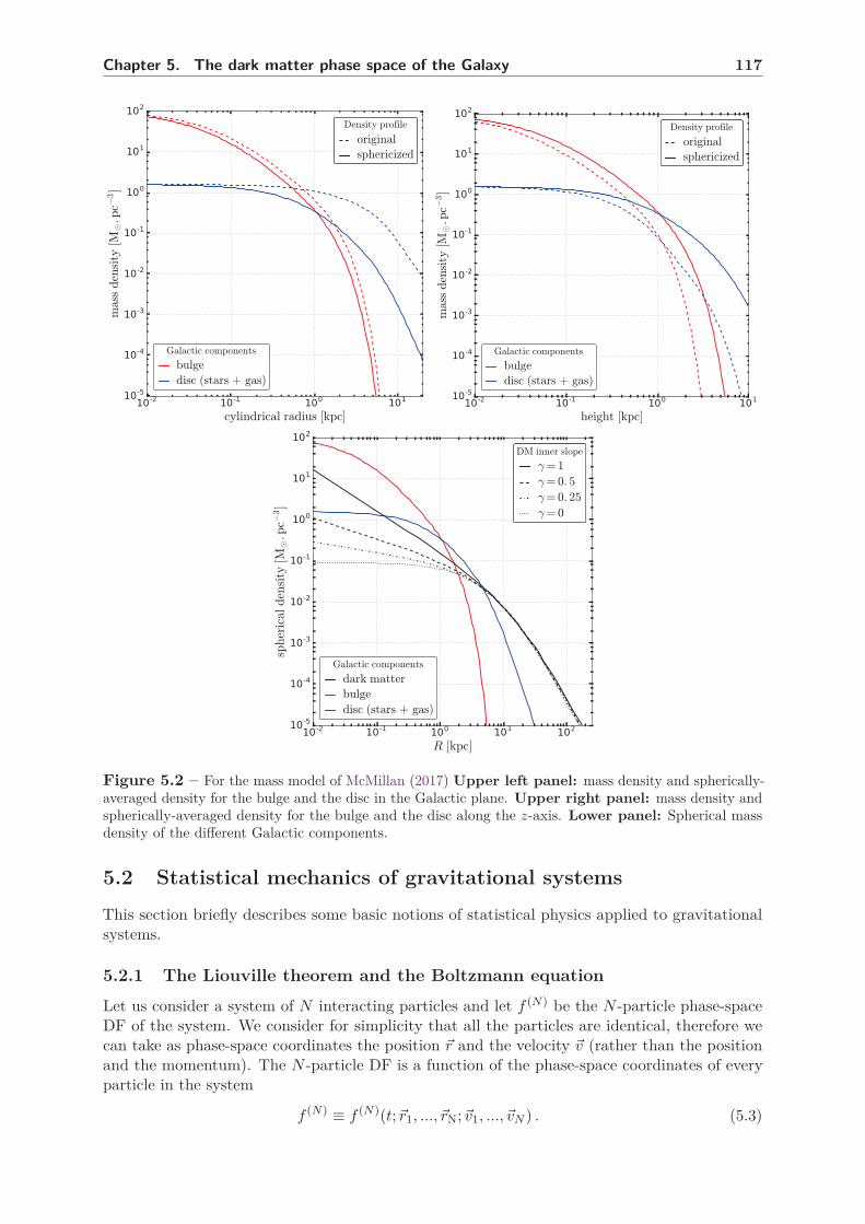
Chapter 5. The dark matter phase space of the Galaxy 117
Figure 5.2 – For the mass model of McMillan (2017) Upper left panel: mass density and spherically-averaged density for the bulge and the disc in the Galactic plane. Upper right panel: mass density andspherically-averaged density for the bulge and the disc along the z-axis. Lower panel: Spherical massdensity of the different Galactic components.
5.2 Statistical mechanics of gravitational systems
This section briefly describes some basic notions of statistical physics applied to gravitationalsystems.
5.2.1 The Liouville theorem and the Boltzmann equation
Let us consider a system of N interacting particles and let f (N) be the N -particle phase-spaceDF of the system. We consider for simplicity that all the particles are identical, therefore wecan take as phase-space coordinates the position þr and the velocity þv (rather than the positionand the momentum). The N -particle DF is a function of the phase-space coordinates of everyparticle in the system
f (N) ≡ f (N)(t;þr1, ..., þrN;þv1, ..., þvN ) . (5.3)

118 5.2. Statistical mechanics of gravitational systems
The distribution is normalised
∫
(
N∏
i=1
d3þri d3þvi
)
f (N) = 1 . (5.4)
If the system is isolated, f (N) obeys the Liouville theorem
df
dt
(N)
≡ ∂f
∂t
(N)
+N
∑
i=1
(
þri.þ∇þrif (N) + þvi.þ∇þvi
f (N))
= 0 . (5.5)
This equation states that the phase-space density of the system is conserved during its evolution.This theorem is valid regardless of the interactions between the particles and the state ofequilibrium of the system, see Binney & Tremaine (1987). In particular, it applies in theout-of-equilibrium regime. If the only interaction between particles is gravitation, we have
þvi =∑
j Ó=i
GN m (þrj − þri)
|þrj − þri|3
= −∑
j Ó=i
þ∇þriΦji ,
(5.6)
where
Φji ≡ − GN m
|þrj − þri|(5.7)
is the gravitational potential between particle i and j. The Liouville equation can then be written
df
dt
(N)
=∂f
∂t
(N)
+N
∑
i=1
þvi.þ∇þrif (N) −
∑
j Ó=i
þ∇þriΦji.þ∇þvi
f (N)
= 0 . (5.8)
For our purposes, it is more convenient to work with the 1-particle distribution function
f (1)(t, þr1, þv1) ≡∫
(
N∏
k=2
d3þrk d3þvk
)
f (N) . (5.9)
Since all particles are identical, we simply write f (1) ≡ f and we call f the phase-space DF fromnow on. The DF is normalised
∫
d3þr d3þv f(t, þr,þv) = 1 . (5.10)
We want to derive an equation for f starting from the Liouville equation (5.5). We integrate theLiouville equation over
∏Nk=2 d3þrk d3þvk. This removes all terms in the sum except the i = 1 term
if we assume f (N) decreases sufficiently fast at infinity so that
∫
d3þriþ∇þri
f (N) = 0 (5.11)∫
d3þviþ∇þvi
f (N) = 0 . (5.12)
We are left with
∂f
∂t+ þv1.þ∇þr1
f −∫
(
N∏
k=2
d3þrk d3þvk
)
þ∇þv1f (N).þ∇þr1
N∑
j=2
Φj1 = 0 . (5.13)

Chapter 5. The dark matter phase space of the Galaxy 119
To simplify the last term in this equation, we further assume f (N) is separable which means itcan be written
f (N) =N∏
n=1
f(t, þrn, þvn) . (5.14)
This implies in particular that the phase-space coordinates of the particles in the system arecompletely uncorrelated. This leads to
∂f
∂t+ þv1.þ∇þr1
f − (N − 1)þ∇þv1f(t, þr1, þv1).þ∇þr1
∫
d3þr2 d3þv2 Φ21 f(t, þr2, þv2) = 0 , (5.15)
where we have used the individual normalization of f and the equality of each term in the sumover j. We define the average gravitational potential at position þr1 through
Φ(þr1) ≡ N
∫
d3þr2 d3þv2 Φ12 f(t, þr2, þv2) , (5.16)
and we get
∂f
∂t+ þv1.þ∇þr1
f − (N − 1)
Nþ∇þv1
f(t, þr1, þv1).þ∇þr1Φ = 0 . (5.17)
We now take the N → ∞ limit and get the collisionless Boltzmann equation
df
dt≡ ∂f
∂t+ þv.þ∇þrf − þ∇þr Φ.þ∇þvf = 0 . (5.18)
This equation is also often called the Vlasov equation, as it is identical to the equation thatdetermines the evolution of a plasma. It is less general than the Liouville equation since it relieson the separability of f (N) and N → ∞. Similar to the Liouville equation, it expresses theconservation of the phase-space density around a particle in the system. Note that according tothis equation, particles are only sensitive to a smooth gravitational potential Φ and do not ”see”the potential generated by each individual particle.
If correlation between particles cannot be neglected, then f (N) cannot be considered separable.In that case, it is useful to consider the 2-particle phase space DF
f (2)(þr1, þr2;þv1, þv2) = f(þr1, þv1)f(þr2, þv2) + g(þr1, þr2;þv1, þv2) , (5.19)
where g is the correlation function of particle 1 and 2. In that case, the Boltzmann equation isnot called collisionless any more and takes the form
df
dt= C[f ] , (5.20)
where
C[f ] ≡ N
∫
d3þr2 d3þv2þ∇þr1
Φ12.þ∇þv1g (5.21)
is the collision operator or encounter operator.
Which equation should we choose to study dark matter systems? We will see in the nextsection that most self-gravitating systems can be considered as being essentially collisionless.

120 5.2. Statistical mechanics of gravitational systems
5.2.2 Relaxation time
We compute the relaxation time of a self-gravitating, homogeneous system, following the derivationof Binney & Tremaine (1987). We consider a test particle moving through a medium consistingof homogeneously distributed point-mass particles. We want to estimate the difference in velocityinduced by the particles distribution with respect to a case where the total mass of these particlesis smoothly distributed. First, we focus on the case of a single encounter: the test particleA passes-by a particle B which we consider at rest, see 5.3. We assume the velocity is smallδv/v ≪ 1, in which case the trajectory of A is approximately a straight line. Consequently, thevelocity change parallel to the trajectory averages to zero and we are left with a perpendicularvelocity change. The perpendicular force felt by A at a given time is then
F⊥ =GN mA mB
x2 + b2cos(θ)
=GN mA mB
b2
[
1 +x2
b2
]−3/2
=GN mA mB
b2
[
1 +
(
vt
b
)2]−3/2
,
(5.22)
where t = 0 is the moment when the distance between A and B is equal to the impact parameterb. By Newton’s second law, we have
mAdþv
dt= þF , (5.23)
which projected to the direction perpendicular to the trajectory leads to
δv =GN mB
b2
∫ +∞
−∞
[
1 +
(
vt
b
)2]−3/2
dt
=2 GN mB
bv.
(5.24)
We recall that this expression is only valid if δv ≪ v which translates into b ≫ bmin where
bmin =2 GN mB
v2. (5.25)
We now have to evaluate the number of encounter experienced by A as it orbits in the massdistribution. We assume this distribution to be a homogeneous sphere of radius R containing Nparticles. The number of encounters with impact parameter between b and b + db after one orbitin the system is then
δn =N
πR22πb db . (5.26)
We can now compute the velocity variance created by these encounters
(δv)2δn =
(
GN mB
bv
)2 N
πR22πb db . (5.27)
Integrating over the impact parameter, we get
∆v2 = 8N
(
GN mB
vR
)2
ln
(
bmax
bmin
)
. (5.28)

Chapter 5. The dark matter phase space of the Galaxy 121
The maximal impact parameter bmax is set by our assumption of a homogeneous distribution,which cannot be true for b > R. Therefore we assume bmax ≃ R. The expression of ∆v2 can besimplified by considering A is on a circular orbit, in which case we have
v ≃√
GNN mB
R, (5.29)
and
bmax
bmin=
R v2
2 GN mB≃ N
2. (5.30)
We finally get the relative change in v2 after one crossing of the system
∆v2
v2=
8
Nln
(
N
2
)
. (5.31)
The number of crossing needed to have a deviation in v2 comparable to the original value is then
ncross =N
8 ln(
N2
) , (5.32)
and two body encounters become relevant after a time
trelax =N
8 ln(
N2
) tcross , (5.33)
where tcross = R/v = R3/2/(GNM)1/2 is the typical crossing time. The crossing time has themore general expression tcross = (GNρ)−1/2 and is also called the dynamical time. trelax is the(two-body) relaxation time. At a time t ≪ trelax, the effect of two-body encounters is subdominantand the dynamics of the system should obey the collisionless Boltzmann equation (5.18). At timet > trelax, two-body encounters start to dominate the dynamics, particles have a diffusive motionand the phase-space DF is solution of the Boltzmann equation with collisions (5.20). Note that ifthe system is not homogeneous the dynamical time depends on the position through the density,therefore relaxation might be important at the center while remaining irrelevant at the edges.
What is the relaxation time of realistic self-gravitating systems? Some stellar systems suchas globular clusters are known to be affected by relaxation. What about dark matter systems? Ifthe DM particle has a mass around the electroweak scale m ∼ 100 GeV, the number of particlesin a halo is gigantic and relaxation is completely irrelevant. As an illustration, we considera DM structure of mass M = 10−10 M⊙ which is near the smallest mass reachable in WIMPmodels, see e.g.Bringmann (2009). The number of particles is M/m ≃ 1050 and the crossingtime tcross ≃ 1 Myr, so relaxation is indeed of no importance there.1 Relaxation can only be ofrelevance for very heavy DM particles. For instance, we can consider the case of Primordial BlackHoles DM with mass MPBH ≃ 10 M⊙ and a halo composed of ∼ 100 PBHs. The cosmologicalradius of the structure is roughly R200 ≃ 0.2 kpc and the relaxation time is trelax ∼ 5 Gyr, sorelaxation should impact structure formation is this case.
5.2.3 Thermodynamic equilibrium?
The statistical treatment exposed so far is very reminiscent of the statistical mechanics of gaseoussystems developed by Maxwell, Boltzmann and Gibbs. A major difference is the nature of theforce driving the evolution of the system. While gaseous systems evolve because of the numerous
1This does not mean the particle nature of DM is irrelevant for WIMP DM structures. In particular, thefree-streaming of DM particles is what sets the minimal mass of DM halos in WIMP models.

122 5.2. Statistical mechanics of gravitational systems
Figure 5.3 – A test particle A approaches at speed v a stationary particle B with an impact parameterb. The trajectory of A is assumed to be a straight line during the encounter.
collisions between their constituents, gravitational systems can be considered as being essentiallycollisionless and driven by the long-ranged gravitational interaction. One can wonder if the resultsof thermodynamics apply in that case. In particular, is there a thermodynamic equilibrium forgravitational systems? The answer to that question is negative: gravitational systems do nothave a thermal equilibrium. A very simple way of seeing this is given by Binney & Tremaine(1987). Let us consider an N-body gravitational system and assume it is in thermal equilibrium.The N-particle phase-space DF should take the usual form
f (N)(þr1, ..., þrN ;þv1, ..., þvN ) =1
Kexp [−β H(þr1, ..., þrN ;þv1, ..., þvN )] , (5.34)
where K is a normalization constant, β = 1/(kBT ), T is the system’s temperature and H itsHamiltonian. The constant K should be fixed by requiring the normalization over the fullphase-space
K =
∫
(
N∏
i=1
d3þri d3þvi
)
exp [−β H(þr1, ..., þrN ;þv1, ..., þvN )] . (5.35)
However, the spatial part of the integral diverges for a gravitational system. It diverges at shortdistances because of the singular behaviour of the gravitational potential, and it diverges at largedistances because the Hamiltonian becomes independent of the position while still being velocitydependent. Consequently, the DF cannot be normalized and there is no thermal equilibrium!In fact, many results of statistical mechanics are not valid for gravitational systems: the heatcapacity is negative, there is no micro-canonical ensemble, entropy cannot be maximized (andconsequently there is no canonical ensemble), etc...
5.2.4 The Jeans equations
The characterization of the dynamics of self-gravitating systems involves solving the collisionlessBoltzmann equation
∂f
∂t+ vi
∂f
∂xi− ∂Φ
∂xi
∂f
∂vi= 0 . (5.36)
Summation over the indices is assumed. There is unfortunately no known classification of thesolutions of this equation. It is possible however to learn about the dynamics of a system withoutsolving the full equation. The idea is to compute the velocity moments of Eq. (5.36). Thezeroth-order moment is
∫
∂f
∂td3þv +
∫
vi∂f
∂xid3þv −
∫
∂Φ
∂xi
∂f
∂vid3þv = 0 . (5.37)

Chapter 5. The dark matter phase space of the Galaxy 123
Multiplying by the total mass of the system (assumed constant), this leads to
∂ρ
∂t+
∂(ρvi)
∂xi= 0 . (5.38)
which is simply the continuity equation for the mass density ρ. Note that this equation involvesfour unknowns, ρ and the components of the mean velocity vi, and therefore cannot be solveunless further assumptions are made. Taking the first-order moment leads to
∂(ρvi)
∂t+
∂(ρvivj)
∂xj= −ρ
∂Φ
∂xi. (5.39)
The first term can be replaced by using the continuity equation and we get
∂vi
∂t+ vj
∂vi
∂xj= − ∂Φ
∂xi− 1
ρ
∂(ρσ2ij)
∂xj, (5.40)
where σ2ij = vivj − vivj is the velocity variance tensor. This equation has the same form as the
Euler equation in Eqs. (3.1) with a pressure tensor pij = ρσ2ij . Hence, in collisionless systems,
the velocity dispersion acts as an effective pressure. Note that Eq. (5.40) together with Eq. (5.38)have again too many unknowns to be solved. Other equations can be added to the system byconsidering the second-order moment of the Boltzmann equation, but this also introduces newunknowns such as vivjvk. We can actually form a system of hierarchical equations by takingmoments of higher and higher order. These are called the Jeans equations after Jeans (1919).Obviously the system of equations has to be truncated at some order, and closed by makingassumptions on the unknown quantities. The time-independent version of Eq. (5.40) is oftenwritten is spherical coordinates
1
ρ
∂(ρv2r )
∂r+ 2
β
rv2
r = −∂Φ
∂r, (5.41)
where we introduced the anisotropy parameter
β(r) ≡ 1 −v2
θ + v2φ
2 v2r
. (5.42)
This can be seen as a differential equation for ρv2r where β(r) is an unknown function. Usually, a
specific form is assumed for β(r) so the equation can be solved.Unlike the Boltzmann equation, the Jeans equation gives informations about the moments of
the phase-space DF rather than the DF itself. In the next section, we present the Eddingtonformalism which enables the determination of the full DF of a spherical system.
5.3 The Eddington formalism
5.3.1 Jeans Theorem
The starting point of the Eddington formalism is the theorem of Jeans (1915). To state thistheorem, we first need to define the integrals of motion. An integral of motion is a function of thephase-space coordinates I[x(t), v(t)] which is conserved along the trajectory of the system, i.e.
d
dtI[x(t), v(t)] =
dx
dt
∂I
∂x+
dv
dt
∂I
∂v= 0 . (5.43)
We see that an integral of motion is by definition a solution of the stationary collisionlessBoltzmann equation, and therefore any function depending on the phase-space coordinates only

124 5.3. The Eddington formalism
through integrals of motion is also solution of the Boltzmann equation since we have
d
dtf [I1, ..., In] =
n∑
i=1
dIi
dt
∂f
∂Ii
= 0 .
(5.44)
Reciprocally, if f is a solution of the stationary collisionless Boltzmann equation then it is alsoan integral of motion, hence the Jeans theorem: any solution of the stationary collisionlessBoltzmann equation depends on the phase-space coordinates only through integrals of motion.Finding phase-space DFs therefore reduces to finding quantities that are conserved along thetrajectory of the system.
5.3.2 Isotropic velocity distributions
The simplest case we can consider is a phase-space DF that only depends on the energyE/m = Φ + v2/2, where m is the particle’s mass and Φ the gravitational potential. This was firstconsidered by Eddington (1916). Since for bounded particles the energy is negative, we insteadconsider the variable E = Ψ − v2/2 where Ψ = Φ0 − Φ up to a constant. This is simply minus theenergy divided by the particle’s mass (we do refer to E as the energy and to Ψ as the potential inthe following). Since the energy only depends on the modulus of the velocity, any phase-space DFthat depends only on the energy describes an isotropic velocity distribution. Consequently, werefer to a DF of the type f(E) as isotropic.2 It is conventional in statistical physics to normalizethe DF to unity so that it can be interpreted as a probability density function, however it ismore convenient for our purposes to normalize the DF to the mass of the system of interest:
ρ(r) =
∫
f(E) d3þv
= 4π
∫ +∞
0v2 f
(
Ψ(r) − v2
2
)
dv ,(5.45)
where ρ is the mass density of the system. Note that the system under study (a galaxy forinstance) can have several components (dark matter and baryons for instance). We are onlyinterested in describing the phase space of the dark matter, therefore in such a case ρ refersto the dark matter mass density ρ = ρDM. The potential Ψ, however, is the total potentialΨ = ΨDM + Ψbar. Note that the DM density and the total potential are independent variablessince one cannot compute the total potential from the DM density alone.
We restrict ourselves to the study of a completely bounded system, where all the particleshave positive energy E and therefore f(E < 0) = 0. The normalization of f is then written as
ρ(r) = 4π
∫ vesc
0v2 f
(
Ψ − v2
2
)
dv , (5.46)
where vesc(r) =√
2Ψ(r) is the escape speed, that is the minimal speed needed for a particle at rto become unbounded. We can perform the change of variable v =
√
2(Ψ − E) in Eq. (5.46) toget
ρ(Ψ) = 4π√
2
∫ Ψ
0
√Ψ − E f(E) dE . (5.47)
Since the potential Ψ is a monotonically decreasing function of the radius, it can be used as asubstitute variable for r and ρ(Ψ) is well defined. We derive Eq. (5.47) with respect to Ψ
dρ
dΨ=
√8π
∫ Ψ
0
f(E)√Ψ − E
dE . (5.48)
2The term ergodic is also used in the literature to describe a DF of this type, see Binney & Tremaine (1987)

Chapter 5. The dark matter phase space of the Galaxy 125
This is an Abel integral equation. The following mathematical result helps us to go further: theequation
f(x) =
∫ x
0
g(t)
(x − t)αdt, 0 < α < 1 (5.49)
has the solution
g(t) =sin(πα)
π
d
dt
∫ t
0
f(x)
(t − x)1−αdx . (5.50)
Applied to Eq. (5.48) this leads to Eddington’s formula
f(E) =1√8π2
d
dE
∫ E
0
1√E − Ψ
dρ
dΨdΨ
. (5.51)
Thus we have found the expression of the phase-space DF in terms of the mass density ρ and thegravitational potential Ψ. This solution is unique, there is only one possible DF that describesa spherical isotropic system. The expression of the DF can be simplified by performing anintegration by parts, then apply the derivative with respect to E . We get
f(E) =1√8π2
[
1√E
(
dρ
dΨ
)
Ψ=0+
∫ E
0
1√E − Ψ
d2ρ
dΨ2dΨ
]
. (5.52)
A striking feature of this expression is a term ∝ E−1/2 which diverges at small energies. Themeaning of this term and the theoretical issues it poses are discussed in Sec. 5.4.
5.3.2.1 Concrete examples
The singular isothermal sphere The mass density profile of the singular isothermal sphere(SIS) is
ρ(r) =σ2
2πGN r2, (5.53)
where σ is a free parameter homogeneous to a velocity. This is actually the one-dimensionvelocity dispersion of the system, as it is shown later. This density profile strongly diverges atthe center of the system. The regularization of this divergence is discussed in Sec. 5.4. The massprofile is
m(r) =2σ2
GNr , (5.54)
and therefore the total mass of the system is infinite. This is not a big problem from the point ofview of Eddington’s method since it accommodates with a finite boundary for the system. Usingthe expression of the mass, one immediately finds the circular speed
v2c = 2 σ2 (5.55)
which is independent of the radius. The gravitational potential can be found by solving Poisson’sequation
1
r2
d
dr
(
r2 dΨ
dr
)
= −4πGN ρ = −2σ2
r2. (5.56)
With the boundary conditions (r2dΨ/dr)r=0 = 0 and Ψ(r0) = 0, we get
Ψ(r) = −2σ2 ln
(
r
r0
)
. (5.57)

126 5.3. The Eddington formalism
Note that the potential diverges both at large and short distances. We can express the massdensity as a function of the potential
ρ(Ψ) =σ2
2πGN r20
exp
(
Ψ
σ2
)
= ρ0 exp
(
Ψ
σ2
)
(5.58)
and inject it in Eddington’s formula Eq. (5.51)
f(E) =ρ0√
8π2σ2
d
dE
∫ E
0
1√E − Ψ
exp
(
Ψ
σ2
)
dΨ . (5.59)
This leads to
f(E) =ρ0
(2πσ2)3/2
1√π
√
σ2
E + eE/σ2erf
√
Eσ2
. (5.60)
The DF diverges at small E , where we have
f(E) ≃ ρ0
(2πσ2)3/2
1√π
√
σ2
E . (5.61)
The behaviour f(E) ∝ E−1/2 at small energies is intrinsic to the Eddington procedure, as seen inEq. (5.52). Since the potential diverges at the center of the system, the energy E takes arbitrarylarge values as a particle falls down the potential well. It is therefore interesting to consider thelimit E ≫ σ2 in Eq. (5.60). This limit considers particles whose energy is dominated by theirpotential energy rather than their kinetic energy. We get
f(E) ≃ ρ0
(2πσ2)3/2eE/σ2
, (5.62)
which is the Boltzmann distribution function, and therefore f diverges at large E . This phase-spaceDF predicts in particular that the velocity distribution is, at any position, the Maxwell-Boltzmanndistribution
fr(þv) =1
(2πσ2)3/2e−v2/(2σ2) (5.63)
The velocity dispersion at radius r is then given by
σ2þv ≡
⟨
þv2⟩
− 〈þv〉2 = 3 σ2 (5.64)
and is therefore independent of the radius. The velocity distribution extends to arbitrary largevelocities, i.e. there is no escape speed to the system. This is not surprising since the escapespeed is defined by E = 0 and we took the limit E ≫ σ2. Note that this approximation breaksdown when the radius gets close to r0 where we have Ψ(r0) = 0, therefore we expect the velocitydistribution to depart from the Maxwell-Boltzmann DF in the outskirts of the system. The DFin Eq. (5.60) and the Boltzmann DF are shown in the left panel of Fig. 5.4.
It is interesting to consider the DF of a system with the SIS profile which contains unboundedparticles. We have to remove the condition f(E < 0) = 0 in Eddington’s calculation to get thecorrect result. This leads to a change of the lower bound of the integral in Eq. (5.60) from E = 0to E = −∞. The expression of the DF is again
f(E) =ρ0
(2πσ2)3/2eE/σ2
. (5.65)
This expression is valid at all energies (positive or negative). The escape speed is still well-definedby vesc =
√
2(Φ(r0) − Φ(r) however, unlike the phase space described by the distribution inEq. (5.60), this phase space contains unbound particles at all positions. In other words, at anyposition r, the phase-space DF includes particles with v > vesc(r). In such a system, the radiusr0 is the position of the bound particle farthest from the center of the system.
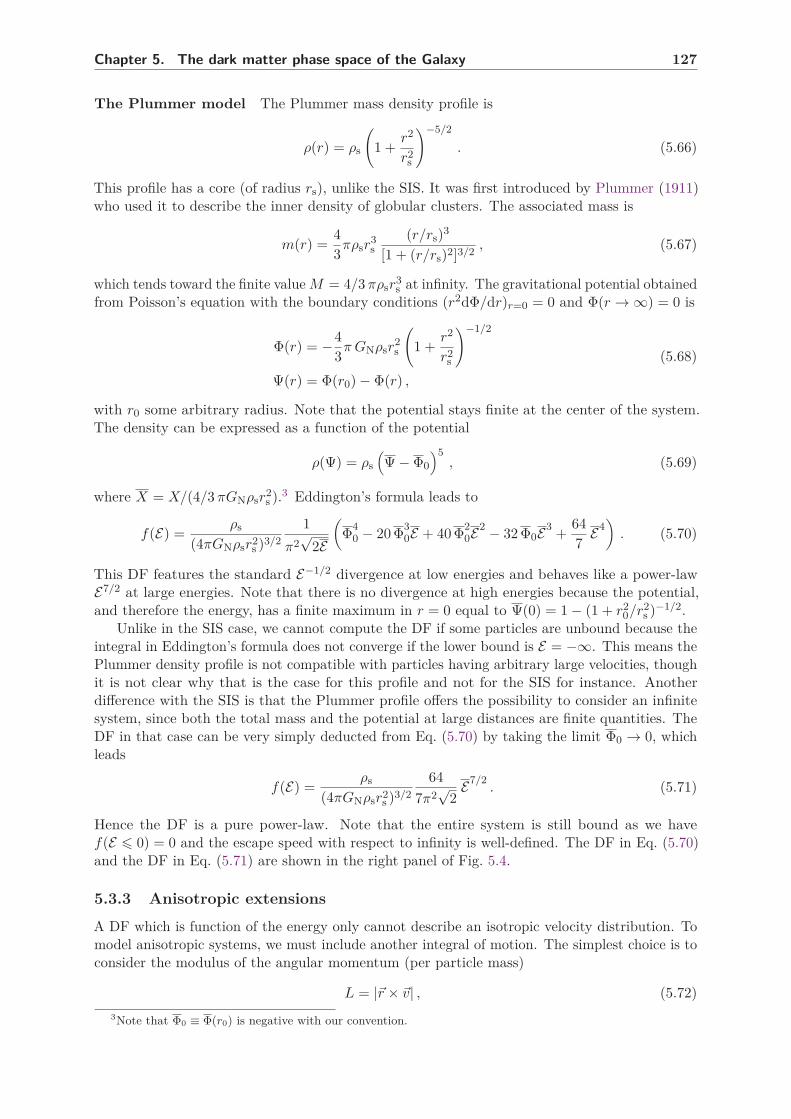
Chapter 5. The dark matter phase space of the Galaxy 127
The Plummer model The Plummer mass density profile is
ρ(r) = ρs
(
1 +r2
r2s
)−5/2
. (5.66)
This profile has a core (of radius rs), unlike the SIS. It was first introduced by Plummer (1911)who used it to describe the inner density of globular clusters. The associated mass is
m(r) =4
3πρsr
3s
(r/rs)3
[1 + (r/rs)2]3/2, (5.67)
which tends toward the finite value M = 4/3 πρsr3s at infinity. The gravitational potential obtained
from Poisson’s equation with the boundary conditions (r2dΦ/dr)r=0 = 0 and Φ(r → ∞) = 0 is
Φ(r) = −4
3π GNρsr
2s
(
1 +r2
r2s
)−1/2
Ψ(r) = Φ(r0) − Φ(r) ,
(5.68)
with r0 some arbitrary radius. Note that the potential stays finite at the center of the system.The density can be expressed as a function of the potential
ρ(Ψ) = ρs
(
Ψ − Φ0
)5, (5.69)
where X = X/(4/3 πGNρsr2s ).3 Eddington’s formula leads to
f(E) =ρs
(4πGNρsr2s )3/2
1
π2√
2E
(
Φ40 − 20 Φ
30E + 40 Φ
20E2 − 32 Φ0E3
+64
7E4
)
. (5.70)
This DF features the standard E−1/2 divergence at low energies and behaves like a power-lawE7/2 at large energies. Note that there is no divergence at high energies because the potential,and therefore the energy, has a finite maximum in r = 0 equal to Ψ(0) = 1 − (1 + r2
0/r2s )−1/2.
Unlike in the SIS case, we cannot compute the DF if some particles are unbound because theintegral in Eddington’s formula does not converge if the lower bound is E = −∞. This means thePlummer density profile is not compatible with particles having arbitrary large velocities, thoughit is not clear why that is the case for this profile and not for the SIS for instance. Anotherdifference with the SIS is that the Plummer profile offers the possibility to consider an infinitesystem, since both the total mass and the potential at large distances are finite quantities. TheDF in that case can be very simply deducted from Eq. (5.70) by taking the limit Φ0 → 0, whichleads
f(E) =ρs
(4πGNρsr2s )3/2
64
7π2√
2E7/2
. (5.71)
Hence the DF is a pure power-law. Note that the entire system is still bound as we havef(E 6 0) = 0 and the escape speed with respect to infinity is well-defined. The DF in Eq. (5.70)and the DF in Eq. (5.71) are shown in the right panel of Fig. 5.4.
5.3.3 Anisotropic extensions
A DF which is function of the energy only cannot describe an isotropic velocity distribution. Tomodel anisotropic systems, we must include another integral of motion. The simplest choice is toconsider the modulus of the angular momentum (per particle mass)
L = |þr × þv| , (5.72)
3Note that Φ0 ≡ Φ(r0) is negative with our convention.

128 5.3. The Eddington formalism
Figure 5.4 – Left panel: isotropic DF of the bound singular isothermal sphere (blue) compared tothe Boltzmann-Gibbs DF (red) Right panel: Isotropic DF of the finite Plummer model (blue) comparedto the infinite model (red).
and a DF of the form f(E , L). Similar to the isotropic case, we normalize the DF to the massthrough
ρ =
∫
f(E , L) d3þv . (5.73)
Changing variables, we get
ρ(Ψ) = 4π
∫ Ψ
0
dEr√
8(Ψ − E)
∫
√2r2(Ψ−E)
0
f(E , L)√
2r2(Ψ − E) − L2dL , (5.74)
where r = r(Ψ) is a function of the potential. This integral equation cannot be inverted likein the isotropic case, and the solution is not unique for a given ρ(Ψ). We must give a precisemeasure of the anisotropy to go any further. This is done through the anisotropy parameter asdefined by Binney (1980)
β(r) ≡ 1 −σ2
θ + σ2φ
2σ2r
= 1 − σ2t
2σ2r
. (5.75)
In this equation, σ2i is the velocity dispersion along spatial coordinate i
σ2i (r) ≡
⟨
v2i
⟩
− 〈vi〉2 =1
ρ(r)
∫
v2i f(r,þv) d3þv . (5.76)
If particles at a position r are on mostly circular orbits, we have σ2r ≪ σ2
t and β → −∞. Ifparticles are on mostly radial orbits, we have σ2
r ≫ σ2t and β ≃ 1. The system is locally isotropic
if β = 0, i.e. 2σ2r = σ2
t . For a given system ρ(Ψ) there are several anisotropy profiles possible,therefore we need to specify β(r) to find an explicit solution to Eq. (5.74).
5.3.3.1 Constant anisotropy models
The simplest case we can consider is a system with an anisotropy parameter independent of theradius, i.e. β(r) = β0 is a constant. It was shown by Cuddeford (1991) that the correspondingDF takes the form
f(E , L) = G(E)L−2β0 . (5.77)

Chapter 5. The dark matter phase space of the Galaxy 129
That this DF effectively leads to a constant anisotropy parameter with β0 is shown in App. D.2.The expression of G can be found by considering the normalization equation
ρ =
∫
f(E , L) d3þv
= 2π
∫ π
0dη sin(η)
∫ vesc
0dv v2 G(E) [rv sin(η)]−2β0 .
(5.78)
Using the integral
∫ π
0[sin(η)]1−2α dη =
√π
Γ (1 − α)
Γ(
32 − α
) , (5.79)
and performing the change of variable v =√
2(Ψ − E), we get
r2β0ρ = λ(β0)
∫ Ψ
0
G(E)
(Ψ − E)β0−1/2dE , (5.80)
where
λ(β0) = 23/2−β0π3/2 Γ (1 − β0)
Γ(
32 − β0
) (5.81)
This is an Abel integral equation of the form in Eq. (5.49) only if 1/2 < β0 < 1. If β0 6 1/2,then we derive Eq. (5.80) n times with respect to Ψ
dn
dΨn
(
r2β0ρ)
= λ(β0)
(
1
2− β0
)
!
∫ Ψ
0
G(E)
(Ψ − E)β0−1/2+ndE , (5.82)
where
n ≡[
3
2− β0
]
(5.83)
is the floor of 3/2 − β0 and
(
1
2− β0
)
! =
(
12 − β0
) (
−12 − β0
)
...(
12 − β0 − (n − 1)
)
for β0 < 12
1 for β0 > 12
(5.84)
This ensures that 0 < β0−1/2+n < 1 and Eq. (5.82) is an Abel equation. This equation is actuallyidentical to the Abel equation found in the isotropic case Eq. (5.48) with the correspondenceρ → r2β0ρ and 1 → n. The solution of Eq. (5.82) is
G(E) =sin([n − 1/2 + β0]π)
πλ(β0)(1/2 − β0)!
d
dE
∫ E
0
dn
dΨn
(
r2β0ρ)
(E − Ψ)n−3/2+β0 dΨ . (5.85)
Note that in the particular case β0 = 0, G is equal to the isotropic DF in Eq. (5.51) thereforethe isotropic case is included in the constant-β models. Just like in the isotropic case, we candevelop this expression to get
G(E) =sin([n − 1/2 + β0]π)
πλ(β0)(1/2 − β0)!
×[
1
E3/2−β0−n
(
dn
dΨnr2β0ρ
)
Ψ=0+
∫ E
0
dn+1
dΨn+1
(
r2β0ρ) dΨ
(E − Ψ)3/2−β0−n
] (5.86)

130 5.3. The Eddington formalism
5.3.3.2 Osipkov-Merritt models
An alternative anisotropic DF was found independently by Osipkov (1979) and Merritt (1985)and takes the form
fom(Q) ≡ f
(
E − L2
2r2a
)
. (5.87)
The corresponding anisotropy parameter is
β(r) =r2
r2 + r2a
, (5.88)
as demonstrated in App. D.2. Unlike the constant-β models, the Osipkov-Merritt (OM) modelslead to a radius-dependent anisotropy. The anisotropy tends to zero at the center of the system,which is therefore almost isotropic for r ≪ ra, and becomes close to one when r ≫ ra. Theradius ra is a free parameter called the anisotropy radius, it controls the transition between theisotropic center and the radial orbits at large radius. The DF is normalized so that
ρ =
∫
fom(Q) d3þv
=4π
√2
1 + r2
r2a
∫ Ψ
0
√
Ψ − Q fom(Q) dQ .(5.89)
This leads to the Abel integral equation
dρOM
dΨ=
√8π
∫ Ψ
0
fom(Q)√Ψ − Q
dQ , (5.90)
where
ρOM(r) ≡(
1 +r2
r2a
)
ρ(r) . (5.91)
The solution of the Abel equation is
fom(Q) =1√8π2
d
dQ
∫ Q
0
1√Q − Ψ
dρOM
dΨdΨ
=1√8π2
[
1√Q
(
dρOM
dΨ
)
Ψ=0+
∫ Q
0
1√Q − Ψ
d2ρOM
dΨ2dΨ
]
.
(5.92)
This is the same expression as the isotropic DF with the correspondence ρ → ρOM. Note thatthe OM models include the isotropic model which is recovered in the limit ra → ∞.
5.3.3.3 More complicated models
The two classes of models presented above (constant-β and OM) both feature one single inde-pendent parameter which completely determines the anisotropy profile. While these models areappealing because of their simplicity, they also lack flexibility and in general their anisotropyprofile is different from those observed in cosmological simulations, see Wojtak et al. (2008);Ludlow et al. (2011); Lemze et al. (2012); Sparre & Hansen (2012); Wojtak et al. (2013). It istherefore useful to consider alternatives models which involve a larger number of parameters.

Chapter 5. The dark matter phase space of the Galaxy 131
Cuddeford models A simple extension of the constant-β and OM models was considered byCuddeford (1991), who looked at DFs of the form
f(E , L) = fom(Q)L−2β0 . (5.93)
This class of models involves two free parameters, β0 and ra. The constant-β models are recoveredin the limit ra → 0 and the OM models are recovered when β0 = 0. The anisotropy parameter is
β(r) =r2 + β0r2
a
r2 + r2a
, (5.94)
as demonstrated in App. D.2. Thus it has radial orbits at large distances β ≃r≫ra 1 but anarbitrary central anisotropy β ≃r≪ra β0. The anisotropy at r = ra is also equal to (1 + β0)/2instead of 1/2 in the OM models. The anisotropy parameter in the constant-β, Osipkov-Merrittand Cuddeford models are compared in Fig. 5.5.
Figure 5.5 – Anisotropy parameter β as defined in Eq. (5.75) as a function of the radius, in theconstant-β model with β0 = 0.3 (red curve), in the Osipkov-Merritt model (blue curve) and in theCuddeford model with β0 = 0.3 (green curve).
Models of Bozorgnia et al The radial anisotropy predicted by the Cuddeford models is stilltoo high with respect to that observed in simulations. To solve this problem, Bozorgnia et al.(2013) proposed a DF which is a linear combination of the constant-β DF and the OM DF:
f(E , L) = w f1(Q) + (1 − w) f2(E)L−2β0 . (5.95)
The DFs f1 and f2 are computed from Eq. (5.92) and Eq. (5.85), respectively. These modelshave three free parameters which can be tuned to fit the average anisotropy profile observed insimulated galactic halos. Unfortunately, the anisotropy parameter does not take a fully analyticalexpression in that case. It can be expressed as
β(r) =w r2
r2 + r2a
σ2r (f1)
σ2r (f)
+ β0(1 − w)σ2
r (f2)
σ2r (f)
. (5.96)
This anisotropy parameter depends on the underlying mass density profile and gravitationalpotential, unlike all the other models we have seen so far.

132 5.4. Theoretical issues and limitations
Models of Wojtak et al To reproduce the anisotropy profiles observed in simulations ofmassive DM halos, Wojtak et al. (2008) proposed the following three-parameters models
f(E , L) = fE(E)
(
1 +L2
2L0
)β0−β∞
L−2β0 . (5.97)
The constants β0 and β∞ are the asymptotical anisotropies at the center and at large radii,respectively. L0 is an angular momentum constant that sets the radius of transition betweenthese two asymptotical regimes. The energy-dependent part fE is derived from the mass densityas usual, though this involves an iterative procedure which makes these models slightly harder tohandle numerically.
5.4 Theoretical issues and limitations
We presented in the previous section the Eddington formalism and some of its anisotropicextensions, which is a powerful method to find phase-space DFs that are solutions of thecollisionless Boltzmann equation. This formalism is especially appealing for DM searches since itprovides a way to built the DM phase-space DF starting from a dynamically constrained massmodel. Using this method however requires the knowledge of its limitations. In particular, itsrange of application has to be well delimited. This section is devoted to the study of the solutionsof the Eddington inversion method. We first discuss non-physical features that generically appearin the phase-space DF, and present several techniques to remove these features. Second, wediscuss the positivity and stability of the solutions, and the consequences these considerationshave on the applicability of Eddington’s method. The content of this section is based mainly onLacroix et al. (2018).
5.4.1 Finite-size systems instability
A generic issue with the Eddington formalism and its extensions is the presence of divergingterm in the phase-space DF. We recall the expression of the isotropic DF
f(E) =1√8π2
[
1√E
(
dρ
dΨ
)
Ψ=0+
∫ E
0
1√E − Ψ
d2ρ
dΨ2dΨ
]
, (5.98)
which features a term ∝ E−1/2 diverging in E = 0, as illustrated in Fig. 5.4. This term isproportional to the derivative of the density with respect to the potential (dρ/dΨ)Ψ=0 evaluatedat the radial boundary of the system where the potential cancels, hence it is related to the shapeof the density profile at the boundary. A divergence at E = 0 is a sign of instability in the system.This can be seen clearly by considering the speed distribution fþr(v) at a given position þr in thesystem
fþr(v) ≡ v2
ρ(þr)
∫
f(þr,þv) dΩ . (5.99)
For an isotropic DF f(þr,þv) = f(E), this is simply
fr(v) =4πv2
ρ(r)f
(
Ψ(r) − v2
2
)
, (5.100)
hence the speed distribution is directly related to the phase-space DF in the isotropic case. FromEq. (5.100), we see that the divergence at E = 0 translates into a divergence at v =
√
2Ψ(r) inthe speed distribution, as illustrated with the Plummer profile in Fig. 5.6. This speed is preciselythe escape speed at r, i.e. the minimal speed needed for a particle at r to escape to the radius
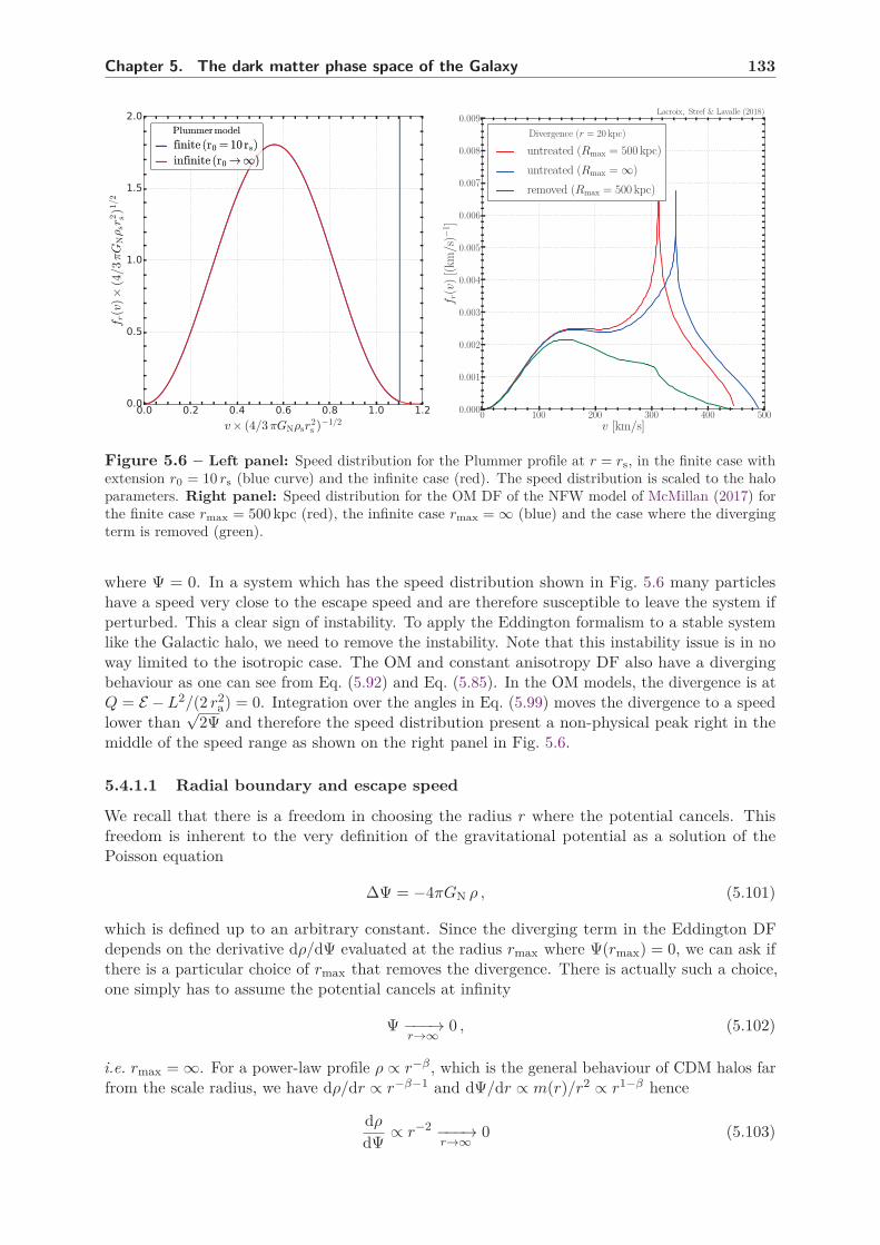
Chapter 5. The dark matter phase space of the Galaxy 133
0 100 200 300 400 500v [km/s]
0.000
0.001
0.002
0.003
0.004
0.005
0.006
0.007
0.008
0.009
f r(v)[(km
/s)−
1 ]
Lacroix, Stref & Lavalle (2018)
Divergence (r = 20 kpc)
untreated (Rmax = 500 kpc)
untreated (Rmax = ∞)
removed (Rmax = 500 kpc)
Figure 5.6 – Left panel: Speed distribution for the Plummer profile at r = rs, in the finite case withextension r0 = 10 rs (blue curve) and the infinite case (red). The speed distribution is scaled to the haloparameters. Right panel: Speed distribution for the OM DF of the NFW model of McMillan (2017) forthe finite case rmax = 500 kpc (red), the infinite case rmax = ∞ (blue) and the case where the divergingterm is removed (green).
where Ψ = 0. In a system which has the speed distribution shown in Fig. 5.6 many particleshave a speed very close to the escape speed and are therefore susceptible to leave the system ifperturbed. This a clear sign of instability. To apply the Eddington formalism to a stable systemlike the Galactic halo, we need to remove the instability. Note that this instability issue is in noway limited to the isotropic case. The OM and constant anisotropy DF also have a divergingbehaviour as one can see from Eq. (5.92) and Eq. (5.85). In the OM models, the divergence is atQ = E − L2/(2 r2
a) = 0. Integration over the angles in Eq. (5.99) moves the divergence to a speedlower than
√2Ψ and therefore the speed distribution present a non-physical peak right in the
middle of the speed range as shown on the right panel in Fig. 5.6.
5.4.1.1 Radial boundary and escape speed
We recall that there is a freedom in choosing the radius r where the potential cancels. Thisfreedom is inherent to the very definition of the gravitational potential as a solution of thePoisson equation
∆Ψ = −4πGN ρ , (5.101)
which is defined up to an arbitrary constant. Since the diverging term in the Eddington DFdepends on the derivative dρ/dΨ evaluated at the radius rmax where Ψ(rmax) = 0, we can ask ifthere is a particular choice of rmax that removes the divergence. There is actually such a choice,one simply has to assume the potential cancels at infinity
Ψ −−−→r→∞
0 , (5.102)
i.e. rmax = ∞. For a power-law profile ρ ∝ r−β , which is the general behaviour of CDM halos farfrom the scale radius, we have dρ/dr ∝ r−β−1 and dΨ/dr ∝ m(r)/r2 ∝ r1−β hence
dρ
dΨ∝ r−2 −−−→
r→∞0 (5.103)

134 5.4. Theoretical issues and limitations
and our phase-space DF is divergence-free while still being solution of the Boltzmann equation.The speed distribution is also regularized, as shown on the left panel in Fig. 5.6 (red curve).Though this is a mathematically sound solution, it is not entirely satisfying.
First, while setting the potential to zero at infinity removes the divergence in the constantanisotropy case (isotropic case included), in general it does not work for the OM models. Thisis because the troublesome derivative in that case is (dρOM/dΨ)Ψ=0 where ρOM is given inEq. (5.91). Let us consider a pure power-law density profile ρ ∝ r−β . The OM pseudo-profile isthen ρOM ∝ r2−β when r ≫ ra. We then have
dρOM
dr∝ r1−β (5.104)
dΨ
dr=
GN m(r)
r2∝ r1−β , (5.105)
and the derivative
dρOM
dΨ=
dρOM
dr
dr
dΨ−−−→r→∞
constant (5.106)
therefore the derivative is non-zero at infinity and the phase-space DF is still divergent. Thisshows that for most DM profiles, the OM models cannot be regularized by taking the radialboundary of the system to infinity. This is illustrated by the speed distribution on the rightpanel in Fig. 5.6. This is the speed distribution at r = 20 kpc predicted by the OM when appliedto the NFW mass model of McMillan (2017), with the anisotropy radius ra = rs = 19.6 kpc. Thedistribution in the case rmax = ∞ features a clear unstable behaviour due to the sharp peak at340 km/s, very similar to the peak observed in the distribution computed for rmax = 500 kpc.
A more serious problem is posed by the physical interpretation of the radius rmax. Thisradius is in some sense the true physical extension of the bound system. Indeed a particle at aradius r > rmax has a negative potential Ψ(r) < 0 and is therefore not bound to the system. Thequestion is then: can we pick an arbitrary large value for that physical extension? This extensionis in fact set by the neighbouring systems. In the case of the Milky Way halo, the distance tothe Andromeda galaxy naturally gives a maximal extension. Since the center of Andromeda isapproximately 800 kpc away from the center of the Milky Way, we do not expect our dark haloto extend much farther than 450-500 kpc. A crucial point is that the physical size of the systemhas consequences on observables deep within the halo, because this size determines the localescape speed. More precisely, the escape speed at radius r is
vesc(r) =√
2Ψ(r) =√
2(φ(rmax) − φ(r)) , (5.107)
where φ(r) is the (negative-defined) gravitational potential cancelling at infinity. This shows thatvesc(r) explicitly depends on rmax. The escape speed is crucial because it is the maximal speed aparticle can have at r if the system is in equilibrium. The local value of the escape speed is inprinciple an observable quantity. It can be inferred from the distribution of nearby high-velocitystars (Leonard & Tremaine, 1990; Piffl et al., 2014) or computed within a full Galactic massmodel (see Sec. 5.1). Changing the value of rmax can strongly impact the escape speed Thisillustrated in Fig. 5.7. We show the relative change in vesc induced by increasing rmax, startingfrom a reference value of rmax = 500 kpc. At 8 kpc, vesc is increased by more than 8%. This is asizeable change because the experimental uncertainty on the local value of vesc is of order 10%,see Piffl et al. (2014). The change in vesc gets more important farther away from the center. Forr = 100 kpc, vesc can be modified by up to 24%. This shows that sending rmax to infinity is nota good approach to regularize the solution of Eddington’s inversion, since it leads to a sizeablemodification of the escape speed everywhere in the system.
In the following, we discuss regularization methods that remove the divergence while keepingthe escape speed essentially unchanged.

Chapter 5. The dark matter phase space of the Galaxy 135
Figure 5.7 – Relative difference between the escape speed for rmax = 500 kpc and the escape speed forrmax > 500 kpc, at different positions in the halo.
5.4.1.2 Modification of the density profile
The divergence in the Eddington DF when the system has a finite extension is an indication thatthe density profile is not realistic in the outer region. This is not surprising since most of the DMprofiles used in the literature are coming from fits within the inner 200 kpc of Milky-Way-likehalos found in simulations. Observational constraints are also local, mostly based on kinematicdata coming from the inner 50 kpc (McMillan, 2017). The kinematics of satellite galaxies havealso been used to set constraints on the MW mass within 300 kpc, though with large uncertainties(Watkins et al., 2010). Therefore the behaviour of the DM density around rmax ∼ 500 kpc iscompletely unprobed and might depart from the typical power-law ρ ∝ r−3 of NFW-like profiles.Here we attempt to modify the initial density profile ρ so that (dρ/dΨ)Ψ=0 = 0 at finite rmax.Let us first consider the Eddington DF in the isotropic case Eq. (5.52) and remove ”by-hand”the diverging term to get a modified DF
F (E) =1√8π2
∫ E
0
dΨ√E − Ψ
d2ρ
dΨ2. (5.108)
Assuming the gravitational potential of the system is not modified by the removal of this term,we can reconstruct the density profile starting from the DF in Eq. (5.108) by computing theintegral
ρ(Ψ) = 4π√
2
∫ Ψ
0F (E)
√Ψ − E dE . (5.109)
By definition of F , this is
ρ(Ψ) = 4π√
2
∫ Ψ
0
[
f(E) − 1√8π2
1√E
(
dρ
dΨ
)
Ψ=0
] √Ψ − E dE , (5.110)
and the initial density profile is given by
ρ(Ψ) = ρ(rmax) + 4π√
2
∫ Ψ
0f(E)
√Ψ − E dE , (5.111)

136 5.4. Theoretical issues and limitations
therefore we get the modified density
ρ(Ψ) = ρ(Ψ) − ρ(rmax) − 2
π
(
dρ
dΨ
)
Ψ=0
∫ Ψ
0
√Ψ − E√
EdE
= ρ(Ψ) − ρ(rmax) − Ψ
(
dρ
dΨ
)
Ψ=0.
(5.112)
This modified profile has a radial derivative
dρ
dr=
dρ
dr− dΨ
dr
(
dρ
dΨ
)
Ψ=0
=dρ
dr− dΨ
dr
(
dρ
dr
)
r=rmax
(
dr
dΨ
)
r=rmax
,
(5.113)
hence(
dρ
dr
)
r=rmax
= 0 (5.114)
by construction. Our calculation is not fully consistent because we assumed the potential is notmodified by the removal of the diverging term. Nevertheless, the Eddington formalism itselfpoints toward a modification of the density profile that regularizes the phase-space DF. Based onthis simple calculation we propose, given a density-potential pair (ρ, Ψ), the following modifiedprofile
ρ ≡ ρ − Ψ
(
dρ
dΨ
)
Ψ=0. (5.115)
This definition differs from Eq. (5.112) by the constant ρ(rmax). This ensures ρ(rmax) = ρ(rmax),unlike the profile in Eq. (5.112) which goes to zero in rmax. The two modified profiles arecompared on the left panel in Fig. 5.8 for a NFW profile cut at rmax = 500 kpc. Both modifiedprofiles significantly differ from the original one near rmax. The biggest difference appears abovethe virial radius R200 ≃ 230 kpc and the density below remains essentially unchanged. The profilein Eq. (5.115) has a 30% deficit at R200 while the profile in Eq. (5.112) has a 40% deficit whichshows the importance of keeping the constant ρ(rmax). The mass profiles, shown on the rightpanel in Fig. 5.8 have an approximate 10% deficit.
If the system has two components (DM and baryons) and its total potential is writtenΨ = Ψdm + Ψbar, we define the modified profile using the DM component only
ρ ≡ ρ − Ψdm
(
dρ
dΨdm
)
Ψdm=0. (5.116)
The modified potential can be computed from Poisson’s equation
Ψ(r′) =
∫ rmax
r
m(r′)
r′2 dr′ , (5.117)
and the derivative with respect to this potential vanishes in rmax by construction, therefore weknow without even constructing the DF that it is non-singular. The radial boundary of thesystem is also preserved by this method. Note that the escape speed, which is the true observable,is still slightly modified because the potential is. Indeed, the original escape speed associated tothe divergent DF is
vesc(r) =√
2Ψ(r) , (5.118)
while the modified escape speed is
vesc(r) =√
2Ψ(r) . (5.119)

Chapter 5. The dark matter phase space of the Galaxy 137
While both these functions go to zero in r = rmax, they are not identical for smaller radii asshown in Fig. 5.9. The relative difference between the escape speed in the different configurationsis only of a few percent.
The discussion above is based on the isotropic case, let us now comment on the anisotropicextensions. The definition of the modified density profile has to be adapted to cancel thedivergence when the density is non-zero. For the constant-β case, we need to cancel the derivative(d(r2β0ρ)/dΨ)Ψ=0 therefore we define the modified density as
ρβ0 = ρ − Ψdm
r2β0
(
d(r2β0ρ)
dΨdm
)
Ψdm=0
. (5.120)
Developing the derivative, this definition leads to
ρβ0 = ρ − Ψdm
(
rmax
r
)2β0(
dρ
dΨdm
)
− 2β0Ψdm
(
rmax
r
)2β0 ρ(rmax)
rmax
(
dr
dΨdm
)
Ψdm=0. (5.121)
Comparing this expression to the isotropic case in Eq. (5.116), we notice that this modifiedprofile is more or less close to the original depending on the sign of β0. If β0 > 0, the differenceis bigger than in the isotropic case while it is smaller if β0 < 0. This illustrated in Fig. 5.10where we show the modified density profile (left panel) and mass profile (right panel) for differentanisotropy model.
For the OM models, our definition is
ρOM = ρ − Ψdm
1 + r2/r2a
(
dρOM
dΨdm
)
Ψdm=0. (5.122)
Working the derivative, we get
ρOM = ρ − Ψdmr2
a + r2max
r2a + r2
(
dρ
dΨdm
)
Ψdm=0− Ψdm
r2a + r2
2rmaxρ(rmax)
(
dr
dΨdm
)
Ψdm=0. (5.123)
This expression shows that the difference between the modified and the original profile is larger inthe OM models than in the isotropic model. The modified density and mass profiles for the OMmodels are shown in Fig. 5.10. Unlike the isotropic modification, this profile is vastly differentfrom the original, especially below the virial radius where the difference goes to a maximum of60% in density and 50% in mass.
Our regularization of the density profile works well for systems with a low or negativeanisotropy parameter. It fails badly for systems that are radially biased like those following theOM phase-space DF.
5.4.1.3 Regularization of the phase-space DF
We now turn to an alternative way of getting rid of the divergence in phase-space. While theprevious method relies on a modification a priori of the density profile used in Eddington’sinversion method, here we modify a posteriori the phase-space DF to get a physically meaningfulquantity.
Removal of the diverging term The simplest way of regularizing the DF is to simply removethe diverging term. This is what we did in the previous section to get the approximative form ofthe modified density profile. Our derivation was not fully consistent however since we assumedthe potential was not modified by the removal of the divergence. Here we perform the sameprocedure but in a consistent way. We remove the diverging term to get a new DF
F (E) ≡ f(E) − 1√8π2
1√E
(
dρ
dΨ
)
Ψ=0=
1√8π2
∫ E
0
d2ρ
dΨ2
dΨ√
E − Ψ. (5.124)

138 5.4. Theoretical issues and limitations
Figure 5.8 – Left panel: NFW density profile (black line) cut at rmax = 500 kpc, with rs = 19.6 kpc.Are also shown the approximative density profile in Eq. (5.112) obtained when removing the divergence(blue line), and our prescription for the regularized density in Eq. (5.115) (red line). Right panel: samething for the mass profile.
Note that we also defined a new energy E which is different from E because the potential of thesystem has been modified. To find the potential of the new system, we have to solve Poisson’sequation
∆Ψdm = −4πGNρ
= −4πGN ×[
ρ0 + 4π√
2
∫ Ψ
0dE F (E)
√
Ψ − E]
.(5.125)
The constant ρ0 is there to allow for a non-zero density where the potential cancels. This equationmust be solved for the DM gravitational potential Ψdm, even though the right-hand side involvesthe total potential Ψ = Ψdm + Ψbar. Since we only modify the DM phase-space DF, the baryonspotential is left unchanged Ψbar = Ψbar. We need boundary conditions on Ψdm and dΨdm/dr tosolve this equation. The original DF is defined for E ∈ [0, Ψ(r = 0)] hence our definition of Fimplies E ∈ [0, Ψ(r = 0)] with Ψ(r = 0) 6 Ψ(r = 0). We want our modified density profile to beas close as possible to the original one therefore we choose the following boundary conditions
Ψ(r = 0) = Ψ(r = 0)dΨdr (r = 0) = dΨ
dr (r = 0) .(5.126)
While the original potential cancels at rmax, there is no reason for Ψ to do the same. We onlyimpose that the original and modified potential be equal at the center of the system, and do notrequire a cancellation of Ψ at rmax. The radius rmax verifying Ψ(rmax) = 0 is found after solvingthe Poisson equation. Once the equation is solved for Ψdm, the evaluation of the second termyields the modified density ρ up to a factor −4πGN.
The density profile obtained after removal of the divergence is shown in Fig. 5.11. Thecalculation was performed in a consistent way by solving the Poisson equation to get the potential.However, as we saw in the previous section, removing the divergence by hand essentially leads tothe modified density profile in Eq. (5.112) hence Fig. 5.8 and 5.10 also apply to this situation. Inpractice, we find the boundary of the system to be very close to the initial boundary rmax ≃ rmax.

Chapter 5. The dark matter phase space of the Galaxy 139
Figure 5.9 – Escape speed as a function of radius for the two modified profiles shown in Fig. 5.8.
Figure 5.10 – Left panel: NFW density profile (black dashed line) compared to its modification inthe isotropic model (red line), constant-β model with β0 = 0.3 and β0 = −0.3 (green and magenta) andthe OM model (blue line). Right panel: same as in the left panel for the mass profile.

140 5.4. Theoretical issues and limitations
King models We now turn to a more physically motivated modification of the DF basedon the so-called King model, named after King (1966) (see also Woolley (1954); Woolley &Robertson (1956); King (1962); Michie (1963); Michie & Bodenheimer (1963); King (1981)). Thismodel was originally designed to deal with the divergences appearing in the singular isothermalsphere system, see 5.3.2.1. While this model was originally designed to study globular clusters, ithas since been applied to galactic halos (Widrow & Dubinski, 2005; Strigari et al., 2017) andsubhalos (Drakos et al., 2017). The general idea is to start from the DF f(E) obtained for aninfinite system rmax = ∞ and defined a new DF
F (E) ≡
f(E + Ec) − f(Ec) for E > 0
0 for E < 0(5.127)
Note that this is the definition used by Drakos et al. (2017), which slightly differs from theoriginal King model. The new DF is by definition continuous in E = 0 and non-divergent.Building the density profile requires solving the Poisson equation (5.125). The definition of theDF implies E ∈ [0, Ψ(r = 0)] with Ψ(r = 0) + Ec 6 Ψ(r = 0). To minimize the difference inpotential/density between the original and final profiles, we set
Ψ(r = 0) = Ψ(r = 0) − EcdΨdr (r = 0) = dΨ
dr (r = 0) .(5.128)
The definition of F guarantees the finiteness of the final density profile. The final radial extensionrmax is set by the value of the energy cutoff Ec. The relation between rmax and Ec is not clearhowever. One needs to solve the Poisson equation for a given Ec and find the radius at whichthe potential goes to zero. If one wants the potential to cancel at a specific radius, one has totune Ec until agreement is reached. In practice however, we find that a good guess for the energycutoff is Ec = Ψ(rmax) where Ψ is the potential of the initial, infinite system.
Unlike the removal ”by-hand” of the divergence, the King-like regularization has a possiblephysical interpretation in terms of tidal stripping. Assuming DM particles (or stars in a stellarsystem) are removed by tidal interactions based on their energy (rather than their angularmomentum). This is supported by some numerical simulations (Choi et al., 2009). The cut inenergy in the initial DF can then be interpreted as the result of tidal interactions between ourGalaxy and neighbouring systems. We show the resulting density and mass profiles in Fig. 5.11.
5.4.1.4 Summary
We shortly summarize our results. We found two main ways of regularizing the DF resultingfrom Eddington’s inversion methods. One way consists in modifying the DM density profilesuch that it cancels the troublesome derivative appearing in the expression of the DF. The otherway is to modify directly the DF to render it finite. We investigated two possible modificationsof the DF, namely the removal ”by-hand” of the diverging term and the so-called King modelapproach. We stress that the modification of the DF is technically slightly more challenging thanthe modification of the density profile because it involves solving Poisson’s equation to get themodified potential and density of the regularized system. In any case, we found that all methodslead to satisfactory modified profiles in the isotropic and tangentially-biased cases. When thesystem is radially-biased however, as in the OM models for instance, all regularization methodsstrongly affect the density profile even in its inner regions. This is because very radial orbitscontribute to the density on a wide range of radius. Removing particles in the outer regions toget rid of the divergence inevitably decreases the density at lower radii as well.
5.4.2 Positivity
We turn to a different though complementary issue concerning the solutions of Eddington-likeinversion methods: the requirement of positivity. Since we want to interpret our solution as

Chapter 5. The dark matter phase space of the Galaxy 141
Figure 5.11 – Same as in Fig. 5.8 with the modified profiles obtained by removing the divergence inthe DF (green curve) or using the King model with a tuning of the initial condition (red) or a particularchoice of the cutoff energy (blue). Left panel: density profiles Right panel: mass profiles.
phase-space DF, it is obvious that it has to be positive over the entire phase space. There isno guarantee that this holds for an arbitrary density-potential pair (ρ, Ψ). In fact, necessaryand sufficient conditions for the positivity of the DF in the isotropic and OM models have beenidentified by Ciotti & Pellegrini (1992) (see also Ciotti (1996)). We consider a multicomponentsystem with potential
Psi =∑
k
Ψk (5.129)
and consider a particular component i with density profile ρi. The OM pseudo-density isρOM,i = ρi × (1 + r2/r2
a) and the OM phase-space DF is fi. A necessary condition for thepositivity of fi is then
dρOM,i
dΨi> 0 for 0 6 Ψi 6 Ψi(0) . (5.130)
If this necessary condition is satisfied, a strong sufficient condition is
d
dΨi
[
dρOM,i
dΨi
(
dΨ
dΨi
)−1 √Ψ
]
> 0 for 0 6 Ψi 6 Ψi(0) . (5.131)
The proof of that theorem is given in Ciotti & Pellegrini (1992). A much simpler, though weaker,sufficient condition for positivity is given by
d2ρOM,i
dΨ2i
> 0 for 0 6 Ψi 6 Ψi(0) . (5.132)
This last condition is very easily proved using the expression of the DF in Eq. (5.92). These twotheorems apply to multicomponent OM models which include the isotropic case in the ra → ∞limit.
We would like to stress that negativity issues are not restricted to multicomponent systems.Though many DM density profiles used in the literature lead to a positive DF (such as NFW,Einasto, Burkert), some profiles are not compatible with the isotropic assumption. These profiles

142 5.4. Theoretical issues and limitations
can be identified starting from the Abel equation (5.48). If the derivative dρ/dΨ goes to zero atsome radius r0, then we have
0 =
∫ Ψ0
0
f(E)√Ψ0 − E dE , (5.133)
with Ψ0 ≡ Ψ(r0). This is only possible if f is negative for a range of potential between 0 and Ψ0.Cored density profiles are expected to have a null derivative at their center. Let us look at aclass of cored profiles parametrized as
ρ(r) = ρs
[
1 +
(
r
rs
)α]−β/α
. (5.134)
This is simply the generalized NFW profile defined in Eq. (3.73) with γ = 0. The radial derivativeof the density is
dρ
dr= −βρsrs
(
r
rs
)α−1 [
1 +
(
r
rs
)α]−1−β/α
(5.135)
∼r→0
−βρsr2−αs rα−1 , (5.136)
and the derivative of the potential is
dΨ
dr= −GN m(r)
r2∼
r→0−4
3πGN ρs r , (5.137)
therefore we get
dρ
dΨ∼
r→0
3 β
4πGN
(
r
rs
)α−2
. (5.138)
If α 6 2, the derivative goes to infinity or, if α = 2, to a finite positive value. If α > 2 however,the derivative goes to zero and the Abel equation imposes
0 =
∫ Ψ(0)
0
f(E)√
Ψ(0) − EdE , (5.139)
which implies that f is negative for some E . To summarize, a single-component system withdensity given by Eq. (5.134) has a positive isotropic DF only if α 6 2. Since our proof is basedon the asymptotic behaviour as r → 0, it also extends to the Osipkov-Merrit models which areisotropic when r ≪ ra. The condition α 6 2 is necessary but not sufficient to ensure positivity.
We now turn to the impact of anisotropy on the positivity of the DF. Let us reconsider theprevious example but assuming now a constant anisotropy parameter β0 Ó= 0. We take β0 6 1/2for now and still consider a single-component system. The pseudo-density is given by r2β0ρ withρ in Eq. (5.134), therefore the asymptotic limits become
dρ
dr∼
r→02β0r2β0−1 , (5.140)
and
dΨ
dr∼
r→0− 4πGN
1 − 2β0r−1−2β0 . (5.141)
The derivative is now
dρ
dΨ∼
r→0−2β0(1 − 2β0)
4πGNr4β0 →
r→0
+∞ if β0 < 00 if β0 > 0
(5.142)

Chapter 5. The dark matter phase space of the Galaxy 143
We can see that a negative β0, which corresponds to tangentially-biased system, ensures thenecessary condition for positivity is satisfied. Note that the asymptotic behaviour no longerdepends on α, only on the sign of β0. If β0 > 0, i.e. the system is radially-biased, the DF isnecessarily non-positive. There is no need to take an asymptotic limit to see that a positive β0
generically endangers the positivity of the DF. This is because a necessary condition for positivity,in the case of constant β0, is
d(r2β0ρ)
dΨ> 0 for 0 6 Ψ 6 Ψ(0) . (5.143)
Let us consider a generalized NFW profile for ρ. If we have 2β0 > γ then d(r2β0ρ)/dr is non-negative and condition (5.143) is violated. This is a particular case of the cusp slope-anisotropytheorem (An & Evans, 2006), which states that a necessary condition for the positivity of theDF is
γ > 2β (5.144)
where γ is the cusp slope and β the central anisotropy. It has been postulated, and demonstratedfor a wide class of models, that this condition holds at any radius (Ciotti & Morganti, 2010),namely
γ(r) > 2β(r) , (5.145)
where
γ(r) ≡ − dρ
d ln r(5.146)
is the logarithmic slope and β(r) is the anisotropy parameter at radius r. This condition furtherrestricts the domain of application of Eddington’s method. We illustrate this limitation byconsidering again the generalized NFW profiles in Eq. (3.73) for which we have
γ(r) = γ + (β − γ)xα
1 + xα. (5.147)
This function must be compared to the anisotropy parameter in Eq. (5.88). The slope γ(r) and2β(r) are shown in Fig. 5.12. We see that 2β(r) can be larger than γ(r) at some radii, if theanisotropy parameter ra is low enough. In a given mass model, with fixed parameters (α, β, γ),this leads to a lower bound on ra. From now on, we only consider the case ra = rs which has thedouble advantage of leading to a positive DF and only requiring a single length scale.
5.4.3 Stability
Though positivity is a restrictive criterion on the pair (ρ, Ψ) that are compatible with Eddington’smethod, it is not a sufficient condition for the DF to give a good description of DM galactic halos.Another crucial condition is stability. While the Jeans theorem ensures that the Eddington DFis a solution of the collisionless Boltzmann equation, it does not say anything about the stabilityof this solution. Since DM halos are stable as far as we can tell, we need to discriminate betweenstable and unstable DFs to make reliable predictions.
5.4.3.1 Analytic criteria
Stability being a very complex issue, it is mainly studied through numerical simulations. Fortu-nately, a few analytic results have been derived. In particular, Antonov’s second law (Antonov,1962; Lebovitz, 1965; Lynden-Bell & Wood, 1968) states that a sufficient condition for an isotropicDF to be stable against non-radial perturbation modes is df/dE > 0. Stability against radial

144 5.4. Theoretical issues and limitations
Figure 5.12 – Value of γ(r) defined in Eq. (5.147) (coloured lines) compared to 2β(r) (black lines).
modes is also assured under the same condition according to the Doremus-Feix-Baumann theorem(Doremus et al., 1971; Kandrup & Sygnet, 1985). Putting these two results together, we get asufficient condition for an isotropic DF to be stable:
df
dE > 0, ∀E > 0 . (5.148)
We wish to test mass models according to this condition. First of all, let us remark the phase-spacedivergence discussed in Sec. 5.4.1 violates condition (5.148), which is in agreement with ourinterpretation of this divergence being an unstable phase-space configuration of the system. Wewant to know if realistic halo configurations can lead to additional instabilities. To this end,we remove the diverging term in the Eddington DF and its extensions, either by considering amodified density profile or removing the divergence by hand.
When studying stability, it is more convenient to have a criterion that does not involve thecomputation of the full DF. The expression of the isotropic DF without the diverging term is
f(E) =1√8π2
∫ E
0
d2ρ
dΨ2
dΨ√E − Ψ
. (5.149)
It is obvious from this expression that df/dE > 0, ∀E > 0 only if d2ρ/dΨ2 > 0, ∀Ψ > 0. Thereverse implication is also true, as one can see by considering the Abel equation
dρ
dΨ=
√8π
∫ Ψ
0
f(E)√Ψ − E
dE , (5.150)
and performing an integration by parts to get
dρ
dΨ= 2
√8π
∫ Ψ
0
√Ψ − E df
dE dE . (5.151)
We can see from this last identity that dρ/dΨ is a growing function of Ψ only if df/dE > 0 ∀E > 0.This proves the equivalence between two sufficient conditions for stability
df
dE > 0, ∀E > 0 ⇐⇒ d2ρ
dΨ2> 0, ∀Ψ > 0 . (5.152)

Chapter 5. The dark matter phase space of the Galaxy 145
The latter condition is much simpler to test in practice. We already encountered this conditionin Eq. (5.132) as a sufficient condition for positivity. Unsurprisingly, a stable DF is also positive.Note that Eq. (5.152) is a sufficient condition but it is not necessary a priori, hence there mightexist systems that violate Eq. (5.152) but still have a stable Eddington DF. In the following,we look at realistic mass models and disregard those that do not satisfy (5.152) as potentiallyunstable. Though this criterion is limited to the isotropic case, it can be partially extended toanisotropic systems. For a DF of the form f(E , L), Doremus et al. (1973) showed that a sufficientcondition for stability against radial modes of perturbations is ∂f/∂E > 0 for all (E , L). For theconstant-β and OM models in Eqs. (5.85) and (5.92), this condition translates into
dG
dE > 0, ∀E > 0 (constant-β) (5.153)
dfom
dQ> 0, ∀Q > 0 (Osipkov-Merritt) (5.154)
Anisotropic systems are sensitive to non-radial perturbations in a very complex way. The possibleappearance of radial-orbit instabilities make the study of stability a very complicated issue inthat case. We refer to analytical (Antonov, 1987; Perez & Aly, 1996; Guo & Rein, 2003; Marechal& Perez, 2010) and numerical studies (Merritt & Aguilar, 1985; Barnes et al., 1986; Meza &Zamorano, 1997) on this subject. The bottom line is that there is no simple criterion ensuringstability against non-radial perturbations, therefore we only consider Eq. (5.154) when lookingat anisotropic DFs but we regard the criterion as a necessary one rather than a sufficient one.
5.4.3.2 Stability of Galactic mass models
We analyse the stability of the isotropic DFs computed for the mass models of McMillan (2017).The isotropic DFs for four different mass models are shown on the upper left panel in Fig. 5.13.When baryons do not contribute to the potential, the DFs are all growing functions of the energyE irrespective of the central slope γ. According to the stability criterion (5.148), these DFsare stable. When the full mass models are considered, i.e. when baryons do contribute to thetotal potential, the DFs significantly flatten and in the γ = 0 case, the stability criterion isviolated. This means that the γ = 0 configuration is not compatible with the assumptions ofspherical symmetry and isotropy: one of these two assumptions should be relaxed to find astable phase-space description. We check the alternative, equivalent criterion in Eq. (5.152) onthe upper right panel in Fig. 5.13. We note that the presence of a dip in the DF, as for theγ = 0 case, has consequences on the shape of the speed distribution. This is shown in Fig. 5.14.While DM speed distributions usually present a single peak, the distribution in the γ = 0 case(magenta line) has two peaks: a very large and high one at v ∼ 450 km/s, and a much smallerone at v ∼ 30 km/s. Note that this unusual feature appears very close to the Galactic centerat r = 0.01 kpc while the speed distribution at larger radii takes a more common shape. It isnot straightforward to interpret this puzzling feature as a mark of instability because it alsoappears in the speed distribution of the γ = 0.25 model (blue line) even though this model isstable according to the upper panel in Fig. 5.13. We note that the third derivative d3ρ/dΨ3
takes negative values for both the γ = 0 and γ = 0.25 models, see the lower panel in Fig. 5.13.This lead us to the following conjecture:
d3ρ
dΨ3> 0, ∀Ψ > 0 (5.155)
is a sufficient criterion to get a single-peak speed distribution at any radius. As stated, this is aconjecture and we do not have a proof of that statement. In the following, we remain agnosticabout the origin of the camel-back shape of speed distributions and only consider the stabilitycriterion given in Eq. (5.152). According to this criterion, an isotropic description of the γ = 0.25is acceptable.

146 5.4. Theoretical issues and limitations
Figure 5.13 – Several quantities computed for the mass models of McMillan (2017), with or withoutbaryons (solid or dashed lines, respectively). Top left panel: isotropic phase-space DF as a function
of the energy. The DFs are in units of (4πGN)−3/2r−3s ρ
−1/2s . Top right panel: second derivative with
respect to the total potential as a function of the potential. The derivatives are in units of (4πGNρsr2s )−2.
Bottom panel: third derivative with respect to the total potential as a function of the potential. Thederivatives are in units of (4πGNρsr
2s )−3.
It is clear from our analysis that baryons can destabilize a DM phase-space configurationwhich would have been stable otherwise. Let us try to quantify that statement. We consider asystem with a DM and a baryonic component and write its total mass m = mdm + mbar andpotential Ψ = Ψdm + Ψbar. The stability criterion is d2ρ/dΨ2 > 0 for all Ψ > 0. Using Poisson’sequation, the radial of the potential can be written
dΨi
dr= −GN mi(r)
r2. (5.156)
Let us try to express the derivative with respect to the full potential as a function of the derivative

Chapter 5. The dark matter phase space of the Galaxy 147
over the DM potential:
d2ρ
dΨ2=
d
dΨ
(
dρ
dΨ
)
=dΨdm
dΨ
d
dΨdm
(
dΨdm
dΨ
dρ
dΨdm
)
=mdm
mdm + mbar
d
dΨdm
(
mdm
mdm + mbar
dρ
dΨdm
)
=
(
mdm
mdm + mbar
)2 d2ρ
dΨ2dm
+mdm
mdm + mbar
dρ
dΨdm
d
dΨdm
(
mdm
mdm + mbar
)
.
(5.157)
The derivative of the mass ratio on the can be further expressed as
d
dΨdm
(
mdm
mdm + mbar
)
=mdm
mdm + mbar
d
dΨdmln
(
mdm
mdm + mbar
)
=d
dΨln
(
mdm
mdm + mbar
)
= − d
dΨln
(
mbar
mdm+ 1
)
= −d
dΨ
(
mbarmdm
)
mbarmdm
+ 1
= − mdm
mdm + mbar
d
dΨ
(
mbar
mdm
)
.
(5.158)
Injecting this result into the expression of d2ρ/dΨ2 we finally get
d2ρ
dΨ2=
(
mdm
mdm + mbar
)2[
d2ρ
dΨ2dm
− dρ
dΨdm
d
dΨ
(
mbar
mdm
)
]
. (5.159)
Using this expression, we find that the stability criterion translates into the inequality
d2ρ
dΨ2dm
/
dρ
dΨdm>
d
dΨ
(
mbar
mdm
)
, (5.160)
where the left-hand side contains only DM-related quantities and all the baryonic contributionsare on the right-hand side. The criterion shows that the impact of baryons on the stabilitydepends on the slope of the ratio mbar/mdm rather than the value of the mass mbar. Thismeans that ”adding more baryons” does not necessarily destabilizes an otherwise stable DF. Thembar/mdm ratio is shown as a function of the total potential on the right panel in Fig. 5.14. Wenote that the ratio (mbulge + mdisc/mdm grows slower than mbulge/mdm, hence the disc stabilizesthe DF with respect to the bulge only configuration, even though the baryonic mass is muchhigher when the two components are included.
We also investigated the impact of changing the bulge’s scale parameters on the stability ofthe isotropic DF. This is illustrated in Fig. 5.15 where we show the sign of Min
[
d2ρ/dΨ2]
. Ifthis quantity is negative, the stability criterion is violated and the system is possibly unstable.The symbols represent the mass models and the red-coloured area the (potential) instabilityregion. One sees that the γ = 0 is inside its own instability region which means it violates thestability criterion. A significant change in the bulge parameters is required to destabilize theγ > 0 models.
5.5 Test of the Eddington formalism on hydrodynamic cosmo-logical simulations
We discussed the Eddington formalism in the previous sections and established its validity range.So far the discussion has focused on the formalism itself and its inner limits. A crucial aspect
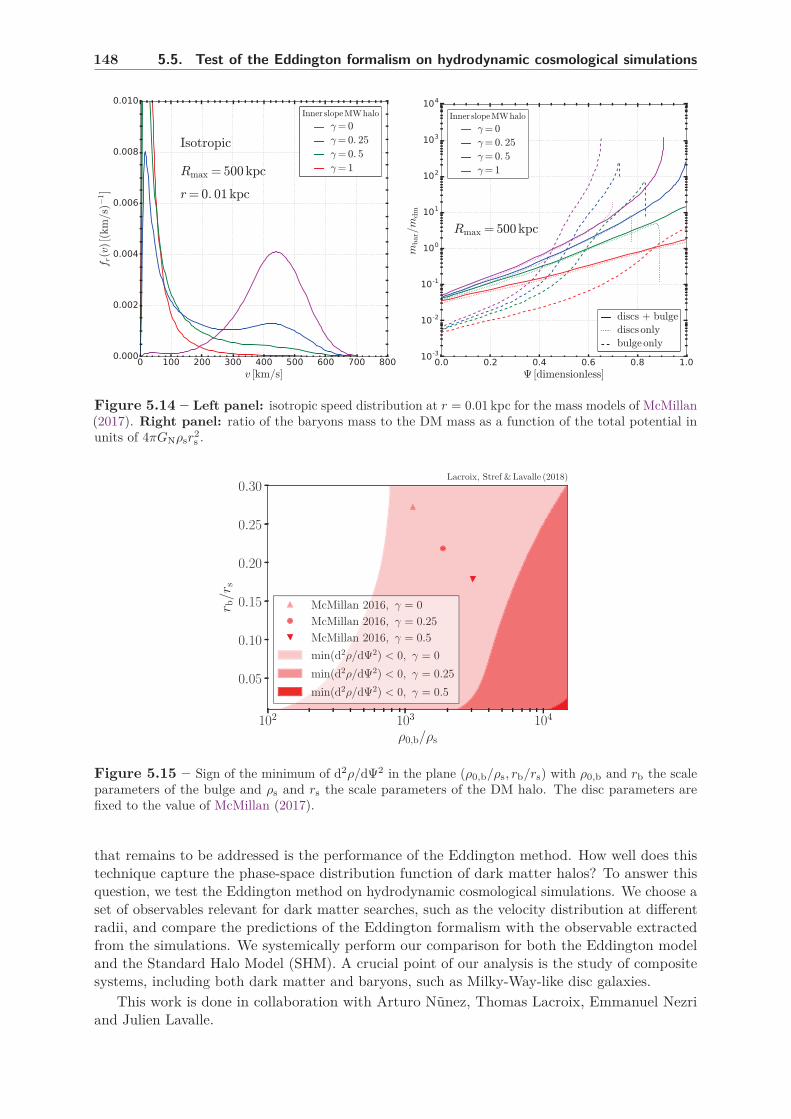
148 5.5. Test of the Eddington formalism on hydrodynamic cosmological simulations
Figure 5.14 – Left panel: isotropic speed distribution at r = 0.01 kpc for the mass models of McMillan(2017). Right panel: ratio of the baryons mass to the DM mass as a function of the total potential inunits of 4πGNρsr
2s .
102
103
104
ρ0,b/ρs
0.05
0.10
0.15
0.20
0.25
0.30
r b/r
s
Lacroix, Stref &Lavalle (2018)
McMillan 2016, γ = 0
McMillan 2016, γ = 0.25
McMillan 2016, γ = 0.5
min(d2ρ/dΨ2) < 0, γ = 0
min(d2ρ/dΨ2) < 0, γ = 0.25
min(d2ρ/dΨ2) < 0, γ = 0.5
Figure 5.15 – Sign of the minimum of d2ρ/dΨ2 in the plane (ρ0,b/ρs, rb/rs) with ρ0,b and rb the scaleparameters of the bulge and ρs and rs the scale parameters of the DM halo. The disc parameters arefixed to the value of McMillan (2017).
that remains to be addressed is the performance of the Eddington method. How well does thistechnique capture the phase-space distribution function of dark matter halos? To answer thisquestion, we test the Eddington method on hydrodynamic cosmological simulations. We choose aset of observables relevant for dark matter searches, such as the velocity distribution at differentradii, and compare the predictions of the Eddington formalism with the observable extractedfrom the simulations. We systemically perform our comparison for both the Eddington modeland the Standard Halo Model (SHM). A crucial point of our analysis is the study of compositesystems, including both dark matter and baryons, such as Milky-Way-like disc galaxies.
This work is done in collaboration with Arturo Nunez, Thomas Lacroix, Emmanuel Nezriand Julien Lavalle.

Chapter 5. The dark matter phase space of the Galaxy 149
5.5.1 Cosmological simulations
5.5.1.1 Description of the simulations
Two sets of simulations are used in this study. The first one consists of two high-resolutionsimulations published in Mollitor et al. (2015), which we labelled Halo B and Halo C. Thesesimulations were run with the RAMSES package (Teyssier, 2002) in 20 Mpc cosmological boxesand using the zoom-in technique with a carefully decomtaminated Lagrangian volume. Theinitial conditions were generated with the MUSIC package (Hahn & Abel, 2011). Conventionalrecipes were used for cooling, ultraviolet background and self-shielding. The gas dynamics, starformation scheme and supernovae (SN) feedback are all described in Mollitor et al. (2015). Thestar formation follows a standard Schmidt law with an adapted density threshold and efficiency(Schmidt, 1959; Kennicutt, 1998). The SN feedback is carried out through a thermal energyinjection after 10 Myr with a Chabrier initial mass function (Chabrier, 2003) with a thermalenergy of 1051 erg per SN event. A non-thermal energy injection is also implemented. We referto Mollitor et al. (2015) for a detailed analysis of these simulations. One of their main features isto exhibit both a compression of the dark matter profile around the scale radius of the disc anda flattening of the dark matter profile below due to the SN feedback.
The second set of simulations are also two cosmological hydrodynamic zoom-in simulationsperformed with the RAMSES package, with a slightly lower resolution. The stellar physics (starformation and SN feedback) is the same. The corresponding high-resolution runs are part of asuite of simulations that will be soon published in a forthcoming paper (Nunez et al., 2018) wherethe authors will consider different subgrid physics of star formation and SN feedback, whichis far beyond the scope of the present study. Those two simulations are labelled respectivelyMochima and Adicora after two Venezuelian beaches favoured by our colleague Arturo.
Regardless of their precise Milky-Way-like morphology and features, we will use thesesimulations as consistent frameworks with regard to gravity to study the phase-space distributionof dark matter and test the Eddington method in a numerical galaxy environment. For the fourobjects we consider (Halo B, Halo C, Mochima and Adicora), both dark-matter-only (DMO) andhydrodynamic runs including baryons are studied.
The mass resolution (mDM, m⋆) and spatial resolution (hsml), as well as the pseudo-virialmass and radius M200 and R200 and the total baryonic mass M⋆, are given in Tab. 5.1 for all theobjects under study.
Run M200 R200 M⋆ mDM m⋆ hsml(1010M⊙) (kpc) (1010M⊙) (M⊙) (M⊙) (pc)
Halo B DMO 49.60 163.5 2.757 × 10⁵
Hydro 50.06 177.54 7.96 2.308 × 10⁵ 2.87 × 10⁴ 151.67
Halo C DMO 62.48 176.36 2.757 × 10⁵
Hydro 55.02 182.23 9.56 2.308 × 10⁵ 2.87 × 10⁴ 151.67
Mochima DMO 91.35 206.34 2.27 × 10⁵
Hydro 82.14 213.2 10.87 1.536 × 10⁶ 1.836 × 10⁵ 281.1
Adicora DMO 91.67 202.46 2.27 × 10⁵
Hydro 81.07 212.7 11.07 1.536 × 10⁶ 1.836 × 10⁵ 281.1
Table 5.1 – Main features of the four simulations at z = 0. The columns are the pseudo-virialmass M200 and radius R200, the baryonic mass M⋆, the mass resolution for dark matter mDM,the mass resolution for baryons m⋆ and the spatial resolution (hsml).

150 5.5. Test of the Eddington formalism on hydrodynamic cosmological simulations
5.5.1.2 Halo shape and level of equilibrium
The Eddington method only applies to spherical systems in dynamical equilibrium. We do notexpect realistic simulated galactic halos to be perfectly spherical nor in perfect equilibrium,therefore we need to measure the departure from these two regimes.
A system of N particles with mass mk, k = 1...N at position þrk can be characterized by itsmass distribution tensor
Mij ≡∑
k
mk rki rkj , (5.161)
where rij ≡ þri ⊗ þrj . We denote the three square root of the eigenvalues of M by a, b and c witha > b > c. We then define the sphericity, the elongation and the triaxiality by
S ≡ c
a(5.162)
e ≡ b
a(5.163)
T ≡ a2 − b2
a2 − c2. (5.164)
A system with spherical symmetry has a = b = c, and therefore S = e = 1 and T is ill-defined.Otherwise a low triaxiality T ≪ 1 corresponds to an oblate system while a high triaxiality T ≃ 1corresponds to a prolate system [see e.g., Bryan et al. (2013)]. The sphericity and triaxialityof the dark matter halo in the hydrodynamical runs are shown as functions of the radius inFig. 5.16. Halos are close to spherical though slightly oblate.
In cosmological simulations, there is no definitive test to assess the level of virialization of ahalo. We use the criterion of Zjupa & Springel (2017) who define a virial ratio
q ≡ 2 Ekin
Epot+ 1 , (5.165)
such that q = 0 for an isolated structure in equilibrium according to the virial theorem. Thekinetic and potential energies are computed according to
Ekin =∑
i
1
2mi v2
i +∑
j
3
2kB Tj (5.166)
Epot =∑
i
∑
j
GN mi mj
|þri − þrj | fij , (5.167)
where the second term on the right-hand side of Eq. (5.166) accounts for the kinetic energy ofgas cells, and the fij factor in Eq. (5.167) accounts for the particular prescription used for theforce-softening on short distances (Shapiro et al., 2004). The virial ratio q in shown on the rightpanel in Fig. 5.16. The Mochima galaxy in the hydrodynamical run is the only one satisfyingthe virial criterion, though we have |q| < 0.2 in all the other cases.
5.5.2 Fitting the galactic components
The dark matter halos are fitted with a generalized NFW density profile
ρDM(r) = ρ0
(
r
rs
)−γ [
1 +
(
r
rs
)α](γ−β)/α
. (5.168)
A density can be assigned to each dark matter particle in the simulation through the proceduredescribed in Dehnen (2002). We refer to this density as the particle density ρpar. A densityvariance σ(ρpar) can also be computed. The density profile can then be fitted by minimizing
χ2ρ =
∑
bin i
(
log10 [ρDM(ri)] − log10 [ρshell(ri)]
σ [log10(ρpar(ri))]
)2
. (5.169)

Chapter 5. The dark matter phase space of the Galaxy 151
Figure 5.16 – Left panel: sphericity (upper panel) and triaxiality (lower panel) for the hydrodynamicsimulations used, as functions of the distance to the galaxy centre. Right panel: virial ratio as definedin Eq. (5.165) for the four simulations considered here.
In this equation, ρshell(ri) is the mean density within a spherical shell of radius ri. Theminimisation is performed on log10(ρ) rather than ρ to get a good fit over a wide range ofradius. An alternative fitting procedure makes use of the mass within a spherical shell ratherthan the mean density. In this case, the fit is obtained by minimizing
χ2m =
∑
bin i
(log10 [mDM(ri)] − log10 [mshell(ri)])2 . (5.170)
We show the density measured in Halo B along with the fits in Fig. 5.17. As one can see, bothfitting procedure lead to very similar results. From definiteness, we used the fits obtained withthe mass fitting procedure in Eq. (5.170). The high density variance above 20-30 kpc in Fig. 5.17is due to the presence of substructures, which start to significantly contribute to the mean darkmatter density (see Chap. 3). The fitting parameters obtained for Halo B are shown in Tab. 5.2.The main differences between the DMO and hydrodynamical runs are seen on parameters rs andγ. Adiabatic compression of the dark halo decreases the value of rs, and supernovae feedbackdecreases the value of γ from an NFW-like value of γ ≃ 1 to a smaller value γ ≪ 1. These twoeffects are also observed in the other halos. The dark matter parameters for the other halos areshown in App. D.3.
Halo B log10(ρ0) rs α β γ[M⊙/kpc3] [kpc]
DMO 7.101± 0.532 10.338± 6.592 1.0± 0 2.785± 0.258 1.101± 0.182
Hydro 7.622± 0.096 4.885± 0.514 2.639± 0.858 2.621± 0.117 0.127± 0.097
Table 5.2 – Parameters of the dark matter halo in Halo B.
The same fitting procedure is applied to baryons in the hydrodynamical runs. We fit thebaryon distribution using the same parametrisation as in McMillan (2017), see App. D.1. Foreach hydrodynamical run, we fit a bulge, a thin stellar disc, a thick stellar disc and one gas disc(for the gas disc, we use the same mass distribution as the stellar disc i.e. a double exponential).The mass profile and fitting parameters for the baryons in Halo B are shown in Fig. 5.18. Themass profiles for the other galaxies are shown in App. D.1.

152 5.5. Test of the Eddington formalism on hydrodynamic cosmological simulations
Figure 5.17 – Left panel: mean density in spherical shells (blue curve) with the associated 1σband (green) for the DMO run of Halo B. We show the fit obtained using the χ2 defined in Eq. (5.169)(black curve) and the χ2 in Eq. (5.170) (dashed red curve). Right panel: same as left panel, for thehydrodynamical run.
5.5.3 Radial boundary and escape speed
As we saw when we discussed the theoretical issues associated with the Eddington formalism,the definition of a finite radial boundary is essential to correctly account for the local value ofthe escape speed. While the radial extension of physical systems like the Milky Way is in generaldifficult to infer, we can extract this information for the simulated galaxies.
The radial boundary Rmax is define as the maximum of the (negative) gravitational potentialaveraged in spherical shells centred on the simulated galaxy. As the radius of the shells getslarger the potential increases to reach a maximum, then decreases again when entering the regionof influence of the nearest neighbouring galaxy. The maximum between the two potential wellsdefines Rmax. This procedure is illustrated in Fig. 5.19 for Halo B, where a radial border ofRmax ≃ 800 kpc is found.
Once the radial border Rmax has been measured, the gravitational potential is defined sothat is is zero at Rmax i.e.
Ψ(r) ≡ − (Φ(Rmax) − Φ(r)) , (5.171)
where Φ is the local potential which is computed within the simulation. The potential is positiveat radii r < Rmax with our definition, which is the convention we used when we discussed theEddington formalism in the two previous sections. As we have seen before, the escape speed at aradius r is defined by
vesc(r) ≡√
2Ψ(r) . (5.172)
An alternative measure of this speed can be obtained by looking at the maximum velocity ofparticles inside radial shells. We refer to this maximum speed as vmax. In a spherical system indynamical equilibrium, we should have vesc(r) = vmax(r) at all r. We compare vesc and vmax forHalo B on Fig. 5.20. The two method roughly agree although we have vesc > vmax in the inner

Chapter 5. The dark matter phase space of the Galaxy 153
Figure 5.18 – Mass profile and fitting parameters for the stellar discs and bulge (upper panel) and thegas disc (lower panel) for the Halo B galaxy.
Figure 5.19 – Left panel: gravitational potential averaged in spherical shells centred on Halo B (grayline). The maximum of the potential, which defines Rmax, is shown by the dashed vertical line. Wealso show the potential along the line of sight connecting the two potential wells (blue line) and the 1σdispersion around (dashed blue lines). Right panel: projected density in a cone around the line of sight.The center of the nearest ”big” neighbour is marked by a blue point.
region r < 10 kpc. Note however that the measure of vmax is limited by statistics in this region

154 5.5. Test of the Eddington formalism on hydrodynamic cosmological simulations
and therefore not reliable. Beyond the virial radius, we observe vesc < vmax. The comparison ofvesc and vmax for the other galaxies is shown in App. D.3.2, where similar features are observed.
Figure 5.20 – Escape speed computed from the potential (blue) compared to maximal velocityof particles in radial shells (green). The comparison is made in the DMO run (left panel) and thehydrodynamical run (right panel).
5.5.4 Velocity distributions
We now turn to the comparison between the Eddington formalism and the simulations. Thefitting procedure provides us with the dark matter density profile as well as the total gravitationalpotential for each galaxy in our sample. Thus we have all we need to compute the phase-spaceDF following the inversion procedure described in Sec. 5.3.2. From the phase-space DF, wecan compute the velocity distribution at any radius r. Here we only show results regarding theisotropic Eddington inversion, where the velocity distribution is simply related to phase-spaceDF through
fþv(þv) =1
ρDM(r)f
(
Ψ(r) − v2
2
)
. (5.173)
Our full analysis will include study of anisotropic cases. We also compare the velocity distributionmeasured in the simulations to the prediction of the SHM. In this model, it is assumed that thevelocity distribution follows the Maxwell-Boltzmann distribution
fmb(þv) ≡(
πv20
)−3/2exp
[
−v2
v20
]
, (5.174)
where the speed v0 is chosen to be the circular speed at radius r: vcirc(r). This model is notdynamically consistent since this distribution is not a solution of the collisionless Boltzmannequation consistent with the dark matter distribution under study. Indeed, the only densityprofile compatible with a Maxwell-Boltzmann velocity distribution is the singular isothermalsphere (see Sec. 5.3.2.1), which does not give a good description of galactic halos. In particular,the Maxwell-Boltzmann extends to arbitrary large velocities i.e. it does not account for a local

Chapter 5. The dark matter phase space of the Galaxy 155
escape speed. It can be truncated at the escape speed for a more realistic modelling, for ainstance with a smooth truncations
fsmooth(þv) ≡ 1
Nsmooth
exp
[
−v2
v20
]
− exp
[
−v2esc
v20
]
, (5.175)
with a normalisation factor
Nsmooth ≡(
πv20
)3/2[
erf(z) − 2 z√π
(
1 +2 z2
3
)
e−z2
]
, (5.176)
with z = v0/vesc.The velocity distributions in Eq. (5.173), Eq. (5.174) and Eq. (5.175) are compared to the
simulation data from Halo B in Fig. 5.21. We show the comparison for the DMO and thehydrodynamical runs. The escape velocity vesc computed from the gravitational potential isshown with its 1σ uncertainty band.
To make a quantitative comparison between the three models, we perform a χ2 test. Thevalue of χ2 is shown on the plots. Regardless of the radius and the model used, the value of χ2
is very high. This means that none of the models give a satisfactory description of the observedvelocity distribution. This is valid for all the objects we considered, see App. D.3.3. This ishardly a surprising fact however, given the crudity of the Maxwell-Boltzmann description or eventhe Eddington method, which assumes spherical symmetry, isotropy and perfect equilibrium.More interesting is the relative performance of the models. We note that the Eddingtonvelocity distribution performs better, in most cases, than the Maxwell-Boltzmann distribution inEq. (5.174). This is especially true at low radii, for 2 kpc < r < 4 kpc and 7 kpc < r < 9 kpc, andit is true for both the DMO and hydrodynamical runs. The reason for the lack of performance ofthe Maxwellian approximation is the difference in the peak velocity. Simulations show a peakvelocity higher than the circular velocity in the central regions. This is compatible with theobservation that simulated halos are in general isotropic at the center, see e.g., Bozorgnia et al.(2013). Since by construction, the Maxwell-Boltzmann distribution has its peak velocity at thecircular velocity, it fails at reproducing the simulations in their central region. This lack ofperformance is also observed for the truncated Maxwell-Boltzmann distribution in Eq. (5.175).However, this distribution performs just as well, if not better, than the Eddington distributionat most radii and in most of our simulated objects. We should recall that this distribution is adhoc and not motivated by first principles, unlike the Eddington formalism. The shape of thecut at vesc is in particular completely arbitrary, which is a limitation of this method since thepresence of this cut is precisely what improves the fit at large radii.
5.5.5 Moments of the velocity distributions
Although all the information is contained in the velocity distribution, dark matter searches areonly sensitive to some of its moments. For instance, direct detection is essentially sensitive to〈1/v〉. The exact moments relevant for dark matter searches will be listed and studied in thenext chapter. For now, we limit ourselves to the quantity 〈vn〉 (r). We directly compare itspredicted value from the distributions in Eq. (5.173), Eq. (5.174) and Eq. (5.175) to the samequantity measured in the simulation. The results for Halo B are shown in Fig. 5.22 while theresults for the other halos are shown in App. D.3.4. The Eddington prediction is compared to the(uncut) Maxwell-Boltzmann prediction. In agreement with the observations made on the velocitydistribution, we see that the Eddington prediction follows the general trend of the moments asfunctions of the radius much better the SHM. Quantitative comparisons and the inclusion of thesmoothly-cut Maxwell-Boltzmann distribution will be featured in the final work.
To conclude on these very preliminary results, we see that the Eddington formalism not onlyprovides a consistent framework to compute the phase-space DF of dark matter halos but also

156 5.5. Test of the Eddington formalism on hydrodynamic cosmological simulations
Figure 5.21 – Velocity distributions measured in Halo B, at 2 kpc < r < 4 kpc (upper left panel),7 kpc < r < 9 kpc (upper right panel), 19 kpc < r < 21 kpc (lower left panel), and 49 kpc < r < 51 kpc.We also show the distribution predicted by the Eddington method, the Maxwell-Boltzmann distributionand the smoothly-truncated Maxwell-Boltzmann distribution.
seems to roughly capture the main features observed in the simulations. In particular, it seemsto perform better than the Maxwell-Boltzmann approximation, which is widely used in darkmatter studies. When completed, our study will include direct comparison of the phase-spacedistributions from the Eddington method and the simulations, as well as the study of anisotropiccases. This will allow us to have a quantitative estimate of the astrophysical uncertainties indark matter studies based on Eddington-like methods, and a good idea of the global performanceof this framework in dark-matter-related searches.

Chapter 5. The dark matter phase space of the Galaxy 157
Figure 5.22 – Left panel: moments of the velocity distributions as functions of the radius (blue curves)in the DMO run of Halo B, compared to the moments of the Maxwell-Boltzmann velocity distribution(red curves) and the Eddington velocity distribution (black curves). Right panel: same as left panel, forthe hydro run of Halo B.


159
Chapter 6
Impact of the phase space on darkmatter searches
In this section, we study the impact of the Eddington inversion formalism on predictions forDM searches. The DM phase-space DF is an important quantity which enters a number ofdifferent searches for DM, such as direct searches, indirect searches for p-wave annihilating DMand Sommerfeld-enhanced annihilation, microlensing searches for compact objects and captureof DM by stars. We present general results relevant for all these approaches. We investigate theimpact of the regularization methods discussed in the previous chapter on some key observables.Finally, we apply the Eddington formalism to indirect searches for p-wave annihilating DMthrough cosmic-ray positrons.
6.1 Direct-searches-like observables
6.1.1 Direct searches
The impact of the velocity distribution on the direct detection event rate in Eq. (1.9) has beenextensively studied in the literature through numerical (Hansen et al., 2006; Fairbairn & Schwetz,2009; Vogelsberger et al., 2009; Kuhlen et al., 2010; Mao et al., 2013) and analytical calculations(Evans et al., 2000; Green, 2001, 2017b). The Eddington method, including its anisotropicextensions, has also been used to make predictions (Ullio & Kamionkowski, 2001; Vergados &Owen, 2003; Catena & Ullio, 2012; Pato et al., 2013; Bhattacharjee et al., 2013; Bozorgnia et al.,2013; Fornasa & Green, 2014; Lavalle & Magni, 2015). In particular, differences between thepredictions of the Eddington formalism and those of the Standard Halo Model (SHM) have beenshown to be important. In the SHM, the velocity distribution in the rest frame of the Galactichalo is assumed to follow the Maxwell-Boltzmann law
fmb(þv) =(
πv20
)−3/2exp
[
−v2
v20
]
. (6.1)
The peak velocity v0 is usually chosen to be the local circular velocity v0 = vcirc(R⊙). Thedistribution in Eq. (6.1) extends to arbitrary large velocities while in a collisionless system inequilibrium we do not expect particles to have a speed exceeding the local escape speed vesc(R⊙).The Maxwell-Boltzmann distribution is often truncated to account for vesc. A sharp cut issometimes implemented
fsharp(þv) =1
Nsharp
[
−v2
v20
]
Θ(vesc − v) , (6.2)
with a normalization
Nsharp =(
πv20
)3/2[
erf(z) − 2 z√π
e−z2]
, (6.3)

160 6.1. Direct-searches-like observables
and z = v0/vesc. A sharp truncation is obviously not physical hence a smooth cut is also foundin the literature
fsmooth(þv) =1
Nsmooth
exp
[
−v2
v20
]
− exp
[
−v2esc
v20
]
Θ(vesc − v) , (6.4)
with
Nsmooth =(
πv20
)3/2[
erf(z) − 2 z√π
(
1 +2 z2
3
)
e−z2
]
. (6.5)
Note that the Maxwell-Boltzmann velocity distribution gives a dynamically consistent descriptionof a collisionless system only if the density profile is that of the (infinite) singular isothermalsphere, see Sec. 5.3.2.1. This is not in agreement with observations hence the Maxwell-Boltzmannapproximation has little theoretical motivation. Nevertheless, it is often assumed to give areasonable description of the DM velocity distribution. Speed distributions with the differentconventions found in the literature are shown on the left panel in Fig. 6.1. These distributionsare computed at the position of the Sun. One sees small differences in the high velocity tail andin the height of the peak.
Figure 6.1 – At the position of the Sun R⊙ = 8.21 kpc in the NFW mass model of McMillan (2017).Left panel: Speed distribution in the SHM . Are shown the Maxwell-Boltzmann (red curve), sharply cut(green curve) and smoothly cut (blue curve) speed distributions. Right panel: Smoothly cut SHM speedDF compared to the Eddington theory for the isotropic (red), Osipkov-Merritt (green) and β0 = −0.3(blue) cases.
We want to compare the Eddington formalism to the SHM with a particular emphasis onthe regularization methods we discussed in the previous chapter. We first show the speeddistributions predicted by the isotropic (red), OM (green) and constant-β with β0 = −0.3 (blue)at R = R⊙ together with the smoothly-cut SHM on the right panel in Fig. 6.1. The phase-spacedivergence has been removed by hand and the speed distribution artificially renormalized toone. Significant differences between the SHM and the Eddington formalism are visible by eye.Irrespective of the model, the peak of the distribution is at v > vcirc rather than vcirc. The peakis also higher in the constant-β model. This is not surprising since β0 < 0 leads to more circularorbits hence a higher peak close to vcirc. Large differences also appear in the tail: the OM modelin particular presents a bump where the divergence was present. The isotropic prediction alsohas more power in the tail. These features have already been pointed out in the literature (see

Chapter 6. Impact of the phase space on dark matter searches 161
e.g.Ullio & Kamionkowski (2001); Vergados & Owen (2003); Fornasa & Green (2014)). Severalregularization methods are introduced in the previous chapter to deal with the phase-spacedivergence and these methods lead to different speed distributions for a given mass model. Wedefine a general function to investigate the impact of these regularizations on direct-searches-likeobservables:
Ξn(vmin, vmax, r) ≡ ω−1(r)
∫
vmin6v6vmax
d3þv vn fþv(þv, r)
ω(r) ≡∫
vmin6v6vmax
d3þv fþv(þv, r) .(6.6)
This function Ξ allows to investigate moments of the velocity distribution relevant for differentDM searches including direct searches and capture by stars (n = −1) and microlensing (n = 1). Anormalization ω is explicitly introduced to get a well-defined average even when the Eddington DFis modified by hand and thus not consistently normalized. We compute the velocity distributionand its moments in the rest frame of the halo and neglect the effects induced by the Galileantransformation to the rest frame of the Earth. This is justified because we essentially try toquantify the differences between the Eddington approach and the SHM, and we do not expectthese differences to depend much on the frame of reference. For direct searches, the relevantmoment is η given in Eq. (1.14). Ignoring the change of frame, this is
η(vmin) ≃ Ξ−1(vmin, vesc, R⊙) . (6.7)
We show η as a function of vmin in Fig. 6.2. The isotropic prediction is shown in the left paneland the Osipkov-Merritt one is shown in the right panel. The lower panel show the relativedifference between the Eddington prediction and the SHM. The largest differences are observed athigh values of vmin, when the contribution of the tail of the speed distribution is most important.This is also where the different regularization methods give the most different results. Neitherthe sharply-cut nor smoothly-cut SHM are in good agreement with Eddington, though thesmoothly-cut SHM is doing significantly better. Comparison with the OM model is shown inthe right panel. The differences there are much larger than in the isotropic case. This is notsurprising given we have not found any satisfactory way of regularizing the divergence in theOM models, see Sec. 5.4.1. Either the divergence is not removed or the DM density profile issignificantly modified.
In conclusion, the prediction of the Eddington theory departs from the SHM in a significantway. The choice of the regularization method is also important, particularly at high vmin. Thiscould have implication for direct searches of low mass WIMPs, since these DM candidatestypically need a large velocity to give a detectable recoil and are therefore sensitive to the highvelocity tail of the speed distribution.
6.1.2 Capture by compact objects, microlensing
The function Ξ is related to observables relevant for other types DM searches. In particular, thequantity
η(vmax, r) = Ξ−1(0, vmax, r) (6.8)
appears when computing the number of DM particles captured by stars or planets. This isimportant since dark matter particles can have an effect on stellar evolution or annihilate at thecore into detectable particles like neutrinos (Press & Spergel, 1985; Silk et al., 1985; Gould, 1987;Salati & Silk, 1989; Bouquet & Salati, 1989b,a; Kouvaris, 2008; Bertone & Fairbairn, 2008; Scottet al., 2009). The varying value of vmax accounts for the escape speed from the particular objectunder consideration (star, planet, etc..). The quantity η at the position of the Sun is shown inFig. 6.3. Again, differences are observable between Eddington’s theory and the SHM. For the

162 6.1. Direct-searches-like observables
Figure 6.2 – Left panel: η integral as a function of vmin. The various curves shown are the sharply-cutSHM (solid magenta), the smoothly-cut SHM (dashed magenta), and the predictions of the Eddingtonformalism for an isotropic system, with the regularizations of the phase-space divergence discussed inSec. 5.4.1, namely setting Rmax to infinity (green), removing the diverging term (red), modifying thedensity profile (blue), regularizing a la King with Ec = Ψ(Rmax) (yellow) or with Ψ(Rmax) = 0 (cyan).Right panel: Same as left panel, for Osipkov-Merritt.
isotropic case (left panel), the regularization method has little impact on the final prediction.This is because most of the difference resides in the tail of the speed distribution while η is onlysensitive to speeds below vmax. Differences between the methods are still important in the OMmodels (right panel).
Figure 6.3 – Same as Fig. 6.2 for η = Ξ−1(0, vmax, R⊙).
Finally, for the sake of completeness we look the mean speed
〈v〉 (r) ≡ Ξ1(0, vesc, r) , (6.9)
which is important for computing expected microlensing event rates (Griest, 1991; Green, 2017a).

Chapter 6. Impact of the phase space on dark matter searches 163
Microlensing is an interesting probe if DM is made of compact objects. It is relevant for primordialblack holes DM (Garcıa-Bellido & Clesse, 2018) and axion DM if it forms miniclusters (Fairbairnet al., 2018). The mean speed is shown as a function of the radius in Fig. 6.4 in the isotropic(top left panel), Osipkov-Merritt (top right panel) and β0 = −0.3 model (bottom panel). Again,we observe important difference between the Eddington technique and the SHM. While the twomethods agree in the outer parts, there prediction significantly differ at the center of the Galaxy,by up to an order of magnitude.
Figure 6.4 – Mean speed profiles for the Standard Halo Model and the Eddington formalism for theisotropic (top left panel), Osipkov-Merritt (top right panel) and β0 = −0.3 (bottom panel) cases. Here weshow the DM-only (thin line) and DM+baryons (thick line) cases, for the McMillan (2017) mass modelsproviding well-behaved Eddington-inverted DFs.

164 6.2. Indirect-searches-like observables
6.2 Indirect-searches-like observables
In this section, we investigate the impact on indirect searches for annihilating DM. The Eddingtonmethod has been used in a few studies to constrain p-wave annihilating DM, see Ferrer & Hunter(2013); Boddy et al. (2017); Petac et al. (2018). Relevant for annihilation is the relative velocitydistribution rather than the speed distribution, therefore we introduce a new function
〈vnr 〉 ≡ κ−1(r)
∫
d3þv1
∫
d3þv2 |þvr|n fþv(þv1, r) fþv(þv2, r)
κ(r) ≡∫
d3þv1
∫
d3þv2 fþv(þv1, r) fþv(þv2, r) ,(6.10)
where þvr = vþv2 − þv1 is the relative velocity. Searches for p-wave annihilating DM typicallyprobe the n = 2 moment i.e. the relative velocity dispersion. In some cases, the annihilationcross-section can be strongly impacted by non-perturbative effects that lead to the so-calledSommerfeld enhancement (Sommerfeld, 1931; Hisano et al., 2003, 2004, 2005; Profumo, 2005;Cirelli et al., 2007; March-Russell et al., 2008; Arkani-Hamed et al., 2009; Pospelov & Ritz, 2009;Lattanzi & Silk, 2009). In that particular case, the relevant moment is n = −1, or n = −2 nearthe resonance features appearing in the cross-section. It is more convenient for computations toperform a change of variables (þv1, þv2) → (þvc, þvr) in Eq. (6.10) with
þvc = (þv1 + þv2)/2þvr = þv2 − þv1
⇐⇒
þv1 = þvc − þvr/2þv2 = þvc + þvr/2
(6.11)
as it is usually done when computing the DM annihilation rate in the early Universe (Gondolo &Gelmini, 1991). Details on the computation are given in App. E. The computation of the momentsin the general anisotropic case is an original result. We show the moments n = −2, −1, 1, 2 inFig. 6.5 for the isotropic case, in Fig. 6.6 for the Osipkov-Merritt models and Fig. 6.7 for theconstant-β model. Following our discussion regarding the stability of the DFs in the previouschapter, we only consider here mass models leading to stable solutions of the Boltzmann equation.The velocity distribution in the Eddington case have been computed without the diverging term.We recall that this is in practice similar to assuming a flattened density profile at the outskirts ofthe halo. One see in Fig. 6.5 that, for both the SHM and the Eddington model, the moments withand without baryons converge at large radii. This is because the total mass, and therefore thegravitational dynamics, is then fully dominated by dark matter, and baryons become irrelevant.Though similar in shape, predictions from the two models are numerically quite different. For then > 0 moments, the Eddington model’s predictions typically exceed the SHM’s. At the centerof the Galaxy, the two models differ by at least an order of magnitude, up to three orders ofmagnitude. The hierarchy of the moments with respect to the value of the dark matter innerslope is also reverted. While the cuspiest mass model (γ = 1) leads to the largest predictionfor the SHM, it is the model the closest to the core (γ = 0.25) that dominates the Eddingtonresult. We stress that even locally at r = R⊙ ∼ 8 kpc, and for all n, there are sizeable differencesbetween the Eddington formalism and the Maxwell-Boltzmann approximation. Therefore, sincethe Eddington formalism turns out to better capture the dynamical properties of the dark matterhalo than the SHM, the latter should only be used to make very rough estimates of p-waveannihilating dark matter signals, even when isotropy is assumed.
We also compared the (isotropic) SHM with some of the anisotropic extensions of theEddington formalism. The prediction of the Osipkov-Merritt model is shown in Fig. 6.6 for aparticular choice of the anisotropy radius ra = rs. Note that the value of rs depends on theunderlying mass model. The result is close to the isotropic case at radii r ≪ ra, as expected fromthe behaviour of the anisotropy parameter. At large radii however, the slope of the momentssteepens significantly. The steepening starts roughly where r ≃ ra which is where the systembegins to be strongly anisotropic. We stress again that the regularization of the diverging term

Chapter 6. Impact of the phase space on dark matter searches 165
changes considerably the underlying profile density profile in the Osipkov-Merritt case (see theprevious chapter). The behaviour of 〈vn
r 〉 beyond r = ra should therefore be treated with caution.We also studied the constant-β case, focusing on β0 = −0.3. We considered a negative anisotropyto get a well-defined DF for all the mass models of relevance here. The corresponding relativespeed moments are shown in Fig. 6.7. They differ from the isotropic ones at all radii, unlikethe Osipkov-Merritt ones, which is not surprising since the constant anisotropy is non-zeroeverywhere.
Regardless of the assumption made on the anisotropy, the Eddington formalism genericallypredicts huge differences with respect to the SHM. The various anisotropic models used allow usto bracket the theoretical uncertainty on the Eddington method.
Figure 6.5 – Moments of the relative velocity distribution, for the Standard Halo Model and theEddington formalism (isotropic case). Here we show the DM-only (thin line) and DM+baryons (thickline) cases, for several mass models from McMillan (2017).

166 6.3. New bounds on p-wave annihilating dark matter
Figure 6.6 – Same as Fig. 6.5, for the Osipkov-Merritt model with ra = rs.
6.3 New bounds on p-wave annihilating dark matter
We turn to a direct application of the Eddington formalism: the constraint of p-wave annihilatingdark matter using cosmic-ray positrons. This work is an extension of the study done by Boudaudet al. (2017) (hereafter B16). We first review the analysis and results of B16, then use the sameidea to derive new bounds on p-annihilating dark matter. This work was done in collaborationwith Mathieu Boudaud, Thomas Lacroix, Julien Lavalle and Pierre Salati.
The authors of B16 derived new constraints on the s-wave annihilation cross-section fordark matter masses in the MeV to TeV range. They studied the contribution of dark matterannihilation, as well as decay, into electrons and positrons and use measurements of the cosmic-rayfluxes of these species to derive new limits. These limits are especially important in the MeVmass range. WIMPs with MeV masses are not light enough to differ significantly from CDMon observable scales, however a variety of scenarios involve dark matter particles in this rangeand provide potential solutions to the small-scale issues (we refer to Sec. 1.4 for a discussion

Chapter 6. Impact of the phase space on dark matter searches 167
Figure 6.7 – Same as Fig. 6.5, for the constant-β model with β0 = −0.3.
on these small-scale problems). For instance, self-interacting dark matter (Chu et al., 2016)and strongly-interacting dark matter (Hochberg et al., 2014) can both be produced thermally ifthe dark matter particle has a mass in the MeV range. Alternatively, if dark matter is coupledto radiation long enough, an oscillatory pattern appears in the power spectrum which canhelp resolve the small-scale tensions (Boehm et al., 2004, 2014). MeV dark matter is alreadyconstrained by a number of observables, including indirect searches with gamma rays (Beacomet al., 2005; Essig et al., 2013). The most stringent bounds currently available are coming fromthe CMB which is very sensitive to energy injection by annihilation or decay at the time ofrecombination (Chen & Kamionkowski, 2004; Slatyer, 2016a; Liu et al., 2016; Poulin et al., 2016).
Dark matter annihilation in the MeV mass range is difficult to probe with cosmic radiationbecause sub-GeV cosmic rays are affected by Solar modulation (see Sec. 4.3). The Solar magneticfield forbid charged particles with sub-GeV energies to reach the Earth. This Solar shieldingextends up to a region called the heliopause. Fortunately, the Voyager 1 spacecraft (Krimigiset al., 1977) crossed the heliopause during the summer of 2012 (Stone et al., 2013). The spacecraft

168 6.3. New bounds on p-wave annihilating dark matter
carries a ”golden record”, destined to advanced extra-terrestrial civilizations, containing amongother things music from such luminaries as Johann Sebastian Bach and Chuck Berry. Of moredirect interest to us is the presence on-board of a cosmic-ray detector sensitive to electrons andpositrons (without discrimination between the two). High-statistics measurements of the e+ + e−
flux unaffected by Solar modulation is therefore available in Stone et al. (2013); Cummings et al.(2016).
6.3.1 Bounds on s-wave annihilation
The authors of B16 used two propagation models for e±. The first model, dubbed A in theiranalysis, is the MAX model whose propagation parameters are shown in Tab. 4.1. The secondmodel, dubbed B, is the model of Kappl et al. (2015) (K15), whose parameters are also shown inTab. 4.1. Both propagation models have comparable values for all parameters except the Alfvenspeed Va. This speed controls the efficiency of reacceleration processes in the magnetic halo.Cosmic rays injected at a given energy E and subject to a strong reacceleration can be detectedat energies E′ > E. In this case, model A has an efficient reacceleration (Va = 117.6 km/s) whilereacceleration in model B is much less efficient (Va = 31.9 km/s). This has strong consequenceson the e± flux, as shown in the right panel in Fig. 6.8. For a dark matter particle with massm = 10 MeV annihilating into e+e−, the e+ + e− flux is shown for model A (green) and model B(blue). While the flux in the B model sharply falls at E = 10 MeV, it extends up to more than 1GeV in the A model. This also implies that at a given mass, the A propagation model is moresensitive to the data points of AMS than the B model.
Solving the propagation equation for electrons and positrons is technically very involvedbecause energy losses and reacceleration are not confined to the disc, as is the case for nuclei,but extend to the whole diffusive halo. A semi-analytic framework to consistently solve thepropagation equation was successfully built by Boudaud et al. (2017). This ”pinching” methodwas used in B16 and is also used in our new p-wave analysis.
The bounds on the s-wave annihilation cross-sections obtained by B16 are shown in the rightpanel on Fig. 6.8, for different annihilation channels. The most stringent bound is obtained,unsurprisingly, for dark matter annihilating directly to electrons and positrons. These bounds areconservative: the B propagation model, with low reacceleration, is used and the Fisk potentialaccounting for solar modulation is fixed to φF = 0.83 GV (which the maximum value foundin Ghelfi et al. (2016)). We note the presence of a ”gap” in the exclusion curve i.e. the curveincreases then sharply decreases again. This is due to the energy range 0.4 MeV to 2 GeV leftunexplored by both Voyager 1 and AMS. These bounds are about an order of magnitude lessstringent than those found with the CMB (Liu et al., 2016) and slightly better than those inferredfrom gamma rays (Essig et al., 2013).
6.3.2 Bounds on p-wave annihilation
We now turn to the computation of the p-wave bounds. The best p-wave bounds currentlyavailable at low masses are coming from the CMB (Liu et al., 2016). A rough order-of-magnitudeestimate tells us that our bounds should be much better than the CMB’s. The CMB bounds arederived assuming a velocity dispersion σv = 100 km/s for WIMPs at the time of recombination.In the Solar neighbourhood, the WIMP velocity dispersion should be comparable to the localcircular velocity σMW
v /√
2 ∼ vc(R⊙) ≃ 240 km/s. To obtain the ”CMB-like” p-wave bound fromthe s-wave bound shown in Fig. 6.8, one can rescale the curves by a factor (σv/σCMB
v )2 0.1. Thisleads to an exclusion curve which is about five orders of magnitude better than the CMB’s. Thismotivates us to investigate the p-wave calculation in a more detailed fashion.
Let us write the annihilation cross-section as
〈σannv〉 = 〈σannv〉0 + σ1c
⟨
v2r
⟩
c2+ ... (6.12)

Chapter 6. Impact of the phase space on dark matter searches 169
Figure 6.8 – Left panel: predictions (e±) for two template cases: a 10 MeV WIMP annihilatinginto e+e− (plus final-state radiation), and a 10 GeV WIMP annihilating into bb. We show the e+ + e−
data from Voyager (red trianges) and the 2e+ data from AMS-2 (black squares). The AMS-2 e+ data ismultiplied by two to compare with the e+ + e− data from Voyager. The AMS-2 data are demodulatedwith a Fisk potential φF = 0.83 GV. Propagation models A and B, and the NFW and cored profiles wereused. Right panel: limits from different annihilation channels, assuming model B, an NFW profile andφF = 0.83. Both plots are taken from Boudaud et al. (2017).
where 〈σannv〉0 is the s-wave contribution, σ1c is the amplitude of the p-wave contribution and⟨
v2r
⟩
is the relative velocity dispersion. Here we assume 〈σannv〉0 = 0 and put constraints on σ1c.All higher-order terms are neglected.
The electron/positron flux can be written in the Green’s function formalism
dφ
dΩ dE=
σ1c
2 m2
∫
dEs
∫
d3þxs Ge(Es, þxs → E, þx)dNe
dE(Es) ρ(þxs)
⟨
v2r
⟩
c2. (6.13)
The injection spectrum dNe/dE is generated with the MicrOMEGAs code (Belanger et al.,2015). The function Ge is a Green’s function of the propagation equation Eq. (4.43). It isconvenient to define an effective annihilation profile
ρ2eff(r) ≡ ρ2(r)
⟨
v2r
⟩
c2, (6.14)
which contains all the relevant information on the dark matter phase-space distribution. Wecompute the relative velocity dispersion using the Eddington formalism. We considered threecases: the isotropic DF, the Osipkov-Merritt model, and the constant anisotropy model withβ0 = −0.3. We also compare with the prediction of the Standard Halo model given in Eq. (??).Two dark matter profiles are considered: the γ = 1 and γ = 0.25 profiles of McMillan (2017). Wedo not consider the cored profile (γ = 0) because the Eddington method leads to an unstable DFin that case (see Sec. 5.4). The effective annihilation profiles are shown in Fig. 6.9. As we havealready seen in the previous section, the prediction of the Eddington model and its extensionslead to a larger velocity dispersion than the SHM over a wide range of radii.
We show the resulting bounds in Fig. 6.10. Our bounds are derived for the same propagationmodels A and B as B16. The left panel shows the bounds assuming an NFW dark matter profileand the right panel shows the bounds for γ = 0.25. We note that the central slope of the darkmatter profile has very impact on the bound obtained with B propagation model, while the Amodel is more sensitive to the shape of the dark halo. This difference in sensitivity is due to

170 6.3. New bounds on p-wave annihilating dark matter
reacceleration: in model A, electrons and positrons being injected near the center of the halo aresubject to efficient enough reacceleration to reach the Earth. In model B, however, e+ and e−
have a more local origin. The uncertainty due to our lack of knowledge of the anisotropy in thedark halo is represented with a coloured band around each exclusion curve. This uncertainty isestimated thanks to our three models for anisotropy (isotropic, Osipkov-Merrit, constant-β). It isfound to be very small regardless of the propagation model or the shape of the dark matter halo.The uncertainty associated with propagations, however, is very important especially at low massand in the ”gap” corresponding to the unexplored energy range. We compare our bounds tothose obtained from the CMB by Liu et al. (2016) and the bound from dwarf spheroidal galaxiescomputed by Zhao et al. (2016).
104
105
106
107
108
109
1010
1011
1012
1013
1014
ρ2 eff(r)[(M
⊙kp
c−3)2]
Boudaud et al. (2018)
Isotropic
Osipkov-Merritt
βanis = −0.3
Standard halo model
γ = 0.25
γ = 1
γ = 0.25
γ = 1
10−2 10−1 100 101
r [kpc]
10−1
100101102103
ρ2 eff/ρ
2 eff,SHM
Figure 6.9 – Effective annihilation profiles as defined in Eq. (6.14). We show the prediction ofEddington’s method in the isotropic case (solid line), the Osipkov-Merrit model (dotted-dashed), theconstant-β model with β0 = −0.3 (dashed) and SHM (dotted). Effective profiles are shown for the γ = 1(red) and γ = 0.25 (blue) mass models.

Chapter 6. Impact of the phase space on dark matter searches 171
10−3 0.01 0.1 1 10 100 103
Dark matter mass mχ [GeV]
10−23
10−22
10−21
10−20
10−19
10−18
10−17
10−16
10−15
10−14
σ1c[cm
3s−
1]
CMB
dSphs
CRs e
− /e+
NFW
SMod insensitive SMod sensitive
Boudaud et al. (2018)
Propagation APropagation BPropagation APropagation B
10−3 0.01 0.1 1 10 100 103
Dark matter mass mχ [GeV]
10−23
10−22
10−21
10−20
10−19
10−18
10−17
10−16
10−15
10−14
σ1c[cm
3s−
1]
CMB
dSphs
CRs e
− /e+
γ = 0.25
SMod insensitive SMod sensitive
Boudaud et al. (2018)
Propagation APropagation BPropagation APropagation B
Figure 6.10 – Left panel: p-wave exclusion curves for the propagation model A (green) and B (blue).We highlight the region unaffected by Solar modulation, corresponding to the data points from Voyager 1.The dark matter halo is the NFW profile of McMillan (2017). Right panel: same as the left panel forthe γ = 0.25 mass model.


173
Conclusion
In this work, we have focused on several aspects of particle dark matter on the Galacticscale. Several general guidelines were followed. We focused on building models and developingtools which allow to capture the structuring of dark matter while remaining consistent withobservational constraints. This is of importance since Galactic dynamics is now entering an eraof very high precision with the recent data release from the Gaıa satellite. A precise evaluationof the astrophysical uncertainties affecting dark matter searches was one of our main objective.Another was to develop techniques applicable to a wide range of dark matter models.
Our main achievement is the construction of the first model of Galactic subhalos consistentwith dynamical constraints. We recall the main ingredients of this model. First, we start from adynamically constrained mass model of the Galaxy (or any other galaxy, since our model is notspecific to the Milky Way). We assume subhalos are spatially distributed along the constraineddark matter density profile. The mass and concentration distributions of subhalos are thoseof field halos, which can be safely extracted from N-body simulations or derived from analyticcomputations (following the Press-Schechter theory for the mass function and the Bullock etal. model for the concentration, for instance). We then account for the interactions betweensubhalos and the host galaxy by computing a tidal for each subhalo. This computation is donein performed using the mass distributions given by the mass model i.e. it is also consistentwith observational constraints. We take into account the effect of the tidal stripping by thegravitational potential of the galaxy, as well as the effect of shocking induced by the stellar disc.For this last effect, we propose our own simple definition of the tidal radius and shown thattidal shocking is very efficient at stripping subhalos from their mass, a result in agreement withsimulations. From this computations, we built a distribution function describing the Galacticsubhalo population. The post-tides mass and concentration distributions, as well as the subhalonumber and mass densities are evaluated. We show that all these quantities strongly depart fromtheir initial, cosmological value.
Our model of subhalos can be applied to a number of dark-matter-related studies. Perhapsthe most obvious application is indirect searches, where subhalos have been known to play animportant role. The systematic enhancement of the annihilation signal, the ”boost”, is estimatedthanks to our model. Theoretical uncertainties associated to the small-scale power spectrum, thedark matter free-streaming scale and the disruption of subhalos by tidal effects are estimated. Wefirst apply our model to gamma-ray searches and show that the boost can very easily be of morethan 100%, which we should dramatically improve exclusion bounds set with the diffuse gammaray background. We investigated another complementary channel with cosmic-ray antiprotons.There again, the boost is shown to be significant. Using several propagation models, we computeexclusion bounds by exploiting the latest data from AMS-2. This shows in particular howimportant it is to incorporate subhalos when trying to interpret an excess in terms of dark matterannihilation.
A complementary work was done on the Eddington inversion method, a tool devised toinfer the phase-space distribution function of collisionless system starting from its density andgravitational potential. This method is of great interest for dark matter searches because itallows to make prediction which are both theoretically consistent (we are using solutions of thecollisionless Boltzmann equation) and in agreement with the observed dynamics (which gives the

174 6.3. New bounds on p-wave annihilating dark matter
density profile and potential). While the appealing character of this method was already pointedbefore, its limitations have been overlooked when applied to dark matter searches. A seriousproblem appears when this technique is applied to finite systems. In this case, the Eddingtonsolution present an unphysical divergence, which must be removed to get acceptable results. Wepropose a number of possible solutions to this issue. Another problem is related to the stability ofEddington’s solution. We show that stability considerations restrict the domain of applicability ofEddington’s method and that some realistic halo configurations actually outside of this domain.
We investigate in a rather general way the impact of these considerations on observablesrelevant for direct and indirect searches. We show that these theoretical issues are of importanceif one wants to make reliable prediction using Eddington’s theory. To illustrate the potentialof this method for dark matter searches, we use cosmic-ray electrons and positrons measuredby Voyager 1 to get new stringent bounds on p-wave annihilating dark matter. The use ofEddington’s method allows to bracket the uncertainties due to our lack of knowledge of thevelocity anisotropy in the dark halo.
A number of projects related to these topics are currently being worked out. We are currentlyworking on the application of our subhalo model to gamma-ray searches with the aim of derivingstringent bounds using the data from Fermi and making prospects for CTA. I am also workingtogether with J. Silk and T. Nakama on deriving new constraints on ultracompact minihalos, anatural extension of CDM subhalos. The clustering of CDM is also relevant for primordial blackholes and axion miniclusters. The impact of clustering on microlensing constraints on the fractionof these objects in the halo is currently largely unexplored. We are currently investigating thisproblem with Sebastien Clesse. Finally, I would like to mention projects related to Galacticdynamics. I am working together with Raphael Errani and Thomas Lacroix on the use of theEddington method to model the effect of tides on subhalos. We are also investigating potentialsignatures of the collective effect of a large population of subhalos on stellar objects such asbinaries and stellar streams.

175
Appendices


177
Appendix A
Mathematical functions andidentities
A.1 Error function
The error function is defined as
erf(x) ≡ 2√π
∫ x
0e−t2
dt . (A.1)
It is normalized so that
erf(x) →x→∞
1 . (A.2)
Also useful is the complementary error function
erfc(x) ≡ 1 − erf(x)
=2√π
∫ ∞
xe−t2
dt .(A.3)
A.2 Gamma and beta functions
The gamma function is defined for all complex numbers except non-positive integers as
Γ(x) ≡∫ ∞
0tx−1e−tdt . (A.4)
It has the following remarkable property
Γ(x + 1) = x Γ(x) , (A.5)
which immediatly leads
Γ(n) = (n − 1)! if n > 1 is an integer . (A.6)
It has the following particular values
Γ
(
1
2
)
=√
π
Γ
(
3
2
)
=
√π
2
Γ
(
5
2
)
=3√
π
4.

178 A.3. Riemann zeta function
A closely-related function is the beta function
B(x, y) ≡∫ 1
0tx−1(1 − t)y−1 dt , (A.7)
which is related to Γ through
B(x, y) =Γ(x)Γ(y)
Γ(x + y). (A.8)
A.3 Riemann zeta function
The Riemann zeta function is defined for all complex number s with Re(s) < 1 as the analyticcontinuation of the series
ζ(s) ≡∞
∑
n=1
1
ns. (A.9)
It is related to the gamma function through the identity
ζ(x) Γ(x) =
∫ ∞
0
tx−1
et − 1dt . (A.10)
It has the particular values
ζ(−1) = − 1
12
ζ(0) = −1
2
ζ(2) =π2
6
ζ(4) =π4
90
The motivated reader can try to prove that all the non-trivial zeros s of ζ have Re(s) = 1/2.
A.4 Bessel functions
A.4.1 Bessel function of the first kind
The Bessel function of the first kind Jα is defined as the solution of the ordinary differentialequation
x2 d2Jα
dx2+ x
dJα
dx+ (x2 − α2) Jα = 0 . (A.11)
The solution has the expression
Jα(x) =∞
∑
n=0
(−1)n
n! Γ(n + α + 1)
(
x
2
)2n+α
. (A.12)
If α is an integer, it has an integral representation
Jα(x) =1
π
∫ π
0cos(απ − x sin(τ)) dτ . (A.13)

Appendix A. Mathematical functions and identities 179
A.4.2 Modified Bessel functions of the second kind
The modified Bessel function of the second kind Kα is defined as the decaying solution of thedifferential equation
x2 d2y
dx2+ x
dy
dx− (x2 + α2)y = 0 . (A.14)
If α > −1/2, this solution can be expressed as an integral
Kα(x) =
√π
Γ(α + 1/2)
(
x
2
)α ∫ ∞
1e−tx(t2 − 1)α−1/2dt . (A.15)
The following recurrence relation is useful
Cα−1(x) − Cα+1(x) =2α
xCα(x) , (A.16)
where Cα ≡ eiαπKα.
A.5 Fourier transform
The Fourier transform of a function f is defined as
f(þk) ≡∫
f(þx) e−iþx.þk dnþx , (A.17)
where n is the number of space dimensions. The function f can be expressed with the inverseFourier transform
f(þx) ≡∫
f(þk) eiþx.þk dnþk
(2π)n. (A.18)
In physics, the Fourier transform is often used to go from real space to momentum space. If þr isa position vector and þp a momentum vector, we have in n dimensions
f(þp) ≡∫
f(þr) e−iþr.þp/~ dnþr , (A.19)
and
f(þr) ≡∫
f(þp) eiþr.þp/~ dnþp
(2π~)n. (A.20)
These definitions are used to define the Dirac delta distribution on momentum space.
(2π~)nδ(n)(þp) ≡∫
e−iþr.þp/~ dnþr . (A.21)


181
Appendix B
The WIMP template
B.1 Thermodynamics
The number of effective degrees of freedom in energy is given by
geff(T ) = g15
π4
∫ ∞
0
u2
e√
u2+x2 + ǫ
√
u2 + x2 du . (B.1)
We introduce y2 ≡ u2 + x2 and y > 0 such that
geff(T ) = g15
π4
∫ ∞
x
√
y2 − x2 y2
ey + ǫdy (B.2)
= g15
π4
∫ ∞
xe−y
√
y2 − x2 y2
1 + ǫ e−ydy . (B.3)
We expand the denominator into a power series
geff(T ) = g15
π4
∞∑
n=1
(−ǫ)n+1∫ ∞
x
√
y2 − x2 y2 e−ny dy , (B.4)
and separate the integral into
geff(T ) = g15
π4
∞∑
n=1
(−ǫ)n+1∫ ∞
x
(
y2 − x2)3/2
y2 e−ny dy + x2∫ ∞
x
√
y2 − x2 y2 e−ny dy
. (B.5)
Using Eq. (A.15), we get
geff(T ) = g15
π4
∞∑
n=1
(−ǫ)n+1
3 x2
n2K2(nx) +
x3
nK1(nx)
. (B.6)
Finally, we use the recursion relation (A.16) to get
geff(T ) = g15
π4
∞∑
n=1
(−ǫ)n+1
(
6 x
n3+
x3
n
)
K1(nx) +3 x2
n2K0(nx)
. (B.7)
A similar calculation leads to the number of effective degrees of freedom in entropy
heff(T ) = g45
4π4
∞∑
n=1
(−ǫ)n+1
(
8x
n3+
x3
n
)
K1(nx) +4x2
n2K0(nx)
. (B.8)

182 B.2. Particle physics
B.2 Particle physics
B.2.1 Conventions and Diracology
We use the following conventions for our calcutions. The Minkowski metric has signature(+ − −−). The Dirac gamma matrices are written in the Dirac basis where they take the form
γ0 =
1 0 0 00 1 0 00 0 −1 00 0 0 −1
γ1 =
0 0 0 10 0 1 00 −1 0 0
−1 0 0 0
γ2 =
0 0 0 −i0 0 i 00 i 0 0
−i 0 0 0
γ1 =
0 0 1 00 0 0 −1
−1 0 0 00 1 0 0
(B.9)
These matrices are defined through there anticommutation relations
γµ, γν = 2ηµνI4 . (B.10)
In particular, we(
γ0)2
= I4 and(
γi)2
= −I4 for i = 1, 2, 3. This immediately leads to
(γµ)† = γ0γµγ0.The fifth gamma matrix γ5 is defined as γ5 ≡ iγ0γ1γ2γ3, which leads to
γ5 =
0 0 1 00 0 0 11 0 0 00 1 0 0
(B.11)
It verifies(
γ5)2
= I4 , (B.12)
and
γ5, γµ
= 0 . (B.13)
We recall the expression of the Dirac spinors for particles
u(þp, ↑) =√
E + m
10p3
E+mp1+ip2
E+m
u(þp, ↓) =√
E + m
01
p1−ip2
E+m−p3
E+m
(B.14)
and for antiparticles
v(þp, ↑) =√
E + m
p1−ip2
E+m−p3
E+m
01
v(þp, ↓) =√
E + m
p3
E+mp1+ip2
E+m
10
(B.15)
where ↑↓ refers to the direction of the spin (up or down). These spinors are by definition solutionsof the Dirac equation
(/p + m I4)u(þp) = 0 (B.16)
(−/p + m I4)v(þp) = 0 , (B.17)
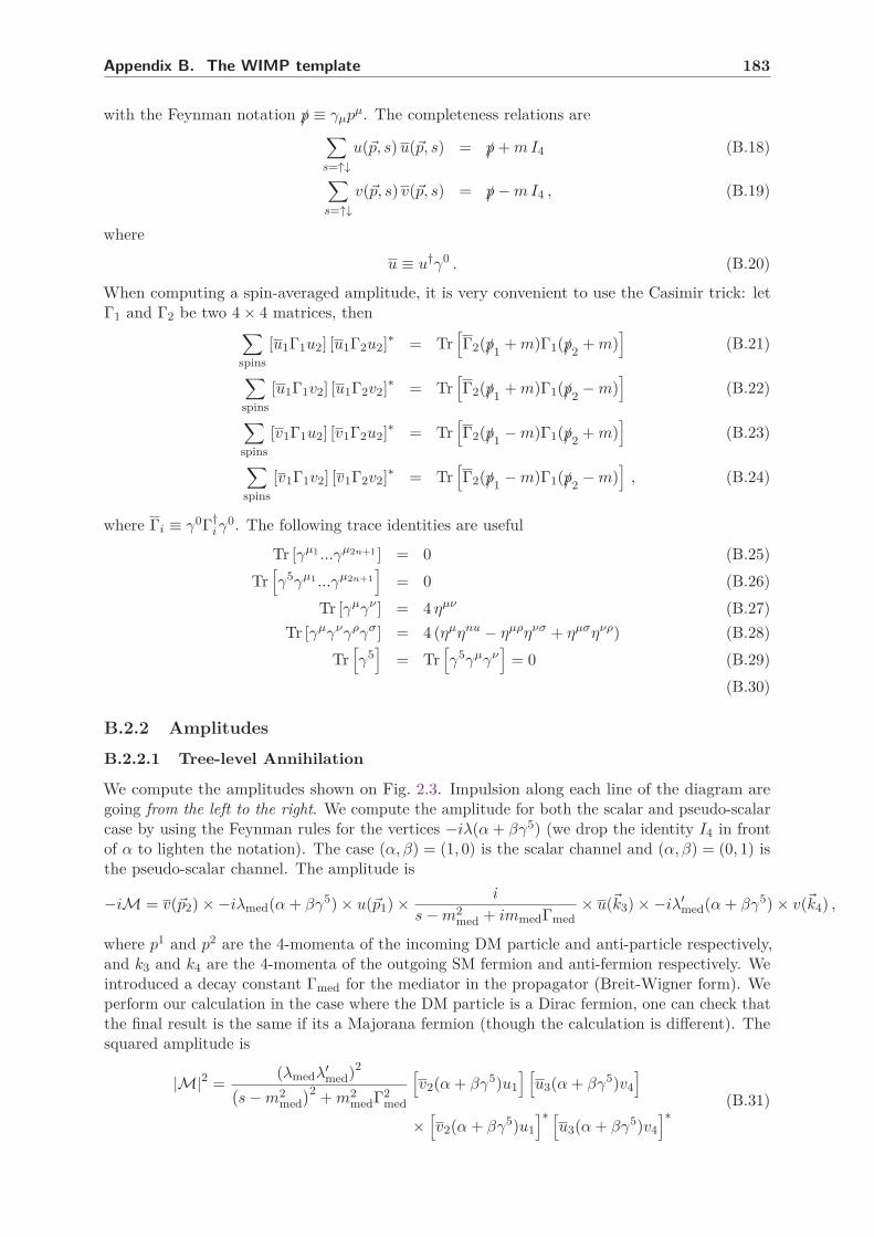
Appendix B. The WIMP template 183
with the Feynman notation /p ≡ γµpµ. The completeness relations are∑
s=↑↓u(þp, s) u(þp, s) = /p + m I4 (B.18)
∑
s=↑↓v(þp, s) v(þp, s) = /p − m I4 , (B.19)
where
u ≡ u†γ0 . (B.20)
When computing a spin-averaged amplitude, it is very convenient to use the Casimir trick: letΓ1 and Γ2 be two 4 × 4 matrices, then
∑
spins
[u1Γ1u2] [u1Γ2u2]∗ = Tr[
Γ2(/p1+ m)Γ1(/p2
+ m)]
(B.21)
∑
spins
[u1Γ1v2] [u1Γ2v2]∗ = Tr[
Γ2(/p1+ m)Γ1(/p2
− m)]
(B.22)
∑
spins
[v1Γ1u2] [v1Γ2u2]∗ = Tr[
Γ2(/p1− m)Γ1(/p2
+ m)]
(B.23)
∑
spins
[v1Γ1v2] [v1Γ2v2]∗ = Tr[
Γ2(/p1− m)Γ1(/p2
− m)]
, (B.24)
where Γi ≡ γ0Γ†i γ
0. The following trace identities are useful
Tr [γµ1 ...γµ2n+1 ] = 0 (B.25)
Tr[
γ5γµ1 ...γµ2n+1
]
= 0 (B.26)
Tr [γµγν ] = 4 ηµν (B.27)
Tr [γµγνγργσ] = 4 (ηµηnu − ηµρηνσ + ηµσηνρ) (B.28)
Tr[
γ5]
= Tr[
γ5γµγν]
= 0 (B.29)
(B.30)
B.2.2 Amplitudes
B.2.2.1 Tree-level Annihilation
We compute the amplitudes shown on Fig. 2.3. Impulsion along each line of the diagram aregoing from the left to the right. We compute the amplitude for both the scalar and pseudo-scalarcase by using the Feynman rules for the vertices −iλ(α + βγ5) (we drop the identity I4 in frontof α to lighten the notation). The case (α, β) = (1, 0) is the scalar channel and (α, β) = (0, 1) isthe pseudo-scalar channel. The amplitude is
−iM = v(þp2) × −iλmed(α + βγ5) × u(þp1) × i
s − m2med + immedΓmed
× u(þk3) × −iλ′med(α + βγ5) × v(þk4) ,
where p1 and p2 are the 4-momenta of the incoming DM particle and anti-particle respectively,and k3 and k4 are the 4-momenta of the outgoing SM fermion and anti-fermion respectively. Weintroduced a decay constant Γmed for the mediator in the propagator (Breit-Wigner form). Weperform our calculation in the case where the DM particle is a Dirac fermion, one can check thatthe final result is the same if its a Majorana fermion (though the calculation is different). Thesquared amplitude is
|M|2 =(λmedλ′
med)2
(
s − m2med
)2+ m2
medΓ2med
[
v2(α + βγ5)u1
] [
u3(α + βγ5)v4
]
×[
v2(α + βγ5)u1
]∗ [
u3(α + βγ5)v4
]∗(B.31)

184 B.2. Particle physics
We average over initial spins, sum over final spins and use the Casimir trick to get
|M|2 ≡ 1
4
∑
spins
|M|2 =1
4
(λmedλ′med)2
(
s − m2med
)2+ m2
medΓ2med
Tr[
(α − βγ5)(/p2− mχ)(α + βγ5)(/p1
+ mχ)]
× Tr[
(α − βγ5)(/k3 + mf)(α + βγ5)(/k4 − mf)]
(B.32)
Developping the traces, we get
|M|2 =(λmedλ′
med)2
(
s − m2med
)2+ m2
medΓ2med
[
α2(s − 4 m2χ) + β2 s
] [
α2(s − 4 m2f ) + β2 s
]
, (B.33)
which leads to Eq. (2.65) in the scalar and pseudo-scalar limits.
B.2.2.2 Tree-level scattering
The amplitudes for tree-level scattering are shown on Fig. 2.4. We call p1 the 4-momentum ofthe incoming DM particle and p2 the 4-momentum of the outgoing DM particle, while k3 and k3
refer to the incoming and outgoing 4-momenta of the SM fermion. We compute the amplitudewith the same trick as for the annihilation by writing α + βγ5, we get
−iM = u(þp2) × −iλmed(α + βγ5) × u(þp1) × i
t − m2med + immedΓmed
× u(þk4) × −iλ′med(α + βγ5) × u(þk3) ,
and the spin-averaged squared amplitude is
|M|2 =(λmedλ′
med)2
(
t − m2med
)2+ m2
medΓ2med
[
α2(t − 4 m2χ) + β2 t
] [
α2(t − 4 m2f ) + β2 t
]
. (B.34)
This can be obtain immediately by taking the annihilation amplitude and substituting s → t.
B.2.3 Invariant phase space and cross-sections
B.2.3.1 Lorentz-invariant phase-space
Let us consider a process 1 + 2 → 3 + 4 + . . . + n. The elementary cross-section for this process is
dσ ≡ 1
4F|M|2(2π)4δ4
(
p1 + p2 −n
∑
i=3
pi
)
d4LIPS , (B.35)
where M is the amplitude of the process, F is the flux factor
F ≡√
(p1.p2)2 − m21m2
2 , (B.36)
and we introduced the Lorentz-invariant phase-space element of volume
d4LIPS ≡n
∏
i=3
d4pi
(2π)4Θ(pi,0)(2π)δ
(
pµi pi,µ − m2
i
)
. (B.37)
The Lorentz invariance is manifest in the definition of d4LIPS however it is more convenient forcomputations to move to another form. We introduce the energy E2 ≡ |þp|2 + m2, rewrite thephase-space element
d4LIPS ≡n
∏
i=3
d4pi
(2π)4Θ(pi,0)(2π)δ
(
p2i,0 − E2
i
)
, (B.38)

Appendix B. The WIMP template 185
and integrate over pi,0 to get
d3LIPS =n
∏
i=3
d3þp
(2π)32Ei(þpi). (B.39)
This form is also Lorentz-invariant since we started from d4LIPS, though it is not manifest.Note that the integration over pi,0 can be performed regardless of the amplitude since thecomponents of the 4-momentum are not independent. One just has to keep in mind the relationE =
√
|þp|2 + m2 when performing the integral over þp.
B.2.3.2 Cross-sections
Annihilation cross-sections The elementary cross-section for the annihilation process 1+2 →3 + 4, where 1 and 2 are DM particles and 3 and 4 SM fermions, is given by
dσann =1
4 F|M|2(2π)4δ4 (p1 + p2 − k3 − k4)
d3þk3
(2π)32E3
d3þk4
(2π)32E4
=1
4 F|M|2(2π)4δ (E1 + E2 − E3 − E4) δ3
(
þp1 + þp2 − þk3 − k4
) d3þk3
(2π)32E3
d3þk4
(2π)32E4.
(B.40)
We perform our calculation in the center-of-mass frame
E1 + E2 =√
s
þp1 + þp2 = þk3 + þk4 = 0 .(B.41)
Since both SM fermions have the same mass mf , the integration over þk4 leads E3 = E4 = E andwe get
dσann =1
4 F|M|2(2π)4δ
(√s − 2E
) d3þk
(2π)64 E2
=1
4 F|M|2(2π)4δ
(√s − 2E
) k dEdΩ
(2π)64 E
=1
4 F|M|2(2π)4 1
2δ
(√s
2− E
)
k dEdΩ
(2π)64 E.
(B.42)
Since the amplitude depends on s only, integration of the solid angle Ω leads a factor of 4π. Sincefor the case of annihilation, the flux factor can be expressed as
F =
√s
2
√
s − 4 m2 , (B.43)
integration of the elementary cross-section over E finally leads
σann =1
16π
1
s
√
s − 4 m2f
s − 4 m2|M|2 . (B.44)
For the two annihilation channels we considered, the expression of the cross-section is
σann =1
16π
(λmedλ′med)2
(
s − m2med
)2+ m2
medΓ2med
(s − 4 m2)1/2(s − 4 m2f )3/2 s−1 scalar
(
s−4 m2f
s−4 m2
)1/2
s pseudoscalar(B.45)
Since the cross-sections are manifestely Lorentz-invariant, these expressions are valid in anyframe even though we made the computation in the rest frame.
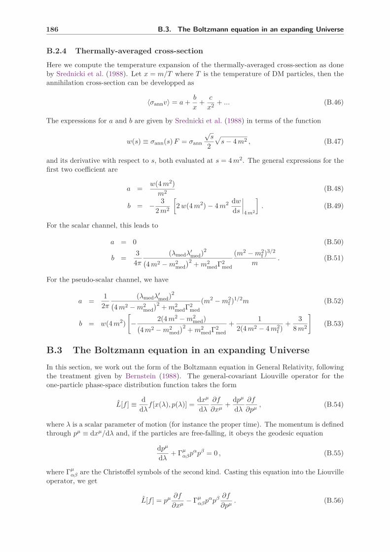
186 B.3. The Boltzmann equation in an expanding Universe
B.2.4 Thermally-averaged cross-section
Here we compute the temperature expansion of the thermally-averaged cross-section as doneby Srednicki et al. (1988). Let x = m/T where T is the temperature of DM particles, then theannihilation cross-section can be developped as
〈σannv〉 = a +b
x+
c
x2+ ... (B.46)
The expressions for a and b are given by Srednicki et al. (1988) in terms of the function
w(s) ≡ σann(s) F = σann
√s
2
√
s − 4 m2 , (B.47)
and its derivative with respect to s, both evaluated at s = 4 m2. The general expressions for thefirst two coefficient are
a =w(4 m2)
m2(B.48)
b = − 3
2 m2
[
2 w(4 m2) − 4 m2 dw
ds
∣
∣
∣
∣
4 m2
]
. (B.49)
For the scalar channel, this leads to
a = 0 (B.50)
b =3
4π
(λmedλ′med)2
(
4 m2 − m2med
)2+ m2
medΓ2med
(m2 − m2f )3/2
m. (B.51)
For the pseudo-scalar channel, we have
a =1
2π
(λmedλ′med)2
(
4 m2 − m2med
)2+ m2
medΓ2med
(m2 − m2f )1/2m (B.52)
b = w(4 m2)
[
− 2(4 m2 − m2med)
(
4 m2 − m2med
)2+ m2
medΓ2med
+1
2(4 m2 − 4 m2f )
+3
8 m2
]
(B.53)
B.3 The Boltzmann equation in an expanding Universe
In this section, we work out the form of the Boltzmann equation in General Relativity, followingthe treatment given by Bernstein (1988). The general-covariant Liouville operator for theone-particle phase-space distribution function takes the form
L[f ] ≡ d
dλf [x(λ), p(λ)] =
dxµ
dλ
∂f
∂xµ+
dpµ
dλ
∂f
∂pµ, (B.54)
where λ is a scalar parameter of motion (for instance the proper time). The momentum is definedthrough pµ ≡ dxµ/dλ and, if the particles are free-falling, it obeys the geodesic equation
dpµ
dλ+ Γµ
αβpαpβ = 0 , (B.55)
where Γµαβ are the Christoffel symbols of the second kind. Casting this equation into the Liouville
operator, we get
L[f ] = pµ ∂f
∂xµ− Γµ
αβpαpβ ∂f
∂pµ. (B.56)

Appendix B. The WIMP template 187
B.3.1 Liouville operator in the flat FLRW metric
The Liouville operator simplifies in a particular metric with the expression of the Christoffelsymbols
Γµαβ =
1
2gµν
[
∂gαν
∂xβ+
∂gβν
∂xα− ∂gαβ
∂xν
]
. (B.57)
We restrict our calculations to the flat Friedmann-Lemaitre-Robertson-Walker (FLRW) metric,which has the simple form
ds2 = dt2 − a2(t) δijdxidxj , (B.58)
It is straightforward to compute
Γi0j =
a
aδi
j
Γ0ij = aa δij .
(B.59)
Note that the FLRW metric is homogeneous and isotropic by definition. Since it is related to themass distribution f through Einstein’s equations, we expect f to only depend on the time t, the
energy p0 and the modulus of the momentum |þp| =√
−a2δijpipj . Injecting the expression of Γµαβ
into Eq. (B.56), we get
L[f ] = p0 ∂f
∂x0+ pi ∂f
∂xi− aa δijpipj ∂f
∂p0− 2
a
ap0pi ∂f
∂pi. (B.60)
The factor of 2 in the last term accounts for the components 0i and i0. The energy is related tothe momentum through Einstein’s relation p0 =
√
m2 + |þp|2 = E which we implement through amass-shell integral
L0[f ] ≡∫
dp0 δ
(
p0 −√
m2 + |þp|2)
L[f ]1
p0. (B.61)
This defines a mass-shell Liouville operator L0. With the mass-shell condition, we get thefollowing simplification
∂
∂xi=
dp0
dxi
∂
∂p0
=d
dxi
(
√
−a2δjkpjpk + m2
)
∂
∂p0
= 0
∂
∂pi= −a2 pi
p0
∂
∂p0
(B.62)
which leads to the final expression
L0[f ] =∂f
∂t− H|þp|2
E
∂f
∂E(B.63)
B.3.2 Liouville operator for the number density
Integrating Eq. (B.63) over the 3-momentum leads to the Liouville operator for the numberdensity. We recall the definion of the number density n as
n(t) ≡ g
∫
d3þp
(2π)3f(þp, t) , (B.64)

188 B.3. The Boltzmann equation in an expanding Universe
where g is the number of internal degrees of freedom. By integration by parts, we get the identity
∫
d3þp
(2π)3
p2
E
∂f
∂E= −3
∫
d3þp
(2π)3
∂f
∂p, (B.65)
and the integrated Liouville operator simplifies to
∫
d3þp
(2π)3L0[f ] =
dn
dt+ 3 H n . (B.66)
B.3.3 Collision operator for two-body annihilation processes
Here we simplify the collision operator appearing in the Boltzmann equation for a process1 + 2 → 3 + 4, closely following the pedagogical treatment given by Gondolo & Gelmini (1991).The full collision operator is quite complicated since it involves all the processes that modify thephase-space distribution of 1. Following Bernstein (1988), we split the operator into two terms,one for the elastic collisions and one for the inelastic ones
C[f1] = CE[f1] + CI[f1] . (B.67)
The inelastic collision operator can be written
CI[f1] ≡ −1
2
∑
spins
∫
[
f1f2(1 ± f3)(1 ± f4) |M12→34|2 − f3f4(1 ± f1)(1 ± f2) |M34→12|2]
× (2π)4δ(4) (p1 + p2 − p3 − p4)
× d3þp2
(2π)32E2
d3þp3
(2π)32E3
d3þp4
(2π)32E4,
(B.68)
where the sum is over initial and final spins, the ± sign is +/− for bosons/fermions and M is aprobability amplitude. We want to derive the evolution equation for the number density thereforewe integrate over the momenta þp1 as in Eq. (B.64). This integration suppress all processes thatdo not change the number density n1, which include elastic collisions. Hence we have
∫
d3þp1
(2π)3CE[f1] = 0 , (B.69)
and the only relevant operator is the one accounting for inelastic collisions. We implementthe mass-shell condition Eq. (B.61) and integrate over the momenta as in Eq. (B.64) to get a”number-density collision operator”
C0[n1] ≡ g1
∫
d3þp1
(2π)3E1CI[f1]
= −∑
spins
∫
[
f1f2(1 ± f3)(1 ± f4) |M12→34|2 − f3f4(1 ± f1)(1 ± f2) |M34→12|2]
× (2π)4δ(4) (p1 + p2 − p3 − p4)
× d3þp1
(2π)32E1
d3þp2
(2π)32E2
d3þp3
(2π)32E3
d3þp4
(2π)32E4.
(B.70)
We neglect the quantum mechanical factors i.e. 1 ± fi ≃ 1. Particles 3 and 4 are assumed inchemical and thermal equilibrium with the bath, hence f3 = f3,eq and f4 = f4,eq. The DMparticle is assumed to be in thermal equilibrium during chemical decoupling, so we can write
fDM(þp) =nDM(T )
nDM,eq(T )fDM,eq(þp) , (B.71)

Appendix B. The WIMP template 189
i.e. the DM phase-space density is proportional to the full chemical and thermal equilibriumdensity, with a temperature-dependent proportionality factor. This assumption of thermalequilibrium of the DM can be relaxed, see Binder et al. (2017) for details. The detailed balanceon 1 + 2 → 3 + 4 implies
f3,eq f4,eq = f1,eq f2,eq . (B.72)
and unitarity leads
∑
spins
∫
|M34→12|2 (2π)4δ(4) (p1 + p2 − p3 − p4)d3þp3
(2π)32E3
d3þp4
(2π)32E4
=∑
spins
∫
|M12→34|2 (2π)4δ(4) (p1 + p2 − p3 − p4)d3þp3
(2π)32E3
d3þp4
(2π)32E4
(B.73)
We introduce the unpolarized cross-section (averaged over incoming spins and summed overoutgoing spins)
4F12 σ12→34 ≡ 1
g1g2
∑
spins
∫
|M12→34|2 (2π)4δ(4) (p1 + p2 − p3 − p4)d3þp3
(2π)32E3
d3þp4
(2π)32E4, (B.74)
where F12 ≡√
(p1.p2)2 − m21m2
2 is the flux factor. With the introduction of the Moller velocity
vm ≡ F12
E1E2, (B.75)
and the definition of the thermally-averaged cross-section
〈σv〉 ≡∫
d3þp1d3þp2 σvm f1f2∫
d3þp1d3þp2 f1f2, (B.76)
the collision operator finally simplifies into
C0[n1] = − 〈σv〉 (n1n2 − n1,eqn2,eq) . (B.77)
B.3.4 Liouville operator for the temperature
Here we derive the form of the Liouville operator when taking the second-moment of Eq. (B.63).With the definition
Tdm ≡ 2
3
1
n
∫
d3þp
(2π)3
þp2
2 mf(þp) , (B.78)
and the identity
∫
d3þp
(2π)3þp2 H þp2
E
∂f
∂E= −5 H 3 n m Tdm (B.79)
obtained by integration by parts, we immediately get
2
3
1
n
∫
d3þp
(2π)3
þp2
2 mL[f ] =
∂Tdm
∂t+ 5 H Tdm . (B.80)
We can use the photon temperature T as an alternate time variable. We have
Tdm = adTdm
da= a H
dT
da
dTdm
dT. (B.81)

190 B.3. The Boltzmann equation in an expanding Universe
Using the constancy of the entropy sa3 = cst and its expression in terms of the effective degreesof freedom Eq. (2.54), we get
dT
da=
ds
da
dT
ds= −s
a
45
2π2
1
heffT 2
(
1 +1
3
d ln heff
d ln T
)−1
, (B.82)
i.e.
Tdm = −s g−1/2∗
2πmp
dTdm
dT, (B.83)
where g∗ is defined in Eq. (2.80) and mp is the reduced Planck mass.
B.3.5 Kinetic decoupling temperature
The expression of the kinetic decoupling temperature is given in Bringmann & Hofmann (2007)
m
Tkd=
(
a
n + 2
)1/(n+2)
Γ
[
n + 1
n + 2
]
. (B.84)
The index n is defined through an expansion of the scattering cross-section
|M|2t=0, s=m2+2mω = cn
(
ω
m
)n
+ O(
(
ω
m
)n+1)
, (B.85)
and
a =∑
f
(
5
2(2π)9geff
)1/2
gSM cn Nn+3MPl
m, (B.86)
where the sum is over SM scattering partners, gSM is their number of internal degrees of freedom,MPl is the Planck mass and
N+j = (1 − 2−j)(j + 1)!ζ(j + 1) (B.87)
N−j = (j + 1)!ζ(j + 1) . (B.88)
The + sign applies to fermions while the − sign applies to bosons.

191
Appendix C
Impact of subhalos on indirect darkmatter searches
C.1 Indirect searches with gamma rays
The Galactic latitude b and longitude l are defined in Fig. C.1. The relations between thesecoordinates and Cartesian coordinates are:
x = dobs − s cos(b) cos(l)
y = −s cos(b) sin(l)
z = s sin(b)
(C.1)
z
Sun (S) Galactic center (C)
(P)
y
x dobs
s
l
b
Galactic plane
rcyl
Figure C.1 – Galactic coordinates (s, b, l) used for the integral along the line of sight.
C.2 Indirect searches with cosmic rays
C.2.1 Effect of propagation parameters
C.2.2 Moving clumps
Here we derive the solution of the transport equation
∂tΨ + þ∇.(þv Ψ) − K∆Ψ = Q(þx, t) , (C.2)

192 C.2. Indirect searches with cosmic rays
Figure C.2 – Same as Fig. 4.10 but varying the diffusion index δ (left panel) or the convective wind Vc
(right panel).
We look for a Green’s function G(t0, þx0 → t, þx) of this equation
∂tG + þ∇.(þv G) − K∆G = δ(t − t0) δ(3)(þx − þx0) . (C.3)
The spatial Fourier transform of the Green’s function G is solution of
∂tG + (iþk.þv + K k2) G = e−iþk.þx0 δ(t − t0) (C.4)
We choose the solution
G(t0, t;þk) = Θ(t − t0) e−iþk.þx0 e−(iþk.þv+K k2)(t−t0) (C.5)
Taking the inverse Fourier transform, this leads to
G(t0, þx0 → t, þx) =Θ(t − t0)
(2π)3
∫
d3þk eiþk.(þx−þx0) e−(iþk.þv+K k2)(t−t0) , (C.6)
which can be straightforwardly integrated to get
G(t0, þx0 → t, þx) = Θ(t − t0)
1
4πK (t − t0)
3/2
exp
[
−þx − þx0 − þv(t − t0)2
4 K (t − t0)
]
. (C.7)
C.2.3 Fluxes and exclusion curves
C.2.4 Variance
The primary antiproton flux from subhalos only can be written as
〈Φsub〉 =dφ
dE dΩ= S
∫
d3þxs G(þxs → þx) Lsub , (C.8)
where Lsub is the subhalo luminosity density given in Eq. (4.17). The factor S depends onparticle-physics-related quantities (mass, cross-section, spectrum). Using the expression of the

Appendix C. Impact of subhalos on indirect dark matter searches 193
Figure C.3 – Contribution from a few annihilation channels. We used the NFW profile of McMillan2017.
101 102 103
WIMP mass [GeV]
10−28
10−27
10−26
10−25
10−24
〈σv〉
[cm
3.s
−1]–s-w
ave
canonical 〈σv〉 for WIMPs
MW Mass Model:McMillan ′17 – cored
Subhalo config:αm = 2
Mcut = 10−6M⊙
p propagation:Med from Maurin+′01/Donato+′04Φmod = 0.83 GV [max from Ghelfi+′16]
Stref, Lacroix & Lavalle 2017
AMS02 p 3-σ bound for χχ → bb[φχχ + φbg < φobs + 3 σobs+th]
no subhalos
with subhalos
101 102 103
WIMP mass [GeV]
10−28
10−27
10−26
10−25
10−24
〈σv〉
[cm
3.s
−1]–s-w
ave
canonical 〈σv〉 for WIMPs
MW Mass Model:McMillan ′17 – cored
Subhalo config:αm = 2
Mcut = 10−6M⊙
p propagation:Kappl+′15 (upd. Winkler ′17)Φmod = 0.83 GV [max from Ghelfi+′16]
Stref, Lacroix & Lavalle 2017
AMS02 p 3-σ bound for χχ → bb[φχχ + φbg < φobs + 3 σobs+th]
no subhalos
with subhalos
Figure C.4 – Same as Fig. 4.16 for cored Galactic dark matter profile.
luminosity, we have
〈Φsub〉 = S∫
dV G
∫
dm
∫
dc Ft ξt (C.9)
= S Nsub
Kt
∫
dV
∫
dm
∫
dcdP
dV
dP
dm
dP
dcG ξt (C.10)
= S Nsub
Kt
∫
dVdP
dVG 〈ξt〉m,c . (C.11)
This is the average contribution for the whole subhalo population. For a single subhalo, theaverage contribution is simply 〈Φsub〉 /Nsub. From this, it is quite clear that we have
⟨
Φ2sub,1
⟩
=S2
Kt
∫
dVdP
dVG2
⟨
ξ2t
⟩
m,c. (C.12)

194 C.2. Indirect searches with cosmic rays
101 102 103
WIMP mass [GeV]
10−28
10−27
10−26
10−25
10−24〈σv〉
[cm
3.s
−1]–s-w
ave
canonical 〈σv〉 for WIMPs
MW Mass Model:McMillan ′17 – cored
Subhalo config:αm = 2
Mcut = 10−6M⊙
p propagation:Med from Maurin+′01/Donato+′04Φmod = 0.83 GV [max from Ghelfi+′16]
Stref, Lacroix & Lavalle 2017
AMS02 p 3-σ bound for χχ → bb[φχχ + φbg < φobs + 3 σobs+th]
no subhalos
with subhalos
101 102 103
WIMP mass [GeV]
10−28
10−27
10−26
10−25
10−24
〈σv〉
[cm
3.s
−1]–s-w
ave
canonical 〈σv〉 for WIMPs
MW Mass Model:McMillan ′17 – cored
Subhalo config:αm = 2
Mcut = 10−6M⊙
p propagation:Kappl+′15 (upd. Winkler ′17)Φmod = 0.83 GV [max from Ghelfi+′16]
Stref, Lacroix & Lavalle 2017
AMS02 p 3-σ bound for χχ → bb[φχχ + φbg < φobs + 3 σobs+th]
no subhalos
with subhalos
Figure C.5 – Same as Fig. 4.17 for cored Galactic dark matter profile.
101 102 103
WIMP mass [GeV]
10−28
10−27
10−26
10−25
10−24
〈σv〉
[cm
3.s
−1]–s-w
ave
canonical 〈σv〉 for WIMPs
MW Mass Model:McMillan ′17 – cored
Subhalo config:αm = 1.9
Mcut = 10−10M⊙
p propagation:Med from Maurin+′01/Donato+′04Φmod = 0.83 GV [max from Ghelfi+′16]
Stref, Lacroix & Lavalle 2017
AMS02 p 3-σ bound for χχ → bb[φχχ + φbg < φobs + 3 σobs+th]
no subhalos
with subhalos
101 102 103
WIMP mass [GeV]
10−28
10−27
10−26
10−25
10−24
〈σv〉
[cm
3.s
−1]–s-w
ave
canonical 〈σv〉 for WIMPs
MW Mass Model:McMillan ′17 – cored
Subhalo config:αm = 1.9
Mcut = 10−10M⊙
p propagation:Kappl+′15 (upd. Winkler ′17)Φmod = 0.83 GV [max from Ghelfi+′16]
Stref, Lacroix & Lavalle 2017
AMS02 p 3-σ bound for χχ → bb[φχχ + φbg < φobs + 3 σobs+th]
no subhalos
with subhalos
Figure C.6 – Same as Fig. 4.18 for cored Galactic dark matter profile.
In the same way, we find the following expressions
⟨
Φ2cross
⟩
=4 S2
Kt
∫
dVdP
dVG2 ρ2
smooth
⟨
m2t
⟩
m,c(C.13)
〈ΦsubΦcross〉 =2 S2
Kt
∫
dVdP
dVG2 ρsmooth 〈ξt mt〉m,c . (C.14)
These are all the expressions needed to compute the flux variance σ2Φ,1 for a single clump. We
can then compute the full variance
σ2Φ = Nsub σΦ,1 . (C.15)

195
Appendix D
The dark matter phase space of theGalaxy
D.1 Mass models of McMillan (2017)
In this work, we make extensive use of the mass models built by McMillan (2017). In thesemodels, the bulge mass density is described by
ρb(R, z) =ρ0,b
(1 + r′/r0)αbexp
[
−(r′/rb)2]
, (D.1)
with
r′ =√
R2 + (z/q)2 . (D.2)
The author fixed αb = 1.8, r0 = 0.075 kpc, rb = 2.1 kpc and q = 0.5. The best fitting model hasρ0,b = 98.4 M⊙.pc−3.
The stellar discs have a density
ρd(R, z) =Σ0
2 zdexp
[
−|z|zd
− R
Rd
]
. (D.3)
The scale heights are fixed to zd = 300 pc for the thin disc and zd = 900 pc for the thick disc.The best fit parameters for the thin and thick discs are given in Tab. D.1.
The gas discs (H and H2) have the density profile
ρg(R, z) =Σ0
4 zdexp
[
−Rm
R− R
Rd
]
sech2(
z
2 zd
)
, (D.4)
where
sech(x) =1
cosh(x)=
2
ex + e−x(D.5)
is the hyperbolic secant. The parameters of the gas discs are fixed and their value is given inTab. D.1.
The dark matter halo has a density profile parametrized with
ρ(r) =ρs
xγ
1
(1 + x)3. (D.6)
The best fitting values of ρs and rs for different γ are given in Tab. D.2.

196 D.2. Anisotropy in the Cuddeford models
Σ0 [M⊙.pc−2] Rd [kpc]
thin 896 2.50
thick 183 3.02
Σ0 [M⊙.pc−2] Rd [kpc] Rd [kpc] zd [kpc]
H 53.1 7 4 0.085
H2 2180 1.5 12 0.045
Table D.1 – Left panel: best fitting parameters for the stellar discs. Right panel: fixed parametersfor the gas discs.
γ 0 0.25 0.5 1
ρs [M⊙.pc−3] 0.09086 0.05261 0.03190 0.00852
rs [kpc] 7.7 9.6 11.7 19.6
Table D.2 – Best fitting parameters of the dark matter halo.
D.2 Anisotropy in the Cuddeford models
This section focuses on the models of Cuddeford (1991) with DF
f(E , L) = G(Q)L−2β0 . (D.7)
We prove that the anisotropy parameter for these models takes the form
β(r) ≡ 1 − σ2t
2σ2r
=r2 + β0r2
a
r2 + r2a
.
(D.8)
Since this is a generalization of the constant-β and Osipkov-Merritt models, this also demonstratesthe form of the anisotropy profile in these two cases. We start by computing the radial velocityvariance σ2
r ≡⟨
þv2r
⟩
− 〈þvr〉2 =⟨
v2 cos2(η)⟩
:
ρ σ2r =
∫
v2r f(E , L) d3þv
= 2π
∫ ∫
v2 cos2(η) G(Q) L−2β0v2 sin(η) dη dv
= 4π
∫ ∫
v2µ2G(Q) L−2β0v2 dµ dv ,
(D.9)
where we used the change of variable cos(η) → µ and µ-parity of the integrand to get the lastidentity. We now make the following change of variable (v, µ) → (Q, L2). One can compute theJacobian and finds
v2dv dµ = − 1
2r2
[
2(Ψ − Q) − L2
r2
(
1 +r2
r2a
)]−1/2
dQ dL2 . (D.10)
What are the bounds on Q and L2 ? As for the Osipkov-Merritt models, we have Q > 0 andsince Q = Ψ − v2/2 − L2/(2r2
a), we have Q 6 Ψ. To find the upper bound on L2, we notice that
Q = Ψ − v2
2cos2(η) − L2
2r2
(
1 +r2
r2a
)
, (D.11)
and therefore
L2 6 L2max ≡ 2r2(Ψ − Q)
1 + r2/r2a
. (D.12)

Appendix D. The dark matter phase space of the Galaxy 197
We now have
ρ σ2r =
2π
r2
∫ Ψ
0dQ G(Q)
∫ L2max
0dL2
√
2(Ψ − Q) − L2
r2
(
1 +r2
r2a
)
L−2β0 , (D.13)
where we replace v2µ2 in Eq. (D.9) using Eq. (D.11). We rescale L2 by L2max to finally obtain
ρ σ2r = 2π
r−2β0
(1 + r2/r2a)1−β0
∫ Ψ
0dQ G(Q)[2(Ψ − Q)]3/2−β0
∫ 1
0dx
√1 − x x−β0 . (D.14)
The integral over x is a particular value of the beta function, see Sec. A.2. Its relation to thegamma function leads
ρ σ2r = π3/2 r−2β0
(1 + r2/r2a)1−β0
Γ(1 − β0)
Γ(5/2 − β0)
∫ Ψ
0dQ G(Q)[2(Ψ − Q)]3/2−β0 . (D.15)
Let us now compute the tangential velocity dispersion
ρ σ2t = 2π
∫ ∫
v2 sin2(η) G(Q) L−2β0v2 sin(η) dη dv
=4π
r2
∫ ∫
G(Q) L2−2β0v2 dµ dv ,(D.16)
where we used v2 sin(η) = L2/r2. Performing the same change of variables as before, we obtain
ρ σ2t = 2π
r−2β0
(1 + r2/r2a)2−β0
∫ Ψ
0dQ G(Q)[2(Ψ − Q)]3/2−β0
∫ 1
0dx (1 − x)−1/2 x1−β0 . (D.17)
Using again the properties of the beta and gamma functions, we finally get
ρ σ2t = 2π3/2 r−2β0
(1 + r2/r2a)2−β0
Γ(2 − β0)
Γ(5/2 − β0)
∫ Ψ
0dQ G(Q)[2(Ψ − Q)]3/2−β0 . (D.18)
We can now compute the ratio
σ2t
2σ2r
=1
1 + r2/r2a
Γ(2 − β0)
Γ(1 − β0)
=1 − β0
1 + r2/r2a
,
(D.19)
and the anisotropy parameter
β(r) =r2 + β0r2
a
r2 + r2a
. (D.20)
D.3 Numerical simulations
D.3.1 Fitting the simulated galaxies
D.3.2 Escape speed
D.3.3 Velocity distributions
D.3.4 Moments of the velocity distributions

198 D.3. Numerical simulations
Halo C log10(ρ0) rs α β γ[M⊙/kpc3] [kpc]
DMO 6.848± 0.472 14.291± 8.514 1.0± 0 2.805± 0.297 1.065± 0.142
Hydro 7.746± 0.126 4.210± 0.441 2.165± 0.627 2.504± 0.104 0.189± 0.122
Table D.3 – Parameters of the dark matter halo in Halo C.
Adicora log10(ρ0) rs α β γ[M⊙/kpc3] [kpc]
DMO 7.181± 0.5 11.288± 6.955 1.0± 0 2.744± 0.257 0.975± 0.195
Hydro 7.667± 0.033 6.671± 0.860 1.407± 0.191 2.756± 0.146 0.090± 0.038
Table D.4 – Parameters of the dark matter halo in Adicora.
Mochima log10(ρ0) rs α β γ[M⊙/kpc3] [kpc]
DMO 6.963± 0.442 13.786± 7.744 1.0± 0 2.721± 0.251 1.066± 0.134
Hydro 7.414± 0.185 7.364± 1.115 1.768± 0.573 2.633± 0.165 0.468± 0.171
Table D.5 – Parameters of the dark matter halo in Mochima.
Figure D.1 – Same as Fig. 5.18, for Halo C.

Appendix D. The dark matter phase space of the Galaxy 199
Figure D.2 – Same as Fig. 5.18, for Adicora.

200 D.3. Numerical simulations
Figure D.3 – Same as Fig. 5.18, for Mochima.
Figure D.4 – Same as Fig. 5.20, for Halo C.

Appendix D. The dark matter phase space of the Galaxy 201
Figure D.5 – Same as Fig. 5.20, for Adicora.
Figure D.6 – Same as Fig. 5.20, for Mochima.

202 D.3. Numerical simulations
Figure D.7 – Same as Fig. 5.21, for Halo C.

Appendix D. The dark matter phase space of the Galaxy 203
Figure D.8 – Same as Fig. 5.21, for Adicora.

204 D.3. Numerical simulations
Figure D.9 – Same as Fig. 5.21, for Mochima.

Appendix D. The dark matter phase space of the Galaxy 205
Figure D.10 – Same as Fig. 5.22, for Halo C.

206 D.3. Numerical simulations
Figure D.11 – Same as Fig. 5.22, for Adicora.

Appendix D. The dark matter phase space of the Galaxy 207
Figure D.12 – Same as Fig. 5.22, for Mochima.


209
Appendix E
Impact of the phase space on darkmatter searches
E.1 Relative velocity distribution
Here we detail the computation of the moments of the relative velocity distribution
〈vnr 〉 =
∫
d3þvr vnr Fþvr
(þvr, r) , (E.1)
with the relative velocity distribution defined as
Fþvr(þvr, r) = κ−1(r)
∫
d3þvc fþv(þv1, r) fþv(þv2, r) , (E.2)
with the normalization
κ(r) =
∫
d3þv1
∫
d3þv2 fþv(þv1, r) fþv(þv2, r) . (E.3)
We performed the change of variables
þvc = (þv1 + þv2)/2þvr = þv2 − þv1
⇐⇒
þv1 = þvc − þvr/2þv2 = þvc + þvr/2 .
(E.4)
E.1.1 Isotropic case
If the velocity distribution is isotropic, we have fþv(þv, r) = fþv(|þv|, r) and the relative velocitydistribution is also isotropic therefore
〈vnr 〉 = 4π
∫ vmaxr
vminr
dvr v2r Fþvr(|þvr|, r) vn
r . (E.5)
We introduce θ as the angle between þvc and þvr, and define µ ≡ cos(θ). The speed of particles 1and 2 can then be expressed as
v1 =
√
v2c +
v2r
4− vcvr µ
v2 =
√
v2c +
v2r
4+ vcvr µ .
(E.6)
In the Galactic frame, we have v1 6 vesc(r) and v2 6 vesc(r) which leads
|µ| 6 µ0 , (E.7)

210 E.2. Bounds on p-wave annihilating dark matter
with
µ0 =vesc(r) − v2
c − v2r /4
vc vr. (E.8)
Eq. (E.4) also leads to vc 6 vesc(r) and vr 6 2 vesc(r). Note that the quantity fþv(þv1, r) fþv(þv2, r)is invariant under the transformation µ → −µ. The relative velocity distribution can then bewritten
Fþvr(þvr, r) = 4πκ−1(r)
∫ vesc(r)
0dvc v2
c
∫ µ0
0dµ fþv(þv1, r) fþv(þv2, r) , (E.9)
and the n-order moment
〈vnr 〉 = 4π
∫ 2 vesc
0dvr v2
r Fþvr(þvr, r) vnr . (E.10)
E.1.2 Anisotropic case
In the anisotropic models, the velocity distribution also depends also depends on the modulus ofthe angular momentum L through
fþv(þv, r) =f(E , L)
ρ(r). (E.11)
In this case, it is still convenient to perform a change of variables from þv1, þv2 to þvc, þvr, providedone uses the appropriate coordinate systems to describe the quantities of interest. We introducethe radial unit vector þer: the system is invariant under rotation around þer hence the integralover þvc leads a factor of 2π, see the left panel in Fig. E.1. There is also an integration over themodulus vcm and the angle αcm between þvcm and þer. To perform the integration over þvr, wemove to a frame with the z-axis defined by þvcm and the y-axis chosen orthogonal to þer, see theright panel in Fig. E.1. In that frame, we have
þvcm = vcm þez
þer = cos(αcm)þez + sin(αcm)þex
þvr = vr [cos(θ)þez + sin(θ) cos(φ)þex + sin(θ) sin(φ)þey]
(E.12)
with θ the angle between þvr and þvcm (already introduced in the isotropic case) and φ thecomplemetary spherical angle. This allows us to write the relative speed distribution as
Fvr(vr, r) = 2πκ−1(r) v2r
∫ vesc(r)
0dvc v2
c
∫ 1
−1dµcm
∫ 2π
0dφ
∫ µ0
−µ0
dµ fþv(þv1, r) fþv(þv2, r) . (E.13)
We used µcm ≡ cos(αcm) in the equation above. We give the expressions of the angular momentumfor each particle
L21 =
∣
∣
∣
∣
þr ×(
þvcm − vr
2
)∣
∣
∣
∣
2
= r2
[
v2r
4(1 − µ2) sin2(φ) +
−vr
2µcm
√
1 − µ2 cos(φ) −√
1 − µ2cm
(
vcm − vr
2µ
)
]
L22 =
∣
∣
∣
∣
þr ×(
þvcm +vr
2
)∣
∣
∣
∣
2
= r2
[
v2r
4(1 − µ2) sin2(φ) +
+vr
2µcm
√
1 − µ2 cos(φ) −√
1 − µ2cm
(
vcm +vr
2µ
)
]
.
(E.14)
E.2 Bounds on p-wave annihilating dark matter

Appendix E. Impact of the phase space on dark matter searches 211
!
"#
%!"
&#
&$
&%
&!"
!
'
(
)
%!"
&$
&%
&!"
"#
$
&#
Figure E.1 – Coordinate systems for the derivation of the relative velocity DF for an anisotropic system.Left panel: frame associated with þr, in which we define þvc. Right panel: coordinate system associatedwith þvc.
10−3 0.01 0.1 1 10 100 103
Dark matter mass mχ [GeV]
10−23
10−22
10−21
10−20
10−19
10−18
10−17
10−16
10−15
10−14
σ1c[cm
3s−
1]
Propagation B
γ = 0.25, Isotropic
Boudaud et al. (2018)
e+e−
µ+µ−
τ+τ−
bb
W+W−
SMod insensitiveSMod sensitiveSMod insensitiveSMod sensitive
Figure E.2 – p-wave constraints for different annihilation channels, for the γ = 0.25 mass model.

212 E.2. Bounds on p-wave annihilating dark matter
10−22
10−21
10−20
10−19
σ1c[cm
3s−
1]
NFW
Propagation A
Boudaud et al. (2018)
Isotropicβanis = −0.3
OMMaxwellian
Isotropicβanis = −0.3
OMMaxwellian
10−3 0.01 0.1 1 10 100 103
Dark matter mass mχ [GeV]
−40
−20
0
20
40
(σ1−
σiso
1)/σiso
1[%
]
10−22
10−21
10−20
10−19
σ1c[cm
3s−
1]
γ = 0.25
Propagation A
Boudaud et al. (2018)
Isotropicβanis = −0.3
OMMaxwellian
Isotropicβanis = −0.3
OMMaxwellian
10−3 0.01 0.1 1 10 100 103
Dark matter mass mχ [GeV]
−40
−20
0
20
40
(σ1−
σiso
1)/σiso
1[%
]
10−22
10−21
10−20
10−19
σ1c[cm
3s−
1]
NFW
Propagation B
Boudaud et al. (2018)
Isotropicβanis = −0.3
OMMaxwellian
Isotropicβanis = −0.3
OMMaxwellian
10−3 0.01 0.1 1 10 100 103
Dark matter mass mχ [GeV]
−40
−20
0
20
40
(σ1−
σiso
1)/σiso
1[%
]
10−22
10−21
10−20
10−19
σ1c[cm
3s−
1]
γ = 0.25
Propagation B
Boudaud et al. (2018)
Isotropicβanis = −0.3
OMMaxwellian
Isotropicβanis = −0.3
OMMaxwellian
10−3 0.01 0.1 1 10 100 103
Dark matter mass mχ [GeV]
−40
−20
0
20
40
(σ1−
σiso
1)/σiso
1[%
]
Figure E.3 – Top panel:. Uncertainties related to the anistropy in the propagation model A, forthe NFW profile (left) and the γ = 0.25 profile (right) Bottom panel: same as the top panel, for thepropagation model B.

213
Appendix F
Resume en francais
F.1 Introduction
F.1.1 Le probleme de la masse manquante: preuves observationnelles
Les physiciens et astronomes sont aujourd’hui confrontes a une multitude de donnees observa-tionnelles pointant vers un deficit de masse dans notre Univers.
La manifestation la plus frappante de ce deficit est a l’echelle des galaxies, notamment lesgalaxies spirales. La mesure des courbes de rotation de ces galaxies permet d’estimer leur masse,et l’on constate que celle-ci differe fortement de la masse extrapolee a partir de la luminosite.Un probleme similaire est present a l’echelle des amas de galaxies, ou des methodes telles quele lentillage graviationnel permettent d’estimer la masse independamment de la luminosite. Laencore, une difference considerable est constatee entre la masse totale et la masse lumineuse.
Un probleme de masse manquante est egalement present aux echelles cosmologiques. L’analysedes anisotropies de temperature du fond diffus micro-ondes a permis l’etablissement du modeleΛCDM qui est aujourd’hui le modele standard de la cosmologie. Ce modele stipule que le budgetenergetique de l’Univers est compose a 70% d’une constante cosmologique Λ, a 25% d’unematiere ”froide” (non-relativiste) et sans interactions, et a 5% de matiere baryonique, c’est-a-direde matiere ordinaire. Cela qu’environ 80% de la matiere dans l’Univers est d’origine et decomposition inconnue. Il est naturel d’identifier cette matiere etrange avec la masse manquantemesuree dans les galaxies et les amas de galaxies.
F.1.2 Le modele ΛCDM aux petites echelles
Le modele ΛCDM rencontre un succes phenomenale lorqu’on le confronte aux observations lieesa des echelles super-galactiques. A l’echelle des galaxies, en revanche, des points de desaccordentre la theorie et les observations apparaissent.
Ces problemes aux petites echelles se manifestent de differentes manieres. Tout d’abord, leprofile de densite aux centres de galaxies semblent etre, dans la plupart des cas, assez plat alorsque ΛCDM predit un profile tres pique pour les halos de matiere sombre. D’autre part, ΛCDMpredit une multitude de petites galaxies satellites associee a notre Voie Lactee, hors seule unepoignee de ces satellites est observee. Finalement, les satellites qui sont effectivement observessont moins massifs que ce que la theorie predit.
Plusieurs solutions ont ete proposees pour resoudre ces problemes. Deux grandes classes desolutions peuvent etres distinguees. On peut tout d’abord suppose que ces tensions montrentun echec du modele ΛCDM, qui doit donc etre modifie. Parmis ces solutions, on peut citer lesmodeles de matiere sombre ”tiede” ou la matiere sombre auto-interagissante. Une autre approcheconsiste a supposer que le modele ΛCDM est correct et les problemes aux petites echelles sont enfait dues aux effets de la matiere ordinaire qui sont encore mal compris a l’echelle galactique.

214 F.2. Histoire thermique des particules massives interagissant faiblement
F.1.3 Approches theoriques du problemes de la matiere sombre
Deux approches theoriques radicalement differentes sont aujourd’hui envisagees pour resoudre leprobleme de la matiere sombre.
Une premiere approche consiste a interpreter la masse manquante comme un echec de latheorie de la gravitation actuellement admise. Selon cette approche, la gravitation Newtonienne etla relativite generale doivent etre modifiees pour expliquer les observations sans faire intervenir unenouvelle forme de matiere. Parmis les theories proposees, on peut citer la Gravite NewtonienneModifiee et ses extensions relativistes.
La seconde approche consiste a supposer que la masse manquante est bien constituee d’uneforme de matiere exotique. Il a ete etablit que la matiere ordinaire ne peut pas etre la matieresombre, cette matiere doit donc etre constituee de particules encore inconnues. De tres nombreuxmodeles de physique des particules incorporent des candidats au titre de particule de matieresombre. On peut citer, entres autres, la supersymetrie, les theories a dimensions supplementaires,les axions et les neutrinos steriles.
F.1.4 Recherches experimentales des particules de matiere sombre
Si la matiere sombre est constituee de particules exotiques et que ces particules ont des interactionsautres que gravitationnelles avec la matiere ordinaires, on peut esperer identifiee ces particulesen suivant plusieurs demarches experimentales.
On peut tout d’abord esperer produire les particules de matiere sombre dans des accelerateursde particules comme le LHC au Cern. Si la matiere sombre peut interagir avec les noyauxatomiques, on peut egalement esperer detecter une collision entre une particule de matiere sombrecosmique et un noyau terrestre. C’est ce que l’on nomme la detection directe. Enfin, si la matieresombre peut s’annihilaler ou est instable, on peut esperer detecter les produits de son annihilation(ou de sa desingration) dans le rayonnement cosmique. On parle alors de detection indirecte.
F.2 Histoire thermique des particules massives interagissant faible-ment
On suppose dans cette section que la particule de matiere sombre est stable, qu’elle a une massetres elevee (typiquement entre quelques GeV et quelques TeV) et des interactions faibles avecles particules standards. On suppose de plus que cette particule peut s’auto-annihiler. Desparticules de ce type sont appelees WIMPs pour Weakly Interacting Massive Particles.
F.2.1 Decouplage chimique
Lorsque la temperature du plasma primordial T est superieure a la masse m de la matiere sombrela reaction χ + χ f + f , ou χ est la matiere sombre et f une particule standard (un lepton ouun quark, par exemple), est a l’equilibre. L’univers etant en expansion, la temperature decroit etle taux d’annihilation Γann de la matiere sombre chute. Lorsque T < m la reaction f + f → χ + χne se produit plus. Enfin arrive un instant ou Γann < H ou H est le parametre de Hubble etl’annihilation de χ devient hautement improbable. On parle de decouple chimique de la matieresombre. Le nombre de particules de matiere sombre est alors fixe et la densite de matiere sombreaujourd’hui peut etre predite. On peut exprimer l’abondance de χ en fonction de la sectionefficace d’annihilation 〈σannv〉 et on trouve
Ωχh2 ≃ 0.1
( 〈σannv〉3 × 10⁻²⁶ cm3/s
)−1
. (F.1)
La coıncidence de la valeur observee de Ωcdmh2 avec une section efficace electrofaible est appeleele ”miracle du WIMP”.

Appendix F. Resume en francais 215
F.2.2 Decouplage cinetique
Apres le decouplage chimique, la matiere sombre reste en equilibre thermique avec le plasma atravers les reactions de diffusion χ + f χ + f . Au bout d’une certain temps, on a Γdiff < H ouΓdiff est le taux de diffusion, et la diffusion devient inefficace. On parle de decouplage cinetiquede la matiere sombre. Ce decouplage est tres important car il fixe la taille des toutes premieresstructures de matiere sombre qui se forment dans l’Univers. Un calcul detaille montre que lamasse de ces structures est tres faible
Mmin ∼ 10−10 − 10−4 M⊙. (F.2)
F.3 Halos et sous-halos de matiere sombre dans l’Univers
F.3.1 Formation des structures
Apres l’egalite matiere-radiation, les perturbations de matiere sombre croissent efficacementjusqu’a s’effondrer et former des halos. Le formalisme de Press-Schechter permet de calculer lafonction de masse de ces objets, et l’on trouve pour le modele ΛCDM
dn
dm∝ m−2 . (F.3)
Le profile de densite ρ des halos est mesure dans les simulations cosmologiques et on trouveune forme universelle, identique pour tous les halos. La densite est fortement piquee au centredu halo ρ(r) ∝ r−1 et se comporte comme ρ(r) ∝ r−3 dans les parties externes. La taille de laregion centrale rapportee a la taille totale de la structure definit sa concentration. Cette quantiteest correlee a la masse de sorte que les plus petits halos sont aussi les plus concentres.
F.3.2 Evolution des sous-halos
Les halos galactiques comme celui de la Voie Lactee sont formes par l’accretion de halos pluspetits. La majeure partie de ces petits halos survit en fait a l’accretion et sont toujours presentsdans les galaxies aujourd’hui. On parle alors de sous-halos. L’interaction de ces sous-halos avec lepotentiel gravitationnel de la galaxie hote, que l’on nomme effets de maree, epluche ces structures,qui perdent ainsi une grande partie de leur masse. Ces interactions, en particulier l’effet de chocdu disque stellaire, sont modelisees en details et la forme finale des sous-halos est precisementcalculee.
F.3.3 Modele contraint des sous-halos Galactiques
Avec tous elements en main, nous construisons un modele de la population Galactique de sous-halos. Ce modele a l’originalite de reposer sur des contraintes observationnelles, c’est-a-direqu’il est coherent par construction avec la dynamique de notre Galaxie telle qu’elle est observee.Nous demontrons que la distribution des sous-halos dans la Galaxies est fortement affecteepar les effets de maree. En particulier, les sous-halos sont epluches bien plus efficacement aucentre de la Galaxie qu’au bord. De plus, une selection des structures s’opere en fonction deleur concentration. Les moins concentrees sont detruites alors que les plus concentrees resistentdavantages aux marees. Ceci augmente la concentration moyenne des structures au centre dela Galaxies. La fonction de masse est elle aussi affectee du fait de la correlation entre masse etconcentration.

216 F.4. Impact des sous-halos sur les recherches indirectes de matiere sombre
F.4 Impact des sous-halos sur les recherches indirectes de matieresombre
La presence de sous-halos, qui sont des regions de surdensite de matiere sombre au sein dela Galaxie, augmente la taux d’annihilation de ces particules. On s’attend donc a ce que lespredictions pour les recherches indirectes soient affectees par la structuration de la matiere sombreaux petites echelles. En utilisant notre modele de sous-halos, nous calculons precisement le”boost” attendus sur les signaux indirectes. Deux canaux complementaires sont ensuite consideres:les rayons gamma et les antiprotons cosmiques.
F.4.1 Impact sur les recherches avec les rayons gamma
Les rayons gamma permettent d’explorer le halo de matiere sombre le long d’une ligne de visee.Nous calculons le facteur de ”boost” en fonction de la ligne de visee et montrons comment cefacteur depend des parametres de la distribution des sous-halos, en particulier les parametresde la fonction de masse. Nous trouvons un boost important au dessus d’une latitude de 30, cequi doit fortement impacter les contraintes sur les modeles microscopiques derivees a partir desdonnees sur les rayons gamma.
F.4.2 Impact sur les recherches avec les antiprotons
Les antiprotons cosmiques forment un canal complementaire des rayons gamma du fait de leurpropagation dans la Galaxie. Contrairement aux photons, les antiprotons sont des particulescharges qui diffusent sur les inhomogeneites du champ magnetique turbulent de la Galaxie. Leurtrajectoire est donc aleatoire. Les antiprotons recus sur Terre ont donc explore un volume moyencontenue dans une sphere autour de la Terre, sphere dont le rayon depend par ailleurs de l’energiedes antiprotons. Nous calculons le boost pour le signal d’antiprotons et montrons sa dependancedans les parametres des sous-halos. Nous montrons enfin comment l’inclusion des sous-halosmodifie les contraintes sur la section efficaces d’annihilation obtenues a partir des donnees del’experience AMS-2.
F.5 L’espace des phases de la matiere sombre Galactique
F.5.1 Le formalisme d’Eddington
La dynamique des particules de matiere sombre dans la Galaxie est gouvernee par l’equation deBoltzmann sans collisions. La methode d’Eddington permet d’obtenir une fonction de distributiondans l’espace des phases f(þr,þv) solution stationnaire de cette equation. Dans l’hypothese oula distribution de vitesse des particules de matiere sombre est isotrope, f est simplement unefonction de l’energie et peut s’exprimer directement en fonction du profile de densite du halo dematiere sombre et du potentiel gravitationnel total du systeme.
L’hypothese d’isotropie peut-etre levee, auquel cas f depend a la fois de l’energie et dela norme du moment angulaire. Plusieurs extensions du modele d’Eddington incorporant del’anisotropie ont ete decouvertes. Nous en discutons deux en details: les modeles a anisotropieconstante, et les modeles de Osipkov-Merrit.
F.5.2 Problemes et limitations du formalisme d’Eddington
Bien que la methode d’Eddington soit connue depuis longtemps, relativement peu d’attention aete portee sur ses limites d’applicabilite. Ces deux aspects sont etudies en detail.
Une premiere limite du formalisme d’Eddington apparaıt lorqu’on l’applique a un systeme detaille finie. La presence d’un bord induit une divergence dans la distribution f . Cette divergence

Appendix F. Resume en francais 217
n’a pas d’origine physique et doit etre regularisee. Nous proposons plusieurs methodes permettantde traiter cette divergence et quantifions precisement l’impact de ces methodes sur f .
Une autre limit concerne le probleme de la stabilite. Rien ne garantit que la solutiond’Eddington soit stable, il faut donc s’en assurer. Il se trouve que de nombreuses configurations[profile de densite, potentiel gravitationnel] amenent a des solutions qui sont instables. Nousdeveloppons des criteres analytiques permettant de determiner la stabilite a priori, et classifionsles systemes problematiques ou le formalisme ne peut pas etre applique.
F.6 Impact de l’espace des phases sur les recherches de matieressombre
F.6.1 Impact generique sur les observables
Les consequences de notre etude sur l’applicabilite du formalisme d’Eddington sont etudiees endetail dans le contexte des recherches de matiere sombre. Nous considerons plusieurs observablesintervenant dans les recherches directes et indirectes, et evaluons l’impact des methodes deregularisations discutees dans le chapitre precedent. Nous comparons systematiquement lespredictions de la methode d’Eddington avec celles du ”Modele Standard du Halo” qui est tressouvent utilise dans ce cadre, et montrons que la difference entre ces deux approches est engenerale tres importante.
F.6.2 Application aux positrons cosmiques
La methode d’Eddington est appliquee de maniere concrete a l’etude des electrons et positronscosmiques. L’exploitation des donnees de la sonde Voyager 1 nous permet de deriver descontraintes tres fortes sur la section efficace d’annihilation des particules de matiere sombre.
F.7 Conclusion
Plusieurs aspects de la recherche de la matiere sombre ont ete abordes au cours de ce travail. Enpartant autant que possible de principes elementaires issus de la physique des particules et de lacosmologie, nous avons construit et developpe un ensemble de modeles et d’outils permettantd’attaquer le probleme de l’identification de la matiere sombre dans la Galaxie. Nous tenons asouligner que les outils que nous avons developpe sont suffisament generaux pour s’appliquera de nombreux modeles de matiere sombre, comme les WIMPs, les axions et les trous noirsprimordiaux. Un grand nombre de pistes de recherches sont ouvertes a l’issue de ce travail. Nousallons continuer a exploiter notre connaissance de la structuration aux petites echelles et del’espace des phase pour explorer l’espace des modeles de matiere sombre. L’application auxrecherches directes et indirectes, deja en parti realise, sera complete par une etude des effetsgravitationnels des petites structures sur la matiere observables.

219
Bibliography
Aad G. et al. (ATLAS Collaboration), The ATLAS Experiment at the CERN Large HadronCollider, JINST 3, S08003 (2008). 14
Abazajian K. N., The Consistency of Fermi-LAT Observations of the Galactic Center witha Millisecond Pulsar Population in the Central Stellar Cluster, JCAP 1103, 010 (2011),arXiv:1011.4275. 17
Abazajian K. N., Canac N., Horiuchi S., Kaplinghat M., Astrophysical and Dark Matter Interpre-tations of Extended Gamma-Ray Emission from the Galactic Center, Phys. Rev. D90, 023526(2014), arXiv:1402.4090. 17
Abazajian K. N., Kaplinghat M., Detection of a Gamma-Ray Source in the Galactic Center Con-sistent with Extended Emission from Dark Matter Annihilation and Concentrated AstrophysicalEmission, Phys. Rev. D86, 083511 (2012), arXiv:1207.6047. 17
Abbott L. F., Sikivie P., A Cosmological Bound on the Invisible Axion, Phys. Lett. B120,133-136 (1983). 11
Abdallah J., Araujo H., Arbey A., Ashkenazi A., Belyaev A., Berger J., Boehm C., Boveia A.,Brennan A., Brooke J., Buchmueller O., Buckley M., Busoni G., Calibbi L., Chauhan S., DaciN., Davies G., De Bruyn I., De Jong P., De Roeck A., de Vries K., Del Re D., De SimoneA., Di Simone A., Doglioni C., Dolan M., Dreiner H., Ellis J., Eno S., Etzion E., FairbairnM., Feldstein B., Flaecher H., Eric F., Genest M.-H., Gouskos L., Gramling J., Haisch U.,Harnik R., Hibbs A., Hoh S., Hopkins W., Ippolito V., Jacques T., Kahlhoefer F., Khoze V. V.,Kirk R., Korn A., Kotov K., Kunori S., Landsberg G., Liem S., Lin T., Lowette S., Lucas R.,Malgeri L., Malik S., McCabe C., Serhan Mete A., Morgante E., Mrenna S., Nakahama Y.,Newbold D., Nordstrom K., Pani P., Papucci M., Pataraia S., Penning B., Pinna D., PoleselloG., Racco D., Re E., Riotto A. W., Rizzo T., Salek D., Sarkar S., Schramm S., Skubic P.,Slone O., Smirnov J., Soreq Y., Sumner T., Tait T. M. P., Thomas M., Tomalin I., Tunnell C.,Vichi A., Volansky T., Weiner N., West S. M., Wielers M., Worm S., Yavin I., Zaldivar B.,Zhou N., Zurek K., Simplified Models for Dark Matter Searches at the LHC, ArXiv e-prints(2015), arXiv:1506.03116. 10, 28
Abercrombie D. et al., Dark Matter Benchmark Models for Early LHC Run-2 Searches: Reportof the ATLAS/CMS Dark Matter Forum, (2015), arXiv:1507.00966. 14
Abeysekara A. U. et al. (HAWC Collaboration), Extended gamma-ray sources around pulsarsconstrain the origin of the positron flux at Earth, Science 358, 911-914 (2017), arXiv:1711.06223.19
Ackermann M., Ajello M., Allafort A., Atwood W. B., Baldini L., Barbiellini G., Bastieri D.,Bechtol K., Bellazzini R., Berenji B., Blandford R. D., Bloom E. D., Bonamente E., BorglandA. W., Bouvier A., Bregeon J., Brigida M., Bruel P., Buehler R., Buson S., Caliandro G. A.,Cameron R. A., Caraveo P. A., Casandjian J. M., Cecchi C., Charles E., Chekhtman A., CheungC. C., Chiang J., Ciprini S., Claus R., Cohen-Tanugi J., Conrad J., Cutini S., de Angelis A.,

220 Bibliography
de Palma F., Dermer C. D., Digel S. W., Do Couto E Silva E., Drell P. S., Drlica-Wagner A.,Favuzzi C., Fegan S. J., Ferrara E. C., Focke W. B., Fortin P., Fukazawa Y., Funk S., FuscoP., Gargano F., Gasparrini D., Germani S., Giglietto N., Giommi P., Giordano F., GirolettiM., Glanzman T., Godfrey G., Grenier I. A., Grove J. E., Guiriec S., Gustafsson M., HadaschD., Harding A. K., Hayashida M., Hughes R. E., Johannesson G., Johnson A. S., Kamae T.,Katagiri H., Kataoka J., Knodlseder J., Kuss M., Lande J., Latronico L., Lemoine-GoumardM., Llena Garde M., Longo F., Loparco F., Lovellette M. N., Lubrano P., Madejski G. M.,Mazziotta M. N., McEnery J. E., Michelson P. F., Mitthumsiri W., Mizuno T., Moiseev A. A.,Monte C., Monzani M. E., Morselli A., Moskalenko I. V., Murgia S., Nakamori T., NolanP. L., Norris J. P., Nuss E., Ohno M., Ohsugi T., Okumura A., Omodei N., Orlando E., OrmesJ. F., Ozaki M., Paneque D., Parent D., Pesce-Rollins M., Pierbattista M., Piron F., Pivato G.,Porter T. A., Raino S., Rando R., Razzano M., Razzaque S., Reimer A., Reimer O., ReposeurT., Ritz S., Romani R. W., Roth M., Sadrozinski H. F.-W., Sbarra C., Schalk T. L., Sgro C.,Siskind E. J., Spandre G., Spinelli P., Strong A. W., Takahashi H., Takahashi T., TanakaT., Thayer J. G., Thayer J. B., Tibaldo L., Tinivella M., Torres D. F., Tosti G., Troja E.,Uchiyama Y., Usher T. L., Vandenbroucke J., Vasileiou V., Vianello G., Vitale V., Waite A. P.,Winer B. L., Wood K. S., Wood M., Yang Z., Zimmer S., Measurement of Separate Cosmic-RayElectron and Positron Spectra with the Fermi Large Area Telescope, Physical Review Letters108, 011103 (2012)a, arXiv:1109.0521. 19
Ackermann M., Ajello M., Atwood W. B., Baldini L., Ballet J., Barbiellini G., Bastieri D.,Bechtol K., Bellazzini R., Berenji B., Blandford R. D., Bloom E. D., Bonamente E., BorglandA. W., Brandt T. J., Bregeon J., Brigida M., Bruel P., Buehler R., Buson S., Caliandro G. A.,Cameron R. A., Caraveo P. A., Cavazzuti E., Cecchi C., Charles E., Chekhtman A., ChiangJ., Ciprini S., Claus R., Cohen-Tanugi J., Conrad J., Cutini S., de Angelis A., de PalmaF., Dermer C. D., Digel S. W., Silva E. d. C. e., Drell P. S., Drlica-Wagner A., Falletti L.,Favuzzi C., Fegan S. J., Ferrara E. C., Focke W. B., Fortin P., Fukazawa Y., Funk S., FuscoP., Gaggero D., Gargano F., Germani S., Giglietto N., Giordano F., Giroletti M., GlanzmanT., Godfrey G., Grove J. E., Guiriec S., Gustafsson M., Hadasch D., Hanabata Y., HardingA. K., Hayashida M., Hays E., Horan D., Hou X., Hughes R. E., Johannesson G., JohnsonA. S., Johnson R. P., Kamae T., Katagiri H., Kataoka J., Knodlseder J., Kuss M., LandeJ., Latronico L., Lee S.-H., Lemoine-Goumard M., Longo F., Loparco F., Lott B., LovelletteM. N., Lubrano P., Mazziotta M. N., McEnery J. E., Michelson P. F., Mitthumsiri W., MizunoT., Monte C., Monzani M. E., Morselli A., Moskalenko I. V., Murgia S., Naumann-Godo M.,Norris J. P., Nuss E., Ohsugi T., Okumura A., Omodei N., Orlando E., Ormes J. F., PanequeD., Panetta J. H., Parent D., Pesce-Rollins M., Pierbattista M., Piron F., Pivato G., PorterT. A., Raino S., Rando R., Razzano M., Razzaque S., Reimer A., Reimer O., SadrozinskiH. F.-W., Sgro C., Siskind E. J., Spandre G., Spinelli P., Strong A. W., Suson D. J., TakahashiH., Tanaka T., Thayer J. G., Thayer J. B., Thompson D. J., Tibaldo L., Tinivella M., TorresD. F., Tosti G., Troja E., Usher T. L., Vandenbroucke J., Vasileiou V., Vianello G., Vitale V.,Waite A. P., Wang P., Winer B. L., Wood K. S., Wood M., Yang Z., Ziegler M., Zimmer S.,Fermi-LAT Observations of the Diffuse γ-Ray Emission: Implications for Cosmic Rays andthe Interstellar Medium, Astrophys. J. 750, 3 (2012)b, arXiv:1202.4039. 17, 95
Ackermann M. et al. (Fermi-LAT Collaboration), Searching for Dark Matter Annihilation fromMilky Way Dwarf Spheroidal Galaxies with Six Years of Fermi Large Area Telescope Data,Phys. Rev. Lett. 115, 231301 (2015), arXiv:1503.02641. 17, 94
Ade P. A. R. et al. (Planck Collaboration), Planck 2013 results. XVI. Cosmological parameters,Astron. Astrophys. 571, A16 (2014), arXiv:1303.5076. 62
Ade P. A. R. et al. (Planck Collaboration), Planck 2015 results. XIII. Cosmological parameters,

Bibliography 221
Astron. Astrophys. 594, A13 (2016), arXiv:1502.01589. 5, 6, 9, 23, 24, 36, 49, 53, 54, 57, 61,81
Adriani O., Barbarino G. C., Bazilevskaya G. A., Bellotti R., Boezio M., Bogomolov E. A.,Bonechi L., Bongi M., Bonvicini V., Borisov S., Bottai S., Bruno A., Cafagna F., Campana D.,Carbone R., Carlson P., Casolino M., Castellini G., Consiglio L., De Pascale M. P., De SantisC., De Simone N., Di Felice V., Galper A. M., Gillard W., Grishantseva L., Jerse G., KarelinA. V., Koldashov S. V., Krutkov S. Y., Kvashnin A. N., Leonov A., Malakhov V., MalvezziV., Marcelli L., Mayorov A. G., Menn W., Mikhailov V. V., Mocchiutti E., Monaco A., MoriN., Nikonov N., Osteria G., Palma F., Papini P., Pearce M., Picozza P., Pizzolotto C., RicciM., Ricciarini S. B., Rossetto L., Sarkar R., Simon M., Sparvoli R., Spillantini P., StozhkovY. I., Vacchi A., Vannuccini E., Vasilyev G., Voronov S. A., Yurkin Y. T., Wu J., Zampa G.,Zampa N., Zverev V. G., PAMELA Measurements of Cosmic-Ray Proton and Helium Spectra,Science 332, 69 (2011), arXiv:1103.4055. 104
Adriani O. et al. (PAMELA Collaboration), An anomalous positron abundance in cosmic rayswith energies 1.5-100 GeV, Nature 458, 607-609 (2009), arXiv:0810.4995. 19
Adriani O. et al. (PAMELA Collaboration), Cosmic-Ray Positron Energy Spectrum Measured byPAMELA, Phys. Rev. Lett. 111, 081102 (2013), arXiv:1308.0133. 19
Agashe K., Servant G., Warped Unification, Proton Stability, and Dark Matter, Physical ReviewLetters:hep-ph/0403143. 10
Aghanim N. et al. (Planck Collaboration), Planck 2018 results. VI. Cosmological parameters,(2018), arXiv:1807.06209. 5, 6
Aguilar M., Aisa D., Alpat B., Alvino A., Ambrosi G., Andeen K., Arruda L., Attig N., AzzarelloP., Bachlechner A., et al., Precision Measurement of the Helium Flux in Primary Cosmic Raysof Rigidities 1.9 GV to 3 TV with the Alpha Magnetic Spectrometer on the International SpaceStation, Physical Review Letters 115, 211101 (2015)a. 104
Aguilar M., Aisa D., Alpat B., Alvino A., Ambrosi G., Andeen K., Arruda L., Attig N., AzzarelloP., Bachlechner A., et al., Precision Measurement of the Proton Flux in Primary Cosmic Raysfrom Rigidity 1 GV to 1.8 TV with the Alpha Magnetic Spectrometer on the InternationalSpace Station, Physical Review Letters 114, 171103 (2015)b. 104
Aguilar M., Alberti G., Alpat B., Alvino A., Ambrosi G., Andeen K., Anderhub H., Arruda L.,Azzarello P., Bachlechner A., Barao F., Baret B., Barrau A., Barrin L., Bartoloni A., BasaraL., Basili A., Batalha L., Bates J., Battiston R., Bazo J., Becker R., Becker U., Behlmann M.,Beischer B., Berdugo J., Berges P., Bertucci B., Bigongiari G., Biland A., Bindi V., BizzagliaS., Boella G., de Boer W., Bollweg K., Bolmont J., Borgia B., Borsini S., Boschini M. J.,Boudoul G., Bourquin M., Brun P., Buenerd M., Burger J., Burger W., Cadoux F., Cai X. D.,Capell M., Casadei D., Casaus J., Cascioli V., Castellini G., Cernuda I., Cervelli F., ChaeM. J., Chang Y. H., Chen A. I., Chen C. R., Chen H., Cheng G. M., Chen H. S., Cheng L.,Chernoplyiokov N., Chikanian A., Choumilov E., Choutko V., Chung C. H., Clark C., ClaveroR., Coignet G., Commichau V., Consolandi C., Contin A., Corti C., Costado Dios M. T.,Coste B., Crespo D., Cui Z., Dai M., Delgado C., Della Torre S., Demirkoz B., Dennett P.,Derome L., Di Falco S., Diao X. H., Diago A., Djambazov L., Dıaz C., von Doetinchem P.,Du W. J., Dubois J. M., Duperay R., Duranti M., D’Urso D., Egorov A., Eline A., EpplingF. J., Eronen T., van Es J., Esser H., Falvard A., Fiandrini E., Fiasson A., Finch E., Fisher P.,Flood K., Foglio R., Fohey M., Fopp S., Fouque N., Galaktionov Y., Gallilee M., Gallin-MartelL., Gallucci G., Garcıa B., Garcıa J., Garcıa-Lopez R., Garcıa-Tabares L., Gargiulo C., GastH., Gebauer I., Gentile S., Gervasi M., Gillard W., Giovacchini F., Girard L., Goglov P., Gong

222 Bibliography
J., Goy- Henningsen C., Grandi D., Graziani M., Grechko A., Gross A., Guerri I., de la GuıaC., Guo K. H., Habiby M., Haino S., Hauler F., He Z. H., Heil M., Heilig J., Hermel R., HoferH., Huang Z. C., Hungerford W., Incagli M., Ionica M., Jacholkowska A., Jang W. Y., JinchiH., Jongmanns M., Journet L., Jungermann L., Karpinski W., Kim G. N., Kim K. S., KirnT., Kossakowski R., Koulemzine A., Kounina O., Kounine A., Koutsenko V., Krafczyk M. S.,Laudi E., Laurenti G., Lauritzen C., Lebedev A., Lee M. W., Lee S. C., Leluc C., Leon VargasH., Lepareur V., Li J. Q., Li Q., Li T. X., Li W., Li Z. H., Lipari P., Lin C. H., Liu D., LiuH., Lomtadze T., Lu Y. S., Lucidi S., Lubelsmeyer K., Luo J. Z., Lustermann W., Lv S.,Madsen J., Majka R., Malinin A., Mana C., Marın J., Martin T., Martınez G., MasciocchiF., Masi N., Maurin D., McInturff A., McIntyre P., Menchaca-Rocha A., Meng Q., MenichelliM., Mereu I., Millinger M., Mo D. C., Molina M., Mott P., Mujunen A., Natale S., NemethP., Ni J. Q., Nikonov N., Nozzoli F., Nunes P., Obermeier A., Oh S., Oliva A., Palmonari F.,Palomares C., Paniccia M., Papi A., Park W. H., Pauluzzi M., Pauss F., Pauw A., PedreschiE., Pensotti S., Pereira R., Perrin E., Pessina G., Pierschel G., Pilo F., Piluso A., PizzolottoC., Plyaskin V., Pochon J., Pohl M., Poireau V., Porter S., Pouxe J., Putze A., QuadraniL., Qi X. N., Rancoita P. G., Rapin D., Ren Z. L., Ricol J. S., Riihonen E., Rodrıguez I.,Roeser U., Rosier-Lees S., Rossi L., Rozhkov A., Rozza D., Sabellek A., Sagdeev R., SandweissJ., Santos B., Saouter P., Sarchioni M., Schael S., Schinzel D., Schmanau M., Schwering G.,Schulz von Dratzig A., Scolieri G., Seo E. S., Shan B. S., Shi J. Y., Shi Y. M., SiedenburgT., Siedling R., Son D., Spada F., Spinella F., Steuer M., Stiff K., Sun W., Sun W. H., SunX. H., Tacconi M., Tang C. P., Tang X. W., Tang Z. C., Tao L., Tassan-Viol J., Ting S. C. C.,Ting S. M., Titus C., Tomassetti N., Toral F., Torsti J., Tsai J. R., Tutt J. C., Ulbricht J.,Urban T., Vagelli V., Valente E., Vannini C., Valtonen E., Vargas Trevino M., VaurynovichS., Vecchi M., Vergain M., Verlaat B., Vescovi C., Vialle J. P., Viertel G., Volpini G., WangD., Wang N. H., Wang Q. L., Wang R. S., Wang X., Wang Z. X., Wallraff W., Weng Z. L.,Willenbrock M., Wlochal M., Wu H., Wu K. Y., Wu Z. S., Xiao W. J., Xie S., Xiong R. Q.,Xin G. M., Xu N. S., Xu W., Yan Q., Yang J., Yang M., Ye Q. H., Yi H., Yu Y. J., Yu Z. Q.,Zeissler S., Zhang J. G., Zhang Z., Zhang M. M., Zheng Z. M., Zhuang H. L., Zhukov V.,Zichichi A., Zuccon P., Zurbach C., First Result from the Alpha Magnetic Spectrometer onthe International Space Station: Precision Measurement of the Positron Fraction in PrimaryCosmic Rays of 0.5-350 GeV, Phys. Rev. Let. 110, 141102 (2013). 19
Aguilar M., Ali Cavasonza L., Alpat B., Ambrosi G., Arruda L., Attig N., Aupetit S., AzzarelloP., Bachlechner A., Barao F., et al., Antiproton Flux, Antiproton-to-Proton Flux Ratio, andProperties of Elementary Particle Fluxes in Primary Cosmic Rays Measured with the AlphaMagnetic Spectrometer on the International Space Station, Physical Review Letters 117,091103 (2016). 18, 108, 113
Aguilar M. et al. (AMS 01 Collaboration), Cosmic-ray positron fraction measurement from 1 to30-GeV with AMS-01, Phys. Lett. B646, 145-154 (2007), arXiv:astro-ph/0703154. 19
Aguilar M. et al. (AMS Collaboration), Precision Measurement of the Boron to Carbon FluxRatio in Cosmic Rays from 1.9 GV to 2.6 TV with the Alpha Magnetic Spectrometer on theInternational Space Station, Phys. Rev. Lett. 117, 231102 (2016). 104, 106, 108
Ahn H. S., Allison P., Bagliesi M. G., Beatty J. J., Bigongiari G., Childers J. T., Conklin N. B.,Coutu S., DuVernois M. A., Ganel O., Han J. H., Jeon J. A., Kim K. C., Lee M. H., Lutz L.,Maestro P., Malinin A., Marrocchesi P. S., Minnick S., Mognet S. I., Nam J., Nam S., NutterS. L., Park I. H., Park N. H., Seo E. S., Sina R., Wu J., Yang J., Yoon Y. S., Zei R., ZinnS. Y., Discrepant Hardening Observed in Cosmic-ray Elemental Spectra, Astrophys. J. Lett.714, L89-L93 (2010), arXiv:1004.1123. 104
Ahrens J. et al. (IceCube Collaboration), Icecube - the next generation neutrino telescope at thesouth pole, Nucl. Phys. Proc. Suppl. 118, 388-395 (2003), arXiv:astro-ph/0209556. 18

Bibliography 223
Ajello M. et al. (Fermi-LAT Collaboration), Fermi-LAT Observations of High-Energy γ-RayEmission Toward the Galactic Center, Astrophys. J. 819, 44 (2016), arXiv:1511.02938. 17
Albert A. et al. (DES, Fermi-LAT Collaboration), Searching for Dark Matter Annihilation inRecently Discovered Milky Way Satellites with Fermi-LAT, Astrophys. J. 834, 110 (2017),arXiv:1611.03184. 17, 94
Aloisio R., Blasi P., De Mitri I., Petrera S., Selected Topics in Cosmic Ray Physics (2018), p. 1.97
Alpher R. A., Bethe H., Gamow G., The origin of chemical elements, Phys. Rev. 73, 803–804(1948). 6
Alpher R. A., Follin J. W., Herman R. C., Physical conditions in the initial stages of the expandinguniverse, Phys. Rev. 92, 1347–1361 (1953). 6
Alpher R. A., Herman R., Evolution of the Universe, Nature 162, 774-775 (1948)a. 3
Alpher R. A., Herman R. C., On the Relative Abundance of the Elements, Physical Review 74,1737-1742 (1948)b. 3
An J. H., Evans N. W., A cusp slope-central anisotropy theorem, Astrophys. J. 642, 752-758(2006), arXiv:astro-ph/0511686. 143
Anderhalden D., Diemand J., Density Profiles of CDM Microhalos and their Implications forAnnihilation Boost Factors, JCAP 1304, 009 (2013), arXiv:1302.0003. 58, 63
Anderson G. W., Castano D. J., Measures of fine tuning, Physics Letters B:hep-ph/9409419. 10
Anderson L. et al. (BOSS Collaboration), The clustering of galaxies in the SDSS-III BaryonOscillation Spectroscopic Survey: baryon acoustic oscillations in the Data Releases 10 and 11Galaxy samples, Mon. Not. Roy. Astron. Soc. 441, 24-62 (2014), arXiv:1312.4877. 6
Ando S., Kamionkowski M., Lee S. K., Koushiappas S. M., Can proper motions of dark-mattersubhalos be detected?, Phys. Rev. D78, 101301 (2008), arXiv:0809.0886. 94
Angulo R. E., Hahn O., Ludlow A., Bonoli S., Earth-mass haloes and the emergence of NFWdensity profiles, (2016), arXiv:1604.03131. 57
Angus G. W., Shan H. Y., Zhao H. S., Famaey B., On the Proof of Dark Matter, the Law ofGravity, and the Mass of Neutrinos, Astrophys. J. Lett.:astro-ph/0609125. 8
Angus G. W., Zhao H., Analysis of galactic tides and stars on CDM microhalos, Mon. Not. Roy.Astron. Soc. 375, 1146-1156 (2007), arXiv:astro-ph/0608580. 72
Antoniadis I., Arkani-Hamed N., Dimopoulos S., Dvali G. R., New dimensions at a millimeter toa Fermi and superstrings at a TeV, Phys. Lett. B436, 257-263 (1998), arXiv:hep-ph/9804398.10
Antonov V. A., Solution of the problem of stability of stellar system Emden’s density law and thespherical distribution of velocities (1962). 143
Antonov V. A., Solution of the Problem of Stability of a Stellar System with Emden’s Density Lawand a Spherical Distribution of Velocities, in Structure and Dynamics of Elliptical Galaxies,Vol. 127 (1987). 145
Arbey A., Lesgourgues J., Salati P., Quintessential halos around galaxies, Phys. Rev. D 64,123528 (2001), arXiv:astro-ph/0105564. 13

224 Bibliography
Arkani-Hamed N., Dimopoulos S., Dvali G. R., The Hierarchy problem and new dimensions at amillimeter, Phys. Lett. B429, 263-272 (1998), arXiv:hep-ph/9803315. 10
Arkani-Hamed N., Dimopoulos S., Dvali G. R., Phenomenology, astrophysics and cosmologyof theories with submillimeter dimensions and TeV scale quantum gravity, Phys. Rev. D59,086004 (1999), arXiv:hep-ph/9807344. 10
Arkani-Hamed N., Finkbeiner D. P., Slatyer T. R., Weiner N., A Theory of Dark Matter, Phys.Rev. D79, 015014 (2009), arXiv:0810.0713. 164
Armengaud E., Palanque-Delabrouille N., Yeche C., Marsh D. J. E., Baur J., Constraining themass of light bosonic dark matter using SDSS Lyman-α forest, Mon. Not. Roy. Astron. Soc.471, 4606-4614 (2017), arXiv:1703.09126. 11, 14
Askew A., Chauhan S., Penning B., Shepherd W., Tripathi M., Searching for Dark Matter atHadron Colliders, Int. J. Mod. Phys. A29, 1430041 (2014), arXiv:1406.5662. 14
Aslanides E. et al. (ANTARES Collaboration), A deep sea telescope for high-energy neutrinos,(1999), arXiv:astro-ph/9907432. 18
Aslanyan G., Price L. C., Adams J., Bringmann T., Clark H. A., Easther R., Lewis G. F., ScottP., Ultracompact minihalos as probes of inflationary cosmology, (2015), arXiv:1512.04597. 83
Atwood W. B. et al. (Fermi-LAT Collaboration), The Large Area Telescope on the FermiGamma-ray Space Telescope Mission, Astrophys. J. 697, 1071-1102 (2009), arXiv:0902.1089.17
Axford W. I., Leer E., Skadron G., The Acceleration of Cosmic Rays by Shock Waves, InternationalCosmic Ray Conference 11, 132 (1977). 100
Baade W., Zwicky F., Remarks on Super-Novae and Cosmic Rays, Physical Review 46, 76-77(1934). 101
Baltz E. A., Wai L., Diffuse inverse Compton and synchrotron emission from dark matterannihilations in galactic satellites, Phys. Rev. D70, 023512 (2004), arXiv:astro-ph/0403528.
Bardeen J. M., Gauge-invariant cosmological perturbations, Phys. Rev. D 22, 1882-1905 (1980).46
Bardeen J. M., Steinhardt P. J., Turner M. S., Spontaneous creation of almost scale-free densityperturbations in an inflationary universe, Phys. Rev. D 28, 679-693 (1983). 52
Barnes J., Goodman J., Hut P., Dynamical instabilities in spherical stellar systems, Astrophys.J. 300, 112-131 (1986). 145
Barrau A., Salati P., Servant G., Donato F., Grain J., Maurin D., Taillet R., Kaluza-Klein darkmatter and Galactic antiprotons, Phys. Rev. D72, 063507 (2005), arXiv:astro-ph/0506389. 18
Bartels R., Ando S., Boosting the annihilation boost: Tidal effects on dark matter subhalos andconsistent luminosity modeling, Phys. Rev. D92, 123508 (2015), arXiv:1507.08656. 64, 76, 94
Bartels R., Krishnamurthy S., Weniger C., Strong support for the millisecond pulsar origin of theGalactic center GeV excess, Phys. Rev. Lett. 116, 051102 (2016), arXiv:1506.05104. 17
Barwick S. W. et al. (HEAT Collaboration), Measurements of the cosmic ray positron fractionfrom 1-GeV to 50-GeV, Astrophys. J. 482, L191-L194 (1997), arXiv:astro-ph/9703192. 19

Bibliography 225
Baudis L., Direct dark matter detection: the next decade, Phys. Dark Univ. 1, 94-108 (2012),arXiv:1211.7222. 14
Beacom J. F., Bell N. F., Bertone G., Gamma-ray constraint on Galactic positron production byMeV dark matter, Phys. Rev. Lett. 94, 171301 (2005), arXiv:astro-ph/0409403. 167
Bekenstein J., Milgrom M., Does the missing mass problem signal the breakdown of Newtoniangravity?, Astrophys. J. 286, 7-14 (1984). 8
Bekenstein J. D., Relativistic gravitation theory for the modified Newtonian dynamics paradigm,Phys. Rev. D 70, 083509 (2004). 8
Bell A. R., The acceleration of cosmic rays in shock fronts - I., Mon. Not. Roy. Astron. Soc. 182,147-156 (1978)a. 100
Bell A. R., The acceleration of cosmic rays in shock fronts - II., Mon. Not. Roy. Astron. Soc.182, 443-455 (1978)b. 100
Berezhko E. G., Ksenofontov L. T., Ptuskin V. S., Zirakashvili V. N., Volk H. J., Cosmic rayproduction in supernova remnants including reacceleration: The secondary to primary ratio,Astron. Astroph. 410, 189-198 (2003). 102
Berezinsky V., Bottino A., Mignola G., High-energy gamma radiation from the galactic centerdue to neutralino annihilation, Phys. Lett. B325, 136-142 (1994), arXiv:hep-ph/9402215. 17
Berezinsky V., Dokuchaev V., Eroshenko Y., Small - scale clumps in the galactic halo and darkmatter annihilation, Phys. Rev. D68, 103003 (2003), arXiv:astro-ph/0301551. 40, 42, 64, 76,94
Berezinsky V., Dokuchaev V., Eroshenko Y., Destruction of small-scale dark matter clumps in thehierarchical structures and galaxies, Phys. Rev. D73, 063504 (2006), arXiv:astro-ph/0511494.72
Berezinsky V., Dokuchaev V., Eroshenko Y., Remnants of dark matter clumps, Phys. Rev. D77,083519 (2008), arXiv:0712.3499. 74
Berezinsky V., Dokuchaev V., Eroshenko Y., Kachelrieß M., Solberg M. A., Superdense cosmo-logical dark matter clumps, Phys. Rev. D 81, 103529 (2010), arXiv:1002.3444. 73
Berezinsky V. S., Bulanov S. V., Dogiel V. A., Ptuskin V. S., Astrophysics of cosmic rays (1990).102
Berezinsky V. S., Dokuchaev V. I., Eroshenko Y. N., Small-scale clumps of dark matter, Phys.Usp. 57, 1-36 (2014), arXiv:1405.2204. 64, 73, 80
Berezinsky V. S., Gurevich A. V., Zybin K. P., Distribution of dark matter in the galaxy andthe lower limits for the masses of supersymmetric particles, Physics Letters B 294, 221-228(1992). 17
Bergstrom L., Dark Matter Candidates, New J. Phys. 11, 105006 (2009), arXiv:0903.4849. 9
Bergstrom L., Bringmann T., Edsjo J., New Positron Spectral Features from SupersymmetricDark Matter - a Way to Explain the PAMELA Data?, Phys. Rev. D78, 103520 (2008),arXiv:0808.3725. 19
Bergstrom L., Edsjo J., Gondolo P., Ullio P., Clumpy neutralino dark matter, Phys. Rev. D59,043506 (1999), arXiv:astro-ph/9806072. 94

226 Bibliography
Bergstrom L., Edsjo J., Ullio P., Cosmic Antiprotons as a Probe for Supersymmetric DarkMatter?, Astrophys. J. 526, 215-235 (1999). 18
Bergstrom L., Snellman H., Observable Monochromatic Photons From Cosmic Photino Annihila-tion, Phys. Rev. D37, 3737-3741 (1988). 16
Bergstrom L., Ullio P., Buckley J. H., Observability of gamma-rays from dark matter neutralino an-nihilations in the Milky Way halo, Astropart. Phys. 9, 137-162 (1998), arXiv:astro-ph/9712318.16, 17
Bernabei R. et al., First model independent results from DAMA/LIBRA-phase2, (2018),arXiv:1805.10486. 14
Bernal J. L., Verde L., Riess A. G., The trouble with H0, JCAP 1610, 019 (2016),arXiv:1607.05617. 6
Bernstein J., Kinetic theory in the expanding universe (1988). 186, 188
Bernstein J., Brown L. S., Feinberg G., The Cosmological Heavy Neutrino Problem Revisited,Phys. Rev. D32, 3261 (1985). 31
Bertone G., Fairbairn M., Compact Stars as Dark Matter Probes, Phys. Rev. D77, 043515 (2008),arXiv:0709.1485. 161
Bertone G., Hooper D., A History of Dark Matter, Submitted to: Rev. Mod. Phys. (2016),arXiv:1605.04909. 1
Bertone G., Hooper D., Silk J., Particle dark matter: Evidence, candidates and constraints, Phys.Rept. 405, 279-390 (2005), arXiv:hep-ph/0404175. 9
Bertschinger E., The Effects of Cold Dark Matter Decoupling and Pair Annihilation on Cos-mological Perturbations, Phys. Rev. D74, 063509 (2006), arXiv:astro-ph/0607319. 40, 41,46
Bhattacharjee P., Chaudhury S., Kundu S., Majumdar S., Sizing-up the WIMPs of Milky Way :Deriving the velocity distribution of Galactic Dark Matter particles from the rotation curvedata, Phys. Rev. D87, 083525 (2013), arXiv:1210.2328. 159
Binder T., Bringmann T., Gustafsson M., Hryczuk A., Early kinetic decoupling of dark matter:when the standard way of calculating the thermal relic density fails, Phys. Rev. D96, 115010(2017), arXiv:1706.07433. 32, 39, 189
Binetruy P., Girardi G., Salati P., Constraints on a system of two neutral fermions from cosmology,Nuclear Physics B 237, 285-306 (1984). 36
Binney J., The radius-dependence of velocity dispersion in elliptical galaxies, Mon. Not. Roy.Astron. Soc. 190, 873-880 (1980). 128
Binney J., Piffl T., The distribution function of the Galaxy’s dark halo, Mon. Not. Roy. Astron.Soc. 454, 3653-3663 (2015), arXiv:1509.06877. 2, 115
Binney J., Tremaine S., Galactic dynamics (1987). 50, 57, 64, 66, 72, 115, 118, 120, 122, 124
Bird S., Cholis I., Munoz J. B., Ali-Haımoud Y., Kamionkowski M., Kovetz E. D., RaccanelliA., Riess A. G., Did LIGO detect dark matter?, Phys. Rev. Lett. 116, 201301 (2016),arXiv:1603.00464. 9

Bibliography 227
Blanchet L., Dipolar particles in general relativity, Classical and Quantum Gravity:gr-qc/0609121.8
Blanchet S., Lavalle J., Diffuse gamma-ray constraints on dark matter revisited. I: the impact ofsubhalos, JCAP 1211, 021 (2012), arXiv:1207.2476. 94
Bland-Hawthorn J., Gerhard O., The Galaxy in Context: Structural, Kinematic, and IntegratedProperties, Ann. Rev. Astron. Astrophys. 54, 529-596 (2016), arXiv:1602.07702. 115
Blandford R., Eichler D., Particle acceleration at astrophysical shocks: A theory of cosmic rayorigin, Phys. Rept. 154, 1-75 (1987). 99, 103
Blasi P., The origin of galactic cosmic rays, 21, 70 (2013), arXiv:1311.7346. 97
Blumenthal G. R., Faber S. M., Primack J. R., Rees M. J., Formation of galaxies and large-scalestructure with cold dark matter., Nature 311, 517-525 (1984). 6
Boddy K. K., Kumar J., Strigari L. E., Wang M.-Y., Sommerfeld-Enhanced J-Factors For DwarfSpheroidal Galaxies, Phys. Rev. D95, 123008 (2017), arXiv:1702.00408. 164
Bode P., Ostriker J. P., Turok N., Halo formation in warm dark matter models, Astrophys. J.556, 93-107 (2001), arXiv:astro-ph/0010389. 13
Boehm C., Ensslin T. A., Silk J., Can Annihilating dark matter be lighter than a few GeVs?, J.Phys. G30, 279-286 (2004), arXiv:astro-ph/0208458. 167
Boehm C., Fayet P., Scalar dark matter candidates, Nucl. Phys. B683, 219-263 (2004), arXiv:hep-ph/0305261. 9
Boehm C., Fayet P., Schaeffer R., Constraining dark matter candidates from structure formation,Phys. Lett. B518, 8-14 (2001), arXiv:astro-ph/0012504. 39, 40
Boehm C., Schaeffer R., Constraints on dark matter interactions from structure formation:Damping lengths, Astron. Astrophys. 438, 419-442 (2005), arXiv:astro-ph/0410591. 40, 43
Boehm C., Schewtschenko J. A., Wilkinson R. J., Baugh C. M., Pascoli S., Using the Milky Waysatellites to study interactions between cold dark matter and radiation, Mon. Not. Roy. Astron.Soc. 445, L31-L35 (2014), arXiv:1404.7012. 167
Bond J. R., Cole S., Efstathiou G., Kaiser N., Excursion set mass functions for hierarchicalGaussian fluctuations, Astrophys. J. 379, 440-460 (1991). 56
Bond J. R., Szalay A. S., Turner M. S., Formation of galaxies in a gravitino-dominated universe,Physical Review Letters 48, 1636-1639 (1982). 13
Borsanyi S. et al., Calculation of the axion mass based on high-temperature lattice quantumchromodynamics, Nature 539, 69-71 (2016), arXiv:1606.07494. 28
Bosma A., PhD thesis, - (1978). 2
Boudaud M., Bueno E. F., Caroff S., Genolini Y., Poulin V., Poireau V., Putze A., Rosier S.,Salati P., Vecchi M., The pinching method for Galactic cosmic ray positrons: implications inthe light of precision measurements, Astron. Astrophys. 605, A17 (2017), arXiv:1612.03924.106, 168
Boudaud M., Cirelli M., Giesen G., Salati P., A fussy revisitation of antiprotons as a tool forDark Matter searches, JCAP 5, 13 (2015), arXiv:1412.5696. 18

228 Bibliography
Boudaud M., Lavalle J., Salati P., Novel cosmic-ray electron and positron constraints on MeVdark matter particles, Phys. Rev. Lett. 119, 021103 (2017), arXiv:1612.07698. 19, 166, 169
Bouquet A., Casse M., Prantzos N., Salati P., Weakly Interacting Massive Particles and SolarNeutrinos, International Cosmic Ray Conference 4, 365 (1987). 18
Bouquet A., Salati P., Dark Matter and the Suppression of Stellar Core Convection, Astrophys.J. 346, 284 (1989)a. 161
Bouquet A., Salati P., Life and death of cosmions in stars, Astron. Astroph. 217, 270-282(1989)b. 161
Bouquet A., Salati P., Silk J., $γ− Ray Lines as a Probe for a Cold Dark Matter Halo, Phys.Rev. D40, 3168 (1989). 16, 17
Boyarsky A., Ruchayskiy O., Shaposhnikov M., The Role of sterile neutrinos in cosmology andastrophysics, Ann. Rev. Nucl. Part. Sci. 59, 191-214 (2009), arXiv:0901.0011. 11, 13
Boylan-Kolchin M., Bullock J. S., Kaplinghat M., Too big to fail? The puzzling darkness of massiveMilky Way subhaloes, Mon. Not. Roy. Astron. Soc. 415, L40-L44 (2011), arXiv:1103.0007. 12
Boylan-Kolchin M., Bullock J. S., Kaplinghat M., The Milky Way’s bright satellites as an apparentfailure of ΛCDM, Mon. Not. Roy. Astron. Soc. 422, 1203-1218 (2012), arXiv:1111.2048. 12
Bozorgnia N., Catena R., Schwetz T., Anisotropic dark matter distribution functions and impacton WIMP direct detection, JCAP 1312, 050 (2013), arXiv:1310.0468. 131, 155, 159
Brans C., Dicke R. H., Mach’s Principle and a Relativistic Theory of Gravitation, PhysicalReview 124, 925-935 (1961). 7
Bringmann T., Particle Models and the Small-Scale Structure of Dark Matter, New J. Phys. 11,105027 (2009), arXiv:0903.0189. 40, 41, 43, 77, 83, 121
Bringmann T., Hofmann S., Thermal decoupling of WIMPs from first principles, JCAP 0704,016 (2007), arXiv:hep-ph/0612238. 39, 40, 41, 77, 83, 190
Bringmann T., Salati P., The galactic antiproton spectrum at high energies: Background ex-pectation vs. exotic contributions, Phys. Rev. D75, 083006 (2007), arXiv:astro-ph/0612514.18
Bringmann T., Scott P., Akrami Y., Improved constraints on the primordial power spectrum atsmall scales from ultracompact minihalos, Phys. Rev. D85, 125027 (2012), arXiv:1110.2484.83
Bringmann T., Weniger C., Gamma Ray Signals from Dark Matter: Concepts, Status andProspects, Phys. Dark Univ. 1, 194-217 (2012), arXiv:1208.5481. 17
Bryan G. L., Norman M. L., Statistical properties of x-ray clusters: Analytic and numericalcomparisons, Astrophys. J. 495, 80 (1998), arXiv:astro-ph/9710107. 59
Bryan S. E., Kay S. T., Duffy A. R., Schaye J., Dalla Vecchia C., Booth C. M., The impactof baryons on the spins and shapes of dark matter haloes, Mon. Not. Roy. Astron. Soc. 429,3316-3329 (2013), arXiv:1207.4555. 150
Bullock J. S., Boylan-Kolchin M., Small-Scale Challenges to the ΛCDM Paradigm, Ann. Rev.Astron. Astrophys. 55, 343-387 (2017), arXiv:1707.04256. 11, 12, 81

Bibliography 229
Bullock J. S., Kolatt T. S., Sigad Y., Somerville R. S., Kravtsov A. V., Klypin A. A., PrimackJ. R., Dekel A., Profiles of dark haloes: evolution, scatter and environment, Mon. Not. Roy.Astron. Soc.:astro-ph/9908159. 61, 62, 63
Belanger G., Boudjema F., Pukhov A., Semenov A., micrOMEGAs4.1: two dark matter candi-dates, Comput. Phys. Commun. 192, 322-329 (2015), arXiv:1407.6129. 169
Calore F., Cholis I., McCabe C., Weniger C., A Tale of Tails: Dark Matter Interpretations ofthe Fermi GeV Excess in Light of Background Model Systematics, Phys. Rev. D91, 063003(2015), arXiv:1411.4647. 17
Calore F., Cholis I., Weniger C., Background Model Systematics for the Fermi GeV Excess, JCAP1503, 038 (2015), arXiv:1409.0042. 17
Calore F., De Romeri V., Di Mauro M., Donato F., Marinacci F., Realistic estimation forthe detectability of dark matter sub-halos with Fermi-LAT, Phys. Rev. D96, 063009 (2017),arXiv:1611.03503. 94
Carlson E., Profumo S., Cosmic Ray Protons in the Inner Galaxy and the Galactic CenterGamma-Ray Excess, Phys. Rev. D90, 023015 (2014), arXiv:1405.7685. 17
Carlson E. D., Machacek M. E., Hall L. J., Self-interacting dark matter, Astrophys. J. 398, 43-52(1992). 13
Carr B., Kuhnel F., Sandstad M., Primordial Black Holes as Dark Matter, Phys. Rev. D94,083504 (2016), arXiv:1607.06077. 9
Carroll S. M., Press W. H., Turner E. L., The cosmological constant, Ann. Rev. Astron. Astrophys.30, 499-542 (1992). 48
Casse F., Lemoine M., Pelletier G., Transport of cosmic rays in chaotic magnetic fields, Phys.Rev. D65, 023002 (2002), arXiv:astro-ph/0109223. 103
Catena R., Ullio P., A novel determination of the local dark matter density, JCAP 1008, 004(2010), arXiv:0907.0018. 2, 115
Catena R., Ullio P., The local dark matter phase-space density and impact on WIMP directdetection, JCAP 1205, 005 (2012), arXiv:1111.3556. 115, 159
Cerdeno D. G., Delahaye T., Lavalle J., Cosmic-ray antiproton constraints on light singlino-likedark matter candidates, Nuclear Physics B 854, 738-779 (2012), arXiv:1108.1128. 18
Cerdeno D. G., Green A. M., Direct detection of WIMPs, pp 347–369 (2010), arXiv:1002.1912.14
Chabrier G., Galactic stellar and substellar initial mass function, Publ. Astron. Soc. Pac. 115,763-796 (2003), arXiv:astro-ph/0304382. 149
Chang L. J., Lisanti M., Mishra-Sharma S., A Search for Dark Matter Annihilation in the MilkyWay Halo, (2018), arXiv:1804.04132. 17, 97
Charbonnier A., Combet C., Maurin D., CLUMPY: A code for γ-ray signals from dark matterstructures, Computer Physics Communications 183, 656-668 (2012), arXiv:1201.4728. 79
Chardonnet P., Fayet P., Salati P., Heavy triplet neutrinos as a new dark-matter option, NuclearPhysics B 394, 35-72 (1993). 10

230 Bibliography
Chatrchyan S. et al. (CMS Collaboration), The CMS Experiment at the CERN LHC, JINST 3,S08004 (2008). 14
Chen X.-L., Kamionkowski M., Particle decays during the cosmic dark ages, Phys. Rev. D70,043502 (2004), arXiv:astro-ph/0310473. 19, 167
Chen X.-l., Kamionkowski M., Zhang X.-m., Kinetic decoupling of neutralino dark matter, Phys.Rev. D64, 021302 (2001), arXiv:astro-ph/0103452. 39
Choi J.-H., Weinberg M. D., Katz N., The dynamics of satellite disrup-tion in cold dark matter haloes, Monthly Notices of the Royal Astronomi-cal Society:/oup/backfile/contentpublic/journal/mnras/400/3/10.1111j .1365 −2966.2009.15556.x/1/mnras0400 − 1247.pdf . 140
Chu X., Garcia-Cely C., Hambye T., Can the relic density of self-interacting dark matter be dueto annihilations into Standard Model particles?, JHEP 11, 048 (2016), arXiv:1609.00399. 167
Ciotti L., The analytical distribution function of anisotropic hernquist+hernquist models, Astro-phys. J. 471, 68 (1996), arXiv:astro-ph/9605084. 141
Ciotti L., Morganti L., How general is the global density slope-anisotropy inequality?, Mon. Not.Roy. Astron. Soc. 408, 1070-1074 (2010), arXiv:1006.2344. 143
Ciotti L., Pellegrini S., Self-consistent two-component models of elliptical galaxies, Mon. Not.Roy. Astron. Soc. 255, 561-571 (1992). 141
Cirelli M., Status of Indirect (and Direct) Dark Matter searches, (2015), arXiv:1511.02031. 16
Cirelli M., Corcella G., Hektor A., Hutsi G., Kadastik M., Panci P., Raidal M., Sala F., StrumiaA., PPPC 4 DM ID: A Poor Particle Physicist Cookbook for Dark Matter Indirect Detection,JCAP 1103, 051 (2011), arXiv:1012.4515. 96, 107
Cirelli M., Fornengo N., Strumia A., Minimal dark matter, Nucl. Phys. B753, 178-194 (2006),arXiv:hep-ph/0512090. 10
Cirelli M., Hambye T., Panci P., Sala F., Taoso M., Gamma ray tests of Minimal Dark Matter,JCAP 1510, 026 (2015), arXiv:1507.05519. 10
Cirelli M., Moulin E., Panci P., Serpico P. D., Viana A., Gamma ray constraints on decayingdark matter, Phys. Rev. D 86, 083506 (2012), arXiv:1205.5283. 17
Cirelli M., Strumia A., Tamburini M., Cosmology and Astrophysics of Minimal Dark Matter,Nucl. Phys. B787, 152-175 (2007), arXiv:0706.4071. 10, 164
Clark H. A., Scott P., Trotta R., Lewis G. F., Substructure considerations rule out dark matterinterpretation of Fermi Galactic Center excess, (2016), arXiv:1612.01539. 17
Clesse S., Garcıa-Bellido J., Seven Hints for Primordial Black Hole Dark Matter, (2017),arXiv:1711.10458. 9
Clowe D., Bradac M., Gonzalez A. H., Markevitch M., Randall S. W., Jones C., Zaritsky D., Adirect empirical proof of the existence of dark matter, Astrophys. J. 648, L109-L113 (2006),arXiv:astro-ph/0608407. 8
Cole D. R., Binney J., A centrally heated dark halo for our Galaxy, Mon. Not. Roy. Astron. Soc.465, 798-810 (2017), arXiv:1610.07818. 115

Bibliography 231
Colless M. et al. (2DFGRS Collaboration), The 2dF Galaxy Redshift Survey: Spectra and redshifts,Mon. Not. Roy. Astron. Soc. 328, 1039 (2001), arXiv:astro-ph/0106498. 6
Colombi S., Dodelson S., Widrow L. M., Large scale structure tests of warm dark matter,Astrophys. J. 458, 1 (1996), arXiv:astro-ph/9505029. 13
Cooley J., Overview of Non-Liquid Noble Direct Detection Dark Matter Experiments, Phys. DarkUniv. 4, 92-97 (2014), arXiv:1410.4960. 15
Corbelli E., Salucci P., The Extended Rotation Curve and the Dark Matter Halo of M33, Mon.Not. Roy. Astron. Soc. 311, 441-447 (2000), arXiv:astro-ph/9909252. 2
Cox D. P., The Three-Phase Interstellar Medium Revisited, Annual Review of Astronomy andAstrophysics 43, 337-385 (2005). 103
Cuddeford P., An analytic inversion for anisotropic spherical galaxies, Mon. Not. Roy. Astron.Soc. 253, 414-426 (1991). 128, 131, 196
Cui M.-Y., Pan X., Yuan Q., Fan Y.-Z., Zong H.-S., Revisit of cosmic ray antiprotons fromdark matter annihilation with updated constraints on the background model from AMS-02 andcollider data, JCAP 1806, 024 (2018), arXiv:1803.02163. 18, 108, 109
Cui M.-Y., Yuan Q., Tsai Y.-L. S., Fan Y.-Z., Possible dark matter annihilation signal in theAMS-02 antiproton data, Phys. Rev. Lett. 118, 191101 (2017), arXiv:1610.03840. 18, 108, 109
Cummings A. C., Stone E. C., Heikkila B. C., Lal N., Webber W. R., Johannesson G., MoskalenkoI. V., Orlando E., Porter T. A., Galactic Cosmic Rays in the Local Interstellar Medium: Voyager1 Observations and Model Results, Astrophys. J. 831, 18 (2016). 168
Cuoco A., Kramer M., Korsmeier M., Novel Dark Matter Constraints from Antiprotons in Lightof AMS-02, Phys. Rev. Lett. 118, 191102 (2017), arXiv:1610.03071. 18, 108, 109
Cyr-Racine F.-Y., Sigurdson K., Zavala J., Bringmann T., Vogelsberger M., Pfrommer C.,ETHOS—an effective theory of structure formation: From dark particle physics to the matterdistribution of the Universe, Phys. Rev. D93, 123527 (2016), arXiv:1512.05344. 43
Daylan T., Finkbeiner D. P., Hooper D., Linden T., Portillo S. K. N., Rodd N. L., SlatyerT. R., The characterization of the gamma-ray signal from the central Milky Way: A case forannihilating dark matter, Phys. Dark Univ. 12, 1-23 (2016), arXiv:1402.6703. 17
de Blok W. J. G., McGaugh S. S., Rubin V. C., High-Resolution Rotation Curves of Low SurfaceBrightness Galaxies. II. Mass Models, Astron. J. 122, 2396-2427 (2001). 12
de Lapparent V., Geller M. J., Huchra J. P., A Slice of the Universe, Astrophys. J. 302, L1(1986). 6
Dehnen W., A Hierarchical <E10>O</E10>(N) Force Calculation Algorithm, Journalof Computational Physics 179, 27-42 (2002), arXiv:astro-ph/0202512. 150
Dehnen W., Binney J., Mass models of the Milky Way, Mon. Not. Roy. Astron. Soc. 294, 429(1998), arXiv:astro-ph/9612059. 2, 115
Dekel A., Devor J., Hetzroni G., Galactic halo cusp-core: tidal compression in mergers, MonthlyNotices of the Royal Astronomical Society 341, 326-342 (2003). 66
Delahaye T., Lavalle J., Lineros R., Donato F., Fornengo N., Galactic electrons and positronsat the Earth: new estimate of the primary and secondary fluxes, Astron. Astroph. 524, A51(2010), arXiv:1002.1910. 19

232 Bibliography
Dicke R. H., Peebles P. J. E., Roll P. G., Wilkinson D. T., Cosmic Black-Body Radiation.,Astrophys. J. 142, 414-419 (1965). 3
Dicus D. A., Kolb E. W., Teplitz V. L., Cosmological Upper Bound on Heavy Neutrino Lifetimes,Phys. Rev. Lett. 39, 168 (1977). 30
Diemand J., Kuhlen M., Madau P., Zemp M., Moore B., Potter D., Stadel J., Clumps andstreams in the local dark matter distribution, Nature 454, 735-738 (2008), arXiv:0805.1244.12, 63, 74, 80, 81
Diemand J., Moore B., Stadel J., Velocity and spatial biases in cold dark matter subhalodistributions, Monthly Notices of the Royal Astronomical Society 352, 535-546 (2004). 74
Diemand J., Moore B., Stadel J., Earth-mass dark-matter haloes as the first structures in theearly Universe, Nature 433, 389-391 (2005), arXiv:astro-ph/0501589. 61, 62, 63
Diemer B., Joyce M., An accurate physical model for halo concentrations, (2018),arXiv:1809.07326. 61
Diemer B., Kravtsov A. V., A universal model for halo concentrations, Astrophys. J. 799, 108(2015), arXiv:1407.4730. 61
Dine M., Fischler W., Srednicki M., A Simple Solution to the Strong CP Problem with a HarmlessAxion, Phys. Lett. 104B, 199-202 (1981). 10
Dodelson S., Widrow L. M., Sterile-neutrinos as dark matter, Phys. Rev. Lett. 72, 17-20 (1994),arXiv:hep-ph/9303287. 11, 13
Donato F., Fornengo N., Maurin D., Salati P., Antiprotons in cosmic rays from neutralinoannihilation, Phys. Rev. D69, 063501 (2004), arXiv:astro-ph/0306207. 18, 106
D’Onghia E., Springel V., Hernquist L., Keres D., Substructure Depletion in the Milky Way Haloby the Disk, Astrophys. J. 709, 1138-1147 (2010), arXiv:0907.3482. 68, 72
Doremus J. P., Baumann G., Feix M. R., Stability of a Self Gravitating System with Phase SpaceDensity Function of Energy and Angular Momentum, Astron. Astroph. 29, 401 (1973). 145
Doremus J.-P., Feix M. R., Baumann G., Stability of Encounterless Spherical Stellar Systems,Physical Review Letters 26, 725-728 (1971). 144
Drakos N. E., Taylor J. E., Benson A. J., The phase-space structure of tidally stripped haloes,Mon. Not. Roy. Astron. Soc. 468, 2345-2358 (2017), arXiv:1703.07836. 87, 140
Drewes M. et al., A White Paper on keV Sterile Neutrino Dark Matter, JCAP 1701, 025 (2017),arXiv:1602.04816. 11, 13
Drlica-Wagner A., Bechtol K., Rykoff E. S., Luque E., Queiroz A., Mao Y. Y., Wechsler R. H.,Simon J. D., Santiago B., Yanny B., Balbinot E., Dodelson S., Fausti Neto A., James D. J., LiT. S., Maia M. A. G., Marshall J. L., Pieres A., Stringer K., Walker A. R., Abbott T. M. C.,Abdalla F. B., Allam S., Benoit-Levy A., Bernstein G. M., Bertin E., Brooks D., Buckley-GeerE., Burke D. L., Carnero Rosell A., Carrasco Kind M., Carretero J., Crocce M., da CostaL. N., Desai S., Diehl H. T., Dietrich J. P., Doel P., Eifler T. F., Evrard A. E., Finley D. A.,Flaugher B., Fosalba P., Frieman J., Gaztanaga E., Gerdes D. W., Gruen D., Gruendl R. A.,Gutierrez G., Honscheid K., Kuehn K., Kuropatkin N., Lahav O., Martini P., Miquel R.,Nord B., Ogando R., Plazas A. A., Reil K., Roodman A., Sako M., Sanchez E., ScarpineV., Schubnell M., Sevilla-Noarbe I., Smith R. C., Soares-Santos M., Sobreira F., Suchyta E.,Swanson M. E. C., Tarle G., Tucker D., Vikram V., Wester W., Zhang Y., Zuntz J., DES

Bibliography 233
Collaboration, Eight Ultra-faint Galaxy Candidates Discovered in Year Two of the Dark EnergySurvey, Astrophys. J. 813, 109 (2015). 12
Drukier A., Stodolsky L., Principles and Applications of a Neutral Current Detector for NeutrinoPhysics and Astronomy, Phys. Rev. D30, 2295 (1984). 14
Drukier A. K., Freese K., Spergel D. N., Detecting Cold Dark Matter Candidates, Phys. Rev.D33, 3495-3508 (1986). 14
Drury L. O., An introduction to the theory of diffusive shock acceleration of energetic particles intenuous plasmas, Reports on Progress in Physics 46, 973-1027 (1983). 99
Du N. et al. (ADMX Collaboration), A Search for Invisible Axion Dark Matter with the AxionDark Matter Experiment, Phys. Rev. Lett. 120, 151301 (2018), arXiv:1804.05750. 16
Durrer R., The theory of CMB anisotropies, J. Phys. Stud. 5, 177-215 (2001), arXiv:astro-ph/0109522. 4
Dutton A. A., Maccio A. V., Cold dark matter haloes in the Planck era: evolution of structuralparameters for Einasto and NFW profiles, Mon. Not. Roy. Astron. Soc. 441, 3359-3374 (2014),arXiv:1402.7073. 61, 62, 63, 77
Dyson F. W., Eddington A. S., Davidson C., A Determination of the Deflection of Light bythe Sun’s Gravitational Field, from Observations Made at the Total Eclipse of May 29, 1919,Philosophical Transactions of the Royal Society of London Series A 220, 291-333 (1920). 7
Eddington A. S., The distribution of stars in globular clusters, Mon. Not. Roy. Astron. Soc. 76,572-585 (1916). 124
Edsjo J., Gondolo P., Neutralino relic density including coannihilations, Phys. Rev. D56, 1879-1894 (1997), arXiv:hep-ph/9704361. 31, 36
Einasto J., On the Construction of a Composite Model for the Galaxy and on the Determinationof the System of Galactic Parameters, Trudy Astrofizicheskogo Instituta Alma-Ata 5, 87-100(1965). 58
Einasto J., On constructing models of stellar systems. II. The descriptive functions and parame-ters., Publications of the Tartu Astrofizica Observatory 36, 357-378 (1968). 58
Einasto J., Kaasik A., Saar E., Dynamic evidence on massive coronas of galaxies, Nature 250,309-310 (1974). 2
Eisenstein D. J., Hu W., Baryonic features in the matter transfer function, Astrophys. J. 496,605 (1998), arXiv:astro-ph/9709112. 53, 54
Eisenstein D. J., Hu W., Power Spectra for Cold Dark Matter and Its Variants, Astrophys.J.:astro-ph/9710252. 53
Ellis J. R., Hagelin J. S., Nanopoulos D. V., Olive K. A., Srednicki M., Supersymmetric Relicsfrom the Big Bang, Nucl. Phys. B238, 453-476 (1984). 10
Errani R., Penarrubia J., Laporte C. F. P., Gomez F. A., The effect of a disc on the population ofcuspy and cored dark matter substructures in Milky Way-like galaxies, Mon. Not. Roy. Astron.Soc. 465, L59-L63 (2017), arXiv:1608.01849. 68
Errani R., Penarrubia J., Walker M. G., Systematics in virial mass estimators for pressure-supported systems, ArXiv e-prints (2018), arXiv:1805.00484. 87

234 Bibliography
Essig R., Kuflik E., McDermott S. D., Volansky T., Zurek K. M., Constraining Light Dark Matterwith Diffuse X-Ray and Gamma-Ray Observations, JHEP 11, 193 (2013), arXiv:1309.4091.167, 168
Evans N. W., Carollo C. M., de Zeeuw P. T., Triaxial haloes and particle dark matter detection,Mon. Not. Roy. Astron. Soc. 318, 1131 (2000), arXiv:astro-ph/0008156. 159
Evoli C., Blasi P., Morlino G., Aloisio R., Origin of the Cosmic Ray Galactic Halo Driven byAdvected Turbulence and Self-Generated Waves, Physical Review Letters 121, 021102 (2018),arXiv:1806.04153. 104
Ewen H. I., Purcell E. M., Observation of a Line in the Galactic Radio Spectrum: Radiationfrom Galactic Hydrogen at 1,420 Mc./sec., Nature 168, 356 (1951). 2
F. Hess V., Uber Beobachtungen der durchdringenden Strahlung bei sieben Freiballonfahrten,Physikalische Zeitschrift 13, 1084–1091 (1912). 97
Fairbairn M., Kraan A. C., Milstead D. A., Sjostrand T., Skands P., Sloan T., Stable massiveparticles at colliders, Phys. Rept.:hep-ph/0611040. 14
Fairbairn M., Marsh D. J. E., Quevillon J., Rozier S., Structure formation and microlensing withaxion miniclusters, Phys. Rev. D97, 083502 (2018), arXiv:1707.03310. 163
Fairbairn M., Schwetz T., Spin-independent elastic WIMP scattering and the DAMA annualmodulation signal, JCAP 0901, 037 (2009), arXiv:0808.0704. 159
Famaey B., McGaugh S. S., Modified Newtonian Dynamics (MOND): Observational Phenomenol-ogy and Relativistic Extensions, Living Reviews in Relativity 15, 10 (2012), arXiv:1112.3960.7
Fermi E., On the Origin of the Cosmic Radiation, Physical Review 75, 1169-1174 (1949). 99
Ferrer F., Hunter D. R., The impact of the phase-space density on the indirect detection of darkmatter, JCAP 1309, 005 (2013), arXiv:1306.6586. 164
Fich M., Blitz L., Stark A. A., The rotation curve of the Milky Way to 2 R(0), Astrophys. J.342, 272-284 (1989). 2
Fitzpatrick A. L., Haxton W., Katz E., Lubbers N., Xu Y., The effective field theory of darkmatter direct detection, Journal of Cosmology and Astro-Particle Physics 2013, 004 (2013),arXiv:1203.3542. 14, 16
Flores R. A., Primack J. R., Observational and theoretical constraints on singular dark matterhalos, Astrophys. J. 427, L1-4 (1994), arXiv:astro-ph/9402004. 12
Forman M. A., The Compton-Getting effect for cosmic-ray particles and photons and the Lorentz-invariance of distribution functions, Planetary and Space Science 18, 25-31 (1970).
Fornasa M., Green A. M., Self-consistent phase-space distribution function for the anisotropicdark matter halo of the Milky Way, Phys. Rev. D89, 063531 (2014), arXiv:1311.5477. 115,159, 161
Fox P. J., Harnik R., Kopp J., Tsai Y., LEP Shines Light on Dark Matter, Phys. Rev. D84,014028 (2011), arXiv:1103.0240. 14
Freedman D. Z., van Nieuwenhuizen P., Ferrara S., Progress toward a theory of supergravity,Phys. Rev. D 13, 3214-3218 (1976). 10

Bibliography 235
Freeman K. C., On the Disks of Spiral and S0 Galaxies, Astrophys. J. 160, 811 (1970). 2
Freese K., Lisanti M., Savage C., Colloquium: Annual modulation of dark matter, Rev. Mod.Phys. 85, 1561-1581 (2013), arXiv:1209.3339. 14
Friedmann A., Uber die Krummung des Raumes, Zeitschrift fur Physik 10, 377-386 (1922). 21
Fukuda S., Fukuda Y., Hayakawa T., Ichihara E., Ishitsuka M., Itow Y., Kajita T., KamedaJ., Kaneyuki K., Kasuga S., Kobayashi K., Kobayashi Y., Koshio Y., Miura M., MoriyamaS., Nakahata M., Nakayama S., Namba T., Obayashi Y., Okada A., Oketa M., Okumura K.,Oyabu T., Sakurai N., Shiozawa M., Suzuki Y., Takeuchi Y., Toshito T., Totsuka Y., YamadaS., Desai S., Earl M., Hong J. T., Kearns E., Masuzawa M., Messier M. D., Stone J. L., SulakL. R., Walter C. W., Wang W., Scholberg K., Barszczak T., Casper D., Liu D. W., GajewskiW., Halverson P. G., Hsu J., Kropp W. R., Mine S., Price L. R., Reines F., Smy M., SobelH. W., Vagins M. R., Ganezer K. S., Keig W. E., Ellsworth R. W., Tasaka S., Flanagan J. W.,Kibayashi A., Learned J. G., Matsuno S., Stenger V. J., Hayato Y., Ishii T., Ichikawa A.,Kanzaki J., Kobayashi T., Maruyama T., Nakamura K., Oyama Y., Sakai A., Sakuda M.,Sasaki O., Echigo S., Iwashita T., Kohama M., Suzuki A. T., Hasegawa M., Inagaki T., KatoI., Maesaka H., Nakaya T., Nishikawa K., Yamamoto S., Haines T. J., Kim B. K., SanfordR., Svoboda R., Blaufuss E., Chen M. L., Conner Z., Goodman J. A., Guillian E., SullivanG. W., Turcan D., Habig A., Ackerman M., Goebel F., Hill J., Jung C. K., Kato T., Kerr D.,Malek M., Martens K., Mauger C., McGrew C., Sharkey E., Viren B., Yanagisawa C., DokiW., Inaba S., Ito K., Kirisawa M., Kitaguchi M., Mitsuda C., Miyano K., Saji C., TakahataM., Takahashi M., Higuchi K., Kajiyama Y., Kusano A., Nagashima Y., Nitta K., Takita M.,Yamaguchi T., Yoshida M., Kim H. I., Kim S. B., Yoo J., Okazawa H., Etoh M., Fujita K.,Gando Y., Hasegawa A., Hasegawa T., Hatakeyama S., Inoue K., Ishihara K., Iwamoto T.,Koga M., Nishiyama I., Ogawa H., Shirai J., Suzuki A., Takayama T., Tsushima F., KoshibaM., Ichikawa Y., Hashimoto T., Hatakeyama Y., Koike M., Horiuchi T., Nemoto M., NishijimaK., Takeda H., Fujiyasu H., Futagami T., Ishino H., Kanaya Y., Morii M., Nishihama H.,Nishimura H., Suzuki T., Watanabe Y., Kielczewska D., Golebiewska U., Berns H. G., BoydS. B., Doyle R. A., George J. S., Stachyra A. L., Wai L. L., Wilkes R. J., Young K. K.,Kobayashi H., Super-Kamiokande Collaboration, The Super-Kamiokande detector, NuclearInstruments and Methods in Physics Research A 501, 418-462 (2003). 18
Gaensler B. M., Slane P. O., The Evolution and Structure of Pulsar Wind Nebulae, Ann. Rev.Astron. Astrophys.:astro-ph/0601081. 19
Gaggero D., Taoso M., Urbano A., Valli M., Ullio P., Towards a realistic astrophysical interpre-tation of the gamma-ray Galactic center excess, JCAP 1512, 056 (2015), arXiv:1507.06129.17
Gaia Collaboration, Brown A. G. A., Vallenari A., Prusti T., de Bruijne J. H. J., Babusiaux C.,Bailer-Jones C. A. L., Gaia Data Release 2. Summary of the contents and survey properties,ArXiv e-prints (2018), arXiv:1804.09365. 76
Gamow G., Expanding Universe and the Origin of Elements, Physical Review 70, 572-573 (1946).6
Gamow G., The Evolution of the Universe, Nature 162, 680-682 (1948)a. 3
Gamow G., The Origin of Elements and the Separation of Galaxies, Physical Review 74, 505-506(1948)b. 3
Gan J., Kang X., van den Bosch F. C., Hou J., An improved model for the dynamical evolutionof dark matter subhaloes, Mon. Not. Roy. Astron. Soc. 408, 2201-2212 (2010), arXiv:1007.0023.64, 75

236 Bibliography
Gao L., Navarro J. F., Cole S., Frenk C., White S. D. M., Springel V., Jenkins A., Neto A. F.,The redshift dependence of the structure of massive LCDM halos, Mon. Not. Roy. Astron. Soc.387, 536 (2008), arXiv:0711.0746. 58
Garcıa-Bellido J., Clesse S., Constraints from microlensing experiments on clustered primordialblack holes, Phys. Dark Univ. 19, 144-148 (2018), arXiv:1710.04694. 163
Garrison-Kimmel S., Wetzel A., Bullock J. S., Hopkins P. F., Boylan-Kolchin M., Faucher-GiguereC.-A., Keres D., Quataert E., Sanderson R. E., Graus A. S., Kelley T., Not so lumpy after all:modelling the depletion of dark matter subhaloes by Milky Way-like galaxies, Mon. Not. Roy.Astron. Soc. 471, 1709-1727 (2017), arXiv:1701.03792. 63
Geller M. J., Huchra J. P., Mapping the Universe, Science 246, 897-903 (1989). 6
Genolini Y., Serpico P. D., Boudaud M., Caroff S., Poulin V., Derome L., Lavalle J., Maurin D.,Poireau V., Rosier S., Salati P., Vecchi M., Indications for a High-Rigidity Break in the Cosmic-Ray Diffusion Coefficient, Physical Review Letters 119, 241101 (2017), arXiv:1706.09812. 104,106
Gervais J.-L., Sakita B., Field Theory Interpretation of Supergauges in Dual Models, Nucl. Phys.B34, 632-639 (1971). 9
Ghelfi A., Barao F., Derome L., Maurin D., Non-parametric determination of H and He interstellarfluxes from cosmic-ray data, Astron. Astrophys. 591, A94 (2016), arXiv:1511.08650. 112, 168
Giesen G., Boudaud M., Genolini Y., Poulin V., Cirelli M., Salati P., Serpico P. D., AMS-02antiprotons, at last! Secondary astrophysical component and immediate implications for DarkMatter, JCAP 1509, 023 (2015), arXiv:1504.04276. 18, 108
Gildener E., Gauge Symmetry Hierarchies, Phys. Rev. D14, 1667 (1976). 9
Ginzburg V. L., Syrovatskii S. I., The Origin of Cosmic Rays (1964). 102
Gleeson L. J., Axford W. I., Solar Modulation of Galactic Cosmic Rays, Astrophys. J. 154, 1011(1968). 102
Gnedin O. Y., Hernquist L., Ostriker J. P., Tidal shocking by extended mass distributions,Astrophys. J. 514, 109-118 (1999), arXiv:astro-ph/9709161. 68, 69
Gnedin O. Y., Ostriker J. P., On the selfconsistent response of stellar systems to gravitationalshocks, Astrophys. J. 513, 626 (1999), arXiv:astro-ph/9902326. 68, 69
Golfand Yu. A., Likhtman E. P., Extension of the Algebra of Poincare Group Generators andViolation of p Invariance, JETP Lett. 13, 323-326 (1971). 9
Gondolo P., Gelmini G., Cosmic abundances of stable particles: improved analysis., NuclearPhysics B 360, 145-179 (1991). 31, 33, 34, 164, 188
Gondolo P., Hisano J., Kadota K., The Effect of quark interactions on dark matter kinetic decou-pling and the mass of the smallest dark halos, Phys. Rev. D86, 083523 (2012), arXiv:1205.1914.40
Goodenough L., Hooper D., Possible Evidence For Dark Matter Annihilation In The Inner MilkyWay From The Fermi Gamma Ray Space Telescope, (2009), arXiv:0910.2998. 17
Goodman J., Ibe M., Rajaraman A., Shepherd W., Tait T. M. P., Yu H.-B., Constraints on DarkMatter from Colliders, Phys. Rev. D82, 116010 (2010), arXiv:1008.1783. 14

Bibliography 237
Goodman J., Ibe M., Rajaraman A., Shepherd W., Tait T. M. P., Yu H.-B., Constraints on LightMajorana dark Matter from Colliders, Phys. Lett. B695, 185-188 (2011), arXiv:1005.1286. 14
Goodman M. W., Witten E., Detectability of Certain Dark Matter Candidates, Phys. Rev. D31,3059 (1985). 14
Gould A., WIMP Distribution in and Evaporation From the Sun, Astrophys. J. 321, 560 (1987).161
Graham A. W., Merritt D., Moore B., Diemand J., Terzic B., Empirical models for Dark MatterHalos. I. Nonparametric Construction of Density Profiles and Comparison with ParametricModels, Astron. J. 132, 2685-2700 (2006), arXiv:astro-ph/0509417. 58
Graham P. W., Irastorza I. G., Lamoreaux S. K., Lindner A., van Bibber K. A., ExperimentalSearches for the Axion and Axion-Like Particles, Ann. Rev. Nucl. Part. Sci. 65, 485-514 (2015),arXiv:1602.00039. 16
Green A. M., The WIMP annual modulation signal and nonstandard halo models, Phys. Rev.D63, 043005 (2001), arXiv:astro-ph/0008318. 159
Green A. M., Astrophysical uncertainties on stellar microlensing constraints on multi-Solar massprimordial black hole dark matter, Phys. Rev. D96, 043020 (2017)a, arXiv:1705.10818. 162
Green A. M., Astrophysical uncertainties on the local dark matter distribution and direct detectionexperiments, J. Phys. G44, 084001 (2017)b, arXiv:1703.10102. 159
Green A. M., Goodwin S. P., On mini-halo encounters with stars, Mon. Not. Roy. Astron. Soc.375, 1111-1120 (2007), arXiv:astro-ph/0604142. 64, 73
Green A. M., Hofmann S., Schwarz D. J., The power spectrum of SUSY - CDM on sub-galacticscales, Mon. Not. Roy. Astron. Soc. 353, L23 (2004), arXiv:astro-ph/0309621. 40, 77
Green A. M., Hofmann S., Schwarz D. J., The First wimpy halos, JCAP 0508, 003 (2005),arXiv:astro-ph/0503387. 40, 54, 61, 77, 83
Greisen K., End to the Cosmic-Ray Spectrum?, Physical Review Letters 16, 748-750 (1966). 98
Griest K., Galactic microlensing as a method of detecting massive compact halo objects, Astrophys.J. 366, 412-421 (1991). 162
Griest K., Seckel D., Three exceptions in the calculation of relic abundances, Phys. Rev. D 43,3191-3203 (1991). 31
Gu P.-H., Lindner M., Sarkar U., Zhang X., WIMP Dark Matter and Baryogenesis, Phys. Rev.D83, 055008 (2011), arXiv:1009.2690. 11
Gunn J. E., Lee B. W., Lerche I., Schramm D. N., Steigman G., Some astrophysical consequencesof the existence of a heavy stable neutral lepton, Astrophys. J. 223, 1015-1031 (1978). 16, 31
Guo Q., White S., Angulo R. E., Henriques B., Lemson G., Boylan-Kolchin M., Thomas P.,Short C., Galaxy formation in WMAP1 and WMAP7 cosmologies, Mon. Not. Roy. Astron.Soc. 428, 1351-1365 (2013), arXiv:1206.0052. 81
Guo Y., Rein G., Stable models of elliptical galaxies, Mon. Not. Roy. Astron. Soc. 344, 1296-1306(2003), arXiv:astro-ph/0203274. 145
Guth A. H., Pi S.-Y., Fluctuations in the new inflationary universe, Physical Review Letters 49,1110-1113 (1982). 52

238 Bibliography
Hagelin J. S., Kane G. L., Cosmic ray antimatter from supersymmetric dark matter, NuclearPhysics B 263, 399-412 (1986). 18
Hagelin J. S., Ng K. W., Olive K. A., A high-energy neutrino signature from supersymmetricrelics, Physics Letters B 180, 375-380 (1986). 18
Hahn O., Abel T., Multi-scale initial conditions for cosmological simulations, Mon. Not. Roy.Astron. Soc. 415, 2101-2121 (2011), arXiv:1103.6031. 149
Hall L. J., Jedamzik K., March-Russell J., West S. M., Freeze-In Production of FIMP DarkMatter, JHEP 03, 080 (2010), arXiv:0911.1120. 37
Hamilton A. J. S., Formulae for growth factors in expanding universes containing matter and acosmological constant, Mon. Not. Roy. Astron. Soc.:astro-ph/0006089. 48
Han J., Cole S., Frenk C. S., Jing Y., A unified model for the spatial and mass distribution ofsubhaloes, Mon. Not. Roy. Astron. Soc. 457, 1208-1223 (2016), arXiv:1509.02175. 64, 75
Hansen S. H., Moore B., Zemp M., Stadel J., A Universal velocity distribution of relaxedcollisionless structures, JCAP 0601, 014 (2006), arXiv:astro-ph/0505420. 159
Harrison E. R., Fluctuations at the threshold of classical cosmology, Phys. Rev. D1, 2726-2730(1970). 53
Hawking S., Gravitationally collapsed objects of very low mass, Mon. Not. Roy. Astron. Soc. 152,75 (1971). 9
Hawking S. W., The Development of Irregularities in a Single Bubble Inflationary Universe,Phys. Lett. 115B, 295 (1982). 52
Hayashi E., Navarro J. F., Taylor J. E., Stadel J., Quinn T. R., The Structural evolution ofsubstructure, Astrophys. J. 584, 541-558 (2003), arXiv:astro-ph/0203004. 74, 82
Heath D. J., The growth of density perturbations in zero pressure Friedmann-Lemaitre universes,Mon. Not. Roy. Astron. Soc. 179, 351-358 (1977). 48
Hillas A. M., Cosmic Rays: Recent Progress and some Current Questions, ArXiv e-printsppastro–ph/0607109 (2006). 99
Hillas A. M., Evolution of ground-based gamma-ray astronomy from the early days to theCherenkov Telescope Arrays, Astroparticle Physics 43, 19-43 (2013). 17
Hiroshima N., Ando S., Ishiyama T., Modeling evolution of dark matter substructure andannihilation boost, Phys. Rev. D97, 123002 (2018), arXiv:1803.07691. 64, 76, 94
Hisano J., Matsumoto S., Nojiri M. M., Unitarity and higher order corrections in neutralino darkmatter annihilation into two photons, Phys. Rev. D67, 075014 (2003), arXiv:hep-ph/0212022.164
Hisano J., Matsumoto S., Nojiri M. M., Explosive dark matter annihilation, Phys. Rev. Lett. 92,031303 (2004), arXiv:hep-ph/0307216. 164
Hisano J., Matsumoto S., Nojiri M. M., Saito O., Non-perturbative effect on dark matterannihilation and gamma ray signature from galactic center, Phys. Rev. D71, 063528 (2005),arXiv:hep-ph/0412403. 164
Hochberg Y., Kuflik E., Volansky T., Wacker J. G., Mechanism for Thermal Relic Dark Matter ofStrongly Interacting Massive Particles, Phys. Rev. Lett. 113, 171301 (2014), arXiv:1402.5143.167

Bibliography 239
Hoekstra H., Bartelmann M., Dahle H., Israel H., Limousin M., Meneghetti M., Masses of galaxyclusters from gravitational lensing, Space Sci. Rev. 177, 75-118 (2013), arXiv:1303.3274. 3
Hofmann S., Schwarz D. J., Stoecker H., Damping scales of neutralino cold dark matter, Phys.Rev. D64, 083507 (2001), arXiv:astro-ph/0104173. 39, 40
Hooper D., Blasi P., Serpico P. D., Pulsars as the Sources of High Energy Cosmic Ray Positrons,JCAP 0901, 025 (2009), arXiv:0810.1527. 19
Hooper D., Goodenough L., Dark Matter Annihilation in The Galactic Center As Seen by theFermi Gamma Ray Space Telescope, Phys. Lett. B697, 412-428 (2011), arXiv:1010.2752. 17
Hooper D., Linden T., On The Origin Of The Gamma Rays From The Galactic Center, Phys.Rev. D84, 123005 (2011), arXiv:1110.0006. 17
Hooper D., Linden T., Measuring the Local Diffusion Coefficient with H.E.S.S. Observations ofVery High-Energy Electrons, (2017), arXiv:1711.07482. 19
Hooper D., Profumo S., Dark matter and collider phenomenology of universal extra dimensions,Phys. Rept. 453, 29-115 (2007), arXiv:hep-ph/0701197. 10
Hu W., Barkana R., Gruzinov A., Cold and fuzzy dark matter, Phys. Rev. Lett. 85, 1158-1161(2000), arXiv:astro-ph/0003365. 11, 13
Hu W., Silk J., Thermalization constraints and spectral distortions for massive unstable relicparticles, Phys. Rev. Lett. 70, 2661-2664 (1993). 19
Hu W. T., PhD thesis, UC, Berkeley (1995), arXiv:astro-ph/9508126. 4
Hui L., Ostriker J. P., Tremaine S., Witten E., Ultralight scalars as cosmological dark matter,Phys. Rev. D95, 043541 (2017), arXiv:1610.08297. 11, 14
Hulse R. A., Taylor J. H., Discovery of a pulsar in a binary system., Astrophys. J. 195, L51-L53(1975). 7
Hut P., Limits on Masses and Number of Neutral Weakly Interacting Particles, Phys. Lett. B69,85 (1977). 30
Hutten M., Combet C., Maier G., Maurin D., Dark matter substructure modelling and sensitivityof the Cherenkov Telescope Array to Galactic dark halos, JCAP 9, 047 (2016), arXiv:1606.04898.94
Hutten M., Combet C., Maurin D., Extragalactic diffuse γ-rays from dark matter annihilation:revised prediction and full modelling uncertainties, JCAP 1802, 005 (2018), arXiv:1711.08323.17
Irsic V., Viel M., Haehnelt M. G., Bolton J. S., Becker G. D., First constraints on fuzzy darkmatter from Lyman-α forest data and hydrodynamical simulations, Phys. Rev. Lett. 119,031302 (2017), arXiv:1703.04683. 11, 14
Ishiyama T., Hierarchical Formation of Dark Matter Halos and the Free Streaming Scale, Astro-phys. J. 788, 27 (2014), arXiv:1404.1650. 58, 63
Ishiyama T., Makino J., Ebisuzaki T., Gamma-ray Signal from Earth-mass Dark Matter Micro-halos, Astrophys. J. Lett. 723, L195-L200 (2010), arXiv:1006.3392. 58, 62, 63
Jeans J. H., On the theory of star-streaming and the structure of the universe, Mon. Not. Roy.Astron. Soc. 76, 70-84 (1915). 123

240 Bibliography
Jeans J. H., Bakerian Lecture, 1917: The Configurations of Rotating Compressible Masses,Philosophical Transactions of the Royal Society of London Series A 218, 157-210 (1919). 123
Jedamzik K., Did something decay, evaporate, or annihilate during Big Bang nucleosynthesis?,Phys. Rev. D70, 063524 (2004), arXiv:astro-ph/0402344. 19
Jedamzik K., Big bang nucleosynthesis constraints on hadronically and electromagneticallydecaying relic neutral particles, Phys. Rev. D74, 103509 (2006), arXiv:hep-ph/0604251. 19
Jungman G., Kamionkowski M., Cosmic ray anti-protons from neutralino annihilation intogluons, Phys. Rev. D49, 2316-2321 (1994), arXiv:astro-ph/9310032. 18
Jungman G., Kamionkowski M., Gamma-rays from neutralino annihilation, Phys. Rev. D51,3121-3124 (1995), arXiv:hep-ph/9501365. 16
Jungman G., Kamionkowski M., Griest K., Supersymmetric dark matter, Phys. Rept. 267,195-373 (1996), arXiv:hep-ph/9506380. 10, 14
Kahlhoefer F., Review of LHC Dark Matter Searches, Int. J. Mod. Phys. A32, 1730006 (2017),arXiv:1702.02430. 14
Kahlhoefer F., Schmidt-Hoberg K., Schwetz T., Vogl S., Implications of unitarity and gaugeinvariance for simplified dark matter models, JHEP 02, 016 (2016), arXiv:1510.02110. 10
Kaluza T., Zum Unitatsproblem der Physik, Sitzungsber. Preuss. Akad. Wiss. Berlin (Math.Phys.) 1921, 966-972 (1921), arXiv:1803.08616. 10
Kamionkowski M., Koushiappas S. M., Kuhlen M., Galactic substructure and dark-matterannihilation in the Milky Way halo, Phys. Rev. D 81, 043532 (2010), arXiv:1001.3144. 64, 76,94
Kandrup H. E., Sygnet J. F., A simple proof of dynamical stability for a class of spherical clusters,Astrophys. J. 298, 27-33 (1985). 144
Kappl R., Reinert A., Winkler M. W., AMS-02 Antiprotons Reloaded, JCAP 1510, 034 (2015),arXiv:1506.04145. 103, 106, 108, 109, 168
Kennicutt Jr. R. C., The Global Schmidt law in star forming galaxies, Astrophys. J. 498, 541(1998), arXiv:astro-ph/9712213. 149
Kim J. E., Weak Interaction Singlet and Strong CP Invariance, Phys. Rev. Lett. 43, 103 (1979).10
King I., The structure of star clusters. I. an empirical density law, Astron. J. 67, 471 (1962). 64,140
King I. R., The structure of star clusters. III. Some simple dynamical models, Astron. J. 71, 64(1966). 140
King I. R., The Dynamics of Globular Clusters, Quarterly Journal of the Royal AstronomicalSociety 22, 227 (1981). 140
Kissmann R., PICARD: A novel code for the Galactic Cosmic Ray propagation problem, Astropart.Phys. 55, 37-50 (2014), arXiv:1401.4035. 105
Kissmann R., Werner M., Reimer O., Strong A. W., Propagation in 3D spiral-arm cosmic-raysource distribution models and secondary particle production using PICARD, Astropart. Phys.70, 39-53 (2015), arXiv:1504.08249. 105

Bibliography 241
Klein O., Quantum Theory and Five-Dimensional Theory of Relativity. (In German and English),Z. Phys. 37, 895-906 (1926). 10
Klypin A. A., Trujillo-Gomez S., Primack J., Dark Matter Halos in the Standard CosmologicalModel: Results from the Bolshoi Simulation, Astrophys. J. 740, 102 (2011), arXiv:1002.3660. 6
Knobel C., An Introduction into the Theory of Cosmological Structure Formation, ArXiv e-prints(2012), arXiv:1208.5931. 45, 49
Kofman L., Linde A. D., Starobinsky A. A., Towards the theory of reheating after inflation, Phys.Rev. D56, 3258-3295 (1997), arXiv:hep-ph/9704452. 37
Kolb E. W., Olive K. A., The Lee-Weinberg Bound Revisited, Phys. Rev. D33, 1202 (1986). 31
Kolmogorov A., The Local Structure of Turbulence in Incompressible Viscous Fluid for VeryLarge Reynolds’ Numbers, Akademiia Nauk SSSR Doklady 30, 301-305 (1941). 103
Koushiappas S. M., Proper motion of gamma-rays from microhalo sources, Phys. Rev. Lett. 97,191301 (2006), arXiv:astro-ph/0606208. 94
Kouvaris C., WIMP Annihilation and Cooling of Neutron Stars, Phys. Rev. D77, 023006 (2008),arXiv:0708.2362. 161
Kraljic D., Sarkar S., How rare is the Bullet Cluster (in a ΛCDM universe)?, JCAP 4, 050(2015), arXiv:1412.7719. 8
Krauss L. M., Srednicki M., Wilczek F., Solar System Constraints and Signatures for DarkMatter Candidates, Phys. Rev. D33, 2079-2083 (1986). 18
Krimigis S. M., Armstrong T. P., Axford W. I., Bostrom C. O., Fan C. Y., Gloeckler G., LanzerottiL. J., The Low Energy Charged Particle (LECP) Experiment on the Voyager Spacecraft, 21,329-354 (1977). 167
Kuhlen M., Diemand J., Madau P., The Dark Matter Annihilation Signal from Galactic Sub-structure: Predictions for GLAST, Astrophys. J. 686, 262 (2008), arXiv:0805.4416. 94
Kuhlen M., Weiner N., Diemand J., Madau P., Moore B., Potter D., Stadel J., Zemp M., DarkMatter Direct Detection with Non-Maxwellian Velocity Structure, JCAP 1002, 030 (2010),arXiv:0912.2358. 159
Lacey C., Cole S., Merger rates in hierarchical models of galaxy formation, Mon. Not. Roy.Astron. Soc. 262, 627-649 (1993). 56
Lacroix T., Stref M., Lavalle J., Anatomy of Eddington-like inversion methods in the context ofdark matter searches, (2018), arXiv:1805.02403. 87, 132
Lattanzi M., Silk J. I., Can the WIMP annihilation boost factor be boosted by the Sommerfeldenhancement?, Phys. Rev. D79, 083523 (2009), arXiv:0812.0360. 164
Lavalle J., 10 GeV dark matter candidates and cosmic-ray antiprotons, Phys. Rev. D 82, 081302(2010), arXiv:1007.5253. 18
Lavalle J., Magni S., Making sense of the local Galactic escape speed estimates in direct darkmatter searches, Phys. Rev. D91, 023510 (2015), arXiv:1411.1325. 159
Lavalle J., Maurin D., Putze A., Direct constraints on diffusion models from cosmic-ray positrondata: Excluding the minimal model for dark matter searches, Phys. Rev. D90, 081301 (2014),arXiv:1407.2540. 106

242 Bibliography
Lavalle J., Pochon J., Salati P., Taillet R., Clumpiness of dark matter and positron annihilationsignal: computing the odds of the galactic lottery, Astron. Astrophys. 462, 827-848 (2007),arXiv:astro-ph/0603796. 19, 76, 106, 113
Lavalle J., Salati P., Dark matter indirect signatures, Comptes Rendus Physique 13, 740-782(2012), arXiv:1205.1004. 16
Lavalle J., Yuan Q., Maurin D., Bi X.-J., Full calculation of clumpiness boost factors for antimattercosmic rays in the light of ΛCDM N-body simulation results. Abandoning hope in clumpinessenhancement?, Astron. Astroph. 479, 427-452 (2008), arXiv:0709.3634. 18, 19, 76, 106, 108,113
Lebovitz N. R., On Schwarzschild’s Criterion for the Stability of Gaseous Masses., Astrophys. J.142, 229 (1965). 143
Lee B. W., Weinberg S., Cosmological lower bound on heavy-neutrino masses, Physical ReviewLetters 39, 165-168 (1977). 9, 30
Lee S. K., Lisanti M., Safdi B. R., Slatyer T. R., Xue W., Evidence for Unresolved γ-Ray PointSources in the Inner Galaxy, Phys. Rev. Lett. 116, 051103 (2016), arXiv:1506.05124. 17
Lemaıtre G., Un Univers homogene de masse constante et de rayon croissant rendant comptede la vitesse radiale des nebuleuses extra-galactiques, Annales de la Societe Scientifique deBruxelles 47, 49-59 (1927). 21
Lemze D., Wagner R., Rephaeli Y., Sadeh S., Norman M. L., Barkana R., Broadhurst T., FordH., Postman M., Profiles of Dark Matter Velocity Anisotropy in Simulated Clusters, Astrophys.J. 752, 141 (2012), arXiv:1106.6048. 130
Leonard P. J. T., Tremaine S., The local Galactic escape speed, Astrophys. J. 353, 486-493 (1990).134
Lewin J. D., Smith P. F., Review of mathematics, numerical factors, and corrections for darkmatter experiments based on elastic nuclear recoil, Astropart. Phys. 6, 87-112 (1996). 14
LIGO Scientific Collaboration, Virgo Collaboration, Observation of Gravitational Waves from aBinary Black Hole Merger, Phys. Rev. Let. 116, 061102 (2016). 7, 9
Linden T., Profumo S., Probing the Pulsar Origin of the Anomalous Positron Fraction withAMS-02 and Atmospheric Cherenkov Telescopes, Astrophys. J. 772, 18 (2013), arXiv:1304.1791.19
Liu H., Slatyer T. R., Zavala J., Contributions to cosmic reionization from dark matter annihilationand decay, Phys. Rev. D94, 063507 (2016), arXiv:1604.02457. 167, 168, 170
Loeb A., Zaldarriaga M., Measuring the Small-Scale Power Spectrum of Cosmic Density Fluctu-ations through 21cm Tomography Prior to the Epoch of Structure Formation, Physical ReviewLetters:astro-ph/0312134. 19
Loeb A., Zaldarriaga M., The Small-scale power spectrum of cold dark matter, Phys. Rev. D71,103520 (2005), arXiv:astro-ph/0504112. 40, 54
Lopez-Honorez L., Mena O., Moline A., Palomares-Ruiz S., Vincent A. C., The 21 cm signaland the interplay between dark matter annihilations and astrophysical processes, JCAP 8, 004(2016), arXiv:1603.06795. 19
Lovell M. R., Frenk C. S., Eke V. R., Jenkins A., Gao L., Theuns T., The properties of warmdark matter haloes, Mon. Not. Roy. Astron. Soc. 439, 300-317 (2014), arXiv:1308.1399. 13

Bibliography 243
Ludlow A. D., Bose S., Angulo R. E., Wang L., Hellwing W. A., Navarro J. F., Cole S., FrenkC. S., The mass–concentration–redshift relation of cold and warm dark matter haloes, Mon.Not. Roy. Astron. Soc. 460, 1214-1232 (2016), arXiv:1601.02624. 61
Ludlow A. D., Navarro J. F., Angulo R. E., Boylan-Kolchin M., Springel V., Frenk C., WhiteS. D. M., The mass-concentration-redshift relation of cold dark matter haloes, Mon. Not. Roy.Astron. Soc. 441, 378-388 (2014), arXiv:1312.0945. 61
Ludlow A. D., Navarro J. F., White S. D. M., Boylan-Kolchin M., Springel V., Jenkins A., FrenkC. S., The density and pseudo-phase-space density profiles of cold dark matter haloes, Mon.Not. Roy. Astron. Soc. 415, 3895-3902 (2011), arXiv:1102.0002. 130
Lynden-Bell D., Statistical mechanics of violent relaxation in stellar systems, Mon. Not. Roy.Astron. Soc. 136, 101 (1967). 57
Lynden-Bell D., Wood R., The gravo-thermal catastrophe in isothermal spheres and the onset ofred-giant structure for stellar systems, Mon. Not. Roy. Astron. Soc. 138, 495 (1968). 143
Maccio A. V., Dutton A. A., van den Bosch F. C., Concentration, spin and shape of dark matterhaloes as a function of the cosmological model: WMAP1, WMAP3 and WMAP5 results, Mon.Not. Roy. Astron. Soc. 391, 1940-1954 (2008), arXiv:0805.1926. 61, 62, 63, 77
Maccio A. V., Paduroiu S., Anderhalden D., Schneider A., Moore B., Cores in warm darkmatter haloes: a Catch 22 problem, Mon. Not. Roy. Astron. Soc. 424, 1105-1112 (2012),arXiv:1202.1282. 13
Maccione L., Evoli C., Gaggero D., Grasso D., 2011, DRAGON: Galactic Cosmic Ray DiffusionCode, Astrophysics Source Code Library, ascl:1106.011. 105
Macias O., Gordon C., Contribution of cosmic rays interacting with molecular clouds to theGalactic Center gamma-ray excess, Phys. Rev. D89, 063515 (2014), arXiv:1312.6671. 17
Malkov M. A., Drury L. O., Nonlinear theory of diffusive acceleration of particles by shock waves,Reports on Progress in Physics 64, 429-481 (2001). 99
Mao Y.-Y., Strigari L. E., Wechsler R. H., Wu H.-Y., Hahn O., Halo-to-halo Similarity and Scatterin the Velocity Distribution of Dark Matter, Astrophys. J. 764, 35 (2013), arXiv:1210.2721.159
March-Russell J., West S. M., Cumberbatch D., Hooper D., Heavy Dark Matter Through theHiggs Portal, JHEP 07, 058 (2008), arXiv:0801.3440. 164
Marciano W. J., Senjanovic G., Predictions of Supersymmetric Grand Unified Theories, Phys.Rev. D25, 3092 (1982). 10
Marechal L., Perez J., Radial orbit instability as a dissipation-induced phenomenon, Mon. Not.Roy. Astron. Soc. 405, 2785-2790 (2010), arXiv:1003.2354. 145
Markevitch M., Gonzalez A. H., Clowe D., Vikhlinin A., David L., Forman W., Jones C., MurrayS., Tucker W., Direct constraints on the dark matter self-interaction cross-section from themerging galaxy cluster 1E0657-56, Astrophys. J. 606, 819-824 (2004), arXiv:astro-ph/0309303.13
Marsh D. J. E., Axion Cosmology, Phys. Rept. 643, 1-79 (2016), arXiv:1510.07633. 11, 14
Martin J., Everything you always wanted to know about the cosmological constant problem (butwere afraid to ask), Comptes Rendus Physique 13, 566-665 (2012), arXiv:1205.3365. 23

244 Bibliography
Martin J., Ringeval C., Vennin V., Encyclopædia Inflationaris, Phys. Dark Univ. 5-6, 75-235(2014), arXiv:1303.3787. 53
Martin S. P., A Supersymmetry primer, (1997), arXiv:hep-ph/9709356. 10
Mashchenko S., Wadsley J., Couchman H. M. P., Stellar Feedback in Dwarf Galaxy Formation,Science 319, 174 (2008), arXiv:0711.4803. 12
Massey R., Kitching T., Richard J., The dark matter of gravitational lensing, Rept. Prog. Phys.73, 086901 (2010), arXiv:1001.1739. 3
Maurin D., USINE propagation code and associated tools, PoS ICRC2015, 484 (2016). 105
Maurin D., Donato F., Taillet R., Salati P., Cosmic rays below z=30 in a diffusion model:new constraints on propagation parameters, Astrophys. J. 555, 585-596 (2001), arXiv:astro-ph/0101231. 104
Maurin D., Taillet R., Donato F., Salati P., Barrau A., Boudoul G., Galactic cosmic ray nucleias a tool for astroparticle physics, (2002), arXiv:astro-ph/0212111. 18, 105, 106
McGaugh S. S., Distinguishing between Cold Dark Matter and Modified Newtonian Dynamics:Predictions for the Microwave Background, Astrophys. J. Lett.:astro-ph/9907409. 8
McGaugh S. S., Lelli F., Schombert J. M., Radial Acceleration Relation in Rotationally SupportedGalaxies, Physical Review Letters 117, 201101 (2016), arXiv:1609.05917. 8
McMillan P. J., Mass models of the Milky Way, Mon. Not. Roy. Astron. Soc. 414, 2446-2457(2011), arXiv:1102.4340. 2, 115
McMillan P. J., The mass distribution and gravitational potential of the Milky Way, Mon. Not.Roy. Astron. Soc. 465, 76-94 (2017), arXiv:1608.00971. 66, 67, 76, 78, 83, 84, 85, 86, 87, 97,115, 117, 133, 134, 135, 145, 146, 148, 151, 160, 163, 165, 169, 171, 195
Merritt D., Spherical stellar systems with spheroidal velocity distributions, Astron. J. 90, 1027-1037 (1985). 130
Merritt D., Aguilar L. A., A numerical study of the stability of spherical galaxies, Mon. Not. Roy.Astron. Soc. 217, 787-804 (1985). 145
Merritt D., Navarro J. F., Ludlow A., Jenkins A., A Universal Density Profile for Dark andLuminous Matter?, Astrophys. J. Lett.:astro-ph/0502515. 58
Meszaros P., The behaviour of point masses in an expanding cosmological substratum, Astron.Astrophys. 37, 225-228 (1974). 42, 53
Meza A., Zamorano N., Numerical Stability of a Family of Osipkov-Merritt Models, Astrophys.J.:astro-ph/9707004. 145
Michie R. W., On the distribution of high energy stars in spherical stellar systems, Mon. Not.Roy. Astron. Soc. 125, 127 (1963). 140
Michie R. W., Bodenheimer P. H., The dynamics of spherical stellar systems, II, Mon. Not. Roy.Astron. Soc. 126, 269 (1963). 140
Milgrom M., A Modification of the Newtonian dynamics as a possible alternative to the hiddenmass hypothesis, Astrophys. J. 270, 365-370 (1983). 7
Milgrom M., Bimetric MOND gravity, Phys. Rev. D 80, 123536 (2009), arXiv:0912.0790. 8

Bibliography 245
Mirabal N., Dark matter vs. Pulsars: Catching the impostor, Mon. Not. Roy. Astron. Soc. 436,2461 (2013), arXiv:1309.3428. 17
Mo H., van den Bosch F. C., White S., Galaxy Formation and Evolution (2010). 45, 48
Moline , Sanchez-Conde M. A., Palomares-Ruiz S., Prada F., Characterization of subhalostructural properties and implications for dark matter annihilation signals, Mon. Not. Roy.Astron. Soc. 466, 4974-4990 (2017), arXiv:1603.04057. 61
Mollitor P., Nezri E., Teyssier R., Baryonic and dark matter distribution in cosmological simula-tions of spiral galaxies, Mon. Not. Roy. Astron. Soc. 447, 1353-1369 (2015), arXiv:1405.4318.12, 149
Moore B., Evidence against dissipationless dark matter from observations of galaxy haloes, Nature370, 629 (1994). 12
Moore B., Diemand J., Stadel J., Quinn T. R., On the survival and disruption of Earth massCDM micro-haloes, (2005), arXiv:astro-ph/0502213. 94
Moore B., Ghigna S., Governato F., Lake G., Quinn T. R., Stadel J., Tozzi P., Dark mattersubstructure within galactic halos, Astrophys. J. 524, L19-L22 (1999), arXiv:astro-ph/9907411.12
Nath P., Arnowitt R., Generalized super-gauge symmetry as a new framework for unified gaugetheories, Physics Letters B 56, 177-180 (1975). 10
Navarro J. F., Eke V. R., Frenk C. S., The cores of dwarf galaxy halos, Mon. Not. Roy. Astron.Soc. 283, L72-L78 (1996), arXiv:astro-ph/9610187. 12
Navarro J. F., Frenk C. S., White S. D. M., The Structure of cold dark matter halos, Astrophys.J. 462, 563-575 (1996), arXiv:astro-ph/9508025. 12, 57, 61
Navarro J. F., Frenk C. S., White S. D. M., A Universal Density Profile from HierarchicalClustering, Astrophys. J. 490, 493-508 (1997). 12, 57
Navarro J. F., Hayashi E., Power C., Jenkins A. R., Frenk C. S., White S. D. M., Springel V.,Stadel J., Quinn T. R., The inner structure of ΛCDM haloes - III. Universality and asymptoticslopes, Mon. Not. Roy. Astron. Soc.:astro-ph/0311231. 58
Neveu A., Schwarz J. H., Factorizable dual model of pions, Nucl. Phys. B31, 86-112 (1971). 9
Ogiya G., Hahn O., What sets the central structure of dark matter haloes?, Mon. Not. Roy.Astron. Soc. 473, 4339-4359 (2018), arXiv:1707.07693. 57, 58
Oh S.-H., de Blok W. J. G., Brinks E., Walter F., Kennicutt Jr. R. C., Dark and LuminousMatter in THINGS Dwarf Galaxies, Astron. J. 141, 193 (2011), arXiv:1011.0899. 12
Olive K. A., Steigman G., Walker T. P., Primordial nucleosynthesis: Theory and observations,Phys. Rept. 333, 389-407 (2000), arXiv:astro-ph/9905320. 6
Oman K. A., Navarro J. F., Fattahi A., Frenk C. S., Sawala T., White S. D. M., Bower R., CrainR. A., Furlong M., Schaller M., Schaye J., Theuns T., The unexpected diversity of dwarf galaxyrotation curves, Mon. Not. Roy. Astron. Soc. 452, 3650-3665 (2015), arXiv:1504.01437. 12
Oort J. H., The force exerted by the stellar system in the direction perpendicular to the galacticplane and some related problems, 6, 249 (1932). 2

246 Bibliography
Osipkov L. P., Spherical systems of gravitating bodies with an ellipsoidal velocity distribution,Pisma v Astronomicheskii Zhurnal 5, 77-80 (1979). 130
Ostriker J. P., Peebles P. J. E., Yahil A., The size and mass of galaxies, and the mass of theuniverse, Astrophys. J. Lett. 193, L1-L4 (1974). 2
Ostriker J. P., Spitzer Jr. L., Chevalier R. A., On the Evolution of Globular Clusters, Astrophys.J. Lett. 176, L51 (1972). 68
Onorbe J., Boylan-Kolchin M., Bullock J. S., Hopkins P. F., Keres D., Faucher-Giguere C.-A.,Quataert E., Murray N., Forged in FIRE: cusps, cores, and baryons in low-mass dwarf galaxies,Mon. Not. Roy. Astron. Soc. 454, 2092-2106 (2015), arXiv:1502.02036. 12
Paczynski B., Gravitational microlensing by the galactic halo, Astrophys. J. 304, 1-5 (1986). 9
Padmanabhan N., Finkbeiner D. P., Detecting dark matter annihilation with CMB polarization:Signatures and experimental prospects, Phys. Rev. D72, 023508 (2005), arXiv:astro-ph/0503486.19
Panov A. D., Adams J. H., Ahn H. S., Bashinzhagyan G. L., Watts J. W., Wefel J. P., WuJ., Ganel O., Guzik T. G., Zatsepin V. I., Isbert I., Kim K. C., Christl M., KouznetsovE. N., Panasyuk M. I., Seo E. S., Sokolskaya N. V., Chang J., Schmidt W. K. H., FazelyA. R., Energy spectra of abundant nuclei of primary cosmic rays from the data of ATIC-2experiment: Final results, Bulletin of the Russian Academy of Sciences, Physics 73, 564-567(2009), arXiv:1101.3246. 104
Pato M., Iocco F., Bertone G., Dynamical constraints on the dark matter distribution in theMilky Way, Journal of Cosmology and Astro-Particle Physics 2015, 001 (2015). 115
Pato M., Strigari L. E., Trotta R., Bertone G., Taming astrophysical bias in direct dark mattersearches, JCAP 1302, 041 (2013), arXiv:1211.7063. 159
Peccei R. D., Quinn H. R., CP Conservation in the Presence of Instantons, Phys. Rev. Lett. 38,1440-1443 (1977). 10
Peebles P. J. E., The Black-Body Radiation Content of the Universe and the Formation ofGalaxies., Astrophys. J. 142, 1317 (1965). 4
Peebles P. J. E., Primordial Helium Abundance and the Primordial Fireball. II, Astrophys. J.146, 542 (1966). 6
Peebles P. J. E., Large-scale background temperature and mass fluctuations due to scale-invariantprimeval perturbations, Astrophys. J. Lett. 263, L1-L5 (1982)a. 3, 13
Peebles P. J. E., Primeval adiabatic perturbations - Effect of massive neutrinos, Astrophys. J.258, 415-424 (1982)b. 3
Peebles P. J. E., Dicke R. H., Origin of the Microwave Radio Background, Nature 211, 574-575(1966). 4
Peebles P. J. E., Schramm D. N., Turner E. L., Kron R. G., The case for the relativistic hot BigBang cosmology, Nature 352, 769-776 (1991). 4
Peebles P. J. E., Yu J. T., Primeval adiabatic perturbation in an expanding universe, Astrophys.J. 162, 815-836 (1970). 4, 53
Penarrubia J., Benson A. J., Effects of dynamical evolution on the distribution of substructures,Mon. Not. Roy. Astron. Soc. 364, 977-989 (2005), arXiv:astro-ph/0412370. 75

Bibliography 247
Penarrubia J., Navarro J. F., McConnachie A. W., The Tidal Evolution of Local Group DwarfSpheroidals, Astrophys. J. 673, 226 (2008), arXiv:0708.3087. 87
Penning B., The pursuit of dark matter at colliders—an overview, J. Phys. G45, 063001 (2018),arXiv:1712.01391. 14
Penzias A. A., Wilson R. W., A Measurement of Excess Antenna Temperature at 4080 Mc/s.,Astrophys. J. 142, 419-421 (1965). 3
Percival W. J. et al. (SDSS Collaboration), Baryon Acoustic Oscillations in the Sloan Digital SkySurvey Data Release 7 Galaxy Sample, Mon. Not. Roy. Astron. Soc. 401, 2148-2168 (2010),arXiv:0907.1660. 6
Perez J., Aly J. J., Stability of spherical stellar systems. 1: Analytical results, Mon. Not. Roy.Astron. Soc. 280, 689 (1996), arXiv:astro-ph/9511103. 145
Perlmutter S., Aldering G., Goldhaber G., Knop R. A., Nugent P., Castro P. G., Deustua S.,Fabbro S., Goobar A., Groom D. E., Hook I. M., Kim A. G., Kim M. Y., Lee J. C., NunesN. J., Pain R., Pennypacker C. R., Quimby R., Lidman C., Ellis R. S., Irwin M., McMahonR. G., Ruiz-Lapuente P., Walton N., Schaefer B., Boyle B. J., Filippenko A. V., Matheson T.,Fruchter A. S., Panagia N., Newberg H. J. M., Couch W. J., Project T. S. C., Measurementsof Ω and Λ from 42 High-Redshift Supernovae, Astrophys. J.:astro-ph/9812133. 7
Petac M., Ullio P., Valli M., On velocity-dependent dark matter annihilations in dwarf satellites,(2018), arXiv:1804.05052. 164
Petraki K., Volkas R. R., Review of asymmetric dark matter, Int. J. Mod. Phys. A28, 1330028(2013), arXiv:1305.4939. 11
Petrou M., PhD thesis, - (1981). 9
Petrovic J., Serpico P. D., Zaharijas G., Galactic Center gamma-ray ”excess” from an active pastof the Galactic Centre?, JCAP 1410, 052 (2014), arXiv:1405.7928. 17
Pieri L., Bertone G., Branchini E., Dark Matter Annihilation in Substructures Revised, Mon.Not. Roy. Astron. Soc. 384, 1627 (2008), arXiv:0706.2101. 94
Pieri L., Lavalle J., Bertone G., Branchini E., Implications of high-resolution simulations onindirect dark matter searches, Phys. Rev. D 83, 023518 (2011), arXiv:0908.0195. 19, 76, 81,94, 106
Piffl T. et al., The RAVE survey: the Galactic escape speed and the mass of the Milky Way,Astron. Astrophys. 562, A91 (2014), arXiv:1309.4293. 134
Piffl T., Penoyre Z., Binney J., Bringing the Galaxy’s dark halo to life, Mon. Not. Roy. Astron.Soc. 451, 639-650 (2015), arXiv:1502.02916. 115
Pillepich A., Springel V., Nelson D., Genel S., Naiman J., Pakmor R., Hernquist L., TorreyP., Vogelsberger M., Weinberger R., Marinacci F., Simulating galaxy formation with theIllustrisTNG model, Mon. Not. Roy. Astron. Soc. 473, 4077-4106 (2018), arXiv:1703.02970. 13
Plummer H. C., On the problem of distribution in globular star clusters, Mon. Not. Roy. Astron.Soc. 71, 460-470 (1911). 127
Pointecouteau E., Silk J., New Constraints on MOND from galaxy clusters, Mon. Not. Roy.Astron. Soc. 364, 654-658 (2005), arXiv:astro-ph/0505017. 8

248 Bibliography
Polisensky E., Ricotti M., Constraints on the Dark Matter Particle Mass from the Number ofMilky Way Satellites, Phys. Rev. D83, 043506 (2011), arXiv:1004.1459. 13
Pontzen A., Governato F., How supernova feedback turns dark matter cusps into cores, Mon.Not. Roy. Astron. Soc. 421, 3464 (2012), arXiv:1106.0499. 12
Pospelov M., Ritz A., Astrophysical Signatures of Secluded Dark Matter, Phys. Lett. B671,391-397 (2009), arXiv:0810.1502. 164
Potgieter M. S., Solar Modulation of Cosmic Rays, Living Reviews in Solar Physics 10, 3 (2013),arXiv:1306.4421. 102
Poulin V., Serpico P. D., Lesgourgues J., A fresh look at linear cosmological constraints on adecaying dark matter component, JCAP 1608, 036 (2016), arXiv:1606.02073. 19, 167
Prada F., Klypin A. A., Cuesta A. J., Betancort-Rijo J. E., Primack J., Halo concentrationsin the standard Λ cold dark matter cosmology, Mon. Not. Roy. Astron. Soc. 423, 3018-3030(2012), arXiv:1104.5130. 61, 62, 63
Preskill J., Wise M. B., Wilczek F., Cosmology of the Invisible Axion, Phys. Lett. B120, 127-132(1983). 10
Press W. H., Schechter P., Formation of Galaxies and Clusters of Galaxies by Self-SimilarGravitational Condensation, Astrophys. J. 187, 425-438 (1974). 55
Press W. H., Spergel D. N., Capture by the sun of a galactic population of weakly interacting,massive particles, Astrophys. J. 296, 679-684 (1985). 18, 161
Primakoff H., Photoproduction of neutral mesons in nuclear electric fields and the mean life ofthe neutral meson, Phys. Rev. 81, 899 (1951). 16
Profumo S., TeV gamma-rays and the largest masses and annihilation cross sections of neutralinodark matter, Phys. Rev. D72, 103521 (2005), arXiv:astro-ph/0508628. 164
Profumo S., Dissecting cosmic-ray electron-positron data with Occam’s Razor: the role of knownPulsars, Central Eur. J. Phys. 10, 1-31 (2011), arXiv:0812.4457. 19
Profumo S., Sigurdson K., Kamionkowski M., What mass are the smallest protohalos?, Phys.Rev. Lett. 97, 031301 (2006), arXiv:astro-ph/0603373. 41
Profumo S., Ullio P., Multi-wavelength Searches for Particle Dark Matter, ArXiv e-prints (2010),arXiv:1001.4086. 16
Pullen A. R., Benson A. J., Moustakas L. A., Nonlinear evolution of dark matter subhalos andapplications to warm dark matter, Astrophys. J. 792, 24 (2014), arXiv:1407.8189. 75
Ramond P., Dual Theory for Free Fermions, Phys. Rev. D3, 2415-2418 (1971). 9
Randall L., Sundrum R., A Large mass hierarchy from a small extra dimension, Phys. Rev. Lett.83, 3370-3373 (1999), arXiv:hep-ph/9905221. 10
Read J. I., The Local Dark Matter Density, J. Phys. G41, 063101 (2014), arXiv:1404.1938. 2
Read J. I., Agertz O., Collins M. L. M., Dark matter cores all the way down, Mon. Not. Roy.Astron. Soc. 459, 2573-2590 (2016), arXiv:1508.04143. 12
Read J. I., Walker M. G., Steger P., The case for a cold dark matter cusp in Draco, (2018),arXiv:1805.06934. 77

Bibliography 249
Rees M. J., Gunn J. E., The origin of the magnetic field and relativistic particles in the CrabNebula, Mon. Not. Roy. Astron. Soc. 167, 1-12 (1974). 19
Reeves H., Audouze J., Fowler W. A., Schramm D. N., On the Origin of Light Elements,Astrophys. J. 179, 909-930 (1973). 6
Regis M., Ullio P., The contribution to the antimatter flux from individual dark matter substruc-tures, ArXiv e-prints (2009), arXiv:0907.5093.
Reinert A., Winkler M. W., A Precision Search for WIMPs with Charged Cosmic Rays, JCAP1801, 055 (2018), arXiv:1712.00002. 18, 106, 108
Renaud F., Bournaud F., Emsellem E., Elmegreen B., Teyssier R., Alves J., Chapon D., CombesF., Dekel A., Gabor J., Hennebelle P., Kraljic K., A sub-parsec resolution simulation of theMilky Way: global structure of the interstellar medium and properties of molecular clouds,Mon. Not. Roy. Astron. Soc. 436, 1836-1851 (2013), arXiv:1307.5639. 13
Riess A. G., Casertano S., Yuan W., Macri L., Anderson J., MacKenty J. W., Bowers J. B.,Clubb K. I., Filippenko A. V., Jones D. O., Tucker B. E., New Parallaxes of Galactic Cepheidsfrom Spatially Scanning the Hubble Space Telescope: Implications for the Hubble Constant,Astrophys. J. 855, 136 (2018), arXiv:1801.01120. 6
Riess A. G. et al., A 2.4% Determination of the Local Value of the Hubble Constant, Astrophys.J. 826, 56 (2016), arXiv:1604.01424. 6
Riess A. G. et al., Milky Way Cepheid Standards for Measuring Cosmic Distances and Appli-cation to Gaia DR2: Implications for the Hubble Constant, Astrophys. J. 861, 126 (2018),arXiv:1804.10655. 6
Riess A. G., Filippenko A. V., Challis P., Clocchiatti A., Diercks A., Garnavich P. M., GillilandR. L., Hogan C. J., Jha S., Kirshner R. P., Leibundgut B., Phillips M. M., Reiss D., SchmidtB. P., Schommer R. A., Smith R. C., Spyromilio J., Stubbs C., Suntzeff N. B., Tonry J.,Observational Evidence from Supernovae for an Accelerating Universe and a CosmologicalConstant, Astron. J.:astro-ph/9805201. 7
Rigault M. et al., Confirmation of a Star Formation Bias in Type Ia Supernova Distances and itsEffect on Measurement of the Hubble Constant, Astrophys. J. 802, 20 (2015), arXiv:1412.6501.7
Roberts M. S., Rots A. H., Comparison of Rotation Curves of Different Galaxy Types, Astron.Astroph. 26, 483-485 (1973). 2
Robertson H. P., Kinematics and World-Structure, Astrophys. J. 82, 284 (1935). 21
Rodriguez-Puebla A., Behroozi P., Primack J., Klypin A., Lee C., Hellinger D., Halo and subhalodemographics with Planck cosmological parameters: Bolshoi–Planck and MultiDark–Plancksimulations, Mon. Not. Roy. Astron. Soc. 462, 893-916 (2016), arXiv:1602.04813. 63
Rogstad D. H., Shostak G. S., Gross Properties of Five Scd Galaxies as Determined from21-CENTIMETER Observations, Astrophys. J. 176, 315 (1972). 2
Rosdahl J., Schaye J., Dubois Y., Kimm T., Teyssier R., Snap, crackle, pop: sub-grid supernovafeedback in AMR simulations of disc galaxies, Mon. Not. Roy. Astron. Soc. 466, 11-33 (2017),arXiv:1609.01296. 13
Rovelli C., Loop quantum gravity, Living Rev. Rel. 1, 1 (1998), arXiv:gr-qc/9710008. 7

250 Bibliography
Rubin V. C., Ford Jr. W. K., Thonnard N., Extended rotation curves of high-luminosity spiralgalaxies. IV - Systematic dynamical properties, SA through SC, Astrophys. J. Lett. 225,L107-L111 (1978). 2
Sachs R. K., Wolfe A. M., Perturbations of a Cosmological Model and Angular Variations of theMicrowave Background, Astrophys. J. 147, 73 (1967). 4
Salati P., The distortions of the microwave background radiation, heavy neutral decaying leptonsand decaying gravitinos, Physics Letters B 163, 236-242 (1985). 19
Salati P., Silk J., A STELLAR PROBE OF DARK MATTER ANNIHILATION IN GALACTICNUCLEI, Astrophys. J. 338, 24-31 (1989). 161
Sanchez-Conde M. A., Prada F., The flattening of the concentration mass relation towards lowhalo masses and its implications for the annihilation signal boost, Mon. Not. Roy. Astron. Soc.442, 2271-2277 (2014), arXiv:1312.1729. 61, 62, 63, 77
Sanders R. H., Resolving the virial discrepancy in clusters of galaxies with modified newtoniandynamics, Astrophys. J. 512, L23 (1999), arXiv:astro-ph/9807023. 8
Sanders R. H., Clusters of galaxies with modified Newtonian dynamics (MOND), Mon. Not. Roy.Astron. Soc. 342, 901 (2003), arXiv:astro-ph/0212293. 8
Sarkar S., Big bang nucleosynthesis and physics beyond the standard model, Rept. Prog. Phys.59, 1493-1610 (1996), arXiv:hep-ph/9602260. 6
Sato K., Kobayashi M., Cosmological Constraints on the Mass and the Number of Heavy LeptonNeutrinos, Prog. Theor. Phys. 58, 1775 (1977). 30
Schmid C., Schwarz D. J., Widerin P., Amplification of cosmological inhomogeneities from theQCD transition, Phys. Rev. D59, 043517 (1999), arXiv:astro-ph/9807257. 39
Schmidt M., The Rate of Star Formation, Astrophys. J. 129, 243 (1959). 149
Schneider A., Structure formation with suppressed small-scale perturbations, Mon. Not. Roy.Astron. Soc. 451, 3117-3130 (2015), arXiv:1412.2133. 13
Schneider A., Krauss L., Moore B., Impact of Dark Matter Microhalos on Signatures for Directand Indirect Detection, Phys. Rev. D82, 063525 (2010), arXiv:1004.5432. 73
Schneider A., Smith R. E., Reed D., Halo Mass Function and the Free Streaming Scale, Mon.Not. Roy. Astron. Soc. 433, 1573 (2013), arXiv:1303.0839. 77
Schwetz T., Zupan J., Dark matter attempts for CoGeNT and DAMA, JCAP 8, 008 (2011),arXiv:1106.6241. 16
Scott P., Fairbairn M., Edsjo J., Dark stars at the Galactic centre - the main sequence, Mon.Not. Roy. Astron. Soc. 394, 82 (2009), arXiv:0809.1871. 161
Sefusatti E., Zaharijas G., Serpico P. D., Theurel D., Gustafsson M., Extragalactic gamma-raysignal from dark matter annihilation: an appraisal, Mon. Not. Roy. Astron. Soc. 441, 1861-1878(2014), arXiv:1401.2117. 17
Sekido Y., Masuda T., Yoshida S., Wada M., The Crab Nebula as an Observed Point Source ofCosmic Rays, Physical Review 83, 658-659 (1951). 101
Serpico P. D., Sefusatti E., Gustafsson M., Zaharijas G., Extragalactic gamma-ray signal fromdark matter annihilation: a power spectrum based computation, Mon. Not. Roy. Astron. Soc.421, L87-L91 (2012), arXiv:1109.0095. 17, 94
Bibliography 251
Servant G., Tait T. M. P., Is the lightest Kaluza-Klein particle a viable dark matter candidate?,Nuclear Physics B:hep-ph/0206071. 10
Shalchi A., ed. 2009, Nonlinear Cosmic Ray Diffusion Theories Vol. 362 of Astrophysics andSpace Science Library. 103
Shapiro P. R., Iliev I. T., Martel H., Ahn K., Alvarez M. A., The Equilibrium structure of CDMhalos, (2004), arXiv:astro-ph/0409173. 150
Sheth R. K., Mo H. J., Tormen G., Ellipsoidal collapse and an improved model for the numberand spatial distribution of dark matter haloes, Mon. Not. Roy. Astron. Soc. 323, 1 (2001),arXiv:astro-ph/9907024. 56
Sheth R. K., Tormen G., Large-scale bias and the peak background split, Mon. Not. Roy. Astron.Soc.:astro-ph/9901122. 56
Shifman M. A., Vainshtein A. I., Zakharov V. I., Can Confinement Ensure Natural CP Invarianceof Strong Interactions?, Nucl. Phys. B166, 493-506 (1980). 10
Shokair T. M. et al., Future Directions in the Microwave Cavity Search for Dark Matter Axions,Int. J. Mod. Phys. A29, 1443004 (2014), arXiv:1405.3685. 16
Sikivie P., Experimental Tests of the Invisible Axion, Phys. Rev. Lett. 51, 1415-1417 (1983). 11
Silk J., Cosmic black body radiation and galaxy formation, Astrophys. J. 151, 459-471 (1968). 4
Silk J., Bloemen H., A gamma-ray constraint on the nature of dark matter, Astrophys. J. Lett.313, L47-L51 (1987). 16, 17
Silk J., Olive K. A., Srednicki M., The Photino, the Sun and High-Energy Neutrinos, Phys. Rev.Lett. 55, 257-259 (1985). 18, 161
Silk J., Srednicki M., Cosmic-ray antiprotons as a probe of a photino-dominated universe, PhysicalReview Letters 53, 624-627 (1984). 18
Silk J., Stebbins A., Clumpy cold dark matter, Astrophys. J. 411, 439-449 (1993). 91, 94
Sin S.-J., Late time cosmological phase transition and galactic halo as Bose liquid, Phys. Rev.D50, 3650-3654 (1994), arXiv:hep-ph/9205208. 13
Sivertsson S., Edsjo J., Publisher’s Note: WIMP diffusion in the solar system including solarWIMP-nucleon scattering [Phys. Rev. D 85, 123514 (2012)], Phys. Rev. D 85, 129905 (2012),arXiv:1201.1895. 18
Skordis C., Generalizing tensor-vector-scalar cosmology, Phys. Rev. D 77, 123502 (2008),arXiv:0801.1985. 8
Slatyer T. R., Indirect dark matter signatures in the cosmic dark ages. I. Generalizing the boundon s-wave dark matter annihilation from Planck results, Phys. Rev. D93, 023527 (2016)a,arXiv:1506.03811. 19, 167
Slatyer T. R., Indirect Dark Matter Signatures in the Cosmic Dark Ages II. Ionization, Heatingand Photon Production from Arbitrary Energy Injections, Phys. Rev. D93, 023521 (2016)b,arXiv:1506.03812. 19
Slatyer T. R., Padmanabhan N., Finkbeiner D. P., CMB Constraints on WIMP Annihila-tion: Energy Absorption During the Recombination Epoch, Phys. Rev. D80, 043526 (2009),arXiv:0906.1197. 19

252 Bibliography
Slatyer T. R., Wu C.-L., General Constraints on Dark Matter Decay from the Cosmic MicrowaveBackground, Phys. Rev. D95, 023010 (2017), arXiv:1610.06933. 19
Slosar A., Melchiorri A., Silk J. I., Test of modified Newtonian dynamics with recent Boomerangdata, Phys. Rev. D:astro-ph/0508048. 8
Smoot G. F., Bennett C. L., Kogut A., Wright E. L., Aymon J., Boggess N. W., Cheng E. S.,de Amici G., Gulkis S., Hauser M. G., Hinshaw G., Jackson P. D., Janssen M., Kaita E.,Kelsall T., Keegstra P., Lineweaver C., Loewenstein K., Lubin P., Mather J., Meyer S. S.,Moseley S. H., Murdock T., Rokke L., Silverberg R. F., Tenorio L., Weiss R., Wilkinson D. T.,Structure in the COBE Differential Microwave Radiometer First-Year Maps, Astrophys. J.396, L1 (1992). 4
Sommerfeld A., Uber die Beugung und Bremsung der Elektronen, Annalen der Physik 403,257-330 (1931). 164
Sparre M., Hansen S. H., The behaviour of shape and velocity anisotropy in dark matter haloes,JCAP 10, 049 (2012), arXiv:1210.2392. 130
Spergel D. N. et al. (WMAP Collaboration), Wilkinson Microwave Anisotropy Probe (WMAP)three year results: implications for cosmology, Astrophys. J. Suppl. 170, 377 (2007), arXiv:astro-ph/0603449. 81
Spergel D. N., Steinhardt P. J., Observational evidence for selfinteracting cold dark matter, Phys.Rev. Lett. 84, 3760-3763 (2000), arXiv:astro-ph/9909386. 13
Spitzer L., Dynamical evolution of globular clusters (1987). 64
Spitzer Jr. L., Disruption of Galactic Clusters., Astrophys. J. 127, 17 (1958). 67, 74
Springel V., Pakmor R., Pillepich A., Weinberger R., Nelson D., Hernquist L., VogelsbergerM., Genel S., Torrey P., Marinacci F., Naiman J., First results from the IllustrisTNG sim-ulations: matter and galaxy clustering, Mon. Not. Roy. Astron. Soc. 475, 676-698 (2018),arXiv:1707.03397. 13, 81
Springel V., Wang J., Vogelsberger M., Ludlow A., Jenkins A., Helmi A., Navarro J. F., FrenkC. S., White S. D. M., The Aquarius Project: the subhalos of galactic halos, Mon. Not. Roy.Astron. Soc. 391, 1685-1711 (2008), arXiv:0809.0898. 12, 58, 63, 64, 66, 74, 80, 81, 97
Springel V., White S. D. M., Jenkins A., Frenk C. S., Yoshida N., Gao L., Navarro J., ThackerR., Croton D., Helly J., Peacock J. A., Cole S., Thomas P., Couchman H., Evrard A., ColbergJ., Pearce F., Simulations of the formation, evolution and clustering of galaxies and quasars,Nature 435, 629-636 (2005). 6
Srednicki M., Olive K. A., Silk J., High-energy neutrinos from the sun and cold dark matter,Nuclear Physics B 279, 804-823 (1987). 18
Srednicki M., Watkins R., Olive K. A., Calculations of relic densities in the early universe,Nuclear Physics B 310, 693-713 (1988). 31, 33, 186
Starobinsky A. A., Dynamics of phase transition in the new inflationary universe scenario andgeneration of perturbations, Physics Letters B 117, 175-178 (1982). 52
Stecker F. W., The cosmic gamma-ray background from the annihilation of primordial stableneutral heavy leptons, Astrophys. J. 223, 1032-1036 (1978). 16
Stecker F. W., GAMMA-RAY CONSTRAINTS ON DARK MATTER RECONSIDERED, Phys.Lett. B201, 529-532 (1988). 17

Bibliography 253
Stecker F. W., Rudaz S., Walsh T. F., Galactic Anti-protons From Photinos, Phys. Rev. Lett.55, 2622-2625 (1985). 18
Steigman G., Dasgupta B., Beacom J. F., Precise Relic WIMP Abundance and its Impact onSearches for Dark Matter Annihilation, Phys. Rev. D86, 023506 (2012), arXiv:1204.3622. 31,36
Stone E. C., Cummings A. C., McDonald F. B., Heikkila B. C., Lal N., Webber W. R., Voyager 1Observes Low-Energy Galactic Cosmic Rays in a Region Depleted of Heliospheric Ions, Science341, 150-153 (2013). 167, 168
Stref M., Lavalle J., Modeling dark matter subhalos in a constrained galaxy: Global mass andboosted annihilation profiles, Phys. Rev. D95, 063003 (2017), arXiv:1610.02233. 64, 65, 67, 74
Strigari L. E., Frenk C. S., White S. D. M., Dynamical Models for the Sculptor Dwarf Spheroidalin a ΛCDM Universe, Astrophys. J. 838, 123 (2017). 140
Strong A. W., Moskalenko I. V., Propagation of cosmic-ray nucleons in the galaxy, Astrophys. J.509, 212-228 (1998), arXiv:astro-ph/9807150. 104, 105
Strong A. W., Moskalenko I. V., Ptuskin V. S., Cosmic-ray propagation and interactions in theGalaxy, Ann. Rev. Nucl. Part. Sci. 57, 285-327 (2007), arXiv:astro-ph/0701517. 103
Sunyaev R. A., Zeldovich Y. B., Small-Scale Fluctuations of Relic Radiation, Astrophysics andSpace Science 7, 3-19 (1970). 4
’t Hooft G., Naturalness, chiral symmetry, and spontaneous chiral symmetry breaking, NATOSci. Ser. B 59, 135-157 (1980). 9, 10
Tan L. C., Ng L. K., Calculation of the equilibrium antiproton spectrum, Journal of Physics GNuclear Physics 9, 227-242 (1983). 108
Tasitsiomi A., Olinto A. V., Detectability of neutralino clumps via atmospheric Cherenkovtelescopes, Phys. Rev. D:astro-ph/0206040. 94
Taylor J. E., Babul A., The Evolution of substructure in galaxy, group and cluster haloes. 1.Basic dynamics, Mon. Not. Roy. Astron. Soc. 348, 811 (2004), arXiv:astro-ph/0301612. 75
Teyssier R., Cosmological hydrodynamics with adaptive mesh refinement: a new high resolutioncode called ramses, Astron. Astrophys. 385, 337-364 (2002), arXiv:astro-ph/0111367. 149
The L. S., White S. D. M., Modified Newtonian dynamics and the Coma cluster, Astron. J. 95,1642-1646 (1988). 8
Tisserand P. et al. (EROS-2 Collaboration), Limits on the Macho Content of the Galactic Halofrom the EROS-2 Survey of the Magellanic Clouds, Astron. Astrophys. 469, 387-404 (2007),arXiv:astro-ph/0607207. 9
Tollet E., Cattaneo A., Mamon G. A., Moutard T., van den Bosch F. C., On stellar mass lossfrom galaxies in groups and clusters, Mon. Not. Roy. Astron. Soc. 471, 4170-4193 (2017),arXiv:1707.06264. 66
Tormen G., Diaferio A., Syer D., Survival of substructure within dark matter haloes, Mon. Not.Roy. Astron. Soc. 299, 728 (1998), arXiv:astro-ph/9712222. 74
Traschen J. H., Brandenberger R. H., Particle Production During Out-of-equilibrium PhaseTransitions, Phys. Rev. D42, 2491-2504 (1990). 37

254 Bibliography
Tremaine S., Gunn J. E., Dynamical role of light neutral leptons in cosmology, Physical ReviewLetters 42, 407-410 (1979). 31
Tulin S., Yu H.-B., Dark Matter Self-interactions and Small Scale Structure, Phys. Rept. 730,1-57 (2018), arXiv:1705.02358. 13
Tully R. B., Fisher J. R., A new method of determining distances to galaxies, Astron. Astroph.54, 661-673 (1977). 8
Turner M. S., Coherent Scalar Field Oscillations in an Expanding Universe, Phys. Rev. D28,1243 (1983). 37
Ullio P., Bergstrom L., Edsjo J., Lacey C., Cosmological dark matter annihilations into γ rays:A closer look, Phys. Rev. D:astro-ph/0207125. 17, 94
Ullio P., Kamionkowski M., Velocity distributions and annual modulation signatures of weaklyinteracting massive particles, JHEP 03, 049 (2001), arXiv:hep-ph/0006183. 159, 161
van de Hulst H. C., Observations of the interstellar hydrogen line of wave length 21 cm made atKootwijk, Netherlands., Astron. J. 56, 144-144 (1951). 2
van den Aarssen L. G., Bringmann T., Pfrommer C., Is dark mat-ter with long-range interactions a solution to all small-scale problems ofΛCDMcosmology?, Phys.Rev.Lett. 109, 231301(2012), arXiv : 1205.5809.13
van den Bosch F. C., Dissecting the Evolution of Dark Matter Subhaloes in the Bolshoi Simulation,Mon. Not. Roy. Astron. Soc. 468, 885-909 (2017), arXiv:1611.02657. 74
van den Bosch F. C., Ogiya G., Dark Matter Substructure in Numerical Simulations: A Tale ofDiscreteness Noise, Runaway Instabilities, and Artificial Disruption, Mon. Not. Roy. Astron.Soc. 475, 4066-4087 (2018), arXiv:1801.05427. 64, 72, 74
van den Bosch F. C., Ogiya G., Hahn O., Burkert A., Disruption of Dark Matter Substructure:Fact or Fiction?, Mon. Not. Roy. Astron. Soc. 474, 3043-3066 (2018), arXiv:1711.05276. 64,72, 74, 82, 97
Van Den Bosch F. C., Tormen G., Giocoli C., The mass function and av-erage mass-loss rate of dark matter subhaloes, Monthly Notices of the RoyalAstronomical Society:/oup/backfile/contentpublic/journal/mnras/359/3/10.1111/j.1365 −2966.2005.08964.x/2/359 − 3 − 1029.pdf . 75
Vergados J. D., Owen D., New velocity distribution for cold dark matter in the context of theEddington theory, Astrophys. J. 589, 17-28 (2003), arXiv:astro-ph/0203293. 159, 161
Viel M., Lesgourgues J., Haehnelt M. G., Matarrese S., Riotto A., Constraining warm dark mattercandidates including sterile neutrinos and light gravitinos with WMAP and the Lyman-alphaforest, Phys. Rev. D71, 063534 (2005), arXiv:astro-ph/0501562. 13
Visinelli L., Gondolo P., Kinetic decoupling of WIMPs: analytic expressions, Phys. Rev. D91,083526 (2015), arXiv:1501.02233. 40
Vitale V., Morselli A., for the Fermi/LAT Collaboration, Indirect Search for Dark Matter fromthe center of the Milky Way with the Fermi-Large Area Telescope, ArXiv e-prints (2009),arXiv:0912.3828. 17

Bibliography 255
Vogelsberger M., Helmi A., Springel V., White S. D. M., Wang J., Frenk C. S., Jenkins A.,Ludlow A. D., Navarro J. F., Phase-space structure in the local dark matter distributionand its signature in direct detection experiments, Mon. Not. Roy. Astron. Soc. 395, 797-811(2009), arXiv:0812.0362. 159
Vogelsberger M., Zavala J., Cyr-Racine F.-Y., Pfrommer C., Bringmann T., Sigurdson K.,ETHOS – an effective theory of structure formation: dark matter physics as a possibleexplanation of the small-scale CDM problems, Mon. Not. Roy. Astron. Soc. 460, 1399-1416(2016), arXiv:1512.05349. 13
Volkov D. V., Akulov V. P., Is the Neutrino a Goldstone Particle?, Phys. Lett. 46B, 109-110(1973). 9
Vysotsky M. I., Dolgov A. D., Zeldovich Ya. B., Cosmological Restriction on Neutral LeptonMasses, JETP Lett. 26, 188-190 (1977). 30
Wagoner R. V., Fowler W. A., Hoyle F., On the Synthesis of Elements at Very High Temperatures,Astrophys. J. 148, 3 (1967). 6
Walker A. G., On the formal comparison of Milne’s kinematical system with the systems ofgeneral relativity, Mon. Not. Roy. Astron. Soc. 95, 263-269 (1935). 21
Watkins L. L., Evans N. W., An J. H., The masses of the Milky Way and Andromeda galaxies,Mon. Not. Roy. Astron. Soc. 406, 264-278 (2010), arXiv:1002.4565. 115, 135
Weinberg M. D., Adiabatic invariants in stellar dynamics. 2. Gravitational shocking, Astron. J.108, 1403 (1994)a, arXiv:astro-ph/9404016. 68, 69
Weinberg M. D., Adiabatic Invariants in Stellar Dynamics: I. Basic concepts, Astron. J. 108,1398 (1994)b, arXiv:astro-ph/9404015. 68, 69
Weinberg S., Gravitation and Cosmology: Principles and Applications of the General Theory ofRelativity (1972). 1, 22, 23, 49
Weinberg S., A New Light Boson?, Phys. Rev. Lett. 40, 223-226 (1978). 10
Weinberg S., The cosmological constant problem, Reviews of Modern Physics 61, 1-23 (1989).23
Wells J. D., Naturalness, Extra-Empirical Theory Assessments, and the Implications of Skepti-cism, ArXiv e-prints (2018), arXiv:1806.07289. 10
Weniger C., A tentative gamma-ray line from Dark Matter annihilation at the Fermi Large AreaTelescope, JCAP 8, 007 (2012), arXiv:1204.2797. 18
Wess J., Zumino B., Supergauge Transformations in Four-Dimensions, Nucl. Phys. B70, 39-50(1974). 9
Widrow L. M., Dubinski J., Equilibrium disk-bulge-halo models for the Milky Way and An-dromeda galaxies, Astrophys. J. 631, 838-855 (2005), arXiv:astro-ph/0506177. 115, 140
Wilczek F., Problem of Strong p and t Invariance in the Presence of Instantons, Phys. Rev. Lett.40, 279-282 (1978). 10
Will C. M., The Confrontation between General Relativity and Experiment, Living Reviews inRelativity 17, 4 (2014), arXiv:1403.7377. 7
256 Bibliography
Winkler M. W., Cosmic Ray Antiprotons at High Energies, JCAP 1702, 048 (2017),arXiv:1701.04866. 18, 108, 109, 112
Wojtak R., Gottlober S., Klypin A., Orbital anisotropy in cosmological haloes revisited, Mon.Not. Roy. Astron. Soc. 434, 1576-1585 (2013), arXiv:1303.2056. 130
Wojtak R., Lokas E. L., Mamon G. A., Gottloeber S., Klypin A., Hoffman Y., The distributionfunction of dark matter in massive haloes, Mon. Not. Roy. Astron. Soc. 388, 815 (2008),arXiv:0802.0429. 130, 132
Woolley R. V. D. R., A study of the equilibrium of globular clusters, Mon. Not. Roy. Astron.Soc. 114, 191 (1954). 140
Woolley R. V. D. R., Robertson D. A., Studies in the equilibrium of globular clusters (II), Mon.Not. Roy. Astron. Soc. 116, 288 (1956). 140
York D. G. et al. (SDSS Collaboration), The Sloan Digital Sky Survey: Technical Summary,Astron. J. 120, 1579-1587 (2000), arXiv:astro-ph/0006396. 6
Yurin D., Springel V., The stability of stellar discs in Milky Way-sized dark matter haloes, Mon.Not. Roy. Astron. Soc. 452, 2367-2387 (2015), arXiv:1411.3729. 68
Zatsepin G. T., Kuz’min V. A., Upper Limit of the Spectrum of Cosmic Rays, Soviet Journal ofExperimental and Theoretical Physics Letters 4, 78 (1966). 98
Zel’dovich Y. B., Novikov I. D., A Hypothesis for the Initial Spectrum of Perturbations in theMetric of the Friedmann Model Universe., Soviet Ast. 13, 754 (1970). 53
Zeldovich Y. B., Sunyaev R. A., The Interaction of Matter and Radiation in a Hot-ModelUniverse, Astrophysics and Space Science 4, 301-316 (1969). 3
Zentner A. R., The Excursion Set Theory of Halo Mass Functions, Halo Clustering, and HaloGrowth, International Journal of Modern Physics D:astro-ph/0611454. 55
Zentner A. R., Berlind A. A., Bullock J. S., Kravtsov A. V., Wechsler R. H., The Physics ofgalaxy clustering. 1. A Model for subhalo populations, Astrophys. J. 624, 505-525 (2005),arXiv:astro-ph/0411586. 75
Zhao H., Taylor J. E., Silk J., Hooper D., Tidal Disruption of the First Dark Microhalos,Astrophys. J. 654, 697-701 (2007), arXiv:astro-ph/0508215. 73
Zhao Y., Bi X.-J., Jia H.-Y., Yin P.-F., Zhu F.-R., Constraint on the velocity dependent darkmatter annihilation cross section from Fermi-LAT observations of dwarf galaxies, Phys. Rev.D93, 083513 (2016), arXiv:1601.02181. 170
Zhitnitsky A. R., On Possible Suppression of the Axion Hadron Interactions. (In Russian), Sov.J. Nucl. Phys. 31, 260 (1980). 10
Zhu Q., Marinacci F., Maji M., Li Y., Springel V., Hernquist L., Baryonic impact on the darkmatter distribution in Milky Way-size galaxies and their satellites, (2015), arXiv:1506.05537.63
Zjupa J., Springel V., Angular momentum properties of haloes and their baryon content in theIllustris simulation, Mon. Not. Roy. Astron. Soc. 466, 1625-1647 (2017), arXiv:1608.01323.150
Zlosnik T. G., Ferreira P. G., Starkman G. D., Modifying gravity with the Aether: An alternativeto Dark Matter, Phys. Rev. D75, 044017 (2007), arXiv:astro-ph/0607411. 8
Bibliography 257
Zwicky F., Die Rotverschiebung von extragalaktischen Nebeln, Helv. Phys. Acta 6, 110-127(1933). 3
Zwicky F., On the Masses of Nebulae and of Clusters of Nebulae, Astrophys. J. 86, 217 (1937).3


Understanding the nature of dark matter is one of the greatest challenges of modern physics.If dark matter is made of particles, we can hope to detect it, directly or indirectly, usingEarth-based or spatial experiments. Make predictions for the outcome of these experiments, orinterpret the results in case of a detection, requires a deep understanding of the structuring ofdark matter in our Galaxy. Starting from particle physics and cosmological considerations, Ibuilt a dynamically constrained model of the Galactic dark halo including a detailed descriptionof its inhomogeneities. The impact of these inhomogeneities on searches with cosmic rays is thenanalysed in details. I also study a method allowing to predict the phase-space distribution ofdark matter particles, and discuss its possible application to dark matter searches. This methodis then applied to searches with cosmic-ray electrons and positrons, and new very stringentconstraints are obtained on microscopic models of dark matter.
Copyright © 2022 FDOKUMEN