Optimization and Engineering, 3, 97–107, 2002c© 2002 Kluwer Academic Publishers. Manufactured in The Netherlands.

Critical Speed Control of a Solar Car

PETER PUDNEY, PHIL HOWLETTCentre for Industrial and Applicable Mathematics, University of South Australia, Mawson Lakes, Australia 5095email: peter.pudney@unisa.edu.auemail: phil.howlett@unisa.edu.au

Abstract. The World Solar Challenge is a 3000 km race for solar powered cars across the Australian continentfrom Darwin to Adelaide. Each car is powered by a panel of photovoltaic cells which convert sunlight intoelectrical power. The power can be used directly to drive the car or stored in a battery for later use. Previous papers(P. Howlett, P. Pudney, T. Tarnopolskaya, and D. Gates, IMA Journal of Mathematics Applied in Business andIndustry vol. 8, pp. 59–81, 1997; P.G. Howlett and P.J. Pudney, Dynamics of Continuous, Discrete and ImpulsiveSystems vol. 4, pp. 553–567, 1998) using a simplified model of the battery, have shown that the optimal strategyis essentially a speedholding strategy. In this paper, with a more realistic model of the battery, we show that theoptimal driving strategy is a critical speed strategy. For an optimal journey with no beginning and no ending thesolar car must always travel at the critical speed. For an optimal journey of finite length the speed must be closeto the critical speed for most of the journey. The critical speed depends on the solar power and will normally varyslowly with time.

Keywords: solar power, optimal control, energy-efficiency

1. Introduction

The World Solar Challenge is a 3,000 km race for solar powered cars across the Australiancontinent from Darwin to Adelaide. The 1999 race was won by the Aurora 101 using adriving strategy devised by the Scheduling and Control Group at the University of SouthAustralia. Although the daily solar radiation was estimated using a Markov model the shortterm driving strategy was essentially the strategy described in this paper. The Aurora 101is shown in figure 1.

The main components of a solar car are a panel of photovoltaic cells which convertsunlight into electrical power, an energy storage system which is usually a battery anda traction system with motor controllers, an electric motor and driven wheels. The drivercontrols the power applied to the traction system. Extra power can be drawn from the batteryif required and excess solar power can be stored. The cars have a mechanical friction brakeand a regenerative braking system. The mechanical brake is essentially a safety mechanismand will be ignored. We assume that the road is level and that the solar power is known inadvance1 although we do not assume a particular formula.

The rules for the World Solar Challenge specify maximum dimensions for the car andthe solar panels and a maximum size for the battery. Up to five kilowatt-hours of electricalenergy may be stored in the battery. This provides enough energy to travel about 250 kmat 90 km/h. The cars race for nine hours each day. The aim of the race is to promote theuse of solar energy and to encourage the development of energy-efficient technology such

98 PUDNEY AND HOWLETT

Figure 1. The Aurora 101, winner of the 1999 World Solar Challenge.

as photovoltaic cells, electric motors, batteries and light weight vehicles. Unusually cloudyconditions during the 1999 race also emphasised the need for good energy managementstrategies.

2. Notation

We use the following notation:

– the position is x = x(t);– the speed is v = v(t);– the charge in the battery is q = q(t);– the solar power is s = s(t);– the power flow from the battery is b = b(t);– the resistive force on the car is R = R(v);– the battery current is I = I (b); and– the power applied to the motor is p = s + b.

3. Problem statement

The driver controls the car by setting the speed on the motor controller, which automaticallyadjusts the motor power p to keep the car at the desired speed. For the purpose of calculatingthe optimal driving strategy we will consider battery power b = p − s to be the control.The mechanical energy applied at the road can be minimised by driving at a constant speedfor the entire race. However, small speed variations can be used to reduce energy losses inthe battery and hence reduce the energy required to complete the race at a given averagespeed. Although the overall problem is to cover a given distance in the shortest possibletime the problem each day is to maximise the distance travelled. In this paper we considerthe following problem.

Problem 1. If the solar radiation is known and the initial and final charges in the batteryare specified calculate a driving strategy that will maximise the distance travelled in a day.

CRITICAL SPEED CONTROL OF A SOLAR CAR 99

4. Problem formulation

We assume that the force generated at the wheels of the car is

F = p

v

where p is the power applied to the drive system and v is the speed of the car. On a levelroad the other significant force acting on the car is a resistive force R = R(v) that dependsonly on the speed of the car and is normally modelled as a quadratic function with positivecoefficients. For our theoretical analysis we will simply assume that R(v) is an increasingfunction of v and that ϕ(v) = vR(v) is convex.2 The motion of the car is described by theequations

dx

dt= v (1)

dv

dt= 1

m

[p

v− R(v)

](2)

with x(0) = x0, v(0) = v0 and v(T ) = vT . The power applied to the motor has two sources:the power s from the solar array and the power b = p − s from the battery. If p < s thenb < 0 and power flows to the battery.

The energy content of the battery is difficult to model, because energy losses vary withthe power applied to the battery. However, the charge efficiency of a battery is often almostperfect, and so it is much easier to model the battery content by charge rather than energy.The battery current required to supply power b is I (b). For many batteries, battery currentalso depends on the charge in the battery and on the charge history. As we will show in thenext section, for the silver-zinc batteries used by Aurora this dependence is not significant.The energy storage equations are

dq

dt= (−1)I (b) (3)

subject to the boundary conditions q(0) = q0 and q(T ) = qT .

5. Silver-zinc batteries

Aurora used silver-zinc cells for the 1996 and 1999 World Solar Challenges. To developa model of a silver-zinc cell, Aurora and the Australian Commonwealth Scientific andIndustrial Research Organisation (CSIRO) tested three different types of silver-zinc cell.The cells were repeatedly subjected to a typical World Solar Challenge discharge profile, asshown and described in figure 2. Cell voltage and current were logged at 20s intervals. Thelogs were then processed to give voltage, current, power and charge drawn from the batteryat 20s intervals. Charge was calculated by integrating the current drawn from the battery.The capacity efficiency of each cell was determined by measuring the charge required to

100 PUDNEY AND HOWLETT

0

- 1 0

- 2 0

- 3 0

- 4 0

- 5 04 03 53 02 52 01 51 050

Charge (Ah)

Time (hours)

Figure 2. Discharge profile for a silver-zinc battery test. The power profile corresponds to almost three days ofthe World Solar Challenge. The vertical lines indicate the end of each day. The shaded areas indicate periods whenthe car is stationary. At the beginning and end of each day the solar panel is pointed at the sun.

recharge the cell after each discharge cycle. Each of the three cells tested had a capacityefficiency of about 97%.

To find a relationship between charge, power and current we first looked at scatter graphsof current against power, voltage against current, and voltage against charge. The graph ofcurrent against power in figure 3 suggests a relationship between power and current that isalmost independent of charge and battery voltage.

A simple quadratic model with the form

I (b) = c1b + c2b2

reflects the fact that current will be zero when power is zero. A least-squares fit to the datagave

I (b) = 0.609b + 0.00324b2

where b is the power in Watts and I is the corresponding current in amperes. This model isfor a single cell. If we have n cells in series then the model becomes

I (b) = 0.609b

n+ 0.00302

(b

n

)2

.

The model was originally developed for the 1996 World Solar Challenge. Unfortunately,Aurora crashed on the outskirts of Darwin and was unable to complete the race. Instead, in

CRITICAL SPEED CONTROL OF A SOLAR CAR 101

2 0

1 5

1 0

5

0

- 5

- 1 0

- 1 52 52 01 51 050- 5- 1 0- 1 5- 2 0- 2 5

Power (W)

Current (A)

Figure 3. Power and current from 6672 points on the discharge profile shown in figure 2.

March 1997 the battery was used to drive the car 250 km at 100 km/h at the Ford ProvingGround, You Yangs, on a day with no sunlight. The distance predicted using the batterymodel was 253 km. The battery model was also used for Aurora’s win in the 1999 WorldSolar Challenge, and for the RACV Energy Challenge in January 2000 when Aurora drove870 km from Sydney to Melbourne in a day.

6. Necessary conditions for an optimal journey

We wish to maximise the distance travelled in a day. We form a Hamiltonian

H = π1v + π2

m

[p

v− R(v)

]− π3 I (b) (4)

with adjoint equations

dπ1

dt= 0 (5)

dπ2

dt= −π1 + π2

m

[p

v2+ R′(v)

](6)

dπ3

dt= 0. (7)

102 PUDNEY AND HOWLETT

Equations (5) and (7) have solutions π1 = A and π3 = AC where A and C are constants.The Hamiltonian can be normalised by letting H∗ = H/A and π2

∗ = π2/A. Dropping the(*) notation and writing

η = π2

mvand ϕ(v) = vR(v)

gives the modified Hamiltonian

H = v + η[s + b − ϕ(v)] − CI(b) (8)

with the state equation

dv

dt= 1

mv[s + b − ϕ(v)] (9)

and the modified adjoint equation

dη

dt= 1

mv[ηϕ′(v) − 1]. (10)

The optimal control maximises the Hamiltonian. The Hamiltonian is maximised when

∂ H

∂b= 0 ⇒ η = CI′(b)

and solving for b gives the optimal control

b� = η − Cc1

2Cc2. (11)

7. Optimal strategies

For a given value of s the optimal strategies are level curves of the maximised Hamiltonian

H � = 1

4Cc2(η − Cc1)

2 − η(ϕ(v) − s) + v. (12)

We will assume for the moment that s is constant. The level curve H � = H0 can be rewrittenin the form

η = CI′(ϕ(v) − s) ±√

4Cc2[C I (ϕ(v) − s) − v + H0]. (13)

This curve is well defined provided v is chosen so that

CI(ϕ(v) − s) ≥ v − H0.

CRITICAL SPEED CONTROL OF A SOLAR CAR 103

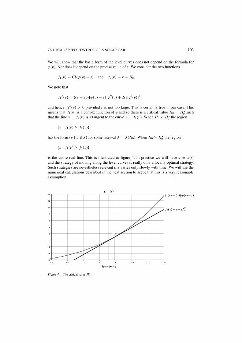
We will show that the basic form of the level curves does not depend on the formula forϕ(v). Nor does it depend on the precise value of s. We consider the two functions

f1(v) = CI(ϕ(v) − s) and f2(v) = v − H0.

We note that

f1′′(v) = {c1 + 2c2[ϕ(v) − s]}ϕ′′(v) + 2c2[ϕ′(v)]2

and hence f1′′(v) > 0 provided s is not too large. This is certainly true in our case. This

means that f1(v) is a convex function of v and so there is a critical value H0 = H �0 such

that the line y = f2(v) is a tangent to the curve y = f1(v). When H0 < H �0 the region

{v | f1(v) ≥ f2(v)}

has the form {v | v /∈ J } for some interval J = J (H0). When H0 ≥ H �0 the region

{v | f1(v) ≥ f2(v)}

is the entire real line. This is illustrated in figure 4. In practice we will have s = s(t)and the strategy of moving along the level curves is really only a locally optimal strategy.Such strategies are nevertheless relevant if s varies only slowly with time. We will use thenumerical calculations described in the next section to argue that this is a very reasonableassumption.

1 4

1 2

1 0

8

6

4

2

0

- 2

- 4

- 61201101009 08 07 06 05 0

Speed (km/h)

f1(v) = C I(ϕ (v) – s)ϕ −1(s)

f2(v) = v – H0 *

v*

Figure 4. The critical value H �0 .

104 PUDNEY AND HOWLETT

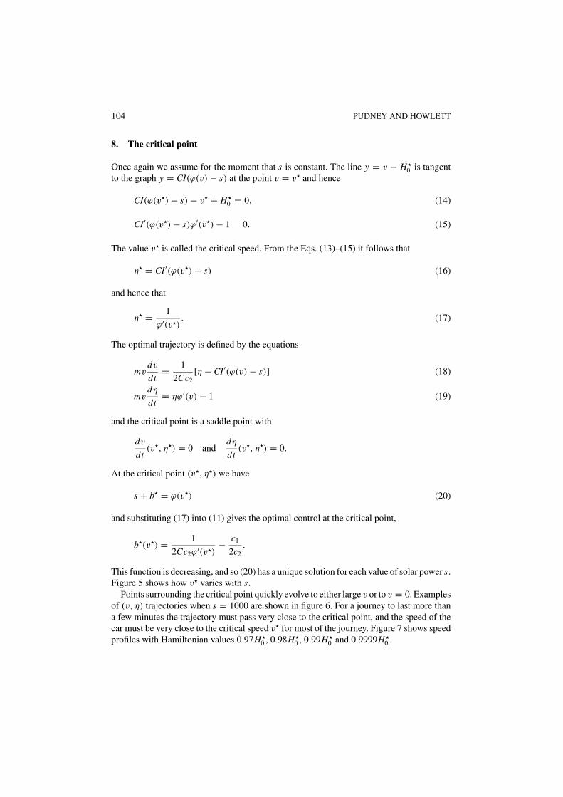
8. The critical point

Once again we assume for the moment that s is constant. The line y = v − H �0 is tangent

to the graph y = CI(ϕ(v) − s) at the point v = v� and hence

CI(ϕ(v�) − s) − v� + H �0 = 0, (14)

CI′(ϕ(v�) − s)ϕ′(v�) − 1 = 0. (15)

The value v� is called the critical speed. From the Eqs. (13)–(15) it follows that

η� = CI′(ϕ(v�) − s) (16)

and hence that

η� = 1

ϕ′(v�). (17)

The optimal trajectory is defined by the equations

mvdv

dt= 1

2Cc2[η − CI′(ϕ(v) − s)] (18)

mvdη

dt= ηϕ′(v) − 1 (19)

and the critical point is a saddle point with

dv

dt(v�, η�) = 0 and

dη

dt(v�, η�) = 0.

At the critical point (v�, η�) we have

s + b� = ϕ(v�) (20)

and substituting (17) into (11) gives the optimal control at the critical point,

b�(v�) = 1

2Cc2ϕ′(v�)− c1

2c2.

This function is decreasing, and so (20) has a unique solution for each value of solar power s.Figure 5 shows how v� varies with s.

Points surrounding the critical point quickly evolve to either large v or to v = 0. Examplesof (v, η) trajectories when s = 1000 are shown in figure 6. For a journey to last more thana few minutes the trajectory must pass very close to the critical point, and the speed of thecar must be very close to the critical speed v� for most of the journey. Figure 7 shows speedprofiles with Hamiltonian values 0.97H �

0 , 0.98H �0 , 0.99H �

0 and 0.9999H �0 .

CRITICAL SPEED CONTROL OF A SOLAR CAR 105

solar power (W)

critical speed (km/h)

9 2

9 1

9 0

8 9

8 8

8 7

8 6

8 5150010005000

Figure 5. The critical speed v� increases with solar power.

0 10 20 30 40 50 60 70 80 90 100 110 1200

1

2

3

4

5

6

7

8

9

10

11

12

speed (km/h)

η (x1000)

Figure 6. For each value of solar power the vector field (v, η) has a unique saddle point (v�, η�). Points sur-rounding the saddle point quickly evolve to either large v or to v < 0. Journeys starting and finishing at v = 0follow a trajectory from the top left corner of the graph to the bottom left corner of the graph. Any journey lastingmore than a few minutes must travel at a speed very close to the critical speed v� for most of the journey.

106 PUDNEY AND HOWLETT

9 0

8 0

7 0

6 0

5 0

4 0

3 0

2 0

1 0

01201101009 08 07 06 05 04 03 02 01 00

Speed (km/h)

Time (s)

(220s)

Figure 7. Speed profiles must pass very close to the critical speed if the journey is to last more than a few seconds.The graph shows speed profiles with Hamiltonian values 0.97H �

0 , 0.98H �0 , 0.99H �

0 and 0.9999H �0 ; even this final

trajectory lasts only 220 seconds.

Since our investigation is directed at finding a journey that lasts for several hours we cansee immediately that a practical strategy must effectively follow the critical point for mostof the time. In practice there should be

– a power phase lasting at most a few minutes while we follow a level curve, using theinitial value of s, from v = 0 to a neighbourhood of the critical point;

– a hold phase lasting for almost the entire journey during which time we follow the criticalpoint and hold at the critical speed; and

– a brake phase lasting at most a few minutes while we follow a level curve, using the finalvalue of s, from a neighbourhood of the critical point to v = 0.

Of course the position of the critical point and the value of the critical speed evolve slowlywith time.

9. Critical curves

The level curve H = H �0 passes through the critical point. Near the critical point we have

I ′(ϕ(v) − s) ≈ I ′(ϕ(v�) − s) + [I ′(ϕ(v) − s)]′(v�)[v − v�]

and

I (ϕ(v) − s) − v − H �0 ≈ 1

2[I (ϕ(v) − s)]′′(v�)[v − v�]2

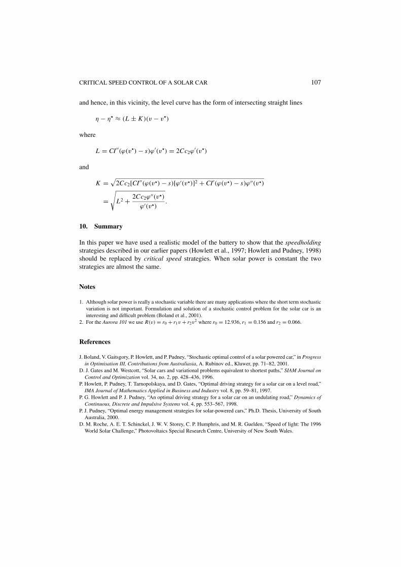
CRITICAL SPEED CONTROL OF A SOLAR CAR 107

and hence, in this vicinity, the level curve has the form of intersecting straight lines

η − η� ≈ (L ± K )(v − v�)

where

L = CI′′(ϕ(v�) − s)ϕ′(v�) = 2Cc2ϕ′(v�)

and

K =√

2Cc2[CI′′(ϕ(v�) − s)[ϕ′(v�)]2 + CI′(ϕ(v�) − s)ϕ′′(v�)

=√

L2 + 2Cc2ϕ′′(v�)

ϕ′(v�).

10. Summary

In this paper we have used a realistic model of the battery to show that the speedholdingstrategies described in our earlier papers (Howlett et al., 1997; Howlett and Pudney, 1998)should be replaced by critical speed strategies. When solar power is constant the twostrategies are almost the same.

Notes

1. Although solar power is really a stochastic variable there are many applications where the short term stochasticvariation is not important. Formulation and solution of a stochastic control problem for the solar car is aninteresting and difficult problem (Boland et al., 2001).

2. For the Aurora 101 we use R(v) = r0 + r1v + r2v2 where r0 = 12.936, r1 = 0.156 and r2 = 0.066.

References

J. Boland, V. Gaitsgory, P. Howlett, and P. Pudney, “Stochastic optimal control of a solar powered car,” in Progressin Optimisation III, Contributions from Australiasia, A. Rubinov ed., Kluwer, pp. 71–82, 2001.

D. J. Gates and M. Westcott, “Solar cars and variational problems equivalent to shortest paths,” SIAM Journal onControl and Optimization vol. 34, no. 2, pp. 428–436, 1996.

P. Howlett, P. Pudney, T. Tarnopolskaya, and D. Gates, “Optimal driving strategy for a solar car on a level road,”IMA Journal of Mathematics Applied in Business and Industry vol. 8, pp. 59–81, 1997.

P. G. Howlett and P. J. Pudney, “An optimal driving strategy for a solar car on an undulating road,” Dynamics ofContinuous, Discrete and Impulsive Systems vol. 4, pp. 553–567, 1998.

P. J. Pudney, “Optimal energy management strategies for solar-powered cars,” Ph.D. Thesis, University of SouthAustralia, 2000.

D. M. Roche, A. E. T. Schinckel, J. W. V. Storey, C. P. Humphris, and M. R. Guelden, “Speed of light: The 1996World Solar Challenge,” Photovoltaics Special Research Centre, University of New South Wales.