
CRC Report No. DP-07-16-1 Identification of Potential ...
402
COORDINATING RESEARCH COUNCIL, INC. 5755 NORTH POINT PARKWAY ● SUITE 265 ● ALPHARETTA, GA 30022 CRC Report No. DP-07-16-1 Identification of Potential Parameters Causing Corrosion of Metallic Components in Diesel Fuel Underground Storage Tanks Final Report July 2021
-
Upload
khangminh22 -
Category
Documents
-
view
4 -
download
0
Transcript of CRC Report No. DP-07-16-1 Identification of Potential ...

COORDINATING RESEARCH COUNCIL, INC. 5755 NORTH POINT PARKWAY ● SUITE 265 ● ALPHARETTA, GA 30022
CRC Report No. DP-07-16-1
Identification of Potential Parameters Causing Corrosion of Metallic
Components in Diesel Fuel Underground Storage Tanks
Final Report
July 2021

ii
The Coordinating Research Council, Inc. (CRC) is a non-profit corporation supported by the petroleum and automotive equipment industries. CRC operates through the committees made up of technical experts from industry and government who voluntarily participate. The four main areas of research within CRC are: air pollution (atmospheric and engineering studies); aviation fuels, lubricants, and equipment performance; heavy-duty vehicle fuels, lubricants, and equipment performance (e.g., diesel trucks); and light-duty vehicle fuels, lubricants, and equipment performance (e.g., passenger cars). CRC’s function is to provide the mechanism for joint research conducted by the two industries that will help in determining the optimum combination of petroleum products and automotive equipment. CRC’s work is limited to research that is mutually beneficial to the two industries involved. The final results of the research conducted by, or under the auspices of, CRC are available to the public.
LEGAL NOTICE
This report was prepared by Battelle and Frederick J. Passman, PhD as an account of work sponsored by the Coordinating Research Council (CRC). Neither the CRC, members of the CRC, Battelle, nor any person acting on their behalf: (1) makes any warranty, express or implied, with respect to the use of any information, apparatus, method, or process disclosed in this report, or (2) assumes any liabilities with respect to use of, inability to use, or damages resulting from the use or inability to use, any information, apparatus, method, or process disclosed in this report. In formulating and approving reports, the appropriate committee of the Coordinating Research Council, Inc. has not investigated or considered patents which may apply to the subject matter. Prospective users of the report are responsible for protecting themselves against liability for infringement of patents.

iii
(Page intentionally left blank)

iv
Identification of Potential Parameters Causing Corrosion of Metallic Components in Diesel Fuel
Underground Storage Tanks
Final Report
Battelle does not engage in research for advertising, sales promotion, or endorsement of our clients’ interests including raising investment capital or recommending investments decisions, or other publicity purposes, or for any use in litigation.
Battelle endeavors at all times to produce work of the highest quality, consistent with our contract commitments. However, because of the research and/or experimental nature of this work the client undertakes the sole responsibility for the consequence of any use or misuse of, or inability to use, any information, apparatus, process or result obtained from Battelle, and Battelle, its employees, officers, or Trustees have no legal liability for the accuracy, adequacy, or efficacy thereof.

v
(Page intentionally left blank)

vi
TABLE OF CONTENTS
1 CONTENTS
1 Contents vi List of Figures ix
List of Tables xi Acronyms and Abbreviations xiv
Executive Summary xix
1 Introduction 1
1.1 Background ......................................................................................................................... 1
1.2 Problem Definition.............................................................................................................. 2
1.3 Project Organization ........................................................................................................... 3
1.4 Project Objectives ............................................................................................................... 3
2 Experimental Methods 3
2.1 Experimental Design ........................................................................................................... 3
2.2 Fuel Additive Partition Coefficient Determination............................................................. 4
2.3 Corrosion Coupon Preparation ........................................................................................... 6
Steel Coupons 6
Fiber-Reinforced Polymer Coupons 7
2.4 Microbiological Challenge Population Development ......................................................... 7
Challenge Population Sources 7
Primary Microcosms 7
Secondary Microcosms 8
2.5 Test Microcosm Preparation ............................................................................................... 8
Fuels 8
Additives 8
Test Microcosm Assembly 9
2.6 Observations and testing ................................................................................................... 10
Periodic Observations 10
Gross Observations 11
Microcosm Sampling 13
Chemistry Testing – Gas Chromatography-Mass Spectrometry 15
Corrosion Testing 16
Microbiological Testing 17

vii
2.7 Statistical Analysis ............................................................................................................ 20
Logistic Regression Analysis 20
Analysis of Variance 20
Stepwise Regression Analysis 20
3 Results and Discussion 22
3.1 Test Plan Development ..................................................................................................... 22
3.2 STOCK Fuel Chemistry .................................................................................................... 25
3.3 Partition coefficient testing ............................................................................................... 25
3.4 Statistical Analysis ............................................................................................................ 29
Background 29
Tier 1 - Stepwise Ordinal Logistic Regression for Aqueous-Fuel Interface 29
Tier 2 - Stepwise Regression of Corrosion Rating Changes between T0 and T6wk. 37
Tier 3 -Semi-quantitative Analysis of Microcosms Containing Steel Coupons that Exhibited High Corrosion Severity 41
3.5 Microcosm Gross Observations ........................................................................................ 45
Conceptual Overview 45
Observations 45
3.6 Corrosion........................................................................................................................... 50
Coupon Corrosion Ratings 50
General Corrosion Rate – Coupon Weight Loss 51
Corrosion Morphology and Elemental Composition 54
3.7 Microbiology..................................................................................................................... 75
Overview 75
Adenosine Triphosphate 75
Microscopy 84
Genomics 86
3.8 Chemistry .......................................................................................................................... 96
Sulfur Concentration 96
Vapor-phase Low Molecular Weight Organic Acids 96
Aqueous-phase Low Molecular Weight Organic Acids 96
Aqueous-phase alcohols 100
Surfactant 101
3.9 Results Summary ............................................................................................................ 110
Microcosm Design 110
Fractional-factorial Test Plan 110

viii
Relationships between Controlled Variables and Corrosion 110
Relationships between Controlled Variables and Gross Observations 111
Relationships among Uncontrolled Variables 111
4 Lessons Learned 113
4.1 Test Plan and Microcosm Design ................................................................................... 113
Fuel preparation 114
4.2 Analysis........................................................................................................................... 115
Subset Selection 115
Corrosion Ratings 115
Microbiology 115
Data Interpretation 116
5 Conclusions 117
5.1 Primary factors affecting corrosivity in fuel microcosms............................................... 117
5.2 Independent variable Interactions ................................................................................... 117
6 Recommendations 117
6.1 Microcosm Design .......................................................................................................... 117
6.2 Specimen Collection ....................................................................................................... 118
6.3 Independent Factor Selection .......................................................................................... 118
6.4 Test plan design .............................................................................................................. 118
6.5 Dependent variables ........................................................................................................ 119
7 References 120
8 Glossary 126
APPENDICES APPENDIX A Microcosm Test Condition Matrix APPENDIX B LC-MS Test Method Parameters APPENDIX C Statistical Data Analysis APPENDIX D Statistical Data Analysis – Ln-transformed data APPENDIX E Gross Observations of Microcosms APPENDIX F Coupon Observations APPENDIX G GCR Data APPENDIX H cATP Data APPENDIX I Microscopy Data Whole APPENDIX J Genomic Data APPENDIX K Chemical Analyses ATTACHMENT 1 Passman et al. [48]

ix
LIST OF FIGURES
Figure 1.Partitioning experiment with 99:1 fuel to water ratio, after 24h. ................................................... 5 Figure 2. Coupons used in test microcosms – a) Low carbon steel coupon (face view); b) FRP coupon
(face view); c) FRP coupon (side view). ..................................................................................... 7 Figure 3. Partial view of test microcosm array – Right: LSD microcosms; Left ULSD microcosms. ....... 10 Figure 4. Test microcosm set-up – a) schematic showing coupon and acid indicator array; b) water-free
(two-phase), ULSD microcosm at week 1; c) water-containing (three-phase) ULSD microcosm at week 2. ............................................................................................................... 10
Figure 5. Corrosion coupons from microcosm 101 at week 12 – suspended from stand used to photograph coupons. .................................................................................................................................... 12
Figure 6. Week 12, microcosm bottom-view images – a) microcosm 59 (B5 LSD over aqueous-phase); b) microcosm 55 (B0 LSD over aqueous-phase). ......................................................................... 13
Figure 7. Positioning of Dräger tube in three-phase microcosm – a) Dräger tube in microcosm 114 showing inlet positioned approximately 3 cm above fuel-aqueous-phase interface; b) close-up view of Dräger tube. ................................................................................................................. 15
Figure 8. Flow diagram part 1 – observation-based testing – gross observations. ..................................... 26 Figure 9. Flow diagram part 2 – observation-based testing – physical, chemical, and microbiological tests.
.................................................................................................................................................. 27 Figure 10. Flow diagram part 3 – observation-based testing – additional physical, chemical, and
microbiological tests. ................................................................................................................ 27 Figure 11. PCRI=5 (vertical axis) versus exposure period (weeks) – from Appendix C, page C-59. ............ 33 Figure 12. Relationship between CI and PCR≥3 with and without CI-treatment ........................................... 33 Figure 13. Corrosion coupons – a) through f): Microcosm 1, coupon 1-2, at weeks 1, 2, 3, 4, 6, and 12; g)
through l) Microcosm 4, coupon 4-2, at weeks 1, 2, 3, 4, 6, and 12. ........................................ 37 Figure 14. Impact of CI on ∆CR week-1 – from Appendix D, page D-6. ................................................... 40 Figure 15. Comparison of weekly CRavg between CI-treated and CI-untreated microcosms – from
Appendix D, page D-6. ............................................................................................................. 40 Figure 16. CI-microbial challenge interaction effect – a) microbially challenged microcosms; b)
unchallenged microcosms (from Appendix D, page D-7). ....................................................... 40 Figure 17. CR rating frequencies by week – a) aqueous-phase exposure; b) aqueous-fuel interface
exposure. ................................................................................................................................... 44 Figure 18. Microcosm gross observations – a) through c) microcosm 1 at Twk3, Twk6, and Wwk12 (all RSGO
= 0); d) through f) microcosm 3 at Twk3, Twk6, and Wwk12 (all RSGO = 5); g) microcosm 1, bottom view at Twk12; h) microcosm 3, bottom view at Twk12. .................................................. 46
Figure 19. Microcosm 19 corrosion coupons with CR provided ................................................................ 51 Figure 20. EDS basics – a) x-ray emission lines; b) example of EDS spectrograph. ................................. 60 Figure 21. Optical micrograph of microcosm #35 specimen with annotated regions of interest. ............... 61 Figure 22. Microcosm #35 – a) SEM micrograph of aqueous-phase corrosion product; b) overall EDS
data; c) spot scan (1) EDS data (area ≈ 0.14 mm2). .................................................................. 61 Figure 23. Microcosm #35 – a) SEM micrograph of aqueous-fuel interface corrosion product; b) overall
EDS data, c) spot scan (1) EDS data (aera ≈ 0.26 mm2). .......................................................... 61 Figure 24. Microcosm #35 – a) SEM micrograph of fuel-phase corrosion product; b), overall EDS data; c)
spot scan (1) EDS data (area ≈ 0.07 mm2). ............................................................................... 62 Figure 25. Optical micrograph of microcosm #40 specimen. ..................................................................... 62 Figure 26. Microcosm #40 – a) SEM micrograph of aqueous-phase corrosion product; b) overall EDS
data; c) spot scan (1) EDS data. ................................................................................................ 63 Figure 27. Microcosm #40 – a): SEM micrograph of aqueous-fuel interface corrosion product; b) overall
EDS data – no heterogeneity observed. .................................................................................... 63

x
Figure 28. Microcosm #40 – a) SEM micrograph of fuel-phase corrosion product; b) overall EDS data; c) spot scan (1) EDS data. ............................................................................................................. 63
Figure 29. Optical micrograph of microcosm #77 specimen. ..................................................................... 65 Figure 30. Microcosm #77 – a) SEM Micrograph of aqueous-phase corrosion product; b) overall EDS
data; c) spot scan (1) EDS data. ................................................................................................ 65 Figure 31. Microcosm #77 – a) SEM micrograph of aqueous-fuel interface corrosion product; b) overall
EDS data; c) spot scan (1) EDS data......................................................................................... 65 Figure 32. Microcosm #77 – a) SEM micrograph of fuel-phase corrosion product; b) overall EDS data; c)
spot scan (1) EDS data. ............................................................................................................. 66 Figure 33. Optical micrograph of microcosm #85 specimen. ..................................................................... 67 Figure 34. Microcosm #85 – a) SEM micrograph of aqueous-phase corrosion product; b) overall EDS
data – no heterogeneity observed. ............................................................................................. 67 Figure 35. Microcosm #85 – a) SEM micrograph of aqueous-fuel interface corrosion product; b) overall
EDS data – no heterogeneity observed. .................................................................................... 67 Figure 36. Microcosm #85 – a) SEM micrograph of fuel-phase corrosion product; b) overall EDS data –
no heterogeneity observed. ....................................................................................................... 68 Figure 37. Optical micrograph of microcosm #100 specimen. ................................................................... 68 Figure 38. Microcosm #100 – a) SEM micrograph of aqueous-phase corrosion product; b) overall EDS
data; c) spot scan (1) EDS data. ................................................................................................ 69 Figure 39. Microcosm #100 – a) SEM micrograph of aqueous-fuel interface corrosion product; b) overall
EDS data – no heterogeneity observed. .................................................................................... 69 Figure 40. Microcosm #100 – a) SEM micrograph of fuel-phase corrosion product; b) overall EDS data;
c) spot scan (1) EDS elemental data. ........................................................................................ 69 Figure 41. Optical micrograph of microcosm #105 specimen. ................................................................... 70 Figure 42. Microcosm #105 – a) SEM micrograph of aqueous-phase corrosion product; b) overall EDS
data; c) spot scan (1) EDS data. ................................................................................................ 70 Figure 43. Microcosm #105 – a) SEM micrograph of aqueous-fuel interface corrosion product; b) overall
EDS data; c) spot scan (1) EDS data......................................................................................... 71 Figure 44. Microcosm #105 – a) SEM micrograph of fuel-phase corrosion product; b) overall EDS data;
c) spot scan (1) EDS data. ......................................................................................................... 71 Figure 45. Microcosm #105 – a) SEM micrograph of vapor-phase corrosion product (inset - ~310 mm2
area around hole through which monofilament from which coupon hung was threaded) ; b) overall EDS data; c) spot scan (1) EDS data. ........................................................................... 71
Figure 46. Optical micrograph of microcosm #109 specimen. ................................................................... 72 Figure 47. Microcosm #109 – a) SEM micrograph of aqueous-phase corrosion product; b) overall EDS
data; c) spot scan (1) EDS data. ................................................................................................ 72 Figure 48. Microcosm #109 – a) SEM micrograph of aqueous-fuel interface corrosion product; b) overall
EDS data; c) spot scan (1) EDS data......................................................................................... 72 Figure 49. Microcosm #109 – a) SEM micrograph of fuel-phase corrosion product; b) overall EDS data;
c) spot scan (1) EDS data. ......................................................................................................... 73 Figure 50. Microcosm #109 – a) SEM micrograph of fuel-phase (∼2 cm to 3 cm above fuel-water
interface) corrosion product (inset – unmeasured area near coupon edge); b) overall EDS data; c) spot scan (1) EDS data. ......................................................................................................... 73
Figure 51. Log10 [cATP] ([𝒄𝒄𝒄𝒄𝒄𝒄𝒄𝒄] ± s) versus time (weeks) between T0 and Twk9 (black line – intentionally challenged; blue line – unchallenged).................................................................. 78
Figure 52. Planktonic ATP-bioburden profile in fuel over aqueous-phase microcosm. Averages and ranges are for 20 microcosms. .................................................................................................. 80
Figure 53. Sessile ATP-bioburden profile on low-carbon steel corrosion coupons in fuel over aqueous-phase microcosms. Averages and ranges are for 18 microcosms. ........................................... 81
Figure 54. Primary morphological features used to classify molds ............................................................ 84 Figure 55. Taxonomic tree of fungal taxa detected in test microcosms. ..................................................... 85

xi
Figure 56. Illustrative microscopic images of fungal growth from microcosms #56 and #61.................... 86 Figure 57. Krona plot for microcosm 40, illustrating significance of each ring. ........................................ 90 Figure 58. Venn diagram illustrating differences among the three microbial populations recovered from
microcosms. .............................................................................................................................. 95 Figure 59. Venn diagrams of taxonomic profile similarities between replicate specimens – a) microcosm
45; b) microcosm 81. ................................................................................................................ 95 Figure 60. Acetic acid Dräger tube -a) schematic from manufacturer’s instruction sheet; b) simulation of
color change when acetic acid concentration is ∼7 ppmv (mg m-1) in sampled air. ................. 96 Figure 61. Relationship between aqueous-phase and interface corrosion coupon corrosion ratings and
[LMOA] – - CRAQ; ° - CRI. .................................................................................................. 100 Figure 62. Surfactants – a) schematic of surfactant molecule showing polar head and nonpolar tail; b)
schematic of invert-emulsion micelle showing polar heads encapsulating water droplet and nonpolar tails extending into the medium (i.e., fuel); c) schematic of invert emulsion micelles dispersed in fuel; d) photo of 10 mL each fuel and water – left: before shaking; right: 24h after shaking (note stability of invert emulsion). ............................................................................ 102
Figure I.1 Microscopic Images of Selected Microcosm Samples. Figure J.1 Krona Plot of Metagenomic Sequencing Results of Microcosms #3 and #4. Figure J.2 Krona Plot of Metagenomic Sequencing Results of Microcosms #21 and #28. Figure J.3 Krona Plot of Metagenomic Sequencing Results of Microcosms #32 and #36. Figure J.4 Krona Plot of Metagenomic Sequencing Results of Microcosms #40. Figure J.5 Krona Plot of Metagenomic Sequencing Results of Microcosms #45A and #45B. Figure J.6 Krona Plot of Metagenomic Sequencing Results of Microcosms #46 and #47. Figure J.7 Krona Plot of Metagenomic Sequencing Results of Microcosms #48 and #56. Figure J.8 Krona Plot of Metagenomic Sequencing Results of Microcosms #57 and #78. Figure J.9 Krona Plot of Metagenomic Sequencing Results of Microcosms #81A and #81B. Figure J.10 Krona Plot of Metagenomic Sequencing Results of Microcosms #102 and #110. Figure J.11 Krona Plot of Metagenomic Sequencing Results of Microcosms #126 and #127.
LIST OF TABLES
Table 1. Fractional factorial test plan – number of microcosms containing each controlled factor. ............ 5 Table 2. Partition coefficient determination test plan. ................................................................................. 6 Table 3. Additive and contaminant concentrations in test fuels. .................................................................. 9 Table 4. Test microcosm gross observation parameters and risk scores. .................................................... 11 Table 5. Microcosms Tested for All Parameters at T0 ................................................................................ 14 Table 6. Summary of Analytical Methods and Sampling Frequency by Sample Type .............................. 14 Table 7. Fractional Factorial Test Plan – Controlled Variables in 128 Microcosms. ................................. 21 Table 8. Fuel and Fuel Additive Partition Test Results – Impact of LSD to Water Ratios on Aqueous-
Phase Conductivity (µS cm-1) All values are averages ± standard deviations. ......................... 28 Table 9. Two-way ANOVA – Five additive treatments x two fuel to water ratios – summary statistics
(sums, averages and variances are conductivities in µS cm-1). ................................................. 28 Table 10. Two-way ANOVA – Five additive treatments x two fuel to water ratios – ANOVA. ............... 29 Table 11. Relationships between independent variables and CR – 12-week microcosm study. ................ 31 Table 12. Summary ANOVA statistics, stepwise regression – aqueous-fuel interface 12-week microcosm
study at T12wk and throughout 12-week exposure period. ......................................................... 32 Table 13. Relationships between independent and dependent variables – 12-week microcosm study. ..... 34

xii
Table 14. Summary ANOVA statistics, stepwise regression between independent and dependent variables – 12-week microcosm study. .................................................................................................... 35
Table 15. ANOVA, F-test summary statistics for week to week ∆CR dt-1 between Twk1 and Twk6. ........... 38 Table 16. Effect of microbial challenge on CR between weeks 1 and 4 – summary statistics. Values are
CRAVG ± s. ................................................................................................................................... 39 Table 17. Effect of microbial challenge on CR between weeks 1 and 4 – ANOVA summary. ................ 39 Table 18. Tier 3 statistical analysis - corrosion rating scenarios. ............................................................... 43 Table 19. Gross observation, overall risk scores (RSGO) for microcosms at weeks 3, 4, 6, 9, and 12. ....... 47 Table 20. Relationship between microcosm gross observation risk scores (RSGO) and corrosion ratings
(CR). ......................................................................................................................................... 49 Table 21. Relationship between microcosm gross observation and [ATP]-based risk scores (RSGO and
RSATP, respectively). ................................................................................................................. 50 Table 22. Test condition profiles in microcosms with greatest and least (𝑮𝑮𝑮𝑮𝑮𝑮 ± s). ................................. 52 Table 23. Test condition profiles in microcosms with greatest and least GCRmax. ..................................... 53 Table 24. Correlation coefficients among dependent variables – [ATP], CGRStd and CR. ......................... 54 Table 25. Corrosion product analysis microcosm subset – independent variable profiles. a ...................... 54 Table 26. Corrosion product analysis microcosm subset –dependent variable profiles. ............................ 55 Table 27. Corrosion deposit elemental analysis by EDS. All values are in wt. %. .................................... 56 Table 28. Corrosion deposit elemental profile correlation coefficients (|r|crit [5 df; α =0.05] = 0.75). Significant
correlation coefficients are highlighted in bold font. ................................................................ 58 Table 30. ATP-bioburdens in ULSD UST bottoms-water samples. ........................................................... 76 Table 31. ATP-bioburdens in aqueous-phases of 1° and 2° microcosms. .................................................. 76 Table 36. Controlled variable profiles of challenged and unchallenged microcosms with aqueous-phase
[cATP]min and [cATP]max at Twk12. ............................................................................................. 79 Table 37. ATP-bioburden correlation coefficients between planktonic and sessile populations in different
microcosm phases. .................................................................................................................... 81 Table 38. ANOVA Summary effect of controlled variables on Twk12 aqueous-phase [cATP]. .................. 82 Table 344. Population diversity differences between challenged and unchallenged microcosms (Fcrit[1,19; α =
0.05] = 4.38). ................................................................................................................................ 89
Table A.1 Fractional factorial fuel corrosivity test plan – microcosm details. Table E.1 Gross observations of 128-jars set up in the microcosm study. Table F.1 Zonal observations in coupon samples 1-3 in the microcosm test. Table G.1 Cumulative average GCR data per microcosm. Table G.2 Cumulative Maximum GCR Data per Microcosm. Microcosm # are Rank Ordered and Color-Coded Dependent on the Severity of Mass Loss (Red – highest, Green – Lowest). Table H.1 cATP data for microcosm samples collected on days 0 and 30. Table H.2 cATP data for microcosm samples collected on day 67. Table H.3 cATP data for microcosm samples collected on day 120. Table H.1 Microscopy – specimen descriptions and interpretive notes. Table I.1 Microscopy – specimen descriptions and interpretive notes. Table J.1 Genomic profile UST Bottoms-water Sample I by Whole Genome Sequencing Analysis. Table J.2 Genomic profile UST Bottoms-water Sample II by Whole Genome Sequencing Analysis. Table J.3 Microbial Diversity in Microcosm # 3 Sample. Table J.4 Microbial Diversity in Microcosm # 4 Sample. Table J.5 Microbial Diversity in Microcosm # 21 Sample. Table J.6 Microbial Diversity in Microcosm # 21 Sample. Table J.7 Microbial Diversity in Microcosm # 28 Sample. Table J.8 Microbial Diversity in Microcosm # 32 Sample.

xiii
Table J.9 Microbial Diversity in Microcosm # 36 Sample. Table J.10 Microbial Diversity in Microcosm # 40 Sample. Table J.11 Microbial Diversity in Microcosm # 45A Sample. Table J.12 Microbial Diversity in Microcosm # 45B Sample. Table J.13 Microbial Diversity in Microcosm # 46 Sample. Table J.14 Microbial Diversity in Microcosm # 47 Sample. Table J.15 Microbial Diversity in Microcosm # 48 Sample. Table J.16 Microbial Diversity in Microcosm # 56 Sample. Table J.17 Microbial Diversity in Microcosm # 57 Sample. Table J.18 Microbial Diversity in Microcosm #78 Sample. Table J.19 Microbial Diversity in Microcosm #81A Sample. Table J.20 Microbial Diversity in Microcosm #81B Sample. Table J.21 Microbial Diversity in Microcosm #102 Sample. Table J.22 Microbial Diversity in Microcosm #110 Sample. Table J.23 Microbial Diversity in Microcosm #126 Sample. Table J.24 Microbial Diversity in Microcosm #127 Sample.

xiv
ACRONYMS AND ABBREVIATIONS
[A] additive concentration
ACC American Chemical Council
ANOVA analysis of variance
AST aboveground storage tank
ATP adenosine triphosphate
BDL below detection limit
BLAST Basic Local Alignment Search Tool
bp base pair
BX biodiesel blend, where X is the vol % FAME in diesel fuel
C carbon
CA conductivity additive
cATP cell-bound ATP (cellular ATP)
CDFA Clean Diesel Fuel Alliance
CFI cold flow improver
CI corrosion inhibitor
CRC Coordinating Research Council, Inc.
CRX corrosion coupon corrosion rating on, where X is the substance with which the coupon surface is in contact. For example, CRI is the corrosion rating at the fuel-aqueous-phase interface and CRAQ is the rating on coupon surfaces in the aqueous-phase.
CX number of carbon atoms in a molecule
DNA deoxyribonucleic acid
DPG Diesel Performance Group
DQO data quality objective
DSATM Deposit & Surface Analysis
E evenness
EDS energy dispersive spectroscopy
EH Shannon’s equitability
EPA U.S. Environmental Protection Agency
EX ethanol blend, where X is the vol % ethanol in gasoline
FAME fatty acid methyl ester

xv
FATG Fuel Additive Technology Group
FCP fuel corrosivity panel
Fe iron
FRP fiber reinforced polymer
FTPI Fiberglass Tank and Pipe Institute
GC gas chromatography
GC-FID gas chromatography – flame ionization detector
GC-MS gas chromatography – mass spectrometry
GCR general corrosion rate
GLY glycerin
GNP gross national product
H Shannon-Wiener diversity index
HSD high sulfur diesel
ITS internal transcribed spacer
K potassium
LSD low sulfur diesel
LMOA low molecular weight organic acids
LMW low molecular weight
LMWA low molecular weight acids
MAL mono-acid, lubricity
MIC microbiologically influenced corrosion
MS mass spectrometry
NACE National Association of Corrosion Engineers
NaCl sodium chloride
NBB National Biodiesel Board
NCH Nationwide Children’s Hospital
NGS next generation sequencing
OTU operational taxonomic unit
OUST Office of Underground Storage Tanks
P phosphorous
PCR polymerase chain reaction

xvi
pi proportion of total sample represented by an individual species (OTU)
ppm part per million
PTFE polytetrafluoroethylene
QAPP Quality Assurance Project Plan
QC quality control
qPCR quantitative PCR
RLU relative light unit
RNA ribonucleic acid
RSGO gross observation based risk score
S sulfur; also, species (OTU) richness
SEM scanning electron microscopy
SME subject matter expert
SOP standard operating procedure
STI Steel Tank Institute
STP submersible turbine pump
tATP total ATP
TDS total dissolved solids
Twk X Test interval – week after which microcosms were started, where X is the week number.
ULSD ultra-low-sulfur diesel
UST underground storage tank
UV ultraviolet
w weight (mass) fraction as %
WGS Whole Genome Sequencing
XRD X-ray diffraction

xvii
ACKNOWLEDGEMENTS
This report represents the results and conclusions from an effort between scientists and engineers represented by the Coordinating Research Council, Inc. (CRC) Diesel Performance Group (DPG) DP-07-16-1 Project Panel. and the Battelle Memorial Institute (Columbus, OH). The members of the FCP include representatives from industry associations, equipment manufacturers, fuel vendors, and service/contractor organizations. This project was funded by the CRC with the goal of determining the actual relationship between the presence of different diesel fuel grades and common contaminants, and fuel system component corrosion.
Battelle Technical Team
CRC Project DP-07-16-1 Panel Membership:
Bera, Tushar Shell
Beu, Paul WaWa
Broughton, Shawn Marathon Petroleum
Chapman, Rick Fuel Quality Consultants
Eckstrom, John C BP
Eichberger, John Fuels Institute
English, Edward W FQS Inc.
Fenwick, Scott Biodiesel Board
Golisz, Suzanne R. ExxonMobil
Gunter, Garry Phillips 66
Haerer, Ryan US EPA
Hernandez, Sandra Chevron
Hove, Jeff Fuels Institute
Howell, Steve Marc IV
Huang, Chung-Hsuan Cummins
Kass, Mike Oak Ridge National Lab
Lax, David API
Lewis, Russ Marathon Petroleum
Long, Rick PEI
Martinez, Jo Chevron
McNutt, Ryan Sigma
Moriarty, Kristi NREL
Mukkada, Nick Chevron
Passman, Fred Consultant
Pollock, Steve Steel Tank
Raney-Pablo, Beth Ford
Renkes, Bob Fiberglass Tank and Pipe
Ryzyi, Sheila (S.M.) Ford
Searles, Prentiss API
Spiker, Keith QuikTrip
Sutton, Tia EMA
James, Ryan, PhD (PM) Gemler, Bryan Koebel, David Cafmeyer, Jeff Gregg, Anne Kucharzyk, Kate, PhD (PI) Eastwood, Stephanie, PhD Hill, Amy Triplett, Cheryl, PhD Garbark, Dan James, Joshua, PhD

xviii
(Page intentionally left blank)

xix
EXECUTIVE SUMMARY
A considerable amount of anecdotal evidence indicated that since 2007, the incidence of corrosion-related, diesel fuel underground storage tank (UST) component failures has increased substantially. Two previous studies were inconclusive, but both postulated that the primary factors contributing to UST system corrosion were diesel fuel sulfur content, free-water, microbial contamination, and presence of ethanol. Both previous studies used data obtained from a limited number of retail and fleet fueling sites.
The CRC Fuel Corrosivity Panel sponsored a laboratory study recognizing that the cost of conducting a third survey of several hundred UST would be no more conclusive than the previous two field efforts. The ultimate test plan was a fractional-factorial design that included eleven independent (controlled) variables: water, sulfur concentration (low-sulfur – LSD – versus ultra-low-sulfur – ULSD – diesel fuel), biodiesel (soy-based, fatty acid methyl ester – FAME), glycerin, ethanol, microbial contamination, common fuel additives (cold flow improver - CFI, conductivity additive – CA, corrosion inhibitor – CI, and a mono-acid lubricity additive – MAL), and fiber-reinforced polymer (FRP). Several dependent (uncontrolled) variables were observed [microcosm gross appearance (RSGO), corrosion coupon corrosion ratings (CR), general corrosion ratings (GCR), adenosine triphosphate bioburdens ([cATP]), taxonomic profiles of contaminant populations, and low molecular weight organic acid (LMOA concentrations]. The test plan was designed to determine whether one or more of the dependent variables – CR, in particular – covaried with one or more of the independent variables. It was not designed to test causes and effects.
The most severe corrosion was observed at the aqueous-fuel interface (CRI) in microcosms that contained fuel over an aqueous-phase. Substantial CRI was visible within a week (Twk1) into the exposure period. Water was the only controlled variable that correlated unequivocally with CR – both CRI (interface corrosion ratings) and CRAQ (aqueous-phase corrosion ratings). The greatest rate of CR change – particularly CRI – (ΔCR dt-1) was observed during the first four weeks of testing (Twk0 to Twk4). At Twk12 CRI was generally greater than CRAQ (CR on surfaces exposed to microcosms’ aqueous-phase). In contrast to CRI and CRAQ, CRF (fuel-phase surface CR) and CRV (vapor-phase surface CR) generally remained unchanged between Twk0 and Twk12.
Unequivocal determination of the relationship between microbial contamination and CR was thwarted by the proliferation of an indigenous (most likely fuel-borne) population in unchallenged microcosms. By week 9 of the study (Twk9) [cATP] in the unchallenged microcosms were indistinguishable from those in the challenged ones. Notwithstanding the comparable bioburdens in challenged and unchallenged microcosms, the rate at which CRs increased between weeks 2 and 6 was generally greater in intentionally challenged microcosms. This suggested that microbes from UST in which corrosion had been observed were more aggressive than those transported as fuel contaminants.
None of the other independent variables correlated consistently with any of the dependent variables. Particularly noteworthy were the absence of consistently significant correlations between fuel grade, or FAME, ethanol, or glycerin presence and corrosion. By some of the statistical analyses, corrosion in ULSD microcosms was less than that in LSD ones. Similarly, corrosion ratings in FAME-containing microcosms tended to be less than in FAME-free ones. Where ethanol correlated significantly with corrosion, the direction of that relationship varied depending on interactions with other controlled variables. Moreover, there was no significant correlation between the presence of ethanol and LMOA concentration. However, among the ten microcosms tested for LMOA, the three in which the acetic acid concentration was >3,000 mg mL-1 had all been dosed with ethanol. The test results suggested that both abiotic and biotic processes contributed to the oxidation of ethanol to acetic acid. Neither fuel grade nor the presence of FAME seemed to influence acetic acid production. These results illustrate the need for further research to better understand how acetic acid accumulates in fuel systems.

xx
One avoidable challenge was the fact that during the study, sub-sets of microcosms were selected for additional testing. However, there was little overlap among subsets – for example, different microcosms were tested for LMOA than those tested ATP-bioburdens. Consequently, it was not possible to assess correlations between ATP-bioburdens and either water-separability properties or LMOA concentrations.
The research tested for the presence, type, and volume of microbial populations (i.e., taxonomic profiles) and found that they varied widely. The taxonomic profiles among tested microcosms were surprisingly varied. There was little similarity between Twk12 microbial populations and the challenge inoculum population. Also, there was no correlation between the number of different types of microbes detected and ATP-bioburdens. Thus, no conclusions could be drawn regarding the relationships between the types of microbes present and CR values. These observations indicate the need for more metagenomic testing in fuel systems.
This was the first CRC-sponsored fuel microcosm study of such magnitude. In the course of completing the study a number of crucial lessons were learned. All laboratory test systems are based on assumptions made during the test design effort. These assumptions enable laboratory simulation of field conditions. Although some relevant assumptions – such as fuel additive partitioning into the aqueous-phase – were tested, others – such as ΔCR dt-1 – were not (see Section 4). In future studies, more care should be taken to articulate assumptions and to test them before launching full-scale testing.
The first four weeks of exposure represent a dynamic period of ATP-bioburden increase (Δ[cATP] dt-1) and ΔCR dt-1. In future studies, observations and testing should be performed weekly during the first month.
The results from this 12-week study confirmed that the presence of free-water was essential to corrosion. The data also suggested that microbiologically influenced corrosions – including biogenic oxidation of ethanol to acetic acid - were important corrosion mechanisms. Based on the results of this study, future studies should focus on the relationships between microbial contamination, FAME, ethanol, and water as factors contributing to diesel fuel system component corrosion.

1
1 INTRODUCTION
1.1 BACKGROUND
Corrosion is the deterioration of a material, usually a metal, that results from a chemical or electrochemical reaction with its environment [1]. It occurs in systems constructed from metals and other engineered materials. Ubiquitous, corrosion affects all sectors of the economy. A 2013 NACE International -sponsored study [2] estimated the global cost of corrosion to be $2.5 trillion (U.S.). Based on a 2018 estimate of global gross national product (GNP) of $135 trillion (U.S.) [3], corrosion costs consume approximately 2 % of the global GNP. Perhaps more significantly, the NACE-sponsored report estimated that the cost of corrosion in the U.S. petroleum sector in 2013 was $7 billion (U.S.). This estimate included pipeline and terminal corrosion costs but did not breakout fuel retail and fleet dispensing operations as a separate category. Consequently, the cost impact of fueling facility corrosion remains unquantified.
Reports of corrosion-related issues in underground storage tank (UST) equipment, dispensers, and epoxy-coated vehicle metal fuel tanks [4] at commercial retail outlets and private bulk fleet storage facilities used to handle diesel fuel are not new. However, the apparent frequency of such reports began to increase starting in 2007, and seem to have increased substantially since 2010 [5]. Anecdotal reports suggest that accelerated corrosion is also affecting metal equipment, such as riser pipes, dispenser filters, tanks, meters or pumps in USTs storing diesel fuel [6,7]. It remains to be determined whether increased reporting reflects increased incidence, awareness, or a combination of the two.
The reported issues include fuel storage tank and fuel dispensing system component corrosion. Several hypotheses have been developed to explain these corrosion failures. One theory is that the increased frequency of corrosion reports coincided with changes to the diesel fuel specifications in 40 CFR 80 Subpart 1, requiring a transition from low sulfur diesel (LSD – sulfur concentration <500 µg g-1) to ultra-low sulfur diesel (ULSD – sulfur concentration ≤15 µg g-1) for all on-highway use [7]. Another theory postulates that the increased use of biodiesel-blended ULSD – ULSD containing biodiesel blend stock at ≥ 5 % by volume – is responsible for the apparent increased incidence of corrosion in ULSD fuel systems. Around the same time as the diesel fuel changes, the Energy Policy Act of 2005 and the Energy Independence and Security Act of 2007 [8] resulted in greater use of biodiesel and ethanol in the US fuel supply. Biodiesel blend-stocks are varied but are most commonly fatty acid methyl esters (FAMEs) produced from soy or rapeseed oil. Other FAME sources include an increasing variety of vegetable oils and animal fats. Biodiesel blends are designated with the letter “B” followed by the nominal FAME concentration in the product. Thus, B5 ULSD is ULSD in which the FAME’s volume fraction is 5 %. Although the oxidative stability and bioresistance of different FAMEs are affected by their chemical properties and varies widely among FAME blend-stocks, there is no requirement to report the FAME’s source in biodiesel fuels.
Increased reports of fuel system corrosion are not limited to ULSD systems. Gasoline retailers have also reported an apparent increase of corrosion incidents. In the U.S., nearly all on-highway, spark-ignition fuel (i.e., gasoline) is now E10 (gasoline containing ethanol at a nominal volume percentage = 10 %). Ethanol is also the primary component of Flex fuel (E85 – gasoline blended with ethanol volume percentage at 51% to 83% [9]. As with ULSD systems, there is no unequivocal proof that the apparent correlation between the change in fuel chemistry and increased incident reports actually reflects increased incidence of corrosion. Passman [11] noted that reports of fuel biodeterioration and fuel system corrosion date back to the late 19th century. Previous diesel corrosion research has identified ethanol presence in diesel fuel systems and suggested it should be included with other variables investigated as potentially contributing factors to diesel corrosion.
During the past two decades, fuel chemistry changes are only one of several watershed changes that have occurred within the petroleum sector. During the late 1990s, the ratio of shell capacity (total fuel terminal

2
storage capacity) to fuel consumption has decreased by approximately 10 % annually [10]. This meant that fuel remained in terminal tanks for shorter periods and, consequently, contaminants had less time to settle out of product before it is transferred to tankers for delivery to retail and fleet fueling sites. Concurrently, ownership of pipelines and terminals has generally moved from vertically integrated petroleum companies to third-party operators [10]. Cradle to grave product stewardship was largely replaced by a network of fungible systems in which product that meets grade specifications can be comingled as it moves through the midstream sector. Traces of contaminants that are below detection limits (BDL) in product samples can accumulate as product moves from refineries to retail and fleet dispensing systems. As the use of ULSD increases, mid-grade gasoline tanks are being converted to ULSD service. Some industry stakeholders have reported that switch-loading – using a given tanker compartment to carry different fuel grades on successive runs – has become a means for cross-contamination that can cause fuel corrosivity issues [6]. As dispensing equipment becomes more sophisticated, tolerances between moving parts have become tighter. Consequently, increased corrosion reporting could reflect the earlier impact a given level of corrosion has on system operation. Alternatively, the increased educational outreach efforts conducted by ASTM, CRC, NACE, Steel Tank Institute, U.S. EPA, and other organizations, might just be increasing operator awareness. Increased awareness can be the primary cause for increased corrosion incident reporting.
The Clean Diesel Fuel Alliance (CDFA) [6] and U.S. Environmental Protection Agency (EPA) Office of Underground Storage Tanks (OUST) [7] have each conducted field surveys investigating these corrosion phenomena – sampling and analyzing water, fuel, and vapor layers from USTs. The CDFA work also evaluated corrosion products from tanks and metallic equipment [6]. Neither investigation yielded conclusive evidence of the corrosion mechanism(s) involved. However, the combination of study results and industry field experience suggested that microbiologically influenced corrosion (MIC) was a leading mechanism of corrosion in diesel USTs [6]. The CDFA report hypothesized that low molecular weight organic acid (LMOA – organic acids with one – C1 – to six – C6 – carbon atoms) production was the primary MIC mechanism. It is well known that LMOA can contribute to ferrous metal corrosion. The CDFA study suggested that fuel and fuel additive molecules, FAME, and glycerol (present as a trace contaminant in FAME) provided the nutrition that supported microbial growth in fuel systems. Microbial use of these chemistries has been known for more than 100 years [11]. Both the CDFA [6] and U.S. EPA [7] reports included the hypothesis, among others, that the blending of FAME into ULSD contributed to the increased incidence of UST and dispensing corrosion. However, as for other possible mechanisms summarized in this section, a direct relationship between biodiesel blends and fuel corrosivity has not been proven.
Although it is not certain whether the increased number of corrosion reports reflects the increased frequency of moderate to heavy corrosion in fuel systems, there is tremendous value in gaining a better understanding of the actual relationship between the presence of different diesel fuel grades and common contaminants, and fuel system component corrosion. This provided the impetus for the current study.
1.2 PROBLEM DEFINITION
Based on the results of the aforementioned CDFA [6] and U.S. EPA [7] studies, the Coordinating Research Council, Inc. (CRC) Diesel Performance Group (DPG) Fuel Corrosion Panel (FCP) agreed that further work should be based on the assumption that increased reports of corrosion issues reflected increased incidence of corrosion problems in retail and fleet fueling systems. After initially debating the relative merits of a third field survey, the FCP members agreed that the most appropriate next step would be a laboratory test. Through the course of a nearly two-year planning process, members of the DPG identified 11 factors that seemed most likely to directly or through interactions contribute to accelerated fuel system component corrosion. The list of factors included those well known to influence corrosion (for example water and microbial contamination), those widely believed to be responsible for increased corrosion incidence (for example, reduction in sulfur concentration and introduction of FAME), and additives that have been introduced to improve fuel stability, lubricity, and other performance properties. The factors included in the final test plan were:

3
• Diesel sulfur content (i.e., ULSD vs. LSD) • Presence of biodiesel at 5% in the fuel • Presence of lubricity additive • Presence of conductivity additive • Presence of cold flow improver (CFI) • Presence of corrosion inhibitor • Presence of fiber reinforced polymer (FRP) material • Presence of free water • Presence of a microbial population • Presence of glycerin • Presence of ethanol
A full factorial test plan design would have been impractical requiring 2,048 microcosms). The DPG designed a modified factorial design. The final test plan – 128 microcosm jars – was designed to identify the primary factors and factor interactions contributing to increased fuel corrosivity. As detailed below, each microcosm had either two (fuel and head-space – vapor phases) or three phases (aqueous, fuel, and vapor). The test period was determined based on historical observations of the time between new equipment installation and first reports of component corrosion.
1.3 PROJECT ORGANIZATION
Battelle conducted this project with technical oversight provided by the FCP. The members of the FCP include representatives from industry associations, equipment manufacturers, fuel vendors, and service/contractor organizations. Nominally, Battelle conducted the research specified in the Quality Assurance Project Plan (QAPP) according to the CRC process and technical guidance. Deviations from the QAPP are summarized in the Methods section.
1.4 PROJECT OBJECTIVES
The primary objective of this project was to determine how the 11selected factors affected ferrous metal corrosion either directly or through interactions among two or more factors. A secondary objective was to use the results to identify appropriate additional laboratory and field studies to further test the conclusions drawn from this study.
2 EXPERIMENTAL METHODS
2.1 EXPERIMENTAL DESIGN
Working under the assumption that the increased number of fuel system corrosion incidents reported reflect the actual increased number of corrosion-related operational issues, the CRC FCP identified 11 factors likely to be responsible for the increased incidence of corrosion. The panel also determined that lab-scale testing was the most appropriate means of assessing how these factors contributed to fuel corrosivity. A complete evaluation of the direct and interaction effects of the eleven factors would have included 211 (2,048) test jars. Recognizing the impracticality of such a large test plan, the FCP developed a fractional factorial experimental design. The final design included 128 test jars (microcosms). Table 1 provides a summary of the plan and Appendix A Table A.1 details the contents of each microcosm.
The 11 factors listed in Table 1 were controlled (or independent) variables – each either included or excluded per the test plan design. To assess the impact of the controlled variables on corrosivity, a number

4
of parameters were observed or measured during the course of a 12-week period. These uncontrolled (or dependent) variables are described in the subsections to follow.
2.2 FUEL ADDITIVE PARTITION COEFFICIENT DETERMINATION
The partition coefficients of corrosion inhibitor (CI), conductivity additive (CA), cold flow improver (CFI) and mono-acid lubricity additive (MAL) were tested to determine the impact of fuel to water ratios. Figure 1 shows the 1 L separatory funnel array used to test partition coefficients. Table 2 summarizes the test plan. Partitioning into the aqueous-phase was measured as conductivity (in µS) and reported as total dissolved solids – TDS (in mg L-1). Additive partitioning into the aqueous phase was determined for two fuel to water ratios: 99:1 (simulating the ratio commonly found in fuel storage tanks) and 70:30 (a practical ratio for use in 2 L microcosms). For the 99:1 ratio tests, 990 mL fuel and 10 mL of aqueous phase solution were used. For the 70:30 tests, the fuel and aqueous-phase volumes were 70 mL and 30 mL, respectively. The aqueous phase was a synthetic bottoms-water – deionized water augmented with NaCl (w = 5 %), ethanol (10,000 ppmv), and glycerin (5,000 ppmv). After additized fuel and aqueous solutions were added to a separatory funnel, the funnel was shaken for 30 sec and then allowed to settle for 24h before the aqueous phase was drained off and tested for conductivity (mS cm-1). Triplicate separatory funnels were used for each additive and fuel to water ratio listed in Table 2. ULSD was used for all partition coefficient testing.

5
Table 1. Fractional factorial test plan – number of microcosms containing each controlled factor.
Factor # Microcosms a
Water b 106
Sulfur [S] – LSD c 64
FAME (volume fraction 5 %) 64
Ethanol (1,000 ppmv) d 51
Glycerin d 51
Microbial challenge d 55
Mono-acid lubricity additive 67
Cold flow improver 63
Corrosion inhibitor 62
Conductivity additive 66
FRP e coupon 63
Notes:
a) Microcosms were 2L glass jars. b) 700 mL – see 2.4.2. c) [S] – Sulfur concentration, LSD ([S] =274 mg L-1) or ULSD ([S] = 5 mg L-1) d) Not added to microcosms that did not contain an aqueous-phase. e) FRP – fiber-reinforced polymer.
Figure 1.Partitioning experiment with 99:1 fuel to water ratio, after 24h.

6
Table 2. Partition coefficient determination test plan.
Additive [A] a Fuel:Water
Fully additized b 413 99:1
70:30
Cold flow improver 200 99:1
70:30
Conductivity additive 3 99:1
70:30
Corrosion inhibitor 10 99:1
70:30
Mono-acid lubricity additive 200
99:1
70:30
Notes:
a) [A] – additive concentration in mg L-1. b) Fully additized fuel included cold flow improver, conductivity additive, corrosion
inhibitor, and mono-acid lubricity additive.
2.3 CORROSION COUPON PREPARATION
Steel Coupons
All steel coupons used in test microcosms were produced from 1/8 inch (0.125 in; 0.318 cm) thick, grade 1018, low carbon steel bar (#8910K394, McMaster-Carr, Aurora, OH). The bar stock was segmented into 7 in x 0.75 in (17.8 cm x 1.9 cm) coupons with a 0.08 in (0.2 cm) hole drilled 0.11 in (0.3 cm) at one end for hanging in the microcosms (Figure 2). The carbon steel coupons were prepared for exposure in accordance with ASTM G1-03e1 Standard Practice for Preparing, Cleaning, and Evaluating Corrosion Test Specimens [12]. The initial cleaning procedure included degreasing the coupon with isopropanol and handling with nitrile gloves. Each coupon was visually inspected, photographed, and weighed prior to exposure to the test conditions.

7
Figure 2. Coupons used in test microcosms – a) Low carbon steel coupon (face view); b) FRP
coupon (face view); c) FRP coupon (side view).
Fiber-Reinforced Polymer Coupons
Fiber-reinforced polymer (FRP) coupons were provided by a member of the Fiberglass Tank and Pipe Institute (FTPI). The composition of the FRP coupons was compliant with ASTM C581-15 Standard Practice for Determining Chemical Resistance of Thermosetting Resins Using in Glass-Fiber Reinforced Structures Intended for Liquid Service [13]. This ASTM standard recognizes that FRP is not homogenous, and that edge effects or exterior resins may confound testing results.
The standard specifies that the test coupons be specially prepared using only the resins that encounter the liquid. The FRP coupon dimensions were similar to those of the steel coupons, except that the hole was 0.16 in (0.4 cm) dia and it was drilled 0.6 in (1.5 cm) from the end of the coupon.
2.4 MICROBIOLOGICAL CHALLENGE POPULATION DEVELOPMENT
Challenge Population Sources 2.4.1.1 Bottom samples were collected in accordance with ASTM D7464-14 [14] from two ULSD UST
known or suspected to have high microbial contamination bioburdens. Immediately after collection, samples were labelled and stored at 4 °C (39 °F) and then shipped via overnight delivery to Battelle’s Columbus OH laboratories.
2.4.1.2 Upon receipt, 5 mL specimens from each UST sample were tested for adenosine triphosphate (ATP) bioburden per ASTM D7687-17 [15].
2.4.1.3 An additional specimen was removed from each sample with cellular ATP concentration ([cATP]) ≥10,000 pg mL-1 (≥4Log10 pg mL-1). This specimen was processed for genomic testing (see Section 2.6.6.2)
Primary Microcosms 2.4.2.1 Two primary microcosms were prepared by adding 500 mL LSD to 100 mL Bushnell-Hass mineral
salts medium [18].
2.4.2.2 Microcosms were inoculated with approximately 20 mL of bottom-water (2.4.1.1) and incubated in the dark at room temperature (20±1 °C; 68±2 °F).
2.4.2.3 The aqueous-phase of each microcosm was tested weekly for ATP-bioburden by ASTM Method D7687 [15].

8
2.4.2.4 Primary microcosms were ready for inoculum transfer when the aqueous-phase’s [cATP] ≥10,000 pg mL-1 (≥Log10 pg mL-1). The [cATP] was the lower threshold for high-bioburden bottoms-water.
Secondary Microcosms 2.4.3.1 Secondary microcosms were prepared in the same manner as primary microcosms (2.4.2).
2.4.3.2 Duplicate LSD microcosms were inoculated with 10 mL of primary microcosm, high-bioburden, aqueous-phase fluid.
2.4.3.3 The aqueous-phase of each microcosm was tested weekly for ATP-bioburden by ASTM Method D7687 [15].
2.4.3.4 Secondary microcosm, aqueous-phase populations were ready for use in test microcosms when their [cATP] ≥10,000 pg mL-1 (≥Log10 pg mL-1)
2.4.3.5 Before the test program began, secondary microcosm specimens were collected and processed for genomic testing (see Section 2.6.6.2 Genomic Testing).
2.5 TEST MICROCOSM PREPARATION Fuels
2.5.1.1 Two fuel grades – LSD and ULSD, were provided by Chevron and clay treated by Southwest Research Institute, before receipt at Battelle.
2.5.1.1.1 The fuels were tested for sulfur concentration by one of the following ASTM methods: D4294 [19], D5453 [20], or D7039 [21].
2.5.1.1.2 The fuels were also tested for water concentration per ASTM D6304 [22].
2.5.1.2 Soy-derived, fatty acid methyl ester (B100 FAME) was provided by the National Biodiesel Board (NBB).
Additives 2.5.2.1 Other than B100, all additives listed in Table 1 were obtained through the coordination of the
American Chemistry Council (ACC) Fuel Additive Technology Group (FATG). Table 3 summarizes the in-fuel concentrations of each of the contaminants or additives (other than FAME and water) in the microcosms to which they were added.

9
Table 3. Additive and contaminant concentrations in test fuels.
Substance mg L-1
Ethanol 10,000 Glycerin 5,000
CFI a 200 MLA b 200
CI c 9±1 d
CA e 2.5±0.5 d
Notes:
a) CFI – cold flow improver. b) MLA – mono-acid lubricity additive. c) CI – corrosion inhibitor. d) 9±1 and 2.5±0.5 reflect pipetter precision limitations. e) CA – conductivity additive.
The cold flow improver (CFI) was ethylene vinyl acetate. The mono-acid lubricity additive (MAL) was a proprietary carboxylic acid. The corrosion inhibitor (CI) was dodecylsuccinic anhydride, and the conductivity additive (CA) polysulfonic acid. Neither Battelle nor the FCP members were informed of any proprietary information regarding the additives used.
Test Microcosm Assembly 2.5.3.1 Based on the determination that the fuel to water ratio did not affect fuel-additive partitioning into
the aqueous-phase as described in Section 3.3, 2L, wide-mouthed, glass jars were used as the test microcosms.
2.5.3.2 Sufficient volumes of LSD and ULSD were additized with one or more of the additives/contaminants to provide a sufficient volume of fuel to dispense into the appropriate test microcosms per Appendix A. First, fuels were blended with B100 FAME to prepare B5 LSD and B5 ULSD. Appropriate volumes of B0 and B5 fuels were then spiked with glycerin, ethanol, or both. Larger volumes of these fuels were split before being dosed with additional additives.
2.5.3.3 Per the Appendix A test plan matrix, 1,300 mL of fuel was dispensed into each of 128 microcosms (Figure 3).
2.5.3.4 Sterile Bushnell-Haas mineral salts medium (2.4.2.1) was prepared (80L), then 500 mL of the medium was dispensed into each of 106 microcosms designated to include an aqueous-phase.
2.5.3.5 A 10 mL volume of secondary microcosm aqueous-phase cell suspension ([cATP] ≥ 4Log10 pg mL-
1) was then added to each of the 55 microcosms designated to be microbially contaminated – designated as intentionally challenged microcosms below.
2.5.3.6 Polytetrafluoroethylene (PTFE) monofilament was used to hang six steel corrosion coupons (2.3.1) from the top of each microcosm. As depicted in Figure 4, coupons were hung to ensure two-phase (Figure 4b – vapor and fuel) or three-phase (Figure 4c – vapor, fuel, and aqueous) exposure. To facilitate corrosion observations, an identification label was placed on each coupon’s suspension cord. Coupons were spaced to minimize the risk of contact between coupons. The length of each coupon’s monofilament was adjusted to ensure that the coupon was exposed to all phases but did not contact the jar’s bottom.
2.5.3.7 Similarly, monofilament was used to hang an FRP coupon (2.3.2) in designated microcosms.

10
2.5.3.8 Passive low molecular weight acid (LMWA) samplers (SKC Acetic Acid Diffusion Tube, Dräger No. 8101071, Eighty-Four, PA) were also suspended in each microcosm.
2.5.3.9 To accommodate the logistics of setting up 128 microcosm jars, jars were divided into two groups, with half of the jars prepared on each of two days. Microcosm groupings are listed in Appendix A, Table A.1, Column B.
2.5.3.10 After test initiation, jars were placed into one of several fume hoods for incubation at room temperature.
2.5.3.11 Exposure to light (both artificial and natural) was minimized during the 12-week test period. The hood sash remained covered and lowered, except during weekly collection or data recording efforts. Although temperature and humidity were not evaluated as part of this study, they were recorded weekly.
Figure 3. Partial view of test microcosm array – Right: LSD microcosms; Left ULSD microcosms.
Figure 4. Test microcosm set-up – a) schematic showing coupon and acid indicator array; b) water-free (two-phase), ULSD microcosm at week 1; c) water-containing (three-phase) ULSD microcosm
at week 2.
2.6 OBSERVATIONS AND TESTING Periodic Observations
2.6.1.1 Microcosms were removed from the fume hoods and photographed at Twk2, Twk3, Twk4, Twk6, Twk9, and Twk12 (where T is time and wk is week). Periodically, gross observations were recorded (2.6.2.1). Each week, corrosion coupons were observed (2.6.2.2)

11
Gross Observations 2.6.2.1 Test microcosms were observed for visible changes at Twk3, Twk4, Twk6, Twk9, and Twk12. Table 4 lists
the parameters included in microcosm gross observations. As depicted in Table 4, a net risk factor (low: 1, moderate: 3, or high: 5) was computed from the individual parameter risk scores.
Table 4. Test microcosm gross observation parameters and risk scores.
PARAMETER CRITERION SCORE PARAMETER CRITERION SCORE
Fuel phase Water phase
Haze ASTM a < 2 1 Turbidity Water-white 0
ASTM 2 to 3 2 Translucent 2
ASTM > 3 3 Opaque 4 Color ASTM b < 2 1 Color ASTM b < 2 1
ASTM 2 to 5 2 ASTM 2 to 5 2
ASTM > 5 3 ASTM > 5 3 Invert emulsion (rag layer) Sediment < 25% 1
Present No 0 (bottom coverage) 25 % to 75 % 2
Yes 3 > 75 % 3
Thickness No rag layer 0 Odor None (fuel volatiles only) 1
< 1 mm 1 Sulfide 3
1 to 3 mm 2 Ammonia 5
> 3 mm 3 Risk Rating Summary
Stalactites/stalagmites No rag layer 0 Risk score sums: Min. 10
No 2 Max. 40
Yes 5
Consistency No rag layer 0 Sums converted to 10 to 15 1
Easily disaggregated 1 Gross Observation Risk 16 to 25 3
Difficult to disperse 2 Score > 25 5
Membranous pellicle 5
Adheres to glass No rag layer 0
No 1 Overrides: c Subtotal for rag layer > 10 5
Yes 3 Subtotal for odor > 1 5 Notes:
a) ASTM D4176 [23] b) ASTM D1500 [24] c) Overrides – regardless of other gross observation risk scores, if the rag layer subtotal > 10 or the
odor subtotal >1, then the gross observation score = 5.

12
2.6.2.2 Corrosion Coupons were observed periodically for percent surface coverage by corrosion deposits.
2.6.2.2.1 For inspection, the coupon array was removed from the microcosm and hung from a support stand (Figure 5). The support stand was disinfected with isopropanol (90 % vol) before each coupon array was hung.
2.6.2.2.2 In an attempt to minimize the impact of light and shading on photographic images (Section 2.6.2.3), for each photo documentation session, the cameras and specimen set up in accordance with a standardized set-up plan. Each photograph captured three designated replicate coupons so that for each array, a time course of corrosion development could be captured.
2.6.2.2.3 As illustrated in Figure 5, the face of each coupon was rated at each of five positions, based on the liquid phase with which the coupon was in contact:
• Aqueous-phase • Fuel-aqueous-phase interface (invert emulsion zone) • Fuel-phase • Fuel-vapor-phase interface • Vapor-phase
Figure 5. Corrosion coupons from microcosm 101 at week 12 – suspended from stand used to
photograph coupons.
Observation zones are noted to left.
2.6.2.2.4 Each zone of the coupon was scored in accordance with NACE TM0172-2001 [25], where coupon corrosion ratings A through E represented the percentage of corrosion coverage on each coupon:
• A= 0 % • B+ = 0 % to 5 % • B = 5 % to 25 % • C = 25 % to 50 % • D = 50 % to 75 % • E = >75 %

13
For computational purposes, the lettered attribute scores were transformed to ordinal values (A=1, B=2, C=3, D=4, and E=5).
2.6.2.3 Photography – as indicated under 2.6.2.2.1, corrosion coupons were removed from microcosms and photographed at intervals during the study period. At weeks 2, 3, 4, 6, 9 and 12 each microcosm was removed from the fume hood to a photo station. Throughout the study, nominally identical conditions (lighting, distance between camera and jar, and camera settings) were maintained so that photographic images of actual changes within each microcosm were not affected by external variables. To record sediment accumulation on microcosm bottoms, at week 12, jars were placed on supports and photographed from underneath (Figure 6).
Figure 6. Week 12, microcosm bottom-view images – a) microcosm 59 (B5 LSD over aqueous-
phase); b) microcosm 55 (B0 LSD over aqueous-phase).
Microcosm Sampling 2.6.3.1 Fuel, aqueous, or both types of samples were collected from selected microcosms at T0 (Table 5)
and subsequently per the schedule summarized in Table 6. All sampling was performed in a chemical fume hood.
2.6.3.2 Volumetric pipets were used to draw samples from tested microcosms. When drawing samples, precautions were taken to minimize disturbances to the liquid layers.
2.6.3.3 An estimated 50 mL of water and 150 mL of fuel was sampled from selected microcosms exhibiting progressed corrosion [i.e., NACE TM0172 ratings (CR) ≥4 at the fuel-aqueous-phase interface] at weeks 4, 9, and 12 (Twk4, Twk9, and Twk12).
2.6.3.4 The vapor-phase of each microcosm was sampled continuously using passive samplers (SKC Acetic Acid Diffusion Tube, Dräger No. 8101071, Eighty-Four, PA). The Dräger tubes were designed to detect low molecular weight (C2 to C6) organic acid (LMOA) formation colorimetrically – with an increasing volume of the tube’s contents changing color from pink to yellow as LMOA were absorbed. The Dräger tubes were graduated to indicate [LMOA] across a range of 0.5 mg L-1 to 100 mg mL-1 based on an 8h exposure period. Had LMOA been detected, the concentration reading on the tube would have been divided by the interval between observations (7-days). Additionally, positive test results would have triggered vapor-phase sample collection and analysts (2.6.4).
2.6.3.5 Dräger tube placement in the microcosms was in accordance with the manufacturer’s recommendation. As shown in in Figure 7, a Dräger tube was placed with its top immersed into the fuel-phase to trap LMOA migrating from the fuel-corrosion coupon interface.

14
Table 5. Microcosms Tested for All Parameters at T0
Jar a Sulfur Biodiesel Microbes Glycerin EtOH Lubricity CFI CI CA H2O FRP
1 LSDF 5% yes no no yes no no no yes no 34 ULSD none no yes yes no no no no yes yes 38 LSDF none no yes no yes yes yes yes yes no 71 ULSD none yes no no yes yes yes no yes no 96 ULSD 5% yes no yes no yes no no yes no
109 LSDF none yes yes yes yes yes no yes yes yes
Note: a) Jar numbers are from Appendix A, Table A.1.
Table 6. Summary of Analytical Methods and Sampling Frequency by Sample Type
Parameter Test Method Frequency a Fuel Phase
cATP Concentration ASTM D7687 b Start, Week 4, 9, 12 (Only IF CR ≥ 4)
C2-C6 organic acids, other unexpected compounds GC/MS (In-house method)
Week 4, 9, 12 (Only IF CR ≥ 4)
Water Phase cATP Concentration ASTM D7687 b Week 4, 9, 12 (Only
IF CR ≥ 4) C2-C6 organic acids, GC/MS (In-
house method) Week 4, 9, 12 (Only IF CR ≥ 4)
Surfactants (phase separability) ASTM D7261 c and D7451 d
Week 12
Vapor Phase Low molecular weight acids Passive sampler
(up to 100 ppm) or GC method
Passive sampler did not indicate presence throughout testing. e
Notes:
a) At Twk18 corrosion coupons were pulled for scanning electron microscopy, energy dispersive x-ray analysis, and general corrosion rate measurements. Additionally, 26 aqueous-phase specimens were collected for ATP-bioburden testing.
b) ASTM D7687 [15] c) ASTM D7261 [16]. Per D7261, the type of filter used depended on whether B0 or
B5 fuel was tested. d) ASTM D7451 [17] e) The positioning of passive sampler in the fuel layer of the microcosms as well as
the regular opening of the microcosm may have prevented accurate indication of volatile acid presence.

15
Figure 7. Positioning of Dräger tube in three-phase microcosm – a) Dräger tube in microcosm 114 showing inlet positioned approximately 3 cm above fuel-aqueous-phase interface; b) close-up view
of Dräger tube.
Chemistry Testing – Gas Chromatography-Mass Spectrometry 2.6.4.1 A modified Marathon gas chromatography-mass spectrometry (GC-MS) protocol was used
(Appendix B):
2.6.4.1.1 Approximately 0.5 µL of the aqueous samples were injected at a 30:1 split ratio into a Model 6890 Agilent GC System connected to a Model 5973 Mass Selective Detector.
2.6.4.1.2 Injection port temperature was 150 oC. The column was a HP-5MS (cross linked 5% di-phenyl-95%-dimethyl siloxane), 25 mm x 30 mm 0.25 µm.
2.6.4.1.3 ChemStation for GC (Agilent Technologies) was used for instrument control and data acquisition and analysis.
2.6.4.1.4 The temperature program was a 2-minute initial hold with a 10 oC min-1 linear ramp from 30 to 325
oC, concluding with a 5-minute hold time at 325 oC.
2.6.4.1.5 An initial solvent delay of 0.5 minutes was included to protect the detector.
2.6.4.1.6 The volumetric flow rate was 1.1 mL min-1. [26]
2.6.4.1.7 Fuel samples were injected onto the same column; however, the temperature program included a 2-minute hold time with a 7 oC min-1 linear ramp from 30 to 325 oC, and ended with a 5-minute hold time at 325 oC with no solvent delay.

16
2.6.4.1.8 For both fuel and aqueous-phase specimens, a reference standard solution (AccuStandard, New Haven, CT) was used for instrument calibration. The reference solution contained: acidic acid, propanoic acid, 2-methyl propanoic acid, butanoic acid, 3-methyl butanoic acid, pentanoic acid, 4-methyl pentanoic acid, hexanoic acid, and heptanoic acid. Volatile acid calibration standard mixtures were diluted from the stock standard mixture (10 mM). For aqueous-phase testing, seven concentrations of methanol and ethanol were prepared to produce a calibration curve that spanned the range of concentrations expected to be present in test specimens. Glycerol was diluted with water to span a range of concentrations for quantification in aqueous samples (0.265 mg mL-1 to 34 mg mL-1).
Corrosion Testing
2.6.5.1 Weight Loss
2.6.5.1.1 Weight loss testing was performed on triplicate coupons after 18-weeks exposure.
2.6.5.1.2 Triplicate steel coupons (2.3.1) were removed from each microcosm.
2.6.5.1.3 Surface organic and inorganic deposits were removed mechanically, using a non-metallic bristle brush.
2.6.5.1.4 Coupons were then cleaned and de-scaled in accordance with ASTM G1 [12] and weighed on a microbalance accurate to ±0.1 g.
2.6.5.1.5 Generalized corrosion rates (GCRs) – in mpy (mils y-1) – were determined as described by Andrade and Alonso [27]. After net weight loss was determined per Equation 1, GCR was computed per Equation 2.
∆𝑀𝑀 = 𝑀𝑀18 − 𝑀𝑀0 (1)
Where: M = mass (mg) M0 = mass (mg) before exposure M18 = mass (mg) after exposure 𝐺𝐺𝐺𝐺𝐺𝐺 = (𝐾𝐾 ∗ ∆𝑀𝑀) / (𝐴𝐴 ∗ 𝑡𝑡 ∗ 𝐷𝐷) (2) Where: K = unit-based constant from ASTM G1 [11] ∆M = change in mass (g) from equation 1 A = coupon surface area (cm2) – Acoupon = 33.87 cm2. t = exposure period (h) – 12 weeks @ 168h week-1 = 2,016h = 0.23 y. D = density of material in mg cm-3 (for coupons used, D = 7.86 x 10³ mg cm-3)
2.6.5.1.6 Using equation 2, GCR per coupon was reported to the nearest 0.1 mpy.
2.6.5.1.7 Average (𝐺𝐺𝐺𝐺𝐺𝐺������) ± standard deviation (s) was computed for each set of triplicate coupons.
2.6.5.2 Microscopy
2.6.5.2.1 After de-scaling, the cleaned coupon surfaces were inspected for obvious pitting. Example pitting attacks were photo documented using a low magnification stereoscope.

17
2.6.5.2.2 A subset of microcosms was selected for examination by scanning electron microscopy (SEM) and energy dispersive spectroscopy (EDS) for further material analysis of the corrosion product. Selection of coupons for examination by SEM and EDS was done under the guidance of FCP members.
• To accommodate SEM chamber space limitations, a 4 cm to 5 cm corrosion coupon section was cut so that portions of aqueous-phase, aqueous-fuel interface, and fuel-phase contact zones were included in the observed subsection. A liquid-cooled abrasive saw was used to remove portions of the coupon on either side of this subsection.
• Low-power magnification (20x to 100x), light microscopy was used to observe corrosion deposit morphology.
• SEM was used to obtain higher magnification imagery. To prepare specimens for SEM, coupon sections were dried in a vacuum oven and then vacuum coated with gold. Surface corrosion products were analyzed by EDS. Multiple SEM fields were tested by EDS when corrosion product appeared to be heterogeneous.
Microbiological Testing
2.6.6.1 Adenosine Triphosphate
2.6.6.1.1 Planktonic ATP-bioburdens (i.e., ATP associated with microbial cells floating in the fuel, interface, and aqueous zones) were determined by the ASTM D7687 [15] test method. Results were reported as [cATP] in pg mL-1. Specimens from the aqueous-phase (∼2 cm above the jar’s bottom) of all four-phase microcosms (vapor, fuel, invert-emulsion, aqueous phases) and from ∼2 cm above the bottom of selected two-phase microcosms (vapor and fuel phases) were collected and tested. Fuel and interface specimens from a sub-set of four-phase microcosms were also collected and tested.
2.6.6.1.2 Sessile ATP-bioburdens (i.e., ATP associated with biofilms that had developed on microcosm surfaces) were assayed using the Deposit and Surface Analysis test kit (DSA – DSA is a trademark of LuminUltra Technologies, Ltd., Fredericton, NB, Canada). Surface swab samples (1 cm2) were collected from corrosion coupons at the bottom, invert emulsion zone, ∼2 cm above the invert emulsion zone and the vapor-phase zone of selected coupons. Coupons were selected for DSA testing based on their gross appearance. Several microcosms had apparent biofilm development on their glass walls. These were also tested by the DSA method. Sessile ATP-bioburdens were reported as [tATP] in pg cm-2, where tATP is total ATP (the ATP contained within intact cells plus the ATP that is either cell-free – dissolved – or bound to cell fragments). Sessile ATP-bioburden testing was not part of the project’s test plan, but was added as an extracurricular parameter, tested only at Twk12.
2.6.6.1.3 Both ASTM D7687 and DSA measurements were performed using test kits and equipment provided by the LuminUltra Technologies, Ltd., Fredericton, NB, Canada.
2.6.6.2 Genomic Testing
2.6.6.2.1 Deoxyribonucleic acid (DNA) extraction
2.6.6.2.1.1 Specimens from selected microcosms were collected in separate 15-mL sterile conical tubes.
2.6.6.2.1.2 DNA was extracted from solid mass samples (i.e., bottom water sediment and fungal mats) by the Ultraclean® Mega Soil DNA Isolation Kit (MO BIO Laboratories, Inc., Carlsbad, CA). The manufacturers protocol – modified for sediment extraction (Battelle Standard Operating Procedure [SOP]) – was used.

18
2.6.6.2.1.3 DNA was extracted from filtered fuel and water samples, by the Meta-G-Nome™ DNA Isolation Kit (Epicentre, Madison, WI). The manufacturer’s protocol for direct extraction from biomass captured on nitrocellulose filters was followed.
2.6.6.2.1.4 Post-extraction cleanup for all samples was performed using OneStep™ polymerase chain reaction (PCR) Inhibitor Removal Kit (Zymo Research Corp., Irvine, CA).
2.6.6.2.1.5 Purified DNA samples were analyzed with an ultraviolet (UV) absorbance (NanoDrop™ 200 spectrophotometer, Thermo Scientific, Waltham, MA), Qubit® dsDNA HS Assay Kit, and SYBR® Gold Nucleic Acid Gel Stain according to the manufacturer’s protocols (Invitrogen/LifeTechnologies, Grand Island, NY).
2.6.6.2.2 Sequencing
2.6.6.2.2.1 Numerically coded aliquots of approximately 0.5 µg to 1 µg DNA per sample were used to create sequencing libraries.
2.6.6.2.2.2 First, genomic DNA was fragmented using a Covaris™ S220 Sonicator (Covaris, Inc., Woburn, MA) to approximately 300 base pairs (bps).
2.6.6.2.2.3 Fragmented DNA was used to synthesize indexed sequencing libraries using the TruSeq DNA Sample Prep Kit V2 (Illumina, Inc., San Diego, CA), according to the manufacturer’s recommended protocol.
2.6.6.2.2.4 Cluster generation was performed on the cBOT using the TruSeq PE Cluster Kit v3 – cBot – HS (Illumina).
2.6.6.2.2.5 Libraries were sequenced with an Illumina HiSeq 2000 at Nationwide Children’s Hospital (NCH) Biomedical Genomics Core (Columbus, OH) using the TruSeq SBS Kit v3 reagents (Illumina) for paired end sequencing with read lengths of 100 bps (200 cycles).
2.6.6.2.2.6 Primary analysis (image analysis and base calling) was performed using HiSeq Control Software version 1.5.15.1 and Real Time Analysis version 1.13.48.
2.6.6.2.2.7 Secondary analysis (demultiplexing) was performed using Illumina CASAVA Software v1.6 on the NCH computer cluster. Sequence data (.fastq files) and QC reports for library construction were delivered to Battelle via an external hard drive.
2.6.6.2.3 16S RRNA and Internal Transcribed Splicer (ITS) Analysis
2.6.6.2.3.1 DNA extracts with less than suitable yields of material for sequencing were also subjected to PCR amplification to detect bacterial DNA.
2.6.6.2.3.2 Primers for 16S sequencing were: Forward (341F): 5′- CCTACGGGNBGCASCAG-3′; and Reverse (850R): 5′- GGACTACNVGGGTATCTAATCC-3, and for ITS sequencing: Forward: 5′- CTTGGTCATTTAGAGGAAGTAA-3′; Reverse: 5′- GCTGCGTTCTTCATCGATGC-3′ were used with Phusion High fidelity DNA polymerase (New England BioLabs, Ipswich, MA) [28].
2.6.6.2.3.3 The thermal cycling parameters were: 98°C for 30 s, 35 cycles of 98 °C for 10 s, 56 °C for 30 s and 72 °C for 60 s, followed by 72°C for 5 minutes in a PTC-200 thermal cycler (Bio-Rad, Hercules, CA).
2.6.6.2.4 Bioinformatics
2.6.6.2.4.1 Sequencing data were received on an external hard drive from the laboratory. The hard drive contained the raw fastq files in gzipped format. These files were transferred to the Battelle High Performance Computing System for analysis.

19
2.6.6.2.4.2 Raw files were unzipped and then merged using the bioinformatic command line paired read merging tool, FLASH1 v.1.2.11. Before running the reads through the Basic Local Alignment Search Tool (BLAST), a filter was applied to the merged reads to remove low quality reads using the fastq quality filter of the FASTX Toolkit2.
2.6.6.2.4.3 All reads that did not pass the fastq quality filter were excluded from further analysis. A plot of the quality for each sample was created using the fastq quality boxplot graph shell script, also part of the FASTX Toolkit. These plots allowed a visual inspection of the average quality for each sample after merging and filtering. All samples were of acceptable quality to move on to BLAST analysis.
2.6.6.2.4.4 The merged and quality filtered reads were sent through BLAST v.2.6.0, to identify the organisms in each sample.
• The 16S samples were analyzed through BLAST using the NCBI 16S database v. June 11, 2017.
• The ITS samples were analyzed through BLAST using the UNITE3 fungal ITS database v. January 12, 2017.
• Post BLAST, additional filtering was used to remove false identifications and low-quality identifications. BLAST results were filtered to remove all results with less than 97% identity over less than 80% of the read length.
• Following this filter, a filter was applied that is designed to remove false positive identifications.
• False positive identifications are defined as hits that comprise less than 0.01 percent of the identifications in the results. False positive hits have too few reads identified as belonging to a given organism to be considered strong identifications.
2.6.6.2.4.5 Two scripts from KronaTools4 were used to get both the TaxID of all filtered BLAST results (reported in an .xlsx spreadsheet) and to generate an interactive Krona plot for relative abundance visualization of the results. The ktClassifyBLAST script gathers the TaxID for all results when the -s flag (summary) is used. The ktImportBLAST script organizes all of the results into a single, interactive plot and exploration of results.
2.6.6.2.4.6 For each organism identified at greater than 0.1% of the sample, a quick search through the scientific literature was performed to determine origin or bioactivity for the identified organisms. The R programming and statistical analysis language was used to create heat maps to compare sample community composition in a plot.
2.6.6.2.5 Diversity Analysis
2.6.6.2.5.1 The Shannon-Wiener Index (H) [29], for determining microbial diversity was calculated using Equation 3:

20
𝐻𝐻 = −∑ 𝑝𝑝𝑖𝑖 ln 𝑝𝑝𝑖𝑖𝑆𝑆𝑖𝑖=1 (3)
Where:
• pi = proportion of total sample represented by an individual species (S – operational taxonomic units – OTU – genetic sequence that is determined [probability ≥ 95 %] to be unique) ii, and
• S = number of species in the sample = species richness
2.6.6.2.5.2 Evenness – the observed diversity index relative to the theoretically possible diversity – was computed as Shannon’s Equitability (EH) per Equation 4. EH values range between 0 and 1, with 1 being complete evenness/diversity. As the number of detected OTU decreases, H approaches 0.
𝐸𝐸𝐻𝐻 = 𝐻𝐻/𝑙𝑙𝑙𝑙 𝑆𝑆 (4)
2.7 STATISTICAL ANALYSIS
All statistical analyses were performed using JMP Statistical Discovery software (JMP is a registered trademark of SAS, Cary, NC). Because most of the corrosion occurred at the aqueous-fuel interface, corrosion ratings at the aqueous-fuel interface were the primary data used for statistical analysis. When appropriate, statistical computations were supplemented with graphical representations.
Descriptive statistics (mean and standard deviation) were calculated and presented for each test condition.
Logistic Regression Analysis 2.7.3.1 The test plan was designed to assess whether one or more of the 11 independent variables (water-
presence, ethanol, etc.) had a statistically significant impact on corrosivity in the test microcosms, individually or through interaction effects. Moreover, except for microbiological and chemical data, observations were ordinal (also referred to as categorical or attribute score). They were reported as whole numbers derived from categorical ranges (see 2.6.2.1). Consequently, ordinal logistic regression was used to predict an ordinal dependent variable given one or more independent variables.
Analysis of Variance 2.7.4.1 Analysis of variance (ANOVA) was used to supplement the logistic regression analysis results and
assess primary and two-factor interaction effects on corrosion rates as computed from the weekly fuel-aqueous interface corrosion scores. Table 7 summarizes the 11 main and 52 two-way interactions analyzed.
2.7.4.2 Dependent variables included in the ANOVA were: coupon weight loss, coupon total corrosion severity rating, and microcosm total risk scores. Total ratings values were natural-log (i.e., loge or ln, where e = 2.718) transformed to satisfy the normality of error terms or the constant variance assumption of the ANOVA method.
Stepwise Regression Analysis 2.7.5.1 Stepwise regression analysis was used to identify statistically significant 2-factor interaction effects.
Those 2-factor interaction effects with P-values < 0.05 were defined as statistically significant and are included in the final model. If P =0.05, there is a 95 % probability that the null hypothesis was wrong – i.e., that conclude that the interaction effect was significant.

21
Table 7. Fractional Factorial Test Plan – Controlled Variables in 128 Microcosms.
Main EffectsSulfur Sulfur*Biodiesel Biodiesel*Mircobes Mircobes*Glycerin Glycerin*EthanolBiodiesel Sulfur*Mircobes Biodiesel*Glycerin Mircobes*Ethanol Glycerin*MAL AdditiveWater Sulfur*Glycerin Biodiesel*Ethanol Mircobes*MAL Additive Glycerin*CFI AdditiveGlycerin Sulfur*Ethanol Biodiesel*MAL Additive Mircobes*CFI Additive Glycerin*Corrosion InhibitorEthanol Sulfur*MAL Additive Biodiesel*CFI Additive Mircobes*Corrosion Inhibitor Glycerin*Conductivity AdditiveMircobes Sulfur*CFI Additive Biodiesel*Corrosion Inhibitor Mircobes*Conductivity Additive Glycerin*FRP MaterialMAL Additive Sulfur*Corrosion Inhibitor Biodiesel*Conductivity Additive Mircobes*FRP Material CFI Additive*Corrosion InhibitorCFI Additive Sulfur*Conductivity Additive Biodiesel*Water MAL Additive*CFI Additive CFI Additive*Conductivity AdditiveCorrosion Inhibitor Sulfur*Water Biodiesel*FRP Material MAL Additive*Corrossion Inhibitor CFI Additive*WaterConductivity Additive Sulfur*FRP Material Corrosion Inhibitor*Conductivity Additive MAL Additive*Conductivity Additive CFI Additive*FRP MaterialFRP Material Conductivity Additive*Water Corrosion Inhibitor*Water MAL Additive*Water Ethanol*MAL Additive
Conductivity Additive*FRP Material Corrosion Inhibitor*FRP Material MAL Additive*FRP Material Ethanol*CFI AdditiveWater*FRP Material Ethanol*Conductivity Additive Ethanol*FRP Material Ethanol*Corrosion Inhibitor
Interaction Effects

22
3 RESULTS AND DISCUSSION
3.1 TEST PLAN DEVELOPMENT
The details of the test plan design are provided in Section 2.1. This section discusses the rationale.
After reviewing Investigation Of Corrosion-Influencing Factors In Underground Storage Tanks With Diesel Service [7], CRC’s FCP members considered alternative strategies for improving the industry’s understanding of what was generally perceived to have been a spike in the frequency with which corrosion damage affected diesel fuel dispensing systems. Alternatives included a variety of survey designs to better quantify the extent of the problem. One of the barriers to the planning effort was the absence of any cost-impact data. A 2014 NACE report [30] estimated that in the U.S. the annual direct cost due to metallic corrosion was $276 billion. The report indicated that the cost to the transportation sector was $29.9 billion annually. However, the NACE report made no mention of corrosion costs borne by the fuel retail and fleet operations sector. None of the FCP members were aware of any analysis of the cost impact of corrosion in diesel fuel dispensing systems. FCP members were aware of operating and environmental risk of corroding diesel systems and engines. Quantitative cost analyses had yet to be developed, so this effort was pursued without such estimation in an effort to proactively help to address this issue. The FCP set about building this effort based on the contributions and findings from the two previous national efforts, while identifying key challenges and opportunities to address them and knowledge gaps in this research approach. Consequently, there was no basis for estimating the potential return on investment on any effort towards reducing the corrosion risk in these systems. Moreover, lessons learned from the two previous survey studies [6, 7] included recognition of the limitations of including too few sites. The panel members agreed that to address this issue, a representative number of UST would need to be included in a future survey design. Equations for determining the required samples size are offered in most statistics textbooks [31]. For a statistically significant survey – one from which the results would be ≥95 % likely to reflect reality – at least 500 UST would need to be inspected and tested. Based on the logistic challenges a survey this large would present, the FCP determined that a laboratory study would be more appropriate.

23
The first step in designing a laboratory study is to identify the most relevant independent variables. Water and microbial contamination are two variables well known to contribute to fuel system corrosion [32]. As reviewed in the Introduction (Section 1.1) implementation of 40 CFR § 80 [33] included the reduction of the sulfur concentration in on-highway diesel fuel ≤ 15 mg L-1. There has been considerable speculation that the move from LSD ([S] ≤ 500 mg L-1) to ULSD ([S] ≤ 15 mg L-
1) contributed to diesel fuel becoming more corrosive. Moreover, the use of biodiesel has increased substantially since the implementation of Renewable Fuel Standard – part of the Energy Policy Act of 2005 [34]. Glycerin is a byproduct of FAME production [35] and potential contaminant of B100 biodiesel blend stock. Increased hydrotreating to remove sulfur for ULSD, also removes nitrogen and oxygen from petroleum-derived diesel blendstocks, converts olefins to paraffins, and can reduce the overall concentration of aromatic compounds, depending upon the severity of the hydrotreating. Removal of these heteroatoms and conversion/removal of some compounds from ULSD means modern diesel fuel will have decreased lubricity and less conductivity but exhibit better thermal oxidation stability and improved corrosivity associated with reactive sulfur compounds as compared to LSDF. Petroleum-derived ULSD typically contains lubricity improvers, conductivity additives, water-related corrosion inhibitors, and cold flow improvers. Biodiesel contains antioxidant to improve stability and prevent the formation of byproducts. When added to petroleum diesel at 1% or greater, biodiesel will typically improve lubricity of the finished product to the point that additional lubricity additive is not required. Evidence of ethanol –introduced via switchloading, or vapor recovery system crossover between tanks containing different fuel grades – was reported in the 2012 Battelle study [6]. That same study hypothesized that Acetobacter spp. recovered from UST samples might have been metabolizing the ethanol to acetic acid. Finally, there has been speculation that ULSD and biodiesel blends can react with the polymer components or additives of FRP. Given that there are numerous combinations of fiber types and polymers used in the manufacturing of FRP USTs, it was recognized that the results from microcosms containing FRP coupons could not be extrapolated to apply generally to all FRP material deployed in the field. The 11 variables listed in Table 1 were selected to assess whether any of them individually (main effects) or through interactions among two or more of them (interaction effects) contributed to increased fuel corrosivity.
After identifying the controlled (independent) variables, the next step was to determine the complexity of the test plan. Full factorial experimental designs are based on three primary considerations:
3.1.4.1 Number of independent variables – discussed above.
3.1.4.2 Number of levels (i.e., concentrations) for each independent variable – for example, a test design could have included various concentrations of dissolved water, ethanol, glycerin, etc. The FCP agreed to focus on two levels – present or absent – for each independent variable. Without replication, an 11 variable x 2 level test plan would have required more than 2,000 test jars (see 2.1).
3.1.4.3 Number of replicates – to differentiate between inherent differences (variability) among systems (microcosms) that are nominally identical (same fuel grade, additives, and contaminants) and differences caused by the presence or absence of a given independent variable, replicates are needed. The appropriate number of replicates is based on the inherent variability of the parameters to be observed or tested. Had duplicate microcosms be included in the test plan, more than 4,000 test jars would have been needed.

24
3.1.4.4 The FCP members agreed that the study’s focus should be on identifying major variables that contributed to fuel corrosivity. Consequently, a fractional-factorial test plan was developed. Fractional-factorial design is based on the sparsity-of-effects principle (i.e., only main effects – for example [S] and two-way interaction affects are relevant). For this study, it was the assumption that the sparsity-of-effects principle applied apropos of understanding increased corrosion aggressiveness in fuel systems. The 128-microcosm test plan was finalized based on these considerations (the number of microcosms is computed from the number of levels – 2 – and the number of factors minus the number of times the full matrix has been fractioned – i.e., ½ → 211-1, ¼ → 211-2, 1/8 → 211-3, and 1/16 → 211-4 = 27 = 128).
In the test plan, ethanol and glycerin was only added to microcosms containing water. The reason was that both ethanol and glycerin are water soluble and thought to accumulate in bottoms water even though they are present in only trace quantities in fuel. During fuel delivery into an underground storage tank, the water bottoms gets disturbed and mixed with fuel. This results in trace ethanol and glycerin present in fuel being extracted into the water bottoms and accumulating over time. This is consistent with results of previous studies which observed measurable quantities of ethanol and glycerin in bottoms water although they were not measurable in fuel ([6] and [7]).
At this point, the contents of the test plan microcosms had been defined, and the next step was to determine microcosm size. Hydrocarbons are non-polar, but many fuel additives have some polarity (a partial ionic charge) that gives them some solubility in water. To simulate field conditions, fuel over water testing is typically performed with 99 parts fuel over 1-part water. To maintain this ratio and have sufficient water to allow for water specimen collection during the test period, each microcosm would need to be > 100 L (26 gal) – 99 L fuel over 1 L water. The logistics of handling 128 100 L microcosms would have been challenging. However, there was concern that varying from the 99:1 fuel to water ratio would affect polar molecule partitioning from the fuel into the underlying water and introduce a bias to the test results. If the fuel to water ratio did not affect partitioning smaller microcosms could be used. Consequently, partitioning was investigated per Section 2.2.
The initial alloy choice for corrosion coupons was A36 steel. The Steel Tank Institute (STI) provided a sheet 10-gauge (0.123 in; 0.312 cm thick) A36 steel. However, scale on the sheet and warping that occurred during the in-house machining process to fabricate coupons from the sheet, rendered the material unsuitable for the purposes of this project. Pre-cut, 1018 grade, low carbon steel coupons proved to be a satisfactory alternative.
Once the test conditions had been determined, it was necessary to identify the parameters to be monitored. The parameters described in Section 2.6 were selected because they were expected to provide the most useful information about the relationships between the independent and dependent variables. More detailed explanations of the rationale for choosing each dependent variable will be provided in Sections 3.5 through 3.8.
Given that the focus was accelerated corrosion, the test period was set for 12-weeks. Based on Passman’s experience [37] an option for extending the test period was included in case there were no visible changes in the microcosms by week 12 (Twk12).

25
The cost of running all of the desired tests on a weekly basis would have been prohibitive. To balance the need for data against the analytical costs, a plan was developed for criteria driven testing. Figures 8, 9, and 10 are flow diagrams that were to have been used to determine which tests were to have been performed prior to Twk12. Microcosm gross observations (2.6.2.1) and coupon corrosion ratings (2.6.2.2) were to be reported weekly. Additional tests included water separability and surfactant production (ASTM D7451 [17], analysis for LMOA (2.6.4), pH, acidity, and ATP-bioburden. Although weekly microcosm and coupon gross observations were performed, the additional tests prescribed in Figures 8 through 10 were not performed because of delays in recording CR data as discussing in Section 4.2.2.
3.2 STOCK FUEL CHEMISTRY
3.2.1 Analysis of the stock fuels’ sulfur and water concentrations showed that the LSD contained 274 µg g-
1 sulfur and 50 mg kg-1 water. The ULSD contained 5 µg g-1 sulfur and 74 mg kg-1 water.
3.3 PARTITION COEFFICIENT TESTING
Within fuel distribution systems, polar organic compounds are known to partition from the fuel phase into the aqueous phase. Passman (unpublished) has observed that historically TDS in diesel fuel system bottoms-waters typically ranged from 150 mg L-1 to 250 mg L-1 (234 mS cm-1 to 312 mS cm-1) but since the late 1990’s TDS in the g L-1 (≥1,560 mS cm-1) range had become common. During CRC FCP meetings, Passman speculated that the order of magnitude TDS increase was due to additive partitioning. As noted in 3.1.6, it was hypothesized that the fuel to water ratio would affect additive and contaminant partitioning from the fuel to water phase. This would, in turn, affect corrosivity. Table 8 presents the summary data in which five treatments under two fuel to water ratio conditions were evaluated in triplicate. For most conditions (i.e., treatment x fuel to water) the variation among replicate separatory funnels was <1 % - indicating excellent repeatability.
Two-way ANOVA of the aqueous-phase conductivity data indicated that the fuel to water ratio did not affect aqueous-phase conductivity at the 0.05 confidence level (Tables 9 and 10).

26
Figure 8. Flow diagram part 1 – observation-based testing – gross observations.

27
Figure 9. Flow diagram part 2 – observation-based testing – physical, chemical, and microbiological
tests.
Figure 10. Flow diagram part 3 – observation-based testing – additional physical, chemical, and
microbiological tests.

28
The results of the partitioning study supported the decision to use 2 L microcosms containing 1,300 mL fuel over 700 mL aqueous solution – ~65 % vol fuel over 35 % vol aqueous solution.
Table 8. Fuel and Fuel Additive Partition Test Results – Impact of LSD to Water Ratios on Aqueous-Phase Conductivity (µS cm-1) All values are averages ± standard deviations.
Treatment 30:70 1:99 |∆|a
All b 85.1 ± 0.10 85.3 ± 0.51 0.2 CA 86.2 ± 0.21 86 ± 2.4 0.2 CFI 85.5 ± 0.42 86.1 ± 0.26 0.6 CI 85.7 ± 0.41 85.1 ± 0.70 0.6
MAL 85.0 ± 0.40 86.1 ± 0.35 1.1 Notes:
a. |∆| - absolute value of the difference of average conductivities in microcosms with 3:70 versus 1:99 water to fuel ratio microcosms.
b. All – conductivity additive (CA), cold flow improver (CFI), corrosion inhibitor (CI), and mono-acid lubricity additive (MAL).
Table 9. Two-way ANOVA – Five additive treatments x two fuel to water ratios – summary statistics (sums, averages and variances are conductivities in µS cm-1).
SUMMARY Full CI CA CFI MAL Total Fuel to water =70:30 Count 3 3 3 3 3 15 Sum 255 257 259 257 255 1283 Average 85 86 86 86 85 86 Variance 0.01 0.16 0.04 0.17 0.16 0.30
99:1
Count 3 3 3 3 3 15 Sum 256 255 258 258 258 1286 Average 85 85 86 86 86 86 Variance 0.26 0.49 6.0 0.07 0.12 1.2
Total
Count 6 6 6 6 6 Sum 511 512 517 515 513 Average 85 85 86 86 86 Variance 0.13 0.37 2.4 0.19 0.52

29
Table 10. Two-way ANOVA – Five additive treatments x two fuel to water ratios – ANOVA.
Source of Variation SS df MS F P-value F crit Fuel to water 0.34 1 0.341 0.455 0.508 4.351 Additive 2.91 4 0.726 0.968 0.447 2.866 Interaction 2.94 4 0.735 0.979 0.441 2.866 Within 15.01 20 0.751 Total 21.20 29
3.4 STATISTICAL ANALYSIS
Background
3.4.1.1 Before providing details of the results from each type of test performed on microcosm specimens, the statistical analysis will be presented. This top-down approach is meant to provide readers with insight to the study’s overall results before delving into the details of individual parameters.
3.4.1.2 The statistical analyses presented here test the null hypothesis (H0) for each of the independent variables main and two-way interaction effects. In this study, H0 postulates that variable X, or its interaction effect did not covary with corrosion on test coupons. Corrosion was assessed as corrosion rating (CRX, where X was the aqueous, fuel, vapor phase or aqueous-fuel interface) or general corrosion rate (GCR).
3.4.1.3 Two types of potential errors affect the interpretation of statistical computations. A Type 1 error occurs when the null hypothesis is incorrectly rejected – i.e., the calculations are interpreted as indicating that a statistically significant relationship exists when it does not. Conversely, a Type 2 error occurs when the null hypothesis is incorrectly accepted – i.e., a statistically significant relationship is incorrectly classified as no relationship. The P-value (or P) statistic indicates the probability of a Type 1 error being made. Thus, when P ≤ 0.05, there is ≤ 5 % probability of a Type 1 error.
3.4.1.4 P ≤ 0.05 is commonly used as the threshold for deciding whether to reject H0, and was the criterion used to assess significance in this study.
3.4.1.5 The statistical analyses presented below include computations suggesting the direction and magnitude of the observed relationships. Direction refers to whether corrosion was greater or diminished when a variable was present. Negative values indicated that there was less coupon corrosion when the variable was present than when it was not. Positive values indicate that there was more severe corrosion. This is not proof of cause and effect. Correlation does not imply causation [36]. The test plan was designed to determine correlations only. Readers are reminded not to assume that either positive or negative correlations reported below imply any cause and effect relationships.
Tier 1 - Stepwise Ordinal Logistic Regression for Aqueous-Fuel Interface
3.4.2.1 The full analysis is provided in Appendix C. This section highlights the inferences drawn from the computations.

30
3.4.2.2 Table 11 highlights the statistically significant correlations between independent variables and corrosion ratings (CR) on corrosion coupon face and edge surfaces in contact with the aqueous, fuel-aqueous-interface (interface), and fuel phases, and edge only in contact with the vapor phase. Note that correlation can be either positive (the values of both parameters move in the same direction – both either increase or decrease) or negative (the value of each parameter moves in the opposite direction of the other – as one increases the other decreases, and vice versa).
• Green and red shaded cells indicated that H0 was rejected. Green shaded cells containing the “↓” symbol indicated that CR was significantly less when the variable was present than when it was absent. Per 3.4.1.4, as used throughout this discussion, significant implies P ≤ 0.05.
• Red shaded cells containing the “↑” indicated that the CR was significantly greater when the variable was present than when it was absent. Substantial ATP-bioburdens developed in both challenged (intentionally inoculated with microbes recovered from contaminated USTs) and unchallenged (microbes present as contaminants in the fuels used for this study) microcosms. Consequently, “Microbes” as used in the following tables indicates that an intentional challenge population had been added to the microcosm.
• Gray shaded cells indicate that there was no significant relationship between the controlled variable (treatment) and CR.
f) Sulfur – LSD = present; ULSD = absent. g) ↑ More deterioration when variable was present than when it was absent. h) ↓ Less deterioration when variable was present than when it was absent.
• Microbes – microcosm challenged intentionally (see 3.5). • The CR at Twk6 and later was ≥4 in all four-phase microcosms but ≤2 in all two-phase
microcosms. This demonstrated that increased corrosivity was unequivocally correlated with the presence of an aqueous-phase. Consequently, water was not among the controlled variables included in Tables 11 and 12.
• There were no significant correlations between the individual treatments and CR on coupon surfaces exposed to the aqueous-phase. However, several significant two-way interaction effects were observed on coupon faces and edges. The interaction effect between sulfur and CFI on aqueous-phase, coupon edge surfaces indicates that CR in microcosms containing LSD + CFI was greater than in those containing ULSD + CFI.
• Only treatments with one or more significant correlations with CR were included in Table 11.
3.4.2.3 Summary statistics for treatments and CR were presented in Table 12. Only main effects and two-way interaction effects were shown. The cell shading scheme was the same as for Table 10.
• The Twk1 to Twk12 category includes data from all 12 weeks (week 1, 2, 3, 4, 6, 9 and 12). • The Twk12 statistics told a different story than the Twk1 to Twk12 computations. • In the Twk12 analysis, ethanol was the only main factor that correlated with high CR ratings.
Four two-way interactions (ethanol + CI, MAL + FRP, sulfur + CA, and sulfur + CFI) correlated with more aggressive CR scores.
• The main factors, FAME and CI were each correlated with less aggressive CR scores, as was the interaction between ethanol and microbial challenge.
• The T12wk relationships between treatments and CR scores observed for ethanol, FAME, CI, ethanol + microbes, and MAL + FRP were also significant for the Twk1 to Twk12 computations.
• Additionally, the main effects of sulfur and microbial challenge – not significant per the Twk12 analytics – were significant when data from all 12 weeks were included in the computations.
• When all 12-weeks’ data were considered, there was also a significant correlation between CR and the ethanol + CA interaction.

31
Table 11. Relationships between independent variables and CR – 12-week microcosm study.
Variable
CR a x Phase
Aqueous Aqueous-Fuel Int b Fuel Vapor
Face Edge Face Edge Face Edge Face c Edge
Sulfur d ↑
Microbes e ↓
FAME ↓ ↓ Glycerin ↓ Ethanol ↓
MAL ↓ CFI ↓ ↓ ↓ CI ↓ ↓ ↓ CA ↓
CFI + Microbes ↓ CI + Microbes ↓
CI + MAL ↑ ↑ Ethanol + CA ↓
Ethanol + Microbes ↑ FAME + CA ↓ ↓ FAME + CFI ↓
FAME + Microbes ↓ Glycerin + CFI ↓
MAL + CA ↓ MAL + Microbes ↑
Sulfur + CA ↑ ↑ Sulfur + FAME ↓
Sulfur + CFI ↑ Notes:
a) CR – corrosion rating. b) Aqueous-fuel int – interface. c) Vapor phase face – no significant correlations. d) ↑ (red fill) More deterioration when variable was present than when it was
absent. ↓ (green fill) Less deterioration when variable was present than when it was absent. No arrow (grey fill) no statistically significant relationship.
e) Microbes – microcosm challenged intentionally (see 3.5).

32
3.4.2.4 Relationships between average weight loss (∆ M %), total corrosion ratings (CR), and gross observation-based overall risk ratings (RSGO) were determined. As discussed in Section 3.6.1, only CR observations at the coupon-fuel-aqueous-phase, three-way-interface (CRI) were used in the statistical analysis of these three parameters. Table 13 showed which main and two-way variables correlated with significant differences in the observed parameters. Table 14 provided a summary of the ANOVA calculations found in Appendix C. Both Tables showed that water was the only variable that had the same impact on all three parameters. The relationship between ATP-bioburdens and corrosion were not included in the ordinal logistic regression analysis.
Table 12. Summary ANOVA statistics, stepwise regression – aqueous-fuel interface 12-week microcosm study at T12wk and throughout 12-week exposure period.
Variable Coupon Surface Corrosion Rating at Aqueous-Fuel Interface
T12wk T1wk toT12wk
Estimate Std Error Chi2 P Estimate Std Error Chi2 P Sulfur a 0.18 0.25 0.55 0.46 0.36 0.091 15.26 <0.0001
Microbes b -0.44 0.25 3.11 0.078 0.22 0.091 6.06 0.014 FAME -0.54 0.256 4.51 0.034 -0.22 0.09 5.67 0.017
Glycerin -0.35 0.25 2.01 0.16 -0.43 0.093 21.49 <0.0001 Ethanol 0.71 0.26 7.27 0.007 0.37 0.091 16.1 <0.0001
MAL -0.22 0.24 0.81 0.37 0.98 0.090 1.18 0.28 CFI 0.17 0.24 0.47 0.49 0.16 0.090 3.16 0.076 CI -0.61 0.26 5.66 0.017 -0.31 0.091 11.85 0.0006 CA 0.14 0.25 0.33 0.57 0.082 0.09 0.82 0.36
FRP 0.23 0.24 0.90 0.34 0.090 0.091 0.99 0.32 Ethanol + Microbes -0.50 0.25 3.92 0.048 -0.3 0.091 11.17 0.0008
Ethanol + CA 0.41 0.092 19.36 <0.0001 Ethanol + CI 0.63 0.26 5.87 0.015 MAL + FRP 0.62 0.26 5.87 0.015 0.39 0.91 18.03 <0.0001 Sulfur + CA 0.38 0.92 16.59 <0.0001 Sulfur + CFI 0.32 0.091 12.36 0.0004
Notes: a) Sulfur – LSD = present; ULSD = absent. b) Microbes – microcosm challenged intentionally (see 3.5).
3.4.2.5 Concerns about the 12-week exposure period being insufficient proved to be unfounded. As shown in Figure 11, by Twk6 the probability of CRI = 5 (PCRI=5) was 67 % and by Twk12 PCR=5 was 85 %.

33
3.4.2.6 Microcosms treated with corrosion inhibitor (CI) had lower CR and RSGO scores than those that were not. Figure 12, excerpted from Appendix C, illustrates the differences between CI-treated and untreated microcosms. Microcosms that had not been treated with corrosion inhibitor had an 90% probability of CR ≥ 3 at Twk2. It was Twk6 before CI-treated microcosms had an 80 % probability of CR ≥ 3. Moreover, the rate (∆PCR≥3 dt-1
– where ∆P is the probability change dt is time lapsed in weeks) at which the probability of CR ≥ 3 (PCR≥3) increased was substantially greater in untreated than in CI-treated microcosms ((∆PCR≥3 dt-1
= 0.4 week-1 versus 0.1 – Figure 12a). Throughout the study, the weekly PCR≥3 for CI-treated microcosms was less than the PCR≥3 for untreated ones (Figure 12b). Figure 12 also illustrates a phenomenon that was common among the four-phase microcosms. In most microcosms, ∆PCR≥3 dt-1
approached zero after week 4. This was partially an artifact of CR. Once CR = 5, ∆PCR≥3 dt-1
= 0. It was impossible to exceed 100 % coverage.
Figure 11. PCRI=5 (vertical axis) versus exposure period (weeks) – from Appendix C, page C-59.
Figure 12. Relationship between CI and PCR≥3 with and without CI-treatment
a) PCR≥3 versus Tx, where X is weeks; b) most likely corrosion severity rating by week – from Appendix C, page C-60.

34
Table 13. Relationships between independent and dependent variables – 12-week microcosm study.
Variable Relationship x Parameter
ΔM (%) a CR b RSGO c
Sulfur ↑ d ↑ Water ↑ ↑ ↑
Microbes e ↓ ↑ FAME
Glycerin ↓ Ethanol ↓
MAL CFI CI ↓ ↓ CA
FRP ↓ CFI + CA ↑
Ethanol + CFI ↓ Ethanol + CI ↓
Ethanol + Microbes ↑ ↓ FAME + CI ↓
FAME + Water ↓ FAME + FRP ↓
Microbes + Glycerin ↑ Sulfur + Water ↔ f
Sulfur + Glycerin ↓ Sulfur + Microbes ↓
Notes: a) ∆M % – average corrosion coupon weight lost Twk12 – Twk0. b) CR – total corrosion rating in the invert emulsion (fuel-water interface) zone. c) RSGO – microcosm gross observation risk rating. d) ↑ More deterioration when variable was present than when it was absent.
↓ Less deterioration when variable was present than when it was absent. e) Microbes – microcosm challenged intentionally (see 3.5). f) ↔ Interaction effect between ULSD and water present for RSGO.

35
Table 14. Summary ANOVA statistics, stepwise regression between independent and dependent variables – 12-week microcosm study.
Variable Parameter
Δ M % a CR b RSGO c
Estimate Std Error t-Ratio P Estimate Std Error t-Ratio P Estimate Std Error t-Ratio P Sulfur -0.000094 0.018 -0.05 0.96 -0.032 0.016 -1.98 0.051 0.15 0.044 3.38 0.001 Water -0.14 0.032 -4.43 <0.001 -0.59 0.028 -21.4 <0.0001 -0.85 0.052 -16.2 <0.0001
Microbes d -0.017 0.020 -0.83 0.41 0.013 0.018 0.75 0.46 -0.19 0.032 -5.99 <0.0001 FAME 0.023 0.018 1.25 0.21 0.039 0.023 1.70 0.093 0.044 0.029 1.5 0.14
Glycerin 0.031 0.020 1.54 0.13 0.0073 0.017 0.42 0.67 -0.016 0.032 -0.49 0.63 Ethanol 0.023 0.020 0.11 0.91 -0.019 0.018 -1.10 0.27 0.20 0.032 6.19 <0.0001
MAL -0.012 0.019 -0.65 0.52 -0.013 0.023 -0.57 0.57 0.033 0.030 1.22 0.23 CFI 0.0038 0.018 0.21 0.84 0.0083 0.016 0.51 0.61 0.045 0.030 1.52 0.13 CI 0.019 0.019 1.00 0.32 0.075 0.016 4.7 <0001 0.073 0.029 2.49 0.014 CA -0.027 0.019 -1.45 0.15 -0.00022 0.016 -0.01 0.99 0.0099 0.029 0.34 0.73
FRP 0.022 0.019 1.15 0.25 0.00094 0.016 0.06 0.96 0.028 0.03 0.93 0.35 CFI + CA 0.044 0.019 2.34 0.021 -0.11 0.029 -3.67 0.0004 CFI + CI 0.040 0.019 2.17 0.032
CFI + FRP 0.045 0.016 2.83 0.0056 CI + FRP 0.033 0.019 1.78 0.078
Ethanol + FAME 0.033 0.018 1.88 0.063 Ethanol + Microbes 0.071 0.018 4.03 0.0001 -0.032 0.032 -1.02 0.31
Ethanol + CFI -0.094 0.030 -3.18 0.0019 Ethanol + CI 0.040 0.019 2.11 0.038 -0.10 0.030 -3.49 0.0007
Ethanol + MAL 0.051 0.019 2.67 0.0088 0.031 0.030 1.05 0.30 Ethanol + FRP 0.025 0.016 1.54 0.13
FAME + CI -0.54 0.029 -1.84 0.069 FAME + Water -0.047 0.023 -2.04 0.044 FAME + FRP -0.97 0.029 -3.33 0.0012
Glycerin + CFI -0.013 0.016 -0.79 0.43 Glycerin + FRP 0.058 0.019 3.07 0.0027 -0.046 0.030 -1.57 0.12

36
Table 14. Continued
Variable Parameter
Δ M % Corrosion Rating RSGO
Estimate Std Error t-Ratio P Estimate Std Error t-Ratio P Estimate Std Error t-Ratio P Glycerin + MAL -0.054 0.030 -1.82 0.072
Microbes + Glycerin 0.067 0.020 3.26 0.0015 -0.089 0.032 -2.81 0.0059
Microbes + MAL 0.036 0.018 1.92 0.058 0.031 0.018 1.79 0.076 MAL + CI 0.034 0.016 2.16 0.033 0.05 0.030 1.75 0.083
MAL + CFI 0.047 0.019 2.52 0.013 MAL + FRP 0.036 0.018 1.96 0.053 0.056 0.030 1.94 0.055
Sulfur + Water 0.33 0.044 7.39 <0.0001 Sulfur + Ethanol 0.025 0.016 1.52 0.13 Sulfur + Glycerin -0.053 0.02 -1.66 0.10 Sulfur + Microbes 0.028 0.016 1.72 0.088 -0.07 0.03 -2.28 0.025
Sulfur + CA -0.045 0.016 -2.80 0.0061 Notes:
a) ∆M % – average corrosion coupon weight lost Twk12 – Twk0. b) CR – corrosion rating in the invert emulsion (fuel-water interface) zone. c) RSGO – microcosm gross observation risk rating. d) Microbes – microcosm challenged intentionally (see 3.5).

37
Tier 2 - Stepwise Regression of Corrosion Rating Changes between T0 and T6wk. 3.4.3.1 As illustrated in Figure 12, the rate at which CR changed from week to week (∆PCR≥3 dt-1) was
greatest during the first four weeks of exposure. Figure 13 illustrates this phenomenon, common among the four-phase but absent in the three-phase microcosms.
Figure 13. Corrosion coupons – a) through f): Microcosm 1, coupon 1-2, at weeks 1, 2, 3, 4, 6, and
12; g) through l) Microcosm 4, coupon 4-2, at weeks 1, 2, 3, 4, 6, and 12.
3.4.3.2 The Tier 2 analysis determined significant main and two-factor interaction relationships between
each of the of the 11 factors on the weekly ∆CR dt-1 during the period Twk1 and Twk6. Only CR at the fuel-aqueous interface (CRI) was analyzed. The full analysis was provided in Appendix D.
3.4.3.3 Table 15 (adopted from Appendix D) was a summary of the ANOVA statistics.
3.4.3.4 The week to week ∆CR dt-1 changes in CI-treated microcosms were significantly less than those in untreated ones. This was illustrated graphically in Figure 14.
3.4.3.5 Table 15 shows that there were significant interaction effects between:
• CA + CFI • CFI + CI • Ethanol + CA • Microbial challenge + CI
3.4.3.6 Figure 14 illustrated the respective week to week ∆CR dt-1 changes in CI-treated and CI-untreated microcosms. The plot represented averages among all CI-treated and untreated microcosms, respectively. The convergence of the two curves between Twk4 and Twk5 reflected the upper limit of CR scoring. As CR scores approached 5, ∆CR dt-1 approached zero.

38
Table 15. ANOVA, F-test summary statistics for week to week ∆CR dt-1 between Twk1 and Twk6.
Variable SS Fcalc P
Sulfur a 0.0017 0.0498 0.824 Microbes b 0.011 0.328 0.568
FAME 0.020 0.569 0.453 Glycerin 0.0029 0.0836 0.773 Ethanol 0.014 0.389 0.534
MAL 0.0073 0.211 0.647 CFI 0.031 0.896 0.346 CI 0.854 24.4 <0.0001 c
CA 0.012 0.354 0.554 FRP 0.032 0.920 0.340
CFI + CA 0.162 4.65 0.034 CFI + CI 0.25 7.32 0.0082
Ethanol + CA 0.259 7.41 0.0078 Ethanol + CI 0.114 3.25 0.075
Glycerin + Microbes 0.091 2.60 0.110 Glycerin + CFI 0.13 3.60 0.061 Glycerin + CI 0.11 3.25 0.075 Microbes + CI 0.16 4.47 0.037
Notes: a) Sulfur – LSD = present; ULSD = absent. b) Microbes – microcosm challenged intentionally (see 3.5). c) Yellow highlighting indicated Fcalc (the computed value of F) was
significant.
3.4.3.7 Figure 15 compared weekly average CR scores in CI-treated and CI-untreated microcosms. At Twk1 there was no apparent difference in average CR scores between treated and untreated microcosms. However, from Twk2 through Twk6 the average CR scores for CI-treated microcosms were consistently lower than those for CI-untreated microcosms.
3.4.3.8 The interaction effect between CI-treatment and microbial challenge was one of the significant interaction effects. The main effect of microbial challenge was not significant. There were 11 microcosms (six unchallenged and five challenged) for which weekly CR scores and Twk12 ATP test data were available. Table 16 summarized the average CR scores in the aqueous-phase and at the aqueous-fuel interface at Twk1, Twk4, and ∆CR (CRwk4 - CRwk1). Week 4 observations were used because CRwk6 = CRwk4 in these 11 microcosms. Table 17 summarized one-way ANOVA computations for the 11 microcosms. Tables 16 and 17 corroborated the microbial challenge results presented in Table 15.

39
Table 16. Effect of microbial challenge on CR between weeks 1 and 4 – summary statistics. Values are CRAVG ± s.
Treatment
Phase Aqueous Aqueous-Fuel Interface
Week ∆CR
Week ∆CR
1 4 1 4 Challenged 1.6±0.55 1.8±0.55 0.2±0.45 1.4±0.55 3±1.5 1±1.3
Unchallenged 1.5±.55 2.2±0.41 0.7±0.82 1.2±0.41 2.2±0.98 1±0.89
Table 17. Effect of microbial challenge on CR between weeks 1 and 4 – ANOVA summary.
Parameter Fcalc a P
CRWK4-AQ 2.02 0.19 CRWK4-I 0.58 0.46 ∆CRAQ 1.29 0.28 ∆CRI 0.09 0.77
Note: a) Fcalc – computed value of the F-statistic. Fcrit – the critical value of F at the 95 %
confidence level was 5.12 (Fcrit [1,10; α =0.05] = 5.12).
Figure 16 illustrated the CI-microbial challenge interaction effect. In unchallenged microcosms at Twk6, CRCI-Treated was less than CRCI-Untreated. A similar relationship between CR and CI-treatment was also seen in the challenged microcosms, but the magnitude of the difference was significantly greater – reflecting the CI-microbial challenge interaction effect.
3.4.3.9 Appendix D provided analogous plots illustrating several of the interaction effects reported in Table 15 and explained in the case of the CI-microbial challenge interaction.

40
C
Figure 14. Impact of CI on ∆CR week-1 – from Appendix D, page D-6.
Figure 15. Comparison of weekly CRavg between CI-treated and CI-untreated microcosms – from
Appendix D, page D-6.
Figure 16. CI-microbial challenge interaction effect – a) microbially challenged microcosms; b)
unchallenged microcosms (from Appendix D, page D-7).
Double arrows show magnitude of ∆CR at Twk6 – 1 - ∆CR Untreated – Unchallenged v. Challenged; 2 - ∆CR Treated –
Unchallenged v. Challenged; 3 - ∆CR Unchallenged – Treated v. Untreated; 4 - ∆CR Challenged – Treated v. Untreated.

41
3.4.3.10 When interpreting these statistics, it was important to recognize that they indicated apparently significant relationships but did not suggest cause and effect. Regarding the CI-microbial challenge interaction effect on CR, the greater difference between CI-treated and untreated microcosms that had been intentionally inoculated (i.e., challenged) than in those that had not, was counter-intuitive. It might have reflected the differences in the microbial populations in challenged versus unchallenged microcosms. These differences were addressed in Section 3.7.2.2.7 and 3.7.4.2.4, below.
Tier 3 -Semi-quantitative Analysis of Microcosms Containing Steel Coupons that Exhibited High Corrosion Severity
3.4.4.1 The Tier 1 and 2 results provided statistical outcomes that indicated significant correlations between microcosm content and CRI and CRAQ. The Tier 3 analysis focused on microcosms in which CR = 5 at Twk9 or earlier.
3.4.4.2 To accomplish this analysis, the corrosion ratings assigned at the end of various weeks were grouped and used to create several CR scenarios. For each corrosion rating scenario (for example CR =5 at Twk6):
• The number of microcosms for a given CR-scenario were tallied. • The subset that contained each of the 11 controlled variables was tallied. • The percentage of microcosms positive for treatment X was computed (i.e., 4 of the 7
microcosms for which CR = 5 at Twk6 contained ULSD. (4 ÷7) x 100 = 57 %). • Percentage categories were assigned (0%, <33%, 50%, >66%, 100%) such that if the
percentage of microcosms in which the variable was present was >0 but <33 % it would be scored as “<33 %”; if present in ≥33 % to ≤66 % of the jars it was scored “50 %”; and present in >66 % but <100 %, it was scored “>66 %.” Consequently, in the CR = 5 at Twk6 scenario, ULSD was recorded as 50 %.
• Microcosms were grouped by scenario, based on the number of microcosms that contained each factor. For example, for the first scenario in Table 18, the corrosion rating had reached 5 at 6 weeks, thus indicating aggressive corrosion. There were only 7 microcosms that fit this scenario and of those microcosms, 100% contained water, about half of the microcosms contained ULSD, glycerin, ethanol, CFI additive, and/or FRP, none of them contained biodiesel, more than 66% of them had been challenged with microbes, more than 66% contained MAL, and less than 33% of them contained corrosion inhibitor and/or conductivity additive. The additional scenarios shown in Table 18 followed the same pattern of development. This semi-quantitative approach considered that any factor for which a non-50% result is shown may have been trending toward association of that factor with either decreased or increased likelihood of corrosion.
3.4.4.3 Table 18 lists six CR-scenarios and showed the relationship between the 11 independent variables and each scenario.
3.4.4.4 Again, using the CR = 5 at Twk6 scenario:
• All of the microcosms contained an aqueous-phase – indicating a strong positive correlation between this factor and CR-scenario.
• Most (>66 %) been microbially challenged – indicating a strong positive correlation between this factor and CR-scenario.
• None contained FAME – indicating a strong negative correlation between this factor and CR-scenario.
• ULSD, glycerin, ethanol, CFI, and FRP were present in approximately half of the microcosms – indicating the absence of any relationship between these factors and the CR-scenario.

42
• MAL was present in >66 % of the microcosms – indicating a positive relationship between its presence and the CR-scenario.
• CI and CA together were present in <33 % of the microcosms – indicating a negative relationship between their presence and the CR-scenario.
3.4.4.5 All corrosion coupons had CR = 1 at T0. Over time, CRAQ and CRI increased in a subset of microcosms. The trends are plotted in Figure 17. At Twk12 six microcosms (19, 105, 114, 115, 122, and 123) had CR = 3 and one (19) had CR =4 on aqueous-phase coupon surfaces (Figure 17a). As noted previously, corrosion was more aggressive at the aqueous-fuel interface (Figure 17b). By Twk12 10 microcosms has CR = 4 at the aqueous-fuel interface (13, 47, 68, 73, 101, 111, 116, 123, 126, and 127), and eight microcosms had CR = 5 (19, 21, 57, 70, 84, 101, 102, and 105). As indicated in Table 18, free-water and microbial contamination were the only controlled variables consistently present in microcosms in which aggressive corrosion was observed.
3.4.4.6 Tier 3 analysis, observations summary: • Two-phase microcosm CR scores at T12 were all 1. • At Twk12 the four-phase microcosm, aqueous-phase CR scores ranged from 2 (44 microcosms)
to 4 (1 microcosm). Accelerated corrosion occurred only in microcosms that had an aqueous-phase.
• Corrosion was more aggressive at the aqueous-fuel interface than on any other coupon surface. • Four-phase microcosm, CRI scores at T12 were all ≥2 and 17 were ≥4.

43
Table 18. Tier 3 statistical analysis - corrosion rating scenarios.
CR-scenario a Number b
of Microcosms
[S] (ULSD) FAME Water Glycerin Ethanol Challenge
Population MAL CFI CI CA FRP
CR = 5 @ Twk6 7 50% 0% 100% 50% 50% >66% >66% 50% <33% <33% 50%
CR = 4 @ Twk6 38 50% <33% 100% 50% 50% >66% 50% 50% <33% 50% 50%
CR = 3 or 4 @ Twk2 and CR = 4 or 5 @ T wk6
19 50% <33% 100% 50% 50% >66% 50% <33% <33% 50% 50%
CR = 3 or 4 @ Twk2 24 50% <33% 100% 50% 50% >66% 50% 50% <33% 50% 50%
CR = 2 or 3 @ Twk1 and CR = 4 or 5 @ T wk6
23 >66% <33% 100% 50% <33% >66% 50% 50% <33% 50% 50%
CR = 2 or 3 @ Twk1 36 50% <33% 100% 50% 50% 50% 50% 50% 50% 50% 50% CR = 1 or 2 @ Twk12 34 50% >66 % 0 % 50 % 50 % 50% >66% 50 % >66% 50% 50%
Notes:
a) CR Scenarios are for overall CR.
b) The column total = 181 microcosms. 53 microcosms were classified as belonging to two categories – for example, some of the
microcosms included in the CR = 5 @ Twk6 scenario were also included in the CR = 3 or 4 @ Twk2 and CR = 4 or 5 @ Twk6 scenario count.

44
• At Twk12 four-phase microcosm, aqueous-fuel CR scores ranged from 2 (41 microcosms) to 5 (8 microcosms).
• Controlled variables that were not associated with either more or less aggressive corrosion included fuel grade ([S]), glycerin, ethanol, MAL, CFI, CI, CA, or FRP.
• Corrosion aggressivity was slightly more common in microbially challenged than in unchallenged microcosms. Ten of 17 microcosms with CR ≥ 4 at the aqueous-fuel interface (59 %) had been challenged. This includes 4 of 8 with CR = 5 and 6 of 10 with CR =4.
• Controlled variables associated with less aggressive corrosion included FAME and CI. • Among the microcosms with CR ≤ 2 at Twk12, > 66 % contained one or more of FAME, MAL,
or CI.
Figure 17. CR rating frequencies by week – a) aqueous-phase exposure; b) aqueous-fuel interface
exposure.

45
3.5 MICROCOSM GROSS OBSERVATIONS Conceptual Overview
3.5.1.1 Gross observations – recording the appearance of each phase of a sample – provided useful information about the sample’s condition. Although, ASTM D4176 [21] focused on reporting fuel haze and particulates, all of the parameters listed in Table 4 were integral to an assessment of the condition of the system from which a sample was collected.
3.5.1.2 The test microcosms simulated UST fuel-water, fuel-vapor-phase, and fuel-surface conditions. The gross observation parameters listed in Table 4 addressed the appearances of fuel, fuel-water interface (invert emulsion, or rag, layer, and fuel-associated bottoms-water – the aqueous-phase).
3.5.1.3 Scoring was based on biodeterioration risk as recommended by Hartman et al. [38] and modified for fuel retail and fleet fuel facilities by Passman (unpublished). For each parameter, results were divided into two or three risk categories. Depending on the parameter, results in the negligible-risk range were assigned a score of either 0 or 1, these in the moderate-risk range were assigned a score of either 2 or 3, and those in the high-risk range were scored as either 4 or 5.
3.5.1.4 Hartman and his colleagues developed the system to assess biodeterioration risks in NATO’s strategic reserves of finished fuels [38]. When used for system biodeterioration risk assessments, gross observations are one of seven parameter categories. The others include climate, engineering, maintenance, chemistry (fuel and fuel-associated water), physical testing, and microbiology.
3.5.1.5 Normally, gross observations include inspection of system components for corrosion. Given that corrosion was the primary dependent variable assessed in this study and has been addressed in 3.3.2, 3.2.3, and 3.3.4, corrosion results were omitted from gross observations.
Observations 3.5.2.1 Microcosms were photographed and observed at Twk3, Twk4, Twk6, Twk9 and Twk12. A summary of the
overall Tx gross observation risk scores (RSGO) were provided in Table 19.
3.5.2.2 Figure 18 illustrated Twk3, Twk6, and Twk12 microcosms with RSGO = 0 and RSGO = 5, respectively.
3.5.2.3 Fifty of the 128 microcosms had RSGO ≤ 1 at Twk12. More than half (58 %) of these low RSGO microcosms had an aqueous-phase.
3.5.2.4 Eight (28 %) of the 29 RSGO ≤ 1 microcosms that contained an aqueous-phase had been intentionally challenged with a microbial inoculum. Among these eight, seven contained ethanol, six were B5 blends, and five were LSD. Ethanol seemed to be the only common factor among low RSGO microcosms that had been challenged.
3.5.2.5 Moderate to high RSGO are typically associated with uncontrolled microbial contamination – i.e., ATP-bioburdens ≥ 3Log10 pg mL-1 in the aqueous-phase, ≥ 1Log10 pg mL-1 in the fuel-phase, or both.
3.5.2.6 To assess the relationship between ATP-bioburden and RSGO, correlation coefficients (r) and percent agreement (after ATP-data were transformed to attribute scores, they were compared with RSGO scores) were computed between these two variables.

46
Figure 18. Microcosm gross observations – a) through c) microcosm 1 at Twk3, Twk6, and Wwk12 (all
RSGO = 0); d) through f) microcosm 3 at Twk3, Twk6, and Wwk12 (all RSGO = 5); g) microcosm 1, bottom view at Twk12; h) microcosm 3, bottom view at Twk12.

47
Table 19. Gross observation, overall risk scores (RSGO) for microcosms at weeks 3, 4, 6, 9, and 12.
Microcosm Overall Risk Score/Week Microcosm
Overall Risk Score/Week Microcosm Overall Risk Score/Week
3 4 6 9 12 3 4 6 9 12 3 4 6 9 12 1 0 0 0 0 0 26 0 0 0 0 0 51 0 0 0 0 0 2 0 0 0 0 0 27 0 0 0 0 0 52 0 0 0 0 0 3 3 5 5 5 5 28 3 3 5 5 5 53 3 5 5 5 5 4 3 3 3 5 5 29 3 3 3 3 3 54 1 1 1 1 3 5 3 5 5 5 5 30 1 1 3 5 5 55 0 0 0 0 0 6 0 0 0 0 0 31 3 3 3 3 5 56 0 0 0 3 3 7 0 0 0 0 0 32 3 3 3 3 3 57 3 3 3 3 3 8 0 0 0 0 0 33 0 0 0 0 0 58 3 3 3 3 5 9 0 0 0 0 0 34 0 0 0 1 1 59 0 0 0 0 0
10 3 3 3 5 5 35 3 3 5 5 5 60 3 3 3 3 3 11 3 3 3 3 3 36 0 0 0 0 0 61 0 0 0 0 0 12 0 1 1 1 1 37 3 3 3 5 5 62 3 3 3 3 5 13 3 3 3 3 3 38 3 3 5 5 5 63 0 0 0 0 0 14 0 0 0 0 0 39 1 3 3 5 5 64 0 0 0 0 0 15 0 1 1 1 1 40 3 3 3 3 5 65 0 0 0 0 0 16 0 0 0 0 0 41 0 0 0 3 3 66 3 3 5 5 5 17 0 0 0 0 0 42 0 0 0 0 0 67 3 3 3 5 5 18 0 0 0 0 0 43 0 0 0 0 0 68 1 1 3 3 3 19 1 1 1 1 1 44 1 1 1 3 3 69 0 3 3 5 5 20 0 1 1 1 1 45 3 5 5 5 5 70 3 3 3 3 5 21 3 3 5 5 5 46 3 3 5 5 5 71 0 0 0 3 3 22 3 1 1 3 3 47 0 0 0 5 5 72 3 3 3 3 3 23 1 1 1 5 5 48 5 5 5 5 5 73 1 1 1 1 1 24 1 1 3 3 3 49 3 5 5 5 5 74 0 1 3 5 5 25 3 3 3 3 3 50 0 0 0 0 0 75 3 3 3 5 5

48
Table 19. Continued
Microcosm Overall Risk Score/Week Microcosm
Overall Risk Score/Week Microcosm Overall Risk Score/Week
3 4 6 9 12 3 4 6 9 12 3 4 6 9 12 76 0 0 0 1 3 95 0 0 0 0 0 114 0 0 0 1 1 77 1 1 1 1 3 96 1 1 1 1 3 115 1 1 1 1 1 78 0 0 3 5 5 97 0 0 0 0 0 116 3 3 3 3 5 79 1 3 5 5 5 98 0 0 3 3 5 117 1 1 3 3 3 80 3 3 3 5 5 99 0 0 0 0 0 118 0 0 0 0 0 81 0 1 1 3 5 100 3 3 3 3 3 119 3 3 3 3 3 82 0 0 0 0 0 101 3 3 3 3 5 120 0 0 0 0 0 83 3 3 3 3 3 102 3 3 3 5 5 121 0 0 0 0 0 84 1 1 3 5 5 103 3 3 5 5 5 122 0 0 0 3 3 85 0 0 0 3 3 104 0 0 0 0 0 123 0 0 0 0 0 86 1 3 3 3 3 105 3 3 3 3 3 124 0 0 0 0 0 87 0 0 0 0 0 106 3 3 3 5 5 125 1 1 3 3 3 88 0 0 0 0 0 107 3 3 5 5 5 126 0 0 0 0 0 89 0 0 3 3 3 108 0 0 0 0 5 127 1 1 3 5 5 90 0 0 0 0 0 109 1 1 1 3 3 128 3 3 3 3 3 91 0 0 0 0 0 110 0 0 1 3 3 92 1 1 1 1 1 111 1 1 1 1 1 93 1 1 1 1 1 112 1 3 3 3 3 94 3 3 3 3 3 113 1 1 1 1 1

49
3.5.2.6.1 Table 20 summarized the relationships between RSGO and corrosion ratings (CR).
Table 20. Relationship between microcosm gross observation risk scores (RSGO) and corrosion ratings (CR).
Parameter Week r a P b RSGO = CR RSGO < CR RSGO > CR RSGO v. CRAQ.
c 6 -0.17 0.22 4% 44% 52% 9 -0.090 0.52 6% 37% 57% 12 -0.12 0.39 6% 35% 59%
RSGO v. CRI d 6 0.35 0.0095 17% 52% 31%
9 0.072 <0.0001 13% 46% 41% 12 0.14 0.31 19% 41% 41%
Notes: a) r – correlation coefficient. b) P – P-value for α = 0.05. c) CRAQ. – Corrosion rating, aqueous-phase coupon face. d) CRI – Corrosion rating, aqueous-fuel interface coupon face.
Although the correlation coefficients between RSGO and CRI were significant at Twk6 and Twk9, none were strong. Bottom-sample gross-observations have been used for decades to assess system and product deterioration [11], [39].
At Twk12, RSGO underestimated aqueous-phase corrosion in 35 % of the microcosms. Given that coupon edge CR were typically 2 or 3 points greater than face CR, RSGO seemed to be underestimating corrosion risk. The apparent disconnect between CR and RSGO observed in this study’s microcosms, suggested a need to conduct comprehensive field studies to objectively assess the correlation between these two variables.
3.5.2.6.2 Table 21 summarized the relationships between RSGO and ATP-bioburdens. Aqueous and fuel-phase planktonic ([cATP]), and aqueous and aqueous-fuel-interface surface ([tATP]) bioburden-based risk scores (RSATP) generally resulted in biodeterioration risk scores that were equal to or greater than those from gross observations. The exception was fuel-phase [cATP] (1.9 ± 0.83) which yielded a lower attribute score than the RSGO in 7 of the 9 microcosms from which fuel [cATP] was tested.
3.5.2.6.3 Correlations between RSGO and RS[cATP] were significant for all pairs except RSGO v. [cATP]Fuels-
phase.
3.5.2.6.4 The ATP and other microbiological test results will be treated in more detail in Section 3.6.

50
Table 21. Relationship between microcosm gross observation and [ATP]-based risk scores (RSGO and RSATP, respectively).
Parameters r a rcrit. b P c RSGO = RSATP RSGO < RSATP RSGO > RSATP
RSGO v. [cATP]Aqueous-phase 0.55 0.30 0.0001 59% 25% 16% RSGO v. [cATP]Fuel-phase 0.66 0.67 0.053 11% 11% 78%
RSGO v. [tATP]Aqueous-phase 0.66 0.30 <0.0001 50% 25% 25% RSGO v. [tATP]Interface 0.64 0.47 0.0043 61% 17% 22% Notes:
a) r – correlation coefficient. b) Rcrit. – the minimum value of r considered to be significant at α = 0.05, based on the number of data
points, n, and computed from n – 2. c) P – P-value for α = 0.05.
3.6 CORROSION Coupon Corrosion Ratings
3.6.1.1 Coupon corrosion rating (CR) was the primary parameter considered in the statistical analysis reported in Section 3.4. Only observations not previously addressed were considered in this section.
3.6.1.2 Weekly CR scores for aqueous, fuel-aqueous-interface, fuel, and vapor-phase contact zones were reported at Twk1, Twk2, Twk3, Twk4, Twk6, Twk9, and Twk12 and provided in Appendix F, Table F.1. Coupon face and edge observations were reported.
3.6.1.3 As noted in 3.5.2.6.1, in many microcosms, CRedge > CRface in each contact zone.
3.6.1.4 It was possible that biomass accumulation interfered with CR reporting. Figures 13i through 13l illustrated the challenge. In each of these Figures (microcosm 4 at Twk4, Twk6, and Twk12) the face of the coupon that had been in contact with the aqueous-phase, was coated by an off-white mass.
3.6.1.5 Corrosion on microcosm 19 coupons was more easily visualized than in other microcosms (Figure 19).

51
Figure 19. Microcosm 19 corrosion coupons with CR provided
a) Twk1; b) Twk3; c) Twk6; d) Twk9; e) Twk12; f) coupon edge @ Twk12. Values for CR per surface are from Appendix F, Table F.1.
Figure 19 also illustrated the subjectivity of corrosion ratings. By Twk1 (Figure 19a), the face of the coupon that was exposed to the microcosm’s aqueous-phase had a uniform grey patina. The CR = 2. A biofilm coating was already visible. At Twk6 face CR at the aqueous-fuel interface was scored 4 and at Twk9 CR = 5. However, corrosion at the interface at Twk6 (Figure 19c) appears to have been heavier than at Twk9 (Figure 19d). As with microcosm 4, it was possible that biofilm coating affected CR reporting. A single analyst performed all CR observations. Although all photographs were to have been taken under nominally identical conditions, a comparison of image size and color, suggest that week-to-week photography setup differences could have been sufficient to impact scoring. Some of the subjectivity might have been addressed by having had at least three analysts independently record CR.
General Corrosion Rate – Coupon Weight Loss 3.6.2.1 After 12-weeks of exposure (Twk12) triplicate coupons were removed from each microcosm and
stored in resealable plastic bags for general corrosion rate (GCR) testing.
3.6.2.2 Actual preparation for GCR testing per 2.6.5.1was initiated at Twk18. Individual coupon GCR were computed from equations (1) and (2). Then average GCR and standard deviations (𝐺𝐺𝐺𝐺𝐺𝐺������ ± s) were computed.
3.6.2.2.1 The % weight loss (DM %) and (𝐺𝐺𝐺𝐺𝐺𝐺������ ± s) data were provided in Appendix G, Table G.1.
3.6.2.2.2 There was considerable variability among replicate coupons. The average coefficient of variation (CV % = (s ̧𝐺𝐺𝐺𝐺𝐺𝐺������) x 100) was 89 % and CV % ranged from 0 % (microcosm 35) to 4,300 % (microcosm 104).
3.6.2.2.3 Microcosms with the greatest and least (𝐺𝐺𝐺𝐺𝐺𝐺������ ± s) were compared for commonalities (Table 22).
• All four microcosms with the greatest (𝐺𝐺𝐺𝐺𝐺𝐺������ ± s) had four phases, had been CA-treated, and had no FRP coupon. Microcosm 87 – with the fifth greatest (𝐺𝐺𝐺𝐺𝐺𝐺������ ± s) had three phases.
• There were no other common, controlled variables among these microcosms. • Among the microcosms with the least (𝐺𝐺𝐺𝐺𝐺𝐺������ ± s), only microcosm 63 contained ethanol.

52
• Note that GCRs were negative (net weigh gains) in 26 microcosms (24 % of the 123 microcosms from which coupon GCR were determined). When observed, weight gain was an artifact of weight measurement variability.
Table 22. Test condition profiles in microcosms with greatest and least (𝑮𝑮𝑮𝑮𝑮𝑮������ ± s).
Microcosm GCR (mpy) Grade FAME Water Glycerin Ethanol Challenge MAL CFI CI CA FRP
Coupon (AVG ± s)
44 1 ± 1.0 ULSD + + - - - + + - + - 3 1.4 ± 0.26 ULSD - + - - - - - + + -
56 1 ± 1.1 LSD + + + - - - - - + - 36 1.2 ± 0.17 ULSD - + - + - + + + + - 87 1.0 ± 0.52 LSD + - - - - - - - - - 8 -0.4 ± 0.17 ULSD + - - - - - + - - + 9 -0.4 ± 0.17 ULSD + - - - - + + + + +
57 -0.5 ± 0.52 LSD - + + - - + + + + - 53 -0.5 ± 0.14 LSD - + - - + - + - - + 120 -0.5 ± 0.62 LSD + - - - - + - - - + 63 -0.6 ± 0.40 LSD + + + + + - - + - +
3.6.2.2.4 To assess worst case effects, Table F.2 ranked microcosms based on the greatest GCR (GCRmax) among triplicate coupons.
3.6.2.2.5 Microcosms with individual coupons that had the greatest GCRmax were also compared for commonalities (Table 23).
• All of the microcosms with the greatest GCRmax had four phases and treated with CA. None were microbially challenged intentionally nor had FRP coupons.
• None of the other controlled factors were uniformly present or absent from these four microcosms.
• Among the microcosms in which maximum coupon weight increases were reported, there were no common, controlled variables.

53
Table 23. Test condition profiles in microcosms with greatest and least GCRmax.
Microcosm GCR
Grade FAME Water Glycerin Ethanol Challenge MAL CFI CI CA FRP Coupon (mpymax)
3 3.14 ULSD - + - - - - - + + - 44 2.96 ULSD + + - - - + + - + - 56 2.90 LSD + + + - - - - - + -
104 2.28 ULSD - + + + - + + - + - 63 -0.18 LSD + + + + + - - + - +
128 -0.18 LSD + + + + + - + - - - 8 -0.21 ULSD + - - - - - + - - + 9 -0.21 ULSD + - - - - + + + + +
53 -0.35 LSD - + - - + - + - - +
3.6.2.2.6 Among the 123 microcosms for which GCR observations were reported, 68 % had GCRmax < 1.0 mpy (Table 24). Only four microcosms have GCRmax ≥2mpy.
3.6.2.2.7 The maximum GCR values were significant (at α = 0.05 – i.e., GCRmax > 1.5 %) for only 20 coupons (5.4 % of 369 coupons examined).
3.6.2.3 In most industrial systems, corrosion coupons are nominally exposed to homogeneous physicochemical conditions – they are fully immersed in a single type of fluid. Although it was recognized during the test design effort that corrosion coupons would be exposed to either three (in microcosms without an aqueous phase) or four (in microcosms with an aqueous-phase) phases, it was anticipated that localized, severe corrosion would be reflected in overall coupon weight-loss. The interface zone was such a small portion of each coupon’s total mass. No attempt was made to either determine the interface zone’s contribution to coupon weight-loss or extrapolate interface weight-loss data to estimate what total coupon GCR would have been had entire coupons been exposed to interface conditions.
Table 24. GCRmax (mpy) distribution among 123 microcosms for which GCR was reported.
Statistic GCR (mpy, max)
≥ 3 ≥2 to < 3 ≥1 to <2 <1 n of 123 4 0 35 84
% 3% 0% 28% 68%
3.6.2.4 The GCR data demonstrated that localized corrosion varied in its severity and dimensions (coverage area) on replicate coupons. This variability translated into substantial GCR variability among replicates. The impact of this variability was illustrated in Table 25.
• There were no significant correlations between corrosion risk scores (CRAQ and CRI) and GCR.
• The absence of significant correlations between other uncontrolled variables were discussed in Sections 3.5.2 and 3.6.3.
• Consequently, although GCR was intended to have been a primary uncontrolled variable for assessing the impact of test conditions on corrosivity, ultimately CR scores were used instead.

54
Table 24. Correlation coefficients among dependent variables – [ATP], CGRStd and CR.
Relationship Statistic
r rcrit P n
[cATP]A v. GCR 0.14 0.019 0.22 79
[cATP]I v. GCR 0.05 0.28 0.85 17 [tATP]A v. GCR 0.17 0.43 0.32 36 [tATP]I v. GCR 0.04 0.19 0.89 16 [cATP]A v. CRAQ 0.31 0.27 0.85 38 [cATP]A v. CRI -0.11 0.27 0.51 38 CRAQ v. GCR 0.27 0.27 0.10 39
CRI v. GCR 0.10 0.27 0.56 39
Corrosion Morphology and Elemental Composition 3.6.3.1 Post-exposure, a subset of seven microcosms were selected based on their end-of study gross
appearance (microcosm and coupons) and independent variables. Table 26 showed the independent variable profile of the selected microcosms. Table 27 summarized their Twk12 RSGO, CR, and ATP-bioburden profiles.
Table 25. Corrosion product analysis microcosm subset – independent variable profiles. a
Microcosm #
Fuel Grade
Biodiesel (%)
Glycerin (mg/L)
Ethanol (mg/L)
Microbial Challenge
MAL (mg/L)
CFI (mg/L)
CI (mg/L) CA FRP
Coupon
35 ULSD 0 0 0 Yes 0 0 0 0 Yes 40 ULSD 0 5000 10000 0 0 0 0 0 Yes 77 ULSD 5 0 10000 Yes 0 200 0 0 0 85 LSD 0 5000 0 0 0 200 0 2.5±0.5 Yes
100 ULSD 0 0 10000 Yes 0 200 0 2.5±0.5 Yes 105 ULSD 0 5000 10000 Yes 200 200 9±1 0 Yes 109 ULSD 5 0 10000 Yes 200 0 0 2.5±0.5 Yes
Note: a) All selected microcosms had four phases: vapor, fuel, aqueous-fuel interface, and aqueous.

55
Table 26. Corrosion product analysis microcosm subset –dependent variable profiles.
Microcosm RSGO CR Twk12 STD
GCRAVG
ATP-bioburden Twk12 [cATP] Log10pg/mL) [tATP] (Log10 pg/cm2)
Aq. Phase Interface Aq. Phase Interface Aq. Phase Interface 35 5 3 5 0.082 4.17 N.D. a N.D N.D. 40 5 4 5 0.258 N.D. N.D. 3.31 N.D. 77 3 3 5 0.373 2.76 2.22 3.90 3.49 85 3 4 5 0.151 1.34 N.D. 3.40 N.D.
100 3 3 5 0.081 3.11 N.D. 4.09 3.84 105 3 3 5 0.492 3.74 N.D. N.D N.D. 109 3 3 4 1.2 4.75 N.D. 3.84 N.D.
Note: a) N.D. – not determined.
3.6.3.2 One steel specimen from each microcosm was extracted from its environment after 18 weeks of exposure and examined per Section 2.6.5.2.
3.6.3.3 Microscopy and EDS focused on the 4 cm to 5 cm length of coupon face that had been exposed to the microcosm’s aqueous, interface, and fuel phases. No corrosion deposits were observed on coupon surfaces exposed to either the fuel-vapor-phase interface or vapor-phase. The size of the coupon subsections was limited by SEM chamber space restraints.
3.6.3.4 Corrosion deposit images are provided in the following subsections, but no attempt was made to speculate on deposit-formation mechanisms.
3.6.3.5 Full image and spot (0.05 mm2 to 0.7 mm2) areas within the images’ elemental analysis were analyzed by EDS.
3.6.3.6 The whole image corrosion deposit elemental profiles were provided in Table 28. There were no discernable relationships for:
• Concentration of any element or elements and liquid phase with which coupon had been in contact,
• Concentration of any element or elements and independent variables, • Concentration of any element and dependent variables.
3.6.3.7 Among these seven microcosms, correlation coefficients among, carbon (C), oxygen (O), iron (Fe), potassium (K), phosphorous (P), sulfur (S), and manganese (Mn) were computed for corrosion deposits in each coupon zone. These were the elements detected in the majority of analyses. The correlation matrixes were provided in Table 29.
• In aqueous phase deposits:
o [Fe] had a strong negative correlation with [C] and [O], respectively (P[α=0.05]
<0.02). o [C] and [O] had a strong positive correlation (P[α=0.05] = 0.038). o [Mn] had a strong negative correlation with [O].
• In aqueous-fuel interface deposits:
o [Fe] had a strong negative correlation with [C] and [O], respectively (P[α=0.05]
<0.02). o [C] and [O] had a strong positive correlation (P[α=0.05] = 0.038).

56
• In fuel-phase deposits:
o [Fe] had a strong negative correlation with [C] (P[α=0.05] = 0.0058) but not with [O] (P[α=0.05] = 0.24).
o [S] had a strong negative correlation with [C] (P[α=0.05] = 0.024).
• In aqueous-phase and interface deposits there was a strong correlation (r = 0.78 – df = 47, α = 0.05, P = <0.00001) between [C] and [O]. However, in fuel-phase deposits, r = 0.24. The correlation between the concentrations of these two elements was not significant (P[α=0.05] = 0.60). This observation coupled with the strong negative correlation between [Fe] and [C] and [O], respectively, in all three phases, suggested that the detected [C]s and [O]s were from residual biofilm. The correlation coefficients between [C]Aqueous and [O]Aqueous and [tATP]Aqueous were not significant (P ≥0.22 – Tables 30 and 31). Interface [tATP] was tested on coupons from only two of the seven microcosms listed in Tables 27 and 30. Consequently, correlations between element concentrations and [tATP]interface could not be computed.
• A strong positive correlation between [Fe] and [O] would be expected in deposits rich in iron oxides. The negative relationship was surprising, but this study was not designed to investigate factors contributing to this relationship.
• Measurable [C] is not typically detected in EDS analysis of petroleum system corrosion deposits (Passman, unpublished). As with the [Fe] and [O] relationship, detection of 7 wt. % to 23 wt. % (14 ± 6.2 wt. %), 6 wt. % to 40 wt. % (20 ± 11 wt. %), and 7 wt. % to 18 wt. % (14 ± 4.1 wt. %) carbon in the aqueous-phase, interface, and fuel-phase coupon corrosion deposits was surprising. However, this study was not designed to investigate factors contributing to this relationship.
Table 27. Corrosion deposit elemental analysis by EDS. All values are in wt. %.
1. Aqueous-phase deposits
Element Microcosm
AVG s Min Max CV a
35 40 77 85 100 105 109 C 20.6 6.7 15 23.2 9.9 10.7 9.8 13.7 6.2 6.7 23.2 0.45 O 24.5 21.2 14.9 18.6 9.2 14.8 22.4 17.9 5.3 9.2 24.5 0.30 Zn 0.6 0.4 0.2 BDLb BDL BDL BDL 0.4 0.2 BDL 0.6 0.50 Na 0.1 BDL BDL 0.1 BDL 0.3 BDL 0.2 0.1 BDL 0.3 0.69 Mg 0.6 0.1 0.2 0.1 BDL 0.2 BDL 0.2 0.2 BDL 0.6 0.86 Al 0.4 0.3 0.3 0.1 0.3 0.6 0.2 0.3 0.2 0.1 0.6 0.50 Si 0.3 0.3 0.3 0.1 0.2 0.4 0.2 0.3 0.1 0.1 0.4 0.38 P 7.7 0.2 0.2 4.1 0.9 4.2 1.1 2.6 2.8 0.2 7.7 1.1 S 0.3 0.3 0.3 0.1 0.3 0.4 0.2 0.3 0.1 0.1 0.4 0.35 Cl 0.4 BDL 0.1 BDL 0.1 BDL BDL 0.2 0.2 BDL 0.4 0.87 K 1.1 0.2 0.1 1.3 0.1 BDL 0.2 0.5 0.5 BDL 1.3 1.1 Ca 0.5 BDL BDL 0.2 0.1 0.2 BDL 0.3 0.2 BDL 0.5 0.69 Mn 0.7 1.5 1.1 0.7 0.9 0.9 0.5 0.9 0.3 0.5 1.5 0.36 Fe 42.2 69.0 66.7 51.3 77.7 66.1 65.2 62.6 11.9 42.2 77.7 0.19 N BDL BDL BDL BDL 0.4 1.1 1.2 0.9 0.4 0.4 1.2 0.48 Ni BDL BDL BDL BDL BDL BDL BDL BDL BDL BDL BDL

57
2. Aqueous-fuel interface deposits
Element Microcosm
AVG a s b Min Max CV c
35 40 77 85 100 105 109 C 14.2 6.4 18.8 40.2 11.4 10.3 21.6 17.6 11.2 6.4 40.2 0.64 O 20.3 22.9 20.1 31.0 22.7 18.2 21.3 22.4 4.1 18.2 31 0.19 Zn BDL d 0.6 BDL 0.3 0.6 BDL 0.3 0.5 0.2 0.3 0.6 0.38 Na 0.2 BDL BDL BDL BDL 0.2 BDL 0.2 0.0 BDL 0.2 0.00 Mg 0.3 BDL 0.3 0.1 0.1 0.1 BDL 0.2 0.1 BDL 0.3 0.61 Al 0.9 0.5 0.1 0.1 0.1 0.5 0.4 0.4 0.3 0.1 0.9 0.80 Si 0.5 0.6 0.1 0.1 0.1 0.2 0.2 0.3 0.2 0.1 0.6 0.81 P 2.2 0.2 0.4 0.4 2 2.5 0.6 1.2 1.0 0.2 2.5 0.84 S 0.6 0.4 0.2 0.3 0.2 0.3 0.2 0.3 0.1 0.2 0.6 0.47 Cl 0.1 BDL BDL BDL BDL BDL BDL 0.1 BDL BDL 0.1 K 1.3 BDL 0.4 BDL 0.2 0.2 0.7 0.6 0.5 BDL 1.3 0.82 Ca 0.2 BDL 0.3 0.2 0.1 BDL BDL 0.2 0.1 BDL 0.3 0.41 Mn 0.9 0.5 0.8 0.2 0.4 1.3 0.6 0.7 0.4 0.2 1.3 0.54 Fe 56.4 67.3 58.6 27.1 62.3 64.9 52.6 55.6 13.5 27.1 67.3 0.24 N 1.3 BDL BDL BDL BDL 1.3 1.5 1.4 0.1 BDL 1.5 0.08 Ni BDL BDL BDL BDL BDL BDL BDL BDL BDL BDL BDL
3. Fuel-phase deposits
Element Microcosm
AVG s Min Max CV 35 40 77 85 100 105 109
C 16.2 6.6 12.2 12.4 17.2 18.2 16.4 14.2 4.1 6.6 18.2 0.29 O 19.2 21.5 17.1 21.7 21.7 24 13 19.7 3.7 13 24 0.19 Zn 0.2 0.5 0.2 0.4 0.3 0.2 BDL 0.3 0.1 BDL 0.5 0.42 Na 0.2 0.2 0.2 0.2 BDL BDL 0.1 0.2 0.0 BDL 0.2 0.25 Mg 0.2 1.3 0.1 0.9 BDL 0.1 BDL 0.5 0.5 BDL 1.3 1.1 Al 1.7 1.5 0.5 0.5 0.4 0.2 0.4 0.7 0.6 0.2 1.7 0.80 Si 0.5 1.6 0.4 0.3 0.2 0.1 0.2 0.5 0.5 0.1 1.6 1.1 P 0.4 0.1 0.2 0.6 0.1 BDL 0.1 0.3 0.2 BDL 0.6 0.83 S 0.6 1.0 0.3 0.3 0.3 0.1 BDL 0.4 0.3 0.1 1 0.74 Cl BDL BDL BDL BDL BDL BDL BDL BDL BDL BDL BDL K 1.8 0.1 1.5 1.5 1.1 0.4 0.5 1.0 0.7 0.1 1.8 0.66 Ca 0.3 BDL 0.2 1.1 0.1 BDL 0.3 0.4 0.4 BDL 1.1 1.0 Mn 1.1 0.6 1.1 0.8 0.8 0.9 0.6 0.8 0.2 0.6 1.1 0.25 Fe 56.3 65.8 66 59.1 57.8 54.6 67.1 61.0 5.2 54.6 67.1 0.09 N 1.3 BDL BDL BDL BDL 1.2 1.1 1.2 0.1 1.1 1.3 0.08 Ni BDL BDL BDL BDL BDL BDL BDL BDL BDL BDL BDL
Notes: a) AVG – average. b) s – standard deviation c) CV – coefficient of variation (s ÷ AVG). d) BDL – below detection limit – not detected.

58
Table 28. Corrosion deposit elemental profile correlation coefficients (|r|crit [5 df; α =0.05] = 0.75). Significant correlation coefficients are highlighted in bold font.
1. Aqueous-phase deposits.
Element C O Fe K P S Mn C 1.00 O 0.78 1.00 Fe -0.98 -0.84 1.00 K -0.12 -0.44 0.09 1.00 P -0.42 -0.49 0.35 0.37 1.00 S -0.21 -0.07 0.06 0.54 0.30 1.00
Mn -0.51 -0.84 0.55 0.36 0.60 0.23 1.00 2. Aqueous-fuel interface deposits.
Element C O Fe K P S Mn C 1.00 O 0.78 1.00 Fe -0.98 -0.84 1.00 K -0.12 -0.44 0.09 1.00 P -0.42 -0.49 0.35 0.37 1.00 S -0.21 -0.07 0.06 0.54 0.30 1.00
Mn -0.51 -0.84 0.55 0.36 0.60 0.23 1.00 3. Fuel-phase deposits.
Element C O Fe K P S Mn C 1.00 O 0.24 1.00 Fe -0.90 -0.51 1.00 K 0.11 -0.64 -0.01 1.00 P -0.24 -0.30 0.07 0.73 1.00 S -0.82 -0.19 0.65 -0.15 0.12 1.00
Mn 0.04 -0.57 0.12 0.72 0.29 -0.08 1.00
3.6.3.8 The results of these analyses of each of the microcosms listed in Tables 26 and 27 were reported in in the following sets of Figures.

59
Table 30. Aqueous-phase and interface corrosion deposit ATP, carbon (C), oxygen(O), and iron (Fe) concentrations. All values are in wt. %.
Microcosm Log10 [tATP] a [C] [O] [Fe] A b I c A I A I A I
35 N.D. d N.D. 20.6 14.2 24.5 20.3 42.2 56.4 40 3.31 N.D. 6.7 6.4 21.2 22.9 69.0 67.3 77 3.90 3.49 15 18.8 14.9 20.1 66.7 58.6 85 3.40 N.D. 23.2 40.2 18.6 31.0 51.3 27.1
100 4.09 3.84 9.9 11.4 9.2 22.7 77.7 62.3 105 N.D N.D. 10.7 10.3 14.8 18.2 66.1 64.9 109 3.84 N.D. 9.8 21.6 22.4 21.3 65.2 52.6 Notes: a) Log10 [tATP] values are in Log10 pg cm-2. b) A – aqueous-phase. c) I – aqueous-phase-fuel interface. d) N.D. – not determined (not tested).
Table 31. Correlation coefficients – corrosion deposit ATP, carbon (C), oxygen(O), and iron (Fe) concentrations.
[tATP] [C] [O] [Fe] [tATP] 1.00 [C] -0.21 1.00 [O] -0.67 -0.05 1.00 [Fe] 0.61 -0.82 -0.53 1.00
3.6.3.8.1 The Figures with SEM images include EDS elemental analysis. Most of the elements were listed with their chemical symbol and the letter K (for example, in Figure 22, carbon was listed as “CK”). A few elements were listed with the letter L (for example, in Figure 22, zinc was listed as “ZnL”).
• The K and L notations referred to x-ray emission lines. They were based on the energy released when electrons transitioned from one principal quantum number (i.e., an electrons quantum state) to another [40].
• The energy released was measured in electron volts (eV) • Figure 20a illustrated the Siegbahn notations for K, L, and M emissions. The alphanumeric
(1s, 2s, 2p, etc.) values referred to the origin and destination atomic orbitals. • Figure 20b illustrated the results of an EDS scan. The counts were photon emissions detected.
Elements were identified based on the energy at which their emissions are detected. Thus, the peak at 3.7 KeV (1 KeV = 1,000 eV) was characteristic of antimony (Sb).

60
Figure 20. EDS basics – a) x-ray emission lines; b) example of EDS spectrograph.
• The bottom row of each analysis included the phrase Matrix Correction ZAF. This indicated that the values on the chart had been corrected for atomic number (Z), self-absorption (A), and fluorescence (F) effects.
• The two data columns reported relative concentrations of the detected elements. The Wt% column listed the weight percentage of the total emissions represented by each element. The At% column listed the relative molar (i.e., number of atoms) abundance of each element. For example, in Figure 22, the data for C and Fe were:
Element Atomic Number
(Z)
Atomic Mass (A)
Wt% At%
C 6 12 20.6 39.1 Fe 26 56 42.2 17.2
• The atomic mass of Fe (AFe) is 4.7x AC. On a Wt. % basis, Fe represented a greater percentage of the corrosion deposit. To illustrate this point, consider rust (iron oxide – Fe2O3). The Fe % as weight fraction = 78 %, but as molar (atomic) fraction = 40 %.
3.6.3.8.2 Full corrosion analysis would have included micrographs of the coupon surface underneath corrosion deposits. The focus of this study was on the relationship between the controlled variables and corrosion development. A detailed assessment of either corrosion deposits or metal surfaces – including determination of the specific processes by which corrosion developed in the different zones within each microcosm or among different microcosms was not part of the study. Consequently, in the following subsections, minimal interpretation of the Figures was provided.
3.6.3.8.3 Microcosm 35 (Figures 21 through 24)
• The general corrosion product was enriched for carbon and oxygen. This is typical for corrosion product that forms in hydrocarbon environments.
• The aqueous-phase corrosion product phosphorous (P) concentration ([P]) was elevated (9.9 wt. % overall, 7.7 wt. % in spot scan. Given that [P] of the steel from which the coupons were produced was < 0.05 wt. %, adsorption from the overlying biofilm was the most likely mechanism.

61
Figure 21. Optical micrograph of microcosm #35 specimen with annotated regions of interest.
Figure 22. Microcosm #35 – a) SEM micrograph of aqueous-phase corrosion product; b) overall EDS data; c) spot scan (1) EDS data (area ≈ 0.14 mm2).
Figure 23. Microcosm #35 – a) SEM micrograph of aqueous-fuel interface corrosion product; b)
overall EDS data, c) spot scan (1) EDS data (aera ≈ 0.26 mm2).

62
Figure 24. Microcosm #35 – a) SEM micrograph of fuel-phase corrosion product; b), overall EDS
data; c) spot scan (1) EDS data (area ≈ 0.07 mm2).
3.6.3.8.4 Microcosm 40 (Figures 25 through 28).
• The elemental profile of the microcosm 40 corrosion product was unexceptional. Elevated oxygen concentration ([O]) reflected metal (iron – Fe) oxide formation.
• The elevated carbon content was likely attributable to the hydrocarbon environment out of which the steel coupon was pulled.
• In the fuel phase there is an increased content of magnesium (Mg), aluminum (Al), and silicon (Si). These can be trace elemental additions in some low alloy steels as evidenced by their background appearance in most of the spectra generated during this analysis. In the corrosion product formed in microcosm #40, they have complexed in higher quantities than nominal.
Figure 25. Optical micrograph of microcosm #40 specimen.

63
Figure 26. Microcosm #40 – a) SEM micrograph of aqueous-phase corrosion product; b) overall
EDS data; c) spot scan (1) EDS data.
Figure 27. Microcosm #40 – a): SEM micrograph of aqueous-fuel interface corrosion product; b)
overall EDS data – no heterogeneity observed.
Figure 28. Microcosm #40 – a) SEM micrograph of fuel-phase corrosion product; b) overall EDS
data; c) spot scan (1) EDS data.

64
3.6.3.8.5 Microcosm 77 (Figures 29 through 32)
• The [K] in the fuel-phase deposit was 15x that found in the aqueous phase deposit. Potassium is not an element found in low-carbon steel. Consequently, it had to have come from the microcosm fluids. Bushnell-Hass medium [18] includes monopotassium phosphate (KPO4), dipotassium phosphate (K2PO4) and potassium nitrate (KNO3). However, if the potassium from the aqueous phase was incorporated into corrosion deposits, detectable (≥0.1 wt. %) [K]s should have been present in all aqueous-phase and interface deposits.
o [K] was BDL in the microcosm 105 aqueous-phase corrosion deposit. o [K] was BDL in the microcosm 40 and 85 interface corrosion deposits. o [K] was ≥0.1 in all fuel-phase corrosion deposits. o Based on these data, [K] in corrosion deposits did not seem to be associated with
Bushnell-Haas medium being present.
• Microcosm 77 included CFI – the composition of which was undisclosed. However, CFI was not present in microcosm 109 in which the [K] enrichment in the interface deposit relative to the aqueous-phase deposit was comparable to that in microcosm 77 (i.e., [K]I = 3.5 [K]A, where I and A were the interface and aqueous-phase corrosion deposits, respectively).
• The third likely factor was microbial load.
o If total ATP-bioburden contributed to [K] enrichment, then the bioburdens in microcosms 77 and 109 would be expected to be comparable. Aqueous-phase and interface planktonic bioburden data were available for both microcosms. Corrosion-coupon surface bioburden data were only available for microcosm 77. Microcosm 77 aqueous-phase bioburden ([cATP]A = 2.76 Log10 pg mL-1) ranked 37th among the 44 microcosms. Microcosm 109 aqueous-phase bioburden ([cATP]A = 4.75 Log10 pg mL-1) ranked 13th among the 44 microcosms. However, their respective interface bioburdens were nearly the same, at [cATP]I = 3.90 Log10 pg mL-1 in microcosm 77 and [cATP]I = 3.84 Log10 pg mL-1 in microcosm 109. This suggests a relationship between [cATP]I and [K] enrichment in the interface corrosion deposits. However, [cATP]I ≥ 3.3 Log10 pg mL-1 in the other EDS examined microsomes. Given that [K]I ranged from <0.1 wt. % to 1.3 wt. % but [cATP]I was 3.7±0.34 Log10 pg mL-1, there did not appear a direct relationship between potassium enrichment in interface corrosion deposits and interface ATP-bioburdens.
• In fuel-phase deposits, [K] ranged from 0.1 wt. % to 1.8 wt. %. There was no other evidence that minerals from the Bushnell-Haas medium had migrated into the fuel-phase. The data collected were insufficient to identify the mechanism by which potassium was enriched in the interface corrosion deposits of some but not all four-phase microcosms.

65
Figure 29. Optical micrograph of microcosm #77 specimen.
Figure 30. Microcosm #77 – a) SEM Micrograph of aqueous-phase corrosion product; b) overall
EDS data; c) spot scan (1) EDS data.
Figure 31. Microcosm #77 – a) SEM micrograph of aqueous-fuel interface corrosion product; b)
overall EDS data; c) spot scan (1) EDS data.

66
Figure 32. Microcosm #77 – a) SEM micrograph of fuel-phase corrosion product; b) overall EDS
data; c) spot scan (1) EDS data.
3.6.3.8.6 Microcosm 85 (Figures 33 through 36)
• The corrosion deposit formed on the microcosm #85 corrosion coupon was more morphologically homogenous than that observed on the other coupons in this subset.
• There was significant charging of the oxide even after gold coating, so micrographs were difficult to render with a high degree of fidelity.
• Phosphorous ([P]A) in the aqueous phase corrosion product was enriched relative to [P]I and [P]F (wt. % [P]A, [P]I and [PF = 4.1, 0.4, and 0.6, respectively). Other microcosms in the subset in which the relative [P]A enrichment was observed were microcosm #35 and #105. The common properties of the microcosms 35 and 85 included the presence of an aqueous-phase, and absence of MAL and CI. All other controlled variables – including fuel grade – differed. There were no readily apparent reasons for [P]A to have been enriched relative to the other phases of their respective microcosms or relative to the [P]s observed in the other five microcosms, regardless of phase.

67
Figure 33. Optical micrograph of microcosm #85 specimen.
Figure 34. Microcosm #85 – a) SEM micrograph of aqueous-phase corrosion product; b) overall
EDS data – no heterogeneity observed.
Figure 35. Microcosm #85 – a) SEM micrograph of aqueous-fuel interface corrosion product; b)
overall EDS data – no heterogeneity observed.

68
Figure 36. Microcosm #85 – a) SEM micrograph of fuel-phase corrosion product; b) overall EDS
data – no heterogeneity observed.
3.6.3.8.7 Microcosm 100 (Figures 37 through 40)
• The density of corrosion deposit coverage over the three exposure phases of the coupon shown in Figure 37 was less than that on any of the other six coupons included in the subset.
• The aqueous-phase and interface corrosion products had slightly elevated [P]s (wt. % = 0.9 and 2.0, respectively) relative to the fuel-phase deposit ([P] = 0.1 wt. %). However, overall (i.e., SEM field-wade) [P]s were substantially less than those reported for microcosms 35 and 85 for aqueous-phase deposits.
• However, as seen in Figure 38, there was a local area (∼0.8 mm2) in which [P] = 11 wt. %.
Figure 37. Optical micrograph of microcosm #100 specimen.

69
Figure 38. Microcosm #100 – a) SEM micrograph of aqueous-phase corrosion product; b) overall
EDS data; c) spot scan (1) EDS data.
Figure 39. Microcosm #100 – a) SEM micrograph of aqueous-fuel interface corrosion product; b)
overall EDS data – no heterogeneity observed.
Figure 40. Microcosm #100 – a) SEM micrograph of fuel-phase corrosion product; b) overall EDS
data; c) spot scan (1) EDS elemental data.

70
3.6.3.8.8 Microcosm 105 (Figures 41 through 45)
• Corrosion deposition was comparable to that seen on the microcosm 100 coupon.
o Both microcosms contained ULSD, ethanol, CFI, and an FRP coupon, and were challenged with the microbial inoculum.
o Microcosm 100 was not treated with glycerin or CI, but microcosm 105 was. o Neither microcosm was treated with FAME.
• The [P] was enriched in the aqueous and interface corrosion deposits relative to [P]A or [P]F (wt. % [P]I, [P]A, and [P]F = 2.5, 4.2, and <0.1, respectively).
Figure 41. Optical micrograph of microcosm #105 specimen.
Figure 42. Microcosm #105 – a) SEM micrograph of aqueous-phase corrosion product; b) overall
EDS data; c) spot scan (1) EDS data.

71
Figure 43. Microcosm #105 – a) SEM micrograph of aqueous-fuel interface corrosion product; b)
overall EDS data; c) spot scan (1) EDS data.
Figure 44. Microcosm #105 – a) SEM micrograph of fuel-phase corrosion product; b) overall EDS
data; c) spot scan (1) EDS data.
Figure 45. Microcosm #105 – a) SEM micrograph of vapor-phase corrosion product (inset - ~310 mm2 area around hole through which monofilament from which coupon hung was threaded) ; b)
overall EDS data; c) spot scan (1) EDS data.
3.6.3.8.9 Microcosm 109 (Figures 46 through 50)
• Although the fuel was treated with FAME but not with CFI or CI, corrosion deposition on the microcosm 109 coupon was similar to that on coupons from microcosms 100 and 105.

72
Figure 46. Optical micrograph of microcosm #109 specimen.
Figure 47. Microcosm #109 – a) SEM micrograph of aqueous-phase corrosion product; b) overall EDS data; c) spot scan (1) EDS data.
Figure 48. Microcosm #109 – a) SEM micrograph of aqueous-fuel interface corrosion product; b)
overall EDS data; c) spot scan (1) EDS data.

73
Figure 49. Microcosm #109 – a) SEM micrograph of fuel-phase corrosion product; b) overall EDS data; c) spot scan (1) EDS data.
Figure 50. Microcosm #109 – a) SEM micrograph of fuel-phase (∼2 cm to 3 cm above fuel-water
interface) corrosion product (inset – unmeasured area near coupon edge); b) overall EDS data; c) spot scan (1) EDS data.
3.6.3.9 As explained in the introduction (Section 1.2), the purpose of this study was to identify significant relationships between a selected set of controlled variables and corrosion in a microcosm array. Consequently, the primary dependent variable was corrosion rating (CR) of coupons exposed to each of the microcosm phases (3.6.1). The additional dependent variables recorded were used to provide additional insights as to how corrosion varied as a function of the main and two-way interaction effects of the controlled variables.
3.6.3.10 The CR data showed an unequivocal relationship with water contact. Corrosion was observed on coupons in all microcosms that contained an aqueous-phase.
3.6.3.11 In contrast, the GCR data did not appear to correlate with any of the main or interaction effects.
3.6.3.12 There were no unequivocal relationships between corrosion morphology as visualized under low powered light microscopy and SEM.

74
3.6.3.13 Similarly, there were no unequivocal relationships between corrosion deposit, elemental profiles and either independent or other dependent variables (i.e., CR, RSGO, or [ATP]). However, one exception was found. There was a correlation between [K]interface and microbes as mentioned in section 3.5.3.8.5., K might have originated from Bushnell-Haas medium.
3.6.3.14 Corrosion coupons were fabricated from grade 1018 low-carbon steel. The elemental composition of Grade 1018 steel is provided in Table 32.
Table 32. Grade 1018 low-carbon steel elemental composition.
Element wt %
min max C 0.13 0.2
Mn 0.3 0.9 P 0.0 0.04 Si 0.15 0.3 S 0.0 0.5
Fe 99.42 98.06
3.6.3.15 The [P] in several deposits was several orders of magnitude greater than that expected due to leaching from the alloy. For example, all of the microcosms (35, 100, 105) with [P] ≥ 2 in the interface deposit were microbially challenged. However, microcosm 77 ([P] = 0.4 wt. %) was also challenged. Still elevated [P] seems to be associated with the intentional challenge, particularly at the aqueous-fuel interface. Unfortunately, biofilm ATP-bioburden data were available for only two coupons.
• Microcosm 77: Log10 [tATP]I = 3.49 pg cm-2. • Microcosm 100 ([P] = 2.0 wt. %): Log10 [tATP]I = 3.84 pg cm-2. • Although the [P] in microcosm 100 was 5x that in microcosm 77, the ATP-bioburdens on
coupon surfaces at the aqueous-fuel interface were not substantially different. However – as will be discussed in Section 3.6 – the types of microbes within the biofilm community are likely to determine the community’s biodeteriogenic activity.
3.6.3.16 Similarly, N and K enrichment in coupon deposits most likely reflect microbial activity.
3.6.3.17 An alternative explanation for K enrichment is the dissolution of potassium-based catalyst from FRP. Potassium-based catalysts are sometimes utilized in production of fiber-reinforced plastics. It is unknown whether a potassium-based catalyst was used in the production of the FRP from which coupons were fabricated for this study.
• Although FRP coupons were in microcosms 35 and 85 – both of which had deposits with the greatest [K]s – FRP coupons were also present in microcosms 40 and 105 – the two with the lowest [K] in their corrosion deposits.
3.6.3.18 In summary, corrosion deposit analysis indicates that typical galvanic chemical corrosion occurred on all coupons exposed to a microcosm aqueous-phase. More severe corrosion in the aqueous-fuel interface zone might reflect an MIC role, but there is no unequivocal evidence of MIC damage.

75
3.7 MICROBIOLOGY Overview
3.7.1.1 Adenosine triphosphate (ATP) was the primary parameter used to monitor microbial loads (bioburdens) in microcosms. Because bioburden quantification is test-method dependent, bioburden as used in this report referred to ATP-bioburden. ATP-bioburden was reported as Log10[ATP] in pg mL-1 for fluid samples and pg cm-2 for surface samples. Additionally, fluid sample [ATP] included only ATP from within intact cells – cellular ATP (cATP). Surface sample [ATP] included cATP, plus free ATP (ATP that was dissolved in the fluid) and cell-fragment ATP (any ATP that was bound to cell fragments that remained intact after cells lysed upon death). Consequently, surface sample [ATP] is reported as total ATP (tATP). Although the [cATP] cell-1 can vary from 0.5 fg cell-1 to 6.5 fg cell-1 (1 fg = 10-15 g) [41, 42], nearly sixty years of reports have shown that an estimate of 1 fg cell-2 correlates well with other bioburden estimates [43, 44, and 45]. ASTM Method D7687 [15] relies on filtration and wash steps to separate whole cells from cell debris. Once these interferences are removed, the whole cells are intentionally lysed to release cATP. The protocol used to detect biofilm ATP does not include these preliminary steps. Consequently, tATP is reported. One limitation of ATP testing is that the [cATP] in dormant cells is orders of magnitude less than [cATP] in metabolically active cells. This means that dormant cells are not typically detected. Although a protocol for detecting dormant cells has been developed [44], it was not used in this project.
3.7.1.2 Genomic test methods have evolved rapidly over the course of the past 20 years [46, 47]. Currently the three major categories are quantitative polymerase chain reaction (qPCR), next generation sequencing (NGS), and whole genome sequencing (WGS). qPCR methods use a short section of ribonucleic acid (RNA) or deoxyribonucleic acid (DNA) as a primer to quantitatively detect microbes. It is generally believed that if the primer targets a section of the genome that is ancient, then the results are representative of most or all of the microbes present. Conversely, if the primer is for a gene that is unique to a single type of microbe (operational taxonomic unit – OTU), qPCR can be used to detect and quantify the presence of that OTU. 16S rRNA and 18S rRNA analyses are types of next generation sequencing (NGS) methodology that provide a relatively rapid assessments of the types of microbes (operational taxonomic units – OTUs) present in mixed populations. 16S rRNA is used to detect prokaryotes (bacteria and archaea) and 18S RNA is used to detect eukaryotes (fungi). WGS examines the entire genomes of microbes in test specimens. In this study, 16S and 18S NGS testing was used to profile microbial populations (metagenomes) in selected underground storage tank (UST) and microcosms.
Adenosine Triphosphate
3.7.2.1 Challenge population development
3.7.2.1.1 The FCP consensus was to use microbes indigenous to UST as the challenge population source material.
3.7.2.1.2 Bottom-samples were collected from six ULSD UST and shipped to Battelle, Columbus OH, for testing and further processing. Upon receipt, bottoms-water specimens were tested by ASTM D7687. The results were summarized in Table 33. Aqueous-phase ATP-bioburdens were classified as heavy if [cATP] ≥ 3Log10 pg mL-1 (i.e., ≥103 pg mL-1) [48].

76
Table 29. ATP-bioburdens in ULSD UST bottoms-water samples.
Sample ID [cATP]
(pg mL-1) (Log10 pg mL-1) 1 100 2.02 2 1 0.00 3 3 0.48 4 40,000 4.60 5 12,000 4.08 6 28,000 4.45
3.7.2.1.3 Bottoms-water samples 1, 2, and 3 were pooled to create primary inoculum #1, and 4, 5, and 6 were pooled to create primary inoculum #2.
3.7.2.1.4 Per 2.4.2, 20 mL of primary inoculum was added to LSD microcosms (500 mL fuel over 100 mL Bushnell-Haas medium) and left to stand at room temperature for a week. These were designated a primary (1°) microcosms.
3.7.2.1.5 After a week, aqueous-phase specimens were collected for ATP testing.
3.7.2.1.6 The ATP-bioburden of robust microbial populations will increase from <2 Log10 pg mL-1 to ≥4 Log10 pg mL-1 within a week. If 1° [cATP] ≥4 Log10 pg mL-1 when tested after one week, 10 mL of aqueous-phase fluid was transferred to secondary ULSD or LSD (2°) microcosms and left to incubate at room temperature for two-weeks. The 4 Log10 pg mL-1 lower control limit was selected to ensure microbial population robustness.
3.7.2.1.7 If 2° aqueous-phase [cATP] ≥4 Log10 pg mL-1 when tested after two weeks, the high bioburden aqueous-phase portions of replicate microcosms were pooled to use as challenge inocula for the 120-day study. Only the aqueous-phases of inoculum #2 2° microcosms were pooled and used to challenge the test microcosms.
3.7.2.1.8 The 1° and 2° microcosm ATP-bioburden data were reported in Table 34.
Table 30. ATP-bioburdens in aqueous-phases of 1° and 2° microcosms.
Sample [cATP]
(pg mL-1) (Log10 pg mL-1)
1° Microcosm 1 22,000 4.34 1° Microcosm 2 10,000 4.00 2° Microcosm 1 12,000 4.08 2° Microcosm 2 12,000 4.08

77
3.7.2.2 ATP-bioburdens in test microcosms.
3.7.2.2.1 The project QAPP called for weekly aqueous-phase [cATP] testing. During the final test plan design effort, this schedule was modified to be conditional (Figure 8). The Figure 8 flow diagram was based on the expectation that CR ≥ 3 and fuel haze rating ≥ 3 would generally be concomitant. In actuality, there was no direct relationship between CR and haze rating. Consequently, limited ATP testing was performed between Twk0 and Twk9.
3.7.2.2.2 ATP testing was performed on six T0 and nine Twk4 microcosms, but only microcosm 77 was common to the two sample sets (Table 35). Three of the six microcosms tested at T0 had been challenged, as had five of the eight tested at Twk4.
3.7.2.2.3 Figure 51 showed the Log10[cATP] ([𝑐𝑐𝐴𝐴𝑐𝑐𝑐𝑐]��������� ± s) for challenged and unchallenged microcosms. Although ATP bioburdens in the two uninoculated microcosms tested at T0 were in the negligible range ([cATP] = 0.4 ± 0.12 Log10 pg mL-1 – T0 fuel-phase [cATP] in these two microcosms were ≤1 pg mL-1), by Twk4 [cATP] = 3.6 ± 0.9 Log10 pg mL-1.
3.7.2.2.4 A limited number of microcosms were tested for ATP-bioburden before Twk9. Among those that were tested before Twk9, the ATP-bioburdens in challenged verse unchallenged microcosms were significantly different at Twk0 and Twk4, but not at Twk6 (F[1,4 df] = 0.0003, P = 0.99). Through Twk4 the average ATP-bioburden in the aqueous-phase of challenged microcosms was 10-times greater than that in unchallenged microcosms.
3.7.2.2.5 Assuming that the T0 and Twk4 microcosms tested were representative of all of the unchallenged microcosms, the ATP-bioburden in the unchallenged microcosms tested at Twk4 indicated that dormant microbes that had been present in the fuel provided for this study had settled into the aqueous-phases, become metabolically active, and subsequently proliferated. As discussed in Section 3.6.2.2.11 and shown in Table 36, this phenomenon of dormant microbes slowly becoming metabolically active is consistent with the positive correlation between aqueous-phase corrosion ratings (CRAQ) and [cATP].
3.7.2.2.6 The complete ATP dataset was provided in Appendix H and was analyzed thoroughly by Passman et al. in a paper presented at the 16th International Symposium on the Stability and Handling of Liquid Fuels [48]. The paper was provided as Attachment 1.
3.7.2.2.7 When the Twk12 aqueous-phase ATP-bioburdens in all four-phase microcosms were compared, Log10 [cATP] = 3 ± 3.0 Log10 pg mL-1 and 4.0 ± 0.1.3 Log10 pg mL-1 in unchallenged and challenged microcosms, respectively. The difference was significant (F[1,44 df] = 10.3, P=0.0024). As reflected in the large standard deviation, in unchallenged microcosms ranged from 0.32 Log10 pg mL-1 to 5.74 Log10 pg mL-1 ([cATP]max – [cATP]min = 5.42 Log10 pg mL-1). The range was much smaller in challenged microcosms (2.75 Log10 pg mL-1 to 5.3 Log10 pg mL-1 ([cATP]max – [cATP]min = 2.55 Log10 pg mL-1). Table 36 summarized the controlled variables of the challenged and unchallenged microcosms with aqueous-phase [cATP]min and [cATP]max at Twk12. These observations suggested that microbial contamination distribution in the fuels used to prepare the microcosms was quite heterogeneous. It is possible that cell masses (flocs) were present in some volumes of fuel used to fill microcosms jars, but not others. Also, the concept of critical inoculum – the minimum number of microbial cells needed to enable a population to reproduce successfully – is common knowledge in microbiology. It is possible that the chemical environment in some microcosms was sufficiently hostile to prevent indigenous microbes from reproducing. It was likely that the challenge inoculum bioburden was consistently greater than the critical inoculum. Consequently, there was substantially less aqueous-phase ATP-bioburden variability among challenged microcosms.

78
Figure 51. Log10 [cATP] ([𝒄𝒄𝒄𝒄𝒄𝒄𝒄𝒄]���������� ± s) versus time (weeks) between T0 and Twk9 (black line –
intentionally challenged; blue line – unchallenged).
Table 5. Microcosms tested for [cATP] at T0, Twk4, and Twk9, with indication of whether they were intentionally challenged with 2° microcosm inoculum.
Microcosm Tested Challenged Twk0 Twk4 Twk9 a + or - 3 N Y Y - 4 N Y Y + 9 N Y Y -
29 Y N N + 30 N Y Y - 35 N Y Y + 39 N Y Y + 40 Y N N - 57 Y N N - 66 Y N N - 74 N Y Y - 77 Y Y Y + 86 N Y Y + 119 Y N N +
Note: a) Most, but not all of the microcosms with an aqueous-phase were tested at Twk9.

79
3.7.2.2.8 Correlations between [cATP] in aqueous, fuel, and interface zones were compared as were correlations between [cATP] and [tATP]. The correlation coefficients were compiled into Table 37.
• [cATP] in the aqueous-phase correlated significantly with [cATP] in the sediment and interface zones, but not with [cATP] in the fuel-phase. It appeared that the invert-emulsion layer functions as a barrier to ATP-bioburden incursion into the fuel-phase.
Table 31. Controlled variable profiles of challenged and unchallenged microcosms with aqueous-phase [cATP]min and [cATP]max at Twk12.
Property Unchallenged Challenged
Log10 [cATP] 0.32 5.74 2.76 5.3 Fuel LSD ULSD ULSD LSD
FAME B5 B5 B0 B5 Glycerin + + + - Ethanol + + - -
MAL - - - - CFI + + - + CI - - + - CA - - + - FRP - + - +
• Sessile ATP-bioburdens showed a similar pattern. Aqueous-phase [tATP] on steel coupons correlated strongly with interface [tATP] but not with fuel-phase [tATP].
• The correlation between aqueous-phase [tATP] and interface [tATP] on FRP coupons was statistically significant but marginally so (r2 = 0.34, P= 0.04).
• Interestingly, aqueous-phase [cATP] and [tATP] correlated with one another, but interface [cATP] and [tATP] did not.
3.7.2.2.9 Additionally, [cATP] and [tATP] were profiled as functions of microcosm phase. Figure 52 profiled [cATP] and Figure 53 profiled [tATP].
• Typical bioburden profiles show maxima within the invert emulsion layer [49]. However, in this study, at Twk12, [cATP] was slightly greater in the aqueous-phase (Log10 [cATP] = 4.0 ± 2.6 pg mL-1) than in the interface zone (Log10[cATP] = 3.0 ± 2.4). This could have been due to either a greater percentage of dormant microbes within the invert emulsion, a high ratio of extracellular polymeric substance (EPS) to cells, or a combination of the two. The apparent difference could also have been a statistical artifact of the [cATP] variability in both phases, among microcosms (three-phase data were collected at Twk12 for only 20 microcosms).
• Negligible (Log10 [tATP] = 0.9 ± 0.2 pg cm-2) ATP-bioburdens were detected on coupons surfaces that had been exposed to the vapor-phase.
• As with planktonic ATP-bioburdens, the greatest [tATP] were recovered from coupons surfaces that had been exposed to the aqueous-phase (Log10 [tATP] = 3.0 ± 1.2 pg cm-2), followed by the interface ((Log10 [tATP] = 1.5 ± 1.4 pg cm-2), and fuel-phase (Log10 [tATP] = 1.0 ± 1.5 pg cm-2), surfaces.

80
Figure 52. Planktonic ATP-bioburden profile in fuel over aqueous-phase microcosm. Averages and
ranges are for 20 microcosms.

81
Table 32. ATP-bioburden correlation coefficients between planktonic and sessile populations in different microcosm phases.
Interface r2 r2crit n P
Planktonic ([cATP])
Aqueous-phase & sediment 0.95 0.9 4 0.03 Aqueous-phase & interface 0.45 0.18 21 0.0009
Aqueous-phase & Fuel 0.38 0.45 9 0.08 Interface & Fuel 0.75 0.56 7 0.01
Sessile ([tATP]) Carbon steel coupons
Aqueous-phase & interface 0.61 0.21 18 0.0001 Aqueous-phase & Fuel 0.37 0.36 11 0.05
Epoxy resin coupons Aqueous-phase & interface 0.34 0.3 13 0.04
Carbon steel & epoxy resin coupons Aqueous-phase 0.34 0.65 6 0.23
Sessile - Planktonic Aqueous-phase 0.69 0.1 39 <0.0000
Interface 0.52 0.56 7 0.06
Figure 53. Sessile ATP-bioburden profile on low-carbon steel corrosion coupons in fuel over
aqueous-phase microcosms. Averages and ranges are for 18 microcosms.

82
3.7.2.2.10 There were no significant relationships between the controlled variables and Twk12 aqueous-phase ATP-bioburdens (Table 38).
3.7.2.2.11 There is a considerable body of literature on the subject of microbiologically influenced corrosion (MIC) [50 to 54]. Results from two previous UST surveys [6, 7] suggested there was a direct relationship between microbial contamination and corrosion in ULSD fuel systems.
• There were no apparent correlations between either planktonic or sessile bioburdens and CGR in the microcosms for which ATP and corrosion rate data were available (Table 35).
• As reported in Table 20, at Twk12 RSGO did not correlate with either CRAQ. or CRI. • As reported in Table 21, at Twk12 [cATP]AQ correlated strongly with RSGO. • The correlation coefficient calculations were based on 6 to 79 data pairs, depending on the
pairs (“n” in Table 39). At apparent absence of significant correlations could have been partially due to the limited number of data sets for some of the parameter pairs.
• The most aggressive corrosion was seen in a 1 cm to 2 cm band at the aqueous-fuel interface. In this zone, the coupon surface was exposed to invert emulsions and metabolically active microbial communities. Biofilm accumulation was also greatest in this zone – providing conditions conducive to localized corrosion cells.
• The localized appearance of substantial corrosion is likely to have biased the general corrosion rate (GCR) results (see 3.6.2). GCR is typically calculated on coupons that are exposed entirely to a single fluid (water, crude oil, petroleum product, etc.).
• Most importantly, the original expectation was that [ATP] in the unchallenged microcosms would have remained at <2 Log10 pg mL-1 – providing a clear distinction between bioburdens in challenged and unchallenged microcosms. Although the aqueous-phase [𝑐𝑐𝐴𝐴𝑐𝑐𝑐𝑐]���������Challenged > [𝑐𝑐𝐴𝐴𝑐𝑐𝑐𝑐]���������Unchallenged, by Twk12, 56 % of the unchallenged microcosms supported ATP-bioburdens ≥ 3 Log10 pg mL-1. This ATP-bioburden similarity between challenged and unchallenged microcosms is likely to have obscured any controlled variable effects.
Table 33. ANOVA Summary effect of controlled variables on Twk12 aqueous-phase [cATP].
Statistic Sulfur Biodiesel (%) Glycerin (ppm) Ethanol (ppm) Microbes
LSD ULSD B0 B5 + a - + b - + c -
AVG 4.2 4.4 3.9 3.5 4.2 4.5 4.5 4.2 4.5 4.1
s 0.77 0.69 0.98 1.48 0.86 0.54 0.54 0.95 0.66 0.75
F 0.69 0.02 0.42 0.84 1.58
P 0.42 0.90 0.52 0.37 0.22
F-crit 4.38 4.35 4.38 4.38 4.38

83
Statistic MAL d CI f Conductivity
Additive FRP Material
+ e - - + g - + h - + - AVG 4.5 4.3 0.7 4.3 4.4 4.3 4.5 4.4 4.3
s 0.79 0.70 0.18 0.69 0.83 0.66 0.81 0.84 0.59 F 0.65 0.001 0.36 0.01 P 0.43 0.97 0.56 0.93
F-crit 4.38 4.38 4.38 4.41 Notes:
a) Glycerin +: 5,000 ppm b) Ethanol +: 10,000 ppm c) Microbes +: Challenged d) MAL – mon-acid lubricity additive e) MAL +: 200 ppm f) CI – corrosion inhibitor g) CI +: 8ppm to 10 ppm h) Conductivity additive +: 2 ppm to 3 ppm
Table 39. Correlations between general corrosion rates and gross observations, respectively and
[ATP].
Relationship Statistic
r |rcrit| P n
GCR v. [cATP]AQ 0.14 0.019 0.22 79 GCR v. [tATP]AQ 0.17 0.43 0.32 36 GCR v. [cATP]I 0.05 0.28 0.85 17 GCR v. [tATP]I 0.04 0.19 0.89 16 GCR v. CRAQ 0.27 0.27 0.10 39 GCR v. CRI 0.10 0.27 0.56 39 CRAQ v. [cATP]AQ 0.031 0.27 0.85 38 CRAQ v. [cATP]I - 0.72 - 6 CRAQ v. [tATP]AQ 0.090 0.33 0.66 26 CRAQ v. [tATP]I -0.20 0.58 0.60 9 CRI v. [cATP]AQ -0.11 0.27 0.51 38 CRI v. [tATP]AQ 0.35 0.72 0.50 6 CRI v. [cATP]I -0.026 0.33 0.90 26 CRI v. [tATP]I -0.49 0.58 0.18 9

84
Microscopy 3.7.3.1 Microscopic observations were performed on aqueous-phase and interface jar wall specimens, and
coupon scrapings from microcosms for which gross observations and [cATP]s indicated that fungal biomass was present. Appendix I, Table I.1 listed 36 specimens examined from 30 microcosms and provided descriptions of the images included in Appendix I.
3.7.3.2 Appendix I, Figure I.1 included 30 micrographs from 28 microcosms.
3.7.3.3 Of the 30 microcosms from which specimens were examined microscopically, 25 (80 %) had unequivocal fungal growth as evidenced by the presence of fungal hyphae (hyphae are tubular filaments that make up the vegetative mass of molds), yeast cells, or both.
3.7.3.3.1 The tentative classification of fungal taxa provided in Table H.1 is based on morphology [55] (Figure 54 illustrated the primary morphological properties used to identify fungi):
• Width and length of cells in hyphae. • Septation between cells in hyphae. • Location and distribution of spores. • Dimorphism – dimorphic fungi can appear as molds or yeasts (single cells that reproduce by
budding). For dimorphic fungi, the predominant form is typically dictated by temperature – with higher temperatures favoring the yeast form.
Figure 54. Primary morphological features used to classify molds
(Source: https://www.bioidea.net/static/media/uploads/nature-rev-LRomani-InfectFungi.jpg).
3.7.3.3.2 Definitive identification relies on genomic testing. Fungal genomic data was discussed in section 3.7.4.3.4.
3.7.3.4 Table 40 lists the fungal genera and species tentatively identified in the test matrix microcosms and Figure 55 illustrates their taxonomical relationships.
• Figure 55 was a simplified taxonomic map. Unlike lines in phylogenic trees (dendograms), the lines in Figure 54 did not reflect genetic histories from domains through species. The dashed lines at each level indicated that there are taxa within that taxonomic level that were not included in the Figure. For example, there are 100’s of Aspergillus species of which only

85
five were listed. Although it was not detected, Hormoconis resinae (now classified as Amorphotheca resinae [56]) was included because it is routinely cited as the predominant fuel-infecting fugal species [57].
Table 40. Tentative classification of fungal taxa identified in test microcosms and listing of the microcosms in which they were observed.
Genus Species Microcosms
Aspergillus fumigates 110, 122, 126, 128 nidulans 28, 32, 46, 76, 85 niger 28, 32, 46, 76, 85, 126, 127
oryzae 3, 41, 45, 61, 67, 70, 78, 79,
86, 93, 99 terreus 102, 110, 122, 126, 127
Candia spp. 41, 47, 48, 49, 61, 67, 70, 78, 79, 86, 93, 99
Paracoccidioides spp. 28, 45, 46, 76, 85, 102, 109, 110, 122, 126, 127
Figure 55. Taxonomic tree of fungal taxa detected in test microcosms.
3.7.3.4.1 Except for microcosms 126 and 127 in which Aspergillus niger was identified, Table J.1 indicated “A. nidulans or A. niger.” This uncertainty was reflected in the dual listings in Table 40.
3.7.3.4.2 No attempt was made to provide species identifications for fungi tentatively identified as belonging to either Candida or Paracoccidioides genera.
3.7.3.4.3 Figure 56 provided examples of two of the photomicrographs included in Appendix I.

86
Figure 56. Illustrative microscopic images of fungal growth from microcosms #56 and #61.
3.7.3.4.4 The taxa tentatively identified in Table I.1 were all ubiquitous members of soil microbiomes. Consequently, it was reasonable to speculate thet airborne fungal spores (aerospora) were introduced into fuel tanks either through vents or with surface runoff introduced through fill-line, spill containment well, overflow return valves.
Genomics
3.7.4.1 Concept
3.7.4.1.1 Although the use of genetic material to identify microbes was pioneered more than a half-century ago [58], 21st century developments in genomic test methodology have made it practical to reliably test fuel and fuel-associated waters [59 and 60].
3.7.4.1.2 At present, there are two relevant categories of genomic tests – quantitative polymerase chain reaction (qPCR) and next generation sequencing (NGS – also referred to as high-throughput sequencing, massively parallel sequencing, or deep sequencing).
• For qPCR testing a short sequence of nucleotides is used as a primer. Depending on the primer selected, qPCR can be used to quantify the population density (gene copies mL-1) of the general microbial population, that of specific taxa (for example the bacterium Pseudomonas aeruginosa), or functional groups (for example, sulfate reducing bacteria). ASTM subcommittee D02.14 on Stability, Cleanliness and Compatibility of Liquid Fuels is currently drafting a proposed new standard practice for quantification of microbial contamination in liquid fuels and fuel-associated water by quantitative Polymerase Chain Reaction (qPCR).
• NGS uses the 16S RNA gene for bacteria and 18S RNA gene for fungi. In both cases, the gene contains conserved zones (nucleotide sequences that are identical in all bacteria or fungi, respectively) and hypervariable zones (nucleotide sequences that are unique to a single type of microbe – operational taxonomic unit – OTU). The 18S RNA region – also known as the internal transcribed spacer (ITS) region – in fungi is more hypervariable and therefore preferred for fungal NGS testing.
• Thus, qPCR is a quantitative tool and NGS is a qualitative tool, best used to determine what OTUs are present in specimens or as a semi-quantitative tool to compare the abundance of each OTU relative to the others detected.
• The precision and accuracy of the sequencing data depend on several critical variables.
o Specimen concentration – typically specimens are either filtered or centrifuged to obtain a mass of cells from which to extract DNA. Given the heterogeneous distribution of microbes in fuels [61], the specimen concentration step can be a substantial source of variation.

87
o DNA extraction – to be detected, DNA must be separated from the cells from which it originates. Microbial cells differ in the ease with which they are lysed (broken open). Cells that are not lysed will not be detected by genomic test methods.
o Classification – DNA detected by genomic test methods is compared with known OTU DNA profiles stored in databases. The statistics used to match DNA in specimens with DNA profiles in databases is quite complex. Matches are based on percent similarities and can be biased by the types of microbial DNA profiles archived in the metagenome database used. The details are not reported in this document, but specimens from the pooled UST bottoms-waters were sent to two independent labs for 16S and 18S sequencing. The results provided by one lab were clearly erroneous. The list of OTU detected had no similarities to published fuel microbiome profiles. Moreover, it was substantially different from profiling performed in-house at Battelle. This illustrates the importance of using only properly vetted metagenomic software and databases.
3.7.4.1.3 In this project, 16S and ITS sequencing was used to characterize the microbiomes in specimens collected from two UST bottoms-water specimens (Appendix J, Tables J.1 and J.2) and the 21 microcosms listed in Table 41. The ATP-bioburdens in all cases were [cATP] >4Log10 pg mL-1 or [tATP] > 4Log10 pg cm-2.
3.7.4.1.4 Specimens were analyzed as described in Section 2.6.6.2.2. The complete data set was provided in Appendix J Tables J.3 through J.24 and Figures J.1 through J.12.
3.7.4.2 Diversity within microcosms
3.7.4.2.1 A total of 139 OTU were detected among 21 microcosms.
3.7.4.2.2 The number of OTU recovered ranged from one (microcosm 76) to 47 (microcosm 40). However, many of these OTU were detected at abundance < 0.06% repeatability limit as discussed in section 3.7.4.3.6.
• The number of OTU recovered was not related to the ATP-bioburden. Microcosms 3, 36, and 40 had the greatest number of OTU (S ≥ 40). Microcosms 76, 102, 47, and 47 had the least number of OTU (S ≤ 5).
• Table 42 compared the aqueous-phase bioburdens from these microcosms. A one-way ANOVA computation determined that FObs = 0.17, where Fcrit[1,4; α = 0.05] = 7.71 and P = 0.72. This means that there is no significant relationship between the number of OTU detected and the [cATP].
• Shannon-Wiener diversity indices (H) ranged from 0.0 to 2.09 in challenged microcosms and from 0.52 to 1.79 in unchallenged microcosms (Table 43). The value of H increases with the number of OTU detected. H = 0 (microcosm 76) indicated that only one OTU was detected.
• The maximum possible Shannon-Wiener diversity index (Hmax) is simply Ln S – the natural logarithm of S. It is used to compute evenness (E).
• Evenness is an expression of the relative abundances of OTU in a specimen. When all OTU are present in the same proportion, H = Hmax and E (H ÷ Hmax = 1).
• Other than microcosms 76, Emicrocosm ranged from 0.01 (microcosm 45) to 0.57 (microcosm 102).
• As will be discussed further, below, duplicate specimens from microcosm 45 were tested. The S-values were 5 and 7 for 45A and B, respectively. Massilia sp. WG5 (a soil bacterium) accounted for >98 % of the recovered gene copies mL-1 in both microcosms. There were four other OTU recovered from microcosm 45A and six others from microcosm 45B.

88
Table 41. Microcosms specimens tested by 16S and ITS sequencing.
Microcosm # Sample Source NGS Analysis 3 aqueous-phase and coupon 16S and ITS 4 aqueous-phase 16S 21 aqueous-phase 16S 28 aqueous-phase 16S and ITS 32 aqueous-phase and coupon 16S 36 aqueous-phase and coupon 16S 40 swab of FRP (in DI water) 16S 40 aqueous-phase 16S 45 fuel-phase 16S, 2 biological replicates 46 sediment 16S 47 aqueous-phase 16S and ITS 48 aqueous-phase and coupon 16S 56 aqueous-phase and coupon 16S 57 steel coupon 16S 76 aqueous-phase and coupon 16S and ITS 78 aqueous-phase and coupon 16S 81 aqueous-fuel interface 16S, 2 biological replicates
102 aqueous-phase and coupon 16S 110 aqueous-phase 16S and ITS 126 aqueous-phase and coupon 16S and ITS 127 aqueous-phase and coupon 16S and ITS
Table 42. ATP-bioburden comparison between microcosms from which greatest and least number of OTU were recovered from aqueous-phase specimens.
Microcosm S [cATP]AQ 3 41 4.80
36 45 0.48 40 47 5.17 76 1 N.D. a
102 4 3.72 47 5 4.70 57 5 3.82
Note: a) N.D. Not determined.
89
Table 43. Microbial diversity in samples selected for sequencing – Shannon-Weiner Diversity Index (H), number of OTU (S), maximum possible diversity index (Hmax), and evenness (E).
Microcosm H S Hmax (Ln S) E Microcosm H S Hmax
(Ln S) E
3 a 1.77 41 3.71 0.48 48 1.17 17 2.83 0.41 4 0.68 9 2.20 0.31 56 0.60 6 1.79 0.34
21 0.53 11 2.40 0.22 57 0.03 5 1.61 0.02 28 0.78 12 2.48 0.32 76 0 1 0 1 32 0.17 7 1.95 0.09 78 1.16 12 2.48 0.47 36 2.10 45 3.81 0.55 81A 0.79 10 2.30 0.35 40 1.95 47 3.85 0.51 81B 0.73 14 2.64 0.28
45A b 0.01 5 1.61 0.01 102 0.43 4 1.39 0.31 45B 0.02 7 1.95 0.01 110 0.88 8 2.08 0.42 46 0.76 8 2.08 0.37 126 2.07 38 3.64 0.57 47 0.49 5 1.61 0.31 127 0.64 32 3.47 0.19 Notes:
a) Uninoculated (unchallenged) microcosms – microcosm number is underlined. b) Duplicate specimens were collected from microcosms 45 and 81. Diversity statistics
are reported as 45A and 45B, and 81A and 81B for the respective replicate A & B specimens.
3.7.4.2.3 One-way ANOVA was used to determine the impact of the population source (challenge population or indigenous growth) on S, H, Hmax, and E, where S was the number of OTU in the specimen, and E was evenness as computed from H ÷ Hmax (Table 44).
Table 34. Population diversity differences between challenged and unchallenged microcosms (Fcrit[1,19; α = 0.05] = 4.38).
Parameter Fobs P-value S 1.40 0.25 H 0.69 0.42
Hmax 0.43 0.52 E 0.54 0.47
• There were no significant differences in the diversity parameters between challenged and unchallenged microcosms. This means that by Twk12 microbial diversity in unchallenged microcosms was comparable to that in challenged microcosms. This similarity might explain that corrosion ratings in challenged and unchallenged microcosms, at the fuel-aqueous-phase interface and in the aqueous-phase were statistically indistinguishable at Twk12.
3.7.4.3 Microbiome taxonomy
3.7.4.3.1 The previous section focused on the statistics of diversity in the microcosms. This section will report the types of microbes detected.
3.7.4.3.2 Tables J.3 through J.24 listed the taxa reported from each specimen. The Krona plots in Figures J.1 through J.11 show in graphic form the same information listed in Tables J.3 through J.24.

90
• Krona plots provide a visual image of the OTU detected, their relative abundances and taxonomic relationships [62].
• As illustrated in Figure 57, each ring represents a different taxonomic level – ranging from domain (ring closest to root) to strain or biovariant (a subdivision of strain). The percentage of the circle shaded by a taxon’s ring (for example, in Figure 57, at the phylum level, Proteobacteria account for ∼64 % of the ring, Firmicutes account for ∼34 %, and “2-more” account for the remaining ∼2 %) indicates its relative abundance.
Figure 57. Krona plot for microcosm 40, illustrating significance of each ring.
3.7.4.3.3 Overall, Acinetobacter johnson, Lactobacillus acidipiscis, and L. paracasei were recovered most commonly, although their relative abundances, when present, ranged from <0.1 % to > 88 % (Table 45). In six of the microcosms tested by 16S and ITS (5, 56, 57, 76, 102, and 110), a single OTU represented >99% of the total microbiome. Moreover, in four of these six microcosms (57, 76, 102, and 110), the dominant taxon was Pseudomonas sp.
3.7.4.3.4 There were apparent qualitative differences between challenged and unchallenged microcosms.
• Table 46 listed the taxa most commonly detected in specimens from challenged microcosms.
o One or more Lactobacillus spp. were detected in each of the challenged microcosms.
o The fungus Aspergillus fischeri was detected in five of the seven challenged microcosms tested by 16S and ITS.

91
Table 45. Relative abundances of the three most commonly detected taxa in microcosms tested by 16S and ITS. Values are percentages.
Microcosm Acinetobacter johnsonii
Lactobacillus acidipiscis
Lactobacillus paracasei
4 0.01 0.29 0.31 21 - 10.91 86.00 28 - 57.42 40.79 36 41.22 - - 40 23.90 - 40.80
45 a 0.04 - 0.05 46 - 55.21 43.65 47 0.02 81.25 - 48 0.05 52.46 30.09 56 0.04 - - 78 - 61.01 -
81 a 0.02 8.85 74.28 102 - 0.01 76.54 126 23.50 - - 127 4.55 0.02 88.17
# microcosms 10 10 10 % microcosms 50 50 50
Note: a) values are averages between duplicate specimens.
• Additional microbial diversity observations at the species level:
o Lactobacillus spp. were the most prevalent in all of the challenged microcosms with highest percentage of relative abundance ranging from 52 % to 76 %.
o Bacillus was the second most abundant genus in challenged microcosms. Its relative abundance was greatest (31 %) in microcosm 4 – B0 ULSD treated with CFI and CA.
o Species of the petroleum diesel fuel degrading genus Oerskovia were present only in microcosm 48 – B5 ULSD with glycerin added.
o Species of Porphyromonas were found in 3 of 7 microcosms.

92
Table 46. List of microbial taxa detected in specimens from challenged microcosms. Numbers indicate percentage of relative abundance. Colors indicate the OTU's relative abundance - high (≥ 5
% shades of blue, darkening with increased %) to low (red).
• Table 47 listed the taxa most commonly detected in specimens from unchallenged
microcosms.
o No OTU was present in all tested microcosm. o The dominant or most prevalent organisms by microcosm were common
hydrocarbon degrading species of Acinetobacter, Lactobacillus, and Pseudomonas.
o Pseudomonas spp. were recovered in specimens from eight of the 13 microcosms on which NGS testing was performed. Various Pseudomonas spp. are known to be hydrocarbon degraders (i.e., they are hydrocarbonoclastic – using hydrocarbons as their sole carbon food source) [63].
o Acinetobacter spp. were recovered from seven and Lactobacillus spp. from five. o Methylobacterium sp. was recovered from microcosm 56. Members of this genus
are known to corrode copper. In microcosm 56 – which contained B0 LSD, glycerin, and CA – the Methylobacterium OTU accounted for 99 % of the microbiome.
o None of the fungal taxa identified tentatively in 3 were detected by ITS.
• Although there were no significant differences in population diversity and a marginal difference in average [cATP]AQ, the taxa in Twk12 unchallenged differed substantially from those in challenged microcosms.
• The two most likely sources of the unchallenged microcosm bioburdens were the fuel samples and laboratory air.
Genus and species/ Microcosm # 4 21 28 32 46 48 81Acinetobacter johnsonii 0.01 0.05 0.03Acinetobacter lwoffii 0.02Aspergillus fischeri 0.09 0.01 0.06 0.02 0.02Bacillus circulans 31.1 1.97 0.18 0.08 10.55 5.06Haemophilus parainfluenzae 0.01 0.06Lactobacillus acidipiscis 0.29 10.91 0.06 0.12 0.08 52.46 17.69Lactobacillus casei 0.07 0.04 0.04 0.04 0.05 0.06Lactobacillus paracasei 0.31 0.27 0.19 0.02 0.16 30.09 76.54Lactobacillus rhamnosus 0.1 0.8 0.11 0.1 0.15 0.56 0.55Lactococcus lactis subsp. lactis 0.01Oerskovia sp. 6.13Porphyromonas sp. 0.01 0.08 0.01Pseudomonas sp. 0.01 0.01 0.03Stenotrophomonas maltophilia 0.01Streptococcus cristatus 0.01

93
Table 47. List of microbial taxa detected in specimens from unchallenged microcosms. Numbers indicate percentage of relative abundance. Colors indicate the OTU's relative abundance - high (≥ 5
% shades of blue, darkening with increased %) to low (red).
o Had laboratory air – introduced during microcosm sampling and other manipulations during which microcosms were uncovered – been the source of microbes infecting the unchallenged microcosms, population profiles in the two types of microcosms would likely have been substantially more similar.
o As discussed at considerable length in Passman, 2013 [11], microbes that contaminate fuel early in the distribution process (i.e., in refinery tanks) can remain dormant and be transported throughout the fuel channel.
Species/ Microcosm # 3 36 40 45 47 56 57 76 78 102 110 126 127Acinetobacter sp. 38 33 0.02 0.002 0.004 30 6Bacillus coagulans 0.02Blastomonas sp. 0.1Caballeronia zhejiangensis 0.08 0.03 0.02 0.02Cronobacter turicensis 0.27 0.4 0.37 0.12Cutibacterium acnes 0.02 0.02Edaphobacter aggregans 0.06Enterobacter sp. 0.8 0.67 0.15Ensifer sp. 0.24Flavobacterium sp. 0.02 0.1Gemella sanguinis 0.14Hammondia hammondi 0.42 0.11Klebsiella aerogenes 0.67 0.38 0.8 0.04Lactobacillus acidipiscis 40.94 0.09 0.06 0.01 88.45Lysinibacillus xylanilyticus 0.04Leifsonia aquatica 0.03Leptothrix cholodnii 0.02Massilia sp. 99Mesorhizobium sp. 3.83 0.02 0.16Methylobacterium sp. 0.33 19 99 0.33 0.2Methyloversatilis discipulorum 0.35Mycolicibacterium mucogenicum 0.83Novosphingobium nitrogenifigens 1.64Paraprevotella clara 0.06Pantholops hodgsonii 0.08Paraburkholderia fungorum 13.19Paraburkholderia phytofirmans 1.12Pelomonas sp. 0.5 0.12 0.34 0.02Penicillium solitum 0.06Porphyromonas sp. 0.88 0.48 0.02 0.12Pseudomonas sp 17.38 9.66 1 100 99.79 99.79 54.1 1.96Prevotella nanceiensis 0.08Ralstonia sp. 53.2 2.3 1.63 1.4 0.19Reyranella massiliensis 0.12Sphingomonas sp. 5.62 0.09 0.03 0.04Sphingopyxis sp. 0.08Stenotrophomonas maltophilia 0.06 12.04 2.72Variovorax paradoxus 1.52

94
In challenged microcosms, the microbes in the inoculum were likely to have been sufficient to prevent those introduced as fuel contaminants from proliferating.
In unchallenged microcosms, absent the competition from the inoculum population, microbes settling from the fuel into the aqueous-phase had an opportunity to proliferate.
• In future studies in which the role of microbes will be considered, all fluids should be filter-sterilized (i.e., pressure filtered through a 0.1 µm filter) before use.
3.7.4.3.5 Comparison of the OTU detected in specimens from challenged Twk12 microcosms and the challenge microbiome indicated that they were quite dissimilar. As illustrated in Figure 58, Twk12 microbiomes in challenged microbiomes were no more similar to the initial challenge microbiome than they were to Twk12 unchallenged microbiomes. Each was <2 % similar to the other.
• Population succession in closed systems is well documented [64]. Invariably, one or more taxa become more predominant and others less.
• In extreme cases, taxa that represent negligible fraction of the original microbiome become dominant over time.
• It is rare for taxa undetected initially to become so dominant as to eclipse the initially predominant taxa.
• The rationale for including genomic testing in this study was to determine if there was any clear relationship between the types of microbes present and corrosion aggressiveness. In-depth monitoring of population dynamics was beyond the project’s scope. Consequently, there were insufficient data collected to further examine how populations in challenged and unchallenged microcosms evolved during the 12-week incubation period.
3.7.4.3.6 As noted above, duplicate specimens from microcosms 45 and 81 were collected and tested by 16S and ITS. The objective was to get some idea of the variability between replicate analyses.
• Although their diversity statistics (Table 44) were similar, the duplicate microcosm 45 specimens were quite different from one another at both the genus and species levels (Figure 59a). Of a total of nine OTU detected in microcosm 45 specimens, only 3 were detected in both. However, Massilia sp. (a Gram-negative, rod-shaped, bacterial species belonging to the beta-proteobacteria class) accounted for > 99 % of the total microbiome in both specimens. Figure J.5 (Appendix J) shows Krona diagrams that illustrate the weighted relative abundances of OTU recovered from the two replicate samples.
• In contrast to the microcosm 45 duplicate specimens, those from microcosm 81 were quite similar. Specimens 81A and 81B had 2 and 4 unique OTU, respectively, but nine of 15 OTU were detected in both specimens. In particular, L. paracasei plus L. acidipiscis accounted for 93 % and 94 %, of the total microbiome in microcosms 81A and 81B respectively, and B. circulans represented an additional 6 % and 5 %, respectively, so that the three OTU represented ≥99% of microbiomes in the two replicate specimens. Figure J.9 (Appendix J) shows Krona diagrams that illustrate the weighted relative abundances of OTU recovered from the two replicate samples.
• • These observations highlighted two challenges with 16S and ITS testing:
o The sources of variability are still being evaluated [59] and can include: Heterogeneous distribution of bioburden in sample source, Heterogeneous distribution in sample, Differences in cell lysis efficacies among replicate specimens,

95
Differences in software analysis of DNA – assigning identical DNA to different OTU.
o Per the last bullet above, the reliability of OTU assignment remains to be fully validated. As ecological databases grow, classifications will become more reliable.
Figure 58. Venn diagram illustrating differences among the three microbial populations recovered
from microcosms.
The overlap among the original challenge population (Inoculum), the population in challenged microcosms at Twk12, and the population that developed in unchallenged microcosms at Twk12 was <2
%.
Figure 59. Venn diagrams of taxonomic profile similarities between replicate specimens – a)
microcosm 45; b) microcosm 81.

96
3.8 CHEMISTRY Sulfur Concentration
3.8.1.1 The fuel samples received at Battelle were mislabeled. The LSD was identified as ULSD and vice versa. In June 2018, specimens were sent to a third part laboratory (ALS, Houston, TX) for testing. The sulfur concentration of fuel originally labelled as LSD was 4 µg g-1 and that of the fuel labelled as ULSD was 274 µg g-1. The respective fuel containers were relabeled, and all subsequent testing including all microcosms testing was performed with correctly identified fuels. The original intention was to perform the partition coefficient studies (3.2) in LSD. Performing them in ULSD had no impact on subsequent testing.
Vapor-phase Low Molecular Weight Organic Acids 3.8.2.1 The decision to use this particular style of acetic acid Dräger tubes was unfortunate. These tubes
were designed to detect gas or vapor-phase acetic acid in air that was actively drawn through the tube.
3.8.2.1.1 For use, both ends of the tube are broken off, one end is inserted into a hand-held vacuum device, and air is drawn into the tube at a known flow-rate for a known time interval.
3.8.2.1.2 The graduations on the tube indicate the acetic acid concentration in a known volume of air.
3.8.2.1.3 Figure 60a illustrated acetic acid Dräger tube design (image from Gastec No. 81 Instructions for acetic acid detector tube, Gastec Corporation, Kanagawa, Japan). Figure 60b illustrated the color change that occurs when acetic acid contacts the indicator medium. The tube in this Figure, indicates that the acetic acid concentration in the sampled air was ∼7 mg m-3 (ppmv).
3.8.2.1.4 As shown in Figure 7, there was no active air-flow through the Dräger tubes suspended into the test microcosms. It was erroneously assumed that acetic acid would diffuse through the fuel phase and into the tube, despite the absence of any air flow. At Twk12, all of the Dräger tubes remained pink. If low molecular weight organic acids (LMOA) such as acetic acid were produced, they remained undetected. We conclude that the Dräger tubes were used incorrectly, and results are therefore meaningless.
Figure 60. Acetic acid Dräger tube -a) schematic from manufacturer’s instruction sheet; b)
simulation of color change when acetic acid concentration is ∼7 ppmv (mg m-1) in sampled air.
Aqueous-phase Low Molecular Weight Organic Acids 3.8.3.1 In fuel systems that include a free-water phase, low molecular weight organic acids (LMOA) can be
produced either through abiotic chemical reactions or as microbial metabolites.

97
3.8.3.1.1 When LMOA are biogenic – produced as microbial metabolites – the various C2 through C6 carboxylic acids are produced in the course of glucose metabolism via the citric acid cycle (AKA the Krebs Cycle, or Tricarboxylic Acid Cycle). These include: acetic (C2H4O2), pyruvic (C3H4O2), malic, (C4H9O5), fumaric (C4H4O4), succinic (C4H6O4), α-ketoglutaric (C5H6O5), isocitric (C6H8O7), cis-aconitic (C6H6O6), and citric (C6H8O7) [65]. The LMOA are classified as weak acids. A weak acid is one that partially dissociates into ions in aqueous solutions. For example, acetic acid dissociates to acetate (C2H3O2
-) and a proton (H+):
C2H4O2 ⇌ C2H3O2- + H+
• Weak organic acids underlying biofilms can be directly corrosive [53] so acid corrosion can be caused by the accumulation of LMOA formed from the reactions described above, or a combination of both [65, 66].
• If the only or primary LMOA present is acetic, its creation can be either abiogenic, biogenic, or both. Members of the genera Acetobacter and Gluconobacter ferment ethanol to acetic acid through a three-step metabolic pathway [66]. Additionally, ethanol can be oxidized to acetic acid abiotically.
3.8.3.1.2 Abiotic oxidation of fuel additives or fuel molecules can also generate LMOA. For example, methane can be oxidized to form formic acid.
3.8.3.2 To determine whether LMOA were accumulating in the test microcosms’ aqueous-phases, and whether such accumulation was primarily biogenic, a subset of microcosms was tested for LMOA.
3.8.3.2.1 The LMOA data are presented in Table 48.
3.8.3.2.2 All of the tested microcosms had acetic acid concentrations ≥ 33 mg mL-1.
3.8.3.2.3 The three microcosms (77, 86, and 96) in which the acetic acid concentrations were ≥3,000 mg mL-
1 had been treated with ethanol and microbially challenged. They varied with regard to fuel grade and presence of FAME.

98
Table 8. LMOA detected in aqueous-phase specimens from selected microcosms sampled at Twk12.
Acid (mg mL-1) a Microcosm 15 21 32 35 39 53 77 79 86 96
Acetic (C2) 96 40 152 33 111 45 3126 214 3756 3818
Propionic (C3) 63 52 64 <0.1 0 64 62 51 209 107
Isobutyric (C4) 0.01 b 0.01 0.01 <0.01 c 0 0.01 0.01 <0.01 99 16
Butanoic (butyric - C4) 0.01 0.01 0.84 0.01 0.01 7.1 3.0 0.01 164 47
3-Methyl butanoic (isovaleric - C5) 1.5 <0.01 0.71 <0.01 0.01 9.71 <0.1 <0.01 139 35
Pentanoic (valeric - C5) 0.01 0.01 3.08 0.01 0.01 9.4 0.55 0.01 196 54
4-Methyl pentanoic acid (C5) 24.65 14.07 28.77 <0.01 13.76 34 22 14 202 71
Hexanoic (C6) 8.3 -8.8 d 11.45 <0.01 0.01 14 2.2 0.01 265 77
Heptanoic (C7) 48.25 23.58 59.88 19.87 27.6 44 32 <0.1 303 119 Notes:
a) Only LMOA detected in one or more microcosms are listed. Those likely to be biogenic are highlighted in bold font.
b) The method’s limits of detection and quantification were 0.001 mg mL-1 and 0.01 mg mL-1, respectively. Detection of the analyte in this range was reported as trace and listed as 0.01 mg mL-1.
c) If an analyte was not detected, it was reported as below the detection limit – <0.01 mg mL-1. d) Analytical artifact.
3.8.3.2.4 Microcosm 15 was also treated with ethanol, but it had not been challenged. The acetic acid concentration in his microcosm was 96 mg mL-1.
3.8.3.2.5 Acetic acid represented from 20 % to 96 % of the LMOA total.
• It was 20 % of the total 230 mg LMOA mL-1 detected in microcosm 53 and 96 % of the total 3,200 mg LMOA mL-1 detected in microcosm 77.
• Microcosm 53 was B0 LSD and microcosm 77 was B5 ULSD + 10,000 ppm ethanol. Both microcosms had been microbially challenged. There were insufficient microcosms tested for LMOA to determine whether either the fuel grade or presence of FAME affected the results.
3.8.3.2.6 Microcosms 21, 35, and 53 all had <100 mg acetic acid mL-1. Although all three had been intentionally challenged, none were dosed with ethanol. All three were B0 LSD. However, per 3.6.3.2.3, neither fuel grade nor FAME appeared to be relevant factors.
3.8.3.2.7 The only controlled factor difference between the microcosms with >3,000 mg acetic acid mL-1 and those with <160 mg acetic acid mL-1 was the presence of ethanol and microbes. This observation supports the hypothesis that acetic acid creation is linked to microbial action on ethanol contamination in diesel fuel UST.
3.8.3.2.8 All of the microcosms except 35 and 39 (both microbially challenged, B0 ULSD with no ethanol added) had ≥3 LMOA that were Krebs cycle byproducts (3.8.3.1.1).
3.8.3.2.9 In most of the microcosms the concentration of abiogenic acids (i.e., 4-Methyl pentanoic acid + hexanoic + heptanoic acid) was >40 mg mL-1.
• The three microcosms with <40 mg abiogenic acids were 21, 32 and 79.

99
o Microcosm 21 contained B0 LSD + glycerin and microbial challenge. o Microcosm 32 contained B5 LSD + glycerin, microbes, CFI and FRP. o Microcosm 79 contained B5 ULSD, but neither glycerin nor microbial challenge.
• There were no universally common controlled variables among the six microcosms with ≥ 50 mg abiotic acid mL-1 other than none contained either CA or CI.
3.8.3.2.10 The data suggest that LMOA were both produced in and partitioned into the aqueous-phase. The former was likely through microbial activity. The latter was abiotic. However, there were insufficient data to support an unequivocal statement beyond noting the near universality of LMOA in aqueous-phase specimens.
3.8.3.2.11 There were no T0, Twk4 or Twk9 data against which to compare the T12wk acid concentrations. Results from early in the study would have helped to differentiate between partitioning and acid creation.
3.8.3.2.12 Comparison of total LMOA concentrations ([LMOA]) and Twk12 coupon corrosion ratings (CR) on aqueous-phase and interface surfaces indicated that there were no significant correlations between either CRAQ or CRI and [LMOA] (Figure 61). The critical value of r was 0.55 and the P-values for CRAQ and CRI versus [LMOA] were 0.88 and 0.68 respectively.
3.8.3.2.13 A limited number of microcosms were tested for LMOA at T0, T4w, T9w, and T12w. Additionally, 28 microcosms were tested at T9w and T12w. The data from Appendix H, Tables H.2 and H.3 are plotted in Figure 62 and show that 25 of 28 samples tested (89%) had measurable concentrations of acetic acid at T12w. Also, 13 of 28 samples (46%) had C3 to C7 organic acids at T12w. In many, but not all of these microcosms, LMOA concentration generally increased with time. Acetic acid concentration increased from T9w to T12w in 20 of 27 samples tested (74%), whereas acetic acid decreased in only 5 of 27 samples (19%) over the same time period. Acetic acid (a C2 acid) formed earlier than C3 to C7 LMOA in 13 of 29 samples (45%) containing acetic acid at T9w. However, among 29 microcosms in which LMOA with C>2 were detected concurrently with acetic acid at T12w, only two (7%) had LMOA with C>2 at T9w. Acetic acid formation nearly always preceded or accompanied heavier LMOA formation.

100
Figure 61. Relationship between aqueous-phase and interface corrosion coupon corrosion ratings
and [LMOA] – - CRAQ; ° - CRI.
Aqueous-phase alcohols 3.8.4.1 The same ten samples analyzed for LMOA were also analyzed for alcohol (methanol, ethanol, and
glycerol). Table 49 presented the alcohol data.
3.8.4.2 Ethanol was detected in all ethanol-treated microcosms.
3.8.4.3 Glycerol (≥150 mg mL-1) was detected in all glycerol-treated microcosms. Trace concentrations of glycerol (0.19 mg mL-1 to 1.4 mg mL-1) were detected in microcosms to which glycerol had not been added intentionally.
3.8.4.3.1 Among the microcosms with traces of glycerol only microcosm 77 had been treated with FAME.
3.8.4.3.2 It was most likely that glycerol detected in aqueous-phase specimens had partitioned from the fuel-phase. Again, there were insufficient samples tested to support any unequivocal statement.
Table 49. Methanol, ethanol, and glycerol in selected microcosm aqueous-phase specimens at Twk12.
Analyte (mg mL-1)
Microcosm 15 21 32 35 39 53 77 79 86 96
Methanol 0 0 2.1 0 0 0 0 0 0 0 Ethanol 30 0 0 0 0 0 25 0 16 23 Glycerol 190 0.36 170 1.4 150 0.19 1.2 330 160 210

101
Fig 62. Acetic acid concentration as a function of microcosm incubation time.
Surfactant 3.8.5.1 As defined in ASTM D7261 [16] Surfactants are surface active materials (or agent) “that could
disarm (deactivate) filter separator (coalescing) elements so that free water is not removed from the fuel in actual service.” Surface active materials are commonly organic molecules that have a polar (hydrophilic – “water loving”) head and a non-polar (hydrophobic – “water hating”) tail (Figure 62a). When fuel, water, and surfactant molecules are present in a vessel, the surfactant molecules encapsulate water into droplets (micelles) (Figure 62b) and create invert emulsions (water micelles in fuel – Figures 62c and 62d). Biosurfactants are surfactants produced by organisms.
3.8.5.1.1 There are 1,000s of biosurfactants [67].
3.8.5.1.2 Common biosurfactants include lipopeptides and glycolipids [68].
3.8.5.2 The presence of surfactants in fuel is most commonly determined by testing the ease with which fuel and water separate after having been mixed. ASTM D7261 [16] uses a separometer to homogenize fuel and water, and then determine separability on a scale of 0 to 100. ASTM D7451 [17] is a visual rating method in which 80 mL of test fuel and 20 mL water (or other aqueous solution) are placed into a graduated tube, mixed by shaking, and permitted to settle. Fuel haze, the degree of phase separation, and the interface appearance are assigned scores.
3.8.5.3 Twenty-eight microcosms were tested by both ASTM D7261 and ASTM D7451 for the presence of surfactants in fuel-phase specimens using equipment donated by Emcee Electronics (Venice, FL). The results were presented in Table 50. Table 50a included the data from ULSD microcosms and Table 50b included the data from LSD microcosms. All tested microcosms had an aqueous-phase.
0
1000
2000
3000
4000
5000
6000
0 30 60 90
Ace
tic A
cid
in A
queo
us P
hase
(µg
ml-1
)
Time (Days)
3
4
5
15
21
29
30
32
35
37
39
40
44
48
53
Microcosm
Wk 12

102
Figure 62. Surfactants – a) schematic of surfactant molecule showing polar head and nonpolar tail;
b) schematic of invert-emulsion micelle showing polar heads encapsulating water droplet and nonpolar tails extending into the medium (i.e., fuel); c) schematic of invert emulsion micelles
dispersed in fuel; d) photo of 10 mL each fuel and water – left: before shaking; right: 24h after shaking (note stability of invert emulsion).
3.8.5.4 Surfactant data from ULSD specimens were compared against those from LSD specimens. A summary of the ANOVA statistics was provided in Table 51.
3.8.5.4.1 The D7261 DSEP ratings were significantly greater in ULSD than in LSD – indicating that, in general, water separated more readily from ULSD than LSD.
3.8.5.4.2 Corroborating the D7261 data, D7451 fuel haze ratings were an average of 2 points greater in LSD (5±1) than in ULSD (3 ± 1).
3.8.5.4.3 Notwithstanding substantial variability among microcosms, the presence of FAME (i.e., B5) degraded water separability significantly (Fcalc = 9.7; FCrit[df 1,26; α = 0.05]; P = 9.7E-5).
• DSEP in B0 ULSD = 70 ± 29 and in B5 ULSD = 20 ± 35. • DSEP in B0 LSD = 16 ± 24 and in B5 LSD = 0.0 ± 0.00.
3.8.5.4.4 Among D7451 properties, the fuel-water separation (SRF-W) and interface condition ratings (CoRI) were significantly better in ULSD than in LSD. This is not surprising as LSD has more polar organic molecules than does ULSD.

103
Table 50a. Fuel-water separability properties in microcosm ULSD.
Microcosm Fuel Grade
D7261 D7451
DSEP Water (mL) Haze SRF-W
a CoRI b
1 B0 ULSD 94 19 3 3 1b 3 B0 ULSD 96 9.5 2 2 1b 4 B0 ULSD 92 9.5 2 2 1b 5 B0 ULSD 81 10 2 2 2 6 B5 ULSD 0 <5 6 3 4 10 B5 ULSD 0 8.5 2 3 3 11 B0 ULSD 0 8 6 3 3 35 B0 ULSD 97 9.5 2 2 1b 37 B0 ULSD 93 10 3 3 2 99 B0 ULSD 69 9.5 3 2 1b
100 B0 ULSD 52 8.5 3 2 4 103 B0 ULSD 75 9 2 2 3 106 B0 ULSD 54 9 3 2 2 111 B5 ULSD 61 8 4 3 4
AVG ± s 62 ± 37 9 ± 4 3 ± 1.4 2.4 ± 0.51 2 ± 1 Notes:
a) SRF-W – Fuel-water separation rating.
b) CoRI – Interface condition rating.

104
Table 50b. Fuel-water separability properties in microcosm LSD.
Microcosm Fuel Grade
D7261 D7451
DSEP Water (mL) Haze SRF-W a CoRI
b
17 B0 LSD 0 7.5 6 3 4 29 B0 LSD 0 7.5 6 3 4 52 B0 LSD 0 9 5 3 2 53 B0 LSD 45 10 5 3 3 54 B0 LSD 43 9.5 5 3 3 58 B0 LSD 0 9 5 3 3 64 B5 LSD 0 9 5 2 3 82 B0 LSD 0 26 2 3 2 83 B0 LSD 0 8.5 6 3 3 91 B5 LSD 0 8 6 3 4 96 B5 LSD 0 7 6 3 4 116 B0 LSD 54 10.5 5 3 3 123 B5 LSD 0 5 6 2 4 128 B5 LSD 0 8.5 6 2 3
AVG ± s 10 ± 20 10 ± 4.9 5 ± 1.1 2.8 ± 0.43 3.2 ± 0.70 Notes:
c) SRF-W – Fuel-water separation rating. d) CoRI – Interface condition rating.
Table 51. ANOVA summary – impact of fuel grade on fuel-water separability properties
(FCrit[df 1,26; α = 0.05] = 4.22).
Parameter Fcalc P D7261 DESP 21.00 9.70E-05
D7451 -Water (mL) 0.069 0.79 D7451 - Fuel Haze 22 6.80E-05
D7451 - SRF-W a 4.0 0.056 D7451 - CoRI b 5.23 0.03
Notes: a) SRF-W – Fuel-water separation rating. b) CoRI – Interface condition rating.
3.8.5.5 If degraded fuel-water separability was caused by biosurfactant production, ATP-bioburdens those microcosms in which DSEP >50 might have been significantly less than those with DSEP <50. To test this, a one-way ANOVA was computed to determine if DSEP and [cATP] were related.
3.8.5.5.1 There were 23 microcosms for which [cATP]AQ and DSEP data were available. DSEP > 50 in 11 and <50 in 12.
3.8.5.5.2 No significant difference in [cATP]AQ was observed. FCalc = 0.0026 (FCrit[df 1,21; α = 0.05] = 4.32 and P = 0.96).

105
3.8.5.5.3 However, as discussed above and in Passman, 2012 [11], bioburden and specific types of biodeteriogenic activities are not necessarily correlated with total bioburdens. Specific types of metabolic activities are functions of the microbial taxa present, the physiological state of each OTU, and chemical signaling among members of the microbiome community. Without further analysis [67, 68] it is impossible to determine whether and what surfactants were in the microcosms with low DSEP values. Additional analysis was beyond the scope of this project.
3.8.5.5.4 Ten microcosms were analyzed for both fuel phase properties and aqueous phase composition at T12w as shown in Tables 52a and 52b. Fuel property analysis included ASTM D4176 [24] Method D7261 [17], and D7451 [16]. The ASTM D4176 test method for haze is designed to detect the presence of free water and particulate matter in fuel. Test results were reported as a rating from 1 to 5 with 1 being clear with no haze. ASTM D7261 was designed to determine the presence of surfactants in fuel which hinder the ability of filter separators to separate free water from fuel. Test results were reported as a rating from 100 to 50 with 100 being the best separability. ASTM D7451 was designed to detect the presence of water-soluble or partially water-soluble components in fuel which could affect the interface and interfere with the fuel’s water separation properties. Test results included three parameters: 1) fuel clarity rating from 1 to 6 with 1 being clear and 6 being opaque, 2) fuel-water separability rating from 1 to 3 with 1 being complete absence of emulsions or precipitates at the fuel-water interface, and 3) interface condition rating from 1 to 4 with 1 being clear and clean.
o As shown in Table 52a, the D4176 haze ratings showed no sensitivity to total oxygenate concentration. Although total oxygenate concentration in the water phase varied by more than two orders of magnitude from 35 to nearly 4600 µg ml-1, the fuel phase remained clear with a haze rating of 1.
o Water separability methods, D7261 and D7451, showed much greater sensitivity to total oxygenates. D7261 water separability showed a trend from good separability (ratings > 90) for fuel in contact with water containing < 150 µg ml-1 total oxygenates to poor separability for most microcosms with total oxygenates > 150 µg ml-1 in the aqueous-phase as shown in Figure 63. Similarly, D7451 fuel clarity ratings tended to increase as total oxygenate concentration increased (Figure 64). Additionally, the Interface Condition Rating worsened as the total oxygenate concentration increased (Figure 65). while Water Separability Rating (Figure 66) did not correlate significantly with oxygenate concentration. However, despite the weak overall correlation, separability worsened when total oxygenate concentration was ≥150 µg mL-1.
o Results for ASTM D7451 Water separability also correlated negatively with LMOA and alcohol concentrations in the aqueous-phase (Figures 67 and 68, respectively). Water Separability ratings generally decreased with increasing LMOA and alcohol concentrations.
o Aqueous composition included Low Molecular weight Organic Acids (LMOA) and alcohols. Individual component concentrations and total oxygenate concentrations (sum of LMOA and alcohols) in the aqueous phase are shown in Table 52b.
o These results suggested that LMOA and alcohols impaired fuels’ separability characteristics. They also demonstrate the value of D7261 and D7451 Water Separability tests to detect the effects of LMOA and alcohols on fuel separability. The Water Separability tests detected the presence of LMOA and alcohols whereas D4176 Haze did not.

106
Table 52a. Fuel properties for ten selected microcosms.
Microcosm ASTM
D4176 Haze by Visual
D7261 Water
Separability
D7451 Water
Separability - Aq. Vol.
(mL)
D7451 Fuel Clarity
Rating
D7451 Fuel-Water Separability
Rating
D7451 Interface Condition
Rating
D7451 Interface Condition
Rating
3 1 96 9.5 2 2 1 B 4 1 92 9.5 2 2 1 B 5 1 81 10 2 2 2
35 1 97 9.5 2 2 1 B 37 1 93 10 3 3 2 53 1 45 10 5 3 3 83 1 0 8.5 6 3 3 96 1 0 7 6 3 4 99 1 69 9.5 3 2 1 B
100 1 52 8.5 3 2 4
Table 52b. Aqueous-phase properties for ten selected microcosms.
Microcosm Acetic Acid (µg/mL)
Total Organic
Acids (µg/mL)
Ethanol (µg/mL)
Glycerin (µg/mL)
Total Alcohols (µg/mL)
Total Oxygenates
(µg/mL)
3 34 34 4.3 15 20 54 4 33 33 0.0 2.4 2.4 35 5 42 54 0.0 131 131 184 35 33 53 0.0 1.4 1.4 54 37 495 495 13 0.1 13 508 53 45 228 0.0 0.2 0.2 228 83 243 243 10 0.1 10 253 96 3818 4344 23 213 235 4580 99 117 117 33 1.6 35 152
100 3820 3820 26 2.0 28 3848

107
Fig 63. Effect of Total Oxygenates on D7261 Water Separability.
Fig 64. Effect of Total Oxygenates on ASTM D7451 Fuel Clarity Ratings.
y = -14.18ln(x) + 141R² = 0.40
0102030405060708090
100
10 100 1000 10000
D72
61 W
ater
Sep
arab
ility
Rat
ing
Total Oxygenates in Aqueous Phase (µg mL-1)
y = 0.54ln(x) + 0.38R² = 0.30
0
1
2
3
4
5
6
10 100 1000 10000
D74
51 F
uel C
lari
ty R
atin
g
Total Oxygenates in Aqueous Phase (µg mL-1)

108
Fig 65. Effect of Total Oxygenates on ASTM D7451 Interface Rating.
Fig 66. Effect of Total Oxygenates on ASTM D7451 Water Separability.
y = 0.66ln(x) - 1.46R² = 0.80
0
1
2
3
4
10 100 1000 10000
D74
51 In
terf
ace
Rat
ing
Total Oxygenates in Aqueous Phase (µg ml-1)
y = 0.13ln(x) + 1.7R² = 0.19
0
1
2
3
10 100 1000 10000
D74
51 F
uel-W
ater
Sep
arab
ility
Rat
ing
Total Oxygenates in Aqueous Phase (µg ml-1)

109
Fig 67. Effect of Total Organic Acid Concentration on Water Separability.
Fig 68. Effect of Alcohol Concentration on Water Separability.
y = -13.6ln(x) + 135R² = 0.42
0102030405060708090
100
10 100 1000 10000
D72
61 W
ater
Sep
arab
ility
Total Organic Acid (LMOA) Concentraion (pg mL-1)
y = -0.22x + 73R² = 0.21
0102030405060708090
100
0 50 100 150 200 250
D72
61 W
ater
Sep
arab
ility
Total Alcohols (pg mL-1)

110
3.9 RESULTS SUMMARY Microcosm Design
3.9.1.1 Preliminary testing established that contrary to conventional wisdom, partitioning of polar fuel additives is not affected by the fuel to water ratio. This finding has important ramifications regarding microcosm design. It validates the used of lower fuel to water ratios – such as 70 to 30 – instead of the commonly used 100 parts fuel to one-part water.
3.9.1.2 The microcosm design did not adequately accommodate for vapor-phase analysis since the Dräger tubes were used incorrectly.
Fractional-factorial Test Plan 3.9.2.1 The test plan was adequate to meet the study’s objective of identifying the primary or interaction-
effect relationships between eleven controlled variables and corrosion on steel coupons.
3.9.2.2 The 12-week exposure period was sufficient for severe (CR > 3) corrosion to occur on coupons.
Relationships between Controlled Variables and Corrosion 3.8.3.1 The only controlled variable (factor) that had an unequivocal impact on corrosion was
water.
3.9.3.1.1 Corrosion was more severe in microcosms that had an aqueous-phase than in those that did not.
3.9.3.1.2 Corrosion ratings (CR) at the fuel-aqueous-phase interface (CRI) were generally greater than those elsewhere on coupons. Also, for each exposure phase (i.e., aqueous, interface, fuel, and vapor), CR on the coupons’ edges were greater than on their faces.
3.9.3.2 The impact of microbial activity on corrosion was largely obscured by high ATP-bioburdens (i.e., [cATP] ≥ 3Log10 pg mL-1) in unchallenged (uninoculated) microcosms. Some of the statistical calculations indicated that corrosion was more severe in challenged than in unchallenged microcosms but no unequivocal statement could be made based on the data set.
3.9.3.3 Statistical analysis of the relationships between the controlled variables and CR indicated a number of statistically significant (i.e., P-values <0.05) but subtle relationships.
3.9.3.3.1 The following factors correlated positively with CR:
• Water
• Ethanol + microbial challenge (interaction effect)
• The following factors correlated negatively with CR:
• Microbial challenge
• CI
• FAME + water (interaction effect)
3.9.3.3.2 CRV-edge in LSD microcosms was > CRV-edge in ULSD microcosms.
3.9.3.3.3 There was a positive correlation between CRI-edge and the interaction of ethanol + microbial challenge.
3.9.3.3.4 Overall, the following factors have a negative correlation with CRI-edge:
• Microbial challenge

111
• FAME • CFI • CI • CI + microbial challenge • FAME + microbial challenge
3.9.3.4 The following factors correlated positively with GCR:
• Water • CFI + CA (interaction effect) • Microbial challenge + glycerin (interaction effect)
3.9.3.5 The following factors correlated negatively with GCR: • Glycerin • FRP
Relationships between Controlled Variables and Gross Observations 3.9.4.1 3.8.4.1 The following factors correlated positively with gross-observation risk scores (RSGO):
• Sulfur concentration (fuel grade) (i.e. CRLSD >CRULSD) • Water • Microbial challenge
3.9.4.2 The following factors correlated negatively with RSGO:
• Primary factors:
o CI o Ethanol
• Interactions:
o Ethanol + CI o Ethanol + CFI o Ethanol + microbial challenge o FAME + CI o FAME + FRP o Sulfur concentration + glycerin o Sulfur concentration + microbial challenge
Relationships among Uncontrolled Variables 3.9.5.1 There was no significant correlation between CR and GCR.
3.9.5.1.1 In 68 % (84) of the microcosms 𝐺𝐺𝐺𝐺𝐺𝐺������ <1.0 mpy.
3.9.5.1.2 In 2 % (3) of the microcosms 𝐺𝐺𝐺𝐺𝐺𝐺������ ≥2.3 mpy.
3.9.5.2 There was no significant correlation between GCR and [ATP] (including cATP and tATP in all microcosm phases).
3.9.5.3 ATP-bioburdens
3.9.5.3.1 There were no significant correlations between controlled variables and ATP-bioburdens.
3.9.5.3.2 By Twk4, aqueous-phase cATP concentrations ([cATP]AQ) were ≥3 Log10 pg mL-1 in >50 % of all microbially challenged and unchallenged microcosms.

112
3.9.5.3.3 At Twk4, [𝑐𝑐𝐴𝐴𝑐𝑐𝑐𝑐]��������� in microbially challenged microcosms was greater than that in unchallenged microcosms, but at Twk9 [𝑐𝑐𝐴𝐴𝑐𝑐𝑐𝑐]��������� in microbially challenged and unchallenged microcosms were no longer significantly different. However, [cATP] in some unchallenged remained low throughout the study.
• Given that in the 1° and 2° microcosms used to cultivate and condition the challenge population, [cATP] ≥4 Log10 pg mL-1 within two-weeks, the substantial ATP-bioburdens in test microcosms, by Twk12 was expected.
• The high ATP-bioburdens in unchallenged microcosms were surprising given that [cATP] was <0.5 pg mL-1 (below detection limits) in the fuels (ULSD and LSD) at T0. These results suggest that commercial fuels transport dormant microbes that can become reactivated when water is present.
3.9.5.3.4 ATP-bioburdens were greatest in aqueous-phase specimens and least in fuel-phase specimens.
• The somewhat greater ATP-bioburdens in the aqueous-phase relative to the aqueous-fuel interface seemed to contradict historical (culture test based) reports of the greatest bioburdens being within the interface zone.
• The observation of [cATP]AQ > [cATP]I might have reflected the relative abundance of dormant cells within biofilms.
3.9.5.4 Genomics
3.9.5.4.1 Population diversity was assessed based on number of OTU detected (S), diversity index (H), and evenness (E).
• S ranged from 1 (microcosm 76) to 47 (microcosm 40). There were no apparent relationships between controlled variables or ATP-bioburdens and S, or between S and corrosivity.
• H ranged from 0.0 (microcosm 76) and 2.1 (microcosm 36). There were no apparent relationships between controlled variables or ATP-bioburdens and H, or between H and corrosivity.
• E ranged from 0.01 (microcosm 45) to 0.57 (microcosm 102). There were no apparent relationships between controlled variables or ATP-bioburdens and E, or between E and corrosivity.
3.9.5.4.2 Taxonomic profiles indicated that there was little similarity between the Twk12 and challenge inoculum populations. Most taxa detected in challenged microcosms at Twk12 had not been detected in the challenge cell suspension. Conversely, nearly all taxa detected in the challenge cell suspension were apparently absent from Twk12 specimens.
3.9.5.4.3 At Twk12, taxonomic profiles of specimens from challenged microcosms were distinct from those of specimens from unchallenged microcosms. Thus, although there were a few OTU recovered from both the challenge suspension and either challenged or unchallenged microcosms, none were detected in all three.
3.9.5.4.4 When all OTU were considered, replicate specimens from microcosm 45 showed substantial taxonomic difference. In contrast, replicate specimens from microcosm 81 were substantially similar to one another. However, when only the OTU that represented >99 % of the total microbiomes in the respective pairs of duplicate samples, the same OTU were recovered as the dominant taxa. This reflected excellent agreement for dominant OTU.
3.9.5.5 Chemistry
3.9.5.5.1 Acetic acid – presumably, the metabolic by-product of ethanol bio-oxidation – was the predominant LMOA detected in microcosm specimens.

113
3.9.5.5.2 There were no significant correlations between [LMOA] and either CRAQ or CRI.
3.9.5.5.3 The only controlled factor difference between microcosms with >3,000 mg mL-1 acetic acid and those with <160 mg mL-1 acetic acid was the presence of ethanol and microbes. This observation supports the hypothesis that acetic acid creation is linked to microbial action on ethanol contamination in diesel fuel UST.
3.9.5.5.4 At T12w, 89% of aqueous samples tested contained acetic acid and nearly half (46%) contained C3 to C7 LMOA. Additionally, LMOA concentration generally – but not invariably – increased with time. Between Twk9 to Twk12, acetic acid concentration increased in 74% and decreased in 19 % of the microcosms tested. Acetic acid formation nearly always preceded or accompanied C3 to C7 LMOA formation.
3.9.5.5.5 The fuel separability properties of ULSD were significantly better than those of LSD.
3.9.5.5.6 Presence of LMOA and alcohols correlated negatively with fuels’ water separability characteristics but had little effect on fuels’ visual appearance as measured by D4176 Haze. Similarly, aqueous phase total oxygenates concentrations ≥150 µg mL-1 was associated with decreased water separability. These results suggested that D7261 and D7451 were sensitive to elevated LMOA, alcohol, and oxygenates concentrations, but D4176 haze ratings were not.
4 LESSONS LEARNED
4.1 TEST PLAN AND MICROCOSM DESIGN
The test plan focused on the relationship between a set of eleven controlled variables and two uncontrolled variables – corrosion ratings and general corrosion risk.
4.1.1.1 To provide supplemental information intended to help explain the observed relationships between the controlled variables and the two corrosion parameters, additional tests were included in the design.
4.1.1.2 To balance the FCP’s desire to obtain useful data and the need to control project costs, certain tests were made conditional (see 3.1.10).
4.1.1.2.1 As depicted in Figure 8 the sole criterion for additional testing was CR≥3.
• In retrospect, the CR corrosion rating at the aqueous-fuel interface should have been the designated parameter, rather than simply CR.
o By Twk1 CRI ≥ 3 on coupons in a substantial number of microcosms. However, the additional testing specified in Figure 8 was not performed. Presumably, this was because the project team used CRAQ to determine whether additional testing was needed. Consequently, in future studies, samples should be collected and tested during the first four weeks.
• RSGO should have been used instead of Particulates as a criterion for additional testing. Few microcosms had >25 % particulate coverage of jar bottoms at Twk12, but some had RSGO ≥ 3 by Twk1.
• Also, in retrospect CRI and RSGO – the gross observation-based risk score should have been identified as co-criteria for additional testing. Additional testing would then have been conditional on either CRI or RSGO ≥ 3.

114
4.1.1.2.2 The test plan did not specify a requirement for at least a subset of microcosms to be tested at T0 to establish a baseline for all dependent variables. Consequently, the rates of change during the first month of testing could not be determined. In future projects, a representative number of microcosms should be tested for all dependent variables at T0.
The microcosm design was not suitable for inclusion of vapor-phase LMOA detection.
4.1.2.1 As discussed in 3.7.2, the Dräger tubes used to detect LMOA produced in the liquid phases or vapor-phase did neither.
4.1.2.1.1 If vapor-phase LMOA are to be detected using a permanently installed device, that device should not contact the microcosm’s liquids.
4.1.2.1.2 Any LMOA that accumulate in a microcosm’s vapor-phase are likely to disperse rapidly, each time the lid is removed.
• Weekly observations of permanently installed detectors would permit determination of LMOA evolution rates (week to week increases in total [LMOA] detected by sensor or weekly sensor replacement).
• Although it is a more expensive option, an alternative approach would have been to fit microcosm lids with a septum. Each week before the lid was removed for coupon inspection, a headspace specimen could have been collected using a syringe designed for GC-MS sampling. The specimen would have then been analyzed by GS-MS or other suitable GC protocol to profile and quantify vapor-phase [LMOA].
4.1.2.1.3 At most retail facilities, ullage (the difference between the fuel volume present and a tank’s capacity) is dynamic. Fuel draw-downs and deliveries mix the fuel and caused 30 % to 60 % ullage volume changes with each product turnover cycle.
• The importance of simulating UST fluid flow dynamics is unclear in an evaluation of factors influencing corrosion.
• It might be beneficial to conduct a small study to compare LMOA accumulation and coupon corrosion ratings in static and dynamic microcosms.
Fuel preparation 4.1.1.1 In future studies, fuels provided to testing labs should include chain-of-custody forms and
a certificate of analysis.
4.1.3.1.1 The fuels received at Battelle had been mislabeled. A simple certificate of analysis that included an indication of the fuel’s color would have enabled the identification of the labelling error before they began project work. Additionally, the fuel samples should have been tested per ASTM D975 to confirm the critical fuel properties of each fuel sample received.
4.1.3.1.2 ATP-bioburden testing does not detect dormant microbes. Although microbes could have been introduced into microcosms as the jars were being set up, it is more likely that they were present in a dormant state in the fuels provided for the study.
4.1.3.1.3 In future studies:
• Received fuels should be tested by both ASTM D6974 [69] and D7687. • Before being dispensed into microcosms, fuels should be pressure filtered through a 0.1 µm
filter into sterile or, minimally, chemically clean containers.

115
4.2 ANALYSIS Subset Selection
4.2.1.1 Subsets of microcosms were selected for genomic and chemical testing. Although these subsets included a similar number of microcosms, relatively few microcosms were subjected to a full set of tests (i.e., [cATP]AQ, [cATP]I, [cATP]F, [tATP]AQ, [tATP]I, [tATP]F, NGS, LMOA, alcohols, surfactants).
4.2.1.2 Microcosms selected for multi-parameter testing should be from the same sub-group so that relationships among uncontrolled and controlled variables can be assessed.
4.2.1.3 Some testing (for example [tATP], ASTM D7164, and D7451) was performed as extracurricular add-on efforts by FCP members. Future studies should incorporate increased up-front planning and coordination during project to ensure that full data sets for a given microcosm are created.
Corrosion Ratings 4.2.2.1 Although corrosion coupons were pulled weekly for observation, CR data were not recorded until
later in the study. Delays in recording CR data were likely to have contributed to the failure to perform the additional conditional tests specified in Figures 8, 9, and 10 during Twk1 through Twk3.
4.2.2.2 In future studies, observations must be completed in accordance with the QAPP. Photos are essential for illustration purposes but are inadequate for testing per the RFP.
4.2.2.3 By Twk2 CRAQ ≠ CRI ≠ CRF. As indicated under 4.1.1.2, additional tests should have been triggered by the highest CRX. Considerable data were lost because only CRAQ data were used as the criterion for additional testing.
4.2.2.4 Substantial differences in CRX translated into the questionable relevance of GCR data.
4.2.2.4.1 Typically, coupons used to determine GCR are fully immersed in a single vapor or fluid phase. It is assumed that for any area of a coupon, weight loss will be uniform within the test method’s reproducibility coefficient. For this reason, in future studies it may be more appropriate to evaluate corrosion rates separately within the various zones (vapor, fuel, fuel-water interface, and aqueous). This may be accomplished either by evaluating each corrosion zone separately on a single coupon, or using separate coupons in each zone.
4.2.2.4.2 At Twk12 CRI ≥ 4 on many coupons. However, the area in contact with the invert-emulsion or emulsion-free aqueous-fuel interface was typically <10 % of the coupon’s total surface area.
4.2.2.4.3 Alternative parameters should be considered in lieu of GCR.
• Corrosion deposit mass • Corrosion deposit minerology • Profilometry • Sub-deposit coupon morphology (i.e., pitting topology, erosion wear, etc.)
Microbiology 4.2.3.1 Biofilm testing was not included in the initial test plan. Added as an extracurricular parameter
(2.6.6.1.2), [tATP] data provided important, relevant information about the relationship between sessile population bioburdens and corrosion ratings. Biofilm bioburden testing should be included in future fuel corrosivity studies.

116
4.2.3.2 Microscopy of suspected fungal masses in Twk12 microcosms provided little useful information. The taxa that were tentatively identified based on their morphologies were not detected by ITS sequencing testing. Without substantial labor spent isolating individual fungal taxa and running physiological tests, there is no basis for assessing the accuracy of either the genomic or morphological results. Low-magnification microscopy of fungal masses should be omitted from future projects except for those in which detection and taxonomic classification of fungi is a primary objective. The apparent disagreement between taxa identified by microscopy and genomic testing raises questions about why the results are different and which method is more accurate. Although this question is likely beyond the scope, it would be an interesting topic of future study.
4.2.3.3 The absence of any OTU profile commonalities among microcosms raised many questions about the utility of this technology in microcosm studies. To better understand populations during the test period, genomic testing should be performed periodically – minimally at monthly intervals, and samples for genomic testing should be drawn from the same microcosm sub-set.
4.2.3.3.1 Quantitative polymerase chain reaction (qPCR) and NGS testing is being performed on specimens collected from all microcosms that had an aqueous-phase.
• In January 2020, microcosms with an aqueous-phase were transported from Battelle to Marathon Petroleum’s Refining, Analytical, and Development (RAD) lab in Catlettsburg, KY.
• In February 2020, microcosms were tested by D7687, and specimens were collected for genomic testing.
• Once the data are available, ATP, qPCR, and NGS data from 18-month microcosms will be compared, and 18-month NGS data will be compared against the Twk12 data provided in this report.
• A stand-alone report will be shared with members of the FCP. • An assessment of lessons learned from the genomic testing performed as part of the project is
pending the completion of the stand-alone report.
Data Interpretation 4.2.4.1 The test plan was designed to assess first and second order relationships between controlled and
uncontrolled variables under laboratory conditions.
4.2.4.2 Readers of this report are cautioned not to conflate correlation (i.e., two or more parameters show similar trends – it seems to always rain when I wear my brown shoes) with causation (intentional changes to one or more controlled variables is reflected in changes to one or more dependent variables – the water in the pot over the fire grew warmer until it boiled).
4.2.4.3 Similarly, the statistical relationships provided in this report indicate the probability that there is a relationship between controlled (independent) and uncontrolled (dependent) variables. In a fractional-factorial test plan, there are insufficient data on which to perform principle component analysis (a set of statistical tools used to assess the magnitude of relationships among variables).

117
5 CONCLUSIONS
5.1 PRIMARY FACTORS AFFECTING CORROSIVITY IN FUEL MICROCOSMS
Mild steel corrosion was unequivocally associated with the presence of an aqueous-fuel interface and, by extension, the presence of free-water. By the end of the test period, CRI ≥ 4 were observed in all microcosms that included an aqueous-phase. Water was the only independent variable that correlated positively with all of the independent variables.
Despite the interference effect of indigenous microbial growth in unchallenged microcosms, it can be tentatively concluded that the presence of the intentional challenge population- originating from retail UST systems in which moderate to severe corrosion was observed – correlated with increased corrosion severity. The conclusion is not unequivocal because the relationship between microbial challenge and corrosion varied, depending on the statistical treatment of the data. Some of the analyses indicated no correlation. Others indicated a positive correlation.
Neither [S] (fuel grade) nor FAME – the two primary factors that differentiate contemporary fuels from those used historically – correlated significantly with either GCR or CR. However, some of the analyses indicated that there was a significant positive correlation between CR and [S]. Similarly, although FAME did not correlate to CR or GCR by some analyses, it correlated negatively by other analyses.
None of the other independent variables had consistently significant correlation coefficients with the dependent variables. For example, depending on the analysis, ethanol was positively, negatively, or not significantly correlated with CR. However, presence of ethanol combined with microbial challenge correlated well with high concentrations of acetic acid in the aqueous phase. This observation supports the hypothesis that acetic acid formation is linked to microbial action on ethanol contamination in the diesel fuel UST.
5.2 INDEPENDENT VARIABLE INTERACTIONS
None of the independent variable two-way interactions were correlated consistently with either CR or GCR. For example, at Twk12, ethanol + microbial challenged correlated positively with CRI-E (CR on coupon edge at interface). However, the correlation was negative with ∆CR dt-1 – the rate at which CR increased during the period week 1 to week 6.
There was minimal indication that FRP was a relevant variable. The correlation between MAL + FRP and ∆CR dt-1 was statistically significant, but not supported by any other indication that FRP either as a primary factor or interacting factor correlated with any of the dependent variables.
6 RECOMMENDATIONS
6.1 MICROCOSM DESIGN
2 L microcosms are adequate and appropriate for bench-scale fuel corrosivity studies.
The use of 800 mL to 1000 mL over 200 mL to 500 mL of an aqueous-phase is also appropriate. It provides adequate volumes of both phases for specimen collection during the course of a study.
To simulate UST fluid dynamic condition while minimizing VOC loss, provisions should be made for periodic removal and replacement of approximately 60 % of the fuel volume. This can be accomplished by simply siphoning fuel from the microcosm.

118
6.1.3.1 Preferably, the microcosm lid would be fitted with inlet and outlet tubing.
6.1.3.1.1 Inlet tubing would open either at or below the aqueous-fuel interface.
6.1.3.1.2 Outlet tubing would open at a level approximately 30 % above the aqueous-fuel interface.
6.1.3.2 Fuel removal should be accomplished either by siphoning or peristaltic pump.
6.1.3.3 Fuel replacement should be by gravity delivery.
6.1.3.4 All components should be equipped with vent filters to reduce the risk of introducing external (i.e., laboratory air) contamination during fluid movement.
Microcosm lids should be fitted with a septum to facilitate vapor-phase specimen collection.
If an installed volatile acid detector is to be used, it should be a device that does not contact the fuel-phase.
All materials used in microcosms should minimally be chemically cleaned, and optimally sterilized before use. Fuels should be filter sterilized per 4.1.3.1.3 before being dispensed into microcosms.
6.2 SPECIMEN COLLECTION
The use of both scheduled and conditional specimen collection is appropriate.
The conditional criteria for conditional sampling should be modified so that either CRI ≥ 3 or RSGO ≥ 3 triggers collection.
Regardless of whether specimens are collected per a schedule or because of conditional criteria, they should be tested for all dependent variables included in the test plan design.
Observational data used to determine the need for conditional sample collection should be recorded as scheduled. Delayed observations of photos prevented potentially critical Twk1 to Twk4 conditional sampling and testing from being completed.
6.3 INDEPENDENT FACTOR SELECTION
Future testing should focus on:
6.3.1.1 Ethanol
6.3.1.2 Microbial contamination
6.3.1.3 Sulfur concentration
6.3.1.4 FAME
In addition to the presence of water, these four factors seemed to correlate with either significantly increased or decreased corrosivity.
6.4 TEST PLAN DESIGN
Future microcosm studies should include replicate microcosms and – if there is a desire to determine magnitude of effects – multiple tiers of each controlled variable.

119
6.4.1.1 Replicate microcosms will make it possible to differentiate between apparent correlations due to random variations and those due to actual relationships. The inconsistencies among correlations observed in this study could have reflected either actual differences in relationships (for example, when a controlled variable or variable-pair correlated with CR at a given observation time, but not with ∆CR dt-1).
6.4.1.2 Multiple tiers will facilitate differentiation between coincidental covariation and causal relationships. Suggested multiple tiered factors include:
6.4.1.2.1 Multiple FAME concentrations (for example: 0 wt. %, 1 wt. %, 5 wt. %, and 10 wt. %).
6.4.1.2.2 Multiple FAME sources (i.e., soy, rapeseed or canola, animal or poultry fat, palm, and coconut).
Extend exposure period to two-years. During extracurricular testing performed at T18mo, substantial vapor-phase corrosion was observed on coupons for which CRV at Twk12 was ≤2.
6.4.2.1 Focus on early (T0 to Twk6) and longer term (T3mo to T24mo) relationships.
6.4.2.1.1 During early period, complete observations, specimen collection, and analysis weekly.
6.4.2.1.2 During longer term period, complete observations, specimen collection, and analysis quarterly (i.e., at Tmo3, Tmo6, Tmo9, T12mo, Tmo15, Tmo18, Tmo21, and Tmo24). If the values of dependent variables at T6mo are not significantly different from the values at T3mo, the intervals should be extended to six-months (Tmo6, Tmo12, Tmo18, and Tmo24).
To accommodate logistical constraints, a series of single factor or two-factor test plans should be executed.
6.4.3.1 For example, a test plan to investigate the relationships between FAME, [S], and microbial contamination would require 146 microcosms:
• Two types of FAME (for example, soy and animal/poultry fat) x four FAME concentrations (see 6.4.1.2.1).
• Three [S]s: ULSD, LSD, and HSD.
• Microbial challenge – present or absent.
• Aqueous-phase-free controls:
o Fuel only – ULSD o Fuel (ULSD) + FAME (soy @ 5 wt. %)
6.4.3.1.1 Triplicate microcosms: 8 FAME x 3 [S] x 2 microbial challenge x 3 replicates = 48 combinations of test conditions x 3 replicates = 144 microcosms. Plus 2 controls = 146 microcosms.
6.4.3.1.2 Using duplicates instead of triplicates would reduce the total number of microcosms to 98. However, if there are substantial differences between duplicate microcosms, it would be difficult to distinguish between outliers and random variation.
6.5 DEPENDENT VARIABLES
Except for GCR, the dependent variables that were included in this study were appropriate. GCR measurments obfuscated the substantial differences in corrosion that occurred on coupon surfaces exposed to the aqueous, interface, fuel, and vapor-phases respectively.
Additional variables that should be considered for inclusion in future studies include:

120
Profilometry to quantify corrosion on different areas of coupons surfaces – particularly at the fuel-water interface.
6.5.3.1 qPCR for total microbial bioburden and for acid producing bacteria.
6.5.3.2 Profilometry (for example atomic force microscopy and optical interferometry) and minerology of corrosion deposits to determine whether corrosion mechanisms vary with test conditions.
6.5.3.3 Examination of unexposed and under-deposit corrosion coupon surfaces.
6.5.3.4 Volatile organic acid accumulation in the vapor-phase.
7 REFERENCES
1. NACE, 2013. NACE Glossary of Corrosion Terms, CORROSION. 1964;20(8):267t-268t. https://doi.org/10.5006/0010-9312-20.8.267t or https://www.nace.org/glossary/corrosion-terminology-c.
2. Koch, G., Varney, J., Thompson, N., Moghissi, O., Gould, M., and Payer, J. 2016. International measures of prevention, application, and economics of corrosion technologies study. NACE International, Houston. 216 pp. http://impact.nace.org/documents/Nace-International-Report.pdf.
3. The World Bank. 2018. Gross domestic product data. The World Bank, IRBD-IDA. http://data.worldbank.org/indicator/NY.GNP.MKTP.PP.CD.
4. Pearson, G. and Oudijk, G., 1993. Investigation and remediation of petroleum product releases from residential storage tanks. Groundwater Monitoring & Remediation, 13(3):124-128. https://doi.org/10.1111/j.1745-6592.1993.tb00081.x.
5. Sowards, J.W. and Mansfield, E., 2014. Corrosion of copper and steel alloys in a simulated underground storage-tank sump environment containing acid-producing bacteria. Corrosion Science, 2014. 87: p. 460-471. http://dx.doi.org/10.1016/j.corsci.2014.07.009.
6. Battelle, 2012. Corrosion in systems storing and dispensing ultra low sulfur diesel (ULSD), hypotheses investigation, study no. 10001550 Final Report, 146 pp, Battelle Memorial Institute, Columbus, OH. https://fuelmanagementservices.com/pdfs/ULSDStoringSystemCorrosion.pdf.
7. U.S. EPA, 2016. Investigation of corrosion-influencing factors in underground storage tanks with diesel service, EPA 510-R-16-001, 68 pp, United States Environmental Protection Agency, Washington, DC. https://www.epa.gov/sites/production/files/2016-07/documents/diesel-corrosion-report_0.pdf.
8. Sissine, F., 2007. Energy independence and security act of 2007: a summary of major provisions. Congressional Research Service, Washington DC. 27 pp. https://www1.eere.energy.gov/manufacturing/tech_assistance/pdfs/crs_report_energy_act_2007.pdf.
9. ASTM, 2019. ASTM D8011-19, Standard specification for ethanol fuel blends for flexible-fuel automotive spark-ignition engines. ASTM International, West Conshohocken, PA, www.astm.org.
10. NPN, 1998. Market Facts 1998. National Petroleum News, Chicago, 146 pp. Available from https://searchworks.stanford.edu/view/10048374.

121
11. Passman, F.J., 2012. Microbial contamination control in fuels and fuel systems since 1980 – a review. International Biodeterioration & Biodegradation 81(1): 87-104, http://dx.doi.org/10.1016/j.ibiod.2012.08.002.
12. ASTM, 2017. G1-03(2017)e1, Standard practice for preparing, cleaning, and evaluating corrosion test specimens, ASTM International, West Conshohocken, PA, 2015, www.astm.org.
13. ASTM, 2015. C581-15, Standard practice for determining chemical resistance of thermosetting resins used in glass-fiber-reinforced structures intended for liquid service, ASTM International, West Conshohocken, PA, www.astm.org.
14. ASTM, 2014. D7464-14, Standard practice for manual sampling of liquid fuels, associated materials and fuel system components for microbiological testing. ASTM International, West Conshohocken, PA, www.astm.org.
15. ASTM, 2017. D7687-17, Standard test method for measurement of cellular adenosine triphosphate in fuel and fuel-associated water with sample concentration by filtration. ASTM International, West Conshohocken, PA, www.astm.org.
16. ASTM, 2017. D7261-17, Standard test method for determining water separation characteristics of diesel fuels by portable separometer. ASTM International, West Conshohocken, PA, www.astm.org.
17. ASTM, 2016. D7451-16, Standard test method for water separation properties of light and middle distillate, and compression and spark ignition fuels. ASTM International, West Conshohocken, PA, www.astm.org.
18. Bushnell, L. and H. Haas, The utilization of certain hydrocarbons by microorganisms. Journal of Bacteriology, 1941. 41(5): p. 653. https://www.ncbi.nlm.nih.gov/pmc/articles/PMC374727/pdf/jbacter00729-0101.pdf.
19. ASTM, 2016. D4294-16e1, Standard test method for sulfur in petroleum and petroleum products by energy dispersive x-ray fluorescence spectrometry. ASTM International, West Conshohocken, PA, www.astm.org.
20. ASTM, 2016, D5453-16e1, Standard test method for determination of total sulfur in light hydrocarbons, spark ignition engine fuel, diesel engine fuel, and engine oil by ultraviolet fluorescence. ASTM International, West Conshohocken, PA, www.astm.org.
21. ASTM, 2015. D7039-15a, Standard test method for sulfur in gasoline, diesel fuel, jet fuel, kerosine, biodiesel, biodiesel blends, and gasoline-ethanol blends by monochromatic wavelength dispersive X-ray Fluorescence Spectrometry. ASTM International, West Conshohocken, PA, www.astm.org.
22. ASTM, 2016. D6304-16e1, Standard test method for determination of water in petroleum products, lubricating oils, and additives by coulometric Karl Fischer titration. ASTM International, West Conshohocken, PA, www.astm.org.
23. ASTM, 2014. D4176-04(2014), Standard test method for free water and particulate contamination in distillate fuels (visual inspection procedures). ASTM International, West Conshohocken, PA, www.astm.org.

122
24. ASTM, 2017. D1500-12(2017), Standard test method for ASTM color of petroleum products (ASTM Color Scale). ASTM International, West Conshohocken, PA, 2015, www.astm.org.
25. NACE, 2001. TM0172-2001-SG, Determining corrosive properties of cargoes in petroleum product pipelines. NACE International, Houston, TX, www.nace.org.
26. Adorno, M.A.T., Hirasawa, J. S., & Varesche, M. B. A., 2014. Development and validation of two methods to quantify volatile acids (C2-C6) by GC/FID: headspace (automatic and manual) and liquid-liquid extraction (LLE). American Journal of Analytical Chemistry, 5(07): 406-414. DOI: 10.4236/ajac.2014.57049.
27. Andrade, C., & Alonso, C., 1996. Corrosion rate monitoring in the laboratory and on-site. Construction and Building Materials, 10(5):315-328. https://doi.org/10.1016/0950-0618(95)00044-5.
28. Klindworth, A., Pruesse, E., Schweer, T., Peplies, J., Quast, C., Horn, M., & Glöckner, F. O., 2013. Evaluation of general 16S ribosomal RNA gene PCR primers for classical and next-generation sequencing-based diversity studies. Nucleic acids research, 2013. 41(1):e1, 11pp. https://doi.org/10.1093/nar/gks808.
29. Spellerberg, I.F., & Fedor, P. J., 2003. A tribute to Claude Shannon (1916–2001) and a plea for more rigorous use of species richness, species diversity and the ‘Shannon–Wiener’Index. Global ecology and Biogeography, 12(3):177-179. https://doi.org/10.1046/j.1466-822X.2003.00015.x.
30. NACE, 2014. Corrosion Costs and Preventive Strategies in the United States. Publication No. FHWA-RD-01-156, U.S. Department of Transportation, Federal Highway Administration, McLean, VA, 12 pp.
31. James, G., Witten, D., Hastie, T., Tibshirani, R., 2017. An introduction to statistical learning: with applications in R (Springer Texts in Statistics) 1st ed. 2013, Corr. 7th printing 2017 Edition, Springer, New York, 426 pp. ISBN-13: 978-1461471370.
32. CRC, 2014. Diesel Fuel Storage and Handling Guide, CRC Report No. 667. Coordinating Research Council, Inc. Alpharetta, GA, 32 pp. http://crcsite.wpengine.com/wp-content/uploads/2019/05/CRC-667.pdf.
33. Motor Vehicle Diesel Fuel Standards and Requirements, 40 CFR § 80.520, https://www.law.cornell.edu/cfr/text/40/80.520.
34. Energy Policy Act of 2005, Public Law 109–58—AUG. 8, 2005, 551 pp. https://www.congress.gov/109/plaws/publ58/PLAW-109publ58.pdf.
35. Gonzalez-Pajuelo M, Meynial-Salles I, Mendes F, Andrade J C, Vasconcelos I, Soucaille P., 2005. Metabolic engineering of clostridium acetobutylicum for the industrial production of 1,3-propanediol from glycerol. Metabolic Engineering 7: 329-336. doi:10.1016/j.ymben.2005.06.001.
36. Aldrich, J. 1995. Correlations genuine and spurious in Pearson and Yule. Statistical Sci. 10(4): 363-376. https://projecteuclid.org/download/pdf_1/euclid.ss/1177009870.

123
37. Passman, F. J., McFarland, B. L., and Hillyer, M. J., 2001. Oxygenated Gasoline Biodeterioration and its Control in Laboratory Microcosms. Intl. Biodeter. Biodeg. 47(2): 95-106. PII: S0964-8305(00)00080-9.
38. Hartman, J., Geva, J., Fass, R., 1992. A computerized expert system for diagnosis and control of microbial contamination in jet fuel and diesel fuel storage systems. In: Giles, H.N. (Ed.), Proceedings of the Fourth International Conference on Stability and Handling of Liquid Fuels, Orlando, Florida, 19e22 November 1991. U.S. Department of Energy, Washington, pp: 153-166.
39. Conlette, O.C., Emmanuel, N. E., & Chijoke, O. G., 2016 Methanogen population of an oil production skimmer pit and the effects of environmental factors and substrate availability on methanogenesis and corrosion rates. Microbial ecology, 2016. 72(1), 175-184. http://doi.org/10.1007/s00248-016-0764-2.
40. Siegbahn, M. 1916. Relations between the K and L series of the high-frequency spectra. Nature 96: 676. https://doi.org/10.1038/096676b0.
41. Holm-Hansen, O. and Booth, C. R., 1966. The measurement of adenosine triphosphate in the ocean and its ecological significance. Limnology and oceanography 11(4): 510-519. https://doi.org/10.4319/lo.1966.11.4.0510.
42. Hamilton, R.D., and Holm-Hansen, O., 1967. Adenosine triphosphate content of marine bacteria. Limnology and Oceanography 12(2):319-324. https://doi.org/10.4319/lo.1967.12.2.0319.
43. Christian, R. R., Hanson, R. B. and Newell, S. Y., 1982. Comparison of methods for measurement of bacterial growth rates in mixed batch cultures. Appl. Env. Microbiol., 43(5):1160-1165. http://dx.doi.org/0099-2240/82/051160-06$02.00/0.
44. Passman, F. J., Egger, G. L. II, Hallahan S., Skinner, B. W., and Deschepper, M., 2009. Real-time testing of bioburdens in metalworking fluids using adenosine triphosphate as a biomass indicator. Tribology Transactions 52(6):788-792. http://dx.doi.org/10.1080/10402000903097486.
45. Passman, F.J. and Küenzi, P., 2015. A Differential Adenosine Triphosphate Test Method for Differentiating between Bacterial and Fungal Contamination in Water-Miscible Metalworking Fluids” International Biodeterioration & Biodegradation 99:125-137. https://doi.org/10.1016/j.ibiod.2015.01.006.
46. Whitaker, R. J. and Banfield, J. F., 2006. Population genomics in natural microbial communities. Trends in Ecology & Evolution, 21(9): 508-516. https://doi.org/10.1016/j.tree.2006.07.001.
47. Sansonetti, P. J., 2018. Dealing with variability and complexity: challenges in disentangling microbial communities. FEMS Microbiology Reviews, 42:113-115. https://doi.org/10.1093/femsre/fux058.
48. Passman, F.J., Schmidt, J, Lewis, R.P. and Christian, P., 2019. The relationship between planktonic and sessile microbial population adenosine triphosphate in diesel fuel microcosms. In: R. E. Morris. Ed. Proceedings of the 16th International Symposium on the Stability and Handling of Liquid Fuels, 08 to 12 September 2019, Long Beach, USA (2019). http://iash.conferencespot.org/69070-iash-1.4569809/t001-1.4569870/f0010-1.4570090/a036-1.4570109/ap103-1.4570112 .

124
49. Hill, E.C., Hill, G.C., 1994. Microbial proliferation in bilges and its relation to pitting corrosion of hull plate of in-shore vessels. Transactions of the Institute of Marine Engineers 105 (4), 174-182. https://s3-eu-west-1.amazonaws.com/media.echamicrobiology.co.uk/2016/05/Microbial-Proliferation-in-Bilges-and-its-Relation-to-Pitting-Corrosion-of-Hull-Plate-of-Inshore-Vessels.pdf.
50. Videla, H.A., 2000. An overview of mechanisms by which sulphate-reducing bacteria influence corrosion of steel in marine environments. Biofouling, 15(1-3):37-47. https://doi.org/10.1080/08927010009386296.
51. Videla, H.A. and Herrera, L.K., 2005. Microbiologically influenced corrosion: looking to the future. Int Microbiol, 8(3):169-180. http://scielo.isciii.es/pdf/im/v8n3/04%20Videla.pdf.
52. Viera, M.R. and Videla, H.A., 1993. Biodeterioration of materials: microbiological corrosion and biofouling. Rev Argent Microbiol, 25(3):157-170. PMID: 8140248.
53. Uprety, B.K., Venkatesagowda, B., and Rakshit, S.K., 2017. Current prospects on production of microbial lipid and other value-added products using crude glycerol obtained from biodiesel industries. BioEnergy Research, 10(4):1117-1137. https://doi.org/10.1007/s12155-017-9857-0.
54. Little, B. and Lee, J, Eds. 2007. Microbiologically influenced corrosion. John Wiley & Sons, Inc. 279 pp., ISBN 978-0-471-77276-7.
55. Webster, J., & Weber, R., 2007. Introduction to fungi. Cambridge University Press.867 pp. ISBN 9780521014830.
56. Parbery, D.G., 1969. Amorphotheca resinae gen. nov., sp. nov.: The perfect state of Cladosporium resinae. Australian Journal of Botany, 17(2):331-357. https://doi.org/10.1071/BT9690331.
57. Rafin, C. and Veignie, E., 2019. Hormoconis resinae, the kerosene fungus, In: McGenity T. Ed. Taxonomy, Genomics and Ecophysiology of Hydrocarbon-Degrading Microbes. Handbook of Hydrocarbon and Lipid Microbiology. Springer, Cham pp 1-20. https://doi.org/10.1007/978-3-319-60053-6_3-1.
58. Marmur, J. and Doty, P., 1962. Determination of the base composition of deoxyribonucleic acid from its denaturation temperature. J. Molec. Biol. 5:109-118. https://doi.org/10.1016/S0022-2836(62)80066-7.
59. Rauch, M.E., Graef, H.W., Rozenzhak, S.M. Jones, S. E., Bleckmann, C. A., Kruger, R. L., Naik, R.R., and Stone, M. O., 2006. Characterization of microbial contamination in United States Air Force aviation fuel tanks. J Ind Microbiol Biotechnol, 33(1): p. 29-36. https://doi.org/10.1007/s10295-005-0023-x.
60. Radwan, O., Gunasekera, T.S., Ruiz, O.N., 2018. Robust Multiplex Quantitative Polymerase Chain Reaction Assay for Universal Detection of Microorganisms in Fuel. Energy & Fuels, 32, 10530-10539. DOI:10.1021/acs.energy&fuels.8b02292.
61. Passman, F. J., 2018. Chapter 8 – Sampling. In: S. J. Rand and A. W. Verstuyft, Eds. ASTM Manual 1 – Significance of Tests for Petroleum Products–9th Edition, ASTM International, West Conshohocken, PA, pp: 119-142 (2018). ISBN 978-0-8031-7108-4.

125
62. Ondov, B. D., Bergman, N. H., and Phillippy, A. M., 2011. Interactive metagenomic visualization in a web browser. BMC Bioinformatics 12:385-994. http://www.biomedcentral.com/1471-2105/12/385.
63. Firmino, F. C., Porcellato, D., Cox, M., Suen, G., Broadbent. J. R., and Steele, L. J., 2020. Characterization of microbial communities in ethanol biorefineries. J. of Industrial Microbiol. Biotech. 47:183–195. https://doi.org/10.1007/s10295-019-02254-7.
64. Pacwa-Płociniczak, M., Płaza, G. A., Poliwoda, A., and Piotrowska-Seget, Z., 2014. Characterization of hydrocarbon-degrading and biosurfactant-producing Pseudomonas sp. P-1 strain as a potential tool for bioremediation of petroleum-contaminated soil. Environ Sci Pollut Res Int. 21(15): 9385–9395. https://doi.org/10.1007/s11356-014-2872-1.
65. Passman, F. J., 2019. Chapter 35 - Biodeterioration. In Totten, G.E, Shah, R. J., and Forester, D. R., Eds. ASTM Manual 37, 2nd Ed., ASTM International, West Conshohocken, PA, pp: 1237-1268. https://doi.org/10.1520/MNL3720150021.
66. Chinnawirotpisan, P., Theeragool, G., Limtong, S., Toyama, H., Adachi, O. O., Matsushita, K., 2003. Quinoprotein alcohol dehydrogenase is involved in catabolic acetate production, while NAD-dependent alcohol dehydrogenase in ethanol assimilation in Acetobacter pasteurianus SKU1108. J. Biosci. Bioeng., 96(6):564-571. https://doi.org/10.1016/S1389-1723(04)70150-4.
67. Youssef, N., Mostafa S. Elshahed, M. S., and McInerney, M. J., 2009. Chapter 6 - Microbial Processes in Oil Fields: Culprits, Problems, and Opportunities. Adv. Appl. Microbiol 66: 141-251. ISSN 0065-2164, https://doi.org/10.1016/S0065-2164(08)00806-X.
68. Vijayakumar, S., and Saravanan, V., 2015. Biosurfactants-Types, Sources and Applications. Research Journal of Microbiology 10(5): 181-192. ISSN 1816-4935 / DOI: 10.3923/jm.2015.181.192.
69. ASTM, 2016. D6974-16, Standard Practice for Enumeration of Viable Bacteria and Fungi in Liquid Fuels—Filtration and Culture Procedures. ASTM International, West Conshohocken, PA, 2016, www.astm.org.

126
8 GLOSSARY
bacterium (pl. bacteria), n—a single cell microorganism characterized by the absence of defined intracellular membranes that define all higher life forms. All bacteria are members of the biological diverse kingdoms Prokaryota and Archaebacteriota. Individual taxa within these kingdoms are able to thrive in environments ranging from sub-zero temperatures, such as in frozen foods and polar ice, to superheated waters in deep-sea thermal vents, and over the pH range <2.0 to >13.0. Potential food sources range from single carbon molecules (carbon dioxide and methane) to complex polymers, including plastics. Oxygen requirements range from obligate anaerobes, which die on contact with oxygen, to obligate aerobes, which die if oxygen pressure falls below a species-specific threshold.
bioburden, n—the level of microbial contamination (biomass) in a system. Typically, bioburden is defined in terms of either biomass or numbers of cells per unit volume or mass or surface area material tested (g biomass/mL; g biomass/g; cells/mL sample, and so forth). The specific parameter used to define bioburden depends on critical properties of the system evaluated and the investigator’s preferences.
biodeterioration, n—the loss of commercial value or performance characteristics, or both, of a product (fuel) or material (fuel system) through biological processes.
biofilm, n—a film or layer of microorganisms, biopolymers, water, and entrained organic and inorganic debris that forms as a result of microbial growth and proliferation at phase interfaces (liquid-liquid, liquid-solid, liquid-gas, and so forth) (synonym: skinnogen layer).
bioinformatics, n – an interdisciplinary branch of statistics and molecular biology that uses information technology and analytics to understand biological data.
biomass, n—biological material including any material other than fossil fuels which is or was a living organism or component or product of a living organism. In biology and environmental science, biomass is typically expressed as density of biological material per unit sample volume, area, or mass (g biomass/g (or /mL or /cm2) sample); when used for products derived from organisms biomass is typically expressed in terms of mass (kg, MT, etc.) or volume (L, m3, bbl, etc.). Products of living organisms include those materials produced directly by living organisms as metabolites (for example, ethanol, various carbohydrates and fatty acids), materials manufactured by processing living organisms (for example, pellets manufactured by shredding and pelletizing plant material) and materials produced by processing living organisms, their components or metabolites (for example, transesterified oil; also called biodiesel).
biosurfactant, n—a biologically produced molecule that acts as a soap or detergent.
consortium (pl. consortia), n—microbial community comprised of more than one species that exhibits properties not shown by individual community members. Consortia often mediate biodeterioration processes that individual taxa cannot.
controlled variable (factor), n – in statistics, a predetermined element of a test plan. For example, in this study, the presence or absence of additives such as cold flow improver are controlled variables – also referred to as independent variables.
Dräger tube, n – glass or polymeric, tubular vessel, packed with a porous substance that has been impregnated with an indicator dye that will change colors proportionally to the concentration of an analyte present in air or gas that is drawn through the tube by a vacuum device.
factor, n – in statistics, a variable in an experiment. Factors can be controlled (independent) or uncontrolled (dependent). See controlled variable and uncontrolled variable definitions.

127
fatty acid, n. – a class of organic molecules that include a carboxyl group (-COOH) and a hydrocarbon chain. Saturated fatty acids have no carbon to carbon double bonds and have the general formula CH3(CH2)nCOOH, where n is the number of CH2 groups in the hydrocarbon chain. Unsaturated fatty acids have one or more carbon to carbon double bonds.
fatty acid methyl ester (FAME), n – the esterification reaction product of a fatty acid with methanol. FAME molecules have the general formula , where R is the hydrocarbon chain. FAME is commonly called biodiesel.
fungus (pl. fungi), n—single cell (typically yeasts) or filamentous (molds) microorganisms that share the property of having the true intracellular membranes (organelles) that characterize all higher life forms (Eukaryotes).
Internal Transcribed Spacer (ITS), n –segment of DNA situated between ribosomal RNA genes, that can be sequenced in order to classify fungi.
discussion – ITS sequencing is the genetic test method used to classify fungi.
low molecular weight acid (LMWA), n – see low molecular weight organic acid. LMWA is term used by the manufacturer of the Dräger tubes used in this study.
low molecular weight organic acid (LMOA), n – a molecule with one to 6 carbon atoms, terminating with a carboxyl group (see fatty acid).
metabolite, n—a chemical substance produced by any of the many complex chemical and physical processes involved in the maintenance of life.
metagenome, n – the genetic content of any group of microorganisms.
microbiologically influenced corrosion (MIC), n—corrosion that is enhanced by the action of microorganisms in the local environment.
microcosm, n – a miniature system used to model larger systems.
next generation sequencing (NGS), n – in genetic testing, is a class of high throughput DNA analysis technologies used to classify organisms based on their genetic properties. Synonyms include high-throughput sequencing and massive parallel sequencing.
polymerase chain reaction (PCR), n – a family of biochemical methods in which repeated cycles of heating and cooling are used to create millions of copies of DNA from a single copy.
quantitative polymerase chain reaction (qPCR), n – a variant of PCR in which the number of DNA copies produced is monitored as a function of time and the signal generated by the DNA concentration in test specimens is compared to that from a standard curve.
ribosomal ribonucleic acid (rRNA), n – the component of living cells in which proteins are synthesized.
discussion – ribosomes contain messenger RNA (mRNA) that transfers genetic information from DNA to rRNA. The rRNA assembles amino acids to produce polypeptides and proteins. 16S rRNA is the component of the 30S subunit of prokaryotic ribosomes that is code for by the 16S rRNA gene. This gene is the region of DNA used to identify OTUs in a specimen.
uncontrolled variable (factor), n – in statistics a parameter whose value is dependent on test conditions. For example, in this study, corrosion ratings and ATP-bioburdens were uncontrolled variables – also referred to as dependent variables.

APPENDIX A Microcosm Test Condition Matrix

Table A.1 Fractional factorial fuel corrosivity test plan – microcosm details.
# Group Sulfur Biodiesel (%) Water Glycerin
(ppm) Ethanol (ppm) Microorganisms
Mono-acid lubricity (MAL)
additive (ppm)
Cold flow improver
(CFI) additive (ppm)
Corrosion inhibitor
(ppm)
Conductivity Additive
(ppm)
FRP Material
1 1 ULSD 0 0 0 0 0 200 0 0 0 0 2 1 ULSD 0 0 0 0 0 200 200 0 2-3 Present 3 1 ULSD 0 Present 0 0 0 0 0 8-10 2-3 0 4 1 ULSD 0 Present 0 0 Present 0 200 0 2-3 0 5 1 ULSD 0 Present 5000 0 Present 0 200 0 2-3 Present 6 1 ULSD 5 0 0 0 0 0 0 0 2-3 Present 7 1 ULSD 5 0 0 0 0 0 0 8-10 2-3 0 8 1 ULSD 5 0 0 0 0 0 200 0 0 Present 9 1 ULSD 5 0 0 0 0 200 200 8-10 2-3 Present
10 1 ULSD 5 Present 0 0 Present 200 0 8-10 0 Present 11 1 ULSD 5 Present 0 10000 0 0 0 0 2-3 Present 12 1 ULSD 5 Present 0 10000 0 0 200 8-10 0 0 13 1 ULSD 5 Present 0 10000 Present 200 200 8-10 2-3 0 14 1 ULSD 5 Present 5000 0 0 200 0 8-10 0 Present 15 1 ULSD 5 Present 5000 10000 0 200 200 0 0 Present 16 1 LSD 0 0 0 0 0 0 0 8-10 0 0 17 1 LSD 0 0 0 0 0 200 0 0 2-3 0 18 1 LSD 0 0 0 0 0 200 200 8-10 2-3 0 19 1 LSD 0 Present 0 0 0 0 200 8-10 2-3 Present 20 1 LSD 0 Present 0 0 0 200 200 0 0 Present 21 1 LSD 0 Present 0 0 Present 200 200 8-10 2-3 Present 22 1 LSD 0 Present 0 10000 0 0 200 0 0 0 23 1 LSD 0 Present 0 10000 0 200 0 0 2-3 Present 24 1 LSD 0 Present 5000 10000 0 0 200 8-10 0 0 25 1 LSD 0 Present 5000 10000 Present 200 0 8-10 2-3 Present
# Group Sulfur Biodiesel (%) Water Glycerin
(ppm) Ethanol (ppm) Microorganisms
Mono-acid lubricity (MAL) additive (ppm)
Cold flow improver
(CFI) additive (ppm)
Corrosion inhibitor
(ppm)
Conductivity Additive
(ppm)
FRP Material

26 1 LSD 5 0 0 0 0 0 200 0 2-3 0 27 1 LSD 5 0 0 0 0 0 200 8-10 0 Present 28 1 LSD 5 Present 0 0 Present 0 200 8-10 0 0 29 1 LSD 5 Present 0 0 Present 200 0 0 0 0 30 1 LSD 5 Present 5000 0 0 200 200 0 0 0 31 1 LSD 5 Present 5000 0 Present 0 0 0 2-3 Present 32 1 LSD 5 Present 5000 0 Present 0 200 0 0 Present 33 2 ULSD 0 0 0 0 0 0 200 8-10 2-3 0 34 2 ULSD 0 Present 0 0 0 200 0 0 0 0 35 2 ULSD 0 Present 0 0 Present 0 0 0 0 Present 36 2 ULSD 0 Present 0 10000 0 200 200 8-10 2-3 0 37 2 ULSD 0 Present 0 10000 Present 200 0 0 2-3 0 38 2 ULSD 0 Present 5000 0 Present 0 0 8-10 2-3 Present 39 2 ULSD 0 Present 5000 0 Present 200 0 0 0 Present 40 2 ULSD 0 Present 5000 10000 0 0 0 0 0 Present 41 2 ULSD 0 Present 5000 10000 0 200 0 8-10 0 0 42 2 ULSD 5 0 0 0 0 200 0 0 2-3 0 43 2 ULSD 5 0 0 0 0 200 200 8-10 0 0 44 2 ULSD 5 Present 0 0 0 200 200 0 2-3 0 45 2 ULSD 5 Present 0 0 0 200 200 8-10 0 Present 46 2 ULSD 5 Present 0 0 Present 200 200 0 2-3 Present 47 2 ULSD 5 Present 5000 0 0 0 0 8-10 0 0 48 2 ULSD 5 Present 5000 0 Present 0 0 0 0 0 49 2 ULSD 5 Present 5000 0 Present 200 200 0 0 0 50 2 LSD 0 0 0 0 0 0 0 0 2-3 Present 51 2 LSD 0 0 0 0 0 200 200 0 0 Present 52 2 LSD 0 Present 0 0 0 200 0 8-10 0 0 53 2 LSD 0 Present 0 0 Present 0 200 0 0 Present 54 2 LSD 0 Present 0 0 Present 200 200 0 2-3 0
# Group Sulfur Biodiesel (%) Water Glycerin
(ppm) Ethanol (ppm) Microorganisms
Mono-acid lubricity (MAL)
additive (ppm)
Cold flow improver
(CFI) additive (ppm)
Corrosion inhibitor
(ppm)
Conductivity Additive
(ppm)
FRP Material

55 2 LSD 0 Present 0 10000 0 200 0 8-10 0 Present 56 2 LSD 0 Present 5000 0 0 0 0 0 2-3 0 57 2 LSD 0 Present 5000 0 0 200 200 8-10 2-3 0 58 2 LSD 0 Present 5000 0 Present 200 200 8-10 0 Present 59 2 LSD 5 Present 0 0 0 0 0 8-10 2-3 Present 60 2 LSD 5 Present 0 10000 Present 0 0 8-10 2-3 0 61 2 LSD 5 Present 5000 0 0 200 0 0 2-3 Present 62 2 LSD 5 Present 5000 0 Present 0 200 8-10 2-3 0 63 2 LSD 5 Present 5000 10000 0 0 200 0 0 Present 64 2 LSD 5 Present 5000 10000 Present 200 0 8-10 0 0 65 3 ULSD 0 0 0 0 0 200 0 8-10 0 Present 66 3 ULSD 0 Present 0 0 Present 200 200 8-10 0 0 67 3 ULSD 0 Present 0 10000 0 200 200 0 0 Present 68 3 ULSD 0 Present 0 10000 Present 0 0 8-10 0 0 69 3 ULSD 0 Present 5000 0 0 0 200 0 0 0 70 3 ULSD 0 Present 5000 0 Present 0 200 8-10 0 Present 71 3 ULSD 0 Present 5000 10000 0 0 0 8-10 2-3 Present 72 3 ULSD 0 Present 5000 10000 Present 0 0 0 2-3 0 73 3 ULSD 0 Present 5000 10000 Present 0 200 8-10 2-3 0 74 3 ULSD 5 Present 0 0 0 0 200 0 0 Present 75 3 ULSD 5 Present 0 0 Present 200 0 8-10 2-3 0 76 3 ULSD 5 Present 0 10000 0 200 0 8-10 2-3 Present 77 3 ULSD 5 Present 0 10000 Present 0 200 0 0 0 78 3 ULSD 5 Present 5000 0 0 0 200 8-10 2-3 0 79 3 ULSD 5 Present 5000 0 0 200 0 0 2-3 0 80 3 LSD 0 Present 0 0 Present 0 0 8-10 2-3 Present 81 3 LSD 0 Present 0 0 Present 200 0 0 2-3 Present 82 3 LSD 0 Present 0 10000 0 0 0 0 2-3 0 83 3 LSD 0 Present 0 10000 Present 200 200 0 0 0
# Group Sulfur Biodiesel (%) Water Glycerin
(ppm) Ethanol (ppm) Microorganisms
Mono-acid lubricity (MAL)
additive (ppm)
Cold flow improver
(CFI) additive (ppm)
Corrosion inhibitor
(ppm)
Conductivity Additive
(ppm)
FRP Material

84 3 LSD 0 Present 5000 0 0 0 0 8-10 0 Present 85 3 LSD 0 Present 5000 0 0 0 200 0 2-3 Present 86 3 LSD 0 Present 5000 10000 Present 0 0 0 0 Present 87 3 LSD 5 0 0 0 0 0 0 0 0 0 88 3 LSD 5 0 0 0 0 200 0 8-10 2-3 Present 89 3 LSD 5 Present 0 0 0 0 0 0 0 0 90 3 LSD 5 Present 0 0 0 0 200 0 2-3 0 91 3 LSD 5 Present 0 10000 0 200 200 0 2-3 Present 92 3 LSD 5 Present 0 10000 Present 200 200 8-10 0 Present 93 3 LSD 5 Present 5000 0 Present 200 0 8-10 0 Present 94 3 LSD 5 Present 5000 0 Present 200 200 8-10 2-3 Present 95 3 LSD 5 Present 5000 10000 0 0 200 8-10 2-3 Present 96 3 LSD 5 Present 5000 10000 Present 200 200 0 2-3 0 97 4 ULSD 0 0 0 0 0 0 200 0 0 0 98 4 ULSD 0 Present 0 0 0 200 0 0 2-3 Present 99 4 ULSD 0 Present 0 10000 0 0 200 8-10 0 Present 100 4 ULSD 0 Present 0 10000 Present 0 200 0 2-3 Present 101 4 ULSD 0 Present 0 10000 Present 200 0 8-10 2-3 Present 102 4 ULSD 0 Present 5000 0 0 200 200 8-10 2-3 Present 103 4 ULSD 0 Present 5000 0 Present 200 0 8-10 2-3 0 104 4 ULSD 0 Present 5000 10000 0 200 200 0 2-3 0 105 4 ULSD 0 Present 5000 10000 Present 200 200 8-10 0 Present 106 4 ULSD 5 Present 0 0 Present 0 0 0 2-3 0 107 4 ULSD 5 Present 0 0 Present 0 200 8-10 2-3 Present 108 4 ULSD 5 Present 0 10000 0 200 0 0 0 0 109 4 ULSD 5 Present 0 10000 Present 200 0 0 0 Present 110 4 ULSD 5 Present 5000 10000 0 0 200 0 2-3 0 111 4 ULSD 5 Present 5000 10000 Present 0 0 8-10 0 Present 112 4 ULSD 5 Present 5000 10000 Present 200 0 0 2-3 Present
# Group Sulfur Biodiesel (%) Water Glycerin
(ppm) Ethanol (ppm) Microorganisms
Mono-acid lubricity (MAL)
additive (ppm)
Cold flow improver
(CFI) additive (ppm)
Corrosion inhibitor
(ppm)
Conductivity Additive
(ppm)
FRP Material

113 4 ULSD 5 Present 5000 10000 Present 200 200 8-10 2-3 0 114 4 LSD 0 Present 0 10000 Present 0 200 8-10 2-3 0 115 4 LSD 0 Present 0 10000 Present 200 0 8-10 0 0 116 4 LSD 0 Present 5000 0 Present 0 0 8-10 0 0 117 4 LSD 0 Present 5000 0 Present 200 0 0 0 0 118 4 LSD 0 Present 5000 10000 0 200 0 0 0 Present 119 4 LSD 0 Present 5000 10000 Present 200 200 0 2-3 Present 120 4 LSD 5 0 0 0 0 200 0 0 0 Present 121 4 LSD 5 0 0 0 0 200 200 8-10 0 0 122 4 LSD 5 Present 0 0 0 200 0 8-10 2-3 0 123 4 LSD 5 Present 0 10000 0 0 0 8-10 0 Present 124 4 LSD 5 Present 0 10000 0 200 200 8-10 0 0 125 4 LSD 5 Present 0 10000 Present 0 0 0 2-3 Present 126 4 LSD 5 Present 5000 10000 0 0 0 8-10 2-3 0 127 4 LSD 5 Present 5000 10000 0 200 0 0 2-3 0 128 4 LSD 5 Present 5000 10000 Present 0 200 0 0 0
# Group Sulfur Biodiesel (%) Water Glycerin
(ppm) Ethanol (ppm) Microorganisms
Mono-acid lubricity (MAL)
additive (ppm)
Cold flow improver
(CFI) additive (ppm)
Corrosion inhibitor
(ppm)
Conductivity Additive
(ppm)
FRP Material

APPENDIX B
LC-MS TEST METHOD PARAMETERS


Jo Martinez
Staff Statistician, Chevron
August 19, 2019
APPENDIX C
Identification of Potential Parameters Causing Corrosion of Metallic Components
in Diesel Underground Storage Tanks(CRC Project No. DP-07-16)
Matrix Analysis

Agenda
• Summary of Conclusions
• Matrix Design
• Rating Data
• Statistical Method
• Model Results• Aqueous (p. 7)
• Aqueous Edge (p. 22)
• Aqueous/Fuel Interface (p. 43)
• Aqueous/Fuel Interface Edge (p. 61)
• Fuel (p. 82)
• Fuel Edge (p. 104)
• Vapor (p. 116)
• Vapor Edge (p. 122)
2

Summary of Conclusions
3
The following effects showed significant changes in corrosion rating as depicted in the logistic model predictions or most likely ratings (none for Vapor phase):
Note: ↓ lower corrosion rating, ↑ higher corrosion rating, Absence, Presence
Aqueous AqEdge AqFuel AqFuel Edge Fuel Fuel Edge Vapor Edge
↓ULSD
↓Biodiesel ↓Biodiesel
↓Microbes
↓MAL Additive
↑CFI Additive, LSDF
↓Corrosion Inhibitor ↓Corrosion Inhibitor ↓Corrosion Inhibitor
↓Biodiesel, LSDF
↓ULSD, Water
↓ULSD, CFI Additive ↓ULSD, CFI Additive
↓ULSD, Conductivity Additive ↓ULSD, Conductivity Additive
↓Biodiesel, Glycerin
↓Biodiesel, Ethanol
↓Biodiesel, Microbes
↓Biodiesel, CFI Additive
↓Conductivity Additive, Water
↓Glycerin, CFI Additive ↓CFI Additive, Glycerin
↓Glycerin, FRP Material
↓Ethanol, Microbes ↓Ethanol, Microbes↑Ethanol, Microbes
↓Corrosion Inhibitor, Ethanol
↓Ethanol, Conductivity Additive
↑MAL Additive, Microbes
↓CFI Additive, Microbes
↓Corrosion Inhibitor, Microbes ↓Corrosion Inhibitor, Microbes
↓Corrosion Inhibitor, MAL Additive ↓Corrosion Inhibitor, MAL Additive↑Corrosion Inhibitor, MAL Additive ↑Corrosion Inhibitor, MAL Additive
↓MAL Additive, Conductivity Additive
↓Corrosion Inhibitor, CFI Additive
↓CFI Additive, Conductivity Additive
↓CFI Additive, FRP Material ↓CFI Additive, FRP Material
↓Corrosion Inhibitor, FRP Material
↓Conductivity Additive, FRP Material

Matrix Design
• Fractional Factorial Design: 211-4 = 128 tests
• Factors (Levels):• Sulfur (LSDF, ULSD)• Biodiesel, % (0, 5)• Water (0, Present)• Glycerin, ppm (0, 5000)• Ethanol, ppm (0, 10000)• Microbes (0, Present)• Mono Acid Lubricity (MAL) Additive, ppm (0, 200)• Cold Flow Improver (CFI) Additive, ppm (0, 200)• DSA-type Corrosion Inhibitor, ppm (0, 8-10)• Conductivity Additive, ppm (0, 2-3)• FRP Material (0, Present)
• Response: Average Corrosion Severity Rating for Samples 1-3
• Objective: Determine factors affecting Corrosion
4

Average Corrosion Severity Rating Data
• Repeated Measurements per matrix condition• Time (week): 7 (1, 2, 3, 4, 6, 9, 12)• Phase (location): 8 (Aqueous, Aqueous Edge, Aqueous/Fuel Interface, Aqueous/Fuel
Interface Edge, Fuel, Fuel Edge, Vapor, Vapor Edge)• Total measurements per condition: 56
• Rating Scheme1 – little to no visible corrosion product2 – light/superficial corrosion3 – mild, but obvious corrosive attack4 – greater than 50% zonal coverage5 – heavy/full/coverage/zonal spread
• Analyses performed on Week 12 and on all weeks (Time) average corrosion severity rating for each of the following phases:
• Aqueous• Aqueous Edge• Aqueous/Fuel Interface • Aqueous/Fuel Interface Edge• Fuel • Fuel Edge• Vapor• Vapor Edge
5

Ordinal Logistic Regression
• Modeled 106 average corrosion severity rating data in Aqueous, Aqueous Edge, Aqueous/Fuel interface and Aqueous/Fuel Edge interface• 22 out of 128 conditions are without Water
• Modeled 128 average corrosion severity rating data in Fuel, Fuel Edge, Vapor and Vapor Edge phases
• Corrosion Severity Rating is an ordinal type of data so Ordinal Logistic Regression is used to analyze this data
• Response variable is the Probability of Corrosion Severity (0-1)• E.g. P(Aq/Fuel Rating ≥ 3) = 0.8
• Regressed Corrosion Severity Rating on:• Main effects (10 or 11) • Two-factor interaction effects (45 or 52)
• Stepwise Ordinal Logistic Regression was applied for variable selection
6

Aqueous Phase
7

Conclusions (Aqueous Phase)Average Corrosion Severity Rating (average of 3 samples)
• 5% Biodiesel has lower probability of high corrosion severity than zero Biodiesel
• 10000 ppm of Ethanol has higher probability of high corrosion severity than zero Ethanol
• Presence of Microbes has lower probability of high corrosion severity than the absence of Microbes
• 8-10 ppm Corrosion inhibitor has lower probability of high corrosion severity than zero corrosion inhibitor
• LSDF has lower probability of high corrosion severity than ULSD in the presence of Microbes
• LSDF has lower probability of high corrosion severity than ULSD without CFI additive while it hashigher probability with CFI additive
• LSDF has lower probability of high corrosion severity than ULSD without Conductivity additive while it has higher probability with Conductivity additive
• 10000 ppm Ethanol has higher probability of high corrosion severity than without Ethanol in theabsence of Microbes
• 10000 ppm Ethanol has lower probability of high corrosion severity than zero Ethanol withConductivity additive while it has higher probability without Conductivity additive
• 200 ppm MAL additive has lower probability of high corrosion severity than zero MAL additive in the presence of FRP Material while it has higher probability in the absence of FRP Material
Average Corrosion Severity Rating by Time (Week)
• Probability of high corrosion severity in Week 2 is significantly higher than Week 1, and Week 3 is significantly higher Week 2
8

Stepwise Ordinal Logistic RegressionAqueous Phase – Week 12
9

Biodiesel Effect – Aq Phase
• 5% Biodiesel has lowerprobability of high corrosion severity than zero Biodiesel
10Where((Sulfur = LSDF) and (Glycerin = 0) and (Microbes = 0) and (Ethanol = 0) and (MAL additive = 0) and (CFI additive = 0) and (Corrosion inhibitor = 0) and (Conductivity Additive = 0) and (FRP Material = 0))

Ethanol Effect – Aq Phase
• 10000 ppm of Ethanol has higher probability of high corrosion severity than zero Ethanol
11Where((Sulfur = LSDF) and (Water = 0) and (Glycerin = 0) and (Microbes = 0) and (Biodiesel = 0) and (MAL additive = 0) and (CFI additive = 0) and (Corrosion inhibitor = 0) and (Conductivity Additive = 0) and (FRP Material = 0))

Microbes Effect – Aq Phase
• Presence of Microbes has lower probability of high corrosion severity than the absence of Microbes
12Where((Sulfur = LSDF) and (Water = 0) and (Glycerin = 0) and (Biodiesel = 0) and (Ethanol = 0) and (MAL additive = 0) and (CFI additive = 0) and (Corrosion inhibitor = 0) and (Conductivity Additive = 0) and (FRP Material = 0))

Corrosion Inhibitor Effect – Aq Phase
• 8-10 ppm Corrosion inhibitor has lower probability of high corrosion severity than zero corrosion inhibitor
13Where((Biodiesel = 0) and (Water = 0) and (Glycerin = 0) and (Microbes = 0) and (Ethanol = 0) and (MAL additive = 0) and (CFI additive = 0) and (Sulfur= LSDF) and (Conductivity Additive = 0) and (FRP Material = 0))

Sulfur-Microbes Interaction Effect• LSDF has lower
probability of high corrosion severity than ULSD when in the presence of Microbes
14Where((Glycerin = 0) and (Ethanol = 0) and (MAL additive = 0) and (CFI additive = 0) and (Corrosion inhibitor = 0) and (Conductivity Additive = 0) and (FRP Material = 0) and (Biodiesel = 0))

Sulfur-CFI Additive Interaction Effect• LSDF has lower probability
of high corrosion severity than ULSD without CFI additive while it has higherprobability with CFI additive
15Where((Glycerin = 0) and (Microbes = 0) and (MAL additive = 0) and (Biodiesel = 0) and (Corrosion inhibitor = 0) and (Conductivity Additive = 0) and (FRP Material = 0) and (Ethanol = 0))

Sulfur-Conductivity Additive Interaction Effect
• LSDF has lower probability of high corrosion severity than ULSD withoutConductivity additive while it has higher probability with Conductivity additive
16Where((Glycerin = 0) and (Microbes = 0) and (MAL additive = 0) and (CFI additive = 0) and (Corrosion inhibitor = 0) and (Biodiesel = 0) and (FRP Material = 0) and (Ethanol = 0))

Ethanol-Microbes Interaction Effect
• 10000 ppm Ethanol hashigher probability of high corrosion severity than zero Ethanol in theabsence of Microbes
17Where((MAL additive = 0) and (Corrosion inhibitor = 0) and (Conductivity Additive = 0) and (FRP Material = 0) and (Sulfur = LSDF) and (Biodiesel = 0) and (CFI additive = 0) and (Glycerin = 0))

Ethanol-Conductivity Additive Interaction Effect
• 10000 ppm Ethanol has lowerprobability of high corrosion severity than zero Ethanol with Conductivity additive while it has higher probability without Conductivity additive
18Where((MAL additive = 0) and (Corrosion inhibitor = 0) and (Microbes= 0) and (FRP Material = 0) and (Sulfur = LSDF) and (Biodiesel = 0) and (CFI additive = 0) and (Glycerin = 0))

MAL Additive-FRP Material Interaction Effect
• 200 ppm MAL additive has lower probability of high corrosion severity than zero MAL in the presence of FRP Material while it has higher probability in the absence of FRP Material
19Where((Corrosion inhibitor = 0) and (Sulfur = LSDF) and (Biodiesel = 0) and (CFI additive = 0) and (Glycerin = 0) and (Microbes = 0) and (Ethanol = 0) and (Conductivity Additive = 0))

Ordinal Logistic RegressionAq Phase – All Weeks
20

Corrosion by Time (Week)
21
• Probability of high corrosion severity in Week 2 is significantly higher than Week 1, and Week 3 is significantly higher Week 2
Where((Sulfur = LSDF) and (Biodiesel = 0) and (Glycerin = 0) and (Ethanol = 0) and (Microbes = 0) and (MAL additive = 0)
and (CFI additive = 0) and (Corrosion Inhibitor = 0) and (Conductivity Additive = 0) and (FRP Material = 0))

Aqueous Edge Phase
22

Conclusions (Aqueous Edge Phase)Average Corrosion Severity Rating (average of 3 samples)
• ULSD has higher probability of high corrosion severity than LSDF
• 5% Biodiesel has lower probability of high corrosion severity than zero Biodiesel
• Presence of Microbes has lower probability of high corrosion severity than the absence of Microbes
• 200 ppm MAL additive has lower probability of high corrosion severity than zero MAL additive
• 200 ppm CFI additive has higher probability of high corrosion severity than zero CFI additive
• LSDF has lower probability of high corrosion severity than ULSD with Biodiesel
• LSDF has lower probability of high corrosion severity than ULSD in the presence of Microbes
• LSDF has lower probability of high corrosion severity than ULSD without CFI additive while it has higher probability with CFI additive
• LSDF has lower probability of high corrosion severity than ULSD without Conductivity additive while it has higher probability with Conductivity additive
• LSDF has lower probability of high corrosion severity than ULSD in the absence of FRP Material
• 5000 ppm Glycerin has lower probability of high corrosion severity than zero Glycerin with CFI additive while it has higherprobability with CFI additive
• 10000 ppm Ethanol has lower probability of high corrosion severity than zero Ethanol without FRP Material while it has higherprobability with FRP Material
• 200 ppm MAL additive has lower probability of high corrosion severity than zero MAL additive in the presence of Microbes
• 200 ppm MAL additive has lower probability of high corrosion severity than zero MAL additive with Conductivity additive
• 8-10 ppm Corrosion inhibitor has lower probability of high corrosion severity than zero corrosion inhibitor in the presence of FRP Material while it has higher probability in the absence of FRP Material
Average Corrosion Severity Rating by Time (Week)
• Probability of high corrosion severity in Week 2 is significantly higher than Week 1, and Week 3 is significantly higher Week 2
• Probability of high corrosion severity in Week 2 is higher than Week 1 more significantly without MAL additive than with MAL additive
23

Stepwise Ordinal Logistic RegressionAqueous Edge Phase – Week 12
24

Sulfur Effect – Aq Edge Phase
• ULSD has higherprobability of high corrosion severity than LSDF
25Where((Biodiesel = 0) and (Glycerin = 0) and (Microbes = 0) and (Ethanol = 0) and (MAL additive = 0) and (CFI additive = 0) and (Corrosion inhibitor = 0) and (Conductivity Additive = 0) and (FRP Material = 0))

Biodiesel Effect – Aq Edge Phase
• 5% Biodiesel has lowerprobability of high corrosion severity than zero Biodiesel
26Where((Sulfur = LSDF) and (Glycerin = 0) and (Microbes = 0) and (Ethanol = 0) and (MAL additive = 0) and (CFI additive = 0) and (Corrosion inhibitor = 0) and (Conductivity Additive = 0) and (FRP Material = 0))

Microbes Effect – Aq Edge Phase
• Presence of Microbes has lower probability of high corrosion severity than the absence of Microbes
27Where((Sulfur = LSDF) and (Glycerin = 0) and (Biodiesel = 0) and (Ethanol = 0) and (MAL additive = 0) and (CFI additive = 0) and (Corrosion inhibitor = 0) and (Conductivity Additive = 0) and (FRP Material = 0))

MAL Additive Effect – Aq Edge Phase
• 200 ppm MAL additive has lower probability of high corrosion severity than zero MAL additive
28Where((Sulfur = LSDF) and (Glycerin = 0) and (Biodiesel = 0) and (Ethanol = 0) and (Microbes = 0) and (CFI additive = 0) and (Corrosion inhibitor = 0) and (Conductivity Additive = 0) and (FRP Material = 0))
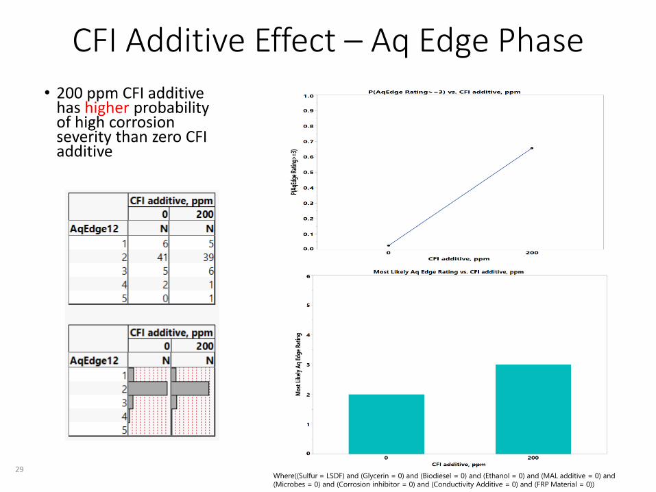
CFI Additive Effect – Aq Edge Phase
• 200 ppm CFI additive has higher probability of high corrosion severity than zero CFI additive
29Where((Sulfur = LSDF) and (Glycerin = 0) and (Biodiesel = 0) and (Ethanol = 0) and (MAL additive = 0) and (Microbes = 0) and (Corrosion inhibitor = 0) and (Conductivity Additive = 0) and (FRP Material = 0))

Sulfur-Biodiesel Interaction Effect
• LSDF has lower probability of high corrosion severity than ULSD with Biodiesel
30Where((Glycerin = 0) and (Ethanol = 0) and (MAL additive = 0) and (CFI additive = 0) and (Corrosion inhibitor = 0) and (Conductivity Additive = 0) and (FRP Material = 0) and (Microbes = 0))

Sulfur-Microbes Interaction Effect
• LSDF has lowerprobability of high corrosion severity than ULSD with Microbes
31Where((Glycerin = 0) and (Ethanol = 0) and (MAL additive = 0) and (CFI additive = 0) and (Corrosion inhibitor = 0) and (Conductivity Additive = 0) and (FRP Material = 0) and (Biodiesel = 0))

Sulfur-CFI Additive Interaction Effect• LSDF has lower probability
of high corrosion severity than ULSD without CFI additive while it has higherprobability with CFI additive
32Where((Glycerin = 0) and (Microbes = 0) and (MAL additive = 0) and (Biodiesel = 0) and (Corrosion inhibitor = 0) and (Conductivity Additive = 0) and (FRP Material = 0) and (Ethanol = 0))

Sulfur-Conductivity Additive Interaction Effect
• LSDF has lower probability of high corrosion severity than ULSD withoutConductivity additive while it has higher probability with Conductivity additive
33Where((Glycerin = 0) and (Microbes = 0) and (MAL additive = 0) and (CFI additive = 0) and (Corrosion inhibitor = 0) and (Biodiesel = 0) and (FRP Material = 0) and (Ethanol = 0))

Sulfur-FRP Material Interaction Effect
• LSDF has lowerprobability of high corrosion severity than ULSD without FRP Material
34Where((Glycerin = 0) and (Microbes = 0) and (MAL additive = 0) and (CFI additive = 0) and (Corrosion inhibitor = 0) and (Biodiesel = 0) and (Conductivity additive = 0) and (Ethanol = 0))

Glycerin-CFI Additive Interaction Effect
• 5000 ppm Glycerin has lower probability of high corrosion severity than zero Glycerin with CFI additive while it has higherprobability with CFI additive
35Where((Ethanol = 0) and (Microbes = 0) and (MAL additive = 0) and (Biodiesel = 0) and (Corrosion inhibitor = 0) and (Conductivity Additive = 0) and (FRP Material = 0) and (Ethanol = 0))

Ethanol-FRP Material Interaction Effect
• 10000 ppm Ethanol haslower probability of high corrosion severity than zero Ethanol without FRP Material while it has higherprobability with FRP Material
36Where((MAL additive = 0) and (Corrosion inhibitor = 0) and (Microbes= 0) and (Conductivity additive= 0) and (Sulfur = LSDF) and (Biodiesel = 0) and (CFI additive = 0) and (Glycerin = 0))

MAL Additive-Microbes Interaction Effect
• 200 ppm MAL additive haslower probability of high corrosion severity than zero MAL additive in the presence of Microbes
37Where((Ethanol = 0) and (Corrosion inhibitor = 0) and (Conductivity Additive = 0) and (FRP Material = 0) and (Sulfur = LSDF) and (Biodiesel = 0) and (CFI additive = 0) and (Glycerin = 0))

MAL Additive-Conductivity Additive Interaction Effect
• 200 ppm MAL additive haslower probability of high corrosion severity than zero MAL additive withConductivity additive
38Where((Corrosion inhibitor = 0) and (Sulfur = LSDF) and (Biodiesel = 0) and (CFI additive = 0) and (Glycerin = 0) and (Microbes = 0) and (Ethanol = 0) and (FRP Material = 0))

Corrosion Inhibitor-FRP Material Interaction Effect
• 8-10 ppm Corrosion inhibitor has lowerprobability of high corrosion severity than zero corrosion inhibitor with FRP Material while it has higherprobability without FRP Material
39Where((MAL additive = 0) and (Sulfur = LSDF) and (Microbes= 0) and (Biodiesel = 0) and (Sulfur = LSDF) and (Biodiesel = 0) and (CFI additive = 0) and (Glycerin = 0))

Ordinal Logistic RegressionAq Edge Phase – All Weeks
40

Corrosion by Time (Week)
41
• Probability of high corrosion severity in Week 2 is significantly higher than Week 1, and Week 3 is significantly higher Week 2
Where((Sulfur = LSDF) and (Biodiesel = 0) and (Glycerin = 0) and (Ethanol = 0) and (Microbes = 0) and (MAL additive = 0)
and (CFI additive = 0) and (Corrosion Inhibitor = 0) and (Conductivity Additive = 0) and (FRP Material = 0))

MAL Additive Effect by Time (Week)
42
• Probability of high corrosion severity in Week 2 is higher than Week 1 more significantly without MAL additive than with MAL additive
Where((Sulfur = LSDF) and (Biodiesel = 0) and (Glycerin = 0) and (Ethanol = 0) and (Microbes = 0) and
(Corrosion Inhibitor = 0) and (CFI additive = 0) and (Conductivity Additive = 0) and (FRP Material = 0))

Aqueous/Fuel Phase
43

Conclusions (Aqueous/Fuel Phase)Average Corrosion Severity Rating (average of 3 samples)
• ULSD has marginally higher probability of high corrosion severity than LSDF
• 5% Biodiesel has lower probability of high corrosion severity than zero Biodiesel
• 200ppm MAL additive has lower probability of high corrosion severity than zero MAL additive
• 8-10ppm Corrosion inhibitor has lower probability of high corrosion severity than zero Corrosion inhibitor
• 5% Biodiesel has lower probability of high corrosion severity than zero Biodiesel more significantly with Ethanol
• 5% Biodiesel has lower probability of high corrosion severity than zero Biodiesel more significantly with CFI Additive
• 5000ppm Glycerin has lower probability of high corrosion severity than zero Glycerin more significantly with Microbes
• 10000ppm Ethanol has lower probability of high corrosion severity than zero Ethanol more significantly withoutMicrobes
• 10000ppm Ethanol has lower probability of high corrosion severity than zero Ethanol more significantly with FRP Material
• 200ppm MAL additive has lower probability of high corrosion severity than zero MAL addtive more significantly without Conductivity Additive
• 8-10ppm Corrosion inhibitor has lower probability of high corrosion severity than zero Corrosion inhibitor more significantly without CFI Additive
• 8-10ppm Corrosion inhibitor has lower probability of high corrosion severity than zero Corrosion inhibitor more significantly without FRP Material
Average Corrosion Severity Rating by Time (Week)
• Significant weekly increases in probability of high corrosion severity between weeks 1, 2, 3, 4 and 6; marginal differences observed between weeks 6, 9 and 12
• More significant increase in probability of high corrosion severity between weeks 1 and 2 without Corrosion inhibitor than with Corrosion inhibitor
44

Stepwise Ordinal Logistic RegressionAqueous/Fuel Phase – Week 12
45

Sulfur Effect – Aq/Fuel Interface
• ULSD has marginally higher probability of high corrosion severity than LSDF
46Where((Biodiesel = 0) and (Glycerin = 0) and (Microbes = 0) and (Ethanol = 0) and (MAL additive = 0) and (CFI additive = 0) and (Corrosion inhibitor = 0) and (Conductivity Additive = 0) and (FRP Material = 0))

Biodiesel Effect – Aq/Fuel Interface
• 5% Biodiesel has lowerprobability of high corrosion severity than zero Biodiesel
47Where((Sulfur = LSDF) and (Glycerin = 0) and (Microbes = 0) and (Ethanol = 0) and (MAL additive = 0) and (CFI additive = 0) and (Corrosion inhibitor = 0) and (Conductivity Additive = 0) and (FRP Material = 0))

MAL Additive Effect – Aq/Fuel Interface
• 200ppm MAL additive has lower probability of high corrosion severity than zero MAL additive
48Where((Biodiesel = 0) and (Glycerin = 0) and (Microbes = 0) and (Ethanol = 0) and (Sulfur = LSDF) and (CFI additive = 0) and (Corrosion inhibitor = 0) and (Conductivity Additive = 0) and (FRP Material = 0))

Corrosion Inhibitor Effect – Aq/Fuel Interface
• 8-10ppm Corrosion inhibitor has lowerprobability of high corrosion severity than zero Corrosion inhibitor
49Where((Biodiesel = 0) and (Glycerin = 0) and (Microbes = 0) and (Ethanol = 0) and (MAL additive = 0) and (CFI additive = 0) and (Sulfur= LSDF) and (Conductivity Additive = 0) and (FRP Material = 0))

Biodiesel-Ethanol Interaction Effect
• 5% Biodiesel has lowerprobability of high corrosion severity than zero Biodiesel more significantly with Ethanol
50Where((Glycerin = 0) and (Microbes = 0) and (MAL additive = 0) and (CFI additive = 0) and (Corrosion inhibitor = 0) and (Conductivity Additive = 0) and (FRP Material = 0) and (Sulfur = LSDF))

Biodiesel-CFI Additive Interaction Effect• 5% Biodiesel has lower
probability of high corrosion severity than zero Biodiesel more significantly with CFI Additive
51 Where((Glycerin = 0) and (Microbes = 0) and (MAL additive = 0) and (Corrosion inhibitor = 0) and (Conductivity Additive = 0) and (FRP Material = 0) and (Sulfur = LSDF) and (Ethanol = 0))

Glycerin-Microbes Interaction Effect• 5000ppm Glycerin has
lower probability of high corrosion severity than zero Glycerin more significantly with Microbes
52 Where((MAL additive = 0) and (Corrosion inhibitor = 0) and (Conductivity Additive = 0) and (FRP Material = 0) and (Sulfur = LSDF) and (Ethanol = 0) and (Biodiesel = 0) and (CFI additive = 0))

Ethanol-Microbes Interaction Effect• 10000ppm Ethanol has lower
probability of high corrosion severity than zero Ethanol more significantly withoutMicrobes
53Where((MAL additive = 0) and (Corrosion inhibitor = 0) and (Conductivity Additive = 0) and (FRP Material = 0) and (Sulfur = LSDF) and (Biodiesel = 0) and (CFI additive = 0) and (Glycerin = 0))

Ethanol-FRP Material Interaction Effect• 10000ppm Ethanol has
lower probability of high corrosion severity than zero Ethanol more significantly with FRP Material
54Where((MAL additive = 0) and (Corrosion inhibitor = 0) and (Conductivity Additive = 0) and (Sulfur = LSDF) and (Biodiesel = 0) and (CFI additive = 0) and (Glycerin = 0) and (Microbes = 0))

MAL Additive-Conductivity Additive Interaction Effect
• 200ppm MAL additive has lower probability of high corrosion severity than zero MAL addtive more significantly without Conductivity Additive
55Where((Corrosion inhibitor = 0) and (Sulfur = LSDF) and (Biodiesel = 0) and (CFI additive = 0) and (Glycerin = 0) and (Microbes = 0) and (Ethanol = 0) and (FRP Material = 0))

Corrosion Inhibitor-CFI Additive Interaction Effect
• 8-10ppm Corrosion inhibitor has lower probability of high corrosion severity than zero Corrosion inhibitor more significantly without CFI Additive
56Where((Sulfur = LSDF) and (Biodiesel = 0) and (Glycerin = 0) and (Microbes = 0) and (Ethanol = 0) and (FRP Material = 0) and (MAL additive = 0) and (Conductivity Additive = 0))

Corrosion Inhibitor-FRP Material Interaction Effect
• 8-10ppm Corrosion inhibitor has lower probability of high corrosion severity than zero Corrosion inhibitor more significantly without FRP Material
57Where((Sulfur = LSDF) and (Biodiesel = 0) and (Glycerin = 0) and (Microbes = 0) and (Ethanol = 0) and (MAL additive = 0) and (Conductivity Additive = 0) and (CFI additive = 0))

Ordinal Logistic RegressionAqueous/Fuel Phase – All Weeks
58

Corrosion by Time (Week)
59
• Significant weekly increases in probability of high corrosion severity between weeks 1, 2, 3, 4 and 6 while marginal differences observed between weeks 6, 9 and 12
Where((Sulfur = LSDF) and (Biodiesel = 0) and (Glycerin = 0) and (Ethanol = 0) and (Microbes = 0) and (MAL additive = 0)
and (CFI additive = 0) and (Corrosion Inhibitor = 0) and (Conductivity Additive = 0) and (FRP Material = 0))

Corrosion Inhibitor Effect by Time (Week)
60
• More significant increase in probability of high corrosion severity between weeks 1 and 2 without Corrosion Inhibitor than with Corrosion Inhibitor
Where((Sulfur = LSDF) and (Biodiesel = 0) and (Glycerin = 0) and (Ethanol = 0) and (Mircobes = 0) and
(MAL additive = 0) and (CFI additive = 0) and (Conductivity Additive = 0) and (FRP Material = 0))

Aqueous/Fuel Edge Phase
61

Conclusions (Aqueous/Fuel Edge Phase)Average Corrosion Severity Rating (average of 3 samples)
• ULSD has marginally higher probability of high corrosion severity than LSDF
• 5% Biodiesel has lower probability of high corrosion severity than zero Biodiesel
• Presence of Microbes has lower probability of high corrosion severity than absence of Microbes
• 200ppm MAL additive has lower probability of high corrosion severity than zero MAL additive
• 8-10ppm Corrosion inhibitor has lower probability of high corrosion severity than zero Corrosion Inhibitor
• LSDF has lower probability of high corrosion severity than ULSD more significantly without Conductivity additive
• 5% Biodiesel has lower probability of high corrosion severity than zero Biodiesel without Ethanol while it has higher probability with Ethanol
• 5% Biodiesel has lower probability of high corrosion severity than zero Biodiesel more significantly with Microbes
• 5% Biodiesel has lower probability of high corrosion severity than zero Biodiesel more significantly with FRP Material
• 5000ppm Glycerin has higher probability of high corrosion severity than zero Glycerin more significantly with Ethanol
• 10000ppm Ethanol has lower probability of high corrosion severity than zero Ethanol more significantly without Microbes while it has higher probability with Microbes
• 8-10ppm Corrosion inhibitor has lower probability of high corrosion severity than zero Corrosion inhibitor more significantly withMicrobes
• 8-10ppm Corrosion inhibitor has lower probability of high corrosion severity than zero Corrosion inhibitor more significantly without MAL Additive
• 200ppm CFI additive has lower probability of high corrosion severity than zero CFI additive more significantly without Glycerin
• 200ppm CFI additive has lower probability of high corrosion severity than zero CFI additive without Conductivity Additive while it has higher probability with Conductivity additive
Average Corrosion Severity Rating by Time (Week)
• Significant weekly increases in probability of high corrosion severity between weeks 1, 2, 3, 4, 6 and 9
• More significant increase in probability of high corrosion severity between weeks 1 and 2 without Corrosion Inhibitor than with Corrosion Inhibitor
62

Stepwise Ordinal Logistic RegressionAqueous/Fuel Edge Phase – Week 12
63

Sulfur Effect – Aq/Fuel Edge Phase
• ULSD has marginally higher probability of high corrosion severity than LSDF
64Where((Biodiesel = 0) and (Glycerin = 0) and (Microbes = 0) and (Ethanol = 0) and (MAL additive = 0) and (CFI additive = 0) and (Corrosion inhibitor = 0) and (Conductivity Additive = 0) and (FRP Material = 0))

Biodiesel Effect - Aq/Fuel Edge Phase
• 5% Biodiesel has lowerprobability of high corrosion severity than zero Biodiesel
65Where((Sulfur = LSDF) and (Glycerin = 0) and (Microbes = 0) and (Ethanol = 0) and (MAL additive = 0) and (CFI additive = 0) and (Corrosion inhibitor = 0) and (Conductivity Additive = 0) and (FRP Material = 0))

Microbes Effect – Aq/Fuel Edge Phase
• Presence of Microbes has lower probability of high corrosion severity than absence of Microbes
66Where((Sulfur = LSDF) and (Glycerin = 0) and (Biodiesel = 0) and (Ethanol = 0) and (MAL additive = 0) and (CFI additive = 0) and (Corrosion inhibitor = 0) and (Conductivity Additive = 0) and (FRP Material = 0))

MAL Additive Effect - Aq/Fuel Edge Phase
• 200ppm MAL additive has lower probability of high corrosion severity than zero MAL additive
67Where((Biodiesel = 0) and (Glycerin = 0) and (Microbes = 0) and (Ethanol = 0) and (Sulfur = LSDF) and (CFI additive = 0) and (Corrosion inhibitor = 0) and (Conductivity Additive = 0) and (FRP Material = 0))

Corrosion Inhibitor Effect - Aq/Fuel Edge Phase
• 8-10ppm Corrosion inhibitor has lowerprobability of high corrosion severity than zero Corrosion Inhibitor
68Where((Biodiesel = 0) and (Glycerin = 0) and (Microbes = 0) and (Ethanol = 0) and (MAL additive = 0) and (CFI additive = 0) and (Sulfur= LSDF) and (Conductivity Additive = 0) and (FRP Material = 0))

Sulfur-Conductivity Additive Interaction Effect
• LSDF has lower probability of high corrosion severity than ULSD more significantly withoutConductivity additive
69Where((Glycerin = 0) and (Microbes = 0) and (MAL additive = 0) and (CFI additive = 0) and (Corrosion inhibitor = 0) and (Biodiesel = 0) and (FRP Material = 0) and (Ethanol = 0))

Biodiesel-Ethanol Interaction Effect
• 5% Biodiesel has lowerprobability of high corrosion severity than zero Biodiesel withoutEthanol while it has higherprobability with Ethanol
70Where((Glycerin = 0) and (Microbes = 0) and (MAL additive = 0) and (CFI additive = 0) and (Corrosion inhibitor = 0) and (Conductivity Additive = 0) and (FRP Material = 0) and (Sulfur = LSDF))

Biodiesel-Microbes Interaction Effect
• 5% Biodiesel has lowerprobability of high corrosion severity than zero Biodiesel more significantly with Microbes
71Where((Glycerin = 0) and (Ethanol = 0) and (MAL additive = 0) and (CFI additive = 0) and (Corrosion inhibitor = 0) and (Conductivity Additive = 0) and (FRP Material = 0) and (Sulfur = LSDF))

Biodiesel-FRP Material Interaction Effect
• 5% Biodiesel has lowerprobability of high corrosion severity than zero Biodiesel more significantly with FRP Material
72 Where((Glycerin = 0) and (Microbes = 0) and (MAL additive = 0) and (Corrosion inhibitor = 0) and (Conductivity Additive = 0) and (CFI Additive = 0) and (Sulfur = LSDF) and (Ethanol = 0))

Glycerin-Ethanol Interaction Effect• 5000ppm Glycerin has
higher probability of high corrosion severity than zero Glycerin more significantly with Ethanol
73 Where((MAL additive = 0) and (Corrosion inhibitor = 0) and (Conductivity Additive = 0) and (FRP Material = 0) and (Sulfur = LSDF) and (Microbes = 0) and (Biodiesel = 0) and (CFI additive = 0))

Ethanol-Microbes Interaction Effect• 10000ppm Ethanol has
lower probability of high corrosion severity than zero Ethanol more significantly without Microbes while it has higher probability withMicrobes
74Where((MAL additive = 0) and (Corrosion inhibitor = 0) and (Conductivity Additive = 0) and (FRP Material = 0) and (Sulfur = LSDF) and (Biodiesel = 0) and (CFI additive = 0) and (Glycerin = 0))

Corrosion Inhibitor-Microbes Interaction Effect
• 8-10ppm Corrosion inhibitor has lowerprobability of high corrosion severity than zero Corrosion inhibitor more significantly with Microbes
75Where((Sulfur = LSDF) and (Biodiesel = 0) and (Glycerin = 0) and (CFI Additive = 0) and (Ethanol = 0) and (FRP Material = 0) and (MAL additive = 0) and (Conductivity Additive = 0))
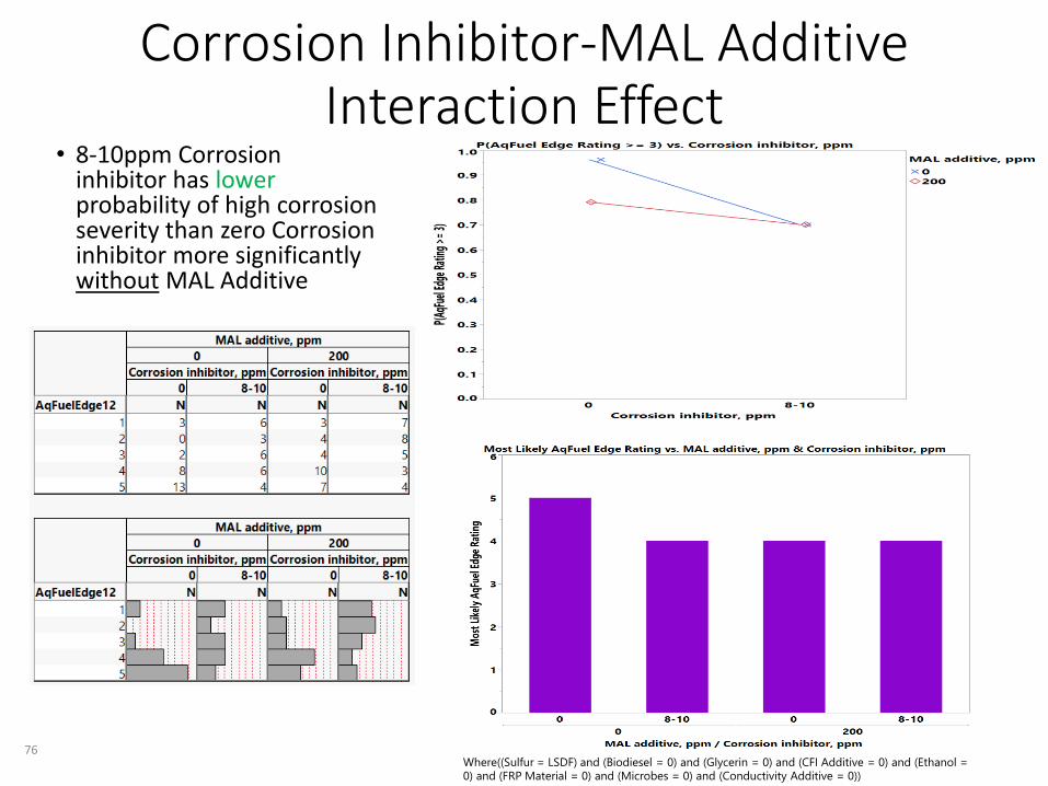
Corrosion Inhibitor-MAL Additive Interaction Effect
• 8-10ppm Corrosion inhibitor has lowerprobability of high corrosion severity than zero Corrosion inhibitor more significantly without MAL Additive
76Where((Sulfur = LSDF) and (Biodiesel = 0) and (Glycerin = 0) and (CFI Additive = 0) and (Ethanol = 0) and (FRP Material = 0) and (Microbes = 0) and (Conductivity Additive = 0))

CFI Additive-Glycerin Interaction Effect
• 200ppm CFI additive has lower probability of high corrosion severity than zero CFI additive more significantly without Glycerin
77 Where((MAL additive = 0) and (Corrosion inhibitor = 0) and (Conductivity Additive = 0) and (FRP Material = 0) and (Sulfur = LSDF) and (Microbes = 0) and (Biodiesel = 0) and (Ethanol = 0))

CFI Additive-Conductivity Additive Interaction Effect
• 200ppm CFI additive has lowerprobability of high corrosion severity than zero CFI additive without Conductivity Additive while it has higher probability with Conductivity additive
78Where((Corrosion inhibitor = 0) and (Sulfur = LSDF) and (Biodiesel = 0) and (MAL additive = 0) and (Glycerin = 0) and (Microbes = 0) and (Ethanol = 0) and (FRP Material = 0))

Ordinal Logistic RegressionAqueous/Fuel Edge Phase – All Weeks
79

Corrosion by Time (Week)
80
• Significant weekly increases in probability of high corrosion severity between weeks 1, 2, 3, 4, 6 and 9.
Where((Sulfur = LSDF) and (Biodiesel = 0) and (Glycerin = 0) and (Ethanol = 0) and (Microbes = 0) and (MAL additive = 0)
and (CFI additive = 0) and (Corrosion Inhibitor = 0) and (Conductivity Additive = 0) and (FRP Material = 0))

Corrosion Inhibitor Effect by Time (Week)
81
• More significant increase in probability of high corrosion severity between weeks 1 and 2 without Corrosion Inhibitor than with Corrosion Inhibitor
Where((Sulfur = LSDF) and (Biodiesel = 0) and (Glycerin = 0) and (Ethanol = 0) and (Mircobes = 0) and
(MAL additive = 0) and (CFI additive = 0) and (Conductivity Additive = 0) and (FRP Material = 0))

Fuel Phase
82

Conclusions (Fuel Phase)Average Corrosion Severity Rating (average of 3 samples)
• ULSD has marginally higher probability of high corrosion severity than LSDF
• 5% Biodiesel has lower probability of high corrosion severity than zero Biodiesel
• Presence of Water has higher probability of high corrosion severity than absence of Water
• 8-10ppm Corrosion inhibitor has lower probability of high corrosion severity than zero Corrosion inhibitor
• LSDF has lower probability of high corrosion severity than ULSD without Ethanol
• 5% Biodiesel has lower probability of high corrosion severity than zero Biodiesel more significantly with LSDF
• 5% Biodiesel has lower probability of high corrosion severity than zero Biodiesel more significantly without Glycerin
• 5% Biodiesel has lower probability of high corrosion severity than zero Biodiesel more significantly with Ethanol
• 5000ppm Glycerin has lower probability of high corrosion severity than zero Glycerin more significantly without FRP Material
• 8-10ppm Corrosion inhibitor has lower probability of high corrosion severity than zero Corrosion inhibitor more significantly without Ethanol
• 8-10ppm Corrosion inhibitor has lower probability of high corrosion severity than zero Corrosion inhibitor without Microbes while it has higherprobability with Microbes
• 8-10ppm Corrosion inhibitor has lower probability of high corrosion severity than zero Corrosion inhibitor without MAL Additive while it has higherprobability with MAL Additive
• 8-10ppm Corrosion inhibitor has lower probability of high corrosion severity than zero Corrosion inhibitor more significantly without FRP Material
• 200ppm CFI Additive has lower probability of high corrosion severity than zero CFI additive without FRP Material while it has higher probability withFRP Material
• 2-3ppm Conductivity additive has lower probability of high corrosion severity than zero Conductivity additive without Water while it has higherprobability with Water
• 2-3ppm Conductivity Additive has lower probability of high corrosion severity than zero Conductivity additive more significantly without FRP Material
• 2-3ppm Conductivity additive has lower probability of high corrosion severity than zero Conductivity additive more significantly with Microbes
Average Corrosion Severity Rating by Time (Week)
• Marginal weekly increases in probability of high corrosion severity between weeks 2 & 3 and weeks 4 & 6
83

Stepwise Ordinal Logistic RegressionFuel Phase – Week 12
84

Sulfur Effect – Fuel Phase
• ULSD has marginally higher probability of high corrosion severity than LSDF
85Where((Biodiesel = 0) and (Water = 0) and (Glycerin = 0) and (Microbes = 0) and (Ethanol = 0) and (MAL additive = 0) and (CFI additive = 0) and (Corrosion inhibitor = 0) and (Conductivity Additive = 0) and (FRP Material = 0))

Biodiesel Effect – Fuel Phase
• 5% Biodiesel has lowerprobability of high corrosion severity than zero Biodiesel
86Where((Sulfur = LSDF) and (Water = 0) and (Glycerin = 0) and (Microbes = 0) and (Ethanol = 0) and (MAL additive = 0) and (CFI additive = 0) and (Corrosion inhibitor = 0) and (Conductivity Additive = 0) and (FRP Material = 0))

Water Effect – Fuel Phase
• Presence of Water has higher probability of high corrosion severity than absence of Water
87Where((Sulfur = LSDF) and (Biodiesel = 0) and (Glycerin = 0) and (Microbes = 0) and (Ethanol = 0) and (MAL additive = 0) and (CFI additive = 0) and (Corrosion inhibitor = 0) and (Conductivity Additive = 0) and (FRP Material = 0))

Corrosion Inhibitor Effect – Fuel Phase
• 8-10ppm Corrosion inhibitor has lowerprobability of high corrosion severity than zero Corrosion inhibitor
88Where((Biodiesel = 0) and (Water = 0) and (Glycerin = 0) and (Microbes = 0) and (Ethanol = 0) and (MAL additive = 0) and (CFI additive = 0) and (Sulfur= LSDF) and (Conductivity Additive = 0) and (FRP Material = 0))

Sulfur-Ethanol Interaction Effect
• LSDF has lowerprobability of high corrosion severity than ULSD without Ethanol
89Where((Glycerin = 0) and (Water = 0) and (Microbes = 0) and (MAL additive = 0) and (CFI additive = 0) and (Corrosion inhibitor = 0) and (Conductivity Additive = 0) and (FRP Material = 0) and (Corrosion inhibitor = 0))

Biodiesel-Sulfur Interaction Effect
• 5% Biodiesel has lowerprobability of high corrosion severity than zero Biodiesel more significantly with LSDF
90Where((Glycerin = 0) and (Water = 0) and (Microbes = 0) and (MAL additive = 0) and (CFI additive = 0) and (Corrosion inhibitor = 0) and (Conductivity Additive = 0) and (FRP Material = 0) and (Ethanol = 0))

Biodiesel-Glycerin Interaction Effect
• 5% Biodiesel has lowerprobability of high corrosion severity than zero Biodiesel more significantly without Glycerin
91Where((Ethanol = 0) and (Water = 0) and (Microbes = 0) and (MAL additive = 0) and (CFI additive = 0) and (Corrosion inhibitor = 0) and (Conductivity Additive = 0) and (FRP Material = 0) and (Sulfur = LSDF))

Biodiesel-Ethanol Interaction Effect
• 5% Biodiesel has lowerprobability of high corrosion severity than zero Biodiesel more significantly with Ethanol
92Where((Glycerin = 0) and (Water = 0) and (Microbes = 0) and (MAL additive = 0) and (CFI additive = 0) and (Corrosion inhibitor = 0) and (Conductivity Additive = 0) and (FRP Material = 0) and (Sulfur = LSDF))

Glycerin-FRP Material Interaction Effect• 5000ppm Glycerin has
lower probability of high corrosion severity than zero Glycerin more significantly without FRP Material
93Where((MAL additive = 0) and (Water =0) and (Corrosion inhibitor = 0) and (Conductivity Additive = 0) and (Sulfur = LSDF) and (Biodiesel = 0) and (CFI additive = 0) and (Ethanol = 0) and (Microbes = 0))

Corrosion Inhibitor-Ethanol Interaction Effect
• 8-10ppm Corrosion inhibitor has lower probability of high corrosion severity than zero Corrosion inhibitor more significantly without Ethanol
94Where((Sulfur = LSDF) and (Water = 0) and (Biodiesel = 0) and (Glycerin = 0) and (Microbes = 0) and (CFI Additive= 0) and (FRP Material = 0) and (MAL additive = 0) and (Conductivity Additive = 0))

Corrosion Inhibitor-Microbes Interaction Effect
• 8-10ppm Corrosion inhibitor has lower probability of high corrosion severity than zero Corrosion inhibitor withoutMicrobes while it has higherprobability with Microbes
95Where((Sulfur = LSDF) and (Water = 0) and (Biodiesel = 0) and (Glycerin = 0) and (Ethanol = 0) and (CFI Additive= 0) and (FRP Material = 0) and (MAL additive = 0) and (Conductivity Additive = 0))

Corrosion Inhibitor-MAL Additive Interaction Effect
• 8-10ppm Corrosion inhibitor has lower probability of high corrosion severity than zero Corrosion inhibitor withoutMAL Additive while it has higher probability with MAL Additive
96Where((Sulfur = LSDF) and (Water = 0) and (Biodiesel = 0) and (Glycerin = 0) and (Ethanol = 0) and (CFI Additive= 0) and (FRP Material = 0) and (Microbes= 0) and (Conductivity Additive = 0))

Corrosion Inhibitor-FRP Material Interaction Effect
• 8-10ppm Corrosion inhibitor has lower probability of high corrosion severity than zero Corrosion inhibitor more significantly without FRP Material
97Where((Sulfur = LSDF) and (Water = 0) and (Biodiesel = 0) and (Glycerin = 0) and (Ethanol = 0) and (CFI Additive= 0) and (MAL Additive = 0) and (Microbes= 0) and (Conductivity Additive = 0))

CFI Additive-FRP Material Interaction Effect
• 200ppm CFI Additive has lower probability of high corrosion severity than zero CFI additive withoutFRP Material while it has higher probability withFRP Material
98Where((Sulfur = LSDF) and (Water = 0) and (Biodiesel = 0) and (Glycerin = 0) and (Ethanol = 0) and (Corrosion Inhibitor= 0) and (MAL Additive = 0) and (Microbes= 0) and (Conductivity Additive = 0))

Conductivity Additive-Water Interaction Effect
• 2-3ppm Conductivity additive has lower probability of high corrosion severity than zero Conductivity additive withoutWater while it has higherprobability with Water
99Where((Glycerin = 0) and (Biodiesel = 0) and (Microbes = 0) and (MAL additive = 0) and (CFI additive = 0) and (Corrosion inhibitor = 0) and (Ethanol = 0) and (FRP Material = 0) and (Sulfur = LSDF))

Conductivity Additive-FRP Material Interaction Effect
• 2-3ppm Conductivity Additive has lower probability of high corrosion severity than zero Conductivity additive more significantly without FRP Material
100 Where((Sulfur = LSDF) and (Water = 0) and (Biodiesel = 0) and (Glycerin = 0) and (Ethanol = 0) and
(CFI Additive= 0) and (Corrosion Inhibitor = 0) and (Microbes= 0) and (MAL Additive = 0))

Conductivity Additive–Microbes Interaction Effect
• 2-3ppm Conductivity additive has lowerprobability of high corrosion severity than zero Conductivity additive more significantly with Microbes
101 Where((Sulfur = LSDF) and (Water = 0) and (Biodiesel = 0) and (Glycerin = 0) and (Ethanol = 0) and
(CFI Additive= 0) and (FRP Material = 0) and (Corrosion Inhibitor = 0) and (MAL Additive= 0))

Ordinal Logistic RegressionFuel Phase – All Weeks
102

Corrosion by Time (Week)
103
• Marginal weekly increases in probability of high corrosion severity between weeks 2 & 3 and weeks 4 & 6.
Where((Sulfur = LSDF) and (Water = 0) and (Biodiesel = 0) and (Glycerin = 0) and (Ethanol = 0) and (Microbes = 0) and (MAL
additive = 0) and (CFI additive = 0) and (Corrosion Inhibitor = 0) and (Conductivity Additive = 0) and (FRP Material = 0))

Fuel Edge Phase
104
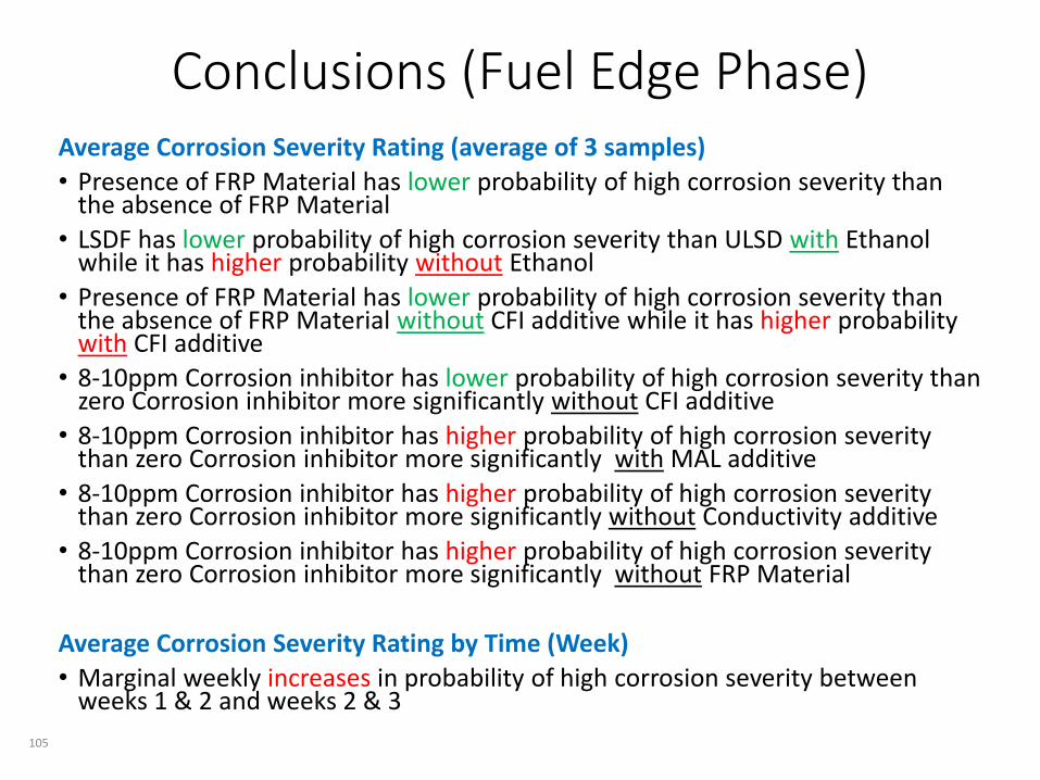
Conclusions (Fuel Edge Phase)Average Corrosion Severity Rating (average of 3 samples)
• Presence of FRP Material has lower probability of high corrosion severity than the absence of FRP Material
• LSDF has lower probability of high corrosion severity than ULSD with Ethanol while it has higher probability without Ethanol
• Presence of FRP Material has lower probability of high corrosion severity than the absence of FRP Material without CFI additive while it has higher probability with CFI additive
• 8-10ppm Corrosion inhibitor has lower probability of high corrosion severity than zero Corrosion inhibitor more significantly without CFI additive
• 8-10ppm Corrosion inhibitor has higher probability of high corrosion severity than zero Corrosion inhibitor more significantly with MAL additive
• 8-10ppm Corrosion inhibitor has higher probability of high corrosion severity than zero Corrosion inhibitor more significantly without Conductivity additive
• 8-10ppm Corrosion inhibitor has higher probability of high corrosion severity than zero Corrosion inhibitor more significantly without FRP Material
Average Corrosion Severity Rating by Time (Week)
• Marginal weekly increases in probability of high corrosion severity between weeks 1 & 2 and weeks 2 & 3
105

Stepwise Ordinal Logistic RegressionFuel Edge Phase – Week 12
106

FRP Material Effect – Fuel Edge Phase
• Presence of FRP Material has lower probability of high corrosion severity than the absence of FRP Material
107Where((Biodiesel = 0) and (Glycerin = 0) and (Microbes = 0) and (Ethanol = 0) and (MAL additive = 0) and (CFI additive = 0) and (Sulfur= LSDF) and (Conductivity Additive = 0) and (Corrosion Inhibitor = 0) and (Water = 0))

Sulfur-Ethanol Interaction Effect
• LSDF has lower probability of high corrosion severity than ULSD with Ethanol while it has higher probability without Ethanol
108Where((Glycerin = 0) and (Water = 0) and (Microbes = 0) and (MAL additive = 0) and (CFI additive = 0) and (Corrosion inhibitor = 0) and (Conductivity Additive = 0) and (FRP Material = 0) and (Corrosion inhibitor = 0))

FRP Material-CFI AdditiveInteraction Effect
• Presence of FRP Material has lower probability of high corrosion severity than the absence of FRP Material without CFI additive while it has higher probability with CFI additive
109 Where((Sulfur = LSDF) and (Water = 0) and (Biodiesel = 0) and (Glycerin = 0) and (Ethanol = 0) and
(Corrosion Inhibitor= 0) and (MAL Additive = 0) and (Microbes= 0) and (Conductivity Additive = 0))

Corrosion Inhibitor-CFI Additive Interaction Effect
• 8-10ppm Corrosion inhibitor has lower probability of high corrosion severity than zero Corrosion inhibitor more significantly without CFI additive
110 Where((Sulfur = LSDF) and (Water = 0) and (Biodiesel = 0) and (Glycerin = 0) and (Microbes = 0) and
(Ethanol= 0) and (FRP Material = 0) and (MAL additive = 0) and (Conductivity Additive = 0))

Corrosion Inhibitor-MAL Additive Interaction Effect
• 8-10ppm Corrosion inhibitor has higherprobability of high corrosion severity than zero Corrosion inhibitor more significantly withMAL additive
111 Where((Sulfur = LSDF) and (Water = 0) and (Biodiesel = 0) and (Glycerin = 0) and (Ethanol = 0) and
(CFI Additive= 0) and (FRP Material = 0) and (Microbes= 0) and (Conductivity Additive = 0))
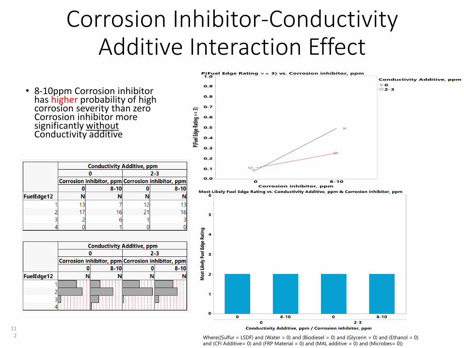
Corrosion Inhibitor-Conductivity Additive Interaction Effect
• 8-10ppm Corrosion inhibitor has higher probability of high corrosion severity than zero Corrosion inhibitor more significantly withoutConductivity additive
112 Where((Sulfur = LSDF) and (Water = 0) and (Biodiesel = 0) and (Glycerin = 0) and (Ethanol = 0)
and (CFI Additive= 0) and (FRP Material = 0) and (MAL additive = 0) and (Microbes= 0))

Corrosion Inhibitor-FRP Material Interaction Effect
• 8-10ppm Corrosion inhibitor has higher probability of high corrosion severity than zero Corrosion inhibitor more significantly without FRP Material
113 Where((Sulfur = LSDF) and (Water = 0) and (Biodiesel = 0) and (Glycerin = 0) and (Ethanol = 0) and
(CFI Additive= 0) and (MAL Additive = 0) and (Microbes= 0) and (Conductivity Additive = 0))

Stepwise Ordinal Logistic RegressionFuel Edge Phase – All Weeks
114

Corrosion by Time (Week)
115
• Marginal weekly increases in probability of high corrosion severity between weeks 1 & 2 and weeks 2 & 3.
Where((Sulfur = LSDF) and (Water = 0) and (Biodiesel = 0) and (Glycerin = 0) and (Ethanol = 0) and (Microbes = 0) and (MAL
additive = 0) and (CFI additive = 0) and (Corrosion Inhibitor = 0) and (Conductivity Additive = 0) and (FRP Material = 0))

Vapor Phase
116

Conclusions (Vapor Phase)
Average Corrosion Severity Rating (average of 3 samples)
• 8-10ppm Corrosion inhibitor has lower probability of high corrosion severity than zero Corrosion inhibitor
Average Corrosion Severity Rating by Time (Week)
• No significant weekly increases in probability of high corrosion severity
117

Stepwise Ordinal Logistic RegressionVapor Phase – Week 12
118

Corrosion Inhibitor Effect – Vapor Phase
• 8-10ppm Corrosion inhibitor has lowerprobability of high corrosion severity than zero Corrosion inhibitor
119Where((Biodiesel = 0) and (Water = 0) and (Glycerin = 0) and (Microbes = 0) and (Ethanol = 0) and (MAL additive = 0) and (CFI additive = 0) and (Sulfur= LSDF) and (Conductivity Additive = 0) and (FRP Material = 0))

Ordinal Logistic RegressionVapor Phase – All Weeks
120

Corrosion by Time (Week)
121
• No significant weekly increases in probability of high corrosion severity.
Where((Sulfur = LSDF) and (Biodiesel = 0) and (Water = 0) and (Glycerin = 0) and (Ethanol = 0) and (Microbes = 0) and (MAL
additive = 0) and (CFI additive = 0) and (Corrosion Inhibitor = 0) and (Conductivity Additive = 0) and (FRP Material = 0))

Vapor Edge Phase
122

Conclusions (Vapor Edge Phase)Average Corrosion Severity Rating (average of 3 samples)
• LSDF has significantly higher probability of high corrosion severity than ULSD
• 10000ppm Ethanol has lower probability of high corrosion severity than zero Ethanol
• Presence of Microbes has lower probability of high corrosion severity than absence of Microbes
• 200ppm MAL additive has higher probability of high corrosion severity than zero MAL additive
• ULSD has lower probability of high corrosion severity than LSDF more significantly without Water
• ULSD has lower probability of high corrosion severity than LSDF more significantly with Microbes
• ULSD has lower probability of high corrosion severity more significantly without CFI additive
• 5% Biodiesel has lower probability of high corrosion severity without Conductivity additive while it has higherprobability with Conductivity additive
• 5000ppm Glycerin has higher probability of high corrosion severity than zero Glycerin more significantly with Ethanol
• 5000ppm Glycerin has higher probability of high corrosion severity than zero Glycerin without MAL additive while it has lower probability with MAL additive
• 10000ppm Ethanol has lower probability of high corrosion severity than zero Ethanol without Microbes while it has higher probability with Microbes
• 200ppm MAL additive has higher probability of high corrosion severity more significantly with Microbes
• 200ppm MAL additive has higher probability of high corrosion severity than zero MAL additive more significantly without FRP Material
• 200ppm CFI additive has lower probability of high corrosion severity than zero CFI additive without Microbes
• 200ppm CFI additive has lower probability of high corrosion severity than zero CFI additive more significantly withoutFRP Material
Average Corrosion Severity Rating by Time (Week)
• Significant weekly increase in probability of high corrosion severity between weeks 2 and 3123

Stepwise Ordinal Logistic RegressionVapor Edge Phase – Week 12
124

Sulfur Effect – Vapor Edge Phase
• LSDF has significantly higher probability of high corrosion severity than ULSD
125Where((Biodiesel = 0) and (Water = 0) and (Glycerin = 0) and (Microbes = 0) and (Ethanol = 0) and (MAL additive = 0) and (CFI additive = 0) and (Corrosion inhibitor = 0) and (Conductivity Additive = 0) and (FRP Material = 0))

Ethanol Effect – Vapor Edge Phase
• 10000ppm Ethanol has lower probability of high corrosion severity than zero Ethanol
126Where((Biodiesel = 0) and (Sulfur = LSDF) and (Glycerin = 0) and (Microbes = 0) and (Water = 0) and (MAL additive = 0) and (CFI additive = 0) and (Corrosion inhibitor = 0) and (Conductivity Additive = 0) and (FRP Material = 0))

Microbes Effect – Vapor Edge Phase
• Presence of Microbes has lower probability of high corrosion severity than absence of Microbes
127Where((Biodiesel = 0) and (Water = 0) and (Glycerin = 0) and (Sulfur = LSDF) and (Ethanol = 0) and (MAL additive = 0) and (CFI additive = 0) and (Corrosion inhibitor = 0) and (Conductivity Additive = 0) and (FRP Material = 0))

MAL Additive Effect – Vapor Edge Phase
• 200ppm MAL additive has higher probability of high corrosion severity than zero MAL additive
128Where((Biodiesel = 0) and (Water = 0) and (Glycerin = 0) and (Microbes = 0) and (Ethanol = 0) and (Sulfur = LSDF) and (CFI additive = 0) and (Corrosion inhibitor = 0) and (Conductivity Additive = 0) and (FRP Material = 0))

Sulfur-Water Interaction Effect
• ULSD has lowerprobability of high corrosion severity than LSDF more significantly without Water
129Where((Glycerin = 0) and (Microbes = 0) and (MAL additive = 0) and (CFI additive = 0) and (Corrosion inhibitor = 0) and (Conductivity Additive = 0) and (FRP Material = 0) and (Biodiesel = 0) and (Ethanol = 0))

Sulfur-Microbes Interaction Effect
• ULSD has lowerprobability of high corrosion severity than LSDF more significantly with Microbes
130Where((Glycerin = 0) and (Water = 0) and (Biodiesel = 0) and (MAL additive = 0) and (CFI additive = 0) and (Corrosion inhibitor = 0) and (Conductivity Additive = 0) and (FRP Material = 0) and (Corrosion inhibitor = 0))

Sulfur-CFI Additive Interaction Effect
• ULSD has lowerprobability of high corrosion severity more significantly without CFI additive
131Where((Glycerin = 0) and (Water = 0) and (Microbes = 0) and (MAL additive = 0) and (Biodiesel = 0) and (Corrosion inhibitor = 0) and (Conductivity Additive = 0) and (FRP Material = 0) and (MAL additive = 0))

Biodiesel-Conductivity AdditiveInteraction Effect
• 5% Biodiesel has lowerprobability of high corrosion severity withoutConductivity additive while it has higherprobability withConductivity additive
132 Where((Glycerin = 0) and (Water = 0) and (Microbes = 0) and (MAL additive = 0) and (Corrosion inhibitor = 0) and (Conductivity Additive = 0) and (CFI Additive = 0) and (Sulfur = LSDF) and (Ethanol = 0))

Glycerin-Ethanol Interaction Effect• 5000ppm Glycerin has
higher probability of high corrosion severity than zero Glycerin more significantly with Ethanol
133 Where((MAL additive = 0) and (Water = 0) and (Corrosion inhibitor = 0) and (Conductivity Additive = 0) and (FRP Material = 0) and (Sulfur = LSDF) and (Microbes = 0) and (Biodiesel = 0) and (CFI additive = 0))

Glycerin-MAL Additive Interaction Effect
• 5000ppm Glycerin has higherprobability of high corrosion severity than zero Glycerin without MAL additive while it has lower probability withMAL additive
134 Where((Microbes= 0) and (Water = 0) and (Corrosion inhibitor = 0) and (Conductivity Additive = 0) and (FRP Material = 0) and (Sulfur = LSDF) and (Microbes = 0) and (Biodiesel = 0) and (Ethanol = 0))

Ethanol-Microbes Interaction Effect
• 10000ppm Ethanol has lowerprobability of high corrosion severity than zero Ethanol without Microbes while it has higher probability withMicrobes
135Where((Glycerin = 0) and (Water = 0) and (Biodiesel= 0) and (MAL additive = 0) and (CFI additive = 0) and (Corrosion inhibitor = 0) and (Conductivity Additive = 0) and (FRP Material = 0) and (Sulfur = LSDF))

MAL Additive-MicrobesInteraction Effect
• 200ppm MAL additive has higher probability of high corrosion severity more significantly withMicrobes
136Where((Glycerin = 0) and (Water = 0) and (Biodiesel = 0) and (Ethanol = 0) and (CFI additive = 0) and (FRP Material = 0) and (Conductivity Additive = 0) and (FRP Material = 0) and (Corrosion inhibitor = 0))

MAL Additive-FRP MaterialInteraction Effect
• 200ppm MAL additive has higher probability of high corrosion severity than zero MAL additive more significantly without FRP Material
137Where((Sulfur = LSDF) and (Water = 0) and (Biodiesel = 0) and (Glycerin = 0) and (Ethanol = 0) and (Corrosion Inhibitor= 0) and (CFI Additive = 0) and (Microbes= 0) and (Conductivity Additive = 0))

CFI Additive-MicrobesInteraction Effect
• 200ppm CFI additive has lower probability of high corrosion severity than zero CFI additive withoutMicrobes
138Where((Glycerin = 0) and (Water = 0) and (Biodiesel = 0) and (MAL additive = 0) and (MAL additive = 0) and (Corrosion inhibitor = 0) and (Conductivity Additive = 0) and (FRP Material = 0) and (Corrosion inhibitor = 0))

CFI Additive-FRP MaterialInteraction Effect
• 200ppm CFI additive has lower probability of high corrosion severity than zero CFI additive more significantly without FRP Material
139Where((Sulfur = LSDF) and (Water = 0) and (Biodiesel = 0) and (Glycerin = 0) and (Ethanol = 0) and (Corrosion Inhibitor= 0) and (MAL Additive = 0) and (Microbes= 0) and (Conductivity Additive = 0))

Ordinal Logistic RegressionVapor Edge Phase – All Weeks
140

Corrosion by Time (Week)
141
• Significant weekly increase in probability of high corrosion severity between weeks 2 and 3.
Where((Sulfur = LSDF) and (Biodiesel = 0) and (Water = 0) and (Glycerin = 0) and (Ethanol = 0) and (Microbes = 0) and (MAL
additive = 0) and (CFI additive = 0) and (Corrosion Inhibitor = 0) and (Conductivity Additive = 0) and (FRP Material = 0))

Jo MartinezStaff Statistician, Chevron
October 21, 2019
APPENDIX D
Identification of Potential Parameters Causing Corrosion of Metallic Components
in Diesel Underground Storage Tanks(CRC Project No. DP-07-16)
Matrix Analysis – Appendix C

Agenda
• Matrix Design• Statistical Method• Model Result for Aqueous/Fuel Interface
2

Matrix Design• Fractional Factorial Design: 211-4 = 128 tests
• Factors (Levels):• Sulfur (LSDF, ULSD)• Biodiesel, % (0, 5)• Water (0, Present)• Glycerin, ppm (0, 5000)• Ethanol, ppm (0, 10000)• Microbes (0, Present)• Mono Acid Lubricity (MAL) Additive, ppm (0, 200)• Cold Flow Improver (CFI) Additive, ppm (0, 200)• DSA-type Corrosion Inhibitor, ppm (0, 8-10)• Conductivity Additive, ppm (0, 2-3)• FRP Material (0, Present)
• Response: Rate of Change Slope (Weeks 1-6)
• Objective: Determine factors affecting Corrosion
3

Analysis of Variance (ANOVA)
• Modeled 106 Rate of Change Slope data in Aqueous/Fuel interface • 22 out of 128 conditions are without Water
• Regressed Slope data on:• Main effects (10) • Two-factor interaction effects (45)
• Stepwise Regression was applied for variable selection
4

Stepwise RegressionAqueous/Fuel Phase – Rate of Change Slope
5

Corrosion Inhibitor Effect – Aq/Fuel Interface
6

Corrosion Inhibitor-Glycerin Interaction Effect
7

Corrosion Inhibitor-Microbes Interaction Effect
8

Corrosion Inhibitor-CFI Additive Interaction Effect
9

APPENDIX E
Gross Observations of Microcosms

Table E-1. Gross Observations of 128-Jars Set up in the Microcosm Study Tot Risk
Jar #PARAMETER CRITERION Week # 3 4 6 9 12 3 4 6 9 12 3 4 6 9 12 3 4 6 9 12 3 4 6 9 12 3 4 6 9 12 3 4 6 9 12 3 4 6 9 12 3 4 6 9 12 3 4 6 9 12
Fuel phaseHaze ASTM < 2 1 1 1 1 1 1 1 1 1 1 1 1 1 1 1 2 1 1 1 2 2 1 1 2 2 2 1 1 1 1 1 1 1 1 1 1 1 1 1 1 1 1 1 1 1 1 1 1 1 1 1
ASTM 2 to 3 2ASTM > 3 3
Color ASTM £ 2 1 1 1 1 1 1 1 1 1 1 1 1 1 1 1 1 1 1 1 1 1 1 1 1 1 1 1 1 1 1 1 1 1 1 1 1 1 1 1 1 1 1 1 1 1 1 1 1 1 1 1ASTM 2 to 5 2ASTM > 5 3
Invert emulsion (rag layer) Present No 0 0 0 0 0 0 0 0 0 0 0 3 3 3 3 3 3 3 3 3 3 3 3 3 3 3 0 0 0 0 0 0 0 0 0 0 0 0 0 0 0 0 0 0 0 0 3 3 3 3 3
Yes 3Thickness No rag layer 0 0 0 0 0 0 0 0 0 0 0 1 1 1 2 2 1 2 2 2 3 1 1 2 2 3 0 0 0 0 0 0 0 0 0 0 0 0 0 0 0 0 0 0 0 0 1 1 1 1 1
< 1 mm 11 to 3 mm 2> 3 mm 3
Stalagtites/stalagmites No rag layer 0 0 0 0 0 0 0 0 0 0 0 2 5 5 5 5 2 2 2 2 5 2 2 2 2 2 0 0 0 0 0 0 0 0 0 0 0 0 0 0 0 0 0 0 0 0 2 2 2 5 5No 2Yes 5
Consistency No rag layer 0 0 0 0 0 0 0 0 0 0 0 1 1 1 1 1 1 1 1 2 5 1 2 5 5 5 0 0 0 0 0 0 0 0 0 0 0 0 0 0 0 0 0 0 0 0 1 1 1 1 1Easily disaggregated 1Difficult to disperse 2Membranous pellicle 5
Water phaseAdheres to glass No reg layer 0 0 0 0 0 0 0 0 0 0 0 3 3 3 3 3 1 3 3 3 3 3 3 3 3 3 0 0 0 0 0 0 0 0 0 0 0 0 0 0 0 0 0 0 0 0 3 3 3 3 3
No 1Yes 3
Turbidity Water-white 0 0 0 0 0 0 0 0 0 0 0 4 4 4 4 4 4 4 4 4 4 4 4 4 4 4 0 0 0 0 0 0 0 0 0 0 0 0 0 0 0 0 0 0 0 0 4 4 4 4 4Translucent 2Opaque 4
Color ASTM £ 2 1 0 0 0 0 0 0 0 0 0 0 1 1 1 1 1 1 1 1 1 1 1 1 2 2 2 0 0 0 0 0 0 0 0 0 0 0 0 0 0 0 0 0 0 0 0 1 1 1 1 1ASTM 2 to 5 2ASTM > 5 3
Sediment < 25% of sample jar bottom 0 0 0 0 0 0 0 0 0 0 2 2 3 3 3 1 1 1 2 2 2 3 3 3 3 0 0 0 0 0 0 0 0 0 0 0 0 0 0 0 0 0 0 0 0 1 1 1 1 1covered 125 to 75 % bottom covered 2> 75 % of bottom covered 3
Risk Rating: Min. 10 2 2 2 2 2 2 2 2 2 2 18 21 22 22 23 15 17 17 20 26 18 20 25 25 25 2 2 2 2 2 2 2 2 2 2 2 2 2 2 2 2 2 2 2 2 17 17 17 20 20Max. 40
Adjusted average: 10 to 15 1 0 0 0 0 0 0 0 0 0 0 3 3 3 3 3 3 3 3 3 3 3 3 3 3 3 0 0 0 0 0 0 0 0 0 0 0 0 0 0 0 0 0 0 0 0 3 3 3 3 316 to 25 3> 25 5
Overrides: Subtotal for rag layer > 10 5 0 0 0 0 0 0 0 0 0 0 0 5 5 5 5 0 5 5 5 5 0 5 5 5 5 0 0 0 0 0 0 0 0 0 0 0 0 0 0 0 0 0 0 0 0 0 0 0 5 5Total Risk 2 2 2 2 2 2 2 2 2 2 21 29 30 30 31 18 25 25 28 34 21 28 33 33 33 2 2 2 2 2 2 2 2 2 2 2 2 2 2 2 2 2 2 2 2 20 20 20 28 28
2 27 8
2 281 2 3 4 5 62 2 31 34 33 2
9 10

Table E-1 (continued). Gross Observations of 128-Jars Set up in the Microcosm Study Tot Risk
Jar #PARAMETER CRITERION Week # 3 4 6 9 12 3 4 6 9 12 3 4 6 9 12 3 4 6 9 12 3 4 6 9 12 3 4 6 9 12 3 4 6 9 12 3 4 6 9 12 3 4 6 9 12 3 4 6 9 12
Fuel phaseHaze ASTM < 2 1 1 1 1 2 2 1 1 1 1 1 1 1 1 2 2 1 1 1 1 1 1 2 3 3 3 1 1 1 1 1 1 1 1 1 1 1 1 1 1 1 1 1 1 1 1 1 1 1 1 1
ASTM 2 to 3 2ASTM > 3 3
Color ASTM £ 2 1 1 1 1 1 1 1 1 1 1 1 1 1 1 1 1 1 1 1 1 1 1 1 1 1 1 3 3 3 3 3 3 3 3 3 3 3 3 3 3 3 3 3 3 3 3 3 3 3 3 3ASTM 2 to 5 2ASTM > 5 3
Invert emulsion (rag layer) Present No 0 3 3 3 3 3 0 0 0 0 0 3 3 3 3 3 0 0 0 0 0 0 0 0 0 0 0 0 0 0 0 0 0 0 0 0 0 0 0 0 0 0 0 0 0 0 0 0 0 0 0
Yes 3Thickness No rag layer 0 1 1 1 1 1 0 0 0 0 0 1 1 1 1 1 0 0 0 0 0 0 0 0 0 0 0 0 0 0 0 0 0 0 0 0 0 0 0 0 0 0 0 0 0 0 0 0 0 0 0
< 1 mm 11 to 3 mm 2> 3 mm 3
Stalagtites/stalagmites No rag layer 0 2 2 2 2 2 0 0 0 0 0 2 2 2 2 2 0 0 0 0 0 0 0 0 0 0 0 0 0 0 0 0 0 0 0 0 0 0 0 0 0 0 0 0 0 0 0 0 0 0 0No 2Yes 5
Consistency No rag layer 0 1 1 1 1 1 0 0 0 0 0 1 1 1 1 1 0 0 0 0 0 0 0 0 0 0 0 0 0 0 0 0 0 0 0 0 0 0 0 0 0 0 0 0 0 0 0 0 0 0 0Easily disaggregated 1Difficult to disperse 2Membranous pellicle 5
Water phaseAdheres to glass No reg layer 0 3 3 3 3 3 0 0 0 0 0 3 3 3 3 3 0 0 0 0 0 0 0 0 0 0 0 0 0 0 0 0 0 0 0 0 0 0 0 0 0 0 0 0 0 0 0 0 0 0 0
No 1Yes 3
Turbidity Water-white 0 4 4 4 4 4 4 4 4 4 4 2 2 2 4 4 2 2 2 4 4 2 2 4 4 4 0 0 0 0 0 0 0 0 0 0 0 0 0 0 0 4 4 4 4 4 2 4 4 4 4Translucent 2Opaque 4
Color ASTM £ 2 1 1 1 1 1 2 1 1 1 2 2 1 1 1 1 1 1 1 1 1 1 1 1 1 2 2 0 0 0 0 0 0 0 0 0 0 0 0 0 0 0 1 1 1 1 1 1 1 1 1 1ASTM 2 to 5 2ASTM > 5 3
Sediment < 25% of sample jar bottom 1 3 3 3 3 1 3 3 3 3 1 1 1 1 1 1 1 1 1 1 1 3 3 3 3 0 0 0 0 0 0 0 0 0 0 0 0 0 0 0 1 1 1 2 2 1 1 2 2 2covered 125 to 75 % bottom covered 2> 75 % of bottom covered 3
Risk Rating: Min. 10 17 19 19 20 21 8 10 10 11 11 15 15 15 18 18 6 6 6 8 8 6 9 12 13 13 4 4 4 4 4 4 4 4 4 4 4 4 4 4 4 10 10 10 11 11 8 10 11 11 11Max. 40
Adjusted average: 10 to 15 1 3 3 3 3 3 1 1 1 1 1 3 3 3 3 3 0 0 0 0 0 1 1 1 1 1 0 0 0 0 0 0 0 0 0 0 0 0 0 0 0 1 1 1 1 1 1 1 1 1 116 to 25 3> 25 5
Overrides: Subtotal for rag layer > 10 5 0 0 0 0 0 0 0 0 0 0 0 0 0 0 0 0 0 0 0 0 0 0 0 0 0 0 0 0 0 0 0 0 0 0 0 0 0 0 0 0 0 0 0 0 0 0 0 0 0 0Total Risk 20 22 22 23 24 9 11 11 12 12 18 18 18 21 21 6 6 6 8 8 7 10 13 14 14 4 4 4 4 4 4 4 4 4 4 4 4 4 4 4 11 11 11 12 12 9 11 12 12 12
8 14 4 4 4 12 1224 12 2113 14 15 16 17 1811 12 19 20

Table E-1 (continued). Gross Observations of 128-Jars Set up in the Microcosm Study Tot Risk
Jar #PARAMETER CRITERION Week # 3 4 6 9 12 3 4 6 9 12 3 4 6 9 12 3 4 6 9 12 3 4 6 9 12 3 4 6 9 12 3 4 6 9 12 3 4 6 9 12 3 4 6 9 12 3 4 6 9 12
Fuel phaseHaze ASTM < 2 1 1 2 2 2 2 1 1 1 1 1 1 1 1 1 1 1 1 1 1 1 1 1 1 1 1 1 1 1 1 1 1 1 1 1 1 1 1 1 1 1 1 1 1 1 1 1 1 1 1 1
ASTM 2 to 3 2ASTM > 3 3
Color ASTM £ 2 1 3 3 3 3 3 3 3 3 3 3 3 3 3 3 3 3 3 3 3 3 3 3 3 3 3 3 3 3 3 3 3 3 3 3 3 3 3 3 3 3 3 3 3 3 3 3 3 3 3 3ASTM 2 to 5 2ASTM > 5 3
Invert emulsion (rag layer) Present No 0 3 3 3 3 3 0 0 0 3 3 0 0 0 3 3 0 0 3 3 3 3 3 3 3 3 0 0 0 0 0 0 0 0 0 0 3 3 3 3 3 3 3 3 3 3 0 0 3 3 3
Yes 3Thickness No rag layer 0 1 1 2 2 2 0 0 0 1 1 0 0 0 2 2 0 0 1 1 1 1 1 1 1 1 0 0 0 0 0 0 0 0 0 0 1 1 2 2 3 2 2 2 2 2 0 0 1 1 2
< 1 mm 11 to 3 mm 2> 3 mm 3
Stalagtites/stalagmites No rag layer 0 2 2 5 5 5 0 0 0 2 2 0 0 0 5 5 0 0 2 2 2 2 2 2 2 2 0 0 0 0 0 0 0 0 0 0 2 2 2 2 5 2 2 2 2 2 0 0 2 5 5No 2Yes 5
Consistency No rag layer 0 1 1 2 5 5 5 0 0 1 1 0 0 0 5 5 0 0 1 1 1 1 1 1 1 1 0 0 0 0 0 0 0 0 0 0 1 1 1 1 5 1 1 1 2 2 0 0 1 1 1Easily disaggregated 1Difficult to disperse 2Membranous pellicle 5
Water phaseAdheres to glass No reg layer 0 1 1 3 3 3 0 0 0 1 1 0 0 0 1 1 0 0 1 1 1 3 3 3 3 3 0 0 0 0 0 0 0 0 0 0 3 3 3 3 3 1 1 1 1 1 0 0 3 3 3
No 1Yes 3
Turbidity Water-white 0 4 4 4 4 4 4 4 4 4 4 4 4 4 4 4 4 4 4 4 4 2 2 2 2 2 0 0 0 0 0 0 0 0 0 0 4 4 4 4 4 4 4 4 4 4 4 4 4 4 4Translucent 2Opaque 4
Color ASTM £ 2 1 1 1 1 1 1 1 1 1 1 1 1 1 1 1 1 1 1 1 1 1 1 1 1 1 1 0 0 0 0 0 0 0 0 0 0 1 1 1 1 1 1 1 1 1 1 1 1 1 1 1ASTM 2 to 5 2ASTM > 5 3
Sediment < 25% of sample jar bottom 1 1 1 1 1 1 1 1 1 1 1 1 1 2 2 1 1 1 1 1 1 1 1 1 1 0 0 0 0 0 0 0 0 0 0 1 1 1 1 1 1 1 1 1 1 1 1 2 2 2covered 125 to 75 % bottom covered 2> 75 % of bottom covered 3
Risk Rating: Min. 10 17 18 24 27 27 15 10 10 17 17 10 10 10 25 25 10 10 17 17 17 17 17 17 17 17 4 4 4 4 4 4 4 4 4 4 19 19 19 19 26 17 17 17 18 18 10 10 20 23 23Max. 40
Adjusted average: 10 to 15 1 3 3 3 3 3 1 1 1 1 1 3 3 3 3 3 1 1 1 1 1 3 3 3 3 3 0 0 0 0 0 0 0 0 0 0 3 3 3 3 3 3 3 3 3 3 3 3 3 3 316 to 25 3> 25 5
Overrides: Subtotal for rag layer > 10 5 0 0 5 5 5 0 0 0 0 0 0 0 0 5 5 0 0 0 0 0 0 0 0 0 0 0 0 0 0 0 0 0 0 0 0 0 0 5 5 5 0 0 0 0 0 0 0 0 5 5Total Risk 20 21 32 35 35 16 11 11 18 18 13 13 13 33 33 11 11 18 18 18 20 20 20 20 20 4 4 4 4 4 4 4 4 4 4 22 22 27 27 34 20 20 20 21 21 13 13 23 31 31
33 18 20 4 4 34 21 3135 1825 26 27 28 29 3021 22 23 24

Table E-1 (continued). Gross Observations of 128-Jars Set up in the Microcosm Study Tot Risk
Jar #PARAMETER CRITERION Week # 3 4 6 9 12 3 4 6 9 12 3 4 6 9 12 3 4 6 9 12 3 4 6 9 12 3 4 6 9 12 3 4 6 9 12 3 4 6 9 12 3 4 6 9 12 3 4 6 9 12
Fuel phaseHaze ASTM < 2 1 1 1 1 1 1 1 2 2 2 3 1 1 1 1 1 1 1 1 1 1 1 1 1 2 2 1 1 1 1 1 2 2 2 2 2 1 1 1 1 1 1 1 1 2 2 1 1 1 1 2
ASTM 2 to 3 2ASTM > 3 3
Color ASTM £ 2 1 3 3 3 3 3 3 3 3 3 3 1 1 1 1 1 1 1 1 1 1 1 1 1 1 1 1 1 1 1 1 1 1 1 1 1 1 1 1 1 1 1 1 1 1 1 1 1 1 1 1ASTM 2 to 5 2ASTM > 5 3
Invert emulsion (rag layer) Present No 0 3 3 3 3 3 3 3 3 3 3 0 0 0 0 0 0 0 0 0 0 3 3 3 3 3 0 0 0 0 0 3 3 3 3 3 3 3 3 3 3 3 3 3 3 3 3 3 3 3 3
Yes 3Thickness No rag layer 0 2 2 2 3 3 1 1 1 1 1 0 0 0 0 0 0 0 0 0 0 2 2 2 2 3 0 0 0 0 0 2 2 2 2 2 1 1 2 2 3 1 1 2 2 2 1 1 1 2 3
< 1 mm 11 to 3 mm 2> 3 mm 3
Stalagtites/stalagmites No rag layer 0 0 0 0 0 5 2 2 2 2 2 0 0 0 0 0 0 0 0 0 0 2 5 5 5 5 0 0 0 0 0 2 2 2 5 5 2 2 5 5 5 2 5 5 5 5 2 2 2 2 2No 2Yes 5
Consistency No rag layer 0 1 1 1 1 5 1 1 1 1 1 0 0 0 0 0 0 0 0 0 0 1 1 2 2 2 0 0 0 0 0 1 1 1 2 5 1 1 5 5 5 1 1 1 5 5 1 1 1 1 2Easily disaggregated 1Difficult to disperse 2Membranous pellicle 5
Water phaseAdheres to glass No reg layer 0 1 1 1 1 3 1 1 1 1 1 0 0 0 0 0 0 0 0 0 0 3 3 3 3 3 0 0 0 0 0 3 3 3 3 3 3 3 3 3 3 1 1 1 1 1 3 3 3 3 3
No 1Yes 3
Turbidity Water-white 0 4 4 4 4 4 4 4 4 4 4 0 0 0 0 0 4 4 4 4 4Translucent 2Opaque 4
Color ASTM £ 2 1 1 1 1 1 1 1 1 1 1 1 0 0 0 0 0 1 1 1 1 2 1 1 1 2 2 1 1 1 1 1 1 1 1 1 1 1 1 1 2 2 1 1 1 2 2 1 1 2 2 3ASTM 2 to 5 2ASTM > 5 3
Sediment < 25% of sample jar bottom 1 1 1 1 1 1 1 1 1 1 0 0 0 0 0 1 2 2 3 3 2 2 2 2 2 1 1 1 1 1 1 1 1 1 1 2 2 2 2 2 1 1 2 3 3 1 1 2 2 3covered 125 to 75 % bottom covered 2> 75 % of bottom covered 3
Risk Rating: Min. 10 15 15 15 15 26 17 18 18 18 19 2 2 2 2 2 8 9 9 10 11 14 17 18 20 20 4 4 4 4 4 14 14 14 18 21 14 14 21 22 22 11 14 15 22 22 13 13 15 15 19Max. 40
Adjusted average: 10 to 15 1 3 3 3 3 3 3 3 3 3 3 0 0 0 0 0 0 0 0 0 0 3 3 3 3 3 0 0 0 0 0 3 3 3 3 3 3 3 3 3 3 3 3 3 3 3 3 3 3 3 316 to 25 3> 25 5
Overrides: Subtotal for rag layer > 10 5 0 0 0 0 5 0 0 0 0 0 0 0 0 0 0 0 0 0 0 0 5 5 5 5 5 0 0 0 0 0 5 5 5 5 5 0 0 5 5 5 0 5 5 5 5 0 0 0 5 5Total Risk 18 18 18 18 34 20 21 21 21 22 2 2 2 2 2 8 9 9 10 11 22 25 26 28 28 4 4 4 4 4 22 22 22 26 29 17 17 29 30 30 14 22 23 30 30 16 16 18 23 27
22 2 11 28 4 29 30 30 273437 38 39 4031 32 33 34 35 36
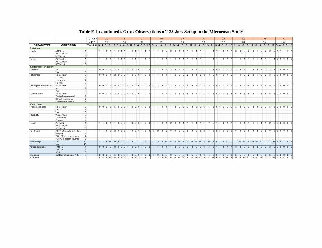
Table E-1 (continued). Gross Observations of 128-Jars Set up in the Microcosm Study Tot Risk
Jar #PARAMETER CRITERION Week # 3 4 6 9 12 3 4 6 9 12 3 4 6 9 12 3 4 6 9 12 3 4 6 9 12 3 4 6 9 12 3 4 6 9 12 3 4 6 9 12 3 4 6 9 12 3 4 6 9 12
Fuel phaseHaze ASTM < 2 1 1 1 1 1 1 1 1 1 1 1 1 1 1 1 1 1 1 1 2 2 1 1 1 1 1 1 1 1 1 1 1 1 1 1 1 3 3 3 3 3 1 2 2 2 2 1 1 1 1 1
ASTM 2 to 3 2ASTM > 3 3
Color ASTM £ 2 1 1 1 1 1 1 1 1 1 1 1 1 1 1 1 1 1 1 1 1 1 1 1 1 1 1 1 1 1 1 1 1 1 1 1 1 1 1 1 1 1 1 1 1 1 1 3 3 3 3 3ASTM 2 to 5 2ASTM > 5 3
Invert emulsion (rag layer) Present No 0 0 0 0 3 3 0 0 0 0 0 0 0 0 0 0 3 3 3 3 3 3 3 3 3 3 3 3 3 3 3 0 0 0 3 3 3 3 3 3 3 3 3 3 3 3 0 0 0 0 0
Yes 3Thickness No rag layer 0 0 0 0 1 2 0 0 0 0 0 0 0 0 0 0 1 1 1 1 1 2 2 2 2 3 1 2 2 2 2 0 0 0 1 2 1 1 2 2 2 1 2 2 3 3 0 0 0 0 0
< 1 mm 11 to 3 mm 2> 3 mm 3
Stalagtites/stalagmites No rag layer 0 0 0 0 2 5 0 0 0 0 0 0 0 0 0 0 2 2 2 2 2 5 5 5 5 5 2 2 5 5 5 0 0 0 5 5 2 2 5 5 5 2 2 5 5 5 0 0 0 0 0No 2Yes 5
Consistency No rag layer 0 0 0 0 1 2 0 0 0 0 0 0 0 0 0 0 1 1 1 1 1 1 5 5 5 5 1 1 2 2 5 0 0 0 5 5 5 5 5 5 5 1 5 5 5 5 0 0 0 0 0Easily disaggregated 1Difficult to disperse 2Membranous pellicle 5
Water phaseAdheres to glass No reg layer 0 0 0 0 5 5 0 0 0 0 0 0 0 0 0 0 1 1 1 1 1 3 3 3 3 3 3 3 3 3 3 0 0 0 3 3 3 3 3 3 3 3 3 3 3 3 0 0 0 0 0
No 1Yes 3
Turbidity Water-white 0Translucent 2Opaque 4
Color ASTM £ 2 1 1 1 1 1 1 0 0 0 0 0 0 0 0 0 0 1 1 1 1 2 1 1 1 1 1 1 1 1 2 2 1 1 1 1 1 1 1 1 1 1 1 1 1 2 2 0 0 0 0 0ASTM 2 to 5 2ASTM > 5 3
Sediment < 25% of sample jar bottom 1 1 1 2 2 0 0 0 0 0 0 0 0 0 0 2 2 3 3 3 1 2 2 2 3 2 2 2 3 3 2 2 2 3 3 3 3 3 3 3 2 2 2 3 3 0 0 0 0 0covered 125 to 75 % bottom covered 2> 75 % of bottom covered 3
Risk Rating: Min. 10 4 4 4 16 20 2 2 2 2 2 2 2 2 2 2 12 12 13 14 15 16 21 21 21 22 14 14 18 20 23 5 5 5 22 22 21 21 24 24 24 14 19 22 24 24 4 4 4 4 4Max. 40
Adjusted average: 10 to 15 1 0 0 0 0 0 0 0 0 0 0 0 0 0 0 0 1 1 1 1 1 3 3 3 3 3 3 3 3 3 3 1 1 1 1 1 3 3 3 3 3 3 3 3 3 3 0 0 0 0 016 to 25 3> 25 5
Overrides: Subtotal for rag layer > 10 5 0 0 0 5 5 0 0 0 0 0 0 0 0 0 0 0 0 0 0 0 5 5 5 5 5 0 5 5 5 5 0 0 0 5 5 5 5 5 5 5 0 5 5 5 5 0 0 0 0 0Total Risk 4 4 4 21 25 2 2 2 2 2 2 2 2 2 2 13 13 14 15 16 24 29 29 29 30 17 22 26 28 31 6 6 6 28 28 29 29 32 32 32 17 27 30 32 32 4 4 4 4 4
30 31 2825 2 2 1641 42 49 5043 44 45 46 47 48
32 32 4

Table E-1 (continued). Gross Observations of 128-Jars Set up in the Microcosm Study Tot Risk
Jar #PARAMETER CRITERION Week # 3 4 6 9 12 3 4 6 9 12 3 4 6 9 12 3 4 6 9 12 3 4 6 9 12 3 4 6 9 12 3 4 6 9 12 3 4 6 9 12 3 4 6 9 12 3 4 6 9 12
Fuel phaseHaze ASTM < 2 1 1 1 1 1 1 1 1 1 1 1 1 2 2 2 3 1 1 1 1 1 1 1 1 1 1 1 1 1 1 1 1 1 1 1 1 1 1 1 1 1 1 2 2 3 3 1 1 1 1 1
ASTM 2 to 3 2ASTM > 3 3
Color ASTM £ 2 1 3 3 3 3 3 3 3 3 3 3 3 3 3 3 3 3 3 3 3 3 3 3 3 3 3 3 3 3 3 3 3 3 3 3 3 3 3 3 3 3 3 3 3 3 3 3 3 3 3 3ASTM 2 to 5 2ASTM > 5 3
Invert emulsion (rag layer) Present No 0 0 0 0 0 0 0 0 0 0 0 3 3 3 3 3 3 3 3 3 3 0 0 0 0 0 0 0 0 3 3 3 3 3 3 3 3 3 3 3 3 0 0 0 0 0 3 3 3 3 3
Yes 3Thickness No rag layer 0 0 0 0 0 0 0 0 0 0 0 1 1 2 2 2 1 1 1 1 1 0 0 0 0 0 0 0 0 1 1 1 1 1 1 1 1 1 1 2 3 0 0 0 0 0 1 1 1 1 1
< 1 mm 11 to 3 mm 2> 3 mm 3
Stalagtites/stalagmites No rag layer 0 0 0 0 0 0 0 0 0 0 0 2 2 2 2 2 2 2 2 2 2 0 0 0 0 0 0 0 0 2 2 2 2 2 2 2 2 2 2 2 5 0 0 0 0 0 2 2 2 2 2No 2Yes 5
Consistency No rag layer 0 0 0 0 0 0 0 0 0 0 0 5 5 5 5 5 1 1 1 1 1 0 0 0 0 0 0 0 0 1 1 1 1 1 1 1 1 1 1 2 5 0 0 0 0 0 1 1 1 1 1Easily disaggregated 1Difficult to disperse 2Membranous pellicle 5
Water phaseAdheres to glass No reg layer 0 0 0 0 0 0 0 0 0 0 0 1 1 1 1 1 1 1 1 1 3 0 0 0 0 0 0 0 0 1 1 1 1 1 1 1 1 1 1 1 3 0 0 0 0 0 3 3 3 3 3
No 1Yes 3
Turbidity Water-white 0Translucent 2Opaque 4
Color ASTM £ 2 1 0 0 0 0 0 1 1 1 1 1 1 1 1 1 1 1 1 1 1 1 1 1 1 1 1 1 1 1 1 1 1 1 1 1 1 1 1 1 1 1 0 0 0 0 0 1 1 1 1 1ASTM 2 to 5 2ASTM > 5 3
Sediment < 25% of sample jar bottom 0 0 0 0 0 1 1 1 1 1 1 1 1 1 1 1 1 1 1 2 1 1 1 1 1 1 1 1 3 3 3 3 3 3 3 1 1 1 1 1 0 0 0 0 0 1 1 1 1 1covered 125 to 75 % bottom covered 2> 75 % of bottom covered 3
Risk Rating: Min. 10 4 4 4 4 4 6 6 6 6 6 17 18 18 18 19 13 13 13 13 16 6 6 6 6 6 6 6 6 15 15 15 15 15 15 15 13 13 13 14 22 4 5 5 6 6 15 15 15 15 15Max. 40
Adjusted average: 10 to 15 1 0 0 0 0 0 0 0 0 0 0 3 3 3 3 3 1 1 1 1 1 0 0 0 0 0 0 0 0 0 0 3 3 3 3 3 3 3 3 3 3 0 0 0 0 0 3 3 3 3 316 to 25 3> 25 5
Overrides: Subtotal for rag layer > 10 5 0 0 0 0 0 0 0 0 0 0 5 5 5 5 5 0 0 0 0 0 0 0 0 0 0 0 0 0 0 0 0 0 0 0 0 0 0 0 0 5 0 0 0 0 0 0 0 0 0 0Total Risk 4 4 4 4 4 6 6 6 6 6 25 26 26 26 27 14 14 14 14 17 6 6 6 6 6 6 6 6 15 15 18 18 18 18 18 16 16 16 17 30 4 5 5 6 6 18 18 18 18 18
51 52 53 54 55 56 57 58 59 604 6 27 17 6 15 18 30 6 18

Table E-1 (continued). Gross Observations of 128-Jars Set up in the Microcosm Study Tot Risk
Jar #PARAMETER CRITERION Week # 3 4 6 9 12 3 4 6 9 12 3 4 6 9 12 3 4 6 9 12 3 4 6 9 12 3 4 6 9 12 3 4 6 9 12 3 4 6 9 12 3 4 6 9 12 3 4 6 9 12
Fuel phaseHaze ASTM < 2 1 1 1 1 1 1 1 1 1 1 1 1 1 1 1 1 1 1 1 1 1 1 1 1 1 1 1 1 1 1 1 1 2 2 2 2 1 1 1 1 1 1 1 1 1 1 1 1 2 3 3
ASTM 2 to 3 2ASTM > 3 3
Color ASTM £ 2 1 3 3 3 3 3 3 3 3 3 3 3 3 3 3 3 3 3 3 3 3 1 1 1 1 1 1 1 1 1 1 1 1 1 1 1 1 1 1 1 1 1 1 1 2 2 1 1 1 1 1ASTM 2 to 5 2ASTM > 5 3
Invert emulsion (rag layer) Present No 0 0 0 0 0 0 3 3 3 3 3 0 0 0 0 0 0 0 0 0 0 0 0 0 0 0 3 3 3 3 3 3 3 3 3 3 3 3 3 3 3 0 3 3 3 3 3 3 3 3 3
Yes 3Thickness No rag layer 0 0 0 0 0 0 1 1 2 2 2 0 0 0 0 0 0 0 0 0 0 0 0 0 0 0 2 2 3 3 3 2 2 2 3 3 1 1 2 2 2 0 1 1 1 1 2 2 2 3 3
< 1 mm 11 to 3 mm 2> 3 mm 3
Stalagtites/stalagmites No rag layer 0 0 0 0 0 0 2 2 2 2 5 0 0 0 0 0 0 0 0 0 0 0 0 0 0 0 2 5 5 5 5 2 2 2 5 5 2 2 2 2 2 0 2 2 5 5 2 2 2 2 5No 2Yes 5
Consistency No rag layer 0 0 0 0 0 0 1 1 1 1 1 0 0 0 0 0 0 0 0 0 0 0 0 0 0 0 1 2 5 5 5 1 1 2 5 5 1 1 2 5 5 0 1 1 2 2 1 1 2 2 5Easily disaggregated 1Difficult to disperse 2Membranous pellicle 5
Water phaseAdheres to glass No reg layer 0 0 0 0 0 0 3 3 3 3 3 0 0 0 0 0 0 0 0 0 0 0 0 0 0 0 3 3 3 3 3 3 3 3 3 3 3 3 3 3 3 0 3 3 3 3 3 3 3 3 3
No 1Yes 3
Turbidity Water-white 0Translucent 2Opaque 4
Color ASTM £ 2 1 1 1 1 1 1 1 1 1 1 1 1 1 1 1 1 1 1 1 1 1 0 0 0 0 0 1 1 1 1 1 1 1 1 1 1 1 1 1 1 1 1 1 1 1 2 1 1 1 2 2ASTM 2 to 5 2ASTM > 5 3
Sediment < 25% of sample jar bottom 2 2 2 3 3 1 1 1 1 1 1 1 2 2 2 1 1 1 1 1 0 0 0 0 0 1 1 1 1 1 1 1 2 3 3 1 1 1 1 1 1 2 2 3 3 1 1 1 1 1covered 125 to 75 % bottom covered 2> 75 % of bottom covered 3
Risk Rating: Min. 10 7 7 7 8 8 15 15 15 15 18 6 6 7 7 7 6 6 6 6 6 2 2 2 2 2 13 17 20 20 20 13 14 16 23 23 13 13 14 17 17 4 14 14 20 21 13 13 15 17 23Max. 40
Adjusted average: 10 to 15 1 0 0 0 0 0 3 3 3 3 3 0 0 0 0 0 0 0 0 0 0 0 0 0 0 0 3 3 3 3 3 3 3 3 3 3 1 1 1 1 1 1 1 1 1 1 3 3 3 3 316 to 25 3> 25 5
Overrides: Subtotal for rag layer > 10 5 0 0 0 0 0 0 0 5 5 5 0 0 0 0 0 0 0 0 0 0 0 0 0 0 0 5 5 5 5 5 5 5 5 5 5 0 0 5 5 5 0 0 0 5 5 5 5 5 5 5Total Risk 7 7 7 8 8 18 18 23 23 26 6 6 7 7 7 6 6 6 6 6 2 2 2 2 2 21 25 28 28 28 21 22 24 31 31 14 14 20 23 23 5 15 15 26 27 21 21 23 25 31
61 62 63 64 65 66 67 68 69 708 26 7 6 2 28 31 23 27 31

Table E-1 (continued). Gross Observations of 128-Jars Set up in the Microcosm Study Tot Risk
Jar #PARAMETER CRITERION Week # 3 4 6 9 12 3 4 6 9 12 3 4 6 9 12 3 4 6 9 12 3 4 6 9 12 3 4 6 9 12 3 4 6 9 12 3 4 6 9 12 3 4 6 9 12 3 4 6 9 12
Fuel phaseHaze ASTM < 2 1 1 1 1 1 1 2 3 3 3 3 1 1 1 1 1 1 1 2 2 2 1 1 1 1 1 1 1 1 1 1 1 2 2 2 2 1 1 1 1 1 1 1 1 2 2 1 1 1 1 1
ASTM 2 to 3 2ASTM > 3 3
Color ASTM £ 2 1 1 1 1 1 1 1 1 1 1 1 1 1 1 1 1 1 1 2 2 2 1 1 1 1 1 1 1 1 1 1 1 1 1 1 1 1 1 1 1 1 1 1 1 1 1 3 3 3 3 3ASTM 2 to 5 2ASTM > 5 3
Invert emulsion (rag layer) Present No 0 0 0 0 3 3 3 3 3 3 3 3 3 3 3 3 0 3 3 3 3 3 3 3 3 3 0 0 0 3 3 3 3 3 3 3 0 0 3 3 3 3 3 3 3 3 3 3 3 3 3
Yes 3Thickness No rag layer 0 0 0 0 2 2 1 1 1 1 1 2 2 2 2 2 0 1 1 2 2 1 1 1 3 3 0 0 0 2 2 2 2 2 2 3 0 0 2 2 3 1 1 3 3 3 1 1 1 2 3
< 1 mm 11 to 3 mm 2> 3 mm 3
Stalagtites/stalagmites No rag layer 0 0 0 0 5 5 2 2 2 2 2 2 2 2 2 2 0 2 5 5 5 2 5 5 5 5 0 0 0 2 5 2 2 2 2 2 0 0 5 5 5 2 2 2 2 2 2 2 2 5 5No 2Yes 5
Consistency No rag layer 0 0 0 0 1 1 1 1 1 1 1 1 1 1 1 1 0 1 2 5 5 1 1 2 2 5 0 0 0 2 5 1 1 1 1 5 0 0 1 5 5 1 1 5 5 5 1 1 1 2 5Easily disaggregated 1Difficult to disperse 2Membranous pellicle 5
Water phaseAdheres to glass No reg layer 0 0 0 0 3 3 3 3 3 3 3 1 1 1 1 1 0 1 1 3 3 3 3 3 3 3 0 0 0 1 1 1 1 1 1 1 0 0 1 3 3 1 3 3 3 3 3 3 3 3 3
No 1Yes 3
Turbidity Water-white 0Translucent 2Opaque 4
Color ASTM £ 2 1 1 1 1 1 1 1 1 1 1 1 1 1 1 1 1 1 1 1 1 1 1 1 1 2 2 1 1 1 1 1 1 1 1 2 3 1 1 1 1 1 1 1 1 2 2 1 1 1 1 1ASTM 2 to 5 2ASTM > 5 3
Sediment < 25% of sample jar bottom 1 1 1 1 1 1 1 1 1 1 1 1 1 1 1 1 1 1 2 2 1 1 1 2 2 1 1 1 2 3 1 1 1 1 1 1 1 1 2 2 1 2 2 3 3 1 1 1 1 1covered 125 to 75 % bottom covered 2> 75 % of bottom covered 3
Risk Rating: Min. 10 4 4 4 16 16 14 15 15 15 15 11 11 11 11 11 4 11 17 23 23 13 16 17 19 22 4 4 4 13 20 11 12 12 13 18 4 4 14 21 21 11 14 18 21 21 15 15 15 19 22Max. 40
Adjusted average: 10 to 15 1 0 0 0 0 0 1 1 1 1 1 1 1 1 1 1 3 3 3 3 3 3 3 3 3 3 0 0 0 0 0 1 1 1 1 1 1 1 1 1 1 3 3 3 3 3 3 3 3 3 316 to 25 3> 25 5
Overrides: Subtotal for rag layer > 10 5 0 0 0 5 5 0 0 0 0 0 0 0 0 0 0 0 0 5 5 5 0 5 5 5 5 0 0 0 0 5 0 0 0 0 5 0 0 5 5 5 0 0 5 5 5 0 0 0 5 5Total Risk 4 4 4 21 21 15 16 16 16 16 12 12 12 12 12 7 14 25 31 31 16 24 25 27 30 4 4 4 13 25 12 13 13 14 24 5 5 20 27 27 14 17 26 29 29 18 18 18 27 30
73 74 75 76 77 7871 72 79 8021 16 12 31 30 25 24 27 29 30

Table E-1 (continued). Gross Observations of 128-Jars Set up in the Microcosm Study Tot Risk
Jar #PARAMETER CRITERION Week # 3 4 6 9 12 3 4 6 9 12 3 4 6 9 12 3 4 6 9 12 3 4 6 9 12 3 4 6 9 12 3 4 6 9 12 3 4 6 9 12 3 4 6 9 12 3 4 6 9 12
Fuel phaseHaze ASTM < 2 1 1 1 1 1 1 1 2 2 3 3 1 2 3 3 3 1 1 1 1 1 2 2 2 2 2 1 2 2 3 3 1 1 1 1 1 1 1 1 1 1 1 1 1 1 1 1 1 1 1 1
ASTM 2 to 3 2ASTM > 3 3
Color ASTM £ 2 1 3 3 3 3 3 3 3 3 3 3 3 3 3 3 3 3 3 3 3 3 3 3 3 3 3 3 3 3 3 3 3 3 3 3 3 3 3 3 3 3 3 3 3 3 3 3 3 3 3 3ASTM 2 to 5 2ASTM > 5 3
Invert emulsion (rag layer) Present No 0 0 3 3 3 3 0 0 0 0 0 3 3 3 3 3 0 0 3 3 3 0 0 0 3 3 3 3 3 3 3 0 0 0 0 0 0 0 0 0 0 0 0 3 3 3 0 0 0 0 0
Yes 3Thickness No rag layer 0 0 1 2 2 3 0 0 0 0 0 1 1 1 1 2 0 0 1 2 2 0 0 0 1 1 1 1 1 1 1 0 0 0 0 0 0 0 0 0 0 0 0 1 1 1 0 0 0 0 0
< 1 mm 11 to 3 mm 2> 3 mm 3
Stalagtites/stalagmites No rag layer 0 0 2 2 2 5 0 0 0 0 0 2 2 2 2 2 0 0 2 5 5 0 0 0 2 2 2 2 2 2 2 0 0 0 0 0 0 0 0 0 0 0 0 2 2 2 0 0 0 0 0No 2Yes 5
Consistency No rag layer 0 0 1 1 2 5 0 0 0 0 0 1 1 1 1 1 0 0 1 5 5 0 0 0 1 1 1 1 1 1 1 0 0 0 0 0 0 0 0 0 0 0 0 1 1 1 0 0 0 0 0Easily disaggregated 1Difficult to disperse 2Membranous pellicle 5
Water phaseAdheres to glass No reg layer 0 0 1 1 1 3 0 0 0 0 0 1 1 1 1 1 0 0 1 3 3 0 0 0 1 1 1 1 1 1 1 0 0 0 0 0 0 0 0 0 0 0 0 1 1 1 0 0 0 0 0
No 1Yes 3
Turbidity Water-white 0Translucent 2Opaque 4
Color ASTM £ 2 1 1 1 1 1 1 1 1 1 1 1 1 1 1 1 1 1 1 1 1 2 1 1 1 1 1 1 1 1 1 1 0 0 0 0 0 0 0 0 0 0 1 1 1 1 1 1 1 1 1 1ASTM 2 to 5 2ASTM > 5 3
Sediment < 25% of sample jar bottom 1 1 1 1 1 2 2 2 2 2 1 1 2 2 2 2 2 2 3 3 1 1 1 2 2 1 1 1 1 1 0 0 0 0 0 0 0 0 0 0 3 3 3 3 3 2 2 3 3 3covered 125 to 75 % bottom covered 2> 75 % of bottom covered 3
Risk Rating: Min. 10 6 13 13 14 22 7 8 8 9 9 13 14 16 16 16 7 7 14 24 25 7 7 7 15 15 13 14 14 15 15 4 4 4 4 4 4 4 4 4 4 8 8 15 15 15 7 7 8 8 8Max. 40
Adjusted average: 10 to 15 1 1 1 1 1 1 0 0 0 0 0 3 3 3 3 3 3 3 3 3 3 1 1 1 1 1 1 1 1 1 1 0 0 0 0 0 0 0 0 0 0 1 1 1 1 1 0 0 0 0 016 to 25 3> 25 5
Overrides: Subtotal for rag layer > 10 5 0 0 0 0 5 0 0 0 0 0 0 0 0 0 0 0 0 0 5 5 0 0 0 0 0 0 0 0 0 0 0 0 0 0 0 0 0 0 0 0 0 0 0 0 0 0 0 0 0 0Total Risk 7 14 14 15 28 7 8 8 9 9 16 17 19 19 19 10 10 17 32 33 8 8 8 16 16 14 15 15 16 16 4 4 4 4 4 4 4 4 4 4 9 9 16 16 16 7 7 8 8 8
85 86 87 88 89 9081 82 83 8428 9 19 33 16 16 4 4 16 8

Table E-1 (continued). Gross Observations of 128-Jars Set up in the Microcosm Study Tot Risk
Jar #PARAMETER CRITERION Week # 3 4 6 9 12 3 4 6 9 12 3 4 6 9 12 3 4 6 9 12 3 4 6 9 12 3 4 6 9 12 3 4 6 9 12 3 4 6 9 12 3 4 6 9 12 3 4 6 9 12
Fuel phaseHaze ASTM < 2 1 1 1 1 1 1 1 1 1 1 1 1 1 1 1 1 1 1 1 1 1 1 1 1 1 1 1 1 1 1 3 1 1 1 1 1 1 1 1 1 1 1 1 1 2 2 1 2 2 2 2
ASTM 2 to 3 2ASTM > 3 3
Color ASTM £ 2 1 3 3 3 3 3 3 3 3 3 3 3 3 3 3 3 3 3 3 3 3 3 3 3 3 3 3 3 3 3 3 1 1 1 1 1 1 1 1 1 1 1 1 1 1 1 1 1 1 1 1ASTM 2 to 5 2ASTM > 5 3
Invert emulsion (rag layer) Present No 0 0 0 0 0 0 3 3 3 3 3 3 3 3 3 3 3 3 3 3 3 0 0 0 0 0 3 3 3 3 3 0 0 0 0 0 0 0 3 3 3 0 0 0 0 0 3 3 3 3 3
Yes 3Thickness No rag layer 0 0 0 0 0 0 1 1 1 1 1 1 1 1 1 1 1 1 1 1 1 0 0 0 0 0 1 1 1 1 1 0 0 0 0 0 0 0 1 2 3 0 0 0 0 0 1 1 1 1 1
< 1 mm 11 to 3 mm 2> 3 mm 3
Stalagtites/stalagmites No rag layer 0 0 0 0 0 0 2 2 2 2 2 2 2 2 2 2 2 2 2 2 2 0 0 0 0 0 2 2 2 2 2 0 0 0 0 0 0 0 2 5 5 0 0 0 0 0 2 2 2 2 2No 2Yes 5
Consistency No rag layer 0 0 0 0 0 0 1 1 1 1 1 1 1 1 1 1 1 1 1 1 1 0 0 0 0 0 1 1 1 1 1 0 0 0 0 0 0 0 2 2 5 0 0 0 0 0 2 2 2 2 2Easily disaggregated 1Difficult to disperse 2Membranous pellicle 5
Water phaseAdheres to glass No reg layer 0 0 0 0 0 0 1 1 1 1 1 1 1 1 1 1 3 3 3 3 3 0 0 0 0 0 1 1 1 1 1 0 0 0 0 0 0 0 3 3 3 0 0 0 0 0 3 3 3 3 3
No 1Yes 3
Turbidity Water-white 0Translucent 2Opaque 4
Color ASTM £ 2 1 1 1 1 1 1 1 1 1 1 1 1 1 1 1 1 1 1 1 1 1 1 1 1 1 1 1 1 1 1 1 0 0 0 0 0 1 1 1 1 1 1 1 1 1 2 1 1 1 1 1ASTM 2 to 5 2ASTM > 5 3
Sediment < 25% of sample jar bottom 2 2 2 2 2 1 1 1 1 1 1 1 1 1 1 1 1 1 1 1 1 1 1 1 1 1 1 1 1 1 0 0 0 0 0 1 1 2 2 2 3 3 3 3 3 1 1 1 1 1covered 125 to 75 % bottom covered 2> 75 % of bottom covered 3
Risk Rating: Min. 10 7 7 7 7 7 13 13 13 13 13 13 13 13 13 13 15 15 15 15 15 6 6 6 6 6 13 13 13 13 15 2 2 2 2 2 4 4 15 18 21 6 6 6 7 8 14 15 15 15 15Max. 40
Adjusted average: 10 to 15 1 0 0 0 0 0 1 1 1 1 1 1 1 1 1 1 3 3 3 3 3 0 0 0 0 0 1 1 1 1 1 0 0 0 0 0 1 1 1 1 1 0 0 0 0 0 1 1 1 1 116 to 25 3> 25 5
Overrides: Subtotal for rag layer > 10 5 0 0 0 0 0 0 0 0 0 0 0 0 0 0 0 0 0 0 0 0 0 0 0 0 0 0 0 0 0 0 0 0 0 0 0 0 0 5 5 5 0 0 0 0 0 5 5 5 5 5Total Risk 7 7 7 7 7 14 14 14 14 14 14 14 14 14 14 18 18 18 18 18 6 6 6 6 6 14 14 14 14 16 2 2 2 2 2 5 5 21 24 27 6 6 6 7 8 20 21 21 21 21
97 98 99 10091 92 93 94 95 967 14 14 18 6 16 2 27 8 21

Table E-1 (continued). Gross Observations of 128-Jars Set up in the Microcosm Study Tot Risk
Jar #PARAMETER CRITERION Week # 3 4 6 9 12 3 4 6 9 12 3 4 6 9 12 3 4 6 9 12 3 4 6 9 12 3 4 6 9 12 3 4 6 9 12 3 4 6 9 12 3 4 6 9 12 3 4 6 9 12
Fuel phaseHaze ASTM < 2 1 1 2 2 2 2 1 1 1 1 1 1 1 1 1 1 1 1 1 1 1 1 1 1 2 2 1 1 1 1 1 1 1 1 1 1 1 1 1 2 2 1 1 1 2 2 1 1 1 1 1
ASTM 2 to 3 2ASTM > 3 3
Color ASTM £ 2 1 1 1 1 1 1 1 1 1 1 1 1 1 1 1 1 1 1 1 1 1 1 1 1 1 1 1 1 1 1 1 1 1 1 1 1 1 1 1 1 1 1 1 1 1 1 1 1 1 1 1ASTM 2 to 5 2ASTM > 5 3
Invert emulsion (rag layer) Present No 0 3 3 3 3 3 3 3 3 3 3 3 3 3 3 3 0 0 0 0 0 3 3 3 3 3 3 3 3 3 3 3 3 3 3 3 0 0 0 0 0 3 3 3 3 3 0 0 3 3 3
Yes 3Thickness No rag layer 0 1 1 1 2 3 2 2 3 3 3 1 2 2 2 3 0 0 0 0 0 1 1 1 1 1 1 2 3 3 3 2 2 3 3 3 0 0 0 0 3 1 1 1 2 2 0 0 1 2 2
< 1 mm 11 to 3 mm 2> 3 mm 3
Stalagtites/stalagmites No rag layer 0 2 2 2 2 2 2 2 2 5 5 2 2 5 5 5 0 0 0 0 0 2 2 2 2 2 2 2 2 5 5 2 2 2 2 5 0 0 0 0 5 2 2 2 2 2 0 0 2 2 2No 2Yes 5
Consistency No rag layer 0 2 2 2 2 5 2 2 5 5 5 1 2 5 5 5 0 0 0 0 0 1 1 1 1 1 1 2 5 5 5 2 2 5 5 5 0 0 0 0 5 1 1 1 1 1 0 0 1 5 5Easily disaggregated 1Difficult to disperse 2Membranous pellicle 5
Water phaseAdheres to glass No reg layer 0 3 3 3 3 3 1 3 3 3 3 3 3 3 3 3 0 0 0 0 0 3 3 3 3 3 3 3 3 3 3 3 3 3 3 3 0 0 0 0 3 1 1 1 3 3 0 0 1 1 1
No 1Yes 3
Turbidity Water-white 0Translucent 2Opaque 4
Color ASTM £ 2 1 1 1 1 1 1 1 1 1 1 1 1 1 1 2 2 1 1 1 1 1 1 1 1 1 1 1 1 1 1 1 1 1 1 1 1 1 1 1 1 2 1 1 1 1 1 1 1 1 1 1ASTM 2 to 5 2ASTM > 5 3
Sediment < 25% of sample jar bottom 1 1 1 2 2 1 1 1 1 1 1 1 1 1 1 3 3 3 3 3 2 2 2 2 2 1 1 1 1 1 2 2 3 3 3 2 3 3 3 3 1 1 1 2 2 2 2 2 3 3covered 125 to 75 % bottom covered 2> 75 % of bottom covered 3
Risk Rating: Min. 10 14 15 15 16 19 12 14 17 20 20 13 14 20 21 21 6 6 6 6 6 14 14 14 15 15 13 14 17 20 20 15 15 19 19 22 5 6 6 7 21 11 11 11 15 15 5 5 12 17 17Max. 40
Adjusted average: 10 to 15 1 3 3 3 3 3 3 3 3 3 3 3 3 3 3 3 0 0 0 0 0 1 1 1 1 1 3 3 3 3 3 3 3 3 3 3 0 0 0 0 0 1 1 1 1 1 1 1 1 1 116 to 25 3> 25 5
Overrides: Subtotal for rag layer > 10 5 5 5 5 5 5 0 5 5 5 5 0 5 5 5 5 0 0 0 0 0 0 0 0 0 0 0 5 5 5 5 5 5 5 5 5 0 0 0 0 5 0 0 0 5 5 0 0 0 5 5Total Risk 22 23 23 24 27 15 22 25 28 28 16 22 28 29 29 6 6 6 6 6 15 15 15 16 16 16 22 25 28 28 23 23 27 27 30 5 6 6 7 26 12 12 12 21 21 6 6 13 23 23
101 102 109 110103 104 105 106 107 10827 28 29 6 16 28 30 26 21 23

Table E-1 (continued). Gross Observations of 128-Jars Set up in the Microcosm Study Tot Risk
Jar #PARAMETER CRITERION Week # 3 4 6 9 12 3 4 6 9 12 3 4 6 9 12 3 4 6 9 12 3 4 6 9 12 3 4 6 9 12 3 4 6 9 12 3 4 6 9 12 3 4 6 9 12 3 4 6 9 12
Fuel phaseHaze ASTM < 2 1 1 1 1 1 1 1 1 1 1 1 1 1 1 1 1 1 1 1 1 1 1 1 1 1 1 1 1 1 1 1 1 1 1 1 1 1 1 1 1 1 1 1 2 2 2 1 1 1 1 1
ASTM 2 to 3 2ASTM > 3 3
Color ASTM £ 2 1 1 1 1 1 1 1 1 1 1 1 1 1 1 1 1 3 3 3 3 3 3 3 3 3 3 3 3 3 3 3 3 3 3 3 3 3 3 3 3 3 3 3 3 3 3 3 3 3 3 3ASTM 2 to 5 2ASTM > 5 3
Invert emulsion (rag layer) Present No 0 3 3 3 3 3 3 3 3 3 3 3 3 3 3 3 0 0 0 1 1 3 3 3 3 3 3 3 3 3 3 3 3 3 3 3 0 0 0 0 0 3 3 3 3 3 0 0 0 0 0
Yes 3Thickness No rag layer 0 1 1 1 1 1 1 2 2 2 3 1 1 1 2 2 0 0 0 1 1 1 1 1 1 1 1 1 2 2 2 1 1 1 1 1 0 0 0 0 0 1 1 1 1 1 0 0 0 0 0
< 1 mm 11 to 3 mm 2> 3 mm 3
Stalagtites/stalagmites No rag layer 0 2 2 2 2 2 2 2 2 2 2 2 2 2 2 2 0 0 0 2 2 2 2 2 2 2 2 2 2 2 5 2 2 2 2 2 0 0 0 0 0 2 2 2 2 2 0 0 0 0 0No 2Yes 5
Consistency No rag layer 0 1 1 1 1 1 1 1 1 1 2 1 1 1 1 1 0 0 0 1 1 1 1 1 1 1 1 1 1 2 5 1 1 1 1 1 0 0 0 0 0 1 1 1 1 1 0 0 0 0 0Easily disaggregated 1Difficult to disperse 2Membranous pellicle 5
Water phaseAdheres to glass No reg layer 0 3 3 3 3 3 3 3 3 3 3 1 1 1 1 1 0 0 0 3 3 1 1 1 1 1 1 3 3 3 3 1 1 1 1 1 0 0 0 0 0 3 3 3 3 3 0 0 0 0 0
No 1Yes 3
Turbidity Water-white 0Translucent 2Opaque 4
Color ASTM £ 2 1 1 1 1 1 1 1 1 1 1 1 1 1 1 1 1 1 1 1 1 1 1 1 1 1 1 1 1 1 1 1 1 1 1 1 1 1 1 1 1 1 1 1 1 1 1 0 0 0 0 0ASTM 2 to 5 2ASTM > 5 3
Sediment < 25% of sample jar bottom 1 1 1 1 1 1 2 2 2 2 1 1 1 1 1 1 1 1 1 1 1 1 1 1 1 1 1 1 1 1 1 1 2 2 2 1 3 3 3 3 1 1 1 1 1 0 0 0 0 0covered 125 to 75 % bottom covered 2> 75 % of bottom covered 3
Risk Rating: Min. 10 13 13 13 13 13 13 14 14 14 15 11 11 11 11 11 6 6 6 13 13 13 13 13 13 13 13 15 15 16 22 13 13 14 14 14 6 8 8 8 8 15 15 16 16 16 4 4 4 4 4Max. 40
Adjusted average: 10 to 15 1 1 1 1 1 1 1 1 1 1 1 1 1 1 1 1 0 0 0 0 0 1 1 1 1 1 3 3 3 3 3 1 1 1 1 1 0 0 0 0 0 3 3 3 3 3 0 0 0 0 016 to 25 3> 25 5
Overrides: Subtotal for rag layer > 10 5 0 0 0 0 0 0 5 5 5 5 0 0 0 0 0 0 0 0 0 0 0 0 0 0 0 0 0 5 5 5 0 0 0 0 0 0 0 0 0 0 0 0 0 0 0 0 0 0 0 0Total Risk 14 14 14 14 14 14 20 20 20 21 12 12 12 12 12 6 6 6 13 13 14 14 14 14 14 16 18 23 24 30 14 14 15 15 15 6 8 8 8 8 18 18 19 19 19 4 4 4 4 4
115 116 117 118 119 120111 112 113 11414 21 12 13 14 30 15 8 19 4

Table E-1 (continued). Gross Observations of 128-Jars Set up in the Microcosm Study
Tot RiskJar #
PARAMETER CRITERION Week # 3 4 6 9 12 3 4 6 9 12 3 4 6 9 12 3 4 6 9 12 3 4 6 9 12 3 4 6 9 12 3 4 6 9 12 3 4 6 9 12Fuel phase
Haze ASTM < 2 1 1 1 1 1 1 1 1 1 1 1 1 1 1 1 1 1 1 1 1 1 1 1 2 3 3 1 2 2 2 2 1 1 1 1 1 1 2 2 3 3ASTM 2 to 3 2ASTM > 3 3
Color ASTM £ 2 1 3 3 3 3 3 3 3 3 3 3 3 3 3 3 3 3 3 3 3 3 3 3 3 3 3 3 3 3 3 3 3 3 3 3 3 3 3 3 3 3ASTM 2 to 5 2ASTM > 5 3
Invert emulsion (rag layer) Present No 0 0 0 0 0 0 0 0 0 3 3 0 0 0 0 0 0 0 0 0 0 3 3 3 3 3 0 0 0 0 0 0 0 3 3 3 3 3 3 3 3
Yes 3Thickness No rag layer 0 0 0 0 0 0 0 0 0 1 1 0 0 0 0 0 0 0 0 0 0 1 1 1 1 1 0 0 0 0 0 0 0 1 1 1 1 1 2 2 2
< 1 mm 11 to 3 mm 2> 3 mm 3
Stalagtites/stalagmites No rag layer 0 0 0 0 0 0 0 0 0 2 2 0 0 0 0 0 0 0 0 0 0 2 2 2 2 2 0 0 0 0 0 0 0 2 2 2 2 2 2 2 2No 2Yes 5
Consistency No rag layer 0 0 0 0 0 0 0 0 0 1 1 0 0 0 0 0 0 0 0 0 0 1 1 1 1 1 0 0 0 0 0 0 0 1 5 5 1 1 1 1 1Easily disaggregated 1Difficult to disperse 2Membranous pellicle 5
Water phaseAdheres to glass No reg layer 0 0 0 0 0 0 0 0 0 1 1 0 0 0 0 0 0 0 0 0 0 1 1 1 1 1 0 0 0 0 0 0 0 3 3 3 3 3 3 3 3
No 1Yes 3
Turbidity Water-white 0Translucent 2Opaque 4
Color ASTM £ 2 1 0 0 0 0 0 1 1 1 1 1 1 1 1 1 1 1 1 1 1 1 1 1 1 1 1 1 1 1 1 1 1 1 1 1 1 1 1 1 1 1ASTM 2 to 5 2ASTM > 5 3
Sediment < 25% of sample jar bottom 0 0 0 0 0 2 2 3 3 3 1 1 1 1 1 1 1 1 1 1 1 1 1 1 1 2 2 2 3 3 3 3 3 3 3 1 1 1 1 1covered 125 to 75 % bottom covered 2> 75 % of bottom covered 3
Risk Rating: Min. 10 4 4 4 4 4 7 7 8 15 15 6 6 6 6 6 6 6 6 6 6 13 13 14 15 15 7 8 8 9 9 8 8 17 21 21 15 16 16 17 17Max. 40
Adjusted average: 10 to 15 1 0 0 0 0 0 1 1 1 1 1 0 0 0 0 0 0 0 0 0 0 1 1 1 1 1 0 0 0 0 0 3 3 3 3 3 3 3 3 3 316 to 25 3> 25 5
Overrides: Subtotal for rag layer > 10 5 0 0 0 0 0 0 0 0 0 0 0 0 0 0 0 0 0 0 0 0 0 0 0 0 0 0 0 0 0 0 0 0 0 5 5 0 0 5 5 5Total Risk 4 4 4 4 4 8 8 9 16 16 6 6 6 6 6 6 6 6 6 6 14 14 15 16 16 7 8 8 9 9 11 11 20 29 29 18 19 24 25 25
127 128121 122 123 124 125 1264 16 6 6 16 9 29 25

APPENDIX F
Coupon Observations

Table F-1. Zonal Observations in Coupon Samples 1-3 in the Microcosm Test
*0 - not applicable, 1 - little to no visible corrosion product, 2 - light/ superficial corrosion, 3 -mild, but obvious corrosive attack, 4 - greater than 50% zonal coverage, 5 - heavy/ full coverage/ zonal spread
Microcosm
1 2 3 4 6 9 12 1 2 3 4 6 9 12 1 2 3 4 6 9 12 1 2 3 4 6 9 12 1 2 3 4 6 9 12 1 2 3 4 6 9 12 1 2 3 4 6 9 12 1 2 3 4 6 9 121 0 0 0 0 0 0 0 0 0 0 0 0 0 0 0 0 0 0 0 0 0 0 0 0 0 0 0 0 1 1 1 2 2 2 2 1 2 2 2 2 2 2 1 1 2 2 2 2 2 1 1 2 2 2 2 22 0 0 0 0 0 0 0 0 0 0 0 0 0 0 0 0 0 0 0 0 0 0 0 0 0 0 0 0 1 1 1 1 1 1 2 1 1 1 1 1 1 2 1 1 1 1 1 1 2 1 1 1 1 1 1 13 1 2 2 2 2 2 2 1 2 2 2 2 2 2 1 2 2 2 3 3 3 1 1 2 2 3 4 4 1 1 1 1 1 2 2 1 1 1 2 2 2 2 1 1 1 1 1 2 2 1 1 1 1 1 1 24 2 2 2 2 2 2 2 2 2 2 2 2 2 2 1 1 3 3 3 3 3 1 3 3 4 5 5 5 1 1 1 1 1 2 2 1 1 1 1 1 1 1 1 1 1 1 1 1 1 1 1 1 1 1 1 15 1 1 2 2 2 2 2 1 1 2 2 2 2 2 1 1 2 2 2 3 3 1 5 5 5 5 5 5 1 1 1 1 1 1 2 1 1 1 2 2 2 2 1 1 1 1 1 1 1 1 1 1 1 1 1 16 0 0 0 0 0 0 0 0 0 0 0 0 0 0 0 0 0 0 0 0 0 0 0 0 0 0 0 0 1 1 1 1 1 1 1 1 1 1 1 1 1 1 1 1 1 1 1 1 1 1 1 1 2 2 2 27 0 0 0 0 0 0 0 0 0 0 0 0 0 0 0 0 0 0 0 0 0 0 0 0 0 0 0 0 1 1 1 1 1 1 1 1 1 1 1 1 1 1 1 1 1 1 1 1 1 1 1 1 2 2 2 28 0 0 0 0 0 0 0 0 0 0 0 0 0 0 0 0 0 0 0 0 0 0 0 0 0 0 0 0 2 2 2 2 2 2 2 2 2 2 2 2 2 2 2 2 2 2 2 2 2 2 2 2 2 2 2 29 0 0 0 0 0 0 0 0 0 0 0 0 0 0 0 0 0 0 0 0 0 0 0 0 0 0 0 0 1 1 1 1 1 1 1 1 1 1 1 1 1 1 1 1 1 1 1 1 1 1 1 1 1 1 1 1
10 2 2 2 2 2 2 2 2 2 2 2 2 2 2 1 1 1 2 2 2 2 1 1 1 1 1 1 1 1 1 1 1 2 2 2 1 1 1 1 1 1 1 1 1 1 1 1 1 1 2 2 2 2 2 2 211 2 2 2 2 2 2 2 1 2 2 2 3 3 3 1 2 2 3 3 3 3 1 2 2 3 3 4 4 1 1 1 1 1 1 1 1 1 1 1 1 1 1 1 1 1 1 1 1 1 1 1 1 1 1 1 112 2 2 2 2 2 2 2 1 2 2 2 2 3 3 1 2 2 3 3 3 3 1 2 3 3 3 3 4 1 1 1 1 1 1 1 2 2 2 2 2 2 2 1 1 1 1 1 1 1 1 1 1 1 1 1 113 1 1 2 2 2 2 2 1 1 2 2 2 2 2 1 1 2 3 3 4 4 1 1 2 3 3 4 4 1 1 1 1 1 1 1 1 1 2 2 2 2 2 1 1 1 1 1 1 1 1 1 2 2 2 2 214 1 1 1 1 1 1 1 1 2 2 2 2 2 2 1 1 1 1 1 1 1 1 1 1 1 1 1 1 1 1 1 1 1 1 1 1 1 1 1 1 1 1 1 1 1 1 1 1 1 1 1 1 1 1 1 115 2 2 2 2 2 2 2 1 1 2 2 2 2 2 1 1 2 2 2 2 2 1 1 1 2 2 2 2 2 2 2 2 2 2 2 2 2 2 2 2 2 2 2 2 2 2 2 2 2 2 2 2 2 2 2 216 0 0 0 0 0 0 0 0 0 0 0 0 0 0 0 0 0 0 0 0 0 0 0 0 0 0 0 0 1 1 1 1 1 1 1 1 2 2 2 2 2 2 1 1 1 1 1 1 1 2 2 2 2 2 2 217 0 0 0 0 0 0 0 0 0 0 0 0 0 0 0 0 0 0 0 0 0 0 0 0 0 0 0 0 1 1 1 1 1 1 1 2 2 2 2 2 2 2 2 2 2 2 2 2 2 3 3 3 3 3 3 318 0 0 0 0 0 0 0 0 0 0 0 0 0 0 0 0 0 0 0 0 0 0 0 0 0 0 0 0 1 1 1 1 1 1 1 1 2 2 2 2 2 2 1 1 1 1 1 1 1 2 2 2 2 2 2 219 1 2 2 3 3 4 4 2 2 4 4 4 5 5 2 2 3 4 4 5 5 2 2 3 4 4 5 5 1 1 1 1 1 1 1 1 1 1 1 1 1 1 1 1 1 1 1 1 1 1 1 1 1 1 1 120 1 2 2 2 2 2 2 1 2 2 2 2 2 2 1 2 2 2 3 3 3 2 2 2 2 3 3 3 1 1 1 1 1 1 1 1 1 1 1 1 1 1 1 1 1 1 1 1 1 1 1 1 1 1 1 121 2 2 2 2 2 2 2 2 2 2 2 2 2 2 2 4 4 5 5 5 5 2 3 4 5 5 5 5 1 1 2 2 2 2 2 2 2 2 2 2 2 2 1 1 1 1 1 1 1 2 2 2 2 2 2 222 1 2 2 2 2 2 3 2 2 2 2 2 3 3 1 2 3 3 3 4 4 1 1 2 2 3 4 5 1 1 1 1 1 1 2 1 1 1 1 1 1 1 1 1 1 1 1 1 1 1 1 1 1 1 1 123 1 1 2 2 2 2 2 1 1 2 2 2 2 2 1 1 1 3 3 3 3 1 1 1 1 1 2 3 2 2 2 2 2 2 2 2 2 2 2 2 2 2 2 2 2 2 2 2 2 2 2 2 2 2 2 224 1 1 1 2 2 2 2 1 1 2 2 2 2 2 1 1 1 1 1 1 1 1 1 1 1 1 1 1 2 2 2 2 2 2 2 2 2 2 2 2 2 2 1 1 1 1 1 1 1 2 2 2 2 2 2 225 1 1 1 1 2 2 2 1 1 2 2 2 2 2 1 1 1 2 3 3 3 1 1 1 1 2 3 3 2 2 2 2 2 2 2 2 2 2 2 2 2 2 1 1 1 1 1 1 1 2 2 2 2 2 2 226 0 0 0 0 0 0 0 0 0 0 0 0 0 0 0 0 0 0 0 0 0 0 0 0 0 0 0 0 1 1 1 1 1 1 1 2 2 2 2 2 2 2 1 1 1 1 1 1 1 1 1 1 1 1 1 127 0 0 0 0 0 0 0 0 0 0 0 0 0 0 0 0 0 0 0 0 0 0 0 0 0 0 0 0 1 1 1 1 1 1 1 2 2 2 2 2 2 2 1 1 1 1 1 1 1 1 1 1 1 1 1 128 1 1 1 1 1 1 1 1 1 1 1 1 1 1 1 1 1 1 1 1 1 1 1 1 1 1 1 1 1 1 1 1 1 1 1 2 2 2 2 2 2 2 1 1 1 1 1 1 1 1 1 1 1 1 1 129 1 1 1 2 2 2 2 1 2 2 2 2 2 2 2 2 2 4 4 4 4 2 2 2 4 4 4 4 1 1 1 1 1 1 1 2 2 2 2 2 2 2 1 1 1 1 1 1 1 2 2 2 2 2 2 230 1 2 2 2 2 2 2 1 1 1 1 1 1 2 1 2 3 4 4 4 4 1 2 2 2 4 4 4 1 1 1 1 1 1 1 2 2 2 2 2 2 2 1 1 1 1 1 1 1 1 1 1 1 1 1 131 1 1 1 2 2 2 2 2 2 2 2 2 2 2 1 2 2 2 2 2 2 1 1 1 1 1 1 1 1 1 1 1 1 1 1 2 2 2 2 2 2 2 1 1 1 1 1 1 1 2 2 2 2 2 2 232 1 1 2 2 2 2 2 1 2 2 2 2 2 2 2 3 3 3 3 3 3 1 1 1 1 1 1 1 1 1 1 1 1 1 1 1 1 2 2 2 2 2 1 1 2 2 2 2 2 1 1 2 2 2 2 233 0 0 0 0 0 0 0 0 0 0 0 0 0 0 0 0 0 0 0 0 0 0 0 0 0 0 0 0 1 1 1 1 1 1 1 1 1 1 1 1 1 1 1 1 1 1 1 1 1 1 1 1 1 1 1 134 1 1 2 2 2 2 2 1 1 1 1 1 2 2 2 2 2 2 4 4 4 1 2 2 2 3 4 4 2 2 2 2 2 2 2 2 2 2 2 2 2 2 2 2 2 2 2 2 2 2 2 2 2 2 2 235 1 3 3 3 3 3 3 1 3 3 3 3 3 3 1 3 4 5 5 5 5 1 3 3 5 5 5 5 1 1 1 1 1 1 1 1 1 1 1 1 1 1 1 1 1 1 1 1 1 1 1 1 1 1 1 136 2 2 2 2 2 2 2 2 2 2 2 2 2 2 2 2 3 3 3 3 3 1 2 3 3 3 3 3 1 1 1 1 1 1 1 1 1 2 2 2 2 2 1 1 1 1 1 1 1 1 1 1 1 1 1 137 1 2 2 2 2 2 2 1 1 1 2 2 2 2 1 2 4 5 5 5 5 1 3 5 5 5 5 5 2 2 2 2 2 2 2 1 1 1 1 1 1 1 1 1 1 1 1 1 1 2 2 2 2 2 2 238 1 1 1 1 2 2 2 1 1 1 1 1 2 2 1 1 1 2 2 2 2 1 1 1 1 1 2 2 1 1 1 1 1 1 1 1 1 1 1 1 2 2 1 1 1 1 1 1 1 1 1 1 1 1 1 139 2 2 2 2 2 2 2 2 2 2 2 2 2 2 2 3 3 3 4 5 5 2 3 3 3 4 5 5 1 1 1 1 1 1 1 1 1 1 1 1 1 1 1 1 1 1 1 1 1 2 2 2 2 2 2 240 1 2 2 2 3 4 4 1 2 2 2 3 4 4 1 2 3 3 4 4 5 1 2 3 3 4 4 5 1 1 1 1 1 1 1 1 1 1 2 2 2 2 1 1 1 1 1 1 1 1 1 1 1 1 1 141 2 2 2 2 2 2 2 2 2 2 2 2 2 2 2 2 2 2 2 3 3 2 2 2 2 2 3 5 1 1 1 1 1 1 1 2 2 2 2 2 2 2 1 1 1 1 1 1 1 1 1 2 2 2 2 242 0 0 0 0 0 0 0 0 0 0 0 0 0 0 0 0 0 0 0 0 0 0 0 0 0 0 0 0 1 1 1 1 1 1 1 1 1 1 1 1 1 1 1 1 1 1 1 1 1 1 1 1 1 1 1 143 0 0 0 0 0 0 0 0 0 0 0 0 0 0 0 0 0 0 0 0 0 0 0 0 0 0 0 0 1 1 1 1 1 1 1 1 1 1 1 1 1 2 1 1 1 1 1 1 1 1 1 1 1 1 1 144 2 2 2 2 2 2 2 2 2 2 2 2 2 2 2 2 3 3 4 5 5 2 2 2 2 3 4 5 1 1 1 1 1 1 1 2 2 2 2 2 2 2 1 1 1 1 1 1 1 1 1 1 2 2 2 245 1 2 2 2 2 2 2 2 2 2 2 2 2 2 1 1 1 1 2 2 2 1 1 1 1 2 2 2 1 1 1 1 1 1 1 2 2 2 2 2 2 2 1 1 1 1 1 1 1 1 1 2 2 2 2 246 2 2 2 2 2 2 2 2 2 2 2 2 2 2 1 1 1 1 1 1 1 1 1 1 1 1 1 1 1 1 1 1 1 1 1 2 2 2 2 2 2 2 1 1 1 2 2 2 2 1 1 1 2 2 2 247 2 2 2 2 2 2 2 2 2 3 3 3 3 3 2 2 2 3 4 4 4 2 2 2 3 4 4 5 2 2 2 2 2 2 2 2 2 2 2 2 3 3 1 1 1 1 1 1 1 2 2 2 2 2 2 248 2 2 2 2 2 2 2 2 2 2 2 2 2 2 1 2 3 4 4 4 4 1 2 3 4 4 4 4 1 1 1 1 1 2 2 1 1 1 1 1 1 1 1 1 1 1 2 2 2 1 1 1 1 1 1 149 2 2 2 2 2 2 2 2 2 2 2 2 2 2 1 1 1 1 1 1 1 1 1 1 1 1 1 1 1 1 1 1 1 1 1 1 1 1 1 1 1 1 1 1 1 1 1 1 1 1 1 2 2 2 2 250 0 0 0 0 0 0 0 0 0 0 0 0 0 0 0 0 0 0 0 0 0 0 0 0 0 0 0 0 1 1 1 1 1 1 1 1 1 1 2 2 2 2 1 1 1 1 1 1 1 1 1 1 1 1 1 1
Average Corrosion Severity for Samples 1 -3Fuel Phase - Edge
CorrosionVapor Phase - Edge CorrosionVapor PhaseFuel PhaseAq/Fuel InterfaceAqueous Phase
Aqueous Phase - Edge Corrosion
Aq/Fuel Interface - Edge Corrosion

Table F-1 (continued). Zonal Observations in Coupon Samples 1-3 in the Microcosm Test
*0 - not applicable, 1 - little to no visible corrosion product, 2 - light/ superficial corrosion, 3 -mild, but obvious corrosive attack, 4 - greater than 50% zonal coverage, 5 - heavy/ full coverage/ zonal spread
Microcosm
1 2 3 4 6 9 12 1 2 3 4 6 9 12 1 2 3 4 6 9 12 1 2 3 4 6 9 12 1 2 3 4 6 9 12 1 2 3 4 6 9 12 1 2 3 4 6 9 12 1 2 3 4 6 9 1251 0 0 0 0 0 0 0 0 0 0 0 0 0 0 0 0 0 0 0 0 0 0 0 0 0 0 0 0 1 1 1 1 1 1 1 1 1 1 1 1 1 1 1 1 1 1 1 1 1 1 1 2 2 2 2 252 2 2 2 2 2 2 2 2 2 2 2 2 2 2 1 1 1 1 2 2 2 2 2 2 2 2 2 2 1 1 2 2 2 2 2 2 3 3 3 3 3 3 1 1 1 1 1 1 1 2 2 2 2 2 2 253 2 2 2 2 2 2 2 2 2 2 2 2 2 2 2 2 3 3 4 4 4 2 2 4 4 4 4 4 1 1 1 1 1 1 1 1 1 2 2 2 2 2 1 2 2 2 2 2 2 1 2 2 2 2 2 254 2 2 2 2 2 2 2 2 2 2 2 2 2 2 1 3 3 3 3 4 5 2 2 2 4 4 4 4 1 1 1 1 1 1 1 1 1 1 1 1 1 1 1 1 1 1 1 1 1 2 2 2 2 2 2 255 2 2 2 2 2 2 2 2 2 2 2 2 2 2 1 1 2 2 2 2 2 1 1 1 1 2 2 3 1 1 1 1 1 1 1 1 1 1 2 2 2 2 1 1 1 1 1 1 1 1 1 1 1 2 2 256 2 2 2 2 3 4 4 1 2 3 3 3 4 4 1 2 3 3 3 4 5 1 2 3 3 3 4 5 1 1 2 2 2 2 2 2 2 2 2 2 2 2 1 1 1 1 1 1 1 1 1 1 1 1 1 157 2 2 2 2 2 2 2 2 2 2 2 2 2 2 1 2 3 3 5 5 5 1 2 3 3 5 5 5 1 1 1 2 2 2 2 2 2 2 2 2 2 2 1 1 1 1 1 1 1 1 1 1 1 1 1 158 2 2 2 2 2 2 2 2 2 2 2 2 2 2 1 1 1 1 1 1 1 1 1 2 2 2 2 2 1 1 1 2 2 2 2 2 2 3 3 4 4 4 1 1 1 1 1 1 1 2 2 2 2 2 2 259 1 1 1 1 1 1 1 1 1 1 1 1 1 1 1 1 1 1 1 1 1 1 1 1 1 1 1 1 1 1 1 1 1 1 1 1 1 1 2 2 2 2 1 1 1 2 2 2 2 1 2 2 2 2 2 260 2 2 2 2 2 2 2 2 2 2 2 2 2 2 1 1 1 1 1 1 1 1 1 1 1 1 1 1 1 1 1 1 1 1 1 2 2 3 3 3 3 3 1 1 1 1 1 1 1 1 2 2 2 2 2 261 2 2 2 2 2 2 2 2 2 2 2 2 2 2 1 3 3 3 3 3 3 1 3 3 3 4 4 4 1 1 2 2 2 2 2 2 2 2 2 2 2 2 1 1 1 1 1 1 1 2 2 2 2 2 2 262 2 2 2 2 2 2 2 2 2 2 2 2 2 2 1 1 1 1 1 1 1 1 1 1 1 1 1 1 1 1 1 1 1 1 1 2 2 2 2 2 2 2 1 1 1 1 1 1 1 1 2 2 2 2 2 263 2 2 2 2 3 3 3 2 2 2 2 2 2 2 2 2 3 3 3 3 3 2 2 3 3 3 3 3 1 1 1 1 1 2 2 1 2 2 2 3 3 3 1 1 1 1 1 1 1 2 2 2 2 2 2 264 2 2 2 2 2 2 2 1 1 1 1 1 1 1 1 1 1 1 1 2 2 1 1 1 1 1 1 1 1 1 1 1 1 1 1 1 2 2 2 2 2 2 1 1 1 1 1 1 1 2 2 2 2 2 2 265 0 0 0 0 0 0 0 0 0 0 0 0 0 0 0 0 0 0 0 0 0 0 0 0 0 0 0 0 1 1 1 1 1 1 1 1 1 2 2 2 2 2 1 1 1 1 1 1 1 1 1 1 1 1 1 166 2 2 2 2 2 2 2 2 2 2 2 3 3 3 1 3 3 3 3 3 3 1 3 3 3 3 3 3 1 1 1 1 1 1 2 2 3 3 3 3 3 3 1 1 1 1 1 1 1 2 2 2 3 3 3 367 1 2 2 2 2 2 2 1 2 2 2 2 2 2 2 2 3 4 5 5 5 2 2 3 4 5 5 5 1 1 1 1 1 2 2 1 1 1 1 1 1 1 1 1 1 1 1 1 1 1 1 1 1 2 2 268 2 2 2 2 2 2 2 2 2 2 2 2 2 2 1 1 1 2 2 3 4 1 1 1 2 2 3 4 1 1 2 2 2 2 2 1 2 3 3 3 3 3 1 1 1 1 1 1 1 2 2 2 2 2 2 269 1 2 2 2 2 2 2 1 2 2 2 2 2 2 2 3 3 3 4 4 5 2 3 3 3 4 4 5 1 1 1 1 1 1 1 1 1 1 1 1 1 1 1 1 1 1 1 1 1 1 1 1 1 1 1 170 1 2 2 2 2 2 2 1 2 2 2 2 2 2 2 2 3 3 4 4 5 2 2 3 3 4 4 4 1 1 1 1 1 1 1 1 1 1 1 1 1 1 1 1 1 1 1 1 1 1 1 1 2 2 2 271 1 2 2 2 2 2 2 1 2 2 2 2 2 2 1 2 2 2 2 2 2 1 2 2 2 2 2 2 1 1 2 2 2 2 2 1 1 2 2 2 2 2 1 1 1 1 1 1 1 2 2 2 2 2 2 272 1 2 2 2 2 2 2 1 2 2 2 2 2 2 2 3 4 4 5 5 5 2 3 4 5 5 5 5 1 1 1 1 1 1 1 1 1 1 1 1 2 2 1 1 1 1 1 1 1 1 1 1 1 1 1 173 2 2 2 2 2 2 2 2 2 2 2 2 2 2 2 2 2 2 3 4 4 2 2 2 2 3 3 3 1 1 1 1 1 1 1 1 1 1 1 1 1 1 1 1 1 1 1 1 1 2 2 2 2 2 2 274 2 2 2 2 2 2 2 2 2 2 2 2 2 2 2 2 3 4 4 4 4 2 2 3 5 5 5 5 1 1 1 1 2 2 2 2 2 3 3 3 3 3 1 1 1 1 1 1 1 2 2 2 2 2 2 275 2 2 2 2 2 2 2 1 2 2 2 2 2 2 1 1 1 1 1 1 2 1 1 1 1 1 1 1 1 1 1 2 2 2 2 1 1 2 3 3 3 3 1 1 1 1 1 1 1 1 1 1 1 1 1 176 1 2 2 2 2 2 2 1 2 2 2 2 2 2 1 1 1 2 2 2 2 1 1 1 2 2 2 2 1 1 1 1 1 1 1 1 1 2 2 2 2 2 1 1 1 1 1 1 1 1 1 1 1 1 1 177 2 2 2 2 2 3 3 2 2 2 2 2 2 2 1 3 3 4 4 5 5 1 3 3 4 4 4 4 1 1 1 1 1 1 1 1 1 1 2 2 2 2 1 1 1 1 1 1 1 1 1 1 1 1 1 178 1 2 2 2 2 2 2 1 2 2 2 2 2 2 1 2 2 2 2 2 2 1 2 2 2 3 3 3 1 1 1 1 2 2 2 1 1 1 1 1 1 1 1 1 1 1 1 1 1 1 1 1 1 1 1 179 1 2 2 2 2 2 2 1 2 2 2 2 2 2 1 3 4 4 4 4 5 1 3 4 4 4 5 5 1 1 1 1 2 2 2 1 1 1 1 1 1 1 1 1 1 1 1 1 1 1 1 2 2 2 2 280 2 2 2 2 2 2 2 2 2 2 2 2 2 2 2 2 2 3 3 3 3 2 2 2 3 3 3 3 1 1 1 1 1 1 1 1 1 1 1 1 1 1 1 1 1 1 1 1 1 1 1 1 1 1 1 181 1 1 1 1 1 1 1 1 1 1 1 1 1 1 1 1 3 3 3 3 3 1 1 3 3 3 3 3 1 1 1 1 1 1 1 1 1 1 1 1 1 1 1 1 1 1 1 1 1 1 2 2 2 2 2 282 1 2 2 2 2 2 2 1 2 2 2 2 2 2 1 3 3 3 4 4 4 1 3 3 3 4 4 4 2 2 2 2 2 2 2 2 2 2 2 2 2 2 1 1 1 1 1 1 1 1 1 2 2 2 2 283 2 2 2 2 2 2 2 2 2 2 2 2 2 2 1 3 3 3 4 4 5 1 3 3 3 4 4 4 1 1 1 2 2 2 2 1 1 2 2 2 2 2 1 1 2 2 2 2 2 1 2 3 3 3 3 384 1 2 2 2 2 2 2 1 2 2 2 2 2 2 2 2 2 2 3 3 5 2 2 2 2 3 3 5 1 1 1 1 1 1 1 2 2 2 2 2 2 2 1 1 1 1 1 1 1 2 2 2 2 2 2 285 1 2 2 2 3 4 4 1 2 2 2 3 4 4 2 2 3 3 3 4 5 2 2 3 3 3 4 5 1 1 1 1 2 2 2 1 1 1 1 2 2 2 1 1 1 1 1 1 1 2 2 2 2 2 2 286 1 2 2 2 2 2 2 1 1 1 1 1 1 1 1 3 4 4 4 5 5 1 3 4 4 4 5 5 1 1 1 2 2 3 3 1 1 1 1 1 1 1 1 1 1 1 1 1 1 1 1 1 2 3 3 387 0 0 0 0 0 0 0 0 0 0 0 0 0 0 0 0 0 0 0 0 0 0 0 0 0 0 0 0 1 1 1 1 1 1 1 1 1 2 2 2 2 2 1 1 1 1 1 1 1 1 1 2 2 2 2 288 0 0 0 0 0 0 0 0 0 0 0 0 0 0 0 0 0 0 0 0 0 0 0 0 0 0 0 0 1 1 1 1 1 1 1 1 1 1 1 2 2 2 1 1 1 2 2 2 2 1 1 1 2 2 2 289 1 1 1 1 1 1 1 1 1 1 1 1 1 1 2 2 3 3 3 3 4 2 2 3 3 3 3 3 1 1 1 1 1 1 1 1 1 1 1 1 2 2 1 1 1 1 1 1 1 1 1 1 1 1 1 190 2 2 3 3 3 3 3 2 2 3 3 3 3 3 1 2 2 3 4 4 4 1 2 2 3 4 4 4 1 1 1 1 1 1 1 1 1 1 1 2 2 2 1 1 1 1 1 1 1 1 1 1 1 1 1 191 2 3 3 3 3 3 3 2 2 2 2 2 2 2 1 1 2 2 2 2 2 1 1 2 2 2 2 2 1 1 2 2 2 2 2 1 2 2 2 2 2 2 1 1 1 1 1 1 1 1 1 1 1 1 1 192 2 2 2 2 2 2 2 1 1 1 1 1 1 1 2 2 2 2 3 3 3 1 1 1 1 1 1 1 1 1 1 1 1 1 1 1 1 1 1 1 1 1 1 1 1 1 1 1 1 1 1 2 3 3 3 393 1 1 1 1 1 1 1 1 1 1 1 1 1 1 1 1 1 1 1 1 1 1 1 1 1 1 1 1 1 1 1 1 1 1 1 1 1 1 1 1 1 1 1 1 1 1 1 1 1 1 1 1 1 1 1 194 1 1 1 1 1 1 1 1 1 1 1 1 1 1 1 1 1 1 1 1 1 1 1 1 1 1 2 2 1 1 1 1 2 2 2 1 1 1 1 1 1 1 1 1 1 1 1 1 1 1 1 1 2 2 2 295 1 2 2 2 2 2 2 1 2 2 2 2 2 2 1 1 1 2 2 2 2 1 1 1 2 2 2 2 1 1 1 1 1 1 1 1 1 1 1 1 1 1 1 1 1 1 1 1 1 1 1 1 1 1 1 196 2 2 2 2 2 2 2 1 1 1 1 1 1 1 2 3 3 3 4 4 4 2 3 3 3 4 4 4 1 1 1 1 1 1 1 1 1 1 1 1 1 1 2 2 2 2 2 3 3 2 2 2 2 2 3 397 0 0 0 0 0 0 0 0 0 0 0 0 0 0 0 0 0 0 0 0 0 0 0 0 0 0 0 0 1 1 1 1 1 1 1 1 1 1 1 2 2 2 1 1 1 1 1 1 1 1 1 1 1 1 1 198 2 3 3 3 3 3 3 2 2 2 2 2 2 2 2 3 3 3 4 4 4 2 3 3 3 4 4 4 1 1 1 1 2 2 2 1 1 1 1 1 1 1 1 1 1 1 1 1 1 1 1 1 1 1 1 199 1 2 2 2 2 2 2 1 2 2 2 2 2 2 1 2 3 3 3 3 3 1 2 3 3 3 3 3 1 1 1 1 1 1 1 1 1 1 2 2 2 2 1 1 1 1 1 1 1 1 1 1 1 1 1 1
100 2 2 2 2 3 3 3 2 2 2 2 3 3 3 2 3 3 4 4 5 5 2 3 3 4 5 5 5 1 1 1 1 2 2 2 2 2 2 2 3 3 3 1 1 1 1 1 1 1 2 2 2 2 2 2 2
Average Corrosion Severity for Samples 1 -3Fuel Phase - Edge
CorrosionVapor Phase - Edge CorrosionVapor PhaseFuel PhaseAq/Fuel InterfaceAqueous Phase
Aqueous Phase - Edge Corrosion
Aq/Fuel Interface - Edge Corrosion

Table F-1 (continued). Zonal Observations in Coupon Samples 1-3 in the Microcosm Test
*0 - not applicable, 1 - little to no visible corrosion product, 2 - light/ superficial corrosion, 3 -mild, but obvious corrosive attack, 4 - greater than 50% zonal coverage, 5 - heavy/ full coverage/ zonal spread.
Microcosm
1 2 3 4 6 9 12 1 2 3 4 6 9 12 1 2 3 4 6 9 12 1 2 3 4 6 9 12 1 2 3 4 6 9 12 1 2 3 4 6 9 12 1 2 3 4 6 9 12 1 2 3 4 6 9 12101 2 2 2 2 2 2 2 2 2 2 2 2 2 2 2 2 3 3 3 4 5 2 2 3 3 3 4 4 1 1 1 1 1 1 1 2 2 2 2 2 2 2 1 1 1 1 1 1 1 2 2 2 2 2 2 2102 2 2 2 2 2 2 2 2 2 2 2 2 2 2 2 2 3 3 4 4 5 2 2 3 3 4 5 5 1 1 1 1 2 2 2 1 1 1 1 1 1 1 1 1 1 1 1 1 1 2 2 2 2 2 2 2103 2 2 2 2 2 2 2 2 2 2 2 2 2 2 1 1 1 1 1 1 1 1 1 1 2 2 2 2 1 1 1 1 1 1 1 1 1 1 1 1 1 1 1 1 1 1 1 1 1 1 1 1 1 1 1 1104 1 2 2 2 2 2 2 1 1 1 1 1 1 1 1 1 1 2 2 2 2 1 1 1 1 1 1 1 1 1 1 1 1 1 1 2 2 2 2 2 2 2 1 1 1 1 1 1 1 1 1 1 1 1 1 1105 2 2 2 2 3 3 3 2 2 2 2 3 3 3 2 2 3 3 4 4 5 2 2 3 4 4 4 4 2 2 2 2 2 2 2 2 3 3 3 3 3 3 1 1 1 1 1 1 1 1 2 2 2 2 2 2106 2 2 2 2 2 2 2 2 2 2 2 2 2 2 1 3 3 4 4 4 4 1 3 3 3 4 4 4 2 2 2 2 2 2 2 2 2 2 2 2 2 2 1 1 1 1 1 1 1 1 1 1 1 1 1 1107 2 2 2 2 2 2 2 2 2 2 2 2 2 2 1 1 2 2 2 2 2 1 1 1 1 1 1 1 1 1 1 1 1 1 1 1 1 1 1 1 1 1 1 1 1 1 1 1 1 2 2 2 2 2 2 2108 2 2 3 3 3 3 3 2 2 2 2 2 2 2 1 1 2 2 2 2 2 1 1 2 2 2 2 2 1 1 1 1 1 1 1 1 1 1 1 1 1 1 1 1 1 1 1 1 1 1 1 1 1 2 2 2109 1 2 3 3 3 3 3 1 2 3 3 3 3 3 2 3 3 4 4 4 4 2 3 4 4 4 4 4 1 1 1 1 1 1 1 1 1 1 1 1 1 1 1 1 1 1 1 1 1 1 1 1 1 1 1 1110 1 1 2 2 2 2 2 1 1 2 2 2 2 2 1 1 1 2 2 4 4 1 1 1 2 2 4 5 1 1 1 1 2 2 2 1 1 2 2 2 2 2 1 1 1 1 1 1 1 2 2 2 2 2 2 2111 2 2 2 2 2 2 2 2 2 2 2 2 2 2 1 1 1 3 3 3 4 1 1 1 3 3 3 4 1 1 1 1 1 1 1 1 1 1 1 1 2 2 1 1 1 1 1 1 1 1 1 1 1 2 2 2112 1 2 2 3 3 3 3 1 2 2 3 3 3 3 1 2 3 3 4 4 5 1 2 3 3 4 4 4 1 1 2 2 2 2 2 2 2 2 2 2 2 2 1 1 2 2 2 2 2 2 2 2 2 2 2 2113 1 2 2 2 2 2 2 1 2 2 2 2 2 2 1 1 1 1 2 2 2 1 1 1 1 2 2 2 1 1 1 1 1 1 1 1 2 2 3 3 3 3 1 1 1 1 1 1 1 1 2 3 3 3 3 3114 1 2 2 2 3 3 3 1 2 2 2 2 2 2 1 1 1 2 3 3 3 1 1 1 2 3 3 3 1 1 1 1 1 1 1 1 1 1 1 1 1 1 1 1 1 1 1 1 1 1 1 1 1 1 1 1115 1 2 3 3 3 3 3 1 1 2 2 2 2 2 1 1 1 1 1 1 1 1 1 1 1 1 1 1 1 1 1 1 2 2 2 1 1 1 2 2 2 2 1 1 1 1 1 1 1 1 1 1 2 2 2 2116 1 1 1 1 1 1 1 2 2 2 2 2 2 2 3 3 3 4 4 4 4 3 3 3 4 4 4 4 1 2 2 2 2 2 2 3 3 3 3 3 3 3 1 1 1 1 1 1 1 1 2 2 2 2 2 2117 1 2 2 2 2 2 2 1 2 2 2 2 2 2 2 3 3 4 4 5 5 2 3 3 4 4 5 5 1 1 1 1 1 1 1 1 2 2 2 2 2 2 1 1 1 1 1 1 1 1 1 2 2 2 2 2118 1 2 2 2 2 2 2 1 2 2 2 2 2 2 1 1 2 2 2 2 2 1 1 2 2 2 2 2 1 1 1 1 1 1 1 1 1 1 1 1 1 1 1 1 1 1 1 1 1 1 2 2 2 2 2 2119 1 2 2 2 2 2 2 1 2 2 2 2 2 2 2 3 3 4 5 5 5 2 3 3 4 5 5 5 1 1 1 1 1 1 1 1 1 1 2 2 2 2 1 1 1 1 1 1 1 1 1 1 1 1 2 2120 0 0 0 0 0 0 0 0 0 0 0 0 0 0 0 0 0 0 0 0 0 0 0 0 0 0 0 0 1 1 1 1 1 1 1 1 2 2 2 2 2 2 1 1 1 1 1 1 1 1 1 2 2 2 2 2121 0 0 0 0 0 0 0 0 0 0 0 0 0 0 0 0 0 0 0 0 0 0 0 0 0 0 0 0 1 1 1 1 1 1 1 1 1 1 1 1 1 1 1 1 1 1 1 1 1 1 1 1 1 1 1 1122 2 3 3 3 3 3 3 2 2 2 2 2 2 2 2 3 3 3 3 3 3 2 3 3 3 3 3 3 1 2 2 2 2 2 2 1 2 2 2 2 2 2 2 2 2 2 2 2 2 2 2 2 2 2 2 2123 1 2 3 3 3 3 3 1 2 2 2 2 2 2 1 2 3 3 4 4 4 1 2 3 3 3 3 3 1 1 1 1 1 1 1 1 1 1 1 1 1 1 1 1 1 1 1 1 1 1 1 1 1 1 1 1124 1 1 2 2 2 2 2 1 1 2 2 2 2 2 1 1 1 1 1 1 1 1 1 2 2 2 2 2 1 1 1 1 1 1 1 1 2 2 2 2 2 2 1 1 1 1 1 1 1 1 1 1 1 1 1 1125 1 2 2 2 2 2 2 1 2 2 2 2 2 2 2 3 3 4 4 5 5 2 3 3 4 4 4 4 1 1 1 1 1 1 1 1 1 1 1 1 1 1 1 1 1 1 1 1 1 2 2 2 2 2 2 2126 1 1 2 2 2 2 2 1 1 2 2 2 2 2 2 2 2 2 3 4 4 2 2 2 2 3 4 5 1 1 1 1 1 1 1 1 1 1 1 1 2 2 1 1 1 1 1 1 1 1 1 1 1 1 2 2127 1 1 2 2 2 2 2 1 1 2 2 2 2 2 1 2 3 3 3 4 4 1 2 3 3 3 3 3 1 1 2 2 2 2 2 1 1 1 1 1 1 1 1 1 1 1 1 1 1 1 1 1 1 1 1 1128 1 1 1 1 1 1 1 1 2 2 2 2 2 2 1 1 1 1 1 1 1 1 1 1 1 1 1 1 1 1 1 1 1 1 1 1 1 1 2 2 2 2 1 1 1 1 1 1 1 1 1 1 1 2 2 2
Average Corrosion Severity for Samples 1 -3Fuel Phase - Edge
CorrosionVapor Phase - Edge CorrosionVapor PhaseFuel PhaseAq/Fuel InterfaceAqueous Phase
Aqueous Phase - Edge Corrosion
Aq/Fuel Interface - Edge Corrosion

APPENDIX G
GCR Data

Table G-1. Cumulative Average GCR Data per Microcosm
Microcosm #
Avg Perc Weight Loss
Std Perc Weight Loss
Avg GCR Std GCR
1 -0.082 0.321 -0.138 0.543 2 -0.077 0.477 -0.138 0.867 3 0.775 0.147 1.379 0.258 4 0.343 0.002 0.62 0 5 0.269 0.057 0.406 0.082 6 0.041 0.153 0.069 0.258 7 -0.203 0.152 -0.345 0.258 8 -0.245 0.1 -0.414 0.169 9 -0.244 0.1 -0.414 0.169
10 0.203 0.152 0.29 0.217 11 -0.082 0.208 -0.138 0.352 12 0.082 0.058 0.138 0.097 13 0.205 0.058 0.29 0.082 14 0.081 0.153 0.138 0.258 15 0.326 0.551 0.494 0.833 16 -0.082 0.058 -0.116 0.082 17 0 0.264 0 0.376 18 0.081 0.208 0.116 0.296 19 0.285 0.115 0.406 0.164 20 0.326 0.116 0.464 0.164 21 0.409 0.323 0.689 0.543 22 0.286 0.116 0.406 0.164 23 0 0.1 0 0.142 24 0.041 0.058 0.058 0.081 25 0.286 0.115 0.406 0.164 26 0.164 0.058 0.247 0.087 27 0.082 0.115 0.124 0.175 28 -0.082 0.153 -0.138 0.258 29 0.122 0.264 0.174 0.376 30 -0.082 0.115 -0.124 0.175 31 0.204 0.208 0.29 0.296 32 0.367 0.099 0.62 0.169 33 0.448 0.207 0.679 0.315 34 0.448 0.058 0.679 0.087 35 0.366 0.001 0.522 0 36 0.732 0.1 1.241 0.169 37 0.569 0.25 0.813 0.358 38 0.325 0.114 0.464 0.164 39 0.448 0.208 0.639 0.296 40 0.164 0.153 0.276 0.258

Microcosm #
Avg Perc Weight Loss
Std Perc Weight Loss
Avg GCR Std GCR
41 0.284 0.229 0.432 0.349 42 -0.001 0.265 0 0.4 43 0 0.1 0 0.151 44 0.98 0.693 1.482 1.048 45 0.08 0.404 0.138 0.682 46 0.366 0.803 0.62 1.351 47 -0.041 0.116 -0.069 0.195 48 0.367 0.459 0.62 0.774 49 0.119 0.753 0.173 1.066 50 0.121 0.263 0.173 0.373 51 -0.13 1.251 -0.185 1.89 52 -0.123 0.437 -0.185 0.66 53 -0.369 0.101 -0.519 0.141 54 0.079 0.707 0.115 1.001 55 0.244 0.36 0.371 0.546 56 0.767 0.671 1.31 1.149 57 -0.287 0.307 -0.483 0.516 58 0.445 0.447 0.639 0.641 59 0 0.173 0 0.262 60 0.326 0.379 0.461 0.534 61 -0.123 0.401 -0.185 0.605 62 0.693 0.152 0.98 0.216 63 -0.37 0.267 -0.556 0.4 64 -0.164 0.232 -0.23 0.326 65 -0.204 0.231 -0.309 0.349 66 0.163 0.115 0.23 0.163 67 0.244 0.263 0.371 0.4 68 0.284 0.664 0.403 0.94 69 -0.082 0.603 -0.124 0.912 70 0.039 0.677 0.058 0.961 71 0.245 0.1 0.371 0.151 72 0.245 0.458 0.346 0.647 73 0 0.1 0 0.141 74 0 0.2 0 0.303 75 -0.246 0.436 -0.346 0.615 76 0.122 0.264 0.207 0.447 77 0.245 0.264 0.346 0.373 78 -0.041 0.253 -0.069 0.425 79 0.082 0.058 0.124 0.087 80 -0.165 0.601 -0.23 0.851

Microcosm #
Avg Perc Weight Loss
Std Perc Weight Loss
Avg GCR Std GCR
81 0.447 0.349 0.758 0.593 82 0.49 0.264 0.718 0.388 83 0.204 0.417 0.288 0.588 84 0.205 0.209 0.309 0.315 85 0.49 0.1 0.741 0.151 86 0.204 0.116 0.286 0.162 87 0.693 0.35 1.018 0.515 88 0.163 0.058 0.215 0.068 89 0.61 0.172 0.898 0.254 90 0.407 0.305 0.599 0.448 91 0.367 0.2 0.539 0.293 92 0.449 0.153 0.634 0.216 93 0.286 0.153 0.4 0.214 94 0.203 0.152 0.286 0.214 95 0.244 0.2 0.359 0.293 96 0.366 0.098 0.515 0.14 97 0.163 0.058 0.239 0.085 98 0.204 0.208 0.299 0.305 99 0.244 0.199 0.359 0.293
100 0.081 0.058 0.114 0.081 101 -0.123 0.361 -0.173 0.509 102 0 0.265 0 0.447 103 0.122 0.3 0.172 0.42 104 0.026 1.769 0.058 2.489 105 0.571 0.35 0.801 0.492 106 0.365 0.263 0.515 0.371 107 0.366 0.173 0.515 0.243 108 0.283 0.49 0.406 0.701 109 0.322 0.847 0.461 1.2 110 -0.001 0.528 0 0.894 111 0.244 0.263 0.343 0.371 112 0.448 0.208 0.629 0.292 113 0.445 0.66 0.629 0.933 114 0.327 0.058 0.458 0.081 115 0.653 0.153 0.958 0.224 116 0.281 0.733 0.406 1.048 117 0.65 0.303 0.958 0.448 118 0.041 0.464 0.06 0.677 119 0.488 0.263 0.741 0.4 120 -0.369 0.437 -0.522 0.62 121 0.204 0.153 0.29 0.217 122 0.244 0.173 0.348 0.246 123 0.285 0.321 0.419 0.471 124 0.162 0.251 0.276 0.425 125 -0.041 0.058 -0.058 0.082 126 0.122 0.264 0.207 0.447 127 0.122 0.264 0.207 0.447 128 -0.163 0.058 -0.247 0.087

Table G-2. Cumulative Maximum GCR Data per Microcosm. Microcosm # are Rank Ordered and Color Coded Dependent on the Severity of Mass Loss (Red – highest, Green – Lowest)
Microcosm # Maximum Coupon GCR (Rank Ordered) GCR Standard Deviation
104 3.135 2.489 44 2.965 1.048 56 2.895 1.149 46 2.275 1.351
113 1.887 0.933 68 1.729 0.94 51 1.668 1.89 3 1.655 0.258
87 1.616 0.515 109 1.556 1.2 15 1.482 0.833 21 1.448 0.543 36 1.448 0.169 48 1.448 0.774 81 1.448 0.593
117 1.437 0.448 58 1.393 0.641
108 1.393 0.701 116 1.393 1.048 49 1.383 1.066 70 1.383 0.961
105 1.373 0.492 119 1.297 0.4 89 1.257 0.254
115 1.257 0.224 110 1.241 0.894 37 1.219 0.358 54 1.210 1.001 60 1.210 0.534 62 1.210 0.216 72 1.210 0.647 33 1.112 0.315 90 1.077 0.448 82 1.077 0.388
123 1.077 0.471 39 1.045 0.296 2 1.034 0.867
45 1.034 0.682 112 1.030 0.292 41 0.927 0.349 55 0.927 0.546 69 0.927 0.912 85 0.927 0.151

Microcosm # Maximum Coupon GCR (Rank Ordered) GCR Standard Deviation
91 0.898 0.293 80 0.864 0.851 83 0.864 0.588 92 0.864 0.216
106 0.858 0.371 107 0.858 0.243 32 0.827 0.169 76 0.827 0.447
124 0.827 0.425 34 0.741 0.087 67 0.741 0.4 84 0.741 0.315 98 0.718 0.305 99 0.718 0.293 95 0.718 0.293 29 0.697 0.376 31 0.697 0.296
122 0.697 0.246 20 0.697 0.164 38 0.697 0.164 50 0.691 0.373 77 0.691 0.373
103 0.686 0.42 93 0.686 0.214 96 0.686 0.14
111 0.686 0.371 1 0.620 0.543
126 0.620 0.447 4 0.620 0
40 0.620 0.258 102 0.620 0.447 127 0.620 0.447 61 0.556 0.605 71 0.556 0.151
118 0.539 0.677 19 0.522 0.164 35 0.522 0 5 0.522 0.082
10 0.522 0.217 17 0.522 0.376 18 0.522 0.296 22 0.522 0.164

Microcosm # Maximum Coupon GCR (Rank Ordered) GCR Standard Deviation
25 0.522 0.164 121 0.522 0.217 75 0.519 0.615
101 0.519 0.509 86 0.515 0.162 94 0.515 0.214
114 0.515 0.081 6 0.414 0.258
14 0.414 0.258 78 0.414 0.425 26 0.371 0.087 42 0.371 0.4 74 0.371 0.303 27 0.371 0.175 52 0.371 0.66 97 0.359 0.085 13 0.348 0.082
120 0.348 0.62 66 0.346 0.163 88 0.311 0.068 12 0.207 0.097 11 0.207 0.352 28 0.207 0.258 47 0.207 0.195 57 0.207 0.516 59 0.185 0.262 43 0.185 0.151 65 0.185 0.349 79 0.185 0.087 23 0.174 0.142 24 0.173 0.081 73 0.173 0.141
100 0.172 0.081 7 0.000 0.258
16 0.000 0.082 30 0.000 0.175 64 0.000 0.326
125 0.000 0.082

APPENDIX H
cATP Data

Table H-1. cATP Data for Microcosm Samples Collected on Days 0 and 30
Measurement Day Microcosm # Matrix cATP (pg ATP/mL) 0 29 water 3,709 0 29 fuel 1 0 40 water 2 0 40 fuel 0 0 57 water 3 0 57 fuel 0 0 66 water 4,202 0 66 fuel 0 0 77 water 1,046 0 77 fuel 0 0 119 water 2,723 0 119 fuel 0
30 30 water 59,841 30 39 water 34,870 30 35 water 21,475 30 86 water 38,135 30 74 water 7,052 30 4 water 32,528 30 9 water 60,031 30 30 fuel 5 30 3 fuel 17 30 3 interphase 16 30 30 interphase 31 30 39 swab 2,988,928

Table H-2. cATP Data for Microcosm Samples Collected on Day 67
Measurement Day Microcosm # Matrix cATP (pg ATP/mL) 67 3 water 36,676 67 4 water 115,693 67 5 water 15,313 67 11 water 5 67 12 water 10 67 13 water 11,242 67 15 water 6 67 15 fuel 4 67 19 water 15,426 67 21 water 20,985 67 21 fuel 74 67 22 water 12,090 67 22 fuel 15 67 23 water 1,414 67 24 water 35,401 67 24 fuel 48 67 25 water 11,541 67 25 fuel 485 67 29 fuel 223 67 29 water 29,874 67 30 water 45,423 67 30 fuel 6 67 31 fuel 77 67 31 water 22,302 67 32 water 23,383 67 35 water 14,236 67 36 water 3 67 37 water 12,673 67 37 fuel 88 67 38 water 188,757 67 38 fuel 506 67 39 water 7,236 67 39 fuel 156 67 40 water 25,253 67 40 fuel 6 67 41 water 8,184 67 41 fuel 187 67 44 water 37,167 67 44 fuel 1 67 47 fuel 295 67 47 water 20,646 67 48 water 39,705 67 48 fuel 13 67 52 fuel 14 67 52 water 7,247 67 53 fuel 144 67 53 water 100,097 67 54 water 12,902 67 57 water 12,501

Measurement Day Microcosm # Matrix cATP (pg ATP/mL) 67 58 fuel 592 67 58 water 85,535 67 67 water 13,522 67 69 water 288 67 72 water 27,144 67 73 water 21,845 67 74 water 3,497 67 75 water 30,413 67 77 water 9,050 67 79 water 17,816 67 81 water 13,959 67 82 water 7 67 82 fuel 3 67 83 water 3,391 67 83 fuel 909 67 85 water 253 67 85 fuel 172 67 86 water 24,297 67 86 fuel 1,814 67 92 water 5,543 67 92 fuel 648 67 96 water 3,774 67 96 fuel 10 67 100 water 17,476 67 102 water 5,232 67 105 water 42,387 67 106 water 70,434 67 109 water 8,446 67 119 water 12,175 67 123 water 66 67 127 water 16,642

Table H-3. cATP Data for Microcosm Samples Collected on Day 120
Measurement Day Microcosm # Matrix cATP (pg ATP/mL) 120 1 water 1 120 3 water 65,531 120 3 water 61,550 120 3 oil 366 120 4 water 76,039 120 4 water 76,039 120 5 interphase 15,251 120 5 water 67,437 120 10 water 79,520 120 11 water 2 120 11 interphase 1 120 11 bottom sediment 1 120 12 water 3 120 12 bottom sediment 4 120 13 water 1,013 120 14 water 8 120 16 water 2 120 16 water 2 120 21 water 122,608 120 23 water 2,306 120 25 water 7,123 120 25 interphase 7,447 120 28 water 24,855 120 29 water 36,897 120 29 interphase 3,776 120 30 water 66,746 120 31 water 53,093 120 32 water 65,940 120 34 water 99,583 120 34 bottom sediment 1,288,629 120 35 water 15,035 120 36 water 3 120 36 fuel 1 120 37 interphase 145 120 37 water 4,860 120 38 interphase 49,569 120 38 water 199,456 120 39 water 27,296 120 41 water 927 120 41 interphase 679 120 42 water 3 120 44 water 35,060 120 44 interphase 13,953 120 45 oil 478 120 45 oil 464 120 45 interphase 2,462 120 46 water 146,761 120 46 bottom sediment 400,927 120 48 water 1,805

Measurement Day Microcosm # Matrix cATP (pg ATP/mL) 120 48 oil 54 120 48 interphase 6,010 120 49 water 42,843 120 51 oil 0 120 52 water 7,520 120 52 bottom sediment 26,571 120 52 interphase 1,224 120 52 fuel 141 120 70 water 44,278 120 110 bottom sediment 177,507 120 110 interphase 2,844 120 126 water 2,330 120 127 water 33,630 120 127 interphase 64,577 120 47 water 50,113 120 53 water 29,719 120 54 water 86,168 120 55 water 164,978 120 57 bottom sediment 2,429 120 57 interphase 2,626 120 57 water 6,566 120 58 water 18,002 120 60 water 8,939 120 61 water 20,010 120 61 bottom sediment 8,670 120 62 interphase 586 120 62 water 39,284 120 63 bottom sediment 5 120 63 water 2 120 64 water 1,081 120 66 water 137,206 120 67 water 7,592 120 68 water 4,114 120 69 water 90 120 69 bottom sediment 323 120 69 interphase 25 120 71 interphase 2 120 71 bottom sediment 272

Measurement Day Microcosm # Matrix cATP (pg ATP/mL) 120 71 water 263 120 73 water 11,774 120 74 bottom sediment 1,105 120 74 water 2,883 120 74 interphase 6,582 120 75 water 69,665 120 76 bottom sediment 5,073 120 77 bottom sediment 69,327 120 77 interphase 166 120 77 fuel 50 120 77 water 1,452 120 78 water 3,975 120 78 interphase 619 120 80 water 50,457 120 81 water 14,366 120 81 interphase 62,148 120 83 water 6,654 120 84 water 1,153 120 85 water 22 120 89 water 15,318 120 90 bottom sediment 48 120 90 water 32 120 91 water 3 120 91 interphase 1 120 92 water 2,323 120 93 water 38,501 120 95 water 22 120 96 water 606 120 97 fuel 7 120 98 water 4,471 120 98 interphase 3 120 99 water 19 120 100 water 1,298 120 101 water 1,193 120 101 fuel 518 120 101 interphase 50,205 120 103 water 76,615 120 103 interphase 8,610

Measurement Day Microcosm # Matrix cATP (pg ATP/mL) 120 104 water 28 120 105 water 5,464 120 106 water 98,772 120 106 fuel 140 120 107 water 32,992 120 108 water 16 120 109 fuel 19 120 109 water 37,188 120 109 bottom sediment 44,582 120 111 water 10,999 120 112 water 24,254 120 112 interphase 1,629 120 113 water 5,235 120 114 water 1,587 120 115 water 1,139 120 116 water 109,248 120 117 water 25,276 120 118 water 120,471 120 119 water 33,818 120 123 water 451,228 120 124 bottom sediment 16,721 120 124 interphase 68 120 124 water 4,147 120 125 water 8,032 120 128 water 76,182

APPENDIX I
Microscopy Data Whole

Table I - 1. Microcosm Samples Down Selected for Microscopy
Microcosm # Microscopy Subject Observations 3 fungal mat Possible presence of mold (Paracoccoidioides) and A. oryzae
28 fungal growth Possible presence of mold (Paracoccoidioides) and A. niger or A. nidulans
32 fungal growth Possible presence of mold (Paracoccoidioides) and A. niger or A. nidulans
36 red-brown spot on fungal mat Iron sulfate deposit (or some other type of metal) 36 fungal mat Iron sulfate deposit (or some other type of metal) 40 fungal mat Iron sulfate deposit (or some other type of metal) 41 fungal mat (black) possible Conidia and folamentus A. oryzae 41 film at interphase possible Conidia and folamentus A. oryzae 44 bottom water metal deposit 44 film at interphase metal deposit 45 interphase possible presence of mold (Paracoccoidioides) and A. oryzae 46 sample growth where the
biofilm splits possible presence of mold (Paracoccoidioides) and A. niger or A. nidulans
47 fungal growth possible Conidia and filamentus A. oryzae 48 fungal growth possible Conidia and filamentus A. oryzae 49 fungal growth possible Conidia and filamentus A. oryzae 56 fungal growth metal deposit 61 interphase possible Conidia and filamentus A. oryzae 67 fungal mat Conidia and germinated Conidia of Aspergillus oryzae RIB40. 70 fungal growth Conidia and germinated Conidia of Aspergillus oryzae RIB40. 71 bottom residue metal deposit 74 sediment metal deposit 76 film at interphase possible presence of mold (Paracoccoidioides) and A. niger or A.
nidulans 78 fungal mat conidia and germinated Conidia of Aspergillus oryzae RIB40. 78 interphase conidia and germinated Conidia of Aspergillus oryzae RIB40. 79 fungal colonies (20X) conidia and germinated Conidia of Aspergillus oryzae RIB40. 85 fungal mat possible presence of mold (Paracoccoidioides) and A. niger or A.
nidulans 86 film at interphase conidia and germinated Conidia of Aspergillus oryzae RIB40. 93 fungal growth - needs rinsed possible Conidia and filamentus A. oryzae
99 -1 bottom water possible Conidia and filamentus A. oryzae 99 -2 interphase possible Conidia and filamentus A. oryzae 102 sample of 'fish eyes', wet
mass Possible presence of Aspergillus terreus or fumigates, mold (Paracoccoidioides)
109 pellicle Possible presence of mold (Paracoccoidioides) 110 take sample of 'fish eyes', wet
mass Possible presence of Aspergillus terreus or fumigates, mold (Paracoccoidioides)
122 fungal growth Possible presence of Aspergillus terreus or fumigates, mold (Paracoccoidioides)
126 fungal mat Possible presence of Aspergillus niger, A. terreus or fumigates, mold (Paracoccoidioides)
127 black growth at interphase Possible presence of Aspergillus niger, A. terreus or fumigates, mold (Paracoccoidioides)

Figure I- 1. Microscopic Images of Selected Microcosm Samples

Figure I-1 (continued). Microscopic Images of Selected Microcosm Samples

Figure I-1 (continued). Microscopic Images of Selected Microcosm Samples

Figure I-1 (continued). Microscopic Images of Selected Microcosm Samples

Figure I-1 (continued). Microscopic Images of Selected Microcosm Samples

Figure I-1 (continued). Microscopic Images of Selected Microcosm Samples

APPENDIX J
Genomic Data

Table J.1 Genomic Profile UST Bottoms-water Sample I by Whole Genome Sequencing Analysis.
Genus/ species % Abundance
Genus/ species % Abundance Pseudomonas 67.44%
Rhodopseudomonas 4.65%
aeruginosa 2.33%
palustris BisA53 2.33% aeruginosa BL14 2.33%
palustris JSC-3b 2.33%
aeruginosa BWH051 2.33%
Rhodobacter 4.65% aeruginosa BWH054 2.33%
capsulatus 2.33%
aeruginosa BWH060 2.33%
sp. SW2 2.33% aeruginosa BWHPSA012 2.33%
Stenotrophomonas 2.33%
aeruginosa BWHPSA028 2.33%
maltophilia K279a 2.33% aeruginosa C52 2.33%
Rhodovulum 2.33%
aeruginosa NCAIM 2.33%
sp. PH10 2.33% aeruginosa PA7 2.33%
Rhodomicrobium 2.33%
aeruginosa PAK 2.33%
vannielii ATCC 17100 2.33% aeruginosa PAO1-VE2 2.33%
Pseudogulbenkiania 2.33%
alcaliphila 2.33%
sp. MAI-1 2.33% balearica DSM 6083 2.33%
Grand Total 100.00%
bauzanensis 2.33%
chlororaphis 2.33%
chlororaphis aureofaciens 2.33%
entomophila L48 2.33%
fluorescens 2.33%
fluorescens R124 2.33%
mendocina 2.33%
monteilii DMS 14164 2.33%
parafulva 2.33%
pseudoalcaligenes 2.33%
putida 2.33%
sp. PAMC 25886 2.33%
sp. URHB0015 2.33%
stutzeri 2.33%
syringae CC1557 2.33%
Rhodoferax 4.65%
ferrireducens 2.33%
ferrireducens T118 2.33%
Acidimicrobium 4.65%
ferrooxidans 2.33%
ferrooxidans DSM 10331 2.33%
Acidiphilium 4.65%
cryptum 2.33%
cryptum JF-5 2.33%

Table J.2 Genomic Profile UST Bottoms-water Sample II by Whole Genome Sequencing Analysis.
Genus/ species % Abundance
Pseudomonas 35.68%
aeruginosa 0.75%
aeruginosa BL08 0.11%
aeruginosa BWH036 0.11%
aeruginosa BWH051 2.34%
aeruginosa NCAIM B.001380 0.11%
aeruginosa PA7 1.92%
alkylphenolia 0.32%
bauzanensis 0.53%
chlororaphis subsp. aurantiaca 25.56%
chlororaphis subsp. aureofaciens 30-84 0.32%
entomophila L48 0.43%
fluorescens 0.21%
fluorescens R124 0.53%
parafulva 1.28%
sp. PAMC 25886 0.21%
sp. URHB0015 0.53%
sp. UW4 0.11%
sp. WCS374 0.11%
syringae CC1557 0.21%
Acidimicrobium 24.71%
ferrooxidans DSM 10331 24.71%
Rhodobacter 11.40%
capsulatus SB 1003 7.77%
sp. SW2 3.62%
Rhodomicrobium 8.73%
vannielii ATCC 17100 8.73%
Acidiphilium 8.09%
cryptum 4.47%

cryptum JF-5 3.62%
Rhodopseudomonas 3.41%
palustris BisA53 3.09%
palustris JSC-3b 0.32%
Acidimicrobium 3.41%
ferrooxidans 3.41%
Pseudogulbenkiania 1.70%
sp. MAI-1 1.70%
Stenotrophomonas 1.06%
maltophilia K279a 1.06%
Rhodoferax 0.75%
ferrireducens 0.75%
Rhodoferax 0.53%
ferrireducens T118 0.53%
Rhodovulum 0.32%
sp. PH10 0.32%
Bacterium 0.11%
copahuensis 0.11%
Azoarcus sp. 0.11%
BH72 0.11%
Grand Total 100.00%

Table J.3 Genomic Profile – Secondary LSD Microcosm Used for Challenge Population Cultivation – Replicate 1
Genus/ species % Abundance
Pseudomonas 37.9% Pseudomonas aeruginosa BL14 0.3% aeruginosa BWH051 2.0% aeruginosa BWH054 0.5% aeruginosa BWH060 0.2% aeruginosa BWHPSA012 0.2% aeruginosa BWHPSA028 0.2% aeruginosa C23 0.6% aeruginosa C52 0.2% aeruginosa NCAIM B.001380 0.6% aeruginosa PA7 0.5% aeruginosa PAK 0.2% aeruginosa PAO1-VE2 0.3% alcaliphila 34 0.5% balearica DSM 6083 0.2% bauzanensis 0.8% chlororaphis subsp. aurantiaca 23% 30-84 0.5% entomophila L48 0.3% fluorescens 0.9% fluorescens R124 0.3% mendocina 0.2% monteilii NBRC 103158 = DSM 14164 0.2% parafulva 0.6% pseudoalcaligenes 1.7% putida 0.3% PAMC 25886 1.4% URHB0015 1.1% stutzeri 0.2% syringae CC1557 0.2%
Acidimicrobium 28% ferrooxidans DSM 10331 26% ferrooxidans 1.4%
Acidiphilium 11.7% cryptum 9.1% cryptum JF-5 2.6% Rhodopseudomonas 3.3%
palustris BisA53 3.2% palustris JSC-3b 0.2%

Rhodoferax 0.5% ferrireducens 0.3% ferrireducens T118 0.2% Rhodomicrobium vannielii ATCC 17100 9.3% Rhodobacter capsulatus SB 1003 5.6% Rhodobacter sp. SW2 2.6% Pseudogulbenkiania sp. MAI-1 0.3% Stenotrophomonas maltophilia K279a 0.8% Rhodovulum sp. PH10 0.3% unidentified 0.2% Grand Total 100.0%

Table J.4 Genomic Profile – Secondary LSD Microcosm Used for Challenge Population Cultivation – Replicate 2
Genus/ species % Abundance
Pseudomonas 35.7% chlororaphis subsp. aurantiaca 26% aeruginosa BWH051 2.3% aeruginosa PA7 1.9% parafulva 1.3% aeruginosa 0.7% aeruginosa BL08 0.1% aeruginosa BWH036 0.1% aeruginosa NCAIM B.001380 0.1% alkylphenolia 0.3% bauzanensis 0.5% chlororaphis subsp. aureofaciens 30-84 0.3% entomophila L48 0.4% fluorescens 0.2% fluorescens R124 0.5% PAMC 25886 0.2% URHB0015 0.5% UW4 0.1% WCS374 0.1% syringae CC1557 0.2%
Acidimicrobium 28% ferrooxidans DSM 10331 25% ferrooxidans 3.4%
Rhodobacter 11.4% capsulatus SB 1003 7.8% SW2 3.6% Acidiphilium 8.1%
cryptum 4.5% cryptum JF-5 3.6%
Rhodopseudomonas 3.4% palustris BisA53 3.1% palustris JSC-3b 0.3%
Rhodoferax 1.3% ferrireducens 0.7% ferrireducens T118 0.5%
Rhodomicrobium vannielii ATCC 17100 9% Stenotrophomonas maltophilia K279a 1% Pseudogulbenkiania sp. MAI-1 1.7% Rhodovulum sp. PH10 0.3% Azoarcus sp. BH72 0.1%

Candidatus acidianus copahuensis 0.1% Grand Total 100.0%

Table J.5 Genomic Profile – Secondary LSD Microcosm Used for Challenge Population Cultivation – Replicate 1 & 2 Combined (Computed Averages)
Genus/ species % Abundance
DUP #1 a DUP #2 AVG b
Pseudomonas 37.2% aeruginosa 5.5% 5.3% 5.4% chlororaphis 24% 26% 25% fluorescens 1.2% 0.7% 1.0% other spp. 7.3% 4.5% 5.9%
Acidimicrobium ferrooxidans 28% 28% 28% Acidiphilium cryptum 11.7% 8.1% 9.9% Rhodopseudomonas palustris 3.3% 3.4% 3.4% Rhodobacter spp. 11.4% 8.2% 9.8% Rhodoferax ferrireducens 0.5% 1.3% 0.9% Rhodomicrobium vannielii ATCC 17100 9.3% 8.7% 9.0% Pseudogulbenkiania sp. MAI-1 0.3% BDL 0.2% Stenotrophomonas maltophilia K279a 0.8% 1.1% 0.9% Rhodovulum sp. PH10 0.3% 0.3% 0.3% Pseudogulbenkiania sp. MAI-1 0.3% 1.7% 1.0% Azoarcus sp. BH72 BDL 0.1% 0.1% Candidatus acidianus copahuensis BDL 0.1% 0.1% unidentified 0.2% - 0.1% Grand Total 100%
Notes:
a) DUP – summarized results from Tables J.3 and J.4. Percentages reflect sums of the total abundance of multiple strains of a given species.
b) AVG – average OTU abundance. Values in bold font are based on sums of all OTU of the listed genus.

Table J.6 Microbial Diversity in Microcosm # 3 Sample.
Genus and species % Grand total Genus and species % Grand totalRalstonia sp. 5_2_56FAA 53.20% Afipia birgiae 34632 0.01%Paraburkholderia fungorum NBRC 102489 13.19% Sphingomonas taxi 0.01%Bradyrhizobium elkanii USDA 76 10.18% Mesorhizobium loti 0.01%Sphingomonas sp. RIT328 5.56% Sphingomonas sp. Root720 0.01%Mesorhizobium sp. F7 3.81% Grand Total 100.00%Caulobacter sp. Root343 2.55%Aquabacterium parvum 2.10%Novosphingobium nitrogenifigens DSM 19370 1.64%Variovorax paradoxus 1.39%Paraburkholderia phytofirmans PsJN 1.12%Bosea sp. LC85 1.04%Mycolicibacterium mucogenicum 0.83%Ralstonia solanacearum CMR15 0.66%Hammondia hammondi 0.42%Methyloversatilis discipulorum 0.35%Mesorhizobium japonicum R7A 0.32%Methylobacterium radiotolerans JCM 2831 0.23%Bradyrhizobium japonicum 22 0.15%Bradyrhizobium sp. STM 3843 0.12%Reyranella massiliensis 521 0.12%Methylibium petroleiphilum PM1 0.10%Blastomonas sp. AAP53 0.10%Variovorax paradoxus B4 0.09%Bradyrhizobium sp. WSM4349 0.09%Pantholops hodgsonii 0.08%Sphingopyxis sp. H115 0.08%Hyphomicrobium sp. 99 0.06%Edaphobacter aggregans DSM 19364 0.06%Bosea thiooxidans 0.04%Variovorax sp. Root434 0.03%Bosea sp. Root381 0.03%Bradyrhizobium sp. WSM3983 0.03%Leifsonia aquatica H1aii 0.03%Leptothrix cholodnii SP-6 0.02%Bradyrhizobium japonicum USDA 6 0.01%Sphingomonas melonis DAPP-PG 224 0.01%Sphingomonas sp. PAMC 26621 0.01%Afipia birgiae 34632 0.01%Sphingomonas taxi 0.01%Mesorhizobium loti 0.01%Sphingomonas sp. Root720 0.01%Grand Total 100.00%

Table J.7 Microbial Diversity in Microcosm # 4 Sample.
Table J.8 Microbial Diversity in Microcosm # 21 Sample.
Genus and species % Grand totalLactobacillus paracasei subsp. paracasei 8700:2 68.00%Bacillus circulans NBRC 13626 31.10%Lactobacillus paracasei 0.31%Lactobacillus acidipiscis DSM 15836 0.29%Lactobacillus rhamnosus LOCK908 0.10%Aspergillus fischeri NRRL 181 0.09%Lactobacillus casei BD-II 0.07%Lactobacillus rhamnosus GG 0.02%Acinetobacter johnsonii XBB1 0.01%Grand Total 100.00%
Genus and species % Grand totalLactobacillus paracasei subsp. paracasei 8700:2 85.76%Lactobacillus acidipiscis DSM 15836 10.91%Bacillus circulans NBRC 13626 1.97%Lactobacillus rhamnosus GG 0.80%Lactobacillus paracasei 0.27%Lactobacillus rhamnosus LOCK908 0.18%Lactobacillus casei BD-II 0.04%Lactobacillus acidipiscis KCTC 13900 0.02%Haemophilus parainfluenzae T3T1 0.01%Porphyromonas sp. KLE 1280 0.01%Aspergillus fischeri NRRL 181 0.01%Grand Total 100.00%

Table J.9 Microbial Diversity in Microcosm # 21 Sample.
Table J.10 Microbial Diversity in Microcosm # 28 Sample.
Genus and species % Grand totalLactobacillus acidipiscis DSM 15836 57.42%Lactobacillus paracasei subsp. paracasei 8700:2 40.79%Lactobacillus rhamnosus GG 1.01%Lactobacillus paracasei 0.19%Bacillus circulans NBRC 13626 0.18%Lactobacillus rhamnosus LOCK908 0.11%Porphyromonas sp. KLE 1280 0.08%Aspergillus fischeri NRRL 181 0.06%Lactobacillus acidipiscis KCTC 13900 0.06%Haemophilus parainfluenzae T3T1 0.06%Lactobacillus casei BD-II 0.04%Pseudomonas sp. RIT288 0.01%Grand Total 100.00%
Genus and species % Grand totalLactobacillus acidipiscis DSM 15836 57.42%Lactobacillus paracasei subsp. paracasei 8700:2 40.79%Lactobacillus rhamnosus GG 1.01%Lactobacillus paracasei 0.19%Bacillus circulans NBRC 13626 0.18%Lactobacillus rhamnosus LOCK908 0.11%Porphyromonas sp. KLE 1280 0.08%Aspergillus fischeri NRRL 181 0.06%Lactobacillus acidipiscis KCTC 13900 0.06%Haemophilus parainfluenzae T3T1 0.06%Lactobacillus casei BD-II 0.04%Pseudomonas sp. RIT288 0.01%Grand Total 100.00%

Table J.11 Microbial Diversity in Microcosm # 32 Sample. Genus and species % Grand totalLactobacillus acidipiscis DSM 15836 96.33%Lactobacillus paracasei subsp. paracasei 8700:2 3.40%Lactobacillus acidipiscis KCTC 13900 0.12%Lactobacillus rhamnosus GG 0.10%Lactobacillus paracasei 0.02%Stenotrophomonas maltophilia D457 0.01%Pseudomonas sp. RIT288 0.01%Grand Total 100.00%

Table J.12 Microbial Diversity in Microcosm # 36 Sample. Genus and species % Grand totalAcinetobacter johnsonii XBB1 37.70%Pseudomonas sp. RIT288 12.30%Stenotrophomonas maltophilia D457 11.87%Acinetobacter lwoffii WJ10621 11.10%Stenotrophomonas maltophilia 10.68%Acinetobacter johnsonii SH046 3.30%Pseudomonas synxantha BG33R 3.09%Ralstonia sp. NT80 2.18%Acinetobacter lwoffii NCTC 5866 = CIP 64.10 = NIPH 512 0.96%Porphyromonas sp. KLE 1280 0.88%Klebsiella aerogenes EA1509E 0.67%Pseudomonas fluorescens R124 0.63%Enterobacter cloacae 0.55%Pelomonas sp. Root1217 0.50%Pseudomonas putida H8234 0.48%Pseudomonas putida HB3267 0.39%Stenotrophomonas maltophilia MTCC 434 0.37%Cronobacter turicensis z610 0.27%Acinetobacter sp. NIPH 1847 0.25%Acinetobacter sp. CIP 102143 0.19%Pseudomonas synxantha 0.17%Acinetobacter johnsonii ANC 3681 0.15%Enterobacter sp. MGH 22 0.15%Pseudomonas sp. URMO17WK12:I11 0.14%Prevotella sp. oral taxon 299 str. F0039 0.12%Ralstonia sp. 5_2_56FAA 0.11%Enterobacter sp. MGH 24 0.10%Sphingomonas melonis DAPP-PG 224 0.09%Prevotella nanceiensis DSM 19126 = JCM 15639 0.08%Caballeronia zhejiangensis 0.08%Acinetobacter johnsonii CIP 64.6 0.07%Pseudomonas chlororaphis 0.06%Pseudomonas aeruginosa MTB-1 0.06%Lysinibacillus xylanilyticus 0.04%Pseudomonas fluorescens NZ007 0.03%Acinetobacter sp. NIPH 809 0.03%Stenotrophomonas maltophilia Ab55555 0.03%Staphylococcus capitis 0.03%Klebsiella pneumoniae 0.02%Stenotrophomonas maltophilia NBRC 14161 0.02%Candidatus Hepatobacter penaei 0.02%Flavobacterium sp. B17 0.02%Bacillus coagulans 0.02%Pseudomonas putida NBRC 14164 0.02%Pseudomonas sp. S13.1.2 0.01%Grand Total 100.00%

Table J.13 Microbial Diversity in Microcosm # 40 Sample.
Genus and species % Grand totalLactobacillus paracasei subsp. paracasei 8700:2 0.405835305Acinetobacter johnsonii XBB1 0.223347213Acinetobacter lwoffii WJ10621 0.076685738Pseudomonas sp. RIT288 0.071443549Stenotrophomonas maltophilia D457 0.06290627Stenotrophomonas maltophilia 0.056256178Pseudomonas synxantha BG33R 0.017463979Acinetobacter johnsonii SH046 0.016145943Ralstonia sp. NT80 0.015337148Haemophilus parainfluenzae T3T1 0.004942635Porphyromonas sp. KLE 1280 0.004822814Acinetobacter lwoffii NCTC 5866 = CIP 64.10 = NIPH 512 0.004553216Enterobacter cloacae 0.004313573Cronobacter turicensis z610 0.004043974Klebsiella aerogenes EA1509E 0.003834287Pseudomonas fluorescens R124 0.003774376Acinetobacter sp. NIPH 1847 0.002815804Lactobacillus paracasei 0.002276608Enterobacter sp. MGH 24 0.001947099Pseudomonas putida H8234 0.001677501Pseudomonas putida HB3267 0.001527724Gemella sanguinis M325 0.001407902Pelomonas sp. Root1217 0.001168259Mycobacterium simiae ATCC 25275 = DSM 44165 0.001078393Ralstonia sp. 5_2_56FAA 0.000958572Acinetobacter sp. CIP 102143 0.00083875Mycobacterium intracellulare subsp. yongonense 05-1390 0.000808795Haemophilus influenzae KR494 0.000718929Streptococcus sp. F0441 0.000688973Acinetobacter ursingii DSM 16037 = CIP 107286 0.000659018Sphingomonas melonis DAPP-PG 224 0.000659018Lactobacillus rhamnosus LOCK908 0.000599107Paraprevotella clara YIT 11840 0.000569152Stenotrophomonas maltophilia MTCC 434 0.000509241Acinetobacter johnsonii CIP 64.6 0.000479286Lactococcus lactis subsp. lactis KLDS 4.0325 0.000479286Enterobacter sp. MGH 22 0.00044933Caballeronia zhejiangensis 0.000329509Pseudomonas synxantha 0.000239643Sphingobacterium sp. Ag1 0.000239643Pseudomonas sp. URMO17WK12:I11 0.000209688Lactobacillus casei BD-II 0.000209688Acinetobacter johnsonii ANC 3681 0.000209688Rhizobium sp. IRBG74 0.000149777Pseudomonas aeruginosa MTB-1 0.000149777Acinetobacter sp. NIPH 809 0.000119821Pseudomonas chlororaphis 0.000119821Grand Total 100.00%

Table J.14 Microbial Diversity in Microcosm # 45A Sample.
Table J.15 Microbial Diversity in Microcosm # 45B Sample.
Table J.16 Microbial Diversity in Microcosm # 46 Sample.
Genus and species % Grand totalMassilia sp. WG5 99.86%Massilia sp. 9096 0.10%Porphyromonas sp. KLE 1280 0.02%Acinetobacter johnsonii XBB1 0.02%Streptococcus sp. F0441 0.01%Grand Total 100.00%
Genus and species % Grand totalMassilia sp. WG5 99.77%Massilia sp. 9096 0.12%Acinetobacter johnsonii XBB1 0.06%Stenotrophomonas maltophilia 0.01%Pseudomonas sp. RIT288 0.01%Lactobacillus paracasei subsp. paracasei 8700:2 0.01%Acinetobacter lwoffii WJ10621 0.01%Grand Total 100.00%
Genus and species % Grand totalLactobacillus acidipiscis DSM 15836 55.21%Lactobacillus paracasei subsp. paracasei 8700:2 43.49%Lactobacillus rhamnosus GG 0.78%Lactobacillus paracasei 0.16%Lactobacillus rhamnosus LOCK908 0.15%Lactobacillus acidipiscis KCTC 13900 0.08%Bacillus circulans NBRC 13626 0.08%Lactobacillus casei BD-II 0.04%Grand Total 100.00%

Table J.17 Microbial Diversity in Microcosm # 47 Sample.
Table J.18 Microbial Diversity in Microcosm # 48 Sample.
Table J.19 Microbial Diversity in Microcosm # 56 Sample.
Genus and species % Grand totalLactobacillus acidipiscis DSM 15836 81.16%Methylobacterium radiotolerans JCM 2831 18.70%Lactobacillus acidipiscis KCTC 13900 0.09%Acinetobacter johnsonii XBB1 0.02%Mesorhizobium sp. F7 0.02%Grand Total 100.00%
Genus and species % Grand totalLactobacillus acidipiscis DSM 15836 52.37%Lactobacillus paracasei subsp. paracasei 8700:2 29.96%Bacillus circulans NBRC 13626 10.55%Oerskovia sp. Root918 6.13%Lactobacillus rhamnosus GG 0.51%Lactobacillus paracasei 0.13%Lactobacillus acidipiscis KCTC 13900 0.09%Lactobacillus rhamnosus LOCK908 0.05%Lactobacillus casei BD-II 0.05%Acinetobacter johnsonii XBB1 0.05%Pseudomonas sp. RIT288 0.03%Stenotrophomonas maltophilia 0.02%Pseudomonas synxantha BG33R 0.02%Aspergillus fischeri NRRL 181 0.02%Acinetobacter lwoffii WJ10621 0.02%Stenotrophomonas maltophilia D457 0.01%Mycobacteroides abscessus subsp. bolletii 50594 0.01%Grand Total 100.00%
Genus and species % Grand totalMethylobacterium sp. 77 72.30%Methylobacterium radiotolerans JCM 2831 27.56%Methylobacterium sp. Leaf91 0.08%Acinetobacter johnsonii XBB1 0.04%Stenotrophomonas maltophilia D457 0.01%Methylobacterium sp. Leaf361 0.01%Grand Total 100.00%

Table J.20 Microbial Diversity in Microcosm # 57 Sample.
Table J.21 Microbial Diversity in Microcosm #78 Sample.
Table J.22 Microbial Diversity in Microcosm #81A Sample.
Genus and species % Grand totalPseudomonas fulva 99.59%Pseudomonas putida H8234 0.20%Pseudomonas fluorescens R124 0.17%Caballeronia zhejiangensis 0.02%Pseudomonas helleri 0.02%Grand Total 100.00%
Genus and species % Grand totalLactobacillus acidipiscis DSM 15836 60.95%Mesorhizobium sp. F7 18.75%Methylobacterium radiotolerans JCM 2831 12.14%Sphingomonas sp. Mn802worker 5.72%Aureimonas sp. AU20 1.20%Methylobacterium sp. AMS5 0.36%Ensifer sp. BR816 0.24%Methylobacterium sp. 77 0.19%Methylobacterium sp. Leaf361 0.17%Mesorhizobium loti 0.16%Lactobacillus acidipiscis KCTC 13900 0.06%Methylobacterium sp. Leaf469 0.06%(blank) 0.00%Grand Total 100.00%
Genus and species % Grand totalLactobacillus paracasei subsp. paracasei 8700:2 71.69%Lactobacillus acidipiscis DSM 15836 21.61%Bacillus circulans NBRC 13626 5.66%Lactobacillus rhamnosus GG 0.44%Lactobacillus paracasei 0.34%Lactobacillus rhamnosus LOCK908 0.12%Aspergillus fischeri NRRL 181 0.07%Lactobacillus casei BD-II 0.03%Lactobacillus acidipiscis KCTC 13900 0.02%Porphyromonas sp. KLE 1280 0.02%Grand Total 100.00%

Table J.23 Microbial Diversity in Microcosm #81B Sample.
Table J.24 Microbial Diversity in Microcosm #102 Sample.
Table J.25 Microbial Diversity in Microcosm #110 Sample.
Genus and species % Grand totalLactobacillus paracasei subsp. paracasei 8700:2 76.20%Lactobacillus acidipiscis DSM 15836 17.68%Bacillus circulans NBRC 13626 5.06%Lactobacillus rhamnosus GG 0.46%Lactobacillus paracasei 0.34%Lactobacillus rhamnosus LOCK908 0.09%Lactobacillus casei BD-II 0.06%Acinetobacter johnsonii XBB1 0.03%Streptococcus sp. F0441 0.02%Aspergillus fischeri NRRL 181 0.02%Lactobacillus acidipiscis KCTC 13900 0.01%Streptococcus cristatus ATCC 51100 0.01%Porphyromonas sp. KLE 1280 0.01%Lactococcus lactis subsp. lactis KLDS 4.0325 0.01%Grand Total 100.00%
Genus and species % Grand totalPseudomonas sp. HPB0071 85.03%Pseudomonas luteola XLDN4-9 14.76%Methylobacterium radiotolerans JCM 2831 0.20%Lactobacillus paracasei subsp. paracasei 8700:2 0.01%Grand Total 100.00%
Genus and species % Grand totalStenotrophomonas maltophilia K279a 65.51%Pseudomonas moraviensis R28-S 27.10%Pseudomonas fluorescens 5.78%Pseudomonas fluorescens R124 0.85%Pseudomonas putida GB-1 0.43%Pseudomonas aeruginosa BWH051 0.20%Pseudomonas parafulva NBRC 16636 = DSM 17004 0.12%Pseudomonas fluorescens A506 0.01%Grand Total 100.00%

Table J.26 Microbial Diversity in Microcosm #126 Sample.
Genus and species % Grand totalPseudomonas sp. HPB0071 36.19%Acinetobacter johnsonii XBB1 21.56%Pseudomonas sp. RIT288 8.60%Stenotrophomonas maltophilia 6.42%Pseudomonas luteola XLDN4-9 6.22%Stenotrophomonas maltophilia D457 5.60%Acinetobacter lwoffii WJ10621 5.60%Acinetobacter johnsonii SH046 1.80%Pseudomonas synxantha BG33R 1.38%Ralstonia sp. NT80 1.32%Pseudomonas monteilii 0.93%Acinetobacter lwoffii NCTC 5866 = CIP 64.10 = NIPH 512 0.90%Klebsiella aerogenes EA1509E 0.80%Cronobacter turicensis z610 0.37%Pelomonas sp. Root1217 0.34%Acinetobacter sp. CIP 102143 0.23%Pseudomonas putida H8234 0.20%Pseudomonas synxantha 0.17%Enterobacter cloacae 0.14%Porphyromonas sp. KLE 1280 0.12%Hammondia hammondi 0.11%Pseudomonas fluorescens R124 0.11%Flavobacterium sp. B17 0.10%Pseudomonas sp. URMO17WK12:I11 0.09%Ralstonia sp. 5_2_56FAA 0.08%Acinetobacter johnsonii CIP 64.6 0.08%Acinetobacter sp. CIP 102637 0.07%Pseudomonas sp. S13.1.2 0.07%Pseudomonas putida HB3267 0.07%Oerskovia turbata 0.06%Acinetobacter johnsonii ANC 3681 0.06%Enterobacter sp. MGH 22 0.03%Pseudomonas chlororaphis 0.03%Sphingomonas melonis DAPP-PG 224 0.03%Pseudomonas sp. NBRC 111130 0.03%Caballeronia zhejiangensis 0.02%Cutibacterium acnes HL096PA1 0.02%Stenotrophomonas maltophilia Ab55555 0.02%Grand Total 100.00%

Table J.27 Microbial Diversity in Microcosm #127 Sample.
Genus and species % Grand totalLactobacillus paracasei subsp. paracasei 8700:2 87.74%Acinetobacter johnsonii XBB1 4.33%Pseudomonas sp. RIT288 1.44%Acinetobacter lwoffii WJ10621 1.43%Stenotrophomonas maltophilia D457 1.41%Stenotrophomonas maltophilia 1.31%Lactobacillus paracasei 0.43%Pseudomonas synxantha BG33R 0.34%Acinetobacter johnsonii SH046 0.20%Ralstonia sp. NT80 0.18%Lactobacillus casei BD-II 0.15%Pseudomonas fluorescens R124 0.14%Cronobacter turicensis z610 0.12%Lactobacillus rhamnosus LOCK908 0.11%Acinetobacter lwoffii NCTC 5866 = CIP 64.10 = NIPH 512 0.10%Enterobacter cloacae 0.09%Veillonella dispar ATCC 17748 0.06%Penicillium solitum 0.06%Klebsiella aerogenes EA1509E 0.04%Acinetobacter sp. NIPH 1847 0.04%Mesorhizobium sp. F7 0.04%Sphingomonas melonis DAPP-PG 224 0.04%Pseudomonas putida H8234 0.03%Enterobacter sp. MGH 24 0.03%Enterobacter sp. MGH 22 0.03%Acinetobacter johnsonii CIP 64.6 0.02%Pelomonas sp. Root1217 0.02%Cutibacterium acnes HL096PA1 0.02%Lactobacillus acidipiscis DSM 15836 0.02%Acinetobacter ursingii DSM 16037 = CIP 107286 0.02%Ralstonia sp. 5_2_56FAA 0.01%Acinetobacter sp. CIP 102143 0.01%Grand Total 100.00%

Table J.28 Summary of Microbial Diversity for All Microcosm Samples
Microcosm 3 4 21 28 32 36 40 45A 45B 46 47 48 56 57 76 78 81A 81B 102 110 126 127Microbial Challenge - + + + + - - - - + - + - - - - + + - - - -
Genus and Species (OTU) Abundance (%)Acinetobacter 0.47 0.37 0.30 0.05Acinetobacter johnsonii 0.01 41.22 24.01 0.02 0.06 0.02 0.05 0.04 0.03 23.50 4.55Acinetobacter Iwoffii 12.06 8.13 0.01 0.02 6.50 1.53Acinetobacter ursingii 0.07 0.02Afipia birgiae 0.01Aquabacterium parvum 2.10Aspergillus fischeri 0.09 0.01 0.06 0.02 0.07 0.02Aureimonas 1.20Bacillus circulans 31.10 1.97 0.18 0.08 10.55 5.66 5.06Bacillus coagulans 0.02Blastomonas 0.10Bosea 1.07Bosea thiooxidans 0.04Bradyrhizobium 0.24Bradyrhizobium elkanii 10.18Bradyrhizobium japonicum 0.16Caballeronia zhejiangensis 0.08 0.03 0.02 0.02Candidatus Hepatobacter penaei 0.02Caulobacter 2.55Cronobacter turicensis 0.27 0.40 0.37 0.12Cutibacterium acnes 0.02 0.02Edaphobacter aggregans 0.06Ensifer 0.24Enterobacter 0.25 0.23 0.03 0.06Enterobacter cloacae 0.55 0.43 0.14 0.09Flavobacterium 0.02 0.10Gemella sanguinis 0.14Haemophilus influenzae 0.07Haemophilus parainfluenzae 0.01 0.06 0.49Hammondia hammondi 0.42 0.11Hyphomicrobium 0.06Klebsiella aerogenes 0.67 0.38 0.80 0.04Klebsiella pneumoniae 0.02Lactobacillus acidipiscis 0.29 10.93 57.48 96.45 55.29 81.25 52.46 61.01 21.63 17.69 0.02Lactobacillus casei 0.07 0.04 0.04 0.02 0.04 0.05 0.03 0.06 0.15Lactobacillus paracasei 68.31 86.03 40.98 3.42 40.60 0.01 43.65 30.09 72.03 76.54 0.01 88.17Lactobacillus rhamnosus 0.12 0.98 1.12 0.10 0.06 0.93 0.56 0.56 0.55 0.11Lactococcus lactis 0.05 0.01Leifsonia aquatica 0.03Leptothrix cholodnii 0.02Lysinibacillus xylanilyticus 0.04Massilia 99.96 99.89Mesorhizobium 3.81 0.02 18.75 0.04Mesorhizobium japonicum 0.32Mesorhizobium loti 0.01 0.16Methylibium petroleiphilum 0.10Methylobacterium 72.39 0.78Methylobacterium radiotolerans 0.23 18.70 27.56 12.14 0.20Methyloversatilis discipulorum 0.35Mycobacterium intracellulare 0.08Mycobacterium simiae 0.11Mycobacteroides abscessus 0.01Mycolicibacterium mucogenicum 0.83Novosphingobium nitrogenifigens 1.64Oerskovia 6.13Oerskovia turbata 0.06Pantholops hodgsonii 0.08Paraburkholderia fungorum 13.19Paraburkholderia phytofirmans 1.12Paraprevotella clara 0.06Pelomonas 0.50 0.12 0.34 0.02Penicillium solitum 0.06Porphyromonas 0.01 0.08 0.88 0.48 0.02 0.02 0.01 0.12Prevotella 0.12Prevotella nanceiensis 0.08Pseudomonas 0.01 0.01 12.45 7.16 0.01 0.03 100.00 85.03 44.98 1.44Pseudomonas aeruginosa 0.06 0.01 0.20Pseudomonas chlororaphis 0.06 0.01 0.03Pseudomonas fluorescens 0.66 0.38 0.17 6.64 0.11 0.14Pseudomonas fulva 99.59Pseudomonas helleri 0.02Pseudomonas luteola 14.76 6.22Pseudomonas monteilii 0.93Pseudomonas moraviensis 27.10Pseudomonas parafulva 0.12Pseudomonas putida 0.89 0.32 0.20 0.43 0.27 0.03Pseudomonas synxantha 3.26 1.77 0.02 1.55 0.34Ralstonia 53.20 2.29 1.63 1.40 0.19Ralstonia solanacearum 0.66Reyranella massiliensis 0.12Rhizobium 0.01Sphingobacterium 0.02Sphingomonas 5.58 5.72Sphingomonas melonis 0.01 0.09 0.07 0.03 0.04Sphingomonas taxi 0.01Sphingopyxis 0.08Staphylococcus capitis 0.03Stenotrophomonas maltophilia 0.01 22.97 11.97 0.01 0.03 0.01 65.51 12.04 2.72Streptococcus 0.07 0.01 0.02Streptococcus cristatus 0.01Variovorax 0.03Variovorax paradoxus 1.48Veillonella dispar 0.06Grand Total 99.89 99.99 99.98 100.01 99.99 100.03 99.75 100.01 99.99 99.99 99.99 100.02 100.00 100.00 100.00 100.00 100.00 100.00 100.00 100.00 99.97 100.01

Figure J.1 Krona Plot of Metagenomic Sequencing Results of Microcosms #3 and #4.

Figure J.2 Krona Plot of Metagenomic Sequencing Results of Microcosms #21 and #28.

Figure J.3 Krona Plot of Metagenomic Sequencing Results of Microcosms #32 and #36.

Figure J.4 Krona Plot of Metagenomic Sequencing Results of Microcosms #40.

Figure J.5 Krona Plot of Metagenomic Sequencing Results of Microcosms #45A and #45B.

Figure J.6 Krona Plot of Metagenomic Sequencing Results of Microcosms #46 and #47.

Figure J.7 Krona Plot of Metagenomic Sequencing Results of Microcosms #48 and #56.

Figure J.8 Krona Plot of Metagenomic Sequencing Results of Microcosms #57 and #78.

Figure J.9 Krona Plot of Metagenomic Sequencing Results of Microcosms #81A and #81B.

Figure J.10 Krona Plot of Metagenomic Sequencing Results of Microcosms #102 and #110.

Figure J.11 Krona Plot of Metagenomic Sequencing Results of Microcosms #126 and #127.

APPENDIX K
Chemical Analyses

Table K-1 . Calibration Curve Concentrations for Volatile Acids, Methanol, and Ethanol Quantification
C7 C6 C5 C4 C3 C2 C1
Molecular
Weight
ug/mL
Stock 0.5829 0.4998 0.4164 0.333 0.2499 0.166 0.0833
Acetic acid 60.02113 600.2113 349.8632 299.9856 249.928 199.8704 149.9928 99.63508 49.9976
Propionic acid 74.036781 732.9641 427.2448 366.3355 305.2063 244.0771 183.1677 121.672 61.05591
2-methyl propanoic
acid 88.052429 880.5243 513.2576 440.086 366.6503 293.2146 220.043 146.167 73.34767
Butanoic acid 88.052429 871.7190 508.125 435.6852 362.9838 290.2824 217.8426 144.7054 72.6142
3-methyl butanoic acid 102.13 1011.0870 589.3626 505.3413 421.0166 336.692 252.6706 167.8404 84.22355
Pentanoic acid 102.068077 1020.6808 594.9548 510.1362 425.0115 339.8867 255.0681 169.433 85.02271
4-methyl pentanoic acid 116.16 1197.6096 698.0866 598.5653 498.6846 398.804 299.2826 198.8032 99.76088
Hexanoic acid 116.16 1153.4688 672.357 576.5037 480.3044 384.1051 288.2519 191.4758 96.08395
Heptanoic acid 130.09938 1281.4789 746.974 640.4832 533.6078 426.7325 320.2416 212.7255 106.7472
Ethanol
102.7 63.2 31.6 15.8 7.9 3.95
Methanol 102.7 63.2 31.6 15.8 7.9 3.95

Table K-2 . Analysis of Composition and Concentration of Organic Acids in Samples Collected at Day 0 and Day 60 in the Fuel Phase the Microcosm Experiment
Sample and Time Point29F D_0
40F D_0
57F D_0
66F D_0
77F D_0
119F D_0
15F D_60
21F D_60
24F D_60
37F D_60
39F D_60
40F D_60
44F D_60
48F D_60
53F D_60
83F D_60
85F D_60
86F D_60
96F D_60
Analyte (ug/mL)Acetic Acid C-2 0.00 0.00 0.00 0.00 0.00 0.00 0.00 0.00 0.00 0.00 0.00 0.00 0.00 trace 0.00 0.00 0.00 trace traceMethanol **linear curve used** trace trace 0.00 trace trace trace trace trace trace 18.80 18.70 15.03 25.23 9.57 10.28 10.85 22.97 18.72 17.62Ethanol **linear curve used** trace trace trace trace trace trace trace 0.00 trace 0.00 0.00 trace 0.00 0.00 0.00 trace 0.00 trace 0.28Propionic Acid C-3 0.00 0.00 0.00 0.00 0.00 0.00 0.00 0.00 0.00 0.00 0.00 0.00 0.00 0.00 0.00 0.00 0.00 trace 0.00Isobutyric Acid 0.00 0.00 0.00 0.00 0.00 0.00 0.00 0.00 0.00 0.00 0.00 0.00 0.00 0.00 0.00 0.00 0.00 0.00 0.00Butanoic Acid C-4 0.00 0.00 0.00 0.00 0.00 0.00 0.00 0.00 0.00 0.00 0.00 0.00 0.00 0.00 0.00 0.00 0.00 0.00 0.003-methyl butanoic acid 0.00 0.00 0.00 0.00 0.00 0.00 0.00 0.00 0.00 0.00 0.00 0.00 0.00 0.00 0.00 0.00 0.00 0.00 0.00Pentanoic Acid C-5 0.00 0.00 0.00 0.00 0.00 0.00 0.00 0.00 0.00 0.00 0.00 0.00 0.00 0.00 0.00 0.00 0.00 0.00 0.004-methyl pentanoic acid 0.00 0.00 0.00 0.00 0.00 0.00 0.00 0.00 0.00 0.00 0.00 0.00 0.00 0.00 0.00 0.00 0.00 0.00 0.00Hexanoic Acid C-6 0.00 0.00 0.00 0.00 0.00 0.00 0.00 0.00 0.00 0.00 0.00 0.00 0.00 0.00 0.00 0.00 0.00 0.00 0.00Heptanoic Acid 0.00 0.00 0.00 0.00 0.00 0.00 0.00 0.00 0.00 0.00 0.00 0.00 0.00 0.00 0.00 0.00 0.00 0.00 0.00Glycerol mg/mL 0.00 0.00 0.00 0.00 0.00 0.00 0.00 0.00 0.00 0.00 0.00 0.00 0.00 0.00 0.00 0.00 0.00 0.00 0.00
trace indicates below the curve but response greater 3/1 S/N
Analytes of Interest Present in Samplesethyl acetate X X X X X2-methyl-propyl ester X8,11-octadecadienoic acid, methyl ester X X X Xoctadecanoic acid methyl ester X X15-methyl heptadecanoic, methyl ester X Xdocosanoic acid methyl ester X X X X Xtetracosanoic methyl ester Xhexadecanoic acid methyl ester X X X10,13-octadecadienoic acid methyl ester X9,13-octadecandienoic acid methyl ester X11-octadecanoic acid methyl ester X14-methyl-pentadecanoic acid methyl ester Xeicosane X X X X X X X X X X X X Xdocosane X X X X X X X X X X X X X X Xnonacosane Xoctacosane X X Xheptacosane X X X X Xtricosane X X X X X X X X X X X X X Xtetracosane X X X X X X X X X X X Xhexacosane X X X X X X X X Xcampestrol Xstigmasterol X.gmma.sitosterol X2,6,10,14-tetramethyl octadecane Xnonahexcontanoic acid Xundecane X X Xdodecane X X X Xtridecane X X X X X Xtetradecane X X X X X X Xpentadecane X X X X X X X X X X Xoctadecane X X X X X X X X X X X Xhexadecane X X X X X X X X X X X Xheptadecane X X X X X X X X X X X X X X Xheneicosane X X X X Xpentatriacontane Xnonadecane X X X X X X X X X X X X X X Xhentriacontane X X X2-methyl nonodecane X7,9-dimethyl hexadecane Xcyclododecyl isothiocyanate X

Table K-3 . Analysis of Composition and Concentration of Organic Acids in Samples Collected on Day 0 in the Water Phase of the Microcosm Experiment
Table K-4 . Analysis of Composition and Concentration of Organic Acids in Samples Collected on Day 30 in the Water Phase of the Microcosm Experiment
Sample 29W D_0 40W D_0 59W D_0 66W D_0 77W D_0 119W D_0Analyte (ug/mL)
Acetic Acid C-2 0.00 0.00 0.00 0.00 69.61 361.02Methanol **linear curve used*** 1.54 1.85 1.52 1.53 1.65 2.36Ethanol **linear curve used** 0.93 0.93 0.93 0.93 0.93 0.93Propionic Acid C-3 0.00 0.00 0.00 0.00 0.00 0.00Isobutyric Acid 0.00 0.00 0.00 0.00 0.00 0.00Butanoic Acid C-4 0.00 0.00 0.00 0.00 0.00 0.003-methyl butanoic acid 0.00 0.00 0.00 0.00 0.00 0.00Pentanoic Acid C-5 0.00 0.00 0.00 0.00 0.00 0.004-methyl pentanoic acid 0.00 0.00 0.00 0.00 0.00 0.00Hexanoic Acid C-6 0.00 0.00 0.00 0.00 0.00 0.00Heptanoic Acid 0.00 0.00 0.00 0.00 0.00 0.00Glycerol mg/ml 0.00 58.51 223.32 0.00 0.00 236.76
for volatile acids, trace indicates below the curve, but is a hit
Sample 3W D_30 4W D_30 30W D_30 35 D_30 39W D_30 74 D_30 86W D_30Analyte (ug/mL)
Acetic Acid C-2 0.00 0.00 0.00 0.00 0.00 0.00 503.13Methanol **linear curve used*** 1.52 1.52 1.52 1.55 1.52 1.52 1.69Ethanol **linear curve used** 0.93 0.93 0.93 0.93 0.93 0.93 0.93Propionic Acid C-3 0.00 0.00 0.00 0.00 33.43 0.00 0.00Isobutyric Acid 0.00 0.00 0.00 0.00 1673.21 0.00 0.00Butanoic Acid C-4 0.00 0.00 0.00 0.00 0.00 0.00 0.003-methyl butanoic acid 0.00 0.00 0.00 0.00 0.00 0.00 0.00Pentanoic Acid C-5 0.00 0.00 0.00 0.00 0.00 0.00 0.004-methyl pentanoic acid 0.00 0.00 0.00 0.00 0.00 0.00 0.00Hexanoic Acid C-6 0.00 0.00 0.00 0.00 0.00 0.00 0.00Heptanoic Acid 0.00 0.00 0.00 0.00 0.00 0.00 0.00Glycerol mg/ml 0.00 0.00 65.34 0.00 119.53 0.00 44.77
for volatile acids, trace indicates below the curve, but is a hit

Table K-5 . Analysis of Composition and Concentration of Organic Acids in Samples Collected on Day 60 in the Water Phase of the Microcosm Experiment
Table K-5 (continued). Analysis of Composition and Concentration of Organic Acids in Samples Collected on Day 60 in the Water Phase of the Microcosm Experiment
Sample3W
D_604W
D_605W
D_6011W D_60
12W D_60
31W D_60
15W D_60
19W D_60
21W D_60
22W D_60
23W D_60
24W D_60
32W D_60
29W D_60
30W D_60
13W D_60
25W D_60
35W D_60
36W D_60
37W D_60
38W D_60
39W D_60
40W D_60
41W D_60
44W D_60
47W D_60
48W D_60
Analyte (ug/mL)Acetic Acid C-2 0.00 0.00 0.00 0.00 0.00 0.00 0.00 0.00 0.00 669.92 0.00 0.00 0.00 0.00 0.00 971.54 2333.89 0.00 0.00 2709.79 580.28 0.00 2726.88 0.00 0.00 0.00 0.00Methanol **linear curve used*** 1.52 1.52 1.54 1.52 1.52 1.52 1.52 1.53 1.53 2.35 7.63 1.65 1.97 1.89 1.54 2.02 1.95 0.00 0.00 0.00 0.00 0.00 0.00 0.00 0.00 0.00 0.00Ethanol **linear curve used** 0.93 0.93 0.93 0.93 0.93 0.93 0.93 0.93 0.93 0.93 0.93 0.93 0.93 0.93 0.93 0.93 0.93 0.00 12.19 25.78 0.00 0.00 31.83 37.92 0.00 0.00 0.00Propionic Acid C-3 0.00 0.00 0.00 0.00 0.00 0.00 0.00 0.00 0.00 0.00 0.00 0.00 0.00 0.00 0.00 0.00 0.00 0.00 0.00 0.00 0.00 0.00 0.00 0.00 0.00 0.00 0.00Isobutyric Acid 0.00 0.00 0.00 0.00 0.00 0.00 0.00 0.00 0.00 0.00 0.00 0.00 0.00 0.00 0.00 0.00 0.00 0.00 0.00 0.00 0.00 0.00 0.00 0.00 0.00 0.00 0.00Butanoic Acid C-4 0.00 0.00 0.00 0.00 0.00 0.00 0.00 0.00 0.00 0.00 0.00 0.00 0.00 0.00 0.00 0.00 0.00 0.00 0.00 0.00 0.00 0.00 0.00 0.00 0.00 0.00 0.003-methyl butanoic acid 0.00 0.00 0.00 0.00 0.00 0.00 0.00 0.00 0.00 0.00 0.00 0.00 0.00 0.00 0.00 0.00 0.00 0.00 0.00 0.00 0.00 0.00 0.00 0.00 0.00 0.00 0.00Pentanoic Acid C-5 0.00 0.00 0.00 0.00 0.00 0.00 0.00 0.00 0.00 0.00 0.00 0.00 0.00 0.00 0.00 0.00 0.00 0.00 0.00 0.00 0.00 0.00 0.00 0.00 0.00 0.00 0.004-methyl pentanoic acid 0.00 0.00 0.00 0.00 0.00 0.00 0.00 0.00 0.00 0.00 0.00 0.00 0.00 0.00 0.00 0.00 0.00 0.00 0.00 0.00 0.00 0.00 0.00 0.00 0.00 0.00 0.00Hexanoic Acid C-6 0.00 0.00 0.00 0.00 0.00 0.00 0.00 0.00 0.00 0.00 0.00 0.00 0.00 0.00 0.00 0.00 0.00 0.00 0.00 0.00 0.00 0.00 0.00 0.00 0.00 0.00 0.00Heptanoic Acid 0.00 0.00 0.00 0.00 0.00 0.00 0.00 0.00 0.00 0.00 0.00 0.00 0.00 0.00 0.00 0.00 0.00 0.00 0.00 0.00 0.00 0.00 0.00 0.00 0.00 0.00 0.00Glycerol mg/ml 0.00 0.00 46.24 0.00 0.00 19.75 67.16 0.00 0.00 0.00 0.00 6.05 17.51 0.00 19.42 0.09 82.23 0.00 0.00 0.00 120.81 38.66 179.93 132.05 0.03 69.93 14.01
for volatile acids, trace indicates below the curve, but is a hit
Sample53W D_60
54W D_60
57W D_60
58W D_60
67W D_60
69W D_60
72W D_60
73W D_60
74W D_60
83W D_60
75W D_60
77W D_60
79W D_60
81W D_60
82W D_60
85W D_60
86W D_60
92W D_60
96W D_60
100W D_60
102W D_60
105W D_60
106W D_60
109W D_60
119W D_60
123W D_60
127W D_60
Analyte (ug/mL)Acetic Acid C-2 0.00 0.00 0.00 0.00 0.00 39.07 725.39 3263.60 0.00 3018.36 0.00 2608.16 311.89 0.00 95.25 0.00 3399.07 1180.46 1196.02 1548.18 82.17 4017.60 330.61 2319.72 5267.92 667.76 153.73Methanol **linear curve used*** 0.00 0.00 0.00 0.00 0.00 0.00 0.00 0.00 0.00 0.00 0.75 0.00 0.00 0.00 0.00 0.00 0.00 0.00 0.00 0.00 0.00 0.00 0.00 0.00 0.00 0.00 0.00Ethanol **linear curve used** 0.00 0.00 0.00 0.00 8.12 0.00 4.41 25.26 0.00 49.17 0.00 31.48 0.00 0.00 42.32 0.00 18.38 18.88 11.45 12.57 2.78 26.99 3.79 23.51 25.55 29.38 42.21Propionic Acid C-3 0.00 0.00 0.00 0.00 0.00 0.00 0.00 0.00 0.00 0.00 0.00 0.00 0.00 0.00 50.97 0.00 0.00 0.00 0.00 0.00 0.00 0.00 0.00 0.00 0.00 0.00 51.93Isobutyric Acid 0.00 0.00 0.00 0.00 0.00 52.60 0.00 0.00 0.00 0.00 0.00 0.00 0.00 0.00 0.00 0.00 0.00 0.00 0.00 0.00 0.00 0.00 0.00 0.00 0.00 0.00 0.00Butanoic Acid C-4 0.00 0.00 0.00 0.00 0.00 0.00 0.00 0.00 0.00 0.00 0.00 0.00 0.00 0.00 0.00 0.00 0.00 0.00 0.00 0.00 0.00 0.00 0.00 0.00 0.00 0.00 0.003-methyl butanoic acid 0.00 0.00 0.00 0.00 0.00 0.00 0.00 0.00 0.00 0.00 0.00 0.00 0.00 0.00 0.00 0.00 0.00 0.00 0.00 0.00 trace trace 0.00 0.00 0.00 0.00 0.00Pentanoic Acid C-5 0.00 0.00 0.00 0.00 0.00 0.00 0.00 0.00 0.00 0.00 0.00 0.00 0.00 0.00 0.00 0.00 0.00 0.00 0.00 0.00 trace trace 0.00 0.00 0.00 0.00 0.004-methyl pentanoic acid 0.00 0.00 0.00 0.00 0.00 0.00 0.00 0.00 0.00 0.00 0.00 0.00 0.00 0.00 0.00 0.00 0.00 0.00 0.00 0.00 21.97 16.47 0.00 0.00 0.00 0.00 0.00Hexanoic Acid C-6 0.00 0.00 0.00 0.00 0.00 0.00 0.00 0.00 0.00 0.00 0.00 0.00 0.00 0.00 0.00 0.00 0.00 0.00 0.00 0.00 3.92 trace 0.00 0.00 0.00 0.00 0.00Heptanoic Acid 0.00 0.00 0.00 0.00 0.00 0.00 0.00 0.00 0.00 0.00 0.00 0.00 0.00 0.00 0.00 0.00 0.00 0.00 0.00 0.00 42.19 41.16 0.00 0.00 0.00 0.00 0.00Glycerol mg/ml 0.00 0.00 0.00 2.39 15.48 0.00 399.26 34.52 164.76 0.00 0.00 0.36 504.28 0.71 1.64 39.74 180.14 1.04 81.66 1.71 188.93 204.68 16.71 3.65 277.72 22.44 220.69
for volatile acids, trace indicates below the curve, but is a hit

Table K-6. Analysis of Composition and Concentration of Organic Acids in Samples Collected on Day 90 in the Water Phase of the Microcosm Experiment
Sample3W
D_904W
D_905W
D_9015W D_90
21W D_90
32W D_90
35W D_90
37W D_90
39W D_90
40W D_90
44W D_90
48W D_90
49W D_90
53W D_90
59W D_90
67W D_90
70W D_90
72W D_90
Analyte (ug/mL)Acetic Acid C-2 33.89 33.00 42.39 95.86 40.02 152.12 32.68 495.29 110.79 3877.17 32.02 198.68 97.44 45.14 0.00 0.00 38.01 446.95Methanol **linear curve used*** 0.00 0.00 0.00 0.00 0.00 2.08 0.00 0.00 0.00 0.20 0.00 0.00 0.36 0.00 0.00 0.00 0.00 0.00Ethanol **linear curve used** 4.34 0.00 0.00 29.67 0.00 0.00 0.00 12.65 0.00 28.35 0.00 0.00 0.00 0.00 0.00 0.00 0.00 13.87Propionic Acid C-3 0.00 0.00 0.00 63.48 51.68 63.81 0.00 0.00 0.00 0.00 0.00 0.00 0.00 63.83 50.30 0.00 53.35 0.00Isobutyric Acid 0.00 0.00 0.00 trace trace trace 0.00 0.00 0.00 0.00 0.00 0.00 0.00 trace 355.76 0.00 0.00 0.00Butanoic Acid C-4 0.00 0.00 0.00 trace trace 0.84 trace 0.00 trace 0.00 0.00 0.00 0.00 7.06 0.00 0.00 trace trace3-methyl butanoic acid 0.00 0.00 0.00 1.51 0.00 0.71 0.00 0.00 trace 0.00 0.00 0.00 0.00 9.71 0.00 0.00 trace tracePentanoic Acid C-5 0.00 0.00 0.00 trace trace 3.08 trace 0.00 trace 0.00 0.00 0.00 0.00 9.40 0.00 0.00 trace trace4-methyl pentanoic acid 0.00 0.00 0.00 24.65 14.07 28.77 0.00 0.00 13.76 0.00 0.00 0.00 0.00 34.35 458.33 0.00 15.35 13.59Hexanoic Acid C-6 0.00 0.00 11.16 8.27 -8.80 11.45 0.00 0.00 trace trace 0.00 0.00 0.00 14.36 0.00 0.00 trace traceHeptanoic Acid 0.00 0.00 0.00 48.25 23.58 59.88 19.87 0.00 27.60 0.00 0.00 0.00 0.00 43.72 0.00 0.00 0.00 0.00Glycerol mg/ml 15.35 2.42 130.94 185.54 0.36 168.21 1.37 0.05 146.26 239.15 0.38 148.89 144.08 0.19 0.00 0.00 58.19 30.19
for volatile acids, trace indicates below the curve, but is a hit

Table K-6 (continued). Analysis of Composition and Concentration of Organic Acids in Samples Collected on Day 90 in the Water Phase of the Microcosm Experiment
Sample74W D_90
77W D_90
79W D_90
83W D_90
85W D_90
86W D_90
96W D_90
99W D_90
100W D_90
101W D_90
105W D_90
109W D_90
119W D_90
125W D_90
126W D_90
127W D_90
Analyte (ug/mL)Acetic Acid C-2 0.00 3126.22 213.99 242.92 115.70 3756.19 3817.53 116.89 3820.17 3638.41 5624.96 2551.66 760.96 2184.23 1332.16 759.23Methanol **linear curve used*** 0.00 0.00 0.00 0.00 0.00 0.00 0.00 0.00 0.00 0.00 0.00 5.44 0.00 0.00 0.52 0.26Ethanol **linear curve used** 0.00 24.97 0.00 9.94 0.00 15.81 22.82 33.14 26.15 22.03 29.15 36.75 10.46 21.79 46.34 42.50Propionic Acid C-3 0.00 62.07 50.88 0.00 0.00 209.37 107.35 0.00 0.00 0.00 0.00 0.00 0.00 0.00 0.00 0.00Isobutyric Acid 0.00 trace 0.00 0.00 0.00 98.88 16.45 0.00 0.00 0.00 0.00 0.00 0.00 0.00 0.00 0.00Butanoic Acid C-4 0.00 2.96 trace 0.00 0.00 164.31 47.34 0.00 0.00 0.00 0.00 0.00 0.00 0.00 0.00 0.003-methyl butanoic acid 0.00 0.00 0.00 0.00 0.00 138.90 35.19 0.00 0.00 trace 0.00 0.00 0.00 0.00 0.00 0.00Pentanoic Acid C-5 0.00 0.55 trace 0.00 0.00 195.97 53.68 0.00 0.00 trace 0.00 0.00 0.00 0.00 0.00 0.004-methyl pentanoic acid 0.00 22.38 14.49 0.00 0.00 202.36 71.09 0.00 0.00 14.51 0.00 0.00 0.00 0.00 0.00 0.00Hexanoic Acid C-6 0.00 2.21 trace 0.00 0.00 264.95 76.87 0.00 0.00 trace 0.00 0.00 0.00 0.00 0.00 0.00Heptanoic Acid 0.00 32.16 0.00 0.00 0.00 302.63 118.79 0.00 0.00 24.96 0.00 0.00 0.00 0.00 0.00 0.00Glycerol mg/ml 0.04 1.22 333.98 0.08 196.94 163.34 212.61 1.64 2.01 3.77 183.79 6.75 44.75 7.81 234.84 229.07
for volatile acids, trace indicates below the curve, but is a hit

Table K-7. Fuel Layer Analytical Samples Collected on Day 90 in the Microcosm Experiment
Microcosm #Contains Biodiese
l
ASTM D4176 Haze Rating
Surfactants By D7261
Aqueous Vol , ml Fuel App Fuel -Water Sep Interface LMA FAME Glycerin Ethanol Other82 N 6 0 26 2 3 2 ND ND ND ND1 N 1 94 19 3 3 1B ND ND ND ND91 Y 5 0 8 6 3 4 ND Y ND ND11 Y 2 0 8 6 3 3 ND Y ND ND
123 Y 2 0 5 6 2 4 ND Y ND ND6 Y 1 0 <5 6 3 4 ND Y ND ND17 N 1 0 7.5 6 3 4 ND ND ND ND52 N 1 0 9 5 3 2 ND ND ND ND3 N 1 96 9.5 2 2 1B ND ND ND ND99 N 1 69 9.5 3 2 1B ND ND ND ND4 N 1 92 9.5 2 2 1B ND ND ND ND35 N 1 97 9.5 2 2 1B ND ND ND ND53 N 1 45 10 5 3 3 ND ND ND ND54 N 1 43 9.5 5 3 3 ND ND ND ND10 Y 1 0 8.5 2 3 3 ND Y ND ND
106 N 1 54 9 3 2 2 ND Y ND ND29 N 1 0 7.5 6 3 4 ND Y ND ND37 N 1 93 10 3 3 2 ND ND ND ND
100 N 1 52 8.5 3 2 4 ND ND ND ND83 N 1 0 8.5 6 3 3 ND ND ND ND5 N 1 81 10 2 2 2 ND ND ND ND
103 N 1 75 9 2 2 3 ND ND ND ND58 N 2 0 9 5 3 3 ND ND ND ND
116 N 1 54 10.5 5 3 3 ND ND ND ND64 Y 1 0 9 5 2 3 ND Y ND ND96 Y 1 0 7 6 3 4 ND Y ND ND
111 Y 1 61 8 4 3 4 ND Y ND ND128 Y 2 0 8.5 6 2 3 ND Y ND ND
Fuel Layer Analtyical Results
Water Sep by D7451 GCMS of Fuel Layer

ATTACHMENT 1
Passman et al.

IASH 2019, the 16TH INTERNATIONAL CONFERENCE ON STABILITY, HANDLING AND USE OF LIQUID FUELS
Long Beach, California USA 08-12 September 2019
THE RELATIONSHIP BETWEEN PLAKTONIC AND SESSILE MICROBIAL POPULATION ADENOSINE TRIPHOSPHATE BIOBURDENS IN DIESEL FUEL MICROCOSMS Frederick J. Passman, PhD1, Jordan Schmidt, PhD2, Russell P. Lewis3, and Perry Christian. PhD3 1 Biodeterioration Control Associates, Inc., PO Box 3659, Princeton NJ, 08540-3659, USA [email protected] 2LuminUltra Technologies, Ltd., 520 King Street, Fredericton, NB, E3B 6G3, Canada, [email protected] 3Marathon Petroleum Company, LP, 11631 US Route 23, Catlettsburg, KY, 41129, USA, [email protected], [email protected]
ABSTRACT
Fluid samples drawn from the fuel, interface and water phases of fuel over water microcosms were tested for cellular Adenosine triphosphate (cATP). Additionally, surface swab samples from steel corrosion coupon surfaces exposed to each of these three phases were collected and tested for total ATP (tATP). Relationships between planktonic and sessile population ATP concentrations were determined, as were relationships among ATP bioburdens in each of the three listed microcosm phases.
This paper describes the relationship between planktonic and biofilm population ATP bioburdens in: 1) the bottoms-water, 2) interface, 3) fuel phases, and 4) biofilms of the tested steel coupons; the relationships among planktonic ATP-bioburdens in each fluid phase and the relationship among biofilm bioburdens on each corrosion coupon zone.
INTRODUCTION
Fuel and fuel system biodeterioration are well documented phenomena. Since Miyoshi’s (1895) seminal paper describing microbial contaminants in gasoline, thousands of research papers have addressed various aspects of fuel and fuel system biodeterioration (Passman, 2012). As the use of fatty acid methyl ester (FAME) blend stocks blended with ultra-low-sulfur diesel (LSD) has increased internationally, interest in biodiesel biodeterioration has grown proportionately. Soriano and her coworkers (2015) reported that population densities, taxonomic diversity, and the relative abundance of the bacterial taxa present also varied among fuels – depending on FAME source and concentration. Subsequently, Bücker et al. (2018) determined that biodiesel

blend biodeterioration rates varied depending on the source of FAME used and the FAME concentration in B5 to B50 blends.
In the U.S. since 2007, an increased incidence of component corrosion in retail fuel dispensing systems has been reported. In response to these reports, the Clean Diesel Fuel Alliance (CDFA) – a consortium of industry stakeholders – and the U.S. EPA, each sponsored field studies to investigate the phenomenon. The CDFA study (Battelle, 2012) included onsite observations and laboratory testing of samples from twelve fuel retail sites. The investigators posed three hypotheses that they hoped to test:
i. Aerobic and/or anaerobic microbes are producing byproducts that are establishing a corrosive environment in ULSD systems;
ii. Aggressive chemical specie(s) (e.g., acetic acid) present in ULSD systems is(are) facilitating aggressive corrosion; and
iii. Additives in the fuel are contributing to the corrosive environment in ULSD systems.
Given the small sample size, the study’s conclusions were equivocal. None of the theories could either be dismissed or validated. The U.S. EPA study included 40 retail sites. One noteworthy outcome was that although 83 % of the underground storage tank (UST) systems inspected were found to have moderate to heavy corrosion only 23 % of site owners were aware of any damage (US EPA, 2016). As with the 2012 study the results did not support any unequivocal conclusions but suggested that biodeterioration was a likely contributing factor. Both studies were limited by the sample size. In the U.S. there are more than 800,000 UST. A representative study would include at least 80,000 UST – a prohibitively expensive undertaking. There is no general consensus on the cost impact of post-2007 retail fuel system. Consequently, there is no economic basis for assessing the potential return on investment for a full root cause analysis effort.
In 2016, members of the Coordinating Research Council, Inc. (CRC) Fuel Corrosivity Panel agreed that instead of attempting a third survey, a multivariate laboratory study would provide a basis for assessing the primary factors contributing to fuel system corrosion. A 128-microcosm laboratory study was commissioned as CRC Project DP-07-16-1. The project’s final report is still pending, so its details are not provided in this paper. Instead, the focus is on adenosine triphosphate (ATP) test results.
The use of ATP to assess fuel and fuel-associated bioburdens has been reported at previous conferences (Passman et al., 2003, Passman and Eachus, 2007, Passman et al., 2007, Passman, 2009, and Passman et al., 2014). Because of its speed, accuracy, ease of use, and small specimen volume required, ASTM D7687 (ASTM, 2017) was used as the primary parameter for monitoring bioburdens in the CRC study microcosm fuels and bottoms-waters. A related ATP

test method was used to assess biofilm population densities of microcosm corrosion coupons. This paper reports the fluid and surface ATP bioburdens.
EXPERIMENTAL
Test Plan
Members of the CRC Fuel Corrosivity Panel designed a 128-microcosm test plan that included the following variables:
• Fuel grade – LSD; ULSD, 500 mL • Monoacid lubricity additive – none or 200 mg L-1 • FAME – none or 5 % by volume • Cold flow improver – none or 200 mg L1 • Ethanol – none or 10,000 mg L-1 • Corrosion inhibitor – none or 8 to 10 mg L-1 • Glycerin – none or 5,000 mg L-1 • Conductivity additive – none or 2 to 3 mg L-1 • Free water – none or 250 mL • Microbial inoculum – added or not
Half of the microcosms contained a 250 mL aqueous phase. Additionally, half contained low sulfur diesel (LSD) and half contained ultra-low-sulfur diesel (ULSD). Of the 64 water-containing microcosms, 32 were inoculated and the balance were not. Similarly, the test plan design included various individual and multiple additive combinations.
All microcosms included four carbon steel corrosion coupons (figure 1). Polymeric resin coupons were suspended into a subset of microcosms. All microcosms were stored in the dark, in fume hoods, at laboratory room temperature (20±2 °C).
Fig 1. LSD over Bushnell-Hass microcosm.
Inoculum
An inoculum was prepared from UST samples. Initially primary microcosms of either LSD or ULSD over Bushnell-Hass medium (Bushnell and Hass, 1941) were inoculated with bottoms-

water samples from microbially contaminated ULSD UST. Once the aqueous-phase ATP-bioburdens were >4Log10 pg mL-1, they were pooled and used to inoculate secondary fuel over Bushnell-Hass medium microcosms. At the beginning of microcosm studies (T0), challenged test microcosms were inoculated with 1 ml of secondary bottoms-water in which the ATP-bioburden was 4.5±0.5Log10 pg mL-1.
ATP Testing
Bottoms-water and fuel phase sample cellular ATP concentrations ([cATP]) were determined by ASTM D7687 (ASTM, 2017). The method was modified in that 5 mL fuel and 1 mL aqueous specimens were tested instead of the 20 mL fuel and 5 mL water specimens prescribed in D7687. Briefly, the specimen was filtered through a 0.7 µm glass fiber filter to capture cells. Interferences were then washed away using a proprietary rinsing agent (LumiClean, LuminUltra Technologies, Ltd, Fredericton, NB, Canada) and air-dried using a 60 mL syringe. The washed and dried cells were then lysed using 1.0 mL of a proprietary lysing agent (UltraLyse 7, LuminUltra Technologies, Ltd, Fredericton, NB, Canada) and flushed into 9.0 mL of a proprietary buffer (UltraLute LuminUltra Technologies, Ltd, Fredericton, NB, Canada). The diluted ATP-extract was then mixed with an equal volume of Luciferin-Luciferase reagent in a cuvette which was then placed into a luminometer. Luminescence was recorded as relative light units (RLU). Test specimen RLU were converted to [cATP] by comparing the results with those obtained from a 1 ng mL-1 ATP reference standard (UltraCheck 1, LuminUltra Technologies, Ltd, Fredericton, NB, Canada). To facilitate data interpretation pg mL-1 values were transformed to Log10 pg mL-1.
Surface (biofilm) was tested using 1 cm x 1 cm swab samples. After sample collection, swabs were immersed into 2.0 mL of UltraLyse 7, vortexed for 30 sec and permitted to stand for 5 min. After the 5 min extraction period, 1.0 mL of UltraLyse 7 was transferred to 9.0 of UltraLute buffer. Luminescence was tested in accordance with ASTM D7687 and RLU were normalized to total ATP concentration ([tATP]) in pg cm-2. As for fluid specimens, [tATP] values were transformed to Log10 pg g-1.
Statistical Analysis
All statistics were computed using the Microsoft (registered trademark of Microsoft Corp., Redmond, WA) Excel Analysis ToolPak Add-in.
RESULTS AND DISCUSSION
Test Method Precision
Eight samples were tested in triplicate to assess [cATP] test method repeatability. The data, shown in Table 1, indicated that the repeatability standard deviation – sr - for ASTM D7687 testing was 0.17 Log10 pg mL-1 (CV = 6 %). Due to limited sample availability, [tATP] repeatability testing was not performed. Previous evaluations indicated that the sr for [tATP]

was approximately 0.5 Log10 pg cm-2 – reflecting the combined effect of the variability of biomass capture during swabbing, ATP extraction from swabs, and heterogeneous bioburden distribution on surfaces (Passman, unpublished).
Table 1. ASTM D7687 repeatability evaluation, microcosm, CRC study microcosms.
SAMPLE 1 2 3 AVG s A 1.43 1.45 1.44 1.44 0.01 B 2.45 2.45 2.44 2.45 0.00 C 3.23 3.24 3.25 3.24 0.01 D 4.23 4.26 4.25 4.25 0.01 E 1.65 1.69 1.71 1.68 0.03 F 2.82 2.80 2.85 2.82 0.02 G 3.98 4.02 4.00 4.00 0.02 H 3.05 3.07 3.10 3.07 0.02
Grand Mean 2.87 sr 0.17
After this repeatability precision evaluation was completed, no other ATP tests were performed in replicate. In this paper, [cATP] results are implied to be X±0.17 Log10 pg mL-1 (where X = Log10 [cATP]) and [tATP] results are implied to be Y±0.17 Log10 pg cm-2 (where Y = Log10 [tATP]).
Inoculation with Challenge Population – Impact
Substantial cATP-bioburdens – ranging from 0.2 Log10 pg mL-1 to 5.7 Log10 pg mL-1 – developed in the unchallenged microcosms (Table 2). One-way analysis of variance (ANOVA) was computed to determine whether intentional inoculation impacted week-12 aqueous-phase bioburdens. The summary statistics, shown in Table 3, indicate that the bioburdens in challenged microcosms were ultimately greater than those in unchallenged microcosms. As will be discussed below, aqueous-phase bioburdens were affected by the microcosms’ chemical composition.
It is noteworthy that although the minimum and maximum ATP-bioburdens in challenged and unchallenged microcosms were comparable, the variability among unchallenged microcosms was much greater than that among challenged ones. The source of microbial contamination in the unchallenged microcosms was not investigated. The Bushnell-Haas medium was sterile when it was dispensed. Although microcosm jars were kept closed during incubation, they were not handled aseptically during set up or periodic coupon removal for inspection. Consequently, laboratory air could have been the contamination source. More likely, dormant bioburdens were

present in the LSD and ULSF fuels or the fuel additives used in the microcosm study. The T0 fuel-phase bioburdens in LSD and ULSD were both <1.0 pg mL-1. Moreover, bioburden distribution in fuels is heterogeneous (Passman, 2018). This also could have accounted for the variability in ATP-bioburdens among unchallenged microcosms.
Table 2. Summary statistics – aqueous-phase cATP-bioburdens in challenged and unchallenged microcosms.
Statistic Microbial Challenge
Unchallenged Challenged Avg 3 4.2
s 1.73 0.71 Median 3.6 4.5
Min 0.2 0.7 Max 5.7 5.3
Table 3. One-way ANOVA impact of inoculating microcosms with intentional challenge population.
SUMMARY Groups Count Sum Average Variance
Unchallenged 20 61 3.0 2.99 Challenged 26 110 4.2 0.51
ANOVA
Source of Variation SS df MS F P-
value F crit Challenge (+ or -) 16.3 1 16.3 10.3 0.0025 4.06 Within Groups 69.6 44 1.6 Total 85.9 45
ATP-bioburden in microcosm phases
Figure 2 provides a profile of planktonic ATP-bioburden as a function of distance from the microcosm’s bottom. Historically, culture-test based fuel system bioburden profiles have shown relative bioburdens as interface > sediment layer > aqueous-phase >> fuel-phase (Passman, 2012). Despite considerable variability among microcosms, the relative concentrations of [cATP] were: aqueous-phase (4±1.3 Log10 pg mL-1) > sediment layer (3±2 Log10 pg mL-1) ≈

interface (3±1.4 Log10 pg mL-1) > fuel-phase (2±0.5 Log10 pg mL-1). The number of aqueous-phase, sediment layer, interface, and fuel-phase specimens tested were: 43, 20, 7, and 7, respectively. The small number of sediment and fuel samples could have impacted the apparent relative bioburden results. Additionally, the substantial variability of sediment ATP-bioburden most likely reflected the heterogeneous distribution of sediment in jar bottoms (figure 3). The data on which figure 2 is based are provided in Supplemental Table S-1.
Fig 2. Fuel microcosm ATP=bioburden profile.
Fig 3. Microcosm jar, bottom-view at T12 weeks.
Surface bioburdens were determined as Log10 [tATP] from 1 cm2 areas at the aqueous-phase (bottom 1 cm), interface-zone (∼2 cm above the coupon’s bottom), fuel-phase (9 cm to 10 cm above the coupon’s bottom), and in the vapor-phase zone (13 cm to 15 cm above the coupon’s bottom). Relative surface bioburdens (figure 4) were: fuel-phase (4±1.2 Log10 pg cm-2) >

aqueous-phase (3±1.0 Log10 pg cm-2) >> interface-zone (1±1.4 Log10 pg cm-2) ≈ vapor-phase (0.9±0.20 Log10 pg cm-2). The low interface-zone ATP bioburden was surprising. The gross appearance of this zone (figure 4) suggested that the ATP-bioburden would have been substantially greater than in the other three zones. Also surprising were the high surface bioburdens recovered from fuel-phase swab samples. However, these results are consistent with moderate to severe corrosion damage (putatively MIC) frequently observed on UST turbine risers (U.S. EPA, 2016). The data on which figure 3 is based are provided in Supplemental Table S-2. The relationship between planktonic and sessile (biofilm) ATP bioburdens will be addressed below.
Fig 4. Fuel microcosm corrosion coupon ATP bioburden profile.
Relationship between ATP concentrations in different microcosm phases
Having determined that ATP-bioburdens differed among microcosm phases, the next step was to examine the relationships between bioburdens in adjacent phases. Correlation coefficients were computed for all interfaces for which there were ≥4 data pairs (i.e., n ≥ 4). The results are summarized in Table 4.
The computations indicated that there were significant correlations between five carbon steel coupon phase-pairs:
• Aqueous-phase and sediment [cATP] • Aqueous-phase and interface [cATP] • Interface and fuel-phase [cATP] • Aqueous-phase and interface [tATP] • Aqueous-phase [cATP] and [tATP]

There we not enough data pairs to permit evaluation of correlations between fuel-phase or interface [cATP] and [tATP]. Similarly, because of the limited number of data pairs, P-values for the following phase-pairs were equivocal (i.e., 0.4 ≤ P ≤ 0.6):
• Carbon steel coupon aqueous-phase & fuel [tATP] • Epoxy resin coupon aqueous-phase & interface [tATP] • Carbon steel coupon interface [cATP] and [tATP]
Table 4. ATP-bioburden correlations between phase pairs in fuel over water microcosms.
Interface Slope Intercept r2 r2crit n P Planktonic ([cATP])
Aqueous-phase & Sediment 1.1 -0.3 0.95 0.9 4 0.03 Aqueous-phase & Interface 0.76 0.1 0.45 0.18 21 0.0009
Aqueous-phase & Fuel 0.33 0.7 0.38 0.45 9 0.08 Interface & Fuel 0.54 0.28 0.75 0.56 7 0.01
Sessile ([tATP]) Carbon steel coupons
Aqueous-phase & Interface 1.0 -0.5 0.61 0.21 18 0.0001 Aqueous-phase & Fuel 0.63 -0.73 0.37 0.36 11 0.05
Epoxy resin coupons Aqueous-phase & Interface 0.64 -0.66 0.34 0.3 13 0.04
Carbon steel & epoxy resin coupons Aqueous-phase 0.5 1.32 0.34 0.65 6 0.23
Sessile - Planktonic Aqueous-phase 0.6 1.28 0.69 0.1 39 <0.0000
Interface 0.62 1.49 0.52 0.56 7 0.06
Relationship between microcosm chemistry and [cATP]
The presence of an intentional aqueous-phase was one of the controlled variables in the microcosm test array. The [cATP] in the one water-free microcosm (B0 ULSD) tested was 0.09 Log10 pg mL-1 (1.2 pg mL-1). As reported above, the fuel-phase [cATP] in the microcosms with an aqueous zone was 2.0 ±0.49 Log10 pg mL-1 (minimum and maximum [cATP]s = 19 pg mL-1
and 510 pg mL-1, respectively). Despite insufficient data to determine the impact of water statistically, it was clear that the development of substantial bioburdens was water-dependent.
One-way ANOVA statistics were computed for each of the other controlled variables and [cATP]. The results, summarized in Table 5 indicate that, except for water, neither fuel

chemistry nor the presence of epoxy resin coupons had significant effects on aqueous-phase, ATP-bioburdens.
Table 5. One-way ANOVA summary: controlled variables versus microcosm aqueous-phase [cATP].
Statistic Sulfur Biodiesel (%) Glycerin (ppm) Ethanol (ppm) Microbes
LSD ULSD B0 B5 + a - + b - + c - AVG 4.2 4.4 3.9 3.5 4.2 4.5 4.5 4.2 4.5 4.1
s 0.77 0.69 0.98 1.48 0.86 0.54 0.54 0.95 0.66 0.75 F 0.69 0.02 0.42 0.84 1.58 P 0.42 0.90 0.52 0.37 0.22
F-crit 4.38 4.35 4.38 4.38 4.38
Stat MAL d CI f Conductivity
Additive FRP Material
+ e - - + g - + h - + - AVG 4.5 4.3 0.7 4.3 4.4 4.3 4.5 4.4 4.3
s 0.79 0.70 0.18 0.69 0.83 0.66 0.81 0.84 0.59 F 0.65 0.001 0.36 0.01 P 0.43 0.97 0.56 0.93
F-crit 4.38 4.38 4.38 4.41 Notes: a) Glycerin +: 5,000 ppm
b) Ethanol +: 10,000 ppm
c) Microbes +: Challenged
d) MAL – mon-acid lubricity additive
e) MAL +: 200 ppm
f) CI – corrosion inhibitor
g) CI +: 8ppm to 10 ppm
h) Conductivity additive +: 2 ppm to 3 ppm

CONCLUSIONS
The ATP-bioburden testing reported in this paper was done as an ancillary effort to CRC Project DP-07-16-1. Consequently, the relationships between [cATP] and [tATP] and other microcosm parameters was not fully considered. Moreover, the number of specimens tested were insufficient to support unequivocal conclusions for several of the relationships reported herein. Notwithstanding these limitations, it was possible to draw several conclusions from the ATP data. Although the conclusion was not novel, the results left no doubt that the presence of water is the primary factor determining whether microbial proliferation will occur in fuels, fuel-associated waters, or fuel system surfaces. Also, it was most likely that dormant microbes transported in the fuels used for the study were able to proliferate in the microcosms that had an aqueous-phase. Unchallenged microcosms developed substantial ATP-bioburdens in and on all microcosm phases.
Unexpectedly, although aqueous-phase [cATP]s were predictive of interface [cATP]s, and interface [cATP]s were predictive of fuel-phase [cATP]s, aqueous-phase [cATP]s were not predictive of fuel-phase [cATP]s. This absence of a significant correlation could have been an artifact of the small sample size, but merits further investigation. In contrast to this non-correlation, in each microcosm phase, the correlation of [cATP] to [tATP] was strong – planktonic bioburdens predicted biofilm bioburdens.
ACKNOWLEDGEMENTS
Much of the microcosm work was performed by Battelle Memorial Institute staff members. The authors are grateful for the work performed primarily by Dr. Bryan Gemler and Dr. Kate Kucharzyk. The authors also appreciate the hospitality provided by the Battelle team, permitting us to visit and perform tests in their laboratory.
CRC’s support of Passman’s travel to Battelle and the non-project work completed by the authors is also gratefully acknowledged.
The authors also acknowledged LuminUltra Technologies, Ltd, Fredericton, NB Canada, for their generous contribution of ATP test reagents and supplies used outside the scope of Project DP-07-16-1.
The authors also acknowledge the support of Marathon Petroleum Company, LCC, Research and Development Center, Catlettsburg, TN for their support of ancillary sampling and testing in support of this investigation.
REFERENCES
ASTM, 2017. D7687-17, Standard Test Method for Measurement of Cellular Adenosine Triphosphate in Fuel and Fuel-associated Water With Sample Concentration by Filtration, ASTM International, West Conshohocken, PA, 2017, www.astm.org, DOI: 10.1520/D7687-17.

Battelle, 2012. Corrosion in systems storing and dispensing ultra low sulfur diesel (ULSD), hypotheses investigation. Study No 10001550, Battelle Memorial Institute, Columbus, OH. 36 pp.
Bücker, F., de Moura, T.M., da Cunha, M.E., de Quadros, P.D., Beker, S.A., Cazarolli, J.C., Caramão, E.B., Frazzon, A.P.G., and Bento, F.M., 2018. Evaluation of the deteriogenic microbial community using qPCR, n-alkanes and FAMEs biodegradation in diesel, biodiesel and blends (B5, B10, and B50) during storage. Fuel 233:911-917, https://doi.org/10.1016/j.fuel.2017.11.076
Bushnell, L.D. and Hass, H.F., 1941. The utilization of certain hydrocarbons by microorganisms. J. Bacteriology 41(5): 653-673.
Miyoshi, M., 1895. Die durchbohrung von membranen durch pilzfäden. Jahrbücher für wissenschaftliche Botanik 28, 269e289.
Passman, F. J., Loomis, L. and Sloyer, J., 2003. Non-conventional methods for estimating fuel system bioburdens rapidly.” In: R. E. Morris. Ed. Proceedings of the 8th International Conference on the Stability and Handling of Liquid Fuels; 14-19 September 2003, Steamboat Springs, CO.
Passman, F. J. and Eachus, A. C., 2007. Adenosine triphosphate as a rapid measure of microbial contamination in fuel systems. In: Bartz, W. J. Ed. “ Fuels 2007 – 6th International Colloquium.” Technische Akademie Esslingen, Ostfildern, Germany. pp: 689-695.
Passman, F. J., English, E. Lindhardt, C., 2007. Using adenosine triphosphate concentration as a measure of fuel treatment microbicide performance. In: R. E. Morris. Ed. Proceedings of the 10th International Conference on the Stability and Handling of Liquid Fuels; 7-11 October, 2007, Tucson, Arizona.
Passman, F. J., 2009. Using adenosine triphosphate to quantify bioburdens in various liquid fuels.” 7th International Fuels Colloquium.” Technische Akademie Esslingen, Ostfildern, Germany. On CD.
Passman, F. J., 2012. Microbial contamination control in fuels and fuel systems since 1980 – A Review. International Biodeterioration & Biodegradation 81(1): 87-104, http://dx.doi.org/10.1016/j.ibiod.2012.08.002
Passman, F. J., Duguay, J., Maradukhel, G., and Merks, M., 2014. Adenosine triphosphate testing – recent advances in the differentiation between bacterial and fungal contamination and detection of dormant microbes in fuel and fuel associated water samples. In: R. E. Morris. Ed. Proceedings of the 13th International Symposium on the Stability and Handling of Liquid Fuels; 06-10 October 2013, Rhodes, Greece. http://iash.omnibooksonline.com/

Passman, F. J., 2018. Chapter 8 – Sampling. In: S. J. Rand and A. W. Verstuyft, Eds. ASTM Manual 1 – Significance of Tests for Petroleum Products–9th Edition, ASTM International, West Conshohocken, pp: 119-142. ISBN 978-0-8031-7108-4.
Soriano, A. U., Martins, L.F., Ventura, E.S.A, de Landa F.H.T.G., Valoni, E.A. , Faria, F.R.D., Ferreira, R.F., Faller, M.C.K., Valério, R.R., Leite, D.C.A., do Carmo, F.L., and Peixoto, R., 2015. Microbiological aspects of biodiesel and biodiesel/diesel blends biodeterioration. International Biodeterioration & Biodegradation 99(1): 102-114, http://dx.doi.org/10.1016/j.ibiod.2014.11.014
U.S. EPA, 2016. Investigation of corrosion-influencing factors in underground storage tanks with diesel service. EPA 510-R-16-001, U.S. Environmental Protection Agency Office of Underground Storage Tanks, Washington, DC., 61 pp.

Supplemental Tables
Table S-1. [cATP] (Log10 pg mL-1) in different phases of fuel over water microcosms.
Fuel Grade Aqueous-phase Interface Fuel-phase Sediment
AVG s AVG s AVG s AVG s ALL 4 1.3 3 1.4 2 0.5 3 2.0 LSD 4 1.3 3 0.9 2 0.3 3 1.5
BO LSD 4 1.1 3 0.6 2 N.C.a 4 0.7 B5 LSD 4 1.1 3 0.6 2 N.C. 4 0.7 ULSD 4 1.3 3 1.5 2 0.5 4 2.6
B0 ULSD 4 0.9 3 1.8 3 0.0 6 0.0 B5 ULSD 4 1.5 3 1.2 2 0.5 2 2.3
Note: a – N.C. – not computed (AVG is result from one specimen).
Table S-2. [tATP] (Log10 pg cm-2) in different phases of fuel over water microcosms.
Fuel Grade Bottom Interface Fuel-phase Vapor-phase
AVG s AVG s AVG s AVG s ALL 3.4 0.95 1 1.4 4 1.2 0.9 0.21 LSD 3 1.0 1 1.6 4 1.4 1.0 N.C.
BO LSD 3.6 0.97 2 1.6 4.5 0.63 1.0 N.C. B5 LSD 3 1.0 -0.2 N.C.a 3 1.9 N.C. N.C. ULSD 3.5 0.92 1 1.3 4 1.1 0.7 N.C.
B0 ULSD 3.7 0.84 0.9 1.1 4 1.5 N.C. N.C. B5 ULSD 3.3 0.98 2 1.6 3.7 0.64 0.7 N.C.
Note: a – N.C. – not computed (AVG is result from one specimen).