CPM Schedule Density: A New Predictor for Productivity Loss

Jeffery L. Ottesen

A dissertation submitted in partial fulfillment of the requirements for the degree of

Doctor of Philosophy

University of Washington

2019

Reading Committee:

Giovanni C. Migliaccio (Chair)

John E. Schaufelberger

William J. Bender

Stephen T. Muench

Program Authorized to Offer Degree:

College of Built Environments

© Copyright 2019

Jeffery L. Ottesen

Abstract

This dissertation addresses construction labor trade stacking, which oftentimes creates

adverse labor inefficiencies, delay and cost overruns on construction projects. Present industry

practice holds that Critical Path Methodology (CPM) scheduling is more accurate with resource

loading assigned to construction activities, and that likelihood for trade stacking is reduced when

managing a resource-loaded schedule. However, despite the potential benefits, and for many

reasons, most contractors choose not to resource load their schedules. This research sought to

create a predictive model for construction labor productivity loss using non-resource loaded

CPM schedules as the primary input. This research advanced under a primary assumption that

regardless of whether a contractor utilizes resource loading or not, the contractor will allocate

enough daily resources to a scheduled activity so that that activity will be completed within its

planned duration. This assumption is captured in a new metric called a Crew Day Resource

(CDR). When planned schedule activities overlap in time, trade stacking occurs and the number

of CDR’s for that day likewise increases. Schedule density refers to the increasing degree of

overlapping activities in a CPM schedule. How that density measure changes from schedule

update to update allowed a predictive mathematical model to be created with strong correlation

between the schedule density and actual observed labor productivity. Five construction projects

were evaluated with emphasis on specific trades including mechanical and electrical work on

three high rise buildings, large bore piping on a power plant, and structural steel work on a

marine maintenance structure. Results of this research are encouraging and justify expansion of

the project sample size, particularly for mechanical and electrical trades in high rise building

projects. Additionally, this study provides the basis for development of a project management

tool that may alert managers of potential construction labor inefficiencies before they occur.

4

Table of Contents

Abstract ....................................................................................................................................... 3

Table of Contents ........................................................................................................................ 4

List of Figures ............................................................................................................................. 8

List of Tables ............................................................................................................................ 12

1 Introduction, Scope and Outline ....................................................................................... 14

The Trouble with Labor Productivity ....................................................................................... 14

A New Metric – Crew Day Resources (CDR) .......................................................................... 15

Scope and Breadth of this Research ......................................................................................... 17

Dissertation Outline .................................................................................................................. 19

2 Literature Review ............................................................................................................... 22

Construction Labor Productivity .............................................................................................. 23

Network Scheduling ................................................................................................................. 32

Deterministic Network Modeling ......................................................................................... 33

Indeterministic Network Scheduling .................................................................................... 35

Line of Balance and Linear Scheduling Methods ................................................................. 35

Bar Chart or Gantt Chart ....................................................................................................... 36

Synchronizing CPM and Resources ......................................................................................... 37

Trade Stacking .......................................................................................................................... 42

Cost Considerations .................................................................................................................. 44

Summary ................................................................................................................................... 45

3 Research Methodology ....................................................................................................... 47

5

Research Approach ................................................................................................................... 47

Applying Theories of Knowledge to Establish a Link Between CPM and Productivity ......... 52

Limitations and Theoretical Challenges ................................................................................... 55

Analysis Framework ................................................................................................................. 57

Summary of Methodology and Research Conclusions ............................................................. 58

4 Application Technique ........................................................................................................ 60

CPM Scheduling and Its Inherent Link to Resources ............................................................... 60

Activity Overlapping and Crew Day Resources (CDR’s) ........................................................ 62

Schedule Density Histograms and Centroids ............................................................................ 69

Curve Fitting ............................................................................................................................. 74

Area Under the Curve ........................................................................................................... 77

Shape of Curve ...................................................................................................................... 77

Centroid ................................................................................................................................. 77

Skewness ............................................................................................................................... 77

Kurtosis ................................................................................................................................. 78

Interpretation of Resultant Vectors ........................................................................................... 79

Independent and Dependent Variables ..................................................................................... 81

Dependent Variable – Labor Productivity ............................................................................ 84

Dependent Variable – Critical Delay .................................................................................... 85

Correlation Matrix .................................................................................................................... 87

Variations Considered ............................................................................................................... 88

Option 1 – Homogenous Data Approach, Planned and Actual Dates Included ................... 89

Option 2 – Planned Dates Only ............................................................................................ 92

6

Use of Early Dates ................................................................................................................ 92

Use of Late Dates .................................................................................................................. 93

5 Technique Applied Step by Step ........................................................................................ 94

High Rise Hotel ........................................................................................................................ 95

Specific Steps in Performing the Technique ............................................................................. 97

Select Project ........................................................................................................................ 97

Collect Data .......................................................................................................................... 97

Perform Schedule Density Analysis ..................................................................................... 99

Perform Regression Analysis .............................................................................................. 104

Results ..................................................................................................................................... 105

Correlation Between Variables ............................................................................................... 110

Conclusions ............................................................................................................................. 116

6 Summary Results of Technique Applied to Other Sample Projects ............................ 118

Comparison of Results for the Sample Projects ..................................................................... 119

Condominium Towers Sample Project – Electrical Trade Work ........................................... 125

Large Bore Piping – Power Plant ........................................................................................... 132

Steel Structure ......................................................................................................................... 140

Overall Correlation Synthesized ............................................................................................. 147

7 Empirical Validation of Results ....................................................................................... 148

Hotel Resort Validation Project .............................................................................................. 148

Delphi Study ........................................................................................................................... 155

Phase 1 ................................................................................................................................ 156

7

Employer Types and Time .............................................................................................. 157

Project Size ..................................................................................................................... 158

Work Experience ............................................................................................................ 158

Factors That Affect Construction Labor Productivity .................................................... 159

Phase 2 ................................................................................................................................ 163

Likelihood for Trade Stacking ........................................................................................ 164

CPM Scheduling ............................................................................................................. 165

Expected Productivity Curve .......................................................................................... 167

Methodology ................................................................................................................... 170

Panelist Responses to Research Results ......................................................................... 174

Strengthening the Model ................................................................................................. 178

Expansion of Knowledge ................................................................................................ 179

Summary Results of Dephi Study ....................................................................................... 179

8 Conclusions ........................................................................................................................ 181

Expanding the Present Body of Knowledge ........................................................................... 181

CPM Alone May Be Sufficient ............................................................................................... 181

A Predictive Model Was Developed ...................................................................................... 182

Validation of Technique and Results ...................................................................................... 184

Practical Application ............................................................................................................... 185

9 List of Appendices ............................................................................................................. 187

10 Bibliography ...................................................................................................................... 188

8

List of Figures

Figure 2-1 Factors That Affect Labor Productivity [Adapted from (Quakkelaar, 1977) and

(Jergeas, Chishty, & Leitner, 2000)] ....................................................................... 23

Figure 2-2 Example Resource Histogram (Stumpo Jr., 1986) ...................................................... 38

Figure 2-3 Example Schedule Activity Distribution Histogram................................................... 41

Figure 3-1 Schematic Diagram of Research Approach (Derived in part from Gliner & Morgan,

2000, p. 62 - 73) ...................................................................................................... 48

Figure 3-2 Analysis Framework ................................................................................................... 58

Figure 4-1 CDRs for Planned Strings of Activities ..................................................................... 63

Figure 4-2 CDRs Required for Planned Concurrent Critical Paths ............................................. 64

Figure 4-3 CDRs for Actual Dates............................................................................................... 67

Figure 4-4 Plan v. Actual CDRs for FRPS Crew......................................................................... 68

Figure 4-5 Example Schedule Density Histogram with Centroid ............................................... 69

Figure 4-6 Resulting Vector by Comparing Two Centroids ........................................................ 70

Figure 4-7 Simple CDR Distribution Histogram Showing One Planned CDR per Day ............. 71

Figure 4-8 Calculated Resultant Force and Distance of Offset CDR’s ....................................... 72

Figure 4-9 Changed Condition and Resulting CDR Distribution Histogram .............................. 73

Figure 4-10 Example Best-Fitting Curve Types for Schedule Density Histograms .................... 76

Figure 4-11 Interpretation of a Resultant Vector Between Two Centroids ................................. 79

Figure 4-12 Generating the Cumulative Centroid Vector Magnitude Curve .............................. 81

Figure 4-13 Example Variables Correlation Matrix .................................................................... 87

Figure 4-14 CDR Histogram for Electrical Work on Condo High Rise Project ......................... 89

9

Figure 4-15 Best Fitting Curve for CDR Histogram for Electrical Work on Condo High Rise

Project ...................................................................................................................... 90

Figure 4-16 CDR Histogram with Data Date at Week No. 112 .................................................. 91

Figure 4-17 CDR Best-Fitting Curve with Data Date at Week No. 112 ..................................... 91

Figure 5-1 Selection Criteria for Project Selection ...................................................................... 94

Figure 5-2 High Rise Hotel Sample Project ................................................................................ 96

Figure 5-3 Summary Flow Chart for Technique Application ...................................................... 97

Figure 5-4 Hotel Baseline Schedule CDR Histogram for Mechanical Trade Work (Data Date at

Week 0) ................................................................................................................. 100

Figure 5-5 Best-Fitting Curve for Hotel Baseline Schedule Histogram (Data Date at Week 0) 101

Figure 5-6 Resultant Vector from Two Schedule Density Histogram Centroids ...................... 103

Figure 5-7 Hotel Project Best-Fitted Curves for Schedule Data Date Shown (March 2013 to

October 2014) ........................................................................................................ 106

Figure 5-8 Hotel Project Best-Fitting Curves for Schedule Data Dates Shown (November 2014

to June 2015) ......................................................................................................... 107

Figure 5-9 High Rise Hotel Sample Project Mechanical Trade Work Correlation Results ...... 114

Figure 5-10 Cumulative Centroid Scalar Value v Cumulative Labor Hours per Percent Complete

............................................................................................................................... 116

Figure 6-1 Predictive Model Form Using Results of the Schedule Density Analysis ............... 120

Figure 6-2 Use of Model to Measure Productivity Inefficiency ................................................ 123

Figure 6-3 Condo Project Photo ................................................................................................ 126

Figure 6-4 Condo Project Best-Fitting Curves for Schedule Data Dates Shown (February 2006

to April 2007) ........................................................................................................ 129

10

Figure 6-5 Condo Project Best-Fitting Curves for Schedule Data Dates Shown (May 2007 to

December 2007) .................................................................................................... 130

Figure 6-6 Condo Project Variables Correlation Matrix Results............................................... 131

Figure 6-7 Piping Project Power Plant....................................................................................... 133

Figure 6-8 Piping Project Best-Fitting Curves for Schedule Data Dates Shown (January 2007 to

December 2007) .................................................................................................... 137

Figure 6-9 Piping Project Best-Fitting Curves for Schedule Data Dates Shown (January 2008 to

June 2008) ............................................................................................................. 138

Figure 6-10 Piping Project Variables Correlation Matrix Results .............................................. 139

Figure 6-11 Structural Steel Project (Source: Daily Journal of Commerce, Seattle, WA January

23, 2017) ................................................................................................................ 141

Figure 6-12 Structural Steel Project Best-Fitting Curves for Schedule Data Dates Shown

(October 2014 to June 2015) ................................................................................. 144

Figure 6-13 Structural Steel Project Best-Fitting Curves for Schedule Data Dates Shown (July

2015 to November 2015) ....................................................................................... 145

Figure 6-14 Structural Steel Project Variables Correlation Matrix Results .............................. 146

Figure 6-15 Synthesized Results of the Regression Analyses .................................................. 147

Figure 7-1 Resort Hotel ............................................................................................................. 149

Figure 7-2 Resort Project Best-Fitting Curve with Outlier Data Included ................................ 150

Figure 7-3 Resort Project Best Fitting Curve with Outliers Removed ...................................... 151

Figure 7-5 Resort Project Log Normal Function Applied to Outliers Removed Data Se ......... 152

Figure 7-5 Delphi Phase 1 – Likert Ratings for Factors that Influence Labor Productivity ...... 160

11

Figure 7-6 Delphi Phase 1 – Respondents Indicated Effects of Trade Stacking on MEP and Steel

Erection Trades ..................................................................................................... 162

Figure 7-7 Delphi Phase 2 Respondents Reported Likelihood for Trade Stacking for Various

Trades .................................................................................................................... 165

Figure 7-8 Delphi Phase 2 Respondents Responses to Statements Regarding CPM Scheduling

............................................................................................................................... 166

Figure 7-9 Delphi Phase 2 Majority Respondent Expected Labor Productivity Curve for the

Mechanical Trade on the High Rise Hotel Sample Project ................................... 168

Figure 7-10 Delphi Phase 2 Respondents Selected Compound Linear Function for Expected

Mechanical Trade Labor Productivity ................................................................... 169

Figure 7-11 Delphi Phase 2 Hypothetical Adverse Polynomial Productivity Curve ................ 170

Figure 7-12 Delphi Phase 2 Expected Effect on Labor Productivity If Centroid Vector Was

Found to Exist in a Given Quadrant ...................................................................... 171

Figure 7-13 Delphi Phase 2 Respondents Expected Labor Productivity for Mechanical Work on

the High Rise Project Given that Centroid Vectors Mostly Fell in Quadrant 1 .... 172

Figure 7-14 Delphi Phase 2 Respondent Responses for Usefulness of Variables Related to Best

Fitting Curves for Schedule Density Histograms .................................................. 173

Figure 7-15 Delphi Phase 2 – Log Normal Function Results for the High Rise Project ........... 175

Figure 7-16 Delphi Phase 2 – Research Results Best Fitted Curves for Piping and Structural

Steel Projects ......................................................................................................... 177

12

List of Tables

Table 4-1 Comparison of Initial and Changed Condition ............................................................ 74

Table 5-1 High Rise Hotel Project - Centroid Results Based on Early Dates ........................... 111

Table 5-2 Hotel Project Best-Fitting Curve Descriptive Values and Area Calculations for Early

Dates ...................................................................................................................... 112

Table 6-1 List of Sample Projects .............................................................................................. 118

Table 6-2 Condo Project - Centroid Results Based on Early Dates .......................................... 127

Table 6-3 Condo Project Best-Fitting Curve Descriptive Values and Area Calculations for Early

Dates ...................................................................................................................... 128

Table 6-4 Piping Project - Centroid Results Based on Early Dates ........................................... 135

Table 6-5 Piping Project Best-Fitting Curve Descriptive Values and Area Calculations for Early

Dates ...................................................................................................................... 136

Table 6-6 Structural Steel Project .............................................................................................. 142

Table 6-7 Structural Steel Project Best-Fitting Curve Descriptive Values and Area Calculations

for Early Dates ...................................................................................................... 143

Table 7-1 Resort Project Centroid Results Based on Early Dates ............................................. 154

Table 7-2 Delphi Phase 1 Represented Employer Types ........................................................... 157

Table 7-3 Delphi Phase 1 Represented Years Experience with Present Employer .................... 157

Table 7-4 Delphi Phase 1 Represented Project Sizes Managed or Constructed ........................ 158

Table 7-5 Delphi Phase 1 Represented Years of Experience per Participant ............................ 158

Table 7-6 Delphi Phase 1 Represented Duties Performed per Participant ................................ 159

Table 7-7 Delphi Phase 1 Reported Proficiency with CPM Scheduling ................................... 159

13

Table 7-8 Delphi Phase 1 – Respondent Response to the Statement, “Trade stacking on a

construction project always results in labor productivity losses.” ........................ 163

14

1 Introduction, Scope and Outline

Benjamin Franklin is credited to say, “By failing to prepare, you are preparing to fail.”

(“Benjamin Franklin: By failing to prepare, you are preparing to fail.,” n.d.) A Critical Path

Methodology (CPM) schedule serves as a fundamental planning tool for owners, architects and

contractors in construction projects (O’Brien, 2006). Used properly, industry available CPM

software can assist contractors to control construction projects by planning work sequences,

allocating sufficient resources to specific work activities (known as “resource-loading” a

schedule) and in tracking budgeted to actual expended costs. CPM has existed since the 1950’s,

but little expansion for use of its basic tenets has occurred since. This research seeks to utilize

data within the CPM schedule and analyze it differently with intent to derive a predictive model

for potential construction labor productivity loss. Such a model, if used, may help contractors

avoid or mitigate productivity losses.

The Trouble with Labor Productivity

Excluding change orders, equipment and material needs on construction projects

generally remain as determinable or fixed variables. Labor, however, often is volatile and

changes frequently. Crew sizes vary day by day depending upon the numbers of workers and the

skill set each worker possesses relative to the task at hand. Even when at full strength and given

the inherent difficulties in construction, the productivity of a given crew changes depending upon

environmental variables such as a learning curve for new tasks, poor weather conditions, or

insufficient space to perform work in an unimpeded manner. Because of this variability and other

constraints placed upon the contractor, not enough contractors use resource-loading capabilities

of CPM software. Even when utilized, by the time all resource data is inserted into the software,

the dynamic nature of construction almost immediately renders that plan obsolete. Consequently,

15

instead of resource loading the schedule, contractors rely upon past experience, or chance that

nothing unusual will occur that may jeopardize timely project completion when creating its

schedules.

Common to all schedules, however, are planned work activities and logic (whether

specific or implied) that define intended work sequence. Whether these schedule activities are

resource loaded or not, they represent a planned and coordinated management effort of time and

resources. Provided the contractor can meet the dates in its schedules with adequate resources, it

follows that at least time-wise, the project will finish on time.

A New Metric – Crew Day Resources (CDR)

This research validates a methodology that was presented in a conference paper entitled,

“Schedule Activity Density Analysis” (Ottesen & Hoshino, 2013). The same paper was later

selected for publication in the AACE’s Cost Engineering Journal (Ottesen & Hoshino, 2014).

These papers introduced the notion of a new measure called a Crew Day Resource (CDR) that

describes an assumed amount of resources necessary for one day of planned work to be

completed within that activity’s planned time duration. For example, if an activity representing

electrical work called “Pull Wires” had a planned original duration of five work days, the

number of CDR’s for this activity is simply one CDR per planned work day, or five CDR’s total,

distributed one CDR per day over the planned five-day duration. The primary assumption here is

that the electrical contractor will provide whatever labor, equipment and material resources are

necessary to meet this planned five-day duration. Without specific resource loading in the

schedule, the analyst cannot know the crew size or required hours each crew member will work

each day to meet the five-day duration.

16

Thus, in a non-resource loaded schedule, the planned resources for an activity are not

identified in the CPM schedule and remain undefined or unknown. The CDR measure intends to

remove these unknowns by assigning an assumed value equal to one CDR unit. As such, the

CDR measure is likened to assigning “X” to an unknown variable in an algebraic equation,

however, in the case of CDR’s, we assign the CDR value a numeric value equal to one, or rather

“one crew day resource,” with specific reference to the labor requirement and assuming that the

required equipment, tools and materials are readily available to support the labor. Stacking, or

overlapping, of say two CDR’s for the same trade on a given day indicates that twice the amount

of labor resources is allocated to that activity on that same day, and implies that if the contractor

is to complete both activities as planned, then twice the amount of resources must be provided

for that day of overlap. Stated another way, as the amount of activity overlapping increases for a

given trade, the schedule density of the planned CDR’s likewise increases. Experience shows

that contractors rarely have twice the available resources on the ready on a day by day basis to

adjust to unexpected events. Instead, they must make adjustments with the labor resources they

do have in trying to recover from experienced inefficiencies and delays.

The CDR schedule density, or for simplicity, use of the term “schedule density”,

represents trade stacking, a term used to describe multiple trades working simultaneously within

close proximity of each other. The schedule density metric may be measured for a single trade or

for multiple trades for any given project with a CPM schedule. This research focused primarily

on evaluating a single trade for each project evaluated.

Experience and the literature review herein confirm that trade stacking usually results in

labor productivity loss. Because this research utilizes measures that quantify the amount of trade

stacking and the resulting adverse effects on labor productivity, use of the term “labor

17

productivity loss” or “labor inefficiencies” herein is deemed to be a result of an increase in trade

stacking.

By evaluating how the CDR schedule densities change from schedule update to update, a

new analysis tool may be developed to identify potential problems in a construction schedule

early on, thereby allowing the contractor to proactively make adjustments in the present to

mitigate potential future labor productivity inefficiencies. With a strong correlation, development

and use of a methodology tool may become a staple provision in public and private works

contracts.

Scope and Breadth of this Research

Schedule data is typically extensive and almost always requires use of computers and

software to properly manage it. This research relies on these data. Large construction projects

have planned durations that span multiple years. This research targets large projects, which

inherently generate large data sets, particularly regarding scheduling.

Achieving strong statistical validation of findings demands a large sample size and that

extensive data be utilized, which likewise requires a tremendous amount of time to acquire and

properly analyze it. Recognizing that practical time and data constraints exist, this research

utilized a triangulation technique to validate its findings. First, this study focused on five projects

with intent to demonstrate the proposed methodology, the reasonableness of results this

methodology generates, and to determine whether pursuit of a larger sample size was warranted

for future study. Statistical methods and regression analysis are employed within these five

projects. Strong correlations identified between variables within these five projects support, but

do not represent a large enough sample size to drive statistical significance of these correlations

broadly. Therefore, a second validation approach was executed by gathering a quorum of

18

industry experts to solicit their experiences and to compare these experiences with results of the

five projects.

Collectively, the five projects included in the empirical portion of this research serve as a

study to test whether a meaningful and quantifiable methodology for predicting labor

productivity loss is possible. The sample projects utilized for this study included:

1. A high rise hotel building and its mechanical trade work,

2. A combined cycle power plant and its bulk piping construction trade,

3. A large structural steel project and its ironworkers’ trade,

4. Twin condominium towers and its electrical trade work, and

5. A resort hotel and its mechanical trade work.

Evaluation focuses primarily with mechanical, electrical and plumbing trade work

because experience and research show that these trades are most likely to experience

productivity loss due to trade stacking. A structural steel project was added to the study for

comparative purposes of a trade that rarely experiences trade stacking to results of the

mechanical trade work which frequently experiences trade stacking. Productivity data for each

trade was documented contemporaneously. The calculated labor productivity rates for each

project were computed and compared against various measures of the schedule densities. These

results support that a predictive model may be developed and viable for each trade analyzed.

Each of the sample projects evaluated experienced claims. Consequently, the sample set

presented herein is admittedly biased. However, whereas projects that experience claims are

most likely to benefit from the model generated from this data set, it follows that application of

this approach may help to avoid claims, or to at least be able to predict potential labor

19

productivity inefficiencies and allow mitigation before these inefficiencies become pervasive and

unrecoverable.

There are two main practical applications of this methodology for any construction

project, regardless of whether the project experiences delay claims or not. First, when the intent

is to avoid claims the methodology described herein could be applied to a construction project

immediately after notice to proceed, so that any change in the centroid from schedule update to

update could be calculated and tracked. If the trending of those changes followed similar patterns

as those quantified herein, then this trending could serve as a warning to the contractor that

forthcoming labor inefficiencies were likely. Appropriate resource management actions could

then be taken before measurable inefficiencies emerged thereby averting potential claims.

Second, this methodology also has significant application in retrospective forensics

because it would allow to track similar trends and then utilize the project’s contemporaneous

records to identify root causes for any delays and labor productivity inefficiencies.

Whereas this study is designed to provide preliminary findings that are significant to the

field, its methodology is of an exploratory nature, meaning that it is only designed to outline and

test a path that can be later used to perform a robust empirical validation of both applications

through the analysis of a larger number of sample projects.

Dissertation Outline

This dissertation begins with an Executive Summary, which highlights key findings of

the research. Chapter 1 presents an introduction, the problem definition, research question and

outline. Chapter 2 presents findings of a literature review. Outside of the author’s own published

paper, this literature review found no mention of the term “Crew Day Resource(s),” CDR’s, or

20

any similar type model presented in this research. For a resource-loaded schedule, the concept of

stacking resources is commonplace. This research follows a similar approach in that the stacking

of planned activities is treated like stacked resources, but unique because that stacking, i.e.,

increase in schedule density, is assigned an unknown quantity to represent those resources.

Following the literature review, Chapter 3 speaks to the research methodology employed.

It shows the conceptual framework, introduction of variables and methodology in developing the

predictive model.

Chapter 4 describes development of the application technique by presenting the

fundamental building blocks of the analysis. Step by step, each principle is presented that

demonstrates how a CPM schedule is utilized to generate a schedule density histogram. From

this histogram, centroids are calculated, and successive centroids are then connected together in

series by vectors. These vectors formulate the basis for correlating the schedule’s density to labor

productivity.

Chapter 5 applies the application technique to one of the five projects – a 20-story high

rise construction project, with emphasis on the mechanical trade work. Schedule density

histograms and best-fitting curves for each of this project’s 18 schedule updates are presented

and analyzed. Results of this analysis demonstrate a strong correlation between the centroid

measure and construction labor productivity. Intent of this chapter is to allow others to apply the

same methodology to their own construction projects.

Chapter 6 presents results of the other projects. In total, four projects were considered

herein (the first four of five listed above) in deriving results. This chapter then compares and

contrasts findings for each of these four projects.

21

Chapter 7 describes efforts to validate results and the applied technique in two ways.

First, application of findings from the first four sample projects were applied to a fifth project.

Notwithstanding the small sample size, results of the analyses for four of the projects were then

applied to the fifth project under a ‘what if’ scenario, or rather, assuming results of the first four

projects were transferrable to similar projects, how would the results fit when applied to another

project?

Second, a quorum of experts was assembled to compare their experiences with findings

of the study. Because this research presents a new approach that is not documented in existing

literature, validation of the results required assembly and consensus of a quorum, or panel, of

experts. A two-step Delphi methodology that relied on surveys was used to solicit expert

judgement from the panel. Phase 1 served as a pre-qualification step of each panelist that

required more than five years of actual field experience, witnessing of trade stacking and an

understanding CPM scheduling. Phase 2 relied on phone interviews wherein results of the study

were presented to panel members. It relied on a common semi-structured interview guide

designed to reinforce the validation of this study’s findings.

The final chapter, Chapter 8, summarizes conclusions and identifies potential additional

research opportunities related to this study.

22

2 Literature Review

Contractors and owners alike have long sought ways to avoid labor productivity

inefficiencies. Consequently, the literature review included searching for research and case

studies related to construction labor productivity. The literature review revealed that authors

recognize labor productivity loss, have devised means to quantify it, and have acknowledged its

importance and integration with construction scheduling. Results of this literature review and

professional experience were used as a roadmap to derive a methodology wherein the

construction schedule, absent resource loading, may be used to predict productivity loss before it

occurs, thereby giving management opportunity to make adjustments to mitigate the losses

before they occur. The derived methodology is unique and based upon industry accepted

guidelines of CPM scheduling and resource management.

A construction project begins with a need, thought or vision of what may be. Architects

and engineers are designers of what we call the “Built Environment,” a field including

“architecture, building science and engineering, construction, landscape and

urbanism”(Chynoweth, 2009). Contractors convert those designs into tangible realities, which

efforts require significant planning, resources, skill and execution. The successful completion of

any construction project requires many input elements such as labor, material and equipment.

Present industry best practices hold that use of proper planning and scheduling to manage

resources generates favorable project outcomes.

The following subsections discuss construction labor productivity and establish accepted

best practices for CPM scheduling, and how these schedules may be used for managing

resources. Then, findings of the literature review are synthesized to derive a plausible approach

for developing a predictive model for potential productivity loss.

23

Construction Labor Productivity

Of the many required elements in construction, labor performance is the most volatile,

particularly in its impact on construction cost and scheduling (Roche, 1981). The basis for this

statement lies in the many variables that can affect how a construction worker performs on a

project. Error! Reference source not found. categorizes human factors and site factors that can

affect construction labor performance. Because no one can effectively control or eliminate all of

these variables, it follows that this greater uncertainty leads to higher risk of variability and

greater likelihood for adverse impacts.

Figure 2-1 Factors That Affect Labor Productivity [Adapted from (Quakkelaar, 1977) and

(Jergeas, Chishty, & Leitner, 2000)]

24

The amount of labor expended (input) to produce a given unit (output) is known as labor

productivity (Ciccarelli & Bennick, 2010). When bidding for new projects, a contractor must

forecast its labor productivity rates for various trades. Cost overruns and delays can occur if the

contractor’s forecasted labor productivity is inaccurate. Thus, it behooves the contractor to track

its planned versus actual labor productivity, and to understand why the two may significantly

differ.

Specific standards for measuring construction labor productivity exist and have been in

effect for decades. Considerable research has occurred on the subject of labor productivity and in

trying to quantify the impacts of each of the variables listed in Figure 2-1Error! Reference source

not found., whether individually or in combinations with two or more of these variables. A few

notable works are mentioned below.

Dr. James Adrian published a book entitled, “Construction Productivity: Measurement

and Improvement” wherein he researched the adverse impacts, expressed as percentages of

reduced productivity, of trade stacking (labor density), prolonged overtime (fatigue) and other

factors (Adrian, 1987). The Mechanical Contractors Association of America (MCAA) published

a manual on change orders which identifies and quantifies factors affecting labor productivity as

percentages of productivity loss (“Change Orders Productivity Overtime,” 2012). Stacking of

Trades is listed first in MCAA’s “Factors Affecting Labor Productivity” table and shows the

percent loss in productivity to range from 10 percent for minor impacts to 30 percent for severe

impacts (“Change Orders Productivity Overtime,” 2012, p. 77). In the author’s experience, this

manual is referenced frequently in contractor-prepared change orders and claims where

productivity inefficiencies were experienced despite MCAA’s explanation that,

25

“To the best of MCAA’s current knowledge, the information contained in the

MCAA Factors was gathered anecdotally from a number of highly experienced

members of the MCAA’s Management Methods Committee. MCAA does not have

in its possession any records indicating that a statistical or other type of

empirical study was undertaken in order to determine the specific factors or the

percentages of loss associated with the individual factors.

Dr. John Borcherding prepared a dissertation on attitudes that affect human resources in

construction, (Borcherding, Stanford University., & Department of Civil Engineering, 1972).

AACE released a Recommended Practice for estimating lost labor productivity in construction

claims (“Estimating Lost Labor Productivity in Construction Claims,” 2014). AACE describes

crowding of labor or stacking of trades as follows:

To achieve good productivity each member of a crew must have sufficient working

space to perform their work without being interfered with by other craftsmen.

When more labor is assigned to work in a fixed amount of space it is probable

that interference may occur, thus decreasing productivity. Additionally, when

multiple trades are assigned to work in the same area, the probability of

interference rises and productivity may decline.

AACE provides accepted methods for quantifying productivity losses due to trade stacking and

other factors.

These sources are important because they address the primary focus of this study

regarding trade stacking. Isolating this variable amidst the many other variables poses a veritable

challenge and may be impossible, which is why correlative results are most likely applicable.

26

In a CPM schedule, the duration of a planned activity is directly related to the planned

productivity for that work (“AACE International Recommended Practice No. 23R-02:

Identification of Activities,” 2007). Forecasting productivity rates can be difficult, which in turn

makes predicting accurate activity durations likewise difficult. Zhou et al. reported (Zhou, Love,

Wang, Teo, & Irani, 2013),

Construction projects are unique in nature and each has their own site

characteristics, weather condition, and crew of labour and fleet of equipment. As

a result, it is difficult to accurately predict the exact duration of each activity.

Other sources confirm that there are many factors that affect productivity and

consequently, the ability to meet planned durations. Lacouture et al. (2014) prepared a list of 169

parameters that affect productivity (Castro-Lacouture, Irizarry, & Ashuri, 2014). Other survey

research identified 83 different factors affecting productivity (Delbecq, 1975). These sources and

others listed below identify the factors that create greatest uncertainty in meeting planned

durations, and therefore, have the greatest influence on productivity. The following paragraphs

present a few of the most salient factors.

Material & Equipment Availability (Dai, Goodrum, & Maloney, 2009) – A simple

question is, “Does the contractor have sufficient materials and tools necessary to perform the

work within the planned durations?” A contractor may have the best, brightest and most skilled

personnel in the world on site, but without materials and proper tools to install them, progress

stalls. The potential downside to both the contractor and project stakeholders is huge. Ways to

mitigate these factors include proactive planning and scheduling, early procurement of long lead

equipment and materials, inclusion of tool allowances such that the latest and best available

27

technologies are being used, and use of schedule analysis tools that provide early detection of

potential problems so resource reallocations can be assessed and implemented.

Construction Management Factors - Dai et al cite studies by Rojas and Aramvareekul

(2003) and Liberda et al. (2003) whose independent studies drew the same conclusion -- that

inefficient management systems, such as inadequate [CPM] scheduling and planning, contributed

to significant productivity loss. This category includes inefficient management. Nasirzadeh

likewise found that project management inefficiencies caused significant productivity loss

(Nasirzadeh & Nojedehi, 2013). These factors adversely affect productivity, but are difficult to

quantify. Criticism of an incomplete or error-riddled CPM schedule comes easy, but linking

those omissions to a quantified productivity loss quantum is essentially impossible. Mitigation

measures include mandatory submittals of schedules and schedule updates per the contract

documents with monetary penalties for noncompliance. Development of new protocols for

schedule and productivity analyses may also prove useful, provided a contractor and owner will

mutually agree to utilize them. This research seeks to create such a protocol to assist in the

management and planning processes.

Advancements in Equipment Technology & Tools (Goodrum & Haas, 2002) - Goodrum

and Haas evaluated productivity rates published in RS Means and found that advancements in

equipment technologies resulted in significant improvements in productivity. Labor productivity

rates have not changed much at all over the past 25 years. However, significant increases in

productivity have resulted from technology advancements. Goodrum and Haas (2002) provide

examples of technology advancements that have increased productivity includingadvancements

in hydraulic controls and microprocessors allows site work machinery to operate with greater

precision and a longer reach for booms and buckets such that excavators and backhoes are

28

capable of digging deeper. As a result, site earthwork activities are being completed faster than

prior to these equipment advancements; andadvent of the pneumatic nail gun significantly

increased framing productivity. Carpenters were able to drive nails with precision by simply

pulling a trigger on the nail gun rather than having to hammer each nail by hand. The issue here

is not so much a mitigation measure as it is looking for ways to implement new technologies to

improve productivity. Use of drones to monitor construction progress is an example of this

(Knight, 2015). Drones utilize video images to photograph progress, or lack thereof, on large

construction projects allowing management to better allocate and utilize resources. Building

information modeling (BIM) is another example (Eastman, Teicholz, Sacks, & Liston, 2011).

BIM allows designers to build three dimensional models of the project and to identify and

resolve potential clashes thereby averting field discovery and the resulting time delays associated

with those undesired discoveries.

Severe Weather and Temperatures (Adrian, 1987) - For hot and humid conditions,

production output losses are near 50%. Constructing in cold temperatures likewise creates

production output losses at or greater than 40%. Depending upon the type of construction, for

example structural steel erection, wind can also severely impact productivity. Best mitigation

measures here are to plan for lesser productivity during historically adverse weather periods,

which flows into proper scheduling and management of the work.

Factors Affecting Labor Resources – This category includes historically understood

factors which continue to impact labor productivity to the present day. These factors are still

significant. Without skilled labor (absenteeism), you may have all the equipment and materials

you need, but the equipment will not operate, nor will the materials install themselves. Spatial

constraints and overcrowding can restrict laborers’ ability to work without interruption and

29

adversely affects labor productivity. The US Army Corps of Engineers (USACE) defines

overcrowding as the increase of all labor types within a given construction work area (Army

Corps of Engineers, 1979). USACE found an adverse impact to construction productivity as

overcrowing increased. Through interviews conducted with foremen and laborers, Borcherding

(1980) also found that overcrowded working conditions adversely affect productivity. Human

factors and fatigue come into play with prolonged overtime. Mitigation measures include

compliance with labor laws, proper planning and scheduling for resources, and implementation

of fair pay and bonus programs to motivate workers to consistently show up for work. This

research taps into this impacting factor via schedule density measurements, which is linked to

trade stacking and increased congestion in work areas.

Utilizing a literature review and several sources, Duah and Syal (2017) identified 24

significant impact factors that affect productivity including (Duah & Syal, 2017):

1. Stacking of trades – one or more trades working in similar work space at the same time;

2. Morale and attitude – low moral adversely affects a laborer’s motivation and work effort;

3. Reassignment of manpower – relocating crews takes time to take down and reset at

another location;

4. Crew size inefficiency – too few or too many workers on a crew affect the rate at which

work progresses;

5. Concurrent operations – work activities occurring in similar times may affect logistics

and movement of materials on a job site;

6. Dilution of supervision – supervised laborers work more efficiently than when

supervision is diluted;

30

7. Learning curve – new work tasks require the workers to first learn how to perform that

task, then productivity increases as the task becomes repeated;

8. Errors and omissions – design deficiencies lead to lost time in the field when trying to

coordinate with the architect or engineer to resolve the issue;

9. Beneficial occupancy – an owner may occupy a portion of the project before construction

is fully completed causing coordination issues that affect a contractor’s productivity;

10. Joint occupancy – where two or more parties have equal right occupy a job site,

coordination and collaborative synchronization is required which takes more time than if

the site were singly occupied;

11. Site access – material availability and laydown areas may be directly affected by

restricted site access, as can the workers’ inabilities to access the site easily themselves;

12. Logistics – movement of equipment, materials and labor within the site can directly affect

productivity;

13. Fatigue – workers require rest and if fatigued are less productive;

14. Ripple effect – caused by changes to the work which can negatively affect other aspects

of the work that are not directly related to the changed work;

15. Overtime – extended periods of overtime cause labor productivity to diminish in part due

to fatigue;

16. Season and weather changes – severe heat or cold affect worker productivity, as does

wind, for example, where cranes would be unable to lift and place materials safely under

windy conditions;

17. Aggravation and stress – similar issue as morale and attitude where a worker’s mental

state may adversely influence their productivity;

31

18. Interference and disruptions – construction labor works most efficiently when a crew gets

into a ‘flow’ of the work without interference and disruptions;

19. Down or idle time – when equipment or labor are idle, progress on those tasks stalls;

20. Acceleration – a broad term referring to completing planned work tasks in shorter time

durations than originally planned where one or more steps are taken to achieve that goal.

Adding a night crew or second shift is an example. With two different crews performing

similar work, additional setup and take down time, and coordination are required that can

reduce productivity for each crew;

21. Working in finished areas – constructing in finished areas leads to unintentional nicks

and damage to previously completed work, which requires rework and repair;

22. Congested drawings – makes reading the plans difficult and delays the contractor’s

ability to execute the work efficiently;

23. Suspension of work – extended down time where a contractor may need to fully

demobilize during the suspension;

24. Phasing and sequence – coordination and proper timing of various trades in performing

their work is essential to efficient productivity.

With so many different variables that can hurt productivity, which is most important? The

answer lies in the specific project at hand and varies from project to project. This research seeks

to find a relationship between CPM scheduling and labor productivity with trade stacking as its

primary focus. Therefore, this research is perhaps most applicable to construction projects prone

to conditions where trade stacking may occur such as with mechanical, electrical and plumbing

trades on building projects, piping activities for process and power plants, and structural steel

erection.

32

Network Scheduling

Given the importance of planning and labor productivity, many planning tools have been

developed to assist the builder to stay on time and within budget. Construction projects may be

categorized broadly by those in which a forecasted completion date may be determined based

upon expected or known quantities, and those where so many unknowns exist that it is

implausible to accurately predict a completion date. For example, construction of a school based

on a completed set of architectural drawings differs significantly from constructing a mine shaft

to unknown depths based upon what soils are actually encountered. In the school example,

quantities, construction methods and work scope are generally known, whereas in the mine

example, quantities, methods and the work scope are essentially unknown. Different network

scheduling techniques apply to each category. Deterministic modeling, such as the widely

recognized Critical Path Methodology (CPM), better applies to generally known work scope and

indeterministic modeling is better suited for projects with undetermined scope and durations.

Other types of construction schedules exist that do not adhere to CPM precepts including,

for example, line of balance (LOB) or linear balance charts (Su & Lucko, 2015), linear

scheduling (Su & Lucko, 2015), graphical evaluation and review technique (GERT) (Nelson,

Azaron, & Aref, 2016), and the project evaluation and review technique (PERT) developed

initially by the US Navy (Smith, 2008, p. 43). Another schedule methodology utilizes a bar chart

or Gantt chart (Baldwin & Bordoli, 2014) (Trauner, Manginelli, Scott, Nagata & Furniss, 2009).

Each of these methodologies is presented briefly below. Refer to the cited references for detailed

explanations.

33

Deterministic Network Modeling

The most notable deterministic network modeling methodology is Critical Path

Methodology (CPM) scheduling (Kelley & Walker, 1959) (O’Brien, 2006). CPM finds the

longest chain of work activities in a schedule network, which defines the critical path, or longest

path, and establishes a forecasted completion date for the project. Successfully completing that

project timely is dependent upon many factors and in large part by the contractor’s labor

productivity.

James E. Kelley, Jr. and Morgan Walker in 1956 developed CPM algorithms that became

the “Activity-on-Arrow” scheduling methodology for E.I. duPont de Nemours & Co (DuPont)

(Kelley & Walker, 1959) (Associated General Contractors of America, 1965) (O’Brien, 2006)

(Kelleher, 2003) (Weaver, n.d.-a) (Weaver, n.d.-b). Fundamental premises of CPM scheduling

include (Ottesen & Martin, 2011):

1. Use of a single master plan for all project task activities facilitates a high degree of

coordination.

2. Work activities are logically linked together based upon required sequencing of

predecessor and successor activities.

3. Based on estimated durations to complete each activity, early and late start and finish

dates for each activity can be calculated.

4. If the maximum time available for an activity to complete equals its duration the activity

is called critical.

5. A project’s longest path is defined as the sum of durations for the chain of activities that

are critical. This path determines the completion date for all activities in the project.

6. A delay to a critical activity will cause a comparable delay in the project completion time.

34

7. If the maximum time available to complete an activity exceeds its duration, the activity is

said to have float. Only after float is absorbed will a delay to that activity cause a

downstream displacement of successor activities.

8. “Crashing,” (or accelerating) a schedule entails changing the schedule’s critical path

activities such that the projected completion date is made earlier.

In 1965, the Associated General Contractors of America (AGC) published the textbook

“CPM in Construction” (Associated General Contractors of America, 1965). AGC identified

ways to control and monitor the CPM schedule during a project, which adds to the premises

above including providing periodic updates to reflect changed work, means, resource

availability, etc. Periodic updates require reevaluation to determine whether the original critical

path had changed.

These principles of CPM scheduling have proven invaluable to the organizations who use

them properly, particularly for large complex projects. Literature on CPM is well consolidated.

With the advent of personal computers, the number of published papers increased exponentially

in 1980’s. Survey results taken in 1990 from Tavakoli and Riachi found 93% of contractors used

CPM scheduling (Tavakoli & Riachi, 1990). This percentage seems to have decreased in later

years according to Galloway (2006) who found that 67% of contractors use CPM and that 50%

of owners require CPM by specification (Galloway, 2006). Regardless, CPM still remains widely

used and will continue to be used in the future as affirmed by a panel of scheduling experts at

AACE International’s 2013 Annual Meeting in Washington, DC (Kelly, Nagata, Sanders, &

Thorndike, 2013). Nagata summed it up succinctly, “CPM scheduling established an extremely

strong foothold in construction by embedding itself into the fabric of project and time

management processes of public (US federal and state) and private contracting.”

35

Indeterministic Network Scheduling

A parallel development of an indeterministic technique called Project Evaluation and

Review Technique (PERT) was underway by the U.S. Navy and the Lockheed Company

(Associated General Contractors of America, 1965). PERT is explained in a later section. From

both efforts emerged The project evaluation and review technique PERT and graphical

evaluation and review technique GERT are useful when the time required to complete an activity

is unknown. Both rely upon stochastic, or probabilistic approaches to estimate construction

activity durations, and follow logical rules for planned sequencing of activities. Monte Carlos

simulation, which relies upon probability distribution functions, may be used to generate these

durations (Karabulut, 2017). GERT differs from PERT in that it allows for both deterministic

and probabilistic approximations, and in allowing use of logical loops in the modeling (Nelson et

al., 2016) (Tao, Wu, Liu, & Lambert, 2017).

Line of Balance and Linear Scheduling Methods

Both the line of balance (LOB) and linear scheduling method (LSM) focus more on work

productivity and delivery in completing a given number of installed units than on planned time

durations to complete a given construction activity. These methods work well where repetitive

activities recur on construction projects. Su and Lucko (2015) explain the primary difference

between these two methods, “In linear schedules, an activity is represented as one line, work

starts from 0, and velocity (productivity) is calculated as the slope of the line; whereas in LOB,

two lines (start and finish events) are needed to represent an activity, work starts from 1, and the

slope of either of its two lines represents the delivery rate.” The difference is subtle. The LSM

utilizes a planned productivity rate, for example, in forecasting a target rate for cubic yards of

concrete placed per day whereas LOB uses a metric for the forecasted average units to be

36

delivered per day based upon expected interruptions to the crew’s work. In effect, LOB allows

the scheduler a bit more control over when the crew resources are deployed and actively

working.

Bar Chart or Gantt Chart

History credits American mechanical engineer Henry L. Gantt for developing a time-

scaled, graphical representation of project activities using horizontal bars (Mubarak, 2015, p.

16). The terms “bar chart” and “Gantt chart” are essentially synonymous. This approach has

application in construction where individual tasks may be arranged and displayed sequentially on

a time-scaled horizontal axis. The level of detail provided in a Gantt chart is determined by the

scheduler. Shorter bars indicate shorter time durations planned to complete the task shown.

Displaying bars sorted by the start date shows the planned sequencing, i.e., logic, in performing

the work, however, the bar chart model itself does not physically contain or show local ties

between the bars. Progress may be observed by comparing actual durations to the planned

durations. Given its simplicity and understandability, use of Gantt charts is perhaps the most

commonly utilized scheduling methodology.

The primary difference with bar chart schedules and CPM schedules is that the bar chart

schedules do not show logical relationships between the work tasks. However, lack of visible

logic on paper does not undermine the required sequencing in the field to complete the work.

The same is true for the other scheduling examples mentioned above. The logic still exists

whether shown in the schedule or not. Some schedules are based solely on estimated labor and

progress is calculated based upon the actual labor hours expended, as observed in turnkey

companies who provide solar installations. In this case, there is no defined critical path per se,

and instead project managers rely upon experience to define work task priorities. Similarly, there

37

is a logical progression to completing the field work regardless of whether that sequencing is

defined in a schedule.

The schedule density measurement used in this study can be applied to bar chart

schedules regardless of whether schedule logic exists or not because the bar chart reflects

planned sequencing of work activities anyway. Care must be taken to verify that if using bar

chart schedules, sufficient detail exists to generate meaningful results. For other non-CPM

scheduling methods, the approach defined herein does not apply.

Synchronizing CPM and Resources

In an effort to synchronize CPM scheduling and resources, resource loading techniques

were developed whereby planned labor resources are assigned to planned work activities in the

construction schedule. CPM software allows the scheduler to assign labor resources to specific

work activities. For example, if a planned wood framing activity requires two carpenters to spend

8 hours each for two days, 32 hours of required carpentry time can be assigned to a two day

activity in the schedule (i.e., 2 carpeners x 8 hrs per day x 2 days = 32 hrs). In complex

schedules, resource loading all activities can require significant efforts.

To ease understanding of resource loaded schedules, histograms and cumulative density

curves are used as graphical representations of schedules. (Peterman, 1978) Histograms

showing the planned laborers per work task on a timescale can be developed from the CPM

schedule similarly to that shown in Error! Reference source not found.. This planning

technique sought to alleviate untenable labor density situations and at the same time, provide for

project continuity (Stumpo, 1986). Error! Reference source not found. demonstrates how the

shifting of labor resources can reduce the peak number of workers needed on a given calendar

day, or rather, in minimizing the number of workers while still completing the planned work on

38

time. Fewer workers mean less input and if the output remains the same, a better productivity

rate results.

Figure 2-2 Example Resource Histogram (Stumpo Jr., 1986)

The histogram in Figure 2-2Error! Reference source not found. can be used to derive

the density of workers (using units of workers per day) on any given calendar day. For example,

on workday 11, a peak of 8 workers per day was forecasted, but was reduced to 4 workers per

day by shifting the planned work activities B and C out in time. Whereas these activities had

float, no delay to the forecasted completion date results by shifting these activities out in time. In

CPM scheduling, float is defined as the difference in days between an activity’s planned early

finish date and its planned start date. If this value is greater than 0, then float is said to exist for

39

that activity. In general, if this calculated value is zero, then the activity is on the critical path and

shifting it out in time would cause delay to the project. The output remains the same in that the

work activities B and C are still completed, but with fewer workers, which means a better overall

productivity rate. The methodology described in this article most closely resembles the schedule

density concept proposed in this dissertation, but only to the extent that overlapped resources

may be summed on a given day and that these summations may vary depending upon the

planned dates for performing that work. As explained in Chapter 3 herein, this research uses a

metric called a crew day resource (CDR) in place of undefined resources within a CPM schedule,

whereas Stumpo’s methodology merely explains what resource leveling can do to a resource-

loaded schedule. The summation of CDR’s and displaying them in a histogram is similar to this

resource loading. Stumpo’s approach was not new in 1986 (the year the article was written) and

remains axiomatic today, which strengthens the derived methodology herein albeit using the

CDR metric.

Utilizing float in a CPM schedule is one way to optimize productivity. Assuming no

float, physical constraints at a site may restrict the maximum number of workers that can safely

and efficiently coexist in a given work space (Peles, 1977). In these instances, preparation of

accurate labor loading charts in combination with the CPM schedule is imperative. For bar chart

schedules, float and a critical path must be estimated (Trauner et al., 2009, p. 56).

Despite the benefits of using such planning techniques, not enough contractors utilize

them because of the perceived additional costs to generate them. Further, this literature review

revealed few defined rubrics by which to determine the effectiveness of a resource-loaded

schedule. One possible rubric involves use of engineering statics principles wherein the centroid

position of any given histogram can be calculated. One article was found where the author

40

utilized engineering concepts of centroids with idealized manning calibrations curves (Clark,

1985). A centroid is defined as the center of mass of a geometric object of uniform density

through which the weight of a body acts through a definite point in the body (Sharma, 2010,

Chapter 6), and is analogous to a thin, flat metal plate. If one were to take a thin wire and attach

it to the face of this metal plate and then lift the plate upward, if attached at the centroid position,

the metal plate would remain perfectly parallel to the original flat surface regardless of the shape

of the surface. The centroid position can be defined in an X and Y Cartesian coordinate system.

The X value is in units of time whereas the Y value represents the number of workers required to

complete the activities planned for a given calendar day. By observing differences in the X and

Y values with different CPM schedule updates, inferences relative to productivity loss and delay

can be made. This study will utilize similar principles of engineering statics in the developed

model.

A similar concept to labor density was found in Ron Winter’s Schedule Analyzer Pro

software (Lucas, 2002) which utilizes a measure called “schedule distribution” when evaluating

a baseline CPM schedule for activity detail consistency (Winter, 2010). Figure 2-3 shows an

example of what Mr. Winter calls an activity distribution histograph which he describes as

follows:

This graph shows the graphical representation of the number of activities

expected to be active over the various periods of the project. . . In theory, the

histograph should look flat and even throughout the project. In reality, there will

probably be a bulge in the middle of the work period. . . this histograph is only an

approximation of the work plan. SA Baseline Checker assumes that all activities

delay their start by one half of their total float.

41

Figure 2-3 Example Schedule Activity Distribution Histogram

While the histogram above contains all activities in a baseline CPM schedule, the

software also will provide basic statistics on the number of activities by trade. With this study, in

order to have like comparisons, at a minimum, similar trades will be compared within

themselves. The method presented herein utilizes similar principles in using histograms, in the

form of area charts and use of centroids, to observe the change in schedule activity densities by

trade over time.

42

Finke described changes in schedule density as predictors of future disruption (Finke,

2000). However, his use of the term “schedule density” differs from this study. According to

Finke schedule density is defined as:

𝑆𝑐ℎ𝑒𝑑𝑢𝑙𝑒 𝐷𝑒𝑛𝑠𝑖𝑡𝑦 = 𝑆𝑢𝑚 𝑜𝑓 𝐴𝑐𝑡𝑖𝑣𝑖𝑡𝑦 𝐷𝑢𝑟𝑎𝑡𝑖𝑜𝑛𝑠𝑆𝑢𝑚 𝑜𝑓 𝐴𝑐𝑡𝑖𝑣𝑖𝑡𝑦 𝐷𝑢𝑟𝑎𝑡𝑖𝑜𝑛𝑠 + 𝑆𝑢𝑚 𝑜𝑓 𝐴𝑐𝑡𝑖𝑣𝑖𝑡𝑦 𝐹𝑟𝑒𝑒 𝐹𝑙𝑜𝑎𝑡𝑠

This equation creates a ratio value greater than zero, but less than or equal to 1. Finke

then adds labor costs for each of the activities in the above equation to create a weighted

schedule density measure based on costs. Following a delaying event, calculated and weighted

schedule density values of before and after the event are compared. The greater value indicates

greater schedule density, and thus, greater impact. In effect, this approach measures the

consumption of float in a CPM schedule. The weighting aspects are used to more accurately

quantify related cost damages. The model will exclude costs, but must account for float as the

Fenke, Stumpo and Winter models do.

The Chartered Institute of Building (CIOB) in its Code of Practice for Project

Management for Construction and Development uses the term “schedule density” to describe the

level of detail reflected in CPM work activities (Chartered Institute of Building Great Britain,

2014) p. 126 The concept holds that it is practically impossible to fully detail a schedule for a

complex project at the first day because too many factors are unknown or yet to be developed.

As more information becomes available, more detail can be integrated into the CPM schedule,

thus, greater number of activities with shorter durations would indicate greater schedule density.

Thus, CIOB’s use of the term is dissimilar to the use of the term herein.

Trade Stacking

Findings of the literature review herein parallel findings of Duah and Syal (2017)

wherein trade stacking was identified as significant factor that affects labor productivity. The

43

following paragraphs summarize trade stacking from a few of the sources that recognize trade

stacking as an impacting factor.

Toronto Change Order Protocol (Toronto Protocol 2010, p. 8), describes stacking of

trades as “Delays in the planned activities of a project result in a deterioration of the construction

schedule. A Change Order, if not properly integrated into the average schedule, can transform an

orderly, sequenced work plan into one in which many operations must be performed

concurrently. The workmen of several trades could become stacked in a limited work area,

creating a situation in which work cannot be done efficiently. A Contractor who was the low

bidder and who scheduled his performance on an optimum time-minimum cost program, may

find himself faced with a minimum time-maximum cost dilemma.”

Mechanical Contractors Association of America (MCAA) Guideline for Contractors

(MCAA 2012, 1976), defines stacking of trades as “operations that take place within physically

limited space with other contractors.” MCAA further indicates that “because of the lack of crew

and equipment restraints [in the schedule], the mechanical subcontractor's activities may become

improperly "stacked" in the schedule in a manner that was totally unanticipated, in turn, leading

to unplanned increases in crew or equipment requirements and their associated inefficiency and

financial impact to the mechanical subcontractor.” (p. 55) Operations that take place within

physically limited space with other contractors results in congestion of personnel, inability to

locate tools conveniently, increased loss of tools, additional safety hazards and increased visitors

such that an optimum crew size cannot be utilized. (p. 77)

The Electrical Contracting Foundation, a subsidiary of the National Electrical

Contractors Association (NECA) studied trade stacking for electrical contractors and found that

acceleration and schedule delay are the two primary causes for trade stacking (Hanna, Russell, &

44

Emerson, 2002). Survey results from 50 NECA members confirmed similarly that acceleration

and delay were the top two causes for trade stacking (Rojas, 2008, p. 81). This study also found

that trade stacking was most likely to occur in the third and fourth quartiles of the project

duration. This finding is consistent with delayed CPM schedules wherein unfinished work

activities are ‘pushed’ outward in time such that absent a time extension, the overlapping or

stacking of planned work tasks increases. Rojas (2008, p.93) performed both a qualitative and

quantitative analysis. The quantitative analysis included regression analyses for construction

productivity for a given number of electrical laborers working within varying square foot areas.

The findings show significantly lesser productivity rates with smaller areas, i.e., greater

congestion and stacking of trades. Rojas (2008) also found that productivity losses were

significantly greater than reported by USACE when non-electrical trades were stacked with

electrical trades. (Rojas, 2008, p. 102)

Whereas the literature review shows that trade stacking can have adverse effects on

construction productivity, the challenge becomes finding a relationship, if one exists, between

CPM scheduling and construction labor productivity.

Cost Considerations

Productivity loss invariably generates financial losses too. On construction projects,

quantifying productivity loss generally requires empirical evaluation such as a measured mile

analysis. The measured mile analysis considers productivity for a time period where the work

progresses unimpeded by external factors or delay that may adversely affect productivity versus

a time period where adverse impacts were experienced (Palmer, 2008) (Ibbs, 2012). The

difference between these two measures can be converted from labor hours into dollars and

represents the inefficiency cost. Recovering these costs, however, may be difficult depending

45

upon provisions of the executed contract between the parties. Duah & Syal (2017) speak to

consequential damages when the timing and scope of changed work affect other aspects of the

project duration or costs beyond the limits of just that particular change order. They then

introduce productivity impact factors that if present can lead to consequential damages and

further indicate that contracts typically prohibit recovery of consequential damages. This places

greater obligation on the contractor to price the full impacts for productivity inefficiencies at the

issuance of a change order, which may be impossible to do accurately in real-time.

Absent acceleration or other means to recover lost time, critical delay on a construction

project can increase a contractor’s overall home office overhead costs (Ottesen & Dignum,

2003). The critical delay may cause trade labor progress to stall, which adversely impacts

productivity. In the author’s experience, existence of critical delay, however, does not always

mean that productivity losses automatically occur. Each delay must be analyzed (preferably

prospectively) relative to the effects it has on the other activities in the schedule to make a

determination of whether productivity inefficiencies may also occur.

Calculation of productivity cost impacts due to inefficiencies is beyond the scope of this

research. Suffice it to affirm that productivity losses bleed profits and leads to claims.

Development of a method that helps the scheduler to forecast inefficiencies before they occur

would be useful and therefore, warrants further investigation.

Summary

In summary, the literature review revealed that CPM scheduling has been widely

accepted by the construction industry since its inception in the 1950’s and that not much has

changed with it since. The planned durations for given construction activities, coupled with the

logical ties between them, determine the critical path of a given CPM schedule and ultimately,

46

the forecasted project completion date. Establishing reasonable and achievable durations is

challenging in large part due to the variability of resources assigned to perform those activities.

Present good industry practice holds that assigning resources to activities in a CPM schedule

enhances that schedule’s accuracy and provides a better resource management tool for the

contractor. Regardless of its benefits, however, for a sundry of reasons most contractors do not

resource load its schedules and the planned durations for activities remain subjective or loosely

based on historic or planned productivity rates to complete those tasks within the assigned

durations. The linking of productivity rates to a CPM construction schedule is commonplace and

has been utilized in the industry for decades, which rates optimally must align with the planned

duration to complete that work, but frequently in practice do not. Consequently, an underlying

assumption with any of these schedules is that the contractor will provide sufficient resources to

complete the work within the assigned durations.

Other non-CPM scheduling methods that utilize stochastic or probabilistic models have

been developed to address the uncertainty within planned durations, but the same underlying

assumption exists with each of these models – that the contractor will provide sufficient

resources to complete the work within the assigned durations.

Significant research has been performed on productivity loss, its causes and magnitudes

of impacts per various factors. The literature review revealed that despite all of the research on

factors that affect productivity, the actual inefficiencies to be encountered and the magnitudes of

those impacts are simply unknown. This research capitalizes on past research that validates the

precepts and rules of construction labor productivity and CPM scheduling, and expands that

paradigm to include schedule density as predictor for productivity loss and delay. No similar

approach or model to that presented herein was found in the literature review. Consequently, this

47

research expands the body of knowledge by filling a gap in predictive modeling for productivity

loss with CPM schedules.

3 Research Methodology

The literature review revealed nothing similar to the proposed methodology described

herein. Recognizing this navigating in unchartered waters, the author follows strict interpretation

of mathematical, engineering, statistical and industry accepted CPM principles. Consistent with

logical reasoning explained in the literature review, the author assumes that if the individually

applied precepts are true and adhered to, then when used in combination in structured and logical

ways, then the resulting findings will likewise have validity. This chapter presents the underlying

theory and bases for evaluating data.

Research Approach

Figure 3-1 illustrates a schematic diagram for this research. Seven steps were followed.

The objective was to determine whether CPM schedule data could be used to develop a

predictive model for productivity loss.

Pursuant to this objective, first a literature review was performed. The findings of

this review were synchronized with the author’s 25 years of experience in working with CPM

scheduling and construction claims. Despite purported benefits of resource loading a CPM

schedule, most contractors do not do it, yet each CPM schedule inherently possesses implied

productivity rates for activities, which are directly related to the resources. The literature review

revealed no model or methodology for predicting productivity loss where resource loading was

absent from a CPM schedule. Thus, a gap in knowledge was discovered and a working

hypothesis was developed under Step 2.

48

Figure 3-1 Schematic Diagram of Research Approach (Derived in part from Gliner &

Morgan, 2000, p. 62 - 73)

Literature Review

Identify Gap & Hypothesis

Data Collection5 Projects

Data Analysis4 Projects

Empirical Validation(1 Project Case Study)

Step 1

Step 3

Step 4

Step 5

Step 6

Step 2

Expert ValidationStep 7

Industry Practice

Develop Research Methodology

Develop Application Technique

Two Phases of Validation

49

Step 2 further defined the original objective to determine whether a correlation exists

between a construction schedule’s density measure (quantified in units of Crew Day Resources,

or CDRs) and field-experienced labor productivity rates. The CDR unit represents whatever crew

resources are needed to perform the work for that day. Because the schedule is not resource-

loaded, this value is unknown and simply assigned an integer value based upon the number of

overlapping schedule activities for a given calendar day. Then, a hypothesis was developed, “If

successive construction schedules demonstrate increases in their respective densities, then a

correlating decrease in labor productivity occurs.” Testing this hypothesis served as the bases

for this study. Stated another way, it was believed that the changes in schedule density may

provide a basis for deriving a predictive model for labor productivity loss.

When labor productivity loss occurs, the contractor must make some change to its plan to

recover the loss otherwise delay results. The underlying theory behind this hypothesis is that

when a contractor’s labor resources are overlapped with each other, or when more than one

workface must be progressed simultaneously, one of two known causes for labor inefficiencies

result:

1. Trade stacking, where workers from two or more different trades are required to perform

work in close proximity with each other at the same time, but cannot do so efficiently due

to induced interferences with each other; or

2. Insufficient labor, where, because of the overlapping of work in the schedule, the

contractor either does not or cannot provide sufficient labor resources to perform the

work at both work faces simultaneously on the same day.

Because there are so many other variables that can contribute to measurable productivity

inefficiency and because there is no way to easily isolate each variable from the available data,

50

perhaps the best result would be to establish a potential correlation between construction

schedule density and experienced field productivity inefficiency. Ernst F. Schumacher, German

statistician and economist said, “Any intelligent fool can make things bigger, more complex, and

more violent. It takes a touch of genius — and a lot of courage to move in the opposite direction”

(Schumacher, n.d.). This research, while acknowledging the many variables that affect

productivity, their interdependencies and complexities between them, moves in an opposite

direction in trying to find an aggregate variable that most saliently addresses trade stacking and

insufficient labor, but not mutually exclusively.

Step 3 involved developing a methodology and technique that utilizes non-resource

loaded CPM schedule data and measures related to schedule density to predict labor productivity

loss. The overall research methodology was derived from established research approaches and

from survey results taken at North America’s largest construction trade show, ConExpo, held in

Las Vegas, Nevada in March 2017 (“CONEXPO-CON/AGG | Highlights from the 2017 Show in

Las Vegas,” n.d.). The application technique was derived from tenets in CPM scheduling with

belief that greater acceptance of the results of this study (whatever they may be) would follow if

each element utilized were already proven and accepted by the industry experts.

The application technique generates output where comparisons may be made with

changes in schedule density versus actual productivity rates over the project’s duration. The

intent of observing these comparisons is to identify any correlation between them. Specifically,

how does a schedule density measure, correlate with labor productivity? Where associative

trends are observed and where individual continuous variables are utilized, regression analysis

was used to determine how well the data ‘fits’ a particular mathematical function.

51

Step 4 involved data collection. Specifically, five actual construction projects were

included in the study as presented in Chapter 1. Four of the five projects were used to identify

the trends and to derive a predictive model generated by application of the technique from Step

3. The fifth project was used for validation of results generated from the other four projects. Data

collected included the contract documents (e.g., executed contract, general conditions, design

drawings, etc.), electronic native copies of the contractor’s CPM schedules, incremental field-

documented progress (weekly or monthly), and actual labor hours expended by week.

Analysis of four of the projects occurred in Step 5. The analysis included generating

schedule density histograms for each CPM schedule update for a given trade. Best-fitting

mathematical curves, i.e., functions, were derived from the histograms and various metrics

utilizing these functions were compared and contrasted from schedule update to update. Trends

were identified and correlations were established between these variables and the actual recorded

field progress. Results from the analyses led to some modifications to the application technique,

thus, the dashed feedback loop line shown in Figure 3-1.

Optimally, there is practical value in being able to take the predictive model derived from

this study and have a contractor or other practitioner be able to apply it to their own project. In

Step 6, results from Step 5 were applied to the fifth construction project with an intent to see how

correlation with an outside project compared when overlaying results of the other four projects

upon it. Observations and findings of this overlay are presented in Chapter 7.

The final step included assembling an expert panel and soliciting opinions of the panelists

via a Delphi Study relative to the findings of the research. Because the methodology developed is

new, validation of results via experts establishes credibility.

52

Applying Theories of Knowledge to Establish a Link Between CPM and Productivity

In the theories of knowledge spectrum spanning from subjectivity to objectivity, without

question, this research weighs heavily on the objective, scientifically-based side because this

research seeks to establish a correlation between schedule density and experienced productivity

loss, which may best be defended using objective and logical measures in mathematics, statistics

and probability.

Logical empiricism (Polkinghorne, 1983, p. 65) provides bases for establishing truth and

knowledge for this research. Logical empiricism holds that observational evidence that confers

high probability on generalizations is sufficient for obtaining general knowledge, and that

experience is of primary importance in giving us knowledge of the world. At issue are the

productivity rates of various crews in performing construction work tasks and the way in which

those rates are inherently or intentionally reflected in a corresponding CPM schedule.

Observation of actual work performance, or the lack thereof, requires measurement and

observational evidence of real-world events. The CPM schedule updates were analyzed and each

of its crew day resource (CDR) densities compared to these performance observations.

Consistent with logical empiricism, the observational evidences drawn from the analyses are

framed in terms of probability measures and likelihoods of results being true, which is sufficient

for making generalizations of knowledge.

When trying to establish truths, scholars generally acknowledge two reasoning

approaches, inductive and deductive. Deductive reasoning is considered working from the top

down, or rather, beginning with a theory and a hypothesis and working toward proving that

theory true or not. Inductive reasoning flows from the bottom up which begins with observations

and then follows a process to determine a theory that explains the observed effects. This study

53

initially utilizes inductive reasoning because in the author’s career it is observed that when a

CPM schedule experiences stacking of activities and trades, productivity losses occur. This

research uses these observations as a starting point to then determine whether there’s a

correlative relationship between the CPM schedule and labor productivity. Theories derived from

this approach will then be derived whereby further deductive studies may follow, which

deductive nomological explanations satisfy explanatory relevance arguments in the strongest

possible sense. (Hempel, 1966) p. 52

Drawing upon research, industry accepted practices and the author’s experience, the

study utilizes empirical data from actual construction projects. Accepted knowledge on CPM

scheduling and labor productivity is applied when developing the study’s methodology.

Optimally with additional research, the sample size used in this study will allow for statistical

analysis and establishing strong correlations backed by tight alpha significance. Unfortunately,

the tremendous amounts of data and overall effort required to analyze 20 or more projects that

reaches this optimal condition exceeds the scope of this research. Instead, a few projects were

evaluated as sample studies and results of these case studies are evaluated with intent to justify

evaluation of a larger data sample size. Therefore, results of the study point to principles that are

likely to be true, but that will require further analysis with a larger sample size to strengthen the

findings. An absolute declaration of truth is unnecessary under logical empiricism theory.

Sufficiency arguments based on reliable justification tools and methodologies suffice.

Even though most of this research relies upon external data and objectivity, there cannot

be, however, a purely objective measurement in this study because of the human interface

between the two primary measurements being made. There are many human factors that affect

experienced labor productivity. For example, the Mechanical Contractors Association of

54

America (MCAA) identifies morale and attitude as being affected by excessive hazard,

competition for overtime, over-inspection, multiple contract changes and rework, disruption of

labor rhythm and scheduling, and/or poor site conditions (MCAA, 2012, p. 77). MCAA claims

that productivity losses for such affects vary from five to 30 percent. These percentages speak to

aggregate values because individually, some workers are more resilient or experienced than

others and therefore, are not as affected by these factors as perhaps other workers would be.

Consequently, a primary element of this research is inherently biased by human behavior

and it will be impossible to isolate any one single of these variables to test its correlation with

schedule density. This fact, however, does not diminish potential significance of findings. Case

studies in construction management frequently face similar challenges, yet case studies are

commonplace in construction management research and provide relevant and useful results.

Examples include,

• Case Study of Delay Impact Analysis of Lost Productivity in Construction Projects -

University of Washington (Huang, Yang, Lee, & Ku, 2011)

• A New Model for Productivity Evaluation in Construction by New Insight Into the

Baseline Productivity (Case Study) (Gavili & Mortaheb, 2015)

• Defining a Mathematical Function for Labor Productivity in Masonry Construction: A

Case Study - University of Washington (Florez & Cortissoz, 2016)

• Evaluation of Factors Affecting Labour Productivity In Construction Industry: A Case

Study (Muhammad et al., 2015)

• Why Do Work Sampling Studies in Construction? The Case of Plumbing Work in

Scandinavia (Josephson & Björkman, 2013)

55

The measured CPM schedule densities calculated in this study likewise stem from a

human’s perception of how that particular construction project should be planned and

constructed. In the author’s experience in having evaluated or worked on more than 180

construction projects, none were completed exactly as originally planned, particularly with

complex projects that span many months or years. A myriad of reasons explains these

differences including for example, human errors made in creation of the schedule, changes to the

work, poorly defined scope, etc.

Limitations and Theoretical Challenges

Because there are so many possible reasons for experienced productivity loss on a

construction site, it is difficult to isolate an actual root cause for it, or to attribute a single factor

to it. Individuals who lean more to the subjective, relativism side of the spectrum may argue that

any resulting model does not specifically include analyses targeted to address human sciences

and human understanding – factors that admittedly influence creation of CPM schedules and

directly influence labor productivity. Possible responses to such criticisms include:

• Expanding the literature review to include studies that specifically target human influences

on CPM scheduling and/or labor productivity rates, and that rely upon findings from those

studies to serve as the beginning laws of my research. Significant research exists on factors

that affect labor productivity. Less research exists regarding human influences on CPM

scheduling.

• Conducting surveys of those people who created the schedules to determine what factors

and information were considered when the schedules were created. It is unlikely, however,

that such individuals will be available or locatable even if each were willing to participate.

Alternatively, schedulers who create CPM schedules similarly to those included in the

56

analysis may be available and inferences can be made from their survey responses and

applied retrospectively to the schedules used in my study.

• Consider other possible variables besides just the schedule density measure. If the

schedules were prepared independently of actual field conditions, then any identified

correlation between the two would be arbitrary and meaningless.

Ultimately, the interactions between the many plausible causes for productivity loss serve

as the greatest threat to internal validity of this study. Other threats to internal validity include:

• Equivalence of Groups – Because virtually no two building projects are alike, it will be

difficult to achieve group equivalence. For example, suppose the author is able to get the

required data for construction of a new fire station from one city, but only able to receive

an office building from another. Both structures are considered buildings, but because

they serve different purposes, can the two reasonably be included in the same group?

• Measurement Validity

- Schedule Data: Vast differences in schedule quality exist from contractor to

contractor, and scheduler to scheduler. While organizations such as AACE

International, the Project Management Institute (PMI), and the American Society

of Civil Engineers (ASCE) and have established criteria for scheduling in terms of

level of detail and recommended practices, actual scheduling practice in the

construction industry largely lacks any form of quality control. Use of schedules

from projects where the contract specifications mandate minimum scheduling

criteria will help reduce this validity threat. Performing surveys (as mentioned

above) may also help to understand the human factors that affect the CPM

57

schedules used in my study and satisfy potential arguments made by researchers

on the subjective side of the theories of knowledge spectrum.

- Productivity Data: Many contractors are excellent builders, but unfortunately

poor at record keeping. Consequently, reported labor productivity rates may

represent mere estimates of what actual measures occurred in the field. Worse, it

is possible that productivity records were either not ever prepared, or not retained

once the project completed. Thus, the very strengths afforded by logical

empiricism and reliabilism may be reduced or worse, unrealized because of

human error in keeping adequate records.

Threats to external validity include:

• Sample Size – Given the extensive amounts of data required, the sample size is small,

albeit sufficient for the assumed normality statistics measures planned to be used. The

small sample size may threaten external validity. A larger data set typically yields greater

external validity and greater statistical strength; and consequently, stronger justification

that my findings are likely true.

• Population and Sample Selection – Access to projects that experienced claims is

prevalent to the author, but will create a biased data set, and therefore, results will be only

generalizable to other projects of similar characteristics. The sample set of data will

represent a target population, but of such refined criteria that it will limit its

transferability to only other similar type projects.

Analysis Framework

Error! Reference source not found.Figure 3-2 below presents the dissertation scope.

Three projects will be considered and analyzed. Results from this analysis will be used to prepare

58

a publishable paper with AGC, ASCE or AACE International. Results from an expert opinion

survey will then be compared to the results under the first publication and a second publishable

paper will be prepared. Depending upon results from both publications, future work may include

evaluating 20 projects to generate statistical significance with empirical data.

Figure 3-2 Analysis Framework

Summary of Methodology and Research Conclusions

This research opened new perspectives and generated new hope for developing a

workable model that may be used to predict construction labor productivity loss from simple

construction schedule data. Given the many factors that contribute to experienced labor

productivity inefficiency, it is not surprising that much research has been performed to identify

and quantify the relative magnitude of their effects. However, the concept of utilizing a non-

20 ProjectsStatistical

Significance

Expert OpinionFocus

Workshops

Sch

Den

sity

Ana

lysi

s5 Projects - High Rise Hotel - Condo Towers - Power Plant - Steel Structure - Resort Hotel

Future

Publication #1 - ASC, ASCE or AACEI

Publication #2 - ASC, ASCE or AACEI

Dissertation Scope

59

resource loaded schedule and its measured density as an independent correlative variable for

productivity loss is uncommon.

This research relies upon logical empiricism theory which uses observational evidence

and probabilities to justify generalizations as sufficient for obtaining general knowledge.

Knowledge is expanded by utilizing reliable belief-forming mechanisms and methodologies

steeped strongly in scientifically based tools such as statistical analyses and probability theory.

While a purely scientific and objective approach and its corresponding results are desired, there

are human factors that inherently exist that cannot easily be addressed without stepping away,

albeit slightly, from the objective side of the spectrum. Use of surveys and reliance upon other

studies that originate from the subjective side of the spectrum assist in addressing this challenge.

Despite inherent challenges to both internal and external validity, results of this research

support that an objective predictive model for construction labor inefficiencies can be developed.

Significant potential benefits await the owners, architects and contractors that implement a

workable model.

60

4 Application Technique

Development of the research technique stems from recognized truths relative to CPM

scheduling, resource allocation, and mathematics. These factors form the building blocks of the

technique presented herein. The following subsections describe fundamental concepts utilized to

develop the technique presented in this study. An underlying assumption is that a CPM schedule

is created by the contractor, but that the contractor chose not to resource load that schedule.

CPM Scheduling and Its Inherent Link to Resources

CPM schedules present planned work activities which are logically linked together on a

timescale. Whereas CPM forecasts a project’s completion date, it follows that time (planned

duration) is a required variable when preparing the sequence of work tasks in a CPM schedule.

Each activity duration is the planned amount of time required to complete that task. Optimally,

resources (e.g., labor, equipment, material and cost) are assigned to each task in a manner that

allows efficient use of those resources in completing the task timely. The assignment of

resources to work activities in the CPM schedule causes the schedule to become “resource-

loaded.” Whether a schedule is resource loaded or not, however, the planned durations of the

activities, usually reflect the scheduler’s consideration for the resources required to complete the

task within that given planned duration.

For example, assume a crew of four carpenters can form up 100 linear feet of a specific

size spread footing in a typical eight-hour work day. If a representative activity in the CPM

schedule has a planned duration of 5 work days, it follows that the crew is capable of installing

500 linear feet of form work within that 5-day duration. This simple calculation may be

overstated because there are a number of assumptions built into it, including:

61

1. That the crew’s productivity rate remains constant, or nearly so, for each of the 5 work

days thereby reflecting a linear distribution of resources over the full duration of the

activity;

2. That the resources assigned are similar to those that were estimated to be able to form

100 linear feet per 8-hour work day;

3. That one “crew,” represented by one CDR unit measurement will perform the work, and

4. That field conditions are similar to those experienced when the estimated productivity

rate was measured.

Resource loading a detailed CPM schedule for a large project can be a daunting task that

requires many hours and availability of a usable and reliable estimating database (Ottesen &

Martin, 2019). Few contractors maintain and retain such records. Additionally, collecting reliable

information from subcontractors timely is nearly impossible, particularly at the early stages of

the project. Consequently, for these and other reasons, contractors usually do not resource-load

their CPM schedules regardless of whether an owner’s specification requires it or not. Provided

the job is constructed timely and without claims, the absence of resource loading proves

insignificant. Conversely, a resource loaded schedule can be a useful management tool,

particularly if the job is experiencing schedule delays, but keeping the information current is

arduous and sometimes pointless because of the dynamic nature of the work. Absent a resource

loaded schedule, has a contractor effectively lost its ability to analyze productivity loss and

recover the costs? The short answer is “no,” but additional effort may be required to establish

entitlement and quantum in a claim.

62

Activity Overlapping and Crew Day Resources (CDR’s)

Figure 4-1 below shows two separate strings of similar activities, one on the critical path

(with zero total float) and the other on a near-critical path with 2 days of float (based on early

dates). Because the strings overlap, there are days where the Excavation and Form, Rebar, Pour,

and Strip (FRPS) crews must work concurrently in two locations. A primary assumption here is

that whatever resources are required to complete one day’s work, those resources must be

doubled if work on both strings is to occur on the same day. Assuming that the shown durations

are accurate, it follows that for Excavation, there must be sufficient resources to complete that

work in two work days. For this study, the author uses the term “crew-day resources” or “CDR”

to represent the unit describing the amount of resources necessary for one work day of planned

work to be completed per the planned durations. The number of planned CDR’s per workday for

the early completion dates are summed at the bottom of the Gantt chart.

For purposes of the analysis, knowing the detailed breakdown of what actually

constitutes a CDR unit is unnecessary and mimics field conditions wherein the prime contractor

establishes a fixed number of workdays to complete a task, whether that task is self-performed or

assigned to a subcontractor, and expects that whatever resources and efforts are required will be

applied to finish the work within the planned duration. Assume now that the two days of float on

the near-critical path string were consumed (delay denoted by the capital letter “F” on January 9th

and 10th). This float erosion causes the second string to become critical concurrently with the

first string. An updated tally of the CDR’s is shown in Figure 4-2.

63

Figure 4-1 CDRs for Planned Strings of Activities

X

X

ID Task Name DurJan 2006

9 10 11 12 13 14 15 16 17 18 19 20 21 22 23 24 25 26 27

4

6

8

2dExcavate F1

3dForm/Rebar F1

3dConcrete F1

1dStrip Forms F1

1dInspect F1

13

15

17

19

1dExcavate F2

2dForm/Rebar F2

3dConcrete F2

1dStrip Forms F2

1dInspect F2

10

21

0d

1d

2

Total Float = +2 (Near-Critical Path)

Total Float = 0 (Critical Path)

ExcavationFRP CrewInspection

TOTAL1

1

1

221 2 2 2 2 1 1

2 2 2 2 2 22 2 11

64

Figure 4-2 CDRs Required for Planned Concurrent Critical Paths

X

X

ExcavationFRP CrewInspection

TOTAL

12 2 2 2

2 2 2 22 21 1

ID Task Name DurJan 2006

9 10 11 12 13 14 15 16 17 18 19 20 21 22 23 24 25 26 27

2

4

6

8

10

13

15

17

19

21

1d

2dExcavate F1

1d

3dForm/Rebar F1

4d

3dConcrete F1

4d

1dStrip Forms F1

1d

1dInspect F1

1d

0d

1dExcavate F2

1d

2dForm/Rebar F2

4d

3dConcrete F2

5d

1dStrip Forms F2

1d

1dInspect F2

1d

Total Float = 0 (Critical Path)

Total Float = 0 (Former near-critical path with 2 days float eroded)

1 11 2 2

222

F F

65

In comparing Figure 4-1 and Figure 4-2, a few observations warrant further discussion.

First, the Excavation crew is required to have 2 CDR’s for one day when operating at the early

dates in Figure 4-1, but is only required to have 1 CDR for three consecutive days when the near

critical path now shares the critical path with zero days of float in Figure 4-2. Working to the

late dates, therefore, would seem the better option for the Excavation crew because it could

perform the work with only one CDR instead of needing two. Also, by consuming the float on

the F2 string, note that the Inspection crew must now perform its work on the F1 and F2 string

on the same day. This means that the Inspection crew must now provide 2 CDRs for one day

instead of just needing one CDR for two consecutive days. If there were only one planned CDR

for the Inspection crew, the unexpected change by float consumption caused by the Excavation

crew may be an adverse impact to the Inspection crew, and at no fault to the Inspection crew.

Finally, the FRPS crew is affected least by the consumption of the float since, in either case, it

must provide at most 2 CDRs on any given work day.

In the case where the Inspector was originally planned to only need one CDR, but was in

the latter case of being forced to work the late dates, the Inspector’s CDR’s increased from one

to 2 CDRs required. This simple tool can alert the Inspector crew in advance of the need to have

two CDRs available and allow it time to mitigate this demand should only one CDR be available.

Thus, delayed work can cause overlapping of planned future work, thereby increasing the

schedule’s activity density, which, in turn, may require additional resources in order to meet the

revised planned dates. Stated another way, the observed sudden increase in the number of

planned concurrent work activities can serve as an indicator of disruption and potential

productivity impacts.

66

Figure 4-3 shows actual progress against the plan and counts the number of actual

concurrently worked activities by day. As shown in the figure, on January 13th, the FRPS crew

worked concurrently on four different activities, which was significantly different from its plan.

With planned durations, the continuous level of work within each activity-duration is assumed to

be the same, that is to say that the work progress is presumed to be equal for each day until 100%

completion is achieved. With actualized durations, it is likewise assumed that durations represent

continuous work. However, where actual durations are significantly extended beyond the

planned durations, it is possible that there are intermittent work stoppages between the actual

start and finish date, which may warrant adjustments to the model such that non-work days are

not counted.

67

Figure 4-3 CDRs for Actual Dates

A comparison of the planned early dates to the actual dates is shown in Figure 4-4. Note

that the actual number of work activities peaks at four in comparison to a max planned peak of

two. There are several possible explanations for this spike. First, the contractor may have

X

X

ExcavationFRP CrewInspection

TOTAL

12

2

22

2 22 4

1

3

2 2

2

2

2

ID Task Name DurJan 2006

9 10 11 12 13 14 15 16 17 18 19 20 21 22 23 24 25 26 27

2

4

6

8

10

13

15

17

19

21

1d

2dExcavate F1

3d

3dForm/Rebar F1

4d

3dConcrete F1

6d

1dStrip Forms F1

2d

1dInspect F1

1d

0d

1dExcavate F2

1d

2dForm/Rebar F2

4d

3dConcrete F2

5d

1dStrip Forms F2

2d

1dInspect F2

1d

Total Float = +2 (Near-Critical Path)

Total Float = 0 (Critical Path)

2

2

1

1

3

3

1 1

1

1

1

411

11

68

increased its CDRs for that day. If not, then this peak could be an indication that the FRPS

contractor is experiencing inefficiencies such that the work is taking longer than planned to

complete. This latter explanation fits the data shown post-January 22nd, which shows that FRPS

work is ongoing despite it being planned to complete by January 20th. Again, the spike in the

actual number of concurrently worked activities serves as an indicator of potential productivity

loss.

Figure 4-4 Plan v. Actual CDRs for FRPS Crew

The above simple, hypothetical examples demonstrate some basic principles related to

the schedule activity distribution density, or rather, the number of planned work activities to

0

1

2

3

4

5

Num

ber o

f Con

curr

ent P

lann

ed W

ork

Activ

ities

FRPS Early DatesFRPS Actual Dates

69

occur simultaneously on any given day, which is directly related to the number of CDRs

assigned to perform that work.

Schedule Density Histograms and Centroids

Utilizing the numeric data found beneath a Gantt chart such as that in Figure 4-3 above,

a histogram may be prepared. Plotting the number of CDR’s for a single trade over time yields a

histogram as shown in Figure 4-5Error! Reference source not found..

Figure 4-5 Example Schedule Density Histogram with Centroid

Treating the histogram as an area of homogenous material and utilizing the principle of

center of mass, the centroid of the histogram can be calculated. According to Rufe, “A centroid

is the geometric center of a line, area, or volume. When working with objects having a

uniformly distributed mass, also known as being homogeneous, the center of mass and center of

70

gravity coincide with the centroid (Rufe, 2013). The centroid is depicted by the triangle in the

figure for a baseline schedule and for a successive schedule update.

For each schedule update, the schedule density histogram for any given trade may be

generated and its respective centroid calculated. In the instance where in successive schedule

updates, the centroid changes from one position to another, a simple geometric condition arises

as shown in Figure 4-6. By connecting the ‘dots’ a vector results, whose scalar magnitude is

calculated by Pythagorean Theorem. In this example, the centroids’ x-component (time)

increased in value, or rather, a delay occurred; and the centroids’ y-component (CDR) also

increased, or rather, greater trade stacking occurred.

Figure 4-6 Resulting Vector by Comparing Two Centroids

Calculating the centroid for a given schedule density histogram follows basic engineering

statics principles. Assume that in a given five-day time period, the schedule shows a single

71

required CDR for each day as shown in Figure 4-7. These CDR’s depict a simple distribution

histogram of one planned CDR per day. The triangle’s tip in the figure represents the origin (0,0)

on a typical Cartesian coordinate system where the y-axis units are in CDR’s and the x-axis units

equal Days. Utilizing simple engineering statics principles of force and moments (i.e., a moment

is defined as a force times a distance, or in this analogy, a unit CDR times a unit Day), assume

that each CDR acts like a weight where gravity pulls downward on a horizontal beam at the end

of each day as depicted by the downward pointing arrows in the figure. As presented, the

downward forces of the CDR’s would cause the static horizontal beam to fall unless there was a

resulting equal, but opposing force to keep it the beam still, i.e., static or stationary.

Figure 4-7 Simple CDR Distribution Histogram Showing One Planned CDR per Day

Figure 4-8 shows the simple calculations to determine the opposing force, Fy, (i.e.,

number of CDR’s) and distance (i.e., number of days) to keep the model balanced. The result is a

force of 5 CDR’s ‘pushing’ opposite at a time ‘distance’ of 3.00 days.

72

Figure 4-8 Calculated Resultant Force and Distance of Offset CDR’s

Next, assume that for various reasons the planned schedule changed such that the CDR

distribution histogram changed to that shown in Figure 4-9. Instead of a single CDR for each

day, we now have stacked work activities that require three CDR’s on Day 3 and two CDR’s on

Days 4 and 5. Again using simple engineering statics principles, a resulting force (CDR) and

distance (Days) are calculated. Now the single resulting force is 9 CDR’s at a time ‘distance’ of

3.33 days.

73

Figure 4-9 Changed Condition and Resulting CDR Distribution Histogram

Table 4-1 compares the initial and changed conditions for these two calculations. The

80% increase in the average number of CDR’s per day warns the contractor of needed

adjustments in crew resources to complete the work within the same planned five days. The 0.33

day increase in time represents a delay, or “drift,” of the schedule, or rather serves as an indicator

of a one-third day delay due to a shift in the required CDR’s. In effect, with the end date fixed,

this drift value quantifies time inefficiency that must be recovered via proper resource allocation

within the original planned duration. This additional 0.33 day increase represents a shift in the x-

component of the centroid for this schedule update. The change in the y-component of the

74

centroid is the average CDR’s for the five days, or rather, 9 CDR’s divided by 5 days equals 1.8

CDR’s per day. This value represents a 0.8 increase in CDR’s when compared to the initial

condition shown in Figure 4-8. Applying this approach to large CPM schedule networks may

help to explain productivity losses and cost creep experienced by contractors.

Table 4-1 Comparison of Initial and Changed Condition

Variable Initial Changed % Change

Ave. CDR’s per Day 1.0 1.8 80%

Time 3.00 Days 3.33 Days 11%

Curve Fitting

The histograms created during a schedule density analysis can be used to identify fitted

mathematical functions (Jacoby, 1997). Curve fitting, also referred to as goodness of fit, involves

finding a mathematical function that captures the “overall behavior” of the data without being

too sensitive to the errors. (Hansen, 2013, p. 3) Statistical tests can be performed to determine

just how well the data fits the curve. Rayner cites David (1966, p. 399) who indicated, “A

goodness of fit procedure is a statistical test of a hypothesis that the sampled population is

distributed in a specific way . . . for example, that the sampled population is normal.”(Rayner,

2009, p. 2) Use of software such as MatLab allows the user to see how different functions fit the

data by iteration. (“MATLAB - MathWorks,” n.d.) The resulting shapes, i.e., areas under the

fitted curves, of the best fitting functions can then be used in the analysis. Common distribution

functions include normal (common bell-shaped curve), skewed, bi-modal (double peaked),

75

exponential and linear fits (Tague, 2005, pp. 296–299). Figure 4-10Error! Reference source not

found. below demonstrates the general shapes of these fitted curves.

76

Figure 4-10 Example Best-Fitting Curve Types for Schedule Density Histograms

Normal

Skewed

Bi-Modal

Linear

77

The generated curves provide additional data that can be evaluated. Measures are

included below.

Area Under the Curve

The total area under the curve can be calculated. For each schedule update, changes in the

calculated area can be measured and observed. Similarly, just the area under the curve for

planned dates may be observed.

Shape of Curve

The shape of the curve may change from update to update. For example, the initial

histogram may be shaped like a single mode normal distribution, whereas subsequent updates

may have two modes such as the bi-modal image shown above.

Centroid

The centroid for the areas under the curve may change from update to update. These

changes may correlate with measured changes in labor productivity.

Skewness

Skewness is a measure of the asymmetry of the data around the sample mean. If

skewness is negative, the data are spread out more to the left of the mean than to the right. If

skewness is positive, the data are spread out more to the right. The skewness of the normal

distribution (or any perfectly symmetric distribution) is zero. The formula for skewness follows.

𝑆𝑘𝑒𝑤𝑛𝑒𝑠𝑠 = ∑ 𝑥 − �̅�𝜎𝑛

78

Kurtosis

Kurtosis is a measure of the combined weight of the tails in relation to the rest of the

distribution. As the tails of a distribution become heavier, the kurtosis value will increase. As the

tails become lighter the kurtosis value will decrease. A histogram with a normal distribution has

a kurtosis of 0. If the distribution is peaked (tall and skinny), it will have a kurtosis greater than 0

and is said to be leptokurtic. If the distribution is flat, it will have a kurtosis value less than zero

and is said to be platykurtic. The formula for kurtosis follows.

𝐾𝑢𝑟𝑡𝑜𝑠𝑖𝑠 = ∑ 𝑥 − �̅�𝜎𝑛 − 3

Kurtosis measures the degree to which a distribution is outlier-prone. The kurtosis of the

normal distribution is 3. Distributions that are more outlier-prone (tall and skinny) “leptokurtic”

than the normal distribution have kurtosis values greater than 3. Distributions that are less

outlier-prone have kurtosis less than 3 (wider and flatter) “platykurtic.” The kurtosis of a

distribution is defined as where μ is the mean of x, σ is the standard deviation of x, and E(t)

represents the expected value of the quantity t.

Use of fitted models may introduce other variables to consider in the analysis that are

heretofore unmentioned. For example, research in Brazil in modeling its crude oil offshore post-

salt production sought to predict future production for long-term energy planning and policy

making. They found that fitted results caused them to consider other variables in their model.

(Nogueira Hallack, Salem Szklo, Olímpio Pereira Júnior, & Schmidt, 2017) Similarly, fitting

curves in this research may reveal other variables to consider.

79

Interpretation of Resultant Vectors

Interpretation of a vector between successive centroids is shown graphically in Figure 0-

11. Concentric rings have been provided on a four-quadrant cartesian plot to serve as a gauge of

the relative level of influence of the observed scalar value on the time and CDR variables.

Figure 0-11 Interpretation of a Resultant Vector Between Two Centroids

a. A vector with a positive x-value indicates a centroid shift in the x-coordinate to

the right, or rather, shows float erosion to the project. Conceptually, if a

contractor performed exactly as planned from one schedule update to the next, the

x-coordinate of the centroid would remain unchanged. In this scenario, there

would be no vector, just an exact overlap of the two centroids. However, when

planned dates are not achieved, a shift in successive centroids occurs.

b. A shift in the x-coordinate to the left, less the previous evaluation period’s

duration, indicates gained time to the project, and generates a vector with a

negative x-value. In effect, gained time results from a contractor’s planned

performance of the work in less time than planned. Various reasons exist to

80

explain gained time including but not limited to acceleration, reduced work scope,

schedule modifications, and better productivity than planned.

c. A shift in the y-coordinate upward indicates greater number of planned work

activities to occur in the same time period, or rather, an increase in the schedule’s

density for that time period. The resulting vector has a positive y-value indicating

greater overlapping of trades.

d. A shift in the y-coordinate downward indicates fewer number of planned work

activities to occur in the same time period, or rather, a decrease in the schedule’s

density for that time period.

The scalar values of each resulting vector are then summed cumulatively and used in the

analysis. In effect, each vector was joined tail-to-tip with its successive vector and the resulting

cumulative totals were plotted (see Figure 4-12).

81

Figure 4-12 Generating the Cumulative Centroid Vector Magnitude Curve

Independent and Dependent Variables

Using the concepts presented above, the following variables are viable and were

evaluated in this study:

1. Schedule Density Area – Calculated as the area of the histogram created by the

schedule’s planned dates. This area has units of time (days) x CDR’s. Much like units of

a static moment calculation is in foot-pounds and applies for those calculations only, this

0

10

20

30

40

50

60

70

1 2 3 4 5

Cum

ulat

ive

Schedule Update

Cumulative Centroid Vector Magnitude

CbaselineBaseline Centroid

CDR

Schedule Data Date0

C11st

Schedule Update Centroid

C22nd

Schedule Update

Centroid

C33rd

Schedule Update Centroid

C44th

Schedule Update

Centroid

+25

+19+13 +8

Schedule Update Cumulative

1 Baseline 02 253 444 575 65

2519

138

Centroid Vector Magnitude

82

time-CDR measurement only has application for this analysis. The area can be quantified

for the histogram to the left or right of the status date of the schedule (also referred to by

P6 as the “data date”), or for the entire histogram. Areas to the left of the schedule’s data

date reflect actual dates of work performed, whereas those areas to the right of the data

date represent the planned unfinished work activities.

2. Areas for Fitted Curve Functions of Schedule Density – Each histogram generated by the

time-CDR data can be fitted with a mathematical function. Use of a function in lieu of

using the density areas specifically provides additional benefits for analysis, including,

a. Visual representation of the histogram with curves instead of rectangular spikes

allows greater ease in observing changes from schedule update to update;

b. Mathematical calculation of multiple modes, commonly referred to as “humps” or

“peaks,” to provide demonstrative comparison of the shapes of data;

c. Statistical calculation of best fitting curves using method of the sum of squares

and R-square values within chosen confidence intervals, which may more easily

be transferred and applied to other projects; and

d. Integration of the function to determine calculated areas to the left or right of the

data date for comparative purposes.

3. Change in Centroid (x,y) Coordinates – For each schedule update, an x-coordinate and a

y-coordinate of the histogram’s centroid can be calculated. The centroid concept applies

to the schedule density histogram. The x-coordinate reflects the time resultant for the

histogram centroid coordinate value. The y-coordinate represents the average CDR

coordinate for the histogram. A centroid may be calculated for the area under the best

fitting function too. A single (x,y) coordinate centroid point provides insufficient

83

information to be useful, however, a comparison of two centroid points allows

comparison of how the centroid changed from one update to the next.

a. The cumulative change in the ∆x coordinate allows for analysis of the x-

coordinate as an independent variable

b. The cumulative change in the ∆y coordinate allows for analysis of the y-

coordinate as an independent variable

4. Centroid Scalar Vectors – Using analytical algebra, the distance between two coordinate

points in a cartesian plane can be represented as a linear vector with a magnitude (length)

and direction (angle value in degrees). This same principle can be applied to the centroid

(x,y) points calculated in each schedule update. Tracking the magnitude and directions

for each vector in succession creates a path in the x-y plane that allows for visual

observation of trends. The points for each path can also be represented by mathematical

functions, which can be compared statistically to functions of other variables.

5. Labor Hours per Percent Complete – For a given trade on a construction project, a

comparative quantum value of labor hours per percent complete (LHPC) can be

quantified. This measure is accepted in the construction and forensics industries to

demonstrate productivity comparisons for like-trade work. This measure considers the

sum total number of labor hours expended to complete one-percent of the overall work

scope for that trade. In general, lower LHPC values are favorable to higher values

because LHPC is a measure of a contractor’s labor productivity. The cumulative trend of

LHPC for successive schedule updates allows for observation of how the contractor’s

labor productivity changes over time.

84

Several independent variables will be considered. For example, one independent variable

to be considered is the delta measurement of a CPM schedule’s density measure (in units of

CDR’s) between its initial state, n, to its updated state, (n+1): 𝐶𝐷𝑅 − 𝐶𝐷𝑅 = 𝐶𝐷𝑅∆

Because it is impossible to control perfectly for other variables that are extraneous to this

study, this independent variable is classified as an attribute independent variable (Gliner, 2000,

p. 49 -50). Direct causal relationships cannot be determined with attribute independent variables,

only correlative relationships (Gliner, 2000, p. 63 - 64). This independent variable is continuous,

however, the CDR∆ values will be categorized both individually and in different groups based

upon ranges of values measured. For example, two different categories may include high and low

values – each grouping representing a group with a similar range of values.

There are two primary dependent variables. The first relates to productivity and the

second to critical delay. Both of these variables are presented below.

Dependent Variable – Labor Productivity

The labor productivity variable is defined as the delta measurement of a contractor’s field

experienced labor productivity (LP) relative to each CPM schedule: 𝐿𝑃 − 𝐿𝑃 = 𝐿𝑃∆

The LP∆ dependent variable is also continuous and will be analyzed both as an individual

variable and, depending upon interim correlation results, grouped into low and high values,

similarly as with the independent CDR∆ variable. Where evaluated as individual values,

regression analysis is applicable.

The LP values will be calculated using the contractors’ actual field records that will allow

understanding of the units produced (output) given the number of labor hours expended (input).

85

The calculations are simple provided the data exists, is available and of relatively good quality.

Getting the data, however, can be very difficult, therefore, this study uses data from large

construction projects where good data exists to perform a test study.

Acquiring data is difficult, therefore, this study uses available data to perform a test study

from four different projects where data was available. Determining causes for productivity losses

is likewise difficult. In forensics claims on construction projects, reliance is placed on the

contemporaneous project records to establish ‘cause and effect’ relationships for productivity

losses. Sometimes, the contemporaneous records fail to provide sufficient detail to draw any

concrete conclusions, and often the witness testimony of project field personnel is sketchy. These

same challenges may surface in performing this study.

Dependent Variable – Critical Delay

The second continuous dependent variable is the measured critical delay to project

Substantial Completion (SC) according to the CPM schedules from its initial state, n, to its

updated state, (n+1): 𝑆𝐶 − 𝑆𝐶 = 𝑆𝐶∆ = 𝐶𝑟𝑖𝑡𝑖𝑐𝑎𝑙 𝐷𝑒𝑙𝑎𝑦

Critical delay is measured directly from the construction schedules being analyzed.

Provided the schedules are based upon reliable data, no subjectivity exists when quantifying

critical delay. Given the dynamic nature of construction projects, schedulers routinely make

schedule modifications when updating schedules, particularly when critical delay is experienced.

These modifications can have an accelerating effect on the schedule, and therefore, influence the

amount of critical delay actually realized. For example, if 10 days of critical delay occurred in a

month, at the end of that month the scheduler makes schedule modifications that compress

planned future work that is on the longest path that reduces the overall longest path by six days.

86

The net resulting critical delay is just four days, not the 10 days actually experienced. Thus,

evaluating critical delay is not as simple as tracking the forecasted substantial completion date in

a CPM schedule from update to update.

Comparing the schedule density relationship with critical delay effectively doubles the

scope of this study, which is not be possible given time and monetary constraints. It is listed here

as a placeholder for possible expansion beyond just evaluating labor productivity.

Because of varying degrees of detail provided in CPM schedules by different contractors,

there are some variables that need control. First, only CDR values taken from schedules with

similar levels of detail must be compared. Projects of similar type and trades within those

schedules must also be considered. For example, comparisons of electricians performing work on

a power plant versus carpenters framing a residential home are not useful. An appropriate

comparison would include electricians working on two different building projects of relatively

similar size.

For this research, deductive inferences must be supplemented with logical reasoning to

address the three possible states of claimed causal results as being either 1) necessary, 2)

sufficient, or 3) both necessary and sufficient. For example, a positive correlation was discovered

between schedule density and reduced labor productivity for mechanical HVAC work. Neither

the schedule itself nor the parameters drawn from it serve as cause(s) for the observed labor

productivity losses. The cause(s) reside somewhere in the life world with actual laborers on the

jobsite. Whereas the schedule is a project management tool intended to assist the contractor in

performing the work efficiently and should be updated periodically to reflect changes and

progress, it follows that the schedules would reflect conditions such as sufficient progress, or

lack thereof, made in the field. The schedules alone cannot adequately explain the productivity

87

loss despite the positive correlation. Further investigation therefore is mandatory to establish the

most likely and probable causes.

Correlation Matrix

Searching for correlation between independent and dependent variables requires iterative

and exhaustive evaluation. Utilizing the variables mentioned above, a comparative matrix (see

Figure 4-13) was prepared for each of the projects evaluated wherein relationships for each of

the variables were compared to another and best-fitting curves were created. Whereas all

variables except the manhours per percent complete were generated from the schedule data, it

follows that strong correlations exist between the schedule data generated variables. To verify

this assumption, regression techniques were utilized and summarized in a correlation matrix.

Figure 4-13 Example Variables Correlation Matrix

88

The correlation matrix compares two variables as indicated by the row header and

column header. For each correlation, three primary pieces of information are given in the

corresponding cell including:

1. A label with an index number and brief description of the best-fitting equation,

2. The standard form of the best-fitting function, and

3. The r-square value of the fit.

Each cell is then color coded based upon the r-square (r2) value and defined as follows:

• Green: Strong Correlation (0.89 < r2 < 1.0)

• Blue: Good Correlation (0.79 < r2 < 0.90)

• White: Inconclusive (0.69 < r2 < 0.80)

• Red: Poor Correlation / No Fit (r2 < 0.70)

The completed correlation matrixes for each of the evaluation projects is presented in Exhibit 4.

As explained in that chapter, the final best-fitting curves were not merely accepted based on

mathematical calculations. Reasonableness and calibration with prior research on labor

productivity were applied which resulted in selecting a good fitting curve, but not necessarily the

best-fitting curve. Still, results confirm a strong correlation between variables.

Variations Considered

This section describes several different variations of the analysis that were

performed with intent of finding a correlation between the variables being considered. Each

variation considered is described below.

89

Option 1 – Homogenous Data Approach, Planned and Actual Dates Included

The first option considered all data to be homogenous throughout the entire

evaluation time period. This means that as work progressed and some activities were completed

and then recorded as actual dates, instead of planned dates, the data points were treated as if all

were planned dates. Figure 4-14 shows the schedule density histogram for electrical work on a

condominium high rise project. The corresponding best fitting curve for this histogram is shown

in Figure 4-15.

Figure 4-14 CDR Histogram for Electrical Work on Condo High Rise Project

90

Figure 4-15 Best Fitting Curve for CDR Histogram for Electrical Work on Condo High

Rise Project

Because this is the baseline schedule, it represents the planned use of electrical trade

workers to complete that work. If work progresses exactly as planned, the histogram and curve

remain unchanged throughout the duration of the project.

If the work does not progress as planned, however, and the histogram and its

corresponding best fit curve will change with each schedule update. Figure 4-16 shows the

actual CDR’s realized (to the left of the data date Week Number 112) and the planned required

CDR’s going forward. The best fitting curve for this histogram looks dramatically different from

the original bell-shaped curve as shown in Figure 4-17.

91

Figure 4-16 CDR Histogram with Data Date at Week No. 112

Figure 4-17 CDR Best-Fitting Curve with Data Date at Week No. 112

Because contractors frequently experience differences between its planned original work

plan and its actual performance, an argument exists to treat the actual and planned data

homogenously, which Option 1 does. Additionally, the contractor’s past performance will

certainly influence its ability to perform future work and Option 1 presumes this to be true. Each

of the variables included in this study were evaluated under the Option 1 scenario.

92

Option 2 – Planned Dates Only

Option 2 evaluated just planned work going forward and excludes actual performance

data. Rationale for this option stems from the original concept that if a contractor performs

according to its plan, then the planned condition will not change with each schedule update. If

the contractor fails to perform according to plan, however, then certainly the planned data will

change from update to update.

From Figure 4-15 above, the electrical work was originally planned to complete at about

Week Number 127. In Figure 4-16, however, we see that as of a schedule update at Week

Number 112, the planned completion has been pushed out to Week Number 141. Thus, there

appears to be a forecasted 14-week delay to electrical work completion which is a clear

indication of a changed planned condition with respect to the original baseline schedule. When

evaluating the schedules, as the work nears completion, the number of planned activities

diminishes and likewise, the number of data points to evaluate in this analysis gets smaller.

When performing the analysis using just the planned dates, i.e., data to the right side of the data

date, because of this diminishing data, evaluation became meaningless when fewer than six data

points remained. For this reason, utilizing this Option 2 approach was abandoned.

Use of Early Dates

The schedule densities were evaluated with respect to the early dates in the CPM

schedule. An activity may have float and use of the early dates accounts for the float. In the

author’s experience, contractors and owners alike work to the early dates. Results of the Delphi

Study in Chapter 7 confirms the author’s experience.

93

Use of Late Dates

The schedule densities were also evaluated with respect to the late dates in the CPM

schedule. Using the late dates means that every activity included in the density measure has no

float. In some instances where the finish milestone was constrained, the late dates in the schedule

preceded the early dates, which made no sense because obviously the contractor would not be

able to meet late dates with large negative float values. Because of the large differences between

early and late dates with the sample projects evaluated and finding no useful correlations using

the late dates, further evaluation of the late dates was abandoned.

94

5 Technique Applied Step by Step

This chapter presents a detailed application of the application technique mentioned in the

prior chapter. The intent is to provide a “cook book” approach whereby others may reproduce the

results and apply it to their own projects. The technique is demonstrated by applying it to the

high rise hotel project mentioned in Chapter 1.

Selection of this project and the others for this research stemmed in part from an initial

screening of the criteria shown in Figure 5-4. Acquiring usable data for each project proved

challenging. Contractors generally tend to construct well, but are not as adept at comprehensive

record keeping. Scores of projects were considered, but only the five utilized herein were

selected based upon available and useable CPM schedules, labor productivity, and trade progress

data.

Figure 0-1 Selection Criteria for Project Selection

CPM Data

• Native electronic files available • Minimum 10 schedule updates in succession• Progress data available

Labor Data

• Daily or weekly labor hours expended by trade available (difficult to acquire)• Trade progress data available

Trade Type

• ConExpo survey found that Mechanical, Electrical and Plumbing (MEP) trades are most likely to experience trade stacking, thus, MEP trades were the focus

• Structural steel trade added for comparison purposes

Likelihood of Use

• If a predictive model were produced by this research, would the model be applicable to a broad range of construction projects?

• Primary target audience is contractor, but the technique may prove useful to owners, developers, engineers and architects

95

Because of the proprietary nature of data being utilized, specific names of contractors and

the respective projects are withheld. Instead, general information is provided – enough to give

the reader a clear understanding of the scope of work. The projects analyzed include:

1. High Rise Hotel (20-stories with three levels of underground parking) 2. Condominium Towers (two 26-story buildings that are alike each with three

levels of underground parking) 3. Large Bore Piping on a Combined Cycle Power Plant 4. Steel Structure (used as a cover for maritime maintenance of ships) 5. Resort Hotel (7-stories with one level of underground parking)

Application of the technique for the high rise hotel project is described in detail in this Chapter 5.

Chapter 6 presents results of the other projects except that the Resort Hotel project was used for

empirical validation of findings generated from results of the other four projects.

High Rise Hotel

The first project considered mechanical trade work on a 20-story high rise hotel in

Washington state (see Figure 5-2). The contract followed the American Institute of Architect’s

Document A133, “Guaranteed Maximum Price Amendment.” The guaranteed maximum price

was not to exceed $60 million. The hotel includes about 400 guest suites, multiple meeting and

conference rooms, two ballrooms, two prefunction areas, underground parking, an indoor pool, a

restaurant and lounge, and a self-contained housekeeping function. Construction work was to

complete within an established contract time of 19 months.

96

Figure 5-2 High Rise Hotel Sample Project

The project experienced delays due to several factors including design changes, time

required to acquire approvals, modifications to permits, restricted spatial logistical issues in

working within a downtown area, and alleged subcontractor productivity delays. Collectively,

these issues created a stacked MEP trade condition. No time extensions were granted during the

project.

The contractor was responsible for preparing the CPM schedule and all schedule updates.

In total, including its baseline schedule, the contractor prepared 47 schedule updates over a 26-

month total project duration. On average, the schedule contained approximately 3500 activities

97

and contained no resource loading. For this sample project, 18 schedules (issued almost monthly

from the seventh month to completion) were evaluated, spanning 27 months.

Specific Steps in Performing the Technique

Figure 0-3 presents a flowchart that shows the summary steps in applying the technique.

Detailed explanation for these steps follows below.

Figure 0-3 Summary Flow Chart for Technique Application

Select Project

The first step was to choose a potential project to analyze. The general criteria for

selection was presented earlier in Figure 0-1.

Collect Data

Collecting the necessary data to perform the analysis is next. Electronic data was

preferred, but not necessary. Specifically, the following data was collected:

• Executed contract and related specifications – In every project, CPM scheduling was

required by specification, including submittal of monthly schedule updates to the owner.

Collect Native CPM Schedule

Data

Activities Assigned by

Trade?

Sufficient Logic?

Schs Used by All

Parties?

Collect Labor Hours Expended

by Trade

Acquire Progress Data

by Trade

Filter Activities for Desired

Trade

Create Schedule Density

Histograms

Calculate Centroids &

Metrics

Generate Best-Fitting Curves for Histograms

Yes

No

Data Valid?

Complete Correlation

Matrix

Calculate Labor Hours per Percent

Complete

Regression Analyses with

Variables

Select Best-Fit Model End

Quantify Labor Inefficiency due

to Trade Stacking

No

Yes

1Select Project

2 - Collect Data

3 - Perform Schedule Density Analysis

4 - Perform Regression Analysis

98

• Native electronic CPM schedules – CPM schedules can contain a significant amount of

information, and therefore, become large data sets to manage. Acquiring electronic data

saved time in preventing to re-enter data and eliminated likelihood of human error in

transcription. Oracle’s P6 software files were used for the High Rise Hotel project.

Hardcopies of the project schedules are provided in Appendix 5A. Once the files were

received, the schedules were checked as follows:

i. Verify activities are distinguishable or assigned by trade. In this instance,

mechanical and plumbing trades were sought.

ii. Verify sufficient logic exists to be able to identify a critical path and float.

Because the analysis is performed on early and late dates from the

schedule, the logic must be sufficiently constructed to allow the software

to calculate the early and late dates for each activity.

iii. Verify the schedule was recognized by both the owner and contractor as

being used to manage the field work. If a predictive model is to be

prepared, it follows that the parties must each recognize the ‘official’

schedule being utilized by the contractor to manage the work.

• Labor hours expended by trade – The analysis compares the productivity actually

achieved by the trade in question. Productivity measures were calculated at similar

intervals as the schedule updates. Source of this data included daily and/or weekly

timesheets for the workers.

• Progress data – In order to estimate the percent of work completed by a given trade for

each month, monthly progress reports and other contemporaneous project records were

used. Productivity was measured in units “labor hours per percent complete,” or rather, a

99

calculation was made to find how many labor hours (on average) were actually expended

by the subcontractor to achieve one percent of its work scope for that month.

Perform Schedule Density Analysis

For the trade in question and beginning with the baseline schedule and all subsequent

schedule updates, schedule density histograms were generated. First, using the native electronic

file and from within P6 software, prepare a filter that selects only those activities for the desired

trade from the CPM schedule. Work activities optimally should be as homogenous as possible

and filtering by a specific trade facilitates this similarity. Using the filter capabilities of P6,

activities related to mechanical and plumbing trades were identified as provided in Appendix

5B. Specific data required as extracted from the native P6 schedule included the Activity ID,

Activity Name / Description, Original Duration (in work days), Calendar ID, Early Start, Early

Finish, Late Start, and Late Finish. Next, copy the filtered data from P6 to a spreadsheet

software, such as Microsoft Excel. Using the early dates only, calculate the number of CDR’s per

work day for the entire filtered set of data. Use of the spreadsheet software eases the process.

Because the process is repetitive when using many different data sets for each schedule update,

the author derived macro applications using Visual Basic to save time when processing the data

within Excel.

Once the sum of CDR’s is calculated per work day, group the daily totals into weekly

totals. Based upon the author’s experience, data received and results of this analysis, findings

show that using weekly tallies align best with typically available labor data, which can then be

summarize with monthly updates and pay applications. Use of daily CDR’s proved to be too

microscopic given the weekly summarized data availability.

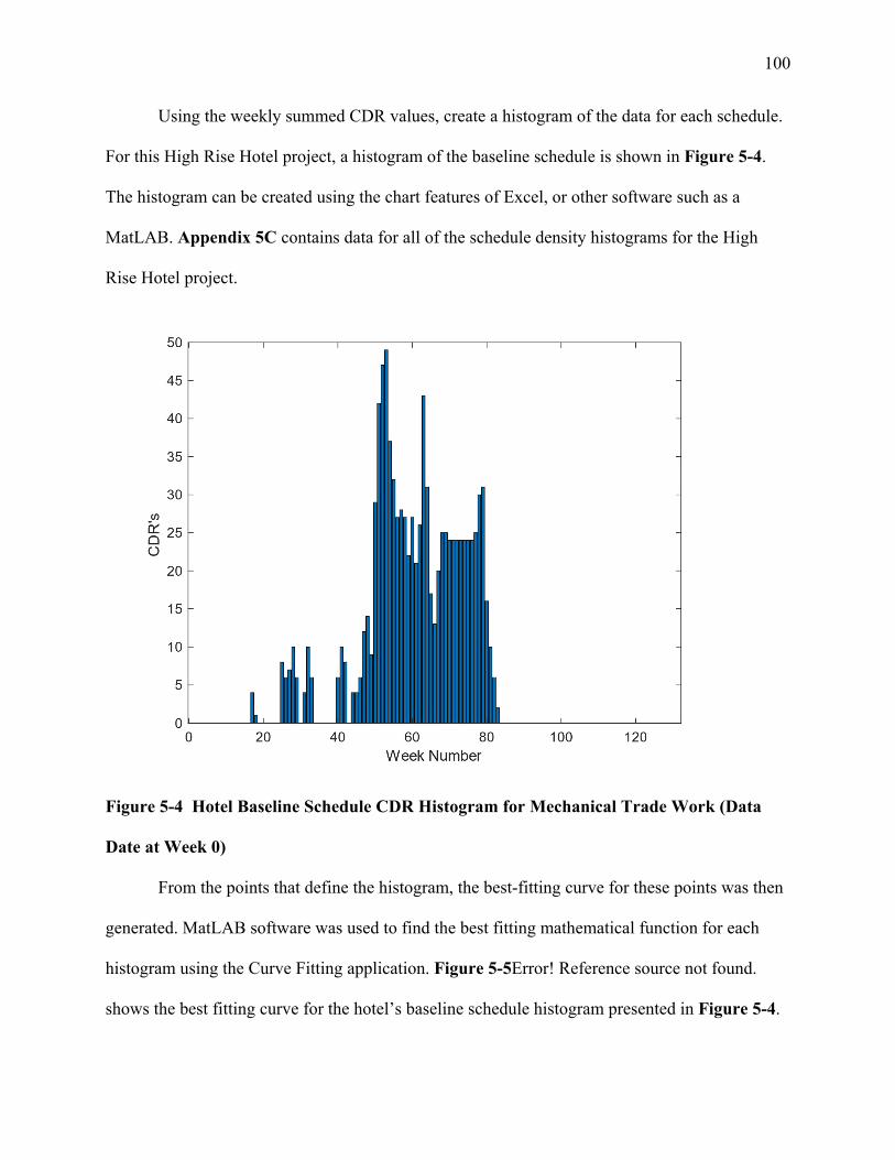
100

Using the weekly summed CDR values, create a histogram of the data for each schedule.

For this High Rise Hotel project, a histogram of the baseline schedule is shown in Figure 5-4.

The histogram can be created using the chart features of Excel, or other software such as a

MatLAB. Appendix 5C contains data for all of the schedule density histograms for the High

Rise Hotel project.

Figure 5-4 Hotel Baseline Schedule CDR Histogram for Mechanical Trade Work (Data

Date at Week 0)

From the points that define the histogram, the best-fitting curve for these points was then

generated. MatLAB software was used to find the best fitting mathematical function for each

histogram using the Curve Fitting application. Figure 5-5Error! Reference source not found.

shows the best fitting curve for the hotel’s baseline schedule histogram presented in Figure 5-4.

101

Instead of columns, however, Figure 5-5 displays the max weekly CDR value as a single point –

one point for every week – instead of displaying it as a column as presented in Figure 5-4.

Selection of the best fitting curve was made based upon goodness of fit using estimation using

least squares regression (Chatterjee, 2013) within MatLAB software. The difference between an

observed value and the fitted value is referred to as the residual amount. The smaller the sum of

the residual values, the better the fit. This measure coupled with an R-square value that is closer

to 1.0 identified the best fitting function for each histogram.

Figure 5-5 Best-Fitting Curve for Hotel Baseline Schedule Histogram (Data Date at Week

0)

Note that the best-fitting curve in Figure 5-5 does not mimic exactly the high points of

the histogram. The curve represents an approximation. Whereas this research attempts to predict

102

estimated construction labor productivity inefficiencies, use of an approximation method for the

general shape of the histogram suffices and produced similar results as if exact use of the

histogram column values were used. Additionally, use of curve fitting via MatLAB allowed for

automating the analysis and evaluating the different variables more quickly and thoroughly using

scripts.

Utilizing the best fitting function, the area under the curve can be calculated. This

calculated area is one variable that is included in the analysis to determine whether a correlation

between the area under the curve and reported productivity exists. Area calculations considered

in the analysis included the full area under the curve, and the area to either the right or left of the

data date. Areas to the left of the data date reflect actual dates, or rather, the number of activities

that were worked on concurrently. Areas to the right represent planned days of concurrent work

activities. Area calculations can be made using the schedule density histogram data itself too.

Use of best fitted curves allows easier comparison of histogram shapes from update to update.

Following the approach presented earlier in Chapter 4, calculate the centroid of the

histogram area. In this case, because the data date is at Week Number zero, all of the data is

planned future work. The x-coordinate of the centroid is calculated by multiplying each weekly

sum of CDR’s by the time distance from the data date Week Number for each CDR sum value.

The sum total is then divided by the total number of CDR’s, which results in a Week Number.

The y-coordinate of the centroid is simply the average number of CDR’s planned for each week.

When comparing how the centroid changes from schedule update to update, a vector and its

magnitude (scalar value) was calculated using basic linear geometry principles as explained

earlier in Chapter 4 and summarized graphically in Figure 0-6 below. The resulting findings for

the centroid calculations listed above for each schedule update are included in Appendix 5D.

103

Figure 0-6 Resultant Vector from Two Schedule Density Histogram Centroids

With the data for successive updates compiled, next, calculate the incremental actual

labor productivity achieved on the project for the trade under investigation. The unit for this

measure is in labor hours expended per each percent complete achieved. Assume that a total of

100 hours were budgeted to complete a given task. It may be simply estimated that it requires 1

hour to achieve 1 percent of the total work; this is the target, or desired productivity. If for

example, 10 hours were expended, but just 5-percent of the work was completed, the actual

productivity would be 10 hrs divided by 5-percent equals 2 labor hours per percent complete,

which is just half of the target productivity. Stated another way, the contractor only achieves 50-

percent of the actual progress for each labor hour expended, which is an indicator or inefficiency.

Productivity rates on construction projects do not remain constant throughout the job.

The first few periods typically experience poorer than optimal productivity due to a learning

curve, and the last periods likewise experience lesser productivity due to rework and basic close-

104

out work (Peles, 1977). These data points are outliers, or anomalies, that can skew observed

correlations (Gupta, 2014). For this reason, the outlier data points are removed before deriving a

best-fit correlative model. Actual labor hours expended for the mechanical and plumbing trades

are presented in Appendix 5E.

Once the incremental labor productivity tallies are completed, the search for correlation

between each of the variables ensues. This step includes comparing variables described in

Chapter 4 and determining whether a correlation exists between them and the labor productivity

measures. Comparisons were made using regression analysis within MatLAB software. These

comparisons were documented in a correlation matrix such as that shown earlier in Figure 4-13.

Ultimately, the goal is to find which measures drawn from the CPM schedule data (i.e.,

independent variables) are strongly correlated with the actual labor productivity data (i.e., the

dependent variable).

Perform Regression Analysis

Utilizing the correlation matrix as a guide, where strong correlation exists between an

independent variable and the dependent variable, further regression analysis was performed

where various forms of the best-fitting curve type were further evaluated. For example, a log

normal function closely resembles an exponential function in shape and fit, although not

identically. Selecting the better of two or more functions that show strong correlation is

determined in part by ease of use if a predictive model were able to be produced. Additionally,

use of similar function types for each project would be desirable to better facilitate industry

acceptance.

Finally, after a best-fitting model function is selected, calculation of the experienced

labor productivity loss due to trade stacking may be estimated using that model. Results

105

presented below demonstrate strong correlation between the cumulative centroid scaler and

expended labor hours per percent complete.

Results

This section presents results of the analysis for the hotel sample project. Figure 5-7 and

Figure 5-8 show the best fitted curves for the High Rise Hotel project based on its early dates.

The axes for each schedule update are identical with time (in weeks) on the x-axis and the

CDR’s on the y-axis. The status date, referred to as the “data date” in P6, is listed below each

curve and represented by the vertical line in each update.

Tracking how the curves change from update to update allows identification of trends in

how the work actually progressed. For example, the High Rise Hotel’s original curve shows a tri-

modal gaussian function beginning with its baseline schedule (data date 06-Mar-13). The bulk of

this mechanical work was planned to occur over an approximate 50-week time period. Six

months later (data date 06-Oct-13), this tri-modal shape is still present, however, the middle

mode became the greatest in terms of the number of overlapping CDR’s. At this time, the bulk of

the mechanical work was then planned to occur over an approximate 30-week time period. Thus,

in comparing these two schedule updates, the planned mechanical work had been compressed,

meaning that a like amount of planned future mechanical work would need to be completed

within 30 weeks instead of the original planned 50 weeks in the baseline schedule. A primary

assumption here is that the number of activities representing the mechanical work in the baseline

is the same as those in the 06-Oct-13 update.

106

Figure 5-7 Hotel Project Best-Fitted Curves for Schedule Data Date Shown (March 2013 to October 2014)

0 20 40 60 80 100 120Week

0

20

40

60

80

100

120

140

160

CD

R

0 20 40 60 80 100 120Week

0

20

40

60

80

100

120

140

160

CD

R

0 20 40 60 80 100 120Week

0

20

40

60

80

100

120

140

160

CD

R

0 20 40 60 80 100 120Week

0

20

40

60

80

100

120

140

160

CD

R

06-Mar-13 06-Oct-13 01-Dec-13

02-Mar-14 05-Jun-14 12-Jul-14

08-Aug-14 08-Sep-14 06-Oct-14

107

Figure 5-8 Hotel Project Best-Fitting Curves for Schedule Data Dates Shown (November 2014 to June 2015)

108

The change in shapes between these two updates is due to actual progress realized (or

not) on the project. As work progresses, the scheduler makes changes to the schedule. AACE’s

Recommended Practice RP 53R-06 “Schedule Update Review – As Applied in Engineering,

Procurement, and Construction” provides “guidelines for the project scheduler to create a

professional schedule update or assess the reasonableness of changes to be made in a schedule

due to a change of project status and progress.” Recommended types of information that are

updated and reported in the schedule for the reporting period include,

• Significant activities started or completed including status of material and

equipment procurement activities;

• Changes to critical path activities in comparison to the critical path shown in the

prior reporting period;

• Identification of any delays and change orders that may affect the work;

• Changes made to the logic or to activities’ planned durations; and

• Explanation of any schedule changes, including changes to the logic sequence or

to activity durations and the impacts to the overall project.

The net effect of the implemented schedule modifications causes the schedule’s density

histogram to change shapes from update to update. If few or no changes are made and the

contractor is performing work according to plan, then the schedule density histogram shape

remains unchanged even though the data date will change as time advances. In the case of this

high rise hotel project, the planned work obviously changed between the March 6, 2013 and

October 6, 2013 schedule updates as indicated by the difference in the best fitting curves for each

update. A possible cause for the change is delayed progress on predecessor work to the

mechanical work. Absent a granted time extension, the start dates of mechanical work would

109

necessarily be pushed to later start dates, but would need to finish on or close to the finish date in

the baseline schedule. Consequently, the same amount of work needed to be accomplished, but

in a shorter duration, which may explain why the original 50-week duration was reduced to 30-

weeks in the first schedule update, and why the second mode value is so much greater in

comparison to the baseline schedule.

By the 01-Dec-13 schedule update, the tri-modal shaped curve changed dramatically.

Instead of seeing definitive peaks, the shape appears to be a single mode gaussian function.

Again, the changed shape is linked to schedule modifications made by the scheduler. The tri-

modal function reappears in the 02-Mar-14 schedule update, but note how the CDR values are

twice that amount shown in the baseline schedule. This observation supports the trade stacking

scenario this analysis seeks to measure.

This model approach accounts for the additional detail the scheduler may include in the

schedule. The addition of detail to a CPM schedule as more information becomes available is

sometimes referred to as a “rolling wave” approach to updating the schedule. For example, say

that three similar trade activities each with seven calendar days duration were planned to occur in

series. The schedule density histogram for this scenario would be a single CDR planned for each

day over 21 calendar days. Assume now that upon receipt of additional information, the

scheduler added more detail to represent these three activities with say four activities each (now

12 activities are used to represent the same prior three activities), and some of those activities

overlapped. According to the model proposed herein, trade stacking increased. Arguably, the

trade stacking existed beforehand using just the three activities but was only measured by the

model when the additional detail was added to the schedule. Whereas many schedulers do add

110

detail as more information becomes available, it follows that the CDR measure alone may not be

as strong as a predictor for productivity loss as initially anticipated.

For each of the schedule updates shown in Figure 5-7 and Figure 5-8, the area totals

were calculated using integral capabilities within MatLAB. Table 5-1 shows results of the early

date calculations in determining the centroids for each schedule update. Table 5-2 presents the

metric results from each update. These data were used to determine correlation between

variables. The labor hours per percent complete measure is also included in this table.

Correlation Between Variables

The following variables were evaluated in comparison to each other:

1. Total Density (“∑ Density” - this value is the sum total of the area histogram generated

by the planned activities in the CPM schedule)

2. Area Total (“f(x) Area Tot No Ex” – calculated integral of the fitted mathematical

function for the schedule density histogram with no data excluded)

3. Area Right of Data Date (“f(x) Area Right No Ex” - integral of the fitted mathematical

function for the schedule density histogram from the data date to the right with no data

excluded)

4. Area Right of Data Date as a Percentage of the Area Total (“f(x) AR % No Ex” - ratio of

item 3 divided by item 2 above)

5. Cumulative sum of the change in the centroid x-coordinate (“Cum ∆x”)

6. Cumulative sum of the change in the centroid y-coordinate (“Cum ∆y”)

7. Cumulative sum of the vector scalar values from the change in centroid coordinates

(“Cum R^2 Scalar”)

111

Table 5-1 High Rise Hotel Project - Centroid Results Based on Early Dates

112

Table 5-2 Hotel Project Best-Fitting Curve Descriptive Values and Area Calculations for Early Dates

Data Date Fit Adj

R-SqFit

RMSEFit #

Coeff

Data Date

Week

First Plan

Week

Last Plan

WeekArea Tot

Area Left of

DD

Area Right of

DD

AR as % of ATot

CumMHrs / % Compl Kurtosis Skewness

06-Mar-13 0.92 3.48 9 1 25 83 956 0 956 100% n/a 4.262 1.50806-Oct-13 0.93 4.40 9 32 17 81 936 0 936 100% n/a 5.983 1.98401-Dec-13 0.91 5.06 6 40 17 84 1159 88 1071 92% n/a 5.765 1.85402-Mar-14 0.90 6.74 6 54 17 83 1178 185 993 84% 388 10.153 2.45105-Jun-14 0.94 6.51 6 68 17 90 1808 933 875 48% 188 4.905 1.72912-Jul-14 0.99 3.21 9 73 17 94 2671 1956 716 27% 263 5.616 1.866

08-Aug-14 0.98 4.06 3 76 17 94 2984 2343 641 21% 307 4.745 1.70208-Sep-14 0.93 4.96 3 81 17 95 3176 2760 416 13% 338 4.295 1.56606-Oct-14 0.93 4.16 3 85 17 99 3375 3018 357 11% 371 4.017 1.457

03-Nov-14 0.98 2.18 3 89 17 101 3556 3249 308 9% 406 3.744 1.35124-Nov-14 0.94 2.92 3 92 17 104 3561 3371 191 5% 425 3.780 1.36622-Dec-14 0.84 4.23 3 96 17 107 3574 3448 126 4% 447 3.839 1.37926-Jan-15 0.95 5.30 3 102 17 116 3893 3558 336 9% 472 3.480 1.22216-Feb-15 0.96 3.69 3 105 17 116 4058 3788 270 7% 487 3.451 1.18216-Mar-15 0.91 6.17 3 109 17 116 4260 4006 254 6% n/a 3.173 1.05813-Apr-15 0.93 3.76 3 113 17 118 4376 4264 113 3% n/a 3.109 1.009

18-May-15 1.00 0.61 3 118 17 120 4492 4448 45 1% n/a 3.105 0.97215-Jun-15 - - - 122 17 122 4528 4520 8 0% n/a 3.117 0.970

113

8. Cumulative Manhours per Percent Complete (“Cum Mhr % Compl” – cumulative sum of

the ratio of labor hours expended to complete one percent of work for each schedule

evaluated)

9. Kurtosis (a measure of how tall and skinny, or short and wide a distribution under

consideration is relative to a typical normal distribution)

10. Skewness (a measure of how asymmetric a distribution function is)

Figure 5-9 presents the resulting correlations for the comparisons of these variables. Any

correlation with an R-square value of 0.895 or greater was considered a strong correlation.

The simplest mathematical fit was sought for each comparison with a linear relationship deemed

to be a benchmark for ease of use. A simple linear equation takes the form 𝑓(𝑥) = 𝑦 = 𝑚𝑥 + 𝑏

where m is the slope of the line and b is the y-axis intercept value. Where a linear relationship

represented the best fit, the slope value is provided in Figure 5-9. Where other mathematical

functions were used, a simplified function “f(x)” is shown as is a small graphic that shows the

relative shape of the curve. Any Gaussian function is based upon the normal distribution, i.e., a

typical bell-shaped curve, although, the varying coefficients cause the typical bell-shape to

change. Detailed backup information for each best-fitting correlation related to the cumulative

manhours per percent complete calculation is provided in Appendix 5F.

114

Figure 5-9 High Rise Hotel Sample Project Mechanical Trade Work Correlation Results

115

For the hotel, as the shape of the schedule density curve changes with respect to its

skewness and kurtosis, an exponential relationship is observed with the cumulative labor hours

per percent complete. This finding supports that the schedule density measurements presented

herein may be used to prepare a predictive model of anticipated productivity loss. Increasing

trends in how the centroid changes from update to update, and the general shape changes of the

area histogram functions can serve as warnings for potential future productivity inefficiencies.

Contractors and owners alike may find this tool useful.

Results in Figure 5-9 show the exponential function as having the best-fit (r-square =

0.998). However, a simpler log normal function was chosen instead because of its more

commonly known shape within the mathematics and scientific communities, simplicity with just

two coefficients instead of four, and because its fit was nearly identical to the exponential

function (r-square = 0.983). The two models are compared in Table 5-2.

Table 5-2 Best-Fitting Model v Chosen Model

Coefficient Best-Fit

Exponential f(x) = a*exp(b*x) +

c*exp(d*x)

Chosen Lognormal

Function f(x) = a * ln(x) ^ b

a 301.5 2.588 b 0.00157 3.009 c -647 - d -0.0188 -

R-sq Value 0.998 0.983 RMSE 5.28 12.77

Figure 5-10 presents the selected curve from the regression analysis for the cumulative

centroid scalar value versus the cumulative labor hours per percent complete.

116

Figure 5-10 Cumulative Centroid Scalar Value v Cumulative Labor Hours per Percent

Complete

This figure serves as a starting point for a predictive model wherein a scheduler can track

how the centroid scalar value changes from update to update, and if that trend is upward like that

shown here, the scheduler may use the function to estimate the potential impact to the amount of

labor hours required to complete unfinished work.

Conclusions

Results of this High Rise Hotel project support that strong correlation exists between

several variables. Most notably is the fitted function for cumulative centroid scalar value versus

0

100

200

300

400

500

600

700

0 50 100 150 200 250 300 350

Cum

ulat

ive L

abor

Hou

rs p

er P

erce

nt Co

mpl

ete

Cumulative Centroid Scalar Value

Hotel MHrs Pct Compl

Hotel Mech f(x) Ln

Slope at any point x = 𝑎 ∗ ln (𝑥 𝑏) = ( )

Fitted Function: f(x) = a*ln(x)^bCoefficient a = 2.588Coefficient b = 3.009Adjusted R-square = 0.983RMSE = 12.77

117

cumulative labor hours per percent complete. The centroid value includes both a time component

and a resource component. Correlation results support that in isolation, the time element, i.e.,

delay, has greater influence on productivity than does the increase in just CDR’s. However,

including the combination of both components in the analysis produces strong correlation and

supports that a predictive model for estimating productivity loss is plausible.

Understandability and ease of use are prerequisites to industry acceptance and application

of the technique presented here. While execution of each individual step is simple, the numerous

iterations performed for each of the variables increase the complexity and time required to

perform the technique. Wading through and validating the data also requires some expertise and

a knowledge of CPM scheduling. Notwithstanding these potential complications, the results

soundly support that the technique works for this project.

118

6 Summary Results of Technique Applied to Other Sample Projects

In total, five sample projects were evaluated as shown in Table 6-1. Two of the projects

evaluated are buildings. Another is a combined cycle power plant. The fourth project included

erection of a large steel structure. These four projects were used to identify relationships between

the schedule density metrics drawn from the CPM schedules. The fifth project, a resort hotel,

was used for empirical validation of findings from the analyses and is presented in the next

chapter. In effect, use of this validation project sought to answer the question, “Are the results

transferable to another project?” Recognizing that the Resort Hotel project is not completely

homogenous to the High Rise Hotel and Condo Towers projects, although similar with respect to

having MEP trades generally working together, the belief was that there may be some value in

seeing how the modeled results from the first four sample projects may be applied.

Table 6-1 List of Sample Projects

Sample Project Type Year Completed

Number of Native

Electronic Schedules

Reliable Labor Hours

Data

Progress Percent

Complete Data

High Rise Hotel 2015 18 Yes Yes Condo Towers 2008 17 Partial Yes Large Bore Piping 2010 15 Yes Yes Steel Structure 2016 14 Yes Yes Resort Hotel (for validation) 2008 15 Yes Yes

Table 6-1 shows that reliable labor and progress percent complete data were found for all

but the Condo Towers project, where labor data was only partially available. For this project, the

schedule density and area calculations were useful and therefore, included in the results herein,

but any comparison to labor hours per percent complete cannot be made for this project due to

lack of complete and reliable data.

119

Because of the proprietary nature of productivity data being utilized and confidentiality

regarding dispute resolution, specific names of contractors and the respective projects are

withheld. Instead, general information is provided – enough to give the reader a clear

understanding of the scope of work.

Comparison of Results for the Sample Projects

The technique demonstrated in Chapter 5 for the High Rise Hotel was applied similarly to

the Piping, Structural Steel and Condominium Towers projects. Results from each analysis were

compared to one another to identify common findings or stark differences, if any. Similarly as

found in the High Rise Hotel project, both the Structural Steel and Piping projects showed strong

statistical correlation between their respective centroid cumulative scalar values and the

cumulative labor hours per percent of work scope completed. Error! Reference source not

found.Figure 6-3 presents the correlations for the High Rise Hotel, Piping and Structural Steel

projects on the same graph.

120

Figure 6-1 Predictive Model Form Using Results of the Schedule Density Analysis

A lognormal equation was found to be a good fit for both the Structural Steel and Piping

projects. This function also matches findings from the High Rise Hotel project. Selecting a

lognormal function, derived from a lognormal distribution, is the correct choice when modeling

something affected by random variation as indicated by Limpert and Stahel, “Empirical evidence

suggests the log‐normal distribution should be selected as a first choice when “amounts” are

modelled – these being quantities that can only take positive values” (Limpert & Stahel, 2017).

They continue,

There is also a theoretical justification for using the log‐normal distribution:

whereas the well‐known central limit theorem, in its classical form, says that the

0

500

1000

1500

2000

2500

0 50 100 150 200 250 300 350

Cum

ulat

ive

Labo

r Hou

rs p

er P

erce

nt C

ompl

ete

Cumulative Centroid Scalar Value

Hotel MHrs Pct Compl Piping MHrs Pct Compl Str Steel MHrs Pct ComplHotel Mech f(x) Ln Piping f(x) Ln Steel f(x) Ln

121

addition of many random “effects” has approximately a Gaussian distribution,

the less well‐known version ascertains that the multiplication of many positive

random variables creates a distribution that is approximately log‐normal.

The ’multiplication of many positive random variables’ applies to this study because of the many

variables that affect labor productivity.

The lognormal function has a sharp slope when the values start at zero and then flattens

out with increasing cumulative centroid scalar values. The coefficients “a” and “b” as shown in

the figure define the steepness of the slope of the line at point zero and in how quickly the slope

of the function levels out with increasing cumulative centroid scalar values. The actual slope of

the line at any point can be calculated by using the derivative of the lognormal equation in

question as follows:

𝑠𝑙𝑜𝑝𝑒 𝑎𝑡 𝑎𝑛𝑦 𝑝𝑜𝑖𝑛𝑡 𝑥 = 𝜕𝜕𝑥 𝑓(𝑥) = 𝑎𝑏 ln (𝑥)( )𝑥

Results from these three projects show that the slope of the line lessens with greater

values of the cumulative centroid scalar value. Interpretation of this graphic indicates that as the

schedule density (derived directly from the CPM schedules) changes over time where both the x-

coordinate (a function of time and delay) and y-coordinate (an indicator of stacked activities for

a given trade) are increasing, the number of labor hours to complete the work likewise increases.

The cumulative sum of each scalar plotted sequentially compared with the calculated

labor hours per percent complete reveals this lognormal correlation between these two variables.

The strongest correlation identified lies in the High Rise Hotel project’s mechanical trade as

indicated by the r-square value of 0.983. This finding aligns with the literature review, the

ConExpo survey results, and the expert panelists’ expectations (presented in Chapter 7) wherein

122

all indicated the greatest likelihood for trade stacking exists in the MEP trades, particularly for

multi-story building projects.

Interestingly, the Structural Steel project also had a strong correlation (r-square value of

0.900). With this project, construction progress was largely governed by the availability of two

large cranes that were required to hoist larger structural steel members into place. When delay

caused a crane to remain stationary longer than planned, this increased the overlapping of

planned future work activities in the CPM schedules. Thus, the erection of roofing steel, purlins

and siding occurred simultaneously rather than more in series, which according to results of this

study, caused labor inefficiencies.

The Piping project showed good, although the lowest (r-square value of 0.732),

correlation of the three projects shown in Figure 6-1. The lower r-square value and the higher

root-mean-square (RMS) value indicates greater variability in the data. Thus, in comparison, the

Piping project had the greatest variability in its data. The large bore piping required on a

combined cycle power plant is extensive and requires thousands of man-days of labor to

complete. The sheer magnitude of these labor hours greatly exceeds those labor hours required to

complete the mechanical work on the High Rise Hotel project, for example, and therefore, the

curve for the Piping project extends to much higher values on the y-axis. One of the expert

panelists indicated that this large variability in labor productivity for piping is explained by a

shortage of skilled piping welders in the US market. He opined that if a consistently skilled labor

force of piping welders existed, the correlation between the variables in Figure 6-1 would be

greater.

Measurement of labor inefficiency may be estimated by comparing the differences

between two values on the x-axis as depicted graphically in Figure 6-2. This figure shows that

123

an increase of 50 units on the cumulative centroid scalar value equates to approximately a 70 unit

increase in the cumulative labor hours required to complete one percent of the work. Thus, quite

literally, the model results may be used to measure labor inefficiency. Creation of a predictive

model would utilize the same lognormal function and could be used similarly if, for example, an

increasing trend of values to the cumulative centroid scalar values were observed.

Figure 6-2 Use of Model to Measure Productivity Inefficiency

That each best fitting relationship for three of the sample projects follows a log normal

function suggests that this function may be used in a predictive manner for estimating

productivity inefficiencies. The function is the same, however, the coefficients are unique to each

project. In retrospective analysis, use of the actual histograms to calculate the changes in

centroids from schedule update to update would be adequate and simplify the application by

0

50

100

150

200

250

300

350

400

450

500

550

600

0 50 100 150 200 250 300 350

Cum

ulat

ive L

abor

Hou

rs pe

r Per

cent

Com

plet

e

Cumulative Centroid Scalar Value

Inefficiency ≈ 70 Mhrs per % Complete

124

foregoing the need to use the lognormal function. In either application, additional research and

evaluation of larger sample sizes are warranted to derive a methodology for better understanding

variables that affect the coefficients based on project type, trade type, available labor, etc.

Further evaluation in comparing the results collectively shows that the change in the

centroid x-coordinate variable has a greater effect on the shape and resulting correlation of the

lognormal function than does any other variable evaluated. The centroid x-coordinate is directly

related to a contractor’s inability to meet its planned dates. When delay occurs and the

contractual completion date remains unchanged, the unfinished work activities are pushed

forward. Thus, in the succeeding schedule update, the centroid x-coordinate will likewise shift to

the right.

Surprisingly, the change in the centroid y-coordinate alone did not consistently show

strong correlation or effect on the model. This variable effect may be attributed to several

reasons. First, often in times of delay a contractor will reduce planned durations in its schedule

update so as to not show delay – particularly if the contractor is responsible for the delay. The

reduced duration would necessarily reduce the likelihood of overlapping activities in the

schedule. Second, there may be float in the CPM schedule with the trade activities being

evaluated. The delayed progress will cause the unfinished work activities to shift to the right, but

not result in any measurable change in CDR’s. Finally, a contractor may choose to work

overtime within the same planned activity duration to recover delay. This approach likewise

would not be reflected in the CDR value derived from the schedule update.

Whereas the centroid value itself represents both time and trade stacking, it makes sense

that this variable was found to have strong correlation with the other metrics observed and with

labor productivity.

125

The following subsections present the results for the respective project listed.

Condominium Towers Sample Project – Electrical Trade Work

Two nearly identical 22-story condominium towers were constructed under the same

contract in Washington State (see Figure 6-3). Parking was provided under the towers, the first

four floors were used for retail and lease business space, and the remaining floors were used for

condominium dwellings. Total construction cost was approximately $100 million. Given a

volatile market which resulted in frequent pricing changes downward for condo sales, the

contractor was held to a strict completion date. When performance fell behind schedule, the MEP

trades stacked up. Labor hour data was kept on the project for the first year, but when the job fell

behind schedule, the prime contractor stopped tracking actual labor hours expended by

subcontractors each month.

126

Figure 6-3 Condo Project Photo

Given the similarities between this project and the hotel high rise, the analyses for all of

the variables were performed, except the labor hours because this data was found to be

incomplete. Results of the condo sample project are presented in Table 6-2 and Table 6-3.

Progression of the best-fitting curves for the condo project schedule density histograms are

shown in Figure 6-4 and Figure 6-5. The variable correlation matrix is presented in Figure 6-6.

127

Table 6-2 Condo Project - Centroid Results Based on Early Dates

Data Date ∑ Density ∑ Work Days

Centroid x Coord

Centroid y Coord

∆ Data Date ∆ x Cum

∆x ∆ y Cum ∆y

R^2 Scalar

CumR^2 Scalar

17-Feb-06 731 318 495.32 2.30 0 0 0 0.000 0.000 0.00 0.0001-Mar-06 741 328 550.33 2.26 12 67.0 67.0 -0.017 -0.017 67.01 67.0110-Apr-06 731 318 443.27 2.30 40 -67.1 0.0 0.018 0.000 -67.05 -0.0416-May-06 731 318 444.97 2.30 36 37.7 37.7 0.000 0.000 37.70 37.6501-Aug-06 739 289 367.17 2.56 77 -0.8 36.9 0.112 0.113 -0.81 36.8501-Nov-06 726 282 276.05 2.57 92 0.9 37.7 0.007 0.119 0.88 37.7329-Dec-06 800 309 199.53 2.59 58 -18.5 19.2 0.006 0.125 -18.53 19.2023-Mar-07 997 312 146.25 3.20 84 30.7 49.9 0.234 0.359 30.72 49.9206-Apr-07 1,029 300 124.27 3.43 14 -8.0 41.9 0.073 0.433 -7.98 41.9401-May-07 1,180 329 90.46 3.59 25 -8.8 33.1 0.046 0.478 -8.81 33.1315-Jun-07 1,279 331 67.39 3.86 45 21.9 55.1 0.077 0.556 21.93 55.0606-Aug-07 1,455 347 39.82 4.19 52 24.4 79.5 0.085 0.641 24.43 79.5031-Aug-07 1,612 341 25.88 4.73 25 11.1 90.6 0.127 0.768 11.06 90.5524-Sep-07 1,670 353 21.16 4.73 24 19.3 109.8 0.001 0.769 19.29 109.8431-Oct-07 1,841 346 12.77 5.32 37 28.6 138.4 0.125 0.894 28.60 138.4427-Nov-07 2,017 350 8.59 5.76 27 22.8 161.3 0.083 0.977 22.83 161.2713-Dec-07 1,555 327 6.12 4.76 16 13.5 174.8 -0.175 0.802 13.53 174.80

128

Table 6-3 Condo Project Best-Fitting Curve Descriptive Values and Area Calculations for Early Dates

Data Date Fit Adj R-sq

Fit RMSE

Fit # Coeff

Data_Date

Week No

First Plan

Week No

Last Plan Week No

AreaTot E NoEx

Area Left DD

Area Right

DD

Area Rt DD Pct of

AT

CumMHrs / % Compl Kurtosis Skewness

17-Feb-06 0.97 1.26 18 28 64 128 704 -10 713 100% n/a 2.062 0.57201-Mar-06 0.95 1.47 18 30 66 140 707 -2 709 100% n/a 1.896 0.50610-Apr-06 0.94 1.68 9 36 64 128 704 -10 713 100% n/a 2.050 0.56816-May-06 0.94 1.66 9 41 70 133 698 -7 705 100% n/a 2.422 0.74401-Aug-06 0.95 1.69 6 52 77 133 723 -5 728 100% n/a 1.880 0.60801-Nov-06 0.89 2.60 6 65 76 133 701 -25 726 100% n/a 2.378 0.83829-Dec-06 0.92 2.18 6 73 69 130 786 9 777 99% n/a 1.717 0.49423-Mar-07 0.91 2.82 9 85 76 140 980 96 885 90% n/a 1.593 0.48806-Apr-07 0.95 2.17 9 87 76 129 991 199 792 80% n/a 1.513 0.41101-May-07 0.96 2.25 9 91 69 134 1169 383 786 67% n/a 2.365 0.81715-Jun-07 0.95 2.77 9 97 69 136 1251 403 848 68% n/a 5.442 1.61206-Aug-07 0.94 3.84 9 105 69 139 1421 646 775 55% n/a 4.527 1.53831-Aug-07 0.94 4.63 6 108 69 141 1613 880 734 45% n/a 5.369 1.68824-Sep-07 0.95 4.33 9 112 69 141 1659 1058 601 36% n/a 3.707 1.41531-Oct-07 0.95 4.90 6 117 69 142 1818 1313 505 28% n/a 3.080 1.25127-Nov-07 0.93 6.12 9 121 69 139 1870 1383 487 26% n/a 5.444 1.54713-Dec-07 0.93 4.67 12 123 69 137 1551 1234 317 20% n/a 1.718 0.570

129

Figure 6-4 Condo Project Best-Fitting Curves for Schedule Data Dates Shown (February 2006 to April 2007)

17-Feb-06 01-Mar-06 10-Apr-06

16-May-06 01-Aug-06 01-Nov-06

29-Dec-06 23-Mar-07 06-Apr-07

130

Figure 6-5 Condo Project Best-Fitting Curves for Schedule Data Dates Shown (May 2007 to December 2007)

01-May-07 15-Jun-07 06-Aug-07

31-Aug-07 24-Sep-07 31-Oct-07

27-Nov-07 13-Dec-07

131

Figure 6-6 Condo Project Variables Correlation Matrix Results

132

Observation of the condo project’s best-fitting curves shows that as time progressed, and

as the electrical trade work was not completed according to plan, the CDR value increases with

each successive schedule update. The increasing CDR value represents increased trade stacking.

The correlation between the manhours per percent complete and the increasing value of the

centroid scaler value supports that increased trade stacking adversely affects labor productivity.

Large Bore Piping – Power Plant

Power, processing and industrial plants typically require significant amounts of

mechanical piping work. The second sample project considered large bore (> 2.5” in diameter)

piping on a power plant located in the southeast United States (see Figure 6-7). Total

construction cost exceeded $100 million. Piping work included layout, welding and setting of

carbon steel and stainless steel piping in and related to the turbine and boiler areas. The piping

work required coordinated efforts between the steel erection and pipe rack constructors. This

project experienced delays that caused planned piping work to stack up. Absent any appreciable

time extensions, the prime contractor was required to maintain schedule despite the increased

schedule density for large bore piping.

To illustrate these principles in a real-world scenario, consider the construction of a large

plant for a public utility. The construction includes significant site civil work, piping (both above

and below ground), structural steel, mechanical, electrical and instrumentation work. CPM

schedules were prepared monthly by the contractor, but were never formally resource loaded.

133

Figure 6-7 Piping Project Power Plant

The project was impacted by three force majeure events including two hurricanes within

two weeks of each other, and a bomb threat that shut the job down for another day. There is a

direct impact caused by the force majeure events where the project was shut down or

significantly disrupted, and a ripple effect where it takes time for the workers to return to site and

ramp back up to full productivity. The direct time impacts of such events are generally easy to

determine. But the contractor struggled to identify the point in time when the ripple effect of the

force majeure events had subsided. Consider a still pond where a stone is suddenly dropped into

the water. The initial wave of the impact is significant and then travels radially outward. The

resulting waves dissipate proportionally to the distance traveled, until ultimately there is a return

to calm. Similarly, these force majeure events act like the stone and the ripple effect is the

impacts caused by those events, which dissipate over time until no lingering impact remains. The

challenge lies in measuring the duration of the impact period with the contemporaneous CPM

schedule data.

134

Results of the piping sample project are presented in Table 6-4 and Table 6-5.

Progression of the best-fitting curves for the condo project schedule density histograms are

shown in Figure 6-8 and Figure 6-9. The variable correlation matrix is presented in Figure 6-

10.

135

Table 6-4 Piping Project - Centroid Results Based on Early Dates

Data Date ∑ Density ∑ Work Days

x Coord Date

Centroid x Coord

Centroid y Coord

∆ Data Date ∆ x Cum

∆x ∆ y Cum ∆y

R^2 Scaler

Cum R^2

Scaler01-Jan-07 3,684 347 23-Dec-07 356.4 10.6 0 0 0 0.000 0.000 0.0 0.026-Feb-07 7,557 383 28-Dec-07 305.6 19.7 56 5.2 5.2 9.114 9.114 10.5 10.526-Mar-07 7,498 374 12-Jan-08 292.7 20.0 28 15.1 20.3 0.317 9.431 15.1 25.630-Apr-07 7,471 309 29-Jan-08 274.0 24.2 35 16.3 36.6 4.130 13.561 16.8 42.404-Jun-07 7,420 309 02-Feb-08 243.3 24.0 35 4.3 40.9 -0.165 13.396 4.3 46.702-Jul-07 7,555 333 29-Jan-08 211.1 22.7 28 -4.2 36.6 -1.325 12.071 -4.4 42.230-Jul-07 7,329 394 09-Feb-08 194.6 18.6 28 11.5 48.1 -4.086 7.985 12.2 54.4

27-Aug-07 7,345 406 01-Feb-08 158.5 18.1 28 -8.0 40.1 -0.510 7.474 -8.0 46.431-Dec-07 6,376 392 19-Mar-08 79.8 16.3 126 47.2 87.3 -1.826 5.649 47.3 93.728-Jan-08 4,482 318 11-Mar-08 44.0 14.1 28 -7.8 79.6 -2.171 3.478 -8.1 85.625-Feb-08 4,831 403 28-Mar-08 32.8 12.0 28 16.8 96.4 -2.107 1.371 16.9 102.524-Mar-08 5,020 416 15-Apr-08 22.9 12.1 28 18.1 114.5 0.080 1.451 18.1 120.728-Apr-08 4,843 342 08-May-08 10.5 14.2 35 22.6 137.0 2.094 3.544 22.7 143.326-May-08 5,553 342 31-May-08 5.7 16.2 28 23.2 160.3 2.076 5.620 23.3 166.723-Jun-08 6,021 339 26-Jun-08 3.4 17.8 28 25.7 185.9 1.524 7.144 25.7 192.4

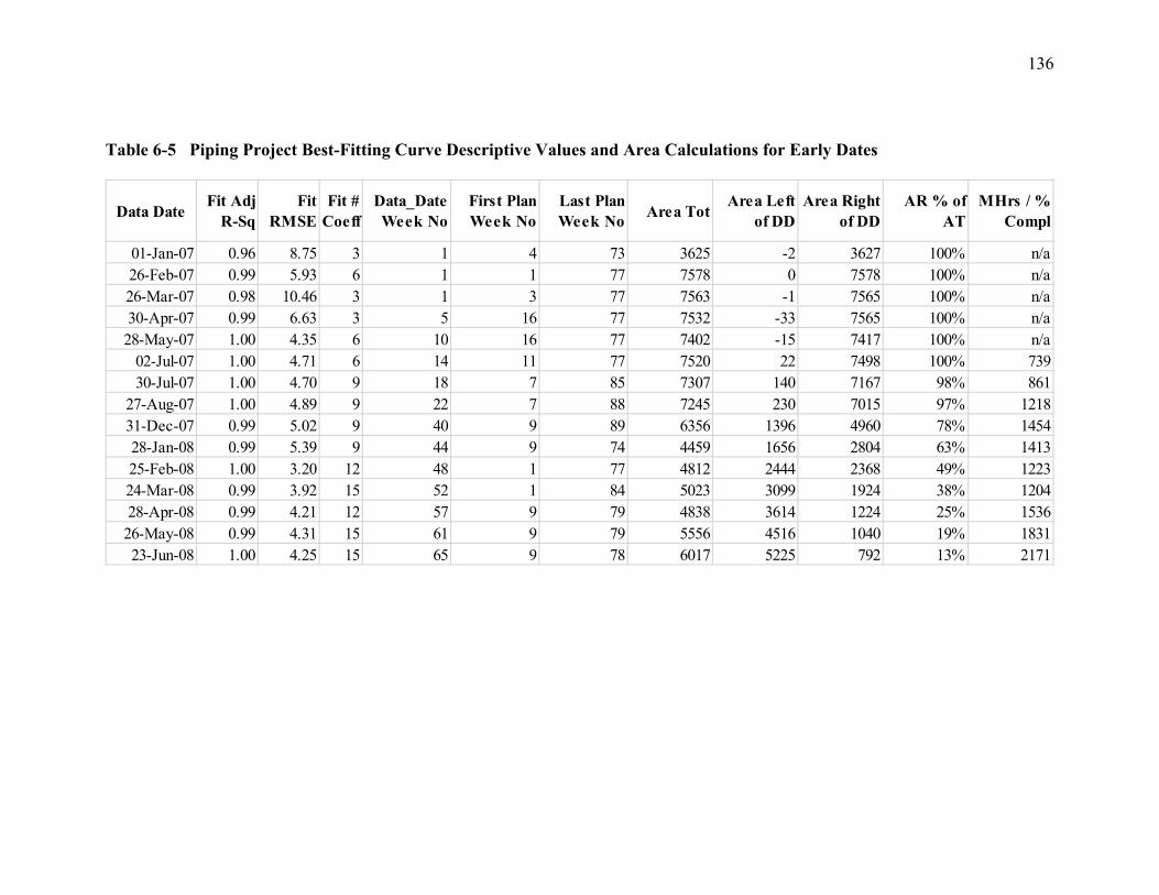
136

Table 6-5 Piping Project Best-Fitting Curve Descriptive Values and Area Calculations for Early Dates

Data Date Fit Adj R-Sq

Fit RMSE

Fit # Coeff

Data_Date Week No

First Plan Week No

Last Plan Week No Area Tot Area Left

of DDArea Right

of DDAR % of

ATMHrs / %

Compl

01-Jan-07 0.96 8.75 3 1 4 73 3625 -2 3627 100% n/a26-Feb-07 0.99 5.93 6 1 1 77 7578 0 7578 100% n/a26-Mar-07 0.98 10.46 3 1 3 77 7563 -1 7565 100% n/a30-Apr-07 0.99 6.63 3 5 16 77 7532 -33 7565 100% n/a

28-May-07 1.00 4.35 6 10 16 77 7402 -15 7417 100% n/a02-Jul-07 1.00 4.71 6 14 11 77 7520 22 7498 100% 73930-Jul-07 1.00 4.70 9 18 7 85 7307 140 7167 98% 861

27-Aug-07 1.00 4.89 9 22 7 88 7245 230 7015 97% 121831-Dec-07 0.99 5.02 9 40 9 89 6356 1396 4960 78% 145428-Jan-08 0.99 5.39 9 44 9 74 4459 1656 2804 63% 141325-Feb-08 1.00 3.20 12 48 1 77 4812 2444 2368 49% 122324-Mar-08 0.99 3.92 15 52 1 84 5023 3099 1924 38% 120428-Apr-08 0.99 4.21 12 57 9 79 4838 3614 1224 25% 1536

26-May-08 0.99 4.31 15 61 9 79 5556 4516 1040 19% 183123-Jun-08 1.00 4.25 15 65 9 78 6017 5225 792 13% 2171

137

Figure 6-8 Piping Project Best-Fitting Curves for Schedule Data Dates Shown (January 2007 to December 2007)

0 20 40 60 80 100 120Week

0

50

100

150

200

250

CD

R

0 20 40 60 80 100 120Week

0

50

100

150

200

250

CD

R

0 20 40 60 80 100 120Week

0

50

100

150

200

250

CD

R

0 20 40 60 80 100 120Week

0

50

100

150

200

250

CD

R

0 20 40 60 80 100 120Week

0

50

100

150

200

250

CD

R

0 20 40 60 80 100 120Week

0

50

100

150

200

250

CD

R

01-Jan-07 26-Feb-07 26-Mar-07

30-Apr-07 28-May-07 02-Jul-07

30-Jul-07 27-Aug-07 31-Dec-07

138

Figure 6-9 Piping Project Best-Fitting Curves for Schedule Data Dates Shown (January 2008 to June 2008)

28-Jan-08 25-Feb-08 24-Mar-08

28-Apr-08 26-May-08 23-Jun-08

139

Figure 6-10 Piping Project Variables Correlation Matrix Results

140

Tracking the change in best-fitting curves for the schedule density histograms shows that

as delay occurs, the planned number of overlapping activities likewise increases. This same trend

is observed in the High Rise Hotel and Condo Tower projects.

Steel Structure

The steel structure project comprised construction of a government steel structure

approximately 100-feet tall and 300-feet in length. Total construction cost exceeded $100

million. The prime contractor experienced delays to concrete work – work that preceded the steel

erection activities. Without a time extension, the prime contractor had to maintain schedule

despite stacked planned structural steel erection work. Because this work involved construction

of a structure with heavy cranes and equipment, the stacking of planned erection work only

carried so far.

Results of the Structural Steel sample project are presented in Table 6-6 and Table 6-7.

Progression of the best-fitting curves for the Structural Steel project schedule density histograms

are shown in Figure 6-11 and Figure 6-12. The variable correlation matrix is presented in

Figure 6-13.

141

Figure 6-11 Structural Steel Project (Source: Daily Journal of Commerce, Seattle, WA

January 23, 2017)

142

Table 6-6 Structural Steel Project

Data Date ∑ Density ∑ Work Days

x Coord Date

Centroid x Coord

Centroid y Coord

∆ Data Date ∆ x Cum ∆x ∆ y Cum ∆y ℝ Scalar Cum ℝ

Scalar

01-Oct-14 274 159 11-Feb-15 133.61 1.72 0 0 0 0.000 0.00 0.0 0.001-Nov-14 264 163 28-Feb-15 119.31 1.62 31 16.7 16.7 -0.104 -0.10 16.69 16.701-Dec-14 248 140 05-Mar-15 94.48 1.77 30 5.2 21.9 0.152 0.05 5.17 21.901-Jan-15 194 123 24-Feb-15 54.75 1.58 31 -8.7 13.1 -0.194 -0.15 -8.73 13.101-Feb-15 445 149 22-Feb-15 21.29 2.99 31 -2.5 10.7 1.409 1.26 -2.84 10.301-Mar-15 813 172 10-Mar-15 9.04 4.73 28 15.7 26.4 1.740 3.00 15.84 26.101-Apr-15 999 184 06-Apr-15 5.59 5.43 31 27.6 54.0 0.703 3.71 27.57 53.701-May-15 1,327 198 04-May-15 3.55 6.70 30 28.0 81.9 1.273 4.98 27.99 81.701-Jun-15 1,392 205 03-Jun-15 2.17 6.79 31 29.6 111.6 0.088 5.07 29.62 111.301-Jul-15 1,431 203 01-Jul-15 0.92 7.05 30 28.8 140.3 0.259 5.33 28.76 140.1

01-Aug-15 1,491 213 01-Aug-15 0.67 7.00 31 30.8 171.1 -0.049 5.28 30.75 170.801-Sep-15 1,530 231 01-Sep-15 0.28 6.62 31 30.6 201.7 -0.377 4.90 30.61 201.401-Oct-15 1,553 249 01-Oct-15 0.03 6.24 30 29.8 231.4 -0.386 4.51 29.75 231.201-Nov-15 1,594 264 01-Nov-15 0.00 6.04 31 31.0 262.4 -0.199 4.31 30.97 262.2

143

Table 6-7 Structural Steel Project Best-Fitting Curve Descriptive Values and Area Calculations for Early Dates

Data Date Fit Adj R-Sq

Fit RMSE

Fit # Coeff

Data_Date Bi-Week

No

First Plan Bi-

Week No

Last Plan Bi-Week

NoArea Tot Area

Left DDArea

Right DD

Area Rt DD Pct

of AT

Cum MHrs per % Compl

01-Oct-14 0.88 3.01 15 1 1 21 291 4 287 100% 25601-Nov-14 0.92 2.34 18 3 1 23 283 6 277 100% 31401-Dec-14 0.92 2.44 24 5 1 21 300 10 290 100% 16601-Jan-15 0.79 3.43 24 8 1 21 178 38 140 79% 19301-Feb-15 0.97 4.17 21 10 1 23 431 312 120 28% 28101-Mar-15 0.98 5.82 24 12 1 23 807 703 103 13% 36001-Apr-15 0.98 6.56 9 14 1 24 993 896 97 10% 451

01-May-15 0.97 9.18 15 16 1 25 1316 1233 82 6% 48701-Jun-15 0.96 11.35 21 18 1 25 1389 1309 80 6% 48201-Jul-15 0.99 5.73 21 20 1 25 1433 1379 54 4% 463

01-Aug-15 0.99 5.92 24 23 1 27 1491 1470 21 1% 47801-Sep-15 0.96 11.05 18 25 1 29 1520 1505 15 1% 47601-Oct-15 0.97 8.38 21 27 1 28 1553 1546 7 0% 47901-Nov-15 0.96 10.03 24 29 1 29 1592 1584 8 1% n/a

144

Figure 6-12 Structural Steel Project Best-Fitting Curves for Schedule Data Dates Shown (October 2014 to June 2015)

0 5 10 15 20 25 30Bi-Week

0

20

40

60

80

100

120

140

160

CD

R

0 5 10 15 20 25 30Bi-Week

0

20

40

60

80

100

120

140

160

CD

R

01-Oct-14 01-Nov-14 01-Dec-14

01-Jan-15 01-Feb-15 01-Mar-15

01-Apr-15 01-May-15 01-Jun-15

145

Figure 6-13 Structural Steel Project Best-Fitting Curves for Schedule Data Dates Shown (July 2015 to November 2015)

0 5 10 15 20 25 30Bi-Week

0

20

40

60

80

100

120

140

160

CD

R

0 5 10 15 20 25 30Bi-Week

0

20

40

60

80

100

120

140

160

CD

R

0 5 10 15 20 25 30Bi-Week

0

20

40

60

80

100

120

140

160

CD

R

0 5 10 15 20 25 30Bi-Week

0

20

40

60

80

100

120

140

160

CD

R

0 5 10 15 20 25 30Bi-Week

0

20

40

60

80

100

120

140

160

CD

R

01-Jul-15 01-Aug-15 01-Sep-15

01-Oct-15 01-Nov-15

146

Figure 6-14 Structural Steel Project Variables Correlation Matrix Results

147

Overall Correlation Synthesized

Considering the results of the first three sample projects, the synthesized results are

shown in

Figure 6-15Error! Reference source not found.. The lognormal function that joins the

cumulative centroid scaler value and cumulative manhours per percent complete represents good

correlation overall. Results in this figure, however, represent the joining of mechanical, piping

and structural steel trades. Thus, caution is warranted when interpreting these results. The lower

r-square value found in applying the methodology to the Resort Hotel sample project presented

in Chapter 7 supports this warning. More research and a larger sample size may help resolve the

differences.

∑ Density f(x) Area Tot No Ex

f(x) Area Right No Ex

f(x) AR % No Ex Cum ∆ x Cum ∆ y Cum R^2

Scalar f(x) Area

Tot No Ex Strong Linear

f(x) Area Right No Ex Inconclusive Inconclusive

f(x) AR % No Ex

Good Linear

Good Linear Inconclusive

Cum ∆ x Strong Exponential

Strong Exponential Inconclusive Strong

Exponential

Cum ∆ y Good Linear

Good Linear Inconclusive Good

Linear Inconclusive

Cum R^2 Scalar

Strong Exponential

Strong Exponential Inconclusive Strong

Exponential Strong Linear Inconclusive

Cum Mhr % Compl

Inconclusive Linear

Inconclusive Linear Inconclusive Good

Lognormal Good

Lognormal Inconclusive Good Lognormal

Kurtosis Project Dependent Skewness Project Dependent

Correlation Rating: Strong 0.89 < r-sq < 1.0; Good 0.79 < r-sq < 0.9; Inconclusive 0.69 < r-sq < 0.8

Figure 6-15 Synthesized Results of the Regression Analyses

148

7 Empirical Validation of Results

Validation of results was performed in two ways. First, the lognormal function derived

from the High Rise Hotel project was applied to the Resort Hotel sample project. There is

practical value in being able to take the predictive model derived from this study and have a

contractor or other practitioner be able to apply it to their own project. The intent is to see how

correlation with an outside project compared when overlaying results of the other four projects

upon it. The second validation effort included assembling an expert panel and soliciting opinions

of the panelists via a Delphi Study relative to the findings of the research. Because the

methodology developed in this study is unique, validation of results via experts and their

collective years of experience help to establish credibility. Both of these validation efforts are

presented below.

Hotel Resort Validation Project

Observed results from the sample projects evaluated were applied to a resort hotel project

located in a mountainous region of central California (see Figure 7-1). The hotel is a 6-story

building with parking located beneath. Total project cost was approximately $50 million. It is

believed that the resulting lognormal functions for the other three sample projects would provide

a good fit for the mechanical work of this Resort Hotel project.

149

Figure 7-1 Resort Hotel

The predictive forecast made prior to evaluation of this resort project included, if the

cumulative centroid scaler value for the resort is continuously increasing, then there will be a

lognormal relationship between this value and the cumulative manhours per percent complete

measure experienced. Regression analysis and derivation of a best-fitting curve were used to vet

this forecast.

150

Figure 7-2 shows the best-fitting curve for the resort project. This curve is an exponential

function and differs in general shape from the log normal functions found in the sample projects.

The data suggests that productivity actually improved even though the cumulative centroid scalar

value continued to increase. The data includes outlier data points, which influence the selection

of the best-fitting function. Outlier data here includes early learning curve time for the first

month of work and wind down time for the last couple months. By removing the outlier data

points as was done for all of the other sample projects, Figure 7-3 results, which looks similar to

the other sample project results.

Figure 7-2 Resort Project Best-Fitting Curve with Outlier Data Included

151

Figure 7-3 Resort Project Best Fitting Curve with Outliers Removed

Removing the outliers results in a best-fitting power function, instead of the exponential

function shown in Figure 7-2. Additionally, the r-square value is less for the power function.

The lognormal function derived from the sample projects was then applied to the resort

project as shown in Error! Reference source not found.. The r-square value was just 0.50, which

shows some correlation, but is not as strong as the correlations found in the sample projects.

152

Figure 7-4 Resort Project Log Normal Function Applied to Outliers Removed Data Se

Several reasons may explain the lesser correlation:

1. The resort project occurred at a non-urban location where the supply of skilled

laborers originates from outside locations and may be less available than in an urban

environment;

2. The resort is only 6-stories tall and by fire code is not classified as a high-rise

structure. In effect, the resort is not as large or complex a project in comparison to the

hotel and condo high rises; and

3. The resort project is located in the mountains and subject to seasonal weather

conditions. While the weather is good, contractors typically spend as many hours as

153

are necessary to finish ahead of snowy/bad weather days, and pay less attention to

productivity.

Results from the calculations for the Resort Hotel sample project are presented in Table

7-1.

154

Table 7-1 Resort Project Centroid Results Based on Early Dates

Data Date ∑ Density ∑ Work Days

x Coord Date

Centroid x Coord

Centroid y Coord

∆ Data Date ∆ x Cum ∆x ∆ y Cum ∆y R^2

Scaler

Cum R^2

Scaler

Cum MHrs / %

Compl17-Apr-06 493 176 14-Sep-06 150.9 2.8 0 0 0 0.000 0.000 0.0 0.0 002-Jun-06 523 222 21-Sep-06 111.7 2.4 46 6.7 6.7 -0.445 -0.445 6.8 6.8 40307-Jul-06 680 197 03-Sep-06 58.5 3.5 35 -18.1 -11.4 1.096 0.651 -18.2 -11.4 443

25-Aug-06 1110 232 21-Sep-06 27.3 4.8 49 17.8 6.4 1.333 1.983 17.9 6.5 60218-Sep-06 1030 217 05-Oct-06 17.5 4.7 24 14.1 20.6 -0.038 1.945 14.1 20.6 67206-Oct-06 1726 228 16-Oct-06 10.6 7.6 18 11.2 31.7 2.824 4.769 11.5 32.1 65429-Jan-07 416 132 26-Mar-07 57.0 3.2 115 161.3 193.1 -4.419 0.350 161.4 193.5 70307-Apr-07 493 113 26-Apr-07 19.2 4.4 68 30.2 223.3 1.211 1.562 30.2 223.7 670

05-May-07 622 129 19-May-07 14.2 4.8 28 23.0 246.2 0.459 2.021 23.0 246.7 68331-May-07 625 140 11-Jun-07 12.0 4.5 26 23.8 270.1 -0.357 1.663 23.8 270.5 686

07-Jul-07 657 156 17-Jul-07 10.7 4.2 37 35.7 305.7 -0.253 1.410 35.7 306.2 63506-Aug-07 834 174 11-Aug-07 5.4 4.8 30 24.7 330.5 0.582 1.992 24.7 330.9 59404-Sep-07 971 175 05-Sep-07 1.6 5.5 29 25.3 355.7 0.755 2.747 25.3 356.2 58901-Oct-07 1288 180 01-Oct-07 0.4 7.2 27 25.7 381.5 1.607 4.354 25.8 382.0 012-Nov-07 1326 197 12-Nov-07 0.1 6.7 42 41.7 423.2 -0.425 3.930 41.7 423.7 0

155

Delphi Study

Pursuant to validating results of the sample study analysis findings, a Delphi Survey was

performed. Results of this study must be tested and validated for logical soundness and general

understandability. In addition to the causal theory presented above, further validation was sought

using a Delphi Study with industry experts.

The Delphi technique is a method of surveying a group of expert panelists systematically

with intent to reach consensus on specific questions (Ellis, 1989). Delphi may be characterized as

a method for structuring a group communication process. The process is effective in allowing a

group of individuals, as a whole, to deal with a complex problem (Linstone & Turoff, 1975) and

is useful for situations where individual judgements must be tapped and combined in order to

address a lack of agreement or incomplete state of knowledge (Delbecq, 1975). The literature

review found that no existing methodology similar to the approach derived herein exists,

therefore, the Delphi technique as applied here sought to expand the state of knowledge in

validating the results. Linstone & Turoff further explain the Delphi method indicating up to four

phases may be required to get consensus,

Usually Delphi . . . undergoes four distinct phases. The first phase is

characterized by exploration of the subject under discussion, wherein each

individual contributes additional information he feels is pertinent to the issue. The

second phase involves the process of reaching an understanding of how the group

views the issue (i.e., where the members agree or disagree and what they mean by

relative terms such as importance, desirability, or feasibility). [I]f there is

significant disagreement, then that disagreement is explored in the third phase to

156

bring out the underlying reasons for the differences and possibly to evaluate

them. The last phase, a final evaluation, occurs when all previously gathered

information has been initially analyzed and the evaluations have been fed back

for consideration.

The Delphi technique scrutinizes the methodology presented in this research utilizing

experts in CPM scheduling, project controls and labor productivity. Questions presented to the

panelists were based on logical reasoning to verify that the methodology was sensible and the

results were reasonable. Results of the Delphi study required just two phases because consensus

was met. Phase 1 served as a pre-qualifying step. Prerequisite qualifications to participate in the

survey included a minimum of 5 years of experience in construction or construction project

management, a knowledge of CPM scheduling and a having witnessed trade stacking. Phase 2

sought the expert panelists' collective experiences regarding trade stacking and construction

labor productivity, and how their experiences correlated with results of this dissertation research.

Results of Phase 2 confirmed a general consensus of the results such that a third phase was

deemed unnecessary.

In total, 106 potential panel experts were contacted for Phase 1, but just 33 responded of

which 31 were qualified to take the Phase 2 survey. For Phase 2, 17 participants completed the

survey. Results for each survey are presented below.

Phase 1

The Phase 1 survey consisted of 10 questions. These questions sought general

information about the type and depth of experience, employment history and knowledge of CPM

and labor productivity. Refer to Exhibit 7A for a complete copy of the survey. The survey was

administered via QuestionPro software and made available via the internet. Potential participants

157

were identified based on professional business contact lists and via construction industry

meetings. Summary results of the Phase 1 survey are presented below. Not every respondent

answered every question. Consequently, the count for respondents in the tables below do not

always equal the number of participants who completed the Phase 1 survey.

Employer Types and Time

Participants were asked the types of employers they have worked with in their careers.

Participants could select more than one employer type. Results show that all employer types are

represented, but that general contractor was the most common (see Table 7-2).

Table 7-2 Delphi Phase 1 Represented Employer Types

Employer Type Employed

in Career Count

Present Employer

Count Public Owner (e.g., government agency) 9 4 Military Branch (e.g., U.S. Corps of Engineers, U.S. Navy, etc.) 4 0 Private Owner (e.g., Developer, Corporation, etc.) 14 7 General Contractor 20 11 Specialty Contractor 9 3 Other (e.g., Consultant, Professor) 6 8

Table 7-3 shows that 19 respondents (more than half) indicated having been more than

10 years with their present employer.

Table 7-3 Delphi Phase 1 Represented Years Experience with Present Employer

Time Count Percent Less than 1 year 0 0.00% 1 to 5 years 12 36.36% 5 to 10 years 2 6.06% More than 10 years 19 54.55%

158

Project Size

Participants were asked to provide the average estimated value of construction projects

they had managed or constructed over the last three years. Results are presented in Table 7-4 .

Twenty-six respondents (approximately 80 percent) indicated having managed or constructed

projects valued at more than $50 million in the past three years.

Table 7-4 Delphi Phase 1 Represented Project Sizes Managed or Constructed

Estimated Project Value Coun

t Percentag

e < $50 Million 7 21.21% $50 to $250 Million 9 27.27% $250 to $500 Million 4 12.12% More than $500 Million 13 39.39%

Work Experience

Participants were asked how many cumulative years of construction field experience or

construction management they possessed. As shown in Table 7-5 , a total of 29 participants

indicated having more than ten years of experience. Participants reporting less than five years of

experience were removed from the pool of potential Phase 2 survey participants.

Table 7-5 Delphi Phase 1 Represented Years of Experience per Participant

Experience Coun

t Percentag

e Less than 5 years 3 9.09% 5 to 10 years 1 3.03% 10 to 15 years 4 12.12% 15 to 20 years 6 18.18% More than 20 years 19 51.52%

Participants were asked to describe the type of duties they perform in their present duties.

Results are shown in Table 7-6 . Given the years of experience participants reported, it is not

159

surprising that much of the daily duties performed includes executive and project management

functions.

Table 7-6 Delphi Phase 1 Represented Duties Performed per Participant

Position Count Percentage Executive 14 30.43% Project Management 11 23.91% Superintendent (or other field manager) 2 4.35% Scheduler 7 15.22% Estimator 3 6.52% Project Controller / Contract Administrator 3 6.52% Other (e.g., educator, consulting) 6 13.04%

Respondents were asked to rate their proficiency with CPM scheduling. Results showed

that 63 percent of the respondents possessed advanced or expert proficiency (see Table 7-7 ).

Table 7-7 Delphi Phase 1 Reported Proficiency with CPM Scheduling

Proficiency Count Percentage Fundamental Awareness (basic knowledge) 2 6.67% Novice (limited experience) 1 3.33% Intermediate (practical application) 8 26.67% Advanced (applied theory) 12 40.00% Expert (recognized authority) 7 23.33%

Factors That Affect Construction Labor Productivity

Utilizing a Likert scale (McIver, 1981, pp. 23–31) with values ranging from 1 (extremely

negative) to 7 (extremely positive), respondents were asked to rate the impact, if any, of factors

identified in literature that influence construction labor productivity. Twenty-four different

factors were presented. These factors mimicked those identified by Dual and Syal, 2017. Results

are presented in Figure 7-5. Backup for the calculated Likert averages as shown in the figure are

presented in Exhibit 7A.

160

Respondents results show that Dilution of Supervision causes a significantly negative

impact on construction labor productivity (average Likert scale equals 2.23). This study focuses

primarily on trade stacking, which had an average Likert scale rating of 2.55, which likewise

falls into the significantly negative category.

Figure 7-5 Delphi Phase 1 – Likert Ratings for Factors that Influence Labor Productivity

A paired t-test was performed to test the hypothesis that the difference between these two

means equal zero, i.e., Ho: µ1 - µ2 = 0. (Ott, 1993, p. 154) Rejection of this hypothesis follows if

the calculated t-value is greater than the alpha level of confidence for a t-distribution, or rather,

reject Ho if t > tα/2 . The calculated t-test statistic for a one-tailed test for these two means was

found to be 0.44, versus a t-distribution value of 2.462 for α/2 = 0.01. Consequently, the null

hypothesis was not rejected and it may be reasonably inferred that the means are not significantly

3.53

3.40

3.07

3.07

3.03

2.97

2.86

2.86

2.86

2.80

2.79

2.77

2.73

2.69

2.60

2.59

2.55

2.47

2.40

2.34

2.30

2.30

2.24

2.23

1 2 3 4 5 6 7

Beneficial Occupancy

Phasing and Sequencing

Acceleration

Morale and Attitude

Congested Drawings

Season and Weather Changes

Aggravation and Stress

Joint Occupancy

Working in Finished Areas

Learning Curve

Concurrent Operations

Overtime

Down or Idle Time

Reassignment of Manpower

Site Access

Fatigue

Trade Stacking

Logistics

Interference and Disruptions

Ripple Effect

Crew Size Inefficiency

Errors and Omissions

Suspension of Work

Dilution of Supervision

Likert Scale

ExtremelyNegative

SignificantlyNegative

MinorNegative

NoImpact

Minor Positive

Significantly Positive

Extremely Positive

161

different. Stated plainly, the trade stacking variable and its perceived impacts on labor

productivity is significant even though trade stacking did not appear with the lowest mean Likert

scale.

Respondents were asked to indicate their observed effects of trade stacking on

construction labor productivity for mechanical, electrical, plumbing and steel erection trades

work. A similar Likert scale was used that ranged from Extremely Negative to Extremely

Positive. Figure 7-6 presents the respondents’ results and shows that in the participants’

experiences, trade stacking caused significantly negative effects on mechanical piping, electrical,

mechanical HVAC, mechanical plumbing and steel erection activities.

162

Figure 7-6 Delphi Phase 1 – Respondents Indicated Effects of Trade Stacking on MEP and

Steel Erection Trades

Respondents were asked to describe the degree to which they agreed or disagreed with

the following statement, “Trade stacking on a construction project always results in labor

productivity losses.” Results were mixed as depicted in Table 7-8 . In total, approximately 63%

of the respondents agree that an adverse impact results from trade stacking. Follow up questions

with participants revealed that in some cases, mostly with tenant improvement projects, trade

stacking was viewed as being potentially more productive because it forced the trades to

coordinate and work potential field conflicts out together rather than working independently.

Overwhelmingly, participants agreed that each situation must be considered based on its own

merits and conditions, which can widely vary from project to project.

2.70

2.63

2.57

2.47

2.43

1 2 3 4 5 6 7

Steel Erection

Mechanical Plumbing

Mechanical HVAC

Electrical

Mechanical Piping

Likert Scale

ExtremelyNegative

SignificantlyNegative

MinorNegative

NoImpact

Minor Positive

Significantly Positive

Extremely Positive

163

Table 7-8 Delphi Phase 1 – Respondent Response to the Statement, “Trade stacking on a

construction project always results in labor productivity losses.”

Response Count Percent Strongly Disagree 0 0.00% Disagree 6 20.00% Neither Agree nor Disagree 5 16.67% Agree 12 40.00% Strongly Agree 7 23.33%

Concluding Phase 1, a total of 31 participants were qualified to complete the Phase 2

survey. Phase 1 also validated that trade stacking caused significantly adverse effects on

construction labor productivity.

Phase 2

Phase 2 consisted of 18 questions, however, many questions were used simply to

establish an understanding of the methodology and not an opinion from the respondent.

Because the research approach presented herein is new, use of the pre-qualified experts from

Phase 1 was necessary to validate results. Before actual results were presented to the panelists,

however, participants were first asked to offer their opinions regarding what they would expect

to see based on a set of conditions from the high rise construction project presented in Chapter 5.

Only after recording these expert opinions were the actual results presented. In effect, intent of

the survey was to verify that the results of this research align with industry expert experience.

As explained below, results from this Phase 2 survey establish consensus agreement with

the results. Consequently, the Delphi study was concluded with just two phases. A complete

copy of the Phase 2 survey is included in Exhibit 7B.

164

The Phase 2 survey was performed via a GoToMeeting.com conference call between the

researcher and the participant. Every survey was recorded to ensure accurate reporting of a

participant’s responses. On average, each survey required 37 minutes to complete. In one

instance, two participants were able to complete the survey while on the same conference call

albeit while using their own computers. In this instance, each participant responded to questions

independently and without discussion between themselves before recording their responses. All

other participants completed the survey independently in a one-on-one conference call.

Results of the Phase 2 survey are presented below in the order of questions presented to

each participant. Results validate the findings of this research and support that further research in

expanding the data set for future research is warranted.

Likelihood for Trade Stacking

Participants were asked to identify the likelihood of trade stacking with various

construction trades. A Likert scale was applied to responses that varied from Highly Unlikely

(score = 1) to Highly Likely (score = 7). Figure 7-7 shows that mechanical, electrical,

plumbing and finishing trades are most likely or highly likely to experience trade stacking. This

result comports with the literature review regarding likelihood for trade stacking with these same

trades.

165

Figure 7-7 Delphi Phase 2 Respondents Reported Likelihood for Trade Stacking for

Various Trades

CPM Scheduling

Respondents were asked to render an opinion regarding the degree to which they agreed

or disagreed with several statements related to CPM scheduling as shown in Figure 7-8 . A

Likert scale of Strongly Disagree (score 1) to Strongly Agree (score 5) was used. Neutral / No

Opinion carried a score of 3. Respondents’ results show general agreement with every statement.

The strongest agreement was found with the statement, “Contractors give critical activities

highest priority.”

166

Figure 7-8 Delphi Phase 2 Respondents Responses to Statements Regarding CPM

Scheduling

Results of the study show that evaluation of the early dates in the schedule updates

produces the strongest correlative results when using regression, best-fit analysis. The expert

panelists’ agreement with the statement, “Contractors manage their construction activities using

the early dates,” lends credibility to utilizing early dates in a CPM schedule when performing the

schedule density analysis.

Participants indicated agreement with the statement, “Resource loaded schedules serve as

better project planning and management tools that schedules without labor resources assigned.”

As established in the literature review, notwithstanding the perception otherwise, few contractors

actually do resource load their schedules. If through additional study it can be shown that the

schedule density histograms generated serve as surrogate measures for actually resource loading

a schedule, the participant’s responses to this question support that potential adaptation of the

schedule density approach may be used in lieu of or in concert with resource loading a schedule.

Participants also reported general agreement, albeit with the lowest of the four average

values, with the statement, “With proper scheduling, a change to construction labor productivity

may be predicted before it occurs.” Results of this study support that development of a

predictive model for forecasting and quantifying productivity loss may be possible.

167

Expected Productivity Curve

Participants were presented with the background information of the High Rise Hotel

sample project that was utilized as a sample project (refer to Chapter 5) and asked to draw the

expected productivity rate over time for the mechanical trade. Participants were provided with

several examples from which to choose, or they had the option to draw their own curve. Of the

17 respondents, 13 (or 76 percent) selected the adverse log normal or exponential function as

shown in Figure 7-9 . For this function, a productivity value of 1.0 represents 100% of the

planned productivity, or rather, the contractor’s productivity is on target as planned. Productivity

values less than 1.0 indicate inefficiency, with greater inefficiency associated with smaller

values. This function mimics the results of this schedule density research that compared the

cumulative centroid scaler value as the independent variable and the manhours per percent

complete as the dependent variable. Thus, the expert panel’s experience validates findings of this

research.

168

Figure 7-9 Delphi Phase 2 Majority Respondent Expected Labor Productivity Curve for

the Mechanical Trade on the High Rise Hotel Sample Project

Generally speaking, the lognormal function shape of the curve in Figure 7-9 shows an

exponential decline in productivity for approximately the first 20 to 25 percent of the impact

duration. Then, the curve flattens out indicating an improvement to incremental productivity, but

the cumulative productivity rate never returns to the planned rate. This observation was audibly

expressed and validated by several of the respondents based on their own experiences.

Two respondents chose a compound linear function as shown in Figure 7-10 . This

function has some commonality to the log normal function shown earlier, the primary difference

being a linear decline in cumulative productivity and then leveling out at some point. Also

similarly, the cumulative productivity rate never returns to the planned value.

0.00

1.00

2.00

0 5 10 15 20 25 30 35 40

Expc

ted

Prod

uctiv

ity R

ate

Week Number

Logrithmic or Power Function - Adverse

169

Figure 7-10 Delphi Phase 2 Respondents Selected Compound Linear Function for

Expected Mechanical Trade Labor Productivity

Two participants selected a polynomial function as shown in Figure 7-11 under the

assumption that the design changes experienced on the hotel high rise would eventually diminish

with progress of the work. One of the two participants then reverted back to the log normal

adverse function when considering the curve was a cumulative measure and not an incremental

measure. Incrementally, the contractor’s productivity would improve as work progressed and

fewer design changes occurred, which in fact, may be represented by a polynomial function.

However, when the participant was reminded that the curve represented cumulative data, the

response was changed to the adverse log normal function. This selection was included in the 13

mentioned earlier.

0.00

1.00

2.00

1 2 3 4 5 6 7 8 9 10 11 12 13 14 15 16 17 18 19 20 21 22 23 24 25 26 27 28 29 30 31 32 33 34 35 36 37 38 39 40 41

Expe

cted

Pro

duct

ivity

Rat

e

Week Number

170

Figure 7-11 Delphi Phase 2 Hypothetical Adverse Polynomial Productivity Curve

Regardless of the expected shape of the function, all 17 experts agreed that for this High

Rise Hotel project, productivity becomes worse when trade stacking begins, or soon thereafter.

Considering that the general shape of a compound linear function is similar to the log normal

function, it may be concluded that 15 of the 17 experts (88 percent) agreed that incremental

productivity eventually improves, however, the cumulative productivity curve never returns to

the original planned productivity. Both of these findings corroborate results of this research.

Methodology

Participants were asked to opine on the methodology employed for this research

regarding generation of a schedule density histogram and its resulting centroid, and then use of

the centroid measures to generate vectors connecting two successive schedule density histograms

that may be evaluated as explained in Chapter 3. Each respondent indicated orally a clear

0.00

1.00

2.00

0 5 10 15 20 25 30 35 40

Expe

cted

Pro

duct

ivity

Rat

e

Week Number

Polynomial - Adverse

171

understanding of the methodology and an acceptance of how the centroids and resulting vectors

were prepared and evaluated. Once this understanding and acceptance was established,

participants were asked to opine on the use of centroid vectors. Specifically, if a centroid vector

was found to exist in one of the standard four quadrants in a cartesian coordinate system, what

would the expected impact to the mechanical labor productivity be? A Likert scale was applied

where Extremely Adverse was given a score equal to 1 and Extremely Positive was scored as a 7.

Results of this question are shown in Figure 7-12 .

Figure 7-12 Delphi Phase 2 Expected Effect on Labor Productivity If Centroid Vector

Was Found to Exist in a Given Quadrant

Participant’s responses show that vectors falling in Quadrant 1 would indicate a

significantly adverse impact to the mechanical trade’s labor productivity. Conversely, where a

172

vector was found to reside in Quadrant 3, positive or better labor productivity would be

expected. Quadrants 2 and 4 were perceived to have just minor adverse impacts. Evaluation of

the hotel high rise project found that most of its centroid vectors fell in Quadrant 1. Results

showed significant productivity inefficiencies for the mechanical trade for these time periods,

which is consistent with the expert panelists experiences and expectations. Once these results

were shared with the panelists, each was asked what the expected effect on productivity would

result for the mechanical trade. All but one participant indicated significantly lower than planned

productivity as shown in Figure 7-13 . Actual results of the research verified that significantly

lower or worse than planned productivity resulted for the mechanical trades on all sample

projects. Thus, the panelists experience again validates the research findings presented herein.

Figure 7-13 Delphi Phase 2 Respondents Expected Labor Productivity for Mechanical

Work on the High Rise Project Given that Centroid Vectors Mostly Fell in Quadrant 1

Participants were then presented with the best fit curves for the schedule density

histograms and asked what features of these curves, if any, they thought may be useful (Likert

score = 1), unsure (Likert scale =2) or not useful (Likert score = 3) in developing a predictive

construction labor productivity loss model. The following variables were presented:

• Total Area Under the Curve

173

• Total Area Under the Curve for Planned Dates Only

• Centroid of the Total Area Under the Curve

• Shape of the Curve

• Change in Average CDR (y-component of histogram centroid)

• Change in Time (x-component of the histogram centroid)

Results of the participants’ responses are shown in Figure 7-14 .

Figure 7-14 Delphi Phase 2 Respondent Responses for Usefulness of Variables Related to

Best Fitting Curves for Schedule Density Histograms

Respondents’ results show that all of the variables may be useful. Respondents indicated

that the Centroid of the Total Area Under the Curve and the Change in Average CDR (y-

1.00 2.00 3.00

Total Area Under the Curve for Planned Dates Only

Total Area Under the Curve

Change in Time (x-component of the histogram centroid)

Shape of the Curve

Centroid of the Total Area Under the Curve

Change in Average CDR (y-component of histogram centroid)

Useful Neutral Not Useful

174

component of the centroid) were both potentially most useful. The variable rated the least useful,

albeit still falling within the useful category, was the Total Area Under the Curve for Planned

Dates Only. Both of these findings align with actual results of the study. Results of this schedule

density research found that use of the centroid and tracking its cumulative change over time has

the strongest correlation with labor productivity, whereas the total area under the curve for just

planned dates was found to have the weakest correlation. This is consistent with the panelists’

responses.

Panelist Responses to Research Results

Following solicitation of the panelists’ responses for all inquiries mentioned above, the

results of the research study for the high rise hotel project were presented. The best fitting curve

was found to be a log normal function where the independent x-axis variable was the cumulative

centroid scaler values and the dependent y-axis variable was the project’s cumulative actual

productivity for its mechanical trade subcontractor in units of manhours per percent complete.

This result is shown graphically in Figure 7-15 .

175

Figure 7-15 Delphi Phase 2 – Log Normal Function Results for the High Rise Project

Results were explained to each of the panelists with respect to the strong correlation as

evidenced by the r-square value of 0.983. Respondents were asked to opine on this curve.

Specifically, did the correlation between the two variables and shape of the curve make sense

based on their professional experience. Overwhelmingly, the responses were favorable in support

of the general statement that, ‘Yes, this curve makes sense and is what I’ve experienced in my

career.’

For respondents who earlier in the survey chose the log normal function as shown in

Figure 7-9 for the expected productivity curve for the mechanical trade, the author pointed out

that the shape of the curve in Figure 7-15 is the same, but a vertical mirrored image of it due to

0

100

200

300

400

500

600

700

0 50 100 150 200 250 300 350

Cum

ulat

ive L

abor

Hou

rs p

er P

erce

nt Co

mpl

ete

Cumulative Centroid Scalar Value

Hotel MHrs Pct Compl

Hotel Mech f(x) Ln

Fitted Function: f(x) = a*ln(x)^bCoefficient a = 2.588Coefficient b = 3.009Adjusted R-square = 0.983RMSE = 12.77

176

the y-variable values. For respondents who chose the compound linear function as shown in

Figure 7-10 , their responses were that the compound linear function generally follows the same

shape as the log normal, so no change to their responses were made. For the two respondents

who chose the polynomial parabolic curve as shown in Figure 7-11 , the author inquired as to

whether the results of this study would cause them to change their response to the earlier

question. One respondent did change the response with the clarification that there is a difference

between a cumulative curve and an incremental curve, and that the first response was based on

the misunderstanding of using incremental values. The second respondent declined to comment

indicating more time would be needed to work the math out before responding.

Respondents were then presented with the best fitted curves for the mechanical piping

work on the power plant job and the structural steel project (see Figure 7-16 ). Similar questions

were asked regarding the reasonableness of the curve and the relationship between the x and y

variables. Responses were again overwhelmingly agreeable. In every instance, the log normal

function was found to be the best fitting curve. Because the analyses measure different trades on

different projects, the coefficients for the best fitting curves are different for each project, but the

mathematical function is the same. R-squared values for each curve follow:

• High Rise Hotel Mechanical Trade r2 = 0.983

• Power Plant Mechanical Piping Trade r2 = 0.732

• Structural Steel Ironworkers r2 = 0.900

177

Figure 7-16 Delphi Phase 2 – Research Results Best Fitted Curves for Piping and

Structural Steel Projects

One panelist commented on the piping curve indicating that the slope of this curve is

much greater today than if this work were performed say two decades ago because there is a

shortage of skilled welders to perform the piping work. Once trade stacking begins and

productivity losses accumulate, these trade workers never recover. Otherwise, this panelist’s

belief is that the curve would flatten out similarly as shown for the high rise and structural steel

projects.

0

500

1000

1500

2000

2500

0 50 100 150 200 250 300 350

Cum

ulat

ive L

abor

Hou

rs p

er P

erce

nt Co

mpl

ete

Cumulative Centroid Scalar Value

Hotel MHrs Pct Compl Piping MHrs Pct Compl Str Steel MHrs Pct Compl

Hotel Mech f(x) Ln Piping f(x) Ln Steel f(x) Ln

178

Strengthening the Model

Panelists were asked how the results of the study could be strengthened. Most

respondents indicated that larger project sample size for each trade would be better. Other

comments included subdividing sample projects by contract type. This comment stems from how

contractors and subcontractors behave under different types of contracts. For example, a lump

sum project bears greater risk for a contractor than say a time and materials contract. The

contractor operating under a lump sum job must maintain productivity efficiency or face greater

risk of financial loss whereas under a time and material contract, the contractor may not feel such

a sense of urgency.

Panelists were concerned that the model may be too complex for contractors to

understand and implement. Each respondent received a hand-held walk through of the

methodology and how the model was developed for this study, but that luxury may not be readily

available in the field. Thus, simplification of every aspect of the model must be emphasized.

One panelist felt that this approach was similar conceptually to a costing software called

Resource Allocation Cost System (RACS) used by Turner Construction, and that integrating cost

into the model may be beneficial. The RACS system is a method of applying dollar values of the

various trade contractors onto a chart. The software calculates a targeted dollars per hour

measure required for the trade to complete its work timely. When invoicing, the trades’ billings

are recorded. If a trade is billing at a rate lower than required to utilize the full budget within the

allotted time, the software creates a backlog or “wave” of unspent dollars and pushes those

dollars forward. This software’s utility offers Turner Construction opportunity to tell the owner

an order magnitude of cost impacts that a change order or RFI may have on unfinished trade

work. The creation of a wave of unspent dollars conceptually is similar to this research where

179

unfinished work durations in the schedule are pushed forward, which also simulates a wave

effect. Thus, the possibility of linking unspent dollars to the unfinished work in the schedule may

strengthen the model.

Finally, one panelist suggested that the x-axis be presented in a time scale [rather than

based on schedule update number] such that results may be correlated to key impacting events

that then can explain the change in the slope of the curve. Consideration should also be given to

understanding how the various trades affect each other. Plotting curves for the MEP trades on the

same chart may help to identify these relationships.

Expansion of Knowledge

In total, 14 of the 17 panelists indicated that they strongly agreed that this research

expanded the body of knowledge in construction labor productivity. The remaining three

panelists selected agreement that this research expanded the body of knowledge.

Each panelist expressed interest in seeing the final results of the study. Many requested a

copy of the final published dissertation. One panelist with more than 40 years of experience as a

practitioner, professor and testifying expert indicated that this research was one of the best

advancements to quantifying labor inefficiencies he had seen in the past two decades. With such

positive feedback, it follows that additional research, development and expansion of the data set

is warranted.

Summary Results of Dephi Study

Results of the Delphi surveys clearly support that the schedule density methodology

developed in this research is new, viable and potentially useful to the construction industry. This

position is supported by responses of 17 experts, each who possess a minimum of 10 years of

experience. Responses verify that trade stacking, particularly in the MEP trades, adversely

180

impacts labor productivity. The proposed methodology herein allows contractors a possible

means to predict labor inefficiencies early such that mitigation measures may be implemented to

minimize those adverse impacts.

181

8 Conclusions

This study contributes to and expands upon the present body of knowledge related to

CPM scheduling and labor resource loading. This chapter summarizes these contributions

relative to the resultant predictive model developed, and identifies primary assumptions and

limitations related to it.

Expanding the Present Body of Knowledge

This study extends the present body of knowledge in CPM scheduling and resource

loading because results herein challenge present industry beliefs indicating that use of resource-

loaded schedules are mandatory for contemporaneously managing labor resources on

construction projects. This study shows that trends within non-resource loaded schedules may be

identified and utilized to predict construction labor productivity loss before it occurs. Nothing in

the literature review revealed anything like the technique and resulting model developed and

showcased herein. This finding represents a significant contribution to the construction industry

and opens possibilities of developing a project management protocol around the model

developed herein to predict and avoid labor productivity loss before it occurs.

CPM Alone May Be Sufficient

Construction projects pose significant challenges for all parties involved, but particularly

for the contractors who frequently assume tremendous risk in completing the project on time,

within budget and of a quality to meet the contract specifications. CPM scheduling was created

to identify ways to ‘crash’ the schedule, i.e., accelerate or save time, when delaying events

threatened timely completion of the work. Recovering time almost always involves labor

resources and an understanding of the productivity those resources can reasonably achieve. It

followed logically that integrating CPM scheduling with resource loading of those schedules

182

would sharpen the accuracy of forecasting a completion date and in more efficiently managing

day to day work on the project.

Unfortunately, industry experience shows that few contractors integrate resource loading

into its CPM schedules, most commonly because of the laborious nature of collecting, vetting,

entering the data into the schedule, and repeating these efforts regularly as conditions on the

project dynamically change daily. Acknowledging contractors’ reluctance to resource load CPM

schedules, while likewise recognizing the potential benefits of linking labor resources to CPM

scheduling, this study sought to find a way for CPM scheduling to be used to predict labor

productivity absent resource loading of the schedules.

A Predictive Model Was Developed

Following basic tenets of CPM scheduling where activities represent contractual work

scope to be performed by a given trade and within a planned time duration, each activity

necessarily carries with it a primary assumption that the contractor will provide enough

materials, equipment and labor resources to complete that task within the planned activity’s time

duration. Without resource loading, a reviewer of the schedule does not know exactly how much

labor or other resources the contractor plans to allocate to meet that task’s planned duration. This

study utilizes a new measure called a Crew Day Resource, or CDR to represent the sufficient

amount of labor resources for the contractor to achieve one full day of work against a planned

activity in its CPM schedule.

CDR’s are additive when schedule activities overlap in time. Increased overlap or

“stacking” of CDR’s occurs in CPM schedule updates when actual progress falls short of

meeting planned durations. In these instances, float erosion and/or delay occurs, and the

remaining unfinished work tasks drift, or rather, are pushed forward in time in the schedule while

183

the project completion date remains the same. An increase in CDR overlap is an indicator of

trade stacking. Both the literature review and the expert panel confirmed that particularly with

MEP trades, trade stacking results in adverse impacts on labor construction productivity. The

CDR value, therefore, serves as a surrogate measure to physically resource loading a CPM

schedule. However, results of this study show that changing values of CDR alone are insufficient

to predict labor productivity loss. A contractor’s inabilities to meet planned durations likewise

contribute to productivity loss.

A measure utilizing the concept of a centroid was developed. This measure contains both

a measure of trade stacking via the CDR values and a time element that considers float erosion

and delay in observing how planned future work drifts from schedule update to update. Several

primary assumptions apply to the technique developed here, including,

1. That the crew’s productivity rate remains constant, or nearly so, thereby reflecting a

linear distribution of resources over the full duration of the activity;

2. That the resources assigned are similar to those that were estimated to be able to

complete the work represented by the schedule activity;

3. That one “crew,” represented by one CDR unit measurement will perform the work per

each schedule activity, and

4. That field conditions are similar to those experienced when the estimated productivity

rate was measured.

Utilizing a standard coordinate x, y cartesian plane, the cumulative change in centroid values

generated strong correlations with actual observed labor productivity using a lognormal function.

184

Findings here show that trends indicating schedule drift, i.e., float erosion and delay,

coupled with an increased overlapping of planned work may be modelled using a lognormal

distribution function of the form: 𝑓(𝑥) = 𝑎 ln(𝑥)

where,

f(x) = estimated cumulative labor hours per percent complete

a and b = coefficients determined by empirical data and regression analysis

x = cumulative centroid scalar value

A lognormal distribution results when the natural log of a variate stems from a normal

distribution and is the result of many random effects acting multiplicatively on the variate. Such

is the case here where so many different variables influence labor productivity, and the difficulty

that exists in trying to separate and quantify each variable individually.

Validation of Technique and Results

The Delphi portion of the study provided an expert validation of this technique supported

by the collective tacit knowledgebase of the panelists, which was composed by professionals

with substantial construction management experience. Panelists unanimously agreed that the

principles utilized in developing the model technique were sound and that the shape of the

resulting lognormal function aligned with their observed field experiences regarding labor

productivity coupled with trade stacking and delay. The expert panelists also agreed that a large

sample size would strengthen the results, but overwhelmingly all agreed that results of this study

indicate that a predictive model for construction labor productivity inefficiencies utilizing non-

resource loaded CPM schedules was plausible.

185

Application of the lognormal model to an outside model showed some correlation,

explained by differences between the sample projects used to develop the lognormal functions

and the actual Hotel Resort project. A limitation of these findings is that they are based upon a

small sample size of projects. Thus, applying the results here to an outside project will likely not

result in such a strong correlation between labor productivity and the cumulative centroid scalar

value as is demonstrated in Chapter 7 herein. Still, the results drawn from this small sample

support that additional study with a larger sample size is warranted. Further study in the

interactions between trades, particularly within the MEP trades, is likewise warranted and

possible with a larger sample size.

Practical Application

Two practical applications of this model are possible. First, the model can be applied to projects

from commencement of construction going forward as a construction management tool that

identifies trends that lead to trade stacking and labor productivity inefficiencies. Intent here is to

allow managers to mitigate the potential adversities either before they occur, or at least to

minimize the impacts of those issues earlier than would otherwise have been possible. Second,

the model is useful as a retrospective analysis to demonstrate how trade stacking increased over

time thereby leading to labor productivity loss, and to quantify the actual loss in productivity

over the life of the project. The retrospective approach may be simplified by using the CDR

histograms generated from the schedule updates in lieu of using the lognormal function.

Successful development and implementation of a predictive model for construction labor

productivity loss requires simplicity and ease of application. Simply stated, nobody will use the

model if it requires too much effort to understand and utilize it. Additional research is required to

develop a simple procedure. Perhaps results from a large sample size may be summarized in a

186

simple table or curve graphic whereby a contractor, for example, can easily identify a change in

the centroid value for a given trade and associate it with a forecasted change in labor productivity

unless some action were taken to reverse the trend. If the parties benefit from use of the model

and it’s easy to understand, they are more likely to apply it. If functionality were included within

existing CPM software that allowed for the centroids of various trades to be tracked from update

to update, it follows that a predictive model could likewise be integrated into the software’s

capabilities. Developing these capabilities present yet another frontier for knowledge expansion

in construction, one of the oldest professions on earth.

187

9 List of Appendices

Appendix No. Description 5A High Rise Hotel Sample Project CPM Schedules 5B High Rise Hotel Sample Project Mechanical and Plumbing Activities 5C High Rise Hotel Sample Project MatLAB Histograms 5D High Rise Hotel Sample Project Calculations of Centroids and Other Metrics 5E High Rise Hotel Sample Project Labor Hours for Mechanical and Plumbing 5F High Rise Hotel Sample Project Best-Fit Correlations with Manhours per

Percent Complete 7A Delphi Study – Phase 1 Factors that Affect Labor Productivity 7B Delphi Study – Phase 2 Online Validation of Results Survey

188

10 Bibliography

AACE International Recommended Practice No. 23R-02: Identification of Activities.

(2007). Association for the Advancement of Cost Engineering International, 7.

Adrian, J. J. (1987). construction productivity improvement - UW Libraries Search.

Retrieved January 29, 2018, from https://alliance-primo.hosted.exlibrisgroup.com/primo-

explore/fulldisplay?docid=CP71103823920001451&context=L&vid=UW&lang=en_US&search

_scope=all&adaptor=Local%20Search%20Engine&tab=default_tab&query=any,contains,constr

uction%20productivity%20improvement&sortby=rank&offset=0

Associated General Contractors of America. (1965). CPM in construction: a manual for

general contractors. Washington: The Contractors.

Baldwin, A., & Bordoli, D. (2014). Handbook for Construction Planning and Scheduling.

Wiley Blackwell.

Benjamin Franklin: By failing to prepare, you are preparing to fail. (n.d.). Retrieved

September 18, 2018, from https://www.quotes.net/quote/36948

Borcherding, J. D., Stanford University., & Department of Civil Engineering. (1972). An

exploratory study of attitudes that affect human resources in building and industrial

construction. Stanford, Calif.: Dept. of Civil Engineering, Stanford University.

Castro-Lacouture, D., Irizarry, J., & Ashuri, B. (2014). Data-driven Approaches to

Discovering Knowledge Gaps Related to Factors Affecting Construction Labor Productivity.

Reston, VA: American Society of Civil Engineers.

Change Orders Productivity Overtime. (2012). Mechanical Contractors Associate of

America, 77–78.

189

Chartered Institute of Building Great Britain. (2014). Code of practice for project

management for construction and development. (Fifth edition.). Chichester, West Sussex. United

Kingdom: John Wiley & Sons, Inc. Retrieved from

http://onlinelibrary.wiley.com/book/10.1002/9781118378168

Chatterjee, S. (2013). Handbook of Regression Analysis. Chicester: Wiley. Retrieved

from http://public.eblib.com/choice/publicfullrecord.aspx?p=1108688

Chynoweth, P. (2009). The built environment interdiscipline. Structural Survey, 27(4),

301–310.

Ciccarelli, J. J., & Bennink, M. J. (2010). Revisiting Lost Productivity: A Primer and

Update for the Industry. In The Authority for Total Cost Management (Vol. 1 of 2, p. CDR.05).

Atlanta, GA. Retrieved from http://toc.proceedings.com/08953webtoc.pdf

Clark, C. (1985). Labor Productivity and Manpower Forecasting. American Association

of Cost Engineers. Transactions of the American Association of Cost Engineers, A.1.1.

CONEXPO-CON/AGG | Highlights from the 2017 Show in Las Vegas. (n.d.). Retrieved

March 23, 2018, from http://www.conexpoconagg.com/visit/2017-conexpo-con-agg-show/

Dai, J., Goodrum, P., & Maloney, W. (2009). Construction Craft Workers’ Perceptions of

the Factors Affecting Their Productivity. Journal of Construction Engineering and Management,

135(3), 217–226.

Delbecq, A. L. (1975). Group techniques for program planning: a guide to nominal

group and Delphi processes. Glenview, Illinois: Scott, Foresman and Company.

Duah, D., & Syal, M. G. M. (2017). Direct and Indirect Costs of Change Orders. Practice

Periodical on Structural Design and Construction, 22(4).

https://doi.org/10.1061/(ASCE)SC.1943-5576.0000342

190

Eastman, C., Teicholz, P., Sacks, R., & Liston, K. (2011). BIM Handbook: a guide to

building information modeling for owners, managers, designers, engineers and contractors. New

York, UNITED STATES: John Wiley & Sons, Incorporated. Retrieved from

http://ebookcentral.proquest.com/lib/washington/detail.action?docID=698898

Ellis, R. (Ed.). (1989). Reid, N (1988) The Delphi technique; its contribution to the

evaluation of professional practice. In Professional competence and quality assurance in the

caring professions. London: Chapman and Hall.

Estimating Lost Labor Productivity in Construction Claims. (2014). The Association for

the Advancement of Cost Engineers, RP 27R-03.

Finke, M. R. (2000). Schedule density as a tool for pricing compensable float

consumption. Cost Engineering, 42(6), 34–37.

Florez, L., & Cortissoz, J. C. (2016). Defining a mathematical function for labor

productivity in masonry construction: a case study. Procedia Engineering, 164(C), 42–48.

https://doi.org/10.1016/j.proeng.2016.11.590

Galloway, P. D. (2006). Survey of the construction industry relative to the use of CPM

scheduling for construction projects. Journal of Construction Engineering and Management,

132(7), 697–711. https://doi.org/10.1061/(ASCE)0733-9364(2006)132:7(697)

Gavili, A., & Mortaheb, M. (2015). A new model for productivity evaluation in

construction by new insight into the baseline productivity (case study). Current World

Environment, 10(Special-Issue1), 542–555. https://doi.org/10.12944/CWE.10.Special-Issue1.67

Gliner, J. A. (2000). Research methods in applied settings: an integrated approach to

design and analysis. Mahwah, N.J.: Lawrence Erlbaum. Retrieved from

http://site.ebrary.com/id/10358679

191

Goodrum, P. M., & Haas, C. T. (2002). Partial Factor Productivity and Equipment

Technology Change at Activity Level in U.S. Construction Industry. Journal of Construction

Engineering and Management, 128(6), 463–472.

Gupta, M. (2014). Outlier detection for temporal data. San Rafael, California: Morgan &

Claypool Publishers. Retrieved from

http://public.eblib.com/choice/publicfullrecord.aspx?p=1676147

Hanna, A., Russell, J., & Emerson, E. (2002). Stacking of trades for electrical

contractors. The Electrical Contracting Foundation, Inc.

Hansen, P. C. (2013). Least squares data fitting with applications. Baltimore, Md.:

Baltimore, Md. : Johns Hopkins University Press.

Hempel, C. G. (1966). Philosophy of natural science. Englewood Cliffs, N.J.: Prentice-

Hall.

Huang, K.-M., Yang, J.-B., Lee, C.-H., & Ku, R.-Y. (2011). Case study of delay impact

analysis of lost productivity in construction projects. In Proceedings of the 28th International

Symposium on Automation and Robotics in Construction, ISARC 2011, 2011, pp.1149-1150 (pp.

1149–1150).

Ibbs, W. (2012). Measured-Mile Principles. Journal of Legal Affairs and Dispute

Resolution in Engineering and Construction, 4(2), 31–39.

https://doi.org/10.1061/(ASCE)LA.1943-4170.0000087

Jacoby, W. (1997). Statistical graphics for univariate and bivariate data. 2455 Teller

Road, Thousand Oaks California 91320 United States of America: SAGE Publications Inc.

https://doi.org/10.4135/9781412985963

192

Jergeas, G., Chishty, M., & Leitner, M. (2000). Construction productivity: A survey of

industry practices. AACE International Transactions, 6A – 6.7.

Josephson, E., & Björkman, L. (2013). Why do work sampling studies in construction?

The case of plumbing work in Scandinavia. Engineering, Construction and Architectural

Management, 20(6), 589–603. https://doi.org/10.1108/ECAM-12-2011-0108

Karabulut, M. (2017). Application of Monte Carlo simulation and PERT/CPM techniques

in planning of construction projects: A case study. Periodicals of Engineering and Natural

Sciences, 5(3), 408–420. https://doi.org/10.21533/pen.v5i3.152

Kelleher, A. H. (2003). An investigation of the expanding role of the critical path method

by ENR’S top 400 contractors (Thesis). Virginia Tech. Retrieved from

https://vtechworks.lib.vt.edu/handle/10919/9889

Kelley, J. E., & Walker, M. R. (1959). Critical-path planning and scheduling (pp. 160–

173). ACM Press. https://doi.org/10.1145/1460299.1460318

Kelly, P. M., Nagata, M. F., Sanders, M. C., & Thorndike, C. L. (2013). The great debate:

Is CPM past its prime? In AACE International Transactions (Vol. 2, pp. 1039–1052).

Knight, W. (2015). Construction drones: drones are being used to capture video footage

that shows construction progress at the Sacramento Kings’ new stadium in California. MIT

Technology Review, 118(6), 17.

Limpert, E., & Stahel, W. A. (2017). The log-normal distribution. Significance, 14(1), 8–

9. https://doi.org/10.1111/j.1740-9713.2017.00993.x

Linstone, H. A., & Turoff, M. (1975). The Delphi method: techniques and applications.

Reading, Mass.: Addison-Wesley PubCo, Advanced Book Program.

193

Lucas, E. (2002). Schedule analyzer pro - an aid in the analysis of delay time impact

analysis. Cost Engineering, 44(8), 30–36.

MATLAB - MathWorks. (n.d.). Retrieved December 9, 2017, from

https://www.mathworks.com/products/matlab.html

McIver, J. P. (1981). Unidimensional scaling. Beverly Hills, Calif.: Sage Publications.

Retrieved from http://site.ebrary.com/id/10667516

Mubarak, S. A. S. A. (2015). Construction project scheduling and control (3rd ed.).

Hoboken, New Jersey: Wiley.

Muhammad, N. Z., Sani, A., Muhammad, A., Balubaid, S., Ernest Ituma, E., & Suleiman,

J. H. (2015). Evaluation of factors affecting labour productivity in construction industry: A case

study. Jurnal Teknologi, 77(12), 87–91. https://doi.org/10.11113/jt.v77.6314

Nasirzadeh, F., & Nojedehi, P. (2013). Dynamic modeling of labor productivity in

construction projects. International Journal of Project Management, 31(6), 903–911.

Nelson, R. G., Azaron, A., & Aref, S. (2016). The use of a GERT based method to model

concurrent product development processes. European Journal of Operational Research, 250(2),

566–578. https://doi.org/10.1016/j.ejor.2015.09.040

Nogueira Hallack, L., Salem Szklo, A., Olímpio Pereira Júnior, A., & Schmidt, J. (2017).

Curve-fitting variants to model Brazil’s crude oil offshore post-salt production. Journal of

Petroleum Science and Engineering, 159(Supplement C), 230–243.

https://doi.org/10.1016/j.petrol.2017.09.015

O’Brien, J. J. (2006). CPM in construction management (6th ed.). New York: McGraw-

Hill.

194

Ott, L. (1993). An introduction to statistical methods and data analysis (4th ed.).

Belmont, Calif.: Duxbury Press.

Ottesen, J. L., & Dignum, J. L. (2003). Alternative Estimation of Home Office Overhead.

AACE International Transactions, 1–1.

Ottesen, J. L., & Hoshino, K. P. (2013). Schedule activity density analysis. In AACE

International Transactions (Vol. 1, pp. 233–253). Retrieved from

https://web.aacei.org/resources/publications/magazines/cost-engineering-journal

Ottesen, J. L., & Hoshino, K. P. (2014). Schedule activity density analysis. Cost

Engineering Mar Apr 2014, Mar/Apr. Retrieved from

http://www.nxtbook.com/ygsreprints/AACE/g40312_aace_ce_marapr2014/index.php#/32

Ottesen, J. L., & Martin, G. A. (2011, February). CPM’s contribution to forensic schedule

analysis. Retrieved March 18, 2018, from

http://www.nxtbook.com/ygsreprints/AACE/g18395aace_feb11/

Ottesen, J. L., & Martin, G. A. (2019). Bare facts and benefits of resource loaded CPM

schedules. ASCE’s Journal of Legal Affairs and Dispute Resolution in Engineering and

Construction, Forthcoming as of 12/2018.

Palmer, G. R. (2008). The measured mile - a better way of using an old tool. AACE

International Transactions, 1–9.

Peles, C. (1977). Productivity analysis - A case study. American Association of Cost

Engineers. Transactions of the American Association of Cost Engineers, 277.

Peterman, G. (1978). Studies in planning and scheduling. AACE International

Transactions, S.2.

195

Polkinghorne, D. (1983). Methodology for the human sciences: systems of inquiry.

Albany: State University of New York Press.

Quakkelaar, A. (1977). Construction Project Planning and Cost Control. American

Association of Cost Engineers. Transactions of the American Association of Cost Engineers,

112.

Rayner, J. C. W. (2009). Smooth tests of goodness of fit using R (2nd ed.). Singapore ;

Hoboken, NJ: Singapore ; Hoboken, NJ : John Wiley & Sons Asia.

Roche, T. (1981). Project Controls-A Force-Account Approach to CM. American

Association of Cost Engineers. Transactions of the American Association of Cost Engineers,

D.A.1.

Rojas, E. M. (2008). Construction productivity: a practical guide for building and

electrical contractors. Ft. Lauderdale, FL: JRoss Pub.

Rufe, P. D. (2013). Statics. Society of Manufacturing Engineers SME. Retrieved from

https://app.knovel.com/hotlink/pdf/rcid:kpFME00023/id:kt00BKEAV1/fundamentals-

manufacturing/statics?kpromoter=Summon

Schumacher, E. (n.d.). Small is beautiful, a guide for the perplexed, and good work.

Retrieved November 7, 2018, from

https://www.goodreads.com/author/show/4615523.Ernst_F_Schumacher

Sharma, D. P. (2010). Engineering mechanics. New Delhi: Dorling Kindersley. Retrieved

from https://www.safaribooksonline.com/library/view/-/9789332503489/?ar

Smith, C. (2008). Superpath: A non-computerized probabilistic scheduling methodology

using first principles of the U. S. Navy’s Program Evaluation Review Technique. ProQuest

196

Dissertations Publishing. Retrieved from http://search.proquest.com/docview/250907691/?pq-

origsite=primo

Stumpo Jr., A. R. (1986). Fundamentals of Critical Path Planning and Scheduling. Cost

Engineering (Morgantown, West Virginia), 28(10), 20–24.

Stumpo, S. (1986). Fundamentals of Critical Path Planning and Scheduling. Cost

Engineering, 28(10), 20.

Su, Y., & Lucko, G. (2015). Comparison and renaissance of classic line-of-balance and

linear schedule concepts for construction industry. Procedia Engineering, 123, 546–556.

https://doi.org/10.1016/j.proeng.2015.10.107

Tague, N. R. (2005). The quality toolbox (2nd ed.). Milwaukee, Wis.: Milwaukee, Wis. :

ASQ Quality Press.

Tao, L., Wu, D., Liu, S., & Lambert, J. H. (2017). Schedule risk analysis for new-product

development: The GERT method extended by a characteristic function. Reliability Engineering

& System Safety, 167, 464–473. https://doi.org/10.1016/j.ress.2017.06.010

Tavakoli, A., & Riachi, R. (1990). CPM Use in ENR Top 400 Contractors. Journal of

Management in Engineering, 6(3), 282–295. https://doi.org/10.1061/(ASCE)9742-

597X(1990)6:3(282)

Trauner, T. J. J., Manginelli, William A, Lowe, J. Scott, Nagata, Mark F, & Furniss,

Brian J. (2009). Project Scheduling. Elsevier. Retrieved from

https://app.knovel.com/hotlink/pdf/rcid:kpCDUTCAT3/id:kt006RJY21

Weaver, P. (n.d.-a). myPrimavera Conference 4 - 6 April 2006 Hyatt, Canberra., 24.

Weaver, P. (n.d.-b). The Origins of Modern Project Management. Retrieved March 30,

2018, from https://mosaicprojects.com.au/Resources_Papers_050.html

197

Winter, R. (2010). Schedule Analyzer Pro for Enterprise [Computer software].

Zhou, J., Love, P. E. D., Wang, X., Teo, K. L., & Irani, Z. (2013). A review of methods

and algorithms for optimizing construction scheduling. Journal of the Operational Research

Society, 64(8), 1091–1105. https://doi.org/10.1057/jors.2012.174