Accepted Manuscript

Could we have predicted the recent downturn in the south african housing mar‐

ket?

Sonali Das, Rangan Gupta, Alain Kabundi

PII: S1051-1377(09)00019-9

DOI: 10.1016/j.jhe.2009.04.004

Reference: YJHEC 1316

To appear in: Journal of Housing Economics

Received Date: 14 October 2008

Please cite this article as: Das, S., Gupta, R., Kabundi, A., Could we have predicted the recent downturn in the south

african housing market?, Journal of Housing Economics (2009), doi: 10.1016/j.jhe.2009.04.004

This is a PDF file of an unedited manuscript that has been accepted for publication. As a service to our customers

we are providing this early version of the manuscript. The manuscript will undergo copyediting, typesetting, and

review of the resulting proof before it is published in its final form. Please note that during the production process

errors may be discovered which could affect the content, and all legal disclaimers that apply to the journal pertain.

ACCEPTED MANUSCRIPT

1

COULD WE HAVE PREDICTED THE RECENT DOWNTURN IN THE SOUTH AFRICAN HOUSING MARKET?

Sonali Das*, Rangan Gupta** and Alain Kabundi#

ABSTRACT

This paper develops large-scale Bayesian Vector Autoregressive (BVAR) models, based on 268 quarterly series, for forecasting annualized real house price growth rates for large-, medium- and small-middle-segment housing for the South African economy. Given the in-sample period of 1980:01 to 2000:04, the large-scale BVARs, estimated under alternative hyperparameter values specifying the priors, are used to forecast real house price growth rates over a 24-quarter out-of-sample horizon of 2001:01 to 2006:04. The forecast performance of the large-scale BVARs are then compared with classical and Bayesian versions of univariate and multivariate Vector Autoregressive (VAR) models, merely comprising of the real growth rates of the large-, medium- and small-middle-segment houses, and a large-scale Dynamic Factor Model (DFM), which comprises of the same 268 variables included in the large-scale BVARs. Based on the one- to four-quarters ahead Root Mean Square Errors (RMSEs) over the out-of-sample horizon, we find the large-scale BVARs to not only outperform all the other alternative models, but to also predict the recent downturn in the real house price growth rates for the three categories of the middle-segment-housing over the period of 2004:01 to 2008:02. Journal of Economic Literature Classification: C11, C13, C33, C53. Keywords: Dynamic Factor Model, BVAR, Forecast Accuracy.

*Senior Researcher, Logistics and Quantitative Methods, CSIR Built Environment, P.O. Box: 395, Pretoria, 0001, South Africa. Email: SDas@csir.co.za, Phone: +27 12 841 3713, Fax: +27 12 841 3037. ** To whom correspondence should be addressed. Associate Professor, Department of Economics, University of Pretoria, Pretoria, 0002, South Africa, Email: Rangan.Gupta@up.ac.za. Phone: +27 12 420 3460, Fax: +27 12 362 5207. # Senior Lecturer, University of Johannesburg, Department of Economics and Econometrics, Johannesburg, 2006, South Africa, Email: akabundi@uj.ac.za. Phone: +27 11 559 2061, Fax: +27 11 559 3039.

ACCEPTED MANUSCRIPT

3

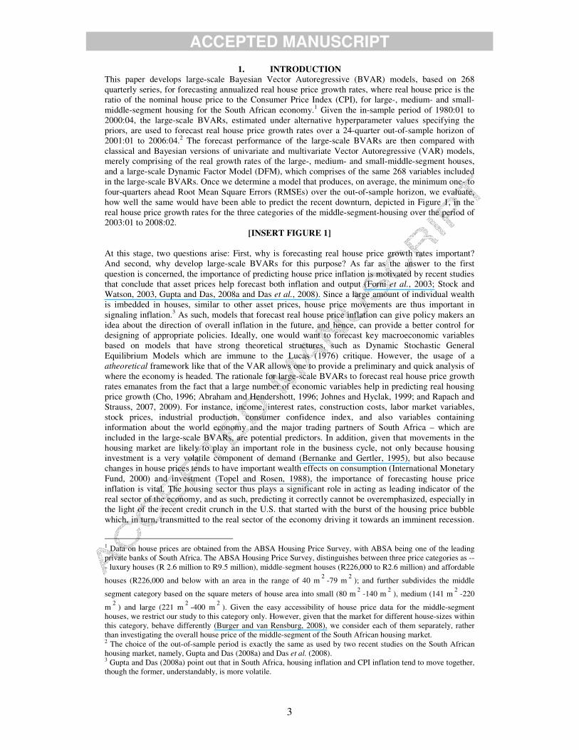
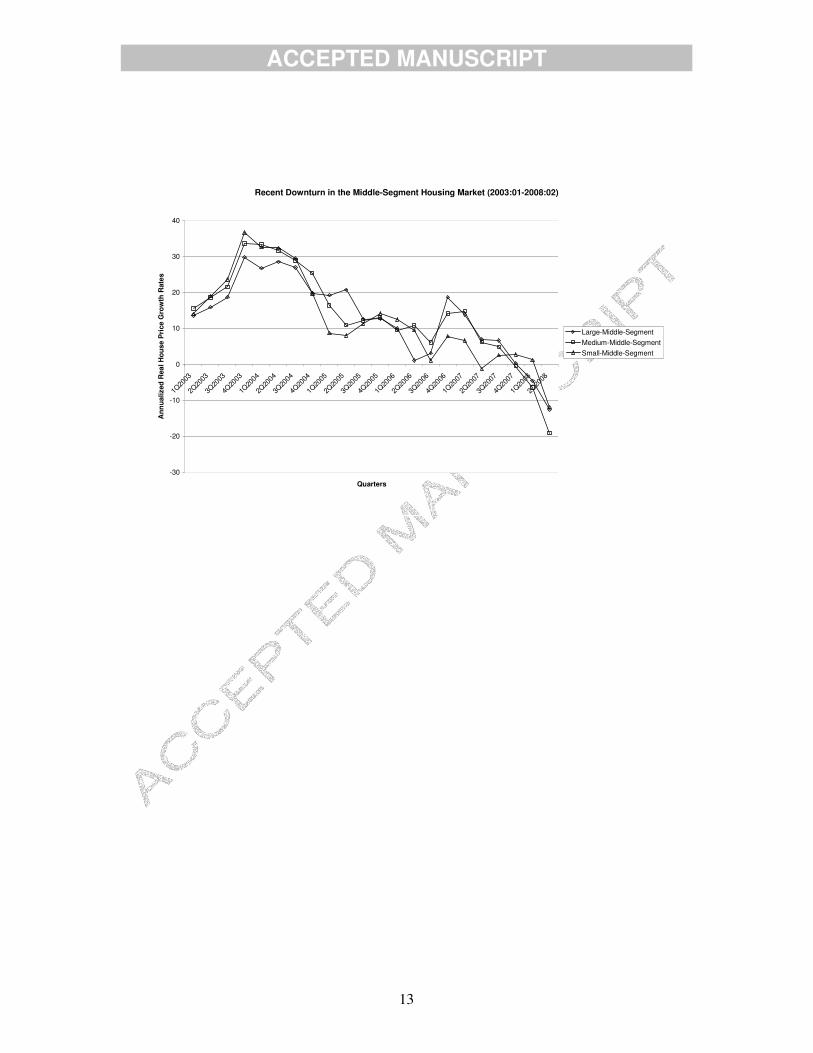
1. INTRODUCTION This paper develops large-scale Bayesian Vector Autoregressive (BVAR) models, based on 268 quarterly series, for forecasting annualized real house price growth rates, where real house price is the ratio of the nominal house price to the Consumer Price Index (CPI), for large-, medium- and small-middle-segment housing for the South African economy.1 Given the in-sample period of 1980:01 to 2000:04, the large-scale BVARs, estimated under alternative hyperparameter values specifying the priors, are used to forecast real house price growth rates over a 24-quarter out-of-sample horizon of 2001:01 to 2006:04.2 The forecast performance of the large-scale BVARs are then compared with classical and Bayesian versions of univariate and multivariate Vector Autoregressive (VAR) models, merely comprising of the real growth rates of the large-, medium- and small-middle-segment houses, and a large-scale Dynamic Factor Model (DFM), which comprises of the same 268 variables included in the large-scale BVARs. Once we determine a model that produces, on average, the minimum one- to four-quarters ahead Root Mean Square Errors (RMSEs) over the out-of-sample horizon, we evaluate, how well the same would have been able to predict the recent downturn, depicted in Figure 1, in the real house price growth rates for the three categories of the middle-segment-housing over the period of 2003:01 to 2008:02.

[INSERT FIGURE 1] At this stage, two questions arise: First, why is forecasting real house price growth rates important? And second, why develop large-scale BVARs for this purpose? As far as the answer to the first question is concerned, the importance of predicting house price inflation is motivated by recent studies that conclude that asset prices help forecast both inflation and output (Forni et al., 2003; Stock and Watson, 2003, Gupta and Das, 2008a and Das et al., 2008). Since a large amount of individual wealth is imbedded in houses, similar to other asset prices, house price movements are thus important in signaling inflation.3 As such, models that forecast real house price inflation can give policy makers an idea about the direction of overall inflation in the future, and hence, can provide a better control for designing of appropriate policies. Ideally, one would want to forecast key macroeconomic variables based on models that have strong theoretical structures, such as Dynamic Stochastic General Equilibrium Models which are immune to the Lucas (1976) critique. However, the usage of a atheoretical framework like that of the VAR allows one to provide a preliminary and quick analysis of where the economy is headed. The rationale for large-scale BVARs to forecast real house price growth rates emanates from the fact that a large number of economic variables help in predicting real housing price growth (Cho, 1996; Abraham and Hendershott, 1996; Johnes and Hyclak, 1999; and Rapach and Strauss, 2007, 2009). For instance, income, interest rates, construction costs, labor market variables, stock prices, industrial production, consumer confidence index, and also variables containing information about the world economy and the major trading partners of South Africa – which are included in the large-scale BVARs, are potential predictors. In addition, given that movements in the housing market are likely to play an important role in the business cycle, not only because housing investment is a very volatile component of demand (Bernanke and Gertler, 1995), but also because changes in house prices tends to have important wealth effects on consumption (International Monetary Fund, 2000) and investment (Topel and Rosen, 1988), the importance of forecasting house price inflation is vital. The housing sector thus plays a significant role in acting as leading indicator of the real sector of the economy, and as such, predicting it correctly cannot be overemphasized, especially in the light of the recent credit crunch in the U.S. that started with the burst of the housing price bubble which, in turn, transmitted to the real sector of the economy driving it towards an imminent recession.

1 Data on house prices are obtained from the ABSA Housing Price Survey, with ABSA being one of the leading private banks of South Africa. The ABSA Housing Price Survey, distinguishes between three price categories as --- luxury houses (R 2.6 million to R9.5 million), middle-segment houses (R226,000 to R2.6 million) and affordable

houses (R226,000 and below with an area in the range of 40 m 2 -79 m 2 ); and further subdivides the middle

segment category based on the square meters of house area into small (80 m 2 -140 m 2 ), medium (141 m 2 -220

m 2 ) and large (221 m 2 -400 m 2 ). Given the easy accessibility of house price data for the middle-segment houses, we restrict our study to this category only. However, given that the market for different house-sizes within this category, behave differently (Burger and van Rensburg, 2008), we consider each of them separately, rather than investigating the overall house price of the middle-segment of the South African housing market. 2 The choice of the out-of-sample period is exactly the same as used by two recent studies on the South African housing market, namely, Gupta and Das (2008a) and Das et al. (2008). 3 Gupta and Das (2008a) point out that in South Africa, housing inflation and CPI inflation tend to move together, though the former, understandably, is more volatile.

ACCEPTED MANUSCRIPT

4

Besides this, the fact that BVARs are quite well-suited in predicting turning points of macroeconomic variables have recently been substantiated by Dua and Ray (1995), Del Negro 2001), Gupta and Sichei (2006), Gupta (2006, 2008), Banerji et al. (2008), Zita and Gupta (2008) and Gupta and Das (2008b) amongst others. To realize the contribution of this study, it is important to place this paper in the context of current research that has been done on forecasting the housing market. In this regard, few studies that are worth mentioning are: Rapach and Strauss (2007, 2009), Gupta and Das (2008a,b), Das et al. (2008). Rapach and Strauss (2007) used an autoregressive distributed lag (ARDL) model framework, containing 25 determinants, to forecast real housing price growth for the individual states of the Federal Reserve’s Eighth District. Given the difficulty in determining apriori the particular variables that are most important for forecasting real housing price growth, the authors also use various methods to combine the individual ARDL model forecasts, which result in better forecast of real housing price growth. Rapach and Strauss (2009) look at doing the same for 20 largest US states based on ARDL models containing large number of potential predictors, including state, regional and national level variables. Once again, the authors reach similar conclusions as far as the importance of combining forecasts are concerned. Given that in practice, forecasters and policymakers often extract information from many series than the ones included in smaller models, like the ones used by Rapach and Strauss (2007, 2009), who also indicate the importance of combining forecast from alternative models, the role of a large-scale models cannot be ignored. In addition, one cannot condone the fact that the main problem of small models, as seen from the studies by Rapach and Strauss (2007, 2009), is in the decision regarding the choice of the correct potential predictors to be included. Due to this reason, Vargas-Silva (2008) uses a Factor Augmented VAR (FAVAR) model containing 120 monthly series to analyze the impact of monetary policy actions on the housing sector of four different regions of the United States. Further, Das et al. (2008) show that forecast performances of Spatial BVARs (SBVARs), developed by Gupta and Das (2008a), to predict regional house prices in the middle-segment housing category of South Africa, can be markedly improved using a DFM. Clearly then, the motivation and the need to forecast house prices using large-scale models is quite compelling. However, to the best of our knowledge, this is the first attempt to look into the ability of large-scale BVARs in forecasting and predicting downturns in real house price growth rates.4,5 The only other study that does look into forecasting the recent downturn in real house price growth rates for the twenty largest states of the US economy, is Gupta and Das (2008b). In this paper, the authors use SBVARs, based merely on real house price growth rates, to predict their downturn over the period of 2004:01 to 2008:01. They find that, though the models are quite well-equipped in predicting the recent downturn, they underestimate the decline in the real house price growth rates by quite a margin. They attribute this underprediction of the models to the lack of any information on fundamentals in the estimation process. Against this backdrop, our paper can thus be viewed as an extension of the abovementioned studies, in the sense that we not only use large-scale BVARs that allow for the role of a widest possible set of domestic, foreign and world fundamentals to affect the housing sector, but also use them to predict the recent downturn in the South African housing market. At this juncture, we must elaborate that given the type of models that we use, the study can easily be carried out for any country(ies). The reason behind using the South African housing market as a case study is simply data driven, especially, as far as data on the 268 macroeconomic variables are concerned, which, in turn, were obtained from the recent study of Gupta and Kabundi (2008a,b,c) and Das et al. (2008).6 The remainder of the paper is organized as follows: Section 2 lays out the basics of the benchmark large-scale BVARs and the alternative models, while, Section 3 discusses the data. Sections 4 and 5 respectively, evaluate the forecasting performances of the models and their ability to predict the recent downturn in the housing market. Finally, Section 6 concludes.

4 Note, Dua and Smyth (1995), Dua and Miller (1996) and Dua et al. (1999) used coincident and leading indexes in BVAR models to forecast home sales for the Connecticut and the overall US economy, respectively. 5 Note, even though just like Gupta and Das (2008a) and Das et al. (2008), we look at the middle-segment of the South African housing market, unlike them, we do not look into regional data. This is simply because the recent downturn in the housing market has been an economy-wide phenomenon and not been restricted to any specific region (ABSA Quarterly Housing Price Review, 2008Q1, 2008Q2 and 2008Q3). 6 See Section 3 for further details.

ACCEPTED MANUSCRIPT

5

2. THE MODEL 2.1 VARs and BVARs The Vector Autoregressive (VAR) model, though ‘atheoretical’, is particularly useful for forecasting purposes. An unrestricted VAR model, as suggested by Sims (1980), can be written as follows:

= + +� � �� � �� � � � � ε (1)

where y is a ( �� ) vector of variables being forecasted; A(L) is a ( � � ) polynomial matrix in the

backshift operator L with lag length p, i.e., A(L) = + + +�

� � ���������������� �

�� � � � � � ; �� is a

( ×�� ) vector of constant terms, and ε is a ( ×�� ) vector of error terms. In our case, we assume

that ε σ ×�� ��� ����� �� ���� ������ �� �� � � � � .

Note the VAR model, generally uses equal lag length for all the variables of the model. One drawback of VAR models is that many parameters need to be estimated, some of which may be insignificant. This problem of overparameterization, resulting in multicollinearity and a loss of degrees of freedom, leads to inefficient estimates and possibly large out-of-sample forecasting errors. One solution, often adapted, is simply to exclude the insignificant lags based on statistical tests. Another approach is to use a near VAR, which specifies an unequal number of lags for the different equations.

However, an alternative approach to overcoming this overparameterization, as described in Litterman (1981), Doan et al. (1984), Todd (1984), Litterman (1986), and Spencer (1993), is to use a BVAR model. Instead of eliminating longer lags, the Bayesian method imposes restrictions on these coefficients by assuming that they are more likely to be near zero than the coefficients on shorter lags. However, if there are strong effects from less important variables, the data can override this assumption. The restrictions are imposed by specifying normal prior distributions with zero means and small standard deviations for all coefficients with the standard deviation decreasing as the lags increase. The exception to this is that the coefficient on the first own lag of a variable has a mean of unity. Litterman (1981) used a diffuse prior for the constant. This is popularly referred to as the ‘Minnesota prior’ due to its development at the University of Minnesota and the Federal Reserve Bank at Minneapolis.

Formally, as discussed above, the means of the Minnesota prior take the following form:

β ββ σ β σ� �� ��� ����� � ��� � � � (2)

where βi denotes the coefficients associated with the lagged dependent variables in each equation of

the VAR, while β j represents any other coefficient. In the belief that lagged dependent variables are

important explanatory variables, the prior means corresponding to them are set to unity. However, for all the other coefficients, β j ’s, in a particular equation of the VAR, a prior mean of zero is assigned to

suggest that these variables are less important to the model.

The prior variances 2βσ

iand 2

βσj, specify uncertainty about the prior means βi = 1, and β j = 0,

respectively. Because of the overparameterization of the VAR, Doan et al. (1984) suggested a formula to generate standard deviations as a function of small numbers of hyperparameters: w, d, and a weighting matrix f(i, j). This approach allows the forecaster to specify individual prior variances for a large number of coefficients based on only a few hyperparameters. The specification of the standard deviation of the distribution of the prior imposed on variable j in equation i at lag m, for all i, j and m, defined as �σ , can be specified as follows:

�� � � �� ��

�= × ×

�

� � � σσσ

(3)

with f(i, j) = 1, if i = j and � otherwise, with ( ≤ ≤� �� ), g(m) = − >� ��� � . Note that σ̂ i is the

estimated standard error of the univariate autoregression for variable i. The ratio � �� σ σ scales the

variables to account for differences in the units of measurement and hence causes specification of the prior without consideration of the magnitudes of the variables. The term w indicates the overall tightness and is also the standard deviation on the first own lag, with the prior getting tighter as we

ACCEPTED MANUSCRIPT

6

reduce the value. The parameter g(m) measures the tightness on lag m with respect to lag 1, and is assumed to have a harmonic shape with a decay factor of d, which tightens the prior on increasing lags. The parameter f(i, j) represents the tightness of variable j in equation i relative to variable i, and by increasing the interaction, i.e., the value of � , we can loosen the prior.7 Note, in the standard

Minnesota-type prior, the overall tightness (w) takes the values of 0.1, 0.2 and 0.3, while, the lag decay (d) is generally chosen to be equal to 0.5, 1.0 and 2.0. The interaction parameter ( � ) is traditionally

set at = 0.5. The small-scale BVARs would be estimated with this set of parameterization of the priors. Given that we have domestic as well as foreign and world variables in the 268 data series used for the large-scale models, and realizing that South Africa is a small open economy, and hence, domestic variables would have minimal, if any, effect on foreign and world variables, while the latter set of variables is sure to have an influence on the South African variables, setting � = 0.5 could be a quite

far fetched from reality. Hence, borrowing from the BVAR models used for regional forecasting, involving both regional and national variables, and following Kinal and Ratner (1986), Shoesmith (1992) and Gupta and Kabundi (2008b,c), the weight of a foreign or world variable in a foreign or world equation, as well as a domestic equation, is set at 0.6. The weight of a domestic variable in other domestic equation is fixed at 0.1 and that in a foreign or world equation at 0.01. Finally, the weight of the domestic variable in its own equation is 1.0. These weights are in line with Litterman’s circle-star structure. Star (foreign or world) variables affect both star and circle (domestic) variables, while circle variables primarily influence only other circle variables.8 Clearly then, the large-scale BVARs are estimated with asymmetric priors. Finally, once the priors have been specified, the alternative BVARs, whether based on 1 or 3 or all the 268 variables, are estimated using Theil's (1971) mixed estimation technique. Specifically, suppose we

denote a single equation of the VAR model as: β ε ε σ= + = �

� � �� � � � �� � ��� � then the stochastic prior restrictions for this single equation can be written as:

��� ��� ��� ���

��� ��� ��� ���

� � � � � �

� � � � � �

� � � � � � � � �

� � � � � � � � �

� � � � � � � � �

� � � � � �

� � � � � � � �� � � �� � � �� � � �� � � �� � � �� � � �

= +� � � �� � � �� � � �� � � �� � � �� � � �� � � �� � � �� � � �� � � �� � � �� � � ���� ��� ��� ���

� � �

� � �

� � �

σ σσ σ

σ σ

(4)

Note, σ= ������� �and the prior means, �� ,and prior variance, �σ , take the forms shown in (2)

and (3). With (4) written as: β= +� � � (5)

and the estimates for a typical equation are derived as follows:

β −= + +�

�� � � � �� � ��� � � � � � � � (6)

Essentially then, the method involves supplementing the data with prior information on the distribution of the coefficients. The number of observations and degrees of freedom are increased by one in an artificial way, for each restriction imposed on the parameter estimates. The loss of degrees of freedom due to over- parameterization associated with a classical VAR model is, therefore, not a concern in the BVARs.

2.2 DFM

��������� �� ����� ��������! ������"�����##$���%�&���������'�� �������(����� )� �)� )������������ �����*� ���+�� ���� ��*��'�� �������������'�* , ����(�+��������������+�� �(���� ��(���������������* �*����- �� �����( ���������.������ �)��,������������ +��,���*��������� ��������������

ACCEPTED MANUSCRIPT

7

This study uses the Dynamic Factor Model (DFM) developed by Forni et al. (2005) to extract common components between macroeconomics series, and then these common components are used to forecast real house price growth rates in South Africa. In the VAR models, since all variables are used in forecasting, the number of parameters to be estimated depends on the number of variables n . With such a large information set, n , the estimation of a large number of parameters leads to a curse of dimensionality, especially in the case of classical VARs. The DFM uses information set accounted by few factors q n<< , which transforms the curse of dimensionality into a blessing of dimensionality. The DFM expresses individual times series as the sum of two unobserved components: a common component driven by a small number of common factors and an idiosyncratic component, which are specific to each variable. The relevance of the method is that the DFM is able to extract the few factors that explain the comovement of all South African macroeconomic variables. Forni et al. (2005) demonstrated that when the number of factors is small relative to the number of variables and the panel is heterogeneous, the factors can be recovered from the present and past observations. Consider an 1n× covariance stationary process )...,,( 1 ′= nt yyY . Suppose that tX is the

standardized version of tY , i.e. tX has a mean zero and a variance equal to one. Under DFM proposed

by Forni et al. (2005) tX is described by a factor model, it can be written as the sum of two orthogonal components:

ittiittiit FfLbx ξλξ +=+= )( (7) or, in vector notation:

ittittt FfLBX ξξ +Λ=+= )( (8)

where tf is a 1×q vector of dynamic factors, ss LBLBBLB +++= ....)( 10 is in an qn ×

matrix of factor loadings of order s , tξ is the 1×n vector of idiosyncratic components, tF is 1×r

vector of static factors, with )1( +≥ sqr . Let tf and tξ be mutually orthogonal stationary processes

and tt fLB )(=χ the common component. In factor analysis jargon ittt fLBX ξ+= )( is referred

to as the dynamic factor model, and ittt FX ξ+Λ= as the static factor model. Similarly, tf is

regarded as vector of the dynamic factors while tF as the vector of the static factors. Since dynamic common factors are latent, they need to be estimated. Forni et al. (2005) estimate dynamic factors through the use of dynamic principal component analysis. It involves the estimating the eigen values and eigen vectors decomposition of spectral density matrix of tX , which is a generalization of orthogonalization process in case of static principal components. The DFM of Forni et al. (2005) is estimated in two steps to solve the end-of-sample problems caused by two-sided filtering encounter with the Dynamic Principle Component Analysis (DPCA) used in Forni et al. (2000). Due to end-of-sample problems this method is not suited for forecasting. Firstly, the DPCA is used to compute estimates of covariance matrices of common and idiosyncratic components of tX at all leads and lags as inverse Fourier transforms of the corresponding estimated spectral density matrices. The spectral density matrix of tX is given by )()()( θθθ ξχ Σ+Σ=Σ . Secondly, these estimates are used in the

construction of r linear combinations of the observations having smallest idiosyncratic-common variance ratio.

3. DATA

While, the small-scale, univariate and 3-variable multivariate, VARs, both the classical and Bayesian variants, include data on only the three variables of interest, namely, the annualized real house price growth rates of the large-, medium- and small-middle-segment houses, the large-scale BVARs and the DFM is estimated based on 268 quarterly series of South Africa, with the data covering the real, nominal, and financial sectors. We also have intangible variables, such as confidence indices, and survey variables. In addition to national variables, the paper uses a set of global variables such as commodity industrial inputs price index and crude oil prices. The data also comprises series of major trading partners such as Germany, the United Kingdom (UK), and the United States (US) of America. The in-sample period contains data from 1980:01 to 2000:04, while the out-of-sample set is 2001:01-

ACCEPTED MANUSCRIPT

8

2006:04.9 All series are seasonally adjusted and were made covariance stationary when estimating the DFM. The more powerful DFGLS test of Elliott, Rothenberg, and Stock (1996), instead of the most popular ADF test, is used to assess the degree of integration of all series. All non-stationary series are made stationary through differencing. The Schwarz information criterion is used in the selecting the appropriate lag length in such a way that no serial correction is left in the stochastic error term. Where there were doubts about the presence of unit root, the KPSS test proposed by Kwiatowski et al., (1992), with the null hypothesis of stationarity, was applied. All series are standardized to have a mean of zero and a constant variance. It must however be pointed out that, non-stationarity is not an issue with the BVAR, since Sims et al. (1990) indicate that with the Bayesian approach entirely based on the likelihood function, the associated inference does not need to take special account of nonstationarity, since the likelihood function has the same Gaussian shape regardless of the presence of nonstationarity. Hence, for the sake of comparison amongst the VARs, both classical and Bayesian, we make no attempt to make the variables stationary, unlike in the DFM.10 There are various statistical approaches in determining the number of factors in the DFM. For example, Bai and Ng (2002) developed some criteria guiding the selection of the number of factors in large dimensional panels. The Principal Component Analysis (PCA) can also be used in establishing the number of factors in the DFM. The PCA suggests that the selection of a number of factors q be based on the first eigen values of the spectral density matrix of �� . Then, the principal components are added until the increase in the explained variance is less than a specific ����=α . The Bai and Ng (2002) approach proposes five static factors, while Bai and Ng (2007) suggests two primitive or dynamic factors. Similar to the latter method, the principal component technique, as proposed by Forni et al. (2000) suggests two dynamic factors. The first two dynamic principal components explain approximately 99 percent of variation, while the eigen value of the third component is 0.05)( 0.005 < .

4. FORECASTING EVALUATION Given the specifications of the models, we estimate the five alternative types of models, namely, the univariate and multivariate versions of the classical VAR and the small-scale BVARs, the large-scale BVAR and the DFM over the period of 1980:01 to 2000:04, based on quarterly data. Then we compute the out-of-sample one- through four-quarters-ahead forecasts for the period of 2001:01 to 2006:04, and compare the forecast accuracy of the alternative models. The different types of the VARs are estimated with eight lags11 of each variable. Since we use eight lags, the initial eight quarters of the sample, 1980:01 to 1981:04, are used to feed the lags. We generate dynamic forecasts, as would naturally be achieved in actual forecasting practice. The models are re-estimated each quarter over the out-of-sample forecast horizon in order to update the estimate of the coefficients, before producing the 4-quarters-ahead forecasts. This iterative estimation and 4-steps-ahead forecast procedure was carried out for 24 quarters, with the first forecast beginning in 2001:01. This experiment produced a total of 24 one-quarter-ahead forecasts, 24-two-quarters-ahead forecasts, and so on, up to 24 4-step-ahead forecasts. The RMSEs12 for the 24, quarter 1 through quarter 4 forecasts are then calculated for the annualized real house price growth rates of the large-, medium- and small-middle-segment housing. The values of the RMSE statistic for one- to four-quarters-ahead forecasts for the period 2001:01 to 2006:04 are then examined. The model that produces the lowest average value for the RMSE is selected as the ‘optimal’ model for a specific category of real house price growth rate.

#!��� ����(� ������������������ �� *��������������,����+�� �(���� ���������� �����������)�/�*����012"���������!�3������+� ��(��� '�����- ��������4���! ������"�����##$��,���, ��������� �������The choice of 8 lags is based on the unanimity of the sequential modified LR test statistic, Akaike information criterion (AIC), the final prediction error (FPE) criterion and the Hannan-Quinn (HQ) information criterion applied to a stable VAR estimated with the 3 variables of concern. Note, stability, as usual, implies that no roots were found to lie outside the unit circle. 12 Note that if t nA + denotes the actual value of a specific variable in period t + n and t t nF + equals the forecast

made in period t for t + n, the RMSE statistic equals the following: ( )21N

t t n t nF AN

+ +� �−�� �� �� �

where N equals

the number of forecasts.

ACCEPTED MANUSCRIPT

9

In Tables 1 through 3, we compare the RMSEs of one- to four-quarters-ahead out-of-sample-forecasts for the period of 2000:01 to 2006:04, generated by the abovementioned alternative models. At this stage, a few words need to be said regarding the choice of the evaluation criterion for the out-of-sample forecasts generated from Bayesian models. As Zellner (1986: 494) points out, the ‘optimal’ Bayesian forecasts will differ depending upon the loss function employed and the form of predictive probability density function. In other words, Bayesian forecasts are sensitive to the choice of the measure used to evaluate the out-of-sample forecast errors. However, Zellner (1986) points out that the use of the mean of the predictive probability density function for a series, is optimal relative to a squared error loss function and the Mean Squared Error (MSE), and hence, the RMSE is an appropriate measure to evaluate performance of forecasts, when the mean of the predictive probability density function is used. This is exactly what we do below in Tables 1 through 3, when we use the average RMSEs over the one- to four-quarter-ahead forecasting horizon.13 The conclusions, regarding each of the three categories of real house price growth rate, based on the average one- to four-quarters-ahead RMSEs, from these tables can be summarized as follows:

(i) Irrespective of the hyperparameters specifying the tightness of the prior and the size of the houses within the middle segment category, the large-scale BVARs, outperform all the other models by quite a distance for each of the one- to four-quarters-ahead out-of-sample forecasts. However, within the large-scale BVARs, the model with the most tight priors (w = 0.1, d = 2.0) is the best performing model on average;

(ii) Based on the average RMSEs, the univariate BVAR models with (w = 0.1, d = 2.0) are a distant second to the large-scale BVARs in each of the three categories of the middle-segment housing. These models are closely followed in the heels by the small-scale BVAR models with same set of hyperparameters specifying the Minnesota prior;

(iii) In all the three cases, the univariate OLS or the Autoregressive model of order 8, the DFM and the VAR, based on the average RMSEs for the out-of-sample horizon of 2001:01 to 2006:04, are ranked as fourth, fifth and sixth respectively.

[INSERT TABLES 1 THROUGH 3]

Note, unlike Das et al. (2008), who found the DFM to be the overwhelming favorite in forecasting regional house price inflation relative to small-scale spatial and non-spatial BVARs and a classical VAR, our results do not indicate so.14 In fact, the DFM is found to be ranked below the univariate and multivariate small-scale BVARs in our case. However, there is no doubt over the capability of the large-scale BVARs in forecasting the economy-wide annualized real house price growth rates of the large-, medium- and small-middle-segment housing. At this stage, we must, however, point to at least two limitations of the Bayesian approach: First, as is clear from Tables 1 to 3, the forecast accuracy is sensitive to the choice of the priors. So if the prior is not well specified, an alternative model used for forecasting may perform better. Second, for the Bayesian models, one requires to specify an objective function, for example the average RMSEs, to search for the ‘optimal’ priors, which in turn, needs to be optimized over the period for which we compute the out-of-sample forecasts. However, there is no guarantee that the chosen parameter values specifying the prior will continue to be ‘optimal’ beyond the period for which it was selected. Nevertheless, the role of BVARs in forecasting macroeconomic variables accurately cannot be underestimated.

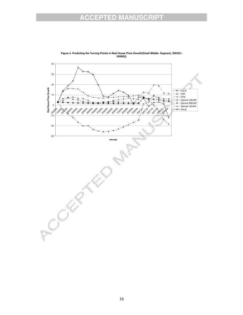
5. PREDICTING THE TURNING POINTS In what follows, we look at the ability of the large-scale BVAR model with (w = 0.1, d = 2.0) in predicting the recent downturn in the real house price growth rate over 2003:01 to 2008:02, in comparison to the AR(8), the VAR, the DFM and those BVARs, univariate and multivariate, that on average produces the minimum average RMSEs for specific values of w and d, specifying the

13 Our conclusions were, however, qualitatively the same based on the Mean Absolute Error (MAE) and Mean Absolute Percentage Error (MAPE). The results are available upon request. 14 Interestingly, when we repeated the forecasting exercise for the regional house price inflation using the large-scale BVAR, we found the model to outperform all the “optimal” models of Das et al. (2008). These results are available upon request.

ACCEPTED MANUSCRIPT

10

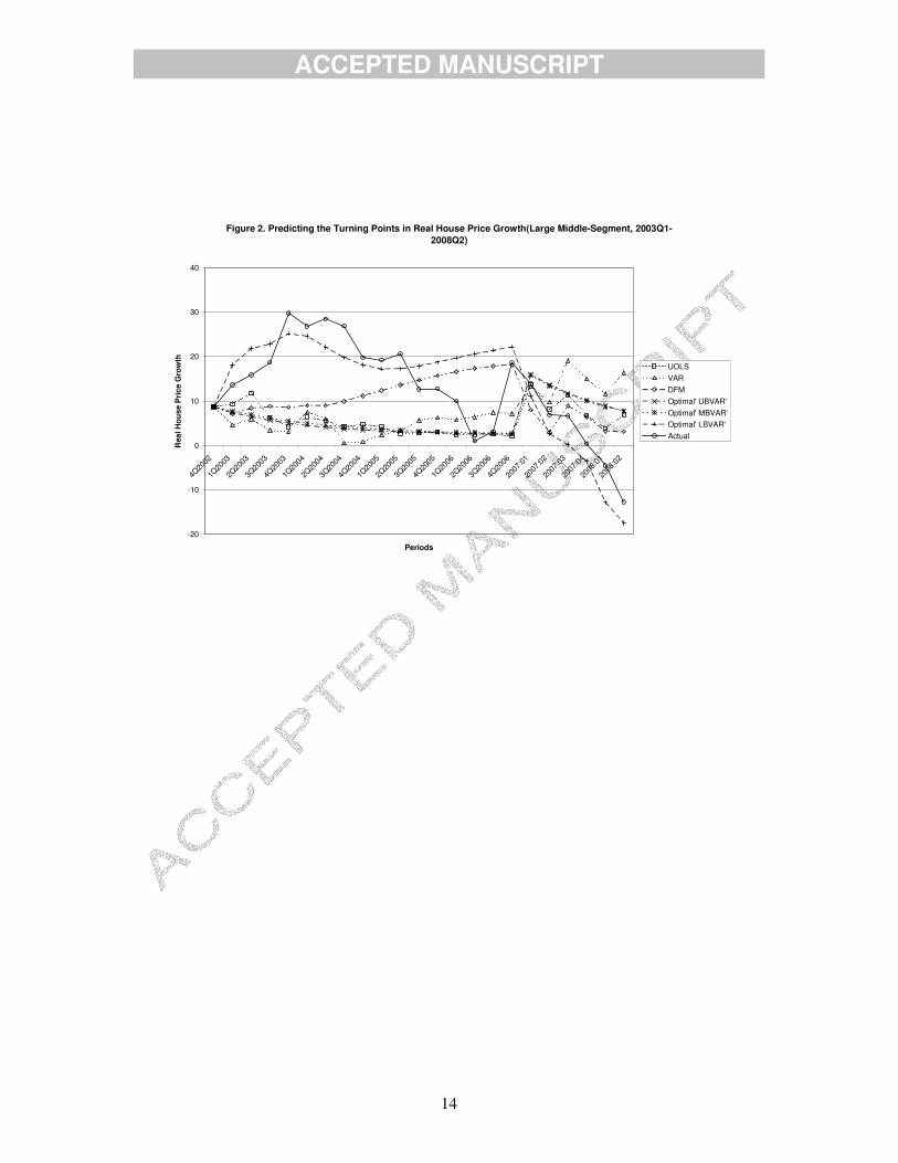
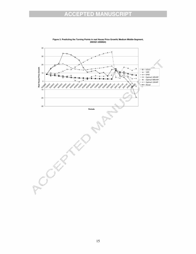
Minnesota prior. As with the large scale BVAR, the univariate and multivariate small-scale BVARs that outperforms the other models within its own category also has a value of w = 0.1, d = 2.0. The decision to choose 2003:01 as the starting date for the models to predict the turning points is simply because the real house price growth rates in the middle-segment of the housing peaked at 2003:04 as depicted in Figure 1. Given that ideally one would want to use available information prior to the turning point, following the methodology of Gupta and Das (2008b), all the ‘optimal’ models are estimated till 2002:04 and then we forecast over the period of 2003:01 till 2008:02. As can be observed from Figures 2 through 4, the ‘optimal’ large-scale BVAR with (w = 0.1, d = 2.0) is clearly the best suited model in predicting the recent downturn in the real house price growth rates of the large-, medium- and small-middle-segment housing over the period of 2003:01 to 2008:02. In general, the optimal large-scale BVAR tends to underpredict over the period of 2003:01 till 2006:04 and over predict the downturn especially when the real growth rate becomes negative in case of the large- and small-middle-segment housing in the latter half of the horizon. The fact that the ‘optimal’ large-scale BVAR does so well in predicting the recent downturn relative to the ‘optimal’ small-scale univariate and multivariate BVARs, is clearly an indication of the role fundamentals play in affecting real house prices, over and beyond the information contained in the growth rates of the lagged real house prices. Moreover, given that the large-scale BVAR model allows for the domestic variables to have a minimal effect on foreign and world variables, while the latter set of variables to have a strong influence on the South African variables, might be causing it to perform better than the DFM, which also includes the same set of variables, both in terms of forecasting and predicting the recent downturn.

[INSERT FIGURES 2 THROUGH 4]

6. CONCLUSIONS

This paper develops large-scale BVAR models, based on 268 quarterly series, for forecasting annualized real house price growth rates for large-, medium- and small-middle-segment housing for the South African economy. Given the in-sample period of 1980:01 to 2000:04, the large-scale BVARs, estimated under alternative hyperparameter values specifying the priors, are used to forecast real house price growth rates over a 24-quarter out-of-sample horizon of 2001:01 to 2006:04. The forecast performance of the large-scale BVARs are then compared with classical and Bayesian versions of univariate and multivariate VAR models, comprising of the real growth rates of the large-, medium- and small-middle-segment houses only, and a large-scale DFM, which comprises of the same 268 variables included in the large-scale BVARs. Once we determine a model that produces, on average, the minimum one- to four-quarters ahead RMSEs over the out-of-sample horizon, we evaluate how well the same would have been able to predict the recent downturn in the real house price growth rates for the three categories of the middle-segment-housing over the period of 2003:01 to 2008:02. Our results indicate that, irrespective of the hyperparameters specifying the tightness of the prior and the size of the houses within the middle segment category, the large-scale BVARs outperform all the other models by a distance for each of the one- to four-quarters-ahead out-of-sample forecasts. However, within the large-scale BVARs, the model with the most tight priors (w = 0.1, d = 2.0) is the best performing model on average. Moreover, this ‘optimal’ large-scale BVAR is also capable of tracking closely the recent downturn in the real house price growth rates for the three categories of the middle-segment-housing over an ex ante period of 2003:01 to 2008:02. In summary, we find a tight-priored large-scale BVAR model, which not only includes the widest possible set of fundamentals that tends to affect the housing market, but also treats South Africa as a small open economy by allowing for asymmetry in the specification of the prior, is the overwhelming favorite to forecast and predict turning points for the middle-segment category of housing. At this juncture, we must elaborate that given the type of models that we use, the study can easily be carried out for any country(ies). There are however, as noted earlier, limitations to using the BVAR approach. First, the forecast accuracy depends critically on the specification of the prior, and second, the selection of the prior based on some objective function for the out-of-sample forecasts may not be ‘optimal’ for the time period beyond the period chosen to produce the out-of-sample forecasts. Besides these, there are two other major concerns, which are however general, to the traditional statistically estimated models used, like the VARs --- both Classical and Bayesian and the DFM, for forecasting at the business cycle frequencies. First, such procedures perform reasonably well as long there are no structural changes experienced by the economy. Such changes, whether in or out of the sample, would then entail the

ACCEPTED MANUSCRIPT

11

models inappropriate. Alternatively, these models are not immune to the ‘Lucas Critique’15. Furthermore, the estimation procedures used here are linear in nature, and hence, they fail to take into account of the nonlinearities in the data. One and, perhaps, the best response to these objections has been the development of micro-founded DSGE models, which are capable of handling both the problems arising out of the structural changes and the issues of nonlinearities16. As in Iacoviello and Neri (2008), future research should concentrate on using DSGE models to model the housing sector of an economy, and then using the same to forecast house prices.

REFERENCES

Abraham JM, Hendershott PH. Bubbles in Metropolitan Housing Markets. Journal of Housing Research 1996; 7; 191–207. ABSA Housing Price Review 2008; Quarter 1, Quarter 2 and Quarter 3. Bai J, Ng S. Determining the Number of Primitive Shocks in Factor Models. Journal of Business and Economic Statistics 2007; 25; 52–60. Bai J, Ng S. Determining the Number of Factors in Approximate Factor Models. Econometrica 2002; 70; 191–221. Banerji A, Dua P, Miller SM. Performance Evaluation of the New Connecticut Leading Employment Index Using Lead Profiles and BVAR Models. Journal of Forecasting 2008; 25; 415-437. Bernanke B, Gertler M. Inside the Black Box: the Credit Channel of Monetary Transmission. Journal of Economic Perspectives 1995; 9; 27–48. Burger P, Van Rensburg LJ. Metropolitan house prices in South Africa: Do they converge? South African Journal of Economics 2008; 76; 291-297 Cho M. House Price Dynamics: A Survey of Theoretical and Empirical Issues. Journal of Housing Research 1996; 7; 145–172. Das S, Gupta R, Kabundi A. Is a DFM Well-Suited for Forecasting Regional House Price Inflation? Forthcoming Economic Research Southern Africa Working Paper 2008. Del Negro M. Turn, Turn, Turn: Predicting Turning Points in Economic Activity. Economic Review 2001; Second Quarter; Federal Reserve Bank of Atlanta. Doan TA, Litterman RB, Sims CA. Forecasting and Conditional Projections Using Realistic Prior Distributions. Econometric Reviews 1984; 3; 1-100. Dua P, Smyth DJ. Forecasting U. S. Home Sales using BVAR Models and Survey Data on Households’ Buying Attitude for Homes. Journal of Forecasting 1995; 14; 217-227. Dua P, Miller SM, Smyth DJ. Using Leading Indicators to Forecast U. S. Home Sales in a Bayesian Vector Autoregressive Framework. Journal of Real Estate Finance and Economics 1999; 18; 191-205. Dua P, Miller SM. Forecasting Connecticut Home Sales in a BVAR Framework Using Coincident and Leading Indexes. Journal of Real Estate Finance and Economics 1996; 13; 219-235. Dua P, Ray SC. A BVAR Model for the Connecticut Economy. Journal of Forecasting 1995; 14; 167-180. Elliott G, Rothenberg TJ, Stock J. Efficient Tests for an Autoregressive Unit Root. Econometrica 1996; 64; 813–836. Forni M, Hallin M, Lippi M, Reichlin L. The Generalized Dynamic Factor Model, One Sided Estimation and Forecasting. Journal of the American Statistical Association 2005; 100; 830–840. Forni M, Hallin M, Lippi M, Reichlin L. Do financial variables help forecasting inflation and real activity in the euro area? Journal of Monetary Economics 2003; 50; 1243-1255. Forni M, Hallin M, Lippi M, Reichlin L. The Generalized Dynamic Factor Model: identification and estimation. Review of Economics and Statistics 2000; 82; 540–554. Gupta R. Bayesian Methods of Forecasting Inventory Investment in South Africa. Forthcoming South African Journal of Economics 2008. Gupta R, Das S. Spatial Bayesian Methods for Forecasting House Prices in Six Metropolitan Areas of South Africa. South African Journal of Economics 2008a; 76; 298-313. Gupta R, Das S. Predicting Downturns in the US Housing Market. Forthcoming Journal of Real Estate

15 See Lucas (1976) for details. 16 For a detailed review of the literature on the use of DSGE models for forecasting, see Liu and Gupta (2007) and Liu et al. (2007, 2008).

ACCEPTED MANUSCRIPT

12

Economics and Finance 2008b. Gupta R, Kabundi A. A Dynamic Factor Model for Forecasting Macroeconomic Variables in South Africa. Department of Economics, University of Pretoria; 2008a; Working Paper No. 200815 Gupta R, Kabundi A. Forecasting Macroeconomic Variables using Large Datasets: Dynamic Factor Model vs Large-Scale BVARs. Department of Economics, University of Pretoria; 2008b; Working Paper No. 200816. Gupta R. Kabundi A. Forecasting Macroeconomic Variables in a Small Open Economy: A Comparison between Small- and Large-Scale Models. Department of Economics, University of Pretoria; 2008c; Working Paper No. 200830. Gupta R. Forecasting the South African Economy with VARs and VECMs. South African Journal of Economics 2006; 74; 611-628. Gupta R, Sichei M. A BVAR Model for the South African Economy. South African Journal of Economics 2006; 74; 391-409. Iacoviello M, Neri S. Housing Market Spillovers: Evidence from an Estimated DSGE Model. Paper provided by Boston College Department of Economics in its series Boston College 2008; Working Papers in Economics with number 659. International Monetary Fund. World Economic Outlook: Asset Prices and the Business Cycle; 2000. Johnes G, Hyclak T. House Prices and Regional Labor Markets. Annals of Regional Science 1999; 33; 33–49. Kinal T, Ratner J. A VAR Forecasting Model of a Regional Economy: Its Construction and Comparison. International Regional Science Review 1986; 10; 113-126. Kwiatowski D, Phillips PCB, Schmidt P, Shin Y. Testing the Null Hypothesis of Stationarity Against the Alternative of a Unit Root: How Sure Are We That Economic Time Series Have a Unit Root? Journal of Econometrics 1992; 54; 159–178. Litterman RB. A Bayesian Procedure for Forecasting with Vector Autoregressions. Working Paper, Federal Reserve Bank of Minneapolis 1981. Litterman RB. Forecasting with Bayesian Vector Autoregressions – Five Years of Experience. Journal of Business and Economic Statistics 1986; 4 ; 25-38. Liu G, Gupta R. A Small-Scale DSGE Model for Forecasting the South African Economy. South African Journal of Economics 2007; 75; 179-193. Liu G, Gupta R, Schaling E. Forecasting the South African Economy: A Hybrid-DSGE Approach. Forthcoming Journal of Economic Studies 2007. Liu G, Gupta R, Schaling E. A New Keynesian DSGE Model for Forecasting the South African Economy. Forthcoming Journal of Forecasting 2008. Lucas, Jr. RE. Econometric Policy Evaluation: A Critique. Carnegie Rochester Conference Series on Public Policy 1976; 1; 19–46. Rapach DE, Strauss JK. Differences in Housing Price Forecastability across U.S. States 2009; 25; 351-371. Rapach DE, Strauss JK. Forecasting Real Housing Price Growth in the Eighth District States. Federal Reserve Bank of St. Louis. Regional Economic Development 2007; 3; 33–42. Shoesmith GL. Co-integration, Error Correction and Medium-Term Regional VAR Forecasting. Journal of Forecasting 1992; 11; 91-109. Sims CA, Stock JH, Watson MW. Inference in Linear Time Series Models with Some Unit Roots. Econometrica 1990; 58; 113-144. Sims CA. Macroeconomics and Reality. Econometrica 1980; 48; 1-48. Spencer DE. Developing a Bayesian Vector Autoregression Model. International Journal of Forecasting 1993; 9; 407-421. Stock JH, Watson MW. Forecasting Output and Inflation: The Role of Asset Prices. Journal of Economic Literature 2003; 41; 788-829. Theil H. Principles of Econometrics. John Wiley: New York; 1971. Todd RM. Improving Economic Forecasting with Bayesian Vector Autoregression. Quarterly Review Federal Reserve Bank of Minneapolis 1984; Fall; 18-29. Topel RH, Rosen S. Housing Investment in the United States. Journal of Political Economy 1988; 96; 718–740. Vargas-Silva C. The Effect of Monetary Policy on Housing: A Factor Augmented Vector autoregression (FAVAR) Approach. Applied Economics Letters 2008; 15; 749-752. Zellner A. A Tale of Forecasting 1001 Series: The Bayesian Knight Strikes Again. International Journal of Forecasting 1986; 2; 494-494. Zita SE, Gupta R. Modelling and Forecasting the Metical-Rand Exchange Rate. ICFAI Journal of Monetary Economics 2008; VI; 63-90.

ACCEPTED MANUSCRIPT

13

Recent Downturn in the Middle-Segment Housing Market (2003:01-2008:02)

-30

-20

-10

0

10

20

30

40

1Q20

03

2Q20

03

3Q20

03

4Q20

03

1Q20

04

2Q20

04

3Q20

04

4Q20

04

1Q20

05

2Q20

05

3Q20

05

4Q20

05

1Q20

06

2Q20

06

3Q20

06

4Q20

06

1Q20

07

2Q20

07

3Q20

07

4Q20

07

1Q20

08

2Q20

08

Quarters

Ann

ualiz

ed R

eal H

ouse

Pri

ce G

row

th R

ates

Large-Middle-SegmentMedium-Middle-SegmentSmall-Middle-Segment

ACCEPTED MANUSCRIPT

14

Figure 2. Predicting the Turning Points in Real House Price Growth(Large Middle-Segment, 2003Q1-2008Q2)

-20

-10

0

10

20

30

40

4Q20

02

1Q20

03

2Q20

03

3Q20

03

4Q20

03

1Q20

04

2Q20

04

3Q20

04

4Q20

04

1Q20

05

2Q20

05

3Q20

05

4Q20

05

1Q20

06

2Q20

06

3Q20

06

4Q20

06

2007

:01

2007

:02

2007

:03

2007

:04

2008

:01

2008

:02

Periods

Rea

l Ho

use

Pri

ce G

row

th

UOLSVARDFMOptimal' UBVAR'Optimal' MBVAR'Optimal' LBVAR'Actual

ACCEPTED MANUSCRIPT

15

Figure 3. Predicting the Turning Points in real House Price Growth( Medium Middle-Segment, 2003Q1-2008Q4)

-30

-20

-10

0

10

20

30

40

4Q20

02

1Q20

03

2Q20

03

3Q20

03

4Q20

03

1Q20

04

2Q20

04

3Q20

04

4Q20

04

1Q20

05

2Q20

05

3Q20

05

4Q20

05

1Q20

06

2Q20

06

3Q20

06

4Q20

06

2007

:01

2007

:02

2007

:03

2007

:04

2008

:01

2008

:02

Periods

Rea

l Ho

use

Pri

ce G

row

th

UOLSVARDFMOptimal' UBVAR'Optimal' MBVAR'Optimal' LBVAR'Actual

ACCEPTED MANUSCRIPT

16

Figure 4. Predicting the Turning Points in Real House Price Growth(Small Middle- Segment, 2003Q1-2008Q2)

-30

-20

-10

0

10

20

30

40

4Q20

02

1Q20

03

2Q20

03

3Q20

03

4Q20

03

1Q20

04

2Q20

04

3Q20

04

4Q20

04

1Q20

05

2Q20

05

3Q20

05

4Q20

05

1Q20

06

2Q20

06

3Q20

06

4Q20

06

2007

:01

2007

:02

2007

:03

2007

:04

2008

:01

2008

:02

Periods

Rea

l Hou

se P

rice

Gro

wth

UOLSVARDFMOptimal' UBVAR'Optimal' MBVAR'Optimal' LBVAR'Actual

ACCEPTED MANUSCRIPT

17

Table 1. RMSEs of One- to Four-quarters Ahead (Large Middle-Segment, 2001:01-2006:4) QA 1 2 3 4 Average UOLS 7.6251 11.1535 12.4930 14.6719 11.4859 VAR 8.2894 13.2600 16.3651 21.7194 14.9085 DFM 10.7001 11.8895 12.3906 13.6091 12.1473

UBVAR 7.6507 10.8855 12.3250 14.0990 11.2400 SBVAR 7.1261 10.0614 11.5019 13.6714 10.5902 w=0.3,d=0.5 LBVAR 2.5138 0.8128 1.7729 0.9020 1.5003 UBVAR 7.6156 10.2381 11.5509 13.1236 10.6320 SBVAR 7.8267 10.7540 12.1414 13.6428 11.0912 w=0.2,d=1 LBVAR 2.3499 0.3116 2.1669 1.0100 1.4596 UBVAR 7.7395 10.3749 11.4148 12.8624 10.5979 SBVAR 7.7199 10.3497 11.3774 12.8060 10.5633 w=0.1,d=1 LBVAR 2.5542 0.4357 1.7550 0.7009 1.3614 UBVAR 7.9524 10.8216 12.2585 13.7656 11.1995 SBVAR 7.8224 10.3813 11.6917 13.1564 10.7630 w=0.2,d=2 LBVAR 1.7410 0.2447 2.2942 1.0257 1.3264 UBVAR 7.7368 10.2601 11.2240 12.6499 10.4677 SBVAR 7.7718 10.3328 11.3300 12.7285 10.5408 w=0.1,d=2 LBVAR 2.1479 0.2178 1.7364 0.5203 1.1556

UBVAR: Univariate BVAR; SBVAR: Small-Scale BVAR; LBVAR: Large-Scale BVAR

ACCEPTED MANUSCRIPT

18

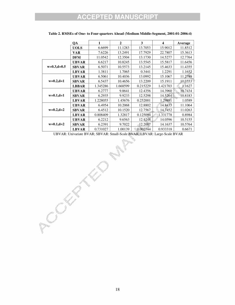
Table 2. RMSEs of One- to Four-quarters Ahead (Medium Middle-Segment, 2001:01-2006:4)

QA 1 2 3 4 Average UOLS 6.6699 11.1283 13.7053 15.9012 11.8512 VAR 7.6226 13.2491 17.7929 22.7807 15.3613 DFM 11.0542 12.3504 13.1730 14.5277 12.7764

UBVAR 6.6217 10.8245 13.5545 15.5817 11.6456 SBVAR 6.5071 10.5573 13.2145 15.4633 11.4355 w=0.3,d=0.5 LBVAR 1.3811 1.7065 0.3441 1.2291 1.1652 UBVAR 6.5061 10.4036 13.0992 15.1067 11.2789 SBVAR 6.5437 10.4656 13.2209 15.1911 11.3553 w=0.2,d=1 LBBAR 1.345286 1.668599 0.215229 1.421703 1.1627 UBVAR 6.2777 9.8641 12.4356 14.3960 10.7434 SBVAR 6.2935 9.9233 12.5298 14.5264 10.8183 w=0.1,d=1 LBVAR 1.228055 1.45676 0.252001 1.29891 1.0589 UBVAR 6.4954 10.2068 12.8802 14.8433 11.1064 SBVAR 6.4512 10.1520 12.7567 14.7452 11.0263 w=0.2,d=2 LBVAR 0.808409 1.32817 0.125094 1.331778 0.8984 UBVAR 6.2212 9.6563 12.1248 14.0596 10.5155 SBVAR 6.2391 9.7022 12.2007 14.1637 10.5764 w=0.1,d=2 LBVAR 0.731027 1.00139 0.002744 0.933318 0.6671

UBVAR: Univariate BVAR; SBVAR: Small-Scale BVAR; LBVAR: Large-Scale BVAR

ACCEPTED MANUSCRIPT

19

Table 3. RMSEs of One- to Four-quarters Ahead (Small Middle-Segment, 2001:01-2006:4) QA 1 2 3 4 Average UOLS 7.1218 10.9471 13.3339 16.0891 11.8730 VAR 7.9998 13.5224 18.1246 23.6199 15.8167 DFM 11.3963 11.6307 12.1631 14.2256 12.3539

UBVAR 7.0812 10.9023 13.4321 15.8916 11.8268 SBVAR 6.7764 10.6527 13.4899 16.2816 11.8001 w=0.3,d=0.5 LBVAR 2.2690 5.2247 3.5924 3.7260 3.7030 UBVAR 7.0021 10.7143 13.2513 15.5501 11.6295 SBVAR 7.1894 10.9627 13.4611 15.6902 11.8259 w=0.2,d=1 LBVAR 1.6219 3.9732 2.3725 2.8725 2.7100 UBVAR 7.1012 10.6804 12.9729 15.2257 11.4951 SBVAR 7.0560 10.6301 12.9526 15.2829 11.4804 w=0.1,d=1 LBVAR 1.6947 3.8056 2.6036 2.8698 2.7434 UBVAR 7.2474 10.9464 13.3839 15.5598 11.7844 SBVAR 7.0765 10.6763 13.1243 15.3775 11.5637 w=0.2,d=2 LBVAR 1.0821 3.0972 2.1133 3.0300 2.3307 UBVAR 7.0911 10.5807 12.8007 15.0435 11.3790 SBVAR 7.0804 10.5700 12.8116 15.1174 11.3948 w=0.1,d=2 LBVAR 1.2918 3.1277 2.1990 2.6840 2.3256

UBVAR: Univariate BVAR; SBVAR: Small-Scale BVAR; LBVAR: Large-Scale BVAR