Copyright

by

Josh Ryan Aldred

2015

The Dissertation Committee for Josh Ryan Aldred Certifies that this is the approved version of the following dissertation:

The Nexus of Energy and Health: A Systems Analysis of Costs and Benefits of Ozone Control by Activated

Carbon Filtration in Buildings

Committee:

Richard Corsi, Supervisor

Atila Novoselac

Kerry Kinney

Howard Liljestrand

Jeffrey Siegel

The Nexus of Energy and Health: A Systems Analysis of Costs and Benefits of Ozone Control by Activated

Carbon Filtration in Buildings

by

Josh Ryan Aldred, B.S.E.; M.S.E.

Dissertation

Presented to the Faculty of the Graduate School of

The University of Texas at Austin

in Partial Fulfillment

of the Requirements

for the Degree of

Doctor of Philosophy

The University of Texas at Austin August 2015

Dedication

To Vanessa, my best friend and wingman for life.

v

Acknowledgements

First of all, I would like to thank my dissertation committee for volunteering to serve on my committee and taking time out of their very busy schedules to help me pursue my goals. I would like to thanks Dr. Corsi for his advice and support, this journey wouldn’t have been possible if he hadn’t taken a small risk on bringing me on board. I would also like to thank Dr. Novoselac for always having an open door policy. I have learned nearly everything I know about HVAC systems and energy modeling from him. Dr. Neil Crain has been a huge help in setting up all of my experiments – I wouldn’t have been able to complete any of my field work without his guidance. Mrs. Dori Eubank has been one of my greatest advocates since I started the PhD program – I’m extremely grateful for her help and support. Dr. J.P. Maestre taught me everything I know about DNA extraction and I’m very grateful he took time out of his busy schedule to teach me something new. Dr. Glenn Morrison has been a great mentor and I’m thankful for his help and comments on the ASHRAE report and my journal articles. Dr. Dwight Romanovicz, Dr. Andrei Dolocan, and Dr. Hugo Celio have been extremely helpful in processing some of my activated carbon filter samples at the Core Microscopy Lab and Texas Materials Institute. The other graduate students in the BEE Research Group have been great sounding boards as I tried new methods and experiments during my research. I would like to personally thank Mark Jackson, Erin Darling, and Kristen Cetin for all their help and advice. The UT Energy Stewards and UT Environmental Health and Safety were extremely helpful in my field studies and I wouldn’t have been able to collect data and take measurements without the help of Amanda Berens, Meagan Jones, and Dennis Nolan. I am very grateful to the UT Green Fee Committee for funding my research in the BME laboratory building. In addition to supporting my research, new equipment and lab supplies were purchased with the Green Fee grant that will help other students pursue their research interests at UT. Finally, I would like to thank ASHRAE, specifically Hal Levin and the Environmental Health Committee, for funding my research. I have really enjoyed tackling a tough problem and having the chance to make a practical contribution to the field of indoor air quality research.

vi

The Nexus of Energy and Health: A Systems Analysis of Costs and Benefits of Ozone Control by Activated

Carbon Filtration in Buildings

Josh Ryan Aldred, Ph.D.

The University of Texas at Austin, 2015

Supervisor: Richard L. Corsi

Americans spend nearly 90% of their lifetimes indoors, where they receive 50-

70% of their exposure to ozone. The US EPA has designated ozone as a hazardous air

pollutant and ozone exposure has been linked to respiratory mortality, hospital

admissions, restricted activity days, and school loss days. In addition, the most

susceptible populations to ozone exposure are children and the elderly, especially if they

suffer from an existing respiratory health condition.

One possible solution to reduce indoor ozone exposure is to use activated carbon

filtration in a building’s heating, ventilation, and air conditioning (HVAC) system. In

many cases, using commercially available activated carbon filters will have minimal

additional capital and energy costs in comparison to standard particle filters.

A complex systems model for evaluating the potential costs and benefits of ozone

control by activated carbon filtration in buildings was developed as part of this

dissertation. The modeling effort included the prediction of indoor ozone concentrations

vii

and exposure with and without activated carbon filtration. As example applications, the

model was used to predict benefit-to-cost ratios for commercial office buildings, long-

term healthcare facilities, K-12 schools, and single-family homes in 12 American cities in

five different climate zones. Health outcomes due to reduced indoor ozone exposure

were determined using the USEPA methodology for outdoor ozone exposure, which

includes city-specific age demographics and disease prevalence. Health benefits were

evaluated using disability-adjusted life-years, which were then converted to a monetary

value to compare with activated carbon filtration costs.

Modeling results indicate that activated carbon filtration during the summer ozone

season should be beneficial and economically feasible in commercial office buildings,

long-term healthcare facilities, and K-12 schools. The benefits of activated carbon

filtration in single-family homes are predicted to be marginal, except for sensitive

populations or in cities with high seasonal ozone and high air conditioning usage.

Field experiments of activated carbon filters in an operational university

laboratory resulted in an average ozone single-pass removal efficiency of 70%. An

additional benefit-cost analysis of activated carbon filtration in the laboratory showed

that ozone-related health costs were reduced by 62% and fan energy costs were reduced

by 21% compared to a baseline condition. Finally, the field study demonstrated that

activated carbon filtration for ozone removal could be economically beneficial in

buildings with very high ventilation due to reductions in health, energy, and filter

replacement and installation costs.

viii

Table of Contents

List of Tables ......................................................................................................... xi  

List of Figures ....................................................................................................... xii  

1. INTRODUCTION ................................................................................................... 1  

1.1. The Issue .......................................................................................................... 1  

1.2. Dissertation Objectives .................................................................................... 2  

1.3. Scope of Research ............................................................................................ 4  

1.4. Major Components and Connections of the Dissertation ................................ 5  

1.5. Outline of Dissertation ..................................................................................... 8  

2. LITERATURE REVIEW ......................................................................................... 9  

2.1. The Role of Activated Carbon Filters in Public Health ................................... 9  

2.2. Impact on Health ............................................................................................ 10  2.2.1. Health Effects of Ozone ..................................................................... 11  

2.2.2. Health Effects of Gaseous Reaction Products ................................... 18  2.2.3. Health Effects of Secondary Organic Aerosols ................................. 24  

ix

2.3. Ozone Removal by Activated Carbon ........................................................... 26  

3. POPULATION MODEL DEVELOPMENT ............................................................. 37  

3.1. Model Derivation ........................................................................................... 37  

3.2. Model Results ................................................................................................ 47  

4. FIELD STUDY METHODS AND RESULTS ............................................................ 56  

4.1. Experimental Methods ................................................................................... 56  

4.2. Results and Analysis ...................................................................................... 61  

5. FILTER TESTING EXPERIMENTAL METHODS AND RESULTS ........................... 66  

5.1. Experimental Methods ................................................................................... 66  

5.2. Results and Analysis ...................................................................................... 70  

6. CONCLUSIONS ................................................................................................... 83  

6.1. Summary of Research Effort ......................................................................... 83  

6.2. Major Research Findings ............................................................................... 84  

6.3. Limitations of Research ................................................................................. 87  

6.4. Strategies to Improve Indoor Health with Activated Carbon Filters ............. 91  

6.5. Research Path Forward .................................................................................. 94  

Appendix A ........................................................................................................... 96  

Paper I. Benefit-Cost Analysis of Commercially Available Activated Carbon Filters for Indoor Ozone Removal in Residential Buildings (submitted to Indoor Air) ...................................................................................................................... 96  

x

Appendix B ......................................................................................................... 163  

Paper II. Cost-Benefit Analysis of Commercially Available Activated Carbon Filters for Indoor Ozone Removal in Buildings (submitted to Science and Technology for the Built Environment) ......................................................................... 163  

Appendix C ......................................................................................................... 190  

Paper III. A Benefit-Cost Analysis of Reduced Ventilation and Carbon Filtration in a University Laboratory Building (submitted to Building and Environment)190  

Appendix D ......................................................................................................... 218  

Matlab code for Monte Carlo simulation used in Appendix A. .......................... 218  

Appendix E ......................................................................................................... 266  

Statistical analysis of systems model parameters ............................................... 266  

References ........................................................................................................... 308  

Curriculum Vita .................................................................................................. 337  

xi

List of Tables

Table 1. Summary of test results from Lee and Davidson (1999). ....................... 30  

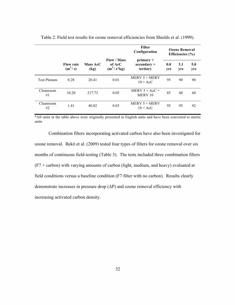
Table 2. Field test results for ozone removal efficiencies from Shields et al. (1999).

.......................................................................................................... 32  

Table 3. Summary of test results from Bekö et al. (2009). ................................... 33  

Table 4. Summary of test results from Bekö et al. (2008). ................................... 34  

Table 5. Health outcomes due to ozone exposure. ................................................ 42  

Table 6. Health benefits and filtration costs per building when using 2-inch activated

carbon filtration in a medium sized commercial office building. .... 54  

Table 7. Highest recorded VOC concentrations in five sample labs in the laboratory

building. ........................................................................................... 63  

Table 8. Parameters for six modeling scenarios of a typical single-family home in

Austin, TX. ....................................................................................... 77  

xii

List of Figures

Figure 1. Major components and connections of the dissertation. Roman numerals

represent the respective dissertation chapter of each major component.

The size of each chapter “sphere” represents the relative amount of time

spent on development, planning, and execution. ............................... 6  

Figure 2. Scanning electron microscope (SEM) images of activated carbon filter

material exposed to low ozone (L) and high ozone (R) for two hours.

The SEM images were captured by the author of this dissertation at the

University of Texas during operational testing of the carbon filters.27  

Figure 3. Illustration showing the interconnected sub models of systems model. 37  

Figure 4. U.S. climate zones and geographic location of 12 sample cities (USEIA,

2014). ............................................................................................... 38  

Figure 6. Comparison of avoided mortalities per year in Phoenix, AZ under three

different 8-hour ozone rollback strategies and with activated carbon

filtration in single-family homes. ..................................................... 50  

Figure 7. Comparison of annual ozone control costs per avoided mortality in Phoenix,

AZ comparing two 8-hour ozone rollback strategies and two strategies

utilizing activated carbon filtration in single-family homes. ........... 51  

Figure 8. Predicted benefit/cost ratios in commercial buildings when using

commercially available 4-inch activated carbon combination filters. The

circular symbols represent the median and range bars represent the 95%

confidence intervals of health functions used in the modeling analysis.

.......................................................................................................... 52  

xiii

Figure 9. Photos of teaching laboratory and air sampling equipment (L) and of active

sampling for VOCs using Tenax-TA® sorbent tubes (R). .............. 57  

Figure 10. Photo of air sampling equipment in the laboratory building air handling

unit (L) and the filter bank with carbon filters installed (R). ........... 60  

Figure 11. Indoor/outdoor ozone concentration ratios in five sample laboratories

building three testing conditions. ..................................................... 62  

Figure 12. Measured concentrations of VOCs before and after a typical bag filter (L)

and an activated carbon filter (R). .................................................... 64  

Figure 13. Schematic of the laboratory test system for activated carbon filters. .. 67  

Figure 14. Photo of the ozone generator (L) used in the test system to maintain a

steady-state inlet ozone concentration. Ozone was measured before and

after the carbon filter (R) using two ozone analyzers. ..................... 69  

Figure 15. Pressure drop versus flow rate measurements for two commercially

available activated carbon filters. Measurements were collected at the

beginning and the end of a two-hour test cycle. .............................. 70  

Figure 16. Single pass removal efficiency for ozone for two commercially available

activated carbon filters at a flow rate of 850 m3/hr (500 cfm) for two

hours. The error bars represent the standard error due to measurement

error. ................................................................................................. 72  

Figure 17. Single pass removal efficiency for ozone for two commercially available

activated carbon filters at a flowrate of 1,700 m3/hr (1,000 cfm) for two

hours. The error bars represent the standard error due to measurement

error. ................................................................................................. 73  

xiv

Figure 18. Single pass removal efficiency and cumulative mass of ozone removed for

the bulk activated carbon filter at a flow rate of 2,550 m3/hr (1,500 cfm)

for 48 hours. The error bars represent the standard error due to

measurement error. .......................................................................... 75  

Figure 19. Relationship between mass of ozone removed through the filter and the

single pass removal efficiency. As more ozone is removed through the

filter, the single pass removal efficiency declines. .......................... 76  

Figure 20. Predicted single pass removal efficiency of activated carbon filter during

the ozone season (1 May – 30 September 2014) in a typical single-

family home in Austin, TX using six different modeling scenarios. 78  

Figure 21. Average ozone exposure in a single-family home when applying activated

carbon filtration across six modeling scenarios. The data labels show

the percent reduction in ozone exposure when compared to a standard

particle filter with no ozone removal. .............................................. 79  

Figure 22. Predicted B/C ratios for six modeling scenarios and three cost

configurations. The solid circle represents the mean B/C ratio and the

error bars represent the 95% confidence intervals. .......................... 81  

1

1. INTRODUCTION

1.1. The Issue

Exposure to ozone and ozone reaction products is harmful to human health. Ozone

reacts with polyunsaturated fatty acids in fluids lining the lung with subsequent adverse

effects in the airway epithelium (Levy et al., 2001). Several researchers have shown a

link between exposure to ozone and premature mortality (Bell et al., 2005; Ito et al.,

2005; Jerrett et al., 2009; Levy et al., 2005; Smith et al., 2009; USEPA, 2006, and

references provided therein). Additionally, there have been several studies that associate

ozone exposure and increases in respiratory-related hospital admissions (e.g., Burnett et

al., 1999), minor restricted activity days (e.g., Ostro and Rothschild, 1989), and school

loss days (e.g., Chen et al., 2000). In a recent analysis, the USEPA estimates that 265 to

450 lives will be saved each year in the United States by reducing the eight-hour ozone

standard by 5 parts per billion (ppb), resulting in potential health benefits of U.S. $7.5B

to $15B (2011 dollars) per year (USEPA, 2014a).

Nearly 1/3 of Americans live and work in counties with ozone concentrations that

exceed the primary eight-hour average National Ambient Air Quality Standard (NAAQS)

for ozone (USEPA, 2014b). The NAAQS for ozone is meant to protect public health,

including the health of sensitive populations such as children, people with asthma, and

the elderly. Ozone concentrations are typically lower indoors than outdoors, largely due

to its reaction with materials in the building envelope, heating, ventilating, and air

2

conditioning (HVAC) system components, building contents, and occupied space (Chen

et al., 2012a; Fadeyi, 2014; Fadeyi et al., 2013; Fadeyi et al., 2009; Morrison et al., 1998;

Stephens et al., 2012; Wang and Morrison, 2010; Wang and Morrison, 2006; Weschler,

2000). Although ozone concentrations are typically lower indoors than outdoors,

Americans spend an average of nearly 90% of their time indoors (Klepeis et al., 2001).

This leads to the indoor environment being important with respect to total inhalation

exposure to ozone. For example, in a study involving 2,500 residences in seven cities,

indoor exposure accounted for 43% to 76% of total daily exposure to ozone, with a mean

of 60% (Weschler, 2006). As such, ozone control in buildings should be further

explored.

1.2. Dissertation Objectives

The overall goal of the dissertation is to evaluate the potential health benefits of

installing MERV-rated combination activated carbon filters in a diverse set of building

environments, including homes, office buildings, healthcare facilities, and schools. A

sample of cities from all climate zones in the U.S. will be used to predict the benefits and

costs of filtration in each climate zone. The health benefits will be evaluated using

disability-adjusted life-years (DALYs), which are a metric used to calculate disease

burden and include factors for years lost to premature mortality and years lost due to

disability per disease incidence. DALYs can also be used to estimate monetary health

costs and benefits due to pollutant exposure. Capital and operating costs of combined

3

activated-carbon filters will be investigated by reviewing the scientific literature,

manufacturer filter specifications, and local HVAC operational characteristics and utility

rates.

Primary research questions include the following:

1. Is there a net benefit (cost vs. health improvement) in utilizing in-duct activated

carbon filters in heating, ventilation, and air-conditioning (HVAC) systems in

commercial and residential buildings? If so, are there parameter thresholds above which

benefits are greater than costs?

2. Will in-duct activated carbon filters in HVAC systems significantly reduce indoor

chemical reactions in office and residential buildings? If so, how can this be quantified,

and by how much?

3. Can modeling results be verified by sampling in realistic indoor environments?

The four primary research objectives are identified below:

1. Complete a detailed literature review related to ozone removal by activated carbon,

indoor ozone chemistry, and health metrics related to ozone and its reaction products.

2. Develop a systems model that can predict the net benefit of utilizing in-duct activated

carbon filters in HVAC systems, and apply the model to realistic scenarios in different

climate zones in residential and commercial indoor environments.

3. Test the single-pass removal efficiency for ozone through common residential

activated carbon filters under realistic operating conditions.

4

4. Develop strategies and policies to use activated carbon filters during periods of high

outdoor ozone concentrations.

1.3. Scope of Research

This study focuses only on in-duct activated carbon filters for ozone control.

Other control media and portable air purifiers were not considered. A mass balance

model was used to estimate indoor ozone and ozone reaction products with and without

activated carbon filtration. The mass balance model was based on assumptions of steady-

state and well-mixed conditions. A limitation of the model was that it did not capture

peak ozone events, rather, average indoor ozone was estimated for the summer ozone

season in order to estimate exposure in accordance with the methodology applied by the

United States Environmental Protection Agency (USEPA). The model was applied

across multiple cities and climate zones in the United States using standardized building

sets and did not incorporate a distribution of the building stock in each city.

Health benefits were determined using disability-adjusted life-years (DALY),

which is a metric used by health organizations such as the World Health Organization

(WHO) to determine the burden of disease across a large population. One DALY is

equivalent to one lost year of healthy life and includes years of life lost to mortality and

morbidity applied across a population of 100,000 or more.

5

The focus of this study involves applications of a systems model as opposed to a

major field campaign. However, field-testing of residential activated carbon filters using

an HVAC test rig was completed as part of this dissertation.

1.4. Major Components and Connections of the Dissertation

An illustration showing the major components and connections of the dissertation

is presented in Figure 1. The literature review included a review of the published

literature on activated carbon filtration for ozone removal, indoor chemistry, the health

outcomes of ozone exposure, and energy and filtration control costs (link A). The

connection between the literature review and sub-models (link A) also included an

extensive review of currently available carbon filter products via phone interviews with

major filter manufacturers. The published and grey literature (including government

reports and data) was also reviewed for the model development (link B) and model

applications (link C). Additionally, a review of the published literature on activated

carbon filter performance, indoor chemistry, energy and control costs, and building

operation were completed for the field study and laboratory experiments (links D and E,

respectively). Finally, the systems model was used in connection with the field study and

laboratory experiments to estimate the economic costs and benefits of activated carbon

filtration in buildings using filter performance metrics measured in the field or laboratory

– these connections are displayed with the dashed arrows in Figure 1.

6

Figure 1. Major components and connections of the dissertation. Roman numerals represent the respective dissertation chapter of each major component. The size of each chapter “sphere” represents the relative amount of time spent on development, planning,

and execution.

As a result of this dissertation research, four journal papers are in review or

development. A list of the journal papers is presented below.

Journal papers in review or development: 1. Aldred, J., Darling, E., Siegel, J., Morrison, G., Corsi, R. (2015). Benefit-cost

analysis of commercially available activated carbon filters for indoor ozone removal in residential buildings. Submitted to Indoor Air.

2. Aldred, J., Darling, E., Siegel, J., Morrison, G., Corsi, R. (2015). Cost-benefit analysis of commercially available activated carbon filters for indoor ozone removal in buildings. Submitted to Science and Technology for the Built Environment.

7

3. Aldred J., Crain, N., Corsi, R., Novoselac, A. (2015). A benefit-cost analysis of reduced ventilation and carbon filtration in a university laboratory building. Submitted to Building and Environment.

4. Aldred, J., Crain, N., Corsi, R. (2015). Scale testing of commercially available

residential activated carbon filters for ozone control. In development.

Additionally, four conference papers were also presented based on this dissertation

research. A list of the conference papers is presented below.

Conference papers presented: 1. Aldred, J., Corsi, R.L., Novoselac, A. (2014). Benefit-Cost Analysis of Reduced

Ventilation in a University Laboratory Building. The 2014 University of Texas Sustainability Symposium.

2. Aldred, J., Corsi, R.L. (2014). A method to estimate the health benefits of activated carbon filtration. Indoor Air 2014: Proceedings of the 13th International Conference on Indoor Air and Climate, paper ID 711.

3. Aldred, J., Darling, E., Corsi, R.L. (2014). A benefit-cost analysis of activated carbon filtration in long-term healthcare facilities. Indoor Air 2014: Proceedings of the 13th International Conference on Indoor Air and Climate, paper ID 714.

4. Aldred, J., Jackson, M., Corsi, R.L. (2014). A method to estimate the health benefits of MERV-rated activated carbon filtration. Indoor Air 2014: Proceedings of the 13th International Conference on Indoor Air and Climate, paper ID 913.

8

1.5. Outline of Dissertation

Background information on indoor ozone chemistry, health effects, and economic

metrics is provided in Chapter 2. The background information includes a discussion of

the effects of ozone and ozone reaction products in buildings, the effectiveness of

activated carbon filters for indoor ozone removal, and the potential health effects of

exposure to ozone and ozone reaction products such as secondary organic aerosols,

formaldehyde, and acetaldehyde. The derivation of the integrated systems model and the

modeling results are described in detail in Chapter 3. Methods and results of the field

study experiments are discussed in Chapter 4. Methods and results of the filter testing

experiments are discussed in Chapter 5. Major research findings and related conclusions

are provided in Chapter 6. Appendices A and B provide in depth methodology of the

integrated systems model and the results of applications in single-family homes

(Appendix A) and commercial buildings (Appendix B). Appendix C provides a detailed

energy and benefit-cost analysis of carbon filtration in an operational university

laboratory. The programming code used for the Monte Carlo simulation in Appendix A

is presented in Appendix D.

9

2. LITERATURE REVIEW

Elements of this background section are taken from a draft report of ASHRAE Research

Project 1491, of which I am a co-author. I am the author of all text taken from the

ASHRAE report.

2.1. The Role of Activated Carbon Filters in Public Health

In the United States, average outdoor ozone concentrations decreased nationally

by 28% between 1980 and 2010, and by approximately a factor of two during the same

period in some air basins such as in the South Coast Air Quality Management District of

Southern California (SCAQMD, 2013; USEPA, 2012a). However, population trends

have involved a large migration from colder regions of the country to areas with a high

operational usage of central air conditioning and heating. In fact, during the past year

eight of the 15 fastest growing cities were in the state of Texas and 14 of the 15 fastest

growing cities were in the south and southeast regions of the U.S. (US Census Bureau,

2013). The combination of increasing migration to warmer climates, the potential for

higher atmospheric temperatures due to climate change, and higher urban emissions of

ozone precursors such as NOX and biogenic VOCs will ultimately result in higher ozone

concentrations in growing cities.

10

Climate change will lead to greater use of central HVAC systems in many

buildings, as well as a greater time of exposure to pollutants in indoor environments.

Activated carbon filters in HVAC systems have been shown to effectively remove ozone

from indoor environments during sustained operation and may lead to significant

reductions in mortality, hospital admissions, asthma exacerbations, and school and work

loss days when utilized in urban areas with high ambient ozone.

2.2. Impact on Health

Previous studies have suggested that building related symptoms are responsible

for a 3-4% reduction in office productivity, which is roughly equal to $50 billion (1997

$USD) in economic losses per year in the United States (Fisk and Rosenfeld, 1997).

Apte et al. (2008) used survey data and measurements from the Building Assessment

Survey and Evaluation (BASE) study on commercial buildings to compare concentrations

of indoor pollutants versus symptoms of building related sickness (BRS). All BRS

symptoms increased with increases in outdoor ozone concentration with the exception of

“dry skin.” Increased BRS symptom reporting was closely tied to late afternoons when

the ambient ozone concentrations were highest. Higher indoor concentrations of

formaldehyde, acetaldehyde, pentanal, hexanal, and nonanal were observed to correlate

with higher ambient ozone concentrations, suggesting that ozone chemistry is an

important source of these reaction products in office buildings. Due to the economic

11

impact of ozone-related BRS symptoms in commercial office buildings—and the less

well-known economic impact of ozone exposure in homes, schools, and other

buildings—further research is warranted on the health impacts caused by exposure to

these harmful pollutants.

2.2.1. HEALTH EFFECTS OF OZONE

Exposure to ambient ozone concentrations initiates cellular damage to lung tissue,

specifically through reactions with polyunsaturated fatty acids (PUFA), amino acid

proteins, and some low-molecular weight compounds such as glutathione, urate, vitamins

C and E, and free amino acids (USEPA, 2006; and references therein). Previous studies

have shown that ozone does not typically penetrate the epithelial lining fluid (ELF) in the

lungs (USEPA, 2006; and references therein). However, the ELF varies in thickness,

which may allow ozone to diffuse through the ELF and react with cellular membranes if

the ELF is less than 0.1 µm thick (USEPA, 2006; and references therein).

Ozone reactions with epithelial cells lead to the formation of by-products that are

similar or identical to those formed when ozone reacts with many indoor surfaces, e.g.,

reactive ozonides, aldehydes, and hydroperoxides (USEPA, 2006; and references

therein). The ozonation of PUFAs in rat lung tissue led to the formation of nonanal and

hexanal at 220 ppb of ozone (USEPA, 2006; and references therein). Ozone reactions

with PUFAs in human lung tissue leads to the formation of heptanal, hexanal, and

12

nonanal (USEPA, 2006; and references therein). Importantly, previous studies have

shown that rats are much more resilient to ozone exposure than humans (USEPA, 2006;

and references therein).

The human lung has natural controls that balance the bidirectional flow of fluids

and cells between the air and blood compartments. Exposure to ozone can upset this

balance, leading to lung inflammation and increased permeability of the ELF.

Inflammation is caused by ozone reactions with antioxidants and unsaturated lipids in the

ELF. The resulting chemical by-products and inflammation facilitate changes in cell

membranes and allow increased mass transport from lung air to the blood stream causing

increased permeability of the ELF. This in turn can lead to higher exposure to co-

pollutants (VOCs, particulate matter) passing through the ELF and into the blood stream

(USEPA, 2006; and references therein).

Increased ozone exposure has been linked to premature mortality. Several

research teams have analyzed data from the National Morbidity and Mortality Air

Pollution Study (NMMAPS), which evaluated air pollution and health data from the

largest 98 cities in the United States from 1987-2000. Bell et al. (2005) found a 0.87%

increase in premature mortality per 10 ppb increase in average daily ozone concentration,

and a 0.35% increase in mortality related to a 10 ppb increase in the one-hour daily

maximum ozone concentration within 0-2 days of the exposure incident. Ito et al. (2005)

predicted a 0.39% increase in premature mortality per 10 ppb increase in one-hour daily

maximum ozone and included seasonal factors, temperature, and use of air conditioning

13

in their meta-analysis. Ito et al. (2005) found an increased mortality risk due to ozone

during the summer periods when ambient ozone is highest. Bell et al. (2006) developed

an exposure-response curve from the NMMAPS dataset for ozone indicating a strong link

between ozone exposure and premature mortality, even at low concentrations. Thurston

and Ito (2001) evaluated time-dependent exposure to ozone and found that many previous

studies had underestimated ozone mortality. Jerrett et al. (2009) utilized mortality data

from the American Cancer Society Cancer Prevention Study (448,850 participants,

188,777 deaths after 18-year follow-up) and USEPA monitoring data for ambient ozone

and PM2.5 for 96 US metropolitan areas to develop an exposure-response curve for ozone

concentration and mortality. They observed that for every 10 ppb increase in one-hour

daily maximum ozone, the risk of death from respiratory causes increased 2.9% in single-

pollutant models (ozone only).

Additional researchers have studied the association between increased ozone

concentrations and mortality, including same day versus lagged effects. Levy et al.

(2005) projected a 0.41% increase in mortality per 10 ppb increase in one-hour daily

maximum ozone concentration by evaluating 48 city-specific research studies on ozone-

related mortality. Their study revealed that same day effects were larger than lagged

effects per ozone incident. Parodi et al. (2005) observed that the variance in the ozone-

mortality relationship depends on the lag time after the ozone incident (0 to 2 days) with

the highest association with mortality one day after the ozone incident. Zhang et al.

(2006) observed an increase of 0.45% in all-cause mortality per 5 ppb increase in eight-

14

hour ozone after a one-day lag for all ages and seasons in Shanghai, China. They found

an increase of 0.53% for cardiovascular mortality and 0.35% for respiratory related

mortality per 5 ppb increase in eight-hour ozone concentration for all seasons.

Seasonal effects of ozone exposure on mortality have also been studied. Kim et

al. (2004) determined an increase in mortality risk (Relative Risk ratio = RR = 1.0336)

for all seasons due to ozone exposure by assuming a threshold concentration of ozone of

27.61 ppb. Their study utilized four years of ambient ozone and mortality data from

Seoul, South Korea. Gryparis et al. (2004) evaluated mortality and ozone data from 23

European cities and found an increase of 0.33% in mortality per 5 ppb increase in one-

hour daily maximum ozone concentration during the summer. They also observed an

increase in all-cause mortality of 0.34% for a 5 ppb increase in two-day average

maximum eight-hour ozone concentration. Parodi et al. (2005) observed an increase in

mortality for all ages and all seasons varying from 1.4-2.4% per 25 ppb increase in one-

hour daily maximum ozone concentration in Genoa, Italy.

An association appears to exist between window air conditioning (AC) units and

increased ozone related mortality, perhaps due to higher air exchange rates in older

homes with these units (Smith et al., 2009). Smith et al. (2009) completed a detailed

meta-analysis of the NMMAPs data including daily temperature, dew point, PM10 and

PM2.5, hourly and daily values for ambient ozone concentrations for 79 of the 98

NMMAPs cities. They also considered window air conditioning and central air

15

conditioning as two different types of air conditioning rather than merging both types of

AC as had been done in previous studies, e.g., Bell and Dominici (2008).

Ozone exposure has also been linked to morbidity, especially respiratory related

illnesses. Mudway and Kelly (2004) developed a linear relationship between ozone

exposure and lung inflammation and airway responses. Brown et al. (2008) and Adams

et al. (2006) linked ozone exposure to decreased pulmonary function and gas exchange in

the respiratory system. McDonnell et al. (1999) observed an increased risk in asthma

diagnoses for males (RR = 2.09, 95% CI = 1.03 to 4.16) for a 27 ppb increase in ambient

ozone concentration. Glad et al. (2012) observed a 2.5% increase in asthma related

emergency department (ED) visits per 10 ppb increase in one-hour maximum ozone two

days following the ozone incident. They observed that the strongest association for ER

visits was four days after the ozone incident. Anderson et al. (1997) observed that an

increase in eight-hour ozone concentration of 25 ppb led to an increase of 4.0% in

hospital admissions for chronic obstructive pulmonary disease (COPD) in six European

cities (lagged 1-3 days).

Increases in ozone concentration and exposure are known to have adverse effects

on children. McConnell et al. (2002) linked ozone exposure to increased asthma

diagnoses among children in a southern California cohort of 3,535 children, especially

among children who played multiple sports outdoors. Tager et al. (2005) related lifetime

ozone exposure to decreased measures of airway function in a cohort of California

adolescents. Yang et al. (2003) associated increased ozone exposure of approximately 10

16

ppb with increased visits to hospital emergency rooms (ER) for both children (RR = 1.22,

95% CI = 1.15 to 1.30) and the elderly (RR = 1.13, 95% CI = 1.09 to 1.18) in a

Vancouver, British Columbia cohort. Increases in ozone exposure have also been linked

to minor restricted activity days (MRADs) and increased school absences (Hubbell et al.,

2005).

Ozone has been found to be a surrogate for increased personal exposure to PM2.5,

especially during the summer (Sarnat et al., 2001 and 2005). Increased PM2.5 exposure

has its own inherent health risks and has been linked to increased mortality due to lung

cancer and cardiovascular disease (Pope et al., 2011). The correlation between ozone and

increased PM2.5 can be explained in-part by the formation of outdoor secondary organic

aerosols. Secondary organic aerosols can also be rapidly formed indoors following

reactions between ozone and terpenoids from scenting agents, cleaners, and other

sources.

The studies described above involved health impacts associated with outdoor

ozone concentration measurements. But the average American spends over 70 years of

their lifetime in indoor environments (based on Klepeis et al., 2001), where

concentrations of ozone increase to some extent when outdoor ozone concentrations

increase. And while indoor ozone concentrations are generally much lower than outdoor

concentrations, nearly half of personal exposure to ozone of outdoor origin takes place

indoors (Weschler, 2006 and references therein). Furthermore, indoor environments

facilitate chemical reactions between ozone and indoor materials, as well as ozone and a

17

wide range of reactive terpenoids that exist in indoor air at higher concentrations than in

outdoor air (Hodgson and Levin, 2003; Weschler, 2000). The by-products of these

reactions often have higher concentrations indoors than outdoors and may be harmful to

human health (Weschler, 2006). Therefore, the indoor and outdoor environments are

undeniably linked, and efforts to remove ozone of outdoor origin from buildings should

dramatically reduce population exposures to ozone and its reaction products.

Chen et al. (2012a) recently completed seminal work that links short-term

mortality with indoor ozone exposure. Human activity patterns were referenced from the

National Human Activity Pattern Survey (NHAPS; see Klepeis et al., 2001) and ozone

mortality data from Bell et al. (2004) were used for 24-hour ozone concentration. Ozone

mortality data for one-hour and eight-hour ozone concentrations were taken from Smith

et al. (2009). A mass balance model was developed and included residential air exchange

rates from Persily et al. (2010) and an assumed ozone decay rate due to reactions with

surfaces of 3/hr. Chen et al. (2012a) also accounted for changes in air exchange rate by

opening windows, an action which leads to higher concentrations of indoor ozone and a

potential for higher mortality rates. The mass balance model included the fraction of

homes per city with air conditioning, and the fraction of time that air conditioning was

operating per city. Chen et al. (2012a) developed several linear regressions between air

exchange rate and ozone mortality, as well as ozone exposure coefficient and ozone

mortality for 18 of the NMMAPS cities. The strongest linear association was between

18

ozone exposure coefficient and mortality for one-hour daily maximum ozone for 18

cities.

Several researchers have evaluated the health benefits of attaining lower ambient

ozone standards nationwide using the willingness-to-pay method. Hubbell et al. (2005)

generated estimates of average ozone concentrations for every county in the United States

using spatial interpolation. Their study incorporated a Monte Carlo analysis to link

average ozone concentration to premature mortality and increased asthma and respiratory

health incidents. Results of their study indicate that achieving an 80 ppb ambient ozone

limit nationwide would prevent 840 mortalities nationwide and result in $6.6B (2012

US$) in health benefits due to decreased mortality and hospital admissions. In a similar

study, Berman et al. (2012) estimated that more than 1,000 premature mortalities could

be prevented each year in the United States by attaining the 75 ppb ambient ozone

standard nationwide.

2.2.2. HEALTH EFFECTS OF GASEOUS REACTION PRODUCTS

Ozone engages in both heterogeneous and homogeneous reactions that lead to the

formation of a broad spectrum of reaction products. Reaction products include hydroxyl

radicals and other radical species, formaldehyde, acetaldehyde, C3 to C10 saturated and

unsaturated aldehydes, light monoketones, dicarbonyls, mono- and dicarboxylic acids,

19

and secondary organic aerosols (SOA) (e.g., Anderson et al., 2012a and 2012b; Sarwar

and Corsi, 2007; Weschler, 2006; Sarwar et al., 2003).

Ozone reaction products have been linked to increases in airway irritation and

decreases in respiratory function (Anderson et al. 2007). Wolkoff et al. (1999 and 2000)

found that respiratory rates in mice decreased by up to 30% and 50% when exposed to

mixtures of ozone and α-pinene or isoprene, respectively. Wolkoff et al. (2008) observed

a greater than 30% reduction of mean respiratory frequency in mice exposed to d-

limonene/ozone mixtures for 30 minutes. They noted that the secondary endo-ozonide of

limonene is similar to ozonides associated with lung surfactants, compounds potentially

causative of pulmonary effects. But while sensory irritation and air flow limitations in

mice are clearly evident during exposure to d-limonene/ozone mixtures, repeated

exposures over a 10-day period did not lead to inflammation of the respiratory tract

(Wolkoff et al., 2012).

Rohr et al. (2003a) studied the effects of ozone/isoprene reaction products on six

murine strains of mice. Sensory irritation was observed in the form of reduced

respiratory frequency and peak expiratory volume/tidal volume. The products that

caused these effects, e.g., specific gaseous products or ultrafine particles, were not

studied. Variations in results between murine strains may indicate genetic variability in

human populations as well.

20

Anderson et al. (2012) found that exposure to 4-oxopentanal causes increased

allergic and irritancy responses, both dermal and pulmonary. 4-Oxopentanal is a

dicarbonyl that is a common reaction product between ozone and squalene, a component

of human skin oil (Wisthaler and Weschler, 2010).

While researchers have in recent years increased the knowledge base related to

ozone reaction products in buildings, the toxicological and epidemiological data related

to nearly all of those products is insufficient to quantify health effects in humans.

However, in a comprehensive review of the indoor air and health literature, Logue et al.

(2011) predicted that exposure to formaldehyde and acetaldehyde are important health

hazards in residential buildings. The remainder of this section focuses on these two

pollutants, each of which has a contribution associated with indoor ozone chemistry.

Formaldehyde is ubiquitous in both residential and non-residential buildings.

Nearly 70% of formaldehyde exposure occurs indoors (Loh et al., 2007). Pressed wood

products such as particleboard and medium density fiberboard are major indoor sources.

But formaldehyde is also an important product associated with ozone reactions with some

unsaturated organic compounds found in indoor air and on materials (Singer et al., 2006;

Weschler, 2006; Weschler and Shields, 1996).

Formaldehyde is classified as a hazardous air pollutant (HAP) under the Clean Air

Act. It is widespread in residential and commercial buildings and is an acute eye and

upper respiratory tract irritant. The California chronic Reference Exposure Level (REL)

21

for formaldehyde is 9 µg/m3, and is based on positive associations, especially among

children with diagnosed asthma, between prolonged exposures to formaldehyde and

allergic sensitization, respiratory symptoms (e.g. coughing, wheezing), or decrements in

lung function (OEHHA, 2008). Several researchers have observed median formaldehyde

concentrations in U.S. homes representative of the larger housing stock that are between

1.9 and 2.4 times greater than the California REL (Gordon et al., 1999; Sax et al., 2006;

Weisel et al., 2005). Logue et al. (2012) predicted that formaldehyde accounted for the

second highest contribution to DALYs behind acrolein amongst hazardous air pollutants

found in U.S. homes.

There is some disagreement as to the importance of formaldehyde on non-cancer

effects at typical indoor concentrations. Wolkoff and Nielsen (2010) provided a detailed

review of non-cancer effects of formaldehyde. They concluded that there is no

experimental or epidemiological evidence amongst either children or adults that indicate

lung effects for formaldehyde exposures less than 1 mg/m3 (≈ 800 ppb at typical indoor

temperatures). Others have noted that there is inconsistent evidence that formaldehyde

causes asthma or other chronic respiratory diseases (Checkoway et al., 2012, and

references provided therein).

Formaldehyde is classified as a probable human carcinogen (Group B1) by the

U.S. Environmental Protection Agency and carcinogenic to humans (Group 1) by the

International Agency for Research on Cancer (IARC). Tests on rats and mice have

shown an increase in nasal squamous cell carcinomas due to long-term exposure to

22

formaldehyde (USEPA, 2014c). Zhang et al. (2010) found that increased formaldehyde

exposure (2.14 ppm vs. 0.026 ppm for control) in factory workers led to decreased white

blood cell production; white blood cell counts for workers exposed to higher

formaldehyde concentrations were 13% less than the counts for the control group. They

also observed that some exposed workers experienced the loss of chromosome 7 in

molecular DNA, which is a preliminary indicator of cancer. Myeloid leukemia has been

shown to have a higher incidence among professions commonly exposed to

formaldehyde and formalin-based fixatives such as anatomists, embalmers, and garment

workers (Zhang et al. 2010). Several authors have noted the potentially high contribution

of formaldehyde to cumulative cancer risk from exposure to air contaminants that are

typically found in residences (Hun et al., 2010; Loh et al., 2007; Sax et al., 2006).

However, the carcinogenic effects of formaldehyde also remain a topic of debate.

Arts et al. (2006) point out that formaldehyde is not carcinogenic in rats at a sustained

exposure of less than 6 ppm. Checkoway et al. (2012) concluded that there is currently

no consistent or strong epidemiologic evidence that formaldehyde is causally related to

any lymphohematopoietic malignancies. Further, Wolkoff and Nielsen (2010) conclude

that at concentrations less than 100 ppb formaldehyde will not lead to cancer risks in the

general population.

Amongst other sources, acetaldehyde is formed via reactions between ozone and

unsaturated organic compounds (Lee et al., 2006a and 2006b). It is classified as a

probable human carcinogen (Group B2) by the USEPA (2012). Increased tumor

23

formation in rats and chromosomal damage to mammal cellular cultures (USEPA, 2014c)

have been attributed to elevated exposures to acetaldehyde. It is a common pollutant

associated with environmental tobacco smoke (Nazaroff and Singer, 2004) and

approximately 15% of acetaldehyde exposure occurs in indoor environments (Loh et al.,

2007). Loh et al. (2007) also found that acetaldehyde has the sixth highest cancer risk

among common HAPs found indoors. Logue et al. (2012) predicted that indoor

acetaldehyde exposure is responsible for the fourth highest DALYs among gaseous

indoor air pollutants, behind only acrolein, formaldehyde, and ozone.

There are a large number of additional reaction products that form as a result of

indoor ozone chemistry. Carbonyls formed as a result of indoor ozone chemistry are

irritants; heavier carbonyls tend to have lower irritation thresholds (Cometto-Muñiz and

Abraham, 1998). Suspect irritants include pinonaldehyde, a stable di-aldehyde that is

formed at high yield in the ozone/α-pinene reaction. Anderson et al. (2007 and 2010)

found, through the application of quantitative structure activity relationships, animal

models and in-vitro exposure systems, that most dicarbonyl compounds are irritants and

sensitizers. Organic acids tend to be roughly 10 times as irritating as their analogous

aldehydes; a number of acids (e.g., formic acid), di-acids (e.g., pinic acid) and

acid/aldehyde compounds (e.g., norpinonic acid) are also formed from indoor ozone

chemistry. Intermediate products, such as ozonides, and hydroperoxy radicals are highly

reactive and may also interact strongly with mucous membranes. Several researchers

have noted that products of reactions between ozone and terpenes are strong airway

24

irritants (Wolkoff et al., 1999 and 2000; Weschler et al., 2006, and references presented

therein). As evidence of eye irritation, the limonene–ozone reaction mixture caused eye-

blink frequency to increase in human subjects (Klenø and Wolkoff, 2004). These

findings are important and worthy of continued attention. However, we were unable to

find data or supporting models that will allow determination of quantifiable health

impacts, e.g., mortality or DALYs, from such products on human populations.

2.2.3. HEALTH EFFECTS OF SECONDARY ORGANIC AEROSOLS

Secondary organic aerosols are a well-documented and major reaction product

associated with indoor ozone chemistry. However, sparse toxicological and

epidemiological data preclude explicit estimates of the health effects of human exposure

SOA formed indoors.

Wolkoff et al. (2008) used a mouse bioassay and indicated significant sensory

effects upon exposure to mixtures of d-limonene and ozone. However, gas-denuded

results showed no effect, leading the authors to conclude that ultrafine particles formed

from ozone/limonene chemistry are not causative of sensory effects in the airways.

Some fraction of outdoor PM2.5 is SOA, and the quantifiable health effects of

outdoor PM2.5 might be extendable to indoor SOA, albeit with substantial caveats and

uncertainty. Logue et al. (2012) found that in 80% of simulated indoor samples in their

study, PM2.5 contributed to the highest number of DALYs among indoor air pollutants.

25

Evidence of PM2.5 as a cardiovascular and respiratory health hazard has been

validated extensively in the literature. In a 26-year study with a cohort of 188,699 non-

smokers, Turner et al. (2011) observed a 15-27% increased risk of lung cancer mortality

for each 10 µg/m3 increase in ambient PM2.5 concentration. Pope et al. (2011) evaluated

the dataset from the 1.2-million-member American Cancer Society cohort and found that

a 10 µg/m3 increase in ambient PM2.5 concentration led to an adjusted relative risk of 1.14

for lung cancer, 1.18 for ischemic heart disease, 1.12 for cardiovascular disease, and 1.09

for cardiopulmonary disease. They also determined that the PM2.5 exposure-response

curve is nearly linear for lung cancer and non-linear (response becomes asymptotic with

higher exposure) for cardiovascular disease (Pope et al., 2011). Jerrett et al. (2009)

observed that PM2.5 exposure and related impacts was dominant in the two-pollutant

model (ozone and PM2.5) when compared to cardiopulmonary, cardiovascular, and

ischemic heart disease related mortality, i.e., ozone had far less impact.

Finally, it is important to note that a large fraction of indoor SOA exists initially

as ultrafine particles. Epidemiological studies on ultrafine particle exposure are not as

extensive as PM2.5. However, ultrafine particles can be transported through the blood

stream and into vital organs such as the liver and brain, and have been noted to cause

inflammatory responses in the respiratory system (Oberdorster et al., 2010). Hoek et al.

(2010) developed mortality relative risk estimates for ultrafine particles and published the

only paper found in the literature to predict a health outcome from ultrafine particles.

26

2.3. Ozone Removal by Activated Carbon

Activated carbon is formed by dehydration and slow heating of organic materials

(e.g., coal, wood, coconut shells) in an anaerobic environment. The finished product has

a large surface area to mass ratio (up to 1,000 m2 per 1 g), which allows gaseous

pollutants to adsorb to and/or react with sites on the AcC. Ozone is removed by

chemisorption via two possible pathways: (1) reaction within a solid carbon matrix with

C=C bonds to form epoxides, and (2) reactions with C=C bonds to form ozonides

(Dusenbury & Cannon, 1996). At ambient ozone concentrations these reactions lead to

the production of small amounts of carbon monoxide, carbon dioxide, water, and some

surface functional groups (Dusenbury and Cannon, 1996).

Over time, the effectiveness of ozone removal by activated carbon is reduced due

to consumption of reaction sites by ozone, physical decomposition of AcC by reactions

with ozone, and the formation of acidic surface oxidation complexes (Álvarez et al.,

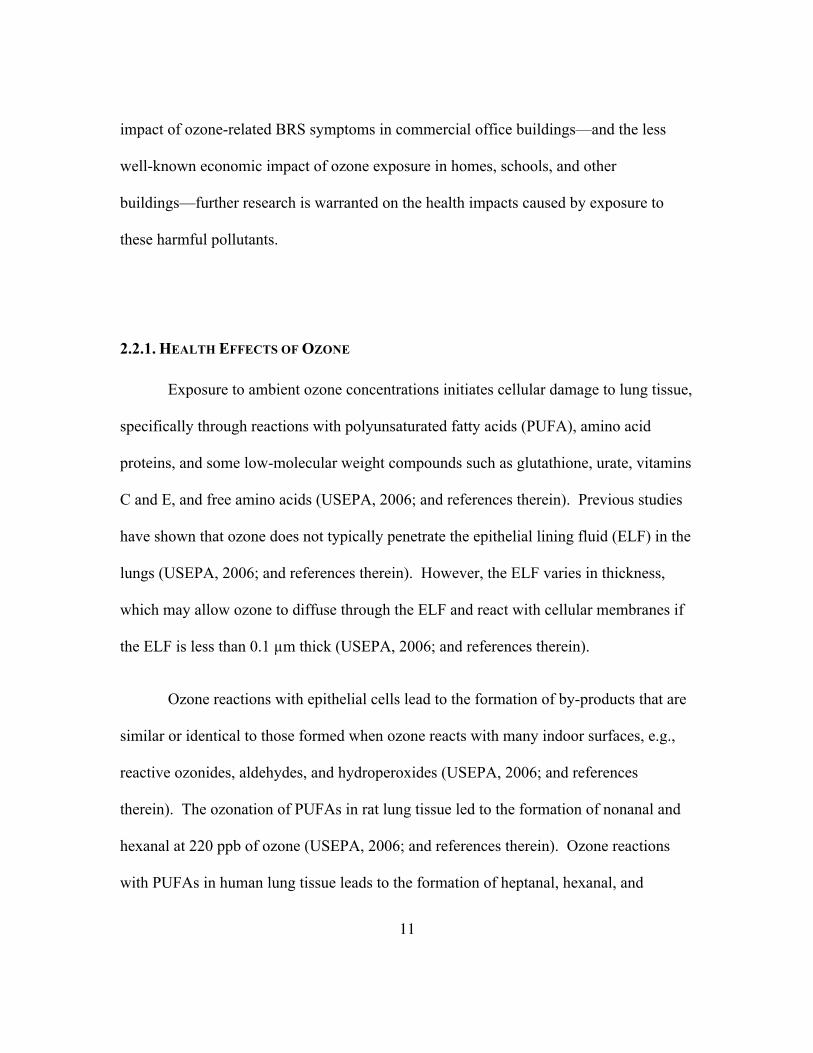
2008; Lee and Davidson, 1999; Muller and Jin, 2009). Figure 2 shows scanning electron

microscope images of activated carbon used in residential activated carbon filters

exposed to low and higher concentrations of ozone for 2 hours. The images clearly show

pitting and overall morphological changes of the activated carbon at elevated exposure to

ozone.

27

Figure 2. Scanning electron microscope (SEM) images of activated carbon filter material exposed to low ozone (L) and high ozone (R) for two hours. The SEM images were

captured by the author of this dissertation at the University of Texas during operational testing of the carbon filters.

Experimental studies have indicated average capacities of 0.20-0.34 grams of

ozone per gram of activated carbon at 50% ozone removal efficiency for beds of granular

activated carbon and non-woven pleat filters loaded with activated carbon (Gundel et al.,

2002; Shields et al., 1999; and references provided therein). As such, periodic

replacement of activated carbon filters in order to maintain a design range of ozone

removal efficiencies is required.

The presence of elevated relative humidity (RH) can reduce the ozone removal

efficiency of AcC, presumably by blockage of reaction sites by water molecules (Álvarez

et al., 2008). Others have tested volatile organic compound (VOC) loaded activated

28

carbon filters and showed reduced ozone removal capacity depending on the type of

adsorbed VOC and the extent of the loading (Metts and Batterman, 2006). On-filter

heterogeneous reactions with d-limonene and resulting reaction products have also been

observed (Metts, 2007). However, the VOC loadings in these studies were much higher

than typically observed in most office buildings or homes.

Several research teams have explored the enhancement of activated carbon for

improved removal of ozone and VOCs (Heisig et al., 1997; Kelly and Kincaid, 1993; Lin

et al., 2008; Takeuchi and Itoh, 1993). Such enhancements have generally involved the

introduction of metal catalysts such as gold or manganese by impregnation into or vapour

deposition onto activated carbon. For example, Lin et al. (2008) showed that activated

carbon fibers amended with gold or manganese by vapour deposition can significantly

enhance ozone removal efficiency relative to activated carbon fibers that were not

amended. However, experiments were completed at ozone concentrations 3 to 4 orders

of magnitude higher than those typical of ambient air.

Lee and Davidson (1999) completed testing on ten different commercially

available AcC filters used to remove ozone. Each filter was tested at an inlet ozone

concentration of 120 ppb at 50% relative humidity. However, tests were completed for

only several hours. In addition to testing for ozone removal, each filter was also

evaluated for pressure drop at a face velocity of 2.54 m/s. Test air was pre-filtered with

high efficiency particulate air (HEPA) filters, thus precluding particle deposition on the

activated carbon filters. Results are summarized in Table 1. The ozone removal

29

efficiency for most filters was initially high (> 94%) and then decreased slightly within

the first thirty minutes of operation. The authors reported that there was no regeneration

of the filters after removing them from ozone for up to 12 hours. The activated carbon

fiber filter (filter #9 in Table 2.3.1) exhibited high ozone removal efficiency (98.3%)

initially, but efficiency quickly decreased to less than 30% after 200 minutes of

continuous exposure to ozone. Lee and Davidson (1999) theorized that this was caused

by degradation of the micropore structure of the filter following oxidation by ozone. The

activated carbon fiber filter also performed poorly with increases in relative humidity,

likely due to water molecules blocking reaction sites on the surface of the activated

carbon within the filter as described by others (Álvarez et al., 2008; Shields et al., 1999).

Interestingly, the other activated carbon filters showed no changes in performance when

RH was varied between 20% and 80%.

Shair (1981) appears to have been the first to complete field-testing of ozone

removal using activated carbon. A make-up air filtration system was installed on a

building in Pasadena, California, using an activated carbon filter bank consisting of nine

61 cm x 61 cm x 76 cm (24” x 24” x 30”) AcC filters. A particle pre-filter that roughly

corresponded to a contemporary MERV 7 filter was used. Ozone control was only used

when outdoor concentrations of ozone exceeded 80 parts per billion (ppb). Testing was

completed for three years, during which time the make-up air filtration unit ran

approximately 1,200 hours per year at an average flow rate of 6.6 m3/s (14,000 ft3/min).

After 1,200 hours of operation the AcC filters removed 95% (+/- 5%) of outdoor ozone

30

and the efficiency slowly declined to 80% at 2,400 hours of operation. Ozone removal

efficiency declined to 50% at 3,600 hours of operation. Pressure drop across the entire

assembly (pre-filter, carbon filter, air monitor, diffuser, dampener, and final diffuser) was

0.29 kPa, which was accommodated by a 3.7 kW (5 hp) fan motor installed in the HVAC

system.

Table 1. Summary of test results from Lee and Davidson (1999).

Test Filter ΔP (kPa)

AcC Area/Mass

(m2 / g) O3 removal (%) (t = 0 - 30 min)

1 3M Model E -- GAC Mesh (w/adhesive) 0.340 +/- 0.010 1,225 94.7 - 94.1%

2 3M Model R -- GAC Mesh 0.580 +/- 0.010 1,225 97.5 - 96.0%

3 Farr Company Farr Sorb PS -- Carbon spheres in foam 0.129 +/- 0.001 5,000

69.7 - 53.0%

4 AAF International Carbon Web -- GAC Mesh (w/adhesive) 0.151 +/- 0.001 1,226 52.1 - 38.0%

5 Hoechst Celanese AQF-2750 -- GAC Mesh in pleated sheets 1.070 +/- 0.010 * 97.3 - 94.7%

6 Hoechst Celanese CPS-9C500C -- GAC Mesh (pleated sheets) 3.700 +/- 0.010 * 98.0 - 93.9%

7 Columbus Industries Polysorb IO5200 -- impregnated carbon 0.165 +/- 0.001 * 94.7 - 94.1%

8 Columbus Industries SupraSorb -- impregnated carbon 0.053 +/- 0.001 * 94.7 - 94.1%

9 PICA USA ACTITEX FC-1200 Activated Carbon Fiber Filter 2.200 +/- 0.100 1,200 94.7 - 94.1%

10 Carus Chemical Company Carulite Ozone Catalyst 0.630 +/- 0.010 * 94.7 – 94.1%

All filters were 1.328 cm in diameter by 1.27 cm thick; tested at 120 ppb O3, 50% RH, 2.54 m/s face velocity

* = not available (hybrid)

31

Shields et al. (1999) demonstrated that relatively large beds packed with granular

activated carbon (GAC) (20 to > 200 kg) can efficiently remove ozone in an actual field

test conducted between five to eight years of continuous service. Filters were tested in

three different configurations over a period of eight years in two cleanrooms and a test

plenum (Table 2). Inlet ozone concentrations ranged from 10 to 80 ppb. The test plenum

had two pre-filters with an average flow rate of 0.28 m3/s (600 ft3/min). The AcC filter in

the test plenum had a single-pass ozone removal efficiency of 90% after five years of

continuous service. The first test classroom had a 30% (~MERV 5) pre-filter, followed

by the AcC filter, and then an 85% (~MERV 10) post-filter in series with a flow rate of

10.2 m3/s (21,700 ft3/min). The charcoal filter in the first test classroom had an ozone

removal efficiency of 60% after eight years of continuous service. The configuration of

the second test classroom included 30% and 85% pre-filters upstream of cooling coils,

followed by the AcC filter. The air flow rate through the system was 1.4 m3/s (3,000

ft3/min). The ozone removal efficiency was 70% after seven years of continuous service.

Pressure drop across the filter assemblies was not provided by the authors. Shields et al.

(1999) hypothesized that the lower ozone removal efficiencies in classroom #1 of their

study were due to the lack of a pre-filter, especially since classroom #1 received 100%

outdoor air. The absence of a pre-filter likely led to particle deposition onto GAC

surfaces, thus shielding reaction sites from ozone. Furthermore, the lower air flow rate

per mass of AcC through the filter in classroom #2 (20% lower than classroom #1)

permitted a higher residence time for ozone in the filter and thus more time for ozone to

react with filter surfaces.

32

Table 2. Field test results for ozone removal efficiencies from Shields et al. (1999).

Flow rate (m3 / s)

Mass AcC (kg)

Flow / Mass of AcC

(m3 / s*kg)

Filter Configuration

primary + secondary +

tertiary

Ozone Removal Efficiencies (%)

0.0 yrs

3.1 yrs

5.0 yrs

Test Plenum 0.28 20.41 0.01 MERV 5 + MERV 10 + AcC 95 90 90

Cleanroom #1 10.20 217.73 0.05 MERV 5 + AcC +

MERV 10 85 60 60

Cleanroom #2 1.41 40.82 0.03 MERV 5 + MERV

10 + AcC 95 95 92

*All units in the table above were originally presented in English units and have been converted to metric units

Combination filters incorporating activated carbon have also been investigated for

ozone removal. Bekö et al. (2009) tested four types of filters for ozone removal over six

months of continuous field-testing (Table 3). The tests included three combination filters

(F7 + carbon) with varying amounts of carbon (light, medium, and heavy) evaluated at

field conditions versus a baseline condition (F7 filter with no carbon). Results clearly

demonstrate increases in pressure drop (ΔP) and ozone removal efficiency with

increasing activated carbon density.

33

Table 3. Summary of test results from Bekö et al. (2009).

Filter

ΔP (kPa)

0 mos.

ΔP (kPa)

3 mos.

ΔP (kPa)

6 mos.

O3 Removal (%)

6 mos. Average

F7 (MERV 13) Fiberglass

(No Carbon)

0.074 +/-

0.001

0.077 +/-

0.001

0.078 +/-

0.001 10%

F7 (MERV 13) + Light

Carbon (100 g/m2)

0.089 +/-

0.001

0.088 +/-

0.001

0.095 +/-

0.001 17%

F7 (MERV 13) + Medium

Carbon (200 g/m2)

0.103 +/-

0.001

0.095 +/-

0.001

0.102 +/-

0.001 28%

F7 (MERV 13) + Heavy

Carbon (400 g/m2)

0.130 +/-

0.004

0.132 +/-

0.001

0.144 +/-

0.001 59%

All tested filter dimensions were 0.6m x 0.6m x 0.3m deep; tested at 21°C, 35% RH, 2.0 m/s face velocity.

Bekö et al. (2008) also tested several configurations of combination filters under

field conditions (varying temperature, relative humidity, and ozone concentration) over a

five-month test period. Although ozone removal efficiencies were not reported, pressure

drop data related to various filter configurations were measured. Data are summarized in

Table 4.

34

Table 4. Summary of test results from Bekö et al. (2008).

First Filter

ΔP (kPa)

Second Filter

ΔP (kPa)

Third Filter

ΔP (kPa)

0 mos. 5 mos.

0 mos. 5 mos.

0 mos. 5 mos.

85% Filter (EU7/F7/ MERV 13

Equivalent)

0.052 +/- 0.001

0.065 +/- 0.004

V-Cell Cartridge (1.7

kg AcC)

0.049 +/- 0.001

0.057 +/- 0.001

None --- ---

AcC V-Cell Cartridge

(1.7 kg AcC)

0.052 +/- 0.001

0.052 +/- 0.002

85% Bag Filter

(EU7/F7/ MERV 13

Equivalent)

0.075 +/- 0.001

0.086 +/- 0.001

V-Cell Cartridge (1.7 kg AcC)

0.048 +/- 0.001

0.050 +/- 0.001

EU7/F7/MERV 13 Combo

Bag Filter (1.3 kg AcC)

0.110 +/- 0.003

0.102 +/- 0.003

None --- --- None ---

---

EU7/F7/MERV 13 Combo Cartridge

Filter (1.3 kg AcC)

0.123 +/- 0.002

0.151 +/- 0.004

None --- --- None ---

---

All filters tested at 1,300 m3/hr flow rate, 2.0 m/s face velocity.

Fisk et al. (2009) studied the performance of MERV 8 hybrid (combination)

filters placed in an office building in Sacramento, California, for an 81-day period from

late summer to mid fall. Each filter had dimensions of 61 cm x 61 cm x 5.1 cm (24” x

24” x 2”), contained 300 g of AcC per 0.09 m2 of filter face, and cost $29/filter. The

filters were used as pre-filters in two filter banks of the building. A third filter bank that

included a similar pre-filter without activated carbon was also studied for comparison.

For most of the 81-day test period the filters were challenged with primarily re-circulated

air with low concentrations of ozone that made it difficult to accurately quantify ozone

removal efficiencies. Toward the end of the study analyses were completed with 100%

35

outdoor air supply. During this two-week period the filters containing AcC removed

60% and 70% of ozone. Importantly, the filter that did not contain AcC removed no

ozone. It is not clear whether ozone removal efficiency would have been lower had the

AcC filters been challenged with a greater fraction of outdoor air throughout most of the

test period. However, the results presented by Fisk et al. (2009) are encouraging given

that they represent an actual application for a nearly three month operating period in an

office building with relatively low-cost AcC filters.

Muller and Jin (2009) tested a combination filter under field conditions over a

three-month period in Atlanta, Georgia. A MERV 6 filter in a commercial building was

replaced with a 10-cm (4-in) thick combination filter with embedded activated carbon.

The filter was evaluated for ozone and VOC removal over the test period and

demonstrated a continuous ozone removal efficiency of greater than 90% during peak

ozone season in Atlanta (May-September). The average ozone concentration over the

test period was 39 ppb with a peak concentration of 145 ppb. Information on temperature,

relative humidity and pressure drop during the field-testing program was not provided.

The life cycle costs of in-duct AcC filtration have not been extensively

documented in the published literature. Shair (1981) described the capital and operating

costs of retrofitting an existing HVAC system with AcC filters to remove ozone. The

capital costs for installing a system in a commercial-type building was $12,000 in 1975,

with an annualized maintenance and operation cost of $600 per year.

36

More recently, Stanley et al. (2011) completed a life-cycle valuation of several

AcC filters used for ozone removal in a hypothetical hospital air handler with an air flow

rate of 3,398 m3/hr (2,000 ft3/min). Their analysis included the following filter types:

carbon-loaded non-woven pleat, cassette with internal V-bank, granular activated carbon

in honeycomb tray, granular activated carbon in V-bank formation, and adsorbent

extruded into an open honeycomb matrix. A MERV 8 pre-filter and MERV 14 final filter

was assumed. Cost analyses were completed based on filter replacement (including labor

costs), energy consumption, and additional hardware requirements. Annualized costs

were determined as increases above a base cost without AcC filtration. After removing

one outlier, the range of annualized incremental cost increases across seven filter systems

was $0.05-$0.16/(m3/hr). This range translates to $170 to $540 for a hospital air handler

that moves 3,398 m3/hr (2,000 cfm). Importantly, Stanley et al. (2011) assumed

continuous (24 hours a day, 365 days per year) operation of the air handling system. This

assumption likely overestimates annual operating costs, as energy costs due to pressure

drop accounted for nearly 50% of the annual operating costs in their assessment.

37

3. POPULATION MODEL DEVELOPMENT

3.1. Model Derivation

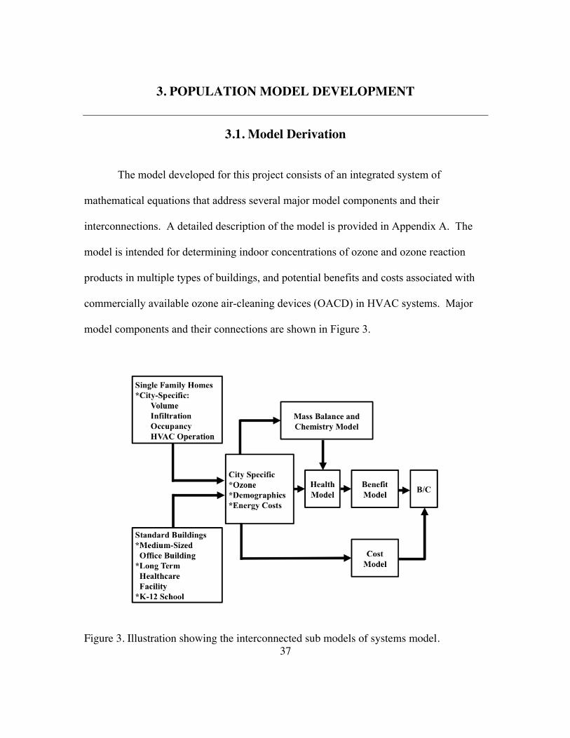
The model developed for this project consists of an integrated system of

mathematical equations that address several major model components and their

interconnections. A detailed description of the model is provided in Appendix A. The

model is intended for determining indoor concentrations of ozone and ozone reaction

products in multiple types of buildings, and potential benefits and costs associated with

commercially available ozone air-cleaning devices (OACD) in HVAC systems. Major

model components and their connections are shown in Figure 3.

Figure 3. Illustration showing the interconnected sub models of systems model.

38

Modeling the Effects of Climate, Geography, and Demographics

The modeling analysis focused on a set of baseline conditions in 12 cities across

the United States – the conditions are discussed in further detail in Appendix A. At least

two cities from each of the five climate zones defined by the Energy Information

Administration were selected for the analysis (USEIA, 2014). Climate zones are defined

by number of heating degree-days and cooling degree-days. The cities selected for this

analysis include: Atlanta, Austin, Buffalo, Chicago, Cincinnati, Houston, Miami,

Minneapolis, New York City, Phoenix, Riverside, and Washington D.C. (Figure 4). This

sample of cities accounts for a broad nationwide sample of population, climate, building

stock, and ambient ozone concentrations.

Figure 4. U.S. climate zones and geographic location of 12 sample cities (USEIA, 2014).

39

In addition, city-specific parameters such as the average occupancy of single-

family homes, population age fractions, and regional energy costs were also accounted

for in the integrated systems model. Single-family homes were modeled using a Monte

Carlo analysis and city-specific housing parameters to determine the ozone removal

effectiveness and benefit/cost (B/C) ratio of activated carbon filtration. Details of the

Monte Carlo analysis methodology and results for single-family homes are described in

Appendix A.

Commercial buildings, including office buildings, long term healthcare facilities,

and K-12 schools were modeled using standardized building parameters defined by (list

who standardizes these and provide references) and city-specific ozone, demographics,

and energy costs. Details on the methods and results of the commercial building

modeling analysis are provided in detail in Appendix B. In all buildings, the major

parameters influencing the benefit-to-cost ratio include outdoor ozone, the make-up

ventilation rate, HVAC operation fraction, cost per kWh of electricity, and filter

efficiency (i.e., single-pass removal efficiency for ozone) of the activated carbon filter.

Mass Balance and Chemistry Model

Core model equations are used to solve for ozone concentration and

concentrations of key reaction products as previously presented by Fadeyi (2014), Chen

et al. (2012a), and Weschler and Shields (2000). The model is designed to estimate

concentrations of ozone and reaction product concentrations for scenarios without any

40

control devices and scenarios with control devices in place. The differences in these

scenarios are used to quantify the health benefits of ozone control. The fate of ozone and

ozone reaction products within a building or zone are estimated using mass balance

equations based on assumptions of well-mixed and steady-state conditions. The time-

averaged mass balance equations for ozone and ozone reaction products are presented as

Equations (1) and (2), respectively.

𝐶!! =  !!!"#! !!!!,!! !!!!,!! !!"!!"#$!!" !!,!!!  

!!!!

!!"!!!!"!!"# !! !!!!,!! !!!!,!! !  !!"#,!!∗ !   !!!!!

(1)

𝐶!" =  !!"!!"#,!!

∗ !!!  !   !!,!! !!  !!!!!!!  !  !!",!

!!!"!!!!"!!"# !! !!!!,!" !!!!,!" !  !!"#,!"

∗ (2)

Where,

λinf = Qinf/V [hr-1] λmake-up = Qmake-up/V [hr-1]

λrec = Qrec/V [hr-1] λexh = Qexh/V [hr-1]

Hon = average annual fraction of time that the HVAC system operates [-] CO3 = concentration of ozone in the occupied space [ppb]

Co,O3 = concentration of ozone in outdoor air [ppb] Cj = concentration of gaseous reactant j in the occupied space [ppb]

EO3 = emission rate of ozone into occupied space [ppb • m3 • hr-1] Epi,f = emission rate of product i from HVAC filter [ppb-m3/hr] = yf,piHonff,pi(Qmake-upCo,o3 + QrecCo3) fc,O3 = single-pass fractional removal of ozone by OACD [-]

ff,O3 = single-pass fractional removal of ozone by HVAC filter [-] kj = bimolecular homogeneous reaction rate constant [ppb-1 • hr-1]

k*dep,O3 = ozone decay rate for integrated background surfaces [hr-1]

41

k*dep,pi = ozone reaction product decay rate for background surfaces [hr-1]

p = fractional penetration through the building envelope for ozone [-]

Qexh = exhaust air volumetric flow rate [m3 • hr-1] Qinf = infiltration air volumetric flow rate [m3 • hr-1]

Qmake-up = make-up (outdoor intake) air volumetric flow rate [m3 • hr-1] Qrec = recirculation air volumetric flow rate [m3 • hr-1]

V = volume of occupied space [m3] αj = conversion factor (ppb to µg/m3) for reactant j (used only for SOA

formation)

yi,j = molar (or mass for SOA) yield of product i from ozone reaction with j [(molesi/molesj) for gas or (µgi/m3 / µgj/m3 for SOA]

ysi = molar (or mass for SOA) yield of product i from ozone reaction with background surfaces [(molesi/molesO3) for gas or (µgi/m3 / µgO3/m3 for SOA]

vd,O3 = deposition velocity of ozone to background surfaces [m/hr] v*

d,pi = deposition velocity of reaction product i to background surfaces [m/hr]

Benefit Model

Benefits are calculated using reductions in disability-adjusted life-years (DALYs)

due to reductions in indoor ozone concentration following the application of activated

carbon filtration. Disability-adjusted life-years are a metric for quantifying the burden of

disease, and incorporate years of life lost from premature mortality and years of life lost

from disability due to the incidence of disease. The methodology for determining change

in health incidence and the corresponding value of DALYs follows previous work

completed by the USEPA (2012b, and references provided therein) and others (Logue et

al., 2012; USEPA, 2010; Huijbregts et al., 2005). The health functions and parameters

42

used in the health analysis for ozone are presented in Table 5. Health functions for

acetaldehyde and formaldehyde are provided in Appendix A.

Table 5. Health outcomes due to ozone exposure.

Health Outcome ICD-9 Code

β (95% CIs)

DALYs per

Incidence Sources

Mortality (25 to 34) J00-J99 0.0045 (0.0015,

0.0074) 27.14 USEPA (2010); Jerrett et al.

(2009); USEPA (2012b); Lopez et al. (2006)

Mortality (35 to 44) J00-J99 0.0045 (0.0015,

0.0074) 24.78

Mortality (45 to 54) J00-J99 0.0045 (0.0015,

0.0074) 22.42

Mortality (55 to 64) J00-J99 0.0045 (0.0015,

0.0074) 18.58

Mortality (65 to 74) J00-J99 0.0045 (0.0015,

0.0074) 13.36

Mortality (75 to 84) J00-J99 0.0045 (0.0015,

0.0074) 9.64

Mortality (85+) J00-J99 0.0045 (0.0015, 0.0074) 5.45

Respiratory HA (18 to 64) 460-519 0.0020 (0.0010,

0.0030) 0.03

USEPA (2012b); Logue et al. (2012); Burnett et al.

(1999); Lvovsky et al. (2000)

Dysrhythmia HA (18 to 64) 427 0.0020 (0.0000,

0.0040) 0.03

Dysrhythmia HA (65+) 493 0.0020 (0.0000,

0.0040) 0.03

MRAD (18 to 64) 0.0026 (0.0011,

0.0041) 0.0005

Hubbell et al. (2005); Ostro and Rothschild (1989);

USEPA (2012b)

School Loss Day (5 to 17)

0.0158 (0.0060, 0.0255) 0.0007

Hubbell et al. (2005); Chen et al. (2000); USEPA

(2012b)

Respiratory HA (65+) 460-519 0.0021 (0.0013,

0.0029) 0.03 USEPA (2012b);

Moolkavgar et al. (1997); Lvovsky et al. (2000)

ICD-9 = International Classification of Disease, version 9 HA = Hospital Admission MRAD = Minor Restricted Activity Day

43

The change in disease incidence for each modeling scenario is calculated using a

baseline condition (no ozone control) and then subtracting the disease incidence when

ozone control is applied and lower occupant exposures to both ozone and its reaction

products occur (Equation 3). The calculations include parameters for baseline incidence,

concentration-response (C-R) functions, DALYs per incidence, and city-specific age

populations (USEPA, 2012b; USEPA, 2011a; USEPA, 2011b; USEPA, 2011c; Logue et

al., 2012, US Census Bureau, 2012). The value of y0 is specific to the disease or health

condition being considered and changes depending on the pollutant, health outcome, and

age.

Δ Incidence = [y0*(1-e- βΔC(freq ) )]*population (3)

Where,

∆Incidence = change in disease incidence for a population [number of disease outcomes]

y0 = baseline prevalence of disease Health OutcomesPopulation-Year

β = concentration-response coefficient Relative RiskConcentration

ΔC = change in pollutant concentration [µg·m-3]

freq = exposure frequency, or fraction of one year where exposure occurs [-]

The number of DALYs per pollution exposure is calculated using Equation (4),

and the estimated health benefit is calculated using Equation (5).

44

DALYs = DALYsIncidence

*ΔIncidence (4)

Benefits = $/DALY x ∆DALYs (5)

Where,

Benefit = monetary benefit associated with reduced DALYs per 100,000 people [$] $/DALY = value of one disability adjusted life year [$·year-1]

∆DALYs = reduction in DALYs (relative to no control) when a control is used [years]

When calculating DALYs, the number of years of life lost per mortality is

dependent on the age at which mortality occurs (Lopez et al., 2006). The greatest

uncertainty in the benefits analysis is attributed to the value of an avoided DALY, more

specifically, what the average person is willing to pay to avoid a health-related issue due

to ozone exposure. One generally accepted approach is to equate one DALY avoided as

approximately equal to three times the per capita gross domestic product (Rascati, 2006).

In the United States, this is equivalent to approximately $150,000 (2014 US dollars) per

avoided DALY (World Bank, 2014). Bobinac et al. (2014) also evaluated the value of a

quality-adjusted life-year (QALY) gained in the Netherlands using a survey incorporating

a broad range of ages, incomes, and educational levels. One QALY gained is equivalent

to one avoided DALY. Their methods used a weighting factor from Tversky and

Kahneman (1992) to integrate decision theory and human behavior under risk. From

45

their survey results, they were able to estimate a probabilistic distribution of what the

average person is willing to pay to gain a QALY. Their results indicated a distribution

with a mean of approximately $140,000 (2014 US dollars) per avoided QALY.

For this dissertation, a distribution of dollars per avoided DALY was developed

based on Bobinac et al. (2014), and was used to estimate the benefits of reduced exposure

to ozone and its reaction products. This method yields lower benefits than the USEPA

methodology used in the Regulatory Impact Analysis for ozone (USEPA, 2008). The

USEPA uses a value per statistical life (VSL) of approximately $9.3M (2014 U.S.

dollars) per life lost regardless of age at the time of death (USBLS, 2014; USEPA,

2011b). In contrast, the DALYs method assigns a value of life based on the years of life

lost compared to the average life expectancy, which results in lower benefits when

compared to the USEPA method. Further information on the DALYs calculations and

benefit model are provided in the supplemental information.

Cost Model

Overall filter costs include the difference in capital costs (materials and labor)

between a standard particle filter and an activated carbon filter, as well as additional

energy costs due to the difference in pressure drop between a standard particle filter and

an activated carbon filter. Other costs such as installation and disposal are not included

in this paper as our analysis focused on commercially available filters designed for

residential HVAC systems. Overall filter costs are calculated for a population of 100,000

46

using Equation (6) and assuming one to two filters per residential HVAC unit during the

summer ozone season (1 May through 30 September):

Costs = Pelec* 𝐸!"#$ + 𝐹!"#$ + 𝐿!"#$ * RF * 100,000Occ.

(6)

Where,

Costs = overall differential cost between activated carbon and conventional particle filters (AcC – particle) per 100,000 persons [$]

Pelec = electricity usage [kWh] due to additional pressure drop =

= !!"#$%&  ∗  ∆!!"##  ∗  !!"_!"!

!"""  ∗  !!"#$

Ecost = electricity cost per kWh [$]

Qfilter = flowrate through the filter [m3·hr-1] ∆Pdiff = difference in pressure drop across the filter between AcC filter and standard

filter [Pa] Hon_tot = total number of hours of HVAC operation [hours]

𝜂!"#$ = overall efficiency of the HVAC fan and motor [-] Fcost = difference in filter costs between AcC filter and standard particle filter [$]

(assumed to equal zero for residences) Lcost = difference in labor, replacement, and disposal costs between AcC and

particle filters [$] (assumed to equal zero for residences) RF = filter replacement frequency [yr-1]

Occ. = building occupancy [persons] (average varies by city)

City specific electricity costs and HVAC operational runtimes are provided in

greater detail in the Appendix A. Overall filter costs are extrapolated for a population of

100,000 in order to compare with DALYs using the same metric (per 100,000 people).

47

3.2. Model Results

Proprietary ozone removal efficiency data provided by a filter manufacturer

estimated an ozone removal efficiency ranging from 60-90% during an 8-week field test

in a hot and humid climate. In order to provide conservative estimates of the filter

performance in single-family homes (typically 1-inch filters), an ozone removal

efficiency of 40% was used in the modelling analysis. The modelling results indicate that

an activated carbon filter with an ozone removal efficiency of 40% would provide

marginal benefits in single-family homes (Figure 5). Further information on the

methodology and modelling results are presented in Appendix A and Appendix B.

48

Figure 5. Benefit-to-cost ratios from using 1-inch (2.5 cm) activated carbon filters in single-family homes. The filled circles represent median values, the filled boxes

represent means, and the whiskers represent the 95% confidence intervals of the Monte Carlo modeling analysis.

Of the 12 target cities, single-family homes in Phoenix would benefit the most

from carbon filtration, followed closely by Riverside. For each of these two cities the

mean B/C ratio is approximately 2.0. High summertime ozone concentrations and

relatively new building stocks characterize these two cities with high air conditioning

usage during summer months. This implies that cities with high summer temperatures

(and by extension high air conditioning usage), high summertime ozone, and a high

proportion of residential air conditioning usage (implying newer building stock) will

benefit the most from residential carbon filtration. Cities that had lower B/C ratios

0 1 2 3 4 5 6 7 8 9

10 11 12 13 14

B/C

Rat

io (1

-inch

filte

r)

49

include Buffalo and Minneapolis. These two cities are characterized by a milder summer

climate and generally lower air conditioning usage (Chen et al., 2012a and 2012b). In

addition, since both cities have milder climates and older building stock, residents may

generally open windows for cooling, eliminating the benefit of activated carbon filters

(Chen et al., 2012a). The upper bound of B/C ratios for each city ranged from

approximately 6 to 13, indicating that some fraction of the population receives significant

benefits from activated carbon filtration on residential buildings. This subset is generally

characterized as a subpopulation with existing respiratory sensitivities (asthma, and other

chronic pulmonary disorders), as well as the population over the age of 65, which

generally has a much higher incidence rate for respiratory morbidity and mortality.

Since the results of activated carbon filtration in single-family homes in Phoenix

appear promising, a secondary analysis of avoided mortalities was conducted. Berman et

al. (2012) compared ozone-related mortalities in Phoenix over three years and three

different ozone rollback strategies. The rollback strategies were in accordance with new

8-hour ozone standards proposed by the USEPA. These analyses in Berman et al. (2012)

were then compared to the number of avoided mortalities in Phoenix when using

activated carbon filters in single-family homes with air conditioning. As shown in Figure

6, utilizing activated carbon filtration in single-family homes would result in nearly

equivalent numbers of avoided mortalities when compared to rolling back the 8-hour

ozone standard to 70 ppb.

50

Figure 6. Comparison of avoided mortalities per year in Phoenix, AZ under three different 8-hour ozone rollback strategies and with activated carbon filtration in single-

family homes.

When utilizing the USEPA’s value of a statistical life of approximately $9.8M

and comparing versus the control costs for each strategy (USEPA, 2011 and USEPA,

2008), the control costs for activated carbon filtration in single-family homes is nearly

one order of magnitude less than the control costs for outdoor ozone reductions (Figure

7). When utilizing activated carbon filtration with 100% HVAC fan operation during the

summer ozone season, the benefits of carbon filtration are greater than the costs. This

implies that activated carbon filtration in homes could be cost-effective at reducing

ozone-related mortalities and should be considered as a strategy to improve public health.

0

5

10

15

20

25

30

2005 2006 2007 2005 2006 2007 2005 2006 2007 2005 2006 2007

Ozone Rollback (75 ppb)

Ozone Rollback (70 ppb)

Ozone Rollback (60 ppb)

No Rollback w/ Carbon Filtration

Avoi

ded

Mor

talit

ies

51

Figure 7. Comparison of annual ozone control costs per avoided mortality in Phoenix, AZ comparing two 8-hour ozone rollback strategies and two strategies utilizing activated

carbon filtration in single-family homes.

For commercial buildings, the modelling results indicate that an activated carbon

filter with an ozone removal efficiency of 60% would provide annual benefit-cost ratios

equal to or greater than 1.0 in all three building types across all 12 cities as shown in

Figure 8.

$1

$10

$100

$1,000

$10,000

$100,000

$1,000,000

$10,000,000

$100,000,000

$1,000,000,000

2005 2006 2007 2005 2006 2007 2005 2006 2007 2005 2006 2007

Ozone Rollback (75 ppb)

Ozone Rollback (70 ppb)

No Rollback w/ Carbon Filtration

No Rollback w/ Carbon Filtration

100% Fan Operation

Con

trol

Cos

t per

Avo

ided

Mor

talit

y

Red line is benefit value for avoided mortality B/C > 1 when costs fall below red line

52

Figure 8. Predicted benefit/cost ratios in commercial buildings when using commercially available 4-inch activated carbon combination filters to remove ozone in 12 U.S. cities. The circular symbols represent the median and range bars represent the 95% confidence

intervals of health functions used in the modeling analysis.

Of the three building types considered in the commercial building analysis, long-

term healthcare facilities have the highest potential to improve health in buildings.

Demographics are an important consideration since only persons over the age of 65 were

0

1

10

100

1,000

Offi

ce B

uild

ing

K-1

2 Sc

hool

Lo

ng-te

rm H

ealth

care

O

ffice

Bui

ldin

g K

-12

Scho

ol

Long

-term

Hea

lthca

re

Offi

ce B

uild

ing

K-1

2 Sc

hool

Lo

ng-te

rm H

ealth

care

O

ffice

Bui

ldin

g K

-12

Scho

ol

Long

-term

Hea

lthca

re

Offi

ce B

uild

ing

K-1

2 Sc

hool

Lo

ng-te

rm H

ealth

care

O

ffice

Bui

ldin

g K

-12

Scho

ol

Long

-term

Hea

lthca

re

Offi

ce B

uild

ing

K-1

2 Sc

hool

Lo

ng-te

rm H

ealth

care

O

ffice

Bui

ldin

g K

-12

Scho

ol

Long

-term

Hea

lthca

re

Offi

ce B

uild

ing

K-1

2 Sc

hool

Lo

ng-te

rm H

ealth

care

O

ffice

Bui

ldin

g K

-12

Scho

ol

Long

-term

Hea

lthca

re

Offi

ce B

uild

ing

K-1

2 Sc

hool

Lo

ng-te

rm H

ealth

care

O

ffice

Bui

ldin

g K

-12

Scho

ol

Long

-term

Hea

lthca

re

Atl Aus Buf Chi Cin Hou Mia Min NYC Pho Riv Wash

Ben

efit/

Cos

t Rat

io (4

-Inc

h Fi

lter)

53

considered in the benefits model. This demographic tends to be the most sensitive to

ozone-related health outcomes, particularly premature respiratory mortality. In fact,

greater than 90% of the benefits are attributed to reduced mortality. The projected

number of lives saved annually range from 103 (Houston) to 195 (Riverside) per 100,000

people. The modeling results indicate that activated carbon filtration in commercial

buildings, especially long-term healthcare facilities, would be extremely beneficial in

reducing exposures to ozone and should be considered as a strategy to improve public

health. Further details on the commercial modeling results are presented in Appendix B.

One of the most important takeaways for the modeling of commercial buildings is

that the energy penalty results in a relatively small contribution to the overall cost of

carbon filtration. For example, in a baseline condition for a medium sized commercial

office building, 7-12% of the total cost of filtration is attributed to the additional energy

required due to pressure drop as shown in Table 6.

The baseline modeling condition for commercial office buildings assumed

standard pricing for electricity charges during the summer ozone season, however, many

utility providers charge demand pricing to commercial customers during the summer

when electicity usage is highest. To explore the effect of demand pricing, the summer

demand charges for commercial customers in Austin, TX was determined and compared

to the baseline charge per kWh used in the previous analysis (Figure 8). As an

approximation, the percent difference was then applied to all twelve cities to determine

the additional costs due to demand pricing in the summer. A second application included

demand pricing and also assumed that the combined HVAC system efficiency (drive,

54

motor, and shaft) was 25% versus the 46% used previously. As shown in Table 6, the

energy penalty peaks at 27% of total filtration costs when considering demand pricing

and low HVAC system efficiency. Even in the most expensive scenario and city, the

benefit-to-cost ratio exceeds 7.0.

Table 6. Health benefits and filtration costs per building when using 2-inch activated carbon filtration in a medium sized commercial office building.

Seasonal Activated Carbon Filtration Costs (2-inch filter) for Medium Commercial Office Building

Baseline Filtration

Filtration with Demand Pricing

Demand Pricing + Low HVAC Efficiency

City

Health Benefits

per Building

Total Costs

Energy Costs (%)

Total Costs

Energy Costs (%)

Total Costs

Energy Costs (%)

Atlanta $6,419 $690 8% $718 12% $787 19% Austin $6,617 $680 7% $711 11% $773 18% Buffalo $7,980 $721 12% $765 17% $871 27% Chicago $6,641 $680 7% $703 10% $760 17%

Cincinnati $8,020 $685 7% $711 11% $773 18% Houston $4,532 $681 7% $703 10% $759 16% Miami $6,290 $690 8% $718 12% $787 19%

Minneapolis $5,875 $686 7% $711 11% $774 18% New York $6,298 $721 12% $764 17% $871 27% Phoenix $8,516 $685 7% $711 11% $773 18%

Riverside $9,198 $705 10% $741 14% $829 24% Wash. DC $7,060 $700 9% $734 14% $815 22%

The results presented in Table 6 reflect that the additional cost of the carbon filter

(compared to a standard particle filter) and the disposal costs ($17 per filter) dominate the

55

overall costs of carbon filtration. This topic will be more pertinent for 4-inch (or thicker)

filters as the pressure drop (and corresponding energy penalty) will be substainally less.

56

4. FIELD STUDY METHODS AND RESULTS

4.1. Experimental Methods

Indoor air quality and energy usage due to reduced ventilation rates in a

laboratory building on the University of Texas campus were measured. The building

selected for this study had laboratory space with very high air exchange rates (as high as

12/hr), as well as sophisticated ventilation control and data collection systems.

The laboratory building used in this study is a 142,000 square foot research

facility that was constructed in 2008, and certified as LEED Silver. It has six primary

floors with the top floor acting as the mechanical space for the facility. The first floor is

entirely below grade and the second floor is partially below grade. The building has nine

air-handling units and 102 separate laboratory heating, ventilating, and air conditioning

(HVAC) zones. In addition, all exhaust air from the laboratories in the building is

collected and directed through a glycol heat recovery system. The recovered exhaust heat

is then used to pre-heat outdoor air before it passes through the heating and cooling coils

in the air-handling unit. Ventilation can be remotely controlled and monitored using a

building automation system (BAS) (Siemens Insight BAS Software, version 3.13). A

photo of one the teaching laboratories and sampling equipment used in the study is shown

in Figure 9.

57

Figure 9. Photos of teaching laboratory and air sampling equipment (L) and of active sampling for VOCs using Tenax-TA® sorbent tubes (R).

Indoor air quality measurements were collected over a course of three weeks

under three different testing scenarios: high ventilation, low ventilation, and low

ventilation with carbon filtration. Primary pollutants of concern were ozone and volatile

organic compounds (VOCs).

Volatile organic compounds were collected using Tenax-TA® with thermal

desorption and gas chromatography/mass spectrometry (Hewlett-Packard gas

chromatograph model number 5890 II outfitted with a HP 5971 mass selective detector).

Each sorption tube was packed with 75 mg of Tenax-TA® sorbent and conditioned in

nitrogen at 300°C for two hours. Active sampling was conducted with two pumps in

Ozone Monitor Teflon (PTFE) Collection Tube Tenax-TA®

sorbent tubes

Sampling Pumps

58

each room during each ventilation condition (Buck Elite-5 Pump 5-6000cc/min 120V).

The pumps were programmed at two different pumping rates, 10 mL/min and 40

mL/min, and the sampling time was 4 hours. For every 10 Tenax-TA® samples collected

in the field, a lab blank and trip blank were used for baseline analysis. Compounds were

identified by using the library compound search in Hewlett Packard’s ChemStation

software and the NIST 11 Mass Spectral Database. The mass of the identified

compounds was estimated using 4-bromofluorobenzene as an internal standard and an

assumed response ratio of 1.0. Samples were collected using a sampling rate of 25

mL/min for four hours and were collected in accordance with U.S. Environmental

Protection Agency (USEPA) methods (TO-17). In addition to sorption tubes, VOCs were

also assessed using summa canisters evaluated by an independent laboratory. The

summa canister samples were collected for 24-hours using USEPA method (TO-15).

Ozone concentrations were measured with two UV-absorbance ozone analyzers

(2B Technologies Inc., Model 202) programmed to ten minute averaging intervals. Both

analyzers were cross calibrated before sampling using a calibrated ozone source (2B

Technologies Inc, Model 306) and three point calibration. The indoor ozone

measurements were collected using a 6 meter piece of PTFE tubing (Fisher Scientific, ¼-

inch O.D., 3/8-inch I.D.), which was positioned with the inlet 30 cm below the ceiling in

the center of the room. The second ozone analyzer collected outdoor ozone concentration

data in the air-handling unit fresh air intake. Outdoor ozone measurements were also

collected from the CAMS 3 air quality monitor in northwest Austin (TCEQ, 2014) to

59

compare against ozone measurements collected in AHU-1. The CAMS 3 air quality

monitor is about five miles (line of sight) from the university campus.

Due to low concentrations of VOCs in the laboratories, a total VOC (TVOC)

concentration was used to quantify VOC concentration. Concentrations of TVOC were

estimated using the total mass under the chromatographic spectra curve from a retention

time of 6 to 16 minutes, and then using the molecular weight of toluene to convert from

the mass concentration to a volumetric concentration expressed in parts per billion by

volume (ppbv).

Ozone and VOC measurements were also collected in the air-handling unit to

compare indoor measurements with an outdoor baseline. A photo of the air monitoring

equipment positioned in the air-handling unit is presented in Figure 10. Further details

on the experimental methods are presented in Appendix C.

60

Figure 10. Photo of air sampling equipment in the laboratory building air handling unit (L) and the filter bank with carbon filters installed (R).

Ozone Monitor

Sampling Tube to Air Handling Unit Outdoor Air Inlet

Pneumatic Switch on Timer

Sampling Tube to Filtered Outdoor Air Filter Bank

61

4.2. Results and Analysis

In the absence of indoor sources, lower ventilation rates should generally lead to a

lower indoor/outdoor (I/O) ozone concentration ratio. However, in this study the I/O

ozone concentration ratio (Figure 11) increased by an average of 23% (ρ < 0.05) under

the reduced ventilation scenario, and the average indoor ozone concentration across the

five rooms increased by roughly 10 parts per billion or 56% (ρ < 0.05).

The increase in ozone in the laboratories under reduced ventilation conditions is

surprising given that ozone has more time to react with indoor surfaces at a lower air

exchange rate. The higher ozone concenctration might be attributed to several factors

that outweigh the increased reaction time. These include decreased ozone deposition to

surfaces caused by the lower air velocity in the room, increased role of ozone sources,

e.g., photocopy machines, at lower air exchange rates, or differences in pressure

distribution that leads to more ozone entering the study zone from other building zones at

lower air exchange rates.

When the activated carbon filters were installed in the air-handling unit at a low

ventilation condition, the average indoor/outdoor ozone concentration ratio decreased by

45% (ρ < 0.05) compared to the low ventilation condition without carbon filters. The

average single pass removal efficiency for ozone through the carbon filters was 70%.

The indoor/outdoor ozone concentration ratio was on average 33% lower (ρ < 0.05) with

the carbon filters installed compared to the high ventilation condition without activated

carbon filtration. These results demonstrate that activated carbon filters are effective at

62

reducing indoor ozone concentrations. Potential benefits in a laboratory building include

reduced exposure of occupants to both ozone and its reaction products, as well as a

reduction of any adverse outcomes of ozone reactions as reported previously in Apte et

al. (2008).

Figure 11. Indoor/outdoor ozone concentration ratios in five sample laboratories building three testing conditions.

Quantification of individual VOCs using Tenax-TA sorbent was difficult because

of the low concentrations of VOCs in the laboratories. Therefore, a total VOC (TVOC)

concentration was used to quantify VOC concentrations for samples collected on Tenax-

0.0

0.1

0.2

0.3

0.4

0.5

0.6

0.7

0.8

0.9

1.0

Hig

h

Low

Car

bon

Hig

h

Low

Car

bon

Hig

h

Low

Car

bon

Hig

h

Low

Car

bon

Hig

h

Low

Car

bon

Lab 1 Lab 2 Lab 3 Lab 4 Lab 5

Indo

or/O

utdo

or O

zone

Rat

io

63

TA sorbent tubes. An average increase of 72% (ρ < 0.05) from 6.3 ppb to 10.9 ppb in

TVOC was observed when the ventilation rate was reduced from the high to low

condition. Specific VOCs were identified and quantified in subsequent testing using

summa canisters and TO-15 collection methods analyzed by an independent laboratory.

The three VOCs with highest concentrations included dichloromethane, n-hexane, and

toluene. The concentrations of VOCs did not vary considerably between the low

ventilation condition and the low ventilation condition with carbon filtration, indicating

that most of the VOCs measured during the sampling period were emitted from indoor

sources in the laboratories. The highest measured concentrations of VOCs are presented

in Table 6 with indicators showing at which ventilation condition the highest

measurement was collected.

Table 7. Highest recorded VOC concentrations in five sample labs in the laboratory building.

        Highest Measured Concentration (µg/m3)

Volatile Organic Compound

CAS Registry Number Lab 1 Lab 2 Lab 3 Lab 4 Lab 5 Outdoor

Chloromethane 74-87-3 0 1 LV 1 LV 2 LV 2 LV 2 LV Acetonitrile 75-05-8 2LV 1 LV 1 LV 1 LV 0 0 Dichloromethane 75-09-2 19 LV 10 LV 9 LV 3 LC 7 LV 7 LV 2-Butanone (MEK) 78-93-3 0 3 LV 3 LC 2 HV 0 2 HV n-Hexane 110-54-3 14 LV 8 LV 5 LV 9 LV 5 LV 4 LV Cyclohexane 110-82-7 0 0 6 LC 4 HV 0 0 Toluene 108-88-3 3 LV 28 LV 29 LV 2 HV 6 LV 3 LV Tetrahydrofuran 109-99-9 0 0 0 0 0 3 LV

HV = High Ventilation LV = Low Ventilation LC = Low Ventilation with Carbon Filters

64

Summa canisters were also collected before and after the bag filters and the

carbon filters during the low ventilation condition. The bag filters were sources of

TVOCs with an outlet (post filter) TVOC concentration 17% higher than the inlet (pre-

filter) concentration (ρ < 0.05). The carbon filters removed VOCs and the outlet (post

filter) concentration was 62% lower than the inlet (pre-filter) concentration (ρ < 0.05).

The measured VOCs before and after each type of filter are presented in Figure 12.

Figure 12. Measured concentrations of VOCs before and after a typical bag filter (L) and an activated carbon filter (R).

0

20

40

60

80

100

120

140

160

180

Pre-

Filte

r Po

st-F

ilter

Pr

e-Fi

lter

Post

-Filt

er

Pre-

Filte

r Po

st-F

ilter

Pr

e-Fi

lter

Post

-Filt

er

Pre-

Filte

r Po

st-F

ilter

Pr

e-Fi

lter

Post

-Filt

er

Pre-

Filte

r Po

st-F

ilter

Pr

e-Fi

lter

Post

-Filt

er

Pre-

Filte

r Po

st-F

ilter

Pr

e-Fi

lter

Post

-Filt

er

Pre-

Filte

r Po

st-F

ilter

Pr

e-Fi

lter

Post

-Filt

er

Pre-

Filte

r Po

st-F

ilter

Pr

e-Fi

lter

Post

-Filt

er

Pre-

Filte

r Po

st-F

ilter

Pr

e-Fi

lter

Post

-Filt

er

1 2 3 4 5 6 7 8 1 2 3 4 5 6 7 8

Bag Filter Carbon Filter

Con

cent

ratio

n (µ

g/m

3 )

1 = Chloromethane 2 = n-Butane 3 = Ethanol 4 = Isopropyl Alcohol 5 = Acetone 6 = 2-Butanone (MEK) 7 = Ethyl Acetate 8 = TVOC

65

The bag filters were a source of VOCs and did not remove ozone. In contrast, the

carbon filters were effective at removing outdoor ozone and VOCs, indicating that carbon

filters could provide additional health benefits due to VOC removal.

66

5. FILTER TESTING EXPERIMENTAL METHODS AND RESULTS

5.1. Experimental Methods

Two different commercially available activated carbon filters marketed for odor

removal in single-family homes were tested in a laboratory test system. Both filters were

new filters and were tested in a clean test system. The filters had dimensions of 51 cm by

64 cm by 3 cm (20 inches by 25 inches by 1 inch). The first filter was composed of

activated carbon fibers with 29 grams of carbon in the filter. The carbon in the first filter

was applied as slurry and attached to polyester fibers using adhesive. From this point,

this filter will be referred to as the activated carbon slurry filter. The second filter was

composed of a pleated pre-filter to remove particles followed by a suspended mesh of

polyester fibers containing 190 grams of bulk carbon approximately 1-2 mm thick. From

this point on, the second filter will be referred to as the bulk activated carbon filter.

Filters were tested in triplicate at two different flow rates for two hours. The two test

flow rates were 850 m3/hr (500 cfm) and 1,700 m3/hr (1000 cfm).

The test system was a closed loop system composed of stainless steel duct

material. Air was moved through the test system using two standard 5-ton residential air

handling units with tested flowrates varying from 0 to 2500 m3/hr (0 to 1500 cfm). Each

air handling unit utilized a variable frequency drive that allowed for power adjustment

from 0% to full power. Seams in the stainless steel duct material were sealed with

aluminum tape to reduce leakage in the system. The flowrate through the system was

measured with a flow station (Shortridge Instruments, Inc., VelGrid) located at the outlet

67

of air handling unit #2. The pressure difference in the flow station was measured with a

digital manometer (Energy Conservancy DG-700 manometer) and converted to a

flowrate in cubic feet per minute using a calibrated air flow monitor (Energy

Conservancy TrueFlow Plate). The pressure drop across the filter was also measured

using a digital manometer (Energy Conservancy DG-700) and pressure drop was

recorded at the beginning and end of the two-hour test cycle. The average pressure drop

and standard error were calculated from five successive instrument readings during every

measurement. A schematic of the laboratory test system is presented in Figure 13.

Figure 13. Schematic of the laboratory test system for activated carbon filters.

Ozone concentrations were measured with two UV-absorbance ozone analyzers

(2B Technologies Inc., Model 202) programmed to one minute averaging intervals. Both

analyzers were cross calibrated before sampling using a calibrated ozone source (2B

Technologies Inc, Model 306) and three point calibration. Ozone measurements were

68

logged every minute over the two hour test cycle. Ozone was measured before and after

the activated carbon filter using two sampling points connected to the ozone analyzers

using a 30 cm (12 inch) piece of PTFE tubing (Fisher Scientific, ¼-inch O.D., 3/8-inch

I.D.). The collection tubes were extended through the sheet metal duct and into the test

system so that the inlet offset the inner surface by 5 cm (2 inches). This was done in

order to avoid boundary level effects on measuring ozone within the test system.

Additionally, the collection tubes were offset from either side of the filter by 30 cm (12

inches) in order to reduce errors in ozone measurement due to turbulence before and after

the filter. Finally, an ozone generator (Yanco Industries, Ltd., OL-80 Ozone Generator)

was used in the laboratory test system to maintain a steady-state inlet ozone concentration

of 50 ppb (+/- 10 ppb) at the pre-filter sampling point. Photos of the ozone generator and

test system are shown in Figure 14. Estimated ozone generation rates for the activated

carbon slurry filter were 19.6 mg/hr (low flowrate) and 28.9 mg/hr (high flowrate). For

the bulk activated carbon filter, the estimated ozone generation rates were 42.5 mg/hr and

73.1 mg/hr for the low and high flowrates, respectively.

69

Figure 14. Photo of the ozone generator (L) used in the test system to maintain a steady-state inlet ozone concentration. Ozone was measured before and after the carbon filter

(R) using two ozone analyzers.

The single pass removal efficiency of the activated carbon filter was determined

by using the pre-filter and post-filter ozone measurements and Equation 7.

   𝜂 = 100  × 1−  !!!  (!"#$!!"#$%&)!!!  (!"#!!"!"#$)

(7)

Where,

𝜂 = single pass removal efficiency of the carbon filter (%) CO3 (post-filter) = ozone concentration on outlet side of the carbon filter (ppb) CO3 (pre-filter) = ozone concentration on inlet side of the carbon filter (ppb)

Ozone Monitor (Pre-filter)

Ozone Monitor (Post-filter)

Activated Carbon Filter

70

The standard error of each single pass removal efficiency measurement was

estimated using error propagation and the measurement error of each ozone analyzer (2

ppb).

5.2. Results and Analysis

Key metrics analyzed in the laboratory study include flow rate through the filter,

pressure drop across the filter, and single pass removal efficiency for ozone. Flowrate

versus pressure drop for both filters are presented in Figure 15. The error bars in the

figure display the standard error of the collected measurements.

Figure 15. Pressure drop versus flow rate measurements for two commercially available activated carbon filters. Measurements were collected at the beginning and the end of a

two-hour test cycle.

0 200 400 600 800 1000 1200 1400 1600 1800

0.00

0.05

0.10

0.15

0.20

0.25

0.30

0.35

0.40

0.45

0

20

40

60

80

100

120

140

0 200 400 600 800 1000

Flowrate (m3/hr)

Pres

sure

Dro

p (in

ches

of w

ater

)

Pres

sure

Dro

p (P

a)

Flowrate (cfm)

Activated Carbon Slurry Filter (Initial)

Activated Carbon Slurry Filter (Final)

Bulk Activated Carbon Filter (Initial)

Bulk Activated Carbon Filter (Final)

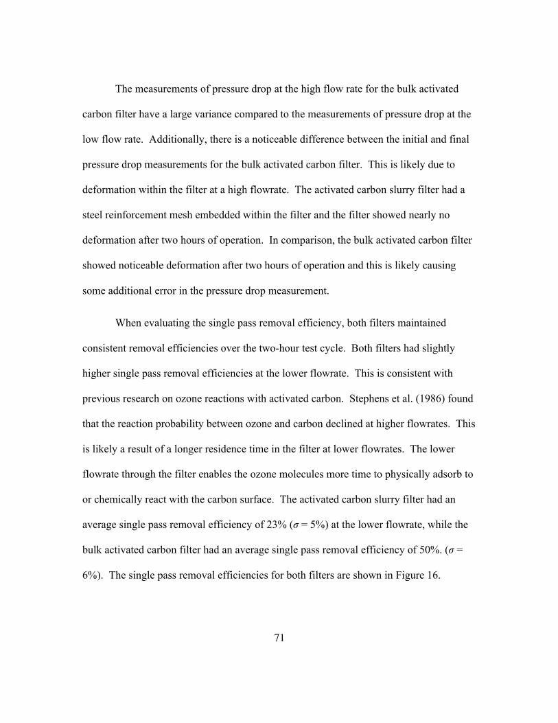
71

The measurements of pressure drop at the high flow rate for the bulk activated

carbon filter have a large variance compared to the measurements of pressure drop at the

low flow rate. Additionally, there is a noticeable difference between the initial and final

pressure drop measurements for the bulk activated carbon filter. This is likely due to

deformation within the filter at a high flowrate. The activated carbon slurry filter had a

steel reinforcement mesh embedded within the filter and the filter showed nearly no

deformation after two hours of operation. In comparison, the bulk activated carbon filter

showed noticeable deformation after two hours of operation and this is likely causing

some additional error in the pressure drop measurement.

When evaluating the single pass removal efficiency, both filters maintained

consistent removal efficiencies over the two-hour test cycle. Both filters had slightly

higher single pass removal efficiencies at the lower flowrate. This is consistent with

previous research on ozone reactions with activated carbon. Stephens et al. (1986) found

that the reaction probability between ozone and carbon declined at higher flowrates. This

is likely a result of a longer residence time in the filter at lower flowrates. The lower

flowrate through the filter enables the ozone molecules more time to physically adsorb to

or chemically react with the carbon surface. The activated carbon slurry filter had an

average single pass removal efficiency of 23% (σ = 5%) at the lower flowrate, while the

bulk activated carbon filter had an average single pass removal efficiency of 50%. (σ =

6%). The single pass removal efficiencies for both filters are shown in Figure 16.

72

Figure 16. Single pass removal efficiency for ozone for two commercially available activated carbon filters at a flow rate of 850 m3/hr (500 cfm) for two hours. The error

bars represent the standard error due to measurement error.

At the high flowrate (1,700 m3/hr), the activated carbon slurry filter had an

average single pass removal efficiency of 17% (σ = 5%) and the bulk activated carbon

filter had an average single pass removal efficiency of 43%. (σ = 6%). The single pass

removal efficiencies for both filters are shown in Figure 17.

0%

10%

20%

30%

40%

50%

60%

70%

0 15 30 45 60 75 90 105 120 135

Sing

le P

ass R

emov

al E

ffic

ienc

y

Time (Mins) Bulk Activated Carbon Filter Replicate #1 Activated Carbon Slurry Filter Replicate #1 Bulk Activated Carbon Filter Replicate #2 Activated Carbon Slurry Filter Replicate #2 Bulk Activated Carbon Filter Replicate #3 Activated Carbon Slurry Filter Replicate #3

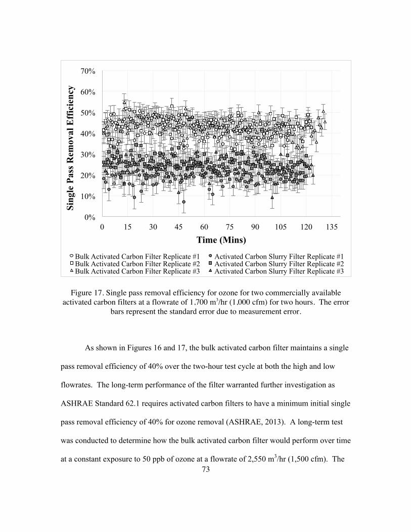
73

Figure 17. Single pass removal efficiency for ozone for two commercially available activated carbon filters at a flowrate of 1,700 m3/hr (1,000 cfm) for two hours. The error

bars represent the standard error due to measurement error.

As shown in Figures 16 and 17, the bulk activated carbon filter maintains a single

pass removal efficiency of 40% over the two-hour test cycle at both the high and low

flowrates. The long-term performance of the filter warranted further investigation as

ASHRAE Standard 62.1 requires activated carbon filters to have a minimum initial single

pass removal efficiency of 40% for ozone removal (ASHRAE, 2013). A long-term test

was conducted to determine how the bulk activated carbon filter would perform over time

at a constant exposure to 50 ppb of ozone at a flowrate of 2,550 m3/hr (1,500 cfm). The

0%

10%

20%

30%

40%

50%

60%

70%

0 15 30 45 60 75 90 105 120 135

Sing

le P

ass R

emov

al E

ffic

ienc

y

Time (Mins)

Bulk Activated Carbon Filter Replicate #1 Activated Carbon Slurry Filter Replicate #1 Bulk Activated Carbon Filter Replicate #2 Activated Carbon Slurry Filter Replicate #2 Bulk Activated Carbon Filter Replicate #3 Activated Carbon Slurry Filter Replicate #3

74

amount of ozone ultimately removed by the filter is of particular interest and can be

calculated using Equation 8.

𝑚𝑎𝑠𝑠  𝑜𝑧𝑜𝑛𝑒!!!!!! 𝑟𝑒𝑚𝑜𝑣𝑒𝑑 = 𝜂𝐶!!𝐻!"𝑄Δ𝑡

!!!!!!   (8)

Where the mass of ozone is in grams and,

η = single pass removal efficiency of the activated carbon filter at time step ti (%)

CO3 = ozone concentration into the filter (g/m3)

Hon = HVAC hourly cycling operation (-)

Q = flowrate through the filter (m3/hour)

Δt = time step (hour)

It was determined that the bulk activated carbon filter would remove ozone up

until 48 hours of operation. Using the relationship in Equation 8, the total mass of ozone

removed by the filter was approximately 23 mg during the 48-hour test cycle. A figure

showing the single pass removal efficiency and cumulative mass of ozone removed over

time is presented in Figure 18.

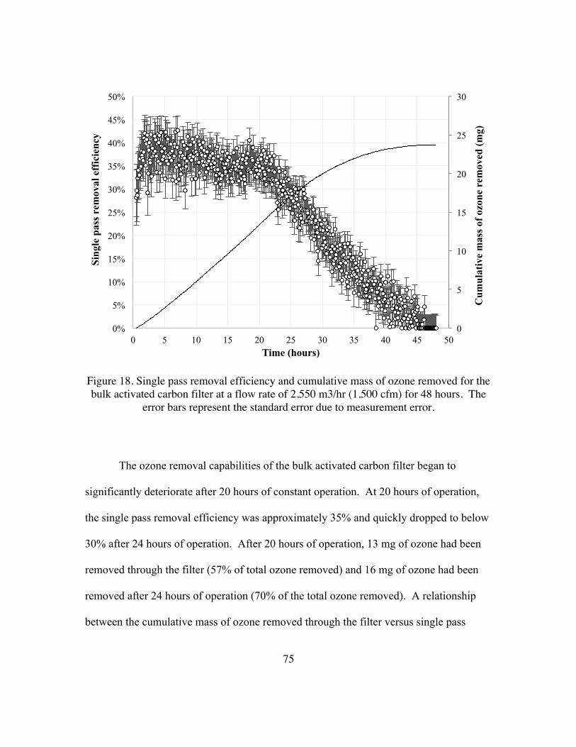
75

Figure 18. Single pass removal efficiency and cumulative mass of ozone removed for the bulk activated carbon filter at a flow rate of 2,550 m3/hr (1,500 cfm) for 48 hours. The

error bars represent the standard error due to measurement error.

The ozone removal capabilities of the bulk activated carbon filter began to

significantly deteriorate after 20 hours of constant operation. At 20 hours of operation,

the single pass removal efficiency was approximately 35% and quickly dropped to below

30% after 24 hours of operation. After 20 hours of operation, 13 mg of ozone had been

removed through the filter (57% of total ozone removed) and 16 mg of ozone had been

removed after 24 hours of operation (70% of the total ozone removed). A relationship

between the cumulative mass of ozone removed through the filter versus single pass

0

5

10

15

20

25

30

0%

5%

10%

15%

20%

25%

30%

35%

40%

45%

50%

0 5 10 15 20 25 30 35 40 45 50

Cum

ulat

ive

mas

s of o

zone

rem

oved

(mg)

Sing

le p

ass r

emov

al e

ffic

ienc

y

Time (hours)

76

removal efficiency was estimated using the data from the filter experiments and is shown

in Figure 19. This relationship predicts the degradation of the filter as it removes ozone

over time, which can be useful for modeling applications.

Figure 19. Relationship between mass of ozone removed through the filter and the single pass removal efficiency. As more ozone is removed through the filter, the single pass

removal efficiency declines.

Cetin and Novoselac (2015) evaluated 189 newer homes (built since 2008) in

Austin, TX and determined average HVAC runtime fractions during the cooling season

for every hour of the day. Using their HVAC cycling data, hourly ozone monitor data for

the 2014 ozone season (TCEQ, 2014), and Equation (1), the performance of the carbon

filter was estimated for six modeling scenarios in a typical single-family home in Austin,

y = -7E-05x3 + 0.0013x2 - 0.008x + 0.3784 R² = 0.96234

0%

5%

10%

15%

20%

25%

30%

35%

40%

45%

0 5 10 15 20 25

Sing

le P

ass R

emov

al E

ffic

ienc

y

Cumulative Ozone Removed (mg)

77

TX. All modeling scenarios assumed that the typical Austin home had a volume of 500

m3, an infiltration air exchange rate of 0.5/hr, and an ozone penetration factor of 0.8.

Additional parameters for each modeling scenario are shown in Table 7.

Table 8. Parameters for six modeling scenarios of a typical single-family home in Austin, TX.

Modeling Condition

Recirc. Flowrate (m3/hr)

Ozone Surface Decay

[AC on] (/hr)

Ozone Surface Decay

[AC off] (/hr)

100% fan operation

when outdoor ozone > 30 ppb

100% fan operation

when home is

occupied

Baseline 2,720 5.4 2.8 No No

Baseline, low reactivity 2,720 2.8 1.5 No No

Baseline, fan on during high ozone 2,720 5.4 2.8 Yes No

Baseline, fan on during high ozone, occupied

2,720 5.4 2.8 Yes Yes

100% fan operation when occupied 2,720 5.4 2.8 No Yes

100% fan operation when occupied, low reactivity

2,720 2.8 1.5 No Yes

Filter performance was estimated at hourly intervals and time-stepped using the

HVAC cycling data from Cetin and Novoselac (2015), hourly outdoor ozone (TCEQ,

2014), Equation (8), and the relationship in Figure 19. The model predicted ozone

reactions with the carbon filter and the cumulative mass of ozone removed since the filter

78

was installed. The cumulative mass of ozone removed by the filter was then used to

predict the single pass removal efficiency of the filter at the next time step and the

process was repeated for the entire ozone season (1 May to 30 September) as shown in

Figure 20.

Figure 20. Predicted single pass removal efficiency of activated carbon filter during the ozone season (1 May – 30 September 2014) in a typical single-family home in Austin,

TX using six different modeling scenarios.

0%

5%

10%

15%

20%

25%

30%

35%

40%

5/1/

2014

5/16

/201

4

5/31

/201

4

6/15

/201

4

6/30

/201

4

7/15

/201

4

7/30

/201

4

8/14

/201

4

8/29

/201

4

9/13

/201

4

9/28

/201

4

Sing

le P

ass R

emov

al E

ffic

ienc

y

Date

Baseline - High Ozone Baseline 100% Fan When Occupied 100% When Occupied + Low Reactivity Baseline - High Ozone & Occupied Baseline Low Reactivity

79

Using the data from Figure 20 and assuming that the home is not occupied from

8am to 6pm daily, the average ozone exposure in the home was determined for each

modeling scenario and compared to a condition with no carbon filtration. Despite the

degradation of the filter over the summer, the average residential ozone exposure

decreased from 15% to 39%. This is a considerable reduction in exposure, especially

when considering that the average person spends about 70% of their lifetimes in their

homes. An illustration comparing the average ozone exposure under the six modeling

scenarios is shown in Figure 21.

Figure 21. Average ozone exposure in a single-family home when applying activated carbon filtration across six modeling scenarios. The data labels show the percent

reduction in ozone exposure when compared to a standard particle filter with no ozone removal.

15%

23%

18% 18%

26%

39%

0

1

2

3

4

Bas

elin

e

Bas

elin

e, lo

w

reac

tivity

Bas

elin

e, h

igh

ozon

e

Bas

elin

e, h

igh

ozon

e +

occu

pied

100%

fan

oper

atio

n +

occu

pied

100%

fan

oper

atio

n +

occu

pied

, low

re

activ

ity

Seas

onal

indo

or o

zone

exp

osur

e (p

pb) AcC Filter No AcC Filter

80

The reductions in ozone exposure for each modeling scenario where then entered

into the systems model (Equations 3, 4, 5, and 6) along with the pressure drop data for the

bulk activated carbon filter (Figure 13). It was estimated that at flowrate of 2,720 m3/hr

(1,600 cfm), the additional pressure drop of utilizing the bulk activated carbon filter

versus a standard particle filter was approximately 165 Pascal (0.66 inches of H2O). It

was also assumed that the additional cost of the bulk activated carbon filter was $10 more

per filter than a standard particle filter. Finally, it was assumed that the electricity costs

in Austin, TX were $0.12 per kWh and that the HVAC unit had an overall (drive, motor,

shaft) efficiency of 25%. An additional analysis was conducted to see if the benefit-to-

cost (B/C) ratio would increase significantly if the pressure drop were reduced 50% and if

the activated carbon filter were to be the same price as a standard particle filter. The

calculated energy costs due to pressure drop across the filter were 80% to 90% of the

overall costs of activated carbon filtration. During the testing of the bulk activated

carbon filter, it was very evident that the filter was deflecting during operation, likely

increasing the pressure drop across the filter. This was likely due to the absence of steel

reinforcing that is common in typical particle filters. It was assumed that a 50% (or

more) reduction in pressure drop could be achieved by reducing the deflection of the

filter with reinforcement. It was also expected that the costs of activated carbon filters

would reach parity with standard particle filters as they become more popular with

consumers. The results of the economic analyses for the bulk activated carbon filter are

shown in Figure 22.

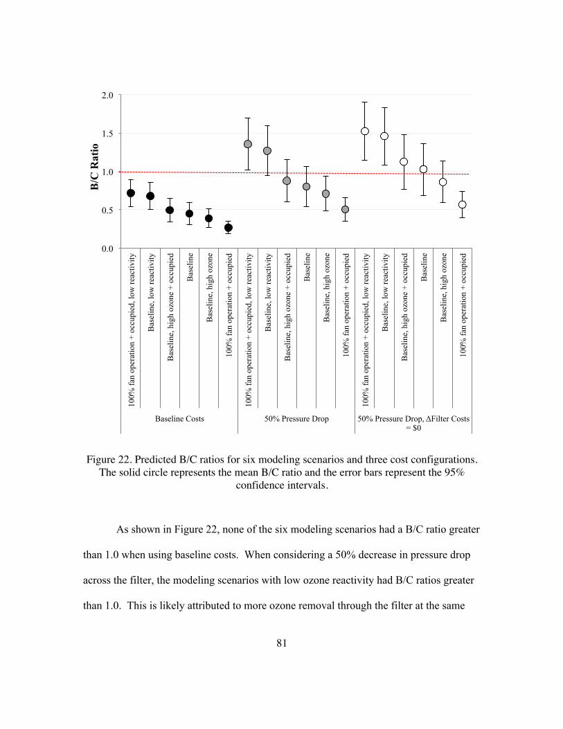
81

Figure 22. Predicted B/C ratios for six modeling scenarios and three cost configurations. The solid circle represents the mean B/C ratio and the error bars represent the 95%

confidence intervals.

As shown in Figure 22, none of the six modeling scenarios had a B/C ratio greater

than 1.0 when using baseline costs. When considering a 50% decrease in pressure drop

across the filter, the modeling scenarios with low ozone reactivity had B/C ratios greater

than 1.0. This is likely attributed to more ozone removal through the filter at the same

0.0

0.5

1.0

1.5

2.0

100%

fan

oper

atio

n +

occu

pied

, low

reac

tivity

Bas

elin

e, lo

w re

activ

ity

Bas

elin

e, h

igh

ozon

e +

occu

pied

Bas

elin

e

Bas

elin

e, h

igh

ozon

e

100%

fan

oper

atio

n +

occu

pied

100%

fan

oper

atio

n +

occu

pied

, low

reac

tivity

Bas

elin

e, lo

w re

activ

ity

Bas

elin

e, h

igh

ozon

e +

occu

pied

Bas

elin

e

Bas

elin

e, h

igh

ozon

e

100%

fan

oper

atio

n +

occu

pied

100%

fan

oper

atio

n +

occu

pied

, low

reac

tivity

Bas

elin

e, lo

w re

activ

ity

Bas

elin

e, h

igh

ozon

e +

occu

pied

Bas

elin

e

Bas

elin

e, h

igh

ozon

e

100%

fan

oper

atio

n +

occu

pied

Baseline Costs 50% Pressure Drop 50% Pressure Drop, ΔFilter Costs = $0

B/C

Rat

io

82

energy costs as the parallel modeling conditions at baseline reactivity. When the pressure

drop across the filter is decreased by 50% and the additional filter cost is zero (i.e., parity

with standard particle filter), the baseline condition has a B/C ratio of 1.3. Additionally,

five of the six modeling scenarios have error bars that exceed 1.0 indicating that the most

sensitive populations would still benefit from residential activated carbon filtration.

These results demonstrate that commercially available activated carbon filters

could be beneficial in homes, especially if the pressure drop and additional filter costs are

reduced. In nearly every case, it was determined that carbon filtration would be

beneficial and economically feasible for the most sensitive populations. This implies that

persons with existing respiratory conditions such as chronic obstructive pulmonary

disorder and asthma should consider purchasing activated carbon filters for their homes

to reduce ozone-related health outcomes. In doing so, they may also benefit

economically due to improved quality of life and reduced medical expenses.

Future work should include testing activated carbon filters that had accumulated

dust during operational use. Investigating the ozone removal capabilities of dust and

deposited chemical compounds may result in higher long-term ozone removal

efficiencies of carbon filters.

83

6. CONCLUSIONS

This chapter includes a brief summary of the overall project effort, major findings,

limitations, potential strategies to increase adoption of carbon filtration in buildings, and

recommendations for future work (path forward).

6.1. Summary of Research Effort

The overall objective of this research was to complete an assessment of the

potential benefits and costs associated with commercially available activated carbon

filters. A systems model was developed to determine the costs and benefits of activated

carbon filtration in multiple types of buildings. Model parameters were based on a

number of sources. These included an intensive search for, and review of, journal articles

in the peer-reviewed literature, conference papers, government reports, and technology

manufacturer websites. Analysis of resulting data allowed for a “state-of-technology”

assessment related to activated carbon filters.

84

6.2. Major Research Findings

Major research findings are presented below.

1. In-duct ozone removal is currently dominated by activated carbon filtration.

However, most carbon filter applications are generally marketed for control of

volatile organic compounds (VOCs) and/or odors, and not for control of ozone.

2. Commercial building applications dominate the activated carbon filter market and are

typically marketed for industrial control of gaseous pollutants.

3. Filter systems vary substantially in design, ranging from non-woven pleats that

contain activated carbon to V-bank trays and cassettes that contain granular activated

carbon.

4. Pleated activated filters appear to be the most common for non-industrial applications

or applications that do not require more costly systems. Most of these pleated filters

are hybrid (combination) systems for removal of both particulate matter and gases.

5. Activated carbon filters are currently of marginal benefit for residential applications

across most cities, with the exception of Riverside, California, and Phoenix, Arizona,

where the B/C ratios are relatively high. The B/C ratio increases with higher outdoor

ozone concentration, greater fractional operation time of HVAC systems, and older

85

populations with higher respiratory disease prevalence.

6. There are additional conditions for which activated carbon filtration becomes more

viable in residential settings, including increased occupancy and the presence of

sensitive individuals. For these special cases the use of activated carbon filtration in

residences appears to be beneficial and worthy of consideration in most cities at this

time.

7. For residential buildings, continuous fan operation during the summer ozone season

(assuming an Electronically Commutated Motor is available) can significantly

increase ozone removal effectiveness. The B/C ratio for such conditions is also

substantially increased for cities that would otherwise have relatively low HVAC

operation during the ozone season (e.g., Buffalo, Chicago, Minneapolis, New York

City), but is only slightly increased for other cities.

8. In general, across target cities the benefit/cost ratio for 1-inch filters is somewhat

lower than for 2-inch and 4-inch filters (the three depths studied herein) due to higher

differential pressure drops and associated energy costs between 1-inch AcC and

conventional particle filters. The B/C ratio is generally slightly lower for 4-inch than

2-inch filters due to higher differential costs for the former.

86

9. The benefits of activated carbon filtration in commercial (office) buildings are much

greater than in residential buildings (B/C several times higher) across all target cities.

Application of activated carbon filters to office buildings appears to be viable at this

time.

10. The benefits of activated carbon filtration in K-12 schools are much higher than for

residences, and such applications appear to be viable at this time. The dominant

benefit in terms of reduced DALYs comes in the form of prevented school loss days.

11. The benefits of activated carbon filtration in long-term health care facilities are

substantial (higher than for other building types that were considered in this study)

and should be considered for adoption at this time. The dominant benefit in terms of

reduced DALYs stems from reduced mortalities and reduced hospital admissions due

to chronic respiratory diseases.

12. The B/C ratio for activated carbon filters is sensitive to the differential cost between

activated carbon and particle filters. It is very likely that as demand for activated

carbon filters increases the cost differential will decrease, making their applications

even more attractive in the future.

13. In absolute terms, the additional cost (e.g., relative to a standard particle filter) of

activated carbon filtration in single-family homes for the summer ozone season is

87

approximately $10 per person or $25 per household. For a 1-inch activated carbon

filter in use during the summer ozone season, approximately 60% of the filtration cost

is attributed to the energy penalty due to additional pressure drop. Future research

should focus on investigating the operational pressure drop of activated carbon filters,

especially in single-family homes. Actual energy pentalties may be much lower than

predicted because of lower flowrates through the filter, resulting in the economical

use of activated carbon filters in single-family homes during the summer ozone

season.

6.3. Limitations of Research

This research was the most rigorous to date with respect to assessment of the benefits

and costs of activated carbon filtration for ozone control in buildings. Nevertheless,

research was limited in several ways.

1. The published and available gray literature related to long-term performance of

activated carbon for removal of ozone, particularly under the highly-variable

environmental conditions often encountered in practice, is sparse. For this study,

existing data were sufficient to develop preliminary assessments of ozone removal

effectiveness in residential and commercial buildings.

2. Average ozone concentrations across a five-month ozone season were used in this

analysis. In turn, the health effects following high/peak ozone events were not

88

captured. Indoor ozone control during such events would increase the benefit/cost

ratios described in this dissertation, particularly for sensitive populations.

3. Indoor ozone concentrations are typically much lower than outdoor ozone

concentrations, even without specific ozone control technologies. In this study we

assumed that there is no threshold below which incremental reductions in indoor

ozone concentration do not have a positive health effect. This is an important issue

that has yet to be effectively resolved by the health science community. If a threshold

is found to exist above typical indoor ozone concentrations the benefits described in

this dissertation might be substantially reduced. Importantly, if a threshold does exist

it will be dependent on averaging time and lowest for long-term averages such as

those used in this study.

4. The health effects of indoor secondary organic aerosols (SOA) are not well defined

and related predictions were largely omitted from this study. The same is true of

many other ozone reaction products, including many carbonyls, di-carbonyls,

carboxylic acids, peroxides, and more. In turn, the predicted health benefits in the

systems model may underestimate the overall health benefits of ozone removal via

activated carbon filtration.

5. Sources of indoor ozone were not included in this study. Such sources may be

important in offices or schools with poorly maintained and highly operated photocopy

89

machines and/or laser printers, or in residences or other buildings in which ion

generators or electrostatic precipitators are used for particle control. For such

scenarios the benefit/cost ratio of activated carbon filtration will increase.

6. In this study, the benefits and costs of ozone control are characterized entirely in

economic terms that are supported by reference to published literature. This requires

that reductions in physical suffering, e.g., from asthma, be quantified in a way that

reflects average societal values, and not necessarily those of individuals who suffer

the most from exposure to ozone. There are costs, both social and health, that are

difficult to impossible to quantify with any degree of accuracy. Those who have the

economic resources to spend more for health benefits may choose to do so. But there

is also a bias against those for whom the required marginal costs are impractical to

pay. These factors are difficult to capture and were not incorporated into the systems

model. As such, it is expected that the results presented herein underestimate the

overall benefit/cost ratio associated with ozone control, particularly for sensitive

sectors of the population.

7. On the cost side of the systems model, there is a substantial uncertainty related to

HVAC system efficiency. In this study, the worst-case scenario (i.e., use lower

boundary of HVAC system efficiency) was generally assumed. However, in

discussions with HVAC subject matter experts the combined system efficiency used

for commercial buildings (including long-term healthcare facilities and K-12 schools)

90

may be higher than values used in this study. This concern was addressed by running

another analysis and assuming a lower HVAC system efficiency. The results are

presented in Table 6. The analysis showed that the capital costs of the filters

(additional cost compared to standard particle filter plus disposal costs) dominated the

total cost of carbon filtration. Even in the worst-case scenario (demand charges plus

25% system efficiency), the highest energy penalty contributed to 27% of the total

cost of carbon filtration in a medium sized commercial office building. Despite the

higher energy costs, the B/C ratio of using carbon filtration still exceeded 7.0.

Although there is some uncertainty in HVAC system efficiency, the overall effect on

total filtration costs is minor, especially for 2-inch and 4-inch filters. Future research

should explore and measure the energy penalties of carbon filters in a large

population of operational buildings to determine the true impact on overall filtration

costs.

8. The effects of carbon filtration on the microbiome of the built environment were not

considered in this research and the impacts on the microbiome are unknown at this

time. This topic should be investigated in greater depth in future research projects

involving activated carbon filtration in HVAC systems.

91

6.4. Strategies to Improve Indoor Health with Activated Carbon Filters

A major research objective was to recommend potential strategies and policies to

utilize activated carbon filtration for ozone removal in buildings. The results of this

research indicated that carbon filtration in commercial office buildings, long-term

healthcare facilities, and K-12 schools during the summer ozone season (1 May to 30

September) would be beneficial. A revision of standards such as ASHRAE Standard

62.1 could result in widespread adoption of carbon filters in urban areas with high

seasonal ozone. Additionally, credentialing programs administered by organizations such

as ASHRAE and the U.S. Green Building Council could offer a path to incentivize

installing carbon filters in buildings.

Many of the health benefits gained by removing ozone in indoor environments

could be considered preventive care and could also improve worker productivity. A

wellness collaboration between health insurance companies and employers could

incentivize installing activated carbon filters in commercial office buildings, especially in

companies that are self-insured and directly bear the financial burden of employee

medical costs. In fact, lost productivity due to health impairments can cost a company

$1,400 to $2,600 per employee annually (Henke et al., 2010). Previous research

predicted that strategies to improve indoor air quality in commercial office buildings

could result in improved worker productivity resulting in benefit-to-cost ratios of 5 to 116

over a 20-year period (Wargocki and Djukanovic, 2005). In all of the modeling scenarios

92

in their research, the typical pay back for improved indoor air quality strategies was less

than two years with an average rate of return of 12.4-21.6%.

The performance of corporate wellness programs have been thoroughly

researched primarily because of the rising costs of medical care (Kelly et al., 2010). In

one case study examining best practices in two self-insured manufacturing companies,

investments in ergonomics and safety interventions resulted in a benefit-to-cost (B/C)

ratio exceeding 10:1 (Hantula et al., 2001). In another recent study involving more than

12,000 corporate wellness participants, the wellness program had an overall B/C ratio of

2.48 and the B/C ratio exceeded 9.0 when only evaluating the benefits of preventative

health risk assessments (Musich et al., 2015). Finally, in an 8-year study of a corporate

wellness program, the long-term B/C ratio averaged 2:1 and participants who had stayed

enrolled for the entire eight years reduced their annual healthcare expenses by 36%

(Schwartz et al., 2014). Average costs to the company ranged from $204 to $288 per

participant per year and annual medical costs were nearly $1,600 less per year compared

to non-participants.

The predicted costs of activated carbon filtration in commercial office buildings

averages less than $0.50 per month per employee. In turn, the company realizes nearly

$17 of health benefits per employee during the ozone season. Additional health and

productivity benefits will be gained due to the removal of volatile organic compounds

through the carbon filter and the reduction of ozone reaction products such as

formaldehyde and acetaldehyde. Therefore, a small investment in activated carbon filters

93

could result in substantial health and productivity benefits for companies and will pay for

itself within one ozone season.

Strategies for residential carbon filtration include using behavioral economics

concepts as default bias and social norms (Stevens, 2014). A strategy incorporating

default bias could involve medical practicioners supplying patients with filters during

office visits in conjunction with follow up visits and health assessments to determine if

the filter was installed and if the filter resulted in any health benefits. Strategies

involoving social norms have been fairly successful and include strategies such as

wearing helments on bikes and using seat belts while driving (Steven, 2014).

Incentivizing carbon filtration can also be a strategy for higher adoption rates in

single-family homes. Nearly a dozen studies were recently funded by the Affordable

Care Act to evaluate Medicaid incentive programs to improve health and encourage

healthy behaviors (Blumenthal et al., 2013). Incentive programs included cash incentives

and vouchers for medical-related expenses. A similar strategy could be implemented to

offset the cost of a residential carbon filter, especially in households that have members

with pre-existing respiratory conditions.

94

6.5. Research Path Forward

An important outcome of an assessment study is the identification of areas for

future research. Several future research areas are listed below.

1. Rigorous lab and field testing are needed to confirm, and expand on, the performance

of activated filters over a wide range of operating and environmental conditions in

actual buildings. Important metrics that should be measured over operational time

include single-pass ozone removal efficiency, pressure drop and air flow rate (and

incremental energy costs), and (if possible) improvements in occupant health,

productivity, and learning performance (for schools).

2. The systems model or other models should be modified and used to assess the

benefits of indoor ozone control during peak ozone events.

3. The systems model should be used for enhanced evaluation of the benefits and costs

of ozone control in buildings, perhaps including a wider range of carbon filter

technologies, building types and cities. With proper parameter distributions Monte

Carlo simulations might also be useful for elucidating fractional population benefits

and costs of activated carbon filtration.

4. Existing data related to reaction product yields and health effects associated with

organic nitrates stemming from NO3• chemistry preclude it from being further

95

considered for quantitative assessment in this study. However, given its potential

importance to human health we believe that nitrogen oxide chemistry should be

incorporated into future benefit/cost analyses related to ozone control, particularly

when data can reasonably support quantitative estimates of reaction products and

their impacts. In addition, we recommend altering the systems in the future to

analyze other air contaminants in the indoor environment.

96

Appendix A

PAPER I. BENEFIT-COST ANALYSIS OF COMMERCIALLY AVAILABLE ACTIVATED CARBON FILTERS FOR INDOOR OZONE REMOVAL IN RESIDENTIAL BUILDINGS (SUBMITTED TO INDOOR AIR)

97

PAPER I

Benefit-Cost Analysis of Commercially Available Activated Carbon Filters for Indoor Ozone Removal in Residential Buildings

(Submitted to Indoor Air)

Abstract

This study involved the development of a model for evaluating the potential costs and

benefits of ozone control by activated carbon filtration in single-family homes. The

modeling effort included the prediction of indoor ozone and ozone reaction products with

and without activated carbon filtration in the HVAC system. As one application, the

model was used to predict benefit-to-cost ratios for single-family homes in 12 American

cities in five different climate zones. Health benefits were evaluated using the disability-

adjusted life-years attributed to the difference in indoor ozone concentration with and

without activated carbon filtration and included city-specific age demographics for each

simulation. Costs of commercially-available activated carbon filters included capital

cost differences when compared to conventional HVAC filters of similar particle removal

rating, energy penalties due to additional pressure drop, and regional utility rates. The

average indoor ozone removal effectiveness ranged from 4 to 20% across the 12 target

cities, and was largely limited by HVAC system operation time. For the parameters

selected in this study, the mean predicted benefit-to-cost ratios for 1-inch filters were

greater than 1.0 in 10 of the 12 cities. However, median values for all 12 target cities

were below 1.0. The benefits of residential activated carbon filters were maximized in

98

cities with high seasonal ozone and HVAC usage, suggesting the importance of targeting

such conditions for activated carbon filter applications.

Introduction

Exposure to ozone and ozone reaction products is harmful to human health.

Ozone reacts with polyunsaturated fatty acids in fluids lining the lung with subsequent

adverse effects in the airway epithelium (Levy et al., 2001). Several researchers have

shown a link between exposures to ozone and premature mortality (Bell et al., 2005; Ito

et al., 2005; Jerrett et al., 2009; Levy et al., 2005; Smith et al., 2009; USEPA, 2006, and

references provided therein). Additionally, there have been several investigations that

associate ozone exposure and increases in respiratory-related hospital admissions (e.g.,

Burnett et al., 1999), minor restricted activity days (e.g., Ostro and Rothschild, 1989),

and school loss days (e.g., Chen et al., 2000). The USEPA estimates that 265 to 450 lives

would be saved per year by reducing the eight hour ozone standard by 5 parts per billion

(ppb), resulting in potential annual health benefits of U.S. $7.5 billion to $15 billion

(2011 dollars) per year (USEPA, 2014a).

Nearly one third of Americans live and work in counties with ozone

concentrations that exceed the primary eight-hour average National Ambient Air Quality

Standard (NAAQS) for ozone, which is currently 75 ppb (USEPA, 2014b). The NAAQS

for ozone is meant to protect public health, including the health of sensitive populations

such as children, people with asthma, and the elderly. Ozone concentrations are typically

lower indoors than outdoors, largely due to its reaction with materials in the building

99

envelope, heating, ventilating, and air conditioning (HVAC) system components,

building contents, and occupied space (Chen et al., 2012a; Fadeyi, 2014; Fadeyi et al.,

2013; Fadeyi et al., 2009; Morrison et al., 1998; Stephens et al., 2012; Wang and

Morrison, 2010; Wang and Morrison, 2006; Weschler, 2000). Although ozone

concentrations are typically lower indoors than outdoors, Americans spend an average of

nearly 90% of their time indoors (Klepeis et al., 2001). This leads to the indoor

environment being important with respect to total inhalation exposure to ozone. For

example, in a study involving 2,500 residences in seven cities, indoor exposure accounted

for 43% to 76% of total daily exposure to ozone, with a mean of 60% (Weschler, 2006).

As such, ozone control in single-family homes should be further explored.

Very little epidemiological research has been dedicated to studying the effects of

ozone exposure in indoor environments. Instead, most epidemiological research on

ozone exposure has relied on ozone measurements taken from outdoor fixed monitors

(Bell et al., 2014; Bell et al., 2006; Bell et al., 2005; Bell et al., 2004; Berman et al.,

2012; Hubbell et al., 2005; USEPA 2014a; USEPA 2012). However, Chen et al. (2012a)

used a simple mass balance model and showed that variations in ozone mortality can be

partially explained by the amount of ozone transported into residential buildings through

infiltration, windows, and HVAC systems. This finding is consistent with observations

that the prevalence of centralized air conditioning systems, which are associated with

lower air exchange rates and lower indoor ozone concentrations, is inversely associated

with ozone-related mortality (Smith et al., 2009).

100

In a seminal study of indoor exposure to ozone, Weschler et al. (1989) concluded

that indoor exposure to ozone is greater than outdoor exposure for many Americans, and

that “relatively inexpensive strategies exist to reduce indoor ozone levels.” Given the

well-established health and welfare impacts of ozone exposure, it is appropriate to

explore the benefits of indoor ozone reduction and the costs of building-scale ozone

control. The purpose of this study is threefold: (1) To determine if commercially

available activated carbon filters are effective at removing ozone in homes; (2) To

determine if using commercially available activated carbon filters is an economically

viable strategy to reduce ozone in homes; (3) To determine conditions for which the

benefits of residential activated carbon filtration might be particularly high, thus

informing public health strategists and standard-setting organizations.

Model Development

The model developed for this project consists of an integrated system that

addresses several major components and their interconnections (Figure 1). The

integrated model is used to determine the concentration of ozone in buildings and is

intended for determining indoor ozone and ozone reaction product concentrations in

multiple types of buildings. In this assessment, we are only evaluating ozone-related

health benefits when using activated carbon filtration in single-family homes.

101

Figure 1. Conceptual model illustrating interconnected sub models of the integrated systems model.

Mass Balance and Chemistry Model

Core model equations are used to solve for ozone concentration and

concentrations of several key reaction products as previously presented in Fadeyi (2014),

Chen et al. (2012a), and Weschler and Shields (2000). The fate of ozone within a

building is estimated using a simplified mass balance equation and assuming a well-

mixed environment. The model is designed to estimate concentrations of ozone for

scenarios without any control devices and scenarios with control devices in place. The

differences in these scenarios are used to quantify the health benefits of ozone control.

The time-averaged mass balance equation for ozone is presented Equations (1). A

detailed derivation of Equation (1) is presented in the supplementary information.

102

𝐶!! =  𝑝𝜆𝑖𝑛𝑓𝐶𝑜,𝑂3

𝜆𝑖𝑛𝑓+𝐻𝑜𝑛𝜆𝑟𝑒𝑐𝑓𝑐,𝑂3+  (𝐻𝑜𝑛𝑘𝑑𝑒𝑝,𝑂3,𝐴𝐶𝑜𝑛∗ +  (1−𝐻𝑜𝑛  )𝑘𝑑𝑒𝑝,𝑂3,𝐴𝐶𝑜𝑓𝑓

∗ )+   𝑘𝑗𝐶𝑗𝑗

(1)

Where,

λinf = infiltration air exchange rate [h-1]

λrec = recirculation air exchange rate of HVAC system [h-1]

Cj = concentration of gaseous reactant j in the occupied space [ppb]

CO3 = concentration of ozone in the occupied space [ppb]

Co,O3 = concentration of ozone in outdoor air [ppb]

fc,O3 = single-pass fractional removal of ozone by an activated carbon filter [-]

Hon = average annual fraction of time that the HVAC system operates [-]

k*dep,O3,AC_on = ozone decay rate for integrated background surfaces w/ HVAC on [h-1]

k*dep,O3, AC_off = ozone decay rate for integrated background surfaces w/ HVAC off [h-1]

kj = bimolecular homogeneous reaction rate constant [ppb-1�hr-1]

p = fractional penetration through the building envelope for ozone [-]

103

Concentrations of common ozone reaction products such as formaldehyde,

acetaldehyde, and secondary organic aerosols can also be determined by mass balance

equations as shown in the supplementary information.

In a preliminary modeling analysis, the health outcomes for formaldehyde and

acetaldehyde were calculated using methods described in Logue et al. (2012) and

Huijbregts et al. (2005). However, the initial modeling results indicated that the health

benefits of reduced reaction products were greatly outweighed by the benefits of

reductions in ozone, on the order of attributing 1% or less of the total overall health

benefits. Additionally, the DALYs calculations for formaldehyde and acetaldehyde were

determined from animal testing and incorporated a large amount of uncertainty

(Huijbregts et al., 2005). In contrast, the ozone-related DALYs were determined from

human exposure models and are commonly used in epidemiological analyses (USEPA,

2012b).

Health outcomes for exposure to secondary organic aerosols (SOA) are very

uncertain due to the size and composition of the aerosols (Polidori et al., 2007).

However, the health effects of ozone-generated SOA exposure may have a higher

oxidative capacity than PM2.5 that could result in oxidative stress in the pulmonary

system (Delfino et al., 2013). Additionally, the small size of SOA may result in a higher

penetration into the respiratory tract. This could subsequently lead to the transport of

SOA to other organs through the circulatory system (Oberdorster et al., 2010). At this

time, it’s difficult to accurately quantify the health benefits of reductions in ozone-

generated SOA, however, this could be an important topic to research given the potential

104

health implications. Therefore, due to the uncertainty in determining the health effects of

reductions in ozone reaction products, only reductions in ozone due to activated carbon

filtration were considered in this analysis.

Ozone Removal Effectiveness

Ozone removal effectiveness is defined as the percent reduction in indoor ozone

concentration when an ozone control device is used relative to an identical condition

when such a device is not used, as described by Equation (2).

Ω = (1 – CAcC/CNo_AcC) × 100% (2)

Where,

Ω = ozone removal effectiveness of activated carbon filter (%)

CAcC = indoor ozone concentration with activated carbon filter installed (ppb)

CNo_AcC = indoor ozone concentration without activated carbon filter installed (ppb)

Benefit Model

Benefits are calculated using reductions in disability-adjusted life-years (DALYs)

due to reductions in indoor ozone concentration following the application of activated

carbon filtration. Disability-adjusted life-years are a metric for quantifying the burden of

disease, and incorporate years of life lost from premature mortality and years of life lost

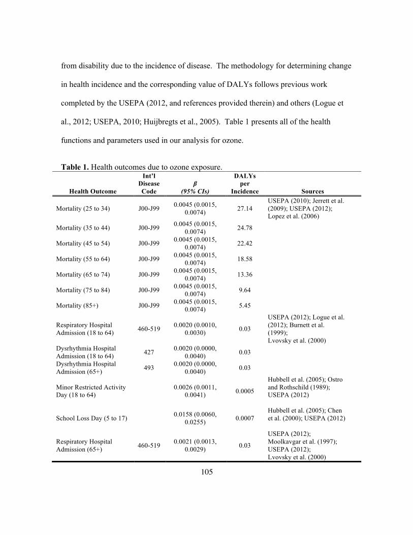
105

from disability due to the incidence of disease. The methodology for determining change

in health incidence and the corresponding value of DALYs follows previous work

completed by the USEPA (2012, and references provided therein) and others (Logue et

al., 2012; USEPA, 2010; Huijbregts et al., 2005). Table 1 presents all of the health

functions and parameters used in our analysis for ozone.

Table 1. Health outcomes due to ozone exposure.

Health Outcome

Int’l Disease Code

β (95% CIs)

DALYs per

Incidence Sources

Mortality (25 to 34) J00-J99 0.0045 (0.0015, 0.0074) 27.14

USEPA (2010); Jerrett et al. (2009); USEPA (2012); Lopez et al. (2006)

Mortality (35 to 44) J00-J99 0.0045 (0.0015, 0.0074) 24.78

Mortality (45 to 54) J00-J99 0.0045 (0.0015, 0.0074) 22.42

Mortality (55 to 64) J00-J99 0.0045 (0.0015, 0.0074) 18.58

Mortality (65 to 74) J00-J99 0.0045 (0.0015, 0.0074) 13.36

Mortality (75 to 84) J00-J99 0.0045 (0.0015, 0.0074) 9.64

Mortality (85+) J00-J99 0.0045 (0.0015, 0.0074) 5.45

Respiratory Hospital Admission (18 to 64) 460-519 0.0020 (0.0010,

0.0030) 0.03

USEPA (2012); Logue et al. (2012); Burnett et al. (1999); Lvovsky et al. (2000)

Dysrhythmia Hospital Admission (18 to 64) 427 0.0020 (0.0000,

0.0040) 0.03

Dysrhythmia Hospital Admission (65+) 493 0.0020 (0.0000,

0.0040) 0.03

Minor Restricted Activity Day (18 to 64)

0.0026 (0.0011, 0.0041) 0.0005

Hubbell et al. (2005); Ostro and Rothschild (1989); USEPA (2012)

School Loss Day (5 to 17) 0.0158 (0.0060,

0.0255) 0.0007 Hubbell et al. (2005); Chen et al. (2000); USEPA (2012)

Respiratory Hospital Admission (65+) 460-519 0.0021 (0.0013,

0.0029) 0.03

USEPA (2012); Moolkavgar et al. (1997); USEPA (2012); Lvovsky et al. (2000)

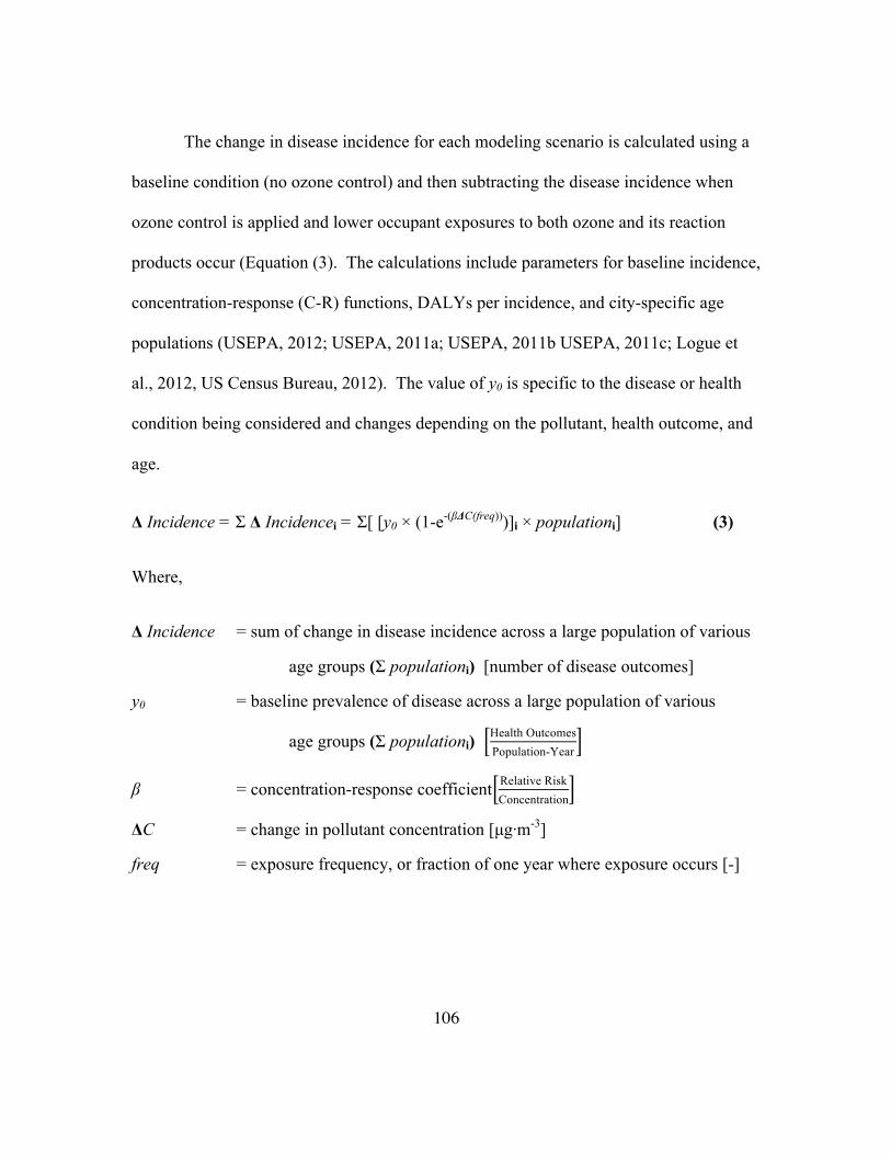
106

The change in disease incidence for each modeling scenario is calculated using a

baseline condition (no ozone control) and then subtracting the disease incidence when

ozone control is applied and lower occupant exposures to both ozone and its reaction

products occur (Equation (3). The calculations include parameters for baseline incidence,

concentration-response (C-R) functions, DALYs per incidence, and city-specific age

populations (USEPA, 2012; USEPA, 2011a; USEPA, 2011b USEPA, 2011c; Logue et

al., 2012, US Census Bureau, 2012). The value of y0 is specific to the disease or health

condition being considered and changes depending on the pollutant, health outcome, and

age.

Δ Incidence = Σ Δ Incidencei = Σ[ [y0 × (1-e-(βΔC(freq)))]i × populationi] (3)

Where,

Δ Incidence = sum of change in disease incidence across a large population of various

age groups (Σ populationi) [number of disease outcomes]

y0 = baseline prevalence of disease across a large population of various

age groups (Σ populationi) Health OutcomesPopulation-Year

β = concentration-response coefficient Relative RiskConcentration

ΔC = change in pollutant concentration [µg·m-3]

freq = exposure frequency, or fraction of one year where exposure occurs [-]

107

Generally, the reduction in indoor ozone concentrations in single-family homes

will be relatively small (typically less than 5 ppb) compared to peak outdoor ozone

events. We used USEPA methodology to convert peak ozone events to seasonal average

concentrations (USEPA, 2012). Additionally, we inquired with a health scientist at the

USEPA (Fann, 2014) to determine if any thresholds are used for ozone in USEPA risk

assessments. The USEPA does not currently use a threshold for ozone exposure and so

we assumed that there would be potential health benefits for small reductions in indoor

ozone concentrations.

The number of DALYs per pollution exposure is calculated using Equation (4),

and the estimated health benefit across a whole population (Σ populationi) is calculated

using Equation (5).

ΔDALYs = DALYsIncidence

× ΔIncidence (4)

Benefits = $/DALY × ΔDALYs (5)

Where,

Benefit = monetary benefit associated with reduced DALYs per 100,000 people [$]

$/DALY = value of one disability adjusted life year [$·year-1]

ΔDALYs = reduction in DALYs (relative to no control) when a control is used [years]

108

When calculating DALYs, the number of years of life lost per mortality is

dependent on the age at which mortality occurs (Lopez et al., 2006). The greatest

uncertainty in the benefits analysis is attributed to the value of an avoided DALY, more

specifically, what the average person is willing to pay to avoid a health-related issue due

to ozone exposure. One generally accepted approach is to equate one DALY avoided as

approximately equal to three times the per capita gross domestic product (Rascati, 2006).

In the United States, this is equivalent to approximately $150,000 (2014 US dollars) per

avoided DALY (World Bank, 2014). Bobinac et al. (2014) also evaluated the value of a

quality-adjusted life-year (QALY) gained in the Netherlands using a survey incorporating

a broad range of ages, incomes, and educational levels. One QALY gained is equivalent

to one avoided DALY. Their methods used a weighting factor from Tversky and

Kahneman (1992) to integrate decision theory and human behavior under risk. From

their survey results, they were able to estimate a probabilistic distribution of what the

average person is willing to pay to gain a QALY. Their results indicated a distribution

with a mean of approximately $140,000 (2014 US dollars) per avoided QALY.

For this paper, a distribution of dollars per avoided DALY was developed based

on Bobinac et al. (2014), and was used to estimate the benefits of reduced exposure to

ozone and its reaction products. This method yields lower benefits than the USEPA

methodology used in the Regulatory Impact Analysis for ozone (USEPA, 2008). The

USEPA uses a value per statistical life (VSL) of approximately $9.3 million (2014 U.S.

dollars) per life lost regardless of age at the time of death (USBLS, 2014; USEPA,

109

2011b). In contrast, the DALYs method assigns a value of life based on the years of life

lost compared to the average life expectancy, which results in lower benefits when

compared to the USEPA method. Further information on the DALYs calculations and

benefit model are provided in the supplemental information.

Cost Model

Overall filter costs include the difference in capital costs (materials and labor)

between a standard particle filter and an activated carbon filter, as well as additional

energy costs due to the difference in pressure drop between a standard particle filter and

an activated carbon filter. Other costs such as installation and disposal are not included

in this paper as our analysis focused on commercially available filters designed for

residential HVAC systems. Overall filter costs are calculated for a population of 100,000

using Equation (6) and assuming one to two filters per residential HVAC unit during the

summer ozone season (1 May through 30 September):

Costs = Pelec × 𝐸!"#$ + 𝐹!"#$ + 𝐿!"#$  ×   RF  ×   100,000Occ.

(6)

Where,

Costs = overall differential cost between activated carbon and conventional particle

filters (AcC – particle) per 100,000 persons [$]

110

Pelec = seasonal electricity usage [kWh] due to additional pressure drop

= !!"#$%&  ×  𝚫!!"##  ×  !!"_!"!

!"""  ×  !!"#$

Ecost = electricity cost per kWh [$]

Qfilter = flowrate through the filter [m3·h-1]

ΔPdiff = difference in pressure drop across the filter between AcC filter and standard

filter [Pa]

Hon_tot = total number of hours of HVAC operation [hours]

𝜂!"#$ = overall efficiency of the HVAC fan and motor [-]

Fcost = difference in filter costs between AcC filter and standard particle filter [$]

(assumed to equal zero for residences)

Lcost = difference in labor, replacement, and disposal costs between AcC and

particle filters [$] (assumed to equal zero for residences)

RF = filter replacement frequency [season-1]

Occ. = building occupancy [persons] (average varies by city)

City specific electricity costs and HVAC operational runtimes are provided in

greater detail in the supplementary information. Overall filter costs are extrapolated for a

population of 100,000 in order to compare with DALYs using the same metric (per

100,000 people).

111

Monte Carlo Simulation

Due to the uncertainty in all of the model parameters, a Monte Carlo simulation

similar to models used previously in Gall et al. (2011) and Morrison et al. (2011) were

used to estimate changes in indoor ozone concentration with and without activated carbon

filters, the difference in DALYs due to changes in ozone exposure, and the benefits and

costs of utilizing activated carbon filters in residences during the summer ozone season.

The key metrics used to measure the impacts of activated carbon filters include

the ozone removal effectiveness and the B/C ratio. A sensitivity analysis of the systems

model was completed to estimate the influence of individual modeling parameters to

changes in ozone removal effectiveness and the benefit-to-cost ratio (B/C). Additional

details on the sensitivity analysis are presented in the supplemental information.

Model parameters that were assumed to not vary geographically are presented in

Table 2. City-specific model parameters are presented in the supplemental information.

Distributions were estimated from the references when possible, and in some cases when

additional data was not available, distributions were estimated using the mean and

standard deviations of data (modeled as normal distributions) reported in the literature.

In those cases where only extreme (i.e., minimum and maximum) values were found in

the literature, a uniform distribution was assumed.

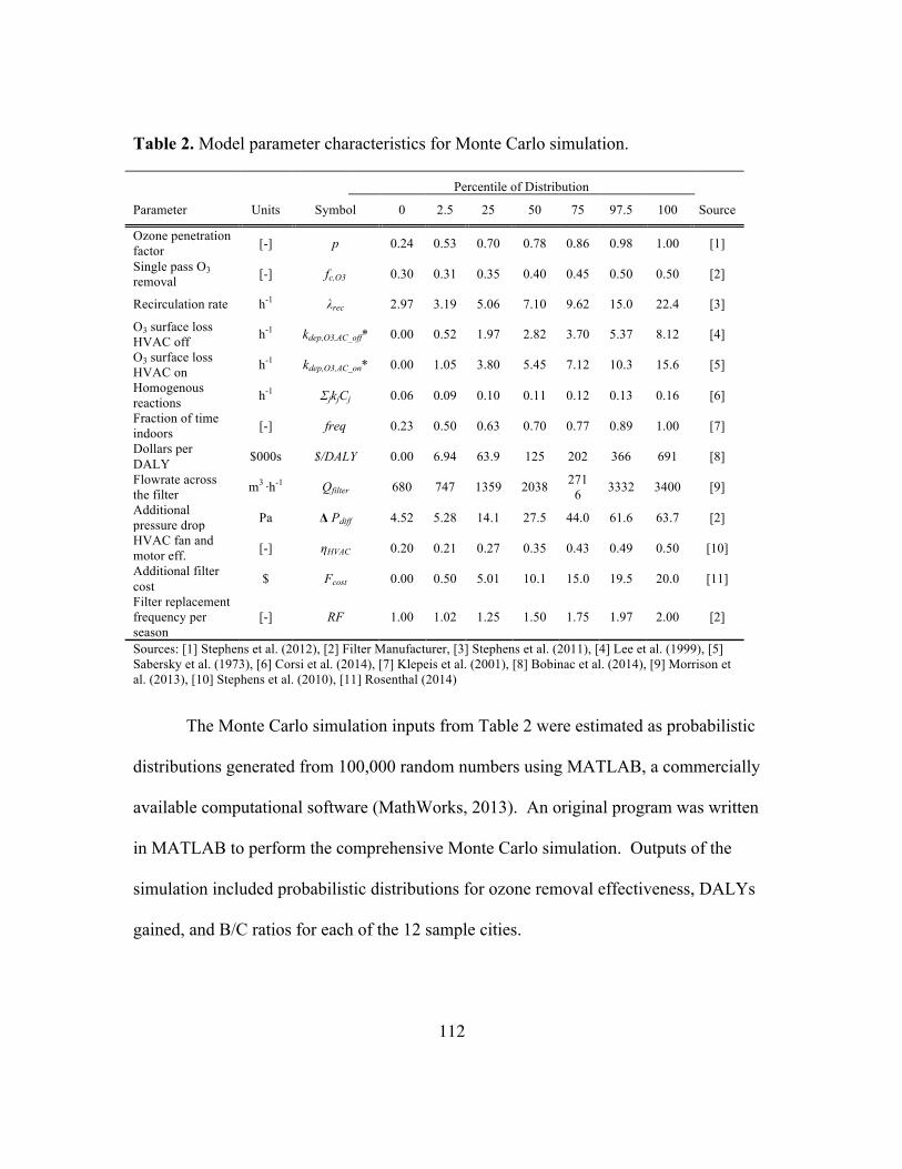
112

Table 2. Model parameter characteristics for Monte Carlo simulation.

Percentile of Distribution

Parameter Units Symbol 0 2.5 25 50 75 97.5 100 Source

Ozone penetration factor [-] p 0.24 0.53 0.70 0.78 0.86 0.98 1.00 [1]

Single pass O3 removal [-] fc,O3 0.30 0.31 0.35 0.40 0.45 0.50 0.50 [2]

Recirculation rate h-1 λrec 2.97 3.19 5.06 7.10 9.62 15.0 22.4 [3]

O3 surface loss HVAC off h-1 kdep,O3,AC_off* 0.00 0.52 1.97 2.82 3.70 5.37 8.12 [4]

O3 surface loss HVAC on h-1 kdep,O3,AC_on* 0.00 1.05 3.80 5.45 7.12 10.3 15.6 [5]

Homogenous reactions h-1 ΣjkjCj 0.06 0.09 0.10 0.11 0.12 0.13 0.16 [6]

Fraction of time indoors [-] freq 0.23 0.50 0.63 0.70 0.77 0.89 1.00 [7]

Dollars per DALY $000s $/DALY 0.00 6.94 63.9 125 202 366 691 [8]

Flowrate across the filter m3 ·h-1 Qfilter 680 747 1359 2038 271

6 3332 3400 [9]

Additional pressure drop Pa Δ Pdiff 4.52 5.28 14.1 27.5 44.0 61.6 63.7 [2]

HVAC fan and motor eff. [-] ηHVAC 0.20 0.21 0.27 0.35 0.43 0.49 0.50 [10]

Additional filter cost $ Fcost 0.00 0.50 5.01 10.1 15.0 19.5 20.0 [11]

Filter replacement frequency per season

[-] RF 1.00 1.02 1.25 1.50 1.75 1.97 2.00 [2]

Sources: [1] Stephens et al. (2012), [2] Filter Manufacturer, [3] Stephens et al. (2011), [4] Lee et al. (1999), [5] Sabersky et al. (1973), [6] Corsi et al. (2014), [7] Klepeis et al. (2001), [8] Bobinac et al. (2014), [9] Morrison et al. (2013), [10] Stephens et al. (2010), [11] Rosenthal (2014)

The Monte Carlo simulation inputs from Table 2 were estimated as probabilistic

distributions generated from 100,000 random numbers using MATLAB, a commercially

available computational software (MathWorks, 2013). An original program was written

in MATLAB to perform the comprehensive Monte Carlo simulation. Outputs of the

simulation included probabilistic distributions for ozone removal effectiveness, DALYs

gained, and B/C ratios for each of the 12 sample cities.

113

Benefit-Cost Analysis of Carbon Filtration in Single-Family Homes in 12 U.S. Cities

The systems model described herein was used to assess changes in indoor ozone,

health incidence, and the B/C ratio for ozone control in 12 U.S. cities. At least two cities

from each of the five climate zones defined by the Energy Information Administration

were selected for the analysis. The following cities were included in the analysis:

Atlanta, Austin, Buffalo, Chicago, Cincinnati, Houston, Miami, Minneapolis, New York

City, Phoenix, Riverside, and Washington D.C. This group of cities represents a broad

nationwide sample of population, climate, building stock, and ambient ozone

concentrations. Housing data for each city were collected from multiple sources,

including the American Housing Survey (AHS) (U.S. Census, 2013), Chen et al. (2012a

and 2012b), and Persily et al. (2010). Data collected on city-specific summer ozone

concentration, electricity costs, HVAC usage, and building characteristics are provided in

the supplemental information.

A final modeling simulation incorporated an assumption that all of the ozone-

related health outcomes would apply only during the summer ozone season. In the

previous analyses, the calculated DALYs were scaled by 5/12 in order to compare the

benefits with the associated filter energy costs from 1 May to 30 September. However, in

other analyses that incorporate USEPA protocols for determining health outcomes from

ozone exposure, the health outcomes for the entire year were assumed to occur during the

ozone season. Berman et al. (2012) and Hubbell et al. (2005) used USEPA modeling

software to evaluate the potential health benefits of reductions in ambient ozone from 1

114

May to 30 September in cities across the U.S. The USEPA regulatory impact assessment

for ozone (USEPA, 2014b) incorporates health outcome functions that were originally

applied to the summer ozone season, and some of the applied ozone controls (e.g.,

regulating gasoline vapor pressure) are only used during the summer season. The results

of the modeling exercise are presented in the supplemental information (Figures S6 and

S7).

Results and Discussion

Results for applications of activated carbon (AcC) filters in single-family homes

in each of 12 target cities are presented in this section. All analyses correspond to only

the summer ozone season, taken to be May 1st to September 30th for each city.

Filter costs were primarily driven by the additional energy costs for 1-inch (2.5

cm) filters due to increased pressure drop. Approximately 60% of the filtration costs

were attributed to energy costs, with the remaining costs attributed to the additional cost

of the filter in comparison to a standard particle filter.

The ozone removal effectiveness of AcC filtration in single-family homes is

presented in Figure 2. Cities with high air-conditioning usage during the ozone season

have the highest values of ozone removal effectiveness. The highest base-case

effectiveness (approximately 20%) occurs for homes in Miami, and is limited by the

frequency of HVAC operation and single-pass ozone removal efficiency for the AcC

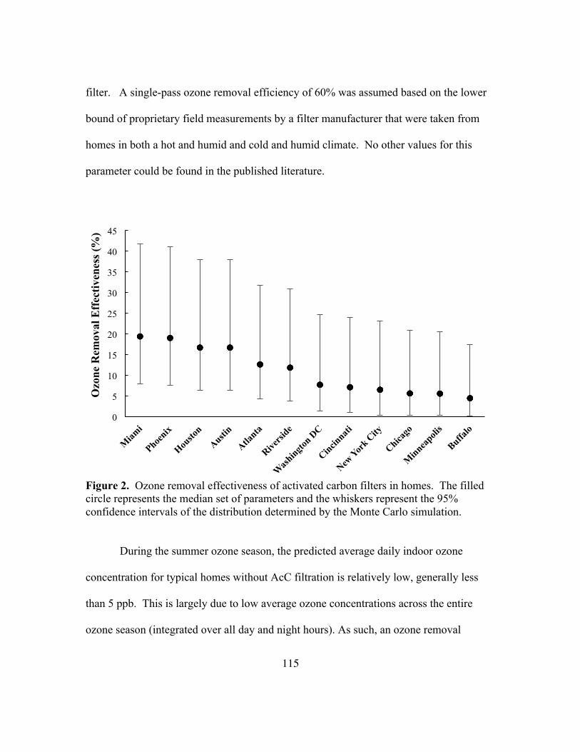
115

filter. A single-pass ozone removal efficiency of 60% was assumed based on the lower

bound of proprietary field measurements by a filter manufacturer that were taken from

homes in both a hot and humid and cold and humid climate. No other values for this

parameter could be found in the published literature.

Figure 2. Ozone removal effectiveness of activated carbon filters in homes. The filled circle represents the median set of parameters and the whiskers represent the 95% confidence intervals of the distribution determined by the Monte Carlo simulation.

During the summer ozone season, the predicted average daily indoor ozone

concentration for typical homes without AcC filtration is relatively low, generally less

than 5 ppb. This is largely due to low average ozone concentrations across the entire

ozone season (integrated over all day and night hours). As such, an ozone removal

0

5

10

15

20

25

30

35

40

45

Ozo

ne R

emov

al E

ffec

tiven

ess (

%)

116

effectiveness of less than 20% leads to very small absolute reductions in averaged indoor

ozone concentrations in each target city, i.e., less than 1 ppb. Of course, the outdoor and

absolute indoor concentrations and concentration reductions are often much higher (by a

factor of 2 to 4) than average values during daily outdoor one-hour or eight-hour peaks.

And there are some conditions in homes, e.g., low background reactivity and high air

exchange rate, which lead to higher indoor ozone concentrations. Importantly, relatively

small reductions (5 ppb) in outdoor ozone concentrations have been shown to yield

population-wide health benefits (e.g., Berman et al. 2012; Hubbell et al. 2005). However,

the published literature is insufficient to determine ozone concentration thresholds below

which reductions in ozone exposure provide tangible health benefits. Our analysis is

based on an assumption of no threshold concentration below which health effects are not

observed. We note that mortality risk associated with increased outdoor ozone

concentrations appears to occur even at low concentrations of tropospheric ozone, with

thresholds as low or lower than approximately 10 ppb for 24-hour averages and 20-30

ppb for daily one-hour maximum concentration (Bell et al., 2006; Kim et al., 2004).

Reductions in annual DALYs per 100,000 people are shown in Figure 3, with

median values ranging from 1 to 5 DALYs per 100,000 per year. Bounds on health

benefits and benefit/cost ratios are based on 95% confidence intervals of health functions

and were used to estimate disability-adjusted life years (DALYs) and mortality.

117

Figure 3. Reductions in DALYs per year from using activated carbon filters in homes. The filled circle represents the median and the whiskers represent the 95% confidence intervals of the DALY parameter distributions determined by the Monte Carlo simulation.

Of the 12 target cities, homes in Phoenix would benefit the most from carbon

filtration, followed closely by Riverside (Figure 4). For each of these two cities the mean

B/C ratio is approximately 2.0. High summertime ozone concentrations and relatively

new building stocks characterize these two cities with high air conditioning usage during

summer months. This implies that cities with high summer temperatures (and by

extension high air conditioning usage), high summertime ozone, and a high proportion of

residential air conditioning usage (implying newer building stock) will benefit the most

0

5

10

15

20

25

30

35

40 R

educ

ed D

ALY

s per

100

,000

118

from residential carbon filtration. Cities that had lower B/C ratios include Buffalo and

Minneapolis. These two cities are characterized by a milder summer climate and

generally lower air conditioning usage (Chen et al., 2012a). In addition, since both cities

have milder climates and older building stock, residents may generally open windows for

cooling and may also experience higher rates of infiltration through the building

envelope. This is an important consideration for our analysis because the filters can only

remove ozone when the HVAC system is operating.. Additionally, cities with older

building stock typically do not have central HVAC systems (Chen et al., 2012a), further

limiting the benefits of activated carbon filtration.

Figure 4. Benefit-to-cost ratios from using activated carbon filters in homes. The filled circle represents the median, the filled box represents the mean, and the whiskers represent the 95% confidence intervals of the distribution determined by the Monte Carlo simulation.

0 1 2 3 4 5 6 7 8 9

10 11 12 13 14

B/C

Rat

io

119

The upper bound of B/C ratios for each city ranged from approximately 6 to 13,

indicating that some fraction of the population receives significant benefits from

activated carbon filtration. This subset is generally characterized as a subpopulation with

existing respiratory sensitivities (asthma, and other chronic pulmonary disorders), as well

as the population over the age of 65, which generally has a much higher incidence rate

for respiratory morbidity and mortality.

In order to explore strategies that significantly improve the impacts of carbon

filtration in homes, the single pass removal efficiency for ozone was varied from 10% to

100% over the summer ozone season to determine what effect this parameter has on the

B/C ratio in Phoenix. This range of single pass removal efficiencies is similar to

experimental results for commercial carbon filters tested at 120 ppb of ozone by Lee and

Davidson (1999). Figure 5 shows results of the model simulation. Even at 100% single

pass removal efficiency, the median B/C ratio is less than 1.0 (0.92). However, the mean

B/C ratio exceeds 1.0 with a single pass removal efficiency of 20% (1.39) and exceeds

2.0 with 40% single pass removal efficiency.

120

Figure 5. Benefit-to-cost ratios for homes in Phoenix, AZ. The filter efficiency is varied to show the B/C over multiple single pass removal efficiencies for ozone. The filled circle represents the median, the filled box represents the mean, and the whiskers represent the 95% confidence intervals of the distribution determined by the Monte Carlo simulation.

Fan operation at 100% increases the ozone removal effectiveness, but its impact

on the benefit/cost ratio is not as obvious. As such, another simulation was conducted to

estimate Ω and B/C ratios in Phoenix homes with 100% fan operation during the summer

ozone season. Although ozone removal effectiveness was optimized (median Ω = 51%),

the additional costs of 100% fan operation resulted in lower B/C ratios compared to using

the standard HVAC cycling operation (median value of 0.68) due to increased energy

costs.

0 1 2 3 4 5 6 7 8 9

10 11 12 13 14 15 16 17 18 19 20

0% 10% 20% 30% 40% 50% 60% 70% 80% 90% 100%

B/C

Rat

io

Ozone Single Pass Removal Efficiency

121

Modeling the “Optimal” Home for Activated Carbon Filtration

A final set of residential analyses was completed to assess reasonable model

parameters that lead to high B/C ratios. We assume that the “optimal” house for

activated carbon filtration will be a home with high occupancy (at least four people per

home), low surface reactivity (typical of homes with tile or wood floors versus carpet),

100% HVAC fan operation utilizing highly efficient electronically commutated motors to

reduce additional energy costs (70% motor efficiency), and high performance filters with

a single pass ozone removal efficiency of 90% or higher. Although not necessarily

maximum values in a true optimization sense, these conditions are referred to here as

“optimal”. Simulation results are presented in Figure 6.

122

Figure 6. Benefit-to-cost ratios from using activated carbon filters in “optimal” homes. The filled circle represents the median, and the filled box represents the mean of the distribution. The whiskers represent the 95% confidence intervals of the Monte Carlo distribution.

As shown in Figure 6, all of the 12 cities have mean B/C values greater than 1.0

for the optimal condition. Phoenix, Cincinnati, and Miami all have median B/C values

greater than 1.0. The benefits of activated carbon filtration in “optimal” homes are most

directly associated with relatively high outdoor ozone concentrations, older population

demographics, and lower local electricity costs. For example, the benefits in Austin and

Houston are actually lower in comparison to standard conditions in those two cities,

because both cities have relatively young populations. Finally, homes with more

0

10

20

30

40

50

60

70

80

90 B

/C R

atio

12.5 8.9

12.9 11.0 11.3 10.5 10.4 10.7 10.0 9.8 7.2 8.3 3.5 4.3 4.2 3.9 3.7 3.5 3.4 3.3 3.2 2.9 2.6 2.2

123

occupants will have higher benefits as more people are sharing the cost of carbon

filtration.

Limitations of the Modeling Effort

Our analysis is conservative with regards to the scope of the health benefits

achieved with carbon filtration, since reductions in secondary organic aerosols (SOAs)

and other reaction products for which DALY parameters are unknown were not included

in the health model. There is also very little research in the published literature regarding

the performance of commercially available activated carbon filters in operational

environments. This is a topic of research that should be investigated further.

Another limitation of this research is that we utilized long-term (i.e., seasonal)

reductions in ozone exposure. Future research should investigate the changes in exposure

in relationship to diurnal variations in outdoor ozone and dynamic HVAC cycling. These

parameters should be investigated in parallel with occupancy in single-family homes to

determine the true reductions in ozone exposure when using activated carbon filters.

Finally, the monetary benefits used in our analysis are conservative (i.e., much

lower) in comparison to methods used by the USEPA to compare the costs and benefits

of lowering ambient ozone standards. When considering the costs of carbon filtration in

single-family homes, we deferred to using higher capital and operating costs when

lacking sufficient data to estimate the true cost of filtration. In reality, the costs of carbon

filtration may be lower, especially if filters are purchased in bulk and in homes with

HVAC motor efficiencies greater than the standard conditions used in our analysis.

124

Conclusion

An integrated (systems) model was developed to estimate the benefits and costs of

in-duct activated carbon control of ozone. The model can be used for any building

scenario. An example application for single family homes in 12 U.S. cities was used

here. When modeling carbon filtration in single-family homes across 12 cities in five

different climate zones in the United States, the median indoor ozone removal

effectiveness ranged from 4 to 20% during the summer ozone season. Due to the

uncertainty of the mass balance and health analyses, a Monte Carlo simulation was used

to estimate the potential benefits and costs of carbon filtration in single-family homes.

For the parameters selected in this study, the mean predicted benefit/cost (B/C) ratios for

1-inch filters were greater than 1.0 in 10 of the 12 cities. However, the median

benefit/cost ratios for all 12 cities were below 1.0, indicating a highly skewed B/C

distribution. The highly skewed distribution is most directly attributed to the monetary

benefits of reduced ozone-related health outcomes, especially in regards to what the

average person is willing-to-pay for improved indoor air quality. Most importantly, the

benefits of carbon filtration were optimized in homes with highly efficient HVAC

systems, low ozone reactivity, high occupancy, and highly efficient carbon filters.

An important outcome of the modeling results described herein is the identification of

areas for future research. Recommendations for future research include rigorous

laboratory and field-testing of commercially available in-duct carbon filters for ozone

removal efficiency and changes in efficiency over time. These filters are typically

marketed for odor control, especially in residential applications. Little work has been

125

conducted to evaluate them for sustained ozone removal. Important metrics that should

be measured over operational time include single-pass ozone removal efficiency, pressure

drop and air flow rate (and incremental energy costs), and potential health effects.

Finally, additional research should focus on how dynamic changes in outdoor ozone,

HVAC cycling operation, and occupancy throughout the day impact exposures to ozone

in single-family homes.

126

Benefit-Cost Analysis of Commercially Available Activated Carbon Filters for

Indoor Ozone Removal in Residential Buildings

Supplemental Information

Equations S1 and S2 were assumed to be steady state in the model so that the

𝜕𝐶/𝜕𝑡 term on the left hand side was assumed to equal zero. The mass balance

parameters were then rearranged algebraically to develop Equation (1) in the main paper.

𝑉𝜕𝐶!!𝜕𝑡 = 𝑝𝑄!"#𝐶!,!! + 1− 𝑓!,!! 1− 𝑓!,!! 𝐻!"𝑄!"#$!!"𝐶!,!!  +  

          1− 𝑓!,!! 1−        𝑓!,!! 𝐻!"𝑄!"#𝐶!! + 𝐸!! − 𝑄!"!𝐶!! − 𝐻!"𝑄!"#𝐶!! − 𝑘!"#,!!∗ 𝐶!!𝑉 −

𝑘!𝐶!𝐶!!𝑉!

(S1)

Assuming a steady state and well mixed condition, Equation (S1) is further simplified:

𝐶!! =  !!!"#! !!!!,!! !!!!,!! !!"!!"#$!!" !!,!!!  

!!!!

!!"!!!!"!!"# !! !!!!,!! !!!!,!! !  !!"#,!!∗ !   !!!!!

(S2)

Other assumptions for single-family homes include: no make-up ventilation, no

ozone emission sources, a standard particle filter does not remove ozone (used for

baseline indoor ozone concentration). It was also assumed that the exhaust rate in single-

family homes would be primarily dominated by exfiltration, therefore 𝜆!"!=

𝜆!"# .    Furthermore, the deposition of ozone to surfaces (kdep, O3*) will be dependent on

127

whether the HVAC system is operating. Therefore, an averaging term was used to

further simplify Equation (S2). The loss of ozone due to homogeneous reactions

( 𝑘!𝐶!! )  was previously estimated using average indoor terpene concentrations and

reaction constants (Corsi et al., 2014). The simplified mass balance for equation for

ozone is presented in Equation (S3).

𝐶!! =

  !!!"#!!,!!!!"#!!!"!!"#!!,!!!  (!!"!!"#,!!,!!!"

∗ !  (!!!!"  )!!"#,!!,!!!""∗ )!   !!!!!

(S3)

Where,

λinf = Qinf/V [hr-1] λmake-up = Qmake-up/V [hr-1]

λrec = Qrec/V [hr-1] λexh = Qexh/V [hr-1]

Hon = average annual fraction of time that the HVAC system operates [--] CO3 = concentration of ozone in the occupied space [ppb, lbm�ft-3]

Co,O3 = concentration of ozone in outdoor air [ppb, lbm�ft-3] Cj = concentration of gaseous reactant j in the occupied space [ppb, lbm�ft-3]

EO3 = emission rate of ozone into occupied space [ppb�m3�hr-1, lbm�hr-1]

fc,O3 = single-pass fractional removal of ozone by OACD [-]

ff,O3 = single-pass fractional removal of ozone by HVAC filter [-] kj = bimolecular homogeneous reaction rate constant [ppb-1

�hr-1, lbm�ft-3]

k*dep,O3 = ozone decay rate for integrated background surfaces [hr-1]

k*dep,O3,AC_on = ozone decay rate for integrated background surfaces with HVAC on [h-1]

128

k*dep,O3, AC_off = ozone decay rate for integrated background surfaces w/HVAC off [h-1]

p = fractional penetration through the building envelope for ozone [-]

Qexh = exhaust air volumetric flow rate [m3�hr-1, ft3

�hr-1] Qinf = infiltration air volumetric flow rate [m3

�hr-1, ft3�hr-1]

Qmake-up = make-up (outdoor intake) air volumetric flow rate [m3�hr-1, ft3

�hr-1] Qrec = recirculation air volumetric flow rate [m3

�hr-1, ft3�hr-1]

V = volume of occupied space [m3, ft3]

Although reaction products were not used in the health functions of this analysis,

the concentration of ozone reaction products in a single-family home can be determined

by using Equations (S4) and (S5).

𝑉 𝜕𝐶!"/𝜕𝑡 = 𝑦!"𝑣!,!!𝐴𝐶!!  + 𝑦!"𝑘!𝐶!𝐶!!𝑉𝛼!! + 𝐻!"𝑄!"# 1− 𝑓!,!" 1− 𝑓!,!" 𝐶!"  +

     𝐸!",! + 𝐸!",! − 𝑄!"!𝐶!" − 𝐻!"𝑄!"#𝐶!" − 𝑣!,!"∗ 𝐴𝐶!" (S4)

 

𝐶!" =  !!"!!"#,!!

∗ !!!  !   !!,!! !!  !!!!!!!  !  !!",!

!!!"!!!!"!!"# !! !!!!,!" !!!!,!" !  !!"#,!"

∗         (S5)  

 Where,

λrec = Qrec/V [hr-1]

λexh = Qexh/V [hr-1] αj = conversion factor (ppb to µg/m3) for reactant j (used only for SOA

formation) Cj = concentration of gaseous reactant j in the occupied space [ppb, lbm�ft-3]

CO3 = concentration of ozone in the occupied space [ppb, lbm�ft-3] Cpi = concentration of ozone reaction product i in the occupied space [ppb,

lbm�ft-3] Epi,c = emission rate of product i due to formation in OACD [ppb�m3

�hr-1, lbm�hr-1]

129

= yc,piHonfc,pi(1-ff,o3)(Qmake-upCo,o3 + QrecCo3) Epi,f = emission rate of product i from HVAC filter [ppb�m3

�hr-1, lbm�hr-1] = yf,piHonff,pi(Qmake-upCo,o3 + QrecCo3) fc,pi = single-pass fractional removal of reaction product i by activated carbon

filter [-] ff,pi = single-pass fractional removal of reaction product i by standard HVAC

filter [-] Hon = average annual fraction of time that the HVAC system operates [--]

k*dep,O3 = ozone decay rate for integrated background surfaces [hr-1]

k*dep,pi = decay of reaction products to background surfaces [hr-1]

kj = bimolecular homogeneous reaction rate constant [ppb-1�hr-1, ft3

�lbm-1�hr-1]

v*d,pi = deposition velocity of reaction product i to background surfaces [m�hr-1,

ft�hr-1] yc,pi = molar yield of product i from O3 reaction with control device (moles

i/moles O3) yf,pi = molar yield of product i from O3 reaction with filter (moles i/moles O3)

yi,j = molar (or mass for SOA) yield of product i from ozone reaction with j [(molesi/molesj) for gas or (µgi�m-3 / µgj�m-3; (lbmi�ft-3 / lbmj�ft-3) for SOA]

ysi = molar (or mass for SOA) yield of product i from ozone reaction with background surfaces [(molesi/molesO3) for gas or (µgi�m-3 / µgO3�m-3; lbmi�ft-3 / lbmO3�ft-3 for SOA]

V = volume of occupied space [m3, ft3]

                       

130

A box model showing the key model parameters is shown in Figure S.1.

Figure S.1. Control volume for mass balance analyses.

Table S.1. Indoor terpene concentrations and ozone bi-molecular reaction rate constants.

Terpene Mean Residential Concentration (ppb)

Ozone Reaction Reaction Rate Constant (ppb-1�hr-1)

α-Pinene 2.70 0.0076 β-Pinene 0.59 0.0014 d-Limonene 3.63 0.0180 Styrene 0.35 0.0015 Linalool 0.23 0.0400 α-Terpineol 0.39 0.0270 Source: Corsi et al., (2014) Table S.2. Metro population of sample cities with regional and climatic zone data.

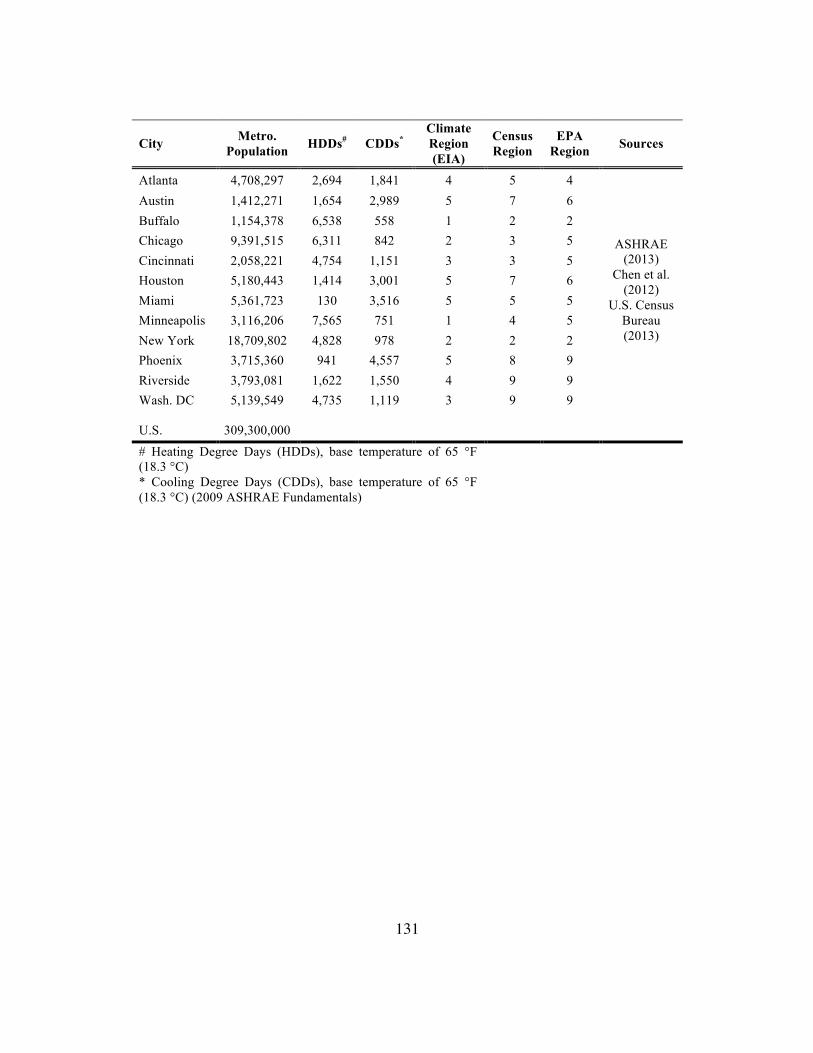
131

City Metro. Population HDDs# CDDs*

Climate Region (EIA)

Census Region

EPA Region Sources

Atlanta 4,708,297 2,694 1,841 4 5 4

ASHRAE (2013)

Chen et al. (2012)

U.S. Census Bureau (2013)

Austin 1,412,271 1,654 2,989 5 7 6 Buffalo 1,154,378 6,538 558 1 2 2 Chicago 9,391,515 6,311 842 2 3 5 Cincinnati 2,058,221 4,754 1,151 3 3 5 Houston 5,180,443 1,414 3,001 5 7 6 Miami 5,361,723 130 3,516 5 5 5 Minneapolis 3,116,206 7,565 751 1 4 5 New York 18,709,802 4,828 978 2 2 2 Phoenix 3,715,360 941 4,557 5 8 9 Riverside 3,793,081 1,622 1,550 4 9 9 Wash. DC 5,139,549 4,735 1,119 3 9 9

U.S. 309,300,000 # Heating Degree Days (HDDs), base temperature of 65 °F (18.3 °C) * Cooling Degree Days (CDDs), base temperature of 65 °F (18.3 °C) (2009 ASHRAE Fundamentals)

132

Table S.3. Residential characteristic data for 12 U.S. cities.

City Housing Units Median House Size (ft2)

Median Year of Construction

Survey Year

Median λinf (hr-1)

Atlanta 1,802,800 2,129 1985 2004 0.43 Austin 354,241# 1,956 n.d.* 2007 0.50 Buffalo 515,500 1,881 1948 2002 0.70 Chicago 3,198,900 2,017 1965 2003 0.61 Cincinnati 647,500 1,935 1962 1998 0.52 Houston 2,160,100 1,956 1980 2007 0.50 Miami 2,419,700 1,914 1978 2007 0.35 Minn. 1,329,700 2,157 1976 2007 0.60 New York 4,849,800 2,043 1951 2003 0.62 Phoenix 1,340,400 1,749 1983 2002 0.42 Riverside 1,511,800 1,735 1985 2002 0.42 Wash. DC 2,133,500 2,493 1974 2007 0.54

U.S. 155,108,000 1,700 1974 2011 0.44 *AHS had no data available for Austin—Houston housing data were used #Austin housing stock only - does not include entire MSA Chen et al. (2012) U.S. Census Bureau (2013) Persily et al. (2010) Table S.4. Residential occupancy data for 12 U.S. cities.

City Household

Occupancy

Atlanta 2.18 Austin 2.37 Buffalo 2.24 Chicago 2.57 Cincinnati 2.17 Houston 2.67 Miami 2.58 Minneapolis 2.17 New York 2.61 Phoenix 2.64 Riverside 3.26 Washington DC 2.13

Source: U.S. Census Bureau (2013)

133

Persily et al. (2010) determined distributions of infiltration air exchange rates

across single-family detached homes in nine geographic regions across the U.S (Table

S.5). They assumed that the homes required conditioned air, the HVAC systems were

balanced (i.e., supply flowrate equals exhaust flowrate), and that no make-up ventilation

was used to bring fresh air into the home. They also assumed all system leaks

(particularly from HVAC ducts) were contained within the conditioned space. Key

parameters of their analysis include demographics, geography, climate, and the year of

construction. Finally, the infiltration air exchange rate distributions from Persily et al.

(2010) account for 80% of the U.S. residential building stock.

Table S.5. City-specific infiltration air exchange rates and distribution percentiles (hr-1). Percentile City 0 2.5 5 10 25 50 75 90 95 97.5 100 Atlanta 0.00 0.07 0.12 0.19 0.33 0.49 0.65 0.80 0.89 0.97 1.74 Austin 0.00 0.05 0.09 0.15 0.28 0.44 0.60 0.75 0.84 0.91 1.59 Buffalo 0.00 0.04 0.08 0.13 0.27 0.44 0.62 0.80 0.90 0.99 1.67 Chicago 0.00 0.04 0.08 0.14 0.27 0.46 0.65 0.84 0.95 1.04 1.83 Cincinnati 0.00 0.04 0.08 0.14 0.27 0.45 0.65 0.83 0.94 1.04 1.69 Houston 0.00 0.05 0.09 0.15 0.28 0.44 0.60 0.75 0.84 0.92 1.43 Miami 0.00 0.07 0.12 0.19 0.33 0.49 0.65 0.80 0.89 0.98 1.56 Minneapolis 0.00 0.04 0.08 0.15 0.29 0.49 0.70 0.89 1.01 1.11 1.85 New York City 0.00 0.04 0.08 0.13 0.27 0.44 0.62 0.79 0.90 0.99 1.63 Phoenix 0.00 0.10 0.15 0.22 0.35 0.51 0.66 0.80 0.88 0.95 1.44 Riverside 0.00 0.06 0.10 0.16 0.27 0.41 0.55 0.67 0.75 0.81 1.25 Washington 0.00 0.07 0.12 0.19 0.33 0.49 0.65 0.81 0.90 0.97 1.59 Source: Persily et al. (2010)

134

City-specific HVAC cycling rate fractions were determined from previous work

compiled by Lawrence Berkeley National Laboratories (LBNL) (Table S.6). The data

compiled by LBNL estimated the total number of hours that a typical residential air

conditioning (AC) unit would operate during the summer cooling season. The median

cycling fraction for each city was calculated by dividing the total number of AC

operation hours by the total number of hours from 1 May to 30 September (3,672). The

probabilistic distribution of the AC cycling rate was unknown, so we assumed a uniform

distribution. We also assumed that the minimum and maximum values were 10% lower

and higher (respectively) than the median value.

Table S.6. City-specific HVAC cycling rate fractions and distribution percentiles during the summer cooling season (1 May to 31 September). Percentile City 0 2.5 5 10 25 50 75 90 95 97.5 100

Atlanta 0.11 0.11 0.12 0.13 0.16 0.21 0.26 0.29 0.30 0.31 0.31

Austin 0.20 0.21 0.21 0.22 0.25 0.30 0.35 0.38 0.39 0.39 0.40

Buffalo 0.00 0.00 0.01 0.01 0.03 0.06 0.10 0.12 0.12 0.13 0.13

Chicago 0.00 0.00 0.01 0.02 0.04 0.09 0.13 0.15 0.16 0.17 0.17

Cincinnati 0.01 0.01 0.02 0.03 0.06 0.11 0.16 0.19 0.20 0.21 0.21

Houston 0.20 0.20 0.21 0.22 0.25 0.30 0.35 0.38 0.39 0.40 0.40

Miami 0.28 0.28 0.29 0.30 0.33 0.38 0.43 0.46 0.47 0.48 0.48

Minneapolis 0.00 0.00 0.01 0.02 0.04 0.09 0.13 0.15 0.16 0.17 0.17

New York City 0.00 0.01 0.01 0.02 0.05 0.10 0.15 0.18 0.19 0.20 0.20

Phoenix 0.27 0.28 0.28 0.29 0.32 0.37 0.42 0.45 0.46 0.46 0.47

Riverside 0.09 0.09 0.10 0.11 0.14 0.19 0.24 0.27 0.28 0.28 0.29 Washington 0.02 0.02 0.03 0.04 0.07 0.12 0.17 0.20 0.21 0.21 0.22 Source: LBNL (2014)

135

Table S.7. Electricity costs per kWh for each of the target cities and end-use. City Residential $/kWh Commercial $/kWh

Atlanta 0.11 0.10 Austin 0.11 0.08 Buffalo 0.18 0.15 Chicago 0.11 0.08 Cincinnati 0.11 0.09 Houston 0.11 0.08 Miami 0.11 0.10 Minneapolis 0.11 0.09 New York City 0.18 0.15 Phoenix 0.11 0.10 Riverside 0.16 0.13

Washington DC 0.12 0.12

Source: USEIA (2014)

136

Table S.8. 8-hour ozone attainment classification and population in nonattainment.

City 8-Hour Ozone Design Value

(ppb)

Attainment Classification

Population in Nonattainment

Counties

Regional Ozone Trend (2000-2012)

Sources

Atlanta 80 Marginal 4,753,017 -17% Austin Attainment 0% Buffalo Attainment -7% Chicago 77 Marginal 9,179,738 -5% Cincinnati 79 Marginal 1,988,951 -5% USEPA (2013a) Houston 84 Marginal 5,891,999 0% USEPA (2013b) Miami Attainment -17% Minn. Attainment 4% NYC 84 Marginal 20,217,137 -7% Phoenix 77 Marginal 3,849,627 -4% Riverside 95 Severe 15 425,806 -9% Wash. DC 81 Marginal 5,136,216 -17%

U.S. Population in Nonattainment 51,442,491 National Avg (-9%)

137

Table S.9. City-specific summer ozone concentrations from 2011 through 2013.

City USEPA Ozone

Monitor Ozone

Season(s) # Obs Min. (ppb)

Median (ppb)

Mode (ppb)

Max. (ppb)

Mean (ppb)

Std. Dev. (ppb)

Atlanta 013-121-0055 2011-2013 10864 2 28 2 114 31 21

2013 3624 2 24 2 114 26 18

2012 3616 2 30 2 114 33 21

2011 3624 2 33 2 99 35 22 Austin 048-453-0014 2011-2013 10213 2 31 13 105 33 17

2013 3624 2 29 13 85 31 16

2012 3429 2 31 30 105 32 16

2011 3160 2 34 38 88 35 18 Buffalo 036-029-0002 2011-2013 10706 2 34 2 95 35 17

2013 3458 2 34 2 86 34 16

2012 3624 2 37 2 95 37 18

2011 3624 2 32 28 81 33 15 Chicago 017-031-0064 2011-2013 10680 2 30 2 139 31 17

2013 3458 2 28 2 73 28 13

2012 3598 2 34 2 110 35 18

2011 3624 2 30 2 139 31 17 Cincinnati 039-061-0006 2011-2013 10732 2 34 2 112 36 19

2013 3624 2 32 29 83 33 16

2012 3511 2 35 2 109 38 20

2011 3597 2 35 2 112 37 21 Houston 048-201-1035 2011-2013 10668 2 20 2 131 23 18

2013 3448 2 19 2 89 22 16

2012 3609 2 19 2 131 23 18

2011 3611 2 22 2 122 25 19 Miami 012-086-0027 2011-2013 10187 2 25 22 101 27 10

2013 3368 2 24 22 101 25 9

2012 3510 2 26 25 77 27 9

2011 3309 2 26 22 88 28 11 Minn. 027-139-0505 2011-2013 10825 2 32 2 102 32 15

2013 3577 2 34 28 83 34 15

2012 3624 2 33 2 102 33 16

2011 3624 2 29 2 82 28 13 NYC 036-061-0135 2011-2013 10423 2 26 2 121 28 16

2013 3624 2 25 2 94 26 14

2012 3624 2 28 2 97 30 17

2011 3175 2 26 2 121 29 18

Phoenix 004-013-3003 2011-2013 10872 2 39 43 98 39 19

2013 3624 2 39 46 98 38 18

2012 3624 2 39 38 96 40 19

2011 3624 2 39 2 95 39 20 Riverside 06-065-0012 2011-2013 8797 2 46 41 127 47 21

2013 2469 2 46 45 115 47 19

2012 2704 2 48 41 117 49 21

2011 3624 2 44 2 127 44 21

Wash. 011-001-0041 2011-2013 10724 2 32 2 102 33 18

2013 3624 2 29 2 90 29 15

2012 3559 2 35 2 102 36 18

2011 3541 2 33 2 101 33 19 Source: USEPA (2014a)

138

Table S.10. Difference in indoor ozone concentrations in single-family homes with and without activated carbon filtration. Percentile

mean

(μ)

std dev (σ) 0 2.5 5 10 25 50 75 90 95 97.5 100

Atlanta 0.53 0.65 0.00 0.02 0.04 0.07 0.15 0.33 0.66 1.18 1.65 2.19 25.7 Austin 0.58 0.67 0.00 0.03 0.05 0.08 0.18 0.38 0.73 1.27 1.75 2.30 19.0 Buffalo 0.24 0.40 0.00 0.00 0.01 0.01 0.04 0.12 0.28 0.57 0.88 1.25 11.0 Chicago 0.26 0.41 0.00 0.00 0.01 0.01 0.05 0.13 0.31 0.64 0.95 1.32 10.4 Cincinnati 0.36 0.53 0.00 0.01 0.02 0.03 0.08 0.20 0.44 0.86 1.25 1.74 17.4 Houston 0.45 0.56 0.00 0.02 0.03 0.06 0.13 0.29 0.57 1.02 1.42 1.89 22.4 Miami 0.55 0.57 0.00 0.04 0.07 0.11 0.21 0.39 0.70 1.16 1.56 2.03 14.4 Minn. 0.28 0.42 0.00 0.00 0.01 0.02 0.05 0.14 0.33 0.66 0.97 1.37 9.34 NYC 0.26 0.41 0.00 0.00 0.01 0.02 0.05 0.13 0.31 0.63 0.94 1.31 12.1 Phoenix 0.82 0.88 0.00 0.06 0.09 0.15 0.29 0.57 1.04 1.75 2.37 3.10 21.9 Riverside 0.61 0.74 0.00 0.03 0.05 0.09 0.19 0.39 0.76 1.35 1.90 2.55 18.5 Wash. DC 0.37 0.51 0.00 0.01 0.02 0.04 0.09 0.21 0.46 0.86 1.25 1.71 13.0

139

Table S.11. Population age fractions by metropolitan area.

Population Age Fractions

City 1 to

4 5 to 14

15 to 24

25 to 34

35 to 44

45 to 54

55 to 64

65 to 74

75 to 84 85+

Atlanta 0.06 0.10 0.17 0.19 0.15 0.13 0.10 0.05 0.03 0.01 Austin 0.07 0.12 0.17 0.21 0.15 0.12 0.09 0.04 0.02 0.01 Buffalo 0.07 0.13 0.18 0.15 0.12 0.14 0.11 0.06 0.04 0.02 Chicago 0.07 0.12 0.15 0.19 0.14 0.13 0.10 0.06 0.03 0.02 Cincinnati 0.07 0.12 0.17 0.17 0.12 0.14 0.11 0.05 0.04 0.02 Houston 0.08 0.15 0.15 0.18 0.16 0.12 0.07 0.05 0.03 0.01 Miami 0.06 0.12 0.14 0.14 0.15 0.15 0.11 0.07 0.05 0.02 Minn. 0.06 0.12 0.18 0.21 0.16 0.12 0.06 0.04 0.03 0.02 New York 0.06 0.12 0.14 0.17 0.14 0.14 0.11 0.06 0.04 0.02 Phoenix 0.08 0.16 0.15 0.16 0.15 0.13 0.09 0.05 0.03 0.01 Riverside 0.08 0.18 0.17 0.15 0.16 0.12 0.06 0.05 0.03 0.01 Wash DC 0.06 0.09 0.17 0.20 0.14 0.13 0.11 0.06 0.04 0.02 Source: U.S. Census Bureau (2012)

The average indoor ozone concentrations from Table S.10 were scaled by 70%

(this assumes that the average person spends 70% of their time in their home) and entered

into the health and benefits model as described in the main text. The health model

incorporates city-specific age populations (Table S.11) for baseline incidence, change in

health incidence, and change in DALYs. The results of the analysis for each of the

sample cities are presented in Tables S.12 through S.23.

140

Table S.12 Population adjusted ozone health outcomes for Atlanta single-family homes.

Affected Population

(out of 100,000 persons) Health Outcome

Baseline Incidence per person Δ Incidence

per 100,000 Δ DALYs per 100,000

y0 mean (μ) 95% CIs

19400 Mortality (25 to 34) 0.00 0.03 0.87 (0.29, 1.44) 15000 Mortality (35 to 44) 0.00 0.04 1.10 (0.37, 1.83) 12500 Mortality (45 to 54) 0.00 0.09 1.94 (0.66, 3.22) 9500 Mortality (55 to 64) 0.01 0.14 2.56 (0.87, 4.25) 5400 Mortality (65 to 74) 0.02 0.18 2.39 (0.81, 3.97) 2900 Mortality (75 to 84) 0.05 0.24 2.31 (0.78, 3.83) 1400 Mortality (85+) 0.13 0.30 1.63 (0.55, 2.70)

46700 Respiratory HA (18

to 64) 0.01 0.17 0.01 (0.00, 0.01)

46700 Dysrhythmia HA

(18 to 64) 0.00 0.03 0.00 (0.00, 0.00)

9700 Dysrhythmia HA

(65+) 0.13 0.92 0.03 (0.00, 0.06) 46700 MRAD (18 to 64) 7.80 536 0.25 (0.10, 0.39)

18800 School Loss Day (5

to 17) 9.90 1042 0.73 (0.28, 1.18)

9700 Respiratory HA

(65+) 0.04 0.32 0.00 (0.00, 0.00) Sources: U.S. Census Bureau (2012); USEPA (2012)

141

Table S.13. Population adjusted ozone health outcomes for Austin single-family homes.

Affected Population

(out of 100,000 persons) Health Outcome

Baseline Incidenc

e per person Δ Incidence

per 100,000 Δ DALYs per 100,000

y0 mean (μ) 95% CIs 20900 Mortality (25 to 34) 0.00 0.04 1.02 (0.35, 1.70) 15000 Mortality (35 to 44) 0.00 0.05 1.20 (0.41, 2.00) 12100 Mortality (45 to 54) 0.00 0.09 2.05 (0.69, 3.41) 8800 Mortality (55 to 64) 0.01 0.14 2.59 (0.88, 4.30) 3800 Mortality (65 to 74) 0.02 0.14 1.84 (0.62, 3.05) 2200 Mortality (75 to 84) 0.05 0.20 1.91 (0.65, 3.18) 1000 Mortality (85+) 0.13 0.23 1.27 (0.43, 2.11)

46350 Respiratory HA (18 to 64) 0.00 0.18 0.01 (0.00, 0.01)

46350 Dysrhythmia HA (18 to 64) 0.00 0.03 0.00 (0.00, 0.00)

7000 Dysrhythmia HA (65+) 0.13 0.73 0.02 (0.00, 0.04)

46350 MRAD (18 to 64) 7.80 582 0.27 (0.11, 0.43)

20350 School Loss Day (5 to 17) 9.90 1232 0.86 (0.33,1.39)

7000 Respiratory HA (65+) 0.04 0.26 0.00 (0.00, 0.00) Sources: U.S. Census Bureau (2012); USEPA (2012)

142

Table S.14. Population adjusted ozone health outcomes for Buffalo single-family homes.

Affected Population

(out of 100,000 persons) Health Outcome

Baseline Incidence

per person

Δ Incidence per 100,000

Δ DALYs per 100,000

y0 mean

(μ) 95% CIs 14500 Mortality (25 to 34) 0.00 0.01 0.30 (0.10, 0.49) 12000 Mortality (35 to 44) 0.00 0.02 0.40 (0.14, 0.67) 14000 Mortality (45 to 54) 0.00 0.04 0.99 (0.34, 1.65) 10800 Mortality (55 to 64) 0.01 0.07 1.33 (0.45, 2.21) 5900 Mortality (65 to 74) 0.02 0.09 1.19 (0.40, 1.98) 4300 Mortality (75 to 84) 0.05 0.16 1.57 (0.53, 2.60) 1500 Mortality (85+) 0.13 0.15 0.80 (0.27, 1.33)

44050 Respiratory HA (18 to 64) 0.01 0.08 0.00 (0.00, 0.00)

44050 Dysrhythmia HA (18 to 64) 0.00 0.01 0.00 (0.00, 0.00)

11700 Dysrhythmia HA (65+) 0.13 0.52 0.02 (0.00, 0.03) 44050 MRAD (18 to 64) 7.80 231 0.11 (0.04, 0.17)

21800 School Loss Day (5 to 17) 9.90 554 0.39 (0.15, 0.63)

11700 Respiratory HA (65+) 0.04 0.18 0.00 (0.00, 0.00) Sources: U.S. Census Bureau (2012); USEPA (2012)

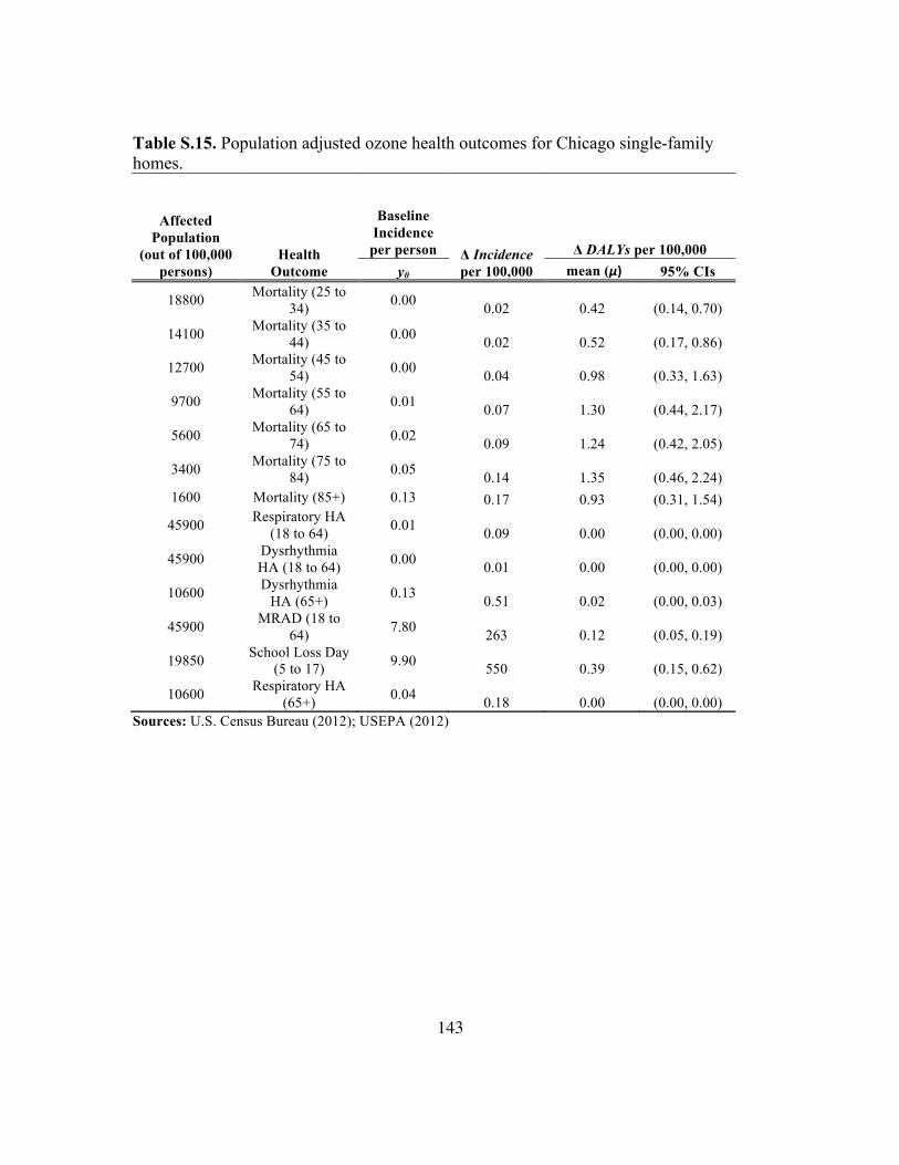
143

Table S.15. Population adjusted ozone health outcomes for Chicago single-family homes.

Affected Population

(out of 100,000 persons)

Health Outcome

Baseline Incidence per person Δ Incidence

per 100,000 Δ DALYs per 100,000

y0 mean (μ) 95% CIs

18800 Mortality (25 to 34) 0.00 0.02 0.42 (0.14, 0.70)

14100 Mortality (35 to 44) 0.00 0.02 0.52 (0.17, 0.86)

12700 Mortality (45 to 54) 0.00 0.04 0.98 (0.33, 1.63)

9700 Mortality (55 to 64) 0.01 0.07 1.30 (0.44, 2.17)

5600 Mortality (65 to 74) 0.02 0.09 1.24 (0.42, 2.05)

3400 Mortality (75 to 84) 0.05 0.14 1.35 (0.46, 2.24)

1600 Mortality (85+) 0.13 0.17 0.93 (0.31, 1.54)

45900 Respiratory HA (18 to 64) 0.01 0.09 0.00 (0.00, 0.00)

45900 Dysrhythmia HA (18 to 64) 0.00 0.01 0.00 (0.00, 0.00)

10600 Dysrhythmia HA (65+) 0.13 0.51 0.02 (0.00, 0.03)

45900 MRAD (18 to 64) 7.80 263 0.12 (0.05, 0.19)

19850 School Loss Day (5 to 17) 9.90 550 0.39 (0.15, 0.62)

10600 Respiratory HA (65+) 0.04 0.18 0.00 (0.00, 0.00)

Sources: U.S. Census Bureau (2012); USEPA (2012)

144

Table S.16. Population adjusted ozone health outcomes for Cincinnati single-family homes.

Affected Population

(out of 100,000 persons) Health Outcome

Baseline Incidence per person Δ Incidence

per 100,000 Δ DALYs per 100,000

y0 mean (μ) 95% CIs

16600 Mortality (25 to 34) 0.00 0.02 0.51 (0.17, 0.85)

11900 Mortality (35 to 44) 0.00 0.02 0.60 (0.20, 1.00)

13700 Mortality (45 to 54) 0.00 0.07 1.47 (0.50, 2.44)

10600 Mortality (55 to 64) 0.01 0.11 1.97 (0.67, 3.27)

5400 Mortality (65 to 74) 0.02 0.12 1.65 (0.56, 2.74)

3800 Mortality (75 to 84) 0.05 0.22 2.09 (0.71, 3.47)

2000 Mortality (85+) 0.13 0.29 1.61 (0.54, 2.67)

44500 Respiratory HA (18 to 64) 0.01 0.12 0.00 (0.00, 0.01)

44500 Dysrhythmia HA (18 to 64) 0.00 0.02 0.00 (0.00, 0.00)

11200 Dysrhythmia HA (65+) 0.14 0.78 0.02 (0.00, 0.05)

44500 MRAD (18 to 64) 7.80 353 0.16 (0.07, 0.26)

20150 School Loss Day (5 to 17) 9.90 772 0.54 (0.21, 0.87)

11200 Respiratory HA (65+) 0.05 0.27 0.00 (0.00, 0.00)

Sources: U.S. Census Bureau (2012); USEPA (2012)

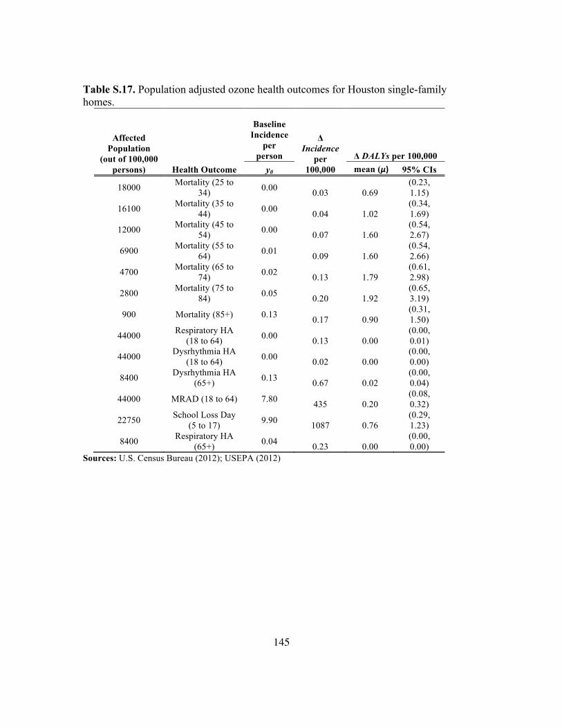
145

Table S.17. Population adjusted ozone health outcomes for Houston single-family homes.

Affected Population

(out of 100,000 persons) Health Outcome

Baseline Incidence

per person

Δ Incidence

per 100,000

Δ DALYs per 100,000 y0 mean (μ) 95% CIs

18000 Mortality (25 to 34) 0.00 0.03 0.69

(0.23, 1.15)

16100 Mortality (35 to 44) 0.00 0.04 1.02

(0.34, 1.69)

12000 Mortality (45 to 54) 0.00 0.07 1.60

(0.54, 2.67)

6900 Mortality (55 to 64) 0.01 0.09 1.60

(0.54, 2.66)

4700 Mortality (65 to 74) 0.02 0.13 1.79

(0.61, 2.98)

2800 Mortality (75 to 84) 0.05 0.20 1.92

(0.65, 3.19)

900 Mortality (85+) 0.13 0.17 0.90 (0.31, 1.50)

44000 Respiratory HA (18 to 64) 0.00 0.13 0.00

(0.00, 0.01)

44000 Dysrhythmia HA (18 to 64) 0.00 0.02 0.00

(0.00, 0.00)

8400 Dysrhythmia HA (65+) 0.13 0.67 0.02

(0.00, 0.04)

44000 MRAD (18 to 64) 7.80 435 0.20 (0.08, 0.32)

22750 School Loss Day (5 to 17) 9.90 1087 0.76

(0.29, 1.23)

8400 Respiratory HA (65+) 0.04 0.23 0.00

(0.00, 0.00)

Sources: U.S. Census Bureau (2012); USEPA (2012)

146

Table S.18. Population adjusted ozone health outcomes for Miami single-family homes.

Affected Population

(out of 100,000 persons) Health Outcome

Baseline Incidence per person

Δ Incidence

per 100,000

Δ DALYs per 100,000 y0 mean (μ) 95% CIs

13700 Mortality (25 to 34) 0.00 0.02 0.64 (0.22, 1.06)

15100 Mortality (35 to 44) 0.00 0.05 1.16 (0.39, 1.92)

14500 Mortality (45 to 54) 0.00 0.10 2.35 (0.79, 3.90)

10700 Mortality (55 to 64) 0.01 0.16 3.01 (1.02, 5.00)

7400 Mortality (65 to 74) 0.02 0.26 3.42 (1.16, 5.68)

4700 Mortality (75 to 84) 0.05 0.40 3.90 (1.32, 6.48)

1900 Mortality (85+) 0.13 0.42 2.31 (0.78, 3.83)

47150 Respiratory HA (18 to 64) 0.01 0.20 0.01

(0.00, 0.01)

47150 Dysrhythmia HA (18 to 64) 0.00 0.03 0.00

(0.00, 0.00)

14000 Dysrhythmia HA (65+) 0.13 1.40 0.04 (0.00, 0.08)

47150 MRAD (18 to 64) 7.80 565 0.26 (0.11, 0.41)

18850 School Loss Day (5 to 17) 9.90 1090 0.76

(0.29, 1.23)

14000 Respiratory HA (65+) 0.04 0.49 0.00 (0.00, 0.00)

Sources: U.S. Census Bureau (2012); USEPA (2012)

147

Table S.19. Population adjusted ozone health outcomes for Minneapolis single-family homes.

Affected Population

(out of 100,000 persons) Health Outcome

Baseline Incidence

per person

Δ Incidence

per 100,000

Δ DALYs per 100,000 y0 mean (μ) 95% CIs

20600 Mortality (25 to 34) 0.00 0.02 0.48 (0.16, 0.80)

16400 Mortality (35 to 44) 0.00 0.03 0.63 (0.21, 1.05)

11800 Mortality (45 to 54) 0.00 0.04 0.96 (0.32, 1.59)

5900 Mortality (55 to 64) 0.01 0.04 0.83 (0.28, 1.38)

4000 Mortality (65 to 74) 0.02 0.07 0.92 (0.31, 1.54)

3300 Mortality (75 to 84) 0.05 0.14 1.37 (0.46, 2.28)

1700 Mortality (85+) 0.13 0.19 1.03 (0.35, 1.72)

44400 Respiratory HA (18 to 64) 0.00 0.08 0.00

(0.00, 0.00)

44400 Dysrhythmia HA (18 to 64) 0.00 0.01 0.00

(0.00, 0.00)

9000 Dysrhythmia HA (65+) 0.14 0.48 0.01 (0.00, 0.03)

44400 MRAD (18 to 64) 7.80 266 0.12 (0.05, 0.20)

21200 School Loss Day (5 to 17) 9.90 615 0.43

(0.16, 0.70)

9000 Respiratory HA (65+) 0.05 0.17 0.00 (0.00, 0.00)

Sources: U.S. Census Bureau (2012); USEPA (2012)

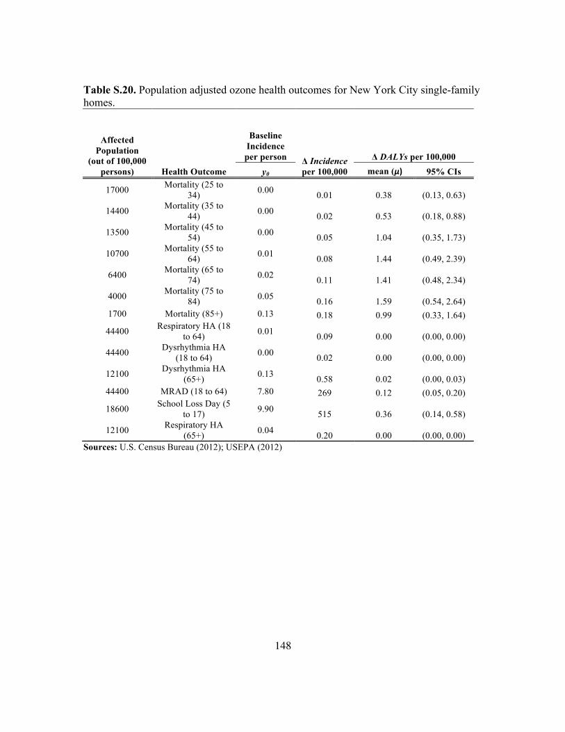
148

Table S.20. Population adjusted ozone health outcomes for New York City single-family homes.

Affected Population

(out of 100,000 persons) Health Outcome

Baseline Incidence per person Δ Incidence

per 100,000 Δ DALYs per 100,000

y0 mean (μ) 95% CIs

17000 Mortality (25 to 34) 0.00 0.01 0.38 (0.13, 0.63)

14400 Mortality (35 to 44) 0.00 0.02 0.53 (0.18, 0.88)

13500 Mortality (45 to 54) 0.00 0.05 1.04 (0.35, 1.73)

10700 Mortality (55 to 64) 0.01 0.08 1.44 (0.49, 2.39)

6400 Mortality (65 to 74) 0.02 0.11 1.41 (0.48, 2.34)

4000 Mortality (75 to 84) 0.05 0.16 1.59 (0.54, 2.64)

1700 Mortality (85+) 0.13 0.18 0.99 (0.33, 1.64)

44400 Respiratory HA (18 to 64) 0.01 0.09 0.00 (0.00, 0.00)

44400 Dysrhythmia HA (18 to 64) 0.00 0.02 0.00 (0.00, 0.00)

12100 Dysrhythmia HA (65+) 0.13 0.58 0.02 (0.00, 0.03)

44400 MRAD (18 to 64) 7.80 269 0.12 (0.05, 0.20)

18600 School Loss Day (5 to 17) 9.90 515 0.36 (0.14, 0.58)

12100 Respiratory HA (65+) 0.04 0.20 0.00 (0.00, 0.00)

Sources: U.S. Census Bureau (2012); USEPA (2012)

149

Table S.21. Population adjusted ozone health outcomes for Phoenix single-family homes.

Affected Population

(out of 100,000 persons) Health Outcome

Baseline Incidence per person

Δ Incidence per 100,000

Δ DALYs per 100,000

y0 mean (μ) 95% CIs 15900 Mortality (25 to 34) 0.00 0.04 1.11 (0.37, 1.84) 14500 Mortality (35 to 44) 0.00 0.07 1.66 (0.56, 2.75) 13300 Mortality (45 to 54) 0.00 0.14 3.21 (1.09, 5.33) 9400 Mortality (55 to 64) 0.01 0.21 3.94 (1.33, 6.55) 4600 Mortality (65 to 74) 0.02 0.24 3.17 (1.07, 5.26) 2600 Mortality (75 to 84) 0.05 0.33 3.22 (1.09, 5.35) 1000 Mortality (85+) 0.13 0.33 1.81 (0.61, 3.01)

45150 Respiratory HA (18 to 64) 0.01 0.27 0.01 (0.00, 0.01)

45150 Dysrhythmia HA (18 to 64) 0.00 0.04 0.00 (0.00, 0.00)

8200 Dysrhythmia HA (65+) 0.13 1.19 0.04 (0.00, 0.07)

45150 MRAD (18 to 64) 7.80 807 0.37 (0.15, 0.59)

23000 School Loss Day (5 to 17) 9.90 1981 1.39 (0.53, 2.24)

8200 Respiratory HA (65+) 0.04 0.42 0.00 (0.00, 0.00)

Sources: U.S. Census Bureau (2012); USEPA (2012)

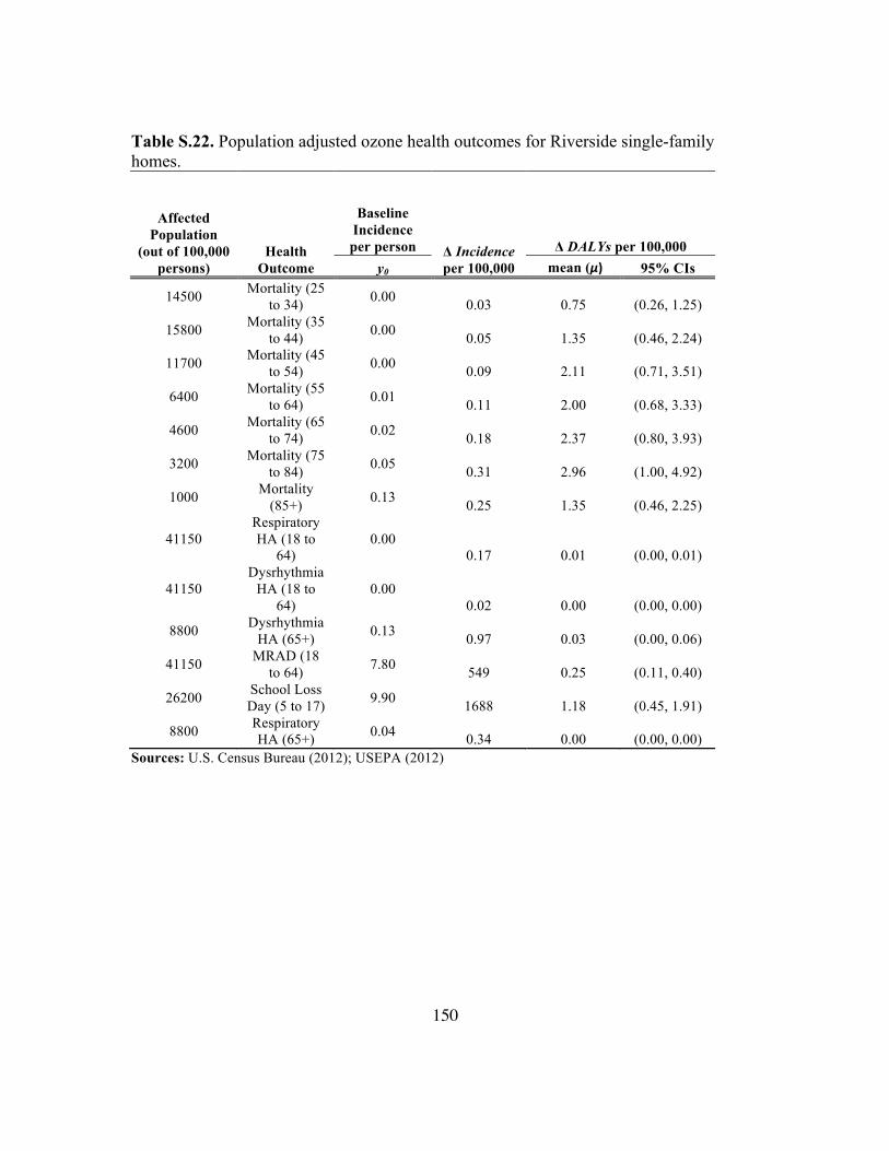
150

Table S.22. Population adjusted ozone health outcomes for Riverside single-family homes.

Affected Population

(out of 100,000 persons)

Health Outcome

Baseline Incidence per person Δ Incidence

per 100,000 Δ DALYs per 100,000

y0 mean (μ) 95% CIs

14500 Mortality (25 to 34) 0.00 0.03 0.75 (0.26, 1.25)

15800 Mortality (35 to 44) 0.00 0.05 1.35 (0.46, 2.24)

11700 Mortality (45 to 54) 0.00 0.09 2.11 (0.71, 3.51)

6400 Mortality (55 to 64) 0.01 0.11 2.00 (0.68, 3.33)

4600 Mortality (65 to 74) 0.02 0.18 2.37 (0.80, 3.93)

3200 Mortality (75 to 84) 0.05 0.31 2.96 (1.00, 4.92)

1000 Mortality (85+) 0.13 0.25 1.35 (0.46, 2.25)

41150 Respiratory HA (18 to

64) 0.00

0.17 0.01 (0.00, 0.01)

41150 Dysrhythmia

HA (18 to 64)

0.00 0.02 0.00 (0.00, 0.00)

8800 Dysrhythmia HA (65+) 0.13 0.97 0.03 (0.00, 0.06)

41150 MRAD (18 to 64) 7.80 549 0.25 (0.11, 0.40)

26200 School Loss Day (5 to 17) 9.90 1688 1.18 (0.45, 1.91)

8800 Respiratory HA (65+) 0.04 0.34 0.00 (0.00, 0.00)

Sources: U.S. Census Bureau (2012); USEPA (2012)

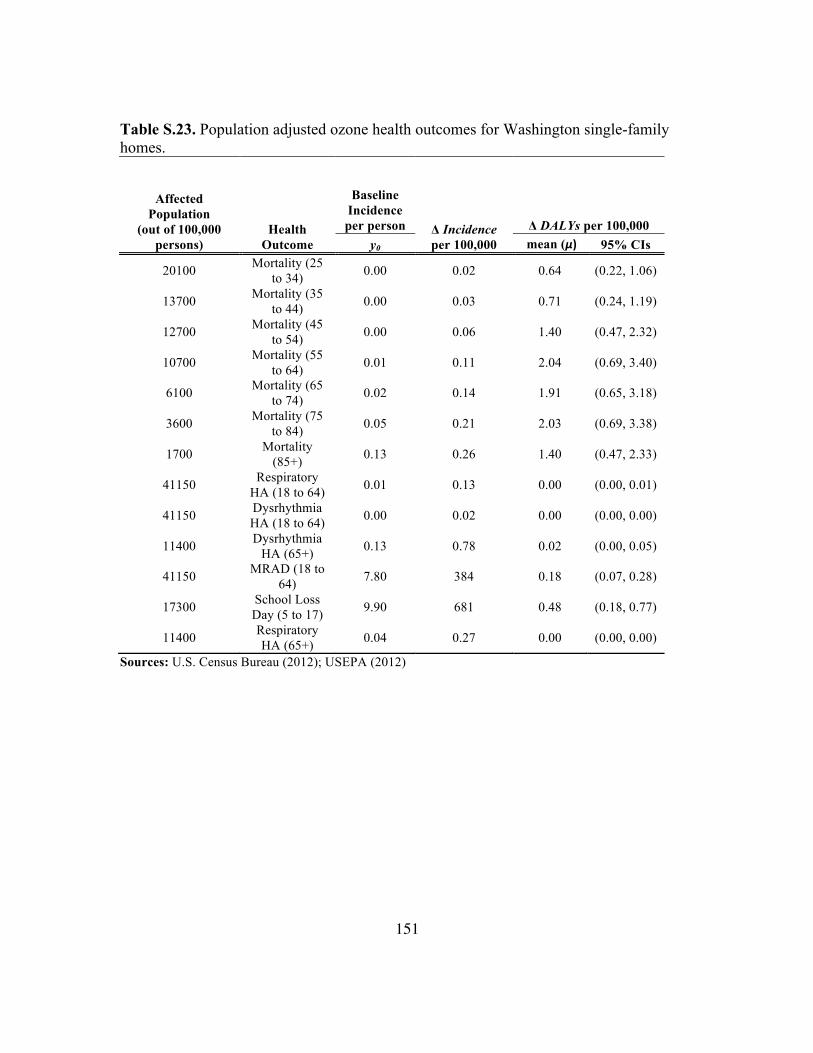
151

Table S.23. Population adjusted ozone health outcomes for Washington single-family homes.

Affected Population

(out of 100,000 persons)

Health Outcome

Baseline Incidence per person Δ Incidence

per 100,000 Δ DALYs per 100,000

y0 mean (μ) 95% CIs

20100 Mortality (25 to 34) 0.00 0.02 0.64 (0.22, 1.06)

13700 Mortality (35 to 44) 0.00 0.03 0.71 (0.24, 1.19)

12700 Mortality (45 to 54) 0.00 0.06 1.40 (0.47, 2.32)

10700 Mortality (55 to 64) 0.01 0.11 2.04 (0.69, 3.40)

6100 Mortality (65 to 74) 0.02 0.14 1.91 (0.65, 3.18)

3600 Mortality (75 to 84) 0.05 0.21 2.03 (0.69, 3.38)

1700 Mortality (85+) 0.13 0.26 1.40 (0.47, 2.33)

41150 Respiratory HA (18 to 64) 0.01 0.13 0.00 (0.00, 0.01)

41150 Dysrhythmia HA (18 to 64) 0.00 0.02 0.00 (0.00, 0.00)

11400 Dysrhythmia HA (65+) 0.13 0.78 0.02 (0.00, 0.05)

41150 MRAD (18 to 64) 7.80 384 0.18 (0.07, 0.28)

17300 School Loss Day (5 to 17) 9.90 681 0.48 (0.18, 0.77)

11400 Respiratory HA (65+) 0.04 0.27 0.00 (0.00, 0.00)

Sources: U.S. Census Bureau (2012); USEPA (2012)

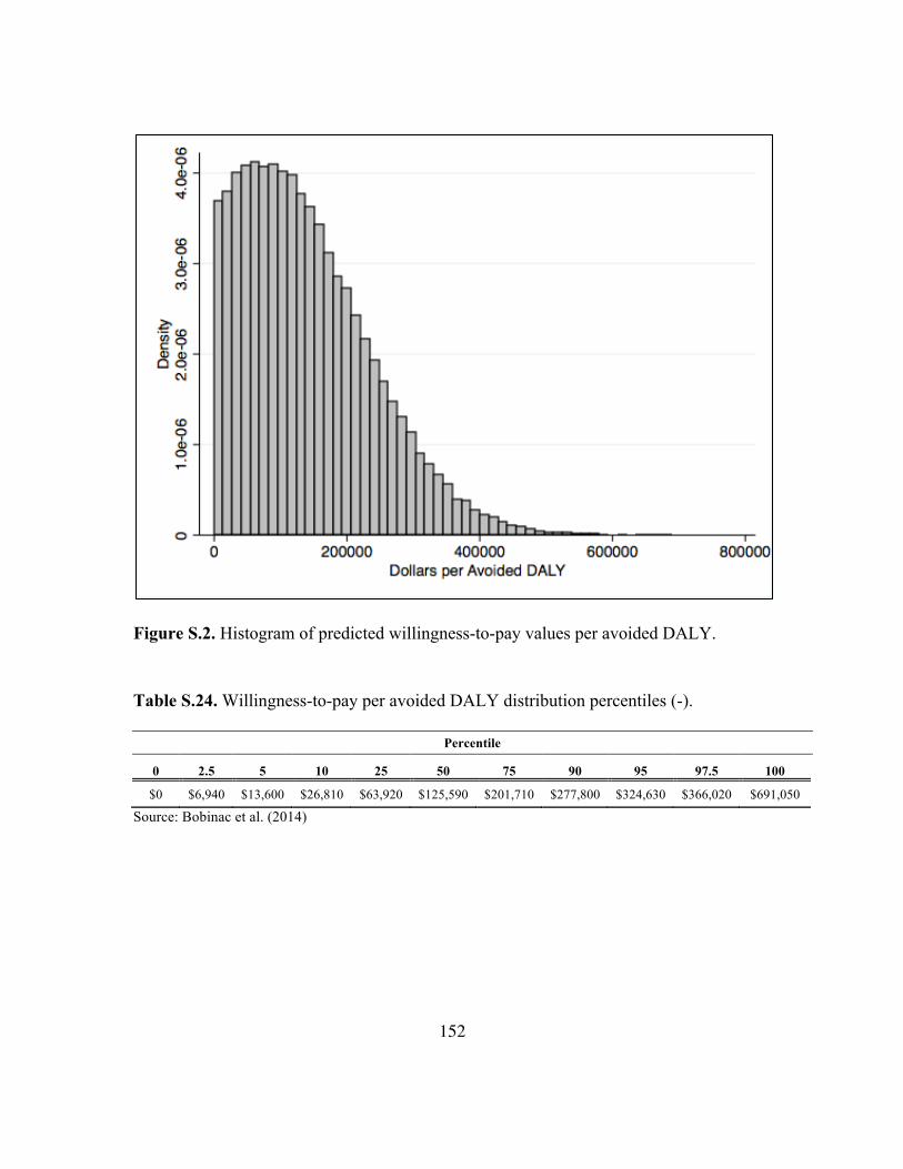
152

Figure S.2. Histogram of predicted willingness-to-pay values per avoided DALY.

Table S.24. Willingness-to-pay per avoided DALY distribution percentiles (-).

Percentile

0 2.5 5 10 25 50 75 90 95 97.5 100

$0 $6,940 $13,600 $26,810 $63,920 $125,590 $201,710 $277,800 $324,630 $366,020 $691,050

Source: Bobinac et al. (2014)

153

A sensitivity analysis of the systems model was conducted to determine which

modeling parameters had the most impact on the final results. The sensitivity analysis

included parameters that affect the transport of ozone from outdoors to indoors, building

and HVAC operational conditions, indoor ozone chemistry, cost inputs for ozone control

via activated carbon filtration, and benefit inputs for disability-adjusted life-years

(DALYs). A base case condition was defined for each model parameter for single-family

homes. Reasonable minimum and maximum values on either sides of the base case were

selected for each parameter.

In order to test the sensitivity against the base case, each parameter was tested

using the minimum and maximum values for that parameter while all other parameters

were held constant at their respective base case values. As each parameter was tested, the

ozone removal effectiveness and the benefit/cost ratio (B/C) were determined. Estimated

base case parameters are presented in S.25 below (Corsi et al., 2014). The sensitivity

analysis results for ozone removal effectiveness and B/C ratios are presented in Figures

S3 and S4, respectively.

154

Table S.25. Parameter values for residential sensitivity analysis. Variable Min Base Case Max Outdoor ozone (ppb) (annual average) 10 30 60 Ozone penetration factor (--) 0.66 0.79 0.92 Volume (m3) 225 500 1500 λinf (hr-1) 0.1 0.5 1.5 Qmake-up (m3�hr-1) 0 0 78 Qrecirculation (m3�hr-1) 2500 2800 3100 Particle filter efficiency for removal of ozone (%) 0 10% 20% AcC filter efficiency (%) 20% 70% 90% Ozone decay rate (hr-1) 1.0 4.0 8.5 α-Pinene concentration (ppb) 0.42 2.64 40.89 α-Pinene ozone rxn rate constant (ppb-1�hr-1) 0.0073 0.0085 0.0292 β-Pinene concentration (ppb) 0.17 0.60 13.02 β Pinene ozone rxn rate constant (ppb-1�hr-1) 0.0011 0.0012 0.0013 d-Limonene concentration (ppb) 0.46 3.17 12.03 d-Limonene ozone rxn rate constant (ppb-1�hr-1) 0.0176 0.0203 0.0575 Styrene concentration (ppb) 0.01 0.32 2.70 Styrene ozone rxn rate constant (ppb-1�hr-1) 0.00075 0.0015 0.003 Linalool concentration (ppb) 0.03 2.47 21.16 Linalool ozone rxn rate constant (ppb-1�hr-1) 0.0396 0.0464 0.0531 α-Terpeniol concentration (ppb) 0.055 0.11 0.22 α-Terpeniol ozone rxn rate constant (ppb-1�hr-1) 0.01 0.027 0.05 Time in environment (%) 35% 70% 100% Average occupancy (--) 1.00 2.59 6.00 Filter replacement frequency per year (--) 1 2 4 Annual average HVAC usage (%) 1% 20% 50% Average HVAC system efficiency (%) 12.5% 25% 50% Difference in filter costs for 1" filter ($)a $0 $5 $15 Difference in filter costs for 2" filter ($)a $0 $10 $20 Difference in filter costs for 4" filter ($)a $0 $15 $25 Cost per kWh ($) $0.07 $0.12 $0.33 Cost per DALY ($) $42,000 $150,000 $220,000

a = difference in filter costs between a particle combination filter and a standard particle filter.

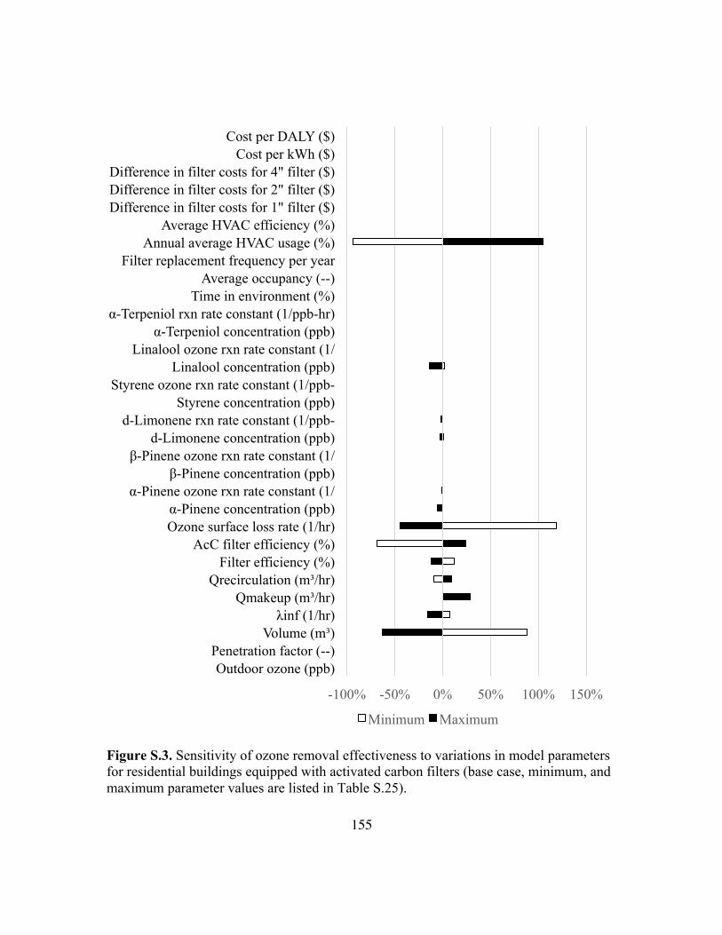
155

Figure S.3. Sensitivity of ozone removal effectiveness to variations in model parameters for residential buildings equipped with activated carbon filters (base case, minimum, and maximum parameter values are listed in Table S.25).

-100% -50% 0% 50% 100% 150%

Outdoor ozone (ppb) Penetration factor (--)

Volume (m³) λinf (1/hr)

Qmakeup (m³/hr) Qrecirculation (m³/hr)

Filter efficiency (%) AcC filter efficiency (%)

Ozone surface loss rate (1/hr) α-Pinene concentration (ppb)

α-Pinene ozone rxn rate constant (1/β-Pinene concentration (ppb)

β-Pinene ozone rxn rate constant (1/d-Limonene concentration (ppb)

d-Limonene rxn rate constant (1/ppb-Styrene concentration (ppb)

Styrene ozone rxn rate constant (1/ppb-Linalool concentration (ppb)

Linalool ozone rxn rate constant (1/α-Terpeniol concentration (ppb)

α-Terpeniol rxn rate constant (1/ppb-hr) Time in environment (%)

Average occupancy (--) Filter replacement frequency per year

Annual average HVAC usage (%) Average HVAC efficiency (%)

Difference in filter costs for 1" filter ($) Difference in filter costs for 2" filter ($) Difference in filter costs for 4" filter ($)

Cost per kWh ($) Cost per DALY ($)

Minimum Maximum

156

Figure S.4. Sensitivity of benefit/cost ratio to variations in model parameters for residential buildings equipped with activated carbon filters (base case, minimum, and maximum parameter values are listed in Table S.25).

-100% 0% 100% 200% 300% 400% 500%

Outdoor ozone (ppb) Penetration factor (--)

Volume (m³) λinf (1/hr)

Qmakeup (m³/hr) Qrecirculation (m³/hr)

Filter efficiency (%) AcC filter efficiency (%)

Ozone surface loss rate (1/hr) α-Pinene concentration (ppb)

α-Pinene ozone rxn rate constant (1/β-Pinene concentration (ppb)

β-Pinene ozone rxn rate constant (1/d-Limonene concentration (ppb)

d-Limonene rxn rate constant (1/ppb-Styrene concentration (ppb)

Styrene ozone rxn rate constant (1/Linalool concentration (ppb)

Linalool ozone rxn rate constant (1/α-Terpeniol concentration (ppb)

α-Terpeniol rxn rate constant (1/ppb-Time in environment (%)

Average occupancy (--) Filter replacement frequency per year

Annual average HVAC usage (%) Average HVAC efficiency (%)

Difference in filter costs for 1" filter Difference in filter costs for 2" filter Difference in filter costs for 4" filter

Cost per kWh ($) Cost per DALY ($)

Minimum Maximum

157

The base case ozone removal effectiveness for residential buildings was 13%.

The annual HVAC operational frequency, building volume, and ozone decay rate have

the greatest impacts on ozone removal effectiveness in residential buildings (Figures S.3).

As expected, filter and electricity costs dominate the overall cost (Figure S.4).

Occupancy is also important because having more people per residence reduces the

individual costs and increases the health benefits, which are shared by more people.

The removal effectiveness of combination activated carbon (AcC) filters for each

target pollutant in residential buildings is higher in residences with low surface loss rates

for ozone (ozone decay rates), e.g., little floor coverage with carpet, and relatively high

HVAC usage. Changes in residential B/C ratios for AcC filtration are primarily

dominated by parameters associated with the filter, including filter costs, electricity costs,

and replacement frequency. Ozone deposition to surfaces is also important, as lower

deposition rates result in a higher benefit associated with activated carbon filtration.

Finally, AcC filters provide significant benefits when ambient ozone is high, indicating

potential for applications only during the summer ozone season.

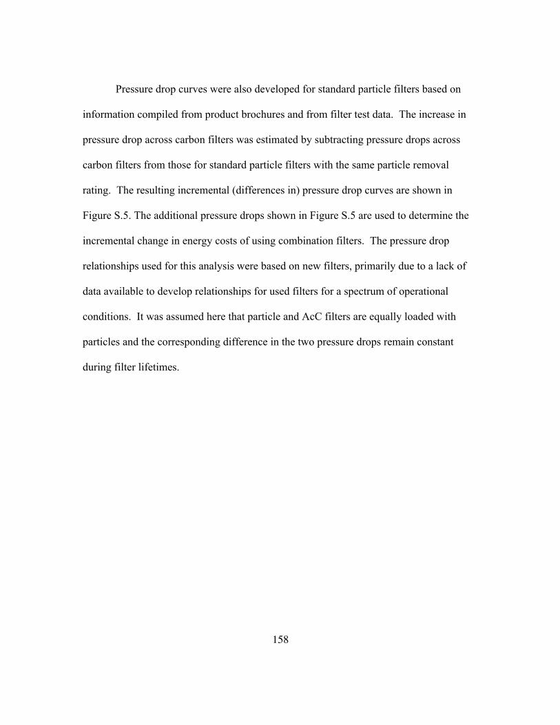
158

Pressure drop curves were also developed for standard particle filters based on

information compiled from product brochures and from filter test data. The increase in

pressure drop across carbon filters was estimated by subtracting pressure drops across

carbon filters from those for standard particle filters with the same particle removal

rating. The resulting incremental (differences in) pressure drop curves are shown in

Figure S.5. The additional pressure drops shown in Figure S.5 are used to determine the

incremental change in energy costs of using combination filters. The pressure drop

relationships used for this analysis were based on new filters, primarily due to a lack of

data available to develop relationships for used filters for a spectrum of operational

conditions. It was assumed here that particle and AcC filters are equally loaded with

particles and the corresponding difference in the two pressure drops remain constant

during filter lifetimes.

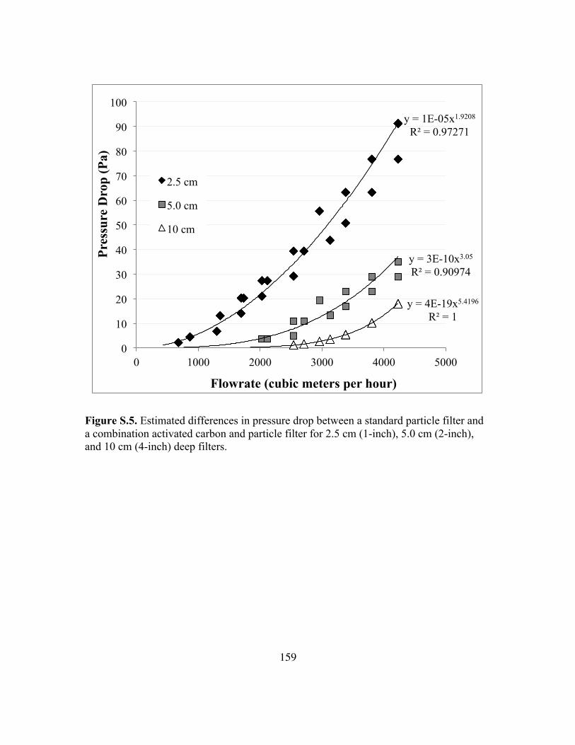
159

Figure S.5. Estimated differences in pressure drop between a standard particle filter and a combination activated carbon and particle filter for 2.5 cm (1-inch), 5.0 cm (2-inch), and 10 cm (4-inch) deep filters.

y = 1E-05x1.9208 R² = 0.97271

y = 3E-10x3.05 R² = 0.90974

y = 4E-19x5.4196 R² = 1

0

10

20

30

40

50

60

70

80

90

100

0 1000 2000 3000 4000 5000

Pres

sure

Dro

p (P

a)

Flowrate (cubic meters per hour)

2.5 cm

5.0 cm

10 cm

160

A final modeling simulation incorporated an assumption that all of the ozone-

related health outcomes would apply only during the summer ozone season. In the

previous analyses, the calculated DALYs were scaled by 5/12 in order to compare the

benefits with the associated filter energy costs from 1 May to 30 September. However, in

other analyses that incorporate USEPA protocols for determining health outcomes from

ozone exposure, the health outcomes for the entire year were assumed to occur during the

ozone season (1 May to 30 September). Berman et al. (2012) and Hubbell et al. (2005)

used USEPA modeling software to evaluate the potential health benefits of reductions in

ambient ozone from 1 May to 30 September in cities across the U.S. The USEPA

regulatory impact assessment for ozone (USEPA, 2014b) incorporates health outcome

functions that were originally applied to the summer ozone season, and some of the

applied ozone controls (e.g., regulating gasoline vapor pressure) are only used during the

summer season. When removing the scaling factor in our model, the median B/C for

Phoenix approaches 1.0 when using a carbon filter with a single pass removal efficiency

for ozone of approximately 45% as shown in Figure S.6. The ASHRAE minimum

standard efficiency for ozone control is 40% (ASHRAE, 2013), which implies that

commercially available carbon filters may be economically viable for ozone removal in

homes, especially for individuals sensitive to ozone. Monetary benefits versus filter

efficiency for this analysis are presented in Figure S.7.

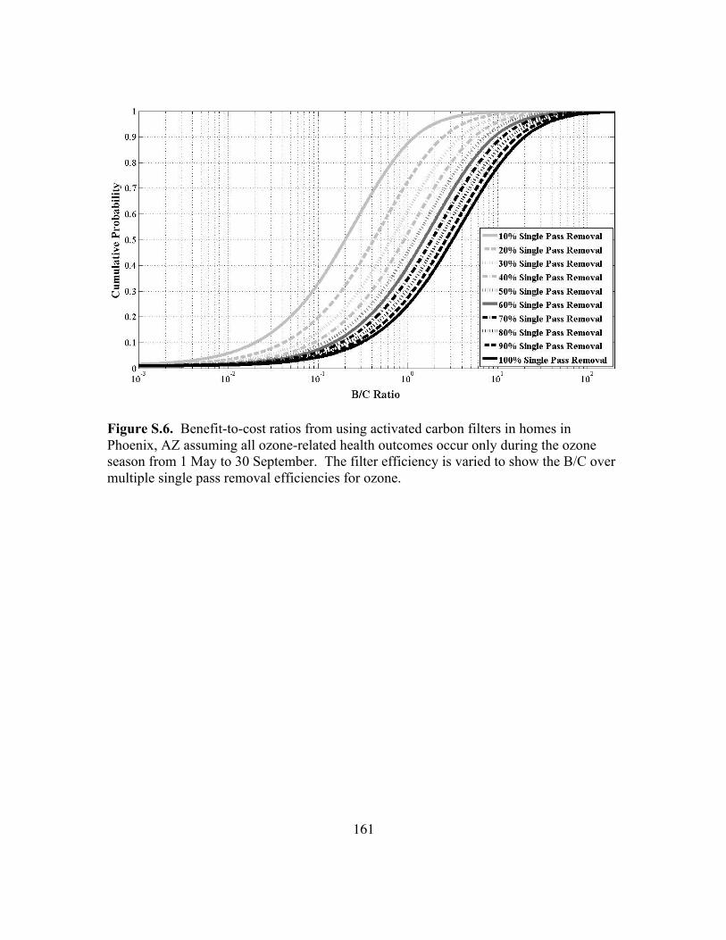
161

Figure S.6. Benefit-to-cost ratios from using activated carbon filters in homes in Phoenix, AZ assuming all ozone-related health outcomes occur only during the ozone season from 1 May to 30 September. The filter efficiency is varied to show the B/C over multiple single pass removal efficiencies for ozone.

162

Figure S.7. Monetary benefits from using activated carbon filters in homes in Phoenix, AZ assuming all ozone-related health outcomes occur only during the ozone season from 1 May to 30 September. The filter efficiency is varied to show the B/C over multiple single pass removal efficiencies for ozone.

163

Appendix B

Paper II. Cost-Benefit Analysis of Commercially Available Activated Carbon Filters for Indoor Ozone Removal in Buildings (submitted to

Science and Technology for the Built Environment)

164

PAPER II

Cost-Benefit Analysis of Commercially Available Activated Carbon Filters for Indoor Ozone Removal in Buildings

(Submitted to Science and Technology for the Built Environment)

Abstract

This study involved the development of a model for evaluating the potential costs

and benefits of ozone control by activated carbon filtration in buildings. The modeling

effort included the prediction of indoor ozone and ozone reaction products with and

without activated carbon filtration in the HVAC system. As one application, the model

was used to predict benefit-to-cost ratios for various types of buildings in 12 American

cities in five different climate zones. Health benefits were evaluated using the disability-

adjusted life-years attributed to the difference in indoor ozone concentration with and

without activated carbon filtration and included city-specific age demographics for each

simulation. Costs of commercially available activated-carbon filters included capital

cost differences when compared to conventional HVAC filters of similar MERV rating,

energy penalties due to additional pressure drop, and regional utility rates. When

assuming a single pass ozone removal efficiency of 60%, carbon filtration during the

ozone season was beneficial and economically viable in commercial office buildings,

long-term healthcare facilities, and K-12 schools. Additionally, benefits for residential

filtration were marginal in most cities, but could be highly beneficial for those with

respiratory illness. Finally, residential filtration could be economically viable for

165

conditions of higher ozone removal efficiencies, lower filter costs, and lower pressure

drop across the filter.

Key Words

Chemistry, control, commercial buildings, disability-adjusted life-years, benefit-cost

analysis, modeling.

Practical Applications

Ozone and ozone reaction products have been linked to increased incidences of mortality

and morbidity. Approximately 50% of ozone exposure occurs indoor. As such, effective

ozone control via carbon filtration can provide health benefits, especially in cities with

high ambient ozone concentrations during the summer ozone season.

Introduction

Tropospheric ozone is formed due to chemical reactions involving nitrogen oxides

(NOx) and volatile organic compounds (VOCs) in the presence of sunlight. Despite an

average decrease in ozone concentrations in the U.S. by 28% since 1980, nearly 1/3 of

Americans still live and work in counties with ozone concentrations that exceed the

primary eight-hour average National Ambient Air Quality Standard (NAAQS) for ozone

(USEPA, 2013). Exposure to ozone has been linked to premature mortality (Bell et al.,

2005; Ito et al., 2005; Jerrett et al., 2009; Levy et al., 2005; Smith et al., 2009; USEPA,

2006, and references provided therein), increases in respiratory-related hospital

166

admissions (e.g., Burnett et al., 1999), minor restricted activity days (e.g., Ostro and

Rothschild, 1989), and school loss days (e.g., Chen et al., 2000). As such, there have

been increasing efforts to develop new methods to reduce ozone concentrations,

including reducing ozone precursors (USEPA, 2014) and recommending ozone filtration

in buildings located in regions with high seasonal ozone concentrations (ASHRAE,

2013a).

Nearly half of personal ozone exposure in the United States occurs in indoor

environments (Weschler, 2006). Indoor ozone concentrations are generally 30-70% of

outdoor ozone concentrations (Weschler, 2000), with much lower percentages in newer

homes with tight construction and air conditioning (Chen et al., 2012; Smith et al., 2009).

Furthermore, exposures to indoor ozone have recently been linked to premature mortality

(Chen et al., 2012).

While indoor ozone can be harmful in its own right, it can also react with

compounds commonly found indoors to create harmful by-products, many of which have

generally higher concentrations indoors than outdoors (Weschler, 2006). More

specifically, ozone can react with material surfaces (heterogeneous reactions) that include

carpet (Wang and Morrison, 2010; Coleman et al., 2008; Wang and Morrison, 2006;

Morrison and Nazaroff, 2002), paint (Cros et al., 2012; Lamble et al., 2011; Reiss et al.,

1995), and ceiling tile (Cros et al., 2012; Lamble et al., 2011) to form C1-C12 carbonyls.

Additionally, ozone will react with unsaturated organic compounds (homogenous

reactions) such as α-pinene, β-pinene, d-limonene, linalool, and styrene, all of which are

167

common in indoor environments (Youssefi and Waring 2012; Logue et al., 2011; Chen

and Hopke, 2010; Chen and Hopke, 2009; Lee et al., 2006; Nazaroff et al., 2006; Ng et

al., 2006; Leungsakul et al., 2005; Nazaroff and Weschler, 2004; Atkinson and Arey,

2003; Fan et al., 2003; Grosjean and Grosjean, 1997; Grosjean and Grosjean, 1996;

Weschler and Shields, 1996; Grosjean et al., 1993).

Ozone-alkene reaction products include irritating and potentially toxic compounds

such as formaldehyde and acetaldehyde (Weschler, 2006), as well as secondary organic

aerosols (SOA) (Chen and Hopke, 2010; Chen and Hopke, 2009; Sarwar and Corsi, 2007;

Fan et al., 2003; Sarwar et al., 2003). Neither the acute nor chronic health effects of

exposure to indoor SOA are well understood.

Activated carbon filters have been shown to be effective at removing ozone in

buildings (Ginestet et al., 2013; Fisk, 2009; Gundel et al., 2002; Shields et al., 1999) and

may be an economically viable method to improve health in the indoor environment.

This will be especially true in buildings with a large proportion of make-up ventilation

air, such as office buildings, health facilities, and schools. The consequences of using

commercially available activated carbon filters can include an increased filter cost

compared to standard filters, potentially higher pressure drop across the filter (and a

higher electricity cost), and longevity of the filter. All of these factors need to be fully

investigated to determine the health benefits and costs of ozone exposure in buildings.

168

Model Development

The overall objective of this study was to complete an assessment of the benefit-

to-cost ratio (B/C) associated with commercially available activated carbon filters in

HVAC systems. To accomplish this objective a systems model consisting of

interconnected components was developed (Figure 1). The model is referred to as

CO3B-Calc.

Figure 1. Conceptual model illustrating interconnected sub models of CO3B-Calc model.

169

The integrated systems model was previously described in detail by Aldred et al.

(2015) and Corsi et al. (2014). Primary metrics of the model include ozone removal

effectiveness and benefit-to-cost ratio. Ozone removal effectiveness is defined as the

percent reduction in indoor ozone concentration when an ozone control device is used

relative to an identical condition when such a device is not used, as described by

Equation (1).

Ω = (1 – CAcC/CNo_AcC) * 100% (1)

Where, Ω = ozone removal effectiveness of activated carbon filter (%) CAcC = indoor ozone concentration with activated carbon filter installed (ppb) CNo_AcC = indoor ozone concentration without activated carbon filter installed (ppb)

The concentrations of ozone and reaction products with and without carbon filtration are

determined from steady-state (time-averaged) mass balance equations. Based on

available health response models (Logue et al., 2012; Huijbregts et al., 2005), only

formaldehyde and acetaldehyde were considered as reaction products in this study.

The health model uses concentration-response functions and city-specific

demographics to determine changes in health incidence due to ozone and reaction product

exposures in accordance with USEPA protocols (USEPA, 2012). The changes in health

incidence are then converted to disability-adjusted life-years (DALYs). A difference in

DALYs (or ΔDALYs) is then determined by subtracting the DALYs due to ozone and

reaction product exposures with carbon filtration from the baseline (no carbon filter)

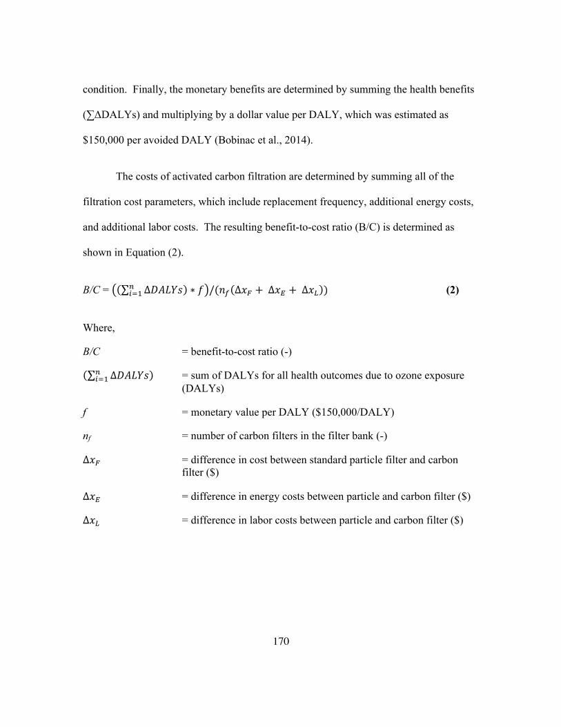
170

condition. Finally, the monetary benefits are determined by summing the health benefits

(∑ΔDALYs) and multiplying by a dollar value per DALY, which was estimated as

$150,000 per avoided DALY (Bobinac et al., 2014).

The costs of activated carbon filtration are determined by summing all of the

filtration cost parameters, which include replacement frequency, additional energy costs,

and additional labor costs. The resulting benefit-to-cost ratio (B/C) is determined as

shown in Equation (2).

B/C = ∆𝐷𝐴𝐿𝑌𝑠!!!! ∗ 𝑓 /(𝑛! ∆𝑥! +  ∆𝑥! +  ∆𝑥! ) (2)

Where,

B/C = benefit-to-cost ratio (-)

∆𝐷𝐴𝐿𝑌𝑠!!!! = sum of DALYs for all health outcomes due to ozone exposure

(DALYs)

f = monetary value per DALY ($150,000/DALY)

nf = number of carbon filters in the filter bank (-)

∆𝑥! = difference in cost between standard particle filter and carbon filter ($)

∆𝑥! = difference in energy costs between particle and carbon filter ($)

∆𝑥! = difference in labor costs between particle and carbon filter ($)

171

Modeling the Effects of Climate, Geography, and Demographics

The modeling analysis focused on the baseline conditions in 12 cities across the

United States. At least two cities from each of the five climate zones defined by the

Energy Information Administration were selected for the analysis (USEIA, 2013).

Climate zones are defined by number of heating degree-days and cooling degree-days.

The cities selected for this analysis include: Atlanta, Austin, Buffalo, Chicago,

Cincinnati, Houston, Miami, Minneapolis, New York City, Phoenix, Riverside, and

Washington D.C. This sample of cities accounts for a broad nationwide sample of

population, climate, building stock, and ambient ozone concentrations. In addition, city-

specific parameters such as the average occupancy of single-family homes, population

age fractions, and regional energy costs were also accounted for in the integrated systems

model. Single-family homes were modeled using city-specific housing parameters to

determine the ozone removal effectiveness and B/C ratio of activated carbon filtration.

Commercial buildings, including office buildings, long term healthcare facilities, and K-

12 schools were modeled using standardized building parameters and city-specific ozone,

demographics, and energy costs.

Modeling Methods for Single-Family Homes

City-specific data sourced from public records and the published literature were

used to model single-family homes in the 12 sample cities (Aldred et al., 2015; Corsi et

al., 2014; LBNL, 2014; USEPA, 2014; USEIA, 2013; USCB, 2012; Stephens et al.,

172

2011; Persily et al., 2010; Lee et al., 1999). The potential benefits from the use of

activated carbon filters include health outcomes for all age groups. For this analysis, only

2-inch filters were considered for the benefit-cost analysis, and it was assumed that two

filters would be required during the summer ozone season (1 May to 30 September) to

maintain a minimum single pass ozone removal efficiency of 60%. Additional modeling

assumptions are presented in Table 1.

Modeling Methods for Commercial Office Building

Mechanical system usage in commercial buildings is governed by the ventilation

requirements of the building. ASHRAE Standard 62.1 (ASHRAE, 2013a) and the

purpose of the building dictate ventilation (i.e., make-up air) requirements. Additional

ventilation air is brought into the building when an air side economizer is used. In this

case, ozone removal by a carbon filter could be much higher as more outdoor air is

cycled through the filter (versus recirculated air).

The U.S. Department of Energy and ASHRAE have developed commercial

prototype building models (USDOE, 2012) for various types of commercial buildings in

accordance with ASHRAE Standard 90.1 (ASHRAE, 2013b). The commercial building

prototypes for small, medium, and large commercial buildings were used in the city-

specific commercial building analysis. Results for medium-sized commercial building

are highlighted in this study.

173

The integrated systems model focuses on health benefits achieved during the peak

ozone season (1 May – 30 September), and it was assumed for this analysis that the

HVAC system is operational 100% while the building is occupied to meet the ventilation

requirements for office buildings. To calculate the energy costs associated with carbon

filtration, it was assumed that the building is occupied during normal working hours (8

hours per day, 5 days per week) and that the HVAC system is operational 11 hours per

day and 5 days per week. It was also assumed that the maximum face velocity of air

entering the carbon filters is 2 m/s, which is equivalent to 2,000 cubic feet per minute

(cfm) for a filter with a face area of 24” x 24” (61cm x 61cm). The number of filters in

the filter bank was determined by the maximum flow rate and by assuming 25% make-up

air. Electricity costs were assumed to be constant, as opposed to demand costs. The

error in this assumption is likely small given that the majorities of the costs for a 2-inch

carbon filter are attributed to capital and labor costs. Other key modeling assumptions

are presented in Table 1.

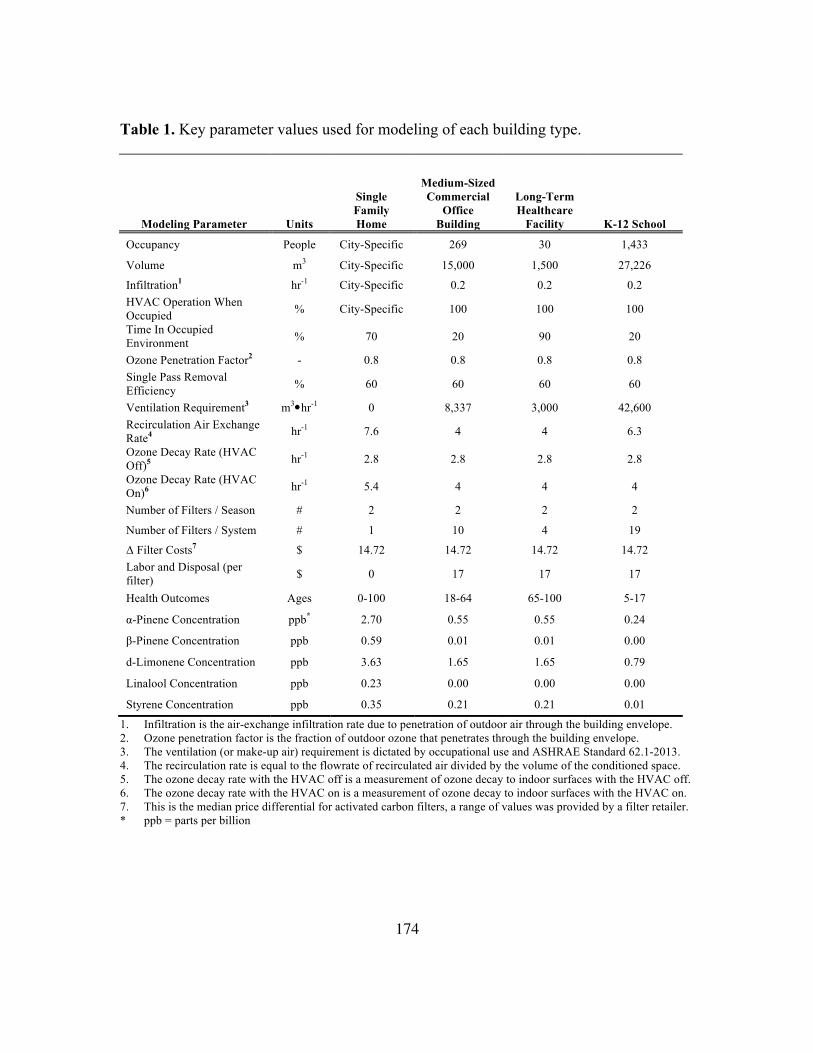
174

Table 1. Key parameter values used for modeling of each building type.

Modeling Parameter Units

Single Family Home

Medium-Sized Commercial

Office Building

Long-Term Healthcare

Facility K-12 School

Occupancy People City-Specific 269 30 1,433

Volume m3 City-Specific 15,000 1,500 27,226

Infiltration1 hr-1 City-Specific 0.2 0.2 0.2 HVAC Operation When Occupied % City-Specific 100 100 100

Time In Occupied Environment % 70 20 90 20

Ozone Penetration Factor2 - 0.8 0.8 0.8 0.8 Single Pass Removal Efficiency % 60 60 60 60

Ventilation Requirement3 m3�hr-1 0 8,337 3,000 42,600 Recirculation Air Exchange Rate4 hr-1 7.6 4 4 6.3

Ozone Decay Rate (HVAC Off)5 hr-1 2.8 2.8 2.8 2.8

Ozone Decay Rate (HVAC On)6 hr-1 5.4 4 4 4

Number of Filters / Season # 2 2 2 2

Number of Filters / System # 1 10 4 19

Δ Filter Costs7 $ 14.72 14.72 14.72 14.72 Labor and Disposal (per filter) $ 0 17 17 17

Health Outcomes Ages 0-100 18-64 65-100 5-17

α-Pinene Concentration ppb* 2.70 0.55 0.55 0.24

β-Pinene Concentration ppb 0.59 0.01 0.01 0.00

d-Limonene Concentration ppb 3.63 1.65 1.65 0.79

Linalool Concentration ppb 0.23 0.00 0.00 0.00

Styrene Concentration ppb 0.35 0.21 0.21 0.01

1. Infiltration is the air-exchange infiltration rate due to penetration of outdoor air through the building envelope. 2. Ozone penetration factor is the fraction of outdoor ozone that penetrates through the building envelope. 3. The ventilation (or make-up air) requirement is dictated by occupational use and ASHRAE Standard 62.1-2013. 4. The recirculation rate is equal to the flowrate of recirculated air divided by the volume of the conditioned space. 5. The ozone decay rate with the HVAC off is a measurement of ozone decay to indoor surfaces with the HVAC off. 6. The ozone decay rate with the HVAC on is a measurement of ozone decay to indoor surfaces with the HVAC on. 7. This is the median price differential for activated carbon filters, a range of values was provided by a filter retailer. * ppb = parts per billion

175

Modeling Methods for Long Term Healthcare Facilities

Long-term healthcare facilities were modelled as light commercial buildings

(volume of 1,500 m3) with 30 occupants, all over the age of 65. Ventilation standards

were based on guidance provided in ASHRAE Standard 170 for healthcare facilities

(ASHRAE, 2008). It was assumed that occupants, i.e., patients, were inside the building

90% of the time. The cost model also included HVAC characteristics typically observed

in light commercial buildings (Azimi and Stephens, 2013). Health benefits were

modelled using health incidence functions for persons over the age of 65 years (USEPA,

2012); health care workers were not considered in the DALY analysis. Building

operation and health benefits were only considered for the summer ozone season (1 May

to 30 September). Age-specific baseline incidence and health parameters are provided in

detail in Aldred et al. (2015) and Corsi et al. (2014). Additional modeling assumptions

are presented in Table 1.

Modeling Methods for K-12 Schools

School facilities were modelled as medium-sized commercial buildings (volume

of 27,226 m3) with 1,433 occupants using the ASHRAE Standard 90.1 Prototype

Building for a primary school (USDOE, 2012). Ventilation standards were based on

guidance provided in ASHRAE Standard 62.1 (ASHRAE, 2013a) for elementary

educational facilities. It was assumed that students are in school buildings 20% of the

year, and that the HVAC system is operational 31% of the year (similar to the

176

commercial building model). The number of filters (19) was determined by assuming a

constant face velocity of 2 m/s, a filter face area of 24” x 24” (61cm x 61cm), and make-

up ventilation required by Standard 62.1. The fraction of make-up air in supply air was

assumed to be 25% (42,600 m3�hr-1).

Health functions for children between the ages of five and 17 were used for the

benefit analysis; teachers and other school staff were not considered in the analysis.

Building operation and health benefits were only considered for the summer ozone

season (1 May to 30 September). For the benefits model, the value per school loss day

used by Hubbell et al. (2005) was adjusted for inflation ($105 in 2014 USD) (U.S.

Bureau of Labor Statistics, 2014). This value incorporates time lost at work by a parent

staying home with a child during the school absence and does not include the direct costs

to the school district, as this cost varies by district and state.

A conversion factor of 1.5 was used to convert average daily ozone to 8-hour

daily ozone per guidance provided in USEPA (2012) and the baseline incidence of school

loss days was assumed to be 9.9 per year per child (Hubbell et al., 2005). It was assumed

that every preventable school absence resulted in 1.6 school loss days and an adjustment

factor of 0.393 was used to estimate exposure in schools during the summer ozone season

(i.e., 39.3% of the school year occurs during the ozone season from 1 May to 30

September) (USEPA, 2012).

177

Modeling Uncertainty

The greatest uncertainty of the results lies in the health functions of the integrated

systems model. In order to accurately capture the uncertainty in the health outcomes,

error propagation was used to determine the mean and 95% confidence intervals of the

calculated DALYs (Spadaro and Rabl, 2008; Burmaster and Hull, 1997; Slob, 1994).

Lognormal functions, specifically the health functions for formaldehyde and

acetaldehyde, were normalized when comparing with normal health functions.

Results and Discussion

The ozone removal effectiveness for in-duct carbon filtration varies by city and by

building type as shown in a sample of cities presented in Figure 2. Removal

effectiveness varies considerably when evaluating single-family homes, as HVAC

cycling rates vary based on cooling demand. Conversely, values of removal effectiveness

are nearly equivalent from city to city for the three other building types, as HVAC

operation is dictated by ventilation requirements for the building type. This is most

evident when evaluating the removal effectiveness in K-12 schools, since schools require

a much higher proportion of ventilation air than commercial office buildings.

178

Figure 2. Ozone removal effectiveness when using activated carbon filters in four types of buildings in six of the twelve sample cities.

In the case of single-family homes, cities with high air-conditioning usage during

the ozone season (Atlanta, Austin, Houston, Miami, Phoenix, and Riverside) have the

highest values of ozone removal effectiveness. The highest effectiveness (just less than

30%) occurs for homes in Miami, and is limited by frequency of HVAC operation and

single-pass ozone removal efficiency for the activated carbon filter (assumed 60% for all

analyses based on a manufacturer survey).

0

10

20

30

40

50

60

70

80

Sing

le F

amily

Hom

e M

ediu

m S

ized

Offi

ce B

uild

ing

Long

Ter

m H

ealth

care

Fac

ility

K

-12

Scho

ol

Sing

le F

amily

Hom

e M

ediu

m S

ized

Offi

ce B

uild

ing

Long

Ter

m H

ealth

care

Fac

ility

K

-12

Scho

ol

Sing

le F

amily

Hom

e M

ediu

m S

ized

Offi

ce B

uild

ing

Long

Ter

m H

ealth

care

Fac

ility

K

-12

Scho

ol

Sing

le F

amily

Hom

e M

ediu

m S

ized

Offi

ce B

uild

ing

Long

Ter

m H

ealth

care

Fac

ility

K

-12

Scho

ol

Sing

le F

amily

Hom

e M

ediu

m S

ized

Offi

ce B

uild

ing

Long

Ter

m H

ealth

care

Fac

ility

K

-12

Scho

ol

Sing

le F

amily

Hom

e M

ediu

m S

ized

Offi

ce B

uild

ing

Long

Ter

m H

ealth

care

Fac

ility

K

-12

Scho

ol

Atlanta Miami Minneapolis New York Phoenix Washington DC

Rem

oval

Eff

ectiv

enes

s (%

)

179

The ozone removal effectiveness for office buildings is much higher (average of

55%) relative to single-family homes due to the requirement for make-up ventilation air,

as well as lower fraction of infiltration toward outdoor-indoor air exchange. The higher

indoor ozone concentrations in the absence of carbon filtration and high ozone removal

effectiveness in office buildings leads to higher absolute reductions in indoor ozone.

Ozone removal effectiveness in long-term healthcare facilities exceeds 60%. This

is primarily due to the large amount of make-up air required for long-term healthcare

facilities (50% make-up air) and a relatively low infiltration rate typical of most light

commercial buildings (0.2 hr-1). Likewise, K-12 schools also require a relatively large

amount of make-up air (at least 25% of supply air), and ozone removal effectiveness

exceeded 60% in every city.

Projected Health Benefits

Overall projected health benefits are a function of the ozone removal

effectiveness of activated carbon filtration and the demographics of each city. Atlanta,

Austin, Houston, Miami, Phoenix, and Riverside have the highest potential health

benefits accrued from carbon filter applications due to high air conditioning usage.

Conversely, the health benefits of carbon filter usage are relatively low in Buffalo,

Chicago, Cincinnati and Minnesota. A majority of the health benefits of reduced ozone

are due to reductions in mortality, especially among older populations. Therefore, health

benefits are increased in cities with large populations of persons 65 years and older, such

180

as Miami (14% over 65), New York (12% over 65), and Buffalo (12% over 65).

Activated carbon filtration may be very beneficial in cities not included in this analysis,

and that have a higher fraction of the population over the age of 65 years old. Therefore,

in addition to HVAC usage during the summer, health benefits will also be impacted by

local demographics, especially the age of the exposed population.

Modeling Results for Single Family Homes

The B/C ratios for applications of activated carbon filters in single family homes

in each of 12 target cities are presented in Figure 3. Phoenix and Riverside are the only

cities with mean B/C ratios above 1.0. This is primarily due to a combination of high

ambient ozone concentration and high air conditioning usage. Although pressure drop is

minimized using a 2-inch filter (versus a 1-inch filter), the increased cost of the filter

remains an obstacle to an increased B/C ratio. The cost of the filter, as opposed to

recurring energy costs, is the primary cost driver for residential carbon filtration,

particularly for 2-inch and thicker filters. As such, reduction in the cost differential

between conventional particle filters and carbon filters is critical for increasing the B/C

ratio. It is expected that as the use of carbon filters become more common, cost

differentials will trend toward or even decrease below the lower value.

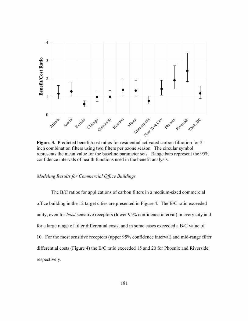
181

Figure 3. Predicted benefit/cost ratios for residential activated carbon filtration for 2-inch combination filters using two filters per ozone season. The circular symbol represents the mean value for the baseline parameter sets. Range bars represent the 95% confidence intervals of health functions used in the benefit analysis.

Modeling Results for Commercial Office Buildings

The B/C ratios for applications of carbon filters in a medium-sized commercial

office building in the 12 target cities are presented in Figure 4. The B/C ratio exceeded

unity, even for least sensitive receptors (lower 95% confidence interval) in every city and

for a large range of filter differential costs, and in some cases exceeded a B/C value of

10. For the most sensitive receptors (upper 95% confidence interval) and mid-range filter

differential costs (Figure 4) the B/C ratio exceeded 15 and 20 for Phoenix and Riverside,

respectively.

0

1

2

3

4 B

enef

it/C

ost R

atio

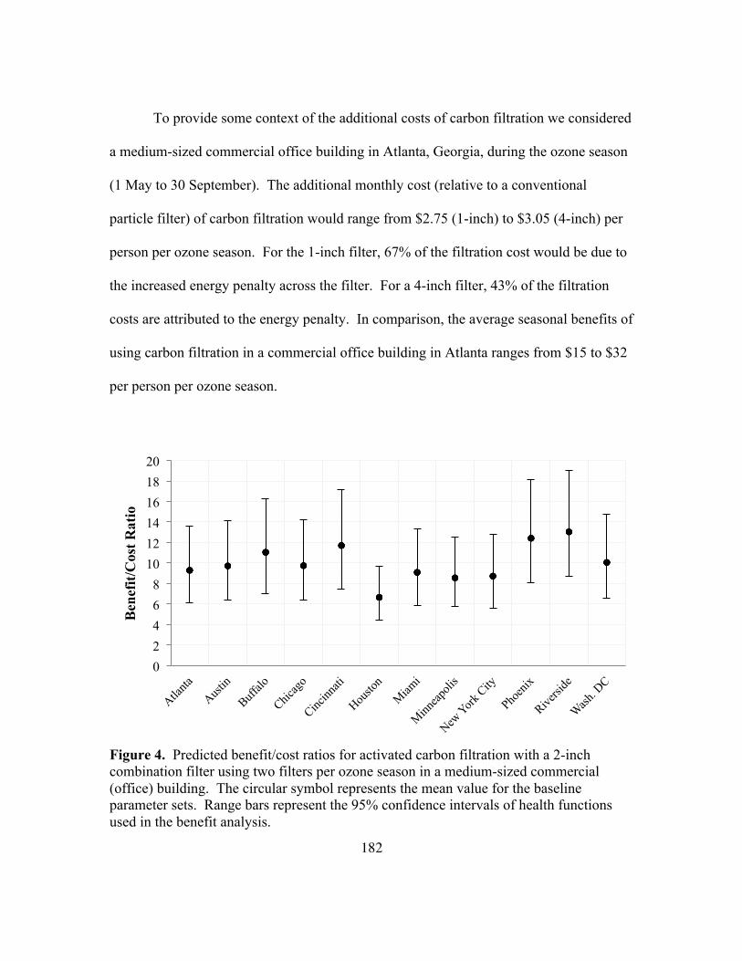
182

To provide some context of the additional costs of carbon filtration we considered

a medium-sized commercial office building in Atlanta, Georgia, during the ozone season

(1 May to 30 September). The additional monthly cost (relative to a conventional

particle filter) of carbon filtration would range from $2.75 (1-inch) to $3.05 (4-inch) per

person per ozone season. For the 1-inch filter, 67% of the filtration cost would be due to

the increased energy penalty across the filter. For a 4-inch filter, 43% of the filtration

costs are attributed to the energy penalty. In comparison, the average seasonal benefits of

using carbon filtration in a commercial office building in Atlanta ranges from $15 to $32

per person per ozone season.

Figure 4. Predicted benefit/cost ratios for activated carbon filtration with a 2-inch combination filter using two filters per ozone season in a medium-sized commercial (office) building. The circular symbol represents the mean value for the baseline parameter sets. Range bars represent the 95% confidence intervals of health functions used in the benefit analysis.

0 2 4 6 8

10 12 14 16 18 20

Ben

efit/

Cos

t Rat

io

183

Modeling Results for Long Term Healthcare Facilities

The predicted health benefits of in-duct activated carbon filtration in long term

healthcare facilities greatly exceed the other building types considered in this analysis.

Demographics are an important consideration. This demographic tends to be the most

sensitive to ozone-related health outcomes, particularly premature respiratory mortality;

greater than 90% of the benefits are attributed to reduced mortality. The projected

number of lives saved annually (Figure 5) exceeds 100 per 100,000 (or 0.1%) for each

target city.

Figure 5. Predicted health benefits of carbon filtration in a long-term healthcare facility. The square symbol represents the mean results of the baseline parameter sets. Range bars represent the 95% confidence intervals of health functions used in the benefit analysis. Only ozone, formaldehyde, and acetaldehyde reductions were considered for the health benefit analysis.

0

500

1000

1500

2000

2500

3000

Red

uced

DA

LYs

Red

uced

Mor

talit

ies

Red

uced

DA

LYs

Red

uced

Mor

talit

ies

Red

uced

DA

LYs

Red

uced

Mor

talit

ies

Red

uced

DA

LYs

Red

uced

Mor

talit

ies

Red

uced

DA

LYs

Red

uced

Mor

talit

ies

Red

uced

DA

LYs

Red

uced

Mor

talit

ies

Red

uced

DA

LYs

Red

uced

Mor

talit

ies

Red

uced

DA

LYs

Red

uced

Mor

talit

ies

Red

uced

DA

LYs

Red

uced

Mor

talit

ies

Red

uced

DA

LYs

Red

uced

Mor

talit

ies

Red

uced

DA

LYs

Red

uced

Mor

talit

ies

Red

uced

DA

LYs

Red

uced

Mor

talit

ies

Atl Aus Buf Chi Cin Hou Mia Min NYC Pho Riv Wash

Hea

lth B

enef

its p

er 1

00,0

00

184

A majority of the health benefits achieved through carbon filtration in long term

health care facilities are attributed to reduced mortalities and reduced hospital admissions

due to chronic respiratory diseases. A combination of high ozone removal effectiveness

and higher respiratory disease prevalence among persons over the age of 65 years yields

significant health benefits due to lower ozone exposure. Since the potential benefits are

high and the costs are relatively low, B/C ratios are in the hundreds as shown for 2-inch

filters in Figure 6.

Figure 6. Predicted benefit/cost ratios for activated carbon filtration with a 2-inch combination filter using two filters per ozone season in a long term healthcare facility. The circular symbol represents the mean value of the baseline parameter sets. Range bars represent the 95% confidence intervals of health functions used in the benefit analysis. Modeling Results for K-12 Schools

The projected school loss days per 100,000 children (with and without activated

carbon filtration) in each of the 12 target cities is presented in Figure 7. The

overwhelming majority of DALYs saved due to carbon filtration in K-12 schools was

0 100 200 300 400 500 600 700 800 900

1,000

Ben

efit/

Cos

t Rat

io

185

attributed to prevented school loss days (99% of all DALYs). Benefit/cost ratios for 2-

inch filters are presented in Figure 8.

Figure 7. Predicted number of annual school loss days in K-12 schools with and without activated carbon filtration. The square symbol represents the mean results of the baseline parameter sets. Range bars represent the 95% confidence intervals of health functions used in the benefit analysis. Only ozone-related school loss day health functions were considered.

0

10000

20000

30000

40000

50000

60000

70000

80000

Scho

ol L

oss D

ays N

o A

cC

Scho

ol L

oss D

ays A

cC

Scho

ol L

oss D

ays N

o A

cC

Scho

ol L

oss D

ays A

cC

Scho

ol L

oss D

ays N

o A

cC

Scho

ol L

oss D

ays A

cC

Scho

ol L

oss D

ays N

o A

cC

Scho

ol L

oss D

ays A

cC

Scho

ol L

oss D

ays N

o A

cC

Scho

ol L

oss D

ays A

cC

Scho

ol L

oss D

ays N

o A

cC

Scho

ol L

oss D

ays A

cC

Scho

ol L

oss D

ays N

o A

cC

Scho

ol L

oss D

ays A

cC

Scho

ol L

oss D

ays N

o A

cC

Scho

ol L

oss D

ays A

cC

Scho

ol L

oss D

ays N

o A

cC

Scho

ol L

oss D

ays A

cC

Scho

ol L

oss D

ays N

o A

cC

Scho

ol L

oss D

ays A

cC

Scho

ol L

oss D

ays N

o A

cC

Scho

ol L

oss D

ays A

cC

Scho

ol L

oss D

ays N

o A

cC

Scho

ol L

oss D

ays A

cC

Atl Aus Buf Chi Cin Hou Mia Min NYC Pho Riv Wash

Scho

ol L

oss D

ays p

er 1

00,0

00 C

hild

ren

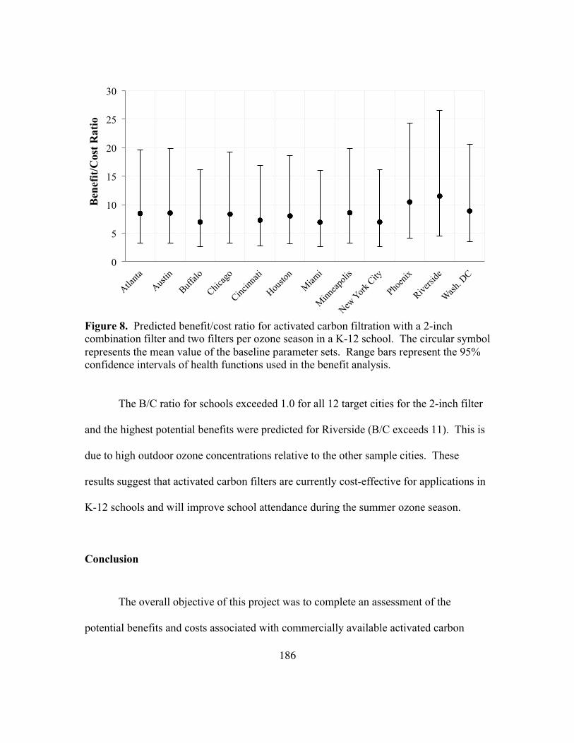
186

Figure 8. Predicted benefit/cost ratio for activated carbon filtration with a 2-inch combination filter and two filters per ozone season in a K-12 school. The circular symbol represents the mean value of the baseline parameter sets. Range bars represent the 95% confidence intervals of health functions used in the benefit analysis.

The B/C ratio for schools exceeded 1.0 for all 12 target cities for the 2-inch filter

and the highest potential benefits were predicted for Riverside (B/C exceeds 11). This is

due to high outdoor ozone concentrations relative to the other sample cities. These

results suggest that activated carbon filters are currently cost-effective for applications in

K-12 schools and will improve school attendance during the summer ozone season.

Conclusion

The overall objective of this project was to complete an assessment of the

potential benefits and costs associated with commercially available activated carbon

0

5

10

15

20

25

30 B

enef

it/C

ost R

atio

187

filters in HVAC systems. To complete this task, an integrated systems model was

developed to evaluate the benefits and costs of carbon filtration in various types of

buildings. Model parameters were based on a number of sources, including the peer-

reviewed literature, conference papers, government reports, technology manufacturer

websites, and direct communications with filter manufacturers. The major findings of

this study indicate that commercially available activated carbon filters are an

economically viable strategy for improving health in commercial office buildings, long

term healthcare facilities, and K-12 schools. These findings apply to cities that are

currently in attainment for USEPA ozone standards and may not require ozone control in

accordance with ASHRAE Standard 62.1 (ASHRAE, 2013a). Furthermore, activated

carbon filtration in homes results in marginal economic benefits and is best utilized in

cities with high seasonal ozone, high HVAC cycling operation, and/or homes with

occupants that suffer from respiratory illnesses.

This study does have several limitations that can be improved through future

research. There is a lack of published and available gray literature related to long-term

performance of activated carbon for removal of ozone, particularly under the highly

variable environmental conditions often encountered in practice. Additional limitations

and topics for further research include the following:

• Ozone concentrations were averaged across a five-month ozone season. As such, the

health effects following high/peak ozone events are not captured. Indoor ozone

188

control during such events would increase the benefit/cost ratios described in this

dissertation, particularly for sensitive populations.

• Indoor ozone concentrations are typically much lower than outdoor ozone

concentrations, even without specific ozone control technologies. In this study, we

assumed that there is no threshold below which incremental reductions in indoor

ozone concentration do not have a positive health effect. This is an important issue

that has yet to be effectively resolved by the health science community.

• Indoor sources of ozone were also not included in this study. Such sources may be

important in offices or schools with poorly maintained and highly operated photocopy

machines. For such scenarios the benefit/cost ratio of carbon filters will increase. The

integrated systems model developed for this study allows for predictions that include

indoor sources of ozone.

• The frequency and time of window opening can affect building occupant exposures to

ozone. These factors were omitted from analysis in this study.

Acknowledgements

This study was primarily supported with funding from ASHRAE (RP-1491, Literature

and Product Review and Cost Benefit Analysis of Commercially Available Ozone Air

Cleaning for HVAC Systems). Additional financial support from ASHRAE was

provided through an ASHRAE Student Grant-in-Aid, the Walter L. and Reta Mae Moore

Graduate Fellowship in Water Resources at the University of Texas at Austin, and the

U.S. Air Force. The views expressed in this article are those of the author and do not

189

reflect the official policy or position of the United States Air Force, U.S. Department of

Defense, or the U.S. government.

190

Appendix C

Paper III. A Benefit-Cost Analysis of Reduced Ventilation and Carbon Filtration in a University Laboratory Building (submitted to Building

and Environment)

191

PAPER III

A Benefit-Cost Analysis of Reduced Ventilation and Carbon Filtration in a University Laboratory Building

(Submitted to Building and Environment) Abstract

This study focused on the benefits and costs of three different experimental ventilation

and filtration conditions in a LEED-rated operational campus laboratory tested during

two seasons in Austin, TX. Ventilation (i.e., make-up air) flow rates were measured, and

energy consumption data were collected in the field and then compared to building

energy usage modeled with numerical methods software. The experimental results were

then extrapolated to predict energy savings for an entire year. Indoor air quality

measurements were collected to determine the potential health consequences of reducing

ventilation rates for purposes of lower energy costs. Ventilation reductions in one air-

handling unit in the building resulted in nearly $50,000 in reduced chilled water, steam,

and fan energy costs per year. A small portion of the savings were then re-invested in

activated carbon filters to remove outdoor ozone and improve indoor air quality. A

benefit-cost analysis was used to determine that lower ventilation rates combined with

activated carbon filtration has potential to reduce ozone-related health costs by 62% and

fan energy costs by an additional 21%. This study demonstrates that ventilation

reductions in laboratory facilities could yield considerable energy savings, of which a

portion could be re-invested in high efficiency activated carbon filtration to improve

indoor air quality and occupant health in laboratories.

192

1. Introduction

The U.S. Energy Information Administration estimates that energy used in

buildings accounts for 40% of energy usage nationwide (U.S. Energy Information

Administration, 2014). In a life cycle assessment of a university building, operational

usage (electricity and HVAC) accounted for over 90% of the building’s life cycle energy

costs over the 75-year lifetime of the building (Scheuer, et al., 2003). Since buildings

account for such a large amount of energy usage, a considerable amount of effort is

underway to design more sustainable and energy efficient buildings. Popular building

rating systems such as the Leadership in Energy and Environmental Design (LEED)

system continue to fuel this trend, but many green building rating systems weigh points

more heavily toward energy usage than indoor air quality. For the LEED Commercial

Interiors certification (version 3), up to 37 points (out of 110 total points) are awarded for

energy savings measures and up to 17 points are awarded for indoor environmental

quality (U.S. Green Buildings Council, 2014).

Several researchers have quantified the chronic health impacts (Logue et al.,

2012) and life cycle costs (Collinge et al., 2013) of exposure to indoor air pollutants. The

projected health and economic benefits of improving indoor air quality can be substantial,

ranging from $17B to $26B per year (Fisk et al., 2011). One solution to improving

indoor air quality while simultaneously saving energy in buildings with high ventilation

rates (e.g., laboratories) is to utilize a strategy of lower ventilation rates with improved

filtration of outdoor air, specifically by using activated carbon filters.

193

Fresh-air ventilation rates in university laboratories often exceed 10 air volume

changes per hour (10 /hr). Maintaining such a high ventilation rate for laboratories

ensures the safety of the occupants against harmful vapors and aerosols. However, since

all of the ventilation air is typically exhausted to the atmosphere, all fresh air brought into

the building must be conditioned at a significant cost in the form of additional fan energy,

chilled water usage, and supply air reheat in the building’s heating, ventilating, and air

conditioning (HVAC) system. In fact, university laboratories typically consume six to

ten times more energy per square foot than comparably sized office buildings (Lawrence

Berkeley National Laboratory, 2008).

In this study, we: (1) investigate, with field measurements, changes in indoor air

quality and energy usage before and after a significant ventilation reduction, (2) evaluate

potential energy savings when comparing the two ventilation scenarios, and (3) determine

the life cycle costs and benefits of installing commercially available activated carbon

filters.

2. Methods

This study was divided into four phases: (i) calibration of energy monitoring

equipment with the building automation system, (ii) winter energy monitoring (two

weeks of active sampling), (iii) summer energy and indoor air quality modeling, with and

without activated carbon filtration (three weeks of active sampling), and (iv) benefit-cost

analyses. Field measurements were limited to three weeks. An illustration showing the

phases and conditions of the sampling plan is presented in Figure 1.

194

Figure 1. Phases and conditions of the sampling schedule.

2.1. Test Building

Indoor air quality and energy usage due to reduced ventilation rates in a

laboratory building on the University of Texas campus were measured. The building

selected for this study had laboratory space with very high air exchange rates (as high as

12/hr), as well as sophisticated ventilation control and data collection systems. The

building is a 142,000 square foot research facility constructed in 2008 and certified as

LEED Silver. It has six primary floors with the top floor acting as the mechanical space

for the facility. The first floor is entirely below grade and the second floor is partially

below grade. The building has nine air-handling units and 102 separate laboratory

heating, ventilating, and air conditioning (HVAC) zones. In addition, all exhaust air from

the laboratories is collected and directed through a glycol heat recovery system. The

recovered exhaust heat is then used to pre-heat outdoor air before it passes through the

Phase I Phase II Phase III Phase IV Fall Winter Summer Fall

Calibration

Energy Monitoring and Data Collection Energy Monitoring and Data Collection

Indoor Air Quality Measurements

Benefit-Cost Analysis

Ventilation Rate

High Low Low High (Baseline) Low (Carbon Filter)

195

heating and cooling coils in the air-handling unit. Ventilation can be remotely controlled

and monitored using a building automation system (BAS) (Siemens Insight BAS

Software, version 3.13). The operational characteristics of the laboratories served are

presented in Table 1.

196

Table 1. Operational characteristics of the laboratory building. Modeling and Experimental Parameters Source Weather file for energy analysis Austin, TX NREL TMY3 Exterior façade (from outside to inside) 2.54 cm thick stone (ST01), 1.91 cm

or less air gap (AL11), moisture barrier (BP03)

Building specifications

Interior wall assembly (from outside to inside)

0.95 cm insulator board (IN63), 15.24 cm thick medium weight concrete block (CB27), 1.27 cm gypsum board (GP01)

Building specifications

Roof construction Steel framing (61 cm on center), no insulation, 1.82 meter overhangs, medium albedo (red tile)

Building specifications

Interior finishes Acoustic tile for the ceilings, vinyl tile flooring, interior frame walls without insulation, horizontal blinds (medium albedo)

Building specifications

Floor to ceiling height 3.05 meters Building specifications Floor to floor height 3.96 meters Building specifications Total square footage 2,139 m2 Building specifications Ventilation reductions, all labs 13,135 m3/hr UT Energy Stewards1 Ventilation reductions, five sample labs 3,141 m3/hr UT Energy Stewards1 Occupancy 24 hours a day, 7 days a week Informal survey Function of space Classrooms and laboratories Building specifications Cooling Chilled water coil Building specifications Cooling thermostat set-point 21°C UT Energy Stewards1 Heating Steam coil, VAV re-heat Building specifications Heating thermostat set-point 18°C UT Energy Stewards1 Air-handling unit fan operation Variable speed Building specifications Ventilation supply Ducted Building specifications Exhaust return Ducted, general exhaust with fume

hoods in some labs Building specifications

Number of air filters in filter bank 24 filters, 61 cm by 61 cm by 48 cm deep bag filters

Building specifications

Filter replacement – maximum pressure drop

400 Pa Building specifications

(1) The UT Energy Stewards are an office within the University’s Facilities Services that focuses on identifying and implementing strategies to reduce energy usage in buildings across campus. 2.2. Calibration and energy field measurements

Three rounds of field measurements were organized to determine overall energy

costs at baseline ventilation conditions and at a lower ventilation rate as shown in Table

2. Five rooms on four different floors serviced by a single air-handling unit (AHU) were

197

considered for the analysis. The building is operated all year and was occupied during

the field campaign. Airflow measurements from the BAS were verified with field

measurements with an airflow capture hood (Airflow Instruments Prohood). Temperature

and relative humidity were verified with data loggers (Onset U12-006) placed in the five

rooms. During the field experiments the BAS was used to collect temperature and

relative humidity data before and after the glycol heat recovery system (pre-heat coil), the

heating coil, and the cooling coil in the air-handling unit. Temperature and relative

humidity measurements were also collected before and after the reheat coil in the supply

ducts servicing each room. Finally, airflow measurements from the BAS were collected

for each room (supply and return). Flow rates for both of the ventilation conditions are

presented in Table 2.

198

Table 2. Supply and exhaust air flow rates in each of the five test labs during high and low ventilation conditions.

High ACH Condition Low ACH Condition

Room Description

Design ACH (1/hr)

Supply (m3/hr)

General Exhaust (m3/hr)

Supply (m3/hr)

General Exhaust (m3/hr)

Adjusted ACH (1/hr)

Lab 1 Optics Lab 7 850 1189 350 690 4

Lab 2 Teaching Lab 6 1104 1274 693 863 4

Lab 3 Teaching Lab 6 1826 1996 1113 1283 4

Lab 4 Wet Lab 10 2421 2187 1223 989 5

Lab 5 Unoccupied 7 1300 1726 980 1405 6

Each ventilation scenario was run for one to two weeks and in sequence with one

another in order to use similar outdoor meteorological conditions. Heating and cooling

energy were determined by using measured airflow rates and equations for latent and

sensible heat for ventilation air passing through the three heat exchangers in the air-

handling unit. Steam usage (kilograms of steam/second) in the AHU heating coil and in

the variable air volume re-heat units in each of the labs was calculated using Equation 1.

The heat recovered from the glycol recovery system to pre-heat outdoor air was also

calculated using Equation 1.

Q = 𝑉𝜌𝑐!∆𝑇 =  𝑚ℎ!" (1)

Q = heat energy [kW]

𝑉 = volumetric air flow rate through the heat exchanger [m3/sec]

𝜌 = density of air at standard temperature and pressure (STP) = 1.2754 [kg/m3]

199

𝑐! = specific heat of air at STP = 1.005 [kJ/°C�kg]

∆𝑇 = difference in temperature across the heat exchanger [°C]

𝑚 = mass flow-rate of steam [kgs/sec]

ℎ!" = latent heat of vaporization = 2,260 [kJ/kg]

The amount of chilled water used in the cooling coil was calculated using

Equation 1. Similarly, steam usage in the AHU heating coil and the re-heat coils in the

variable air volume units in each laboratory were calculated using air flow rates, the

difference in temperature across the coil, and Equation 1. Electrical fan energy was

collected from the BAS system, which was reported in kilowatt-hours (kWh). The

University of Texas produces its own chilled water, steam, and electricity using a high

efficiency chiller and cogeneration. On average, the university pays lower energy costs

than most utilities ($0.58 per kWh of chilled water, $0.06 per kWh of electricity, and

$0.04 per kilogram of steam). Total energy savings were estimated by taking the

difference of calculated energy costs at baseline and reduced ventilation conditions.

2.3. Indoor air quality measurements

Indoor air quality measurements were collected in parallel with the energy field

measurements. Pollutants of concern included ozone, particulate matter, and volatile

organic compounds (VOCs). Carbon dioxide was also measured.

Volatile organic compounds were collected using Tenax-TA® with thermal

desorption and gas chromatography/mass spectrometry (Hewlett-Packard gas

chromatograph model number 5890 II outfitted with a HP 5971 mass selective detector).

200

Each sorption tube was packed with 75 mg of Tenax-TA® sorbent and conditioned in

nitrogen at 300°C for two hours. Active sampling was conducted with two pumps in

each room during each ventilation condition (Buck Elite-5 Pump 5-6000cc/min 120V).

The pumps were programmed at two different pumping rates, 10 mL/min and 40

mL/min, and the sampling time was 4 hours. For every 10 Tenax-TA® samples collected

in the field, a lab blank and trip blank were used for baseline analysis. Compounds were

identified by using the library compound search in Hewlett Packard ChemStation

software and the NIST 11 Mass Spectral Database. The mass of the identified

compounds was estimated using 4-bromofluorobenzene as an internal standard and an

assumed response ratio of 1.0. Samples were collected using a sampling rate of 25

mL/min for four hours and were collected in accordance with U.S. Environmental

Protection Agency (USEPA) methods (TO-17). In addition to sorption tubes, VOCs were

also assessed using summa canisters evaluated by an independent laboratory. The

summa canister samples were collected for 24-hours using USEPA method (TO-15).

Ozone concentrations were measured with two UV-absorbance ozone analyzers

(2B Technologies Inc., Model 202) programmed to ten minute averaging intervals. Both

analyzers were cross calibrated before sampling using a calibrated ozone source (2B

Technologies Inc, Model 306) and three point calibration. The indoor ozone

measurements were collected using a 6 meter piece of PTFE tubing (Fisher Scientific, ¼-

inch O.D., 3/8-inch I.D.), which was positioned with the inlet 30 cm below the ceiling in

the center of the room. The second ozone analyzer collected outdoor ozone concentration

data in the air-handling unit fresh air intake. Outdoor ozone measurements were also

201

collected from the CAMS 3 air quality monitor in northwest Austin (TCEQ, 2014) to

compare against ozone measurements collected in AHU-1. The CAMS 3 air quality

monitor is about five miles (line of sight) from the university campus.

Due to low concentrations of VOCs in the laboratories, a total VOC (TVOC)

concentration was used to quantify VOC concentration. Concentrations of TVOC were

estimated using the total mass under the chromatographic spectra curve from a retention

time of 6 to 16 minutes, and then using the molecular weight of toluene to convert from

the mass concentration to a volumetric concentration expressed in parts per billion by

volume (ppbv).

Particulate matter was measured using a six-channel optical particle counter (TSI

Aerotrak Model 9306). Measurements were taken continuously in a teaching laboratory

during three weeks of ventilation changes. Particles were divided into six size bins based

on aerodynamic diameter (dp). The following bins were selected: dp < 0.3 µm, dp of 0.3

to 1.0 µm, dp of 1.0 to 2.5 µm, dp of 2.5 to 5.0 µm, dp of 5.0 to 10.0 µm, and dp > 10.0

µm. Measurements were collected using particle counts per cubic meter and

measurements were recorded every 30 minutes during the three weeks of field tests.

Particle mass was estimated by converting particle number counts assuming a particle

density of 1 g/cm3 and geometric mean dp for each size bin.

Carbon dioxide (CO2) concentrations were collected using a Telaire Model 7001

CO2 monitor. Data were collected in a teaching laboratory over three weeks and

measurements were logged every five minutes using a data logger (Onset U12-006).

Formaldehyde was also measured using a continuous formaldehyde monitor (Shinyei

202

FFM-MD), however all of the measurements taken within the building were below the

limit of detection of the instrument (10 ppb).

2.4. Cost-benefit analysis: energy savings and indoor pollutant exposure

Indoor air quality in buildings with high ventilation rates is generally dominated

by pollution of outdoor origin, e.g., ozone. Exposure to ozone can be harmful to human

health. Ozone reacts with polyunsaturated fatty acids in fluids lining the lung with

subsequent adverse effects in the airway epithelium (Levy et al., 2001). Additionally,

ozone exposure has been linked to respiratory related mortalities and hospital admissions

(USEPA, 2012). Finally, a recent study has linked indoor ozone exposure to ozone-

related mortalities at relatively low ozone concentrations (Chen et al., 2012).

The predicted health costs of ozone exposure in the laboratory building was

estimated using the CO3B-Calc model (Corsi et al., 2014). The CO3B-Calc model

employs health-impact functions to determine the economic costs of exposure to harmful

air pollutants such as ozone. The health impacts are converted to disability-adjusted life-

years (DALYs), which can be monetized (Bobinac et al., 2014). Reductions in exposure

to pollutants can thus be translated to a reduction in DALYs, and effective monetary

benefit. Occupancy in the laboratories was estimated at 300 people ranging in age from

18 to 24 who occupy the laboratories 20 hours per week for 30 weeks per year (typical

academic year). Energy savings are estimated by a combination of modeling and field

measurements as described previously.

203

2.4.1. Activated carbon filtration

Activated carbon filters are known to remove ozone and other outdoor pollutants

in operational environments (Ginestet et al., 2013; Shields et al., 1999). Ozone is an

oxidizing agent (Weschler, 2004) and reacts with surfaces (heterogeneous reactions) and

other gaseous species in bulk air (homogeneous reactions) to yield potentially harmful

gaseous by-products such as secondary organic aerosols (SOAs), formaldehyde,

acetaldehyde, and hydroxyl radicals (Weschler, 2011). The benefits of carbon filtration

include reductions in ozone and ozone reaction products such as SOAs, as well as

potential reductions in speciated and total VOCs.

One bank of 24 particle filters that supplies 100% make-up air to laboratories with

a maximum design flowrate of 81,600 m3/hr was replaced with activated carbon filters.

The filters were substituted for existing bag filters at the low ventilation rate, and the low

ventilation rate was maintained after the carbon filters were installed. The activated

carbon filters selected for this study were Koch Filter Corporation Durakleen high

efficiency gas phase filters. The face area of the filters was 61 cm x 61 cm and the filters

were placed within a rigid sheet metal box that was 30 cm deep. The carbon was

composed of coconut shell charcoal with a surface area of 1,100 m2/g (evaluated using

BET method), and the carbon mesh size was 20 x 50. According to the filter

manufacturer, no adhesives were used in the carbon filter.

The additional costs of carbon filtration include higher filter costs (compared to

bag filters), but this cost is much lower than the cost savings due to energy reductions

from lower ventilation rates in the laboratories.

204

3. Results and Discussion

3.1. Energy field measurements

Energy field measurements were collected over two seasons, late winter/early

spring, and late summer/early fall. The first collection period lasted nearly three weeks,

with one week at high ventilation rate and two weeks at the reduced ventilation rate. The

second collection period lasted three weeks and included three test scenarios: one week

at baseline (high) ventilation rate, one week at reduced ventilation rate, and one week at

reduced ventilation rate with activated carbon filtration.

During the winter tests, it was determined that the glycol recovery heat exchanger

was fully operational and was effectively pre-heating cold outdoor air using recycled

exhaust air. Average hourly energy costs for the five labs were compared using a two-

sample one-tailed statistical t-test. In the comparison, energy costs decreased by 35% (ρ

<0.00001) during the winter ventilation reductions.

The glycol heat exchanger was not operational during the summer test

experiments. However, the ventilation reductions still resulted in energy savings.

Average hourly energy costs for the five test labs decreased by 3% (ρ <0.00001) between

the high and low ventilation conditions during the summer tests. The savings were more

substantial when comparing the high condition to the low ventilation rate combined with

carbon filters. Average hourly energy costs decreased by 12% (ρ <0.00001) between the

low ventilation condition with and without carbon filters, and 14% (ρ <0.00001) when

comparing the high ventilation condition versus the low condition with carbon filters.

This is likely attributable to reductions in fan energy as the new carbon filters have a

205

lower initial pressure drop (25 Pa) than the bag filters that were previously installed (100

Pa). The fan energy savings were substantial, and average fan energy decreased by 5% (ρ

<0.00001) between the high and low ventilation conditions, and 21% (ρ <0.00001)

between the low ventilation condition versus low ventilation with carbon filters. Average

fan energy decreased by 25% (ρ <0.00001) when comparing the high ventilation

condition versus the low condition with carbon filters.

Data from both the winter and summer tests were analyzed to estimate annual cost

savings from the ventilation reductions. The analysis included energy savings with and

without the glycol heat recovery system. Two polynomial expressions (with heat

recovery and without heat recovery) were applied to the data using statistical tools in

SPSS software (IBM Corporation, 2013). Outdoor temperature was used as the

dependent variable and annual energy cost was the independent variable in the analysis.

The annual energy costs with and without heat recovery are shown in Figure 2 as a

function of outdoor temperature. The polynomial relationships are shown in Equations 4

and 5 below, and are specific to the building tested.

206

Figure 2. Annual cost per cubic foot per minute of ventilation air in the laboratory building versus outdoor dry bulb temperature.

Energy Cost ($) / m3/hr (no heat recovery)

= 0.0002(Tout)3 + 0.0178(Tout)2 – 0.3897(Tout) + 4.4434 (4)

Energy Cost ($) / m3/hr (heat recovery)

= 0.00007(Tout)3 + 0.0083(Tout)2 – 0.1264(Tout) + 2.1816 (5)

Where Tout is the outdoor dry-bulb temperature in degrees Celsius.

Both polynomial relationships were analyzed hourly using TMY3 meteorological data

(Wilcox and Marion, 2008) for Austin, TX. The average annual energy costs per m3/hr

0

1

2

3

4

5

6

7

-5 0 5 10 15 20 25 30

Ann

ual

Cos

t ($)

/ m

3 /hr

Outdoor Temperature (°C)

Heat Recovery

No Heat Recovery

207

of ventilation air were also estimated. For the five test laboratories, the estimated

ventilation reductions were 3,141 m3/hr , leading to $11,315 in annual energy savings.

For all forty rooms served by the AHU, the estimated ventilation reductions were 13,135

m3/hr, leading to $47,300 in annual energy savings.

3.2. Indoor air quality

Quantification of individual VOCs using Tenax-TA sorbent tubes was difficult

because of the low concentrations of VOCs in the laboratories. Therefore, a total VOC

(TVOC) concentration was used to quantify VOC concentrations for samples collected

on Tenax-TA sorbent tubes. An average increase of 72% (ρ < 0.05) from 6.3 ppb to 10.9

ppb in TVOC was observed when the ventilation rate was reduced from the high to low

condition.

Specific VOCs were identified and quantified in subsequent testing using summa

canisters and TO-15 collection methods analyzed by an independent laboratory. The

three VOCs with highest concentrations included dichloromethane, n-hexane, and

toluene. The concentrations of VOCs did not vary considerably between the low

ventilation condition and the low ventilation condition with carbon filtration, indicating

that most of the VOCs measured during the sampling period were emitted from indoor

sources in the laboratories. The highest measured concentrations of VOCs are presented

in Table 3 with indicators showing at which ventilation condition the highest

measurement was collected.

208

Summa canisters were also collected before and after the bag filters and the

carbon filters during the low ventilation condition. The bag filters were sources of

TVOCs, with an outlet (post filter) TVOC concentration 17% higher than the inlet (pre-

filter) concentration (ρ < 0.05). The carbon filters removed VOCs; the outlet (post filter)

concentration was 62% lower than the inlet (pre-filter) concentration (ρ < 0.05).

Table 3. Highest recorded VOC concentrations in five sample laboratories.

        Highest Measured Concentration (µg/m3)

Volatile Organic Compound

CAS Registry Number Lab 1 Lab 2 Lab 3 Lab 4 Lab 5 Outdoor

Chloromethane 74-87-3 0 1 LV 1 LV 2 LV 2 LV 2 LV Acetonitrile 75-05-8 2LV 1 LV 1 LV 1 LV 0 0 Dichloromethane 75-09-2 19 LV 10 LV 9 LV 3 LC 7 LV 7 LV 2-Butanone (MEK) 78-93-3 0 3 LV 3 LC 2 HV 0 2 HV n-Hexane 110-54-3 14 LV 8 LV 5 LV 9 LV 5 LV 4 LV Cyclohexane 110-82-7 0 0 6 LC 4 HV 0 0 Toluene 108-88-3 3 LV 28 LV 29 LV 2 HV 6 LV 3 LV Tetrahydrofuran 109-99-9 0 0 0 0 0 3 LV

HV = High Ventilation LV = Low Ventilation LC = Low Ventilation with Carbon Filters

In the absence of indoor sources, lower ventilation rates should generally lead to a

lower indoor/outdoor (I/O) ozone concentration ratio. However, in this study the I/O

ozone concentration ratio (Figure 2) increased by an average of 23% (ρ < 0.05) under the

reduced ventilation scenario, and the average indoor ozone concentration across the five

rooms increased by roughly 10 parts per billion, or 56% (ρ < 0.05) (Figure 3). The

increase in ozone in the laboratories under reduced ventilation conditions is likely due to

209

decreased ozone deposition to surfaces caused by the lower air velocity in the room, the

increased role of indoor ozone sources, e.g., photocopy machines, at lower ventilation

rates or some combination of the two. In addition, all of the labs are negatively

pressurized in comparison to adjoining rooms and hallways, many of which were

supplied by a different air-handling unit.

When the activated carbon filters were installed in the air-handling unit at a low

ventilation condition, the average indoor/outdoor ozone concentration ratio decreased by

45% (ρ < 0.05) compared to the low ventilation condition without carbon filters. The

indoor/outdoor ozone concentration ratio was on average 33% lower (ρ < 0.05) with the

carbon filters installed compared to the high ventilation condition without activated

carbon filtration. This result indicates that activated carbon filters can be effective at

reducing indoor ozone concentrations. In addition, installation of the activated carbon

filters will reduce exposure to ozone reaction products, and could potentially lead to

reductions in symptoms of sick building syndrome (Apte et al., 2008). Finally, replacing

the existing bag filters with activated carbon filters could provide additional health

benefits due to reduced ozone-initiated reactions with the bag filters (Buchanan et al.,

2008).

210

Figure 3. Indoor/outdoor ozone concentration ratios in five sample laboratories building three testing conditions.

Observed concentrations of particles in the laboratories were generally very low

under all three experimental conditions. For PM10 (dp < 10 µm), average absolute mass

concentrations increased from 0.24 µg/m3 (high ventilation) to 0.40 µg/m3 (low

ventilation), and to 0.99 µg/m3 (low ventilation with carbon filter). The average outdoor

PM2.5 concentrations in the Austin area during the experiments were 5.2 µg/m3 (σ = 2.5

µg/m3) (TCEQ, 2014). In contrast, the average indoor PM2.5 concentration at high

ventilation was 0.023 µg/m3 (σ = 0.016 µg/m3), the average indoor PM2.5 concentration at

low ventilation was 0.030 µg/m3 (σ = 0.017 µg/m3), and the average indoor PM2.5

concentration with carbon filtration was 0.162 µg/m3 (σ = 0.106 µg/m3). The much lower

0.0

0.1

0.2

0.3

0.4

0.5

0.6

0.7

0.8

0.9

1.0

Hig

h

Low

Car

bon

Hig

h

Low

Car

bon

Hig

h

Low

Car

bon

Hig

h

Low

Car

bon

Hig

h

Low

Car

bon

Lab 1 Lab 2 Lab 3 Lab 4 Lab 5

Indo

or/O

utdo

or O

zone

Rat

io

211

indoor PM2.5 concentrations relative to background are a result of make-up air filtration

and particle deposition to indoor surfaces.

A boxplot of the distributions of particle measurements under all three

experimental conditions is presented in Figure 4. Particle concentrations may have

increased somewhat under the carbon filter test scenario due to a combination of carbon

dust detaching from the carbon filters and lower deposition rates for particles, likely

because of more quiescent conditions in the laboratories. Finally, some accumulated dust

was likely released from the cooling and heating coils during and after the filter change.

Figure 4. Summary of particle mass concentrations in five sample laboratories under three testing conditions. Boxes show 25th percentile, median, and 75th percentile of measurements. Whiskers represent 1.5 times the interquartile range.

212

Carbon dioxide (CO2) measurements did not change significantly during the three

experimental conditions (Figure 5). There was an average CO2 concentration increase of

19% between the high and low conditions (ρ < 0.01). However, the average difference in

CO2 concentrations was not statistically significant between the low condition and the

low condition with carbon filters (ρ = 0.14), an expected result given the inert nature of

CO2. In all cases, the CO2 measurements were less than 1,000 ppm, which is below the

recommended concentrations for indoor environments (ASHRAE, 2010).

Figure 5. Summary of CO2 concentrations in five sample laboratories under three testing conditions. The dotplot shows the distribution of measurements taken over the three experimental conditions.

213

3.4. Cost-benefit analysis results

Results from the ozone field measurements and data collected from the building

specifications were used to calibrate the CO3B-Calc model, e.g., to estimate factors such

as the ozone deposition loss rate. Comparing model results with the field measurements,

it was estimated that the ozone deposition loss rate was approximately 5.0 /hr at high

ventilation rates, and 1.2 /hr at low ventilation rates. The difference is likely attributed to

a reduction in air turbulence in the rooms due to lower ventilation flow rates. Weschler

(2000) observed ozone deposition loss rates as low a 0.8 /hr in a telephone office and as

high as 7.6 /hr in a cleanroom, indicating that the estimates are within the range of values

found in previous experiments of similar type buildings. Sabersky et al. (1973) also

investigated ozone decay rates in several types of buildings and found that HVAC system

operation plays an important role in ozone decay to surfaces as ozone decay rates in a

home were nearly double when the HVAC system was on compared to when the HVAC

system was off.

Field measurements of the carbon filters installed in the laboratory building

confirmed a single pass removal efficiency of greater than 70% for ozone after one month

of continuous service. Fisk (2009) measured similar single pass removal efficiencies in

an office building using activated carbon filters. In his study, activated carbon filters

were able to maintain a single pass removal efficiency for ozone of 60% after two months

of operation. The filters were exposed to recirculated building air for the first month,

followed by one month of exposure to 100% outdoor air.

214

Filter and labor costs were estimated from discussions with university

maintenance staff and a filter retailer. Typical filter replacement of bag filters takes place

nearly every 3 months. The carbon filters installed in the laboratory building have a

much lower pressure drop than the bag filters previously used for particle removal, and

are expected to last at least 6 months before replacement is required. Annual fan energy

costs were extrapolated from fan energy costs measured during the three experimental

conditions. In addition to pressure drop across the filters, the fan must pull air across

three sets of heat exchangers resulting in substantial fan energy costs and estimated total

pressure drops ranging from 280 to 320 Pascals.

Annual DALYs due to ozone exposure were estimated using the CO3B-Calc

model. Health costs were estimated using a value of $150,000 per DALY (Bobinac et al.,

2014).

Parameters for CO3B-Calc application, and estimated net annual costs for

filtration and filtration plus health for the three experimental conditions are presented in

Table 3. A key takeaway is the net annual filtration costs (last two rows in Table 3).

Although activated carbon filters are more expensive than the existing bag filters on a per

filter basis, the activated carbon filters have lower fan energy costs and replacement

frequency. In the case of the test building, the net additional annual costs of activated

carbon filtration are approximately $1,500 per year. This is less than 5% of the energy

savings gained by reducing the ventilation rates, resulting in net energy savings of

$45,000 per year. Additional benefits of activated carbon filtration include the health

benefits gained due to reduced ozone exposure in the building. When considering the

215

monetary value of these health benefits, the net annual filtration cost with activated

carbon filters is less than net annual filtration costs for both the high and low ventilation

conditions when using the existing bag filters. This strategy demonstrates that energy

savings and improvements in indoor air quality are not mutually exclusive, especially

after the installation of activated carbon filters. Furthermore, this strategy should be

considered for other types of buildings that require substantial quantities of ventilation

air, such as commercial office buildings, K-12 schools, and healthcare facilities.

Table 3. CO3B-Calc parameter inputs for three experimental conditions resulting in net annual costs of filtration and health.

CO3B-Calc Parameter Inputs and Results High

Ventilation Low

Ventilation

Low Ventilation

with Carbon

Volume 6,519 m3 6,519 m3 6,519 m3

Ventilation Supply 41,965 m3/hr

28,831 m3/hr

28,831 m3/hr

Exhaust Flowrate 51,330 m3/hr

38,196 m3/hr

38,196 m3/hr

Occupancy 300 people 300 people 300 people Average Time in Building 7% 7% 7% Ozone Deposition Loss Rate 5.0 /hr 1.2 /hr 1.2 /hr Single Pass Ozone Removal in Air Filters 10% 10% 70% Average Outdoor Ozone Concentration 28 ppb 28 ppb 28 ppb Average Indoor Ozone Concentration 13 ppb 16 ppb 6 ppb Filter Replacement Cost $50 $50 $150 Replacement Frequency 4X per year 4X per year 2X per year Number of Filters in Filter Bank 24 filters 24 filters 24 filters Labor Installation Costs $66 $66 $132 Annual Fan Energy Costs $7,008 $6,132 $5,256 DALYS due to Ozone Exposure 0.0159 0.0195 0.0074 Annual Health Costs due to Ozone Exposure $2,385 $2,925 $1,110 Net Annual Costs (Filtration) $12,072 $11,196 $12,720 Net Annual Costs (Filtration and Health) $14,457 $14,121 $13,830

216

4. Conclusion

Ventilation reductions in a large academic laboratory facility can net significant

energy savings. This strategy could be implemented in newer laboratory buildings that

allow for the automated control and monitoring of make-up air. Estimated annual energy

savings in the 40 rooms supplied by AHU-1 in the laboratory building described herein

would be approximately $47,000 per year when the reduced ventilation condition is

maximized (i.e, within equipment tolerances).

Health benefits can also be achieved if a small percentage (on the order of 5% or

less) of energy savings are used to improve indoor air quality by application of activated

carbon filters to treat supply air for ozone. The activated carbon filters used in this study

also reduced fan energy when compared to traditional bag filters. The combined annual

costs of filtration (energy, capital, and labor costs) and health when utilizing activated

carbon filters are approximately 4% lower than the baseline condition resulting in a

combined net benefit of $47,488 per year when the filters are employed in conjunction

with reduced ventilation strategies. The most important takeaway of this study is that it is

possible to simultaneously garner energy savings and improve indoor air quality in

operational laboratories when reinvesting a portion of the energy savings in high

efficiency activated carbon filtration.

Further studies are warranted to validate the potential for simultaneous reduction

in building energy use and improved indoor air quality. A scoping analysis of the net

benefits across highly ventilated laboratory buildings in different climate zones would be

217

beneficial in the future to assess large-scale potential for building energy use and it’s

effects on public health.

Acknowledgements

The University of Texas Green Fee Committee funded this study and provided

tuition support to Josh Aldred. This study was conducted in collaboration with the

University of Texas Environmental Health and Safety office and the University of Texas

Energy Stewards. Additional financial support was provided through an ASHRAE

Student Grant-in-Aid, the Walter L. and Reta Mae Moore Graduate Fellowship in Water

Resources at the University of Texas at Austin, and the U.S. Air Force. The views

expressed in this article are those of the author and do not reflect the official policy or

position of the United States Air Force, U.S. Department of Defense, or the U.S.

government.

218

Appendix D

Matlab code for Monte Carlo simulation used in Appendix A.

219

%Code for MC analysis of 12 U.S. cities %Key outputs include B/C ratio, delta DALYs, delta O3 indoors %Residential penetration factor estimated from Stephens et al. (2012) %Environmental Science and Technology Journal pd = makedist('Normal', 'mu', 0.79, 'sigma', 0.13); t = truncate(pd, 0, 1); Y = random(t, 100000, 1); P = Y; %Residential infiltration data estimated from Persily et al. (2010) Indoor Air Journal %Atlanta mu and sigma 0.48 0.25 %Austin mu and sigma 0.42 0.25 %Buffalo mu and sigma 0.41 0.29 %Chicago mu and sigma 0.42 0.31 %Cincinn mu and sigma 0.42 0.31 %Houston mu and sigma 0.42 0.25 %Miami mu and sigma 0.48 0.25 %Minneap mu and sigma 0.45 0.33 %NYC mu and sigma 0.41 0.29 %Phoenix mu and sigma 0.50 0.23 %Riversi mu and sigma 0.40 0.21 %Wash DC mu and sigma 0.48 0.25 pd = makedist('Normal', 'mu', 0.48, 'sigma', 0.25); t = truncate(pd, 0, 5); Y = random(t, 100000, 1); Atl_Inf = Y; pd = makedist('Normal', 'mu', 0.42, 'sigma', 0.25); t = truncate(pd, 0, 5); Y = random(t, 100000, 1); Aus_Inf = Y; pd = makedist('Normal', 'mu', 0.41, 'sigma', 0.29); t = truncate(pd, 0, 5); Y = random(t, 100000, 1); Buf_Inf = Y; pd = makedist('Normal', 'mu', 0.42, 'sigma', 0.31); t = truncate(pd, 0, 5); Y = random(t, 100000, 1); Chi_Inf = Y; pd = makedist('Normal', 'mu', 0.42, 'sigma', 0.31); t = truncate(pd, 0, 5); Y = random(t, 100000, 1); Cin_Inf = Y;

220

pd = makedist('Normal', 'mu', 0.42, 'sigma', 0.25); t = truncate(pd, 0, 5); Y = random(t, 100000, 1); Hou_Inf = Y; pd = makedist('Normal', 'mu', 0.48, 'sigma', 0.25); t = truncate(pd, 0, 5); Y = random(t, 100000, 1); Mia_Inf = Y; pd = makedist('Normal', 'mu', 0.45, 'sigma', 0.33); t = truncate(pd, 0, 5); Y = random(t, 100000, 1); Min_Inf = Y; pd = makedist('Normal', 'mu', 0.41, 'sigma', 0.29); t = truncate(pd, 0, 5); Y = random(t, 100000, 1); NYC_Inf = Y; pd = makedist('Normal', 'mu', 0.50, 'sigma', 0.23); t = truncate(pd, 0, 5); Y = random(t, 100000, 1); Phx_Inf = Y; pd = makedist('Normal', 'mu', 0.40, 'sigma', 0.21); t = truncate(pd, 0, 5); Y = random(t, 100000, 1); Riv_Inf = Y; pd = makedist('Normal', 'mu', 0.48, 'sigma', 0.25); t = truncate(pd, 0, 5); Y = random(t, 100000, 1); Wsh_Inf = Y; A = [Atl_Inf Aus_Inf Buf_Inf Chi_Inf Cin_Inf Hou_Inf Mia_Inf Min_Inf NYC_Inf Phx_Inf Riv_Inf Wsh_Inf]; Infiltration = A; datasum=prctile(Infiltration,[0 2.5 5 10 25 50 75 90 95 97.5 100],1); filename ='Infiltration.xlsx'; xlswrite(filename, datasum); %Single pass removal efficiency for carbon filters estimated from field %experiments pd = makedist('Uniform','Lower',.5,'Upper',.7); Y = random(pd, 100000,1); fO3 = Y;

221

%Summer HVAC cycling estimated from LBNL data using # AC compressor hours pd = makedist('Uniform','Lower',.11,'Upper',.31); Y = random(pd, 100000,1); Atl_Hon = Y; pd = makedist('Uniform','Lower',.20,'Upper',.40); Y = random(pd, 100000,1); Aus_Hon = Y; pd = makedist('Uniform','Lower',0,'Upper',.13); Y = random(pd, 100000,1); Buf_Hon = Y; pd = makedist('Uniform','Lower',0,'Upper',.17); Y = random(pd, 100000,1); Chi_Hon = Y; pd = makedist('Uniform','Lower',.01,'Upper',.21); Y = random(pd, 100000,1); Cin_Hon = Y; pd = makedist('Uniform','Lower',.20,'Upper',.40); Y = random(pd, 100000,1); Hou_Hon = Y; pd = makedist('Uniform','Lower',.28,'Upper',.48); Y = random(pd, 100000,1); Mia_Hon = Y; pd = makedist('Uniform','Lower',0,'Upper',.17); Y = random(pd, 100000,1); Min_Hon = Y; pd = makedist('Uniform','Lower',0,'Upper',.20); Y = random(pd, 100000,1); NYC_Hon = Y; pd = makedist('Uniform','Lower',.27,'Upper',.47); Y = random(pd, 100000,1); Phx_Hon = Y; pd = makedist('Uniform','Lower',.09,'Upper',.29); Y = random(pd, 100000,1); Riv_Hon = Y; pd = makedist('Uniform','Lower',.02,'Upper',.22); Y = random(pd, 100000,1);

222

Wsh_Hon = Y; % 100% fan operation option %Atl_Hon = wons; %Aus_Hon = wons; %Buf_Hon = wons; %Chi_Hon = wons; %Cin_Hon = wons; %Hou_Hon = wons; %Mia_Hon = wons; %Min_Hon = wons; %NYC_Hon = wons; %Phx_Hon = wons; %Riv_Hon = wons; %Wsh_Hon = wons; A = [Atl_Hon Aus_Hon Buf_Hon Chi_Hon Cin_Hon Hou_Hon Mia_Hon Min_Hon NYC_Hon Phx_Hon Riv_Hon Wsh_Hon]; Cycling = A; datasum=prctile(Cycling,[0 2.5 5 10 25 50 75 90 95 97.5 100],1); filename ='Cycling.xlsx'; xlswrite(filename, datasum); %Outdoor ozone data from NMMAPs and USEPA pd = makedist('Normal', 'mu', 31, 'sigma', 21); t = truncate(pd, 2,114); Y = random(t, 100000, 1); Atl_O3 = Y; pd = makedist('Normal', 'mu', 33, 'sigma', 17); t = truncate(pd, 2,105); Y = random(t, 100000, 1); Aus_O3 = Y; pd = makedist('Normal', 'mu', 35, 'sigma', 17); t = truncate(pd,2,95); Y = random(t, 100000, 1); Buf_O3 = Y; pd = makedist('Normal', 'mu', 31, 'sigma', 17); t = truncate(pd, 2,139); Y = random(t, 100000, 1); Chi_O3 = Y; pd = makedist('Normal', 'mu', 36, 'sigma', 19); t = truncate(pd, 2,112); Y = random(t, 100000, 1); Cin_O3 = Y;

223

pd = makedist('Normal', 'mu', 23, 'sigma', 18); t = truncate(pd,2,131); Y = random(t, 100000, 1); Hou_O3 = Y; pd = makedist('Normal', 'mu', 27, 'sigma', 10); t = truncate(pd, 2,101); Y = random(t, 100000, 1); Mia_O3 = Y; pd = makedist('Normal', 'mu', 32, 'sigma', 15); t = truncate(pd, 2,102); Y = random(t, 100000, 1); Min_O3 = Y; pd = makedist('Normal', 'mu', 28, 'sigma', 16); t = truncate(pd, 2,121); Y = random(t, 100000, 1); NYC_O3 = Y; pd = makedist('Normal', 'mu', 39, 'sigma', 19); t = truncate(pd, 2,98); Y = random(t, 100000, 1); Phx_O3 = Y; pd = makedist('Normal', 'mu',47, 'sigma',21 ); t = truncate(pd, 2,127); Y = random(t, 100000, 1); Riv_O3 = Y; pd = makedist('Normal', 'mu', 33, 'sigma', 18); t = truncate(pd, 2,102); Y = random(t, 100000, 1); Wsh_O3 = Y; %Average Recirculation Rates - Stephens et al. (2011) Building and Environ. pd = makedist('Normal', 'mu', 7.6, 'sigma', 6.7); t = truncate(pd, 4.3, 32.5); Y = random(t, 100000,1); Recirc = Y; % adjustment factor since truncating oversampled higher values and raised the mean/median Recirc = Recirc./1.45; %Ozone surface loss rates - Lee et al. (1999) and Sabersky et al. (1973) pd = makedist('Normal', 'mu', 2.8, 'sigma', 1.3); t = truncate(pd,0,15);

224

Y = random(t, 100000, 1); AC_off_SR = Y; pd = makedist('Normal', 'mu', 5.4, 'sigma', 2.5); % didn't have a sigma for Sabersky 1973 so estimated based on ratio between mu and sigma from % Lee et al. (1999) t = truncate(pd,0,20); Y = random(t, 100000, 1); AC_on_SR = Y; %City specific ozone surface loss rates wons = ones(100000,1); Atl_SR = (Atl_Hon.*AC_on_SR) + (wons - Atl_Hon).*AC_off_SR; Aus_SR = (Aus_Hon.*AC_on_SR) + (wons - Aus_Hon).*AC_off_SR; Buf_SR = (Buf_Hon.*AC_on_SR) + (wons - Buf_Hon).*AC_off_SR; Chi_SR = (Chi_Hon.*AC_on_SR) + (wons - Chi_Hon).*AC_off_SR; Cin_SR = (Cin_Hon.*AC_on_SR) + (wons - Cin_Hon).*AC_off_SR; Hou_SR = (Hou_Hon.*AC_on_SR) + (wons - Hou_Hon).*AC_off_SR; Mia_SR = (Mia_Hon.*AC_on_SR) + (wons - Mia_Hon).*AC_off_SR; Min_SR = (Min_Hon.*AC_on_SR) + (wons - Min_Hon).*AC_off_SR; NYC_SR = (NYC_Hon.*AC_on_SR) + (wons - NYC_Hon).*AC_off_SR; Phx_SR = (Phx_Hon.*AC_on_SR) + (wons - Phx_Hon).*AC_off_SR; Riv_SR = (Riv_Hon.*AC_on_SR) + (wons - Riv_Hon).*AC_off_SR; Wsh_SR = (Wsh_Hon.*AC_on_SR) + (wons - Wsh_Hon).*AC_off_SR; A = [Atl_SR Aus_SR Buf_SR Chi_SR Cin_SR Hou_SR Mia_SR Min_SR NYC_SR Phx_SR Riv_SR Wsh_SR]; Surface_Loss = A; datasum=prctile(Surface_Loss,[0 2.5 5 10 25 50 75 90 95 97.5 100],1); filename ='Surface Loss.xlsx'; xlswrite(filename, datasum); % Homogeneous Reactions --> Derived from CO3B-Calc Model % average terpene concentrations and reaction rates pulled from the

225

% literature (multiple sources) % avg conc. avg. rxn rate with ozone % alpha-pinene... 2.7ppb 0.0076 ppb-1 hr-1 % beta-pinene.... 0.6ppb 0.0014 ppb-1 hr-1 % d-limonene..... 3.6ppb 0.0180 ppb-1 hr-1 % styrene........ 0.4ppb 0.0015 ppb-1 hr-1 % linalool....... 0.2ppb 0.0400 ppb-1 hr-1 % alpha-terpeniol 0.4ppb 0.0270 ppb-1 hr-1 % assume a normal concentration and stdev of 0.01/hr pd = makedist('Normal', 'mu', 0.1069, 'sigma', 0.01); t = truncate(pd,0,1); Y = random(t, 100000, 1); bulkair_rxns = Y; % Indoor ozone - AcC filter Atl_Cin_AcC = (P.*Atl_Inf.*Atl_O3)./((Atl_Inf + Atl_Hon.*Recirc.*(wons-fO3))+Atl_SR+bulkair_rxns); Aus_Cin_AcC = (P.*Aus_Inf.*Aus_O3)./((Aus_Inf + Aus_Hon.*Recirc.*(wons-fO3))+Aus_SR+bulkair_rxns); Buf_Cin_AcC = (P.*Buf_Inf.*Buf_O3)./((Buf_Inf + Buf_Hon.*Recirc.*(wons-fO3))+Buf_SR+bulkair_rxns); Chi_Cin_AcC = (P.*Chi_Inf.*Chi_O3)./((Chi_Inf + Chi_Hon.*Recirc.*(wons-fO3))+Chi_SR+bulkair_rxns); Cin_Cin_AcC = (P.*Cin_Inf.*Cin_O3)./((Cin_Inf + Cin_Hon.*Recirc.*(wons-fO3))+Cin_SR+bulkair_rxns); Hou_Cin_AcC = (P.*Hou_Inf.*Hou_O3)./((Hou_Inf + Hou_Hon.*Recirc.*(wons-fO3))+Hou_SR+bulkair_rxns); Mia_Cin_AcC = (P.*Mia_Inf.*Mia_O3)./((Mia_Inf + Mia_Hon.*Recirc.*(wons-fO3))+Mia_SR+bulkair_rxns); Min_Cin_AcC = (P.*Min_Inf.*Min_O3)./((Min_Inf + Min_Hon.*Recirc.*(wons-fO3))+Min_SR+bulkair_rxns); NYC_Cin_AcC = (P.*NYC_Inf.*NYC_O3)./((NYC_Inf + NYC_Hon.*Recirc.*(wons-fO3))+NYC_SR+bulkair_rxns); Phx_Cin_AcC = (P.*Phx_Inf.*Phx_O3)./((Phx_Inf + Phx_Hon.*Recirc.*(wons-fO3))+Phx_SR+bulkair_rxns); Riv_Cin_AcC = (P.*Riv_Inf.*Riv_O3)./((Riv_Inf + Riv_Hon.*Recirc.*(wons-fO3))+Riv_SR+bulkair_rxns);

226

Wsh_Cin_AcC = (P.*Wsh_Inf.*Wsh_O3)./((Wsh_Inf + Wsh_Hon.*Recirc.*(wons-fO3))+Wsh_SR+bulkair_rxns); % Indoor ozone - No AcC filter Atl_Cin_NoAcC = (P.*Atl_Inf.*Atl_O3)./(Atl_Inf+Atl_SR+bulkair_rxns); Aus_Cin_NoAcC = (P.*Aus_Inf.*Aus_O3)./(Aus_Inf+Aus_SR+bulkair_rxns); Buf_Cin_NoAcC = (P.*Buf_Inf.*Buf_O3)./(Buf_Inf+Buf_SR+bulkair_rxns); Chi_Cin_NoAcC = (P.*Chi_Inf.*Chi_O3)./(Chi_Inf+Chi_SR+bulkair_rxns); Cin_Cin_NoAcC = (P.*Cin_Inf.*Cin_O3)./(Cin_Inf+Cin_SR+bulkair_rxns); Hou_Cin_NoAcC = (P.*Hou_Inf.*Hou_O3)./(Hou_Inf+Hou_SR+bulkair_rxns); Mia_Cin_NoAcC = (P.*Mia_Inf.*Mia_O3)./(Mia_Inf+Mia_SR+bulkair_rxns); Min_Cin_NoAcC = (P.*Min_Inf.*Min_O3)./(Min_Inf+Min_SR+bulkair_rxns); NYC_Cin_NoAcC = (P.*NYC_Inf.*NYC_O3)./(NYC_Inf+NYC_SR+bulkair_rxns); Phx_Cin_NoAcC = (P.*Phx_Inf.*Phx_O3)./(Phx_Inf+Phx_SR+bulkair_rxns); Riv_Cin_NoAcC = (P.*Riv_Inf.*Riv_O3)./(Riv_Inf+Riv_SR+bulkair_rxns); Wsh_Cin_NoAcC = (P.*Wsh_Inf.*Wsh_O3)./(Wsh_Inf+Wsh_SR+bulkair_rxns); % Delta indoor ozone (NoAcc - AcC) Atl_Cin = Atl_Cin_NoAcC - Atl_Cin_AcC; Aus_Cin = Aus_Cin_NoAcC - Aus_Cin_AcC; Buf_Cin = Buf_Cin_NoAcC - Buf_Cin_AcC; Chi_Cin = Chi_Cin_NoAcC - Chi_Cin_AcC; Cin_Cin = Cin_Cin_NoAcC - Cin_Cin_AcC; Hou_Cin = Hou_Cin_NoAcC - Hou_Cin_AcC; Mia_Cin = Mia_Cin_NoAcC - Mia_Cin_AcC;

227

Min_Cin = Min_Cin_NoAcC - Min_Cin_AcC; NYC_Cin = NYC_Cin_NoAcC - NYC_Cin_AcC; Phx_Cin = Phx_Cin_NoAcC - Phx_Cin_AcC; Riv_Cin = Riv_Cin_NoAcC - Riv_Cin_AcC; Wsh_Cin = Wsh_Cin_NoAcC - Wsh_Cin_AcC; A = [Atl_Cin Aus_Cin Buf_Cin Chi_Cin Cin_Cin Hou_Cin Mia_Cin Min_Cin NYC_Cin Phx_Cin Riv_Cin Wsh_Cin]; Delta_Cin = A; datasum=prctile(Delta_Cin,[0 2.5 5 10 25 50 75 90 95 97.5 100],1); filename ='Delta_Cin.xlsx'; xlswrite(filename, datasum); H=boxplot(Delta_Cin,'width',.5,'PlotStyle','compact','boxstyle', 'outline','symbol','o','medianstyle','line','colors','k','labels',{'Atl','Aus','Buf','Chi','Cin','Hou','Mia','Min','NYC','Phx','Riv','Wsh'}); set(findobj(gca,'Type','text'),'FontSize',12,'fontweight','bold','FontName','Times New Roman'); set(gcf,'color','w'); set(gca, 'FontSize', 12, 'fontweight','bold','FontName','Times New Roman') ylabel('Delta Ozone Concentration (ppb)', 'FontSize', 16,'fontweight','bold','FontName','Times New Roman') saveas(gcf,'Delta Ozone.fig') filename ='Delta_Cin_all.xlsx'; xlswrite(filename, Delta_Cin); % Ozone Removal Effectiveness Atl_Rem = wons - Atl_Cin_AcC./Atl_Cin_NoAcC; Aus_Rem = wons - Aus_Cin_AcC./Aus_Cin_NoAcC; Buf_Rem = wons - Buf_Cin_AcC./Buf_Cin_NoAcC; Chi_Rem = wons - Chi_Cin_AcC./Chi_Cin_NoAcC; Cin_Rem = wons - Cin_Cin_AcC./Cin_Cin_NoAcC; Hou_Rem = wons - Hou_Cin_AcC./Hou_Cin_NoAcC; Mia_Rem = wons - Mia_Cin_AcC./Mia_Cin_NoAcC;

228

Min_Rem = wons - Min_Cin_AcC./Min_Cin_NoAcC; NYC_Rem = wons - NYC_Cin_AcC./NYC_Cin_NoAcC; Phx_Rem = wons - Phx_Cin_AcC./Phx_Cin_NoAcC; Riv_Rem = wons - Riv_Cin_AcC./Riv_Cin_NoAcC; Wsh_Rem = wons - Wsh_Cin_AcC./Wsh_Cin_NoAcC; A = [Atl_Rem Aus_Rem Buf_Rem Chi_Rem Cin_Rem Hou_Rem Mia_Rem Min_Rem NYC_Rem Phx_Rem Riv_Rem Wsh_Rem]; Rem_Eff = A; Rem_Eff = 100.*Rem_Eff; datasum=prctile(Rem_Eff,[0 2.5 5 10 25 50 75 90 95 97.5 100],1); filename ='Rem_Eff.xlsx'; xlswrite(filename, datasum); H=boxplot(Rem_Eff,'width',.5,'PlotStyle','traditional','boxstyle', 'outline','symbol','','medianstyle','line','colors','k','labels',{'Atl','Aus','Buf','Chi','Cin','Hou','Mia','Min','NYC','Phx','Riv','Wsh'}); set(findobj(gca,'Type','text'),'FontSize',12,'fontweight','bold','FontName','Times New Roman'); set(gcf,'color','w'); set(gca, 'FontSize', 12, 'fontweight','bold','FontName','Times New Roman') ylabel('Ozone Removal Effectiveness (%)', 'FontSize', 16,'fontweight','bold','FontName','Times New Roman') saveas(gcf,'Removal Effectiveness.fig') filename ='Rem_Eff_all.xlsx'; xlswrite(filename, Rem_Eff); % Time In - Estimated from Klepeis et al. (2001) - estimated sigma as 0.1 pd = makedist('Normal', 'mu', .7, 'sigma', .1); t = truncate(pd, 0,1); Y = random(t, 100000, 1); TimeIn = Y; % Exposure period during summer ozone season -> May through September O3_season = 5/12;

229

% DALYs and Benefits calculations % Willingness to pay distribution from Bobinac et al. (2014) Journal of % Pharmaeconomics pd = makedist('Normal','mu',140000,'sigma',280000); %Estimated distribution from Bobinac et al. (2014) t = truncate(pd, 0, 20000000); Y = random(t, 100000,1); Y = 0.5.*Y; %Adjustment factor to bring large sampling distribution back to original mean WTP_DALY = Y; %because the truncate and random functions oversampled higher values in the distribution % DALYs distributions derived from city-specific age distributions in % CO3B-Calc model for 1 ppb of ozone exposure for one year % 1.16 is an adjustment factor for all of the distributions Atlanta_DALY=normrnd(43.54, 18.07, 100000, 1); %Distribution Atlanta_DALY=Atlanta_DALY./1.16; %Adjustment - distributions from 1.16 ppb ozone in CO3B-Calc Atl_AcC_DALYs = Atlanta_DALY.* Atl_Cin.*TimeIn.*O3_season; %DALYs * Cin * TimeIn * seasonal adjustment Atlanta_Mort=normrnd(3.19,7.57, 100000, 1); %Same process for estimated mortalities Atlanta_Mort=Atlanta_Mort./1.16; Atl_AcC_Morts = Atlanta_Mort.* Atl_Cin.*TimeIn.*O3_season; Atlanta_Benefit=Atl_AcC_DALYs.*WTP_DALY; %#DALYs avoided * value of an avoided DALY Austin_DALY=normrnd(37.68, 16.11, 100000, 1); Austin_DALY=Austin_DALY./1.16; Aus_AcC_DALYs = Austin_DALY.* Aus_Cin.*TimeIn.*O3_season; Austin_Mort=normrnd(2.54,6.39, 100000, 1); Austin_Mort=Austin_Mort./1.16; Aus_AcC_Morts = Austin_Mort.* Aus_Cin.*TimeIn.*O3_season; Austin_Benefit=Aus_AcC_DALYs.*WTP_DALY; Buffalo_DALY=normrnd(48.87,19.85, 100000, 1); Buffalo_DALY=Buffalo_DALY./1.16; Buf_AcC_DALYs = Buffalo_DALY.* Buf_Cin.*TimeIn.*O3_season; Buffalo_Mort=normrnd(3.71,8.91, 100000, 1); Buffalo_Mort=Buffalo_Mort./1.16; Buf_AcC_Morts = Buffalo_Mort.* Buf_Cin.*TimeIn.*O3_season; Buffalo_Benefit=Buf_AcC_DALYs.*WTP_DALY;

230

Chicago_DALY=normrnd(45.89,18.86, 100000, 1); Chicago_DALY=Chicago_DALY./1.16; Chi_AcC_DALYs = Chicago_DALY.* Chi_Cin.*TimeIn.*O3_season; Chicago_Mort=normrnd(3.47,8.06, 100000, 1); Chicago_Mort=Chicago_Mort./1.16; Chi_AcC_Morts = Chicago_Mort.* Chi_Cin.*TimeIn.*O3_season; Chicago_Benefit=Chi_AcC_DALYs.*WTP_DALY; Cincinnati_DALY=normrnd(48.52,19.74, 100000, 1); Cincinnati_DALY=Cincinnati_DALY./1.16; Cin_AcC_DALYs = Cincinnati_DALY.*Cin_Cin.*TimeIn.*O3_season; Cincinnati_Mort=normrnd(3.86,8.70, 100000, 1); Cincinnati_Mort=Cincinnati_Mort./1.16; Cin_AcC_Morts = Cincinnati_Mort.*Cin_Cin.*TimeIn.*O3_season; Cincinnati_Benefit=Cin_AcC_DALYs.*WTP_DALY; Houston_DALY=normrnd(38.52,16.38, 100000, 1); Houston_DALY=Houston_DALY./1.16; Hou_AcC_DALYs = Houston_DALY.*Hou_Cin.*TimeIn.*O3_season; Houston_Mort=normrnd(2.63,6.54, 100000, 1); Houston_Mort=Houston_Mort./1.16; Hou_AcC_Morts = Houston_Mort.*Hou_Cin.*TimeIn.*O3_season; Houston_Benefit=Hou_AcC_DALYs.*WTP_DALY; Miami_DALY=normrnd(53.90,21.55, 100000, 1); Miami_DALY=Miami_DALY./1.16; Mia_AcC_DALYs = Miami_DALY.*Mia_Cin.*TimeIn.*O3_season; Miami_Mort=normrnd(4.27,9.92, 100000, 1); Miami_Mort=Miami_Mort./1.16; Mia_AcC_Morts = Miami_Mort.*Mia_Cin.*TimeIn.*O3_season; Miami_Benefit=Mia_AcC_DALYs.*WTP_DALY; Minneapolis_DALY=normrnd(41.04,17.23, 100000, 1); Minneapolis_DALY=Minneapolis_DALY./1.16; Min_AcC_DALYs = Minneapolis_DALY.*Min_Cin.*TimeIn.*O3_season; Minneapolis_Mort=normrnd(3.19,6.99, 100000, 1); Minneapolis_Mort=Minneapolis_Mort./1.16; Min_AcC_Morts = Minneapolis_Mort.*Min_Cin.*TimeIn.*O3_season; Minneapolis_Benefit = Min_AcC_DALYs.*WTP_DALY; NYC_DALY=normrnd(49.80, 20.17, 100000, 1); NYC_DALY=NYC_DALY./1.16; NYC_AcC_DALYs = NYC_DALY.*NYC_Cin.*TimeIn.*O3_season; NYC_Mort=normrnd(3.84, 8.97, 100000, 1); NYC_Mort=NYC_Mort./1.16; NYC_AcC_Morts = NYC_Mort.*NYC_Cin.*TimeIn.*O3_season;

231

NYC_Benefit = NYC_AcC_DALYs.*WTP_DALY; Phoenix_DALY=normrnd(40.37,17.00, 100000, 1); Phoenix_DALY=Phoenix_DALY./1.16; Phx_AcC_DALYs = Phoenix_DALY.*Phx_Cin.*TimeIn.*O3_season; Phoenix_Mort=normrnd(2.75, 6.99, 100000, 1); Phoenix_Mort=Phoenix_Mort./1.16; Phx_AcC_Morts = Phoenix_Mort.*Phx_Cin.*TimeIn.*O3_season; Phoenix_Benefit = Phx_AcC_DALYs.*WTP_DALY; Riverside_DALY=normrnd(38.98, 16.52, 100000, 1); Riverside_DALY=Riverside_DALY./1.16; Riv_AcC_DALYs = Riverside_DALY.*Riv_Cin.*TimeIn.*O3_season; Riverside_Mort=normrnd(2.74, 6.65, 100000, 1); Riverside_Mort=Riverside_Mort./1.16; Riv_AcC_Morts = Riverside_Mort.*Riv_Cin.*TimeIn.*O3_season; Riverside_Benefit = Riv_AcC_DALYs.*WTP_DALY; Washington_DALY=normrnd(48.11,19.61, 100000, 1); Washington_DALY=Washington_DALY./1.16; Wsh_AcC_DALYs = Washington_DALY.*Wsh_Cin.*TimeIn.*O3_season; Washington_Mort=normrnd(3.69,8.59, 100000, 1); Washington_Mort=Washington_Mort./1.16; Wsh_AcC_Morts = Washington_Mort.*Wsh_Cin.*TimeIn.*O3_season; Washington_Benefit = Wsh_AcC_DALYs.*WTP_DALY; %DALYs A = [Atl_AcC_DALYs Aus_AcC_DALYs Buf_AcC_DALYs Chi_AcC_DALYs Cin_AcC_DALYs Hou_AcC_DALYs Mia_AcC_DALYs Min_AcC_DALYs NYC_AcC_DALYs Phx_AcC_DALYs Riv_AcC_DALYs Wsh_AcC_DALYs]; DALYs = A; datasum=prctile(DALYs,[0 2.5 5 10 25 50 75 90 95 97.5 100],1); filename ='DALYs.xlsx'; xlswrite(filename, datasum); H=boxplot(DALYs,'width',.75,'PlotStyle','traditional','symbol','','medianstyle','line','colors','k','labels',{'Atl','Aus','Buf','Chi','Cin','Hou','Mia','Min','NYC','Phx','Riv','Wsh'}); set(findobj(gca,'Type','text'),'FontSize',12,'fontweight','bold','FontName','Times New Roman'); set(gcf,'color','w'); set(gca, 'FontSize', 12, 'fontweight','bold','FontName','Times New Roman')

232

ylabel('DALYs Gained per 100,000 People', 'FontSize', 16,'fontweight','bold','FontName','Times New Roman') saveas(gcf,'DALYs.fig') filename ='DALYs_all.xlsx'; xlswrite(filename, DALYs); % Mortalities A = [Atl_AcC_Morts Aus_AcC_Morts Buf_AcC_Morts Chi_AcC_Morts Cin_AcC_Morts Hou_AcC_Morts Mia_AcC_Morts Min_AcC_Morts NYC_AcC_Morts Phx_AcC_Morts Riv_AcC_Morts Wsh_AcC_Morts]; Morts = A; datasum=prctile(Morts,[0 2.5 5 10 25 50 75 90 95 97.5 100],1); filename ='Morts.xlsx'; xlswrite(filename, datasum); H=boxplot(Morts,'width',.75,'PlotStyle','traditional','symbol','','medianstyle','line','colors','k','labels',{'Atl','Aus','Buf','Chi','Cin','Hou','Mia','Min','NYC','Phx','Riv','Wsh'}); set(findobj(gca,'Type','text'),'FontSize',12,'fontweight','bold','FontName','Times New Roman'); set(gcf,'color','w'); set(gca, 'FontSize', 12, 'fontweight','bold','FontName','Times New Roman') ylabel('Mortalities Avoided per 100,000 People', 'FontSize', 16,'fontweight','bold','FontName','Times New Roman') saveas(gcf,'Morts.fig') filename ='Morts_all.xlsx'; xlswrite(filename, Morts); % Benefits A = [Atlanta_Benefit Austin_Benefit Buffalo_Benefit Chicago_Benefit Cincinnati_Benefit Houston_Benefit Miami_Benefit Minneapolis_Benefit NYC_Benefit Phoenix_Benefit Riverside_Benefit Washington_Benefit]; Benefit = A; datasum=prctile(Benefit,[0 2.5 5 10 25 50 75 90 95 97.5 100],1); filename ='Benefit.xlsx'; xlswrite(filename, datasum); filename ='Benefit_all.xlsx'; xlswrite(filename, Benefit);

233

H=boxplot(Benefit,'width',.75,'PlotStyle','compact','symbol','o','medianstyle','line','colors','k','labels',{'Atl','Aus','Buf','Chi','Cin','Hou','Mia','Min','NYC','Phx','Riv','Wsh'}); set(findobj(gca,'Type','text'),'FontSize',12,'fontweight','bold','FontName','Times New Roman'); set(gcf,'color','w'); set(gca, 'FontSize', 12, 'fontweight','bold','FontName','Times New Roman') ylabel('Benefits [$] per 100,000 People', 'FontSize', 16,'fontweight','bold','FontName','Times New Roman') saveas(gcf,'Benefits.fig') % Energy Calcs % Flowrate through the filter % Estimated 400 cfm per ton of cooling and 1-5 tons per home % CARB Report -> Morrison et al. (2013) pd = makedist('Uniform','Lower',680,'Upper',3400); Y = random(pd, 100000,1); Q_cmh = Y; Q_cms = Q_cmh./3600; % Delta pressure drop from ASHRAE Report Delta_P_1 = 0.0001.*(Q_cmh).^1.6435; % Estimate residential HVAC fan / motor efficiency from Stephens et al. % (2010) HVAC&R Journal pd = makedist('Uniform', 'Lower', .2, 'Upper',0.5); t = truncate(pd, 0, 1); Y = random(t, 100000,1); Eff=Y; % Time of operation during the ozone season Hon_Atl_tot = 8760*(5/12).*Atl_Hon; Hon_Aus_tot = 8760*(5/12).*Aus_Hon; Hon_Buf_tot = 8760*(5/12).*Buf_Hon; Hon_Chi_tot = 8760*(5/12).*Chi_Hon; Hon_Cin_tot = 8760*(5/12).*Cin_Hon; Hon_Hou_tot = 8760*(5/12).*Hou_Hon;

234

Hon_Mia_tot = 8760*(5/12).*Mia_Hon; Hon_Min_tot = 8760*(5/12).*Min_Hon; Hon_NYC_tot = 8760*(5/12).*NYC_Hon; Hon_Phx_tot = 8760*(5/12).*Phx_Hon; Hon_Riv_tot = 8760*(5/12).*Riv_Hon; Hon_Wsh_tot = 8760*(5/12).*Wsh_Hon; % Calculated additional kWh during ozone season Pelec_Atl = (Q_cms.*Delta_P_1.*Hon_Atl_tot)./(1000.*Eff); Pelec_Aus = Q_cms.*Delta_P_1.*Hon_Aus_tot./(1000.*Eff); Pelec_Buf = Q_cms.*Delta_P_1.*Hon_Buf_tot./(1000.*Eff); Pelec_Chi = Q_cms.*Delta_P_1.*Hon_Chi_tot./(1000.*Eff); Pelec_Cin = Q_cms.*Delta_P_1.*Hon_Cin_tot./(1000.*Eff); Pelec_Hou = Q_cms.*Delta_P_1.*Hon_Hou_tot./(1000.*Eff); Pelec_Mia = Q_cms.*Delta_P_1.*Hon_Mia_tot./(1000.*Eff); Pelec_Min = Q_cms.*Delta_P_1.*Hon_Min_tot./(1000.*Eff); Pelec_NYC = Q_cms.*Delta_P_1.*Hon_NYC_tot./(1000.*Eff); Pelec_Phx = Q_cms.*Delta_P_1.*Hon_Phx_tot./(1000.*Eff); Pelec_Riv = Q_cms.*Delta_P_1.*Hon_Riv_tot./(1000.*Eff); Pelec_Wsh = Q_cms.*Delta_P_1.*Hon_Wsh_tot./(1000.*Eff); % Electricity costs for each city per kWh pd = makedist('Uniform','Lower',.09,'Upper',.13); Y = random(pd, 100000,1); cost_kWh_Atl = Y; pd = makedist('Uniform','Lower',.09,'Upper',.13); Y = random(pd, 100000,1); cost_kWh_Aus = Y;

235

pd = makedist('Uniform','Lower',.16,'Upper',.20); Y = random(pd, 100000,1); cost_kWh_Buf = Y; pd = makedist('Uniform','Lower',.09,'Upper',.13); Y = random(pd, 100000,1); cost_kWh_Chi = Y; pd = makedist('Uniform','Lower',.09,'Upper',.13); Y = random(pd, 100000,1); cost_kWh_Cin = Y; pd = makedist('Uniform','Lower',.09,'Upper',.13); Y = random(pd, 100000,1); cost_kWh_Hou = Y; pd = makedist('Uniform','Lower',.09,'Upper',.13); Y = random(pd, 100000,1); cost_kWh_Mia = Y; pd = makedist('Uniform','Lower',.09,'Upper',.13); Y = random(pd, 100000,1); cost_kWh_Min = Y; pd = makedist('Uniform','Lower',.16,'Upper',.20); Y = random(pd, 100000,1); cost_kWh_NYC = Y; pd = makedist('Uniform','Lower',.09,'Upper',.13); Y = random(pd, 100000,1); cost_kWh_Phx = Y; pd = makedist('Uniform','Lower',.14,'Upper',.18); Y = random(pd, 100000,1); cost_kWh_Riv = Y; d = makedist('Uniform','Lower',.10,'Upper',.14); Y = random(pd, 100000,1); cost_kWh_Wsh = Y; % Electricity costs -> kWh * $/kWh Atl_elec_costs = Pelec_Atl.*cost_kWh_Atl; Aus_elec_costs = Pelec_Aus.*cost_kWh_Aus; Buf_elec_costs = Pelec_Buf.*cost_kWh_Buf; Chi_elec_costs = Pelec_Chi.*cost_kWh_Chi;

236

Cin_elec_costs = Pelec_Cin.*cost_kWh_Cin; Hou_elec_costs = Pelec_Hou.*cost_kWh_Hou; Mia_elec_costs = Pelec_Mia.*cost_kWh_Mia; Min_elec_costs = Pelec_Min.*cost_kWh_Min; NYC_elec_costs = Pelec_NYC.*cost_kWh_NYC; Phx_elec_costs = Pelec_Phx.*cost_kWh_Phx; Riv_elec_costs = Pelec_Riv.*cost_kWh_Riv; Wsh_elec_costs = Pelec_Wsh.*cost_kWh_Wsh; %Filter costs pd = makedist('Uniform','Lower',0,'Upper',20); Y = random(pd, 100000,1); Filter_cost = Y; %Filter replacement -> assume 1-2 filters per ozone season pd = makedist('Uniform','Lower',1,'Upper',2); Y = random(pd, 100000,1); Filter_replace = Y; % Number of homes per 100,000 ppl -> divide 100,000 by average occupancy % per home Atl_Homes_per100K=100000/2.18; Aus_Homes_per100K=100000/2.37; Buf_Homes_per100K=100000/2.24; Chi_Homes_per100K=100000/2.57; Cin_Homes_per100K=100000/2.17; Hou_Homes_per100K=100000/2.67; Mia_Homes_per100K=100000/2.58; Min_Homes_per100K=100000/2.17; NYC_Homes_per100K=100000/2.61; Phx_Homes_per100K=100000/2.64; Riv_Homes_per100K=100000/3.26; Wsh_Homes_per100K=100000/2.13; % Overall Filter Costs (OFC) -> electricity + filter costs % assuming no additional labor costs

237

OFC_Atl = (Atl_elec_costs + Filter_cost.*Filter_replace).*Atl_Homes_per100K; OFC_Aus = (Aus_elec_costs + Filter_cost.*Filter_replace).*Aus_Homes_per100K; OFC_Buf = (Buf_elec_costs + Filter_cost.*Filter_replace).*Buf_Homes_per100K; OFC_Chi = (Chi_elec_costs + Filter_cost.*Filter_replace).*Chi_Homes_per100K; OFC_Cin = (Cin_elec_costs + Filter_cost.*Filter_replace).*Cin_Homes_per100K; OFC_Hou = (Hou_elec_costs + Filter_cost.*Filter_replace).*Hou_Homes_per100K; OFC_Mia = (Mia_elec_costs + Filter_cost.*Filter_replace).*Mia_Homes_per100K; OFC_Min = (Min_elec_costs + Filter_cost.*Filter_replace).*Min_Homes_per100K; OFC_NYC = (NYC_elec_costs + Filter_cost.*Filter_replace).*NYC_Homes_per100K; OFC_Phx = (Phx_elec_costs + Filter_cost.*Filter_replace).*Phx_Homes_per100K; OFC_Riv = (Riv_elec_costs + Filter_cost.*Filter_replace).*Riv_Homes_per100K; OFC_Wsh = (Wsh_elec_costs + Filter_cost.*Filter_replace).*Wsh_Homes_per100K; A = [OFC_Atl OFC_Aus OFC_Buf OFC_Chi OFC_Cin OFC_Hou OFC_Mia OFC_Min OFC_NYC OFC_Phx OFC_Riv OFC_Wsh]; Costs = A; datasum=prctile(Costs,[0 2.5 5 10 25 50 75 90 95 97.5 100],1); filename ='Costs.xlsx'; xlswrite(filename, datasum); filename ='Costs_all.xlsx'; xlswrite(filename, Costs);

238

H=boxplot(Costs,'width',.75,'PlotStyle','compact','symbol','o','medianstyle','line','colors','k','labels',{'Atl','Aus','Buf','Chi','Cin','Hou','Mia','Min','NYC','Phx','Riv','Wsh'}); set(findobj(gca,'Type','text'),'FontSize',12,'fontweight','bold','FontName','Times New Roman'); %set(H(7,:),'Visible','off') set(gcf,'color','w'); set(gca, 'FontSize', 12, 'fontweight','bold','FontName','Times New Roman') %ylim([-5000000 35000000]) ylabel('Costs [$] per 100,000 People', 'FontSize', 16,'fontweight','bold','FontName','Times New Roman') saveas(gcf,'Costs.fig') B_C_Atl = Atlanta_Benefit./OFC_Atl; B_C_Aus = Austin_Benefit./OFC_Aus; B_C_Buf = Buffalo_Benefit./OFC_Buf; B_C_Chi = Chicago_Benefit./OFC_Chi; B_C_Cin = Cincinnati_Benefit./OFC_Cin; B_C_Hou = Houston_Benefit./OFC_Hou; B_C_Mia = Miami_Benefit./OFC_Mia; B_C_Min = Minneapolis_Benefit./OFC_Min; B_C_NYC = NYC_Benefit./OFC_NYC; B_C_Phx = Phoenix_Benefit./OFC_Phx; B_C_Riv = Riverside_Benefit./OFC_Riv; B_C_Wsh = Washington_Benefit./OFC_Wsh; A = [B_C_Atl B_C_Aus B_C_Buf B_C_Chi B_C_Cin B_C_Hou B_C_Mia B_C_Min B_C_NYC B_C_Phx B_C_Riv B_C_Wsh]; B_C = A; datasum=prctile(B_C,[0 2.5 5 10 25 50 75 90 95 97.5 100],1); filename ='B_C_Ratio.xlsx'; xlswrite(filename, datasum); M = mean(B_C);

239

xlRange = 'M1'; xlswrite(filename, M, xlRange); H=boxplot(B_C,'width',.5,'PlotStyle','traditional','symbol','','medianstyle','line','colors','k','labels',{'Atl','Aus','Buf','Chi','Cin','Hou','Mia','Min','NYC','Phx','Riv','Wsh'}); set(findobj(gca,'Type','text'),'FontSize',12,'fontweight','bold','FontName','Times New Roman'); set(gcf,'color','w'); set(gca, 'FontSize', 12, 'fontweight','bold','FontName','Times New Roman') filename ='B_C_Ratio_all.xlsx'; xlswrite(filename, B_C); cdfplot(B_C_Atl); hold on cdfplot(B_C_Aus); cdfplot(B_C_Buf); cdfplot(B_C_Chi); cdfplot(B_C_Cin); cdfplot(B_C_Hou); cdfplot(B_C_Mia); cdfplot(B_C_Min); cdfplot(B_C_NYC); cdfplot(B_C_Phx); cdfplot(B_C_Riv); cdfplot(B_C_Wsh); hold off

240

%%%%%%%%%%%%%%%%%%%%%%%%%%%%%%%%%%%%%%%%%%%%%%%%%%%%%%%%%%%%%%%%%%%%%%%% % NEW SCRIPT % %%%%%%%%%%%%%%%%%%%%%%%%%%%%%%%%%%%%%%%%%%%%%%%%%%%%%%%%%%%%%%%%%%%%%%% %MC code for analysis of filter removal efficiency in Phoenix AZ %Key outputs include B/C for varying single pass removal efficiencies % activated carbon filters in homes %Residential penetration factor estimated from Stephens et al. (2012) %Environmental Science and Technology Journal pd = makedist('Normal', 'mu', 0.79, 'sigma', 0.13); t = truncate(pd, 0, 1); Y = random(t, 100000, 1); P = Y; %Residential infiltration data estimated from Persily et al. (2010) Indoor Air Journal %Atlanta mu and sigma 0.48 0.25 %Austin mu and sigma 0.42 0.25 %Buffalo mu and sigma 0.41 0.29 %Chicago mu and sigma 0.42 0.31 %Cincinn mu and sigma 0.42 0.31 %Houston mu and sigma 0.42 0.25 %Miami mu and sigma 0.48 0.25 %Minneap mu and sigma 0.45 0.33 %NYC mu and sigma 0.41 0.29 %Phoenix mu and sigma 0.50 0.23 %Riversi mu and sigma 0.40 0.21 %Wash DC mu and sigma 0.48 0.25 pd = makedist('Normal', 'mu', 0.50, 'sigma', 0.23); t = truncate(pd, 0, 5); Y = random(t, 100000, 1); Phx_Inf = Y; fCO3_0 = 0; fCO3_10 = 0.10; fCO3_20 = 0.20; fCO3_30 = 0.30; fCO3_40 = 0.40; fCO3_50 = 0.50; fCO3_60 = 0.60; fCO3_70 = 0.70; fCO3_80 = 0.80; fCO3_90 = 0.90; fCO3_100 = 1.0;

241

%Summer HVAC cycling estimated from LBNL data using # AC compressor hours pd = makedist('Uniform','Lower',.27,'Upper',.47); Y = random(pd, 100000,1); Phx_Hon = Y; % 100% fan operation option %Atl_Hon = wons; %Aus_Hon = wons; %Buf_Hon = wons; %Chi_Hon = wons; %Cin_Hon = wons; %Hou_Hon = wons; %Mia_Hon = wons; %Min_Hon = wons; %NYC_Hon = wons; %Phx_Hon = wons; %Riv_Hon = wons; %Wsh_Hon = wons; pd = makedist('Normal', 'mu', 39, 'sigma', 19); t = truncate(pd, 2,98); Y = random(t, 100000, 1); Phx_O3 = Y; %Average Recirculation Rates - Stephens et al. (2011) Building and Environ. pd = makedist('Normal', 'mu', 7.6, 'sigma', 6.7); t = truncate(pd, 4.3, 32.5); Y = random(t, 100000,1); Recirc = Y; % adjustment factor since truncating oversampled higher values and raised the mean/median Recirc = Recirc./1.45; %Ozone surface loss rates - Lee et al. (1999) and Sabersky et al. (1973) pd = makedist('Normal', 'mu', 2.8, 'sigma', 1.3); t = truncate(pd,0,15); Y = random(t, 100000, 1); AC_off_SR = Y;

242

pd = makedist('Normal', 'mu', 5.4, 'sigma', 2.5); % didn't have a sigma for Sabersky 1973 so estimated based on ratio between mu and sigma from % Lee et al. (1999) t = truncate(pd,0,20); Y = random(t, 100000, 1); AC_on_SR = Y; %City specific ozone surface loss rates wons = ones(100000,1); Phx_SR = (Phx_Hon.*AC_on_SR) + (wons - Phx_Hon).*AC_off_SR; % Homogeneous Reactions --> Derived from CO3B-Calc Model % average terpene concentrations and reaction rates pulled from the % literature (multiple sources) % avg conc. avg. rxn rate with ozone % alpha-pinene... 2.7ppb 0.0076 ppb-1 hr-1 % beta-pinene.... 0.6ppb 0.0014 ppb-1 hr-1 % d-limonene..... 3.6ppb 0.0180 ppb-1 hr-1 % styrene........ 0.4ppb 0.0015 ppb-1 hr-1 % linalool....... 0.2ppb 0.0400 ppb-1 hr-1 % alpha-terpeniol 0.4ppb 0.0270 ppb-1 hr-1 % assume a normal concentration and stdev of 0.01/hr pd = makedist('Normal', 'mu', 0.1069, 'sigma', 0.01); t = truncate(pd,0,1); Y = random(t, 100000, 1); bulkair_rxns = Y; % Indoor ozone - AcC filter Phx_Cin_AcC_0 = (P.*Phx_Inf.*Phx_O3)./((Phx_Inf + Phx_Hon.*Recirc.*(wons-fCO3_0))+Phx_SR+bulkair_rxns); Phx_Cin_AcC_10 = ((P.*Phx_Inf.*Phx_O3)./((Phx_Inf + Phx_Hon.*Recirc.*(wons-fCO3_10))+Phx_SR+bulkair_rxns))-Phx_Cin_AcC_0; Phx_Cin_AcC_20 = (P.*Phx_Inf.*Phx_O3)./((Phx_Inf + Phx_Hon.*Recirc.*(wons-fCO3_20))+Phx_SR+bulkair_rxns)-Phx_Cin_AcC_0; Phx_Cin_AcC_30 = (P.*Phx_Inf.*Phx_O3)./((Phx_Inf + Phx_Hon.*Recirc.*(wons-fCO3_30))+Phx_SR+bulkair_rxns)-Phx_Cin_AcC_0; Phx_Cin_AcC_40 = (P.*Phx_Inf.*Phx_O3)./((Phx_Inf + Phx_Hon.*Recirc.*(wons-fCO3_40))+Phx_SR+bulkair_rxns)-Phx_Cin_AcC_0; Phx_Cin_AcC_50 = (P.*Phx_Inf.*Phx_O3)./((Phx_Inf + Phx_Hon.*Recirc.*(wons-fCO3_50))+Phx_SR+bulkair_rxns)-Phx_Cin_AcC_0; Phx_Cin_AcC_60 = (P.*Phx_Inf.*Phx_O3)./((Phx_Inf + Phx_Hon.*Recirc.*(wons-fCO3_60))+Phx_SR+bulkair_rxns)-Phx_Cin_AcC_0; Phx_Cin_AcC_70 = (P.*Phx_Inf.*Phx_O3)./((Phx_Inf + Phx_Hon.*Recirc.*(wons-fCO3_70))+Phx_SR+bulkair_rxns)-Phx_Cin_AcC_0;

243

Phx_Cin_AcC_80 = (P.*Phx_Inf.*Phx_O3)./((Phx_Inf + Phx_Hon.*Recirc.*(wons-fCO3_80))+Phx_SR+bulkair_rxns)-Phx_Cin_AcC_0; Phx_Cin_AcC_90 = (P.*Phx_Inf.*Phx_O3)./((Phx_Inf + Phx_Hon.*Recirc.*(wons-fCO3_90))+Phx_SR+bulkair_rxns)-Phx_Cin_AcC_0; Phx_Cin_AcC_100 = (P.*Phx_Inf.*Phx_O3)./((Phx_Inf + Phx_Hon.*Recirc.*(wons-fCO3_100))+Phx_SR+bulkair_rxns)-Phx_Cin_AcC_0; % Time In - Estimated from Klepeis et al. (2001) - estimated sigma as 0.1 pd = makedist('Normal', 'mu', .7, 'sigma', .1); t = truncate(pd, 0,1); Y = random(t, 100000, 1); TimeIn = Y; % Exposure period during summer ozone season -> May through September O3_season = 5/12; % DALYs and Benefits calculations % Willingness to pay distribution from Bobinac et al. (2014) Journal of % Pharmaeconomics pd = makedist('Normal','mu',140000,'sigma',280000); %Estimated distribution from Bobinac et al. (2014) t = truncate(pd, 0, 20000000); Y = random(t, 100000,1); Y = 0.5.*Y; %Adjustment factor to bring large sampling distribution back to original mean WTP_DALY = Y; %because the truncate and random functions oversampled higher values in the distribution % DALYs distributions derived from city-specific age distributions in % CO3B-Calc model for 1 ppb of ozone exposure for one year % 1.16 is an adjustment factor for all of the distributions Phoenix_DALY=normrnd(40.37,17.00, 100000, 1); Phoenix_DALY=Phoenix_DALY./1.16; Phx_AcC_DALYs_0 = Phoenix_DALY.*Phx_Cin_AcC_0.*TimeIn.*O3_season; Phx_AcC_DALYs_10 = Phoenix_DALY.*Phx_Cin_AcC_10.*TimeIn.*O3_season; Phx_AcC_DALYs_20 = Phoenix_DALY.*Phx_Cin_AcC_20.*TimeIn.*O3_season; Phx_AcC_DALYs_30 = Phoenix_DALY.*Phx_Cin_AcC_30.*TimeIn.*O3_season; Phx_AcC_DALYs_40 = Phoenix_DALY.*Phx_Cin_AcC_40.*TimeIn.*O3_season; Phx_AcC_DALYs_50 = Phoenix_DALY.*Phx_Cin_AcC_50.*TimeIn.*O3_season; Phx_AcC_DALYs_60 = Phoenix_DALY.*Phx_Cin_AcC_60.*TimeIn.*O3_season; Phx_AcC_DALYs_70 = Phoenix_DALY.*Phx_Cin_AcC_70.*TimeIn.*O3_season; Phx_AcC_DALYs_80 = Phoenix_DALY.*Phx_Cin_AcC_80.*TimeIn.*O3_season; Phx_AcC_DALYs_90 = Phoenix_DALY.*Phx_Cin_AcC_90.*TimeIn.*O3_season;

244

Phx_AcC_DALYs_100 = Phoenix_DALY.*Phx_Cin_AcC_100.*TimeIn.*O3_season; Phoenix_Mort=normrnd(2.75, 6.99, 100000, 1); Phoenix_Mort=Phoenix_Mort./1.16; Phx_AcC_Morts_0 = Phoenix_Mort.*Phx_Cin_AcC_0.*TimeIn.*O3_season; Phx_AcC_Morts_10 = Phoenix_Mort.*Phx_Cin_AcC_10.*TimeIn.*O3_season; Phx_AcC_Morts_20 = Phoenix_Mort.*Phx_Cin_AcC_20.*TimeIn.*O3_season; Phx_AcC_Morts_30 = Phoenix_Mort.*Phx_Cin_AcC_30.*TimeIn.*O3_season; Phx_AcC_Morts_40 = Phoenix_Mort.*Phx_Cin_AcC_40.*TimeIn.*O3_season; Phx_AcC_Morts_50 = Phoenix_Mort.*Phx_Cin_AcC_50.*TimeIn.*O3_season; Phx_AcC_Morts_60 = Phoenix_Mort.*Phx_Cin_AcC_60.*TimeIn.*O3_season; Phx_AcC_Morts_70 = Phoenix_Mort.*Phx_Cin_AcC_70.*TimeIn.*O3_season; Phx_AcC_Morts_80 = Phoenix_Mort.*Phx_Cin_AcC_80.*TimeIn.*O3_season; Phx_AcC_Morts_90 = Phoenix_Mort.*Phx_Cin_AcC_90.*TimeIn.*O3_season; Phx_AcC_Morts_100 = Phoenix_Mort.*Phx_Cin_AcC_100.*TimeIn.*O3_season; Phoenix_Benefit_0 = Phx_AcC_DALYs_0.*WTP_DALY; Phoenix_Benefit_10 = Phx_AcC_DALYs_10.*WTP_DALY; Phoenix_Benefit_20 = Phx_AcC_DALYs_20.*WTP_DALY; Phoenix_Benefit_30 = Phx_AcC_DALYs_30.*WTP_DALY; Phoenix_Benefit_40 = Phx_AcC_DALYs_40.*WTP_DALY; Phoenix_Benefit_50 = Phx_AcC_DALYs_50.*WTP_DALY; Phoenix_Benefit_60 = Phx_AcC_DALYs_60.*WTP_DALY; Phoenix_Benefit_70 = Phx_AcC_DALYs_70.*WTP_DALY; Phoenix_Benefit_80 = Phx_AcC_DALYs_80.*WTP_DALY; Phoenix_Benefit_90 = Phx_AcC_DALYs_90.*WTP_DALY; Phoenix_Benefit_100 = Phx_AcC_DALYs_100.*WTP_DALY; cdfplot(Phoenix_Benefit_10); hold on cdfplot(Phoenix_Benefit_20); cdfplot(Phoenix_Benefit_30); cdfplot(Phoenix_Benefit_40); cdfplot(Phoenix_Benefit_50); cdfplot(Phoenix_Benefit_60); cdfplot(Phoenix_Benefit_70); cdfplot(Phoenix_Benefit_80); cdfplot(Phoenix_Benefit_90); cdfplot(Phoenix_Benefit_100); hold off saveas(gcf,'Phoenix Benefits.fig') % Energy Calcs

245

% Flowrate through the filter % Estimated 400 cfm per ton of cooling and 1-5 tons per home % CARB Report -> Morrison et al. (2013) pd = makedist('Uniform','Lower',680,'Upper',3400); Y = random(pd, 100000,1); Q_cmh = Y; Q_cms = Q_cmh./3600; % Delta pressure drop from ASHRAE Report Delta_P_1 = 0.0001.*(Q_cmh).^1.6435; % Estimate residential HVAC fan / motor efficiency from Stephens et al. % (2010) HVAC&R Journal pd = makedist('Uniform', 'Lower', .2, 'Upper',0.5); t = truncate(pd, 0, 1); Y = random(t, 100000,1); Eff=Y; % Time of operation during the ozone season Hon_Phx_tot = 8760*(5/12).*Phx_Hon; % Calculated additional kWh during ozone season Pelec_Phx = Q_cms.*Delta_P_1.*Hon_Phx_tot./(1000.*Eff); % Electricity costs for each city per kWh pd = makedist('Uniform','Lower',.09,'Upper',.13); Y = random(pd, 100000,1); cost_kWh_Phx = Y; % Electricity costs -> kWh * $/kWh Phx_elec_costs = Pelec_Phx.*cost_kWh_Phx; %Filter costs pd = makedist('Uniform','Lower',0,'Upper',20); Y = random(pd, 100000,1); Filter_cost = Y;

246

%Filter replacement -> assume 1-2 filters per ozone season pd = makedist('Uniform','Lower',1,'Upper',2); Y = random(pd, 100000,1); Filter_replace = Y; % Number of homes per 100,000 ppl -> divide 100,000 by average occupancy % per home Phx_Homes_per100K=100000/2.64; % Overall Filter Costs (OFC) -> electricity + filter costs % assuming no additional labor costs OFC_Phx = (Phx_elec_costs + Filter_cost.*Filter_replace).*Phx_Homes_per100K; B_C_Phx_0 = Phoenix_Benefit_0./OFC_Phx; B_C_Phx_10 = Phoenix_Benefit_10./OFC_Phx; B_C_Phx_20 = Phoenix_Benefit_20./OFC_Phx; B_C_Phx_30 = Phoenix_Benefit_30./OFC_Phx; B_C_Phx_40 = Phoenix_Benefit_40./OFC_Phx; B_C_Phx_50 = Phoenix_Benefit_50./OFC_Phx; B_C_Phx_60 = Phoenix_Benefit_60./OFC_Phx; B_C_Phx_70 = Phoenix_Benefit_70./OFC_Phx; B_C_Phx_80 = Phoenix_Benefit_80./OFC_Phx; B_C_Phx_90 = Phoenix_Benefit_90./OFC_Phx; B_C_Phx_100 = Phoenix_Benefit_100./OFC_Phx; cdfplot(B_C_Phx_10); hold on cdfplot(B_C_Phx_20); cdfplot(B_C_Phx_30); cdfplot(B_C_Phx_40); cdfplot(B_C_Phx_50); cdfplot(B_C_Phx_60); cdfplot(B_C_Phx_70); cdfplot(B_C_Phx_80); cdfplot(B_C_Phx_90); cdfplot(B_C_Phx_100); hold off saveas(gcf,'Phoenix Filter Efficiency.fig')

247

%Summer HVAC cycling estimated from LBNL data using # AC compressor hours %pd = makedist('Uniform','Lower',.27,'Upper',.47); %Y = random(pd, 100000,1); Phx_Hon_Fan = 1; % 100% fan operation option %Atl_Hon = wons; %Aus_Hon = wons; %Buf_Hon = wons; %Chi_Hon = wons; %Cin_Hon = wons; %Hou_Hon = wons; %Mia_Hon = wons; %Min_Hon = wons; %NYC_Hon = wons; %Phx_Hon = wons; %Riv_Hon = wons; %Wsh_Hon = wons; pd = makedist('Normal', 'mu', 39, 'sigma', 19); t = truncate(pd, 2,98); Y = random(t, 100000, 1); Phx_O3 = Y; Phx_SR_fan = (wons.*AC_on_SR); % Homogeneous Reactions --> Derived from CO3B-Calc Model % average terpene concentrations and reaction rates pulled from the % literature (multiple sources) % avg conc. avg. rxn rate with ozone % alpha-pinene... 2.7ppb 0.0076 ppb-1 hr-1 % beta-pinene.... 0.6ppb 0.0014 ppb-1 hr-1 % d-limonene..... 3.6ppb 0.0180 ppb-1 hr-1 % styrene........ 0.4ppb 0.0015 ppb-1 hr-1 % linalool....... 0.2ppb 0.0400 ppb-1 hr-1 % alpha-terpeniol 0.4ppb 0.0270 ppb-1 hr-1 % assume a normal concentration and stdev of 0.01/hr

248

pd = makedist('Normal', 'mu', 0.1069, 'sigma', 0.01); t = truncate(pd,0,1); Y = random(t, 100000, 1); bulkair_rxns = Y; % Indoor ozone - AcC filter Phx_Cin_AcC_0_fan = (P.*Phx_Inf.*Phx_O3)./((Phx_Inf + Phx_Hon_Fan.*Recirc.*(wons-fCO3_0))+Phx_SR+bulkair_rxns); Phx_Cin_AcC_10_fan = ((P.*Phx_Inf.*Phx_O3)./((Phx_Inf + Phx_Hon_Fan.*Recirc.*(wons-fCO3_10))+Phx_SR+bulkair_rxns))-Phx_Cin_AcC_0_fan; Phx_Cin_AcC_20_fan = (P.*Phx_Inf.*Phx_O3)./((Phx_Inf + Phx_Hon_Fan.*Recirc.*(wons-fCO3_20))+Phx_SR+bulkair_rxns)-Phx_Cin_AcC_0_fan; Phx_Cin_AcC_30_fan = (P.*Phx_Inf.*Phx_O3)./((Phx_Inf + Phx_Hon_Fan.*Recirc.*(wons-fCO3_30))+Phx_SR+bulkair_rxns)-Phx_Cin_AcC_0_fan; Phx_Cin_AcC_40_fan = (P.*Phx_Inf.*Phx_O3)./((Phx_Inf + Phx_Hon_Fan.*Recirc.*(wons-fCO3_40))+Phx_SR+bulkair_rxns)-Phx_Cin_AcC_0_fan; Phx_Cin_AcC_50_fan = (P.*Phx_Inf.*Phx_O3)./((Phx_Inf + Phx_Hon_Fan.*Recirc.*(wons-fCO3_50))+Phx_SR+bulkair_rxns)-Phx_Cin_AcC_0_fan; Phx_Cin_AcC_60_fan = (P.*Phx_Inf.*Phx_O3)./((Phx_Inf + Phx_Hon_Fan.*Recirc.*(wons-fCO3_60))+Phx_SR+bulkair_rxns)-Phx_Cin_AcC_0_fan; Phx_Cin_AcC_70_fan = (P.*Phx_Inf.*Phx_O3)./((Phx_Inf + Phx_Hon_Fan.*Recirc.*(wons-fCO3_70))+Phx_SR+bulkair_rxns)-Phx_Cin_AcC_0_fan; Phx_Cin_AcC_80_fan = (P.*Phx_Inf.*Phx_O3)./((Phx_Inf + Phx_Hon_Fan.*Recirc.*(wons-fCO3_80))+Phx_SR+bulkair_rxns)-Phx_Cin_AcC_0_fan; Phx_Cin_AcC_90_fan = (P.*Phx_Inf.*Phx_O3)./((Phx_Inf + Phx_Hon_Fan.*Recirc.*(wons-fCO3_90))+Phx_SR+bulkair_rxns)-Phx_Cin_AcC_0_fan; Phx_Cin_AcC_100_fan = (P.*Phx_Inf.*Phx_O3)./((Phx_Inf + Phx_Hon_Fan.*Recirc.*(wons-fCO3_100))+Phx_SR+bulkair_rxns)-Phx_Cin_AcC_0_fan; % DALYs distributions derived from city-specific age distributions in % CO3B-Calc model for 1 ppb of ozone exposure for one year % 1.16 is an adjustment factor for all of the distributions Phoenix_DALY=normrnd(40.37,17.00, 100000, 1); Phoenix_DALY=Phoenix_DALY./1.16; Phx_AcC_DALYs_0_fan = Phoenix_DALY.*Phx_Cin_AcC_0_fan.*TimeIn.*O3_season;

249

Phx_AcC_DALYs_10_fan = Phoenix_DALY.*Phx_Cin_AcC_10_fan.*TimeIn.*O3_season; Phx_AcC_DALYs_20_fan = Phoenix_DALY.*Phx_Cin_AcC_20_fan.*TimeIn.*O3_season; Phx_AcC_DALYs_30_fan = Phoenix_DALY.*Phx_Cin_AcC_30_fan.*TimeIn.*O3_season; Phx_AcC_DALYs_40_fan = Phoenix_DALY.*Phx_Cin_AcC_40_fan.*TimeIn.*O3_season; Phx_AcC_DALYs_50_fan = Phoenix_DALY.*Phx_Cin_AcC_50_fan.*TimeIn.*O3_season; Phx_AcC_DALYs_60_fan = Phoenix_DALY.*Phx_Cin_AcC_60_fan.*TimeIn.*O3_season; Phx_AcC_DALYs_70_fan = Phoenix_DALY.*Phx_Cin_AcC_70_fan.*TimeIn.*O3_season; Phx_AcC_DALYs_80_fan = Phoenix_DALY.*Phx_Cin_AcC_80_fan.*TimeIn.*O3_season; Phx_AcC_DALYs_90_fan = Phoenix_DALY.*Phx_Cin_AcC_90_fan.*TimeIn.*O3_season; Phx_AcC_DALYs_100_fan = Phoenix_DALY.*Phx_Cin_AcC_100_fan.*TimeIn.*O3_season; Phoenix_Mort=normrnd(2.75, 6.99, 100000, 1); Phoenix_Mort=Phoenix_Mort./1.16; Phx_AcC_Morts_0_fan = Phoenix_Mort.*Phx_Cin_AcC_0_fan.*TimeIn.*O3_season; Phx_AcC_Morts_10_fan = Phoenix_Mort.*Phx_Cin_AcC_10_fan.*TimeIn.*O3_season; Phx_AcC_Morts_20_fan = Phoenix_Mort.*Phx_Cin_AcC_20_fan.*TimeIn.*O3_season; Phx_AcC_Morts_30_fan = Phoenix_Mort.*Phx_Cin_AcC_30_fan.*TimeIn.*O3_season; Phx_AcC_Morts_40_fan = Phoenix_Mort.*Phx_Cin_AcC_40_fan.*TimeIn.*O3_season; Phx_AcC_Morts_50_fan = Phoenix_Mort.*Phx_Cin_AcC_50_fan.*TimeIn.*O3_season; Phx_AcC_Morts_60_fan = Phoenix_Mort.*Phx_Cin_AcC_60_fan.*TimeIn.*O3_season; Phx_AcC_Morts_70_fan = Phoenix_Mort.*Phx_Cin_AcC_70_fan.*TimeIn.*O3_season; Phx_AcC_Morts_80_fan = Phoenix_Mort.*Phx_Cin_AcC_80_fan.*TimeIn.*O3_season; Phx_AcC_Morts_90_fan = Phoenix_Mort.*Phx_Cin_AcC_90_fan.*TimeIn.*O3_season; Phx_AcC_Morts_100_fan = Phoenix_Mort.*Phx_Cin_AcC_100_fan.*TimeIn.*O3_season; Phoenix_Benefit_0_fan = Phx_AcC_DALYs_0_fan.*WTP_DALY; Phoenix_Benefit_10_fan = Phx_AcC_DALYs_10_fan.*WTP_DALY; Phoenix_Benefit_20_fan = Phx_AcC_DALYs_20_fan.*WTP_DALY; Phoenix_Benefit_30_fan = Phx_AcC_DALYs_30_fan.*WTP_DALY;

250

Phoenix_Benefit_40_fan = Phx_AcC_DALYs_40_fan.*WTP_DALY; Phoenix_Benefit_50_fan = Phx_AcC_DALYs_50_fan.*WTP_DALY; Phoenix_Benefit_60_fan = Phx_AcC_DALYs_60_fan.*WTP_DALY; Phoenix_Benefit_70_fan = Phx_AcC_DALYs_70_fan.*WTP_DALY; Phoenix_Benefit_80_fan = Phx_AcC_DALYs_80_fan.*WTP_DALY; Phoenix_Benefit_90_fan = Phx_AcC_DALYs_90_fan.*WTP_DALY; Phoenix_Benefit_100_fan = Phx_AcC_DALYs_100_fan.*WTP_DALY; % Energy Calcs % Flowrate through the filter % Estimated 400 cfm per ton of cooling and 1-5 tons per home % CARB Report -> Morrison et al. (2013) pd = makedist('Uniform','Lower',680,'Upper',3400); Y = random(pd, 100000,1); Q_cmh = Y; Q_cms = Q_cmh./3600; % Delta pressure drop from ASHRAE Report Delta_P_1 = 0.0001.*(Q_cmh).^1.6435; % Estimate residential HVAC fan / motor efficiency from Stephens et al. % (2010) HVAC&R Journal pd = makedist('Uniform', 'Lower', .2, 'Upper',0.5); t = truncate(pd, 0, 1); Y = random(t, 100000,1); Eff=Y; % Time of operation during the ozone season Hon_Phx_tot_fan = 8760*(5/12).*Phx_Hon_Fan; % Calculated additional kWh during ozone season Pelec_Phx_fan = Q_cms.*Delta_P_1.*Hon_Phx_tot_fan./(1000.*Eff); % Electricity costs for each city per kWh pd = makedist('Uniform','Lower',.09,'Upper',.13); Y = random(pd, 100000,1); cost_kWh_Phx = Y;

251

% Electricity costs -> kWh * $/kWh Phx_elec_costs_fan = Pelec_Phx_fan.*cost_kWh_Phx; %Filter costs pd = makedist('Uniform','Lower',0,'Upper',20); Y = random(pd, 100000,1); Filter_cost = Y; %Filter replacement -> assume 1-2 filters per ozone season pd = makedist('Uniform','Lower',1,'Upper',2); Y = random(pd, 100000,1); Filter_replace = Y; % Number of homes per 100,000 ppl -> divide 100,000 by average occupancy % per home Phx_Homes_per100K=100000/2.64; % Overall Filter Costs (OFC) -> electricity + filter costs % assuming no additional labor costs OFC_Phx_fan = (Phx_elec_costs_fan + Filter_cost.*Filter_replace).*Phx_Homes_per100K; B_C_Phx_0_fan = Phoenix_Benefit_0_fan./OFC_Phx_fan; B_C_Phx_10_fan = Phoenix_Benefit_10_fan./OFC_Phx_fan; B_C_Phx_20_fan = Phoenix_Benefit_20_fan./OFC_Phx_fan; B_C_Phx_30_fan = Phoenix_Benefit_30_fan./OFC_Phx_fan; B_C_Phx_40_fan = Phoenix_Benefit_40_fan./OFC_Phx_fan; B_C_Phx_50_fan = Phoenix_Benefit_50_fan./OFC_Phx_fan; B_C_Phx_60_fan = Phoenix_Benefit_60_fan./OFC_Phx_fan; B_C_Phx_70_fan = Phoenix_Benefit_70_fan./OFC_Phx_fan; B_C_Phx_80_fan = Phoenix_Benefit_80_fan./OFC_Phx_fan; B_C_Phx_90_fan = Phoenix_Benefit_90_fan./OFC_Phx_fan; B_C_Phx_100_fan = Phoenix_Benefit_100_fan./OFC_Phx_fan; cdfplot(B_C_Phx_10_fan); hold on cdfplot(B_C_Phx_20_fan);

252

cdfplot(B_C_Phx_30_fan); cdfplot(B_C_Phx_40_fan); cdfplot(B_C_Phx_50_fan); cdfplot(B_C_Phx_60_fan); cdfplot(B_C_Phx_70_fan); cdfplot(B_C_Phx_80_fan); cdfplot(B_C_Phx_90_fan); cdfplot(B_C_Phx_100_fan); hold off saveas(gcf,'Phoenix Filter Efficiency with fan.fig')

253

%%%%%%%%%%%%%%%%%%%%%%%%%%%%%%%%%%%%%%%%%%%%%%%%%%%%%%%%%%%%%%%%%%%%%%%% % NEW SCRIPT % %%%%%%%%%%%%%%%%%%%%%%%%%%%%%%%%%%%%%%%%%%%%%%%%%%%%%%%%%%%%%%%%%%%%%%% %New script for Phoenix AZ – assuming all health benefits for ozone % % removal will occur during the summer ozone season %Residential penetration factor estimated from Stephens et al. (2012) %Environmental Science and Technology Journal pd = makedist('Normal', 'mu', 0.79, 'sigma', 0.13); t = truncate(pd, 0, 1); Y = random(t, 100000, 1); P = Y; %Residential infiltration data estimated from Persily et al. (2010) Indoor Air Journal %Atlanta mu and sigma 0.48 0.25 %Austin mu and sigma 0.42 0.25 %Buffalo mu and sigma 0.41 0.29 %Chicago mu and sigma 0.42 0.31 %Cincinn mu and sigma 0.42 0.31 %Houston mu and sigma 0.42 0.25 %Miami mu and sigma 0.48 0.25 %Minneap mu and sigma 0.45 0.33 %NYC mu and sigma 0.41 0.29 %Phoenix mu and sigma 0.50 0.23 %Riversi mu and sigma 0.40 0.21 %Wash DC mu and sigma 0.48 0.25 pd = makedist('Normal', 'mu', 0.50, 'sigma', 0.23); t = truncate(pd, 0, 5); Y = random(t, 100000, 1); Phx_Inf = Y; fCO3_0 = 0; fCO3_10 = 0.10; fCO3_20 = 0.20; fCO3_30 = 0.30; fCO3_40 = 0.40; fCO3_50 = 0.50; fCO3_60 = 0.60; fCO3_70 = 0.70; fCO3_80 = 0.80; fCO3_90 = 0.90; fCO3_100 = 1.0;

254

%Summer HVAC cycling estimated from LBNL data using # AC compressor hours pd = makedist('Uniform','Lower',.27,'Upper',.47); Y = random(pd, 100000,1); Phx_Hon = Y; % 100% fan operation option %Atl_Hon = wons; %Aus_Hon = wons; %Buf_Hon = wons; %Chi_Hon = wons; %Cin_Hon = wons; %Hou_Hon = wons; %Mia_Hon = wons; %Min_Hon = wons; %NYC_Hon = wons; %Phx_Hon = wons; %Riv_Hon = wons; %Wsh_Hon = wons; pd = makedist('Normal', 'mu', 39, 'sigma', 19); t = truncate(pd, 2,98); Y = random(t, 100000, 1); Phx_O3 = Y; %Average Recirculation Rates - Stephens et al. (2011) Building and Environ. pd = makedist('Normal', 'mu', 7.6, 'sigma', 6.7); t = truncate(pd, 4.3, 32.5); Y = random(t, 100000,1); Recirc = Y; % adjustment factor since truncating oversampled higher values and raised the mean/median Recirc = Recirc./1.45; %Ozone surface loss rates - Lee et al. (1999) and Sabersky et al. (1973) pd = makedist('Normal', 'mu', 2.8, 'sigma', 1.3); t = truncate(pd,0,15); Y = random(t, 100000, 1); AC_off_SR = Y;

255

pd = makedist('Normal', 'mu', 5.4, 'sigma', 2.5); % didn't have a sigma for Sabersky 1973 so estimated based on ratio between mu and sigma from % Lee et al. (1999) t = truncate(pd,0,20); Y = random(t, 100000, 1); AC_on_SR = Y; %City specific ozone surface loss rates wons = ones(100000,1); Phx_SR = (Phx_Hon.*AC_on_SR) + (wons - Phx_Hon).*AC_off_SR; % Homogeneous Reactions --> Derived from CO3B-Calc Model % average terpene concentrations and reaction rates pulled from the % literature (multiple sources) % avg conc. avg. rxn rate with ozone % alpha-pinene... 2.7ppb 0.0076 ppb-1 hr-1 % beta-pinene.... 0.6ppb 0.0014 ppb-1 hr-1 % d-limonene..... 3.6ppb 0.0180 ppb-1 hr-1 % styrene........ 0.4ppb 0.0015 ppb-1 hr-1 % linalool....... 0.2ppb 0.0400 ppb-1 hr-1 % alpha-terpeniol 0.4ppb 0.0270 ppb-1 hr-1 % assume a normal concentration and stdev of 0.01/hr pd = makedist('Normal', 'mu', 0.1069, 'sigma', 0.01); t = truncate(pd,0,1); Y = random(t, 100000, 1); bulkair_rxns = Y; % Indoor ozone - AcC filter Phx_Cin_AcC_0 = (P.*Phx_Inf.*Phx_O3)./((Phx_Inf + Phx_Hon.*Recirc.*(wons-fCO3_0))+Phx_SR+bulkair_rxns); Phx_Cin_AcC_10 = ((P.*Phx_Inf.*Phx_O3)./((Phx_Inf + Phx_Hon.*Recirc.*(wons-fCO3_10))+Phx_SR+bulkair_rxns))-Phx_Cin_AcC_0; Phx_Cin_AcC_20 = (P.*Phx_Inf.*Phx_O3)./((Phx_Inf + Phx_Hon.*Recirc.*(wons-fCO3_20))+Phx_SR+bulkair_rxns)-Phx_Cin_AcC_0; Phx_Cin_AcC_30 = (P.*Phx_Inf.*Phx_O3)./((Phx_Inf + Phx_Hon.*Recirc.*(wons-fCO3_30))+Phx_SR+bulkair_rxns)-Phx_Cin_AcC_0; Phx_Cin_AcC_40 = (P.*Phx_Inf.*Phx_O3)./((Phx_Inf + Phx_Hon.*Recirc.*(wons-fCO3_40))+Phx_SR+bulkair_rxns)-Phx_Cin_AcC_0; Phx_Cin_AcC_50 = (P.*Phx_Inf.*Phx_O3)./((Phx_Inf + Phx_Hon.*Recirc.*(wons-fCO3_50))+Phx_SR+bulkair_rxns)-Phx_Cin_AcC_0; Phx_Cin_AcC_60 = (P.*Phx_Inf.*Phx_O3)./((Phx_Inf + Phx_Hon.*Recirc.*(wons-fCO3_60))+Phx_SR+bulkair_rxns)-Phx_Cin_AcC_0; Phx_Cin_AcC_70 = (P.*Phx_Inf.*Phx_O3)./((Phx_Inf + Phx_Hon.*Recirc.*(wons-fCO3_70))+Phx_SR+bulkair_rxns)-Phx_Cin_AcC_0;

256

Phx_Cin_AcC_80 = (P.*Phx_Inf.*Phx_O3)./((Phx_Inf + Phx_Hon.*Recirc.*(wons-fCO3_80))+Phx_SR+bulkair_rxns)-Phx_Cin_AcC_0; Phx_Cin_AcC_90 = (P.*Phx_Inf.*Phx_O3)./((Phx_Inf + Phx_Hon.*Recirc.*(wons-fCO3_90))+Phx_SR+bulkair_rxns)-Phx_Cin_AcC_0; Phx_Cin_AcC_100 = (P.*Phx_Inf.*Phx_O3)./((Phx_Inf + Phx_Hon.*Recirc.*(wons-fCO3_100))+Phx_SR+bulkair_rxns)-Phx_Cin_AcC_0; % Time In - Estimated from Klepeis et al. (2001) - estimated sigma as 0.1 pd = makedist('Normal', 'mu', .7, 'sigma', .1); t = truncate(pd, 0,1); Y = random(t, 100000, 1); TimeIn = Y; % Exposure period during summer ozone season -> May through September O3_season = 1.0; % DALYs and Benefits calculations % Willingness to pay distribution from Bobinac et al. (2014) Journal of % Pharmaeconomics pd = makedist('Normal','mu',140000,'sigma',280000); %Estimated distribution from Bobinac et al. (2014) t = truncate(pd, 0, 20000000); Y = random(t, 100000,1); Y = 0.5.*Y; %Adjustment factor to bring large sampling distribution back to original mean WTP_DALY = Y; %because the truncate and random functions oversampled higher values in the distribution % DALYs distributions derived from city-specific age distributions in % CO3B-Calc model for 1 ppb of ozone exposure for one year % 1.16 is an adjustment factor for all of the distributions Phoenix_DALY=normrnd(40.37,17.00, 100000, 1); Phoenix_DALY=Phoenix_DALY./1.16; Phx_AcC_DALYs_0 = Phoenix_DALY.*Phx_Cin_AcC_0.*TimeIn.*O3_season; Phx_AcC_DALYs_10 = Phoenix_DALY.*Phx_Cin_AcC_10.*TimeIn.*O3_season; Phx_AcC_DALYs_20 = Phoenix_DALY.*Phx_Cin_AcC_20.*TimeIn.*O3_season; Phx_AcC_DALYs_30 = Phoenix_DALY.*Phx_Cin_AcC_30.*TimeIn.*O3_season; Phx_AcC_DALYs_40 = Phoenix_DALY.*Phx_Cin_AcC_40.*TimeIn.*O3_season; Phx_AcC_DALYs_50 = Phoenix_DALY.*Phx_Cin_AcC_50.*TimeIn.*O3_season; Phx_AcC_DALYs_60 = Phoenix_DALY.*Phx_Cin_AcC_60.*TimeIn.*O3_season; Phx_AcC_DALYs_70 = Phoenix_DALY.*Phx_Cin_AcC_70.*TimeIn.*O3_season; Phx_AcC_DALYs_80 = Phoenix_DALY.*Phx_Cin_AcC_80.*TimeIn.*O3_season; Phx_AcC_DALYs_90 = Phoenix_DALY.*Phx_Cin_AcC_90.*TimeIn.*O3_season;

257

Phx_AcC_DALYs_100 = Phoenix_DALY.*Phx_Cin_AcC_100.*TimeIn.*O3_season; Phoenix_Mort=normrnd(2.75, 6.99, 100000, 1); Phoenix_Mort=Phoenix_Mort./1.16; Phx_AcC_Morts_0 = Phoenix_Mort.*Phx_Cin_AcC_0.*TimeIn.*O3_season; Phx_AcC_Morts_10 = Phoenix_Mort.*Phx_Cin_AcC_10.*TimeIn.*O3_season; Phx_AcC_Morts_20 = Phoenix_Mort.*Phx_Cin_AcC_20.*TimeIn.*O3_season; Phx_AcC_Morts_30 = Phoenix_Mort.*Phx_Cin_AcC_30.*TimeIn.*O3_season; Phx_AcC_Morts_40 = Phoenix_Mort.*Phx_Cin_AcC_40.*TimeIn.*O3_season; Phx_AcC_Morts_50 = Phoenix_Mort.*Phx_Cin_AcC_50.*TimeIn.*O3_season; Phx_AcC_Morts_60 = Phoenix_Mort.*Phx_Cin_AcC_60.*TimeIn.*O3_season; Phx_AcC_Morts_70 = Phoenix_Mort.*Phx_Cin_AcC_70.*TimeIn.*O3_season; Phx_AcC_Morts_80 = Phoenix_Mort.*Phx_Cin_AcC_80.*TimeIn.*O3_season; Phx_AcC_Morts_90 = Phoenix_Mort.*Phx_Cin_AcC_90.*TimeIn.*O3_season; Phx_AcC_Morts_100 = Phoenix_Mort.*Phx_Cin_AcC_100.*TimeIn.*O3_season; Phoenix_Benefit_0 = Phx_AcC_DALYs_0.*WTP_DALY; Phoenix_Benefit_10 = Phx_AcC_DALYs_10.*WTP_DALY; Phoenix_Benefit_20 = Phx_AcC_DALYs_20.*WTP_DALY; Phoenix_Benefit_30 = Phx_AcC_DALYs_30.*WTP_DALY; Phoenix_Benefit_40 = Phx_AcC_DALYs_40.*WTP_DALY; Phoenix_Benefit_50 = Phx_AcC_DALYs_50.*WTP_DALY; Phoenix_Benefit_60 = Phx_AcC_DALYs_60.*WTP_DALY; Phoenix_Benefit_70 = Phx_AcC_DALYs_70.*WTP_DALY; Phoenix_Benefit_80 = Phx_AcC_DALYs_80.*WTP_DALY; Phoenix_Benefit_90 = Phx_AcC_DALYs_90.*WTP_DALY; Phoenix_Benefit_100 = Phx_AcC_DALYs_100.*WTP_DALY; cdfplot(Phoenix_Benefit_10); hold on cdfplot(Phoenix_Benefit_20); cdfplot(Phoenix_Benefit_30); cdfplot(Phoenix_Benefit_40); cdfplot(Phoenix_Benefit_50); cdfplot(Phoenix_Benefit_60); cdfplot(Phoenix_Benefit_70); cdfplot(Phoenix_Benefit_80); cdfplot(Phoenix_Benefit_90); cdfplot(Phoenix_Benefit_100); hold off saveas(gcf,'Phoenix Benefits 1.0 Ozone.fig') % Energy Calcs % Flowrate through the filter % Estimated 400 cfm per ton of cooling and 1-5 tons per home

258

% CARB Report -> Morrison et al. (2013) pd = makedist('Uniform','Lower',680,'Upper',3400); Y = random(pd, 100000,1); Q_cmh = Y; Q_cms = Q_cmh./3600; % Delta pressure drop from ASHRAE Report Delta_P_1 = 0.0001.*(Q_cmh).^1.6435; % Estimate residential HVAC fan / motor efficiency from Stephens et al. % (2010) HVAC&R Journal pd = makedist('Uniform', 'Lower', .2, 'Upper',0.5); t = truncate(pd, 0, 1); Y = random(t, 100000,1); Eff=Y; % Time of operation during the ozone season Hon_Phx_tot = 8760*(5/12).*Phx_Hon; % Calculated additional kWh during ozone season Pelec_Phx = Q_cms.*Delta_P_1.*Hon_Phx_tot./(1000.*Eff); % Electricity costs for each city per kWh pd = makedist('Uniform','Lower',.09,'Upper',.13); Y = random(pd, 100000,1); cost_kWh_Phx = Y; % Electricity costs -> kWh * $/kWh Phx_elec_costs = Pelec_Phx.*cost_kWh_Phx; %Filter costs pd = makedist('Uniform','Lower',0,'Upper',20); Y = random(pd, 100000,1); Filter_cost = Y;

259

%Filter replacement -> assume 1-2 filters per ozone season pd = makedist('Uniform','Lower',1,'Upper',2); Y = random(pd, 100000,1); Filter_replace = Y; % Number of homes per 100,000 ppl -> divide 100,000 by average occupancy % per home Phx_Homes_per100K=100000/2.64; % Overall Filter Costs (OFC) -> electricity + filter costs % assuming no additional labor costs OFC_Phx = (Phx_elec_costs + Filter_cost.*Filter_replace).*Phx_Homes_per100K; B_C_Phx_0 = Phoenix_Benefit_0./OFC_Phx; B_C_Phx_10 = Phoenix_Benefit_10./OFC_Phx; B_C_Phx_20 = Phoenix_Benefit_20./OFC_Phx; B_C_Phx_30 = Phoenix_Benefit_30./OFC_Phx; B_C_Phx_40 = Phoenix_Benefit_40./OFC_Phx; B_C_Phx_50 = Phoenix_Benefit_50./OFC_Phx; B_C_Phx_60 = Phoenix_Benefit_60./OFC_Phx; B_C_Phx_70 = Phoenix_Benefit_70./OFC_Phx; B_C_Phx_80 = Phoenix_Benefit_80./OFC_Phx; B_C_Phx_90 = Phoenix_Benefit_90./OFC_Phx; B_C_Phx_100 = Phoenix_Benefit_100./OFC_Phx; cdfplot(B_C_Phx_10); hold on cdfplot(B_C_Phx_20); cdfplot(B_C_Phx_30); cdfplot(B_C_Phx_40); cdfplot(B_C_Phx_50); cdfplot(B_C_Phx_60); cdfplot(B_C_Phx_70); cdfplot(B_C_Phx_80); cdfplot(B_C_Phx_90); cdfplot(B_C_Phx_100); hold off saveas(gcf,'Phoenix Filter Efficiency 1.0 Ozone.fig')

260

%Summer HVAC cycling estimated from LBNL data using # AC compressor hours %pd = makedist('Uniform','Lower',.27,'Upper',.47); %Y = random(pd, 100000,1); Phx_Hon_Fan = 1; % 100% fan operation option %Atl_Hon = wons; %Aus_Hon = wons; %Buf_Hon = wons; %Chi_Hon = wons; %Cin_Hon = wons; %Hou_Hon = wons; %Mia_Hon = wons; %Min_Hon = wons; %NYC_Hon = wons; %Phx_Hon = wons; %Riv_Hon = wons; %Wsh_Hon = wons; pd = makedist('Normal', 'mu', 39, 'sigma', 19); t = truncate(pd, 2,98); Y = random(t, 100000, 1); Phx_O3 = Y; Phx_SR_fan = (wons.*AC_on_SR); % Homogeneous Reactions --> Derived from CO3B-Calc Model % average terpene concentrations and reaction rates pulled from the % literature (multiple sources) % avg conc. avg. rxn rate with ozone % alpha-pinene... 2.7ppb 0.0076 ppb-1 hr-1 % beta-pinene.... 0.6ppb 0.0014 ppb-1 hr-1 % d-limonene..... 3.6ppb 0.0180 ppb-1 hr-1 % styrene........ 0.4ppb 0.0015 ppb-1 hr-1 % linalool....... 0.2ppb 0.0400 ppb-1 hr-1 % alpha-terpeniol 0.4ppb 0.0270 ppb-1 hr-1 % assume a normal concentration and stdev of 0.01/hr pd = makedist('Normal', 'mu', 0.1069, 'sigma', 0.01);

261

t = truncate(pd,0,1); Y = random(t, 100000, 1); bulkair_rxns = Y; % Indoor ozone - AcC filter Phx_Cin_AcC_0_fan = (P.*Phx_Inf.*Phx_O3)./((Phx_Inf + Phx_Hon_Fan.*Recirc.*(wons-fCO3_0))+Phx_SR+bulkair_rxns); Phx_Cin_AcC_10_fan = ((P.*Phx_Inf.*Phx_O3)./((Phx_Inf + Phx_Hon_Fan.*Recirc.*(wons-fCO3_10))+Phx_SR+bulkair_rxns))-Phx_Cin_AcC_0_fan; Phx_Cin_AcC_20_fan = (P.*Phx_Inf.*Phx_O3)./((Phx_Inf + Phx_Hon_Fan.*Recirc.*(wons-fCO3_20))+Phx_SR+bulkair_rxns)-Phx_Cin_AcC_0_fan; Phx_Cin_AcC_30_fan = (P.*Phx_Inf.*Phx_O3)./((Phx_Inf + Phx_Hon_Fan.*Recirc.*(wons-fCO3_30))+Phx_SR+bulkair_rxns)-Phx_Cin_AcC_0_fan; Phx_Cin_AcC_40_fan = (P.*Phx_Inf.*Phx_O3)./((Phx_Inf + Phx_Hon_Fan.*Recirc.*(wons-fCO3_40))+Phx_SR+bulkair_rxns)-Phx_Cin_AcC_0_fan; Phx_Cin_AcC_50_fan = (P.*Phx_Inf.*Phx_O3)./((Phx_Inf + Phx_Hon_Fan.*Recirc.*(wons-fCO3_50))+Phx_SR+bulkair_rxns)-Phx_Cin_AcC_0_fan; Phx_Cin_AcC_60_fan = (P.*Phx_Inf.*Phx_O3)./((Phx_Inf + Phx_Hon_Fan.*Recirc.*(wons-fCO3_60))+Phx_SR+bulkair_rxns)-Phx_Cin_AcC_0_fan; Phx_Cin_AcC_70_fan = (P.*Phx_Inf.*Phx_O3)./((Phx_Inf + Phx_Hon_Fan.*Recirc.*(wons-fCO3_70))+Phx_SR+bulkair_rxns)-Phx_Cin_AcC_0_fan; Phx_Cin_AcC_80_fan = (P.*Phx_Inf.*Phx_O3)./((Phx_Inf + Phx_Hon_Fan.*Recirc.*(wons-fCO3_80))+Phx_SR+bulkair_rxns)-Phx_Cin_AcC_0_fan; Phx_Cin_AcC_90_fan = (P.*Phx_Inf.*Phx_O3)./((Phx_Inf + Phx_Hon_Fan.*Recirc.*(wons-fCO3_90))+Phx_SR+bulkair_rxns)-Phx_Cin_AcC_0_fan; Phx_Cin_AcC_100_fan = (P.*Phx_Inf.*Phx_O3)./((Phx_Inf + Phx_Hon_Fan.*Recirc.*(wons-fCO3_100))+Phx_SR+bulkair_rxns)-Phx_Cin_AcC_0_fan; % DALYs distributions derived from city-specific age distributions in % CO3B-Calc model for 1 ppb of ozone exposure for one year % 1.16 is an adjustment factor for all of the distributions Phoenix_DALY=normrnd(40.37,17.00, 100000, 1); Phoenix_DALY=Phoenix_DALY./1.16; Phx_AcC_DALYs_0_fan = Phoenix_DALY.*Phx_Cin_AcC_0_fan.*TimeIn.*O3_season; Phx_AcC_DALYs_10_fan = Phoenix_DALY.*Phx_Cin_AcC_10_fan.*TimeIn.*O3_season;

262

Phx_AcC_DALYs_20_fan = Phoenix_DALY.*Phx_Cin_AcC_20_fan.*TimeIn.*O3_season; Phx_AcC_DALYs_30_fan = Phoenix_DALY.*Phx_Cin_AcC_30_fan.*TimeIn.*O3_season; Phx_AcC_DALYs_40_fan = Phoenix_DALY.*Phx_Cin_AcC_40_fan.*TimeIn.*O3_season; Phx_AcC_DALYs_50_fan = Phoenix_DALY.*Phx_Cin_AcC_50_fan.*TimeIn.*O3_season; Phx_AcC_DALYs_60_fan = Phoenix_DALY.*Phx_Cin_AcC_60_fan.*TimeIn.*O3_season; Phx_AcC_DALYs_70_fan = Phoenix_DALY.*Phx_Cin_AcC_70_fan.*TimeIn.*O3_season; Phx_AcC_DALYs_80_fan = Phoenix_DALY.*Phx_Cin_AcC_80_fan.*TimeIn.*O3_season; Phx_AcC_DALYs_90_fan = Phoenix_DALY.*Phx_Cin_AcC_90_fan.*TimeIn.*O3_season; Phx_AcC_DALYs_100_fan = Phoenix_DALY.*Phx_Cin_AcC_100_fan.*TimeIn.*O3_season; Phoenix_Mort=normrnd(2.75, 6.99, 100000, 1); Phoenix_Mort=Phoenix_Mort./1.16; Phx_AcC_Morts_0_fan = Phoenix_Mort.*Phx_Cin_AcC_0_fan.*TimeIn.*O3_season; Phx_AcC_Morts_10_fan = Phoenix_Mort.*Phx_Cin_AcC_10_fan.*TimeIn.*O3_season; Phx_AcC_Morts_20_fan = Phoenix_Mort.*Phx_Cin_AcC_20_fan.*TimeIn.*O3_season; Phx_AcC_Morts_30_fan = Phoenix_Mort.*Phx_Cin_AcC_30_fan.*TimeIn.*O3_season; Phx_AcC_Morts_40_fan = Phoenix_Mort.*Phx_Cin_AcC_40_fan.*TimeIn.*O3_season; Phx_AcC_Morts_50_fan = Phoenix_Mort.*Phx_Cin_AcC_50_fan.*TimeIn.*O3_season; Phx_AcC_Morts_60_fan = Phoenix_Mort.*Phx_Cin_AcC_60_fan.*TimeIn.*O3_season; Phx_AcC_Morts_70_fan = Phoenix_Mort.*Phx_Cin_AcC_70_fan.*TimeIn.*O3_season; Phx_AcC_Morts_80_fan = Phoenix_Mort.*Phx_Cin_AcC_80_fan.*TimeIn.*O3_season; Phx_AcC_Morts_90_fan = Phoenix_Mort.*Phx_Cin_AcC_90_fan.*TimeIn.*O3_season; Phx_AcC_Morts_100_fan = Phoenix_Mort.*Phx_Cin_AcC_100_fan.*TimeIn.*O3_season; Phoenix_Benefit_0_fan = Phx_AcC_DALYs_0_fan.*WTP_DALY; Phoenix_Benefit_10_fan = Phx_AcC_DALYs_10_fan.*WTP_DALY; Phoenix_Benefit_20_fan = Phx_AcC_DALYs_20_fan.*WTP_DALY; Phoenix_Benefit_30_fan = Phx_AcC_DALYs_30_fan.*WTP_DALY; Phoenix_Benefit_40_fan = Phx_AcC_DALYs_40_fan.*WTP_DALY; Phoenix_Benefit_50_fan = Phx_AcC_DALYs_50_fan.*WTP_DALY;

263

Phoenix_Benefit_60_fan = Phx_AcC_DALYs_60_fan.*WTP_DALY; Phoenix_Benefit_70_fan = Phx_AcC_DALYs_70_fan.*WTP_DALY; Phoenix_Benefit_80_fan = Phx_AcC_DALYs_80_fan.*WTP_DALY; Phoenix_Benefit_90_fan = Phx_AcC_DALYs_90_fan.*WTP_DALY; Phoenix_Benefit_100_fan = Phx_AcC_DALYs_100_fan.*WTP_DALY; % Energy Calcs % Flowrate through the filter % Estimated 400 cfm per ton of cooling and 1-5 tons per home % CARB Report -> Morrison et al. (2013) pd = makedist('Uniform','Lower',680,'Upper',3400); Y = random(pd, 100000,1); Q_cmh = Y; Q_cms = Q_cmh./3600; % Delta pressure drop from ASHRAE Report Delta_P_1 = 0.0001.*(Q_cmh).^1.6435; % Estimate residential HVAC fan / motor efficiency from Stephens et al. % (2010) HVAC&R Journal pd = makedist('Uniform', 'Lower', .2, 'Upper',0.5); t = truncate(pd, 0, 1); Y = random(t, 100000,1); Eff=Y; % Time of operation during the ozone season Hon_Phx_tot_fan = 8760*(5/12).*Phx_Hon_Fan; % Calculated additional kWh during ozone season Pelec_Phx_fan = Q_cms.*Delta_P_1.*Hon_Phx_tot_fan./(1000.*Eff); % Electricity costs for each city per kWh pd = makedist('Uniform','Lower',.09,'Upper',.13); Y = random(pd, 100000,1); cost_kWh_Phx = Y; % Electricity costs -> kWh * $/kWh

264

Phx_elec_costs_fan = Pelec_Phx_fan.*cost_kWh_Phx; %Filter costs pd = makedist('Uniform','Lower',0,'Upper',20); Y = random(pd, 100000,1); Filter_cost = Y; %Filter replacement -> assume 1-2 filters per ozone season pd = makedist('Uniform','Lower',1,'Upper',2); Y = random(pd, 100000,1); Filter_replace = Y; % Number of homes per 100,000 ppl -> divide 100,000 by average occupancy % per home Phx_Homes_per100K=100000/2.64; % Overall Filter Costs (OFC) -> electricity + filter costs % assuming no additional labor costs OFC_Phx_fan = (Phx_elec_costs_fan + Filter_cost.*Filter_replace).*Phx_Homes_per100K; B_C_Phx_0_fan = Phoenix_Benefit_0_fan./OFC_Phx_fan; B_C_Phx_10_fan = Phoenix_Benefit_10_fan./OFC_Phx_fan; B_C_Phx_20_fan = Phoenix_Benefit_20_fan./OFC_Phx_fan; B_C_Phx_30_fan = Phoenix_Benefit_30_fan./OFC_Phx_fan; B_C_Phx_40_fan = Phoenix_Benefit_40_fan./OFC_Phx_fan; B_C_Phx_50_fan = Phoenix_Benefit_50_fan./OFC_Phx_fan; B_C_Phx_60_fan = Phoenix_Benefit_60_fan./OFC_Phx_fan; B_C_Phx_70_fan = Phoenix_Benefit_70_fan./OFC_Phx_fan; B_C_Phx_80_fan = Phoenix_Benefit_80_fan./OFC_Phx_fan; B_C_Phx_90_fan = Phoenix_Benefit_90_fan./OFC_Phx_fan; B_C_Phx_100_fan = Phoenix_Benefit_100_fan./OFC_Phx_fan; cdfplot(B_C_Phx_10_fan); hold on cdfplot(B_C_Phx_20_fan); cdfplot(B_C_Phx_30_fan); cdfplot(B_C_Phx_40_fan);

265

cdfplot(B_C_Phx_50_fan); cdfplot(B_C_Phx_60_fan); cdfplot(B_C_Phx_70_fan); cdfplot(B_C_Phx_80_fan); cdfplot(B_C_Phx_90_fan); cdfplot(B_C_Phx_100_fan); hold off saveas(gcf,'Phoenix Filter Efficiency with fan.fig')

266

Appendix E

Statistical analysis of systems model parameters

267

Multivariate Linear Regression

Variables Entered/Removeda

Model Variables Entered

Variables Removed Method

1 Qmakeup, Ozone_out, filter_eff, dollar_kwh, A85_plus, A1_4, A55_64, A35_44, A15_24, hvac_op, A25_34, A75_84, A45_54, A65_74, A5_14b

. Enter

a. Dependent Variable: B_C b. Tolerance = .000 limit reached.

Model Summary

Model R R Square Adjusted R

Square Std. Error of the

Estimate 1 .989a .978 .972 31.582 a. Predictors: (Constant), Qmakeup, Ozone_out, filter_eff, dollar_kwh, A85_plus, A1_4, A55_64, A35_44, A15_24, hvac_op, A25_34, A75_84, A45_54, A65_74, A5_14

268

ANOVAa

Model Sum of Squares df Mean Square F Sig.

1 Regression 2318309.756 15 154553.984 154.957 .000b Residual 51864.634 52 997.397 Total 2370174.390 67

a. Dependent Variable: B_C b. Predictors: (Constant), Qmakeup, Ozone_out, filter_eff, dollar_kwh, A85_plus, A1_4, A55_64, A35_44, A15_24, hvac_op, A25_34, A75_84, A45_54, A65_74, A5_14

Coefficientsa

Model

Unstandardized Coefficients

Standardized Coefficients

t Sig. B Std. Error Beta 1 (Constant) 348.094 737.376 .472 .639

Ozone_out 2.538 .750 .085 3.382 .001 hvac_op -50.671 72.977 -.089 -.694 .491 dollar_kwh 37.831 156.506 .006 .242 .810 filter_eff 57.333 62.751 .023 .914 .365 A1_4 2285.399 1594.771 .333 1.433 .158 A5_14 -1318.595 929.809 -2.785 -1.418 .162 A15_24 -992.999 874.961 -.372 -1.135 .262 A25_34 -347.967 791.664 -.236 -.440 .662 A35_44 -844.079 793.089 -.487 -1.064 .292 A45_54 -139.901 969.286 -.071 -.144 .886 A55_64 -911.315 915.839 -.339 -.995 .324 A65_74 -282.642 729.714 -.315 -.387 .700 A75_84 850.254 804.717 .609 1.057 .296 A85_plus -1188.277 758.925 -.352 -1.566 .123 Qmakeup .021 .011 1.775 1.952 .056

a. Dependent Variable: B_C

269

Excluded Variablesa

Model Beta In t Sig. Partial

Correlation

Collinearity Statistics Tolerance

1 occupancy -13.238b -.807 .423 -.112 1.576E-6 dollar_daly .b . . . .000

a. Dependent Variable: B_C b. Predictors in the Model: (Constant), Qmakeup, Ozone_out, filter_eff, dollar_kwh, A85_plus, A1_4, A55_64, A35_44, A15_24, hvac_op, A25_34, A75_84, A45_54, A65_74, A5_14

270

Single Family Homes Simulation Run

Notes Output Created 23-APR-2015 08:14:40 Comments Input Data /Users/joshaldred/Document

s/test_22_april_2015.sav Active Dataset DataSet1 Filter <none> Weight <none> Split File <none> N of Rows in Working Data File

68

271

Simulation Summary Maximum cases* 100000 Input filtering Input: Ozone_out Minimum value >= .00

Maximum value <= 100.00 Cases filtered 2.3% Sensitivity analysis iterations 2 Sensitivity analysis Iteration 1 Simulated cases 100000

Cases filtered 2.3% Iteration 2 Simulated cases 100000

Cases filtered 2.3% Stopping criteria achieved Yes Total simulated cases 200000 Simulation Plan File: /Users/joshaldred/Documents/singlefamilyhomev2.splan Cases may be filtered because of either targets or inputs that are outside of the specified ranges. Filtered cases are not included in the simulated cases count. *. Maximum cases is the same for each iteration.

Iterations for Sensitivity Analysis

Input Field: Qmakeup

Uniform Distribution Parameter

Value Iteration 1 max 62.50

min .00 Iteration 2 max 30.00

min .00

Qmakeup:max* Mean Std.

Deviation Median Minimum Maximum

B_C 62.500 28.722 37.509 27.608 -74.83 200.71 30.000 28.452 37.429 27.270 -74.32 194.33

272

Descriptive Statistics of Scale Inputs

Qmakeup:max* Mean Std.

Deviation Minimum Maximum Ozone_out 62.500 30.777 14.135 .00 96.38

30.000 30.802 14.120 .00 93.43 Qmakeup 62.500 31.286 18.017 .00 62.50

30.000 14.971 8.670 .00 30.00 dollar_kwh 62.500 .150 .029 .10 .20

30.000 .151 .029 .10 .20 filter_eff 62.500 .550 .202 .20 .90

30.000 .549 .202 .20 .90 hvac_op 62.500 .300 .087 .15 .45

30.000 .300 .087 .15 .45 *. Iterated input field: Qmakeup. Fixed distribution parameters: min = .00. Data are regenerated for each iteration.

273

Correlations Qmakeup:max=62.50*

dollar_kwh filter_eff hvac_op Ozone_out Qmakeup dollar_kwh 1.000 -.091 -.297 .319 -.116 filter_eff -.091 1.000 .229 -.060 -.129 hvac_op -.297 .229 1.000 -.046 .359 Ozone_out .319 -.060 -.046 1.000 .032 Qmakeup -.116 -.129 .359 .032 1.000 Correlations between simulated inputs may differ from correlations specified for those inputs in the simulation plan. Excluded fields (fixed inputs and inputs with categorical distributions): A15_24 A1_4 A25_34 A35_44 A45_54 A55_64 A5_14 A65_74 A75_84 A85_plus* *. Sensitivity analysis based on iterations of input field: Qmakeup. Fixed distribution parameters: min = .00

Qmakeup:max=30.00*

dollar_kwh filter_eff hvac_op Ozone_out Qmakeup dollar_kwh 1.000 -.045 -.301 .293 -.123 filter_eff -.045 1.000 .240 -.067 -.106 hvac_op -.301 .240 1.000 -.060 .410 Ozone_out .293 -.067 -.060 1.000 .010 Qmakeup -.123 -.106 .410 .010 1.000 Correlations between simulated inputs may differ from correlations specified for those inputs in the simulation plan. Excluded fields (fixed inputs and inputs with categorical distributions): A15_24 A1_4 A25_34 A35_44 A45_54 A55_64 A5_14 A65_74 A75_84 A85_plus* *. Sensitivity analysis based on iterations of input field: Qmakeup. Fixed distribution parameters: min = .00

274

275

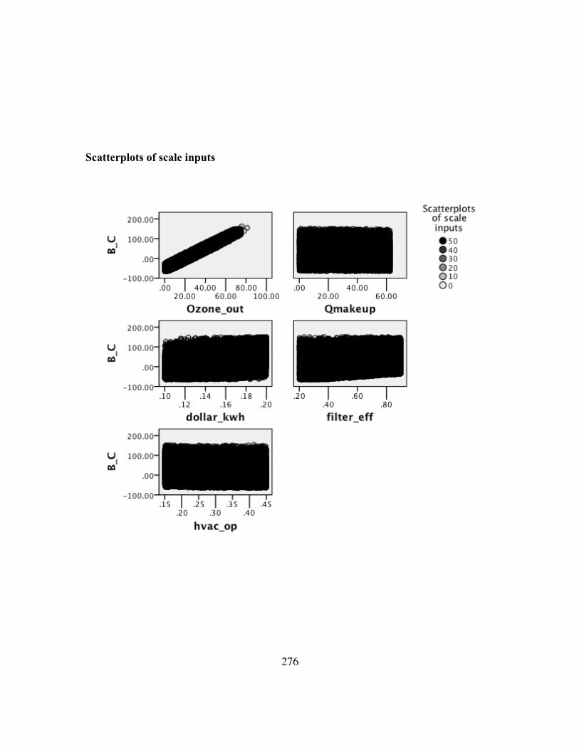
276

Scatterplots of scale inputs

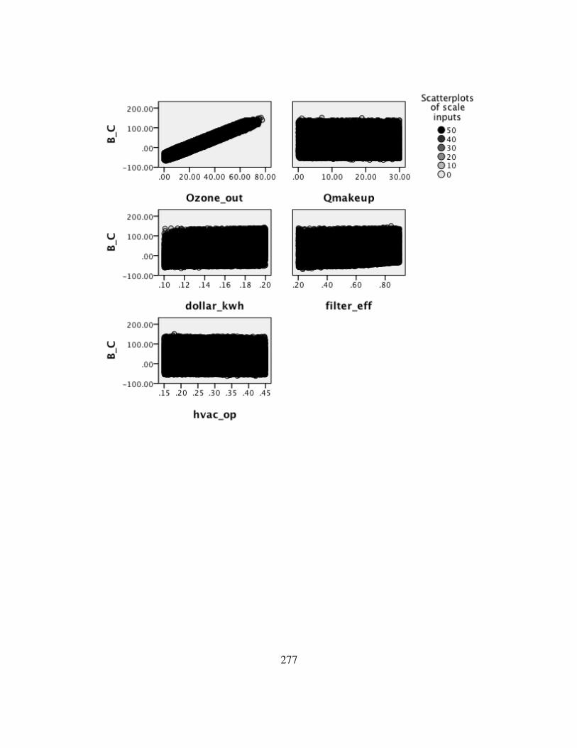
277

278

Tornado Charts

279

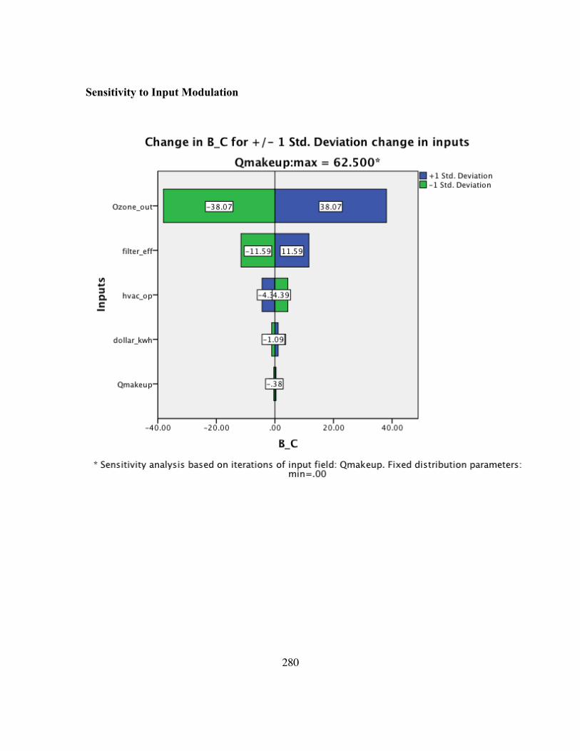
280

Sensitivity to Input Modulation

281

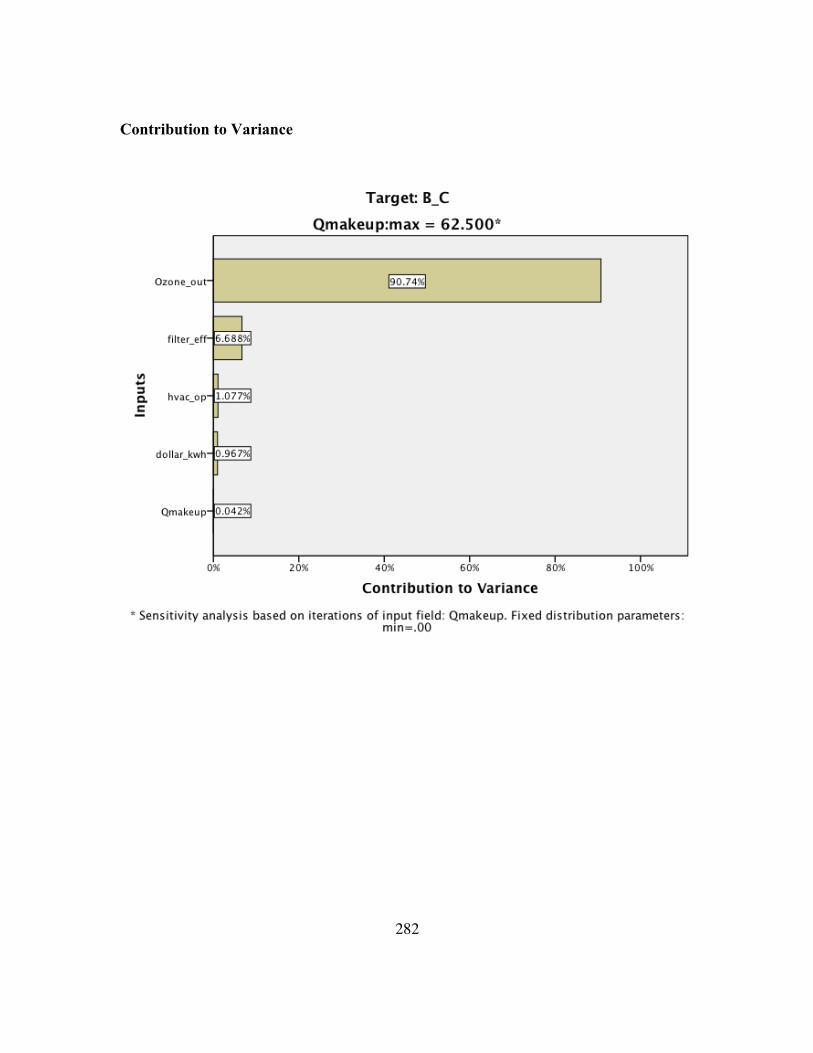
282

Contribution to Variance

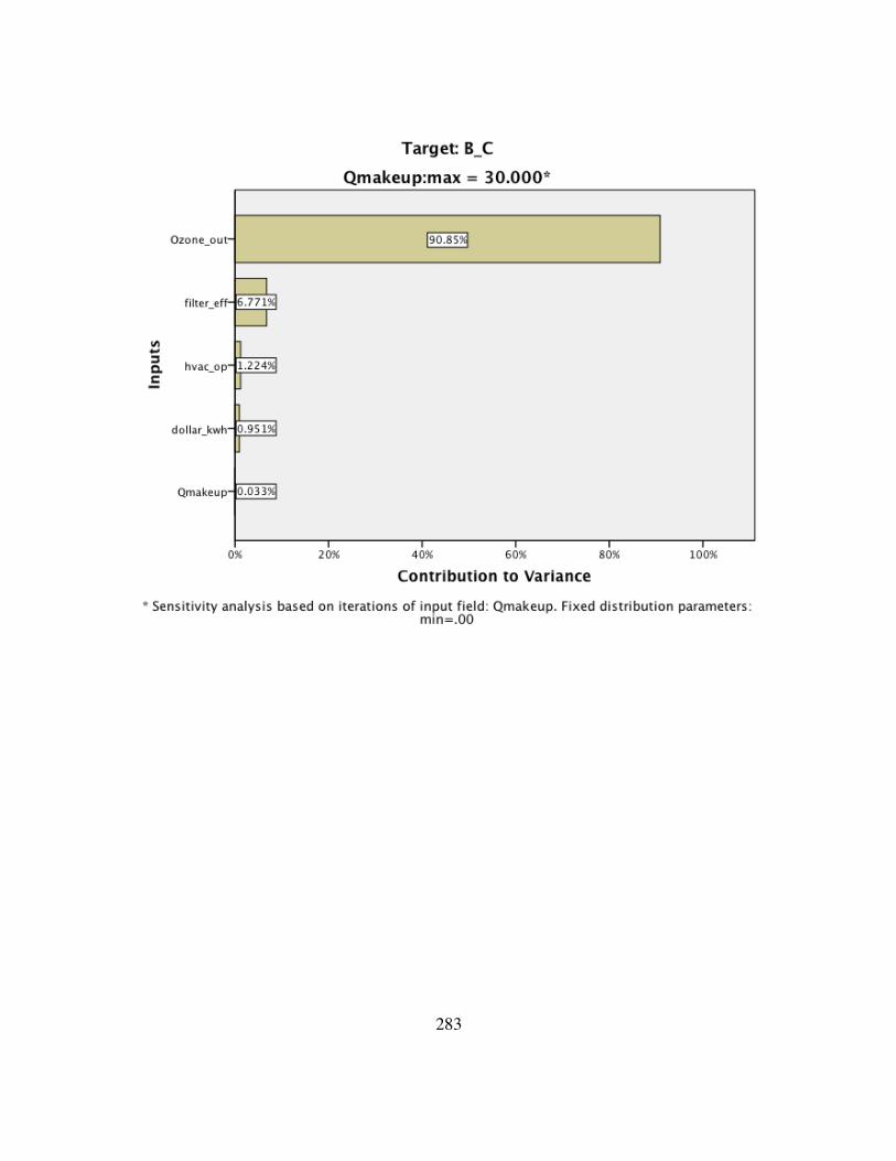
283

284

Commercial Office Building Simulation Run

Notes Output Created 23-APR-2015 08:03:45 Comments Input Data /Users/joshaldred/Document

s/test_22_april_2015.sav Active Dataset DataSet1 Filter <none> Weight <none> Split File <none> N of Rows in Working Data File

68

Simulation Summary

Maximum cases 100000 Total simulated cases 100000 Input filtering Input: Ozone_out Minimum value >= .00

Maximum value <= 100.00 Cases filtered 2.3% Simulation Plan File: /Users/joshaldred/Documents/medofficebldgv1.splan Cases may be filtered because of either targets or inputs that are outside of the specified ranges. Filtered cases are not included in the simulated cases count.

285

Mean Std.

Deviation Median Minimum Maximum

95% Confidence Interval for Mean Lower Upper

B_C 19.948 43.858 19.174 -113.48 234.46 19.677 20.220

Descriptive Statistics of Scale Inputs

Mean Std. Deviation Minimum Maximum Ozone_out 30.777 14.135 .00 96.38 Qmakeup 8502.298 1153.074 6500.01 10499.99 dollar_kwh .150 .029 .10 .20 filter_eff .550 .202 .20 .90 hvac_op .900 .058 .80 1.00

Correlations

dollar_kwh filter_eff hvac_op Ozone_out Qmakeup dollar_kwh 1.000 -.091 -.297 .319 -.116 filter_eff -.091 1.000 .229 -.060 -.129 hvac_op -.297 .229 1.000 -.046 .359 Ozone_out .319 -.060 -.046 1.000 .032 Qmakeup -.116 -.129 .359 .032 1.000 Correlations between simulated inputs may differ from correlations specified for those inputs in the simulation plan. Excluded fields (fixed inputs and inputs with categorical distributions): A15_24 A1_4 A25_34 A35_44 A45_54 A55_64 A5_14 A65_74 A75_84 A85_plus

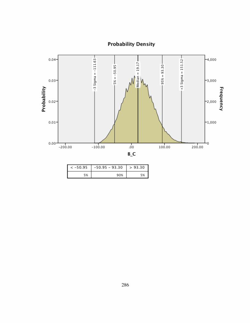
286

287

288

289

Tornado Charts

290

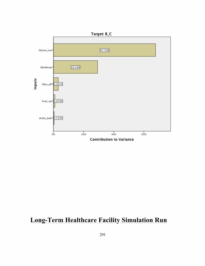
291

Long-Term Healthcare Facility Simulation Run

292

Notes Output Created 22-APR-2015 19:56:18 Comments Input Data /Users/joshaldred/Document

s/test_22_april_2015.sav Active Dataset DataSet1 Filter <none> Weight <none> Split File <none>

Files Saved Simulated Cases File /Users/joshaldred/Document

s/SPSS/NursingHomev1.splan

Simulation Summary

Maximum cases 100000 Total simulated cases 100000 Input filtering Input: Ozone_out Minimum value >= .00

Maximum value <= 100.00 Cases filtered 2.3% Simulation Plan File: /Users/joshaldred/Documents/SPSS/NursingHomev1.splan Cases may be filtered because of either targets or inputs that are outside of the specified ranges. Filtered cases are not included in the simulated cases count.

Mean Std.

Deviation Median Minimum Maximum

95% Confidence Interval for Mean Lower Upper

B_C 448.150 47.969 447.309 303.33 656.94 447.852 448.447

293

Descriptive Statistics of Scale Inputs Mean Std. Deviation Minimum Maximum A85_plus .150 .023 .11 .19 Ozone_out 30.778 14.106 .00 97.93 dollar_kwh .150 .029 .10 .20 filter_eff .550 .202 .20 .90 hvac_op .900 .058 .80 1.00

Correlations

A85_plus dollar_kwh filter_eff hvac_op Ozone_out A85_plus 1.000 -.409 -.254 .130 .008 dollar_kwh -.409 1.000 -.120 .354 -.002 filter_eff -.254 -.120 1.000 .247 -.057 hvac_op .130 .354 .247 1.000 .007 Ozone_out .008 -.002 -.057 .007 1.000 Correlations between simulated inputs may differ from correlations specified for those inputs in the simulation plan. Excluded fields (fixed inputs and inputs with categorical distributions): A15_24 A1_4 A25_34 A35_44 A45_54 A55_64 A5_14 A65_74 A75_84 Qmakeup

294

295

296

297

Tornado Charts

298

299

K-12 Schools Simulation Run

300

Notes Output Created 22-APR-2015 20:10:58 Comments Input Data /Users/joshaldred/Document

s/test_22_april_2015.sav Active Dataset DataSet1 Filter <none> Weight <none> Split File <none> N of Rows in Working Data File

68

Simulation Summary

Maximum cases 100000 Total simulated cases 100000 Input filtering Input: Ozone_out Minimum value >= .00

Maximum value <= 100.00 Cases filtered 2.3% Simulation Plan File: /Users/joshaldred/Documents/SPSS/K12Schoolv1.splan Cases may be filtered because of either targets or inputs that are outside of the specified ranges. Filtered cases are not included in the simulated cases count.

Mean Std.

Deviation Median Minimum Maximum

95% Confidence Interval for Mean Lower Upper

B_C 3.104 37.116 1.803 -98.67 180.60 2.874 3.334

301

Descriptive Statistics of Scale Inputs

Mean Std. Deviation Minimum Maximum Ozone_out 30.835 14.151 .00 95.63 dollar_kwh .150 .029 .10 .20 filter_eff .548 .202 .20 .90 hvac_op .900 .058 .80 1.00

Correlations

dollar_kwh filter_eff hvac_op Ozone_out dollar_kwh 1.000 -.024 -.302 .288 filter_eff -.024 1.000 .240 -.088 hvac_op -.302 .240 1.000 -.044 Ozone_out .288 -.088 -.044 1.000 Correlations between simulated inputs may differ from correlations specified for those inputs in the simulation plan. Excluded fields (fixed inputs and inputs with categorical distributions): A15_24 A1_4 A25_34 A35_44 A45_54 A55_64 A5_14 A65_74 A75_84 A85_plus Qmakeup

302

303

304

305

Tornado Charts

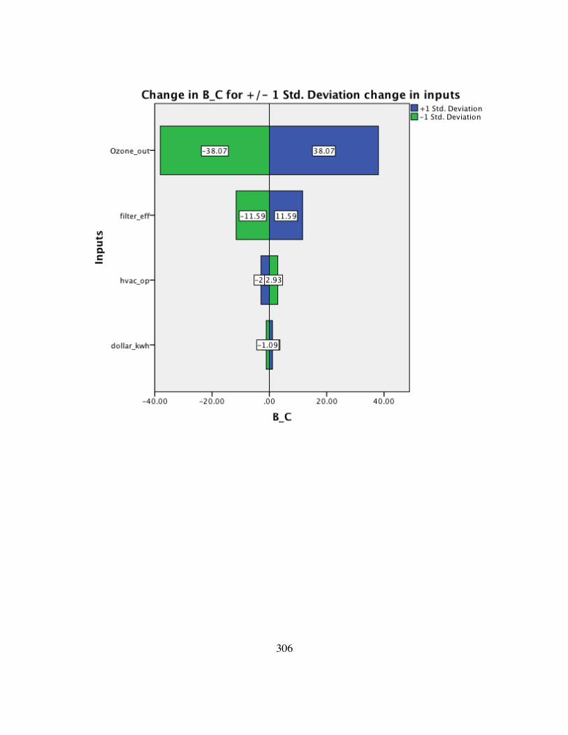
306

307

308

References

Adams, W. C. (2006). Comparison of chamber 6.6-h exposures to 0.04-0.08 PPM ozone

via square-wave and triangular profiles on pulmonary responses. Inhalation Toxicology,

18(2), 127–136. http://doi.org/10.1080/08958370500306107

Aldred, J., Darling, E., Morrison, G., & Siegel, J., Corsi, R. (2005). Benefit-Cost Analysis of

Commercially Available Activated Carbon Filters for Indoor Ozone Removal in

Residential Buildings.

Alvarez, P. M., Masa, F. J., Jaramillo, J., Beltran, F. J., & Gomez-Serrano, V. (2008). Kinetics

of ozone decomposition by granular activated carbon. Industrial & Engineering

Chemistry Research, 47(8), 2545–2553. http://doi.org/10.1021/ie071360z

Anderson, G. B., Krall, J. R., Peng, R. D., & Bell, M. L. (2012). Is the Relation Between

Ozone and Mortality Confounded by Chemical Components of Particulate Matter?

Analysis of 7 Components in 57 US Communities. American Journal of Epidemiology,

176(8), 726–732. http://doi.org/10.1093/aje/kws188

Anderson, H. R., Spix, C., Medina, S., Schouten, J. P., Castellsague, J., Rossi, G., …

Katsouyanni, K. (1997). Air pollution and daily admissions for chronic obstructive

pulmonary disease in 6 European cities: Results from the APHEA project. European

Respiratory Journal, 10(5), 1064–1071. http://doi.org/10.1183/09031936.97.10051064

Anderson, S. E., Franko, J., Jackson, L. G., Wells, J. R., Ham, J. E., & Meade, B. J. (2012).

Irritancy and Allergic Responses Induced by Exposure to the Indoor Air Chemical 4-

Oxopentanal. Toxicological Sciences, 127(2), 371–381.

http://doi.org/10.1093/toxsci/kfs102

309

Anderson, S. E., Jackson, L. G., Franko, J., & Wells, J. R. (2010). Evaluation of Dicarbonyls

Generated in a Simulated Indoor Air Environment Using an In Vitro Exposure System.

Toxicological Sciences, 115(2), 453–461. http://doi.org/10.1093/toxsci/kfq067

Anderson, S. E., Wells, J. R., Fedorowicz, A., Butterworth, L. F., Meade, B. J., & Munson, A.

E. (2007). Evaluation of the contact and respiratory sensitization potential of volatile

organic compounds generated by simulated indoor air chemistry. Toxicological Sciences,

97(2), 355–363. http://doi.org/10.1093/toxsci/kfm043

Apte, M. G., Buchanan, I. S. H., & Mendell, M. J. (2008). Outdoor ozone and building-related

symptoms in the BASE study. Indoor Air, 18(2), 156–170. http://doi.org/10.1111/j.1600-

0668.2008.00521.x

ASHRAE-American Society of Heating, Ventilation, and Air-Conditioning Engineers. (2008).

Ventilation of��� Health Care Facilities. Atlanta, GA.

ASHRAE-American Society of Heating, Ventilation, and Air-Conditioning Engineers.

(2013a). Energy Standard for Buildings Except Low-Rise Residential Buildings (No.

ASHRAE Standard 90.1-2013). Atlanta, GA.

ASHRAE-American Society of Heating, Ventilation, and Air-Conditioning Engineers.

(2013b). Ventilation and Acceptable Indoor Air Quality in Low-Rise Residential

Buildings (No. No. ASHRAE Standard 62.2-2013). Atlanta, GA.

ASHRAE-American Society of Heating, Ventilation, and Air-Conditioning Engineers.

(2013c). Ventilation for Acceptable Indoor Air Quality (No. ASHRAE Standard 62.1-

2013). Atlanta, GA.

310

ASHRAE - American Society of Heating, Refrigeration, and Air-Conditioning Engineers.

(2009). ASHRAE Handbook - Fundamentals.

Atkinson, R., & Arey, J. (2003). Gas-phase tropospheric chemistry of biogenic volatile

organic compounds: a review. Atmospheric Environment, 37, S197–S219.

http://doi.org/10.1016/S1352-2310(03)00391-1

Azimi, P., & Stephens, B. (2013). HVAC filtration for controlling infectious airborne disease

transmission in indoor environments: Predicting risk reductions and operational costs.

Building and Environment, 70, 150–160.

Beko, G., Clausen, G., & Weschler, C. J. (2008). Sensory pollution from bag filters, carbon

filters and combinations. Indoor Air, 18(1), 27–36. http://doi.org/10.1111/j.1600-

0668.2007.00501.x

Beko, G., Fadeyi, M. O., Clausen, G., & Weschler, C. J. (2009). Sensory pollution from bag-

type fiberglass ventilation filters: Conventional filter compared with filters containing

various amounts of activated carbon. Building and Environment, 44(10), 2114–2120.

http://doi.org/10.1016/j.buildenv.2009.03.002

Bell, M. L., & Dominici, F. (2008). Effect modification by community characteristics on the

short-term effects of ozone exposure and mortality in 98 US communities. American

Journal of Epidemiology, 167(8), 986–997. http://doi.org/10.1093/aje/kwm396

Bell, M. L., Dominici, F., & Samet, J. M. (2005). A meta-analysis of time-series studies of

ozone and mortality with comparison to the national morbidity, mortality, and air

pollution study. Epidemiology, 16(4), 436–445.

http://doi.org/10.1097/01.ede.0000165817.40152.85

311

Bell, M. L., Ebisu, K., Peng, R. D., & Dominici, F. (2009). Adverse Health Effects of

Particulate Air Pollution Modification by Air Conditioning. Epidemiology, 20(5), 682–

686. http://doi.org/10.1097/EDE.0b013e3181aba749

Bell, M. L., McDermott, A., Zeger, S. L., Samet, J. M., & Dominici, F. (2004). Ozone and

short-term mortality in 95 US urban communities, 1987-2000. Jama-Journal of the

American Medical Association, 292(19), 2372–2378.

http://doi.org/10.1001/jama.292.19.2372

Bell, M. L., Peng, R. D., & Dominici, F. (2006). The exposure-response curve for ozone and

risk of mortality and the adequacy of current ozone regulations. Environmental Health

Perspectives, 114(4), 532–536. http://doi.org/10.1289/ehp.8816

Berman, J. D., Fann, N., Hollingsworth, J. W., Pinkerton, K. E., Rom, W. N., Szema, A. M.,

Curriero, F. C. (2012). Health Benefits from Large-Scale Ozone Reduction in the United

States. Environmental Health Perspectives, 120(10), 1404–1410.

Blumenthal, K. J., Saulsgiver, K. A., Norton, L., Troxel, A. B., Anarella, J. P., Gesten, F. C.,

Volpp, K. G. (2013). Medicaid Incentive Programs To Encourage Healthy Behavior

Show Mixed Results To Date And Should Be Studied And Improved. Health Affairs,

32(3), 497–507. http://doi.org/10.1377/hlthaff.2012.0431

Bobinac, A., van Exel, J., Rutten, F. F. H., & Brouwer, W. B. F. (2014). The Value of a

QALY: Individual Willingness to Pay for Health Gains Under Risk.

Pharmacoeconomics, 32(1), 75–86. http://doi.org/10.1007/s40273-013-0110-1

312

Brown, J. S., Bateson, T. F., & McDonnell, W. F. (2008). Effects of exposure to 0.06 ppm

ozone on FEV1 in humans: A secondary analysis of existing data. Environmental Health

Perspectives, 116(8), 1023–1026. http://doi.org/10.1289/ehp.11396

Buchanan, I. S. H., Mendell, M. J., Mirer, A. G., & Apte, M. G. (2008). Air filter materials,

outdoor ozone and building-related symptoms in the BASE study. Indoor Air, 18(2),

144–155. http://doi.org/10.1111/j.1600-0668.2008.00519.x

Burmaster, D. E., & Hull, D. A. (1997). Using Lognormal distributions and Lognormal

probability plots in probabilistic risk assessments. Human and Ecological Risk

Assessment, 3(2), 235–255.

Burnett, R. T., Smith-Doiron, M., Stieb, D., Cakmak, S., & Brook, J. R. (1999). Effects of

particulate and gaseous air pollution on cardiorespiratory hospitalizations. Archives of

Environmental Health, 54(2), 130–139.

Cetin, K., Novoselac, A. (2015). Single and multi-family residential HVAC system

operational characteristics and use patterns in a cooling-dominated climate. Manuscript

submitted for preparation.

Checkoway, H., Boffetta, P., Mundt, D. J., & Mundt, K. A. (2012). Critical review and

synthesis of the epidemiologic evidence on formaldehyde exposure and risk of leukemia

and other lymphohematopoietic malignancies. Cancer Causes & Control, 23(11), 1747–

1766. http://doi.org/10.1007/s10552-012-0055-2

Chen, C., Zhao, B., & Weschler, C. J. (2012a). Assessing the Influence of Indoor Exposure to

“Outdoor Ozone” on the Relationship between Ozone and Short-term Mortality in US

313

Communities. Environmental Health Perspectives, 120(2), 235–240.

http://doi.org/10.1289/ehp.1103970

Chen, C., Zhao, B., & Weschler, C. J. (2012b). Indoor Exposure to “Outdoor PM10”

Assessing Its Influence on the Relationship Between PM10 and Short-term Mortality in

US Cities. Epidemiology, 23(6), 870–878.

http://doi.org/10.1097/EDE.0b013e31826b800e

Chen, L., Jennison, B. L., Yang, W., & Omaye, S. T. (2000). Elementary school absenteeism

and air pollution. Inhalation Toxicology, 12(11), 997–1016.

Chen, X., & Hopke, P. K. (2009). A chamber study of secondary organic aerosol formation by

linalool ozonolysis. Atmospheric Environment, 43(25), 3935–3940.

http://doi.org/10.1016/j.atmosenv.2009.04.033

Chen, X., & Hopke, P. K. (2010). A chamber study of secondary organic aerosol formation by

limonene ozonolysis. Indoor Air, 20(4), 320–328. http://doi.org/10.1111/j.1600-

0668.2010.00656.x

Coleman, B. K., Destaillats, H., Hodgson, A. T., & Nazaroff, W. W. (2008). Ozone

consumption and volatile byproduct formation from surface reactions with aircraft cabin

materials and clothing fabrics. Atmospheric Environment, 42(4), 642–654.

http://doi.org/10.1016/j.atmosenv.2007.10.001

Collinge, W., Landis, A. E., Jones, A. K., Schaefer, L. A., & Bilec, M. M. (2013). Indoor

environmental quality in a dynamic life cycle assessment framework for whole buildings:

Focus on human health chemical impacts. Building and Environment, 62, 182–190.

http://doi.org/10.1016/j.buildenv.2013.01.015

314

Cometto-Muniz, J. E., & Abraham, M. H. (2010). Odor Detection by Humans of Lineal

Aliphatic Aldehydes and Helional as Gauged by Dose-Response Functions. Chemical

Senses, 35(4), 289–299. http://doi.org/10.1093/chemse/bjq018

Corsi, R., Aldred, J., Darling, E., Morrison, G., & Siegel, J. (2014). Literature and Product

Review and Cost Benefit Analysis of Commercially Available Ozone Air Cleaning for

HVAC Systems (No. ASHRAE RP 1491). American Society of Heating, Refrigeration,

and Air Conidtioning Engineers.

Cros, C. J., Morrison, G. C., Siegel, J. A., & Corsi, R. L. (2012). Long-term performance of

passive materials for removal of ozone from indoor air. Indoor Air, 22(1), 43–53.

http://doi.org/10.1111/j.1600-0668.2011.00734.x

Delfino, R. J., Staimer, N., Tjoa, T., Gillen, D. L., Schauer, J. J., & Shafer, M. M. (2013).

Airway inflammation and oxidative potential of air pollutant particles in a pediatric

asthma panel. Journal of Exposure Science and Environmental Epidemiology, 23(5),

466–473. http://doi.org/10.1038/jes.2013.25

Dusenbury, J. S., & Cannon, F. S. (1996). Advanced oxidant reactivity pertaining to granular

activated carbon beds for air pollution control. Carbon, 34(12), 1577–1589.

http://doi.org/10.1016/S0008-6223(96)00113-3

Fadeyi, M. O. (2014). Mass balance modeling of building recirculation rates and filtration

efficiencies effects on secondary organic aerosols derived from ozone-initiated chemistry.

Building Simulation, 7(2), 165–173. http://doi.org/10.1007/s12273-013-0139-2

Fadeyi, M. O., Weschler, C. J., & Tham, K. W. (2009). The impact of recirculation,

ventilation and filters on secondary organic aerosols generated by indoor chemistry.

315

Atmospheric Environment, 43(22-23), 3538–3547.

http://doi.org/10.1016/j.atmosenv.2009.04.017

Fadeyi, M. O., Weschler, C. J., Tham, K. W., Wu, W. Y., & Sultan, Z. M. (2013). Impact of

Human Presence on Secondary Organic Aerosols Derived from Ozone-Initiated

Chemistry in a Simulated Office Environment. Environmental Science & Technology,

47(8), 3933–3941. http://doi.org/10.1021/es3050828

Fan, Z. H., Lioy, P., Weschler, C., Fiedler, N., Kipen, H., & Zhang, J. F. (2003). Ozone-

initiated reactions with mixtures of volatile organic compounds under simulated indoor

conditions. Environmental Science & Technology, 37(9), 1811–1821.

http://doi.org/10.1021/es026231i

Fann, N. (2014, January). Correspondence with J. Aldred. Austin, TX.

Fisk, W. (2009). Ozone Removal by Filters Containing Activated Carbon: A Pilot Study. In

Proceedings of the 9th International Conference on Healthy Buildings. Syracuse, NY.

Fisk, W. J., Black, D., & Brunner, G. (2011). Benefits and costs of improved IEQ in US

offices. Indoor Air, 21(5), 357–367. http://doi.org/10.1111/j.1600-0668.2011.00719.x

Fisk, W. J., & Rosenfeld, A. H. (1997). Estimates of improved productivity and health from

better indoor environments. Indoor Air-International Journal of Indoor Air Quality and

Climate, 7(3), 158–172. http://doi.org/10.1111/j.1600-0668.1997.t01-1-00002.x

Gall, E., Siegel, J. A., & Corsi, R. (2011). Zero-Energy Removal of Ozone in Residences.

Ashrae: Transactions 2011, Vol 117, Pt 1, 117, 411–418.

316

Ginestet, A., Pugnet, D., Tissot, A., & Henninot, M. (2013). On-Site Particle and Gas

Filtration Efficiencies of Air Handling Unit Filters in Industrial and Non Industrial

Building. International Journal of Ventilation, 12(2), 151–158.

Glad, J. A., Brink, L. L., Talbott, E. O., Lee, P. C., Xu, X., Saul, M., & Rager, J. (2012). The

Relationship of Ambient Ozone and PM2.5 Levels and Asthma Emergency Department

Visits: Possible Influence of Gender and Ethnicity. Archives of Environmental &

Occupational Health, 67(2), 103–108. http://doi.org/10.1080/19338244.2011.598888

Godwin, C., & Batterman, S. (2007). Indoor air quality in Michigan schools. Indoor Air,

17(2), 109–121. http://doi.org/10.1111/j.1600-0668.2006.00459.x

Gordon, S. M., Callahan, P. J., Nishioka, M. G., Brinkman, M. C., O’Rourke, M. K.,

Lebowitz, M. D., & Moschandreas, M. J. (1999). Residential environmental

measurements in the National Human Exposure Assessment Survey (NHEXAS) pilot

study in Arizona: preliminary results for pesticides and VOCs. Journal of Exposure

Analysis and Environmental Epidemiology, 9(5), 456–470.

http://doi.org/10.1038/sj.jea.7500042

Grosjean, D., Williams, E., Grosjean, E., Andino, J., & Seinfeld, J. (1993). Atmospheric

Oxidation of Biogenic Hydrocarbons -- Reaction of Ozone with Beta-Pinene, D-

Limonene and Trans-Caryophyllene. Environmental Science & Technology, 27(13),

2754–2758. http://doi.org/10.1021/es00049a014

Grosjean, E., & Grosjean, D. (1996). Carbonyl products of the gas-phase reaction of ozone

with 1-alkenes. Atmospheric Environment, 30(24), 4107–4113.

http://doi.org/10.1016/1352-2310(96)00176-8

317

Grosjean, E., & Grosjean, D. (1997). Gas phase reaction of alkenes with ozone: Formation

yields of primary carbonyls and biradicals. Environmental Science & Technology, 31(8),

2421–2427. http://doi.org/10.1021/es970075b

Gryparis, A., Forsberg, B., Katsouyanni, K., Analitis, A., Touloumi, G., Schwartz, J., …

Dortbudak, Z. (2004). Acute effects of ozone on mortality from the “Air pollution and

health: A European approach” project. American Journal of Respiratory and Critical

Care Medicine, 170(10), 1080–1087. http://doi.org/10.1164/rccm.200403-333OC

Gundel, Lara A., Sullivan, Douglas P., Katsapov, Gregory Y., & Fisk, William J. (2002). A

pilot study of energy efficient air cleaning for ozone (No. DE-AC03-76SF00098).

Berkeley, CA 94720: Lawrence Berkeley National Laboratory.

Hantula, D. A., Rajala, A. K., Kellerman, E. G. B., & Bragger, J. L. D. (2001). The value of

workplace safety: A time-based utility analysis model. Journal of Organizational

Behavior Management, 21(2), 79–98. http://doi.org/10.1300/J075v21n02_09

Heisig, C., Zhang, W. M., & Oyama, S. T. (1997). Decomposition of ozone using carbon-

supported metal oxide catalysts. Applied Catalysis B-Environmental, 14(1-2), 117–129.

http://doi.org/10.1016/S0926-3373(97)00017-9

Henke, R. M., Carls, G. S., Short, M. E., Pei, X., Wang, S., Moley, S., Goetzel, R. Z. (2010).

The relationship between health risks and health and productivity costs among employees

at Pepsi bottling group. Journal of Occupational and Environmental Medicine, 52(5),

519–527. http://doi.org/10.1097/JOM.0b013e3181dce655

318

Hodgson, A. T., & Levin, H. (2003, April 21). Volatile Organic Compounds in Indoor Air: A

Review of Concentrations Measured in North America Since 1990. Lawrence Berkeley

National Laboratory, Berkeley, California, USA Report LBNL-51715.

Hoek, G., Boogaard, H., Knol, A., De Hartog, J., Slottje, P., Ayres, J. G., … Van der Sluijs, J.

(2010). Concentration Response Functions for Ultrafine Particles and All-

Cause Mortality and Hospital Admissions: Results of a European Expert

Panel Elicitation. Environmental Science & Technology, 44(1), 476–482.

http://doi.org/10.1021/es9021393

Hubbell, B. J., Hallberg, A., McCubbin, D. R., & Post, E. (2005). Health-related benefits of

attaining the 8-hr ozone standard. Environmental Health Perspectives, 113(1), 73–82.

Huijbregts, M. A. J., Rombouts, L. J. A., Ragas, A. M. J., & Meent, D. van de. (2005).

Human-Toxicological Effect and Damage Factors of Carcinogenic and Noncarcinogenic

Chemicals for Life Cycle Impact Assessment. Integrated Environmental Assessment and

Management, 1(3), 181–244.

Hun, D. E., Corsi, R. L., Morandi, M. T., & Siegel, J. A. (2010). Formaldehyde in residences:

long-term indoor concentrations and influencing factors. Indoor Air, 20(3), 196–203.

http://doi.org/10.1111/j.1600-0668.2010.00644.x

IBM Corporation. (2013). IBM SPSS Statistics (Version 22.0). Armonk, NY.

Ito, K., De Leon, S. F., & Lippmann, M. (2005). Associations between ozone and daily

mortality - Analysis and meta-analysis. Epidemiology, 16(4), 446–457.

http://doi.org/10.1097/01.ede.0000165821.90114.7f

319

Jerrett, M., Burnett, R. T., Pope, C. A., Ito, K., Thurston, G., Krewski, D., … Thun, M. (2009).

Long-Term Ozone Exposure and Mortality. New England Journal of Medicine, 360(11),

1085–1095. http://doi.org/10.1056/NEJMoa0803894

Kelly, T., & Kinkead, D. (1993). Testing of Chemically Treated Adsorbent Air Purifiers.

Ashrae Journal-American Society of Heating Refrigerating and Air-Conditioning

Engineers, 35(7), 14–23.

Kelly, E., Carls, G. S., Lenhart, G., Mauceri, E., Columbus, D., Cavuoti, A., & Goetzel, R. Z.

(2010). The Novartis Health Index: A method for valuing the economic impact of risk

reduction in a workforce. Journal of Occupational and Environmental Medicine, 52(5),

528–535. http://doi.org/10.1097/JOM.0b013e3181dbe339

Kim, S. Y., Lee, J. T., Hong, Y. C., Ahn, K. J., & Kim, H. (2004). Determining the threshold

effect of ozone on daily mortality: an analysis of ozone and mortality in Seoul, Korea,

1995-1999. Environmental Research, 94(2), 113–119.

http://doi.org/10.1016/j.envres.2003.09.006

Kleno, J., & Wolkoff, P. (2004). Changes in eye blink frequency as a measure of trigeminal

stimulation by exposure to limonene oxidation products, isoprene oxidation products

and nitrate radicals. International Archives of Occupational and Environmental Health,

77(4), 235–243. http://doi.org/10.1007/s00420-003-0502-1

Klepeis, N. E., Nelson, W. C., Ott, W. R., Robinson, J. P., Tsang, A. M., Switzer, P., …

Engelmann, W. H. (2001). The National Human Activity Pattern Survey (NHAPS): a

resource for assessing exposure to environmental pollutants. Journal of Exposure

320

Analysis and Environmental Epidemiology, 11(3), 231–252.

http://doi.org/10.1038/sj.jea.7500165

Lamble, S. P., Corsi, R. L., & Morrison, G. C. (2011). Ozone deposition velocities, reaction

probabilities and product yields for green building materials. Atmospheric Environment,

45(38), 6965–6972. http://doi.org/10.1016/j.atmosenv.2011.09.025

Lawrence Berkeley National Laboratory Center for Building Science Applications Team.

(2003, August). A Design Guide for Energy-Efficient Research Laboratories. Retrieved

March 9, 2013, from http://ateam.lbl.gov/Design-Guide/index.htm

(LBNL) Lawrence Berkeley National Laboratory. (2014). Home Energy Saver. Retrieved

November 18, 2014, from https://sites.google.com/a/lbl.gov/hes-public/page-

archive/appendices/appendix-c

Lee, A., Goldstein, A. H., Keywood, M. D., Gao, S., Varutbangkul, V., Bahreini, R., …

Seinfeld, J. H. (2006). Gas-phase products and secondary aerosol yields from the

ozonolysis of ten different terpenes. Journal of Geophysical Research-Atmospheres,

111(D7). http://doi.org/10.1029/2005JD006437

Lee, A., Goldstein, A. H., Kroll, J. H., Ng, N. L., Varutbangkul, V., Flagan, R. C., & Seinfeld,

J. H. (2006). Gas-phase products and secondary aerosol yields from the

photooxidation of 16 different terpenes. Journal of Geophysical Research-Atmospheres,

111(D17). http://doi.org/10.1029/2006JD007050

Lee, K., Vallarino, J., Dumyahn, T., Ozkaynak, H., & Spengler, J. D. (1999). Ozone decay

rates in residences. Journal of the Air & Waste Management Association, 49(10), 1238–

1244.

321

Lee, P., & Davidson, J. (1999). Evaluation of activated carbon filters for removal of ozone at

the PPB level. American Industrial Hygiene Association Journal, 60(5), 589–600.

http://doi.org/10.1080/00028899908984478

Leungsakul, S., Jaoui, M., & Kamens, R. M. (2005). Kinetic mechanism for predicting

secondary organic aerosol formation from the reaction of d-limonene with ozone.

Environmental Science & Technology, 39(24), 9583–9594.

http://doi.org/10.1021/es0492687

Levy, J. I., Carrothers, T. J., Tuomisto, J. T., Hammitt, J. K., & Evans, J. S. (2001). Assessing

the public health benefits of reduced ozone concentrations. Environmental Health

Perspectives, 109(12), 1215–1226. http://doi.org/10.1289/ehp.011091215

Levy, J. I., Chemerynski, S. M., & Sarnat, J. A. (2005). Ozone exposure and mortality - An

empiric Bayes metaregression analysis. Epidemiology, 16(4), 458–468.

http://doi.org/10.1097/01.ede.0000165820.08301.b3

Lin, Y.-C., Chang, C.-L., Lin, T.-S., Bai, H., Yan, M.-G., Ko, F.-H., … Huang, C.-H. (2008).

Application of physical vapor deposition process to modify activated carbon fibers for

ozone reduction. Korean Journal of Chemical Engineering, 25(3), 446–450.

http://doi.org/10.1007/s11814-008-0076-4

Logue, J. M., McKone, T. E., Sherman, M. H., & Singer, B. C. (2011). Hazard assessment of

chemical air contaminants measured in residences. Indoor Air, 21(2), 92–109.

http://doi.org/10.1111/j.1600-0668.2010.00683.x

322

Logue, J. M., Price, P. N., Sherman, M. H., & Singer, B. C. (2012). A Method to Estimate the

Chronic Health Impact of Air Pollutants in US Residences. Environmental Health

Perspectives, 120(2), 216–222. http://doi.org/10.1289/ehp.1104035

Loh, M. M., Levy, J. I., Spengler, J. D., Houseman, E. A., & Bennett, D. H. (2007). Ranking

cancer risks of organic hazardous air pollutants in the United States. Environmental

Health Perspectives, 115(8), 1160–1168. http://doi.org/10.1289/ehp.9884

Lopez, A. D., Mathers, C. D., Ezzati, M., Jamison, D. T., & Murray, C. J. L. (2006). Global

Burden of Disease and Risk Factors. World Bank.

Lvovsky, K., Hughes, G., Maddison, D., Ostro, B., & Pearce, D. (2000). Environmental Costs

of Fossil Fuels (Environment Department Papers No. Paper No. 78) (pp. 1–104).

Washington, DC: World Bank.

MathWorks (2013). MATLAB release 2013a, student edition. Natick, MA.

McConnell, R., Berhane, K., Gilliland, F., London, S. J., Islam, T., Gauderman, W. J., …

Peters, J. M. (2002). Asthma in exercising children exposed to ozone: a cohort study.

Lancet, 359(9304), 386–391. http://doi.org/10.1016/S0140-6736(02)07597-9

McDonnell, W. F., Abbey, D. E., Nishino, N., & Lebowitz, M. D. (1999). Long-term ambient

ozone concentration and the incidence of asthma in nonsmoking adults: The ahsmog

study. Environmental Research, 80(2), 110–121. http://doi.org/10.1006/enrs.1998.3894

Metts, T. A. (2007). Heterogeneous reactions of ozone and D-limonene on activated carbon.

Indoor Air, 17(5), 362–371. http://doi.org/10.1111/j.1600-0668.2007.00484.x

323

Metts, T. A., & Batterman, S. A. (2006). Effect of VOC loading on the ozone removal

efficiency of activated carbon filters. Chemosphere, 62(1), 34–44.

http://doi.org/10.1016/j.chemosphere.2005.04.049

Moolgavkar, S. H., Luebeck, E. G., & Anderson, E. L. (1997). Air pollution and hospital

admissions for respiratory causes in Minneapolis St. Paul and Birmingham.

Epidemiology, 8(4), 364–370. http://doi.org/10.1097/00001648-199707000-00003

Morrison, G. C., & Nazaroff, W. W. (2002). Ozone interactions with carpet: Secondary

emissions of aldehydes. Environmental Science & Technology, 36(10), 2185–2192.

http://doi.org/10.1021/es0113089

Morrison, G. C., Nazaroff, W. W., Cano-Ruiz, J. A., Hodgson, A. T., & Modera, M. P. (1998).

Indoor air quality impacts of ventilation ducts: Ozone removal and emissions of volatile

organic compounds. Journal of the Air & Waste Management Association, 48(10), 941–

952.

Morrison, G., Shaughnessy, R., & Shu, S. (2011). Setting maximum emission rates from

ozone emitting consumer appliances in the United States and Canada. Atmospheric

Environment, 45(11), 2009–2016. http://doi.org/10.1016/j.atmosenv.2010.11.058

Mudway, I. S., & Kelly, F. J. (2004). An investigation of inhaled ozone dose and the

magnitude of airway inflammation in healthy adults. American Journal of Respiratory

and Critical Care Medicine, 169(10), 1089–1095. http://doi.org/10.1164/rccm.200309-

13251-1325PP

Muller, C. O., & Jin, L. (2009). Beyond Ozone: Cleaning Outdoor Air for Improved IAQ. In

X. S. Zhang, H. Qian, B. Zhou, & Y. G. Yin (Eds.), . Presented at the 6th International

324

Symposium on Heating, Ventilation, and Air Conditioning, Vols I-III, Proceedings,

Nanjing, Peoples Republic of China.

Musich, S., McCalister, T., Wang, S., & Hawkins, K. (2015). An evaluation of the Well at

Dell health management program: health risk change and financial return on investment.

American Journal of Health Promotion, 29(3), 147–157.

http://doi.org/10.4278/ajhp.131115-QUAN-582

Nazaroff, W. W., Coleman, B. K., Destaillats, H., Hodgson, A. T., Liu, D.-L., Lunden, M. M.,

Weschler, C. J. (2006). Indoor Air Chemistry: Cleaning Agents, Ozone and Toxic Air

Contaminants (No. California Air Resources Boad Contract No. 01-336). Lawrence

Berkeley National Laboratory.

Nazaroff, W. W., & Singer, B. C. (2004). Inhalation of hazardous air pollutants from

environmental tobacco smoke in US residences. Journal of Exposure Analysis and

Environmental Epidemiology, 14, S71–S77. http://doi.org/10.1038/sj.jea.7500361

Nazaroff, W. W., & Weschler, C. J. (2004). Cleaning products and air fresheners: exposure to

primary and secondary air pollutants. Atmospheric Environment, 38(18), 2841–2865.

http://doi.org/10.1016/j.atmosenv.2004.02.040

Ng, N. L., Kroll, J. H., Keywood, M. D., Bahreini, R., Varutbangkul, V., Flagan, R. C., …

Goldstein, A. H. (2006). Contribution of first- versus second-generation products to

secondary organic aerosols formed in the oxidation of biogenic hydrocarbons.

Environmental Science & Technology, 40(7), 2283–2297.

http://doi.org/10.1021/es052269u

325

Oberdorster, G., Elder, A., Finkelstein, J., Frampton, M., Hopke, P., Peters, A., … Utell, M.

(2010). Assessment of Ambient UFP Health Effects:Linking Sources to Exposure and

Responses in Extrapulmonary Organs (No. EPA Grant R827354). University of

Rochester.

Office of Environmental Health Hazard Assessment (OEHHA). (2008). Air Toxics Hot Spots

Program Risk Assessment Guidelines. Technical Support Document for the Derivation of

Noncancer Reference Exposure Levels. California Environmental Protection Agency.

Ostro, B., & Rothschild, S. (1989). Air-Pollution and Acute Respiratory Morbidity - An

Observational Study. Environmental Research, 50(2), 238–247.

http://doi.org/10.1016/S0013-9351(89)80004-0

Parodi, S., Vercelli, M., Garrone, E., Fontana, V., & Izzotti, A. (2005). Ozone air pollution

and daily mortality in Genoa, Italy between 1993 and 1996. Public Health, 119(9), 844–

850. http://doi.org/10.1016/j.puhe.2004.10.007

Persily, A., Musser, A., & Emmerich, S. J. (2010). Modeled infiltration rate distributions for

U.S. housing. Indoor Air, 20(6), 473–485. http://doi.org/10.1111/j.1600-

0668.2010.00669.x

Polidori, A., Arhami, M., Sioutas, C., Delfino, R. J., & Allen, R. (2007). Indoor/outdoor

relationships, trends, and carbonaceous content of fine particulate matter in retirement

homes of the Los Angeles basin. Journal of the Air & Waste Management Association,

57(3), 366–379.

Pope, C. A., Burnett, R. T., Turner, M. C., Cohen, A., Krewski, D., Jerrett, M., … Thun, M. J.

(2011). Lung Cancer and Cardiovascular Disease Mortality Associated with Ambient Air

326

Pollution and Cigarette Smoke: Shape of the Exposure-Response Relationships.

Environmental Health Perspectives, 119(11), 1616–1621.

http://doi.org/10.1289/ehp.1103639

Rascati, K. (2009). Essentials of Pharmacoeconomics. Baltimore, MD: Lippincott, Williams,

and Wilkins.

Reiss, R., Ryan, P., Koutrakis, P., & Tibbetts, S. (1995). Ozone Reactive Chemistry on

Interior Latex Paint. Environmental Science & Technology, 29(8), 1906–1912.

http://doi.org/10.1021/es00008a007

Richard Corsi, Josh Aldred, Erin Darling, Glenn Morrison, & Jeffrey Siegel. (2014).

Literature and Product Review and Cost Benefit Analysis of Commercially Available

Ozone Air Cleaning for HVAC Systems (No. Research Project 1491). Austin, TX:

American Society of Heating, Refrigeration, and Air Conidtioning Engineers.

Rohr, A. C., Shore, S. A., & Spengler, J. D. (2003). Repeated exposure to isoprene oxidation

products causes enhanced respiratory tract effects in multiple murine strains. Inhalation

Toxicology, 15(12), 1191–1207. http://doi.org/10.1080/08958370390229870

Rohr, A. C., Weschler, C. J., Koutrakis, P., & Spengler, J. D. (2003). Generation and

quantification of ultrafine particles through terpene/ozone reaction in a chamber setting.

Aerosol Science and Technology, 37(1), 65–78.

http://doi.org/10.1080/02786820390112597

Rosenthal, J. (2014, April). Correspondence with J. Aldred. Austin, TX.

327

Sabersky, R., Sinema, D., & Shair, F. (1973). Concentrations, Decay Rates, and Removal of

Ozone and Their Relation to Establishing Clean Indoor Air. Environmental Science &

Technology, 7(4), 347–353. http://doi.org/10.1021/es60076a001

Sarnat, J. A., Brown, K. W., Schwartz, J., Coull, B. A., & Koutrakis, P. (2005). Ambient gas

concentrations and personal particulate matter exposures - Implications for studying the

health effects of particles. Epidemiology, 16(3), 385–395.

http://doi.org/10.1097/01.ede.0000155505.04775.33

Sarnat, J. A., Schwartz, J., Catalano, P. J., & Suh, H. H. (2001). Gaseous pollutants in

particulate matter epidemiology: Confounders or surrogates? Environmental Health

Perspectives, 109(10), 1053–1061. http://doi.org/10.2307/3454961

Sarwar, G., & Corsi, R. (2007). The effects of ozone/limonene reactions on indoor secondary

organic aerosols. Atmospheric Environment, 41(5), 959–973.

http://doi.org/10.1016/j.atmosenv.2006.09.032

Sarwar, G., Corsi, R., Allen, D., & Weschler, C. (2003). The significance of secondary organic

aerosol formation and growth in buildings: experimental and computational evidence.

Atmospheric Environment, 37(9-10), 1365–1381. http://doi.org/10.1016/S1352-

2310(02)01013-0

Sax, S. N., Bennett, D. H., Chillrud, S. N., Ross, J., Kinney, P. L., & Spengler, J. D. (2006). A

cancer risk assessment of inner-city teenagers living in New York City and Los Angeles.

Environmental Health Perspectives, 114(10), 1558–1566.

http://doi.org/10.1289/ehp.8507

328

SCAQMD (South Coast Air Quality Management District). (2013). Historic Ozone Air

Quality Trends. Retrieved January 11, 2013, from

http://www.aqmd.gov/smog/O3trend.html.

Scheuer, C., Keoleian, G. A., & Reppe, P. (2003). Life cycle energy and environmental

performance of a new university building: modeling challenges and design implications.

Energy and Buildings, 35(10), 1049–1064. http://doi.org/10.1016/S0378-7788(03)00066-

5

Schwartz, S. M., Mason, S. T., Wang, C., Pomana, L., Hyde-Nolan, M. E., & Carter, E. W.

(2014). Sustained economic value of a wellness and disease prevention program: an 8-

year longitudinal evaluation. Population Health Management, 17(2), 90–99.

http://doi.org/10.1089/pop.2013.0042

Shair, F. H. (1981). Relating Indoor Pollutant Concentrations of Ozone and Sulfur Dioxide

to those Outside: Economic Reduction of Indoor Ozone through Selective Filtration of

the Make- Up Air. ASHRAE Transactions, 87, 116–139.

Shields, H. C., Weschler, C. J., & Naik, D. (1999).

Ozone Removal by Charcoal Filters after Continuous Extensive Use (5 to 8 years). In

Proceedings of the 8th International Conference on Indoor Air Quality and Climate (Vol.

4, pp. 49–54).

Singer, B. C., Destaillats, H., Hodgson, A. T., & Nazaroff, W. W. (2006). Cleaning products

and air fresheners: emissions and resulting concentrations of glycol ethers and

terpenoids. Indoor Air, 16(3), 179–191. http://doi.org/10.1111/j.1600-0668.2005.00414.x

329

Slob, W. (1994). Uncertainty Analysis in Multiplicative Models. Risk Analysis, 14(4), 571–

576. http://doi.org/10.1111/j.1539-6924.1994.tb00271.x

Smith, R. L., Xu, B., & Switzer, P. (2009). Reassessing the relationship between ozone and

short-term mortality in. Inhalation Toxicology, 21, 37–61.

http://doi.org/10.1080/08958370903161612

Spadaro, J. V., & Rabl, A. (2008). Estimating the uncertainty of damage costs of pollution: A

simple transparent method and typical results. Environmental Impact Assessment Review,

28(2-3), 166–183. http://doi.org/10.1016/j.eiar.2007.04.001

Stanley, W. B. M., Ligman, B. K., Rahmathullah, M. A., & Nance, N. J. (2011). Life Cycle

Valuation of Gas-Phase Filters for Ozone Removal. Presented at the The 12th

International Conference of Indoor Air Quality and Climate, Austin, TX.

Stephens, B., Gall, E. T., & Siegel, J. A. (2012). Measuring the Penetration of Ambient Ozone

into Residential Buildings. Environmental Science & Technology, 46(2), 929–936.

http://doi.org/10.1021/es2028795

Stephens, B., Siegel, J. A., & Novoselac, A. (2011). Operational characteristics of residential

and light-commercial air-conditioning systems in a hot and humid climate zone. Building

and Environment, 46(10), 1972–1983. http://doi.org/10.1016/j.buildenv.2011.04.005

Stevens, J. (2014). Topical Review: Behavioral Economics as a Promising Framework for

Promoting Treatment Adherence to Pediatric Regimens. Journal of Pediatric Psychology,

39(10), 1097–1103. http://doi.org/10.1093/jpepsy/jsu071

330

Tager, I. B., Balmes, J., Lurmann, F., Ngo, L., Alcorn, S., & Kunzli, N. (2005). Chronic

exposure to ambient ozone and lung function in young adults. Epidemiology, 16(6), 751–

759. http://doi.org/10.1097/01.ede.0000183166.68809.b0

Takeuchi, Y., & Itoh, T. (1993). Removal of Ozone From Air by Activated Carbon Treatment.

Separations Technology, 3(3), 168–175. http://doi.org/10.1016/0956-9618(93)80017-L

TCEQ. (2014, March 18). Air Quality Data and Evaluations. Retrieved November 1, 2014,

from http://www.tceq.state.tx.us/agency/data/aq-data.html

Thurston, G. D., & Ito, K. (2001). Epidemiological studies of acute ozone exposures and

mortality. Journal of Exposure Analysis and Environmental Epidemiology, 11(4), 286–

294. http://doi.org/10.1038/sj.jea.7500169

Turner, M. C., Krewski, D., Pope, C. A., Chen, Y., Gapstur, S. M., & Thun, M. J. (2011).

Long-term Ambient Fine Particulate Matter Air Pollution and Lung Cancer in a Large

Cohort of Never-Smokers. American Journal of Respiratory and Critical Care Medicine,

184(12), 1374–1381. http://doi.org/10.1164/rccm.201106-1011OC

Tversky, A., & Kahneman, D. (1992). Advances in Prospect-Theory - Cumulative

Representation of Uncertainty. Journal of Risk and Uncertainty, 5(4), 297–323.

http://doi.org/10.1007/BF00122574

U.S. Bureau of Labor Statistics. (2014, November). CPI Inflation Calculator. Retrieved

November 20, 2014, from http://data.bls.gov/cgi-bin/cpicalc.pl

US Census Bureau. (2012, April). Households and Families: 2010. Retrieved August 20, 2013,

from http://www.census.gov/prod/cen2010/briefs/c2010br-14.pdf

331

US Census Bureau. (2013a). Texas Cities Lead Nation in Population Growth, Census Bureau

Reports - Population - Newsroom - U.S. Census Bureau. Retrieved February 4, 2014,

from http://www.census.gov/newsroom/releases/archives/population/cb13-94.html

US Census Bureau. (2013b, July 24). American Housing Survey. Retrieved September 20,

2013, from http://www.census.gov/housing/ahs/

USDOE (U.S. Department of Energy). (2012). Commercial Prototype Building Models.

Retrieved January 14, 2014, from

http://www.energycodes.gov/development/commercial/90.1_models

U.S. Energy Information Administration. (2013, August 7). Commercial Building Energy

Consumption Survey. Retrieved September 20, 2013, from

http://www.eia.gov/consumption/commercial/

U.S. Energy Information Administration. (2014a, June 18). How much energy is consumed in

residential and commercial buildings in the United States? Retrieved from

http://www.eia.gov/tools/faqs/faq.cfm?id=86&t=1

U.S. Energy Information Administration. (2014b, October). Electric Power Monthly.

Retrieved November 18, 2014, from

http://www.eia.gov/electricity/monthly/epm_table_grapher.cfm?t=epmt_5_6_b

USEPA. (2006). Air Quality Criteria for Ozone and Related Photochemical Oxidants (No.

EPA/600/R-05/004aF-cF). Washington, DC: U.S. Environmental Protection Agency.

USEPA. (2008). Final Ozone NAAQS Regulatory Impact Analysis (No. EPA-452/R-08-003).

Research Triangle Park, NC.

332

USEPA. (2010). Quantitative Health Risk Assessment for Particulate Matter (No. EPA-

452/R-10-005) (pp. 1–531). Research Triangle Park, NC. Retrieved from

http://www.epa.gov/ttnnaaqs/standards/pm/data/20100209RA2ndExternalReviewDraft.p

df

USEPA. (2011a). Integrated Science Assessment of Ozone and Related Photochemical

Oxidants (First External Review Draft) (No. EPA/600/R-10/076A). Washington, DC:

U.S. Environmental Protection Agency.

USEPA. (2011b). Regulatory Impact Analysis Final National Ambient Air Quality Standard

for Ozone. Research Triangle Park, NC.

USEPA. (2011c). The Benefits and Costs of the Clean Air Act from 1990 to 2020 - Final

Report. Washington, DC: U.S. Environmental Protection Agency.

USEPA. (2012, November 28). National Trends in Ozone Levels. Retrieved January 11, 2013,

from http://www.epa.gov/airtrends/ozone.html

USEPA. (2013a, January 17). EPA AirData. Retrieved September 20, 2013, from

https://ofmext.epa.gov/AQDMRS/aqdmrs.html

USEPA. (2013b, August 15). 8-Hour Ozone Nonattainment Areas. Retrieved December 18,

2013, from http://www.epa.gov/oaqps001/greenbk/map8hr.html

USEPA. (2013c, September 3). Air Trends - Ozone. Retrieved September 23, 2013, from

http://www.epa.gov/airtrends/ozone.html#oznat

USEPA. (2014a). Regulatory Impact Analysis of the Proposed Revisions to the National

Ambient Air Quality Standards for Ground-Level Ozone (No. EPA-452/P-14-006).

Research Triangle Park, NC.

333

USEPA. (2014b, July). Summary Nonattainment Area Population Exposure Report. Retrieved

November 20, 2014, from http://www.epa.gov/airquality/greenbook/popexp.html

USEPA. (n.d.). Integrated Risk Information System (IRIS) [Reports & Assessments].

Retrieved November 1, 2014, from http://www.epa.gov/IRIS/

USEPA -- Office of Air Quality Planning and Standards. (2012). BenMAP - Environmental

Benefits Mapping and Analysis Program - User’s Manual Appendices.

U.S. Green Buildings Council. (2014). USGBC Headquarters Scorecard. Retrieved from

http://www.usgbc.org/projects/usgbc-headquarters?view=scorecard

Wang, H., & Morrison, G. (2010). Ozone-surface reactions in five homes: surface reaction

probabilities, aldehyde yields, and trends. Indoor Air, 20(3), 224–234.

http://doi.org/10.1111/j.1600-0668.2010.00648.x

Wang, H., & Morrison, G. C. (2006). Ozone-initiated secondary emission rates of aldehydes

from indoor surfaces in four homes. Environmental Science & Technology, 40(17), 5263–

5268. http://doi.org/10.1021/es060080s

Wargocki, P., & Djukanovic, R. (2005). Simulations of the potential revenue from investment

in improved indoor air quality in an office building. ASHRAE Transactions, 111.

Weisel, C. P., Zhang, J. (Jim), Turpin, B. J., Morandi, M. T., Colome, S., Stock, T. H., &

Spektor, D. M. (2005). Relationships of Indoor, Outdoor, and Personal Air (RIOPA) Part

I. Collection Methods and Descriptive Analyses (130 Part 1). Health Effects Institute.

Weschler, C. J. (2000). Ozone in indoor environments: Concentration and chemistry. Indoor

Air-International Journal of Indoor Air Quality and Climate, 10(4), 269–288.

http://doi.org/10.1034/j.1600-0668.2000.010004269.x

334

Weschler, C. J. (2004). Chemical reactions among indoor pollutants: what we’ve learned in

the new millennium. Indoor Air, 14, 184–194. http://doi.org/10.1111/j.1600-

0668.2004.00287.x

Weschler, C. J. (2006). Ozone’s impact on public health: Contributions from indoor exposures

to ozone and products of ozone-initiated chemistry. Environmental Health Perspectives,

114(10), 1489–1496. http://doi.org/10.1289/ehp.9256

Weschler, C. J., & Shields, H. C. (1996). Production of the hydroxyl radical in indoor air.

Environmental Science & Technology, 30(11), 3250–3258.

http://doi.org/10.1021/es960032f

Weschler, C. J., & Shields, H. C. (1999). Indoor ozone/terpene reactions as a source of indoor

particles. Atmospheric Environment, 33(15), 2301–2312. http://doi.org/10.1016/S1352-

2310(99)00083-7

Weschler, C. J., & Shields, H. C. (2000). The influence of ventilation on reactions among

indoor pollutants: Modeling and experimental observations. Indoor Air-International

Journal of Indoor Air Quality and Climate, 10(2), 92–100. http://doi.org/10.1034/j.1600-

0668.2000.010002092.x

Weschler, C. J., Wells, J. R., Poppendieck, D., Hubbard, H., & Pearce, T. A. (2006).

Workgroup report: Indoor chemistry and health. Environmental Health Perspectives,

114(3), 442–446. http://doi.org/10.1289/ehp.8271

Wilcox, S., & Marion, W. (2008). User’s Manual for TMY3 Data Sets (No. NREL/TP-581-

43156). Golden, Colorado: National Renewable Energy Laboratory.

335

Wisthaler, A., & Weschler, C. J. (2010). Reactions of ozone with human skin lipids: Sources

of carbonyls, dicarbonyls, and hydroxycarbonyls in indoor air. Proceedings of the

National Academy of Sciences of the United States of America, 107(15), 6568–6575.

http://doi.org/10.1073/pnas.0904498106

Wolkoff, P., Clausen, P. A., Larsen, K., Hammer, M., Larsen, S. T., & Nielsen, G. D. (2008).

Acute airway effects of ozone-initiated d-limonene chemistry: Importance of gaseous

products. Toxicology Letters, 181(3), 171–176.

http://doi.org/10.1016/j.toxlet.2008.07.018

Wolkoff, P., Clausen, P. A., Larsen, S. T., Hammer, M., & Nielsen, G. D. (2012). Airway

effects of repeated exposures to ozone-initiated limonene oxidation products as model of

indoor air mixtures. Toxicology Letters, 209(2), 166–172.

http://doi.org/10.1016/j.toxlet.2011.12.008

Wolkoff, P., Clausen, P. A., Wilkins, C. K., Hougaard, K. S., & Nielsen, G. D. (1999).

Formation of strong airway irritants in a model mixture of (+)-alpha-pinene/ozone.

Atmospheric Environment, 33(5), 693–698. http://doi.org/10.1016/S1352-

2310(98)00292-1

Wolkoff, P., Clausen, P. A., Wilkins, C. K., & Nielsen, G. D. (2000). Formation of strong

airway irritants in terpene/ozone mixtures. Indoor Air, 10(2), 82–91.

http://doi.org/10.1034/j.1600-0668.2000.010002082.x

Wolkoff, P., & Nielsen, G. D. (2010). Non-cancer effects of formaldehyde and relevance for

setting an indoor air guideline. Environment International, 36(7), 788–799.

http://doi.org/10.1016/j.envint.2010.05.012

336

World Bank. (2014, November). World Bank Economic Data. Retrieved November 20, 2014,

from http://data.worldbank.org/country/united-states#cp_wdi

Yang, Q. Y., Chen, Y., Shi, Y. L., Burnett, R. T., McGrail, K. M., & Krewski, D. (2003).

Association between ozone and respiratory admissions among children and the elderly in

Vancouver, Canada. Inhalation Toxicology, 15(13), 1297–1308.

http://doi.org/10.1080/08958370390241768

Youssefi, S., & Waring, M. S. (2012). Predicting secondary organic aerosol formation from

terpenoid ozonolysis with varying yields in indoor environments. Indoor Air, 22(5), 415–

426. http://doi.org/10.1111/j.1600-0668.2012.00776.x

Zhang, L., Tang, X., Rothman, N., Vermeulen, R., Ji, Z., Shen, M., … Lan, Q. (2010).

Occupational Exposure to Formaldehyde, Hematotoxicity, and Leukemia-Specific

Chromosome Changes in Cultured Myeloid Progenitor Cells. Cancer Epidemiology

Biomarkers & Prevention, 19(1), 80–88. http://doi.org/10.1158/1055-9965.EPI-09-0762

Zhang, Y., Huang, W., London, S. J., Song, G., Chen, G., Jiang, L., … Kan, H. (2006). Ozone

and daily mortality in Shanghai, China. Environmental Health Perspectives, 114(8),

1227–1232. http://doi.org/10.1289/ehp.9014

337

Vita

Josh Ryan Aldred received his Master of Science in Engineering degree from the

University of Texas at Austin in 2010 with a focus on Environmental and Water

Resources Engineering. After a teaching assignment as an Assistant Professor at the U.S.

Air Force Academy, Josh returned to the University of Texas to pursue further graduate

work under the advisement of Dr. Richard Corsi.

Permanent email: joshaldred@gmail.com

This dissertation was typed by Josh Ryan Aldred.