Copyright by Eli Willard 2019 - The University of Texas at Austin

Copyright

by

Eli Willard

2019

The Thesis Committee for Eli Willard certifies that this is theapproved version of the following thesis:

Acoustic Transducer Design for Active Reflection

Cancellation in a Finite Volume Wave Propagation

Laboratory

APPROVED BY

SUPERVISING COMMITTEE:

Michael R. Haberman, Supervisor

Johan O.A. Robertsson



Laboratory

by

Eli Willard

THESIS

Presented to the Faculty of the Graduate School of

The University of Texas at Austin

in Partial Fulfillment

of the Requirements

for the Degree of

MASTER OF SCIENCE IN ENGINEERING

THE UNIVERSITY OF TEXAS AT AUSTIN

May 2019

For Athena

Acknowledgments

The completion of this project could not have been possible without

the help of many individuals. I would like to extend my utmost thanks to

my advisor, Dr. Michael R. Haberman, for welcoming me into the research

group, and for providing constant support, advice, and guidance throughout

my time in graduate School. I would also like to express my sincere gratitude

to Prof. Dr. Johan O.A. Robertsson and Dr. Dirk-Jan van Manen of ETH

Zurich, who have supported this research and have graciously allowed me to

participate in the WaveLab project.

Additionally, I would like to thank my colleagues, Theodore Becker and

Nele Borsing of ETH Zurich, and Justin Dubin and Benjamin Goldsberry of

the University of Texas at Austin, for providing support in the lab, feedback

on writing and research, and friendship along the way. The mass production

of the transducers described in this report was made possible by the expertise

of the engineering and technical staff at the Applied Research Laboratories,

including Robert Abney and Bryon Kwapil. Lastly, I would like to thank

my girlfriend, Athena, for her dedication and encouragement throughout the

writing of this thesis.

v



Laboratory

Eli Willard, M.S.E.

The University of Texas at Austin, 2019

Supervisor: Michael R. Haberman

This thesis describes the design, fabrication and experimentally ob-

tained electro-acoustic response of an acoustic transducer suite constructed for

use in the Wave Propagation Laboratory (WaveLab) at ETH Zurich. Wave-

Lab aims to immerse a physical acoustic experiment within a real-time vir-

tual numerical environment by implementing immersive boundary conditions

(IBCs)[1, 2]. When scale-model ultrasonic experimentation is not possible, a

system with IBCs allows for low frequency, reflection-free acoustic measure-

ments in a small physical domain. Additionally, the WaveLab IBCs are imple-

mented to simulate interactions with virtual scatterers and media with arbi-

trary physics of wave propagation. The physical experiment of the WaveLab

facility consists of a water tank measuring only 2 m on a side. The IBCs are

realized through a massive computational engine coupled with a dense array of

sensing and emitting acoustic transducers, which are used to sense and inject

vi

intricate wavefields at hundreds of locations inside the physical experiment.

Criteria for the transducers are discussed in terms of individual and overall

system response. The design parameters and associated models include sen-

sitivity, scattering strength, directivity, frequency response, noise floor, and

the dynamic range of the system. The transducer designs and models are

presented alongside their physical prototypes and experimental results.

vii

Table of Contents

Acknowledgments v

Abstract vi

List of Tables xii

List of Figures xiii

Chapter 1. Introduction 1

1.1 Motivation . . . . . . . . . . . . . . . . . . . . . . . . . . . . . 1

1.2 Project Goals . . . . . . . . . . . . . . . . . . . . . . . . . . . 3

1.3 Project Summary . . . . . . . . . . . . . . . . . . . . . . . . . 4

1.3.1 System Specifications . . . . . . . . . . . . . . . . . . . 4

1.3.2 Hydrophone Design . . . . . . . . . . . . . . . . . . . . 5

1.3.3 Acoustic Source Design . . . . . . . . . . . . . . . . . . 6

1.3.4 Conclusions and Future Work . . . . . . . . . . . . . . . 6

1.4 Modeling Approach . . . . . . . . . . . . . . . . . . . . . . . . 6

1.4.1 Background on Piezoelectricity . . . . . . . . . . . . . . 7

1.4.2 Lumped element models and equivalent circuits . . . . . 10

1.4.3 Finite Element Models . . . . . . . . . . . . . . . . . . . 14

1.5 Measurement Approach . . . . . . . . . . . . . . . . . . . . . . 15

1.5.1 Electrical Input Impedance . . . . . . . . . . . . . . . . 15

1.5.2 Transmit Voltage Response . . . . . . . . . . . . . . . . 15

1.5.3 Receive Voltage Sensitivity . . . . . . . . . . . . . . . . 17

1.5.4 Scanning Laser Doppler Vibrometry . . . . . . . . . . . 18

Chapter 2. System Design Criteria 19

2.1 WaveLab System Operation . . . . . . . . . . . . . . . . . . . 19

2.2 Source Budget . . . . . . . . . . . . . . . . . . . . . . . . . . . 24

2.3 Transducer Design Requirements . . . . . . . . . . . . . . . . . 26

viii

Chapter 3. Hydrophone Design 29

3.1 Hydrophone Design Theory . . . . . . . . . . . . . . . . . . . . 29

3.1.1 Sensitivity . . . . . . . . . . . . . . . . . . . . . . . . . 29

3.1.2 Directivity . . . . . . . . . . . . . . . . . . . . . . . . . 30

3.1.3 Bandwidth . . . . . . . . . . . . . . . . . . . . . . . . . 31

3.1.4 Self-Noise . . . . . . . . . . . . . . . . . . . . . . . . . . 32

3.1.5 Diffraction and Scattering . . . . . . . . . . . . . . . . . 34

3.1.6 Mechanical Design . . . . . . . . . . . . . . . . . . . . . 35

3.2 Sensing Element Design . . . . . . . . . . . . . . . . . . . . . . 37

3.3 Hydrophone Equivalent Circuit . . . . . . . . . . . . . . . . . 39

3.3.1 Radial Mode Circuit Parameters . . . . . . . . . . . . . 42

3.3.2 Axial Mode . . . . . . . . . . . . . . . . . . . . . . . . . 48

3.3.3 Blocking Force and Output Voltage . . . . . . . . . . . 53

3.3.4 Radiation Impedance . . . . . . . . . . . . . . . . . . . 55

3.3.5 Effects of End-Caps . . . . . . . . . . . . . . . . . . . . 56

3.3.6 Cable Effects . . . . . . . . . . . . . . . . . . . . . . . . 57

3.3.7 Stacked Sensing Elements . . . . . . . . . . . . . . . . . 58

3.3.8 Summary of Hydrophone Equivalent Circuit . . . . . . . 59

3.4 Prototype Specifications . . . . . . . . . . . . . . . . . . . . . 59

3.5 COMSOL Finite Element Model . . . . . . . . . . . . . . . . . 61

3.5.1 Model Definition . . . . . . . . . . . . . . . . . . . . . . 61

3.5.2 Physics Implementation . . . . . . . . . . . . . . . . . . 63

3.5.3 Meshing Considerations . . . . . . . . . . . . . . . . . . 64

3.5.4 Input Impedance . . . . . . . . . . . . . . . . . . . . . . 65

3.5.5 Scattering Characteristics . . . . . . . . . . . . . . . . . 69

3.5.6 Directivity . . . . . . . . . . . . . . . . . . . . . . . . . 73

3.5.7 Receive Sensitivity . . . . . . . . . . . . . . . . . . . . . 75

3.6 Prototype Characteristics . . . . . . . . . . . . . . . . . . . . . 77

3.6.1 Input Electrical Impedance . . . . . . . . . . . . . . . . 77

3.6.2 Receive Sensitivity . . . . . . . . . . . . . . . . . . . . . 81

3.6.3 Self-Noise . . . . . . . . . . . . . . . . . . . . . . . . . . 82

3.6.4 Dynamic Range . . . . . . . . . . . . . . . . . . . . . . 84

3.7 Summary . . . . . . . . . . . . . . . . . . . . . . . . . . . . . . 84

ix

Chapter 4. Source Design 87

4.1 Source Design Theory . . . . . . . . . . . . . . . . . . . . . . . 87

4.1.1 Source Level . . . . . . . . . . . . . . . . . . . . . . . . 87

4.1.2 Directivity . . . . . . . . . . . . . . . . . . . . . . . . . 88

4.1.3 Bandwidth . . . . . . . . . . . . . . . . . . . . . . . . . 91

4.1.4 Size . . . . . . . . . . . . . . . . . . . . . . . . . . . . . 91

4.1.5 Impulse Response . . . . . . . . . . . . . . . . . . . . . 92

4.1.6 Mechanical Design . . . . . . . . . . . . . . . . . . . . . 95

4.2 Review of Low-Frequency Sources . . . . . . . . . . . . . . . . 97

4.2.1 Tonpilz Transducers . . . . . . . . . . . . . . . . . . . . 97

4.2.2 Flexural Transducers . . . . . . . . . . . . . . . . . . . . 99

4.2.3 Bender Mode X-Spring . . . . . . . . . . . . . . . . . . 100

4.3 Equivalent Circuit . . . . . . . . . . . . . . . . . . . . . . . . . 103

4.4 X-Spring Design . . . . . . . . . . . . . . . . . . . . . . . . . . 106

4.4.1 Introduction to Direct Stiffness Method . . . . . . . . . 106

4.4.2 Defining Nodes, Elements, and Boundary Conditions . . 109

4.4.3 Basic Element Stiffness . . . . . . . . . . . . . . . . . . 110

4.4.4 Local to Global Transformation . . . . . . . . . . . . . . 111

4.4.5 Applied Load and Nodal Displacement Vectors . . . . . 113

4.4.6 Displacement and Eigenvalue Solutions . . . . . . . . . 114

4.5 COMSOL Finite Element Model . . . . . . . . . . . . . . . . . 116

4.5.1 Model Definition . . . . . . . . . . . . . . . . . . . . . . 116

4.5.2 Physics Implementation . . . . . . . . . . . . . . . . . . 117

4.6 Prototype Specifications . . . . . . . . . . . . . . . . . . . . . 120

4.7 Prototype Characterization . . . . . . . . . . . . . . . . . . . . 123

4.7.1 Eigenmodes of the X-Spring . . . . . . . . . . . . . . . . 123

4.7.2 Electrical Input Impedance . . . . . . . . . . . . . . . . 127

4.7.3 Piston Velocity . . . . . . . . . . . . . . . . . . . . . . . 128

4.7.4 Transmit Voltage Response . . . . . . . . . . . . . . . . 132

4.7.5 Directivity . . . . . . . . . . . . . . . . . . . . . . . . . 133

4.8 Source Budget . . . . . . . . . . . . . . . . . . . . . . . . . . . 135

4.9 Deviations from rigid boundaries on the emitting surface . . . 137

4.10 Whitening of the source transfer function . . . . . . . . . . . . 140

4.11 Summary . . . . . . . . . . . . . . . . . . . . . . . . . . . . . . 143

x

Chapter 5. Conclusion and Future Work 145

Appendices 149

Appendix A. Hydrophone Fabrication 150

Appendix B. BMX Source Fabrication 157

Appendix C. APC Piezoceramic Material Properties 164

Appendix D. MATLAB Code for an Equivalent Circuit Modelof a Hydrophone with an End-Capped CylindricalSensing Element 166

Appendix E. MATLAB Code for a Direct Stiffness-Based X-Spring Design Tool 177

Bibliography 185

Vita 188

xi

List of Tables

1.1 Electrical and mechanical impedance analogs. . . . . . . . . . 12

2.1 Qualitative and quantitative transducer design goals. . . . . . 27

3.1 USRD F50 hydrophone performance characteristics. . . . . . . 39

3.2 Summary of hydrophone equivalent circuit parameters. . . . . 59

4.1 Source budget parameters of the WaveLab transducer system. 137

C.1 APC Piezoceramic Material Properties [3]. . . . . . . . . . . . 165

xii

List of Figures

1.1 The WaveLab tank. . . . . . . . . . . . . . . . . . . . . . . . . 2

1.2 Different shapes and sizes of piezoelectric ceramics. From PhysikInstrumente (PI) GmbH & Co. KG. . . . . . . . . . . . . . . . 7

1.3 Example of an RLC resonator circuit. . . . . . . . . . . . . . . 10

1.4 Equivalent circuit for a general piezoelectric element. . . . . . 13

2.1 Illustration of the physical domain immersed in the numericaldomain, allowing for interactions with virtual scatterers witharbitrary physics of wave propagation. . . . . . . . . . . . . . 20

2.2 Illustration of the emitting surface and the recording surfaceinside the physical domain. . . . . . . . . . . . . . . . . . . . . 21

2.3 Functional flow diagram of WaveLab system operation. . . . . 23

2.4 Functional flow diagram of the recording surface. . . . . . . . 23

2.5 Functional flow diagram of the emitting surface. . . . . . . . . 24

3.1 Receive voltage sensitivity of the Bruel & Kjær 8105 sphericalhydrophone. . . . . . . . . . . . . . . . . . . . . . . . . . . . . 30

3.2 Directivity patterns of a type F50 hydrophone in the verticalplane. . . . . . . . . . . . . . . . . . . . . . . . . . . . . . . . 32

3.3 A spherical hydrophone (Bruel & Kjaer model 8105). . . . . . 36

3.4 Cutaway of the USRD F50 Hydrophone. . . . . . . . . . . . . 38

3.5 A simple hydrophone equivalent circuit. . . . . . . . . . . . . . 39

3.6 Comprehensive equivalent circuit for a cylindrical sensitive ele-ment. . . . . . . . . . . . . . . . . . . . . . . . . . . . . . . . . 41

3.7 Geometry and coordinate system of the radial-mode piezoelec-tric cylinder. . . . . . . . . . . . . . . . . . . . . . . . . . . . . 42

3.8 Circumferential expansion of the cylinder. . . . . . . . . . . . 44

3.9 Geometry and coordinate system of the axial-mode piezoelectriccylinder. . . . . . . . . . . . . . . . . . . . . . . . . . . . . . . 48

3.10 Axial expansion of the cylinder. . . . . . . . . . . . . . . . . . 50

xiii

3.11 Real and imaginary parts of the radiation impedance of anequivalent sphere. . . . . . . . . . . . . . . . . . . . . . . . . . 56

3.12 Different configurations of stacked cylinders with end caps. . . 58

3.13 COMSOL hydrophone geometry in axisymmetric plane. . . . . 62

3.14 Meshed geometry of the hydrophone in a water domain. . . . . 65

3.15 Modeled electrical input impedance of cylinder element. . . . . 67

3.16 FEM mode shapes of a piezoelectric tube. . . . . . . . . . . . 68

3.17 Electrical input impedance of cylinder element with end-caps. 69

3.18 Model geometry of hydrophone with overmold. . . . . . . . . . 70

3.19 Hydrophone mounting configurations. . . . . . . . . . . . . . . 71

3.20 FEM horizontal scattered field of the hydrophone. . . . . . . . 72

3.21 FEM vertical scattered field of the hydrophone. . . . . . . . . 73

3.22 FEM hydrophone horizontal directivity. . . . . . . . . . . . . . 73

3.23 FEM hydrophone vertical directivity. . . . . . . . . . . . . . . 74

3.24 FEM model of effect of mounting stem on hydrophone directivity. 75

3.25 Modeled hydrophone RVS. . . . . . . . . . . . . . . . . . . . . 76

3.26 As-built hydrophone prototype. . . . . . . . . . . . . . . . . . 77

3.27 Electrical input impedance of cylinder element with end-caps. 78

3.28 Measured electrical input impedance of cylinder element withend-caps. . . . . . . . . . . . . . . . . . . . . . . . . . . . . . . 79

3.29 Measured electrical input impedance of potted hydrophone. . . 80

3.30 Measured hydrophone RVS. . . . . . . . . . . . . . . . . . . . 82

3.31 Hydrophone self-noise spectral density. . . . . . . . . . . . . . 83

4.1 Directivity of a circular piston for ka�1. . . . . . . . . . . . . 90

4.2 Example of an underdamped oscillator. . . . . . . . . . . . . . 94

4.3 Example of a critically damped oscillator. . . . . . . . . . . . 94

4.4 Example of an overdamped oscillator. . . . . . . . . . . . . . . 95

4.5 Prototype Tonpilz transducer. . . . . . . . . . . . . . . . . . . 97

4.6 Illustration of the bender-mode drive stack. . . . . . . . . . . 100

4.7 Bender mode X-spring (BMX) source showing the bending ac-tion and piston motion in the z direction. . . . . . . . . . . . . 102

4.8 BMX equivalent circuit. . . . . . . . . . . . . . . . . . . . . . 103

xiv

4.9 Illustration of the interaction between the bender bar and theX-spring. . . . . . . . . . . . . . . . . . . . . . . . . . . . . . . 104

4.10 Parametric X-spring geometry. . . . . . . . . . . . . . . . . . . 107

4.11 Frame element with combined rotational and axial displacements.108

4.12 Frame analysis of X-spring showing reduced degrees of freedom. 109

4.13 BMX drive stack geometry. . . . . . . . . . . . . . . . . . . . 118

4.14 BMX assembly geometry. . . . . . . . . . . . . . . . . . . . . . 119

4.15 Bender-mode drive stack prototype. . . . . . . . . . . . . . . . 122

4.16 BMX source prototype. . . . . . . . . . . . . . . . . . . . . . . 122

4.17 BMX prototype in housing. . . . . . . . . . . . . . . . . . . . 123

4.18 First mode shape of the X-spring as computed by the directstiffness method, falling at 3.1 kHz. . . . . . . . . . . . . . . . 125

4.19 FEM mode shape of the X-spring frame element. . . . . . . . 126

4.20 FEM mode shape of the X-spring. . . . . . . . . . . . . . . . . 126

4.21 Impedance of bender-mode drive stack. . . . . . . . . . . . . . 128

4.22 Drive stack FEM mode shape. . . . . . . . . . . . . . . . . . . 129

4.23 In-air piston velocity of bare BMX assembly. . . . . . . . . . . 130

4.24 Effect of housing on measured BMX piston velocity. . . . . . . 131

4.25 TVR of BMX source. . . . . . . . . . . . . . . . . . . . . . . . 133

4.26 Measured BMX beam pattern at 9 kHz. . . . . . . . . . . . . 134

4.27 Theoretical directivity of the baffled BMX source at 9 kHz. . . 135

4.28 Rear side of the representative emitting surface. . . . . . . . . 138

4.29 LDV scan points and dimensions of the representative emittingsurface. . . . . . . . . . . . . . . . . . . . . . . . . . . . . . . 139

4.30 Measured velocity magnitude of the representative emitting sur-face at the resonance frequency of the source. . . . . . . . . . 140

4.31 Demonstration of the matched filter used to remove the sourcetransfer function from a 3 kHz Ricker wavelet. . . . . . . . . . 142

5.1 Front side of a panel of the in-situ emitting surface. . . . . . . 146

5.2 Back side of a panel of the in-situ emitting surface. . . . . . . 146

A.1 Several cut-to-length hydrophone cables with etching compoundapplied to the tips. . . . . . . . . . . . . . . . . . . . . . . . . 151

A.2 Attaching cable leads to the piezoelectric cylinder. . . . . . . . 152

xv

A.3 Gluing end-caps to the cylinder. . . . . . . . . . . . . . . . . . 153

A.4 Partial Stycast overmold on the piezoelectric cylinder. . . . . . 154

A.5 Full Stycast overmold on the piezoelectric cylinder. . . . . . . 155

A.6 Completed hydrophone with removed flashing. . . . . . . . . . 156

B.1 The X-spring and Piston fastened together with machine screws. 158

B.2 Assembled bender drive stacks, each consisting of a copper elec-trode plate sandwiched between two piezoelectric plates. . . . 159

B.3 Drive stacks fitted into X-springs, with a small amount of epoxyaround the edges to keep the drive stack in place. . . . . . . . 160

B.4 Preparing the BMX transducer to be sealed inside the PVChousing. . . . . . . . . . . . . . . . . . . . . . . . . . . . . . . 161

B.5 An O-ring is used to offset the piston from the PVC housing. . 162

B.6 The potted BMX transducer. . . . . . . . . . . . . . . . . . . 163

xvi

Chapter 1

Introduction

1.1 Motivation

The ETH-Zurich WaveLab is a proposed acoustic and seismic wave

experimentation laboratory that aims to fully immerse a physical wave prop-

agation experiment in a virtual numerical environment [1, 2]. The system

allows for wave experiments ranging from 1-10 kHz within a finite volume of

only 8 m3, and is capable of simulating interactions with scatterers in a larger

virtual domain with completely arbitrary physics of wave propagation. The

physical experiment is linked to the real-time numerical domain using exact

or immersive boundary conditions.

Immersive boundary conditions (IBCs) are a set of radiation boundary

conditions that enable nonreflecting boundaries in numerical wave propaga-

tion experiments [2]. These boundary conditions are enforced by injecting a

secondary wavefield on the boundary to destructively interfere with the pri-

mary outgoing wave. Therefore, a system with IBCs allows for reflection-free

acoustic measurements of complex materials in a small physical domain. Wave-

Lab’s IBCs are realized through a massive computational engine coupled to

a dense array of approximately 1,000 sensing and emitting acoustic transduc-

1

ers. The transducers are used to simultaneously sense outgoing and scattered

acoustic waves, and are able to create a reflection-cancelling surface and in-

ject interactions with virtual scatterers. This thesis will outline the design

process for a suite of sensing and emitting acoustic transducers, which are of-

fered for consideration in use of the WaveLab system. The design parameters

and associated models presented in this thesis include sensitivity, scattering

strength, directivity, frequency response, noise floor, and the dynamic range

of the system. The transducer designs and models are presented alongside

their physical prototypes and experimental measurements of the performance

of those prototypes.

2 m2 m

2 m

Figure 1.1: The WaveLab tank. Each side of the tank is 2 m long.

2

1.2 Project Goals

The purpose of this thesis is to present a mature and wholly developed

hydrophone and acoustic source design for use in the WaveLab system. The

transducer designs will enable one to replicate the models, physical prototypes,

and measurements presented herein. The transducer design process is outlined

by the following objectives:

1. Identify transducer performance goals and metrics in relation to require-

ments from the WaveLab system. In some cases, these requirements have

informed design constraints and objects due to lessons learned from the

system design and measurements of the prototype performance.

2. Compare literature, patents, and existing transducer prototypes against

the system criteria. These previous works will lay a rough foundation for

the transducer design. A design candidate shall be chosen for detailed

study.

3. Validate and refine the design candidate with equivalent circuit and finite

element models. These models provide a high-level insight to the detailed

workings of the transducers, and allow for tuning, shaping, and adapting

of the design until the system requirements are satisfied.

4. Construct physical prototypes with specifications and tolerances that

match the design as closely as possible. Prototypes should minimize

cost and should conform to best manufacturing practices.

3

5. Experimentally measure prototypes and benchmark against their respec-

tive models to assess performance.

In many instances, it will be necessary to reiterate through the entire

design process due to unforeseen interactions or mechanisms that are manifest

in the as-built prototypes. This process can complete many cycles until a

satisfactory prototype has been developed.

1.3 Project Summary

The WaveLab transducer design, prototype fabrication, and prelimi-

nary experimental demonstration is described in four chapters. A brief outline

of each chapter is as follows.

1.3.1 System Specifications

The transducer design process begins with the identification of the re-

quirements of the WaveLab system. Chapter 2 begins by providing a concep-

tual explanation of the system and details the envisioned use of the transducers

in the system. A functional flow diagram is presented to show how the system

components interact with each other and influence the overall transducer de-

sign. Quantitative design criteria are established using this information. The

criteria include the desired frequency response, the requirements on transducer

size and directionality, and the characteristics of the desired impulse and step

response. A generalized source budget is developed to define qualitative per-

formance targets and to determine the limits of the transducer system.

4

1.3.2 Hydrophone Design

The hydrophone and projector design must be tasked in parallel, since

the performance of one influences the requirements of the other. However, for

the purpose of clarity, the hydrophone and source design are presented sepa-

rately. A discussion of the hydrophone design begins in Ch. 3 with an analysis

of the Underwater Sound Reference Division (USRD) Type F50 Hydrophone,

an underwater sound receiver developed in 1971 for deep-submergence acous-

tic measurements. A design involving hollow cylindrical piezoelectric elements

is selected, and an equivalent circuit model is constructed. The purpose of the

equivalent circuit model is to predict resonances, electrical input impedance,

receive sensitivity, and noise floor across a range of frequencies. A finite ele-

ment model is constructed and compared against the equivalent circuit outputs

and is also used to estimate hydrophone directivity.

Next, finite element models are used to study the acoustic field scattered

when a plane-wave is incident upon the hydrophone in a variety of prospec-

tive mounting configurations. These results are validated with an analytical

solution for the scattered field of a plane-wave incident on an infinite elastic

cylinder. Finally, a comprehensive self-noise model is developed as an input

for the source budget defined in Ch. 2. Prototypes are constructed, and their

performance is measured and compared against models to assess performance

criteria.

5

1.3.3 Acoustic Source Design

The acoustic source design begins in Ch. 4 with an analysis of cantilever

and X-spring driven flextensional sources, and a design candidate is chosen for

use in WaveLab. The design candidate is a bender-bar piezoelectric drive stack

coupled to a magnifying X-spring with a round piston head-mass. A direct

stiffness method is used to design the resonance of the transducer. Next, the

beam patterns of a circular piston are analytically calculated and compared to

a finite element model of the as-built transducer assembly. Measurements of

prototype transducers are then made with Scanning Laser Doppler Vibrometry

(SLDV) and conventional source calibration techniques. These measurements

are compared to models and evaluated with respect to system requirements.

Next, a comprehensive source budget is presented with the complete model

parameters.

1.3.4 Conclusions and Future Work

Chapter 5 summarizes the work presented in Ch. 2-4 in the context

of the WaveLab system, and presents insights for future applications of this

transducer design.

1.4 Modeling Approach

The design approach presented in this thesis relies heavily on analyt-

ical and numerical models, such as equivalent circuits and the finite element

method. These models are then evaluated against the performance of physical

6

Figure 1.2: Different shapes and sizes of piezoelectric ceramics. From PhysikInstrumente (PI) GmbH & Co. KG.

prototypes of the transducers to provide feedback to the transducer models.

The fundamentals of the modeling and measurement approach, will be refer-

enced frequently throughout this thesis, are discussed in this section.

1.4.1 Background on Piezoelectricity

The hydrophones and sources presented in this thesis use piezoelec-

tric ceramic elements as the primary means of electroacoustic transduction.

Piezoelectric ceramics, also known as piezoceramics, are polarized anisotropic

crystalline materials that can be formed and machined into a variety of shapes

and sizes. Transducer characteristics are heavily influenced by the piezoelectric

element geometry, polarization direction, and ceramic composition.

When a mechanical stress or an acoustical pressure is incident upon a

piezoelectric element, an electric field is generated across the electrodes of the

7

element in the direction of polarization. This phenomenon is known as the

direct piezoelectric effect and is exploited by acoustic sensors, which convert

acoustical signals into measurable electric voltages. The piezoelectric effect can

be described by a form of Hooke’s law of elasticity, a set of linear equations

which relate stress, T , strain, S, electric field, E, and electric displacement, D.

If T and S are considered to be symmetric second-rank tensors, the constitutive

piezoelectric equations can be written in strain-charge form as

Si = sEijTj + dt

ni (1.1)

and

Dm = dmjTj + εTmnEn. (1.2)

The material constants in the constitutive equations are:

� sE, a 6× 6 matrix of elastic compliances at constant electric field,

� d, a 6× 3 matrix of piezoelectric strain constants (dt is the transpose of

d),

� and εT, a 3× 3 matrix of permittivity coefficients.

The coefficients of of the constitutive equation can be combined to form a

9 × 9 matrix with 45 unique coefficients. Many of these coefficients can be

eliminated when appropriate boundary conditions are applied. Depending

8

on the application, the constitutive piezoelectric equations can be written in

stress-charge form as:

Ti = cEijSj − et

ni (1.3)

and

Dm = emjSj + εSmnEn (1.4)

where cE is a 6 × 6 matrix of stiffness coefficients and e is a 3 × 6 matrix of

piezoelectric coefficients.

Inversely, an electric potential applied across the electrodes of a piezo-

electric element will create a tensile or compressive strain in the element in the

direction of polarization. For instance, a voltage applied to a piezoelectric bar

which is poled parallel to its length will cause the bar to expand or contract in

its length dimension proportionally to the applied electric field. This is known

as the reciprocal piezoelectric effect and is exploited by acoustic sources to

produce sound.

Piezoelectric reciprocity implies that a single piezoelectric element can

be used for both sensing and transmitting applications. However, in many

cases such as underwater sonar or the WaveLab, this arrangement is not ideal.

Namely, the piezoelectric element used in the hydrophone design is very dif-

ferent than the element used in the source design, as shown in Ch. 3 and 4.

This is because the sources and hydrophones have separate requirements for

9

−+V

R

I

LC

Figure 1.3: Example of an RLC resonator circuit.

resonance, power output, and sensitivity. Further, in the WaveLab system, the

source and sensing surfaces must be physically separate in space. The trans-

ducer characteristics are dependent on element geometry, material properties,

and polarization direction, and can be physically modeled with an analytical

modeling technique known as an equivalent circuit.

1.4.2 Lumped element models and equivalent circuits

The performance of a transducer can be well-approximated by a first-

order equivalent circuit [4], which reduces a complex circuit or network into

multiple physical domains. Equivalent circuits help to inform initial designs

by permitting rapid evaluation of system performance, and provide physical

insight that is difficult to gain using FEM or experimentation. In an equivalent

circuit, each physical domain is represented by a basic RLC electrical resonator

circuit, and the domains are linked together with representative transformers.

RLC circuits comprise idealized electrical components, including resistance, R,

inductance, L, and capacitance, C, which are connected in series or parallel.

An example of a series RLC circuit is shown in figure 1.3.

10

The input impedance of a series RLC circuit is a frequency-dependent

complex quantity defined as the ratio of voltage, V , to current, I, at the circuit

input. The impedance of a series RLC circuit is given as

Zs =V

I= jωL+R +

1

jωC(1.5)

where ω is angular frequency and j is the imaginary number, j =√−1.

Resonance occurs at the frequency where the series impedance of the

circuit is at a minumum [5]. At this frequency, the capacitance and inductance

are equal but 180◦ out of phase. At resonance, the maximum amount of energy

is dissipated through the circuit; therefore, transducers have the highest effi-

ciency when they are operated near resonance. Below the resonant frequency,

the circuit is dominated by its capacitive effects; far above the resonance, the

circuit is dominated by its inductive effects.

In a physical domain, these electrical components are analogous to the

idealized mechanical components of a lumped-element system consisting of

mass, M , mechanical resistance, Rm, and effective compliance, CE, each of

which are driven in parallel by a time-varying force. In this system, force

(or acoustic pressure), F , is analogous to voltage, and particle velocity, u, is

analogous to current. Like the RLC circuit, the mechanical impedance of a

parallel spring-mass-damper system is defined as the ratio of force, or acoustic

pressure, to particle velocity such that

Zm =F

u= jωM +Rm +

1

jωCE. (1.6)

11

Table 1.1: Electrical and mechanical impedance analogs.

Mechanical/Electrical Analog Mechanical Impedance Electrical ImpedanceMass/Inductance 1/jωM jωLCompliance/Capacitance jωCE 1/jωCResistance Rm RForce/Voltage F VVelocity/Current u IDisplacement/Charge

∫udt Q

The resonance of a mechanical system occurs when the impedance is at a

minimum, or when kinetic and potential energies are equal and velocity is at

a maximum. The system is dominated by the effects of kinetic energy below

resonance and the effects of potential energy above resonance. Table 1.1 shows

the map between electrical and mechanical impedance analogs.

A piezoelectric transducer describes both electrical and mechanical do-

mains through the electrical components of the equivalent circuit. In an equiv-

alent circuit, the mechanical components are represented by their electrical

impedance analogs. The electrical domain is governed by the clamped capac-

itance, C0, and the electrical loss conductance, G0. Both of these parameters

are electrical material properties that arise from the piezoceramic’s capacitor-

like behavior [3].

The mechanical and electrical domains are linked to each other through

the electromechanical turns ratio, N . The turns ratio is a means of expressing

the efficiency of the electromechanical transduction process and is represented

12

1 : N

C01/G0−+V

Electrical Domain

CE

M Rm

u

Zr

Mechanical Domain

Figure 1.4: Equivalent circuit for a general piezoelectric element.

as a transformer in the equivalent circuit. To solve an equivalent circuit, the

mechanical domain is transformed into the electrical domain. The outputs

of an equivalent circuit can include input electrical impedance, velocity and

volume acceleration of the piezoelectric element, hydrophone sensitivity, and

source frequency response.

Figure 1.4 is the equivalent circuit for a general piezoelectric element

with a voltage applied across the electrodes, showing both mechanical and

electrical domains. Zr represents the radiation impedance acting on the trans-

ducer, which is discussed with detail in Ch. 3 and 4.

A major assumption of the equivalent circuit is that its components are

much smaller than a wavelength; therefore, equivalent circuits are incapable of

capturing nonlinear and higher-order effects. It is also difficult for equivalent

circuits to model features such as parasitic resonances, mode coupling, finite

size effects, and effects due to potting and housing. For this reason, the finite

element method will be used in conjunction with equivalent circuits to provide

a more detailed analysis of the transducer behavior.

13

1.4.3 Finite Element Models

The Finite Element Method (FEM) is a useful numerical tool that can

be used for transducer characterization. FEM involves discretizing a trans-

ducer into a finite number of elements, applying appropriate boundary condi-

tions, and using variational methods to approximate a solution to the govern-

ing differential equations. FEM models are capable of the same outputs as the

equivalent circuit, but can solve for higher-order effects that the equivalent cir-

cuit cannot. The solution accuracy is dependent on the number of discretized

elements; however, the more elements used, the higher the computational cost.

For acoustic FEM applications, a general practice is that the discrete meshed

elements should be no larger than one sixth of the smallest wavelength in the

study [6].

In this project, the transducers are modeled with COMSOL Multi-

physics v5.3a. COMSOL is an FEM-based simulation software package that is

capable of modeling physics such as piezoelectric effects, solid mechanics, and

pressure acoustics. COMSOL allows for modeling in axisymmetric, 2D or 3D

spacial dimensions. Computational time can be significantly reduced by using

lower dimensions, however, not all physics interfaces are available at lower di-

mensions. The COMSOL models presented in this project take advantage of

lower spacial dimensions where possible.

14

1.5 Measurement Approach

1.5.1 Electrical Input Impedance

The in-air electrical input impedance (magnitude and phase) of a trans-

ducer can be measured to validate equivalent circuit models, finite element

models, and can be used to identify fundamental resonances and parasitic res-

onances due to construction defects. The impedance is measured by directly

connecting the transducer leads to a Keysight E4990A Impedance Analyzer

with all faces and edges of the transducer free from constraints (zero stress

boundary conditions). The impedance measurements in this thesis are made

with sweeps as low as 100 Hz up to 200 kHz to capture the electrical behavior

of the transducer over a wide range of frequencies. As explained, the resonant

frequencies of the transducer can be determined from the impedance minima,

which are accompanied by a 180◦ shift in phase.

An impedance analyzer can also measure the low-frequency capacitance

and dielectric loss of the transducer. These are important parameters that are

material properties of the piezoceramic. These properties directly affect power

output and sensitivity and are used in equivalent circuit models.

1.5.2 Transmit Voltage Response

The transmit response of an acoustic source is a measure of how well

the source can convert an electrical signal into an acoustical pressure. The

transmit response spectrum of an underwater acoustic source is typically pre-

sented as Transmit Voltage Response (TVR). TVR, given by equation 1.7, is

15

defined as the frequency spectrum of pressure generated at a distance of one

meter per applied volt [7]. TVR is reported in dB referenced to 1 µ Pa/V at

1 m.

TV R = 20 log10

(Ms

Mref

)(1.7)

where Ms is the RMS pressure measured by a calibrated hydrophone at a

distance of 1 m divided by the applied voltage, and Mref is the reference

pressure of 1 µ Pa/V at 1 m.

The sources reported in this project were calibrated at the University

of Texas Applied Research Laboratories Lake Travis Test Station. The trans-

ducers are submerged to a depth of 30 feet to the center axis of the projector

face. A Navy H52 hydrophone, fabricated and calibrated by Underwater Sound

Reference Division (USRD) of the Naval Undersea Warfare Center (NUWC),

is used as a reference hydrophone. The reference hydrophone is positioned

a known distance away from the center axis of the projector. The source

is excited with a 20 Vrms, 500-millisecond linear frequency modulated sweep,

spanning 500 Hz to 20 kHz. The output from the reference hydrophone is

recorded. The frequency response of the source is found by cross-correlating

the recording with the input sweep, time windowing the impulse response of

the direct arrival, taking the Fourier transform, and finding the ratio of the

recorded spectra to the input spectra.

16

1.5.3 Receive Voltage Sensitivity

Hydrophone sensitivity indicates how efficiently a hydrophone can con-

vert a measured acoustical signal to a voltage, and is typically presented as

a Receive Voltage Sensitivity (RVS). RVS is an important metric of a hy-

drophone’s fluctuation in sensitivity over a range of frequencies. RVS, given

by equation 1.8 is defined as the ratio of a hydrophone’s output voltage to the

sound pressure level of the wave incident on the hydrophone. RVS values are

typically reported in dB referenced to 1 volt per µ pascal.

RV S = 20 log10

(Mh

Mref

)(1.8)

where Mh is the RMS pressure measured by the unknown hydrophone and

Mref is the RMS pressure measured by a reference hydrophone.

In an RVS calibration, an unknown hydrophone and a calibrated refer-

ence hydrophone are positioned equal distances from a source which is capable

of exciting the entire bandwidth of both hydrophones. The hydrophones in

the project were calibrated in a 12-foot-deep tank at the University of Texas

Applied Research Laboratories. The source is excited with a linear frequency-

modulated sweep ranging from 1-200 kHz. The cross-correlation method is

used to determine the spectral amplitudes for the unknown and reference hy-

drophones.

17

1.5.4 Scanning Laser Doppler Vibrometry

The Scanning Laser Doppler Vibrometer (SLDV) is a powerful tool for

analyzing and visualizing vibrations of transducers. In this project, the SLDV

is used to map the velocity magnitude and phase over the face of a trans-

ducer to assess performance at various stages of construction where underwa-

ter calibrations are not possible. Additionally, the SLDV system allows for

visualization of a transducer’s mode shapes by animating the time-harmonic

displacements of the measured surface at a given frequency. These mode shape

visualizations, as well velocity and phase measurements, can be directly com-

pared to FEM models for validation purposes.

18

Chapter 2

System Design Criteria

2.1 WaveLab System Operation

As briefly outlined in Ch. 1, the WaveLab system aims to fully im-

merse a physical wave experiment within a virtual numerical environment.

The system utilizes immersive boundary conditions (IBCs) to allow waves to

propagate between physical and virtual domains without reflections at the

boundaries [1, 2]. This allows for the physical laboratory to be virtually ex-

panded in size, allowing for frequencies as low as 1 kHz within a water-filled

tank measured 2m × 2m × 2m. Additionally, the virtual domain is capable

of simulating a medium with completely arbitrary physics of wave propaga-

tion. This concept is illustrated in Fig. 2.1, showing the full immersion of

the physical domain inside the virtual domain, and indicating an interaction

between the physical domain and a virtual scatterer. The IBCs are imple-

mented with the help of a custom data acquisition, computation, and control

system that consists of 500 field programmable gate arrays (FPGAs), devel-

oped exclusively for WaveLab by National Instruments. The system unites an

“emitting surface” and a “recording surface” to record, compute, and inject

intricate wavefields at hundreds of locations in real-time.

19

Virtual domain

Physical domain

1, c1

2, c2

3, c3

Figure 2.1: Illustration of the physical domain immersed in the numericaldomain, allowing for interactions with virtual scatterers with arbitrary physicsof wave propagation.

Mathematically, the emitting surface is a distribution of closely-spaced

monopole acoustic sources which line the boundaries of the tank. The emitting

surface cancels reflections from outgoing waves from the boundaries and injects

interactions from the virtual background medium. The sources are mounted

so that the radiating faces are flush with the walls of the tank. Further details

of the source are presented in Ch. 4.

Likewise, theory prescribes that the recording surface is a collection of

hydrophones positioned inside the tank approximately 25 cm away from the

emitting surface. The surface consists of two staggered grids of hydrophone,

used to measure the gradient of the scalar pressure field of incoming waves.

The recorded pressure gradient is used to derive the vector quantity particle

velocity of the incoming wave in real-time. The recorded data is passed to the

data acquisition, computation, and control system where it is extrapolated to

the boundary and through the virtual background medium. An illustration of

20

the recording and emitting surface is shown in Fig. 2.2.

Virtual domain

Physical domain

Srec

Semt

Figure 2.2: Illustration of the emitting surface, Semt, and the recording surface,Srec inside the physical domain.

There are several steps in the WaveLab experiment operation that will

shape the quantitative and qualitative transducer design requirements. Fig. 2.3

provides a functional flow diagram that outlines the WaveLab operation pro-

cedure:

1. A pressure source injects a given wavelet, R (s), into the physical domain

(Si) at an arbitrary location.

2. The direct wave propagates through the physical domain and is reflected

from the physical experiment, Rr (s).

3. The recording surface, Srec, measures the pressure and its gradient, and

the computational engine derives the vector quantity particle velocity.

21

The recording process has three subcomponents, which are shown in

Fig. 2.4:

(i) The incoming signal is detected by the hydrophone and is convolved

with the hydrophone RVS and directivity. Hydrophone thermal

noise and other miscellaneous forms of electrical interference are

unavoidably introduced into to the signal.

(ii) The recorded signal is amplified by a fixed amount with a pream-

plifier. The signal is convolved with the frequency response of the

preamplifier, and preamplifier noise is added to the signal.

(iii) The signal is passed to the data acquisition board (DAQ). The

data is first recorded at a sample rate of 50 MHz with a maximum

resolution of 2 Vpp (1.414 Vrms), and is then downsampled to 20 kHz.

This dictates that the source and hydrophone should be useable at

least to the Nyquist frequency of 10 kHz.

4. The WaveLab system (WL) simulates the wavefield as it approaches the

walls of the tank (i.e., the emitting surface). The system computes the

implicit wavefield separation of incoming and outgoing wavefields, and

extrapolates the outgoing wavefield required to cancel the reflections.

5. The extrapolated wavefield is injected into the physical domain through

the emitting surface, Semt, and reflections from the boundaries are ac-

tively cancelled. The emitting process occurs in two steps, which are

show in figure 2.5:

22

(i) Anti-imaging, or a reconstruction filter, is applied the extrapolated

wavefield signal to avoid stair-stepping and the artificial generation

of higher frequencies. A voltage amplifier applies a fixed amount

of gain to the outgoing signal, and the signal is convolved with the

frequency response of the amplifier.

(ii) The signal is convolved with the source TVR and directivity and is

actuated through a given source in the distribution.

Si

1

Srec

3Rr(s)

2

WL

4

Semt

5

R(s) +

+

Figure 2.3: Functional flow diagram of WaveLab system operation.

Hydrohone

3.1

Preamp.

3.2

DAQ

3.3

∗RVS,D(θ) gain

Figure 2.4: Functional flow diagram of the recording surface.

This entire operation is performed in the span of 200 µs, which places

a critical importance on the design of the impulse response of the source and

23

Vamp

5.1

Source

5.2

gain ∗TVR,D(θ)

Figure 2.5: Functional flow diagram of the emitting surface.

hydrophone to minimize the latency of the system. To accurately reproduce

the physically propagating wave, all hardware signatures (such as impulse

and frequency response) are removed from the measurement and injection

processes. This is achieved by convolving the extrapolated wavefield with the

inverse impulse response of the hardware[2].

Although the source and hydrophone have different individual functions

and requirements, their designs are inter-reliant. A modified source budget can

be used to clearly outline how the source and hydrophone interact with each

other and with the WaveLab system.

2.2 Source Budget

The modified source budget is modeled after the SONAR equation,

which estimates the signal excess (SE) of a SONAR system [8], or the amount

by which the signal-to-noise ratio (SNR) exceeds the detection threshold. In

this case, the source budget applies to a single source and a single hydrophone.

The source budget is used to estimate the total source level needed to yield

a given signal excess as measured by the hydrophone. Source level, SL, is

defined as the on-axis sound pressure level radiated by a projector at a given

24

distance from the receiver. Source level is dependent on the transmit voltage

response (TVR), drive voltage, and distance between the source and receiver

such that,

SL = TVR− 20 log10 (| ~r |) + 20 log10 Vgain,src, (2.1)

where | ~r | is the distance from the source to the receiver. Assuming that the

hydrophone has a known receive voltage sensitivity (RVS) and thermal-noise

floor, NF, the modified source budget is given by

SE = SL + RVS− NF. (2.2)

Hydrophone thermal noise will be discussed at length in Ch. 3. Note that

preamplifier gain is not included in the source budget because it is assumed

that any preamplifier gain will proportionally increase the hydrophone self-

noise level. Moreover, the source budget does not account for noise in the

preamplifier, DAQ, or noise due to electromagnetic interference.

To maximize the signal excess, source level and hydrophone sensitivity

should be maximized, and the hydrophone noise floor should be minimized.

The upper bounds of the source level are confined by the power output ca-

pabilities of the voltage amplifier; however, undesirable harmonic distortion

in the piezoelectric elements may occur well before this limit is reached [3].

Additionally, precautions must be taken to ensure that the source level will

not overdrive the hydrophone preamplifier or data acquisition board and in-

25

troduce distortion in the received signal. The lower bounds of the modified

source are defined by the hydrophone sensitivity, noise floor, and the strength

of the scattered signal.

2.3 Transducer Design Requirements

Several qualitative and quantitative design requirements have been de-

fined from the operational specifics and the source budget. The requirements

for the source and hydrophone are outlined in this section.

The following descriptive requirements are placed on the sources that

comprise the emitting surface. Each source must:

(a) be able to reproduce signals with frequencies under 10 kHz, and ideally

should have a flat frequency response over this band,

(b) maximize power output so sources can cancel the direct wave from the

injection source at arbitrary location within the physical domain,

(c) be small enough so that sources can be spaced a maximum of 7.5 cm

apart.

(d) have an impulse response such that the source attains steady state in

under 150 µs,

(e) have uniform distribution of radiated sound when mounted in the Wave-

Lab emitting surface wall.

26

The hydrophones that make up the recording surface have similar re-

quirements. Specifically, each hydrophone must:

(a) have sufficient dynamic range to enable measurement of reflections that

are several dB down from the direct wave,

(b) minimize self-noise to increase the dynamic range of the system,

(c) minimize physical size and scattered acoustic field, as the theory pre-

scribes an acoustically transparent recording surface,

(d) have a flat receive sensitivity across the experimental frequency band,

(e) have a uniform receive sensitivity (within 3 dB) at all horizontal and

vertical angles of incidence.

Table 2.1: Qualitative and quantitative transducer design goals.

Design Parameter Hydrophone SourceDirectivity Omnidirectional Baffled monopoleFrequency response Flat <10 kHz Smooth <10 kHzSize Minimize <7.5 cm in diameterSensitivity(Transmit/receive)

Maximize Maximize

Self-noise Minimize -Transient behavior Minimize rise and ring-down times

The design requirements are summarized in Table 2.1. At this point,

the design methodology, operational specifics, and transducer requirements

have been established. The next two chapters are devoted to the design of the

27

hydrophone and source transducers for the WaveLab. When both designs are

fully established, an updated source budget will be presented to demonstrate

the system operability.

28

Chapter 3

Hydrophone Design

3.1 Hydrophone Design Theory

Hydrophones are electro-acoustic devices that convert underwater acous-

tic pressure variations to measurable electrical signals proportional to the pres-

sure amplitude. There are several design parameters and characteristics that

affect the efficiency of the electro-acoustic conversion. This chapter will begin

by discussing the general hydrophone design parameters and desirable hy-

drophone characteristics. The fundamental design aspects of a hydrophone

include sensitivity, directivity, bandwidth, noise floor, scattering of the inci-

dent wave one wishes to measure, and mechanical robustness.

3.1.1 Sensitivity

The sensitivity of a hydrophone is a metric of how efficiently the hy-

drophone converts acoustical pressure variations to an electrical signal over a

range of frequencies of interest. Sensitivity is reported in the form of its Re-

ceive Voltage Sensitivity (RVS) in dB referenced to the sensitivity of 1 V/µPa.

This choice of reference results in typical RVS values on the order of -200 dB

re 1 V/µPa. The conversion from an RVS value to voltage output is straight

forward. For example, if a hydrophone has a sensitivity of -200 dB re 1 V/µPa,

29

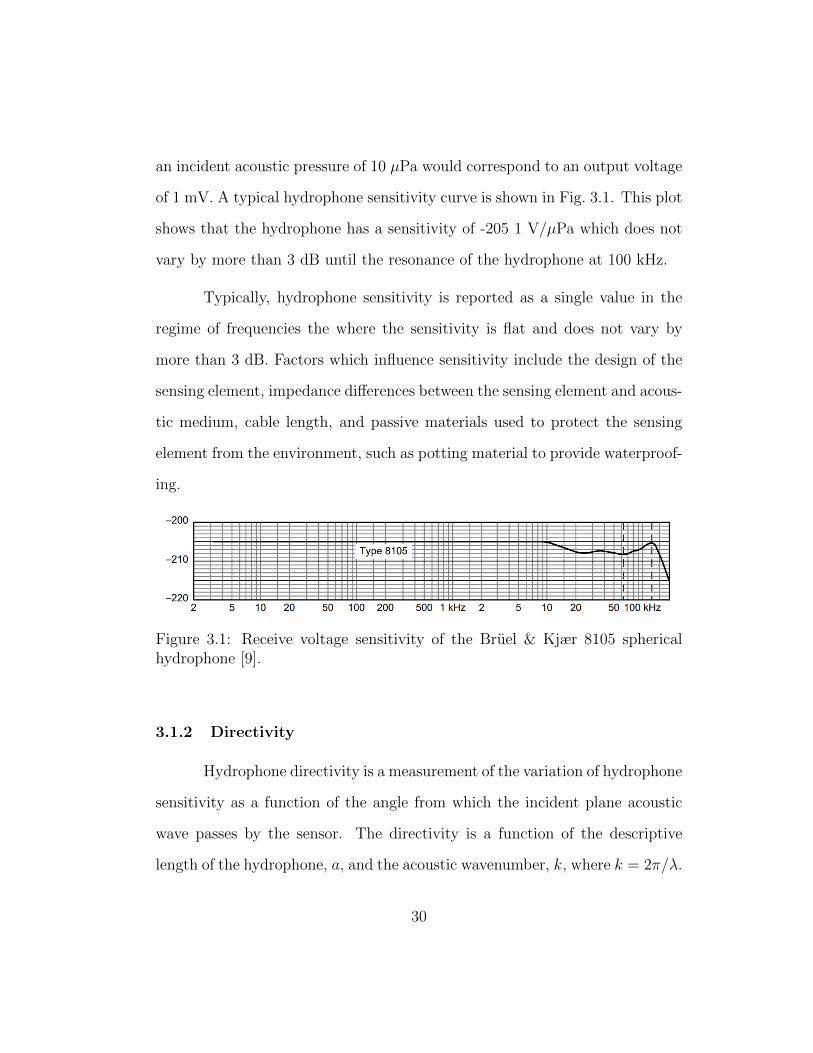
an incident acoustic pressure of 10 µPa would correspond to an output voltage

of 1 mV. A typical hydrophone sensitivity curve is shown in Fig. 3.1. This plot

shows that the hydrophone has a sensitivity of -205 1 V/µPa which does not

vary by more than 3 dB until the resonance of the hydrophone at 100 kHz.

Typically, hydrophone sensitivity is reported as a single value in the

regime of frequencies the where the sensitivity is flat and does not vary by

more than 3 dB. Factors which influence sensitivity include the design of the

sensing element, impedance differences between the sensing element and acous-

tic medium, cable length, and passive materials used to protect the sensing

element from the environment, such as potting material to provide waterproof-

ing.

Figure 3.1: Receive voltage sensitivity of the Bruel & Kjær 8105 sphericalhydrophone [9].

3.1.2 Directivity

Hydrophone directivity is a measurement of the variation of hydrophone

sensitivity as a function of the angle from which the incident plane acoustic

wave passes by the sensor. The directivity is a function of the descriptive

length of the hydrophone, a, and the acoustic wavenumber, k, where k = 2π/λ.

30

The directivity is usually expressed as a function of the non-dimensional prod-

uct ka, which provides a metric of the relative size of the hydrophone to the

wavelength of sound being measured. When a is much smaller than a wave-

length, (i.e., ka�1), the hydrophone is equally sensitive to acoustic pressures

at all angles and is omnidirectional [10]. At higher frequencies, a is compa-

rable to the wavelength of the incident sound and ka ≈ 1. In this frequency

range, nulls in the sensitivity occur at angles where the net pressure variation

across the hydrophone is negligible. In this frequency range, one begins to

observe directions where the hydrophone has maximum sensitivity, known as

the acoustic axis, and secondary maxima (sidelobes) appear in between the

sensitivity nulls. The half-power beamwidth of a hydrophone is defined as

the angle between the half-power points of the main lobe, where sensitivity

decreases by 3 dB when compared to the sensitivity on the acoustic axis. An

example of a hydrophone directivity pattern is given in Fig. 3.2.

3.1.3 Bandwidth

Hydrophone bandwidth is defined as the usable frequency range of the

hydrophone. In this range, the sensitivity is flat and does not fluctuate by more

than 3 dB. In most hydrophones, the maximum frequency of the bandwidth

occurs at the frequency of the fundamental resonance of the hydrophone, which

is marked by a peak in sensitivity followed by a sharp decrease at a rate of

12 dB per octave. For most applications, it is important to design the sensing

element such that the fundamental resonance will not lie within the desired

31

Figure 3.2: Directivity patterns of a type F50 hydrophone in the vertical plane[11].

bandwidth. As an example, Fig. 3.1 shows the RVS of the Bruel & Kjær

8105 hydrophone. The bandwidth of this transducer spans from 0.1 Hz to the

fundamental resonance at 100 kHz, and the RVS is -205 dB re 1 V/µPa.

3.1.4 Self-Noise

Hydrophones have an inherent self-noise due to the electrical dissipa-

tion mechanisms of the sensing element. For the cases considered in this work,

the sensing element is a piezoelectric material so the source of self-noise and

model approximations will be related to hydrophones with piezoelectric sensing

elements.The mechanisms that lead to thermal noise include electrical dissipa-

tion, usually expressed as the dielectric loss factor, as well as mechanical losses

32

associated with the mechanical loss factor and transformed into the electrical

domain via electro-mechanical coupling. These mechanisms cause thermal en-

ergy in the sensing element to generate a small amount of electrical noise.

This electrical noise cannot be removed since it is due to random molecular

motion, and it is thus known as the self-noise floor. It is also notable that the

passive materials used to house the sensing elements also contain dissipative

mechanisms and can thus indirectly lead to increases in the noise floor of the

sensor.

In regards to applications, the noise floor ultimately defines the lower

bound of the dynamic range of the sensor since the noise floor will inhibit

the measurement of signals that have lower amplitudes than the self-noise

floor. Additional sources of noise in the hydrophone signal can arise from

the data acquisition system and preamplifier electronics, mechanical strain in

the hydrophone cable, and electromagnetic and radio-frequency interference.

Those sources of noise can be viewed as independent of the thermal noise floor,

and are thus additive noise that must be considered in the design of the various

electrical components and sensing system associated with the sensing element.

A very useful model of the hydrophone self-noise level is the Johnson-

Nyquist noise formula [4]. Johnson-Nyquist noise is dependent on the resistive

component of the total electrical input impedance of the hydrophone, Rh,

where Rh is a complex function of the sensing element and all of the electro-

mechanical components associated with the hydrophone (i.e. overmold, solder

joints, etc). The value of Rh can be measured or computed from an equivalent

33

circuit. Given the input resistance of the hydrophone from either a model or

measurement, the equivalent mean-squared noise voltage is given as:

〈V 2〉 = 4KTRh∆f, (3.1)

where K is Boltzman’s constant (1.381 × 10−23 J/K), T is the absolute tem-

perature of the water in Kelvin, and ∆f is the bandwidth of the frequency bin

in Hz, which is commonly evaluated in 1 Hz bands [4]. To directly compare

the noise level to an acoustic signal, the mean-squared noise voltage level can

be expressed as an equivalent mean-square noise pressure. The mean-square

noise pressure (or noise spectral density), 〈P 2n〉, is found by dividing the mean-

square noise voltage, 〈V 2〉, by the hydrophone sensitivity, M , in units of V/Pa

such that ⟨P 2n

⟩=⟨V 2⟩/M2. (3.2)

Noise spectral density is useful when comparing the relative levels of incoming

acoustic signals to the noise floor; it is critical that the noise floor of any

hydrophone does not exceed the minimum expected amplitude of the signal

one wishes to measure.

3.1.5 Diffraction and Scattering

When a hydrophone is comparable in size to a wavelength in the acous-

tic medium, it will scatter the impinging sound field. As a result, the pressure

surrounding the hydrophone will differ from the actual pressure at the mea-

surement point in the absence of the hydrophone, which is the quantity one

34

wishes to measure. The inability to measure the field without disturbing the

field is a fundamental limitation of all measurement devices regardless of phys-

ical domain. However, it is important to keep this in mind when designing

hydrophones that are meant to function in an array of sensors since even low

scattered amplitudes can result in a large disruption in the overall field when

large numbers of hydrophones are present. The acoustic field scattered by a

hydrophone is characterized by a directivity similar to the receive sensitivity

directivity pattern discussed in Sec. 3.1.2, where the variation in amplitude of

the fields scattered in the vertical and horizontal planes is presented on a polar

plot for single frequencies. In most cases, the strength of the scattered field

is measured in dB relative to the incident pressure wave. For a given sensing

element (such as a piezoelectric ceramic), the primary contributor to the mag-

nitude of scattered field is the size of the element relative to the wavelength of

acoustic field. This places an importance on the size of the hydrophone and

translates to the requirement that the hydrophone should be small compared

to the shortest acoustic wavelength of interest (i.e. for the highest frequency

signal of interest), such that the scattered field is negligible across the entire

frequency range to be measured.

3.1.6 Mechanical Design

A well-built hydrophone should be mechanically and electrically robust.

Apart from being completely waterproof, the hydrophone should be able to

withstand minor shocks and bumps, should resist corrosion, and should have

35

Figure 3.3: A spherical hydrophone (Bruel & Kjaer model 8105).

low susceptibility to electromagnetic interference. For example, it is important

that the encapsulation material, known as potting, does not greatly affect the

response of the sensing element. For low hydrostatic pressures, a minimal

amount of potting should be used. When considering mass production, it

is also important to be mindful of material cost, machining capabilities, and

ease of fabrication. An example of a hydrophone with a robust mechanical

design is shown in Fig. 3.3, showing a rugged nitrile butadiene rubber overmold

bonded to a spherical piezoelectric sensing element. This hydrophone has

several other mechanical features that have no actual acoustical function, such

as the positioning belt and the long “stem” that is likely used for strain relief.

In practice, any additional mechanical features should be designed to have an

insignificant effect on the acoustic performance of the hydrophone.

36

3.2 Sensing Element Design

A wide variety of consumer and military-grade hydrophones are con-

structed from spherical-shell or cylindrical-tube piezoelectric elements. While

spherical sensing elements generally have exceptional performance character-

istics, they are notoriously expensive due to complex ceramic machining and

molding operations. For cost-minded reasons, the spherical-shell sensing ele-

ment is not investigated in this thesis. Alternatively, hydrophone designs that

incorporate finite-length, hollow cylindrical piezoelectric elements are much

more cost effective. One such hydrophone is the Type F50 hydrophone, de-

signed by the US Navy Underwater Sound Reference Division (USRD).

The USRD Type F50 hydrophone was designed in 1971 [11], and was

subsequently employed as a reference hydrophone by the US Naval Sea Systems

Command. The design was intended to offer broad-band sensing capability,

be physically small, and moderately sensitive for multi-purpose functionality.

The sensing element consists of two radially-polarized, finite-length, thick-

walled piezoelectric cylinders. The end of each cylinder is fitted with an end-

cap to maintain an air-backed boundary on the inner-radius. This physical

boundary is an excellent approximation of a stress-free, or pressure-release,

boundary. Magnesium rims are bonded to the ends of cylinder with epoxy,

and a magnesium insert with O rings is fitted into the cylinder and positioned

so that the O rings seal on the magnesium rims. The O rings mechanically

decouple the insert from the sensing element to avoid any resonances which

could potentially limit the bandwidth. The two sensing elements are held

37

within a cylindrical frame of expanded metal, which serves as an electrostatic

shield and protective guard. A butyl-rubber boot is fitted around the frame to

provide robust waterproofing for harsh environmental conditions. The boot is

filled with castor oil, which serves as an acoustic impedance matching medium

between the element and the rubber boot. A cutaway of the hydrophone is

illustrated in Fig. 3.4

1 2

3

Figure 3.4: Cutaway of the USRD F50 Hydrophone [11]. (1) Butyl boot; (2)cylindrical-tube piezoelectric sensing elements; (3) rigid end-caps.

The bandwidth of the F50 hydrophone is terminated at the fundamen-

tal resonance frequency of the cylindrical sensing element. If the length of

the cylinder is small compared to its circumference, and there are no flexural

resonances in the end-caps, the cylindrical sensing element will resonate in

a breathing radial mode, which is marked by an expansion and contraction

in circumference. If the length of the cylinder is comparable to its circum-

ference, the modal characteristics become more complicated, giving rise to

axial and bending modes. The frequencies at which these modes occur de-

pend on the material properties of the ceramic and the specific length, width,

38

and radial thickness of the sensing elements. It is important to account for

the bandwidth-limiting potential of these modes. A few of the performance

characteristics of the F50 hydrophone are outlined in Table 3.1. Since these

characteristics satisfy the hydrophone design requirements outlined in Ch. 2,

the cylindrical sensing element can be qualified as a candidate for further study

and development.

Table 3.1: USRD F50 hydrophone performance characteristics.

Design Parameter Value

Bandwidth 1 Hz - 70 kHzVoltage sensitivity -206 dB re 1V/µPa at 5 kHzDirectivity Omnidirectional within 1 dB in all planes up to 30 kHz

3.3 Hydrophone Equivalent Circuit

1 : N

C01/G0

+

−

V

CE

M Rm

uZr

Fb

Figure 3.5: A simple hydrophone equivalent circuit.

Equivalent circuit modeling is a well-known and convenient means of

modeling the electro-acoustic behavior of acoustic transducers. Equivalent

39

circuit models provide quick and efficient information about the resonant be-

havior of a system, but are incapable of modeling higher-order effects. An

equivalent circuit can be used to model hydrophone performance character-

istics such as sensitivity, bandwidth, and noise floor. The equivalent circuit

can account for numerous mechanisms such as cable length, sensing element

geometry and material properties, mechanical and electrical losses, and scat-

tering effects. A simple hydrophone equivalent circuit that accounts for one

mechanical resonance is shown in Fig. 3.5. The circuit components are identi-

cal to the example equivalent circuit presented in Ch. 1, but for a hydrophone,

the effort variable, which is represented as a voltage input in previous exam-

ples, is replaced by an open-circuit output voltage. Furthermore, the blocked

force Fb (which represents the incident pressure field) is added as a source

term to the mechanical domain. The current generated by the blocked force is

appropriately translated into the electrical domain via the electro-mechanical

transformer, N , and a voltage is measured at the output terminal.

This section provides the derivation of a comprehensive equivalent cir-

cuit for a hydrophone using a radially-polarized, finite-length, hollow piezo-

electric cylinder. The circuit parameters of the radial and axial modes of

the cylinder element are derived individually and then integrated into a sin-

gle equivalent circuit. First, the circuit parameters are derived for the radial

mode, following the derivation from Sherman and Butler [4] and Joseph [12].

Since no assumption has been made about the circumference of the cylinder

compared to its length, it is necessary to account for axial modes of the cylin-

40

der to ensure that the hydrophone bandwidth is not limited by the axial mode.

The axial-mode equivalent circuit parameters are derived in Sec. 3.3.2, and the

circuit parameters for both the axial and radial modes are combined to form

a comprehensive equivalent circuit. Finally, the equivalent circuit is modified

to account for effects associated with end-caps, overmold, and cable.

I

1/G0 C0

1 : NA

CEA

Mm Rm

uA

Zr

Fb

+

−

V

CER

Mm Rm

uR

Zr

Fb

1 : NR

Figure 3.6: Comprehensive equivalent circuit for a cylindrical sensitive ele-ment.

Figure 3.6 shows the comprehensive hydrophone equivalent circuit, ac-

counting for both radial and axial cylinder modes. As seen in the example

circuit from Ch. 1, the circuit left of the transformers represents the electrical

domain of the hydrophone, while the circuit to the right represents the me-

chanical domain. The mechanical domain is subdivided into two branches: the

radial branch (top) and the axial branch (bottom). It is necessary to split the

41

L

t a

x2

x3

x1

Figure 3.7: Geometry and coordinate system of the radial-mode piezoelectriccylinder.

domain into two branches to account for the orthogonal modes of the piezo-

electric element. In other words, the radial and axial modes of the cylinder are

caused by independent stiffnesses and transformer ratios, and thus require in-

dividual circuits. The unknown circuit parameters that will be derived in this

section include dielectric loss, G0, clamped capacitance, C0, effective short-

circuit compliance, CE, mass, M , radiation impedance, Zr, and blocked force,

Fb. The subscripts R andA are used to indicate the unique circuit parameter

for the radial and axial mode respectively.

3.3.1 Radial Mode Circuit Parameters

Consider the cylindrical tube shown in Fig. 3.7 of length, L, wall thick-

ness, t, and mean radius a = (OD + ID) /2. The cylinder is radially polarized

with electrodes on the inner and outer lateral surfaces. Let the local coor-

dinates x1, x2, and x3 define the circumferential, axial, and radial directions

42

respectively. When the radial mode of the cylinder is vibrationally excited,

it is assumed that the primary stress and strain are in the circumferential

direction and the electric field is orthogonal to this direction.

The analysis of the radial mode begins by applying the appropriate

boundary conditions to the constitutive piezoelectric equations discussed in

Ch. 1. It is assumed that the wall thickness, t, is small compared to the

mean radius, a, and that the ends of the cylinder are free to move so that

there is a zero-stress boundary condition in the x2 and x3 directions such that

T2 = T3 = 01. Since t is small, it can also be assumed that the electrode

surfaces are equipotential and E1 = E2 = 0 throughout the cylinder. This

leads to the reduced constitutive equations

S1 = sE11T1 + d31E3, (3.3)

and

D3 = d31T1 + εT33E3, (3.4)

where S1 is the circumferential strain, E3 is the electric field in the radial

1The assumption that that the primary stress is in the circumferential direction becomesless accurate as the length of the cylinder increases. For a long cylinder, the axial stressT2 becomes non-negligible. Holding the assumption of zero axial strain, the axial and

circumferential stresses are related by S2 = 0 = sE21T1 + sE22T2, yielding T2 =−sE21sE22

T2. As a

result, the axial stress effectively stiffness the ring, raising the resonance frequency of theradial mode.

43

a a+ξ

Figure 3.8: Circumferential expansion of the cylinder.

direction, T1 is the circumferential stress, and D3 is the electric displacement

aligned with the radial direction.

In the radial mode, a time-harmonic voltage, V , applied to the elec-

trodes of the piezoelectric element will cause the circumference of the cylinder

to proportionally expand or contract by an amount ξ, as shown in Fig. 3.8.

The electric field, E3, can be approximated as the ratio of applied voltage to

wall thickness,

E3 =V

t. (3.5)

The circumferential strain is approximated as S1 = ξ/a. Likewise, T1 can be

rewritten in terms of the circumferential force, F , such that

S1 =ξ

a= sE

11

(F

tL

)+ d31

(V

t

). (3.6)

Solving for F yields

F =

(tL

sE11a

)ξ −

(Ld31

sE11

)V, (3.7)

44

where the total radial force within the cylinder is given as

Fr = 2πF. (3.8)

The radial equation of motion is given by Newton’s second law, where

Mξ = F0 − Fr = F0 − 2πF. (3.9)

Here, M is the mass of the cylinder and F0 is any miscellaneous force acting

radially on the cylinder, which can include radiation loading and force due

to an incoming acoustic wave. The mass of the cylinder is given by M =

2πρatL, where ρ is the density of the ceramic. Note that the dot convention

has been used to indicate derivation with respect to time. Substituting the

circumferential force into Eq. (3.7) and rearranging leads to

Mξ = F0 − 2π

[(tL

sE11a

)ξ −

(Ld31

sE11

)V

]. (3.10)

The radial equation of motion can be expressed as an inhomogeneous

second-order differential equation, yielding

Mξ + 2π

(tL

sE11a

)ξ = F0 + 2π

(Ld31

sE11

)V, (3.11)

or, in terms equivalent circuit parameters,

Mξ +

(1

CE

)ξ = F0 +NV, (3.12)

45

where CE is the effective short-circuit radial compliance, and N is the elec-

tromechanical turns ratio. Further, a viscous damping term Rm can be added

to account for mechanical loss. Under time-harmonic conditions, Eq. (3.12)

becomes

jωMξ +1

jωCEξ +Rmξ = F0 +NV. (3.13)

For a simple vibrating piezoelectric cylinder, the only external force is

the radiation impedance. Setting F0 equal to the radiation force on the radial

moving surface, Zr, the solution for radial velocity, ξ, becomes

ξ =NV

jωM + (1/jωCE) +Rm + Zr

, (3.14)

where the mechanical impedance Zm = V/ξ.

The electrical input impedance is obtained by eliminating T1 from

Eqs. (3.3) and (3.4), yielding the dielectric displacement

D3 = d31

(1

sE11

S1 −d31

sE11

E3

)+ εT33E3. (3.15)

The clamped dielectric constant, εS33, is given for constant S1 strain as

εS33 = εT33

(1− k2

31

), (3.16)

where k31 is the piezoelectric coupling factor, given by k31 = d231/s

E11ε

T33.

46

From here, Eq. (3.15) is rewritten as

D3 = (d31/sE11) S1 + εS33 E3. (3.17)

With dielectric displacement D31 given by the charge per unit area, Q,

S1 given by ξ/a, and E3 given by V/t, Eq. (3.17) is rewritten as

Q

2πaL=

(d31

sE11a

)ξ + εS33

V

t. (3.18)

The clamped capacitance is evaluated at constant S1 such that

C0 = ∂Q/∂V = (2πaLεS33)/t. (3.19)

The input current, I, is taken as the derivative of the charge with respect to

time, leading to

I =dQ

dt=

(2πLd31

sE11

)ξ + C0

dV

dt, (3.20)

where the term 2πLd31/sE11 is again equal to N, the electromagnetic turns ratio.

Assuming a time-harmonic voltage, Eq. (3.17) can be rewritten as

I =dQ

dt= Nξ + jωC0V. (3.21)

The final form of the electrical input impedance is found by substitut-

ing radial velocity, ξ, from Eq. (3.14), and adding a term G0 to account for

electrical loss conductance, leading to

47

L

ta

x2

x3

x1

Figure 3.9: Geometry and coordinate system of the axial-mode piezoelectriccylinder.

Z =V

I=

N2

jωM +(

1jωCE

)+Rm + Zr

+ jωC0 +G0

−1

. (3.22)

At this point, the stiffness and transformer parameters of the radial

branch of the equivalent circuit have been determined. The section will pro-

ceed by deriving the same parameters for the axial branch of the circuit. Ra-

diation impedance and blocking force will be addressed when all other circuit

parameters have been accounted for.

3.3.2 Axial Mode

The derivation of the axial circuit parameters is carried out in a similar

fashion to the radial mode. In this axial mode, the primary stress and strain are

in the axial direction of the cylinder, while the electric field is still orthogonal to

48

the cylinder circumference. The coordinate system is redefined to be consistent

with the literature-given piezoceramic material properties, which specify x1 as

the direction of primary stress. Let the local coordinates x1, x2, and x3 define

the axial, circumferential, and radial directions, respectively. The boundary

conditions are enforced by assuming plane-strain conditions, zero stress on the

walls of the cylinder (T2 = 0), and equipotential surfaces (E1 = E2 = 0). The

constitutive piezoelectric equations can be rewritten with T as the independent

variable such that

T1 = CE11S1 + CE

13S3 − e31E3 (3.23)

and

D3 = e31S1 + e33S3 + εS33E3, (3.24)

where Cij is the elastic stiffness coefficient, and ekm and εkm are piezoelectric

constants.

The equivalent stiffness is found with the open circuit conditions

T1 = C11S1 + C13S3. (3.25)

Equation (3.25) can be rewritten as

T1 = S1(C11 + C13ν13), (3.26)

49

where ν13 is Poisson’s ratio, equal to −C13/C33. The axial stiffness coefficient,

Cp,l is given as

Cp,1 =T1

S1

= C11 +C2

13

C33

. (3.27)

L

L+ξ

Figure 3.10: Axial expansion of the cylinder.

The nth axial mode occurs when integer multiples of the wavelength

are equal to twice the cylinder height, or when

λp,1 = 2L/n. (3.28)

At the resonance frequency, fr, the wavelength λp,1 = cp,1/fr where cp,l is the

axial wavespeed in the ceramic. The axial wave speed is given as

cp,1 =

√Cp,1

ρ, (3.29)

where ρ is the density of the ceramic. For the first axial mode (n = 1), the

50

resonant frequency is

fr =1

2L

√Cp,1

ρ. (3.30)

The effective axial stiffness, KE, is given where

ω2r =

KE

M=(πL

)2 Cp,1

ρ. (3.31)

The effective axial compliance, CE, is therefore given as

CE =1

KE=

(L

2π3at

)Cp,1. (3.32)

The electromechanical turns ratio, N , can be determined from the

piezoelectric coupling coefficient, k. The piezoelectric coupling coefficient is a

measurement of the amount of energy that is transduced from one domain to

another, where the coupling factor is generally defined as

k2 =energy transduced

total energy input. (3.33)

The coupling factor can also be expressed in terms of energy density, which

can be readily derived from the piezoelectric constitutive equations. k can

be expressed as the ratio of the mutual elastic and dielectric energy density,

Umut, to the geometric mean of the elastic strain energy density, US, and the

dielectric energy density, UD [13]:

k =Umut√USUD

. (3.34)

51

The energy densities can be calculated from the constitutive piezoelectric equa-

tions as

U =1

2(SiTi +DmEm) . (3.35)

Enforcing the appropriate boundary conditions, the strain energy becomes

U =1

2(S1T1 +D3E3) . (3.36)

Substituting T1 from Eq. (3.23) and writing S3 = ν31S3 yields

U =1

2

[S2

1

(CE

11 + CE13ν31

)+ εS33E

23 + e33ν31S1E3

]. (3.37)

From here, the total energy density can be split apart into individual compo-

nents:

US =1

2

[S2

1

(CE

11 + CE13ν31

)], (3.38)

Umut =1

2

[εS33E

23

], (3.39)

and

UD =1

2[e33ν31S1E3] . (3.40)

The effective axial coupling coefficient, keff,l is found by substituting Eqs. (3.38-

52

3.40) into Eq. (3.34) such that

keff,l = e33ν13

(CE

11 + CE13ν13ε

S33

)− 12 . (3.41)

The transformer turns ratio, N , can readily be calculated from the

effective coupling coefficient, the clamped capacitance, C0 (as determined from

Eq. (3.19)), and the effective mechanical compliance, CE, from Eq. (3.32). This

results in the expression

k2 =N2CE

C0 +N2CE(3.42)

or

N =

√k2C0

CE (1− k2). (3.43)

At this point, the equivalent circuit parameters have been defined for

both radial and axial branches. The mechanical mass, Mm and viscous damp-

ing resistance Rm, are unchanged in the axial branch since they are inherent

material properties of the ceramic. In most cases, it is appropriate to tune the

damping resistance parameter to match the quality factor of the resonances

with observations and measurements. From here, the equivalent circuit is fur-

ther developed with the derivation of blocked force and radiation impedance.

3.3.3 Blocking Force and Output Voltage

When an acoustic pressure Pi is incident upon the hydrophone, the

total force acting on the sensing element becomes

F = Zrξ + Fb, (3.44)

53

where Zr is the radiation impedance and ξ is the particle velocity of the incom-

ing wave. The blocked force, Fb, is the integral of local acoustic pressure over

the face of the hydrophone. The radiation impedance is included in this term

to account for the reaction of the acoustic medium when the surface of the

hydrophone is set into vibration. When the size of the hydrophone approaches

the wavelength scale, the diffraction constant Da should be included in the

blocked force such that

Fb = DaPi. (3.45)

The diffraction constant of a cylinder has been solved for several specific ra-

diation cases [4].

The circuit output voltage, V , forms a voltage divider with the blocked

force, Fb, such that

V = Z0 (Fb/N)[Z0 +

(Zm + Zr/N

2)], (3.46)

where Z0 is the clamped electrical impedance and Zm is the equivalent mechan-

ical impedance from both radial and axial branches. The blocked forces and

radiation impedances are appropriately transformed into the electrical domain

by the transformer at each modal branch.

54

3.3.4 Radiation Impedance

Radiation impedance affects the amount of power that can be transmit-

ted from an acoustic medium into the hydrophone. The radiation impedance

is defined [10] as

Zr =Pav

u0

=

∫∫S

PidS = Rr + jXr, (3.47)

where Pi is the local sound pressure incident on the face of the hydrophone,

and Rr and Xr are the resistive and reactive components of the impedance

respectively. The radiation impedance affects the hydrophone performance by

contributing a resistive loss to the transmitted power, and decreases resonant

frequencies due to the increased mass from the fluid load on the receiving face.

Although there is no closed-form solution for the radiation impedance

of a finite cylinder, the cylinder can be well approximated as a sphere with

equivalent radiating area as =√

bL2

where b is the outer radius of the cylinder

[4]. The radiation impedance becomes

Zr = Rr + jωMr = Aρ0c0

[(kas)

2 + jkas

]/[1 + (kas)

2], (3.48)

where A = 4πa2s , rho0 and c0 are the density and sound speed of the acoustic

medium, and k is the wavenumber, given by ω/c0. The normalized resistive

and reactive components of the radiation impedance are shown in Fig. 3.11.

55

0 2 4 6 8 10ka

s

0

0.2

0.4

0.6

0.8

1

Zr /

A0c 0

Radiation impedance of equivalent sphere

Xr

Rr

Figure 3.11: Real and imaginary parts of the radiation impedance of an equiv-alent sphere.

3.3.5 Effects of End-Caps

The cylinder end-caps are used to seal the inner air cavity and maintain

a pressure relase inside the cylinder element. In doing so, the stress boundary

conditions of the cylinder are altered. Langevin has thoroughly considered

the effect on stress and sensitivity from both exposed-end and capped-end

configurations [14]. The sensitivity of a radially polarized cylinder with inner

radius a and outer radius b is given as

M =

∫ b

a

[g33Tr + g31 (Tθ + Tz)] dr, (3.49)

where g33 and g31 are piezoelectric voltage constants, and Tr, Tθ, and Tz are the

56

polar stresses generated by the incident acoustic wave. For both end-exposed

and end-capped conditions it is assumed that the inside lateral surface of the

cylinder is shielded from radiation, while the outside lateral surface is exposed

to a uniform radiation field Pi. The boundary conditions for the end-exposed

case take the form

Tr =a2b2Pi

b2 − a2

(1

R2− 1

a2

), (3.50)

Tθ =a2b2Pi

b2 − a2

(− 1

R2− 1

a2

), (3.51)

and

TZ = −Pi (3.52)

In the capped-end configuration, the ends of the cylinder are subject

to a radiation field b2Pi/ (b2 − a2). The axial stress, TZ, and the subsequent

sensitivity is increased by a factor of −b2/ (b2 − a2).

3.3.6 Cable Effects

A long cable with a high capacitance will reduce the sensitivity of a

hydrophone. The cable capacitance, Cc, forms a voltage divider with the

hydrophone free capacitance, Cf . The output voltage at the end of the cable

becomes

Vc =V Cf

Cf + Cc

, (3.53)

where V is the voltage output of the hydrophone without the cable. For

57

Figure 3.12: Different configurations of stacked cylinders with end caps.

example, if the cable capacitance were equal to the hydrophone free capaci-

tance, the sensitivity would be reduced by a factor of 2. In situations where

a long cable is required, it is advantageous to design a hydrophone with a

high free-capacitance or to place the preamplifier as close to the sensing ele-

ment as possible. For the purpose of this project, it was not feasible to place

the preamplifier close to the sensing element due to scattering concerns and

limitations of space.

3.3.7 Stacked Sensing Elements

The cylindrical sensing elements can be stacked atop one another and

wired in parallel, as show in 3.12. This stacked configuration will increase the

total hydrophone capacitance, which leads to a lower self-noise floor, and can

help mitigate the parasitic capacitance that occurs when using long cables.

However, if the length of the cylinder stack is greater than the cylinder cir-

cumference, the structure is susceptible to lower-frequency axial and bending

modes that could unexpectedly limit the hydrophone bandwidth.

58

3.3.8 Summary of Hydrophone Equivalent Circuit

The derived parameters for the hydrophone equivalent circuit are listed

in Table 3.2. These parameters can readily be adapted for use with arbitrary

piezoceramic material properties and cylinder dimensions.

Table 3.2: Summary of hydrophone equivalent circuit parameters.

Parameter Value

Electrical resistance, R0 (ωCftanδ)−1

Clamped capacitance, C0 (2πaLεS33)/t

Radial branch transformer turns ratio, NR 2π(

Ld31sE11

)Longitudinal branch transformer turns ratio, NL

√k2C0

CE(1−k2)

Radial stiffness, CER 2π

(tLsE11a

)Longitudinal compliance, CE

L

(L

2π3at

)Cp,1

Effective mass, Mm 2πρatL

Radiation impedance, Zr Aρ0c0

[(kas)

2 + jkas

]/[1 + (kas)

2]Blocking force, Fb DaPi

3.4 Prototype Specifications

Piezoelectric cylinders are available off-the-shelf in several standard

sizes. From a mass-manufacturing standpoint, it is much more viable to use

standard sized elements as opposed to custom sizes. The hydrophone equiva-

lent circuit can be used to characterize the various standard cylinders to select

the most appropriate size for the application. The standard sizes should be

assessed for resonant frequency, noise floor, size, and sensitivity.

After a brief survey of readily available materials in the laboratory, a

59

design was proposed. The hydrophone prototype consisted of:

1. A cylinder made of APC 840 piezoceramic2, with wall thickness of 1 mm,

length of 10 mm, and outer diamter of 10 mm. Favoring a smaller size,

the hydrophone was intended to be fabricated from only one cylinder

element as opposed to numerous stacked elements.

2. End caps machined from 1.5 mm-thick Macor ceramic. Macor was cho-

sen specifically for its machinability and high stiffness to avoid end-cap

flexural resonances from interfering with the band of operation.

3. A low-noise coaxial cable with a Teflon outer jacket.

4. A 3 mm-thick potting layer made of Henkel Loctite Stycast 2651 Epoxy

Encapsulant. On the cable side, the potting layer was designed to taper

to a stem for ease of mounting and positioning. Stycast was chosen over

the traditional urethane potting because of its higher stiffness and lower

damping. It was previously observed that thick layers of urethane can

negatively impact the receive sensitivity, and the impact from Stycast

is reduced due to its high stiffness. Additionally, uncured liquid Stycast

has a much lower viscosity than urethane, making it easier to pour into

a mold and degas without trapping any bubbles in the hydrophone.

2APC 840 is a proprietary ceramic manufactured by APC International. It is approxi-mately equivalent to PZT-4 ceramic.

60

These design parameters will be used as the basis for the equivalent

circuit, finite element models and physical prototypes. Before constructing

the physical prototypes, the design will be verified with equivalent circuit and

finite element models. These models will be used to predict impedance, RVS,

noise floor, and scattering, and will ensure that the proposed design meets the

performance requirements established in Ch. 2.

3.5 COMSOL Finite Element Model

The equivalent circuit is effective for modeling the general hydrophone

behavior, but is incapable of modeling higher order effects. An FEM model

can account for both simple and higher order effects such as flexural reso-

nances of the end caps, mode coupling, or effects due to potting, all of which

can significantly alter the hydrophone performance. The section will begin

by detailing the setup of the FEM model in COMSOL Multiphysics. The

model setup includes geometry definition and material selection, physics im-

plementation, and meshing considerations. The section will conclude with the

model results, including electrical input impedance, scattering characteristics,

directivity, and receive sensitivity. The model results are compared to the

equivalent circuit where applicable.

3.5.1 Model Definition

To reduce computational cost, the hydrophone model is represented in

a 2D-axisymmetric domain. In this axisymmetric domain, the plane geom-

61

Macor caps

PZT-4 cylinder

Poling

direction

V+ V-

Figure 3.13: COMSOL hydrophone geometry in axisymmetric plane.

etry shown in Fig. 3.13 is revolved about the global r = 0 axis. Although

consistency has been verified between 2D-axisymmetric and full 3D models,

the axisymmetric domain is limited in that the system is restricted to two

degrees of freedom. For this reason, an axisymmetric model is incapable of

modeling higher-order modes and construction defects, such as misalignment

between the cylinder and the end caps. These misalignments have previously

been observed to cause phase variations over the surface of the hydrophone

and unexpected modal behavior.

PZT-4 piezoelectric material properties are applied to the cylinder, and

Macor material properties are applied to the end-caps. These material proper-

ties are tabulated in Appendix C. At the second stage of analysis, the overmold

geometry is defined and Stycast material properties are prescribed to the pot-

ting layer. The entire hydrophone is exposed to an unbounded water domain,

62

which is surrounded by a PML to absorb propagating background radiation.

3.5.2 Physics Implementation

The hydrophone physics are implemented with COMSOL’s Pressure

Acoustics, Solid Mechanics and Electrostatics modules. The Pressure Acous-

tics module is used to solve the constitutive Helmholtz wave equation in the

water domain. A far-field pressure calculation is defined on the boundary

between the water domain and the PML; this calculation allows for the com-

putation of amplitude and phase of the acoustic pressure at any point outside

of the computational domain. This tool can be used to plot directivity pat-

terns and scattering strength. A background radiation condition is applied to

the water domain, and is used to simulate a plane-wave that is incident on the

hydrophone. The plane-wave propagation vector is defined by the global +z

or +r coordinate, depending on the desired hydrophone receive configuration.

The hydrophone receive configurations are further detailed in Sec. 3.5.5.

The Solid Mechanics module is applied to the piezoelectric element,

end-caps, and overmold. This module, when applied to the mechanical do-

main of the model, uses linear stress-strain equations along with a small de-

formation assumption. An isotropic loss factor is applied to each mechanical

component to model viscous damping losses in the material. From here, it is

necessary to adjust COMSOL’s default piezolectric poling direction. COM-

SOL’s material library automatically assumes that the ceramic polarization

direction is aligned with the global z axis. To specify a radially poled condi-

63

tion, the material polarization direction must be normal to the r axis. This is

achieved by changing the piezoelectric material model’s coordinate system to

the predefined zx-plane system.

The Electrostatics module is then applied to the piezoelectric cylinder.

A floating potential, V0, is specified on the inside lateral wall of the cylinder,

and a ground is defined on the opposite wall. A surface integral is defined

along the inside lateral wall of cylinder to measure the voltage output from

the piezo element in response to the incident plane-wave pressure field.

The multiphysics coupling modules include the Acoustic-Structure Bound-

ary and Piezoelectric Effect. The Acoustic-Structure Boundary is applied to

the interface of the water domain and hydrophone surface, and links the Pres-

sure Acoustics to the Solid Mechanics. Radiation impedance is accounted for

in the Solid Mechanics interface, where the fluid load effectively acts as a me-

chanical load. The Piezoelectric Effect module couples the Electrostatics and

Structural Mechanics modules by solving the constitutive linear piezoelectric

equations.

3.5.3 Meshing Considerations

To accurately resolve the pressure amplitude and phase in the water

domain, the maximum mesh element size should be no larger than 1/5th of the

smallest wavelength in the study. The water domain is meshed with free tri-

angular elements, and the PML is meshed with swept quadrilateral elements.

A single boundary-layer mesh is created water domain-PML interface to fa-

64

cilitate a smooth transition from triangular to quadrilateral elements. The

hydrophone structure is meshed with triangular elements, with a minimum

resolution of two elements in narrow regions. The meshed geometry is shown

in Fig. 3.14.

Hydrophone

PML

Water

Figure 3.14: Meshed geometry of the hydrophone in a water domain.

3.5.4 Input Impedance

To understand how individual components affect the transducer re-

sponse, the electrical input impedance is modeled at various stages of hy-

drophone assembly. To model impedance, the principal of piezoelectric reci-

procity is used, such that no background pressure field is required. First, the

bare cylindrical element without end-caps is modeled entirely outside of the

water domain. This model is equivalent to measuring the input impedance of

the unconstrained bare element in air. Instead of a floating potential, an elec-

tric potential of V0 = 1V is applied to the inside lateral wall of the cylinder.

65

A current-density surface integral I0 is defined on the same surface, where the

integral is computed in the revolved domain. A frequency sweep is defined

from 1 to 250 kHz to capture the modal behavior of the cylinder over a broad

range of frequencies. The complex input impedance is defined as:

Z = V0/I0 (3.54)

From here, the electrical input impedance can be plotted as a magnitude and

a phase angle. The FEM results for electrical input impedance of the bare-

element case are shown in Fig. 3.15.

The finite element modeled impedance shows three distinct resonances,

whereas the equivalent circuit only predicts two (the radial and axial mode).

To interpret the three resonances predicted by FEM, the 3D mode shapes for

each resonance can be visualized in COMSOL. 3.16 shows the mode shapes

of the three distinct resonances predicted by the finite element model. The

mode shapes show that the first two resonances, which occur at 112 and 120

kHz, are likely variations of a radial mode coupled with a bending mode. The

bending mode likely arises from the fact that the cylinder’s length is equal to its

circumference. This modal behavior was unexpected because the equivalent

circuit is not capable of modeling bending modes; however, the equivalent

circuit and finite element model both agree that there is radial mode behavior

in the vicinity of 116 kHz. The highest frequency predicted resonance at

181 kHz is an axial mode, which is in good agreement with the axial mode

calculated by the equivalent circuit at 165 kHz.

66

0 50 100 150 200 250100

102

105

jZj,

[+]

Impedance of cylinder element without caps

0 50 100 150 200 250Frequency, [kHz]

-100

-50

0

50

100

Phas

e, [°]

COMSOLEquiv. Circuit

Figure 3.15: Modeled electrical input impedance of cylinder element. Thefirst resonance of the equivalent circuit is the radial mode, and the secondresonance is the axial mode.

Next, the model considers the effects of end-caps. As in the previous

case, the structure is free from any acoustic load. The results of the electrical

input impedance with the end-capped cylinder are shown in Fig. 3.17. The

model indicates that the two lowest radial-bending resonances are pushed to-

gether to form one single mode. This effect likely arises from the fact that

the end caps act as an additional radial stiffness in parallel with the open

ends of the cylinder. This increased stiffness couples the two distinct radial-

bending modes into one effective resonance. At the axial resonance, the end

67

(a) (c)(b)

Figure 3.16: FEM mode shapes of a piezoelectric tube. (a) 112 kHz; (b) 120kHz; (c) 181 kHz.

caps behave like masses added in series to the structure. This increase in mass

causes the axial resonance to decrease in frequency. The results of this model

illustrate the importance of using a stiff but light material for the end-caps. If

the caps are too compliant, then they are liable to flexural resonances and a

reduced band of operation; if the caps are too heavy, the axial resonance could

be significantly reduced in frequency.

Finally, the model considers the case where the sensing element is en-

capsulated in Stycast epoxy and submerged in water. The geometry of the

Sycast overmold is shown in Fig. 3.18. Due to the significant series increase

in mass from the Stycast, the fundamental resonance (and theoretical band-

width) is reduced to 60 kHz. If a wider bandwidth were required, it would be

advisable to use a potting material with a lower density or to design a thinner

potting layer. No additional parasitic resonances were caused by the addition

of the potting layer.

68

0 50 100 150 200 250100

102

105

jZj,

[+]

Impedance of cylinder element with caps

0 50 100 150 200 250Frequency, [kHz]

-100

-50

0

50

100

Phas

e, [°]

Equiv. CircuitCOMSOL

Figure 3.17: Electrical input impedance of cylinder element with end-caps.The first resonance of the equivalent circuit is the radial mode, and the secondresonance is the axial mode.

3.5.5 Scattering Characteristics

When an incoming wave is incident on the recording surface, a certain

amount of the wave will be scattered from each individual hydrophone. The

amount of scattering is dependent on the frequency of the incoming signal

and the size of the hydrophone. It is necessary to model the scattering of

a representative plane wave from an individual hydrophone to ensure that

the hydrophone’s scattered field will not interfere with the recorded outgoing

signals which enter the numerical simulation.

69

Stycast

overmold

Mounting

stem

Figure 3.18: Model geometry of hydrophone with overmold.

The scattering characteristics of the hydrophone were modeled for two

configurations:

1. Vertical configuration - the plane wave propagation is parallel to the

center axis of the cylinder.

2. Horizontal configuration - the plane wave propagation is normal to the

center axis of the cylinder.

The mounting configurations are illustrated in Fig. 3.19, showing the reference

direction of the plane wave and its incidence upon the hydrophone. The refer-

ence angle θ is defined such that the plane wave is incident on the hydrophone

at 180◦.

A background pressure condition is specified on the water domain,

where the plane wave amplitude is equal to 1 Pa. The plane wave direc-

70

θ

Figure 3.19: Hydrophone configurations: vertical (top) and horizontal (bot-tom).

tion is specified according to the desired hydrophone configuration. Due to

the 2D-axisymmetry, the COMSOL built-in plane wave expansion is required

to achieve the correct wave direction for the horizontal configuration. This fea-

ture requires extra setup and post-processing, and is outlined in the COMSOL

documentation [15].

To validate the FEM model, the horizontally mounted case is com-

pared against the analytical solution for the scattering from an infinitely long

isotropic elastic cylinder [16]. The scattered field is expressed in the form of

a directivity plot. The scattered field is plotted in dB down from the inci-

dent plane wave, where the forward-traveling plane wave is incident upon the

hydrophone at θ = 180◦. The modeled scattered field of the horizontal config-

uration is compared to the analytical solution in Fig. 3.21, where the dashed

line indicates the analytical solution.

71

The model is in good agreement with the analytical solution, showing

that the amplitude of the scattered field becomes larger as the wavelength

approaches the size of the hydrophone. At the highest frequency of the study,

the maximum of the scattered field is 50 dB down from the incident pressure

wave. After the FEM model has been validated, the model considers scattering

from the hydrophone in the vertical mounting condition. The magnitude of

the modeled scattered field in the vertical configuration is shown in Fig. 3.20.

Similar to the horizontal case, the majority of the scattered field lies in the

back-scattered plane, with a magnitude up to 50 dB down from the incident

wave.

Overall, the models show that the orientation of the hydrophone has a

small effect on the expected scattered field. In both cases, the back-scattered

field is stronger than the forward-scattered field, and the maximum amount of

scattered sound pressure from each individual hydrophone is expected to be

50 dB down from an incident plane wave.

Figure 3.20: FEM horizontal scattered field of the hydrophone. (-) FEM; (···)analytical.

72

Figure 3.21: FEM vertical scattered field of the hydrophone.

3.5.6 Directivity

0°

30°

60°90°

120°

150°

180°

210°

240°270°

300°

330°

-1.5

-1

-0.5 [dB]

FEM hydrophone horizontal directivity

3 kHz

6 kHz

9 kHz

Figure 3.22: FEM hydrophone horizontal directivity.

The directivity of the hydrophone can be modeled in COMSOL using

the principal of piezoelectric reciprocity. Similar to the scattering model, the

vertical and horizontal mounting positions are considered. Reciprocity is used

such that a background radiation condition is not required, and an electric

potential can be applied to the inner surface of the cylinder. The hydrophone,

73

0°

30°

60°

90°

120°

150°

180°

210°

240°

270°

300°

330°

-1.5

-1

-0.5 [dB]

FEM hydrophone vertical directivity

3 kHz

6 kHz

9 kHz

Figure 3.23: FEM hydrophone vertical directivity.

which now acts as a source, is allowed to radiate freely into the water domain,

where the far-field pressure amplitude is normalized and plotted as a function

of angle. The model shows that for both mounting cases, the hydrophone is

omnidirectional within 3 dB up to 9 kHz. In the vertical case, the hydrophone

becomes slightly directive at higher frequencies, with -1 dB nulls at the ends

of the hydrophone. The FEM horizontal and vertical directivities are plotted

in Figs. 3.22 and 3.23.

In early versions of the design, the model provided evidence that a long

mounting stem, similar to the one shown in Fig. 3.18, adversely affects the

directivity of the hydrophone. In an optimal design, the length of the mounting

stem should be minimized, or the mounting stem should be decoupled from

74

0°

30°

60°

90°

120°

150°

180°

210°

240°

270°

300°

330°

-4

-3

-2

-1 [dB]

FEM hydrophone vertical directivity [9 kHz]

Short stem

Long stem

Figure 3.24: FEM model of effect of mounting stem on hydrophone directivity.

the hydrophone entirely. An example of the change in directivity due to the

mounting stem is shown in Fig. 3.24.

3.5.7 Receive Sensitivity

To model receive sensitivity, a floating-potential condition is applied

to the inner boundary of the cylinder. A background radiation condition is

applied to the water domain, where a plane wave of amplitude 1 Pa propagates

in the global +z direction.

The modeled RVS is plotted in Fig. 3.25. When accounting for the

additional mass of the Stycast, the modeled RVS is in fair agreement with the

equivalent circuit. Both models show that the bandwidth is terminated the

75

radial resonance at 55-60 kHz. The difference in resonance can be explained

by minor differences in material properties and damping parameters between

the FEM model and the equivalent circuit.

The FEM model predicts a more pronounced decrease in sensitivity

at 40 kHz due to refractive effects, however, these effects do not alter the

flat-band sensitivity by more than 3 dB. Accounting for both models, the

predicted effective bandwidth of the hydrophone (where sensitivity does not

vary by more than 3 dB) is 55-60 kHz, with a receive sensitivity of -207 dB re.

1 V/µPa.

100

101

102

Frequency, [kHz]

-230

-225

-220

-215

-210

-205

-200

-195

-190

-185

RV

S, [d

B r

e 1 V

/P

a]

Modeled hydrophone RVS

FEM

Equiv. circuit

Figure 3.25: Modeled hydrophone RVS.

76

3.6 Prototype Characteristics

A prototype was constructed following the specifications outlined by

section 3.4. The cross-secion of the overmold was designed according to the

geometry shown in Fig. 3.18. Complete details of the prototype design and

construction are included in Appendix A. This section will characterize the pro-

totype against the models and performance targets. The as-built hydrophone

prototype is shown in Fig. 3.26.

Figure 3.26: As-built hydrophone prototype.

3.6.1 Input Electrical Impedance

At each stage of construction, the input electrical impedance was mea-

sured and compared against the models to identify defective elements, gluing

misalignments, and other construction defects. These defects were mainly ap-

parent as parasitic or unexpected resonances. Elements that failed to match

the modeled impedance were rejected. First, the impedance of a single cylinder

77

0 50 100 150 200 250100

102

105

jZj,

[+]


0 50 100 150 200 250Frequency, [kHz]

-100

-50

0

50

100

Phas

e, [°]

Equiv. CircuitCOMSOLMeasured

Figure 3.27: Electrical input impedance of cylinder element with end-caps.

element was measured and compared to the finite element and equivalent cir-

cuit models. The measured impedance of the bare cylinder element is plotted

in Fig. 3.27. The modeled resonances are in good agreement with the measure-

ment: the impedance curve reveals two closely-spaced resonances (which, as

discussed, are hypothesized to be coupled radial-bending modes) around 112

kHz, and a third resonance (determined to be an axial mode) at 180 kHz. The

close match in impedance indicates that the piezo material properties used in

the FEM model are accurate.

Once end-caps were glued to the cylinder and the epoxy had fully cured,

the impedance was remeasured. Similar to the FEM model, the two radial-

78

0 50 100 150 200 250100

102

105

jZj,

[+]

Impedance of cylinder element with caps

0 50 100 150 200 250Frequency, [kHz]

-100

-50

0

50

100

Phas

e, [°]

Equiv. CircuitCOMSOLMeasured

Figure 3.28: Measured electrical input impedance of cylinder element withend-caps.

bending resonances measured around 112 kHz were pushed together to form

one effective resonance at 120 kHz. Once again, this effect is most likely due

to the stiffness of the end-caps acting in parallel with the radial stiffness of the

cylinder. Additionally, the added mass of the end-caps decreased the frequency

of the axial mode to 160 kHz as expected. Next, 7 m of low-noise coaxial cable

was attached to the capped sensing element. No difference in impedance was

observed because the cable was relatively short and had a low capacitance.

The measured impedance of the end-capped cylinder is plotted in Fig. 3.28.

Finally, when the Stycast was potted around the sensing element, the

79

0 20 40 60 80 10010

2

105

Z, [

]


0 20 40 60 80 100

Frequency, [kHz]

-90

-85

-80

-75

-70

Phas

e, [°]

Equiv. circuitFEMMeasured

Figure 3.29: Measured electrical input impedance of potted hydrophone.

fundamental resonance was significantly decreased to 60 kHz. As previously

seen in the FEM and equivalent circuit models, this decrease in resonant fre-

quency is due to the series increase in mass from the Stycast. Overall, the

Stycast accounted for an added mass of 6.6 g. The impedance of the fully

assembled hydrophone is shown in Fig. 3.29. There is a mismatch between

impedance and resonance seen in the equivalent circuit, likely due to slight

material differences and damping parameters. In order to avoid the substan-

tial decrease in resonance (and reduction of bandwidth) caused by the Stycast,

it would be advisable to use as little potting material as possible. In this case,

a 3 mm-thick layer of Stycast was required to completely cover the solder joint

on the outside wall of the cylinder.

80

From the impedance measurement, the hydrophone can be expected to

have a bandwidth up to the fundamental resonance at 60 kHz. To truly cap-

ture the hydrophone bandwidth, a receive sensitivity measurement is required,

which can reveal unexpected performance issues that are not apparent in the

impedance.

3.6.2 Receive Sensitivity

The receive sensitivity was measured in a 12-foot deep tank at the Ap-

plied Research Laboratories at the University of Texas at Austin. A calibrated

reference hydrophone (USRD type H52) and the hydrophone prototype were

submerged to a depth of 6 feet, and were positioned an equal distance from

a broadband source (USRD Type F56 spherical source). The end of the hy-

drophone prototype cable was connected to a preamplifier with a gain of 26

dB. The source was excited with a 500 ms linear frequency-modulated (LFM)

chirp spanning from 1-200 kHz. 64 bursts were captured and averaged. The

signal was recorded with both the reference and the prototype hydrophones.

The recorded signals were cross-correlated, and the voltage sensitivity was

found as the ratio of spectral voltages as described in Ch. 1. The measured

RVS is plotted in Fig. 3.30.

The measured RVS is in good agreement with both the FEM and equiv-

alent circuit models. The measurement shows an approximate bandwidth of

60 kHz with a nominal receive sensitivity of -207 dB. It is worth noting that

a higher receive sensitivity could have been achieved by using a cylindrical

81

100

101

102

Frequency, [kHz]

-230

-225

-220

-215

-210

-205

-200

-195

-190

-185

RV

S, [d

B r

e 1 V

/P

a]Hydrophone RVS

FEM

Equiv. circuit

Measured

Figure 3.30: Measured hydrophone RVS.

element with a larger circumference.

3.6.3 Self-Noise

To measure the hydrophone self-noise, the hydrophone was submerged

in a tank of water at room temperature. The end of the hydrophone cable

was connected to a preamplifier with 26 dB of gain, and the preamplifier

output was directly connected to an oscilloscope. A 1 s time window was

recorded; this signal represented the sum of the hydrophone noise and the total

noise of the recording system. To account for the recording system noise, the

82

hydrophone was physically removed from the signal path and the input of the

preamplifier was shorted. The recorded system noise was deconvolved from the

first measurement (system noise plus hydrophone noise), leaving only the noise

from the hydrophone. In Fig. 3.31, the spectrum of the noise is presented as a

noise-pressure spectral density. The theoretical noise level, which is calculated

from the Johnson thermal noise, is plotted alongside. The majority of the

noise lies in the lower frequency bands, with a maximum spectral density of

40 dB re. 1 µPa/√Hz.

100 101

Frequency, [kHz]

-60

-50

-40

-30

-20

-10

0

10

20

30

40

50

[dB

re

(1 7

Pa)2 /

Hz]

H2-1E self-noise spectral density

MeasuredTheoretical

Figure 3.31: Hydrophone self-noise spectral density.

83

3.6.4 Dynamic Range

To reiterate from Ch. 2, the dynamic range of the system is defined as

the ratio of the maximum voltage resolution of the DAQ (VDAQ) to the RMS

noise floor of the hydrophone (NF ). The voltage resolution of the DAQ limits

the amplitude of the loudest possible undistorted signal, and the noise floor of

the hydrophone limits the amplitude of the smallest measurable signal. More

formally, dynamic range in dB is given by:

DR = 20×log10

(VDAQ

NF

)(3.55)

From the experimental measurements, the RMS noise floor of the hy-

drophone across the 10 kHz band was determined to be 9 µV. Given that the

WaveLab DAQ has a maximum voltage resolution of 1.414 VRMS, the hypo-

thetical dynamic range of the system is on the order of 104 dB. It is important

to note this value reflects only the noise floor of the hydrophone, and neglects

electrical noise of the system. In practice, the dynamic range will likely be

significantly reduced due to noise from the preamplifier and electrical inter-

ference from miscellaneous sources. This noise can be reduced by ensuring

that all electrical components are appropriately shielded and grounded, and

by using a high-quality preamplifier.

3.7 Summary

In summary, this chapter has presented the design of a hydrophone

with:

84

1. A bandwidth of 60 kHz.

2. A receive sensitivity of -207 dB.

3. Vertical and horizontal omnidirectionality up to 10 kHz.

4. A low amount of acoustic scattering from incident waves.

5. A low thermal-noise floor.

While the design is functional and satisfies the performance require-

ments, several parameters could be optimized for future revisions. The hy-

drophone performance is negatively impacted by the mass of the overmold,

which has been shown to limit the receive bandwidth and narrow the directiv-

ity. Future designs could consider making use of a thinner overmold, or using

a mounting stem that is mechanically decoupled from the hydrophone struc-

ture. Furthermore, the equivalent circuit model implies that the hydrophone

sensitivity and noise floor could be improved by using a sensing element with a

shorter length, thicker walls, and larger outer radius. However, a design with

this sensing element geometry was not considered, favoring the availability of

off-the-shelf piezoelectric elements.

Overall, the design presented in this chapter has been validated by a

comprehensive equivalent circuit model, a finite element analysis, and exper-

imental measurements. The performance of the hydrophone prototype meets

the targets outlined in Ch. 2, and is therefore suitable for use in the Wave-

Lab system. Several key design considerations have been discussed, such as

85

sensing element geometry, effects of end caps and stacked cylinder elements,

and cable length. Photos and drawings that pertain to the hydrophone fab-

rication process are shown in Appendix A. This thesis will proceed with an

in-depth analysis of the source design, which was developed in parallel with

the hydrophone design.

86

Chapter 4

Source Design

4.1 Source Design Theory

Acoustic sources are used to convert electrical signals into acoustic pres-

sures. Like the hydrophone, there are several design parameters and charac-

teristics that affect the efficiency of the voltage-to-pressure conversion. This

chapter will begin by discussing the general parameters that are important

when designing a source. These parameters include source level, directivity,

bandwidth, impulse response, and size.

4.1.1 Source Level

Source level is a direct measurement of the acoustic pressure produced

by a source for a given input voltage at a given distance, usually specified as

1 meter. Source level is related to TVR, but source level measurements do

not include a reference voltage or distance. Source level is a function of the

sinusoidally varying velocity at the radiating face of the source.

In Ch. 2, the system requirements specified that the source level must

be high enough to cancel boundary reflections. To meet this requirement,

the source level should be maximized while retaining a smooth undistorted

87

frequency response.

The basis of source level can be understood by investigating the acoustic

properties of a finite monopole. The time-harmonic pressure p of a general

pulsating sphere of radius a at a field point located at a radial distance r from

the radiating sphere is given as [10]

p = ρ0c0u0jka2

1 + jka

ej[ωt−k(r−a)]

r, (4.1)

where ρ0 and c0 are the density and sound speed of the acoustic medium,

respectively, ω is the angular frequency, and u0 is the velocity at the surface

of the sphere. Sound intensity (or sound power) is defined as the time average

of the energy flow through a unit area, and is given by

I =|p2|

2ρ0c0

(4.2)

From Eqs. 4.1 and 4.2, it can be seen that sound power is proportional

to the radius and surface velocity of the sphere. Therefore, in order to max-

imize source level, it is important to design a source such that its resonance

frequency lies within the desired band of operation. Further away from the

resonance frequency, a higher amount of power is required to maintain a given

surface velocity and source level.

4.1.2 Directivity

The source directivity, or beam pattern, is a measurement of the source’s

radiated pressure as a function of angle at a given frequency. One of the main

88

requirements established in Ch. 2 was that the sources should have uniform

distribution of radiated sound when mounted in the walls of the tank. More

broadly, the WaveLab requirements prescribe that the sources should behave

as point monopoles, or baffled simple sources.

A baffled simple source is defined as an infinite surface that is rigid (i.e.

has zero surface velocity), except for a small section which vibrates normal to

the surface [10]. The small vibrating section is known as the radiating piston,

and the surrounding surface is known as the baffle. The purpose of the baffle

is to restrict the sound field to the forward hemisphere, and to decouple the

sound field in the forward and backward hemispheres. The pressure at any

point in the acoustic field of a baffled circular piston of radius a is found by

taking the Rayleigh integral over the entire surface of the piston [10]. The

resulting pressure at any field point (r, θ) in the acoustic far-field is

p (r, θ; t) =jaρ0c0u0

r

J1(ka sin θ)

sin θej(ωt−kr), (4.3)

where ρ0 and c0 are the density and sound speed of the acoustic medium,

respectively, u0 is the piston velocity normal to the baffle surface, and J1 is

the first-order Bessel function of the first kind. The directivity of the baffled

piston is defined as the ratio of the pressure as a function of angle to the

on-axis pressure (θ = 0) such that

D (θ) =J1(ka sin θ)

sin θ. (4.4)

89

In the special case of an unbaffled circular piston, the directivity is

defined as [17]

D (θ)unbaffle =1

2(1 + cos θ)D (θ)baffle , (4.5)

where D (θ)baffle is the directivity of the baffled piston given by Eq. 4.4. This

expression is useful for cases where it is not practical to mount a source in

large rigid baffle. The ka � 1 directivity of a circular piston for the baffled

and unbaffled case is shown in Fig. 4.1

0°

30°

60°

90°

120°

150°

180°

-9 -6 -3 0 [dB]

Circular piston directivity, ka<<1

Baffled Unbaffled

Figure 4.1: Directivity of a circular piston for ka�1.

It is important to note that both the baffled and unbaffled directivity

functions require the piston to be vibrating uniformly with no amplitude or

phase variations across the radiating face. Phase and amplitude variations

can arise from parasitic resonances of the device or flexural resonances of the

piston head itself. When these phase variations occur, the source will no longer

90

behave as a point monopole and will radiate an uneven distribution of sound.

This places a high level of importance on the mechanical design of piston head,

which is further discussed in Sec. 4.1.6.

4.1.3 Bandwidth

The bandwidth, or frequency response of a source, is used to describe

the range of frequencies that the source can accurately reproduce. The source

bandwidth is defined as the region where the response does not vary by more

than +/- 3 dB, where the lowest usable frequency of the source occurs at

the fundamental resonance. At frequencies below resonance, the stiffness-

controlled impedance causes the piston velocity to rise rapidly at a rate of 6

dB per octave as the source approaches resonance. At resonance, the source

vibrates at maximum velocity, the electrical impedance is at a minimum, and

the TVR is at a maximum. Far above resonance, the impedance becomes

mass-controlled and the velocity falls at a rate of -6 dB per octave.

4.1.4 Size

The particle velocity and pressure of a finite-size monopole of radius a

is given by [10]

u(r) = u0a2 (1 + jkr)

r (1 + jka)

ej[ωt−k(r−a)]

r(4.6)

and

p = ρ0c0u0

jka2

1 + jka

ej[ωt−k(r−a)]

r(4.7)

91

respectively. The impedance at any field point r≥a is

Z =p

u(r)= ρ0c0

jkr

1 + jkr= ρ0c0

[k2r2

1 + k2r2+ j

kr

1 + k2r2

]. (4.8)

The mechanical impedance seen by the source is found by evaluating

Eq. 4.8 at the surface of the source (r = a) and then multiplying by the source

surface area such that

Zmech|r=a =Sp

u(r)|r=a = 4π a2ρ0c0

[k2a2

1 + k2a2+ j

ka

1 + k2a2

]. (4.9)

When the size of the source is large compared to a wavelength, i.e. ka�1,

the mechanical impedance seen by the source becomes entirely real and resis-

tive, and the source radiates efficiently into the acoustic medium. Conversely,

when the size of the source is much smaller than a wavelength, i.e. ka�1,

the impedance seen by the source is entirely reactive and no sound power is

radiated at all, meaning that it is very difficult for small sources to reproduce

low frequency sounds. It quickly becomes impractical to design a source that

is large compared to wavelength; one must keep in mind that the size of the

transducer is proportional to weight and cost. Specific to the WaveLab appli-

cation, the diameter of the piston head should be designed to be as large as

possible, given the space constraints, in order to maximize acoustic efficiency.

4.1.5 Impulse Response

An impulse response is defined as the reaction of a dynamic system in

response to a brief input signal, called an impulse. The impulse response of a

92

system provides time, frequency, and phase information about how the system

reacts to external change. The impulse response provides information about

the system transient response characteristics – an indication of how rapidly a

system at equilibrium can respond to an impulse and return to equilibrium.

The transient behavior of the system is characterized by the resonance fre-

quency and the amount of inherent viscous damping, which can be quantified

by the Q-factor and the damping ratio. The Q-factor is a dimensionless pa-

rameter that characterizes the bandwidth of a resonant peak relative to its

center frequency. A high Q indicates a lower amount of energy lost relative to

the stored energy of the system. The Q-factor of a given resonance is defined

as

Q = fr/∆f,hp, (4.10)

where fr is the center frequency of the resonance and ∆f,hp is the difference

of the frequencies at the half-power (3 dB down) points from the resonance.

The damping ratio, ξ, is directly related the Q-factor by ξ = 1/2Q. The

damping ratio, which affects the settling time of the system, falls into one of

three categories.

� Underdamped: the system oscillates with a decaying time envelope until

it reaches steady state. The rate of decay is proportional to the damping

ratio, where a high damping ratio corresponds to fewer oscillations until

steady state.

93

Figure 4.2: Example of an underdamped oscillator.

� Critically damped: occurs when the damping ratio is equal to one. The

critically damped system will quickly reach steady state without any

additional oscillations about the steady state value.

Figure 4.3: Example of a critically damped oscillator.

� Overdamped: the damping ratio is greater than one. There will be no

oscillations about the steady state value, but it will take longer to reach

the steady state value than the critically damped case.

94

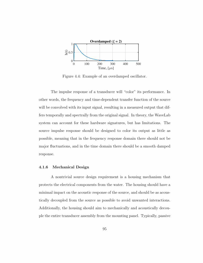
Figure 4.4: Example of an overdamped oscillator.

The impulse response of a transducer will “color” its performance. In

other words, the frequency and time-dependent transfer function of the source

will be convolved with its input signal, resulting in a measured output that dif-

fers temporally and spectrally from the original signal. In theory, the WaveLab

system can account for these hardware signatures, but has limitations. The

source impulse response should be designed to color its output as little as

possible, meaning that in the frequency response domain there should not be

major fluctuations, and in the time domain there should be a smooth damped

response.

4.1.6 Mechanical Design

A nontrivial source design requirement is a housing mechanism that

protects the electrical components from the water. The housing should have a

minimal impact on the acoustic response of the source, and should be as acous-

tically decoupled from the source as possible to avoid unwanted interactions.

Additionally, the housing should aim to mechanically and acoustically decou-

ple the entire transducer assembly from the mounting panel. Typically, passive

95

materials such as urethane are used to insulate the transducer’s electronics and

cover any surfaces that are subject to corrosion. Because the sources are in-

tended only for shallow submersion, an air cavity inside the transducer housing

is deemed acceptable. For situations that involve higher hydrostatic pressures,

it would be advisable to oil-fill any air cavities.

The electrical cables attached to the source should be of low-enough

gauge to withstand high current for high-power applications. The cable gauge

is to be determined based on the power amplifier capabilities and the source

impedance. Additionally, to avoid degradation, the cable jacket should be a

waterproof material such as butyl-rubber or polyethylene.

The WaveLab theory prescribes that the sources will be spaced a max-

imum of 7.5 cm apart. This places a great importance on small form factor

for the transducer and the entire transducer housing. Due to the relationship

between piston radius and acoustic impedance, as outlined in Sec. 4.1.4, the

housing should allow for the largest possible piston radius.

A detailed design of the radiating piston head is required to avoid flexu-

ral resonances that occur within the band of operation. When the piston head

resonates in a flexure mode, the overall acoustic output is drastically reduced

and undesirable beam patterns begin to form due to phase variations across

the face of the piston. For this reason, pistons are typically tapered to increase

their geometric stiffness, thereby moving the flexural resonance far outside of

the band of operation. It is important to design a piston that is both light

and stiff to avoid such parasitic resonances.

96

4.2 Review of Low-Frequency Sources

From the low-frequency requirements of the WaveLab system, the source

must provide an adequate sound power level in the 1-10 kHz band. This sec-

tion will begin with an analysis and literature review the Tonpilz transducer

and flexural-type transducer, which are both commonly used in mid to low-

frequency applications. These transducers have unique response characteris-

tics, sizes, and mechanical design procedures. At the conclusion of this section,

a design candidate will be chosen and further developed.

4.2.1 Tonpilz Transducers

1

2

3

Figure 4.5: Prototype Tonpilz transducer. (1) Drive stack; (2) Tail mass; (3)Piston head.

97

Tonpilz transducers are typically used in sonar applications due to their

mid-frequency, high sound power capabilities [4, 13, 17]. The Tonpilz trans-

ducer consists of a narrow drive stack sandwiched between a heavy tail mass

and a light, stiff piston head. The drive stack is typically comprised of a drive

stack of active, parallel-wired piezoelectric rings which resonate in an axial

mode. The drive stack is used to actuate the piston head, and a heavy inertial

tail mass is positioned on the opposite side of the stack. The tail mass di-

rects the velocity of the drive stack to the piston head, thereby increasing the

piston velocity and radiated sound power [17]. The Tonpilz name (German

for “sound mushroom”) comes from the transducer’s characteristic mushroom-

like cross section. The Tonpilz transducer has the advantage of a simple and

low-cost construction, has a high sound output at resonance, and can be read-

ily modeled with an equivalent circuit to tune parameters such as resonance

frequency.

In the early stages of the project, a Tonpilz source prototype was con-

structed for preliminary in-situ tests in the WaveLab tank. The piston head

consisted of a large, relatively light head mass machined from aluminum, and

was driven by a stack of four axially-poled, parallel-wired piezoelectric rings.

A heavy tail mass was machined from steel and positioned at the rear of the

drive stack. The entire assembly was held in compression by a center bolt, and

was given a rudimentary coat of urethane to protect the electrical components.

The prototype exhibited a measured in-air resonance of approximately

20 kHz, with a TVR of 100 dB re. 1 µPa/V at 1 m at 10 kHz. It was concluded

98

that the as-built prototype was not able to meet the WaveLab system speci-

fications, due to the insufficient source level as a result of the high resonance

frequency. After further design and modeling, it was determined that a Ton-

pilz source with a sufficiently low resonance frequency would be impractically

large, heavy and bulky. For these reasons, the Tonpilz source was disqualified

as a design candidate. Fig. 4.5 shows the fully assembled Tonpilz prototype

before the addition of the urethane overmold.

4.2.2 Flexural Transducers

Flexural transducers have long been used in applications that require

very low resonance frequencies and compact sizes [4, 18]. Flexural transducers

make use of one or more piezoelectric elements, either bars, plates, or discs,

that are constrained to resonate in inextensional bending modes. These struc-

tures are typically much more compliant in bending than in tension, leading to

much lower resonance frequencies for a given size. An example of a piezoelec-

tric transducer that resonates in a bending mode is the trilaminar bender-bar.

The trilaminar bender-bar consists of an inactive electrode, usually

brass or copper, sandwiched between two thickness-poled piezoelectric bars.

The bars are both poled in the same direction relative to the assembly of the

drive stack. When an electrical potential is applied to the inactive electrode,

and a ground is applied to the electrodes on the opposite side of each bar,

the bars are met with opposing electric polarities but the same piezoelectric

poling direction. This causes the top bar to expand and the bottom bar

99

to contract, forcing the stack into a bending mode, where the neutral plane

is inextensional. A drive cycle is completed by reversing the electric polarity,

causing the inflection of the stack to flip. This concept is illustrated in Fig. 4.6,

showing the result of combining the motions of two individual bar elements.

While the trilaminar bender bar transducer is well suited for low-frequency,

small size applications, the problem lies in devising a mounting system for

holding the bar to maximize its usefulness.

+

-

- z

x

Figure 4.6: Illustration of the bender-mode drive stack, showing the piezoelec-tric poling direction and the direction of displacement of each plate.

4.2.3 Bender Mode X-Spring

The Bender Mode X-spring (BMX) transducer was originally identified

and patented in 2002 by Image Acoustics, Inc. [4, 19]. The patent desrcibes,

“An electro-mechanical transducer, which provides amplified piston motion

from an orthogonal drive direction... The piston motion is amplified by lever

arms, which are typically attached to a piezoelectric or electrostrictive drive

system. The arrangement allows a compact, high output transducer design.”

In principle, the BMX combines the low-frequency resonance of a trilaminar

bender-bar drive stack with a flextensional X-spring and a piston head. The

100

X-spring is a type of lever arm that translates and magnifies the rotational

velocity of the bending drive stack to +/−z motion of a piston head. The mass

of the drive stack is designed to be considerably higher than the spring and

piston mass, so that the drive stack behaves as an inertial reaction mass against

the moving mass of the piston in order to maximize the piston velocity. Like

the Tonpilz, the piston head is designed to be light and stiff, and is attached

to the center of the X-spring, the location of greatest motion. By design, the

face of the piston is larger than the face of the X-spring to achieve a higher

volume velocity of the source in the acoustic medium.

As detailed further on in this chapter, the most critical design com-

ponent of the BMX is the design of the X-spring. As the drive stack flexes

outwards, the arms of the X-spring are pushed outwards, causing the con-

nected piston head to move in the +z direction. Conversely, when the drive

cycle is reversed, the arms of the spring are pulled inwards and the piston head

moves in the −z direction. The lever arm has a length L given by L2 = a2 +b2,

where b is half the length of the drive stack and a is the inclination height of

the spring. The magnification of motion provided by the X-spring is a function

of the slope of the lever arms, given by

Mf =da

db= −b/a. (4.11)

Therefore, in order to maximize the magnification ratio, it is desirable to

increase b or decrease a. A diagram of the BMX source is shown in Fig. 4.7,

showing the bender-mode drive stack, X-spring, and piston head.

101

Figure 4.7: Bender mode X-spring (BMX) source showing the bending actionand piston motion in the z direction [4].

While not addressed by the patent, the most significant feature of the

BMX transducer is the fact that its fundamental resonance is dictated by the

X-spring geometry. If the X-spring lever arm is sufficiently thin, the drive stack

will excite a low frequency beam-bending mode within the X-spring structure,

which is directly translated to vertical motion of the piston. As observed from

models and measurements, it is possible to excite a fundamental mode in the

X-spring that is several kHz lower than the resonance of the bender drive

stack. This finding implies that resonance of the transducer can be fine-tuned

according to the relatively simple X-spring geometry, eliminating the need

for custom piezoelectric elements. A detailed analysis of the X-spring design

will be presented in Sec. 4.4. The performance characteristics outlined by the

patent indicate that the BMX source is suitable for use in WaveLab. The

chapter will proceed with an in-depth analysis of the BMX source, providing

the appropriate models and experimental measurements that verify the claims

of the patent. First, an equivalent circuit of the BMX transducer will be used

102

to further demonstrate the mechanisms of the transducer.

4.3 Equivalent Circuit

Figure 4.8: BMX equivalent circuit.

The equivalent circuit shown in Fig. 4.8 is a useful aid in understanding

the mechanics of the BMX transducer. The equivalent circuit comprises three

sections: the electrical domain, the mechanical drive stack domain, and the

mechanical X-spring and piston domain. As described in Sec. 4.2.3, the drive

stack consists of a thin copper or brass electrode sandwiched between two

axially-poled square piezoelectric plates. In the equivalent circuit, the drive

voltage is supplied at the input of the electrical domain, which comprises

the clamped capacity, C0, and the dielectric loss G0 of the drive stack. The

electrical impedance is transformed into a mechanical impedance through the

electromechanical turns ratio N .

The drive stack mechanical domain is comprised of the short circuit

compliance, CE, and mass M of the drive stack, which includes the mass of

both active piezoelectric elements and the copper or brass electrode. A resistive

term Rm is used to account for viscous damping and losses that occur within

103

the drive stack. Woollett [18] has analyzed the bender bar transducer and

has developed equivalent circuit parameters for a number of cases. The turns

ratio N is used to transform the input electrical impedance into a mechanical

impedance within the drive stack. At this stage, the drive stack imparts a

velocity ud into the hinge of the X-spring. The transformer turns ratio N

governs the proportional bending moment that is transferred from the drive

stack into the X-spring.

θ θ

Ms Ms

Cs Cs

w(x)

Figure 4.9: Illustration of the interaction between the bender bar and theX-spring.

A lumped element system, shown in Fig. 4.9, can be used to visualize

the interaction of the bender bar and the X-spring. The system is constrained

to two degrees of freedom: transverse displacement, w (x), and rotation θ.

When the bender bar and X-spring are coupled together, the bending motion

of the bar causes the hinge of the X-spring to rotate by an amount θ. This

rotational displacement is resisted by the compliance of the X-spring, Cs, which

effectively acts as a torsional spring. The parallel combination of Cs and the

mass of the X-spring and piston, Ms, leads to a flexural resonance of the X-

spring and subsequent motion of the piston at the velocity us. The resonance

of the X-spring can be tuned by adjusting the spring stiffness or the spring

104

and piston mass, however, since the piston velocity is reduced by the inertial

motion of the drive stack, it is important to minimize the mass of the spring

and piston.

The third stage of the circuit represents the X-spring, piston, and acous-

tic medium. The circuit components of this stage include the lumped X-spring

compliance, Cs and the mass of the X-spring and piston assembly, Ms. The

fundamental resonance of the transducer occurs when Cs resonates with Ms.

The velocity imparted into the X-spring by the bender bar is amplified by a

factor of −b/a due to the lever arm action of the X-spring, which results in ver-

tical motion of the piston. The piston is loaded by the radiation impedance Zr,

which lowers the fundamental resonance frequency and increases the damping.

The challenge in the derivation of the full equivalent circuit lies in the

spring-bender bar elastic boundary condition. To determine the bending mo-

ment exerted on the X-spring, the vertical deflection curve of the bender bar

must be known. If the bender bar was simply supported at its neutral axis, one

could assume that the deflection is purely parabolic, with maximum deflection

at the center of the bar and zero deflection at the ends of the bar. However,

this assumption does not hold when elastic supports exist at the ends of the

bar. Although the derivation of the equivalent circuit has been omitted from

this report, Woollett [18] has laid a foundation for the future work with the

derivation of the dynamic model of a bender bar coupled to elastic leaf hinge

supports. This derivation accounts for the mechanical and electrical proper-

ties of the elastically supported bender bar, and accounts for the suspension

105

resonance which occurs when the static mass of the bar resonates with the

flexrual stiffness of the leaf hinge. In calculating the suspension resonance,

Woollett treats the stiffness of the leaf quasi-statically. In a similar vain, a

static method presented in the following chapter will be used to design the

resonance of the BMX X-spring.

4.4 X-Spring Design

From the equivalent circuit of Fig. 4.8, it is apparent that the resonance

of the transducer can be lowered by increasing the mass of the spring-piston

assembly or by decreasing the stiffness of the X-spring. However, by increasing

the mass of the assembly, the inertial reaction of the drive stack is reduced,

leading to a lower piston velocity. For this reason, it is desirable to adjust

the X-spring stiffness to tune the transducer resonance. The resonance of the

X-spring can be approximated using a straight-forward modeling approach

known as the direct stiffness method. The goal of this approach is to reduce

the spring geometry into adjustable parameters that can be used to tune the

spring resonance. These parameters, which are illustrated in Fig. 4.10, include

lever arm thickness, t, and slope a/b. Additionally, the model can account for

a range of material properties.

4.4.1 Introduction to Direct Stiffness Method

The direct stiffness method is a matrix analysis technique commonly

implemented in the finite element method, and can be used to calculate un-

106

t

a

b

Figure 4.10: Parametric X-spring geometry.

known joint displacements and structural eigenfrequencies. In the direct stiff-

ness method, local member force-displacement relationships are expressed in

terms of unknown displacements and internal forces. Under equilibrium, the

method can be used to directly solve for unknown displacements, internal

forces, and the eigenfrequencies of the structure. The method assumes that

the X-spring can be represented as a structure comprised of 2D prismatic

isotropic Euler-Bernoulli beam elements with simple structural constraints.

Further, the method assumes that plane sections remain plane, there are no

distributed loads along the beam, and neglects the effects of rotary inertia.

Using Euler-Bernoulli beam elements, the analysis direct is capable of

accounting for bending moments and axial forces inside the beam elements.

An unconstrained Euler-Bernoulli frame element has a total of six degrees of

freedom, including horizontal translational, vertical translational, and rota-

tional displacements. The six degrees of freedom of an Euler-Bernoulli frame

element are illustrated in Fig. 4.11.

The procedure of the direct stiffness method, for any arbitrary beam

element, is as follows [20]:

107

θi θj

p

MiMj

Figure 4.11: Frame element with combined rotational and axial displacements.

1. Define nodal coordinates, element locations, beam properties, applied

loads and structural constraints.

2. Calculate and define the basic properties of individual members, includ-

ing stiffness k, mass M ′, and inclination angle α.

3. Transform the basic element properties from local coordinates to a global

coordinate system, and assemble a global stiffness matrix [K] and mass

matrix [M ].

4. Formulate the applied load vector {F} and nodal displacement vector

{r}. Reduce the system appropriately given boundary conditions from

structural constraints.

5. Solve for free nodal displacements, support reactions, and eigenfrequen-

cies of the structure.

108

α2

3

1

2

u2

v22

u1

v11

A, E, I, L

A, E, I, 0.5L

b

a

Figure 4.12: Frame analysis of X-spring showing reduced degrees of freedom.

4.4.2 Defining Nodes, Elements, and Boundary Conditions

The nodal coordinates are defined according to the geometry of the

X-spring, where each representative beam element has two nodes. The nodal

coordinates are parameterized by the height and length of spring lever arm,

a and b respectively. These coordinates define the locations of the beam ele-

ments, where the length of each element is given by L. To accurately repre-

sent the X-spring geometry, the hinge arm (which is attached to an ideal drive

stack) between nodes 1 and 2 is assumed to equal to L/2.

Once the element locations are defined, material and geometric prop-

erties are prescribed to each beam element. It is assumed that the spring

extends out of the page by an amount equal to b. The third tuneable pa-

rameter is the thickness of the element, t. Figure 4.12 is an illustration of

the simple frame structure that is used to represent the symmetric left half of

109

the X-spring geometry. Element 1 represents the hinge, which is subject to

the drive stack bending moment, and element 2 represents the spring lever

arm. Before constraints are applied, each node is subject to three degrees of

freedom: u, v, and θ.

Next, boundary conditions are imposed upon the system. The reso-

nance of the spring is most accurately modeled with a free-fixed boundary con-

dition, where nodes 1 and 2 are unconstrained and node 3 is completely fixed

against translation or rotational displacement. A clockwise-positive bending

moment is applied to node 1 to represent the moment applied by the bender

drive stack. The applied moment and nodal constraints will be used to reduce

the system degrees of freedom and solve for nodal displacements.

4.4.3 Basic Element Stiffness

Next, the basic member stiffness, force, displacement, and mass matri-

ces are formulated. The unconstrained element has combined rotational and

axial translational displacements,

{r} =

uvθ

, (4.12)

basic member force,

{S} =

Mi

Mj

θ

, (4.13)

110

and basic member stiffness

[k] =E

L

4I 2I 02I 4I 00 0 A

. (4.14)

These components govern the basic stiffness relation {S} = [k]{v}. After

the basic stiffness is calculated for elements 1 and 2 , the basic-to-local and

local-to-global coordinate transformations are applied.

4.4.4 Local to Global Transformation

To assemble a complete stiffness and mass matrix relationship, all con-

stitutive elements must use a consistent, global coordinate system. Basic forces

{S} and nodal displacements {v} within the individual elements are converted

to local forces {F ′} and local displacements {r′} through the basic-to-local

transformation matrix

T =

0 1/L 1 0 −1/L 00 1/L 0 0 −1/L 1−1 0 0 1 0 0

. (4.15)

The local stiffness relationship becomes {F ′} = [k′]{r′}, where the transformed

local element stiffness is given by

[k′] = TT [k]T. (4.16)

Similarly, the local mass matrix given by the Euler-Bernoulli beam theory

111

becomes

[M ′] =ρAL

420

140 0 0 70 0 00 156 22L 0 54 −13L0 22L 4L2 0 13L −3L2

70 0 0 140 0 00 54 13L 0 156 −22L0 −13L −3L2 0 −22L 4L2

. (4.17)

To transform local coordinates to the global system, the inclination

component matrix, LD, is used to account for the inclination angle α of each

element such that

LD =

[LB 00 LB

], (4.18)

where

LB =

cosα sinα 0− sinα cosα 0

0 0 1

. (4.19)

The global element stiffness transformation is found by applying

[K] = LTD [k′]LD. (4.20)

Likewise, the global element mass is given by

[M ] = LTD [M ′]LD. (4.21)

Once each element’s stiffness and mass is expressed in terms of the

global coordinate system, the global matrices can be assembled. The global

112

matrices are assembled by summing the stiffness or mass contribution of each

element at the appropriate degree of freedom. The result is a 9 × 9 stiffness

matrix and a 9×9 mass matrix. Next, boundary conditions are enforced based

on the structural constraints.

4.4.5 Applied Load and Nodal Displacement Vectors

The X-spring structural constraints take the form of free and fixed con-

ditions. Each node of the system has a structural constraint. For free degrees

of freedom, reaction forces are set to zero and displacements are unknown;

for supported degrees of freedom the displacements are set to zero and the

reaction forces are unknown. The moment M is applied to the bender drive

stack to node 1. Node 2 is completely unconstrained and has unknown dis-

placement component. Node 3 is fixed, therefore, the displacement component

is zero and the internal reaction forces are unknown. There are 2 degrees of

freedom for each node, and the force and nodal displacement vectors are each

of size 9× 1. The nodal displacement vector becomes

{r} =

u1

v1

θ1

u2

v2

θ2

u3

v3

θ3

=

u1

v1

θ1

u2

v2

θ2

000

, (4.22)

113

and the load vector becomes

{F} =

Fu,1

Fv,1

Fθ,1Fu,2

Fv,2

Fθ,2Fu,3

Fv,3

Fθ,3

=

00M

000Fu,3

Fv,3

Fθ,3

. (4.23)

To enforce the boundary conditions, the rows and columns of the stiffness and

mass matrix are reduced where displacements are zero. In total, each matrix is

reduced by three degrees of freedom, and each matrix has size 6×6. Likewise,

the force and displacement vectors are each reduced to size 6× 1. The system

has a total of six degrees of freedom.

4.4.6 Displacement and Eigenvalue Solutions

When the matrices have been appropriately reduced by the boundary

conditions, the nodal displacements are found by inverting the reduced stiffness

matrix such that

{rred} = [Kred]−1{Fred}. (4.24)

To solve for the eigenvalues of the system, the mass, stiffness and dis-

placements are related by a reduced form of the equation of motion. Assuming

no damping, the equation of motion, in matrix form, reduces to

[M ]{u}+ [K]{u} = 0. (4.25)

114

A time-harmonic solution is assumed such that

{u} = {Φ}ejωt, (4.26)

where Φ is the eigenvector or mode shape. Substituting into the equation of

motion and appropriately reducing yields the eigenequation([K]− ω2[M ]

){Φ} = 0. (4.27)

The representation of 6 × 6 stiffness and mass matrices in the eigenequation

leads to a set of 6 discrete eigenfrequencies ω2i where the ith natural frequency

of the X-spring is given by fi = ωi/2π. Finally, the fundamental resonance of

the X-spring is given as the first eigenfrequency.

While the direct stiffness tool only serves to estimate the resonance of

the X-spring, the calculated resonances are in good agreement with measure-

ments and FEM, as shown in Sec. 4.7.1. In reality, the direct stiffness method

is an oversimplification of the X-spring structure, because it neglects the stiff-

ness boundary condition of the drive stack, and does not account for wave

motion within the spring. However, the purpose of the model is to provide

a rapid evaluation of the X-spring resonance given a certain geometry. For

a more in depth analysis of the X-spring, FEM will be used to validate the

results of the direct stiffness model, and will also be used to examine the mode

shapes of the X-spring and the transducer assembly.

115

4.5 COMSOL Finite Element Model

A finite element analysis was performed to predict the performance of

the BMX source relative to the experimentally measured quantities of the as-

built prototypes. Compared to the direct stiffness model, the FEM model can

account for complex eigenmodes of the X-spring, and provides a more accu-

rate representation of the interaction between the drive stack and the X-spring.

Ideally, after designing the geometry of the X-spring from the direct stiffness

model, one would use FEM to model the as-built transducer assembly. This

section will begin by detailing the setup of the FEM model in COMSOL Mul-

tiphysics. The model setup mirrors the setup of the hydrophone FEM model,

which includes geometry definition and material selection, physics implemen-

tation, and meshing considerations. The FEM results are compared directly

to measurements in Sec. 4.7.

4.5.1 Model Definition

To reduce computational cost, the prismatic geometry of the BMX

transducer can be entirely represented in a 2D domain. Although the con-

sistency between 2D and full 3D models has been verified, the 2D model is

incapable of modeling fabrication errors, such as drive stack misalignment,

which has been observed to cause uneven phase variations throughout the X-

spring and piston head. The model outputs of the FEM study include mode

shapes of the X-spring, electrical input impedance, piston velocity, transmit

voltage response (TVR), and directivity.

116

4.5.2 Physics Implementation

The transducer model is implemented similarly to the hydrophone FEM

model, utilizing COMSOL’s Pressure Acoustics, Solid Mechanics and Electro-

static physics modules. The Pressure Acoustics module is used to solve the

constitutive Helmholtz wave equation in the water domain. A far-field pres-

sure calculation is defined on the boundary between the water domain and the

perfectly matched layer (PML), which allows for the calculation of the ampli-

tude and phase of the far-field pressure radiated by the source. The far-field

pressure variable is used to compute TVR and the directivity of the source.

The Solid Mechanics module is applied to the entire transducer struc-

ture, include X-spring, piston head, and drive stack. The module uses linear

stress-strain equations with a small deformation assumption. An isotropic loss

factor is applied to each mechanical component to model viscous damping; the

amount of loss is adjusted based on the Q-factor of the resonances measured

in the in-air electrical input impedance. The piezoelectric element material

model is left unchanged from COMSOL’s default +z poling direction, since

both active elements of the drive stack are axially poled in the same direction.

A line average is defined to the piston head boundary, used to measure the

average normal velocity amplitude and phase of the piston head.

The electrostatics module is applied to both of the active drive stack

elements. An electric potential, V0, is specified on the electrode boundaries,

and a ground is defined on outer lateral surface of each element. A surface in-

tegral is specified on the electrode boundaries to calculate the electrical input

117

impedance. The 2D COMSOL geometry of the drive stack, showing piezoelec-

tric poling direction and the polarity of the applied electric field, is shown in

Fig. 4.13.

1

2

-

-

+

+

Figure 4.13: BMX drive stack geometry.

The physics modules are linked through the Acoustic-Structure Bound-

ary and Piezoelectric Effect Multiphysics coupling modules. The Acoustic-

Structure Boundary, which links the Pressure Acoustics and Solid Mechanics

modules, is applied to the interface of the water domain and piston head. Ra-

diation impedance is accounted for in the Solid Mechanics interface, where the

fluid load effectively acts as a mechanical load. The Piezoelectric Effect mod-

ule couples the Electrostatics and Structural Mechanics modules by solving

the constitutive linear piezoelectric equations.

PZT-5H material properties are applied to the active drive stack ele-

118

ments, copper material properties are applied to the drive stack electrode, and

aluminum material properties are applied to the X-spring and piston struc-

ture. The face of the piston is exposed to an unbounded water domain, which

is surrounded by a PML to absorb propagating background radiation. The

COMSOL geometry of the full transducer assembly is shown in Fig. 4.14.

1

3

2

Figure 4.14: BMX assembly geometry. (1) bender-bar drive stack; (2) X-spring; (3) piston head

The directivity and source pressure level are calculated in the same

manner described in Sec. 3.5. The TVR, as calculated from the modeled

source pressure level, is given by [21]

TVR = 20 logpRMS/VRMS

1µPaV −1. (4.28)

where pRMS is the RMS pressure at 1 m from the piston head and VRMS is

119

equal to 1 V. pRMS is computed as

pRMS =

√1

2pp∗, (4.29)

where the pressure p at 1 m from the face of the piston is obtained using

COMSOL’s farfield pressure expression pfar(0,1)1. The variable p∗ is the

complex conjugate of the pressure p, given by conj(pfar(0,1)).

4.6 Prototype Specifications

A prototype BMX source was constructed using off-the-shelf piezoelec-

tric elements along with a custom-machined X-spring/piston assembly. The

components of the transducer are listed below, with relative geometries, ma-

terials, and a brief description of the fabrication process.

1. The drive stack consisted of two thickness-poled square piezoelectric

plates made from APC 850 ceramic 2. The plates measured 25.4 mm

per side, with a thickness of 3.18 mm. The plates were silvered on the

top and bottom faces. The drive stack was assembled using a conductive

silver epoxy to glue a 1 mm thick square copper electrode in between

the two piezoelectric plates. A positive lead was soldered to the cop-

per electrode, and ground leads were soldered to outward-facing silvered

1The pfar variable has changed to pext as of COMSOL version 5.4.2APC 850 is a proprietary ceramic manufactured by APC International. It is approxi-

mately equivalent to PZT-5 ceramic.

120

faces of the assembled drive stack. The assembled drive stack is shown

in Fig. 4.15.

2. To achieve a low resonance frequency, the X-spring was designed to be

as thin as possible to avoid significant tool chattering during the milling

process. The piston was milled seperately from the X-spring, and the two

components were fastened together with machine screws. Referencing

the dimensions described in Sec. 4.4.2, the X-spring lever arm had an

average thickness of 0.9 mm, a length b of 12.7 mm, and a height a of 0.6

mm. The piston head was designed with a diameter of 47 mm, with a

tapered center to prevent head-flexure resonances from occurring in the

frequency band of operation.

3. Kapton tape was applied to edges of the drive stack to prevent an elec-

trical short between the drive stack and spring/piston assembly, and the

drive stack was epoxied into the assembly. The full as-built assembly is

shown in Fig. 4.16.

4. The assembly was placed into a hollow cylindrical housing machined

from PVC, with a flange around the circumference of the housing for

mounting purposes. A small bead of RTV silicone was spread inside the

gap in between the piston and the housing to prevent urethane from

leaking inside the housing cavity. A thin layer of urethane was poured

on top of the piston to protect the piston head from corrosion. The fully

potted and housed transducer is shown in Fig. 4.17.

121

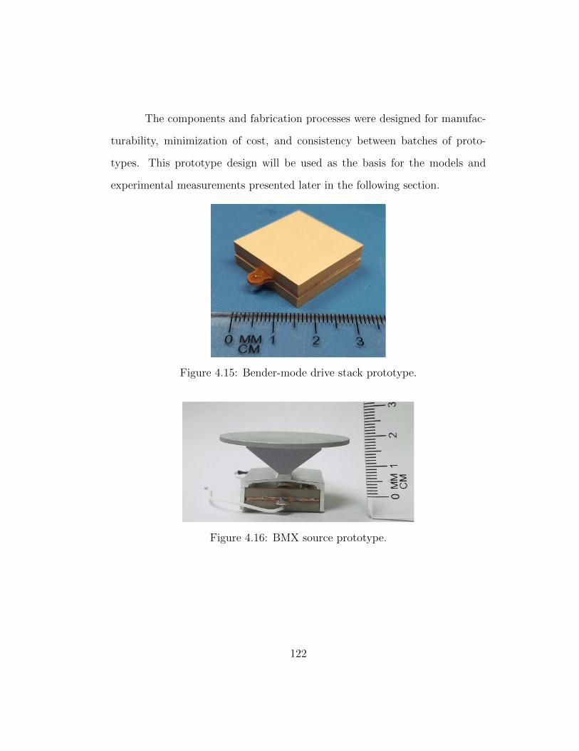
The components and fabrication processes were designed for manufac-

turability, minimization of cost, and consistency between batches of proto-

types. This prototype design will be used as the basis for the models and

experimental measurements presented later in the following section.

Figure 4.15: Bender-mode drive stack prototype.

Figure 4.16: BMX source prototype.

122

1

2

Figure 4.17: BMX prototype in housing. (1) urethane sealing layer; (2) PVChousing with mounting flange.

4.7 Prototype Characterization

4.7.1 Eigenmodes of the X-Spring

The eigenfrequencies of the 0.9 mm-thick X-spring spring were approx-

imated using the direct stiffness method outlined in Sec. 4.4.2. To validate the

model, the results were compared to a simplified FEM model of the X-spring

structure. The simplified FEM model consisted of the same beam geometry,

material properties, and boundary conditions that were used in the direct stiff-

ness model. From here, a more complex 2D FEM model was used to compute

the eigenmodes of the fully assembled transducer, and the resonances and cor-

responding mode shapes were compared to the results of the direct stiffness

model and the simplified FEM model.

123

The direct stiffness model was computed using the beam geometry

listed in Sec. 4.6 along with aluminum material properties, resulting in a pre-

dicted X-spring resonance of 3.1 kHz. The deformed mode shape as predicted

by the direct stiffness method is plotted in Fig. 4.18. Similary, the simpli-

fied FEM X-spring model predicted a fundamental resonance of 3.4 kHz. The

FEM-computed mode shape is shown in Fig. 4.19, showing a nearly identi-

cal deformation to that predicted by the direct stiffness model. The direct

stiffness model slightly under-predicts the spring resonance estimated by the

FEM model, likely due to simplifications assumed by the Euler-Bernoulli beam

method. Nonetheless, the nearly identical solutions validate the direct stiffness

method. This tool can be used to rapidly design the X-spring resonance, elim-

inating the need to iterate through computationally expensive FEM models.

The direct stiffness tool lacks the ability to predict the change in reso-

nance that occurs when the bender bar drive stack is coupled to the X-spring.

For this reason, a more complex 2D FEM model is developed. Using the same

X-spring dimensions and material properties as the simplified FEM model, an

in-air study was carried out on the fully assembled transducer, active drive

stack included. The resonance of the transducer was located by examining the

modeled electrical input impedance, revealing a fundamental resonance fre-

quency of 3 kHz. The corresponding deformed mode shape of the transducer,

shown in Fig. 4.20, indicates that, as expected, the X-spring lever arms vi-

brate in a bending mode, and actuate the piston in the z direction. The in-air

124

0 5 10

mm

-2

0

2

4

6

8

10

mm

X-spring mode shape, direct stiffness method

2 32

1

1

Figure 4.18: First mode shape of the X-spring as computed by the directstiffness method, falling at 3.1 kHz.

resonance of 3 kHz is reasonably close to the resonance frequency estimated

by the direct stiffness model.

Although the direct stiffness method is an oversimplification of the

physics of the X-spring, it can be seen that the model provides a good approx-

imation for the transducer resonance, and provides insight to the behavior of

the X-spring. As an ideal application, one would use the direct stiffness model

to roughly design the X-spring geometry, and would afterwards program the

geometry into a more complex FEM model. In this case, the outputs of the

complex FEM model are described in the following subsections.

125

Figure 4.19: FEM mode shape of the X-spring frame element.

Figure 4.20: FEM mode shape of the X-spring.

126

4.7.2 Electrical Input Impedance

Electrical input impedance measurements were made in several steps

to check for fabrication flaws and consistency with the FEM model. First,

the impedance of the standalone bender bar drive stack was measured, using

a frequency sweep of 100 Hz to 50 kHz to capture the full resonant behavior

of the drive stack. To verify the piezoelectric material properties used in the

FEM model, the measured and modeled impedances were compared, assessing

alignment of the resonances and antiresonances. It is essential to verify FEM

material properties because, as seen in Ch. 3, a slight material mismatch can

can lead to inaccurately modeled resonances and acoustic responses. A fun-

damental resonance of the drive stack was observed at 30 kHz, which tracked

well with the FEM model. At resonance, the FEM-calculated mode shape

indicated that the drive stack vibrates with the expected flexural motion. The

impedance of the bender-mode drive stack is shown in Fig. 4.21, and the FEM

mode shape is shown in Fig. 4.22.

Next, the drive stack was epoxied into the X-spring/piston assembly.

The upper frequency of the impedance sweep was narrowed to 10 kHz to

increase the frequency resolution in the desired band of operation. The trans-

ducer was held so that no surfaces were constrained and the impedance was

measured, indicating a fundamental resonance at approximately 3 kHz. This

measured resonance tracks well with the X-spring resonance modeled by the

direct stiffness method, the simplified FEM spring model, and the FEM full

assembly model.

127

0 10 20 30 40 50 6010

0

105

Z,

[]

Bender drive stack impedance

0 10 20 30 40 50 60

Frequency, [kHz]

-100

-50

0

50

100

Ph

ase,

[°]

Measured

FEM

Figure 4.21: Impedance of bender-mode drive stack.

4.7.3 Piston Velocity

At various stages of fabrication, the normal velocity of the piston head

was measured with a scanning laser doppler vibrometer (LDV) to provide an

accurate benchmark of prototype performance, and to check for fabrication

errors and consistency with models. The major benefit of the LDV is the

ability to predict the acoustic response of the transducer at non-waterproof

stages of fabrication. This eliminates a good degree of uncertainty, where

problems can be identified at specific processes instead of not knowing what is

128

Figure 4.22: Drive stack FEM mode shape.

happening when it’s underwater. Similar to the benefit of the input impedance

measurement, the LDV can help to identify unexpected resonances and piston

head phase variations that could affect the acoustic response of the transducer.

First, the piston normal velocity was measured for the full transducer

assembly without housing and potting. The transducer was suspended in the

air with soft elastic bands to avoid constraining the vibration in any direc-

tion. A linear frequency-modulated (LFM) chirp with an amplitude of 50Vpp

was driven through the source, and the corresponding velocity magnitude and

phase was measured at approximately 50 points over the entire surface of the

piston. Confirming the FEM model predictions, the piston velocity measure-

ments indicate a sharp, high-velocity resonance at 3 kHz. At this frequency,

the velocity phase is consistent for each of the 50 measurement points, indicat-

ing uniform motion of the piston. The measured piston velocity is compared

to the FEM model in Fig. 4.23. Comparing the measurement to the FEM

model, velocity magnitude and phase are both in agreement, showing that the

129

velocity undergoes a 180◦ phase shift at resonance.

1 2 3 4 5 6 7 8 9 10

10-4

10-2

Vel

. M

ag.,

[m

/s /

V]

BMX piston velocity in air, no housing

1 2 3 4 5 6 7 8 9 10

Frequency, [kHz]

-100

-50

0

50

100

Ph

ase,

[°] Measured

FEM

Figure 4.23: In-air piston velocity of bare BMX assembly.

Next, the source was sealed inside the PVC housing with RTV silicone,

and a thin layer of urethane was potted on the face of the transducer. The

normal velocity of the newly-potted piston face was remeasured with an iden-

tical experimental setup. The results, plotted in Fig. 4.24, indicate that the

resonance was slightly reduced in frequency and was moderately damped. In

reality, the damping due to the potting was desirable in that the bandwidth

of the transducer was significantly widened, marked by the increase in piston

130

velocity in the off-resonance band. However, caution must be exercised when

designing the potting mechanism; in the fabrication process it was observed

that excessive amounts of RTV sealant and urethane clamped the piston, ef-

fectively increasing the stiffness of the system. In some drastic cases, this

error led to an increase in resonance frequency by up to 2 kHz. Once the LDV

measurements had inidicated that the finished prototype was satisfactory, a

range of acoustic tests were performed to further characterize the source.

1 2 3 4 5 6 7 8 9 10

10-4

10-2

Vel

. M

ag.,

[m

/s /

V]

Measured BMX piston velocity

1 2 3 4 5 6 7 8 9 10

Frequency, [kHz]

-100

-50

0

50

100

Ph

ase,

[°]

No housing

Housing

Figure 4.24: Effect of housing on measured BMX piston velocity.

131

4.7.4 Transmit Voltage Response

Transmit voltage response of the BMX prototype was measured at the

ARL Lake Travis Test Station (LTTS), a specialized underwater acoustics

research facility located on Lake Travis in Austin, Texas. The source was

attached to a rotating column and was submerged to a depth of 9 m. The

source was driven by an LFM chirp spanning from 100 Hz to 20 kHz, with

a drive voltage of 100 Vpp. The emitted signal was recorded with a USRD

H52 standard hydrophone at a distance of 12 m. Several averages were taken

to account for miscellaneous background noise. The RVS of the standard

hydrophone was deconvolved from the recorded signal to recover the unaltered

frequency-dependent response of the source. The measured TVR is compared

to the TVR predicted by FEM in Fig. 4.25.

The measured TVR is in fair agreement with the FEM model, with

the most notable difference being the resonance frequency and Q-factor. The

predicted resonance is roughly 800 Hz lower than the measured resonance.

This same difference was observed in the LDV-measured piston velocity from

Fig. 4.23, indicating that the difference in resonance can be attributed to dif-

ferences in the as-built X-spring from the FEM model. The difference between

model and measurement emphasizes that the X-spring is very sensitive to mi-

nor changes in geometry, which in some cases arise purely from the machining

process. To achieve close agreement between measurement and model, it is

imperative to specify tight machining tolerances on the thickness of the spring

lever arm. Further differences seen in the measurement can be attributed to

132

1 2 3 4 5 6 7 8 9 10

Frequency, [kHz]

80

90

100

110

120

130

140d

B r

e 1

P

a/V

@ 1

mTVR of BMX source

Measured

FEM

Figure 4.25: TVR of BMX source.

the manner in which the piston is sealed and overmolded into the housing.

4.7.5 Directivity

The source directivity was measured at LTTS at select frequencies.

The source was mounted to a rotating column and submerged to a depth of

9 m. The column was initially positioned such that the center axis of the the

piston head was aimed at the acoustic axis of the standard hydrophone, with

this beginning position marked at θ = 90◦. A 10-cycle sinusoidal tone burst

was driven through the source at a given frequency, and several averages were

recorded. The column was rotated by a small amount and the source signal

was recorded at the new angle. This process was repeated until the full 180◦

133

beam pattern had been captured at each of the desired frequencies.

To process the recordings into a coherent directivity plot, a window

was specified around the steady-state portion of the direct arrival of the source

signal at each angle. The source amplitude at every angle was found by taking

the mean of the Hilbert transform of the windowed direct arrival, and the

amplitudes over all angles were normalized with respect to the signal with the

highest amplitude. The BMX directivity at 9 kHz is plotted in Fig. 4.26.

0°

30°

60°

90°

120°

150°

180°-9 -6 -3 0 [dB]

BMX unbaffled direcitivity, f = 9 kHz

Measured

FEM

Theory

Figure 4.26: Measured BMX beam pattern at 9 kHz.

The measured directivity was directly compared to the FEM model

and the analytical solution for an unbaffled piston from Sec. 4.1.2, demon-

strating agreement within 1 dB between the measurement the models. As

further observed in Sec. 4.1.2, piston directivity theory prescribes that the

BMX transducer will gain nearly 7 dB in directivity at θ = 0◦ and θ = 180◦

134

when placed inside of a baffle. A comparison of theoretical beam patterns of

the BMX transducer at 9 kHz is shown in Fig. 4.27. This provides conclusive

evidence that the source will exhibit omnidirectionality when mounted on the

emitting surface of the WaveLab tank. One factor that would potentially alter

the source directivity is acoustic coupling from the source into the emitting

surface, causing the emitting surface to deviate from a perfectly rigid baffle.

This concern is addressed in greater detail in Sec. 4.9.

0°

30°

60°

90°

120°

150°

180°-9 -6 -3 0 [dB]

Theoretical BMX direcitivity, f = 9 kHz

Unbaffled

Baffled

Figure 4.27: Theoretical directivity of the baffled BMX source at 9 kHz.

4.8 Source Budget

Once all the parameters of the source budget have been obtained, in-

cluding source TVR, hydrophone RVS, and hydrophone noise floor level, NF,

the source budget can be completed. Reiterating from Ch. 2, the signal excess,

135

or dynamic range, given by the source budget is

SE = SL + RVS− NF, (4.30)

where the source level, SL, is given by

SL = TVR− 20log10 (r) + 20log10Vgain,src. (4.31)

To evaluate the maximum expected source level, TVR is evaluated at

the resonance of the BMX source, yielding a value of 121 dB re 1 µPa/V 1 m.

Furthermore, the distance between source and receiver is chosen to be 40 cm,

the average distance between the in-situ emitting surface and the recording

surface. Assuming the voltage amplifier is capable of providing a gain of

140 Vpp, the maximum expected source level is 172 dB re 1 µPa. Using the

measured hydrophone RVS of -207 dB re 1 V/µPa, the maximum expected

unamplified voltage output from the hydrophone is on the order of 18 mV.

With a hydrophone self-noise floor of 9 µV, or -100 dB re 1 V, the transducer

system will theoretically provide a maximum signal excess of 65 dB. The source

budget parameters are tabulated in Table 4.1.

It is important to recall that, in practice, other contributors of noise

will significantly reduce the expected signal excess of the system. These forms

of noise include electrical noise from the preamplification and recording elec-

tronics, electrical interference, and acoustical noise from the laboratory. Noise

can be mitigated by properly shielding and grounding electrical components,

and by using high quality amplifiers.

136

Table 4.1: Source budget parameters of the WaveLab transducer system.

Parameter ValueTVR 121 dB re 1 µPa/V @ 1 mRVS -207 dB re 1 V/muPaNF -100 dB re 1 VSL (140 Vpp, r = 40 cm) 172 dB re 1 µPaSE 65 dB

4.9 Deviations from rigid boundaries on the emittingsurface

The WaveLab theory prescribes monopole source behavior that depends

on a rigid boundary at the emitting surface [2], however, in practice a com-

pletely rigid boundary condition is impossible to achieve due to the elastic

nature of the tank wall medium. This places an importance on decoupling

the sources from the walls that make up the emitting surface. To study the

expected magnitude of acoustic coupling into the walls, a test was conducted

involving three source prototypes mounted on an aluminum plate, a small scale

representation of the in-situ emitting surface configuration.

Three identical BMX prototypes were mounted to a 14

in. thick, 2 ft ×

2 ft aluminum plate, with a 18

in. thick corprene gasket sandwiched between

each housing flange and the aluminum plate. Corprene, a type of rubber-

impregnated cork, was chosen as the decoupling mechanism due to its well-

regarded use as an acoustic isolation material. The decoupling mechanism is

illustrated in Fig. 4.28, showing the backside of the transducers mounted to the

aluminum plate. The sources were mounted so that the face of each urethane

137

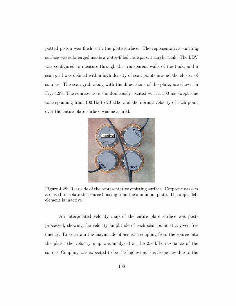
potted piston was flush with the plate surface. The representative emitting

surface was submerged inside a water-filled transparent acrylic tank. The LDV

was configured to measure through the transparent walls of the tank, and a

scan grid was defined with a high density of scan points around the cluster of

sources. The scan grid, along with the dimensions of the plate, are shown in

Fig. 4.29. The sources were simultaneously excited with a 500 ms swept sine

tone spanning from 100 Hz to 20 kHz, and the normal velocity of each point

over the entire plate surface was measured.

Inactive

Figure 4.28: Rear side of the representative emitting surface. Corprene gasketsare used to isolate the source housing from the aluminum plate. The upper-leftelement is inactive.

An interpolated velocity map of the entire plate surface was post-

processed, showing the velocity amplitude of each scan point at a given fre-

quency. To ascertain the magnitude of acoustic coupling from the source into

the plate, the velocity map was analyzed at the 2.8 kHz resonance of the

source. Coupling was expected to be the highest at this frequency due to the

138

24 in14 i

n

BMX-3 BMX-2

BMX-1Inactive

Figure 4.29: LDV scan points and dimensions of the representative emittingsurface.

maximum velocity of the source. Figure 4.30 shows the plate velocity map,

where bright spots of high velocity indicate the locations of the three sources

on the plate. At the resonance frequency of the source, the magnitude of the

velocity on the face of each source is 30 dB higher than any point on the plate,

indicating a small amount of coupling from the sources to the plate.

While the coupling into the plate was significantly lower than the mag-

nitude of the velocity of the sources, the coupling indicated that the plate

deviated from a true rigid boundary. To further reduce coupling into the

plate, more work would need to be done to study different gasket materials,

mounting methods, and plate material and thickness. A heavier plate, or a

139

-80 -70 -60 -50 -40

dB re 1 m/s / V

Velocity magnitude of representative emitting surface, f = 2.8 kHz

Figure 4.30: Measured velocity magnitude of the representative emitting sur-face at the resonance frequency of the source.

plate made from a lossy material, would be more resistant to energy transfer

from the source, and should behave more appropriately as a rigid boundary.

4.10 Whitening of the source transfer function

To physically implement the IBCs, the WaveLab theory requires com-

plete removal of the impulse response of all hardware components involved

in the measurement, including sensors and sources [2]. Whitening is defined

as the process by which the frequency response of transducer is made to be

nearly flat in the frequency band of interest. To whiten the impulse response

of the BMX source, an nth order matched filter is used to estimate the inverse

140

source transfer function, and the wavelet one wishes to inject is convolved

with the filter. While a higher number of filter coefficients corresponds to a

more accurate estimation of the inverse transfer function, the maximum num-

ber of coefficients is limited by the latency of the system. For this reason,

the source must be able to reproduce the wavelet as accurately as possible,

i.e., the source transfer function should be as flat as possible. If the source

transfer function has a wide variance across the frequency band, the system-

implemented matched filter will not accurately be able to estimate the inverse

transfer function.

To validate the suitability of the matched filter with the BMX proto-

type, an experiment was conducted with a single plate-mounted source sub-

merged in a transparent water-filled tank. The source was driven with a Ricker

wavelet with a center frequency ranging from 1 to 9 kHz and an amplitude

of 50 Vpp. The entire face of the submerged source was scanned with the

LDV, and the average piston velocity magnitude and phase was recorded. A

matched filter with 103 coefficients at sampling rate of 256 kHz was used to

estimate the inverse transfer function, given the source input wavelet and the

measured output, leading to a total time lag of 0.2 ms. The original input

wavelet was convolved with the filter, and the new impulse-corrected wavelet

was excited through the source and remeasured.

In Fig. 4.31, the input 3 kHz Ricker wavelet is compared to the uncor-

rected and the corrected measured output. In the time domain, the measured

uncorrected wavelet is characterized by several ringing oscillations after the ini-

141

tial pulse, reflecting the underdamped nature of the source. In the frequency

domain, the majority of the spectral energy is centered around the resonance

frequency of the source at 2.75 kHz as opposed to the 3 kHz center frequency

of the input wavelet. Furthermore, notches in the spectrum align with the

measured TVR. After the offline filter convolution, the corrected wavelet is

characterized by a major decrease in ringing, and a more uniform distribution

of spectral energy in line with the input wavelet.

7 8 9 10 11 12

t, [ms]

-1

-0.5

0

0.5

1

Vel

oci

ty (

no

rmal

ized

)

LDV measurement of 3 kHz Ricker wavelet

0 2 4 6 8 10

Frequency, [kHz]

0

0.5

1

Am

pli

tud

e

Input

Uncorrected output

Corrected output

Figure 4.31: Demonstration of the matched filter used to remove the sourcetransfer function from a 3 kHz Ricker wavelet.

142

The results encouragingly indicate the source transfer function, marked

by excessive ringing oscillations and uneven spectrum, can be corrected to a

relatively high degree by a matched filter that falls within the system latency

limits. The matched filter struggles to correct wavelets with center frequencies

lower than the resonance frequency of the source, because the source has a low

sound power output in this region.

4.11 Summary

In summary, this chapter has presented the design of an acoustic pro-

jector with

1. a bandwidth of 12 kHz,

2. a resonance frequency of 2.75 kHz with a transmit response of 120 dB

re 1 µPa/V at 1 m,

3. horizontal omnidirectionality up to 9 kHz kHz,

4. a low amount of acoustic coupling into the representative emitting sur-

face,

5. and a compact size.

Throughout the design process, critical performance characteristics such

as TVR, piston velocity, and directivity were modeled with the finite element

method to validate experimental measurements. In Sec. 4.4, an X-spring de-

sign tool was presented to allow one to tune the X-spring resonance given

143

certain dimensions. In combination with FEM, this tool allows for rapid de-

velopment of a BMX transducer with a desired resonance frequency. For future

work, a comprehensive equivalent circuit should be developed to better under-

stand the interaction between the bender-mode drive stack and the X-spring,

as well as to account for the effects of radiation impedance and stiffness asso-

ciated with the housing and potting.

From experimental measurements, it was observed that the housing

and potting negatively impacted the performance of the source by introducing

parasitic resonances and raising the resonance frequency. While the housing

and potting are necessary to protect the electrical components of the source

against water, future revisions of the design should consider an alternative

approach to the housing. Namely, a superior design would identify a means of

waterproofing the transducer without clamping the piston head to the housing

body, as was suspected to be the case for the current prototype. Nonetheless,

preliminary results have shown that the transfer function of the source, which is

dominated by its low frequency resonance, can be effectively removed through

the use of a matching filter. The experimental results, along with the finite

element analysis, objectively demonstrate that the BMX source satisfies the

performance requirements of the WaveLab system. Photos and drawings that

pertain to the BMX fabrication process are shown in Appendix B.

144

Chapter 5

Conclusion and Future Work

In conclusion, this thesis has presented the design of a source and a

hydrophone suitable for use in the WaveLab system. Experimental measure-

ments and models have shown that the source and hydrophone designs meet

the performance criteria prescribed by the WaveLab theory. Aside from the

WaveLab theory, the transducer designs have considered mechanical robust-

ness, production cost, manufacturability, and physical size constraints. A suite

of transducer design tools have been developed to allow for rapid development

of future designs. Collectively, a source budget has been presented in to esti-

mate the dynamic range and expected signal excess of the entire transducer

system, and preliminary experiments have demonstrated the in-situ use of the

transducers. As of spring 2019, the transducer fabrication process has been

developed, streamlined, and executed by the engineering and technical staff

at the Applied Research Laboratories, aiming for a complete delivery of 800

BMX sources and 800 hydrophones by mid 2019. Photographs of a panel of

the in-situ emitting surface are shown in Fig. 5.1 and Fig. 5.2.

While the transducer designs ultimately satisfy the WaveLab perfor-

mance requirements, certain characteristics of the source and hydrophone

145

Figure 5.1: Front side of a panel of the in-situ emitting surface. Photographcourtesy of Nele Borsing.

Figure 5.2: Back side of a panel of the in-situ emitting surface. Photographcourtesy of Nele Borsing.

146

could be improved for future revisions. In Ch. 3, it was shown that the hy-

drophone performance was negatively impacted by the excessive mass of the

Stycast overmold, which effectively limited the receive bandwidth and nar-

rowed the directivity. Future designs should consider the use of a thinner

layer of overmold material, or a less dense material in general. Furthermore,

the hydrophone equivalent circuit model suggests that sensitivity and noise

floor could be significantly improved by using a cylindrical sensing element

with a shorter length, thicker walls, and a larger outer radius. Lastly, it should

be noted that no additional consideration was given to the type of piezoce-

ramic that was used in the hydrophone prototype in the interest of time and

cost. A more desirable response could be achieved by using PZT-5H ceramic

instead of PZT-4, given the higher dielectric constant and coupling factor of

PZT-5 [4].

Throughout the BMX source fabrication process, it became quickly ap-

parent that the housing mechanism was the largest weakness of the transducer.

Namely, in some prototypes a slight excess of RTV silicone and urethane, used

for sealing and waterproofing the piston head, tended to clamp the piston and

couple the piston motion to the PVC housing. This resulted in a significantly

increase resonance frequency, and a parasitic resonance induced by flexural

motion of the PVC housing. This problem was mitigated by using a mini-

mal amount of sealing material, however, future designs should reconsider the

sealing mechanism entirely. In addition to future work on the BMX source, a

complete equivalent circuit should be developed following the dynamic model

147

of the bender bar attached to an elastic support presented by Woollett [18].

The equivalent circuit will allow for a better understanding of the interaction

between the bender-mode drive stack and the X-spring, and in combination

with the direct stiffness X-spring design tool, will allow for accurate, rapid

development of the BMX source.

148

Appendices

149

Appendix A

Hydrophone Fabrication

The following steps describe the fabrication process used to develop the

hydrophone prototype described in Ch. 3.

1. To promote adhesion with the stycast, a sodium-based etchant is applied

to the ends of the Teflon-jacketed hydrophone cable. The cable turns

black as a result of the etching compound.

2. The cable leads are soldered to the inner and outer electroded walls of

the piezoelectric cylinder.

3. End-caps machined from Macor are glued to the piezoelectric cylinder

with a non-sag epoxy.

4. To ensure alignment of the cylinder inside the mold, the cylinder is par-

tially overmolded with a proprietary mix of Henkel Loctite Stycast 2651.

5. The remaining half of the cylinder is overmolded, resulting in a large

amount of flashing from the mold inlet.

6. The flashing is removed, and the hydrophone is complete.

150

Figure A.1: Several cut-to-length hydrophone cables with etching compoundapplied to the tips.

151

Figure A.2: Attaching cable leads to the piezoelectric cylinder.

152

Figure A.3: Gluing end-caps to the cylinder.

153

Figure A.4: Partial Stycast overmold on the piezoelectric cylinder.

154

Figure A.5: Full Stycast overmold on the piezoelectric cylinder.

155

Figure A.6: Completed hydrophone with removed flashing.

156

Appendix B

BMX Source Fabrication

The following steps describe the fabrication process used to develop the

BMX prototype described in Ch. 4.

1. Loctite is applied to three machine screws, and the piston and X-spring

are fastened together.

2. The piezoelectric plates and copper electrode plate are glued together

with a conductive silver epoxy.

3. Leads are soldered to the drive stack. The drive stack is fitted into the

X-spring and glued in place with a small amount non-sag epoxy around

the outer edges.

4. The leads of the drive stack are spliced to a longer neoprene cable, and

the assembly is fitted inside the flanged PVC housing.

5. A silicone O-ring is used to offset the piston head from the PVC housing.

A small amount of pressure is applied to the piston head to crush the

O-ring, and a thin bead of RTV silicone is traced around the edge of the

piston head. The purpose of the RTV is the seal the gap between the

157

piston head and the PVC housing, preventing any urethane leaks into

the housing cavity.

6. An adhesion promoter is applied to the inner lip of the PVC housing and

the aluminum piston head, and a proprietary mix of black urethane is

poured in a uniform layer on top of the piston. The urethane is cured in

an oven for 24 hours, and allowed to cool. The source is now complete.

Figure B.1: The X-spring and Piston fastened together with machine screws.

158

Figure B.2: Assembled bender drive stacks, each consisting of a copper elec-trode plate sandwiched between two piezoelectric plates.

159

Figure B.3: Drive stacks fitted into X-springs, with a small amount of epoxyaround the edges to keep the drive stack in place.

160

Figure B.4: Preparing the BMX transducer to be sealed inside the PVC hous-ing.

161

Figure B.5: An O-ring is used to offset the piston from the PVC housing.

162

Figure B.6: The potted BMX transducer.

163

Appendix C

APC Piezoceramic Material Properties

The following table describes the material properties of APC 840 and

APC 850, which are piezoceramics proprietary to APC International [3]. These

material properties have been used in hydrophone equivalent circuit outlined

in Sec. 3.3.

164

Table C.1: APC Piezoceramic Material Properties [3].

APC Material: 840 850Equivalent Ceramic PZT-4 PZT-5ARelative Dielectric ConstantKT 1275 1375Dielectric Dissipation Factortanδ .006 ≤.020Electromechanical Coupling Factorkp 0.59 0.63k33 0.72 0.72k31 0.35 0.36k15 0.70 0.68Piezoelectric Charge Constant [10−12 C/N or 10−12 m/V]d33 290 400−d31 125 175−d15 480 590Young’s Modulus [GPa]YE

11 80 63YE

33 68 54Density [kg/m3]ρ 7600 7600

165

Appendix D

MATLAB Code for an Equivalent Circuit

Model of a Hydrophone with an End-Capped

Cylindrical Sensing Element

The following MATLAB code was used to calculate the equivalent cir-

cuit model parameters described in Sec.3.3, adapted from Sherman and Butler

[4] and Joseph [12].

% Equivalent circuit model of a hydrophone with an end-capped cylindrical

% sensing element. Adapted from "Transducers

% and Arrays for Underwater Sound" by C. H. Sherman and J. L. Butler, and

% "A Comparison of Models for a Piezoelectric 31-Mode Segmented Cylindrical

% Transducer" by N.J. Joseph.

%

% Inputs:

% Geometry

% a - inside radius of piezo cylinder, [m]

% b - outside radius of piezo cylinder, [m]

% l - length of individual cylinder, [m]

% n - number of cylinders wired in parallel

166

% t - wall thickness, [m]

% cap_t - end-cap thickness, [m]

% da - inside radius machining tolerance, [m]

% db - outside diameter machining tolerance, [m]

% P0 - incident pressure, [Pa]

% Material properties

% tand - measured average dielectric loss tangent, []

% K33T - free, relative dielectric constant, []

% g33 - 33 piezo voltage constant, [Vm/N]

% g31 - 31 piezo voltage constant, [Vm/N]

% d31 - 31 piezo charge constant, [C/N]

% Y11E - 11 Young’s modulus at constant electric field, [N/m^2

% s11E - 11 elastic compliance -"-, [m^2/N]

% s12E - 12 elastic compliance -"-, [m^2/N]

% k31 - 31 electromechanical coupling factor

% rho - ceramic density, [kg/m^3]

% end cap properties

% Rhocap - density of end cap, [kg/m^3]

% Ycap - Young’s modulus of end cap material, [Pa]

% Nu_cap - poisson’s ratio of end cap material, []

% Mstycast - total mass of potting material, [kg]

%

% Outputs:

167

% Z - complex electrical input impedance

% Ms - receive voltage sensitivity, [dB re 1 V/uPa]

% Mk - receive sensitivity corrected for long cables, [dB re 1 V/uPa]

% Pn_dB - equivalent noise pressure level, [dB re 1 uPa^2/Hz]

% EW Fall 2018

clc

clear

close all

j = 1i;

% Initialize Parameters

% define hydrophone geometry

% for large cylinder:

% a = (15.75/2)*1e-3; % inside radius of piezo cylinder, [m]

% b = (19/2)*1e-3; % outside radius of piezo cylinder, [m]

% l = (5.6)*1e-3; % length of individual cylinder, [m]

% for small cylinder:

168

a = 4e-3; % inside radius of piezo cylinder, [m]

b = 5e-3; % outside radius of piezo cylinder, [m]

l = 10e-3; % length of individual cylinder, [m]

n = 1; % number of cylinders wired in parallel

t = b-a; % wall thickness, [m]

D = 2*b; % hydrophone diameter, [m]

alpha = a/b;

am = (a+b)/2; % mean radius, [m]

cap_t = 1.5e-3; % end-cap thickness, [m]

L = n*l; % length of hydrohone assembly (without end caps), [m]

Ac = 2*pi*am*t; % area of cylinder face, [m]

da = .25e-3/2; % inside radius machining tolerance, [m]

db = 0.38e-3/2; % outside diameter machining tolerance, [m]

P0 = 1; % incident pressure, [Pa]

% define piezoelectric constants for material APC840

e0 = 8.85e-12; % permittivity of free space, [F/m]

tand = .009; % measured average dielectric loss tangent, []

K33T = 1175; % free, relative dielectric constant, []

g33 = 26.5e-3; % 33 piezo voltage constant, [Vm/N]

169

g31 = -11e-3; % 31 piezo voltage constant, [Vm/N]

d31 = -125e-12; % 31 piezo charge constant, [C/N]

Y11E = 8e10; % 11 Young’s modulus at constant electric field, [N/m^2

s11E = 1/Y11E; % 11 elastic compliance -"-, [m^2/N]

s12E = -4.05e-12; % 12 elastic compliance -"-, [m^2/N]

k31 = 0.35; % 31 electromechanical coupling factor

rho = 7600; % ceramic density, [kg/m^3]

% calculate misc. values

% 11 elastic compliance at constant charge density, [m^2/N]

s11D = s11E - ((d31^2)/(e0*K33T));

% effective elastic compliance, [m^2/N]

Sb = (4*e0*K33T*s11D*s11E)/(4*e0*K33T*s11E-3*d31^2);

v12E = -s12E/s11E; % 12 Poisson’s ratio

C1 = 2*pi*e0*K33T*l/log(b/a); % free capacitance of one element

% C1 = 2.93e-9; % measured capacitance of one cylinder, [F]

Cf = C1 * n; % free capacitance of N cylinders wired in parallel, [F]

dg33 = .2*g33; % +/- 20% g33 tolerance

dg31 = .2*g31; % +/- 20% g31 tolerance

% Free-field voltage sensitivity of a radially-poled end-capped cylinder

% (from Langevin derivation for comparison purposes)

170

% sensitivity of cylinder, [V/Pa]

Vl = (-b/(1+alpha))*((1-alpha)*g33+(2+alpha)*g31);

% calculate error in free-field sensitivity

dV = (((b^2)*((1-alpha)^2)*(dg33^2)/((1+alpha)^2))...

+ ((b^2)*((2+alpha)^2)*(dg31^2)/((1+alpha)^2))...

+ ((da^2)*((2*g33+g31)^2)/((1+alpha)^4))...

+ (((((1+2*alpha-(alpha^2))*g33+(2+4*alpha+(alpha^2))*g31)^2)...

/((1+alpha)^4))*(db^2)))^(1/2);

% Langevin free-field sensitivity, [dB re 1 V/uPa]

M_lang = 20*log10(Vl*1e-6);

% error in free-field sensitivity, [dB]

dM_lang = 20*log10(exp(1))*(Vl^-1)*dV;

% Equivalent circuit impedance

% define frequency vector

f = linspace(100,250e3, 2e3);

w = 2*pi.*f;

% end cap properties

171

Rhocap = 2520; % density of macor cap [kg/m^3]

Ycap = 66.9e9; % Young’s modulus of macor [Pa]

Ccap = 1/Ycap;

Nu_cap = .29; % macor poisson’s ratio

% calculate masses

Mcap = 2*pi*(b^2)*(1.5e-3)*Rhocap; % mass of macor cap, [kg]

Mstycast = .0066; % measured Stycast mass

M = (rho*2*pi*am*t*L) + Mcap + Mstycast; % mass of piezo element, [kg]

% calculate radiation impedance (approximated by sphere)

as = sqrt(b*L/2);

A = 4*pi*as^2; % radiating area of equivalent sphere, [m]

rho0 = 1000; % water density, [kg/m^3]

c0 = 1481; % water sound speed, [m/s]

k = w./c0; % wavenumber

ka = k.*as; % k-a parameter

% approximate radiation impedance of equivalent sphere

Zr = .5*A*rho0*c0*((ka.^2)+j.*ka)/(1+ka.^2);

% Radial mode parameters

N_r = 2*pi*L*d31/s11E; % transformer turns ratio

CE_r = s11E*am/(2*pi*t*L); % effective radial compliance

172

CE_r_eff = CE_r + Ccap;

e33S = e0*K33T*(1-k31^2);

C0 = (2*pi*am*L/t)*e33S; % clamped radial capacitance

% Axial mode parameters

C11 = 139e9;

C13 = 74.28e9;

C33 = 115e9;

nu13 = -C13/C33;

e33 = 15.1;

K33S=635;

e33s = K33S*e0;

Ceff = C11 - ((C13^2)/C33); % effective stiffness

KE_l = pi^2*Ac*Ceff/L;

k_pl = -e33*nu13/sqrt((C11+C13*nu13)*e33s);

CE_l = 1/KE_l;

C0_l = e33S*2*pi*am*L/t;

N_l = sqrt(((k_pl^2)*C0)/(CE_l*(1-k_pl^2)));

Reff = 10; % effective mechanical resistance

G0 = w.*Cf*tand; % electric loss conductancce

R0 = 1./G0; % electric loss resistance

173

% radial mechanical impedance

Zmech_r = (N_r^2)./(Reff + j.*w*M + (1./(j.*w*CE_r)) + Zr);

% axial mechanical impedance

Zmech_l = (N_l^2)./(Reff + j.*w*M + (1./(j.*w*CE_l)) + Zr);

% total mechanical impedance

Zt = Zmech_r + Zmech_l;

% electrical impedance

Z0 = 1./(G0 + j.*w*C0);

Z = 1./(G0 + j.*w*C0 + Zt); % circuit input impedance

phase = rad2deg(angle(Z));

% sensitivity

% diffraction coefficient of infinite cylinder

Da = (2./(pi*k*b)).*((besselj(1, k.*b).^2)+(bessely(1,k.*b).^2)).^(-1/2);

Fb = 2.*Da*pi*b*L; % force incident on hydrophone

Fr = Fb./N_r;

Fl = Fb./N_l;

Ft = Fr + Fl;

174

V = Z0.*(Ft)./(Z0 + 1./Zt); % voltage output [V]

Ms = 20*log10(abs(V)*1e-6); % sensitivity, [dB re 1 V/uPa]

% Sensitivity correction

% correct sensitivity for parasitic capacitances associated with cables and

% hook-up wires

cable_length = 4.5; % [m] of PCB 003 low-noise coax cable

Ck = 90e-12 * cable_length; % cable capacitance, [F]

Vk = (Cf/(Cf+Ck)) * V; % reduced sensitivity at end of cable, [V/Pa]

Mk = 20*log10(abs(Vk)*1e-6); % corrected sensitivity, [dB re 1 V/uPa]

figure

semilogx(f(1:10:end)/1e3, Mk(1:10:end)-2)

xlabel(’Frequency, [kHz]’)

ylabel(’ RVS [dB re 1 V/\muPa]’)

title(’Equivalent Circuit RVS corrected’)

grid on

set(gca, ’FontSize’, 14)

% hydrophone noise (with cable)

175

K = 1.381e-23; % Boltzman’s constant [J/K]

T = 294; % water temperature [K]

df = 1; % frequency bin [Hz]

Rh = real(Z); % equivalent electrical resistance

Vj = sqrt(4*K*T*Rh*df); % RMS Johnson noise voltage

Pn_dB = -198 + 10*log10(Rh) - Ms; % equivalent noise pressure level

figure

semilogx(f/1e3, Pn_dB, ’LineWidth’, 2)

title(’Modeled thermal noise’)

xlabel(’Frequency, [kHz]’)

ylabel(’Spectrum pressure level dB re (1 \muPa^2)/Hz’)

grid on

set(gca, ’FontSize’, 14)

176

Appendix E

MATLAB Code for a Direct Stiffness-Based

X-Spring Design Tool

The following MATLAB code was used to implement the direct stiffness

method to estimate X-spring resonance based on a given spring geometry,

following Gattas and Albermani [20].

% Direct stiffness method for estimation of X-spring resonance based on

% spring geometry.

% Based on CIVL3340 L7 lecture notes from J. Gattas and F. Albermani, the

% University of Queensland, Australia and CE 381R lecture notes from L.

% Kallivokas, the University of Texas at Austin

%

% Inputs:

% a - lever arm Y component [m]

% b - lever arm X component (such that the slope of the arm is a/b) [m]

% t - lever arm thickness [m]

% E - Young’s modulus of spring material [Pa]

% rho - density of spring material [kg/m^3]

%

177

% Outputs:

% fr - structural resonance frequency [Hz]

%

% EW Spring 2019

clc

clear

close all

% model inputs

a = .0013; % lever arm Y component [m]

b = .011; % lever arm X component [m]

t = 1e-3; % spring thickness [m]

E = 70E9; % Young’s modulus [Pa]

rho = 2700; % density [kg/m^3]

% initialize parameters

N = 2; % specify number of elements

alpha = [pi/2,atan(a/b)]; % element inclination angle

% populate stiffness matrix and force vector

178

% global stiffness matrix will be of size 9 x 9 (three DOF at each node)

K = zeros(3*(N+1),3*(N+1));

M = zeros(3*(N+1),3*(N+1));

F = zeros(3*(N+1),1);

% beam properties

L = [sqrt(a^2+b^2)/2,sqrt(a^2+b^2)]; % length of element 1, element 2

I = (2*b*t^3)/12; % moment of interia

A = t*2*b; % beam cross-sectional area

for n = 1:N

index = (3*n-2):(3*n+3);

c = cos(alpha(n));

s = sin(alpha(n));

% assemble element stiffness matrix

% inclination component

L_B = [c s 0;-s c 0;0 0 1];

% global shape function

L_D = [L_B,zeros(size(L_B));zeros(size(L_B)),L_B];

% local transformation

179

T = [0 1/L(n) 1 0 -1/L(n) 0;0 1/L(n) 0 0 -1/L(n) 1;-1 0 0 1 0 0];

% local stiffness

k_s = [4*E*I/L(n) 2*E*I/L(n) 0;2*E*I/L(n) 4*E*I/L(n) 0;0 0 A*E/L(n)];

% basic member stiffness

k_p = T’*k_s*T;

% element stiffness matrix

Ke = L_D’*k_p*L_D;

% assemble element mass matrix

Mea = [140 0 0; 0 156 22*L(n); 0 22*L(n) 4*L(n)^2];

Meb = [70 0 0;0 54 -13*L(n);0 13*L(n) -3*L(n)^2];

Mec = [70 0 0;0 54 13*L(n);0 -13*L(n) -3*L(n)^2];

Med = [140 0 0; 0 156 -22*L(n); 0 -22*L(n) 4*L(n)^2];

me = (rho*A*L(n)/420)*[Mea Meb; Mec Med];

Me = L_D’*me*L_D; % basic element mass matrix

% assemble global matrices

K(index, index) = K(index, index) + Ke;

M(index, index) = M(index, index) + Me;

end

% enforce BCs based on boundary condition

180

% Reduced stiffness and mass matrix for free-fixed condition

Kr = K(1:6, 1:6);

Mr = M(1:6, 1:6);

Fr = [0;0;0;0;0;-1];

% compute eigenfrequencies

[V,D] = eig(Kr,Mr);

% pick lowest eigenfrequency

omega = sqrt(min(D(D>0)));

fr = omega/(2*pi);

disp(’a=’), disp(a)

disp(’b=’), disp(b)

disp(’Estimated resonance frequency [Hz]:’)

disp(fr)

% calculate nodal displacements

r = zeros(9,1);

r(1:6) = Kr\Fr;

% plot

% Adapted from A. Prakash, Class Lecture, Topic: "Structural Analysis II."

% CE47400, School of Civil Engineering, Purdue University, Indiana, Spring

181

% 2014.

% Nodes

nodes = [0,0;0,L(1);b,L(1)+a];

% Elements

elems = [1 2; 2 3];

Ne1 = size(elems,1);

Nnodes = size(nodes,1);

figure,

plot(nodes(:,1),nodes(:,2),’k.’)

hold on, axis equal;

for ie1 = 1 : Ne1

elnodes = elems(ie1, 1:2);

nodexy = nodes(elnodes, :);

plot(nodexy(:,1), nodexy(:,2),’k--’)

end

% plot new mode shape

182

Magnification = 2; % set scale of deformation

ndivs = 20;

xydisp = [r(1:3:end) r(2:3:end)];

nodesnew = nodes + Magnification*xydisp;

plot(nodesnew(:,1),nodesnew(:,2),’O’,’MarkerEdgeColor’,’k’, ...

’MarkerFaceColor’,’r’,’MarkerSize’,10)

hold on; axis equal;

for ie1 = 1:Ne1

elnodes = elems(ie1, 1:2);

E1 = [ (nodes(elnodes(2),1)-nodes(elnodes(1),1))...

(nodes(elnodes(2),2)-nodes(elnodes(1),2))];

le = norm(E1);

E1 = E1/le;

E2 = [-E1(2) E1(1)];

eldofs = 3*(elnodes(1)-1)+1:3*elnodes(1);

eldofs = [eldofs 3*(elnodes(2)-1)+1:3*elnodes(2)];

eldisp = r(eldofs);

Qrot = [E1;E2];

Qrot(3,3)=1;

183

Tmatrix = [Qrot zeros(3); zeros(3) Qrot];

eldispLOC = Tmatrix*eldisp;

for jj = 1:ndivs+1

xi = (jj-1)/ndivs;

xdispLOC = eldispLOC(1)*(1-xi)+eldispLOC(4)*xi;

ydispLOC = eldispLOC(2)*(1-3*xi^2+2*xi^3)+eldispLOC(5)*...

(3*xi^2-2*xi^3) + eldispLOC(3)*le*(xi-2*xi^2+xi^3) +...

eldispLOC(6)*le*(-xi^2+xi^3);

xydisp = (Qrot([1,2],[1,2]))’*[xdispLOC;ydispLOC];

plotpts(jj,1) = nodes(elnodes(1),1) + xi*le*E1(1) +...

Magnification*xydisp(1);

plotpts(jj,2) = nodes(elnodes(1),2) + xi*le*E1(2) +...

Magnification*xydisp(2);

end

plot(plotpts(:,1),plotpts(:,2),’k.-’,’LineWidth’,2)

end

184

Bibliography

[1] M. Vasmel, J. O. A. Robertsson, D.-J. van Manen, and A. Curtis, “Im-

mersive experimentation in a wave propagation laboratory,” The Journal

of the Acoustical Society of America, vol. 134, no. 6, pp. EL492–EL498,

2013.

[2] T. S. Becker, D.-j. V. Manen, C. M. Donahue, C. Barlocher,

N. Borsing, F. Broggini, T. Haag, J. O. A. Robertsson, D. R. Schmidt,

S. A. Greenhalgh, and T. E. Blum, “Immersive Wave Propagation

Experimentation: Physical Implementation and One-Dimensional

Acoustic Results,” Physical Review X, vol. 8, no. 3, p. 31011, 2018.

[Online]. Available: https://doi.org/10.1103/PhysRevX.8.031011

[3] Piezoelectric Ceramics: Principles and Applications. Mackeyville, PA:

APC International, 2011.

[4] C. H. Sherman and J. L. Butler, Transducers and Arrays for Underwater

Sound. Springer Science+Business Media, 2007.

[5] APC International Ltd, “Determining Resonance Frequency,” Tech.

Rep., 2014. [Online]. Available: https://www.americanpiezo.com/

[6] A. L. Bonomo and M. J. Isakson, “Modeling the Acoustic Scattering from

Axially Symmetric Fluid , Elastic, and Poroelastic Objects due to Non-

185

symmetric Forcing Using COMSOL Multiphysics,” in COMSOL Conf. in

Boston, (2016)., 2016.

[7] M. Pollack, Principles of Marine Bioacoustics, 2010.

[8] T. Xu and L. Xu, Eds., Digital Underwater Acoustic Communications.

Academic Press, 2017.

[9] Bruel & Kjær, “Product Data Sheet: Hydrophones – Types 8103,

8104, 8105 and 8106 (BP0317-19),” Nærum, Denmark, 2018. [Online].

Available: http://www.lthe.fr/IGE/IMG/pdf/DocBruelKjaerHydro.pdf

[10] D. T. Blackstock, Fundamentals of Physical Acoustics. John Wiley &

Sons, Inc., 2000.

[11] A. C. Tims, “A New Capped-Cylinder Design for an Underwater Sound

Transducer (USRD Type F50),” The Journal of the Acoustical Society of

America, vol. 51, no. 5B, pp. 1751–1758, 1972.

[12] N. J. Joseph, “A Comparison of Models for a Piezoelectric 31-Mode Seg-

mented Cylindrical Transducer,” Master’s thesis, The University of Texas

at Austin, 2013.

[13] O. B. Wilson, An introduction to the theory and design of sonar trans-

ducers. Washington, D.C.: Naval Sea Systems Command, 1985.

[14] R. A. Langevin, “The Electro-Acoustic Sensitivity of Cylindrical Ceramic

Tubes,” The Journal of the Acoustical Society of America, vol. 26, no. 3,

pp. 421–427, 1954.

186

[15] COMSOL Multiphysics v. 5. 4, “Plane Wave Scattering off a 2D Axisym-

metric Object: Plane Wave Expansion Approach,” Stockholm, Sweden,

2018.

[16] J. J. Faran, “Sound scattering by solid cylinders and spheres,” The Jour-

nal of the Acoustical Society of America, vol. 23, no. 4, pp. 405–418,

1951.

[17] K. K. Nguyen, “Design and Comparison of Single Crystal and Ceramic

Tonpilz Transducers,” Master’s thesis, The University of Texas at Austin,

2010.

[18] R. S. Woollett, The Flexural Bar Transducer. Newport, RI: Naval Un-

derwater Systems Center, 1986.

[19] J. L. Butler and A. L. Butler, “Single-sided electro-mechanical transduc-

tion apparatus,” 2002, US Patent 6654316B1.

[20] J. Gattas and F. Albermani, “CIVL3340 L7: Introduction to Direct Stiff-

ness Method,” Lecture Notes, 2015.

[21] COMSOL Multiphysics v. 5. 4, “Piezoelectric Tonpilz Transducer,” Stock-

holm, Sweden, 2018.

187

Vita

Eli Willard was born in Albuquerque, NM. He attended the University of New

Mexico where he graduated Cum Laude in December 2015 with a Bachelor’s

degree in mechanical engineering. In August 2016, he began his graduate

studies at the University of Texas at Austin, studying mechanical engineering

with a focus in acoustics. Throughout the graduate program, Eli worked as

a Graduate Research Assistant under Dr. Michael Haberman at the Applied

Research Laboratories (ARL). In March 2019, he took a full-time position at

ARL, where he continues to pursue his interests in acoustics and mechanical

engineering.

Address: [email protected]

This thesis was typeset with LATEX� by the author.

�LATEX is a document preparation system developed by Leslie Lamport as a specialversion of Donald Knuth’s TEX Program.

188

Copyright by Eli Willard 2019 - The University of Texas at Austin

Documents

Transcript of Copyright by Eli Willard 2019 - The University of Texas at Austin