HAL Id: tel-02272258https://hal.archives-ouvertes.fr/tel-02272258

Submitted on 27 Aug 2019

HAL is a multi-disciplinary open accessarchive for the deposit and dissemination of sci-entific research documents, whether they are pub-lished or not. The documents may come fromteaching and research institutions in France orabroad, or from public or private research centers.

L’archive ouverte pluridisciplinaire HAL, estdestinée au dépôt et à la diffusion de documentsscientifiques de niveau recherche, publiés ou non,émanant des établissements d’enseignement et derecherche français ou étrangers, des laboratoirespublics ou privés.

Control Theory for Computing Systems: Application tobig-data cloud services & location privacy protection

Sophie Cerf

To cite this version:Sophie Cerf. Control Theory for Computing Systems: Application to big-data cloud services & locationprivacy protection. Systems and Control [cs.SY]. UNIVERSITÉ GRENOBLE ALPES, 2019. English.�tel-02272258�

THÈSEPour obtenir le grade de

DOCTEUR DE LACOMMUNAUTÉ UNIVERSITÉ GRENOBLE ALPESSpécialité : AP - Automatique-Productique

Arrêté ministériel : 25 mai 2016

Présentée par

Sophie CERF

Thèse dirigée par Nicolas MARCHAND, DR CNRSet codirigée par Bogdan ROBU, CR CNRS

préparée au sein du GIPSA-labet de l’ École doctorale « Électronique, Électrotechnique, Automatiqueet Traitement du Signal »

Control Theory for Computing Systems:Application to big-data cloud services &location privacy protection.

Thèse soutenue publiquement le 16 mai 2019Jury composé de :

Madame VANA KALOGERAKIASSOCIATE PROFESSOR, ATHENS UNIVERSITY, RapporteurMonsieur KARL-ERIK ARZENPROFESSOR, LUND UNIVERSITY, RapporteurMonsieur ERIC KERRIGANREADER, IMPERIAL COLLEGE LONDON, ExaminateurMadame, SARA BOUCHENAKPROFESSOR, INSA LYON, PrésidenteMonsieur NICOLAS MARCHANDDIRECTEUR DE RECHERCHE, CNRS DÉLÉGATION ALPES, Directeur de thèseMonsieur BOGDAN ROBUMAÎTRE DE CONFÉRENCES, UNIVERSITÉ GRENOBLE-ALPES, Co-Directeur dethèse

Contents

Contents i

List of Figures v

List of Tables viii

I Generalities 3

1 Introduction 51.1 Context, Motivation and Applications . . . . . . . . . . . . . . . . . . . . . . . . . 51.2 Main Results and Collaborations . . . . . . . . . . . . . . . . . . . . . . . . . . . . 7

1.2.1 Publications . . . . . . . . . . . . . . . . . . . . . . . . . . . . . . . . . . . 71.2.2 Collaborations . . . . . . . . . . . . . . . . . . . . . . . . . . . . . . . . . . 81.2.3 Technical contributions . . . . . . . . . . . . . . . . . . . . . . . . . . . . . 9

1.3 Thesis Outline . . . . . . . . . . . . . . . . . . . . . . . . . . . . . . . . . . . . . . 91.4 Reading Roadmap . . . . . . . . . . . . . . . . . . . . . . . . . . . . . . . . . . . . 11

2 Background and Motivation 132.1 Basics on Control Theory . . . . . . . . . . . . . . . . . . . . . . . . . . . . . . . . 13

2.1.1 Assumptions and Representations . . . . . . . . . . . . . . . . . . . . . . . 132.1.2 Objectives . . . . . . . . . . . . . . . . . . . . . . . . . . . . . . . . . . . . 142.1.3 Tools of a Control Engineer . . . . . . . . . . . . . . . . . . . . . . . . . . . 142.1.4 Applications . . . . . . . . . . . . . . . . . . . . . . . . . . . . . . . . . . . 17

2.2 On the use of Control Theory for Computing Systems . . . . . . . . . . . . . . . . . 172.2.1 Eligible Computing Systems . . . . . . . . . . . . . . . . . . . . . . . . . . 182.2.2 Promises of control for software adaptation . . . . . . . . . . . . . . . . . . 182.2.3 Benefits . . . . . . . . . . . . . . . . . . . . . . . . . . . . . . . . . . . . . 192.2.4 Challenges . . . . . . . . . . . . . . . . . . . . . . . . . . . . . . . . . . . 19

3 Related Work 213.1 Monitoring Techniques for Software Adaptation . . . . . . . . . . . . . . . . . . . . 21

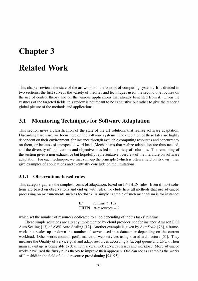
3.1.1 Observations-based rules . . . . . . . . . . . . . . . . . . . . . . . . . . . . 213.1.2 MAPE-K . . . . . . . . . . . . . . . . . . . . . . . . . . . . . . . . . . . . 223.1.3 Queuing Theory . . . . . . . . . . . . . . . . . . . . . . . . . . . . . . . . . 223.1.4 Game Theory . . . . . . . . . . . . . . . . . . . . . . . . . . . . . . . . . . 233.1.5 Machine Learning . . . . . . . . . . . . . . . . . . . . . . . . . . . . . . . . 243.1.6 Discrete Event Systems . . . . . . . . . . . . . . . . . . . . . . . . . . . . . 25

3.2 On the Use of Control Theory for Computing Systems . . . . . . . . . . . . . . . . . 26

i

ii

3.2.1 Motivation for using Control Theory . . . . . . . . . . . . . . . . . . . . . . 263.2.2 Application fields . . . . . . . . . . . . . . . . . . . . . . . . . . . . . . . . 263.2.3 Objectives . . . . . . . . . . . . . . . . . . . . . . . . . . . . . . . . . . . . 273.2.4 Sensors and performance metrics . . . . . . . . . . . . . . . . . . . . . . . . 273.2.5 Actuators and control signal . . . . . . . . . . . . . . . . . . . . . . . . . . 273.2.6 Modeling . . . . . . . . . . . . . . . . . . . . . . . . . . . . . . . . . . . . 273.2.7 Control . . . . . . . . . . . . . . . . . . . . . . . . . . . . . . . . . . . . . 283.2.8 Evaluation . . . . . . . . . . . . . . . . . . . . . . . . . . . . . . . . . . . . 283.2.9 Publications trends . . . . . . . . . . . . . . . . . . . . . . . . . . . . . . . 283.2.10 Limitations and open challenges . . . . . . . . . . . . . . . . . . . . . . . . 28

4 Objectives and Contributions 314.1 Privacy and Utility for Mobility Data . . . . . . . . . . . . . . . . . . . . . . . . . . 314.2 Performance and Reliability of Cloud Services . . . . . . . . . . . . . . . . . . . . . 334.3 Contributions of the Thesis . . . . . . . . . . . . . . . . . . . . . . . . . . . . . . . 35

4.3.1 Automatic Choice and Configuration of Location Privacy Protection Mecha-nisms . . . . . . . . . . . . . . . . . . . . . . . . . . . . . . . . . . . . . . 35

4.3.2 Dynamic Control of Utility and Location Privacy . . . . . . . . . . . . . . . 354.3.3 Adaptive Control for Cloud Service Performance Robust to Plant and Envi-

ronment Changes . . . . . . . . . . . . . . . . . . . . . . . . . . . . . . . . 364.3.4 Cost-aware Optimal Control of Performance and Availability of Cloud Services 36

II Privacy and Utility Aware Control of Users’ Mobility Data 37

5 Location Privacy Background and Related Work 415.1 Mobility traces and datasets . . . . . . . . . . . . . . . . . . . . . . . . . . . . . . 415.2 Notions of Location Privacy . . . . . . . . . . . . . . . . . . . . . . . . . . . . . . 43

5.2.1 Threats . . . . . . . . . . . . . . . . . . . . . . . . . . . . . . . . . . . . . 435.2.2 Definitions . . . . . . . . . . . . . . . . . . . . . . . . . . . . . . . . . . . 44

5.3 Location Privacy Protection Mechanisms . . . . . . . . . . . . . . . . . . . . . . . . 445.4 Evaluation of LPPMs . . . . . . . . . . . . . . . . . . . . . . . . . . . . . . . . . . 47

5.4.1 Privacy metric . . . . . . . . . . . . . . . . . . . . . . . . . . . . . . . . . . 485.4.2 Utility metric . . . . . . . . . . . . . . . . . . . . . . . . . . . . . . . . . . 495.4.3 Illustration of Privacy and Utility Metrics with LPPMs . . . . . . . . . . . . 51

5.5 LPPM Configuration . . . . . . . . . . . . . . . . . . . . . . . . . . . . . . . . . . 52

6 PULP: Privacy and Utility through LPPMs Parametrization 556.1 Introduction . . . . . . . . . . . . . . . . . . . . . . . . . . . . . . . . . . . . . . . 55

6.1.1 Description . . . . . . . . . . . . . . . . . . . . . . . . . . . . . . . . . . . 556.1.2 Problem Statement . . . . . . . . . . . . . . . . . . . . . . . . . . . . . . . 566.1.3 Proposed Approach . . . . . . . . . . . . . . . . . . . . . . . . . . . . . . . 57

6.2 PULP Framework . . . . . . . . . . . . . . . . . . . . . . . . . . . . . . . . . . . . 576.2.1 Profiler . . . . . . . . . . . . . . . . . . . . . . . . . . . . . . . . . . . . . 586.2.2 Modeler . . . . . . . . . . . . . . . . . . . . . . . . . . . . . . . . . . . . . 586.2.3 Configurator . . . . . . . . . . . . . . . . . . . . . . . . . . . . . . . . . . . 59

6.3 Configuration Laws . . . . . . . . . . . . . . . . . . . . . . . . . . . . . . . . . . . 606.3.1 PULP ’s Ratio-Based Configuration Law . . . . . . . . . . . . . . . . . . . 606.3.2 P-thld Law: Privacy Above a Minimum Threshold . . . . . . . . . . . . . . 61

iii

6.3.3 U -thld Law: Utility Above a Minimum Threshold . . . . . . . . . . . . . . 626.3.4 PU -thld : Privacy and Utility Above Minimum Thresholds . . . . . . . . . 62

6.4 PULP Evaluation . . . . . . . . . . . . . . . . . . . . . . . . . . . . . . . . . . . . 636.4.1 Experimental Setup . . . . . . . . . . . . . . . . . . . . . . . . . . . . . . . 636.4.2 Evaluation of the PULP Modeler . . . . . . . . . . . . . . . . . . . . . . . . 646.4.3 Evaluation of the PULP Configurator . . . . . . . . . . . . . . . . . . . . . 666.4.4 Comparison with State of the Art . . . . . . . . . . . . . . . . . . . . . . . . 68

6.5 Conclusion . . . . . . . . . . . . . . . . . . . . . . . . . . . . . . . . . . . . . . . 69

7 dynULP: dynamic control of Utility and Location Privacy 757.1 Introduction . . . . . . . . . . . . . . . . . . . . . . . . . . . . . . . . . . . . . . . 75

7.1.1 Context, Hypothesis and Motivation . . . . . . . . . . . . . . . . . . . . . . 757.1.2 Proposed Approach . . . . . . . . . . . . . . . . . . . . . . . . . . . . . . . 76

7.2 Control Problem Formulation . . . . . . . . . . . . . . . . . . . . . . . . . . . . . . 777.2.1 Overview . . . . . . . . . . . . . . . . . . . . . . . . . . . . . . . . . . . . 777.2.2 Formalization . . . . . . . . . . . . . . . . . . . . . . . . . . . . . . . . . . 777.2.3 Illustrated motivation . . . . . . . . . . . . . . . . . . . . . . . . . . . . . . 80

7.3 Privacy Modeling . . . . . . . . . . . . . . . . . . . . . . . . . . . . . . . . . . . . 827.3.1 Overview . . . . . . . . . . . . . . . . . . . . . . . . . . . . . . . . . . . . 827.3.2 Inputs Scenario . . . . . . . . . . . . . . . . . . . . . . . . . . . . . . . . . 827.3.3 Static Characterization . . . . . . . . . . . . . . . . . . . . . . . . . . . . . 827.3.4 Dynamic modeling . . . . . . . . . . . . . . . . . . . . . . . . . . . . . . . 84

7.4 Control Strategy . . . . . . . . . . . . . . . . . . . . . . . . . . . . . . . . . . . . . 857.4.1 Objectives . . . . . . . . . . . . . . . . . . . . . . . . . . . . . . . . . . . . 857.4.2 Linear Control Problem Formulation . . . . . . . . . . . . . . . . . . . . . . 867.4.3 PI Formulation . . . . . . . . . . . . . . . . . . . . . . . . . . . . . . . . . 867.4.4 Anti-windup . . . . . . . . . . . . . . . . . . . . . . . . . . . . . . . . . . . 86

7.5 dynULP Evaluation . . . . . . . . . . . . . . . . . . . . . . . . . . . . . . . . . . . 877.5.1 Methodology . . . . . . . . . . . . . . . . . . . . . . . . . . . . . . . . . . 877.5.2 Modeling . . . . . . . . . . . . . . . . . . . . . . . . . . . . . . . . . . . . 897.5.3 Control . . . . . . . . . . . . . . . . . . . . . . . . . . . . . . . . . . . . . 94

7.6 Conclusion . . . . . . . . . . . . . . . . . . . . . . . . . . . . . . . . . . . . . . . 100

8 Conclusions on Location Privacy 101

IIIPerformance and Reliability of Hadoop Cloud Services 103

9 BigData Cloud Services: Background and Related Works 1079.1 Cloud Services . . . . . . . . . . . . . . . . . . . . . . . . . . . . . . . . . . . . . 1079.2 A BigData Processing Framework: Hadoop/MapReduce . . . . . . . . . . . . . . . 1089.3 Problem Statement . . . . . . . . . . . . . . . . . . . . . . . . . . . . . . . . . . . 1099.4 Related Works . . . . . . . . . . . . . . . . . . . . . . . . . . . . . . . . . . . . . . 111

9.4.1 Cloud Performance Monitoring . . . . . . . . . . . . . . . . . . . . . . . . . 1119.4.2 MapReduce Performance Monitoring . . . . . . . . . . . . . . . . . . . . . 1119.4.3 Benchmarking and Platforms . . . . . . . . . . . . . . . . . . . . . . . . . . 112

9.5 Background on Control Theory applied to MapReduce . . . . . . . . . . . . . . . . 1139.5.1 Input and output signals . . . . . . . . . . . . . . . . . . . . . . . . . . . . . 1139.5.2 Modeling . . . . . . . . . . . . . . . . . . . . . . . . . . . . . . . . . . . . 114

iv

9.5.3 Control . . . . . . . . . . . . . . . . . . . . . . . . . . . . . . . . . . . . . 1159.5.4 Limitations . . . . . . . . . . . . . . . . . . . . . . . . . . . . . . . . . . . 116

10 Adaptive Control for Robust Cloud Services 11710.1 Introduction . . . . . . . . . . . . . . . . . . . . . . . . . . . . . . . . . . . . . . . 117

10.1.1 Context and Approach . . . . . . . . . . . . . . . . . . . . . . . . . . . . . 11710.1.2 Illustrated Motivation . . . . . . . . . . . . . . . . . . . . . . . . . . . . . . 118

10.2 Control Strategy . . . . . . . . . . . . . . . . . . . . . . . . . . . . . . . . . . . . . 12010.2.1 Preliminary Formulation . . . . . . . . . . . . . . . . . . . . . . . . . . . . 12010.2.2 Going beyond hypotheses . . . . . . . . . . . . . . . . . . . . . . . . . . . . 121

10.3 Adaptive Controller Evaluation . . . . . . . . . . . . . . . . . . . . . . . . . . . . . 12310.3.1 Evaluation Setup . . . . . . . . . . . . . . . . . . . . . . . . . . . . . . . . 12310.3.2 Simulation Results . . . . . . . . . . . . . . . . . . . . . . . . . . . . . . . 12410.3.3 Experimental Results . . . . . . . . . . . . . . . . . . . . . . . . . . . . . . 127

10.4 Conclusion . . . . . . . . . . . . . . . . . . . . . . . . . . . . . . . . . . . . . . . 130

11 Cost-aware Control of Cloud Services 13111.1 Introduction . . . . . . . . . . . . . . . . . . . . . . . . . . . . . . . . . . . . . . . 13111.2 Preliminaries . . . . . . . . . . . . . . . . . . . . . . . . . . . . . . . . . . . . . . 13411.3 Control Strategy . . . . . . . . . . . . . . . . . . . . . . . . . . . . . . . . . . . . . 136

11.3.1 The Lyapunov based triggering strategy . . . . . . . . . . . . . . . . . . . . 13611.3.2 Stability of the proposed scheme . . . . . . . . . . . . . . . . . . . . . . . . 136

11.4 Evaluation . . . . . . . . . . . . . . . . . . . . . . . . . . . . . . . . . . . . . . . . 13711.4.1 Experimental conditions and methodology . . . . . . . . . . . . . . . . . . . 13711.4.2 Cost based event triggering mechanism validation . . . . . . . . . . . . . . . 13811.4.3 Input-constrained control . . . . . . . . . . . . . . . . . . . . . . . . . . . . 13811.4.4 Evaluation using a real MapReduce workload . . . . . . . . . . . . . . . . . 141

11.5 Conclusion . . . . . . . . . . . . . . . . . . . . . . . . . . . . . . . . . . . . . . . 143

12 Conclusions on MapReduce Control 145

IVConclusions and Perspectives 147

V Résumé en français 151

Bibliography 159

VIAppendix: Machine learning algorithms as systems to control 173

A Duo Learning for Classifications with Noisy Labels 175

B Robust Anomaly Detection on Unreliable Data 181

C Feedback Control for Online Training of Neural Networks 191

List of Figures

2.1 Block diagram: control representation of a system . . . . . . . . . . . . . . . . . . . . . 132.2 High-level representation of a controlled system . . . . . . . . . . . . . . . . . . . . . . 152.3 Simplest controlled system: a Proportional Controller . . . . . . . . . . . . . . . . . . . 15

3.1 MAPE-K autonomic manager [98]. . . . . . . . . . . . . . . . . . . . . . . . . . . . . . 223.2 Queuing basic model [89]. . . . . . . . . . . . . . . . . . . . . . . . . . . . . . . . . . 223.3 Game theory payoff matrix, basic example. . . . . . . . . . . . . . . . . . . . . . . . . 243.4 Machine learning simple example: k-nearest neighbor classifier [177]. . . . . . . . . . . 253.5 Discrete Event System Control Schema[156]. . . . . . . . . . . . . . . . . . . . . . . . 26

4.1 Location Based Services . . . . . . . . . . . . . . . . . . . . . . . . . . . . . . . . . . 324.2 Usages and threats of mobility data when using a LBS. . . . . . . . . . . . . . . . . . . 324.3 Location Privacy Protection Mechanism . . . . . . . . . . . . . . . . . . . . . . . . . . 324.4 Common Cloud Services . . . . . . . . . . . . . . . . . . . . . . . . . . . . . . . . . . 334.5 News breaks showing that unmastered resource leads to service unavailability. All out-

ages were caused by unusual workload, where some where however expected to be ofhuge amplitude. . . . . . . . . . . . . . . . . . . . . . . . . . . . . . . . . . . . . . . . 34

5.1 GPS data are dynamic. Mobility data of a user from Cabspotting dataset illustration: (a)on a map and (b) trough speed over time of various activities (a stop and two movements). 43

5.2 Synthetic mobility trace scenario. . . . . . . . . . . . . . . . . . . . . . . . . . . . . . . 435.3 Obfuscation of a mobility trace using Geo-I. Illustration on a Cabspotting user for various

configurations. (a) user raw trace, (b) obfuscation with ε = 10−2, (c) obfuscation withε = 10−2.5. . . . . . . . . . . . . . . . . . . . . . . . . . . . . . . . . . . . . . . . . . 46

5.4 Obfuscation of a mobility trace using Promesse. Illustration on a Cabspotting user forvarious configurations. (a) user raw trace, (b) obfuscation with ε = 400m, (c) with ε =1000m. . . . . . . . . . . . . . . . . . . . . . . . . . . . . . . . . . . . . . . . . . . . 47

5.5 Privacy computation: schematic examples of how POI retrieval is computed for a singleuser when using Geo-I and Promesse. . . . . . . . . . . . . . . . . . . . . . . . . . . . 51

5.6 Utility computation: schematic examples of how cell coverage is computed for a singleuser when using Geo-I and Promesse. . . . . . . . . . . . . . . . . . . . . . . . . . . . 52

6.1 The same LPPM can result in different privacy and utility metrics: examples from 4users using Promesse with ε = 100m and Geo-I with two different configurations: ε1 =0.01m−1 and ε2 = 0.005m−1. . . . . . . . . . . . . . . . . . . . . . . . . . . . . . . . 56

6.2 PULP framework . . . . . . . . . . . . . . . . . . . . . . . . . . . . . . . . . . . . . . 576.3 Impact of LPPMs configuration on a user’s privacy and utility metrics – Real system

vs. modeled system (for one cabspotting user used as an example). . . . . . . . . . . . . 596.4 Automatic configuration laws in PULP . . . . . . . . . . . . . . . . . . . . . . . . . . 596.5 Illustration of PU -ratio configuration law for three schematic LPPMs with wpr/ut = 2. . 61

v

vi

6.6 PULP modeler accuracy. Cumulative distribution function (cdf) among all users. . . . . 656.11 Execution time comparison, Geolife dataset . . . . . . . . . . . . . . . . . . . . . . . . 686.7 PU -ratio configuration law evaluation. (a) Recommended LPPM and its configuration

(b) for Geo-I, (c) for Promesse. Achieved (d) level of privacy and (e) utility when usersare protected according to PULP recommendations, and the corresponding (f) privacy toutility ratio. Four objective ratios wpr/ut are illustrated: 0.5, 1, 2 and 3. . . . . . . . . . . 70

6.8 PU -thld configuration law evaluation. (a) Recommended LPPM and its configuration(b) for Geo-I, (c) for Promesse. Achieved (d) level of privacy and (e) utility when usersare protected according to PULP recommendations, and the corresponding (f) privacy toutility ratio. Five objective couples of constraints on privacy and utility are illustrated. . . 71

6.9 P-thld configuration law evaluation. (a) Recommended LPPM and its configuration (b)for Geo-I, (c) for Promesse. Achieved (d) level of privacy and (e) utility when usersare protected according to PULP recommendations, and the corresponding (f) privacy toutility ratio. Five objective constraints on privacy Prmin are illustrated: 0.3, 0.5, 0.7, 0.8,0.9. . . . . . . . . . . . . . . . . . . . . . . . . . . . . . . . . . . . . . . . . . . . . . 72

6.10 U -thld configuration law evaluation. (a) Recommended LPPM and its configuration (b)for Geo-I, (c) for Promesse. Achieved (d) level of privacy and (e) utility when usersare protected according to PULP recommendations, and the corresponding (f) privacy toutility ratio. Five objective constraints on utility Utmin are illustrated: 0.3, 0.5, 0.7, 0.8, 0.9. 73

7.1 Working scenario: location data are sent continuously and the service is received constantly 767.2 Classic control schema applied for privacy protection of a location based service user. . . 777.3 Privacy metric computation on a simple mobility trace. . . . . . . . . . . . . . . . . . . 807.4 Privacy and utility variations over time for various static LPPM configurations. Data from

a cabspotting user. . . . . . . . . . . . . . . . . . . . . . . . . . . . . . . . . . . . . . . 817.5 Static characteristics of the ε to privacy function, for various disturbance scenario. . . . . 837.6 System step response. Input from ε = 10−1 m−1 to ε = 10−2 m−1, during a stop (constant

disturbance). . . . . . . . . . . . . . . . . . . . . . . . . . . . . . . . . . . . . . . . . . 847.7 Feedback loop with signal and transfer functions notations . . . . . . . . . . . . . . . . 867.8 Privacy dynamic model validation with control variable steps. . . . . . . . . . . . . . . . 907.9 Privacy dynamic model validation with user’s speed steps. . . . . . . . . . . . . . . . . 907.10 Privacy dynamic model validation on substantial synthetic data, constant control signal. . 927.11 Privacy dynamic model validation on substantial synthetic data and control signal. . . . . 927.12 Privacy dynamic model validation on a real mobility trace, with constant control signal. . 937.13 Privacy dynamic model validation on a real mobility trace with a realistic control signal. 937.14 Dynamical privacy control of a stopped user with step privacy specifications. . . . . . . . 947.15 Dynamical privacy control with constant privacy specifications, with user’s speed steps. . 957.16 Dynamical privacy control with constant privacy specifications on substantial synthetic

data. . . . . . . . . . . . . . . . . . . . . . . . . . . . . . . . . . . . . . . . . . . . . . 967.17 Dynamical privacy control with substantial synthetic data and privacy specifications. . . 977.18 Dynamical privacy control on a real mobility trace, with constant privacy specifications. . 987.19 Dynamical privacy control, real mobility trace with a privacy specifications scenario. . . 99

9.1 Cloud IaaS platform adoption in 2017, percentage of applications deployed. [9] . . . . . 1089.2 MapReduce step-wise functional scheme. [60] . . . . . . . . . . . . . . . . . . . . . . . 1099.3 MapReduce Service Time model. . . . . . . . . . . . . . . . . . . . . . . . . . . . . . . 1149.4 MapReduce Service Time and Availability model. . . . . . . . . . . . . . . . . . . . . . 115

10.1 MapReduce State of the Art Modeling. [25] . . . . . . . . . . . . . . . . . . . . . . . . 118

vii

10.2 MapReduce State of the Art Feedback and Feedforward Control experimental perfor-mance for a comprehensive client disturbance scenario. . . . . . . . . . . . . . . . . . . 119

10.3 MapReduce adaptive control schema. . . . . . . . . . . . . . . . . . . . . . . . . . . . 12010.4 Client disturbance Scenario . . . . . . . . . . . . . . . . . . . . . . . . . . . . . . . . . 12310.5 Bode diagram of the transfer functions given in eq. (10.7) and (10.14) a) without PI b)

with PI for aN = aN =−0.92, aN =−0.84 and aN =−0.96 . . . . . . . . . . . . . . . . 12410.6 Controllers performance comparison with overestimated model gain. . . . . . . . . . . . 12510.7 Controller performance with characteristic time variation. . . . . . . . . . . . . . . . . . 12510.8 Controller performance for various plant gain scenarios, with and without PI . . . . . . . 12610.9 Experimental performance in Open Loop (no control). . . . . . . . . . . . . . . . . . . . 12710.10Experimental performance with the adaptive feedforward and feedback controller. . . . . 12810.11Experimental performance of the adaptive controller for a comprehensive workload. . . . 129

11.1 On-line shopping website - MapReduce workload on a 2,000-node cluster [155] . . . . . 13211.2 Comparison of time-based, error-based and cost-based controller performance without

constraints on the number of allowed reconfigurations . . . . . . . . . . . . . . . . . . . 13911.3 Comparison of cost-based controller performance with and without constraints on the

control changing time . . . . . . . . . . . . . . . . . . . . . . . . . . . . . . . . . . . . 14011.4 Cost-based event function . . . . . . . . . . . . . . . . . . . . . . . . . . . . . . . . . . 14111.5 Evaluation of cost-based controllers on a real 1-day MapReduce workload scaled to our

cluster size. . . . . . . . . . . . . . . . . . . . . . . . . . . . . . . . . . . . . . . . . . 142

List of Tables

5.1 30-days Mobility trace datasets . . . . . . . . . . . . . . . . . . . . . . . . . . . . . . . 425.2 Overview of Location-Based Services and the location properties used (’+’ for main pur-

pose and ’-’ for accessory need) to satisfy the end-user. . . . . . . . . . . . . . . . . . . 49

6.1 PULP output for selected users . . . . . . . . . . . . . . . . . . . . . . . . . . . . . . . 66

7.1 dynULP parameters sum-up. . . . . . . . . . . . . . . . . . . . . . . . . . . . . . . . . 88

10.1 Experimental controllers performance comparison on the simple workload scenario. Bestresults are in bold. . . . . . . . . . . . . . . . . . . . . . . . . . . . . . . . . . . . . . . 130

11.1 Cost comparison of different solutions based on a 1-day real workload . . . . . . . . . . 142

viii

Acknowledgements

Science, in its research form, aims at escaping from subjectivity and biases, but in the end isalways carried out by human beings.

A PhD thesis is known to be the apotheosis of an individual’s educational path, but in the end, itexists only thanks to fruitful and benevolent interactions.

State of the art contributions seems to bring the society further, but in the end, the tools go beyondtheir originator and are as righteous as the people using them.

I dedicate this chapter for acknowledging all those who participated in this work, in all the possi-ble ways; and to those who will use it as a humble stone for building their own project, may they doit consciously and serenely.

In the first place, I would like to thank my advisors Bogdan, Sara and Nicolas for their directions,advises, ideas, support, encouragements, devotion and fellowship. During this four-year experience,they taught me how to independently carry out researches while taking advantage of any collabora-tion. Aside from the scientific quality of their work, they are devoted teachers.

I had the great opportunity to collaborate with researchers from diverse horizon, I thank SoniaBen Mokhtar, Antoine Boutet, Lydia Y. Chen, Robert Birke and Ioan D. Landau. My special thanksgo also to the (former) students with whom I directly worked with, Mihaly Berekmeri, Vincent Pri-mault, Mohamed Maouche and Zilong Zhao. They were very dedicated in explaining and sharingtheir works, they contributed a lot in this thesis.

This work would not have been qualified as a PhD contribution without careful reviews and ex-aminations. I thank the jury members Vana Kalogeraki, Karl-Erik Arzen and Eric Kerrigan for thetime and expertise they gave during this process.

The research environment is as important as all of the above mentioned contributors of the manuscript.Thanks to my colleagues from LIRIS and Gipsa-lab, the fruitful discussions with my fellow researcherand the great help of technical and administrative services, which importance is way too often forgot-ten.

Aside from the scientific aspect, a PhD is also psychological challenge. All my gratefulness goesto my relatives that helped me in this experience. To my dear friends from the lab that always had abeer and a card game at the rightful time. All the cheerful friends with whom I share my daily, myweekends and my reflections. À ma famille, pour leur soutien inconditionnel. And to the one that fitsin all those categories.

Eventually, thanks to you, reader of this piece of work, to hopefully make it contribute to theworld’s knowledge and expertise, and not let it as a great but vain experience.

1

Part I

Generalities

3

Chapter 1

Introduction

This first chapter presents the motivation of the approach taken in this thesis of using control theory asa tool for software adaptation, and its application to two use-cases. Beforehand, some useful contextis detailed on those key notions. The present manuscript’s outlines are given, and reading advises areprovided as a concluding section.

1.1 Context, Motivation and ApplicationsComputing systems, either for personal use or in the industrial world, are constantly growing inamount and complexity. Smartphones provide user-based services such as personalized recommen-dations or adapted roaming. Companies have access to growing amounts of information about theirclients and/or their environment and use them to develop business-intelligence based analytics andservices. These two simple examples highlight that computing tools are used, directly or indirectly,with various degrees of consciousness and apprehension, by most people in their everyday life.

The last decade has seen the culmination of differentiation between software and hardware. Cloudservices have emerged as the new computing paradigms up to a point where companies that havefailed following this trend are now facing major difficulties. Its principle is to provide access tohardware infrastructures or services and take care of its maintenance so that clients can deploy theirown application without having to deal with hardware or operating systems issues. Cloud providersown datacenters all around the globe and their clients can access those resources distantly. Customersand contents of the cloud are extremely diverse, ranging from a simple person using Gmail or iCloudStorage to international companies or organizations running large data analytics. This example showsthe interconnectivity and concurrency of softwares sharing the same resources and networks. Anotherevery-day life illustration of such dependencies - this time outside of the cloud world - is the battle forcomputing and energy resources lead by applications and operating system on a smartphone. Data,tasks and resources need to be managed to maximize the quality of services.

Softwares are highly dependent on the environment in which they are running, and this environ-ment is constantly changing [98, 144]. Whether it is their workload or the concurrent applications,the running environment of softwares are highly dynamic. A recent example, particularly timely forresearchers, is the outage of the latex cloud service Overleaf that happened synchronously to a fa-mous machine learning conference [145]. At another scale, the hardware itself on which the softwareis running can change, sometimes even constantly and unpredictably if the service is run on the cloud[93]. It is also quite often that softwares have to run on hardware that did not even exist when it hasbeen designed, and that sometimes implies disrupting technologies.

Users and clients are asking for continuous availability, optimal performance and reliability; andthey are always more demanding. Moreover, they are asking for guarantees of those properties, of-

5

6

ten embodied in service-level agreements (SLAs). Meeting SLA is a key challenge for all serviceproviders. Eventually, the clients requirements are sometimes changing during runtime of the soft-ware, requiring system adaptation [164].

All those changes of context and requirements are enforced on the software even though this laterhas incomplete knowledge about its environment (specifically in the case of cloud-based services). Itsworking conditions are most of the time uncertain but also unpredictable, e.g. workload estimation.

Another important point is the energy consumption of large or small computing systems and, to alarger extent, their running costs. Each non optimal decisions either on the software runtime strategyor on the resources usage leads in useless extra costs. Given the scale of datacenters, the spread ofmobile devices and the always increasing usage of computing systems, wise and sparing planning ofresources need to be achieved.

Eventually, given the increasing complexity of computing tools, the question of their practicalusage, either by technical experts or simple users, raises. State-of-the art technologies mean alwaysmore specialized experts to install them, configure them and monitor their behavior in real time, at apoint where these tasked are hardly feasible by humans anymore. On the other side of the pipeline,end-user are more and more non-experts that hardly benefited from education on computing andsoftware usage. The usage of software tools should be adaptable to all kind of users.

A solution to all these challenges is software adaptation. It is a discipline of software engineeringwhich aims at modifying the software’s parameters/mode/resources in reaction to changes of its ownbehavior or of its environment. Many different tools can be used to realize adaptation in practice, suchas queuing theory, machine learning or control theory. In this work, we choose to focus on this lasttechnique. Control theory is an engineering field that aims at monitoring dynamic systems, throughthe use of feedback loops. It started to be well established since the early 1900’s, for its applicationsto industrial systems, notably in aeronautics. Due to its history for systems ruled by physics’ laws, itis only since the late 2000’s that its application to computing systems has been investigated. However,its strong mathematical background and its formal guarantees on the results makes control theory aprevalent solution for software adaptation. This is well illustrated by the significant rise in the numberof papers about this topic [162].

In order to illustrate the potential of the use of control theory for software adaptation, two comple-mentary computing systems will be studied. The first one deals with one side of the computing world,namely the user of smartphone. More specifically, we investigate the protection of people’s privacywhen sharing their localization through applications. Particular attention is paid on the quality of thegeo-localized service received. The literature on the use of control theory for privacy issues is almostnon-existing, which makes this use-case a real playground where everything is to be built, from thedefinition of user’s objectives to the privacy-ensuring setup. Cyber-privacy challenges are of priorimportance for the people but still lack of solutions. Moreover, the specific properties of such newformulation of control problems has a lot to bring to the research community.

The second use-case is the monitoring of performance and reliability of cloud-based BigDataservices, through resource allocation and admission control. This application deals with the other sideof the computing ecosystem, namely the data scientists and experts. This flourishing area of researchhas already produced many works and solutions, the efforts now focus on always more optimal andreliable outcomes. In this context, we advocated to use state of the art control theory tools to deal withthis well established challenge. Indeed, highly complex systems can benefit from all the experienceand maturity of control theory. On the other hand, a new application field means new objectives, newchallenges and new formulations that will make control theory grow.

Those two applications that will be further developed in this manuscript are complementary intwo ways. First, they are from two area of the vast computing world which reflects the complexityand diversity of challenges, from providing an accessible and useful tool for a large population, to

7

building up the state of the art tools for data scientists. Second, most of the vast control theorydomain is illustrated, from its very beginning where problem has to be formulated and where simpletools can be applied to the most complex non-linear time varying system for which recently developedtechniques are required.

A third use-case has been studied alongside and following this thesis work. The computing sys-tems under consideration are machine learning algorithms, such as the well known k-means, decisiontrees or the popular neural networks. Their control has been investigated in two complementary ways.First, the challenge of robustness of the learning process regarding noise in the dataset was raised.Second, research has been focused on the parametrization of the algorithms, with the introduction offeedback action.

1.2 Main Results and Collaborations

1.2.1 PublicationsThe work developed in this thesis has lead to several contributions which have been published invarious venues, both the control and computing systems communities:

International Journals

• Sophie Cerf, Sara Bouchenak, Bogdan Robu, Nicolas Marchand, Vincent Primault, Sonia BenMokhtar, Antoine Boutet, Lydia Y. Chen. Automatic Privacy and Utility Preservation forMobility Data: A Nonlinear Model-Based Approach. IEEE Transaction on Dependable andSecure Computing (TDSC) [45].• Submitted: Sophie Cerf, Bogdan Robu, Nicolas Marchand, Sara Bouchenak. Utility-Aware

Modeling and Control of Location Privacy. IEEE Transaction on Automatic Control (TAC),special issue: Security and Privacy of Distributed Algorithms and Network Systems.

International Conferences with Proceedings

• Sophie Cerf, Mihaly Berekmeri, Nicolas Marchand, Sara Bouchenak, Bogdan Robu. AdaptiveModelling and Control in Distributed Systems. PhD Forum 34th International Symposiumon Reliable Distributed Systems (SRDS 2015), Sep 2015, Montreal, Canada [39].• Sophie Cerf, Bogdan Robu, Nicolas Marchand, Antoine Boutet, Vincent Primault, Sonia Ben

Mokhtar, Sara Bouchenak. Toward an Easy Configuration of Location Privacy ProtectionMechanisms. Poster at ACM/IFIP/USENIX Middleware conference, Dec 2016, Trente, Italy[48].• Sophie Cerf, Mihaly Berekmeri, Bogdan Robu, Nicolas Marchand, Sara Bouchenak. Towards

Control of MapReduce Performance and Availability. Fast Abstract in the 46th AnnualIEEE/IFIP International Conference on Dependable Systems and Networks (DSN 2016), Jun2016, Toulouse, France [42].• Sophie Cerf, Mihaly Berekmeri, Bogdan Robu, Nicolas Marchand, Sara Bouchenak. Adaptive

Optimal Control of MapReduce Performance, Availability and Costs. 11th InternationalWorkshop on Feedback Computing co-located with the 13th IEEE International Conference onAutonomic Computing (ICAC 2016), Jul 2016, Wurzburg, Germany [40].• Sophie Cerf, Mihaly Berekmeri, Bogdan Robu, Nicolas Marchand, Sara Bouchenak. Cost

Function based Event Triggered Model Predictive Controllers - Application to Big DataCloud Services. 55th IEEE Conference on Decision and Control (CDC 2016), Dec 2016, LasVegas, United States [41].

8

• Sophie Cerf, Vincent Primault, Antoine Boutet, Sonia Ben Mokhtar, Sara Bouchenak, BogdanRobu, Nicolas Marchand. Données de mobilité : protection de la vie privée vs. utilitédes données. Conférence francophone d’informatique en parallélisme, architecture et systèmeComPAS, Jun 2017, Sophia Antipolis, France [46].

• Sophie Cerf, Mihaly Berekmeri, Bogdan Robu, Nicolas Marchand, Sara Bouchenak, IoanLandau. Adaptive Feedforward and Feedback Control for Cloud Services. IFAC WorldCongress, Jul 2017, Toulouse, France [43].

• Sophie Cerf, Sonia Ben Mokhtar, Sara Bouchenak, Nicolas Marchand, Bogdan Robu. DynamicModeling of Location Privacy Protection Mechanisms. 18th IFIP International Conferenceon Distributed Applications and Interoperable Systems (DAIS 2018), June 2018, Madrid, Spain[38].

• Sophie Cerf, Bogdan Robu, Nicolas Marchand, Sonia Ben Mokhtar, Sara Bouchenak. A Con-trol Theoretic Approach for Location Privacy in Mobile Applications. 2nd IEEE Confer-ence on Control Technology and Applications (CCTA 2018), Aug. 2018, Copenhagen, Den-mark [49].

• Sophie Cerf, Robert Birke, Lydia Y. Chen. Duo Learning for Classifications with NoisyLabels. Continual Learning Workshop, Neural Information Processing Systems (NIPS 2018),Dec. 2018, Montréal, Canada [44].

• Zilong Zhao, Sophie Cerf, Robert Birke, Bogdan Robu, Sara Bouchenak, Sonia Ben Mokhtar,Lydia Y. Chen. Robust Anomaly Detection on Unreliable Data. 49th IEEE/IFIP InternationalConference on Dependable Systems and Networks (DSN 2019), June 2019, Portland, Oregon,USA [187].

• Zilong Zhao, Sophie Cerf, Bogdan Robu, Nicolas Marchand. Feedback Control for OnlineTraining of Neural Networks. 3rd IEEE Conference On Control Technology And Applica-tions (CCTA 2019), Aug. 2019, Hong Kong, China [188].

1.2.2 CollaborationsThose works has been conducted thanks to fruitful collaborations:

• Pr. Sara Bouchenak (LIRIS lab, INSA-Lyon) on all the contributions of this manuscript,

• Dr. Sonia Ben Mokhtar (LIRIS lab, INSA-Lyon) on Location Privacy,

• Dr. Lydia Y. Chen (TU Delft) on data analytics and privacy,

• Pr. Ioan D. Landau (Gipsa-lab, Univ. Grenoble-Alpes) on adaptive control of Clouds,

• Dr. Antoine Boutet (Privatics, INRIA Lyon) on Location Privacy,

• Dr. Mihaly Berekmeri (Equifax UK) on modeling and control of Hadoop,

• Dr. Robert Birke (ABB Research) on data analytics and privacy,

• Dr. Vincent Primault (University College London) on Location Privacy.

I also had the great opportunity to work 5 months at IBM Research Center, Zürich, Switzerlandfrom July to November 2018 in the form of an intership. I developed fruitful collaboration with Dr.Lydia Y. Chen and Dr. Robert Birke (former researchers at IBM) that expanded my research interestin the direction of machine learning, see the corresponding publication in Appendices A B and C.

9

1.2.3 Technical contributionsTo foster the theoretical contributions presented in the above mentioned publications, technical ad-vances were made. For the control of MapReduce over a cloud environment, the experimental envi-ronment developed in the Gipsa-lab by Mihaly Berekmeri [25] was re-used, maintained and extendedto run more controllers and under more sophisticated workload conditions. The setup consists inMatlab-based control laws running locally on a computer while Lunix bash scripts are used for theinterface between the remote cluster and the local computer.

For location privacy experimentations, the JSON-based setup developed in the LIRIS laboratoryby Vincent Primault [149] was used. For the dynamical control of privacy, an independent Matlabexperimental setup was built, allowing easy development and evaluation of modeling and controltools.

1.3 Thesis OutlineThis thesis is organized in six main parts. The first part is a general overview on control of computingsystems and the place of this work in the corresponding state of the art. The second part is dedicated tothe control of privacy and utility of geolocalized data in the context of personal mobile device use. Thethird part details the contributions made on the area of performance and dependability guarantees forcloud-based BigData services. The fourth part draws conclusions on this work and provides insightsof future works that would worth investigating on. The fifth part is a extended summary in Frenchof this manuscript and eventually the sixth part contains the appendices that gathers the publicationson the third application use-case, the control of learning algorithms. These contributions are onlypresented as annex of this manuscript, as they were initiated as a side project during an internship inthe company IBM. However, they evolved as being the continuity of the application of control theoryfor computing systems during the very last months of this thesis work, thus their are included to thismanuscript through papers in appendix.

Each part is divided in chapters, which contents are briefly described in the following.

Part 1 - Generalities.Chapter 1 - Introduction. The current chapter presents the context of this work, the approach and

applications taken and the reasons that motivated their choice. Main results, in terms of publicationsand codes, and collaborations are presented and a reading roadmap is provided.

Chapter 2 - Background and Motivation. The second chapter provides background on controltheory for those who are not familiar with this domain. The description is made in a pedagogicalway, by giving the objectives, describing the major tools and concepts such as sensors, actuators,models and controllers. Examples of applications are also given. Basics are provided regarding theuse of control theory for computing systems, starting with the condition of this duo and explainingthe advantages of the combination for both domains, concluding with the challenges it represents.

Chapter 3 - Related Work is then detailed. First, an overview of the different tools and theoriesused for achieving software adaptation, namely observation-based rules, MAPE-K, queuing theory,game theory, machine learning and discrete-event systems. For each of those techniques, backgroundon the theory is given, followed by examples of its application in our context and eventually limita-tions of the approach are given. A second section is dedicated to the analysis of the state of the art oncontrol of computing systems. Different aspects are reviewed, such as the analysis of the works’ moti-vations and their application domains. Control-specific aspects are then detailed: objectives, sensors,actuators, models, controllers and evaluation. Notes on publications trends are given. Eventually,limitations and the corresponding challenges of control of computing systems are listed.

10

Chapter 4 - Objectives and Contributions. Concluding the first part, the fourth chapter sums-upthe objectives of this works following the state of the art limitations highlighted beforehand. Theseobjectives are put in perspective of two uses cases: location privacy and utility; and cloud performanceand dependability. Contributions of this thesis are presented in four points with mention of the relatedpublications, each contribution being a distinct chapter in the next two parts - after an introductionchapter for each.

Part 2 - Privacy and Utility Aware Control of Users’ Mobility Data.Chapter 5 - Location Privacy Background and Related Works. After the general introduction

on location privacy given in the previous chapter, more details are given. The mobility data aredescribed, the notion of privacy is defined both formally and through threats examples. The state of theart mechanisms of privacy protection specially designed for location-related issues are then presented.Methods to evaluate the so called Location Privacy Protection Mechanisms (LPPMs) are overviewed,with special focus on privacy and utility metrics and on their practical illustration. Eventually, wereview the related works aiming at configuring LPPMs, independently of the technique used.

Chapter 6 - PULP: Privacy and Utility through LPPMs Parametrization. This first contri-bution chapter presents PULP, a framework that realize user-level LPPMs choice and configurationto meet privacy and utility objectives, in the case of already collected databases needing privacyenhancement. An introduction on this scenario and on our proposed approach is first given. Thefollowing section describes PULP’s framework and its three components: the profiler, the modelerand the configurator. PULP enables four objectives formulations, all combining differently privacyand utility aspects, each of them and their corresponding configuration law are presented. Evaluationis eventually performed using mobility data collected on people in the wild.

Chapter 7 - dynULP: dynamical control of Utility and Location Privacy. The second contri-bution on location privacy is presented in the seventh chapter. The scenario here is a mobile deviceuser using geolocalized services through time and willing to protect her privacy, while still benefitingof the service. After discussions on this context and on the proposed approach, dynULP solution ispresented in three steps: problem formulation, modeling and control law. Each time, the approachis visualized and validated on synthetically generated mobility data. Afterwards, global evaluation iscarried out on real location data. An analysis of the work and on its perspective is then discussed.

Chapter 8 - Conclusions on Location Privacy. The last chapter of Part 2 summarizes the con-tributions on the protection of users’ location privacy and the preservation of their service utility.

Part 3 - Performance and Reliability of Hadoop Cloud Services.Chapter 9 - BigData Cloud Services: Background and Related Works. The eighth chapter

gives context to the second area of contribution of this manuscript: the control of a cloud-basedbigdata framework: Hadoop. After presenting the above mentioned service, related work on thestate of the art of cloud control is reviewed. The control formulation on Hadoop configuration, takenfrom the state of the art, is then described and will serve as a basis for the development of the twocontributions detailed in the next sections.

Chapter 10 - Adaptive Control for Robust Cloud Services. State of the art techniques of controlare used in this section to improve Hadoop robustness to unpredicted fluctuations in its workload andunmeasured ones for its environment. This specific issue is put in context and motivated, and theapproach we took is presented. The adaptation-based control strategy is then described, in principleand in details. Evaluation is performed on a real platform deployed on a nation-wide grid with over50 computing resources.

Chapter 11 - Cost-aware Control of Cloud Services. The last contribution of this thesis isgiven in the ninth chapter. Here three contradictory objectives are formulated: performance in terms

11

of execution time of jobs, availability which is the rate of accepted requests, and costs and energyefficiency. For this scenario, an optimal model-predictive controller with a designed event-triggeredapproach is developed. This control strategy is presented with mathematical preliminaries. Evaluationis carried out using a real MapReduce workload.

Chapter 12 - Conclusions on MapReduce Control. Eventually, the contributions of this thesison the control of cloud services are summarized.

Part 4 - Conclusion and Perspectives.Conclusions on this thesis contributions and broadly on the control of computing system is given.

Future works are put in perspective of the two applications use-cases presented: location privacy andcloud services; and on the on-going work on control of learning algorithms.

Part 5 - Résumé en français.This thesis work has been funded and conducted in the frame of the French communities of univer-

sities, and is thus briefly presented in French.

Part 6 - Appendix - Machine learning algorithms as systems to control.This ending thesis, the most recent works on control of computing systems through the use-case of

machine learning is given in appendix.

1.4 Reading RoadmapThis manuscript can interest various types of readers in their background and interests. This sectionaims at directing the reader to relevant chapters.

For the reader with a control theory background and interested about the contributions of thismanuscript in this field. Chapter 2 Section 2.1 on control theory background can be eluded, while thenext Section 2.2 gathers the interesting challenges of control of computing systems. Chapter 4 can beused to get familiar and possibly chose the application of interest, if not both. For location privacy,Chapter 5 gives relevant background while Chapter 7 is the core control contribution. For Hadoopperformance and reliability monitoring, Chapter 9 sets the useful computing background while thenext two Chapters 10 and 11 are the contributions. The reader can also be interested in looking atAppendix C, which presents the use of a feedback algorithm to control the training phase of a neuralnetwork, with application to image classification.

For the reader with interest in location privacy. If not familiar with control theory, please startwith Chapter 2. Then all the Part II is of relevant interest. Chapter 5 should be read first, the two otherChapters 7 and 6 can be looked at independently.

For the reader with interest in Hadoop cloud-service performance and reliability control. If notfamiliar with control theory, please refer to Chapter 2 for relevant background. The Part III gathersall the work on this topic. Chapter 9 detailing background and state of the art should be read first, thetwo other Chapters 10 and 11 can be read without order.

For the reader with interest in machine learning. Chapter 2 should be read first in case back-ground on control theory is needed. The Part VI gathers all the works on the machine learning topic.No general introduction is given, one can successively read Appendix A and then Appendix B onthe topic of robustness to noise. The Appendix C on the use of a feedback controller can be readindependently.

Chapter 2

Background and Motivation

This chapter gives a general overview on Control Theory and on its use for Computing applications.First, basic concepts of control are explained as an attempt to depict the global picture of the field.Then, the association of control and software adaptation is motivated. Readers having notions oncontrol can skip the first section.

2.1 Basics on Control TheoryThis section is for readers willing to have a first approach of control theory. More details and formalformulations about relevant points will be given in due course in dedicated chapters. It is organizedas follows. First, the assumptions and hypothesis that define the scope of control systems, as wellas dedicated representation, are presented. Second an overview of the goals one can achieve withcontrol theory is given. Then, the most common tools used by control engineers and researchers arepresented in simple terms. Some insights on the possible application areas of control conclude thisoverview of the field. For a complete introduction to control theory for computing systems, refer toHellerstein et al.’s book [91].

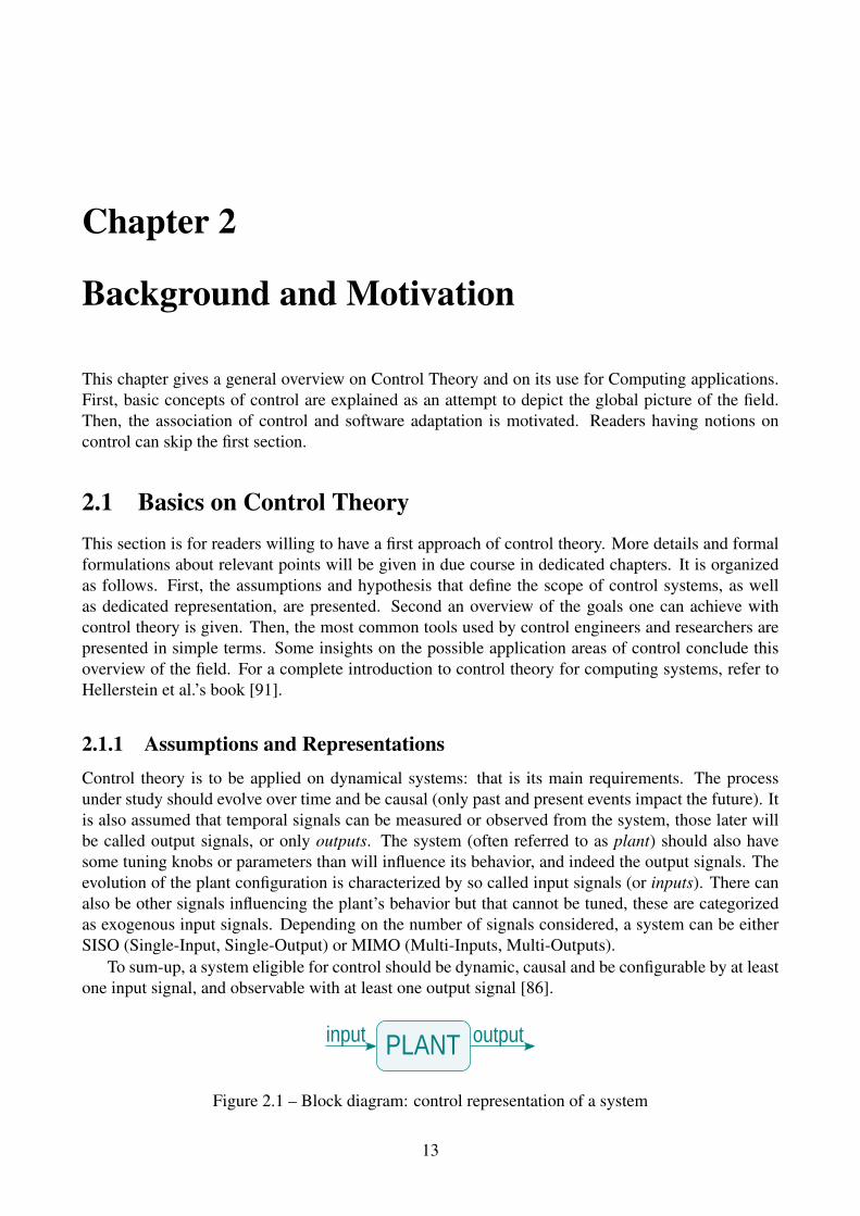
2.1.1 Assumptions and RepresentationsControl theory is to be applied on dynamical systems: that is its main requirements. The processunder study should evolve over time and be causal (only past and present events impact the future). Itis also assumed that temporal signals can be measured or observed from the system, those later willbe called output signals, or only outputs. The system (often referred to as plant) should also havesome tuning knobs or parameters than will influence its behavior, and indeed the output signals. Theevolution of the plant configuration is characterized by so called input signals (or inputs). There canalso be other signals influencing the plant’s behavior but that cannot be tuned, these are categorizedas exogenous input signals. Depending on the number of signals considered, a system can be eitherSISO (Single-Input, Single-Output) or MIMO (Multi-Inputs, Multi-Outputs).

To sum-up, a system eligible for control should be dynamic, causal and be configurable by at leastone input signal, and observable with at least one output signal [86].

PLANT outputinput

Figure 2.1 – Block diagram: control representation of a system

13

14

The usual way to illustrate a control system is to use block schemas, such as the one of Figure 2.1.In those representations, the arrows represent signals evolving with time. Block are systems that canbe seen as transformations functions on the signals. The classic representation of a system eligible forcontrol is thus a block called plant with an arrow entering on the left hand side representing the inputand an arrow on the right hand side pointing outside representing the measured output. The arrowshapes are here to remind that signals are evolving over time and the plant causality.

2.1.2 ObjectivesGiven such a system, three complementary goals can be achieved when using control theory:

• Stability. The basic idea behind the term stability is that, given a bounded input signal, theoutput signal should also be bounded. As such, the system is stable and do not diverge toinfinity. While some systems are inherently stable (e.g. a heating device), some other areinstable in absence of control strategy (e.g. a inverted pendulum). Control can be used tostabilize an unstable system, but most of all it should ensure to keep stable an originally stableone.

• Bring the system to a set point. Once the system is ensured to be stable, one may wantto decide on how the plant should behave. This translates to objectives values on the outputsignal, such as the temperature of a heating device. The main notions of performance regardingoutput reference values in this context are the precision of the achieved set point compared tothe desired one, the settling time taken to achieve the set point, and the overshoot above theachieved set-point. This objective is often referred to as a tracking problem.

• Disturbance Rejection. As no system evolves in a perfectly mastered environment, a controlstrategy should be able to deal with exogenous influences. Whether these disturbances can bemeasured or not, modeled or not; control theory provides ways to reject them, i.e. minimizetheir impact on the plant outputs. This aspect of control is called a regulation problem.

The three objectives: stability, tracking and regulation are the main reasons of using the controltheory. In order to provide solutions to achieve these goals, some specific tools have been developedor re-used from other disciplines. The major ones are presented in the next subsection. The use ofthese tools have open new possibilities, making some people use them to achieve new goals than whatthey where designed for. These complementary control objectives are dependent on the tool itself,and thus will be explained after the tools description. Examples of such side objectives are modelingof systems or estimation of unmeasurable characteristics of the plant.

2.1.3 Tools of a Control EngineerAn overview of the methods used to solve control problems is given next. First, the idea of feedbackloops is depicted. Second, insights on modeling tools are provided. Then, the control usage offrequency domain is shortly presented. Eventually, last paragraphs explains the usage of appliedmathematic tools by control scientists.

2.1.3.1 Feedback loops and controllers

The idea behind control theory is the use of feedback loops [62]. The configuration of the plant iscomputed based on the measurement of its state: the output signal is fed back to decide on the inputsignal. The mathematical relation that links the output to the input is called controller. Going back

15

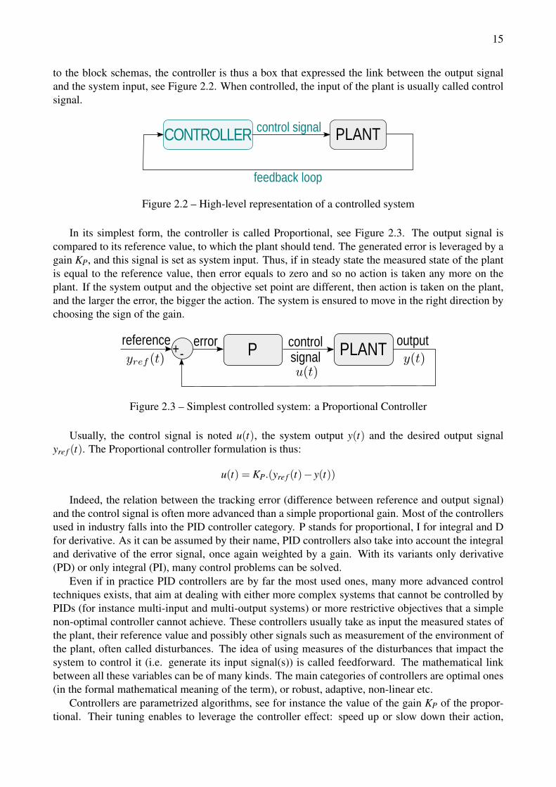
to the block schemas, the controller is thus a box that expressed the link between the output signaland the system input, see Figure 2.2. When controlled, the input of the plant is usually called controlsignal.

PLANT

feedback loop

control signalCONTROLLER

Figure 2.2 – High-level representation of a controlled system

In its simplest form, the controller is called Proportional, see Figure 2.3. The output signal iscompared to its reference value, to which the plant should tend. The generated error is leveraged by again KP, and this signal is set as system input. Thus, if in steady state the measured state of the plantis equal to the reference value, then error equals to zero and so no action is taken any more on theplant. If the system output and the objective set point are different, then action is taken on the plant,and the larger the error, the bigger the action. The system is ensured to move in the right direction bychoosing the sign of the gain.

Figure 2.3 – Simplest controlled system: a Proportional Controller

Usually, the control signal is noted u(t), the system output y(t) and the desired output signalyre f (t). The Proportional controller formulation is thus:

u(t) = KP.(yre f (t)− y(t))

Indeed, the relation between the tracking error (difference between reference and output signal)and the control signal is often more advanced than a simple proportional gain. Most of the controllersused in industry falls into the PID controller category. P stands for proportional, I for integral and Dfor derivative. As it can be assumed by their name, PID controllers also take into account the integraland derivative of the error signal, once again weighted by a gain. With its variants only derivative(PD) or only integral (PI), many control problems can be solved.

Even if in practice PID controllers are by far the most used ones, many more advanced controltechniques exists, that aim at dealing with either more complex systems that cannot be controlled byPIDs (for instance multi-input and multi-output systems) or more restrictive objectives that a simplenon-optimal controller cannot achieve. These controllers usually take as input the measured states ofthe plant, their reference value and possibly other signals such as measurement of the environment ofthe plant, often called disturbances. The idea of using measures of the disturbances that impact thesystem to control it (i.e. generate its input signal(s)) is called feedforward. The mathematical linkbetween all these variables can be of many kinds. The main categories of controllers are optimal ones(in the formal mathematical meaning of the term), or robust, adaptive, non-linear etc.

Controllers are parametrized algorithms, see for instance the value of the gain KP of the propor-tional. Their tuning enables to leverage the controller effect: speed up or slow down their action,

16

refine the precision in reaching the desired state, reduce the use of resources, etc. The parametrizationof a controller also depends on the system’s dynamics and behavior. For instance, a thermal system isway slower than a electric engine, thus the same controller with the same parameters applied for bothsystems is not likely to be efficient (neither stable) in all cases. This motivates the use of modeling.

2.1.3.2 Modeling

Models in control theory are mathematical equations that predict the current output(s) of a system,knowing its previous ones and the input signal(s) applied. Other signals can also be taken into account,such as the disturbances of the environment on the plant. Models can have various memory size(called order, the number of past values of the signals needed to predict the current one), and ofcourse parametrization.

The mathematical tools to represent the models are quite specific to control theory. They usethe Laplace transform, which idea is to transform derivative and integral functions in products anddivisions. The SISO systems are often modeled by a transfer function, which is a link between theinput and the output of the system. It is more formally the ratio of the output over the input, bothbeing in Laplace transform.

Multi-variable (MIMO) systems use more advanced modeling techniques called state-space rep-resentation, linking the states, inputs and disturbances to the derivative of the states. These statesare all signals that are needed to describe the system. Some of them are measurable and thus calledoutputs (sometimes subject to a transformation), other are not, and thus are mostly intermediate ofcalculation. As a concrete example, let’s take consider a pendulum. To fully describe its behavior,both the position of the mass and its speed are needed. However, most of the time only the position ismeasured. The pendulum two states are thus the mass position and speed, but only position is calledsystem output. Note that there exist an infinity of state-space representations of a system.

In order to find the order and parameters of a system’s model, two main techniques exist. Thefirst one consist in studying the system from a physical point of view, i.e. computing the behaviorallaws that links the input(s) to the output(s). This is for instance what is done if one wants to model aelectrical engine. The rotation speed can be linked to the engine input voltage though other physicalquantities. This solution has the advantage of being accurate, but can become complex or even im-possible to apply depending on the system to be controlled. In the case that interest us in this thesis,computing systems such as softwares do not depend on such kind of laws. The other tool of controltheory for modeling is called identification, or black-box approach. The idea behind it is to vary theinput(s) of the plant and observe the output(s), and try to fit the observed behavior with a classicalmodel, which order and parameters can be varied. Controlled systems being always more complexand large, identification is the most used technique. One of its advantages is being able to leveragethe model complexity (and thus its precision) in order to have a computationally practical model. Itis worth noticing that, for a good behavior is closed loop, the model does not need to be perfect.

Models are usually computed to derive a proper controller that will enable to reach the objectives.However, the development of advanced modeling tools for dynamical systems are sometimes used asan end-goal, for instance is the biological domain, when trying to model complex dynamical systems.

2.1.3.3 Time and Frequency Domains

As in signal processing, the systems can be considered with two complementary points of view:the time or the frequency domains. The use of time domain is linked to the nature of the controlsystems, that have to be dynamic. However, the use of the frequency domain helps the analysis andeven sometimes the design of controllers. This will be the case in this thesis when designing robustcontrollers (see Chapter 10).

17

Some requirements can also be expressed in the frequency domain, for instance when workingin the acoustic field where specific frequencies have to be attenuated. In a general way, the study ofcontrol systems in the frequency domain helps for analyzing stability, performance, etc. in all possiblescenarios that the system can encounter.

2.1.3.4 Filters, optimization and other applied mathematics tools

Even though the large usage of control in industry can be sum up to PID controllers, state-of-the-art companies and indeed researchers are working with advanced control problems, being close toapplied mathematics. Optimization techniques are largely used for instance to find the best inputsignal(s) that fits the performance objectives, to minimize the use of resources, and so on. As a mainexample of the contribution of control theory to the broad work of mathematics users is the workof Kalman on filters. From a control perspective, Kalman filters are used as so called observers, thatestimate the states of Multi-Input Multi-Output systems that cannot be measured. Similar to modelingtools, estimation techniques initially developed with the idea of deriving a controller are now widelyused as such for other applications, such as image processing to mention only one.

2.1.4 Applications

Control being a tool with few constraints regarding the application system, it has been used in an verylarge variety of fields [86]. To still try to give a overview, one can start by explaining the historicaldomains that have motivated the emergence of control, and thus move to specific domains that cannow benefit of control theory in its most advanced forms.

The most basic applications of control are for mechanic and thermodynamic systems. Temperatureregulation of a room or an oven, speed rotation of an engine, or water levels in tanks are simple every-day examples. Control is now widely used in automotive, aeronautics, drones industries and all kindof plants such as chemistry, nuclear or hydraulic ones. Event if the terminology of application maynot be appropriated, the large and common contributions of control to mathematics is to be stated.

Control is also used in new and promising fields of application. Biological systems are nowadaysstudied with the point of view of control to better understand the natural regulation systems that existsfor instance in human bodies. Large scale and distributed systems such as electric grids and networksare also a state-of-the-art application of control, particularly when considering issues of connectionof local renewable sources. Eventually, computing systems are a promising field to be explored bycontrol theorists and engineers. Section 2.2 is dedicated to the motivation of this association, whileSection 3.2 of Chapter 3 overviews its state-of-the-art works. Eventually, Chapter 4 presents the twoapplication cases this thesis will focus on.

2.2 On the use of Control Theory for Computing SystemsUsing the basic notions overviewed given in Section 2.1, the use of control for software adaptationis considered in this section. First, a precision is made on the notion of computing system that canbenefit from control, corresponding to the assumptions required. Second, the achievements a controlapproach can provide is investigated from the point of view of a computer scientist. Then, the advan-tages of the association is highlighted, from the point of view of both fields. Finally, the challengesone has to face when trying this approach are depicted, justifying the interest of researchers on thisquestion.

18

2.2.1 Eligible Computing Systems

Computing systems are omnipresent in our society, and even though they emerged quite recently, theirdiversity is huge. So what is meant by computing systems in this context? A first categorization canbe done between hardware and software. Both are eligible to benefit from control theory. However,this thesis focuses on software applications.

Coming back to assumptions, a controlled system first has to be dynamic, i.e. evolve with time.In computing terms, that means that the process should be on-line, or in real time. However, thistemporal dimension is often scale-dependent. Let us take the example of a query request. From ahigh scale perspective, this can be seen as an event that, when successively repeated, consist in adynamical system. At a smaller scale, all the processes involved in the request (network, computing,etc.) can also be seen as a dynamic system on its own. Consequently, the problem formulation playsan important role in the control approach.

The second main requirement is the possibility of tuning the system in an on-line fashion. Indeed,one need to be able to adjust the behavior of the system over time to control its performance. Forinstance, if an application is launched with a given amount of computing resources and there is noway to leverage them while running, it will not be possible to control the application run time.

Third, the system willing to be controlled should be observable, which means that the desiredcharacteristic should be measured or estimated, possibly indirectly. If the response time of queriescannot be evaluated in real time, it will not be possible to decide on a control strategy to acceleratethem.

These last two constraints (tunable input and measurable output of the system) are usually issuesthat can be overpassed by the development of system add-ons if it is not present by default, if dealingwith softwares. However, sometimes the constraints on the system prevent from doing so, for instancewhen working with certified codes or embedded systems with limited resources. Once again, thisbrings us to the challenge of problem formulation, where actuators (i.e. tuning mechanisms) andsensors (i.e. measure of the system state) have to be designed and implemented.

2.2.2 Promises of control for software adaptation

Computing systems are most of the time stable. The contribution of control is thus not consideredthere, even though one main contribution of the control is to offer guarantees about the stability ofcomplex systems. Performance monitoring and robustness to external factors are thus the contribu-tions of control that mostly interest computer scientists.

In software adaptation, it is often an easy task to find ways to tune the system. Indeed, they havea multitude of parameters that can be fixed but this task is very complex. Finding appropriate ways tochose these parameters is precisely the purpose of control. After defining objectives such as responsetime or resource consumption, controllers tune the system to reach these requirements. This often nontrivial dynamic relation between desired outputs and controllable inputs are dealt by the controller.

Another contribution of control is disturbance rejection, which in computing terms means han-dling the impact of the changing environment, or external factors, on the system. For instance, thesteep raise in the number of people visiting a website requires the augmentation of dedicated resourcesto avoid a crash. Control algorithms can detect such circumstances and adapt the system accordingly.

On top of all this, the mature mathematical foundations of control enable to provide analyticalguarantees about all the above mentioned contributions.

19

2.2.3 BenefitsThe advantages of using control on computing applications are for both community. A quick overviewis given in the next two paragraphs.

2.2.3.1 For the computing world

Computer scientists using control can rely on tools developed decades ago in well known, efficientand complete formulation. Having a feedback, i.e. a closed loop, enables to monitor the states (data,tasks, resources, etc.) of the systems to better understand its current behavior and better regulate it.Control framework also enable to clearly formulate one’s objectives, e.g. quality of service, and alsoto leverage them if needed, through the use of cost functions. Thus, all aspects of the application canbe taken into account, such as energetic or financial costs.

Feedforward loops (or other advanced controllers) take into account the environment of the systemto decide on its later configuration. This is a significant advantage in computer science as most of thesystems to control are not isolated: they often are subsystems in a bigger framework. Adaptationalgorithms are able to react to the changes in the plant itself, for instance dealing with applicationhaving multiple steps or stages. A side advantage of control approached is that they provide anestimation or even prediction of the unmeasured metrics, for instant workload or completion rate oftasks.

Last but not least, control theory provides mathematical guarantees of its performance and robust-ness. This means that service providers can engage themselves to their clients and be aware of therisks they are taking, even sometimes in the case of faults or attacks. From a juridic point of view itcan also be very interesting, this means that results obligation can be realized and checked in practice.

2.2.3.2 For the control community

Computer science is not yet another application field of control, whereas, it has a lot to offer. Controlhas been developed and largely used for physics-rules systems. It has brought many constraints onthe systems that, when dealing with computing systems do not exists any more. Thus, many newpossibilities are open for control theory to expand, new control laws to be built and so on.

Another particularity of computing systems is their scale and complexity. Control theory startedrecently dealing with such systems, for instance country-size electrical grids including local inter-mittent sources. Advances in control of computing systems will also help the communities of othercontrol application fields.

2.2.4 ChallengesEven though the use of control for computing system has been proved possible and beneficial for bothfields, this approach is still at its premises. The main challenges to face are regarding the problemformulation, i.e. finding the appropriate tunable input and performance output signal for the software.The terminologies used is both fields are different and even sometimes contradictory. A simple ex-ample is the notion of response time, which for computing people means the time for a request tobe answered, while for control people it is the time it takes for a objective to be reached. One canalso think of the principle of adaptation, which in computer science means reacting to changes in theplant or in the environment (which is what a controller do), while in control theory the adaptation isone step higher, the control law itself is changing over time. Consequently, defining the bounds of thesystem, its inputs and outputs that satisfy control conditions is a major part of the work.

Additional complexity comes from the properties of the systems themselves [99]. They have avariety of time dynamics, power consumption and cost scales that require specific tuning of each

20

control approach to the problem considered. Systems often involve multiple metrics with variouscriticalities, each signal being able to vary over several orders of magnitude, requiring the controlsolution to be scalable. Most computing systems also present hybrid behavior depending of the scaleat which they are considered, mixing discrete-events dynamics (for instance between the variousfunctions of a software), discrete-time (sequential execution of a program) or even continuous-time(for instance if the heat dissipation is looked at for cost-related issues). All those challenges are whatmotivates researchers to find appropriate formulations and tools to overcome them.

Chapter 3

Related Work

This chapter reviews the state of the art works on the control of computing systems. It is divided intwo sections, the first surveys the variety of theories and techniques used, the second one focuses onthe use of control theory and on the various applications that already benefited from it. Given thevastness of the targeted fields, this review is not meant to be exhaustive but rather to give the reader aglobal picture of the methods and applications.

3.1 Monitoring Techniques for Software AdaptationThis section gives a classification of the state of the art solutions that realize software adaptation.Discarding hardware, we focus here on the software systems. The execution of these later are highlydependent on their environment, for instance through available computing resources and concurrencyon them, or because of unexpected workload. Mechanisms that realize adaptation are thus needed,and the diversity of applications and objectives has led to a variety of solutions. The remaining ofthe section gives a non-exhaustive but hopefully representative overview of the literature on softwareadaptation. For each technique, we first sum-up the principle (which is often a field on its own), thengive examples of applications and eventually conclude on the limitations.

3.1.1 Observations-based rulesThis category gathers the simplest forms of adaptation, based on IF-THEN rules. Even if most solu-tions are based on observations and end up with rules, we elude here all methods that use advancedprocessing on measurements such as feedback. A simple example of such mechanism is for instance:

IF runtime > 10sTHEN #-resources = 2

which set the number of resources dedicated to a job depending of the its tasks’ runtime.These simple solutions are already implemented by cloud provider, see for instance Amazon EC2

Auto Scaling [13] of AWS Auto Scaling [12]. Another example is given by AutoScale [76], a frame-work that scales up or down the number of server used in a datacenter depending on the currentworkload. Other works monitor performance of web services using shared architecture [51]. Theymeasure the Quality of Service goal and adapt resources accordingly (accept queue and CPU). Theirmain advantage is being able to deal with several web services classes and workload. More advancedworks have used the fuzzy rules theory to improve their approach. One can see as examples the worksof Jamshidi in the field of cloud resource provisioning [94, 95].

21

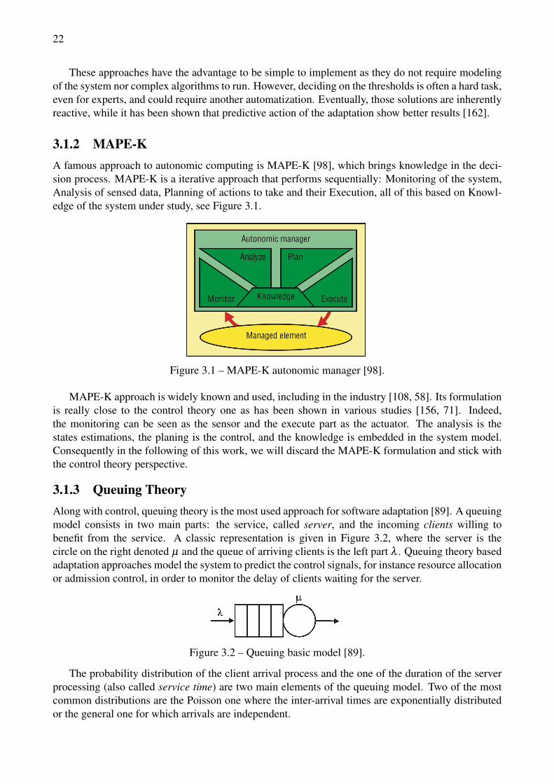
22

These approaches have the advantage to be simple to implement as they do not require modelingof the system nor complex algorithms to run. However, deciding on the thresholds is often a hard task,even for experts, and could require another automatization. Eventually, those solutions are inherentlyreactive, while it has been shown that predictive action of the adaptation show better results [162].

3.1.2 MAPE-KA famous approach to autonomic computing is MAPE-K [98], which brings knowledge in the deci-sion process. MAPE-K is a iterative approach that performs sequentially: Monitoring of the system,Analysis of sensed data, Planning of actions to take and their Execution, all of this based on Knowl-edge of the system under study, see Figure 3.1.

Figure 3.1 – MAPE-K autonomic manager [98].

MAPE-K approach is widely known and used, including in the industry [108, 58]. Its formulationis really close to the control theory one as has been shown in various studies [156, 71]. Indeed,the monitoring can be seen as the sensor and the execute part as the actuator. The analysis is thestates estimations, the planing is the control, and the knowledge is embedded in the system model.Consequently in the following of this work, we will discard the MAPE-K formulation and stick withthe control theory perspective.

3.1.3 Queuing TheoryAlong with control, queuing theory is the most used approach for software adaptation [89]. A queuingmodel consists in two main parts: the service, called server, and the incoming clients willing tobenefit from the service. A classic representation is given in Figure 3.2, where the server is thecircle on the right denoted µ and the queue of arriving clients is the left part λ . Queuing theory basedadaptation approaches model the system to predict the control signals, for instance resource allocationor admission control, in order to monitor the delay of clients waiting for the server.

Figure 3.2 – Queuing basic model [89].

The probability distribution of the client arrival process and the one of the duration of the serverprocessing (also called service time) are two main elements of the queuing model. Two of the mostcommon distributions are the Poisson one where the inter-arrival times are exponentially distributedor the general one for which arrivals are independent.

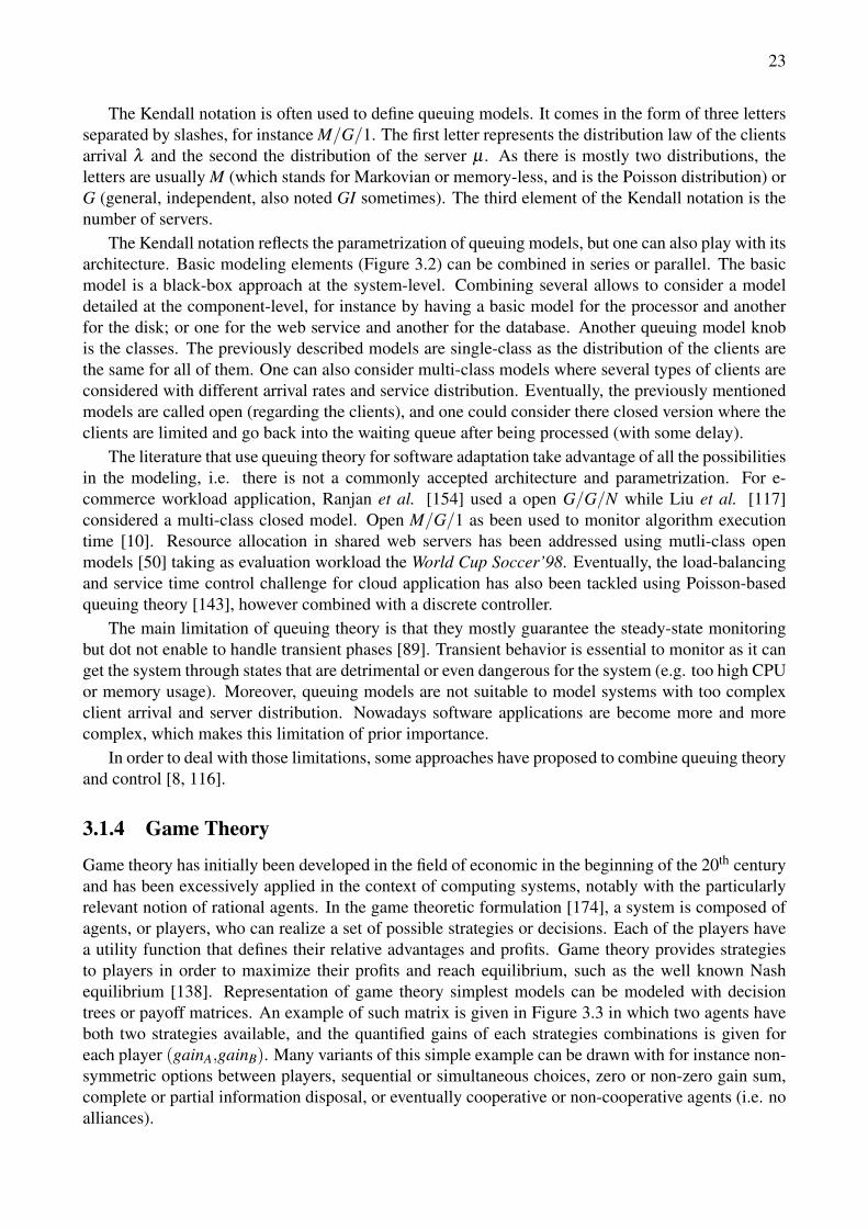
23

The Kendall notation is often used to define queuing models. It comes in the form of three lettersseparated by slashes, for instance M/G/1. The first letter represents the distribution law of the clientsarrival λ and the second the distribution of the server µ . As there is mostly two distributions, theletters are usually M (which stands for Markovian or memory-less, and is the Poisson distribution) orG (general, independent, also noted GI sometimes). The third element of the Kendall notation is thenumber of servers.

The Kendall notation reflects the parametrization of queuing models, but one can also play with itsarchitecture. Basic modeling elements (Figure 3.2) can be combined in series or parallel. The basicmodel is a black-box approach at the system-level. Combining several allows to consider a modeldetailed at the component-level, for instance by having a basic model for the processor and anotherfor the disk; or one for the web service and another for the database. Another queuing model knobis the classes. The previously described models are single-class as the distribution of the clients arethe same for all of them. One can also consider multi-class models where several types of clients areconsidered with different arrival rates and service distribution. Eventually, the previously mentionedmodels are called open (regarding the clients), and one could consider there closed version where theclients are limited and go back into the waiting queue after being processed (with some delay).

The literature that use queuing theory for software adaptation take advantage of all the possibilitiesin the modeling, i.e. there is not a commonly accepted architecture and parametrization. For e-commerce workload application, Ranjan et al. [154] used a open G/G/N while Liu et al. [117]considered a multi-class closed model. Open M/G/1 as been used to monitor algorithm executiontime [10]. Resource allocation in shared web servers has been addressed using mutli-class openmodels [50] taking as evaluation workload the World Cup Soccer’98. Eventually, the load-balancingand service time control challenge for cloud application has also been tackled using Poisson-basedqueuing theory [143], however combined with a discrete controller.

The main limitation of queuing theory is that they mostly guarantee the steady-state monitoringbut dot not enable to handle transient phases [89]. Transient behavior is essential to monitor as it canget the system through states that are detrimental or even dangerous for the system (e.g. too high CPUor memory usage). Moreover, queuing models are not suitable to model systems with too complexclient arrival and server distribution. Nowadays software applications are become more and morecomplex, which makes this limitation of prior importance.

In order to deal with those limitations, some approaches have proposed to combine queuing theoryand control [8, 116].

3.1.4 Game Theory

Game theory has initially been developed in the field of economic in the beginning of the 20th centuryand has been excessively applied in the context of computing systems, notably with the particularlyrelevant notion of rational agents. In the game theoretic formulation [174], a system is composed ofagents, or players, who can realize a set of possible strategies or decisions. Each of the players havea utility function that defines their relative advantages and profits. Game theory provides strategiesto players in order to maximize their profits and reach equilibrium, such as the well known Nashequilibrium [138]. Representation of game theory simplest models can be modeled with decisiontrees or payoff matrices. An example of such matrix is given in Figure 3.3 in which two agents haveboth two strategies available, and the quantified gains of each strategies combinations is given foreach player (gainA,gainB). Many variants of this simple example can be drawn with for instance non-symmetric options between players, sequential or simultaneous choices, zero or non-zero gain sum,complete or partial information disposal, or eventually cooperative or non-cooperative agents (i.e. noalliances).

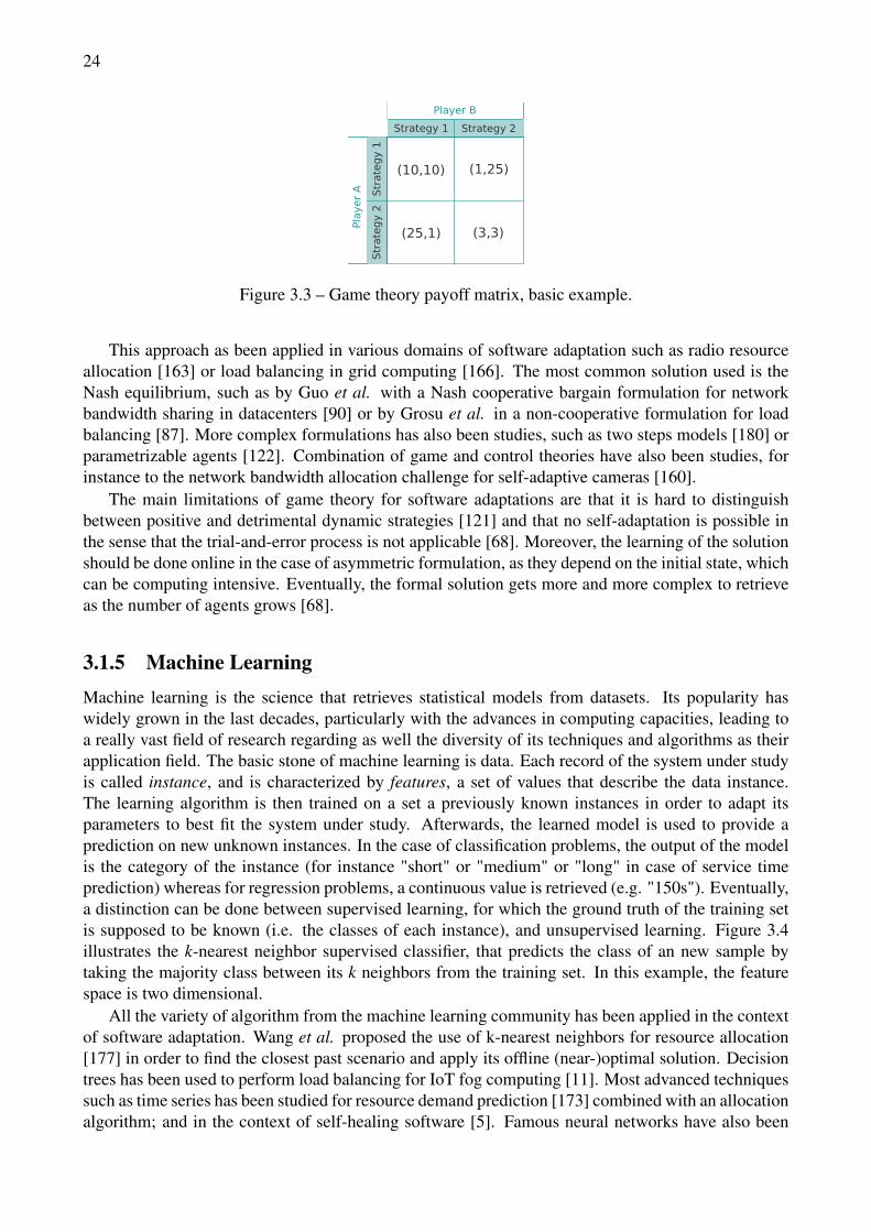
24

(3,3)

(1,25)

(25,1)

(10,10)

Strategy 1

Str

ate

gy 2

Str

ate

gy 1

Strategy 2

Player B

Pla

yer

A

Figure 3.3 – Game theory payoff matrix, basic example.

This approach as been applied in various domains of software adaptation such as radio resourceallocation [163] or load balancing in grid computing [166]. The most common solution used is theNash equilibrium, such as by Guo et al. with a Nash cooperative bargain formulation for networkbandwidth sharing in datacenters [90] or by Grosu et al. in a non-cooperative formulation for loadbalancing [87]. More complex formulations has also been studies, such as two steps models [180] orparametrizable agents [122]. Combination of game and control theories have also been studies, forinstance to the network bandwidth allocation challenge for self-adaptive cameras [160].

The main limitations of game theory for software adaptations are that it is hard to distinguishbetween positive and detrimental dynamic strategies [121] and that no self-adaptation is possible inthe sense that the trial-and-error process is not applicable [68]. Moreover, the learning of the solutionshould be done online in the case of asymmetric formulation, as they depend on the initial state, whichcan be computing intensive. Eventually, the formal solution gets more and more complex to retrieveas the number of agents grows [68].

3.1.5 Machine LearningMachine learning is the science that retrieves statistical models from datasets. Its popularity haswidely grown in the last decades, particularly with the advances in computing capacities, leading toa really vast field of research regarding as well the diversity of its techniques and algorithms as theirapplication field. The basic stone of machine learning is data. Each record of the system under studyis called instance, and is characterized by features, a set of values that describe the data instance.The learning algorithm is then trained on a set a previously known instances in order to adapt itsparameters to best fit the system under study. Afterwards, the learned model is used to provide aprediction on new unknown instances. In the case of classification problems, the output of the modelis the category of the instance (for instance "short" or "medium" or "long" in case of service timeprediction) whereas for regression problems, a continuous value is retrieved (e.g. "150s"). Eventually,a distinction can be done between supervised learning, for which the ground truth of the training setis supposed to be known (i.e. the classes of each instance), and unsupervised learning. Figure 3.4illustrates the k-nearest neighbor supervised classifier, that predicts the class of an new sample bytaking the majority class between its k neighbors from the training set. In this example, the featurespace is two dimensional.

All the variety of algorithm from the machine learning community has been applied in the contextof software adaptation. Wang et al. proposed the use of k-nearest neighbors for resource allocation[177] in order to find the closest past scenario and apply its offline (near-)optimal solution. Decisiontrees has been used to perform load balancing for IoT fog computing [11]. Most advanced techniquessuch as time series has been studied for resource demand prediction [173] combined with an allocationalgorithm; and in the context of self-healing software [5]. Famous neural networks have also been

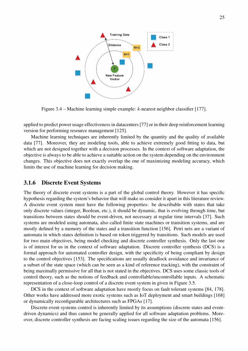
25

Figure 3.4 – Machine learning simple example: k-nearest neighbor classifier [177].

applied to predict power usage effectiveness in datacenters [77] or in their deep reinforcement learningversion for performing resource management [125].

Machine learning techniques are inherently limited by the quantity and the quality of availabledata [77]. Moreover, they are modeling tools, able to achieve extremely good fitting to data, butwhich are not designed together with a decision processes. In the context of software adaptation, theobjective is always to be able to achieve a suitable action on the system depending on the environmentchanges. This objective does not exactly overlap the one of maximizing modeling accuracy, whichlimits the use of machine learning for decision making.

3.1.6 Discrete Event SystemsThe theory of discrete event systems is a part of the global control theory. However it has specifichypothesis regarding the system’s behavior that will make us consider it apart in this literature review.A discrete event system must have the following properties: be describable with states that takeonly discrete values (integer, Boolean, etc.), it should be dynamic, that is evolving through time, buttransitions between states should be event-driven, not necessary at regular time intervals [37]. Suchsystems are modeled using automata, also called finite state machines or transition systems, and aremostly defined by a memory of the states and a transition function [156]. Petri nets are a variant ofautomata in which states definition is based on token triggered by transitions. Such models are usedfor two main objectives, being model checking and discrete controller synthesis. Only the last oneis of interest for us in the context of software adaptation. Discrete controller synthesis (DCS) is aformal approach for automated controller design, with the specificity of being compliant by designto the control objectives [153]. The specifications are usually deadlock avoidance and invariance ofa subset of the state space (which can be seen as a kind of reference tracking), with the constraint ofbeing maximally permissive for all that is not stated in the objectives. DCS uses some classic tools ofcontrol theory, such as the notions of feedback and controllable/uncontrollable inputs. A schematicrepresentation of a close-loop control of a discrete event system in given in Figure 3.5.

DCS in the context of software adaptation have mostly focus on fault tolerant systems [84, 178].Other works have addressed more exotic systems such as IoT deployment and smart buildings [168]or dynamically reconfigurable architectures such as FPGAs [17].

Discrete event systems control is inherently limited by its assumptions (discrete states and event-driven dynamics) and thus cannot be generally applied for all software adaptation problems. More-over, discrete controller synthesis are facing scaling issues regarding the size of the automata [156].

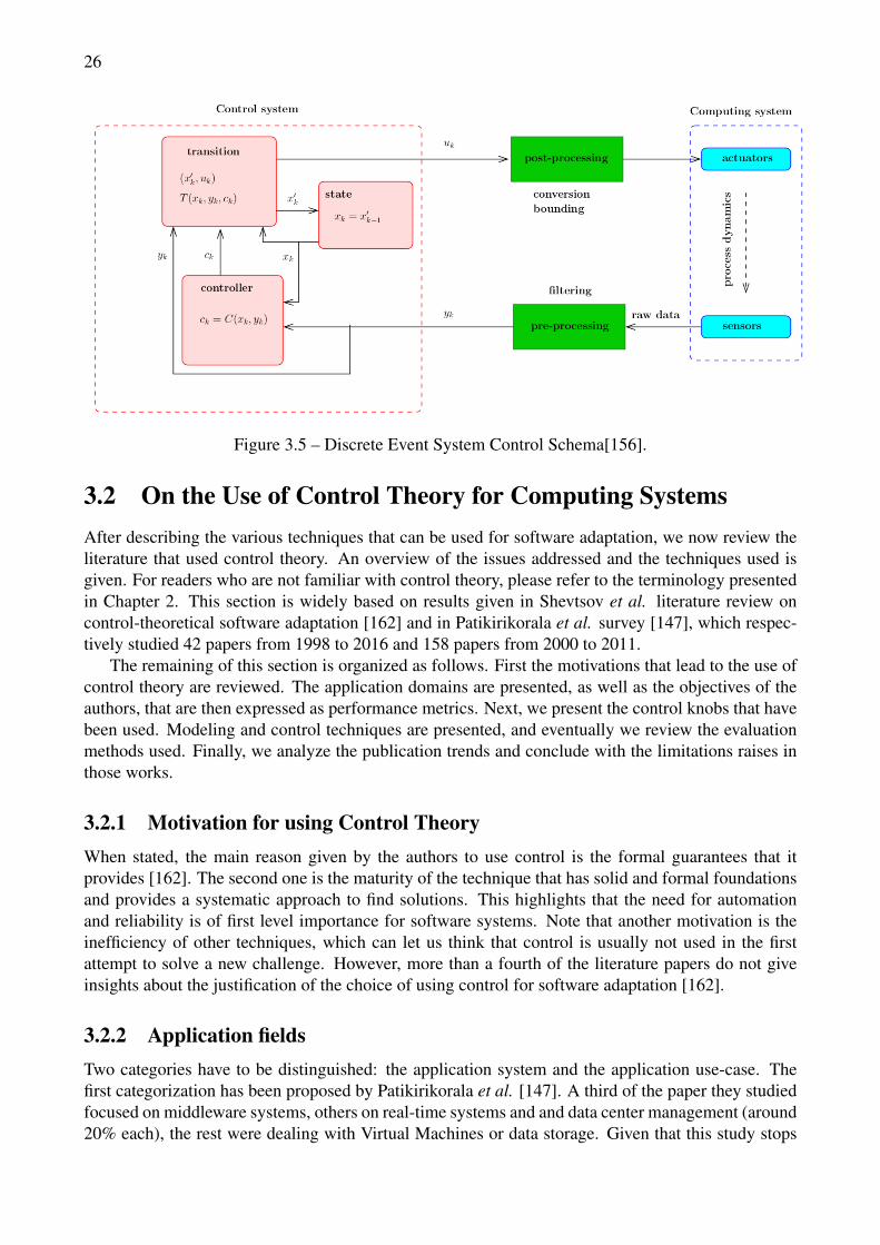
26

Figure 3.5 – Discrete Event System Control Schema[156].

3.2 On the Use of Control Theory for Computing SystemsAfter describing the various techniques that can be used for software adaptation, we now review theliterature that used control theory. An overview of the issues addressed and the techniques used isgiven. For readers who are not familiar with control theory, please refer to the terminology presentedin Chapter 2. This section is widely based on results given in Shevtsov et al. literature review oncontrol-theoretical software adaptation [162] and in Patikirikorala et al. survey [147], which respec-tively studied 42 papers from 1998 to 2016 and 158 papers from 2000 to 2011.

The remaining of this section is organized as follows. First the motivations that lead to the use ofcontrol theory are reviewed. The application domains are presented, as well as the objectives of theauthors, that are then expressed as performance metrics. Next, we present the control knobs that havebeen used. Modeling and control techniques are presented, and eventually we review the evaluationmethods used. Finally, we analyze the publication trends and conclude with the limitations raises inthose works.

3.2.1 Motivation for using Control TheoryWhen stated, the main reason given by the authors to use control is the formal guarantees that itprovides [162]. The second one is the maturity of the technique that has solid and formal foundationsand provides a systematic approach to find solutions. This highlights that the need for automationand reliability is of first level importance for software systems. Note that another motivation is theinefficiency of other techniques, which can let us think that control is usually not used in the firstattempt to solve a new challenge. However, more than a fourth of the literature papers do not giveinsights about the justification of the choice of using control for software adaptation [162].

3.2.2 Application fieldsTwo categories have to be distinguished: the application system and the application use-case. Thefirst categorization has been proposed by Patikirikorala et al. [147]. A third of the paper they studiedfocused on middleware systems, others on real-time systems and and data center management (around20% each), the rest were dealing with Virtual Machines or data storage. Given that this study stops

27

at the early 2010’s, one can expect that the proportion of virtual machine and cloud configuration issignificantly higher nowadays. However we did not found a more recent global study to highlight thispoint.

Regarding the use-case, most of the papers focus on web application (i.e. e-commerce) or on im-age or video processing [162]. Some works also focus on service-based systems and search engines.One can notice also that few works have dealt with software testing and development [34, 96].

3.2.3 ObjectivesThe three main objectives of control theory are performance, reliability and energy consumption.Some minor aspects are also taken into account, such as security or usability. They can be expressedthough three formulations: setpoint tracking, with eventually confidence intervals, disturbance rejec-tion and minimization or maximization of a quantity (with the use of a cost function if some goals areconflicting). According to Shevtsov et al. [162], 85% of the works are motivated by changes in theenvironment (disturbance rejection), 70% by changes in the requirements (i.e. set point) and fewer(15%) are also driven by changes in the software itself.

3.2.4 Sensors and performance metricsMetrics measured by sensors can be distinguished in three main categories: software utility, resourceutilization and software inefficiency [162]. The utility is measured with variables such as responsetime (in around 40% of the papers [147]), throughput, latency or video quality and processing speed.Resource utilization gathers processor/CPU/memory utilization, power consumption and bandwidth.Eventually, software inefficiency is measured with metrics such as miss ratio or failure rate.

Note that only 15% of the papers describe the sensor and its implementation, while the vast ma-jority only describe the metrics used [162].

3.2.5 Actuators and control signalThe actuators being highly application dependent, their categorization is not a easy task. Three typesof actuators have been identified [162]: parametric, component or mode adaptation. Parametric adap-tations are the modification of the parameters of the software system, for instance the degree of qualityof a filter. Component adaptation intervene a degree of abstraction higher, for example the load of aservice or the number of service instances. Eventually, mode change can be for instance a switch tothe preference given to each service.

The particularity of software adaptation regarding actuator is that it is rather easy to create andremove some [71]. However, one should be specifically careful when designing an actuator (the samecan apply to sensors) that this later is consistent with further modifications of the software understudy.

3.2.6 ModelingThe most common model used for software applications is a linear, time-invariant black-box discretemodel [162, 147]. In this case, the link between the control signal and the performance metric is linear(i.e. not quadratic, exponential, etc.), the parameters do not depends on the time variable, and thislater is considered at regular time intervals (not in a continuous way). The parameters of the modelare found using system identification techniques, that subtly solicit the system, record its behaviorand fit it with a model. The use of black-box is particularly spread because its an easy process thatcan deal with highly complex systems and still enable to derive performance guarantees. Even though

28

many studies state that their system is non-linear, linear modeling is preferred, maybe because of lackof tools as simple and practical in the non-linear case.

However, when linear black-box is not used, models tends to be non-linear and analytical [162],even though it represents a smaller portion of the literature. Most of the combination in terms oflinearity, continuity, time-variance and model type (analytical of black-box) can still be found in thestate of the art, even though only the two above mentioned combinations are popular.

As for the dimensions of the model, 60% are MIMO (multi-inputs multi-outputs) while 40% areSISO (single input and output) [147].

3.2.7 ControlAlmost all the controllers used were including feedback, and a small portion of them where also usingfeedforward to deal with workload rates [147]. The most used controller is by far the PID one (50%of the reviewed papers [162]), with a preference for its PI declination. They are mainly used in SISOscenarios, for regulation and tracking objectives, and are most of the time adaptive to compensate forthe linear modeling of a non-linear system. The second main trend is the use of Model PredictiveControllers, mostly with MIMO discrete time models, in a non adaptive formulation, to deal with aminimization or maximization objective.

Some specific structures of controller can also be found, such as hierarchical control, switchingcontrol or cascaded control.

3.2.8 EvaluationThree kind of evaluation methods are used: formal analyze, simulations and real-case experimentalstudy. All three are widely used, simulations being however quite limited, and the quality and the gen-eralizability of experimental use-cases are limited. Some benchmark and workloads are commonlyused for some works such as [147]. The main qualities that are looked at are indeed performance,efficiency, costs and reliability. The metrics used to guarantee those later properties in control theoryare stability, settling time, overshoot, steady state error, robustness, optimality and control signal us-age [162]. All of them are commonly used for evaluation, stability and settling time being the mostspread ones.

3.2.9 Publications trendsAside from the technical content of papers, two interesting metadata to look at are the publicationyear of the papers as well as their venue. Both review papers [147, 162] concluded that the numberof publication per year is significantly increasing, showing a growing interest of control theory forsoftware adaptation. They also reported that the source of publication of such contributions are largelyspread among venues and communities. There is however a higher number of paper published inthe software engineering community, showing a higher interest in using control theory as a tool forsolving software issues as to use computing systems adaptation as a playground for control scientists,at least from the point of view of the global communities.

3.2.10 Limitations and open challengesEach design step previously detailed is subject to limitations. Using control theory for software re-quire the use of new sensors and actuators that were not included in the design phase, such as theevaluation of the cost of adaptation. Some others are crucial notions that however still lack of com-monly accepted metrics, such a security, resilience or privacy. From an architectural/implementation

29

point of view, actuators and sensors need to be consistent and evolve with the different versions of thesoftware.

The most common type of modeling used (linear time invariant discrete model) is still ineffectivewhen dealing with sharp and drastic disturbances. More research need to be done regarding theproperties of the models and how to chose them (linearity, continuity, etc.). The same conclusioncan be drawn about controllers. Even though various types of controller are used, few research hasbeen done to derive a systematic procedure regarding how to chose the best controller type. A recentstudy has highlighted the promises of using more advanced modeling and control techniques such asclosed-loop metrics or real-time cooperative model predictive controllers [99].

Eventually, while the formal background of control theory is often cited at the number one rea-son to choose this technique compared to another, the analysis of these guarantees in the evaluationprocess is many times missing.

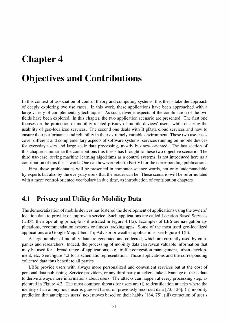
Chapter 4

Objectives and Contributions

In this context of association of control theory and computing systems, this thesis take the approachof deeply exploring two use cases. In this work, these applications have been approached with alarge variety of complementary techniques. As such, diverse aspects of the combination of the twofields have been explored. In this chapter, the two application scenario are presented. The first onefocuses on the protection of mobility-related privacy of mobile devices’ users, while ensuring theusability of geo-localized services. The second one deals with BigData cloud services and how toensure their performance and reliability in their extremely variable environment. These two use-casescover different and complementary aspects of software systems, services running on mobile devicesfor everyday users and large scale data processing, mostly business oriented. The last section ofthis chapter summarize the contributions this thesis has brought to these two objective scenario. Thethird use-case, seeing machine learning algorithms as a control systems, is not introduced here as acontribution of this thesis work. One can however refer to Part VI for the corresponding publications.

First, these problematics will be presented in computer-science words, not only understandableby experts but also by the everyday users that the reader can be. These scenario will be reformulatedwith a more control-oriented vocabulary in due time, as introduction of contribution chapters.

4.1 Privacy and Utility for Mobility Data

The democratization of mobile devices has fostered the development of applications using the owners’location data to provide or improve a service. Such applications are called Location Based Services(LBS), their operating principle is illustrated in Figure 4.1(a). Examples of LBS are navigation ap-plications, recommendation systems or fitness tracking apps. Some of the most used geo-localizedapplications are Google Map, Uber, TripAdvisor or weather applications, see Figure 4.1(b).

A large number of mobility data are generated and collected, which are currently used by com-panies and researchers. Indeed, the processing of mobility data can reveal valuable information thatmay be used for a broad range of applications, e.g., traffic congestion management, urban develop-ment, etc. See Figure 4.2 for a schematic representation. Those applications and the correspondingcollected data thus benefit to all parties.

LBSs provide users with always more personalized and convenient services but at the cost ofpersonal data publishing. Service providers, or any third party attackers, take advantage of these datato derive always more informations about users. The attacks can happen at every processing step, aspictured in Figure 4.2. The most common threats for users are (i) reidentification attacks where theidentity of an anonymous user is guessed based on previously recorded data [73, 126], (ii) mobilityprediction that anticipates users’ next moves based on their habits [184, 75], (iii) extraction of user’s

31

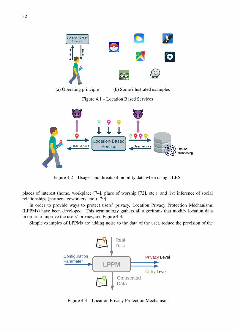
32

(a) Operating principle (b) Some illustrated examples

Figure 4.1 – Location Based Services

Figure 4.2 – Usages and threats of mobility data when using a LBS.

places of interest (home, workplace [74], place of worship [72], etc.) and (iv) inference of socialrelationships (partners, coworkers, etc.) [29].

In order to provide ways to protect users’ privacy, Location Privacy Protection Mechanisms(LPPMs) have been developed. This terminology gathers all algorithms that modify location datain order to improve the users’ privacy, see Figure 4.3.

Simple examples of LPPMs are adding noise to the data of the user, reduce the precision of the

Figure 4.3 – Location Privacy Protection Mechanism

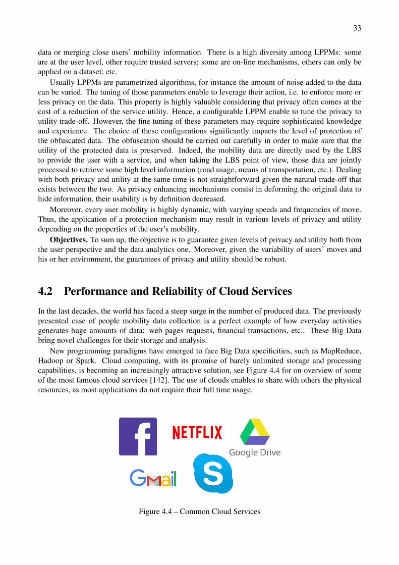
33

data or merging close users’ mobility information. There is a high diversity among LPPMs: someare at the user level, other require trusted servers; some are on-line mechanisms, others can only beapplied on a dataset; etc.

Usually LPPMs are parametrized algorithms, for instance the amount of noise added to the datacan be varied. The tuning of those parameters enable to leverage their action, i.e. to enforce more orless privacy on the data. This property is highly valuable considering that privacy often comes at thecost of a reduction of the service utility. Hence, a configurable LPPM enable to tune the privacy toutility trade-off. However, the fine tuning of these parameters may require sophisticated knowledgeand experience. The choice of these configurations significantly impacts the level of protection ofthe obfuscated data. The obfuscation should be carried out carefully in order to make sure that theutility of the protected data is preserved. Indeed, the mobility data are directly used by the LBSto provide the user with a service, and when taking the LBS point of view, those data are jointlyprocessed to retrieve some high level information (road usage, means of transportation, etc.). Dealingwith both privacy and utility at the same time is not straightforward given the natural trade-off thatexists between the two. As privacy enhancing mechanisms consist in deforming the original data tohide information, their usability is by definition decreased.

Moreover, every user mobility is highly dynamic, with varying speeds and frequencies of move.Thus, the application of a protection mechanism may result in various levels of privacy and utilitydepending on the properties of the user’s mobility.

Objectives. To sum up, the objective is to guarantee given levels of privacy and utility both fromthe user perspective and the data analytics one. Moreover, given the variability of users’ moves andhis or her environment, the guarantees of privacy and utility should be robust.

4.2 Performance and Reliability of Cloud ServicesIn the last decades, the world has faced a steep surge in the number of produced data. The previouslypresented case of people mobility data collection is a perfect example of how everyday activitiesgenerates huge amounts of data: web pages requests, financial transactions, etc.. These Big Databring novel challenges for their storage and analysis.

New programming paradigms have emerged to face Big Data specificities, such as MapReduce,Hadoop or Spark. Cloud computing, with its promise of barely unlimited storage and processingcapabilities, is becoming an increasingly attractive solution, see Figure 4.4 for on overview of someof the most famous cloud services [142]. The use of clouds enables to share with others the physicalresources, as most applications do not require their full time usage.

Figure 4.4 – Common Cloud Services

34

One of the biggest appeals of cloud computing is the on-demand assigning of shared hardwareresources to software applications, called elastic resource provisioning. This enables to provide moreresources to applications that need it when they need it, and thus try to optimize the resource usage.Therefore, there is a growing need for frameworks that efficiently deal with the dynamics of clusterresources [119].

Current autonomic resource provisioning approaches that are deployed in public clouds still don’twork optimally for real time applications. In most clouds, if an application has to meet run timecriteria, a reactive algorithm scales the resources to the demand. However, it requires high level ofexpertise to decide on how much to intervene, as it depends on many factors that are not necessarydirectly accessible. The difficulty of the task is increased by the fact that the optimal configurationcan vary due to the shared use of hardware resources or workloads fluctuations over time [20], amongmany other factors [103]. Therefore, there is a need for fully automatized and robust cluster scalingalgorithms able to deal with these environment disturbances.

Ensuring service performance is essential as missing deadlines result in consequent financiallosses. It is estimated that an on-line brokerage industry service unavailability costs around 100.000$per minute. For on-line shopping companies, page load-time should not be more than 2 seconds orusers tend to give up their shopping or switch to another seller, resulting in revenue loss for companies[137]. Figure 4.5 gives examples of unmastered resource usage that led to significant consequencesfor companies. Cloud providers have to guarantee service performance and availability in order towin users’ loyalty and avoid to huge financial impacts.

Figure 4.5 – News breaks showing that unmastered resource leads to service unavailability. All out-ages were caused by unusual workload, where some where however expected to be of huge amplitude.

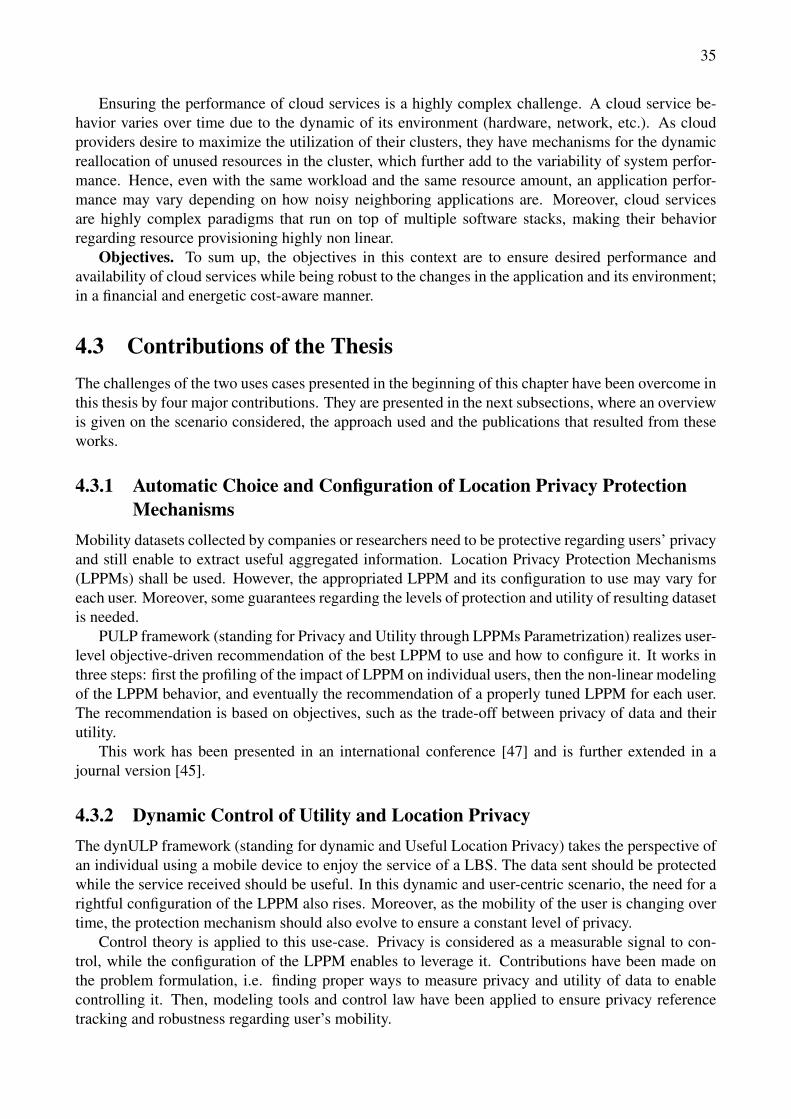
35

Ensuring the performance of cloud services is a highly complex challenge. A cloud service be-havior varies over time due to the dynamic of its environment (hardware, network, etc.). As cloudproviders desire to maximize the utilization of their clusters, they have mechanisms for the dynamicreallocation of unused resources in the cluster, which further add to the variability of system perfor-mance. Hence, even with the same workload and the same resource amount, an application perfor-mance may vary depending on how noisy neighboring applications are. Moreover, cloud servicesare highly complex paradigms that run on top of multiple software stacks, making their behaviorregarding resource provisioning highly non linear.

Objectives. To sum up, the objectives in this context are to ensure desired performance andavailability of cloud services while being robust to the changes in the application and its environment;in a financial and energetic cost-aware manner.

4.3 Contributions of the ThesisThe challenges of the two uses cases presented in the beginning of this chapter have been overcome inthis thesis by four major contributions. They are presented in the next subsections, where an overviewis given on the scenario considered, the approach used and the publications that resulted from theseworks.

4.3.1 Automatic Choice and Configuration of Location Privacy ProtectionMechanisms

Mobility datasets collected by companies or researchers need to be protective regarding users’ privacyand still enable to extract useful aggregated information. Location Privacy Protection Mechanisms(LPPMs) shall be used. However, the appropriated LPPM and its configuration to use may vary foreach user. Moreover, some guarantees regarding the levels of protection and utility of resulting datasetis needed.

PULP framework (standing for Privacy and Utility through LPPMs Parametrization) realizes user-level objective-driven recommendation of the best LPPM to use and how to configure it. It works inthree steps: first the profiling of the impact of LPPM on individual users, then the non-linear modelingof the LPPM behavior, and eventually the recommendation of a properly tuned LPPM for each user.The recommendation is based on objectives, such as the trade-off between privacy of data and theirutility.

This work has been presented in an international conference [47] and is further extended in ajournal version [45].

4.3.2 Dynamic Control of Utility and Location PrivacyThe dynULP framework (standing for dynamic and Useful Location Privacy) takes the perspective ofan individual using a mobile device to enjoy the service of a LBS. The data sent should be protectedwhile the service received should be useful. In this dynamic and user-centric scenario, the need for arightful configuration of the LPPM also rises. Moreover, as the mobility of the user is changing overtime, the protection mechanism should also evolve to ensure a constant level of privacy.

Control theory is applied to this use-case. Privacy is considered as a measurable signal to con-trol, while the configuration of the LPPM enables to leverage it. Contributions have been made onthe problem formulation, i.e. finding proper ways to measure privacy and utility of data to enablecontrolling it. Then, modeling tools and control law have been applied to ensure privacy referencetracking and robustness regarding user’s mobility.

36

The work can be found in two international conferences [38, 49] and a journal submission is underreview.

4.3.3 Adaptive Control for Cloud Service Performance Robust to Plant andEnvironment Changes

The cost of cloud services is continuously decreasing, hence service performance is becoming a keydifferentiator between providers. Solutions that aim to guarantee Service Level Objectives (SLO) interm of performance by controlling cluster size are already used by cloud providers. However mostof these control solutions are based on static if-then rules, they are therefore inefficient in handlingthe highly varying service dynamics of cloud environments.

In this thesis, a novel adaptive control approach realizing resource allocation is presented that isrobust to these phenomena. It consists of PI and feedforward controller which parameters are adaptedonline. The use of adaptation enables to improve control efficiency and robustness with respect tovariations in the dynamic of the system.

Results of this approach have been presented in two international conferences [43, 110].

4.3.4 Cost-aware Optimal Control of Performance and Availability of CloudServices

High rate cluster reconfigurations is a costly issue in Big Data Cloud services. Current control solu-tions manage to scale the cluster according to the workload, however they do not try to minimize thenumber of system reconfigurations.

This thesis presents a novel event-triggered optimal control approach. The triggering mechanismrelies on a Model Predictive Controller and is defined upon the value of the optimal cost function,to reduce the number of control changes but also ensures a very reactive behavior to changes ofexogenous inputs.

This work has lead to a publication in the control community [41].

Part II

Privacy and Utility Aware Control of Users’Mobility Data

37

39

This part tackles the issue of location privacy, i.e. the protection of people’s privacy for whomtheir mobility information is shared with untrusted parties. Two scenario appear: (i) the locations arebroadcasted in exchange of a service delivered to the mobile device user, e.g. a geo-located weatherforecast, or (ii) datasets of many users are used to performs analytics, e.g. finding the most crowdedstreets in a city. In both cases, two main notions can be identified: knowing the privacy protection ofmobile devices holders and the utility or quality of the service.

The tools of modeling, configuration and control for this use-case is presented here. Chapter 6presents PULP (Privacy and Utility through LPPM Parametrization), a framework that address thestatic scenario where a mobility database has been recorded and privacy protection needs to be per-formed, wisely in order to ensure some accuracy of the performed analytics on it. Such scenario isparticularly pervading since the European regulation GPDR effective since May 2018 [79]. PULPfinds the best Location Privacy Protection Mechanism and configures it at a user granularity to satisfyboth privacy and utility objectives. Chapter 7 presents dynULP (dynamic Utility-preserving Loca-tion Privacy) the user-side version of PULP, which performs online protection of location data beforesending it to a third party while keeping a eye on the returned service quality. In dynULP, the actionof the protection mechanism is leveraged on line to cope with changes in users’ mobility and envi-ronment, and its objectives are driven in a way that enables the user to choose high utility when sheneeds it, and enforced privacy (i.e. relaxed utility) otherwise. Beforehand, Chapter 5 gives all thecontext and background needed to fully understand the data and mechanisms involved, and presentthe related works from the state of the art. Eventually, Chapter 8 concludes on the contributions ofthose works regarding location privacy, and gives perspectives for future works.

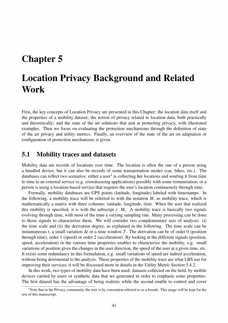
Chapter 5

Location Privacy Background and RelatedWork

First, the key concepts of Location Privacy are presented in this Chapter: the location data itself andthe properties of a mobility dataset; the notion of privacy related to location data, both practicallyand theoretically; and the state of the art solutions that aim at protecting privacy, with illustratedexamples. Then we focus on evaluating the protection mechanisms through the definition of stateof the art privacy and utility metrics. Finally, an overview of the state of the art on adaptation orconfiguration of protection mechanisms is given.

5.1 Mobility traces and datasetsMobility data are records of locations over time. The location is often the one of a person usinga handled device, but it can also be records of some transportation modes (car, bikes, etc.). Thedatabases can reflect two scenarios: either a user1 is collecting her locations and sending it from timeto time to an external service (e.g. crowdsensing applications) possibly with some remuneration; or aperson is using a location-based service that requires the user’s location continuously through time.

Formally, mobility databases are GPS points (latitude, longitude) labeled with timestamps. Inthe following, a mobility trace will be referred to with the notation M, as mobility trace, which ismathematically a matrix with three columns: latitude, longitude, time. When the user that realizedthis mobility is specified, it is with the subscript i: Mi. A mobility trace is basically two signalsevolving through time, with most of the time a varying sampling rate. Many processing can be doneto those signals to characterize them. We will consider two complementary axis of analysis: (i)the time scale and (ii) the derivation degree, as explained in the following. The time scale can beinstantaneous t, a small variation ∆t or a time window T . The derivation can be of order 0 (positionthrough time), order 1 (speed) or order 2 (acceleration). By looking at the different signals (position,speed, acceleration) in the various time properties enables to characterize the mobility, e.g. smallvariations of position gives the changes in the user direction, the speed of the user at a given time, etc.It exists some redundancy in this formulation, e.g. small variations of speed are indeed acceleration,without being detrimental to the analysis. These properties of the mobility trace are what LBS use forimproving their services, it will be discussed more in details in the Utility Metric Section 5.4.2.

In this work, two types of mobility data have been used: datasets collected on the field, by mobiledevices carried by users or synthetic data that we generated in order to emphasis some properties.The first dataset has the advantage of being realistic while the second enable to control and cover

1Note that in the Privacy community, the user is by convention referred to as a female. This usage will be kept for therest of this manuscript.

41

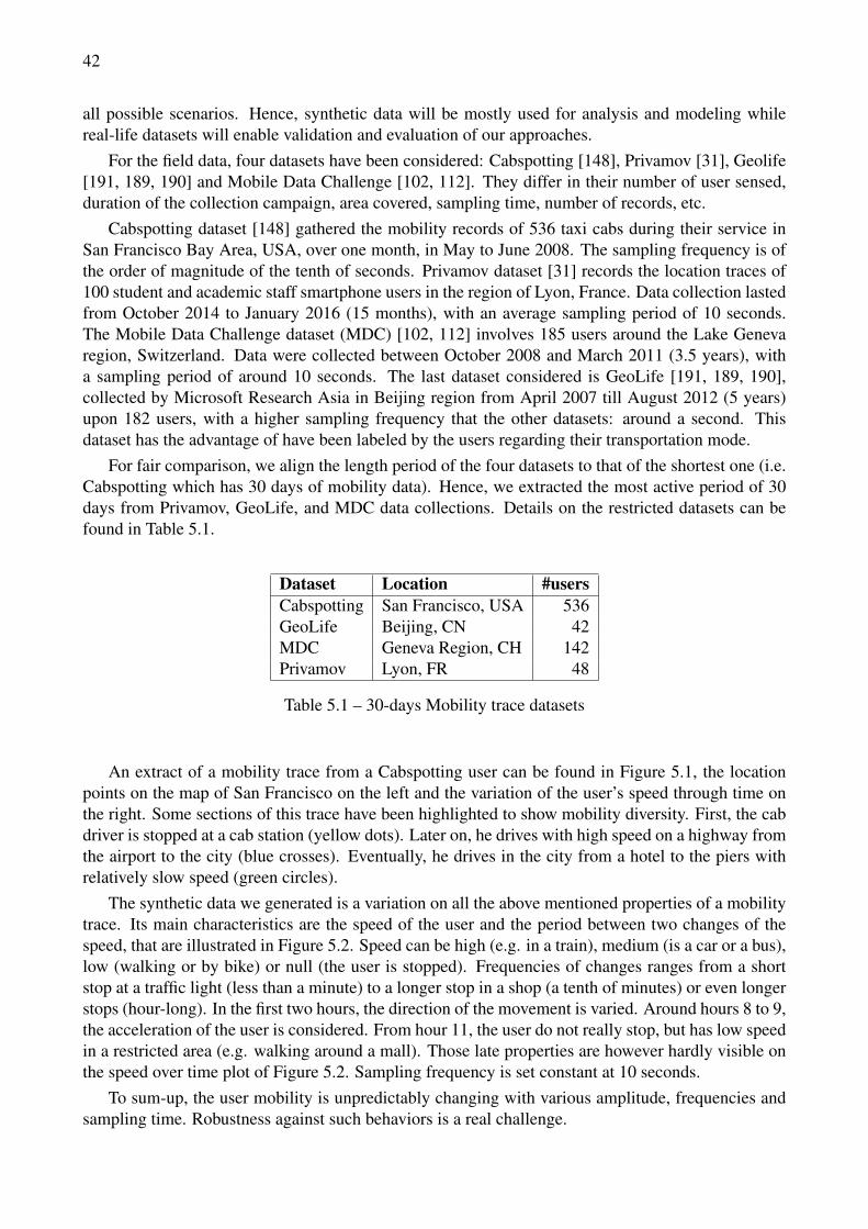
42

all possible scenarios. Hence, synthetic data will be mostly used for analysis and modeling whilereal-life datasets will enable validation and evaluation of our approaches.

For the field data, four datasets have been considered: Cabspotting [148], Privamov [31], Geolife[191, 189, 190] and Mobile Data Challenge [102, 112]. They differ in their number of user sensed,duration of the collection campaign, area covered, sampling time, number of records, etc.

Cabspotting dataset [148] gathered the mobility records of 536 taxi cabs during their service inSan Francisco Bay Area, USA, over one month, in May to June 2008. The sampling frequency is ofthe order of magnitude of the tenth of seconds. Privamov dataset [31] records the location traces of100 student and academic staff smartphone users in the region of Lyon, France. Data collection lastedfrom October 2014 to January 2016 (15 months), with an average sampling period of 10 seconds.The Mobile Data Challenge dataset (MDC) [102, 112] involves 185 users around the Lake Genevaregion, Switzerland. Data were collected between October 2008 and March 2011 (3.5 years), witha sampling period of around 10 seconds. The last dataset considered is GeoLife [191, 189, 190],collected by Microsoft Research Asia in Beijing region from April 2007 till August 2012 (5 years)upon 182 users, with a higher sampling frequency that the other datasets: around a second. Thisdataset has the advantage of have been labeled by the users regarding their transportation mode.

For fair comparison, we align the length period of the four datasets to that of the shortest one (i.e.Cabspotting which has 30 days of mobility data). Hence, we extracted the most active period of 30days from Privamov, GeoLife, and MDC data collections. Details on the restricted datasets can befound in Table 5.1.

Dataset Location #usersCabspotting San Francisco, USA 536GeoLife Beijing, CN 42MDC Geneva Region, CH 142Privamov Lyon, FR 48

Table 5.1 – 30-days Mobility trace datasets

An extract of a mobility trace from a Cabspotting user can be found in Figure 5.1, the locationpoints on the map of San Francisco on the left and the variation of the user’s speed through time onthe right. Some sections of this trace have been highlighted to show mobility diversity. First, the cabdriver is stopped at a cab station (yellow dots). Later on, he drives with high speed on a highway fromthe airport to the city (blue crosses). Eventually, he drives in the city from a hotel to the piers withrelatively slow speed (green circles).

The synthetic data we generated is a variation on all the above mentioned properties of a mobilitytrace. Its main characteristics are the speed of the user and the period between two changes of thespeed, that are illustrated in Figure 5.2. Speed can be high (e.g. in a train), medium (is a car or a bus),low (walking or by bike) or null (the user is stopped). Frequencies of changes ranges from a shortstop at a traffic light (less than a minute) to a longer stop in a shop (a tenth of minutes) or even longerstops (hour-long). In the first two hours, the direction of the movement is varied. Around hours 8 to 9,the acceleration of the user is considered. From hour 11, the user do not really stop, but has low speedin a restricted area (e.g. walking around a mall). Those late properties are however hardly visible onthe speed over time plot of Figure 5.2. Sampling frequency is set constant at 10 seconds.

To sum-up, the user mobility is unpredictably changing with various amplitude, frequencies andsampling time. Robustness against such behaviors is a real challenge.

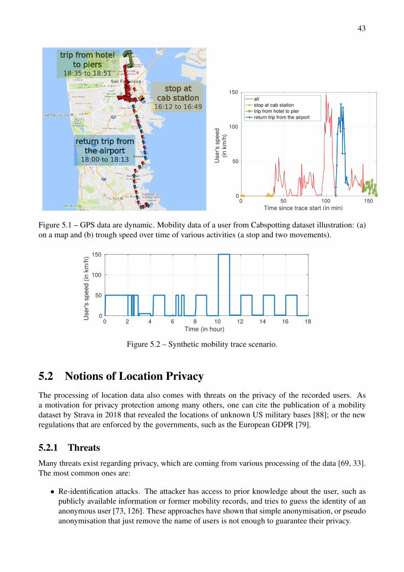
43

trip from hotelto piers

18:35 to 18:51

stop at cab station

16:12 to 16:49

return trip fromthe airport

18:00 to 18:13

0 50 100 150Time since trace start (in min)

0

50

100

150

Use

r's s

peed

(in k

m/h

)

allstop at cab stationtrip from hotel to pierreturn trip from the airport

Figure 5.1 – GPS data are dynamic. Mobility data of a user from Cabspotting dataset illustration: (a)on a map and (b) trough speed over time of various activities (a stop and two movements).

0 2 4 6 8 10 12 14 16 18Time (in hour)

0

50

100

150

Use

r's s

peed

(in

km/h

)

Figure 5.2 – Synthetic mobility trace scenario.

5.2 Notions of Location PrivacyThe processing of location data also comes with threats on the privacy of the recorded users. Asa motivation for privacy protection among many others, one can cite the publication of a mobilitydataset by Strava in 2018 that revealed the locations of unknown US military bases [88]; or the newregulations that are enforced by the governments, such as the European GDPR [79].

5.2.1 ThreatsMany threats exist regarding privacy, which are coming from various processing of the data [69, 33].The most common ones are:

• Re-identification attacks. The attacker has access to prior knowledge about the user, such aspublicly available information or former mobility records, and tries to guess the identity of ananonymous user [73, 126]. These approaches have shown that simple anonymisation, or pseudoanonymisation that just remove the name of users is not enough to guarantee their privacy.

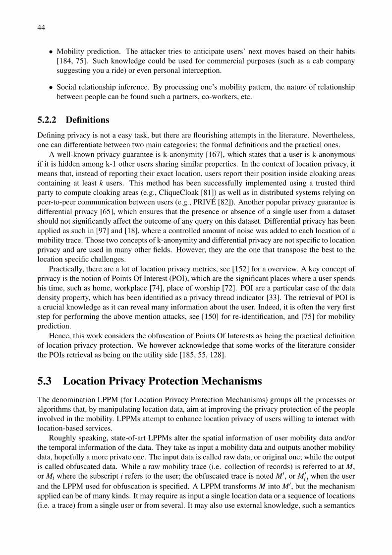
44

• Mobility prediction. The attacker tries to anticipate users’ next moves based on their habits[184, 75]. Such knowledge could be used for commercial purposes (such as a cab companysuggesting you a ride) or even personal interception.

• Social relationship inference. By processing one’s mobility pattern, the nature of relationshipbetween people can be found such a partners, co-workers, etc.

5.2.2 DefinitionsDefining privacy is not a easy task, but there are flourishing attempts in the literature. Nevertheless,one can differentiate between two main categories: the formal definitions and the practical ones.

A well-known privacy guarantee is k-anonymity [167], which states that a user is k-anonymousif it is hidden among k-1 other users sharing similar properties. In the context of location privacy, itmeans that, instead of reporting their exact location, users report their position inside cloaking areascontaining at least k users. This method has been successfully implemented using a trusted thirdparty to compute cloaking areas (e.g., CliqueCloak [81]) as well as in distributed systems relying onpeer-to-peer communication between users (e.g., PRIVÉ [82]). Another popular privacy guarantee isdifferential privacy [65], which ensures that the presence or absence of a single user from a datasetshould not significantly affect the outcome of any query on this dataset. Differential privacy has beenapplied as such in [97] and [18], where a controlled amount of noise was added to each location of amobility trace. Those two concepts of k-anonymity and differential privacy are not specific to locationprivacy and are used in many other fields. However, they are the one that transpose the best to thelocation specific challenges.

Practically, there are a lot of location privacy metrics, see [152] for a overview. A key concept ofprivacy is the notion of Points Of Interest (POI), which are the significant places where a user spendshis time, such as home, workplace [74], place of worship [72]. POI are a particular case of the datadensity property, which has been identified as a privacy thread indicator [33]. The retrieval of POI isa crucial knowledge as it can reveal many information about the user. Indeed, it is often the very firststep for performing the above mention attacks, see [150] for re-identification, and [75] for mobilityprediction.

Hence, this work considers the obfuscation of Points Of Interests as being the practical definitionof location privacy protection. We however acknowledge that some works of the literature considerthe POIs retrieval as being on the utility side [185, 55, 128].

5.3 Location Privacy Protection MechanismsThe denomination LPPM (for Location Privacy Protection Mechanisms) groups all the processes oralgorithms that, by manipulating location data, aim at improving the privacy protection of the peopleinvolved in the mobility. LPPMs attempt to enhance location privacy of users willing to interact withlocation-based services.

Roughly speaking, state-of-art LPPMs alter the spatial information of user mobility data and/orthe temporal information of the data. They take as input a mobility data and outputs another mobilitydata, hopefully a more private one. The input data is called raw data, or original one; while the outputis called obfuscated data. While a raw mobility trace (i.e. collection of records) is referred to at M,or Mi where the subscript i refers to the user; the obfuscated trace is noted M′, or M′i j when the userand the LPPM used for obfuscation is specified. A LPPM transforms M into M′, but the mechanismapplied can be of many kinds. It may require as input a single location data or a sequence of locations(i.e. a trace) from a single user or from several. It may also use external knowledge, such a semantics

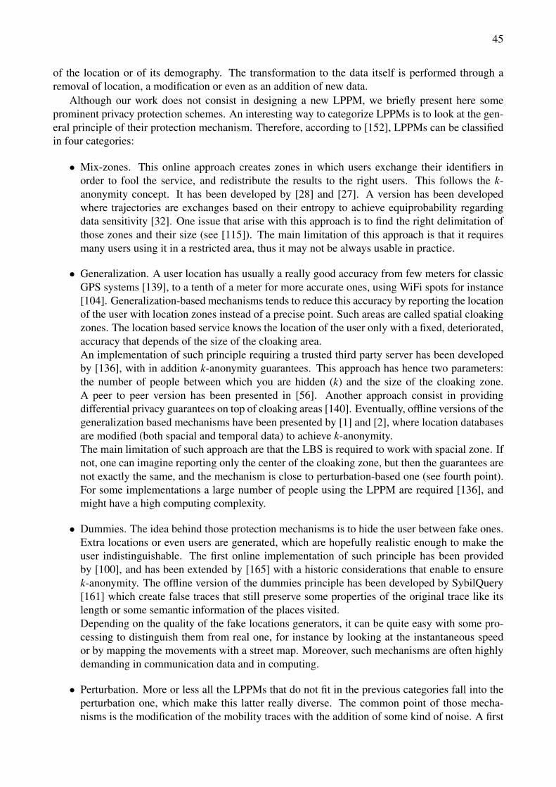
45

of the location or of its demography. The transformation to the data itself is performed through aremoval of location, a modification or even as an addition of new data.

Although our work does not consist in designing a new LPPM, we briefly present here someprominent privacy protection schemes. An interesting way to categorize LPPMs is to look at the gen-eral principle of their protection mechanism. Therefore, according to [152], LPPMs can be classifiedin four categories:

• Mix-zones. This online approach creates zones in which users exchange their identifiers inorder to fool the service, and redistribute the results to the right users. This follows the k-anonymity concept. It has been developed by [28] and [27]. A version has been developedwhere trajectories are exchanges based on their entropy to achieve equiprobability regardingdata sensitivity [32]. One issue that arise with this approach is to find the right delimitation ofthose zones and their size (see [115]). The main limitation of this approach is that it requiresmany users using it in a restricted area, thus it may not be always usable in practice.

• Generalization. A user location has usually a really good accuracy from few meters for classicGPS systems [139], to a tenth of a meter for more accurate ones, using WiFi spots for instance[104]. Generalization-based mechanisms tends to reduce this accuracy by reporting the locationof the user with location zones instead of a precise point. Such areas are called spatial cloakingzones. The location based service knows the location of the user only with a fixed, deteriorated,accuracy that depends of the size of the cloaking area.An implementation of such principle requiring a trusted third party server has been developedby [136], with in addition k-anonymity guarantees. This approach has hence two parameters:the number of people between which you are hidden (k) and the size of the cloaking zone.A peer to peer version has been presented in [56]. Another approach consist in providingdifferential privacy guarantees on top of cloaking areas [140]. Eventually, offline versions of thegeneralization based mechanisms have been presented by [1] and [2], where location databasesare modified (both spacial and temporal data) to achieve k-anonymity.The main limitation of such approach are that the LBS is required to work with spacial zone. Ifnot, one can imagine reporting only the center of the cloaking zone, but then the guarantees arenot exactly the same, and the mechanism is close to perturbation-based one (see fourth point).For some implementations a large number of people using the LPPM are required [136], andmight have a high computing complexity.

• Dummies. The idea behind those protection mechanisms is to hide the user between fake ones.Extra locations or even users are generated, which are hopefully realistic enough to make theuser indistinguishable. The first online implementation of such principle has been providedby [100], and has been extended by [165] with a historic considerations that enable to ensurek-anonymity. The offline version of the dummies principle has been developed by SybilQuery[161] which create false traces that still preserve some properties of the original trace like itslength or some semantic information of the places visited.Depending on the quality of the fake locations generators, it can be quite easy with some pro-cessing to distinguish them from real one, for instance by looking at the instantaneous speedor by mapping the movements with a street map. Moreover, such mechanisms are often highlydemanding in communication data and in computing.

• Perturbation. More or less all the LPPMs that do not fit in the previous categories fall into theperturbation one, which make this latter really diverse. The common point of those mecha-nisms is the modification of the mobility traces with the addition of some kind of noise. A first

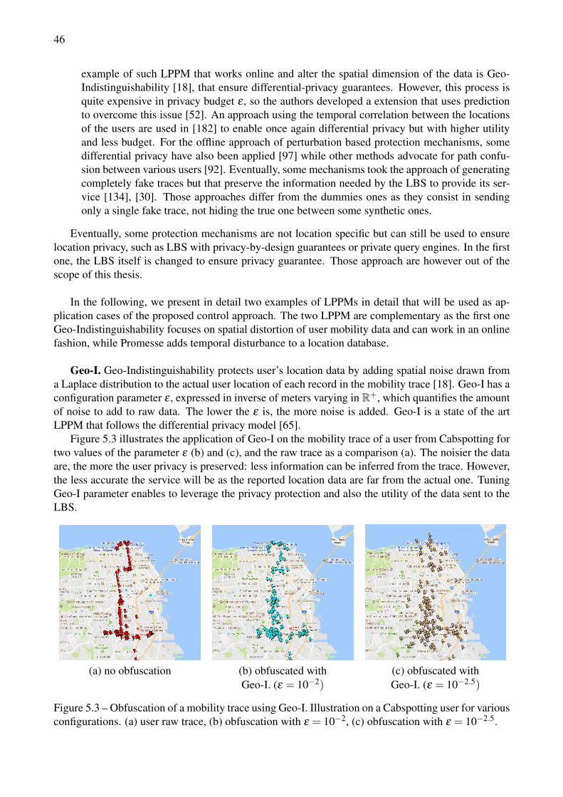
46

example of such LPPM that works online and alter the spatial dimension of the data is Geo-Indistinguishability [18], that ensure differential-privacy guarantees. However, this process isquite expensive in privacy budget ε , so the authors developed a extension that uses predictionto overcome this issue [52]. An approach using the temporal correlation between the locationsof the users are used in [182] to enable once again differential privacy but with higher utilityand less budget. For the offline approach of perturbation based protection mechanisms, somedifferential privacy have also been applied [97] while other methods advocate for path confu-sion between various users [92]. Eventually, some mechanisms took the approach of generatingcompletely fake traces but that preserve the information needed by the LBS to provide its ser-vice [134], [30]. Those approaches differ from the dummies ones as they consist in sendingonly a single fake trace, not hiding the true one between some synthetic ones.

Eventually, some protection mechanisms are not location specific but can still be used to ensurelocation privacy, such as LBS with privacy-by-design guarantees or private query engines. In the firstone, the LBS itself is changed to ensure privacy guarantee. Those approach are however out of thescope of this thesis.

In the following, we present in detail two examples of LPPMs in detail that will be used as ap-plication cases of the proposed control approach. The two LPPM are complementary as the first oneGeo-Indistinguishability focuses on spatial distortion of user mobility data and can work in an onlinefashion, while Promesse adds temporal disturbance to a location database.

Geo-I. Geo-Indistinguishability protects user’s location data by adding spatial noise drawn froma Laplace distribution to the actual user location of each record in the mobility trace [18]. Geo-I has aconfiguration parameter ε , expressed in inverse of meters varying in R+, which quantifies the amountof noise to add to raw data. The lower the ε is, the more noise is added. Geo-I is a state of the artLPPM that follows the differential privacy model [65].

Figure 5.3 illustrates the application of Geo-I on the mobility trace of a user from Cabspotting fortwo values of the parameter ε (b) and (c), and the raw trace as a comparison (a). The noisier the dataare, the more the user privacy is preserved: less information can be inferred from the trace. However,the less accurate the service will be as the reported location data are far from the actual one. TuningGeo-I parameter enables to leverage the privacy protection and also the utility of the data sent to theLBS.

(a) no obfuscation (b) obfuscated with (c) obfuscated withGeo-I. (ε = 10−2) Geo-I. (ε = 10−2.5)

Figure 5.3 – Obfuscation of a mobility trace using Geo-I. Illustration on a Cabspotting user for variousconfigurations. (a) user raw trace, (b) obfuscation with ε = 10−2, (c) obfuscation with ε = 10−2.5.

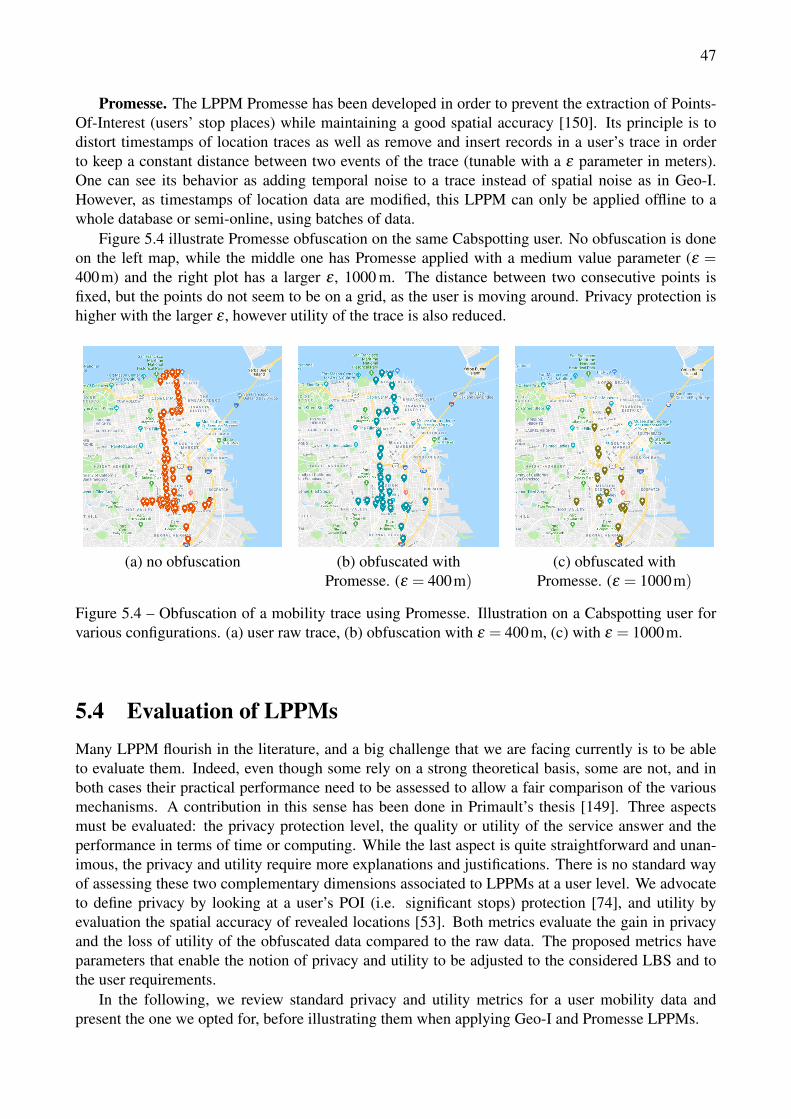
47

Promesse. The LPPM Promesse has been developed in order to prevent the extraction of Points-Of-Interest (users’ stop places) while maintaining a good spatial accuracy [150]. Its principle is todistort timestamps of location traces as well as remove and insert records in a user’s trace in orderto keep a constant distance between two events of the trace (tunable with a ε parameter in meters).One can see its behavior as adding temporal noise to a trace instead of spatial noise as in Geo-I.However, as timestamps of location data are modified, this LPPM can only be applied offline to awhole database or semi-online, using batches of data.

Figure 5.4 illustrate Promesse obfuscation on the same Cabspotting user. No obfuscation is doneon the left map, while the middle one has Promesse applied with a medium value parameter (ε =400m) and the right plot has a larger ε , 1000 m. The distance between two consecutive points isfixed, but the points do not seem to be on a grid, as the user is moving around. Privacy protection ishigher with the larger ε , however utility of the trace is also reduced.

(a) no obfuscation (b) obfuscated with (c) obfuscated withPromesse. (ε = 400m) Promesse. (ε = 1000m)

Figure 5.4 – Obfuscation of a mobility trace using Promesse. Illustration on a Cabspotting user forvarious configurations. (a) user raw trace, (b) obfuscation with ε = 400m, (c) with ε = 1000m.

5.4 Evaluation of LPPMsMany LPPM flourish in the literature, and a big challenge that we are facing currently is to be ableto evaluate them. Indeed, even though some rely on a strong theoretical basis, some are not, and inboth cases their practical performance need to be assessed to allow a fair comparison of the variousmechanisms. A contribution in this sense has been done in Primault’s thesis [149]. Three aspectsmust be evaluated: the privacy protection level, the quality or utility of the service answer and theperformance in terms of time or computing. While the last aspect is quite straightforward and unan-imous, the privacy and utility require more explanations and justifications. There is no standard wayof assessing these two complementary dimensions associated to LPPMs at a user level. We advocateto define privacy by looking at a user’s POI (i.e. significant stops) protection [74], and utility byevaluation the spatial accuracy of revealed locations [53]. Both metrics evaluate the gain in privacyand the loss of utility of the obfuscated data compared to the raw data. The proposed metrics haveparameters that enable the notion of privacy and utility to be adjusted to the considered LBS and tothe user requirements.

In the following, we review standard privacy and utility metrics for a user mobility data andpresent the one we opted for, before illustrating them when applying Geo-I and Promesse LPPMs.

48

5.4.1 Privacy metric5.4.1.1 Overview

Notions of privacy have already been presented in Section 5.2, we now discuss how to evaluate thelocation privacy protection of a user. We will not try to give an exhaustive list of the metrics that havebeen used in the literature but only sum up two surveys that give a good overview of those methods[107, 152]. Privacy can be evaluated using (i) formal guarantees such as k-anonymity or ε differentialprivacy, (ii) data distortion such as entropy of the data or (iii) attack correctness, which consist insimulating a malicious behavior and see what can be retrieved from the data.

This work will consider a privacy metric of this third category, i.e. the robustness to POI retrieval.We do not claim that privacy can be reduced to this metric, however it is the one we found the mostrelevant for location privacy due to its intermediate scale between data point and global knowledge,and it has been significantly mentioned and used in the literature [75, 150].

5.4.1.2 Definition

In the following, we formally define the metric used, starting with the notion of Point of Interest. Notethat this definition only apply for evaluating the privacy of a mobility dataset.

A POI (point of interest) is a meaningful geographical area where a user made a significant stop.A POI is defined by the position of a centroid of a given diameter d where the user stayed for at leastt minutes. We define poi(M) as the set of POIs retrieved from the mobility trace M.

Using the concept of POI and poi(·) set, we aim to quantify a user’s privacy level by how POIsretrieved from the obfuscated data (under LPPM j) successfully match the POIs retrieved from thenon-obfuscated data, i.e., comparison between set of poi(Mi) and poi(M′i j). We define the functionMatched(poi(M′i j),poi(Mi)) that, given two sets of POIs, derive the subset of poi(M′i j) containing thePOIs that match with POIs in the second set poi(Mi). Two POIs are considered as matched if theyare sufficiently close to one another (dmax being the maximal distance threshold). To formally defineprivacy, one can either use the measurement of precision (Ppr(i, j)) which defines the ratio between thenumber of obfuscated trace’s POIs successfully matched with real POIs and the number of obfuscatedPOIs,

Ppr(i, j) =|Matched(poi(M′i j),poi(Mi))|

|poi(M′i j)|,

or recall (Rpr(i, j)) which defines the ratio between the number of obfuscated trace’s POIs successfullymatched with real POIs and the number of real POIs,

Rpr(i, j) =|Matched(poi(M′i j),poi(Mi))|

|poi(Mi)|.

The precision function assesses the accuracy of the matching while the recall function evaluates thecompleteness. To cater to both measurements, we advocate using F-score (see eq. (5.1)) to reconcileboth the precision and recall.

We formally write the privacy metric, showing the normalized percentage of successfully hidden(non-matched) POIs, after applying LPPM j on user i as:

Pr(i, j) = 1− 2 ·Ppr(i, j) ·Rpr(i, j)Ppr(i, j)+Rpr(i, j)

. (5.1)

This privacy metric is defined in the range [0,1] where a higher value reflects a better protection.Leveraging the POI diameter d, its minimal stay time t and the matching threshold dmax enables a

user’s conception of her privacy to be clearly defined. For instance, a user wanting to hide her home

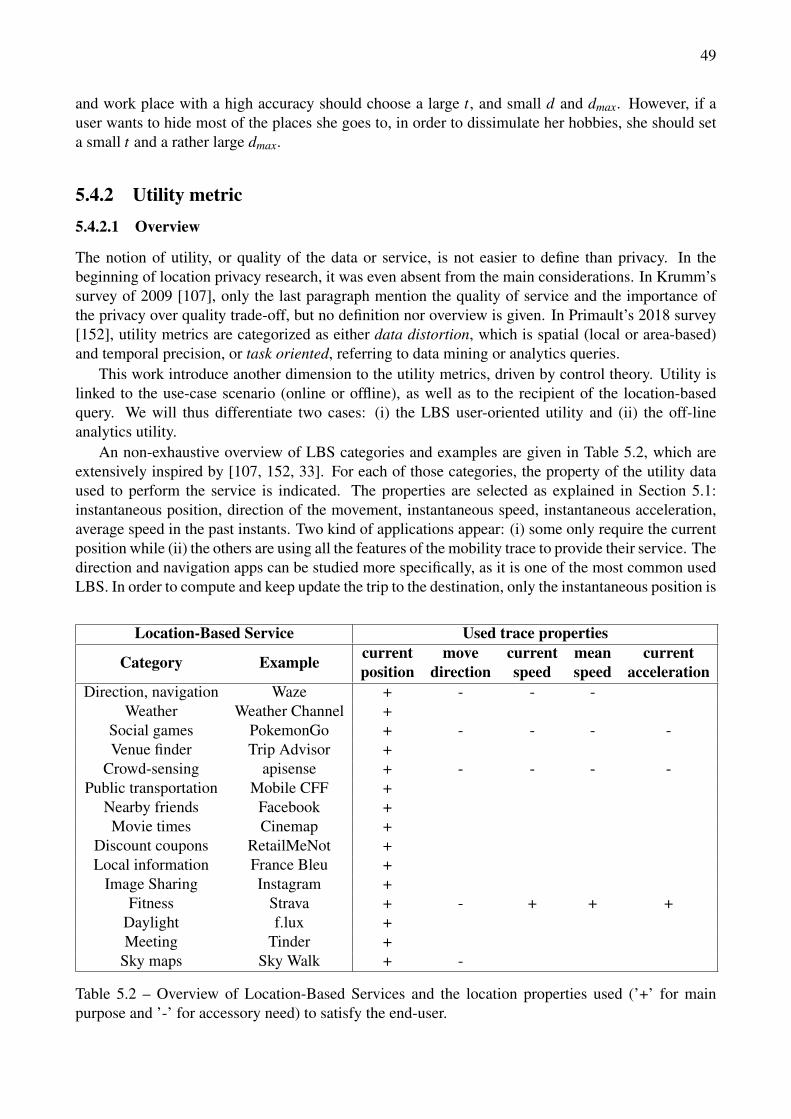
49

and work place with a high accuracy should choose a large t, and small d and dmax. However, if auser wants to hide most of the places she goes to, in order to dissimulate her hobbies, she should seta small t and a rather large dmax.

5.4.2 Utility metric5.4.2.1 Overview

The notion of utility, or quality of the data or service, is not easier to define than privacy. In thebeginning of location privacy research, it was even absent from the main considerations. In Krumm’ssurvey of 2009 [107], only the last paragraph mention the quality of service and the importance ofthe privacy over quality trade-off, but no definition nor overview is given. In Primault’s 2018 survey[152], utility metrics are categorized as either data distortion, which is spatial (local or area-based)and temporal precision, or task oriented, referring to data mining or analytics queries.

This work introduce another dimension to the utility metrics, driven by control theory. Utility islinked to the use-case scenario (online or offline), as well as to the recipient of the location-basedquery. We will thus differentiate two cases: (i) the LBS user-oriented utility and (ii) the off-lineanalytics utility.

An non-exhaustive overview of LBS categories and examples are given in Table 5.2, which areextensively inspired by [107, 152, 33]. For each of those categories, the property of the utility dataused to perform the service is indicated. The properties are selected as explained in Section 5.1:instantaneous position, direction of the movement, instantaneous speed, instantaneous acceleration,average speed in the past instants. Two kind of applications appear: (i) some only require the currentposition while (ii) the others are using all the features of the mobility trace to provide their service. Thedirection and navigation apps can be studied more specifically, as it is one of the most common usedLBS. In order to compute and keep update the trip to the destination, only the instantaneous position is

Location-Based Service Used trace properties

Category Example currentposition

movedirection

currentspeed

meanspeed

currentacceleration

Direction, navigation Waze + - - -Weather Weather Channel +

Social games PokemonGo + - - - -Venue finder Trip Advisor +

Crowd-sensing apisense + - - - -Public transportation Mobile CFF +

Nearby friends Facebook +Movie times Cinemap +

Discount coupons RetailMeNot +Local information France Bleu +

Image Sharing Instagram +Fitness Strava + - + + +

Daylight f.lux +Meeting Tinder +

Sky maps Sky Walk + -

Table 5.2 – Overview of Location-Based Services and the location properties used (’+’ for mainpurpose and ’-’ for accessory need) to satisfy the end-user.

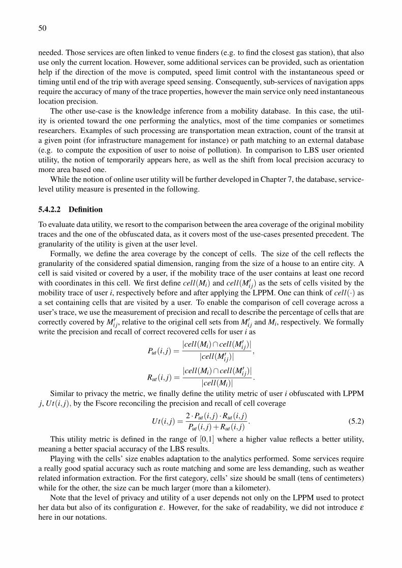
50

needed. Those services are often linked to venue finders (e.g. to find the closest gas station), that alsouse only the current location. However, some additional services can be provided, such as orientationhelp if the direction of the move is computed, speed limit control with the instantaneous speed ortiming until end of the trip with average speed sensing. Consequently, sub-services of navigation appsrequire the accuracy of many of the trace properties, however the main service only need instantaneouslocation precision.

The other use-case is the knowledge inference from a mobility database. In this case, the util-ity is oriented toward the one performing the analytics, most of the time companies or sometimesresearchers. Examples of such processing are transportation mean extraction, count of the transit ata given point (for infrastructure management for instance) or path matching to an external database(e.g. to compute the exposition of user to noise of pollution). In comparison to LBS user orientedutility, the notion of temporarily appears here, as well as the shift from local precision accuracy tomore area based one.

While the notion of online user utility will be further developed in Chapter 7, the database, service-level utility measure is presented in the following.

5.4.2.2 Definition

To evaluate data utility, we resort to the comparison between the area coverage of the original mobilitytraces and the one of the obfuscated data, as it covers most of the use-cases presented precedent. Thegranularity of the utility is given at the user level.

Formally, we define the area coverage by the concept of cells. The size of the cell reflects thegranularity of the considered spatial dimension, ranging from the size of a house to an entire city. Acell is said visited or covered by a user, if the mobility trace of the user contains at least one recordwith coordinates in this cell. We first define cell(Mi) and cell(M′i j) as the sets of cells visited by themobility trace of user i, respectively before and after applying the LPPM. One can think of cell(·) asa set containing cells that are visited by a user. To enable the comparison of cell coverage across auser’s trace, we use the measurement of precision and recall to describe the percentage of cells that arecorrectly covered by M′i j, relative to the original cell sets from M′i j and Mi, respectively. We formallywrite the precision and recall of correct recovered cells for user i as

Put(i, j) =|cell(Mi)∩ cell(M′i j)|

|cell(M′i j)|,

Rut(i, j) =|cell(Mi)∩ cell(M′i j)|

|cell(Mi)|.

Similar to privacy the metric, we finally define the utility metric of user i obfuscated with LPPMj, Ut(i, j), by the Fscore reconciling the precision and recall of cell coverage

Ut(i, j) =2 ·Put(i, j) ·Rut(i, j)Put(i, j)+Rut(i, j)

. (5.2)

This utility metric is defined in the range of [0,1] where a higher value reflects a better utility,meaning a better spacial accuracy of the LBS results.

Playing with the cells’ size enables adaptation to the analytics performed. Some services requirea really good spatial accuracy such as route matching and some are less demanding, such as weatherrelated information extraction. For the first category, cells’ size should be small (tens of centimeters)while for the other, the size can be much larger (more than a kilometer).

Note that the level of privacy and utility of a user depends not only on the LPPM used to protecther data but also of its configuration ε . However, for the sake of readability, we did not introduce ε

here in our notations.

51

5.4.3 Illustration of Privacy and Utility Metrics with LPPMsTo better illustrate the definition of privacy and utility, we use a schematic example by applying Geo-Iand Promesse on a synthetic user’s trace, see Figure 5.5 and 5.6.

Computing privacy metric In Figure 5.5 (a), the raw mobility trace of the user Mi is representedwith the small squares, each square being a location record. We overdraw the mobility trace of theuser after using Geo-I (M′i j), configured with a high ε i.e. low noise (small dots). We clearly seethat the trace obfuscated with Geo-I corresponds to the original one but with some noise. For thosetwo traces, we illustrate their Points-of-Interest (POIs) with large circles. The set of POIs of theoriginal trace poi(Mi) are the dashed circles, while POIs of the obfuscated trace poi(M′i j) are thecontinuous ones. Based on those sets, we can compute the number of obfuscated POIs that match thereal ones (here the two top ones Matched(poi(M′i j),poi(Mi)) = 2). Then our privacy metrics can thanbe computed using the precision of the matching of POIs and its recall, that both are 2/3. Then, the

level of privacy is 1−2.2/3∗2/32/3+2/3

= 0.33.

Figure 5.5 (b) is similar to Figure 5.5 (a) but here the considered LPPM is Promesse. In this case,the obfuscated data M′i j (the small stars) are spatially regularly distributed (time-stamps are modified).In this illustration, all obfuscated POIs correspond to the real ones, the privacy precision is 1 and its

recall is 1/3. The resulting privacy value is then 2.1∗1/31+1/3

= 0.5.

⏹ raw trace Mi trace with Geo-I Mij'

raw POI poi(Mi) POI with Geo-I poi(Mij')

⏺ ⏹ raw trace Mi trace with Promesse Mij'*

raw POI poi(Mi) POI with Promesse poi(Mij')

(a) Geo-I (b) Promesse

Figure 5.5 – Privacy computation: schematic examples of how POI retrieval is computed for a singleuser when using Geo-I and Promesse.

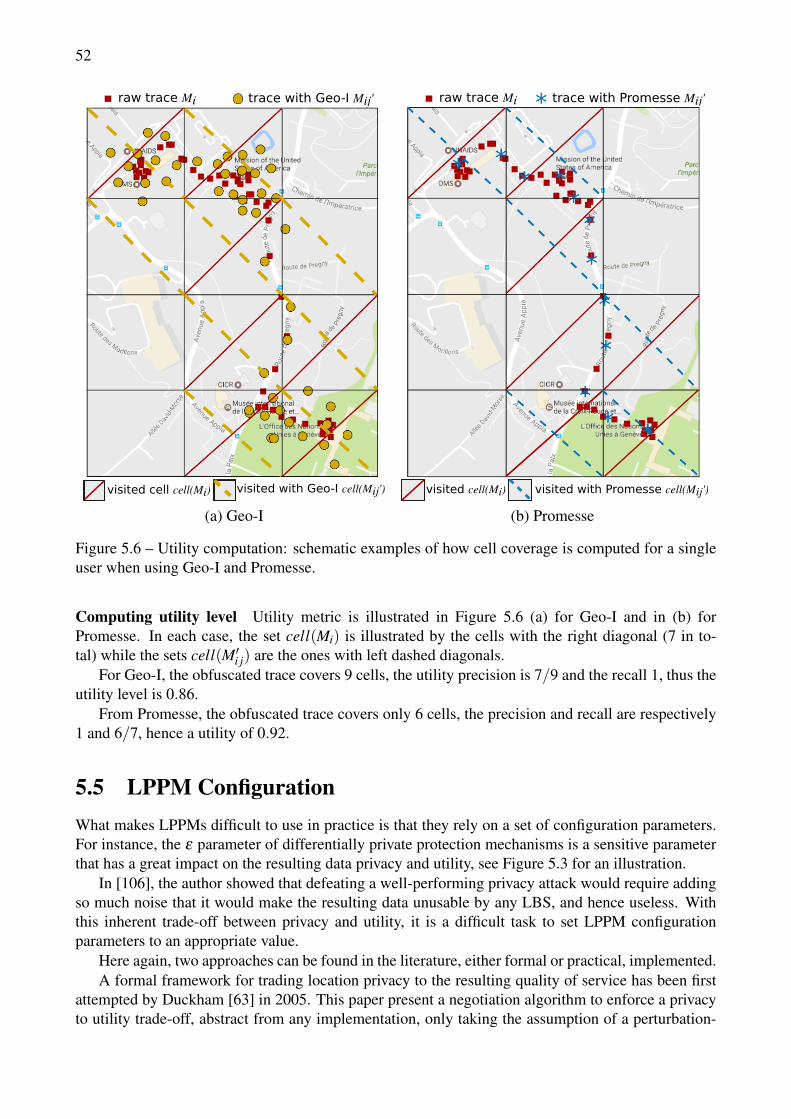
52

⏹ raw trace Mi trace with Geo-I Mij'

visited with Geo-I cell(Mij')

⏺

visited cell cell(Mi)

⏹ raw trace Mi trace with Promesse Mij'

visited cell(Mi) visited with Promesse cell(Mij')

*

(a) Geo-I (b) Promesse

Figure 5.6 – Utility computation: schematic examples of how cell coverage is computed for a singleuser when using Geo-I and Promesse.

Computing utility level Utility metric is illustrated in Figure 5.6 (a) for Geo-I and in (b) forPromesse. In each case, the set cell(Mi) is illustrated by the cells with the right diagonal (7 in to-tal) while the sets cell(M′i j) are the ones with left dashed diagonals.

For Geo-I, the obfuscated trace covers 9 cells, the utility precision is 7/9 and the recall 1, thus theutility level is 0.86.

From Promesse, the obfuscated trace covers only 6 cells, the precision and recall are respectively1 and 6/7, hence a utility of 0.92.

5.5 LPPM ConfigurationWhat makes LPPMs difficult to use in practice is that they rely on a set of configuration parameters.For instance, the ε parameter of differentially private protection mechanisms is a sensitive parameterthat has a great impact on the resulting data privacy and utility, see Figure 5.3 for an illustration.

In [106], the author showed that defeating a well-performing privacy attack would require addingso much noise that it would make the resulting data unusable by any LBS, and hence useless. Withthis inherent trade-off between privacy and utility, it is a difficult task to set LPPM configurationparameters to an appropriate value.

Here again, two approaches can be found in the literature, either formal or practical, implemented.A formal framework for trading location privacy to the resulting quality of service has been first

attempted by Duckham [63] in 2005. This paper present a negotiation algorithm to enforce a privacyto utility trade-off, abstract from any implementation, only taking the assumption of a perturbation-

53

based LPPM. However, this approach do not get rid of the challenge of the LPPM configuration, andonly consider a static scenario, unlike in our approaches.

A few works have been proposed to help a user choose a LPPM configuration that fits his actualneeds. Agir et. al [3] proposed an adaptive mechanism that dynamically computes the size of thecloaking area the user will be hidden within. More specifically, starting at a given parametrizationof the LPPM, they iteratively modify the configuration in a way that strengthen the privacy until aminimum privacy level, fixed by the user, is met. However, their privacy estimation routine has acomplexity of O(L2), L being the maximum number of locations that a cloaked area can be formedof. This routine is further repeated until required privacy level is met or at most λ times.

Theodorakopoulos et al. [170] presented new LPPMs that adapt to the user mobility pattern.Knowing that a user trace is highly repetitive and correlated, it makes the user especially vulnera-ble and in the need for personalized protection. The attacked is considered as a playing a BayesianStackelberg game, in which he knows the details of the LPPM used and the profile of the user. Con-figuration parameter of the LPPMs are optimally computed.

L2P2 is a solution that enable to refine the size of the cloaking area of a user LPPM, based onher location-dependent privacy requirements [179]. This paper is one of the very few that address theissue of a real-time LPPM configuration, knowing that users’ privacy objective vary depending onboth their location and their need.

Chatzikokolakis et. al introduced an extension of Geo-I that uses contextual information to adaptthe effective privacy level [53]. Specifically, the amount of noise effectively added to locations de-pends whether the user is located in a dense urban area or in the countryside. This qualification isdone by looking at the density of venues (e.g., restaurants, monuments, amenities) in the vicinity.It is expected that the number of venues is higher in urban environments and will better hide theuser’s interests in the area than if located outside of a city. However, this approach still requires someparametrization from the user side, which is not objective-driven. Koufogiannis et al. adopts a similarapproach, by combining differential privacy and the density of the surrounding areas, and prove thistranslate into a locally Lipschitz constraint [105].

Primault et al. presented ALP, a system that configures a LPPM depending on users objec-tives [151]. This solution relies on a greedy approach that iteratively evaluates the privacy and utilityfor refining configuration parameters. Evaluating privacy and utility has a complexity depending onthe objectives under consideration, varying between O(L) and O(L2). Moreover, the convergence isnot ensured and consequently there is no guarantee that the objectives are actually met. However,this work is the closest to our approach, given its user-level objective formulation both in privacy andutility, defined in an applied way.

Chapter 6

PULP: Privacy and Utility through LPPMsParametrization

This chapter presents PULP , a framework that automatically chooses between protection mechanismsand configure the chosen one in order to meet privacy protection objectives on a mobility dataset whileguaranteeing utility on its processing. PULP performs profiling runs on the dataset and then usesnonlinear models to capture the impact of each LPPM on data privacy and utility levels. Eventually,PULP uses those models to find the suitable protection mechanism and automatically configures itfor each user in order to achieve objectives in terms of both privacy and utility. Before describingand evaluation PULP framework, some background is given regarding the working scenario, problemstatement and motivation.

6.1 Introduction

6.1.1 DescriptionGeolocation data is increasingly used to improve the quality of online services. Hence, a large numberof mobility data is generated and currently used by companies and researchers. Indeed, the processingof mobility data can reveal valuable information that may be used for a broad range of applications,e.g., traffic congestion management, urban development, etc. The work presented in this sectionfocuses on these outbreaking mobility databases, and will not consider real-time online mobility data.However, the processing of location data also comes with threats to the privacy of the recorded users.As a motivation for privacy protection on mobility databases, one can cite the publication of themobility dataset by Strava in 2018 that revealed the maps of unknown US military bases [88]; or thenew regulations that are enforced by governments, such as the European GDPR [79].

To overcome these privacy issues, many efforts in the literature aim to develop protection mech-anisms. The protection efforts are not only motivated by cautious companies and researchers but aremore and more forced by national and international governments and organizations. The so-called Lo-cation Privacy Protection Mechanisms (LPPM) modify the location information of users to improvetheir privacy level. An overview of the literature on the protections mechanisms has been providedin Chapter 5, Section 5.3. LPPMs need fine tuning of their parameters which may require sophisti-cated knowledge and experience. The choice of these configurations (e.g. the amount of noise anddata granularity) significantly impacts the level of protection of the obfuscated data. The obfuscationshould be carried out carefully to make sure that the utility of the protected data is preserved. Indeed,the processing of the mobility data aims to retrieve some high level information (e.g. road usage andmeans of transportation). Dealing with both privacy and utility simultaneously is not straightforward

55

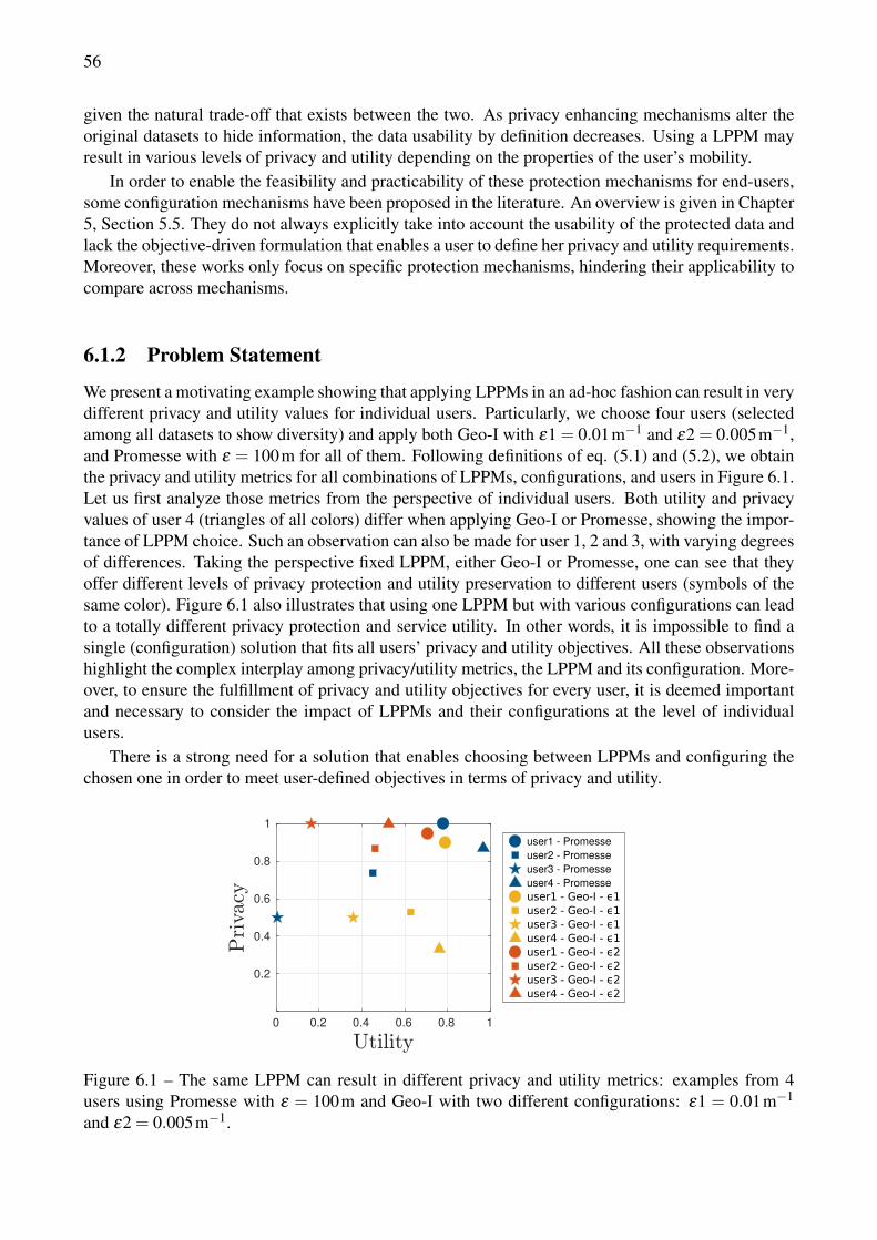
56

given the natural trade-off that exists between the two. As privacy enhancing mechanisms alter theoriginal datasets to hide information, the data usability by definition decreases. Using a LPPM mayresult in various levels of privacy and utility depending on the properties of the user’s mobility.

In order to enable the feasibility and practicability of these protection mechanisms for end-users,some configuration mechanisms have been proposed in the literature. An overview is given in Chapter5, Section 5.5. They do not always explicitly take into account the usability of the protected data andlack the objective-driven formulation that enables a user to define her privacy and utility requirements.Moreover, these works only focus on specific protection mechanisms, hindering their applicability tocompare across mechanisms.

6.1.2 Problem Statement

We present a motivating example showing that applying LPPMs in an ad-hoc fashion can result in verydifferent privacy and utility values for individual users. Particularly, we choose four users (selectedamong all datasets to show diversity) and apply both Geo-I with ε1 = 0.01m−1 and ε2 = 0.005m−1,and Promesse with ε = 100m for all of them. Following definitions of eq. (5.1) and (5.2), we obtainthe privacy and utility metrics for all combinations of LPPMs, configurations, and users in Figure 6.1.Let us first analyze those metrics from the perspective of individual users. Both utility and privacyvalues of user 4 (triangles of all colors) differ when applying Geo-I or Promesse, showing the impor-tance of LPPM choice. Such an observation can also be made for user 1, 2 and 3, with varying degreesof differences. Taking the perspective fixed LPPM, either Geo-I or Promesse, one can see that theyoffer different levels of privacy protection and utility preservation to different users (symbols of thesame color). Figure 6.1 also illustrates that using one LPPM but with various configurations can leadto a totally different privacy protection and service utility. In other words, it is impossible to find asingle (configuration) solution that fits all users’ privacy and utility objectives. All these observationshighlight the complex interplay among privacy/utility metrics, the LPPM and its configuration. More-over, to ensure the fulfillment of privacy and utility objectives for every user, it is deemed importantand necessary to consider the impact of LPPMs and their configurations at the level of individualusers.

There is a strong need for a solution that enables choosing between LPPMs and configuring thechosen one in order to meet user-defined objectives in terms of privacy and utility.

0 0.2 0.4 0.6 0.8 1

0.2

0.4

0.6

0.8

1

user1 - Promesse

user2 - Promesse

user3 - Promesse

user4 - Promesse

Figure 6.1 – The same LPPM can result in different privacy and utility metrics: examples from 4users using Promesse with ε = 100m and Geo-I with two different configurations: ε1 = 0.01m−1

and ε2 = 0.005m−1.

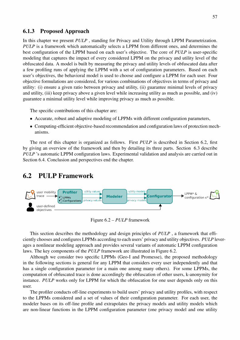
57

6.1.3 Proposed ApproachIn this chapter we present PULP , standing for Privacy and Utility through LPPM Parametrization.PULP is a framework which automatically selects a LPPM from different ones, and determines thebest configuration of the LPPM based on each user’s objective. The core of PULP is user-specificmodeling that captures the impact of every considered LPPM on the privacy and utility level of theobfuscated data. A model is built by measuring the privacy and utility levels of obfuscated data aftera few profiling runs of applying the LPPM with a set of configuration parameters. Based on eachuser’s objectives, the behavioral model is used to choose and configure a LPPM for each user. Fourobjective formulations are considered, for various combinations of objectives in terms of privacy andutility: (i) ensure a given ratio between privacy and utility, (ii) guarantee minimal levels of privacyand utility, (iii) keep privacy above a given level while increasing utility as much as possible, and (iv)guarantee a minimal utility level while improving privacy as much as possible.

The specific contributions of this chapter are:

• Accurate, robust and adaptive modeling of LPPMs with different configuration parameters,

• Computing-efficient objective-based recommendation and configuration laws of protection mech-anisms.

The rest of this chapter is organized as follows. First PULP is described in Section 6.2, firstby giving an overview of the framework and then by detailing its three parts. Section 6.3 describePULP ’s automatic LPPM configuration laws. Experimental validation and analysis are carried out inSection 6.4. Conclusion and perspectives end the chapter.

6.2 PULP Framework

Figure 6.2 – PULP framework

This section describes the methodology and design principles of PULP , a framework that effi-ciently chooses and configures LPPMs according to each users’ privacy and utility objectives. PULP lever-ages a nonlinear modeling approach and provides several variants of automatic LPPM configurationlaws. The key components of the PULP framework are illustrated in Figure 6.2.

Although we consider two specific LPPMs (Geo-I and Promesse), the proposed methodologyin the following sections is general for any LPPM that considers every user independently and thathas a single configuration parameter (or a main one among many others). For some LPPMs, thecomputation of obfuscated trace is done accordingly the obfuscation of other users, k-anonymity forinstance. PULP works only for LPPM for which the obfuscation for one user depends only on thisuser.

The profiler conducts off-line experiments to build users’ privacy and utility profiles, with respectto the LPPMs considered and a set of values of their configuration parameter. For each user, themodeler bases on its off-line profile and extrapolates the privacy models and utility models whichare non-linear functions in the LPPM configuration parameter (one privacy model and one utility

58

model for each LPPM). According to users’ objectives and privacy & utility models, the configuratorsuggests the suitable LPPM and its configuration.

PULP is effective for processing databases already collected, with protection mechanisms thatwork at the user level, and one main configuration parameter. Indeed, PULP is not suitable for onlineprocesses, as it does not include temporal aspects in the decision making.

The rest of this section presents each component of PULP . Then, Section 6.3 describes PULP ’sautomatic LPPM configuration laws.

6.2.1 ProfilerThe aim of the profiler is to obtain the values of privacy and utility of individual users under a givenLPPM and its configuration parameter set of values. The profiler takes as input a user’s mobilitytrace Mi and loops on all LPPMs and on a set of their possible configurations. The outputs are theresulting list of privacy and utility metrics values for all cases. Specifically, the profiler considers twoLPPMs, Geo-I with ε ∈ [10−4,1] in meter−1 and Promesse with ε ∈ [50,104] in meter where rangevalues are chosen according to the LPPMs’ conceptors recommendations. The necessary number ofconfiguration values is driven by the fitting accuracy of the modeler. The set of configuration valuesto run and its size is chosen such that a certain accuracy of the model is reached. The number ofvalues required depends on the accuracy target as well as the functional form of models. Suggestionson how to choose them are given in Section 6.4.2.3.

6.2.2 ModelerThe aim of the modeler is to derive the functional relation between privacy/utility metrics and theconfiguration parameter of a given LPPM, i.e., Pr(i, j) = F i, j

pr (ε) and Ut(i, j) = F i, jut (ε).

To search for the most suitable and general function, we conduct numerous data fitting schemeson our datasets. Figure 6.3 depicts commonly seen dependency between privacy/utility and ε , viaan example of applying Geo-I and Promesse on a cabspotting user (continuous lines). Experimentalconditions are further detailed in Section 6.4.1. The curves’ shape can be explained by the limitedranges of privacy and utility metrics in [0,1] and the insensitiveness of metrics to extreme values ofε . These observations lead us to choose the arctan function as our base model, instead of generalpolynomial functions. The general shape of our observations causes us to use ln(ε) to fit the arctanmodel of F i, j

pr and F i, jut , instead of ε directly.

Now, we formally introduce the utility and privacy models with four coefficients each. For sakeof simplicity, index i of the user and j of LPPM are not used in the following notation even if there isone privacy model and one utility model per user and per LPPM.

Fpr(ε) = apr. tan−1 (bpr(ln(ε)− cpr))+dpr, (6.1)

Fut(ε) = aut . tan−1 (but(ln(ε)− cut))+dut . (6.2)

Illustrations of model shapes are given in Figure 6.3, in dashed lines.The physical meaning of model parameters in both Fpr and Fut are: a and d represent the two

saturation levels, a models their amplitude and d their offset. b characterizes the transition speedbetween the saturation levels while parameter c corresponds to the ε value that results in the medianprivacy (or utility) value. Specific values of parameters in Fut and Fpr need to be learned from eachcombination of user i and LPPM j. The proposed models have the computational advantage that thereare only four coefficients to be learned.

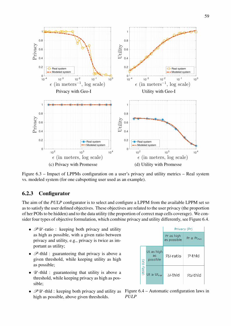
59

10-4

10-3

10-2

10-1

100

0

0.2

0.4

0.6

0.8

1

Real system

Modeled system

10-4

10-3

10-2

10-1

100

0

0.2

0.4

0.6

0.8

1

Real system

Modeled system

Privacy with Geo-I Utility with Geo-I

102

103

104

0

0.2

0.4

0.6

0.8

1

Real system

Modeled system

102

103

104

0

0.2

0.4

0.6

0.8

1

Real system

Modeled system

(c) Privacy with Promesse (d) Utility with Promesse

Figure 6.3 – Impact of LPPMs configuration on a user’s privacy and utility metrics – Real systemvs. modeled system (for one cabspotting user used as an example).

6.2.3 ConfiguratorThe aim of the PULP configurator is to select and configure a LPPM from the available LPPM set soas to satisfy the user defined objectives. These objectives are related to the user privacy (the proportionof her POIs to be hidden) and to the data utility (the proportion of correct map cells coverage). We con-sider four types of objective formulation, which combine privacy and utility differently, see Figure 6.4.

Figure 6.4 – Automatic configuration laws inPULP

• PU -ratio : keeping both privacy and utilityas high as possible, with a given ratio betweenprivacy and utility, e.g., privacy is twice as im-portant as utility;

• P-thld : guaranteeing that privacy is above agiven threshold, while keeping utility as highas possible;

• U -thld : guaranteeing that utility is above athreshold, while keeping privacy as high as pos-sible;

• PU -thld : keeping both privacy and utility ashigh as possible, above given thresholds.

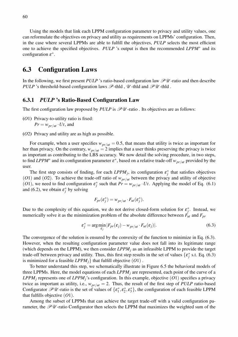
60

Using the models that link each LPPM configuration parameter to privacy and utility values, onecan reformulate the objectives on privacy and utility as requirements on LPPMs’ configuration. Then,in the case where several LPPMs are able to fulfill the objectives, PULP selects the most efficientone to achieve the specified objectives. PULP ’s output is then the recommended LPPM∗ and itsconfiguration ε∗.

6.3 Configuration LawsIn the following, we first present PULP ’s ratio-based configuration law PU -ratio and then describePULP ’s threshold-based configuration laws P-thld , U -thld and PU -thld .

6.3.1 PULP ’s Ratio-Based Configuration LawThe first configuration law proposed by PULP is PU -ratio . Its objectives are as follows:

(O1) Privacy-to-utility ratio is fixed:Pr = wpr/ut ·Ut, and

(O2) Privacy and utility are as high as possible.

For example, when a user specifies wpr/ut = 0.5, that means that utility is twice as important forher than privacy. On the contrary, wpr/ut = 2 implies that a user thinks preserving the privacy is twiceas important as contributing to the LBS accuracy. We now detail the solving procedure, in two steps,to find LPPM∗ and its configuration parameter ε∗, based on a relative trade-off wpr/ut provided by theuser.

The first step consists of finding, for each LPPM j, its configuration ε∗j that satisfies objectives(O1) and (O2). To achieve the trade-off ratio of wpr/ut between the privacy and utility of objective(O1), we need to find configuration ε∗j such that Pr = wpr/ut ·Ut. Applying the model of Eq. (6.1)and (6.2), we obtain ε∗j by solving

Fpr(ε∗j ) = wpr/ut ·Fut(ε

∗j ).

Due to the complexity of this equation, we do not derive closed-form solution for ε∗j . Instead, wenumerically solve it as the minimization problem of the absolute difference between Fut and Fpr

ε∗j = argmin

ε j|Fpr(ε j)−wpr/ut ·Fut(ε j)|. (6.3)

The convergence of the solution is ensured by the convexity of the function to minimize in Eq. (6.3).However, when the resulting configuration parameter value does not fall into its legitimate range(which depends on the LPPM), we then consider LPPM j as an infeasible LPPM to provide the targettrade-off between privacy and utility. Thus, this first step results in the set of values {ε∗j s.t. Eq. (6.3)is minimized for a feasible LPPM j} that fulfill objective (O1) .

To better understand this step, we schematically illustrate in Figure 6.5 the behavioral models ofthree LPPMs. Here, the model equations of each LPPM j are represented, each point of the curve of aLPPM j represents one of LPPM j’s configuration. In this example, objective (O1) specifies a privacytwice as important as utility, i.e., wpr/ut = 2. Thus, the result of the first step of PULP ratio-basedConfigurator PU -ratio is the set of values of {ε∗1 ,ε∗2 ,ε∗3}, the configuration of each feasible LPPMthat fulfills objective (O1).

Among the subset of LPPMs that can achieve the target trade-off with a valid configuration pa-rameter, the PU -ratio Configurator then selects the LPPM that maximizes the weighted sum of the

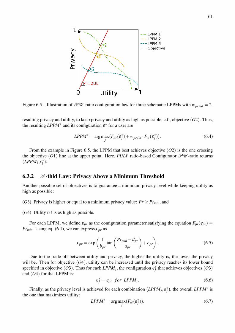
61

Figure 6.5 – Illustration of PU -ratio configuration law for three schematic LPPMs with wpr/ut = 2.

resulting privacy and utility, to keep privacy and utility as high as possible, c.f., objective (O2). Thus,the resulting LPPM∗ and its configuration ε∗ for a user are

LPPM∗ = argmaxj(Fpr(ε

∗j )+wpr/ut ·Fut(ε

∗j )). (6.4)

From the example in Figure 6.5, the LPPM that best achieves objective (O2) is the one crossingthe objective (O1) line at the upper point. Here, PULP ratio-based Configurator PU -ratio returns(LPPM1,ε

∗1 ).

6.3.2 P-thld Law: Privacy Above a Minimum ThresholdAnother possible set of objectives is to guarantee a minimum privacy level while keeping utility ashigh as possible:

(O3) Privacy is higher or equal to a minimum privacy value: Pr ≥ Prmin, and

(O4) Utility Ut is as high as possible.

For each LPPM, we define εpr as the configuration parameter satisfying the equation Fpr(εpr) =Prmin. Using eq. (6.1), we can express εpr as

εpr = exp(

1bpr

tan(

Prmin−dpr

apr

)+ cpr

). (6.5)

Due to the trade-off between utility and privacy, the higher the utility is, the lower the privacywill be. Then for objective (O4), utility can be increased until the privacy reaches its lower boundspecified in objective (O3). Thus for each LPPM j, the configuration ε∗j that achieves objectives (O3)and (O4) for that LPPM is:

ε∗j = εpr f or LPPM j. (6.6)

Finally, as the privacy level is achieved for each combination (LPPM j,ε∗j ), the overall LPPM∗ is

the one that maximizes utility:LPPM∗ = argmax

j(Fut(ε

∗j )). (6.7)

62

6.3.3 U -thld Law: Utility Above a Minimum ThresholdSimilarly, one can set the constraint on a minimal level of utility while keeping privacy as high aspossible:

(O5) Utility is not below a given minimum utility threshold Ut ≥Utmin,

(O6) With the highest data privacy Pr.

For each LPPM, we define εut such that Fut(εut) =Utmin:

εut = exp(

1but

tan(

Utmin−dut

aut

)+ cut

). (6.8)

Here, objective (O6) is ensured given objective (O5) iff ε converges to the highest value thatguarantees Fut(ε) ≥ Utmin, due to the trade-off between the two. Thus, the configuration ε∗j forLPPM j is

ε∗j = εut f or LPPM j. (6.9)

In order to elect the protection mechanism LPPM∗, we compare the values of privacy of theobfuscated data and choose the following:

LPPM∗ = argmaxj(Fpr(ε

∗j )). (6.10)

6.3.4 PU -thld : Privacy and Utility Above Minimum ThresholdsThis configuration law aims at guaranteeing that the level of privacy and the level of utility of theobfuscated data are above given thresholds:

(O7) Privacy is higher than or equal to a given minimum threshold: Pr ≥ Prmin, and

(O8) Utility is higher than or equal to a given minimum threshold: Ut ≥Utmin.

The trade-off between privacy and utility described in Section 6.1.2 shows that the utility func-tion Fut(ε) and privacy function Fpr(ε) have opposite directions of variation, both functions beingmonotonous. Let us first make the hypothesis that the privacy function is decreasing and utility func-tion increasing (which is the case for Geo-I for example). Then the objective (O7) of a thresholdvalue on privacy Fpr(ε)≥ Prmin can be written as:

ε ≤ εpr

And (O8) Fut(ε)≥Utmin asε ≥ εut .

Then the two objectives can be combined in one condition with regard to the value of the config-uration parameter:

εut ≤ ε ≤ εpr.

Then for users for whom εut ≤ εpr, all the parameters in the range [εut ;εpr] satisfy the objectives, andPULP returns the mean value of the range:

ε∗ =

εpr + εut

2. (6.11)

63

Otherwise if εut ≥ εpr, there is no solution to both objectives (O7) and (O8) for this particularcombination of LPPM and user.

Similarly, if the utility function on a LPPM decreases while the privacy function increases (as forPromesse for instance), the objectives can be written as:

εpr ≤ ε ≤ εut

and the condition of the existence of a solution is thus εut ≥ εpr. However, in the case where a solutionexists, PULP returns the same solution as eq. (6.11).

Once the configuration ε∗j of each LPPM j is found, if any, the protection mechanism LPPM∗ isselected as follows: the values of privacy and utility are compared by computing their weighted sum,after using each LPPM j in its previously calculated configuration :

LPPM∗ = argmaxj(Prmin ·Fpr(ε

∗j )+Utmin ·Fut(ε

∗j )). (6.12)

6.4 PULP EvaluationPULP ’s validation is carried out in three steps: first, an analysis of the modeler with an emphasis onthe accuracy of the derived models and on their robustness; second, the configurator evaluation thatillustrates its effectiveness in choosing a suitable LPPM to achieve different user’s objectives; andeventually a comparison with the state of the art. Prior to those core results, the experimental setup isdepicted.

6.4.1 Experimental SetupFor the experimental validation of PULP , two different machines were used. The profiler was ex-ecuted on a machine running Ubuntu 14.04 and equipped with 50Gb of RAM and 12 cores clockedat 1.2 GHz. We run the profiler using the 30-days datasets. The modeler and the configurator useMatlab R2016b on a Ubuntu 14.04 equipped with 3.7Gb of RAM and 4 cores clocked at 2.5 GHz.

The number of configuration of each LPPM to be tested by the profiler has been set at first to17 for Geo-I and 10 for Promesse, corresponding to 4 values per decade of the definition range,uniformly distributed. The modeler searches for each user’s model by fitting the experimental datausing fminunc, and the PU -ratio configuration law uses min (both are Matlab functions).

The metrics of privacy and utility used have first been parametrized to correspond to our datasetscollected in dense-cities. For measuring privacy, we consider POIs of a maximum diameter of d =200 m and a minimal stay time of t = 15 min. In order to calculate intersections between sets ofPOIs, we consider that two POIs matched if their centroids are within dmax = 100 m from each other.Google’s S2 geometry library [157] is used for cell extraction when computing utility. The size ofthe cells is highly related to the nature of the LBS. Indeed, a navigation application needs a spatialaccuracy at a really fine level while a recommendation system needs accuracy at a neighborhood level.We consider cells at level 15, which corresponds to areas having the size of around 300 meters (cityblock or neighborhood).

As initial values for the models’ parameters of eq. (6.1) and (6.2), we choose the following:

a The metric amplitude. The arctan function varies between −π

2 and π

2 . Our metrics have beendefined to vary between 0 and 1. Moreover, we expect Geo-I utility function and Promesseprivacy function to be increasing and Geo-I privacy function and Promesse utility function tobe decreasing. Consequently, we set a = 1

πfor Geo-I utility and Promesse privacy and a =− 1

π

for Geo-I privacy and Promesse utility.

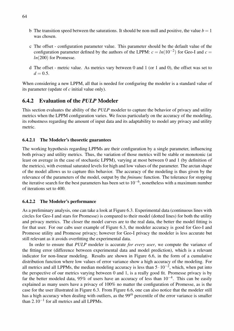
64

b The transition speed between the saturations. It should be non-null and positive, the value b = 1was chosen.

c The offset - configuration parameter value. This parameter should be the default value of theconfiguration parameter defined by the authors of the LPPM: c = ln(10−2) for Geo-I and c =ln(200) for Promesse.

d The offset - metric value. As metrics vary between 0 and 1 (or 1 and 0), the offset was set tod = 0.5.

When considering a new LPPM, all that is needed for configuring the modeler is a standard value ofits parameter (update of c initial value only).

6.4.2 Evaluation of the PULP ModelerThis section evaluates the ability of the PULP modeler to capture the behavior of privacy and utilitymetrics when the LPPM configuration varies. We focus particularly on the accuracy of the modeling,its robustness regarding the amount of input data and its adaptability to model any privacy and utilitymetric.

6.4.2.1 The Modeler’s theoretic guarantees

The working hypothesis regarding LPPMs are their configuration by a single parameter, influencingboth privacy and utility metrics. Thus, the variation of those metrics will be stable or monotonic (atleast on average in the case of stochastic LPPM), varying at most between 0 and 1 (by definition ofthe metrics), with eventual saturated levels for high and low values of the parameter. The arctan shapeof the model allows us to capture this behavior. The accuracy of the modeling is thus given by therelevance of the parameters of the model, output by the fminunc function. The tolerance for stoppingthe iterative search for the best parameters has been set to 10−6, nonetheless with a maximum numberof iterations set to 400.

6.4.2.2 The Modeler’s performance

As a preliminary analysis, one can take a look at Figure 6.3. Experimental data (continuous lines withcircles for Geo-I and stars for Promesse) is compared to their model (dotted lines) for both the utilityand privacy metrics. The closer the model curves are to the real data, the better the model fitting isfor that user. For our cabs user example of Figure 6.3, the modeler accuracy is good for Geo-I andPromesse utility and Promesse privacy; however for Geo-I privacy the modeler is less accurate butstill relevant as it avoids overfitting the experimental data.

In order to ensure that PULP modeler is accurate for every user, we compute the variance ofthe fitting error (difference between experimental data and model prediction), which is a relevantindicator for non-linear modeling. Results are shown in Figure 6.6, in the form of a cumulativedistribution function where low values of error variance show a high accuracy of the modeling. Forall metrics and all LPPMs, the median modeling accuracy is less than 5 ·10−2, which, when put intothe perspective of our metrics varying between 0 and 1, is a really good fit. Promesse privacy is byfar the better modeled data, 95% of users have an accuracy of less than 10−4. This can be easilyexplained as many users have a privacy of 100% no matter the configuration of Promesse, as is thecase for the user illustrated in Figure 6.3. From Figure 6.6, one can also notice that the modeler stillhas a high accuracy when dealing with outliers, as the 99th percentile of the error variance is smallerthan 2.10−1 for all metrics and all LPPMs.

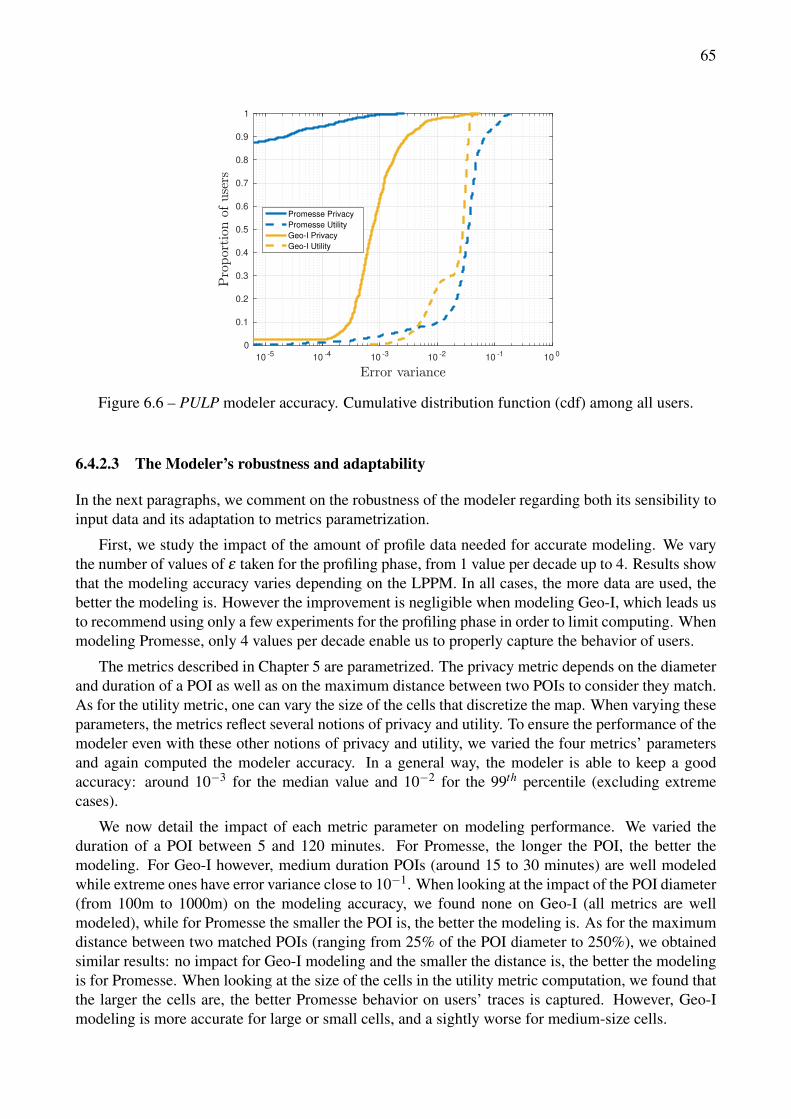
65

10 -5 10 -4 10 -3 10 -2 10 -1 10 00

0.1

0.2

0.3

0.4

0.5

0.6

0.7

0.8

0.9

1

Promesse Privacy

Promesse Utility

Geo-I Privacy

Geo-I Utility

Figure 6.6 – PULP modeler accuracy. Cumulative distribution function (cdf) among all users.

6.4.2.3 The Modeler’s robustness and adaptability

In the next paragraphs, we comment on the robustness of the modeler regarding both its sensibility toinput data and its adaptation to metrics parametrization.

First, we study the impact of the amount of profile data needed for accurate modeling. We varythe number of values of ε taken for the profiling phase, from 1 value per decade up to 4. Results showthat the modeling accuracy varies depending on the LPPM. In all cases, the more data are used, thebetter the modeling is. However the improvement is negligible when modeling Geo-I, which leads usto recommend using only a few experiments for the profiling phase in order to limit computing. Whenmodeling Promesse, only 4 values per decade enable us to properly capture the behavior of users.

The metrics described in Chapter 5 are parametrized. The privacy metric depends on the diameterand duration of a POI as well as on the maximum distance between two POIs to consider they match.As for the utility metric, one can vary the size of the cells that discretize the map. When varying theseparameters, the metrics reflect several notions of privacy and utility. To ensure the performance of themodeler even with these other notions of privacy and utility, we varied the four metrics’ parametersand again computed the modeler accuracy. In a general way, the modeler is able to keep a goodaccuracy: around 10−3 for the median value and 10−2 for the 99th percentile (excluding extremecases).

We now detail the impact of each metric parameter on modeling performance. We varied theduration of a POI between 5 and 120 minutes. For Promesse, the longer the POI, the better themodeling. For Geo-I however, medium duration POIs (around 15 to 30 minutes) are well modeledwhile extreme ones have error variance close to 10−1. When looking at the impact of the POI diameter(from 100m to 1000m) on the modeling accuracy, we found none on Geo-I (all metrics are wellmodeled), while for Promesse the smaller the POI is, the better the modeling is. As for the maximumdistance between two matched POIs (ranging from 25% of the POI diameter to 250%), we obtainedsimilar results: no impact for Geo-I modeling and the smaller the distance is, the better the modelingis for Promesse. When looking at the size of the cells in the utility metric computation, we found thatthe larger the cells are, the better Promesse behavior on users’ traces is captured. However, Geo-Imodeling is more accurate for large or small cells, and a sightly worse for medium-size cells.

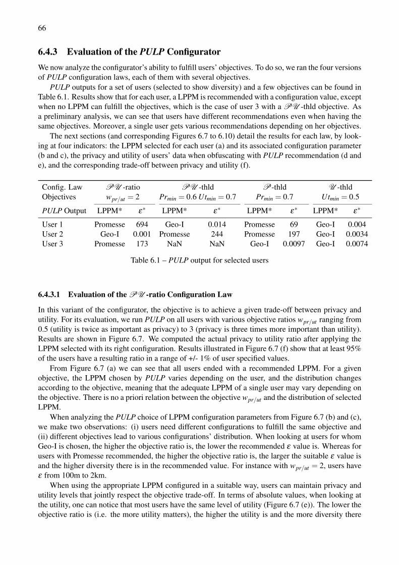
66

6.4.3 Evaluation of the PULP ConfiguratorWe now analyze the configurator’s ability to fulfill users’ objectives. To do so, we ran the four versionsof PULP configuration laws, each of them with several objectives.

PULP outputs for a set of users (selected to show diversity) and a few objectives can be found inTable 6.1. Results show that for each user, a LPPM is recommended with a configuration value, exceptwhen no LPPM can fulfill the objectives, which is the case of user 3 with a PU -thld objective. Asa preliminary analysis, we can see that users have different recommendations even when having thesame objectives. Moreover, a single user gets various recommendations depending on her objectives.

The next sections (and corresponding Figures 6.7 to 6.10) detail the results for each law, by look-ing at four indicators: the LPPM selected for each user (a) and its associated configuration parameter(b and c), the privacy and utility of users’ data when obfuscating with PULP recommendation (d ande), and the corresponding trade-off between privacy and utility (f).

Config. Law PU -ratio PU -thld P-thld U -thldObjectives wpr/ut = 2 Prmin = 0.6 Utmin = 0.7 Prmin = 0.7 Utmin = 0.5

PULP Output LPPM* ε∗ LPPM* ε∗ LPPM* ε∗ LPPM* ε∗

User 1 Promesse 694 Geo-I 0.014 Promesse 69 Geo-I 0.004User 2 Geo-I 0.001 Promesse 244 Promesse 197 Geo-I 0.0034User 3 Promesse 173 NaN NaN Geo-I 0.0097 Geo-I 0.0074

Table 6.1 – PULP output for selected users

6.4.3.1 Evaluation of the PU -ratio Configuration Law

In this variant of the configurator, the objective is to achieve a given trade-off between privacy andutility. For its evaluation, we run PULP on all users with various objective ratios wpr/ut ranging from0.5 (utility is twice as important as privacy) to 3 (privacy is three times more important than utility).Results are shown in Figure 6.7. We computed the actual privacy to utility ratio after applying theLPPM selected with its right configuration. Results illustrated in Figure 6.7 (f) show that at least 95%of the users have a resulting ratio in a range of +/- 1% of user specified values.

From Figure 6.7 (a) we can see that all users ended with a recommended LPPM. For a givenobjective, the LPPM chosen by PULP varies depending on the user, and the distribution changesaccording to the objective, meaning that the adequate LPPM of a single user may vary depending onthe objective. There is no a priori relation between the objective wpr/ut and the distribution of selectedLPPM.

When analyzing the PULP choice of LPPM configuration parameters from Figure 6.7 (b) and (c),we make two observations: (i) users need different configurations to fulfill the same objective and(ii) different objectives lead to various configurations’ distribution. When looking at users for whomGeo-I is chosen, the higher the objective ratio is, the lower the recommended ε value is. Whereas forusers with Promesse recommended, the higher the objective ratio is, the larger the suitable ε value isand the higher diversity there is in the recommended value. For instance with wpr/ut = 2, users haveε from 100m to 2km.

When using the appropriate LPPM configured in a suitable way, users can maintain privacy andutility levels that jointly respect the objective trade-off. In terms of absolute values, when looking atthe utility, one can notice that most users have the same level of utility (Figure 6.7 (e)). The lower theobjective ratio is (i.e. the more utility matters), the higher the utility is and the more diversity there

67

is in the utility values. For privacy, the same trend is observed: most users have the same privacy butthe lower the objective ratio is, the more diversity there is in the privacy values (see Figure 6.7 (d)).

With an objective expressed as a trade-off between privacy and utility, PULP finds a suitableLPPM for all users and guarantees a high utility and privacy to almost all of them.

6.4.3.2 Evaluation of the PU -thld Configuration Law

In this section we evaluate the PULP PU -thld configuration law, aiming to achieve privacy andutility at levels higher than some minimal thresholds. The evaluation, reported in Figure 6.8, has beencarried out with five couples of objectives.

First, it is important to notice that some users do not have any LPPM recommended, as can be seenin Figure 6.8 (a). High utility constraints seem to hamper the feasibility of recommending suitableLPPMs. Recommendations range from less than 10% of all users (Prmin = 0.5,Utmin = 0.9) to morethan 95% (Prmin = 0.3,Utmin = 0.5). Most of the recommendations are Geo-I. The higher the utilityconstraint, the more Geo-I is recommended. When looking at values of the LPPM configurationparameter, for Geo-I the general trend is that ε is lower when privacy constraint in high, except in theextreme case where Utmin = 0.9. For Promesse, the higher the utility constraint, the smaller ε is.

The privacy criteria is always satisfied, and almost no user gets the limit privacy Prmin, see Figure6.8 (d). However, when the utility constraint is high, most users tend to have a privacy close to itsbound. All users have their utility criteria fulfilled (see Figure 6.8 (e)). The utility of most users isreally high: 80% of them have a utility above 0.8 (0.6 for Prmin = 0.9,Utmin = 0.4). As for the privacyto utility ratio, within a set of objectives most users (70-90%) have the same privacy to utility ratio(Figure 6.8 (f)).

PULP is not able to find a suitable LPPM for all users using this objective formulation; however,when it can, the privacy and utility are, most of the time, way above the minimum values required.

6.4.3.3 Evaluation of the P-thld Configuration Law

Here the objective is to guarantee that the privacy is above a given level. Results are given in Figure6.9. PULP can recommend a suitable LPPM and fulfill all users’ objectives considered here. Around10 to 20% of users can even achieve higher privacy levels than the requested threshold (even 80%for the objective Prmin = 0.9), see Figure 6.9 (d). These proportions correspond to users to whichPromesse is recommended, see correspondence with Figure 6.9 (a).

For those Promesse users, the utility is quite low but for the other 80% of users, utility is morethan 0.5 (Figure 6.9 (e)). Moreover, the higher the privacy limit, the lower the utility. Looking at theprivacy to utility ratio (Figure 6.9 (f)), for 80% of users (those with Geo-I recommended), the lowerthe privacy limit, the higher the ratio (allowing more utility to the data) and all users have the sameprivacy to utility ratio. However, for 20% of them (Promesse users) the ratio is always the same nomatter what the objective.

As for the parameter values, for users with Geo-I recommended, the higher the objective is, thesmaller ε is. Users with Promesse recommended always seem to have the same ε recommended nomatter what the value of the objective, except for Prmin = 0.9 where ε is at its upper bound for mostusers.

When PULP guarantees a minimal privacy level, but two distinctive types of users are observed.Some have are recommended Geo-I, a limited privacy and a high utility; while the others use Promessewith a high privacy but a low utility.

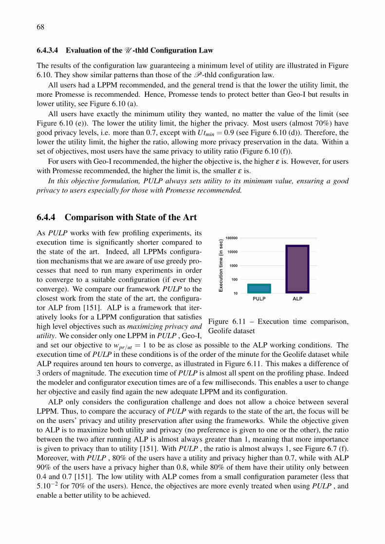
68

6.4.3.4 Evaluation of the U -thld Configuration Law

The results of the configuration law guaranteeing a minimum level of utility are illustrated in Figure6.10. They show similar patterns than those of the P-thld configuration law.

All users had a LPPM recommended, and the general trend is that the lower the utility limit, themore Promesse is recommended. Hence, Promesse tends to protect better than Geo-I but results inlower utility, see Figure 6.10 (a).

All users have exactly the minimum utility they wanted, no matter the value of the limit (seeFigure 6.10 (e)). The lower the utility limit, the higher the privacy. Most users (almost 70%) havegood privacy levels, i.e. more than 0.7, except with Utmin = 0.9 (see Figure 6.10 (d)). Therefore, thelower the utility limit, the higher the ratio, allowing more privacy preservation in the data. Within aset of objectives, most users have the same privacy to utility ratio (Figure 6.10 (f)).

For users with Geo-I recommended, the higher the objective is, the higher ε is. However, for userswith Promesse recommended, the higher the limit is, the smaller ε is.

In this objective formulation, PULP always sets utility to its minimum value, ensuring a goodprivacy to users especially for those with Promesse recommended.

6.4.4 Comparison with State of the Art

Figure 6.11 – Execution time comparison,Geolife dataset

As PULP works with few profiling experiments, itsexecution time is significantly shorter compared tothe state of the art. Indeed, all LPPMs configura-tion mechanisms that we are aware of use greedy pro-cesses that need to run many experiments in orderto converge to a suitable configuration (if ever theyconverge). We compare our framework PULP to theclosest work from the state of the art, the configura-tor ALP from [151]. ALP is a framework that iter-atively looks for a LPPM configuration that satisfieshigh level objectives such as maximizing privacy andutility. We consider only one LPPM in PULP , Geo-I,and set our objective to wpr/ut = 1 to be as close as possible to the ALP working conditions. Theexecution time of PULP in these conditions is of the order of the minute for the Geolife dataset whileALP requires around ten hours to converge, as illustrated in Figure 6.11. This makes a difference of3 orders of magnitude. The execution time of PULP is almost all spent on the profiling phase. Indeedthe modeler and configurator execution times are of a few milliseconds. This enables a user to changeher objective and easily find again the new adequate LPPM and its configuration.

ALP only considers the configuration challenge and does not allow a choice between severalLPPM. Thus, to compare the accuracy of PULP with regards to the state of the art, the focus will beon the users’ privacy and utility preservation after using the frameworks. While the objective givento ALP is to maximize both utility and privacy (no preference is given to one or the other), the ratiobetween the two after running ALP is almost always greater than 1, meaning that more importanceis given to privacy than to utility [151]. With PULP , the ratio is almost always 1, see Figure 6.7 (f).Moreover, with PULP , 80% of the users have a utility and privacy higher than 0.7, while with ALP90% of the users have a privacy higher than 0.8, while 80% of them have their utility only between0.4 and 0.7 [151]. The low utility with ALP comes from a small configuration parameter (less that5.10−2 for 70% of the users). Hence, the objectives are more evenly treated when using PULP , andenable a better utility to be achieved.

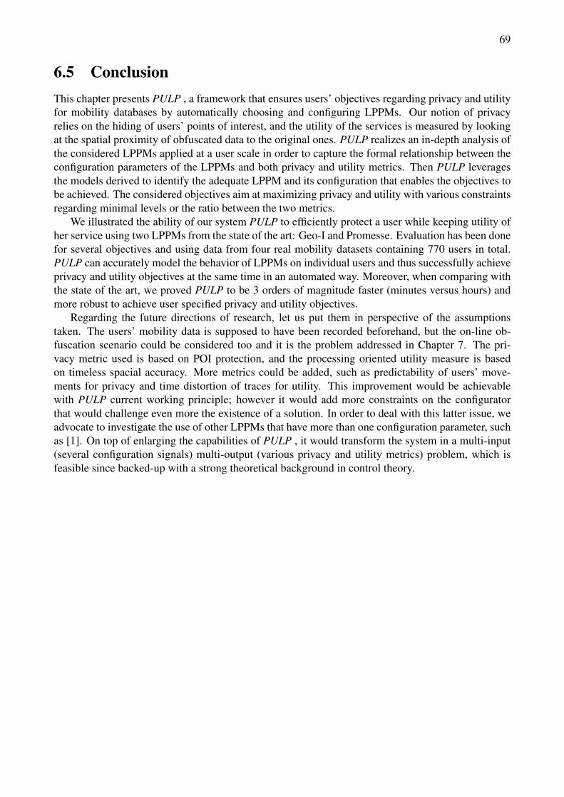
69

6.5 ConclusionThis chapter presents PULP , a framework that ensures users’ objectives regarding privacy and utilityfor mobility databases by automatically choosing and configuring LPPMs. Our notion of privacyrelies on the hiding of users’ points of interest, and the utility of the services is measured by lookingat the spatial proximity of obfuscated data to the original ones. PULP realizes an in-depth analysis ofthe considered LPPMs applied at a user scale in order to capture the formal relationship between theconfiguration parameters of the LPPMs and both privacy and utility metrics. Then PULP leveragesthe models derived to identify the adequate LPPM and its configuration that enables the objectives tobe achieved. The considered objectives aim at maximizing privacy and utility with various constraintsregarding minimal levels or the ratio between the two metrics.

We illustrated the ability of our system PULP to efficiently protect a user while keeping utility ofher service using two LPPMs from the state of the art: Geo-I and Promesse. Evaluation has been donefor several objectives and using data from four real mobility datasets containing 770 users in total.PULP can accurately model the behavior of LPPMs on individual users and thus successfully achieveprivacy and utility objectives at the same time in an automated way. Moreover, when comparing withthe state of the art, we proved PULP to be 3 orders of magnitude faster (minutes versus hours) andmore robust to achieve user specified privacy and utility objectives.

Regarding the future directions of research, let us put them in perspective of the assumptionstaken. The users’ mobility data is supposed to have been recorded beforehand, but the on-line ob-fuscation scenario could be considered too and it is the problem addressed in Chapter 7. The pri-vacy metric used is based on POI protection, and the processing oriented utility measure is basedon timeless spacial accuracy. More metrics could be added, such as predictability of users’ move-ments for privacy and time distortion of traces for utility. This improvement would be achievablewith PULP current working principle; however it would add more constraints on the configuratorthat would challenge even more the existence of a solution. In order to deal with this latter issue, weadvocate to investigate the use of other LPPMs that have more than one configuration parameter, suchas [1]. On top of enlarging the capabilities of PULP , it would transform the system in a multi-input(several configuration signals) multi-output (various privacy and utility metrics) problem, which isfeasible since backed-up with a strong theoretical background in control theory.

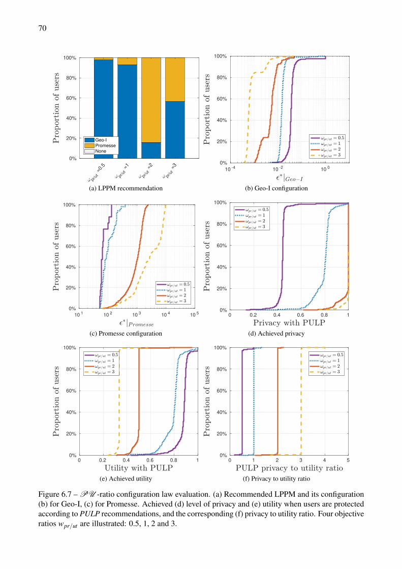
70

pr/u

t=0

.5

pr

/ut=1

pr

/ut=2

pr

/ut=3

0%

20%

40%

60%

80%

100%

Geo-I

Promesse

None

(a) LPPM recommendation

10-4

10-2

100

0%

20%

40%

60%

80%

100%

(b) Geo-I configuration

101

102

103

104

105

0%

20%

40%

60%

80%

100%

(c) Promesse configuration

0 0.2 0.4 0.6 0.8 1

0%

20%

40%

60%

80%

100%

(d) Achieved privacy

0 0.2 0.4 0.6 0.8 1

0%

20%

40%

60%

80%

100%

(e) Achieved utility

0 1 2 3 4 5

0%

20%

40%

60%

80%

100%

(f) Privacy to utility ratio

Figure 6.7 – PU -ratio configuration law evaluation. (a) Recommended LPPM and its configuration(b) for Geo-I, (c) for Promesse. Achieved (d) level of privacy and (e) utility when users are protectedaccording to PULP recommendations, and the corresponding (f) privacy to utility ratio. Four objectiveratios wpr/ut are illustrated: 0.5, 1, 2 and 3.

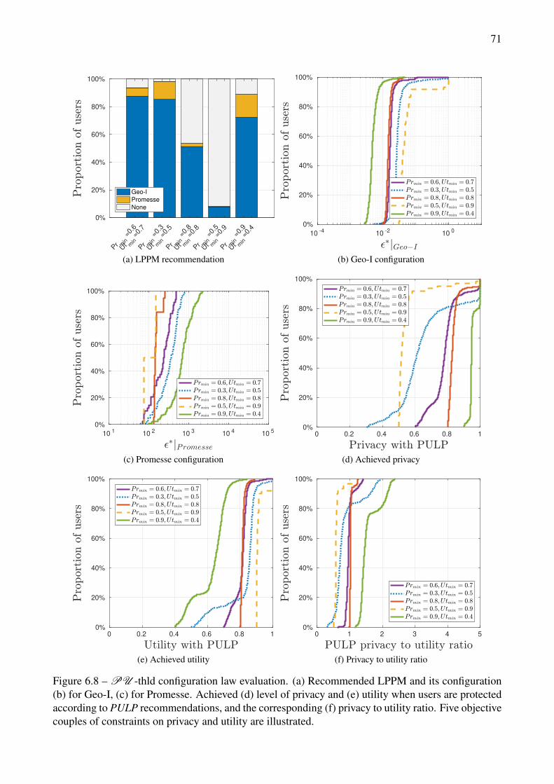
71

Pr m

in

=0.6

Ut m

in

=0.7

Pr m

in

=0.3

Ut m

in

=0.5

Pr m

in

=0.8

Ut m

in

=0.8

Pr m

in

=0.5

Ut m

in

=0.9

Pr m

in

=0.9

Ut m

in

=0.4

0%

20%

40%

60%

80%

100%

Geo-I

Promesse

None

(a) LPPM recommendation

10-4

10-2

100

0%

20%

40%

60%

80%

100%

(b) Geo-I configuration

101

102

103

104

105

0%

20%

40%

60%

80%

100%

(c) Promesse configuration

0 0.2 0.4 0.6 0.8 1

0%

20%

40%

60%

80%

100%

(d) Achieved privacy

0 0.2 0.4 0.6 0.8 1

0%

20%

40%

60%

80%

100%

(e) Achieved utility

0 1 2 3 4 5

0%

20%

40%

60%

80%

100%

(f) Privacy to utility ratio

Figure 6.8 – PU -thld configuration law evaluation. (a) Recommended LPPM and its configuration(b) for Geo-I, (c) for Promesse. Achieved (d) level of privacy and (e) utility when users are protectedaccording to PULP recommendations, and the corresponding (f) privacy to utility ratio. Five objectivecouples of constraints on privacy and utility are illustrated.

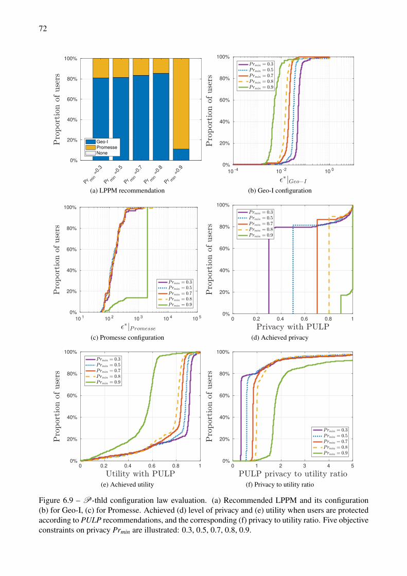
72

Pr m

in

=0.3

Pr m

in

=0.5

Pr m

in

=0.7

Pr m

in

=0.8

Pr m

in

=0.9

0%

20%

40%

60%

80%

100%

Geo-I

Promesse

None

(a) LPPM recommendation

10-4

10-2

100

0%

20%

40%

60%

80%

100%

(b) Geo-I configuration

101

102

103

104

105

0%

20%

40%

60%

80%

100%

(c) Promesse configuration

0 0.2 0.4 0.6 0.8 1

0%

20%

40%

60%

80%

100%

(d) Achieved privacy

0 0.2 0.4 0.6 0.8 1

0%

20%

40%

60%

80%

100%

(e) Achieved utility

0 1 2 3 4 5

0%

20%

40%

60%

80%

100%

(f) Privacy to utility ratio

Figure 6.9 – P-thld configuration law evaluation. (a) Recommended LPPM and its configuration(b) for Geo-I, (c) for Promesse. Achieved (d) level of privacy and (e) utility when users are protectedaccording to PULP recommendations, and the corresponding (f) privacy to utility ratio. Five objectiveconstraints on privacy Prmin are illustrated: 0.3, 0.5, 0.7, 0.8, 0.9.

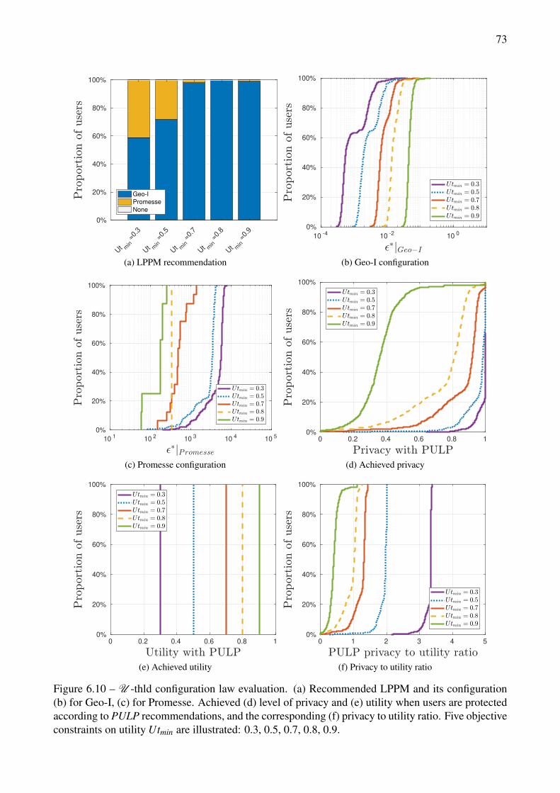
73

Ut m

in

=0.3

Ut m

in

=0.5

Ut m

in

=0.7

Ut m

in

=0.8

Ut m

in

=0.9

0%

20%

40%

60%

80%

100%

Geo-I

Promesse

None

(a) LPPM recommendation

10-4

10-2

100

0%

20%

40%

60%

80%

100%

(b) Geo-I configuration

101

102

103

104

105

0%

20%

40%

60%

80%

100%

(c) Promesse configuration

0 0.2 0.4 0.6 0.8 1

0%

20%

40%

60%

80%

100%

(d) Achieved privacy

0 0.2 0.4 0.6 0.8 1

0%

20%

40%

60%

80%

100%

(e) Achieved utility

0 1 2 3 4 5

0%

20%

40%

60%

80%

100%

(f) Privacy to utility ratio

Figure 6.10 – U -thld configuration law evaluation. (a) Recommended LPPM and its configuration(b) for Geo-I, (c) for Promesse. Achieved (d) level of privacy and (e) utility when users are protectedaccording to PULP recommendations, and the corresponding (f) privacy to utility ratio. Five objectiveconstraints on utility Utmin are illustrated: 0.3, 0.5, 0.7, 0.8, 0.9.

Chapter 7

dynULP: dynamic control of Utility andLocation Privacy

In this chapter, we are interested in the online control of privacy. A mobile device user can constantlysend her current location and benefit from geo-localized services. She indeed wants to protect herprivacy while still enjoying a reasonable quality of service. Compared to PULP’s approach presentedin Chapter 6, dynULP is at the user level, locally on the mobile device, thus the service utility consid-ered here is the quality of the LBS answers. We advocate to use a control-theoretic approach for twomain reasons, being (i) the end-user do not want to bother with the understanding and configurationof a LPPM and (ii) the problem is by definition dynamic and needs fine adaptation through time sincethe user is mobile in a dynamic environment.

A simple controller is presented, that ensures privacy according to the user’s requirements, whilebeing robust to her movement. To help the initial tuning of the controller, a control-oriented modelof the protection mechanism is derived. For each modeling and control steps, the methods usedare illustrated and validated on synthetic mobility data, which enable the full understanding of theapproaches. Afterwards, an evaluation using real users mobility records is also provided. dynULPapproach shows good results both for achieving a desired privacy level and for keeping it despitedisturbances. The quality of the resulting service is also maintained at a reasonable level.

The outlines of this Chapter are as follows. After a deeper introduction and motivation of dynULPscenario (Section 7.1), the formulation of the problem in control words is given, with a emphasis onthe output metric sensing: real-time privacy (Section 7.2). Then the two-step modeling approach(static then dynamic) is carried out (Section 7.3). Then the control strategy is presented (Section 7.4).Eventually, an evaluation of the modeling and controller consisting in a proof of concept of the controlapproach is given (Section 7.5) before a conclusion that end this chapter (Section 7.6).

7.1 Introduction

7.1.1 Context, Hypothesis and MotivationThe democratization of mobile devices has fostered the development of services using the users’location data to provide or improve a service. Everyday examples of Location Based Services (LBS)are navigation applications, recommendation systems or fitness tracking apps. Some of those servicesare one-shot, they need one location point to provide their service e.g. a weather app. Some othersneed dynamic records, for instance navigation or gaming apps. We advocate in this work to considerthem all as dynamic, for two main reasons. First, people using "one-shot location" application do notnecessary turn on and off instantaneously the GPS option on their phone, thus the records are still sent

75

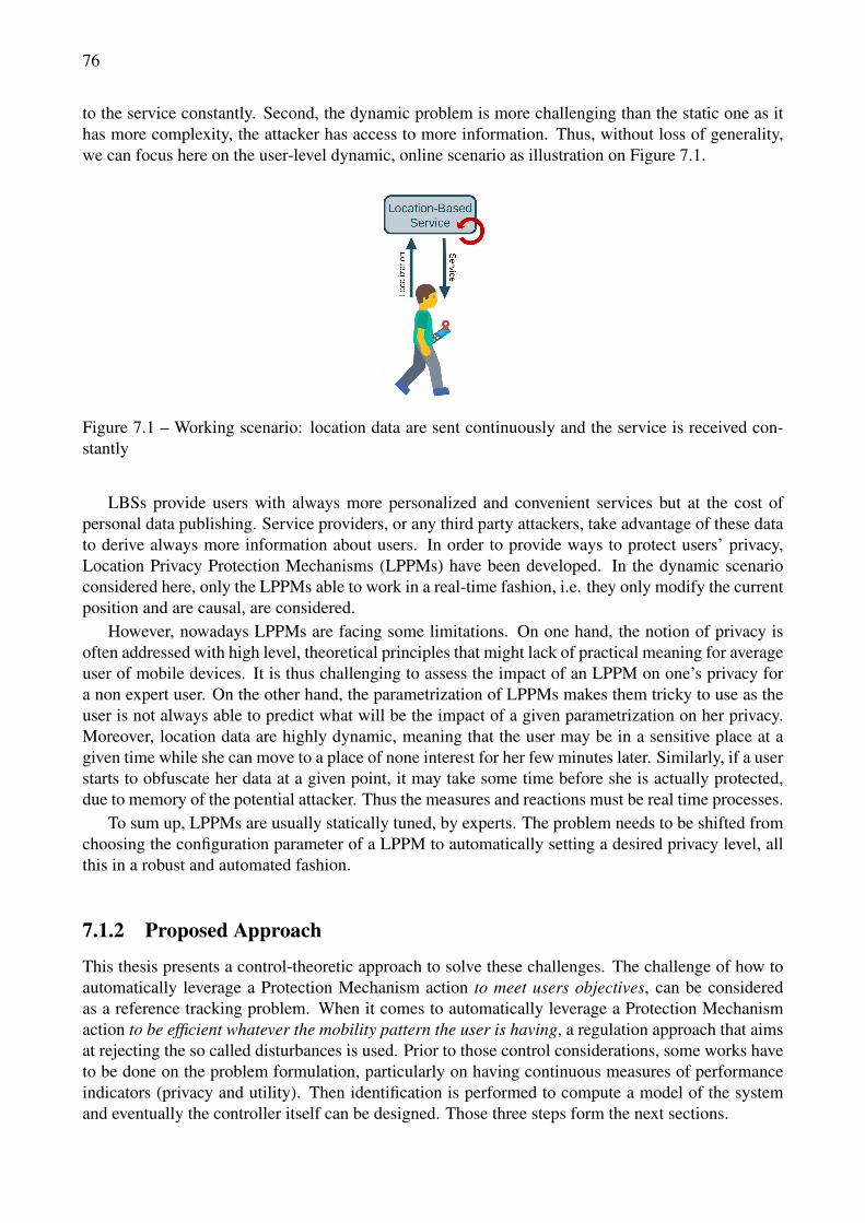
76

to the service constantly. Second, the dynamic problem is more challenging than the static one as ithas more complexity, the attacker has access to more information. Thus, without loss of generality,we can focus here on the user-level dynamic, online scenario as illustration on Figure 7.1.

Figure 7.1 – Working scenario: location data are sent continuously and the service is received con-stantly

LBSs provide users with always more personalized and convenient services but at the cost ofpersonal data publishing. Service providers, or any third party attackers, take advantage of these datato derive always more information about users. In order to provide ways to protect users’ privacy,Location Privacy Protection Mechanisms (LPPMs) have been developed. In the dynamic scenarioconsidered here, only the LPPMs able to work in a real-time fashion, i.e. they only modify the currentposition and are causal, are considered.

However, nowadays LPPMs are facing some limitations. On one hand, the notion of privacy isoften addressed with high level, theoretical principles that might lack of practical meaning for averageuser of mobile devices. It is thus challenging to assess the impact of an LPPM on one’s privacy fora non expert user. On the other hand, the parametrization of LPPMs makes them tricky to use as theuser is not always able to predict what will be the impact of a given parametrization on her privacy.Moreover, location data are highly dynamic, meaning that the user may be in a sensitive place at agiven time while she can move to a place of none interest for her few minutes later. Similarly, if a userstarts to obfuscate her data at a given point, it may take some time before she is actually protected,due to memory of the potential attacker. Thus the measures and reactions must be real time processes.

To sum up, LPPMs are usually statically tuned, by experts. The problem needs to be shifted fromchoosing the configuration parameter of a LPPM to automatically setting a desired privacy level, allthis in a robust and automated fashion.

7.1.2 Proposed Approach

This thesis presents a control-theoretic approach to solve these challenges. The challenge of how toautomatically leverage a Protection Mechanism action to meet users objectives, can be consideredas a reference tracking problem. When it comes to automatically leverage a Protection Mechanismaction to be efficient whatever the mobility pattern the user is having, a regulation approach that aimsat rejecting the so called disturbances is used. Prior to those control considerations, some works haveto be done on the problem formulation, particularly on having continuous measures of performanceindicators (privacy and utility). Then identification is performed to compute a model of the systemand eventually the controller itself can be designed. Those three steps form the next sections.

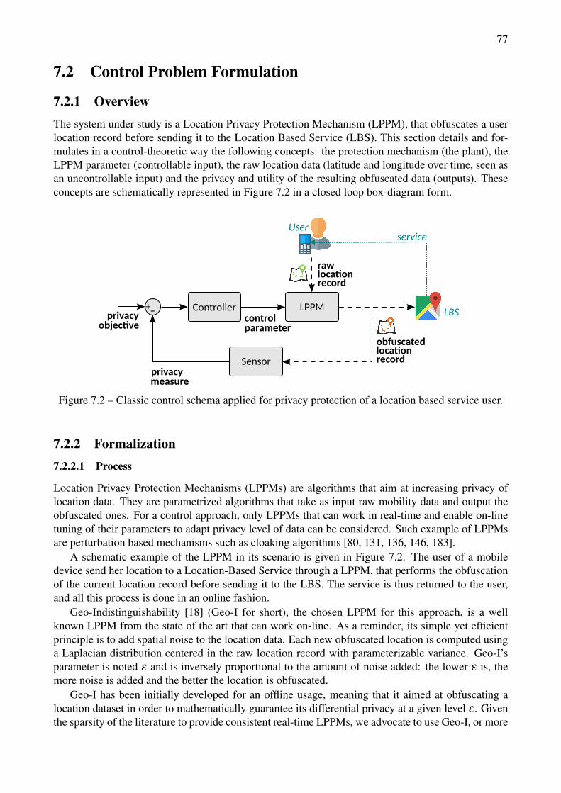
77

7.2 Control Problem Formulation

7.2.1 OverviewThe system under study is a Location Privacy Protection Mechanism (LPPM), that obfuscates a userlocation record before sending it to the Location Based Service (LBS). This section details and for-mulates in a control-theoretic way the following concepts: the protection mechanism (the plant), theLPPM parameter (controllable input), the raw location data (latitude and longitude over time, seen asan uncontrollable input) and the privacy and utility of the resulting obfuscated data (outputs). Theseconcepts are schematically represented in Figure 7.2 in a closed loop box-diagram form.

Figure 7.2 – Classic control schema applied for privacy protection of a location based service user.

7.2.2 Formalization7.2.2.1 Process

Location Privacy Protection Mechanisms (LPPMs) are algorithms that aim at increasing privacy oflocation data. They are parametrized algorithms that take as input raw mobility data and output theobfuscated ones. For a control approach, only LPPMs that can work in real-time and enable on-linetuning of their parameters to adapt privacy level of data can be considered. Such example of LPPMsare perturbation based mechanisms such as cloaking algorithms [80, 131, 136, 146, 183].

A schematic example of the LPPM in its scenario is given in Figure 7.2. The user of a mobiledevice send her location to a Location-Based Service through a LPPM, that performs the obfuscationof the current location record before sending it to the LBS. The service is thus returned to the user,and all this process is done in an online fashion.

Geo-Indistinguishability [18] (Geo-I for short), the chosen LPPM for this approach, is a wellknown LPPM from the state of the art that can work on-line. As a reminder, its simple yet efficientprinciple is to add spatial noise to the location data. Each new obfuscated location is computed usinga Laplacian distribution centered in the raw location record with parameterizable variance. Geo-I’sparameter is noted ε and is inversely proportional to the amount of noise added: the lower ε is, themore noise is added and the better the location is obfuscated.

Geo-I has been initially developed for an offline usage, meaning that it aimed at obfuscating alocation dataset in order to mathematically guarantee its differential privacy at a given level ε . Giventhe sparsity of the literature to provide consistent real-time LPPMs, we advocate to use Geo-I, or more

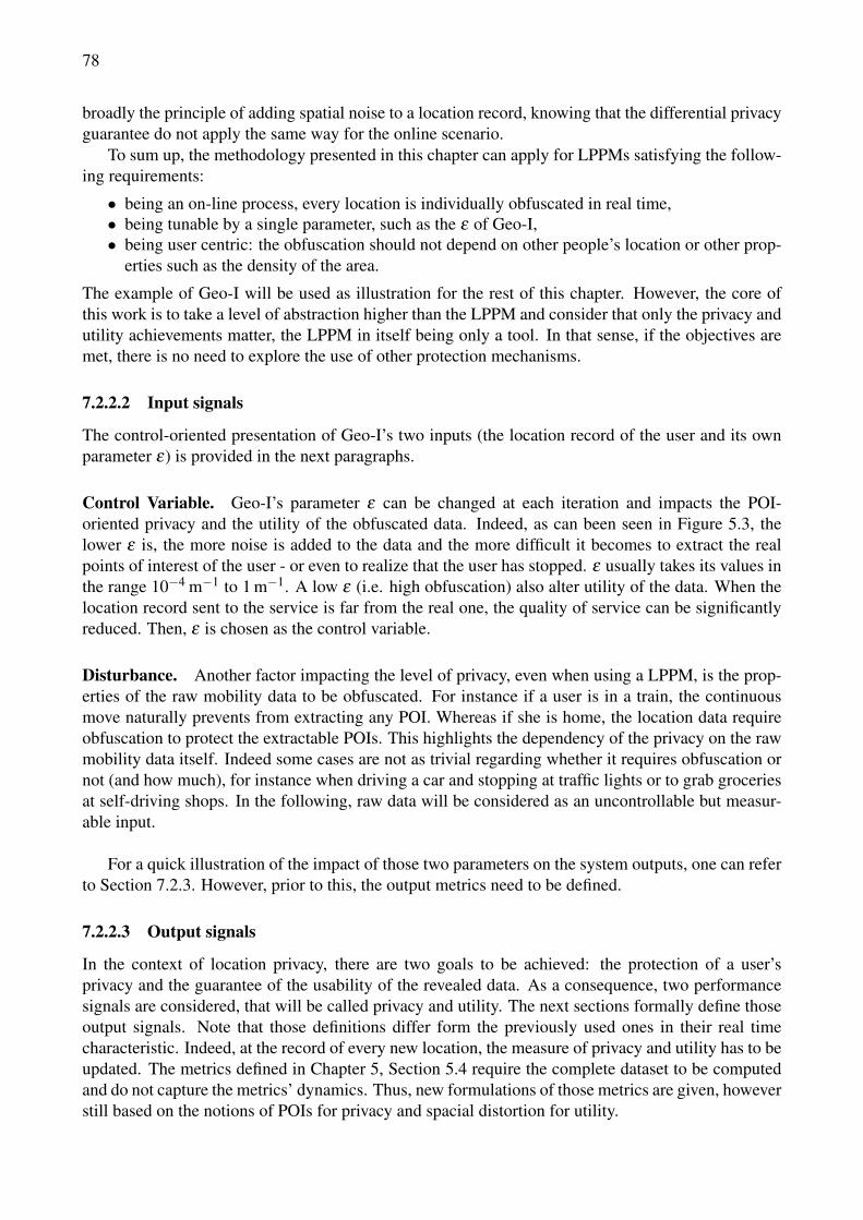
78

broadly the principle of adding spatial noise to a location record, knowing that the differential privacyguarantee do not apply the same way for the online scenario.

To sum up, the methodology presented in this chapter can apply for LPPMs satisfying the follow-ing requirements:

• being an on-line process, every location is individually obfuscated in real time,• being tunable by a single parameter, such as the ε of Geo-I,• being user centric: the obfuscation should not depend on other people’s location or other prop-

erties such as the density of the area.

The example of Geo-I will be used as illustration for the rest of this chapter. However, the core ofthis work is to take a level of abstraction higher than the LPPM and consider that only the privacy andutility achievements matter, the LPPM in itself being only a tool. In that sense, if the objectives aremet, there is no need to explore the use of other protection mechanisms.

7.2.2.2 Input signals

The control-oriented presentation of Geo-I’s two inputs (the location record of the user and its ownparameter ε) is provided in the next paragraphs.

Control Variable. Geo-I’s parameter ε can be changed at each iteration and impacts the POI-oriented privacy and the utility of the obfuscated data. Indeed, as can been seen in Figure 5.3, thelower ε is, the more noise is added to the data and the more difficult it becomes to extract the realpoints of interest of the user - or even to realize that the user has stopped. ε usually takes its values inthe range 10−4 m−1 to 1 m−1. A low ε (i.e. high obfuscation) also alter utility of the data. When thelocation record sent to the service is far from the real one, the quality of service can be significantlyreduced. Then, ε is chosen as the control variable.

Disturbance. Another factor impacting the level of privacy, even when using a LPPM, is the prop-erties of the raw mobility data to be obfuscated. For instance if a user is in a train, the continuousmove naturally prevents from extracting any POI. Whereas if she is home, the location data requireobfuscation to protect the extractable POIs. This highlights the dependency of the privacy on the rawmobility data itself. Indeed some cases are not as trivial regarding whether it requires obfuscation ornot (and how much), for instance when driving a car and stopping at traffic lights or to grab groceriesat self-driving shops. In the following, raw data will be considered as an uncontrollable but measur-able input.

For a quick illustration of the impact of those two parameters on the system outputs, one can referto Section 7.2.3. However, prior to this, the output metrics need to be defined.

7.2.2.3 Output signals

In the context of location privacy, there are two goals to be achieved: the protection of a user’sprivacy and the guarantee of the usability of the revealed data. As a consequence, two performancesignals are considered, that will be called privacy and utility. The next sections formally define thoseoutput signals. Note that those definitions differ form the previously used ones in their real timecharacteristic. Indeed, at the record of every new location, the measure of privacy and utility has to beupdated. The metrics defined in Chapter 5, Section 5.4 require the complete dataset to be computedand do not capture the metrics’ dynamics. Thus, new formulations of those metrics are given, howeverstill based on the notions of POIs for privacy and spacial distortion for utility.

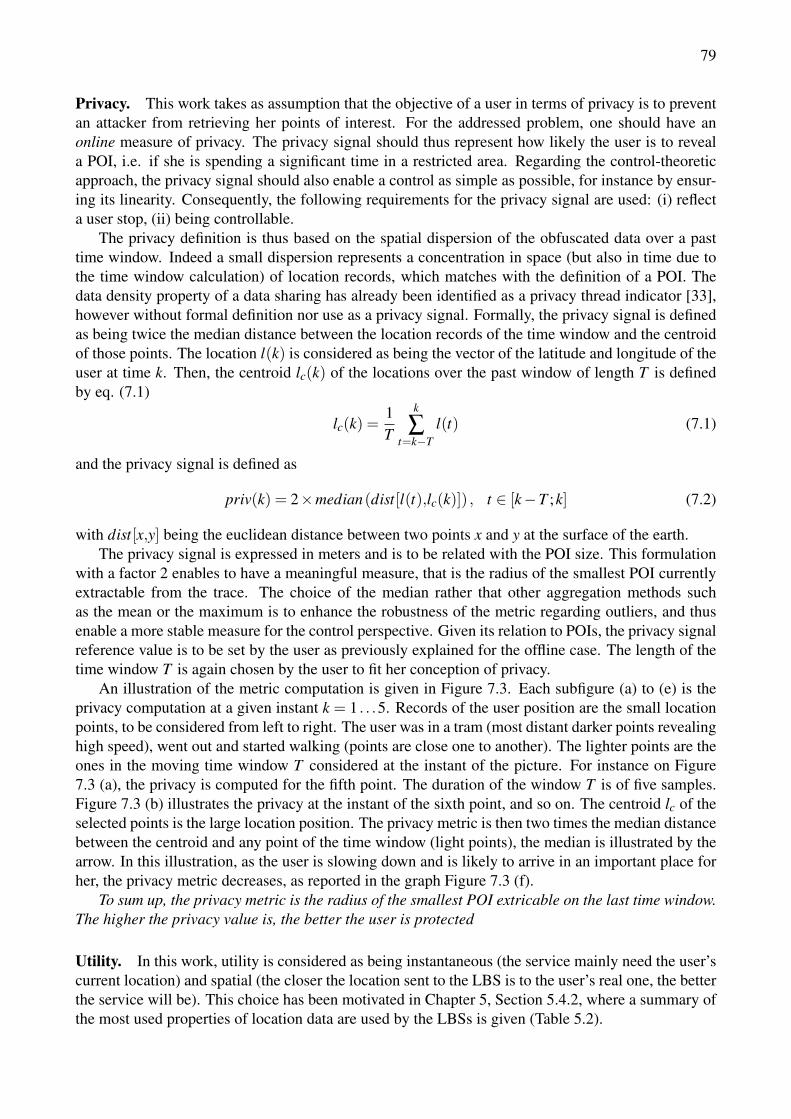
79

Privacy. This work takes as assumption that the objective of a user in terms of privacy is to preventan attacker from retrieving her points of interest. For the addressed problem, one should have anonline measure of privacy. The privacy signal should thus represent how likely the user is to reveala POI, i.e. if she is spending a significant time in a restricted area. Regarding the control-theoreticapproach, the privacy signal should also enable a control as simple as possible, for instance by ensur-ing its linearity. Consequently, the following requirements for the privacy signal are used: (i) reflecta user stop, (ii) being controllable.

The privacy definition is thus based on the spatial dispersion of the obfuscated data over a pasttime window. Indeed a small dispersion represents a concentration in space (but also in time due tothe time window calculation) of location records, which matches with the definition of a POI. Thedata density property of a data sharing has already been identified as a privacy thread indicator [33],however without formal definition nor use as a privacy signal. Formally, the privacy signal is definedas being twice the median distance between the location records of the time window and the centroidof those points. The location l(k) is considered as being the vector of the latitude and longitude of theuser at time k. Then, the centroid lc(k) of the locations over the past window of length T is definedby eq. (7.1)

lc(k) =1T

k

∑t=k−T

l(t) (7.1)

and the privacy signal is defined as

priv(k) = 2×median(dist[l(t),lc(k)]) , t ∈ [k−T ;k] (7.2)

with dist[x,y] being the euclidean distance between two points x and y at the surface of the earth.The privacy signal is expressed in meters and is to be related with the POI size. This formulation

with a factor 2 enables to have a meaningful measure, that is the radius of the smallest POI currentlyextractable from the trace. The choice of the median rather that other aggregation methods suchas the mean or the maximum is to enhance the robustness of the metric regarding outliers, and thusenable a more stable measure for the control perspective. Given its relation to POIs, the privacy signalreference value is to be set by the user as previously explained for the offline case. The length of thetime window T is again chosen by the user to fit her conception of privacy.

An illustration of the metric computation is given in Figure 7.3. Each subfigure (a) to (e) is theprivacy computation at a given instant k = 1 . . .5. Records of the user position are the small locationpoints, to be considered from left to right. The user was in a tram (most distant darker points revealinghigh speed), went out and started walking (points are close one to another). The lighter points are theones in the moving time window T considered at the instant of the picture. For instance on Figure7.3 (a), the privacy is computed for the fifth point. The duration of the window T is of five samples.Figure 7.3 (b) illustrates the privacy at the instant of the sixth point, and so on. The centroid lc of theselected points is the large location position. The privacy metric is then two times the median distancebetween the centroid and any point of the time window (light points), the median is illustrated by thearrow. In this illustration, as the user is slowing down and is likely to arrive in an important place forher, the privacy metric decreases, as reported in the graph Figure 7.3 (f).

To sum up, the privacy metric is the radius of the smallest POI extricable on the last time window.The higher the privacy value is, the better the user is protected

Utility. In this work, utility is considered as being instantaneous (the service mainly need the user’scurrent location) and spatial (the closer the location sent to the LBS is to the user’s real one, the betterthe service will be). This choice has been motivated in Chapter 5, Section 5.4.2, where a summary ofthe most used properties of location data are used by the LBSs is given (Table 5.2).

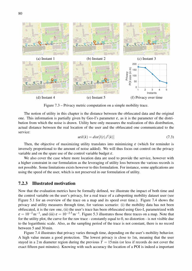
80

(a) Instant 1 (b) Instant 2 (c) Instant 3

1 2 3 4 5Instants

0

50

100

150

200

Priv

acy

POI s

ize

(in m

)

(d) Instant 4 (e) Instant 5 (f) Privacy over time

Figure 7.3 – Privacy metric computation on a simple mobility trace.

The notion of utility in this chapter is the distance between the obfuscated data and the originalone. This information is partially given by Geo-I’s parameter ε , as it is the parameter of the distri-bution from which the noise is drawn. Utility here only measures the realization of this distribution,actual distance between the real location of the user and the obfuscated one communicated to theservice:

util(k) = dist[l(t),l′(k)] (7.3)

Then, the objective of maximizing utility translates into minimizing ε (which for reminder isinversely proportional to the amount of noise added). We will thus focus out control on the privacyvariable and on the spare use of the control variable budget ε .

We also cover the case where more location data are used to provide the service, however witha higher constraint in our formulation as the leveraging of utility loss between the various records isnot possible. Some limitations exists however to this formulation. For instance, some applications areusing the speed of the user, which is not preserved in our formulation of utility.

7.2.3 Illustrated motivationNow that the evaluation metrics have be formally defined, we illustrate the impact of both time andthe control variable on the user’s privacy, for a real trace of a cabspotting mobility dataset user (seeFigure 5.1 for an overview of the trace on a map and its speed over time.). Figure 7.4 shows theprivacy and utility measures through time, for various scenario: (i) the mobility data has not beenobfuscated, it is the raw one, (ii) the user’s trace has been obfuscated using Geo-I, parametrized withε = 10−2 m−1, and (iii) ε = 10−2.5 m−1. Figure 5.3 illustrates those three traces on a map. Note thatfor the utility plot, the curve for the raw trace - constantly equal to 0, no distortion - is not visible dueto the logarithmic scale. Also, as the sampling period of the trace is not constant, there is no recordbetween 5 and 30 min.

Figure 7.4 illustrates that privacy varies through time, depending on the user’s mobility behavior.A high value means a good protection. The lowest privacy is close to 1m, meaning that the userstayed in a 2 m diameter region during the previous T = 15min (or less if records do not cover theexact fifteen past minutes). Knowing with such accuracy the location of a POI is indeed a important

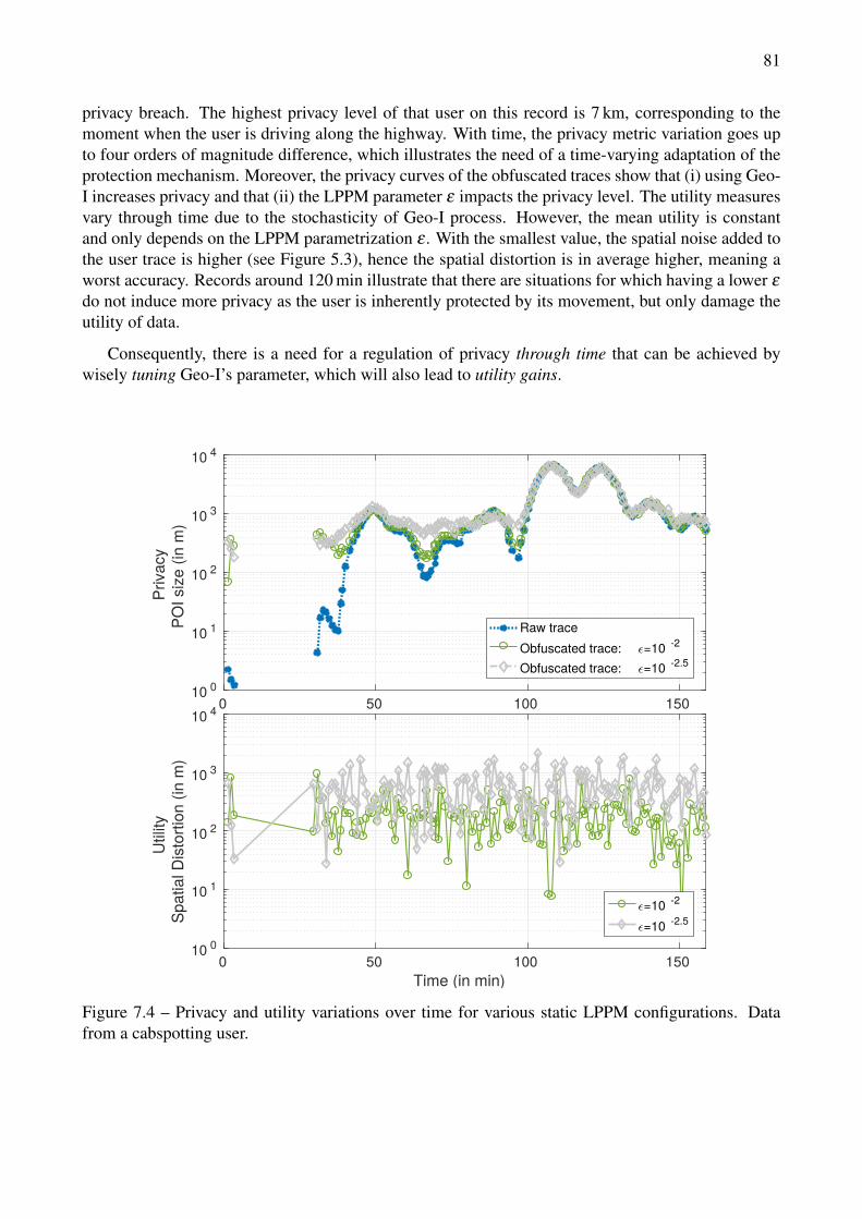
81

privacy breach. The highest privacy level of that user on this record is 7 km, corresponding to themoment when the user is driving along the highway. With time, the privacy metric variation goes upto four orders of magnitude difference, which illustrates the need of a time-varying adaptation of theprotection mechanism. Moreover, the privacy curves of the obfuscated traces show that (i) using Geo-I increases privacy and that (ii) the LPPM parameter ε impacts the privacy level. The utility measuresvary through time due to the stochasticity of Geo-I process. However, the mean utility is constantand only depends on the LPPM parametrization ε . With the smallest value, the spatial noise added tothe user trace is higher (see Figure 5.3), hence the spatial distortion is in average higher, meaning aworst accuracy. Records around 120 min illustrate that there are situations for which having a lower ε

do not induce more privacy as the user is inherently protected by its movement, but only damage theutility of data.

Consequently, there is a need for a regulation of privacy through time that can be achieved bywisely tuning Geo-I’s parameter, which will also lead to utility gains.

0 50 100 150Time (in min)

10 0

10 1

10 2

10 3

10 4

Priv

acy

POI s

ize

(in m

)

Raw traceObfuscated trace: =10 -2

Obfuscated trace: =10 -2.5

0 50 100 150Time (in min)

10 0

10 1

10 2

10 3

10 4

Util

itySp

atia

l Dis

torti

on (i

n m

)

=10 -2

=10 -2.5

Figure 7.4 – Privacy and utility variations over time for various static LPPM configurations. Datafrom a cabspotting user.

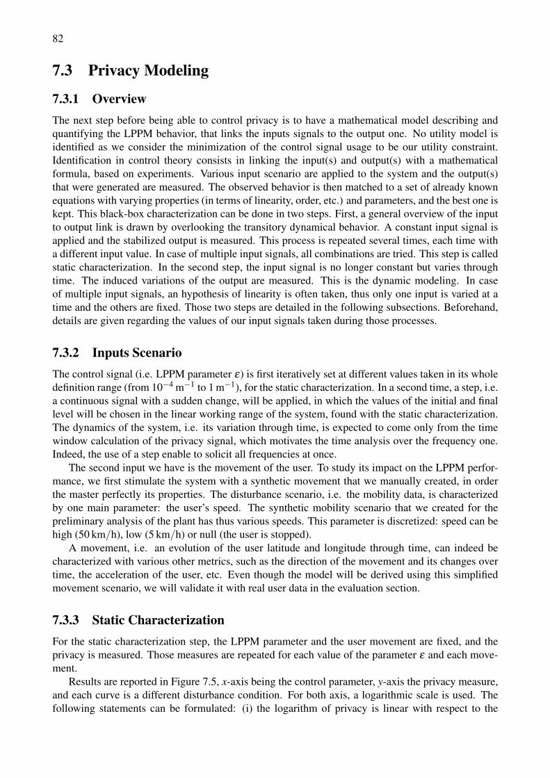
82

7.3 Privacy Modeling

7.3.1 OverviewThe next step before being able to control privacy is to have a mathematical model describing andquantifying the LPPM behavior, that links the inputs signals to the output one. No utility model isidentified as we consider the minimization of the control signal usage to be our utility constraint.Identification in control theory consists in linking the input(s) and output(s) with a mathematicalformula, based on experiments. Various input scenario are applied to the system and the output(s)that were generated are measured. The observed behavior is then matched to a set of already knownequations with varying properties (in terms of linearity, order, etc.) and parameters, and the best one iskept. This black-box characterization can be done in two steps. First, a general overview of the inputto output link is drawn by overlooking the transitory dynamical behavior. A constant input signal isapplied and the stabilized output is measured. This process is repeated several times, each time witha different input value. In case of multiple input signals, all combinations are tried. This step is calledstatic characterization. In the second step, the input signal is no longer constant but varies throughtime. The induced variations of the output are measured. This is the dynamic modeling. In caseof multiple input signals, an hypothesis of linearity is often taken, thus only one input is varied at atime and the others are fixed. Those two steps are detailed in the following subsections. Beforehand,details are given regarding the values of our input signals taken during those processes.

7.3.2 Inputs ScenarioThe control signal (i.e. LPPM parameter ε) is first iteratively set at different values taken in its wholedefinition range (from 10−4 m−1 to 1 m−1), for the static characterization. In a second time, a step, i.e.a continuous signal with a sudden change, will be applied, in which the values of the initial and finallevel will be chosen in the linear working range of the system, found with the static characterization.The dynamics of the system, i.e. its variation through time, is expected to come only from the timewindow calculation of the privacy signal, which motivates the time analysis over the frequency one.Indeed, the use of a step enable to solicit all frequencies at once.

The second input we have is the movement of the user. To study its impact on the LPPM perfor-mance, we first stimulate the system with a synthetic movement that we manually created, in orderthe master perfectly its properties. The disturbance scenario, i.e. the mobility data, is characterizedby one main parameter: the user’s speed. The synthetic mobility scenario that we created for thepreliminary analysis of the plant has thus various speeds. This parameter is discretized: speed can behigh (50 km/h), low (5 km/h) or null (the user is stopped).

A movement, i.e. an evolution of the user latitude and longitude through time, can indeed becharacterized with various other metrics, such as the direction of the movement and its changes overtime, the acceleration of the user, etc. Even though the model will be derived using this simplifiedmovement scenario, we will validate it with real user data in the evaluation section.

7.3.3 Static CharacterizationFor the static characterization step, the LPPM parameter and the user movement are fixed, and theprivacy is measured. Those measures are repeated for each value of the parameter ε and each move-ment.

Results are reported in Figure 7.5, x-axis being the control parameter, y-axis the privacy measure,and each curve is a different disturbance condition. For both axis, a logarithmic scale is used. Thefollowing statements can be formulated: (i) the logarithm of privacy is linear with respect to the

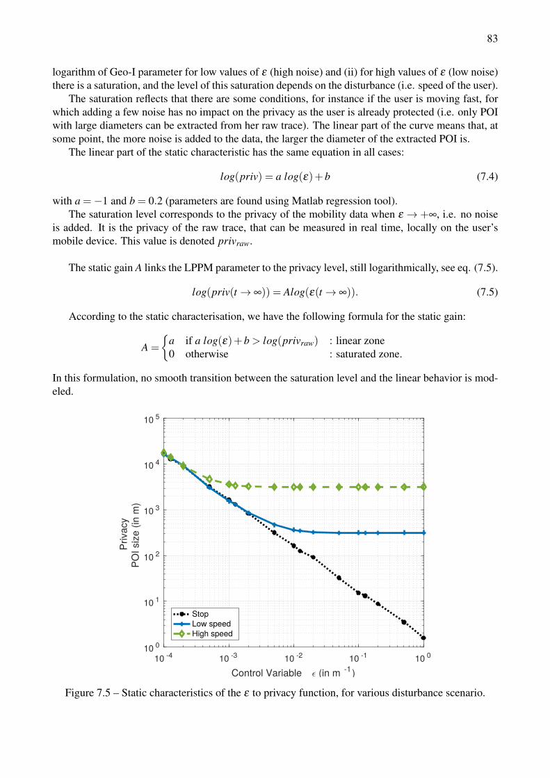
83

logarithm of Geo-I parameter for low values of ε (high noise) and (ii) for high values of ε (low noise)there is a saturation, and the level of this saturation depends on the disturbance (i.e. speed of the user).

The saturation reflects that there are some conditions, for instance if the user is moving fast, forwhich adding a few noise has no impact on the privacy as the user is already protected (i.e. only POIwith large diameters can be extracted from her raw trace). The linear part of the curve means that, atsome point, the more noise is added to the data, the larger the diameter of the extracted POI is.

The linear part of the static characteristic has the same equation in all cases:

log(priv) = a log(ε)+b (7.4)

with a =−1 and b = 0.2 (parameters are found using Matlab regression tool).The saturation level corresponds to the privacy of the mobility data when ε → +∞, i.e. no noise

is added. It is the privacy of the raw trace, that can be measured in real time, locally on the user’smobile device. This value is denoted privraw.

The static gain A links the LPPM parameter to the privacy level, still logarithmically, see eq. (7.5).

log(priv(t→ ∞)) = Alog(ε(t→ ∞)). (7.5)

According to the static characterisation, we have the following formula for the static gain:

A =

{a if a log(ε)+b > log(privraw) : linear zone0 otherwise : saturated zone.

In this formulation, no smooth transition between the saturation level and the linear behavior is mod-eled.

10 -4 10 -3 10 -2 10 -1 10 0

Control Variable (in m -1)

10 0

10 1

10 2

10 3

10 4

10 5

Priv

acy

POI s

ize

(in m

)

StopLow speedHigh speed

Figure 7.5 – Static characteristics of the ε to privacy function, for various disturbance scenario.

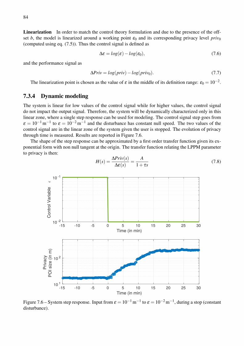
84

Linearization In order to match the control theory formulation and due to the presence of the off-set b, the model is linearized around a working point ε0 and its corresponding privacy level priv0(computed using eq. (7.5)). Thus the control signal is defined as

∆ε = log(ε)− log(ε0), (7.6)

and the performance signal as

∆Priv = log(priv)− log(priv0). (7.7)

The linearization point is chosen as the value of ε in the middle of its definition range: ε0 = 10−2.

7.3.4 Dynamic modelingThe system is linear for low values of the control signal while for higher values, the control signaldo not impact the output signal. Therefore, the system will be dynamically characterized only in thislinear zone, where a single step response can be used for modeling. The control signal step goes fromε = 10−1 m−1 to ε = 10−2 m−1 and the disturbance has constant null speed. The two values of thecontrol signal are in the linear zone of the system given the user is stopped. The evolution of privacythrough time is measured. Results are reported in Figure 7.6.

The shape of the step response can be approximated by a first order transfer function given its ex-ponential form with non null tangent at the origin. The transfer function relating the LPPM parameterto privacy is then:

H(s) =∆Priv(s)

∆ε(s)=

A1+ τs

(7.8)

-15 -10 -5 0 5 10 15 20 25 30Time (in min)

10 -2

10 -1

Con

trol V

aria

ble

-15 -10 -5 0 5 10 15 20 25 30Time (in min)

10 1

10 2

Priv

acy

POI s

ize

(in m

)

Figure 7.6 – System step response. Input from ε = 10−1 m−1 to ε = 10−2 m−1, during a stop (constantdisturbance).

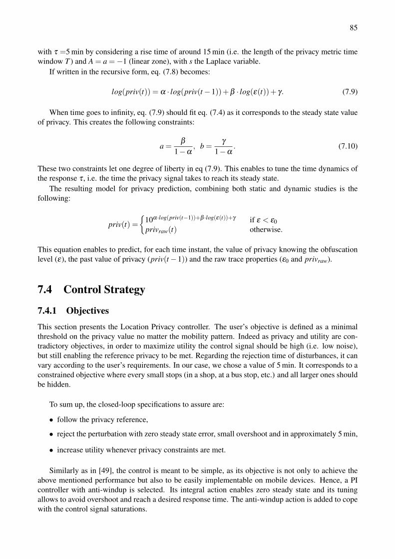
85

with τ =5 min by considering a rise time of around 15 min (i.e. the length of the privacy metric timewindow T ) and A = a =−1 (linear zone), with s the Laplace variable.

If written in the recursive form, eq. (7.8) becomes:

log(priv(t)) = α · log(priv(t−1))+β · log(ε(t))+ γ. (7.9)

When time goes to infinity, eq. (7.9) should fit eq. (7.4) as it corresponds to the steady state valueof privacy. This creates the following constraints:

a =β

1−α, b =

γ

1−α. (7.10)

These two constraints let one degree of liberty in eq (7.9). This enables to tune the time dynamics ofthe response τ , i.e. the time the privacy signal takes to reach its steady state.

The resulting model for privacy prediction, combining both static and dynamic studies is thefollowing:

priv(t) ={

10α·log(priv(t−1))+β ·log(ε(t))+γ if ε < ε0privraw(t) otherwise.

This equation enables to predict, for each time instant, the value of privacy knowing the obfuscationlevel (ε), the past value of privacy (priv(t−1)) and the raw trace properties (ε0 and privraw).

7.4 Control Strategy

7.4.1 Objectives

This section presents the Location Privacy controller. The user’s objective is defined as a minimalthreshold on the privacy value no matter the mobility pattern. Indeed as privacy and utility are con-tradictory objectives, in order to maximize utility the control signal should be high (i.e. low noise),but still enabling the reference privacy to be met. Regarding the rejection time of disturbances, it canvary according to the user’s requirements. In our case, we chose a value of 5 min. It corresponds to aconstrained objective where every small stops (in a shop, at a bus stop, etc.) and all larger ones shouldbe hidden.

To sum up, the closed-loop specifications to assure are:

• follow the privacy reference,

• reject the perturbation with zero steady state error, small overshoot and in approximately 5 min,

• increase utility whenever privacy constraints are met.

Similarly as in [49], the control is meant to be simple, as its objective is not only to achieve theabove mentioned performance but also to be easily implementable on mobile devices. Hence, a PIcontroller with anti-windup is selected. Its integral action enables zero steady state and its tuningallows to avoid overshoot and reach a desired response time. The anti-windup action is added to copewith the control signal saturations.

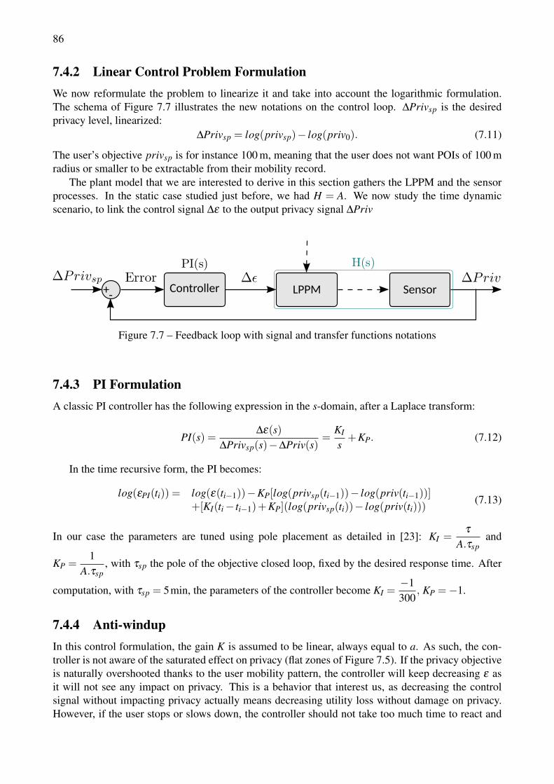
86

7.4.2 Linear Control Problem FormulationWe now reformulate the problem to linearize it and take into account the logarithmic formulation.The schema of Figure 7.7 illustrates the new notations on the control loop. ∆Privsp is the desiredprivacy level, linearized:

∆Privsp = log(privsp)− log(priv0). (7.11)

The user’s objective privsp is for instance 100 m, meaning that the user does not want POIs of 100 mradius or smaller to be extractable from their mobility record.

The plant model that we are interested to derive in this section gathers the LPPM and the sensorprocesses. In the static case studied just before, we had H = A. We now study the time dynamicscenario, to link the control signal ∆ε to the output privacy signal ∆Priv

LPPM Sensor+-Controller

Figure 7.7 – Feedback loop with signal and transfer functions notations

7.4.3 PI FormulationA classic PI controller has the following expression in the s-domain, after a Laplace transform:

PI(s) =∆ε(s)

∆Privsp(s)−∆Priv(s)=

KI

s+KP. (7.12)

In the time recursive form, the PI becomes:

log(εPI(ti)) = log(ε(ti−1))−KP[log(privsp(ti−1))− log(priv(ti−1))]+[KI(ti− ti−1)+KP](log(privsp(ti))− log(priv(ti)))

(7.13)

In our case the parameters are tuned using pole placement as detailed in [23]: KI =τ

A.τspand

KP =1

A.τsp, with τsp the pole of the objective closed loop, fixed by the desired response time. After

computation, with τsp = 5min, the parameters of the controller become KI =−1300

, KP =−1.

7.4.4 Anti-windupIn this control formulation, the gain K is assumed to be linear, always equal to a. As such, the con-troller is not aware of the saturated effect on privacy (flat zones of Figure 7.5). If the privacy objectiveis naturally overshooted thanks to the user mobility pattern, the controller will keep decreasing ε asit will not see any impact on privacy. This is a behavior that interest us, as decreasing the controlsignal without impacting privacy actually means decreasing utility loss without damage on privacy.However, if the user stops or slows down, the controller should not take too much time to react and

87

decrease the control signal. In order to ensure such behavior, an anti wind-up strategy is added, in theform of an actuator saturation (see [175]):

ε(ti) = min(max(εPI(ti),εmin),εmax). (7.14)

where threshold are chosen according to Geo-I’s common range of variations [εmin,εmax] = [10−4,1] m−1.

7.5 dynULP EvaluationBoth the modeling and the control are evaluated in this section. We first give an overview of themethodology: the scenario considered and the performance indicators used for the evaluation.

7.5.1 MethodologyResults presented in this section are the outputs of single runs. No averaging is done on several similarexperiments in order (i) to preserve the explainability of the impacts of the signals on each other, (ii)to fit as much as possible to the online scenario with only one-shot opportunities for the controller, and(iii) not to hide the difficulty of controlling a stochastic system by showing only its average control.

7.5.1.1 Inputs scenarios

The evaluation aims at illustrating three points: (i) the understanding and explainability of the mod-eling and control, (ii) the generality of their performance in front of a diversity of situations and (iii)the applicability of the solution on a real-life mobility scenario. The inputs of the model (mobilitytrace and ε signal) and the ones of the controller (mobility trace and the reference signal) are set inorder to reflect those three points, as explained in the following:

• Mobility trace. First a simple scenario is used, in which the user is considered either stopped,or moving with a constant speed (low or medium), with step variations between those situations.The mobility trace used for generality validation is the synthetic one presented in Chapter 5,Section 5.1, which gathers more complex moves such as turns, acceleration, micro-stops, etc.Eventually, the applicability in practice is tested using a real-life mobility record, the one of aCabspotting user, also presented in Chapter 5, Section 5.1.

• LPPM parameter ε . It is set by the controller in order to meet the reference signal. However,in the modeling phase it is a free signal that should be set in order to stimulate the plant. In itssimplest form, ε is constant at the median value of its definition range, 10−2. A step signal -instantaneous change from one value to another - is also used. Eventually, we generate a morecomplex signal, with various amplitudes (10−4 m−1 to 1 m−1) and periods (from one 10 s, i.e.about a sampling period of the mobility trace, to 30 min).

• Privacy specification privsp. When needed, e.g. for the control evaluation, the reference valueis either (i) constant at 500 m (POI of max 1 km of diameter), (ii) a step, or (iii) a random signalwith varying amplitude (from 1 m to 10 km) and period (from 5 min to 5 h). Changes in thespecifications are made by the user herself, thus are not as frequent as the changes in ε , thatare driven by the controller. Regarding the values of amplitude values, they range from verylow, i.e. the stop place can be determined with the precision of a meter, to really large, the stoplocation cannot be more precise than several kilometers.

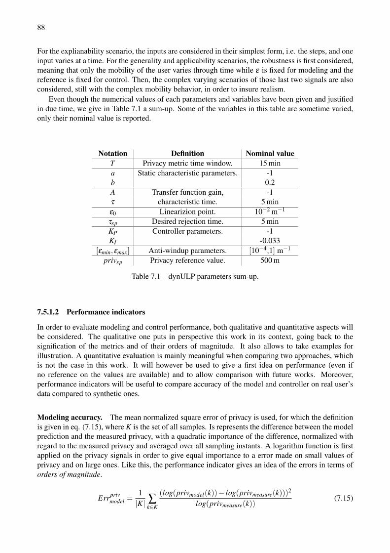
88

For the explianability scenario, the inputs are considered in their simplest form, i.e. the steps, and oneinput varies at a time. For the generality and applicability scenarios, the robustness is first considered,meaning that only the mobility of the user varies through time while ε is fixed for modeling and thereference is fixed for control. Then, the complex varying scenarios of those last two signals are alsoconsidered, still with the complex mobility behavior, in order to insure realism.

Even though the numerical values of each parameters and variables have been given and justifiedin due time, we give in Table 7.1 a sum-up. Some of the variables in this table are sometime varied,only their nominal value is reported.

Notation Definition Nominal valueT Privacy metric time window. 15 mina Static characteristic parameters. -1b 0.2A Transfer function gain, -1τ characteristic time. 5 minε0 Linearizion point. 10−2 m−1

τsp Desired rejection time. 5 minKP Controller parameters. -1KI -0.033

[εmin,εmax] Anti-windup parameters. [10−4,1] m−1

privsp Privacy reference value. 500 m

Table 7.1 – dynULP parameters sum-up.

7.5.1.2 Performance indicators

In order to evaluate modeling and control performance, both qualitative and quantitative aspects willbe considered. The qualitative one puts in perspective this work in its context, going back to thesignification of the metrics and of their orders of magnitude. It also allows to take examples forillustration. A quantitative evaluation is mainly meaningful when comparing two approaches, whichis not the case in this work. It will however be used to give a first idea on performance (even ifno reference on the values are available) and to allow comparison with future works. Moreover,performance indicators will be useful to compare accuracy of the model and controller on real user’sdata compared to synthetic ones.

Modeling accuracy. The mean normalized square error of privacy is used, for which the definitionis given in eq. (7.15), where K is the set of all samples. Is represents the difference between the modelprediction and the measured privacy, with a quadratic importance of the difference, normalized withregard to the measured privacy and averaged over all sampling instants. A logarithm function is firstapplied on the privacy signals in order to give equal importance to a error made on small values ofprivacy and on large ones. Like this, the performance indicator gives an idea of the errors in terms oforders of magnitude.

Errprivmodel =

1|K| ∑k∈K

(log(privmodel(k))− log(privmeasure(k)))2

log(privmeasure(k))(7.15)

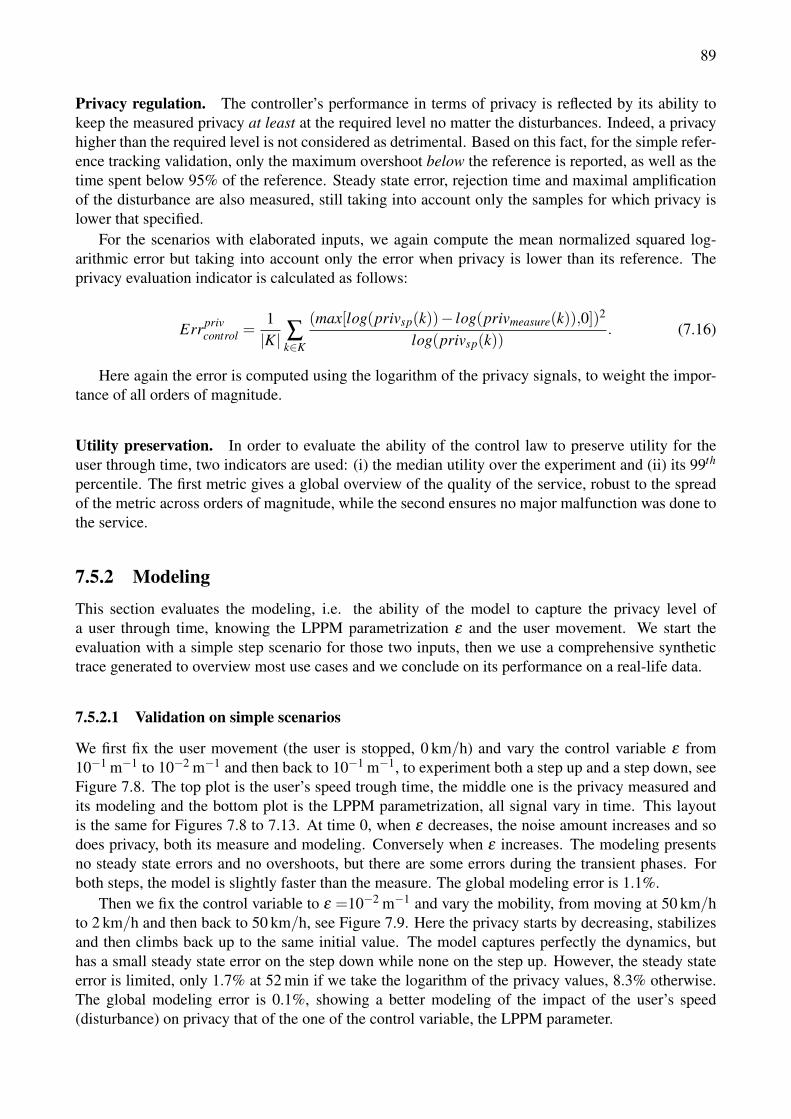
89

Privacy regulation. The controller’s performance in terms of privacy is reflected by its ability tokeep the measured privacy at least at the required level no matter the disturbances. Indeed, a privacyhigher than the required level is not considered as detrimental. Based on this fact, for the simple refer-ence tracking validation, only the maximum overshoot below the reference is reported, as well as thetime spent below 95% of the reference. Steady state error, rejection time and maximal amplificationof the disturbance are also measured, still taking into account only the samples for which privacy islower that specified.

For the scenarios with elaborated inputs, we again compute the mean normalized squared log-arithmic error but taking into account only the error when privacy is lower than its reference. Theprivacy evaluation indicator is calculated as follows:

Errprivcontrol =

1|K| ∑k∈K

(max[log(privsp(k))− log(privmeasure(k)),0])2

log(privsp(k)). (7.16)

Here again the error is computed using the logarithm of the privacy signals, to weight the impor-tance of all orders of magnitude.

Utility preservation. In order to evaluate the ability of the control law to preserve utility for theuser through time, two indicators are used: (i) the median utility over the experiment and (ii) its 99th

percentile. The first metric gives a global overview of the quality of the service, robust to the spreadof the metric across orders of magnitude, while the second ensures no major malfunction was done tothe service.

7.5.2 Modeling

This section evaluates the modeling, i.e. the ability of the model to capture the privacy level ofa user through time, knowing the LPPM parametrization ε and the user movement. We start theevaluation with a simple step scenario for those two inputs, then we use a comprehensive synthetictrace generated to overview most use cases and we conclude on its performance on a real-life data.

7.5.2.1 Validation on simple scenarios

We first fix the user movement (the user is stopped, 0 km/h) and vary the control variable ε from10−1 m−1 to 10−2 m−1 and then back to 10−1 m−1, to experiment both a step up and a step down, seeFigure 7.8. The top plot is the user’s speed trough time, the middle one is the privacy measured andits modeling and the bottom plot is the LPPM parametrization, all signal vary in time. This layoutis the same for Figures 7.8 to 7.13. At time 0, when ε decreases, the noise amount increases and sodoes privacy, both its measure and modeling. Conversely when ε increases. The modeling presentsno steady state errors and no overshoots, but there are some errors during the transient phases. Forboth steps, the model is slightly faster than the measure. The global modeling error is 1.1%.

Then we fix the control variable to ε =10−2 m−1 and vary the mobility, from moving at 50 km/hto 2 km/h and then back to 50 km/h, see Figure 7.9. Here the privacy starts by decreasing, stabilizesand then climbs back up to the same initial value. The model captures perfectly the dynamics, buthas a small steady state error on the step down while none on the step up. However, the steady stateerror is limited, only 1.7% at 52 min if we take the logarithm of the privacy values, 8.3% otherwise.The global modeling error is 0.1%, showing a better modeling of the impact of the user’s speed(disturbance) on privacy that of the one of the control variable, the LPPM parameter.

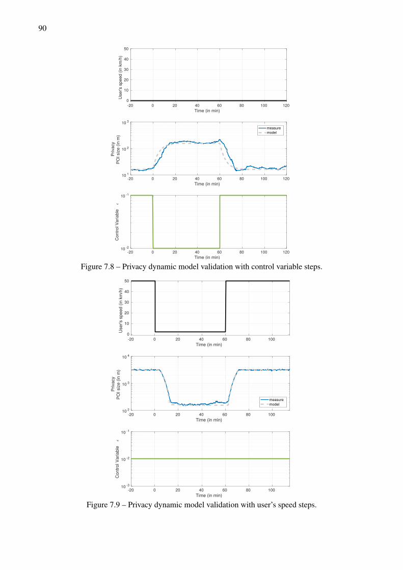
90

-20 0 20 40 60 80 100 120Time (in min)

10 -2

10 -1

Con

trol V

aria

ble

-20 0 20 40 60 80 100 120Time (in min)

10 1

10 2

10 3

Priv

acy

POI s

ize

(in m

)

measuremodel

-20 0 20 40 60 80 100 120Time (in min)

0

10

20

30

40

50

Use

r's s

peed

(in

km/h

)

Figure 7.8 – Privacy dynamic model validation with control variable steps.

-20 0 20 40 60 80 100Time (in min)

10 -3

10 -2

10 -1

Con

trol V

aria

ble

-20 0 20 40 60 80 100Time (in min)

10 2

10 3

10 4

Priv

acy

POI s

ize

(in m

)

measuremodel

-20 0 20 40 60 80 100Time (in min)

0

10

20

30

40

50

Use

r's s

peed

(in

km/h

)

Figure 7.9 – Privacy dynamic model validation with user’s speed steps.

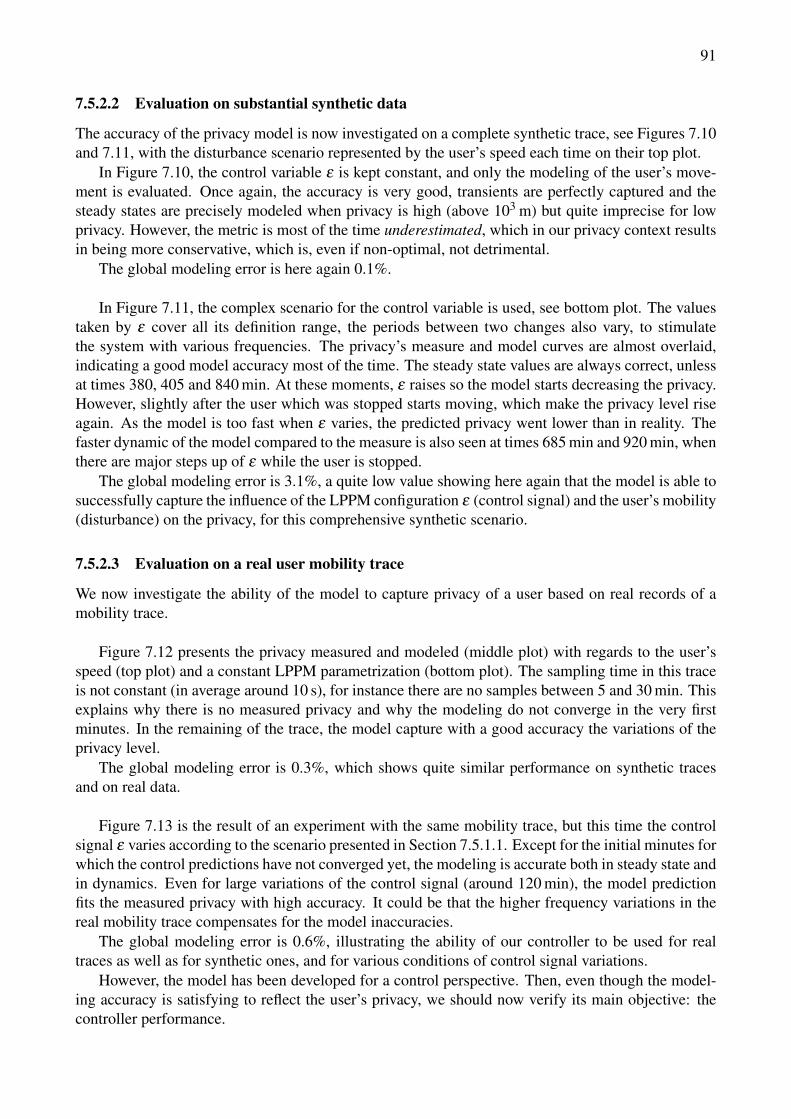
91

7.5.2.2 Evaluation on substantial synthetic data

The accuracy of the privacy model is now investigated on a complete synthetic trace, see Figures 7.10and 7.11, with the disturbance scenario represented by the user’s speed each time on their top plot.

In Figure 7.10, the control variable ε is kept constant, and only the modeling of the user’s move-ment is evaluated. Once again, the accuracy is very good, transients are perfectly captured and thesteady states are precisely modeled when privacy is high (above 103 m) but quite imprecise for lowprivacy. However, the metric is most of the time underestimated, which in our privacy context resultsin being more conservative, which is, even if non-optimal, not detrimental.

The global modeling error is here again 0.1%.

In Figure 7.11, the complex scenario for the control variable is used, see bottom plot. The valuestaken by ε cover all its definition range, the periods between two changes also vary, to stimulatethe system with various frequencies. The privacy’s measure and model curves are almost overlaid,indicating a good model accuracy most of the time. The steady state values are always correct, unlessat times 380, 405 and 840 min. At these moments, ε raises so the model starts decreasing the privacy.However, slightly after the user which was stopped starts moving, which make the privacy level riseagain. As the model is too fast when ε varies, the predicted privacy went lower than in reality. Thefaster dynamic of the model compared to the measure is also seen at times 685 min and 920 min, whenthere are major steps up of ε while the user is stopped.

The global modeling error is 3.1%, a quite low value showing here again that the model is able tosuccessfully capture the influence of the LPPM configuration ε (control signal) and the user’s mobility(disturbance) on the privacy, for this comprehensive synthetic scenario.

7.5.2.3 Evaluation on a real user mobility trace

We now investigate the ability of the model to capture privacy of a user based on real records of amobility trace.

Figure 7.12 presents the privacy measured and modeled (middle plot) with regards to the user’sspeed (top plot) and a constant LPPM parametrization (bottom plot). The sampling time in this traceis not constant (in average around 10 s), for instance there are no samples between 5 and 30 min. Thisexplains why there is no measured privacy and why the modeling do not converge in the very firstminutes. In the remaining of the trace, the model capture with a good accuracy the variations of theprivacy level.

The global modeling error is 0.3%, which shows quite similar performance on synthetic tracesand on real data.

Figure 7.13 is the result of an experiment with the same mobility trace, but this time the controlsignal ε varies according to the scenario presented in Section 7.5.1.1. Except for the initial minutes forwhich the control predictions have not converged yet, the modeling is accurate both in steady state andin dynamics. Even for large variations of the control signal (around 120 min), the model predictionfits the measured privacy with high accuracy. It could be that the higher frequency variations in thereal mobility trace compensates for the model inaccuracies.

The global modeling error is 0.6%, illustrating the ability of our controller to be used for realtraces as well as for synthetic ones, and for various conditions of control signal variations.

However, the model has been developed for a control perspective. Then, even though the model-ing accuracy is satisfying to reflect the user’s privacy, we should now verify its main objective: thecontroller performance.

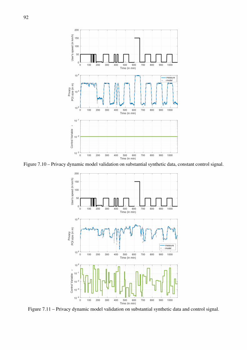
92

0 100 200 300 400 500 600 700 800 900 1000Time (in min)

10 -3

10 -2

10 -1

Con

trol V

aria

ble

0 100 200 300 400 500 600 700 800 900 1000Time (in min)

10 2

10 3

10 4

Priv

acy

POI s

ize

(in m

)

measuremodel

0 100 200 300 400 500 600 700 800 900 1000Time (in min)

0

50

100

150

200

Use

r's s

peed

(in

km/h

)

Figure 7.10 – Privacy dynamic model validation on substantial synthetic data, constant control signal.

0 100 200 300 400 500 600 700 800 900 1000Time (in min)

10 -4

10 -3

10 -2

10 -1

10 0

Con

trol V

aria

ble

0 100 200 300 400 500 600 700 800 900 1000Time (in min)

10 0

10 5

Priv

acy

POI s

ize

(in m

)

measuremodel

0 100 200 300 400 500 600 700 800 900 1000Time (in min)

0

50

100

150

200

Use

r's s

peed

(in

km/h

)

Figure 7.11 – Privacy dynamic model validation on substantial synthetic data and control signal.

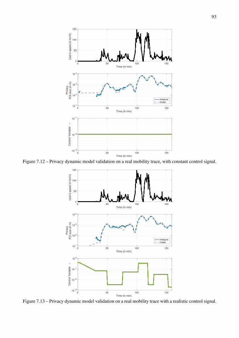
93

Figure 7.12 – Privacy dynamic model validation on a real mobility trace, with constant control signal.

Figure 7.13 – Privacy dynamic model validation on a real mobility trace with a realistic control signal.

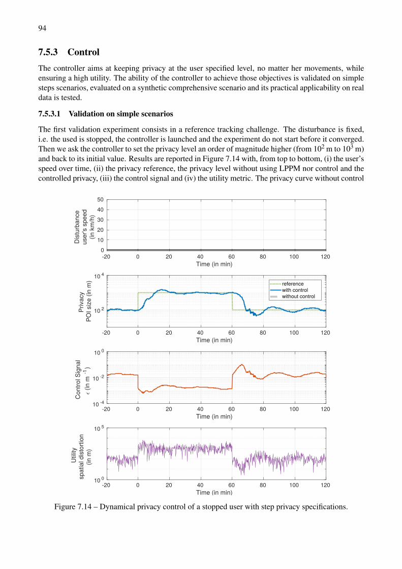
94

7.5.3 ControlThe controller aims at keeping privacy at the user specified level, no matter her movements, whileensuring a high utility. The ability of the controller to achieve those objectives is validated on simplesteps scenarios, evaluated on a synthetic comprehensive scenario and its practical applicability on realdata is tested.

7.5.3.1 Validation on simple scenarios

The first validation experiment consists in a reference tracking challenge. The disturbance is fixed,i.e. the used is stopped, the controller is launched and the experiment do not start before it converged.Then we ask the controller to set the privacy level an order of magnitude higher (from 102 m to 103 m)and back to its initial value. Results are reported in Figure 7.14 with, from top to bottom, (i) the user’sspeed over time, (ii) the privacy reference, the privacy level without using LPPM nor control and thecontrolled privacy, (iii) the control signal and (iv) the utility metric. The privacy curve without control

-20 0 20 40 60 80 100 120Time (in min)

10 2

10 4

Priv

acy

PO

I siz

e (in

m) reference

with controlwithout control

-20 0 20 40 60 80 100 120Time (in min)

01020304050

Dis

turb

ance

user

's sp

eed

(in k

m/h

)

-20 0 20 40 60 80 100 120Time (in min)

10 -4

10 -2

10 0

Con

trol S

igna

l(in

m-1

)

-20 0 20 40 60 80 100 120Time (in min)

10 0

10 5

Util

itysp

atia

l dis

torti

on (i

n m

)

Figure 7.14 – Dynamical privacy control of a stopped user with step privacy specifications.

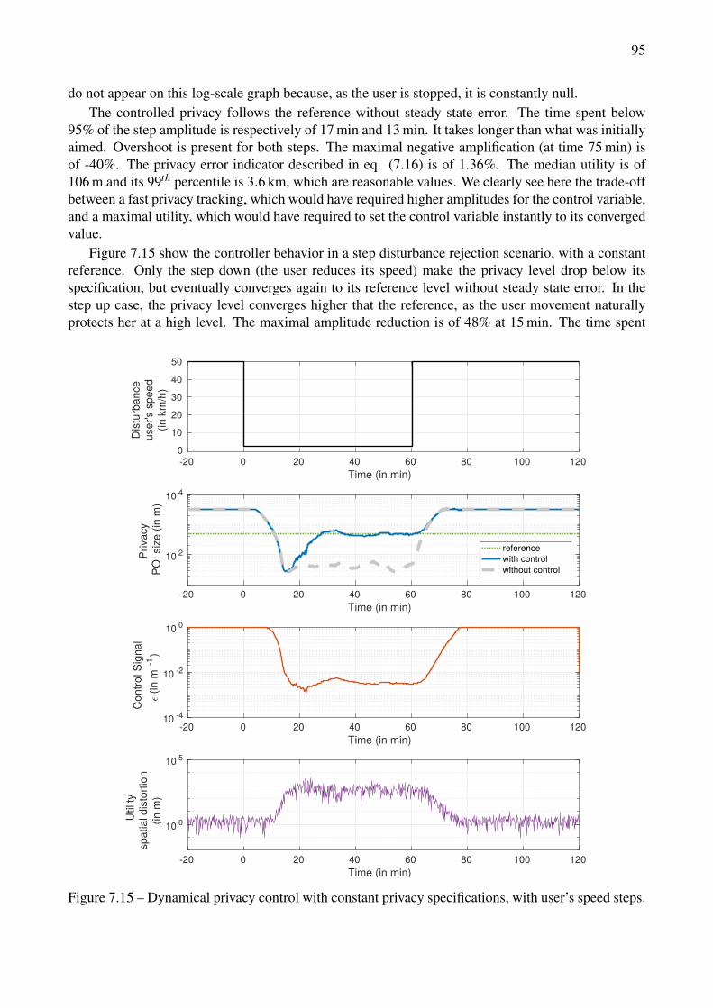
95

do not appear on this log-scale graph because, as the user is stopped, it is constantly null.The controlled privacy follows the reference without steady state error. The time spent below

95% of the step amplitude is respectively of 17 min and 13 min. It takes longer than what was initiallyaimed. Overshoot is present for both steps. The maximal negative amplification (at time 75 min) isof -40%. The privacy error indicator described in eq. (7.16) is of 1.36%. The median utility is of106 m and its 99th percentile is 3.6 km, which are reasonable values. We clearly see here the trade-offbetween a fast privacy tracking, which would have required higher amplitudes for the control variable,and a maximal utility, which would have required to set the control variable instantly to its convergedvalue.

Figure 7.15 show the controller behavior in a step disturbance rejection scenario, with a constantreference. Only the step down (the user reduces its speed) make the privacy level drop below itsspecification, but eventually converges again to its reference level without steady state error. In thestep up case, the privacy level converges higher that the reference, as the user movement naturallyprotects her at a high level. The maximal amplitude reduction is of 48% at 15 min. The time spent

-20 0 20 40 60 80 100 120Time (in min)

10 2

10 4

Priv

acy

PO

I siz

e (in

m)

referencewith controlwithout control

-20 0 20 40 60 80 100 120Time (in min)

0

10

20

30

40

50

Dis

turb

ance

user

's sp

eed

(in k

m/h

)

-20 0 20 40 60 80 100 120Time (in min)

10 -4

10 -2

10 0

Con

trol S

igna

l(in

m-1

)

-20 0 20 40 60 80 100 120Time (in min)

10 0

10 5

Util

itysp

atia

l dis

torti

on (i

n m

)

Figure 7.15 – Dynamical privacy control with constant privacy specifications, with user’s speed steps.

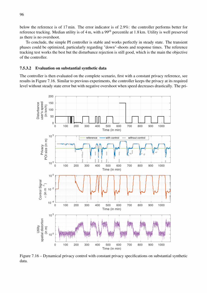
96

below the reference is of 17 min. The error indicator is of 2.9%: the controller performs better forreference tracking. Median utility is of 4 m, with a 99th percentile at 1.8 km. Utility is well preservedas there is no overshoot.

To conclude, the simple PI controller is stable and works perfectly in steady state. The transientphases could be optimized, particularly regarding "down"-shoots and response times. The referencetracking test works the best but the disturbance rejection is still good, which is the main the objectiveof the controller.

7.5.3.2 Evaluation on substantial synthetic data

The controller is then evaluated on the complete scenario, first with a constant privacy reference, seeresults in Figure 7.16. Similar to previous experiments, the controller keeps the privacy at its requiredlevel without steady state error but with negative overshoot when speed decreases drastically. The pri-

0 100 200 300 400 500 600 700 800 900 1000Time (in min)

10 0

10 5

Priv

acy

PO

I siz

e (in

m) reference with control without control

0 100 200 300 400 500 600 700 800 900 1000Time (in min)

0

50

100

150

200

Dis

turb

ance

user

's sp

eed

(in k

m/h

)

0 100 200 300 400 500 600 700 800 900 1000Time (in min)

10 -4

10 -2

10 0

Con

trol S

igna

l(in

m-1

)

0 100 200 300 400 500 600 700 800 900 1000Time (in min)

10 0

10 5

Util

itysp

atia

l dis

torti

on (i

n m

)

Figure 7.16 – Dynamical privacy control with constant privacy specifications on substantial syntheticdata.

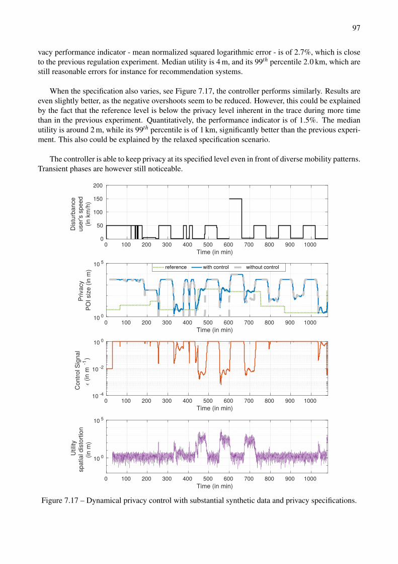
97

vacy performance indicator - mean normalized squared logarithmic error - is of 2.7%, which is closeto the previous regulation experiment. Median utility is 4 m, and its 99th percentile 2.0 km, which arestill reasonable errors for instance for recommendation systems.

When the specification also varies, see Figure 7.17, the controller performs similarly. Results areeven slightly better, as the negative overshoots seem to be reduced. However, this could be explainedby the fact that the reference level is below the privacy level inherent in the trace during more timethan in the previous experiment. Quantitatively, the performance indicator is of 1.5%. The medianutility is around 2 m, while its 99th percentile is of 1 km, significantly better than the previous experi-ment. This also could be explained by the relaxed specification scenario.

The controller is able to keep privacy at its specified level even in front of diverse mobility patterns.Transient phases are however still noticeable.

0 100 200 300 400 500 600 700 800 900 1000Time (in min)

10 0

10 5

Priv

acy

PO

I siz

e (in

m) reference with control without control

0 100 200 300 400 500 600 700 800 900 1000Time (in min)

0

50

100

150

200

Dis

turb

ance

user

's sp

eed

(in k

m/h

)

0 100 200 300 400 500 600 700 800 900 1000Time (in min)

10 -4

10 -2

10 0

Con

trol S

igna

l(in

m-1

)

0 100 200 300 400 500 600 700 800 900 1000Time (in min)

10 0

10 5

Util

itysp

atia

l dis

torti

on (i

n m

)

Figure 7.17 – Dynamical privacy control with substantial synthetic data and privacy specifications.

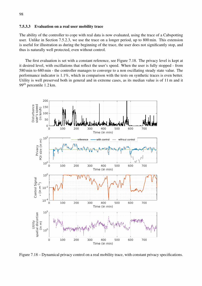
98

7.5.3.3 Evaluation on a real user mobility trace

The ability of the controller to cope with real data is now evaluated, using the trace of a Cabspottinguser. Unlike in Section 7.5.2.3, we use the trace on a longer period, up to 800 min. This extensionis useful for illustration as during the beginning of the trace, the user does not significantly stop, andthus is naturally well protected, even without control.

The first evaluation is set with a constant reference, see Figure 7.18. The privacy level is kept atit desired level, with oscillations that reflect the user’s speed. When the user is fully stopped - from580 min to 680 min - the controller manages to converge to a non oscillating steady state value. Theperformance indicator is 1.1%, which in comparison with the tests on synthetic traces is even better.Utility is well preserved both in general and in extreme cases, as its median value is of 11 m and it99th percentile 1.2 km.

Figure 7.18 – Dynamical privacy control on a real mobility trace, with constant privacy specifications.

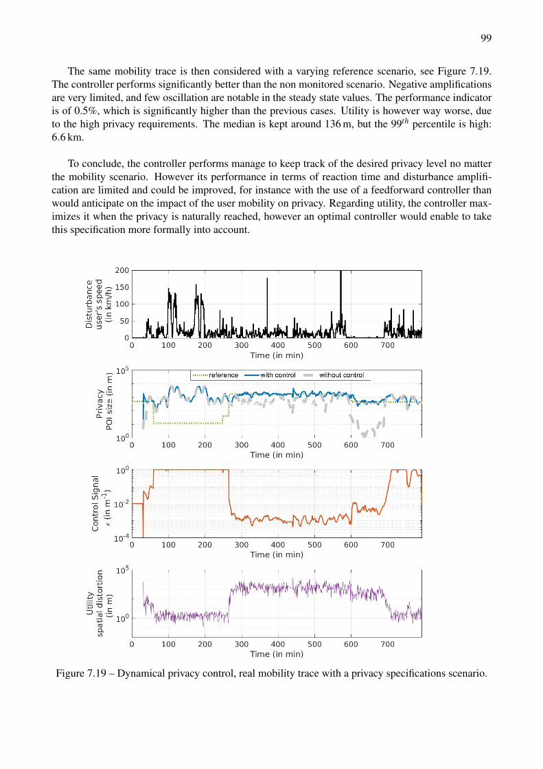
99

The same mobility trace is then considered with a varying reference scenario, see Figure 7.19.The controller performs significantly better than the non monitored scenario. Negative amplificationsare very limited, and few oscillation are notable in the steady state values. The performance indicatoris of 0.5%, which is significantly higher than the previous cases. Utility is however way worse, dueto the high privacy requirements. The median is kept around 136 m, but the 99th percentile is high:6.6 km.

To conclude, the controller performs manage to keep track of the desired privacy level no matterthe mobility scenario. However its performance in terms of reaction time and disturbance amplifi-cation are limited and could be improved, for instance with the use of a feedforward controller thanwould anticipate on the impact of the user mobility on privacy. Regarding utility, the controller max-imizes it when the privacy is naturally reached, however an optimal controller would enable to takethis specification more formally into account.

Figure 7.19 – Dynamical privacy control, real mobility trace with a privacy specifications scenario.

100

7.6 ConclusionThis chapter focused on the use of Location-Based Services through time, i.e. the user’s location issent periodically. This scenario is particularly sensible to privacy attacks if a malicious agent hasaccess to the real-time position of the user. The focus has been made on the user’s points of inter-est, a low level indicator of habits and identity. Location Privacy Protection Mechanisms (LPPMs)have been developed in order to address those threats. However, the use of LPPMs comes with anunavoidable reduction of the service utility, as informations are degraded to ensure privacy. Threeissues remain open with state of the art LPPMs: (i) the usability by a non expert, especially regardingLPPMs’ configuration, (ii) the possibility to change one’s privacy requirements through time, and (iii)the robustness to users’ mobility specificities.

In this thesis a control-based approach is proposed that enables a user to control their privacy whenusing such protection mechanisms while keeping an eye on utility, regardless of the user mobilitybehavior. Contributions are on the novel problem formulation and particularly a definition of real-time Points of Interest oriented privacy metric, on the modeling of the system and on a first PI controlstrategy. Evaluation was carried out both in simulation and using real data collected on the field.Results consist in a proof of concept that highlights the relevance of the control-based formulationand the efficiency of the controller to regulate privacy in a utility aware way.

Limitations of this work are on the transient efficiency of the controller, that we would like to actfaster and with less overshoot. Moreover, the evaluation illustrates the possibility of using dynULPis multiple scenario, but do not consist in a proof of usability on all users and in all situations. Thefuture of this work should thus be oriented in two directions. First its extensive evaluation using datacollected from many real users with all possible mobility patterns. This large scale work requires adeeper work regarding the performance indicators of the control, to be able to significantly aggregateall the experiments results. Second, more advanced control techniques could be used to tackle thePI limitations. One can for instance add a feed-forward action on top a the feedback one in order toanticipate for the impact of the user’ movement on the privacy level, and this react faster. A optimalcontroller could also be use in order to better manage the trade-off between utility and privacy.

As a conclusion, dynULP is a promising initial work that opens the door for deep research on thedynamical control of privacy and utility in the context of user-centric location privacy.

Chapter 8

Conclusions on Location Privacy

This ending chapter of Part II highlights this thesis contributions with regards to the Location Privacydomain, its limitations and its perspectives.

The use of mobile devices has enabled the development of Location-Based Services, and thecollection and computation of location databases. The benefits of such resources are vast and coverall the spectrum of the computing world, from the smartphone user to the data scientist. However,location data are highly sensitive information for the user from which they have been recorded. Itis possible, for instance, to discover someone’s home or work place using mobility data, and morebroadly any point of interest of the mobile user. During the last decade, awareness has be raisedon such privacy considerations, both coming from the people and the institutions, that enforce moreand more data-privacy regulations. While stopping the use of mobile devices is indeed a privacy-protecting action, computer scientists have developed more moderated solutions that aim at ensuringto the users the services while being privacy-compliant. Those so called Location Privacy ProtectionMechanisms can be used either at the individual level, on a mobile device, or in the case where the datahave already been collected and need to be protected, at a database level. In both cases, the questionof the LPPMs usability raises. As pointed out earlier, there exist an inherent trade-off between privacyand utility, that has made most LPPM tunable. The smartphone users do want to be protected but donot necessary want to know how or have to configure the tool whenever they require higher utility(in case of a sudden strong service need) or higher privacy (when the service in use do not requireprecise location). Indeed the specificities of the user movement also make her more threatened atsome moments than at others, a proper protection mechanism should be able to take this into account.From the data analyst point of view, the literature on LPPMs is so broad that the adequate choice foreach individual of the database is a real challenge. And once again, the question of the configurationof the LPPM itself raises.

The two contributions of this part tackle those challenges. dynULP has been designed as a highabstraction level tool for people carrying mobile devices. The users just have to define a desiredprivacy level, that they can change through time, and dynULP realizes the data obfuscation beforesending the location to the LBS. This solution relies on a control theory formulation of the locationprivacy challenge, that enables the user to be automatically protected through time, with a controllermonitoring at each instant the her privacy level. PULP is a tool for the data scientist. It processesdatabases and recommends a LPPM and its configuration for all the database’s users individually.PULP framework is objective-driven, which enables the database owner to have guarantees on theprivacy and utility levels achieved in the obfuscated database.

The two systems are complementary, as they cover all the aspects of the location privacy issue.PULP can be either used on databases that have already been recorded and for which dynULP cannotbe applied, or in combination, jointly dealing with all the sources of malicious usages of location data,

101

102

see Figure 4.2 on page 32.Some limitations still persist. First, the notion of privacy used in this work is related to Points Of

Interest, which is a notion that requires two aspects that have to be fixed: the size limit of the POIand its minimal duration time. Even if this parametrization enables to distinct a stop at a traffic lightfrom a night spent at home, they can still be hard to set precisely according to each one concept of itsprivacy limit. The second limitation comes from the restriction of the privacy concept to the notionof POIs. If only one definition has to be taken, it is indeed a relevant choice as the POI extraction ismost of the time a preprocessing phase to more complex privacy attacks. However, this one notiondo not cover all the complexity of the privacy challenge. Seemingly, the utility metric that was used(spatial distortion) is also a low level one, and is thus easily generalizable. However, specific servicesrequire specific informations regarding the mobility trace, that may not be preserved by focusing onlyon this utility notion.

This being said, the perspectives of the works are the following. First, awareness on the privacythreats have to be raised, more specificly on the time aspect of the issue: users have no control ondata that have already been broadcasted, and the accumulation of data about an individual makes hereven more vulnerable. On a more technical aspect, more metrics could be used to precise the notionsof privacy and utility. Predictability of the next locations or probability of re-identification are twocommon notions of privacy which could benefit to PULP and dynULP. On the utility side, one couldinvestigate the use of service-specific metrics. For instance, in the crowd-sourcing application, thepreservation of the inference of a map of attributes (for example a map of pollution levels) in pres-ence of obfuscated data would be an interesting challenge for database analysts. On a lower level, thepreservation of the user’s speed would be of great interest, for instance for navigation applications.Eventually, we aim at implementing dynULP as a smartphone application, as its low computing al-gorithm would enable it to be embedded. PULP framework could also be spread in companies, forinstance to ensure their GDPR compliance [79].

As a conclusion, PULP and dynULP works are two solutions that tackle the location privacyapplicability challenge from two complementary approaches, useful both for everyday smartphonesusers and data scientists.

Part III

Performance and Reliability of HadoopCloud Services

103

105

The second area of contribution of this thesis is on the performance monitoring of BigData cloudservices. Tremendous amounts of data are generated everyday, and their processing is extremely valu-able for companies and for the society. MapReduce and its open source implementation Hadoop haveemerged as state of the art frameworks to realize BigData processing. However, data analytics andhardware management are two distinct computing area, requiring different expertise. This contexthas foster the emergence of the cloud paradigm, enabling the on-demand use of cluster resources forany type of applications or services. Indeed, many issues raise from this new configuration such asservices performance monitoring, availability, cost-efficiency, guarantees, robustness, etc. This partinvestigates the use of advanced control theory tools to tackle those challenges.

Chapter 9 provides the required background about cloud services and the MapReduce frameworkand provide real-world examples. The key challenges regarding BigData cloud services are then mo-tivated. An overview of the state of the art solutions realizing MapReduce or cloud performancemonitoring is given. A specific focus is made on the works based on control theory providing thenecessary problem formulation and modeling basics, required to understand the following two con-tribution chapters. Eventually, the state of the art limitations are highlighted.

Chapter 10 presents the first contribution: the adaptive control of MapReduce. The presentedsolution consists in an automated tool for MapReduce performance monitoring (in terms of jobsresponse time) able to work in an environment perturbed by both the clients workload and the inherentvariability of the platform and network. First, this problem is motivated by illustrating the limitationsof the state of the art. Then, an adaptive feedback and feedforward controller is developed which,by re-learning on-line the MapReduce model, adapts the control strategy. The controller stabilityverification is provided, and its performance are evaluated both in simulation and on a real cloudplatforms running BigData MapReduce jobs.

The second contribution, presented in Chapter 11, focuses on the monitoring of multiple con-tradictory objectives: jobs performance, service availability and cost-efficiency. An optimal modelpredictive controller is developed, and an event-based mechanism is added for cost-awareness. How-ever, the event-based control related works lack of a proper solution for the cost formulation specificto the cloud resources usage and pricing. Thus, a new event triggering method is developed, thatenables to better deal with the cloud costs. Stability and validation of the new controller is presented.Evaluation of its performance in simulation using a real-life BigData processing workload is carriedout.

Eventually, Chapter 12 puts those contributions in perspective to the BigData cloud services needsand state of the art; limitations are drawn and ideas for future works are proposed.

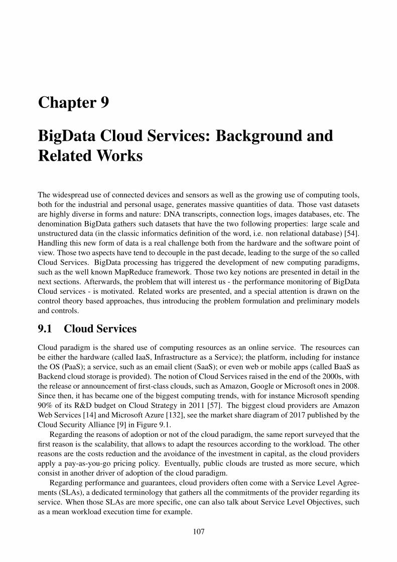
Chapter 9

BigData Cloud Services: Background andRelated Works

The widespread use of connected devices and sensors as well as the growing use of computing tools,both for the industrial and personal usage, generates massive quantities of data. Those vast datasetsare highly diverse in forms and nature: DNA transcripts, connection logs, images databases, etc. Thedenomination BigData gathers such datasets that have the two following properties: large scale andunstructured data (in the classic informatics definition of the word, i.e. non relational database) [54].Handling this new form of data is a real challenge both from the hardware and the software point ofview. Those two aspects have tend to decouple in the past decade, leading to the surge of the so calledCloud Services. BigData processing has triggered the development of new computing paradigms,such as the well known MapReduce framework. Those two key notions are presented in detail in thenext sections. Afterwards, the problem that will interest us - the performance monitoring of BigDataCloud services - is motivated. Related works are presented, and a special attention is drawn on thecontrol theory based approaches, thus introducing the problem formulation and preliminary modelsand controls.

9.1 Cloud ServicesCloud paradigm is the shared use of computing resources as an online service. The resources canbe either the hardware (called IaaS, Infrastructure as a Service); the platform, including for instancethe OS (PaaS); a service, such as an email client (SaaS); or even web or mobile apps (called BaaS asBackend cloud storage is provided). The notion of Cloud Services raised in the end of the 2000s, withthe release or announcement of first-class clouds, such as Amazon, Google or Microsoft ones in 2008.Since then, it has became one of the biggest computing trends, with for instance Microsoft spending90% of its R&D budget on Cloud Strategy in 2011 [57]. The biggest cloud providers are AmazonWeb Services [14] and Microsoft Azure [132], see the market share diagram of 2017 published by theCloud Security Alliance [9] in Figure 9.1.

Regarding the reasons of adoption or not of the cloud paradigm, the same report surveyed that thefirst reason is the scalability, that allows to adapt the resources according to the workload. The otherreasons are the costs reduction and the avoidance of the investment in capital, as the cloud providersapply a pay-as-you-go pricing policy. Eventually, public clouds are trusted as more secure, whichconsist in another driver of adoption of the cloud paradigm.

Regarding performance and guarantees, cloud providers often come with a Service Level Agree-ments (SLAs), a dedicated terminology that gathers all the commitments of the provider regarding itsservice. When those SLAs are more specific, one can also talk about Service Level Objectives, suchas a mean workload execution time for example.

107

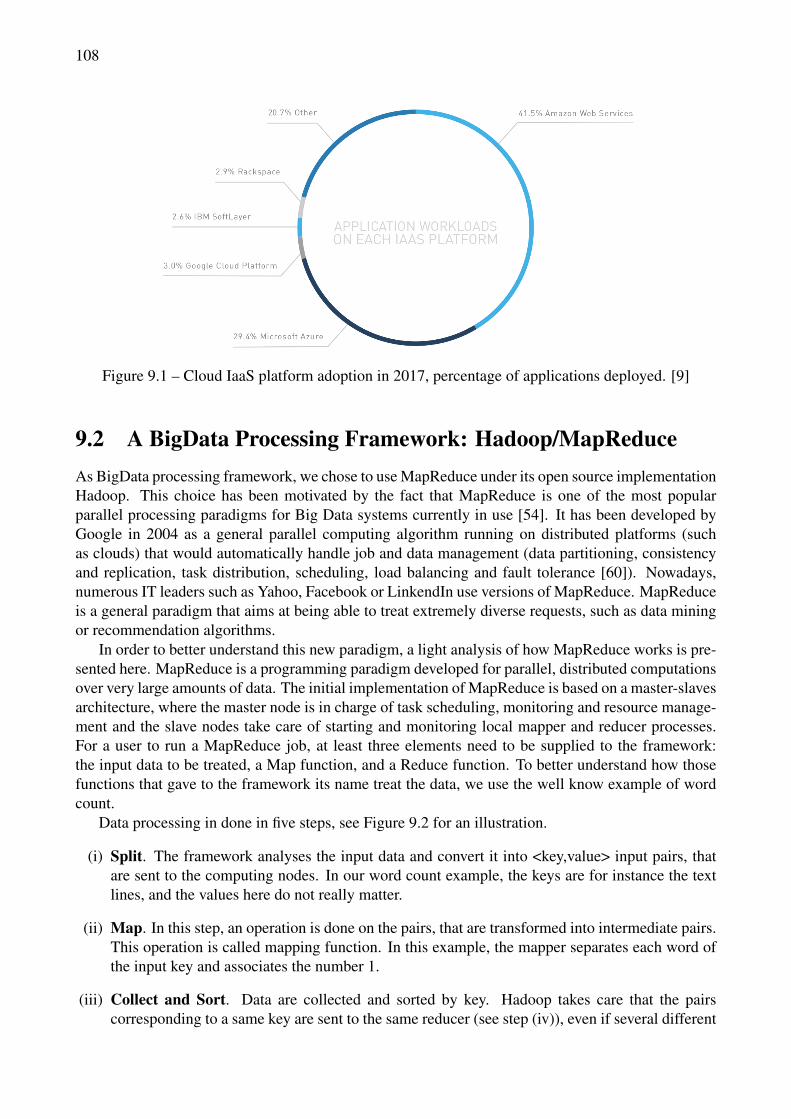
108

Figure 9.1 – Cloud IaaS platform adoption in 2017, percentage of applications deployed. [9]

9.2 A BigData Processing Framework: Hadoop/MapReduceAs BigData processing framework, we chose to use MapReduce under its open source implementationHadoop. This choice has been motivated by the fact that MapReduce is one of the most popularparallel processing paradigms for Big Data systems currently in use [54]. It has been developed byGoogle in 2004 as a general parallel computing algorithm running on distributed platforms (suchas clouds) that would automatically handle job and data management (data partitioning, consistencyand replication, task distribution, scheduling, load balancing and fault tolerance [60]). Nowadays,numerous IT leaders such as Yahoo, Facebook or LinkendIn use versions of MapReduce. MapReduceis a general paradigm that aims at being able to treat extremely diverse requests, such as data miningor recommendation algorithms.

In order to better understand this new paradigm, a light analysis of how MapReduce works is pre-sented here. MapReduce is a programming paradigm developed for parallel, distributed computationsover very large amounts of data. The initial implementation of MapReduce is based on a master-slavesarchitecture, where the master node is in charge of task scheduling, monitoring and resource manage-ment and the slave nodes take care of starting and monitoring local mapper and reducer processes.For a user to run a MapReduce job, at least three elements need to be supplied to the framework:the input data to be treated, a Map function, and a Reduce function. To better understand how thosefunctions that gave to the framework its name treat the data, we use the well know example of wordcount.

Data processing in done in five steps, see Figure 9.2 for an illustration.

(i) Split. The framework analyses the input data and convert it into <key,value> input pairs, thatare sent to the computing nodes. In our word count example, the keys are for instance the textlines, and the values here do not really matter.

(ii) Map. In this step, an operation is done on the pairs, that are transformed into intermediate pairs.This operation is called mapping function. In this example, the mapper separates each word ofthe input key and associates the number 1.

(iii) Collect and Sort. Data are collected and sorted by key. Hadoop takes care that the pairscorresponding to a same key are sent to the same reducer (see step (iv)), even if several different

109

Figure 9.2 – MapReduce step-wise functional scheme. [60]

keys can be sent to a same reducer. For instance, all the pairs containing the same word are sentto the same reducer, but a reducer can treat several words.

(iv) Reduce. The reducer executes the second function: transforming the intermediate pairs in theoutput ones. For word count, the reduce function is to sum up the number of iteration of a wordand return pairs with unique key and the value corresponding to its occurrence count in the entiretext.

(v) Store. Output pairs are then wrote back in a file.

The main criticism against MapReduce is regarding the restriction of problem that it can addressusing its current formulation. For instance, treatments on image databases are not a suitable MapRe-duce problem. Advances in performance and implementation efficiency have been done since the firstrelease of MapReduce, see Hadoop 2 (YARN) and Hadoop 3 for instance. Even if this work is devel-oped and validated on Hadoop 1, the high level problem formulation enables to apply its principleson versions 2 and 3.

To conclude, MapReduce/Hadoop is a computing framework that enable the processing of un-structured data where the classic SQL-based approach have failed or shown too slow results. Its wideadoption in the industrial world makes it a attractive use-case for this thesis.

9.3 Problem StatementThis section highlights the challenges that rises from the use of the MapReduce framework on publicclouds, see for instance Amazon EMR [15] or Azure HDInsight [133].

Public clouds are open to everyone: multiple clients can send requests at the same time, thusgenerating a concurrency for the access to specific resources such as network, which influences theservice performance. A single client also launches multiple MapReduce jobs, that concurrently accessthe cluster nodes. If multiple concurrent jobs are running, the amount of resources allocated foreach job is reduced and thus the job service time is low. However, the distribution of those jobs isnot necessary known in advance. For instance, for an e-commerce company running MapReduceto perform sale recommendation based on client preferences, the workload is directly linked to thewebsite frequenting which varies in time. Moreover, the jobs are highly heterogeneous between the

110

different clients, and can also be so between the pool of a client’s jobs. The workload of the systemis independent of the cloud provider and can be really brisk [83], it can thus be considered as adisturbance impacting the system performance.

For a client using MapReduce, it is essential to have guarantees in term of service performance,dependability and costs. In the example of the recommendation task, the company needs to have thelist of recommended products in a few tenth of seconds, otherwise their webpage will take too muchtime to be loaded. Poor jobs performance lead to end-user performance degradation and eventuallylost of loyalty, and thus need to be avoided [137]. From the cloud provider point of view, this servicetime (the time it takes for a user request to be treated) is thus a performance metric that should beincluded in its Service Level Agreements. Aside from the performance perspective, availability of theservices must be ensured, both for the MapReduce client that wants to ensure that most of its tasks areexecuted (and thus most of its end-users benefit from a service), and for the cloud provider, that needsall its clients to be served. A last objective is the cost efficiency. From the provider point of view,running a MapReduce service has a cost in terms of energy consumption but also hardware usage,wear and maintenance, which results in financial costs. Regarding the MapReduce clients, the pay-as-you-go pricing strategy of clouds also translates into resource minimization objectives. Obviously,all those objectives of performance, availability and cost efficiency are contradictory: a trade-off thatsatisfy both the cloud provider and the clients have to be achieved and ensured.

However, the guarantees formulated by the cloud providers in their SLAs are mainly focused onavailability and dependability of their resources, i.e. their hardware, rather on what is of interest fortheir clients: the application-level availability and performance. Regarding the MapReduce frame-work itself, it has been designed to maximize throughput, resource utilization and jobs performance,while the clients are more interested in the workload level performance. Even if those objectivesare related, they are not directly equivalent for instance in case of job concurrency. Here again, theobjectives must be shifted from low level ones to service ones.

We now investigate the reasons that make this difference between resources/jobs quality and ser-vice performance. First, a cloud is a highly dynamic environment, in which the hardware is constantlychanging, both at short term (connection/shutdown of new nodes, resources concurrency, networkbottlenecks [113], etc.) and longer term (addition of new types of resources for instance). All thosechanges through time are hard to measure and sometimes come from unknown sources, due to thecomplexity of nowadays cloud infrastructures. As cloud providers desire to maximize the utilizationof their clusters, they have mechanisms for the dynamic reallocation of unused resources in the clus-ter, which further add to the variability of system performance. Hence, even with the same workloadand the same resource amount, an application performance may vary depending on how noisy neigh-boring applications are. Moreover, cloud services are highly complex paradigms that run on top ofmultiple software stacks and on heterogeneous nodes [19], making their behavior regarding resourceprovisioning highly non linear. For a software engineer, these unknown variation are particularlydifficult to deal with. On top of the environment and workload dynamics, the MapReduce itself isevolving through time. At a low scale, the realization of Map and Reduce functions are not all syn-chronous, leading to slight variations of the large scale system behavior. The framework is also notsafe from software failures [159]. Moreover, as stated before, many new versions and updates of theMapReduce Hadoop framework are released, changing every time a bit MapReduce performance.

A simple action that can be done to modify the services run time is to play with the number of re-sources of the cloud allocated to the jobs. For the MapReduce use case, adding resources, commonlyknown as nodes, to the cluster will increase the number of Map and Reduce functions processing theinput data leading to a reduction of the service time. And conversely if the number of resources goesdown. The cluster size consists then in a control knob that can influence both the service performanceand indeed the costs. Another impacting factor is the admission control, i.e. the monitoring of the

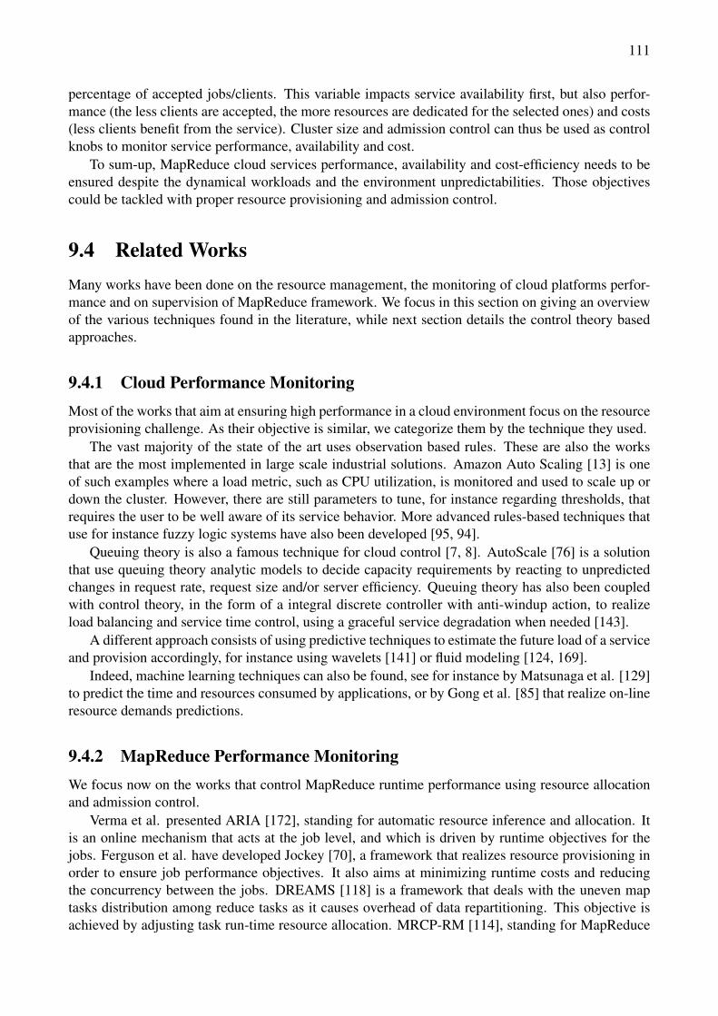
111

percentage of accepted jobs/clients. This variable impacts service availability first, but also perfor-mance (the less clients are accepted, the more resources are dedicated for the selected ones) and costs(less clients benefit from the service). Cluster size and admission control can thus be used as controlknobs to monitor service performance, availability and cost.

To sum-up, MapReduce cloud services performance, availability and cost-efficiency needs to beensured despite the dynamical workloads and the environment unpredictabilities. Those objectivescould be tackled with proper resource provisioning and admission control.

9.4 Related WorksMany works have been done on the resource management, the monitoring of cloud platforms perfor-mance and on supervision of MapReduce framework. We focus in this section on giving an overviewof the various techniques found in the literature, while next section details the control theory basedapproaches.

9.4.1 Cloud Performance MonitoringMost of the works that aim at ensuring high performance in a cloud environment focus on the resourceprovisioning challenge. As their objective is similar, we categorize them by the technique they used.

The vast majority of the state of the art uses observation based rules. These are also the worksthat are the most implemented in large scale industrial solutions. Amazon Auto Scaling [13] is oneof such examples where a load metric, such as CPU utilization, is monitored and used to scale up ordown the cluster. However, there are still parameters to tune, for instance regarding thresholds, thatrequires the user to be well aware of its service behavior. More advanced rules-based techniques thatuse for instance fuzzy logic systems have also been developed [95, 94].

Queuing theory is also a famous technique for cloud control [7, 8]. AutoScale [76] is a solutionthat use queuing theory analytic models to decide capacity requirements by reacting to unpredictedchanges in request rate, request size and/or server efficiency. Queuing theory has also been coupledwith control theory, in the form of a integral discrete controller with anti-windup action, to realizeload balancing and service time control, using a graceful service degradation when needed [143].

A different approach consists of using predictive techniques to estimate the future load of a serviceand provision accordingly, for instance using wavelets [141] or fluid modeling [124, 169].

Indeed, machine learning techniques can also be found, see for instance by Matsunaga et al. [129]to predict the time and resources consumed by applications, or by Gong et al. [85] that realize on-lineresource demands predictions.

9.4.2 MapReduce Performance MonitoringWe focus now on the works that control MapReduce runtime performance using resource allocationand admission control.

Verma et al. presented ARIA [172], standing for automatic resource inference and allocation. Itis an online mechanism that acts at the job level, and which is driven by runtime objectives for thejobs. Ferguson et al. have developed Jockey [70], a framework that realizes resource provisioning inorder to ensure job performance objectives. It also aims at minimizing runtime costs and reducingthe concurrency between the jobs. DREAMS [118] is a framework that deals with the uneven maptasks distribution among reduce tasks as it causes overhead of data repartitioning. This objective isachieved by adjusting task run-time resource allocation. MRCP-RM [114], standing for MapReduce

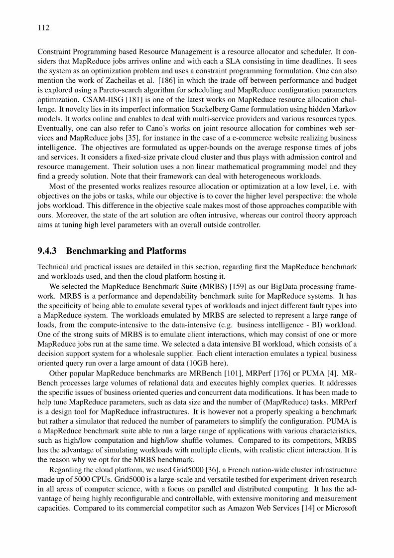
112

Constraint Programming based Resource Management is a resource allocator and scheduler. It con-siders that MapReduce jobs arrives online and with each a SLA consisting in time deadlines. It seesthe system as an optimization problem and uses a constraint programming formulation. One can alsomention the work of Zacheilas et al. [186] in which the trade-off between performance and budgetis explored using a Pareto-search algorithm for scheduling and MapReduce configuration parametersoptimization. CSAM-IISG [181] is one of the latest works on MapReduce resource allocation chal-lenge. It novelty lies in its imperfect information Stackelberg Game formulation using hidden Markovmodels. It works online and enables to deal with multi-service providers and various resources types.Eventually, one can also refer to Cano’s works on joint resource allocation for combines web ser-vices and MapReduce jobs [35], for instance in the case of a e-commerce website realizing businessintelligence. The objectives are formulated as upper-bounds on the average response times of jobsand services. It considers a fixed-size private cloud cluster and thus plays with admission control andresource management. Their solution uses a non linear mathematical programming model and theyfind a greedy solution. Note that their framework can deal with heterogeneous workloads.

Most of the presented works realizes resource allocation or optimization at a low level, i.e. withobjectives on the jobs or tasks, while our objective is to cover the higher level perspective: the wholejobs workload. This difference in the objective scale makes most of those approaches compatible withours. Moreover, the state of the art solution are often intrusive, whereas our control theory approachaims at tuning high level parameters with an overall outside controller.

9.4.3 Benchmarking and PlatformsTechnical and practical issues are detailed in this section, regarding first the MapReduce benchmarkand workloads used, and then the cloud platform hosting it.

We selected the MapReduce Benchmark Suite (MRBS) [159] as our BigData processing frame-work. MRBS is a performance and dependability benchmark suite for MapReduce systems. It hasthe specificity of being able to emulate several types of workloads and inject different fault types intoa MapReduce system. The workloads emulated by MRBS are selected to represent a large range ofloads, from the compute-intensive to the data-intensive (e.g. business intelligence - BI) workload.One of the strong suits of MRBS is to emulate client interactions, which may consist of one or moreMapReduce jobs run at the same time. We selected a data intensive BI workload, which consists of adecision support system for a wholesale supplier. Each client interaction emulates a typical businessoriented query run over a large amount of data (10GB here).

Other popular MapReduce benchmarks are MRBench [101], MRPerf [176] or PUMA [4]. MR-Bench processes large volumes of relational data and executes highly complex queries. It addressesthe specific issues of business oriented queries and concurrent data modifications. It has been made tohelp tune MapReduce parameters, such as data size and the number of (Map/Reduce) tasks. MRPerfis a design tool for MapReduce infrastructures. It is however not a properly speaking a benchmarkbut rather a simulator that reduced the number of parameters to simplify the configuration. PUMA isa MapReduce benchmark suite able to run a large range of applications with various characteristics,such as high/low computation and high/low shuffle volumes. Compared to its competitors, MRBShas the advantage of simulating workloads with multiple clients, with realistic client interaction. It isthe reason why we opt for the MRBS benchmark.

Regarding the cloud platform, we used Grid5000 [36], a French nation-wide cluster infrastructuremade up of 5000 CPUs. Grid5000 is a large-scale and versatile testbed for experiment-driven researchin all areas of computer science, with a focus on parallel and distributed computing. It has the ad-vantage of being highly reconfigurable and controllable, with extensive monitoring and measurementcapacities. Compared to its commercial competitor such as Amazon Web Services [14] or Microsoft

113

Azure [132], it has the advantage of being free and open access for researcher. It is also a masteredplatform which enables reproducible research, while the industrial versions are constantly evolving,making them more suitable for evaluation purposes than for the research work itself.

The combination of the MRBS benchmark and Grid5000 platform have already been used in theBigData cloud control context. Berekméri [25] developed a tool to launch and monitor MapReducejobs on Grid5000, combined with a Matlab interface that enables to design and implement monitoringalgorithms, i.e. controllers. This experimental setup is used for the evaluation of the control strategiespresented in this thesis.

9.5 Background on Control Theory applied to MapReduceThe control problem formulation for BigData Cloud Control has been first introduced by Berekemeriand al. in 2014 [24] and further extended in the following years [26, 25]. This section is a detailedreview of those works, on which this thesis contributions are based. In a first time, the signals used asperformance indicators and control knobs are defined. Second, dynamical models of their impact oneach other are introduced. Those models lead to the development of controllers, which are presentedin two categories: the feedback and feedforward based runtime monitoring, and the multi-dimensionsoptimal control of runtime and availability.

9.5.1 Input and output signalsThe output metrics of interest for our control problem are:

Service Time. Noted yST , it is the average run time of jobs that finished in the previous timewindow. The lower the service time is, the faster the clients requests are completed. Depending onthe MapReduce tasks, it can go from few seconds to several minutes or even hours. The size of thesize window is 15 min, as fixed in [25] for the BI applications.

Availability. It is the ratio of accepted MapReduce jobs over all received jobs, during the lasttime window, refereed to with the notation yAV . Availability is thus between 0 and 1, this later valuemeaning a 100% availability of the service, the best value achievable.

The input signals - control knobs that can be varied or external disturbances the service undergo -impacting those performance metrics are:

Cluster Size. One simple action that can be done to control the on-line service time is to modifythe number of resources of the cloud allocated to the jobs. For the MapReduce use case, addingresources, commonly known as nodes, to the cluster will increase the number of Map and Reducefunctions processing the input data leading to a reduction of the service time. If the number ofresources (nodes) diminishes, the results are converse. The cluster size is then one of our controlsignal uN .

Workload. In the case of public clouds, multiple clients send requests at the same time thusgenerating a varying input workload which influences the service performance. If multiple concurrentjobs are running, the amount of resources allocated for each job is reduced and thus the job servicetime increases. As the workload of the system is independent of the cloud provider we will considerit as a disturbance dC.

Admission Control. Client requests can be rejected, when the available resources are consideredtoo few to satisfy all the incoming workload for instance. Admission control is thus another inputvariable for our control, it is the number of accepted clients uAC. Note that there is no more acceptedclients that the demand: uAC ≤ dC.

Those input variables are linearized around a working point of 10 clients and 20 nodes [24].Hence, the signals only express variations.

114

9.5.2 ModelingThe modeling of the service time and availability are presented independently and afterwards gatheredinto a MIMO formulation. We proceed like this as some of the controllers will only take into accountservice time monitoring, and thus only SISO modeling.

9.5.2.1 Service Time Model

A dynamic model that predicts MapReduce cluster performance (i.e. the average service time ofthe last finished jobs) with respect to the number of nodes of the cluster and the number of clientssending requests was proposed and experimentally validated by Berekméri et al. [24]. Its schematicrepresentation is given in Figure 9.3.

Figure 9.3 – MapReduce Service Time model.

The system is considered linear in its operating region. The models were first identified as con-tinuous transfer functions and then discretized using the sampling period Ts = 30 sec. The resultingequation is2:

yST (t) = YC(q−1)uAC(t)+YN(q−1)uN(t). (9.1)

YC(q−1) is the direct path transfer function, the link between the number of clients and the servicetime performance metric, and YN(q−1) represents the compensatory path that enables to modify thecluster size to control the service time. Both models were identified as first-order transfer functionwith delays, as described in eq. (9.2):

YC(q−1) =bCq−1

1+aCq−1 q−rC , YN(q−1) =bNq−1

1+aNq−1 q−rN , (9.2)

with bC = 1.0716, aC =−0.7915, rC = 8, bN =−0.17951, aN =−0.919 and rN = 5.Note that when there is no admission control, uAC = dC in eq. (9.1), as illustrated in Fig. 9.3.

9.5.2.2 Availability Model

Availability is impacted by the number of clients rejected by the MapReduce framework. It is thus acombination of the workload, i.e. number of demands dC, and the upper acceptance threshold uAC.

yAV (t) = YAC(q−1)[dC(t)−uAC(t)] =bACq−1

1+aACq−1 [dC(t)−uAC(t)]. (9.3)

Parameters of the availability model are bAC = 0.1548, aAC =−0.946 [25].2The complex variable z−1 will be used to characterize the system’s behavior in the frequency domain and the delay

operator q−1 will be used for the time domain analysis.

115

9.5.2.3 MIMO Model

The multi signal representation of MapReduce modeling combining the previous models is repre-sented in Figure 9.4. A MIMO linear discrete model can be expressed in the following formulation:{

xk+1 = Axk +Bukyk =Cxk,

(9.4)

with yk the output vector at the kth sampling time: y = (yST ,yAV )T ; uk the vector of inputs (both

controllable and uncontrollable) u = (uN ,dC,uAC)T and xk the states vector. Starting from the SISO

formulations of eqs. (9.1) and (9.3), there exist automated tools to derive the non unique MIMOformulation of eq. (9.4). Using Matlab tf2ss function, the number of states is 4. Those states have noconcrete physical explanation, we thus do not detail them here.

++

YN

YC

+- YAC

Service Time

Availability

Cluster Size

Max Clients

Clients

CONTROLINPUTS OUTPUTS

DISTURBANCE

Figure 9.4 – MapReduce Service Time and Availability model.

Some work has also be done on the adaptation of those models online, both for the service timemodeling [39] and on the MIMO model [40]. Those works use a Recursive Least Square Estimator toupdate the models parameters at each execution time, depending on an estimated gain and a covariancematrix. The adaptation of those models are used to cope with the non-linearities of the system whilekeeping a linear model. However, those models have shown limited results when coupled with acontrol strategy, as the estimation optimization in those works is toward the model accuracy, not thecontrol performance, contrary to the work presented in Chapter 10.

9.5.3 ControlSeveral control laws have been developed: a feedback and feedforward controller for the service timemonitoring [26], and a Model Predictive Controller for the joint service time and availability control[25, ?].

The service time controller time-domain equation is given in eq. (9.5):

uN(t) = PI(q−1)[yST,re f (t)− yST (t)]+FF(q−1)dC(t), (9.5)

with yST,re f (t) the reference value for the service time. The PI equation is classically PI(s) =KI

s+KP,

with s the Laplace variable and the values KI = 0.25584 and KP = 0.0012372. The feedforwardcontrol is in fact a static one, i.e. only a gain FF(s) = 5.96958 [26].

116

A event-based version of this feedback and feedforward control has also been developed [26], thattriggers the control signal update based on the service time error rather that in a regular time-basedfashion.

The multi objectives control law, called MR-Ctrl, is a model predictive controller that uses thefollowing cost function:

J = minUk

(Yk−Yre f )T Q(Yk−Yre f )+UT

k RUk, (9.6)

where Uk = (uk,uk+1, . . . ,uk+N)T , Yk = (yk,yk+1, . . . ,yk+N)

T and Yre f = (yre f , . . . ,yre f ) are the se-lected/predicted values of the signals on the optimization horizon of N samples. yre f is the vectorof reference values for the system outputs, fixed here: yre f = (yST,re f ,yAV,re f )

T . This control law issubmitted to the following constraints:

∀k,0 < uAC(k)≤ dC(k) and uN(k)≤ umaxN . (9.7)

Integral action and compensation for actuation delay are also added to cope with modeling errorsand control oscillatory behavior. States are estimated using the Luenberger observer [25].

9.5.4 LimitationsThe two main limitations of the previously presented control of MapReduce are regarding robustnessand cost-efficiency, as illustrated in due time in Section 10.1 and Section 11.1.

An analysis of the cloud system behavior detailed in Section 9.3 intuitively shows that the systemsis non linear and time variant, thus the previous linear model is not accurate for a wide range of inputor disturbance values, so neither is the control law. Therefore, Chapter 10 develops an adaptivetechnique to cope with system and environment uncertainties.

Moreover, the MR-Ctrl controller do not take into account the specificities of the cloud-basedsystem regarding costs. For instance, resources in a cloud are rented and priced based on the timethey where used, but with a minimal threshold that usually correspond the time needed to start orinitialized them. To tackle this cost formulation, a new event-based optimal control law is presentedin Chapter 11.

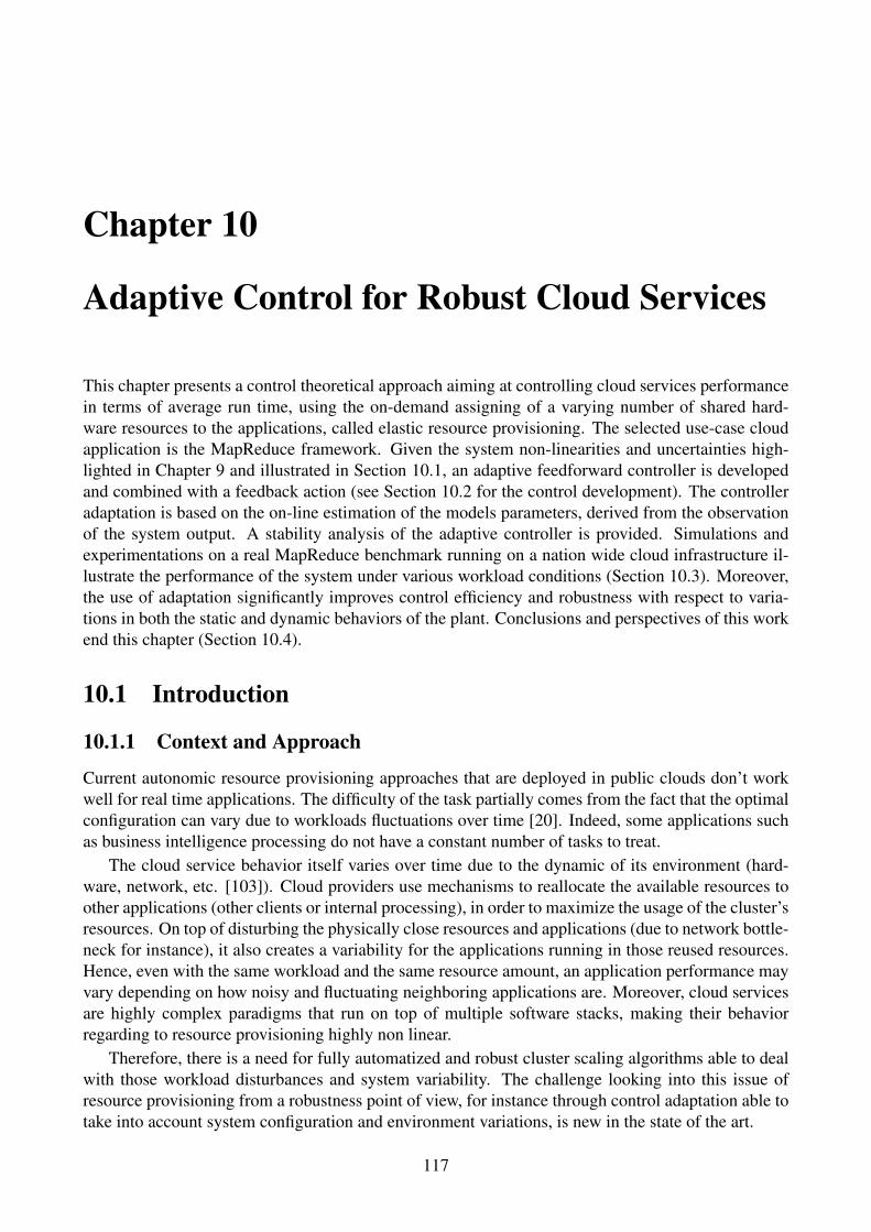
Chapter 10

Adaptive Control for Robust Cloud Services

This chapter presents a control theoretical approach aiming at controlling cloud services performancein terms of average run time, using the on-demand assigning of a varying number of shared hard-ware resources to the applications, called elastic resource provisioning. The selected use-case cloudapplication is the MapReduce framework. Given the system non-linearities and uncertainties high-lighted in Chapter 9 and illustrated in Section 10.1, an adaptive feedforward controller is developedand combined with a feedback action (see Section 10.2 for the control development). The controlleradaptation is based on the on-line estimation of the models parameters, derived from the observationof the system output. A stability analysis of the adaptive controller is provided. Simulations andexperimentations on a real MapReduce benchmark running on a nation wide cloud infrastructure il-lustrate the performance of the system under various workload conditions (Section 10.3). Moreover,the use of adaptation significantly improves control efficiency and robustness with respect to varia-tions in both the static and dynamic behaviors of the plant. Conclusions and perspectives of this workend this chapter (Section 10.4).

10.1 Introduction

10.1.1 Context and Approach

Current autonomic resource provisioning approaches that are deployed in public clouds don’t workwell for real time applications. The difficulty of the task partially comes from the fact that the optimalconfiguration can vary due to workloads fluctuations over time [20]. Indeed, some applications suchas business intelligence processing do not have a constant number of tasks to treat.

The cloud service behavior itself varies over time due to the dynamic of its environment (hard-ware, network, etc. [103]). Cloud providers use mechanisms to reallocate the available resources toother applications (other clients or internal processing), in order to maximize the usage of the cluster’sresources. On top of disturbing the physically close resources and applications (due to network bottle-neck for instance), it also creates a variability for the applications running in those reused resources.Hence, even with the same workload and the same resource amount, an application performance mayvary depending on how noisy and fluctuating neighboring applications are. Moreover, cloud servicesare highly complex paradigms that run on top of multiple software stacks, making their behaviorregarding to resource provisioning highly non linear.

Therefore, there is a need for fully automatized and robust cluster scaling algorithms able to dealwith those workload disturbances and system variability. The challenge looking into this issue ofresource provisioning from a robustness point of view, for instance through control adaptation able totake into account system configuration and environment variations, is new in the state of the art.

117

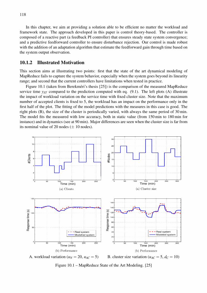
118

In this chapter, we aim at providing a solution able to be efficient no matter the workload andframework state. The approach developed in this paper is control theory-based. The controller iscomposed of a reactive part (a feedback PI controller) that ensures steady state system convergence;and a predictive feedforward controller to ensure disturbance rejection. Our control is made robustwith the addition of an adaptation algorithm that estimate the feedforward gain through time based onthe system output observation.

10.1.2 Illustrated Motivation

This section aims at illustrating two points: first that the state of the art dynamical modeling ofMapReduce fails to capture the system behavior, especially when the system goes beyond its linearityrange; and second that the current controllers have limitations when tested in practice.

Figure 10.1 (taken from Berekméri’s thesis [25]) is the comparison of the measured MapReduceservice time yST compared to the prediction computed with eq. (9.1). The left plots (A) illustratethe impact of workload variation on the service time with fixed cluster size. Note that the maximumnumber of accepted clients is fixed to 5, the workload has an impact on the performance only in thefirst half of the plot. The fitting of the model predictions with the measures in this case is good. Theright plots (B), the size of the cluster is periodically varied, with always the same period of 30 min.The model fits the measured with low accuracy, both in static value (from 150 min to 180 min forinstance) and in dynamics (see at 90 min). Major differences are seen when the cluster size is far fromits nominal value of 20 nodes (± 10 nodes).

A. workload variation (uN = 20, uAC = 5) B. cluster size variation (uAC = 5, dC = 10)

Figure 10.1 – MapReduce State of the Art Modeling. [25]

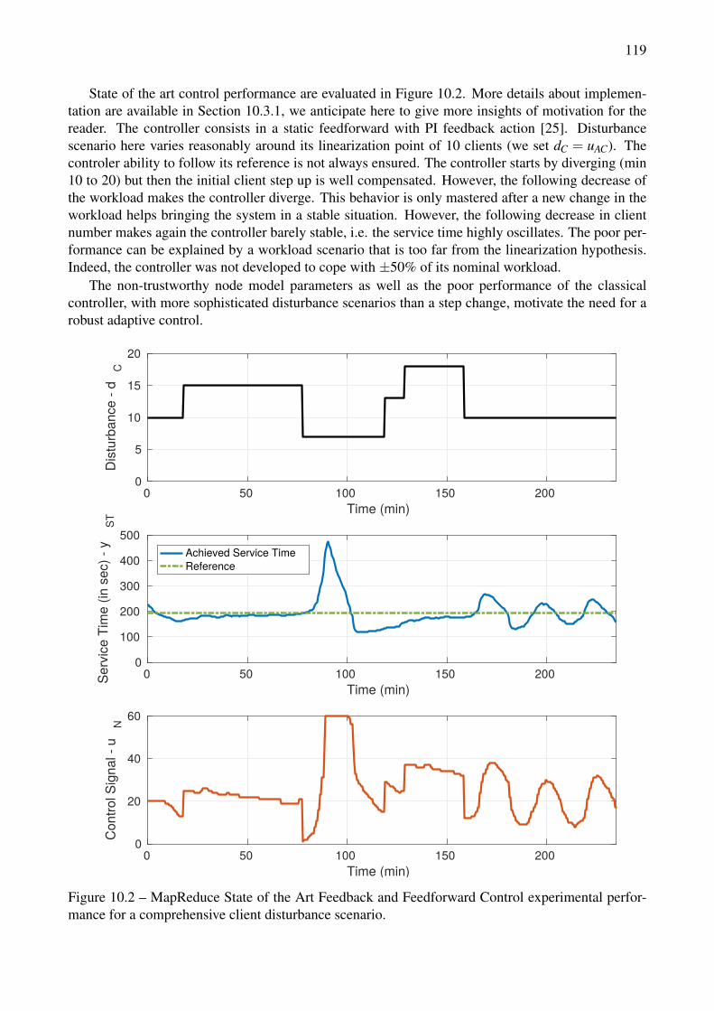
119

State of the art control performance are evaluated in Figure 10.2. More details about implemen-tation are available in Section 10.3.1, we anticipate here to give more insights of motivation for thereader. The controller consists in a static feedforward with PI feedback action [25]. Disturbancescenario here varies reasonably around its linearization point of 10 clients (we set dC = uAC). Thecontroler ability to follow its reference is not always ensured. The controller starts by diverging (min10 to 20) but then the initial client step up is well compensated. However, the following decrease ofthe workload makes the controller diverge. This behavior is only mastered after a new change in theworkload helps bringing the system in a stable situation. However, the following decrease in clientnumber makes again the controller barely stable, i.e. the service time highly oscillates. The poor per-formance can be explained by a workload scenario that is too far from the linearization hypothesis.Indeed, the controller was not developed to cope with ±50% of its nominal workload.

The non-trustworthy node model parameters as well as the poor performance of the classicalcontroller, with more sophisticated disturbance scenarios than a step change, motivate the need for arobust adaptive control.

0 50 100 150 200Time (min)

0

5

10

15

20

Dis

turb

ance

- d

C

0 50 100 150 200Time (min)

0

100

200

300

400

500

Serv

ice

Tim

e (in

sec

) - y

ST

Achieved Service TimeReference

0 50 100 150 200Time (min)

0

20

40

60

Con

trol S

igna

l - u

N

Figure 10.2 – MapReduce State of the Art Feedback and Feedforward Control experimental perfor-mance for a comprehensive client disturbance scenario.

120

10.2 Control StrategyThe control presented in this chapter consists of a PI controller, for asymptotic zero reference trackingerror, and a feedforward loop, for dynamic disturbance compensation. A real time adaptation of thefeedforward compensator is added to the state-of-the-art controller, in order to take into account theunknown and time-varying system’s parameters. The parameter adaptation algorithm is based on themeasures of the system outputs in reaction to client disturbances [111, 109]. The control scheme isgiven in Figure 10.3, with the previously seen MapReduce performance model in the light blue dottedbox and the adaptation algorithm in purple.

yST,ref(t)

uN(t)

eST(t)

dC(t)

yST(t)Service �me

#Nodes

#Clients

Referenceservice �me

YN

Compensatory Path

YC

Direct Path

+ + +-

PI

PI controller

g

FeedForwadcontroller

+

+Error

PAA

ParametersAdapta�onAlgorithm

MapReduce System

Figure 10.3 – MapReduce adaptive control schema.

10.2.1 Preliminary FormulationUnder the classical feedback-feedforward control loop (in black on Figure 10.3, without the PAAadaptation path in purple) and using the eq. (9.2), the optimal value of the 0-order feedforwardcontroller is given by:

u∗N, f f (t) =−bC(1+aN)

bN(1+aC).dC(t), g∗dC(t). (10.1)

For the initial development of the adaptation algorithm, we will make the following hypotheses:

(H1) the effect of the PI controller can be neglected in front of the feedforward one,

(H2) equal dynamics (aC = aN),

(H3) equal and known delays (rC = rN).

Then the algorithm will be extended for the cases where hypothesis H1, H2 and H3 do not hold.Let us define the adaptive feedforward control algorithm as:

uN, f f (t) = g(t)dC(t) (10.2)

where g is given by

g(t +1) = g(t)+αx(t +1)eST (t +1)

= g(t)+αx(t +1)

1+αx2(t +1)e0

ST (t +1) with α > 0. (10.3)

121

The filtered disturbance x is defined by:

x(t), sgn(bN)F(q−1)dC(t) =sgn(bN)q−(rN+1)

1+ aNq−1 dC(t), (10.4)

where the a priori adaptation error e0ST (t + 1) is the value of the regulation error at time t + 1 and

is based on the estimation of g(t): e0ST (t + 1) = e0

ST (t + 1/g(t)). The a priori error e0ST (t + 1) is

considered as a performance metric for our system. One can also define the a posteriori error eST (t +1) = e0

ST (t +1/g(t +1)) which, based on eq. (10.3), gives:

eST (t +1) =1

1+αx2(t +1)e0

ST (t +1). (10.5)

Theorem 1 For the scheme represented in Figure 10.3, under the hypothesis H1, H2 and H3, usingthe adaptive feedforward control given by eq. (10.2) to (10.4), one has:

limt→∞eST (t +1) = limt→∞e0ST (t +1) = 0 (10.6)

for any initial conditions provided that:

H ′(z−1) =1+ aNz−1

1+aNz−1 (10.7)

is a strictly positive real transfer function.

Note that this later condition is always satisfied provided that |aN |< 1 (stability condition for themodel) and aN ≤ 0.

Proof: Under the hypothesis H1, H2 and H3, the expression of the error eST for a fixed value g is(see Figure 10.3):

eST (t +1) = e0ST (t +1) =

bNq−(rN+1)

1+aNq−1 (g∗− g)dC(t +1) (10.8)

Filtering dC(t) by the filter F given in eq. (10.4) allows to rewrite eq. (10.8) as:

eST (t +1) = |bN |1+ aNq−1

1+aNq−1 (g∗− g)x(t) (10.9)

When replacing g with g(t + 1) and neglecting the additional vanishing term resulting from the noncommutativity of time varying operators, one has:

eST (t +1) = |bN |1+ aNq−1

1+aNq−1 (g∗− g(t +1))x(t) (10.10)

Eq. (10.10) has the standard form of an a posteriori adaptation error equation and one can usestraight-forwardly the results of [111], Chapter 3, Theorem (3.2). �

Note that the proof have shown the convergence of the adaptation error (i.e. the performancevariable). However, the convergence of g→ g∗ is related to the richness of the disturbance signal dC.

10.2.2 Going beyond hypothesesWe know take one by one the assumptions taken during the initial formulation to overcome them; andthus have an adaptation algorithm that works in the general case.

122

10.2.2.1 When the effect of the PI controller cannot be neglected (H1)

The continuous time PI controller has the transfer function:

PI(s) =KI

s+KP (10.11)

Using the difference approximation1−q−1

TS(with TS being the sampling period) for differential op-

erator one gets:

PI(q−1) =KITS +KP−KPq−1

1−q−1 =r0 + r1q−1

1−q−1 =BK(q−1)

AK(q−1)(10.12)

Using the results of [109], Chapter 15, Section 15.17, eq. (15.86) for our particular scheme (with thevalues AK = 1−q−1, BK = r0+ r1q−1, BN = bN q−(rN+1), AN = 1+aN q−1, S = 1, AM = 1, BM = 0),one gets:

eST (t +1) =q−(rN+1)|bN |(1−q−1)[g∗− g(t +1)]dC(t)

(1+aNq−1)(1−q−1)+bN(r0 + r1q−1)q−(rN+1)(10.13)

Using the parameter adaptation algorithm given in Section 10.2.1, the stability condition becomesthat the following transfer function

H ′′(z−1) =(1− z−1)(1+ aNz−1)

(1+aNz−1)(1− z−1)+bN(r0 + r1z−1)z−(rN+1)(10.14)

should be a strictly positive real transfer function.If this condition is not satisfied, taking into account eq. (10.13), one can use instead the filter F

given in eq. (10.4) to filter FPI:

FPI(q−1) =sgn(bN)q−(rN+1)bN(1−q−1)

(1+ aNq−1)(1−q−1)+ bN(r0 + r1q−1)q−(rN+1)(10.15)

10.2.2.2 When clients and nodes impact on service time do not have the same dynamics:aC 6= aN (H2)

Denoting the unmeasurable output of the disturbance propagation path YC(q−1) by z(t), eq. (10.13)becomes in the presence of the PI controller:

eST (t +1) = H ′′(q−1)([g− g(t +1)]dC(t)+ [aN−aC]z(t)) (10.16)

Since the adaptation does not affect directly the second term in the left hand side of eq. (10.16),we have to analyze its influence. As z(t) is the output of an asymptotically stable plant whose inputis bounded, it will also be bounded. Therefore the signal δ (t) = [aN − aC]z(t) will be bounded.Furthermore, due to the PI controller, the effect of this disturbance term will go to 0 asymptotically insteady state for a constant value of dC(t), since in eq. (10.13) the numerator of the transfer operatorcontains (1−q−1). This also holds if there is no PI since, for a constant disturbance, the adaptationalgorithm will interpret this term as an additional constant disturbance which will be canceled.

10.2.2.3 Transfer delays are different but known: rC 6= rN (H3)

Hypothesis H3 on delays can be relaxed to rN ≤ rG but both know. A delay corresponding of thedifference rC− rN is added to the feedforward-based control signal part uN, f f .

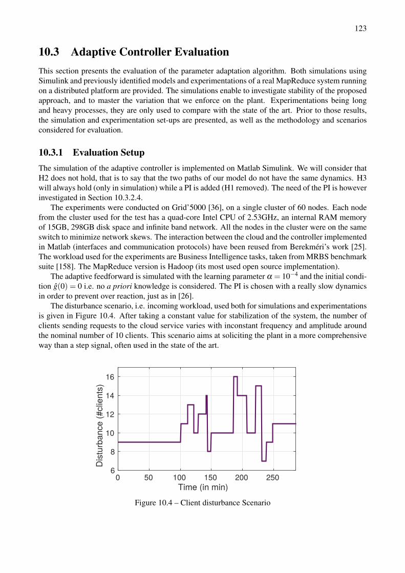
123

10.3 Adaptive Controller EvaluationThis section presents the evaluation of the parameter adaptation algorithm. Both simulations usingSimulink and previously identified models and experimentations of a real MapReduce system runningon a distributed platform are provided. The simulations enable to investigate stability of the proposedapproach, and to master the variation that we enforce on the plant. Experimentations being longand heavy processes, they are only used to compare with the state of the art. Prior to those results,the simulation and experimentation set-ups are presented, as well as the methodology and scenariosconsidered for evaluation.

10.3.1 Evaluation SetupThe simulation of the adaptive controller is implemented on Matlab Simulink. We will consider thatH2 does not hold, that is to say that the two paths of our model do not have the same dynamics. H3will always hold (only in simulation) while a PI is added (H1 removed). The need of the PI is howeverinvestigated in Section 10.3.2.4.

The experiments were conducted on Grid’5000 [36], on a single cluster of 60 nodes. Each nodefrom the cluster used for the test has a quad-core Intel CPU of 2.53GHz, an internal RAM memoryof 15GB, 298GB disk space and infinite band network. All the nodes in the cluster were on the sameswitch to minimize network skews. The interaction between the cloud and the controller implementedin Matlab (interfaces and communication protocols) have been reused from Berekméri’s work [25].The workload used for the experiments are Business Intelligence tasks, taken from MRBS benchmarksuite [158]. The MapReduce version is Hadoop (its most used open source implementation).

The adaptive feedforward is simulated with the learning parameter α = 10−4 and the initial condi-tion g(0) = 0 i.e. no a priori knowledge is considered. The PI is chosen with a really slow dynamicsin order to prevent over reaction, just as in [26].

The disturbance scenario, i.e. incoming workload, used both for simulations and experimentationsis given in Figure 10.4. After taking a constant value for stabilization of the system, the number ofclients sending requests to the cloud service varies with inconstant frequency and amplitude aroundthe nominal number of 10 clients. This scenario aims at soliciting the plant in a more comprehensiveway than a step signal, often used in the state of the art.

Time (in min)0 50 100 150 200 250

Dis

turb

ance

(#cl

ient

s)

6

8

10

12

14

16

Figure 10.4 – Client disturbance Scenario

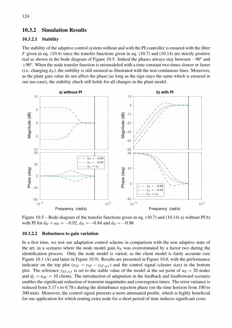
124

10.3.2 Simulation Results10.3.2.1 Stability

The stability of the adaptive control system without and with the PI controller is ensured with the filterF given in eq. (10.4) since the transfer functions given in eq. (10.7) and (10.14) are strictly positivereal as shown in the bode diagram of Figure 10.5. Indeed the phases always stay between −90o and+90o. When the node transfer function is mismodeled with a time constant two times slower or faster(i.e. changing aN), the stability is still ensured as illustrated with the non continuous lines. Moreover,as the plant gain value do not affect the phase (as long as the sign stays the same which is ensured inour use-case), the stability check still holds for all changes in the plant model.

-10

-5

0

5

10

Mag

nitu

de (d

B)

10 -5 10 0-90

-45

0

45

90

Phas

e (d

eg)

a) without PI

Frequency (rad/s)

-50

-40

-30

-20

-10

0

10

Mag

nitu

de (d

B)

10 -5 10 0-45

0

45

90

Phas

e (d

eg)

b) with PI

Frequency (rad/s)

Figure 10.5 – Bode diagram of the transfer functions given in eq. (10.7) and (10.14) a) without PI b)with PI for aN = aN =−0.92, aN =−0.84 and aN =−0.96

10.3.2.2 Robustness to gain variation

In a first time, we test our adaptation control scheme in comparison with the non adaptive state ofthe art, in a scenario where the node model gain bN was overestimated by a factor two during theidentification process. Only the node model is varied, as the client model is fairly accurate (seeFigure 10.1 (A) and latter in Figure 10.9). Results are presented in Figure 10.6, with the performanceindicator on the top plot (eST = yST − yST,re f ) and the control signal (cluster size) in the bottomplot. The reference yST,re f is set to the stable value of the model at the set point of uN = 20 nodesand dC = uAC = 10 clients. The introduction of adaptation in the feedback and feedforward scenarioenables the significant reduction of transient magnitudes and convergence times. The error variance isreduced from 5.17 s to 0.78 s during the disturbance rejection phase (on the time horizon from 100 to300 min). Moreover, the control signal presents a more attenuated profile, which is highly beneficialfor our application for which renting extra node for a short period of time induces significant costs.

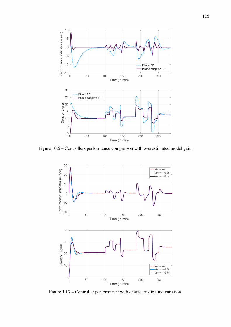
125

0 50 100 150 200 250Time (in min)

-15

-10

-5

0

5

10

Perfo

rman

ce in

dica

tor (

in s

ec)

PI and FFPI and adaptive FF

0 50 100 150 200 250Time (in min)

0

5

10

15

20

25

30

Con

trol S

igna

l

PI and FFPI and adaptive FF

Figure 10.6 – Controllers performance comparison with overestimated model gain.

0 50 100 150 200 250Time (in min)

-20

-10

0

10

20

30

Perfo

rman

ce in

dica

tor (

in s

ec)

0 50 100 150 200 250Time (in min)

0

10

20

30

40

Con

trol S

igna

l

Figure 10.7 – Controller performance with characteristic time variation.

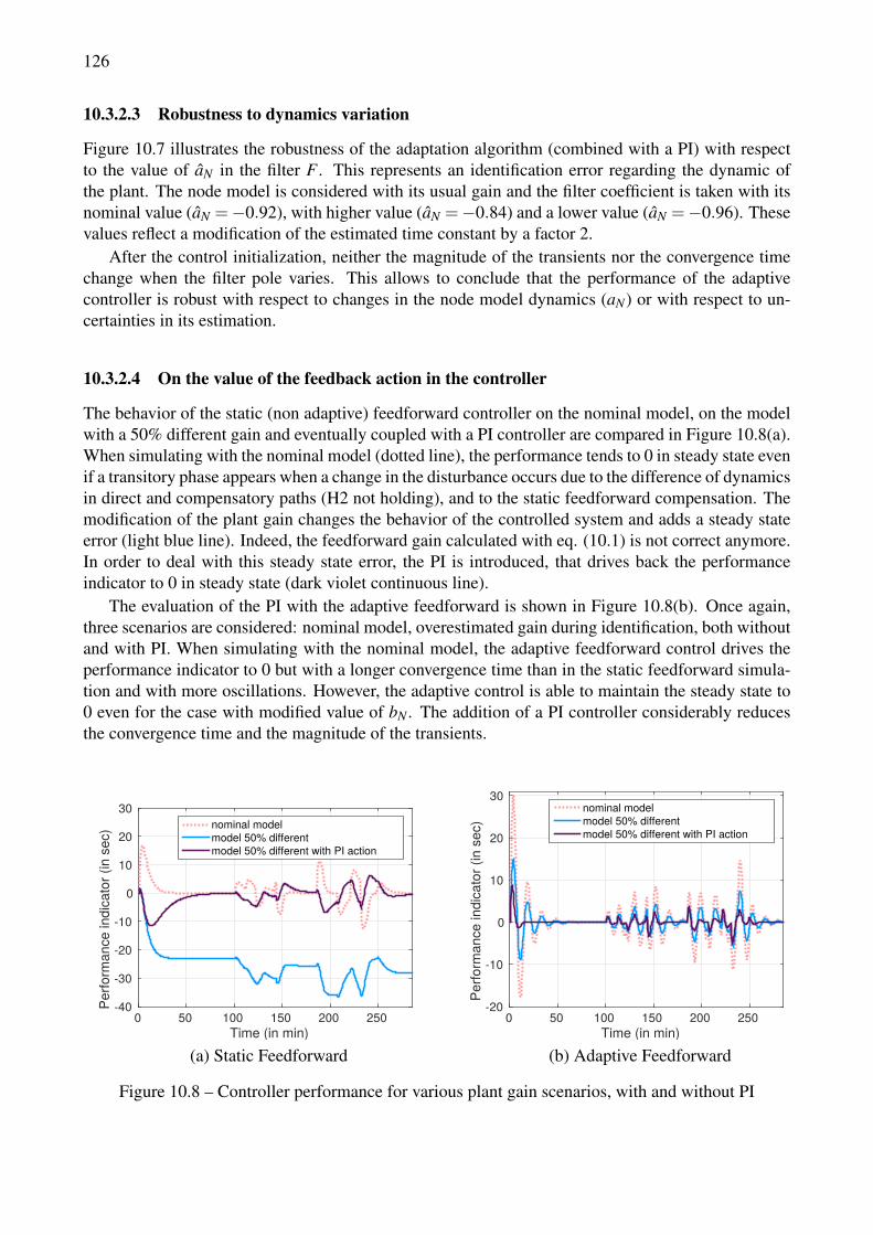
126

10.3.2.3 Robustness to dynamics variation

Figure 10.7 illustrates the robustness of the adaptation algorithm (combined with a PI) with respectto the value of aN in the filter F . This represents an identification error regarding the dynamic ofthe plant. The node model is considered with its usual gain and the filter coefficient is taken with itsnominal value (aN =−0.92), with higher value (aN =−0.84) and a lower value (aN =−0.96). Thesevalues reflect a modification of the estimated time constant by a factor 2.

After the control initialization, neither the magnitude of the transients nor the convergence timechange when the filter pole varies. This allows to conclude that the performance of the adaptivecontroller is robust with respect to changes in the node model dynamics (aN) or with respect to un-certainties in its estimation.

10.3.2.4 On the value of the feedback action in the controller

The behavior of the static (non adaptive) feedforward controller on the nominal model, on the modelwith a 50% different gain and eventually coupled with a PI controller are compared in Figure 10.8(a).When simulating with the nominal model (dotted line), the performance tends to 0 in steady state evenif a transitory phase appears when a change in the disturbance occurs due to the difference of dynamicsin direct and compensatory paths (H2 not holding), and to the static feedforward compensation. Themodification of the plant gain changes the behavior of the controlled system and adds a steady stateerror (light blue line). Indeed, the feedforward gain calculated with eq. (10.1) is not correct anymore.In order to deal with this steady state error, the PI is introduced, that drives back the performanceindicator to 0 in steady state (dark violet continuous line).

The evaluation of the PI with the adaptive feedforward is shown in Figure 10.8(b). Once again,three scenarios are considered: nominal model, overestimated gain during identification, both withoutand with PI. When simulating with the nominal model, the adaptive feedforward control drives theperformance indicator to 0 but with a longer convergence time than in the static feedforward simula-tion and with more oscillations. However, the adaptive control is able to maintain the steady state to0 even for the case with modified value of bN . The addition of a PI controller considerably reducesthe convergence time and the magnitude of the transients.

Time (in min)0 50 100 150 200 250

Perfo

rman

ce in

dica

tor (

in s

ec)

-40

-30

-20

-10

0

10

20

30nominal modelmodel 50% differentmodel 50% different with PI action

Time (in min)0 50 100 150 200 250

Perfo

rman

ce in

dica

tor (

in s

ec)

-20

-10

0

10

20

30nominal modelmodel 50% differentmodel 50% different with PI action

(a) Static Feedforward (b) Adaptive Feedforward

Figure 10.8 – Controller performance for various plant gain scenarios, with and without PI

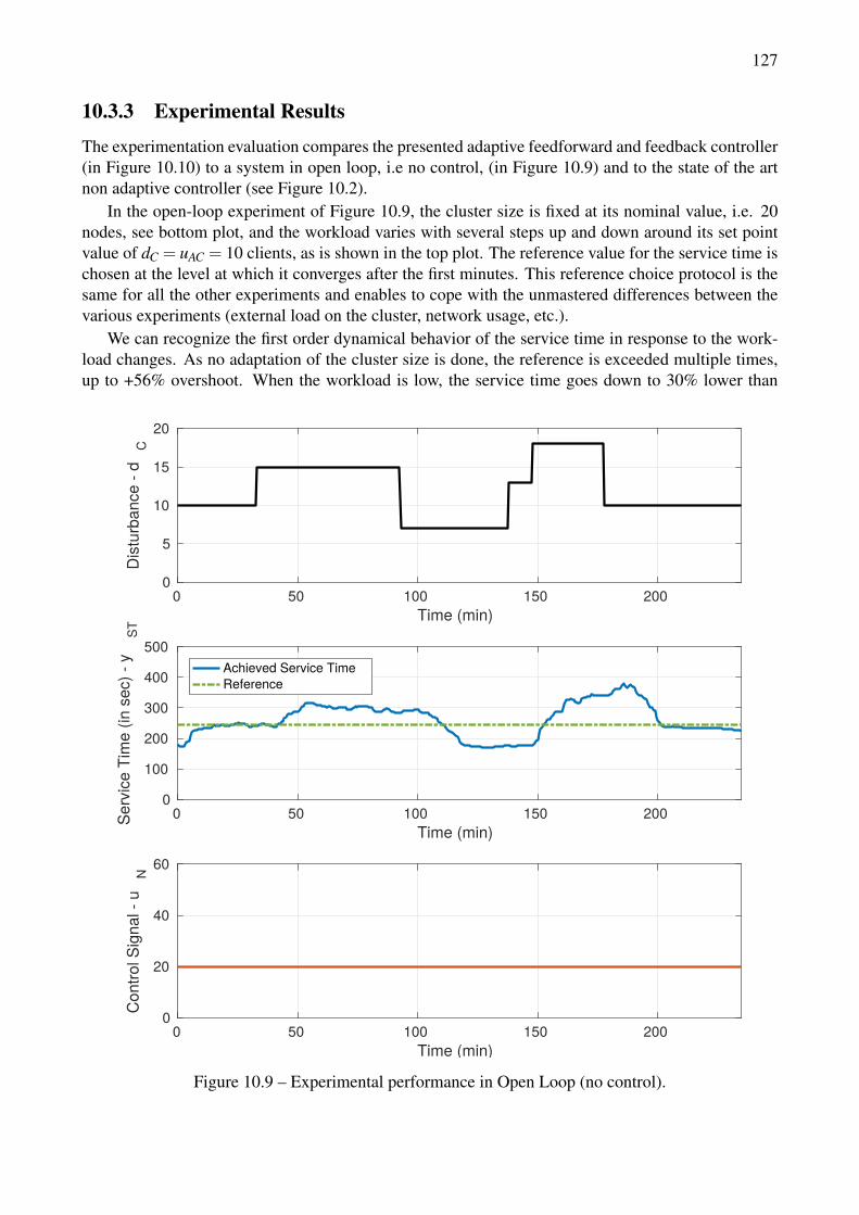
127

10.3.3 Experimental Results

The experimentation evaluation compares the presented adaptive feedforward and feedback controller(in Figure 10.10) to a system in open loop, i.e no control, (in Figure 10.9) and to the state of the artnon adaptive controller (see Figure 10.2).

In the open-loop experiment of Figure 10.9, the cluster size is fixed at its nominal value, i.e. 20nodes, see bottom plot, and the workload varies with several steps up and down around its set pointvalue of dC = uAC = 10 clients, as is shown in the top plot. The reference value for the service time ischosen at the level at which it converges after the first minutes. This reference choice protocol is thesame for all the other experiments and enables to cope with the unmastered differences between thevarious experiments (external load on the cluster, network usage, etc.).

We can recognize the first order dynamical behavior of the service time in response to the work-load changes. As no adaptation of the cluster size is done, the reference is exceeded multiple times,up to +56% overshoot. When the workload is low, the service time goes down to 30% lower than

0 50 100 150 200Time (min)

0

5

10

15

20

Dis

turb

ance

- d

C

0 50 100 150 200Time (min)

0

100

200

300

400

500

Serv

ice

Tim

e (in

sec

) - y

ST

Achieved Service TimeReference

0 50 100 150 200Time (min)

0

20

40

60

Con

trol S

igna

l - u

N

Figure 10.9 – Experimental performance in Open Loop (no control).

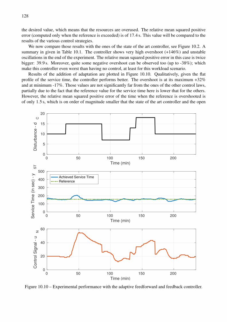
128

the desired value, which means that the resources are overused. The relative mean squared positiveerror (computed only when the reference is exceeded) is of 17.4 s. This value will be compared to theresults of the various control strategies.

We now compare those results with the ones of the state of the art controller, see Figure 10.2. Asummary in given in Table 10.1. The controller shows very high overshoot (+146%) and unstableoscillations in the end of the experiment. The relative mean squared positive error in this case is twicebigger: 39.9 s. Moreover, quite some negative overshoot can be observed too (up to -38%); whichmake this controller even worst than having no control, at least for this workload scenario.

Results of the addition of adaptation are plotted in Figure 10.10. Qualitatively, given the flatprofile of the service time, the controller performs better. The overshoot is at its maximum +32%and at minimum -17%. Those values are not significantly far from the ones of the other control laws,partially due to the fact that the reference value for the service time here is lower that for the others.However, the relative mean squared positive error of the time when the reference is overshooted isof only 1.5 s, which is on order of magnitude smaller that the state of the art controller and the open

0 50 100 150 200Time (min)

0

5

10

15

20

Dis

turb

ance

- d

C

0 50 100 150 200Time (min)

0

100

200

300

400

500

Serv

ice

Tim

e (in

sec

) - y

ST

Achieved Service TimeReference

0 50 100 150 200Time (min)

0

20

40

60

Con

trol S

igna

l - u

N

Figure 10.10 – Experimental performance with the adaptive feedforward and feedback controller.

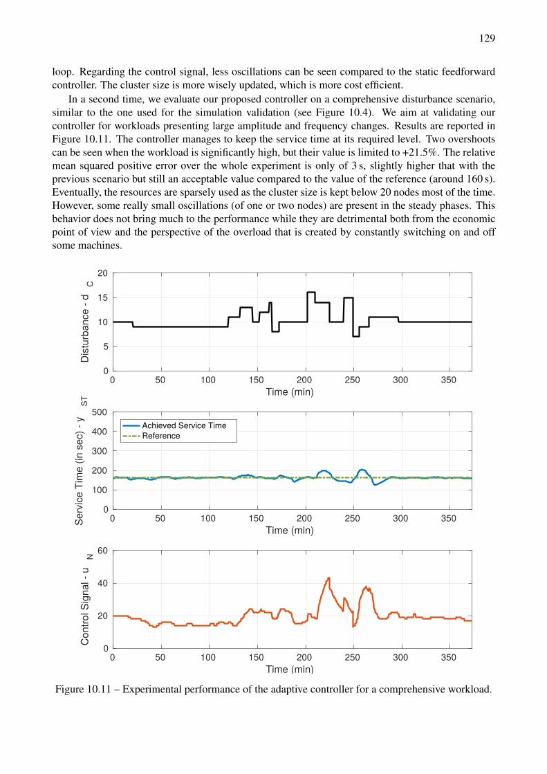
129

loop. Regarding the control signal, less oscillations can be seen compared to the static feedforwardcontroller. The cluster size is more wisely updated, which is more cost efficient.

In a second time, we evaluate our proposed controller on a comprehensive disturbance scenario,similar to the one used for the simulation validation (see Figure 10.4). We aim at validating ourcontroller for workloads presenting large amplitude and frequency changes. Results are reported inFigure 10.11. The controller manages to keep the service time at its required level. Two overshootscan be seen when the workload is significantly high, but their value is limited to +21.5%. The relativemean squared positive error over the whole experiment is only of 3 s, slightly higher that with theprevious scenario but still an acceptable value compared to the value of the reference (around 160 s).Eventually, the resources are sparsely used as the cluster size is kept below 20 nodes most of the time.However, some really small oscillations (of one or two nodes) are present in the steady phases. Thisbehavior does not bring much to the performance while they are detrimental both from the economicpoint of view and the perspective of the overload that is created by constantly switching on and offsome machines.

0 50 100 150 200 250 300 350Time (min)

0

5

10

15

20

Dis

turb

ance

- d

C

0 50 100 150 200 250 300 350Time (min)

0

100

200

300

400

500

Serv

ice

Tim

e (in

sec

) - y

ST

Achieved Service TimeReference

0 50 100 150 200 250 300 350Time (min)

0

20

40

60

Con

trol S

igna

l - u

N

Figure 10.11 – Experimental performance of the adaptive controller for a comprehensive workload.

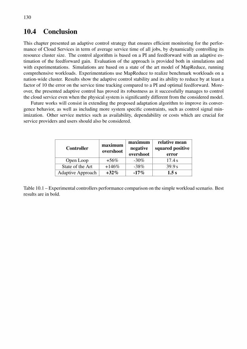
130

10.4 ConclusionThis chapter presented an adaptive control strategy that ensures efficient monitoring for the perfor-mance of Cloud Services in term of average service time of all jobs, by dynamically controlling itsresource cluster size. The control algorithm is based on a PI and feedforward with an adaptive es-timation of the feedforward gain. Evaluation of the approach is provided both in simulations andwith experimentations. Simulations are based on a state of the art model of MapReduce, runningcomprehensive workloads. Experimentations use MapReduce to realize benchmark workloads on anation-wide cluster. Results show the adaptive control stability and its ability to reduce by at least afactor of 10 the error on the service time tracking compared to a PI and optimal feedforward. More-over, the presented adaptive control has proved its robustness as it successfully manages to controlthe cloud service even when the physical system is significantly different from the considered model.

Future works will consist in extending the proposed adaptation algorithm to improve its conver-gence behavior, as well as including more system specific constraints, such as control signal min-imization. Other service metrics such as availability, dependability or costs which are crucial forservice providers and users should also be considered.

Controller maximumovershoot

maximumnegative

overshoot

relative meansquared positive

errorOpen Loop +56% -30% 17.4 s

State of the Art +146% -38% 39.9 sAdaptive Approach +32% -17% 1.5 s

Table 10.1 – Experimental controllers performance comparison on the simple workload scenario. Bestresults are in bold.

Chapter 11

Cost-aware Control of Cloud Services

BigData cloud services performance are evaluated by the jobs runtime, as presented so far, but also bymetrics such as the service availability and its cost efficiency. This chapter develops a control strategythat enables to take those multiple objectives into account. The formulation is a Model PredictiveControl (MPC) with the addition of a event-based triggering mechanism (instead of a classical time-based control signal generation). The triggering mechanisms of the control theory state of the art didnot correspond to the objectives of cost-efficiency specific to our cloud application. This made usdevelop a new cost-function based triggering mechanism. The theoretical contribution of this chapterhowever goes beyond the MapReduce use case, as it can be applied for all non linear discrete timesystems. Stability proof of the controller is provided, as well as simulation validation of the controlperformance. We also evaluate the approach on the cloud use-case using simulations of a real worldworkload, showing 8% cost saving (based on Amazon EC2 pricing) compared to the classic error-based event triggered control.

After an introduction on motivation and related works (Section 11.1), the some background andformalism is provided on the optimal control formulation, see Section 11.2. The new control strategyis presented in Section 11.3 while Section 11.4 depicts its evaluation.

11.1 IntroductionWhen running requests on an online service, three major objectives can be formulated: maximizationof the performance in terms of run time, maximization of the service availability and reduction ofthe costs. Those are the common criterias that make the clients choose one platforms rather thananother. While the previous chapter was focusing only on the first objective, we are now interestedin a complete framework able to satisfy performance, availability and cost requirements. Indeed,they are contradictory objectives to achieve. For instance, if very few requests are accepted andmany resources are dedicated to the remaining tasks, the performance will be excellent but the otherobjectives won’t be satisfyingly reached. To be able to monitor the cloud service, two control knobsare commonly available: resource cluster scaling and admission control. Indeed, too large clustershave high monetary and energetic costs, while too small ones bring poor performance, often resultingin financial and commercial penalties [67]. Those considerations lead to the use of a multi-input andmulti-output control problem formulation.

The cost efficiency objective can be directly linked to the cluster size, as more machines meansmore power and network consumption. Any change in the number of resources implies a novel recon-figuration of the system which takes considerable time and costs money due to system unavailabilityand/or poor performance [119]. Moreover, quick changes in the control value (thus a high rate re-configuration of the cluster) can overload the communication channels and lead to an accumulation

131

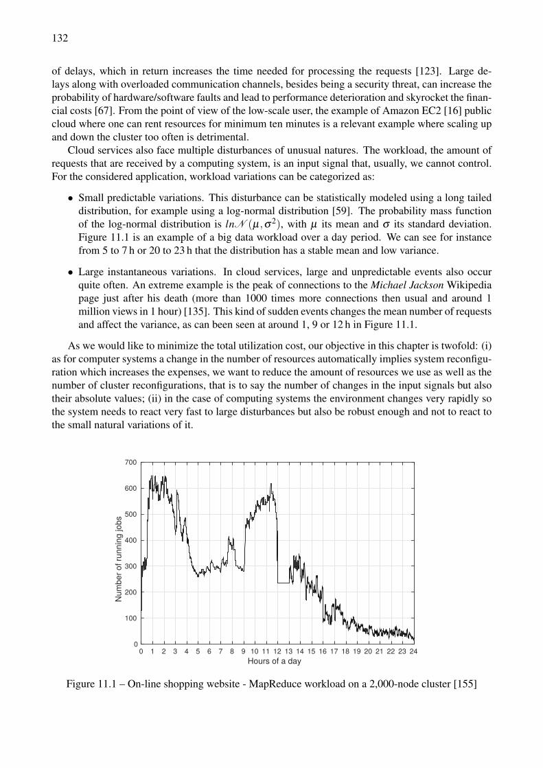
132

of delays, which in return increases the time needed for processing the requests [123]. Large de-lays along with overloaded communication channels, besides being a security threat, can increase theprobability of hardware/software faults and lead to performance deterioration and skyrocket the finan-cial costs [67]. From the point of view of the low-scale user, the example of Amazon EC2 [16] publiccloud where one can rent resources for minimum ten minutes is a relevant example where scaling upand down the cluster too often is detrimental.

Cloud services also face multiple disturbances of unusual natures. The workload, the amount ofrequests that are received by a computing system, is an input signal that, usually, we cannot control.For the considered application, workload variations can be categorized as:

• Small predictable variations. This disturbance can be statistically modeled using a long taileddistribution, for example using a log-normal distribution [59]. The probability mass functionof the log-normal distribution is lnN (µ,σ2), with µ its mean and σ its standard deviation.Figure 11.1 is an example of a big data workload over a day period. We can see for instancefrom 5 to 7 h or 20 to 23 h that the distribution has a stable mean and low variance.

• Large instantaneous variations. In cloud services, large and unpredictable events also occurquite often. An extreme example is the peak of connections to the Michael Jackson Wikipediapage just after his death (more than 1000 times more connections then usual and around 1million views in 1 hour) [135]. This kind of sudden events changes the mean number of requestsand affect the variance, as can been seen at around 1, 9 or 12 h in Figure 11.1.

As we would like to minimize the total utilization cost, our objective in this chapter is twofold: (i)as for computer systems a change in the number of resources automatically implies system reconfigu-ration which increases the expenses, we want to reduce the amount of resources we use as well as thenumber of cluster reconfigurations, that is to say the number of changes in the input signals but alsotheir absolute values; (ii) in the case of computing systems the environment changes very rapidly sothe system needs to react very fast to large disturbances but also be robust enough and not to react tothe small natural variations of it.

Hours of a day0 1 2 3 4 5 6 7 8 9 10 11 12 13 14 15 16 17 18 19 20 21 22 23 24

Num

ber o

f run

ning

jobs

0

100

200

300

400

500

600

700

Figure 11.1 – On-line shopping website - MapReduce workload on a 2,000-node cluster [155]

133

Related work regarding the control of cloud services has been presented in Chapter 9. We willhowever mention here the work of Berekméri et al. on the control of MapReduce service time withcost efficiency objectives [26]. The used controller was with feedback and feedforward action, bothcoupled with an threshold-based triggering strategy to reduce the cluster size updates. However noneof the state of the art solutions are explicitly designed to reduce the cluster reconfiguration rate in amulti objectives context.

In this chapter, we present event-based control techniques to reduce the number of cluster recon-figurations. For the control community, the use of event mechanisms let hope for a reduction in theuse of resources [22, 64] without degrading performance [120] and with stability and robustness guar-antees [127]. However, all the numerous event-based control strategies in the literature are focusedon stability and performance guarantees. Those researches are motivated by the communication orcomputation reduction in networked controlled systems which are different objectives from reducingthe number of reconfigurations while guaranteeing an acceptable level of performance.

Event based control consist of switching the control from an traditional time-based periodic com-putation to an event-based one. Today triggering strategies are based on level-crossing by the mea-surement error (for instance when using PID controllers [21, 64]) or more generally by some Lya-punov function (see for instance [171]) or on the vanishing of an event-function related to a ControlLyapunov Function (see for instance [127]). Other event triggering mechanisms are linear functionsof the measurement error as in [78], [61]. In all cases, the decision of updating the control law or notusually does not use a prediction of what will happen in the future. Those formulations are reactive, inthe sense that control is triggered only when the impact of disturbances has driven the system to crossa critical threshold. Predictive methods that consider explicitly the future evolution of the currentstate are very encouraging but until now, few methods of this type have been developed. Eqtami etal.’s work [66] is an example of this type where the prediction is based on thresholds crossing aroundthe desired states.

Deciding on the triggering based on threshold crossing might not be the best solution in all cases.For example, an acceptable state at present time which leads to an undesirable behavior in the futurecan be handled by the predictive controller straight away, thus improving performance. Conversely,an undesired behavior in the present time but which leads to a stable situation in the future may not betaken care of, to reduce events number and reconfigurations. Furthermore, when dealing with multi-input and multi-output (MIMO) systems, the measurement errors alone are not sufficient to decideif the system is in a critical state and needs a control actuation. Indeed, the multiples signals impactone another and a same value of the error for an output does not necessary reflect a critical situationfor the system according to other signals values. For example, a CPU usage of 90% reflect a normalbehavior if memory usage is high while it is alarming if memory usage is low.

In this chapter, we suggest an triggering mechanism based upon the optimal cost function forModel Predictive Controllers (MPC) that addresses the issues presented above: the calculation ofthe cost function which by definition deals with the different weights of the performance signalsand takes into account, the future behavior of the system on the prediction horizon using the model.Furthermore, constraints on the command shape (for instance the command should be constant ona time window) combined with an event mechanism ensure that changes in the command signal arereduced while other specifications still hold.

134

11.2 PreliminariesLet us first define the notation used and formalize the optimization problem. We consider a generalnonlinear discrete time system described by the equations{

xk+1 = f (xk,uk)yk = g(xk)

(11.1)

where x ∈ Rnx is the vector of describing the states, y ∈ Rny is the measured outputs and u ∈ Rnu

the control variables. We assume that f (0,0) = 0 and g(0) = 0. Only stabilization at the origin isconsidered here, as most problem formulations can be transformed to such stabilization points. Thesubscript k of a variable stands for its value at time kTS, TS being the sampling period. We define atime horizon of N ∈ N instants, N > 0. The N notation in this Chapter is not referring to the clustersize variable as in Chapters 9 and 10. In this section, we assume the system has no delay neither con-straint on the control or state values. Extending the proposed results to delayed or constrained systemscan however be done as classically in model predictive control. The MapReduce application typicallyhas delays, saturation constraints on the control and positivity constraints on the states values. Theapplicability of this technique will be validated on such complex system, but theory is provided onlyfor the system under the hypothesis of no delay nor constraint.

Let U ∈ Rnu×N be a control profile over the horizon N defined by:

U :=(u0 u1 · · · uN−1

)(11.2)

For any initial condition xi, and any control profile U ∈ Rnu×N , we define the corresponding statetrajectory X ∈ Rnx×(N+1) by:

X(xi,U) :=(x0 x1 · · · xN

)(11.3)

with{

x0 := xixk+1 = f (xk,uk) ∀k ∈ {0, . . . ,N−1} , (11.4)

and we associate to this state trajectory, the output trajectory Y ∈ Rny×(N+1) defined by Y (X) :=(y0 y1 . . . yN

)with ∀k ∈ {0, . . . ,N}, yk = g(xk). Note that in the above definitions, the trajectories

are defined on the time horizon only. Let J : Rnx×Rnu×N → R+ be some cost function depending onan initial condition xi and a control profile U . A very common definition of the cost function for astabilization objective is the quadratic cost of the form:

J(xi,U) =N

∑k=1

X |Tk+1(xi,U)QxX |k+1(xi,U)+U |Tk RU |k, (11.5)

where X |k(xi,U) (resp. U |k) denotes the kth column of X(xi,U) (resp. U), T is the transpose operator.Qx and R are positive, definite matrices of appropriate sizes. Note the shift in the indexes: U |k = uk−1and X |k = xk−1. For a reference tracking objective, the cost function could be:

J(xi,U) =N

∑k=1

Y |Tk+1QYY |k+1 +U |Tk RU |k, (11.6)

with QY and R positive, definite matrices of appropriate sizes, Y |k := Y |k(X(xi,U))−Y re f |k whereY re f ∈ Rny×(N+1) is the reference trajectory on the time horizon N. Finally, let us define the set U ofcontrols as:

U (xi) :={

U ∈ Rnu×N s.t. X |N+1(xi,U) = 0}. (11.7)

U is the set of control profiles that satisfy a terminal constraint at the end of the horizon on the statevariable. The final constraint is very common for stability purposes [130].

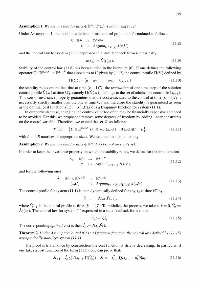
135

Assumption 1 We assume that for all x ∈ Rnx , U (x) is not an empty set.

Under Assumption 1, the model predictive optimal control problem is formulated as follows:

U : Rnx → Rnu×N

x 7→ ArgminU∈U (x) J(x,U),(11.8)

and the control law for system (11.1) expressed in a state feedback form is classically:

u(xk) := U |1(xk). (11.9)

Stability of the control law (11.8) has been studied in the literature [6]. If one defines the followingoperator Π : Rnu×N →Rnu×N that associates to U given by (11.2) the control profile Π(U) defined by

Π(U) :=(u1 u2 . . . uN−1 0nu×1,

)(11.10)

the stability relies on the fact that at time (k+ 1)TS, the translation of one time step of the solutioncontrol profile U(xk) at time kTS, namely Π(U(xk)), belongs to the set of admissible control U (xk+1).This sort of invariance property guarantees that the cost associated to the control at time (k+1)TS isnecessarily strictly smaller than the one at time kTS and therefore the stability is guaranteed as soonas the optimal cost function J(x) := J(x,U(x)) is a Lyapunov function for system (11.1).

In our particular case, changing the control value too often may be financially expensive and needto be avoided. For this, we propose to remove some degrees of freedom by adding linear constraintson the control variable. Therefore, we extend the set U as follows:

V (xi) :={

U ∈ Rnu×N s.t. X |N+1(xi,U) = 0 and AU = B}, (11.11)

with A and B matrices of appropriate sizes. We assume that it is not empty:

Assumption 2 We assume that for all x ∈ Rnx , V (x) is not an empty set.

In order to keep the invariance property on which the stability relies, we define for the first iteration

Λ0 : Rnx → Rnu×N

x 7→ ArgminV∈V (x) J(x,V ),(11.12)

and for the following ones

Λ : Rnx×Rnu×N → Rnu×N

(x,U) 7→ ArgminV∈V (x)∪{Π(U)} J(x,V ).(11.13)

The control profile for system (11.1) is then dynamically defined for any xk at time kT by:

Vk := Λ(xk,Vk−1), (11.14)

where Vk−1 is the control profile at time (k− 1)T . To initialize the process, we take at k = 0, V0 :=Λ0(x0). The control law for system (1) expressed in a state feedback form is then:

uk := Vk|1. (11.15)

The corresponding optimal cost is then Jk := J(xk,Vk).

Theorem 2 Under Assumption 2, and if J is a Lyapunov function, the control law defined by (11.15)asymptotically stabilizes system (11.1).

The proof is trivial since by construction the cost function is strictly decreasing. In particular, ifone takes a cost function of the form (11.5), one can prove that:

Jk+1− Jk ≤ J(xk+1,Π(Vk))− Jk =−xTk+1Qxxk+1−uT

k Ruk. (11.16)

136

11.3 Control StrategyThis section presents a triggering algorithm for MPC control laws (11.9) and (11.15) defined in theprevious section. This strategy will decide when the control profile needs to be recalculated. For sakeof simplicity, we assume in the following that the cost function J is of the form of eq. (11.5).

11.3.1 The Lyapunov based triggering strategy

To any state xk of the system at time kTS and any control profile Wk−1 at time (k− 1)TS, we as-sociate two corresponding costs, namely Jk defined as previously by Jk := J(xk,Λ0(xk)) and Jk :=J(xk,Π(Wk−1)). The first cost Jk corresponds to the cost if one updates the control with its optimalvalue whereas, Jk is the cost obtained keeping the previous control profile. Note that by construction,one has the following inequality: Jk ≥ Jk. We can now define the event function e : Rnx×R+→{0,1}by:

ek =

{1 if Jk− Jk ≥ εJ Jk or if k = 00 otherwise.

(11.17)

The proposed MPC event-triggered control profile Wk at time kTS is then:

Wk =

{Λ0(xk) if ek = 1

Π(Wk−1) otherwise.(11.18)

The control law to apply is as previously the first element of the control profile, that is:

wk =Wk|1. (11.19)

Note that if e = 0 the control profile of the last time period is applied and then wk = Wk|1 = Wk−1|2 .Hence, contrary to usual event-based control, the input control value is not kept constant in the pro-posed scheme. The control profile is updated when the cost can be reduced by a factor of 1+ εJ withrespect to the cost when keeping the same control profile.

Choice of εJ The threshold εJ from eq.(11.17) should be chosen carefully. If it is too small, thecontroller will unnecessarily react to noise, model uncertainties or observer error (if one), while if εJis too large we may not react fast enough to disturbances. The tuning of εJ can be done in a trainingphase using data from an open-loop experiment with disturbances.

Whatever the value of εJ might be, the point is that the threshold is relative to the current valueof expected cost function. This means that we can detect disturbances that do not have a comparableabsolute cost.

11.3.2 Stability of the proposed scheme

The proposed scheme asymptotically stabilizes the system at the origin since it ensures the strictdecrease of the cost function until the origin is reached:

Theorem 3 Under Assumption 2, and if J is a Lyapunov function, the control law defined by (11.19)asymptotically stabilizes system (11.1).

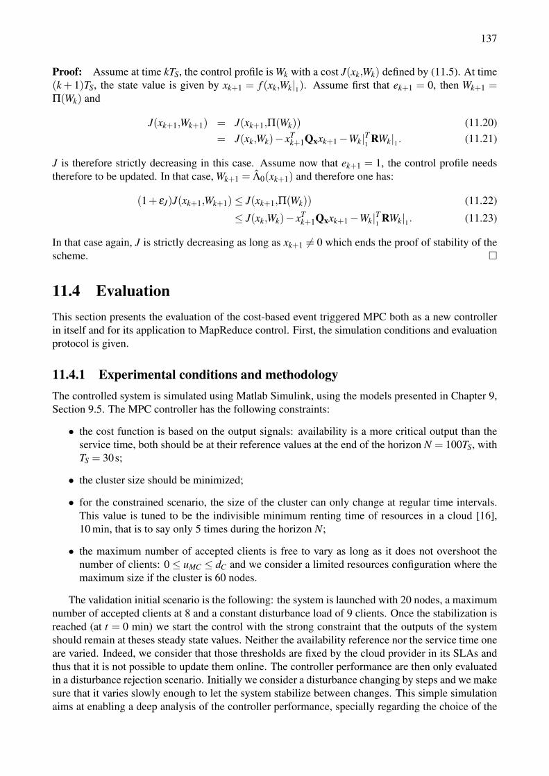
137

Proof: Assume at time kTS, the control profile is Wk with a cost J(xk,Wk) defined by (11.5). At time(k + 1)TS, the state value is given by xk+1 = f (xk,Wk|1). Assume first that ek+1 = 0, then Wk+1 =Π(Wk) and

J(xk+1,Wk+1) = J(xk+1,Π(Wk)) (11.20)= J(xk,Wk)− xT

k+1Qxxk+1−Wk|T1 RWk|1. (11.21)

J is therefore strictly decreasing in this case. Assume now that ek+1 = 1, the control profile needstherefore to be updated. In that case, Wk+1 = Λ0(xk+1) and therefore one has:

(1+ εJ)J(xk+1,Wk+1)≤ J(xk+1,Π(Wk)) (11.22)

≤ J(xk,Wk)− xTk+1Qxxk+1−Wk|T1 RWk|1. (11.23)

In that case again, J is strictly decreasing as long as xk+1 6= 0 which ends the proof of stability of thescheme. �

11.4 EvaluationThis section presents the evaluation of the cost-based event triggered MPC both as a new controllerin itself and for its application to MapReduce control. First, the simulation conditions and evaluationprotocol is given.

11.4.1 Experimental conditions and methodologyThe controlled system is simulated using Matlab Simulink, using the models presented in Chapter 9,Section 9.5. The MPC controller has the following constraints:

• the cost function is based on the output signals: availability is a more critical output than theservice time, both should be at their reference values at the end of the horizon N = 100TS, withTS = 30s;

• the cluster size should be minimized;

• for the constrained scenario, the size of the cluster can only change at regular time intervals.This value is tuned to be the indivisible minimum renting time of resources in a cloud [16],10 min, that is to say only 5 times during the horizon N;

• the maximum number of accepted clients is free to vary as long as it does not overshoot thenumber of clients: 0 ≤ uMC ≤ dC and we consider a limited resources configuration where themaximum size if the cluster is 60 nodes.

The validation initial scenario is the following: the system is launched with 20 nodes, a maximumnumber of accepted clients at 8 and a constant disturbance load of 9 clients. Once the stabilization isreached (at t = 0 min) we start the control with the strong constraint that the outputs of the systemshould remain at theses steady state values. Neither the availability reference nor the service time oneare varied. Indeed, we consider that those thresholds are fixed by the cloud provider in its SLAs andthus that it is not possible to update them online. The controller performance are then only evaluatedin a disturbance rejection scenario. Initially we consider a disturbance changing by steps and we makesure that it varies slowly enough to let the system stabilize between changes. This simple simulationaims at enabling a deep analysis of the controller performance, specially regarding the choice of the

138

triggering function threshold εJ . Eventually, the record of a 1-day workload from a real cluster (seeFigure 11.1) is used for validation of the controller in a genuine situation (Section 11.4.4).

In a first time, the performance of our new event triggered function is compared to the state ofthe art time triggered controller and error-based event triggered control. Then, the addition of theconstraints on the cluster size control signal will be studied. Eventually, we simulate a 1-day usage ofour controller based on a real scenario and compute the costs saving induced by our approach.

11.4.2 Cost based event triggering mechanism validationFirst we compare our method referred to as cost based event solution to an error based one and a timebased controller. All the solutions are calculated without specific constraints on the input signals,as described by eq. (11.9). For the error based triggering mechanism the event function is eitherwhen the control law over the whole horizon has been applied or when one of the outputs crossesa certain threshold. As for the choice of the thresholds, we fixed εJ = 0.5 based on training data toensure no false alarms (see more in Figure 11.4), then we chose the error-method thresholds so thatthe event-based and the cost based solutions ensure the same performance.

Results are shown in Figure 11.2. For comparable performance in term of reference trackingand inputs variations, we observe that the cost based controller generates only 6 events over a 150-minute period, which represents 98.5% less events than the time triggered solution (300 events intotal), and 71.5% less than the error based controller (21 events). Moreover, due to the dynamic of thesystem, once the error thresholds are crossed it takes some time to stabilize the outputs signal insidethe threshold-defined bounds which leads to several events generated by the error based method aftereach disturbance occurs. However, the cost based method takes into account this dynamic throughstates predictions thus removing these redundant events. Hence, with significantly less computingefforts our proposed event mechanism can guarantee comparable performance.

11.4.3 Input-constrained controlSecond, we simulate the behavior of the cost-based constrained controller forced to have constantvalues of the input signal uN on large time intervals (see eq. (11.15)), that we compare to its un-constrained version (eq. (11.9)). Results are given in Figure 11.3: with comparable performance inreference tracking for both outputs and the exact same number of events, the constrained controllerimposes 94.5% less changes in the cluster size.

Furthermore, nonlinear delays caused by communication channel congestion happening whencluster reconfigurations are too frequents were not taken into account in our modeling. Consequentlywe expect that in real on-line experiments with the real MapReduce system, the constrained cost-based event method will also significantly improve the performance in terms of availability and ser-vice time.

Threshold choice

When looking at the event function (Figure 11.4), we see that the condition for triggering an eventgives no false alarm and reacts each time workload conditions change. Moreover, every event iscaused by a clearly marked threshold crossing, it is an indicator of the robustness of our methodregarding the value of εJ .

Furthermore, we see in Figure 11.4 the importance of the threshold expressed as a percentage. Justafter an event, the cost J is way higher than just before as it takes time and resources for the systemto reach specifications again, however this high value of J does not necessary reflect that anotherdisturbance happened.

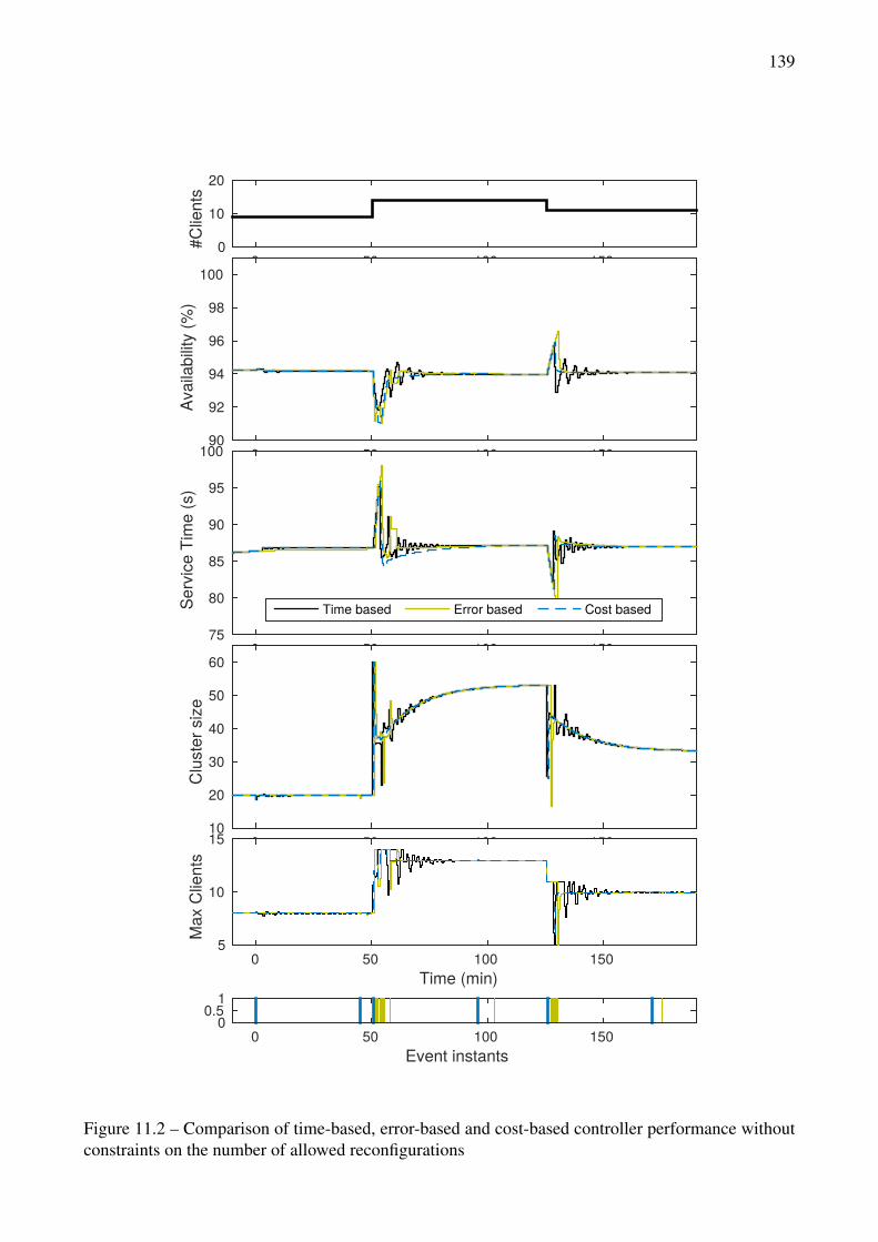
139

0 50 100 150

#Clie

nts

0

10

20

0 50 100 150

Avai

labi

lity

(%)

90

92

94

96

98

100

Time (min)0 50 100 150

Serv

ice

Tim

e (s

)

75

80

85

90

95

100

Time based Error based Cost based

Time (min)0 50 100 150

Clu

ster

siz

e

10

20

30

40

50

60

Time (min)0 50 100 150

Max

Clie

nts

5

10

15

Event instants0 50 100 150

00.5

1

Figure 11.2 – Comparison of time-based, error-based and cost-based controller performance withoutconstraints on the number of allowed reconfigurations

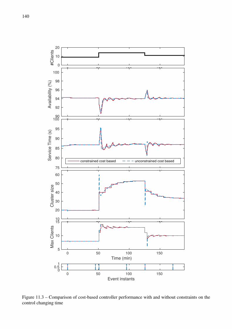
140

0 50 100 150

#Clie

nts

0

10

20

0 50 100 150

Avai

labi

lity

(%)

90

92

94

96

98

100

Time (min)0 50 100 150

Serv

ice

Tim

e (s

)

75

80

85

90

95

100

constrained cost based unconstrained cost based

Time (min)0 50 100 150

Clu

ster

siz

e

10

20

30

40

50

60

Time (min)0 50 100 150

Max

Clie

nts

5

10

15

Event instants0 50 100 150

00.5

1

Figure 11.3 – Comparison of cost-based controller performance with and without constraints on thecontrol changing time

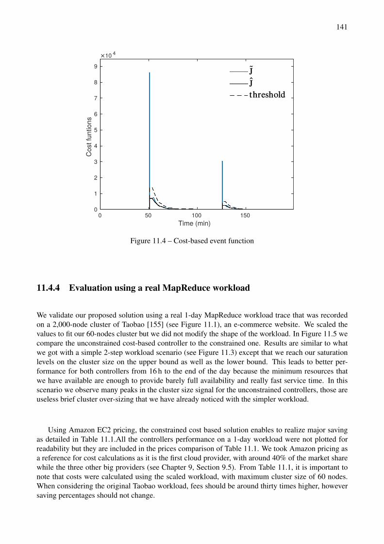
141

Figure 11.4 – Cost-based event function

11.4.4 Evaluation using a real MapReduce workload

We validate our proposed solution using a real 1-day MapReduce workload trace that was recordedon a 2,000-node cluster of Taobao [155] (see Figure 11.1), an e-commerce website. We scaled thevalues to fit our 60-nodes cluster but we did not modify the shape of the workload. In Figure 11.5 wecompare the unconstrained cost-based controller to the constrained one. Results are similar to whatwe got with a simple 2-step workload scenario (see Figure 11.3) except that we reach our saturationlevels on the cluster size on the upper bound as well as the lower bound. This leads to better per-formance for both controllers from 16 h to the end of the day because the minimum resources thatwe have available are enough to provide barely full availability and really fast service time. In thisscenario we observe many peaks in the cluster size signal for the unconstrained controllers, those areuseless brief cluster over-sizing that we have already noticed with the simpler workload.

Using Amazon EC2 pricing, the constrained cost based solution enables to realize major savingas detailed in Table 11.1.All the controllers performance on a 1-day workload were not plotted forreadability but they are included in the prices comparison of Table 11.1. We took Amazon pricing asa reference for cost calculations as it is the first cloud provider, with around 40% of the market sharewhile the three other big providers (see Chapter 9, Section 9.5). From Table 11.1, it is important tonote that costs were calculated using the scaled workload, with maximum cluster size of 60 nodes.When considering the original Taobao workload, fees should be around thirty times higher, howeversaving percentages should not change.

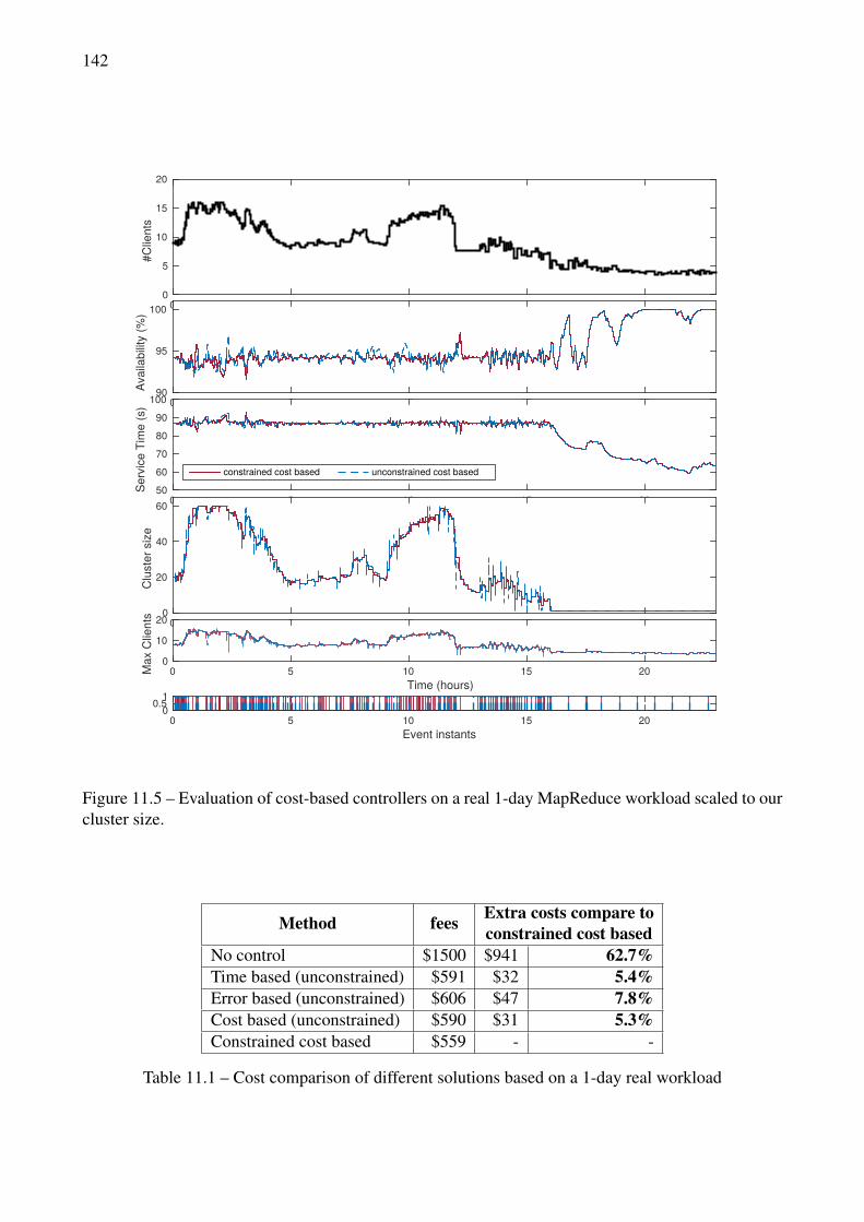
142

0 5 10 15 20

#Clie

nts

0

5

10

15

20

0 5 10 15 20

Avai

labi

lity

(%)

90

95

100

Time (min)0 5 10 15 20

Serv

ice

Tim

e (s

)

5060708090

100

constrained cost based unconstrained cost based

Time (min)0 5 10 15 20

Clu

ster

siz

e

0

20

40

60

Time (hours)0 5 10 15 20M

ax C

lient

s

0

10

20

Event instants0 5 10 15 20

00.51

Figure 11.5 – Evaluation of cost-based controllers on a real 1-day MapReduce workload scaled to ourcluster size.

Method fees Extra costs compare toconstrained cost based

No control $1500 $941 62.7%Time based (unconstrained) $591 $32 5.4%Error based (unconstrained) $606 $47 7.8%Cost based (unconstrained) $590 $31 5.3%Constrained cost based $559 - -

Table 11.1 – Cost comparison of different solutions based on a 1-day real workload

143

11.5 ConclusionIn this chapter we presented a new event mechanism for model predictive controllers which has twoaims: (i) to reduce the number of events without degrading performance and (ii) to reduce the changesin the control inputs thus reacting to large disturbances and being robust to smaller ones.

The latter constraint is particularly relevant in the context of big-data cloud services where a highfrequency of cluster reconfiguration has major financial and energetic costs and leads to performancedegradation. The event mechanism developed here is a function of the cost function defined in theoptimal problem, and not based on measurement error as has often be the case until now. This enablestaking into account predictions of the system trajectory over a time horizon. In order to handle thereduction of input changes we add constraints to the MPC formulation, allowing changes only atregular time intervals.

The controller also has the advantage of being able to follow objectives expressed with variousmetrics: service time performance, service availability and costs. The multi-signal cloud controlconsists in a valuable improvement for the fulfillment of cloud services SLAs.

Evaluation is carried out in simulation on a model which was previously validated on a realMapReduce system. The simulations show that the constrained cost-based event triggered MPCsignificantly reduce the number of events as well as changes in the control law. We generate 86%less events in comparison to an error based method and we obtain at least 8% cost savings whensimulating with a real 1-day workload (based on Amazon EC2 pricing).

The next steps of this work would be to validate the constrained cost-based event triggered MPCapproach through experiments using the latest MapReduce release on a public Cloud such as AmazonEC2. We expect to have more promising results due to the reduction of cluster reconfigurationswhich are even more costly on the real system due to congestion of communication channels leadingto performance degradation. However, the variability of the system highlighted in Chapter 10 mightlead us to add a robustness oriented aspect to our controller.

Chapter 12

Conclusions on MapReduce Control

This ending chapter of Part III highlights this thesis contributions with regards to the bigdata cloudservices monitoring domain, its limitations and its perspectives.

The growing development of computing devices as well as their capacities soar has generatedmassive amounts of so called bigdata. They are a windfall for companies that are able to extract fromthem many valuable informations. The advances in data processing has been fostered by the rise ofthe cloud computing paradigm, in which resources are made available and maintained as a service forclients that just want to run their processing without dealing with the hardware or low level softwarestacks. MapReduce/Hadoop is one of the most famous paradigm for bigdata processing able to workin such cloud infrastructure. As for any service, the guarantee of its performance is a key challengeboth for the cloud provider and the client running MapReduce jobs. The execution time of the clients’requests as well as the service availability are two of the prevalent indicators of the service quality. Inorder to guarantee them, the cloud provider can realize elastic resource provisioning and admissioncontrol.

The works presented in this thesis use control theory to approach this performance monitoringchallenge. Starting from the state of the art, we presented two main contributions. First, the problemis addressed from the robustness perspective. Given the limits of the state of the art to capture the nonlinear behavior of the MapReduce framework and to ensure performance in case of highly dynamicworkload, an adaptive controller has been developed. It consists in a PI feedback control with gainfeedforward action, which parameter is adapted on line based on the system observed behavior. Thisapproach has been validated both in simulation and by using a MapReduce benchmark on a real clus-ter. However, the monitoring of jobs execution time only do not enable to apprehend the complexityof the agreements between a cloud provider and his clients. The second contribution of this part real-izes the joint optimal control of jobs service time and service availability. An emphasis is done on thecost efficiency, which leads to the development of a new event-based triggering mechanism for theModel Predictive Controller used. The triggering mechanism is based on the Lyapunov cost functionof the system, which enables to minimize the reconfigurations of the cluster, as it is the main sourceof expenses in the cloud paradigm. Results are promising but however need to be evaluated on a realcloud.

The robustness and cost-efficiency challenges are indeed complementary and a combination ofboth approaches of adaptation and event-based control could stand as a promising solution. However,adaptation for a MIMO model and triggering mechanisms able to deal with time varying systems aremore complex problems that would require extended research work. The benefits of such solutionswould go beyond the bigdata cloud control problem.

Nevertheless, those works present some limitations. The first one is the related to the metricschoice. An ideal control satisfies the objectives for the values and behavior of the signal and costs

145

146

functions used for the problem formulation. Thus, aside from the technical achievements, the defi-nition of the problem is of first importance. For instance, the performance metric that was picked inthis work is the average execution time of the jobs that finished in the last time slot. However, manyother choices could have been made: computing the 99th percentile instead of the average, takinginto account the duration of the running jobs instead of the finished ones, etc. A deeper study of theusuals SLAs of cloud providers could be of great use to refine those metrics. Moreover, the additionof new dimensions to the problem should be considered, to cope with new demands of the clients,such as dependability to hardware and software failure or security guarantees. The definition of awider MIMO problem could enable to take into account all those aspects.

In a second time, let us recall some of the hypothesis that were taken for this work: the clusterhas homogeneous resources, the jobs of the workload are of similar nature and the MapReduce ver-sion is fixed. In order to increase the robustness of the presented approaches, the cases when thoseassumptions do not hold should be tested. The homogeneity of current cloud is often a reality atsmall scale. However, the datacenters are nowadays highly heterogeneous, with application specifichardware such as GPUs. The adaptation algorithm presented in Chapter 10 could however enableto deal to some extent with those differences, whereas it still needs to be tested. Eventually, evenif the experimentations were done on a real cluster deployment, Grid5000 is a research environmentwith eased deployment facilities. The application of the presented control technique on a commercialcloud hosting MapReduce framework, such as Amazon EMR [15], is still a technical challenge.

Part IV

Conclusions and Perspectives

147

149

This thesis presented the use of control theory for autonomous computing systems. Being inthe middle of two distinct research domains, a comprehensive introduction was drawn. The twofields were presented and put in perspective, both with an accessible introduction and then in a moretechnical way. The related work was then overviewed, first by reviewing the various tools for softwareadaptation and then by focusing on detailing the solutions using control theory. The approach takenin this work was to address this issue through two computing system applications, enabling to addressvarious problem specifications and to develop varied modeling and control techniques; but also toinvestigate diverse and complementary aspects of the computing world.

First, we focused on the location privacy challenge. Mobile devices’ users send queries to servicesand include their location data to have a geo-localized answer, such as weather predictions or nearestpoints of interests suggestion. Then, all those location data may be collected in a database, whichprocessing is of great interest (infer road usage frequency and the transportation mode used, derivepopularity of places, etc.). Indeed, all those useful services comes at the price of personal informationdisclosure and is thus an major privacy breach. Our approach consisted in providing tools for themobile device user and the data processing instance to protect data privacy without sacrificing theirutility. More specifically, starting from the state of the art Location Privacy Protection Mechanisms(LPPMs), we combined them and configured them in a dynamic way that fulfill both the users’ privacyand utility requirements. From a control theory perspective, this work provided the first formulationof the location privacy challenge in terms of definition of the plant, the control input, the disturbancesignal as well as the performance outputs. Identification was performed to derive a model of thesystem and a first controller was presented to serve as a proof of concept.

Second, we considered the use-case of a bigdata processing framework running remotely on acloud. Monitoring of performance in terms of response time of the jobs and availability of the servicewere the main objectives, which can be achieved by tuning the resource cluster size and by realizingadmission control. Controllers were designed in order to ensure the monitoring robustness to thesystem changes and workload variations, and to minimize the service costs. Advanced control tech-niques for achieving multi-objectives have been developed and applied: a robust adaptive feedbackcontroller and a event-based triggering mechanism for optimal control.

Conclusions regarding the contribution of this thesis, its limitations and perspective for the dif-ferent application domains have been drawn in the respective parts. The works of this thesis hasbrought significant improvement regarding the state of the art, whether by the novelty of the problemformulation or by the resulting performance of the controlled system.

On top of aiming to provide novel solutions for the specific use-cases, this work also enable todraw lessons on benefits and difficulties of using control theory to adapt software systems.

Computing applications are ruled by laws that are far from the physics ones, as usually consideredin the control theory framework. This leads to particularities in the systems’ behaviors and constraints.Taking the location privacy challenge, the metrics considered were varying over several orders ofmagnitudes, with equal semantic importance of the performance on each of them. For the cloudcontrol problem, the system’s costs were computed not only based on resource usage but also takinginto account a minimal utilization time for each instance, corresponding to the minimal renting timeon a cloud platform. Those two examples illustrate that the control theory has to be extended to copewith those new behaviors, for instance by adding a logarithmic normalization of the metrics, or bydefining a new cost function of the optimal controller. Software systems adaptation enables to extendthe theory of control.

The benefits of the use of control for the various computing applications are even more valuable.First, it provides a well defined methodology that is able to address many monitoring challenges.Depending on how clear the problem is formulated, with regards to performance metrics and controlknobs, the development of modeling and control can be straightforward. From this, the monitored

150

closed-loop system can be further studied to derive mathematical guarantees of its stability or perfor-mance. This is highly relevant, for instance when a certification of the algorithms is needed, e.g. inthe aeronautics industry.

Moreover, some limitations can be drawn. For instance, one can go back to the working hypothesisof control theory: a dynamical system is considered with at least one observable output and a control-lable input. The observability and controllability can often be dealt with for software applications bythe design of new sensor or actuator algorithms, but at the cost of modifying the initial system, whichis not always feasible or desirable. The dynamic hypothesis is the main limitation of control theory forsuch applications, while being also its main advantage. It enables to deal with problem formulationsthat have barely been addressed in the computing world (e.g. location privacy control) while it is ofno use for the static monitoring, even though such static challenge are often still unsolved problems(e.g. configuration of privacy protection mechanisms for static mobility databases).

Stepping back from the technical perspective, working at the intersection of different scientificfield induces some difficulties which, as basic as they appear, significantly slow down the researchprocess. For instance, some scientific terms are not defined and used in the same way. One canmention the expressions "response time" which is a measure of the controller convergence speed incontrol theory while it is the execution time of a request in the cloud computing world; or "utility"which can be either the objective function of a user to be maximized or reflect the quality of theservice provided to the user. Moreover, the expanse of the contributions over distinct publicationcommunities harden the literature review and the works diffusion.

We now take a look at the general perspectives of the association of control theory and softwareadaptation. Following the trends in the computing world, a promising direction of research is theinclusion of new performance metrics such as security level of applications or privacy protectionguarantees. Those concerns are among the first ones for industrials and individuals whereas theyare barely dealt with. The focus should particularly be done on the dynamic consideration of thosemetrics, acknowledging that they can evolve according to varying requirements or modifications inthe external environment. Indeed, with such sensitive aspects, the results of a security or privacymonitoring should come with guarantees both on the performance and on its robustness regardingchanges in its internal behavior and on the ones of its environment.

On top of considering new performance indicators, the focus should be done on the control of newkind of softwares. The recent soar of machine learning, both in the development of new algorithmsand on the spreading of its applications, make it a prevalent class of systems that is interesting toaddress from the control theory perspective. Machine learning applications show impressive resultsregarding their accuracy performance, while little works have been dedicated to the study of theirrobustness and most of all on the guarantees of their results. Those two limitations are areas forwhich the control theory has decades of expertise that can benefit both domains. Moreover, learningalgorithms can be considered as modeling tools, while most of the time the modeling prediction ismeant to derive a monitoring strategy. The association of learning with the decision and actuationtools of control could enable to consider the challenges in their entirety, in a way to optimize thedecision process and not necessary the modeling accuracy. This direction of research has been inves-tigated alongside and following this thesis work, the main results are presented as appendix of thismanuscript, see Part VI.

The combination of control theory and software systems has shown significant benefits for theresearch community, and still presents promising perspectives in which the science of the trade-offs,robustness and guarantees, will be combined with the state of the art solutions of the peak problemsof the industrial and social worlds.

Part V

Résumé en français

151

153

Cette thèse présente l’utilisation de la théorie du contrôle pour l’automatisation des systèmesinformatiques.

Les systèmes informatiques, que ce soit pour un usage personnel ou dans le monde industriel,sont de plus en plus nombreux et complexes. Les smartphones fournissent des services basés surl’utilisateur tels que des recommandations personnalisées. Les entreprises ont accès à une quantitécroissante d’informations sur leurs clients et/ou leur environnement, et les utilisent pour développerdes analyses et des services basés sur l’intelligence économique. Ces deux exemples simples mon-trent que les outils informatiques sont utilisés, directement ou indirectement, à différents degrés deconscience, par la plupart des gens dans leur vie quotidienne.

La dernière décennie a vu le point culminant de la différenciation entre le logiciel et le matériel.Cette thèse se concentre uniquement sur l’aspect service et logiciel. Dans ce contexte, l’on retrouvesouvent les mêmes objectifs généraux: performance, disponibilité, fiabilité, bas coûts, sécurité, re-spect de la vie privée. Ces objectifs à atteindre sont désirés avec des propriétés telles que la robustesseou des garanties.

Une solution à tous ces défis est l’adaptation logicielle. Cette discipline vise à modifier lesparamètres/mode/ressources d’un logiciel en réaction aux changements de son propre comporte-ment ou de son environnement. De nombreux outils différents peuvent être utilisés pour réaliserl’adaptation dans la pratique, tels que la théorie des files d’attente, l’apprentissage automatique ou lathéorie du contrôle. Dans ce travail, nous avons choisi de nous concentrer sur cette dernière technique.La théorie du contrôle est un domaine de l’ingénierie qui vise à surveiller les systèmes dynamiques,grâce à l’utilisation de boucles de rétroaction. Il a commencé à être bien établi depuis le début des an-nées 1900, pour ses applications aux systèmes industriels, notamment dans l’aéronautique. En raisonde son histoire pour les systèmes régis par les lois de la physique, ce n’est que depuis la fin des an-nées 2000 que son application aux systèmes informatiques a été étudiée. Cependant, sa forte culturemathématique et ses garanties formelles sur les résultats font de la théorie du contrôle une solutionprédominante pour l’adaptation logicielle. Ceci est bien illustré par l’augmentation significative dunombre d’articles sur ce sujet.

Dans ce contexte d’association de la théorie du contrôle et des systèmes informatiques, cette thèseadopte l’approche d’explorer en profondeur deux cas d’utilisation. Dans ce travail, ces applicationsont été abordées avec une grande variété de techniques complémentaires. Ainsi, divers aspects dela combinaison des deux domaines ont été explorés. La première est axée sur la protection de lavie privée liée à la mobilité des utilisateurs d’appareils mobiles, tout en assurant la convivialité desservices géolocalisés. La seconde traite des services BigData Cloud et de la manière d’assurer leurperformance et leur fiabilité dans leur environnement extrêmement variable. Les deux applicationsqui sont développées dans ce manuscrit sont complémentaires à deux égards. Premièrement, ils provi-ennent de deux domaines du vaste monde informatique qui reflètent la complexité et la diversité desdéfis à relever, qu’il s’agisse de fournir un outil accessible et utile pour une grande population oude mettre au point des outils à la fine pointe de la technologie pour les spécialistes des données.Deuxièmement, la plus grande partie du vaste domaine de la théorie du contrôle est illustrée, dès letout début, là où le problème doit être formulé et où des outils simples peuvent être appliqués ausystème non linéaire le plus complexe variant dans le temps pour lequel des techniques récemmentdéveloppées sont nécessaires.

Un troisième cas d’utilisation a été étudié en parallèle et à la suite de ce travail de thèse. Lessystèmes informatiques considérés sont des algorithmes d’apprentissage automatique, tels que les k-means, les arbres de décision ou les célèbres réseaux des neurones. Leur contrôle a été étudié sousdeux angles complémentaires. Premièrement, le défi de la robustesse du processus d’apprentissagevis-à-vis du bruit dans la base de données a été soulevé. Deuxièmement, les travaux se sont concen-trées sur la paramétrisation des algorithmes, avec l’introduction d’une boucle de rétroaction.

154

Protection de vie privée des données de mobilité

La première application traite d’un côté du monde de l’informatique, à savoir l’utilisateur de smart-phone. Plus précisément, nous étudions la protection de la vie privée des personnes lors du partagede leur localisation par le biais d’applications. Une attention particulière est portée à la qualité duservice géolocalisé reçu. La littérature sur l’utilisation de la théorie du contrôle pour les questions deprotection de la vie privée est presque inexistante, ce qui fait de ce cas d’utilisation un véritable terrainde jeu où tout doit être construit, de la définition des objectifs de l’utilisateur à la mise en place de laprotection de la vie privée et à son évaluation. Les défis de la cybersécurité et de la protection de vieprivée sont d’une importance primordiale mais cependant manquent de solutions aussi bien pratiquesque théoriques. De plus, les propriétés spécifiques à cette nouvelle formulation d’un problème decontrôle ont beaucoup à apporter à la communauté des chercheurs en automatique.

La démocratisation des appareils mobiles a favorisé le développement d’applications utilisant lesdonnées de localisation des propriétaires pour fournir ou améliorer un service. Ces applications sontappelées services basés sur la localisation (LBS) et sont par exemple les applications de navigation,les systèmes de recommandation ou les applications de suivi de la condition physique.

Un grand nombre de données de mobilité sont générées, collectées, et actuellement utilisées parles entreprises et les chercheurs. En effet, le traitement de ces données peut révéler des informationsprécieuses qui peuvent être utilisées pour un large éventail d’applications, par exemple, la gestion dutrafic routier, la planification urbaine, etc. Ces services et les données collectées correspondantes prof-itent donc à toutes les parties, mais au prix de la publication de données personnelles. Les fournisseursde services, ou tout attaquant tiers, profitent de ces données pour obtenir toujours plus d’informationssur les utilisateurs. Les attaques peuvent se produire à chaque étape de traitement. Les menaces lesplus courantes pour les utilisateurs sont les attaques de réidentification où l’identité d’un utilisateuranonyme est devinée à partir de données précédemment enregistrées, la prédiction de la mobilité quianticipe les prochains déplacements des utilisateurs en fonction de leurs habitudes, l’extraction descentres d’intérêt de l’utilisateur (domicile, lieu de travail, lieu de culte, etc.) et la déduction des re-lations sociales (partenaires, collègues de travail, etc.). Afin d’offrir des moyens de protéger la vieprivée des utilisateurs, des mécanismes de protection de la vie privée liée à la localisation (LPPM)ont été élaborés. Cette terminologie regroupe tous les algorithmes qui modifient les données de local-isation afin d’améliorer la confidentialité des utilisateurs.

Des exemples simples de LPPM sont l’ajout de bruit aux données de l’utilisateur, la réduction dela précision des données ou la fusion des informations de mobilité des utilisateurs proches. Il existeune grande diversité parmi les LPPM : certains agissent au niveau de l’utilisateur, d’autres nécessitentdes tiers de confiance ; certains sont des mécanismes en ligne, d’autres ne peuvent être appliqués quesur un ensemble de données ; etc.

Habituellement, les LPPMs sont des algorithmes paramétrés, par exemple la quantité de bruitajoutée aux données peut varier. L’ajustement de ces paramètres permet de nuancer leur action, c’est-à-dire de protéger plus ou moins la vie privée des données. Cette propriété est très précieuse étantdonné que la protection de la vie privée se fait souvent au prix d’une réduction de l’utilité du ser-vice. Par conséquent, un LPPM configurable permet d’ajuster le compromis entre la confidentialité etl’utilité. En effet, les données de mobilité sont directement utilisées par le LBS pour fournir un serviceà l’utilisateur, et lorsqu’il adopte le point de vue du LBS, ces données sont traitées conjointement pourrécupérer certaines informations de haut niveau (utilisation de la route, moyens de transport, etc.). Iln’est pas facile de traiter à la fois de la protection de la vie privée et de l’utilité, étant donné le com-promis naturel qui existe entre les deux. Comme les mécanismes d’amélioration de la protection dela vie privée consistent à déformer les données originales pour cacher l’information, leur utilité estpar définition réduite.

155

De plus, chaque mobilité d’utilisateur est très dynamique, avec des vitesses et des fréquences dedéplacement variables. Ainsi, l’application d’un mécanisme de protection peut donner lieu à dif-férents niveaux de confidentialité et d’utilité selon les propriétés de la mobilité de l’utilisateur.

Toutefois, le réglage fin de ces paramètres peut nécessiter des connaissances et une expérienceapprofondies. L’objectif est de garantir des niveaux donnés de confidentialité et d’utilité tant dupoint de vue de l’utilisateur que de l’analyse des données de manière automatisée. De plus, comptetenu de la variabilité des déplacements des utilisateurs et de leur environnement, les garanties deconfidentialité et d’utilité doivent être solides. Deux contributions correspondant à deux scenariod’utilisation différents ont été développés.

Scénario statique: traitement d’une base de donnée de mobilité.Les données de mobilité collectées par les entreprises ou les chercheurs doivent protéger la vie privéedes utilisateurs tout en permettant l’extraction d’informations agrégées utiles. Pour cela, des mé-canismes de protection de la vie privée (LPPM) sont utilisés. Cependant, le LPPM approprié etsa configuration à utiliser peuvent varier pour chaque utilisateur et suivant son objectif. En outre,des garanties concernant les niveaux de protection et l’utilité de l’ensemble de données obtenu sontnécessaires.

Le système PULP (pour Privacy and Utility through LPPMs Parametrization) permet à l’utilisateurde recommander le meilleur LPPM à utiliser et comment le configurer. Il fonctionne en trois étapes: l’analyse de l’impact du LPPM sur la vie privée des individus et sur l’utilité du service, puis lamodélisation non linéaire du comportement du LPPM, et enfin la recommandation d’un LPPM cor-rectement réglé pour chaque individu de la base de donnée. La recommandation est fondée sur desobjectifs, tels que la quantification du compromis entre protection des données et utilité. Quatre basesde données de mobilité regroupant plus de 770 utilisateurs sur plusieurs années a été utilisée pourl’évaluation de PULP.

Scénario dynamique: diffusion dynamique de localisation.Le système dynULP (pour dynamic and Useful Location Privacy) prend le point de vue d’une per-sonne utilisant un appareil mobile pour profiter du service géolocalisé. Les données envoyées doiventêtre protégées tandis que le service reçu doit être utile. Dans ce scénario dynamique et centré surl’utilisateur, la nécessité d’une configuration correcte du LPPM se pose également. En outre, étantdonné que la mobilité de l’utilisateur évolue dans le temps, le mécanisme de protection devrait égale-ment évoluer pour assurer un niveau constant de protection de la vie privée.

La théorie du contrôle est appliquée à ce cas d’utilisation. Le respect de la vie privée est considérécomme un signal mesurable à contrôler, tandis que la configuration du LPPM permet de l’influencer.Des contributions ont été apportées à la formulation du problème, c’est-à-dire à la recherche demoyens appropriés pour mesurer la protection de la vie privée et l’utilité des données afin de per-mettre leur contrôle. Ensuite, des outils de modélisation et des lois de contrôle ont été appliquéespour assurer le suivi de référence (en terme de niveau de vie privée) et la robustesse vis à vis de lamobilité de l’utilisateur.

Les deux systèmes sont complémentaires, car ils couvrent tous les aspects de la question de laprotection de la vie privée. PULP peut être utilisé soit sur des bases de données qui ont déjà étéenregistrées et pour lesquelles dynULP ne peut pas être appliqué, soit en combinaison, en traitantconjointement toutes les sources d’utilisations malveillantes des données de localisation (à la diffusionet au cours du traitement).

156

Des améliorations de ces deux contributions pourraient être faites, notamment sur la complétiondes notions de vie privée (par exemple en ajoutant la notion de prédictibilité de la trajectoire) etd’utilité. L’implémentation de dynULP en tant qu’application pour smartphone est prévue, car sonfaible algorithme de calcul lui permet d’être embarqué. Le système PULP pourrait également êtreétendu aux entreprises, par exemple pour assurer leur conformité au GDPR.

En conclusion, les travaux PULP et dynULP sont deux solutions qui relèvent le défi de l’applicabilitéde la protection de la vie privée à partir de deux approches complémentaires, utiles à la fois pour lesutilisateurs quotidiens de smartphones et les experts en traitement des données.

Services BigData sur le CloudLe deuxième cas d’utilisation est la garantie de performance et de fiabilité des services BigData surle cloud, par le biais de l’allocation de ressource et du contrôle des admissions. Cette applicationtraite de l’autre face de l’écosystème informatique, à savoir les entreprises et les experts en traitementde données. Ce domaine de recherche florissant a déjà produit de nombreux travaux et solutions, lesefforts se concentrent maintenant sur des résultats toujours plus avancés et fiables. Dans ce contexte:les systèmes très complexes peuvent bénéficier de toute l’expérience et de la maturité de la théorie ducontrôle. D’autre part, un nouveau champ d’application signifie de nouveaux objectifs, de nouveauxdéfis et de nouvelles formulations qui feront croître la théorie du contrôle en elle-même.

Au cours des dernières décennies, le monde a été confronté à une forte augmentation du nom-bre de données produites. Le cas précédemment présenté de la collecte de données sur la mobilitédes personnes est un parfait exemple de la façon dont les activités quotidiennes génèrent d’énormesquantités de données : requêtes de pages Web, transactions financières, etc. Ces BigData posent denouveaux défis quant à leur stockage et leur analyse.

De nouveaux paradigmes de programmation sont apparus pour faire face aux spécificités de BigData, tels que MapReduce, Hadoop ou Spark. Le cloud computing, qui promet des capacités de stock-age et de traitement presque illimitées, devient une solution de plus en plus attrayante. L’utilisationdu cloud permet de partager avec d’autres les ressources physiques, car la plupart des applications nenécessitent pas leur utilisation à plein temps.

L’un des plus grands attraits du cloud computing est l’affectation à la demande de ressourcesmatérielles partagées à des applications logicielles, appelée allocation élastique des ressources. Celapermet de fournir plus de ressources aux applications qui en ont besoin quand elles en ont besoin, etdonc d’essayer d’optimiser l’utilisation de ces ressources. Par conséquent, il y a un besoin croissantde solutions pour traiter efficacement la dynamique des ressources des clusters.

Les approches actuelles d’allocation de ressources qui sont déployées dans les clouds publics nefonctionnent toujours pas de manière optimale pour les applications en temps réel. Dans la plupartdes clouds, si une application doit répondre à des critères de temps d’exécution, un algorithme réactifadapte le nombre de ressources à la demande. Cependant, il faut un haut niveau d’expertise pourdécider de l’ampleur de l’intervention, car elle dépend de nombreux facteurs qui ne sont pas néces-sairement directement accessibles. La difficulté de la tâche est accrue par le fait que la configurationoptimale peut varier à cause de l’utilisation partagée des ressources matérielles ou des fluctuations descharges de travail au fil du temps, et de nombreux autres facteurs. Par conséquent, il est nécessaire dedisposer d’algorithmes de mise à l’échelle des clusters entièrement automatisés et robustes capablesde traiter ces perturbations de l’environnement.

Les fournisseurs de cloud doivent garantir la performance et la disponibilité des services afinde fidéliser les utilisateurs et d’éviter des impacts financiers importants. Garantir la performancedes services cloud est un défi extrêmement complexe. Même avec la même charge de travail etla même quantité de ressources, les performances d’une application peuvent varier en fonction du

157

niveau de bruit des applications voisines. De plus, les services cloud sont des paradigmes très com-plexes qui s’exécutent sur plusieurs couches de logiciels, ce qui rend leur comportement concernantl’approvisionnement en ressources non linéaire.

Les objectifs dans ce contexte sont d’assurer la performance et la disponibilité souhaitées desservices cloud tout en étant robustes aux changements de l’application et de son environnement; touten étant sensible aux coûts financiers et énergétiques.

Contrôle adaptatif pour la garantie des performances de service cloud robustesaux changements du système et de son environnement.Le coût des services cloud ne cesse de diminuer, ce qui fait que la performance des services est entrain de devenir un facteur clé de différenciation entre les fournisseurs. Des solutions qui visent àgarantir des objectifs de niveau de service en terme de performance en contrôlant la taille des clusterssont déjà utilisées par les fournisseurs de cloud. Cependant, la plupart de ces solutions de contrôlesont basées sur des règles réactives statiques, elles sont donc inefficaces pour gérer la dynamique deservice très variable des environnements cloud.

Dans cette thèse, une nouvelle approche de contrôle adaptatif réalisant l’allocation des ressourcesest présentée qui est robuste à ces phénomènes. Il se compose d’un PI et d’un régulateur à rétroactiondont les paramètres sont adaptés en ligne. L’utilisation de l’adaptation permet d’améliorer l’efficacitéet la robustesse du contrôle par rapport aux variations de la dynamique du système. Cette approche aété validée à la fois en simulation et en utilisant un benchmark MapReduce sur un cluster réel.

Contrôle optimal des performances et de la disponibilité des services cloud entenant compte des coûts.Les multiples reconfigurations des clusters est un problème coûteux dans les services cloud traitantdes BigData. Les solutions de contrôle actuelles parviennent à faire évoluer le cluster en fonctionde la charge de travail, mais elles ne cherchent pas à minimiser le nombre de reconfigurations dusystème.

Cette thèse présente une nouvelle approche de contrôle optimale déclenchée par des événement(event-based control). Le mécanisme de déclenchement s’appuie sur un contrôleur prédictif basésur un modèle (Model Predictive Control) et est défini sur la valeur de la fonction du coût, afin deréduire le nombre de changements de contrôle mais aussi d’assurer un comportement très réactif auxchangements des entrées exogènes. Les résultats sont prometteurs mais doivent être évalués sur unvrai cloud.

Néanmoins, ces contributions présentent certaines limites, liées par exemple au choix des signauxobjectifs de performance ou à l’hypothèse d’homogénéité du cluster. Afin d’accroître la robustessedes approches présentées, il convient de tester les cas où ces hypothèses ne tiennent.

Finalement, même si les expérimentations ont été faites sur un déploiement réel de cluster, Grid5000est un environnement de recherche avec des facilités de déploiement. L’application de la techniquede contrôle présentée sur un framework commercial d’hébergement en nuage MapReduce, tel queAmazon EMR, est encore un défi technique.

En plus de viser à fournir des solutions novatrices pour les cas d’utilisation spécifiques, ce travailpermet également de faire un pas en arrière et de tirer des leçons sur les avantages et les difficultésd’utiliser la théorie du contrôle pour adapter les systèmes logiciels.

158

Les applications informatiques sont régies par des lois qui sont loin des lois de la physique, commeon le considère habituellement dans le cadre de la théorie du contrôle. Cela conduit à des particularitésdans les comportements et les contraintes des systèmes. La théorie du contrôle doit être étendue pourfaire face à ces nouveaux comportements.

Les avantages de l’utilisation du contrôle pour les différentes applications informatiques sont en-core plus précieux. Premièrement, elle fournit une méthodologie bien définie qui permet de relever denombreux défis en matière de surveillance. Selon la clarté de la formulation du problème, en ce quiconcerne les mesures de performance et les boutons de commande, le développement de la modélisa-tion et de la commande peut être simple. A partir de là, le système en boucle fermée surveillé peut êtreétudié plus avant pour en déduire des garanties mathématiques de stabilité ou de performance. Ceciest très pertinent, par exemple lorsqu’une certification des algorithmes est nécessaire, par exempledans l’industrie aéronautique.

De plus, certaines limites peuvent être observées. L’hypothèse dynamique est la principale limitede la théorie du contrôle pour de telles applications, tout en étant aussi son principal avantage. Il per-met de traiter des formulations de problèmes qui ont à peine été abordées dans le monde informatiquealors qu’il n’est d’aucune utilité pour la surveillance statique, même si ce défi statique reste souventdes problèmes non résolus.

En prenant du recul par rapport à la perspective technique, le travail à l’intersection de différentsdomaines scientifiques induit certaines difficultés qui, ralentissent considérablement le processus derecherche. Par exemple, certains termes scientifiques ne sont pas définis et utilisés de la mêmemanière. De plus, l’étendue des contributions sur des communautés de publication distinctes durcitl’analyse documentaire et la diffusion des contributions.

Examinons maintenant les perspectives générales de l’association de la théorie du contrôle etde l’adaptation logicielle. Suivant les tendances du monde informatique, l’inclusion de nouvellesmesures de performance telles que le niveau de sécurité des applications ou les garanties de protec-tion de la vie privée constitue un axe de recherche prometteur. Ces préoccupations sont parmi lespremières pour les industriels et les particuliers alors qu’elles sont à peine prises en compte.

En plus de considérer de nouveaux indicateurs de performance, l’accent devrait être mis sur lecontrôle de nouveaux types de logiciels. L’essor récent de l’apprentissage automatique, tant dans ledéveloppement de nouveaux algorithmes que dans la diffusion de ses applications, en fait une classedominante de systèmes qu’il est intéressant d’aborder sous l’angle de la théorie du contrôle. Les ap-plications d’apprentissage automatique donnent des résultats impressionnants en termes de précision,alors que peu de travaux ont été consacrés à l’étude de leur robustesse au bruit et surtout à la garantiede leurs résultats. Ces deux limites sont des domaines pour lesquels la théorie du contrôle possède desdécennies d’expertise qui peut profiter aux deux domaines. De plus, les algorithmes d’apprentissagesont considérés comme des outils de modélisation, alors que la plupart du temps, la prédiction demodélisation est destinée à dériver une stratégie d’action. L’association de l’apprentissage avec lesoutils de contrôle permet de considérer les défis dans leur globalité, de manière à optimiser le proces-sus de décision et non pas nécessairement la précision de la modélisation. Cette direction de recherchea été étudiée en parallèle et à la suite de ce travail de thèse, les principaux résultats sont présentés enannexe de ce manuscrit, voir Partie VI.

La combinaison de la théorie de la régulation et des systèmes logiciels s’est révélée bénéfiquepour la communauté des chercheurs, et présente encore des perspectives prometteuses dans lesquellesla science des compromis, de la robustesse et des garanties sera combinée avec les solutions les plusavancées des problèmes les plus importants du monde industriel et social.

Bibliography

[1] Osman Abul, Francesco Bonchi, and Mirco Nanni. Never walk alone: Uncertainty foranonymity in moving objects databases. In Data Engineering, 2008. ICDE 2008. IEEE 24thInternational Conference on, pages 376–385. IEEE, 2008.

[2] Osman Abul, Francesco Bonchi, and Mirco Nanni. Anonymization of moving objectsdatabases by clustering and perturbation. Information Systems, 35(8):884 – 910, 2010.

[3] Berker Agir, Thanasis G. Papaioannou, Rammohan Narendula, Karl Aberer, and Jean-PierreHubaux. User-side adaptive protection of location privacy in participatory sensing. GeoInfor-matica, 18(1):165–191, 2014.

[4] Faraz AHMAD, Seyong LEE, Mithuna THOTTETHODI, and T Vijaykumar. Puma: Purduemapreduce benchmarks suite. Technical report, 2012.

[5] Dhiya Al-Jumeily, Abir Hussain, and Paul Fergus. Using adaptive neural networks to provideself-healing autonomic software. International Journal of Space-Based and Situated Comput-ing, 5(3):129–140, 2015.

[6] M. Alamir and G. Bornard. On the stability of receding horizon control of nonlinear discrete-time systems. Systems & Control Letters, 23(4):291–296, 1994.

[7] A. Ali-Eldin, J. Tordsson, and E. Elmroth. An adaptive hybrid elasticity controller for cloudinfrastructures. In IEEE Network Operations and Management Symposium (NOMS), pages204–212. IEEE, 2012.

[8] Ahmed Ali-Eldin, Maria Kihl, Johan Tordsson, and Erik Elmroth. Efficient provisioning ofbursty scientific workloads on the cloud using adaptive elasticity control. In Proceedings of the3rd workshop on Scientific Cloud Computing, ScienceCloud ’12, pages 31–40. ACM, ACM,2012.

[9] Cloud Security Alliance. Custom Applications and IaaS Trends2017. https://cloudsecurityalliance.org/artifacts/custom-applications-and-iaas-trends-2017/, 2019-01-04.

[10] Jussara Almeida, Virgilio Almeida, Danilo Ardagna, Chiara Francalanci, and Marco Trubian.Resource management in the autonomic service-oriented architecture. In Autonomic Comput-ing, 2006. ICAC’06. IEEE International Conference on, pages 84–92. IEEE, 2006.

[11] Aymen Abdullah Alsaffar, Hung Phuoc Pham, Choong-Seon Hong, Eui-Nam Huh, and Mo-hammad Aazam. An architecture of iot service delegation and resource allocation based oncollaboration between fog and cloud computing. Mobile Information Systems, 2016, 2016.

159

160

[12] Amazon. Amazon web services AWS Auto Scaling. https://aws.amazon.com/autoscaling/, 2018-11-07.

[13] Amazon. EC2 Auto Scaling. https://aws.amazon.com/ec2/autoscaling/,2018-11-07.

[14] Amazon. Amazon Web Services (AWS) - Cloud Computing Services. https://aws.amazon.com/, 2019-01-04.

[15] Amazon. Amazon Web Services - elastic MapReduce EMR. https://aws.amazon.com/emr/, 2019-01-05.

[16] Amazon. Amazon web services EC2. https://aws.amazon.com/ec2/, 2019-01-28.

[17] Xin An, Eric Rutten, Jean-Philippe Diguet, and Abdoulaye Gamatié. Model-based design ofcorrect controllers for dynamically reconfigurable architectures. ACM Transactions on Embed-ded Computing Systems (TECS), 15(3):51, 2016.

[18] Miguel E. Andrés, Nicolás E. Bordenabe, Konstantinos Chatzikokolakis, and CatusciaPalamidessi. Geo-indistinguishability: Differential Privacy for Location-based Systems. InCCS, pages 901–914. ACM, 2013.

[19] Julio C.S. Anjos, Ivan Carrera, Wagner Kolberg, Andre Luis Tibola, Luciana B. Arantes, andClaudio R. Geyer. Mra++: Scheduling and data placement on mapreduce for heterogeneousenvironments. Future Generation Computer Systems, 42:22 – 35, 2015.

[20] Ismail Ari, Bo Hong, Ethan L Miller, Scott A Brandt, and Darrell DE Long. Managing flashcrowds on the internet. In 11th IEEE/ACM Int. Symposium on Modeling, Analysis and Simu-lation of Computer Telecommunications Systems, pages 246–249, 2003.

[21] K. E. Årzén. A simple event-based PID controller. In Preprints of the 14th World Congress ofIFAC, 1999.

[22] K. J. Aström. Event based control. In Alessandro Astolfi and Lorenzo Marconi, editors, Anal-ysis and Design of Nonlinear Control Systems, pages 127–147. Springer Berlin Heidelberg,2008.

[23] K. J. Åström and T. Hägglund. PID controllers: theory, design, and tuning, 2nd Edition,volume 2. The Instrumentation, Systems, and Automation Society, 1995.

[24] M. Berekmeri, D. Serrano, S. Bouchenak, N. Marchand, and B. Robu. A control approach forperformance of big data systems. In Proceeedings of the 19th World Congress of IFAC, 2014.

[25] Mihaly Berekmeri. Modeling and control of cloud services : application to MapReduce per-formance and dependability. Theses, Université Grenoble Alpes, November 2015.

[26] Mihaly Berekmeri, Damián Serrano, Sara Bouchenak, Nicolas Marchand, and Bogdan Robu.Feedback Autonomic Provisioning for Guaranteeing Performance in MapReduce Systems.IEEE Transactions on Cloud Computing, 6(4):1004–1016, 2016.

[27] Alastair R Beresford and Frank Stajano. Location privacy in pervasive computing. IEEEPervasive computing, (1):46–55, 2003.

161

[28] Alastair R Beresford and Frank Stajano. Mix zones: User privacy in location-aware services.In Pervasive Computing and Communications Workshops, 2004. Proceedings of the SecondIEEE Annual Conference on, pages 127–131. IEEE, 2004.

[29] Igor Bilogrevic, Kévin Huguenin, Murtuza Jadliwala, Florent Lopez, Jean-Pierre Hubaux,Philip Ginzboorg, and Valtteri Niemi. Inferring Social Ties in Academic Networks UsingShort-Range Wireless Communications. Wpes, pages 179–188, 2013.

[30] Vincent Bindschaedler and Reza Shokri. Synthesizing plausible privacy-preserving locationtraces. In Security and Privacy (SP), 2016 IEEE Symposium on, pages 546–563. IEEE, 2016.

[31] Antoine Boutet, Sonia Ben Mokhtar, Louafi Bouzouina, Patrick Bonnel, Olivier Brette, Li-onel Brunie, Mathieu Cunche, Stephane D’alu, Vincent Primault, Patrice Raveneau, HerveRivano, and Razvan Stanica. PRIVA’MOV: Analysing Human Mobility Through Multi-SensorDatasets. In NetMob, 2017.

[32] I. Boutsis and V. Kalogeraki. Privacy preservation for participatory sensing data. In 2013 IEEEInternational Conference on Pervasive Computing and Communications (PerCom), pages 103–113, March 2013.

[33] Ioannis Boutsis and Vana Kalogeraki. Location Privacy-Preserving Applications and Services,pages 373–398. Springer International Publishing, 2018.

[34] Kai-Yuan Cai, Bo Gu, Hai Hu, and Yong-Chao Li. Adaptive software testing with fixed-memory feedback. Journal of Systems and Software, 80(8):1328–1348, 2007.

[35] Lorela Cano, Giuliana Carello, and Danilo Ardagna. A framework for joint resource allocationof mapreduce and web service applications in a shared cloud cluster. Journal of Parallel andDistributed Computing, 2018.

[36] F. Cappello, E. Caron, M. Dayde, F. Desprez, Y. Jegou, P. Primet, E. Jeannot, S. Lanteri,J. Leduc, N. Melab, G. Mornet, R. Namyst, B. Quetier, and O. Richard. Grid’5000: A largescale and highly reconfigurable grid experimental testbed. In Proceedings of the 6th IEEE/ACMInternational Workshop on Grid Computing, pages 99–106, 2005.

[37] Christos G Cassandras and Stephane Lafortune. Introduction to discrete event systems.Springer Science & Business Media, 2009.

[38] Sophie Cerf, Sonia Ben Mokhtar, Sara Bouchenak, Nicolas Marchand, and Bogdan Robu. Dy-namic Modeling of Location Privacy Protection Mechanisms. In Silvia Bonomi and EtienneRivière, editors, 18th IFIP WG 6.1 International Conference on Distributed Applications andInteroperable Systems (DAIS 2018), Held as Part of the 13th International Federated Confer-ence on Distributed Computing Techniques (DisCoTec 2018), volume LNCS-10853 of LectureNotes in Computer Science, pages 26–39, Madrid, Spain, June 2018. Springer InternationalPublishing.

[39] Sophie Cerf, Mihaly Berekmeri, Nicolas Marchand, Sara Bouchenak, and Bogdan Robu.Adaptive Modelling and Control in Distributed Systems. In Phd Forum 34th InternationalSymposium on Reliable Distributed Systems (SRDS) 2015, Montreal, Canada, September 2015.McGill University.

162

[40] Sophie Cerf, Mihaly Berekmeri, Bogdan Robu, Nicolas Marchand, and Sara Bouchenak.Adaptive Optimal Control of MapReduce Performance, Availability and Costs. In 11th Inter-national Workshop on Feedback Computing (Feedback Computing 2016), Wurzburg, Germany,July 2016.

[41] Sophie Cerf, Mihaly Berekmeri, Bogdan Robu, Nicolas Marchand, and Sara Bouchenak. CostFunction based Event Triggered Model Predictive Controllers - Application to Big Data CloudServices. In 55th IEEE Conference on Decision and Control (CDC 2016), Proceedings of the55th IEEE International Conference on Decision and Control, Las Vegas, NV, United States,December 2016.

[42] Sophie Cerf, Mihaly Berekmeri, Bogdan Robu, Nicolas Marchand, and Sara Bouchenak. To-wards Control of MapReduce Performance and Availability. In Matthieu Roy, Javier AlonsoLopez, and Antonio Casimiro, editors, 46th Annual IEEE/IFIP International Conference onDependable Systems and Networks (DSN 2016), DSN2016-FAST-ABSTRACT, Toulouse,France, June 2016.

[43] Sophie Cerf, Mihaly Berekmeri, Bogdan Robu, Nicolas Marchand, Sara Bouchenak, andIoan Doré Landau. Adaptive Feedforward and Feedback Control for Cloud Services. In 20thIFAC World Congress (IFAC WC 2017), volume 50 of 20th IFAC World Congress, pages 5504– 5509, Toulouse, France, July 2017.

[44] Sophie Cerf, Robert Birke, and Lydia Y. Chen. Duo Learning for Classifications with NoisyLabels. In Continual Learning Workshop, Neural Information Processing Systems (NIPS),Montréal, Canada, December 2018.

[45] Sophie Cerf, Sara Bouchenak, Bogdan Robu, Nicolas Marchand, Vincent Primault, SoniaBen Mokhtar, Antoine Boutet, and Lydia Y. Chen. Automatic Privacy and Utility Preservationof Mobility Data: A Nonlinear Model-Based Approach. IEEE Transactions on Dependableand Secure Computing, 2019. (to appear).

[46] Sophie Cerf, Vincent Primault, Antoine Boutet, Sonia Ben Mokhtar, Sara Bouchenak, NicolasMarchand, and Bogdan Robu. Données de mobilité : protection de la vie privée vs. utilitédes données. In Conférence francophone d’informatique en parallélisme, architecture et sys-tème (ComPAS), Proceedings of the Conférence francophone d’informatique en parallélisme,architecture et système (ComPAS), Sophia Antipolis, France, June 2017.

[47] Sophie Cerf, Vincent Primault, Antoine Boutet, Sonia Ben Mokhtar, Robert Birke, SaraBouchenak, Lydia Y Chen, Nicolas Marchand, and Bogdan Robu. Pulp: Achieving privacyand utility trade-off in user mobility data. In Reliable Distributed Systems (SRDS), 2017 IEEE36th Symposium on, pages 164–173. IEEE, 2017.

[48] Sophie Cerf, Bogdan Robu, Nicolas Marchand, Antoine Boutet, Vincent Primault, SoniaBen Mokhtar, and Sara Bouchenak. Toward an Easy Configuration of Location Privacy Pro-tection Mechanisms. In ACM/IFIP/USENIX Middleware conference, Trente, Italy, December2016. Communication orale sur poster.

[49] Sophie Cerf, Bogdan Robu, Nicolas Marchand, Sonia Ben Mokhtar, and Sara Bouchenak. Acontrol-theoretic approach for location privacy in mobile applications. In 2018 IEEE Confer-ence on Control Technology and Applications (CCTA), pages 1488–1493. IEEE, 2018.

163

[50] Abhishek Chandra, Weibo Gong, and Prashant Shenoy. Dynamic resource allocation for shareddata centers using online measurements. In International Workshop on Quality of Service,pages 381–398. Springer, 2003.

[51] Abhishek Chandra, Prashant Pradhan, Renu Tewari, Sambit Sahu, and Prashant Shenoy. Anobservation-based approach towards self-managing web servers. Computer Communications,29(8):1174–1188, 2006.

[52] Konstantinos Chatzikokolakis, Catuscia Palamidessi, and Marco Stronati. A predictivedifferentially-private mechanism for mobility traces. In International Symposium on PrivacyEnhancing Technologies Symposium, pages 21–41. Springer, 2014.

[53] Konstantinos Chatzikokolakis, Catuscia Palamidessi, and Marco Stronati. Constructing elasticdistinguishability metrics for location privacy. In PETS, volume 2015, pages 156–170, 2015.

[54] Min Chen, Shiwen Mao, and Yunhao Liu. Big data: A survey. Mobile networks and applica-tions, 19(2):171–209, 2014.

[55] C Cheng, Haiqin Yang, Michael Lyu, and Irwin King. Where you like to go next: Successivepoint-of-interest recommendation. IJCAI International Joint Conference on Artificial Intelli-gence, pages 2605–2611, 01 2013.

[56] Chi-Yin Chow, Mohamed F Mokbel, and Xuan Liu. A peer-to-peer spatial cloaking algorithmfor anonymous location-based service. In Proceedings of the 14th ACM international sympo-sium on Advances in geographic information systems, pages 171–178. ACM, 2006.

[57] CloudTimes. Microsoft says to spend 90% of r&d on cloud strategy. https://web.archive.org/web/20131018050315/http://cloudtimes.org/2011/04/12/microsoft-says-to-spend-90-of-rd-on-cloud-strategy/, 2011.

[58] Rogério De Lemos, Holger Giese, Hausi A Müller, Mary Shaw, Jesper Andersson, MarinLitoiu, Bradley Schmerl, Gabriel Tamura, Norha M Villegas, Thomas Vogel, et al. Softwareengineering for self-adaptive systems: A second research roadmap. In Software Engineeringfor Self-Adaptive Systems II, pages 1–32. Springer, 2013.

[59] T. De Ruiter. A workload model for MapReduce. PhD thesis, TU Delft, Delft University ofTechnology, 2012.

[60] J. Dean and S. Ghemawat. MapReduce: simplified data processing on large clusters. Commu-nications of the ACM, 51(1):107–113, 2008.

[61] MCF Donkers and WPMH Heemels. Output-based event-triggered control with guaranteed-gain and improved and decentralized event-triggering. Automatic Control, IEEE Transactionson, 57(6):1362–1376, 2012.

[62] John C Doyle, Bruce A Francis, and Allen R Tannenbaum. Feedback control theory. CourierCorporation, 2013.

[63] Matt Duckham and Lars Kulik. A formal model of obfuscation and negotiation for locationprivacy. In International conference on pervasive computing, pages 152–170. Springer, 2005.

[64] S. Durand and N. Marchand. Further results on event-based pid controller. In Proceedings ofthe European Control Conference (ECC), 2009.

164

[65] Cynthia Dwork. Differential Privacy. In Automata, Languages and Programming, volume4052 of Lecture Notes in Computer Science, pages 1–12. Springer Berlin Heidelberg, 2006.

[66] A. Eqtami, D. V. Dimarogonas, and K. J. Kyriakopoulos. Event-triggered control for discrete-time systems. In Proceedings of the IEEE American Control Conference, 2010.

[67] Evolven. Downtime, outages and failures - understanding their true costs.http://www.evolven.com/, 18 September 2013.

[68] Shaheen S Fatima, Michael Wooldridge, and Nicholas R Jennings. A comparative study ofgame theoretic and evolutionary models of bargaining for software agents. Artificial Intelli-gence Review, 23(2):187–205, 2005.

[69] Kassem Fawaz and Kang G. Shin. Location privacy protection for smartphone users. In Pro-ceedings of the 2014 ACM SIGSAC Conference on Computer and Communications Security,CCS ’14, pages 239–250, New York, NY, USA, 2014. ACM.

[70] Andrew D. Ferguson, Peter Bodik, Srikanth Kandula, Eric Boutin, and Rodrigo Fonseca.Jockey: guaranteed job latency in data parallel clusters. In Pascal Felber, Frank Bellosa, andHerbert Bos, editors, EuroSys, pages 99–112. ACM, 2012.

[71] Antonio Filieri, Martina Maggio, Konstantinos Angelopoulos, Nicolas D’Ippolito, IliasGerostathopoulos, Andreas Hempel, Henry Hoffmann, Pooyan Jamshidi, Evangelia Kaly-vianaki, Cristian Klein, Filip Krikava, Sasa Misailovic, Vittorio Papadopoulos, Alessandro,Suprio Ray, Molzam Sharifloo, Amir, Stepan Shevtsov, Mateusz Ujma, and Thomas Vogel.Software engineering meets control theory. In Proceedings of the 10th International Sympo-sium on Software Engineering for Adaptive and Self-Managing Systems, pages 71–82, Firenze,Italy, May 2015. IEEE Press.

[72] Lorenzo Franceschi-Bicchierai. Redditor cracks anonymous data trove topinpoint muslim cab drivers. http://mashable.com/2015/01/28/redditor-muslim-cab-drivers/, January 2015.

[73] Sebastien Gambs, Marc-Olivier Killijian, and Miguel Nunez del Prado Cortez. De-anonymization Attack on Geolocated Data. 2013 12th IEEE International Conference on Trust,Security and Privacy in Computing and Communications, pages 789–797, 2013.

[74] Sébastien Gambs, Marc-Olivier Killijian, and Miguel Núñez del Prado Cortez. Show Me HowYou Move and I Will Tell You Who You Are. Transactions on Data Privacy, 4(2):103–126,August 2011.

[75] Sébastien Gambs, Marc-Olivier Killijian, and Miguel Núñez del Prado Cortez. Next place pre-diction using mobility markov chains. In Proceedings of the First Workshop on Measurement,Privacy, and Mobility, page 3. ACM, 2012.

[76] Anshul Gandhi, Mor Harchol-Balter, Ram Raghunathan, and Michael A Kozuch. Autoscale:Dynamic, robust capacity management for multi-tier data centers. ACM Transactions on Com-puter Systems (TOCS), 30(4):14, 2012.

[77] Jim Gao and Ratnesh Jamidar. Machine learning applications for data center optimization.Google White Paper, 2014.

165

[78] Eloy Garcia and Panos J Antsaklis. Model-based event-triggered control for systems withquantization and time-varying network delays. Automatic Control, IEEE Transactions on,58(2):422–434, 2013.

[79] GDPR. reform of eu data protection rules, May 2018.

[80] Bugra Gedik and Ling Liu. A customizable k-anonymity model for protecting location privacy.Technical report, Georgia Institute of Technology, 2004.

[81] Bugra Gedik and Ling Liu. Location privacy in mobile systems: A personalized anonymiza-tion model. In Distributed Computing Systems, 2005. ICDCS 2005. Proceedings. 25th IEEEInternational Conference on, pages 620–629. IEEE, 2005.

[82] Gabriel Ghinita, Panos Kalnis, Ali Khoshgozaran, Cyrus Shahabi, and Kian-Lee Tan. Privatequeries in location based services: anonymizers are not necessary. In Proceedings of the 2008ACM SIGMOD international conference on Management of data, pages 121–132. ACM, 2008.

[83] Bogdan Ghit, Nezih Yigitbasi, Alexandru Iosup, and Dick Epema. Balanced resource al-locations across multiple dynamic mapreduce clusters. SIGMETRICS Perform. Eval. Rev.,42(1):329–341, June 2014.

[84] Alain Girault and Éric Rutten. Automating the addition of fault tolerance with discrete con-troller synthesis. Formal Methods in System Design, 35(2):190, 2009.

[85] Z. Gong, X. Gu, and J. Wilkes. Press: Predictive elastic resource scaling for cloud systems. InInternational Conference on Network and Service Management (CNSM), pages 9–16. IEEE,2010.

[86] Graham C Goodwin, Stefan F Graebe, and Mario E Salgado. Control system design. UpperSaddle River, 13, 2001.

[87] Daniel Grosu and Anthony T Chronopoulos. Noncooperative load balancing in distributedsystems. Journal of parallel and distributed computing, 65(9):1022–1034, 2005.

[88] The Guardian. Fitness tracking app strava gives away location of secret usarmy bases. https://www.theguardian.com/world/2018/jan/28/fitness-tracking-app-gives-away-location-of-secret-us-army-bases,January 2018.

[89] Jordi Guitart, Jordi Torres, and Eduard Ayguadé. A survey on performance management forinternet applications. Concurrency and Computation: Practice and Experience, 22(1):68–106,2010.

[90] Jian Guo, Fangming Liu, Dan Zeng, John CS Lui, and Hai Jin. A cooperative game basedallocation for sharing data center networks. In INFOCOM, 2013 Proceedings IEEE, pages2139–2147. IEEE, 2013.

[91] Joseph L Hellerstein, Yixin Diao, Sujay Parekh, and Dawn M Tilbury. Feedback control ofcomputing systems. John Wiley & Sons, Inc., New Jersey, 2004.

[92] Baik Hoh and Marco Gruteser. Protecting location privacy through path confusion. In Securityand Privacy for Emerging Areas in Communications Networks, 2005. SecureComm 2005. FirstInternational Conference on, pages 194–205. IEEE, 2005.

166

[93] Connor Imes, David HK Kim, Martina Maggio, and Henry Hoffmann. Poet: a portable ap-proach to minimizing energy under soft real-time constraints. In Real-Time and EmbeddedTechnology and Applications Symposium (RTAS), 2015 IEEE, pages 75–86. IEEE, 2015.

[94] Pooyan Jamshidi, Aakash Ahmad, and Claus Pahl. Autonomic resource provisioning for cloud-based software. In Proceedings of the 9th international symposium on software engineeringfor adaptive and self-managing systems, pages 95–104. ACM, 2014.

[95] Pooyan Jamshidi, Amir Sharifloo, Claus Pahl, Andreas Metzger, and Giovani Estrada.Self-learning cloud controllers: Fuzzy q-learning for knowledge evolution. arXiv preprintarXiv:1507.00567, 2015.

[96] Yonghua Ji, Vijay S Mookerjee, and Suresh P Sethi. Optimal software development: A controltheoretic approach. Information Systems Research, 16(3):292–306, 2005.

[97] Kaifeng Jiang, Dongxu Shao, Stéphane Bressan, Thomas Kister, and Kian-Lee Tan. Publish-ing trajectories with differential privacy guarantees. In Proceedings of the 25th InternationalConference on Scientific and Statistical Database Management, page 12. ACM, 2013.

[98] Jeffrey O Kephart and David M Chess. The vision of autonomic computing. Computer, (1):41–50, 2003.

[99] Eric C. Kerrigan. Feedback and time are essential for the optimal control of computing sys-tems. IFAC-PapersOnLine, 48(23):380 – 387, 2015. 5th IFAC Conference on Nonlinear ModelPredictive Control NMPC 2015.

[100] Hidetoshi Kido, Yutaka Yanagisawa, and Tetsuji Satoh. Protection of location privacy usingdummies for location-based services. In Data Engineering Workshops. 21st International Con-ference on, pages 1248–1248. IEEE, 2005.

[101] Kiyoung Kim, Kyungho Jeon, Hyuck Han, Shin-gyu Kim, Hyungsoo Jung, and Heon Y Yeom.Mrbench: A benchmark for mapreduce framework. In Parallel and Distributed Systems, 2008.ICPADS’08. 14th IEEE International Conference on, pages 11–18. IEEE, 2008.

[102] N. Kiukkonen, Blom J., O. Dousse, Daniel Gatica-Perez, and Laurila J. Towards rich mobilephone datasets: Lausanne data collection campaign. In ICPS, 2010.

[103] Younggyun Koh, Rob Knauerhase, Paul Brett, Mic Bowman, Zhihua Wen, and Calton Pu. Ananalysis of performance interference effects in virtual environments. In IEEE Int. Symposiumon Performance Analysis of Systems & Software, pages 200–209, 2007.

[104] Manikanta Kotaru, Kiran Joshi, Dinesh Bharadia, and Sachin Katti. Spotfi: Decimeter levellocalization using wifi. SIGCOMM Comput. Commun. Rev., 45(4):269–282, August 2015.

[105] Fragkiskos Koufogiannis and George J Pappas. Location-dependent privacy. In Decision andControl (CDC), 2016 IEEE 55th Conference on, pages 7586–7591. IEEE, 2016.

[106] John Krumm. Inference attacks on location tracks. In International Conference on PervasiveComputing, pages 127–143. Springer, 2007.

[107] John Krumm. A survey of computational location privacy. Personal and Ubiquitous Comput-ing, 13(6):391–399, 2009.

167

[108] Philippe Lalanda, Ada Diaconescu, and Mccann A. Julie. Autonomic Computing - Principles,Design and Implementation. Undergraduate Topics in Computer Science. Springer, May 2013.

[109] Ioan D Landau, Tudor-Bogdan Airimit,oaie, Abraham Castellanos-Silva, and Aurelian Con-stantinescu. Adaptive and Robust Active Vibration Control: Methodology and Tests. Springer,2016.

[110] Ioan D Landau, Jaime Saavedra, Sophie Cerf, Bogdan Robu, Nicolas March, and SaraBouchenak. Can adaptive feedforward control improve operation of cloud services? In 201826th Mediterranean Conference on Control and Automation (MED), pages 1–9. IEEE, 2018.

[111] Ioan Doré Landau, Rogelio Lozano, Mohammed M’Saad, and Alireza Karimi. Adaptive con-trol: algorithms, analysis and applications. Springer Science & Business Media, 2011.

[112] Juha K. Laurila, Daniel Gatica-Perez, Imad Aad, Jan Blom, Olivier Bornet, Trinh Minh Tri Do,Olivier Dousse, Julien Eberle, and Markus Miettinen. From big smartphone data to worldwideresearch: The mobile data challenge. Pervasive Mob. Comput., 9(6):752–771, December 2013.

[113] Zhao Li, Yao Shen, Bin Yao, and Minyi Guo. Ofscheduler: A dynamic network optimizerfor mapreduce in heterogeneous cluster. International Journal of Parallel Programming,43(3):472–488, 2015.

[114] N. Lim, S. Majumdar, and P. Ashwood-Smith. Mrcp-rm: A technique for resource alloca-tion and scheduling of mapreduce jobs with deadlines. IEEE Transactions on Parallel andDistributed Systems, 28(5):1375–1389, May 2017.

[115] Xinxin Liu, Han Zhao, Miao Pan, Hao Yue, Xiaolin Li, and Yuguang Fang. Traffic-awaremultiple mix zone placement for protecting location privacy. In INFOCOM, 2012 ProceedingsIEEE, pages 972–980. IEEE, 2012.

[116] Xue Liu, Jin Heo, Lui Sha, and Xiaoyun Zhu. Adaptive control of multi-tiered web applicationsusing queueing predictor. In Network Operations and Management Symposium, 2006. NOMS2006. 10th IEEE/IFIP, pages 106–114. IEEE, 2006.

[117] Zhen Liu, Mark S Squillante, and Joel L Wolf. On maximizing service-level-agreement profits.In Proceedings of the 3rd ACM conference on Electronic Commerce, pages 213–223. ACM,2001.

[118] Zhihong Liu, Qi Zhang, Mohamed Faten Zhani, Raouf Boutaba, Yaping Liu, and ZhenghuGong. Dreams: Dynamic resource allocation for mapreduce with data skew. In IntegratedNetwork Management (IM), 2015 IFIP/IEEE International Symposium on, pages 18–26. IEEE,2015.

[119] T. Lorido-Botran, J. Miguel-Alonso, and J. Lozano. A review of auto-scaling techniques forelastic applications in cloud environments. Journal of Grid Computing, 12(4):559–592, 2014.

[120] J. Lunze and D. Lehmann. A state-feedback approach to event-based control. Automatica,46:211–215, 2010.

[121] Frank D Macías-Escrivá, Rodolfo Haber, Raul Del Toro, and Vicente Hernandez. Self-adaptivesystems: A survey of current approaches, research challenges and applications. Expert Systemswith Applications, 40(18):7267–7279, 2013.

168

[122] Martina Maggio, Enrico Bini, Georgios Chasparis, and Karl-Erik Årzén. A game-theoreticresource manager for rt applications. In Real-Time Systems (ECRTS), 2013 25th EuromicroConference on, pages 57–66. IEEE, 2013.

[123] N. Maheshwari, R. Nanduri, and V. Varma. Dynamic energy efficient data placement andcluster reconfiguration algorithm for mapreduce framework. Future Generation ComputerSystems, 28(1):119–127, 2012.

[124] L. Malrait, S. Bouchenak, and N. Marchand. Fluid modeling and control for server systemperformance and availability. In Proceedings of the 39th annual IEEE/IFIP International Con-ference on Dependable Systems and Networks (DSN), 2009. inria-00367666.

[125] Hongzi Mao, Mohammad Alizadeh, Ishai Menache, and Srikanth Kandula. Resource manage-ment with deep reinforcement learning. In Proceedings of the 15th ACM Workshop on HotTopics in Networks, pages 50–56. ACM, 2016.

[126] Mohamed Maouche, Sonia Ben Mokhtar, and Sara Bouchenak. Ap-attack: A novel user re-identification attack on mobility datasets. In MobiQuitous. ACM, 2017.

[127] Nicolas Marchand, Sylvain Durand, and Jose Fermi Guerrero Castellanos. A general formulafor event-based stabilization of nonlinear systems. IEEE Transactions on Automatic Control,58(5):1332–1337, 2013.

[128] S. Maroulis, I. Boutsis, and V. Kalogeraki. Context-aware point of interest recommendationusing tensor factorization. In 2016 IEEE International Conference on Big Data (Big Data),pages 963–968, Dec 2016.

[129] A. Matsunaga and J. Fortes. On the use of machine learning to predict the time and resourcesconsumed by applications. In Proceedings of the 2010 10th IEEE/ACM International Confer-ence on Cluster, Cloud and Grid Computing, pages 495–504, 2010.

[130] D. Q. Mayne and H. Michalska. Receding horizon control of nonlinear systems. IEEE Trans.on Automatic Control, 35(7):814–824, 1990.

[131] Kristopher Micinski, Philip Phelps, and Jeffrey S Foster. An empirical study of location trun-cation on android. Weather, 2:21, 2013.

[132] Microsoft. Azure Cloud Computing Platform & Services. https://azure.microsoft.com/en-us/, 2019-01-04.

[133] Microsoft. Azure HDInsight - Hadoop, Spark, & Kafka Service | Microsoft Azure. https://azure.microsoft.com/en-us/services/hdinsight/, 2019-01-05.

[134] Darakhshan J Mir, Sibren Isaacman, Ramón Cáceres, Margaret Martonosi, and Rebecca NWright. Dp-where: Differentially private modeling of human mobility. In Big Data, 2013IEEE International Conference on, pages 580–588. IEEE, 2013.

[135] D. Mituzas. Wikipedia embarrassment. http://dom.as/2009/06/26/embarrassment/, 29 June 2009.

[136] Mohamed F Mokbel, Chi-Yin Chow, and Walid G Aref. The new casper: Query processingfor location services without compromising privacy. In Proceedings of the 32nd internationalconference on Very large data bases, pages 763–774. VLDB Endowment, 2006.

169

[137] Fiona Fui-Hoon Nah. A study on tolerable waiting time: how long are web users willing towait? Behaviour & Information Technology, 23(3):153–163, 2004.

[138] John Nash. Non-cooperative games. Annals of mathematics, pages 286–295, 1951.

[139] Navigation National Coordination Office for Space-Based Positioning and Timing. Gps accu-racy, 2017.

[140] Hoa Ngo and Jong Kim. Location privacy via differential private perturbation of cloaking area.In Computer Security Foundations Symposium (CSF), 2015 IEEE 28th, pages 63–74. IEEE,2015.

[141] H. Nguyen, Z. Shen, X. Gu, S. Subbiah, and J. Wilkes. Agile: Elastic distributed resourcescaling for infrastructure-as-a-service. In Proceedings of the 10th International Conference onAutonomic Computing, pages 69–82. USENIX, 2013.

[142] Nyansa. Voyance Live. https://www.nyansa.com/voyancelive/, May 2016.

[143] T. Nylander, M. Thelander Andrén, K. Årzén, and M. Maggio. Cloud application predictabil-ity through integrated load-balancing and service time control. In 2018 IEEE InternationalConference on Autonomic Computing (ICAC), pages 51–60, Sep. 2018.

[144] Peyman Oreizy, Nenad Medvidovic, and Richard N Taylor. Runtime software adaptation:framework, approaches, and styles. In Companion of the 30th international conference onSoftware engineering, pages 899–910. ACM, 2008.

[145] Overleaf. https://twitter.com/overleaf/status/1063595461540495360,Nov 2018.

[146] Xiao Pan, Jianliang Xu, and Xiaofeng Meng. Protecting location privacy against location-dependent attacks in mobile services. IEEE Transactions on Knowledge and Data Engineering,24(8):1506–1519, 2012.

[147] Tharindu Patikirikorala, Alan Colman, Jun Han, and Liuping Wang. A systematic survey onthe design of self-adaptive software systems using control engineering approaches. In Soft-ware Engineering for Adaptive and Self-Managing Systems (SEAMS), 2012 ICSE Workshopon, pages 33–42. IEEE, June 2012.

[148] Michal Piorkowski, Natasa Sarafijanovic-Djukic, and Matthias Grossglauser.CRAWDAD dataset epfl/mobility (v. 2009-02-24). Downloaded fromhttp://crawdad.org/epfl/mobility/20090224, February 2009.

[149] Vincent Primault. Practically Preserving and Evaluating Location Privacy. PhD thesis, Uni-versité de Lyon; INSA Lyon, 2018.

[150] Vincent Primault, Sonia Ben Mokhtar, Cédric Lauradoux, and Lionel Brunie. Time distortionanonymization for the publication of mobility data with high utility. In TrustCom, pages 539–546, 2015.

[151] Vincent Primault, Antoine Boutet, Sonia Ben Mokhtar, and Lionel Brunie. Adaptive locationprivacy with alp. In Reliable Distributed Systems (SRDS), 2016 IEEE 35th Symposium on,pages 269–278. IEEE, 2016.

170

[152] Vincent Primault, Antoine Boutet, Sonia Ben Mokhtar, and Lionel Brunie. The long road tocomputational location privacy: A survey. IEEE Communications Surveys & Tutorials, 2018.

[153] Peter JG Ramadge and W Murray Wonham. The control of discrete event systems. Proceedingsof the IEEE, 77(1):81–98, 1989.

[154] Supranamaya Ranjan, Jerome Rolia, Ho Fu, and Edward Knightly. Qos-driven server migrationfor internet data centers. In Quality of Service, 2002. Tenth IEEE International Workshop on,pages 3–12. IEEE, 2002.

[155] Z. Ren, X. Xu, J. Wan, W. Shi, and M. Zhou. Workload characterization on a productionHadoop cluster: A case study on Taobao. In IEEE International Symposium on WorkloadCharacterization, pages 3–13, 4-6 Nov 2012.

[156] Eric Rutten, Nicolas Marchand, and Daniel Simon. Feedback control as mape-k loop in auto-nomic computing. In Software Engineering for Self-Adaptive Systems III. Assurances, pages349–373. Springer, 2017.

[157] S2, a spherical geometry library. Available online at https://github.com/google/s2-geometry-library-java.

[158] A. Sangroya, D. Serrano, and S. Bouchenak. Benchmarking dependability of mapreduce sys-tems. In Reliable Distributed Systems (SRDS), 2012 IEEE 31st Symposium on, pages 21–30,Oct 2012.

[159] Amit Sangroya, Damián Serrano, and Sara Bouchenak. Benchmarking Dependability ofMapReduce Systems. In IEEE 31st Symposium on Reliable Distributed Systems (SRDS), pages21 – 30, Irvine, CA, 8-11 Oct. 2012.

[160] Gautham Nayak Seetanadi, Luis Oliveira, Luis Almeida, Karl-Erik Arzén, and Martina Mag-gio. Game-theoretic network bandwidth distribution for self-adaptive cameras. SIGBED Rev.,15(3):31–36, August 2018.

[161] Pravin Shankar, Vinod Ganapathy, and Liviu Iftode. Privately querying location-based serviceswith sybilquery. In Proceedings of the 11th international conference on Ubiquitous computing,pages 31–40. ACM, 2009.

[162] Stepan Shevtsov, Mihaly Berekmeri, Danny Weyns, and Martina Maggio. Control-theoreticalsoftware adaptation: A systematic literature review. IEEE Transactions on Software Engineer-ing, 44(8):784–810, 2018.

[163] Lingyang Song, Dusit Niyato, Zhu Han, and Ekram Hossain. Game-theoretic resourceallocation methods for device-to-device communication. IEEE Wireless Communications,21(3):136–144, 2014.

[164] Vítor E Silva Souza, Alexei Lapouchnian, and John Mylopoulos. (requirement) evolutionrequirements for adaptive systems. In Proceedings of the 7th International Symposium onSoftware Engineering for Adaptive and Self-Managing Systems, pages 155–164. IEEE Press,2012.

[165] Leon Stenneth, S Yu Phillip, and Ouri Wolfson. Mobile systems location privacy:“mobipriv”a robust k anonymous system. In Wireless and Mobile Computing, Networking and Communi-cations (WiMob), 2010 IEEE 6th International Conference on, pages 54–63. IEEE, 2010.

171

[166] Riky Subrata, Albert Y Zomaya, and Bjorn Landfeldt. A cooperative game framework for qosguided job allocation schemes in grids. IEEE Transactions on Computers, 57(10):1413–1422,2008.

[167] Latanya Sweeney. k-anonymity: A model for protecting privacy. International Journal ofUncertainty, Fuzziness and Knowledge-Based Systems, 10(05):557–570, 2002.

[168] Adja Ndeye Sylla, Maxime Louvel, Eric Rutten, and Gwenaël Delaval. Modular and hierar-chical discrete control for applications and middleware deployment in iot and smart buildings.In 2018 IEEE Conference on Control Technology and Applications (CCTA), pages 1472–1479.IEEE, 2018.

[169] M. Thammawichai and E. C. Kerrigan. Energy-Efficient Real-Time Scheduling for Two-TypeHeterogeneous Multiprocessors. arXiv e-prints, July 2016.

[170] George Theodorakopoulos, Reza Shokri, Carmela Troncoso, Jean-Pierre Hubaux, and Jean-Yves Le Boudec. Prolonging the hide-and-seek game: Optimal trajectory privacy for location-based services. In Proceedings of the 13th Workshop on Privacy in the Electronic Society,pages 73–82. ACM, 2014.

[171] Manel Velasco, Pau Martí, and Enrico Bini. On lyapunov sampling for event-driven controllers.In Decision and Control, 2009 held jointly with the 2009 28th Chinese Control Conference.CDC/CCC 2009. Proceedings of the 48th IEEE Conference on, pages 6238–6243. IEEE, 2009.

[172] Abhishek Verma, Ludmila Cherkasova, and Roy H. Campbell. Aria: automatic resource infer-ence and allocation for mapreduce environments. In Proceedings of the 8th ACM internationalconference on Autonomic computing, ICAC ’11, pages 235–244, New York, NY, USA, 2011.ACM.

[173] Manish Verma, GR Gangadharan, Nanjangud C Narendra, Ravi Vadlamani, Vidyadhar Inam-dar, Lakshmi Ramachandran, Rodrigo N Calheiros, and Rajkumar Buyya. Dynamic resourcedemand prediction and allocation in multi-tenant service clouds. Concurrency and Computa-tion: Practice and Experience, 28(17):4429–4442, 2016.

[174] John Von Neumann and Oskar Morgenstern. Theory of games and economic behavior (com-memorative edition). Princeton university press, 2007.

[175] D Vrancic. Design of anti-windup and bumpless transfer protection. PhD thesis, University ofLjubljana, J. Stefan Institute, 1996.

[176] Guanying Wang, Ali R Butt, Prashant Pandey, and Karan Gupta. Using realistic simulationfor performance analysis of mapreduce setups. In Proceedings of the 1st ACM workshop onLarge-Scale system and application performance, LSAP ’09, pages 19–26, New York, NY,USA, 2009. ACM, ACM.

[177] Jun-Bo Wang, Junyuan Wang, Yongpeng Wu, Jin-Yuan Wang, Huiling Zhu, Min Lin, andJiangzhou Wang. A machine learning framework for resource allocation assisted by cloudcomputing. IEEE Network, 32(2):144–151, 2018.

[178] Yin Wang, Hyoun Kyu Cho, Hongwei Liao, Ahmed Nazeem, Terence P Kelly, StéphaneLafortune, Scott Mahlke, and Spyros A Reveliotis. Supervisory control of software execu-tion for failure avoidance: Experience from the gadara project. IFAC Proceedings Volumes,43(12):259–266, 2010.

172

[179] Yu Wang, Dingbang Xu, Xiao He, Chao Zhang, Fan Li, and Bin Xu. L2p2: Location-awarelocation privacy protection for location-based services. In INFOCOM, 2012 Proceedings IEEE,pages 1996–2004. IEEE, 2012.

[180] Guiyi Wei, Athanasios V Vasilakos, Yao Zheng, and Naixue Xiong. A game-theoretic methodof fair resource allocation for cloud computing services. The journal of supercomputing,54(2):252–269, 2010.

[181] Wei Wei, Xunli Fan, Houbing Song, Xiumei Fan, and Jiachen Yang. Imperfect information dy-namic stackelberg game based resource allocation using hidden markov for cloud computing.IEEE Transactions on Services Computing, 11(1):78–89, 2018.

[182] Yonghui Xiao and Li Xiong. Protecting locations with differential privacy under temporalcorrelations. In Proceedings of the 22nd ACM SIGSAC Conference on Computer and Commu-nications Security, pages 1298–1309. ACM, 2015.

[183] Toby Xu and Ying Cai. Feeling-based location privacy protection for location-based services.In Proceedings of the 16th ACM conference on Computer and communications security, pages348–357. ACM, 2009.

[184] Gökhan Yavas, Dimitrios Katsaros, Özgür Ulusoy, and Yannis Manolopoulos. A data miningapproach for location prediction in mobile environments. Data & Knowledge Engineering,54(2):121–146, 2005.

[185] Mao Ye, Peifeng Yin, Wang-Chien Lee, and Dik-Lun Lee. Exploiting geographical influencefor collaborative point-of-interest recommendation. In Proceedings of the 34th InternationalACM SIGIR Conference on Research and Development in Information Retrieval, SIGIR ’11,pages 325–334, New York, NY, USA, 2011. ACM.

[186] Nikos Zacheilas and Vana Kalogeraki. A pareto-based scheduler for exploring cost-performance trade-offs for mapreduce workloads. EURASIP Journal on Embedded Systems,2017(1):29, Jul 2017.

[187] Zilong Zhao, Sophie Cerf, Robert Birke, Bogdan Robu, Sara Bouchenak, Sonia Ben Mokhtar,and Lydia Y. Chen. Robust Anomaly Detection on Unreliable Data. In 49th IEEE/IFIP In-ternational Conference on Dependable Systems and Networks (DSN), Portland, Oregon, USA,June 2019.

[188] Zilong Zhao, Sophie Cerf, Bogdan Robu, and Nicolas Marchand. Feedback Control for OnlineTraining of Neural Networks. In 3rd IEEE Conference On Control Technology And Applica-tions (CCTA), Hong Kong, China, August 2019.

[189] Yu Zheng, Quannan Li, Yukun Chen, Xing Xie, and Wei-Ying Ma. Understanding mobilitybased on gps data. In Proceedings of the 10th international conference on Ubiquitous comput-ing, pages 312–321. ACM, 2008.

[190] Yu Zheng, Xing Xie, and Wei-Ying Ma. Geolife: A collaborative social networking serviceamong user, location and trajectory. IEEE Data Eng. Bull., 33(2):32–39, 2010.

[191] Yu Zheng, Lizhu Zhang, Xing Xie, and Wei-Ying Ma. Mining interesting locations and travelsequences from gps trajectories. In WWW, pages 791–800, 2009.

Part VI

Appendix: Machine learning algorithms assystems to control

173

Appendix A

Duo Learning for Classifications with NoisyLabels

The following paper results from the work conducted from July to November 2018 during an in-ternship at IBM Research Center, Zürich, Switzerland. It has been published in the second Contin-ual Learning Workshop at the Thirty-second Conference on Neural Information Processing Systems(NIPS 2018) [44].

175

Duo Learning for Classifications with Noisy Labels

Sophie CerfUniv. Grenoble Alpes

Francesophie.cerf@gipsa-lab.fr

Robert BirkeABB Research

Switzerlandrobert.birke@abb.ch

Lydia Y. ChenTU Delft

Netherlandsy.chen-10@tudelft.nl

Abstract

While the vast amount of user-generated data powers up machine learning basedapplications in our daily life, the variation of data quality may undermine theeffectiveness of learning. In this paper, we demonstrate how classification algo-rithms can possibly be deteriorated by incorporating the data influx with noisylabels in the context of continuous learning. We design duo-learning frameworkthat adaptively learn the dynamics of underlying data quality in junction with anon-line classification model. Our objective is to maximize the accuracy improve-ment rate from the initial data by actively selecting minimum amounts of ”clean”data over time. The problem generalizes across multiple application scenarios ofcontinuous learning with noisy label data that are intrinsic or adversarial in the la-bel generating process. Our preliminary results show that effective data selectioncan achieve a good accuracy improvement using a fraction amount of data in-stances, and avoid the pitfall of divergence from continuously learning from noisylabel data.

1 Introduction

The vast amount of user-generated data, files, and images greatly enhances the applicability of ma-chine learning technologies in our daily life. Indeed, datasets openly available in the wild comein different qualities, due to unsophisticated and unreliable processes of data generation and labelannotation, or malicious adversaries. For example, similar images from Google search could showdifferent classification labels [12]. When continuously learning from such data that is subject to la-bel noises, the arising question is its impact on the classification algorithm over time or alternativelyits associated prices/values. Let us take the crowd sourcing example: how to determine the price forannotating images to be paid to users that can produce more accurate class labels than others.

The specific question considered in the paper is the following. How to build a classification modelthat intelligently selects the data and continuously improves the accuracy from a minimum amountof data instances that are subject to fluctuating label noises? The challenge lies in capturing thedynamics of data quality which is not directly observable but only via classification outcomes thatin turn is coupled with the noise level of data labels. When encountering noisy data labels, theclassification errors are thus attributed to the classification models as well as intrinsic wrong inputs.Moreover, the noise levels can vary significantly across datasets produced by different individualsor robots. Using data with noisy labels may degrade the classification results and slow down thelearning speed in the long run, or worse, make it diverge.

In this paper, we develop an on-line duo learning framework that continuously learns both data labelmodel and classifier from arriving datasets that are subject to label noises. Our objective is to learnthe classifier efficiently from a minimum amount of non-noisy data instances. For every batch ofnew data, we solicit data instances with non-noisy labels based on the label model that predicts if thesample unit is noisy. Our preliminary results on the random forests classifier on five datasets showthat continuously cleansing data can result into a better learning efficiency, i.e., the improvement of

Preprint. Work in progress.

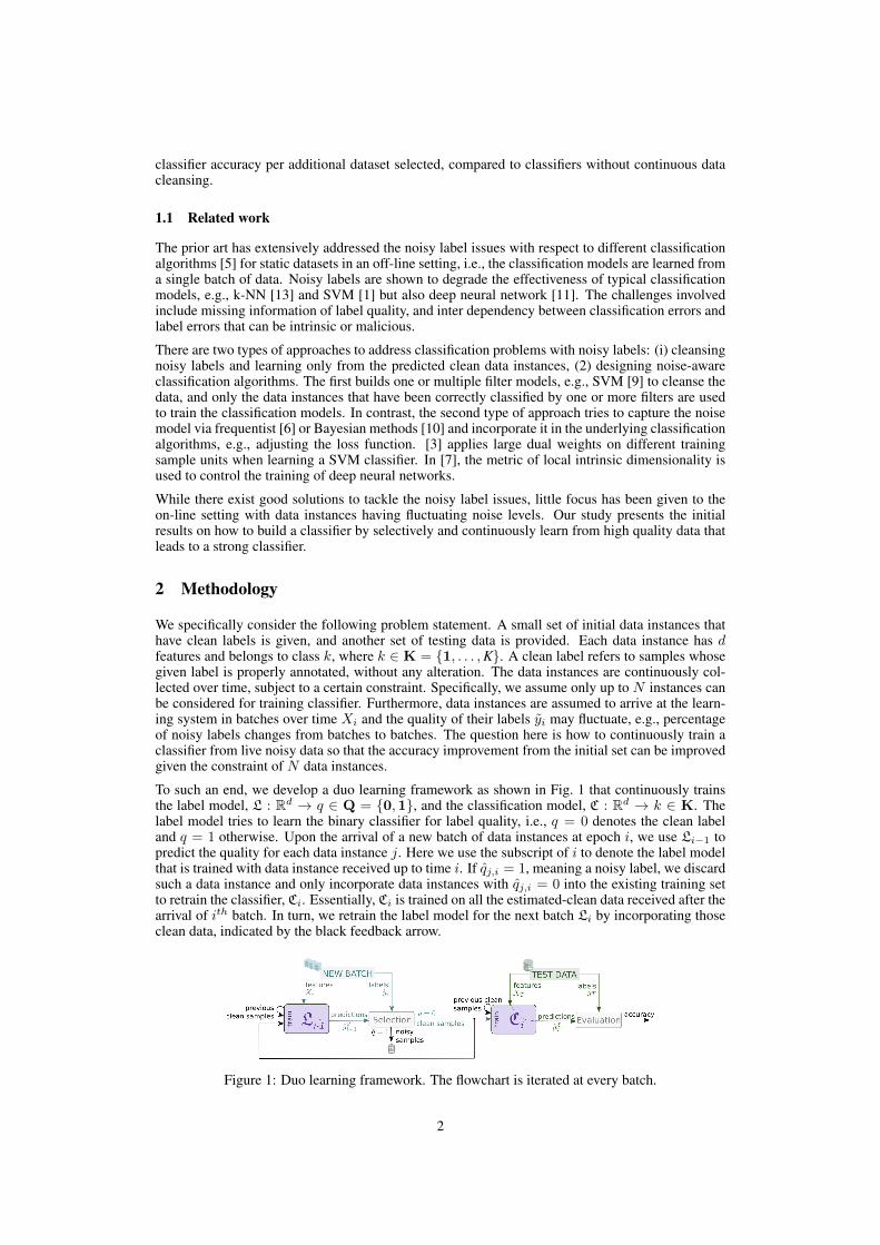
classifier accuracy per additional dataset selected, compared to classifiers without continuous datacleansing.

1.1 Related work

The prior art has extensively addressed the noisy label issues with respect to different classificationalgorithms [5] for static datasets in an off-line setting, i.e., the classification models are learned froma single batch of data. Noisy labels are shown to degrade the effectiveness of typical classificationmodels, e.g., k-NN [13] and SVM [1] but also deep neural network [11]. The challenges involvedinclude missing information of label quality, and inter dependency between classification errors andlabel errors that can be intrinsic or malicious.

There are two types of approaches to address classification problems with noisy labels: (i) cleansingnoisy labels and learning only from the predicted clean data instances, (2) designing noise-awareclassification algorithms. The first builds one or multiple filter models, e.g., SVM [9] to cleanse thedata, and only the data instances that have been correctly classified by one or more filters are usedto train the classification models. In contrast, the second type of approach tries to capture the noisemodel via frequentist [6] or Bayesian methods [10] and incorporate it in the underlying classificationalgorithms, e.g., adjusting the loss function. [3] applies large dual weights on different trainingsample units when learning a SVM classifier. In [7], the metric of local intrinsic dimensionality isused to control the training of deep neural networks.

While there exist good solutions to tackle the noisy label issues, little focus has been given to theon-line setting with data instances having fluctuating noise levels. Our study presents the initialresults on how to build a classifier by selectively and continuously learn from high quality data thatleads to a strong classifier.

2 Methodology

We specifically consider the following problem statement. A small set of initial data instances thathave clean labels is given, and another set of testing data is provided. Each data instance has dfeatures and belongs to class k, where k ∈ K = {1, . . . ,K}. A clean label refers to samples whosegiven label is properly annotated, without any alteration. The data instances are continuously col-lected over time, subject to a certain constraint. Specifically, we assume only up to N instances canbe considered for training classifier. Furthermore, data instances are assumed to arrive at the learn-ing system in batches over time Xi and the quality of their labels yi may fluctuate, e.g., percentageof noisy labels changes from batches to batches. The question here is how to continuously train aclassifier from live noisy data so that the accuracy improvement from the initial set can be improvedgiven the constraint of N data instances.

To such an end, we develop a duo learning framework as shown in Fig. 1 that continuously trainsthe label model, L : Rd → q ∈ Q = {0,1}, and the classification model, C : Rd → k ∈ K. Thelabel model tries to learn the binary classifier for label quality, i.e., q = 0 denotes the clean labeland q = 1 otherwise. Upon the arrival of a new batch of data instances at epoch i, we use Li−1 topredict the quality for each data instance j. Here we use the subscript of i to denote the label modelthat is trained with data instance received up to time i. If qj,i = 1, meaning a noisy label, we discardsuch a data instance and only incorporate data instances with qj,i = 0 into the existing training setto retrain the classifier, Ci. Essentially, Ci is trained on all the estimated-clean data received after thearrival of ith batch. In turn, we retrain the label model for the next batch Li by incorporating thoseclean data, indicated by the black feedback arrow.

Figure 1: Duo learning framework. The flowchart is iterated at every batch.

2

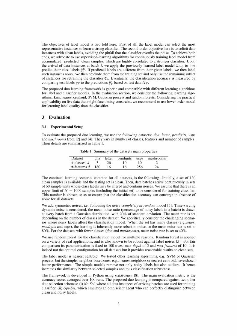
The objectives of label model is two fold here. First of all, the label model can select the mostrepresentative instances to learn a strong classifier. The second-order objective here is to solicit datainstances with clean labels, avoiding the pitfall that the classifier overfits the noise. To achieve bothends, we advocate to use supervised-learning algorithms for continuously training label model fromaccumulated ”predicted” clean samples, which are highly correlated to a stronger classifier. Uponthe arrival of data instances at batch i, we apply the previously learned label model Li−1 to firstpredict their class labels yLi . If predicted labels are different from their given labels, we then labelsuch instances noisy. We then preclude them from the training set and only use the remaining subsetof instances for retraining the classifier Ci. Eventually, the classification accuracy is measured bycomparing test labels yT to the predictions ycT based on test data XT .

The proposed duo learning framework is generic and compatible with different learning algorithmsfor label and classifier models. In the evaluation section, we consider the following learning algo-rithms: knn, nearest centroid, SVM, Gaussian process and random forests. Considering the practicalapplicability on live data that might face timing constraint, we recommend to use lower order modelfor learning label quality than the classifier.

3 Evaluation

3.1 Experimental Setup

To evaluate the proposed duo learning, we use the following datasets: dna, letter, pendigits, uspsand mushrooms from [2] and [4]. They vary in number of classes, features and number of samples.Their details are summarized in Table 1.

Table 1: Summary of the datasets main properties

Dataset dna letter pendigits usps mushrooms#-classes k 3 26 10 10 2#-features d 180 16 16 256 24

The continual learning scenario, common for all datasets, is the following. Initially, a set of 150clean samples is available and the testing set is clean. Then, data batches arrive continuously in setsof 50 sample units whose class labels may be altered and contains noises. We assume that there is anupper limit of N = 1000 samples (including the initial set) to be considered for training classifier.This number is chosen so as to ensure that the classification accuracy can converge in absence ofnoise for all datasets.

We add symmetric noises, i.e. following the noise completely at random model [5]. Time-varyingdynamic noise is considered, the mean noise ratio (percentage of noisy labels in a batch) is drawnat every batch from a Gaussian distribution, with 20% of standard deviation. The mean rate is setdepending on the number of classes in the dataset. We specifically consider the challenging scenar-ios where noisy labels affect the classification model. When the set has many classes (e.g.,letter,pendigits and usps), the learning is inherently more robust to noise, so the mean noise rate is set to80%. For the datasets with fewer classes (dna and mushrooms), mean noise rate is set to 40%.

We use random forest for the classification model for multiple reasons. Random forest is appliedon a variety of real applications, and is also known to be robust against label noises [5]. For faircomparison its parametrization is fixed to 100 trees, max-depth of 5 and max-features of 10. It isindeed not the optimal configuration for all datasets but it provides reasonable results on clean sets.

The label model is nearest centroid. We tested other learning algorithms, e.g. SVM or Gaussianprocess, but the simpler neighbor-based ones, e.g., nearest neighbors or nearest centroid, have shownbetter performance. The simple models remove not only noisy labels but also outliers. It henceincreases the similarity between selected samples and thus classification robustness.

The framework is developed in Python using scikit-learn [8]. The main evaluation metric is theaccuracy score, averaged over 100 runs. The proposed duo learning is compared against two otherdata selection schemes: (i) No-Sel, where all data instances of arriving batches are used for trainingclassifier, (ii) Opt-Sel, which emulates an omniscient agent who can perfectly distinguish betweenclean and noisy labels.

3

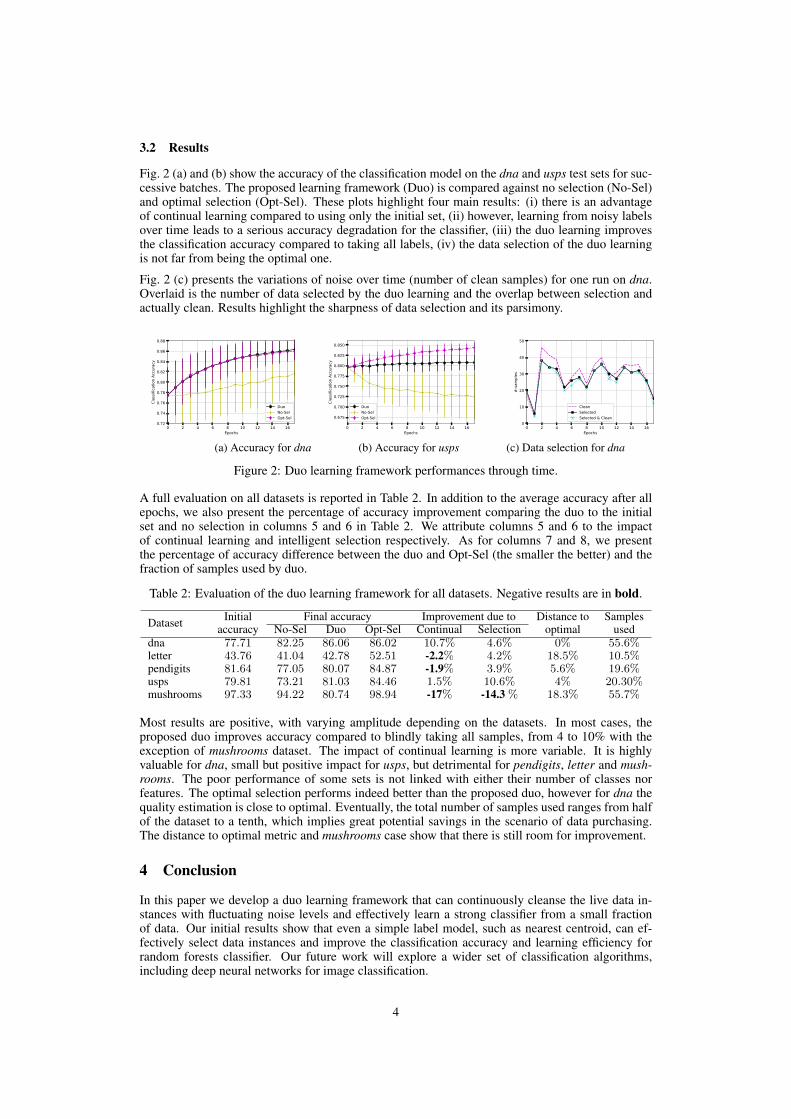
3.2 Results

Fig. 2 (a) and (b) show the accuracy of the classification model on the dna and usps test sets for suc-cessive batches. The proposed learning framework (Duo) is compared against no selection (No-Sel)and optimal selection (Opt-Sel). These plots highlight four main results: (i) there is an advantageof continual learning compared to using only the initial set, (ii) however, learning from noisy labelsover time leads to a serious accuracy degradation for the classifier, (iii) the duo learning improvesthe classification accuracy compared to taking all labels, (iv) the data selection of the duo learningis not far from being the optimal one.

Fig. 2 (c) presents the variations of noise over time (number of clean samples) for one run on dna.Overlaid is the number of data selected by the duo learning and the overlap between selection andactually clean. Results highlight the sharpness of data selection and its parsimony.

0 2 4 6 8 10 12 14 16Epochs

0.72

0.74

0.76

0.78

0.80

0.82

0.84

0.86

0.88

Classif

icatio

n Ac

curacy

DuoNo-SelOpt-Sel

0 2 4 6 8 10 12 14 16Epochs

0.675

0.700

0.725

0.750

0.775

0.800

0.825

0.850

Classifica

tion Ac

curacy

DuoNo-SelOpt-Sel

0 2 4 6 8 10 12 14 16Epochs

0

10

20

30

40

50

#-samples

CleanSelectedSelected & Clean

(a) Accuracy for dna (b) Accuracy for usps (c) Data selection for dna

Figure 2: Duo learning framework performances through time.

A full evaluation on all datasets is reported in Table 2. In addition to the average accuracy after allepochs, we also present the percentage of accuracy improvement comparing the duo to the initialset and no selection in columns 5 and 6 in Table 2. We attribute columns 5 and 6 to the impactof continual learning and intelligent selection respectively. As for columns 7 and 8, we presentthe percentage of accuracy difference between the duo and Opt-Sel (the smaller the better) and thefraction of samples used by duo.

Table 2: Evaluation of the duo learning framework for all datasets. Negative results are in bold.

Dataset Initialaccuracy

Final accuracy Improvement due to Distance tooptimal

SamplesusedNo-Sel Duo Opt-Sel Continual Selection

dna 77.71 82.25 86.06 86.02 10.7% 4.6% 0% 55.6%letter 43.76 41.04 42.78 52.51 -2.2% 4.2% 18.5% 10.5%pendigits 81.64 77.05 80.07 84.87 -1.9% 3.9% 5.6% 19.6%usps 79.81 73.21 81.03 84.46 1.5% 10.6% 4% 20.30%mushrooms 97.33 94.22 80.74 98.94 -17% -14.3 % 18.3% 55.7%

Most results are positive, with varying amplitude depending on the datasets. In most cases, theproposed duo improves accuracy compared to blindly taking all samples, from 4 to 10% with theexception of mushrooms dataset. The impact of continual learning is more variable. It is highlyvaluable for dna, small but positive impact for usps, but detrimental for pendigits, letter and mush-rooms. The poor performance of some sets is not linked with either their number of classes norfeatures. The optimal selection performs indeed better than the proposed duo, however for dna thequality estimation is close to optimal. Eventually, the total number of samples used ranges from halfof the dataset to a tenth, which implies great potential savings in the scenario of data purchasing.The distance to optimal metric and mushrooms case show that there is still room for improvement.

4 Conclusion

In this paper we develop a duo learning framework that can continuously cleanse the live data in-stances with fluctuating noise levels and effectively learn a strong classifier from a small fractionof data. Our initial results show that even a simple label model, such as nearest centroid, can ef-fectively select data instances and improve the classification accuracy and learning efficiency forrandom forests classifier. Our future work will explore a wider set of classification algorithms,including deep neural networks for image classification.

4

References[1] Wenjuan An and Mangui Liang. Fuzzy support vector machine based on within-class scatter

for classification problems with outliers or noises. Neurocomput., 110:101–110, June 2013.ISSN 0925-2312.

[2] Chih-Chung Chang and Chih-Jen Lin. Libsvm: A library for support vector machines.ACM Trans. Intell. Syst. Technol., 2(3):27:1–27:27, May 2011. ISSN 2157-6904. doi:10.1145/1961189.1961199. URL http://doi.acm.org/10.1145/1961189.1961199.

[3] Ofer Dekel and Ohad Shamir. Good learners for evil teachers. In Proceedings of the 26th An-nual International Conference on Machine Learning, ICML 2009, Montreal, Quebec, Canada,June 14-18, 2009, pages 233–240, 2009.

[4] Ayhan Demiriz (demira@rpi. edu, Kristin P Bennett, John Shawe, and Taylor jst@cs. rhul. ac.uk. Linear programming boosting via column generation. (bennek@rpi.edu).

[5] Benoıt Frenay and Michel Verleysen. Classification in the presence of label noise: A survey.IEEE Trans. Neural Netw. Learning Syst., 25(5):845–869, 2014.

[6] Yunlei Li, Lodewyk F. A. Wessels, Dick de Ridder, and Marcel J. T. Reinders. Classificationin the presence of class noise using a probabilistic kernel fisher method. Pattern Recognition,40(12):3349–3357, 2007.

[7] Xingjun Ma, Yisen Wang, Michael E. Houle, Shuo Zhou, Sarah M. Erfani, Shu-Tao Xia, Su-danthi N. R. Wijewickrema, and James Bailey. Dimensionality-driven learning with noisylabels. In ICML 2018, pages 3361–3370.

[8] F. Pedregosa, G. Varoquaux, A. Gramfort, V. Michel, B. Thirion, O. Grisel, M. Blondel, P. Pret-tenhofer, R. Weiss, V. Dubourg, J. Vanderplas, A. Passos, D. Cournapeau, M. Brucher, M. Per-rot, and E. Duchesnay. Scikit-learn: Machine learning in Python. Journal of Machine LearningResearch, 12:2825–2830, 2011.

[9] Nicola Segata, Enrico Blanzieri, Sarah Jane Delany, and Padraig Cunningham. Noise reductionfor instance-based learning with a local maximal margin approach. J. Intell. Inf. Syst., 35(2):301–331, 2010.

[10] James D. Stamey and Richard Gerlach. Bayesian model selection for logistic regression withclassified outcomes. Statist. Model, 7(3):255–273, 2007.

[11] Arash Vahdat. Toward robustness against label noise in training deep discriminative neuralnetworks. In NIPS, pages 5601–5610, 2017.

[12] Yisen Wang, Weiyang Liu, Xingjun Ma, James Bailey, Hongyuan Zha, Le Song, and Shu-TaoXia. Iterative learning with open-set noisy labels. In CVPR 2018.

[13] D. Randall Wilson and Tony R. Martinez. Reduction techniques for instance-basedlearningalgorithms. Mach. Learn., 38(3):257–286, March 2000.

5

Appendix B

Robust Anomaly Detection on UnreliableData

The following paper has been accepted for publication in the 49th IEEE/IFIP International Conferenceon Dependable Systems and Networks (DSN 2019) as a practical experience report [187].

181

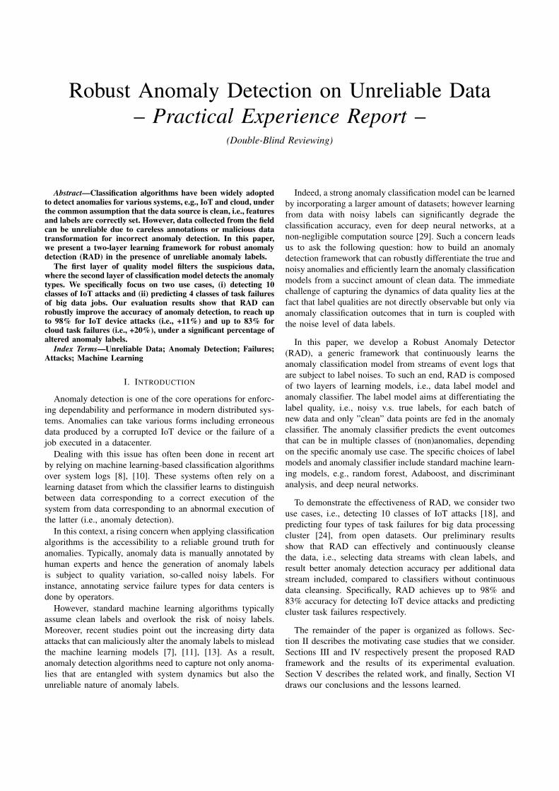
Robust Anomaly Detection on Unreliable Data– Practical Experience Report –

(Double-Blind Reviewing)

Abstract—Classification algorithms have been widely adoptedto detect anomalies for various systems, e.g., IoT and cloud, underthe common assumption that the data source is clean, i.e., featuresand labels are correctly set. However, data collected from the fieldcan be unreliable due to careless annotations or malicious datatransformation for incorrect anomaly detection. In this paper,we present a two-layer learning framework for robust anomalydetection (RAD) in the presence of unreliable anomaly labels.

The first layer of quality model filters the suspicious data,where the second layer of classification model detects the anomalytypes. We specifically focus on two use cases, (i) detecting 10classes of IoT attacks and (ii) predicting 4 classes of task failuresof big data jobs. Our evaluation results show that RAD canrobustly improve the accuracy of anomaly detection, to reach upto 98% for IoT device attacks (i.e., +11%) and up to 83% forcloud task failures (i.e., +20%), under a significant percentage ofaltered anomaly labels.

Index Terms—Unreliable Data; Anomaly Detection; Failures;Attacks; Machine Learning

I. INTRODUCTION

Anomaly detection is one of the core operations for enforc-ing dependability and performance in modern distributed sys-tems. Anomalies can take various forms including erroneousdata produced by a corrupted IoT device or the failure of ajob executed in a datacenter.

Dealing with this issue has often been done in recent artby relying on machine learning-based classification algorithmsover system logs [8], [10]. These systems often rely on alearning dataset from which the classifier learns to distinguishbetween data corresponding to a correct execution of thesystem from data corresponding to an abnormal execution ofthe latter (i.e., anomaly detection).

In this context, a rising concern when applying classificationalgorithms is the accessibility to a reliable ground truth foranomalies. Typically, anomaly data is manually annotated byhuman experts and hence the generation of anomaly labelsis subject to quality variation, so-called noisy labels. Forinstance, annotating service failure types for data centers isdone by operators.

However, standard machine learning algorithms typicallyassume clean labels and overlook the risk of noisy labels.Moreover, recent studies point out the increasing dirty dataattacks that can maliciously alter the anomaly labels to misleadthe machine learning models [7], [11], [13]. As a result,anomaly detection algorithms need to capture not only anoma-lies that are entangled with system dynamics but also theunreliable nature of anomaly labels.

Indeed, a strong anomaly classification model can be learnedby incorporating a larger amount of datasets; however learningfrom data with noisy labels can significantly degrade theclassification accuracy, even for deep neural networks, at anon-negligible computation source [29]. Such a concern leadsus to ask the following question: how to build an anomalydetection framework that can robustly differentiate the true andnoisy anomalies and efficiently learn the anomaly classificationmodels from a succinct amount of clean data. The immediatechallenge of capturing the dynamics of data quality lies at thefact that label qualities are not directly observable but only viaanomaly classification outcomes that in turn is coupled withthe noise level of data labels.

In this paper, we develop a Robust Anomaly Detector(RAD), a generic framework that continuously learns theanomaly classification model from streams of event logs thatare subject to label noises. To such an end, RAD is composedof two layers of learning models, i.e., data label model andanomaly classifier. The label model aims at differentiating thelabel quality, i.e., noisy v.s. true labels, for each batch ofnew data and only ”clean” data points are fed in the anomalyclassifier. The anomaly classifier predicts the event outcomesthat can be in multiple classes of (non)anomalies, dependingon the specific anomaly use case. The specific choices of labelmodels and anomaly classifier include standard machine learn-ing models, e.g., random forest, Adaboost, and discriminantanalysis, and deep neural networks.

To demonstrate the effectiveness of RAD, we consider twouse cases, i.e., detecting 10 classes of IoT attacks [18], andpredicting four types of task failures for big data processingcluster [24], from open datasets. Our preliminary resultsshow that RAD can effectively and continuously cleansethe data, i.e., selecting data streams with clean labels, andresult better anomaly detection accuracy per additional datastream included, compared to classifiers without continuousdata cleansing. Specifically, RAD achieves up to 98% and83% accuracy for detecting IoT device attacks and predictingcluster task failures respectively.

The remainder of the paper is organized as follows. Sec-tion II describes the motivating case studies that we consider.Sections III and IV respectively present the proposed RADframework and the results of its experimental evaluation.Section V describes the related work, and finally, Section VIdraws our conclusions and the lessons learned.

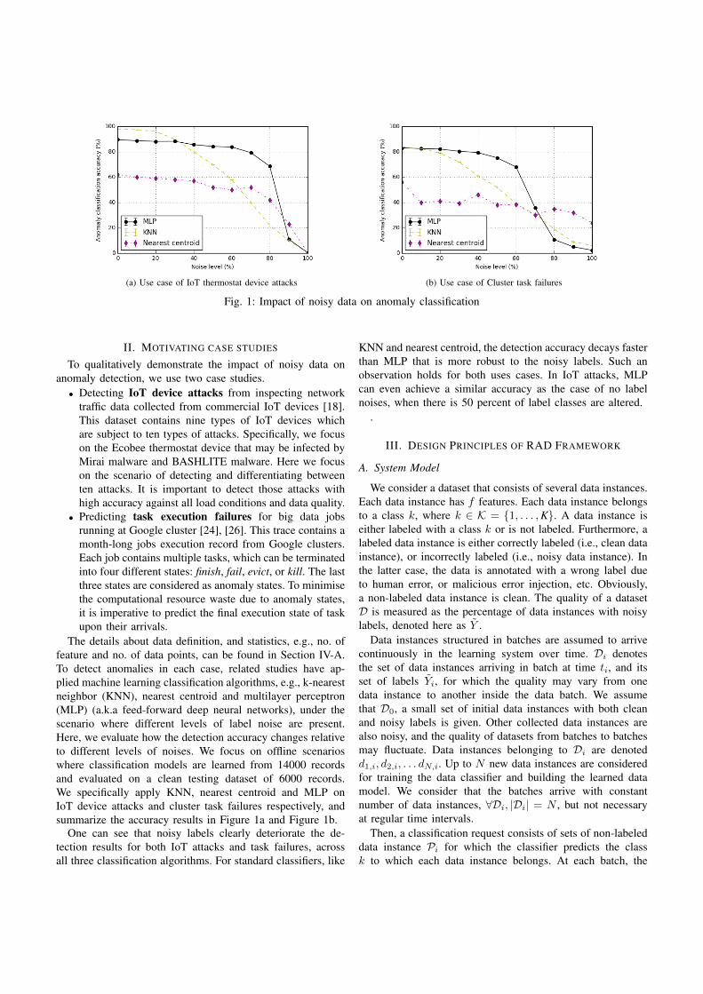
(a) Use case of IoT thermostat device attacks (b) Use case of Cluster task failures

Fig. 1: Impact of noisy data on anomaly classification

II. MOTIVATING CASE STUDIES

To qualitatively demonstrate the impact of noisy data onanomaly detection, we use two case studies.• Detecting IoT device attacks from inspecting network

traffic data collected from commercial IoT devices [18].This dataset contains nine types of IoT devices whichare subject to ten types of attacks. Specifically, we focuson the Ecobee thermostat device that may be infected byMirai malware and BASHLITE malware. Here we focuson the scenario of detecting and differentiating betweenten attacks. It is important to detect those attacks withhigh accuracy against all load conditions and data quality.

• Predicting task execution failures for big data jobsrunning at Google cluster [24], [26]. This trace contains amonth-long jobs execution record from Google clusters.Each job contains multiple tasks, which can be terminatedinto four different states: finish, fail, evict, or kill. The lastthree states are considered as anomaly states. To minimisethe computational resource waste due to anomaly states,it is imperative to predict the final execution state of taskupon their arrivals.

The details about data definition, and statistics, e.g., no. offeature and no. of data points, can be found in Section IV-A.To detect anomalies in each case, related studies have ap-plied machine learning classification algorithms, e.g., k-nearestneighbor (KNN), nearest centroid and multilayer perceptron(MLP) (a.k.a feed-forward deep neural networks), under thescenario where different levels of label noise are present.Here, we evaluate how the detection accuracy changes relativeto different levels of noises. We focus on offline scenarioswhere classification models are learned from 14000 recordsand evaluated on a clean testing dataset of 6000 records.We specifically apply KNN, nearest centroid and MLP onIoT device attacks and cluster task failures respectively, andsummarize the accuracy results in Figure 1a and Figure 1b.

One can see that noisy labels clearly deteriorate the de-tection results for both IoT attacks and task failures, acrossall three classification algorithms. For standard classifiers, like

KNN and nearest centroid, the detection accuracy decays fasterthan MLP that is more robust to the noisy labels. Such anobservation holds for both uses cases. In IoT attacks, MLPcan even achieve a similar accuracy as the case of no labelnoises, when there is 50 percent of label classes are altered.

.

III. DESIGN PRINCIPLES OF RAD FRAMEWORK

A. System Model

We consider a dataset that consists of several data instances.Each data instance has f features. Each data instance belongsto a class k, where k ∈ K = {1, . . . ,K}. A data instance iseither labeled with a class k or is not labeled. Furthermore, alabeled data instance is either correctly labeled (i.e., clean datainstance), or incorrectly labeled (i.e., noisy data instance). Inthe latter case, the data is annotated with a wrong label dueto human error, or malicious error injection, etc. Obviously,a non-labeled data instance is clean. The quality of a datasetD is measured as the percentage of data instances with noisylabels, denoted here as Y .

Data instances structured in batches are assumed to arrivecontinuously in the learning system over time. Di denotesthe set of data instances arriving in batch at time ti, and itsset of labels Yi, for which the quality may vary from onedata instance to another inside the data batch. We assumethat D0, a small set of initial data instances with both cleanand noisy labels is given. Other collected data instances arealso noisy, and the quality of datasets from batches to batchesmay fluctuate. Data instances belonging to Di are denotedd1,i, d2,i, . . . dN,i. Up to N new data instances are consideredfor training the data classifier and building the learned datamodel. We consider that the batches arrive with constantnumber of data instances, ∀Di, |Di| = N , but not necessaryat regular time intervals.

Then, a classification request consists of sets of non-labeleddata instance Pi for which the classifier predicts the classk to which each data instance belongs. At each batch, the

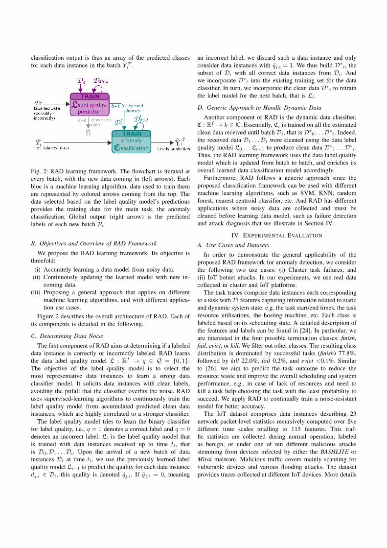
classification output is thus an array of the predicted classesfor each data instance in the batch Y Pi .

Fig. 2: RAD learning framework. The flowchart is iterated atevery batch, with the new data coming in (left arrows). Eachbloc is a machine learning algorithm, data used to train themare represented by colored arrows coming from the top. Thedata selected based on the label quality model’s predictionsprovides the training data for the main task, the anomalyclassification. Global output (right arrow) is the predictedlabels of each new batch Pi.

B. Objectives and Overview of RAD Framework

We propose the RAD learning framework. Its objective isthreefold:

(i) Accurately learning a data model from noisy data.(ii) Continuously updating the learned model with new in-

coming data.(iii) Proposing a general approach that applies on different

machine learning algorithms, and with different applica-tion use cases.

Figure 2 describes the overall architecture of RAD. Each ofits components is detailed in the following.

C. Determining Data Noise

The first component of RAD aims at determining if a labeleddata instance is correctly or incorrectly labeled. RAD learnsthe data label quality model L : Rf → q ∈ Q = {0, 1}.The objective of the label quality model is to select themost representative data instances to learn a strong dataclassifier model. It solicits data instances with clean labels,avoiding the pitfall that the classifier overfits the noise. RADuses supervised-learning algorithms to continuously train thelabel quality model from accumulated predicted clean datainstances, which are highly correlated to a stronger classifier.

The label quality model tries to learn the binary classifierfor label quality, i.e., q = 1 denotes a correct label and q = 0denotes an incorrect label. Li is the label quality model thatis trained with data instances received up to time ti, thatis D0,D1 . . .Di. Upon the arrival of a new batch of datainstances Di at time ti, we use the previously learned labelquality model Li−1 to predict the quality for each data instancedj,i ∈ Di, this quality is denoted qj,i. If qj,i = 0, meaning

an incorrect label, we discard such a data instance and onlyconsider data instances with qj,i = 1. We thus build D∗i, thesubset of Di with all correct data instances from Di. Andwe incorporate D∗i into the existing training set for the dataclassifier. In turn, we incorporate the clean data D∗i to retrainthe label model for the next batch, that is Li.

D. Generic Approach to Handle Dynamic Data

Another component of RAD is the dynamic data classifier,C : Rf → k ∈ K. Essentially, Ci is trained on all the estimatedclean data received until batch Di, that is D∗0 . . .D∗i. Indeed,the received data D1 . . .Di were cleaned using the data labelquality model L0 . . .Li−1 to produce clean data D∗1 . . .D∗i.Thus, the RAD learning framework uses the data label qualitymodel which is updated from batch to batch, and enriches itsoverall learned data classification model accordingly.

Furthermore, RAD follows a generic approach since theproposed classification framework can be used with differentmachine learning algorithms, such as SVM, KNN, randomforest, nearest centroid classifier, etc. And RAD has differentapplications where noisy data are collected and must becleaned before learning data model, such as failure detectionand attack diagnosis that we illustrate in Section IV.

IV. EXPERIMENTAL EVALUATION

A. Use Cases and Datasets

In order to demonstrate the general applicability of theproposed RAD framework for anomaly detection, we considerthe following two use cases: (i) Cluster task failures, and(ii) IoT botnet attacks. In our experiments, we use real datacollected in cluster and IoT platforms.

The task traces comprise data instances each correspondingto a task with 27 features capturing information related to staticand dynamic system state, e.g. the task start/end times, the taskresource utilisations, the hosting machine, etc. Each class islabeled based on its scheduling state. A detailed description ofthe features and labels can be found in [24]. In particular, weare interested in the four possible termination classes: finish,fail, evict, or kill. We filter out other classes. The resulting classdistribution is dominated by successful tasks (finish) 77.8%,followed by kill 22.0%, fail 0.2%, and evict <0.1%. Similarto [26], we aim to predict the task outcome to reduce theresource waste and improve the overall scheduling and systemperformance, e.g., in case of lack of resources and need tokill a task help choosing the task with the least probability tosucceed. We apply RAD to continually train a noise-resistantmodel for better accuracy.

The IoT dataset comprises data instances describing 23network packet-level statistics recursively computed over fivedifferent time scales totalling to 115 features. This traf-fic statistics are collected during normal operation, labeledas benign, or under one of ten different malicious attacksstemming from devices infected by either the BASHLITE orMirai malware. Malicious traffic covers mainly scanning forvulnerable devices and various flooding attacks. The datasetprovides traces collected at different IoT devices. More details

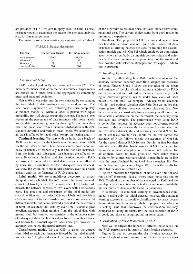
are provided in [18]. We aim to apply RAD to build a noise-resistant model to categorize the attacks for post fact analysis,e.g., for threat assessment.

The main dataset characteristics are summarized in Table I.

TABLE I: Dataset description

Use case Cluster task failures IoT device attacks

#data instances 57,000 33,000#classes K 4 11#features f 27 115data batch size 600 300

B. Experimental Setup

RAD is developed in Python using scikit-learn [21]. Themain performance evaluation metric is accuracy. Experimentsare carried out 5 times, results are aggregated by computingmean and standard deviation.

Noise. We inject noise into the two datasets by exchangingthe true label of data instances with a random one. Thelabel noise is symmetric, i.e., following the noise completelyat random model [9] where a label is picked with equalprobability from all classes except the true one. The noise levelrepresents the percentage of data instances with noisy labels.We emulate time-varying noise by drawing for each new databatch the noise level from a Gaussian distribution with 20%standard deviation and various mean levels. We assume thatall data is affected by label noise, except the testing data.

Continual learning. We start with an initial data batch of3000 data instances for the Cluster task failures dataset, 6000for the IoT devices one. Then, data instances arrive continu-ously in batches of respectively 600 and 300 data instances.Both the initial and subsequent data batches are affected bynoise. To kick-start the label and classification models in RADwe assume to know which initial data instances are affectedby noise (no assumptions for the subsequent data batches).We show the evolution of the model accuracy over data batcharrivals until the performance of RAD converges.

Label model. We use a multilayer perceptron to assessthe quality of each label. For IoT dataset, the neural networkconsists of two layers with 28 neurons each. For Cluster taskdataset, the network consists of two layers with 110 neuronseach. The precision and robustness of the label model arecritical to filter out the noisy/malicious labels and provide aclean training set to the classification model. We considereddifferent models, but neural networks provided the best resultsin terms of accuracy and stability over time. Adaboost gaveexcellent accuracy when training from the initial data withground truth, but resulted too sensitive to the unknown noiseof subsequent data batches. Random forest is another choiceand known to be robust against label noise [9], however itsaccuracy was below the neural network one.

Classification model. We use KNN to assign the correctclass label to each data instance filtered by the label model.We set k to 5. Higher values of k can increase the resilience

of the algorithm to residual noise, but also induce extra com-putational cost. The current choice stems from good results inpreliminary experiments.

Baselines. The proposed RAD is compared against twobaseline data selection schemes: (i) No-Sel, where all datainstances of arriving batches are used for training the classifi-cation model; and, (ii) Opt-Sel which emulates an omniscientagent who can perfectly distinguish between clean and noisylabels. The two baselines are representative of the worst andbest possible data selection strategies and we expect RAD tofall in between.

C. Handling Dynamic Data

We start by illustrating how RAD enables to increase theanomaly detection accuracy over time, despite the presenceof noise. Figures 3 and 4 show the evolution of the meanand variance of the classification accuracy achieved by RADon the thermostat and task failure datasets, respectively. Eachfigure moreover presents results under two levels of labelnoise: 30% and 40%. We compare RAD against no selection(No-Sel) and optimal selection (Opt-Sel). One can notice thatlearning from all data instances without cleansing (i.e., No-Sel curves) gives consistently lower accuracy in all cases. Forthe attacks classification on the thermostat, the accuracy evenoscillates and diverges. The performance when using RADis better. First because the accuracy does not diverge, secondbecause it always consistently increase until it saturates. Forthe IoT attack dataset, the end accuracy is around 98%, forthe cluster tasks around 83%. While for the first dataset theaccuracy of RAD follows closely the accuracy of Opt-Sel,for the second dataset RAD follows Opt-Sel at first but thensaturates after 40 data batch arrivals. RAD is efficient forvarious classification applications, however not optimal forall of them. Note that RAD gives also more stable resultsas shown by shorter errorbars which in magnitude are in linewith the ones obtained by an ideal data cleansing. For No-Sel the bars are significantly larger. We discuss the results forother IoT devices in Section IV-F.

Figure 5 presents the variations of noise over time for onerun on IoT thermostat dataset where mean noise rate sets to30%. Overlaid is the number of data selected by RAD and theoverlap between selection and actually clean. Results highlightthe sharpness of data selection and its parsimony.

In summary: (i) continual learning is advantageous com-pared to using only the initial dataset; however, (ii) continuallearning exposes us to possible classification accuracy degra-dation stemming from noisy labels if proper data selectionis lacking, (iii) RAD improves the classification accuracycompared to taking all labels, (iv) the data selection of RADis good, and close to being optimal in some cases.

D. Evaluation of Noise Robustness of RAD

Next we investigate the impact of different noise levels onthe RAD performance in terms of classification accuracy.

Figures 6a and 6b present the classification accuracy forvarious levels of noise, ranging from 0% (all data are clean)

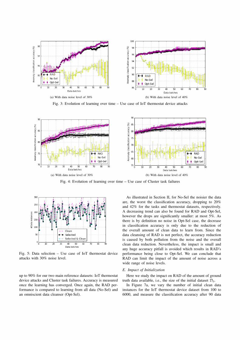
(a) With data noise level of 30% (b) With data noise level of 40%

Fig. 3: Evolution of learning over time – Use case of IoT thermostat device attacks

(a) With data noise level of 30% (b) With data noise level of 40%

Fig. 4: Evolution of learning over time – Use case of Cluster task failures

Fig. 5: Data selection – Use case of IoT thermostat deviceattacks with 30% noise level.

up to 90% for our two main reference datasets: IoT thermostatdevice attacks and Cluster task failures. Accuracy is measuredonce the learning has converged. Once again, the RAD per-formance is compared to learning from all data (No-Sel) andan omniscient data cleanser (Opt-Sel).

As illustrated in Section II, for No-Sel the noisier the dataare, the worst the classification accuracy, dropping to 20%and 42% for the tasks and thermostat datasets, respectively.A decreasing trend can also be found for RAD and Opt-Sel,however the drops are significantly smaller: at most 5%. Asthere is by definition no noise in Opt-Sel case, the decreasein classification accuracy is only due to the reduction ofthe overall amount of clean data to learn from. Since thedata cleansing of RAD is not perfect, the accuracy reductionis caused by both pollution from the noise and the overallclean data reduction. Nevertheless, the impact is small andany huge accuracy pitfall is avoided which results in RAD’sperformance being close to Opt-Sel. We can conclude thatRAD can limit the impact of the amount of noise across awide range of noise levels.

E. Impact of InitializationHere we study the impact on RAD of the amount of ground

truth data available, i.e., the size of the initial dataset D0.In Figure 7a, we vary the number of initial clean data

instances for the IoT thermostat device dataset from 100 to6000, and measure the classification accuracy after 90 data

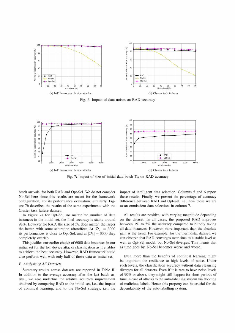
(a) IoT thermostat device attacks (b) Cluster task failures

Fig. 6: Impact of data noises on RAD accuracy

(a) IoT thermostat device attacks (b) Cluster task failures

Fig. 7: Impact of size of initial data batch D0 on RAD accuracy

batch arrivals, for both RAD and Opt-Sel. We do not considerNo-Sel here since this results are meant for the frameworkconfiguration, not its performance evaluation. Similarly, Fig-ure 7b describes the results of the same experiments with theCluster task failure dataset.

In Figure 7a for Opt-Sel, no matter the number of datainstances in the initial set, the final accuracy is stable around98%. However for RAD, the size of D0 does matter: the largerthe better, with some saturation aftereffect. At |D0| = 3000its performances is close to Opt-Sel, and at |D0| = 6000 theycompletely overlap.

This justifies our earlier choice of 6000 data instances in ourinitial set for the IoT device attacks classification as it enablesto achieve the best accuracy. However, RAD framework couldalso perform well with only half of those data as initial set.

F. Analysis of All Datasets

Summary results across datasets are reported in Table II.In addition to the average accuracy after the last batch ar-rival, we also underline the relative accuracy improvementobtained by comparing RAD to the initial set, i.e., the impactof continual learning, and to the No-Sel strategy, i.e., the

impact of intelligent data selection. Columns 5 and 6 reportthese results. Finally, we present the percentage of accuracydifference between RAD and Opt-Sel, i.e., how close we areto an omniscient data selection, in column 7.

All results are positive, with varying magnitude dependingon the dataset. In all cases, the proposed RAD improvesbetween 1% to 5% the accuracy compared to blindly takingall data instances. However, more important than the absolutegain is the trend. For example, for the thermostat dataset, wecan observe that RAD converges over time to a stable level aswell as Opt-Sel model, but No-Sel diverges. This means thatas time goes by, No-Sel becomes worse and worse.

Even more than the benefits of continual learning mightbe important the resilience to high levels of noise. Undersuch levels, the classification accuracy without data cleansingdiverges for all datasets. Even if it is rare to have noise levelsof 90% or above, they might still happen for short periods oftime in case of attacks to the auto-labelling system via floodingof malicious labels. Hence this property can be crucial for thedependability of the auto-labelling system.

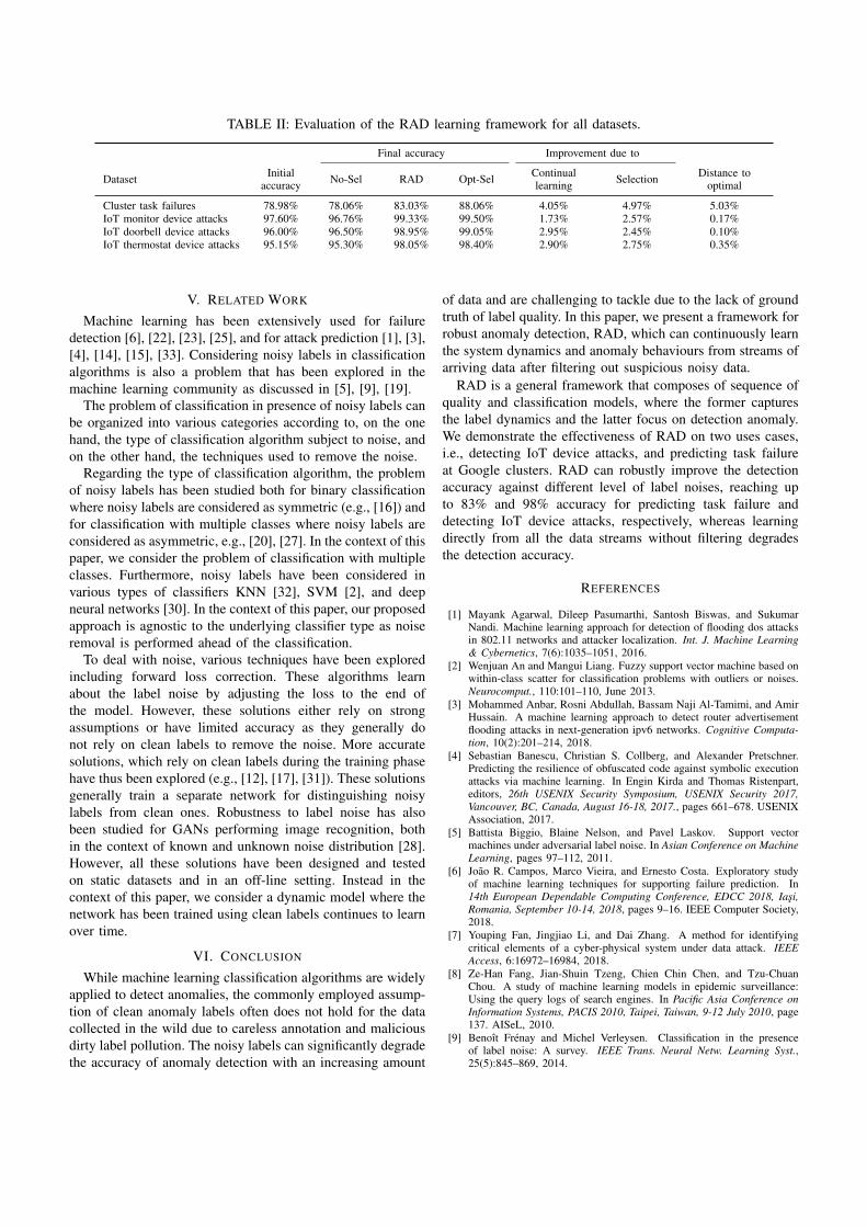
TABLE II: Evaluation of the RAD learning framework for all datasets.

Final accuracy Improvement due to

Dataset Initialaccuracy No-Sel RAD Opt-Sel Continual

learning Selection Distance tooptimal

Cluster task failures 78.98% 78.06% 83.03% 88.06% 4.05% 4.97% 5.03%IoT monitor device attacks 97.60% 96.76% 99.33% 99.50% 1.73% 2.57% 0.17%IoT doorbell device attacks 96.00% 96.50% 98.95% 99.05% 2.95% 2.45% 0.10%IoT thermostat device attacks 95.15% 95.30% 98.05% 98.40% 2.90% 2.75% 0.35%

V. RELATED WORK

Machine learning has been extensively used for failuredetection [6], [22], [23], [25], and for attack prediction [1], [3],[4], [14], [15], [33]. Considering noisy labels in classificationalgorithms is also a problem that has been explored in themachine learning community as discussed in [5], [9], [19].

The problem of classification in presence of noisy labels canbe organized into various categories according to, on the onehand, the type of classification algorithm subject to noise, andon the other hand, the techniques used to remove the noise.

Regarding the type of classification algorithm, the problemof noisy labels has been studied both for binary classificationwhere noisy labels are considered as symmetric (e.g., [16]) andfor classification with multiple classes where noisy labels areconsidered as asymmetric, e.g., [20], [27]. In the context of thispaper, we consider the problem of classification with multipleclasses. Furthermore, noisy labels have been considered invarious types of classifiers KNN [32], SVM [2], and deepneural networks [30]. In the context of this paper, our proposedapproach is agnostic to the underlying classifier type as noiseremoval is performed ahead of the classification.

To deal with noise, various techniques have been exploredincluding forward loss correction. These algorithms learnabout the label noise by adjusting the loss to the end ofthe model. However, these solutions either rely on strongassumptions or have limited accuracy as they generally donot rely on clean labels to remove the noise. More accuratesolutions, which rely on clean labels during the training phasehave thus been explored (e.g., [12], [17], [31]). These solutionsgenerally train a separate network for distinguishing noisylabels from clean ones. Robustness to label noise has alsobeen studied for GANs performing image recognition, bothin the context of known and unknown noise distribution [28].However, all these solutions have been designed and testedon static datasets and in an off-line setting. Instead in thecontext of this paper, we consider a dynamic model where thenetwork has been trained using clean labels continues to learnover time.

VI. CONCLUSION

While machine learning classification algorithms are widelyapplied to detect anomalies, the commonly employed assump-tion of clean anomaly labels often does not hold for the datacollected in the wild due to careless annotation and maliciousdirty label pollution. The noisy labels can significantly degradethe accuracy of anomaly detection with an increasing amount

of data and are challenging to tackle due to the lack of groundtruth of label quality. In this paper, we present a framework forrobust anomaly detection, RAD, which can continuously learnthe system dynamics and anomaly behaviours from streams ofarriving data after filtering out suspicious noisy data.

RAD is a general framework that composes of sequence ofquality and classification models, where the former capturesthe label dynamics and the latter focus on detection anomaly.We demonstrate the effectiveness of RAD on two uses cases,i.e., detecting IoT device attacks, and predicting task failureat Google clusters. RAD can robustly improve the detectionaccuracy against different level of label noises, reaching upto 83% and 98% accuracy for predicting task failure anddetecting IoT device attacks, respectively, whereas learningdirectly from all the data streams without filtering degradesthe detection accuracy.

REFERENCES

[1] Mayank Agarwal, Dileep Pasumarthi, Santosh Biswas, and SukumarNandi. Machine learning approach for detection of flooding dos attacksin 802.11 networks and attacker localization. Int. J. Machine Learning& Cybernetics, 7(6):1035–1051, 2016.

[2] Wenjuan An and Mangui Liang. Fuzzy support vector machine based onwithin-class scatter for classification problems with outliers or noises.Neurocomput., 110:101–110, June 2013.

[3] Mohammed Anbar, Rosni Abdullah, Bassam Naji Al-Tamimi, and AmirHussain. A machine learning approach to detect router advertisementflooding attacks in next-generation ipv6 networks. Cognitive Computa-tion, 10(2):201–214, 2018.

[4] Sebastian Banescu, Christian S. Collberg, and Alexander Pretschner.Predicting the resilience of obfuscated code against symbolic executionattacks via machine learning. In Engin Kirda and Thomas Ristenpart,editors, 26th USENIX Security Symposium, USENIX Security 2017,Vancouver, BC, Canada, August 16-18, 2017., pages 661–678. USENIXAssociation, 2017.

[5] Battista Biggio, Blaine Nelson, and Pavel Laskov. Support vectormachines under adversarial label noise. In Asian Conference on MachineLearning, pages 97–112, 2011.

[6] Joao R. Campos, Marco Vieira, and Ernesto Costa. Exploratory studyof machine learning techniques for supporting failure prediction. In14th European Dependable Computing Conference, EDCC 2018, Iasi,Romania, September 10-14, 2018, pages 9–16. IEEE Computer Society,2018.

[7] Youping Fan, Jingjiao Li, and Dai Zhang. A method for identifyingcritical elements of a cyber-physical system under data attack. IEEEAccess, 6:16972–16984, 2018.

[8] Ze-Han Fang, Jian-Shuin Tzeng, Chien Chin Chen, and Tzu-ChuanChou. A study of machine learning models in epidemic surveillance:Using the query logs of search engines. In Pacific Asia Conference onInformation Systems, PACIS 2010, Taipei, Taiwan, 9-12 July 2010, page137. AISeL, 2010.

[9] Benoıt Frenay and Michel Verleysen. Classification in the presenceof label noise: A survey. IEEE Trans. Neural Netw. Learning Syst.,25(5):845–869, 2014.

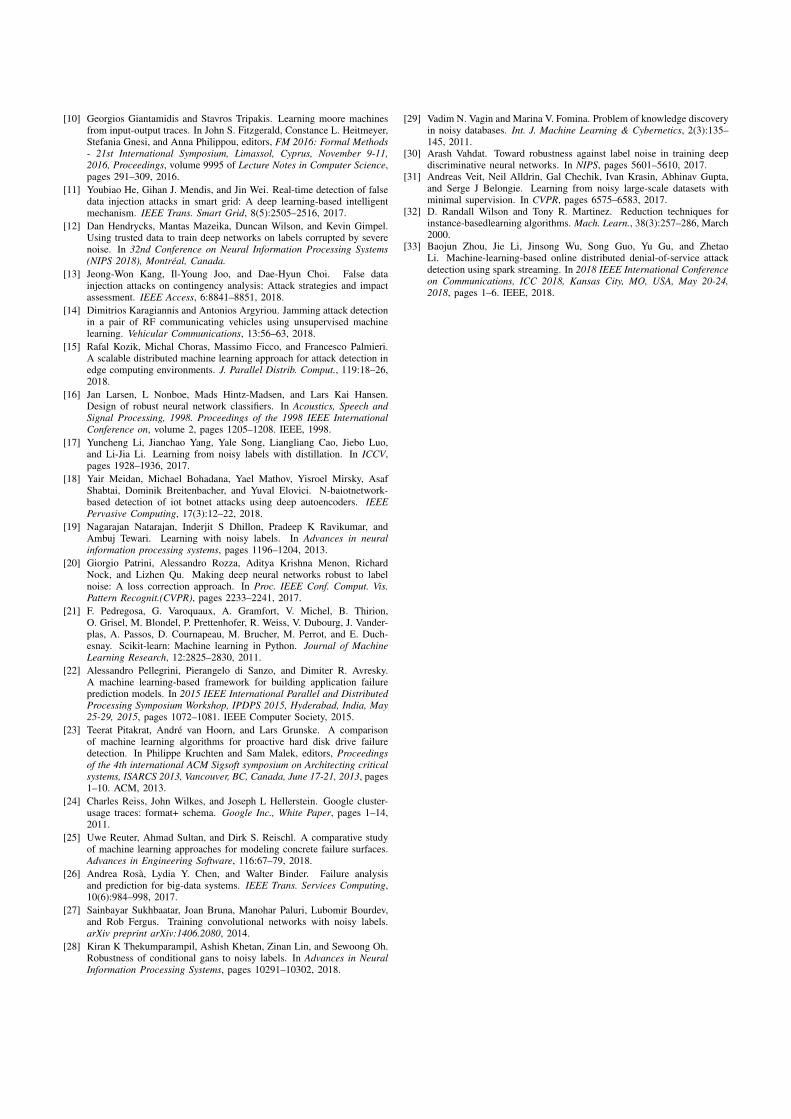
[10] Georgios Giantamidis and Stavros Tripakis. Learning moore machinesfrom input-output traces. In John S. Fitzgerald, Constance L. Heitmeyer,Stefania Gnesi, and Anna Philippou, editors, FM 2016: Formal Methods- 21st International Symposium, Limassol, Cyprus, November 9-11,2016, Proceedings, volume 9995 of Lecture Notes in Computer Science,pages 291–309, 2016.

[11] Youbiao He, Gihan J. Mendis, and Jin Wei. Real-time detection of falsedata injection attacks in smart grid: A deep learning-based intelligentmechanism. IEEE Trans. Smart Grid, 8(5):2505–2516, 2017.

[12] Dan Hendrycks, Mantas Mazeika, Duncan Wilson, and Kevin Gimpel.Using trusted data to train deep networks on labels corrupted by severenoise. In 32nd Conference on Neural Information Processing Systems(NIPS 2018), Montreal, Canada.

[13] Jeong-Won Kang, Il-Young Joo, and Dae-Hyun Choi. False datainjection attacks on contingency analysis: Attack strategies and impactassessment. IEEE Access, 6:8841–8851, 2018.

[14] Dimitrios Karagiannis and Antonios Argyriou. Jamming attack detectionin a pair of RF communicating vehicles using unsupervised machinelearning. Vehicular Communications, 13:56–63, 2018.

[15] Rafal Kozik, Michal Choras, Massimo Ficco, and Francesco Palmieri.A scalable distributed machine learning approach for attack detection inedge computing environments. J. Parallel Distrib. Comput., 119:18–26,2018.

[16] Jan Larsen, L Nonboe, Mads Hintz-Madsen, and Lars Kai Hansen.Design of robust neural network classifiers. In Acoustics, Speech andSignal Processing, 1998. Proceedings of the 1998 IEEE InternationalConference on, volume 2, pages 1205–1208. IEEE, 1998.

[17] Yuncheng Li, Jianchao Yang, Yale Song, Liangliang Cao, Jiebo Luo,and Li-Jia Li. Learning from noisy labels with distillation. In ICCV,pages 1928–1936, 2017.

[18] Yair Meidan, Michael Bohadana, Yael Mathov, Yisroel Mirsky, AsafShabtai, Dominik Breitenbacher, and Yuval Elovici. N-baiotnetwork-based detection of iot botnet attacks using deep autoencoders. IEEEPervasive Computing, 17(3):12–22, 2018.

[19] Nagarajan Natarajan, Inderjit S Dhillon, Pradeep K Ravikumar, andAmbuj Tewari. Learning with noisy labels. In Advances in neuralinformation processing systems, pages 1196–1204, 2013.

[20] Giorgio Patrini, Alessandro Rozza, Aditya Krishna Menon, RichardNock, and Lizhen Qu. Making deep neural networks robust to labelnoise: A loss correction approach. In Proc. IEEE Conf. Comput. Vis.Pattern Recognit.(CVPR), pages 2233–2241, 2017.

[21] F. Pedregosa, G. Varoquaux, A. Gramfort, V. Michel, B. Thirion,O. Grisel, M. Blondel, P. Prettenhofer, R. Weiss, V. Dubourg, J. Vander-plas, A. Passos, D. Cournapeau, M. Brucher, M. Perrot, and E. Duch-esnay. Scikit-learn: Machine learning in Python. Journal of MachineLearning Research, 12:2825–2830, 2011.

[22] Alessandro Pellegrini, Pierangelo di Sanzo, and Dimiter R. Avresky.A machine learning-based framework for building application failureprediction models. In 2015 IEEE International Parallel and DistributedProcessing Symposium Workshop, IPDPS 2015, Hyderabad, India, May25-29, 2015, pages 1072–1081. IEEE Computer Society, 2015.

[23] Teerat Pitakrat, Andre van Hoorn, and Lars Grunske. A comparisonof machine learning algorithms for proactive hard disk drive failuredetection. In Philippe Kruchten and Sam Malek, editors, Proceedingsof the 4th international ACM Sigsoft symposium on Architecting criticalsystems, ISARCS 2013, Vancouver, BC, Canada, June 17-21, 2013, pages1–10. ACM, 2013.

[24] Charles Reiss, John Wilkes, and Joseph L Hellerstein. Google cluster-usage traces: format+ schema. Google Inc., White Paper, pages 1–14,2011.

[25] Uwe Reuter, Ahmad Sultan, and Dirk S. Reischl. A comparative studyof machine learning approaches for modeling concrete failure surfaces.Advances in Engineering Software, 116:67–79, 2018.

[26] Andrea Rosa, Lydia Y. Chen, and Walter Binder. Failure analysisand prediction for big-data systems. IEEE Trans. Services Computing,10(6):984–998, 2017.

[27] Sainbayar Sukhbaatar, Joan Bruna, Manohar Paluri, Lubomir Bourdev,and Rob Fergus. Training convolutional networks with noisy labels.arXiv preprint arXiv:1406.2080, 2014.

[28] Kiran K Thekumparampil, Ashish Khetan, Zinan Lin, and Sewoong Oh.Robustness of conditional gans to noisy labels. In Advances in NeuralInformation Processing Systems, pages 10291–10302, 2018.

[29] Vadim N. Vagin and Marina V. Fomina. Problem of knowledge discoveryin noisy databases. Int. J. Machine Learning & Cybernetics, 2(3):135–145, 2011.

[30] Arash Vahdat. Toward robustness against label noise in training deepdiscriminative neural networks. In NIPS, pages 5601–5610, 2017.

[31] Andreas Veit, Neil Alldrin, Gal Chechik, Ivan Krasin, Abhinav Gupta,and Serge J Belongie. Learning from noisy large-scale datasets withminimal supervision. In CVPR, pages 6575–6583, 2017.

[32] D. Randall Wilson and Tony R. Martinez. Reduction techniques forinstance-basedlearning algorithms. Mach. Learn., 38(3):257–286, March2000.

[33] Baojun Zhou, Jie Li, Jinsong Wu, Song Guo, Yu Gu, and ZhetaoLi. Machine-learning-based online distributed denial-of-service attackdetection using spark streaming. In 2018 IEEE International Conferenceon Communications, ICC 2018, Kansas City, MO, USA, May 20-24,2018, pages 1–6. IEEE, 2018.

Appendix C

Feedback Control for Online Training ofNeural Networks

The following paper has been accepted for publication in the third IEEE Conference On ControlTechnology And Applications (CCTA 2019) [188].

191

Feedback Control for Online Training of Neural Networks

Zilong Zhao1, Sophie Cerf1 , Bogdan Robu1 and Nicolas Marchand1

Abstract— Convolutional neural networks (CNNs) are com-monly used for image classification tasks, raising the challengeof their application on data flows. During their training,adaptation is often performed by tuning the learning rate. Usuallearning rate strategies are time-based i.e. monotonously de-creasing. In this paper, we advocate switching to a performance-based adaptation, in order to improve the learning efficiency.We present E (Exponential)/PI (Proportional Integral)-Control,a conditional learning rate strategy that combines a feedback PIcontroller based on the CNN loss function, with an exponentialcontrol signal to smartly boost the learning and adapt the PI pa-rameters. Stability proof is provided as well as an experimentalevaluation using two state of the art image datasets (CIFAR-10and Fashion-MNIST). Results show better performances thanthe related works (faster network accuracy growth reachinghigher levels) and robustness of the E/PI-Control regarding itsparametrization.

I. INTRODUCTION

Convolutional neural networks (CNNs) are popular ma-chine learning algorithms for image classification , as theyare well suited for visual pattern recognition and requirelow preprocessing [1]. Like all neural networks, CNNs areparametrized with so-called weights that enable to tune thenetwork prediction model to fit the task. Those weights arelearned iteratively based on training data using methods suchas gradient descent. In this paper, we consider a scenariowhere data comes dynamically in batches (not all data isinitially available), previous data batches being discarded atthe arrival of a new one. This type of scenarios is verycommon in our everyday life if we think about sequentialcollection of a video flow or daily crowdsourcing [2] [3].

The learning rate parameter is used to weight the impactof a new epoch on the previously learned model. Thus,in the gradient-based algorithms, there are two factors thatinfluence the reach of the gradient global minimum: thenetwork’s weights initialization and the learning rate policy.The weights initialization is often dealt with by setting themall null or generated from a uniform distribution [4]. Thelearning rate controls the speed to approach the minimum.A large learning rate will accelerate the converging speed butat the risk of diverging [5]. A small learning rate will slowlyapproach the minimum with less tendency to skip over it,but may fall into a local minimum.

The objective is thus to set the learning rate strategy inorder to learn from the data as fast as possible to reachthe maximum CNN’s predictions accuracy. The dynamicdata collection scenario raises the challenge of a learningrate scheduling able to deal with the combination of epoch

1 GIPSA-lab, Univ. Grenoble Alpes, CNRS, Grenoble INP, 38000 Greno-ble, France firstname.lastname@gipsa-lab.fr

learning (take the most out of the currently available data)with batch learning (being able to include new data withoutforgetting the previous ones).

A learning rate strategy is defined by its initial valueand its evolution law. The tuning of both is a significantchallenge for the deep learning community [6]. Accordingto Bengio [5], a learning rate of 0.01 typically works as adefault value for standard multi-layer neural networks. Healso recommends a classic strategy to find a more suitablevalue for a given architecture and dataset. Its principle is totry several values on a subset of the dataset and comparethe best validation accuracy for a fixed training time; andthe lowest training time to reach a given validation accuracy[7]. Learning rate evolution laws are usually of two kinds:time-based or adaptive. Time-based learning strategies [5] arethe most famous ones: the learning rate follows a predefinedfunction (polynomial, exponential, etc.) that should decreasethrough time to ensure stability. The adaptive techniquesare based on the gradient: they are reactive techniques thatset the learning rate according to the past values of thegradient [8], [9]. Given the definition of the gradient descenttraining law, a learning rate indexed on the gradient value isalways decreasing with time. The monotonous decrease ofthe learning rate is a well-established use that has rarely beenquestioned. However, Smith [7] presents promising resultswith a cyclical learning rate law of triangular shape, and Anet al. [10] introduced a time decreasing law with small sineoscillations. Indeed, we advocate that a brief increase in thelearning rate could enable both to reach faster the globalminimum and avoid being blocked in a local one.

Moreover, the issue with the state of the art learningrate laws regarding our continual learning scenario is thatthey do not take into account the dynamic of data comingin. They are predefined functions that do not adapt to theperformances of the CNN training. Even by re-initializingthe learning rate rule at each batch, it will not take intoaccount the precision improvement through time that resultsfrom the memory of the previous batches.

In this work, we advocate using a control-based approachto adapt the learning rate in order to reach a high networkaccuracy in a short amount of time. The principle is to switchfrom time decreasing rules to a performance-based rule to beable to increase the learning rate when necessary. P and PIcontrol strategies are initially developed. Then we presentE/PI-Control, a hybrid strategy for setting the learning ratethat combines both a time-based rule, with a first initial phaseof an exponential growth of the learning rate, with a PIcontroller triggered by the network loss function. The initialE phase additionally allows the PI to be tuned on-line, thus

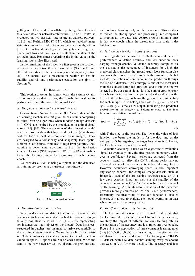
getting rid of the need of an off-line profiling phase to adaptto a new dataset or network architecture. The E/PI-Control isevaluated on two classical state of the art datasets (CIFAR-10 [11] and Fashion-MNIST [12]), which are labelled imagedatasets commonly used to train computer vision algorithms[13]. Our control shows higher accuracy, faster rising time,lower final loss and more stable results than the state of theart techniques. Robustness regarding the initial value of thelearning rate is also illustrated.

In the remaining of the paper, we first present the problemstatement in a control theory formulation (Section II) andillustrate two state of the art learning rate strategies (SectionIII). The control law is presented in Section IV and itsstability analysis and performance evaluation are given inSection V.

II. BACKGROUND

This section presents, in control terms, the system we aimat monitoring, its disturbances, the signals that evaluate itsperformances and the available control knob.

A. The plant: a convolutional neural network

Convolutional Neural Networks (CNN) are state of theart learning mechanisms that give the best results comparingto other learning algorithms when modeling image datasets[14]. CNNs are inspired by the organization of animal visualcortex [15], [16]. They are a type of deep learning modelmade to process data that have grid patterns (neighboringfeatures form a local structure such as in images). Theyare designed to automatically and adaptively learn spatialhierarchies of features, from low to high-level patterns. CNNtraining is done using algorithms such as the StochasticGradient Descent (SGD) optimizer. We use SGD as it enablesto set the learning rate at the beginning of each trainingepoch.

We consider a CNN as being our plant, and the data usedin training are seen as a disturbance, see Figure 1.

Fig. 1: CNN control schema.

B. The disturbance: data batches

We consider a training dataset that consists of several datainstances, such as images. And each data instance belongsto only one class c, where c ∈ {1, . . . ,C}, representingfor instance the main object on the picture. Data instances,structured in batches, are assumed to arrive sequentially tothe learning system over time. We set that each batch consistsof B data instances. One iteration on the whole batch iscalled an epoch, E epochs are run on each batch. When thedata of the new batch arrives, we discard the previous data

and continue learning only on the new ones. This enablesto reduce the storing space and processing time comparedto keeping all the data. The control system sampling timeis thus one epoch, while the disturbance time scale is thebatches’ one.

C. Performance Metrics: accuracy and loss

Two signals can be used to evaluate a neural networkperformance: validation accuracy and loss function, bothvarying through epochs. Validation accuracy, computed onthe test set, is the percentage of instances for which thepredicted class matches the ground truth. Loss function alsocompares the model predictions with the ground truth, butincludes the notion of confidence in the prediction throughthe use of a distance. Cross-entropy is one of the most usedmulticlass classification loss function, and is thus the one weselected to be our output signal. It is the sum of cross-entropyerror between targets and the predicted values done on thetest set. We define yi,c as being the ground truth, indicatingfor each image i if it belongs to class c (yi,c = 1) or not(yi,c = 0). yi,c is the CNN output, indicating the predictedprobability of the image i to belong to class c. The lossfunction thus defined as follows:

loss = − 1

T

T∑i=1

C∑c=1

yi,clog(yi,c) + (1− yi,c)log(1− yi,c)

(1)

with T the size of the test set. The lower the value of lossfunction, the better the model is for the data, and as theentropy can’t be negative, the target loss value is 0. Hence,the loss function is our error signal.

Validation accuracy is used as an a posteriori evaluationsignal, as eventually, only the final prediction matters, what-ever its confidence. Several metrics are extracted from theaccuracy signal to reflect the CNN training performances.The end value of the accuracy is indeed the key factor.However, accuracy’s converging speed is also importantengineering concern: for complex image datasets such asImageNet, state of the art training strategies take up to afew days. Another important metric is the stability of theaccuracy curve, especially for the epochs toward the endof the learning. A low standard deviation of the accuracyprovides more guarantees on the final CNN performances.Eventually, the final value of the loss function is also ofinterest, as it allows to evaluate the model overfitting on datawhen compared to accuracy value.

D. The Control Signal: the learning rate

The learning rate λ is our control signal. To illustrate thatthe learning rate is a control signal for our online scenario,we study the impact of different constant learning rate onthe variation of the accuracy and loss functions over epochs.Figure 2 is the application of three constant learning rates(λ ∈ {0.005, 0.01, 0.05}, corresponding to Bengio’s recom-mendation [5], larger and smaller) for training on CIFAR-10 dataset, with new data batches arriving every 60 epochs(see Section V-A for more details). The accuracy and loss

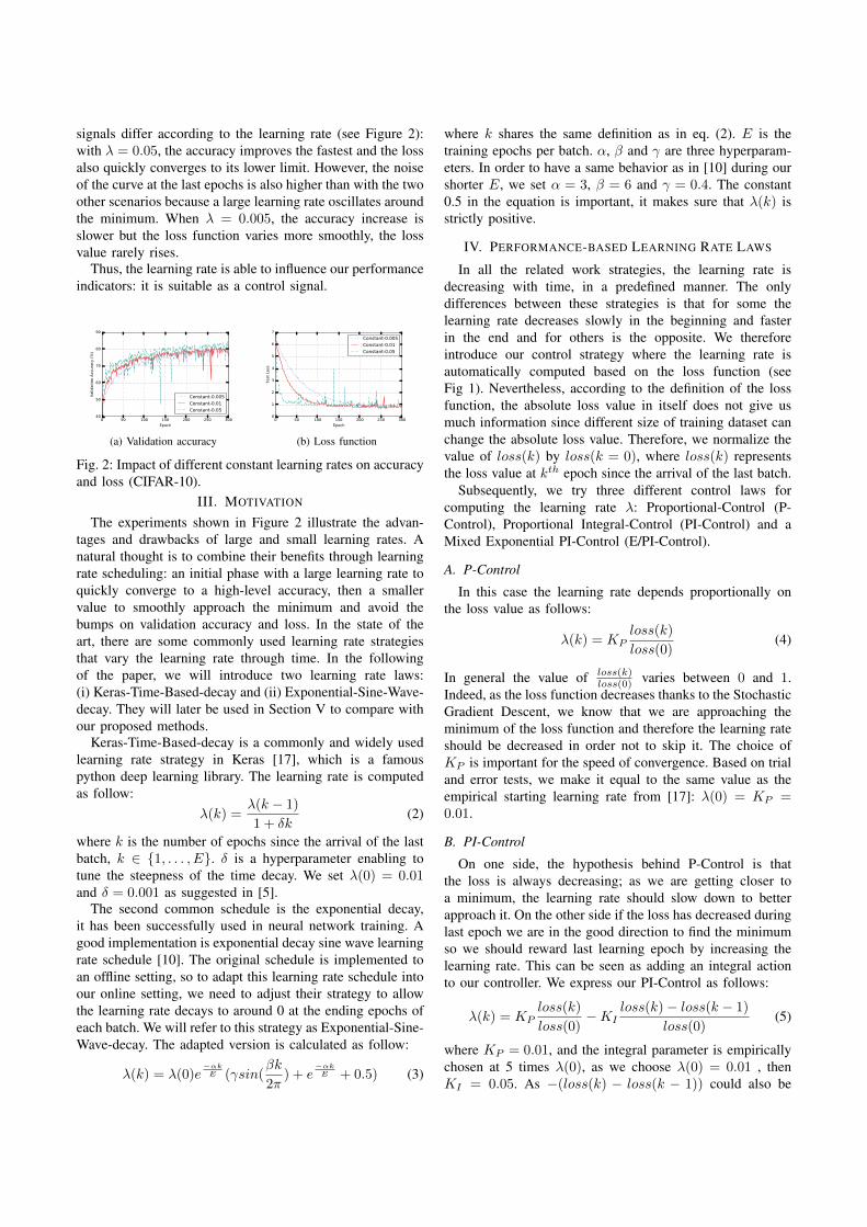
signals differ according to the learning rate (see Figure 2):with λ = 0.05, the accuracy improves the fastest and the lossalso quickly converges to its lower limit. However, the noiseof the curve at the last epochs is also higher than with the twoother scenarios because a large learning rate oscillates aroundthe minimum. When λ = 0.005, the accuracy increase isslower but the loss function varies more smoothly, the lossvalue rarely rises.

Thus, the learning rate is able to influence our performanceindicators: it is suitable as a control signal.

(a) Validation accuracy (b) Loss function

Fig. 2: Impact of different constant learning rates on accuracyand loss (CIFAR-10).

III. MOTIVATION

The experiments shown in Figure 2 illustrate the advan-tages and drawbacks of large and small learning rates. Anatural thought is to combine their benefits through learningrate scheduling: an initial phase with a large learning rate toquickly converge to a high-level accuracy, then a smallervalue to smoothly approach the minimum and avoid thebumps on validation accuracy and loss. In the state of theart, there are some commonly used learning rate strategiesthat vary the learning rate through time. In the followingof the paper, we will introduce two learning rate laws:(i) Keras-Time-Based-decay and (ii) Exponential-Sine-Wave-decay. They will later be used in Section V to compare withour proposed methods.

Keras-Time-Based-decay is a commonly and widely usedlearning rate strategy in Keras [17], which is a famouspython deep learning library. The learning rate is computedas follow:

λ(k) =λ(k − 1)

1 + δk(2)

where k is the number of epochs since the arrival of the lastbatch, k ∈ {1, . . . , E}. δ is a hyperparameter enabling totune the steepness of the time decay. We set λ(0) = 0.01and δ = 0.001 as suggested in [5].

The second common schedule is the exponential decay,it has been successfully used in neural network training. Agood implementation is exponential decay sine wave learningrate schedule [10]. The original schedule is implemented toan offline setting, so to adapt this learning rate schedule intoour online setting, we need to adjust their strategy to allowthe learning rate decays to around 0 at the ending epochs ofeach batch. We will refer to this strategy as Exponential-Sine-Wave-decay. The adapted version is calculated as follow:

λ(k) = λ(0)e−αkE (γsin(

βk

2π) + e

−αkE + 0.5) (3)

where k shares the same definition as in eq. (2). E is thetraining epochs per batch. α, β and γ are three hyperparam-eters. In order to have a same behavior as in [10] during ourshorter E, we set α = 3, β = 6 and γ = 0.4. The constant0.5 in the equation is important, it makes sure that λ(k) isstrictly positive.

IV. PERFORMANCE-BASED LEARNING RATE LAWS

In all the related work strategies, the learning rate isdecreasing with time, in a predefined manner. The onlydifferences between these strategies is that for some thelearning rate decreases slowly in the beginning and fasterin the end and for others is the opposite. We thereforeintroduce our control strategy where the learning rate isautomatically computed based on the loss function (seeFig 1). Nevertheless, according to the definition of the lossfunction, the absolute loss value in itself does not give usmuch information since different size of training dataset canchange the absolute loss value. Therefore, we normalize thevalue of loss(k) by loss(k = 0), where loss(k) representsthe loss value at kth epoch since the arrival of the last batch.

Subsequently, we try three different control laws forcomputing the learning rate λ: Proportional-Control (P-Control), Proportional Integral-Control (PI-Control) and aMixed Exponential PI-Control (E/PI-Control).

A. P-Control

In this case the learning rate depends proportionally onthe loss value as follows:

λ(k) = KPloss(k)

loss(0)(4)

In general the value of loss(k)loss(0) varies between 0 and 1.

Indeed, as the loss function decreases thanks to the StochasticGradient Descent, we know that we are approaching theminimum of the loss function and therefore the learning rateshould be decreased in order not to skip it. The choice ofKP is important for the speed of convergence. Based on trialand error tests, we make it equal to the same value as theempirical starting learning rate from [17]: λ(0) = KP =0.01.

B. PI-Control

On one side, the hypothesis behind P-Control is thatthe loss is always decreasing; as we are getting closer toa minimum, the learning rate should slow down to betterapproach it. On the other side if the loss has decreased duringlast epoch we are in the good direction to find the minimumso we should reward last learning epoch by increasing thelearning rate. This can be seen as adding an integral actionto our controller. We express our PI-Control as follows:

λ(k) = KPloss(k)

loss(0)−KI

loss(k)− loss(k − 1)

loss(0)(5)

where KP = 0.01, and the integral parameter is empiricallychosen at 5 times λ(0), as we choose λ(0) = 0.01 , thenKI = 0.05. As −(loss(k) − loss(k − 1)) could also be

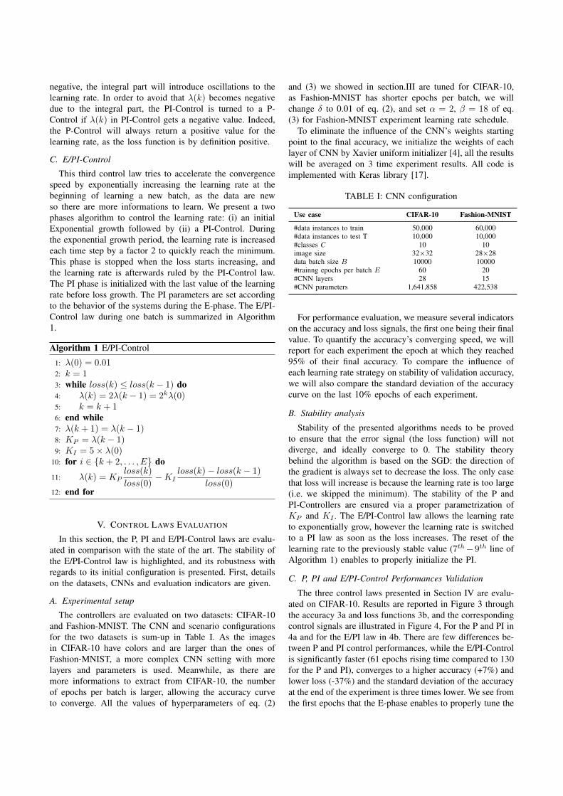
negative, the integral part will introduce oscillations to thelearning rate. In order to avoid that λ(k) becomes negativedue to the integral part, the PI-Control is turned to a P-Control if λ(k) in PI-Control gets a negative value. Indeed,the P-Control will always return a positive value for thelearning rate, as the loss function is by definition positive.

C. E/PI-Control

This third control law tries to accelerate the convergencespeed by exponentially increasing the learning rate at thebeginning of learning a new batch, as the data are newso there are more informations to learn. We present a twophases algorithm to control the learning rate: (i) an initialExponential growth followed by (ii) a PI-Control. Duringthe exponential growth period, the learning rate is increasedeach time step by a factor 2 to quickly reach the minimum.This phase is stopped when the loss starts increasing, andthe learning rate is afterwards ruled by the PI-Control law.The PI phase is initialized with the last value of the learningrate before loss growth. The PI parameters are set accordingto the behavior of the systems during the E-phase. The E/PI-Control law during one batch is summarized in Algorithm1.

Algorithm 1 E/PI-Control

1: λ(0) = 0.012: k = 13: while loss(k) ≤ loss(k − 1) do4: λ(k) = 2λ(k − 1) = 2kλ(0)5: k = k + 16: end while7: λ(k + 1) = λ(k − 1)8: KP = λ(k − 1)9: KI = 5× λ(0)

10: for i ∈ {k + 2, . . . , E} do

11: λ(k) = KPloss(k)

loss(0)−KI

loss(k)− loss(k − 1)

loss(0)12: end for

V. CONTROL LAWS EVALUATION

In this section, the P, PI and E/PI-Control laws are evalu-ated in comparison with the state of the art. The stability ofthe E/PI-Control law is highlighted, and its robustness withregards to its initial configuration is presented. First, detailson the datasets, CNNs and evaluation indicators are given.

A. Experimental setup

The controllers are evaluated on two datasets: CIFAR-10and Fashion-MNIST. The CNN and scenario configurationsfor the two datasets is sum-up in Table I. As the imagesin CIFAR-10 have colors and are larger than the ones ofFashion-MNIST, a more complex CNN setting with morelayers and parameters is used. Meanwhile, as there aremore informations to extract from CIFAR-10, the numberof epochs per batch is larger, allowing the accuracy curveto converge. All the values of hyperparameters of eq. (2)

and (3) we showed in section.III are tuned for CIFAR-10,as Fashion-MNIST has shorter epochs per batch, we willchange δ to 0.01 of eq. (2), and set α = 2, β = 18 of eq.(3) for Fashion-MNIST experiment learning rate schedule.

To eliminate the influence of the CNN’s weights startingpoint to the final accuracy, we initialize the weights of eachlayer of CNN by Xavier uniform initializer [4], all the resultswill be averaged on 3 time experiment results. All code isimplemented with Keras library [17].

TABLE I: CNN configuration

Use case CIFAR-10 Fashion-MNIST

#data instances to train 50,000 60,000#data instances to test T 10,000 10,000#classes C 10 10image size 32×32 28×28data batch size B 10000 10000#trainng epochs per batch E 60 20#CNN layers 28 15#CNN parameters 1,641,858 422,538

For performance evaluation, we measure several indicatorson the accuracy and loss signals, the first one being their finalvalue. To quantify the accuracy’s converging speed, we willreport for each experiment the epoch at which they reached95% of their final accuracy. To compare the influence ofeach learning rate strategy on stability of validation accuracy,we will also compare the standard deviation of the accuracycurve on the last 10% epochs of each experiment.

B. Stability analysis

Stability of the presented algorithms needs to be provedto ensure that the error signal (the loss function) will notdiverge, and ideally converge to 0. The stability theorybehind the algorithm is based on the SGD: the direction ofthe gradient is always set to decrease the loss. The only casethat loss will increase is because the learning rate is too large(i.e. we skipped the minimum). The stability of the P andPI-Controllers are ensured via a proper parametrization ofKP and KI . The E/PI-Control law allows the learning rateto exponentially grow, however the learning rate is switchedto a PI law as soon as the loss increases. The reset of thelearning rate to the previously stable value (7th−9th line ofAlgorithm 1) enables to properly initialize the PI.

C. P, PI and E/PI-Control Performances Validation

The three control laws presented in Section IV are evalu-ated on CIFAR-10. Results are reported in Figure 3 throughthe accuracy 3a and loss functions 3b, and the correspondingcontrol signals are illustrated in Figure 4, For the P and PI in4a and for the E/PI law in 4b. There are few differences be-tween P and PI control performances, while the E/PI-Controlis significantly faster (61 epochs rising time compared to 130for the P and PI), converges to a higher accuracy (+7%) andlower loss (-37%) and the standard deviation of the accuracyat the end of the experiment is three times lower. We see fromthe first epochs that the E-phase enables to properly tune the

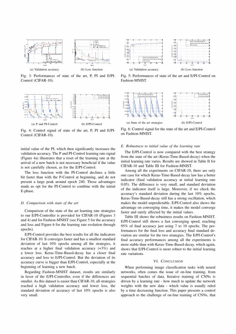
(a) Validation accuracy (b) Loss function

Fig. 3: Performances of state of the art, P, PI and E/PI-Control (CIFAR-10).

(a) P and PI-Control (b) E/PI-Control

Fig. 4: Control signal of state of the art, P, PI and E/PI-Control (CIFAR-10).

initial value of the PI, which then significantly increases thevalidation accuracy. The P and PI-Control learning rate signal(Figure 4a) illustrates that a reset of the learning rate at thearrival of a new batch is not necessary beneficial if the valueis not carefully chosen, as for the E/PI-Control.

The loss function with the PI-Control declines a littlebit faster than with the P-Control at beginning, and do notpresent a large peak around epoch 240. Those advantagesmade us opt for the PI-Control to combine with the initialE-phase.

D. Comparison with state of the art

Comparison of the state of the art learning rate strategiesto our E/PI-Controller is provided for CIFAR-10 (Figures 3and 4) and for Fashion-MNIST (see Figure 5 for the accuracyand loss and Figure 6 for the learning rate evolution throughepochs).

E/PI-Control provides the best results for all the indicatorsfor CIFAR-10. It converges faster and has a smallest standarddeviation of last 10% epochs among all the strategies, itreaches at a higher final validation accuracy (+3%) anda lower loss. Keras-Time-Based-decay has a closer finalaccuracy and loss to E/PI-Control. But the deviation of itsaccuracy curve is bigger than E/PI-Control, especially at thebeginning of learning a new batch.

Regarding Fashion-MNIST dataset, results are similarlyin favor of the E/PI-Controller, even if the differences aresmaller. As this dataset is easier than CIFAR-10, all strategiesreached a high validation accuracy and lower loss, thestandard deviation of accuracy of last 10% epochs is alsovery small.

(a) Validation accuracy (b) Loss function

Fig. 5: Performances of state of the art and E/PI-Control onFashion-MNIST.

(a) State of the art strategies (b) E/PI-Control

Fig. 6: Control signal for the state of the art and E/PI-Controlon Fashion-MNIST.

E. Robustness to initial value of the learning rate

The E/PI-Control is now compared with the best strategyfrom the state of the art (Keras-Time-Based-decay) when theinitial learning rate varies. Results are showed in Table II forCIFAR-10 and Table III for Fashion-MNIST.

Among all the experiments on CIFAR-10, there are onlyone case for which Keras-Time-Based-decay law has a betterindicator (final validation accuracy at initial learning rate0.05). The difference is very small, and standard deviationof the indicator itself is large. Moreover, if we check theaccuracy’s standard deviation during the last 10% epochs,Keras-Time-Based-decay still has a strong oscillation, whichmakes the model unpredictable. E/PI-Control also shows theadvantage on converging time, it makes the model convergefaster and rarely affected by the initial values.

Table III shows the robustness results on Fashion-MNIST.E/PI-Control still shows a fast converging speed, reaching95% of final accuracy just using 7 to 10 epochs. The per-formances for the final loss and accuracy final standard de-viation are similar for the two strategies. The E/PI-Control’sfinal accuracy performances among all the experiments ismore stable than with Keras-Time-Based-decay, which again,shows that E/PI-Control is more robust to the initial learningrate variations.

VI. CONCLUSION

When performing image classification tasks with neuralnetworks, often comes the issue of on-line training, fromsequential batches of data. Iterative training of CNNs isdriven by a learning rate - how much to update the networkweights with the new data - which value is usually ruledby a time decreasing function. This paper presents a controlapproach to the challenge of on-line training of CNNs, that

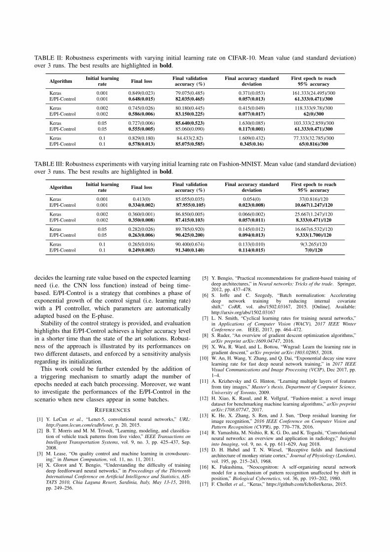
TABLE II: Robustness experiments with varying initial learning rate on CIFAR-10. Mean value (and standard deviation)over 3 runs. The best results are highlighted in bold.

Algorithm Initial learningrate Final loss Final validation

accuracy (%)Final accuracy standard

deviationFirst epoch to reach

95% accuracy

Keras 0.001 0.849(0.023) 79.075(0.485) 0.371(0.053) 161.333(24.495)/300E/PI-Control 0.001 0.648(0.015) 82.035(0.465) 0.057(0.013) 61.333(0.471)/300

Keras 0.002 0.745(0.026) 80.180(0.445) 0.415(0.049) 118.333(9.78)/300E/PI-Control 0.002 0.586(0.006) 83.150(0.225) 0.077(0.017) 62(0)/300

Keras 0.05 0.727(0.006) 85.640(0.523) 1.630(0.085) 103.333(2.859)/300E/PI-Control 0.05 0.555(0.005) 85.060(0.090) 0.117(0.001) 61.333(0.471)/300

Keras 0.1 0.829(0.180) 84.433(2.82) 1.609(0.432) 77.333(32.785)/300E/PI-Control 0.1 0.578(0.013) 85.075(0.585) 0.345(0.16) 65(0.816)/300

TABLE III: Robustness experiments with varying initial learning rate on Fashion-MNIST. Mean value (and standard deviation)over 3 runs. The best results are highlighted in bold.

Algorithm Initial learningrate Final loss Final validation

accuracy (%)Final accuracy standard

deviationFirst epoch to reach

95% accuracy

Keras 0.001 0.413(0) 85.055(0.035) 0.054(0) 37(0.816)/120E/PI-Control 0.001 0.334(0.002) 87.955(0.105) 0.023(0.008) 10.667(1.247)/120

Keras 0.002 0.360(0.001) 86.850(0.005) 0.066(0.002) 25.667(1.247)/120E/PI-Control 0.002 0.350(0.008) 87.415(0.103) 0.057(0.011) 8.333(0.471)/120

Keras 0.05 0.282(0.026) 89.785(0.920) 0.145(0.012) 16.667(6.532)/120E/PI-Control 0.05 0.263(0.006) 90.425(0.200) 0.094(0.013) 9.333(1.700)/120

Keras 0.1 0.265(0.016) 90.400(0.674) 0.133(0.010) 9(3.265)/120E/PI-Control 0.1 0.249(0.003) 91.340(0.140) 0.114(0.015) 7(0)/120

decides the learning rate value based on the expected learningneed (i.e. the CNN loss function) instead of being time-based. E/PI-Control is a strategy that combines a phase ofexponential growth of the control signal (i.e. learning rate)with a PI controller, which parameters are automaticallyadapted based on the E-phase.

Stability of the control strategy is provided, and evaluationhighlights that E/PI-Control achieves a higher accuracy levelin a shorter time than the state of the art solutions. Robust-ness of the approach is illustrated by its performances ontwo different datasets, and enforced by a sensitivity analysisregarding its initialization.

This work could be further extended by the addition ofa triggering mechanism to smartly adapt the number ofepochs needed at each batch processing. Moreover, we wantto investigate the performances of the E/PI-Control in thescenario when new classes appear in some batches.

REFERENCES

[1] Y. LeCun et al., “Lenet-5, convolutional neural networks,” URL:http://yann.lecun.com/exdb/lenet, p. 20, 2015.

[2] B. T. Morris and M. M. Trivedi, “Learning, modeling, and classifica-tion of vehicle track patterns from live video,” IEEE Transactions onIntelligent Transportation Systems, vol. 9, no. 3, pp. 425–437, Sep.2008.

[3] M. Lease, “On quality control and machine learning in crowdsourc-ing,” in Human Computation, vol. 11, no. 11, 2011.

[4] X. Glorot and Y. Bengio, “Understanding the difficulty of trainingdeep feedforward neural networks,” in Proceedings of the ThirteenthInternational Conference on Artificial Intelligence and Statistics, AIS-TATS 2010, Chia Laguna Resort, Sardinia, Italy, May 13-15, 2010,pp. 249–256.

[5] Y. Bengio, “Practical recommendations for gradient-based training ofdeep architectures,” in Neural networks: Tricks of the trade. Springer,2012, pp. 437–478.

[6] S. Ioffe and C. Szegedy, “Batch normalization: Acceleratingdeep network training by reducing internal covariateshift,” CoRR, vol. abs/1502.03167, 2015. [Online]. Available:http://arxiv.org/abs/1502.03167

[7] L. N. Smith, “Cyclical learning rates for training neural networks,”in Applications of Computer Vision (WACV), 2017 IEEE WinterConference on. IEEE, 2017, pp. 464–472.

[8] S. Ruder, “An overview of gradient descent optimization algorithms,”arXiv preprint arXiv:1609.04747, 2016.

[9] X. Wu, R. Ward, and L. Bottou, “Wngrad: Learn the learning rate ingradient descent,” arXiv preprint arXiv:1803.02865, 2018.

[10] W. An, H. Wang, Y. Zhang, and Q. Dai, “Exponential decay sine wavelearning rate for fast deep neural network training,” in 2017 IEEEVisual Communications and Image Processing (VCIP), Dec 2017, pp.1–4.

[11] A. Krizhevsky and G. Hinton, “Learning multiple layers of featuresfrom tiny images,” Master’s thesis, Department of Computer Science,University of Toronto, 2009.

[12] H. Xiao, K. Rasul, and R. Vollgraf, “Fashion-mnist: a novel imagedataset for benchmarking machine learning algorithms,” arXiv preprintarXiv:1708.07747, 2017.

[13] K. He, X. Zhang, S. Ren, and J. Sun, “Deep residual learning forimage recognition,” 2016 IEEE Conference on Computer Vision andPattern Recognition (CVPR), pp. 770–778, 2016.

[14] R. Yamashita, M. Nishio, R. K. G. Do, and K. Togashi, “Convolutionalneural networks: an overview and application in radiology,” Insightsinto Imaging, vol. 9, no. 4, pp. 611–629, Aug 2018.

[15] D. H. Hubel and T. N. Wiesel, “Receptive fields and functionalarchitecture of monkey striate cortex,” Journal of Physiology (London),vol. 195, pp. 215–243, 1968.

[16] K. Fukushima, “Neocognitron: A self-organizing neural networkmodel for a mechanism of pattern recognition unaffected by shift inposition,” Biological Cybernetics, vol. 36, pp. 193–202, 1980.

[17] F. Chollet et al., “Keras,” https://github.com/fchollet/keras, 2015.

198

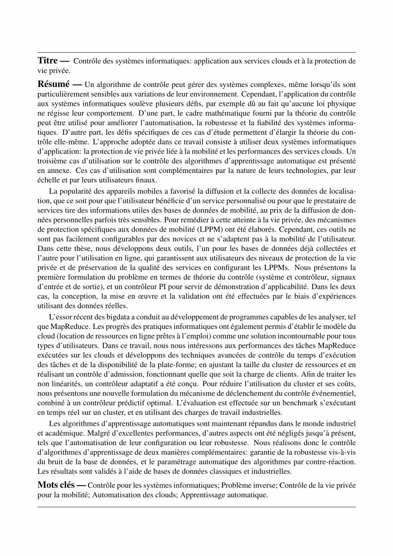
Titre — Contrôle des systèmes informatiques: application aux services clouds et à la protection devie privée.

Résumé — Un algorithme de contrôle peut gérer des systèmes complexes, même lorsqu’ils sontparticulièrement sensibles aux variations de leur environnement. Cependant, l’application du contrôleaux systèmes informatiques soulève plusieurs défis, par exemple dû au fait qu’aucune loi physiquene régisse leur comportement. D’une part, le cadre mathématique fourni par la théorie du contrôlepeut être utilisé pour améliorer l’automatisation, la robustesse et la fiabilité des systèmes informa-tiques. D’autre part, les défis spécifiques de ces cas d’étude permettent d’élargir la théorie du con-trôle elle-même. L’approche adoptée dans ce travail consiste à utiliser deux systèmes informatiquesd’application: la protection de vie privée liée à la mobilité et les performances des services clouds. Untroisième cas d’utilisation sur le contrôle des algorithmes d’apprentissage automatique est présentéen annexe. Ces cas d’utilisation sont complémentaires par la nature de leurs technologies, par leuréchelle et par leurs utilisateurs finaux.

La popularité des appareils mobiles a favorisé la diffusion et la collecte des données de localisa-tion, que ce soit pour que l’utilisateur bénéficie d’un service personnalisé ou pour que le prestataire deservices tire des informations utiles des bases de données de mobilité, au prix de la diffusion de don-nées personnelles parfois très sensibles. Pour remédier à cette atteinte à la vie privée, des mécanismesde protection spécifiques aux données de mobilité (LPPM) ont été élaborés. Cependant, ces outils nesont pas facilement configurables par des novices et ne s’adaptent pas à la mobilité de l’utilisateur.Dans cette thèse, nous développons deux outils, l’un pour les bases de données déjà collectées etl’autre pour l’utilisation en ligne, qui garantissent aux utilisateurs des niveaux de protection de la vieprivée et de préservation de la qualité des services en configurant les LPPMs. Nous présentons lapremière formulation du problème en termes de théorie du contrôle (système et contrôleur, signauxd’entrée et de sortie), et un contrôleur PI pour servir de démonstration d’applicabilité. Dans les deuxcas, la conception, la mise en œuvre et la validation ont été effectuées par le biais d’expériencesutilisant des données réelles.

L’essor récent des bigdata a conduit au développement de programmes capables de les analyser, telque MapReduce. Les progrès des pratiques informatiques ont également permis d’établir le modèle ducloud (location de ressources en ligne prêtes à l’emploi) comme une solution incontournable pour toustypes d’utilisateurs. Dans ce travail, nous nous intéressons aux performances des tâches MapReduceexécutées sur les clouds et développons des techniques avancées de contrôle du temps d’exécutiondes tâches et de la disponibilité de la plate-forme; en ajustant la taille du cluster de ressources et enréalisant un contrôle d’admission, fonctionnant quelle que soit la charge de clients. Afin de traiter lesnon linéarités, un contrôleur adaptatif a été conçu. Pour réduire l’utilisation du cluster et ses coûts,nous présentons une nouvelle formulation du mécanisme de déclenchement du contrôle événementiel,combiné à un contrôleur prédictif optimal. L’évaluation est effectuée sur un benchmark s’exécutanten temps réel sur un cluster, et en utilisant des charges de travail industrielles.

Les algorithmes d’apprentissage automatiques sont maintenant répandus dans le monde industrielet académique. Malgré d’excellentes performances, d’autres aspects ont été négligés jusqu’à présent,tels que l’automatisation de leur configuration ou leur robustesse. Nous réalisons donc le contrôled’algorithmes d’apprentissage de deux manières complémentaires: garantie de la robustesse vis-à-visdu bruit de la base de données, et le paramétrage automatique des algorithmes par contre-réaction.Les résultats sont validés à l’aide de bases de données classiques et industrielles.

Mots clés — Contrôle pour les systèmes informatiques; Problème inverse; Contrôle de la vie privéepour la mobilité; Automatisation des clouds; Apprentissage automatique.

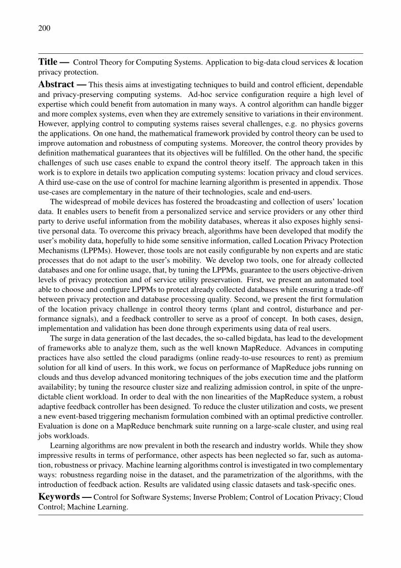
200

Title — Control Theory for Computing Systems. Application to big-data cloud services & locationprivacy protection.

Abstract — This thesis aims at investigating techniques to build and control efficient, dependableand privacy-preserving computing systems. Ad-hoc service configuration require a high level ofexpertise which could benefit from automation in many ways. A control algorithm can handle biggerand more complex systems, even when they are extremely sensitive to variations in their environment.However, applying control to computing systems raises several challenges, e.g. no physics governsthe applications. On one hand, the mathematical framework provided by control theory can be used toimprove automation and robustness of computing systems. Moreover, the control theory provides bydefinition mathematical guarantees that its objectives will be fulfilled. On the other hand, the specificchallenges of such use cases enable to expand the control theory itself. The approach taken in thiswork is to explore in details two application computing systems: location privacy and cloud services.A third use-case on the use of control for machine learning algorithm is presented in appendix. Thoseuse-cases are complementary in the nature of their technologies, scale and end-users.

The widespread of mobile devices has fostered the broadcasting and collection of users’ locationdata. It enables users to benefit from a personalized service and service providers or any other thirdparty to derive useful information from the mobility databases, whereas it also exposes highly sensi-tive personal data. To overcome this privacy breach, algorithms have been developed that modify theuser’s mobility data, hopefully to hide some sensitive information, called Location Privacy ProtectionMechanisms (LPPMs). However, those tools are not easily configurable by non experts and are staticprocesses that do not adapt to the user’s mobility. We develop two tools, one for already collecteddatabases and one for online usage, that, by tuning the LPPMs, guarantee to the users objective-drivenlevels of privacy protection and of service utility preservation. First, we present an automated toolable to choose and configure LPPMs to protect already collected databases while ensuring a trade-offbetween privacy protection and database processing quality. Second, we present the first formulationof the location privacy challenge in control theory terms (plant and control, disturbance and per-formance signals), and a feedback controller to serve as a proof of concept. In both cases, design,implementation and validation has been done through experiments using data of real users.

The surge in data generation of the last decades, the so-called bigdata, has lead to the developmentof frameworks able to analyze them, such as the well known MapReduce. Advances in computingpractices have also settled the cloud paradigms (online ready-to-use resources to rent) as premiumsolution for all kind of users. In this work, we focus on performance of MapReduce jobs running onclouds and thus develop advanced monitoring techniques of the jobs execution time and the platformavailability; by tuning the resource cluster size and realizing admission control, in spite of the unpre-dictable client workload. In order to deal with the non linearities of the MapReduce system, a robustadaptive feedback controller has been designed. To reduce the cluster utilization and costs, we presenta new event-based triggering mechanism formulation combined with an optimal predictive controller.Evaluation is done on a MapReduce benchmark suite running on a large-scale cluster, and using realjobs workloads.

Learning algorithms are now prevalent in both the research and industry worlds. While they showimpressive results in terms of performance, other aspects has been neglected so far, such as automa-tion, robustness or privacy. Machine learning algorithms control is investigated in two complementaryways: robustness regarding noise in the dataset, and the parametrization of the algorithms, with theintroduction of feedback action. Results are validated using classic datasets and task-specific ones.

Keywords — Control for Software Systems; Inverse Problem; Control of Location Privacy; CloudControl; Machine Learning.

201