
Contributions to the Study of Autism Spectrum Brain Connectivity
164
Contributions to the Study of Autism Spectrum Brain Connectivity By Moises Martin Silva Choque Department of Computer Science and Artificial Intelligence PhD Advisor: Prof. Dr. Manuel Graña Romay UPV-EHU Universidad del País Vasco Euskal Herriko Unibertsitatea Donostia - San Sebastián 2021 (c) 2021 Moisés Martín Silva Choque
-
Upload
khangminh22 -
Category
Documents
-
view
1 -
download
0
Transcript of Contributions to the Study of Autism Spectrum Brain Connectivity
Contributions to the Study ofAutism Spectrum Brain
Connectivity
By
Moises Martin Silva Choque
Department of Computer Science and Artificial Intelligence
PhD Advisor:Prof. Dr. Manuel Graña Romay UPV-EHU
Universidad del País VascoEuskal Herriko Unibertsitatea
Donostia - San Sebastián2021
(c) 2021 Moisés Martín Silva Choque

Contributions to the Study of Autism SpectrumBrain Connectivity
by
Moises Silva
Abstract
Abstract Autism Spectrum Disorder (ASD) is a largely prevalent neu-
rodevelopmental condition with a big social and economical impact af-
fecting the entire life of families. There is an intense search for biomarkers
that can be assessed as early as possible in order to initiate treatment
and preparation of the family to deal with the challenges imposed by the
condition. Brain imaging biomarkers have special interest. Specifically,
functional connectivity data extracted from resting state functional mag-
netic resonance imaging (rs-fMRI) should allow to detect brain connec-
tivity alterations. Machine learning pipelines encompass the estimation
of the functional connectivity matrix from brain parcellations, feature
extraction and building classification models for ASD prediction. The
works reported in the literature are very heterogeneous from the compu-
tational and methodological point of view. In this Thesis we carry out
a comprehensive computational exploration of the impact of the choices
involved while building these machine learning pipelines.

Originality Statement
I hereby declare that this submission is my own work and to the best of
my knowledge it contains no materials previously published or written by
another person, or substantial proportions of material which have been
accepted for the award of any other degree or diploma at The University
of the Basque Country or any other educational institution, except where
due acknowledgement is made in the thesis. Any contribution made to
the research by others, with whom I have worked at The University of the
Basque Country or elsewhere, is explicitly acknowledged in the thesis. I
also declare that the intellectual content of this thesis is the product of
my own work, except to the extent that assistance from others in the
project’s design and conception or in style, presentation and linguistic
expression is acknowledged.
The author hereby grants to University of the Basque Country permission
to reproduce and to distribute copies of this thesis document in whole or
in part.
Signed:


Acknowledgements - Agradecimientos
I would like to thank God for his never-ending grace, mercy, and provision
in order to finish this research.
I would like to express my deep gratitude to Dr. Manuel Graña, my re-
search supervisor, for their patient guidance, help, encouragement, sup-
port, valuable expertise and sharing knowledge of this research work.
I would like to thanks the Carolina Foundation for allowing me to obtain
a scholarship for a doctoral stay in the Basque Country.
I thank with love to Yovanna, my wife. She has been my best friend
and great companion for finishing this job. To my children, Valeria and
Thiago, you are my inspiration with your games and happiness.
Finally, I wish to thank my great family parents and siblings for their
support and encouragement throughout my study.


Contents
1 Introduction 9
1.1 Background and Motivation . . . . . . . . . . . . . . . . . . . . . . . 9
1.1.1 Prevalence . . . . . . . . . . . . . . . . . . . . . . . . . . . . . 10
1.1.2 Diagnosis . . . . . . . . . . . . . . . . . . . . . . . . . . . . . 10
1.1.3 Datasets . . . . . . . . . . . . . . . . . . . . . . . . . . . . . . 11
1.1.4 Pattern recognition for CAD . . . . . . . . . . . . . . . . . . . 11
1.1.5 Brain functional connectivity . . . . . . . . . . . . . . . . . . 11
1.1.6 Computational pipeline . . . . . . . . . . . . . . . . . . . . . . 12
1.2 Objectives . . . . . . . . . . . . . . . . . . . . . . . . . . . . . . . . . 14
1.3 Contributions . . . . . . . . . . . . . . . . . . . . . . . . . . . . . . . 14
1.4 Publications . . . . . . . . . . . . . . . . . . . . . . . . . . . . . . . . 15
1.5 Structure of the thesis . . . . . . . . . . . . . . . . . . . . . . . . . . 15
2 State of the art of Autism diagnostic technological tools 17
2.1 Introduction . . . . . . . . . . . . . . . . . . . . . . . . . . . . . . . . 17
2.2 Behavior measurement based CAD approaches. . . . . . . . . . . . . 19
2.3 EEG based CAD approaches. . . . . . . . . . . . . . . . . . . . . . . 22
2.4 MRI based biomarkers. . . . . . . . . . . . . . . . . . . . . . . . . . . 23
2.5 MRI based CAD approaches . . . . . . . . . . . . . . . . . . . . . . . 27
2.6 Public data resources . . . . . . . . . . . . . . . . . . . . . . . . . . . 28
2.7 Concluding remarks . . . . . . . . . . . . . . . . . . . . . . . . . . . . 30
3 State of the art of brain connectivity analysis for Autism 31
3.1 Brain imaging . . . . . . . . . . . . . . . . . . . . . . . . . . . . . . 31vii

Contents viii
3.1.1 Kinds of noise found in brain MRI . . . . . . . . . . . . . . . 32
3.1.2 The fMRI experiment . . . . . . . . . . . . . . . . . . . . . . 34
3.1.3 The resting state fMRI experiment . . . . . . . . . . . . . . . 36
3.1.4 Preprocesing . . . . . . . . . . . . . . . . . . . . . . . . . . . 36
3.1.5 Brain parcellations . . . . . . . . . . . . . . . . . . . . . . . . 41
3.1.6 Connectivity matrices . . . . . . . . . . . . . . . . . . . . . . 43
3.2 Related works . . . . . . . . . . . . . . . . . . . . . . . . . . . . . . . 44
3.2.1 Anatomical brain imaging . . . . . . . . . . . . . . . . . . . . 44
3.2.2 Functional connectivity . . . . . . . . . . . . . . . . . . . . . . 46
3.2.3 Dataset heterogeneity . . . . . . . . . . . . . . . . . . . . . . . 46
3.2.4 Summary information . . . . . . . . . . . . . . . . . . . . . . 47
4 Machine learning background 49
4.1 Introduction . . . . . . . . . . . . . . . . . . . . . . . . . . . . . . . . 49
4.2 Classifier model building methods . . . . . . . . . . . . . . . . . . . 50
4.2.1 Random Forest (RF) . . . . . . . . . . . . . . . . . . . . . . . 50
4.2.2 K-Nearest Neighbors (KNN) . . . . . . . . . . . . . . . . . . . 53
4.2.3 Gaussian Naive Bayes (GNB) . . . . . . . . . . . . . . . . . . 54
4.2.4 Support Vector Classifier (SVC) . . . . . . . . . . . . . . . . . 56
4.2.5 Logistic regression (LR) . . . . . . . . . . . . . . . . . . . . . 56
4.2.6 Least absolute shrinkage and selection operator (LASSO) . . . 58
4.2.7 Ridge Classifier (RC) . . . . . . . . . . . . . . . . . . . . . . . 59
4.2.8 Bayesian Ridge Classifier (BRC) . . . . . . . . . . . . . . . . . 63
4.2.9 Multi-layer Perceptron (MLP) . . . . . . . . . . . . . . . . . . 63
4.3 Feature extraction/selection . . . . . . . . . . . . . . . . . . . . . . . 64
4.3.1 Probabilistic Principal Component Analysis (PCA) . . . . . . 65
4.3.2 Isometric Mapping (Isomap) . . . . . . . . . . . . . . . . . . . 66
4.3.3 Local Linear Embedding (LLE) . . . . . . . . . . . . . . . . . 66
4.3.4 Multi-Dimensional Scaling (MDS) . . . . . . . . . . . . . . . . 68
4.3.5 Factor Analyisis (FA) . . . . . . . . . . . . . . . . . . . . . . . 70
4.4 Classification performance evaluation . . . . . . . . . . . . . . . . . . 72

Contents ix
5 Deep Learning Background 75
5.1 Introduction . . . . . . . . . . . . . . . . . . . . . . . . . . . . . . . 75
5.2 Traditional Machine learning, Transfer learning and Fine tunning . . 76
5.3 Architectures used . . . . . . . . . . . . . . . . . . . . . . . . . . . . 79
5.3.1 VGG16 and VGG19 . . . . . . . . . . . . . . . . . . . . . . . 79
5.3.2 Resnet . . . . . . . . . . . . . . . . . . . . . . . . . . . . . . . 81
6 Results of Machine Learning Approaches 87
6.1 The experimental dataset . . . . . . . . . . . . . . . . . . . . . . . . 87
6.2 General remarks on the results . . . . . . . . . . . . . . . . . . . . . . 89
6.3 Effect of the brain parcellation . . . . . . . . . . . . . . . . . . . . . 90
6.4 Effect of the connectivity matrix estimation . . . . . . . . . . . . . . 95
6.5 Effect of the classifier building method . . . . . . . . . . . . . . . . . 95
6.6 Effect of the feature extraction/selection . . . . . . . . . . . . . . . . 98
6.7 Best results . . . . . . . . . . . . . . . . . . . . . . . . . . . . . . . . 98
7 Results of Deep Learning Approaches 101
7.1 Matlab implementation . . . . . . . . . . . . . . . . . . . . . . . . . 101
7.2 Google codelab implementation . . . . . . . . . . . . . . . . . . . . . 103
7.3 Conclussions on DL performance . . . . . . . . . . . . . . . . . . . . 103
8 Conclusions and future work 105
8.1 Conclusions . . . . . . . . . . . . . . . . . . . . . . . . . . . . . . . . 105
8.2 Future work . . . . . . . . . . . . . . . . . . . . . . . . . . . . . . . . 106
Bibliography 107

Contents x

List of Figures
1 Flujo de proceso típico de una analisis predictivo de la condición TAE
basada en datos de imagen funcional de resonancia magnetica que
permite calcular la matriz de conectividad cerebral. 1) Parecelación
del cerebro, 2) obtención de las series temporales representativas de
cada región cerebral, 3) cálculo de la matriz de conectividad basada
en una medida de similitud entre series temporales, 4) construccion
demodelos predictivos y realizacion de experimentos de validacion
cruzada, 5) resultados de la capacidad de discriminación TAE versus
desarrollos típicos (DT) . . . . . . . . . . . . . . . . . . . . . . . . . . 2
2 Impacto relativo de la extracción de caracteristicas versus los clasifi-
cadores utilizados. . . . . . . . . . . . . . . . . . . . . . . . . . . . . 5
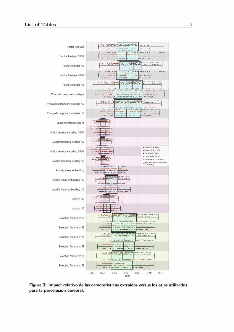
3 Impact relativo de las características extraidas versus los atlas uti-
lizados para la parcelación cerebral. . . . . . . . . . . . . . . . . . . 6
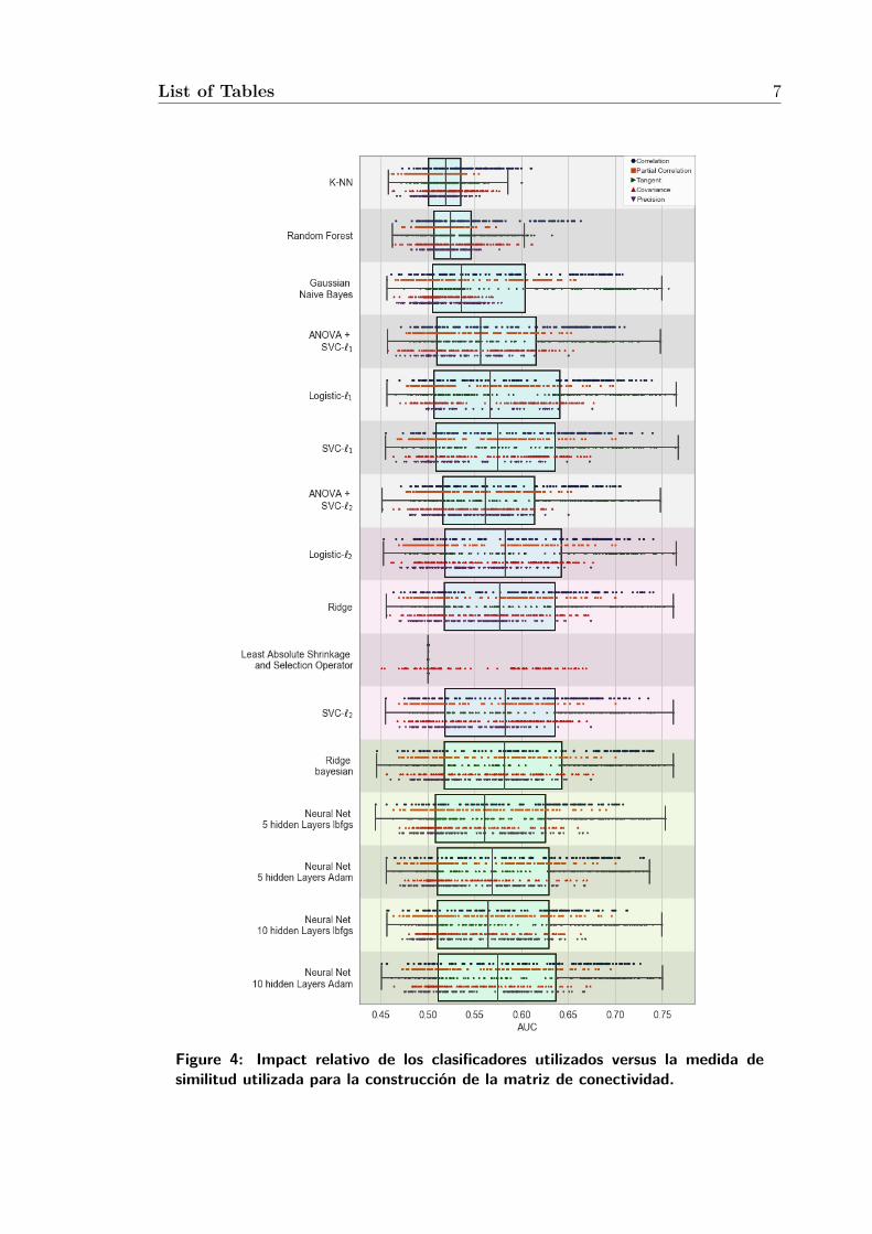
4 Impact relativo de los clasificadores utilizados versus la medida de
similitud utilizada para la construcción de la matriz de conectividad. 7xi

List of Figures xii
1.1 Functional connectome predictive analysis pipeline steps after rs-
fMRI data preprocessing (not shown): 1) given a parcellation of the
brain, 2) obtain the representative time series of each region by aver-
aging the time series of voxels within the region, 3) build the connec-
tivity matrix by computing a similarity measure between each pair of
representative time series, 4) carry out cross-validation experiments,
using Machine Learning algorithms for feature extraction and classi-
fier training; 5) report test results on the prediction of the ASC vs
TD. . . . . . . . . . . . . . . . . . . . . . . . . . . . . . . . . . . . . 13
3.1 Examples of common MRI artifacts: (A) k-space artifact; (B) ghost-
ing in a phantom; (C) susceptibility artifact; and (D) spatial normal-
ization artifact. [1] . . . . . . . . . . . . . . . . . . . . . . . . . . . . 33
3.2 Block design fMRI experiment. A neural response to the state change
from A to B in the stimulus is accompanied by a hemodynamic re-
sponse that is detected by the rapid and continuous acquisition of MR
images sensitized to BOLD signal changes. Using single- or multi-
variate time series analysis methods, the average signal difference
between the two states is computed for the scan and a contrast map
generated. A statistical activation map is finally obtained using a
suitable threshold for the difference; the map depicts the probability
that a voxel is activated given the uncertainty due to noise and the
small BOLD signal differences. . . . . . . . . . . . . . . . . . . . . . . 35
3.3 An image (top left) is warped to match a template (top right) to
produce a spatially normalized version (top center). For clarity, the
original image was approximately aligned with the template, and the
warping was only done in two dimensions. The bottom row shows
the difference between the template and image, both before and after
the warping [2]. . . . . . . . . . . . . . . . . . . . . . . . . . . . . . . 37
3.4 Skull-stripping steps: (A) input images, (B) brain contouring, and
(C) removal of nonbrain tissues [3]. . . . . . . . . . . . . . . . . . . . 38

List of Figures xiii
3.5 Realigment: (A) input image, (B) Voxel-Based Registration Method,
and (C) Boundary-Based Registration Method [4] . . . . . . . . . . . 38
3.6 Results of the smoothing data analysis: t-maps (top) and thresholded
images (bottom) obtained using spatially adaptive smoothing and
fixed Gaussian kernels with various widths from [5]. . . . . . . . . . . 39
3.7 Different methods of Slice time correction: A) FSL B)SPM and C)FS 39
4.1 A graphical representation of a binary decision tree splitting the space
recursively. . . . . . . . . . . . . . . . . . . . . . . . . . . . . . . . . 51
4.2 Recursive binary partition of a two-dimensional space obtained as a
result of the binary tree in 4.1. . . . . . . . . . . . . . . . . . . . . . 52
5.1 Different learning processes (a) traditional machine learning, and (b)
transfer learning. . . . . . . . . . . . . . . . . . . . . . . . . . . . . . 77
5.2 Types of transfer learning [6] . . . . . . . . . . . . . . . . . . . . . . 78
5.3 An overview of the VGG-16 model architecture, this model uses sim-
ple convolutional blocks to transform the input image to a 1000class
vector representing the classes of the ILSVRC. . . . . . . . . . . . . 80
5.4 Different ConvNet Architectures [7]. . . . . . . . . . . . . . . . . . . . 82
5.5 Residual learning a building block . . . . . . . . . . . . . . . . . . . . 83
5.6 Architecture RESNET . . . . . . . . . . . . . . . . . . . . . . . . . . 85
6.1 Impact of feature selection versus classifiers. . . . . . . . . . . . . . . 91
6.2 Impact of features versus the atlas parcelation of the brain . . . . . . 92
6.3 Impact of classifiers versus the connectivity measure . . . . . . . . . . 93
6.4 Density plots of the median AUC results achieved from the different
brain parcellations tested in the experiments. . . . . . . . . . . . . . . 94
6.5 Density plots of the median AUC results achieved from the different
measures used to build the connectivity matrices. . . . . . . . . . . . 95

List of Figures xiv
6.6 Density plots of the median AUC results achieved from the differ-
ent classifiers tested in the experiments. Neural10a =10 hidden lay-
ers MLP trained with adam procedure, SVC L2= non sparse SVC,
b_ridge=bayesian ridge regression, GNB=gaussian naive Bayes, RF=random
forest. . . . . . . . . . . . . . . . . . . . . . . . . . . . . . . . . . . . 96
6.7 Density plots of the median AUC results achieved from the different
feature extraction approaches. PCA2 = PCA retaining only half of
the features, MDS2000, fa2000= MDS, FA retaining 2000 features,
LNE3=LNE retaining one third of the features, p90= PCC selection
90% percentile. . . . . . . . . . . . . . . . . . . . . . . . . . . . . . . 97

List of Tables
2.1 Behavioral approaches to CAD for ASC characterization. . . . . . . 20
2.2 Summary of Biomarker and CAD findings for autism. . . . . . . . . 24
3.1 Number of regions of the brain parcellations used in this Thesis. . . 41
3.2 State of the art results of the classification ASC vs. TD on the
functional connectivity data of ABIDE I dataset. 24ISC=24 inter-
hemispheric selected connections, Acc=Accuracy, ADM=additional
demographic features, AUC= Area under the ROC, BASC=Bootstrap
Analysis of Stable Clusters, CC200=Craddock200, DNN= Deep neu-
ral network, E3DCNN=ensemble 3D convolutional networks, ECM=eigenvalues
of connectivity matrix; EGC=Ensemble of GCNs, GNB=Gaussian
naive Bayes, GNG=G naive graph, HO= Harvard Oxford, kNN=k-
Nearest Neighbors, LDA=linear discriminant analysis, LR= logistic
regression, LSTM=Long Short-Term Memory networks, maLRR=
multisite adaptation low rank decomposition, MODL= massive on-
line dictionary learning, MSDL=multi-subject dictionary learning,
MTGM=multi-task graphical model, NC= network centralities; RF=random
forest, RRC=ridge regression classification, SFM=spatial feature de-
tection method, SFS= sequential feature selection, SGC=spectral
graph convolution, SP=stochastic parcellation, TT=Teilarach & Tournoux,
WC=Ward’s clustering. . . . . . . . . . . . . . . . . . . . . . . . . . 45
6.1 Demographics distribution per site of the ABIDE I dataset. Test =
the subject underwent DSM IV TR test. A = Autism, C = Control . 88xv

List of Tables xvi
6.2 One sided (row>column) Wilcoxon’s rank sum test p-values between
median AUC results achieved from the different parcellations used to
extract representative time series for the connectivity matrices. . . . . 90
6.3 One sided (row>column) Wilcoxon’s rank sum test p-values between
median AUC results achieved from the different measures used to
build the connectivity matrices: cv=covariance, pc=partial correla-
tion, p= precision, t=tangent, c=correlation, max=maximummedian
AUC achieved. . . . . . . . . . . . . . . . . . . . . . . . . . . . . . . 94
6.4 One sided (row>column) Wilcoxon’s rank sum test p-values between
median AUC results achieved by the diverse kind of classifiers ex-
perimented with. Neural10a =10 hidden layers MLP trained with
adam procedure, SVC `2= non sparse SVC, b_ridge=bayesian ridge
regression, GNB=gaussian naive Bayes, RF=random forest. . . . . . 96
6.5 One sided (row>column) Wilcoxon’s rank sum test p-values between
median AUC results achieved from the different best versions of the
feature extraction algorithms. PCA2 = PCA retaining only half of
the features, MDS2000, fa2000= MDS, FA retaining 2000 features,
LNE3=LNE retaining one third of the transformed features. . . . . . 97
6.6 Best median AUC scores found in cross-validation repetitions, with
corresponding settings (parcellation, feature extraction, classifier, and
connectivity measure) that achieved it. . . . . . . . . . . . . . . . . . 99
6.7 Best Acc scores found in cross-validation, with corresponding settings
(parcellation, feature selection, classifier, and connectivity measure)
that achieved it. . . . . . . . . . . . . . . . . . . . . . . . . . . . . . 99
7.1 Results of explored CNN topologies. We report median accuracy,
brain parcellation (parcel.) and connectivity measure (conn. meas.)
with best results. n@m denotes a convolution layer with n filters
of size m. full denotes full connectivity layer. Output is always a
softmax of two units. E denotes the number of CNNs in an ensemble. 102

Resumen en castellano
Introducción
La prevalencia de los transtornos del espectro autista (TAE) es creciente y se han
desarrollado soluciones técnicas para ayudar a un diagnóstico más preciso y más
temprano. Más preciso debido a la heterogeneidad de la esta condición que presenta
caracteristicas muy dispares, hasta el punto que es dificil de establecer fronteras en-
tre fenotipos concretos. Las soluciones tecnológicas van desde el estudio objetivo del
comportamiento mediante técnicas de monitorización del movimiento o de respuesta
a estímulos, como soluciones de visión por computador que analizan la existencia de
patrones de movimientos repetitivos típicos de esta condicion, o como aplicaiones
implementadas en tablets que permiten monitorizar mediante los sistemas inerciales
incorporados a la tablet la dinámica de la respuesta en el manejo de la tableta y
su interaccion, hasta los métodos de observación de la actividad neuronal, como los
sistemas de electroencefalografía (EEG) o los métodos de observación basados en
imagen de resonancia magnética. Concretamente, se busca la estructura de la conec-
tividad entre regiones del cerebro para comprobar si existen indicadores (biomar-
cadores) de la condición en esta estructura cerebral. Se consideran las redes que se
crean en reposo, en el denominado resting state. La imagen funcional de resonan-
cia magnética juega un papel fundamental en esta investigación puesto que aporta
una gran resolución espacial para la localización de los efectos correlacionados con
la condición TAE. Se han generado en la comunidad cientifica bases de datos de
sujetos TAE y controles de gran tamaño para el estudio sistemático de la existencia
de estos biomarcadores. En esta Tesis Doctoral, nos hemos concentrado en una base
de datos concreta, denominada ABIDE, que recoge un alto numero de sujetos. De1

List of Tables 2
Figure 1: Flujo de proceso típico de una analisis predictivo de la condición TAEbasada en datos de imagen funcional de resonancia magnetica que permite calcu-lar la matriz de conectividad cerebral. 1) Parecelación del cerebro, 2) obtenciónde las series temporales representativas de cada región cerebral, 3) cálculo dela matriz de conectividad basada en una medida de similitud entre series tem-porales, 4) construccion demodelos predictivos y realizacion de experimentos devalidacion cruzada, 5) resultados de la capacidad de discriminación TAE versusdesarrollos típicos (DT)
ella hemos seleccionado sujetos control y sujetos con diagnóstico TAE definitivo, un
total de 871, para la realización de experimentos computacionales sobre sus matri-
ces de conectividad cerebral extraidas a partir de sus datos de imagen funcional de
resonancia magnética en estado de reposo.
El flujo de proceso general para el analisis mediante algoritmos de aprendizaje
máquina sobre la información de conectividad cerebral se ilustra en la figura 1.
Las matrices de conectividad cerebral funcional se extraen de los datos de imagen
funcional en estado de reposo y se procesan como sigue:
1. Se aplica una parecelación del cerebro a los volumenes de datos funcionales de
resonancia magnética. Existen varias parcelaciones definidas en la literatura,
por lo que corresponde seleccionar una de ellas.
2. Las series temporales asociadas a los voxeles que están incluidos en una región
cerebral se agregan para obtener una unica serie temporal que será la repre-
sentante de esa región cerebral, usualmente mediante el calculo del promedio.
3. Se construye la matriz de conectividad calculando la similitud entre los rep-
resentantes de cada par de regiones de la parcelacion cerebral. Existen varias
alternativas en la literatura sobre cual es la medida de similitud más apropiada.
List of Tables 3
La matriz de conectivdad es siempre simétrica y se puede interpretar como la
matriz de adyacencia de un grafo definido sobre las regiones del cerebro.
4. La matriz de conectividad es la materia prima para los procesos de aprendizaje
máquina que incluyen técnicas de extracción de caracteristicas (features) y
técnicas de construcción de clasificadores basados en dichas caracteristicas
como entrada. La selección de características corresponde a la selección de
conexiones cerebrales específicas en base a criterios de saliencia de la similitud
entre regiones. En este caso, las conexiones seleccionadas pueden pasar a ser
biomarcadores para la condición TAE.
5. Se realizan experimentos de validación cruzada para establecer el rendimiento
relativo de cada una de las posibilidades de elección técnica en cada fase del
flujo general
El rendimiento de los algoritmos de clasificación puede estar fuertemente influido
por las decisiones tomadas en cada fase del proceso, concretamente la selección
de la cohorte, la parcelación del volumen cerebral, la estimación de la matriz de
conectividad, el algoritmo de extracción/seleccion de características y el modelo de
clasificador.
Objetivos y metodología
El objetivo fundamental de esta Tesis Doctoral es la evaluación del impacto de
las distintas elecciones que se realizan al llevar a cabo el proceso general en el
rendimiento discriminante entre TAE y sujetos con desarrollo típico. Para ello se ha
realizado una exploración exhaustiva de todas las posibles combinaciones respetando
la metodología rigurosa de la evaluación de sistemas de clasificación. Esto es, hemos
realizado múltiples repeticiones de un proceso de validación cruzada con separación
estricta de los conjuntos de datos de entrenamiento y de test, con absoluta separación
de los procesos de entrenamiento respecto de los datos de test.

List of Tables 4
Contribuciones
Las contribución principal de esta Tesis Doctoral es un exhaustivo examen del efecto
que tiene la elección de la parcelación del cerebro, la medida de similitud utilizada
para construir la matriz de conectividad, el proceso de extracción de características,
y el modelo de clasificación entrenado sobre las características extraidas de las ma-
trices de conectividad. En este trabajo se ha evitado introducir sesgos como los que
introduce la selección de la cohorte experimental. Este proceso de selección explica
los resultados muy elevados de rendimiento que no son transferibles a otras cohortes
extraidas de la misma base de datos ABIDE.
Resultados
Las figuras 2, 2, y 3 sumarizan los resultados obtenidos en los experimentos con-
frontando los clasificadores utilizados, los atlas de parcelación, las medidas de simil-
itud y la extracción de caracteristicas.
En la figura 2 se puede apreciar que el efecto de la extracción de caracteristicas
es muy superior al de la selección de un clasificador específico, especialmente el
analisis factorial, analisis de componentes principales y la correlación de Pearson
son comparables. En la figure 3 se aprecia la misma situacion, en la que los métodos
de extracción de características tienen mucho más efecto que los atlas de parcelación.
Finalmente, en la figura 4 se observa que las medidas basadas en la tangente y la
correlacion tiene la mayor varianza. En general, la elección del clasificador no tiene
un gran impacto, salvo pequeños efectos de KNN y Random Forest.
Conclusiones
La primera conclusión extraida de nuestro trabajo experimental es el bajo rendimiento
obtenido en general. Este bajo rendimiento se debe a la heterogeneidad de los datos,
que proceden de diversos centros los cuales tienen distintos instrumentos de resonan-
cia magnética, distintos protocolos de imagen, y distintos protocolos de diagnóstico
lo que lleva a etiquetados inhomogeneos y a datos que presentan una alta variabil-

List of Tables 5
Figure 2: Impacto relativo de la extracción de caracteristicas versus los clasifi-cadores utilizados.
List of Tables 6
Figure 3: Impact relativo de las características extraidas versus los atlas utilizadospara la parcelación cerebral.
List of Tables 7
Figure 4: Impact relativo de los clasificadores utilizados versus la medida desimilitud utilizada para la construcción de la matriz de conectividad.

List of Tables 8
idad intercentro. La segunda gran conclusión es que el mayor efecto se produce
en la selección de características, mientras que la selección del clasificador es casi
irrelevante.

Chapter 1
Introduction
This chapter presents the background and motivation for this Thesis in section
1.1. Section 1.2 describes the objectives of this research work. A summary of
the generated contributions is given in section 1.3. The research environment and
context are described in section ??. The related publications are listed in section
1.4. Section 1.5 presents the structure of this Thesis.
1.1 Background and Motivation
Autism Spectrum Condition (ASC) [8,9] is a highly prevalent, heritable and hetero-
geneous neurodevelopmental disorder that has distinctive cognitive features often
cooccuring with other psychiatric or neurological disorders. It is the subject of a
broad and intense research effort, with more than 40 EU funded research projects
devoted to some of its aspects in the last 20 years. Similar effort is being done
in China, USA, Russia, and South America looking for its causes at various levels:
genetic, metabolic, neural or brain based. Searching for the pathogenesis leads also
to findings which are also diagnostic indications, i.e. biomarkers of the disorder that
can be used to guide early diagnosis, which in its turn may allow to apply thera-
peutic or palliative treatments from an early age. ASC computer aided diagnosis
(CAD) has been gaining interest in the scientific community in the recent years,
aiming to contribure to its early detection. In this report we gather the approaches
that have been reported in the recent literature trying to be comprehensive, though9

1.1. Background and Motivation 10
keeping pace of the reported results may be difficult. Some CAD approaches are
based on behavioral characterizations, while the majority of approaches are based
on the analysis of brain neural activity and morphology in some way or another.
Most recent studies are focused on the detection of brain functional connectivity
anomalies using specific signals such as electroencephalographic (EEG) recordings
or functional magnetic resonance imaging (fMRI). The emergence of large public
repositories of data is boosting research in this topic.
1.1.1 Prevalence
Across the Autism and Developmental Disabilities Monitoring (ADDM) Network
sites, estimated ASC prevalence among children aged 8 years was 23.4 per 1,000 (one
in 43) boys and 5.2 per 1,000 (one in 193) girls [10]. Thus ASC appears to require
specific research programs contemplating explictly the impact of sex/gender related
issues [11, 12]. Some references [13] state that the overall worldwide prevalence of
ASC is as high as 1% of the population, while others [14] argue that non specific
diagnostic criteria recently included in the diagnostic protocol produce as an artifact
the 20-fold increase in its prevalence. Therefore, the heterogeneity in ASC features
that hinders the identification of biomarkers could be a side effect of excessively
wide diagnostic criteria. A recent normative study [15] on brain cortical structure
modeled by a probabilistic predictive model concluded that there is some indication
that sexual-related characteristics of the brain are highly correlated with ASC.
1.1.2 Diagnosis
ASC is currently diagnosed on the basis of qualitative information obtained from
parent interviews and clinical observation, which leads to disturbing differences be-
tween sites [16]. Given its great prevalence, automated approaches to assist diagno-
sis [17, 18] are highly desirable. Increasingly, clinical neuroscience focus is shifting
to find metrics derived from brain imaging [19] that may be useful to predict di-
agnostic category, disease progression, or response to intervention, e.g. looking for
endophenotype using multivariate analysis approaches [20]. These metrics come

1.1. Background and Motivation 11
from machine learning approaches to the study of brain structure and function.
Some of them can be considered as neuroimage based biomarkers that would be
helpful to guide early interventions. Currently, the research community has not
yet identified reliable and reproducible biomarkers for ASC. Clinical heterogeneity,
methodological standardization and cross-site validation raise issues that must be
addressed before further progress can be achieved [21].
1.1.3 Datasets
A central role in the effort to obtain robust and reproducible biomarkers is played by
the availability of public datasets, such as the Autism Brain Imaging Data Exchange
(ABIDE) dataset [22, 23] that includes demographic, clinical information and data
from several magnetic resonance imaging (MRI) modalities allowing for a variety of
studies such as brain maturity estimation as a biomarker of brain abnormality [24].
1.1.4 Pattern recognition for CAD
A wide variety of machine learning and pattern recognition studies on the develop-
ment of CAD systems for ASC have been reported [25] exploiting a variety of infor-
mation sources, including structural, diffusion and functional MRI, as well as elec-
troencephalography (EEG) [26–28], additional demographic and clinical data [29],
and behavioral measurements captured by computer vision or other body mea-
surement approaches [30]. There are meta-analysis confirmations of ASC imaging
biomarkers from anatomical MRI [31], and diffusion MRI imaging [32, 33]. The
latter showing white matter integrity disruption. Connectivity based brain par-
cellation [34] provided additional evidence of altered white matter connectivity in
ASC.
1.1.5 Brain functional connectivity
A main goal of this Thesis is the exploration and validation of ASC biomarker dis-
covery based on brain functional connectivity information using artificial intelligence
approaches, namely namely machine learning and deep learning techniques. Brain
1.1. Background and Motivation 12
functional connectivity analysis based on resting state functional MRI (rs-fMRI) can
be done by seed analysis, where the specific connectivity relative to a selected brain
region is compared across subjects and populations [34], or on the basis of brain
parcellations into a set of regions of interest (ROIs) which can be defined either
by anatomical guidelines or by data driven unsupervised segmentation [35]. In any
case, rs-fMRI connectivity analysis has been accepted as a source of information for
the discovery of biomarkers of psychiatric disorders [36] such as schizophrenia [37]
and ASC [21].
Neuroimage biomarker discovery over functional connectivity data may be guided
by statistically significant differences between ASC and typically developing (TD)
subjects. For instance, t-test on the dynamical network strength of ASC vs. TD was
reported to confirm identification of aberrant connectivity in ASC subjects [38], and
significant differences between ASC and TD in the level of activation of thalamic
connectivity have been identified by independent component analysis (ICA) [39]. In
predictive analysis approaches to biomarker identification, the subject’s condition
(ASC vs. TD) prediction performance achieved is the measure of the biomarker
significance. Predictor models are built by machine learning techniques, often con-
sisting of two steps: a dimensionally reduction (aka feature extraction or feature
selection) followed by a classification step for class prediction. Though discrimi-
nation between ASC and TD is the most common paradigm, some works [40, 41]
compare ASC with Schizophrenia over a small cohort, while others consider patterns
for discrimination among low-functioning and high-functioning ASC subjects [42].
1.1.6 Computational pipeline
The general pipeline of predictive analysis for brain connectivity based biomarkers
is illustrated in Figure 1.1. Functional connectivity matrices are extracted from
preprocessed rs-fMRI data as follows:
1. A parcellation of the brain is defined;
2. The time series corresponding to the voxels in each region of the parcellation
are aggregated into one representative time series often by averaging;

1.1. Background and Motivation 13
Figure 1.1: Functional connectome predictive analysis pipeline steps after rs-fMRIdata preprocessing (not shown): 1) given a parcellation of the brain, 2) obtain therepresentative time series of each region by averaging the time series of voxelswithin the region, 3) build the connectivity matrix by computing a similaritymeasure between each pair of representative time series, 4) carry out cross-validation experiments, using Machine Learning algorithms for feature extractionand classifier training; 5) report test results on the prediction of the ASC vs TD.
3. The connectivity matrix is built computing the similarity among the repre-
sentatives of each pair of regions in the parcellation. Hence the connectivity
matrix is always a symmetric matrix that can be interpreted as the adjacency
matrix of a graph representing the relations among brain regions.
4. The connectivity matrix is then used as the raw data for machine learning
processes which may involve feature extraction/selection. Feature selection
involves the selection of specific connections that may become identified as
biomarkers.
5. Predictive performance is estimated by the training/testing of classification
models often in a cross-validation scheme.
Predictive performance may be heavily influenced by the decisions made at each
step of the study, namely by the cohort selection, the choice of brain volume parcel-
lation, the functional connectivity matrix estimation procedure, the feature selec-
tion/extraction algorithm applied, and the classification model building algorithm.
After the cross-validation assessment, the cross-validation classification performance
results may be used to identify biomarkers in the connectivity matrix.

1.2. Objectives 14
1.2 Objectives
The main objective of this thesis is to explore the eficiency of machine learning
approaches, including more recent deep learning techniques, to the CAD of ASC
subjets, stated as a classification problem of ASC versus healthy controls (aka typ-
ically developing (TD) children).
We want to assess the impact of the various metaparameter choices in com-
putational pipeline of Figure 1.1. If possible we would like to select the optimal
combination of such metaparameter choices.
Operational objectives implemented in the pursue of this general objective are:
• Identifiying and recovering a representative dataset for the realization of the
computational experiments
• Implementation of the exploitation of the diverse feature extraction, classi-
fier building algorithms, cross validation procedures, and performance result
collection and analysis.
• Carrying out the computational experiments assessing the performance of the
various combinations of metaparameter choices, managing the combinatorial
complexity of the data coming out from the experiments.
1.3 Contributions
In this Thesis, the functional connectivity matrix computed from rs-fMRI data is
the sole source of information for classification.
We explore the impact of choices made in the implementation of the machine
learning pipeline of Figure 1.1 for the prediction of ASC vs. TD.
We have carried out extensive cross-validation experiments over the algorithmic
choices at each step of the classification model building pipeline.
We report the impact on predictive performance ASC vs TD of all combinations
of:
• five feature extraction/selection approaches,
1.4. Publications 15
• six brain parcellations,
• five functional connectivity matrix computation methods, and
• ten classification model building techniques.
This comprehensive comparison of classical machine learning approaches encom-
passes more than eleven thousand (11500) cross-validation experiments.
We report statistically significant differences in performance found as well as
direct comparison to state of the art published results.
We found that specific combinations of pipeline choices can boost the perfor-
mance of ASC vs. TD classification based on brain functional connectivity data.
The software needed to replicate the experiments reported in this Thesis have
been published in github1.
1.4 Publications
Publications related with the content of this Thesis:
• Impact of Machine Learning Pipeline Choices in Autism Prediction From Func-
tional Connectivity Data; Graña, M. & Silva, M. International Journal of
Neural Systems , Vol. 31 , pp. 2150009 , 2021
• Impacto y regulación de la inteligencia artificial en el ámbito sanitario Karina
Medinaceli, M. S. REVISTA IUS , 2021
• On Machine Learning for Autism prediction from functional connectivityMoi-
ses Silva , Manuel Graña, CORES21, The 12th International Conference on
Computer Recognition Systems June 28–30, 2021 Bydgoszcz, Poland
1.5 Structure of the thesis
This thesis is structured as follows:
1https://github.com/mmscnet/Impact-feature-extraction-in-Autism

1.5. Structure of the thesis 16
• Chapter 2 discusses the role fo computer aided systems in the dignosis of
Autism Spectrum Condition. We review several paradigms besides the brain
connectivity approach that is the main focus of the Thesis.
• Chapter 3 provides a detailed review of approaches and resources for the anal-
ysis of brain connectivity directed to the finding of biomarkers of Autism
Spectrum Condition from the point of view of machine learning.
• Chapter 4 provides the descritption of the machine learning tools and tech-
niques applied in the search of optimal classification of Autism Spectrum Con-
dition subjects on the basis of brain connectivity.
• Chapter 5 provides the description of the deep learning approaches tested in
the framework of this Thesis, including transfer learning approaches.
• Chapter 6 provides the report of the results achieved with machine learning
techniques over the ABIDE database.
• Chapter 7 reports the results achieved over the ABIDE dataset using deep
learning techniques.
• Finally, Chapter 8 presents the conclusions and future lines of work.

Chapter 2
State of the art of Autism
diagnostic technological tools
In this Chapter we review the state of the art on the use of technological support
for the diagnosis of autism. The contents of the Chapter are as follows: Section
2.2 presents behavior measurement based CAD approaches. Section 2.3 presents
EEG based CAD approaches. Section 2.4 presents MRI based biomarker finding
efforts. Section 2.5 presents MRI based CAD approaches. Section 2.6 presents public
available data repositories. Finally, Section 2.7 gives some concluding remarks.
2.1 Introduction
Computer aided diagnosis (CAD) aims to help the clinical practitioner to achieve
early and accurate diagnosis of ASC in order to try to apply early treatments hop-
ing to improve the child’s condition in some way. Recent randomised control tri-
als [43–48] emphasize the improved effect achieved when the treatment is applied
at early ages, even todlers. Here we will not discuss the clinical aspects such as
treatment protocols or diagnositic procedures follow in the clinic, focusing only on
the technological aspects. A CAD system often is composed of some technological
device that allows to measure the behavior or some biological or physiological as-
pect of the subject, and some classifier system built by machine learning techniques
that provides the diagnosis suggestion. Machine leraning can be used to build hi-17

2.1. Introduction 18
erarchies of categories which may help to refine diagnostic process [49], but mostly
is used to give a response to the question “Is this child at high risk of ASC?”. It
is important to keep in mind that ASC is a quite heterogeneous condition that is
still under revision by the clinical experts, therefore all the technological solutions
would be always limited in their scope by some a priori selection of measures and
expected observations. Regarding the kind of knowledge modeling approach used,
the literature offers a wide variety:
• Rule based expert systems [50].
• Deep learning architectures [51,52] and shallow artificial neural networks [53].
• Support Vector Machines [52, 54–57].
• Statistical inference (i.e. ANOVA) is traditionally used in biomarker identifi-
cation.
Regarding the kind of information used, the literature refers the following at least:
• Qualitative information produced by reports from parents and caregivers [50,
58].
• Genetic and metabolic information such as the selection of microarray ex-
pression data [54, 55, 59, 60], or the detection of specific metabolites that are
hypothesized to be related to ASC [56].
• Brain imaging data, often from diverse MRI modalities [21]. Structural brain
imaging is widely recognized as a rich source of information for the neuropsy-
chological analysis of the brain [61–65]. Also, brain functional imaging may
be providing a wealth of information on the effects on brain connectivity that
may be at the root of the ASC [66–72]. Diffussion spectrum MRI have been
also proposed [73–75] for high precision white matter fiber tracking. Finally,
there are increasingly facilities for multimodal data processing [76].
• Diverse motion capture devices which provide quantitative information about
the subject responses and motion.

2.2. Behavior measurement based CAD approaches. 19
• EEG data that can be used either for brain functional connectivity analysis
or as features for classification processes.
• Functional near-infrared spectroscopy (fNIRS) is a recent approach to measure
the brain activitiy wich already gives some discrimination results regarding the
processing of faces by ASC children [77].
Most of the CAD approaches are developed over small local datasets, posing prob-
lems of reproducibility and generalization of the results. In some areas, such as brain
imaging, there are efforts to collect big repositories of data coming from many re-
search centers. As will be discussed later, these efforts pose the additional difficulty
of dealing with inter center variability of data recording procedures and methods.
2.2 Behavior measurement based CAD approaches.
Some approaches use behavioral information measured by computer vision or an-
other sensing technique. They can be rooted in an enactive approach to autism
understanding [101], focusing on disruptions to action perception [102]. Table 2.1
summarizes the literature found so far1. Some approaches measure the response of
the child to stylized representations, such as the discrimination of geometric figures
from visualization of grasping [103]. In general, a wide variety of sensors can and
have been used to monitor the behavior and assess the risk of ASC [104–106] either in
isolation or in some kind of information fusion. For instance, in [79] authors propose
the measurement using computer vision of the imitation response of ASC children
versus neurotypical children to discriminate them. Another non intrusive approach
to discriminate ASC children uses the inertial information of a smart tablet [80].
The authors find definitive patterns of motion that are compatible with the ASC
clinical characterization, larger and faster motions, stronger forces at contact, with
1Explanation of acronyms: CA conversation analyis, CV computer vision, EMT eye motiontracking, EOG electrooculogram, FD face detection, FER facial expression recognition, MoCapMotion Capture, MA mobile application, WA wrist accelerometers, GE gaze estimation, HPEhead pose estimation, LE landmark extraction, MI Magneto-Inertial, MMN mismatch negativity,OMC object motion capture, PA pupil analysis, POMDP Partially Observable Markov DecisionProcess SR speech recognition.

2.2. Behavior measurement based CAD approaches. 20
Table 2.1: Behavioral approaches to CAD for ASC characterization.
ref sensor approach robot?
[78] CA
[79] CV
[80] tablet dynamical analysis
[81] kinect MoCap
[82] WA dynamical analysis
[83] CV FD,LE,GE, HPE,FER
[84], [85], [86, 87] CV MoCap
[88] CV GE,PA y
[89] EOG EMT
[90] MA pictograms
[91] CV,SR name calling
[92] CV OMC
[93] CA, MMN
[94] EMT
[95] CV FD
[96] CV POMDP y
[97] Haptic, kinect
[98] tablet target tracking
[99] MI
[100] CV MoCap y

2.2. Behavior measurement based CAD approaches. 21
more distal use of space. Another approach uses the Kinect V2 sensor in order to
measure the motions of the subjects and try to detect stereotypical motor reactions
which are the hallmark of autism in clinical diagnosis processes. The experiments
reported with motion captured from professional actors promised that this detection
can be achieved with great probability [81]. Detection of motion by means of wrist
accelerometers has been reported by [82] achieving discrimination of children at high
risk versus low risk of ASC in the realization of some motor tasks. A comprehen-
sive behavior observation system encompasing face detection, landmark extraction,
gaze estimation, head pose estimation and facial expression recognition has been
proposed in [83] to make a continuous assessment of the evolution of the ASC sub-
jects under treatment. Another motion analysis system, tracking the motion of
diverse body parts while the subjects are inmersed in an interactive discussion in-
volving turn taking, has demonstrated significant differences between ASC and TD
subjects [84]. Similarly, tracking body motion while engaging with a social robot
was found discriminant in [85]. Computing the dynamic time warping (DTW) dis-
tance between the robot motion and the child motion while engaging in an imitation
game was intended as a measure of impairment in [100]. The examination of the
gaze and the pupil while interacting with a robotic avatar has been also shown to
be lead to moderate classification accuracy [88]. The measurement of eye motion
when tracking objects by means of an electrooculogram has been also show capable
of high accuracy discrimination of ASC subjects [89], while serving also to train the
subjects to perform more accurate object tracking. Also it showed that the ASC
children retain intact shape appreciation while losing emotional content [94]. From
a different point of view, proposal in [96] consists in the modeling of child behav-
ior by means of Partially Observable Markov Decision Process (POMCP) from the
incomplete observations made by a robot interacting with the child.
In a different approach, a mobile application is proposed [90] that helps in the
screening of children by evaluating their responses to pictogram based questionaire.
Childs with high risk of ASC are referred to a specialized centre. Another early
screening proposal involves the close monitoring of classroom to study the reaction
to name calling of the children [91]. This system has voice recognition as well
2.3. EEG based CAD approaches. 22
as human body posture and reaction monitoring. For instance, subject vitality is
measured by tracking object motion speed using hidden infrared markers with six
infrared cameras, while the subjects are performing simple picking tasks [92]. The
measurement of stereotypical motion was also a way to characterize ASC interacting
skills [86, 87]. The measurement of reaching acts mediated by a robotic arm was
found to differ from ASC to TD young adults [107] with better performance for
ASC when the error refers to properctive senses, while it is the converse when error
is measured by visión. The analysis of brain volumes through MRI indicates that
there are significant variations of volume in lobule VI, and parts of lobule VIII.
The responses to a mismatch experiment of sounds (vowel, vowel duration, conso-
nant, syllable frequency, syllable intensity) showed significant differences in children
(8-12 year old) with asperger syndrome in intensity and frequency relative to typ-
ically developing children [93] leading to conclude aberrant cortical sound-speech
discrimination in Asperger syndrome children. Conversation analysis is used while
a ASC child is interacting with a robot trying to ascertain if he has perseverative
talking features [78] one of the traits of high performing ASC children. The se-
quential analysis showed that recurrence may be driven by the interaction scenario.
Other experiments measured the response of ASC versus TD children when viewing
silouhettes of human and robotic [108] measuring the mimicry as the project results.
Target tracking in a tablet device provides behavioral information that can be
used for assessment of sensorial impairment [98], while a magneto-inertial platform
is proposed in [99] for the assessment of motor skills.
2.3 EEG based CAD approaches.
Electroencephalographic (EEG) sensors of neural activity have been also used to
explore the feasibility of identifying brain biomarkers of ASC or to implement CAD
systems based on their readings. Some works have achieved discrimination between
ASC and TD children in small cohorts [109] applying some feature extraction pro-
cedures that include the techniques from non-linear chaotic time series analysis and
time frequency decomposition, such as the fractal dimension. Another proposed

2.4. MRI based biomarkers. 23
computational pipeline involves wavelet decomposition, entropy feature extraction
from each EEG sub-band and a classifier based on ANNs [53]. Another kind of
ANN, uses the self-organizing map (SOM) for feature extraction reporting results of
a number of conventional classifiers upon the SOM features [110]. Classification ori-
ented research, however, does not provide clinical or biological insights because it is
often impossible to translate back the significative features into biological causes or
biomarkers that can be useful to understand the condition and propose treatments.
Looking for biomarkers, a recent systematic review of studies that have used EEG
and magnetoencephalography (MEG) data for brain connectivity analysis reports
underconnectivity in long-range connections for ASC subjects, while local connec-
tions seem to be unafected [111]. Recent approaches fuse EEG information with
other sources such as MRI information [112].
2.4 MRI based biomarkers.
Another track for research into the existence of anomalies in brain morphology
and functionality connectivity is the use of various modalities of magnetic resonance
imaging (MRI), namely structural (T1-weighted) MRI, resting state functional MRI
(rs-fMRI) and diffusion weighted imaging (DWI), and magnetic resonance spec-
troscopy (MRS) are the most relevant modalities found in the literature aiming to
identify ASC biomarkers [126, 134]. Table 2.1 provides a summary of the literature
worked out so far2.
The neural circuit mechanisms taking care of the regulation of social behaviors
are key to find such biomarkers [135]. For instance, structural MRI has provided
2Explanation of acronyms: Machine learning RF: Random Forest; SVM: Support Vector Machine; CART:Classification and Regression Trees; GBM: Gradient Boosting Machine; RFE: Recursive Features Elimination; PSO:Particle Swarm Optimization; DBN: Deep Belief Network; DNN: Deep Neural Network; ICA: Independent Com-ponent Analysis; GCT Granger Causality Test; LSTM: Long Short-Rerm Memory; ROI: Region of Interest; GLM:General Linear Model; RW: Random Walk; WBA: voxel-wise Whole Brain Analysis; Anatomical referencesRSFG: Right Superior Frontal Gyrus, MFG: Middle Frontal Gyrus; IFG: Inferior Frontal Gyrus; FFA: FusiformFace Area; OFA: Occipital Face Area; EBA: Extrastriate Body Area; STS: Sulcus Temporal Superior; CC: CorpusCallosum; LUF: Left Uncinate Fasciculus; SLF : Superior Longitudinal Fasciculus; CP: Cerebral Peduncle; SCC:Splenium Corpus Callosum; PCC : Posterior Cingulate Cortex; SFG/mPFC: Superior Frontal Gyrus/Medial Pre-frontal Cortex; LPC: Left Parietal Cortex; RPC: Right parietal Cortex; Hipp: Hhippocampal formation; RSN:Resting State Network; CB: Cingulum Bundle; A/SL-F: Arcuate/Superior Longitudinal Fasciculus; UF: UncinateFasciculus.

2.4. MRI based biomarkers. 24
Table2.2:
Summary
ofBiom
arkerand
CAD
findingsfor
autism.
refMod.
BD
Anal.
Findingsreview
[113]fM
RI
IMAGEN
RSFG
,rMFG
[114]sM
RI,D
TI
y
[115]DTI
ROI,W
BA
CC,C
B,A
/SL-F,UF,ST
Gy
[116]rs-fM
RI
ABID
ELST
M
[117]rs-fM
RI
ABID
EROI,D
NN
[118]rs-fM
RI,sM
RI
ABID
EROI,D
BN
[119]rs-fM
RI
ABID
ERW
[120]rs-fM
RI
ABID
ESV
M(+
PSO
,RFE)
[121]rs-fM
RI
13ASC
-13TD
ICA,G
CT,G
LM
[122]fM
RI
ABID
EROI
PCC,m
PC
[123]sM
RI,D
TI,1H
-MRS
15ADS:18T
DCART,R
OI
CC,IFG
[112]fM
RI,D
TI,EG
G3ASC
ROI,IC
APCUN/P
CC,SFG
/mPFC
,LPC,R
PC
[124]DTI
voxelCP,SC
Cy
[125]DTI
SLF,LUF,C
Cy
[126]sM
RI,fM
RI,rs-fM
RI,D
TI
y
[127]DTI,M
RI
22ASC
;10TD
voxelAmigdala,H
ipp
[128]sM
RI
ABID
ERF,G
BM
VIQ
,AS
[129]sM
RI
ABID
ERF,SV
M,G
BM
[130]fM
RI
15ASC
;14TD
RFE,SV
M,voxel
FFA,O
FA,EB
A,ST
S
[131]DTI
30ASC
,30TD
CC,sA
CC
[132]ABID
Edeep
learn
[133]rsfM
RI

2.4. MRI based biomarkers. 25
evidence of atypical brain lateralization of subjects with ASC [136] in a cohort of 67
ASC subjects and 69 neurotypical subjects with matching IQ and relevant personal
characteristics.
The study of brain regions related to language [137] suggests that the child
can discern the social quality of behavior, but he has limited capability to explain
and rationalize it. These findings confirm the general assessment [138] that ASC
subjects suffer impairments of audio processing at neural level. Other approaches
focus on the motor disabilities searching for correlated regions and performance in
the brain [139]. Other neurophysiological models such as the mirror neurons [140]
seem to have been abandoned in the recent years [141].
Image biomarker findings are quite diverse [134]. Structural MRI findings using
voxel based differences are sometimes contradictory and inconsistent, and heavily
dependent on the technique used and the age of subjects, though some increase in
gray matter and white matter volume was consistently reported, as well as corpus
callosum decrease in volume. Morphological differences in thalamus and striatum
have been also reported using structural features [142]. A long term longitudinal (ac-
cross late childhood, adolescence and adulthood) big scale study of cortical thickness
is reported in [143]. Increased cortical thickness was reported for ASC in the range
between 6 years and adolescence [143], with differences decreasing towards adult-
hood. Other authors report significant differences in temporoparietal regions [144].
One of the questions raised is whether the differences in measurements found in
older children may be due to the actual ASC effects or the years of social disfunc-
tion. Hence, the current preferences of researchers looking for ASC biomarkers is to
do the observations in very early ages, even toddlers. Tractography analysis based
on fractional anisotropy coefficients extracted from DWI data have shown consistent
degradation of main neural tracts, pointing to a degradation of brain connectivity.
Fusion of DTI and sMRI volumetric information has shown differences in preschool
ASC children [127]. The study of brain connectivity in toddlers comparing ASC
with other developmental disorders has been reported using DWI and streamlined
tractography [145]. Over an anatomical parcellation of the brain, the neural path-
ways between them were extracted, and the connectivity strength between brain
2.4. MRI based biomarkers. 26
regions was estimated. The results point to overconnectivity in ASC toddlers versus
other developmental disorders.
The analysis of functional connectivity based on rs-fMRI data has found also
many incoherent or contradictory results heavily dependent on the heterogeneity
of population samples, analysis methods and design of the resting state scan [146].
The accepted conclusion so far is that there is some form of compensation between
reduced long-range connectivity and increased short-range connectivity [111]. The
functional parcellation of the insula allowed to find differences of insula functional
connectivity between ASC and neurotypical subjects [147]. Another study detected
effects in the extrastriate body area (EBA) [148] in fMRI when the task is the
contigency detection of one’s movements with others. Other studies found altered
connectivity from/to the superior temporal sulcus (STS) [149,150].
In reviews of white matter connectivity studies [32,114,124,125], mostly done on
DTI data, it was found recently that there is evidence of alterations in the connec-
tivity of the limbic system, contributing to ASC social impairment, while previous
reviews emphasized decreased connectivity of the corpus callosum, cingulum, and
temporal lobe [115]. On a functional MRI study [151] involving age and IQ matching
ASC and TD subjects playing “stone paper scissor” against human/robot/random
computer some reversed effect on the hypothalamus activity was found in ASC sub-
jects. On the other hand, other authors focus on the motor functional system [139]
as the key to improve the ASC subject outcomes. A recent work points in the di-
rection of alterations of the brain microstructure while the macrostructural features
are mostly preservated as the neurological causes for ASC [152].
The spatial shifting of resting state networks, such as the default mode network,
has been also tested as a biomarker for ASC [153]. The parcellation of the brain
activity into intrinsic connectivity networks allowed to assess their spatial variabil-
ity and its discriminant power, finding that ASC showed greater spatial variability.
These results help to harmonize the contradictory findings of underconnectivity and
overconnectivity in several studies [154]. Increase in intrasubject variability brain
connectivity in time, due to diverse factors such as caffeine intake between sessions,
has been found a potential biomarker for ASC [122]. Connectivity of the thalamus

2.5. MRI based CAD approaches 27
cortex has been studied by rs-fMRI brain networks and anatomical connectivity
computed by diffusion weighted imaging tractography [155] finding diverse patterns
of underconnectivity. On other effort, the connectivity between the cerebellum and
the temporoparietal junction was analyzed in detail using both independent compo-
nent analysis and seed based connectivity analysis [156] finding perturbed input to
the temporal-parietal regions from the cerebelar areas. Some task oriented studies,
such as the longitudinal study in [113] looks at the reward processing brain related
regions and functional connections.
2.5 MRI based CAD approaches
Biomarker identification aims to detect brain regions, connections or biochemical
signatures that show significant differences between ASC and neurotypical popu-
lations. CAD goes one step further, it produces a decision on the diagnosis that
can be used by the clinical practitioner with some confidence. CAD systems re-
quire sophisticated machine learning tools, such as multiview multitask ensembles
of classifiers [157]. Classification experiments based on structural MRI morphologi-
cal features extracted using FreeSurfer give low scores [129].
A tensor based approach to estimate connectivity in rs-fMRI is proposed in [158]
that it is able to extract both the connectome representation and the dynamic
functional connectivity for each subject finding discriminant effects on the putamen
connectivity for ASC subjects. Fine temporal analysis of the rs-fMRI time series, by
clustering them into short time intervals that may be shared between brain regions,
allows more precise classification [159,160]. On the other hand, structural features of
brain cortex were used by random forest classifier to produce reliable predictions in
toddlers [161]. Independent component analysis (ICA) and Granger Connectivity
Analysis (GCA) of rs-fMRI from high functioning autism showed discriminating
differences that can lead to automated classification [121].
A multimodal approach, involving structural and functional MRI is followed
in [52] where nonstationary independent components are extracted as fMRI fea-
tures and an sparse autoencoder extracts texture features from the structural MRI.

2.6. Public data resources 28
These features are used to train/test a SVM classifier. SVM and recursive feature
extraction (RFE) allow to classifiy children into ASC and control [130]. In another
study [123] a decision tree classification was applied to features extracted from mul-
timodal MRI information, though the sample is very small (#ASC=19, #TD= 18).
On other study, the use of random forest classifiers give a much better classification
accuracy that SVM+RFE [120]. It was claimed in [162] that it is possible to dis-
criminate ASC from controls on the basis of a few abnormal functional connections,
however conclusions do not seem well supported to us.
Deep learning is having also a definitive impact in the recent attempts to con-
struct CAD systems. For instance, Deep Belief Networks have been reported [51,117]
to achieve ASC children discrimination fusing structural MRI imaging data and rs-
fMRI data. Another approach [52] uses sparse autoencoders to extract feature filters
from structural MRI, which are applied to the 3D structural MRI by a convolution
neural network for feature extraction. A linear decomposition by ICA is applied to
extract rs-fMRI connectivity features after appropriate signal bandpass. Structural
and functional features are finally entered to a linear support vector machine (SVM)
classifier. However, deep learning approaches are blind, in the sense that no biolog-
ical information is provided by them, so there is no explanation that may lead the
clinical practice to find treatments. Long Short-Term Memories (LSTM) have been
applied to classification of ASC children [116] using ABIDE data.
The brain dynamics of ASC young adults is compared with TD matched in IQ
and age [119] looking for significant differences. It is found that dynamic transitions
identified from rs-fMRI data are differently coorelated with IQ in TD and ASC
subjects: for TD subjects IQ is correlated to the frequency of transitions, while for
ASC subjects is correlated with brain dinamics stability.
2.6 Public data resources
Looking forward to achieve more robust classification results [157, 163], big repos-
itories of multi-center information are becoming available, most including several
modalities of brain imaging data [164]. However, inter-site variability seriously im-

2.6. Public data resources 29
pedes the data analysis [165]. After removing inter-center variability predictive
classification results reported are close to random noise, enforcing the conclusion
that more specific differential diagnostic tools are needed because of the actual het-
erogeneity of the brain structures in ASC subjects. Also, fine subdivisions of the
disorder are proposed as a way to improve automated diagonistic decisions [128]. The
state of the publicly available data resources until 2017 was summarized in [166],
here we review some of the most relevant up to date
Simons Foundation Autism Research Initiative (SFARI) SFARI is a repos-
itory of genetic samples of 2700 families with at least a descentdant that has ASC
traits. A subset of subjects called the Simons Variation in Individuals Project
(VIP), 200 cases, have also fMRI and sMRI data. The data website is http:
//www.sfari.org. The data can be accessed after registration.
Autism Brain Imaging Data Exchange (ABIDE) The first collection ABIDE
I is presented in [167]. It was built up aggregating data available from several
institutions. It contains data from 1112 subjects, 539 with ASC and 573 healthy,
aging range is from 7 up to 64 years. There are rs-fMRI and sMRI data as well
as phenotipic information. The second collection ABIDE II is presented in [168]
after adding 487 ASC and 557 healthy subjects from additional institutions. The
new data collection includes DWI data for 284 subjects, as well as psychological
variables for all new subjets. Both datasets are available from http://fcon_1000.
projects.nitrc.org/indi/abide/, where a curated bibliographic list is also given
(up to March 2017), including publications about ABIDE availability (up to August
2016).
IMAGEN It is a result of EU FP6 funded project LSHM-CT- 2007-037286 in
the period 2007-2012. The main goal of the project was to identify the genetic
and neurobiological roots of the ASC in european adolescents. The consortium was
composed of 20 institutions from UK, Germany, France, Norway, Canda and Ireland.
The dataset contains stratified data from three main periods of subjects life: Phase
1: adolescents 15-16 years old; Phase 2: the same subjects in the range 18-20 years,
2.7. Concluding remarks 30
and Phase 3: at 22 years. It contains data from 2223 subjects. It is not specific for
ASC subjects. The data includes biological and psychological tests data. The data
can be accessed, after registration, from http://www.imagen-europe.com.
2.7 Concluding remarks
Computer aided diagnosis (CAD) systems for ASC are currently a hot focus of re-
search, because they may provide early detection leading to improved treatment.
CAD systems provide the clinical practitioner with a recommendation of the diag-
nosis, which may (or may not) be based on accepted biomarkers. Black-box CAD
systems are not easily accepted because the medical staff requires understanding
the recommendation from a causality point of view. Therefore, future efforts must
emphasize explainability in order to get acceptance in the medical community.

Chapter 3
State of the art of brain
connectivity analysis for Autism
This Chapter summarizes the state of the art in the analysis of brain connectivity
looking for biomarkers or computer aided diagnostic systems for Autism spectrum
condition (ASC). Section 3.1 provides a brief revision of protocols of magetic reso-
nance imaging (MRI) for the brain. Section 3.2 provides a review of previous works
focused on the brain MRI data, specifically based on the data from the ABIDE
dataset that has been used also in our experiments.
3.1 Brain imaging
Brain imaging technologies are divided into two main categories: structural imag-
ing and functional imaging. Structural imaging techniques are used for studying
the anatomy of the brain and diagnosing disorders, for example, detecting tumors
or physical injuries. Functional brain imaging techniques are used to measure the
activity of the brain and analyze how it changes overtime to understand the brain
functions and dynamics. Magnetic Resonance Imaging (MRI) can be used for both
structural and functional brain imaging, the latter usually denoted as fMRI. Ad-
ditional techniques for functional brain data aquisition are electroencephalography
(EEG) and magnetoencephalography (MEG). fMRI has become a popular tool for
psychologists trying to examine normal and abnormal brain function. Over the last31
3.1. Brain imaging 32
decade it has provided new insight to the investigation of how memories are formed,
language, pain, learning and emotion to name but a few areas of research. fMRI is
also being applied in clinical and commercial settings. Recently, machine learning
techniques are extensively applied to extract useful information from fMRI [169].
In the following subsections we will give a short revision of the fundamentals of
processing MRI data for brain imaging applications.
3.1.1 Kinds of noise found in brain MRI
As with almost all types of physical measurements, MRI data can be corrupted by
acquisition artifacts. These artifacts arise from a variety of sources, including head
movement, brain internal motion, such as the vascular effects related to periodic
physiological fluctuations, and computational errors introduced by reconstruction
and interpolation processes. In particular, MRI data often contain transient spike
artifacts and slow drift over time related to a variety of sources, including magnetic
gradient instability, radio frequency interference, and movement induced and physi-
ologically induced in homogeneities in the magnetic field. These artifacts will likely
lead to violations of the assumptions of normally and identically distributed errors
that are commonly made in subsequent statistical analysis. Unless these sources of
noise are properly tackled with, they will reduce statistical power in group level anal-
ysis, and will increase false positives in single-subject inference. Of course, the effect
in machine learning predictive approaches will be catastrophic. It is very important
to perform a careful examination of the data, in order to have an early detection
of these problems. However, for some modalities such as fMRI the large amount
of data prevents this exhaustive examination. For instance, fMRI often presents a
substantial slow drift of the signal over time, which may induce significant signal
variations that may confound the statistical analysis or the predictive models. The
introductory chapter in [1] collects visualization of some types of MRI artifacts that
are reproduced in Figure 3.1.

3.1. Brain imaging 33
Figure 3.1: Examples of common MRI artifacts: (A) k-space artifact; (B) ghostingin a phantom; (C) susceptibility artifact; and (D) spatial normalization artifact. [1]

3.1. Brain imaging 34
3.1.2 The fMRI experiment
The fMRI signal is produced by the variable presence of oxigen in the blood as a
reponse to the need of energy due to activation of the neurons carrying some cog-
nitive task. The Blood-oxygen-level-dependent (BOLD) signal captures the haemo-
dynamic response that provides more oxygen to working neurons than to inactive
neurons.
The typical fMRI task activation experiment utilizes visual, auditory or other
stimuli to induce two or more different cognitive states in the subject following an
alternating sequence, while collecting MRI volumes continuously [170]. In a task
with a two-condition design, one cognitve state corresponds to the experimental
condition, while the other corresponds to the control condition. The aim of the
experiment and data processing is to assess if there are specific locations in the
brain that have specific neural responses to the task, i.e. that change their activity
according to the change in proposed cognitive state. This is done through multi-
ple statistical tests carried out over all the brain space that try to falsify the null
hypothesis of no change in the BOLD signal correlated with the task.
When the experiment follows a block design, the alternation between the experi-
mental and control conditions are shown in Figure 3.2. Each block typically lasts in
the order of tens of seconds. A jittered event-related (ER) design (not shown) may
be useful to characterize the amplitude or timing of the hemodynamic response. In
the ER design, task events are relatively brief happening at non-constant intervals
of control condition so long that allow a more fully return of the hemodynamic
response to baseline state. The detail of the design of the task greatly influences
the degree to which valid inferences can be drawn from the measured time series
data. The research must ensure of separating the effect of interest changes between
experimental and control conditions from confounding effects, like the attention of
the subject or his emotional valence.
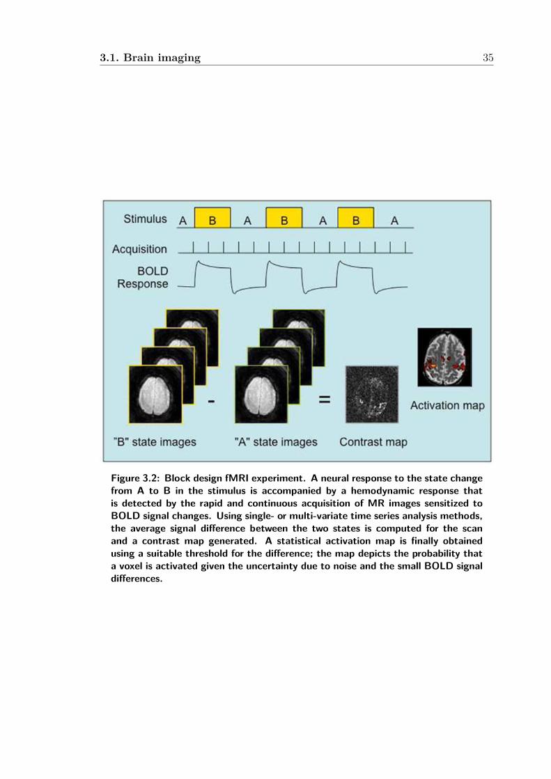
3.1. Brain imaging 35
Figure 3.2: Block design fMRI experiment. A neural response to the state changefrom A to B in the stimulus is accompanied by a hemodynamic response thatis detected by the rapid and continuous acquisition of MR images sensitized toBOLD signal changes. Using single- or multi-variate time series analysis methods,the average signal difference between the two states is computed for the scanand a contrast map generated. A statistical activation map is finally obtainedusing a suitable threshold for the difference; the map depicts the probability thata voxel is activated given the uncertainty due to noise and the small BOLD signaldifferences.

3.1. Brain imaging 36
3.1.3 The resting state fMRI experiment
Contrary to the task oriented fMRI experiments, the resting state fMRI (rs-fMRI)
experiments do not impose any cognitive or motor task to the subject. Subjects
are instructed to stay relaxed, doing nothing and trying not to fall sleep or loss
conscience. The aim is to examine the ground state of the brain and its connectivity.
It has the advantage that any kind of subjects can perform the experiment, whatever
their cognitive impedements, if they can stay quiet for a while. The analysis of the
rs-fMRI data has been tackled with diverse approaches, for instance independent
component analysis (ICA) allowed to discover the default mode networks (DMN).
A common approach is to compute the average signal of each region of a given
brain parcellation and to estimate the connection strength between regions as some
measure of correlation or similarity among these representative signals. The latter
is the approach pursued in this Thesis.
3.1.4 Preprocesing
The preprocessing methods customarily applied to the fMRI data include skull strip-
ping, spatial normalization, realignment for motion correction, and smoothing for
noise reduction [?]:
• Skull stripping. After all the brain images in the fMRI sequence have been
converted to a predefined shape and size, the structure of the skull along with
other parts of the body (i.e. eyes, spinal cord and the muscles in the face and
neck) are removed because they do not provide any useful information.
• Spatial normalization. The size and shape of the human brain varies from
subject to subject. We must ensure that each point in one brain volume
corresponds to the same location in another brain volume, in order to have
anatomically comparable values (i.e. we do not compare different brain struc-
tures in the subjects). Therefore, all the brain volumes must be registered
and warped to a standard template. The most conventional is the Montreal
Neurological Institute (MNI) for structural MRI.
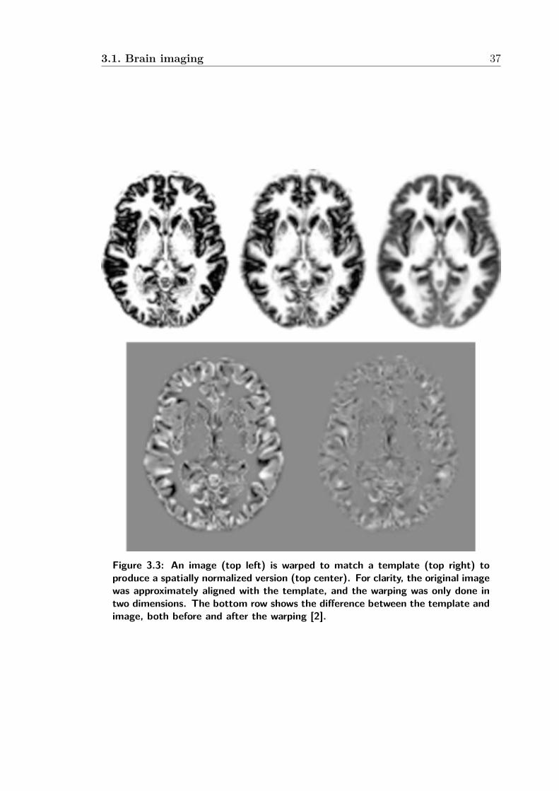
3.1. Brain imaging 37
Figure 3.3: An image (top left) is warped to match a template (top right) toproduce a spatially normalized version (top center). For clarity, the original imagewas approximately aligned with the template, and the warping was only done intwo dimensions. The bottom row shows the difference between the template andimage, both before and after the warping [2].
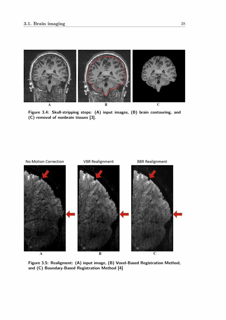
3.1. Brain imaging 38
Figure 3.4: Skull-stripping steps: (A) input images, (B) brain contouring, and(C) removal of nonbrain tissues [3].
Figure 3.5: Realigment: (A) input image, (B) Voxel-Based Registration Method,and (C) Boundary-Based Registration Method [4]
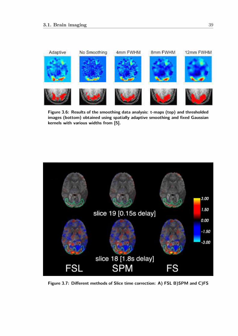
3.1. Brain imaging 39
Figure 3.6: Results of the smoothing data analysis: t-maps (top) and thresholdedimages (bottom) obtained using spatially adaptive smoothing and fixed Gaussiankernels with various widths from [5].
Figure 3.7: Different methods of Slice time correction: A) FSL B)SPM and C)FS
3.1. Brain imaging 40
• Realignment. When the head moves during an experimental run or between
runs (also termed within-run vs. between runs head movements), the corre-
spondence between image location and brain anatomical region will be chang-
ing slightly between MRI volume captures, i.e. motions can cause a given voxel
to contain signal from two different types of tissue or a loss of data. This effect
is more easy to visualize at the edges of the imaging volume. Furthermore,
movement of the head will alter the uniformity of the magnetic field that has
been shimmed for one particular head position. Finally, head motion can have
consequences for activation timing/pattern of excitation, given that each exci-
tation pulse is targeted to one slice at a time and the head is moving through
different slices during acquisition. Motion correction adjusts the series of MRI
volumes to ensure that the brain appears in the same position by a process
called co-registration [171].
• Smoothing (Noise reduction). The spatial noise present in the fMRI scans is
assumed to be Gaussian noise, independent for each voxel, and zero-mean. We
expect that convolving the BOLD volumes, after realignment, with a Gaussian
smoothing kernel will remove most of this Gaussian noise improving the Signal
to Noise Ratio (SNR). The main inconvenient of this process is that for very
low SNR, the amount of smoothing required may damage the information
content of the fMRI volumes.
• Slice time correction. The fMRI data for each subject is a time series of MRI
scans. Each scan should correspond to a particular point in time recording
the instantaneous BOLD information. However, recording each slice in the
volume requires some time. Therefore, the data captured at different brain
regions are obtained at different points in time. Slice time correction method
uses the Fourier transform of the signal at each voxel across time to perform the
time series interpolation in order to obtain time homogeneous BOLD volumes.
• Coregistration. The anatomical label maps of the brain are created to over
an sMRI template. Therefore, the sMRI scan is used to coregister the fMRI
data to the right dimensions allowing to overlaid the anatomical labe lel map

3.1. Brain imaging 41
Table 3.1: Number of regions of the brain parcellations used in this Thesis.Atlas #ROIs
Automated Anatomical Labeling (AAL) 116Eickhoff-Zilles (EZ) 116Harvard-Oxford (HO) 110
Talarach and Tournoux (TT) 110Dosenbach 160 160
Craddock 200 (CC200) 200
on the fMRI data in order to produce the brain parcellations discussed below.
This is required so that we can have a one to one match of the ROIs defined
in the atlas with the areas in the fMRI data.
3.1.5 Brain parcellations
Korbinian Brodmann subdivided the cerebral cortex into numerous areas based on
regional differences in the distribution, density, shape, and size of cell bodies [172,
173] providing one of the first brain anatomical parcellation allowing researchers to
investigate brain-behavioral associations with developmental [174], cognitive , and
clinical phenotypes [175].
In our works on the functional connectivity analysis, the parcellations presented
in Table 3.1 were applied in order to obtain the region representative time series
for each of the regions of the selected parcellations. As discussed in [35] there are
several approaches to the definition of the brain parcellation which may lead to
significant differences in the computational experiments outcomes [175, 176]. On
the one hand, we consider in this paper the anatomically guided parcellations such
as the Tailarach and Tournoux (TT), Eickhoff-Zilles [177], Harvard Oxford (HO)
[178], and the Automated Anatomical Labeling (AAL) [179, 180] defined from the
brain segmentation of selected control populations. On the other hand, we consider
parcellations are produced from the segmentation of the rs-fMRI time series of the
brain volume using clustering techniques, such as the Dosenbach [174] and Craddok
[181] parcellations. All these atlases were defined at the conventional resolution of
sMRI of 1mm3. In order to reduce their resolution to conventional fMRI resolution
of 3mm3 nearest neighbor interpolation was used.
3.1. Brain imaging 42
• Tailarach and Tournoux. The Co-Planar Stereotactic Atlas of the Human
Brain by Talairach and Tournoux (1988) [?] is based on the anteroposterior
commissural system and contains gross anatomy onaxial, coronal, and sagittal
sections. The Talairach and Tournoux (TT) atlas has widespread familiarity
and utilization, and the associated Talairach transformation is a practical way
for normalizing brain images. Developed initially for stereotactic and func-
tional neurosurgery, the TT atlas iswidely used in human brain mapping for
brain comparison across subjects [?] and the number of references to it has
been growing exponentially [?]. In addition, the Talairach system is the most
frequently used coordinate system in human brain mapping [182]. The TT
atlas distributed with AFNI was coregistered and warped into template space.
• Eickhoff-Zilles. The Eickhoff-Zilles(EZ) atlas [177] was derived from the max-
propagation atlas distributed with the SPM Anatomy Toolbox. The atlas was
transformed into template space using the Colin 27 template (also distributed
with the toolbox) as an intermediary.
• Harvard-Oxford. The Harvard-Oxford (HO) atlas [178] was developed at the
Center for Morphometric Analysis (CMA), and distributed with the FMRIB
Software Library (FSL). It comes with a probability distribution for each brain
region obtained from a Maximum A posteriori (MAP) estimate. The HO atlas
is split into cortical and subcortical probabilistic atlases. A 25% threshold was
applied to each of these atlases and they were subsequently bisected into left
and right hemispheres at the midline (x = 0). ROIs representing left/right
WM, left/right GM, left/right CSF and brainstem were removed from the
subcortical atlas.
• Automated Anatomical Labeling (AAL). The AAL atlas [179, 180] is dis-
tributed with the AAL Toolbox.
• Dosenbach 160. The Dosenbach 160 atlas [174] distributed with DPARSF/DPABI
includes 160 4.5-mm radius spheres placed at coordinates extracted from Ta-
ble S6 in Dosenbach et al., 20104. These regions were identified from meta-
analyses of task-related fMRI studies.

3.1. Brain imaging 43
• Craddock 200 (CC200) [183]: Functional parcellation was accomplished using
a two-stage spatially-constrained functional procedure applied to preprocessed
and unfiltered resting state data corresponding to 41 individuals from an inde-
pendent dataset. A grey matter mask was constructed by averaging individual-
level grey matter masks derived by automated segmentation. Individual-level
connectivity graphs were constructed by treating each gray matter voxel as
a node and defining edges between nodes whose temporal correlation among
3D neighborhoods was above a preset threshold. Each graph was partitioned
into 200 regions using normalized cut spectral clustering. Association matri-
ces were constructed from the clustering results by setting the connectivity
between voxels to 1 if they are in the same ROI and 0 otherwise. A group-
level correspondence matrix was constructed by averaging the individual level
association matrices and subsequently partitioned into 200 regions using nor-
malized cut clustering. Labels were generated for each of the resulting ROIs
from their overlap with AAL, EZ, HO, and TT atlases using the cluster naming
script distributed with the pyClusterROI toolbox .
3.1.6 Connectivity matrices
The first step of a computational pipeline dealing with rsfMRI data is the estimation
of the connectivity matrices. In the experimental works reported in Chapters 6 and
76 we have considered five similarity metrics to build the connectivity matrices from
the time series representatives of the brain parcellations which are available from
the nilearn python package (https://nilearn.github.io/modules/generated/
nilearn.connectome.ConnectivityMeasure.html). At the root of these compu-
tations is the robust estimation of the covariance matrix of the time series. We
use the Ledoit-Wolf shrinkage estimator [184] following methodological recommen-
dations in [175, 176]. The connectivity matrices are constructed according to the
following connectivity measures:
• The covariance matrix computed using the Ledoit-Wolf shrinkage estimator
[184],
3.2. Related works 44
• The Pearson Correlation Coefficient (PCC) [185] among each pair of ROI time
series, which is computed as the normalization of the covariance matrix [186].
• The precision computed as the inverse of the covariance matrix.
• The partial correlation obtained regressing out all other connections for each
pair of regions [187].
• The tangent space representation of the matrices obtained by whitening them
[188].
Hence, for each subject in the ABIDE dataset and brain parcellation we have five
different connectivity matrices as input for the feature extraction and classifier cross-
validation.
3.2 Related works
Artificial intelligence tools and problem solving approaches [208] are contributing
to the understanding and predictive analysis of ASC. Overall, there is increasing
evidence that specific features extracted from MRI neuroimaging can be used to
discriminate ASC from TD. However, there is a wide variety of methodological and
computational approaches tested on widely different cohorts and imaging modalities
[21,209].
3.2.1 Anatomical brain imaging
Regarding anatomical brain imaging, predictive models can be built based on anatom-
ical differences computed by voxel based morphometry (VBM) over gray and white
matter segmentations of T1-weighted MRI data. Experiments over a small cohort
have reported average accuracies cross-validation experiments below 70% for a series
of stratified computational experiments [210]. However, a similar study [211] using
voxel based morphometry (VBM) significative differences of diverse stratifications
of female and male subjects of the ABIDE dataset reported much higher accuracies,
above 90% in several subgroups. On the other hand, the use of 3D convolutional
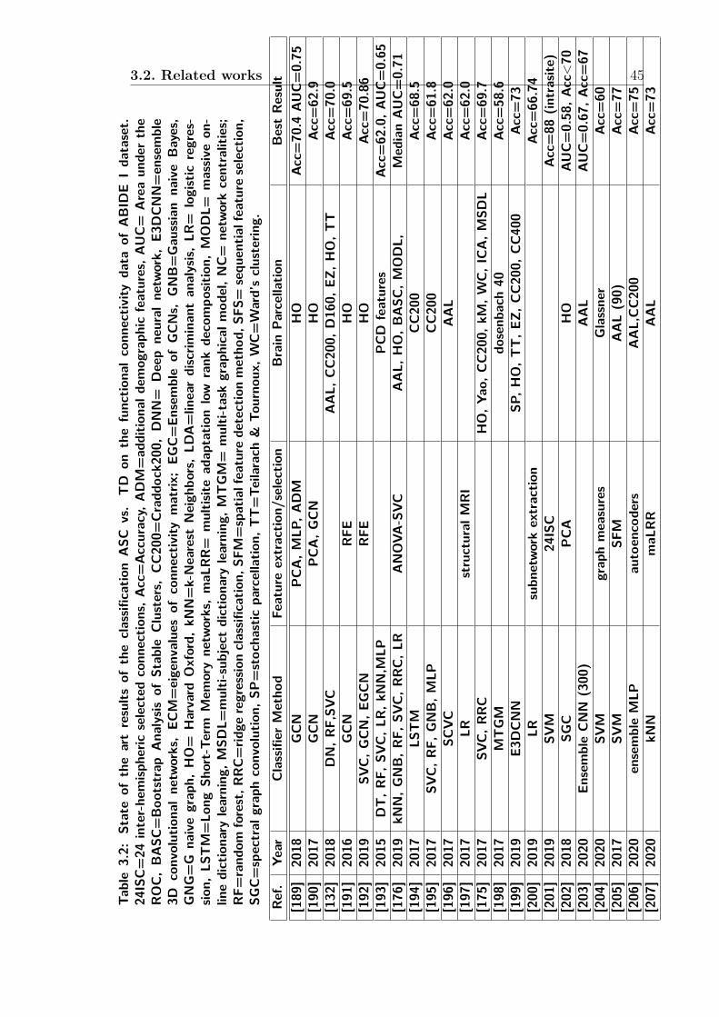
3.2. Related works 45
Table3.2:
Stateof
theartresults
oftheclassifi
catio
nASC
vs.
TD
onthefunctio
nalconn
ectiv
itydata
ofABID
EIdataset.
24ISC=24
inter-hemisp
heric
selected
conn
ectio
ns,A
cc=Accuracy,ADM=additio
nald
emograph
icfeatures,A
UC=
Areaun
derthe
ROC,BASC
=Boo
tstrap
Analysis
ofStable
Clusters,
CC200=
Cradd
ock200,DNN=
Deepneural
network,
E3DCNN=ensemble
3Dconvolutionalnetworks,EC
M=eigenvaluesof
conn
ectiv
itymatrix
;EG
C=En
sembleof
GCNs,
GNB=GaussiannaiveBayes,
GNG=G
naivegraph,
HO=
Harvard
Oxford,
kNN=k-Nearest
Neigh
bors,LD
A=lineardiscrim
inantanalysis,
LR=
logistic
regres-
sion,
LSTM=Lo
ngSh
ort-Te
rmMem
orynetworks,maL
RR=
multisite
adaptatio
nlow
rank
decompo
sition,
MODL=
massiv
eon
-linedictionary
learning
,MSD
L=multi-subjectdictionary
learning
,MTGM=
multi-task
graphicalm
odel,N
C=
networkcentralities;
RF=
rand
omforest,R
RC=rid
geregressio
nclassifi
catio
n,SF
M=spatialfeature
detectionmetho
d,SF
S=sequ
entia
lfeature
selection,
SGC=spectral
graphconvolution,
SP=stochastic
parcellatio
n,TT=Te
ilarach
&To
urno
ux,W
C=Ward’sclusterin
g.Ref.
Year
Classifier
Metho
dFeatureextractio
n/selection
Brain
Parcellatio
nBestResult
[189]
2018
GCN
PCA,M
LP,A
DM
HO
Acc=70.4
AUC=0.75
[190]
2017
GCN
PCA,G
CN
HO
Acc=62.9
[132]
2018
DN,R
F,SV
CAAL,
CC200,
D160,
EZ,H
O,T
TAcc=70.0
[191]
2016
GCN
RFE
HO
Acc=69.5
[192]
2019
SVC,G
CN,E
GCN
RFE
HO
Acc=70.86
[193]
2015
DT,R
F,SV
C,L
R,k
NN,M
LPPCD
features
Acc=62.0,A
UC=0.65
[176]
2019
kNN,G
NB,R
F,SV
C,R
RC,L
RANOVA
-SVC
AAL,
HO,B
ASC
,MODL,
MedianAUC=0.71
[194]
2017
LSTM
CC200
Acc=68.5
[195]
2017
SVC,R
F,GNB,M
LPCC200
Acc=61.8
[196]
2017
SCVC
AAL
Acc=62.0
[197]
2017
LRstructural
MRI
Acc=62.0
[175]
2017
SVC,R
RC
HO,Y
ao,C
C200,
kM,W
C,ICA,M
SDL
Acc=69.7
[198]
2017
MTGM
dosenb
ach40
Acc=58.6
[199]
2019
E3DCNN
SP,H
O,T
T,E
Z,CC200,
CC400
Acc=73
[200]
2019
LRsubn
etworkextractio
nAcc=66.74
[201]
2019
SVM
24ISC
Acc=88
(intrasite
)[202]
2018
SGC
PCA
HO
AUC=0.58,A
cc<70
[203]
2020
EnsembleCNN
(300)
AAL
AUC=0.67,A
cc=67
[204]
2020
SVM
graphmeasures
Glassner
Acc=60
[205]
2017
SVM
SFM
AAL(90)
Acc=77
[206]
2020
ensembleMLP
autoencoders
AAL,CC200
Acc=75
[207]
2020
kNN
maL
RR
AAL
Acc=73
3.2. Related works 46
neural networks (3D-CNN) [212] on the complete ABIDE structural MRI dataset
reported an accuracy of 70%. Hence, there is a strong selection effect that may bias
significantly the reported results. Significance weighted principal component anal-
ysis allows to remove the effects of site data acquisition improving discrimination
based on anatomical imaging [213].
3.2.2 Functional connectivity
Works based on functional connectivity information extracted from rs-fMRI data
have been predominant in the latter times. They have been carried out over a
wide variety of cohorts, testing many computational approaches. Relevant brain
connection selection using logistic regression [162] achieved accuracy of 85% by a
linear classifier in a leave one out validation over a small cohort (74 high-functioning
adult ASCs and 107 adult TDs). Further validation on an independent subset
of the ABIDE dataset (N=88) achieved a remarkable accuracy of 75%. Another
work [214] reports accuracies over 80% on a small cohort of paired 20 ASC and
20 TD children using hyperconnectivity networks as features for a SVM classifier,
while other authors [215] reported on the results of multilinear regression over the
functional connectivity matrices after PCA dimensionality reduction of a cohort of
85 ASC and 163 TD children finding specific imbalances in brain connectivity for
ASC children. However, the heterogeneity of the cohorts points to powerful selection
bias in the results. In other words, the selection of which subjects are used for the
experiments has a strong effect in the results reported.
3.2.3 Dataset heterogeneity
The heterogeneity of the data in ABIDE as illustrated by the demographic informa-
tion shown in Table 6.1 is a source of bad results for machine learning approaches.
Experiments concerning single sites report overly optimistic results that can not
be achieved with the entire ABIDE dataset or a large subsample [216]. For in-
stance, some works carry out separate intra-site cross-validation experiments re-
porting as the global result over the database the average of the separate intra-site

3.2. Related works 47
results [201,217]. This selection strategy overlooks the differences among sites, doing
the crossvalidation on coherent data.
The selection of the experimental cohort among the ABIDE subjects varies
among studies, often for unexplained reasons. For instance, the benchmarking
work [176] selected 871 subjects, after visual quality inspection of the data, while
our own selection includes 884 subjects because our exclussion reason is diagnostic.
Therefore we have excluded from Table 3.2 references such as the recursive feature
selection on 532 subjects [218], the time series clustering approach tested on 814
subjects [219], and others that report results on ABIDE subsamples of 209 [220],
365 [39], 182 [221], 211 [222], and 119 [223] subjects .
3.2.4 Summary information
Table 3.2 summarizes the state of the art regarding the classification of subjects
into ASC or TD on the basis of functional connectivity matrices extracted from the
rs-fMRI data published in the ABIDE I dataset [22,23]. The criteria for inclusion in
this table are (1) that the references report results on the (almost) complete ABIDE
I dataset in order to be comparable to our own results reported below, and (2) that
they report results using only features extracted from the functional connectivity
matrices. We have excluded results obtained adding other kinds of information, such
as the graph convolutional networks (GCN) enriched with demographic information
[189], and the features extracted from structural and MRI data [206].
The selected references of Table 3.2 apply the conventional machine learning
validation methodology uniformly. Works report the average results of repetitions
of k-fold cross-validation results where the training and any feature extraction is
restricted to the training dataset avoiding the double dipping issues [224,225], with
training and testing datasets selected across original sites contributing to ABIDE
listed in Table 6.1. The performance reports in the references of Table 3.2 are
usually in terms of the average Accuracy. Some works report the AUC as a more
robust performance measure [176,189,202], and some report the median and 5% and
95% percentiles of the AUC [202]. Maximal accuracy and AUC results found in the
literature are 77% and .75, respectively. Regarding reproducibility of the results,

3.2. Related works 48
one key issue is the availability of the actual data used in the experiments, which
is heavily dependent on rs-fMRI preprocessing, brain parcellation, and functional
connectivity matrix estimation. In many instances, obtaining the same dataset is not
possible, so we prefer to work on the publicly available preprocessed connectomes.
We feel that results reported over this dataset are fairly comparable.
Columns of Table 3.2 reflect the choices made in the steps of the process of Fig-
ure 1.1, namely on brain parcellation, feature extraction, and classification method.
Most works do not report on the specific functional connectivity matrix estima-
tion procedure. The most popular brain parcellations are the HO [178], and the
AAL [179,180], whose definitions are guided by anatomical criteria. However, data
driven parcellations have also been assessed in the literature applying dictionary
learning, independent component analysis (ICA), clustering approaches, stochastic
parcellations according to a random selection of sites (SP), and the selections of sites
following biomarkers reported in the literature, such as [173]. The feature extraction
processes applied are widely varying among references. Some works report graph
measures, other PCA and recursive feature selection (RFE), sequential feature se-
lection (SFS), or the use of ANOVA to select the most relevant connections [176].
Unlike conventional machine learning classifier model building approaches, studies
using deep learning [203] do not have a separate feature extraction process. Convo-
lutional Neural Networks (CNN) that learn from the data to carry out a hierarchy
of feature extraction processes have been also applied to the task of defining ASC
classification systems [226–232].

Chapter 4
Machine learning background
This Chapter provides some background ideas and definitions on Machine Learning
techniques that have been used in the computational pipeline proposed in Figure 1.1.
Section 4.1 gives some introductory terminology. Section 4.2 provides details on the
classifier building models. Section 4.3 provides details on the feature extraction and
feature selection methods that have been applied to the brain connectivity matrices.
Section 4.4 describes the performance evaluation procedures and metrics used to
report results in Chapter 6.
4.1 Introduction
Machine learning is a field of artificial intelligence that provides the machine with
theability to learn from data without providing specific instructions. Machine learn-
ing is divided into three broad categories: supervised learning, unsupervised learn-
ing, and semi-supervised learning. In machine learning terms, this goal is formulated
as the supervised learning task of inferring from collected data a model that predicts
the value of an output variable based on the observedvalues of input variables. As
such, finding an appropriate model is based on the assumption that the output vari-
able does not take its value at random and that there exists a relation between the
inputs and the output [233]. Unlike supervised learning, in unsupervised learning,
there is no corresponding output for the input data. The goal of unsupervised learn-
ing is to draw inference and learn the structure and patterns of the data. Cluster49

4.2. Classifier model building methods 50
analysis is the most common example of unsupervised learning. Semi-supervised
learning is a category of machine learning which falls between supervised and un-
supervised learning. In semi-supervised learning techniques, besides using labeled
data, unlabeled is used the learning process [169].
4.2 Classifier model building methods
We have applied classifier building methods that are available from the open and
free source Python library scikit-learn v0.22 (https://scikit-learn.org/) [234].
In this section we describe the classifiers that have been tested:
4.2.1 Random Forest (RF)
Random Forest (RF) [235] is a supervised learning algorithm and a popular ensemble
method that combines by majority voting the response from a committee of decision
trees [236] trained upon bootstrapped versions of the training data. The "forest" it
builds, is an ensemble of decision trees; usually trained with the “bagging” method.
Moreover, the variables used to compute each node split are randomly selected. The
basic premise of the algorithm is that building a small decision tree with few features
is a computationally cheap process [237]. A tree-based model involves recursively
partitioning the given dataset into two groups based on a certain criterion until a
predetermined stopping condition is met. At the bottom of decision trees are the leaf
nodes where the decision on the class is performed. Figure 4.1 illustrates a recursive
partitioning of a two-dimensional input space with axis-aligned boundaries. Each
time the input space is partitioned in a direction parallel to one of the axes. In the
figure, the first split is defined by x2 ≥ a2. Then, the two resulting subspaces are
partitioned: The left branch corresponds to the split on x1 ≥ a4. The right branch
is first split by the rule x1 ≥ a1, and then one of its subbranches is split by the ryle
x2 > a3. Figure 4.2 is a graphical representation of the space partition in figure 4.1.
Depending on how the partition and stopping criteria are set, decision trees can
be designed for both classification tasks (categorical outcome, for example, logistic
regression) and regression tasks (continuous outcome).

4.2. Classifier model building methods 51
Figure 4.1: A graphical representation of a binary decision tree splitting the spacerecursively.
For both classification and regression problems, the subset of predictor variables
selected to split an internal node depends on predetermined splitting criteria that
are formulated as an optimization problem. A common splitting criterion in classi-
fication problems is entropy, which is the practical application of Shannon’s source
coding theorem that specifies the lower bound on the length of a random variable’s
bit representation. At each internal node of the decision tree, entropy is given by
the equation (4.1) where c is the number of unique classes and pi is the prior prob-
ability of each given class. This value is maximized to gain the most information at
every split of the decision tree. For regression problems, a commonly used splitting
criterion is the mean squared error at each internal node:
E = −c∑i=1
pi × log(pi) (4.1)
A drawback of decision trees is that they are prone to overfitting, which means
that the model follows the idiosyncrasies of the training dataset too closely and
performs poorly on the test data, i.e. unknown data at training time. Overfitted
decision trees lead to low generalization performance.

4.2. Classifier model building methods 52
Figure 4.2: Recursive binary partition of a two-dimensional space obtained as aresult of the binary tree in 4.1.
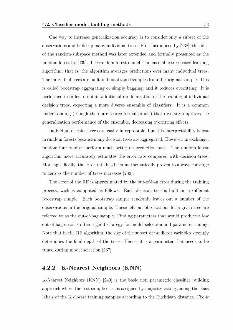
4.2. Classifier model building methods 53
One way to increase generalization accuracy is to consider only a subset of the
observations and build up many individual trees. First introduced by [238], this idea
of the random-subspace method was later extended and formally presented as the
random forest by [239]. The random forest model is an ensemble tree-based learning
algorithm; that is, the algorithm averages predictions over many individual trees.
The individual trees are built on bootstraped samples from the original sample. This
is called bootstrap aggregating or simply bagging, and it reduces overfitting. It is
performed in order to obtain additional randomization of the training of individual
decision trees, expecting a more diverse ensemble of classifiers. It is a common
understanding (though there are scarce formal proofs) that diversity improves the
generalization performance of the ensemble, decreasing overfitting effects.
Individual decision trees are easily interpretable, but this interpretability is lost
in random forests because many decision trees are aggregated. However, in exchange,
random forests often perform much better on prediction tasks. The random forest
algorithm more accurately estimates the error rate compared with decision trees.
More specifically, the error rate has been mathematically proven to always converge
to zero as the number of trees increases [239].
The error of the RF is approximated by the out-of-bag error during the training
process, wich is computed as follows. Each decision tree is built on a different
bootstrap sample. Each bootstrap sample randomly leaves out a number of the
observations in the original sample. These left-out observations for a given tree are
referred to as the out-of-bag sample. Finding parameters that would produce a low
out-of-bag error is often a good strategy for model selection and parameter tuning.
Note that in the RF algorithm, the size of the subset of predictor variables strongly
determines the final depth of the trees. Hence, it is a parameter that needs to be
tuned during model selection [237].
4.2.2 K-Nearest Neighbors (KNN)
K-Nearest Neighbors (KNN) [240] is the basic non parametric classifier building
approach where the test sample class is assigned by majority voting among the class
labels of the K closest training samples according to the Euclidean distance. Fix &

4.2. Classifier model building methods 54
Hodges were the first to propose a KNN classifier algorithm as early as the year of
1951 for performing pattern classification task [241].
The KNN algorithm essentially boils down to forming a majority vote between
the K most similar instances to a given “unseen” observation. Similarity is defined
according to a distance metric between two data points. A popular choice is the
Euclidean distance, but other measures can be more suitable for a given setting,
such as the Manhattan, Chebyshev and Hamming distances. More formally, given a
positive integer K, a stored training data sample of feature vectors with associated
class labels S = {yi, ωi}Ni=1, an unseen observation x, and a similarity metric φ (y,x),
a KNN classifier performs [242] the following steps:
1. It runs through the whole dataset computing {di = φ (yi,x)}Ni=1 . The nearest
neighboring set A is composed of the K points in the training data that are
closest to x, . K is usually odd to prevent tie situations.
2. It then estimates the conditional probability for each class, that is, the fraction
of points in A with that given class label. (I(z) is the indicator function which
evaluates to I when the argument z is true and 0 otherwise)
P (ωx = j,X = x) = 1k
∑i∈AI(ωi = j)) (4.2)
3. Finally, input x gets assigned to the class with the largest probability.
4.2.3 Gaussian Naive Bayes (GNB)
Gaussian Naive Bayes (GNB) [240] assumes the statistical independence of the fea-
tures, so that the classifier can be built as an aggregation of one dimensional not
interacting classifiers modeled by a loose mixture of Gaussians. Naive Bayes is used
widely [243] in many applications such as: text categorization [244], document judg-
ment and data stream classification [245]. Naive Bayes is a generative model based
classifier [246] with a fast learning and testing process.
Bayesian classifiers are straightforwardly derived from the Bayes rule and prob-
ability theorems. It has been proven that learning the optimal Bayesian classifier

4.2. Classifier model building methods 55
from training data is an NP-hard problem [247]. A simplified version of Bayesian
classifier called naive Bayes uses two assumptions. The first is that attributes are
conditionally independent given the class label. The second is that, no latent at-
tribute affects the label prediction process [248].
Assume, the vector (x1, . . . , xn) represents the n attributes of the instance x. Let
it be c the class label of the instance x. The probability of observing x given the
class label c can be computed by as follows:
p(x1, . . . , xn |c) =n∏i=1
= p(xi |c) (4.3)
In order to predict the class label of instance x, its probability to belong to each
class is computed. The class with the maximum probability is identified as the class
label of the instance x. Formally:
C(x)NB = arg maxc
{p(x1, . . . , xn |c)}c (4.4)
The conditional independence assumption between the attributes in naive Bayes is
weak, and rarely correct in most real problems except of situations in which the
attributes are extracted from independent stochastic processes. Some methods have
been introduced for improving the conditional independence assumption in naive
Bayes.
Gaussian naive Bayes classification is an instance of naive Bayes method assum-
ing that each the attribute follows a Gaussian distribution given the class label. For
example, suppose that ith attribute is continuous and its class conditional mean and
variance are denoted by uc,i and σ2c,i, respectively, given the class label c. Hence, the
probability of observing the value xi in ith attribute given the class label c, is given
by the normal distribution:
p(xi|c) = 1√2πσ2
c,i
exp(−
(xi−µc,i)2
2σ2c,i
) (4.5)

4.2. Classifier model building methods 56
4.2.4 Support Vector Classifier (SVC)
Support Vector Classifier (SVC) [249,250] looks for the maximum margin hyperplane
discriminating the sample into two classes solving a linear programing problem on
the relevance of the samples to this class boundary. We use the linear kernel version
because its response is more stable, needs less parameter tuning, and is more efficient
computationally. In some instances we carry out a variable selection procedure based
on their statistical significance in an ANOVA analysis [251]. We consider both sparse
(`1) and non-sparse (`2) regularization terms. We test the two implementations
available from scikit-learn, based respectively on libsvm (https://www.csie.ntu.
edu.tw/~cjlin/libsvm/) and liblinear (https://www.csie.ntu.edu.tw/~cjlin/
liblinear/) libraries.
The foundations of Support Vector Machines (SVM) have been developed by
Vapnik [252] and gained popularity due to many promising features such as bet-
ter empirical performance. The formulation uses the Structural Risk Minimization
(SRM) principle, which has been shown to be superior [253], to traditional Empirical
Risk Minimization (ERM) principle, used by conventional neural networks. SRM
minimizes an upper bound on the expected risk, whereas ERM minimizes the error
on the training data. It is this difference which equips SVM with a greater ability to
generalize, which is the goal in statistical learning. SVMs were developed to solve
the classification problem, but recently they have been extended to solve regression
problems [254].
4.2.5 Logistic regression (LR)
Logistic regression (LR) [255–257] is the classical approach that models the probabil-
ity of the binary classes by a logistic linear function, enabling linear regression solvers
to cope with classification problems. We apply both sparse (`1) and non-sparse (`2)
regularizations. Unlike linear regression which outputs continuous number values,
logistic regression transforms its output using the logistic sigmoid function to return
a probability value which can then be mapped to two or more discrete classes. There
are thre types of logistic regression: Binary, Multi and Ordinal.

4.2. Classifier model building methods 57
In linear regression we tried to predict the value of y(i) for the i-th example x(i)
using a linear function y = hθ(x) = θ>x. This is clearly not a solution for pre-
dicting binary-valued labels (y(i) ∈ {0, 1}). In logistic regression we use a different
hypothesis class to try to predict the probability of a given example belonging to
the “1” class versus the probability that it belongs to the “0” class. Specifically, LR
tries to learn a function of the form:
P (y = 1 |x) = hθ(x) = 11 + exp
(θ>x
) ≡ σ(θ>x
)(4.6)
P (y = 0 |x) = 1− P (y = 1 |x) = 1−hθ(x) (4.7)
The function σ(z) ≡ 11+exp(−z) is often called the “sigmoid” or “logistic” function.
It is an S-shaped function that “squashes” the value of(θ>x
)into the range [0, 1]
so that we may interpret hθ(x) as a probability. Our goal is to search for a value of
θ so that the probability P (y = 1 |x) = hθ(x) is large when x belongs to the “1”
class and small when x belongs to the “0” class (so that P (y = 0 |x) is large). For a
set of training examples with binary labels{
(x(i), y(i)) : i = 1, . . . ,m}the following
cost function measures how well a given hθ does this prediction:
J(θ) = −∑i
(y(i)log(hθ(x(i))) + (1−y(i))log(1−hθ(x(i)))) (4.8)
When y(i) = 1 minimizing the cost function means that we need to make hθ(x(i))
large, and when y(i) = 0 we want to make 1− hθ large as explained above. We can
learn to classify our training data by minimizing J(θ) to find the best choice of θ.
Once we have done so, we can classify a new test point as “1” or “0” by checking
which of these two class labels is most probable: if P (y = 1|x) > P (y = 0|x) then
we label the example as a “1”, and “0” otherwise. This is the same as checking
whether hθ(x) > 0.5
To minimize J(θ) we can use the tools of linear regression. We need to provide
a function that computes J(θ) and ∇θJ(θ) for any requested choice of θ. The

4.2. Classifier model building methods 58
derivative of J(θ) as given above with respect to θj is as follows:
∂J(θ)∂θj
=∑i
x(i)j (hθ(x(i))− y(i)) (4.9)
Written in its vector form, the entire gradient can be expressed as follows:
∇θJ(θ) =∑i
x(i)(hθ(x(i))− y(i)). (4.10)
This is essentially the same as the gradient for linear regression except that now
hθ(x) = σ(θ>x) (4.11)
.
4.2.6 Least absolute shrinkage and selection operator (LASSO)
Least absolute shrinkage and selection operator (LASSO) [258] is a sparse (`1) reg-
ularized regression method that performs simultaneously variable selection and reg-
ularization. The lasso is a shrinkage method like ridge, with subtle but important
differences. The lasso estimate is defined by
βlasso = arg minβ
N∑i=1
(yi − β0 −∑
xijβ0)2 (4.12)
subject to
Xpj = |βj| ≤ t (4.13)
It is possible to re-parametrize the constant β0 by standardizing the predictors;
the solution for β0 is y, and thereafter the model is fitted without an intercept. In
the signal processing literature, the lasso is also known as basis pursuit [259]. We
can also write the lasso problem in the equivalent Lagrangian form
βlasso = arg minβ
12
N∑i=1
(yi − β0 −∑j
xijβj)2 + λp∑j=1|βj|
(4.14)
.
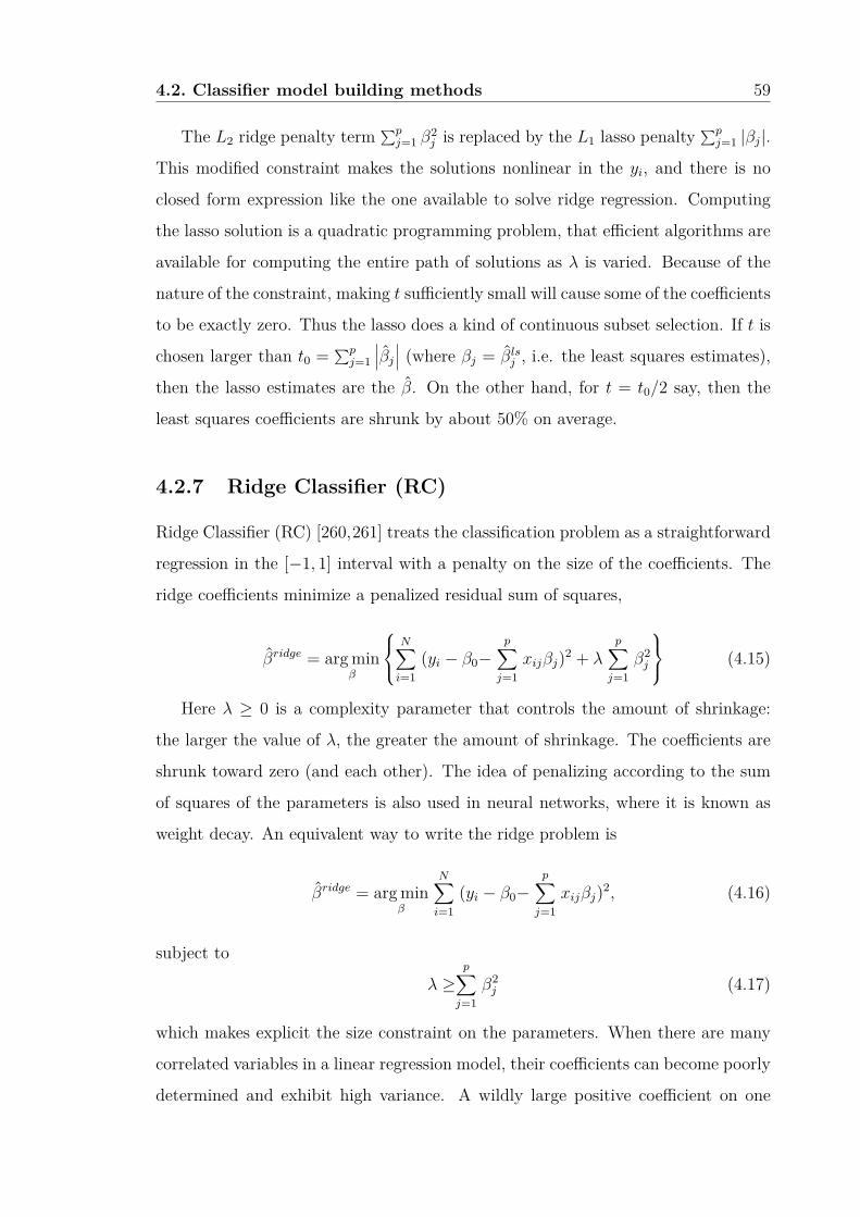
4.2. Classifier model building methods 59
The L2 ridge penalty term ∑pj=1 β
2j is replaced by the L1 lasso penalty ∑p
j=1 |βj|.
This modified constraint makes the solutions nonlinear in the yi, and there is no
closed form expression like the one available to solve ridge regression. Computing
the lasso solution is a quadratic programming problem, that efficient algorithms are
available for computing the entire path of solutions as λ is varied. Because of the
nature of the constraint, making t sufficiently small will cause some of the coefficients
to be exactly zero. Thus the lasso does a kind of continuous subset selection. If t is
chosen larger than t0 = ∑pj=1
∣∣∣βj∣∣∣ (where βj = βlsj , i.e. the least squares estimates),
then the lasso estimates are the β. On the other hand, for t = t0/2 say, then the
least squares coefficients are shrunk by about 50% on average.
4.2.7 Ridge Classifier (RC)
Ridge Classifier (RC) [260,261] treats the classification problem as a straightforward
regression in the [−1, 1] interval with a penalty on the size of the coefficients. The
ridge coefficients minimize a penalized residual sum of squares,
βridge = arg minβ
N∑i=1
(yi − β0−p∑j=1
xijβj)2 + λp∑j=1
β2j
(4.15)
Here λ ≥ 0 is a complexity parameter that controls the amount of shrinkage:
the larger the value of λ, the greater the amount of shrinkage. The coefficients are
shrunk toward zero (and each other). The idea of penalizing according to the sum
of squares of the parameters is also used in neural networks, where it is known as
weight decay. An equivalent way to write the ridge problem is
βridge = arg minβ
N∑i=1
(yi − β0−p∑j=1
xijβj)2, (4.16)
subject to
λ ≥p∑j=1
β2j (4.17)
which makes explicit the size constraint on the parameters. When there are many
correlated variables in a linear regression model, their coefficients can become poorly
determined and exhibit high variance. A wildly large positive coefficient on one

4.2. Classifier model building methods 60
variable can be canceled by a similarly large negative coefficient on its correlated
cousin. By imposing a size constraint on the coefficients, this problem is alleviated.
The ridge solutions are not equivariant under scaling of the inputs, and so one
normally standardizes the inputs before solving equation (4.15). In addition notice
that the intercept β0 has been left out of the penalty term. Penalization of the
intercept would make the procedure depend on the origin chosen for Y ; that is,
adding a constant c to each of the targets yi would not simply result in a shift of the
predictions by the same amount c. It can be shown that the solution to equation
(4.15) can be separated into two parts, after reparametrization using centered inputs:
each xij gets replaced by xij−xj . We estimate β0byy = 1N
∑N1 yi. The remaining co-
efficients get estimated by a ridge regression without intercept, using the centered
xij . Henceforth we assume that this centering has been done, so that the input
matrix X has p (rather than p+ 1) columns.
Writing the criterion of equation (4.15) in matrix form, we have
RSS(λ) = (y −Xβ)T (y −Xβ) + λβTβ, (4.18)
and the ridge regression solutions are easily seen to be given by the following ex-
pression:
βridge = (XTX + λI)−1XTy, (4.19)
where I is the p×p identity matrix. Notice that with the choice of quadratic penalty
βTβ, the ridge regression solution is again a linear function of y. The solution adds a
positive constant to the diagonal of XTX before inversion. This makes the problem
nonsingular, even if XTX is not of full rank, and was the main motivation for ridge
regression when it was first introduced in statistics [262]. In the case of orthonormal
inputs, the ridge estimates are just a scaled version of the least squares estimates,
that is, βridge = β/(1 + λ).
Ridge regression can also be derived as the mean or mode of a posterior distri-
bution, with a suitably chosen prior distribution. In detail, suppose yi ∼ N(β0 +
xTi β, σ2), and the parameters βj are each distributed as N(0, τ 2), independently of
one another. Then the (negative) log-posterior density of β, with τ 2 and σ2 assumed

4.2. Classifier model building methods 61
known, is equal to the expression in curly braces in eq. (4.15), with λ = σ2/τ 2. Thus
the ridge estimate is the mode of the posterior distribution; since the distribution is
Gaussian, it is also the posterior mean.
The singular value decomposition (SVD) of the centered input matrix X gives us
some additional insight into the nature of ridge regression. This de- composition is
extremely useful in the analysis of many statistical methods. The SVD of the N ×p
matrix X has the form
X = UDV T . (4.20)
Here U and V are N × p and p × p orthogonal matrices, with the columns of U
spanning the column space of X, and the columns of V spanning the row space. D
is a p × p diagonal matrix, with diagonal entries d1 ≥ d2 ≥ ... ≥ dp ≥ 0 called the
singular values of X. If one or more values dj = 0, then X is singular. Using the
singular value decomposition we can write the least squares fitted vector as
Xβls = X(XTX)−1XTy = UUTy, (4.21)
after some simplification. Note that UTy are the coordinates of y with respect
to the orthonormal basis U . Q and U are generally different orthogonal bases for
the column space of X. Note that since λ ≥ 0, we have d2j/(d2
j + λ) ≤ 1. Like
linear regression, ridge regression computes the coordinates of y with respect to the
orthonormal basis U . It then shrinks these coordinates by the factors d2j/(d2
j + λ).
This means that a greater amount of shrinkage is applied to the coordinates of
basis vectors with smaller d2j . The SVD of the centered matrix X is another way of
expressing the principal components of the variables in X. The sample covariance
matrix is given by S = XTX/N , and from eq. (4.15) we have
XTX = V D2V T , (4.22)
which is the eigen decomposition of XTX (and of S, up to a factor N). The
eigenvectors vj (columns of V ) are also called the principal components of X. The
first principal component direction v1 has the property that z1 = Xv1 has the largest

4.2. Classifier model building methods 62
sample variance amongst all normalized linear combinations of the columns of X.
This sample variance is easily seen to be
V ar(z1) = V ar(Xv1) = d21N, (4.23)
and in fact z1 = Xv1 = u1d1. The derived variable z1 is called the first principal com-
ponent of X, and hence u1 is the normalized first principal component. Subsequent
principal components zj have maximum variance d2j/N , subject to being orthogonal
to the earlier ones. Conversely the last principal component has minimum variance.
Hence the small singular val- ues dj correspond to directions in the column space
of X having small variance, and ridge regression shrinks these directions the most.
If we consider fitting a linear surface over this domain (the Y -axis is sticking out
of the page), the configuration of the data allow us to determine its gradient more
accurately in the long direction than the short. Ridge regression protects against
the potentially high variance of gradients estimated in the short directions. The
implicit assumption is that the response will tend to vary most in the directions of
high variance of the inputs. This is often a reasonable assumption, since predictors
are often chosen for study because they vary with the response variable, but need
not hold in general.
The following monotone decreasing function of λ is the effective degrees of free-
dom of the ridge regression fit.
df(λ) = tr[X(XTX + λI)−1XT
]= tr(Hλ) =
p∑j=1
d2j2j + λ
. (4.24)
Usually in a linear-regression fit with p variables, the degrees-of-freedom of the fit
is p, the number of free parameters. The idea is that although all p coefficients in a
ridge fit will be non-zero, they are fit in a restricted fashion controlled by λ. Note
that df(λ) = p when λ = 0 (no regularization) and df(λ)→ 0 as λ→∞. Of course
there is always an additional one degree of freedom for the intercept, which was
removed apriori.

4.2. Classifier model building methods 63
4.2.8 Bayesian Ridge Classifier (BRC)
Bayesian Ridge Classifier (BRC) [263] performs the ridge regression in a Bayesian
framework modeling the priors of the coefficients as a spherical Gaussian distribution
whose parameters follow prior Gamma distributions. Model fit and hyper-parameter
estimation is carried out concurrently allowing for better adaptability to the data
at hand. Bayesian regression allows a natural mechanism to survive insufficient
data or poorly distributed data by formulating linear regression using probability
distributors rather than point estimates. The output or response y is assumed
to drawn from a probability distribution rather than estimated as a single value.
Mathematically, to obtain a fully probabilistic model the response y is assumed to
be Gaussian distributed around Xw as follows:
p(y |X,w, α) = N(y |Xw, α) (4.25)
.
One of the most useful type of Bayesian regression is Bayesian Ridge regression
which estimates a probabilistic model of the regression problem. Here the prior for
the coefficient w is given by spherical Gaussian as follows:
p (w |λ) = N(w∣∣∣0, λ−1Ip
). (4.26)
4.2.9 Multi-layer Perceptron (MLP)
Multi-Layer Perceptron (MLP) [264] implements the classical artificial neural net-
work architecture with sigmoid activation functions in the hidden and output layers
trained by backpropagation of the error at the output layer. We apply both the
adam and the L-BFGS solvers. We explore MLP architectures with 5 and 10 hidden
layers in order to assess the impact of different hierarchical representational depths.
Historically, MLP were motivated by the functionality of the human brain. In-
deed, the first neural network was devised by McCulloch and Pitts [265] in an
attempt to model a biological neuron. A McCulloch and Pitts neuron is a function
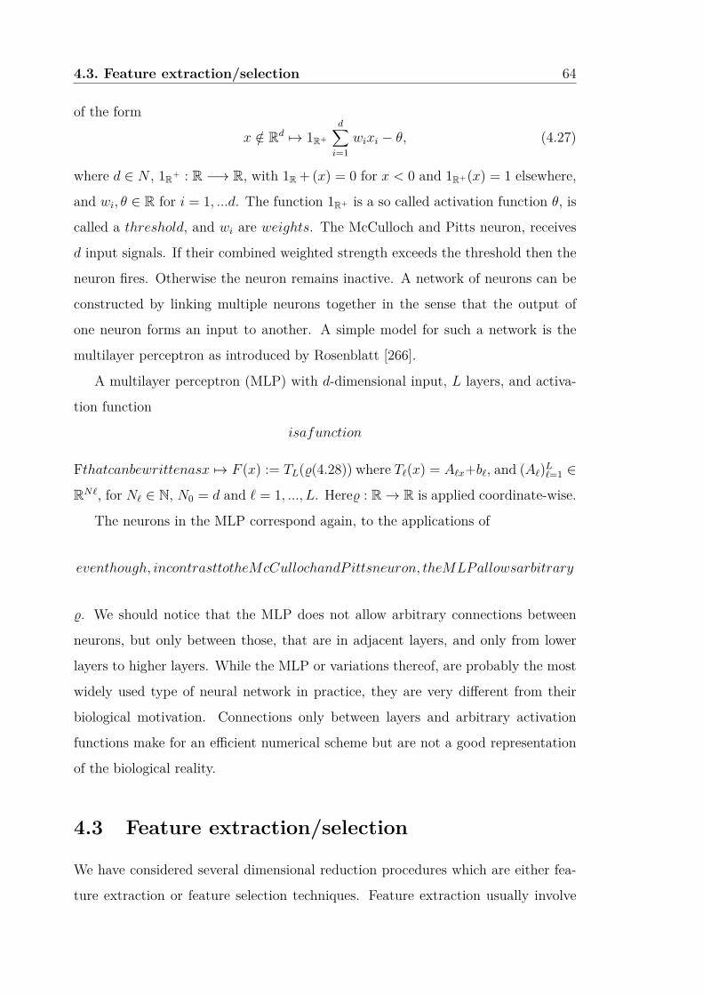
4.3. Feature extraction/selection 64
of the form
x /∈ Rd 7→ 1R+
d∑i=1
wixi − θ, (4.27)
where d ∈ N , 1R+ : R −→ R, with 1R + (x) = 0 for x < 0 and 1R+(x) = 1 elsewhere,
and wi, θ ∈ R for i = 1, ...d. The function 1R+ is a so called activation function θ, is
called a threshold, and wi are weights. The McCulloch and Pitts neuron, receives
d input signals. If their combined weighted strength exceeds the threshold then the
neuron fires. Otherwise the neuron remains inactive. A network of neurons can be
constructed by linking multiple neurons together in the sense that the output of
one neuron forms an input to another. A simple model for such a network is the
multilayer perceptron as introduced by Rosenblatt [266].
A multilayer perceptron (MLP) with d-dimensional input, L layers, and activa-
tion function
isafunction
Fthatcanbewrittenasx 7→ F (x) := TL(%(4.28)) where T`(x) = A`x+b`, and (A`)L`=1 ∈
RN`, for N` ∈ N, N0 = d and ` = 1, ..., L. Here% : R→ R is applied coordinate-wise.
The neurons in the MLP correspond again, to the applications of
eventhough, incontrasttotheMcCullochandPittsneuron, theMLPallowsarbitrary
%. We should notice that the MLP does not allow arbitrary connections between
neurons, but only between those, that are in adjacent layers, and only from lower
layers to higher layers. While the MLP or variations thereof, are probably the most
widely used type of neural network in practice, they are very different from their
biological motivation. Connections only between layers and arbitrary activation
functions make for an efficient numerical scheme but are not a good representation
of the biological reality.
4.3 Feature extraction/selection
We have considered several dimensional reduction procedures which are either fea-
ture extraction or feature selection techniques. Feature extraction usually involve

4.3. Feature extraction/selection 65
some transformation of the feature space where the meaning of the original vari-
ables is lost unless there is some backprojection transformation. Feature selection
preserves some of the original variables discarding others. As feature extraction
techniques we have applied the following ones available in the scikit-learn Python
package:
4.3.1 Probabilistic Principal Component Analysis (PCA)
Probabilistic Principal Component Analysis (PCA) [267] is a probabilistic approach
to the estimation of the eigendecomposition of the feature vectors covariance ma-
trix instead of the conventional singular value decomposition (SVD) approach. A
maximum likelihood approach is followed for this estimation under the assumption
of a Gaussian multivariate model.
Principal component analysis (PCA) [268] is a well-established technique for di-
mensionality reduction, and a chapter on the subject may be found in numerous texts
on multivariate analysis. Examples of its many applications include data compres-
sion, image processing, visualisation, exploratory data analysis, pattern recognition
and time series prediction.
The most common derivation of PCA is in terms of a standardised linear pro-
jection which maximises the variance in the projected space [269, 270]. For a set
of observed d-dimensional data vectors {tn}, n ∈ {1...N} the q principal axes wj,
j ∈ {1...N}, are those orthonormal axes onto which the retained variance under pro-
jection is maximal. It can be shown that the vectors wj are given by the q dominant
eigenvectors of the sample covariance matrix S = ∑n(tn − t)(tn − t)T/N , where t is
the data sample mean, such that Swj = λwj. The q principal components of the ob-
served vector tn are given by the vector xn = W T (tn−t), whereW = (w1, w2, ..., wq).
The variables xj are then uncorrellated such that the covariance matrix ∑xnxTn/N
is diagonal with elements λj.
A complementary property of PCA, and that most closely related to the orig-
inal discussions of [271] is that, of all orthogonal linear projections x0 = W T (t0 −
t), the principal component projection minimises the squared reconstruction error∑n
∥∥∥tn − tn∥∥∥2, where the optimal linear reconstruction of tn is given by tn = Wxn+t

4.3. Feature extraction/selection 66
.
4.3.2 Isometric Mapping (Isomap)
Isometric Mapping (Isomap) [272] looks for a low dimension embedding of the feature
space which preserves the geodesic distances among the data samples. It involves
the search for the nearest neighbors, the shortest-path search between samples, and
the computation of the partial eigendecomposition.
Assume a cloud of high dimensional data points{x1, x2, ..., xN} , xi ∈ RM that
lie on a smooth K-dimensional manifold. In most cases of practical interest K is
much smaller than the data dimension M(K � M). Isomap builds upon MDS
but attempts to compute the low-dimensional representation by estimating pairwise
geodesic distances. For sufficiently close pairs, referred to as neighboring points, the
euclidean distance provides a good approximation of geodesic distance [273], [274].
For faraway points, one needs to walk through these neighboring pairs in the shortest
way possible to evaluate the geodesic distance. That can be achieve defficiently
by applying a shortest path algorithm on a graph comprising edges that connect
neighboring points. Here we introduce notations for these concepts. The graph
is denoted as G = (V,E) in which V = {x1, x2, ..., xN} denotes the set of nodes,
and E is the set of edges connecting neighboring samples. There are two ways of
determining the neighbors of a point are K-nearest neighbors [275], or all points
within a fixed range ε. For neighboring nodes xi and xj, the weight is taken to be
wi,j = ||xi − xj||2. If we take xixj to be the shortest route between xi and xj, we
could compute geodesic distances as dG(xi, xj) = w(xi xj) in which w(.) denotes
weight of the path. Finally, we seek a set of low-dimensional point denoted by
{y1, y2, ..., yN} in RK t hat preserves pair wise geodesic distances [276].
4.3.3 Local Linear Embedding (LLE)
Local Linear Embedding (LLE) is manifold learning approach that can be assimi-
lated to a sequence of PCA transformations, which try to benefit from and enhance
the local linear structure of the data [277].

4.3. Feature extraction/selection 67
The high-dimensional coordinates of each patch can be mapped into correspond-
ing local co-ordinates by means of an essentially linear tmation. LLE attempts to
find a global transformation of the high-dimensional coordinates into low dimen-
sional ones by exploiting adjacencyinformation about closely located data points,
this information being aform of summarisation of the local transformations between
the high and low dimensional co-ordinates. Suppose that the data set comprises
vectors {x1, ..., xN} ∈ RD. In the first step, for each 1 ≤ i ≤ N , nearest neighbours
of xi are identified by using a preselected criterion for close proximity and further
indexed by a set N(i) ⊂ 1, ..., N . In the second step, weights wijj ∈ N(i) are found
that optimally reconstruct xi from ts nearest neighbours. These weights minimise
the local reconstruction error
E(i)loc({wij}j∈N(i)) =
∥∥∥∥∥∥xi−∑
j∈N(i)wijxj
∥∥∥∥∥∥ ,2 (4.29)
where ‖·‖ is the Euclidean norm, subject to the condition ∑j∈N(i)
wij = 1.
A key property of the optimal weights is that they are invariant to three types
of transformation:
1. Scaling. Multiplying all co-ordinates by a scalar factor scales the errors E(i)loc
uniformly and hence yields the same weights
2. Orthogonal transformation. Distances are invariant to rotation and mirror-
reflection and so too is each E(i)loc
3. Translation. The weights are constrained to sum to one, so an offset to all
co-ordinates does not affect the value of any E(i)loc
Suppose that the data points are sampled densely from the underlying low-dimensional
manifold. Then, for each point xi, there exists a linear map composed of a trans-
lation, rotation and scaling, that maps the high-dimensional coordinates of a close
neighbourhood of xi to corresponding local coordinates on the manifold. Since
the weights computed in the high dimensional space are invariant to the three con-
stituent mappings, it is natural to take these weights as a basis for there construction

4.3. Feature extraction/selection 68
of the local co-ordinates. In fact, all local neighbourhoods can be reconstructed si-
multaneously if a specific optimisation problem is solved. The cost function for this
problem measures how well low dimensional coordinates of any given point yi ∈ Rd
are reconstructed from the neighbouring points yjj∈N(i) using the weights computed
in the previous step; here d is a dimension index fixed beforehand, usually at a
value much smaller than D. More specifically, in the third step, LLE minimises the
reconstruction error. This optimisation is similar to that in the first step, except
that now the weights are fixed and the low dimensional coordinates are sought. To
obtain an essentially unique solution, the yi are constrained to have zero mean and
an identity covariance matrix [278].
4.3.4 Multi-Dimensional Scaling (MDS)
Multi-Dimensional Scaling (MDS) [279] looks for a dimensional reduction of the
feature space such that the relative ordering of the distances between samples in the
original space are preserved in the reduced dimension space.
Proximity data, the input to MDS, consist of dissimilarity information for pairs
of objects. This contrasts with multivariate data that consist of attribute informa-
tion forindividualobjects. If the objects are labeled i = 1, ..., N , we will assume
that proximity data are given by dissimilarity values Di,j. (If the data are given
as similarities, a monotone decreasingtransformation will convert them to dissim-
ilarities.) The goal of MDS is to map the objects i = 1, ..., N to “configuration”
or “embedding” points {x1, ..., xN} ∈ Rkin such a way that the given dissimilari-
ties Di,j are well approximated by the distances ‖xi − xj‖. The choice ofembedding
dimension k is arbitrary in principle, but low in practice: k = 1, 2, 3 are the most
frequently used dimensions, for the simple reason that the points serve as easily
visualized representors of the objects. In realdata, there are typically many more
objects, and the dissimilarities usually contain error as well as bias with regard to
the fitted distances.
The oldest version of MDS, called classical scaling, is due to Torgerson (1952).
It is, however, a later version due to [280, 281] that has become the leading MDS
method. Kruskal defined MDS in terms of minimization of a loss function called
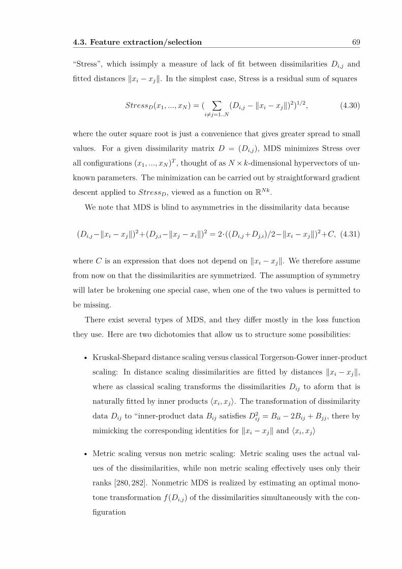
4.3. Feature extraction/selection 69
“Stress”, which issimply a measure of lack of fit between dissimilarities Di,j and
fitted distances ‖xi − xj‖. In the simplest case, Stress is a residual sum of squares
StressD(x1, ..., xN) = (∑
i 6=j=1..N(Di,j − ‖xi − xj‖)2)1/2, (4.30)
where the outer square root is just a convenience that gives greater spread to small
values. For a given dissimilarity matrix D = (Di,j), MDS minimizes Stress over
all configurations (x1, ..., xN)T , thought of as N ×k-dimensional hypervectors of un-
known parameters. The minimization can be carried out by straightforward gradient
descent applied to StressD, viewed as a function on RNk.
We note that MDS is blind to asymmetries in the dissimilarity data because
(Di,j−‖xi − xj‖)2+(Dj,i−‖xj − xi‖)2 = 2·((Di,j+Dj,i)/2−‖xi − xj‖)2+C, (4.31)
where C is an expression that does not depend on ‖xi − xj‖. We therefore assume
from now on that the dissimilarities are symmetrized. The assumption of symmetry
will later be brokening one special case, when one of the two values is permitted to
be missing.
There exist several types of MDS, and they differ mostly in the loss function
they use. Here are two dichotomies that allow us to structure some possibilities:
• Kruskal-Shepard distance scaling versus classical Torgerson-Gower inner-product
scaling: In distance scaling dissimilarities are fitted by distances ‖xi − xj‖,
where as classical scaling transforms the dissimilarities Dij to aform that is
naturally fitted by inner products 〈xi, xj〉. The transformation of dissimilarity
data Dij to “inner-product data Bij satisfies D2ij = Bii − 2Bij +Bjj, there by
mimicking the corresponding identities for ‖xi − xj‖ and 〈xi, xj〉
• Metric scaling versus non metric scaling: Metric scaling uses the actual val-
ues of the dissimilarities, while non metric scaling effectively uses only their
ranks [280, 282]. Nonmetric MDS is realized by estimating an optimal mono-
tone transformation f(Di,j) of the dissimilarities simultaneously with the con-
figuration
4.3. Feature extraction/selection 70
A difference between classical and distance scaling is that inner products rely on
an origin in the coordinate system, while distances do not; a set of inner products
determines uniquely a set of distances, but a set of distances determines a set of
inner products only modulo change of origin. To avoid arbitrariness, one constrains
classical scaling to mean-centered configurations. Another difference between clas-
sical and distance scaling is that distance scaling requires iterative minimization
while classical scaling can be solved with inexpensive eigendecompositions. Just
the same, we implemented classical scaling with iterative gradient descent on a loss
function called “Strain”, which parallels gradient descent on Stress in distance scal-
ing. This computational uniformity has advantages because it is straightforward to
introduceweights and missing values in Strain and Stress, which is not possible in
eigen decompositions [283].
4.3.5 Factor Analyisis (FA)
Factor Analysis (FA) [284, 285] tries to explain the observed variables as a linear
model of unseen latent variables. The conventional approach assumes a Gaussian
prior for the distribution of the latent variables. Changing the prior distribution
gives way to diverse algorithms
Factor analysis is a statistical method used to describe variability among ob-
served, correlated variables in terms of apotentially lower number of unobserved
variables called factors. The observed variables are modeled as linear combinations
of the potential factors, plus "error" terms. The information gained about the in-
terdependencies between observed variables can be used later to reduce the set of
variables in a dataset. Computationally this technique is equivalent to low rank
approximation of the matrix of observed variables. Factor analysis originated in
psychometrics, and is used in behavioral sciences, social sciences, marketing, prod-
uct management, operations research, and other applied sciences that deal with
large quantities of data.
Suppose we have a set of observable random variables {x1, ..., xn} , with means
{µ1, ..., µn}. Suppose for some unknown constants lij and k−unobserved random

4.3. Feature extraction/selection 71
variables Fj, where i ∈, ..., p and j ∈, ..., k, where k < p , that we have
xi − µi = li1F1 + ...+ likFk + εi. (4.32)
Here, the εi are independently distributed error terms with zero mean and finite
variance, which may not be the same for all i. Let V ar(εi) = ψi, so that we
have cov(ε) = Diag(ψ1, ..., ψp) = ψ and E(ε) = 0. In matrix expresion, we have
x− µ = LF + ε
If we have observations, then we will have the dimensions xpxn, Lpxk, and Fkxn.
Each column of x and F denote values for one particular observation, and matrix
L does not vary across observations. Also we will impose the following assumptions
on F .
1. F and ε are independent
2. E(F ) = 0
3. Cov(F ) = I (to make sure that the factors are uncorrelated)
4. Any solution of the above set of equations following the constraints F for is
defined as the factors, and L as the loading matrix.
Suppose Cov(x − µ) = ∑. Then note that from the conditions just imposed on,
either we have
Cov(x− µ) = Cov(LF + ε)
or ∑= LCov(F )LT + Cov(ε)
or ∑= LLT + ψ
Note that for any orthogonal matrix Q if we set L = LQ and F = QTF , the
criteria for being factors and factor loadings still hold. Hence a set of factors and
factor loadings is identical only up to orthogonal transformations.

4.4. Classification performance evaluation 72
4.4 Classification performance evaluation
In the computational experiments reported in Chapter 6, we carry out one hun-
dred repetitions of the 10-fold cross-validation for each combination of experimen-
tal factors. Feature extraction/selection parameters are always computed only on
the training dataset and applied in the test dataset to avoid double dipping is-
sues [224,225]. Most of the papers in the literature report the accuracy (Acc) of the
classification results averaged after the repetition of 10-fold cross-validation experi-
ments. Accuracy is computed as
Acc = (TP + TN)/N
where N is the number of test samples, and TP and TN are the number of cor-
rect positive and negative predictions on the test set, respectively. Some papers on
ASC prediction based on brain connectivity [176] report the area under the receiver
operating curve (ROC) (AUC) [286] as a more general and robust measure of the
classifier performance. The accuracy is determined by the actual decision thresh-
old applied to classify the test samples, while the ROC plots the balance of false
positives (FP ) versus TP across the entire range of decision threshold values. Foll-
lowing the lead of [176] we report in Chapter 6 the median, 5% and 95% percentile
values of the cross-validation repetitions results instead of the average value as a
better description of their distribution. We plot the densities of the median AUC
results across the repetitions of cross-validation experiments in order to visualize
their distribution for different pipeline choices. The plots use the density() func-
tion in R that generates smooth curves that are not always bounded in the interval
[0, 1]. To provide a quantitative ranking of the choices, we carry out one sided non-
parametric Wilcoxon’s rank sum tests among all pairwise combinations of choices
for each pipeline module. For each test we consider the results of all cross-validation
repetitions with all possible choice combinations for the remaining pipeline modules.
We present the p-values of these tests in tables organized as follows: for each table
entry the null hypothesis is that the median AUC of the row choice is greater than
that of the column choice. We specify (row>column) at each table caption as a

4.4. Classification performance evaluation 73
reminder to the reader.

4.4. Classification performance evaluation 74
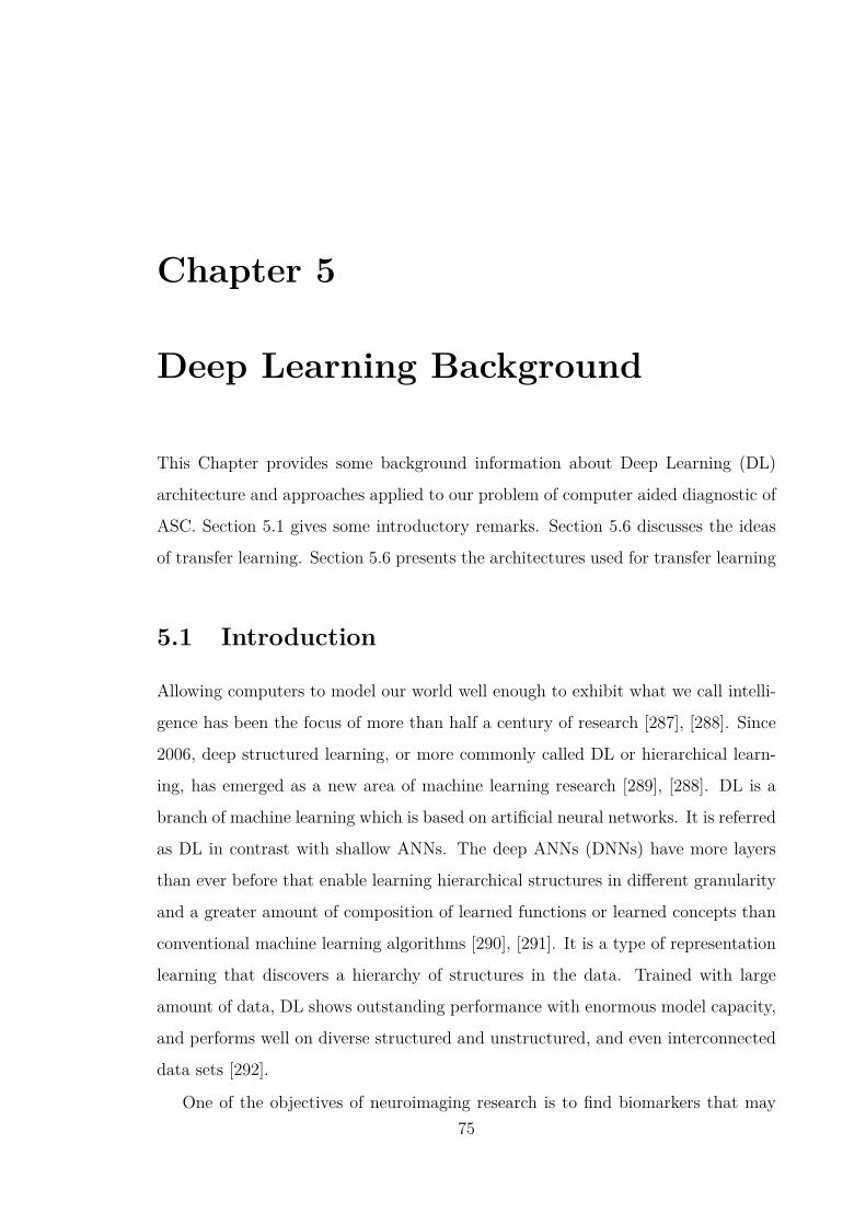
Chapter 5
Deep Learning Background
This Chapter provides some background information about Deep Learning (DL)
architecture and approaches applied to our problem of computer aided diagnostic of
ASC. Section 5.1 gives some introductory remarks. Section 5.6 discusses the ideas
of transfer learning. Section 5.6 presents the architectures used for transfer learning
5.1 Introduction
Allowing computers to model our world well enough to exhibit what we call intelli-
gence has been the focus of more than half a century of research [287], [288]. Since
2006, deep structured learning, or more commonly called DL or hierarchical learn-
ing, has emerged as a new area of machine learning research [289], [288]. DL is a
branch of machine learning which is based on artificial neural networks. It is referred
as DL in contrast with shallow ANNs. The deep ANNs (DNNs) have more layers
than ever before that enable learning hierarchical structures in different granularity
and a greater amount of composition of learned functions or learned concepts than
conventional machine learning algorithms [290], [291]. It is a type of representation
learning that discovers a hierarchy of structures in the data. Trained with large
amount of data, DL shows outstanding performance with enormous model capacity,
and performs well on diverse structured and unstructured, and even interconnected
data sets [292].
One of the objectives of neuroimaging research is to find biomarkers that may75

5.2. Traditional Machine learning, Transfer learning and Fine tunning 76
assist the diagnosis of brain disorders and/or help treat these disorders [292]. Using
DL algorithms to investigate neurological malfunctions has the advantage of allevi-
ating feature engineering, and an ever-increasing number of neuroimaging studies
are turning to DL enabled methods in order to demystify these neurological disor-
ders [293], [294], [295], [199], [296], [297], [298]. DL methods are penetrating clinical
practice and reshaping medical imaging research community, and research articles
involving DL are accumulating at a fast pace. In this Thesis, we do not attempt
an exhaustive review on DL, but mainly focus on fMRI images based brain disorder
diagnosis and show the landscape of the active research initiatives. There are many
different approaches to analyze fMRI images from different perspectives. Features
can be extracted from fMRI images to perform disorder classifications. Different
feature extraction methods and data analysis tools can result in different DL mod-
els [292].
5.2 Traditional Machine learning, Transfer learn-
ing and Fine tunning
Traditional machine learning techniques are based on the model of isolated, single
task learning wherein knowledge from a past task is not leveraged for other tasks;
however, many machine learning methods work well only under a common assump-
tion: the training and test data are drawn from the same feature space and the
same distribution [299]. No knowledge is retained which can be transferred from
one paradigm to another [300]. When the distribution changes, most statistical
models need to be rebuilt from scratch using newly collected training data. In many
real world applications, it is expensive or impossible to re-collect the needed training
data and rebuild the models [299].
Transfer learning or Domain Adaptation, related to the difference in the distri-
bution of the train and test set. The need for transfer learning may arise when
the data can be frequently outdated. In this case, the labeled data obtained inone
time period may not follow the same distribution in a later time period [299]. This
can be understood the same as a projecting all new inputs through a pre-trained
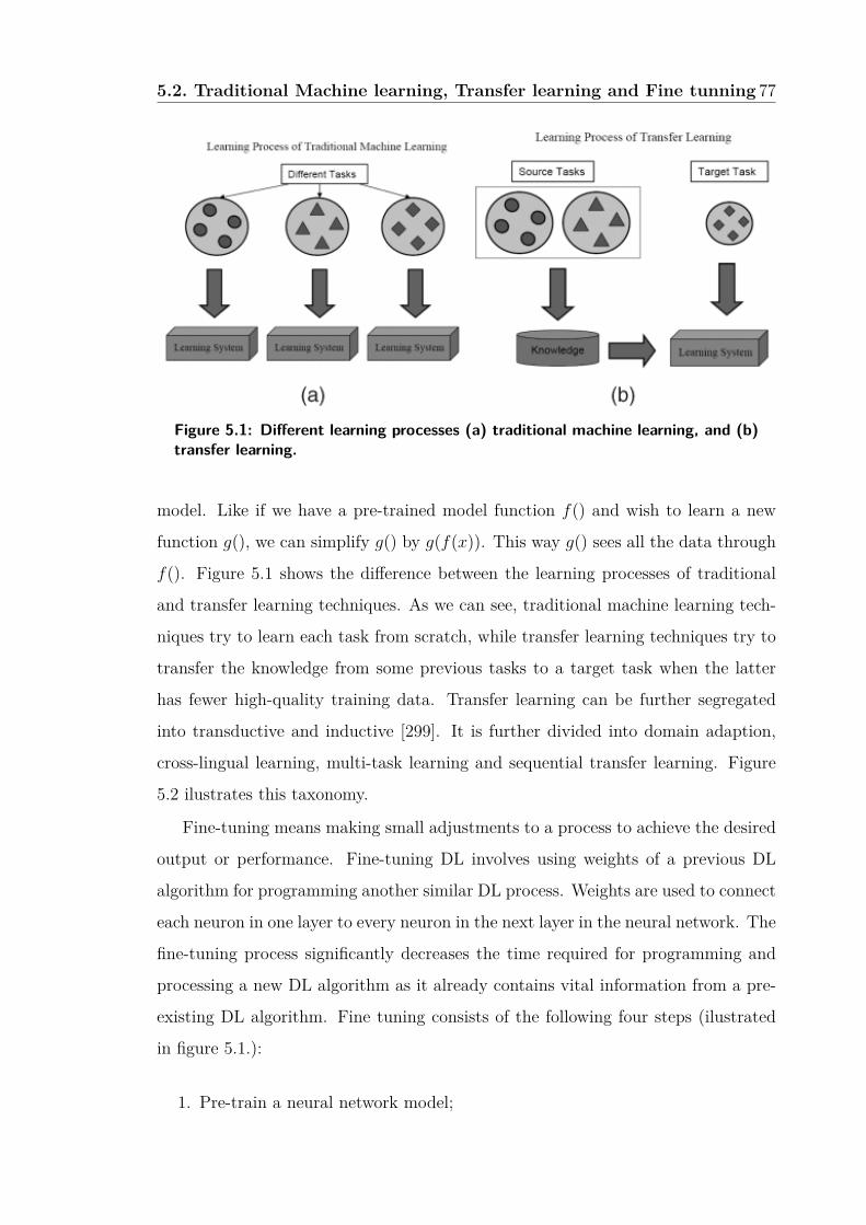
5.2. Traditional Machine learning, Transfer learning and Fine tunning 77
Figure 5.1: Different learning processes (a) traditional machine learning, and (b)transfer learning.
model. Like if we have a pre-trained model function f() and wish to learn a new
function g(), we can simplify g() by g(f(x)). This way g() sees all the data through
f(). Figure 5.1 shows the difference between the learning processes of traditional
and transfer learning techniques. As we can see, traditional machine learning tech-
niques try to learn each task from scratch, while transfer learning techniques try to
transfer the knowledge from some previous tasks to a target task when the latter
has fewer high-quality training data. Transfer learning can be further segregated
into transductive and inductive [299]. It is further divided into domain adaption,
cross-lingual learning, multi-task learning and sequential transfer learning. Figure
5.2 ilustrates this taxonomy.
Fine-tuning means making small adjustments to a process to achieve the desired
output or performance. Fine-tuning DL involves using weights of a previous DL
algorithm for programming another similar DL process. Weights are used to connect
each neuron in one layer to every neuron in the next layer in the neural network. The
fine-tuning process significantly decreases the time required for programming and
processing a new DL algorithm as it already contains vital information from a pre-
existing DL algorithm. Fine tuning consists of the following four steps (ilustrated
in figure 5.1.):
1. Pre-train a neural network model;

5.2. Traditional Machine learning, Transfer learning and Fine tunning 78
Figure 5.2: Types of transfer learning [6]

5.3. Architectures used 79
Algorithm 5.1 Fine tuning process in transfer learning.
2. Create a new neural network model (We assume that these model parameters
contain the knowledge learned from the source dataset and this knowledge will
be equally applicable to the target dataset);
3. Add an output layer whose output size is the number of target dataset cate-
gories to the target model, and randomly initialize the model parameters of
this layer and the last
4. Train the target model on a target dataset, such as a chair dataset.
5.3 Architectures used
5.3.1 VGG16 and VGG19
In 2014 the Visual Geometry Group from Oxford University as second in the ILSVRC
challenge for classification using a very deep but simple convolutional neural net-
work architecture that has come to be known as VGG [301]. VGG is used as a
pre-processing model. Compared with traditional convolutional neural networks, it
has been improved in network depth. It uses an alternating structure of multiple
convolutional layers and non-linear activation layers, which is better than a single
convolution The layer structure can better extract image features, use Maxpooling
for downsampling, and modify the linear unit (ReLU) as the activation function,
5.3. Architectures used 80
Figure 5.3: An overview of the VGG-16 model architecture, this model usessimple convolutional blocks to transform the input image to a 1000class vectorrepresenting the classes of the ILSVRC.
that is, select the largest value in the image area as the pooled value of the area.
The down sampling layer is mainly used to improve the anti-distortion ability of
the network to the image, while retaining the main features of the sample and re-
ducing the number of parameters [7]. This model has become very popular inthe
research community due to its simple approach and becausethe pre-trained weights
were made freely available online, facilitating thefine-tuning of this powerful model
on new tasks [302]. Several of the papers reviewed make use of this model, and so
its network architecture is provided in Figure 5.3.
The structure of the VGG network shown in Figure 5.3 is explained [302] as
follows:
• The first and second convolutional layers are comprised of 64 feature kernel
filters and size of the filter is 3×3. As input image (RGB image with depth
3) passed into first and second convolutional layer, dimensions changes to
224x224x64. Then the resulting output is passed to max pooling layer with a
stride of 2.
• The third and fourth convolutional layers are of 124 feature kernel filters and
size of filter is 3×3. These two layers are followed by a max pooling layer with

5.3. Architectures used 81
stride 2 and the resulting output will be reduced to 56x56x128.
• The fifth, sixth and seventh layers are convolutional layers with kernel size
3×3. All three use 256 feature maps. These layers are followed by a max
pooling layer with stride 2.
• Eighth to thirteen are two sets of convolutional layers with kernel size 3×3.
All these sets of convolutional layers have 512 kernel filters. These layers are
followed by max pooling layer with stride of 1.
• Fourteen and fifteen layers are fully connected hidden layers of 4096 units
followed by a softmax output layer (Sixteenth layer) of 1000 units.
In another work [7] found training VGG16 and VGG19 challenging (specifically
regarding convergence on the deeper networks), so in order to make training easier,
they first trained smaller versions of VGG with less weight layers (columns A and
C) first. They experiment with 6 models, with different numbers of trainable layers.
Based on the number of models the two most popular models are VGG16 and
VGG19. The specifics of the architectures are in Figure 5.2.
5.3.2 Resnet
In 2012, [303] rolled out the red carpet for the Deep Convolutional Neural Network.
This was the first time this architecture was more successful that traditional, hand-
crafted feature learning on the ImageNet. Their DCNN, named AlexNet, contained
8 neural network layers, 5 convolutional and 3 fully-connected. This laid the foun-
dational for the traditional CNN, a convolutional layer followed by an activation
function followed by a max pooling operation [304]. Deep networks naturally inte-
grate low/mid/high-level features [305] and classifiers in an end-to-end multi-layer
fashion, and the “levels” of features can be enrichedby the number of stacked layers
(depth). When deeper networks are able to start converging, a degradation prob-
lem has been exposed: with the network depth increasing, accuracy gets saturated
(which might beunsurprising) and then degrades rapidly [306]. Unexpectedly, such
degradation is not caused by overfitting, and adding more layers to a suitably deep

5.3. Architectures used 82
Figure 5.4: Different ConvNet Architectures [7].

5.3. Architectures used 83
Figure 5.5: Residual learning a building block
model leads to higher training error [307], [308]. This problem of training very deep
networks has been alleviated with the introduction of ResNet or residual networks
and these Resnets are made up from Residual Blocks, such as the one illustrated in
Figure 5.6.
The very first thing we notice to be different is that there is a direct connection
which skips some layers (may vary in different models) in between. This “skip
connection” is the core of residual blocks. Due to this skip connection, the output of
the layer is not the same now. Without using this skip connection, the input x gets
multiplied by the weights of the layer followed by adding a bias term. Next, this
term goes through the activation function, z() and we get our output as H(x). i.e.
H(x)=f(wx + b) or H(x) = z(x). Now with the introduction of skip connection,
the output is changed to H(x) = z(x) + x
There appears to be a slight problem with this approach when the dimensions
of the input vary from that of the output which can happen with convolutional and
pooling layers. In this case, when dimensions of z(x) are different from x, we can
take the following approach: The skip connection is padded with extra zero entries
to increase its dimensions. The projection method is used to match the dimension
which is done by adding 1×1 convolutional layers to input. In such a case, the
output is: H(x) = z(x) + w1x. Here we add an additional parameter w1 whereas
no additional parameter is added when using the first approach.
ResNet network uses a 34-layer plain network architecture inspired by VGG-19

5.3. Architectures used 84
in which then the shortcut connection is added. The skip connections in ResNet
solve the problem of vanishing gradient in deep neural networks by allowing this
alternate shortcut path for the gradient to flow through. The other way that these
connections help is by allowing the model to learn the identity functions which
ensures that the higher layer will perform at least as good as the lower layer, and
not worse [304]. These shortcut connections then convert the architecture into the
residual network as shown in the figure 5.6.

5.3. Architectures used 85
Figure 5.6: Architecture RESNET

5.3. Architectures used 86

Chapter 6
Results of Machine Learning
Approaches
In this Chapter we provide experimental results of a large combination of choices
in the design of the computational pipeline introduced in Figure 1.1. Section 6.1
describes the experimental dataset extracted from the ABIDE repository. Section
6.2 provides some general remarks on the experimental results. Section 6.3 examines
the effect of the brain parcelation. Section 6.3 discusses the effect of the connectivity
matrix definition. Section 6.5 presents the effect of the classification model chosen.
Section 6.6 shows the effect of the choice of the feature selection method. Section
6.7 summarizes the best results of the experimental work. Finally, the best results
are compared with the state of the art of Table 3.2.
6.1 The experimental dataset
In this section we will first introduce the dataset used, then we comment on the brain
parcellations and functional connectivity measures considered. The next subsections
describes the classifier building methods employed, and the feature extraction and
feature selection methods examined. Finally, we comment on the performance mea-
sures selected to report results.
The dataset analyzed in the study is extracted from the Autism Brain Imaging
Data Exchange (ABIDE) [22,23] that provides rsfMRI acquisitions of 1112 subjects87
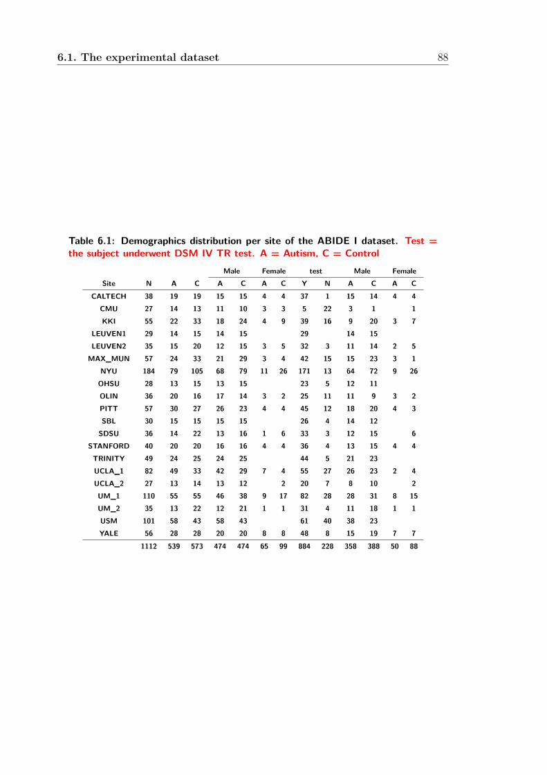
6.1. The experimental dataset 88
Table 6.1: Demographics distribution per site of the ABIDE I dataset. Test =the subject underwent DSM IV TR test. A = Autism, C = Control
Male Female test Male FemaleSite N A C A C A C Y N A C A C
CALTECH 38 19 19 15 15 4 4 37 1 15 14 4 4CMU 27 14 13 11 10 3 3 5 22 3 1 1KKI 55 22 33 18 24 4 9 39 16 9 20 3 7
LEUVEN1 29 14 15 14 15 29 14 15LEUVEN2 35 15 20 12 15 3 5 32 3 11 14 2 5MAX_MUN 57 24 33 21 29 3 4 42 15 15 23 3 1
NYU 184 79 105 68 79 11 26 171 13 64 72 9 26OHSU 28 13 15 13 15 23 5 12 11OLIN 36 20 16 17 14 3 2 25 11 11 9 3 2PITT 57 30 27 26 23 4 4 45 12 18 20 4 3SBL 30 15 15 15 15 26 4 14 12SDSU 36 14 22 13 16 1 6 33 3 12 15 6
STANFORD 40 20 20 16 16 4 4 36 4 13 15 4 4TRINITY 49 24 25 24 25 44 5 21 23UCLA_1 82 49 33 42 29 7 4 55 27 26 23 2 4UCLA_2 27 13 14 13 12 2 20 7 8 10 2UM_1 110 55 55 46 38 9 17 82 28 28 31 8 15UM_2 35 13 22 12 21 1 1 31 4 11 18 1 1USM 101 58 43 58 43 61 40 38 23YALE 56 28 28 20 20 8 8 48 8 15 19 7 7
1112 539 573 474 474 65 99 884 228 358 388 50 88
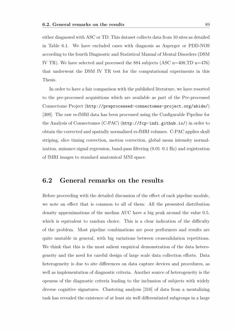
6.2. General remarks on the results 89
either diagnosed with ASC or TD. This dataset collects data from 10 sites as detailed
in Table 6.1. We have excluded cases with diagnosis as Asperger or PDD-NOS
according to the fourth Diagnostic and Statistical Manual of Mental Disorders (DSM
IV TR). We have selected and processed the 884 subjects (ASC n=408,TD n=476)
that underwent the DSM IV TR test for the computational experiments in this
Thesis.
In order to have a fair comparison with the published literature, we have resorted
to the pre-processed acquisitions which are available as part of the Pre-processed
Connectome Project (http://preprocessed-connectomes-project.org/abide/)
[309]. The raw rs-fMRI data has been processed using the Configurable Pipeline for
the Analysis of Connectomes (C-PAC) (http://fcp-indi.github.io/) in order to
obtain the corrected and spatially normalized rs-fMRI volumes. C-PAC applies skull
striping, slice timing correction, motion correction, global mean intensity normal-
ization, nuisance signal regression, band-pass filtering (0.01–0.1 Hz) and registration
of fMRI images to standard anatomical MNI space.
6.2 General remarks on the results
Before proceeding with the detailed discussion of the effect of each pipeline module,
we note an effect that is common to all of them: All the presented distribution
density approximations of the median AUC have a big peak around the value 0.5,
which is equivalent to random choice. This is a clear indication of the difficulty
of the problem. Most pipeline combinations are poor performers and results are
quite unstable in general, with big variations between crossvalidation repetitions.
We think that this is the most salient empirical demonstration of the data hetero-
geneity and the need for careful design of large scale data collection efforts. Data
heterogeneity is due to site differences on data capture devices and procedures, as
well as implementation of diagnostic criteria. Another source of heterogeneity is the
openess of the diagnostic criteria leading to the inclussion of subjects with widely
diverse cognitive signatures. Clustering analysis [310] of data from a mentalizing
task has revealed the existence of at least six well differentiated subgroups in a large

6.3. Effect of the brain parcellation 90
Table 6.2: One sided (row>column) Wilcoxon’s rank sum test p-values betweenmedian AUC results achieved from the different parcellations used to extractrepresentative time series for the connectivity matrices.
AAL CC200 D160 EZ HO TT max AUCAAL 2.06e-15 2.404e-68 1.632e-30 2.127e-31 1.340e-36 0.753CC200 1 6.098e-30 4.169e-06 1.164e-05 2.089e-10 0.767D160 1 1 1 1 1 0.669EZ 1 1 4.032e-14 4.721e-01 2.372e-02 0.748HO 1 1 8.746e-15 5.278e-01 2.602e-02 0.739TT 1 1 1.032e-08 9.762e-01 9.739e-01 0.734
sample of ASC and controls. Finally, sex is a demonstrated source of heterogenity.
Sex has bee proven to have a significant effect on the neurobiology of autism [11].
Figure 6.1 summarizes the impact of feature selection/extraction methods versus
the classifiers. It can be easily appreciated that the effect of feature extraction is
greater than that of the classifier of choice, specifically the factor analysis, PCA
and correlation based selection are quite comparable feature computation methods.
Figure 6.2 summarizes the impact of feature computation versus the brain parce-
lation applied to extract brain regions. Results show the greater effect of feature
computation methods, with the same qualitative results as above. Figure 6.3 sum-
marizes the impact of classifiers versus the chosen connectivity measure, the results
for the tangent and correlation measures show the greatest variances. Other than
that theclassifiers do not have a clear ranking, except for the lower performance of
k-NN and random forest.
6.3 Effect of the brain parcellation
Figure 6.4 shows the density plots corresponding to the aggregation of the median
AUC results per brain parcellation used. As expected, these distributions are not
Gaussian shaped, some of them are markedly multimodal. In the case of AAL, the
distribution is pretty close to an uniform distribution. Most parcellation distribu-
tions have a big peak at the 0.5 value of the median AUC with a low tail of values
above 0.7. We use one sided Wilcoxon’s rank sum test to assess quantitatively the
improvement of results achieved with each parcellation. Table 6.2 shows the p-values

6.3. Effect of the brain parcellation 91
Figure 6.1: Impact of feature selection versus classifiers.
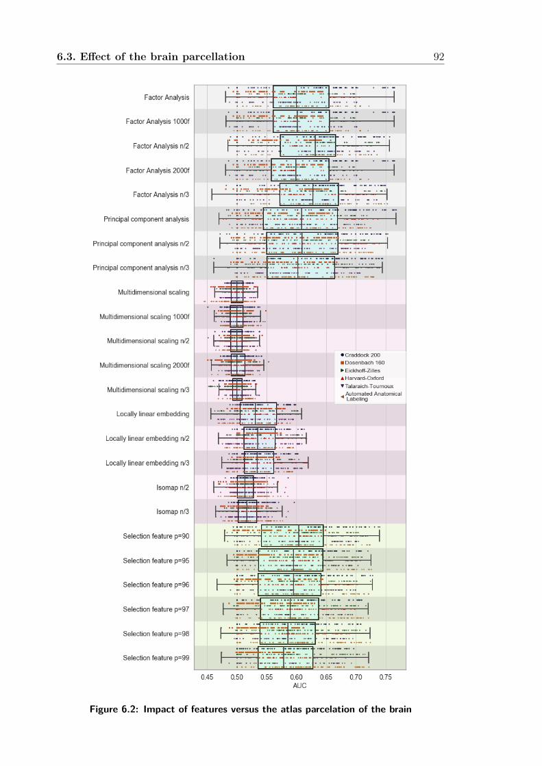
6.3. Effect of the brain parcellation 92
Figure 6.2: Impact of features versus the atlas parcelation of the brain

6.3. Effect of the brain parcellation 93
Figure 6.3: Impact of classifiers versus the connectivity measure
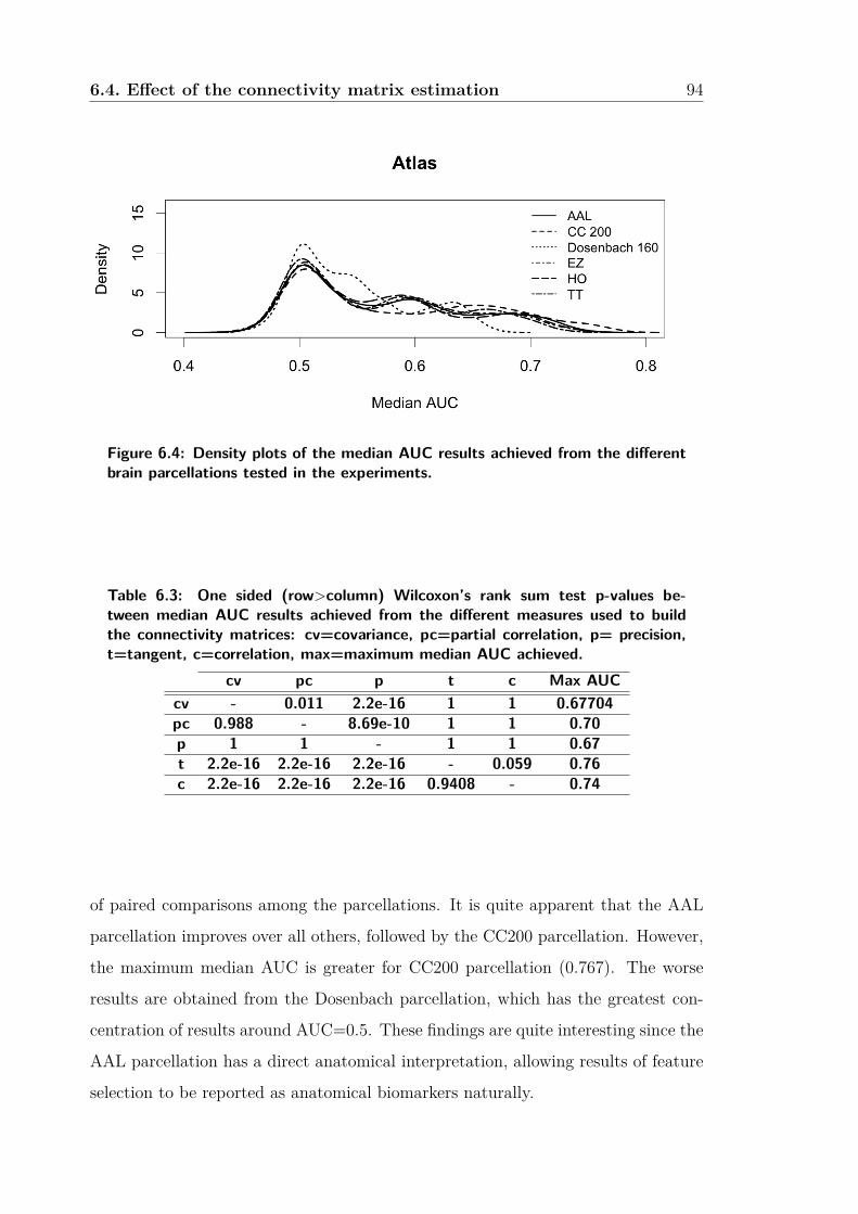
6.4. Effect of the connectivity matrix estimation 94
Figure 6.4: Density plots of the median AUC results achieved from the differentbrain parcellations tested in the experiments.
Table 6.3: One sided (row>column) Wilcoxon’s rank sum test p-values be-tween median AUC results achieved from the different measures used to buildthe connectivity matrices: cv=covariance, pc=partial correlation, p= precision,t=tangent, c=correlation, max=maximum median AUC achieved.
cv pc p t c Max AUCcv - 0.011 2.2e-16 1 1 0.67704pc 0.988 - 8.69e-10 1 1 0.70p 1 1 - 1 1 0.67t 2.2e-16 2.2e-16 2.2e-16 - 0.059 0.76c 2.2e-16 2.2e-16 2.2e-16 0.9408 - 0.74
of paired comparisons among the parcellations. It is quite apparent that the AAL
parcellation improves over all others, followed by the CC200 parcellation. However,
the maximum median AUC is greater for CC200 parcellation (0.767). The worse
results are obtained from the Dosenbach parcellation, which has the greatest con-
centration of results around AUC=0.5. These findings are quite interesting since the
AAL parcellation has a direct anatomical interpretation, allowing results of feature
selection to be reported as anatomical biomarkers naturally.
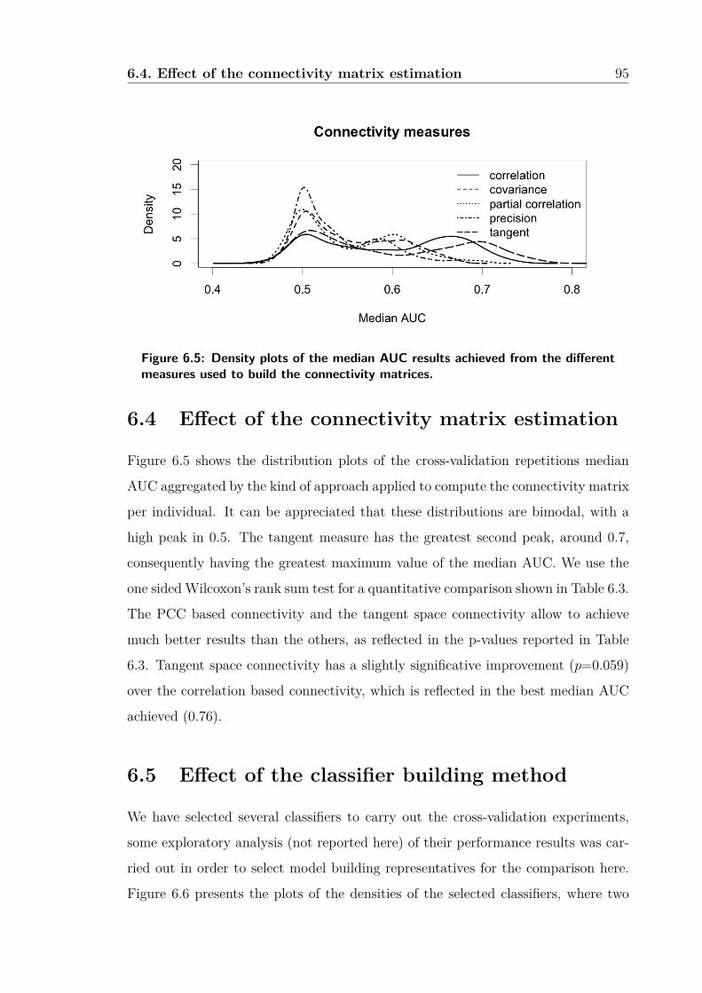
6.4. Effect of the connectivity matrix estimation 95
Figure 6.5: Density plots of the median AUC results achieved from the differentmeasures used to build the connectivity matrices.
6.4 Effect of the connectivity matrix estimation
Figure 6.5 shows the distribution plots of the cross-validation repetitions median
AUC aggregated by the kind of approach applied to compute the connectivity matrix
per individual. It can be appreciated that these distributions are bimodal, with a
high peak in 0.5. The tangent measure has the greatest second peak, around 0.7,
consequently having the greatest maximum value of the median AUC. We use the
one sided Wilcoxon’s rank sum test for a quantitative comparison shown in Table 6.3.
The PCC based connectivity and the tangent space connectivity allow to achieve
much better results than the others, as reflected in the p-values reported in Table
6.3. Tangent space connectivity has a slightly significative improvement (p=0.059)
over the correlation based connectivity, which is reflected in the best median AUC
achieved (0.76).
6.5 Effect of the classifier building method
We have selected several classifiers to carry out the cross-validation experiments,
some exploratory analysis (not reported here) of their performance results was car-
ried out in order to select model building representatives for the comparison here.
Figure 6.6 presents the plots of the densities of the selected classifiers, where two
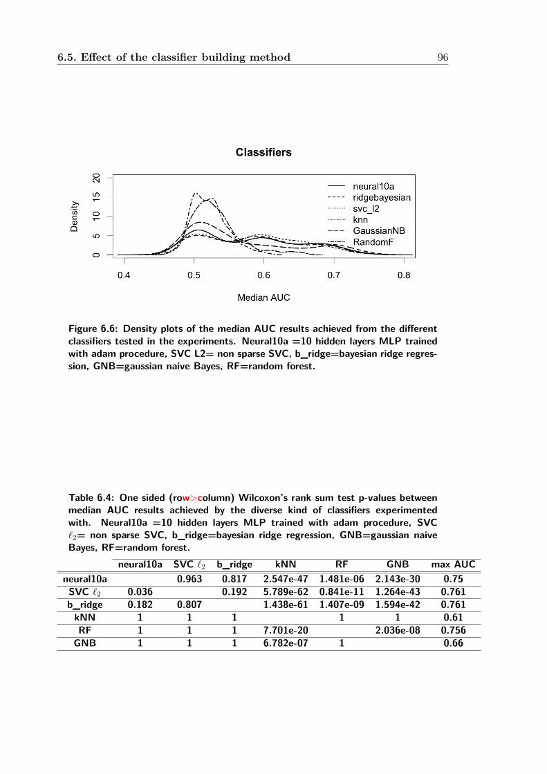
6.5. Effect of the classifier building method 96
Figure 6.6: Density plots of the median AUC results achieved from the differentclassifiers tested in the experiments. Neural10a =10 hidden layers MLP trainedwith adam procedure, SVC L2= non sparse SVC, b_ridge=bayesian ridge regres-sion, GNB=gaussian naive Bayes, RF=random forest.
Table 6.4: One sided (row>column) Wilcoxon’s rank sum test p-values betweenmedian AUC results achieved by the diverse kind of classifiers experimentedwith. Neural10a =10 hidden layers MLP trained with adam procedure, SVC`2= non sparse SVC, b_ridge=bayesian ridge regression, GNB=gaussian naiveBayes, RF=random forest.
neural10a SVC `2 b_ridge kNN RF GNB max AUCneural10a 0.963 0.817 2.547e-47 1.481e-06 2.143e-30 0.75SVC `2 0.036 0.192 5.789e-62 0.841e-11 1.264e-43 0.761b_ridge 0.182 0.807 1.438e-61 1.407e-09 1.594e-42 0.761kNN 1 1 1 1 1 0.61RF 1 1 1 7.701e-20 2.036e-08 0.756GNB 1 1 1 6.782e-07 1 0.66

6.6. Effect of the feature extraction/selection 97
Figure 6.7: Density plots of the median AUC results achieved from the differentfeature extraction approaches. PCA2 = PCA retaining only half of the features,MDS2000, fa2000= MDS, FA retaining 2000 features, LNE3=LNE retaining onethird of the features, p90= PCC selection 90% percentile.
Table 6.5: One sided (row>column) Wilcoxon’s rank sum test p-values betweenmedian AUC results achieved from the different best versions of the feature ex-traction algorithms. PCA2 = PCA retaining only half of the features, MDS2000,fa2000= MDS, FA retaining 2000 features, LNE3=LNE retaining one third ofthe transformed features.
PCA2 MDS2000 LNE3 p90 fa2000 Max AUCPCA2 1.248e-116 8.525e-55 0.0029 0.078 0.75
MDS2000 1 1 1 1 0.55LNE3 1 4.878e-66 1 1 0.62fa200 0.921 1.577e-122 6.900e-59 0.0833 0.76
groups of classifiers can be easily identified visually, one group of less performing
classifiers whose mass of results is centered around median AUC=0.5, and the other
that achieve better responses. The results of the one-sided Wilcoxon’s rank sum test
in Table 6.4 provide confirmation of the qualitative identification of two groups of
classifiers. Top performing are sparse SVC `2, ridge classifier and the MLP with 10
hidden layers. Among them, the sparse SVC has an almost significant improvement
over the other two. These results are in agreement with state of the art results.

6.6. Effect of the feature extraction/selection 98
6.6 Effect of the feature extraction/selection
Feature extraction consists of a data space transformation where the new variables
lose the meaning of the original space, i.e. the anatomical localization of the ef-
fects. Feature selection (such as the PCC based connection selection) preserves the
meaning of the original variables, because the selected variables are not transformed.
Feature selection is the preferred approach for the medical researchers because they
can explain and compare the found biomarkers in the framework of the medical
literature.
We have explored the effect of the feature extraction and feature selection pro-
cedures described above. The Isometric Map has been discarded as its results were
far worse than any other feature extraction method. For the other methods we have
made an exploration of the performance achieved when varying the number of fea-
tures retained, finding slight significant improvements leading to specific selections
for each approach that are compared in Table 6.5 using the one sided Wilkoxon’s
rank sum test as the density functions plotted in Figure 6.7 are far from Gaussian in
most cases (exception made of MDS which appears to be almost Gaussian). PCA2
has an almost uniform distribution in the interval [0.5,0.7] of AUC values. Regard-
ing Table 6.5, PCA2 improves significantly over the other procedures, althought the
significance of the improvement over FA is short.
6.7 Best results
One of the conclusions that can be extracted from the previous sections is that find-
ing good performing pipelines requires exploration of many computational choices
where most of them will not achieve good results. Here we have selected the best
performing pipelines found by exhaustive search over our experimental results, some
of them improving over most of the results reported in the state of the art of Table
3.2. Table 6.6 gives the best median AUC scores found, together with the 5% and
95% percentiles of the cross-validation results in our experiments for comparison
with the most comprehensive exploration of results to date [176], where the best re-
ported results are 0.66, 0.711, and 0.756 for the 5%, 50%, 95% percentiles of median

6.7. Best results 99
Table 6.6: Best median AUC scores found in cross-validation repetitions, withcorresponding settings (parcellation, feature extraction, classifier, and connectiv-ity measure) that achieved it.
Settings AUC percentilesParcel. Feat. extr. Classifier conn. meas. 5% median 95%cc200 fa logistic `1 tangent 0.733 0.765 0.803cc200 pca logistic `2 tangent 0.739 0.765 0.801cc200 fa svc `1 tangent 0.739 0.764 0.803cc200 fa1000 logistic `1 tangent 0.733 0.765 0.803cc200 pca svc `1 tangent 0.735 0.767 0.805cc200 fa2000 logistic `1 tangent 0.733 0.765 0.803cc200 fa2000 svc `1 tangent 0.739 0.764 0.803
Best reported to date [176] 0.66 0.711 0.756
Table 6.7: Best Acc scores found in cross-validation, with corresponding settings(parcellation, feature selection, classifier, and connectivity measure) that achievedit.
Settings Acc percentilesparcel. Feat. ext. Classifier conn. meas. 5% median 95%cc200 fa logistic `1 tangent 66.9 69.9 72.3cc200 fa svc `1 tangent 65.7 69.9 72.8cc200 fa1000 logistic `1 tangent 66.9 69.9 72.3cc200 fa1000 svc `1 tangent 65.7 69.9 72.8cc200 fa2000 logistic `1 tangent 66.9 69.9 72.3cc200 fa2000 svc `1 tangent 65.7 69.9 72.8cc200 pca logistic `2 tangent 67.3 70.5 72.1cc200 pca svc `1 tangent 65.9 70.1 72.1
Best reported to date [203] - - 77

6.7. Best results 100
AUC distribution across all repetitions of the cross-validation experiments. This
comparison shows the impact of feature extraction approaches to enhance classifi-
cation results. Because many of the results in the literature are reported in terms
of accuracy, we include here the corresponding accuracy tables. Table 6.7 gives the
instances with the best accuracy results of our experiments, comparing favorably
with the results gathered in Table 3.2. Some recent results [199, 203] have been
achieved using brain parcellations that are not accessible, hence direct comparison
against them is not possible for us.
Chapter 7
Results of Deep Learning
Approaches
In this Chapter we report two experiences on the application of Deep Learning (DL)
to the ASC discrimination based on the connectivity matrices. The first was imple-
mented in Matlab and reported in Section 7.1. Section 7.2 tells our last experience
using the Google Codelabs environment to apply DL, and transfer learning to this
problem. Section 7.3 gives some comments on our attempts to apply DL to this
problem.
7.1 Matlab implementation
We report a series experiments on the application of CNNs [264,311] over the connec-
tivity matrices obtained with the diverse parcellations and connectivity measures.
CNNs carry out induction of feature extraction filters at diverse abstraction levels,
hence no feature extraction have been included in the experiment. We have used
the Matlab implementation of CNNs, publishing the code and the data in zenodo1. The number of the experiments is limited by available computing resources.Table
7.1 gives the best results achieved by each CNN topology after 10 repetitions of
10-fold crossvalidation with each setting. One of the difficulties of the application
1https://zenodo.org/record/4121200
101
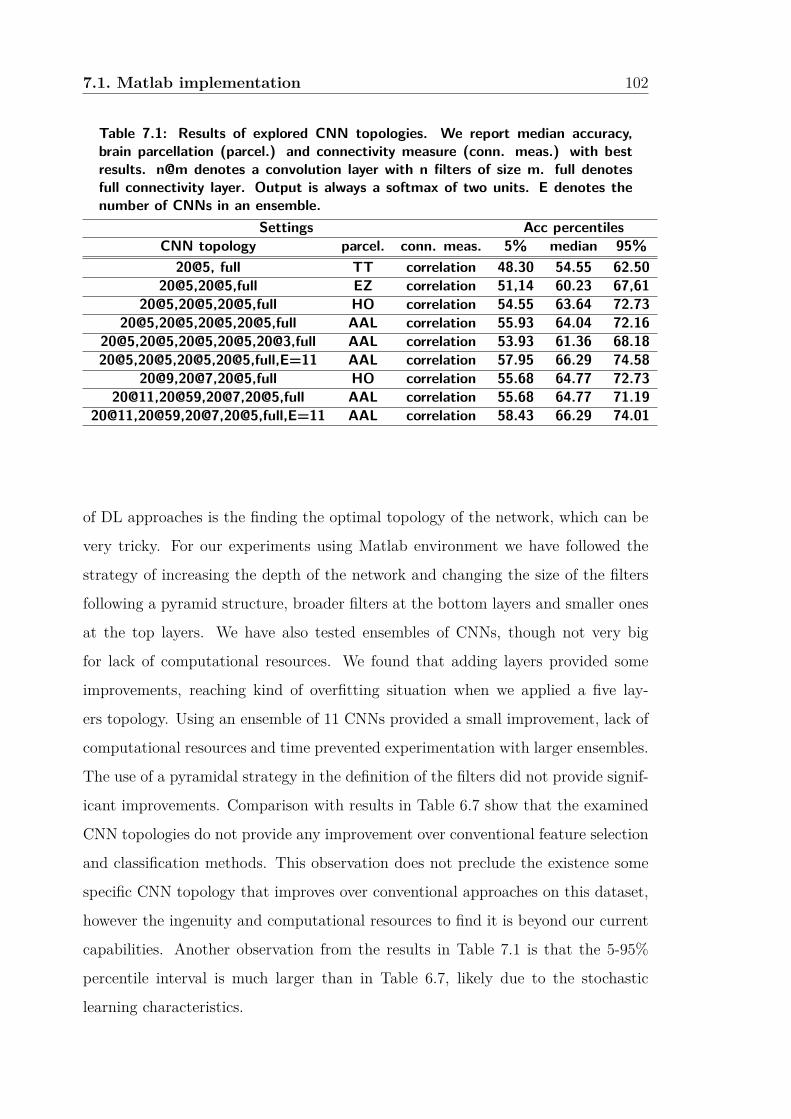
7.1. Matlab implementation 102
Table 7.1: Results of explored CNN topologies. We report median accuracy,brain parcellation (parcel.) and connectivity measure (conn. meas.) with bestresults. n@m denotes a convolution layer with n filters of size m. full denotesfull connectivity layer. Output is always a softmax of two units. E denotes thenumber of CNNs in an ensemble.
Settings Acc percentilesCNN topology parcel. conn. meas. 5% median 95%20@5, full TT correlation 48.30 54.55 62.50
20@5,20@5,full EZ correlation 51,14 60.23 67,6120@5,20@5,20@5,full HO correlation 54.55 63.64 72.73
20@5,20@5,20@5,20@5,full AAL correlation 55.93 64.04 72.1620@5,20@5,20@5,20@5,20@3,full AAL correlation 53.93 61.36 68.1820@5,20@5,20@5,20@5,full,E=11 AAL correlation 57.95 66.29 74.58
20@9,20@7,20@5,full HO correlation 55.68 64.77 72.7320@11,20@59,20@7,20@5,full AAL correlation 55.68 64.77 71.19
20@11,20@59,20@7,20@5,full,E=11 AAL correlation 58.43 66.29 74.01
of DL approaches is the finding the optimal topology of the network, which can be
very tricky. For our experiments using Matlab environment we have followed the
strategy of increasing the depth of the network and changing the size of the filters
following a pyramid structure, broader filters at the bottom layers and smaller ones
at the top layers. We have also tested ensembles of CNNs, though not very big
for lack of computational resources. We found that adding layers provided some
improvements, reaching kind of overfitting situation when we applied a five lay-
ers topology. Using an ensemble of 11 CNNs provided a small improvement, lack of
computational resources and time prevented experimentation with larger ensembles.
The use of a pyramidal strategy in the definition of the filters did not provide signif-
icant improvements. Comparison with results in Table 6.7 show that the examined
CNN topologies do not provide any improvement over conventional feature selection
and classification methods. This observation does not preclude the existence some
specific CNN topology that improves over conventional approaches on this dataset,
however the ingenuity and computational resources to find it is beyond our current
capabilities. Another observation from the results in Table 7.1 is that the 5-95%
percentile interval is much larger than in Table 6.7, likely due to the stochastic
learning characteristics.

7.2. Google codelab implementation 103
7.2 Google codelab implementation
Using the resources provided by Google Codelabs2 we carried out some experiments
with little success. Transfer learning using as base network the VGG16, MobileNet
and Resnet50 networks achieved very poor results of average accuracy 0.4615, in-
dependently of the brain parcellation used. Fully trained CNN on the connectivity
matrix obtained from the AAL and CC200 atlas increased to Acc = 54.00.
The model was expected to improve around the predefined repositories and ar-
chitecture with Tensorflow and Keras (https://tfhub.dev/), but having tested with
images given the existing example-based tests, these improve up to 20%. In our
case, its applicability and existing information is almost null. On the other hand,
this occurs with the tensorflow 2.0 version, the previous reviews and comments were
given with the Tensorflow 1.0 version. It is interesting to mention that there are
significant differences between both versions at the time of their execution, this is
due to the updating of the libraries, improvements to the development model or
others that do not facilitate continuity in order to generate a robust model.
7.3 Conclussions on DL performance
Our conclussions on the applicability of DL to ASC discrimination based on brain
connectivity are very negative. It does not seem evident that DL will be providing
much better results than the conventional machine learning approaches. Besides our
experience reported above the literature has several examples of attempts to apply
DL to ASC prediction on the ABIDE dataset. In order to discuss comparative re-
sults we face the issue of the diversity of the underlying pipeline selections and DL
design pecularities. We have not found in the literature an exhaustive exploration
of DL approaches over the brain parcellations and connectivity measures compa-
rable to ours. However, we have shown that they have quite significant effect on
the predictive performance. For instance, experiments involving a large ensamble
of 300 CNNs [203] was carried out on a very specific irreproducible brain parcella-
2https://codelabs.developers.google.com/?cat=all
7.3. Conclussions on DL performance 104
tion and connectivity matrix constructions, with ad hoc simplified CNN topologies
found by after a long trial and error process with little succes (Acc=67). A greater
computational (irreproducible) tour de force of training an ensemble of 3D CNN ap-
plied on the normalized rs-fMRI data [199] provided a small improvement (Acc=72).
The use of recurrent networks such as the LSTM [194] did not achieve better re-
sults than the conventional approaches (Acc=68%). Graph convolutional networks
(GCN) [189, 191] did not provide significant improvement over conventional results
in Table 6.7 achieving the best result Acc=70 adding ancilliary information to the
connectivity data. Even using ensembles of GCN [192] did not add significant ben-
efits. Using autoencoders for feature extraction combined with conventional MLP
classifier provided one of the best reported results [206] .

Chapter 8
Conclusions and future work
In this Chapter we provide summarized conclussions of the work carried out in
Section (8.1) and some lines of future work in Section (8.1).
8.1 Conclusions
The predictive approach to the analysis of brain connectivity from rs-fMRI data is
gaining importance in recent studies. In this approach, brain connectivity biomark-
ers are confirmed by the predictive performance in the classification between target
populations. Up to this date there is no comprehensive study of the impact of the
choices that can be made while building the machine learning pipelines, hence we
have carried out a comprehensive assessment on the ABIDE I dataset, finding that
some feature extraction procedures provide a boost on the performance of the clas-
sifiers across several connectivity matrix building approaches, namely the classical
principal component analysis (PCA) and factor analysis (FA).
A key issue is the reproducibility of the results, that depends on the availability
of the data and the precise computational resources to other researchers in the
community. For this reason, we emphasize the public availability of the data and
programming resources used for this study via github1 and zenodo2 repositories.
1https://github.com/mmscnet/Impact-feature-extraction-in-Autism2https://zenodo.org/record/4121200
105
8.2. Future work 106
8.2 Future work
Future work should address the extension of the computational experiments to the
full extent of the ABIDE II dataset. Other conectomics datasets collecting sub-
jects and controls from connectivity analysis regarding other diseases will also be
considered. Additionally, innovative machine learning approaches [312–315] will be
explored. The instability of the validation of the predictive approaches in many
instances of neuroscience datasets is an issue of methodological concern. In the
case of the ABIDE dataset the sources of this instability are the heterogeneity of
the subjects, diagnostic criteria implementation, and the data capture differences
among sites. Future work will explore the relevance of novel validation approaches
such as the works underlying the statistical agnostic mapping [316] to provide more
robust performance predictions leading to better grounded biomarker identification.
Bibliography
[1] M. Lindquist. 1 principles of functional magnetic resonance imaging. 2014.
[2] J. Ashburner and K.J. Friston. Voxel based morphometry. In Encyclopedia of
Neuroscience, pages 471–477. Elsevier, 2009.
[3] Mohammad-Parsa Hosseini, Mohammad-Reza Nazem-Zadeh, Dario Pompili,
Kourosh Jafari-Khouzani, Kost Elisevich, and Hamid Soltanian-Zadeh. Com-
parative performance evaluation of automated segmentation methods of hip-
pocampus from magnetic resonance images of temporal lobe epilepsy patients.
Medical Physics, 43(1):538–553, jan 2016.
[4] Pei Huang, Johan D. Carlin, Richard N. Henson, and Marta M. Correia. Im-
proved motion correction of submillimetre 7t fMRI time series with boundary-
based registration (BBR). NeuroImage, 210:116542, apr 2020.
[5] Martin A. Lindquist, Ji Meng Loh, and Yu (Ryan) Yue. Adaptive spatial
smoothing of fMRI images. Statistics and Its Interface, 3(1):3–13, 2010.
[6] Sebastian Ruder. Neural Transfer Learning for Natural Language Processing.
PhD thesis, National University of Ireland, Galway, 2019.
[7] Karen Simonyan and Andrew Zisserman. Very deep convolutional networks
for large-scale image recognition. September 2014.
[8] Catherine Lord, Traolach S. Brugha, Tony Charman, James Cusack, Guil-
laume Dumas, Thomas Frazier, Emily J. H. Jones, Rebecca M. Jones, An-
drew Pickles, Matthew W. State, Julie Lounds Taylor, and Jeremy Veenstra-107

Bibliography 108
VanderWeele. Autism spectrum disorder. Nature Reviews Disease Primers,
6(1):5, 2020.
[9] Shreya Bhat, U Rajendra Acharya, Hojjat Adeli, G Muralidhar Bairy, and
Amir Adeli. Autism: cause factors, early diagnosis and therapies. Rev Neu-
rosci, 25(6):841–850, 2014.
[10] National Center on Birth Defects, Developmental (Centers for Disease Con-
trol, Prevention). Division of Congenital, Developmental Disorders., Debo-
rah L. Christensen, Jon Baio, Kim Van Naarden Braun, Deborah Bilder, Jane
Charles, John N. Constantino, Julie Daniels, Maureen S. Durkin, Robert T.
Fitzgerald, Margaret Kurzius-Spencer, Li-Ching Lee, Sydney Pettygrove,
Cordelia Robinson, Eldon Schulz, Chris Wells, Martha S. Wingate, Walter
Zahorodny, and Marshalyn Yeargin-Allsopp. Mmwr. surveillance summaries
: Morbidity and mortality weekly report. surveillance summaries ; v. 65, no.
ss-13. 65(13), November 16, 2018.
[11] Meng-Chuan Lai, Michael V. Lombardo, John Suckling, Amber N. V. Ruigrok,
Bhismadev Chakrabarti, Christine Ecker, Sean C. L. Deoni, Michael C. Craig,
Declan G. M. Murphy, Edward T. Bullmore, MRC AIMS Consortium, and
Simon Baron-Cohen. Biological sex affects the neurobiology of autism. Brain,
136(9):2799–2815, 08 2013.
[12] Meng-Chuan Lai, Michael V Lombardo, Bonnie Auyeung, Bhismadev
Chakrabarti, and Simon Baron-Cohen. Sex/gender differences and autism:
setting the scene for future research. J Am Acad Child Adolesc Psychiatry,
54(1):11–24, Jan 2015.
[13] Meng-Chuan Lai, Michael V Lombardo, and Simon Baron-Cohen. Autism.
The Lancet, 383(9920):896–910, 2013.
[14] Laurent Mottron and Danilo Bzdok. Autism spectrum heterogeneity: fact or
artifact? Molecular Psychiatry, 2020.
Bibliography 109
[15] C Ecker, DS Andrews, CM Gudbrandsen, and et al. Association between the
probability of autism spectrum disorder and normative sex-related phenotypic
diversity in brain structure. JAMA Psychiatry, 74(4):329–338, 2017.
[16] Catherine Lord, Eva Petkova, Vanessa Hus, Weijin Gan, Feihan Lu, Donna M.
Martin, Opal Ousley, Lisa Guy, Raphael Bernier, Jennifer Gerdts, Molly Al-
germissen, Agnes Whitaker, James S. Sutcliffe, Zachary Warren, Ami Klin,
Celine Saulnier, Ellen Hanson, Rachel Hundley, Judith Piggot, Eric Fom-
bonne, Mandy Steiman, Judith Miles, Stephen M. Kanne, Robin P. Goin-
Kochel, Sarika U. Peters, Edwin H. Cook, Stephen Guter, Jennifer Tjernagel,
Lee Anne Green-Snyder, Somer Bishop, Amy Esler, Katherine Gotham, Rhi-
annon Luyster, Fiona Miller, Jennifer Olson, Jennifer Richler, and Susan Risi.
A Multisite Study of the Clinical Diagnosis of Different Autism Spectrum
Disorders. Archives of General Psychiatry, 69(3):306–313, 03 2012.
[17] Shreya Bhat, U. Rajendra Acharya, Hojjat Adeli, G. Muralidhar Bairy, and
Amir Adeli. Automated diagnosis of autism: in search of a mathematical
marker. Reviews in the Neurosciences, 25(6):851 – 861, 2014.
[18] Tao Chen, Ye Chen, Mengxue Yuan, Mark Gerstein, Tingyu Li, Huiying Liang,
Tanya Froehlich, and Long Lu. The development of a practical artificial in-
telligence tool for diagnosing and evaluating autism spectrum disorder: Mul-
ticenter study. JMIR Med Inform, 8(5):e15767, May 2020.
[19] Hidir Selcuk Nogay and Hojjat Adeli. Machine learning (ml) for the diag-
nosis of autism spectrum disorder (asd) using brain imaging. Reviews in the
Neurosciences, (0):000010151520200043, 2020.
[20] Fermín Segovia, Rosemary Holt, Michael Spencer, Juan M. Górriz, Javier
Ramírez, Carlos G. Puntonet, Christophe Phillips, Lindsay Chura, Simon
Baron-Cohen, and John Suckling. Identifying endophenotypes of autism: a
multivariate approach. Frontiers in Computational Neuroscience, 8:60, 2014.
[21] L Q Uddin, D R Dajani, W. Voorhies, H. Bednarz, and R K Kana. Progress
and roadblocks in the search for brain-based biomarkers of autism and
Bibliography 110
attention-deficit/hyperactivity disorder. Translational Psychiatry, 7(8):e1218–
e1218, 2017.
[22] A Di Martino, C-G Yan, Q Li, E Denio, F X Castellanos, K Alaerts, J S
Anderson, M Assaf, S Y Bookheimer, M Dapretto, B Deen, S Delmonte,
I Dinstein, B Ertl-Wagner, D A Fair, L Gallagher, D P Kennedy, C L Keown,
C Keysers, J E Lainhart, C Lord, B Luna, V Menon, N J Minshew, C S Monk,
S Mueller, R-A Müller, M B Nebel, J T Nigg, K O’Hearn, K A Pelphrey,
S J Peltier, J D Rudie, S Sunaert, M Thioux, J M Tyszka, L Q Uddin, J S
Verhoeven, N Wenderoth, J L Wiggins, S H Mostofsky, and M P Milham. The
autism brain imaging data exchange: towards a large-scale evaluation of the
intrinsic brain architecture in autism. Molecular Psychiatry, 19:659 EP –, 06
2013.
[23] Adriana Di Martino, David O’Connor, Bosi Chen, Kaat Alaerts, Jeffrey S.
Anderson, Michal Assaf, Joshua H. Balsters, Leslie Baxter, Anita Beggiato,
Sylvie Bernaerts, Laura M. E. Blanken, Susan Y. Bookheimer, B. Blair
Braden, Lisa Byrge, F. Xavier Castellanos, Mirella Dapretto, Richard De-
lorme, Damien A. Fair, Inna Fishman, Jacqueline Fitzgerald, Louise Gal-
lagher, R. Joanne Jao Keehn, Daniel P. Kennedy, Janet E. Lainhart, Beatriz
Luna, Stewart H. Mostofsky, Ralph-Axel Müller, Mary Beth Nebel, Joel T.
Nigg, Kirsten O’Hearn, Marjorie Solomon, Roberto Toro, Chandan J. Vaidya,
Nicole Wenderoth, Tonya White, R. Cameron Craddock, Catherine Lord, Ben-
nett Leventhal, and Michael P. Milham. Enhancing studies of the connectome
in autism using the autism brain imaging data exchange ii. Scientific Data,
4:170010 EP –, 03 2017.
[24] Benjamin Gutierrez Becker, Tassilo Klein, and Christian Wachinger. Gaus-
sian process uncertainty in age estimation as a measure of brain abnormality.
NeuroImage, 175:246 – 258, 2018.
[25] Thomas Wolfers, Dorothea L. Floris, Richard Dinga, Daan van Rooij,
Christina Isakoglou, Seyed Mostafa Kia, Mariam Zabihi, Alberto Llera, Ra-
janikanth Chowdanayaka, Vinod J. Kumar, Han Peng, Charles Laidi, Dafnis

Bibliography 111
Batalle, Ralica Dimitrova, Tony Charman, Eva Loth, Meng-Chuan Lai, Emily
Jones, Sarah Baumeister, Carolin Moessnang, Tobias Banaschewski, Chris-
tine Ecker, Guillaume Dumas, Jonathan O’Muircheartaigh, Declan Murphy,
Jan K. Buitelaar, Andre F. Marquand, and Christian F. Beckmann. From pat-
tern classification to stratification: towards conceptualizing the heterogeneity
of autism spectrum disorder. Neuroscience & Biobehavioral Reviews, 104:240
– 254, 2019.
[26] Mehran Ahmadlou, Hojjat Adeli, and Amir Adeli. Improved visibility graph
fractality with application for the diagnosis of autism spectrum disorder. Phys-
ica A: Statistical Mechanics and its Applications, 391(20):4720 – 4726, 2012.
[27] Mehran Ahmadlou and Hojjat Adeli. Complexity of weighted graph: A new
technique to investigate structural complexity of brain activities with applica-
tions to aging and autism. Neuroscience Letters, 650:103 – 108, 2017.
[28] Mehran Ahmadlou, Hojjat Adeli, and Amir Adeli. Fuzzy synchronization
likelihood-wavelet methodology for diagnosis of autism spectrum disorder.
Journal of Neuroscience Methods, 211(2):203 – 209, 2012.
[29] E. Puerto, J. Aguilar, C. López, and D. Chávez. Using multilayer fuzzy cog-
nitive maps to diagnose autism spectrum disorder. Applied Soft Computing,
75:58 – 71, 2019.
[30] Alicia d’Anjou, Manuel Graña, and Francois Moutet. Brief survey about the
search for biomarkers and computer aided diagnosis of autism spectrum disor-
der. Technical Report http://doi.org/10.5281/zenodo.1408202, Zenodo, 2018.
[31] Alex M. Pagnozzi, Eugenia Conti, Sara Calderoni, Jurgen Fripp, and
Stephen E. Rose. A systematic review of structural mri biomarkers in autism
spectrum disorder: A machine learning perspective. International Journal of
Developmental Neuroscience, 71:68 – 82, 2018.
[32] Stephanie H. Ameis and Marco Catani. Altered white matter connectivity as
a neural substrate for social impairment in autism spectrum disorder. Cortex,
Bibliography 112
62:158 – 181, 2015. Special issue: The clinical anatomy of the limbic lobe and
connected structures.
[33] Xin Di, Azeezat Azeez, Xiaobo Li, Emad Haque, and Bharat B. Biswal. Dis-
rupted focal white matter integrity in autism spectrum disorder: A voxel-
based meta-analysis of diffusion tensor imaging studies. Progress in Neuro-
Psychopharmacology and Biological Psychiatry, 82:242 – 248, 2018.
[34] Joshua H. Balsters, Dante Mantini, and Nicole Wenderoth. Connectivity-
based parcellation reveals distinct cortico-striatal connectivity fingerprints in
autism spectrum disorder. NeuroImage, 170:412 – 423, 2018. Segmenting the
Brain.
[35] Salim Arslan, Sofia Ira Ktena, Antonios Makropoulos, Emma C. Robinson,
Daniel Rueckert, and Sarah Parisot. Human brain mapping: A systematic
comparison of parcellation methods for the human cerebral cortex. NeuroIm-
age, 170:5 – 30, 2018. Segmenting the Brain.
[36] Neil D. Woodward and Carissa J. Cascio. Resting-State Functional Connec-
tivity in Psychiatric Disorders. JAMA Psychiatry, 72(8):743–744, 08 2015.
[37] Manuel Graña, Leire Ozaeta, and Darya Chyzhyk. Resting state effective con-
nectivity allows auditory hallucination discrimination. International Journal
of Neural Systems, 27(05):1750019, 2017. PMID: 28274168.
[38] Priya Aggarwal and Anubha Gupta. Multivariate graph learning for detecting
aberrant connectivity of dynamic brain networks in autism. Medical Image
Analysis, 56:11 – 25, 2019.
[39] Zening Fu, Yiheng Tu, Xin Di, Yuhui Du, Jing Sui, Bharat B. Biswal, Zhiguo
Zhang, N. de Lacy, and V.D. Calhoun. Transient increased thalamic-sensory
connectivity and decreased whole-brain dynamism in autism. NeuroImage,
190:191 – 204, 2019. Mapping diseased brains.

Bibliography 113
[40] Andry Andriamananjara, Rayan Muntari, and Alessandro Crimi. Overlaps
in brain dynamic functional connectivity between schizophrenia and autism
spectrum disorder. Scientific African, 2:e00019, 2019.
[41] Dana Mastrovito, Catherine Hanson, and Stephen Jose Hanson. Differ-
ences in atypical resting-state effective connectivity distinguish autism from
schizophrenia. NeuroImage: Clinical, 18:367 – 376, 2018.
[42] Maya A. Reiter, Lisa E. Mash, Annika C. Linke, Christopher H. Fong, Inna
Fishman, and Ralph-Axel Müller. Distinct patterns of atypical functional con-
nectivity in lower-functioning autism. Biological Psychiatry: Cognitive Neu-
roscience and Neuroimaging, 4(3):251 – 259, 2019.
[43] Joanna Granich, Alena Dass, Margherita Busacca, Dennis Moore, Ange-
lika Anderson, Svetha Venkatesh, Thi Duong, Pratibha Vellanki, Amanda
Richdale, David Trembath, Darin Cairns, Wendy Marshall, Tania Rodwell,
Madeleine Rayner, and Andrew J. O. Whitehouse. Randomised controlled
trial of an ipad based early intervention for autism: Toby playpad study pro-
tocol. BMC Pediatrics, 16(1):167, Oct 2016.
[44] Silvana E Mengoni, Karen Irvine, Deepshikha Thakur, Garry Barton, Ker-
stin Dautenhahn, Karen Guldberg, Ben Robins, David Wellsted, and Shivani
Sharma. Feasibility study of a randomised controlled trial to investigate the
effectiveness of using a humanoid robot to improve the social skills of children
with autism spectrum disorder (kaspar rct): a study protocol. BMJ Open,
7(6), 2017.
[45] Dennis W. Moore, Svetha Venkatesh, Angelika Anderson, Stewart Greenhill,
Dinh Phung, Thi Duong, Darin Cairns, Wendy Marshall, and Andrew J. O.
Whitehouse. Toby play-pad application to teach children with asd – a pi-
lot trial. Developmental Neurorehabilitation, 18(4):213–217, 2015. PMID:
23869435.
Bibliography 114
[46] IP Oono, EJ Honey, and H McConachie. Parent mediated early intervention
for young children with autism spectrum disorders (asd). Cochrane Database
of Systematic Reviews, (4), 2013.
[47] B Reichow, K Hume, EE Barton, and BA Boyd. Early intensive behavioral
intervention (EIBI) for young children with autism spectrum disorders (ASD).
Cochrane Database of Systematic Reviews, (5), 2018.
[48] Andrew J.O. Whitehouse, Joanna Granich, Gail Alvares, Margherita Busacca,
Matthew N. Cooper, Alena Dass, Thi Duong, Rajes Harper, Wendy Marshall,
Amanda Richdale, Tania Rodwell, David Trembath, Pratibha Vellanki, Den-
nis W. Moore, and Angelika Anderson. A randomised controlled trial of an
ipad-based application to complement early behavioural intervention in autism
spectrum disorder. Journal of Child Psychology and Psychiatry, 58(9):1042–
1052, 2017.
[49] Elena Cravedi, Emmanuelle Deniau, Marianna Giannitelli, Hugues Pellerin,
Virginie Czernecki, Tiphanie Priou, Jean Xavier, Angele Consoli, Andreas
Hartmann, and David Cohen. Disentangling tourette syndrome heterogeneity
through hierarchical ascendant clustering. Dev Med Child Neurol, 2018.
[50] Pashalina Lialiou, Dimitrios Zikos, and John Mantas. Quality of Life through
Quality of Information, volume 180 of Studies in Health Technology and In-
formatics, chapter Development and Evaluation of an Expert System for the
Diagnosis of Child Autism, pages 1185 – 1187. IOS Press, 2012.
[51] Maryam Akhavan Aghdam, Arash Sharifi, and Mir Mohsen Pedram. Combi-
nation of rs-fMRI and sMRI data to discriminate autism spectrum disorders
in young children using deep belief network. Journal of Digital Imaging, May
2018.
[52] Bhaskar Sen, Neil C. Borle, Russell Greiner, and Matthew R. G. Brown. A
general prediction model for the detection of ADHD and autism using struc-
tural and functional mri. PLOS ONE, 13(4):1–28, 04 2018.
Bibliography 115
[53] Ridha Djemal, Khalil AlSharabi, Sutrisno Ibrahim, and Abdullah Alsuwailem.
EEG-based computer aided diagnosis of autism spectrum disorder using
wavelet, entropy, and ann. BioMed Research International, 2017:9, 2017.
[54] Shilan S. Hameed, Rohayanti Hassan, and Fahmi F. Muhammad. Selection
and classification of gene expression in autism disorder: Use of a combination
of statistical filters and a gbpso-svm algorithm. PLOS ONE, 12(11):1–25, 11
2017.
[55] Tomasz Latkowski and Stanislaw Osowski. Computerized system for recogni-
tion of autism on the basis of gene expression microarray data. Computers in
Biology and Medicine, 56:82 – 88, 2015.
[56] Genyuan Li, Olivia Lee, and Herschel Rabitz. High efficiency classification of
children with autism spectrum disorder. PLOS ONE, 13(2):1–23, 02 2018.
[57] Changchun Liu, Karla Conn, Nilanjan Sarkar, and Wendy Stone. Physiology-
based affect recognition for computer-assisted intervention of children with
autism spectrum disorder. International Journal of Human-Computer Studies,
66(9):662 – 677, 2008.
[58] Anurag Sharma, Arun Khosla, Mamta Khosla, and Yogeswara Rao. Fast
and accurate diagnosis of autism (fada): a novel hierarchical fuzzy system
based autism detection tool. Australasian Physical & Engineering Sciences in
Medicine, Jul 2018.
[59] Tomasz Latkowski and Stanislaw Osowski. Gene selection in autism – com-
parative study. Neurocomputing, 250:37 – 44, 2017. Applications in Compu-
tational Intelligence (Selected an improved papers of the 13th International
Work-Conference on Artificial Neural Networks, IWANN2015).
[60] Mahmoud Mansouri, Ann-Charlotte Thuresson, Catalina Betancur, Marion
Leboyer, Christopher Gillberg, Cordelia Langford, and Niklas Dahl. P3:
Array-cgh for the identification of autism susceptibility loci. European Jour-
nal of Medical Genetics, 48(4):449 – 450, 2005. Includes programme and

Bibliography 116
abstracts of the Marie Curie Conferences and Training Courses on arrayCGH
and Molecular Cytogenetics.
[61] Erin D. Bigler. Structural image analysis of the brain in neuropsychology
using magnetic resonance imaging (mri) techniques. Neuropsychology Review,
25(3):224–249, 2015.
[62] Andrew J. Steven, Jiachen Zhuo, and Elias R. Melhem. Diffusion kurtosis
imaging: An emerging technique for evaluating the microstructural environ-
ment of the brain. American Journal of Roentgenology, 202(1):W26–W33,
2018/05/31 2013.
[63] Nan-kuei Chen, Hing-Chiu Chang, Ali Bilgin, Adam Bernstein, and
Theodore P. Trouard. A diffusion-matched principal component analysis
(dm-pca) based two-channel denoising procedure for high-resolution diffusion-
weighted mri. PLOS ONE, 13(4):e0195952–, 04 2018.
[64] Geetha Soujanya Chilla, Cher Heng Tan, Chenjie Xu, and Chueh Loo Poh.
Diffusion weighted magnetic resonance imaging and its recent trend—a survey.
Quantitative Imaging in Medicine and Surgery, 5(3):407–422, 06 2015.
[65] Aurobrata Ghosh and Rachid Deriche. A survey of current trends in dif-
fusion mri for structural brain connectivity. Journal of Neural Engineering,
13(1):011001, 2016.
[66] Rajesh K. Kana, Lucina Q. Uddin, Tal Kenet, Diane Chugani, and Ralph-
Axel Müller. Brain connectivity in autism. Frontiers in Human Neuroscience,
8:349, 2014.
[67] Maggie S M Chow, Sharon L Wu, Sarah E Webb, Katie Gluskin, and D T
Yew. Functional magnetic resonance imaging and the brain: A brief review.
World Journal of Radiology, 9(1):5–9, 01 2017.
[68] Jodie R. Gawryluk, Erin L. Mazerolle, and Ryan C. N. D’Arcy. Does functional
mri detect activation in white matter? a review of emerging evidence, issues,
and future directions. Frontiers in Neuroscience, 8:239, 2014.
Bibliography 117
[69] KA Smitha, K Akhil Raja, KM Arun, PG Rajesh, Bejoy Thomas, TR Kapil-
amoorthy, and Chandrasekharan Kesavadas. Resting state fmri: A review on
methods in resting state connectivity analysis and resting state networks. The
Neuroradiology Journal, 30(4):305–317, 2018/05/25 2017.
[70] H. Lv, Z. Wang, E. Tong, L. M. Williams, G. Zaharchuk, M. Zeineh, A. N.
Goldstein-Piekarski, T. M. Ball, C. Liao, and M. Wintermark. Resting-state
functional mri: Everything that nonexperts have always wanted to know.
American Journal of Neuroradiology, 01 2018.
[71] Bharat B. Biswal. Resting state fmri: A personal history. NeuroImage,
62(2):938–944, 2012.
[72] Alexander Westphal, Avery Voos, and Kevin Pelphrey. Chapter 8 - functional
magnetic resonance imaging as a biomarker for the diagnosis, progression,
and treatment of autistic spectrum disorders. In Robert A. McArthur, editor,
Translational Neuroimaging, pages 221 – 243. Academic Press, 2013.
[73] V. J. Wedeen, R. P. Wang, J. D. Schmahmann, T. Benner, W. Y. I. Tseng,
G. Dai, D. N. Pandya, P. Hagmann, H. D’Arceuil, and A. J. de Crespigny.
Diffusion spectrum magnetic resonance imaging (dsi) tractography of crossing
fibers. NeuroImage, 41(4):1267–1277, 2008.
[74] J. Wedeen Van, Patric Hagmann, Isaac Tseng Wen-Yih, G. Reese Timothy,
and M. Weisskoff Robert. Mapping complex tissue architecture with diffu-
sion spectrum magnetic resonance imaging. Magnetic Resonance in Medicine,
54(6):1377–1386, 2018/05/29 2005.
[75] G Russell Glenn, Li-Wei Kuo, Yi-Ping Chao, Chu-Yu Lee, Joseph A Helpern,
and Jens H Jensen. Mapping the orientation of white matter fiber bundles: A
comparative study between diffusion tensor imaging (dti), diffusional kurtosis
imaging (dki), and diffusion spectrum imaging (dsi). AJNR. American journal
of neuroradiology, 37(7):1216–1222, 07 2016.

Bibliography 118
[76] Andre Santos Ribeiro, Luis Miguel Lacerda, Hugo Alexandre Ferreira, and
Alessandro Tavano. Multimodal imaging brain connectivity analysis (mibca)
toolbox. PeerJ, 3:e1078, 2015.
[77] Corinne E Jung, Lars Strother, David J Feil-Seifer, and Jeffrey J Hutsler.
Atypical asymmetry for processing human and robot faces in autism revealed
by fnirs. PLoS One, 11(7):e0158804–e0158804, 2016.
[78] Penny Stribling, John Rae, and Paul Dickerson. Using conversation analysis to
explore the recurrence of a topic in the talk of a boy with an autism spectrum
disorder. Clin Linguist Phon, 23(8):555–582, 2009.
[79] Baihua Li, Arjun Sharma, James Meng, Senthil Purushwalkam, and Emma
Gowen. Applying machine learning to identify autistic adults using imitation:
An exploratory study. PLOS ONE, 12(8):1–19, 08 2017.
[80] Anna Anzulewicz, Krzysztof Sobota, and Jonathan T. Delafield-Butt. Toward
the autism motor signature: Gesture patterns during smart tablet gameplay
identify children with autism. Scientific Reports, 6:31107 EP –, 08 2016.
[81] Joon Young Kang, Ryunhyung Kim, Hyunsun Kim, Yeonjune Kang, Susan
Hahn, Zhengrui Fu, Mamoon I. Khalid, Enja Schenck, and Thomas Thesen.
Automated tracking and quantification of autistic behavioral symptoms using
microsoft kinect. In J.D. Westwood et al., editor, Medicine Meets Virtual
Reality 22, volume 220 of Studies in Health Technology and Informatics. IOS
Press, 2016.
[82] Valentina Focaroli, Fabrizio Taffoni, Shelby M. Parsons, Flavio Keller, and
Jana M. Iverson. Performance of motor sequences in children at heightened
vs. low risk for asd: A longitudinal study from 18 to 36 months of age. Frontiers
in Psychology, 7:724, 2016.
[83] M. Del Coco, M. Leo, P. Carcagnì, F. Famà, L. Spadaro, L. Ruta, G. Pioggia,
and C. Distante. Study of mechanisms of social interaction stimulation in
autism spectrum disorder by assisted humanoid robot. IEEE Transactions on
Cognitive and Developmental Systems, pages 1–1, 2018.
Bibliography 119
[84] J. Noel, M. De Niear, N. S. Lazzara, and M. T. Wallace. Uncoupling between
multisensory temporal function and non-verbal turn-taking in autism spec-
trum disorder. IEEE Transactions on Cognitive and Developmental Systems,
pages 1–1, 2018.
[85] Bi Ge, Hae Won Park, and Ayanna M. Howard. Identifying engagement from
joint kinematics data for robot therapy prompt interventions for children with
autism spectrum disorder. In Arvin Agah, John-John Cabibihan, Ayanna M.
Howard, Miguel A. Salichs, and Hongsheng He, editors, Social Robotics. ICSR
2016, volume Lecture Notes in Computer Science, vol 9979, pages 531–540,
Cham, 2016. Springer International Publishing.
[86] Nuno Gonçalves, José L. Rodrigues, Sandra Costa, and Filomena Soares. Au-
tomatic detection of stereotypical motor movements. Procedia Engineering,
47:590 – 593, 2012. 26th European Conference on Solid-State Transducers,
EUROSENSOR 2012.
[87] José L. Rodrigues, Nuno Gonçalves, Sandra Costa, and Filomena Soares.
Stereotyped movement recognition in children with asd. Sensors and Actua-
tors A: Physical, 202:162 – 169, 2013. Selected Papers from the 26th European
Conference on Solid-State Transducers Kraków, Poland, 9-12 September 2012.
[88] K. S. Lohan, E. Sheppard, G. E. Little, and G. Rajendran. Towards improved
child robot interaction by understanding eye movements. IEEE Transactions
on Cognitive and Developmental Systems, pages 1–1, 2018.
[89] Anwesha Banerjee, Monalisa Pal, Shreyasi Datta, D.N. Tibarewala, and Amit
Konar. Eye movement sequence analysis using electrooculogram to assist autis-
tic children. Biomedical Signal Processing and Control, 14:134 – 140, 2014.
[90] K. A. A. Mamun, S. Bardhan, M. A. Ullah, E. Anagnostou, J. Brian, S. Akhter,
and M. G. Rabbani. Smart autism — a mobile, interactive and integrated
framework for screening and confirmation of autism. In 2016 38th Annual
International Conference of the IEEE Engineering in Medicine and Biology
Society (EMBC), pages 5989–5992, Aug 2016.

Bibliography 120
[91] W. Liu, T. Zhou, C. Zhang, X. Zou, and M. Li. Response to name: A dataset
and a multimodal machine learning framework towards autism study. In 2017
Seventh International Conference on Affective Computing and Intelligent In-
teraction (ACII), pages 178–183, Oct 2017.
[92] Giuseppe Di Cesare, Laura Sparaci, Annalisa Pelosi, Luigi Mazzone, Giulia
Giovagnoli, Deny Menghini, Emanuele Ruffaldi, and Stefano Vicari. Differ-
ences in action style recognition in children with autism spectrum disorders.
Front Psychol, 8:1456–1456, 2017.
[93] T. Kujala, S. Kuuluvainen, S. Saalasti, E. Jansson-Verkasalo, L. von Wendt,
and T. Lepistö. Speech-feature discrimination in children with asperger syn-
drome as determined with the multi-feature mismatch negativity paradigm.
Clinical Neurophysiology, 121(9):1410 – 1419, 2010.
[94] Bora Han, Charles Tijus, Florence Le Barillier, and Jacqueline Nadel. Mor-
phing technique reveals intact perception of object motion and disturbed per-
ception of emotional expressions by low-functioning adolescents with autism
spectrum disorder. Res Dev Disabil, 47:393–404, 2015.
[95] Basilio Noris, Karim Benmachiche, Julien Meynet, Jean-Philippe Thiran, and
Aude G. Billard. Analysis of head-mounted wireless camera videos for early
diagnosis of autism. In Marek Kurzynski, Edward Puchala, Michal Wozniak,
and Andrzej Zolnierek, editors, Computer Recognition Systems 2, pages 663–
670, Berlin, Heidelberg, 2007. Springer Berlin Heidelberg.
[96] Frano Petric, Domagoj Tolić, Damjan Miklić, Zdenko Kovačić, Maja Cepanec,
and Sanja Šimleša. Towards a robot-assisted autism diagnostic protocol: Mod-
elling and assessment with pomdp. In Honghai Liu, Naoyuki Kubota, Xi-
angyang Zhu, Rüdiger Dillmann, and Dalin Zhou, editors, Intelligent Robotics
and Applications, pages 82–94, Cham, 2015. Springer International Publishing.
[97] Elisabeth Söchting, Johannes Hartl, Martin Riederer, Christian Schönauer,
Hannes Kaufmann, and Claus Lamm. Development of tests to evaluate the
sensory abilities of children with autism spectrum disorder. Procedia Computer
Bibliography 121
Science, 67:193 – 203, 2015. Proceedings of the 6th International Conference
on Software Development and Technologies for Enhancing Accessibility and
Fighting Info-exclusion.
[98] Laura Sparaci, Domenico Formica, Francesca Romana Lasorsa, Luigi Maz-
zone, Giovanni Valeri, and Stefano Vicari. Untrivial pursuit: Measuring motor
procedures learning in children with autism. Autism Res, 8(4):398–411, 2015.
[99] Fabrizio Taffoni, Valentina Focaroli, Domenico Formica, Eugenio Gugliemelli,
Flavio Keller, and Jana M Iverson. Sensor-based technology in the study of
motor skills in infants at risk for asd. Proc IEEE RAS EMBS Int Conf Biomed
Robot Biomechatron, pages 1879–1883, 2012.
[100] Indika B. Wijayasinghe, Isura Ranatunga, Namrata Balakrishnan, Nicoleta
Bugnariu, and Dan O. Popa. Human–robot gesture analysis for objective
assessment of autism spectrum disorder. International Journal of Social
Robotics, 8(5):695–707, Nov 2016.
[101] Hanne De Jaegher. Embodiment and sense-making in autism. Front Integr
Neurosci, 7:15–15, 2013.
[102] Martha D. Kaiser and Kevin A. Pelphrey. Disrupted action perception in
autism: Behavioral evidence, neuroendophenotypes, and diagnostic utility.
Developmental Cognitive Neuroscience, 2(1):25 – 35, 2012.
[103] Marco Turi, Filippo Muratori, Francesca Tinelli, Maria Concetta Morrone,
and David C Burr. Autism is associated with reduced ability to interpret
grasping actions of others. Sci Rep, 7(1):12687–12687, 2017.
[104] John-John Cabibihan, Hifza Javed, Mohammed Aldosari, Thomas W Frazier,
and Haitham Elbashir. Sensing technologies for autism spectrum disorder
screening and intervention. Sensors (Basel), 17(1), 2016.
[105] Domenico Campolo, Massimo Molteni, Eugenio Guglielmelli, Flavio Keller,
Cecilia Laschid, and Paolo Dario. Towards development of biomechatronic

Bibliography 122
tools for early diagnosis of neurodevelopmental disorders. Conf Proc IEEE
Eng Med Biol Soc, 1:3242–3245, 2006.
[106] Marco Leo, Marco Del Coco, Pierluigi Carcagnì, Pier Luigi Mazzeo, Paolo
Spagnolo, and Cosimo Distante. Intelligent vision system for asd diagnosis
and assessment. In Jacques Blanc-Talon, Cosimo Distante, Wilfried Philips,
Dan Popescu, and Paul Scheunders, editors, Advanced Concepts for Intelligent
Vision Systems, pages 534–546, Cham, 2016. Springer International Publish-
ing.
[107] Mollie K Marko, Deana Crocetti, Thomas Hulst, Opher Donchin, Reza Shad-
mehr, and Stewart H Mostofsky. Behavioural and neural basis of anomalous
motor learning in children with autism. Brain, 138(Pt 3):784–797, 2015.
[108] Anthony Haffey, Clare Press, Garret O’Connell, and Bhismadev Chakrabarti.
Autistic traits modulate mimicry of social but not nonsocial rewards. Autism
Res, 6(6):614–620, 2013.
[109] Shreya Bhat, U. Rajendra Acharya, Hojjat Adeli, G. Muralidhar Bairy, and
Amir Adeli. Automated diagnosis of autism: in search of a mathematical
marker. 25:851, 2018-07-17T14:19:44.285+02:00 2014.
[110] Enzo Grossi, Chiara Olivieri, and Massimo Buscema. Diagnosis of autism
through EEG processed by advanced computational algorithms: A pilot study.
Computer Methods and Programs in Biomedicine, 142:73 – 79, 2017.
[111] Christian O’Reilly, John D. Lewis, and Mayada Elsabbagh. Is functional brain
connectivity atypical in autism? a systematic review of EEG and MEG stud-
ies. PLOS ONE, 12(5):1–28, 05 2017.
[112] B. A. Cociu, S. Das, L. Billeci, W. Jamal, K. Maharatna, S. Calderoni,
A. Narzisi, and F. Muratori. Multimodal functional and structural brain con-
nectivity analysis in autism: A preliminary integrated approach with eeg, fmri
and dti. IEEE Transactions on Cognitive and Developmental Systems, pages
1–1, 2017.

Bibliography 123
[113] N Mikita, E Simonoff, D S Pine, R Goodman, E Artiges, T Banaschewski, A L
Bokde, U Bromberg, C Büchel, A Cattrell, P J Conrod, S Desrivières, H Flor,
V Frouin, J Gallinat, H Garavan, A Heinz, B Ittermann, S Jurk, J L Martinot,
M L Paillère Martinot, F Nees, D Papadopoulos Orfanos, T Paus, L Poustka,
M N Smolka, H Walter, R Whelan, G Schumann, and A Stringaris. Disentan-
gling the autism-anxiety overlap: fmri of reward processing in a community-
based longitudinal study. Translational Psychiatry, 6:e845 EP –, 06 2016.
[114] M.T. Ismail Marwa, S. Keynton Robert, M. M. O. Mostapha Mahmoud,
Ahmed H. ElTanboly, Manuel F. Casanova, L. Gimel’farb Georgy, and Ay-
man El-Baz. Studying autism spectrum disorder with structural and diffusion
magnetic resonance imaging: A survey. Frontiers in Human Neuroscience,
10:211, 2016.
[115] Brittany G. Travers, Nagesh Adluru, Chad Ennis, Do P. M. Tromp, Dan
Destiche, Sam Doran, Erin D. Bigler, Nicholas Lange, Janet E. Lainhart, and
Andrew L. Alexander. Diffusion tensor imaging in autism spectrum disorder:
A review. Autism Research, 5(5):289–313, 2012.
[116] Nicha C. Dvornek, Pamela Ventola, Kevin A. Pelphrey, and James S. Duncan.
Identifying autism from resting-state fmri using long short-term memory net-
works. In Qian Wang, Yinghuan Shi, Heung-Il Suk, and Kenji Suzuki, editors,
Machine Learning in Medical Imaging, pages 362–370, Cham, 2017. Springer
International Publishing.
[117] Anibal Sólon Heinsfeld, Alexandre Rosa Franco, R. Cameron Craddock, Au-
gusto Buchweitz, and Felipe Meneguzzi. Identification of autism spectrum
disorder using deep learning and the abide dataset. NeuroImage: Clinical,
17:16–23, 2018.
[118] Maryam Akhavan Aghdam, Arash Sharifi, and Mir Mohsen Pedram. Combi-
nation of rs-fmri and smri data to discriminate autism spectrum disorders in
young children using deep belief network. Journal of Digital Imaging, 2018.

Bibliography 124
[119] Takamitsu Watanabe and Geraint Rees. Brain network dynamics in high-
functioning individuals with autism. Nature Communications, 8:16048 EP –,
07 2017.
[120] Colleen P. Chen, Christopher L. Keown, Afrooz Jahedi, Aarti Nair, Mark E.
Pflieger, Barbara A. Bailey, and Ralph-Axel Müller. Diagnostic classification
of intrinsic functional connectivity highlights somatosensory, default mode,
and visual regions in autism. NeuroImage: Clinical, 8:238–245, 2015.
[121] Antoine Bernas, Evelien M. Barendse, Albert P. Aldenkamp, Walter H.
Backes, Paul A. M. Hofman, Marc P. H. Hendriks, Roy P. C. Kessels, Frans
M. J. Willems, Peter H. N. de With, Svitlana Zinger, and Jacobus F. A.
Jansen. Brain resting state networks in adolescents with high functioning
autism: Analysis of spatial connectivity and temporal neurodynamics. Brain
and Behavior, 8(2):e00878, 2018/05/25 2018.
[122] Maryam Falahpour, Wesley K.Thompson, Angela E.Abbott, Afrooz Jahedi,
Mark E.Mulvey, Michael Datko, Thomas T.Liu, and Ralph-Axel Muller. Un-
derconnected, but not broken? dynamic functional connectivity mri shows
underconnectivity in autism is linked to increased intra-individual variability
across time. Brain Connectivity, 6(5), 2016.
[123] Lauren E Libero, Thomas P DeRamus, Adrienne C Lahti, Gopikrishna Desh-
pande, and Rajesh K Kana. Multimodal neuroimaging based classification of
autism spectrum disorder using anatomical, neurochemical, and white matter
correlates. Cortex, 66:46–59, 05 2015.
[124] Xin Di, Azeezat Azeez, Xiaobo Li, Emad Haque, and Bharat Biswal. Dis-
rupted focal white matter integrity in autism spectrum disorder: A voxel-
based meta-analysis of diffusion tensor imaging studies. Progress in Neuro-
Psychopharmacology and Biological Psychiatry, 82:242–248, 03 2018.
[125] Yuta Aoki, Osamu Abe, Yasumasa Nippashi, and Hidenori Yamasue. Compar-
ison of white matter integrity between autism spectrum disorder subjects and

Bibliography 125
typically developing individuals: a meta-analysis of diffusion tensor imaging
tractography studies. Molecular Autism, 4:25–25, 2013.
[126] Sungji Ha, In-Jung Sohn, Namwook Kim, Hyeon Jeong Sim, and Keun-Ah
Cheon. Characteristics of brains in autism spectrum disorder: Structure,
function and connectivity across the lifespan. Experimental Neurobiology,
24(4):273–284, 12 2015.
[127] Anna Pichiecchio and Tiziana Carigi. Brain diffusion tensor imaging and
volumetric analysis: Grey and white matter changes in preschool children
with autism spectrum disorder. Autism-Open Access, 06, 01 2016.
[128] Gajendra J. Katuwal, Stefi A. Baum, Nathan D. Cahill, and Andrew M.
Michael. Divide and conquer: Sub-grouping of asd improves asd detection
based on brain morphometry. PLOS ONE, 11(4):e0153331–, 04 2016.
[129] G. J. Katuwal, N. D. Cahill, S. A. Baum, and A. M. Michael. The predictive
power of structural mri in autism diagnosis. In 2015 37th Annual Interna-
tional Conference of the IEEE Engineering in Medicine and Biology Society
(EMBC), pages 4270–4273, 2015.
[130] Guillaume Chanel, Swann Pichon, Laurence Conty, Sylvie Berthoz, Coralie
Chevallier, and Julie Grèzes. Classification of autistic individuals and con-
trols using cross-task characterization of fmri activity. NeuroImage : Clinical,
10:78–88, 2016.
[131] K. Nickel, L. Tebartz van Elst, E. Perlov, D. Endres, G. T. Müller, A. Riedel,
T. Fangmeier, and S. Maier. Altered white matter integrity in adults with
autism spectrum disorder and an iq >100: a diffusion tensor imaging study.
Acta Psychiatrica Scandinavica, 135(6):573–583, 2017.
[132] Anibal Sólon Heinsfeld, Alexandre Rosa Franco, R. Cameron Craddock, Au-
gusto Buchweitz, and Felipe Meneguzzi. Identification of autism spectrum
disorder using deep learning and the abide dataset. NeuroImage: Clinical,
17:16 – 23, 2018.

Bibliography 126
[133] Tetsuya Iidaka. Resting state functional magnetic resonance imaging and
neural network classified autism and control. Cortex, 63:55 – 67, 2015.
[134] Dongyun Li, Hans-Otto Karnath, and Xiu Xu. Candidate biomarkers in chil-
dren with autism spectrum disorder: A review of mri studies. Neuroscience
Bulletin, 33(2):219–237, Apr 2017.
[135] Patrick Chen and Weizhe Hong. Neural circuit mechanisms of social behavior.
Neuron, 98(1):16 – 30, 2018.
[136] Dorothea L. Floris, Meng-Chuan Lai, Tibor Auer, Michael V. Lombardo,
Christine Ecker, Bhismadev Chakrabarti, Sally J. Wheelwright, Edward T.
Bullmore, Declan G.M. Murphy, Simon Baron-Cohen, and John Suckling.
Atypically rightward cerebral asymmetry in male adults with autism strat-
ifies individuals with and without language delay. Human Brain Mapping,
37(1):230–253, 2016.
[137] Elizabeth J Carter, Diane L Williams, Nancy J Minshew, and Jill F Lehman.
Is he being bad? social and language brain networks during social judgment
in children with autism. PLoS One, 7(10):e47241–e47241, 2012.
[138] K. O’Connor. Auditory processing in autism spectrum disorder: A review.
Neuroscience & Biobehavioral Reviews, 36(2):836 – 854, 2012.
[139] Leanne Chukoskie, Jeanne Townsend, and Marissa Westerfield. Chapter seven
- motor skill in autism spectrum disorders: A subcortical view. In Genevieve
Konopka, editor, Neurobiology of Autism, volume 113 of International Review
of Neurobiology, pages 207 – 249. Academic Press, 2013.
[140] Lindsay M. Oberman, Edward M. Hubbard, Joseph P. McCleery, Eric L.
Altschuler, Vilayanur S. Ramachandran, and Jaime A. Pineda. Eeg evidence
for mirror neuron dysfunction in autism spectrum disorders. Cognitive Brain
Research, 24(2):190 – 198, 2005.

Bibliography 127
[141] Antonia F. de C. Hamilton. Reflecting on the mirror neuron system in autism:
A systematic review of current theories. Developmental Cognitive Neuro-
science, 3:91–105, 2013.
[142] Manuela Schuetze, Min Tae M Park, Ivy YK Cho, Frank P MacMaster, MMal-
lar Chakravarty, and Signe L Bray. Morphological alterations in the thalamus,
striatum, and pallidum in autism spectrum disorder. Neuropsychopharmacol-
ogy, 41:2627 EP –, 04 2016.
[143] Budhachandra S. Khundrakpam, John D. Lewis, Penelope Kostopoulos, Felix
Carbonell, and Alan C. Evans. Cortical thickness abnormalities in autism
spectrum disorders through late childhood, adolescence, and adulthood: A
large-scale mri study. Cerebral Cortex, 27(3):1721–1731, 2017.
[144] Daniel Y.-J. Yang, Danielle Beam, Kevin A. Pelphrey, Sebiha Abdullahi, and
Roger J. Jou. Cortical morphological markers in children with autism: a
structural magnetic resonance imaging study of thickness, area, volume, and
gyrification. Molecular Autism, 7(1):11, Jan 2016.
[145] E. Conti, J. Mitra, S. Calderoni, K. Pannek, K. K. Shen, A. Pagnozzi, S. Rose,
S. Mazzotti, D. Scelfo, M. Tosetti, F. Muratori, G. Cioni, and A. Guzzetta.
Network over-connectivity differentiates autism spectrum disorder from other
developmental disorders in toddlers: A diffusion MRI study. Human Brain
Mapping, 38(5):2333–2344, 2017.
[146] Jocelyn V Hull, Zachary J Jacokes, Carinna M Torgerson, Andrei Irimia,
and John Darrell Van Horn. Resting-state functional connectivity in autism
spectrum disorders: A review. Frontiers in Psychiatry, 7:205, 2016.
[147] Takashi Yamada, Takashi Itahashi, Motoaki Nakamura, Hiromi Watanabe,
Miho Kuroda, Haruhisa Ohta, Chieko Kanai, Nobumasa Kato, and Ryu-
ichiro Hashimoto. Altered functional organization within the insular cortex in
adult males with high-functioning autism spectrum disorder: evidence from
connectivity-based parcellation. Molecular Autism, 7(1):41, Oct 2016.
Bibliography 128
[148] Yuko Okamoto, Ryo Kitada, Hiroki C Tanabe, Masamichi J Hayashi, Takanori
Kochiyama, Toshio Munesue, Makoto Ishitobi, Daisuke N Saito, Hisakazu T
Yanaka, Masao Omori, Yuji Wada, Hidehiko Okazawa, Akihiro T Sasaki, To-
moyo Morita, Shoji Itakura, Hirotaka Kosaka, and Norihiro Sadato. Attenua-
tion of the contingency detection effect in the extrastriate body area in autism
spectrum disorder. Neurosci Res, 87:66–76, 2014.
[149] Kevin A Pelphrey and Elizabeth J Carter. Charting the typical and atypical
development of the social brain. Dev Psychopathol, 20(4):1081–1102, 2008.
[150] Elizabeth Redcay. The superior temporal sulcus performs a common function
for social and speech perception: Implications for the emergence of autism.
Neuroscience & Biobehavioral Reviews, 32(1):123 – 142, 2008.
[151] Thierry Chaminade, David Da Fonseca, Delphine Rosset, Gordon Cheng, and
Christine Deruelle. Atypical modulation of hypothalamic activity by social
context in asd. Research in Autism Spectrum Disorders, 10:41 – 50, 2015.
[152] Clare Gibbard. Structural connectivity of the brain in autism spectrum disor-
der. PhD thesis, UCL (University College London), 2016.
[153] Adonay S. Nunes, Nicholas Peatfield, Vasily Vakorin, and Sam M. Doesburg.
Idiosyncratic organization of cortical networks in autism spectrum disorder.
NeuroImage, 2018.
[154] AE Abbott, A Nair, CL Keown, M Datko, A Jahedi, I Fishman, and
RA Muller. Patterns of atypical functional connectivity and behavioral links in
autism differ between default, salience, and executive networks. Cereb Cortex.,
26(10):4034–45, 2016.
[155] Nair Aarti, Carper Ruth A., Abbott Angela E., Chen Colleen P., Solders
Seraphina, Nakutin Sarah, Datko Michael C., Fishman Inna, and Müller
Ralph-Axel. Regional specificity of aberrant thalamocortical connectivity in
autism. Human Brain Mapping, 36(11):4497–4511, 2015.

Bibliography 129
[156] Kajsa M. Igelstrom, Taylor W. Webb, and Michael S. A. Graziano. Functional
connectivity between the temporoparietal cortex and cerebellum in autism
spectrum disorder. Cerebral Cortex, 27(4):2617–2627, 2017.
[157] J. Wang, Q. Wang, H. Zhang, J. Chen, S. Wang, and D. Shen. Sparse mul-
tiview task-centralized ensemble learning for asd diagnosis based on age- and
sex-related functional connectivity patterns. IEEE Transactions on Cybernet-
ics, 49(8):3141–3154, 2019.
[158] Y Zhu, X Zhu, M Kim, J Yan, and G Wu. A tensor statistical model for quan-
tifying dynamic functional connectivity. Inf Process Med Imaging., 10265:398–
410, 2017.
[159] Chong-Yaw Wee, Pew-Thian Yap, and Dinggang Shen. Diagnosis of autism
spectrum disorders using temporally distinct resting-state functional connec-
tivity networks. CNS Neuroscience & Therapeutics, 22(3):212–219, 2016.
[160] Yingying Zhu, Xiaofeng Zhu, Han Zhang, Wei Gao, Dinggang Shen, and
Guorong Wu. Reveal consistent spatial-temporal patterns from dynamic
functional connectivity for autism spectrum disorder identification. In Se-
bastien Ourselin, Leo Joskowicz, Mert R. Sabuncu, Gozde Unal, and William
Wells, editors, Medical Image Computing and Computer-Assisted Intervention
– MICCAI 2016, pages 106–114, Cham, 2016. Springer International Publish-
ing.
[161] Xiang Xiao, Hui Fang, Jiansheng Wu, ChaoYong Xiao, Ting Xiao, Lu Qian,
FengJing Liang, Zhou Xiao, Kang Kang Chu, and Xiaoyan Ke. Diagnostic
model generated by MRI-derived brain features in toddlers with autism spec-
trum disorder. Autism Research, 10(4):620–630, 2016.
[162] Noriaki Yahata, Jun Morimoto, Ryuichiro Hashimoto, Giuseppe Lisi,
Kazuhisa Shibata, Yuki Kawakubo, Hitoshi Kuwabara, Miho Kuroda, Takashi
Yamada, Fukuda Megumi, Hiroshi Imamizu, JoséE. Náñez Sr, Hidehiko Taka-
hashi, Yasumasa Okamoto, Kiyoto Kasai, Nobumasa Kato, Yuka Sasaki,
Takeo Watanabe, and Mitsuo Kawato. A small number of abnormal brain

Bibliography 130
connections predicts adult autism spectrum disorder. Nature Communica-
tions, 7(1):11254, 2016.
[163] Wang Jun, Wang Qian, Peng Jialin, Nie Dong, Zhao Feng, Kim Minjeong,
Zhang Han, Wee Chong-Yaw, Wang Shitong, and Shen Dinggang. Multi-
task diagnosis for autism spectrum disorders using multi-modality features: A
multi-center study. Human Brain Mapping, 38(6):3081–3097, 2017.
[164] B J Casey, Tariq Cannonier, May I Conley, Alexandra O Cohen, Deanna M
Barch, Mary M Heitzeg, Mary E Soules, Theresa Teslovich, Danielle V Del-
larco, Hugh Garavan, Catherine A Orr, Tor D Wager, Marie T Banich,
Nicole K Speer, Matthew T Sutherland, Michael C Riedel, Anthony S Dick,
James M Bjork, Kathleen M Thomas, Bader Chaarani, Margie H Mejia, Don-
ald J Jr Hagler, M Daniela Cornejo, Chelsea S Sicat, Michael P Harms, Nico
U F Dosenbach, Monica Rosenberg, Eric Earl, Hauke Bartsch, Richard Watts,
Jonathan R Polimeni, Joshua M Kuperman, Damien A Fair, and Anders M
Dale. The adolescent brain cognitive development (abcd) study: Imaging ac-
quisition across 21 sites. Dev Cogn Neurosci, 32:43–54, Aug 2018.
[165] FJ Martinez-Murcia, MC Lai, JM Gorriz, J Ramirez, AM Young, SC Deoni,
C Ecker, MV Lombardo, MRC AIMS Consortium, S Baron-Cohen, DG Mur-
phy, ET Bullmore, and J Suckling. On the brain structure heterogeneity of
autism: Parsing out acquisition site effects with significance–weighted princi-
pal component analysis. Human Brain Mapping, 38(3):1208–1223, 2018/08/13
2016.
[166] Reem Al-jawahiri, Elizabeth Milne, and Jon Brock. Resources available for
autism research in the big data era: a systematic review. PeerJ, 5:e2880, 2017.
[167] Adriana Di Martino, Chao-Gan Yan, Qingyang Li, Erin Denio, Francisco X
Castellanos, Kaat Alaerts, Jeffrey S Anderson, Michal Assaf, Susan Y
Bookheimer, Mirella Dapretto, Ben Deen, Sonja Delmonte, Ilan Dinstein,
Birgit Ertl-Wagner, Damien A Fair, Louise Gallagher, Daniel P Kennedy,
Christopher L Keown, Christian Keysers, Janet E Lainhart, Catherine Lord,

Bibliography 131
Beatriz Luna, Vinod Menon, Nancy Minshew, Christopher S Monk, Sophia
Mueller, Ralph-Axel Müller, Mary Beth Nebel, Joel T Nigg, Kirsten O’Hearn,
Kevin A Pelphrey, Scott J Peltier, Jeffrey D Rudie, Stefan Sunaert, Marc
Thioux, J Michael Tyszka, Lucina Q Uddin, Judith S Verhoeven, Nicole Wen-
deroth, Jillian L Wiggins, Stewart H Mostofsky, and Michael P Milham. The
autism brain imaging data exchange: Towards large-scale evaluation of the
intrinsic brain architecture in autism. Molecular psychiatry, 19(6):659–667, 06
2014.
[168] Adriana Di Martino, David O’Connor, Bosi Chen, Kaat Alaerts, Jeffrey S.
Anderson, Michal Assaf, Joshua H. Balsters, Leslie Baxter, Anita Beggiato,
Sylvie Bernaerts, Laura M. E. Blanken, Susan Y. Bookheimer, B. Blair
Braden, Lisa Byrge, F. Xavier Castellanos, Mirella Dapretto, Richard De-
lorme, Damien A. Fair, Inna Fishman, Jacqueline Fitzgerald, Louise Gal-
lagher, R. Joanne Jao Keehn, Daniel P. Kennedy, Janet E. Lainhart, Beatriz
Luna, Stewart H. Mostofsky, Ralph-Axel Müller, Mary Beth Nebel, Joel T.
Nigg, Kirsten O’Hearn, Marjorie Solomon, Roberto Toro, Chandan J. Vaidya,
Nicole Wenderoth, Tonya White, R. Cameron Craddock, Catherine Lord, Ben-
nett Leventhal, and Michael P. Milham. Enhancing studies of the connectome
in autism using the autism brain imaging data exchange ii. Scientific Data,
4:170010 EP –, 03 2017.
[169] Taban Eslami. High Performance and Machine Learning Algorithms for Brain
fMRI Data fMRI Data. PhD thesis, Western Michigan University Western
Michigan Univ, April 2020.
[170] Gary H. Glover. Overview of functional magnetic resonance imaging. Neuro-
surgery Clinics of North America, 22(2):133–139, apr 2011.
[171] WikiBooks. Neuroimaging data process-
ing/realignment. Technical report, WikiBooks,
https://en.wikibooks.org/wiki/NeuroimagingDataP rocessing/Realignment, April2021.

Bibliography 132
[172] Katrin Amunts and Karl Zilles. Architectonic mapping of the human brain beyond
brodmann. Neuron, 88(6):1086–1107, dec 2015.
[173] Jonathan D. Power, Alexander L. Cohen, Steven M. Nelson, Gagan S. Wig,
Kelly Anne Barnes, Jessica A. Church, Alecia C. Vogel, Timothy O. Laumann,
Fran M. Miezin, Bradley L. Schlaggar, and Steven E. Petersen. Functional network
organization of the human brain. Neuron, 72(4):665 – 678, 2011.
[174] Nico U. F. Dosenbach, Binyam Nardos, Alexander L. Cohen, Damien A. Fair,
Jonathan D. Power, Jessica A. Church, Steven M. Nelson, Gagan S. Wig, Ale-
cia C. Vogel, Christina N. Lessov-Schlaggar, Kelly Anne Barnes, Joseph W. Dubis,
Eric Feczko, Rebecca S. Coalson, John R. Pruett, Deanna M. Barch, Steven E.
Petersen, and Bradley L. Schlaggar. Prediction of individual brain maturity using
fmri. Science, 329(5997):1358–1361, 2010.
[175] Alexandre Abraham, Michael P. Milham, Adriana Di Martino, R. Cameron Crad-
dock, Dimitris Samaras, Bertrand Thirion, and Gael Varoquaux. Deriving repro-
ducible biomarkers from multi-site resting-state data: An autism-based example.
NeuroImage, 147:736 – 745, 2017.
[176] Kamalaker Dadi, Mehdi Rahim, Alexandre Abraham, Darya Chyzhyk, Michael Mil-
ham, Bertrand Thirion, and Gaël Varoquaux. Benchmarking functional connectome-
based predictive models for resting-state fMRI. NeuroImage, 192:115–134, may 2019.
[177] Simon B. Eickhoff, Tomas Paus, Svenja Caspers, Marie-Helene Grosbras, Alan C.
Evans, Karl Zilles, and Katrin Amunts. Assignment of functional activations to
probabilistic cytoarchitectonic areas revisited. NeuroImage, 36(3):511 – 521, 2007.
[178] Rahul S. Desikan, Florent Ségonne, Bruce Fischl, Brian T. Quinn, Bradford C.
Dickerson, Deborah Blacker, Randy L. Buckner, Anders M. Dale, R. Paul Maguire,
Bradley T. Hyman, Marilyn S. Albert, and Ronald J. Killiany. An automated
labeling system for subdividing the human cerebral cortex on mri scans into gyral
based regions of interest. NeuroImage, 31(3):968 – 980, 2006.
[179] Edmund T. Rolls, Chu-Chung Huang, Ching-Po Lin, Jianfeng Feng, and Marc Joliot.
Automated anatomical labelling atlas 3. NeuroImage, page 116189, 2019.

Bibliography 133
[180] N. Tzourio-Mazoyer, B. Landeau, D. Papathanassiou, F. Crivello, O. Etard, N. Del-
croix, B. Mazoyer, and M. Joliot. Automated anatomical labeling of activations
in spm using a macroscopic anatomical parcellation of the mni mri single-subject
brain. NeuroImage, 15(1):273 – 289, 2002.
[181] R. Cameron Craddock, G.Andrew James, Paul E. Holtzheimer III, Xiaoping P. Hu,
and Helen S. Mayberg. A whole brain fmri atlas generated via spatially constrained
spectral clustering. Human Brain Mapping, 33(8):1914–1928, 2012.
[182] Wieslaw L Nowinski and Dmitry Belov. The cerefy neuroradiology atlas: a ta-
lairach–tournoux atlas-based tool for analysis of neuroimages available over the in-
ternet. NeuroImage, 20(1):50–57, sep 2003.
[183] R. Cameron Craddock, G.Andrew James, Paul E. Holtzheimer, Xiaoping P. Hu, and
Helen S. Mayberg. A whole brain fMRI atlas generated via spatially constrained
spectral clustering. Human Brain Mapping, 33(8):1914–1928, jul 2011.
[184] Olivier Ledoit and Michael Wolf. A well-conditioned estimator for large-dimensional
covariance matrices. Journal of Multivariate Analysis, 88(2):365 – 411, 2004.
[185] Karl Pearson. Notes on regression and inheritance in the case of two parents. Pro-
ceedings of the Royal Society of London, 58:240–242, 1895.
[186] Andrew Zalesky, Alex Fornito, and Ed Bullmore. On the use of correlation as a
measure of network connectivity. NeuroImage, 60(4):2096 – 2106, 2012.
[187] Stephen M. Smith, Karla L. Miller, Gholamreza Salimi-Khorshidi, Matthew Web-
ster, Christian F. Beckmann, Thomas E. Nichols, Joseph D. Ramsey, and Mark W.
Woolrich. Network modelling methods for fmri. NeuroImage, 54(2):875 – 891, 2011.
[188] G. Varoquaux, F. Baronnet, A. Kleinschmidt, P. Fillard, and B. Thirion. Detection
of brain functional-connectivity difference in post-stroke patients using group-level
covariance modeling. In MICCAI, 2010.
[189] Sarah Parisot, Sofia Ira Ktena, Enzo Ferrante, Matthew Lee, Ricardo Guerrero,
Ben Glocker, and Daniel Rueckert. Disease prediction using graph convolutional

Bibliography 134
networks: Application to autism spectrum disorder and alzheimer’s disease. Medical
Image Analysis, 48:117 – 130, 2018.
[190] Sofia Ira Ktena, Sarah Parisot, Enzo Ferrante, Martin Rajchl, Matthew Lee, Ben
Glocker, and Daniel Rueckert. Distance metric learning using graph convolutional
networks: Application to functional brain networks, 2017.
[191] Sarah Parisot, Sofia Ira Ktena, Enzo Ferrante, Matthew Lee, Ricardo Guerrerro
Moreno, Ben Glocker, and Daniel Rueckert. Spectral graph convolutions for
population-based disease prediction, 2017.
[192] R. Anirudh and J. J. Thiagarajan. Bootstrapping graph convolutional neural net-
works for autism spectrum disorder classification. In ICASSP 2019 - 2019 IEEE
International Conference on Acoustics, Speech and Signal Processing (ICASSP),
pages 3197–3201, May 2019.
[193] M. N. Parikh, H. Li, and L. He. Enhancing Diagnosis of Autism With Optimized
Machine Learning Models and Personal Characteristic Data. Front Comput Neu-
rosci, 13:9, 2019.
[194] Nicha C. Dvornek, Pamela Ventola, Kevin A. Pelphrey, and James S. Duncan. Iden-
tifying autism from resting-state fmri using long short-term memory networks. In
Qian Wang, Yinghuan Shi, Heung-Il Suk, and Kenji Suzuki, editors, Machine Learn-
ing in Medical Imaging, pages 362–370, Cham, 2017. Springer International Pub-
lishing.
[195] Ravi Tejwani, Adam Liska, Hongyuan You, Jenna Reinen, and Payel Das. Autism
classification using brain functional connectivity dynamics and machine learning.
2017.
[196] Julia Leonard, John Flournoy, Christine Paula Lewis de los Angeles, and Kirstie
Whitaker. How much motion is too much motion? determining motion thresholds
by sample size for reproducibility in developmental resting-state MRI. Research
Ideas and Outcomes, 3:e12569, mar 2017.

Bibliography 135
[197] Swati Rane, Eshin Jolly, Anne Park, Hojin Jang, and Cameron Craddock. Develop-
ing predictive imaging biomarkers using whole-brain classifiers: Application to the
ABIDE i dataset. Research Ideas and Outcomes, 3:e12733, mar 2017.
[198] Chandan Singh, Beilun Wang, and Yanjun Qi. A constrained, weighted-l1 mini-
mization approach for joint discovery of heterogeneous neural connectivity graphs.
2017.
[199] Meenakshi Khosla, Keith Jamison, Amy Kuceyeski, and Mert R. Sabuncu. Ensemble
learning with 3d convolutional neural networks for functional connectome-based
prediction. NeuroImage, 199:651–662, oct 2019.
[200] Colin J. Brown, Steven P. Miller, Brian G. Booth, Jill G. Zwicker, Ruth E. Grunau,
Anne R. Synnes, Vann Chau, and Ghassan Hamarneh. Predictive connectome sub-
network extraction with anatomical and connectivity priors. Computerized Medical
Imaging and Graphics, 71:67 – 78, 2019.
[201] Qin Li, Benjamin Becker, Xi Jiang, Zhiying Zhao, Qiong Zhang, Shuxia Yao, and
Keith M. Kendrick. Decreased interhemispheric functional connectivity rather than
corpus callosum volume as a potential biomarker for autism spectrum disorder.
Cortex, 119:258 – 266, 2019.
[202] Sofia Ira Ktena, Sarah Parisot, Enzo Ferrante, Martin Rajchl, Matthew Lee, Ben
Glocker, and Daniel Rueckert. Metric learning with spectral graph convolutions on
brain connectivity networks. NeuroImage, 169:431 – 442, 2018.
[203] Matthew Leming, Juan Manuel Górriz, and John Suckling. Ensemble deep learning
on large, mixed-site fmri datasets in autism and other tasks. International Journal
of Neural Systems, online first(0):2050012, 2020. PMID: 32308082.
[204] Abdelbasset Brahim and Nicolas Farrugia. Graph fourier transform of fmri tem-
poral signals based on an averaged structural connectome for the classification of
neuroimaging. Artificial Intelligence in Medicine, 106:101870, 2020.
[205] Vigneshwaran Subbaraju, Mahanand Belathur Suresh, Suresh Sundaram, and Sun-
dararajan Narasimhan. Identifying differences in brain activities and an accurate

Bibliography 136
detection of autism spectrum disorder using resting state functional-magnetic reso-
nance imaging : A spatial filtering approach. Medical Image Analysis, 35:375 – 389,
2017.
[206] Mladen Rakić, Mariano Cabezas, Kaisar Kushibar, Arnau Oliver, and Xavier Lladó.
Improving the detection of autism spectrum disorder by combining structural and
functional mri information. NeuroImage: Clinical, 25:102181, 2020.
[207] M. Wang, D. Zhang, J. Huang, P. Yap, D. Shen, and M. Liu. Identifying autism
spectrum disorder with multi-site fmri via low-rank domain adaptation. IEEE Trans-
actions on Medical Imaging, 39(3):644–655, 2020.
[208] Juan M. Gorriz, Javier Ramirez, Andres Ortiz, Francisco J. Martinez-Murcia,
Fermin Segovia, John Suckling, Matthew Leming, Yu-Dong Zhang, Jose Ramon
Alvarez-Sanchez, Guido Bologna, Paula Bonomini, Fernando E. Casado, David
Charte, Francisco Charte, Ricardo Contreras, Alfredo Cuesta-Infante, Richard J.
Duro, Antonio Fernandez-Caballero, Eduardo Fernandez-Jover, Pedro Gomez-Vilda,
Manuel Graña, Francisco Herrera, Roberto Iglesias, Anna Lekova, Javier de Lope,
Ezequiel Lopez-Rubio, Rafael Martinez-Tomas, Miguel A. Molina-Cabello, An-
tonio S. Montemayor, Paulo Novais, Daniel Palacios-Alonso, Juan J. Pantrigo,
Bryson R. Payne, Felix de la Paz Lopez, Maria Angelica Pinninghoff, Mariano
Rincon, Jose Santos, Karl Thurnhofer-Hemsi, Athanasios Tsanas, Ramiro Varela,
and Jose M. Ferrandez. Artificial intelligence within the interplay between natu-
ral and artificial computation: Advances in data science, trends and applications.
Neurocomputing, 410:237 – 270, 2020.
[209] Sun Jae Moon, Jinseub Hwang, Rajesh Kana, John Torous, and Jung Won Kim.
Accuracy of machine learning algorithms for the diagnosis of autism spectrum dis-
order: Systematic review and meta-analysis of brain magnetic resonance imaging
studies. JMIR Ment Health, 6(12):e14108, Dec 2019.
[210] Juan M. Górriz, Javier Ramírez, F. Segovia, Francisco J. Martínez, Meng-Chuan
Lai, Michael V. Lombardo, Simon Baron-Cohen, and John Suckling and. A machine
Bibliography 137
learning approach to reveal the NeuroPhenotypes of autisms. International Journal
of Neural Systems, 29(07):1850058, aug 2019.
[211] Vigneshwaran Subbaraju, Suresh Sundaram, Sundararajan Narasimhan, and Ma-
hanand Belathur Suresh. Accurate detection of autism spectrum disorder from
structural mri using extended metacognitive radial basis function network. Expert
Systems with Applications, 42(22):8775 – 8790, 2015.
[212] Hossein Shahamat and Mohammad Saniee Abadeh. Brain mri analysis using a deep
learning based evolutionary approach. Neural Networks, 126:218 – 234, 2020.
[213] Francisco Jesus Martinez-Murcia, Meng-Chuan Lai, Juan Manuel Gorriz, Javier
Ramirez, Adam M. H. Young, Sean C. L. Deoni, Christine Ecker, Michael V. Lom-
bardo, MRC AIMS Consortium, Simon Baron-Cohen, Declan G. M. Murphy, Ed-
ward T. Bullmore, and John Suckling. On the brain structure heterogeneity of
autism: Parsing out acquisition site effects with significance-weighted principal com-
ponent analysis. Human Brain Mapping, 38(3):1208–1223, 2017.
[214] Lucina Q. Uddin, Kaustubh Supekar, Charles J. Lynch, Amirah Khouzam, Jennifer
Phillips, Carl Feinstein, Srikanth Ryali, and Vinod Menon. Salience Network–Based
Classification and Prediction of Symptom Severity in Children With Autism. JAMA
Psychiatry, 70(8):869–879, 08 2013.
[215] Robert X. Smith, Kay Jann, Mirella Dapretto, and Danny J. J. Wang. Imbalance
of functional connectivity and temporal entropy in resting-state networks in autism
spectrum disorder: A machine learning approach. Frontiers in Neuroscience, 12:869,
2018.
[216] Xinyu Guo, Kelli C. Dominick, Ali A. Minai, Hailong Li, Craig A. Erickson, and
Long J. Lu. Diagnosing autism spectrum disorder from brain resting-state functional
connectivity patterns using a deep neural network with a novel feature selection
method. Frontiers in Neuroscience, 11, aug 2017.
[217] Xiaoxiao Li, Yufeng Gu, Nicha Dvornek, Lawrence H. Staib, Pamela Ventola, and
James S. Duncan. Multi-site fmri analysis using privacy-preserving federated learn-

Bibliography 138
ing and domain adaptation: Abide results. Medical Image Analysis, 65:101765,
2020.
[218] Canhua Wang, Zhiyong Xiao, and Jianhua Wu. Functional connectivity-based clas-
sification of autism and control using svm-rfecv on rs-fmri data. Physica Medica,
65:99 – 105, 2019.
[219] Maciel C. Vidal, João R. Sato, Joana B. Balardin, Daniel Y. Takahashi, and André
Fujita. ANOCVA in r: A software to compare clusters between groups and its
application to the study of autism spectrum disorder. Frontiers in Neuroscience,
11, jan 2017.
[220] Joanne C. Beer, Howard J. Aizenstein, Stewart J. Anderson, and Robert T. Krafty.
Incorporating prior information with fused sparse group lasso: Application to pre-
diction of clinical measures from neuroimages. Biometrics, June 2019.
[221] Yazhou Kong, Jianliang Gao, Yunpei Xu, Yi Pan, Jianxin Wang, and Jin Liu.
Classification of autism spectrum disorder by combining brain connectivity and deep
neural network classifier. Neurocomputing, 324:63 – 68, 2019. Deep Learning for
Biological/Clinical Data.
[222] Seok-Jun Hong, Reinder Vos de Wael, Richard A. I. Bethlehem, Sara Lariviere,
Casey Paquola, Sofie L. Valk, Michael P. Milham, Adriana Di Martino, Daniel S.
Margulies, Jonathan Smallwood, and Boris C. Bernhardt. Atypical functional con-
nectome hierarchy in autism. Nature Communications, 10(1):1022, 2019.
[223] Kenia Martínez, Magdalena Martínez-García, Luis Marcos-Vidal, Joost Janssen,
Francisco X. Castellanos, Clara Pretus, Óscar Villarroya, Laura Pina-Camacho,
Covadonga M. Díaz-Caneja, Mara Parellada, Celso Arango, Manuel Desco, Jorge
Sepulcre, and Susanna Carmona. Sensory-to-cognitive systems integration is asso-
ciated with clinical severity in autism spectrum disorder. Journal of the American
Academy of Child & Adolescent Psychiatry, 2019.
[224] Katherine S. Button. Double-dipping revisited. Nature Neuroscience, 22(5):688–690,
2019.

Bibliography 139
[225] Nikolaus Kriegeskorte, W Kyle Simmons, Patrick S F Bellgowan, and Chris I Baker.
Circular analysis in systems neuroscience: the dangers of double dipping. Nature
Neuroscience, 12(5):535–540, 2009.
[226] Miguel A. Molina-Cabello, Rafael Marcos Luque-Baena, Ezequiel Lopez-Rubio, and
Karl Thurnhofer-Hemsi. Vehicle type detection by ensembles of convolutional neural
networks operating on super resolved images. Integrated Computer-Aided Engineer-
ing, 25:321–333, 2018.
[227] Peng Wang and Xiangzhi Bai. Regional parallel structure based cnn for thermal
infrared face identification. Integrated Computer-Aided Engineering, 25:247–260,
2018.
[228] J. F. Torres, A. Galicia, A. Troncoso, and F. Martinez-Alvarez. A scalable approach
based on deep learning for big data time series forecasting. Integrated Computer-
Aided Engineering, 25:335–348, 2018.
[229] F. J. Vera-Olmos, E. Pardo, H. Melero, and N. Malpica. Deepeye: Deep convolu-
tional network for pupil detection in real environments. Integrated Computer-Aided
Engineering, 26:85–95, 2019.
[230] Tao Yang, Cindy Cappelle, Yassine Ruichek, and Mohammed El Bagdouri. Multi-
object tracking with discriminant correlation filter based deep learning tracker. In-
tegrated Computer-Aided Engineering, 26:273–284, 2019.
[231] Keisuke Maeda, Sho Takahashi, Takahiro Ogawa, and Miki Haseyama. Convolu-
tional sparse coding-based deep random vector functional link network for distress
classification of road structures. Computer-Aided Civil and Infrastructure Engineer-
ing, 34(8):654–676, 2019.
[232] Seongdeok Bang, Somin Park, Hongjo Kim, and Hyoungkwan Kim. Encoder–
decoder network for pixel-level road crack detection in black-box images. Computer-
Aided Civil and Infrastructure Engineering, 34(8):713–727, 2019.
[233] Gilles Louppe. UNDERSTANDING RANDOM FORESTS from theory to practice.
PhD thesis, University of LiÚge, 2014.

Bibliography 140
[234] Fabian Pedregosa, Gael Varoquaux, Alexandre Gramfort, Vincent Michel, Bertrand
Thirion, Olivier Grisel, Mathieu Blondel, Peter Prettenhofer, Ron Weiss, Vin-
cent Dubourg, Jake Vanderplas, Alexandre Passos, David Cournapeau, Matthieu
Brucher, Matthieu Perrot, and Edouard Duchesnay. Scikit-learn: Machine learning
in python. JMLR, 12:2825–2830, 2011.
[235] L. Breiman. Random forests. Machine Learning, 45(1):5–32, 2001.
[236] L. Breiman, J. Friedman, R. Olshen, and C. Stone. Classification and Regression
Trees. Wadsworth, Belmont, CA, 1984.
[237] Matthias Schonlau and Rosie Yuyan Zou. The random forest algorithm for statistical
learning. 20:3–29, 2020.
[238] Tin Kam Ho. Random decision forests.
[239] Leo Breiman. 45:5–32, 2001.
[240] R. Tibshirani T. Hastie and J. Friedman. Elements of Statistical Learning. Springer,
2009.
[241] Evelyn Fix and J. L. Hodges. Discriminatory analysis. nonparametric discrimination:
Consistency properties. International Statistical Review / Revue Internationale de
Statistique, 57(3):238–247, 1989.
[242] Kevin Zakka. A complete guide to k-nearest-neighbors with applications in
python and r. Technical report, https://kevinzakka.github.io/2016/07/13/k-
nearest-neighbor/, April 2020.
[243] Ali Haghpanah Jahromi and Mohammad Taheri. A non-parametric mixture of gaus-
sian naive bayes classifiers based on local independent features, 2017.
[244] Liangxiao Jiang, Zhihua Cai, Harry Zhang, and Dianhong Wang. Naive bayes text
classifiers: a locally weighted learning approach. 25:273–286, 2013.
[245] C. Hue, M. Boullé, and V. Lemaire. Online learning of a weighted selective naive
bayes classifier with non-convex optimization. Advances in Knowledge Discovery
and Management (AKDM-6), 665:3–17, 2017.

Bibliography 141
[246] Andrew Ng and Michael Jordan. On discriminative vs. generative classifiers: A
comparison of logistic regression and naive bayes. In T. Dietterich, S. Becker, and
Z. Ghahramani, editors, Advances in Neural Information Processing Systems, vol-
ume 14. MIT Press, 2002.
[247] David Heckerman, Dan Geiger, and David M. Chickering. Learning bayesian net-
works: The combination of knowledge and statistical data. 20:197–243, 1995.
[248] Philippe Besnard. Estimating continuous distributions in bayesian classifiers; Un-
certainty in artificial intelligence : proceedings of the Eleventh Conference (1995) :
August 18-20, 1995. Morgan Kaufmann Publishers, San Francisco, Calif, 1995.
[249] Nello Cristianini and Elisa Ricci. Support Vector Machines, pages 928–932. Springer
US, Boston, MA, 2008.
[250] C. Cortes and V. Vapnik. Support-vector network. Mach. Learn., 20:273–297, 1995.
[251] D. R. Cox. Principles of statistical inference. Cambridge University Press, Cam-
bridge New York, 2006.
[252] Vladimir Vapnik. Tong ji xue xi li lun de ben zhi. Qing hua da xue chu ban she,
Beijing, 2000.
[253] Burges Christopher J.C. A tutorial on support vector machines for patternrecogni-
tion. 1998.
[254] Vladimir Vapnik, Steven Golowich, and Alex Smola. Support vector method for
function approximation, regression estimation and signal processing. In M. C. Mozer,
M. Jordan, and T. Petsche, editors, Advances in Neural Information Processing
Systems, volume 9. MIT Press, 1997.
[255] D.A. Freedman. Statistical Models: Theory and Practice. Cambridge University
Press, 2009.
[256] Fang-Lan Hsiang-Fu Yu and Chih-Jen Lin Huang. Dual coordinate descent methods
for logistic regression and maximum entropy models. Machine Learning, 85(1–2):41–
75, 2011.

Bibliography 142
[257] SH Walker and DB Duncan. Estimation of the probability of an event as a function
of several independent variables. Biometrika, 54:167–178, 1967.
[258] Robert Tibshirani. Regression shrinkage and selection via the lasso. Journal of the
Royal Statistical Society. Series B (methodological), 58(1):267–88, 1996.
[259] Scott Shaobing Chen, David L. Donoho, and Michael A. Saunders. Atomic decom-
position by basis pursuit. SIAM Journal on Scientific Computing, 20(1):33–61, jan
1998.
[260] A.E. Hoerl. Application of ridge analysis to regression problems. Chemical Engi-
neering Progress, 58(3):54–59, 1962.
[261] A.N. Tikhonov and V.Y. Arsenin. Solution of Ill-posed Problems. Winston & Sons,
Washington, 1977.
[262] Arthur E. Hoerl and Robert W. Kennard. Ridge regression: Biased estimation for
nonorthogonal problems. Technometrics, 12(1):55–67, feb 1970.
[263] M.E. Tipping. Sparse bayesian learning and the relevance vector machine. Journal
of Machine Learning Research, 1:211–244, 2001.
[264] G.E. Hinton. Connectionist learning procedures. Artificial intelligence, 40:185–234,
1989.
[265] W. S. McCulloch and W. Pitts. A logical calculus of the ideas immanent in nervous
activity. 1943. Bulletin of mathematical biology, 52:99–115; discussion 73–97, 1990.
[266] F. ROSENBLATT. The perceptron: a probabilistic model for information storage
and organization in the brain. Psychological review, 65:386–408, November 1958.
[267] M. Tipping and C. Bishop. Probabilistic principal component analysis. Journal of
the Royal Statistical Society Series B, 61(Part 3):611–622, 2002.
[268] I. T. Jolliffe. Principal Component Analysis. Springer-Verlag GmbH, November
2002.
Bibliography 143
[269] H. Hotelling. Analysis of a complex of statistical variables into principal components.
Journal of Educational Psychology, 24(6):417–441, 1933.
[270] Michael E. Tipping and Christopher M. Bishop. Probabilistic principal component
analysis. Royal Statistical Society, SeriesB, 61, Part 3, pp. 611â622, 1999.
[271] Karl Pearson. LIII. on lines and planes of closest fit to systems of points in space.
The London, Edinburgh, and Dublin Philosophical Magazine and Journal of Science,
2(11):559–572, nov 1901.
[272] Joshua B. Tenenbaum, Vin de Silva, and John C. Langford. A global geometric
framework for nonlinear dimensionality reduction. Science, 290(5500):2319–2323,
2000.
[273] Mukund Balasubramanian and Eric Schwartz. Schwartz, e.l.: The isomap algorithm
and topological stability. science 295, 5552. Science (New York, N.Y.), 295:7, 02
2002.
[274] Mira Bernstein, Vin De Silva, John C. Langford, and Joshua B. Tenenbaum. Graph
approximations to geodesics on embedded manifolds, 2000.
[275] Thomas Seidl and Hans-Peter Kriegel. Optimal multi-step k-nearest neighbor search.
In Proceedings of the 1998 ACM SIGMOD international conference on Management
of data - SIGMOD '98. ACM Press, 1998.
[276] Amir Najafi, Amir Joudaki, and Emad Fatemizadeh. Nonlinear dimensionality re-
duction via path-based isometric mapping. IEEE Transactions on Pattern Analysis
and Machine Intelligence, 38(7):1452–1464, 2016.
[277] Sam T. Roweis and Lawrence K. Saul. Nonlinear dimensionality reduction by locally
linear embedding. Science, 290(5500):2323–2326, 2000.
[278] WOJCIECH CHOJNACKI and MICHAEL J. BROOKS. A NOTE ON THE LO-
CALLY LINEAR EMBEDDING ALGORITHM. International Journal of Pattern
Recognition and Artificial Intelligence, 23(08):1739–1752, dec 2009.

Bibliography 144
[279] I. Borg and Groenen P. Modern Multidimensional Scaling - Theory and Applications.
Springer Series in Statistics, 1997.
[280] J. Kruskal. Multidimensional scaling by optimizing goodness of fit to a nonmetric
hypothesis. Psychometrika, 29(1):1–27, 1964.
[281] J. B. Kruskal. Nonmetric multidimensional scaling: A numerical method. Psy-
chometrika, 29(2):115–129, jun 1964.
[282] Roger N. Shepard. The analysis of proximities: Multidimensional scaling with an
unknown distance function. i. Psychometrika, 27(2):125–140, jun 1962.
[283] Andreas Buja, Deborah F Swayne, Michael L Littman, Nathaniel Dean, Heike Hof-
mann, and Lisha Chen. Data visualization with multidimensional scaling. Journal
of Computational and Graphical Statistics, 17(2):444–472, jun 2008.
[284] R.B. Cattell. Factor analysis. Harper., New York, 1952.
[285] R.B. Cattell. Use of Factor Analysis in Behavioral and Life Sciences. Plenum, New
York, 1978.
[286] Tom Fawcett. Roc graphs with instance-varying costs. Pattern Recognition Letters,
27(8):882 – 891, 2006. ROC Analysis in Pattern Recognition.
[287] Li Deng. Deep learning: Methods and applications. Foundations and Trends® in
Signal Processing, 7(3-4):197–387, 2014.
[288] Yoshua Bengio. Learning Deep Architectures for AI. Now Publishers Inc, October
2009.
[289] Geoffrey E. Hinton, Simon Osindero, and Yee-Whye Teh. A fast learning algorithm
for deep belief nets. Neural Computation, 18(7):1527–1554, jul 2006.
[290] Kwang Gi Kim. Book review: Deep learning. Healthcare Informatics Research,
22(4):351, 2016.
[291] David Calhas and Rui Henriques. Eeg to fmri synthesis: Is deep learning a candi-
date? September 2020.

Bibliography 145
[292] Wutao Yin, Longhai Li, and Fang-Xiang Wu. Deep learning for brain disorder
diagnosis based on fMRI images. Neurocomputing, oct 2020.
[293] Sandra Vieira, Walter H.L. Pinaya, and Andrea Mechelli. Using deep learning to
investigate the neuroimaging correlates of psychiatric and neurological disorders:
Methods and applications. Neuroscience & Biobehavioral Reviews, 74:58–75, mar
2017.
[294] Sergey M. Plis, Devon R. Hjelm, Ruslan Salakhutdinov, Elena A. Allen, Henry J.
Bockholt, Jeffrey D. Long, Hans J. Johnson, Jane S. Paulsen, Jessica A. Turner, and
Vince D. Calhoun. Deep learning for neuroimaging: a validation study. Frontiers
in Neuroscience, 8, aug 2014.
[295] Gerard Martí-Juan, Gerard Sanroma-Guell, and Gemma Piella. A survey on ma-
chine and statistical learning for longitudinal analysis of neuroimaging data in
alzheimer’s disease. Computer Methods and Programs in Biomedicine, 189:105348,
jun 2020.
[296] Taeho Jo, Kwangsik Nho, and Andrew J. Saykin. Deep learning in alzheimer's
disease: Diagnostic classification and prognostic prediction using neuroimaging data.
Frontiers in Aging Neuroscience, 11, aug 2019.
[297] Guangming Zhu, Bin Jiang, Liz Tong, Yuan Xie, Greg Zaharchuk, and Max Win-
termark. Applications of deep learning to neuro-imaging techniques. Frontiers in
Neurology, 10, aug 2019.
[298] Nianyin Zeng, Hong Qiu, Zidong Wang, Weibo Liu, Hong Zhang, and Yurong
Li. A new switching-delayed-PSO-based optimized SVM algorithm for diagnosis
of alzheimer’s disease. Neurocomputing, 320:195–202, dec 2018.
[299] Sinno Jialin Pan and Qiang Yang. A survey on transfer learning. IEEE Transactions
on Knowledge and Data Engineering, 22(10):1345–1359, oct 2010.
[300] Dipanjan Sarkar. A comprehensive hands-on guide to transfer learning with real-
world applications in deep learning. Technical report, Deep Learning on Steroids
with the Power of Knowledge Transfer!, November 2018.

Bibliography 146
[301] Esther Guerra, Juan de Lara, Alessio Malizia, and Paloma Díaz. Supporting user-
oriented analysis for multi-view domain-specific visual languages. Information and
Software Technology, 51(4):769–784, apr 2009.
[302] Will Nash, Tom Drummond, and Nick Birbilis. A review of deep learning in the
study of materials degradation. npj Materials Degradation, 2(1), nov 2018.
[303] Alex Krizhevsky, Ilya Sutskever, and Geoffrey E. Hinton. ImageNet classification
with deep convolutional neural networks. Communications of the ACM, 60(6):84–90,
may 2017.
[304] Hussain Mujtaba. Introduction to resnet or residual network. Technical report,
https://www.mygreatlearning.com/blog/resnet/, September 2020.
[305] Matthew D Zeiler and Rob Fergus. Visualizing and understanding convolutional
networks. November 2013.
[306] Kaiming He, Xiangyu Zhang, Shaoqing Ren, and Jian Sun. Deep residual learning
for image recognition. In 2016 IEEE Conference on Computer Vision and Pattern
Recognition (CVPR). IEEE, jun 2016.
[307] Kaiming He and Jian Sun. Convolutional neural networks at constrained time cost.
December 2014.
[308] Rupesh Kumar Srivastava, Klaus Greff, and JÃŒrgen Schmidhuber. Highway net-
works. May 2015.
[309] Craddock Cameron, Benhajali Yassine, Chu Carlton, Chouinard Francois, Evans
Alan, Jakab András, Khundrakpam Budhachandra, Lewis John, Li Qingyang, Mil-
ham Michael, Yan Chaogan, and Bellec Pierre. The neuro bureau preprocessing
initiative: open sharing of preprocessed neuroimaging data and derivatives. Fron-
tiers in Neuroinformatics, 7, 2013.
[310] Michael V. Lombardo, Meng-Chuan Lai, Bonnie Auyeung, Rosemary J. Holt, Carrie
Allison, Paula Smith, Bhismadev Chakrabarti, Amber N. V. Ruigrok, John Suckling,
Edward T. Bullmore, Anthony J. Bailey, Simon Baron-Cohen, Patrick F. Bolton,

Bibliography 147
Edward T. Bullmore, Sarah Carrington, Marco Catani, Michael C. Craig, Eileen M.
Daly, Sean C. L. Deoni, Christine Ecker, Francesca Happé, Julian Henty, Peter
Jezzard, Patrick Johnston, Derek K. Jones, Michael V. Lombardo, Anya Madden,
Diane Mullins, Clodagh M. Murphy, Declan G. M. Murphy, Greg Pasco, Amber
N. V. Ruigrok, Susan A. Sadek, Debbie Spain, Rose Stewart, Sally J. Wheelwright,
Steven C. Williams, C. Ellie Wilson, Michael C. Craig, Declan G. M. Murphy, and
MRC AIMS Consortium. Unsupervised data-driven stratification of mentalizing
heterogeneity in autism. Scientific Reports, 6(1):35333, 2016.
[311] Y. LeCun, L. Bottou, Y. Bengio, and P. Haffner. Gradient-based learning applied to
document recognition. Proceedings of the IEEE, 86(11):2278–2324, November 1998.
[312] Mehran Ahmadlou and Hojjat Adeli. Enhanced probabilistic neural network with
local decision circles: A robust classifier. Integrated Computer-Aided Engineering,
17:197–210, 2010.
[313] M. H. Rafiei and H. Adeli. A new neural dynamic classification algorithm. IEEE
Transactions on Neural Networks and Learning Systems, 28(12):3074–3083, 2017.
[314] Danilo R. Pereira, Marco Antonio Piteri, AndreN. Souza, Joao Paulo Papa, and
Hojjat Adeli. Fema: a finite element machine for fast learning. Neural Computing
and Applications, 32(10):6393–6404, 2020.
[315] Kazi Md. Rokibul Alam, Nazmul Siddique, and Hojjat Adeli. A dynamic ensem-
ble learning algorithm for neural networks. Neural Computing and Applications,
32(12):8675–8690, 2020.
[316] J.M. Gorriz, C. Jimenez-Mesa, R. Romero-Garcia, F. Segovia, J. Ramirez,
D. Castillo-Barnes, F.J. Martinez-Murcia, A. Ortiz, D. Salas-Gonzalez, I.A. Illan,
C.G. Puntonet, D. Lopez-Garcia, M. Gomez-Rio, and J. Suckling. Statistical ag-
nostic mapping: A framework in neuroimaging based on concentration inequalities.
Information Fusion, 66:198 – 212, 2021.