Context-Based Object-Class Recognition and Retrieval by Generalized Correlograms

IEEE TRANSACTIONS ON PATTERN ANALYSIS AND MACHINE INTELLIGENCE, 2005 1

Context-Based Object-Class Recognition and

Retrieval by Generalized Correlograms.

Jaume Amores1, Nicu Sebe2, and Petia Radeva1

1Computer Vision Center, UAB, Spain

2University of Amsterdam, The Netherlands

December 23, 2005 DRAFT


Abstract

We present a novel approach for retrieval of object categories based on a novel type of image

representation: the Generalized Correlogram (GC). In our image representation, the object is described

as a constellation of GCs where each one encodes informationabout some local part and the spatial

relations from this part to others (i.e. the part’s context). We show how such a representation can be

used with fast procedures that learn the object category with weak supervision and efficiently match the

model of the object against large collections of images. In the learning stage, we show that by integrating

our representation with Boosting the system is able to obtain a compact model that is represented

by very few features, where each feature conveys key properties about the object’s parts and their

spatial arrangement. In the matching step, we propose direct procedures that exploit our representation

for efficiently considering spatial coherence between the matching of local parts. Combined with an

appropriate data organization such as Inverted Files, we show that thousands of images can be evaluated

efficiently. The framework has been applied to the standard CALTECH database with seven object

categories and clutter, and we show that our results are favorably compared against state-of-the-art

methods in both computational cost and accuracy.

Index Terms

object recognition, retrieval, boosting, spatial pattern, contextual information

I. INTRODUCTION

Given the large amount of information available in the form of digital images, it is fundamental

to develop efficient image retrieval systems. Content-Based Image Retrieval (CBIR) has become

the natural alternative to traditional keyword-based approaches, where a CBIR system is able

to retrieve images based on their intrinsic visual content,and avoid the manual annotation of

large collections. In this paper we present an object-basedCBIR system, where the scope is to

retrieve images that depict objects from some category specified by the user.

In a traditional retrieval scenario, the user presents someimage examples depicting the desired

object and the system retrieves images similar to these examples, following the so-called query

by example approach [1], [2], [3]. Lately it has been seen that introducing machine learning

techniques is fundamental for accurate retrieval of categories [4], [5], [6]. Using machine learning

techniques, the system learns a model of the object categoryfrom the set of presented examples,

and then retrieves those images that are likely to depict an instance of this model. In this case, the



problem is closely related to the general problem of recognition of object categories, although

important constraints have to be considered in a retrieval application. First, the burden on the user

should be kept low. This is usually done by reducing the number of image examples needed

to learn the model, and by avoiding manual segmentation of these examples if the training

images contain clutter. Another option is to do manual labelling of some of the parts if the

object is represented by collections of parts, etc. Second,the time spent in learning the model

should be small, in order to make the system of practical use.After learning the object’s model,

scanning for relevant images in the database (i.e. images likely to contain the object) should

be also fast. Learning from few examples, in short time, and with low supervision (i.e. without

manual segmentation or other forms of supervision) is also very important in general object-

class recognition when the ultimate goal is to construct dictionaries with thousands of models

automatically learned [7], [8], [9]. On the other hand, in a retrieval application we can pre-

compute the representation of images in the database, and employ suitable data organization

techniques (such asR∗-trees or other indexing structures) that permit to efficiently search

for relevant images. This facility is not always present in ageneral object-class recognition

application.

Choosing an appropriate image representation greatly facilitates to obtain methods that effi-

ciently learn the relevant information about the category in short time, and methods that efficiently

match instances of the object in large collections of images. There is broad agreement upon the

suitability of representing objects as collections of local parts and their mutual spatial relations.

Restricting the description to local parts of the image leads to higher robustness against clutter

and partial occlusion than traditional global representations (e.g. global appearance projected by

PCA [10], [11]), whereas incorporating spatial relations between parts adds significant distinctive-

ness to the representation. The common approach is to employgraph-based representations that

deal separately with local parts (nodes of the graph) and spatial relations (arcs of the graph) [9],

[12], [13], [14], [15]. The problem with this approach is thecomplexity of considering both

local properties and spatial relations described separately in nodes and arcs, where learning and

matching graph representations is known to be very expensive.

In this work, we consider a novel type of representation where each feature vector encodes

information about local parts of the object and, at the same time, about the spatial relations

between these parts. This permits to efficiently consider both types of information when learning



and matching the representation of the images. In the following we describe our approach in

more detail.

A. Overview of the Approach

Our system is based on three important components: the extraction of the image representation,

a learning architecture with weak supervision, and a matching algorithm for detecting the

presence of the object in any image.

In the first component, we introduce the constellation of Generalized Correlograms (GCs) as

image representation. Each GC is associated with one part ofthe image and represents both

its local properties and the spatial relations from the restof the parts to the current one, i.e.

it represents the context of the current part. The GCs have a large dimensionality but are very

sparse. Also, different GCs of the image intersect each other and share common features.

In the learning architecture, we propose to use a two-step approach: i) matching of homologous

parts across objects of the training set and ii) learning thekey characteristics about these parts

and their spatial arrangement.

In the matching step, parts of the object are put in correspondence across different images of

the training set. For example, consider learning a car, we would put in correspondence the front

wheel in different images of cars, the same for the license plate, etc. Our matching step consists

of two parts. First, we ask the user to manually segment the object in very few images of the

training set. We apply a fast non-rigid registration procedure and build an initial model. Then,

we match this model against the rest of the images of the training set by using a fast procedure

similar to Chamfer matching, where each part of the model is matched with the most similar

one from another image. As each part is described by one GC andwhen comparing parts from

the model and parts from another image we are simultaneouslyconsidering the similarity of

local attributes and the similarity of their spatial relations to the rest of the parts, so that spatial

coherence is efficiently introduced in the matching.

After this matching step, we can learn the key characteristics of parts, and the characteristic

spatial arrangement of these parts. For this purpose, we propose to use Boosting as a fast

procedure that simultaneously learns the object’s parts and their spatial arrangement. Note that, in

our case, each feature vector encodes both local propertiesof parts and relational properties of the

spatial relations of parts, therefore Boosting only needs to examine single feature vectors in order



to learn both types of information efficiently. Further, by Boosting decision or regression stumps

(as weak classifier) we obtain a feature selection behavior [16] that permits us to build a very

compact model of the object, where few features are selectedthat convey relevant information

about both local parts and their spatial arrangement.

After learning the model, we match this model against imagesof the database in order to

recognize the presence or absence of the desired object in each image. The matching procedure

used in this stage is basically the same as the one utilized before for building the model. This

consists of multi-scale Chamfer-like matching and considers local and relational information

efficiently.

We introduced the core of the above presented approach in [17], where we focused mostly

on obtaining an efficient learning stage. In this paper, we further exploit the advantages of our

representation in matching and learning, and significantlyspeed up both steps. In the matching

step, we show how to take advantage of the high sparseness of our representation by using an

appropriate data organization: the Inverted File from information retrieval. In the learning step, we

show how to exploit the redundancy of our collection of GCs, where different GCs share common

features, by using Joint Boosting as learning technique [8]. Joint Boosting was proposed as a

multi-class learner that exploits common characteristicsof different classes of objects. Integrated

with our representation, it permits to obtain a compact model where few features shared among

different GCs of the model are learned. This further speeds up the evaluation of images, as few

features need to be examined. Finally, we present a detailedevaluation of the computational cost

in both learning and retrieval stages. The system is appliedto different object categories with

characteristic spatial arrangement and pictured from the same side. It is invariant to translation,

large scaling and small rotations, and it is robust against changes in illumination.

The rest of the paper is organized as follows. In section II wereview related approaches.

Section III describes our image representation, and section IV explains the general procedure

for learning and recognizing the object category. Section Vdescribes our implementation by

using Boosting as learning technique, and section VI explains how to speed up the matching

with Inverted Files. Finally, in section VII we present results and conclude in section VIII.



II. RELATED WORK

We comment here on weakly supervised methods applied to the task of object categorization

(for recognition and retrieval), paying special attentionto works that integrate a local parts-

based representation and the spatial relations between parts of the object. As commented above,

the common approach for representing arrangements of localparts is to use different types of

graphs. Despite the flexibility of this approach, graph-matching is known to be a NP-complete

problem, where spatial relations impose complex dependencies in the matching of individual

nodes. Recently, Fergus et al. [9] proposed a weakly supervised framework with Expectation-

Maximization (EM) that iterates between matching sample graphs to current graph model and

estimating the parameters of the model. They propose to use A∗ search for efficient search of the

optimal graph-matching and report a learning cost of more than one day. Hong and Huang [12]

use EM and relaxation for sub-optimal matching, with costO(N4), whereN is the number

of nodes in the graph. This complexity is still prohibitive for large number of nodes given in

complex images.

Instead of graphs, some authors integrate both local and spatial (relational) information into a

single descriptor [18], [19], [20]. Given a pre-computed vocabulary of parts, Agarwal et al. [18]

use a binary feature vector where every possible combination of two detected parts and a given

spatial relation between them is represented by a bit of the vector. The system requires to use

a vocabulary of class-specific parts obtained with manuallytunned parameters, and the authors

only test this approach for one object category (cars viewedfrom the side). In contrast, we

use generic descriptors for local parts, which allows us to pre-compute and organize the data

in efficient indexing structures. Nelson and Selinger [19] use descriptors that integrate local

fragments of the object’s silhouette and their mutual disposition in square windows. They use

it along with a voting scheme and nearest-neighbor, and obtain good categorization results but

with training sets free of clutter. Applied to attentive filtering, Amit and Geman [20] extract a

large pool of different flexible arrangements of local edge groupings, and use feature selection

for obtaining the most discriminative ones.

Our image representation approach (the Generalized Correlogram) estimates a joint distribution

of local and relational properties, and it is closely related to the other correlograms defined

previously, but with important differences. Correlogramsin [21], [22], [23], [24] extended the



global color histogram to include spatial information, usepixel-level properties, and are global

representations sensitive to clutter. Their scope was to retrieve images of the same scene under

different viewpoints. Another type of correlogram is the Shape Context [25] that describes only

spatial relations of contour points, i.e. do not consider relations between local parts of the object,

and the scope was to retrieve binary silhouettes. In contrast, our GCs are semi-local descriptors

and represent generic collections of local parts and their arrangement.

III. I MAGE REPRESENTATION: CONSTELLATION OF GENERALIZED CORRELOGRAMS

The image is represented by a constellation of Generalized Correlograms (GCs), each one

describing a different part of the image together with its context. Potential parts of the object

are obtained by extraction of features at informative points of the image such as the edges and

corners. In our case it is important to not miss any informative location, so that we use as

informative points all the contour points of the image. Notethat not all the extracted points are

necessarily placed onto the object of interest and in the learning stage we will deal with this.

Let P = ~pjNj=1 be a dense set ofN contour points (see Fig. 1(a)). Let~lj = (lj1, lj2, . . . , ljd) be

a locald-dimensional feature vector measuring the local properties around the point~pj . Each local

vector~lj is linearly quantized intol′j that has a finite range of discrete valuesl′j ∈ 1, . . . , nL.

From the dense set of pointsP we sample a more sparse set of reference pointsX = ~xiMi=1,

whereM N . The sampling is done by keeping a set of points that have maximum distance

to each other as in [25] (see Fig. 1(b)).X contains points that are located at informative

positions and cover the whole image from every angle. Associated with each reference point

~xi, a contextual descriptorhi is extracted as follows. Let the spatial relation(~xi − ~pj) from

the reference to any point~pj be expressed in polar coordinates(αij, rij) : αij = (~xi − ~pj),

rij = ‖~xi − ~pj‖. The angle and radius are quantized intonα andnr bins respectively. LetAu be

the u-th bin of angles,u = 1, . . . , nα, and letRv be thev-th bin of radius1, v = 1, . . . , nr.

The GChi associated with reference~xi measures the distribution of points~pj according to

their spatial position relative to the reference and their local properties. This is estimated by the

1Let α′

ij be the quantized angle,α′

ij ∈ 1, . . . , nα, and letr′ij be the quantized radius,r′ij ∈ 1, . . . , nr. The bin Au

consists of angles whose quantized value isu:

(~xi − ~pj) ∈ Au iif α′

ij = u. The binRv consists of radius whose quantized

value isv: ‖~xi − ~pj‖ ∈ Rv iif r′ij = v.



(a) (b)

~x1

~x2~x3

(c) (d) (e)

Fig. 1. (a) A dense cloud of points at contours of the image (inblack). (b) A sampled set of points taken as reference (in white).

(c)-(e) Log-polar spatial quantization of our descriptor given three different references~x1, ~x2, ~x3. The image representation is

a set of descriptors, one for each reference point~xi

histogram:

hi(u, v, w) =1

N|~pj ∈ P : (~xi − ~pj) ∈ Au, ‖~xi − ~pj‖ ∈ Rv, l

′

j = w|, (1)

The dimensionality of the GChi is nα×nr ×nL. The elements of this correlogram are arranged

into one 1D vector denoted as~hi. Let us denote ashki the k-th element of this vector, where

k = 1, . . . , K andK = nα × nr × nL is the dimensionality.

The angle and radius are quantized using the same log-polar quantization as Belongie et

al. [25] (see Figs. 1(c)-(e)): the angle is quantized intonα = 12 bins, and thelogarithm of

the radius is quantized intonr = 5 bins. The log-polar quantization makes the descriptor more

sensitive to local context.

Fig. 2 illustrates a GC descriptor that uses as local attributes the direction of the edges at each

point, i.e. where~lj is the angle of the tangent of contour point~pj. The tangent is quantized into 4

different bins. Figs. 2(a)-(d) show thick points whose quantized tangent is1, . . . , 4 respectively.

For eachw = 1, . . . , 4 (figs. 2(a)-(d)), points that fall into spatial bin(u, v) and have quantized

local descriptorw (thick points) contribute to correlogram’s bin(u, v, w). Note that the local

tangent alone is enough (in this example) for separating most of the points between object (car)

and background, where in this example the car viewed from theside mostly has horizontal



−200 −100 0 100 200 300 400

−50

0

50

100

150

200

250

300

350

w = 1

(u,v)

~xi

−200 −100 0 100 200 300 400

−50

0

50

100

150

200

250

300

350

w = 2

(u,v)

~xi

(a) (b)

−200 −100 0 100 200 300 400

−50

0

50

100

150

200

250

300

350

w = 3

(u,v)

~xi

−200 −100 0 100 200 300 400

−50

0

50

100

150

200

250

300

350

w = 4

~xi

(u,v)

(c) (d)

Fig. 2. Illustration of Generalized Correlogram (GC) associated with xi. In this example, points are described by the local

directionality of edges. Thick points represent those whose associated descriptor is quantized into binw = 1, . . . , 4 (for figs. (a)-

(d) respectively).

contours (Fig. 2(a)). This illustration is valid for any type of local descriptor other than tangent.

As local properties, we use the angle of the tangent at~pj, which we callθj , and also the

dominant colorcj at ~pj . In the following we explain in detail how these local properties are

extracted.

A. Extraction of local properties

We perform region-segmentation and use the boundaries of the resulting blobs as contours

of the image. Region-segmentation permits to avoid multiple false edges at textured regions of

the image. In our implementation, we use the segmentation algorithm of [26], which utilizes

k-means based on texture and color. The number of clusters ink-means is obtained by first

using 2 clusters and iteratively increasing this number until the intra-cluster distance is below a

predefined thresholdε. This threshold is set to a small value, in order to obtain over-segmentation



and avoid losing contours of the image. After k-means, we apply the postprocessing step of [27]

that obtains contiguous blobs and more accurate contours.

After region segmentation, the contours are smoothed, the tangent of the smoothed contour

at ~pj is measured, and the angleθj of this tangent is obtained. This angle is then quantized into

nθ bins.

The color is linearly quantized and mapped into one dimension, letnc be the resulting number

of color bins. In the previous framework, the color information associated with point~pj ∈ P is

represented by assigning~pj to one color bin. This would be the case if there was always a single

dominant color in the local area around~pj. As in practice this is not the case, we perform a fuzzy

assignment of point~pj to several color bins. Hence,~pj does not belong completely to only one

color bin, but it belongs in some proportion to several colorbins, the sum of these proportions

adding up to 1. In the present work we use the local color histogramγj : 1, 2, . . . , nc → [0, 1]

for obtaining thecolor membership functionfor ~pj .

B. Final representation

In order to build the final descriptor~hi we could use local descriptors~lj = (θj , cj) that gather

both color and tangent, and linearly quantize them intonL = nθ × nc bins. However, using this

approach we obtain a GC with very large dimensionality:nα×nr×nθ×nc. Instead, we consider

GCs that separately use only tangent or only color as local property. Let~hti be a GC that uses

only the tangent as local property, and let~hci be a GC that uses only color as local property. The

final descriptor for reference~xi is the concatenation of both types of GCs:~hi = ~hti ~hc

i , where

denotes concatenation of vectors. This GC has much lower dimensionality:nα × nr(nθ + nc),

but it is also a bit less distinctive2.

In order to provide scale invariance, we must normalize the distancesrij by the size of the

object. As we do not know a priori the scale of our objects, we must compute the contextual de-

scriptors for different scales fixed a priori. LetS be the number of scales. The final representation

2Conducted experiments showed that by using this simplified descriptor the resulting recognition accuracy was very similar

(just slightly lower in a few object categories), while the processing cost was significantly lower.



of the image is expressed as:

H = HsSs=1

Hs = ~hisMi=1

whereHs is the set ofM descriptors scaled according to thes-th scale (recall thatM is the

number of reference points taken from the image).

IV. L EARNING AND MATCHING STRATEGIES

Learning objects as constellations of parts leads to the necessity of putting in correspondence

homologousparts across different images. IfC is the total number of object’s parts, the output

of the matching step isC setsTc, c = 1, . . . , C, whereTc gathers descriptors representing the

c-th object’s part in each image of the training set. With thisset, we can train a classifier that

learns the characteristics of this part.

In our case, we have a constellation of descriptors where each one represents both one part

and its context. Therefore, we match homologous contexts across images of our training set. That

is, we match the same part and with the same context in different images. After the matching

is performed, we can learn a model that is a constellation of parametric contexts:

Ω = 〈ωc, ~ϕc〉Cc=1,

whereωc identifies thec-th model context and is associated with a vector of parameters ~ϕc. The

c-th set of homologous contextsTc is used by the classifier for obtaining parameters~ϕc of the

model contextωc.

Before explaining how the training setsTc, c = 1, . . . , C, are obtained (i.e. the matching step),

we first explain how recognition is performed once we have learned the modelΩ.

A. Recognition

Suppose that we have learned a modelΩ = 〈ωc, ~ϕc〉Cc=1, and we get a new imageI that

we want to evaluate, i.e. decide whether or not it contains anobject that is an instance of the

modelΩ. Assume for now that descriptors are only extracted at one scale, so that the imageI

is represented by only one setH = ~hiMi=1 with M contextual descriptors.



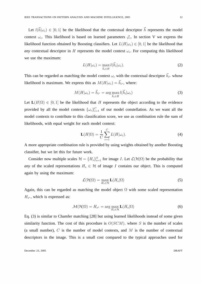
Let l(~h|ωc) ∈ [0, 1] be the likelihood that the contextual descriptor~h represents the model

context ωc. This likelihood is based on learned parameters~ϕc. In section V we express the

likelihood function obtained by Boosting classifiers. LetL(H|ωc) ∈ [0, 1] be the likelihood that

any contextual descriptor inH represents the model contextωc. For computing this likelihood

we use the maximum:

L(H|ωc) = max~hi∈H

l(~hi|ωc). (2)

This can be regarded as matching the model contextωc with the contextual descriptor~hi∗ whose

likelihood is maximum. We express this asM(H|ωc) = ~hi∗, where:

M(H|ωc) = ~hi∗ = arg max~hi∈H

l(~hi|ωc) (3)

Let L(H|Ω) ∈ [0, 1] be the likelihood thatH represents the object according to the evidence

provided by all the model contextsωcCc=1 of our model constellation. As we want all the

model contexts to contribute to this classification score, we use as combination rule the sum of

likelihoods, with equal weight for each model context:

L(H|Ω) =1

C

C∑

c=1

L(H|ωc). (4)

A more appropriate combination rule is provided by using weights obtained by another Boosting

classifier, but we let this for future work.

Consider now multiple scalesH = HsSs=1 for imageI. Let L(H|Ω) be the probability that

any of the scaled representationsHs ∈ H of image I contains our object. This is computed

again by using the maximum:

L(H|Ω) = maxHs∈H

L(Hs|Ω) (5)

Again, this can be regarded as matching the model objectΩ with some scaled representation

Hs∗, which is expressed as:

M(H|Ω) = Hs∗ = arg maxHs∈H

L(Hs|Ω) (6)

Eq. (3) is similar to Chamfer matching [28] but using learnedlikelihoods instead of some given

similarity function. The cost of this procedure isO(SCM), whereS is the number of scales

(a small number),C is the number of model contexts, andM is the number of contextual

descriptors in the image. This is a small cost compared to thetypical approaches used for



graphs [9], [29], [12]. For example, relaxation has costO(KC2M2), whereK is the number

of iterations until convergence, and combinatorial matching has exponential costO(MC) [9].

In these approaches, parts are described by only local properties (also called unary values) and

the spatial dependencies between different parts must be considered after matching. Thus, many

possible matching combinations are tested and the one with highest spatial coherence (along

with local similarity) is chosen. Using a more direct approach is justified in our case because

the spatial dependencies are, to some extent, integrated into the description of each part (by

using contextual information). This allows us to introducespatial coherence by just matching

each context in the model with the one with highest likelihood in the image. In section VI we

describe how to speed up the explained recognition procedure by exploiting the sparseness of

our descriptors.

B. Matching with low supervision

As explained above, before learning the model we match homologous contexts in the training

set. Our procedure consists of two stages. In the first stage,we apply the registration procedure

of [25] to a small set of manually segmented images. As a result of registration, we obtain sets

of homologous contexts across a small number of images, and we can learn an initial modelΩ.

Then, we use this model and the matching explained in the previous section (Eqs. (3) and (6)) to

obtain homologous descriptors for the rest of the training set. Basically, given a non-segmented

imageI from the training set, we match every model contextωc ∈ Ω with the descriptor of image

I that maximizes the likelihood of representingωc, and we use the scale that has the highest

likelihood according to all the model contextsωcCc=1. In more detail, the whole procedure can

be decomposed in the following steps.

1) Manually segment few positive images. LetI ′1, . . . , I

′V be the set of manually segmented

images.

2) Select image representantI ′r as the image that minimizes the Chamfer distance to all the

other imagesI ′v (we refer to [25]).

3) SampleC points~xc, c = 1, . . . , C from the segmented object of representantI ′r. The c-th

point ~xc is picked as reference for model contextωc.

4) Register the representantI ′r againstI ′

v, v = 1, . . . , V by using Thin-Plate Splines and

Shape Contexts (we refer to [25]). Registration matches points ~xc from I ′r to a point~q



from I ′v, for eachv = 1, . . . , V . Let ~qc,v be the point that matches~xc in imageI ′

v, and

let ~hc,v be its corresponding descriptor. As the image is manually segmented, we pick the

descriptor~hc,v at the scale closest to the real size of the object.

5) Build initial training sets. For eachc = 1, . . . , C, define thec-th set of homologous

descriptors asPc = ~hc,vVv=1. This set represents positive instances of the model context

ωc. As negative instances, take all the descriptors in every scale from negative images,

and build the negative setN . This negative set is the same for all the model contextsωc.

Finally, build thec-th training setTc by using positive setPc and negative setN .

6) Learn initial modelΩ. For eachc = 1, . . . , C, train a Boosting classifier (see section V)

with Tc and obtain the parameters~ϕc associated with model contextωc, c = 1, . . . , C.

7) Match in the rest of (non-segmented) positive imagesIu, u = 1, . . . , U . Let theu-th image

Iu be represented byHu. The matching is performed in two steps. First, we detect the

scale of the object by using Eq. (6). LetHu,s∗ = M(Hu|Ω) be this scale. Then, for each

ωc we match the descriptor at the detected scale by using Eq. (3). Let hc,u = M(Hu,s∗|ωc).

8) Build the final training sets. For eachc = 1, . . . , C, use as positive set the matching de-

scriptorshc,uUu=1 together with the descriptors of manually segmented imageshc,v

Vv=1.

The negative setN is the same as before (i.e. every negative descriptor in every scale in

every negative image).

9) Train again the classifier with the complete final trainingsets and obtain the complete final

constellation of model contextsωc with parameters~ϕc, c = 1, . . . , C.

In our implementation, the initial model is built by using contextual descriptors based on only

the local structure (i.e. without considering color). After matching in all positive images, the

final model is based on both color and structure (tangent) as local information. We decided to

follow this procedure because color is not usually characteristic in all the parts of the object,

and we only want to learn this property once we have a large enough training set. In this sense,

we regard the local structure (tangent) as more reliable andcharacteristic than color.

V. IMPLEMENTATION WITH BOOSTING

Recently, there has been a lot of research in classifiers thathave a good generalization perfor-

mance by maximizing the margin. Well-known examples of suchclassifiers are Boosting [30] and

Support Vector Machines (SVM). Boosting provides a good theoretical and practical convergence



to a low error rate in few iterations, its speediness being one of the major advantages over other

algorithms such as SVM [30].

The key idea of Boosting is to improve the performance of a so-called weak classifier

by constructing an ensemble of such classifiers. Each weak classifier complements the ones

previously added to the ensemble by focusing on those training examples that were frequently

misclassified. In this work, we use two types of Boosting classifiers, the original AdaBoost [30],

and Joint Boosting [8]. In the following we describe each of them in turn.

A. AdaBoost with decision stumps

Table I provides the algorithmic view of AdaBoost with decision stumps as weak classifier,

where we use the version described in [16], and decision stumps as weak classifier. A decision

stumpf(~h, k, p, θ) is a threshold function over a single dimension, defined as:

f(~h, k, p, θ) =

1 if phk < pθ

0 otherwise(7)

wherek is the dimension selected by the weak classifier,θ is the threshold andp is the polarity

indicating the direction of the inequality. Decision stumps produces axis-orthogonal hyperplanes

and can be viewed as single node decision trees.

The idea of AdaBoost is to train several weak classifiers overdifferent weighted distributions

of the data. At the beginning, the weights of the examples areinitialized so as to provide the

same emphasis over positive and negative examples (see Table I). These weights are then updated

at each round of AdaBoost, in such a way that the weight is increased for those examples that

were incorrectly classified by the weak classifiers obtainedat previous rounds. Finally, each

weak classifierft is added with weightαt to the ensemble (or strong classifier)F , where the

weight αt is larger as the errorεt gets smaller (see Table I).

1) Boosting as a feature selection process:Boosting decision stumps as weak classifier leads

to a learning algorithm that can be interpreted to also perform feature selection [16], [4], [8]. A

decision stump is a weak classifier that is restricted to a single feature or dimension of the feature

space. Therefore, the numberT of weak classifiers added to the Boosting ensemble represents

an upper bound on the number of utilized features3. Boosting represents an aggressive method

3Note that different classifiers may use the same dimension



TABLE I

ADABOOST WITH DECISION STUMPS

• Given the training set~h1, . . . ,~hn and labels:Y = y1, . . . , yn whereyi = 0, 1 for negative and positive examples,

respectively

• Given number of iterationsT .

• Initialize weights:

w1,i =

12m

if yi = 1

12l

if yi = 0

wherem and l are the number of positive and negative examples respectively.

• for t = 1, . . . , T

1) Normalize weights:wt,i ←wt,i

nj=1

wt,j

2) Find decision stumpft that minimizes weighted error:

εt = mink,p,θn

i=1 wt,i|ft(~hi, k, p, θ)− yi|

3) βt ←εt

1−εt

4) Update weights:wt+1,i ← wt,iβ1−eit ,

whereei is 0 if ~hi is correctly classified and 1 otherwise.

5) Compute weight offt : αt ← log 1βt

• Return ensemble:F =T

t=1αtft

Tt=1

αt

for selecting a small number of weak classifiers (and corresponding features) that provide good

classification performance.

In our case, each feature of our space represents at the same time certain local object part’s

attributes together with some spatial relation from this part to the reference. Therefore, integrating

Boosting with our contextual descriptors, we obtain a compact model where few discriminant

features are selected that represent both local part’s attributes and their spatial arrangement.

2) Implementation details:In order to choose the weak classifierf(~h, k, p, θ) that minimizes

the weighted error, an exhaustive search over parameters〈k, p, θ〉 must be performed. As ex-

plained in [16], this search can be done in timeO(nK), wheren is the number of examples and

K the number of dimensions. This is based on the fact that for every dimensionk, we only need

to consider as possible thresholdsθ the different values of the examples along this dimension.

We refer to [16] for a detailed explanation on the implementation. The cost is exactly∑K

k=1 nk,

wherenk is the number ofdifferentvalues alongk-th dimension. In the presence of sparse data,

we do not need to process all the zero values, so that we avoid to process most of the elements.



Let us see how AdaBoost is integrated in the framework of section IV. For each training set

Tc, c = 1, . . . , C we call AdaBoost using as training dataTc. As a result, we obtain4T parameters:

kc,t, pc,t, θc,t, αc,tTt=1, which form thec-th vector of parameters~ϕc of model contextωc. With

these parameters, we obtain as likelihood functionl(~h|ωc) the Boosting ensemble defined in

Table I:

l(~h|ωc) = F (~h; ~ϕc) =

∑T

t=1 αc,tf(~h, kc,t, pc,t, θc,t)∑T

t=1 αc,t

.

In section VI we explain an efficient evaluation of this likelihood using inverted files.

B. Sharing features by Joint Boosting

Note that each model contextωc represents a class of homologous contexts extracted from

images of the same object category. AdaBoost is trained independently to detect each class of

context in new images. Rather than independently training each context detector, in this section

we explain how to train all the detectors jointly by exploiting common features shared by

contextual “views” of the same object category. We use the Joint Boosting algorithm proposed

by Torralba et al. [8] that explicitly learns to share features across multiple classes, and we

apply it for finding common features that can be shared between different context classes of the

same object category. As a result, we can obtain the same recognition accuracy by using fewer

features. This makes the recognition stage faster.

Joint Boosting was designed as a multi-class Boosting classifier in [8], where GentleBoost is

used as the original two-class Boosting version [31], coming from a statistical additive view of

Boosting. The multi-class classifier can be expressed as an additive model of the form:

F (~h, c) =

T∑

t=1

ft(~h, c),

wherec is the class label and~h is the input vector as before. The weak classifierft is defined

here as a regression stump that is similar to the decision stumps and has the form:ft(~h) =

aδ(hk > θ)+ b, whereδ(.) is the indicator function anda, b are regression parameters (note that

b does not contribute to the classification).

The key idea of Joint Boosting is to try to share weak classifiers (also called features in

Boosting literature) among different classes. This is doneby examining many possible subsets

of classes, and for each one evaluating how well some featurefits to all the classes in the subset.



Let S be one possible subset of classes. For this subset, we obtaina weak classifier (feature)

that best separates the classes of that subset from the background class, and evaluate the error

obtained by using the resulting sharing. The procedure thenconsists of evaluating every possible

sharing (subset of classesS), fitting a weak classifier to each of them, and picking the subset

that maximally reduces the weighted classification error for all the classes of the training set.

The resulting algorithm is shown in Table II.

If C is the number of classes, at each round we have to evaluate2C − 1 possible subsets of

classes and letS(n) be then-th subset,n = 1, . . . , 2C − 1. For subsetS(n), the weak classifier

ft(~h, c) has the form:

ft(~h, c) =

aδ(hki > θ) + b if c ∈ S(n)

kc if c /∈ S(n)(8)

This weak classifier has parametersa, b, k, θ and kc for every c /∈ S(n). These parameters are

estimated so as to minimize the following weighted square error [31], [8]:

Jwse =

C∑

c=1

wci (z

ci − ft(~hi, c))

2, (9)

wherezci is the membership label fori-th example, indicating if it belongs to classc or not with

values1,−1 respectively, andwci is the weight for examplei and classc. Minimizing this error

produces the following parameters forft [8]:

b =

∑c∈S(n)

∑i wiz

ci δ(h

ki ≤ θ)

∑c∈S(n)

∑i wiδ(hk

i ≤ θ), (10)

a + b =

∑c∈S(n)

∑i wiz

ci δ(h

ki > θ)

∑c∈S(n)

∑i wiδ(h

ki > θ)

, (11)

kc =

∑i wiz

ci∑

i wi

c /∈ S(n) (12)

For all the classesc in the setS(n), the functionft(~h, c) is a shared regression stump. For the

classes that do not share this feature,c /∈ S(n), the functionft(~h, c) is a constantkc different

for each class. These constants do not contribute to the finalclassification, and are introduced

in order to prevent sharing features due to the difference inthe number of positive examples in

each class.



TABLE II

JOINT BOOSTING

• Initialize the weightswci = 1 and setF (~h, c) = 0, i = 1, . . . , n, andc = 1, . . . , C.

• for t = 1, . . . , T

1) for n = 1, . . . , 2C − 1

a) Fit shared stump:

ft(~h, c) =

aδ(hki > θ) + b if c ∈ S(n)

kc if c /∈ S(n)

b) Evaluate error:

Jwse(n) = C

c=1 wci (z

ci − ft(~hi, c))

2

2) Select the sharing with minimum error,n = arg minn Jwse(n), and pick the corresponding shared featureft(~h, c).

3) Update:

F (~hi, c)← F (~hi, c) + ft(~hi, c)

wci ← wc

i e−zc

i ft(~hi,c)

1) Efficient computation:In order to find the optimal sharingS(n) we need to evaluate2C−1

possible subsets of classes, which is very slow. Instead, a greedy search heuristic is proposed

in [8] that reduces the cost toO(C2). We start by computing the best feature for each single

class, and choose the class that maximally reduces the overall error. Then we select the second

class that has the best error reduction when jointly considered with the first. This is iterated until

all the classes have been added. Finally, from all the examined subsets we select the one that

provides largest error reduction.

Also, the parameters in Eqs. (10)- (12) need only be computedonce for each single class, we

refer to [8] for a detailed explanation.

2) Implementation details:Joint Boosting can be directly applied to learn theC classes

ωc, c = 1, . . . , C after building the training sets as explained in section IV-B. The background

class consists of all the feature vectors in negative images, and receives the labelc = 0. Let

nc be the number of examples in classc. In our case, the initialization of weights is done as

follows. If examplei does not belong to background class, then:

wci =

12nc

if zci = 1

0 if zci = −1



for c = 1, . . . , C. This avoids to discriminate between different context classes of the same object,

i.e. we do not regard a certain contextual descriptor of somepart of the object as a negative

example of another part of the object. If examplei is from background class, thenwci = 1

2n0for

c = 1, . . . , C. The factor 12nc

gives the same weight to positive and negative examples ofc-th

class, i.e.∑

i wci = 1.

VI. DATA ORGANIZATION : THE INVERTED FILE

After learning the model, section IV-A explains how to matchit against images. This can be

efficiently done by exploiting the sparseness of our GCs if weorganize the data appropriately.

In this section we explain how this can be done by using Inverted Files (IF) [32], which speeds

up the evaluation of large collections of images. The IF is a mechanism originally applied in

information retrieval to browse for documents with text. Each possible word is a feature of the

document, where the number of possible features (i.e. dimensions) is very large, but the number

of actual features present in a document is small. Instead oforganizing the data by documents,

the IF organizes it by words. For each word, a list of documents that contain this word, along

with the frequency of apparition in each document, is maintained. In our case, for each dimension

of feature space, the IF maintains a list with the indexes of the descriptors in the database that

have a non-zero value in the corresponding dimension, together with the value.

Let us see how one weak classifier of the Boosting ensemble is evaluated using the IF structure.

We focus on decision stumps as weak classifier (see section VI-A for regression stumps). Let

θ be its threshold,k the dimension chosen by the weak classifier, andα the weight of the

weak classifier. The weak classifier evaluates as positive those descriptors whose value ink-th

dimension is lower thanθ (see section VI-A for details). For each entry (dimension) in the

IF the negativevalues are stored in ascending order, so that the virtual null values are put at

the end of the list (when training the classifier we also use negative values). We use binary

search for obtaining the first descriptor in the database whose value is lower thanθ. This has

a costO(log nk) if nk is the number of descriptors in the database that are not nullalongk-th

dimension. From the first descriptor found, we visit all the descriptors until the beginning of the

list and we addα to the likelihood of these descriptors. Letpk be the fraction of descriptors

in the list whose value is lower thanθ: 0 ≤ pk ≤ 1. The cost of evaluating the weak classifier

is O(lognk + pknk). Note that we can evaluate all the weak classifiers that share the same



dimensionk in only one pass along the IF list of this dimension.

The complete likelihoodlc associated with thec-th model contextωc, c = 1, . . . , C is a

boosting ensemble ofT weak classifiers. This likelihood is evaluated onto descriptors h that

have a non-null value along dimensions spanned by ensemblelc. Let n be the average number

of descriptors that are not null along each dimension. Letp be the average fraction of not-

null descriptors that are evaluated along each dimension (i.e. descriptors whose value along this

dimension is lower than the threshold of the stump). LetT ′ be the average number of dimensions

used by eachlc, whereT ′ is upper bounded by the number of roundsT in Boosting. It can be

seen that the total cost of searching in the IF file is coarselyO(CT ′ log n+CT ′pn) ≈ O(CT ′pn),

where0 ≤ p ≤ 1.

The advantage of using IF is mostly to exploit the sparsenessof the data so that only a small

fraction n of the total number of descriptors is processed. Using the Joint Boosting procedure,

the total numberT of weak classifiers is reduced, and the search procedure is very efficient, as

evaluated in section VII.

A. Implementation details

Decision stumps also have a polarity parameterp that specifies the direction of the inequality

(lower or greater). From the first descriptor found, we visitall the descriptors until the beginning

of the list and we addα or substractα to the likelihood of these descriptors if the polarityp

of the weak classifier is 1 or -1 respectively. In order to obtain a meaningful likelihood, the

maintained sum must be initialized to a proper value: for each weak classifier with negative

polarity, its weightα is added to the initial sum.

In the case of regression stumps (section V-B), we also storenegative values and sort them

in ascending order. When evaluating a weak classifier, instead of adding the likelihoodαt we

should adda + b to descriptors whose value isgreater than θ, and we should add onlyb to

the rest. Instead, we begin by considering that the descriptors have likelihooda + b, search for

descriptors whose value islower thanθ, and substracta to the likelihood of these descriptors4.

By this way, we avoid to process the null values.

4Exactly, the initialization isa + b for weak classifiers used by the current class, andkc for weak classifiers not used by this

class. The search in the IF is only done for weak classifiers used by the current class. Also, as is the case of decision stumps,

we only need to initialize the sum maintained for each scale of each image, so that we avoid to initialize all the descriptors.



Fig. 3. Sample of CALTECH’s database, the last three columnsare background data-sets.

VII. RESULTS

We performed experiments on a standard database for object-class recognition, the CALTECH

database [9], recently used by many authors [18], [9], [15],[33]. It consists of 7316 images

divided into 7 different object categories plus 3 differentsets of background images: in color,

in gray-level, and road backgrounds for testing car recognition (Fig. 3).

A. Experimental setup

Results in CALTECH database were compared against the best of related methods such as

the one by Fergus et al. [9] and the one by Weber et al. [13]. These methods also work with

weak supervision and they exploit information about both local parts of the object and their

spatial arrangement. In order to provide a fair comparison,we used the same protocol in the

experiments. Each time the training set consisted of approximately half the object’s data set

(positive set) and half the background’s data set (negativeset), and the test set consisted of

the other half of both data sets. The specific images includedin training and test are explicitly

indicated as part of CALTECH database for most of the categories (written in bold typeface in

Table III). Table III indicates the number of training and test images used for each data set. We

used the indicated training and test sets included in CALTECH, whenever they were available.

For the background categories, only the number of training and test images are indicated, but not

the specific images used in each part, so that we used 5 different random partitions and averaged

the results afterwards (also indicating the standard deviation). Note that the benchmark [9] only



Motorbike Plane Car Face Spotted Leaf Car Gray Road Color

rear Cat side Bg. Bg. Bg.

Training 400 400 400 218 100 93 550 400 400 400

Test 426 674 755 232 100 93 170 500 970 120

Total 826 1074 1155 450 200 186 720 900 1370 520

TABLE III

NUMBER OF IMAGES PER CATEGORY.

used one random partition for each data set. In our method, 10images were randomly picked

and coarsely segmented by hand for each experiment. This represents a very small proportion,

10 out of 400 images which is the typical number of positive images used for training.

Unless explicitly stated, we used the color backgrounds as negative images. The accuracy

was measured by Receiver-Operating Curve equal error rates, defined as p(True positive)=1-

p(False positive). For example, a91% figure indicates that91% of foreground images were

correctly classified but9% of background images were incorrectly classified (i.e. thought to be

foreground) [9].

In the construction of our GCs, we used a fixed setting. The number of scalesS was set

to 7, a number that performed well in practice, and we used a fixed range: from 65 pixels to

140, that cover a large range of scales. RGB color was quantized into 3,2,2 bins and tangent

into 4 bins. While the quantization of color was coarse, it permitted to obtain more robustness

against variations in illumination than a finer quantization, and it allowed to obtain descriptors

of moderate size. Experimentally we saw that including thiscolor information significantly

improved the results. For gray-level images, we quantized the gray-level into 16 bins (obviously,

whenever the gray-level background data set was used, the positive set was also transformed to

gray-level5). The resulting dimensionality of the descriptors is 960 dimensions for color images

and 1200 dimensions for gray-level images. In order to make the GCs more sparse, we took the

5 most frequent colors of the local color histograms (see Section III), set to 0 the rest of the

entries, and normalize so that the new color histogram adds up to 1.

In order to obtain the reference points, we sampled10% the number of detected contour points,

5This was done by using the standard procedure that maps the original RGB space to LUV and takes the band L as gray-level.



Method Motorbike Plane Car Face Spotted Leaf Car

rear cat side

Others 92.5% 90.2% 90.3% 96.4% 90.0% 84.0% -

(Gray Backgr.) [9] [9] [9] [9] [9] [13]

Boost. Context. 96.7% 92.5% 95.8% 95.2% 92.8% 98.0% 95.7%

(Gray Backgr.) (1.3%) (1.1%) (0.2%) (0.9%) (0.9%) (0.4%) (1.0%)

Boost. Context 94.2% 94.4% 95.8% 90.5% 86.1% 96.3% 95.7%

(Color Backgr.) (0.9%) (1.5%) (0.2%) (1.1%) (1.6%) (1.1%) (1.0%)

TABLE IV

ROC EQUAL ERROR RATE INCALTECH USING ADABOOST. IN PARENTHESES, THE STANDARD DEVIATION ACROSS

DIFFERENT DATA-SET PARTITIONS.

with a minimum of 100 points. In average this yielded 161 points per image. The numberC of

model contexts was obtained as follows. First, 100 points were sampled from the contours of

manually segmented images. Then, as part of the registration algorithm in [25], some outliers

were removed, which are points whose spatial structure in hand-segmented images differs from

other points in a quantity bigger than a certain threshold (we refer to [25]). The resulting number

of points is the number of model contexts; in average this was55. Finally, in all the cases we

trained with 20 thousand negative descriptors randomly sampled from negative images (see

section IV-B).

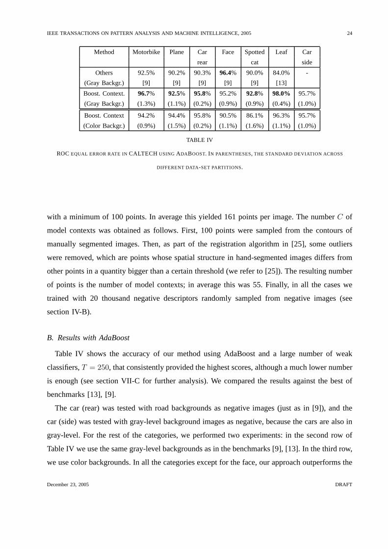
B. Results with AdaBoost

Table IV shows the accuracy of our method using AdaBoost and alarge number of weak

classifiers,T = 250, that consistently provided the highest scores, although amuch lower number

is enough (see section VII-C for further analysis). We compared the results against the best of

benchmarks [13], [9].

The car (rear) was tested with road backgrounds as negative images (just as in [9]), and the

car (side) was tested with gray-level background images as negative, because the cars are also in

gray-level. For the rest of the categories, we performed twoexperiments: in the second row of

Table IV we use the same gray-level backgrounds as in the benchmarks [9], [13]. In the third row,

we use color backgrounds. In all the categories except for the face, our approach outperforms the



benchmarks, whereas the difference is not large in the latter case. In Section VII-D we compare

the computational cost. The car (side) category was used in [9] but for spatially localizing the

instances of the car in each image. This was not the scope of our present work. Finally, we can

see that the color background data-set is more challenging,as the results are generally worse.

The gray-level background images were taken with the same camera and with low contrast,

while the color backgrounds are heterogeneous images takenfrom the internet. Even with a

more difficult data-set, our approach performs better in themajority of categories. The worst

performance was obtained with the spotted cat category, dueto the large variability of pose. In

this case, the imposed spatial quantization is not so suitable, but the inclusion of local properties

permits boosting to focus on local parts rather than their spatial arrangement. This is analyzed

in Section VII-E by comparison with a pure spatial approach (Shape Context [25]) (see Fig. 9).

In the rest of the experiments we use the color background data-set.

In some categories, the object usually appears in backgrounds of similar characteristics (see

Fig. 3). The plane usually appears in the middle of the sky, people usually appear indoors (in

offices) and the spotted cat usually appears in the forrest. In these cases, our system inevitably

learns the correlation with the background. This is not necessarily a disadvantage in retrieval,

for example we can expect an airplane to be surrounded by sky,and this information is useful in

order to retrieve images likely to contain planes. The important issue is that our context-based

method is also able to recognize the object across very different and cluttered backgrounds

(see Fig. 4). In the car (rear) category, there is no correlation with the background because the

background is exactly the same both in the positive and negative images (note that the negative

images consist of roads without cars).

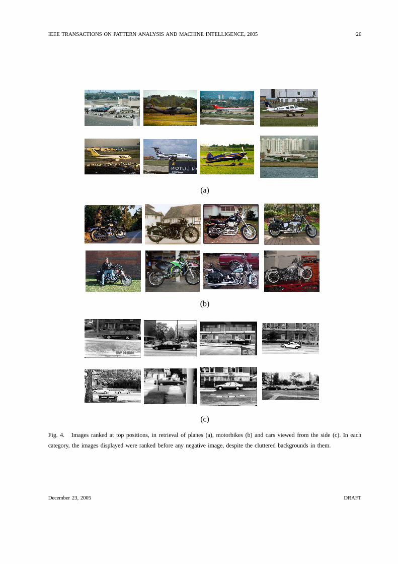
Fig. 4 shows examples of successfully retrieved images for three different categories. We show

the images ranked according to the likelihood provided by the learned model. All these images

were ranked with higher likelihood than any negative image,despite the fact that they contain

very different and cluttered backgrounds.

In Fig. 5, each row shows examples of matching between the learned model and new images.

The first row displays the matching of one part from the model of the car (rear) category, where

this model part is matched with image points near the red light on the left of the car. In the

motorbike category the matching part lies in the same relative position of the object (always

below), despite the confusing clutter. For the face, the matching part is near the left ear of the



(a)

(b)

(c)

Fig. 4. Images ranked at top positions, in retrieval of planes (a), motorbikes (b) and cars viewed from the side (c). In each

category, the images displayed were ranked before any negative image, despite the cluttered backgrounds in them.



(a)

(b)

(c)

Fig. 5. Parts from the model and their correspondence with parts from images. In each row, the white circles represent thepart

from the image that matches with the same part from the model.We show the matching of one part from the car rear model

(a), the matching of one part from the motorbike model (b), and the matching of one part from the face model (c).

face. Note that, while in many images the matching is at the same relative part of the object

(e.g. at left part of car, beneath the motorbike, at left partof face), the correspondence does not

need to be at the point level (i.e. it does not need to be the same point of the object). Instead,

the matching is done at the part and context level, i.e. locations whose local properties match

the ones from the model’s part and locations in the same relative position around the object,

whose context matches the one from the model (e.g. the left part of the face, the left part of the

car, etc).

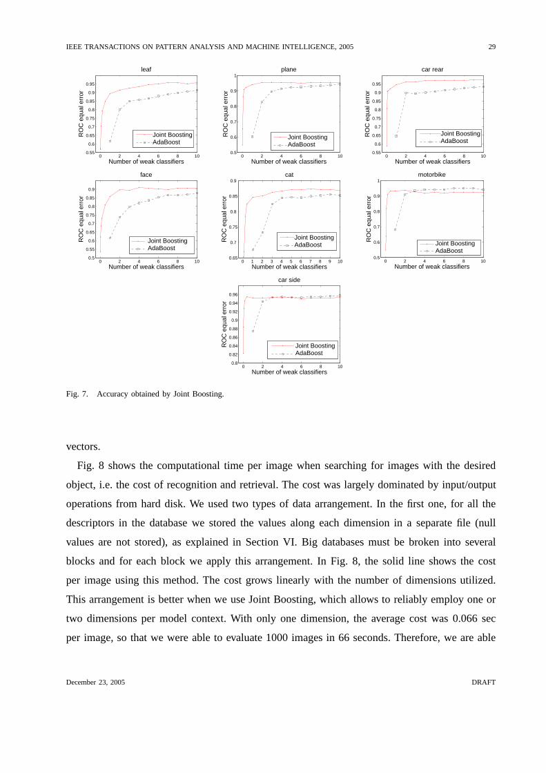
C. Sharing features among model contexts

Our contextual descriptors live in spaces of 960 dimensions. AdaBoost is efficient at obtaining

a relevant subspace where we can discriminate with only 25-50 features (weak classifiers)

obtaining an accuracy close to the maximum (see Fig. 6). Notethat each weak classifier selects

one single dimension of the feature space, so that the numberof weak classifiers is an upper

bound on the number of utilized features. In average, with 25and 50 features we obtained

respectively98% and 99% of the maximum accuracy. However, each model context uses an



50 100 150 200 2500.7

0.75

0.8

0.85

0.9

0.95

Number of weak classifiers

RO

C e

qual

err

or

car rearspotted catmotorbikeface

50 100 150 200 250

0.7

0.75

0.8

0.85

0.9

0.95


RO

C e

qual

err

or

leafplanecar side

Fig. 6. Accuracy obtained by AdaBoost.

independent set of features, so that the total number of features is multiplied by the number of

model contexts. The average number of model contexts is 50, thus we need 1250-2500 features

in total.

The total number of features can be significantly reduced if we jointly train all the model

contexts using Joint Boosting (Section V-B). Fig. 7 compares the accuracy as a function of

features per model context using both AdaBoost and Joint Boosting. As can be seen from this

figure, using Joint Boosting we can reliably pick very few features per model context. With

only one feature per model context we obtained in average91.3% of accuracy, whereas with

AdaBoost we obtained70.2% in average. Note that we can also use less than one feature per

model context with Joint Boosting.

D. Computational cost

The cost in learning the complete model was evaluated using AdaBoost. Without exploiting the

sparseness, the maximum cost was 4 hours (usingT = 250 weak classifiers per model context).

The timings are obtained with a 2.4 GHz processor. Exploiting the sparseness we reduced the

cost to 1 hour and 33 minutes. In contrast, the learning cost of the benchmark [9] is 36 hours

for a 2.0 GHz desktop. As shown in Fig. 6, we can use much fewer weak classifiers obtaining

almost the same accuracy. WithT = 50, we obtained a maximum cost of 38 minutes (this is

more than 50 times faster than the benchmark). Table V shows the cost of each part of the

algorithm, where I/O refers to input/output operations from hard disk, i.e. reading, gathering and

writing data in order to build the separate training sets. The matching procedure was done by

searching in inverted files, where here each image is arranged in a separate inverted file. As can

be seen, the cost was dominated by the input/output operations, due to the size of the feature



0 2 4 6 8 100.55

0.6

0.65

0.7

0.75

0.8

0.85

0.9

0.95


RO

C e

qual

err

or

leaf

Joint BoostingAdaBoost

0 2 4 6 8 100.5

0.6

0.7

0.8

0.9

1


RO

C e

qual

err

or

plane


0 2 4 6 8 100.55

0.6

0.65

0.7

0.75

0.8

0.85

0.9

0.95


RO

C e

qual

err

or

car rear


0 2 4 6 8 100.5

0.55

0.6

0.65

0.7

0.75

0.8

0.85

0.9


RO

C e

qual

err

or

face


0 1 2 3 4 5 6 7 8 9 100.65

0.7

0.75

0.8

0.85

0.9


RO

C e

qual

err

or

cat


0 2 4 6 8 100.5

0.6

0.7

0.8

0.9

1


RO

C e

qual

err

or

motorbike


0 2 4 6 8 100.8

0.82

0.84

0.86

0.88

0.9

0.92

0.94

0.96


RO

C e

qual

err

or

car side


Fig. 7. Accuracy obtained by Joint Boosting.

vectors.

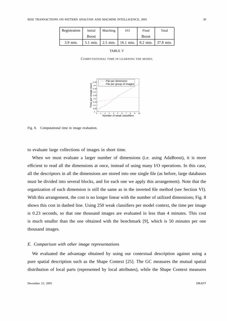
Fig. 8 shows the computational time per image when searchingfor images with the desired

object, i.e. the cost of recognition and retrieval. The costwas largely dominated by input/output

operations from hard disk. We used two types of data arrangement. In the first one, for all the

descriptors in the database we stored the values along each dimension in a separate file (null

values are not stored), as explained in Section VI. Big databases must be broken into several

blocks and for each block we apply this arrangement. In Fig. 8, the solid line shows the cost

per image using this method. The cost grows linearly with thenumber of dimensions utilized.

This arrangement is better when we use Joint Boosting, whichallows to reliably employ one or

two dimensions per model context. With only one dimension, the average cost was 0.066 sec

per image, so that we were able to evaluate 1000 images in 66 seconds. Therefore, we are able



Registration Initial Matching I/O Final Total

Boost Boost

3.9 min. 5.1 min. 2.5 min. 16.1 min. 8.2 min. 37.8 min.

TABLE V

COMPUTATIONAL TIME IN LEARNING THE MODEL

0 1 2 3 4 5 6 7 8 9 100

0.05

0.1

0.15

0.2

0.25

0.3

0.35

0.4

0.45

Tim

e pe

r im

age

(sec

)


File per dimensionFile per group of images

Fig. 8. Computational time in image evaluation.

to evaluate large collections of images in short time.

When we must evaluate a larger number of dimensions (i.e. using AdaBoost), it is more

efficient to read all the dimensions at once, instead of usingmany I/O operations. In this case,

all the descriptors in all the dimensions are stored into onesingle file (as before, large databases

must be divided into several blocks, and for each one we applythis arrangement). Note that the

organization of each dimension is still the same as in the inverted file method (see Section VI).

With this arrangement, the cost is no longer linear with the number of utilized dimensions; Fig. 8

shows this cost in dashed line. Using 250 weak classifiers permodel context, the time per image

is 0.23 seconds, so that one thousand images are evaluated inless than 4 minutes. This cost

is much smaller than the one obtained with the benchmark [9],which is 50 minutes per one

thousand images.

E. Comparison with other image representations

We evaluated the advantage obtained by using our contextualdescription against using a

pure spatial description such as the Shape Context [25]. TheGC measures the mutual spatial

distribution of local parts (represented by local attributes), while the Shape Context measures



Fig. 9. Comparison of Generalized Correlogramg against other representations, using ROC equal error rates. Results were

obtained by using Joint Boosting with 10 weak classifiers permodel part.

the spatial distribution of the silhouette of the object (represented by its contour points). We

also evaluated the advantage of using a contextual description over using a local description: a

constellation of local descriptors, each one describing one salient point or part of the image.

Fig. 9 shows the results with each type of representation, where the setting was the same for

all the representations. The local description was obtained by using the same local attributes as

in our descriptor, i.e. the local description is a local histogram of color and tangent for each

contour point of the image. Results were obtained by Joint Boosting with 10 weak classifiers

per model part6. The accuracy of Joint Boosting with this number of weak classifiers is close

to or higher to independent boosting (i.e. AdaBoost) with 250 weak classifiers (except for the

motorbike where it is lower).

The advantage of using our representation was significant ascan be seen from this figure,

sometimes dramatically:10% of difference for the car side and8% for the car rear and for

the plane, measured against the best of the other methods. Although also significant, the lowest

difference was obtained using the leaf and cat categories, each time considering the best perfor-

mance between Shape Context and local histograms. Note thatthe other representations do not

6Note that the other two representations are also constellations of descriptors: Shape Contexts and local histograms, so that

we learned a constellation of parts in each case.



show a constant difference between each other. The local description was more accurate than

the Shape Context in four categories, while the Shape Context was more accurate in the other

three. The Shape Context performed poorly in categories such as the cat, where the variability

of pose is large. In this category it is better to use local attributes.

VIII. D ISCUSSION

In this paper we proposed a novel type of parts-based object representation, the Generalized

Correlogram (GC). The image was built by a collections of GCs, where each one represents

specific attributes localized at the same time in several parts of the image holding a specific

spatial relationship. This makes the representation rarely found in random images. Further,

the representation is built upon very sparse spaces, where many possible combinations of part

arrangements can exist, but only a few ones are actually present in a given image.

We showed that simple and efficient learning and matching procedures can be obtained by

exploiting this type of representation. This is based on thefact that directly evaluating a single

feature vector, both local attributes and their arrangement are considered, and that these vectors

are efficiently evaluated due to their high sparseness. The proposed methodology combines

appropriate state-of-the-art methods: we used non-rigid registration, Chamfer-like multi-scale

matching, and Inverted Files for efficiently putting in correspondence homologous parts in the

learning stage; and integrated AdaBoost and Joint Boostingfor learning a compact model where

few features characterize local parts and their arrangement at the same time.

In the experimental section we showed that the computational complexity of our approach is

significantly lower than the ones needed by the state-of-the-art graph-based object representa-

tions [13], [9], while the resulting accuracy was higher. Wealso demonstrated the significant

advantage of using both local and spatial information over using only local representations or pure

spatial descriptors such as Shape Context [25]. Our methodology worked with weak supervision,

with no part-labelling required, with cluttered training sets, and very few manually segmented

images. Combined with the fact that learning the model is done is short time and that thousands

of images can be quickly evaluated, the framework is an appropriate tool for Content-Based

Image Retrieval.

The framework is applicable to objects viewed from the same side and with characteristic

spatial pattern. As future work, we would like to combine several types of spatial quantization



to relax spatial restrictions. We would also like to test theimprovement if we use class-specific

local features, where we believe that our method permits to increase the accuracy of any pure local

representation. For example, we could use Expectation-Maximization for grouping characteristic

parts of the category, and integrate it into class-specific GCs. The efficiency could be also

increased by using interest points with automatic scale selection, and scaling GCs accordingly

(instead of using a multi-scale approach). Finally, it would be also important to include invariance

against large rotations and against different 3D views.

ACKNOWLEDGMENT

Work supported by Ministerio de Educacion y Ciencia, grant: TIC2000-1635-C04-04.

REFERENCES

[1] M. Flickner, H. Sawhney, W. Niblack, J. Ashley, Q. Huang,B. Dom, M. Gorkani, J. Hafner, D. Lee, D. Petkovic, D. Steele,

and P. Yanker, “Query by image and video content: The QBIC system,” IEEE Computer, pp. 23–32, 1995.

[2] A. W. M. Smeulders, M. Worring, S. Santini, A. Gupta, and R. Jain, “Content-based image retrieval at the end of the early

years,” IEEE TPAMI, vol. 22, no. 12, pp. 1349–1380, December 2000.

[3] Y. Rui, T. S. Huang, and S.-F. Chang, “Image retrieval: Past present and future,”Journal of Visual Communication and

Image Representation, vol. 10, pp. 1–23, 1999.

[4] K. Tieu and P. Viola, “Boosting image retrieval,”Int. J. Comput. Vision, vol. 56, no. 1-2, pp. 17–36, 2004.

[5] T. S. Huang, X. S. Zhou, M. Nakazato, Y. Wu, and I. Cohen, “Learning in content-based image retrieval,” in2nd

International Conference on Development and Learning (ICDL’02), IEEE, Ed., June 2002.

[6] Q. Tian, Y. Wu, J. Yu, and T. S. Huang, “Self-supervised learning based on discriminative nonlinear features for image

classification,”Pattern Recognition, vol. 38, pp. 903–917, 2005.

[7] L. Fei-Fei, R. Fergus, and P. Perona, “A bayesian approach to unsupervised one-shot learning of object categories,”in

IEEE Proc. ICCV, vol. 2, 2003, pp. 1134–1142.

[8] A. Torralba, K. P. Murphy, and W. T. Freeman, “Sharing features: Efficient boosting procedures formulticlass object

detection.” inProc. CVPR, vol. 2, 2004, pp. 762–769.

[9] R. Fergus, P. Perona, and A. Zisserman, “Object class recognition by unsupervised scale-invariant learning,” inIEEE Proc.

CVPR, 2003.

[10] M. Turk and A. Pentland, “Eigenfaces for recognition,”Journal of Cognitive Neuro-science, vol. 3, no. 1, pp. 71–86, 1991.

[11] A. Pentland, R. W. Picard, and S. Sclaroff, “Photobook -content-based manipulation of image databases,”International

Journal of Computer Vision, vol. 18, no. 3, pp. 233–254, 1996.

[12] P. Hong and T. S. Huang, “Spatial pattern discovery by learning a probabilistic parametric model from multiple attributed

relational graphs,”Journal of Discrete Applied Mathematics, vol. 139, no. 1-3, pp. 113–135, April 2003.

[13] M. Weber, M. Welling, and P. Perona, “Towards automaticdiscovery of object categories,” inIEEE Proc. CVPR, June

2000, pp. 101–108.



[14] S. Helmer and D. G. Lowe, “Object recognition with many local features,” inWorkshop on Generative Model Based Vision

2004 (GMBV), 2004.

[15] D. Crandall, P. Felzenszwalb, and D. Huttenlocher, “Spatial priors for part-based recognition using statisticalmodels,” in

IEEE CVPR, 2005.

[16] P. Viola and M. J. Jones, “Robust-real time face detection,” Int’l J. of Computer Vision, vol. 57, no. 2, pp. 137–154, 2004.

[17] J. Amores, N. Sebe, and P. Radeva, “Fast spatial patterndiscovery integrating boosting with constellations of contextual

descriptors,” inProc. IEEE CVPR, vol. 2, 2005, pp. 769–774.

[18] S. Agarwal, A. Awan, and D. Roth, “Learning to detect objects in images via a sparse, part-based representation,”IEEE

TPAMI, vol. 26, no. 11, pp. 1475–1490, November 2004.

[19] R. C. Nelson and A. Selinger, “Large-scale tests of a keyed, appearance-based 3-d object recognition system,”Vision

Research, vol. 38, no. 15, pp. 2469–2488, 1998.

[20] Y. Amit and D. Geman, “A computational model for visual selection,”Neural Computation, vol. 11, pp. 1691–1715, 1999.

[21] J. Huang, S. R. Kumar, M. Mitra, W. J. Zhu, and R. Zabih, “Spatial color indexing and applications,”Int’l Journal of

Computer Vision, vol. 35, no. 3, pp. 245–268, 1999.

[22] A. Rao, R. Srihari, and Z. Zhang, “Geometric histogram:A distribution of geometric configurations of color subsets,” in

Proceedings of SPIE: Internet Imaging, vol. 3964, 2000, pp. 91–101.

[23] T. Gevers and A. W. M. Smeulders, “Pictoseek: Combiningcolor and shape invariant features for image retrieval,”IEEE

Transactions On Image Processing, vol. 9, no. 1, pp. 102–119, January 2000.

[24] Y. Wang, F. Makedon, and A. Chakrabarti, “R*-histograms: Efficient representation of spatial relations between objects of

arbitray topology,” inProc. of ACM Multimedia, 2004, pp. 356–359.

[25] S. Belongie, J. Malik, and J. Puzicha, “Shape matching and object recognition using shape contexts.”IEEE Trans. PAMI,

vol. 24, no. 24, pp. 509–522, April 2002.

[26] Y. Chen and J. Wang, “A region-based fuzzy feature matching approach to content-based image retrieval,”IEEE TPAMI,

vol. 24, no. 9, pp. 1252–1267, 2002.

[27] C. Carson, S. Belongie, H. Greenspan, and J. Malik, “Blobworld: image segmentation using expectation-maximization and

its application to image querying,”IEEE TPAMI, vol. 24, no. 8, pp. 1026–1038, 2002.

[28] H. G. Barrow, J. M. Tenenbaum, R. C. Bolles, and H. C. Wolf, “Parametric correspondence and chamfer matching: Two

new techniques for image matching,” inProc. Int. Joint Conf. Artificial Intelligence, 1977, pp. 659–663.

[29] W. Christmas, J. Kittler, and M. Petrou, “Structural matching in computer vision using probabilistic relaxation,” IEEE

TPAMI, vol. 17, no. 8, pp. 749–764, August 1995.

[30] Y. Freund and R. E. Schapire, “A short introduction to boosting,” Journal of Japanese Society for Artificial Intelligence,

1999.

[31] J. Friedman, T. Hastie, and R. Tibshirani, “Additive logistic regression: A statistical view of boosting.”Annals of statistics,

vol. 38, no. 2, pp. 337–374, 2000.

[32] D. Squire, W. Muller, H. Muller, and T. Pun, “Content-based query of image databases: Inspirations from text retrieval,”

Pattern Recognition Letters, vol. 21, pp. 1193–1198, 2000.

[33] T. V. Pham and A. W. M. Smeulders, “Object recognition with uncertain geometry and uncertain part detection,”Computer

Vision and Image Understanding, vol. 99, pp. 241–258, 2005.


Context-Based Object-Class Recognition and Retrieval by Generalized Correlograms

Documents

Transcript of Context-Based Object-Class Recognition and Retrieval by Generalized Correlograms