Contact Dynamics in 3 Dimensions: Some Explorations of Reeb-Beltrami Fields

Contact Dynamics in 3 Dimensions: Some Explorations of

Reeb-Beltrami Fields

Andrew Havens

December 16, 2014

Abstract

We give a brief overview of the setting and philosophy of contact dynamics, and then focus onthe 3-dimensional case, where the astounding results of Etnyre and Ghrist [4] give a correspondencebetween Reeb vector fields and Beltrami fields. We then turn our attention to some specific examplesof both while in select cases the correspondence is explicitly made. Using simple numerics, we try tounderstand and visualize the qualitative behavior of the chosen examples.

1 What is a Contact Structure?

1.1 Defining Contact Structures

We begin with a mild amusement. A friend proposes a game: first, this friend specifies a smooth non-vanishing vector field F ∈ X(R3) := Γ(TR3) (i.e. smoothly assigns a tangent vector at every point ofR3), and then you specify a smooth non-vanishing vector field G ∈ X(R3) which is nowhere parallel to F .Thus, together you have specified a smoothly varying distribution of tangent planes. Next, you choosea point p ∈ R3, and your friend chooses another point q ∈ R3. You are then seated in a flying saucerhovering at p, designed so that it can thrust forward and rotate without needing to adjust the pitchof the saucer plane. However, the flying saucer can only travel along paths such that the saucer plane(which we will assume contains your velocity vector) remains tangent to the specified plane distribution.The mission is to transport a tangle of topologists in this UFO from p to q. Your friend wins the gameif the point q is chosen so that you are unable to arrive at your destination, and thus are subjected tospending an indeterminate amount of time flying around with the topologists. Otherwise, you win bysuccessfully delivering the topologists to their destination. Under what conditions can you accomplishyour mission and win the game?

Before accepting a potentially futile mission (which involves spending time with a knot of topologists,all the worse1!) you seek conditions on the distribution of planes that would ensure you can completethe flight. Feeling too shy to ask the giddy gang for assistance, you decide to review the theory of vectorfield distributions on manifolds yourself. Let H ⊂ TR3 be the distribution specified by your friend,identified as a sub-bundle of the tangent bundle of R3 (which is naturally diffeomorphic to R3 × R3—a fact convenient for visualization). By the well known theorem of Frobenius, if this distribution iscompletely integrable, then there exists a foliation of R3 by surfaces tangent to H, and if the system islocally integrable around a point x ∈ R3 then there exists a local foliation by integrable subsurfaces.To say you can always accomplish your mission is to say that for any pair of points p, q ∈ R3 there’s apath connecting them, such that the tangent bundle of the path is a subbundle of the distribution H.

You realize quickly that your mission cannot be a success unless there are no neighborhoods wherethe distribution is integrable, for, within any neighborhood possessing integral subsurfaces, to ensurethat you cannot travel to q from your chosen point p your friend merely has to specify q on a leaf of

1I consider this joke at the expense of topologists acceptable, since my primary research interests at present belong tothe area of low-dimensional differential topology; I’m also known to occasionally travel in gangs of ≤ 4 low-dimensionaltopologists.

1

M645 - Dynamical Systems 12-10-14 Reeb-Beltrami Fields

the foliation disjoint from any leaf containing p (if the leaves extend to a neighborhood containing p;otherwise your friend could simply choose q in a neighborhood whose leaves cannot be extended to aneighborhood of p, which would imply an obstruction, e.g. a leaf consisting of a closed surface enclosingsome neighborhood).

Thus, to ensure that you can win no matter which point your friend specifies, in the very leastyou must choose your vector field so that the distribution is maximally non-integrable: writing thedistribution H as the span of the two smooth pointwise linearly-independent vector fields F and G, itmust be the case that the Lie bracket [F,G] is a vector field everywhere transverse to H, else there isa neighborhood where Frobenius tells us we can find integral submanifolds. We will henceforth referto a maximally non-integrable distribution of (hyper-)planes as a contact distribution. The remarkablefact is that, if the distribution defined by F and G is a contact distribution, then you can always find apath tangent to the distribution from p to q, no matter choice of p and q in R3. A curve whose tangentspace is contained in a contact distribution is called a Legendre curve for that contact distribution.

We switch perspectives: consider H = spanF,G as the kernel of some smooth one-form, α ∈Ω1(R3). Then since α(F ) = 0 = α(G), and [F,G] /∈ kerα we note that

0 6= α([F,G]) = α([F,G])− F (α(G)) +G(α(F )) = −dα(F,G) ,

whence dα is a non-degenerate two form when restricted to the contact distribution. It follows thatα ∧ dα is a non-vanishing top degree form, called a contact volume form.

We are now prepared to define contact structures on manifolds in greater generality. For simplicitywe consider the case of an orientable manifold M with hyperplane bundle H such that the quotientbundle TM/H is orientable (as a bundle).

Definition 1.1. Given M as above endowed with a maximally non-integrable hyperplane distributionH ⊂ TM, the pair (M,H) is referred to as a contact manifold, and the specification of H on a givenM is called a contact structure. Because TM/H is orientable one can find a globally defined one formα ∈ Ω1(M) such that H = kerα; α is then called a contact form for the contact structure H.

Contact structures can exist without global contact forms [2, p. 70] , but we will restrict our attentionto the case where we can define global contact forms, since in the sequel our considerations of contactdynamics evolve from the choice of a contact form. There are also restrictions on the existence ofcontact structures, the most notable being dimension. Even if there is no global contact form, there arealways local contact forms, and as in the preceding discussion, for a contact form α the two form dα isnondegenerate when restricted to H. Since the rank of the subbundle H is one less than the dimensionof M and dα is a non-degenerate two form on H, we conclude that the dimension of M is odd since therank of H is necessarily even.

A quick criterion for determining if a one form α ∈ Ω1(M2n+1) is a contact form for some contactstructure is to check if it can be used to build a contact volume form: α∧ (dα)n must be a volume formif α is a contact form, and conversely, if α∧ (dα)n ∈ Ω2n+1(M2n+1) is a non-vanishing 2n+ 1 form, thenit is a contact volume form and α defines a contact distribution H := kerα. Note that there are manycontact forms for a given contact structure: if H = kerα, then H = ker fα for any nowhere vanishingf ∈ C∞(M). Thus there is not a uniquely specified choice of contact form or contact volume for a givencontact structure. It is often convenient however to fix a contact form to specify a contact structure.An example, to be explored in greater depth later, is the standard form for R3: αstd := dz+xdy. Moregenerally, on R2n+1 with coordinates (z, x1, y1, . . . xn, yn), the standard form is αstd := dz+

∑ni=1 x

idyi.It earns its name due to the following theorem:

Theorem (Darboux). Given a contact manifold (M,H) and a point p ∈ M, there exists a coordinatechart

ÄU , (z, x1, y1, . . . xn, yn)

äcentered at p such that

H|U = ker

(dz +

n∑i=1

xidyi).

2


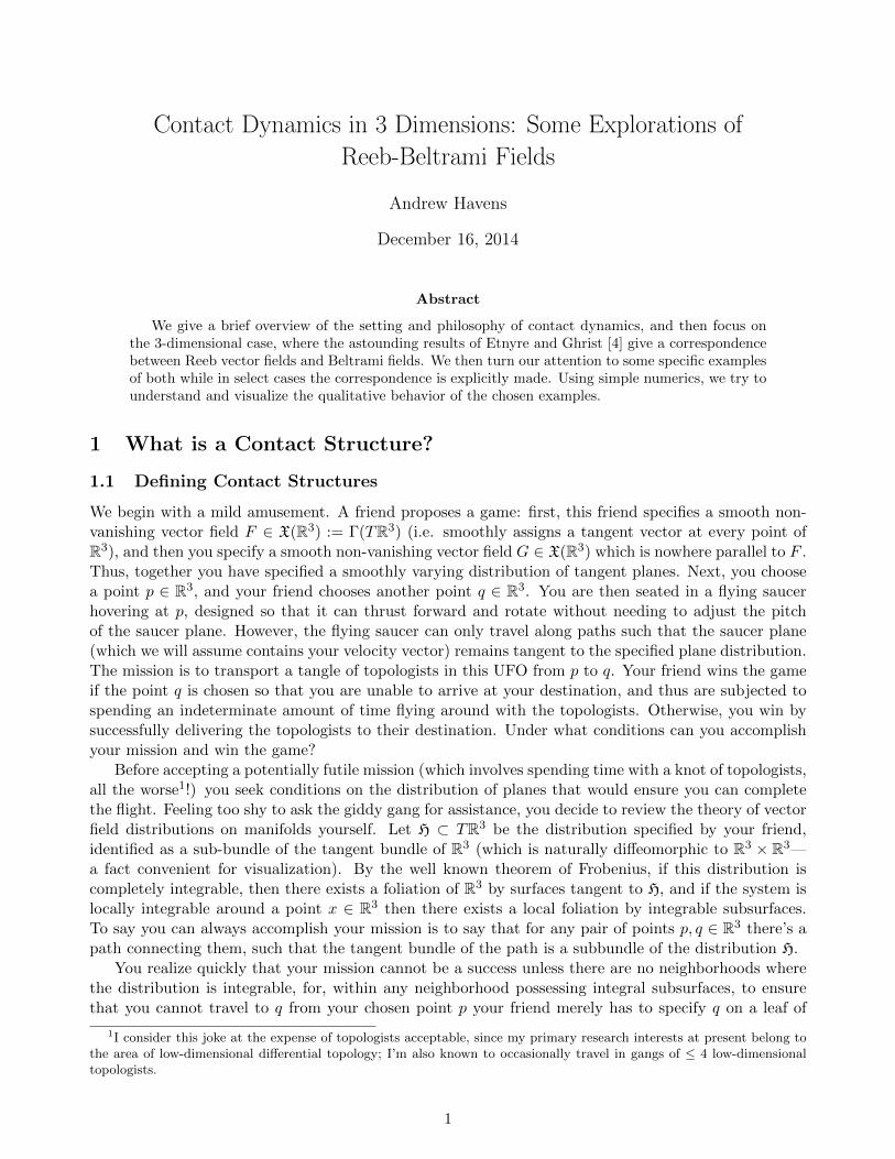
Returning to R3 with the standard contact structure, as determined by the form αstd := dz + xdy,we can exploit the diffeomorphism TR3 ∼= R3×R3 to create a vivid image of the plane distribution. Toeach point of R3 we may attach a plane spanned by the vectors i and j − xk which correspond to thetangent vector fields ∂x and ∂y − x∂z which span kerαstd.

Figure 1: A visualization of some planes of the plane field Hstd on R3. Note the symmetry induced by translations(x, y, z) 7→ (x, y + t, z). There is another, unillustrated symmetry: vertically translating this swatch of planesproduces another swatch of contact planes in Hstd; this corresponds to the contactomorpishms (x, y, z) 7→ (x, y, z+t) generated by the flow of the Reeb vector field Rαstd = ∂z of the form αstd. See the next section for definitions.

Note that the contact volume associated to αstd is the usual metric volume on R3 with respectto the Euclidean metric. We can construct a normal form for a contact structure on R3 in cylindricalcoordinates as well: the form αrstd := dz+r2 dθ defines a contact structure on R3 with plane distribution

Hrstd = span¶∂r, r

2∂z − ∂θ©.

1.2 Characteristic Foliations and Tight versus Overtwisted Contact Structures

Contact structures on 3 manifolds come in two very topologically different flavors: tight and overtwisted[1, p. 33]. To define these for a contact manifold (M3,H) we first consider embeddings of disks D →M,though the following construction applies to any embedded surface S → M. Let TD ⊂ TM be thetangent bundle of the D viewed as a subbundle of TM. The key observation is that H ∩ TD defines aline field with (generically finitely many) singular points p ∈ D where the disk is tangent to the planedistribution H). This line field can then be integrated to yield a foliation of the disk, with singularitiesoccurring precisely at points of tangency [8, p. 78]. We call this foliation the characteristic foliationFD,H of the disk D (or more generally of the embedded surface S). For example, the characteristicfoliation of a flat disk embedded with center on the z-axis and parallel to the coordinate plane z = 0in (R3,Hrstd) consists of radial segments emanating from the center, which is the only singularity. If onebubbles this disk into a hemisphere while leaving the boundary fixed, the radial lines become “spirals”,twisting up into a single singularity at the north pole.

One might suspect a “less tame” contact structure might support more interesting foliations onembedded disks. Let us provide an example: consider the one form defined in cylindrical coordinates

3


on R3 by αoτ = r cos r dz + r sin r dθ. Note that this indeed is a contact form, as

αoτ ∧ dαoτ =

Å1 +

sin 2r

2r

ãr dr ∧ dθ ∧ dz 6= 0 for r > 0 ,

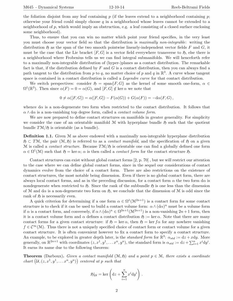
and so αoτ ∧ dαoτ defines a volume form where the coordinates are well defined. Unlike Hrstd whoseplanes never rotate past the vertical as one travels along a ray θ = θ0 away from the origin, for thecontact structure Hoτ := kerαoτ as one travels along rays θ = θ0 the planes complete infinitely manycomplete rotations. Consider now an embedding of a disk D with radius π in (R3,Hoτ ) centered on thez-axis, tangent to the coordinate plane z = 0 on the boundary, but raised slightly in the center. Notethat for r = π, αoτ (π) = −π dz. Thus the boundary is a limit cycle for the leaves of the characteristicfoliation, which spiral from the center of the disk out toward the boundary. We say such a disk isovertwisted.

Definition 1.2. A contact 3-manifold (M3,H) is said to be overtwisted if there exists a disk D → M

such that the characteristic foliation FD,H arising from the singular line field H ∩ TD possess a limitcycle, i.e. a closed leaf which is an accumulation orbit for other leaves of the foliation. If no overtwisteddisks exist in (M3,H) we say that the contact structure H is tight.

Figure 2: On the right is a visualization of some planes of Hrstd, and on the left is a visualization of theovertwisted structure Hoτ on R3.

In particular, the standard structure Hstd on R3 and its radially-symmetric counter part Hrstd are tight,while Hoτ is overtwisted.

For the remainder of the paper, we would like to investigate the connections between certain dynam-ical constructions arising from a contact structure on a three manifold, and steady-state fluid mechanicson three manifolds. Let us fix some notation going forward: (M,H) will always denote an oriented 2n+1dimensional smooth contact manifold, and (M,H, α) will denote a smooth 2n + 1 dimensional contactmanifold with α ∈ Ω1(M) a fixed global contact form for H. However, whenever possible, examples willbe taken to be three dimensional.

2 Contact Dynamics - An Overview

2.1 Reeb and Contact Fields

In 1948 Seifert posed the following question: Does every non-vanishing vector field on S3 possess closedorbits? Counterexamples of class C1 and even C∞ are known [2], so we look to a slightly more rigid

4


generalization. Suppose instead that we are interested in nonsingular flows preserving a distinguishedvolume form µ ∈ Ω3(M) on M = S3 or R3. Thus we investigate vector fields F ∈ X(M) such that

0 = LFµ = d(ιFµ) .

Since H2dR(M) = 0, we conclude that ιFµ ∈ Ω2(M) is exact, so there is some α ∈ Ω1(M) such that

ιFµ = dα. Then ιFdα = ιF ιFµ = 0. If ιFα > 0 throughout M, we call F positive for α. If a volumepreserving flow on M comes from a field F which is positive for α, then α ∧ dα is also a volume form.In this case we may normalize F by setting R = F/ιFα so that ιRα = 1, and observe that R preservesthe new volume form α ∧ dα:

LR(α ∧ dα) = (LRα) ∧ dα− α ∧ (LRdα) = 0− α ∧ d(LRα) = 0 .

This motivates the following philosophy: to study volume preserving flows on R3, S3, or any other3-manifold with vanishing second de Rham cohomology, one may instead choose to investigate vectorfields R satisfying

ιRdα = 0

ιRα = 1

α ∧ dα is a volume form.

Since α ∧ dα is in fact a contact volume form, we implicitly arrived at a contact structure on ourmanifold of interest, M. Vector fields satisfying these conditions with respect to a contact structure arethemselves objects worthy of study, even without the additional structure of a preserved volume, or theassumption that there is no second cohomology.

Definition 2.1. Given a contact manifold (M,H) and a global contact form α for H, there is a uniquevector field Rα satisfying ιRdα = 0 and ιRα = 1, called a Reeb vector field for the contact form α on(M,H). A vector field F ∈ ker dα which is positive with respect to α, i.e. ιFα > 0 throughout M, iscalled a Reeb-like vector field, and its flow is said to be a Reeb-like flow.

A first crucial observation is that the flow ΨRα : M×R→M of the Reeb vector field Rα associatedto a contact form α actually preserves α and thus also preserves the contact structure: for all t ∈ R,(Ψt

Rα)∗α = α, and for any contact plane Ξp ∈ H, p ∈ M, (Ψt

Rα)∗Ξp = ΞΨtRα (p). A diffeomorphism with

the property of preserving the contact structure is called a contactomorphism. Note that preservingthe contact form is a stronger condition than preserving the contact structure. To distinguish these,we consider, in the language adopted by Geiges [6, p. 32] (in the spirit of Sophus Lie) the notions ofinfinitesimal automorphisms and strict infinitesimal automorphisms of the contact manifold.

Definition 2.2. Let (M,H) be a contact manifold. For a vector field X ∈ X(M), let Ψt be the (local)flow associated to X. We call X an infinitesimal automorphism of the contact structure H if Ψt

∗(H) = H(wherever Ψt

∗ is well defined); we may also refer to X as a contact vector field. A contact vector fieldon (M,H, α) which further satisfies Ψ∗tα = α is known as a strict infinitesimal automorphism for thecontact form α, or occasionally as a strict contact vector field.

Example 2.1. Let us show that the Reeb vector field of (R3,Hstd, αstd) is in fact R = ∂z. Let Rstd =Rx∂x +Ry∂x +Rz∂x be the desired Reeb vector field. Then

0 = ιRstddαstd = dx ∧ dy(Rx∂x +Ry∂x +Rz∂x, ·) = Rx dx−Ry dy

=⇒ Rx = 0 = Ry

1 = αstd(Rstd) = Rz + xRy = Rz

=⇒ Rz = 1 ,

and thus Rstd = ∂z as claimed. One might now be concerned that Reeb fields aren’t very interesting,but on the contrary, we will later see just how chaotic they can be, even for the simple contact structuresdescribed so far.

5


The richness of the dynamics of contact and Reeb vector fields comes in part from their variety: agiven contact structure supports unfathomably diverse dynamics via uncountably many vector fields ofcontact and Reeb type:

Theorem 2.1. Given a contact manifold (M,H, α), there is a bijective correspondence between smoothfunctions H ∈ C∞(M) functions on M and infinitesimal automorphisms of H (dependent on α). More-over, given our initial contact form α, there is a bijection between non-vanishing smooth functions onM and pairs (α, Rα) of contact forms and their Reeb fields on (M,H).

Proof. The second assertion follows readily from the fact that the space of global annihilating one formsAnn(H) for H is a line bundle, whence given a non-vanishing section of T ∗M which is in Ann(H), one canobtain all other forms α ∈ Ann(H) via scaling by non-vanishing smooth functions f ∈ C∞(M). Sincethe set of vector fields annihilating dα is also a line bundle (dα is nondegenerate on a codimension 1subbundle of TM), it follows that the normalization α(Rα) = 1 determines a unique Reeb vector fieldfor α, which establishes the uniqueness asserted in definition 2.2.

For the second assertion, the correspondence is explicitly defined as follows: given H ∈ C∞(M), weproduce an infinitesimal automorphism XH satisfying the relations

α(XH) = H and

ιXHdα = ιRαd(Hα) ,

where Rα is the Reeb vector field for α. It is immediate that Rα is annihilated by the one formιRαd(Hα) = dH(Rα)α− dH. By non-degeneracy of dα on H, inclusion of contact vector fields into dαinduces an isomorphism from Ann(Rα) to TM/H ∼= C∞(M). Thus given H, we can find XH = HRα+Ywhere Y ∈ H which satisfies ιXHdα = dH(Rα)α − dH, and conversely given a contact vector field Xthere is a unique vector field Y such that X = α(X)Rα + Y is determined by the above conditions,where H = α(X). We just need to check that the vector field XH corresponding to H is indeed acontact vector field. It suffices to show that LXHα = µα for some µ : M → R. Indeed, if LXHα = µα,then one obtains the ordinary differential equation

d

dt

ÄΨtXH

ä∗α =

ÄΨtXH

ä∗LXHα =

ÄΨtXH

ä∗(µα) =

Äµ Ψt

XH

äÄΨtXH

ä∗α ,

whose solution is ÄΨtXH

ä∗α =

Çexp

∫ t

0µ Ψτ

XHdτ

åα .

Thus, if LXHα = µα then the flow ΨtXH

preserves the line bundle kerα = H, i.e. XH is an infinitesimalautomorphism. Now, if XH is the vector field produced from H ∈ C∞(M) by the procedure above, thenby Cartan’s magic formula

LXHα = ιXHdα+ d(ιXHα)

= dH(Rα)α− dH + dÄα(XH)

ä= dH(Rα)α .

This correspondence is perhaps not a mere coincidence of linear algebra and differential equations,but points to something deeper about contact structures. The role of the “potential” H associated toan infinitesimal automorphism of (M,H) is strongly analogous to the case of Hamiltonian functions ona symplectic manifold and their Hamiltonian vector fields (or symplectic gradients; the correspondencedepends on the symplectic form just as our contact automorphism correspondence depends on thecontact form). One thus arrives at the following language which emphasizes this parallel:

Definition 2.3. For a contact manifold (M,H, α) and a given H ∈ C∞(M), we say XH is a contactvector field for the contact Hamiltonian H.

6


Just as with the symplectic case, one can extend this language to time dependent contact Hamilto-nians by showing that there is a parallel correspondence between smooth families of functions Htt∈R,H ∈ C∞(M × R) and smooth one parameter families XHt ∈ X(M × R) of contact vector fields, whichyield contact isotopies. The proof is completely analogous, except that one appeals to the existenceand uniqueness of solutions to non-autonomous ordinary differential equations, in this case arising fromsmooth time dependent vector fields, or smooth families of contact forms. The machinery of time-dependent contact Hamiltonian dynamics allow for many differential topological constructions sensitiveto the contact structure of a given contact manifold but these would take us far afield.

2.2 The Weinstein Conjecture

Weinstein like Seifert chose to consider the question of existence of periodic orbits, but confined hisattention to the class of Reeb flows on contact manifolds. He proposed the following conjecture in 1979[10]:

Conjecture 2.1. Let (M,H, α) be a closed contact manifold with contact form α, and let Rα be theassociated Reeb vector field. Then the flow Ψt

Rαof the Reeb field admits a periodic orbit.

Much work had been done to understand the state of conjecture For example, Hofer and Viterboproved that it holds in special cases such as S3, contact manifolds with vanishing second homotopy, andfor overtwisted contact structures [2, p. 78]. For a closed three manifold, the conjecture is now resolvedin general by the work of Clifford Taubes, who applied gauge-theoretic invariants (Seiberg-Witten-Floertheory) to prove the result [9].

2.3 Classifying Reeb fields for a given Contact Distribution

We now explore the variety of Reeb fields for a given contact structure. Suppose a contact manifold(M,H) admits a global contact form α ∈ Ω1(M). Then H = ker fα for any f ∈ C∞(M) such that f isnowhere vanishing. A natural question is “how does rescaling α to fα alter the Reeb field?”

If Rfα is the Reeb field for the contact form fα, then we know that Rfα ∈ ker d(fα) and fα(Rfα) =1. Thus the new conditions can be written as

ιRfαd(fα) = df(Rfα)α− α(Rfα)df + fιRfαdα = 0 ,

ιRfαα = 1f .

Little can be said about the specific dynamics which can result from such a rescaling of the contactform without working with some explicit contact form in coordinates. A naıve first question mightbe “can every vector field transverse to the contact field be realized as a Reeb field for some choiceof rescaled contact form?” The answer is resoundingly “no” even in the simplest cases, as we shallpresently see. The above conditions are linear algebraic conditions on Rfα once fα is known, but ifgiven a non-vanishing R ∈ X(M) and a contact form α, if one wishes to determine if R = Rfα for somef , it is necessary that f = 1/α(R) while simultaneously f must satisfy the partial differential equation

df(R)α− α(R)df + fιRdα = 0 .

One can reduce this to a PDE for the coefficients of R and hope to classify all solutions of the PDE, butalas, the resulting equation is highly nonlinear even for the simplest choices of contact form α, such asthe standard structure on R2n+1. But upon inspection it is apparent that the PDE presents a conditionstrictly stronger than transversality.

A better approach is to fix a contact form α for H and let the set of smooth, non-vanishing functionson M parametrize the set of Reeb fields Rfα which can be associated to H = ker fα. Let us see whatwe can say concretely for the standard form αstd = dz + x dy for R3 with the standard tight structure.

7


Let f ∈ C∞(R3) be a non-vanishing function. Writing R = Rx∂x + Ry∂y + Rz∂z for our Reeb fieldand using the notation fx := ∂xf , fy := ∂yf , and fz := ∂zf for the coordinate derivatives of f , weconsider solutions of

ιRd(fαstd) = (Rxfx+Ryfy+Rzfz)(dz+xdy)− (Rz+xRy)(fxdx+fydy+fzdz)+f(Rxdy−Rydx) = 0 ,

subject to the normalization f(Rz + xRy) = 1. This is equivalent to seeking a normalized element ofthe kernel of the matrix

Af :=

0 −f − xfx −fxf + xfx 0 xfz − fyfx fy − xfz 0

.Since this is a 3× 3 skew-symmetric matrix, it corresponds to a cross product operator, e.g. it can

be realized as the matrix of

−Ç

(fy − xfz)∂x − fx∂y + (f + xfx)∂z

å× : TR3 → TR3 ,

in the coordinate basis ∂x, ∂y, ∂z of TR3. Thus an element of the kernel of Af is parallel to the vectorfield (fy−xfz)∂x− fx∂y + (f +xfx)∂z. Using the normalization, one finds that the desired Reeb vectorfield of the contact form f αstd = f(dz + x dy) is thus

R =1

f2

Ç(fy − xfz) ∂x − fx ∂y + (f + xfx) ∂z

å.

Note that choosing f ≡ 1 yields Rstd = ∂z, as expected.A similar computation shows that on (R3,Hrstd) for fαrstd, where f ∈ C∞(R3) is nonzero for r 6= 0,

the Reeb vector fields have the form

R =1

2rf2

Ç(fθ − r2fz) ∂r − fr ∂θ + (2rf + r2fr) ∂z

åFinally, we also look at the overtwisted contact structure on R3 determined by αoτ = r cos r dz +

r sin r dθ. Here one finds that

R =1

(r + sin r cos r)f2

Ç(fθ cos r−rfz sin r) ∂r+(f sin r−fr cos r)∂θ+(rfr sin r+f sin r+rf cos r)∂z)

å.

The case where f ≡ 1 yields the vector field

Roτ =1

(r + sin r cos r)

Çsin r ∂θ + (sin r + r cos r) ∂z

åWe will later examine a few cases of choices of f and visualize the integral curves of the preceding

Reeb fields for the chosen f using simple numerics. First we introduce the astounding connectionbetween contact dynamics and hydrodynamics.

3 The Etnyre-Ghrist Correspondence

3.1 General Euler Equations and Beltrami Fields

Let R3 be considered as a Riemannian manifold with the usual flat Riemannian metric given by thestandard inner product structure on (TR3, 〈·, ·〉) ∼= (R3, 〈·, ·〉), let µ := dx ∧ dy ∧ dz ∈ Ω3(R3) be themetric volume form, and for vector fields X,Y ∈ TR3 let ∇XY denote covariant differentiation of Y

8


along X (∇ denotes the Levi-civita connection). Then the classical Euler equations for an inviscid,incompressible fluid in R3 take the form

∂tX +∇XX = −grad p

divX = 0 ,

where p is a generally time-dependent function modeling pressure. We wish to consider Euler equationsin a more general setting of a Riemannian 3-manifold (M, g) with a distinguished volume form (whichmay or may not be the metric volume form). In this generality, the first Euler equation may be writtendown identically where it is understood that grad p is defined using the metric g, and ∇ is the Levi-Civita connection associated to g. On R3 the second equation is equivalent to stipulating that the flowof X preserves the metric volume µ. For a general Riemannian 3-manifold (M, g) we would equivalentlyrequire LXVolg = 0. Thus if we would like our Euler fluid to preserve a distinguished volume form µ(not necessarily the metric volume), then we replace the second condition by the equation

LXµ = 0 .

As Etnyre and Ghrist show [4], the Euler equations on a Riemannian three manifold preserving thevolume form µ can be described by an equivalent differential system

∂t(ιXg) + LX(ιXg) = −dÄp− 1

2 ιXιXgä

LXµ = 0 .

To interpret the term LX(ιXg), one can define a general curl operator on a Riemannian threemanifold, dependent on the distinguished volume µ as well as the Riemannian structure:

Definition 3.1. Given 3-manifold (M, g) with a distinguished volume form µ ∈ Ω3(M), and a vectorfield X ∈ X(M), define the (g, µ)-curl of X to be the unique vector field curl µ(X) which satisfies

ιcurlµ(X)µ = d(ιXg) .

When there is no ambiguity about the chosen volume form or the metric, one simply speaks of curl andwrites curlµ(X) = ∇×X.

Note that by the definition of the (g, µ)-curl and from Cartan’s magic formula, one can write

LX(ιXg) = d(ιX(ιXg)) + ιXd(ιXg) = d(ιXιXg) + ιXι∇×Xµ ,

whence our differential system for the Euler equations becomes

∂t(ιXg) + ιXι∇×Xµ = −dÄp+ 1

2 ιXιXgä

LXµ = 0 .

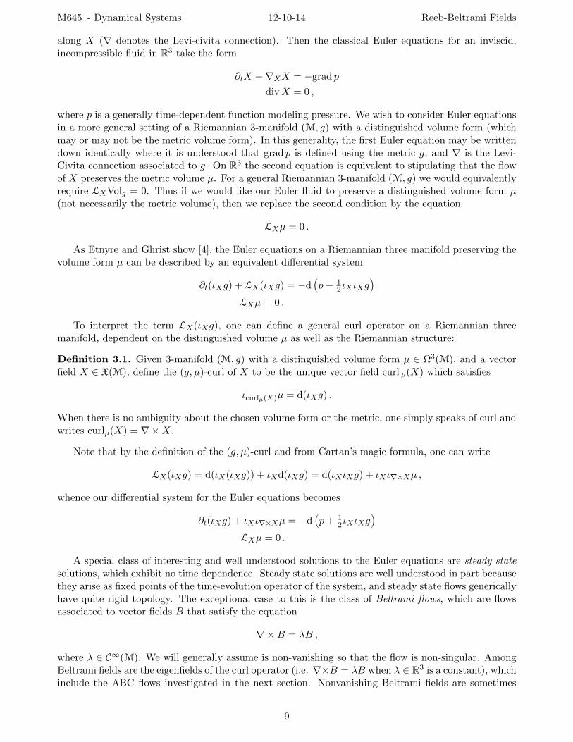
A special class of interesting and well understood solutions to the Euler equations are steady statesolutions, which exhibit no time dependence. Steady state solutions are well understood in part becausethey arise as fixed points of the time-evolution operator of the system, and steady state flows genericallyhave quite rigid topology. The exceptional case to this is the class of Beltrami flows, which are flowsassociated to vector fields B that satisfy the equation

∇×B = λB ,

where λ ∈ C∞(M). We will generally assume is non-vanishing so that the flow is non-singular. AmongBeltrami fields are the eigenfields of the curl operator (i.e. ∇×B = λB when λ ∈ R3 is a constant), whichinclude the ABC flows investigated in the next section. Nonvanishing Beltrami fields are sometimes

9


called rotational Beltrami fields. Note that a vector field B ∈ X(M) is a Beltrami field if and only ifgiven a volume form µ ∈ Ω3(M), B satisfies ιBι∇×Bµ ≡ 0.

A natural question in the context of steady state solutions to the Euler equations is the “hyr-dodynamical Seifert conjecture”: all analytic steady state solutions to the Euler equations on S3 admitperiodic orbits, independent of the Riemannian structure and preserved volume on S3. For non-Beltramiflows, this can be answered in the positive using topological techniques (see [4]) and we will see that infact this conjecture is resolved positively for the Beltrami case via a correspondence connecting Beltramiflows to contact dynamics.

3.2 The Theorem and Its Consequences

The conditions of being a Beltrami field, like the conditions to be a Reeb field, are constrained by partialdifferential equations which capture geometric structure; in the case of Reeb fields it was the contactstructure, and in the case of a Beltrami field it is the pairing of a volume form and a Riemannian metric.What makes Etnyre and Ghrist’s work so impactful is that they are able to show that these two classesare closely related, so that one can use information about one geometric structure to inform one aboutdynamics arising in the other.

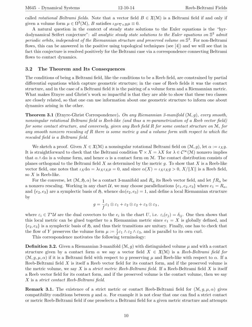
Theorem 3.1 (Etnyre-Ghrist Correspondence). On any Riemannian 3-manifold (M, g), every smooth,nonsingular rotational Beltrami field is Reeb-like (and thus a re-parametrization of a Reeb vector field)for some contact structure, and conversely, given any Reeb field R for some contact structure on M, forany smooth nonzero rescaling of R there is some metric g and a volume form with respect to which therescaled field is a Beltrami field.

We sketch a proof. Given X ∈ X(M) a nonsingular rotational Beltrami field on (M, g), let α := ιXg.It is straightforward to check that the Beltrami condition ∇×X = λX for λ ∈ C∞(M) nonzero impliesthat α∧ dα is a volume form, and hence α is a contact form on M. The contact distribution consists ofplanes orthogonal to the Beltrami field X as determined by the metric g. To show that X is a Reeb-likevector field, one notes that ιXdα = λιXιXµ = 0, and since α(X) = ιXιXg > 0, X/‖X‖ is a Reeb field,so X is Reeb-like.

For the converse, let (M,H, α) be a contact 3-manifold and Rα its Reeb vector field, and let fRα bea nonzero rescaling. Working in any chart U , we may choose parallelizations e1, e2, e3 where e1 = Rα,and e2, e3 are a symplectic basis of H, whence dα(e2, e3) = 1, and define a local Riemannian structureby

g =1

fε1 ⊗ ε1 + ε2 ⊗ ε2 + ε3 ⊗ ε3 ,

where εi ∈ T ∗U are the dual covectors to the ei in the chart U , i.e. εi(ej) = δij . One then shows thatthis local metric can be glued together to a Riemannian metric since e1 = X is globally defined, ande2, e3 is a symplectic basis of H, and thus their transitions are unitary. Finally, one has to check thatthe flow of Y preserves the volume form µ := 1

f ε1 ∧ ε2 ∧ ε3, and is parallel to its own curl.This correspondence motivates the following terminology:

Definition 3.2. Given a Riemannian 3-manifold (M, g) with distinguished volume µ and with a contactstructure given by a contact form α we say a vector field X ∈ X(M) is a Reeb-Beltrami field for(M, g, µ, α) if it is a Beltrami field with respect to g preserving µ and Reeb-like with respect to α. If aReeb-Beltrami field X is itself a Reeb vector field for its contact form, and if the preserved volume isthe metric volume, we say X is a strict metric Reeb-Beltrami field. If a Reeb-Beltrami field X is itselfa Reeb vector field for its contact form, and if the preserved volume is the contact volume, then we sayX is a strict contact Reeb-Beltrami field.

Remark 3.1. The existence of a strict metric or contact Reeb-Beltrami field for (M, g, µ, α) givescompatibility conditions between g and α. For example it is not clear that one can find a strict contactor metric Reeb-Beltrami field if one preselects a Beltrami field for a given metric structure and attempts

10


to construct a contact form for which it is a Reeb field. However, given a contact structure with contactform α, it is always possible to construct a metric as in the proof so that Rα is a strict contact and metricReeb-Beltrami field, by taking the unit scaling of Rα and thus setting g := ε1 ⊗ ε1 + ε2 ⊗ ε2 + ε3 ⊗ ε3,and µ := ε1 ∧ ε2 ∧ ε3.

An immediate corollary of the correspondence is that every-Reeb-like vector field gives rise to a steadystate solution for a perfect incompressible fluid satisfying Euler equations with respect to some suitableRiemannian metric. Of further interest is the use of contact geometry to prove results about existenceof closed orbits in Beltrami fields. From Taube’s proof of the Weinstein conjecture, this correspondenceyields that any nonsingular rotational Beltrami flow on a closed 3-manifold has a periodic orbit.

A once open matter of investigation, in the spirit of Seifert’s conjecture and the general thrustof dynamical system theory, was to understand the topology of possible closed orbits for a Beltramifield. The Etnyre-Ghrist correspondence translates the condition of being Beltrami, which comes froma partial differential equation, to the condition of being Reeb-like, which for a given contact form isa linear algebraic condition (annihilating the exterior derivative of the contact form) coupled with ananalytic condition (non-vanishing of contraction with the contact form). Hence one converts the problemof understanding the possible topologies of Beltrami flows into understanding the topologies of solutionsto the nonlinear ordinary differential equations for Reeb Fields arising in contact geometry. But, aswe’ve seen, Reeb fields come parametrized by nonzero smooth functions, which gives incredible freedomto construct complex dynamics. Moreover, one can apply surgery techniques to piece together contactstructures on different pieces of a manifold, in order to produce closed orbits of a Reeb field with anyselected knotting and linking type. Thus, the class of Beltrami fields on a given 3-manifold also mustpossess the ability to support closed orbits of arbitrary knotting and linking type.

More surprising however, is the following result of Etnyre and Ghrist [5]:

Theorem 3.2. For some Riemannian structure on S3, there exists a steady, nonsingular analytic Bel-trami field X ∈ Xω(S3) whose flow simultaneously possesses periodic orbits of all knot and link types.

Of course, to isolate a particular such flow for a given metric and witness the infinitude of knottedand linked orbits on S3 is perhaps untenable: the various cut and paste constructions needed to producethe knotted flowlines involve altering the Riemannian structure. Etnyre and Ghrist pose as an openquestion the exhibition of such a flow on the standard round S3, and also on Euclidean R3. Ghrist andHolmes showed that there are simple ODE systems on R3 possessing all knot and link types as closedorbits [7], but to date the it is unknown whether there are steady state solutions to Euler’s equationsfor Euclidean R3 with this knotted flowline property.

4 Examples of Beltrami and Reeb flows

4.1 The ABC fields

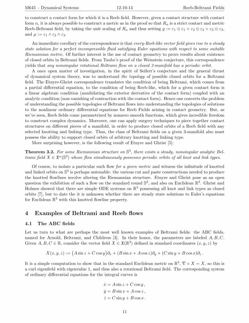
Let us turn to what are perhaps the most well known examples of Beltrami fields: the ABC fields,named for Arnold, Beltrami, and Childress [3]. In their honor, the parameters are labeled A,B,C.Given A,B,C ∈ R, consider the vector field X ∈ X(R3) defined in standard coordinates (x, y, z) by

X(x, y, z) :=ÄA sin z + C cos y

ä∂x + (B sinx+A cos z)∂y + (C sin y +B cosx)∂z .

It is a simple computation to show that in the standard Euclidean metric on R3, ∇×X = X, so this isa curl eigenfield with eigenvalue 1, and thus also a rotational Beltrami field. The corresponding systemof ordinary differential equations for the integral curves is

x = A sin z + C cos y ,

y = B sinx+A cos z ,

z = C sin y +B cosx .

11


Figure 3: On the left is a visualization of the ABC field X as a vector field on R3 for parameters A = 1,B = 9

√3/20, C = 7/20, and on the right is a visualization of the corresponding plane field HABC on R3.

Note that X is not just smooth–X is Cω. The flow will be nonsingular if and only if the vectorfield is non-vanishing, which puts conditions on the admissible parameters. Up to rescaling, a suitablecondition to ensure that the flow is nonsingular is to take A = 1 and B,C ∈ R+ with 0 < B2 +C2 < 1.

To make explicit the correspondence, we compute the contact structure associated to the generalABC field. The contact one form is

αABC := ιXg =ÄA sin z + C cos y

ädx+ (B sinx+A cos z) dy + (C sin y +B cosx) dz ,

and the plane distribution is then HABC = kerαABC . This gives a contact volume of

α ∧ dα = ‖X‖2 dx ∧ dy ∧ dz .

Thus the contact volume is not the preserved metric volume, and so the ABC fields are not able to berealized as strict contact Reeb-Beltrami fields.

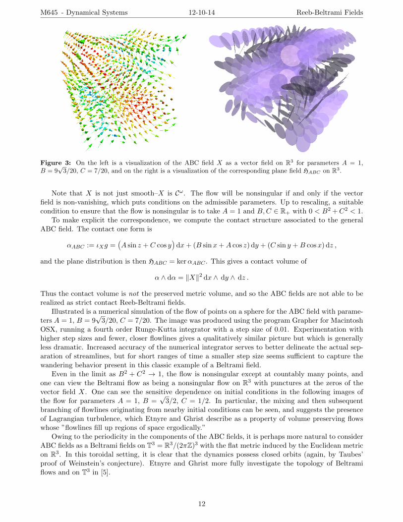
Illustrated is a numerical simulation of the flow of points on a sphere for the ABC field with parame-ters A = 1, B = 9

√3/20, C = 7/20. The image was produced using the program Grapher for Macintosh

OSX, running a fourth order Runge-Kutta integrator with a step size of 0.01. Experimentation withhigher step sizes and fewer, closer flowlines gives a qualitatively similar picture but which is generallyless dramatic. Increased accuracy of the numerical integrator serves to better delineate the actual sep-aration of streamlines, but for short ranges of time a smaller step size seems sufficient to capture thewandering behavior present in this classic example of a Beltrami field.

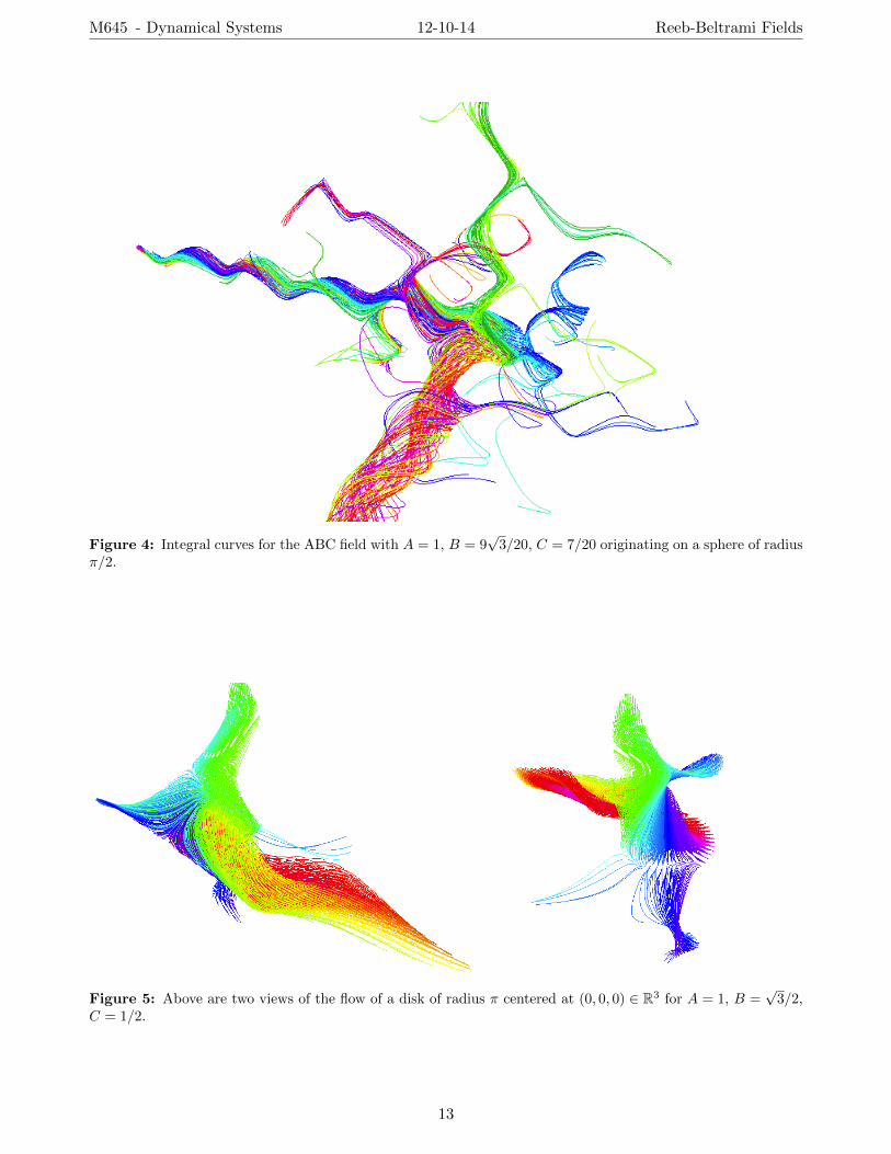
Even in the limit as B2 + C2 → 1, the flow is nonsingular except at countably many points, andone can view the Beltrami flow as being a nonsingular flow on R3 with punctures at the zeros of thevector field X. One can see the sensitive dependence on initial conditions in the following images ofthe flow for parameters A = 1, B =

√3/2, C = 1/2. In particular, the mixing and then subsequent

branching of flowlines originating from nearby initial conditions can be seen, and suggests the presenceof Lagrangian turbulence, which Etnyre and Ghrist describe as a property of volume preserving flowswhose ”flowlines fill up regions of space ergodically.”

Owing to the periodicity in the components of the ABC fields, it is perhaps more natural to considerABC fields as a Beltrami fields on T3 = R3/(2πZ)3 with the flat metric induced by the Euclidean metricon R3. In this toroidal setting, it is clear that the dynamics possess closed orbits (again, by Taubes’proof of Weinstein’s conjecture). Etnyre and Ghrist more fully investigate the topology of Beltramiflows and on T3 in [5].

12


Figure 4: Integral curves for the ABC field with A = 1, B = 9√

3/20, C = 7/20 originating on a sphere of radiusπ/2.

Figure 5: Above are two views of the flow of a disk of radius π centered at (0, 0, 0) ∈ R3 for A = 1, B =√

3/2,C = 1/2.

13


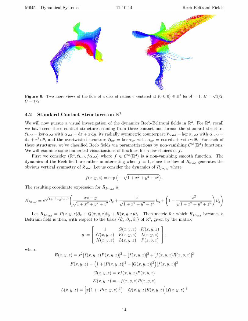
Figure 6: Two more views of the flow of a disk of radius π centered at (0, 0, 0) ∈ R3 for A = 1, B =√

3/2,C = 1/2.

4.2 Standard Contact Structures on R3

We will now pursue a visual investigation of the dynamics Reeb-Beltrami fields in R3. For R3, recallwe have seen three contact structures coming from three contact one forms: the standard structureHstd = kerαstd with αstd = dz + x dy, its radially symmetric counterpart Hrstd = kerαrstd with αrstd =dz + r2 dθ, and the overtwisted structure Hoτ = kerαoτ with αoτ = cos rdz + r sin r dθ. For each ofthese structures, we’ve classified Reeb fields via parametrizations by non-vanishing C∞(R3) functions.We will examine some numerical visualizations of flowlines for a few choices of f .

First we consider (R3,Hstd, fαstd) where f ∈ C∞(R3) is a non-vanishing smooth function. Thedynamics of the Reeb field are rather uninteresting when f ≡ 1, since the flow of Rαstd generates theobvious vertical symmetry of Hstd. Let us consider the dynamics of Rfαstd where

f(x, y, z) = expÄ−»

1 + x2 + y2 + z2ä.

The resulting coordinate expression for Rfαstd is

Rfαstd = e√

1+x2+y2+z2

(xz − y√

1 + x2 + y2 + z2∂x +

x√1 + x2 + y2 + z2

∂y +

Ç1− x2√

1 + x2 + y2 + z2

å∂z

)

Let Rfαstd = P (x, y, z)∂x + Q(x, y, z)∂y + R(x, y, z)∂z. Then metric for which Rfαstd becomes aBeltrami field is then, with respect to the basis ∂x, ∂y, ∂z of R3, given by the matrix

g :=

1 G(x, y, z) K(x, y, z)G(x, y, z) E(x, y, z) L(x, y, z)K(x, y, z) L(x, y, z) F (z, y, z)

,where

E(x, y, z) = x2[f(x, y, z)P (x, y, z)]2 + [f(x, y, z)]2 + [f(x, y, z)R(x, y, z)]2

F (x, y, z) =(1 + [P (x, y, z)]2 + [Q(x, y, z)]2

)[f(x, y, z)]2

G(x, y, z) = xf(x, y, z)P (x, y, z)

K(x, y, z) = −f(x, y, z)P (x, y, z)

L(x, y, z) =[xÄ1 + [P (x, y, z)]2

ä−Q(x, y, z)R(x, y, z)

][f(x, y, z)]2

14


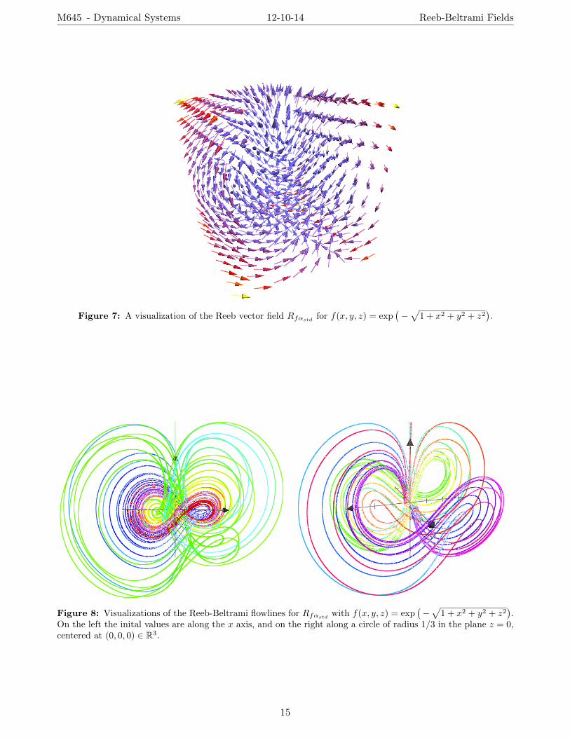
Figure 7: A visualization of the Reeb vector field Rfαstd for f(x, y, z) = exp(−√

1 + x2 + y2 + z2).

Figure 8: Visualizations of the Reeb-Beltrami flowlines for Rfαstd with f(x, y, z) = exp(−√

1 + x2 + y2 + z2).

On the left the inital values are along the x axis, and on the right along a circle of radius 1/3 in the plane z = 0,centered at (0, 0, 0) ∈ R3.

15


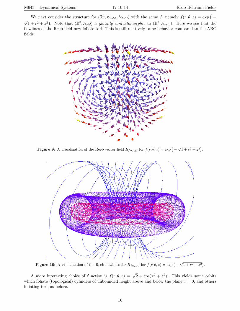
We next consider the structure for (R3,Hrstd, fαstd) with the same f , namely f(r, θ, z) = expÄ−√

1 + r2 + z2ä. Note that (R3,Hstd) is globally contactomorphic to (R3,Hrstd). Here we see that the

flowlines of the Reeb field now foliate tori. This is still relatively tame behavior compared to the ABCfields.

Figure 9: A visualization of the Reeb vector field Rfαrstd for f(r, θ, z) = exp(−√

1 + r2 + z2).

Figure 10: A visualization of the Reeb flowlines for Rfαrstd for f(r, θ, z) = exp(−√

1 + r2 + z2).

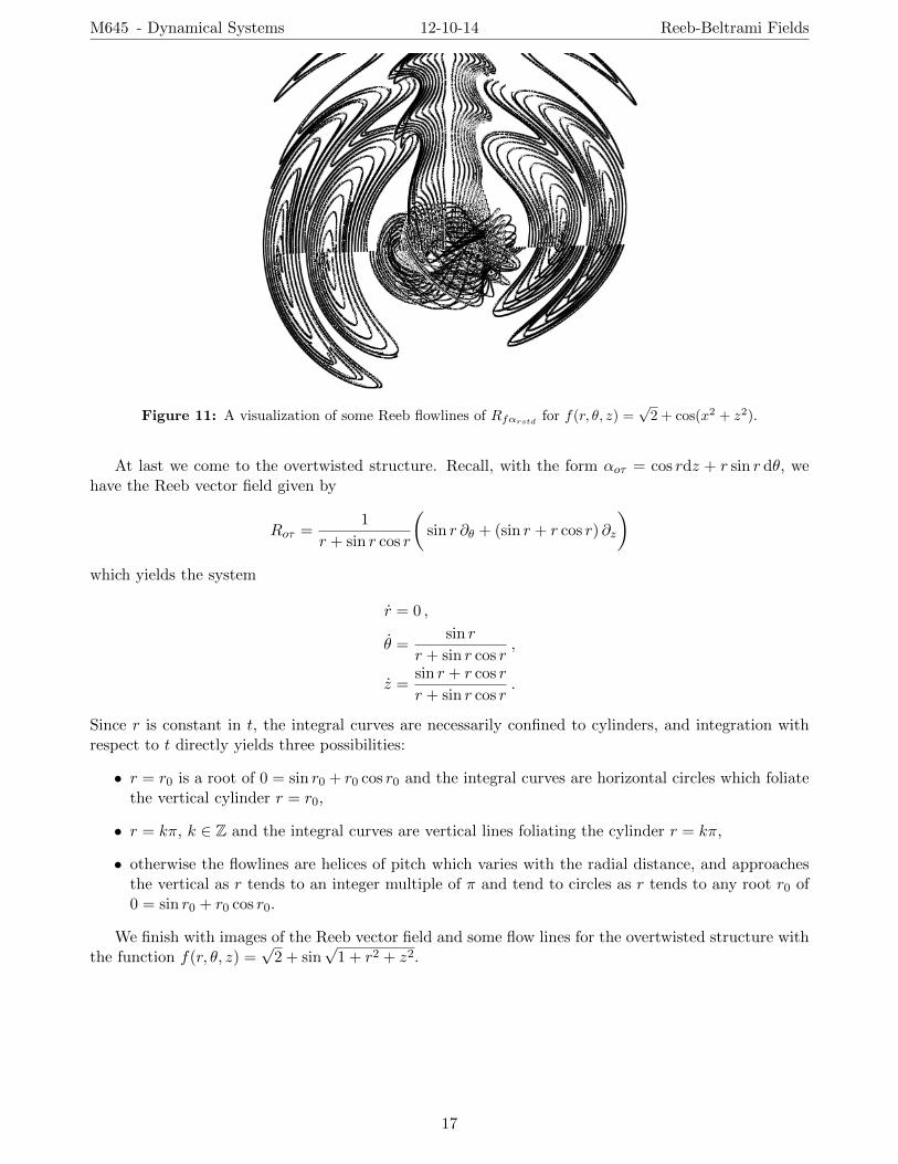
A more interesting choice of function is f(r, θ, z) =√

2 + cos(x2 + z2). This yields some orbitswhich foliate (topological) cylinders of unbounded height above and below the plane z = 0, and othersfoliating tori, as before.

16


Figure 11: A visualization of some Reeb flowlines of Rfαrstd for f(r, θ, z) =√

2 + cos(x2 + z2).

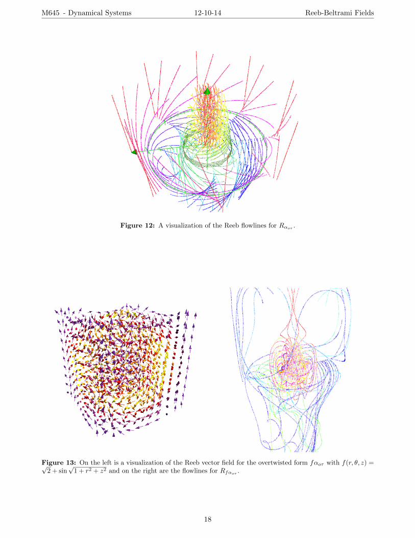
At last we come to the overtwisted structure. Recall, with the form αoτ = cos rdz + r sin r dθ, wehave the Reeb vector field given by

Roτ =1

r + sin r cos r

Çsin r ∂θ + (sin r + r cos r) ∂z

åwhich yields the system

r = 0 ,

θ =sin r

r + sin r cos r,

z =sin r + r cos r

r + sin r cos r.

Since r is constant in t, the integral curves are necessarily confined to cylinders, and integration withrespect to t directly yields three possibilities:

• r = r0 is a root of 0 = sin r0 + r0 cos r0 and the integral curves are horizontal circles which foliatethe vertical cylinder r = r0,

• r = kπ, k ∈ Z and the integral curves are vertical lines foliating the cylinder r = kπ,

• otherwise the flowlines are helices of pitch which varies with the radial distance, and approachesthe vertical as r tends to an integer multiple of π and tend to circles as r tends to any root r0 of0 = sin r0 + r0 cos r0.

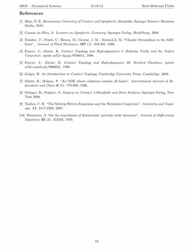
We finish with images of the Reeb vector field and some flow lines for the overtwisted structure withthe function f(r, θ, z) =

√2 + sin

√1 + r2 + z2.

17


Figure 12: A visualization of the Reeb flowlines for Rαoτ .

Figure 13: On the left is a visualization of the Reeb vector field for the overtwisted form fαoτ with f(r, θ, z) =√2 + sin

√1 + r2 + z2 and on the right are the flowlines for Rfαoτ .

18


References

[1] Blair, D. E. Riemannian Geometry of Contact and Symplectic Manifolds, Springer Science+BusinessMedia, 2010.

[2] Cannas da Silva, A. Lectures on Symplectic Geometry. Springer-Verlag, Heidelberg, 2008.

[3] Dombre, T.; Frisch, U.; Henon, M.; Greene, J. M. ; Soward,A. M. “Chaotic Streamlines in the ABCflows”, Journal of Fluid Mechanics 167 (1): 353-391, 1986.

[4] Etnyre, J.; Ghrist, R. Contact Topology and Hydrodynamics I: Beltrami Fields and the SeifertConjecture. eprint arXiv:dg-ga/9708011, 1998.

[5] Etnyre, J.; Ghrist, R. Contact Topology and Hydrodynamics III: Knotted Flowlines. eprintarXiv:math-ph/9906021, 1998.

[6] Geiges, H. An Introduction to Contact Topology. Cambridge University Press, Cambridge, 2008.

[7] Ghrist, R.; Holmes, P. “An ODE whose solutions contain all knots”, International Journal of Bi-furcation and Chaos 6 (5): 779-800, 1996.

[8] Ozbagci, B.; Stipsicz, A. Surgery on Contact 3-Manifolds and Stein Surfaces, Springer-Verlag, NewYork 2004.

[9] Taubes, C. H. “The Seiberg-Witten Equations and the Weinstein Conjecture”, Geometry and Topol-ogy : 11: 2117-2202, 2007.

[10] Wienstein, A “On the hypotheses of Rabinowitz’ periodic orbit theorems”. Journal of DifferentialEquations 33 (3): 353358, 1979.

19

Contact Dynamics in 3 Dimensions: Some Explorations of Reeb-Beltrami Fields

Documents

Transcript of Contact Dynamics in 3 Dimensions: Some Explorations of Reeb-Beltrami Fields