Computer simulation of the linear and nonlinear optical properties of liquid benzene: Itslocal fields, refractive index, and second nonlinear susceptibilityR. H. C. Janssen, J.-M. Bomont, D. N. Theodorou, S. Raptis, and M. G. Papadopoulos Citation: The Journal of Chemical Physics 110, 6463 (1999); doi: 10.1063/1.478549 View online: http://dx.doi.org/10.1063/1.478549 View Table of Contents: http://scitation.aip.org/content/aip/journal/jcp/110/13?ver=pdfcov Published by the AIP Publishing Articles you may be interested in Linear and second-order nonlinear optical properties of ionic organic crystals J. Chem. Phys. 141, 104109 (2014); 10.1063/1.4894483 Investigation of the linear and second-order nonlinear optical properties of molecular crystals within the local fieldtheory J. Chem. Phys. 139, 114105 (2013); 10.1063/1.4819769 Theoretical investigation on the linear and nonlinear susceptibilities of urea crystal J. Chem. Phys. 128, 244713 (2008); 10.1063/1.2938376 Calculation of refractive indices and third-harmonic generation susceptibilities of liquid benzene and water:Comparison of continuum and discrete local-field theories J. Chem. Phys. 114, 876 (2001); 10.1063/1.1327261 Microscopic calculation of the third-order nonlinear optical susceptibility of DEANST crystal J. Chem. Phys. 107, 7926 (1997); 10.1063/1.475106

This article is copyrighted as indicated in the article. Reuse of AIP content is subject to the terms at: http://scitation.aip.org/termsconditions. Downloaded to IP:

193.50.135.10 On: Thu, 23 Oct 2014 12:39:14

Computer simulation of the linear and nonlinear optical properties of liquidbenzene: Its local fields, refractive index, and second nonlinearsusceptibility

R. H. C. Janssen, J.-M. Bomont, and D. N. Theodoroua)

Department of Chemical Engineering, University of Patras, GR 26500 Patras, Greece and Instituteof Chemical Engineering and High Temperature Chemical Processes, GR 26500 Patras, Greece

S. Raptis and M. G. PapadopoulosInstitute of Organic and Pharmaceutical Chemistry, National Hellenic Research Foundation, VassileosConstantinou 48, GR 11635 Athens, Greece

~Received 25 September 1997; accepted 28 December 1998!

Molecular dynamics~MD! simulation and subsequent analysis of the macroscopic polarizationdeveloped in response to ‘‘a posteriori’’ applied electric fields or of spontaneous fluctuations in theinstantaneous polarization under zero applied field is used to assess the nonlinear optical propertiesof a polarizable liquid. Three strategies are proposed for the electrostatic analysis, all using as inputstatic ‘‘gas phase’’~hyper!polarizabilities, obtained fromab initio calculations. All three strategiesare shown to accurately reproduce the experimentally measured refractive index and secondnonlinear susceptibility of liquid benzene. The simulation also predicts the distribution oforientations and magnitudes of the local electric fields experienced by the molecules in the liquid,and the nonlinear contributions to the local fields. This approach gives an 8% higher estimate of thesecond nonlinear susceptibility of liquid benzene than the Lorentz local field factor approach, inbetter agreement with experimental values. ©1999 American Institute of Physics.@S0021-9606~99!51612-7#

I. INTRODUCTION

Nonlinear optical ~NLO! processes are becoming in-creasingly important in the optoelectronics industry.1,2 Ofgreat importance are, for instance, high speed all-opticalswitching and computing, which rely on changes of the re-fractive index of a material with the intensity of an appliedlaser field.3 Obviously, the efficiency of such a nonlinearprocess relies heavily on the properties of the materials em-ployed in it. Currently, there is an increasing tendency tostudy the use of organic molecular and polymeric materialsin such applications, since they are easily processable, showhigh optical damage thresholds, and can in principle be tai-lored for a specific application by the methods of organicchemistry.1–4

Thus far, the study of nonlinear optical properties ofmolecular materials has mainly focused on identifying mol-ecules showing large nonlinear responses, i.e., moleculeshaving high hyperpolarizabilities. Theoretically, single mol-ecule ‘‘gas phase’’ hyperpolarizabilities have been estimatedby ab initio ~e.g., Refs. 5 and 6! and semiempirical~e.g.,Refs. 7 and 8! quantum chemical approaches. Experimen-tally, the electric field-induced second-harmonic generation~EFISH! technique9–11 and, more recently, the hyper-Rayleigh scattering~HRS! technique12 have been developedand exploited to estimate molecular hyperpolarizabilities inthe liquid phase. Gas-phase measurements,13 which would

allow for a direct comparison between experimentally andquantum chemically obtained hyperpolarizabilities, are oftennot possible, since NLO-active molecules have very highdipole moments, which do not allow evaporating them intothe gas phase. Therefore, a local field factor approach,14 es-sentially a direct extension of the classical Lorentz local fieldapproximation for dielectric material properties,15 is com-monly used to extract single molecule ‘‘gas phase’’ hyper-polarizabilities from experiments performed in the liquidphase. Although the local field factor procedure is generallyaccepted, there is every reason to doubt its validity in ex-tracting molecular properties such as the~hyper!polarizabilities.15 Therefore, in order to compare di-rectly experimental and calculated hyperpolarizabilities,there is a need to establish quantitative relations between themacroscopic material properties measured in experimentsand the molecular properties obtained from quantum chemi-cal work. Attempts to accomplish this have been undertakenby Willets and Rice16 and Yu and Zerner,17 who have trieddirectly to incorporate the effect of the environment of amolecule intoab initio calculations via a reaction field ap-proach.

We believe that it is inherently more accurate to use ahierarchical scheme which iterates between quantum chemi-cal and statistical mechanical calculations to accomplish theabove task in the following way: Gas-phase~hyper!polariz-abilities obtained from theab initio calculations are used asinput values in a classical~molecular dynamics or MonteCarlo! simulation, which subsequently produces the distribu-tion of the electric fields experienced by the molecules.

a!Author to whom correspondence should be addressed at the University ofPatras; electronic mail: doros@sequoia.chemeng.upatras.gr

JOURNAL OF CHEMICAL PHYSICS VOLUME 110, NUMBER 13 1 APRIL 1999

64630021-9606/99/110(13)/6463/12/$15.00 © 1999 American Institute of Physics

This article is copyrighted as indicated in the article. Reuse of AIP content is subject to the terms at: http://scitation.aip.org/termsconditions. Downloaded to IP:

193.50.135.10 On: Thu, 23 Oct 2014 12:39:14

These fields can, if necessary, be used to correct the gas-phase hyperpolarizability values in a newab initio round,etc. Such a hierarchical approach would be ideally suited toestimating the influence of the environment on the molecular~hyper!polarizabilities~the so-called ‘‘solvent effect’’!. Cur-rently, it is believed that this effect may increase the firsthyperpolarizability by a factor of 2 or more relative to thegas phase, with serious consequences on properties.16–19

The objective of the work presented in this paper was toestablish a quantitative relation between the macroscopic andmolecular NLO properties of a molecular liquid and to assessthe magnitudes and orientations of the local electric fieldsexperienced by the molecules in such a liquid. Liquid ben-zene has been chosen as a test case, because of its relativesimplicity and the fact that it has been studied extensivelyboth by optical experiments and by simulations.

We have used a combined quantum mechanical–statistical mechanical approach to accomplish the task: Inputto our molecular simulations are static polarizabilities andhyperpolarizabilities obtained fromab initio quantum chemi-cal calculations on isolated molecules. Our calculations showthat, for this system, it is not necessary to refine further theab initio molecular properties of our benzene model. Feed-back of our results to the quantum level is not necessary inthe current case.

Our approach, implemented using three different strate-gies, has further allowed us to test the local field factor ap-proach for the nonlinear susceptibility of liquid benzene. Wehave found that the local field factor approach predicts an8% lower second-order nonlinear susceptibility than our ap-proach if we use the same molecular polarizability (a i j ) andhyperpolarizability (g i jkl ) tensors as input. We believe thatthe difference between the two approaches may well point toinaccuracies in the local field factor approach, because thecurrent approach involves much less simplifying assump-tions. Our findings are supported by Sta¨helin et al., whoseexperiments on gaseous and liquid acetonitrile also point toan invalidity of the local field factor approach.19

Our computational approach utilizes the molecular dy-namics technique to generate a sequence of liquid configu-rations for a fluid consisting of polarizable molecules in theabsence of external electric fields. The instantaneous polar-ization that each configuration would develop when sub-jected to an electromagnetic field is computed by solving theequations of electrostatics within the configuration of inter-est, using as input molecular polarizabilities and hyperpolar-izabilities calculated from quantum mechanics. Subse-quently, the macroscopic polarization of the fluid is obtainedby averaging the instantaneous polarization of individualconfigurations. The coupling of the induced part of the in-stantaneous polarization to the imposed field is taken intoaccount in weighting configurations during this averagingprocess. From the computed dependence of the macroscopicpolarization on the macroscopic electric field, the linear andnonlinear electric susceptibilities are extracted using two dif-ferent strategies. As a third strategy, the susceptibilities areextracted from an analysis of spontaneous fluctuations in theinstantaneous polarization in an equilibrium liquid free of

externally imposed electric fields. All three strategies lead tothe same results in the case of benzene.

Several complications have to be overcome in the pro-posed approach. Generating a trajectory~sequence of con-figurations of the field-free liquid! requires an accurateknowledge of particle–particle interactions. Not only arethese interactions of long-range character~they need to behandled by Ewald summation20–22!, but interparticle forcesare also dependent on the local environment of each particle.This latter feature is caused by the polarizable nature of theparticles. The interparticle forces that arise due to the polar-izability of the particles can in principle be determined self-consistently~see e.g., Refs. 23 and 24!, but this amounts toan enormous increase in computational cost~by more than afactor of 10!. In order to keep sufficient computational speed,we resort to a major simplification in the interparticle poten-tial: The sacrifice of the polarizable nature of the moleculesduring the simulation. Molecular dynamics~MD! trajectoriesare generated using a force field cast in terms of Lennard-Jones~LJ! interactions and Coulomb interactions betweenpermanent charges only, which, however, reproduces experi-mentally observed equilibrium structural, thermodynamic,and transport properties satisfactorily. After generating a rep-resentative set of liquid configurations with the simplifiedinterparticle potential, the polarizable nature of the mol-ecules is restored, which then allows for calculation of thelocal electric fields experienced by the molecules, the polar-ization developing in response to an external field, and theoptical properties of the fluid. Our procedure, which is justi-fied in the Sec. II, thus amounts to a decoupling of the elec-trostatics problem from the generation of the liquid configu-rations, much in the spirit of the work of Ladanyiet al.25,26

The outline of the rest of this paper is as follows. In Sec.II we mention the basic equations governing the macroscopicand microscopic behavior of a NLO material in an externallyapplied electric field, discuss the molecular model we use,and present our three strategies for extracting the linear andnonlinear susceptibilities. In Sec. III we present and discussour results on the liquid structure~Sec. III A!, the local elec-tric fields ~Sec. III B!, and the macroscopic optical propertiesof liquid benzene~Sec. III C!. Conclusions are drawn inSec. IV.

II. THEORETICAL CONSIDERATIONS

A. Problem formulation and computational strategiesemployed

Applying an electric fieldE0 to a macroscopic amount ofmaterial generally induces a polarizationP in the material,given by27,14

P5x=

~1!•E1x

T

~2!:EE1xU

~3!AEEE1••• . ~1!

The polarizationP is defined as the material’s dipole mo-ment per unit volume.E is the macroscopic field in the ma-terial, i.e., the field that would be measured if the materialwere placed in a capacitor. TheEE and EEE are tensorialterms nonlinear inE. Note thatE is not equal to the appliedfield E0, but is given by

e0E05e0E1Psurf, ~2!

6464 J. Chem. Phys., Vol. 110, No. 13, 1 April 1999 Janssen et al.

This article is copyrighted as indicated in the article. Reuse of AIP content is subject to the terms at: http://scitation.aip.org/termsconditions. Downloaded to IP:

193.50.135.10 On: Thu, 23 Oct 2014 12:39:14

where Psurf is the surface polarization of the macroscopicbody ~see Chaps. 10 and 11 of Ref. 28!. Thex

=

(1), xT

(2), andxU

(3) in Eq. ~1! are, respectively, the linear susceptibility ten-sor, and the first and second nonlinear susceptibility tensors.These susceptibilities are the material properties of interest.Thex

=

(1) can be related to the refractive index tensorn=

of thematerial via

x=

~1!5e0~n=•n=21=! ~3!

in which e0 is the dielectric permittivity of vacuum and 1=

theunit tensor. Generally,x

=

(1)•E@x

T

(2):EE@xU

(3)AEEE; thenonlinear contributions can only be observed experimentallyfor E.105 V/m. Note that thex (n)’s normally are functionsof the frequency of the applied field. At optical frequencies,far away from molecular resonances, this frequency depen-dence may be neglected as a first reasonableapproximation.10,15

The molecular counterpart of Eq.~1! is given by14

m i5m0,i1m i , ind5m0,i1a=•Eloc,i1b

T:EEloc,i

1gU

AEEEloc,i1••• ~4!

in which Eloc,i is the local electric field experienced by mol-eculei, andEEloc,i andEEEloc,i are the higher order electricfield tensors formed fromEloc,i , denoting nonlinear contri-butions tom i . Equation~4! states that the dipole moment ofmoleculei is determined by a sum of its permanent dipolemomentm0,i ~which is zero in the case of benzene!, an in-duction contribution determined by the molecule’s polariz-ability tensora

=, and contributions nonlinear inEloc,i deter-

mined by the hyperpolarizabilitiesbT

and gU. The

~hyper!polarizabilitiesa=, bT, andg

Uare molecular properties,

depending on the frequency of the local electric fields. Atoptical frequencies, far away from electronic resonances, wemay again ignore this frequency dependence as a first ap-proximation.

The problem that we are addressing in this paper is howto obtain x

=

(1) and xU

(3) from the molecular~hyper!polariz-abilities of benzene by electrostatic analysis of a representa-tive set of liquid configurations. (x

T

(2) is zero for isotropicsystems.! A second objective is to assess the strength andorientation ofEloc,i in the absence of an externally imposedfield.

Consider a model molecular fluid ofN molecules in vol-umeV at temperatureT, in which the charge distribution isrepresented in terms of fixed partial charges,zia , on specificsites a of the moleculesi and point dipoles,m i , ind, at themolecular centers of mass~c.m.!. The partial charges areresponsible for the permanent dipole momentm0,i

5(aziar ia on each molecule, while the induced part ofm i isdetermined by local fields according to Eq.~4!. Followingthe usual convention of molecular simulations, we will re-gard the liquid as periodic over length scales exceeding thelength of the simulation box.20,22 Let

L=

5ULX 0 0

0 LY 0

0 0 LZ

Ube a matrix formed from the edge lengths of the primarysimulation box. The contents of the primary box of volumeV are copied into image boxes located at positionsL

=•m rela-

tive to the parent box,m being a vector of integer compo-nents.

In the presence of a macroscopic fieldE, each micro-scopic configurationr of the fluid will develop an instanta-neous polarizationP , given by

P 5P ~r ,E!51

V (i 51

N

m i51

V (i 51

N

~m0,i1m i , ind!5P 01P ind .

~5!

The dipole momentsm i needed for calculatingP arerelated to the local fields through Eq.~4!. In turn, the localfield Eloc,i at the c.m. of each moleculei may be obtained byiterative self-consistent solution of Eq.~4! together with

Eloc,i52]f i

]r1E ~6!

with the electrostatic potential ati given by

f i5 (m50

9(

j

8 S (b

zjb

4pe0ur i , jb1L=•mu

12m j , ind•~r i j 1L

=•m!

4pe0ur i j 1L=•mu3 D . ~7!

In Eqs. ~6! and ~7!, vector r i j points from the c.m. of mol-ecule j to the c.m. of moleculei, while vector r i , jb pointsfrom siteb of moleculej to the c.m. of moleculei. The primeon the summation overj indicates thatj 5 i should be ex-cluded form50. The double prime in them sum denotesthat we only sum over the absolutely convergent part of thetotal sum(m50 . One has a freedom to construct differentshapes of a macroscopic body by summing overm in differ-ent ways, but, as long as theE field in the macroscopic bodyis homogeneous~which is the case for generalized ellip-soids!, the values of theE fields differ only by a termPsurf/e0, defined in Eq.~2!. This Psurf is therefore the valueof the conditionally convergent part of the total sum(m50 .Equations~6! and ~7!, which are formulated in terms ofEand(m509 , are therefore identical to a description in terms ofE0 and the full sum(m50 . The formulation chosen hereavoids the need to explicitly considerPsurf in the electrostat-ics problem, since the absolutely convergent part,(m509 , canbe obtained directly by Ewald summation29 ~see Sec. II C!.

The macroscopic polarization of the fluid,P, is given by

P5* dr P ~r ,E!exp$2@U0~r !2V P ~r ,E!•E#/~kBT!%

* dr exp$2@U0~r !2V P ~r ,E!•E#/~kBT!%, ~8!

whereU0(r ) is the potential energy of configurationr in theabsenceof a macroscopic field (E50). The second term inthe exponential of Eq.~8!, involving a coupling of the instan-taneous polarization with the field, introduces a bias relativeto the probability distribution of configurations in the ab-

6465J. Chem. Phys., Vol. 110, No. 13, 1 April 1999 Janssen et al.

This article is copyrighted as indicated in the article. Reuse of AIP content is subject to the terms at: http://scitation.aip.org/termsconditions. Downloaded to IP:

193.50.135.10 On: Thu, 23 Oct 2014 12:39:14

sence of a field and may lead to a field-induced perturbationof the average structure by the field. Denoting by

^A&5* dr A~r !exp@2U0~r !/~kBT!#

* dr exp@2U0~r !/~kBT!#~9!

the equilibrium ensemble average of a configuration-dependent propertyA(r ) in the absence of a field, we canrewrite Eq.~8! as

P5^P ~r ,E!exp@VP ~r ,E!•E/~kBT!#&

^exp@VP~r ,E!•E/~kBT!#&. ~10!

In our work, we are interested in the response to oscillatingfields at optical frequencies. Clearly, the rotational degreesof freedom determining the orientation of permanent mo-lecular dipole moments do not have the time to relax inresponse to the field at these frequencies, i.e., the fieldEcouples only to electronic degrees of freedom and not to themotion of the molecule as a whole. Since molecular orienta-tions arenot in equilibrium with respect to the macroscopicfield, the permanent dipolesm i ,0 , if existent, shouldnot con-tribute to the weighting factor exp@VP(r ,E)•E/(kBT)#, andthe correct form of Eq.~10! for our problem is

P5^P ~r ,E!exp@VP ind~r ,E!•E/~kBT!#&

^exp@VP ind~r ,E!•E/~kBT!#&. ~11!

Expanding the right-hand side of Eq.~11! in powers ofEand matching term by term with Eq.~1! leads to the follow-ing fluctuation relations forx

=

(1) andxU

(3):

x=

~1!5K 1

kBTVP P ind1

]P ind

]E L , ~12!

xU

~3!5K 1

6

]3P ind

]E3 11

2kBTV

]2P ind

]E2 P ind

1]P ind

]E H 1

kBTV

]P ind

]E1

1

2S 1

kBTD 2

V2P indP indJ1P H 1

2kBTV

]2P ind

]E2 1S 1

kBTD 2

V2P ind

]P ind

]E

11

6S 1

kBTD 3

V3P indP indP indJ L2K 1

kBTVP P ind1

]P ind

]E L K 1

kBTV

]P ind

]E

11

2S 1

kBTD 2

V2P indP indL . ~13!

All brackets in Eqs.~12! and ~13! denote equilibriumensemble averages taken under the conditionE50, in thesense of Eq.~9!. All terms on the right-hand side of Eq.~12!are second-order tensors. All terms on the right-hand side ofEq. ~13! are fourth-order tensors.

In the special case of a molecular model with no perma-nent charges (zia50), Eqs. ~5!–~7! applied to the caseE50 lead toP 5P ind50 for all configurations and Eqs.~12!and ~13! simplify to

x=

~1!5K ]P ind

]E L ~14!

and

xU

~3!5K 1

6

]3P ind

]E3 L 11

kBTVF K ]P ind

]E

]P ind

]E L2K ]P ind

]E L K ]P ind

]E L G . ~15!

Equation~15! shows thatxU

(3) is shaped by two equilib-rium, field-free contributions: The average of a ‘‘purelythird-order’’ term, and the variance of a ‘‘first-order’’ termwhose average equalsx

=

(1). In this respect, Eq.~15! is remi-niscent of Eq.~4! of Ref. 30 for the Kerr constant describingelectric field-induced birefringence in a system of axiallysymmetric molecules.

We use the formulation presented above to computex=

(1)

and xU

(3) by three different strategies. Our first (P(E)-fit!strategy considers a number of fieldsE of different magni-tudes being applied on the macroscopic fluid. For each fieldE, the macroscopic polarizationP is calculated via Eq.~11!as a ratio of two equilibrium ensemble averages over con-figurations sampled in the course of a simulation of the field-free fluid. The macroscopic fieldsE are low enough, suchthat the weighting factor exp@VPind(r ,E)•E/(kBT)# is nottoo different from 1 and most of the configurations visited inthe field-free simulation contribute significantly to thefield-on averages, i.e., the sampling for computingP throughEq. ~11! is efficient. OnceP has been obtained for the dif-ferent imposed values ofE, a nonlinear regression based onEq. ~1! with x

T

(2)50T

is performed on all (E,P) pairs to ex-tractx

=

(1) andxU

(3). The quality of the fit is used as a guide toensure that the imposedE values are weak enough for higherthan third-order terms in Eq.~1! to be unimportant.

Our second~subtraction! strategy is again based on com-puting P(E), but utilizes only a single value for the magni-tude of the imposed fieldE. For thatE, P is calculated intwo ways: First, Eq.~11! is applied as in theP(E)- fit strat-egy, using full values for the molecular propertiesa

=andg

U.

Then, the calculation is performed for a second time usingthe full a

=, but settingg

Uequal to zero. The response com-

puted from this second calculation is taken asx=

(1)•E and

used to extractx=

(1). On the other hand, the difference be-tween the first and second responses is taken asx

U

(3)AEEE@compare Eq.~1!# and used to computex

U

(3). Clearly, this isan approximate calculation that should give the same resultsas the P(E)-fit strategy only for weakly nonlinear sub-stances. The incentive for implementing it here is that,through its consideration of a single field magnitude, it ismuch less expensive computationally than theP(E) fit.

Our third ~fluctuation! strategy is based directly on thefluctuation equations~12! and ~13!. x

=

(1) and xU

(3) are com-puted as ensemble averages over the sampled field-free con-

6466 J. Chem. Phys., Vol. 110, No. 13, 1 April 1999 Janssen et al.

This article is copyrighted as indicated in the article. Reuse of AIP content is subject to the terms at: http://scitation.aip.org/termsconditions. Downloaded to IP:

193.50.135.10 On: Thu, 23 Oct 2014 12:39:14

figurations. For each configuration, the required derivativesof Pind with respect toE are obtained numerically by finitedifferences, by imposing on the configuration a small-step-size grid ofE values aroundE50 and solving the electro-statics problem at each value. The fluctuation strategy is themost rigorous, but also the most demanding computationallyof the three, owing to the finite difference derivative calcu-lations it entails.

Details of the numerical implementation of the threestrategies are given in Sec. II C.

To generate representative samples of equilibrium field-free configurations, one can use either Monte Carlo~MC! ormolecular dynamics~MD! methods.20,22 We have chosen toemploy MD. Strictly, the interaction potentialU0(r ) used togenerate MD trajectories should incorporate partial charge-induced dipole and induced dipole–induced dipole interac-tions computed from thezia and instantaneousm i , ind valuesthrough self-consistent solution of Eqs.~4!, ~6!, and~7! withE50 at every simulation step. In practice, such a MD inte-gration scheme would be exceedingly time consuming. Fur-thermore, reliable intermolecular force fields incorporatingpolarization effects are unavailable. Instead, we have gener-ated our MD trajectories using a conventional force fieldproposed in the literature, which is cast in terms of pairwiseLJ interactions between atoms and Coulomb interactions be-tween partial charges~see Sec. II C!. In other words, our MDtrajectories are generated with a potential energy function ofthe form

U5(i

(a

(j Þ i

(b

S Aab

r ia, jb12

2Bab

r ia, jb6 D

1 (m50

(i

(a

(j

8 S (b

ziazjb

4pe0ur ia, jb1L=•mu D . ~16!

The symbolr ia, jb denotes the vector pointing from atomb ofmolecule j to atom a of molecule i. Coulomb forces weresummed with the Ewald method.

For each molecular configuration stored in the course ofthe MD trajectory, we solve the full electrostatics problemusing Eqs.~4!, ~6!, and~7! under zero or nonzero imposedEto determineEloc,i , P , andP ind , henceP via Eq. ~11!. De-coupling the electrostatics problem from the problem of gen-erating MD trajectories affords a manageable scheme for thecomputational prediction of macroscopic susceptibilities.

B. Molecular model and simulation details

A 12-site molecular model is used for benzene.31–37TheLJ parameters we employ are taken from the work of Bartellet al.35 The CC and CH bond lengths, respectively, 1.401and 1.031 Å, are also taken from Ref. 35. Partial charges ofz50.147ueu were located at the C and H atoms. The value ofthe charges was chosen to obtain reasonable agreement withthe range of experimentally observed quadrupole moments37

and with the partial charges obtained fromab initio quantumcalculations.38

In the electrostatics calculations, assigning a point-dipole moment to the c.m. of each molecule was consideredto be sufficient to mimic the molecular response to the local

environment; calculations on crystalline benzene, in which apoint dipole was assigned to each CH group of the molecule,have given nearly identical results for the refractive indextensor as a single molecular dipole calculation~see Ref. 29and references cited therein!.

For the computation of the polarizability (a=) and second

hyperpolarizability (gU) components of the benzene molecule

we employed field-dependent energies,U(E), determined atthe MP4@SDQ# level of theory,39,40by using theGAUSSIAN 94

program.41 The basis set reported by Sadlej has been used.42

The field-dependent energies,U(E), the electric fieldstrengths,E, varied between60.002 and60.008 a.u. insteps of 0.001 a.u., and the property components are con-nected by a set of linear equations which are solved by asingular value decomposition method~SVD!.43 The molecu-lar geometry used in the quantum calculations is as describedin Ref. 44. It differs slightly from the geometry used in theMD simulation. The reported~hyper!polarizability values arestatic, no frequency dependence is included. Note that thefirst hyperpolarizabilityb

Tis zero for the centrosymmetric

benzene molecule.1 All molecular data employed in the MDsimulations are summarized in Table I. In this table, the val-ues of the~hyper!polarizability tensor elements are given inatomic units, but conversion to SI units is straightforward45

~1 a.u. ofa=

50.164 867310240 C2 m2 J21 and 1 a.u. ofgU

50.623 597310264 C4 m4 J23). Elements of the~hyper!po-larizability tensor not mentioned in Table I are zero due tomolecular symmetries.

The calculated~hyper!polarizability tensor elements leadto orientationally averaged~hyper!polarizabilities of, respec-tively, a51/3( ia i i 568.27 a.u. andg5 1

15( i( j (g i i j j 1g i j j i

1g i j i j )52530 a.u.. These compare reasonably well to theexperimental values ofa569.51 a.u.46 and g52727 a.u.,47

as determined from gas-phase measurements~Ref. 48 reportsa value ofg54090 a.u., but this value should be multiplied

TABLE I. Molecular data employed in MD simulation.

CC bond length~Å! 1.401CH bond length~Å! 1.031

Partial H charge~e! 0.147Partial C charge~e! 20.147

LJ parametersACC (kcal mol21 Å12! 692 949.3BCC (kcal mol21 Å6! 547.6ACH (kcal mol21 Å12! 88 214.6BCH (kcal mol21 Å6! 103.7AHH (kcal mol21 Å12! 5021.5BHH (kcal mol21 Å6! 15.82

Polarizabilitya=

~a.u.!a

axx5ayy 80.03azz 44.74

Second hyperpolarizabilitygU

~a.u.!a

gxxxx5gyyyy 2421.5gzzzz 2176.5gxxyy5gxyxy5gxyyx5gyyxx5gyxyx5gyxxy 825gxxzz5gxzxz5gxzzx5gzzxx5gzxzx5gzxxz

5gyyzz5gyzyz5gyzzy5gzzyy5gzyzy5gzyyz 995.5

az axis is chosen perpendicular to the plane of the benzene-ring.

6467J. Chem. Phys., Vol. 110, No. 13, 1 April 1999 Janssen et al.

This article is copyrighted as indicated in the article. Reuse of AIP content is subject to the terms at: http://scitation.aip.org/termsconditions. Downloaded to IP:

193.50.135.10 On: Thu, 23 Oct 2014 12:39:14

by a factor 2/3 to allow comparison to quantum calculations;see Appendix D of Ref. 10!.

Our MD simulation was performed on a system ofN572 molecules. The start configuration for the simulationswas the crystal structure constructed from data of Cravenet al.48 Initial velocities were assigned to the atoms accord-ing to a Maxwell–Boltzmann distribution. Results from onerun, about 270 ps long, are presented. We did not save dataduring the equilibration part of the runs. The 270 ps are fullyequilibrated and completely used for data collection. Mo-lecular positions and velocities were saved every 0.1 ps.

The simulation was run in a box of 22.5321.0322.5 Åwith periodic boundary conditions at average temperatureand pressure of 300 K and 200 bar. A cutoff distance of 10 Åwas used for the LJ interactions.

The intramolecular constraint forces were handled by theconstraint dynamics method of Edberg, Evans, andMorriss.49 During the simulation, three primary atoms permolecule, determining the orientation and position of themolecular plane, were tracked. The positions of the otheratoms were determined at each time step from the positionsof the primary atoms.50 The equations of motion were inte-grated via a fourth-order predictor–corrector scheme20 with atime step of 1 fs. Excellent energy conservation was ob-served for the MD run~maximum and minimum energiesobtained during the run differed by less than 0.1%!.

C. Electrostatics

The electrostatics problem is described by Eqs.~4!, ~6!,and~7!. The equations have to be solved for each fluid con-figuration saved during the MD run. In order to do so wehave used the Ewald summation technique.20–22 Althoughthe periodicity assumed for the model liquid when using thistechnique is clearly artificial, we believe that the methodprovides a more satisfactory representation of the real situa-tion than a simple cutoff for the electrostatic forces, as prac-ticed in for instance Ref. 23.

Utilizing the above-mentioned approach we have rewrit-ten Eqs.~6! and ~7! as

Eloc,i5E1EPC,i1Edip,i , ~17!

with the electric field that is due to the partial chargesb ofmoleculesj given by

4peoEPC,i5(j Þ i

N

(b

zjbS erfc~kr i , jb!

r i , jb3

12k

Ap

exp~2k2r i , jb2 !

r i , jb2 D r i , jb

21

V(kÞ0

(j 51

N

(b

4pzjb

k2exp~ i k•r i , jb!

3exp~2k2/4k2!i k ~18!

and the part of the field that is due to the induced dipoles ofthe moleculesj Þ i , given by

4pe0Edip,i52(j Þ i

N S erfc~kr i j !

r i j3

12k

Ap

exp~2k2r i j2 !

r i j2 D m j

1~r i j •m j !(j Þ i

N S 3er f c~kr i j !

r i j5

12k

Ap

exp~2k2r i j2 !

r i j2 ~3/r i j

2 12k2!D r i j

121

V(kÞ0

(j 51

N 4pm j•k

k2exp~ i k•r i j !

3exp~2k2/4k2!k14

3

k3

Apm i . ~19!

Note thatEPC,i corresponds to the first term in Eq.~7! andEdip,i corresponds to the second term in Eq.~7!. In Eqs.~18!and~19!, erfc denotes the complementary error function, de-

fined by erfc(x)5122/Ap*0xe2t2 dt. Equations ~18! and

~19! are derived by straightforward extension of the deriva-tion of the potential energy expressions Eqs.~5.20! and~5.21! of Ref. 20, using the ideas outlined in Appendix B ofRef. 22. In these equations, the parameterk, which deter-mines the width of the Gaussian screening distribution, hasto be chosen large enough to effectively screen the partialcharges~i.e., to ensure rapid convergence of the real spacesums in the equations such that only screened electrostaticinteractions within the parent box have to be considered!, butsmall enough to limit the number of wave vectorsk that needto be taken into account to let the Fourier space sums con-verge. Convergence tests have let us choosek56A3/ALX

21LY21LZ

2 and uku52pu(mX /LX ,mY /LY ,mZ /LZ)u with each of themX ,mY ,mZ assuming integer val-ues between26 and 6 as the terms in thek-space sum. Thischoice proved more than sufficient to ensure convergence. Inthe Fourier sum of Eqs.~18! and~19! we do not include thek50 term, since it corresponds to the conditionally conver-gent part of the PC and dipolar fields,22,29 i.e., the value ofthe k50 term is given byPsurf.

Substitution of Eqs.~4!, ~18!, and~19! in Eq. ~17! givesa set of 7233 coupled equations for thex, y, andz compo-nents ofEloc,i . This has been solved iteratively via a stan-dard Newton–Raphson scheme. Note that ignoring the non-linear terms in Eq.~4! linearizes the electrostatics problem. Itwas checked that our solution procedure converged in oneiteration for this case.

SettingE50 in Eq. ~17! allows one to obtain the distri-bution of local electric fields experienced by the molecules inthe material in the absence of an external field. We haveinvestigated both the linear case, in which the hyperpolariz-ability contribution to the induced dipole moment is ignored,and the full problem including nonlinear terms in Eq.~4!.Explicit nonlinear contributions to the local fields were ob-tained by subtraction of the linear from the full solution.

6468 J. Chem. Phys., Vol. 110, No. 13, 1 April 1999 Janssen et al.

This article is copyrighted as indicated in the article. Reuse of AIP content is subject to the terms at: http://scitation.aip.org/termsconditions. Downloaded to IP:

193.50.135.10 On: Thu, 23 Oct 2014 12:39:14

To obtain the optical material properties, the electrostat-ics equations have been solved withEPC,i50 for both zeroand nonzero values ofE ~see Sec. II A!. SettingEPC,i50 iscommon practice29 in nonlinear optics work on crystals andserves to separate the optical contributions to the fluid polar-ization P from the frequency-independent PC contributions.(EPC,iEPC,iE contributions toP have a different frequencydependence than the desiredEEE contribution, which is ob-served in actual NLO experiments.!

Reweighting by the factor exp@VP ind•E/(kBT)# in Eq.~11! is only practical ifVP ind•E/(kBT)5( im i , ind•E/(kBT)<1. In the case of benzene at 300 K this condition is obeyed

for E values well over 108V/m, i.e., beyond the field inten-sities used in experimental setups. For largerE’s, reweight-ing the field-free configurations would give poor results, be-cause in this case the relative importance of a fewconfigurations would overshadow all the others.

In implementing theP(E)-fit strategy for the calculationof x

=

(1) andxU

(3) we have applied fieldsE of magnitude 106,53106, 107, 53107, 108, and 53108 V/m along each coor-dinate direction. The subtraction strategy was implementedusing anE field of 107 V/m. For the fluctuation strategy,derivatives of the components of the instantaneous inducedpolarization with respect to the components of the field, re-quired in Eqs.~12! and ~13!, were estimated numerically bythe finite difference schemes:

]P ind

]E UE50

5P ind~DE!2P ind~2DE!

2DE1O ~DE2!, ~20!

]2P ind

]E2 UE50

5P ind~DE!22P ind~0!1P ind~2DE!

DE2 1O ~DE2!, ~21!

]3P ind

]E3 UE50

5P ind~2DE!22P ind~DE!12P ind~2DE!2P ind~22DE!

2DE3 1O ~DE2!. ~22!

A step size ofDE5107 V/m was used in all finite differencecalculations, after confirming that all estimates obtained areindependent of the exact step size used in this range ofDE.

From the estimatedx=

(1), values of the refractive indextensorn

=were obtained via Eq.~3! for all three strategies

employed.

III. RESULTS AND DISCUSSION

This section is divided in three parts. First, the equilib-rium fluid structure is compared to experimental x-ray dif-fraction data~Sec. III A!; secondly, results for the local fieldsexperienced by the molecules in the model liquid are shown~Sec. III B!; finally, we present results for the macroscopicoptical properties of the model fluid in Sec. III C. These re-sults are also compared to experimental measurements.

A. Liquid structure

In Fig. 1 the Fourier-transform,hCC(k), of the CC-radialdistribution function is compared to thehCC(k) obtainedfrom x-ray diffraction data by Narten.51 The hCC(k) is de-fined by

hCC~k!54prE0

`

~gCC~r !21!sinkr

krr 2 dr, ~23!

where r denotes the liquid density in molecules/Å3 andgCC(r ) is the CC-pair distribution function. It is seen fromFig. 1 that there is reasonable agreement between the liquidstructures seen in experiment and theory, despite the fact thatthe simulation is run atT5295 K andp5200 bar, whereas

Texptl5298 K and pexptl51 atm. ~The agreement obtainedillustrates the general fact that liquid structure is not a verysensitive function of pressure.!

In our opinion, Fig. 1 offers strong support for the utilityof the benzene model that was employed in the MD simula-tion. Further support comes from the molecular self-diffusivity, estimated from the MD asDs5(1.760.1)31025 cm2/s, in reasonable agreement with the range ofexperimental values that have been reported.32 Furthermore,

FIG. 1. Comparison of predicted and experimental x-ray diffraction data forliquid benzene. The experimental data~dashed line! at T5298 K andp51 atm are taken from Ref. 51. The full line is calculated from the simu-lation data (T5295 K, p5200 bar!.

6469J. Chem. Phys., Vol. 110, No. 13, 1 April 1999 Janssen et al.

This article is copyrighted as indicated in the article. Reuse of AIP content is subject to the terms at: http://scitation.aip.org/termsconditions. Downloaded to IP:

193.50.135.10 On: Thu, 23 Oct 2014 12:39:14

we have noticed that the molecular model used by us pro-duced structural results remarkably similar to the model em-ployed by Linseet al.31–33All in all, we believe that our MDsimulation of the benzene liquid is as good as any othersimulation employing a 12-site model. Further structural, dy-namic, and thermodynamic data are not shown, but may beobtained from us.

B. Local fields

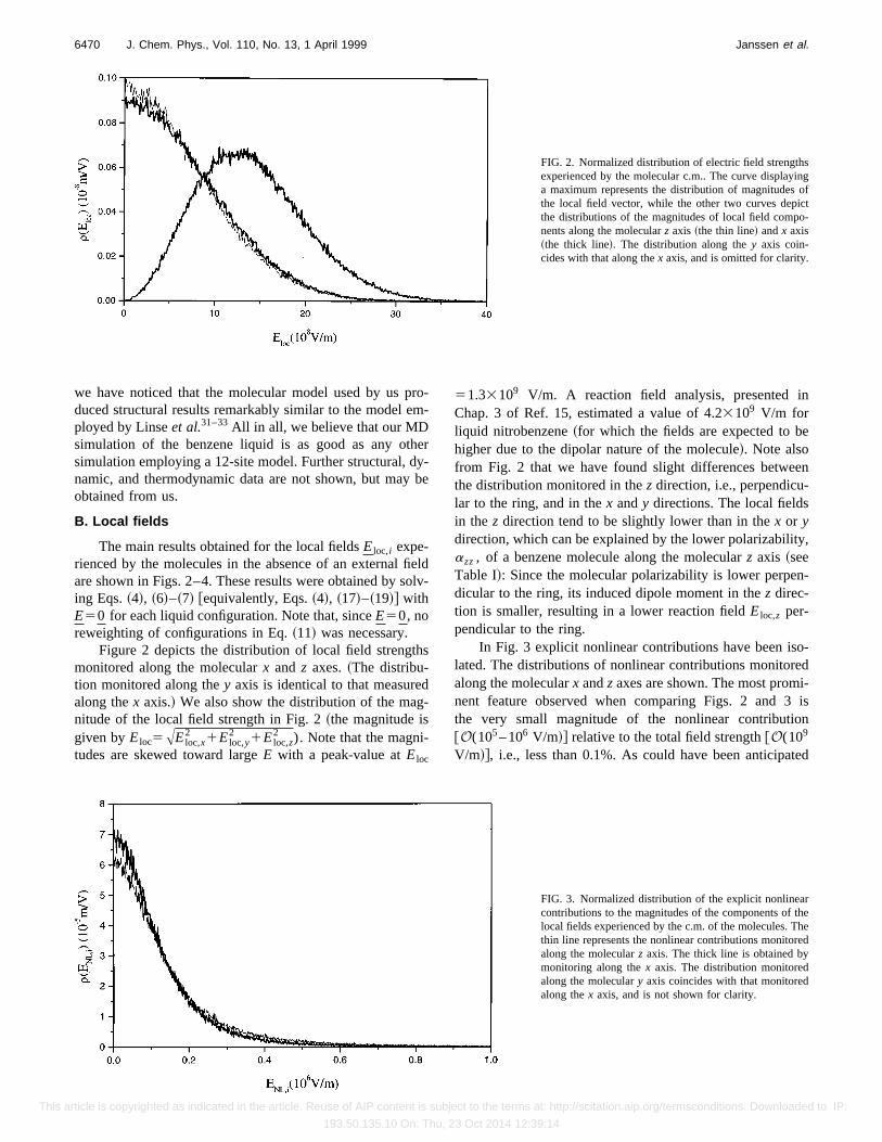
The main results obtained for the local fieldsEloc,i expe-rienced by the molecules in the absence of an external fieldare shown in Figs. 2–4. These results were obtained by solv-ing Eqs.~4!, ~6!–~7! @equivalently, Eqs.~4!, ~17!–~19!# withE50 for each liquid configuration. Note that, sinceE50, noreweighting of configurations in Eq.~11! was necessary.

Figure 2 depicts the distribution of local field strengthsmonitored along the molecularx and z axes.~The distribu-tion monitored along they axis is identical to that measuredalong thex axis.! We also show the distribution of the mag-nitude of the local field strength in Fig. 2~the magnitude isgiven byEloc5AEloc,x

2 1Eloc,y2 1Eloc,z

2 ). Note that the magni-tudes are skewed toward largeE with a peak-value atEloc

51.33109 V/m. A reaction field analysis, presented inChap. 3 of Ref. 15, estimated a value of 4.23109 V/m forliquid nitrobenzene~for which the fields are expected to behigher due to the dipolar nature of the molecule!. Note alsofrom Fig. 2 that we have found slight differences betweenthe distribution monitored in thez direction, i.e., perpendicu-lar to the ring, and in thex andy directions. The local fieldsin the z direction tend to be slightly lower than in thex or ydirection, which can be explained by the lower polarizability,azz, of a benzene molecule along the molecularz axis ~seeTable I!: Since the molecular polarizability is lower perpen-dicular to the ring, its induced dipole moment in thez direc-tion is smaller, resulting in a lower reaction fieldEloc,z per-pendicular to the ring.

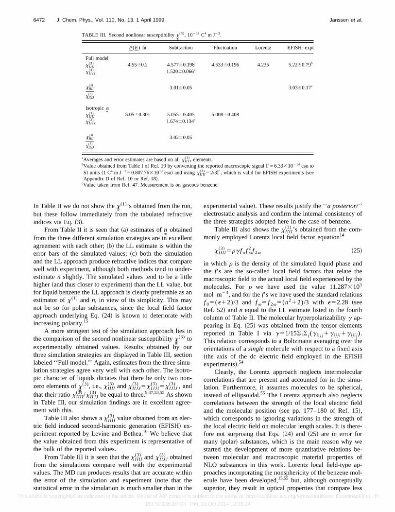
In Fig. 3 explicit nonlinear contributions have been iso-lated. The distributions of nonlinear contributions monitoredalong the molecularx andz axes are shown. The most promi-nent feature observed when comparing Figs. 2 and 3 isthe very small magnitude of the nonlinear contribution@O(105– 106 V/m!# relative to the total field strength@O(109

V/m!#, i.e., less than 0.1%. As could have been anticipated

FIG. 2. Normalized distribution of electric field strengthsexperienced by the molecular c.m.. The curve displayinga maximum represents the distribution of magnitudes ofthe local field vector, while the other two curves depictthe distributions of the magnitudes of local field compo-nents along the molecularz axis ~the thin line! andx axis~the thick line!. The distribution along they axis coin-cides with that along thex axis, and is omitted for clarity.

FIG. 3. Normalized distribution of the explicit nonlinearcontributions to the magnitudes of the components of thelocal fields experienced by the c.m. of the molecules. Thethin line represents the nonlinear contributions monitoredalong the molecularz axis. The thick line is obtained bymonitoring along thex axis. The distribution monitoredalong the moleculary axis coincides with that monitoredalong thex axis, and is not shown for clarity.

6470 J. Chem. Phys., Vol. 110, No. 13, 1 April 1999 Janssen et al.

This article is copyrighted as indicated in the article. Reuse of AIP content is subject to the terms at: http://scitation.aip.org/termsconditions. Downloaded to IP:

193.50.135.10 On: Thu, 23 Oct 2014 12:39:14

from its apolar character, we indeed find that benzene is atruly linear substance. Its electrostatics in the absence of anexternal electric field can be fully quantified in terms of thelinear polarizabilitya

=. A second feature noted from Fig. 3 is

that the nonlinear contributions to the local fields tend to beslightly higher along the molecularz axis.

In Fig. 4, the distribution of angles formed by the localfields Eloc,i with the molecularz axis is shown (u500 cor-responds to alignment ofEloc,i with the z axis!. The dashedline indicates the distribution that would have been obtainedif there had been no directional preference ofEloc,i . Clearly,the local fields tend to lie in the plane of the molecules~be-cause the molecular polarizability is largest in the plane ofthe ring!.

We conclude from Figs. 2 to 4 that the proposed methodis able to capture both the~nonlinear contributions to the!magnitude and the orientational distribution of the local elec-tric fields experienced by the molecules in liquid benzene.We believe this to be of importance in the study of bothlinear and nonlinear optical material properties: Knowing thestrength and orientational distribution of the local field on themolecules may be useful input forab initio quantum chemi-cal work geared toward quantifying the magnitude of thesolvent effect on the~hyper!polarizabilities of polar sub-stances.

C. Macroscopic optical properties

Results for the refractive indexn, obtained from thex=

(1)

values extracted from the simulation according to the threedifferent strategies explained in Secs. II A and II C, areshown in Table II, in the row labeled ‘‘Full model.’’ Someresults representative of the performance of theP(E)-fit ap-proach are shown in Fig. 5. Table II also lists an experimen-tally obtained value of the refractive index,52 as well as theestimate of n obtained from the commonly employedLorenz–Lorentz~LL ! equation,15

n221

n2125

r

3e0a, ~24!

with r being the density of the simulated liquid phase andaobtained from the values appearing in Table I asa51/3( ia i i . The values and error bars forn reported in TableII represent averages and standard deviations of thenII com-ponents monitored along the different axes of the simulationbox. In all cases studied, the computedn

=tensor was found to

fulfill the symmetries expected of an isotropic liquid: Off-diagonal elements were equal to zero and diagonal elementswere equal to each other within the error of the simulation.

TABLE II. Refractive indexn.

P(E) fit Subtraction Fluctuation LLa Exptlb

Full model 1.491260.006 1.491260.0052 1.491860.0095 1.4876 •••Isotropica

=1.499960.0067 1.499960.0063 1.500560.0063 1.4876 •••

1.5011

aValue based on the molar density of the simulated fluid,r511.2873103 mol m23

bValue at 300 K, 1 atm (rexptl511.2373103 mol m23) for the sodium D line, taken from Ref. 52.

FIG. 4. Normalized orientational distribution of the local fields.u590°corresponds to a field in the plane of the benzene ring. The solid line isobtained from the simulation run and the dashed line denotes the distributioncorresponding to the case of no directional preference of the local fields.

FIG. 5. The points show the dependence of theX component of the macro-scopic polarizationPX on the macroscopic fieldEX , as obtained by impos-ing on the model fluid fields of various magnitudes directed along theX axisof the laboratory coordinate frame. The curve is a best fit of the equationPX5xXX

(1)EX1xXXXX(3) EX

3 to the simulation points. The values ofxXX(1) and

xXXXX(3) are extracted from this fit according to theP(E) fit strategy.

6471J. Chem. Phys., Vol. 110, No. 13, 1 April 1999 Janssen et al.

This article is copyrighted as indicated in the article. Reuse of AIP content is subject to the terms at: http://scitation.aip.org/termsconditions. Downloaded to IP:

193.50.135.10 On: Thu, 23 Oct 2014 12:39:14

In Table II we do not show thex=

(1)’s obtained from the run,but these follow immediately from the tabulated refractiveindices via Eq.~3!.

From Table II it is seen that~a! estimates ofn=

obtainedfrom the three different simulation strategies are in excellentagreement with each other;~b! the LL estimate is within theerror bars of the simulated values;~c! both the simulationand the LL approach produce refractive indices that comparewell with experiment, although both methods tend to under-estimaten slightly. The simulated values tend to be a littlehigher~and thus closer to experiment! than the LL value, butfor liquid benzene the LL approach is clearly preferable as anestimator ofx (1) andn, in view of its simplicity. This maynot be so for polar substances, since the local field factorapproach underlying Eq.~24! is known to deteriorate withincreasing polarity.15

A more stringent test of the simulation approach lies inthe comparison of the second nonlinear susceptibilityx

U

(3) toexperimentally obtained values. Results obtained by ourthree simulation strategies are displayed in Table III, sectionlabeled ‘‘Full model.’’ Again, estimates from the three simu-lation strategies agree very well with each other. The isotro-pic character of liquids dictates that there be only two non-zero elements ofx

U

(3), i.e.,x IIII(3) andx IIJJ

(3) 5x IJJI(3) 5x IJIJ

(3) , andthat their ratiox IIII

(3) /x IIJJ(3) be equal to three.9,47,53,55As shown

in Table III, our simulation findings are in excellent agree-ment with this.

Table III also shows ax IIII(3) value obtained from an elec-

tric field induced second-harmonic generation~EFISH! ex-periment reported by Levine and Bethea.10 We believe thatthe value obtained from this experiment is representative ofthe bulk of the reported values.

From Table III it is seen that thex IIII(3) andx IIJJ

(3) obtainedfrom the simulations compare well with the experimentalvalues. The MD run produces results that are accurate withinthe error of the simulation and experiment~note that thestatistical error in the simulation is much smaller than in the

experimental value!. These results justify the ‘‘a posteriori’’electrostatic analysis and confirm the internal consistency ofthe three strategies adopted here in the case of benzene.

Table III also shows thex IIII(3) ’s obtained from the com-

monly employed Lorentz local field factor equation14

x IIII~3! 5rg f of v

2 f 2v ~25!

in which r is the density of the simulated liquid phase andthe f’s are the so-called local field factors that relate themacroscopic field to the actual local field experienced by themolecules. Forr we have used the value 11.2873103

mol m23, and for thef’s we have used the standard relationsf 05(e12)/3 and f v5 f 2v5(n212)/3 with e52.28 ~seeRef. 52! andn equal to the LL estimate listed in the fourthcolumn of Table II. The molecular hyperpolarizabilityg ap-pearing in Eq.~25! was obtained from the tensor-elementsreported in Table I viag51/15( i( j (g i i j j 1g i j j i 1g i j i j ).This relation corresponds to a Boltzmann averaging over theorientations of asinglemolecule with respect to a fixed axis~the axis of the dc electric field employed in the EFISHexperiments!.54

Clearly, the Lorentz approach neglects intermolecularcorrelations that are present and accounted for in the simu-lation. Furthermore, it assumes molecules to be spherical,instead of ellipsoidal.55 The Lorentz approach also neglectscorrelations between the strength of the local electric fieldand the molecular position~see pp. 177–180 of Ref. 15!,which corresponds to ignoring variations in the strength ofthe local electric field on molecular length scales. It is there-fore not surprising that Eqs.~24! and ~25! are in error formany ~polar! substances, which is the main reason why westarted the development of more quantitative relations be-tween molecular and macroscopic material properties ofNLO substances in this work. Lorentz local field-type ap-proaches incorporating the nonsphericity of the benzene mol-ecule have been developed,15,55 but, although conceptuallysuperior, they result in optical properties that compare less

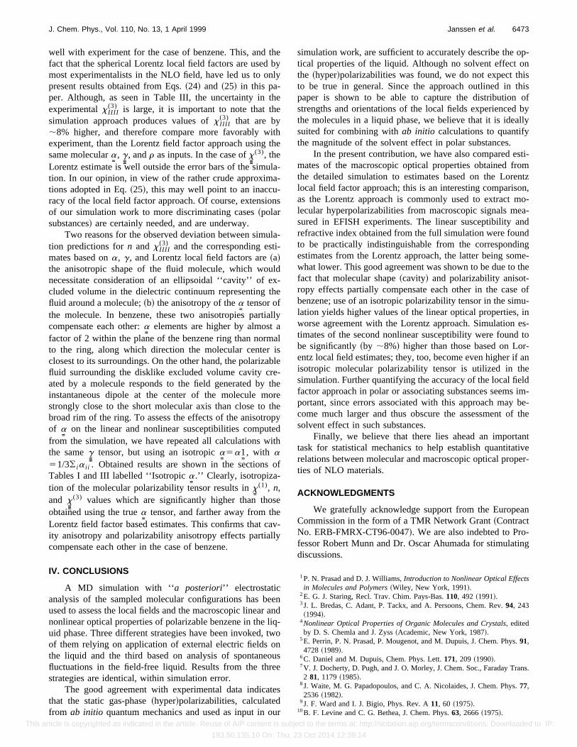
TABLE III. Second nonlinear susceptibilityxU

(3), 10233 C4 m J23.

P(E) fit Subtraction Fluctuation Lorentz EFISH–expt

Full modelx IIII

(3) 4.5560.2 4.57760.198 4.53360.196 4.235 5.2260.79b

x IIJJ(3) 1.52060.066a

xIIII~3!

xIIJJ~3!

3.0160.05 3.0360.17c

Isotropica=

x IIII(3) 5.0560.301 5.05560.405 5.00860.408

x IIJJ(3) 1.67460.134a

xIIII~3!

xIIJJ~3!

3.0260.05

aAverages and error estimates are based on allx IIJJ(3) elements.

bValue obtained from Table I of Ref. 10 by converting the reported macroscopic signalG56.33310214 esu toSI units ~1 C4 m J2350.807 7631019 esu! and usingx IIII

(3) 52/3G, which is valid for EFISH experiments~seeAppendix D of Ref. 10 or Ref. 18!.

cValue taken from Ref. 47. Measurement is on gaseous benzene.

6472 J. Chem. Phys., Vol. 110, No. 13, 1 April 1999 Janssen et al.

This article is copyrighted as indicated in the article. Reuse of AIP content is subject to the terms at: http://scitation.aip.org/termsconditions. Downloaded to IP:

193.50.135.10 On: Thu, 23 Oct 2014 12:39:14

well with experiment for the case of benzene. This, and thefact that the spherical Lorentz local field factors are used bymost experimentalists in the NLO field, have led us to onlypresent results obtained from Eqs.~24! and ~25! in this pa-per. Although, as seen in Table III, the uncertainty in theexperimentalx IIII

(3) is large, it is important to note that thesimulation approach produces values ofx IIII

(3) that are by;8% higher, and therefore compare more favorably withexperiment, than the Lorentz field factor approach using thesame moleculara

=, gU, andr as inputs. In the case ofx

U

(3), theLorentz estimate is well outside the error bars of the simula-tion. In our opinion, in view of the rather crude approxima-tions adopted in Eq.~25!, this may well point to an inaccu-racy of the local field factor approach. Of course, extensionsof our simulation work to more discriminating cases~polarsubstances! are certainly needed, and are underway.

Two reasons for the observed deviation between simula-tion predictions forn and x IIII

(3) and the corresponding esti-mates based ona, g, and Lorentz local field factors are~a!the anisotropic shape of the fluid molecule, which wouldnecessitate consideration of an ellipsoidal ‘‘cavity’’ of ex-cluded volume in the dielectric continuum representing thefluid around a molecule;~b! the anisotropy of thea

=tensor of

the molecule. In benzene, these two anisotropies partiallycompensate each other:a

=elements are higher by almost a

factor of 2 within the plane of the benzene ring than normalto the ring, along which direction the molecular center isclosest to its surroundings. On the other hand, the polarizablefluid surrounding the disklike excluded volume cavity cre-ated by a molecule responds to the field generated by theinstantaneous dipole at the center of the molecule morestrongly close to the short molecular axis than close to thebroad rim of the ring. To assess the effects of the anisotropyof a

=on the linear and nonlinear susceptibilities computed

from the simulation, we have repeated all calculations withthe sameg

Utensor, but using an isotropica

=5a1

=, with a

51/3( ia i i . Obtained results are shown in the sections ofTables I and III labelled ‘‘Isotropica

=.’’ Clearly, isotropiza-

tion of the molecular polarizability tensor results inx=

(1), n,and x

U

(3) values which are significantly higher than thoseobtained using the truea

=tensor, and farther away from the

Lorentz field factor based estimates. This confirms that cav-ity anisotropy and polarizability anisotropy effects partiallycompensate each other in the case of benzene.

IV. CONCLUSIONS

A MD simulation with ‘‘a posteriori’’ electrostaticanalysis of the sampled molecular configurations has beenused to assess the local fields and the macroscopic linear andnonlinear optical properties of polarizable benzene in the liq-uid phase. Three different strategies have been invoked, twoof them relying on application of external electric fields onthe liquid and the third based on analysis of spontaneousfluctuations in the field-free liquid. Results from the threestrategies are identical, within simulation error.

The good agreement with experimental data indicatesthat the static gas-phase~hyper!polarizabilities, calculatedfrom ab initio quantum mechanics and used as input in our

simulation work, are sufficient to accurately describe the op-tical properties of the liquid. Although no solvent effect onthe ~hyper!polarizabilities was found, we do not expect thisto be true in general. Since the approach outlined in thispaper is shown to be able to capture the distribution ofstrengths and orientations of the local fields experienced bythe molecules in a liquid phase, we believe that it is ideallysuited for combining withab initio calculations to quantifythe magnitude of the solvent effect in polar substances.

In the present contribution, we have also compared esti-mates of the macroscopic optical properties obtained fromthe detailed simulation to estimates based on the Lorentzlocal field factor approach; this is an interesting comparison,as the Lorentz approach is commonly used to extract mo-lecular hyperpolarizabilities from macroscopic signals mea-sured in EFISH experiments. The linear susceptibility andrefractive index obtained from the full simulation were foundto be practically indistinguishable from the correspondingestimates from the Lorentz approach, the latter being some-what lower. This good agreement was shown to be due to thefact that molecular shape~cavity! and polarizability anisot-ropy effects partially compensate each other in the case ofbenzene; use of an isotropic polarizability tensor in the simu-lation yields higher values of the linear optical properties, inworse agreement with the Lorentz approach. Simulation es-timates of the second nonlinear susceptibility were found tobe significantly~by ;8%! higher than those based on Lor-entz local field estimates; they, too, become even higher if anisotropic molecular polarizability tensor is utilized in thesimulation. Further quantifying the accuracy of the local fieldfactor approach in polar or associating substances seems im-portant, since errors associated with this approach may be-come much larger and thus obscure the assessment of thesolvent effect in such substances.

Finally, we believe that there lies ahead an importanttask for statistical mechanics to help establish quantitativerelations between molecular and macroscopic optical proper-ties of NLO materials.

ACKNOWLEDGMENTS

We gratefully acknowledge support from the EuropeanCommission in the form of a TMR Network Grant~ContractNo. ERB-FMRX-CT96-0047!. We are also indebted to Pro-fessor Robert Munn and Dr. Oscar Ahumada for stimulatingdiscussions.

1P. N. Prasad and D. J. Williams,Introduction to Nonlinear Optical Effectsin Molecules and Polymers~Wiley, New York, 1991!.

2E. G. J. Staring, Recl. Trav. Chim. Pays-Bas.110, 492 ~1991!.3J. L. Bredas, C. Adant, P. Tackx, and A. Persoons, Chem. Rev.94, 243~1994!.

4Nonlinear Optical Properties of Organic Molecules and Crystals, editedby D. S. Chemla and J. Zyss~Academic, New York, 1987!.

5E. Perrin, P. N. Prasad, P. Mougenot, and M. Dupuis, J. Chem. Phys.91,4728 ~1989!.

6C. Daniel and M. Dupuis, Chem. Phys. Lett.171, 209 ~1990!.7V. J. Docherty, D. Pugh, and J. O. Morley, J. Chem. Soc., Faraday Trans.2 81, 1179~1985!.

8J. Waite, M. G. Papadopoulos, and C. A. Nicolaides, J. Chem. Phys.77,2536 ~1982!.

9J. F. Ward and I. J. Bigio, Phys. Rev. A11, 60 ~1975!.10B. F. Levine and C. G. Bethea, J. Chem. Phys.63, 2666~1975!.

6473J. Chem. Phys., Vol. 110, No. 13, 1 April 1999 Janssen et al.

This article is copyrighted as indicated in the article. Reuse of AIP content is subject to the terms at: http://scitation.aip.org/termsconditions. Downloaded to IP:

193.50.135.10 On: Thu, 23 Oct 2014 12:39:14

11F. Kajzar, I. Ledoux, and J. Zyss, Phys. Rev. A36, 2210~1987!.12K. Clays and A. Persoons, Phys. Rev. Lett.66, 2980~1991!.13I. R. Gentle and G. L. D. Ritchie, J. Phys. Chem.93, 7740~1989!.14J. A. Armstrong, N. Bloembergen, J. Ducuing, and P. S. Pershan, Phys.

Rev.127, 1918~1962!.15C. J. F. Bottcher,Theory of Electric Polarization~Elsevier, Amsterdam,

1952!.16A. Willets and J. E. Rice, J. Chem. Phys.99, 426 ~1993!.17J. Yu and M. C. Zerner, J. Chem. Phys.100, 7487~1994!.18A. Willets, J. E. Rice, D. M. Burland, and D. P. Shelton, J. Chem. Phys.

97, 7590~1992!.19M. Stahelin, C. R. Moylan, D. M. Burland, A. Willets, J. E. Rice, D. P.

Shelton, and E. A. Donley, J. Chem. Phys.98, 5595~1993!.20M. P. Allen and D. J. Tildesley,Computer Simulation of Liquids~Claren-

don, Oxford, 1987!.21S. W. de Leeuw, J. W. Perram, and E. R. Smith, Proc. R. Soc. London,

Ser. A373, 27 ~1980!.22D. Frenkel and B. Smit,Understanding Molecular Simulation~Academic,

London, 1996!.23M. Sprik and M. L. Klein, J. Chem. Phys.89, 7556~1988!.24G. Ruocco and M. Sampoli, Mol. Phys.82, 875 ~1994!.25L. C. Geiger and B. M. Ladanyi, J. Chem. Phys.87, 191 ~1987!.26B. M. Ladanyi, J. Chem. Phys.78, 2189~1983!.27P. A. Franken, A. E. Hill, C. W. Peters, and G. Weinreich, Phys. Rev.

Lett. 7, 118 ~1961!.28R. P. Feynman,The Feynman Lectures on Physics~Addison–Wesley,

Reading, MA, 1964!, Vol. 2.29R. W. Munn, Mol. Phys.64, 1 ~1988!.30M. R. Battaglia, T. I. Cox, and P. A. Madden, Mol. Phys.37, 1413~1979!.31G. Karlstrom, P. Linse, A. Wallqvist, and B. Jo¨nsson, J. Am. Chem. Soc.

105, 3777~1983!.32P. Linse, J. Am. Chem. Soc.106, 5425~1984!.33P. Linse, S. Engstro¨m, and B. Jo¨nsson, Chem. Phys. Lett.115, 95 ~1985!.34C. J. Craven, P. D. Hatton, and G. S. Pawley, J. Chem. Phys.98, 8244

~1993!.35L. S. Bartell, L. R. Sharkey, and X. Shi, J. Am. Chem. Soc.110, 7006

~1988!.36D. E. Williams and T. L. Starr, Comput. Chem. Eng.1, 173 ~1977!.

37R. Q. Snurr, A. T. Bell, and D. N. Theodorou, J. Phys. Chem.97, 13742~1993!.

38W. C. Ermler, R. S. Mulliken, and E. Clementi, J. Am. Chem. Soc.98,388 ~1976!.

39C. Moller and M. S. Plesset, Phys. Rev.46, 618 ~1934!.40J. A. Pople, J. S. Binkley, and R. Seeger, Int. J. Quantum Chem., Quantum

Chem. Symp.10, 1 ~1976!.41GAUSSIAN 94, M. J. Frisch, G. W. Trucks, H. B. Schlegel, P. M. W. Gill, B.

G. Johnson, M. A. Robb, J. R. Cheeseman, T. A. Keith, G. A. Petersson,J. A. Montgomery, K. Raghavachari, M. A. Al-Laham, V. G. Zakrzewski,J. V. Ortiz, J. B. Foresman, J. Cioslowski, B. B. Stefanov, A. Nanay-akkara, M. Challacombe, P. Y. Peng, P. Y. Ayala, M. W. Wong, J. L.Andres, E. S. Replogle, R. Gomperts, R. L. Martin, D. J. Fox, J. S. Bin-kley, D. J. Defrees, J. Baker, J. P. Stewart, M. Head-Gordon, C. Gonzalez,and J. A. Pople, Inc., Pittsburgh PA, 1995.

42A. J. Sadlej, Collect. Czech. Chem. Commun.53, 1995~1988!.43C. Adant, M. Dupuis, and J.-L. Bre´das, Int. J. Quantum Chem., Quantum

Chem. Symp.29, 497 ~1995!.44Numerical Data and Functional Relationships in Science and Technology,

edited by K.-H. Hellwege and A. M. Hellwege, Landolt-Bo¨rnstein, NewSeries, Group II: Atomic and Molecular Physics Vol. 7~Springer, Berlin,1976!.

45D. M. Bishop, Rev. Mod. Phys.62, 343 ~1990!.46M. P. Bogaard, A. D. Buckingham, M. G. Corfield, D. A. Dunmur, and A.

H. White, Chem. Phys. Lett.12, 558 ~1972!.47J. F. Ward and D. S. Elliot, J. Chem. Phys.69, 5438~1978!.48C. J. Craven, P. D. Hatton, C. J. Howard, and G. S. Pawley, J. Chem.

Phys.98, 8236~1993!.49R. Edberg, D. J. Evans, and G. P. Morriss, J. Chem. Phys.84, 6933

~1986!.50G. Ciccotti, M. Ferrario, and J. P. Ryckaert, Mol. Phys.47, 1253~1982!.51A. H. Narten, J. Chem. Phys.67, 2102~1977!.52Handbook of Chemistry and Physics, edited by R. C. Weast~CRC, Boca

Raton, FL, 1988!.53I. J. Bigio and J. F. Ward, Phys. Rev. A9, 35 ~1974!.54R. S. Finn, Ph.D. thesis, University of Michigan, 1971.55T. Keyes and B. M. Ladanyi, inAdvances in Chemical Physics~Wiley,

New York, 1984!, Vol. LVI, p. 41.

6474 J. Chem. Phys., Vol. 110, No. 13, 1 April 1999 Janssen et al.

This article is copyrighted as indicated in the article. Reuse of AIP content is subject to the terms at: http://scitation.aip.org/termsconditions. Downloaded to IP:

193.50.135.10 On: Thu, 23 Oct 2014 12:39:14