Complex Analysis and Digital Geometry - uu .diva
366
-
Upload
khangminh22 -
Category
Documents
-
view
1 -
download
0
Transcript of Complex Analysis and Digital Geometry - uu .diva

������������������ ��������
������������ ��������������������������������� � �����
��


Complex Analysis andDigital Geometry
Proceedings from the Kiselmanfest, 2006
Editor: Mikael Passare

������������� ���������������� ������������������������������ ������!����" ������#����$��%����&'�� ��( ��)�&'��� *������+�� $��� ,������������ ����-$ � �)�".�/.���0�� �)��%��� �����������)��#���
1���2��� ����#��������#�2������2������������2���0�#������$�3��������2���04�5���6��7�!� )�%0�6����8. 9.�: ���2�,�% ;�<��

Table of contents
Preface . . . . . . . . . . . . . . . . . . . . . . . . . . . . . . . . . . . . . . . . . . . . . . . . . . . . . . . . . 7Mikael Passare
Christer Kiselman’s mathematics . . . . . . . . . . . . . . . . . . . . . . . . . . . . 9Bibliography. Christer Oscar Kiselman . . . . . . . . . . . . . . . . . . . . . . . . . . 27Curriculum Vitae. Christer Oscar Kiselman . . . . . . . . . . . . . . . . . . . . . 39Eric Bedford; Kyounghee Kim
The number of periodic orbits of a rational differenceequation . . . . . . . . . . . . . . . . . . . . . . . . . . . . . . . . . . . . . . . . . . . . . . . . . . . . . 47
Slimane Benelkourchi; Vincent Guedj; Ahmed ZeriahiPlurisubharmonic functions with weak singularities . . . . . . . . . . . 57
Bo BerndtssonA remark on approximation on totally real sets . . . . . . . . . . . . . . 75
Valérie BerthéDiscrete geometry and symbolic dynamics . . . . . . . . . . . . . . . . . . . . 81
Zbigniew BłockiDefining nonlinear elliptic operators for non-smooth functions 111
Urban CegrellApproximation of plurisubharmonic functions in hyperconvexdomains . . . . . . . . . . . . . . . . . . . . . . . . . . . . . . . . . . . . . . . . . . . . . . . . . . . . . 125
Jean-Pierre DemaillyEstimates on Monge–Ampère operators derived from a localalgebra inequality . . . . . . . . . . . . . . . . . . . . . . . . . . . . . . . . . . . . . . . . . . . . 131
Ahmed ZeriahiAppendix to the previous article: A stronger version ofDemailly’s estimate on Monge–Ampère operators . . . . . . . . . . . . 144
Pierre DolbeaultAbout the characterization of some residue currents . . . . . . . . . . 147
John Erik Fornæss; Yinxia Wang; Erlend Fornæss WoldLaminated harmonic currents . . . . . . . . . . . . . . . . . . . . . . . . . . . . . . . . 159
Kang-Tae Kim; Norman Levenberg; Hiroshi YamaguchiRobin functions for complex manifolds and applications . . . . . . 175
Laurent Najman; Gilles Bertrand; Michel Couprie; Jean CoustyDiscrete region merging and watersheds . . . . . . . . . . . . . . . . . . . . . . 199

Takeo OhsawaLevi flat hypersurfaces in complex manifolds . . . . . . . . . . . . . . . . . 223
Nils Øvrelid; Sophia VassiliadouL2-solvability results for ∂ on complex spaces withsingularities . . . . . . . . . . . . . . . . . . . . . . . . . . . . . . . . . . . . . . . . . . . . . . . . . 233
Christian RonseBounded variation in posets, with applications inmorphological image processing . . . . . . . . . . . . . . . . . . . . . . . . . . . . . . 249
Jean SerraThe random spread model . . . . . . . . . . . . . . . . . . . . . . . . . . . . . . . . . . . 283
Józef SiciakOn approximation by incomplete multivariate polynomials . . . . 311
Yum-Tong SiuDynamic multiplier ideal sheaves and the construction ofrational curves in Fano manifolds . . . . . . . . . . . . . . . . . . . . . . . . . . . . 323
Program of the Kiselmanfest in May, 2006 . . . . . . . . . . . . . . . . . . . . . . 361

Preface
Ne zorgu – estu felica! 1
Dear Reader,It was in the beautiful month of May of 2006 that an expectant
crowd of mathematicians from near and far gathered in Uppsala for theKiselmanfest. Christer Kiselman had just reached the prime age of sixty-seven, at which retirement is stipulated by current Swedish legislation,and this had been found a golden occasion to bring together Christer’smany colleagues and mathematical friends for a scientific meeting.For us, the organizers of the symposium, the task of arranging the
event had been significantly lightened by the universal high esteem en-joyed by Christer. When approaching prospective speakers we were metwith a practically unanimous eagerness to accept our invitation, so itwas not difficult to compose a world-class scientific program for the con-ference. It is a pleasant duty once again to thank all the participants ofthe Kiselmanfest for their involvement.We were also fortunate to find a number of generous sponsors for the
symposium. Substantial contributions were received from the Wenner-Gren Center Foundation, Gustaf Sigurd Magnuson’s Fund, the SwedishScience Council (VR), and from the City of Uppsala. Moreover, Upp-sala University provided munificent financing through its Presidency, itsFaculty of Science and Technology, its Division of Mathematics and Com-puter Science, and its Graduate School in Mathematics and Computing.We gratefully acknowledge the support of all these institutions.The full name of the conference was The Kiselmanfest—an Interna-
tional Symposium on Complex Analysis and Digital Geometry. There is avery natural explanation for this apparently heterogeneous title. Duringmost of his academic career, Christer has worked in the field of severalcomplex variables, and he has had a great influence on the developmentof this subject both in Uppsala, in Sweden, and abroad. The Pluri-complex Seminar that he started already in the early 1970s (althoughthe name was introduced only in 1980) has hosted numerous interna-tional experts from all over the globe, and fostered a large number ofstudents. For the past decade, however, the primary scientific interest of
1Esperanto: Don’t worry—be happy!

8 Mikael Passare
Christer has veered towards the very different, and perhaps more tangi-ble, world of digital geometry and mathematical morphology. Also herehe has quickly become a highly respected authority. Actually, this reori-entation appears quite in line with Christer’s general broad-mindednessand his genuine curiosity for new knowledge, be it discrete convexity orPersian grammar.The present proceedings volume has had a very protracted birth in-
deed, but here it now finally is. Our sincere thanks go to all the authorsfor their efforts and their patience, and to the anonymous referees fortheir many valuable comments. Let us now hope that both Christer andyou as a reader will enjoy this book.
For the organizers,Berkeley, November 22, 2009Mikael Passare

Christer Kiselman’s mathematics
Mikael Passare
1. Partial differential equations
When he was a student for the degree of Licentiate of Philosophy atStockholm University, Christer Kiselman received a research problemfrom his advisor Lars Hörmander. The goal was to prove, in analogy withBernard Malgrange’s famous paper (1956), existence and approximationtheorems for solutions to initial-value problems in a convex open set Ωin Rn:
P (D)u = f in Ω,
Qj(D)u = gj on the hyperplane {x ∈ Ω;xn = 0}.Here P and the Qj are partial differential operators with constant coef-ficients.For the approximation by exponential solutions of smooth solutions
to the homogeneous problem it suffices by the Hahn–Banach theorem toprove that any distribution μ ∈ E ′(Ω) which vanishes on the exponen-tial solutions can be written μ = P (−D)ν + ρ for some ν, ρ ∈ E ′(Ω),where ρ has support in the plane xn = 0 and is such that it yields zerowhen applied to smooth functions with zero initial data. By the Fouriertransformation, this amounts to a division algorithm F = PG + H forentire functions, provided estimates can be proved which show that thequotient G and the remainder H are actually Fourier transforms of dis-tributions with support in Ω. (In Malgrange’s case the remainder H iszero.) Kiselman could prove this for hyperbolic operators P , and thiswas presented in a chapter in the licentiate thesis [64-1].1
For non-hyperbolic operators, the algorithm did not yield distribu-tions: the quotient G and the remainder H are in general not Fouriertransforms of distributions, so the proof cannot be finished in the sameway. However, they are still entire functions of expononential type, whichimplies that they are transforms of analytic functionals. Therefore theproof went through as expected in the space of analytic functionals in a
1This notation refers to the paper [64-1] in Kiselman’s bibliography, pp. 27–38.

10 Mikael Passare
complex domain Ω in Cn, yielding the desired existence and approxima-tion theorems for holomorphic solutions in certain convex domains in Cn,and actually characterizing the convex open sets where such theoremshold. Only this complex part was later published in [65-1].The case of non-hyperbolic operators in the case of real variables
is still not finished. At the Nordan 4 in Örnsköldsvik in 2000, LarsHörmander (2005) took up this question for the real domain again. Hepresented a necessary and sufficient condition (albeit rather implicit) onthe polynomials P and Qj in order that a distribution be orthogonal toall exponential solutions of the initial-value problem.The failure of the division algorithm to work for distributions in the
non-hyperbolic case explains why Kiselman took up the study of analyticfunctionals in the spirit of André Martineau (1930–1972). His work alsoled to a new result giving sufficient geometric conditions for a convex orpolynomially convex set to be the only convex or polynomially convexsupport, respectively, of an analytic functional [65-2]. Martineau laterweakened the hypotheses in the convex case (1967b); however, he didnot treat polynomial convexity, since his methods were dependent onthe linear structure of Cn. For one complex variable, the sets which areunique supports were characterized in [65-2] and [68-3].
2. Analytic functionals and entire functions of exponen-tial type
Kiselman was invited to spend the academic year 1965/1966 as a Memberof the Institute for Advanced Study in Princeton, NJ. Hörmander wasthere as Faculty and could continue his role as thesis advisor.During his stay at the institute, Kiselman proved a theorem on the
existence of entire functions with prescribed indicator. Pierre Lelong hadearlier proved that for a plurisubharmonic function which is complex ho-mogeneous of order one, there exists an entire function with the givenfunction as indicator. Kiselman could extend this result to functionswhich are only positively homogeneous of order one [67-1]. Martineauworked independently on this problem and proved a similar but moregeneral theorem for indicators of arbitrary positive order which are sup-posed to be continuous (1966). In (1967a) he extended it to generalupper semicontinuous (not necessarily continuous) indicators. For a fi-nal version, see his report at Séminaire Lelong (1967c).The methods of proof were different: Kiselman used the Borel trans-
formation (which works only for order one) whereas Martineau usedHörmander’s L2 methods for the ∂ operator. However, both of them had

Christer Kiselman’s mathematics 11
traveled the same road albeit in opposite directions: Kiselman startedwith the L2-methods, but could get them to work only for Hölder-continuous indicators, whereas Martineau started with the Borel trans-formation.An intermediate result in [67-1] is the fact that the set in projective
n-space given in homogeneous coordinates by
Ωf = {z ∈ Cn+1; f(tz1, . . . , tzn) < Re (tzn+1) for some t ∈ C}
is pseudoconvex if f is plurisubharmonic, positively homogeneous of de-gree one and not identically −∞. This was done by a calculation whichlater gave rise to the minimum principle for plurisubharmonic functions.The question of uniqueness of supports was considered in [67-1] with
the help of an indicator of functionals operating on the class of func-tions ef , where f is not necessarily linear. Already here holomorphicand plurisubharmonic functions defined on infinite-dimensional spacesappear, and Kiselman proved for instance a general lim-sup-star theo-rem for plurisubharmonic functions in such spaces [67-1: Theorem 2.1].He also proved a theorem on approximation of homogeneous plurisub-harmonic functions in Cn by smooth ones [67-1: Theorem 2.5].In analogy with analytic functionals in one complex variable, Kisel-
man studied functionals on the space of solutions to an arbitrary partialdifferential equation with constant coefficients [68-1]. The solutions couldbe either C∞ smooth or distribution solutions. He characterized carri-ers of such functionals in terms of the Borel transform (or potential) aswell as in terms of the growth at infinity of the Fourier transform of thefunctionals.
3. Lineal convexity
In October, 1966, Kiselman received an invitation from Martineau tojoin him in Montpellier. This was in response to the paper [65-2]. How-ever, Martineau planned to move to Nice, where Jean Dieudonné (1906–1992), “un Doyen très dynamique,”2 was in the process of collecting astrong team. “C’est décidé. Je vais à Nice et vous m’y suivez. Eneffet la section de Nice est d’accord pour vous prendre comme Maîtrede conférences associé.”3 In Nice, there were, beside Dieudonné andMartineau, Adrien Douady (1935–2006), Pierre Grisvard (1940–1994),Christian Houzel, Paul Krée, and Martin Zerner. Among the youngerwere Joël Briançon, Chin-Cheng Chen, and André Hirschowitz. Also
2André Martineau 1967-02-25, letter to Kiselman.3André Martineau 1967-01-23, letter to Kiselman.

12 Mikael Passare
visiting during that year were Gunter Bengel, Hiroko Morimoto, MitsuoMorimoto, and, during part of the year, Pierre Schapira.It was in Nice that Kiselman learnt about a kind of complex convex-
ity called lineal convexity,4 which is between pseudoconvexity and usualconvexity in strength; see Martineau (1968). It was however only in 1978that he himself wrote an article on the subject [78-2]. He later returnedto it [96-1, 97-1, 98-1].Kiselman encouraged Mats Andersson, Ragnar Sigurdsson and me to
write a survey article on the many scattered results on lineal convexity;however, the project grew from an article to a book jointly authored byus; preprints circulated from 1991 on, and the book finally appeared in2004 (Andersson et al. 2004).A set A in Rn is defined to be convex if {a, b} ⊂ A implies that the
rectilinear segment [a, b] is contained in A. This is a kind of global defi-nition. But if we have a connected open set with smooth boundary thereis also an infinitesimal characterization: if Ω has a boundary of class C2,then it is convex if and only if the Hessian of a defining function is posi-tive semidefinite in the tangent space at every boundary point. Similarly,a connected open set in Cn with boundary of class C2 is pseudoconvex ifand only if the Levi form of a defining function is positive semidefinite inthe complex tangent space at every boundary point (the Levi condition).Heinrich Behnke and Ernst Peschl (1935) introduced the notion of
weak lineal convexity, known then as Planarkonvexität, and formulated asimilar infinitesimal condition for it: for a weakly lineally convex open setin C2, the real Hessian of a defining function is positive semidefinite inthe complex tangent space at every boundary point (the Behnke–Peschlcondition). The Hauptsatz of Behnke and Peschl (1935) was that thecorresponding strong condition, i.e., that the real Hessian be positivedefinite, is sufficient for weak lineal convexity.Thus the problem left open in 1935 was to prove that semidefiniteness
is sufficient. Kiselman [98-1] proved this: if Ω is an open connectedsubset of Cn with boundary of class C2 satisfying the Behnke–Peschlcondition, then it is weakly lineally convex, which means that the unionof all complex hyperplanes which do not meet Ω contains the boundaryof Ω.While a convex or pseudoconvex domain can be approximated by
smooth strongly convex or smooth strongly pseudoconvex domains, re-spectively, the corresponding approximation of lineally convex domainsis problematic. It was only recently that Jacquet (2006, 2008:39) proved
4The French term is convexité linéelle, the Russian line�na� vypuklost�,lineınaya vypuklost′. Some authors use linear convexity in English.

Christer Kiselman’s mathematics 13
that any weakly lineally convex open set with C2 boundary can be ap-proximated by sets of the same kind with C∞ boundary and satisfyingthe strong Behnke–Peschl condition. For sets with C1 boundary theproblem seems to be open.Kiselman’s proof was simplified by Hörmander; see Andersson et al.
(2004:59) and Hörmander (2008).
4. Extension of solutions of partial differential equations
It is a natural question to ask which is the largest domain to which asolution to a partial differential equation can be extended as a solution.This problem was completely solved for C∞ solutions in convex domainsand equations with constant coefficients in [69-1]. Distribution solutionswere proved to admit extensions to the same domains, but it was notproved that these domains are optimal. Since the extension may bedefined in an open set in Cn or more generally in Rk × Cn−k, k =0, . . . , n, even though the solution is defined only in an open set in Rn,Kiselman had to study partially holomorphic functions, and could forinstance characterize the convex complex domains to which solutions toan elliptic partial differential equation can be extended, in particularharmonic functions. During this study, he also obtained some results onclosure operators (cleistomorphisms; in French fermeture de Moore orapplications enveloppantes, a term proposed by Hirschowitz), a class ofoperators in ordered structures which appear naturally when one studiesextensions of functions [69-1, 71-B].
5. The minimum principle for plurisubharmonicfunctions
The shadow of a convex body is convex, but a linear image of a pseudo-convex set need not be pseudoconvex. Expressed with the help of func-tions, we may express these facts as follows. If F : Rm×Rn → [−∞,+∞]is a convex function, then its marginal function H, defined as
H(x1, . . . , xm) = infy∈Rn
F (x1, . . . , xm, y1, . . . , yn), x ∈ Rm,
is convex. But if F : Cm × Cn → [−∞,+∞[ is plurisubharmonic as afunction of m+ n complex variables, then its marginal function H neednot be plurisubharmonic. An easy example with m = n = 1 is
F (x, y) = 2Re (xy) + |y|2 = |x+ y|2 − |x|2, (x, y) ∈ C2,

14 Mikael Passare
which is plurisubharmonic in C2, but has marginal function H given by
H(x) = infy∈C
F (x, y) = −|x|2, x ∈ C,
a concave function which is not subharmonic anywhere. Kiselman wantedto find a simple condition on F which did imply that its marginal func-tion is plurisubharmonic, and he found that this is so if F is independentof the imaginary parts Im yj of the variables yj [78-1]. This result becameknown as Kiselman’s minimum principle for plurisubharmonic functions.His original proof, as well as the proof published in [94-2], used differen-tial calculus, and was actually not so far from the calculation in [67-1:Theorem 3.1], but the proof in [78-1] used instead the sub-mean-valueproperty expressed by integrals.The minimum principle was used to prove several results, e.g., in
[79-2] and [94-1]. Generalizations to a Lie-group setting were obtainedby Jean-Jacques Loeb (1985). Using this generalization of Kiselman’sminimum principle, Zhou Xiang Yu (1998) was able to prove that the ex-tended future tube is a domain of holomorphy. This was a long-standingconjecture originating in quantum field theory.Bo Berndtsson (1998) generalized the minumum principle to an ana-
logue of Prékopa’s theorem, which says that the p-marginal function Hp,0 < p < +∞, defined by
e−pHp(x) =∫Rn
e−pF (x,y)dy, x ∈ Rm,
is convex if F is convex. Berndtsson proved that when F is plurisub-harmonic in Cm ×Cn and independent of the imaginary parts Im yj ofthe yj , j = 1, . . . , n, then Hp, defined as
e−pHp(x) =∫Rn
e−pF (x,y)dRe y, x ∈ Cm,
is plurisubharmonic if F is plurisubharmonic. As p → +∞, we get theoriginal theorem both in the convex case and the plurisubharmonic case.
6. Lelong numbers of plurisubharmonic functions
The minimum principle enables us to attenuate the singularities of aplurisubharmonic function in the sense that it yields, given a plurisub-harmonic function f and a positive number α, a very simple constructionof a plurisubharmonic function fα with Lelong number νfα = (νf−α)+ =max(νf − α, 0). This means that the singularities as measured by the

Christer Kiselman’s mathematics 15
Lelong number are weakened by a uniform amount α at points whereνf � α, and give Lelong number zero where νf � α. Thus the differencebetween the Lelong numbers at different points is kept constant as longas they are at least equal to α, but the quotient between the Lelongnumbers increases: if for two points x and y we have νf (y) > νf (x) > 0,then
νfα(y)νfα(x)
=νf (y)− ανf (x)− α
=νf (y)− νf (x)νf (x)− α
+ 1→ +∞
as α→ νf (x) while α < νf (x). This is of interest since the Hörmander–Bombieri theorem on the integrability of functions of the form e−cf pro-duces analytic varieties—see Bombieri (1970), Skoda (1972: Proposition7.1), and Hörmander (1990:Theorem 4.4.4). Kiselman was able to usethis to get a short proof of Siu’s theorem that the superlevel sets{x ∈ Ω; νf (x) � α} of a plurisubharmonic function f are analytic vari-eties [79-2].The Lelong number of a plurisubharmonic function at a point mea-
sures how strong its singularity is at that point. At a seminar in Monastirin March, 1986, Kiselman introduced a refined Lelong number whichtakes into account also the direction in which the singularity points[87-1].The refined Lelong number νf (x, y) depends on the point x in the
domain in Cn where f is defined, and a vector y ∈ Rn. Explicitly, letv(x, y) be the mean value of f over the distinguished boundary of thepolydisk with center at x and radii eyj , j = 1, . . . , n. Then the refinedLelong number at x is the function
Rn+ � y �→ νf (x, y) = lim
t→−∞v(x, ty)t
.
In the special case when y = (1, 1, . . . , 1) we get νf (x, y) = νf (x).A motivation for his definition is that the Lelong number νf (x) of
a function f at a point x alone cannot determine the Lelong numberof the composition f ◦ h of f with a holomorphic mapping h: one hasνf◦h(x) � νf (h(x)), and the inequality can be strict. As an example, letus take h : C2 → C2 defined as h(x1, x2) = (x1, x1x2). Then the Lelongnumber νf◦h(0) = νf◦h(0, y) of f ◦ h at the origin, where y = (1, 1), isequal to νf (0, z) with z = (1, 2). More generally, if
h(x) = (xm111 xm12
2 · · ·xm1nn , . . . , xmn1
1 xmn22 · · ·xmnn
n ),
then the refined Lelong number of the blow-up f ◦ h is
νf◦h(0, y) = νf (0, z), where zj =∑
mjkyk.

16 Mikael Passare
The vector y is therefore transformed by a linear mapping: z = My.This gives rise to an estimate νf◦h(x) � Cνf (h(x)) with a constant Cdetermined by h.The superlevel sets are analytic varieties just as for the classical
Lelong number: for every y ∈ Rn with yj > 0 and every real number α,the set {x ∈ ω; νf (x, y) � α} is an analytic variety, a result presented ata seminar in 1986 [87-1] and proved in [92-1, 94-1].In a related article [00-1], Kiselman studied estimates
νf◦h(a) � Cνf (h(a)),
where h is a holomorphic mapping from Cm to Cn, and proved that theyhold for all plurisubharmonic functions f defined near h(a) if and onlyif the image under h of every neighborhood of a contains interior points.This paper also contains a study of the asymptotic behavior as t→ −∞of the volume of the sublevel sets
Af (t) = {z ∈ Ω; f(z) � t}, t ∈ R,
of a plurisubharmonic function in Ω ∈ Cn.Demailly later generalized the refined Lelong numbers by replacing
the function maxj log |xj | by a more general plurisubharmonic function ϕ(1987). Thus he defined generalized Lelong numbers of a closed positivecurrent T of bidegree (n− p, n− p) with respect to a plurisubharmonicfunction ϕ satisfying some conditions as the limit
ν(T, ϕ) = limr→−∞ ν(T, ϕ, r),
whereν(T, ϕ, r) =
1(2π)p
∫ϕ<r
T ∧ ddcmax(ϕ, s),
with some (or any) s < r. He proved analyticity theorems for the sublevelsets of these functionals.
7. Convexity
How smooth is the shadow of a C∞ smooth convex body in R3? Perhapssurprisingly, it is not necessarily of class C2. However, the curvature ofthe boundary of the shadow always exists; in other words, the boundaryof the shadow is described by a function which is twice differentiable, butits second derivative need not be continuous. This result was proved byKiselman in [86-1]. Actually, for the conclusion to hold, the smoothnessassumption can be relaxed: it is enough that the boundary be of class

Christer Kiselman’s mathematics 17
C2,1, i.e., with Lipschitz-continuous second derivatives. To see that thesecond derivative need not be continuous, we consider a C∞ function
f(x, y) = x2(4− y − 12y
2) + u(y), (x, y) ∈ R2,
where u is even and satisfies u′(0) = 0 with second derivative
u′′(y) = sin2(1/y) exp(−1/y), y > 0.
It has the property that its marginal function
h(x) = infy∈R
f(x, y), x ∈ R,
possesses a second derivative, but there exists sequences (aj) and (bj) ofpositive numbers tending to zero such that (h′′(aj) − h′′(bj)) does nottend to zero.However, if we strengthen the hypothesis by assuming that the
boundary of the convex body in R3 is analytic, then the boundary of theshadow is of Hölder class C2+ε for some positive ε [86-1: Theorem 2.2].A related question was considered in [87-2]: How smooth is the vector
sum of two smooth convex bodies? The vector sum, or Minkowski sum,is a special case of a projected image, but the regularity classes involvedare quite different. To be precise, if A and B are two convex sets in Rn
with boundary of class Ck, does their vector sum also have a boundaryof class Ck? The answer is in the affirmative if and only if k = 1 orn = 2 and k = 2, 3, 4.What happens if we assume analytic boundaries? Kiselman proved
that the vector sum A + B = {x + y;x ∈ A, y ∈ B} of two convex setsA and B in R2 does not have a boundary of class C∞ even if A and Bhave analytic boundaries. The best one can prove is that the boundary ofA+B is of Hölder class C6 2
3 , i.e., it is of class C6 and the sixth derivativeis Hölder continuous of class 2
3 . That this degree of smoothness cannotbe improved follows from the simple example when the boundaries of Aand B are described close to the origin by functions f(x) = x4/4 andg(x) = x6/6; then the boundary of A+B is described near the origin bya function
h(x) = 16x
6 + 34 |x|20/3 + r(x),
where r ∈ C7.More generally, the boundary ∂(A1 + · · · + Ak) of the vector sum
of finitely many convex sets Aj with analytic boundaries can be locallydescribed by a function h(x) = xp+1g(x, x2/m), where g is a C∞ function

18 Mikael Passare
of two variables satisfying g(0, 0) > 0 and where (p,m) is one of the pairs
(1, 1), (3, 1), (5, 3), (7, 15), (9, 105), (11, 315), (13, 3465),
(15, 45045), (17, 45045), . . .
[87-2, 92-2]. The pair (5, 3) yields the Hölder class C20/3, the first classwhich is not contained in C∞, and is optimal as we have seen.In [92-2] Kiselman studied regularity classes of functions that appear
in these problems.In convex analysis there are three operations often performed on func-
tions: that of taking the largest convex minorant; that of taking thelargest lower semicontinuous minorant; and that of replacing a functionby the constant −∞ if it attains that value somewhere, but otherwise notchanging it. Let us call these operators c, l, and m, respectively. Theygenerate a semigroup which Kiselman investigated in [02-1]. The motiva-tion for studying these operators is that when taking the Fenchel trans-form (also called the Legendre transform) of a function Rn → [−∞,+∞]twice, one obtains a minorant ˜f of f which is equal to (m ◦ l ◦ c)(f).Kiselman determined completely the structure of this semigroup,
showed that it has eighteen elements (see page 26), and also showed inwhich spaces these elements actually give rise to different operators. InR2, for instance, there are sixteen different operators: the three elementsl ◦m ◦ c, l ◦m ◦ c ◦ l and m ◦ l ◦ c define the same operator. In a normedspace of infinite dimension, there are eighteen different operators.The semigroup was called “Kiselman’s semigroup” by Ganna Kudr-
yavtseva and Volodymyr Mazorchuk (2009), who studied semigroupswith an arbitrary number of generators obeying the same axioms.Seidon Alsaody (2007) determined the number of elements in semi-
groups with four or five generators and gave lower and upper bounds forthe number of elements in all the semigroups.
8. Complex analysis in infinite-dimensional spaces
To solve the Levi problem means to find a holomorphic function in agiven pseudoconvex domain which cannot be continued to any largerdomain. Explicitly, this means to find f ∈ O(Ω) such that for everypoint c ∈ Ω, the largest open ball with center at c to which f can beextended as a holomorphic function is equal to the largest open ball withcenter at c which is contained in Ω. Stated in this way, the problem has asense in a normed space. Lawrence Gruman and Kiselman [72-1] solvedthis problem in a Banach space with a Schauder basis. In the proof theprojections x �→ πn(x) =
∑n1 xjej play an essential role, where
∑∞1 xjej

Christer Kiselman’s mathematics 19
is the representation of x in terms of a Schauder basis (ej). It seems thatin a Banach space without a basis, where such projections are missing,the problem is still open.A holomorphic function defined on a normed space E has a radius
of boundedness, which is the radius R(x) of the largest ball B(x, r) ={y; ‖y−x‖ < r} such that the function is bounded in every ball B(x, r′)with r′ < r. In infinite dimensions, the radius of boundedness can befinite even if the function is entire. A simple example is f(x) =
∑∞j=0 x
jj ,
x = (xj)∞0 ∈ c0, the Banach space of sequences tending to zero equippedwith the supremum norm. This function is entire but its radius ofboundedness is 1 at every point.So we may ask which functions E � x �→ R(x) on a normed space E
can be the radius of boundedness of some entire function. Clearly sucha radius must be Lipschitz continuous, |R(x) − R(y)| � ‖x − y‖, andit is not difficult to see that − logR is plurisubharmonic. But are theseproperties also sufficient?The answer is in the affirmative for E = l1, but not for lp, p > 1 (cf.
the inequality (8.1) below, which yields a stronger condition than theLipschitz condition when p > 1).Kiselman introduced a measure of how the unit ball tapers off when
we go out from the origin. He defined the inner and outer moduli ofa normed space E with respect to a topology τ as follows. Considernumbers m and M such that
(x+mB) ∩ U ⊂ B and B ∩ V ⊂ x+MB,
where B is the unit ball of E and where U and V are τ -neighborhoodsof x. Then the inner modulus m(x) of E at x is the supremum of all msuch that this holds for some U , and the outer modulus M(x) of E at xis the infimum of all M such that this holds for some V .If every τ -neighborhood of the origin contains a straight line, such as
is the case with the various weak topologies one works with in infinite-dimensional spaces, it is easy to see that
1− ‖x‖ � m(x) �M(x) � 1 + ‖x‖, ‖x‖ < 1.
For E = L1( ]0, 1[ ) equipped with the weakened topology σ(E,E′) wehave m(x) = 1− ‖x‖ and M(x) = 1 + ‖x‖.If we consider the Banach space E = lp for 1 � p < +∞, we obtain
m(x) = M(x) = (1 − ‖x‖p)1/p, ‖x‖ < 1, which has a nice geometricsignificance.Kiselman also defined a local radius of boundedness as follows. Given
a function u : E → [−∞,+∞] and a topology τ on E, the τ -local radius

20 Mikael Passare
of boundedness of u at x is the supremum of all numbers r such that uis bounded from above on (x+ rB) ∩W for some τ -neighborhood W ofx. Let us denote it by Rτ,u(x) and let us define a domain
Ωτ,u = {(x, t) ∈ E ×C; |t| < Rτ,u(x)}.
We define two normed spaces E1 and E2: they are equal to E ×C withopen unit ball equal to
{(x, t) ∈ E ×C; |t| < m(x)}
and the convex hull of
{(x, t) ∈ E ×C; |t| < M(x)},
respectively. Now Kiselman could prove under some natural conditionsthat
(8.1) d2((x, 0), �Ω) � Rτ,u(x) � d1((x, 0), �Ω), x ∈ E,
where dj is the distance measured in Ej , j = 1, 2. For spaces likelp, where the inner and outer moduli agree, this turns into an equal-ity. And it is natural to conjecture that any function which satisfiesthis equality is actually a radius of convergence of some entire function[76-1:51]. Kiselman could prove this in special cases [76-1, 77-3]. Thegeneral case seems still to be open. The problem is related to the Leviproblem for functions of bounded type, i.e., functions which are boundedwhen ‖x‖ + 1/d(x, �Ω) is bounded.
9. Functions on discrete sets
Kiselman took up the study of several classes of functions defined ondiscrete sets: convex functions [04-1], subharmonic functions [05-2], andholomorphic functions [05-1, 08-3].
9.1. Convex functions
Several definitions of convex functions on discrete spaces like Zn havebeen proposed. One of them is studied in [04-1]. A function f : Zn−1 → Zis said to be Zn-convex if there exists a convex subset C of Rn such that{(x, y) ∈ Zn−1 × Z; f(x) � y} = C ∩ Zn.Following Jean-Pierre Reveillès (1991:45), a hyperplane D in Zn is
defined by a double inequality
D = {x ∈ Zn; 0 � α · x+ β < h} = {x ∈ Zn; 0 < (−α) · x− β + h � h}.

Christer Kiselman’s mathematics 21
The definition suffers from a certain lack of symmetry—there must bea strict inequality on one side and a non-strict inequality on the other.This asymmetry is removed in Kiselman’s paper [04-1]. A refined digitalhyperplane is defined as a set D contained in a slab
T = {x ∈ Zn; 0 � α · x+ β � h}
and containing the corresponding strict slab
T ∗∗ = {x ∈ Zn; 0 < α · x+ β < h}
for some α �= 0, β ∈ R, and h > 0, thus T ∗∗ ⊂ D ⊂ T , and satisfyingcertain natural conditions on h and the sets where strict and non-strictinequalities occur—they are now not on the same side everywhere [04-1,Definition 6.2].For certain values of h, a refined hyperplane can then be identified
with the graph of a function f : Zn−1 → Z such that both f and −fare Zn-convex. An easy example is the function f : Z → Z defined byf(x) = 0 for x < 0, f(x) = 1 for x � 0, whose graph is a refined digitalhyperplane but not a hyperplane in the sense of Reveillès. The sequenceof differences (f(x+ 1)− f(x))x∈Z for this function is a skew Sturmianword in the terminology of Morse and Hedlund (1940:8).
9.2. Subharmonic functions
The Dirichlet problem for subharmonic functions on discrete sets wasstudied in [05-2]. A function λ : X×X → [0,+∞[ is said to be a weightfunction if the set {y ∈ X; f(x, y) �= 0} is finite for every x ∈ X and∑
y∈X λ(x, y) > 0 for every x ∈ X. We then define the λ-Laplacian Δλfof a function f : X → R by
Δλf(x) =∑y∈X
λ(x, y)(f(y)− f(x)
), x ∈ X,
and say that f is λ-subharmonic if Δλf(x) � 0 for all x ∈ X. Thisdefinition is quite flexible, and the weight function can be chosen so thatthe λ-subharmonic functions mimic the subharmonic functions as wellas the subsolutions to the heat equation.Kiselman showed that, for finite X and arbitrary weight functions,
a natural discrete counterpart of the Dirichlet problem has a uniquesolution, thus generalizing classical results by Phillips and Wiener (1923)and Blanc (1939). He also proved the same result for infinite X underspecial conditions.

22 Mikael Passare
In his thesis, Ola Weistrand (2005) used some of the results of [05-2]in his study of shape description in three dimensions.Abtin Daghighi wrote an M.Sc. thesis (2005) giving a survey of known
results on the discrete Dirichlet problem as well as some new results forinfinite X.
9.3. Holomorphic functions
Holomorphic functions on discrete sets were introduced by Rufus PhilipIsaacs (1941) under the name monodiffric functions. He mainly stud-ied two difference operators mimicking the Cauchy–Riemann differentialoperator, and called the classes of functions he defined monodiffric func-tions of the first and second kind. In two papers [05-1, 08-3], Kiselmancontinued this study and proved several results for both classes, e.g., ondomains of holomorphy in one variable and the Hartogs phenomenon intwo discrete complex variables. For the Cauchy–Riemann operator ofthe second kind, or in the sense of Jacqueline Ferrand (1944), he studiedtwo fundamental solutions, the first of which is closely related to theDelannoy numbers in combinatorics.
10. Digital geometry
In 1995, Kiselman invited Gunilla Borgefors to a seminar. Her talk hadthe title Digital distance transforms—when are they metrics? and shepresented a number of open problems concerning the distance transfor-mation, an often used tool in image processing. Kiselman could solvesome of these problems [96-2].This was the starting point for his interest in digital geometry and
later in mathematical morphology, manifested in his courses in 2002 and2004, resulting in sets of lecture notes [02-A, 04-A].The Khalimsky topology on the integer line Z, or more generally on
the group Zn of integer points in n dimensions, has the property thatZn becomes connected. On the other hand, the complement Z� {a} ofa point a is not connected, just like R � {a}. These properties makeZn look like Rn in some respects; at any rate it is a good candidate fortopological studies of continuous functions of integer variables. Curvesand tori have nice analogues in Zn, but to define more general manifolds(even spheres) with integer points is highly non-trivial.Erik Melin (2007, 2008) has done work on the problem of defining
discrete manifolds in a satisfying way. He discussed three possible defi-nitions of a Khalimsky manifold, and found that the third of them hassatisfying properties.

Christer Kiselman’s mathematics 23
In her thesis, Hanna Uscka-Wehlou (2009a) connected the theoriesof binary words, continued fractions, and digital straight lines in theplane—three seemingly very different fields. She studied runs of letters,runs of runs, runs of runs of runs, and so on, and proved a new fixed-pointtheorem for Sturmian words using continued fractions. She also discov-ered two equivalence relations for the set of digital lines with irrationalslope (2009b).Shiva Samieinia (forthc.) investigated the combinatorial properties
of the Khalimsky topology on the integers. She determined for examplethe number of continuous functions on an interval [0, n − 1] ∩ Z of ninteger points and with values in an interval of two, three or four points.The sequences of numbers of such functions have interesting properties;some of the sequences are related to sequences known in other contexts,like the Fibonacci sequence, the Schröder and Delannoy arrays. Shedetermined the asymptotic properties of these sequences as well.
11. Mathematical morphology
In his lectures in 2002 and 2004, Kiselman presented a generalizationof Galois theory, the theory of residuated mappings, and the theory ofadjunctions, three fields with essentially equivalent results but of verydiverse origins [02-A, 04-A]. The topic was further developed in [07-2]and [forthc.]. The theory proposes a convenient unified formalism forfundamental operators of mathematical morphology, including dilations,erosions, cleistomorphisms (closure operators), and anoiktomorphisms(kernel operators) in terms of generalized inverses and generalized quo-tients of mappings between complete lattices and, more generally, pre-ordered sets.
12. Discrete optimization
Lately Kiselman has started to work in discrete optimization and in par-ticular attacked the counterparts of three classical results in optimizationof functions of real variables.The first of these results is the fact, already mentioned in section 5,
that the marginal function of a convex function is convex; the secondis that a local minimum of a convex function is a global minimum; thethird that disjoint convex sets can be separated by a hyperplane, a formof the Hahn–Banach theorem.In these three cases, the most obvious definition of a convex function
on Z2, viz. that the function has a convex extension to R2, does notwork: the conclusion fails to hold in each of the cases.

24 Mikael Passare
In a note in the Comptes Rendus [08-1], Kiselman proves that acertain class of functions of two integer variables yields good resultswith respect to all three problems. Work on more than two variables isin progress.
References
Papers by Kiselman referred to in brackets are listed in the bibliography, pp. 27–38.Seidon Alsaody (2007). Determining the elements of a semigroup. Uppsala: Uppsala
University, Department of Mathematics. Report 2007:3. 18 pp.Mats Andersson; Mikael Passare; Ragnar Sigurdsson (2004). Complex Convexity and
Analytic Functionals. Birkhäuser. xi + 160 pp.H[einrich] Behnke; E[rnst] Peschl (1935). Zur Theorie der Funktionen mehrerer kom-
plexer Veränderlichen. Konvexität in bezug auf analytische Ebenen im kleinenund großen. Math. Ann. 111, 158–177.
Bo Berndtsson (1998). Prekopa’s theorem and Kiselman’s minimum principle forplurisubharmonic functions. Math. Ann. 312, 785–792.
Charles Blanc (1939). Une interpretation élémentaire des théorèmes fondamentauxde M. Nevanlinna. Comment. Math. Helv. 12, (1939-40), 153–1163.
Enrico Bombieri (1970). Algebraic values of meromorphic maps. Invent. Math. 10,267–287; Addendum, 11, 163–166.
Abtin Daghighi (2005). The Dirichlet problem for certain discrete structures. Upp-sala: Uppsala University, Department of Mathematics. Master (One Year) The-sis; Project Report 2005:4. 29 pp.
Jean-Pierre Demailly (1987). Nombres de Lelong généralisés, théorèmes d’intégralitéet d’analyticité. Acta Math. 159, No. 3-4, 153–169.
Jacqueline Ferrand (1944). Fonctions préharmoniques et fonctions préholomorphes.Bull. Sci. Math. 68, 152–180.
Lars Hörmander (1990). An Introduction to Complex Analysis in Several Variables.Amsterdam & al.: North-Holland.
Lars Hörmander (2005). Approximation av lösningar till randvärdesproblem samt avhela funktioner [Approximation of solutions to boundary problems and of entirefunctions]. Nordan Fyra, pp. 8–9. Abstracts of Nordan 4, held in Örnsköldsvik2000. [Stockholm: Stockholm University 2005.]
Lars Hörmander (2008). Weak linear convexity and a related notion of concavity.Math. Scand. 102, no. 1, 73–100.
Rufus Philip Isaacs (1941). A finite difference function theory. Univ. Nac. TucumánRevista A 2, 177–201.
David Jacquet (2006). C-convex domains with C2 boundary. Complex. Var. EllipticEqu. 51, no. 4, 303–312.
David Jacquet (2008). On Complex Convexity. Doctoral Dissertation in Mathematics.Stockholm: Stockholm University. 70 pp.
Ganna Kudryavtseva; Volodymyr Mazorchuk (2009). On Kiselman’s semigroup.Yokohama Math. J. 55, 21–46.

Christer Kiselman’s mathematics 25
Jean-Jacques Loeb (1985). Action d’une forme réelle d’un groupe de Lie complexesur les fonctions plurisousharmoniques. Ann. Inst. Fourier (Grenoble) 35, no. 4,59–97.
Bernard Malgrange (1956). Existence et approximation des solutions des équationsaux dérivées partielles et des équations de convolution. Ann. Inst. Fourier(Grenoble) 6, 271–355.
André Martineau (1966). Indicatrices de croissance des fonctions entières de N -variables. Invent. Math. 2, 81–86. (Submitted 1966-07-11.)
André Martineau (1967a). Indicatrices de croissance des fonctions entières de N -variables. Corrections et compléments. Invent. Math. 3, 16–19. (Submitted1967-02-10.)
André Martineau (1967b). Unicité du support d’une fonctionnelle analytique : Unthéorème de C. O. Kiselman. Bull. Sci. Math. (2) 91, 131–141.
André Martineau (1967c). Utilisation de la d′′-cohomologie à croissance dans lathéorie des indicatrices de croissance des fonctions entières. In: Séminaired’analyse dirigé par Pierre Lelong, pp. 8-01–8-12. 6e année: 1965/66. Paris:Secrétariat mathématique, 1967. (Lecture of June 6, 1966; text edited June,1967.)
André Martineau (1968). Sur la notion d’ensemble fortement linéellement convexe.An. Acad. Brasil. Ci. 40, 427–435.
Erik Melin (2007). Digital surfaces and boundaries in Khalimsky spaces. J. Math.Imaging Vision 28, no. 2, 169–177.
Erik Melin (2008). Continuous digitization in Khalimsky spaces. J. Approx. Theory150, no. 1, 96–116.
Marston Morse; Gustav A. Hedlund (1940). Symbolic dynamics II. Sturmian trajec-tories. Amer. J. Math. 62, No. 1, 1–42.
H. B. Phillips; N. Wiener (1923). Nets and the Dirichlet problem. J. of Math. andPhysics, Massachusetts Institute, 105–124.
J[ean]-P[ierre] Reveillès (1991). Géométrie discrète, calcul en nombres entiers et al-gorithmique. Strasbourg: Université Louis Pasteur. Thèse d’État. 251 pp.
Shiva Samieinia (forthc.). The number of Khalimsky-continuous functions on inter-vals. Rocky Mountain J. Math. (to appear).
Henri Skoda (1972). Sous-ensembles analytiques d’ordre fini ou infini dans Cn. Bull.Soc. Math. France 100, 353–408.
Hanna Uscka-Wehlou (2009a). Digital Lines, Sturmian Words, and Continued Frac-tions. Uppsala Dissertations in Mathematics 65. Uppsala: Uppsala University.
Hanna Uscka-Wehlou (2009b). Two equivalence relations on digital lines with irra-tional slopes. A continued fraction approach to upper mechanical words. Theoret.Comput. Sci. 410, 3655–3669.
Ola Weistrand (2005). Global Shape Description of Digital Objects. Uppsala Disser-tations in Mathematics 43. Uppsala: Uppsala University.
Zhou Xiang Yu (1998). A proof of the extended future tube conjecture. (Russian.)Izv. Ross. Akad. Nauk Ser. Mat. 62, No. 1, 211–224; translation in Izv. Math.62, No. 1, 201–213.
Stockholm University, Department of MathematicsSE-106 91 Stockholm, [email protected]

• 1..............................................................................................................................................................................................
............................................................................................................................
........................................................................................................................................................................................................•c • l • m............................................................................................................................
........................................................................................................................................................................................................
..............................................................................................................................................................................................
............................................................................................................................
.......................................................................................................................................................................................
.................................................................................................................................................................................................•cl •cm • lm.......................................................................................................................................................................................................................................................
.......................................................................................................................................................................................................................................................
........................................................................................................................................................................................................
........................................................................................................................................................................................
............................................................................................................................•lc •clm •ml
.......................................................................................................................................................................................................................................................
........................................................................................................................................................................................
........................................................................................................................................................................................................•lcm •mc •cml............................................................................................................................
.......................................................................................................................................................................................
........................................................................................................................................................................................................
..............................................................................................................................................................................................
............................................................................................................................
.................................................................................................................................................................................................•lmc • lcml •mcl..............................................................................................................................................................................................
............................................................................................................................
........................................................................................................................................................................................................• lmcl......................................................................................................................................................................................................................• 0
The Hasse diagram of Kiselman’s semigroup K3 with three generators
c, l, m and eighteen elements. The element mlc = 0 is the zero element.
See page 18 and reference [02-1], page 30.

Bibliography
Christer Oscar Kiselman
Theses
64-1. Existens och approximation av holomorfa lösningar till randproblem ikonvexa områden [Existence and approximation of holomorphic solu-tions to boundary problems in convex domains. Thesis for the Degreeof filosofie licentiat, submitted to Stockholm University. [Approved on1964-03-21. Part of the results were published in 65-1.]
66-1. Studies in Analytic Functionals and Functions of Exponential Type. Sum-mary of Doctoral Dissertation, submitted to Stockholm University, 1966.[Approved on 1966-12-03. The thesis consists of a short summary andthe publications 65-1, 65-2 and 67-1.]
Mathematics
65-1. Existence and approximation theorems for solutions of complex ana-logues of boundary problems. Arkiv för matematik 6 (1967), 193–207(1965, 1966).
65-2. On unique supports of analytic functionals. Arkiv för matematik 6(1967), 307–318 (1965, 1966).
67-1. On entire functions of exponential type and indicators of analytic func-tionals. Acta Mathematica 117 (1967), 1–35. (Submitted 1966-05-31.)
68-1. Functionals on the space of solutions to a differential equation with con-stant coefficients. The Fourier and Borel transformations. MathematicaScandinavica 23 (1968), 27–53.
68-2. Existence of entire functions of one variable with prescribed indicator.Arkiv för matematik 7 (1969), 505–508 (1968).
68-3. Compacts d’unicité pour les fonctionnelles analytiques en une variable.Comptes Rendus de l’Académie des Sciences (Paris), Série A, 266(1968), 661–663.
68-4. Supports des fonctionnelles sur un espace de solutions d’une équation auxdérivées partielles à coefficients constants. In: Séminaire Pierre Lelong(Analyse) Année 1967–68, pp. 118–126. Lecture Notes in Mathematics71. Springer-Verlag, 1968.
69-1. Prolongement des solutions d’une équation aux dérivées partielles à co-efficients constants. Bulletin de la Société mathématique de France 97(1969), 329–356.

28 Christer O. Kiselman
70-1. (U. Cegrell; C. O. Kiselman) Några anmärkningar om summabiliter[Some remarks on summability methods]. Nordisk Matematisk Tidskrift18 (1970), 127–136.
72-1. (Lawrence Gruman; Christer O. Kiselman) Le problème de Levi dans lesespaces de Banach à base. Comptes Rendus de l’Académie des Sciences(Paris), Série A, 274 (1972), 1296–1299.
76-1. On the radius of convergence of an entire function in a normed space.Annales Polonici Mathematici 33 (1976), 39–55.
77-1. Geometric aspects of the theory of bounds for entire functions in normedspaces. In: M. C. Matos (Ed.), Infinite Dimensional Holomorphy and Ap-plications, pp. 249–275. North-Holland Mathematics Studies 12, 1977.
77-2. Fonctions delta-convexes, delta-sousharmoniques et delta-plurisoushar-moniques. In: Séminaire Pierre Lelong (Analyse) Année 1975/76, pp. 93–107. Lecture Notes in Mathematics 578. Springer-Verlag, 1977.
77-3. Construction de fonctions entières à rayon de convergence donné. In:Séminaire Pierre Lelong (Analyse) Année 1975/76, pp. 246–253. LectureNotes in Mathematics 578. Springer-Verlag, 1977.
77-4. Supports des profonctionnelles analytiques. In: Équations aux dérivéespartielles en dimension infinie; Séminaire Paul Krée, 1975/76, No. 9; 7pages. Paris, 1977.
77-5. Att åskådliggöra komplexa avbildningar [How to visualize complex map-pings]. Elementa 60 (1977), 175–180.
77-6. La transformation de Legendre partielle pour les fonctions plurisous-harmoniques. In: Colloque d’Analyse Harmonique et Complexe, 5 pp.Marseille: Université Aix–Marseille I, 1977.
78-1. The partial Legendre transformation for plurisubharmonic functions. In-ventiones Mathematicae 49 (1978), 137–148.
78-2. Sur la convexité linéelle. Anais da Academia Brasileira de Ciências 50(4)(1978), 455–458.
79-1. Plurisubharmonic functions and plurisubharmonic topologies. In: J. A.Barroso (Ed.), Advances in Holomorphy, pp. 431–449. North-HollandMathematics Studies 34, 1979.
79-2. Densité des fonctions plurisousharmoniques. Bulletin de la Société Mathé-matique de France 107 (1979), 295–304.
81-1. How to recognize supports from the growth of functional transforms inreal and complex analysis. In: S. Machado (Ed.), Functional Analysis,Holomorphy, and Approximation Theory, pp. 366–372. Lecture Notes inMathematics 843. Springer-Verlag, 1981.
81-2. The growth of restrictions of plurisubharmonic functions. In: L. Nach-bin (Ed.), Mathematical Analysis and Applications, Essays Dedicated toLaurent Schwartz, pp. 435–454. Advances in Mathematics Supplemen-tary Studies, vol. 7B. Academic Press, 1981.
82-1. Stabilité du nombre de Lelong par restriction à une sous-variété. In:Séminaire Pierre Lelong – Henri Skoda (Analyse) Années 1980/81 etColloque de Wimereux, Mai 1981, pp. 324–336. Lecture Notes in Math-ematics 919. Springer-Verlag, 1982.

Bibliography 29
83-1. The use of conjugate convex functions in complex analysis. In: J. Ław-rynowicz; J. Siciak (Eds.), Complex Analysis, pp. 131–142. Banach Cen-ter Publications, vol. 11. Warszawa: PWN, 1983.
83-2. The growth of compositions of a plurisubharmonic function with entiremappings. In: Analytic Functions Błażejewko 1982, pp. 257–263. Lec-ture Notes in Mathematics 1039. Springer-Verlag, 1983.
84-1. Croissance des fonctions plurisousharmoniques en dimension infinie. An-nales de l’Institut Fourier de l’Université de Grenoble 34 (1984), 155–183.
84-2. Sur la définition de l’opérateur de Monge–Ampère complexe. In: Ana-lyse Complexe; Proceedings of the Journées Fermat – Journées SMF,Toulouse 1983, pp. 139–150. Lecture Notes in Mathematics 1094.Springer-Verlag, 1984.
86-1. How smooth is the shadow of a smooth convex body? Journal of theLondon Mathematical Society (2) 33 (1986), 101–109.
86-2. Dimensioner bortom och mellan de vanliga [Dimensions beyond andbetween the usual ones]. In: Strukturerna bakom mönstren; NFR:s årsbok1986, 39–50. Stockholm: Naturvetenskapliga forskningsrådet, 1986.
87-1. Un nombre de Lelong raffiné. (Seminar in March, 1986.) In: Sémi-naire d’Analyse Complexe et Géométrie 1985–87, pp. 61–70. Faculté desSciences de Tunis & Faculté des Sciences et Techniques de Monastir,1987.
87-2. Smoothness of vector sums of plane convex sets. Mathematica Scandi-navica 60 (1987), 239–252.
89-1. La kultura signifo de la matematiko. Tutmondaj Sciencoj kaj Teknikoj,No. 3/4, October 1989, pp. 44–50 (Esperanto); pp. 51–55 (Chinese).Ponteto, No. 119, October 1990, pp. 2–13 (Japanese and Esperanto).Fréttabréf Íslenzka stærðfræðafélagsins, June 1994, pp. 35–44 (Icelandic).
89-2. Gaussiska primtal [Gaussian primes]. In: Välj specialarbete i matematik:idéer till specialarbeten i matematik för gymnasister: samlade som en delav FRN-projektet Information om högskolan i gymnasiet, pp. 195–202.Djursholm: Institut Mittag-Leffler 1989, viii + 357 pp. ISBN 91-7170-851-0.
90-1. (Christer Kiselman; Kurt Nordström) A mathematical analysis of thekinetics of duplex formation. The EMBO Journal 9, No. 11 (1990),3783–3785.
91-1. Tangents of plurisubharmonic functions. In: Gong Sheng; Lu Qi-keng;Wang Yuan; Yang Lo, International Symposium in Memory of Hua LooKeng, vol. II, pp. 157–167. Science Press and Springer-Verlag, 1991.
91-2. A study of the Bergman projection in certain Hartogs domains. In: E.Bedford; J. P. D’Angelo; R. E. Greene; S. G. Krantz (Eds.), SeveralComplex Variables and Complex Geometry, pp. 219–231. Proceedings ofSymposia in Pure Mathematics, vol. 52 (1991), Part 3.
92-1. La teoremo de Siu por abstraktaj nombroj de Lelong. Aktoj de InternaciaScienca Akademio Comenius, vol. 1, pp. 56–65. Beijing, 1992. ISBN 7-5052-0042-9.

30 Christer O. Kiselman
92-2. Regularity classes for operations in convexity theory. Kodai Mathemati-cal Journal 15 (1992), 354–374.
93-1. Order and type as measures of growth for convex or entire functions.Proceedings of the London Mathematical Society (3) 66 (1993), 152–186.
94-1. Attenuating the singularities of plurisubharmonic functions. AnnalesPolonici Mathematici 60 (1994), 173–197.
94-2. Plurisubharmonic functions and their singularities. In: P. M. Gauthier;G. Sabidussi (Eds.), Complex Potential Theory, pp. 273–323. NATO ASISeries, Series C, vol. 439. Kluwer Academic Publishers, 1994.
96-1. Lineally convex Hartogs domains. Acta Mathematica Vietnamica 21(1996), No. 1, 69–94.
96-2. Regularity properties of distance transformations in image analysis.Computer Vision and Image Understanding 64 (1996), 390–398. (Thispaper is not mentioned in MathSciNet.)
97-1. Duality of functions defined in lineally convex sets. Universitatis Iagel-lonicae Acta Mathematica 35 (1997), 7–36.
97-2. Matematiken i kulturen och kulturen i matematiken [In Swedish]. In:Annales Academiæ Regiæ Scientiarum Upsaliensis 1995-1996 31 (1997),41–50. [A translation into English by Magnus Carlehed, entitled TheCultural Significance of Mathematics, is available.]
98-1. A differential inequality characterizing weak lineal convexity. Mathema-tische Annalen 311 (1998), 1–10.
00-1. Ensembles de sous-niveau et images inverses des fonctions plurisous-harmoniques. Bulletin des Sciences mathématiques 124 (2000), 75–92.
00-2. Plurisubharmonic functions and potential theory in several complex vari-ables. In: Jean-Paul Pier (Ed.), Development of Mathematics 1950–2000,pp. 655–714. Birkhäuser, 2000.
00-3. Digital Jordan curve theorems. In: Gunilla Borgefors; Ingela Nyström;Gabriella Sanniti di Baja (Eds.), Discrete Geometry for Computer Im-agery, 9th International Conference, DGCI 2000, Uppsala, Sweden, De-cember 13–15, 2000, pp. 46–56. Lecture Notes in Computer Science1953, Springer, 2000. (This paper is not mentioned in MathSciNet.)
02-1. A semigroup of operators in convexity theory. Transactions of the Amer-ican Mathematical Society 354 (2002), 2035–2053 (electronically pub-lished on January 8, 2002; print version published in May, 2002).
02-2. Generalized Fourier transformations: the work of Bochner and Carlemanviewed in the light of the theories of Schwartz and Sato. In: TakahiroKawai; Keiko Fujita (Eds.), Microlocal Analysis and Complex FourierAnalysis, pp. 166–185. Singapore: World Scientific, 2002.
03-1. La geometrio de la komputila ekrano. In: Michela Lipari (Ed.), Interna-cia Kongresa Universitato, pp. 1–12. Rotterdam: Universala EsperantoAsocio, 2003. 83 pp.
03-2. Behnke–Peschl-villkoret är tillräckligt för svag lineell konvexitet [TheBehnke–Peschl condition is sufficient for weak lineal convexity]. In:Nordan Ett, p. 6. Abstracts from Nordan 1, held in Trosa 1997-03-14–16,15 pp. [Stockholm: Stockholm University 2003.]

Bibliography 31
04-1. Convex functions on discrete sets. In: R. Klette; J. Žunić (Eds.), Com-binatorial Image Analysis. 10th International Workshop, IWCIA 2004;Auckland, New Zealand, December 1–3, 2004; Proceedings, pp. 443–457.Lecture Notes in Computer Science 3322 (2004). (This paper is listedbut not reviewed in MathSciNet.)
05-1. Functions on discrete sets holomorphic in the sense of Isaacs, or mono-diffric functions of the first kind. Science in China, Series A, Mathemat-ics 48 (2005), Supplement, 86–96.
05-2. Subharmonic functions on discrete structures. In: Irene Sabadini; DanieleC. Struppa; David F. Walnut (Eds.), Harmonic Analysis, Signal Process-ing, and Complexity. Festschrift in Honor of the 60th Birthday of CarlosA. Berenstein, pp. 67–80. Progress in Mathematics, vol. 238, 2005, xi +162 pp. ISBN: 0-8176-4358-3. Boston, Basel, Berlin: Birkhäuser.
05-3. Lineell konvexitet, C-konvexitet och konvexitet [Lineal convexity, C-convexity, and convexity]. In: Nordan Fyra, p. 13. Abstracts fromNordan 4, held in Örnsköldsvik 2000-05-05–07, 18 pp. [Stockholm: Stock-holm University 2005.]
07-1. Enkonduko al distribucioj. Acta Sanmarinensia, vol. VI (2004), No. 4,pp. 105–132. Academiae Internationalis Scientiarum (AIS). Göttingen:Leins Verlag, 2007.
07-2. Division of mappings between complete lattices. In: G. J. F. Banon;J. Barrera; U. de Mendonça Braga-Neto (Eds.), Mathematical Morphol-ogy and its Applications to Signal and Image Processing. Proceedingsof the 8th International Symposium on Mathematical Morphology, Riode Janeiro, RJ, Brazil, October 10–13, 2007, pp. 27–38. Saõ José dosCampos, SP: MCT/INPE.
07-3. Urban Cegrells matematik [Urban Cegrell’s mathematics]. In: NordanSju, p. 10. Abstracts from Nordan 7, held in Visby 2003-05-23–25, 17pp. [Stockholm: Stockholm University 2007.]
08-1. Minima locaux, fonctions marginales et hyperplans séparants dansl’optimisation discrète. Comptes Rendus de l’Académie des SciencesParis, Sér. I 346, 49–52.
08-2. Datorskärmens geometri [The geometry of the computer screen]. In:Ola Helenius; Karin Wallby (Eds.), Människor och matematik – läse-bok för nyfikna [People and Mathematics—Reading for the Curious],pp. 211–229. Göteborg: Nationellt centrum för matematikutbildning,NCM, 2008. ISBN 978-91-85143-08-5, 390 pp.
08-3. Functions on discrete sets holomorphic in the sense of Ferrand, or mono-diffric functions of the second kind. Science in China, Series A, Mathe-matics, April 2008, 51, No. 4, 604–619.
08-4. Matematikens två språk [The two languages of matematics]. In: HåkanLennerstad; Christer Bergsten (Eds.), Matematiska språk. Sju essäerom symbolspråkets roll i matematiken [Mathematical Languages. SevenEssays on the Role of Symbolic Language in Mathematics], pp. 19–42.Stockholm: Santérus Förlag 2008. ISBN 978-91-7359-018-1. 142 pp.
09-1. Vyacheslav Zakharyuta’s complex analysis. In: Aydın Aytuna & al.(Eds.), Functional Analysis and Complex Analysis: International Con-

32 Christer O. Kiselman
ference on Functional Analysis and Complex Analysis, September 17–21,2007, Sabancı University, İstanbul, pp. 1–15. Contemporary Mathemat-ics 481. Providence, RI: American Mathematical Society 2009.
09-2. Frozen history: Reconstructing the climate of the past. Analysis, Par-tial Differential Equations and Applications. The Vladimir Maz′ya An-niversary Volume, pp. 97–114. Series: Operator Theory, Advances andApplications, vol. 193. Basel: Birkhäuser Verlag.
To appear
[forthc.] Inverses and quotients of mappings between ordered sets. Imageand Vision Computing (to appear).
Lecture notes and reports
68-A. Notions de logique. Cours professé à la Faculté des Sciences de Nice1967-68. Nice 1968. 45 pp.
71-A. (C. O. Kiselman; K.-G. Görsten; T. Waller) Differentialekvationer [Dif-ferential Equations]. Lecture Notes. Uppsala University, Department ofMathematics, 1971. iii + 160 pp.
71-B. Some remarks on closure operators. Report 1971:24. Uppsala University,Department of Mathematics, 1971. 7 pp.
71-C. On the Garsia–Sawyer condition for uniform convergence of Fourier se-ries. Report 1971:25. Uppsala University, Department of Mathematics,1971. 8 pp.
72-A. Plurisubharmonic functions in vector spaces. Report 1972:39. UppsalaUniversity, Department of Mathematics, 1972. 11 pp.
85-A. Matematika terminaro Esperanto-angla-franca-sveda. Report 1985:14.Uppsala University, Department of Mathematics, 1985. iv + 30 pp.
86-A. Konvekseco en kompleksa analitiko unu-dimensia. Lecture Notes1986:LN2. Uppsala University, Department of Mathematics, 1986. iii +66 pp.
91-A. Konvexa mängder och funktioner [Convex sets and functions]. LectureNotes 1991:LN1, 34 pages. Uppsala University, Department of Mathe-matics, 1991.
91-B. Konveksaj aroj kaj funkcioj. Lecture Notes 1991:LN2. Uppsala Univer-sity, Department of Mathematics, 1991. 35 pp.
99-A. Approximation by Polynomials. Lecture Notes 1999:LN1. Uppsala Uni-versity, Department of Mathematics, 1999. 40 pp.
01-A. Lectures on Geometry. Lecture Notes 2001:LN1. Uppsala University,Department of Mathematics, 2001. 42 pp.
02-A. Digital Geometry and Mathematical Morphology. Lecture Notes. Upp-sala University, Department of Mathematics, 2002. 78 pp. Available atwww.math.uu.se/˜kiselman
04-A. Digital Geometry and Mathematical Morphology. Lecture Notes. Upp-sala University, Department of Mathematics, 2004. 95 pp. Available atwww.math.uu.se/˜kiselman

Bibliography 33
05-A. Matematikens två språk [The two languages of mathematics.] Report2005:25. Uppsala University, Department of Mathematics 2005. 16 pp.Medlemsblad, Nr. 11, June 2005, pp. 21–42, published by Svensk föreningför matematikdidaktisk forskning.
07-A. Trois problèmes en convexité digitale : minima locaux, fonctions margi-nales et hyperplans séparants. Lecture at GeoNet VI, Porto-Novo, 2007-06-12, 10 pp.
An unpublished manuscript
Le théorème de Holmgren dans la théorie des hyperfonctions (deux variables).Manuscript, Stockholm 1969. 6 pp.
Linguistics
88-a. La problemo de duarangaj derivajoj en Esperanto. Akademiaj Studoj1987 , 65–75. Bailieboro, Canada: Esperanto Press, 1988. ISBN 0-919186-33-5.
90-a. Nomoj de matematikaj operacioj en Esperanto. Serta Gratvlatoria inHonorem Juan Régulo, vol. IV, pp. 683–697. La Laguna: Universidad deLa Laguna, 1990.
91-a. Vortkreaj procezoj de Esperanto. Scienca Revuo 42 (1991), 95–109.ISSN 0048-9557.
92-a. Kial ni hejtas la hejmon sed sajnas fajfi pri la fajlado? Literatura Foiro138 (1992), 213–216.
92-b. Studo pri la vorto dateno. Matematiko Translimen 7 (1992), 41–45.ISBN 2-904752-00-5.
93-a. Primitiveco de kelkaj adverboj. La Letero de l’Akademio de Esperanto25 (1993), p. 8. ISSN 0986-1181.
95-a. Transitivaj kaj netransitivaj verboj en Esperanto. In: P. Chrdle (Ed.), LaStato kaj Estonteco de la Internacia Lingvo Esperanto. Proceedings ofthe First Symposium of the Academy of Esperanto, July, 1994, pp. 24–40.Dobřichovice (Prague): Kava-Pech, 1995. (A translation into Chineseappeared in La Mondo, 1997: 5–6: 16–17; 1997: 7–8: 22–24; 1997: 9–10: 11–13.)
95-b. Vad är ett naturligt tal? Ett exempel på matematisk språkvård [Whatis a natural number? An example of mathematical language planning].Språk och Stil, Tidskrift för svensk språkforskning 4 1994 (1995), 133–143.
01-a. La sveda faklingvo en tekniko, matematiko kaj natursciencoj. In: Fiedler,Sabine; Liu Haitao (Eds.), Studoj pri interlingvistiko. Festlibro omage alla 60-jarigo de Detlev Blanke. Studien zur Interlingvistik. Festschrift fürDetlev Blanke zum 60. Geburtstag, pp. 40–56. Dobřichovice (Prague):Kava-Pech, 2001. ISBN 80-85853-53-1.

34 Christer O. Kiselman
01-b. Kreado de matematikaj terminoj. In: Christer Kiselman; Geraldo Mattos(Eds.), Lingva Planado kaj Leksikologio. Language Planning and Lexi-cology, pp. 173–187. Proceedings of an international symposium held inZagreb, July 28–30, 2001. Chapecó-SC: Fonto, 2001.
01-c. Svenskt fackspråk inom teknik, matematik och naturvetenskap [The sit-uation of Swedish in the fields of technology, mathematics, and the nat-ural sciences]. In: Libens Merito. Festskrift till Stig Strömholm, pp. 225–243. Acta Academiæ Regiæ Scientiarum Upsaliensis 21 (2001).
08-a. Esperanto: its origins and early history. In: Andrzej Pelczar (Ed.), PraceKomisji Spraw Europejskich PAU. Tom II, pp. 39–56. Kraków: PolskaAkademia Umieje↪tności, 2008, 79 pp.
08-b. (Christer Kiselman; Lars Mouwitz)Matematiktermer för skolan [Mathe-matical Terms for School Use]. Göteborg: Göteborg University, NationalCenter for Mathematics Education. 312 pp.
08-c. Språkens rikedomar och terminologins problem [The treasures of lan-guages and the problems of terminology]. In: Christer Kiselman; LarsMouwitz, Matematiktermer för skolan [Mathematical Terms for SchoolUse], pp. 287–292. Göteborg: Göteborg University, National Center forMathematics Education.
Other publications
77-i. “Fria” intagningen till högskolan [Unlimited access to higher education].Letter to the Editor, Upsala Nya Tidning, 1977-01-11.
81-i. Krymper världen? [Is the world shrinking?] Letter to the Editor, UpsalaNya Tidning, 1981-11-12.
81-ii. Några personliga tankar om esperanto [Some personal thoughts on Es-peranto]. La Espero, No. 6, 1981, p. 101.
82-i. Varför behöver vi ett konstgjort språk? [Why do we need an artificiallanguage?] Skolvärlden, No. 23, 1982-10-01, pp. 6–7.
82-ii. Kan man umgås (civiliserat) på en planet med tretusen språk? [Canone associate (in a civilized manner) on a planet with three thousandlanguages?] Universen, No. 8, November 1982.
83-i. Fråga: Vad är ett världsspråk? [Question: What is a world language?]La Espero, No. 2, 1983, pp. 21–22.
85-i. Pli ol sciencpopulariga. Review of: Ilona Koutny (Ed.), Matematiko,instruado de matematiko kaj komputotekniko: prelegoj de Interkomputo,Budapest 1982. (Budapest: NJSZT.) Esperanto, 1985, October, p. 172.
85-ii. Esperanto – världens farligaste språk? [Esperanto—the most dangerouslanguage of the world?] Upsala Nya Tidning 1985-12-19. [Ursprungligtitel: Världens farligaste språk måste bekämpas med alla medel. Originaltitle: The most dangerous language of the world must be fought by allavailable means.]
86-i. Språk för internationell kultur [A language for international culture].Upsala Nya Tidning 1986-01-02. [Ursprunglig titel: Esperanto för eninternationell kultur! Original title: Esperanto for an international cul-ture!]

Bibliography 35
86-ii. Framtidens språkutbildning finns redan nu i Bengtsfors [The languageeducation of the future is already there in Bengtsfors]. Dalslänningen1986-01-21.
86-iii. Review of: Principoj por elekto de matematikaj kaj stokastikaj terminojen Esperanto by Olaf Reiersøl (Oslo: University of Oslo, 1985, 40 pp.,ISBN 82 553 0583 1). Esperanto, 1986, July-August, p. 132.
89-i. Kulturell mångfald kontra kulturell likriktning [Cultural diversity versuscultural uniformity]. In: Aira Kankkunen (Ed.), Debatt om tvåspråkighet[Debate on Bilingualism], pp. 9–12. Göteborg: Esperanto-Societo deGotenburgo. 30 pp.
90-i. Review of: The Science of Fractal Images by Heinz-Otto Peitgen andDietmar Saupe (New York: Springer-Verlag, 1988, XIV + 312 pp., ISBN0-387-96608-0). [In Swedish.] Elementa 73 (1990), No. 2, p. 104.
91-i. Review of: Fractal Geometry. Mathematical Foundations and Applica-tions by Kenneth Falconer (Chichester: John Wiley & Sons, 1990, xxii+ 288 pp., ISBN 0-471-92287-0). [In Swedish.] Elementa 74 (1991), No.2, p. 103.
92-i. Review of: Enkonduko al problemsolva originala KJ-metodo byKawakita Jiro. Esperanto, January 1992, p. 13.
92-ii. Review of: Fractals, Chaos, Power Laws. Minutes from an Infinite Par-adise by Manfred Schröder (New York: Freeman and Company, 1990,429 pp., ISBN 0-7167-2136-8). [In Swedish.] Elementa 75 (1992), No. 2,p. 94.
92-iii. Ankorau pri komputiloj kaj supersignoj. La Espero, No. 4/5, 1992, p. 9.92-iv. Review of: Measure, Topology, and Fractal Geometry by Gerald A. Edgar
(New York: Springer-Verlag, 1990, 230 pp., ISBN 0-387-97272-2). [InSwedish.] Elementa 75 (1992), No. 3, p. 156.
93-i. Review of: Fractals for the Classroom: Strategic Activities Volume Oneby Heinz-Otto Peitgen, Hartmut Jürgens, Dietmar Saupe, Evan Malet-sky, Terry Perciante, Lee Yunker (New York: Springer-Verlag, 1991, xii+ 128 pp., ISBN 0-387-97346-X). [In Swedish.] Elementa 76 (1993),p. 44.
94-i. Review of: Vetenskapens vackra verktyg – matematiken som arbetsred-skap. Naturvetenskapliga forskningsrådets årsbok 1993. (Naturveten-skapliga forskningsrådet, 1993, 135 pp., ISBN 91-546-0337-4). [InSwedish.] Elementa 77 (1994), No. 4, p. 206.
95-i. La antauiranto de Esperanto. Review of: Konciza Gramatiko de Vola-puko by André Cherpillod (Cougenard 1995, 48 pp.). Monato, September1995, p. 23.
96-i. Ludoj, sed ne tiuj. Review of: Enkonduko en la teorion de lingvaj lu-doj. Cu mi lernu Esperanton? ; Einführung in die Theorie sprachlicherSpiele. Soll ich Esperanto lernen? by Reinhard Selten and JonathanPool (Berlin and Paderborn, 1995, 148 pp.). Monato, May 1996, p. 20.
96-ii. Historio de la volapuka movado. Review of: Historio de la universalalingvo Volapuko by Johann Schmidt, translated by Philippe Combot(Cougenard, 1996, 30 + XXII pp.). Monato, August 1996, p. 21.
98-i. Libereco de kreado estu homa rajto. Esperanto, No. 5, May 1998, p. 85.

36 Christer O. Kiselman
99-i. Eklipso de la suno. Kontakto, No. 172 (1999:4), p. 9.99-ii. Akademio en Berlino. La Ondo de Esperanto, No. 10 (1999), p. 5.99-iii. Akademio sin prezentas ankau prelege. Heroldo de Esperanto, No. 10-11
(1999), p. 2.99-iv. Suna eklipso 1999 08 11. Fonto 19, No. 227, November 1999, pp. 30–31.00-i. Internationella matematikåret [World Mathematical Year 2000]. In:
Akademinyheter, No. 2, 2000, pp. 4–6.00-ii. Matematikåret: Affischer till svenska skolor! [World Mathematical Year:
Posters for Swedish schools!]. In: Integralen, Natur och Kulturs tidskriftför lärare i matematik och naturvetenskap vid gymnasieskolan/Komvux,Ht 2000, pp. 7–8.
00-iii. Snöflingekurva på julpostfrimärke [A snowflake curve on a Christmaspostage stamp]. Akademinyheter, No. 8, 2000, p. 3.
01-i. La fondo de Akademio Comenius. In: Carlo Minnaja (Ed.), Eseoj mem-ore al Ivo Lapenna, pp. 101–104. Internacia Scienca Instituto IvoLapenna. Copenhagen: www.kehlet.com, 2001. ISBN 87-87089-09-2.
01-ii. Simpozio pri lingva planado kaj leksikologio en Zagrebo. La Ondo deEsperanto, No. 10, 2001, p. 7. Also in: La Hirundo, No. 024, October2001, p. 6, and Fonto, No. 251, November 2001, pp. 30–32.
02-i. Akademien och matematiken [The Academy and Mathematics]. Berät-telse över Kungl. Vetenskapsakademiens verksamhet 2001 (DocumentaNo. 75), 2002, pp. 48–50. ISSN 0347-5719.
02-ii. Fundamentaj vortoj en la Akademia Vortaro. Fonto, No. 260, August2002, p. 34.
02-iii. Normer finns för datum [There are norms for the writing of dates].Letter to the Editor, Dagens Nyheter 2002-11-17.
02-iv. Review of: On the Foundations of Nonlinear Generalized Functions I andII, by M. Grosser, E. Farkas, M. Kunzinger, R. Steinbauer (Providence,R.I.: American Mathematical Society, 2001. 95 pp. ISBN 0-8218-2729-4). [In Swedish.] Elementa 85, No. 4, 2002, p. 221.
02-v. Datering och logisk ordning [Writing dates, and logical order]. Letterto the Editor, Dagens Nyheter 2002-12-14.
03-i. The toast proposed by Christer O. Kiselman. [Speech at the occasionof a conference in honor Józef Siciak, Bielsko-Biała, September, 2001.]Annales Polonici Mathematici 80 (2003), 19–20.
04-i. Sam Svensson och Ormen Friske [Sam Svensson and the Ormen Friske].An appendix in: Rune Edberg, Vikingaskeppet Ormen Friskes under-gång. Ett drama i det kalla krigets skugga. (The loss of the Viking ShipOrmen Friske. A Drama in the Shadow of the Cold War), pp. 273–291.Huddinge: Södertörn Archaeological Studies 2, 2004, 291 pp.
04-ii. Vem bär ansvaret för byggfusk? [Who is responsible for shoddy work-manship?] Universen, Nr. 6, 2004-05-27, p. 3. [Ursprunglig titel: Ar-betsmiljön på Uppsala universitet – eller 40 centimeter från döden. Orig-inal title: The working environment at Uppsala University—or 16 inchesfrom death.]
04-iii. The Swedish Mathematics Delegation. In: Stockholm Intelligencer, 8–9.Springer-Verlag 2004.

Bibliography 37
04-iv. Opening address. In: Rudolf Strässer; Gerd Brandell; Barbro Grevholm;Ola Helenius (Eds.), Educating for the Future. Proceedings of an Inter-national Symposium on Mathematics Teacher Education. Preparationof Mathematics Teachers for the Future, Malmö University, Sweden, 5–7May 2003, pp. 7–8. Stockholm: The Royal Swedish Academy of Sciences,2004.
05-i. Kulturens kraft [The force of culture]. In: Gunnar Berg (Ed.), Detmatematiska kulturarvet, pp. 71–74. Dialoger 71-72, 2005. ISSN 0283-5207, ISBN 91-975060-4-4.
05-ii. (Christer Kiselman; Sven Halldin; Ulf Danielsson; Karin Carlson; AmaliaMattsson; Martin Rutberg) “Svenska språket dör ut på landets univer-sitet” [ “ The Swedish language is dying at the country’s universities” ].Dagens Nyheter 2005-06-17, page 6. [Ursprunglig rubrik: Utbildningensinternationalisering och demokratin. Original title: The international-ization of education, and democracy.]
05-iii. (Amalia Mattsson; Christer Kiselman; Karin Carlson; Martin Rutberg;Sven Halldin; Ulf Danielsson) Utbildningens internationalisering ochdemokratin [The internationalization of education, and democracy].Qvartilen, Svenska statistikersamfundets tidskrift, vol. 20, No. 3, p. 15–16, September, 2005.
08-i. Inledning [Introduction]. In: Ola Helenius; Karin Wallby (Eds.), Män-niskor och matematik – läsebok för nyfikna [People and Mathematics—Reading for the Curious], pp. 1–6. Göteborg: Nationellt centrum förmatematikutbildning, NCM, 2008. ISBN 978-91-85143-08-5, 390 pp.
08-ii. Ploriga, la prelego plej bela. Heroldo de Esperanto, No. 10 (2125), July13 – August 3, 2008, p. 4. [Report on a lecture on Vincent van Gogh byKatalin Kováts, Rotterdam July 22, 2008.]
09-i. Antauparolo. In: Renato Corsetti (Ed.), Vojoj de interlingvistiko: deBruno Migliorini al la nuna tempo. Aktoj de la studtago en la univer-sitato de Florenco, 26a de julio 2006a, pp. 7–8. Pisa: Edistudio 2008,2009.
To appear
Hilelismo, homaranismo kaj neutrale-homa religio. Manuscript 15 pp. (to ap-pear).La evoluo de la pensado de Zamenhof pri religioj kaj la rolo de lingvoj. Manu-script 20 pp. In: Religiaj kaj filozofiaj ideoj de Zamenhof: kultura kaj sociafono (to appear). Rotterdam: Universala Esperanto-Asocio.
Editorial Work
Editor, Arkiv för matematik 1970–1977Managing Editor, Acta Mathematica 1988–1994Editor (with Paul Neergaard), Aktoj de Internacia Scienca
Akademio Comenius, vol. 1 (Beijing) 1992

38 Christer Kiselman
Editor, Matematiko Translimen, No. 7 1992Expert and writer for Nationalencyclopedin, the Swedish
National Encyclopedia 1987–1996Expert for the mathematical terms in a French-Swedish
dictionary: Fransk-svensk ordbok, XIV + 1007 pp.,Stockholm: Natur och Kultur (1995) 1995
Editor, Complex Analysis and Differential Equations.Proceedings of the Marcus Wallenberg Symposium inHonor of Matts Essén, Held in Uppsala, Sweden,June 15–18, 1997. Uppsala: Uppsala University (1999) 1997–1999
Editor, Esperantologio / Esperanto Studies, Issue No. 1 1999Editor (with Geraldo Mattos) of Language Planning and
Lexicology: Proceedings of an international symposiumheld in Zagreb, July 28–30, 2001. Chapecó, SC (Brazil):Fonto 2001
Editor, Esperantologio / Esperanto Studies, Issue No. 2 2001Editor, Symposium on Communication Across Cultural
Boundaries; Simpozio pri interkultura komunikado,Göteborg 2003. 157 pp. Dobřichovice (Czechia): Kava-Pech 2005
Editor, Esperantologio / Esperanto Studies, Issue No. 3 2005Editor, The Graduate School in Mathematics and Computing:
Report 2001–2006. 84 pp. Uppsala: Uppsala University,April 2006 2006
Editor, Esperantologio / Esperanto Studies, Issue No. 4 2009Editor, Religiaj kaj filozofiaj ideoj de Zamenhof: kultura kaj
socia fono. Rotterdam: Universala Esperanto-Asocio 2009Editor, Regional and Interregional Cooperation to Strenghten
Basic Sciences in Developing Countries, Proceedings of aconference organized by the International ScienceProgramme, Uppsala University 2009–2010
An unpublished short story
Mästerdetektiven Sebastian Alexander Efraim Päronkärna [The Master PrivateInvestigator Sebastian Alexander Efraim Päronkärna]. Typewritten manuscript,Stockholm 1948-02-08. 10 pp.

Curriculum Vitae
Christer Oscar Kiselman
PersonalBorn in Stockholm, Sweden April 8, 1939Home address: Tuvängsvägen 38, SE-756 45 Uppsala, SwedenTelephone: +46 18 300708 (home); +46 708 870708 (cellular)University address: Uppsala University, Department of
Mathematics, P. O. Box 480, SE-751 06 Uppsala, SwedenTelephone: +46 18 4713216. Fax: +46 18 4713201E-mail addresses: [email protected], [email protected] pages in Swedish, Esperanto, English, and French:
http://www.math.uu.se/˜kiselman
EducationStudentexamen at Norra real, Stockholm May 11, 1957Filosofie kandidatexamen in Mathematics, Theoretical
Philosophy, and Astronomy, Stockholm University(corresponding to 180 ECTS Credit Points).Diploma signed on July 1, 1958(Later supplemented by more Mathematics andMeteorology)
Military service in the Royal Swedish Air Force June 9, 1959 July 9, 1960Filosofie licentiatexamen in Mathematics, Stockholm
University April 10, 1964Filosofie doktorsgrad, Stockholm University.
Ph.D. thesis defended on December 3, 1966Docent in Mathematics, Stockholm University.
Appointed on December 22, 1966Introductory Course in Persian (15 ECTS Credit Points) January 26, 2008Persian Oral and Written Communication [A] (7.5 ECTS
Credit Points) November 21, 2008Persian History and Religions [A] (7.5 ECTS Credit
Points) December 10, 2008Persian Grammar [A] (7.5 ECTS Credit Points) December 12, 2008Persian Texts [A] (7.5 ECTS Credit Points) January 9, 2009

40 Christer Kiselman
Oral and Written Language Proficiency [Persian B](7.5 ECTS Credit Points) May 8, 2009
Persian Grammar [B] (7.5 ECTS Credit Points) May 15, 2009Persian Literature [B] (7.5 ECTS Credit Points) June 5, 2009Languages and Literature in the Middle East,
Central and South Asia (7.5 ECTS Credit Points) November 24, 2009
Professional ExperienceAssistant calculator, Stockholm Observatory June and August, 1957Assistant, Stockholm University 1961 1963Associate Teacher (biträdande lärare), Stockholm
University 1963 1965Member, Institute for Advanced Study,
Princeton, NJ, USA July, 1965 June, 1966Assistant Professor (docent), Stockholm University 1967Visiting Professor (Maître de conférences associé ),
Université de Nice October 1, 1967 September 30, 1968Associate Professor, Uppsala University, appointed by
the King of Sweden, H. M. Gustaf VI Adolf April 1, 1968 1979Visiting Professor, Université de Paris VI April 1 May 31, 1976Chaired Professor, Uppsala University 1979 April 30, 2006Visiting Professor, Université de Bordeaux I March 1 31, 1982Visiting Professor, Université d’Aix-Marseille I April 1 30, 1986Visiting Professor, Université de Toulouse III January 1 31, 1987Visiting Professor, Université de Toulouse III September 1 30, 1990Visiting Professor, Université de Grenoble I March 1 31, 1991Professor Emeritus, Uppsala University May 1, 2006 date
HonorsDocteur Honoris Causa, Université Paul Sabatier, Toulouse.
Approved by the Minister of National Education on July 6, 2000Title awarded in Toulouse on May 17, 2002
Gold medal for Zealous and Devoted Public Service,Kingdom of Sweden June 8, 2001
Officier de l’Ordre National du Mérite. Nominated by thePresident of the French Republic, Jacques Chirac, bydecree of April 5, 2002The insignia of the order handed over by the Ambassadorof France to Sweden, Patrick Imhaus, on October 23, 2002.
Gustavus Adolphus Gold Medal, awarded by UppsalaUniversity on May 15, 2006

Curriculum Vitae 41
Memberships in academies and professional societiesSwedish Astronomical Society (life member) 1954 dateSwedish Mathematical Society (life member) 1960s dateAmerican Mathematical Society (life member) 1966 dateSociété Mathématique de France 1960s dateRoyal Academy of Arts and Sciences, Uppsala 1983 dateRoyal Society of Sciences, Uppsala 1984 dateInternational Academy of Sciences, San Marino 1984 dateInternacia Scienca Akademio Comenius 1986 dateAcademy of Esperanto 1989[ 2016]Royal Swedish Academy of Sciences 1990 dateEuropean Mathematical Society 1990s datePolska Akademia Umieje↪tności (Polish Academy of
Arts and Sciences) 2002 dateConfirmed by the President of the Republic of Polandon July 12, 2002. The diploma handed over by theAmbassador of Poland to Sweden, Marek Prawda,on June 10, 2003.
CommissionsChairman, Department of Mathematics, Uppsala
University 1971-07-01 1975-06-30Treasurer, Swedish Mathematical Society 1970 1972Chairman, Department of Mathematics,
Uppsala University 1977-01-01 12-31Chairman, Committee for Undergraduate Education in
Mathematics and Computer Science, Uppsala University 1977 1983Vice Dean, Division of Mathematics and Physics,
Uppsala University 1985-07-01 1987-06-30Vice President, Internacia Scienca Asocio Esperantista 1986 1993Secretary General, Internacia Scienca Akademio Comenius 1986 dateScientific Director, Institut Mittag-Leffler, Djursholm,
Sweden Academic year 1987/1988Member, Board of Institut Mittag-Leffler 1989 2005Vice Chairman, Swedish National Committee for Mathematics 1990 1994Commissioned by Sennacieca Asocio Tutmonda to revise with
H. S. Holdgrün the mathematical terms in La nova plenailustrita vortaro de Esperanto (2002), 1264 pp. 1991 2001
Dean for Mathematics and Computer Science,Uppsala University 1992-07-01 1993-06-30
Dean, Division of Mathematics and ComputerScience, Uppsala University 1993-07-01 1996-06-30

42 Christer Kiselman
Member, Academy Council, Royal Swedish Academy of Sciences 1993 1999Chairman, Group on information of the Faculty of
Science and Technology, Uppsala University 1994-01-29 1999-10-31Chairman, Group for equality between women and
men, Faculty of Science and Technology,Uppsala University 1994-10-18 1996-10-14
Chairman, Swedish National Committee for Mathematics 1994 2002Commissioned by Sennacieca Asocio Tutmonda to revise
with Ingemar Kaj the statistical terms in La novaplena ilustrita vortaro de Esperanto (2002), 1264 pp. 1995 1996
Member, Committee on equality between women andmen, Uppsala University 1997-09 1998-06-30
Chairman, Board of Institut Mittag-Leffler 1997 2003Vice President, Academy of Esperanto 1998 2004Senator, Uppsala University 1999-07-01 2002-06-30Director, Graduate School in Mathematics and
Computing (FMB) 2001 2006-04-30Project leader, Mathematical Terms for School Use,
commissioned by the National Center forMathematics Education (NCM) 2001 2008
Member, Committee on Engineering Education, Facultyof Science and Technology, Uppsala University 2002 2005
Member, Board of the Centre for Image Analysis 2003 2006-12-31Member, National Mathematics Delegation, appointed
by the Government of Sweden 2003-03 2004-09Member, Reference Group for Mathematics at ISP, International
Science Programme. Visits to Kenya (2003), Senegal (2005),Cameroon (2006), Benin (2007), Ethiopia (2007 and 2009) 2003 date
Member, The Language Group of the Faculty ofScience and Technology, Uppsala University 2003-06-10 2006-04-30
Secretary, Commission of the International CongressUniversity (Vilnius, Florence, Yokohama) 2005 2007
Chairman, Board of the Matts Essén Foundation 2005 2007Member, Committee for the Ingvar Lindqvist Prize of the
Royal Swedish Academy of Sciences 2006 2008Adjoint Member, the Reference Group (Steering Group)
for the Graduate School in Mathematics and Modelling,Academy South-East 2007-01-31 date
Expert for an application to organize education for theMaster Degree (Two Years), commissioned by theSwedish National Agency for Higher Education 2007

Curriculum Vitae 43
Lecturer, Summer School in Digital Geometry andMathematical Morphology, Swedish Society forAutomated Image Analysis 2007-08-14 17
Thesis advising: undergraduate thesesJohan Tysk, On the multiplication of distributions (5 credit points) 1981Patrik Gustavsson, Fraktalgeometri [Fractal geometry ] (10 credit
points) 1988Björn Ivarsson, Radontransformationen [The Radon transformation]
(20 credit points) 1995Pontus Andersson, Preservation of regularity under some operations
on convex sets (20 credit points) 1995Pierre Charbit and Julien Melleray (ENS Lyon), Approximation
of holomorphic functions by entire functions in infinite-dimensional spaces (10 credit points) 1999
Erik Melin, Connectedness and continuity in digital spaces withthe Khalimsky topology (20 credit points) 2003
Sara Nordström, Sömnadens geometri [The Geometry of Seams](20 credit points) 2003
Abtin Daghighi, The Dirichlet problem for certain discrete structures(20 credit points) 2005
Thesis advising: theses for the Degree of filosofie licentiatGerd Becker (Brandell), On the relation between the real and
complex structures in some categories of complex linear spaces 1971Christer Borell, Integral inequalities for starshaped functions 1972Stefan Halvarsson, Extension of entire functions with controlled
growth 1992Jonas Avelin, Hardy spaces of analytic multifunctions 1995Björn Ivarsson, Interior regularity of solutions to a complex
Monge–Ampère equation 1999Erik Melin, Digitization in Khalimsky spaces 2005Shiva Samieinia, Digital straight line segments and curves
(Presented at Stockholm University) 2007
Thesis advising: theses for the Ph.D.Christer Borell, Convex measures on infinite-dimensional vector
spaces 1974Urban Cegrell, Removable singularities for plurisubharmonic
functions and related problems 1975Bengt Josefson, Analytic phenomena in l∞(A) and c0(A) 1975Aboubakr Bayoumi, Holomorphic functions on metric vector spaces 1979Gunnar Berg, Bounded holomorphic functions of several variables 1979

44 Christer Kiselman
Leif Abrahamsson, Extension of holomorphic mappings 1982Mikael Passare, Residues, currents, and their relation to ideals
of holomorphic functions 1984Wang Xiaoqin, Singular integrals and analyticity theorems in
several complex variables 1990Stanley Einstein-Matthews, Extremal plurisubharmonic functions
and complex Monge–Ampère operators 1993Stefan Halvarsson, Duality in convexity theory applied to growth
problems in complex analysis 1996Jonas Avelin, Differential calculus for multifunctions and
nonsmooth functions 1997Björn Ivarsson, Regularity and boundary behavior of solutions
to complex Monge–Ampère equations 2002Thomas Ernst, A new method for q-calculus. (Sten Kaijser was
his principal advisor prior to December, 2001; after thatassistant advisor.) 2002
Ola Weistrand, Global shape description of digital objects.(Gunilla Borgefors and Örjan Smedby were his other advisors.) 2005
Erik Melin, Digital geometry and Khalimsky spaces. (GunillaBorgefors and Mikael Passare were his other advisors.) 2008
Hanna (Hania) Uscka-Wehlou, Digital lines, Sturmian words, andcontinued fractions. (Maciej Klimek, Gunilla Borgefors, andMikael Passare were her other advisors.) 2009
Recent involvement in the organization of conferencesInternational Symposium on Language Planning and Lexicology, ISLPL 2001,
held in Zagreb, Croatia, 2001-07-28 30. Main organizer and Vice Presi-dent of the Organizing Committee.
Preparation of Mathematics Teachers for the Future, an international researchsymposium held in Malmö 2003-05-05 07. Member of the OrganizingCommittee.
Symposium on Communication Across Cultural Boundaries, held inGöteborg 2003-08-02 03. Main organizer and President of the ProgramCommittee.
International Conference on Complex Analysis in Several Variables,Sundsvall 2004-06-21 24. Member of the Scientific Committee.
Fourth European Congress of Mathematics, 4ECM, Stockholm 2004-06-2707-02. Member of the Organizing Committee.
First International Conference on Several Complex Variables and Complex Ge-ometry, China SCVCG1, Beijing 2004-08-23 27. Member of the Organiz-ing Committee.
Tenth International Workshop on Combinatorial Image Analysis, IWCIA,Auckland 2004-12-01 03. Member of the Program Committee.

Curriculum Vitae 45
24th Nordic and 1st Franco-Nordic Congress of Mathematicians, Reykjavík,2005-01-06 09. Member of the Scientific Committee.
12th International Conference on Discrete Geometry for Computer Imagery,DGCI 2005, Poitiers, 2005-04-13 15. Member of the Program Committee.
Conference in Complex Analysis in honor of Henri Skoda, Paris,2005-09-12 16. Member of the Organizing and Scientific Committee.
Rolf Schock Prize Meeting in Mathematics, Stockholm 2005-10-26. Memberof the Organizing Committee.
Digital Geometry for Computer Imagery, DGCI, Szeged, 2006-10-25 27.Member of the Program Committee.
GeoNet VI, Porto-Novo, 2007-06-10 17. Scientifically responsible for thetheme Discrete and Combinatorial Geometry, 2007-06-10 12.
International Symposium on Mathematical Morphology, ISMM, Rio de Janeiro,2007-10-10 13. Member of the Program Committee.
Digital Geometry for Computer Imagery, DGCI, Lyon, 2008-04-16 18. Mem-ber of the Reviewing Committee.
Nordic-Russian Symposium in Honor of Vladimir Maz′ya, Stockholm, 2008-08-25 27. Member of the Organizing Committee.
Conference on Esperanto Studies, Białystok, July 30, 2009. Organizer.Regional and Interregional Cooperation to Strengthen Basic Sciences in De-
veloping Countries, Addis Ababa, September 1 4, 2009. Member of theInternational Advisory Committee and editor of the proceedings volume.
Mini-Conference on Digital Geometry, Uppsala, 2009-09-24. Main organizer.15th IAPR International Conference on Discrete Geometry for Computer Im-
agery (DGCI), 2009-09-30 10-02, Montréal (QC), Canada. Member ofthe Program Committee.
13th International Workshop on Combinatorial Image Analysis, IWCIA’09,Cancun, Mexico, 2009-11-24 27. Member of the Reviewing and ProgramCommittee.

Bo Sundqvist, Vice-Chancellor of Uppsala University, pins the GustavusAdolphus Gold Medal on Christer Kiselman’s lapel, May 15, 2006.
Photo: Christian Nygaard.

The number of periodic orbits of arational difference equation
Eric Bedford∗ and Kyounghee Kim
Dedicated to Christer Kiselman
§0. Introduction
Here we consider difference equations of the form
zn+1 = g(zn, zn−1) =p(zn, zn−1)q(zn, zn−1)
, (0.1)
where g is a rational function of two variables, which we write as aquotient of polynomials without common factor. Given starting valuesz0 = x and z1 = y, equation (0.1) gives rise to an infinite sequence(zn)n�0, as long as the denominator in (0.1) does not vanish. One ofthe basic questions here is to find the periodic sequences generated by(0.1), i.e., sequences for which zj+p = zj for all j. We refer to the booksby Kulenović & Ladas (2005), Kulenović & Merino (2002), and Grove &Ladas (2005) for expanded discussions of this question. Here we describea method for giving an upper bound on the complex periodic sequencesof period p. We note that equations (0.1) have been widely studied inthe real domain, frequently for zn > 0; when we obtain an upper boundon the number of complex periodic points, this upper bound also appliesto the periodic sequences which are real (or positive).Let us write (0.1) as a rational map
F (x, y) = (y, g(x, y)) (0.2)
of the plane. It is most natural for us to consider F as a map of thecomplex plane C2. In fact, we will work with the extension of FX : X →X to a compactification X of C2. We let Ind(F ) denote the set ofpoints of indeterminacy of F . The set Ind(F ) is finite and has theproperties: (1) F is holomorphic on X � Ind(F ), and (2) F cannot be
∗ Supported in part by the NSF.

48 Eric Bedford and Kyounghee Kim
extended continuously to any point of Ind(F ). (In fact, F blows q up toa subvariety of X.) We will consider the set
Fix ′n = {z ∈ C2 : F jz ∈ C2 � Ind(F ) ∀ 1 � j � n, and fnz = z}.
Thus a point (x, y) belongs to Fix ′n if and only if the corresponding se-quence (zn) is periodic for some period p which divides n. The mappingsF that we consider here will have only isolated periodic points, and eachsuch point q has a well-defined (algebraic) multiplicity μq, which at aregular point is the multiplicity of q as a solution of the pair of equations(x, y)− Fn(x, y) = (0, 0). We let
#Fix ′n =∑
q∈Fix ′n
μq
denote the number of fixed points counted with multiplicity. The mul-tiplicity is � 1, so an upper bound on #Fix ′n gives an upper bound onthe number of points in Fix ′n.We will consider linear fractional recurrences of the form
zn+1 =a0 + a1zn−1 + a2znb0 + b1zn−1 + b2zn
. (0.3)
For instance, the host-parasite model (see Kulenović & Merino 2002:181),which is customarily presented as
xn+1 =αxn1 + βyn
yn+1 =γxnyn1 + βyn
(0.4)
may be re-written in the form (0.3) (see §2). Our first result is:
Theorem 0.1. The periodic solutions of (0.3) satisfy
#Fix ′n � Fn+1 + Fn−1, (0.5)
where Fn denotes the nth Fibonacci number. For generic aj and bj,equality holds in (0.5).
We may also consider the special case
zn+1 =a+ znb+ zn−1
. (0.6)
Let us define a Fibonacci-like sequence defined by ϕn+3 = ϕn + ϕn+1
and with starting values ϕ1 = 0, ϕ2 = 2, ϕ3 = 3.

The number of periodic orbits 49
Theorem 0.2. The periodic points of (0.6) satisfy
#Fix ′n � ϕn + 2. (0.7)
Further, equality holds in (0.7) for generic a and b.
The method of proof is an adaptation of the Lefschetz Fixed-Point The-orem. In §1 we discuss this method, which was used for a different familyof rational maps in Bedford & Diller (2005). In §2 we give the proofsof Theorems 1 and 2. And in §3 we show how it may be applied totwo other examples. Favre (1998) gives rather general estimates for thenumber of periodic points of a birational map of P2 for which the degreeof fn is dn.
§1. Lefschetz Fixed-Point Theorem
Let us consider a polynomial map F : C2 → C2 which is given as
F (x, y) = (fd(x, y), gd(x, y)) + · · · , (1.1)
where fd and gd are homogeneous polynomials of degree d, and the dotsindicate terms of lower degree. We suppose that {fd = gd = 0} ={(0, 0)}. Such a polynomial map has a continuation to a holomorphicmap F : P2 → P2, where P2 denotes the projective plane, with pointsrepresented by homogeneous coordinates [x0 : x1 : x2]. Thus P2 =C2 ∪ Σ0, where we identify points of C2 with points of P2 by the map(x, y) �→ [1 : x : y], and Σ0 = {x0 = 0} is the hyperplane at infinity.The cohomology of P2 is H∗(P2;Z) ∼= H0 ⊕H2 ⊕H4 ∼= Z⊕ Z⊕ Z.
For any rational map, the action of F ∗ on H0 is the identity and F ∗
acts by multiplication by the topological degree dtop on H4. Since F isholomorphic and is homogeneous of degree d, we have dtop = d2, and F ∗
acts as multiplication by d on H2. Thus the total map on cohomologyis given by the diagonal matrix
F ∗|H∗(P2) =
⎛⎝1 dd2
⎞⎠ .
If d > 1, then the fixed points of F are isolated, and so the LefschetzFixed-Point Theorem tells us that the number of fixed points is given bythe trace of the mapping on cohomology:
#Fix (F ) = Tr(F ∗|H∗(P2)) = 1 + d+ d2.
Here the expression #Fix (F ) denotes the sum of the multiplicites of thefixed points in P2. If we wish to find Fix ′1(F ), then we consider which

50 Eric Bedford and Kyounghee Kim
of the fixed points are at infinity. We see that Σ0 is invariant, and therestriction F |Σ0 is given by the rational map
[0 : x1 : x2] �→ [0 : fd(x1, x2) : gd(x1, x2)].
If we count the fixed points of F |Σ0 using the Lefschetz Fixed-PointTheorem argument above, we find #Fix (F |Σ0) = 1 + d. Thus we cancount the fixed points in C2 as #Fix ′1(F ) = d2.Now we observe that Fn is a mapping satisfying (1.1), and the degree
of Fn is dn. Applying our formula, we have #Fix ′n = d2n.Let us next consider a mapping that arises in the so-called SI epi-
demic model (see Kulenović & Merino 2002:186):
g : (S, I) �→ (S + αSI, I − αSI). (1.2)
We note that a related model, of the form
(S, I) �→ (S + αSI + λI, (1− λ)I − αSI) (1.3)
can be treated in the same way. We may extend g to projective spaceby setting S = x1/x0 and I = x2/x0. This gives
g[x0 : x1 : x2] = [x20 : x1(x0 − αx2) : x2(x0 − αx1)].
We see that g defines a holomorphic map of P2 except at the indetermi-nacy locus
Ind(g) = {e1 = [0 : 1 : 0], e2 = [0 : 0 : 1]}.We see that both points e1 and e2 blow up to the hyperplane at infinityΣ0. The hyperplane at infinity is exceptional in the sense that
Σ0 � {e1, e2} �→ [0 : 1 : −1].
Further, we note that [0 : 1 : −1] ∈ Σ0 and is a fixed point of g.We observe that the algebraic degree of g is 2, and the topological
degree is also 2. Thus we have
g∗|H∗(P2) =
⎛⎝1 g∗|H2
degtop
⎞⎠ =⎛⎝1 2
2
⎞⎠ .
Now the trace of g∗ is equal to the intersection number between thediagonal Δ ⊂ P2 × P2 and g−1Δ (see Fulton 1984). In the case of ourmapping, the intersection points are isolated, and we have
Tr(g∗) = 1 + 2 + 2 =∑
q∈Δ∩g−1Δ
μq.

The number of periodic orbits 51
The points of Δ ∩ g−1Δ � Ind(g) are exactly the fixed points of g.For a point q ∈ (Δ ∩ g−1Δ) ∩ Ind(g) there are two possibilities: (1) qblows up to a curve γ � q; or (2) there is an exceptional curve E whichcontains q and g(E � Ind(g)) = q; (or both). We have seen above thate1 and e2 are in case (1): they are indeterminate points which blow upto Σ0, and e1, e2 ∈ Σ0. We note that while [0 : 1 : −1] /∈ Ind(g) it is incase (2), since it is the image of the exceptional curve Σ0. Further, sinceΣ0 is mapped to itself, we see that there can be no orbit which intersectsboth C2 and Σ0. Thus there are no periodic points whose orbits passthrough infinity. This gives:
#Fix ′1(g) = Tr(g∗|H∗)− 3 = 2.
We observe that applying this argument to (1.2) and (1.3) is the same,since we are only concerned with the behavior of points at infinity, andthis is not influenced by the lower degree terms of g.In order to discuss Fix ′n, we consider the iterate gn. Σ0 is the only
exceptional curve for g, and Σ0 is taken to a fixed point. Thus there isno exceptional curve that is mapped to Ind(g) by an iterate of g. Thisis the criterion given by Fornæss & Sibony (1995) for a map of P2 tosatisfy deg(gn) = (deg(g))n = 2n. Thus we have
g∗|H∗ =
⎛⎝1 2n
2n
⎞⎠ .
and so the intersection number of Δ ∩ g−nΔ is 1 + 2 · 2n. Now the 3points e1, e2 and [0 : 1 : −1] exhaust all the indeterminacy points andexceptional images, so there are no new “fake periodic points” for higherperiod. This gives
#Fix ′n(g) = 2 · 2n − 2.
§2. Linear Fractional Recurrences
We wish now to show how to apply the ideas of §1 to the maps (0.3)and (0.6). Let us start by rewriting the recurrence (0.3) as a planarmap of the form (0.2). Rewriting this mapping in terms of homogeneouscoordinates [x0 : x1 : x2] = [1 : x : y], we have
F [x0 : x1 : x2] = [x0β · x : x2β · x : x0α · x],where α = (a0, a1, a2) and β = (b0, b1, b2). F is invertible, so the topo-logical degree is 1, and we have
F ∗|H∗(P2) =
⎛⎝1 21
⎞⎠ .

52 Eric Bedford and Kyounghee Kim
The points of indeterminacy are Ind(F ) = {e1, p0, pγ}, where p0 =[0 : −β2 : β1] and pγ = [β1α2 − β2α1 : −β0α2 + α0β2 : α1β0 − α0β1].See Bedford & Kim (2006) for details. For generic values of α and β,e1 ∈ Δ ∩ f−1Δ has multiplicity 2. First, e1 is a fixed point becausee1 ∈ Σ0, which is an exceptional curve, and Σ0 �→ e1, and second itsatisfies the property (2) above, because e1 blows up to the curve ΣB,and e1 ∈ ΣB. Taking the intersection number and subtracting the mul-tiplicity of e1, we have
#Fix ′1(F ) = Tr(F∗|H∗)− 2 = 2.
We note that for non-generic values of α and β this becomes #Fix ′1(F ) �2.We now want to treat higher iterates of F , but deg(Fn) �=
(deg(F ))n. This is seen because, Σ0 �→ e1 ∈ Ind(F ), i.e., the forwardorbit of an exceptional curve enters the indeterminacy locus. We dealwith this situation by using the approach of Diller & Favre (2001), inwhich we replace P2 by a space on which the passage to cohomologyis consistent with iteration. In this case, we work with the space Y ,which is obtained by blowing up the point e1; further details are givenin Bedford & Kim (2006: §2, 3). H2(Y ;Z) is generated by the class of ahyperplane H and the blowup fiber E1. With respect to this basis, theinduced rational map FY : Y → Y acts on H2(Y ;Z) according to
F ∗Y |H2(Y ) =(2 1−1 −1
).
The map FY has two exceptional curves, which are denoted Σβ and Σγ ,and Ind(FY ) consists of two points. For generic α and β, the orbitsof Σβ and Σγ do not meet the indeterminacy locus, so the map FY isregular on H2, which means that (Fn
Y )∗ = (F ∗Y )
n. Using this, as well asthe defining properties of the Fibonacci numbers Fn, we have
(Fn)∗ =(2 1−1 −1
)n
=(Fn+2 Fn
−Fn −Fn−2
).
Thus we obtain
#Fix ′n = Fn+2 − Fn−2 = Fn+1 + Fn−1.
This proves Theorem 1.
Another formulation. Let us show how to rewrite the mapping (0.4) asa (linear fractional) difference equation (0.3) with a0 = a1 = 0, a2 = α,

The number of periodic orbits 53
b0 = 1, b1 = γ, and b2 = −β/α. Applying (0.4) we have
γxn − βyn+1 =γxn + γβxnyn1 + βyn
− γβxnyn1 + βyn
=γxn
1 + βyn=γ
αxn+1.
Thusyn+1 =
γ
β
(xn −
1αxn+1
), (2.1)
which means that the sequence {(xn, yn)} in (0.4) is determined by thesequence {xn}. From the first equation in (0.4) and (2.1) we have
xn+1 =αxn
1 + γxn−1 − βαxn
,
so the sequence {xn} satisfies (0.3) with the given values of aj and bj .
Proof of Theorem 2. Now let us consider the map (0.6), which is themapping (0.3), but restricted to the (non-generic) case α = (a, 0, 1)and β = (b, 1, 0). There are three points of indeterminacy Ind(F ) ={e1, e2, p}, and there are three exceptional curves Σ0, Σβ and Σα. Wehave Σβ �→ e2 ∈ Ind(F ) and Σ0 �→ e1 ∈ Ind(F ). We let X denote thespace obtained from P2 by blowing up e1 and e2. We let FX : X →X denote the induced rational map. FX has one indeterminate pointInd(FX) = {p}. The line Σα ⊂ X is exceptional, and Σα �→ q �→ FXq �→F 2Xq �→ · · · . For generic values of a and b, the orbit of the exceptional linedoes not land on Ind(FX) = {p}. In this case we have (F ∗X)n = (Fn
X)∗.
If H denotes the class of a general hyperplane in X, and if E1 andE2 are the exceptional blowup fibers, then {H,E1, E2} gives an orderedbasis for H2(X;Z). In Bedford & Kim (2006:§4) we saw that
F ∗X =
⎛⎝ 2 1 1−1 −1 0−1 −1 −1
⎞⎠with respect to this basis.The characteristic polynomial of A := F ∗X is x
3 − x − 1 so we haveA3 −A− I = 0. It follows that each entry ani,j of An satisfies
an+3i,j = an+1
i,j + ani,j .
Now let ϕn be the sequence satisfying the linear recurrence ϕn+3 =ϕn+1 + ϕn, and which has starting values ϕ0 = 3 (= Tr(I)), ϕ1 = 0 (=Tr(A)), and ϕ2 = 2 (= Tr(A2)). It follows that ϕn = Tr(An) for all n,which proves Theorem 2.

54 Eric Bedford and Kyounghee Kim
§3. Two Examples
In this section we will consider two maps that arise as biological models.The first (see Kulenović & Merino 2002:174]) is
g : (xn+1, yn+1) =(αxn +
xna0 + a1xn + a2yn
, βyn +yn
b0 + b1xn + b2yn
).
For this map, we determine the topological degree as well as the degreeas a homogeneous polynomial. Then we show that deg(gn) = (deg(g))n
and count the spurious fixed points.Finding the number of preimages of a generic point, we see that
dtop = 4. Checking for indeterminate points in C2, we see that we havefractions of the form 0/0 at pa := (0,−a0/a2) and pb := (−b0/b1, 0). Thepoint pa blows up to a horizontal line, which contains e1 ∈ P2; and pbblows up to a vertical line, which contains e2 ∈ P2.If we write g in homogeneous coordinates, we find the mapping
g[x0 : x1 : x2] = [x0�a(x)�b(x) : x1�b(x)m1(x) : x2�a(x)m2(x)],
where �a(x) = a0x0+a1x1+a2x2, �b is similar, and m1 and m2 are linearfunctions. Thus g has algebraic degree 3. Let us set La = {�a = 0}and Lb = {�b = 0}. The points of indeterminacy are then Ind(g) ={pa, pb, qa, qb, r}, where qa = La ∩ Σ0 = [0 : −a2 : a1], qb = Lb ∩ Σ0 =[0 : −b2 : b1], and r = La ∩ Lb. We observe, also, that pa ∈ La andpb ∈ Lb. The Jacobian determinant of g is given by �a�bR(x), whereR(x) is quartic. In fact, {R = 0} is a curve of branch points. Thus theset of exceptional curves consists of La �→ e1 and Lb �→ e2. The pointse1 and e2 are regular (not indeterminate) and are fixed. Since the orbitsof exceptional curves never enter the indeterminacy locus, it follows thatdeg(gn) = (deg(g))n = 3n. Thus we have
gn∗|H∗(P2) =
⎛⎝1 3n
4n
⎞⎠ .
Now we count the points that are not in Fix ′n, but which will con-tribute to the intersection number of Δ ∩ f−1Δ. Namely, we have the(regular) fixed points e1 and e2 at infinity. Further, we have pa, whichblows up to La � pa, and pb, which blows up to Lb � pb, for a total countof 4. For generic parameters, we have qa �= qb, etc, so taking the traceand subtracting the excess multiplicity, we have
#Fix ′n = 3n + 4n − 3.

The number of periodic orbits 55
We apply a similar analysis to
f(x, y) =(axy + x+ yb+ x+ y
,cxy + x+ yd+ x+ y
)(see Kolenović & Merino 2002:172). This map differs from the previousone because it needs to be regularized.First, we note that the topological degree of f is 2. If we rewrite
this mapping in terms of homogeneous coordinates [x0 : x1 : x2] =[1 : x : y] on projective space P2 then we have
f [x0 : x1 : x2] = [x0(bx0 + x1 + x2)(dx0 + x1 + x2) :(dx0 + x1 + x2)(ax1x2 + x0x1 + x0x2) :(bx0 + x1 + x2)(cx1x2 + x0x1 + x0x2)].
To find the exceptional curves, we look at the Jacobian, which is
x0(x1 − x2)(bx0 + x1 + x2)(dx0 + x1 + x2)Q(x)
for some quadratic polynomial Q(x). The line {x1 = x2} consists ofbranch points; all of the other critical curves are exceptional:
{x0 = 0} �→ [0 : a : c] ∈ Σ0, {bx0 + x1 + x2 = 0} �→ e1,{dx0 + x1 + x2 = 0} �→ e2,
{Q(x) = 0} �→ [ac(b− d) : a(a− c)d : b(a− c)c].We observe that [0 : a : c] ∈ Σ0 is a fixed point of f (at infinity).The three points of indeterminacy are obtained by finding the points ofintersection of exceptional curves:
Ind(f) = {[0 : 1 : −1], e1, e2}.We see that [0 : 1 : −1] blows up to Σ0 � [0 : 1 : −1], so that thispoint will also be part of our intersection count when we are using theLefschetz index.Now let π : Z → P2 denote the complex manifold obtained by blow-
ing up e1 and e2. If H is the class of a generic hyperplane, and if E1
and E2 are the exceptional (blow-up) fibers, then {H,E1, E2} is a ba-sis for H2(Z). Since e1 and e2 both blow up to lines, we find thatf∗ZH = 3H − E1 − E2. Further, the preimages of e1 and e2 are lineswhich contain neither e1 nor e2. Thus f∗ZE1 = f∗ZE2 = H.It follows that
f∗Z |H∗(Z) =
⎛⎜⎜⎜⎜⎝1
3 1 1−1 0 0−1 0 0
2
⎞⎟⎟⎟⎟⎠ .

56 Eric Bedford and Kyounghee Kim
Now we consider the behavior of fZ : Z → Z. The only excep-tional hypersurfaces are {x0 = 0}, which maps to a fixed point, and{Q(x) = 0}, and there is only one point of indeterminacy: Ind(fZ) =[0 : 1 : −1]. For generic parameters, the orbit of {Q = 0} will be disjointfrom Ind(fZ). Thus, for generic parameters, we have (f∗Z)
n = (fnZ)∗ for
n = 1, 2, 3, . . . The number of spurious periodic points for fZ is still 2,and so we subtract them from the index to obtain
#Fix ′n = Tr(f∗nZ )− 2.
The characteristic polynomial of f∗Z |H2(Z) is x(x2−3x+2), so τn =Tr(f∗nZ |H2) satisfies τn+2 = 3τn+1 − 2τn, with initial condtions τ1 = 3and τ2 = 5. Thus τn = 2n + 1, and for generic parameters we have#Fix ′n = τn + 2n − 1 = 2n+1. For arbitrary parameters, this gives anupper bound for #Fix ′n.
References
E. Bedford; J. Diller (2005). Real and complex dynamics of a family of birationalmaps of the plane: the golden mean subshift. Amer. J. Math. 127, no. 3, 595–646.
E. Bedford; K.-H. Kim (2006). Periodicities in linear fractional recurrences: degreegrowth of birational surface maps. Michigan Math. J. 54, no. 3, 647–670.
J. Diller; C. Favre (2001). Dynamics of meromorphic maps of surfaces. Amer. J.Math. 123, 1135–1169.
C. Favre (1998). Points périodiques d’applications birationnelles de P2. Ann. Inst.Fourier (Grenoble) 48, no. 4, 999–1023.
J.-E. Fornæss; N. Sibony (1995). Complex dynamics in higher dimension. II, pp.135–182, in Modern methods in complex analysis, Ann. of Math. Stud. 137.
W. Fulton (1984). Intersection Theory, Ergeb. Math. Grenzgeb. Springer-Verlag.E. Grove; G. Ladas (2005). Periodicities in nonlinear difference equations. Advances
in Discrete Mathematics and Applications, 4. Boca Raton, FL: Chapman & HallCRC.
M. Kulenović; G. Ladas (2002). Dynamics of second order rational difference equa-tions. With open problems and conjectures. Boca Raton, FL: Chapman & HallCRC.
M. Kulenović; O. Merino (2002). Discrete Dynamical Systems and Difference Equa-tions with Mathematica. Boca Raton, FL: Chapman & Hall CRC.
Indiana University, Bloomington, IN [email protected]
Florida State University, Tallahassee, FL [email protected]

Plurisubharmonic functions with weak singularities
Slimane Benelkourchi, Vincent Guedj, and Ahmed Zeriahi
Dedicated to Professor C. O. Kiselman on the occasion of his retirement
Abstract. We study the complex Monge–Ampère operator in boundedhyperconvex domains of Cn. We introduce several classes of weakly sin-gular plurisubharmonic functions: these are functions of finite weightedMonge–Ampère energy. They generalize the classes introduced byU. Cegrell, and give a stratification of the space of (almost) all un-bounded plurisubharmonic functions. We give an interpretation ofthese classes in terms of the speed of decreasing of the Monge–Ampèrecapacity of sublevel sets and solve associated complex Monge–Ampèreequations.
1. Introduction
Let Ω ⊂ Cn be a bounded hyperconvex domain. We let T (Ω) de-note the set of plurisubharmonic “test functions,” i.e., the convex coneof all bounded plurisubharmonic functions ϕ defined on Ω such thatlimz→ζ ϕ(z) = 0 for every ζ ∈ ∂Ω, and
∫Ω(dd
cϕ)n < +∞.In two seminal papers [Ce 1, 2], U. Cegrell was able to define and
study the complex Monge–Ampère operator (ddc·)n on special classesof unbounded plurisubharmonic functions in Ω, whose definitions are asfollows:
• the classDMA(Ω) 1 is the set of plurisubharmonic functions u suchthat for all z0 ∈ Ω, there exists a neighborhood Vz0 of z0 and uj ∈T (Ω), a decreasing sequence which converges towards u in Vz0 andsatisfies supj
∫Ω(dd
cuj)n < +∞. U. Cegrell has shown [Ce 2] thatthe operator (ddc·)n is well defined on DMA(Ω) and continuousunder decreasing limits. The class DMA(Ω) is stable under takingmaximum and it is the largest class with these properties (Theorem4.5 in [Ce 2]). The class DMA(Ω) turns out to be the domain ofdefinition of the complex Monge–Ampère operator as was shownby Z. Błocki [Bl 1, 2];
2000 Mathematics Subject Classification. 32W20, 32U05, 32U15.1This class is denoted E (Ω) by U. Cegrell.

58 Slimane Benelkourchi, Vincent Guedj, and Ahmed Zeriahi
• the class F (Ω) is the “global version” of DMA(Ω): a function ubelongs to F (Ω) iff there exists uj ∈ T (Ω) a sequence decreasingtowards u in all of Ω, which satisfies supj
∫Ω(dd
cuj)n < +∞;
• the class Fa(Ω) is the set of functions u ∈ F (Ω) whose Monge–Ampère measure (ddcu)n is absolutely continuous with respect tocapacity, i.e., it does not charge pluripolar sets;
• the class E p(Ω) (respectively F p(Ω)) is the set of functions u forwhich there exists a sequence of functions uj ∈ T (Ω) decreasingtowards u in all of Ω, and so that supj
∫Ω(−uj)p(ddcuj)n < +∞
(respectively supj∫Ω[1 + (−uj)p](ddcuj)n < +∞).
One purpose of this article is to use the formalism developed in [GZ]in a compact setting to give a unified treatment of all these classes.Given an increasing function χ : R− → R−, we consider the set Eχ(Ω) ofplurisubharmonic functions of finite χ-weighted Monge–Ampère energy.These are functions u ∈ PSH(Ω) such that there exists uj ∈ T (Ω)decreasing to u, with
supj∈N
∫Ω(−χ) ◦ uj(ddcuj)n < +∞,
Many important properties follow from the observation that the Monge–Ampère measures 1{u>−j}(ddcuj)n strongly converge towards (ddcu)n inΩ�{u = −∞}, when uj := max(u,−j) are the “canonical approximants”of u:
Theorem A. If u ∈ DMA(Ω), then for all Borel sets B contained inΩ� {u = −∞}, ∫
B(ddcu)n = lim
j→∞
∫B∩{u>−j}
(ddcuj)n,
where uj := max(u,−j) are the canonical approximants.
We establish this result in section 2 and derive several consequences. Thisyields in particular simple proofs of quite general comparison principles.The classes Eχ(Ω) have very different properties, depending on
whether χ(0) = 0 or χ(0) �= 0, χ(−∞) = −∞ or χ(−∞) �= −∞, χis convex or concave. We study these in section 3 and give a capacitaryinterpretation of them in section 4. Let us stress in particular Corol-lary 4.3, which gives an interesting characterization of the class E p(Ω) ofU. Cegrell, in terms of the speed of decreasing of the capacity of sublevelsets:

Plurisubharmonic functions with weak singularities 59
Proposition B. For any real number p > 0, E p(Ω) ={ϕ ∈ PSH−(Ω);
∫ +∞
0(−ϕ)n+p−1CapΩ({ϕ < −t})dt < +∞
}.
Here CapΩ denotes the Monge–Ampère capacity introduced by E. Bed-ford and B. A. Taylor [BT1]. Of course E p(Ω) = Eχ(Ω), for χ(t) :=−(−t)p.Our formalism allows us to consider further natural subclasses of
PSH(Ω), especially functions with finite “high-energy” (when χ increasesfaster than polynomials at infinity). We study in section 5 the range ofthe Monge–Ampère operator on these classes. Given a positive finiteBorel measure μ on Ω, we set
Fμ(t) := sup(μ(K);K ⊂ Ω compact, CapΩ(K) � t), t � 0.
Observe that F := Fμ is an increasing function on R+ which satisfies
μ(K) � F (CapΩ(K)) for all Borel subsets K ⊂ X.
The measure μ does not charge pluripolar sets iff F (0) = 0.When F (x) � xα vanishes of order α > 1, S. Kołodziej has proved
[K 2] that the equation μ = (ddcϕ)n admits a unique continuous solutionwith ϕ|∂Ω = 0. If F (x) � xα with 0 < α < 1, it follows from the work ofU. Cegrell [Ce 1] that there is a unique solution in some class F p(Ω).Another objective of this article is to fill in the gap between
Cegrell’s and Kołodziej’s results, by considering all intermediate domi-nating functions F . Write F (x) = x[ε(− lnx/n)]n, where ε : R+ → [0,∞[is nonincreasing.Our second main result is:
Theorem C. Assume for all compact subsets K ⊂ Ω,
μ(K) � Fε(CapΩ(K)), where Fε(x) = x[ε(− lnx/n)]n.
Then there exists a unique function ϕ ∈ F (Ω) such that μ = (ddcϕ)n
andCapΩ({ϕ < −s}) � exp(−nH−1(s)), for all s > 0,
Here H−1 is the reciprocal function of H(x) = e∫ x0 ε(t)dt+ s0(μ).
In particular ϕ ∈ Eχ(Ω) where −χ(−t) = exp(nH−1(t)/2).
Note in particular that when μ � CapΩ (i.e., ε ≡ 1), then μ = (ddcϕ)nfor a function ϕ ∈ F (Ω) such that CapΩ({ϕ < −s}) decreases exponen-tially fast. Simple examples show that this bound is sharp (see [BGZ]).

60 Slimane Benelkourchi, Vincent Guedj, and Ahmed Zeriahi
For similar results in the case of compact Kähler manifolds, we referthe reader to [GZ, EGZ, BGZ].
Remerciements. — C’est un plaisir de contribuer à ce volume enl’honneur de Christer Kiselman, dont nous avons toujours apprécié lagentillesse et la grande élégance mathématique.
2. Canonical approximants
We let PSH(Ω) denote the set of plurisubharmonic functions on Ω (pshfor short), and fix u ∈ PSH(Ω). E. Bedford and B. A. Taylor havedefined in [BT2] the nonpluripolar part of the Monge–Ampère measureof u: the sequence μ(j)
u := 1{u>−j}(ddcmax[u,−j])n is a nondecreasingsequence of positive measures. Its limit μu is the “nonpluripolar part of(ddcu)n,” defined as
μu(B) = limj→∞
∫B∩{u>−j}
(ddcmax[u,−j])n
for any Borel set B ⊂ Ω.In general μu is not locally bounded near {u = −∞} (see, e.g., [Ki]),
but if u ∈ DMA(Ω) then μu is a regular Borel measure:
Theorem 2.1. If u ∈ DMA(Ω), then for all Borel sets B contained inΩ� {u = −∞}, ∫
B(ddcu)n = lim
j→∞
∫B∩{u>−j}
(ddcuj)n,
where uj := max(u,−j). In particular, μu = 1{u>−∞}(ddcu)n.The measure (ddcu)n puts no mass on pluripolar sets E ⊂ {u > −∞}.
Proof. Note that this convergence result is local in nature, hence we canassume, without loss of generality, that u ∈ F (Ω). For s > 0 considerthe psh function hs := max(u/s+1, 0). Observe that hs increases to theBorel function 1{u>−∞} and {hs = 0} = {u � −s}. We claim that
hs(ddcmax(u,−s))n = hs(ddcu)n , for all s > 0,
in the sense of measures on Ω.Indeed, recall that we can find a sequence of continuous tests func-
tions uk in T (Ω) decreasing towards u (see Theorem 2.1 in [Ce 2]). Itfollows from Proposition 5.1 in [Ce 2] that hs(ddcmax(uk,−s))n con-verges weakly to hs(ddcmax(u,−s))n and hs(ddcuk)n converges weaklyto hs(ddcu)n as k →∞.

Plurisubharmonic functions with weak singularities 61
Since max(uk,−s) = uk on {uk − s}, which is an open neighborhoodof the set {u− s}, we infer that
hs(ddcmax(u,−s))n = hs(ddcu)n
as claimed.Observe that
hs(ddcmax(u,−s))n = hs1{u−s}(ddcu)n = hsμ(s)u
increases as s ↑ +∞ towards 1{u>−∞}μu = μu, as follows from the mono-tone convergence and Radon–Nikodym theorems. Similarly hs(ddcu)n
converges to 1{u>−∞}(ddcu)n. Thus μu = 1{u>−∞}(ddcu)n; this showsthe desired convergence on any Borel set B ⊂ Ω� {u = −∞}. �
Note that if u ∈ Fa(Ω) then∫B(dd
cu)n = limj→∞∫B(dd
cuj)n, for allBorel subsets B ⊂ Ω (see Theorem 3.4).As an application, we give a simple proof of the following general
version of the comparison principle (see also [NP]).
Theorem 2.2. Let u ∈ DMA(Ω) and v ∈ PSH−(Ω). Then
1{u>v}(ddcu)n = 1{u>v}(ddcmax(u, v))n.
Proof. Set uj = max(u,−j) and vj = max(v,−j). Recall from [BT 2]that the desired equality is known for bounded psh functions,
1{uj>vj+1}(ddcuj)n = 1{uj>vj+1}(dd
cmax(uj , vj+1))n.
Observe that {u > v} ⊂ {uj > vj+1}, hence
1{u>v} · 1{u>−j}(ddcuj)n = 1{u>v} · 1{u>−j}(ddcmax(u, v,−j))n
= 1{u>v} · 1{max(u,v)>−j}(ddcmax(u, v,−j))n.
It follows from Theorem 2.1 that 1{u>−j}(ddcuj)n converges in the strongsense of Borel measures towards μu = 1{u>−∞}(ddcu)n. Observe that1{u>v}1{u>−∞} = 1{u>v}. We infer, by using Theorem 2.1 again withmax(u, v), that
1{u>v}(ddcu)n = 1{u>v}(ddcmax(u, v))n.
The following result has been proved by U. Cegrell [Ce 3]. We providehere a simple proof using Theorem 2.2, yet another consequence of thefact that the Monge–Ampère measures 1{u>−j}(ddcuj)n strongly con-verge towards 1{u>−∞}(ddcu)n when uj := max(u,−j) are the “canoni-cal approximants” (Theorem 2.1).

62 Slimane Benelkourchi, Vincent Guedj, and Ahmed Zeriahi
Corollary 2.3. Let ϕ ∈ F (Ω) and u ∈ DMA(Ω) such that u � 0. Then∫{ϕ<u}
(ddcu)n �∫{ϕ<u}∪{ϕ=−∞}
(ddcϕ)n
Proof. Since ψ := max{u, ϕ} ∈ F (Ω) and ϕ � ψ on Ω, it follows that∫Ω(ddcψ)n �
∫Ω(ddcϕ)n.
Indeed this is clear when ϕ ∈ T (Ω) by integration by parts and followsby approximation when ϕ ∈ F (Ω) (see [Ce 2]).We infer by using Theorem 2.2,∫
{ϕ<u}(ddcu)n =
∫{ϕ<u}
(ddcmax(u, ϕ))n
=∫
Ω(ddcmax(u, ϕ))n −
∫{ϕ�u}
(ddcmax(u, ϕ))n
�∫
Ω(ddcϕ)n −
∫{ϕ>u}
(ddcϕ)n −∫{ϕ=u}
(ddcmax(u, ϕ))n
�∫{ϕ�u}
(ddcϕ)n.
Now take 0 < ε < 1 and apply the previous result to get∫{εϕ<u}
(ddcu)n �∫{εϕ�u}
(ddcεϕ)n = εn∫{εϕ�u}
(ddcϕ)n.
The desired inequality follows by letting ε→ 1, since {εϕ < u} increasesto {ϕ < u} and {εϕ � u} increases to {ϕ < u} ∪ {ϕ = −∞}. �
Note that Corollary 2.3 is still valid when ϕ, u ∈ DMA(Ω) under thecondition {ϕ < u} � Ω.The following comparison principle is due to U. Cegrell (see Theorem
5.15 in [Ce 2] and Theorem 3.7 in [Ce 3]).
Corollary 2.4. Let ϕ ∈ Fa(Ω) and u ∈ DMA(Ω), such that (ddcϕ)n �(ddcu)n. Then u � ϕ.
In particular if (ddcu)n = (ddcϕ)n with u, ϕ ∈ Fa(Ω), then u = ϕ.
Proof. The proof is a consequence of Corollary 2.3 as follows from stan-dard arguments (see, e.g., [BT 1] for bounded psh function). �

Plurisubharmonic functions with weak singularities 63
Note that the result still holds when u ∈ DMA(Ω) is such that (ddcu)nvanishes on pluripolar sets and u � v near ∂Ω. However it fails in F (Ω)(see [Ce 2] and [Z]).Now, as another consequence of Theorem 2.2, we provide the follow-
ing result which will be useful in the sequel:
Corollary 2.5. Fix ϕ ∈ F (Ω). Then for all s > 0 and t > 0,
(2.1) tnCapΩ({ϕ < −s− t}) �∫
(ϕ<−s)(ddcϕ)n � snCapΩ({ϕ < −s}).
In particular
(2.2)∫
Ω(ddcϕ)n = lim
s↓0snCapΩ(ϕ � −s) = sup
s>0snCapΩ(ϕ < −s).
Moreover a negative function u ∈ PSH(Ω) belongs to F (Ω) if and onlyif sups>0 s
nCapΩ(u < −s) < +∞
The inequalities (2.1) was proved for psh test functions in [K 3] (see also[CKZ] and [EGZ]). For ϕ ∈ F (Ω) ∩ L∞(Ω), it follows by approxima-tion and quasi-continuity. In the general case, it can be deduced usingTheorem 2.1. The last assertion follows easily from (2.1). It was firstobtained in [B].
3. Weighted energy classes
Definition 3.1. Let χ : R− → R− be an increasing function. We letEχ(Ω) denote the set of all functions u ∈ PSH(Ω) for which there existsa sequence uj ∈ T (Ω) decreasing to u in Ω and satisfying
supj∈N
∫Ω(−χ) ◦ uj (ddcuj)n <∞.
This definition clearly contains the classes of U. Cegrell:
• Eχ(Ω) = F (Ω) if χ is bounded and χ(0) �= 0;
• Eχ(Ω) = E p(Ω) if χ(t) = −(−t)p;
• Eχ(Ω) = F p(Ω) if χ(t) = −1− (−t)p.
We will give hereafter interpretation of the classes F (Ω) ∩ L∞(Ω) andFa(Ω) in terms of weighted energy as well.Let us stress that the classes Eχ(Ω) are very different whether χ(0) �=
0 (finite total Monge–Ampère mass) or χ(0) = 0.

64 Slimane Benelkourchi, Vincent Guedj, and Ahmed Zeriahi
To simplify we consider in the sequel the case χ(0) �= 0, so thatall functions under consideration have a well defined Monge–Ampèremeasure of finite total mass in Ω. Note however that many results tofollow still hold when χ(0) = 0.
Proposition 3.2. Let χ : R− → R− be an increasing function such thatχ(−∞) = −∞ and χ(0) �= 0. Then
Eχ(Ω) ⊂ Fa(Ω).
In particular the Monge–Ampère measure (ddcu)n of a function u ∈Eχ(Ω) is well defined and does not charge pluripolar sets. More precisely,
Eχ(Ω) ={u ∈ F (Ω);χ ◦ u ∈ L1((ddcu)n)
}.
Proof. Fix u ∈ Eχ(Ω) and uj ∈ T (Ω), a defining sequence such that
supj
∫Ωχ(uj)(ddcuj)n < +∞.
The condition χ(0) �= 0 implies that Eχ(Ω) ⊂ F (Ω). In particular theMonge–Ampère measure (ddcu)n is well defined. It follows from theupper semi-continuity of u that −χ(u)(ddcu)n is bounded from above byany cluster point of the bounded sequence −χ(uj)(ddcuj)n. Therefore∫Ω(−χ) ◦ u(ddcu)n < +∞, in particular (ddcu)n does not charge the set{χ(u) = −∞}, which coincides with {u = −∞}, since χ(−∞) = −∞. Itfollows therefore from Theorem 2.1 that the measure (ddcu)n does notcharge pluripolar sets.To prove the last assertion, the reverse inclusion remains to be shown,
Eχ(Ω) ⊃{u ∈ F (Ω);χ ◦ u ∈ L1((ddcu)n)
}.
So fix u ∈ F (Ω) such that χ ◦ u ∈ L1((ddcu)n). It follows from [K1]that there exists, for each j ∈ N, a function uj ∈ T (Ω) such that(ddcuj)n = 1{u>jρ}(ddcu)n, where ρ ∈ T (Ω) any defining function forΩ = {ρ < 0}. Observe that (ddcu)n � (ddcuj+1)n � (ddcuj)n. We inferfrom Corollary 2.4 that (uj) is a decreasing sequence and u � uj . Themonotone convergence theorem thus yields∫
Ω(−χ) ◦ uj(ddcuj)n
=∫
Ω(−χ) ◦ uj1{u>jρ}(ddcu)n →
∫Ω(−χ) ◦ u(ddcu)n < +∞,
so that u ∈ Eχ(Ω). �
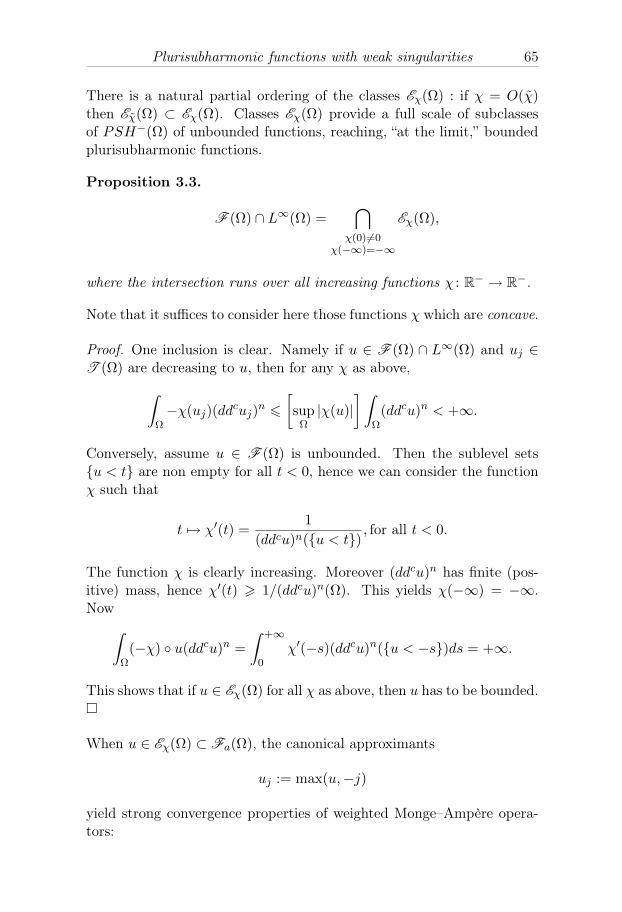
Plurisubharmonic functions with weak singularities 65
There is a natural partial ordering of the classes Eχ(Ω) : if χ = O(χ)then Eχ(Ω) ⊂ Eχ(Ω). Classes Eχ(Ω) provide a full scale of subclassesof PSH−(Ω) of unbounded functions, reaching, “at the limit,” boundedplurisubharmonic functions.
Proposition 3.3.
F (Ω) ∩ L∞(Ω) =⋂
χ(0) �=0χ(−∞)=−∞
Eχ(Ω),
where the intersection runs over all increasing functions χ : R− → R−.
Note that it suffices to consider here those functions χ which are concave.
Proof. One inclusion is clear. Namely if u ∈ F (Ω) ∩ L∞(Ω) and uj ∈T (Ω) are decreasing to u, then for any χ as above,∫
Ω−χ(uj)(ddcuj)n �
[supΩ|χ(u)|
] ∫Ω(ddcu)n < +∞.
Conversely, assume u ∈ F (Ω) is unbounded. Then the sublevel sets{u < t} are non empty for all t < 0, hence we can consider the functionχ such that
t �→ χ′(t) =1
(ddcu)n({u < t}) , for all t < 0.
The function χ is clearly increasing. Moreover (ddcu)n has finite (pos-itive) mass, hence χ′(t) � 1/(ddcu)n(Ω). This yields χ(−∞) = −∞.Now∫
Ω(−χ) ◦ u(ddcu)n =
∫ +∞
0χ′(−s)(ddcu)n({u < −s})ds = +∞.
This shows that if u ∈ Eχ(Ω) for all χ as above, then u has to be bounded.�
When u ∈ Eχ(Ω) ⊂ Fa(Ω), the canonical approximants
uj := max(u,−j)
yield strong convergence properties of weighted Monge–Ampère opera-tors:

66 Slimane Benelkourchi, Vincent Guedj, and Ahmed Zeriahi
Theorem 3.4. Let χ : R− → R− be an increasing function such thatχ(−∞) = −∞ and χ(0) �= 0. Fix u ∈ Eχ(Ω) as set uj = max(u,−j).Then for each Borel subset B ⊂ Ω,∫
Bχ(uj)(ddcuj)n →
∫Bχ(u)(ddcu)n.
Let us stress that this convergence result is stronger than Theorem 5.6 in[Ce 1]: on one hand we produce here an explicit (and canonical) sequenceof bounded approximants, on the other hand the convergence holds inthe strong sense of Borel measures.
Proof. We first show that (ddcuj)n converges towards (ddcu)n “in thestrong sense of Borel measures,” i.e., (ddcuj)n(B) → (ddcu)n(B), forany Borel set B ⊂ Ω. Observe that for j ∈ N∗ fixed and 0 < s < j,{u < −s} = {uj < −s}. It follows from Corollary 2.5 that∫
Ω(ddcuj)n =
∫Ω(ddcu)n.
Therefore∫{u�−j}
(ddcuj)n =∫
Ω(ddcuj)n −
∫{u>−j}
(ddcuj)n
=∫
Ω(ddcuj)n −
∫{u>−j}
(ddcu)n =∫{u�−j}
(ddcu)n.
Thus if B ⊂ Ω is a Borel subset,∣∣∣∣∫B(ddcuj)n −
∫B(ddcu)n
∣∣∣∣ �∫{u�−j}
(ddcuj)n +∫{u�−j}
(ddcu)n
� 2∫{u�−j}
(ddcu)n → 0, as j → +∞.
The proof that χ ◦ uj(ddcuj)n converges strongly towards χ ◦ u(ddcu)ngoes along similar lines, once we observe that∫
{u�−j}−χ ◦ uj(ddcuj)n = −χ(−j)
∫{u�−j}
(ddcuj)n =
− χ(−j)∫{u�−j}
(ddcu)n �∫{u�−j}
−χ ◦ u(ddcu)n.
�

Plurisubharmonic functions with weak singularities 67
4. Capacity estimates
Of particular interest for us here are the classes Eχ(Ω), where the weightχ : R− → R− has fast growth at infinity. It is useful in practice tounderstand these classes through the speed of decreasing of the capacityof sublevel sets.The Monge–Ampère capacity has been introduced and studied by
E. Bedford and B. A. Taylor in [BT1]. Given K ⊂ Ω a Borel subset, itis defined as
CapΩ(K) := sup(∫
K(ddcu)n;u ∈ PSH(Ω),−1 � u � 0
).
Definition 4.1.
Eχ(Ω) :={ϕ ∈ PSH(Ω);
∫ +∞
0tnχ′(−t)CapΩ({ϕ < −t})dt < +∞
}.
The classes Eχ(Ω) and Eχ(Ω) are closely related:
Proposition 4.2. The classes Eχ(Ω) are convex and stable under max-imum: if ϕ ∈ Eχ(Ω) and ψ ∈ PSH−(Ω), then max(ϕ,ψ) ∈ Eχ(Ω).
One always has Eχ(Ω) ⊂ Eχ(Ω), while
Eχ(Ω) ⊂ Eχ(Ω), where χ(t) = χ(2t).
Proof. The convexity of Eχ(Ω) follows from the following simple obser-vation: if ϕ,ψ ∈ Eχ(Ω) and 0 � a � 1, then
{aϕ+ (1− a)ψ < −t} ⊂ {ϕ < −t} ∪ {ψ < −t} .
The stability under maximum is obvious.Assume ϕ ∈ Eχ(Ω). We can assume without loss of generality ϕ � 0
and χ(0) = 0. Set ϕj := max(ϕ,−j). It follows from Corollary 2.5 that∫Ω(−χ) ◦ ϕj (ddcϕj)n =
∫ +∞
0χ′(−t)(ddcϕj)n(ϕj < −t)dt
�∫ +∞
0χ′(−t)tnCapΩ(ϕ < −t)dt < +∞.
This shows that ϕ ∈ Eχ(Ω). The other inclusion goes similarly, using thesecond inequality in Corollary 2.5Observe that Eχ(Ω) ⊂ Eχ(Ω) with χ(t) = χ(2t), as follows by apply-
ing inequalities of Corollary 2.5 with t = s. �

68 Slimane Benelkourchi, Vincent Guedj, and Ahmed Zeriahi
Observe that Eχ(Ω) = Eχ(Ω) when χ(t) = −(−t)p. We thus obtain acharacterization of U. Cegrell’s classes E p(Ω) in terms of the speed ofdecreasing of the capacity of sublevel sets. This is quite useful sincethis second definition does not use the Monge–Ampère measure of thefunction (nor of its approximants):
Corollary 4.3.
E p(Ω) ={ϕ ∈ PSH−(Ω);
∫ +∞
0tn+p−1CapΩ({ϕ < −t})dt < +∞
}.
This also provides us with a characterization of the class Fa(Ω):
Corollary 4.4.Fa(Ω) =
⋃χ(0) �=0,
χ(−∞)=−∞
Eχ(Ω).
As we shall see in the proof, it is sufficient to consider here functions χthat are convex.
Proof. The inclusion ⊃ follows from Proposition 3.2. To prove the re-verse inclusion, it suffices to show that if u ∈ Fa(Ω), then there exists afunction χ such that u ∈ Eχ(Ω): this is because
⋃Eχ =
⋃Eχ. Set
h(t) := tnCapΩ({u < −t}) and h(t) := sups>t
h(s), t > 0.
The function h is bounded, decreasing and converges to zero at infinity.
Consider χ(t) := −1/√h(−t) for all t < 0. Thus χ : R− → R− is convex
increasing, with χ(0) �= 0 and χ(−∞) = −∞. Moreover∫ ∞
0tnχ′(−t)CapΩ({ϕ < −t})dt �
12
∫ ∞
0
−h′(s)h1/2(s)
ds = h1/2(0) < +∞,
as follows from Corollary 2.5. �
Let us observe that a negative psh function u belongs to F (Ω) if andonly if h(0) < +∞ (see Corollary 2.5).
We end up this section with the following useful observation. Letχ : R− → R− be a non-constant concave increasing function. Its inversefunction χ−1 : R− → R− is convex, hence for all ϕ ∈ PSH(Ω), thefunction χ−1 ◦ ϕ is plurisubharmonic,
ddcχ−1 ◦ ϕ = (χ−1)′ ◦ ϕddcϕ+ (χ−1)′′dϕ ∧ dcϕ � 0.

Plurisubharmonic functions with weak singularities 69
NowCapΩ({χ−1 ◦ ϕ < −t}) = CapΩ ({ϕ < χ(−t)})
decreases (very) fast if χ has (very) fast growth at infinity. Thus χ−1 ◦ϕbelongs to some class Eχ(Ω), where χ is completely determined by χ andhas approximately the same growth order. This shows in particular thatthe class Eχ(Ω) characterizes pluripolar sets, whatever the growth of χ:
Theorem 4.5. Let P ⊂ Ω be a (locally) pluripolar set. Then for anyconvex increasing function χ : R− → R− with χ(−∞) = −∞, there existsϕ ∈ Eχ(Ω) such that
P ⊂ {ϕ = −∞}.
5. The range of the complex Monge–Ampère operator
Throughout this section, μ denotes a fixed positive Borel measure offinite total mass μ(Ω) < +∞ which is dominated by the Monge–Ampèrecapacity. We want to solve the following Monge–Ampère equation
(ddcϕ)n = μ with ϕ ∈ F (Ω),
and measure how far the (unique) solution ϕ is from being bounded, byassuming that μ is suitable dominated by the Monge–Ampère capacity.Measures dominated by the Monge–Ampère capacity have been ex-
tensively studied by S. Kołodziej in [K 1, 2, 3]. The main result of hisstudy, achieved in [K 2], can be formulated as follows. Fix ε : R→ [0,∞[a continuous decreasing function and set Fε(x) := x[ε(− lnx/n)]n. If forall compact subsets K ⊂ Ω,
μ(K) � Fε(CapΩ(K)), and∫ +∞
ε(t)dt < +∞,
then μ = (ddcϕ)n for some continuous function ϕ ∈ PSH(Ω) withϕ|∂Ω = 0.
The condition∫ +∞
ε(t)dt < +∞ means that ε decreases fast enoughtowards zero at infinity. This gives a quantitative estimate on how fastε(− lnCapΩ(K)/n), hence μ(K), decreases towards zero as Cap Ω(K)→0.When
∫ +∞ε(t)dt = +∞, it is still possible to show that μ = (ddcϕ)n
for some function ϕ ∈ F (Ω), but ϕ will generally be unbounded. Wenow measure how far it is from being so:
Theorem 5.1. Assume for all compact subsets K ⊂ Ω,
(5.1) μ(K) � Fε
(CapΩ(K)
).

70 Slimane Benelkourchi, Vincent Guedj, and Ahmed Zeriahi
Then there exists a unique function ϕ ∈ F (Ω) such that μ = (ddcϕ)n,and
CapΩ({ϕ < −s}) � exp(−nH−1(s)), for all s > 0,
Here H−1 is the reciprocal function of H(x) = e∫ x0 ε(t)dt+ s0(μ).
In particular ϕ ∈ Eχ(Ω) with −χ(−t) = exp(nH−1(t)/2).
For examples showing that these estimates are essentially sharp, we referthe reader to section 4 in [BGZ].
Proof. The assumption on μ implies in particular that it vanishes onpluripolar sets. It follows from [Ce 2] that there exists a unique ϕ ∈Fa(Ω) such that (ddcϕ)n = μ. Set
f(s) := − 1nlogCapΩ({ϕ < −s}), ∀s > 0.
The function f is increasing and f(+∞) = +∞, since Cap Ω vanishes onpluripolar sets.It follows from Corollary 2.5 and (5.1) that for all s > 0 and t > 0,
tnCapΩ(ϕ < −s− t) � μ(ϕ < −s) � Fε (CapΩ({ϕ < −s})) .
Therefore
(5.2) log t− log ε ◦ f(s) + f(s) � f(s+ t).
We define an increasing sequence (sj)j∈N by induction. Setting
sj+1 = sj + eε ◦ f(sj), for all j ∈ N.
The choice of s0. We choose s0 � 0 large enough so that f(s0) � 0.We must insure that s0 = s0(μ) can chosen to be independent of ϕ. Itfollows from Corollary 2.5 that
CapΩ({ϕ < −s}) �μ(Ω)sn
, ∀s > 0
hence f(s) � log s− 1/n logμ(Ω). Therefore f(s0) � 0 if s0 = μ(Ω)1/n.The growth of sj. We can now apply (5.2) and get f(sj) � j+f(s0) � j.Thus limj f(sj) = +∞. There are two cases to be considered.If s∞ = lim sj ∈ R+, then f(s) ≡ +∞ for s > s∞, i.e.,
CapΩ(ϕ < −s) = 0, ∀s > s∞.
Therefore ϕ is bounded from below by −s∞, in particular ϕ ∈ Eχ(Ω) forall χ.

Plurisubharmonic functions with weak singularities 71
Assume now (second case) that sj → +∞. For each s > 0, thereexists N = Ns ∈ N such that sN � s < sN+1. We can estimate s �→ Ns,
s � sN+1 =N∑0
(sj+1 − sj) + s0 =N∑0
e ε ◦ f(sj) + s0
� e
N∑0
ε(j) + s0 � e
∫ N
0ε(t)dt+ s0 =: H(N),
where s0 = s0 + eε(0). Therefore H−1(s) � N � f(sN ) � f(s), hence
CapΩ(ϕ < −s) � exp(−nH−1(s)).
Set now g(t) = −χ(−t) = exp(nH−1(t)/2). Then∫ ∞
0tng′(t)CapΩ(ϕ < −t)dt
� n
2
∫ ∞
0tn
1ε(H−1(t)) + s0
exp(−nH−1(t)/2)dt
� C
∫ ∞
0(t+ 1)n exp(n(α− 1)t)dt < +∞.
This shows that ϕ ∈ Eχ(Ω) where χ(t) = − exp(nH−1(−t)/2). �
We now generalize U. Cegrell’s main result [Ce 1].
Theorem 5.2. Let χ : R− → R− be an increasing function such thatχ(−∞) = −∞. Suppose there exists a locally bounded function F : R+ →R+ such that lim supt→+∞ F (t)/t < 1, and
(5.3)∫
Ω(−χ) ◦ u dμ � F (Eχ(u)), ∀ u ∈ T (Ω),
where Eχ(u) :=∫Ω(−χ) ◦ u(ddcu)n denotes the χ-energy of u.
Then there exists a function ϕ ∈ Eχ(Ω) such that μ = (ddcϕ)n.
Proof. The assumption on μ implies in particular that it vanishes onpluripolar sets. It follows from [Ce 2] that there exists a function u ∈T (Ω) and f ∈ L1
loc
((ddcu)n
)such that μ = f(ddcu)n.
Consider μj := min(f, j)(ddcu)n. This is a finite measure whichis bounded from above by the Monge–Ampère measure of a boundedfunction. It follows therefore from [K 1] that there exist ϕj ∈ T (Ω) suchthat
(ddcϕj)n = min(f, j)(ddcu)n.

72 Slimane Benelkourchi, Vincent Guedj, and Ahmed Zeriahi
The comparison principle shows that ϕj is a decreasing sequence. Setϕ = limj→∞ ϕj . It follows from (5.3) that Eχ(ϕj)(F (Eχ(ϕj)))−1 � 1,hence supj�1Eχ(ϕj) <∞. This yields ϕ ∈ Eχ(Ω).We conclude now by continuity of the Monge–Ampère operator along
decreasing sequences that (ddcϕ)n = μ. �
When χ(t) = −(−t)p (class F p(Ω)), p � 1, the above result was es-tablished by U. Cegrell in [Ce 1]. Condition (5.3) is also necessary inthis case, and the function F can be made quite explicit: there existsϕ ∈ F p(Ω) such that μ = (ddcϕ)n if and only if μ satisfies (5.3) withF (t) = Ctp/(p+n), for some constant C0.Actually, the measure μ satisfies (5.3) for χ(t) = −(−t)p, and F (t) =
C · tp/(p+n), p > 0, if and only if F p(Ω) ⊂ Lp(μ) (see [GZ]).We finally remark that this condition can be interpreted in terms of
domination by capacity.
Proposition 5.3. If F p(Ω) ⊂ Lp(μ), then there exists C > 0 such that
μ(K) � C · CapΩ(K)p
p+n , for all K ⊂ Ω.
Conversely if μ(·) � Cap αΩ(·) for some α > p/(p + n), then F p(Ω) ⊂
Lp(μ).
Proof. The estimate (5.3) applied to u = u∗K , the relative extremal func-tion of the compact K, yields
μ(K) =∫
Ω1K · dμ �
∫Ω(−u∗K)pdμ
� C
(∫Ω(−u∗K)p(ddcu∗K)n
) pp+n
= C [CapΩ(K)]p
n+p .
Conversely, assume that μ(K) � C ·Cap αΩ(K) for all compactK ⊂ Ω,
where αp/(n+ p) then (5.3) is satisfied. Indeed, if u ∈ F p(Ω), then∫Ω(−u)pdμ = p
∫ ∞
1tp−1μ(u < −t)dt+O(1)
� Cp
∫ ∞
1tp−1
[CapΩ(u < −t)
]αdt+O(1)
� C[ ∫ ∞
1tn+p−1CapΩ(u < −t)dt
]α[ ∫ ∞
1t[p−1−α(n+p−1)]/βdt
]β+O(1),
where α+β = 1. The first integral converges by Corollary 4.3, the latterone is finite since p− 1− α(n+ p− 1) > α− 1 = −β. �

Plurisubharmonic functions with weak singularities 73
References
[BT 1] E. Bedford; B. A. Taylor (1982). A new capacity for plurisubharmonic func-tions. Acta Math. 149 (1982), no. 1-2, 1–40.
[BT2] E. Bedford; B. A. Taylor (1987). Fine topology, Šilov boundary, and (ddc)n.J. Funct. Anal. 72 (1987), no. 2, 225–251.
[B] S. Benelkourchi (2006). A note on the approximation of plurisubharmonic func-tions. C. R. Math. Acad. Sci. Paris, 342, 647–650.
[BGZ] S. Benelkourchi; V. Guedj; A. Zeriahi (2008). A priori estimates for weaksolutions of complex Monge–Ampère equations. Ann. Scuola Norm. Sup. PisaCl. Sci. (5), Vol. VII-1, 81–96.
[BJZ] S. Benelkourchi; B. Jennane; A. Zeriahi (2005). Polya’s inequalities, globaluniform integrability and the size of plurisubharmonic lemniscates. Ark. Mat.43, 85–112 .
[Bl 1] Z. Błocki (2004). On the definition of the Monge–Ampère operator in C2.Math. Ann. 328, no. 3, 415–423.
[Bl 2] Z. Błocki (2006). The domain of definition of the complex Monge–Ampèreoperator. Amer. J. Math. 128 (2006), no. 2, 519–530.
[Ce 1] U. Cegrell (1998). Pluricomplex energy. Acta Math. 180, no. 2, 187–217.[Ce 2] U. Cegrell (2004). The general definition of the complex Monge–Ampère op-
erator. Ann. Inst. Fourier (Grenoble) 54, no. 1, 159–179.[Ce 3] U. Cegrell (2008). A general Dirichlet problem for the complex Monge–Ampère
operator. Ann. Polon. Math. 94, no. 2, 131–147.[CKZ] U. Cegrell; S. Kołodziej; A. Zeriahi (2005). Subextension of plurisubharmonic
functions with weak singularities. Math. Z. 250 (2005), no. 1, 7–22.[EGZ] P. Eyssidieux; V. Guedj; A. Zeriahi (2009). Singular Kähler–Einstein metrics.
J. Amer. Math. Soc. 22, 607–639.[Ki] C. O. Kiselman (1984). Sur la définition de l’opérateur de Monge–Ampère com-
plexe. In: Analyse complexe. Proceedings, Toulouse 1983, 139–150. LectureNotes in Math. 1094, Berlin: Springer-Verlag.
[GZ] V. Guedj; A. Zeriahi (2007). The weighted Monge–Ampère energy of quasi-plurisubharmonic functions. J. Funct. Anal. 250, no. 2, 442–482.
[K 1] S. Kołodziej (1994). The range of the complex Monge–Ampère operator. Indi-ana Univ. Math. J. 43, no. 4, 1321–1338.
[K 2] S. Kołodziej (1999). The complex Monge–Ampère equation. Acta Math. 180,no. 1, 69–117.
[K 3] S. Kołodziej (2005). The complex Monge–Ampère equation and pluripotentialtheory. Mem. Amer. Math. Soc. 178, no. 840, x + 64 pp.
[NP] V. K. Nguyen; H. H. Pham (ms). Some properties of the complex Monge–Ampère operator in the Cegrell’s classes and application. Preprint, arXiv:math/0704.0359.
[Z] A. Zeriahi (1997). Pluricomplex Green functions and the Dirichlet problem forthe complex Monge–Ampère operator. Michigan Math. J. 44, no. 3, 579–596.

74 Slimane Benelkourchi, Vincent Guedj, and Ahmed Zeriahi
Slimane Benelkourchi, Vincent Guedj, and Ahmed ZeriahiInstitut de Mathématiques de Toulouse, Laboratoire Emile Picard,Université Paul Sabatier,118, route de Narbonne, FR-31062 Toulouse Cedex 09, France{benel, guedj, zeriahi}@math.ups-tlse.fr

A remark on approximation on totally real sets
Bo Berndtsson
Abstract. We give a new proof of a theorem on approximation ofcontinuous functions on totally real sets.
1. Introduction
Let Ω be a pseudoconvex open set in Cn, and let ϕ be a C2-smooth non-negative plurisubharmonic function in Ω, satisfying i∂∂ϕ � δβ, where βis the Euclidean volume form and δ > 0. Then
E := {ϕ = 0}
is a totally real set.Associated to the function ϕ and to any positive number k we have
the orthogonal projection operator Pk from
L2(Ω, e−kϕ)
toA2(Ω, e−kϕ),
the latter space being the Bergman space, i.e., the subspace of holomor-phic functions in L2(Ω, e−kϕ).We shall prove the following theorem:
Theorem 1.1. Let u be a smooth function of compact support in Ω. LetK be a compact subset of Ω. Then
supE∩K
|u− Pk(u)| �C√k,
for some constant C.
In particular it follows that any continuous function on E can be approx-imated uniformly on compacts of E by functions holomorphic in Ω. Sinceany totally real submanifold of class C1 can be given as the zeroset of a

76 Bo Berndtsson
strictly plurisubharmonic function defined in some neighbourhood of themanifold, Theorem 1.1 contains the theorem of Hörmander and Wermer(1969) and Nirenberg and Wells (1967) as well as the generalization tothe C1-case of Harvey and Wells (1969).Just like the original proofs in Harvey & Wells (1969) and Nirenberg
& Wells (1967), the proof of Theorem 1.1 is based on Hörmander’s L2-estimates for the ∂-operator. One difference between the proofs is thatwe will use the weight factor e−kϕ in the estimates. We shall then usethe following consequence of Hörmander’s theorem.
Theorem 1.2. Let ϕ be a plurisubharmonic function in a pseudoconvexdomain Ω, satisfying i∂∂ϕ � δβ. Let f be a ∂-closed form of bidegree(0, 1) in Ω, and let v be the L2-minimal solution to the equation ∂v = fin L2(Ω, e−kϕ). Then, for k > 0,
(1.1)∫|v|2e−kϕ � (1/δk)
∫|f |2e−kϕ.
The important feature of this theorem here is that the estimates getsbetter as k increases. The same estimate holds if we replace kϕ by ϕk
where i∂∂ϕk � kδβ.The next step in the proof is the observation that something sim-
ilar happens in uniform norms, at least if we shrink the domain a lit-tle. This is not entirely trivial, but nor is it a deep observation—theshrinking of the domain avoids the main difficulty in passing from L2 touniform norms. The main point in the proof is a variant of the Donnelly–Fefferman trick.
Theorem 1.3. Let ϕ be a plurisubharmonic function in a pseudocon-vex domain Ω satisfying i∂∂ϕ � δβ. Let v be the L2(Ω, e−kϕ)-minimalsolution to the equation ∂v = f . Then, if K is a compact subset of Ω,
supK|v|2e−kϕ � Cδ,K
ksupΩ|f |2e−kϕ.
We apply Theorem 1.3 to f = ∂u where u is, say, a test function. Since
u− Pk(u) = v,
it follows that with E = ϕ−1(0)
supE∩K
|u− Pk(u)|2 � Cδ,K
ksupΩ|f |2e−kϕ � Cδ,K
ksupΩ|f |2,
if ϕ � 0, and Theorem 1.1 follows.

Approximation on totally real sets 77
It is interesting to note that the proof of the approximation theoremhere also has some features in common with the proof of (a generalizationof) the Hörmander–Wermer theorem of Baouendi & Treves (1981). Theirproof is based on convolution with a Gaussian kernel, whereas here weapply the Bergman kernel. However, in the model case ϕ = x2, theBergman kernel is Gaussian, so the two proofs are actually quite similarin this case.IfK is a compact subset of E, which is moreover polynomially convex,
we can choose the weight function ϕ so that it has logarithmic growth atinfinity. The holomorphic functions Pk(u) are then polynomials of degreek, and Theorem 1.1 estimates the degree of approximation by 1/
√k, if
u is of class C1. This is not quite as good as one would expect; at leastif E is a smooth manifold the right degree of approximation should be1/k. Possibly this flaw comes from letting E be a quite general set. Atany rate it seems hard to do better with the methods in this paper.One might also notice that Theorem 1.3 works equally well in un-
bounded domains, so minor modifications should give Carleman-typeapproximation as well, see Carleman (1927) and Manne (1993).Finally, I would like to thank Said Asserda and the referee for point-
ing out several inaccuracies and obscurities in the first version of thispaper.
2. Proof of Theorem 1.3
Theorem 1.3 is not really new—it follows readily from results inBerndtsson (2001, 1997) and in particular Delin (1998)—but here weshall indicate a concise proof for the case at hand. The main ingredi-ent is a variant of the Donnelly–Fefferman trick which will give us anAgmon-type estimate.
Theorem 2.1. Assume i∂∂ϕ � 5β. Then, with notation as in theintroduction, for any a in Cn
(2.1)∫|v|2e−kϕ−√k|z−a| � C/k
∫|f |2e−kϕ−√k|z−a|.
Proof. Assume for simplicity of notation that a = 0. Let ψ be the convexfunction defined by
ψ(t) = t
for t � 1 andψ(t) = t2/2 + 1/2
for t < 1. Let χ(z) = ψ(|z|). Then |χ−|z|| is bounded, so it is enough toprove (2.1) with
√k|z| replaced by χ(z
√k). Moreover ∂χ is bounded by

78 Bo Berndtsson
1, and i∂∂χ � β. It is especially the last property that is of importancehere and is the reason for introducing the function χ. Put
χk(z) = χ(z√k) and vk := ve−χk .
Since v is orthogonal to all holomorphic functions in L2(Ω, e−kϕ), itfollows that vk is orthogonal to all holomorphic functions for the scalarproduct in L2(Ω, e−kϕ+χk) (we may assume in the proof that Ω is boundedso that the L2-spaces do not change when we vary the weight). Hencevk is the L2minimal solution to a certain ∂-equation. Now,
i∂∂(kϕ− χk) � 4kβ
so it follows from the Hörmander estimate (1.1) that
(2.2)∫|vk|2e−kϕ+χk � 1/(4k)
∫|∂vk|2e−kϕ+χk .
The left hand side of equation (2.2) equals∫|v|2e−kϕ−χk .
In the right hand side we have
∂vk = (f − vk∂χk)e−χk .
Since ∂χk is bounded by√k we can absorb the contribution to (2.2)
coming from the second term vk∂χk in the left hand side of (2.2), and(2.1) follows. �
We are now ready for the proof of Theorem 1.3. By scaling, we may ofcourse assume that i∂∂ϕ � 5β. Let a be a point in Ωk that again forsimplicity we take equal to 0. After changing frame locally at 0 we canassume that, near the origin,
ϕ(z) = q(z, z) + o(|z|2),
where q is an hermitian form. (This means the following: Near the originwe can, since ϕ is of class C2, write
ϕ(z) = 2ReP (z) + q(z, z) + o(|z|2),
where P is a holomorphic polynomial of degree 2. We then write
v′ = ve−P (z)

Approximation on totally real sets 79
for v andf ′ = fe−P (z)
for f , which changes the weight function ϕ to ϕ− 2ReP = q + o(|z|2).)
Note that kq(z, z) is bounded by a constant when |z| < 1/k. Thisconstant certainly depends on the point a that we have taken equal to0, but it is uniform as long as a ranges over a compact subset of Ω. Wethen get∫
|z|2<1/k|v|2 � C/k sup |f |2e−kϕ
∫e−√k|z| � C sup |f |2e−kϕ/kn+1.
Normalize so thatsup |f |2e−kϕ � 1.
Then, in particular, ∂v is bounded by a constant for |z|2 < 1/k. Theinequality
(2.3) |v(0)|2 � C(kn∫|z|2<1/k
|v|2 + 1ksup
|z|2<1/k
|f |2),
then shows that|v(0)|2 � 1/k,
which is what we wanted to prove. To verify (2.3) one can apply theBochner–Martinelli integral formula
v(0) = cn∫(∂(vξ(|z|2/k) · ∂|z|2n−2),
where ξ(t) is a smooth function that equals 1 for t < 1/2 and 0 for t > 1.
References
Baouendi, M. S.; Trèves, F. (1981). A property of the functions and distributionsannihilated by a locally integrable system of complex vector fields. Ann. of Math.(2) 113, no. 2, 387–421.
Berndtsson, Bo (1997). Uniform estimates with weights for the ∂-equation. J. Geom.Anal. 7, no. 2, 195–215.
Berndtsson, Bo (2001). Weighted estimates for the ∂-equation. Complex analysisand geometry (Columbus, OH, 1999), 43–57. Ohio State Univ. Math. Res. Inst.Publ., 9, Berlin: de Gruyter.
Carleman, T. (1927). Sur un théorème de Weierstrass. Arkiv för Matematik, Astro-nomi och Fysik 20B, no. 4, 5 pp.
Delin, Henrik (1998). Pointwise estimates for the weighted Bergman projection kernelin Cn, using a weighted L2 estimate for the ∂ equation. Ann. Inst. Fourier(Grenoble) 48, no. 4, 967–997.

80 Bo Berndtsson
Bo Berndtsson lecturing at the Kiselmanfest, May 18, 2006.Photo: Christian Nygaard.
Harvey, F. Reese; Wells, R. O., Jr. (1972). Holomorphic approximation and hyper-function theory on a C1 totally real submanifold of a complex manifold. Math.Ann. 197, 287–318.
Hörmander, L.; Wermer, J. (1969). Uniform approximation on compact sets in Cn.Math. Scand. 23, 5–21.
Manne, P. (1993). Carleman approximation on totally real submanifolds of a complexmanifold. In: Several complex variables (Stockholm, 1987/1988), pp. 519–528.Math. Notes, 38, Princeton, NJ: Princeton Univ. Press.
Nirenberg, Ricardo; Wells, R. O., Jr. (1967). Holomorphic approximation on realsubmanifolds of a complex manifold. Bull. Amer. Math. Soc. 73, 378–381.
Department of Mathematics,Chalmers University of Technology and the University of GöteborgSE-412 96 Göteborg, [email protected]

Discrete geometry and symbolic dynamics
Valerie Berthe
Avec mes pensees les plus amicales pour Christer Kiselman
1. Introduction
The aim of this survey is to illustrate various connections that existbetween word combinatorics and arithmetic discrete geometry throughthe discussion of some discretizations of elementary Euclidean objects(lines, planes, surfaces). We focus on the role played by dynamicalsystems (toral rotations mainly) that can be associated in a naturalway with these discrete structures. We show how classical techniques insymbolic dynamics applied to some codings of such discretizations allowone to obtain results concerning the enumeration of configurations andtheir statistical properties. Note that we have no claim to exhaustivity:the examples that we detail here have been chosen for their simplicity.Let us first illustrate this interaction with Figure 1.1 below, where
a piece of an arithmetic discrete plane in R3 is depicted, as well as itsorthogonal projection onto the antidiagonal plane Δ: x1+x2+x3 = 0 inR3, which can be considered as a piece of a tiling of the plane by threekinds of lozenges, and lastly, its coding as a two-dimensional word overa three-letter alphabet.
Figure 1.1: Left: arithmetic discrete plane. Middle: tiling of the plane.Right: two-dimensional word.

82 Valerie Berthe
This paper is organized as follows. We first start with the most simplesituation, namely discrete lines and Sturmian words (see Section 2).Section 3 is devoted to the higher-dimensional case, i.e., to the study ofarithmetic discrete planes. We generalize this study performed mainlyin the so-called naive case, first, to a broader class of arithmetic discreteplanes in Section 4, and second, to functional stepped surfaces in Section5. Section 6 is concerned with the generation of arithmetic discreteplanes by so-called generalized substitutions. Special focus is given tothe duality between arithmetic discrete planes and discrete lines in thethree-dimensional space. One key tool will be the so-called Rauzy fractalassociated with the cubic Pisot number of minimal polynomialX3−X2−X − 1 = 0.
2. Sturmian words and discrete lines
This section is concerned with the connections between arithmetic dis-crete lines and Sturmian words. A substantial literature has been de-voted to the study of discrete lines, as illustrated for instance in thesurveys [KR04, BCK07]. Let us start by recalling the definition of anarithmetic discrete line, introduced by Reveilles in [Rev91].
Definition 1. Let v ∈ R2, and μ, ω ∈ R. The (lower) arithmetic discreteline D(v, μ, ω) is defined as
D(v, μ, ω) = {x ∈ Z2; 0 � 〈x,v〉+ μ < ω}.
The parameter μ is called the translation parameter of D(v, μ, ω), andω is called the width of D(v, μ, ω).
Two natural cases are more particularly studied: if ω = ||v||∞, thenD(v, μ, ω) is said to be naive, and if ω = ||v||1, then D(v, μ, ω) is saidstandard.
Figure 2.1: Left: A naive discrete line. Right: A standard discrete line.
One checks that a naive (resp. standard) arithmetic discrete line ismade of horizontal and diagonal (resp. horizontal and vertical) steps.

Discrete geometry and symbolic dynamics 83
One can code such a standard line by using the Freeman code [Fre70]over the two-letter alphabet {0, 1} as follows: one codes horizontal stepsby a 0, and diagonal ones by a 1. One gets a so-called Stumian word(un)n∈N ∈ {0, 1}N. More precisely, Sturmian words satisfy:Definition 2 (Morse-Hedlund [MH40]). Let Rα : R/Z → R/Z, x �→x + α mod 1 be the rotation of angle α of the one-dimensional torusT = R/Z. Let u = (un)n∈N ∈ {0, 1}N. The infinite word u is a Sturmianword if there exist α ∈ (0, 1), α �∈ Q, x ∈ R, such that
∀n ∈ N, un = i⇐⇒ Rnα(x) = nα+ x ∈ Ii (mod 1),
with I0 = [0, 1− α[, I1 = [1− α, 1[ or I0 = ]0, 1− α], I1 = ]1− α, 1] .For more on Sturmian words, see the surveys [AS02, Lot02, PF02] andthe references therein.The following lemma is classical for the study of Sturmian words.
Its interest for further generalizations is stressed in the survey [BFZ05].
Lemma 1. The word w = w1 · · ·wn over the alphabet {0, 1} is a factorof the Sturmian word u if and only if
Iw1 ∩R−1α Iw2 ∩ · · · ∩R−n+1
α Iwn �= ∅.Proof. By definition, one has
∀i ∈ N, un = i⇐⇒ nα+ x ∈ Ii (mod 1).One first notes that ukuk+1 · · ·un+k−1 = w1 · · ·wn if and only if⎧⎪⎪⎨⎪⎪⎩
kα+ x ∈ Iw1
(k + 1)α+ x ∈ Iw2
· · ·(k + n− 1)α+ x ∈ Iwn .
One then applies the density of (nα)n∈N in R/Z (recall that α is assumedto be an irrational number).
One first notes that the condition of Lemma 1 does not depend on x butonly on α. One easily checks that the sets
Iw1 ∩R−1α Iw2 ∩ · · · ∩R−n+1
α Iwn
are intervals of T = R/Z. Furthermore, the factors of u of length nare in one-to-one correspondence with the n + 1 intervals of T whoseend-points are given by −kα mod 1, for 0 � k � n. This implies thattwo Sturmian words coding the same rotation have the same factors.Furthermore, Sturmian words have exactly n+1 factors of length n, forevery n ∈ N. This is even a characterization of Stumian words:

84 Valerie Berthe
Theorem 2 (Coven-Hedlund [CH73]). A word u ∈ {0, 1}N is Sturmianif and only if it has exactly n+ 1 factors of length n.
The function that associates with a word the number of its factors of agiven length is called the complexity function. For more on this function,see for instance [AS02, All94, Fer99].More generally, one deduces from Lemma 1 various combinatorial
properties of Sturmian words, such as the expression of densities of fac-tors [Ber96], that can be deduced from the equidistribution of the se-quence (nα)n∈N. Indeed, the frequency of occurrence of the word w inthe Sturmian word u is equal to the length of the interval Iw.Let us note that Definition 2 can be restated in terms of dynamical
systems as follows. A dynamical system (X,T ) is defined as the actionof a continuous and onto map T on a compact space X. An example ofa geometric dynamical system is given by (T, Rα).Given a dynamical system (X,T ), a point x ∈ X, and a parti-
tion P = {P0, . . . ,Pk−1} of X, the sequence u = (un)n∈N defined byun = i whenever Tnx ∈ Pi, for n ∈ N, is called a coding of the dy-namical system (X,T ). A Sturmian word is thus a coding of the dy-namical system (T, Rα) with respect either to the two-interval partition{I0 = [0, 1− α[ , I1 = [1− α, 1[ } or to {I0 = ]0, 1− α] , I1 = ]1− α, 1] }.As another example, let us consider symbolic dynamical systems.
Let A be a finite set. We endow A N with the product topology of thediscrete topology on A . Let u ∈ A N. Let L (u) be the set of its factors.The shift S is defined as S : A N → A N, (un)n∈N �→ (un+1)n∈N. Thesymbolic dynamical system generated by u is (Xu, S) with
Xu := {Sn(u); n ∈ N} = {v ∈ A N; L (v) ⊂ L (u)} ⊂ A N.
Since two Sturmian words coding the same rotation have the same setof factors, then one checks that the symbolic dynamical system generatedby a Sturmian word coding the rotation Rα consists of all the Sturmianwords that code the same rotation.Note that several combinatorial properties of Sturmian words or of
naive arithmetic discrete lines, respectively, have been studied and statedindependently: for instance, the notion of balance, and the chord prop-erty respectively, have been considered in [MH38, MH40, Lot02, PF02]for Sturmian words, and in [Fre74, Ros74, Hun85, Mel05] in discretegeometry. For more details on the connections between Sturmian wordsand discrete lines, see for instance Ch. 1 of [Jam05b], and more gener-ally, for references on discrete lines, see the surveys [KR04, BCK07]. See[AD03, BDJR08] for complexity-like results. See also [Fer08, UW08] for

Discrete geometry and symbolic dynamics 85
recent results in discrete geometry in connection with continued frac-tions.
3. Discrete planes
Let us consider now the higher-dimensional case.
Definition 3. Let v ∈ R3, and μ, ω ∈ R. The arithmetic discretehyperplane P(v, μ, ω) is defined as
P(v, μ, ω) = {x ∈ Z3; 0 � 〈x,v〉+ μ < ω}.
If ω = ||v||∞, then P(v, μ, ω) is said to be naive. If ω = ||v||1, thenP(v, μ, ω) is said to be standard.
A piece of a naive discrete plane (left) as well as a piece of a standarddiscrete plane (right) are depicted in the figure below.
Figure 3.1: Left: Naive discrete plane. Right: Standard discrete plane.
Let us see now how to associate with a standard arithmetic discreteplane a coding as a two-dimensional word on a three-letter alphabetthat plays the role of the Freeman code for arithmetic discrete lines,such as described in Section 2.Let (e1, e2, e3) stand for the canonical basis of R3. Let x ∈ Z3 and
i ∈ {1, 2, 3}. Let E1, E2 and E3 be the three following faces:
E1 ={λe2 + μe3; (λ, μ) ∈ [0, 1[2
},
E2 ={−λe1 + μe3; (λ, μ) ∈ [0, 1[2
},
E3 ={−λe1 − μe2; (λ, μ) ∈ [0, 1[2
}.
We call pointed face the set x+Ei. The point x is called the distin-guished vertex of the face x + Ei. Note that each pointed face includesexactly one integer point, namely, its distinguished vertex.Let P := P(v, μ, ||v||1) be a standard arithmetic discrete plane. One
associates with P a so-called stepped plane P defined as the union of

86 Valerie Berthe
faces of integral cubes that connect the points of P, as depicted inFigure 1.1 (left). By an integral cube we mean a translate by a vectorwith integral entries of the fundamental unit cube
U ={ ∑
1�i�n
λiei; λi ∈ [0, 1], for all i}
with integral vertices. The stepped plane P is thus defined as theboundary of the set of integral cubes that intersect the lower open half-space {x ∈ Z3; 〈x,v〉 + μ � 0}. The vertices (that is, the points withinteger coordinates) of P are exactly the points of the arithmetic dis-crete plane P, according for instance to [BV00b].Let Δ be the antidiagonal plane of equation x1+x2+x3 = 0 and let
π0 be the orthogonal projection onto Δ. Note that π0(Z3) is a lattice inΔ with basis (π0(e1), π0(e2)), and that π0(e3) = −π0(e1)−π0(e2). If weuse this basis for π0(Z3), then the restriction of π0 to Z3 becomes thefollowing map, also denoted by π0 by abuse of notation:
π0 : Z3 −→ Z2, x �→ (x1 − x3, x2 − x3).
According to [BV00b, ABI02], the restriction of the projection mapπ0 to P is one-to-one and onto Δ:
∀(m,n) ∈ Z2, ∃! (x, i) such that x+ Ei ⊂P, π0(x) = (m,n). (3.1)
Furthermore, the projections of the faces of the stepped plane P tilethe diagonal plane Δ with three kinds of lozenges (see Figure 1.1).We then provide the stepped planeP with a two-dimensional coding
as follows. The two-dimensional coding of the stepped plane P is thetwo-dimensional word U ∈ {1, 2, 3}Z2
defined, for all (m,n) ∈ Z2 and alli ∈ {1, 2, 3}, by
Um,n = i ⇐⇒ ∃ (x, i) such that x+ Ei ⊂P, π0(x) = (m,n).
According to (3.1), the value of U at each point (m1,m2) is well-defined.One checks (e.g., see [BV00b, ABI02, ABS04]) that for (m,n) ∈ Z2 andi ∈ {1, 2, 3}, then Um,n = i if and only if:
mv1 + nv2 + μ mod v1 + v2 + v3 ∈ [v1 + · · ·+ vi−1, v1 + · · ·+ vi[. (3.2)
Let us now introduce an analogue of the dynamical system (T, Rα)that is coded by the two-dimensional word U . Given two continuous andonto maps T1 and T2 acting on X and satisfying T1 ◦ T2 = T2 ◦ T1, the

Discrete geometry and symbolic dynamics 87
Z2-action by T1 and T2 on X, that we denote by (X,T1, T2), is definedas
∀(m,n) ∈ Z2, ∀x ∈ X, (m,n) · x = Tm1 ◦ Tn
2 (x).
As an example, consider a Z2-action by two rotations on the torus R/Z,that is, the Z2-action defined by
(m,n) · x = Rmα R
nβ(x) = x+mα+ nβ mod 1.
Given any partition {P1, . . . , Pd} of the torus and a point x, we candefine a (two-dimensional) word U = (Um,n)(m,n)∈Z2 ∈ {1, 2, . . . , d}Z2
coding the orbit of x under this Z2-action by Um,n = i whenever Rmα R
nβ x
belongs to Pi, for (m,n) ∈ Z2. The two-dimensional coding given by(3.2) is an example of such a coding.After a suitable renormalization by ||v||1 of the parameters involved,
one thus defines two-dimensional Sturmian words as follows:
Definition 4 ([BV00b]). Let U = (Um,n)(m,n)∈Z2 ∈ {1, 2, 3}Z2. The
two-dimensional word U is said to be a two-dimensional Sturmian wordif there exist x ∈ R, and α, β ∈ R such that 1, α, β are Q-linearlyindependent and α+ β < 1 such that
∀(m,n) ∈ Z2, Um,n = i⇐⇒ Rmα R
nβ(x) = x+ nα+mβ ∈ Ii (mod 1),
withI1 = [0, α[ , I2 = [α, α+ β[ , I3 = [α+ β, 1[
orI1 = ]0, α] , I2 = ]α, α+ β] , I3 = ]α+ β, 1] .
Hence, a two-dimensional Sturmian word is a coding of a Z2-action bytwo rotations on R/Z.Let us state now the analogue of Lemma 1. We first consider finite
rectangular arrays of consecutive letters, that is, rectangular words
W =
⎡⎢⎣ w0,n−1 · · · wm−1,n−1...
...w0,0 · · · wm−1,0.
⎤⎥⎦We say that w has size (m,n). The rectangular complexity of the two-dimensional word U is the function pU (m,n) which associates with each(m,n) ∈ N2, m and n being nonzero, the cardinality of the set of rect-angular factors of size (m,n) occurring in U .

88 Valerie Berthe
The analogue of Lemma 1 can be stated as follows: the word
W =
⎡⎢⎣ w0,n · · · wm,n...
...w0,0 · · · wm,0
⎤⎥⎦is a factor of the two-dimensional Sturmian word U if and only if⋂
0�i�m,0�j�n
R−iα R
−jβ Iwi,j �= ∅. (3.3)
We first deduce that for a given (α, β), the language of rectangularfactors of U is here again the same for every x. We also deduce resultsconcerning the counting of rectangular factors of a given size: thereare exactly mn + m + n factors of size (m,n) in the two-dimensionalSturmian word U . We can deduce not only topological results from (3.3)but also metrical results: the frequencies of rectangular factors of size(m,n) of a two-dimensional Sturmian word take at most min(m,n) +5 values [BV00b]. For more on two-dimensional Sturmian words, see[BV00a, BV00b, BV01, BT04].Let us note that we have chosen in Definition 4 to restrict ourselves to
rationally independent parameters. Usually in arithmetic discrete geom-etry, parameters are chosen to be integers. The results discussed abovecan also be obtained for standard arithmetic discrete planes P(v, μ, ω),whatever is the value taken by dimQ(v1, v2, v3) (which can take the value1, 2, 3), either by direct application of Bezout’s lemma if the parameters(v1, v2, v3) are coprime integers, or from the density of the sequence(nα)n∈Q, for α being assumed to be irrational. For more details, see thecomplete study performed in [Jam05b].Note that we consider here standard arithmetic discrete planes. Re-
call that when replacing the norm ‖·‖1 by the norm ‖·‖∞ in the definitionof arithmetic discrete planes, one gets naive arithmetic discrete planes.The latter are usually considered in discrete geometry. Both notions arestrongly related as shown, e.g., in [SDC04], Theorem 1.
4. Functionality
Naive arithmetic discrete planes have been widely studied (see, e.g.,[DRR95, AAS97, VC99, Ger99b, Ger99a, VC00, Jac01, Jac02, BB02,BB05, BCK07, Kis04, AD08]) and are well known to be functional, i.e.,in a one-to-one correspondence with the integer points of one of thecoordinate planes by an orthogonal projection map. In other words,

Discrete geometry and symbolic dynamics 89
given a naive arithmetic discrete plane P and the suitable coordinateplane, then for any integer point P of this coordinate plane, there existsa unique point of P obtained from P by adding a third coordinate.The aim of this section is first to show how to extend the notion of
functionality for naive arithmetic discrete planes to a larger family ofarithmetic discrete planes. Secondly, we deduce from the functionalitya suitable coding of a dynamical system acting on the torus, in orderto get information on local configurations, according to the strategydescribed in Section 2 and 3. The results we present here are from[BFJ05, BFJP07].Instead of projecting on a coordinate plane, we shall introduce in
Section 4.1 a suitable orthogonal projection map on a plane along adirection α = (α1, α2, α3) ∈ Z3, in some sense dual to the normal vectorof the discrete plane P (v, μ, ω). By dual, we mean here
〈α,v〉 = α1v1 + α2v2 + α3v3 = ω,
so that the projection of Z3 and the points of the discrete planeP (v, μ, ω)are in one-to-one correspondence (see Lemma 3 below). We then intro-duce in Section 4.2 the notion of local configurations and (m,n)-cubeswhich will play the role of factors.One interest of the notion of functionality is to reduce a three-
dimensional problem to a two-dimensional one, allowing a better un-derstanding of the combinatorial and geometric properties of arithmeticdiscrete planes: this allows us, first, to recode in Section 4.3 arithmeticdiscrete planes by a two-dimensional word over the two-letter alphabet{0, 1} (similarly as explained in Section 3), and second, to exhibit fromthis coding many geometric properties of arithmetic discrete planes (setof local configurations, enumeration of (m,n)-cubes, statistical proper-ties . . . ). This is the object of Section 4.4.
4.1. Functional vectors
An arithmetic discrete plane P(v, μ, ω) is said to be rational if the pa-rameters v, μ, ω belong to Z or have integer entries. One easily checksthat one can choose parameters satisfying v ∈ Z3, μ ∈ Z, ω ∈ N andgcd(v1, v2, v3) = 1.LetP(v, μ, ω) be an arithmetic discrete plane, and letα ∈ Z3 be such
that gcd{α1, α2, α3} = 1. Let πα : R3 −→ {x ∈ R3, 〈α,x〉 = 0} be theaffine orthogonal projection map onto the plane {x ∈ R3, 〈α,x〉 = 0}along the vector α.
Lemma 3. [BFJP07] Let α ∈ Z3 be such that gcd(α1, α2, α3) = 1. Themap πα : P(v, μ, ω) −→ πα(Z3) is a bijection if and only if |〈α,v〉| = ω.

90 Valerie Berthe
By Bezout’s lemma, for any rational arithmetic discrete planeP(v, μ, ω), with v ∈ Z3, μ ∈ Z, ω ∈ N and gcd{v1, v2, v3} = 1, thereexists a vector α ∈ Z3 such that 〈α,v〉 = ω. A vector α ∈ Z3 is said tobe functional if it satisfies conditions gcd(α1, α2, α3) = 1 and 〈α,x〉 = ω.Hence, any rational arithmetic discrete plane has functional vectors.We will make in all that follows the following assumption: there
exists a functional vector α ∈ Z3 for which there exists i ∈ {1, 2, 3} suchthat αi = 1, say α3 = 1. Note that, since ω = α1v1 + α2v2 + α3v3,then the hypothesis α3 = 1 is equivalent to ω ∈ v1Z + v2Z + v3, i.e.,ω − v3 ∈ gcd(v1, v2)ZThere does not always exist a functional vector α with α3 = 1. Con-
sider for instance the case v = (6, 10, 15) with ω = 20: it is impossibleto express ω as α1v1 + α2v2 + α3v3 with one of the αi’s equal to 1.Let Γα be the lattice obtained by projecting the arithmetic discrete
plane P(v, μ, ω) on the third coordinate plane along the functional vec-tor α. Under the previous assumption, one has Γα = Ze1 + Ze2. Thishypothesis gives an explicit and simple expression of the preimage of apoint in Γα. Indeed, the map π−1
α : Γα→ P satisfies for all y ∈ Γα withy = y1e1 + y2e2:
π−1α (y) = y −
⌊v1y1 + v2y2 + μω
⌋α.
We define the height HP,α(y) at y as the third coordinate x3 of x =π−1α (y) ∈ P. One has
HP,α(y) = −⌊v1y1 + v2y2 + μ
ω
⌋. (4.1)
4.2. Local configurations and (m,n)-cubes
We want now to apply the functionality to the enumeration of (m,n)-cubes and local configurations, generalizing the study performed fornaive planes in [VC97, Sch97, Ger99b, Ger99a, VC99, Jac02, AD08].For the sake of consistency in notation, we call them here m-cubes withm = (m1,m2) rather than (m,n)-cubes.Let P := P(v, μ, ω) be an arithmetic discrete plane satisfying the
hypothesis of Section 4.1. Let α ∈ Z3 such that gcd(α1, α2, α3) = 1 and〈α,v〉 = ω. We assume that α3 = 1 in all that follows, i.e., ω − v3 ∈v1Z+ v2Z.Let m ∈ (N�)2 be given. By m-cube we mean a local configuration
in the discrete plane that can be observed thanks to πα through an m-window in the functional lattice Γα = Ze1+Ze2 (see Figure 4.2). More

Discrete geometry and symbolic dynamics 91
precisely, the m-cube C (y,m) of P is defined as the following subset ofP:
C (y,m) ={π−1α (y + z); z ∈ [[0,m1 − 1]]e1 + [[0,m2 − 1]]e2
}.
Two m-cubes C and C ′ are said translation equivalent if there exists avector z ∈ Z3 such that C ′ = C + z.
Figure 4.1: From left to right: the (3, 3)-cube of P(v, 0, 9) (resp.P(v, 0, 11), P(v, 0, 21), P(v, 0, 37)) centered at (0, 0, 0), where v =6e1 + 10e2 + 15e3, and projected along the vector −e1 + e3 (resp.e1 − e2 + e3, e1 + e3, 2e1 + e2 + e3).
In order to enumerate the different types of m-cubes that occur in P,that is, the different equivalence classes for the translation equivalence,we represent them as local configurations as follows. An (m1 × m2)-rectangular word L = [Li1,i2 ](i1,i2)∈[[0,m1−1]]×[[0,m2−1]] over the infinite al-phabet Z is called an m-local configuration of P if there exists y ∈ Z2
such that:
L = [HP,α(z)−HP,α(y)]z∈[[0,m1−1]]e1+[[0,m2−1]]e2,
where the height is defined in Equation (4.1).Let us note that a local configuration is a plane partition. Indeed a
plane partition of N ∈ N is a rectangular word
w = [wi1,i2 ](i1,i2)∈[[0,m1−1]]×[[0,m2−1]]
over the infinite alphabet N satisfying N =∑
i,j wi,j and, for all i1 ∈[[0,m1 − 1]] and i2 ∈ [[0,m2 − 1]], max{wi1+1,i2 , wi1,i2+1} � wi1,i2 .
4.3. A coding as a two-dimensional word
Our stategy is now the following: we recode arithmetic discrete planesaccording to a two-dimensional word U ∈ {0, 1}Z2
over the two-letter al-phabet {0, 1}, namely a so-called generalized Rote word [Rot94], follow-ing the approach of [Vui99, BV01], and in the same flavour of the codingsperformed in Section 3. Such a two-dimensional word codes a Z2-action

92 Valerie Berthe
by two rotations with respect to a partition of the one-dimensional torusinto two intervals of length 1/2. We then express m-cubes as equiva-lence classes of rectangular factors of the two-dimensional word U , andshow, for every m ∈ N2, that the number of m-cubes in P(v, μ, ω) iscomputed by enumerating points on the one-dimensional torus.Note that m-cubes are subsets of arithmetic discrete planes whereas
m-local configurations are two-dimensional words over an infinite alpha-bet. To be able to get words over a finite alphabet, let us introduce atwo-dimensional word coding in a natural way the parity of the heightsHP,α(y), for y in the lattice Γα = Ze1 + Ze2, according to [Vui99].Indeed, for a naive discrete plane P, it is well known that, given two
points x and x′ of P such that their projections by πα are 4-connectedin the functional plane, then |x3−x′3| � 1. In other words, the differencebetween the heights of x and x′ is at most 1.A quite unexpected fact is that this property holds for any arithmetic
discrete plane with α3 = 1. More precisely, it is easy to see that, for ally ∈ Γα and i = 1, 2, HP,α (y + ei) − HP,α (y) takes only two values,namely −�vi/ω� and −�vi/ω�−1. In each case, one of these values is odd,whereas the other one is even; we define E1 and O1 to be respectivelythe even and the odd value taken by −�v1/ω� and −�v1/ω�− 1; wesimilarly define E2 and O2. It is now natural to introduce the followingtwo-dimensional word of parity of heights by identifying Γα to Z2:
U = (Ui1,i2)(i1,i2)∈Z2 = (HP,α(y) mod 2)y∈Z2 ∈ {0, 1}Z2. (4.2)
The two-dimensional word U satisfies, for each (i1, i2) ∈ Z2,
Ui1,i2 = 0 if and only if v1i1 + v2i2 + μ mod 2ω ∈ [0, ω[.
Indeed, one checks that Ui1,i2 = 0 if and only if⌊v1i1+v2i2+μ
ω
⌋is even,
that is, v1i1 + v2i2 + μ mod 2ω ∈ [0, ω[.The word U is a two-dimensional Rote word. One-dimensional Rote
words have been introduced in [Rot94]; they are defined as the infinitewords u over the alphabet {0, 1} that have exactly 2n factors of length nfor every positive integer n, and whose set of factors is closed under com-plementation, i.e., every word obtained by interchanging zeros and onesin a factor of the infinite word u is still a factor of u. Two-dimensionalRote words have been studied for instance in [Vui99, BV01].Let us now make explicit the connection between local configurations
and factors of U .Let W = [wi1,i2 ](i1,i2)∈[[0,m1−1]]×[[0,m2−1]] be a rectangular word of size
m1 ×m2 over {0, 1}. We define the complement W of W as follows:
W = [wi1,i2 ](i1,i2)∈[[0,m1−1]]×[[0,m2−1]], where 1 = 0 and 0 = 1.
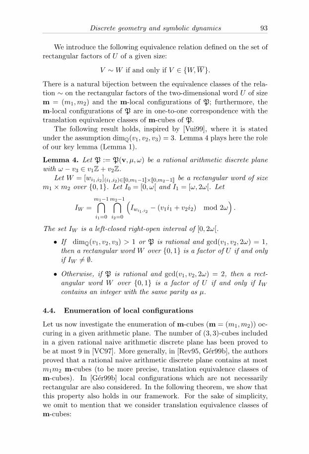
Discrete geometry and symbolic dynamics 93
We introduce the following equivalence relation defined on the set ofrectangular factors of U of a given size:
V ∼W if and only if V ∈ {W,W}.
There is a natural bijection between the equivalence classes of the rela-tion ∼ on the rectangular factors of the two-dimensional word U of sizem = (m1,m2) and the m-local configurations of P; furthermore, them-local configurations of P are in one-to-one correspondence with thetranslation equivalence classes of m-cubes of P.The following result holds, inspired by [Vui99], where it is stated
under the assumption dimQ(v1, v2, v3) = 3. Lemma 4 plays here the roleof our key lemma (Lemma 1).
Lemma 4. Let P := P(v, μ, ω) be a rational arithmetic discrete planewith ω − v3 ∈ v1Z+ v2Z.
Let W = [wi1,i2 ](i1,i2)∈[[0,m1−1]]×[[0,m2−1]] be a rectangular word of sizem1 ×m2 over {0, 1}. Let I0 = [0, ω[ and I1 = [ω, 2ω[. Let
IW =m1−1⋂i1=0
m2−1⋂i2=0
(Iwi1,i2
− (v1i1 + v2i2) mod 2ω).
The set IW is a left-closed right-open interval of [0, 2ω[.
• If dimQ(v1, v2, v3) > 1 or P is rational and gcd(v1, v2, 2ω) = 1,then a rectangular word W over {0, 1} is a factor of U if and onlyif IW �= ∅.
• Otherwise, if P is rational and gcd(v1, v2, 2ω) = 2, then a rect-angular word W over {0, 1} is a factor of U if and only if IWcontains an integer with the same parity as μ.
4.4. Enumeration of local configurations
Let us now investigate the enumeration of m-cubes (m = (m1,m2)) oc-curing in a given arithmetic plane. The number of (3, 3)-cubes includedin a given rational naive arithmetic discrete plane has been proved tobe at most 9 in [VC97]. More generally, in [Rev95, Ger99b], the authorsproved that a rational naive arithmetic discrete plane contains at mostm1m2 m-cubes (to be more precise, translation equivalence classes ofm-cubes). In [Ger99b] local configurations which are not necessarilyrectangular are also considered. In the following theorem, we show thatthis property also holds in our framework. For the sake of simplicity,we omit to mention that we consider translation equivalence classes ofm-cubes:

94 Valerie Berthe
Theorem 5. Let P := P(v, μ, ω) be a discrete plane with ω − v3 ∈v1Z+v2Z. Let m = (m1,m2) ∈ (N�)2. Then, P contains at most m1m2
m-cubes. More precisely, one has:
1. If dimQ(v1, v2, v3) = 1, v ∈ Z3, μ ∈ Z, ω ∈ Z, and gcd(v) = 1,then P contains at most ω m-cubes for every m = (m1,m2) ∈(N�)2. Moreover, for m1 and m2 large enough, P contains exactlyω m-cubes.
2. Let us assume dimQ(v1, v2, v3) = 2. Let (p1, p2) ∈ Z2 be a genera-tor of the lattice of periods of the two-dimensional word U . ThenP contains at most m1|p2|+m2|p1| −min{m1, |p1|}min{m2, |p2|}m-cubes for (m1,m2) ∈ N2.
3. If dimQ(v1, v2, v3) = 3, then P contains exactly m1m2 m-cubes forevery m = (m1,m2) ∈ (N�)2.
Let us note that the bounds for m1 and m2 upon which the previousresults hold (cases (1) and (2) in Theorem 5) can be explicitly computedin terms of v and ω. The proof is a direct application of Lemma 4. Formore details, see [BFJP07].We thus can establish that the computation of the frequency of oc-
currence of an m-cube of P(v, μ, ω) can be reduced to the calculationof the length of an interval of the torus R/ωZ. For more details, see[BFJP07]. We also investigate in [BFJP07] the closure of the set ofm-cubes of P(v, μ, ω) under the action of a particular geometric trans-formation: the centrosymmetry.
5. Stepped surfaces
Let us generalize the codings as two-dimensional words introduced inSection 3 for arithmetic discrete planes to more general discrete objects,namely the functional stepped surfaces as introduced in [Jam04]. Seealso [Jam05a, JP05, Jam05b, ABFJ07].A functional discrete surface is defined as a union of pointed faces
Ei, for i = 1, 2, 3 (defined in Section 3) such that the orthogonal pro-jection π0 onto the antidiagonal plane Δ: x1 + x2 + x3 = 0 induces anhomeomorphism from the discrete surface onto Δ.As done for functional arithmetic discrete planes, one then provides
a discrete surface with a coding as a two-dimensional word over a three-letter alphabet [Jam04, JP05]. Indeed, let S be a functional steppedsurface. One has
S ∩ Z3 = {x; ∃ i such that x+ Ei ⊂ S }.

Discrete geometry and symbolic dynamics 95
Furthermore, given (m1,m2) ∈ Z2, there exists a unique face x+Ei ⊂ Ssuch that (m1,m2) = π0(x). The following coding is thus well-defined:a two-dimensional word U ∈ {1, 2, 3}Z2
is said to be the coding of thefunctional stepped surface S if for all (m1,m2) ∈ Z2 and for everyi ∈ {1, 2, 3}:
Um1,m2 = i ⇐⇒ ∃(x, i), such that x+Ei ∈ S , π0(x) = (m1,m2).
We illustrate this with the following figure, where a piece of a discretesurface in R3 is depicted, as well as its orthogonal projection π0 ontothe plane Δ: x1+x2+x3 = 0, and its coding as a two-dimensional wordover a three-letter alphabet.
2
3
3
3
3
3
3
3
3
3
3
3
3
3
3
3
3
3
3
3
3
3
3
3
3
3
3
3
3
3
3
3
3
3
3
3 3 3
3
3
3
3
3
3
3
1
1
1
1
1
1
1
1
1
1
1
11
1
1
1
1
1
11
1
1
1
1
1
1
1
1
1
1
1
1
1
1
1
1
1
1
1
1
1
2
2
2
2 2
2
2 2
2
2
2 2
2
2
2
2
2
2 2
2
2
2
2
2
2
2
2
2
2
2
22
2
2
2
Figure 5.1: From discrete surfaces to multidimensional words via tilings
Let us quote the following nice characterization of codings of discretesurfaces [Jam04]. Let U ∈ {1, 2, 3}Z2
. Then U is a coding of a discretesurface if and only if the factors of U of the shape given in Figure 5.2 areincluded in the set of factors depicted in Figure 5.2. The main differencebetween a stepped surface and a stepped plane is thus that it is possibleto locally recognize whether a set of points in Z3 is a subset of the setof vertices of a stepped surface.

96 Valerie Berthe
x y
z
Figure 5.2: Permitted factors and their 3-dimensional representation.
6. From discrete to continuous structures
The aim of this section, based on the surveys [Lot05, BS05, BBLT06], isto show how to generate standard arithmetic discrete planes by meansof a generalized substitution. We work out here in details the exampleof the Tribonacci substitution.
6.1. The Tribonacci substitution
Let A be a finite set. As usual in word combinatorics, we denote byA ∗ the set of words over A and by ε the empty word. The set A ∗
endowed with the concatenation map is a free monoid. A substitutionis an endomorphism of the free monoid A ∗. A substitution naturallyextends to the set of one-sided words A N. A fixed point of σ is a wordu = (ui)i∈N ∈ A N that satisfies σ(u) = u .We consider the Tribonacci substitution σ : {1, 2, 3}∗ → {1, 2, 3}∗ de-
fined on the letters of the alphabet {1, 2, 3} as follows: σ : 1 �→ 12,2 �→ 13, 3 �→ 1. The Tribonacci word is the (unique) fixed point of thesubstitution σ. More precisely, by noticing that σj(1) is a nontrivialprefix of the word σj+1(1), the sequence of words
1, σ(1), σ2(1), . . . , σn(1), . . .
is easily seen to converge to an infinite word denoted by σω(1). The firstterms of this word are
1 2 1 3 1 2 1 1 2 1 3 1 2 1 2 1 · · ·
Note that the length, denoted by |σj(1)|, of σj(1) satisfies the Tribonaccirecurrence: |σj+3(1)| = |σj+2(1)| + |σj+1(1)| + |σj(1)|, for every j ∈ N,hence the name.

Discrete geometry and symbolic dynamics 97
The Tribonacci substitution has been introduced and studied in[Rau82]. For more results and references on the Tribonacci substitu-tion, see [AR91, AY81, IK91, Lot05, Mes98, Mes00, PF02].The incidence matrix Mσ = (mi,j)1�i,j�n of a substitution σ has
entries mi,j = |σ(j)|i, where the notation |w|i stands for the numberof occurrences of the letter i in the word w. A substitution σ is calledprimitive if there exists an integer n such that σn(a) contains at least oneoccurrence of the letter b for every pair (a, b) ∈ A 2. This is equivalentto the fact that its incidence matrix is primitive, i.e., there exists anonnegative integer n such that Mn
σ has only positive entries.If a substitution σ is primitive, then the Perron–Frobenius theorem
ensures that the incidence matrix Mσ has a simple real positive domi-nant eigenvalue β, which admits as associated right and left eigenvectorsvectors with positive entries. A substitution σ is called unimodular ifdet Mσ = ±1. A substitution σ is said to be Pisot if its incidence ma-trixMσ has a real dominant eigenvalue β > 1 such that, for every othereigenvalue λ, one has 0 < |λ| < 1. The characteristic polynomial of theincidence matrix of such a substitution is irreducible over Q, and thedominant eigenvalue β is a Pisot number (that is, an algebraic integerwith all Galois conjugates having modulus less than 1). Furthermore, itcan be proved that Pisot substitutions are primitive [PF02].The incidence matrix of the Tribonacci substitution σ is
Mσ =
⎡⎣ 1 1 11 0 00 1 0
⎤⎦ .This matrix is easily seen to be primitive. The characteristic polynomialofMσ is X3−X2−X−1; this polynomial admits one positive root β > 1(the dominant eigenvalue) and two complex conjugates α and α, with|α| < 1. Hence the Tribonacci substitution is Pisot and the number β is aPisot number. The matrixMσ admits as eigenspaces in R3 one expandingeigenline (generated by the eigenvector with positive coordinates uβ =(1/β, 1/β2, 1/β3) associated with the eigenvalue β) and a real contractingeigenplane Hc. Let vβ be the left eigenvector ofMσ with positive entriesnormalized so that 〈vβ ,uβ〉 = 1. The contracting plane Hc has equation〈x,vβ〉 = 0.One associates with the Tribonacci word u = (un)n�0 a broken line
starting from 0 in Z3 and approximating the expanding line generatedby uβ as follows. We introduce the abelianization map f of the freemonoid {1, 2, 3}∗ defined by
f : {1, 2, 3}∗ → Z3, f(w) = |w|1e1 + |w|2e2 + |w|3e3,

98 Valerie Berthe
where (e1, e2, e3) stands for the canonical basis of R3. Note that forevery finite word w, we have f(σ(w)) =Mσf(w).The Tribonacci broken line is defined as the broken line which joins
with segments of length 1 the points f(u0u1 · · ·uN−1), N ∈ N (see Figure6.1). In other words, we describe this broken line by starting from theorigin, and then by reading successively the letters of the Tribonacciword u, going one step in direction ei if one reads the letter i.One easily deduces from the fact that σ is a Pisot substitution that
the vectors f(u0u1 . . . uN ), N ∈ N, stay within bounded distance of theexpanding line ofMσ, which is exactly the direction given by the vectorof probabilities of occurrence of the letters 1, 2, 3 in u. One can considerthis broken line as a discrete approximation of the line generated bythe vector uβ . It is then natural to try to represent these points byprojecting them along the expanding direction onto a transverse plane,that we chose here to be the contracting plane Hc of Mσ.Let π stand for the projection in R3 onto the contracting plane along
the expanding line generated by the vector vβ . We thus define the setRσ as the closure of the projections of the vertices of the Tribonaccibroken line:
Rσ := {π(f(u0 . . . uN−1)); N ∈ N}.
The set Rσ is called the Rauzy fractal associated with the Tribonaccisubstitution σ (see Figure 6.1). It can be divided into three pieces, calledbasic pieces, defined for i = 1, 2, 3 as
Rσ(i) = {π(f(u0 . . . uN−1)); uN = i, N ∈ N}.
One checks that the Rauzy fractal is a compact set which is theclosure of its interior; it has nonzero measure, fractal boundary, and itis the attractor of some graph-directed iterated function system [Rau82].Furthermore, the pieces Rσ(i), for i = 1, 2, 3 are disjoint in measure.One interesting feature of the Rauzy fractal is that it can tile the
plane in two different ways [Rau82, IR06]. These two tilings are depictedin Figure 6.2. The first one corresponds to a periodic tiling (a latticetiling), and the second one to a self-substitutive tiling.By tiling of Rd, we mean here tilings by translation having finitely
many tiles up to translation (a tile is assumed to be the closure of itsinterior): there exist a finite set of tiles Ti and a finite number of trans-lation sets Γi such that
Rd =⋃i
⋃γi∈Γi
(Ti + γi),

Discrete geometry and symbolic dynamics 99
and distinct translates of tiles have non-intersecting interiors; we assumefurthermore that each compact set in Rd intersects a finite number oftiles. By a lattice tiling we mean that there exists a lattice Γ such that
Rd =⋃γ∈Γ
(T + γ),
where T =⋃
i Ti.
Figure 6.1: The Tribonacci broken line and the Rauzy fractal.
Figure 6.2: Lattice and self-substitutive Tribonacci tilings.
6.2. Discrete planes and tilings
The self-substitutive Tribonacci tiling depicted in Figure 6.2 has closeconnections with arithmetic discrete planes. We consider indeed thestandard lower arithmetic discrete plane with parameter μ = 0 associ-ated with the left eigenvector vβ that we denote for short by Pσ. Letus recall that vβ has positive entries. One has
Pσ =
⎧⎨⎩x ∈ Z3; 0 � 〈x,vβ〉 < ||vβ||1 =∑
i=1,2,3
〈ei,vβ〉
⎫⎬⎭ .
We also consider the stepped plane Pσ associated with it as definedin Section 3. This discretization of the contracting hyperplane Hc =
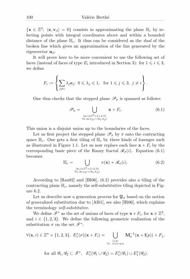
100 Valerie Berthe
{x ∈ Z3; 〈x,vβ〉 = 0} consists in approximating the plane Hc by se-lecting points with integral coordinates above and within a boundeddistance of the plane Hc. It thus can be considered as the dual of thebroken line which gives an approximation of the line generated by theeigenvector uβ.It will prove here to be more convenient to use the following set of
faces (instead of faces of type Ei introduced in Section 3): for 1 � i � 3,we define
Fi :=
⎧⎨⎩∑j �=i
λjej ; 0 � λj � 1, for 1 � j � 3, j �= i
⎫⎬⎭ .
One thus checks that the stepped plane Pσ is spanned as follows:
Pσ =⋃
(x,i)∈Z3×{1,2,3}0�〈x,vβ〉<〈ei,vβ〉
x+ Fi. (6.1)
This union is a disjoint union up to the boundaries of the faces.Let us first project the stepped plane Pσ by π onto the contracting
space Hc. One gets a first tiling of Hc by three kinds of lozenges suchas illustrated in Figure 1.1. Let us now replace each face x+ Fi by thecorresponding basic piece of the Rauzy fractal Rσ(i). Equation (6.1)becomes
Hc =⋃
(x,i)∈Z3×{1,2,3}0�〈x,vβ〉<〈ei,vβ〉
π(x) +Rσ(i). (6.2)
According to [Rau82] and [IR06], (6.2) provides also a tiling of thecontracting plane Hc, namely the self-substitutive tiling depicted in Fig-ure 6.2.Let us describe now a generation process for Pσ based on the notion
of generalized substitution due to [AI01], see also [IR06], which explainsthe terminology self-substitutive.We define F ∗ as the set of unions of faces of type x+Fi, for x ∈ Z3,
and i ∈ {1, 2, 3}. We define the following geometric realization of thesubstitution σ on the set F ∗:
∀(x, i) ∈ Zn × {1, 2, 3}, E∗1(σ)(x+ Fi) =⋃(j,p)
∃s, σ(j)=pis
M−1σ (x+ l(p)) + Fj ,
for all G1,G2 ⊂ F ∗, E∗1(G1 ∪ G2) = E∗1(G1) ∪ E∗1(G2).

Discrete geometry and symbolic dynamics 101
Figure 6.3: Generation of Pσ by iterates of E∗1(σ).
Theorem 6. [AI01] Let σ be the Tribonacci substitution. The steppedplane Pσ is stable under the action of E1(σ)∗ and contains the unit cube
U := F1 ∪ F2 ∪ F3.
The iterates (E1(σ)∗)n(U ) all belong to Pσ, and they generate largerand larger pieces of the stepped plane Pσ. By taking the limit and byprojecting by π, one gets
Hc = limn→+∞π(E1(σ)∗)n(U ).
After projection and renormalization, the sequence of pieces
Mnσπ(E1(σ)∗)n(U )
is convergent and its limit is equal to the Rauzy fractal:
Rσ = limn→+∞M
nσπ(E1(σ)∗)n(U ).
Hence the vertices of the pieces (E1(σ)∗)n(U ) generate the arithmeticdiscrete plane Pσ as illustrated in Fig. 6.2.For more on generalized substitutions and generation of discrete
planes, see [ABI02, ABS04, ABFJ07, Fer06, Fer07].
6.3. Rauzy tilings
We have seen that two tilings can be associated with the Rauzy fractal,namely, a self-substitutive tiling and a lattice tiling, as illustrated inFigure 6.2. This latter tiling plays an important role in the spectralstudy of the substitutive dynamical system (Xσ, S) generated by the

102 Valerie Berthe
Tribonacci word (as defined in Section 2). Indeed, one of the mainincentives behind the introduction of Rauzy fractals is the followingresult:
Theorem 7. [Rau82] Let σ be the Tribonacci substitution
σ : 1 �→ 12, 2 �→ 13, 3 �→ 1.
The Rauzy fractal Rσ (considered as a subset of R2) is a fundamentaldomain of T2. Let Rβ : T2 → T2, x �→ x+(1/β, 1/β2). The symbolic dy-namical system (Xσ, S) is measure-theoretically isomorphic to the toraltranslation (T2, Rβ).
In other words, the Tribonacci word u is a coding with respect to thepartition of the two-dimensional torus T2 by the three pieces Rσ(i), fori = 1, 2, 3 of an orbit of a point of T2 under the action of the translationRβ .We can now explain what kind of discrete approximation the Tri-
bonacci broken line provides for the line generated by the vector uβ .As a consequence of Theorem 7, one proves that the only points in Z3
whose projection by π belongs to the interior of Rσ are the vertices ofthe broken line. Hence the broken line is obtained by a selection processwhich consists in shifting the Rauzy fractal along the direction uβ andselecting points in Z3 in this strip. Note that the words associated withbroken lines obtained by shifting the unit cube along a given directionare called billiard words (see for instance [AMST94, Bar95]). General-izations of the Tribonacci word are given by the so-called Arnoux–Rauzywords [AR91] and more generally by the family of episturmian words.Billiard words and episturmian words are two widely studied families ofinfinite words in word combinatorics.The Tribonacci lattice tiling has been widely studied and presents
many interesting features. In particular, the Tribonacci central tile hasa “nice” topological behavior (0 is an inner point and it is shown tobe connected with simply connected interior [Rau82]), which leads tointeresting applications in Diophantine approximation [CHM01], wherepoints of the broken line corresponding to σn(1), n ∈ N, are provedto produce best approximations for the vector ( 1
β ,1β2 ) for a given norm
associated with the matrix Mσ. See also [HM06] for a similar study inthe case of a family of cubic Pisot numbers with complex conjugates.Rauzy fractals can more generally be associated with Pisot substi-
tutions (see [BK06, CS01a, CS01b, IR06, Mes00, Mes02, Sie03, Sie04]and the surveys [BS05, PF02]), as well as with Pisot β-shifts under thename of central tiles (see [Aki98, Aki99, Aki00, Aki02]), but they also

Discrete geometry and symbolic dynamics 103
can be associated with abstract numeration systems [BR05], as well aswith some automorphisms of the free group [ABHS06]. Theorem 7 isexpected to hold in this context: this is the so-called Pisot conjecture.
Conjecture 1. Let σ be a Pisot unimodular substitution. The followingequivalent conditions are conjectured to hold:
1. the symbolic dynamical system (Xσ, S) is measure-theoreticallyisomorphic to a translation on the torus;
2. (Xσ, S) has a pure discrete spectrum;
3. the associated Rauzy fractal Rσ generates a lattice tiling, i.e.,
Kβ =⋃γ∈Γ
(Rσ + γ),
with the union being disjoint in measure, and Γ being a lattice.
The conjecture holds true for two-letter alphabets [BD02, HS03, Hos92].Substantial literature is devoted to Conjecture 1 which is reviewed in[PF02], Ch. 7. See also [BK06, BK05, BBK06, BS05, IR06] for recentresults.
6.4. Back to stepped planes
Generalized substitutions (introduced in Section 6.2) are proved in[ABFJ07] to act not only on stepped planes, but also on stepped surfaces.Furthermore, a geometric version of Brun multidimensional continuedfraction algorithm acting on stepped surfaces is given in [BF08] in termsof generalized substitutions. This geometric extension of the Brun algo-rithm is motivated by the discrete plane recognition problem: given a setof points in Zd, is there a naive arithmetic discrete plane that containsit? A strategy based on multidimensional continued fractions inspiredby the one-dimensional Sturmian case is thus given in [BF08, Fer08].Indeed, in the one-dimensional case, there exists a natural strategy
for the recognition problem based on word combinatorics. Let us recallthat a substitution is a morphism of the free monoid whereas an S-adicword is an infinite word generated as the limit of an infinite compo-sition of a finite number of substitutions (for more details, see Ch. 12in [PF02]). Sturmian words are proved to be S-adic words; the rulesfor the iteration of these substitutions follow the continued fraction ofthe slope of the line which is coded. We deduce from the combinatorialproperties of Sturmian words the following two facts: First, factors 00

104 Valerie Berthe
and 11 cannot occur simultaneoulsy in a Sturmian word, that is, oneof the two letters 0 and 1 occurs as an isolated letter. Hence, up to aprefix of length 1, any infinite Sturmian word can be written as σ0(v)or σ1(v), where v is an infinite word over {0, 1}, and the substitutionsσ0 and σ1 are defined as σ0 : 0 �→ 0, 1 �→ 10 and σ1 : 0 �→ 01, 1 �→ 1.Secondly, we use the fact that v is itself a Sturmian word. We can thusreiterate the process. Suppose now we are given a connected union oftranslates of horizontal and vertical segments with integer vertices andlength 1. We apply the previous process to the finite word coding thisunion of segments by taking care of the boundaries. This correspondsto the method developed in discrete geometry terms in [Wu82, Tro93].Let us note that the recognition problem is classical and central in the
field of discrete geometry for the segmentation of discrete surfaces andfor polyhedrization issues, for instance. Indeed, numerous applicationscan be derived in image analysis and synthesis, volume modeling, pat-tern recognition, etc. There exist various strategies for the discrete planerecognition problem, as described, for instance, in the survey [BCK07].These methods are based on linear programming, on computational ge-ometry by performing separability tests, or on the so-called preimagetechnique which consists in determining the set of parameters of thearithmetic discrete planes that contain the given set of points.
7. Conclusion
Let us conclude by giving a brief list of geometric discretizations thatcan be described by symbolic codings of dynamical systems.
• Standard arithmetic discrete lines and Sturmian words are partic-ular codings of rotations over the one-dimensional torus T with respectto a two-interval partition, one interval having as length the parameterof the rotation.
• Similarly, standard arithmetic discrete planes and two-dimensionalSturmian words are codings of a Z2-action by rotations over the one-dimensional torus T with respect to a three-interval partition, with twointervals having as respective length the parameters of the Z2-action.
• More generally, functional arithmetic discrete planes can be codedthanks to generalized Rote words defined as codings of a Z2-action byrotations over the one-dimensional torus T with respect to a two-intervalpartition, with two intervals of the same length. For more examples ofcodings associated with naive or standard arithmetic discrete planesexpressed in terms of dynamical systems, see [Jam05b], where codingsby remainders, by umbrellas and by parity of heights are considered.

Discrete geometry and symbolic dynamics 105
• In a dual way, we have seen how to associate with the Tribonaccisubstitution a broken line that can be considered as a discrete line inR3. A lattice tiling by the Rauzy fractal can then be produced that hasclose connection with a rotation on the two-dimensional torus T2.
• Lastly, let us quote [BN07] as an example of a symbolic codingof discrete rotations defined as the composition of Euclidean rotationswith a rounding operation, as studied in [NR03, NR04, NR05]. Indeed,it is possible to encode all the information concerning a discrete rota-tion as two multidimensional words Cα and C ′α called configurations.These configurations Cα and C ′α can be coded by discrete dynamicalsystems defined by a Z2-action on the two-dimensional torus T2. As aconsequence, results concerning densities of occurrence of symbols canbe deduced.
References
[AAS97] E. Andres; R. Acharya; C. Sibata (1997). Discrete analytical hyperplanes.Graph. Models Image Process. 59, 302–309.
[ABFJ07] P. Arnoux; V. Berthe; T. Fernique; D. Jamet (2007). Functional steppedsurfaces, flips and generalized substitutions. Theoret. Comput. Sci. 380,251–267.
[ABHS06] P. Arnoux; V. Berthe; A. Hilion; A. Siegel (2006). Fractal representationof the attractive lamination of an automorphism of the free group. Ann.Inst. Fourier (Grenoble) 56, 2161–2212.
[ABI02] P. Arnoux; V. Berthe; S. Ito (2002). Discrete planes, Z2-actions, Jacobi-Perron algorithm and substitutions. Ann. Inst. Fourier (Grenoble) 52,305–349.
[ABS04] P. Arnoux; V. Berthe; A. Siegel (2004). Two-dimensional iterated mor-phisms and discrete planes. Theoret. Comput. Sci. 319, 145–176.
[AD03] M. Tajine; A. Daurat (2003). On local definitions of length of digitalcurves. In: Proceedings of DGCI 2003, pp. 114–123. Lecture Notes inComputer Science 2886. Springer.
[AD08] A. Daurat; M. Tajine; M. Zouaoui (2008). About the frequencies of somepatterns in digital planes. Application to area estimators. In: Proceed-ings of DGCI 2008, pp. 45–56. Lecture Notes in Computer Science 4992.Springer.
[AI01] P. Arnoux; S. Ito (2001). Pisot substitutions and Rauzy fractals. Bull.Belg. Math. Soc. Simon Stevin 8, 181–207.
[Aki98] S. Akiyama (1998). Pisot numbers and greedy algorithm. In: Numbertheory (Eger, 1996), pp. 9–21. De Gruyter.
[Aki99] S. Akiyama (1999). Self affine tilings and Pisot numeration systems.In: K. Gyory; S. Kanemitsu (Eds.), Number Theory and its Applications(Kyoto 1997), pp. 7–17. Kluwer Academic Publishers.

106 Valerie Berthe
[Aki00] S. Akiyama (2000). Cubic Pisot units with finite beta expansions. In:Algebraic Number Theory and Diophantine Analysis (Graz, 1998), pp.11–26. Berlin: de Gruyter.
[Aki02] S. Akiyama (2002). On the boundary of self affine tilings generated byPisot numbers. J. Math. Soc. Japan 54, 283–308.
[All94] J.-P. Allouche (1994). Sur la complexite des suites infinies. Bull. Belg.Math. Soc. Simon Stevin 1, 133–143. Journees Montoises (Mons, 1992).
[AMST94] P. Arnoux; C. Mauduit; I. Shiokawa; J. I. Tamura (1994). Complexity ofsequences defined by billiards in the cube. Bull. Soc. Math. France 122,1–12.
[AR91] P. Arnoux; G. Rauzy (1991). Representation geometrique de suites decomplexite 2n + 1. Bull. Soc. Math. France 119, 199–215.
[AS02] J.-P. Allouche; J. O. Shallit (2002). Automatic sequences: Theory andApplications. Cambridge: Cambridge University Press.
[AY81] P. Arnoux; J.-C. Yoccoz (1981). Construction de diffeomorphismespesudo-Anosov. C. R. Acad. Sci. Paris, Ser. A 292, 75–78.
[Bar95] Yu. Baryshnikov (1995). Complexity of trajectories in rectangular bil-liards. Commun. Math. Phys. 174, 43–56.
[BB02] V. E. Brimkov; R. P. Barneva (2002). Graceful planes and lines. Theoret.Comput. Sci. 283, 151–170.
[BB05] V. E. Brimkov; R. P. Barneva (2005). Plane digitizations and relatedcombinatorial problems. Discrete Applied Mathematics 147, 169–186.
[BBK06] V. Baker; M. Barge; J. Kwapisz (2006). Geometric realization and coinci-dence for reducible non-unimodular Pisot tiling spaces with an applicationto beta-shifts. Ann. Inst. Fourier (Grenoble) 56, 2213–2248.
[BBLT06] G. Barat; V. Berthe; P. Liardet; J. M. Thuswaldner (2006). Dynamicaldirections in numeration. Ann. Inst. Fourier (Grenoble) 56, 1987–2092.
[BCK07] V. E. Brimkov; D. Coeurjolly; R. Klette (2007). Digital planarity – areview. Discrete Applied Mathematics 155, 468–495.
[BD02] M. Barge; B. Diamond (2002). Coincidence for substitutions of Pisottype. Bull. Soc. Math. France 130, 619–626.
[BDJR08] N. Bedaride; E. Domenjoud; D. Jamet; J.-L. Remy (ms 2008). On thenumber of balanced words of given length and height over a two-letteralphabet.
[Ber96] V. Berthe (1996). Frequences des facteurs des suites sturmiennes. Theoret.Comput. Sci. 165, 295–309.
[BF08] V. Berthe; T. Fernique (ms 2008). Brun expansions of stepped surfaces.
[BFJ05] V. Berthe; C. Fiorio; D. Jamet (2005). Generalized functionality forarithmetic discrete planes. In: Proceedings of DGCI 2005, pp. 276–286.Lecture Notes in Computer Science 3429. Springer.
[BFJP07] V. Berthe; C. Fiorio; D. Jamet; F. Philippe (2007). On some applica-tions of generalized functionality for arithmetic discrete plane. Image andVision Computing 25, 1671–1684.

Discrete geometry and symbolic dynamics 107
[BFZ05] V. Berthe; S. Ferenczi; L. Q. Zamboni (2005). Interactions between dy-namics, arithmetics and combinatorics: the good, the bad, and the ugly.In: Algebraic and topological dynamics, pp. 333-364. Contemp. Math. 385.Amer. Math. Soc.
[BK05] M. Barge; J. Kwapisz (2005). Elements of the theory of unimodular Pisotsubstitutions with an application to β-shifts. In: Algebraic and topologicaldynamics, pp. 89-99. Contemp. Math. 385. Amer. Math. Soc.
[BK06] M. Barge; J. Kwapisz (2006). Geometric theory of unimodular Pisotsubstitution. Amer. J. Math. 128, 1219–1282.
[BN07] V. Berthe; B. Nouvel (2007). Discrete rotations and symbolic dynamics.Theoret. Comput. Sci. 380, 276–280.
[BR05] V. Berthe; M. Rigo (2005). Abstract numeration systems and tilings.In: Proceedings of MFCS 2005, pp. 131–143. Lecture Notes in ComputerScience 3618. Springer.
[BS05] V. Berthe; A. Siegel (2005). Tilings associated with beta-numeration andsubstitutions. Integers 5 (3):A2, 46 pp.
[BT04] V. Berthe; R. Tijdeman (2004). Lattices and multi-dimensional words.Theoret. Comput. Sci. 319, 177–202.
[BV00a] V. Berthe; L. Vuillon (2000). Suites doubles de basse complexite. J.Theor. Nombres Bordeaux 12, 179–208.
[BV00b] V. Berthe; L. Vuillon (2000). Tilings and rotations on the torus: a two-dimensional generalization of Sturmian sequences. Discrete Math. 223(1-3), 27–53.
[BV01] V. Berthe; L. Vuillon (2001). Palindromes and two-dimensional Sturmiansequences. J. Autom. Lang. Comb. 6, 121–138.
[CH73] E. M. Coven; G. A. Hedlund (1973). Sequences with minimal blockgrowth. Math. Systems Theory 7, 138–153.
[CHM01] N. Chekhova; P. Hubert; A. Messaoudi (2001). Proprietes combinatoires,ergodiques et arithmetiques de la substitution de Tribonacci. J. Theor.Nombres Bordeaux 13, 371–394.
[CS01a] V. Canterini; A. Siegel (2001). Automate des prefixes-suffixes associe aune substitution primitive. J. Theor. Nombres Bordeaux 13, 353–369.
[CS01b] V. Canterini; A. Siegel (2001). Geometric representation of substitutionsof Pisot type. Trans. Amer. Math. Soc. 353, 5121–5144.
[DRR95] I. Debled-Rennesson; J.-P. Reveilles (1995). New approach to digitalplanes. In: Vision geometry III (Boston, MA, USA), Proc. SPIE, 2356,pp. 12–21.
[Fer99] S. Ferenczi (1999). Complexity of sequences and dynamical systems. Dis-crete Math. 206, 145–154.
[Fer06] T. Fernique (2006). Multidimensional Sturmian sequences and generalizedsubstitutions. Int. J. Found. Comput. Sci. 17, 575–600.
[Fer07] T. Fernique (2007). Pavages, fractions continues et geometrie discrete.PhD thesis, Universite de Montpellier II.
[Fer08] T. Fernique (2008). Generation and recognition of digital planes usingmulti-dimensional continued fractions. In: Proceedings of DGCI 2008, pp.33–44. Lecture Notes in Computer Science 4992. Springer.

108 Valerie Berthe
[Fre70] H. Freeman (1970). Boundary encoding and processing. In: Picture Pro-cessing and Psychopictorics, pp. 241–266. New York: Academic Press.
[Fre74] H. Freeman (1974). Computer processing of line-drawing images. ACMComputing Surveys 6, 57–97.
[Ger99a] Y. Gerard (1999). Contribution a la geometrie discrete. PhD thesis,Universite d’Auvergne.
[Ger99b] Y. Gerard (1999). Local configurations of digital hyperplanes. In: Pro-ceedings of DGCI 1999, pp. 65–75. Lecture Notes in Computer Science1568. Springer.
[HM06] P. Hubert; A. Messaoudi (2006). Best simultaneous diophantine approx-imations of Pisot numbers and Rauzy fractals. Acta Arithmetica 124,1–15.
[Hos92] B. Host (ms 1992). Representation geometrique des substitutions sur 2lettres. Unpublished manuscript.
[HS03] M. Hollander; B. Solomyak (2003). Two-symbol Pisot substitutions havepure discrete spectrum. Ergodic Theory Dynam. Systems 23, 533–540.
[Hun85] S. H. Y. Hung (1985). On the straightness of digital arcs. In: IEEE Trans-actions on Pattern Analysis and Machine Intelligence, volume PAMI-7,pp. 203–215.
[IK91] S. Ito; M. Kimura (1991). On Rauzy fractal. Japan J. Indust. Appl. Math.8 (3), 461–486.
[IR06] S. Ito; H. Rao (2006). Atomic surfaces, tilings and coincidences I. Irre-ducible case. Israel J. Math. 153 129–156.
[Jac01] M.-A. Jacob-Da Col (2001). Applications quasi-affines et pavages du plandiscret. Theoret. Comput. Sci. 259, 245–269.
[Jac02] M.-A. Jacob-Da Col. About local configurations in arithmetic planes.Theoret. Comput. Sci. 283, 183–201.
[Jam04] D. Jamet (2004). On the language of standard discrete planes and sur-faces. In: Proceedings of IWCIA 2004, pp. 232–247. Lecture Notes inComputer Science 3322. Springer.
[Jam05a] D. Jamet (2005). Coding stepped planes and surfaces by two-dimensionalsequences over a three-letter alphabet. Technical Report 05047, LIRMM,Universite de Montpellier II, UMR 5506, July.
[Jam05b] D. Jamet (2005). Geometrie discrete : une approche par la combinatoiredes mots. PhD thesis, Universite de Montpellier II.
[JP05] D. Jamet; G. Paquin (2005). Discrete surfaces and infinite smooth words.In: Proceedings of FPSAC’05.
[Kis04] C. O. Kiselman (2004). Convex functions on discrete sets. In: Proceedingsof IWCIA’2004, pp. 443–457. Lecture Notes in Computer Science 3322.Springer.
[KR04] R. Klette; A. Rosenfeld (2004). Digital straightness—a review. DiscreteApplied Mathematics 139, 197–230.
[Lot02] M. Lothaire (2002). Algebraic combinatorics on words. Encyclopedia ofMathematics and its Applications, volume 90. Cambridge: CambridgeUniversity Press.

Discrete geometry and symbolic dynamics 109
[Lot05] M. Lothaire (2005). Applied combinatorics on words. Encyclopedia ofMathematics and its Applications, volume 105. Cambridge: CambridgeUniversity Press.
[Mel05] E. Melin. Digital straight lines in the Khalimsky plane. Math. Scand. 96,49–64.
[Mes98] A. Messaoudi (1998). Proprietes arithmetiques et dynamiques du fractalde Rauzy. J. Theor. Nombres Bordeaux 10, 135–162.
[Mes00] A. Messaoudi (2000). Frontiere du fractal de Rauzy et systeme denumeration complexe. Acta Arith. 95, 195–224.
[Mes02] A. Messaoudi (2002). Tribonacci multiplication. Appl. Math. Lett. 15,981–985.
[MH38] M. Morse; G. A. Hedlund (1938). Symbolic dynamics. Amer. J. Math.60, 815–866.
[MH40] M. Morse; G. A. Hedlund (1940). Symbolic dynamics II. Sturmian tra-jectories. Amer. J. Math. 62, 1–42.
[NR03] B. Nouvel; E. Remila (2003). On colorations induced by discrete rotations.In: Proceedings of DGCI 2003, pp. 174–183. Lecture Notes in ComputerScience 2886. Springer.
[NR04] B. Nouvel; E. Remila (2004). Characterization of bijective discretizedrotations. In: Proceedings of IWCIA 2004, pp. 248–259. Lecture Notes inComputer Science 3322. Springer.
[NR05] B. Nouvel; E. Remila (2005). Configurations induced by discrete rotations:Periodicity and quasiperiodicity properties. Discrete Applied Mathematics2-3, 325–343.
[PF02] N. Pytheas Fogg (2002). Substitutions in Dynamics, Arithmetics andCombinatorics. Edited by V. Berthe; S. Ferenczi; C. Mauduit; A. Siegel.Lecture Notes in Mathematics 1794. Berlin: Springer-Verlag.
[Rau82] G. Rauzy (1982). Nombres algebriques et substitutions. Bull. Soc. Math.France 110, 147–178.
[Rev91] J.-P. Reveilles (1991). Geometrie discrete, calcul en nombres entiers etalgorithmique. These d’Etat, Universite Louis Pasteur, Strasbourg.
[Rev95] J.-P. Reveilles (1995). Combinatorial pieces in digital lines and planes. In:Vision geometry IV (San Diego, CA), Proceedings SPIE, 2573, pp. 23–24.
[Ros74] A. Rosenfeld (1974). Digital straight lines segments. In: IEEE Transac-tions on Computers, pp. 1264–1369.
[Rot94] G. Rote (1994). Sequences with subword complexity 2n. J. NumberTheory 46, 196–213.
[Sch97] J.-M. Schramm (1997). Coplanar tricubes. In: Proceedings of DGCI 97,pp. 87–98. Lecture Notes in Computer Science 1347. Springer.
[SDC04] I. Sivignon; F. Dupont; J.-M. Chassery (2004). Discrete surfaces segmen-tation into discrete planes. In: Proceedings of IWCIA’04, pp. 458–473.Lecture Notes in Computer Science 3322. Springer.
[Sie03] A. Siegel (2003). Representation des systemes dynamiques substitutifsnon unimodulaires. Ergodic Theory Dynam. Systems 23, 1247–1273.

110 Valerie Berthe
[Sie04] A. Siegel (2004). Pure discrete spectrum dynamical system and periodictiling associated with a substitution. Ann. Inst. Fourier (Grenoble) 54288–299.
[Tro93] A. Troesch (1993). Interpretation geometrique de l’algorithme d’Euclideet reconnaissance de segments. Theoret. Comput. Sci. 115, 291–320.
[UW08] H. Uscka-Wehlou (2008). Continued fractions and digital lines with irra-tional slopes. In: Proceedings of DGCI 2008, pp. 93–104. Lecture Notesin Computer Science 4992. Springer.
[VC97] J. Vittone; J.-M. Chassery (1997). Coexistence of tricubes in digital naiveplane. In: Proceedings of DGCI 1997, pp. 99–110. Lecture Notes in Com-puter Science 1347. Springer.
[VC99] J. Vittone; J.-M. Chassery (1999). (n, m)-cubes and Farey nets for naiveplanes understanding. In: G. Bertrand; M. Couprie; L. Perroton (Eds.),Proceedings of DGCI 1999, pp. 76–87. Lecture Notes in Computer Sciences1568. Springer.
[VC00] J. Vittone; J.-M. Chassery (2000). Recognition of digital naive planesand polyhedrization. In: Proceedings of DGCI 2000, pp. 296–307. LectureNotes in Computer Sciences 1953. Springer.
[Vui99] L. Vuillon (1999). Local configurations in a discrete plane. Bull. BelgianMath. Soc. 6, 625–636.
[Wu82] L.-D. Wu (1982). On the chain code of a line. IEEE Transactions onPattern Analysis and Machine Intelligence, 4, 359–368.
LIRMM, CNRS UMR 5506,161 rue Ada,FR-34392 Montpellier Cedex 5, [email protected]

Defining nonlinear elliptic operatorsfor non-smooth functions
Zbigniew Błocki
Dedicated to Christer Kiselman on the occasion of his retirement
Abstract. We discuss the problem of defining basic nonlinear ellipticoperators of second order (real and complex Monge–Ampère operators,more general Hessian operators) for natural classes of non-smooth func-tions associated with them (convex, plurisubharmonic, etc.) and surveyrecent developments in this area.
1. Introduction
One of the basic facts of classical potential theory is that a Laplacianof an arbitrary, not necessarily smooth, subharmonic function can bewell defined as a nonnegative Radon measure. The aim of this articleis to describe the problem of defining, for natural classes of non-smoothfunctions, the most important nonlinear elliptic operators of second or-der: the real and complex Monge–Ampère operators and more generalHessian operators. The problem of defining them stems from the factthat we cannot multiply distributions. Our perspective here will be thereal theory, so when discussing for example the complex Monge–Ampèreoperator we will treat it in fact as a real operator defined on real-valuedfunctions on domains of Cn � R2n (but of course it depends in a crucialway on the complex structure).First, we will present a rather general definition of an elliptic oper-
ator of second order and associate with it a natural class of admissiblefunctions. Since all the problems discussed here are of purely local char-acter, we will not specify open sets in Rn where considered functionsare defined (we may treat them as germs at the origin). For smooth udefined on an open subset of Rn we consider operators of the form
F (u) = F (D2u),
where D2u = (∂2u/∂xi∂xj) is the (real) Hessian matrix of u and F is a
Classification 35J60, 32W20 (2000).Partially supported by KBN grant #2 P03A 03726.

112 Zbigniew Błocki
smooth real-valued function defined on the space S of all real symmetricn× n matrices. We first define the cone of admissible matrices:
SF := {A ∈ S : F (A+B) � 0 for all B ∈ S+},
whereS+ := {A ∈ S : A � 0}.
The operator F is called elliptic (in the weak sense) if(∂F
∂aij(A)
)∈ S+, A ∈ SF .
The definition of the matrix (∂F/∂aij(A)) is a little bit ambiguous, forS is only a linear subspace of Rn2 and it is not a priori clear how oneshould extend functions defined only on S . More precisely, we can saythat (∂F/∂aij(A)) is the symmetric matrix uniquely determined by
tr[(
∂F
∂aij(A)
)B
]=d
dtF (A+ tB)
∣∣∣∣t=0
, B ∈ S .
Note that F is elliptic if and only if
F (A+B) � F (A), A ∈ SF , B ∈ S+.
We will say that a smooth function u is admissible for F if its HessianD2u is an admissible matrix at every point.If the set of admissible matrices SF is a convex cone, then one can
easily define a notion of a non-smooth admissible function. Namely, wemay then write
(2) SF =⋂
B∈ bS
{A ∈ S : tr(AB) � 0},
where S is a subset of S+ (note that S is usually not uniquely deter-mined), and we say that an upper-semicontinuous u ∈ L1
loc is admissibleif
tr(D2uB) =∑i,j
bij∂2u
∂xi∂yj� 0, B = (bij) ∈ S
(in the distributional sense). Moreover, every admissible u can be ap-proximated pointwise from above by smooth admissible functions, be-cause for ρ � 0 and B ∈ S we have tr(D2(u ∗ ρ)B) = tr(D2uB) ∗ ρ � 0and thus the standard regularizations u ∗ ρ are also admissible.However, it is not at all clear how to define F (u) for non-smooth
admissible u and as we will see it is not so simple (sometimes even notpossible) even for the most basic operators.

Nonlinear elliptic operators 113
2. The real Monge–Ampère operator
It is the model example of a nonlinear elliptic operator of second order:
(3) M(u) = detD2u.
One can show that SM = S+ and that it is of the form (2), where by Swe may take for example the whole S+. Hence, the admissible functionsfor M are precisely convex functions.The usefulness of the Monge–Ampère operator in geometry is
mainly caused by the fact that the Gauss curvature of a hypersurfaceof Rn+1 which is a graph of a function u of n variables is given by
K =detD2u
(1 + |∇u|2)n/2+1.
Defining M for non-smooth convex functions gives in particular the no-tion of Gauss curvature (as a measure) of an arbitrary convex hypersur-face.It is clear that the right hand-side of (3) cannot be directly defined in
terms of distributions, since we cannot multiply them. The constructionof the measureM(u) for arbitrary convex u is due to A. D. Aleksandrov.The starting point is the following observation: if u, defined on a convexdomain Ω ∈ Rn, is smooth and strongly convex (i.e., D2u > 0), then∇u, treated as a mapping Ω → Rn, is injective and diffeomorphic andits Jacobian is precisely detD2u. For every Borel subset E ⊂ Ω we havetherefore
(4)∫EdetD2u dλ = λ(∇u(E))
(λ denotes the Lebesgue measure). Moreover, the set ∇u(E) (calledgradient image) can be naturally defined also for non-smooth convexfunctions by means of affine supporting functions:
∇u(x) := {y ∈ Rn : u(x) + 〈· − x, y〉 � u}, ∇u(E) :=⋃x∈E∇u(x).
It follows from the properties of convex functions that at every x theset ∇u(x) is non-empty. If u is differentiable at x, then of course ∇u(x)consists of one vector.It remains to be shown that the right hand-side of (4) defines a mea-
sure on the σ-algebra of Borel sets. The key is the following result:
Theorem 1 (Aleksandrov [1]). For arbitrary convex u the set of y ∈ Rn
that belong to gradient images of more than one point is of Lebesguemeasure zero.

114 Zbigniew Błocki
One can namely show (see also [19]) that if y ∈ ∇u(x)∩∇u(x) for somex �= x, then the conjugate of u
v(y) := supx(〈x, y〉 − u(x)), y ∈ Rn,
is not differentiable at y. But it is well known that convex functions aredifferentiable almost everywhere.An alternative, more analytic way of constructing the measure M(u)
will be presented below when we discuss the complex Monge–Ampèreoperator (see also [19]).
3. The complex Monge–Ampère operator
For smooth u defined on an open subset of Cn we set
(5) M c(u) := det(
∂2u
∂zj∂zk
).
This operator appears in many areas of complex analysis and geometry.In a spectacular way it was used by Yau [23] in the proof of the Cal-abi conjecture and in the construction of a Kähler–Einstein metric oncompact Kähler manifolds with either negative or vanishing first Chernclass. Its usefulness is caused by the fact that the Ricci curvature of aKähler metric (gjk) is given by
Rpq = −∂2
∂zp∂zqlog det(gjk),
and (gjk) is locally a complex Hessian of a certain smooth function.First note that M c is a real operator in the sense that if u is real-
valued, then so is M c(u). We may therefore consider notions defined inthe introduction. Every real symmetric 2n × 2n matrix we write in theform
A =(P QQt R
),
where P,Q,R are real n×n matrices such that P and R are symmetric.Then
F (A) = 4−n det[P +R+ i(Q−Qt)].
One can show that SMc consists of A with
P +R+ i(Q−Qt) � 0,

Nonlinear elliptic operators 115
which is equivalent to (P +R Qt −QQ−Qt P +R
)� 0.
The set SMc is of the form (2): by S we may take the set of all non-negative hermitian matrices X + iY , which we identify with matrices ofthe form (
X −YY X
)∈ S+.
Admissible functions for M c are thus characterized by the condition(∂2u
∂zj∂zk
)� 0,
that is, we get precisely the class plurisubharmonic functions.To define the operator M c for non-smooth plurisubharmonic func-
tions is especially important in pluripotential theory, which is a counter-part of classical potential theory in several complex variables—see, e.g.,[2], [13], [18]. The complex Monge–Ampère operator in many respectsbehaves similarly as the real one and one could expect to define M c(u)as a nonnegative measure for every non-smooth admissible u. It turnsout not to be the case. It was first shown by Shiffman and Taylor (see[20]). A simpler example was proposed by Kiselman [17]: the function
u(z) = (− log |z1|)1/n(|z2|2 + · · ·+ |zn|2 − 1)
is plurisubharmonic in a neighborhood of the origin, smooth away fromthe set {z1 = 0}, but M c(u) is not integrable near {z1 = 0}.We see therefore that the real and complex Monge–Ampère operators
have some crucial differences. As described in [6], attempts to apply thereal methods in the complex case too closely may sometimes fail.The complex Monge–Ampére operator can however be defined for
certain crucial non-smooth plurisubharmonic functions, which is suffi-cient in most applications in pluripotential theory. It was achieved byBedford and Taylor: in [3] for continuous and in [5] for locally boundedfunctions. Contrary to the geometric construction of Alexandrov (whichcannot be repeated in the complex case), the construction of Bedfordand Taylor is analytic. Its main tool is the theory of complex currentscreated mostly by Lelong. We will now describe the main ideas behindthis construction.For p, q = 0, 1, . . . , n−1 we consider complex forms of bidegree (p, q):
T =∑J,K
TJKdzJ ∧ dzK ,

116 Zbigniew Błocki
where the summation is over indices of the form J = (j1, . . . , jp), K =(k1, . . . , kq), where 1 � j1 < · · · < jp � n, 1 � k1 < · · · < kq � n, anddzJ = dzj1 ∧ · · · ∧ dzjp , dzK = dzk1 ∧ · · · ∧ dzkq (see, e.g., [15]). If thecoefficients TJK are distributions, then we call T a current, if they areof order zero (that is, they are complex measures), then we will say thatT is a current of order zero. For a current T we define the operators ∂and ∂:
∂T =∑J,K
n∑j=1
∂TJK∂zj
dzj ∧ dzJ ∧ dzK ,
∂T =∑J,K
n∑j=1
∂TJK∂zj
dzj ∧ dzJ ∧ dzK .
The obtained current ∂T is bidegree (p + 1, q) and ∂T is of bidegree(p, q + 1). Note that ∂ + ∂ = d. Since d2 = 0, it follows that ∂2 = 0,∂
2 = 0 and ∂∂ + ∂∂ = 0. If we now set dc := i(∂ − ∂), then ddc = 2i∂∂.One can easily check that for smooth u
(ddcu)n = ddcu ∧ · · · ∧ ddcu = 4nn! det(
∂2u
∂zj∂zk
)dλ.
Therefore, the complex Monge–Ampère operator can be written in termsof the operators d, dc, which is very useful when integrating by parts.For a locally bounded plurisubharmonic function u and k = 1, . . . ,
n, Bedford and Taylor [5] inductively defined the current (ddcu)k :=ddc(u(ddc)k−1) and showed that it is of order zero. Note that we canmultiply locally bounded functions by currents of order zero (becausetheir coefficients are complex measures) and we will of course get a cur-rent of order zero. One of the basic results is the continuity of theoperator (ddc)k for decreasing sequences:
Theorem 2 (Bedford, Taylor [5]). If uj is a sequence of plurisubhar-monic functions decreasing to u ∈ L∞loc, then (ddcuj)k converges weakly(that is in the weak ∗ toopology) to (ddcu)k.
Every z ∈ Cn can be written in the form z = x + iy, where x, y ∈Rn. If the function u(z) = u(x + iy) does not depend on y, then itis plurisubharmonic (as a function of z) if and only if it is convex (asa function of x). In other words, we may treat convex functions ascontinuous plurisubharmonic functions. The Bedford–Taylor definitionthus gives in particular another definition of the real Monge–Ampèreoperator. As shown in [19], both definitions are equivalent.

Nonlinear elliptic operators 117
4. The domain of definition of the complex Monge–Ampère operator
As we have already noticed, M c(u) cannot be well defined as a measurefor arbitrary plurisubharmonic u. It turns out that it is possible tocharacterize quite precisely the domain of definition of M c. This wasrecently done in [7] for n = 2 and in [9] for arbitrary n.In order to explain what we precisely mean by the domain of def-
inition D of M c, let us first analyze two examples due to Cegrell. In[10] he showed that there exists a sequence uj of smooth plurisubhar-monic functions converging weakly (and thus in Lp
loc for every p < ∞,see, e.g., [16]) to a smooth plurisubharmonic u such that M c(uj) doesnot converge even weakly to M c(u). This shows in particular that themonotone convergence appearing in Bedford–Taylor’s Theorem 2 is cru-cial and cannot be replaced with weak convergence (and equivalentlywith Lp
loc convergence).On the other hand, following [11], consider the unbounded plurisub-
harmonic functionu(z) = 2 log |z1 · · · zn|
as well as two sequences of smooth plurisubharmonic functions decreasingto u,
uj(z) = log(|z1 · · · zn|2 + 1/j),vj(z) = log(|z1|2 + 1/j) + · · ·+ log(|zn|2 + 1/j).
One can check that M c(uj) converges weakly to 0 but M c(vj) to πnδ0,where by δ0 we denote the point mass.In view of the above examples the following definition of the subclass
D of the class of plurisubharmonic functions is completely natural: wesay that a plurisubharmonic function u belongs to D if there exists anonnegative Radon measure μ such that for every sequence of smoothplurisubharmonic functions uj decreasing to u, the sequenceM c(uj) con-verges weakly to μ. Note that this definition is of a purely local character(we really consider germs of functions) and thus the sequence uj may bedefined on a smaller open set than u. For u ∈ D we set M c(u) = μ (it isobvious that for a given u there can be at most one such a measure μ).From the first of the above Cegrell examples it is clear that we can-
not replace the monotone convergence in the definition of D with weakconvergence. From the second example it follows that we must considerall approximating sequences uj and it is not enough to check the conver-gence only for one sequence. One can easily show (see [7]) that D is themaximal subclass of the class of plurisubharmonic functions where the

118 Zbigniew Błocki
operator M c can be defined, so that (5) holds for smooth functions andM c is continuous for decreasing sequences.As noticed already by Bedford and Taylor in [3] (see also [4]), if u is
smooth in Ω ⊂ C2, then integration by parts gives∫ϕ(ddcu)2 = −
∫du ∧ dcu ∧ ddcϕ, ϕ ∈ C∞0 (Ω).
It follows that that the complex Monge–Ampère operator in C2 can bewell defined for functions belonging to the Sobolev space W 1,2
loc . It isnot obvious, however, whether, firstly, the so defined operator is contin-uous for decreasing sequences of functions and, secondly, these are allplurisubharmonic functions for which the operator can be well defined.Both questions were answered in the affirmative in [7] and we thus havethe following precise description of the domain of definition of the com-plex Monge–Ampère operator in C2:
Theorem 3 [7]. For n = 2 the class D consists precisely of plurisubhar-monic functions belonging to W 1,2
loc .
The characterization of D for n � 3 turns out to be more complicated,both in terms of the statement of the result as well as its proof.
Theorem 4 [9]. For a negative plurisubharmonic u the following areequivalent
i) u ∈ D ;ii) For all sequences of smooth plurisubharmonic functions uj de-
creasing to u the sequence (ddcuj)n is weakly bounded;iii) For all sequences of smooth plurisubharmonic functions uj de-
creasing to u, the sequences
(6) |uj |n−2−pduj ∧ dcuj ∧ (ddcuj)p ∧ ωn−p−1, p = 0, 1, . . . , n− 2,
(ω := ddc|z|2 is the Kähler form in Cn) are weakly bounded;iv) There exists a sequence of smooth plurisubharmonic functions
uj decreasing to u such that the sequences (6) are weakly bounded.
From the equivalence of i) and ii) it follows that if there exists a de-creasing approximating sequence whose Monge–Ampère measures arenot weakly convergent, then we can find another sequence whose Monge–Ampère measures are not even weakly bounded. The importance of con-dition iii) is that, contrary to ii) (by the Cegrell example from [11]), wecan replace the quantifier for all with there exists. This means that

Nonlinear elliptic operators 119
for a given u it is enough to check weak boundedness of (6) for just oneapproximating sequence, for example for the regularizations of u.The following example shows that the condition of local weak bound-
edness of (6) is in fact optimal: for q = 1, . . . , n− 1 let
u(z) := log(|z1|2 + · · ·+ |zq|2), uj(z) := log(|z1|2 + · · ·+ |zq|2 + 1/j).
Then (6) is locally weakly bounded for p �= q− 1 (it vanishes for p � q),but not for p = q − 1.Theorem 4 and its proof can be used to prove the following important
property of D which does not seem to be an easy consequence of thedefinition:
Theorem 5 [9]. If u ∈ D and v is plurisubharmonic and such thatu � v, then v ∈ D .
One can also show that D is equal to the class E defined by Cegrell in[12] (the definition of E , contrary to D , is not local, the fact that theclass E is indeed a local one follows from the equality E = D). A resultfrom [12] is used in the proofs of Theorems 3 and 4.
5. The real Hessian operator
For m = 1, . . . , n we consider the elementary symmetric functions
Sm(λ) =∑
1�i1<···<im�n
λi1 · · ·λim , λ = (λ1, . . . , λn) ∈ Rn,
Sm(A) = Sm(λ(A)), A ∈ S ,
where λ(A) = (λ1, . . . , λn) are the eigenvalues of the matrix A. Thefunctions Sm are determined by
(λ1 + t) · · · (λn + t) =n∑
m=0
Sm(λ)tn−m, det(A+ tI) =n∑
m=0
Sm(A)tn−m,
t ∈ R, where we set S0 := 1. The real Hessian operator is defined by
(7) Hm(u) = Sm(D2u).
We get H1 = Δ and Hn =M .One can show that
SHm = {A ∈ S : Sj(A) � 0, j = 1, . . . ,m},

120 Zbigniew Błocki
that Hm is an elliptic operator, and that SHm satisfies (2) with
S = {(∂Sm/∂aij(A)) ∈ S+ : A ∈ SHm}.(The necessary multi-linear algebra is provided by [14].) We thus haveadmissible functions for Hm, they are called m-convex. Of course, 1-convex means subharmonic and n-convex is equivalent to convex.The operator Hm for m-convex functions was defined by Trudinger
andWang. First in [21] they did it for continuousm-convex functions andshowed the continuity for uniformly convergent sequences. Moreover,they showed that for m > n/2 all m-convex functions are continuous andthat the weak convergence (which for subharmonic functions is equivalentto convergence in Lp
loc for p < n/(n − 2)) implies the local uniformconvergence. However, for m � n/2 there exist discontinuous m-convexfunctions. In general, we have the following deep result:
Theorem 6 (Trudinger & Wang [22]). For every m-convex u one canuniqely define a measure Hm(u) so that (7) holds for smooth functionsand the operator is continuous for weakly convergent sequences.
We have already seen that an analogous result is false for the com-plex Monge–Ampère operator—by the Cegrell example [10] it does noteven hold for smooth plurisubharmonic functions. Interestingly, boththe Bedford–Taylor analytic methods [3], [5], and the Cegrell example[10] turned out to be inspiring for Trudinger and Wang, although theirresult is purely real and not true in the complex case. The geometricconstruction of Alexandrov is of no use for the Hessian operator (eventhe definition ofm-convex functions is analytic and there is no equivalentgeometric definition as is the case for m = n). In the proof of Theorem 6successive integration by parts was used, partly similar to the one from[5].Important examples of m-convex functions are the fundamental so-
lutions for the operator Hm (i.e., Hm(E) = δ0):
E(x) = λ−1/mn
(n
m
)−1/m{
m2m−n |x|(2m−n)/m, m �= n
2 ,
log |x|, m = n2 ,
where λn denotes the volume of the unit ball in Rn. Note that E is notbounded if m � n/2. One has
E ∈W 1,qloc ⇔ q <
nm
n−mand, for m � n/2,
E ∈ Lploc ⇔ p <
nm
n− 2m.

Nonlinear elliptic operators 121
It follows from [22] that in both cases the fundamental solution is anextremal example:
Theorem 7 (Trudinger & Wang [22]) Every m-convex function is inW 1,q
loc for every q < nm/(n−m).
From the Sobolev embedding theorem we then immediately obtain:
Corollary 8. If m � n/2, then m-convex functions are in Lploc for every
p < nm/(n− 2m).
6. The complex Hessian operator
It is defined in the same way as in the real case:
Hcm(u) = Sm
((∂2u
∂zj∂zk
)), m = 1, . . . , n,
for functions u on open subsets of Cn (of course Sm is real for hermitianmatrices, since their eigenvalues are real). The operator Hc
m can also beexpressed in terms of the operators d and dc:
(ddcu)m ∧ ωn−m = 4n−m/2m! Sm
((∂2u
∂zj∂zk
))dλ.
By Hm denote the set of all (1, 1)-forms with constant coefficients
β =n∑
j,k=1
ajki dzj ∧ dzk, ajk ∈ C,
such that the matrix (ajk) is hermitian (i.e., β = β) and βj ∧ ωn−j � 0for j = 1, . . . ,m. One can show (see [8]; the proofs are based on [14])that
β1 ∧ · · · ∧ βm ∧ ωn−m � 0, β1, . . . , βm ∈Hm,
and that u is admissible for Hcm if and only if
(ddcu)j ∧ ωn−j � 0, j = 1, . . . ,m,
which is equivalent to
ddcu ∧ β1 ∧ · · · ∧ βm−1 ∧ ωn−m � 0, β1, . . . , βm−1 ∈Hm.
Similarly as we did for the complex Monge–Ampère operator we couldstate these conditions in terms of the real matrix D2u and define thesets SHc
mand S .

122 Zbigniew Błocki
Admissible functions for Hcm we will call m-subharmonic. (Perhaps
a more logical term m-plurisubharmonic is already in use and denotesa completely different class of functions.) Again, 1-subharmonic meanssubharmonic and n-subharmonic means plurisubharmonic. Note that,similarly as before, if u(x+ iy) does not depend on y, then u is m-convex(with respect to x ∈ Rn) if and only if it is m-subharmonic (with respectto z = x + iy ∈ Cn). The m-convex functions can be therefore treatedas special cases of m-subharmonic functions.We have the following fundamental solution for Hc
m:
Ec(z) = λ−1/m2n
(n
m
)−1/m{− m
n−m |z|−2(n−m)/m, m < n,
log |z|, m = n.
One can easily check that
Ec ∈W 1,qloc ⇔ q <
2nm2n−m, Ec ∈ Lp
loc ⇔ p <nm
n−m,
and we can ask if the optimal results, similar to Theorem 7 and Corollary8, hold in this case as well.On the one hand, we cannot expect a result similar to Theorem 7,
that is, that allm-subharmonic functions are inW 1,qloc for every q <
2nm2n−m .
For log |z1| is plurisubharmonic (and thus m-subharmonic for every m)but log |z1| /∈W 1,2
loc . In general, gradient estimates similar to Theorem 7do not hold in the complex case.On the other hand, the following conjecture seems plausible:
Conjecture. Every m-subharmonic function is in Lploc for all p <
nm/(n−m).
First note that a necessary (but not sufficient if 1 < m < n) conditionfor a function to be m-subharmonic is that it is subharmonic on every(n−m+ 1)-dimensional complex subspace. Integrating along such sub-spaces one then easily concludes that m-subharmonic functions are inLploc for every
p <2(n−m+ 1)
2(n−m+ 1)− 2 =n−m+ 1n−m
(note that 2k is the real dimension of a k-dimensional complex subspace).This trivial estimate was improved in [8] for p < n/(n−m).It is perhaps interesting to compare the real Hessian operator Hn
in Cn ∼= R2n with the complex Monge–Ampère operator M c and thecorresponding classes of admissible functions. We obtain two nonlinearlogarithmic potential theories, real and complex, that are very different

Nonlinear elliptic operators 123
from each other. In particular, Theorem 6 holds for the real one and fails,even in a much weaker form, for the complex one. The latter dependsheavily on the choice of a complex structure on R2n, whereas the realone is independent of it.
References
1. A. D. Aleksandrov (1955). Die innere Geometrie der konvexen Flächen. Berlin:Akademie-Verlag.
2. E. Bedford (1993). Survey of pluri-potential theory. In: J. E. Fornæss (Ed.),Several Complex Variables, Proceedings of the Mittag-Leffler Institute 1987-88,pp. 48–97. Princeton, NJ: Princeton University Press.
3. E. Bedford; B. A. Taylor (1976). The Dirichlet problem for a complex Monge–Ampère equation. Invent. Math. 37, 1–44.
4. E. Bedford; B. A. Taylor (1978). Variational properties of the complex Monge–Ampère equation. I. Dirichlet principle. Duke. Math. J. 45, 375–403.
5. E. Bedford; B. A. Taylor (1982). A new capacity for plurisubharmonic functions.Acta Math. 149, 1–41.
6. Z. Błocki (2003). Interior regularity of the degenerate Monge–Ampère equation.Bull. Austral. Math. Soc. 68, 81–92.
7. Z. Błocki (2004). On the definition of the Monge–Ampère operator in C2. Math.Ann. 328, 415–423.
8. Z. Błocki (2005). Weak solutions to the complex Hessian equation. Ann. Inst.Fourier 55, 1735–1756.
9. Z. Błocki (2006). The domain of definition of the complex Monge–Ampère oper-ator. Amer. J. Math. 128, 519–530.
10. U. Cegrell (1983). Discontinuité de l’opérateur de Monge–Ampère complexe. C.R. Acad. Sci. Paris, Ser. I Math. 296, 869.-871.
11. U. Cegrell (1986). Sums of continuous plurisubharmonic functions and the com-plex Monge–Ampère operator in Cn. Math. Z. 193, 373–380.
12. U. Cegrell (2004). The general definition of the complex Monge–Ampère opera-tor. Ann. Inst. Fourier 54, 159–179.
13. J.-P. Demailly (1997). Complex Analytic and Differential Geometry, available athttp://www-fourier.ujf-grenoble.fr/edemailly/books.html.
14. L. Gårding (1959). An inequality for hyperbolic polynomials. J. Math. Mech. 8,957–965.
15. L. Hörmander (1990). An Introduction to Complex Analysis in Several Variables.North-Holland.
16. L. Hörmander (1983). The Analysis of Linear Partial Differential Operators I.Springer-Verlag.
17. C. O. Kiselman (1983). Sur la définition de l’opérateur de Monge–Ampère com-plexe. In: Proc. Analyse Complexe, Toulouse 1983, pp. 139–150. Lecture Notesin Mathematics 1094. Springer.
18. M. Klimek (1991), Pluripotential Theory. Clarendon Press.19. J. Rauch; B. A. Taylor (1997). The Dirichlet problem for the multidimensional
Monge–Ampère equation. Rocky Mountain Math. J. 7, 345–364.

124 Zbigniew Błocki
20. Y.-T. Siu (1975). Extension of meromorphic maps into Kähler manifolds. Ann.of Math. 102, 421–462.
21. N. S. Trudinger; X.-J. Wang (1997). Hessian measures I. Topol. Methods Non-linear Anal. 10, 225–239.
22. N. S. Trudinger; X.-J. Wang (1999). Hessian measures II. Ann. of Math. 150,579–604.
23. S.-T. Yau (1978). On the Ricci curvature of a compact Kähler manifold and thecomplex Monge–Ampère equation, I. Comm. Pure Appl. Math. 31, 339–411.
Jagiellonian University, Institute of Mathematics,Łojasiewicza 6, PL-30-348 Kraków, [email protected]

Approximation of plurisubharmonic functionsin hyperconvex domains
Urban Cegrell
Dedicated to Professor C. O. Kiselman on the occasion of his retirement
1. Introduction
The purpose of this note is to study global approximation of plurisubhar-monic functions. We denote by PSH−(Ω) the class of negative plurisub-harmonic functions defined on the domain Ω in Cn
A bounded domain Ω in Cn is called hyperconvex if there is a negativeexhaustion function for Ω; a function ψ ∈ PSH−(Ω) such that
{z ∈ Ω;ψ(z) < c} � Ω, ∀c < 0.
We are going to consider the problem of global approximation offunctions in PSH−(Ω) by decreasing sequences of functions in E0(Ω),Ω hyperconvex. Here E0(Ω) is the class of bounded plurisubharmonicfunctions u such that lim
z→ξu(z) = 0, ∀ξ ∈ ∂Ω, and
∫Ω
(ddcu)n < +∞. See
Cegrell (1998, 2004) for further properties of this and related classes.For ω � Ω, we write h∗ω for the smallest upper semicontinuous majo-
rant ofhω(z) = sup
(ϕ(z);ϕ ∈ PSH−(Ω);ϕ|ω � −1
).
If we take ω to be a ball B, then B is an example of a so-calledL-regular set, and h∗B = hB is continuous on Ω, so there is always acontinuous exhaustion function hB = ψ with
∫Ω
(ddcψ)n < +∞. Thus ψ
can be chosen in E0 ∩ C(Ω).It was proved by Kerzman and Rosay (1981, Prop. 1.2) that ψ can
be chosen to be C∞-smooth and strictly plurisubharmonic on Ω.Using this result together with (the first part of) Theorem 1.1 below,
one can apply a theorem of Richberg (1968) to prove that if Ω is anyhyperconvex domain of Cn, then to every u ∈ PSH−(Ω) there is asequence of strictly plurisubharmonic functions uj ∈ PSH− ∩ C∞(Ω),j ∈ N, such that uj converges in Cn- capacity to u as j → +∞.

126 Urban Cegrell
In (2004) we proved
Theorem 1.1. Suppose Ω is a hyperconvex domain of Cn. To every u ∈PSH−(Ω), there is a decreasing sequence of functions ψj ∈ E0 ∩ C(Ω),j ∈ N, and supp(ddcψj)n � Ω such that ψj → u as j → +∞.
The purpose of this note is to prove the following theorem and corollary.We do not use the theorems of Kerzman, Rosay and Richberg in ourproofs.
Theorem 1.2. Suppose Ω is a hyperconvex domain of Cn. To ev-ery u ∈ PSH−(Ω), there is a decreasing sequence of functions ψj inE0 ∩ C∞(Ω), j ∈ N, such that ψj → u as j → +∞.
Corollary 1.3. Suppose Ω is a hyperconvex domain of Cn. Then thereis a strictly plurisubharmonic exhaustion function ψ ∈ E0 ∩ C∞(Ω) forΩ.
This note is a revised version of Cegrell (2001). It is with great pleasurewe thank Pham Hoang Hiep for pointing out that the theorem above isa consequence of the proof of the main result in (2001).
2. Proof of Theorem 1.2
We start with some auxiliary results.
Lemma 2.1. Suppose Ω′ � Ω is strictly pseudoconvex. If g ∈ PSH−(Ω)and is continuous in Ω, then
g = sup(ϕ(z);ϕ ∈ PSH−;ϕ|Ω′ � g|Ω′
)∈ E0 ∩ C(Ω).
Proof. Since Ω′ is smooth, g is continuous on Ω′ and therefore on Ω bya theorem of Walsh (1968). �
The next lemma is due to P. Guan (2002). We give here a simplifiedproof.
Lemma 2.2. Let b : R → R+ be a smooth convex function, ε > 0, andassume b(x) = |x|, |x| > ε. If ϕ,ψ ∈ PSH(Ω), then
ϕ+ ψ + b(ϕ− ψ) ∈ PSH.Proof. Since
b(x) = sup(kx+ l;−1 � k � 1, kt+ l � b(t) ∀ real t
),
we haveϕ+ ψ + b(ϕ− ψ) = sup
(ϕ+ ψ + k(ϕ− ψ) + l
)= sup
((1 + k)ϕ+ (1− k)ψ + l
)∈ PSH.

Approximation of plurisubharmonic functions 127
Corollary 2.3. If ϕ,ψ ∈ PSH ∩ C∞(Ω) and if ω is a neighborhood of{ϕ = ψ}, then there is a v ∈ PSH ∩C∞(Ω) such that v � max(ϕ,ψ) onΩ and v = max(ϕ,ψ) on Ω� ω.
We now prove Theorem 1.2.
Proof. Assume first u ∈ E0 ∩ C(Ω) with supp(ddcu)n � Ω.Let 1 < a < 2 be given. We claim that we can find ψ ∈ E0 ∩ C∞(Ω)
with au � ψ � u.Assuming the claim is true, we finish the proof of Theorem 1.2.If u ∈ PSH−(Ω), then there is by Theorem 1.1 a sequence
uj ∈ E0 ∩ C(Ω), uj ↘ u, with supp(ddcuj)n � Ω.
Using the claim we can choose ψj ∈ E0 ∩ C∞(Ω),
(1− 1/(j + 1))uj � ψj � (1− 1/j)uj
and it follows that ψj decreases to u.The claim remains to be shown. We can of course assume that u is
not identically zero.We are going to construct a sequence of domains and functions.Let Ω0 be any strictly pseudoconvex set such that supp(ddcu)n �
Ω0 � Ω and let 1 < b < a, c < 0, so that au < bu+ c near Ω0. Approxi-mate bu with the usual convolution regularization ϕ′0, plurisubharmonicand smooth near {2u � c} and such that ϕ′0 < u on Ω0. The functionϕ0 is defined as max(2u, ϕ′0 + c) on {2u < c} and 2u elsewhere. Thenϕ0 ∈ PSH− ∩ C(Ω) and
ϕ0 = sup(ϕ ∈ PSH−(Ω);ϕ|Ω0 � ϕ0|Ω0
)∈ E0 ∩ C(Ω)
by Lemma 2.1. We have au < bu+c < ϕ0 = ϕ0 < u on Ω0, and since u ismaximal outside Ω0, it follows that au < ϕ0 < u on Ω. Also, {au � ϕ0}is compact in Ω and ϕ0 is smooth near {au � ϕ0}.Let Ω′0 with Ω0 � Ω′0 � Ω be given. We will construct ϕ1, ϕ1 and Ω1
so that(i) Ω′0 � Ω1 � Ω, Ω1 strictly pseudoconvex,(ii) ϕ1, ϕ1 ∈ PSH− ∩ C(Ω),(iii) ϕ0 = ϕ1 on Ω0,(iv) au < ϕ1 < u on Ω,(v) ϕ1 = ϕ1 on Ω1,(vi) {au � ϕ1} � Ω,(vii) ϕ1 is C∞ near {au � ϕ1}.

128 Urban Cegrell
Take Ω1 to be any strictly pseudoconvex set such that Ω0 � Ω1 � Ω andϕ0 < au on �Ω1, which is possible since {au � ϕ0} is compact in Ω.Let 1 < b < a and c < d < 0 so that au < bu + d < ϕ0 near Ω1.
This is possible since au < ϕ0 < u on Ω. Approximate bu + d with theusual convolution regularization ϕ′′1, plurisubharmonic and smooth near{2u � d} and such that ϕ′′1 < ϕ0 on Ω1. Defining ϕ′1 = max(ϕ′′1, 2u)we obtain a function in E0 ∩ C(Ω) since ϕ′′1 < d near {2u = d}. Alsoϕ′1 = ϕ′′1 near {au � ϕ′1}.Note that {z ∈ Ω; au < ϕ0 = ϕ′1} � {au < min(ϕ0, ϕ
′1)} � Ω0 and
let W � {au < min(ϕ0, ϕ′1)}� Ω0 be an open neigborhood of
{z ∈ Ω; au < ϕ0 = ϕ′1}.
Then, by Corollary 2.3, we can find a ϕ1 ∈ E0(Ω), ϕ1 < u on Ω so thatϕ1 � max(ϕ0, ϕ
′1) with equality outside W . Furthermore ϕ1 is smooth
on W and ϕ1 = ϕ0 on Ω0. It follows that ϕ1 is smooth near {au � ϕ1}(containing Ω1). For ϕ1 = ϕ′1 if ϕ0 < au � ϕ1 and both ϕ0 and ϕ′1 aresmooth near {au � ϕ0} ∩ {au � ϕ′1}.Define
ϕ1 = sup(ϕ ∈ PSH−(Ω);ϕ|Ω1 � ϕ1|Ω1
).
It is now clear that ϕ1, ϕ1 and Ω1 satisfies properties (i)–(vii).Using the above argument, we can choose a sequence of functions ϕj
and sets Ωj , forming a fundamental sequence for Ω.Define ψ = lim
j→+∞ϕj .
Then ψ ∈ E0 ∩ C∞, for 0 � ψ � au, so, since u ∈ E0, so is ψ. Andif ω � Ω, then ω ⊂ Ωjω for some jω and ψ|ω = ϕjω |ω ∈ C∞, whichcompletes the proof of Theorem 1.2. �
3. Proof of Corollary 1.3
Proof. By Theorem 1.2 there is a function u ∈ E0 ∩ C∞(Ω), u < 0.Choose M so that |z|2 −M � −1 on Ω.Define ψj = max(u, (|z|2 −M)/j). Then ψj ∈ E0 ∩ C(Ω) and ψj is
smooth outside {u = (|z|2−M)/j}. By Corollary 2.3, we can modify ψj
to ψj on any neighborhood of {u = (|z|2−M)/j} so that ψj ∈ E0∩C∞(Ω)and ψj = ψj outside the neighborhood. Using Corollary 5.6 in Cegrell(2004), we now choose a sequence aj ∈ (0, 1) such that ψ =
∑ajψj ∈
E0(Ω). Then ψ is also smooth and strictly plurisubharmonic on Ω. Forif w is any open and relatively compact subset of Ω, then there is anindex jw such that ψj = (|z|2 − M)/j on w for all j > jw. Thenψ =
∑jw1 ajψj+
∑∞jw+1 aj(|z|2−M)/j on w, which completes the proof.
�

Approximation of plurisubharmonic functions 129
References
Cegrell, U. (1998). Pluricomplex energy. Acta Math. 180:2, 187–217.Cegrell, U. (2001). Exhaustion functions for hyperconvex domains. Research report
No. 10. Mid Sweden University.Cegrell, U. (2004). The general definition of the complex Monge–Ampère operator.
Ann. Inst. Fourier (Grenoble) 54, 159–179.Guan, P. (2002). The extremal functions associated to intrinsic norms. Ann. of Math.
(2) 156, 197–211.Kerzman, N.; Rosay, J.P. (1981). Fonctions plurisousharmoniques d’exhaustion
bornées et domaines taut. Math. Ann. 257, 171–184.Richberg, R. (1968). Stetige streng pseudokonvexe Funktionen. Math. Ann. 175,
257–286.Walsh, J. B. (1968). Continuity of envelopes of plurisubharmonic functions. J. Math.
Mech. 18, 143–148.
Umeå University, Department of MathematicsSE-901 87 Umeå, Sweden

Jean-Pierre Demailly lecturing at the Kiselmanfest, May 15, 2006.Photo: Christian Nygaard.

Estimates on Monge-Ampère operators derivedfrom a local algebra inequality
Jean-Pierre Demailly
Dedicated to Professor Christer Kiselman on the occasion of hisretirement
Abstract. The goal of this short note is to relate the integrability prop-erty of the exponential e−2ϕ of a plurisubharmonic function ϕ with iso-lated or compactly supported singularities, to a priori bounds for theMonge–Ampère mass of (ddcϕ)n. The inequality is valid locally or glob-ally on an arbitrary open subset Ω in Cn. We show that
∫Ω(ddϕ)n < nn
implies∫
Ke−2ϕ < +∞ for every compact subset K in Ω, while func-
tions of the form ϕ(z) = n log |z−z0|, z0 ∈ Ω, appear as limit cases. Theresult is derived from an inequality of pure local algebra, which turnsout a posteriori to be equivalent to it, proved by A. Corti in dimensionn = 2, and later extended by L. Ein, T. de Fernex and M. Mustaţa toarbitrary dimensions.
Résumé. Le but de cette note est d’établir une relation entre la pro-priété d’intégrabilité de l’exponentielle e−2ϕ d’une fonction plurisous-harmonique ϕ dont les singularités sont isolées ou à support compact,et la donnée de bornes a priori pour la masse de Monge–Ampère de(ddcϕ)n. L’inégalité obtenue a lieu aussi bien localement que globa-lement, ceci sur un ouvert arbitraire Ω de Cn. Nous montrons quel’hypothèse
∫Ω(ddϕ)n < nn entraîne
∫Ke−2ϕ < +∞ pour tout sous-
ensemble compactK de Ω, les fonctions de la forme ϕ(z) = n log |z−z0|,z0 ∈ Ω, apparaissant comme des cas limites. Le résultat se déduit d’unepure inégalité d’algèbre locale, qui se trouve a posteriori lui être équi-valente, successivement démontrée par A. Corti en dimension n = 2,puis étendue par L. Ein, T. de Fernex et M. Mustaţa en dimensionsarbitraires.
Key words. Monge–Ampère operator, local algebra, monomial ideal, Hilbert–Samuel multiplicity, log-canonical threshold, plurisubharmonic function, Ohsawa–Takegoshi L2 extension theorem, approximation of singularities, birational rigidity.
Mots-clés. Opérateur de Monge–Ampère, algèbre locale, idéal monomial,multiplicité de Hilbert–Samuel, seuil log-canonique, fonction plurisousharmonique,théorème d’extension L2 d’Ohsawa–Takegoshi, approximation des singularités, rigi-dité birationnelle.
AMS Classification. 32F07, 14B05, 14C17.

132 Jean-Pierre Demailly
1. Main result
Here we put dc = i2π (∂ − ∂) so that ddc = i
π∂∂. The normalization ofthe dc operator is chosen such that we have precisely (ddc log |z|)n = δ0for the Monge–Ampère operator in Cn. The Monge–Ampère operator isdefined on locally bounded plurisubharmonic functions according to thedefinition of Bedford–Taylor [BT76, BT82]; it can also be extended toplurisubharmonic functions with isolated or compactly supported polesby [Dem93]. Our main result is the following a priori estimate for theMonge–Ampère operator acting on functions with compactly supportedpoles.
(1.1) Main Theorem. Let Ω be an open subset in Cn, K a compactsubset of Ω, and let ϕ be a plurisubharmonic function on Ω such that−A � ϕ � 0 on Ω�K and∫
Ω(ddcϕ)n �M < nn.
Then there is an a priori upper bound for the Lebesgue integral of e−2ϕ,namely ∫
Ke−2ϕdλ � C(Ω,K,A,M),
where the constant C(Ω,K,A,M) depends on the given parameters butnot on the function ϕ.
We first make a number of elementary remarks.
(1.2) The result is optimal as far as the Monge–Ampère bound M < nn
is concerned, since functions ϕε(z) = (n − ε) log |z − z0|, z0 ∈ K◦ ⊂ Ωsatisfy
∫Ω(dd
cϕε)n = (n − ε)n, but∫K e
−2ϕεdλ tends to +∞ as ε tendsto zero.
(1.3) The assumption −A � ϕ � 0 on Ω � K is required, as it forcesthe poles of ϕ to be compactly supported—a condition needed to defineproperly the Monge–Ampère measure (ddcϕ)n (see, e.g., [Dem93]). Inany case, the functions ϕε(z) = 1
2 ln(|z1|2+ ε2) satisfy∫Ω(dd
cϕε)n = 0 <nn, but
∫K e
−2ϕεdλ is unbounded as ε tends to 0, whenever K containsat least one interior point located on the hyperplane z1 = 0. The limitϕ(z) = ln |z1| of course does not have compactly supported poles. Insuch a circumstance, C. O. Kiselman [Ki84] observed long ago that theMonge–Ampère mass of (ddcϕ)n need not be finite or well defined.
(1.4) The a priori estimate (1.1) can be seen as a nonlinear analogue ofSkoda’s criterion for the local integrability of e−2ϕ. Let us recall Skoda’s

Estimates on Monge–Ampère operators 133
criterion: if the Lelong number ν(ϕ, z0) satisfies ν(ϕ, z0) < 1, then e−2ϕ
is locally integrable near z0, and if ν(ϕ, z0) � n, then∫V e
−2ϕdλ = +∞on every neighborhood V of z0. The gap between 1 and n is an importantfeature of potential theory in several complex variables, and it thereforelooks like an interesting bonus that there is no similar discrepancy for theestimate given by Theorem (1.1). One of the reasons is that (ddcϕ)n takesinto account all dimensions simultaneously, while the Lelong number onlydescribes the minimal vanishing order with respect to arbitrary lines (orholomorphic curves). �
The proof consists of several steps, the main of which is a reduction tothe following result of local algebra, due to A. Corti [Cor00] in dimension2 and L. Ein, T. de Fernex and M. Mustaţa [dFEM04] in general.
(1.5) Theorem. Let J be an ideal in the rings of germs OCn,0 ofholomorphic functions in n variables, such that the zero variety V (J )consists of the single point {0}. Let e(J ) be the Samuel multiplicity ofJ , i.e.,
e(J ) = limk→+∞
n!kndimOCn,0/J k,
the leading coefficient in the Hilbert polynomial of J . Then the log-canonical threshold of J satisfies
lc(J ) � n
e(J )1/n ,
and the equality case occurs if and only if the integral closure J of J isa power ms of the maximal ideal.Recall that the log-canonical threshold lc(J ) of an ideal J is the
supremum of all numbers c > 0 such that (|g1|2 + · · ·+ |gN |2)−c is inte-grable near 0 for any set of generators g1, . . . , gN of J . If this supremumis less than 1
[this is always the case after replacing J by a sufficiently
high power Jm, which yields e(Jm) = mne(J ) and lc(Jm) = 1m lc(J )
],
the integrability condition means exactly that the divisor cD associatedwith a generic element D = Div(f), f ∈ J , is Kawamata log terminal(klt), i.e., that after blowing up and resolving the singularities to geta divisor with normal crossings, the associated divisor μ∗(cD) − E hascoefficients < 1, where μ is the blow-up map and E its jacobian divisor(see, e.g., [DK00] for details).In fact, Theorem (1.5) follows from Theorem (1.1) by taking Ω equal
to a small ball B(0, r) ⊂ Cn and ϕ(z) = c2 log
∑j |gj |2, where g1, . . . , gN
are local generators of J . For this, one observes that the Monge–Ampèremass of (ddcϕ)n carried by {0} is equal to cne(J ) (Lemma 2.1 below),

134 Jean-Pierre Demailly
hence the integrability of (|g1|2 + · · · + |gN |2)−c = e−2ϕ holds true assoon as cne(J ) < nn ; notice that the integral
∫B(0,r)(dd
cϕ)n convergesto the mass carried by 0 as the radius r tends to zero.However, the strategy of the proof goes the other way round: The-
orem (1.1) will actually be derived from Theorem (1.5) by means ofthe approximation techniques for plurisubharmonic functions developpedin [Dem92] and the result on semi-continuity of singularity exponents(= log-canonical thresholds) obtained in [DK00]. It is somewhat strangethat one has to make a big detour through local algebra (and approxi-mation of analytic objects by polynomials, as in [DK00]), to prove whatfinally appears to be a pure analytic estimate on Monge–Ampère opera-tors.It would be interesting to know whether a direct proof can be ob-
tained by methods which are more familiar to analysts (integration byparts, convexity inequalities, integral kernels for ∂, . . . ).1 One of the con-sequences of our use of a “purely qualitative” algebraic detour is that theconstants C(Ω,K,A,M) appearing in Theorem (1.1) are non effective.On the other hand, we would like to know what kind of dependance thisconstants have, e.g., on nn −M > 0, and also what are the extremalfunctions (for instance in the case when Ω and K are concentric balls).The question is perhaps more difficult than it would first appear, sincethe most obvious guess is that the extremal functions are singular oneswith a logarithmic pole ϕ(z) ∼ λ log |z−z0| ; the reason for this expecta-tion is that the equality case in Theorem (1.5) is achieved precisely whenthe integral closure of the ideal J is equal to a power of the maximalideal.I would like to thank I. Chel′tsov, R. Lazarsfeld, L. Ein, T. de Fernex,
M. Mustaţa for explaining to me the algebraic issues involved in the in-equalities just discussed (see, e.g., [Che05]). It is worth mentioning thatinequality (1.5) is related to deep questions of algebraic geometry such asthe birational (super)rigidity of Fano manifolds ; for instance, followingideas of Corti and Pukhlikov ([Cor95], [Cor00]), it is proved in [dFEM03]that every smooth hypersurface of degree N in PN is birationally super-rigid at least for 4 � N � 12, hence that such a hypersurface cannot berational—this is a far-reaching generalization of the classical result byIskovskikh–Manin ([IM72], [Isk01]) that 3-dimensional quartics are notrational.I am glad to dedicate this paper to Professor C. O. Kiselman whose
work has been a great source of inspiration for my own research in com-
1Added in proof: Such a pluripotential-theoretic proof has been obtained in 2008by Åhag et al. [ÅCKPZ].

Estimates on Monge–Ampère operators 135
plex analysis, especially on all subjects related to Monge–Ampère op-erators, Lelong numbers and attenuation of singularities of plurisubhar-monic functions [Kis78, 79, 84, 94a, 94b]. Various incarnations of theseconcepts and results appear throughout the present paper.
2. Proof of the integral inequality
The first step is to related Monge–Ampère masses to Samuel multiplici-ties. The relevant result is probably known, but we have not been ableto find a precise reference in the literature.
(2.1) Lemma. In a neighborhood of 0 ∈ Cn, let ϕ(z) = 12 log
∑Nj=1 |gj |2,
where g1, . . . , gN are germs of holomorphic functions which have 0 astheir only common zero. Then the Monge–Ampère mass of (ddcϕ)n car-ried by {0} is equal to the Samuel multiplicity e(J ) of the ideal J =(g1, . . . , gN ) ⊂ OCn,0.
Proof. For any point a ∈ GN,n, the Grassmannian of n-dimensionalsubspaces in CN , we define
ϕa(z) =12log
n∑i=1
∣∣∣ N∑j=1
λijgj(z)∣∣∣2,
where (λjk) is the (n × N)-matrix of an orthonormal basis of the sub-space a. It is easily shown that ϕa is defined in a unique way and thatwe have the Crofton-type formula
(2.2) (ddcϕ(z))n =∫a∈GN,n
(ddcϕa(z))ndμ(a),
where μ is the unique U(N)-invariant probability measure on the Grass-mannian. In fact this can be proved from the related equality
(ddc log |w|2)n =∫a∈GN,n
(ddc log |πa(w)|2)ndμ(a),
where CN � w �→ πa(w) is the orthogonal projection onto a ⊂ Cn, whichitself follows by unitary invariance and a degree argument (both sideshave degree one as bidegree (n, n) currents on the projective space PN−1).One then applies the substitution w = g(z) to get the general case. Theright hand side of (2.2) is well defined since the poles of ϕa form a finiteset for a generic point a in the Grassmannian; then (ddcϕa(z))n is justa sum of Dirac masses with integral coefficients (the local degree of the

136 Jean-Pierre Demailly
corresponding germ of map ga : z �→(∑
1�j�N λijgj(z))1�i�N
from Cn
to Cn near the given point). By a continuity argument, the coefficient ofδ0 is constant except on some analytic stratum in the Grasmannian, andby Fubini, the mass carried by (ddcϕ)n at 0 is thus equal to the degree ofga at 0 for generic a. Now, it is a well-known fact of commutative algebrathat the Hilbert–Samuel multiplicity e(J ) is equal to the intersectionnumber of the divisors associated with a generic n-tuple of elements of J(Bourbaki, Algèbre Commutative [BAC83], VIII 7.5, Prop. 7). Thatintersection number is also equal to the generic value of the Monge–Ampère mass (
ddc log |λ1 · g|)∧ · · · ∧
(ddc log |λn · g|
)(0).
By averaging with respect to the λj ’s, this appears to be the same asthe generic value of (ddcϕa)n(0). �We now briefly recall the ideas involved in the proof of Theorem (1.5),as taken from [dFEM04]. In order to prove the main inequality of (1.5)(which can be rewritten as e(J ) � nn/lc(J )n), it is sufficient to showthat
(2.3) dimOCn,0/J � nn/(n! lc(J )n).
In fact, since by definition lc(J k) = 1k lc(J ), a substitution of J by J k
in (2.3) yieldsn!kndimOCn,0/J k � nn/lc(J )n
an we get the expected inequality (1.5) by letting k tend to +∞. Now, byfixing a multiplicative order on the coordinates zj , it is well known thatone can construct a flat family (Js)s∈C,0 depending on a small complexparameter s such that J0 is a monomial ideal and OCn,0/Js � OCn,0/Jfor all s �= 0 (see Eisenbud [Ei95] for a nice discussion in the algebraiccase). The semicontinuity property of the log-canonical threshold (seefor example [DK00]) implies that lc(J0) � lc(Js) for small s.The proof is then reduced to the case when J is a monomial ideal,
i.e., an ideal generated by a family of monomials (zβj ). In the lattersituation, the argument proceeds from an explicit formula for lc(J ) dueto J. Howald [Ho01]: let P (J ) be the Newton polytope of J , i.e., theconvex hull of the points β ∈ Nn associated with all monomials zβ ∈ J ;then putting e = (1, . . . , 1) ∈ Nn,
1lc(J ) = min
(α > 0 ; α · e ∈ P (J )
)

Estimates on Monge–Ampère operators 137
(the reader can take this as a clever exercise on the convergence of in-tegrals defined by sums of monomials in the denominator). Let F bethe facet of P (J ) which contains the point 1
lc(J )e, and let∑xj/aj = 1,
aj > 0, be the equation of this hypersurface in Rn. Let us denote also byF+ and F− the open half-spaces delimited by F , such that Rn
+∩F− is rela-tively compact and Rn
+∩F+ is unbounded. Then Vol(Rn+∩F−) = 1
n!
∏aj
and therefore, since Rn+ � P (J ) contains Rn
+ ∩ F−, we get
Vol(Rn+ � P (J )) � Vol(Rn
+ ∩ F−) =1n!
∏aj .
On the other hand, dimOCn,0/J is at least equal to the number ofelements of Nn �P (J ), which is itself at least equal to Vol(Rn
+ �P (J ))since the unit cubes β+[0, 1]n with β ∈ Nn�P (J ) cover the complementRn
+ � P (J ). This yields
dimOCn,0/J � 1n!
∏aj .
As 1lc(J )e belongs to F , we have
∑1/aj = lc(J ). The inequality between
geometric and arithmetic means implies(∏ 1aj
)1/n� 1n
∑ 1aj=lc(J )n
and inequality (2.3) follows. We refer to [dFEM04] for the discussion ofthe equality case. �The next ingredient is the following basic approximation theorem forplurisubharmonic functions through the Bergman kernel trick and theOhsawa–Takegoshi theorem [OT87], the first version of which appearedin [Dem92]. We start with the general concept of complex singularity ex-ponent introduced in [DK00], which extends the concept of log-canonicalthreshold.
(2.4) Definition. Let X be a complex manifold and ϕ be a plurisubhar-monic (psh) function on X. For any compact set K ⊂ X, we introducethe “complex singularity exponent” of ϕ on K to be the nonnegative num-ber
cK(ϕ) = sup(c � 0; exp(−2cϕ) is L1 on a neighborhood of K
),
and we define the “Arnold multiplicity” to be λK(ϕ) = cK(ϕ)−1:
λK(ϕ) = inf(λ > 0; exp(−2λ−1ϕ) is L1 on a neighborhood of K
).

138 Jean-Pierre Demailly
In the case where ϕ(z) = 12 log
∑ |gj |2, the exponent cz0(ϕ) is thesame as the log-canonical threshold of the ideal J = (gj) at the point z0.
(2.5) Theorem [Dem92, DK00]. Let ϕ be a plurisubharmonic functionon a bounded pseudoconvex open set Ω ⊂ Cn. For every real numberm > 0, let Hmϕ(Ω) be the Hilbert space of holomorphic functions f on Ωsuch that
∫Ω |f |2e−2mϕdV < +∞ and let ψm = 1
2m log∑
k |gm,k|2, where(gm,k)k is an orthonormal basis of Hmϕ(Ω). Then:
(a) There are constants C1, C2 > 0 independent of m and ϕ such that
ϕ(z)− C1
m� ψm(z) � sup
|ζ−z|<rϕ(ζ) +
1mlog
C2
rn
for every z ∈ Ω and r < d(z, ∂Ω). In particular, ψm converges toϕ pointwise and in L1
loc topology on Ω when m→ +∞ and
(b) The Lelong numbers of ϕ and ψm are related by
ν(ϕ, z)− n
m� ν(ψm, z) � ν(ϕ, z) for every z ∈ Ω.
(c) For every compact set K ⊂ Ω, the Arnold multiplicity of ϕ, ψm
and of the multiplier ideal sheaves I(mϕ) are related by
λK(ϕ)−1m
� λK(ψm) =1mλK(I(mϕ)) � λK(ϕ).
The final ingredient is the following fundamental semicontinuity resultfrom [DK00].
(2.6) Theorem [DK00]. Let X be a complex manifold. Let Z1,1+ (X)
denote the space of closed positive currents of type (1, 1) on X, equippedwith the weak topology, and let P(X) be the set of locally L1 psh functionson X, equipped with the topology of L1 convergence on compact subsets(= topology induced by the weak topology). Then
(a) The map ϕ �→ cK(ϕ) is lower semi-continuous on P(X), and themap T �→ cK(T ) is lower semi-continuous on Z1,1
+ (X).
(b) (“Effective version”). Let ϕ ∈ P(X) be given. If c < cK(ϕ) and ψconverges to ϕ in P(X), then e−2cψ converges to e−2cϕ in L1 normover some neighborhood U of K.
(2.7) Proof of Theorem (1.1). Assume that the conclusion of Theorem(1.1) is wrong. Then there exist a compact setK ⊂ Ω, constantsM < nn

Estimates on Monge–Ampère operators 139
and A > 0, and a sequence ϕj of plurisubharmonic functions such that−A � ϕj � 0 on Ω �K and
∫Ω(dd
cϕj)n � M , while∫K e
−2ϕjdλ tendsto +∞ as j tends to +∞. By well-known properties of potential theory,the condition −A � ϕj � 0 on Ω � K ensures that the sequence (ϕj)is relatively compact in the L1
loc topology on Ω: in fact, the LaplacianΔϕj is a uniformly bounded measure on every compact of Ω �K, andthis property extends to all compact subsets of Ω by Stokes’ theoremand the fact that there is a strictly subharmonic function on Ω ; we thenconclude by an elementary (local) Green kernel argument. Thereforethere exists a subsequence of (ϕj) which converges almost everywhereand in L1
loc topology to a limit ϕ such that −A � ϕ � 0 on Ω�K and∫Ω(dd
cϕ)n �M . On the other hand, we must have cK(ϕ) � 1 by (2.6 b)(hence
∫K e
−2(1+ε)ϕdλ = +∞ for every ε > 0).As cK(ϕ) = infz∈K c{z}(ϕ) and z �→ c{z}(ϕ) is lower semicontinuous,
there exists a point z0 ∈ K such that c{z0}(ϕ) � 1. By Theorem (2.5)applied on a small ball B(z0, r), we can approximate ϕ by a sequence ofpsh functions of the form ψm = 1
2m log∑ |gm,k|2 on B(z0, r). Inequality
(2.5 c) shows that we have
c{z0}(ψm) �1
1/c{z0}(ϕ) − 1/m� 11− 1/m < 1 + ε
for m large, hence c{z0}((1 + ε)ψm) � 1. However, the analytic strataof positive Lelong numbers of ϕ must be contained in K, hence they areisolated points in Ω, and thus the poles of ψm are isolated. By the weakcontinuity of the Monge–Ampère operator, we have∫
B(z0,r′)(ddc(1 + ε)ψm)n � (1 + ε)n+1
∫B(z0,r′)
(ddcϕ)n � (1 + ε)n+1Mn
form large, for any r′ < r. If ε is chosen so small that (1+ε)n+1Mn < nn,then the Monge–Ampère mass of (1+ ε)ψm at z0 is strictly less than nn,but the log-canonical threshold is at most equal to 1. This contradictsinequality (1.5), when using Lemma 2.1 to identify the Monge–Ampèremass with the Samuel multiplicity. �
(2.8) Remark. As the proof shows, the arguments are mostly of a localnature (the main problem is to ensure convergence of the integral of e−2ψ
on a neighborhood of the poles of an approximation ψ of ϕ with logarith-mic poles). Therefore Theorem (1.1) is also valid for a plurisubharmonicfunction ϕ on an arbitrary nonsingular complex variety X, provided thatX does not possess positive dimensional complex analytic subsets (anyopen subset Ω in a Stein manifold will thus do). We leave the readercomplete the obvious details.

140 Jean-Pierre Demailly
(2.9) Remark. The proof is highly nonconstructive, so it seems at thispoint that there is no way of producing an explicit bound C(Ω,K,A,M).It would be interesting to find a method to calculate such a bound, evena suboptimal one.
(2.10) Remark. The equality case in Theorem (1.5) suggests that ex-tremal functions with respect to the integral
∫K e
−2ϕdλ might be func-tions with Monge–Ampère measure (ddcϕ)n concentrated at one pointz0 ∈ K, and a logarithmic pole at z0. We are unsure what the correctboundary conditions should be, so as to actually get nice extremal func-tions of this form. We expect that an adequate condition is to assumethat ϕ has zero boundary values. Further potential-theoretic argumentswould be needed for this, since prescribing the boundary values is notenough to get the relative compactness of the family in the weak topol-ogy (but this might be the case with the granted additional upper boundnn on the Monge–Ampère mass).2
We end this discussion by stating two generalizations of Theorem(1.1) whose algebraic counterparts are useful as well for their applicationsto algebraic geometry (see [Che05] and [dFEM03]).
(2.11) Theorem. Let Ω be an open subset in Cn, K a compact sub-set of Ω, and let ϕ,ψ be plurisubharmonic functions on Ω such that−A � ϕ,ψ � 0 on Ω�K, with cK(ψ) � 1
γ , γ < 1 and∫Ω(ddcϕ)n �M < nn(1− γ)n.
Then ∫Ke−2ϕ−2ψdλ � C(Ω,K,A, γ,M),
where the constant C(Ω,K,A, γ,M) depends on the given parameters butnot on the functions ϕ, ψ.
Proof. This is an immediate consequence of Hölder’s inequality for theconjugate exponents p = 1/(1 − γ − ε) and q = 1/(γ + ε), applied tothe functions f = exp(−2ϕ) and g = exp(−2ψ): when ε > 0 is smallenough, the Monge–Ampère hypothesis for ϕ precisely implies that fis in Lp(K) thanks to Theorem (1.1), and the assumption cK(ψ) � 1
γimplies by definition that g is in Lq(K). �In the case where D =
∑γjDj is an effective divisor with normal cross-
ings and ψ has codimension 1 analytic singularities given by D (i.e.,2After the present paper was completed, Ahmed Zeriahi sent us a short proof of
this fact, and also derived a stronger integral bound valid on the whole of Ω. See theAppendix on page 144.

Estimates on Monge–Ampère operators 141
ψ(z) ∼ ∑γj log |zj | in suitable local analytic coordinates), we see that
Theorem (2.11) can be applied with γ = max(γj) and with the Monge–Ampère upper bound nn(1 −max(γj))n. In this circumstance, it turnsout that the latter bound can be improved.
(2.12) Theorem. Let Ω be an open subset in Cn, K a compact subsetof Ω, and ϕ a plurisubharmonic function on Ω such that −A � ϕ � 0on Ω�K. Assume that there are constants 0 � γ1, . . . , γn < 1 such that∫
Ω(ddcϕ)n �M < nn
∏1�j�n
(1− γj).
Then ∫Ke−2ϕ(z)
∏1�j�n
|zj |−2γjdλ � C(Ω,K,A, γj ,M),
where the constant C(Ω,K,A, γj ,M) depends on the given parametersbut not on the function ϕ.
Proof. In the case when γj is the form γj = 1 − 1/pj and pj � 1 is aninteger, Theorem (2.12) can be derived directly from the arguments ofthe proof of Theorem (1.1). Since the estimate is essentially local, weonly have to check convergence near the poles of ϕ, in the case when ϕhas an isolated analytic pole located on the support of the divisor D.Assume that the pole is the center of a polydisk D(0, r) =
∏D(0, rj),
in coordinates chosen so that the components of D are the coordinateshyperplanes zj = 0. We simply apply Theorem (1.1) to the functionϕ(z) = ϕ(zp1
1 , . . . , zpnn ) (with pj = 1 if the component zj = 0 does not
occur in D). We then get∫Q
D(0,r
1/pjj
)(ddcϕ)n = p1 · · · pn∫
D(0,r)
(ddcϕ)n =∏(1− γj)−1
∫D(0,r)
(ddcϕ)n
by a covering degree argument, while∫Q
D(0,ρ
1/pjj
)e−2eϕdλ =∫
D(0,ρ)
e−2ϕ(∏
|zj |2(1−1/pj))−1
dλ
by a change of variable ζ = zpj
j . We do not have such a simple argumentwhen the γj ’s are arbitrary real numbers less than 1. In that case,the proof consists of repeating the steps of Theorem (1.1), with theadditional observation that the statement of local algebra corresponding

142 Jean-Pierre Demailly
to Theorem (2.12) (i.e., with ϕ(z) = c log∑ |gj |2 possessing one isolated
pole) is still valid by [dFEM03, Lemma 2.4]. �
References
[ÅCKPZ] Åhag, P.; Cegrell, U.; Kołodziej, S.; Pham, H. H.; Zeriahi, A. (ms). Partialpluricomplex energy and integrability exponents of plurisubharmonic functions.arXiv:math.CV/0804.3954v3.
[BAC83] Bourbaki, N. (1983). Algèbre Commutative, chapter VIII et IX. Paris: Mas-son.
[BT76] Bedford, E.; Taylor, B. A. (1976). The Dirichlet problem for a complexMonge–Ampère equation. Invent. Math. 37, 1–44.
[BT82] Bedford, E.; Taylor, B. A. (1982). A new capacity for plurisubharmonicfunctions. Acta Math. 149, 1–41.
[Che05] Chel′tsov, I. (2005). Birationally rigid Fano manifolds. Uspekhi Mat. Nauk60:5, 71–160. Russian Math. Surveys 60:5, 875–965.
[Cor95] Corti, A. (1995). Factoring birational maps of threefolds after Sarkisov. J.Algebraic Geom. 4, 223–254.
[Cor00] Corti, A. (2000). Singularities of linear systems and 3-fold birational geom-etry. London Math. Soc. Lecture Notes Ser. 281, 259–312.
[dFEM03] de Fernex, T.; Ein, L.; Mustaţa, M. (2003). Bounds for log canonicalthresholds with applications to birational rigidity. Math. Res. Lett. 10, 219–236.
[dFEM04] de Fernex, T.; Ein, L.; Mustaţa, M. (2004). Multiplicities and log canon-ical thresholds. J. Algebraic Geom. 13, 603–615.
[Dem90] Demailly, J.-P. (1992). Singular hermitian metrics on positive line bundles;Proceedings of the Bayreuth conference “Complex algebraic varieties”, April 2–6,1990. K. Hulek, T. Peternell, M. Schneider, F. Schreyer (Eds.), Lecture Notes inMathematics 1507. Springer-Verlag.
[Dem92] Demailly, J.-P. (1992). Regularization of closed positive currents and Inter-section Theory. J. Alg. Geom. 1, 361–409.
[Dem93] Demailly, J.-P. (1993). Monge–Ampère operators, Lelong numbers and in-tersection theory. Complex Analysis and Geometry, Univ. Series in Math., V. An-cona; A. Silva (Eds.). New-York: Plenum Press.
[DK00] Demailly, J.-P.; Kollár, J. (2001). Semi-continuity of complex singularityexponents and Kähler–Einstein metrics on Fano orbifolds. Ann. Sci. Ecole Norm.Sup. (4) 34, 525–556.
[Ho01] Howald, J. (2001). Multiplier ideals of monomial ideals. Trans. Amer. Math.Soc. 353, 2665–2671.
[IM72] Iskovskikh, V. A.; Manin, Yu. I. (1971, 1972). Three-dimensional quarticsand counterexamples to the Lüroth problem. Mat. Sb. 86 (1971), 140–166. En-glish translation in Math. Sb. 15 (1972), 141–166.
[Isk01] Iskovskikh, V. A. (2001). Birational rigidity and Mori theory. Uspekhi Mat.Nauk 56:2, 3–86. English translation in Russian Math. Surveys 56:2, 207–291.
[Kis78] Kiselman, C. O. (1978). The partial Legendre transformation for plurisub-harmonic functions. Inventiones Math. 49, 137–148
[Kis79] Kiselman, C. O. (1979). Densité des fonctions plurisousharmoniques. Bull.Soc. Math. France, 107, 295–304.
Estimates on Monge–Ampère operators 143
[Kis84] Kiselman, C. O. (1984). Sur la définition de l’opérateur de Monge–Ampèrecomplexe. In: Analyse Complexe; Proceedings of the Journées Fermat – JournéesSMF, Toulouse 1983, pp. 139–150. Lecture Notes in Mathematics 1094, Springer-Verlag.
[Kis94a] Kiselman, C. O. (1994). Attenuating the singularities of plurisubharmonicfunctions. Ann. Polon. Math. 60, 173–197.
[Kis94b] Kiselman, C. O. (1994). Plurisubharmonic functions and their singularities.In: Complex Potential Theory. P. M. Gauthier; G. Sabidussi (Eds.), 273–323.NATO ASI Series, Series C, Vol. 439 Kluwer Academic Publishers.
[OhT87] Ohsawa, T.; Takegoshi, K. (1987). On the extension of L2 holomorphicfunctions. Math. Z. 195, 197–204.
[Puk87] Pukhlikov, A.V. (1987). Birational automorphisms of a four-dimensionalquintic. Invent. Math. 87, 303–329.
[Puk02] Pukhlikov, A.V. (2002). Birational rigid Fano hypersurfaces. Izv. Ross.Akad. Nauk Ser. Mat. 66:6, 159–186. English translation in Izv. Math. 66, 1243–1269
Université de Grenoble I, Département de Mathématiques,Institut Fourier, FR-38402 Saint-Martin d’Hères, [email protected](Version of November 23, 2007)

Appendix: A stronger version of Demailly’s estimate
on Monge–Ampère operators
Ahmed Zeriahi
As suggested in Remark (2.10), page 140, of J.-P. Demailly’s paper in thepresent volume, it is possible to weaken the hypotheses of Theorem (1.1)therein so as to merely assume that the psh function ϕ on Ω has zeroboundary values on ∂Ω, in the sense that the limit of ϕ(z) as z ∈ Ωtends to any boundary point z0 ∈ ∂Ω is zero (see below for an evenweaker interpretation). In addition to this, the integral bound for e−2ϕ
can be obtained as a global estimate on Ω, and not just on a compactsubset K ⊂ Ω. Recall that a complex space is said to be hyperconvexif it possesses a bounded (say < 0) strictly plurisubharmonic exhaustionfunction.
(A.1) Theorem. Let Ω be a bounded hyperconvex domain in Cn and letϕ be a plurisubharmonic function on Ω with zero boundary values, suchthat ∫
Ω(ddcϕ)n �M < nn.
Then there exists a uniform constant C ′(Ω,M) > 0 independent of ϕsuch that ∫
Ωe−2ϕdλ � C ′(Ω,M).
Proof. The first step consists of showing that there is a uniform estimate
(A.2)∫Ke−2ϕdλ � C ′′(Ω,K,M)
for every compact subset K ⊂ Ω. Indeed, the compactness argumentused in the proof of Theorem (1.1) still works in that case, thanks to thefollowing observation.
(A.3) Observation. The class P0,M (Ω) of psh functions ϕ on Ω withzero boundary values and satisfying
∫Ω(dd
cϕ)n �M is a relatively com-pact subset of L1
loc(Ω) and its closure P0,M (Ω) consists of functions shar-

A stronger version of Demailly’s estimate 145
ing the same properties, except that they only have zero boundary valuesin the more general sense introduced by Cegrell ([Ceg04], see below).
This statement is proved in detail in [Zer01]. The argument can besketched as follows. According to [Ceg04], denote by E0(Ω) the set of“test” psh functions, i.e., bounded psh functions with zero boundary val-ues, such that the Monge–Ampère measure has finite mass on Ω. Then,thanks to n successive integration by parts, one shows that there existsa constant cn > 0 such that if ϕ and ψ are functions in the class E0(Ω),one has ∫
Ω(−ϕ)n(ddcψ)n � cn‖ψ‖nL∞
∫Ω(ddcϕ)n.
This estimate is rather standard and was probably stated explicitly forthe first time by Z. Błocki [Bło93]. It is clear by means of a standard trun-cation technique that this estimate is still valid when ϕ ∈ P0,M (Ω) andψ ∈ E0(Ω). This proves that P0,M (Ω) is relatively compact in L1
loc(Ω).In order to determine the closure P0,M (Ω) of P0,M (Ω), one can use
the class F(Ω) defined by Cegrell [Ceg04]. By definition, F(Ω) is theclass of negative psh functions ϕ on Ω such that there exists a nonin-creasing sequence of test psh functions (ϕj) in the class E0(Ω) whichconverges towards ϕ and such that supj
∫Ω(dd
cϕj)n < +∞. Cegrellshowed that the Monge–Ampère operator is still well defined on F(Ω)and is continuous on nonincreasing sequences in that space. It is thenrather easy to show that the closure of P0,M (Ω) in L1
loc(Ω) coincideswith the class of psh functions ϕ ∈ F(Ω) such that
∫Ω(dd
cϕ)n � M .In fact, if (ϕj) is a sequence of elements of P0,M (Ω) which convergesin L1
loc(Ω) towards ϕ, one knows that ϕ is the upper regularized limitϕ = (lim supj ϕj)∗ on Ω. By putting ψj := (supk�j ϕk)∗, one obtains anonincreasing sequence of functions of P0,M (Ω) which converges towardsϕ and since ϕj � ψj � 0, these functions have zero boundary values, andthe comparison principle implies that
∫Ω(dd
cψj)n �∫Ω(dd
cϕj)n � M .This proves that ϕ ∈ F(Ω). The inequality
∫Ω(dd
cϕ)n � M also holdstrue, since (ddcψj)n → (ddcϕ)n weakly. The estimate (A.2) now followsfrom the arguments given by Demailly for Theorem (1.1).The second step consists in a reduction of Theorem (A.1) to estimate
(A.2) of the first step, thanks to a subextension theorem with controlof the Monge–Ampère mass. Actually, let ϕ be as above and let Ω bea bounded hyperconvex domain of Cn (e.g., a Euclidean ball) such thatΩ ⊂ Ω. Then by [CZ03], there exists ϕ ∈ F(Ω) such that ϕ � ϕ on Ωand
∫Ω(dd
cϕ)n �∫Ω(dd
cϕ)n �M . From this we conclude by (A.2) that

146 Ahmed Zeriahi
∫Ωe−2ϕdλ �
∫Ωe−2ϕdλ � C ′′(Ω,Ω,M).
The desired estimate is thus proved with C ′(Ω,M) = C ′′(Ω,Ω,M). �
References
[Bło93] Błocki, Z. (1993). Estimates for the complex Monge–Ampère operator. Bull.Polish. Acad. Sci. Math. 41, 151–157.
[Ceg04] Cegrell, U. (2004). The general definition of the complex Monge–Ampèreoperator. Ann. Inst. Fourier (Grenoble) 54, 159–197.
[CZ03] Cegrell, U.; Zeriahi, A. (2003). Subextension of plurisubharmonic functionswith bounded Monge–Ampère mass. C. R. Acad. Sci. Paris, série I 336, 305–308.
[Zer01] Zeriahi, A. (2001). Volume and capacity of sublevel sets of a Lelong class ofplurisubharmonic functions. Indiana Univ. Math. J. 50, 671–703.
Université Paul Sabatier – Toulouse 3,Laboratoire de Mathématiques Émile Picard, UMR 5580 du CNRS,118, Route de Narbonne, FR-31062 Toulouse Cedex 4, France

About the characterization of some residue currents
Pierre Dolbeault
Contents
1. Introduction2. Preliminaries: local description of a residue current3. The case of simple poles4. Expression of the residue current of a closed differential form5. Generalization of Picard’s theorem. Structure of residue
currents of closed meromorphic forms6. Remarks about residual currents
1. Introduction
1.1. Residue current in dimension 1. Let ω = g(z)dz be a mero-morphic 1-form on a small enough open set 0 ∈ U ⊂ C having 0 asunique pole, with multiplicity k:
g =k∑
l=1
a−l
zl+ a holomorphic function.
Note that ω is d-closed.Let ψ = ψ0dz ∈ D1(U) be a 1-test form. In general gψ is not
integrable, but the principal value,
vp[ω](ψ) = limε→0
∫|z|�ε
ω ∧ ψ
exists, and dvp[ω] = d′′vp[ω] = Res[ω] is the residue current of ω. Forany test function ϕ on U ,
Res[ω](ϕ) = limε→0
∫|z|=ε
ω ∧ ϕ.
Then Res[ω] = 2πi res0(ω)δ0 + dB =k−1∑j=0
bj∂j
∂zjδ0, where res0(ω) = a−1
is the Cauchy residue. We remark that δ0 is the integration current on

148 Pierre Dolbeault
the subvariety {0} of U , that D =k−1∑j=0
bj∂j
∂zjand that bj = λja−j , where
the λj are universal constants.Conversely, given the subvariety {0} and the differential operator D,
then the meromorphic differential form ω is equal to gdz up to a holomor-phic form; hence the residue current Res[ω] = Dδ0 can be constructed.
1.2. Characterization of holomorphic chains. P. Lelong (1957)proved that a complex analytic subvariety V in a complex analytic man-ifold X defines an integration current ϕ �→ [V ](ϕ) =
∫RegV ϕ on X. More
generally, a holomorphic p-chain is a current∑l∈L
nl[Vl] where nl ∈ Z, [Vl]
is the integration current defined by an irreducible p-dimensional com-plex analytic subvariety Vl, the family (Vl)l∈L being locally finite.During more than twenty years, J. King [K 71], Harvey-Shiffman [HS
74], Shiffman [S 83], H. Alexander [A 97] succeeded in proving the fol-lowing structure theorem: Holomorphic p-chains on a complex manifoldX are exactly the rectifiable d-closed currents of bidimension (p, p) on X.In the case of section 1.1, Res[ω] is the holomorphic chain with com-
plex coefficients 2πi res0(ω)δ0 if and only if 0 is a simple pole of ω.
1.3. Our aim is to characterize residue currents using rectifiable currentswith coefficients that are principal values of meromorphic differentialforms and holomorphic differential operators acting on them.We present a few results in this direction.The structure theorem of section 1.2 concerns complex analytic va-
rieties and closed currents. So, after generalities on residue currents ofsemi-holomorphic differential forms, we will concentrate on residue cur-rents of closed meromorphic forms.
2. Preliminaries: local description of a residue current[D 93, section 6]
2.1. We will consider a finite number of holomorphic functions de-fined on a small enough open neighbourhood U of the origin 0 of Cn,with coordinates (z1, . . . , zn). For convenient coordinates, any semi-meromorphic differential form, for U small enough, can be written α/f ,where α ∈ E ·(U), f ∈ O(U), and
f = uj∏k
jρrkk ,

Residue currents 149
where the jρk are irreducible distinct Weierstrass polynomials in zj andthe rk ∈ N are independent of j, moreover uj is a unit at 0, i.e., for Usmall enough, uj does not vanish on U . Let Bj be the discriminant ofthe polynomial jρ =
∏k jρk and let Yk = Z(jρk); it is clear that Yk is
independent of j. Let Y =⋃
k Yk and Z = Sing Y .After shrinkage of (0 ∈) U , the following expressions of 1/f are valid
on U : for every j ∈ {1, . . . , n},
1f= u−1
j
∑k
rk∑μ=1
jckμ1
jρμk
where jckμ is a meromorphic function whose polar set, in Yk, is containedin Z(Bj). Notice that Bj is a holomorphic function of (z1, . . . , zj , . . . , zn).In the following, for simplicity, we omit the unit u−1
j .
2.2. Let ω = 1/f , vp[ω](ψ) = limε→0
∫|f |�ε
ω ∧ ψ; ψ ∈ Dn,n(U). The
residue of ω is
Res[ω] = (dvp− vp d)[ω] = (d′′vp− vp d′′)[ω].
For every ϕ ∈ Dn,n−1(U), let ϕ =n∑
j=1
ϕj with
ϕj = ψjdz1 ∧ · · · ∧ dz1 ∧ · · · ∧ dzj ∧ · · · .
Then, from Herrera–Lieberman [HL 71] and the next lemma about Bj
we have:
Res[ω](ϕ) =n∑
j=1
∑k
rk∑μ=1
limδ→0
limε→0
∫|Bj |�δ,|jρk|=ε
jckμ1
jρμk
ϕj .
The lemma we have used here is the following.
Lemma 2.1. [D 93, Lemma 6.2.2].
Res[ω](ϕj) = limδ→0
limε→0
∫|Bj |�δ,|f |=ε
ωϕj .
Outside Z(Bj), for |jρk| small enough (since∂jρk∂zj
�= 0), we take(z1, . . . , zj−1,j ρk, zj+1, . . . , zn) as local coordinates.

150 Pierre Dolbeault
2.3. Notation. For the sake of simplicity, until the end of this sectionwe assume that j = 1 and write ρk, ckμ instead of 1ρk, 1ckμ. OutsideZ(B1) we take (ρk, z2, . . . , zn) as local coordinates; then, for every C∞
function h and every s ∈ N, we have
∂sh
∂ρsk=
1
(∂ρk∂z1)2s−1
Dsh for s � 1,
where Ds =s∑
α=1
βsα
∂α
∂zα1, βs
α is a holomorphic function determined by ρk
and D0 =(∂ρk∂z1
)−1.
Let
gμl =(μ−1l
)(∂ρk∂z1
)−2μ+4Dl
(ckμ
∂ρk∂z1
), 0 � l � μ− 2;
gμμ−1 =1(
∂ρk∂z1
)2μ−3Dμ−1
(ckμ
∂ρk∂z1
).
Let vp1Yk,B1
[gμl ] also denote the direct image, by the inclusion Yk →U , of the Cauchy principal value vpYk,B1
[gμl ] of gμl |Yk
,
Dμ,l1,k =
μ−1−l∑α=1
(−1)αβμ−1−lα
∂α
∂zα1,
and Dμ,μ−11,k = id.
2.4. Final expression of the residue. All what has been done forj = 1 is valid for any j ∈ {1, . . . , n}: the principal value vpj(k, μ, l) =vpj
Yk,Bj[gμl ] defined on Yk and the holomorphic differential operator D
μ,lj,k.
We also denote by vpj(k, μ, l) the direct image of the principal value bythe canonical injection Y ↪→ U . Then, denoting by L the inner product,we have:
(∗)Res[ω](ϕ)
= 2πin∑
j=1
⎡⎣∑k
rk∑μ=1
1(μ− 1)!
μ−1∑l=0
Dμ,lj,kvpj(k, μ, l)
⎤⎦(∂
∂zjLϕj
).

Residue currents 151
3. The case of simple poles
3.1. The case ω = 1/f
Lemma 3.1. For a simple pole and for every k, jck1 is holomorphic.
Proof. Let w = zj and y = (z1, . . . , zj , . . . , zn). At points z ∈ U whereBj(z) �= 0, for given y, let wks, s = 1, . . . , sk, be the zeros of ρk. For
given y, ρk =sk∏s=1
(w − wks),
1f= uj
∑k
sk∑s=1
jC k,s1 (w − wks)−1,
where jC k,s1 =
1∂∂wf(wks, y)
; let∏s
σ denote the product for all σ �= s,
sk∑s=1
jC k,s1 (w − wks)−1 =
sk∑s=1
jC k,s1
∏sσ(w − wkσ)∏σ(w − wkσ)
= jck1(w, y)ρ
−1k
with
jck1(w, y) =
sk∑s=1
∏sσ(w − wkσ)∂∂wf(wks, y)
[D 57, IV.B.3 and C.1].
Here jck1(w, y) holomorphically extends to points of U where the ws are
not all distinct because, if ws appearsm times in∏
σ(w−wkσ), it appears
(m − 1) times in the numerator and the denominator of∏s
σ(w − wkσ)∂∂wf(wks, y)
.
"#
All the poles of ω are simple, i.e., for every k, rk = 1; then μ = 1, l = 0.
Res[ω](ϕ) = 2πin∑
j=1
[∑k
D1,0j,kvpj(k, 1, 0)
](∂
∂zjLϕj
).
But D1,01,k = id; D0 =
(∂ρk∂z1
)−1; gμμ−1 =
1(∂ρk∂z1
)2μ−3Dμ−1
(ckμ∂ρk∂z1
);
g10 =
1(∂ρk∂z1
)−1D0
(ck1∂ρk∂z1
)

152 Pierre Dolbeault
=1(
∂ρk∂z1
)−1
(∂ρk∂z1
)−1( ck1∂ρk∂z1
)=
(∂ρk∂z1
)−1ck1;
vpj(k, 1, 0) = vpjYk,Bj
[g10] = vpj
Yk,Bj
[(∂ρk∂zj
)−1jck1
],
hence
Res[ω](ϕ) = 2πin∑
j=1
[∑k
vp jYk,Bj
[(∂ρk∂zj
)−1jck1
](∂
∂zjLϕj
)],
where jck1 is holomorphic.
3.2. The case of any degree. Let ω = α/f . Then Res[ω] = α ∧Res(1/f). Moreover, dRes[ω] = ± Res [dω], then Res [ω] is d-closed ifω is d-closed.
4. Expression of the residue current of a closed meromor-phic differential form
In this section and a part of the following one, we give statements onresidue currents according to the general hypotheses and proofs of sec-tions 2 and 3. Proofs in a particular case where the polar set is equi-singular and the singularity of the polar set is a 2-codimensional smoothsubmanifold are given in [D 57, IV.D].
4.1. Closed meromorphic differential forms
4.1.1. Let ω = α/f be a d-closed meromorphic differential p-form.From section 2.1 we get ω =
∑ωk with ωk =
∑rkμ=1
jckμα
jρμkfor every
j = 1, . . . , n. We have
jckμ =jakμ(z1, . . . , zn)
jbkμ(z1, . . . , zj , . . . , zn),
where a and b are holomorphic. Then dω =∑dωk and dωk is the
quotient of a holomorphic form by a product of jbkμ(z1, . . . , zj , . . . , zn)and jρ
rk+1k (see [D 57, IV.D.1]).
As at the end of section 2.2, using the local coordinates
(z1, . . . , zj−1, ρk, zj+1, . . . , zn),

Residue currents 153
we have
(4.1) ωk =rk∑
μ=1
[jAk
μ ∧ jρ−μk djρk + jρ
−μk B′k
],
where the coefficients are meromorphic.
Let Rj be the ring of meromorphic forms on U whose coefficients
are quotients of holomorphic forms on U by products of powers of∂jρk∂zj
and jbkμ.
Lemma 4.1. Assume that dωk ∈ Rj. Then
ωk =j ρ−1k djρk ∧ akj + βk
j + dRkj
with
Rkj =
rk−1∑ν=1
jekνjρ
−νk and dakj = djρk ∧ ka′j + C
kj jρk,
where akj , βkj ,j e
kν ,
k a′j , Cj ∈ Rj and are independent of dzj.
4.1.2. Let ϕ be of type (n− p, n− 1). Then
ϕ =∑
ϕj , with ϕj =∑
ψl1,··· ,ln−pdzl1 ∧ · · · ∧ dzln−p ∧ · · · ∧ dzj ∧ · · ·
Proposition 4.2. Let ω = α/f be a d-closed meromorphic p-form onU . Given a coordinate system on U , and with the notation of section2.1, there exist a current Sp−1,1
j such that d′′Sj |U�Z = 0, suppSj = Yand, for every k, j, a d-closed meromorphic (p− 1)-form Ak
j on Yk withpolar set Z such that
Res[ω](ϕ) =n∑
j=1
(2πi
∑k
vpYk,BjAk
j + d′Sj
)(∂
∂zjLϕj
).
When the coordinate system is changed, the first term of the parenthesisis modified by addition of 2πi
∑k d′ vpYk,Bj
[F kj ], where F k
j is a mero-morphic (p− 2)-form on Yk with polar set Z.
Here 2πi∑n
j=1
∑k vpYk,Bj
Akj (.j) will be called the reduced residue
of ω.Clearly, the possible factor dzj disappears in the expression of ϕj
when the jth coordinate is replaced by jρk in ϕj as in ωk; so in thefollowing we will omit ∂
∂zjL .

154 Pierre Dolbeault
Proof. Apply the proof of (*) (section 2) to the meromorphic form ofLemma 4.1.We shall use the expression of Res[ω](ϕ) of section 2.2 for ω closed.For k and j fixed, we consider
Jkj = limδ→0
limε→0
∫|Bj |�δ,|jρk|=ε
ωk(ϕj).
Then Res[ω](ϕ) =∑kj
Jkj ,
limδ→0
limε→0
∫|Bj |�δ,|jρk|=ε
dRkj ∧ ϕj = (−1)p lim
δ→0limε→0
∫|Bj |�δ,|jρk|=ε
Rkj ∧ dϕj .
Let Skj be the current defined by
Skj (ψj) = − lim
δ→0limε→0
∫|Bj |�δ,|jρk|=ε
Rkj ∧ ψj .
By Lemma 4.1, Rkj is independent of dzj .
Let ψj = dzj ∧ ηj + ξj , where ξj is independent of dzj , then ηj =∂
∂zjLψj .After a change of coordinates:
Skj (ψj) = − lim
δ→0limε→0
∫|Bj |�δ|jρk|=ε
(∂ρk∂zj
)−1
Rkj ∧ dρk ∧ ηj
= (−1)p2πi limδ→0
∑ν
∫Yk|Bj |�δ
(ν − 1)!−1(∂ν−1
(je
kν ∧ ηj
(∂jρk
∂zj
)−1)∂jρk
ν−1
)jρk=0
.
We have Sj(ψj) =∑k
Skj .
The rest of the proof is straightforward. "#
Corollary 4.3. The current Sj is obtained by application of holomorphicdifferential operators to currents principal values of meromorphic formssupported by the irreducible components Y .
Proof. The corollary follows from the above expression for Sj and thecomputations in section 2. "#
We remark that d′ itself is a holomorphic differential operator.

Residue currents 155
4.2. Particular cases
4.2.1. The case p = 1. With the notation of Proposition 4.2, theforms Ak
j are of degree 0 and are d-closed, hence constant and unique:the reduced residue is a divisor with complex coefficients.
4.2.2. With the hypotheses and the notation of Propostion 4.2, if allthe multiplicities rk are equal to 1, the reduced residue is uniquely de-termined and the current S = 0.
4.4. Comparison with the expression of Res[ω] in section 2,when ω is d-closed. The reduced residue is equal to
2πin∑
j=1
[∑k
vp jYk,Bj
[(∂ρk∂zj
)−1jck1
](∂
∂zjL (α ∧ ·)j
)].
It is well defined if all the poles of ω are simple.
5. Generalization of Picard’s theorem. Structure ofresidue currents of closed meromorphic forms
5.1. The theorem of Picard [P 01] characterizes the divisor with complexcoefficients associated to a d-closed differential form of degree 1 of thethird kind on a complex projective algebraic surface: the divisor has tobe homologous to 0; it has been generalized by S. Lefschetz (1924) andA. Weil (1947). It is also a particular case of the theorem of Dickenstein–Sessa [DS 85]: Analytic cycles are residual currents, with a variant byD. Boudiaf [B 92, Ch. 1, sect. 3].
5.2. Main results
Theorem 5.1. Let X be a complex manifold which is compact Kähleror Stein, and Y be a complex hypersurface of X, then Y =
⋃ν Yν is a
locally finite union of irreducible hypersurfaces; let Z = SingY . Let Aν
be a d-closed meromorphic (p− 1)-form on Yν with polar set Yν ∩Z suchthat the current t = 2πi
∑ν vpYν
Aν is d-closed.Then the following two conditions are equivalent.
(i). t is the residue current of a d-closed meromorphic p-form on Xhaving Y as polar set with multiplicity one;(ii). t = dv on X, where v is a current, i.e., is cohomologous to 0 on X.
Proof. From section 4 locally, and a sheaf cohomology machinery glob-ally. "#

156 Pierre Dolbeault
For p = 1, the Aν are complex constants, then t is the divisor withcomplex coefficients 2πi
∑ν AνYν .
So, under the hypotheses of Theorem 5.1, every residue current cohomol-ogous to 0 appears as a divisor whose coefficients are principal values ofmeromorphic functions.
Let Rlocq,q (X) be the vector space of locally rectifiable currents of bidi-
mension (q, q) on the complex manifold X and
RlocCq,q (X) = Rloc
q,q ⊗Z C(X).
Theorem 5.2. Let T ∈ RlocCq,q (X), dT = 0. Then T is a holomorphic
q-chain with complex coefficients.
This is the structure theorem of holomorphic chains of Harvey–Shiff-man–Alexander for complex coefficients.
Theorem 5.3. Let X be a Stein manifold or a compact Kähler manifold.Then the following conditions are equivalent.(i). T ∈ RlocC
n−1,n−1(X), T = dV ;(ii). T is the residue current of a d-closed meromorphic 1-form on Xhaving supp T as polar set with multiplicity 1.
In the same way, we can reformulate Theorem 5.1 with rectifiable cur-rents:
Theorem 5.4. Let X be a Stein manifold or a compact Kähler manifold.Then the following conditions are equivalent.(i). T =
∑ν aνTν , with Tν ∈ RlocC
n−1,n−1(X), d-closed, and aν a principalvalue of a meromorphic (p− 1)-form on supp Tν , such that T = dV ;(ii). T is the residue current of a d-closed meromorphic p-form on Xhaving
⋃l Tl as polar set with multiplicity 1.
5.3. Remark. The global Theorem 5.1 gives also local results since anyopen ball centered in 0 in Cn is a Stein manifold.
5.4. With the notation of Proposition 4.2, what has been done with thecurrent 2πi
∑ν vpYν
Aν is possible with the current S defined as follows.Let ψ =
∑j ψj , then S(ψ) =
∑j Sj(ψj). Then we get generalizations
of the theorems in sections 5.2 and 5.3 completing the programme ofsection 1.3.

Residue currents 157
6. Remarks about residual currents [CH 78], [DS 85]
In the classical definition and notation, we consider residual currentsRp[μ] = RpP 0[μ], where μ is a semi-meromorphic form α
f1···fp, and α a
differential (p, 0)-form. Then, Rp[μ] satisfies a formula analogous to (*)of section 2.4 ([D 93], section 8).Picard’s theorem is valid for any p, from the result of Dickenstein–
Sessa quoted in section 5.1. So generalizations of theorems in sections5.2 to 5.4, for residual currents, seem valid.
References
[A 97] H. Alexander. Holomorphic chains and the support hypothesis conjecture. J.Amer. Math. Soc. 10 (1997), 123–138.
[B 92] D. Boudiaf. Thèse de l’Université Paris VI. (1992).[CH 78] H. Coleff; M. Herrera. Les courants résiduels associés à une forme méro-
morphe. Springer Lecture Notes in Math. 633 (1978).[DS 85] A. Dickenstein; C. Sessa. Canonical reprentatives in moderate cohomology.
Inv. Math. 80, 417–434 (1985).[D 57] P. Dolbeault. Formes différentielles et cohomologie sur une variété analytique
complexe, II. Ann. of Math. 65 (1957), 282–330.[D 93] P. Dolbeault. On the structure of residual currents. Several complex variables,
Proceedings of the Mittag-Leffler Institute, 1987-1988, Princeton Math. Notes 38(1993), 258–273.
[HS 74] R. Harvey; B. Shiffman. A characterization of holomorphic chains. Ann. ofMath. 99 (1974), 553–587.
[HL 71] M. Herrera; D. Lieberman. Residues and principal values on complex spaces.Math. Ann. 194 (1971), 259–294.
[K 71] J. King. The currents defined by analytic varieties. Acta Math. 127 (1971),185–220.
[P 01] E. Picard. Sur les intégrales des différentielles totales de troisième espèce dansla théorie des surfaces algébriques. Ann. Sci. E.N.S. 18 (1901), 397–420.
[S 83] B. Shiffman. Complete characterization of holomorphic chains of codimensionone. Math. Ann. 274 (1986), 233–256.
Université Pierre et Marie Curie-Paris 6, I.M.J. (U.M.R. 7586 du C.N.R.S.)[email protected]

Christer Kiselman thanks Bo Sundqvist, Vice-Chancellor of UppsalaUniversity, May 15, 2006.Photo: Christian Nygaard.

Laminated harmonic currents
John Erik Fornæss1, Yinxia Wang, and Erlend Fornæss Wold2
Dedicated to Christer Kiselman on the occasion of his retirement
Abstract. In this paper we prove the equivalence of two definitions oflaminated harmonic currents.
1. Introduction
Let K be a relatively closed subset of the bidisk in C2, laminated byholomorphic graphs, w = fα(z), fα(0) = α, |fα| < 1. We denote thelamination byL . By [Sl] we can assume the lamination extends to Δ×C.We will discuss two notions of harmonic currents. Let T be a positive(1, 1) current supported on K. We assume that T is the restriction of acurrent defined on a neighborhood of the closure of K in C2. The currentis said to be harmonic if i∂∂T = 0. We denote by [Γα] the current ofintegration along the graph Γα of fα. Let λ be the continuous 1 formdw − f ′α(z)dz.
Definition 1.1. We say that T is weakly directed by L if λ ∧ T = 0.
Definition 1.2. We say that T is directed by L if there is a transversalpositive Borel measure μ and a Borel measurable function ϕ on %2 suchthat ϕ|Γα is stictly positive and harmonic for μ-almost all α and we havethat
T (ω) =∫ [ ∫
Γα
ϕ · ω]dμ.
Main Theorem. T is weakly directed if and only if it is directed.
This theorem was proved in [FWWb] for the case of closed currents. Theexample from [FWWb] shows that the theorem fails in C3. Howeverit is shown in [FS] that the result holds in arbitrary dimension if thelamination is transversally C 2.
1 The first author is supported by an NSF grant.2 The third author is supported by Schweizerische Nationalfonds grant 200021-
116165/1.Keywords: Approximation, currents, test functions.2000 AMS classification. Primary: 57R30, Secondary: 32U40.

160 John Erik Fornæss, Yinxia Wang, and Erlend Fornæss Wold
2. Estimates of higher order derivatives
The proof of the main theorem depends on an approximation result forpartially smooth functions, and to prove this result we need estimatesfor the derivatives of the functions fα.Recall the following estimate for the infinitesimal Kobayashi metric
on %∗ := {z ∈ C; 0 < |z| < 1}: If f : %→ %∗ is holomorphic, then
(2.1) |f ′(0)| � 2|f(0)| log 1|f(0)| .
From this it follows that
(2.2) |f ′(z)− g′(z)| � 4|f(z)− g(z)| log 1|f(z)− g(z)|
if f, g are holomorphic on Δ, f(z) �= g(z) on Δ, |f−g| < 1 and |z| < 1/2.We need a similar estimate for the second derivative. To get a simpler
expression we assume that |f(0)| � 1/e.The following is probably standard but we include the proof for com-
pleteness.
Lemma 2.1. Let f : % → % be a holomorphic map fixing the origin.Then |f ′′(0)| � 4.
Proof. The function f has some expansion
f(z) = az + bz2 + · · ·
By the Schwarz Lemma we have that |a| � 1, so the function g(z) :=12(f(z)− az) = b
2z2 + · · · defines a map g : %→ %. Since
lim|z|→1
|g(z)||z| � 1
we get by the maximum principle that the map z �→ b2z + · · · defines a
map from the unit disk into itself. So by the Schwarz lemma again wehave that |b|/2 � 1. Since f ′′(0) = 2b we get the result. �
Lemma 2.2. Let f : %→ %∗ be holomorphic and assume that |f(0)| �1/e. In that case
|f ′′(0)| � 16 · |f(0)|[log
1|f(0)|
]2
.

Laminated harmonic currents 161
Proof. Since composition with a rotation does not change the modulusor the modulus of any derivative we may assume that f(0) = x0 > 0.Let h(z) = log f(z) and choose the branch such that h(0) = log x0 <0. Let k(z) denote the function k(z) = −h(z)/h(0) and let L denotethe map from the left half-plane into the unit disk defined by L(z) =(z + 1)/(z − 1). Then L ◦ k is a map from the unit disk into itself withL ◦ k(0) = 0 and so we have that
(2.3) |[L ◦ k]′′(0)| � 4.
We start by looking at the derivative of L ◦ k. We have[L ◦ k(z)]′′(z0) = [L′(k(z)) · k′(z)]′(z0)
= [L′′(k(z)) · k′(z)2](z0) + [L′(k(z)) · k′′(z)](z0),and since
k′(z)(z0) =[log f(z)−h(0)
]′(z0) =
[f ′(z)
−h(0) · f(z)
](z0),
we obtain that
k′′(z)(z0) =[
f ′′(z)−h(0) · f(z) −
f ′(z)2
−h(0) · f(z)2](z0).
Using the fact that |L′′(−1)| = |L′(−1)| = 12 and the inequality
|z1 + z2| � |z2| − |z1| we get from (2.3) that
4 � |L′′(k(0)) · k′(0)2 + L′(k(0)) · k′′(0)|
⇒ |L′(k(0)) · k′′(0)| � 4 + |L′′(k(0)) · k′(0)2|
⇒ 12 |k′′(0)| � 4 + 1
2 |k′(0)2|
⇔∣∣∣∣ f ′′(0)−h(0) · f(0) −
f ′(0)2
−h(0) · f(0)2∣∣∣∣ � 8 + ∣∣∣∣ f ′(0)
−h(0) · f(0)
∣∣∣∣2⇒
∣∣∣∣ f ′′(0)−h(0) · f(0)
∣∣∣∣ � 8 + ∣∣∣∣ f ′(0)−h(0) · f(0)
∣∣∣∣2 + ∣∣∣∣ f ′(0)2
−h(0) · f(0)2∣∣∣∣
⇒ |f ′′(0)| � 8 · | − h(0) · f(0)|+ |f ′(0)|2| − h(0) · f(0)| +
∣∣∣∣f ′(0)2f(0)
∣∣∣∣ .Using the fact that h(0) = log f(0) = − log 1
f(0) and the estimate (2.1)for the first derivative we get that
|f ′′(0)| � 8|f(0)| log 1|f(0)| + 4|f(0)| log
1|f(0)| + 4|f(0)|
[log
1|f(0)|
]2
,

162 John Erik Fornæss, Yinxia Wang, and Erlend Fornæss Wold
and since log 1|f(0)| � 1 if |f(0)| � 1/e, the result follows. �
By scaling we get:
Corollary 2.3. Let f1, f2 ∈ O(%) and assume that f1(z) �= f2(z) forall z ∈ %. Assume also that ‖f1 − f2‖ � 1/e. Then for all z ∈ 1
2% wehave that
|f ′′1 (z)− f ′′2 (z)| � 64 · |f1(z)− f2(z)|[log
1|f1(z)− f2(z)|
]2
.
3. Approximation of partially smooth functions
Assume now that we have a lamination L of % × C by holomorphicgraphs Γw, i.e., for each point (0, w), there is a graph Γw = {(z, fw(z))},% × C =
⋃w Γw and Γw1 ∩ Γw2 = ∅ if w1 �= w2. We assume that
fw(0) = w for all w. The map (z, w) �→ fw(z) is a holomorphic motionof C in C parametrized by the unit disk, and it is known that the mapis continuous [MSS]. It follows then that for any positive real numbersR, ε and any 0 < t0 < 1
2 , there is a δ0 > 0 such that
|w1 − w2| < δ0 ⇒ |fw1(z)− fw2(z)| < ε
if |w1|, |w2| � 2R and |z| � 2t0. It also follows that there exists a t0 > 0such that
t0%×R% ⊂⋃
|w|<2R
Γw.
We will prove an approximation theorem. Let π = (π1, π2) denote thecontinuous projection which sends Γα to α.We define a class of partiallysmooth functions:
A :={ϕ ∈ C (Δ× C);ϕ(z, fc(z)) ∈ C 2(Γc),
Φ(x1, x2, w) :=∂ϕ(x1, x2, fc(x1, x2))
∂x1, w = fc(x1, x2) ∈ C (Δ× C),
Ψ(x1, x2, w) :=∂ϕ(x1, x2, fc(x1, x2))
∂x2, w = fc(x1, x2) ∈ C (Δ× C),
Θij(x1, x2, w) :=∂2ϕ(x1, x2, fc(x1, x2))
∂xi∂xj, w = fc(x1, x2) ∈ C (Δ× C)
}.
Theorem 3.1. For any positive real number R the following holds: Forall g ∈ A and all ε > 0 there exists a function h ∈ C 2(Δ × RΔ) such

Laminated harmonic currents 163
that for every point (x1, x2, w) = (x1, x2, fα(x1, x2)) ∈ Δ×RΔ :
‖h− g‖Δ×RΔ < ε∣∣∣ ∂∂xj[(h− g)(x1, x2, fα(x1, x2)]
∣∣∣ < ε for j = 1, 2,∣∣∣ ∂2
∂xi∂xj[(h− g)(x1, x2, fα(x1, x2)]
∣∣∣ < ε for i, j = 1, 2,The theorem follows from the following weaker approximation result:
Proposition 3.2. For any positive real number R there exists a positivereal number t0 such that the following holds: For all ε > 0 there existsa function h ∈ C 2(t0Δ × RΔ) such that for every point (x1, x2, w) =(x1, x2, fα(x1, x2)) ∈ t0Δ×RΔ :
‖h− π‖t0Δ×RΔ < ε∣∣∣ ∂∂xj[h(x1, x2, fα(x1, x2)]
∣∣∣ < ε for j = 1, 2,∣∣∣ ∂2
∂xi∂xj[h(x1, x2, fα(x1, x2)]
∣∣∣ < ε for i, j = 1, 2.Proof. The implication Proposition 3.2 ⇒ Theorem 3.1 follows by thesame arguments as in the corresponding implication in [FWWb], pages3–5. We give here a sketch of the implication:Step 1 is to show that if the conclusion of Proposition 3.2 holds on
t0%×R%, then the conclusion of Theorem 3.1 holds on t0%×R%.For j, k ∈ Z let Ujk denote the open square
(j − 1, j + 1)× (k − 1, k + 1) ⊂ R2
and let {Λjk} be a smooth partition of unity relative to the cover {Ujk}.Then any square [m,m+ 1]× [n, n+ 1] intersects four Ujk’s. For δ > 0let cδ(j, k) = jδ + kδ · i, and define ψδ
jk(z) = g(z, fcδ(j,k)(z)). Define
ψδ(z, w) :=∑j,k∈Z
Λjk
(π(z, w)δ
)· ψδ
jk(z).
Now ψδ → g as δ → 0, uniformly on compacts and in C k-norm alonggraphs. Step 1 is concluded by approximating the function π usingProposition 3.2.Now Theorem 3.1 holds locally, and one obtains the Theorem by
gluing the local approximations using a partition of unity. �

164 John Erik Fornæss, Yinxia Wang, and Erlend Fornæss Wold
Proof of Proposition 3.2. We will show that we may approximate theprojection π1—the case of π2 is the same. Start by fixing t0 and δ0 as inthe discussion in the beginning of this section, with ε < 1/e.For 0 < δ < δ0√
2and j, k ∈ Z we let cδ(j, k) denote the point cδ(j, k) =
δj + δk · i. Then for points z ∈ % we let Γδjk(z) denote the set of points
Γδjk(z) ={fcδ(j,k)(z), fcδ(j+1,k)(z), fcδ(j,k+1)(z), fcδ(j+1,k+1)(z)
}.
We let Rδjk(z) denote the quadrilateral with corners in Γ
δjk(z). (See
Lemma 3.4 below.) In [FWWb] we introduced the coordinate change
wjk(z, w) :=w − fcδ(j,k)(z)
fcδ(j+1,k) − fcδ(j,k)(z)
Recall the following two lemmas from [FWWb].
Lemma 3.3. (Lemma 7 in [FWWb]) If t0 and δ are small enough wehave that |fcδ(j+1,k)(z)−fcδ(j,k)(z)| � δ2 for all |z| � t0 and |δj+δk ·i| �2R.
Lemma 3.4. (Grid Lemma, Lemma 3 in [FWWb]) Fix N . Then thereexists a real number t0 > 0 independent of δ so that if |�|, |m| < N then∣∣∣wjk
(z, fcδ(j+�,k+m)(z)
)− wjk
(z, fcδ(j+�,k+m)(0)
)∣∣∣ < 1/10for all |z| < t0 and j, k.
The last lemma tells us that as long as |z| � t0 we may write the fiberover z as a union of quadrilateral regions Rδ
jk(z) with corners Γδjk(z),
and any two distinct regions have disjoint interiors.We define preliminary continuous functions tδjk(z, w) on the quadri-
lateral regions Rδjk(z). For v ∈ [0, 1] let q1v(z) denote the point
(1− v)fcδ(j,k)(z) + vfcδ(j+1,k)(z)
and let q2v(z) denote the point (1− v)fcδ(j,k+1)(z)+ vfcδ(j+1,k+1)(z). De-fine tδjk to be constantly equal to v on the line (1− u)q1v(z) + uq2v(z) foru ∈ [0, 1].Next choose a smooth function χ ∈ C 2([0, 1]) such that χ(v) = 0 for
v ∈[0, 1
4
]and such that χ(v) = 1 for v ∈
[34 , 1
]. We define
hδjk(z, w) := jδ + δ · χ(tδjk(z, w))

Laminated harmonic currents 165
for all (z, w) ∈ Rδjk(z). Note that each function is constant near the “ver-
tical” edges of the quadrilateral where it is defined; hence the functionspatch up to a single continuous function hδ on t0%×C which is smoothacross the “vertical” edges where the quadrilaterals come together. Toget a globally smooth function we first extend each hδjk across the “hori-zontal” edges and then glue the functions together.Fix an Rδ
jk(z). The map
wjk(z, w) = (y1(z, w), y2(z, w)) :=w − fcδ(j,k)(z)
fcδ(j+1,k) − fcδ(j,k)(z)
gives a linear change of coordinates of the fiber over z and we defineRδ
jk(z) to be Rδjk(z) in the wjk coordinates. We also let
˜Rδj(k−1)(z) denote
Rδj(k−1) in the wjk coordinates. The quadrilaterals Rδ
jk(z) and˜Rδj(k−1)(z)
now share the line segment γ between 0 and 1. Let tδjk ◦ wjk = tδjk.Note that by Lemma 3.4 the remaining corners (the ones not on γ)
are “close” to the points (0, 1), (1, 1), (0,−1) and (1,−1). This meansthat if we consider the lines in Rδ
jk on which the function tδjk was defined
to be constant, and restrict ourselves to the ones that meet γ in theinterval
[18 , 1 − 1
8
], we see that they can be extended across γ and into
˜Rδj(k−1)(z) until they meet the line y2 = −μ for some positive number
μ—and μ is independent of δ,j, k and z as long as |z| � t0. This meansthat the function tδjk can be extended along these lines. And since thefunction χ is constant on the intervals
[0, 1
8
]and
[1 − 1
8 , 1]we see that
hδjk extends smoothly to˜Rδj(k−1)(z) ∩ {y2 � −μ}. The function ˜hδj(k−1)
extends similarly in the other direction, and we may extend like thisat each “horizontal” line segment where two quadrilaterals meet. We letP δjk(z) denote the extended quadrilaterals—P
δjk(z) in the old coordinates.
We glue the functions together using the coordinates given by wjk:Let ϕ be a smooth function ϕ ∈ C 2(R) such that ϕ(x) = 0 for all x � −μand such that ϕ(x) = 1 for all x � μ, and define
hδ(z, w) = ϕ(π2(w(z, w)))·hδjk(z, w)+(1−ϕ)(π2(w(z, w)))·hδj(k−1)(z, w),
for all (z, w) ∈ P δjk(z) ∩ P δ
j(k−1)(z). Fix a constant C � 1 such that allderivatives of χ and ϕ up to order 2 is bounded by C.In [FWWb] we proved that hδ → π1 uniformly and in C 1-norm on
leaves as δ → 0, and so it remains the get estimates for the secondderivatives.Fix a point (z0, w0) ∈ t0%×R%. Then w0 = fc(z0) for some c, and
we write hδc(z) = hδ(z, fc(z)) and set z = x1 + ix2. The proposition willfollow from the following result:

166 John Erik Fornæss, Yinxia Wang, and Erlend Fornæss Wold
Proposition 3.5. We have that ∂2hδc(z)
∂xm∂xl(z0)→ 0 as δ → 0.
Proof. Note as we go along that the estimates we get do not depend onthe particular choice of the point (z0, w0). For each δ we have that w0 iscontained in some Rδ
jk(z0). We will show that we have good estimatesfor the derivatives independent of δ, j and k.Note first that if |fc(z0)−fcδ(j,k)(z)| � 1
10 |fcδ(j+1,k)(z0)−fcδ(j,k)(z0)|,then the function hδc is constant near z0, so it is enough to consider thecase where
|fc(z0)− fcδ(j,k)(z0)| >110|fcδ(j+1,k)(z0)− fcδ(j,k)(z0)|.
Because of Lemma 3.4 we also have that
(i) |fc(z0)− fcδ(j,k)(z0)| � 2|fcδ(j+1,k)(z0)− fcδ(j,k)(z0)|,(ii) |fcδ(j+l,k+m)(z0)− fcδ(j,k)(z0)| � 2|fcδ(j+1,k)(z0)− fcδ(j,k)(z0)|
for l,m ∈ {0, 1}.We start by considering the function tδjk restricted to the graph
(z, fc(z)), and we write tc(z) = tδjk(z, fc(z)). We use as above the realnotation (y1(z, w), y2(z, w)) = wjk(z, w), and we write
(iii) (a1(z), a2(z)) = w(z, fcδ(j,k+1)(z)),(iv) (b1(z), b2(z)) = w(z, fcδ(j+1,k+1)(z)),(v) (yc1(z), y
c2(z)) = w(z, fc(z)).
If we move the corners (a1(z), a2(z)) to the point (0, 1) by the map
(y1(z), y2(z)) �→ (y1(z), y2(z)) =(y1(z)− y2(z)
a1(z)a2(z)
,y2(z)a2(z)
).
we recall from [FWWb], page 8, that the map tc is given by
(A)
tc(z) =b2(z)yc1(z)
b2(z) + yc2(z)(b1(z)− 1)
=b2(z)[yc1(z)−
yc2(z)a1(z)a2(z) ]
b2(z) + yc2(z)[b1(z)−b2(z)a1(z)
a2(z) − 1].
We need estimates for the derivatives of the components of this ex-pression.

Laminated harmonic currents 167
Lemma 3.6. There is a constant K (� 1)—independent of j, k and δ—such that the following holds∣∣∣∣∂yci∂xl
(z)∣∣∣∣ , ∣∣∣∣∂ai∂xl
(z)∣∣∣∣ , ∣∣∣∣ ∂bi∂xl
(z)∣∣∣∣ � K log 1
110
δ2∣∣∣∣ ∂2yci∂xl∂xm
(z)∣∣∣∣ , ∣∣∣∣ ∂2ai∂xl∂xm
(z)∣∣∣∣ , ∣∣∣∣ ∂2bi∂xl∂xm
(z)∣∣∣∣ � K
[log 1
110
δ2
]2.
Proof. We do the calculations for the functions yci (z)—the other casesare similar. We have that
(yc1(z), yc2(z)) = w(z, fc(z)) =
fc(z)− fcδ(j,k)(z)fcδ(j+1,k)(z)− fcδ(j,k)(z)
,
and so differentiation and using Corollary 2.3 and (2.2) from Section 2gives∣∣∣∣ ∂∂z w(z, fc(z))
∣∣∣∣ �∣∣∣∣∣ f ′c(z)− f ′cδ(j,k)
(z)
fcδ(j+1,k)(z)− fcδ(j,k)(z)
∣∣∣∣∣+
∣∣∣∣∣(fc(z)− fcδ(j,k)(z))(f ′cδ(j+1,k)(z)− f ′
cδ(j,k)(z))
(fcδ(j+1,k)(z)− fcδ(j,k)(z))2
∣∣∣∣∣� 8 log 1
|fc(z)− fcδ(j,k)(z)|
+ 8 log1
|fcδ(j+1,k)(z)− fcδ(j,k)(z)|
� K log1
110 |fcδ(j+1,k)(z)− fcδ(j,k)(z)|
.

168 John Erik Fornæss, Yinxia Wang, and Erlend Fornæss Wold
∣∣∣ ∂2
∂z2w(z, fc(z))
∣∣∣�
∣∣∣∣∣ f ′′c (z)− f ′′cδ(j,k)(z)
fcδ(j+1,k)(z)− fcδ(j,k)(z)
∣∣∣∣∣+ 2
∣∣∣∣∣(f′c(z)− f ′cδ(j,k)
(z))(f ′cδ(j+1,k)
(z)− f ′cδ(j,k)
(z))
(fcδ(j+1,k)(z)− fcδ(j,k)(z))2
∣∣∣∣∣+
∣∣∣∣∣(fc(z)− fcδ(j,k)(z))(f ′′cδ(j+1,k)(z)− f ′′
cδ(j,k)(z))
(fcδ(j+1,k)(z)− fcδ(j,k)(z))2
∣∣∣∣∣+
∣∣∣2(fcδ(j+1,k)(z)− fcδ(j,k)(z))∣∣∣
×∣∣∣∣∣(fc(z)− fcδ(j,k)(z))(f ′cδ(j+1,k)
(z)− f ′cδ(j,k)
(z))2
(fcδ(j+1,k)(z)− fcδ(j,k)(z))4
∣∣∣∣∣ ,
∣∣∣ ∂2
∂z2w(z, fc(z))
∣∣∣� 128
[log
1|fc(z)− fcδ(j,k)(z)|
]2
+ 4 · 16 log 1|fc(z)− fcδ(j,k)(z)|
· log 1|fcδ(j+1,k)(z)− fcδ(j,k)(z)|
+ 128
[log
1|fcδ(j+1,k)(z)− fcδ(j,k)(z)|
]2
+ 4 · 16[log
1|fcδ(j+1,k)(z)− fcδ(j,k)(z)|
]2
� K
[log 1
110|f
cδ(j+1,k)(z)−f
cδ(j,k)(z)|
]2
Using Lemma 3.3 we may conclude that

Laminated harmonic currents 169
(i)∣∣∣∣∂yci∂xl
(z)∣∣∣∣ � K log
1110δ
2;
(ii)∣∣∣∣ ∂2yci∂xl∂xm
(z)∣∣∣∣ � K
[log
1110δ
2
]2
.
Corollary 3.7. There is a constant K (� 1)—independent of j, k andδ—such that ∣∣∣∣ ∂tc∂xl (z)
∣∣∣∣ � K log 1110
δ2,∣∣∣∣ ∂2tc
∂xl∂xm(z)
∣∣∣∣ � K[log 1
110
δ2
]2.
Proof. Note first that the denominator of tc(z) in (A) is bounded awayfrom zero. Using the grid lemma we see that∣∣∣∣b1(z)− b2(z)a1(z)
a2(z)− 1
∣∣∣∣ � |b1(z)− 1|+∣∣∣∣b2(z)a1(z)
a2(z)
∣∣∣∣ ,� 110+
1110 · 1
10910
=29.
Since b2(z) > 910 and since |yc2(z)| � 2, we see that the denominator is
bigger than 13 . We also have that a2(z) is bigger than 9
10 and that all theterms are bounded by some constant. Differentiating tc(z) once we get afraction T1(z)/N1(z) consisting of sums of products of the functions andtheir first derivatives. As we have seen, |N(z)| and |b2(z)| are boundedfrom below, and so all non-bounded contributions comes from the firstderivative parts in the sum. Hence the first estimate follows from Lemma3.6.Similarly, differentiating tc(z) twice we get a fraction T2(z)/N2(z)
consisting of sums of products of the functions, their first derivatives,and their second derivatives. All non-bounded contributions comes fromthe derivative parts in the sum, and these are either second derivativesor products of two first derivatives. Again we only have to consider thefinite number of possible combinations so the second estimate followsfrom Lemma 3.6. �
Now we are ready to finish the proof of the proposition. We may assumethat the point (z0, fc(z0)) is either contained in
Rδjk(z0)� (P δ
j(k−1)(z0) ∪ P δj(k+1)(z0))

170 John Erik Fornæss, Yinxia Wang, and Erlend Fornæss Wold
or in Rδjk(z0) ∩ P δ
j(k−1)(z0).In the first case we simply have that
hδc(z) = jδ + δχ(tc(z)).
We have that
(a)∣∣∣∣ ∂∂xl [χ(tc(z))]
∣∣∣∣ = ∣∣∣∣∂χ∂t (tc(z)) · ∂tc∂xl (z)∣∣∣∣ � CK log
1110δ
2,
(b)
∣∣∣∣ ∂2
∂xl∂xm[χ(tc(z))]
∣∣∣∣ = ∣∣∣∂2χ
∂t2(tc(z)) ·
∂tc∂xm
(z) · ∂tc∂xl(z)
+∂χ
∂t(tc(z)) ·
∂2tc∂xl∂xm
(z)∣∣∣
� CK2[log 1
110
δ2
]2+ CK
[log 1
110
δ2
]2
� 2CK2[log 1
110
δ2
]2.
We get that
(c)∣∣∣∣ ∂∂xl [hδjk(z)]
∣∣∣∣ � δ · CK log 1110δ
2
and that
(d)∣∣∣∣ ∂2
∂xl∂xm[hδc(z)]
∣∣∣∣ � δ · 2CK2
[log
1110δ
2
]2
→ 0 as δ → 0.
This concludes case number one.Similarly to (a) and (b) we get that
(e)∣∣∣∣ ∂∂xl [ϕ(yc2(z))]
∣∣∣∣ � CK log1
110δ
2,
(f)∣∣∣∣ ∂2
∂xl∂xm[ϕ(yc2(z))]
∣∣∣∣ � 2CK2
[log
1110δ
2
]2
.
We get the following:
∂
∂xl[hδ(z, fc(z))] =
∂
∂xlϕ(yc2(z)) · hδjk(z, fc(z))
+ ϕ(yc2(z)) ·∂
∂xl[hδjk(z, fc(z))]
− ∂
∂xlϕ(yc2(z)) · hδj(k−1)(z, fc(z))
+ (1− ϕ)(yc2(z)) ·∂
∂xl[hδj(k−1)(z, fc(z))];

Laminated harmonic currents 171
∣∣∣∣ ∂2
∂xl∂xm[hδ(z, fc(z))]
∣∣∣∣ = ∣∣∣ ∂2
∂xl∂xmϕ(yc2(z)) · hδjk(z, fc(z))
+∂
∂xlϕ(yc2(z)) ·
∂
∂xmhδjk(z, fc(z))
+∂
∂xmϕ(yc2(z)) ·
∂
∂xl[hδjk(z, fc(z))]
+ ϕ(yc2(z)) ·∂2
∂xl∂xm[hδjk(z, fc(z))]
− ∂2
∂xl∂xmϕ(yc2(z)) · hδj(k−1)(z, fc(z))
− ∂
∂xlϕ(yc2(z)) ·
∂
∂xmhδj(k−1)(z, fc(z))
− ∂
∂xmϕ(yc2(z)) ·
∂
∂xl[hδj(k−1)(z, fc(z))]
+ (1− ϕ)(yc2(z)) ·∂2
∂xl∂xm[hδj(k−1)(z, fc(z))]
∣∣∣;∣∣∣ ∂2
∂xl∂xm[hδ(z, fc(z))]
∣∣∣�
∣∣∣∣ ∂2
∂xl∂xmϕ(yc2(z)) · (hδjk(z, fc(z))− hδj(k−1)(z, fc(z)))
∣∣∣∣+
∣∣∣∣ ∂∂xlϕ(yc2(z)) · ∂
∂xmhδjk(z, fc(z))
∣∣∣∣+
∣∣∣∣ ∂
∂xmϕ(yc2(z)) ·
∂
∂xl[hδjk(z, fc(z))]
∣∣∣∣+
∣∣∣∣ϕ(yc2(z)) · ∂2
∂xl∂xm[hδjk(z, fc(z))]
∣∣∣∣+
∣∣∣∣ ∂∂xlϕ(yc2(z)) · ∂
∂xmhδj(k−1)(z, fc(z))
∣∣∣∣+
∣∣∣∣ ∂
∂xmϕ(yc2(z)) ·
∂
∂xl[hδj(k−1)(z, fc(z))]
∣∣∣∣+
∣∣∣∣(1− ϕ)(yc2(z)) · ∂2
∂xl∂xm[hδj(k−1)(z, fc(z))]
∣∣∣∣� δ10C2K2
⎡⎢⎣log 1110δ2
⎤⎥⎦2
→ 0, as δ → 0,
as follows by using (c), (d), (e), (f) and the fact that |hδjk(z, fc(z)) −hδj(k−1)(z, fc(z))| � δ. �
This concludes the proof of Proposition 3.2.

172 John Erik Fornæss, Yinxia Wang, and Erlend Fornæss Wold
4. Application to Harmonic Currents
Lemma 4.1. Let Tα be a positive (1, 1) current supported on a complexcurve in %2. If i∂∂T = 0, then T is integration against a harmonicfunction.
Sketch proof. By the Riesz Representation Theorem the current is inte-gration against some measure, and the lemma reduces to the followingclaim: Let μ be a positive measure on the unit disk % and assume thatthe linear functional defined by
T (f) =∫fdμ
satisfies i∂∂T = 0. Then T is integration against some harmonic func-tion.First we smoothen the measure μ by convolution, i.e., we get a family
of smooth functions gε such that
(4.1) limε→0
∫f · gε dxdy → T (f)
for all f . Using Fubini’s theorem one sees that all functions gε are har-monic, and since (4.1) gives uniform L1-estimates for the family {gε}we have that it is in fact a normal family. We let g be a limit of somesequence as ε→ 0 and we get that T (f) =
∫f · g dxdy. �
Proof of Main Theorem. We need to show that Weakly Directed ⇒Directed—the other implication is the same as in [FWWb] and does notrely on the notion of harmonicity. By [Sl] we may assume that L is alamination of %×C as in the previous section, hence we may invoke theapproximation result.As in [FWWb] we follow Sullivan [Su], and it follows from the fact
that T is weakly directed that T is given by
T (ω) =∫Tα(ω)dμ′
where μ′ is the transversal measure, and the current Tα is given by∫Γαωdσα, where σα is a probability measure supported on Γα. Briefly,
the reason is that the assumption that T is weakly directed implies thatT can be represented by a measure μ on%2, and then by [B] the measureμ disintegrates with respect to the projection π along the leaves of L .We need to show that Tα is harmonic for μ′-almost all α. Take a
test function h. The map α �→ Tα(i∂∂h) is in L1(μ′), and so the map

Laminated harmonic currents 173
L : g �→∫g · Tα(i∂∂h)dμ′ is a linear functional on Cc(%). We want to
show that L(g) = 0 for all functions g ∈ Cc(%) and hence conclude thatthe function α �→ Tα(i∂∂h) is zero μ′-almost everywhere.
So take an arbitrary continuous function g(α) and extend it contin-uously along leaves. By the approximation result—Theorem 3.1—thereexists a sequence gj of C 2-smooth functions such that gj → g uniformlyand in C k norm on leaves for k = 1, 2. Since T is harmonic we have that∫
Tα(i∂∂(gj · h))dμ′ = 0,
and so
0 =∫Tα(i∂∂gj ∧ h)dμ′ +
∫Tα(i∂gj ∧ ∂h)dμ′
+∫Tα(i∂gj ∧ ∂h)dμ′ +
∫gjTα(i∂∂h)dμ′
⇒∫gjTα(i∂∂h)dμ′ → 0
as j →∞. It follows that i∂∂Tα(h) = 0 for μ′-almost all α, and repeatingthe argument for a dense set of h′s gives the result. �
References
[B] Bourbaki, N. (2004). Integration I, Chapters 1–6. Berlin, Heidelberg: Springer-Verlag.
[FS] Fornæss, J. E.; Sibony, N. (2005). Harmonic currents and finite energy of lami-nations. GAFA 15, 962–1003.
[FWWa] Fornæss, J. E.; Wang, Y.; Wold, E. F (2008). Approximation of partiallysmooth functions. Proceedings of Qikeng Lu conference, June 2006. Sci. ChinaSer. A 51, no. 4, 553–561.
[FWWb] Fornæss, J. E.; Wang, Y.; Wold, E. F (2008). Laminated Currents. ErgodicTheory and Dynamical Systems 28, 1465–1478.
[MSS] Mañé, P.; Sad P.; Sullivan D. (1983). On the dynamics of rational maps. Ann.Sci. École Norm. Sup. 16, 193–217.
[Sl] Słodkowski, Z (1991). Holomorphic motions and polynomial hulls. Proc. Amer.Math. Soc. 111, 347–355.
[Su] Sullivan, D. (1976). Cycles for the dynamical study of foliated manifolds andcomplex manifolds. Invent. Math. 36, 225–255.
[AM] Astala, K.; Martin, G. J (2001). Holomorphic motions, In: Papers on Analysis,A volume dedicated to Olli Martio on the occasion of his 60th birthday. Jyväskylä:Univ. Jyväskylä, Report 83, 27–40.

174 John Erik Fornæss, Yinxia Wang, and Erlend Fornæss Wold
John Erik FornæssMathematics Department, The University of Michigan, East HallAnn Arbor, MI 48109, [email protected]
Yinxia WangDepartment of Mathematics, Henan UniversityKaifeng, CN-475001, [email protected]
Erlend Fornæss WoldMatematisk instituttPostboks 1053, BlindernNO-0316 Oslo, [email protected]

Robin functions for complex manifolds and applications
Kang-Tae Kim, Norman Levenberg, and Hiroshi Yamaguchi
Dedicated to Professor Christer Kiselman
1. Introduction
In [Y] and [LY] we analyzed the second variation of the Robin functionassociated to a smooth variation of domains in Cn for n � 2; i.e., D =⋃
t∈B(t,D(t)) ⊂ B × Cn is a variation of domains D(t) in Cn eachcontaining a fixed point z0 and with ∂D(t) of class C∞ for every t inB := {t ∈ C; |t| < ρ}. For such t and for z ∈ D(t) we let g(t, z) be theR2n-Green function for the domain D(t) with pole at z0; i.e., g(t, z) isharmonic in D(t) � {z0}, g(t, z) = 0 for z ∈ ∂D(t), and g(t, z) − ‖z −z0‖2−2n is harmonic near z0. We call
λ(t) := limz→z0
[g(t, z)− 1
‖z − z0‖2n−2
]the Robin constant for (D(t), z0). Then
∂2λ
∂t∂t(t) = −cn
∫∂D(t)
k2(t, z)‖∇zg‖2dSz − 4cn∫D(t)
n∑a=1
∣∣∣∣ ∂2g
∂t∂za
∣∣∣∣2 dVz.(1.1)
Here, cn = 1(n−1)Ωn
is a positive dimensional constant, where Ωn is thearea of the unit sphere in Cn, dSz and dVz are the Euclidean area elementon ∂D(t) and volume element on D(t), ∇zg = ( ∂g
∂z1, . . . , ∂g
∂zn) and
k2(t, z) :=∂2ψ∂t∂t‖∇zψ‖2 − 2&
(∂ψ∂t
∑na=1
∂ψ∂za
∂2ψ∂t∂za
)+
∣∣∂ψ∂t
∣∣2Δzψ
‖∇zψ‖3
is the Levi-curvature of ∂D at (t, z). The function ψ(t, z) is a definingfunction for D . In particular, if D is pseudoconvex at a point (t, z) withz ∈ ∂D(t), it follows that k2(t, z) � 0 so that −λ(t) is subharmonic in B.

176 Kang-Tae Kim; Norman Levenberg; Hiroshi Yamaguchi
Given a bounded domain D in Cn, we let Λ(z) be the Robin constant for(D, z). We call Λ(z) the Robin function for D. Then the above formulayields part of the following result (cf. [Y] and [LY]).
Theorem 1.1. Let D be a bounded pseudoconvex domain in Cn withC∞ boundary. Then log (−Λ(z)) and −Λ(z) are real-analytic, strictlyplurisubharmonic exhaustion functions for D.
We now study a generalization of the second variation formula (1.1) tocomplex manifolds. This new formula (2.1) will be given in the nextsection. After discussing conditions which ensure that the correspond-ing function −λ is subharmonic in section 3, we will use (2.1) to developa “rigidity lemma” (Lemma 3.4) which is a key tool in constructingstrictly plurisubharmonic exhaustion functions for pseudoconvex sub-domains D with smooth boundary in certain complex Lie groups andin certain complex homogeneous spaces; i.e., we use a Robin functionto verify that D is Stein. As an example, we recover the result that apseudoconvex domain with smooth boundary in the Grassmann mani-fold G(k, n) is Stein (cf. T. Ueda [U], A. Hirshowitz [H]). Furthermore,using (2.1) in Theorem 5.9, we characterize the pseudoconvex domainswith smooth boundary which are not Stein in a complex homogeneousspace. In particular, in Theorem 5.11 we determine all such domains inthe standard flag space. Moreover, in a sense which will be made pre-cise in Corollary 4.3, the c-Robin functions we construct in this settingare the “best possible” plurisubharmonic exhaustion functions—indeed,they are minimal functions in the sense of S�lodkowski & Tomassini [ST].Some of the results were announced without proof in [LY2]; in this
paper, we provide the outline of proofs and illustrate the significance ofthis generalization of the second variation formula with concrete exam-ples. Full details are given in [KLY].
2. The variation formula
Our general set-up is this: letM be an n-dimensional complex manifold(compact or not) equipped with a Hermitian metric
ds2 =n∑
a,b=1
gabdza ⊗ dzb
and let ω := i∑n
a,b=1 gabdza ∧ dzb be the associated real (1, 1) form. Asin the introduction, we take n � 2. We write gab := (gab)
−1 for theelements of the inverse matrix to (gab) and G := det(gab). Then using

Robin functions for complex manifolds and applications 177
the Hodge ∗-operator for ds2 we obtain the real Laplacian operator Δ.In local coordinates, this operator acting on functions has the form
Δu = −2[ n∑
a,b=1
gba∂2u
∂zb∂za+12
n∑a,b=1
( 1G
∂Ggba
∂za
∂u
∂zb+1G
∂Ggab
∂za
∂u
∂zb
)].
Given a nonnegative C∞ function c = c(z) onM , we call a C∞ functionu on an open set D ⊂ M c-harmonic on D if Δu + cu = 0 on D.In particular, given a neighborhood U of p0, we can find a c-harmonicfunction Q0 in U � {p0} satisfying limp→p0 Q0(p)d(p, p0)2n−2 = 1, whered(p, p0) is the geodesic distance between p and p0 with respect to themetric ds2. We call Q0 a fundamental solution for Δ and c at p0. Fixingp0 in a smoothly bounded domain D � M and fixing a fundamentalsolution Q0, the c-Green function g for (D, p0) is the c-harmonic functionin D � {p0} which is continuous up to ∂D with g = 0 on ∂D and withg(p) − Q0(p) regular at p0. The c-Green function always exists (cf.Nakai-Sario [NS]) and is nonnegative on D. Then
λ := limp→p0
[g(p)−Q0(p)]
is called the c-Robin constant for (D, p0).Now let D =
⋃t∈B(t,D(t)) ⊂ B ×M be a C∞ variation of domains
D(t) in M each containing a fixed point p0 and with ∂D(t) of classC∞ for t ∈ B. This means that there exists ψ(t, z) which is C∞ ina neighborhood N ⊂ B × M of {(t, z); t ∈ B, z ∈ ∂D(t)}, negativein N ∩ {(t, z); t ∈ B, z ∈ D(t)}, and for each t ∈ B, z ∈ ∂D(t),we require that ψ(t, z) = 0 and ∂ψ
∂zi(t, z) �= 0 for some i = 1, . . . , n.
We call ψ(t, z) a defining function for D . Since we are assuming thatB×{p0} ⊂ D , we can consider g(t, z), the c-Green function for (D(t), p0),and the corresponding c-Robin constant λ(t). The c-Green functiong(t, z) extends to be C∞ beyond ∂D(t) and λ(t) is of class C∞ on B.Our formula is the following:
∂2λ
∂t∂t(t) = −cn
∫∂D(t)
k2(t, z)n∑
a,b=1
(gab
∂g
∂za
∂g
∂zb
)dσz
− cn2n−2
(∥∥∥∂ ∂g∂t
∥∥∥2
D(t)+12
∥∥∥√c∂g∂t
∥∥∥2
D(t)
)− cn2n−1
&∫D(0)
∂g
∂t
[1i∂ ∗ ω ∧ ∂ ∂g
∂t+1i∂ ∗ ω ∧ ∂ ∂g
∂t
],
(2.1)
where dσz is the area element on ∂D(t) with respect to the metric ds2

178 Kang-Tae Kim; Norman Levenberg; Hiroshi Yamaguchi
and
k2(t, z) :=[ n∑a,b=1
gab∂ψ
∂za
∂ψ
∂zb
]−3/2×
[ ∂2ψ
∂t∂t
n∑a,b=1
gab∂ψ
∂za
∂ψ
∂zb− 2&∂ψ
∂t
( n∑a,b=1
gab∂ψ
∂za
∂2ψ
∂zb∂t
)− 12
∣∣∣∣∂ψ∂t∣∣∣∣2Δzψ
].
Here k2(t, z) is a real-valued function for (t, z) ∈ ∂D which is indepen-dent of both the choice of defining function ψ(t, z) for D and of thechoice of local parameter z in the manifold M . We call k2(t, z) the Leviscalar curvature with respect to the metric ds2.
3. Subharmonicity and rigidity of −λ
We impose the following condition on the Hemitian metric ds2 on M :
∂ ∗ ω = 0 on M. (3.1)
Since∂ ∗ ω = ∂ω ∧ ωn−2 =
12dω ∧ ωn−2 = 0 on M,
this condition is weaker than ds2 being Kahler (dw = 0) if n � 3. In therest of this section (except Remark 3.3) we will assume that ds2 satisfiescondition (3.1) on M .
Theorem 3.1. Under condition (3.1) the second variation formula (2.1)of λ(t) reduces to
∂2λ
∂t∂t(t) = −cn
∫∂D(t)
K2(t, z)n∑
a,b=1
(gab
∂g
∂za
∂g
∂zb
)dσz
− cn2n−2
{∥∥∥∥∂ ∂g∂t∥∥∥∥2
D(t)
+12
∥∥∥∥√c∂g∂t∥∥∥∥2
D(t)
},
where
K2(t, z) =[ n∑a,b=1
gab∂ψ
∂za
∂ψ
∂zb
]−3/2×
[ ∂2ψ
∂t∂t
n∑a,b=1
gab∂ψ
∂za
∂ψ
∂zb− 2&∂ψ
∂t
n∑a,b=1
gab∂ψ
∂za
∂2ψ
∂zb∂t
+∣∣∣∣∂ψ∂t
∣∣∣∣2 n∑a,b=1
gab∂2ψ
∂za∂zb
].

Robin functions for complex manifolds and applications 179
Thus K2(t, z) is equal to k2(t, z) in which the last term −12 |
∂ψ∂t |2Δzψ is
replaced by +|∂ψ∂t |2(∑n
a,b=1 gab ∂2ψ
∂za∂zb). If, in addition, D is pseudoconvex
in B ×M , then K2(t, z) � 0 on ∂D . From Theorem 3.1 we have thenext result.
Theorem 3.2. Under condition (3.1), if D is pseudoconvex in B ×M ,then −λ(t) is subharmonic on B.
Remark 3.3. We consider the following condition on the metric ds2 onM :
Wds2 :=1i∂∂ ∗ ω − ‖∂ ∗ ω‖2ω
n
n!� 0 (3.2)
as an (n, n) form on M . If ds2 satisfies condition (3.2) and if D ispseudoconvex in B ×M , then −λ(t) is subharmonic on B. Condition(3.2) is weaker than (3.1). For example, on the unit ball
M = {z ∈ Cn; ‖z‖ < 1}
in Cn, n � 2, take ds2 := |dz|2(1−‖z‖2)2
, where |dz|2 is the Euclidean metricin Cn. Then Wds2 > 2n+1(n− 1)(1− ‖z‖2)−2ndV > 0 on M .
In the rest of this section we will assume that D is pseudoconvex inB ×M . Theorem 3.1 yields the following.
Lemma 3.4. (Rigidity). If there exists t0 ∈ B at which ∂2λ∂t∂t(t0) = 0,
then ∂g∂t (t0, z) ≡ 0 for z ∈ D(t0) provided at least one of the following
conditions hold:(i) c(z) �≡ 0 on D(t0);(ii) ∂D(t0) is not Levi flat.
Corollary 3.5. If λ(t) is harmonic in B, then D = B ×D(0) (trivialvariation) provided (i) or (ii) holds.
We next consider the following set-up. Let F : B ×M → M be a holo-morphically varying, one-parameter family of automorphisms ofM ; i.e.,F (t, z) is holomorphic in (t, z) with ∂F
∂t �= 0 for (t, z) ∈ M , and, foreach t ∈ B, the mapping Ft : M → M via Ft(z) := F (t, z) is an auto-morphism of M . Then the mapping T : B ×M → B ×M defined asT (t, z) = (t, w) := (t, F (t, z)) provides a fiber-wise automorphism of M ;i.e., for each t ∈ B, the map w = F (t, z) is an automorphism of M . Wewrite z = φ(t, w) for the inverse of w = F (t, z). Let ds2 be a Hermitianmetric onM satisfying condition (3.1) and let c(z) � 0 be a C∞ functionon M . Fix a pseudoconvex domain D � M and let D := T (B × D).

180 Kang-Tae Kim; Norman Levenberg; Hiroshi Yamaguchi
This is a variation of pseudoconvex domains D(t) = F (t,D) in the im-age space B×M of T . Assume there exists a common point w0 in eachdomain D(t), t ∈ B. Let g(t, w) and λ(t) denote the c-Green functionand c-Robin constant of (D(t), w0) for the Laplacian Δ associated tods2. We obtain the following fundamental result, utilizing the rigiditylemma.
Corollary 3.6. If ∂2λ∂t∂t(t0) = 0 at some t0 ∈ B, and (i) or (ii) in Lemma
3.4 holds, then the vector field
Θ :=n∑
k=1
∂φk∂t(t0, F (t0, z))
∂
∂zk
on M is a nonvanishing, holomorphic vector field with the property thatthe entire integral curve I(z0) associated to Θ for any initial point z0 ∈∂D lies on ∂D.
In addition, the corollary yields that the integral curve I(z0) of the vectorfield Θ with initial value z0 ∈ D (Dc) always lies in D (Dc).
Remark 3.7. For t ∈ B we define
Θ(t, z) :=n∑
k=1
∂φk∂t(t, F (t, z))
∂
∂zk.
This is a holomorphic vector field defined on all of M . Thus Θ : B �t �→ Θ(t, z) is a variation of holomorphic vector fields on M . In the casewhen c ≡ 0 on M , we have ∂2λ
∂t∂t(t0) = 0 for some t0 ∈ B if and only if
Θ(t0, z) is a tangential vector field on ∂D; i.e., for each z ∈ ∂D, Θ(t0, z)lies in the complex tangent space to ∂D at z.
4. Complex Lie Groups
We apply Corollary 3.6 of the previous section to the study of complexLie groups. Let M be a connected complex Lie group of complex di-mension n with identity e. By a theorem of Kazama, Kim and Oh [K2],there always exists a Kahler metric on M ; thus, we conclude that M isequipped with a Hermitian metric ds2 satisfying condition (3.1). We fixsuch a Hermitian metric and a strictly positive C∞ function c = c(z)on M throughout this section. We recall some general properties offinite-dimensional complex Lie groups. Let M be a connected complexLie group of complex dimension n. We let X denote the set of all left-invariant holomorphic vector fields X onM , which is identified with the

Robin functions for complex manifolds and applications 181
Lie algebra for M . We write exp tX for the integral curve of X withinitial value e. We note that for any ζ ∈M the integral curve of X withinitial value ζ is given by ζ exp tX.Let D � M be a pseudoconvex domain in M with C∞ boundary.
Fix X ∈ X � {0}, ζ ∈ D and B = {t ∈ C; |t| < ρ} with ρ > 0sufficiently small so that ζ exp tX ∈ D for t ∈ B. We consider theholomorphic map T : B ×M → B ×M defined as T (t, z) = (t, w) :=(t, F (t, z)) where F (t, z) := z(ζ exp tX)−1. Let D = T (B×D). Fixing avalue of t ∈ B, we will write D(t) := F (t,D) = D · (ζ exp tX)−1. Sinceeach D(t) contains e, we can construct the c-Robin constant λ(t) for(D(t), e). From Corollary 3.6 we have the following.
Lemma 4.1. Suppose ∂2λ∂t∂t(t0) = 0 for some t0 ∈ B. Then the integral
curve z exp tX, t ∈ C, with initial value z, of the holomorphic vectorfield X satisfies for A = D, ∂D, or Dc,
1. z ∈ A implies z exp tX ∈ A for all t ∈ C;
2. A · z−1 = A · (z exp tX)−1 for all t ∈ C and all z ∈M .
Indeed, the vector field Θ in Corollary 3.6 coincides with X.We continue in the setting of a complex Lie group M . Consider the
following automorphism T of M ×M : T (z, w) = (z,W ) := (z, wz−1).Let D �M be a domain with C∞ boundary and let D := T (D ×D) =⋃
z∈D(z,D(z)) where
D(z) := D · z−1 = {wz−1;w ∈ D}.
This is a variation of domains D(z) inM with parameter space D ⊂M .Note that e ∈ D(z) for all z ∈ D. Let G(z,W ) be the c-Green functionfor (D(z), e) and Λ(z) the c-Robin constant. Then Λ(z) is a C∞ functionon D, called the c-Robin function for D. Let {ak(z)}k=1,...,n be theeigenvalues (repeated with multiplicity) of the complex Hessian matrix[∂2(−Λ)∂zj∂zk
]j,kat z ∈ D.
Lemma 4.2. Suppose D is pseudoconvex. Then −Λ(z) is a plurisub-harmonic exhaustion function for D. Furthermore, if ai(ζ) = 0 fori = 1, . . . , k � n for some ζ ∈ D, then there exist k linearly independentholomorphic vector fields X1, . . . , Xk in X which satisfy the followingconditions: for each z ∈ D and each X = Xi, i = 1, . . . , k,

182 Kang-Tae Kim; Norman Levenberg; Hiroshi Yamaguchi
i. D · (z exp tX)−1 = D · z−1, t ∈ C;ii. Λ(z exp tX) = Λ(z), t ∈ C;iii. {z exp tX ∈M ; t ∈ C} � D.
Corollary 4.3. Suppose D � M is pseudoconvex. If the complex Hes-sian matrix
[∂2(−Λ)∂zj∂zk
(ζ)]
has a zero eigenvalue with multiplicity k � 1 atsome point ζ ∈ D, then the complex Hessian matrix of any plurisub-harmonic exhaustion function s(z) for D has a zero eigenvalue withmultiplicity at least k at each point z ∈ D.
We remark that the conclusion of the corollary implies, in particular,that D is not Stein.We now address the following Levi problem: for a complex Lie group
M , when is a pseudoconvex domain D � M with C∞ boundary Stein?An answer is provided in the following result.
Theorem 4.4. Let D � M be a pseudoconvex domain with smoothboundary which is not Stein. Then there exists a subalgebra X0 of X withd := dimX0 � 1 such that, if we let H ⊂ M denote the correspondingconnected Lie subgroup to X0, then
1. D is foliated by right cosets of H such that D =⋃
z∈D zH withzH � D, and any generalized analytic curve γ := {z = z(t); t ∈ C}with γ � D is contained in some coset zH;
2. if H is closed in M and π :M �→M/H is the canonical projection,then H is a complex torus and there exists a Stein domain D0 �M/H with smooth boundary such that D = π−1(D0).
Note that H is a d-dimensional, non-singular analytic set in M which isnot necessarily closed. We call H a generalized analytic set. Thus thegeneralized analytic curve γ in 1. is a 1-dimensional analytic set in Dwhich is not assumed to be closed in D.We briefly outline the proof. Fix ζ ∈ D and define
X0 :={X ∈ X; ∂
2Λ(ζ exp tX)∂t∂t
∣∣t=0= 0
}.
By Lemma 4.1 we have dimX0 � 1 and
D ·[ζ
m∏k=1
(exp tkXk)]−1
= D · ζ−1, for all tk ∈ C, Xk ∈ X0.
This implies that X0 is a Lie subalgebra of X, so that we may considerthe connected Lie subgroupH corresponding to X0. Using the Frobeniustheorem we verify that Theorem 4.4 holds for X0 and H.

Robin functions for complex manifolds and applications 183
Remark 4.5. For Theorem 4.4 we used the left-invariant holomorphicvector fields on M to construct the c-Robin function Λ(z) for D and theLie subgroupH ofM . In a similar fashion we may use the right-invariantholomorphic vector fields on M to construct the corresponding c-Robinfunction Λ(z) for D and Lie subgroup H of M . The latter assertion in1. in the theorem implies that H = H; moreover, we have zH = Hz forz ∈ M . Thus the subgroup H in Theorem 4.4 is a normal subgroup ofM .
Remark 4.6. In Theorem 4.4, if H is not closed in M , the closure Hof H in M is a closed real Lie subgroup of M whose real dimension mis less than 2n. In this case, we have the real Lie subalgebra r0 ⊂ Xcorresponding to H, and the projection π : M → M/H, where M/His a real manifold of dimension 2n − m. From properties 1. and 2. inLemma 4.1, H is a compact real submanifold in M and D is foliatedby right cosets of H. Furthermore, D0 := π(D) is a relatively compactdomain with smooth boundary in M/H and D = π−1(D0).
We next discuss concrete examples of complex Lie groups M as in The-orem 4.4 or Remark 4.6. Grauert gave an example of a complex Liegroup M and a pseudoconvex domain D ⊂ M with smooth boundarywhich is not Stein. Moreover, in his example, D admits no noncon-stant holomorphic functions. This domain lies in a complex torus T ofcomplex dimension 2. Our next goal is to describe all pseudoconvexsubdomains D of T with smooth boundary which are not Stein (cf. T.Ohsawa [O1, O2]). The key tools we will use are Theorem 4.4 and Re-mark 4.6. We begin with real 4-dimensional Euclidean space R4 withcoordinates x = (x1, x2, x3, x4). Let
e1 = (1, 0, 0, 0), e2 = (0, 1, 0, 0), e3 = (0, 0, 1, 0), e4 = (0, 0, ξ, 1) in R4,
where ξ is an irrational number. Initially we consider the real 4-dimen-sional torus:
T := R4/[e1, e2, e3, e4] = T1 × T2,
where T1 = Rx1,x2/[(1, 0), (0, 1)], and T2 = Rx3,x4/[(1, 0), (ξ, 1)]. Follow-ing Grauert, we impose the complex structure z = x1+ix3, w = x2+ix4
on T . Then T , equipped with this complex structure, becomes a complextorus T of complex dimension 2. Note that e1, e2, e3, e4 correspond to(1, 0), (0, 1), (i, 0), (iξ, i) in C2, and the complex Lie algebra of the com-plex Lie group T is X = {α ∂
∂z + β∂∂w : α, β ∈ C}. Grauert showed
that D = D(c1, c2) := {c1 < & z < c2} ⊂ T, where 0 � c1 < c2 < 1,is a pseudoconvex domain which admits no nonconstant holomorphicfunctions.

184 Kang-Tae Kim; Norman Levenberg; Hiroshi Yamaguchi
Let D � T be a pseudoconvex domain with smooth boundary whichis not Stein. We consider the c-Robin function Λ(z, w) on D, wherec ≡ 1 on T. By Theorem 4.4 there exists X = α ∂
∂z + β∂∂w ∈ X with
(α, β) �= (0, 0) such that D(exp tX)−1 = D, t ∈ C. Since the integralcurve exp tX, t ∈ C for X passing through 0 in T is the curve (z, w) =(αt, βt) ∈ Cz × Cw, t ∈ C, the equality D(exp tX)−1 = D for t ∈ Csimply means that D+(αt, βt) = D for t ∈ C. Since dim T = 2, the Liesubalgebra X0 associated to D from Theorem 4.4 and the correspondingLie subgroup H are of the form
X0 = {cX ∈ X; c ∈ C}, H = {(αt, βt) ∈ T; t ∈ C}.We have three cases: (1) α = 0; (2) β = 0; (3) α, β �= 0. In the cases (1)and (2) it is not difficult to determine the form of the domain D. Thespecific example of Grauert is case (1). In case (3) we write β/α = a+ib,where a, b are real. If b = 0 it is again straightforward to determine theform of D. The situation when b �= 0 is the most general and mostinteresting case to determine the form of D. In this case the integralcurve exp tX, t ∈ C starting at (0, 0) can be written in the form
S : x2 + ix4 = (a+ ib)(x1 + ix3) in R4. (4.1)
We have the following:
1. (i) There exist six integers m,n,m′ ∈ Z; n′, p, q ∈ Z+, where(m,n) = ±1, (m′, n′) = ±1, (p, q) = 1, such that a, b can be written inthe following form:
a =p1p2 + q1q2p21 + q
21
, b =p2q1 − p1q2p21 + q
21
, (4.2)
where
M ′ := m′ + n′ξ, p1 :=M ′p, p2 := n′p, q1 := mq, q2 := nq. (4.3)
1. (ii) The integral curve S in (4.1) contains the following two points:
(q(m,n), p(M ′, n′)), (p(1/n, 0), q(1/n′, 0) + η(M ′, n′)),
where η = pnn′
p22+q2
2p2q1−p1q2
is irrational.
2. (i) The closure H of H in T is a closed real Lie subgroup of Twhose corresponding real Lie subalgebra r0 of X is generated by{
q1∂
∂x1+ q2
∂
∂x2, p1
∂
∂x3+ p2
∂
∂x4,
(p2q1 − p1q2)∂
∂x1+ (p1p2 + q1q2)
∂
∂x3+ (p22 + q
22)∂
∂x4
}.

Robin functions for complex manifolds and applications 185
We proceed to give a more precise description of H. Assuming 1.,let
L1 : {(x1, x2);mx2 = nx1} = {t(m,n); t ∈ R} in Rx1 × Rx2 ;L2 : {(x3, x4);M ′x4 = n′x3} = {t(M ′, n′); t ∈ R} in Rx3 × Rx4 .
Since m,n ∈ Z, L1 defines a simple closed curve l1 in the real torus T1,and from (4.3), specifically, from the relation M ′ = m′ + n′ξ, L2 definesa simple closed curve l2 in the real torus T2. Given 0 � s � 1, define
L1(s) := L1 + ps(1/n, 0) = {t(m,n) + ps(1/n, 0); t ∈ R} in Rx1 × Rx2 ;
L2(s) := L2+qs(1/n′, 0) = {t(M ′, n′)+qs(1/n′, 0); t ∈ R} in Rx3×Rx4 .
Then L1(s) and L2(s) also define simple closed curves l1(s) and l2(s)in T1 and T2; l1(s) is a curve in T1, which, in Rx1 × Rx2 , is parallel tol1 translated by the vector ps( 1
n , 0). Similarly, l2(s) is parallel to l2 inRx3 × Rx4 translated by the vector qs(
1n′ , 0). We have li = li(0) = li(1)
for i = 1, 2 and
(l1(s′)× l2(s′)) ∩ (l1(s′′)× l2(s′′)) = ∅ if s′ �= s′′.
2. (ii) The set Σ :=⋃
0�s�1 l1(s) × l2(s) is a real, 3-dimensionalcompact submanifold of T, and H = Σ. Given 0 � t � 1, if we defineΣ(t) := (t, 0; 0, 0)+H = (t, 0; 0, 0)+Σ, a coset of H, then Σ(0) = Σ(1) =Σ = H and Σ(t′) ∩ Σ(t′′) = ∅ in T if t′ �= t′′.3. We have T =
⋃0�t�1Σ(t). The quotient space T/H = R/[1] = S1
and D =⋃
t1<t<t2Σ(t), where 0 � t1 < t2 < 1.
We also have a converse statement.
4. Given integers m,n,m′ ∈ Z; n′, p, q ∈ Z+ with (m,n) = ±1,(m′, n′) = ±1, (p, q) = 1, we can find a, b ∈ R satisfying (4.2) and (4.3)to construct a pseudoconvex domain D ⊂ T with smooth boundary whichis not Stein. This domain has the property that D(p exp tX)−1 = D forall t ∈ C and for all p ∈ D where X is a nonzero holomorphic vectorfield. The Lie subgroup H of T corresponding to the Lie subalgebraX0 = {cX ∈ X; c ∈ C} is equal to {w = (a + bi)z}. Moreover, everyholomorphic function on D is constant.
Remark 4.7. Let �∗1 be a conjugate closed curve for �1 in T1, i.e., takem1, n1 ∈ Z such that m1n − mn1 = 1; thus the vertices (0, 0), (m,n)and (m1, n1) determine a fundamental domain of T1. The curve �∗1 cor-responds to the segment joining (0, 0) and (m1, n1) in T1. Similarly, let

186 Kang-Tae Kim; Norman Levenberg; Hiroshi Yamaguchi
�∗2 be a conjugate closed curve for �2 in T2 determined by the relationm′1n′−m′n′1 = 1. The following figure gives a visual interpretation of theLie subgroup H of T and its closure H. The set T p,q
1 is the pq-sheetedtorus over T1 winding p times along l∗1 and q times along l1, while T
q,p2 is
the pq-sheeted torus over T2 winding q times along l∗2 and p times alongl2.
T1T2
q(m, n)
p(m1, n1)
p(M ′, n′)
q(M ′1, n
′1)
F (qm + pm1, qn + pn1)
(qm + pm1, qn + pn1)
0 0
T p,q1 T q,p
2
F (p(m1, n1))
5. Complex homogeneous spaces
In this section, we let M be an n-dimensional complex space with theproperty that there exists a finite-dimensional connected complex Liegroup G of complex dimension m � n consisting of automorphisms ofM which we assume acts transitively on M . For a fixed z ∈ M , letHz := {g ∈ G; g(z) = z} be the isotropy subgroup of G for z. ThenHz is a complex (m−n)-dimensional analytic set in G without singularpoints. We let G/Hz denote the set of all left cosets gHz. This quotientspace G/Hz has the structure of a complex n-dimensional manifold;moreover, if we let πz : G → G/Hz be the coset mapping πz(g) = gHz
and we let ψz : G→ M be the mapping ψz(g) = g(z), then there existsan isomorphism αz : G/Hz →M such that αz ◦ πz = ψz on G.Let D � M be a domain with C∞ boundary in M . For z ∈ M , we
letD(z) := {g ∈ G; g(z) ∈ D} = ψ−1
z (D)
be an open set in G which may be unbounded and/or non-connected.Thus D(z) is a set of cosets modulo Hz in G, i.e., D(z) may be con-sidered as a subset of G/Hz in such a way that αz maps D(z)/Hz
biholomorphically to D, and e ∈ D(z) (∂D(z), D(z)c) if and only ifz ∈ D (∂D, Dc). We obtain a variation of open sets D(z) in G with

Robin functions for complex manifolds and applications 187
parameter z ∈M :DM : z ∈M → D(z) ⊂ G.
As usual we identify the variation DM with the (m+n)-dimensional setDM =
⋃z∈M (z,D(z)) ⊂M ×G.
Lemma 5.1. DM is a locally holomorphically trivial variation.
A result of Kazama [K] states that a complex Lie group G is weaklycomplete; i.e., G admits a C∞ plurisubharmonic exhaustion function.Using this we can prove the following.
Proposition 5.2. Let D be pseudoconvex in M and fix z ∈ M . D(z)is pseudoconvex in G; and there exists a sequence of piecewise smoothpseudoconvex sets {Dn(z)}n;Dn(z) ⊂ G such that Dn(z) � Dn+1(z) andD(z) =
⋃∞n=1Dn(z).
Fix z ∈ D. If Hz is connected in G, then D(z) is connected in G. If D(z)is not connected, we decompose it into connected components D(z) =⋃∞
j=1D(j)(z), where D(1)(z) = D′(z) is the connected component of
D(z) which contains e. Then we have the following elementary fact:
D′(h(z)) = D′(z)h−1 for z ∈ D and h ∈ D′(z). (5.1)
We define D :=⋃
z∈D(z,D(z)), a variation of domains D(z) ⊂ G withparameter z ∈ D:
D : z ∈ D → D(z) ⊂ G.
Fix a Kahler metric ds2 on G (recall that such a metric exists by [K2])and let c be a strictly positive C∞ function on G. As shown in section 4,for a fixed z ∈ D, since e ∈ D(z), we can form the c-Robin constant λ(z)for (D(z), e). We recall that the c-Green function is defined by the usualexhaustion method in the case of an unbounded connected domain D(z)(see, for example, Chapter IV in [AS]). If D(z) is not connected, we takethe connected component D′(z) of D(z) which contains e and considerthe c-Robin constant λ(z) for D′(z) with pole at e. We call this functionthe c-Robin function for D. By standard methods from potential theoryit follows that λ(z) is smooth in D. Since ∂D is smooth in G, ande ∈ ∂D(z) for z ∈ ∂D, we have λ(z) → −∞ as z → ∂D; i.e., −λ(z)is a smooth exhaustion function for D. We have the following result,utilizing Theorem 3.2 and Proposition 5.2.
Theorem 5.3. If D �M is a smoothly bounded pseudoconvex domain,then −λ(z) is a plurisubharmonic exhaustion function on D.

188 Kang-Tae Kim; Norman Levenberg; Hiroshi Yamaguchi
Let D � M be a smoothly bounded pseudoconvex domain. We nextdiscuss conditions under which −λ(z) is strictly plurisubharmonic onD. Suppose not; i.e., suppose there exists a point z0 ∈ D at which thecomplex Hessian
[∂2(−λ)∂zj∂zk
(z0)]has a zero eigenvalue so that
∂2(−λ)(z0 + at)∂t∂t
∣∣t=0= 0
for some direction a ∈ Cn, a �= 0. By a standard result in the theoryof homogeneous spaces, M ≈ G/Hz0 via ψz0(g) = g(z0). Thus thereexists a left-invariant holomorphic vector field X on G such that thetangent vector of the curve (exp tX)(z0) at z0 is equal to a in M and∂2(−λ(exp tX(z0))
∂t∂t|t=0 = 0. Noting that exp tX ∈ D′(z0) for |t| sufficiently
small, we apply Lemma 4.1 to G,D′(z0), and e (corresponding to M,D,and ζ in the lemma). Under the assumption that g ∈ D′(z0), we obtainthe following equivalent properties:
a. ∂2(−λ(g exp tX(z0))
∂t∂t|t=0 = 0;
b. g exp tX ∈ D′(z0) for all t ∈ C with similiar statements for ∂D′(z0)and D′(z0)
c;
c. D′(g(z0)) = D′(g exp tX(z0)) for all t ∈ C;
d. λ(g(z0)) = λ(g exp tX(z0)) for all t ∈ C;
e. {g exp tX(z0) ∈M ; t ∈ C} is relatively compact in D.
Hence if −λ is not strictly plurisubharmonic at z0, for any g ∈ D′(z0)we obtain a one-dimensional holomorphic curve
g(C) = g({exp tX(z0); t ∈ C}) � D,
on which λ is constant, with value λ(g(z0)).
We mention a result of D. Michel [M] for compact M : if D admits astrictly pseudoconvex boundary point, then D is Stein. This follows inthe case of a domain D with C∞ boundary from our results above andproperty b.
What are some sufficient conditions on the pair (M,G) which in-sure that for any relatively compact, smoothly bounded pseudoconvexdomain D in M , the Robin function λ(z) for D has the property that−λ(z) is strictly plurisubharmonic on D ? We discuss two conditions.

Robin functions for complex manifolds and applications 189
Recall that H ′z0 denotes the connected component of the isotropy sub-group Hz0 of G for z0 which contains the identity e. Our first sufficientcondition is that the pair (M,G) satisfies the three point property: forany triple of distinct points z0, z1 and z2 in M , there exists an elementg ∈ Hz0 ∩ D′(z1) with g(z1) = z2. As an example, take M = Cn
and G = {all translations and all rotations of Cn}, or M = Pn andG = GL(n+1,C). On the other hand, the complex Grassmannian man-ifold M = G(k, n) with G = GL(n,C) does not satisfy the three pointcondition if 2 � k � n − 2. The second sufficient condition is that thepair (M,G) satisfies the spanning property: for any z0 ∈M and for anyone-dimensional complex analytic curve C lying in a neighborhood of z0in M and passing through z0, we can find n elements hi, i = 1, . . . , n,in H ′z0 with the following property: if ai denotes the complex tangentvector of hi(C) at z0, then we require that {(a1, . . . , an)} span Cn. Theimportance of these notions occurs in the following result, which is basedon items a. ∼ e. and (5.1).Theorem 5.4. Let (M,G) satisfy the three point property or the span-ning property. Then for any pseudoconvex domain D � M with C∞
boundary, if we let λ(z) be the c-Robin function for D, then −λ(z) is astrictly plurisubharmonic exhaustion function for D; i.e., D is Stein.
The complex Grassmannian manifold G(k, n) satisfies the spanning con-dition. Therefore, the c-Robin function−λ(z) onD is a strictly plurisub-harmonic exhaustion function for any pseudoconvex domain D with C∞
boundary in G(k, n). This result has been obtained by T. Ueda [U] (seealso A. Hirschowitz [H]) by a different method in the more general situ-ation when D is any finite or infinitely sheeted unramified pseudoconvexdomain over G(k, n). The flag space M = Fn with G = GL(n,C) doesnot satisfy the spanning property if n � 3. There are very few resultson the Levi problem in Fn (cf. Y.-T. Siu [S], K. Adachi [A]). Theorem5.9 characterizes the smoothly bounded pseudoconvex domains whichare not Stein in a general homogeneous space. We then apply this resultto Fn in Theorem 5.11. We continue to use the notation M , G, e withdimG = m and dimM = n � m. Fix z ∈ M and, as before, we writeHz for the isotropy subgroup of G for z and H ′z for the connected com-ponent of Hz containing e, which is a closed, irreducible anaytic subsetof G with dimH ′z = m0 := m − n. We let X denote the complex Liealgebra consisting of all left-invariant holomorphic vector fields X on Gand we write hz for the Lie subalgebra of X which corresponds to theLie subgroup H ′z of G with dim hz = m0.Let D �M be a pseudoconvex domain with smooth boundary which
is not Stein. We form the c-Robin function λ(z) on D. Since D is

190 Kang-Tae Kim; Norman Levenberg; Hiroshi Yamaguchi
not Stein, there exists a point z0 ∈ D such that −λ(z) is not strictlyplurisubharmonic at z0. We consider
Xz0 := {X ∈ X;∂2(−λ)(exp tX(z0))
∂t∂t|t=0 = 0}. (5.2)
From the equivalence of properties a. and b. and the assumption that Dis not Stein we have hz0 � Xz0 . Utilizing further a. ∼ e., we obtain thefollowing technical, but fundamental result.
Lemma 5.5. Let ν ∈ Z+ and let gi, hi ∈ H ′z0; Xi ∈ Xz0; ti ∈ C, i =1, 2, . . . , ν; and g ∈ D′(z0). Then
(1) g[ ν∏i=1
gi(exp tiXi)h−1i
]∈ D′(z0);
(2) D′(g[ ν∏i=1
(gi(exp tiXi)h−1i
](z0)
)= D′(g(z0)).
Thus
λ(g[ ν∏i=1
(gi(exp tiXi)h−1i
](z0)) = λ(g(z0)) = const.
for ν, hi, gi, ti, Xi in Lemma 5.5. This gives us important informationabout Xz0 .
Lemma 5.6. The set Xz0 defined in (5.2) is a complex Lie subalgebraof X. Let X ∈ Xz0 and g ∈ H ′0. If Y ∈ X is such that the tangent vectorof the curve CY := {exp tY (z0) ∈ M ; t ∈ C} at z0 in M coincides withthat of the curve g(CX) at z0, then Y ∈ X0.
We consider the quotient space M ′ = G/H ′z0 which is a homogeneousspace with Lie transformation group G acting transitively on M ′. Notethat M ′ has the same dimension, n, as M . We write w0 for the point inM ′ which corresponds to H ′z0 . Then we have the projection ψw0 : G →M ′ via ψw0(g) = g(w0). We write Hw0 := H ′z0 ⊂ G and hw0 := hz0 ⊂X, so that Hw0 is the connected isotropy subgroup of G for w0 ∈ M ′
whose Lie subalgebra is hw0 with dim hw0 = dim hz0 = m0. A pointw in M ′ is identified with gHw0 where g(w0) = w. We consider themapping π : M ′ �→ M defined by π(gH ′z0) = gHz0 ; this is well-definedand π(gw) = gπ(w). Since H ′z0 is a normal subgroup of Hz0 , (π,M
′) isa normal covering of M .Given D �M, we set D := π−1(D) ⊂M ′. Note that D is not neces-
sarily relatively compact in M ′ nor is it necessarily connected. However

Robin functions for complex manifolds and applications 191
D has no relative boundary in M ′ except π−1(∂D), and π(w) ∈ ∂Dfor w ∈ ∂D. We decompose D into its connected components Dj , j =1, 2, . . . in M ′: D =
⋃∞j=1 Dj . We let D1 be the component containing
w0. Recall that we have the decomposition of D(z0) in G into connectedcomponents: D(z0) =
⋃∞j=1D
(j)(z0), where D(1)(z0) = D′(z0). Thusafter rearranging the indices, if necessary, we may assume
Dj = {g(w0) ∈M ′; g ∈ D(j)(z0)}, j = 1, 2, . . . .
We define λ(w) := λ(π(w)) for w ∈ D. Then λ(w) is a plurisubharmonicfunction on D with the property that for w0 ∈ ∂D, limw→w0 λ(w) = −∞.Moreover, if D0 � D and D0 := π−1(D0), then λ(w) is bounded in D0.The properties of the function λ on D carry over to the function λ on D.
Lemma 5.7. For z ∈ D and w ∈ π−1(z) ∩ D, define
Xw :=
{X ∈ X; ∂
2λ(exp tX(w))∂t∂t
∣∣t=0= 0
}.
Then Xw = Xz, and if g ∈ D′(z) and X ∈ Xw, then g exp tX(w) ∈ D1
and λ(g exp tX(w)) = λ(g(w)) = const. for t ∈ C.
The set Xw is a Lie subalgebra of X such that hw0 � Xw0 � X. Weset dim Xw0 := m0 + m1 < m. We let Σw0 denote the connected Liesubgroup of G which corresponds to Xw0 . Thus
Hw0 =
⎧⎨⎩ν∏
j=1
exp tjAj ; ν ∈ Z+, tj ∈ C, Aj ∈ hw0
⎫⎬⎭ ;
Σw0 =
⎧⎨⎩ν∏
j=1
exp tjAj ; ν ∈ Z+, tj ∈ C, Aj ∈ Xw0
⎫⎬⎭ .
By the Frobenius theorem Σw0 is an irreducible (m0 +m1)-dimensionalgeneralized analytic set in G. We set
σw0 := ψw0(Σw0) = {g(w0) ∈M ′; g ∈ Σw0},
which is an irreducible m1-dimensional generalized analytic set in M ′
passing through w0. Let w ∈ M ′ and let g ∈ G such that g(w0) = w.We call σw := ψw0(gΣw0) = gσw0 the integral manifold for Xw0/hw0
passing through w in M ′. This notation makes sense since σw does not

192 Kang-Tae Kim; Norman Levenberg; Hiroshi Yamaguchi
depend on the element g ∈ G with g(w0) = w. These integral manifolds,together with Lemma 5.7, provide foliations of M ′ and D1:
M ′ =⋃g∈G
gσw0 , D1 =⋃
g∈D′(z0)
gσw0 . (5.3)
We also have the following result from Lemma 5.7.
Lemma 5.8. Let w′ ∈ D1 and let g′ ∈ D′(z0) with g′(w0) = w′. Let l bea one-dimensional complex analytic curve lying in a neighborhood U ofw′ in D1 and passing through w′ such that λ(w) is constant on l. Thenl ⊂ g′σw0.
In case Hz0 ⊂ G is connected, we have M ′ = M ; D1 = D; D′(z0) =D(z0); w0 = z0 and π = identity map, and we may write σw0 = σz0in M , Σw0 = Σz0 in G and ψw0 = ψz0 . Thus the foliations in (5.3) arefoliations of M and D:
M =⋃g∈G
gσz0 , D =⋃
g∈D(z0)
gσz0 .
This verifies the first assertion in 1-a of Case 1 in Theorem 5.9 below. Ifwe assume that σz0 is closed inM , which is equivalent to the hypothesisof 1-b in this theorem, the above foliation of M induces M0 := M/σz0 ,which is a nonsingular complex manifold with dimM0 = n −m1 � 1.This comes from the foliation ofM via the analytic projection π0 : M →M0 defined as
π0(z′) = π0(g′Hz0) = w′ = gσz0 .
Moreover, the above foliation ofD inducesD0 := D/σz0 ; this is a domainin M0 with D = π−1
0 (D0). These remarks verify the first assertion in1-b. The rest of the assertions in 1-a and 1-b follow from Lemma 5.8.The precise proof of Theorem 5.9 requires the Frobenius theorem.
Theorem 5.9. [Main Theorem] Let M be a complex homogeneous spaceM of finite dimension n and let G be a connected complex Lie transfor-mation group of finite dimension m � n which acts transitively on M .Let D � M be a pseudoconvex domain with smooth boundary which isnot Stein.
Case 1. If the isotropy subgroup Hz of G for z ∈M is connected in G:
1-a. M (D) is foliated by generalized nonsingular analytic sets σz in Min such a way that each set σz in M (D) is relatively compact in M(D) with 1 � dimσz < n. Furthermore, any generalized analyticcurve γ : t→ z(t), t ∈ C with γ � D is contained in some σz.

Robin functions for complex manifolds and applications 193
1-b. If there exists at least one such analytic set σz as in 1-a whichis closed in M (so that σz is a nonsingular analytic set in M),then there exists a complex manifold M0 and a holomorphic mapπ0 : M �→M0 such that each set π−1
0 (a), a ∈M0 is equivalent toσz. Moreover, there exists a Stein domain D0 � M0 with smoothboundary such that D = π−1
0 (D0).
Case 2. If the isotropy subgroup Hz is not connected in G:
There exists a domain E ⊂ M with D � E such that 1-a and1-b in Case 1 are valid if we replace M by E (and π0,M0, D0 byappropriate π0, E0, D0).
For the proof of Case 2, we note that the foliation (5.3) of D1 inducesa foliation of D. Indeed, since (D1, π) is a normal covering of D, fixingz ∈ D and any points wk ∈ D1 ∩ π−1(z), k = 1, 2, we have π(σw1) =π(σw2) � D. Thus if we set σz = π(σw) with π(w) = z, then D =⋃
z∈D σz is a foliation of D. For Case 2, we can take a domain E withE ⊂M and D � E such that E ∩Hz = D ∩Hz for z ∈ D.
We apply Case 1-b in Theorem 5.9 to the flag space Fn to determineall pseudoconvex domains D � Fn with smooth boundary which arenot Stein. The flag space Fn is the set of all nested sequences
z : {0} ⊂ F1 ⊂ F2 ⊂ · · · ⊂ Fn−1 ⊂ Cn, (5.4)
where Fi (i = 1, . . . , n − 1) is an i-dimensional vector subspace of Cn.Given A = (aij)i,j ∈ GL(n,C) we define an isomorphism A of Fn.Consider first the linear transformation A of Cn given by
A (z1, . . . , zn) = (Z1, . . . , Zn) := (z1, . . . , zn) tA
where tA is the matrix transpose of A. Given z ∈ Fn as in (5.4), wethen define A (z) ∈ Fn via
A (z) : {0} ⊂ A (F1) ⊂ A (F2) ⊂ · · · ⊂ A (Fn−1) ⊂ Cn. (5.5)
In this way GL(n,C) acts transitively on Fn; i.e., Fn is a homogeneousspace with Lie transformaion group GL(n,C).We fix the following point O in Fn:
O :={0} ⊂ F 01 ⊂ F 0
2 ⊂ · · · ⊂ F 0n−1 ⊂ Cn,

194 Kang-Tae Kim; Norman Levenberg; Hiroshi Yamaguchi
where F 0i : zi+1 = · · · = zn = 0, i = 1, . . . , n − 1. We call O the base
point of Fn. The isotropy subgroup H0 of GL(n,C) for the point O isthe set of all upper triangular non-singular matrices:
H0 =
⎧⎪⎪⎪⎨⎪⎪⎪⎩⎛⎜⎜⎜⎝a11 a12 · · · a1n
0 a22 · · · a2n
. . . . . .0 0 0 ann
⎞⎟⎟⎟⎠ ∈ GL(n,C)⎫⎪⎪⎪⎬⎪⎪⎪⎭ .
In particular, H0 is connected in GL(n,C). Since Fn ≈ GL(n,C)/H0,we have dim Fn = N := n(n−1)
2 and dim H0 =n(n+1)
2 . We identifythe Lie algebra g for GL(n,C) with the space X consisting of all left-invariant holomorphic vector fields on GL(n,C), and we write h0 for theLie subalgebra of g which corresponds to H0. As local coordinates of aneighborhood of the base point O in Fn we can take⎛⎜⎜⎜⎜⎝
1. . . 0
tij. . .
1
⎞⎟⎟⎟⎟⎠ , tij ∈ C, 1 � j < i � n− 1,
where the point O corresponds to the identity I in GL(n,C). Equiva-lently
t = (t21, t31, . . . , tn1; t32, . . . , tn2; . . . ; tn,n−1)
≡ (t1, t2, . . . , tN ) ∈ CN ,
where O corresponds to the origin 0 in CN . We call these local co-ordinates the standard local coordinates at O. For any A = (aij)i,j ∈GL(n,C) which is sufficiently close to I, each subspace A (F 0
k ) (k =1, . . . , n− 1) in (5.5) can be written as
A (F 0k ) : Zi = α
(k)i1 Z1 + α
(k)i2 Z2 + · · ·+ α(k)
ik Zk, i = k + 1, . . . , n,
where (α(k)i1 , . . . , α
(k)i k ) = (ai1, . . . , ai k)A
−1kk and Akk = (aij)i,j=1,...k. Us-
ing the standard local coordinates t at O, the point A (O) in Fn hascoordinates
(γ21, γ31, . . . , γn1; γ32, . . . , γn2; . . . ; γnn−1),
where γij is determined as follows. For 1 � i � n − 1, we considerthe (n − i) × i-matrix Ri := (akl)i+1�k�n;1�l�i and we write A−1
ii :=(akli )k,l=1,...,i. Then
(γi i−1, . . . , γn i−1) = (a1ii , . . . , a
iii )
tRi, i = 2, . . . , n. (5.6)

Robin functions for complex manifolds and applications 195
We let Mn(C) denote the set of all n × n-matrices with coefficientsin C. Let X = (λij)i,j ∈Mn(C). Each X corresponds to a left-invariantholomorphic vector field vX on GL(n,C). If g = (xij)ij ∈ GL(n,C),then
vX(g) =n∑
i,j=1
λijXij , where Xij =n∑
k=1
xki∂
∂xkj.
Thus we identify the vector field vX on GL(n,C) with the matrix X inMn(C). The integral curve CX of vX with initial value I is of the form
CX = {exp tX ∈ GL(n,C); t ∈ C},
and the integral curve of vX with initial value A ∈ GL(n,C) is given byACX ∈ GL(n,C). From (5.6) and direct calculation, we can verify thefollowing.
Lemma 5.10. Let X ∈Mn(C) and let h be an upper triangular matrixin Mn(C). Then the two holomorphic curves
CX(O) := {(exp tX)(O) ∈ Fn; t ∈ C},CX+h(O) := {(exp t(X + h))(O) ∈ Fn; t ∈ C}
in Fn passing through the base point O at t = 0 have the same tangentvector at O. Writing X = (λij)i,j, the direction of this vector at Owritten in terms of the standard local coordinates t at O is given by
(λ21, λ31, . . . , λn1;λ32, . . . , λn2; . . . ;λnn−1).
We define a generalized flag space FMn . Let M := (m1,m2, . . . ,mμ)
be a fixed, finite sequence of positive integers with 1 � mj � n andm1 + · · · +mμ = n. Define nj := m1 +m2 + · · · +mj for j = 1, . . . , μ,and consider a sequence ζ of subspaces in Cn
ζ : {0} ⊂ Sn1 ⊂ Sn2 ⊂ · · · ⊂ Snμ−1 ⊂ Cn,
where Snj is an nj-dimensional subspace for j = 1, . . . , μ − 1. We letFM
n denote the set of all such sequences ζ of nested subspaces and wecall this the M-flag space in Cn. In particular, FM
n coincides with Fn
if and only if μ = n. It is easy to see that GL(n,C) acts transitively onFM
n . We fix the following point in FMn as the base point:
OM : Snj = {znj+1 = · · · = zn = 0}, j = 1, . . . , μ− 1.

196 Kang-Tae Kim; Norman Levenberg; Hiroshi Yamaguchi
Then the isotropy subgroup HM0 of GL(n,C) for OM is the set of allmatrices h of the form
h =
⎛⎜⎜⎜⎜⎜⎜⎜⎜⎜⎜⎜⎜⎜⎜⎜⎜⎜⎜⎜⎜⎜⎜⎜⎝
h1 (∗) (∗) (∗)
0 h2 (∗) (∗)
0 0 hj (∗)
0 0 0 hμ
⎞⎟⎟⎟⎟⎟⎟⎟⎟⎟⎟⎟⎟⎟⎟⎟⎟⎟⎟⎟⎟⎟⎟⎟⎠where hj ∈ GL(mj ,C) for j = 1, . . . , μ. Hence
(i) FMn ≈ GL(n,C)/HM0 ;
(ii) H0 ⊂ HM0 and HM0 /H0 ≈ Fm1 × · · · ×Fmμ ;
(iii) there exists a holomorphic projection πM : Fn �→ FMn such
that(πM)−1(ζ) ≈ Fm1 × · · · × Fmμ , ζ ∈ FM
n .
This is used to obtain the desired description of non-Stein pseudoconvexdomains in Fn.
Theorem 5.11. Let D � Fn be a pseudoconvex domain with smoothboundary which is not Stein. Then there exists a unique sequence M =(m1, . . . ,mμ) with 1 � μ < n and a Stein domain D0 � FM
n such thatD ≈ (πM)−1(D0).
We outline the proof. We may assume that D contains the base pointO and we consider the c-Robin function λ(z) for D. If we define
X0 :={X ∈ X; ∂
2λ(exp tX(O))∂t∂t
∣∣t=0= 0
},
then Lemma 5.6 and Lemma 5.10 imply that X0 is a Lie subalgebra ofX such that the connected Lie subgroup Σ0 of GL(n,C) correspondingto X0 coincides with some HM0 . Then 1-b in Theorem 5.9 yields D =(πM)−1(D0).

Robin functions for complex manifolds and applications 197
References
[A] K. Adachi (1985). Le probleme de Levi pour les fibres grassmanniens et lesvarietes de drapeaux. Pacific J. Mem. 116, 1–6.
[AS] L. V. Ahlfors; L. Sario (1960). Riemann Surfaces. Princeton, NJ: PrincetonUniversity Press.
[H] A. Hirshowitz (1975). Le probleme de Levi pour les espaces homogenes. Bull.Soc. Math. France 103, 191–201.
[K] H. Kazama (1973). On pseudoconvexity of complex Lie groups. Mem. Fac. Sci.Kyushu Univ. 27, 241–247.
[K2] H. Kazama; D. K. Kim; C. Y. Oh (2000). Some remarks on complex Lie Group.Nagoya Math. J. 157, 47–57.
[KLY] K.-T. Kim; N. Levenberg; H. Yamaguchi. Robin functions for complex mani-folds and applications. Mem. Amer. Math. Soc. (to appear).
[LY] N. Levenberg; H. Yamaguchi (1991). The metric induced by the Robin function.Mem. Amer. Math. Soc. 92 #448, 1–156.
[LY2] N. Levenberg; H. Yamaguchi (1998). Robin functions for complex manifoldsand applications. CR Geometry and Isolated Singularities, Report of RIMS ofKyoto Univ. 1037, 138–142.
[M] D. Michel (1976). Sur les ouverts pseudoconvexes des espaces homogenes. C. R.Acad. Sci. Paris, Ser. A, Math. 283, 779–783.
[NS] M. Nakai; L. Sario (1970). Classification Theory of Riemann Surfaces. New-York: Springer-Verlag.
[O1] T. Ohsawa (2006). On the Levi-flats in complex tori of dimension two. Publ.Res. Inst. Math. Sci. 42, no. 2, 361–377.
[O2] T. Ohsawa (2006). Supplement to: “On the Levi-flats in complex tori of dimen-sion two.” Publ. Res. Inst. Math. Sci. 42, no. 2, 379–382.
[S] Y.-T. Siu (1978). Pseudoconvexity and the Problem of Levi. Bull. Amer. Math.Soc. 84, 481–512.
[ST] Z. S�lodkowski; G. Tomassini (2004). Minimal kernels of weakly complete spaces.J. Funct. Anal. 210, 125–147.
[U] T. Ueda (1980). Pseudoconvex domains over Grassmann manifolds. J. Math.Kyoto Univ. 20, 391–394.
[Y] H. Yamaguchi (1989). Variations of pseudoconvex domains over Cn. Mich. Math.J. 36, 415–457.
Kang-Tae Kim, Department of Mathematics, Pohang University of Science [email protected]
Norman Levenberg, Department of Mathematics, Indiana [email protected]
Hiroshi Yamaguchi, 2-6-20-3, Shiro-machi, Hikone, Shiga JP-522-0068, [email protected]

Zbigniew Błocki, Björn Ivarsson, and Maciej Klimek, May 15, 2006.Photo: Christian Nygaard.

Discrete region merging and watersheds
Laurent Najman, Gilles Bertrand,
Michel Couprie, and Jean Cousty
Abstract. This paper summarizes some results of the authors concern-ing watershed divides and their use in region merging schemes.
The first aspect deals with properties of watershed divides thatcan be used in particular for hierarchical region merging schemes. Weintroduce the mosaic to retrieve the altitude of points along the divideset. A desirable property is that, when two minima are separated bya crest in the original image, they are still separated by a crest of thesame altitude in the mosaic. Our main result states that this is the caseif and only if the mosaic is obtained through a topological thinning.
The second aspect is closely related to the thinness of watersheddivides. We present fusion graphs, a class of graphs in which any regioncan be always merged without any problem. This class is equivalentto the one in which watershed divides are thin. Topological thinningsdo not always produce thin divides, even on fusion graphs. We alsopresent the class of perfect fusion graphs, in which any pair of neigh-boring regions can be merged through their common neighborhood. Animportant theorem states that the divides of any ultimate topologicalthinning are thin on any perfect fusion graph.
Introduction
A popular approach to image segmentation, called region merging [19,22], consists of progressively merging pairs of regions until a certaincriterion is satisfied. The criterion which is used to identify the nextpair of regions which will merge, as well as the stopping criterion arespecific to each particular method.Given a grayscale image, how is it possible to obtain an initial set
of regions for a region merging process? The watershed transform [4,15, 23] is a powerful tool for solving this problem. Let us consider a 2Dgrayscale image as a topographical relief, where dark pixels correspondto basins and valleys, whereas bright pixels correspond to hills and crests.
Keywords: segmentation, graph, mosaic, (topological) watershed, separation,merging.

200 L. Najman; G. Bertrand; M. Couprie; J. Cousty
(a) (b) (c)
xy w
z
A B
C
D
(d) (e)
Figure 1: (a) Original image (cross-section of a brain, after applying agradient operator). (b) Watershed of (a) with the 4-adjacency (in black).(c) Interior points for the previous image (in black). (d) A zoom on apart of (b). The points z and w are interior points. (e) Watershed of (a)with the 8-adjacency (in black). There are no interior points.
Suppose that we are interested in segmenting “dark” regions. Intuitively,the watersheds of the image are constituted by the crests which separatethe basins corresponding to regional minima; see Fig. 1 (a), (b). Dueto noise and texture, real-world images often have a huge number ofregional minima, hence the “mosaic” aspect of Fig. 1 (b). In the case ofa graph (e.g., an adjacency graph defined on a subset of Z2), a watershedmay be thought of as as a “separating set” of vertices which cannot bereduced without merging some connected components of its complement.
Surprisingly, for various reasons, some watershed algorithms do notalways produce a watershed (in the sense stated above), although theyproduce a thick divide set that separates the dark regions. For imple-menting region merging schemes, such thickness is a problem. On the

Discrete region merging and watersheds 201
other hand, the use of watershed divides in hierarchical region mergingschemes [3, 18] impose some constraints on the placement of those di-vides, and we have to check the effectiveness of divides with respect tosuch constraints.This paper summarizes some of the main results [1, 5, 6, 8, 12, 13, 17]
obtained by the authors regarding these two questions.To evaluate the effectiveness of divides, we have to consider the al-
titude of points of the original image along the divide set. We call thegrayscale image thus obtained a mosaic. A first goal of this paper is toexamine some properties of mosaics related to image segmentation. Wesay informally that a watershed algorithm produces a “separation” if theminima of the mosaic are of the same altitude as the ones of the originalimage and if, when two minima are separated by a crest in the originalimage, they are still separated by a crest of the same altitude in the mo-saic. The formal definition relies on the altitude of the lowest pass whichseparates two minima, named connection value (see also [1, 16, 17]). Animportant theorem [17] states that a mosaic is a separation if and onlyif it is obtained through a topological thinning [1, 5], a transform thatmodifies the original image while preserving some topological properties,namely the connectivity of each lower cross-section.However, a topological thinning does not always give a watershed.
Furthermore, even in the case where the result of a watershed algorithmis a watershed, the question of the thinness of the watershed is not solved.Indeed, let us look at the following example. Given a subset E of Z2
and the graph (E,Γ1) which corresponds to the usual 4-adjacency rela-tion, we observe that a watershed may contain some “interior points,”i.e., points which are not adjacent to any point outside the watershed(see Fig. 1 (c), (d). We can say that a watershed on Γ1 is not necessarilythin. On the other hand, such interior points do not seem to appearin any watershed on Γ2, which corresponds to the 8-adjacency. Are thewatersheds on Γ2 always thin? We will see that it is indeed true. Moreinterestingly, we summarize in this paper a framework that allows thestudy of the property of thinness of watersheds in any kind of graph.One of the main theorems of [8] is the identification of the class of graphsin which any watershed is necessarily thin (see Thm. 3.8).Let us now turn back to the region merging problem. What happens
if we want to merge a couple of neighboring regions A and B, and if eachpixel adjacent to these two regions is also adjacent to a third one, whichis not wanted in the merging? Fig. 1 (d) illustrates such a situation,where x is adjacent to regions A,B,C and y to A,B,D. This problemhas been identified in particular by T. Pavlidis (see [19], section 5.6:

202 L. Najman; G. Bertrand; M. Couprie; J. Cousty
“When three regions meet”), and has been dealt with in some practicalways, but until now a systematic study of properties related to mergingin graphs has not been done. A major contribution of [8] is the definitionand the study of four classes of graphs, with respect to the possibility of“getting stuck” in a merging process (Sec. 3.1, Sec. 3.3). In this paper,we expose two of these four classes of graphs. In particular, we say thata graph is a fusion graph if any region A in this graph can always bemerged with another region B, without problems with other regions.The most striking outcome of [8] is that the class of fusion graphs isprecisely the class of graphs in which any watershed is thin (Thm. 3.8).For morphological merging schemes, it is important to obtain a wa-
tershed which is both thin and which is a separation. We thus haveto obtain a topological thinning whose divide is thin. In one of thefour classes of graphs introduced in [8], called the class of perfect fu-sion graphs, any pair of neighboring regions A,B can always be merged,without problems with other regions, by removing all the pixels whichare adjacent to both A and B. We will see that the divide of any ul-timate topological thinning is thin on perfect fusion graphs [12]. Suchproperties show that perfect fusion graphs offer an ideal framework forregion merging schemes.In the last section of this paper, we give an intuitive idea of a graph
on Zn (for any n) that we call the perfect fusion grid [8], which is indeed aperfect fusion graph, and which is “between” the direct adjacency graph(which generalizes the 4-adjacency to Zn) and the indirect adjacencygraph (which generalizes the 8-adjacency). Furthermore, in [7], we provethat this n-dimensional grid is the unique grid (up to a translation) thatpossesses those two properties.
1. Discrete watersheds: definitions and heuristics
1.1. Basic notions and notation
Let A and B be two sets. We write A ⊆ B if A is a subset of B, wewrite A ⊂ B if A is a proper subset of B (i.e., if A is a subset of B andA �= B).In this paper, E stands for a finite nonempty set. We denote by |E|
the number of elements of E, and by 2E the set composed of all thesubsets of E. We writeX for the complement ofX in E, i.e., X = E�X.We define a graph as a pair (E,Γ) where Γ is a binary relation on E
(i.e., Γ ⊆ E × E), which is reflexive (for all x in E, (x, x) ∈ Γ) andsymmetric (for all x, y in E, (y, x) ∈ Γ whenever (x, y) ∈ Γ). Eachelement of E is called a vertex or a point . We will also denote by Γ the

Discrete region merging and watersheds 203
map from E to 2E such that, for all x ∈ E, Γ(x) = {y ∈ E | (x, y) ∈ Γ}.If y ∈ Γ(x), we say that y is adjacent to x. We define also the map Γ∗
such that for all x ∈ E, Γ∗(x) = Γ(x) � {x}. Let X ⊆ E, we defineΓ(X) =
⋃x∈X Γ(x), and Γ
∗(X) = Γ(X)�X. If y ∈ Γ(X), we say thaty is adjacent to X. If X,Y ⊆ E and Γ(X) ∩ Y �= ∅, we say that Y isadjacent to X (or that X is adjacent to Y , since Γ is symmetric). LetG = (E,Γ) be a graph and let X ⊆ E. We define the subgraph of Ginduced by X as the graph GX = (X,Γ∩ [X ×X]). In this case, we alsosay that GX is a subgraph of G.Let (E,Γ) be a graph, let X ⊆ E. A path in X is a sequence π =
〈x0, ..., xl〉 such that xi ∈ X, i ∈ [0, l], and xi ∈ Γ(xi−1), i ∈ [1, . . . , l].We also say that π is a path from x0 to xl in X. Let x, y ∈ X. We saythat x and y are linked for X if there exists a path from x to y in X.We say that X is connected if any x and y in X are linked for X.Let Y ⊆ X. We say that Y is a connected component of X, or
simply a component of X, if Y is connected and if Y is maximal forthis property, i.e., Z = Y whenever Y ⊆ Z ⊆ X and Z connected. Wedenote by C (X) the set of all the connected components of X.In image processing, we are often interested by vertex-weighted
graphs. We denote by F (E) the set composed of all maps from E to Z.A map F ∈ F (E) is also called an image, and if x ∈ E, F (x) is called thealtitude of x (for F ). Let F ∈ F (E). We write Fk = {x ∈ E | F (x) ≥ k}with k ∈ Z, Fk is called an upper section of F , and Fk is called a lowersection of F . A non-empty connected component of a lower section Fk
is called a (level k) lower-component of F . A level k lower-componentof F that does not contain a level (k−1) lower-component of F is calleda (regional) minimum of F . We denote by M (F ) the set of minimaof F .A subset X of E is flat for F if any two points x, y of X are such
that F (x) = F (y). If X is flat for F , we denote by F (X) the altitude ofany point of X for F .
Important remark. From now on, (E,Γ) denotes a graph, and wefurthermore assume for simplicity that E is connected.
Notice that, nevertheless, the subsequent definitions and properties maybe easily extended to non-connected graphs.
1.2. Watersheds
Informally, in a graph, a watershed may be thought of as a “separatingset” of vertices which cannot be reduced without merging some compo-nents of its complement; see Fig. 2 (d). We first give formal definitions

204 L. Najman; G. Bertrand; M. Couprie; J. Cousty
x y
(a) (b) (c) (d)
Figure 2: Illustration of W -thinning and watershed. (a) A graph (E,Γ)and a subset X (black points) of E. The point x is a border point whichis W -simple, and y ∈ int(X) (see section 3.2). (b) The set Y = X � {x}(black points) is a W -thinning of X. (c) The set Z (black points) is aW -thinning of both X and Y . The sets Y and Z are not watersheds:some W -simple points exist in both sets. (d) A watershed of X (blackpoints), which is also a watershed of Y and of Z.
of these concepts (see [1, 5]) and related ones, then we derive someproperties which will be used in the sequel.
Definition 1.1. Let X ⊆ E, and let p ∈ X. We say that p is W -simple(for X) if p is adjacent to exactly one component of X.
In this definition and the following ones, the prefix “W -” stands forwatershed. In Fig. 2 (a), x is border point and a W -simple point for theset X constituted by the black vertices.Fig. 9 (b), z is aWe are now ready to define the notion of watershed which is central
to this section.
Definition 1.2. Let X ⊆ E, let Y ⊆ X. We say that Y is aW -thinningof X, written X ↘W Y , ifi) Y = X or ifii) there exists a set Z ⊆ X which is a W -thinning of X and a point p ∈Z which is W -simple for Z, such that Y = Z � {p}.A set Y ⊆ X is a watershed (in (E,Γ)) if Y ↘W Z implies Z = Y .A subset Y of X is a watershed of X if Y is a W -thinning of X and ifY is a watershed.A watershed Y is non-trivial if Y �= ∅ and Y �= E.
Definition 1.3. Let X, Y be non-empty subsets of E. We say that Yis an extension of X if X ⊆ Y and if each component of Y containsexactly one component of X. We also say that Y is an extension of Xif X and Y are both empty.

Discrete region merging and watersheds 205
Theorem 1.4. [1] Let X and Y be subsets of E. The subset Y is aW -thinning of X if and only if Y is an extension of X.
1.3. Extension-by-flooding: a heuristic for watersheds
0 1 2 3 2 1 1
1 2 3 4 3 2 1
2 3 4 5 4 3 2
3 4 5 6 5 4 3
2 3 4 5 4 3 2
2 2 3 4 3 2 1
2 2 2 3 2 1 0
1 1 1 0 1 1 1
1 1 1 0 1 1 1
1 1 1 0 1 1 1
0 0 0 0 0 0 0
1 1 1 0 1 1 1
1 1 1 0 1 1 1
1 1 1 0 1 1 1
0 0 0 3 1 1 1
0 0 0 4 1 1 1
0 0 0 5 1 1 1
3 4 5 6 5 4 3
2 2 2 5 0 0 0
2 2 2 4 0 0 0
2 2 2 3 0 0 0
(a) (b) (c)
Figure 3: (a) An image, (b) a minima extension of (a), and (c) theassociated mosaic.
Numerous segmentation algorithms associate an influence zone to eachminimum of the image, by producing an extension of the set of minimaof the image. This is in particular the case for most of the algorithmsproposed in the literature to compute watersheds of grayscale maps.Let X be a subset of E, and let F ∈ F (E). We say that X is a
minima extension of F if X is an extension of M (F ), the set of minimaof F . The complement of a minima extension of F in E is called a divideset of F . Figure 3 shows a simple example of a minima extension. Exceptwhen specified otherwise, in the examples of the paper, the underlyinggraph (E,Γ) corresponds to the 4-adjacency relation on a subset E ⊂ Z2,i.e., for all x = (x1, x2) ∈ E,
Γ(x) = {(x1, x2), (x1 + 1, x2), (x1 − 1, x2), (x1, x2 + 1), (x1, x2 − 1)} ∩E.
A popular presentation of the watershed in the morphological com-munity is based on a flooding paradigm. Let us consider the grayscaleimage as a topographical relief: the gray level of a pixel becomes theelevation of a point, the basins and valleys of the relief correspond tothe dark areas, whereas the mountains and crest lines correspond to thelight areas. Let us imagine the surface being immersed in a lake, withholes pierced in local minima. Water fills up basins starting at theselocal minima, and, at points where waters coming from different basinswould meet, dams are built. As a result, the surface is partitioned intoregions or basins separated by dams, called watershed divides.Among the numerous algorithms [20, 23] that were developed follo-
wing this idea, F. Meyer’s algorithm [14] (called flooding algorithm in

206 L. Najman; G. Bertrand; M. Couprie; J. Cousty
the sequel) is probably the simplest to describe and understand. It isbased on a simple heuristics that consists in looking at the pixels of theimage by increasing gray levels. Starting from an image F ∈ F (E)and the set M composed of all points belonging to the regional minimaof F , the flooding algorithm expands as much as possible the set M ,while preserving the connected components of M . This heuristic can bedescribed as follows:
(1) Attribute to each minimum a label, two distinct minima havingdistinct labels; mark each point belonging to a minimum with thelabel of the corresponding minimum. Initialize two sets Q and Vto the empty set.
(2) Insert every non-marked neighbor of every marked point in theset Q;
(3) Extract from the set Q a point x which has the minimal altitude,that is, a point x such that F (x) = min{F (y) | y ∈ Q}. Insert xin V . If all marked points in Γ(x) have the same label, then• Mark x with this label; and• Insert in Q every y ∈ Γ(x) such that y /∈ Q ∪ V ;
(4) Repeat step 3 until the set Q is empty.
Let F ∈ F (E), and let X be the set composed of all the points labeledby the flooding algorithm applied to F . We call any such setX producedby the flooding algorithm an extension-by-flooding (of F ). Note that, ingeneral, there may exists several extension-by-flooding of a given mapF . It is easy to prove the following result: any extension-by-flooding isindeed a minima extension of F , and furthermore, the complement ofany extension-by-flooding is a watershed in the sense of Definition 1.2.The extension-by-flooding of the image depicted in Figure 3 (a) is
the image depicted in Figure 3 (b). Let us illustrate the behaviour of thealgorithm on another example, the one of Figure 4 (a), which presentsan image with three minima at altitudes 0, 1 and 2.
– The minima at altitudes 2, 1, 0 are marked with the labels A, B, Crespectively (Figure 4 (b)). All the non-marked neighbors of the markedpoints are put into the set Q.
– The first point which is extracted from the set Q is the point x ataltitude 10, which has points marked B and C among its neighbors(Figure 4 (b)). This point cannot be marked.
– The next point to process is one of the points at altitude 20, for instance

Discrete region merging and watersheds 207
2 2 2 2 2 2 2
2 2 20 20 20 2 2
2 20 10 10 10 20 2
30 30 10 10 10 30 30
1 30 10 10 10 30 0
1 1 30 10 30 0 0
1 1 1 10 0 0 0
A A A A A A A
A A 20 20 20 A A
A 20 10 10 10 20 A
30 30 10 10 10 30 30
B 30 10 10 10 30 C
B B 30 10 30 C C
B B B 10 C C C
y
x
A A A A A A A
A A 20 A 20 A A
A 20 10 10 10 20 A
30 30 10 10 10 30 30
B 30 10 10 10 30 C
B B 30 10 30 C C
B B B 10 C C C
A A A A A A A
A A 20 A 20 A A
A 20 A A A 20 A
30 30 A A A 30 30
B 30 A A A 30 C
B B 30 A 30 C C
B B B 10 C C C
(a) (b) (c) (d)A A A A A A A
A A A A A A A
A A A A A A A
30 30 A A A 30 30
B 30 A A A 30 C
B B 30 A 30 C C
B B B 10 C C C
A A A A A A A
A A A A A A A
A A A A A A A
30 A A A A A 30
B 30 A A A 30 C
B B 30 A 30 C C
B B B 10 C C C
1 1 1 1 1 1 1
1 1 1 1 1 1 1
1 1 1 1 1 1 1
0 1 1 1 1 1 0
1 0 1 1 1 0 1
1 1 0 1 0 1 1
1 1 1 0 1 1 1
2 2 2 2 2 2 2
2 2 2 2 2 2 2
2 2 2 2 2 2 2
30 2 2 2 2 2 30
1 30 2 2 2 30 0
1 1 30 2 30 0 0
1 1 1 10 0 0 0
(e) (f) (g) (h)
Figure 4: (a) Original image. (b)–(f) Several steps of the extensionalgorithm. (g) The extension-by-flooding of (a), and (h) the associatedmosaic. One can note that the contour at altitude 20 in the originalimage (a) is not present in the mosaic (h).
y (Figure 4 (b)). The only marked points in the neighborhood of such apoint are marked with the label A, and thus y is marked with the labelA (Figure 4 (c)), and the points at altitude 10 which are neighbors of yare put into the set Q.
– The next points to process are points at altitude 10. A few steps later,all points at altitude 10 but x are processed, and marked with the labelA (Figure 4 (d)).
– Then the other points at altitude 20 are processed. They are markedwith the label A (Figure 4 (e)). The next points to process are thoseat altitude 30, and we finally obtain the set of labeled points shown inFigure 4 (f).
Figure 4 (g) shows the extension-by-flooding of Figure 4 (a).
1.4. Minima extensions and mosaics
Intuitively, for application to image analysis, the divide set representsthe location of points which best separate the dark objects (regionalminima), in terms of gray level difference (contrast). In order to evaluatethe effectiveness of this separation, we have to consider the values ofpoints along the divide set. This motivates the following definition.

208 L. Najman; G. Bertrand; M. Couprie; J. Cousty
Definition 1.5. Let F ∈ F (E) and let X be a minima extension of F .The mosaic of F associated with X is the map FX ∈ F (E) such that– for any x /∈ X, FX(x) = F (x); and– for any x ∈ X, FX(x) = min{F (y) | y ∈ Cx}, where Cx denotes theconnected component of X that contains x.
The term mosaic for this kind of construction was coined by S. Beucher[2]. The image of Figure 3 (c) is the mosaic associated with the extension-by-flooding of 3 (b). The image of Figure 4 (h) is the mosaic associatedwith the extension by flooding 4 (g).We now state two fundamental remarks that we are going to develop.
Remark 1.6. We observe that (informally speaking) the extension-by-flooding algorithm does not preserve the “contrast” of the original image.In the original image, to go from, e.g., the minimum at altitude 0 to theminimum at altitude 2, one has to climb to at least an altitude of 20.We observe that such a “contour” is not present in the mosaic producedby the algorithm. Let us emphasize that configurations similar to theexamples presented in this paper are found in real-world images, withall usual adjacencies.
Remark 1.7. We observe that the extension-by-flooding algorithm is notmonotone, in the sense where several pixels at altitude 20 are extractedfrom the queue Q after some pixels at altitude 30.
2. Minima extensions, separations and topological water-shed
This section introduces the formal framework that leads to a betterunderstanding of the previous observations. In particular, two notionsare pivotal in the sequel: minima extension for maps, and separation.Let F be a map and let FX be the mosaic of F associated with a
minima extension X of F . It is natural to try to associate any regionalminimum of FX to a connected component of X and conversely, andto compare the altitude of each minimum of FX to the altitude of thecorresponding minimum of F . We will see with forthcoming propertiesand examples, that both problems are in fact closely linked.Let F and G inF (E). We note G � F if for all x ∈ E, G(x) � F (x).The following definition extends to maps the minima extension pre-
viously defined for sets.
Definition 2.1. Let F and G in F (E) such that G ≤ F . We say thatG is a minima extension (of F ) if:i) the set composed by the union of all the minima of G is a minima

Discrete region merging and watersheds 209
15 15 15 15 15 15 15
15 15 20 20 20 15 15
15 20 10 10 10 20 15
30 30 10 10 10 30 30
1 30 10 10 10 30 0
1 1 30 10 30 0 0
1 1 1 10 0 0 0
1 1 1 1 1 1 1
1 1 1 1 1 1 1
1 1 1 1 1 1 1
0 1 1 1 1 1 0
1 0 1 1 1 0 1
1 1 0 1 0 1 1
1 1 1 0 1 1 1
10 10 10 10 10 10 10
10 10 10 10 10 10 10
10 10 10 10 10 10 10
30 10 10 10 10 10 30
1 30 10 10 10 30 0
1 1 30 10 30 0 0
1 1 1 10 0 0 0
(a) (b) (c)
Figure 5: (a) An image, (b) the extension-by-flooding of (a), and (c) themosaic of (a) associated to (b).
extension of F ; andii) for any X ∈ M (F ) and Y ∈ M (G) such that X ⊆ Y , we haveF (X) = G(Y ).
The image 4 (h) is an example of a mosaic that is a minima extensionof the image 4 (a). On the other hand, Figure 5 (a) shows an image Fand Figure 5 (c) shows the mosaic FX associated with the extension-by-flooding X of F (Figure 5 (b)). One can notice that the connectedcomponent of X which corresponds to the minimum of altitude 15 for Fhas an altitude of 10 for FX , and is not a minimum of FX . Thus, thismosaic FX is not a minima extension of F .We can now turn back to a more precise analysis of remark 1.6. To
this aim, we present the connection value and the separation. Intuitively,the connection value between two points corresponds to the lowest al-titude to which one has to climb to go from one of these points to theother.
Definition 2.2. Let F ∈ F (E). Let π = 〈x0, . . . , xn〉 be a path in thegraph (E,Γ), we set F (π) = max{F (xi) | i = 0, . . . , n}.
Let x, y be two points of E, the connection value for F between xand y is F (x, y) = min{F (π) | π ∈ Π(x, y)}, where Π(x, y) is the set ofall paths from x to y.
Let X,Y be two subsets of E, the connection value for F between Xand Y is defined by F (X,Y ) = min{F (x, y), for any x ∈ X and anyy ∈ Y }.
A notion equivalent to the connection value up to an inversion of F(that is, replacing F by −F ), has been introduced by A. Rosenfeld [21]under the name of degree of connectivity for studying connectivity in theframework of fuzzy sets. Figure 6 illustrates the connection value on theimage F of Figure 4 (a).

210 L. Najman; G. Bertrand; M. Couprie; J. Cousty
2 2 2 2 2 2 2
2 2 20 20 20 2 2
2 20 10 10 10 20 2
30 30 10 10 10 30 30
1 30 10 10 10 30 0
1 1 30 10 30 0 0
1 1 1 10 0 0 0x
y 2 2 2 2 2 2 2
2 2 20 20 20 2 2
2 20 10 10 10 20 2
30 30 10 10 10 30 30
1 30 10 10 10 30 0
1 1 30 10 30 0 0
1 1 1 10 0 0 0
2 2 2 2 2 2 2
2 2 20 20 20 2 2
2 20 10 10 10 20 2
30 30 10 10 10 30 30
1 30 10 10 10 30 0
1 1 30 10 30 0 0
1 1 1 10 0 0 0 z
(a) (b) (c)
Figure 6: Illustration of paths and connection values on the image F ofFigure 4 (a). (a) A path π1 from the point x to the point y such thatF (π1) = 30. (b) A path π2 from the point x to the point y such thatF (π2) = 20. It is not possible to find a path from x to y with a lowermaximal altitude, hence F (x, y) = 20. (c) A path π3 from the pointx to the point z such that F (π3) = 10, and we can easily check thatF (x, z) = 10.
Informally, a transformation “preserves the separation” if, when twopoints are separated by a crest in the original map, they are still sepa-rated by a crest of the same “height” in the transform.
Definition 2.3 ([1]). Let F ∈ F (E), let x, y ∈ E. We say that x andy are separated (for F ) if F (x, y) > max{F (x), F (y)}.
We say that x and y are k-separated (for F ) if they are separatedfor F and if k = F (x, y).
Let G ∈ F (E), with G ≤ F . We say that G is a separation of F if,for all x and y in E, whenever x and y are k-separated for F , x and yare k-separated for G.
We say that G is a strong separation of F is G is both a separationof F and a minima extension of F .
Remark 2.4. We can now restate Remark 1.6 using the notions intro-duced in this section. Figure 4 shows that a mosaic produced by theflooding algorithm is not always a minima extension of the original map.Figure 5 shows that a mosaic produced by the flooding algorithm, evenin the case where it is a minima extension, is not necessarily a separationof the original map.
2.1. Mosaics and topological watersheds
A different approach to the watershed was presented by M. Couprie andG. Bertrand [5]. The idea is to transform the image F into an image Gwhile preserving some topological properties of F , namely the number

Discrete region merging and watersheds 211
of connected components of the lower cross-sections of F . A minimaextension of F can then be obtained easily from G, by extracting theregional minima of G.Thanks to the notion of cross-sections, we extend W -simple points
to grayscale images, and we introduce W -thinnings and topological wa-tersheds.
Definition 2.5. Let F ∈ F (E), x ∈ E, and k = F (x).The point x is W -destructible (for F ) if x is W -simple for the upper
section Fk.We say that G ∈ F (E) is a W -thinning of F if G = F or if G may
be derived from F by iteratively lowering W -destructible points by one.We say that G ∈ F (E) is a topological watershed of F if G is a
W -thinning of F and if there is no W -destructible point for G.
As a consequence of the definition, a topological watershed G of a map Fis a map which has the same number of regional minima as F . Further-more, the number of connected components of any lower cross-section ispreserved during this transformation. Quasi-linear algorithms for com-puting the topological watershed transform can be found in [6].By the very definition of a W -destructible point, it may easily be
proved that, if G is a W -thinning of F , then the union of all minimaof G is a minima extension of F . This motivates the following definition.
Definition 2.6. Let F ∈ F (E) and let G be a W -thinning of F . Themosaic of F associated with G is the mosaic of F associated with theunion of all minima of G.
We have the following property.
Proposition 2.7. [17] Let F ∈ F (E), let G be a W -thinning of F ,and let H be the mosaic of F associated with G. Then H is a minimaextension of F .
Notice that in general, there exist different topological watersheds fora given map F . Figure 7 (a) presents one of the possible topologicalwatersheds of Figure 4 (a), and Figure 7 (b) shows the associated ex-tension map. One can note that both Figure 7 (a) and Figure 7 (b) areseparations of Figure 4 (a).
2.2. Mosaics and separations
Recently, G. Bertrand [1] showed that a mathematical key underlyingthe topological watershed is the separation. The following theorem states

212 L. Najman; G. Bertrand; M. Couprie; J. Cousty
2 2 2 2 2 2 2
2 2 20 20 20 2 2
2 20 1 10 0 20 2
20 1 1 10 0 0 20
1 1 1 10 0 0 0
1 1 1 10 0 0 0
1 1 1 10 0 0 0
2 2 2 2 2 2 2
2 2 20 20 20 2 2
2 20 1 10 0 20 2
30 1 1 10 0 0 30
1 1 1 10 0 0 0
1 1 1 10 0 0 0
1 1 1 10 0 0 0
(a) (b)
Figure 7: Example of topological watershed. (a) a topological watershedof figure 4 (a). (b) the associated mosaic.
the equivalence between the notions of W -thinning and strong separa-tion. The “if” part implies in particular that a topological watershed ofan image F preserves the connection values between the minima of F .Furthermore, the “only if” part of the theorem mainly states that ifone needs a lowering transformation which is guaranteed to preserve theconnection values between the minima of the original map, then thistransformation is necessarily a W -thinning.
Theorem 2.8. [1] Let F and G be two elements of F (E). The mapG is a W -thinning of F if and only if G is a strong separation of F .
We have proved [17] that the mosaic associated with any W -thinning ofa map F is also a W -thinning of F (and thus, it is a separation of F ).Furthermore, we have also proved that an arbitrary mosaic FX of a mapF is a separation of F if and only if FX is a W -thinning of F .
Theorem 2.9. [17] Let F ∈ F (E), let X be a minima extension of F ,and let FX be the mosaic of F associated with X. Then FX is a sepa-ration of F if and only if FX is a W -thinning of F .
3. Fusion graphs
Region merging [19, 22] is a popular approach to image segmentation.Starting with an initial partition of the image pixels into connectedregions, which can in some cases be separated by some boundary pixels,the basic idea consists of progressively merging pairs of regions untilsome criterion is satisfied. The criterion which is used to identify thenext pair of regions which will merge, as well as the stopping criterion arespecific to each particular method. Certain methods do not use graphvertices in order to separate regions, nevertheless, even these methodsfall in the scope of this study through the use of line graphs [9–11].

Discrete region merging and watersheds 213
3.1. Merging
y
z
w
xy
z
w
xy
z
w
x
(a) (b) (c)
Figure 8: Illustration of merging. (a) A graph (E,Γ) and a subsetX of E(black points). (b) The black points represent X �S with S = {x, y, z}.(c) The black points represent X � S′ with S′ = {w}.
Consider the graph (E,Γ) depicted in Fig. 8 (a), where a subset X of E(black vertices) separates its complement X into four connected com-ponents. If we replace the set X by, for instance, the set X � S, whereS = {x, y, z}, we obtain a set which separates its complement into threecomponents, see Fig. 8 (b): we can also say that we “merged two compo-nents of X through S”. This operation may be seen as an “elementarymerging” in the sense that only two components of X were merged. Onthe opposite, replacing the set X by the set X � S′, where S′ = {w},see Fig. 8 (c), would merge three components of X. We also see that thecomponent of X which is below w (in light gray) cannot be merged byan “elementary merging” since any attempt to merge it must involve thepoint w, and thus also the three components of X adjacent to this point.In this section, we introduce definitions and basic properties related tosuch merging operations in graphs.
Definition 3.1. Let X ⊂ E and S ⊆ X. We say that S is F -simple(for X) if S is adjacent to exactly two components A,B ∈ C (X) suchthat A ∪B ∪ S is connected.
Let p ∈ X. We say that p is F -simple (for X) if {p} is F -simplefor X.
In this definition, the prefix “F -” stands for fusion. For example, inFig. 8 (a), the point z is F -simple while x, y, w are not. Also, the sets{z}, {x, y}, {x, z}, {y, z}, {x, y, z} are F -simple, but the sets {x}, {y}and {w} are not.
Definition 3.2. Let X ⊂ E. Let A and B ∈ C (X), with A �= B. Wesay that A and B can be merged (for X) if there exists S ⊆ X such thatS is F -simple for X, and A and B are precisely the two components of

214 L. Najman; G. Bertrand; M. Couprie; J. Cousty
X adjacent to S. In this case, we also say that A and B can be mergedthrough S (for X).
We say that A can be merged (for X) if there exists B ∈ C (X) suchthat A and B can be merged for X.
For example, in Fig. 8 (a), the component of X in light gray cannot bemerged, but each of the three white components can be merged for X.From Def. 1.2 and Thm. 1.4, if X is a watershed, any extension of
X is equal to X. We have the following corollary.
Corollary 3.3. Let (E,Γ) be a graph, let X ⊂ E be a watershed andlet A ∈ C (X). The subset A can be merged for X if and only if thereexists a vertex x ∈ Γ∗(A) which is F -simple for X.
3.2. Thinness, region merging and watersheds
From the definition of an F -simple point, it appears that merging regionswill be more or less difficult depending on the thinness of watersheds.The notions of thinness and interior are closely related.
Definition 3.4. Let X ⊆ E, the interior of X is the set
int(X) = {x ∈ X | Γ(x) ⊆ X}.
We say that the set X is thin if int(X) = ∅.
w
z
(a) (b) (c) (d) (e)
Figure 9: Illustration of thin and non-thin watersheds. (a) A graph(E,Γ) and a subset X (black points) of E. (b) A subset Y (black points)of E which is a thin watershed; it is a watershed of the set X shownin (a). The points z and w are both separating for Y . (c), (d), (e) Thesubset X represented by black and gray points is a watershed which isnot thin: int(X) is depicted by the gray points.
A watershed is a set which contains no W -simple point, but some ofthe examples given in Fig. 2 show that such a set is not always thin

Discrete region merging and watersheds 215
(in the sense of Def. 3.4). Fig. 2 (d) and Fig. 9 (b) are two examples ofwatersheds which are thin: in both cases, the set of black points has noW -simple point and no inner point. Fig. 9 (c) (d) show two examples ofnon-thin watersheds.
2 3 50 2
3 50 3 50
255 128 50 4
2 255 128 50
1 2 255 5
(a)
2 2 50 2
2 50 3 50
255 1 50 4
1 1 1 50
1 1 255 5
(b)
2 2 50 2
2 50 3 50
255 50 50 4
1 255 50 50
1 1 255 5
(c)
Figure 10: Divides of topological watershed are not always watersheds.(a) An image. (b) the mosaic of the extension-by-flooding of (a). (c) thetopological watershed of (a).
When looking at gray-level images, things get even worse. Thepreservation of connection values has an impact on the thinness of topo-logical watersheds. As shown in Fig. 10 (c), divides of topological water-sheds can be thick, and furthermore they are not always watersheds. Onthe contrary, the extension-by-flooding Fig. 10 (b) is a watershed, but itdoes not preserve the connection values.Section 3.1 and the next one constitute a theoretical basis for the
study of region merging methods. The problems encountered by certainof these methods (see [19], section 5.6: “When three regions meet”)can be avoided by using exclusively the notion of merging introducedin section 3.1. In the sequel, we investigate several classes of graphswith respect to the possibility of “getting stuck” in a merging process.The most striking result of the next section is a theorem which statesthe equivalence between one of these classes and the class of graphs inwhich any binary watershed is thin. In section 3.4, we will see that thereexists a class of graphs in which extension-by-floodings areW -thinnings,a result which is non trivial.
3.3. Fusion and perfect fusion graphs
We begin with the definition of two classes of graphs adapted for merg-ing.
Definition 3.5. We say that a graph (E,Γ) is a fusion graph if for anyX ⊆ E such that |C (X)| ≥ 2, each A ∈ C (X) can be merged for X.

216 L. Najman; G. Bertrand; M. Couprie; J. Cousty
Let X ⊂ E, and let A and B ∈ C (X), A �= B. We set Γ∗(A,B) =Γ∗(A) ∩ Γ∗(B). We say that A and B are neighbors if Γ∗(A,B) �= ∅.
Definition 3.6. We say that the graph (E,Γ) is a perfect fusion graphif, for any X ⊆ E, any A and B ∈ C (X) which are neighbors can bemerged through Γ∗(A,B).
Basic examples and counterexamples of fusion and perfect fusion graphsare given in Fig. 11.These classes are linked by inclusion relations. The following prop-
erty clarifies these links.
Proposition 3.7. [8] Any perfect fusion graph is a fusion graph. Theconverse is not true.
(g) (f) (p)
Figure 11: Examples and counterexamples for different classes of graphs.(g) A graph which is not a fusion graph, (f) a fusion graph which is not aperfect fusion graph, (p) a perfect fusion graph. In the graphs (g, f), theblack vertices constitute a set X which serves to prove that the graphdoes not belong to the pre-cited class.
Now we present the main theorem of this section, which establishes thatthe class of graphs for which any watershed is thin is precisely the classof fusion graphs. As an immediate consequence of this theorem andProp. 3.7, we see that all watersheds in perfect fusion graphs are thin.
Theorem 3.8. [8] A graph G is a fusion graph if and only if anynon-trivial watershed in G is thin.
Let us look at some examples to illustrate this property. The graphsof Fig. 9 (c), Fig. 9 (d) and Fig. 9 (e) are not fusion graphs; we see thatthey may indeed contain a non-thin watershed. Fig. 9 (d) shows thatthe usual 4-adjacency relation is not a fusion graph. On the other hand,we have proved that the usual 8-adjacency is a fusion graph, and thusany watershed is thin on an 8-adjacency graph.We give below three necessary and sufficient conditions for character-
izing perfect fusion graphs. Recall that in perfect fusion graphs, any two

Discrete region merging and watersheds 217
components A, B of C (X) which are neighbors can be merged throughΓ∗(A) ∩ Γ∗(B). Thus, perfect fusion graphs constitute an ideal frame-work for region merging methods. In the sequel, we will use the symbolG to denote the graph of Fig. 12.
Figure 12: Graph G used for a characterization of perfect fusion graphs(Thm. 3.9).
Theorem 3.9 ([8]). Let (E,Γ) be a graph. The four following state-ments are equivalent:i) (E,Γ) is a perfect fusion graph;ii) for any non-trivial watershed Y in E, each point x in Y is F -simple;iii) for any connected subset A of E, the subgraph of (E,Γ) induced by Ais a fusion graph;iv) the graph G is not a subgraph of (E,Γ).
(a) (b)
Figure 13: Illustration of Theorem 3.9. (a) G (in bold) is a subgraphof the 8-adjacency relation. (b) G is not a subgraph of this perfectfusion graph.
As an illustration of Theorem 3.9, we can see on Figure 13 that the graphG is a subgraph of the usual 8-adjacency relation, and thus graphsinduced by the 8-adjacency relation are not perfect fusion graphs.We conclude this section with a nice property of perfect fusion graphs,
which can be useful to design hierarchical segmentation methods based

218 L. Najman; G. Bertrand; M. Couprie; J. Cousty
on watersheds and region splitting. Consider the example of Fig. 14 (a),where a watershed X (black points) in the graph G separates X into twocomponents. Consider now the set Y (gray points) which is a watershedin the subgraph of G induced by one of these components. We can seethat the union of the watersheds, X ∪ Y , is not a watershed, since thepoint x is W -simple for X ∪ Y . Prop. 3.10 shows that this problemcannot occur in any perfect fusion graph.
x
(a) (b)
Figure 14: Illustrations for Prop. 3.10. (a) The graph (8-adjacencyrelation) is not a perfect fusion graph, and the union of the watershedsis not a watershed. (b) The graph is a perfect fusion graph, the propertyholds.
Proposition 3.10. [8] Let G = (E,Γ) be a graph. If G is a perfectfusion graph, then for any watershed X ⊂ E in G and for any watershedY ⊂ A in GA, where A ∈ C (X) and GA is the subgraph of G inducedby A, the set X ∪ Y is a watershed in G.
3.4. Topological watersheds and perfect fusion graphs
In the previous section, we have seen that an interesting framework forregion merging is the class of perfect fusion graphs. For morphologicalmerging schemes [3, 18], we still have to preserve the connection values.One of the consequences is that the divide of a topological watershedcan be thick, even on fusion graphs. The following theorem shows thatthis is not the case anymore on perfect fusion graphs. Furthermore, wecan compute a W -thinning using the flooding algorithm.
Theorem 3.11. [13] Let G = (E,Γ) be a perfect fusion graph and letF ∈ F (E). The divide of any topological watershed of F is thin.Let X be an extension-by-flooding of F . Then the mosaic FX associatedwith X is a W -thinning of F . Furthemore X is a thin watershed.

Discrete region merging and watersheds 219
BA
D
C
A
D
E
(a) (b) (c)
Figure 15: (a) A watershed of Fig. 1 (a) obtained on the perfect fusiongrid; (b) a zoom of a part of (a) where the regions A, B, C and Dcorrespond to the regions shown in Fig. 1 (c); in gray, the correspondingperfect fusion grid is superimposed; (c) same as (b) after having mergedB and C to form a new region, called E.
Note that the previous statement is false on fusion graphs which are notperfect fusion graphs (see counterexamples in [13]).
Another property states [13] that on perfect fusion graphs, the flood-ing algorithm is monotone, in the sense of remark 1.7: points of E areprocessed according to increasing altitude.
3.5. Perfect fusion grids
We conclude this section by intuitively introducing the perfect fusiongrid [8]: this is a grid for structuring n-dimensional digital images thatis a perfect fusion graph, whatever the dimension n. It is depicted in2D on Fig. 14 (b) and Fig. 15 (b), (c).
It does thus constitute a structure on which neighboring regions canalways be merged through their common neighborhood without problemwith other regions. Fig. 15 (a) shows a watershed of Fig. 1 (a) obtainedon this grid. Remark that the problems pointed out in the introductiondo not exist in this case. The watershed does not contain any innerpoint. Any pair of neighboring regions can be merged by simply remov-ing from the watershed the points which are adjacent to both regions(Fig. 15 (b), (c)). Furthermore, the resulting set is still a watershed. Ob-serve that this grid is “between” the usual grids. In [7], it was provedthat this is the unique such graph.

220 L. Najman; G. Bertrand; M. Couprie; J. Cousty
(a) (b) (c)
Figure 16: Region merging on perfect fusion grid. (a), (b), (c) Severalsteps of merging starting from Fig. 15 (a).
4. Conclusion
In this paper, we have presented a framework that allows in particu-lar the analysis of watershed algorithms. We have also described someclasses of graphs adapted for region merging schemes. An important goalof this framework is to help the design of such schemes (see Fig. 16), andin particular morphological hierarchical merging schemes known underthe name of geodesic saliency of watershed contours [18] schemes.In [10, 11] we also study definitions and properties of watersheds
in the framework of edge-weighted graphs, a subclass of perfect fusiongraphs. An important result is that in this framework, watersheds can bedefined following the intuitive idea of flowing drops of water. Moreover,we have established the consistency of these watersheds with respect todefinition in terms of catchment basins, and proved their optimality interms of minimum spanning forests.
References
[1] G. Bertrand (2005). On topological watersheds. J. Math. Imaging Vision 22(2-3), 217–230, May.
[2] S. Beucher (1990). Segmentation d’images et morphologie mathematique. PhDthesis, Ecole des Mines de Paris, France.
[3] S. Beucher (1994). Watershed, hierarchical segmentation and waterfall algo-rithm. In: J. Serra; P. Soille (Eds.), Proc. Mathematical Morphology and itsApplications to Image Processing, pp. 69–76, Fontainebleau, France. Kluwer.
[4] S. Beucher; C. Lantuejoul (1979). Use of watersheds in contour detection. In:procs. Int. Workshop on Image Processing Real-Time Edge and Motion Detec-tion/Estimation.
[5] M. Couprie; G. Bertrand (1997). Topological grayscale watershed transform. In:SPIE Vision Geometry V Proceedings 3168, 136–146.

Discrete region merging and watersheds 221
[6] M. Couprie; L. Najman; G. Bertrand (2005). Quasi-linear algorithms for thetopological watershed. J. Math. Imaging Vision 22 (2-3), 231–249, May.
[7] J. Cousty; G. Bertrand (2009). Uniqueness of the perfect fusion grid on Zd. J.Math. Imaging Vision 34 (3), 291–306.
[8] J. Cousty; G. Bertrand; M. Couprie; L. Najman (2008). Fusion graphs: mergingproperties and watersheds. J. Math. Imaging Vision 30, 87–104.
[9] J. Cousty; G. Bertrand; L. Najman; M. Couprie (2007). Watershed cuts. In:Mathematical Morphology and its Applications to Signal and Image Processing,Proc. 8th International Symposium on Mathematical Morphology, pp. 301–312.
[10] J. Cousty; G. Bertrand; L. Najman; M. Couprie (2009). Watershed cuts: Min-imum spanning forests and the drop of water principle. IEEE Trans. PatternAnal. Mach. Intell. 31 (8), 1362–1374.
[11] J. Cousty; G. Bertrand; L. Najman; M. Couprie (forthc.). Watershed cuts:Thinnings, shortest-path forests and topological watersheds. IEEE Trans. Pat-tern Anal. Mach. Intell. (to appear).
[12] J. Cousty; M. Couprie; L. Najman; G. Bertrand (2006). Grayscale watershedson perfect fusion graphs. In: Proc of the 11th Combinatorial Image Analysis, pp.60–73. Lecture Notes in Computer Science 4040. Springer.
[13] J. Cousty; M. Couprie; L. Najman; G. Bertrand (2008). Weighted fusion graphs:merging properties and watersheds. Discrete Appl. Math. 156 (15), 3011–3027.
[14] F. Meyer (1991). Un algorithme optimal de ligne de partage des eaux. In: Actesdu 8eme Congres AFCET, pp. 847–859, Lyon-Villeurbanne, France.
[15] F. Meyer; S. Beucher (1990). Morphological segmentation. J. Visual Communi-cation and Image Representation 1 (1), 21–46.
[16] L. Najman; M. Couprie (2003). Watershed algorithms and contrast preservation.DGCI’03, pp. 62–71. Lecture Notes in Computer Science 2886. Springer.
[17] L. Najman; M. Couprie; G. Bertrand (2005). Watersheds, mosaics and theemergence paradigm. Discrete Applied Mathematics 147 (2-3), 301–324, April.
[18] L. Najman; M. Schmitt (1996). Geodesic saliency of watershed contours andhierarchical segmentation. IEEE Trans. on Pattern Analysis and Machine In-telligence 18 (12), 1163–1173, December.
[19] T. Pavlidis (1977). Structural Pattern Recognition. Springer Series in Electro-physics, vol. 1, chapter 4–5, pp. 90–123. Springer.
[20] J. B. T. M. Roerdink; A. Meijster (2000). The watershed transform: Definitions,algorithms and parallelization strategies. Fundamenta Informaticae 41, 187–228.
[21] A. Rosenfeld (1983). On connectivity properies of grayscale pictures. PatternRecognition 16, 47–50.
[22] A. Rosenfeld; A. C. Kak (1982). Digital picture processing, volume 2, chapter 10,section 10.4.2.d (region merging). Academic Press.
[23] L. Vincent; P. Soille (1991). Watersheds in digital spaces: An efficient algorithmbased on immersion simulations. IEEE Trans. on Pattern Analysis and MachineIntelligence, 13 (6), 583–598, June.

222 L. Najman; G. Bertrand; M. Couprie; J. Cousty
Laurent Najman, Gilles Bertrand, Michel Couprie, Jean Cousty,Universite Paris-Est,Laboratoire d’Informatique Gaspard-Monge,Equipe A3SI, ESIEE, Cite Descartes,Boıte postale 99,FR-93162 Noisy-le-Grand Cedex, France{l.najman, m.couprie, g.bertrand, j.cousty}@esiee.fr

Levi flat hypersurfaces in complex manifolds
Takeo Ohsawa
Introduction
In 1958 H. Grauert proved: If Ω is a bounded strongly pseudoconvexdomain in a complex manifold, then Ω is holomorphically convex (cf.Grauert 1958). He showed also that the assumption of strong pseudo-convexity cannot be weakened to pseudoconvexity (cf. Grauert 1963).For instance, if T is a complex 2-torus
C2
/Z
(10
)+ Z
(01
)+ Z
(ii
)+ Z
(0√2i
)and
Ω0 ={[(
zw
)]∈ T
∣∣∣∣ 0 < Rew < 12},
then Ω0 is pseudoconvex but there exist no nonconstant holomorphicfunctions on Ω0.
A remarkable property of Ω0 is that the Levi form of the boundary∂Ω0 is everywhere zero, or equivalently ∂Ω0 is locally pseudoconvex fromboth sides.A real hypersurface in a complex manifold with this property is said
to be Levi flat. Levi flat hypersurfaces will be assumed to be compactunless otherwise stated.For real analytic hypersurfaces, Levi flatness is equivalent to local
existence of pluriharmonic defining functions. Accordingly, Levi flat hy-persurfaces are naturally related to global existence questions in complexanalysis.The purpose of the present note is to report on the activity on Levi
flat hypersurfaces in these decades, including discoveries of examples andnonexistence theorems.

224 Takeo Ohsawa
1. Levi flat circle bundles
Levi flat hypersurfaces naturally arise as circle bundles in P1-bundlesover compact complex manifolds. Here the circle is identified with theboundary of the unit disc D = {z ∈ C | |z| < 1} and the transitionfunctions of P1-bundles are assumed to be locally constant and withvalues in
PSU(1, 1) ={eiθ
z − aaz − 1
∣∣∣∣ θ ∈ R, a ∈ D
}.
Given a compact complex manifold M , these circle bundles over Mare nothing but the boundaries of disc bundles arising from elements ofHom(π1(M),AutD). Here π1(M) denotes the fundamental group of M .If a homomorphism ρ from π1(M) to Aut (D) has a commutative
group as its image, it is relatively easy to analyze the associated discbundle, say Ωρ.For instance the following is straightforward.
Proposition 1.1. If Im ρ fixes a point of D, then the disc bundle Ωρ isholomorphically convex if and only if Im ρ is finite.
If Im ρ does not fix any point of D but fixes some point on ∂D, then thedisc bundle associated to ρ is biholomorphically equivalent to a domainin the total space of an affine line bundle, or a C∗-bundle (C∗ = C�{0}),according to the number of the fixed points of ρ.If dimM = 1, these spaces are easily seen to be a Stein manifold (cf.
Ueda 1983). This implies the following.
Proposition 1.2. If dimM = 1 and Im ρ is commutative and does notfix any point of D, then Ωρ is Stein.
In particular, there exists a Stein disc bundle over every compact Rie-mann surface of genus � 1.Such a phenomenon was observed more explicitly in (Ohsawa 1982b),
where a Stein domain with Levi flat boundary and with a productstructure was found. Namely, in terms of an inhomogeneous coordi-nate ζ of P1 and the coordinate z of C we define a domain Ω1 inP1 × (C∗/{em | m ∈ Z}) by
Ω1 = {(ζ, [z]) | Re ζz > 0}.
Then ∂Ω1 is Levi flat and Ω1 is biholomorphically equivalent to
C∗ × {w ∈ C | e−2π2< |w| < 1}
by the map (ζ, [z])→ (ζ, (ζz)2πi).

Levi flat hypersurfaces 225
Preceding this example, it had been known that one obtains a domainwith generically strictly pseudoconvex boundary if one similarly movesa disc in the ζ-plane instead of a half plane (cf. Diederich & Fornaess1977, Diederich & Ohsawa 1982).As was noted by D. Barrett (1986), two domains of such a kind can be
biholomorphically equivalent by a map which is not smoothly extendableto the boundary. An analytic fact underlying this phenomenon is thatthe Bergman projections of these domains are irregular (cf. C. Kiselman1991).Coming back to the disc bundle Ωρ, it turned out in 1985 that the
following is true.
Theorem 1.3 (cf. Diederich & Ohsawa 1985). If M is Kähler, then Ωρ
admits a C∞ plurisubharmonic exhaustion function.
A proof of Theorem 1.3 is obtained by combining Proposition 1.1, anextension of Proposition 1.2 for higher dimensional M , and the followingvariant of Eells–Sampson’s theorem.
Proposition 1.4 (cf. Diederich & Ohsawa 1985). If Im ρ is not commu-tative, then for any Riemannian metric on M and the Poincaré metricon D, the bundle π : Ωρ →M admits a harmonic section.
Since such harmonic sections are pluriharmonic if M is Kähler by Siu’scomputation (cf. Siu 1980), fiberwise geodesic distance from the har-monic section becomes plurisubharmonic.Problem 1. Classify Ωρ (for the case dimM = 1) up to biholomorphicequivalence. Is there any natural structure on the parameter space?
2. Levi flat hypersurfaces in torus bundles
S. Nemirovski (1999) found another class of Levi flat hypersurfaces con-taining ∂Ω1.Let C be a compact Riemann surface, let L π−→ C be a holomorphic
line bundle, and let s be a meromorphic section of L with simple zerosand simple poles.Let
C ′ = C � (s−1(0) ∪ s−1(∞)),L′ = L� {0-section}
and
L′′ = L′ � π−1(s−1(0) ∪ s−1(∞)).

226 Takeo Ohsawa
Then C∗ acts on L′ fiberwise, and so does R∗ (= R � {0}) and Z(� {2m | m ∈ Z} ⊂ R∗).We put
X = (R∗ · s(C ′)/Z)− ⊂ L′/Z.Then X is a Levi flat hypersurface and its complement is Stein, be-
cause it is a Stein bundle with 1-dimensional fiber over a Stein manifoldC ′.Nemirovski’s construction can be generalized in two ways:1. Let M be a smooth projective algebraic variety and let L π−→ M
be an ample line bundle which admits a holomorphic section s such thats−1(0) is smooth.Let
M ′ =M � s−1(0),L′ = L� {0-section},L′′ = L′ � π−1(s−1(0))
and
X = (R∗ · s(M ′)/Z)− ⊂ L′/Z.Then by the same reason as above X is Levi flat and Xc is Stein.Note that L′/Z is not Kähler if dimM � 1.2. Let T be a complex torus and let π : T → C be a principal T -
bundle. Let g be the Lie algebra of T , let ω be a meromorphic connectionof T with pole Pω, and let Θ ∈ H2(C, g) � g be the curvature of ω. Letg0 be the kernel of the exponential map exp: g→ T .
Proposition 2.1 (cf. Ohsawa 2006, 2009). If Θ = 0, then for any closedsubgroup Γ ⊂ T of real codimension one, there exists ν0 ∈ N such that,for every ν � ν0 one can find a finite set Σ ⊂ C of cardinality ν anda meromorphic connection ω with Pω ⊂ Σ in such a way that, for anyx ∈ T with π(x) �∈ Pω, the union of parallel transports of x + Γ by ωalong the paths in C � Pω leaving from x has a Levi flat closure in T .If Θ �= 0, Γ admits a connection ω as above if and only if exp iRΘ ⊂ Γand expRΘ ∩ Γ = expZΘ.
Remark 2.2. In Nemirovski’s example, one may take d log s as ω.
3. Nonexistence theorems
A. LinsNeto (1999) proved that there exist no real analytic Levi flathypersurfaces in Pn if n � 3.This can be generalized as follows.

Levi flat hypersurfaces 227
Theorem 3.1 (cf. Ohsawa 2007). Let M be a compact Kähler manifoldof dimension n � 3 and let X be a real analytic Levi flat hypersurface inM . Then M �X is not a Stein manifold.
LinsNeto’s result follows from Theorem 3.1 because locally Stein domainsin Pn are either Stein or Pn by a theorem of R. Fujita (1963).For the application, it is useful to generalize Theorem 3.1 as in the
following.
Theorem 3.2 (cf. Ohsawa 2007). Let M and X be as above. ThenM � X does not admit any C2 plurisubharmonic exhaustion functionwhose Levi form has at least 3 positive eigenvalues outside a compactsubset.
For the proof we need two extension theorems of Hartogs type:
Theorem 3.3 (cf. Grauert & Riemenschneider 1970). Let D be abounded domain with C2-smooth boundary in a Kähler manifold of di-mension n. Suppose that the sums of q eigenvalues of the Levi formof ∂D are everywhere strictly positive on ∂D. Then, for any Nakanosemipositive vector bundle E → D,
H0,k0 (D,E∗) = 0 if k � n− q.
Here H0,k0 denotes the Dolbeault cohomology of type (0, k) with compact
supports.
Corollary 3.4. In the above situation, the natural restriction maps
H0,k(D,E∗) −→ H0,k(D �K,E∗) (k < n− q)
are surjective for any compact subset K ⊂ D.
Theorem 3.5 (cf. Ohsawa 1982a, Demailly 1990, Ohsawa & Takegoshi1988). Let D be as above. Suppose moreover that ∂D admits a plurisub-harmonic defining function. Then, for any flat Hermitian vector bundleF → D and any compact set K ⊂ D, the natural restriction maps
Hs,t(D,F ) −→ Hs,t(D �K,F )
are surjective if s+ t < n− q.
Proof of Theorem 3.2. Suppose that there exists an exhaustion functionϕ on M �X as above.

228 Takeo Ohsawa
Step 1. Since X is real analytic and Levi flat, there exists a systemof holomorphic 1-forms ω = {ωα}α∈A defined on open sets Uα ⊂M suchthat
U =⋃α∈A
Uα ⊃ X
and Kerωα,x = T1,0x X for any x ∈ Uα ∩X.
Then ωα = eαβωβ with eαβ holomorphic on Uα ∩ Uβ .Let N → U be the line bundle associated to eαβ . Then ω is identified
with a holomorphic section of Ω1(N), the sheaf of N -valued holomorphic1-forms on U .
Step 2. Since N |X is topologically trivial, we may put
eαβ = expσαβ
with σαβ+σβγ+σγα = 0 on Uα∩Uβ∩Uγ replacing {Uα} by a refinementif necessary.Then the cocycle {σαβ} can be extended to M as a cocycle by The-
orem 3.3, since n � 3 and ϕ is plurisubharmonic and its Levi form Lϕ
admits at least 2 positive eigenvalues outside a compact subset.Therefore N extends to a topologically trivial line bundle N →M .SinceM is compact and Kählerian, N admits a flat Hermitian struc-
ture.
Step 3. Since N is flat and Lϕ admits at least 3 positive eigenvaluesnear X, by Theorem 3.5 ω can be extended to a N -valued holomorphic1-form ω on M . Since M is compact Kähler, dω = 0. This means thatone can find a system of nonvanishing holomorphic functions fα on Uα
such that|eαβ | = |fα/fβ| on Uα ∩ Uβ
and d(f−1α ωα) = 0 on Uα.
Step 4. Shrinking Uα if necessary one can find holomorphic func-tions Fα such that
f−1α ωα = dFα on Uα.
SincedFα = eiθαβdFβ
holds for some θαβ ∈ R,
Fα = eiθαβFβ + cαβ , cαβ ∈ C.

Levi flat hypersurfaces 229
Step 5. The above transition relations between Fα’s mean that
d(z, w) = |Fα(z)− Fα(w)|
is a well defined function on a neighbourhood say V of the diagonal inU × U .We put
δ(z) = inf(z,w)∈V ∩(U×X)
d(z, w).
Clearly δ(z) > 0 if and only if z �∈ X and limz→X
δ(z) = 0.
Take ε > 0 so that δ−1(ε) is compact, and let z ∈ δ−1(ε) be apoint where ϕ|δ−1(ε) takes its maximum. Since F−1
α (Fα(z)) ⊂ δ−1(ε),ϕ|F−1
α (Fα(z)) attains its maximum at z. But this contradicts with themaximum principle for plurisubharmonic functions, for Lϕ has at least2 positive eigenvalues near X. �
Y.-T. Siu (2000) proved the following theorem.
Theorem 3.6. There exist no C∞ Levi flat hypersurfaces in Pn if n � 3.
The regularity assumption was recently weakened by Cao and Shaw(2007).
4. A reduction theorem
After Theorem 3.2 it becomes a natural task to classify Levi flat hyper-surfaces in compact Kähler manifolds whose complements admit pluri-subharmonic exhaustion functions, although there remains a hard ques-tion whether or not every locally pseudoconvex bounded domain ina Kähler manifold carries a plurisubharmonic exhaustion function (cf.Grauert 1991, Diederich & Fornaess 1982).In Ohsawa (ms) we could deduce the following from Theorem 3.2.
Theorem 4.1. Let T be a complex torus of dimension � 3 equipped witha flat metric, and let X ⊂ T be a real analytic Levi flat hypersurface.Then either X is flat or there exists a complex n-torus T ′ with n = 1 or2, a surjective holomorphic map π : T → T ′ and a Levi flat hypersurfaceX ′ ⊂ T ′ such that X = π−1(X ′).
For the proof, a formula of K. Matsumoto (2004) is very useful.

230 Takeo Ohsawa
References
Barrett, D. (1986). Biholomorphic domains with inequivalent boundaries. Invent.Math. 85, 373–377.
Cao, Jianguo; Shaw, Mei-Chi (2007). The ∂-Cauchy problem and nonexistence ofLipschitz Levi-flat hypersurfaces in CPn with n � 3. Math. Z. 256, no. 1,175–192.
Demailly, J.-P. (1990). Cohomology of q-convex spaces in top degree. Math. Z. 204,283–295.
Diederich, K.; Fornaess, J. E. (1977). Pseudoconvex domains: an example withnontrivial Nebenhülle. Math. Ann. 225, 275–292.
Diederich, K; Fornaess, J. E. (1982). A smooth pseudoconvex domain without pseu-doconvex exhaustion. Manuscripta Math. 39, 119–123.
Diederich, K.; Ohsawa, T. (1982). A Levi problem on two dimensional complexmanifolds. Math. Ann. 261, 255–261.
Diederich & Ohsawa (1985). Harmonic maps and disc bundles over compact Kählermanifolds. Publ. RIMS, Kyoto Univ. 21, 819–833.
Fujita, R. (1963). Domaines sans point critique intérieur sur l’espace projectif com-plexe. J. Math. Soc. Japan 15, 443–473.
Grauert, H. (1958). On Levi’s problem, and the imbedding of real-analytic manifolds.Ann. Math. 68, 460–472.
Grauert, H. (1963). Bemerkenswerte pseudokonvexe Mannigfaltigkeiten. Math. Z.81, 377–392.
Grauert, H. (1991). The methods of the theory of functions of several complex vari-ables. In: P. Hilton; F. Hirzebruch; R. Remmert (Eds.), Miscellanea mathema-tica, pp. 129–143.
Grauert, H.; Riemenschneider, O. (1970). Kählersche Mannigfaltigkeiten mit hyper-q-konvexem Rand. In: Problems in Analysis, Sympos. in honor of S. Bochner,pp. 61–79. Princeton, NJ: Princeton Univ. Press.
Kiselman, C. O. (1991). A study of the Bergman projection in certain Hartogsdomains. In: Several complex variables and complex geometry, pp. 219–231. Proc.Symp. Pure Math. 52, Part 3, Providence, RI: American Mathematical Society.
LinsNeto, A. (1999). A note on projective Levi flats and minimal sets of algebraicfoliations. Ann. Inst. Fourier (Grenoble) 49, 1369–1385.
Matsumoto, K. (2004). Levi form of logarithmic distance to complex submanifoldsand its application to developability. In: Adv. Stud. in Pure Math. 42, pp. 203–207.
Nemirovski, S. (1999). Stein domains with Levi-flat boundaries in compact complexsurfaces. Math. Notes, 66, 522–525.
Ohsawa, T. (1981). A reduction theorem for cohomology groups of very stronglyq-convex Kähler manifolds, Invent. Math. 63, 335–354.
Ohsawa, T. (1982a). A reduction theorem for cohomology groups of very stronglyq-convex Kähler manifolds. Addendum. Invent. Math. 66, 391–393.
Ohsawa, T. (1982b). A Stein domain with smooth boundary which has a productstructure. Publ. RIMS, Kyoto Univ. 18, 1185–1186.
Ohsawa, T. (2006). On the Levi-flats in complex tori of dimension two, Publ. RIMS,Kyoto Univ. 42, 361–377, Supplement: ibid, 379–382.

Levi flat hypersurfaces 231
Ohsawa, T. (2007). On the complement of Levi-flats in Kähler manifolds of dimension� 3. Nagoya Math. J. 185, 161–169.
Ohsawa, T. (2009). A reduction theorem for stable sets of holomorphic foliations oncomplex tori. Nagoya Math. J. 195, 1–16.
Ohsawa, T. (ms). On real-analytic Levi-flats in complex tori. Preprint.Ohsawa, T.; Takegoshi, K. (1988), Hodge spectral sequence on pseudoconvex domains.
Math. Z. 197, 1–12.Siu, Y.-T. (1980). The complex analyticity of harmonic maps and the strong rigidity
of compact Kähler manifolds. Ann. of Math. 112, 73–111.Siu, Y.-T. (2000). Nonexistence of smooth Levi-flat hypersurfaces in complex projec-
tive spaces of dimension � 3. Ann. of Math. 151, 1217–1243.Ueda, T. (1983). On the neighborhood of a compact complex curve with topologically
trivial normal bundle. J. Math. Kyoto Univ. 22, 583–607.
Graduate School of Mathematics, Nagoya UniversityJP-464-8602 Nagoya, [email protected]


L2-solvability results for ∂ on complexspaces with singularities
Nils Øvrelid and Sophia Vassiliadou
Dedicated to Christer Kiselman
1. Introduction
Let X be a complex analytic set embedded in some CN (resp. a com-plex projective variety embedded in some CPN ). Let X ′ denote the set ofsmooth points of X. The restriction on X ′ of the Euclidean metric in CN
(resp. the Fubini–Study metric in CPN ) induces an incomplete metric onX ′, which we call the ambient metric. We consider smooth forms f onX ′ such that f, ∂f are square integrable on X ′ with respect to the am-bient metric and let (A p,q
(2) (X′), ∂) denote the corresponding Dolbeault
complex for each p � 0. Since the ambient metric is incomplete whenwe consider the L2-setting, there could be many different closed exten-sions for the ∂ operator, which might lead to different L2-∂-cohomologygroups. We are primarily interested in the weak (distributional) exten-sion of ∂ (let us denote it by ∂w). We wish to answer the followingquestions:Global problem: Given f ∈ Lp,q
(2)(X′), where q is a positive integer,
satisfying ∂w f = 0 on X ′, does there exist a u ∈ Lp,q−1(2) (X ′) such that
∂wu = f on X ′?Local Problem: Let x be a singular point of X and let Uδ be a smallStein neighborhood of x. Let U ′δ denote the set of smooth points of Uδ.Given f ∈ Lp,q
(2)(U′δ), where q is a positive integer, satisfying ∂w f = 0 on
U ′δ, does there exist a u ∈ Lp,q−1(2) (U ′δ) such that ∂wu = f on U ′δ?
(a) If there are obstructions, i.e., we have non-trivial Lp,q(2)-∂w-cohomology
groups Hp,q(2) , can we identify them?
(b) For the local problem and for varieties with isolated singularities canwe relate the dimensions of these cohomology groups to certain invariantsof the singularities?

234 Nils Øvrelid and Sophia Vassiliadou
(c) For the global problem and for projective varieties are the globalL2-∂w-cohomology groups birational invariants?Partial results have been obtained for this specific problem for (b) oncomplete intersection isolated singularities (see [FOV]); for (a), (b) onprojective surfaces with isolated singularities (see [PS3]); and for (c) onprojective surfaces with isolated singularities [N1, P, PS2].A lot of work has been done in the past twenty years for solving ∂ with
L2-estimates on complex spaces with isolated singularities. The inter-ested reader may consult the papers by Brüning–Peyerimhoff–Schröder[BPS], Epstein–Henkin [EH], Haskell [Has], Nagase [N, N1], Ohsawa [O1,O2, O3, O4, O5, O6, O7], Pardon [P], Pardon & Stern [PS1, PS2, PS3],Saper [Sa1, Sa2].There is a parallel program to investigate L∞-estimates for ∂ on
complex spaces with singularities. We briefly mention the papers byHenkin–Polyakov in the late 80s [HeP], Fornaess–Gavosto [FG] in thelate 90s and some recent work by Acosta–Zeron [AZ] and Ruppenthal [R].The main scope of this article is to give a survey of some L2-solvability
results for ∂ on complex spaces with singularities highlighting some ofthe techniques used to prove such results and concentrating mainly onour work (past and present).Unless otherwise noted, in what follows ∂ will denote the weak ∂w
operator.
1.1. On the local problem: early approaches
Concerning the local problem for varieties with isolated singularitiesthree main avenues have been developed:
Branched covering method for the ∂ operator: We can consider X as afinite branched cover over a suitable Cn. We can remove a hypersurfaceS from X such that π : X � S → Cn is unbranched. On X � S we cansolve ∂u = f using Hörmander’s L2-theory. Then we can use a detailedgeometric analysis of the singular space to modify this u to obtain asolution with L2-estimates up to a finite-dimensional set of obstructions.This method works well for (p, 1)-forms but not for general (p, q)-formswith q > 1.This approach is based on the observation that the estimates in [H],
(section 2.2) extend verbatim from domains of holomorphy in Cn to SteinRiemann domains over Cn. Let (Ω, π), where π : Ω → Cn, be a SteinRiemann domain equipped with the pull-back of the Euclidean metricby π. When ψ is a plurisubharmonic function on Ω and f ∈ L2, loc
(0,1) (Ω)
with ∂f = 0, then there exists a solution u to ∂u = f in Ω satisfying

L2-solvability results for ∂ 235
(1.1)∫
Ω|u|2 (1 + ‖z‖2)−2 e−ψ dV �
∫Ω|f |2 e−ψdV
whenever the right-hand side is finite. Here |f | and dV are defined interms of the pull-back of the Euclidean metric. In particular, there is asolution u satisfying
(1.2)∫
Ω|u|2 e−ψ dV � eδ2
∫Ω|f |2 e−ψdV
whenever δ := diam(π(Ω)) is finite.This method was applied successfully by Fornæss in [F] for homo-
geneous surfaces X in the unit ball in C3. There were two projectionsπj : C3 → C2 for j = 1, 2 such that πj |X is a finite branched covering.The ramification loci Σj intersect only at 0. Each Σj is a finite union oflines through the origin. According to Hörmander’s L2-theory for SteinRiemann domains there exist solutions to ∂uj = f on X � Σj . Thenthe difference of these solutions is a meromorphic function with poles onΣ1 ∪ Σ2. By analyzing its Laurent series expansion in conical neighbor-hoods of the lines in Σ1, Fornæss showed that the vanishing of a certainfinite set of coefficients in this expansion is a necessary and sufficientcondition for the solvability of ∂u = f in L2(X ′). Moreover he provedthat the dimensions of the local L2-(0, 1)-∂-cohomology groups grow atmost like d3, where d > 2 is the degree of the homogeneous polynomialthat defines the surface.In [DFV], this approach was extended to a general isolated surface
singularity in CN . In particular X was an irreducible two-dimensionalsubvariety of the unit ball in CN with an isolated singularity at 0.The main result in [DFV] was the finite-dimensionality of the L0,1
(2)-∂-cohomology group of a deleted neighborhood of 0 in X. Unlike the casein Fornæss’ paper though, a clear bound on the dimension of this localcohomology group was not obtained.
Method by construction of complete Kähler metrics: In a series of papersthroughout the 80s Ohsawa introduced ideas from complex geometryto attack both the local and global problem. Inspired by earlier workof Donnelly and Fefferman in [DF] he showed that whenever (X, ds2)is an n-dimensional complete Kähler manifold whose Kähler form ωis given by a bounded potential (i.e., whenever there exists a smoothstrictly plurisubharmonic function ψ such that ω = i∂∂ψ and |∂ψ|i∂∂ψis bounded), then the L2-∂w-cohomology groups of X (with respect tothis complete metric) vanish for all bidegrees (p, q) with p+ q �= n.

236 Nils Øvrelid and Sophia Vassiliadou
Different techniques were employed to attack the local problem de-pending on whether p+q > n or p+q < n. When X is an n-dimensionalirreducible complex analytic set in CN with an isolated singularity at 0,Ohsawa constructed in [O1] a family of auxiliary complete Kähler met-rics {ωε := i∂∂ψε}ε in a deleted ball X ′r around 0 such that the lengthsof ∂ψε with respect to ωε were uniformly bounded from above. Usingthe uniform vanishing of the Lp,q
(2)-∂w-cohomology groups (with respectto ωε) for bidegrees (p, q) with p+ q > n and a standard weak limit ar-gument, he was able to obtain the existence of a square-integrable (withrespect to the ambient metric) solution u to the equation ∂wu = f onX ′r thus showing that the local L
p,q(2)-∂w-cohomology groups vanish when
p + q > n. Demailly [D] independently introduced this idea of using afamily of auxiliary complete Kähler metrics to prove vanishing theoremsfor incomplete manifolds.Understanding the local Lp,q
(2)-∂w-cohomology groups of bidegree (p, q)with p+q < n turned out to be trickier. Ohsawa relied on previous workof Andreotti and Vesentini [AV] on some vanishing theorems for the Lp,q
(2)-∂w-cohomology groups of complete Kähler manifolds with coefficients onvector bundles. More precisely, Ohsawa constructed a complete Kählermetric on a deleted neighborhood of 0 in X with Kähler form ω := i∂∂φ(φ was an appropriate strictly plurisubharmonic function on X ′r) andproved that certain weighted Lp,q
(2)-∂w-cohomology groups of X′r (with
respect to ω) vanish when p+ q < n. As a consequence of this vanishinghe obtained a solution u (compactly supported in Xr) to ∂wu = f on X ′r,whenever f was a square-integrable (with respect to the ambient metric),∂w-closed form, of bidegree (p, q) with p + q < n, compactly supportedon Xr. However, he did not obtain more concrete information on theoriginal local Lp,q
(2)-∂-cohomology groups when p+ q < n. Ohsawa’s workwas primarily geared towards proving the Cheeger–Goresky–MacPhersonconjecture and not so much in establishing the best possible descriptionof these local cohomology groups. Similarly, the local Lp,q
(2)-∂-cohomologygroups when p+ q = n and p > 0, q > 0 remained a mystery.
The desingularization method: In the previous two methods one workson the original singular space. However, we can desingularize X, i.e.,consider a proper holomorphic map π : X → X such that X is smooth,π : X �E → X � SingX is a biholomorphism and E = π−1(SingX) is adivisor with normal crossings. The pull back under the resolution mapof the ambient metric on X ′ degenerates along the exceptional divisor Eto a pseudometric γ. So one is faced with the hard task of understandinghow the pull back of an L2 form on the regular part of the variety looks

L2-solvability results for ∂ 237
like on X. This has been done by Hsiang and Pati [HP], Nagase [N1] forprojective surfaces with isolated singularities and recently by Taalman[T] (following an idea of Pardon and Stern [PS3]) for three-dimensionalprojective varieties with isolated singularities. For a form f ∈ Lp,q
(2)(X′r)
(with respect to the ambient metric) its pull-back π∗f need not belongto Lp,q
2, σ(Xr), where σ is any non-degenerate metric on X. However,by tensoring π∗f with some section of L (mE)—where L (mE) is theholomorphic line bundle associated to the divisor mE—for a sufficientlylarge m, we produce a form that is in Lp,q
2, σ(Xr, L (mE)). Then the hopeis that we might be able to inject our local Lp,q
(2)-∂-cohomology groups
into certain Lp,q(2)-cohomology groups on the blow-up manifold Xr with
coefficients in L (mE). Since Xr is a smoothly bounded manifold withstrongly pseudoconvex boundary, these latter groups are finite dimen-sional for q > 0 (see [KR]).
1.2. Some results on Lp,q(2)-∂- cohomology on varieties with
isolated singularities
In [FOV] we refined Ohsawa’s arguments and obtained more precise in-formation about the local Lp,q
(2)-∂- cohomology groups for bidegrees (p, q)with p + q < n. One of the key observations in our paper [FOV] wasthat questions about local solvability to the ∂-problem on X ′r can be re-duced (via Ohsawa’s solvability result for forms with compact support)to questions about solving ∂ on “spherical rings” around the singularity.The L2-(p, q)-∂-cohomology groups of these rings when p + q < n and1 � q � n − 2 were finite dimensional as these rings satisfied conditionZ(q) (see [FK]). The L2-(0, n − 1)-∂-cohomology groups of these ringsalso turned out to be finite dimensional but the proof for that was moresubtle and it boiled down to solving an L2-Cauchy problem for ∂ on astrictly pseudoconvex domain in a complex manifold.The most technical part in our paper [FOV] was an adaptation of
ideas of Hörmander [H1] (Chapter 3) that allowed us to prove that ifwe can solve ∂ with L2-estimates in a smaller neighborhood around theorigin, then we will encounter no further obstructions to solving ∂ on theoriginal deleted neighborhood of 0 in X. This result turned out to becrucial when we tried to relate these local Lp,q
(2)-∂-cohomology groups tocertain sheaf cohomology groups. In particular, we showed (Corollary 1.7in [FOV]) that the natural inclusion of Lp,q
(2)(X′r) → Lp,q
2,loc(X′r) induces
an isomorphism on the corresponding cohomology groups Hp,q(2)(X
′r) ∼=
Hq(X ′r,Ωp|X′
r) when p + q � n − 2 and 1 � q � n − 2, while when

238 Nils Øvrelid and Sophia Vassiliadou
p + q � n − 1 and q > 0 the corresponding map is injective. When Xis a hypersurface and 1 � q < n − 1, a theorem of Scheja [S] togetherwith our result would tell us that there are no obstructions to solving ∂locally for (0, q), ∂-closed forms.Stephen S. T. Yau had computed in [Y] (Theorem B and Theorem
3.2) the dimensions of the ∂b-cohomology groups of strongly pseudo-convex manifolds that are modifications of Stein spaces with isolatedsingularities. He showed that they are equal to the sum of the Brieskorninvariants of the singularities. In our paper [FOV] we gave another de-scription of the local Lp,q
(2)-∂-cohomology groups and using Yau’s result weobtained a much clearer picture of the local Lp,q
(2)-∂-cohomology groups.Let r0 > 0 with r0 < r be a regular value for N(z) := ‖z‖ in X ′. ThenΣ := N−1(r0) is a smooth compact strictly pseudoconvex hypersurfacein X∗. The cohomology groups Hp,q
b (Σ) of the ∂b complex (Lp,q(2)(Σ), ∂b)
are finite dimensional for 1 � q � n − 2 and the cohomology classescan be represented by smooth forms (see for example [FK]). We con-structed in [FOV] a well-defined map θ : Hp,q
(2)(X′r) → Hp,q
b (Σ) and weshowed that θ is injective when p+ q � n− 1, q > 0 and bijective whenp+ q � n− 2, q > 0. When (X, 0) is a hypersurface isolated singularity,combining our result with Yau’s computations we were able to show thatfor p+ q � n− 2 and 1 � q � n− 2 the local Lp,q
(2)-∂-cohomology groupsvanish, while when p + q = n − 1 and 1 � q � n − 2 we obtained thebound dimCH
p,q(2)(X
′r) � τ0, where τ0 is the Tjurina number of the singu-
larity. Recall that when (X, 0) is a hypersurface isolated singularity inCN and X = {f = 0}, the Tjurina number at 0 is defined by
τ0 := dimCC[z1, . . . , zN ]
(f, ∂f∂z1, . . . , ∂f
∂zN).
Inspired by previous work of Nagase, Pardon, and Pardon & Sternon the global problem for projective surfaces with isolated singularities[N, P, PS1, PS2], we followed the desingularization method [OV′] andconstructed a well-defined
Hp,q(2)(X
′r)→ Hq(Xr,Ωp ⊗ O(mE)),
where Xr := π−1(Xr).Using our results from [FOV] (in particular that if we can solve ∂
in a smaller neighborhood of 0 we will encounter no further obstruc-tions to solving ∂ on X ′r) we showed that whenever p+ q < n the abovemap is injective. But the right-hand side sheaf cohomology groups are fi-nite dimensional—since Xr is a smoothly bounded manifold with strictly

L2-solvability results for ∂ 239
pseudoconvex boundary—hence the local cohomology groups would befinite dimensional. It is of some interest to determine exactly the imageof the above homomorphism.Pardon and Stern announced in [PS3] a description of the local Lp,q
(2)-∂-cohomology groups of projective surfaces with isolated singularitiesusing a very delicate analysis on how the pull-back of forms looks like neardifferent components of the exceptional divisor. Knowing a description ofthe pull-back of the Fubini–Study metric on the desingularized manifoldplayed a key role to their analysis.
1.3. On the local problem for complex spaces withnon-isolated singularities
Very little is known about the Lp,q(2)-∂- cohomology groups (with respect
to the ambient metric) of the regular part of a small neighborhood U of asingular point x, when the singular locus consists of non-isolated points.Applying Ohsawa’s refinement of the Donnely–Fefferman inequality, Par-don and Stern proved in [PS1] that one can always solve ∂u = f locallyfor ∂-closed square integrable (n, q)-forms f, but with shrinking of theoriginal neighborhood. Berndtsson and Sibony have obtained Pardonand Stern’s local solvability result for ∂ on (n, q) forms when the va-riety is of codimension 1, as a special case of a more general theoremabout solving ∂ on currents (see Theorem 8.5 in [BS] and Appendix B inloc. cit). Ohsawa constructed in [O6] near each singular point x, a com-plete Kähler metric and showed that certain weighted Lp,q
(2)-∂-cohomologygroups with respect to this metric vanish. However, no information wasobtained for the local Lp,q
(2)-∂-cohomology groups with respect to the am-bient metric.
2. Results on L2-∂-cohomology on varieties withnon-isolated singularities
In [FOV1] we addressed the question of whether one can solve the equa-tion ∂u = f on Ω∗, the set of smooth points of an open relatively compactStein subset Ω of an n-dimensional reduced Stein space X, for a ∂-closed(p, q) form f on Ω∗ that vanishes to “high order” on a set A that containsthe singular set of X. We showed that, given any positive integer N0,there exists a positive integer N = N(N0,Ω) such that for any ∂-closedform f on Ω∗, vanishing to order N on A, there exists a solution u to∂u = f that vanishes to order N0 on A.

240 Nils Øvrelid and Sophia Vassiliadou
Surprisingly enough, the proof of our theorem did not involve anytranscendental L2-techniques. We desingularized our space X, proveda canonical vanishing theorem for certain sheaf cohomology groups inthe resolved space and used Łojasiewicz’s inequalities to relate pointwisenorms of forms and their pull-backs. These inequalities will be a goodsubstitute to our lack of understanding how the metric transforms undera desingularization.Later on, we looked at a very special case of complex spaces with non-
isolated singularities, those that arise as product singularities. In [OV],we studied the ∂ problem on X × Δ, where (X, 0) was a germ of ann-dimensional isolated singularity in CN and Δ was the unit disk. Thisturned out to be an interesting example since it showed us that the Lp,q
(2)-∂-complex on such a space is not locally constructible (this property isone of the main properties that characterize an intersection complex). Inthat paper we utilized results from our earlier paper [FOV] and modifiedDolbeault–Grothendieck’s solution operator for the polydisk to provethat for Y := X ′r × Δ and when H0,1
(2) (X′r) �= {0} we can always find a
subspace E of the space of square-integrable ∂-closed forms Z0,1(2) (Y ) such
that for all f ∈ E there exists a solution u to ∂u = f on U ×Δ′, whereU ⊂ X ′r and Δ′ ⊂⊂ Δ and u ∈ L2(U ×Δ′). Moreover, Z0,1
(2) (Y ) = E⊕Vand
V ={∑
ηj(z) gj(w); {ηj} basis of H0,1(2) (X
′r), gj ∈ OL2(Δ)
}(in particular E is a closed subspace of infinite codimension on Z0,1
(2) (Y )).
3. On the global problem
3.1. Some results on varieties with isolated singularities
In a series of papers in the late 80s and early 90s that culminated inOhsawa’s proof of the Cheeger–Goresky–MacPherson conjecture, Ohsawadescribed explicitly the global Lp,q
(2)-∂-cohomology groups of projectivevarieties X with isolated singularities when |p + q − n| � 2 and wheren := dimCX. More precisely he showed that when p+ q � n−2 we haveHp,q
(2)(X′) ∼= Hq(X ′,Ωp), the smooth Dolbeault cohomology, while when
p + q � n + 2 he showed that Hp,q(2)(X
′) ∼= Hqc (X ′,Ωp). When X is a
projective surface with isolated singularities more precise results aboutthe Lp,q
(2)-∂-cohomology groups were obtained by Nagase [N1], Pardon [P],Pardon & Stern [PS1], and Haskell [H].

L2-solvability results for ∂ 241
3.2. Some results on varieties with non-isolated singularities
Progress has been made in understanding the global L2-∂w-cohomologygroups of some projective varieties with arbitrary singularities. Thereseem to be two ways of looking at global Lp,q
(2)-∂w-cohomology groups ofsuch varieties.
The desingularization method for the ∂-problem: We resolve the singu-larity and identify the Lp,q
(2)-∂-cohomology groups on X′ with cohomology
groups of global sections on X of the push-forward of appropriate sheaveson X (the blow-up manifold). Then one tries to show that these lattercohomology groups are cohomology groups on X of an appropriate coher-ent sheaf. To do so one needs to solve a local ∂-problem. This approachwas applied successfully by Pardon and Stern in [PS1] for forms of bide-gree (n, q) with 1 � q � n, where n = dimCX. They were able to showthat Hn,q
(2) (X′) ∼= Hn,q(X). Unfortunately, this approach does not yield
any information for the L2-(p, q)-∂-cohomology groups when p �= n.The several complex variables approach: In [OV2] we have succededin obtaining a new global finite-dimensionality result for L2-(p, 1)-∂-cohomology groups of projective varieties X with general singularities.More precisely we showed the following:
Theorem 3.1. There exists a closed subspace H of finite codimensionon Zp,1
(2) (X′), the space of ∂-closed, (p, 1)-square integrable forms (with
respect to the ambient metric) on X ′ and a positive constant C such thatfor all f ∈H there exists a (p, 0) form u on X ′ such that ∂u = f on X ′
and ∫X′|u|2FS dVFS � C
∫X′|f |2FS dVFS ,
where | |FS and dVFS denote the pointwise norm and volume elementwith respect to the Fubini–Study metric.
In contrast to our previous work [FOV] that was based on constructionof complete Kähler metrics and comparing weighted Lp,q
(2)-∂- cohomologyand L2-cohomology our present approach is based on traditional severalcomplex variables arguments and is inspired by the work of Fornaess in[F] and its generalization in [DFV]. Starting with a projective variety X,whose regular part is endowed with the restriction of the Fubini–Studymetric, we look at its affine pieces X0, . . . , XN . For each affine piece wechoose a family of non-degenerate projections πj : Xi → Cn along withsubvarieties Σπj such that πj : Xi �Σπj → Cn is a local biholomorphismand
⋃(Xi � Σπj ) = X
′. Now the set Wj := Xi � Σπj inherits a metricfrom the pull back of the Euclidean metric in Cn and let us denote the

242 Nils Øvrelid and Sophia Vassiliadou
pointwise norm with respect to this metric by | |j and volume elementdVj . Let (πj ,Wj ,Σπj )
Mj=1 be an enumeration of the various projections
of the affine pieces. When f ∈ L2(X ′, dVFS) we can show that f satisfiesestimates of the following form:∫
Wj
|f |2j e−ψj dVj � C
∫X′|f |2FS dVFS ,
where ψj are specific plurisubharmonic functions and C is some posi-tive constant independent of j. Here | |FS , dVFS denote the pointwisenorm and volume element induced by the Fubini–Study metric on RegX.Then we use Hörmander’s L2-theory to obtain L2 solutions vj (with re-spect to the metric induced on Wj by the pull back of the Euclideanmetric in Cn) to ∂v = f on Wj . The delicate part in our analysis isto use Łojasiewicz’s inequalities to obtain good control of the boundarybehavior of | |j , dVj on Wj in terms of the Fubini–Study metric. Theforms hjj′ := vj − vj′ are holomorphic on Wj ∩ Wj′ . From what weknow about their boundary behavior we can deduce from sheaf-theoreticresults that they lie in a finite-dimensional vector space of holomorphicp-forms. Since the map f �→ {hjj′}{1�j<j′�M} is linear, we have thathjj′ = 0 for all j, j′, whenever f lies in a finite-codimensional subspaceof Zp,1
(2) (X′). In this case, we can show that the vj define an L2 solution
v (with respect to the ambient metric) to ∂v = f on X ′.As a by-product of the techniques used in our paper [OV2] we ob-
tained a weighted L2-estimate for ∂ on irreducible affine algebraic sub-varieties of CN with general singularities. In particular we proved thefollowing:
Corollary 3.2. Let X be an irreducible, n-dimensional affine subvarietyof CN and let ψ be a strictly plurisubharmonic function on X ′ with atmost logarithmic growth (i.e., ψ(z) � A log(1 + ‖z‖2) + B for someA,B � 0) and not necessarily bounded from below. Let
Z(p,1)ψ :=
{f ∈ L2,loc
(p,1)(X′, dVE); ∂f = 0 on X ′;
∫X′|f |2E e−ψdVE <∞
}.
Then there exists a subspace H ⊂ Z(p,1)ψ of finite codimension such that
for all f ∈H there exists a u ∈ L2,loc(p,0)(X
′, dVE) with ∂u = f on X ′ and∫X′|u|2E (1 + ‖z‖2)−2 e−ψ dVE � C
∫X′|f |2E e−ψ dVE ,
where C is some positive constant.

L2-solvability results for ∂ 243
By dVE we denote the volume induced on X ′ by the restriction ofthe Euclidean metric in CN .Our main theorem in [OV2] can also be used to prove finite-
dimensionality results for some local L2-∂-cohomology groups of vari-eties with isolated singularities. In particular, let X be an irreduciblen-dimensional analytic set in CN with an isolated singularity at 0. In[FOV];(section 9) a question was raised about understanding the L2-∂-(p, q)-cohomology groups Hp,q
(2)(X′r) (with respect to the Euclidean met-
ric) of the regular part of a small Stein neighborhood of 0 in X whenp + q = n and p, q > 0. With the aid of our main theorem in [OV2] wecan prove
Corollary 3.3. Under the above assumptions, Hn−1,1(2) (X ′r) are finite di-
mensional.
Let us sketch briefly the proof of the finite dimensionality of L2-(0, 1)-∂-cohomology groups on projective varieties with general singularities (forthe finite dimensionality of the Lp,1
(2)-∂-cohomology groups see [OV2]).Proof. Let φi : CN → CPN for i = 0, . . . , N be the maps that send(z1, z2, . . . , zN ) to [z1 : · · · : 1 : zi+1 : · · · zN ], where we insert 1 inthe (i + 1)-st place and let Hi := CPN � φi(CN ). For k �
(Nn
)we
consider the projections πk : CN → Cn on the n-th coordinate planes;πk(z1, . . . , zN ) = (zi1(k), . . . , zin(k)). Elementary multi-linear algebrashows that for every n-dimensional linear subspace L in CN there is
a k �(Nn
)such that ‖πk(v)‖ �
(Nn
)− 12 ‖v‖ for v ∈ L.
Let Θ : {1, . . . ,M} → {0, . . . , N} × {1, . . . ,(Nn
)} be an enumeration
of{(i, k) : πk |X′
i
is non-degenerate }
sending j �→ (i(j), k(j)). For simplicity we set πj := πk(j) and
Σj := Ramification locus of πj |X′i(j)
,
and letWj := Xi(j) �Σj . Then πj : Wj → Cn is an unbranched Riemanndomain but it need not be Stein in general. However, there is a propersubvariety Σ′j of Xj , containing Σj such that Xj �Σ′j is Stein. Then wecan apply Hörmander’s L2-theory to obtain an solution uj that satisfiescertain weighted L2-estimates. But this solution extends to a solution of∂uj = f on Wj satisfying the same estimates.Let f ∈ L2
(0,1)(X′, dVFS) be such that ∂f = 0 on X ′. Let fi :=
φi∗f denote the pull-back of f on each affine coordinate chart and let| |E , dVE (resp. | |, dV ) denote the pointwise norm and volume element

244 Nils Øvrelid and Sophia Vassiliadou
with respect to the induced Euclidean metric (with respect to the inducedFubini–Study metric) on X ′i. We have the elementary estimates∫
X′i
|fi|2E (1 + ‖z‖2)−n dVE � ‖f‖2FS
for all i, 0 � i � N . Moreover, for i = i(j) we have |fi|2j dVj � |fi|2E dVEon Wj . Recall that | |j , dVj are the pointwise norm and volume elementon Wj induced by the pull-back of the Euclidean metric in Cn by πj .By what we discussed earlier, taking as ψj(z) := n log(1 + ‖z‖2)
we have that fi ∈ L0,1(2)(Wj , dVj , ψj), the space of weighted (with weight
e−ψj ) square-integrable (with respect to the dVj metric) (0, 1) forms.Hence by Hörmander’s theory there exists a function uj solving ∂uj = fion Wj that satisfies the following estimates∫
Wj
|uj |2 (1 + ‖z‖2)−(n+2) dVj � ‖f‖2FS .
We want to study the behavior of |uj |, dVj in terms of the Fubini–Study metric as we approach the boundary of Wj . To do so we shallwrite dVE = mj(z) dVj , where mj is a smooth function on Wj . By anelementary application of the inverse function theorem we can obtainlocal formulas for the mj(z) that yield estimates of the form
mj(z) � C(1 + ‖z‖2)l (maxK |ΔK(z)|)−2n,
where ΔK are some (N − n) × (N − n) minors of the Jacobian matrixthat determines Σj . A global Łojasiewicz-type inequality of Ji–Kollár–Shiffman [JKS] will give in our case
C maxK |ΔK(z)| �(dE(z,Σj)(1 + ‖z‖2
)B′
for some positive constants C,B′, which combined with the previousestimate on uj will yield
(3.1)∫Wj
|uj |2(min(1, dE(z, Σj))B (1 + ‖z‖2)−c′ dVE � C‖f‖2FS
for some positive constants B, c′.Let vj := ((φi(j))−1)∗(uj) on Wj := φi(j)(Wj). Using (3.1) we can
further show that

L2-solvability results for ∂ 245
(3.2)∫Wj
|vj |2 d(z,Σ∗j )B dVFS � C‖f‖2FS ,
where B is a positive constant, Σ∗j := φi(j)(Σj) ∪ (X ∩ Hi(j)), whereHi(j) = CPN � φi(j)(CN ) and d(z,Σ∗j ) is the distance induced by theFubini–Study metric. Let us define Σ :=
⋃Mj=1(X � Wj) =
⋃Mj=1Σ
∗j .
For each A > 0, let
EA :={h ∈ O(X � Σ);
∫X�Σ |h(w)|2 d(w,Σ)A dVFS <∞
}.
Suppose for the moment that vj = vj′ on Wj ∩ Wj′ for all j, j′. Thenwe can define a solution v to ∂v = f on X ′.We can choose a covering of CPN =
⋃Ni=0 φi(B(0, R)), where B(0, R)
is the Euclidean ball in CN centered at 0 and having radius R >√N + 1.
Let c be a positive constant smaller than√(
Nn
)and let us look at the
sets
W ′j := {z ∈Wj ∩B(0, R); ‖πj(v)‖ > c ‖v‖ for all v ∈ TzXi(j)}.
Then the sets W ′j := φi(j)(W
′j) for j = 1, . . . ,M also cover X ′. More-
over, there is a positive constant C such that on W ′j we have
|u|2 dVFS � C (φ−1i(j))
∗ (|uj |2 (1 + ‖z‖2)−n−2 dVj)
since ‖z‖ � R and dVj and dVE are comparable onWj . Hence the globalsolution v will satisfy the following estimate∫
X′|u|2 dVFS � CM ‖f‖2FS .
For j, j′ with 1 � j < j′ � M, let hjj′ := (vj − vj′)�(X�Σ) and let Tdenote the bounded linear operator
T : Zp,1(2) (X
′) → E(M2 )A ,
f �→ (hjj′)1�j<j′�M .
Let H be the kernel of this map. If we could show that EA is a finite-dimensional vector space, then the codimension of H in Zp,1
(2) would befinite and by what we discussed earlier, whenever f ∈H we will be ableto find a solution to ∂u = f in L2(X ′). To conclude the proof we needthe following lemma.

246 Nils Øvrelid and Sophia Vassiliadou
Lemma 3.4. For each A > 0, EA is a finite-dimensional vector space.
To prove the lemma, we consider a homogeneous polynomial Q(Z) ofdegree d vanishing on Σ but not identically on X. Then Q correspondsto a global holomorphic section σ in the twisting bundle O(d). Forν > 0 large enough σν is a section of O(νd) that vanishes to so highorder so that h σν has a removable singularity along Σ and extends to aholomorphic section of O(νd) over X. The space of such sections thoughis finite dimensional and EA embeds into it as a subspace.
Note added in proof: Since the paper was written in 2007, Ruppenthal[Rup1, Rup2] and Ruppenthal & Zeron [RZ1, RZ2] have obtained newresults regarding L2-solvability for the Cauchy–Riemann operator on cer-tain varieties with singularities.
References
[AZ] F. Acosta; E. Zeron. Hölder estimates for the ∂ equation on surfaces withsimple singularities. arXiv:math.CV/0607502.
[AV] A. Andreotti; E. Vesentini (1965). Carleman estimates for the Laplace–Beltramiequation on complex manifolds. Publ. IHES, t. 25, no. 2, 81–130.
[BS] B. Berndtsson; N. Sibony (2002). The ∂-equation on a positive current. Invent.Math. 147, 371–428.
[BPS] J. Brüning; N. Peyerimhoff; H. Schröder (1990). The ∂-operator on algebraiccurves. Commun. Math. Phys. 129, 525–534.
[BDIP] J. Bertin; J.-P. Demailly; L. Illusie; C. Peters (2002). Introduction to HodgeTheory. SMF/AMS Texts and Monographs, vol. 8, AMS.
[D] J.-P. Demailly (1982). Estimations L2 pour l’ operateur ∂ d’ un fibré vectorielholomorphe semi-positif au-dessus d’un variété Kahlérienne complète. Ann. Sci.École Norm. Sup. (4) 11, 457–511.
[DFV] K. Diederich; J. E. Fornæss; S. Vassiliadou (2003). Local L2-results for ∂ ona singular surface. Math. Scand. 92, 269–294.
[DF] H. Donnelly; C. Fefferman (1982). L2-cohomology and index theorem for theBergman metric. Ann. of Math. (2), 118, 593–618.
[EH] C. Epstein; G. Henkin. (2001). Can a good manifold come to a bad end? Proc.Steklov Inst. Math., 235, no. 4, 64–86.
[FK] G. Folland; J. J. Kohn (1972). The Neumann problem for the Cauchy–RiemannComplex. Ann. of Math. Stud. 75. Princenton, NJ: Princeton Univ. Press.
[F] J. E. Fornæss (1999). L2-results for ∂ in a conic. In: International Symposium,Complex Analysis and Related Topics, Guernavaca. Operator theory: Advancesand Applications. Birkhauser.
[FG] J. E. Fornæss; E. Gavosto (1998). The Cauchy–Riemann equation on singularspaces. Duke Math. Journ. 93, 453–477.
[FOV] J. E. Fornæss; N. Øvrelid; S. Vassiliadou (2005). Local L2-results for ∂: Theisolated singularities case. Internat. J. of Math. 16, no. 4, 387–418.
[FOV1] J. E. Fornæss; N. Øvrelid; S. Vassiliadou (2005). Semiglobal results for ∂ oncomplex spaces with arbitrary singularities. Proc. AMS 133, no. 8, 2377–2386.

L2-solvability results for ∂ 247
[Has] P. Haskell (1980). L2-Dolbeault complexes on singular curves and surfaces.Proc. Amer. Math. Soc. 107, 517–526.
[HeP] G. Henkin; P. Polyakov (1989). The Grothendieck–Dolbeault lemma for com-plete intersections. C. R. Acad. Sci. Paris, Sér. I Math. 308, 405–409.
[H] L. Hörmander (1990). An introduction to Complex Analysis in Several Variables.North-Holland Mathematical Library. Third edition.
[H1] L. Hörmander (1965). L2-estimates and existence theorems for the ∂ operator.Acta Math. 113, 89–152.
[HP] W. C. Hsiang; V. Pati (1985). L2-cohomology of normal projective surfaces I,Invent. Math. 81, 395–412.
[JKS] S. Ji; J. Kollár; B. Shiffman (1992). A global Łojasiewicz inequality for alge-braic varieties. Trans. Amer. Math. Soc. 329, no. 2, 813–818.
[KR] J. J. Kohn; H. Rossi (1965). On the extension of holomorphic functions fromthe boundary of a complex manifold. Ann. of Math. (2) 81, no. 2, 451–472.
[L] S. Łojasiewicz (1991). Introduction to Complex Analytic Geometry. Basel, Boston,Berlin: Birkhäuser Verlag.
[N] M. Nagase (1989). Remarks on the L2-Dolbeault cohomology of projective vari-eties with isolated singularities. J. Math. Soc. Japan 41, 97–116.
[N1] M. Nagase (1990). Remarks on the L2-Dolbeault cohomology groups of singularalgebraic surfaces and curves. Publ. Res. Inst. Math. Sci. 26, no. 5, 867–883.
[O1] T. Ohsawa (1987). Hodge Spectral Sequence on Compact Kähler spaces. Publ.RIMS, Kyoto University, 23, 265–274.
[O2] T. Ohsawa (1991). Supplement to “Hodge Spectral Sequence on Compact Käh-ler spaces”. Publ. RIMS. Kyoto University 27, 505–507.
[O3] T. Ohsawa (1993). On L2-cohomology groups of isolated singularities. Adv.Stud. Pure Math. 22, 247–263.
[O4] T. Ohsawa (1997). A report on isolated singularities by transcendental meth-ods. Adv. Stud. Pure Math. 25, 276–284.
[O5] T. Ohsawa (1999). Some applications of L2-estimates to complex geometry.Sugaku Expositions, 12, no. 2, 127–150.
[O6] T. Ohsawa (1992). On the L2-cohomology of complex spaces. Math. Z. 209,519–530.
[O7] T. Ohsawa (1992). On the L2 cohomology of complex spaces II. Nagoya Math.J. 127, 49–59.
[OV′] N. Øvrelid; S. Vassiliadou. Unpublished manuscript.[OV] N. Øvrelid; S. Vassiliadou (2006). Solving ∂ on product singularities. Complex
Variables and Elliptic Equations 51, no. 3, 225–237.[OV2] N. Øvrelid; S. Vassiliadou. Some L2-results for ∂ on projective varieties with
general singularities. Amer. J. Math. 131, no. 1, 129–151.[P] W. Pardon (1989). The L2-∂-cohomology of an algebraic surface. Topology 28,
no. 2, 171–195.[PS1] W. Pardon; M. Stern (1991). L2-∂-cohomology of complex projective varieties.
J. Amer. Math. Soc. 4, 603–621.[PS2] W. Pardon; M. Stern (2001). Pure Hodge structure on the L2-cohomology of
varieties with isolated singularities. J. reine angew. Math. 533, 55–80.[PS3] W. Pardon; M. Stern. Pure Hodge structure on the L2-cohomology of varieties
with isolated singularities. Preprint available at arXiv:math.AG/9711003.

248 Nils Øvrelid and Sophia Vassiliadou
[R] J. Ruppenthal (2006). Zur Regularität der Cauchy–Riemannschen Differential-gleighungen auf komplexen Räumen. Ph.D. thesis, University of Bonn.
[Rup1] J. Ruppenthal (2009). About the ∂-equation at isolated singularities withregular exceptional set. Intern. J. Math. 20, 459–489.
[Rup2] J. Ruppenthal (2009). The ∂-equation on homogeneous varieties with anisolated singularity, Math. Z. 263, 447–472.
[RZ1] J. Ruppenthal; E. S. Zeron (2009). An explicit ∂-integration formula forweighted homogeneous varieties. Michigan Math. Jour. 58 441–457.
[RZ2] J. Ruppenthal; E. S. Zeron, An explicit ∂-integration formula for weightedhomogeneous varieties II: forms of higher degree, Michigan Math. Jour. (to ap-pear).
[Sa1] L. Saper (1985). L2-cohomology and intersection homology of certain algebraicvarieties with isolated singularities. Invent. Math. 82, 207–255.
[Sa2] L. Saper (1992). L2-cohomology of Kähler varieties with isolated singularities.J. Differential Geom. 36, 89–161.
[S] G. Scheja (1961). Riemannsche Hebbarkeitssätze für Cohomologieklassen. Math.Ann. 144, 345–360.
[T] L. Taalman (2001). The Nash sheaf of a complete resolution. Manuscripta Math.106, no. 2, 249–270.
[Y] Stephen S. T. Yau (1981). Kohn–Rossi Cohomology and its Applications to theComplex Plateau Problem, I. Ann. of Math. 113, iss. 1, 67–110.
Nils Øvrelid,University of Oslo, Department of Mathematics, P.O. Box 1053 Blindern,NO-0316 Oslo, [email protected]
Sophia Vassiliadou,Georgetown University, Department of Mathematics,Washington D.C. 20057, [email protected]

Bounded variation in posets, with applications
in morphological image processing
Christian Ronse
Abstract. This paper is motivated by a problem in morphologicalimage processing: how to construct a flat operator on grey-level im-ages (numerical functions) from a non-increasing operator on binaryimages (sets). The solution involves the decomposition of a functionwith bounded variation into a linear combination of increasing (or de-creasing) functions, and this for several types of functions, defined onvarious domains: subsets of a space, discrete or continuous numericalvalues, vectors, etc. Therefore we study bounded variation for functionsdefined on an arbitrary poset (partially ordered set), and the relatedtopic of function summation. Of particular interest is the decomposi-tion of a binary valued function into an alternating sum and differenceof increasing binary valued functions.
1. Motivation
Mathematical morphology [6, 12, 13, 14] is a branch of image processingthat relies on lattice-theoretical and geometrical operations. It is usedfor processing binary, grey-level and multivalued images, as well as manyother imaging structures.Consider a space of points E, which can be Euclidean (E = Rn) or
digital (E = Zn). Image intensities are numerical values, they range ina closed subset T of R = R ∪ {−∞,+∞}; for example in the digitalcase, one can take T to be an interval in Z = Z∪{−∞,+∞}. Then onemodels binary images as subsets of E, grey-level images as numericalfunctions E → T , and multivalued images (e.g., colour, multispectral,or multimodal) as functions E → Tm for some integer m > 1.An operator is a map transforming an image into an image. There
are thus operators on binary images (that is, maps P(E)→P(E)), ongrey-level images (that is, maps TE → TE ) or on multivalued images(that is, maps (Tm)E → (Tm)E ). There is a systematic method forconstructing an operator on grey-level or multivalued images from anincreasing operator on binary images: the flat extension.

250 Christian Ronse
Let us write V for the set of image values (thus V = T for grey-levelimages and V = Tm for multivalued images). It is ordered (numericallyfor T , and componentwise for Tm) and constitutes a complete lattice [1].Write ⊥ and , for the least and greatest elements of V . For an imageF : E → V and v ∈ V , the threshold set [6] is
Xv(F ) = {p ∈ E | F (p) � v}. (1)
The set Xv(F ) is decreasing in v: v′ > v =⇒ Xv′(F ) ⊆ Xv(F ); inother words, threshold sets form a stack [10, 11]. We illustrate such astack in Figure 1 for E = R and V = T , a bounded interval in R: thesets {t} ×Xt(F ) for t ∈ T pile up.
T
E
F
tX ( )Fx{ }t
Figure 1: Here E = R and V = T = [a, b] ⊂ R. The hypograph of F isthe set {(h, t) ∈ E × T | t � F (h)}, and its horizontal cross-sections arethe sets {t} ×Xt(F ) for t ∈ T .
For B ⊆ E and v ∈ V , the cylinder of base B and level v is thefunction CB,v given by
∀p ∈ E, CB,v(p) ={v if p ∈ B,⊥ if p /∈ B. (2)
A function F : E → V is the upper envelope of the sets {v}×Xv(F ), inother words
F =∨v∈V
CXv(F ),v.
Consider now an operator ψ : P(E) → P(E) that is increasing :X ⊆ Y =⇒ ψ(X) ⊆ ψ(Y ). For F : E → V , the sets ψ (Xv(F )) form astack, they decrease with v. We can take the upper envelope of the sets{v} × ψ (Xv(F )), that is:
ψV (F ) =∨v∈V
Cψ(Xv(F )),v. (3)

Bounded variation in posets, with applications 251
Then ψV : V E → V E : F �→ ψV (F ) is the flat operator corresponding toψ, or the flat extension of ψ [10, 11]. For every point p ∈ E we have
ψV (F )(p) =∨{v ∈ V | p ∈ ψ (Xv(F ))} . (4)
We illustrate this construction in Figure 2 for the example of Figure 1,and the operator ψ being a dilation [12]. More precisely, for X ∈P(E)and p ∈ E, let Xp = {x + p | x ∈ X} (the translate of X by p). Thenthe Minkowski addition ⊕ and subtraction - are defined by setting forX,B ∈P(E):
X ⊕B =⋃b∈B
Xb and X -B =⋂b∈B
X−b.
This leads to two operatorsP(E)→P(E): the dilation byB, δB : X �→X ⊕B, and the erosion by B, εB : X �→ X -B.
T
E
dilation byδ = T F( )δ
t F( )t{ } ( )Xx δ
Figure 2: Again E = R and V = T = [a, b] ⊂ R. The function F ofFigure 1 is shown dashed. Here the operator ψ is the dilation δ by asegment centered about the origin (the latter is shown as a big dot). Thesets {t}× δ (Xt(F )) pile up, their upper envelope is the function δT (F ).
Now if we take a non-increasing operator, things do not work well. Thesets ψ (Xv(F )) do not anymore form a stack, since they do not decreasewith v. Let us illustrate this in the case where V = T , a lattice ofnumerical grey-levels. We show in Figure 3 what formula (4) gives whenψ is the set difference between a dilation δ and an erosion ε. In thisexample, we obtain the same result on F as the flat extension of thedilation: [δ� ε]T (F ) = δT (F ). In general, for a function G, we will haveδT (G) � [δ � ε]T (G) � δT (G)− εT (G), cf. Figure 4.However common practice considers that the flat extension of a set-
theoretical difference of operators should be the arithmetical difference

252 Christian Ronse
{ }t x
T
E
ψT F( ) ψ = dilation \ erosion by
tXψ ( )F( )
Figure 3: Still E = R and V = T = [a, b], and the above function Fis shown dashed. Here ψ(X) = δ(X) � ε(X) for the dilation δ and theerosion ε by a segment centered about the origin. The sets{t} × ψ (Xt(F )) do not pile up correctly.
E
T T
ψT G( )
G dilation \ erosion byψ =
Figure 4: The same as in Figure 3 with another function G. HereδT (G)−εT (G) would give the height of union of all sets {t}×ψ (Xt(F )).

Bounded variation in posets, with applications 253
of their flat extensions: [δ � ε]T (F ) = δT (F ) − εT (F ). How can weredefine flat extension in order to obtain such a result?The solution to our problem was hinted at in Section V.2 of [9].
Although the point of view of that paper was finitary (considering theflat extension of functions {0, 1}n → {0, 1} into functions Tn → T , andapplying them to image filters where the value at a point p is computedfrom the values of points in a finite window W (p) around p), and re-stricted to numerical functions (V = T ), the approach can be extendedto our general framework. This paper proposed two different ideas thatwill finally lead to the same result.The first idea is that the sets ψ (Xt(F )) should not be superposed
by a supremum of cylinders, but numerically summed or integrated overt ∈ T , following the method introduced by [2] for median filters, andextended in [15] to arbitrary flat operators.For an operator ψ : P(E) → P(E), let ψb : P(E) → {0, 1}E be
such that for X ∈P(E), ψb(X) is the characteristic function of ψ(X):
∀X ∈P(E), ∀p ∈ E, ψb(X)(p) ={1 if p ∈ ψ(X),0 if p /∈ ψ(X). (5)
Then for ψ increasing we have for any F ∈ TE and p ∈ E:
• in the discrete case T = {⊥ = t0, . . . , tn = ,}:
ψT (F )(p) = ⊥+n∑
i=1
(ti − ti−1)ψb (Xti(F )) (p). (6)
• in the continuous case T = [⊥,,]:
ψT (F )(p) = ⊥+∫ �
⊥ψb (Xt(F )) (p) dt. (7)
In fact, in [2, 15] it was assumed that T = {0, . . . , n}, so there (6) tookthe form
ψT (F )(p) =n∑
i=1
ψb (Xi(F )) (p).
For the sake of simplicity, let us assume that ⊥ = 0. Then one could take(6), (7) as the definition of the flat extension of any operator, increasingor not. For our example with ψ given by ψ(X) = δ(X) � ε(X), asε(X) ⊆ δ(X) for all X ∈ P(E), we have [δ � ε]b = δb − εb, and bythe linearity of summation and integration, (6), (7) give [δ � ε]T (F ) =δT (F ) − εT (F ). This is exactly what intuition tells us: arithmetical

254 Christian Ronse
difference is the extension to numerical functions of the set differenceX � Y for Y ⊆ X.Now this definition should not be restricted to the two particular
cases T = {⊥ = t0, . . . , tn = ,} and T = [⊥,,] of purely discrete andpurely continuous numerical values, but should be given for any latticeV of numerical values or multivalued vectors. Furthermore, the twoequations (6), (7) should be unified into a single one, involving a generalsummation operation on V , applied to the function V → {0, 1} : v �→ψb (Xv(F )) (p). This will be the topic of Section 4. We will see thatsuch a summation generalizing the ones of (6), (7) can be constructedfor functions that are linear combinations of bounded decreasing (orincreasing) functions, in other words functions with bounded variation.The second idea of [9] is that a function with binary values should be
expressed as a linear combination of increasing binary-valued functions.We proposed there to decompose a function f : {0, 1}n → {0, 1} into theform f1 − f2 + f3 − · · · + (−1)rfr of increasing functions fi : {0, 1}n →{0, 1} such that f1 > · · · > fr (where r is an integer > 0). This wasstated without justification, the details were announced to appear in amanuscript in preparation, but the latter was never written. It is easy toobtain such a decomposition by induction on the number of v ∈ {0, 1}nsuch that f(v) = 1. Now for ψ : P(E)→P(E), we would like to havea similar decomposition
ψb = ψb1 − ψb
2 + ψb3 + · · ·+ (−1)rψb
r,
from which we would deduce the same decomposition for the flat exten-sion:
ψT = ψT1 − ψT
2 + ψT3 + · · ·+ (−1)rψT
r . (8)
However, the space E is not necessarily finite. Hence such a decompo-sition is not guaranteed (the above argument by induction cannot beapplied). We will see that the necessary and sufficient condition is thatthe functions P(E) → {0, 1} : X �→ ψb(X)(p) for p ∈ E are of uniformbounded variation, in other words the same bound holds for their to-tal variation for all p ∈ E. This will imply in particular that for everyF ∈ TE and p ∈ E, the function v �→ ψb (Xt(F )) (p) will have its summa-tion well-defined, in other words the formula generalizing (6), (7) will bevalid. In fact, assuming ⊥ = 0, we will then have the decomposition (8).We see thus that bounded variation is at the core of the theory of
the flat extension of non-increasing set operators, so it will be the maintheme of this paper. It is organised as follows. Section 2 studies boundedvariation of functions defined on an arbitrary poset (partially ordered

Bounded variation in posets, with applications 255
set) and with real values. Section 3 analyses functions with binary val-ues, and their decomposition as an alternating sum and difference ofincreasing binary functions. Section 4 defines a summation for real-valued functions defined on a poset included in Rm, m � 1; for m = 1,it gives the integral in the continuous case, and in the discrete case thesummation used in (6); for m > 1, it gives a vector whose i-th com-ponent (i = 1, . . . ,m) corresponds to the summation on the i-th axis.Section 5 briefly discusses the application of our results to the definitionand construction of the flat extension of non-increasing set operators.Finally the conclusion summarizes our findings.A complete theory and discussion on the definition and construc-
tion of flat morphological operators from non-increasing set operatorswill be the subject of a further paper. In particular, it will deal withthe case where ⊥ �= 0, and it will also consider linear combinations ofbinary operators that have non-binary values, such as the “Laplacian”δb + εb − 2idb (where id is the identity operator).
2. Bounded variation in a poset
Bounded variation is a classic topic in functions R → R. See for ex-ample Section 3.5 of [3], from which the following exposition is inspired.Rohwer and Wild [8] showed that this property is significant in theframework of flat morphological filters on functions Z→ R.Let P be a poset, that is, a set with a partial order relation � [1].
Write < for the corresponding strict partial order, that is, x < y ⇔(x � y, x �= y). In practice P can be P(E), the set of parts of aspace E (ordered by inclusion), or a closed interval T in R, or P = Tm
(ordered componentwise). We say that the order � is total if for allx, y ∈ P , either x < y or x = y or y < x; then P is called a chain. Fora, c ∈ P , we say that c covers a [1] if a < c and there is no b ∈ P witha < b < c.We will consider functions P → R; define for each such function its
positive, negative and total variation, and analyse the situation whenthe latter is bounded. Note that the bounded variation of functionsP → R has been studied in [4, 5] in the restricted case where the order� is total.For x ∈ R, let [x]+ and [x]− be the positive and negative parts of x:
[x]+ = max(x, 0) ={x if x � 0,0 if x � 0;

256 Christian Ronse
and
[x]− = [−x]+ = max(−x, 0) ={|x| if x � 0,0 if x � 0.
Then x = [x]+ − [x]− and |x| = [x]+ + [x]−.A strictly increasing sequences in P is a (n + 1)-tuple (s0, . . . , sn),
where n ∈ N, s0, . . . , sn ∈ P and s0 < · · · < sn. The set of suchsequences is ordered by inclusion, where (r0, . . . , rm) ⊆ (s0, . . . , sn) iff{r0, . . . , rm} ⊆ {s0, . . . , sn}, that is, iff (r0, . . . , rm) = (sj0 , . . . , sjm) for0 � j0 < · · · < jm � n; we say then that (r0, . . . , rm) is a sub-sequenceof (s0, . . . , sn).Let f : P → R. For any strictly increasing sequence, we define the
positive, negative and total variation of f on it:
PV(s0,...,sn)(f) =n∑
i=1
[f(si)− f(si−1)
]+,
NV(s0,...,sn)(f) =n∑
i=1
[f(si)− f(si−1)
]−,
TV(s0,...,sn)(f) =n∑
i=1
∣∣f(si)− f(si−1)∣∣.
(9)
These three numbers are nonnegative. Then a sequence (s0, . . . , sm+n)(where m,n � 0) satisfies:
PV(s0,...,sm+n)(f) = PV(s0,...,sm)(f) + PV(sm,...,sm+n)(f),
NV(s0,...,sm+n)(f) = NV(s0,...,sm)(f) +NV(sm,...,sm+n)(f),
TV(s0,...,sm+n)(f) = TV(s0,...,sm)(f) + TV(sm,...,sm+n)(f).
(10)
Lemma 1. For any strictly increasing sequence (s0, . . . , sn) and sub-sequence (r0, . . . , rm) in P , we have PV(r0,...,rm)(f) � PV(s0,...,sn)(f),NV(r0,...,rm)(f) � NV(s0,...,sn)(f) and TV(r0,...,rm)(f) � TV(s0,...,sn)(f).
Proof. We prove this result for PV using induction on n−m (the proofis the same for NV and TV ). For n − m = 0 this is obvious. Forn−m = 1, either (s0, . . . , sn) = (s0, r0, . . . , rm) and (10) gives
PV(s0,r0,...,rm)(f) = PV(s0,r0)(f) + PV(r0,...,rm)(f) � PV(r0,...,rm)(f),
or (s0, . . . , sn) = (r0, . . . , rm, sn) and (10) gives
PV(r0,...,rm,sn)(f) = PV(r0,...,rm)(f) + PV(rm,sn)(f) � PV(r0,...,rm)(f),
or (s0, . . . , sn) = (r0, . . . , rt, sj , rt+1 . . . , rm); then
PV(rt,sj ,rt+1)(f) = [f(sj)− f(rt)]+ + [f(rt+1)− f(sj)]+

Bounded variation in posets, with applications 257
� [f(sj)−f(rt)+f(rt+1)−f(sj)]+ = [f(rt+1)−f(rt)]+ = PV(rt,rt+1)(f),
and (10) gives
PV(s0,...,sn)(f) = PV(r0,...,rt,sj ,rt+1...,rm)(f)= PV(r0,...,rt)(f) + PV(rt,sj ,rt+1)(f) + PV(rt+1,...,rm)(f)� PV(r0,...,rt)(f) + PV(rt,rt+1)(f) + PV(rt+1,...,rm)(f)= PV(r0,...,rm)(f).
For n − m > 1, we have (r0, . . . , rm) ⊆ (t0, . . . , tp) ⊆ (s0, . . . , sn) form < p < n, and the induction hypothesis gives then
PV(s0,...,sn)(f) � PV(t0,...,tp)(f) � PV(r0,...,rm)(f).
Let a, b ∈ P with a < b. Consider the interval
[a, b] = {x ∈ P | a � x � b}.
Let S(a, b) be the set of strictly increasing sequences in P that start ina and end in b:
S(a, b) = {(s0, . . . , sn) | n ∈ N, a = s0 < · · · < sn = b}. (11)
Taking the supremum of variations (9) for all sequences in S(a, b), oneobtains the positive (resp., negative, total) variation PV[a,b](f) (resp.,NV[a,b](f), TV[a,b](f)) of f on [a, b]:
PV[a,b](f) = sup{PV(s0,...,sn)(f) | (s0, . . . , sn) ∈ S(a, b)},NV[a,b](f) = sup{NV(s0,...,sn)(f) | (s0, . . . , sn) ∈ S(a, b)},TV[a,b](f) = sup{TV(s0,...,sn)(f) | (s0, . . . , sn) ∈ S(a, b)},
(12)
Note that these three variations can be infinite; they are thus in theinterval [0,+∞]. The identity |x| = [x]+ + [x]− gives
∀(s0, . . . , sn) ∈ S(a, b), TV(s0,...,sn)(f) = PV(s0,...,sn)(f) +NV(s0,...,sn)(f),
so by taking the supremum over all such sequences, we get
TV[a,b](f) = PV[a,b](f) +NV[a,b](f). (13)
We say that f is of bounded variation on [a, b], and write f ∈ BV [a, b],if TV[a,b](f) is finite, in other words, PV[a,b](f) and NV[a,b](f) are bothfinite. Now the identity x = [x]+ − [x]− gives
∀(s0, . . . , sn) ∈ S(a, b),
PV(s0,...,sn)(f)−NV(s0,...,sn)(f) =n∑
i=1
(f(si)− f(si−1)
)= f(b)− f(a),

258 Christian Ronse
that is, PV(s0,...,sn)(f)+ f(a) = NV(s0,...,sn)(f)+ f(b). Taking the supre-mum, we get
a < b : PV[a,b](f) + f(a) = NV[a,b](f) + f(b), (14)
and in case of bounded variation the terms are finite, so
a < b, f ∈ BV [a, b] : PV[a,b](f)−NV[a,b](f) = f(b)− f(a). (15)
The following generalizes a remark in Section 3.5 of [3]:
Lemma 2. Let P be poset, let a, c ∈ P , where a < c but c does notcover a, and let f : P → R. Then
PV[a,c](f) = supb;a<b<c
[PV[a,b](f) + PV[b,c](f)
],
NV[a,c](f) = supb;a<b<c
[NV[a,b](f) +NV[b,c](f)
],
TV[a,c](f) = supb;a<b<c
[TV[a,b](f) + TV[b,c](f)
].
If P is a chain, then for every b ∈ P such that a < b < c, we have
PV[a,c](f) = PV[a,b](f) + PV[b,c](f),NV[a,c](f) = NV[a,b](f) +NV[b,c](f),TV[a,c](f) = TV[a,b](f) + TV[b,c](f).
Proof. We prove the result for PV ; the proof is the same for NV andTV . Every (s0, . . . , sn) ∈ S(a, b) and (t0, . . . , tm) ∈ S(b, c) can be con-catenated into (s0, . . . , sn = t0, . . . , tm) ∈ S(a, c), and (10) gives
PV(s0,...,sn)(f) + PV(t0,...,tm)(f) = PV(s0,...,sn=t0,...,tm)(f) � PV[a,c](f),
so by taking the supremum over all sequences in S(a, b) and S(b, c), weget PV[a,b](f) + PV[b,c](f) � PV[a,c](f). Hence
PV[a,c](f) � supb;a<b<c
[PV[a,b](f) + PV[b,c](f)
]. (16)
Now let (r0, . . . , rp) ∈ S(a, c). If p = 1, then for every b with a < b < c,Lemma 1 and (10) give
PV(r0,r1)(f) � PV(r0,b,r1)(f) = PV(r0,b)(f) + PV(b,r1)(f)� PV[a,b](f) + PV[b,c](f).
If p > 1, (10) gives
PV(r0,...,rp)(f) = PV(r0,r1)(f)+PV(r1,...,rp)(f) � PV[a,r1](f)+PV[r1,c](f),

Bounded variation in posets, with applications 259
with a < r1 < c. Thus in any case, there exists b ∈ P such that a < b < cand PV(r0,...,rp)(f) � PV[a,b](f) + PV[b,c](f), so by taking the supremumin S(a, c),
PV[a,c](f) � supb;a<b<c
[PV[a,b](f) + PV[b,c](f)
]. (17)
From the double inequality (16), (17), the equality follows.Suppose now that P is a chain, and take any b ∈ P such that a <
b < c. Given (r0, . . . , rp) ∈ S(a, c), as r0 = a < b < c = rp, there issome i ∈ {1, . . . , p} such that ri−1 < b but ri �< b, that is, b � ri (sincethe order is total). Thus (r0, . . . , rp) ⊆ (r0, . . . , ri−1, b, ri, . . . , rp) (forb = ri, this sequence reduces to (r0, . . . , ri−1, b, ri+1, . . . , rp)). Then byLemma 1 and (10) we have
PV(r0,...,rp)(f) � PV(r0,...,ri−1,b,ri,...,rp)(f)= PV(r0,...,ri−1,b)(f) + PV(b,ri,...,rp)(f) � PV[a,b](f) + PV[b,c](f),
hence PV[a,c](f) � PV[a,b](f) + PV[b,c](f). By (16), the equality follows.
It follows in particular that PV[a,b](f), NV[a,b](f) and TV[a,b](f) increasewhen the interval [a, b] increases, in other words when a decreases andb increases. In the limiting case where a = b, S(a, a) contains theunique sequence a = s0, and then trivially PV[a,a](f) = NV[a,a](f) =TV[a,a](f) = 0. Thus (13), (14), (15) are true for a � b, as well asLemma 2 for a � b � c, including the case of equality a = b or b = c.The following will be used later on:
Lemma 3. Let P be poset and let f, g, h : P → R such that g and h arenonnegative and increasing, and f = g − h. Then for a ∈ P :[
f(a)]+ � g(a) and
[f(a)
]− � h(a),
and for a, b ∈ P with a < b:
PV[a,b](f) � g(b)− g(a) and NV[a,b](f) � h(b)− h(a).
Proof. Given u, v, w ∈ R such that v, w � 0 and u = v − w, either
v � w, u+ = u = v − w � v and u− = 0 � w,
orv � w, u+ = 0 � v and u− = −u = w − v � w;

260 Christian Ronse
thus u+ � v and u− � w anyway. Applying this with u = f(a), v = g(a)and w = h(a), we get
[f(a)
]+ � g(a) and[f(a)
]− � h(a).For si−1 < si we have
f(si)− f(si−1) =[g(si)− g(si−1)
]−
[h(si)− h(si−1)
],
where g(si)− g(si−1), h(si)− h(si−1) � 0. By the above, we have[f(si)− f(si−1)
]+ � g(si)− g(si−1)
and [f(si)− f(si−1)
]− � h(si)− h(si−1).
Thus for (s0, . . . , sn) ∈ S(a, b) we have
PV(s0,...,sn)(f) =n∑
i=1
[f(si)− f(si−1)
]+�
n∑i=1
[g(si)− g(si−1)
]= g(b)− g(a),
and similarly NV(s0,...,sn)(f) � h(b)−h(a). Taking the supremum for all(s0, . . . , sn) ∈ S(a, b), we get PV[a,b](f) � g(b) − g(a) and NV[a,b](f) �h(b)− h(a).
We will say that f is of bounded variation on P (or briefly, f is BV ) ifsup{TV[a,b](f) | a, b ∈ P, a < b} <∞; in other words, all PV[a,b](f) andNV[a,b](f) (a, b ∈ P , a < b) are bounded by some real M . Note that ifP has a least element ⊥ and a greatest element ,, this is equivalent toTV[⊥,�](f) <∞, that is, both PV[⊥,�](f) and NV[⊥,�](f) are finite.For example let P = P(Z), and let Ψ: P → {0, 1} be defined by
Ψ(X) = 1 if X is a segment of odd length, and Ψ(X) = 0 otherwise. It isnot of bounded variation, because for Yt = {1, . . . , t} (t = 1, 2, 3, . . .), Ytis increasing in t, and Ψ(Yt) will indefinitely alternate between 1 and 0.Assume that P has a least element ⊥. Now we define the positive,
negative and total variation functions PV [f ], NV [f ], TV [f ] : P → [0,∞]as follows:
∀x ∈ P, PV [f ](x) = PV[⊥,x](f), NV [f ](x) = NV[⊥,x](f)and TV [f ](x) = TV[⊥,x](f) = PV[⊥,x](f) +NV[⊥,x](f).
Note that PV [f ](⊥) = NV [f ](⊥) = TV [f ](⊥) = 0. Next, we define fPand fN , the positive and negative increments of f , by
∀x ∈ P, fP (x) =[f(⊥)
]+ + PV [f ](x),fN (x) =
[f(⊥)
]− +NV [f ](x). (18)
We have then the following:

Bounded variation in posets, with applications 261
Proposition 4. Let P be poset with least element ⊥, and let f : P → R.Then:
1. PV [f ] and NV [f ] are increasing.
2. For x ∈ P , PV [f ](x) + f(⊥) = NV [f ](x) + f(x); if f is BV, then
f(x) = f(⊥) + PV [f ](x)−NV [f ](x) = fP (x)− fN (x). (19)
3. f is increasing iff NV [f ] = 0; for f BV, this holds iff for all x ∈ P ,f(x) = f(⊥) + PV [f ](x).
4. f is decreasing iff PV [f ] = 0; for f BV, this holds iff for all x ∈ P ,f(x) = f(⊥)−NV [f ](x).
5. If f = g − h for g, h : P → R nonnegative and increasing, thenfor all x ∈ P we have PV [f ](x) � g(x) − g(⊥), NV [f ](x) �h(x)− h(⊥), fP (x) � g(x) and fN (x) � h(x).
Proof. 1. For x < y, by Lemma 2 we have PV [f ](y) � PV [f ](x) +PV[x,y](f), with PV[x,y](f) � 0, and similarly for NV .Item 2 follows from (14), (15) with a = ⊥ and b = x, and the fact
that f(⊥) =[f(⊥)
]+ − [f(⊥)
]−.3. If f is increasing, for si−1 < si we have
[f(si)−f(si−1)
]− = 0, soNV(s0,...,sn)(f) = 0 for any strictly increasing sequence, and NV[a,b](f) =0 for any interval [a, b]. If f is not increasing, there are a, b ∈ P witha < b and f(a) > f(b); then S(a, b) contains the sequence a = s0 < s1 =b, with
[f(s1)− f(s0)
]−> 0, so NV(s0,s1)(f) > 0, hence NV[a,b](f) > 0;
by Lemma 2, NV [f ](b) � NV [f ](a) + NV[a,b](f) > 0. Therefore f isincreasing iff NV [f ] is identically 0. For f BV, PV [f ](x) is finite for allx ∈ P , so by item 2 we have NV [f ](x) = 0 iff f(x) = f(⊥) + PV [f ](x).Item 4 is shown in the same way as 3.5. Applying Lemma 3 with a = ⊥ and b = x, we get
[f(⊥)
]+ �g(⊥),
[f(⊥)
]− � h(⊥), PV [f ](x) � g(x)−g(⊥) and NV [f ](x) � h(x)−h(⊥). Then
fP (x) =[f(⊥)
]+ + PV [f ](x) � g(⊥) +(g(x)− g(⊥)
)= g(x)
and
fN (x) =[f(⊥)
]−+NV [f ](x) � h(⊥) +(h(x)− h(⊥)
)= h(x).

262 Christian Ronse
Combining items 1, 2 and 5, we deduce:
Corollary 5. Let P be poset with least element ⊥, and let f : P → R.Then f is of bounded variation iff there exist g, h : P → R bounded,nonnegative and increasing, such that f = g−h, and then the least suchg and h are fP and fN .
A similar result was given in [4] when P is a chain.The principle of duality states that for a set P with a partial order
relation �, the inverse relation � is also a partial order, so every state-ment has a dual where one exchanges � with �, ⊥ with ,, etc. Thusif P has a greatest element ,, we have the dual positive and negativevariation functions PV ∗[f ], NV ∗[f ] : P → [0,∞] given by
∀x ∈ P, PV ∗[f ](x) = NV[x,�](f) and NV ∗[f ](x) = PV[x,�](f).
They are decreasing, and for f BV we have
f(x) = f(,) + PV ∗[f ](x)−NV ∗[f ](x)=
([f(,)
]+ + PV ∗[f ](x))− ([f(,)
]− +NV ∗[f ](x)).In fact, f is BV iff f is the difference of two bounded, nonnegative anddecreasing functions P → R.
3. Binary functions
We will now study the variation of binary functions, and their decom-position as a combination of increasing binary functions. But we needbeforehand to decompose a function P → {0, . . . , n} (n > 0) as a sum ofbinary functions, using the method of threshold summation of [2, 15]; infact, this corresponds to (6) for T = {0, . . . , n} and ψ being the identity.For f : P → N and t ∈ N, let ξt(f) be the characteristic function of thethreshold set Xt(f):
ξt(f) : P → {0, 1} : x �→{1 if f(x) � t,0 if f(x) < t.
Then we have the following:
Lemma 6. Let P be poset and let f : P → {0, . . . , n} (n ∈ N). Thenξ1(f) � · · · � ξn(f) and f =
∑ni=1 ξi(f). Conversely, given
f1, . . . , fN : P → {0, 1}
such that f1 � · · · � fN and f =∑n
i=1 fi, we have fi = ξi(f) fori = 1, . . . , n. Furthermore, if f is increasing, then ξi(f) is increasing fori = 1, . . . , n.

Bounded variation in posets, with applications 263
Proof. Let x ∈ P and m = f(x) (0 � m � n). For i = 1, . . . , n, we have:ξi(f)(x) = 1 for i � m and 0 for i > m. Hence ξi+1(f)(x) � ξi(f)(x)for i = 1, . . . , n− 1, and ∑n
i=1 ξi(f)(x) = m = f(x). Now f1(x) � · · · �fN (x) with
∑ni=1 fi(x) = f(x) = m, so we deduce that fi(x) = 1 for
i � m and 0 for i > m, that is, fi(x) = ξi(f)(x) for i = 1, . . . , n. Asthese properties hold for all x ∈ P , we conclude that ξi+1(f) � ξi(f)(i = 1, . . . , n − 1), f = ∑n
i=1 ξi(f) and fi = ξi(f) (i = 1, . . . , n). Iff is increasing, then for x, y ∈ P with x < y, f(x) � f(y), and fori = 1, . . . , n, we have ξi(f)(x) = 1 ⇒ f(x) � i ⇒ f(y) � i ⇒ξi(f)(y) = 1, so ξi(f)(x) � ξi(f)(y); thus ξi(f) is increasing.
Let us now consider binary functions. For a function f : P → {0, 1}, letI(f) be the least increasing function g : P → {0, 1} such that g � f ;then we have
∀x ∈ P, I(f)(x) = sup{f(y) | y ∈ P, y � x}.
Note that since I(f) � f and both f and I(f) are P → {0, 1}, I(f)− fwill be a function P → {0, 1}. On the other hand, PV [f ] and NV [f ]will be P → N, and for f BV, PV [f ] and NV [f ] will be P → {0, . . . , n}for some n ∈ N. Here (18) becomes
fP = f(⊥) + PV [f ] and fN = NV [f ]. (20)
DefinefT = fP + fN = f(⊥) + TV [f ]. (21)
Lemma 7. Let P be a poset with least element ⊥, and let f : P → {0, 1}be of bounded variation. Then:
1. For every x ∈ P , fP (x) = .fT (x)/2/, fN (x) = �fT (x)/2� andf(x) ≡ fT (x) mod 2, that is, for every m ∈ N:
• if fT (x) = 2m, then fP (x) = fN (x) = m and f(x) = 0;
• if fT (x) = 2m + 1, then fP (x) = m + 1, fN (x) = m andf(x) = 1.
2. For every m ∈ N∗, ξm(fP ) = ξ2m−1(fT ) and ξm(fN ) = ξ2m(fT ).
3. I(f) = ξ1(fP ) = ξ1(fT ).
4. Let g = I(f)−f ; then g(⊥) = 0, gP = PV [g] = fN , gN = NV [g] =fP − ξ1(fP ) and gT = TV [g] = fT − ξ1(fT ).
5. Given x ∈ P such that TV [f ](x) > 0, there exists y ∈ P withy < x and TV [f ](y) = TV [f ](x)− 1.

264 Christian Ronse
Proof. 1. By (19) in Proposition 4, we have f(x) = fP (x) − fN (x),while fT (x) = fP (x) + fN (x) by (21). Thus f(x) = fT (x) − 2fN (x),so f(x) ≡ fT (x) mod 2. Also, fP (x) =
(fT (x) + f(x)
)/2 and fN (x) =(
fT (x) − f(x))/2. Thus for fT (x) = 2m we have f(x) = 0, hence
fP (x) = fN (x) = m, while for fT (x) = 2m+ 1 we have f(x) = 1, hencefP (x) = m + 1 and fN (x) = m. In both cases fP (x) = .fT (x)/2/ andfN (x) = �fT (x)/2�.2. Apply item 1. Take any x ∈ P . For fT (x) � 2m − 1 we have
fP (x) � .(2m− 1)/2/ = m, while for fT (x) � 2m− 2 we have fP (x) �.(2m− 2)/2/ = m− 1 < m; thus fP (x) � m ⇔ fT (x) � 2m− 1, henceξm(fP )(x) = ξ2m−1(fT )(x). For fT (x) � 2m we have fN (x) � �2m/2� =m, while for fT (x) � 2m−1 we have fN (x) � �(2m−1)/2� = m−1 < m;thus fN (x) � m ⇔ fT (x) � 2m, hence ξm(fN )(x) = ξ2m(fT )(x).3. By item 2, ξ1(fP ) = ξ1(fT ). Take any x ∈ P . If I(f)(x) = 0,
then for all y � x we have f(y) = 0, thus f(⊥) = 0, and for (s0, . . . , sn) ∈S(⊥, x), we have f(s0) = · · · = f(sn) = 0, leading to PV(s0,...,sn)(f) = 0;we deduce then that PV [f ](x) = 0. If I(f)(x) = 1, then either f(⊥) = 1,or there is some y ∈ P with ⊥ < y � x and f(y) = 1, so PV [f ](x) �PV [f ](y) � PV(⊥,y)(f) = 1. Thus by (20):
I(f)(x) = 0 ⇔ f(⊥) = PV [f ](x) = 0 ⇔ f(⊥) + PV [f ](x) = 0⇔ fP (x) = 0 ⇔ ξ1(fP )(x)) = 0.
As I(f) and ξ1(fP ) are binary functions, we deduce that I(f) = ξ1(fP ).4. I(f)(⊥) = sup{f(y) | y ∈ P, y � ⊥} = f(⊥), so g(⊥) =
0. By (20) we have gP = PV [g] and gN = NV [g]. By Lemma 6,fP − ξ1(fP ) =
∑i>1 ξi(fP ), a nonnegative and increasing function. By
item 3, g = I(f)− f = ξ1(fP )− f , hence
g = ξ1(fP )− f = ξ1(fP )−(fP − fN
)= fN −
(fP − ξ1(fP )
)and f = ξ1(fP )− g = ξ1(fP )−
(gP − gN
)=
(gN + ξ1(fP )
)− gP ,
where fN , fP−ξ1(fP ), gN+ξ1(fP ) and gP are nonnegative and increasingfunctions. Applying item 5 of Proposition 4, we obtain gP � fN , gN �fP − ξ1(fP ), fP � gN + ξ1(fP ) and fN � gP , that is, gP = fN andgN = fP − ξ1(fP ). Then
PV [g]+NV [g] = gP+gN = fN+fP−ξ1(fP ) = fT−ξ1(fP ) = fT−ξ1(fT ),
so gT = TV [g] = fT − ξ1(fT ).5. Let m = TV [f ](x). By definition, there is some (s0, . . . , sn) ∈
S(⊥, x) such that m = TV(s0,...,sn)(f) =∑n
i=1
∣∣f(si)−f(si−1)∣∣. As f has
binary values, each |f(si)−f(si−1)∣∣ is 0 or 1; let t = i−1 for the greatest

Bounded variation in posets, with applications 265
i such that |f(si) − f(si−1)∣∣ = 1. Thus TV(s0,...,st)(f) = m − 1 and
TV(st,...,sn)(f) = 1. Let y = st; then TV[⊥,y](f) � m−1, TV[y,x] � 1, andby Lemma 2, m = TV [f ](x) � TV[⊥,y](f)+TV[y,x](f). We conclude thenthat TV [f ](y) = TV[⊥,y](f) = m − 1 and TV[y,x](f) = 1, in particulary < x.
Using Lemma 6, fP and fN can be decomposed as sums of binary func-tions, so that f will be an alternating sum and difference of increasingbinary functions:
Theorem 8. Let P be poset with least element ⊥, and let f : P → {0, 1}be of bounded variation, with maxx∈P fT (x) = v > 0. Then there arev increasing functions f1, . . . , fv : P(E) → {0, 1} such that f1 > f2 >· · · > fv > 0,
f = f1 − f2 + · · ·+ (−1)v−1fv, (22)
and for each s = 1, . . . , v,
fs = ξs(fT ) =
{ξ s+1
2(fP ) if s is odd,
ξ s2(fN ) if s is even,
(that is, f1 = ξ1(fT ) = ξ1(fP ), f2 = ξ2(fT ) = ξ1(fN ), f3 = ξ3(fT ) =ξ2(fP ), f4 = ξ4(fT ) = ξ2(fN ), . . . ) and
fs = I((−1)s−1f +
s−1∑i=1
(−1)s−1−ifi
)(23)
(that is, f1 = I(f), f2 = I(−f + f1), f3 = I(f − f1 + f2), . . . ). Fur-thermore, given a decomposition f = g1 − g2 + · · · + (−1)w−1gw withg1, . . . , gw : P(E) → {0, 1} increasing and g1 � g2 � · · · � gw, thenw � v, and for each s = 1, . . . , v, gs � fs. Conversely, any functionf : P → {0, 1} having a decomposition of the form (22) for increasingf1, . . . , fv : P(E)→ {0, 1} is of bounded variation.
Proof. For every s > 0, let fs = ξs(fT ); thus fs is identically 0 for s > v.By Lemma 6, f1 � f2 � · · · � fv � fv+1 = 0 and the functions fsare increasing (because fT is increasing). There is some x ∈ P withfT (x) = v, and by item 5 of Lemma 7, for every x ∈ P such thatfT (x) > f(⊥) (that is, TV [f ](x) > 0), there is some y ∈ P such thatfT (y) = fT (x)− 1 (that is, TV [f ](y) = TV [f ](x)− 1). Hence for everys ∈ {f(⊥), . . . , v}, there is some x ∈ P with fT (x) = s, so fs(x) = 1 andfs+1(x) = 0. Therefore f1 > f2 > · · · > fv > fv+1 = 0.

266 Christian Ronse
By item 2 of Lemma 7, for s odd, s = 2m− 1 and fs = ξ2m−1(fT ) =ξm(fP ) = ξ s+1
2(fP ), while for s even, s = 2m and fs = ξ2m(fT ) =
ξm(fN ) = ξ s2(fN ). By (19) in Proposition 4 and Lemma 6,
f = fP − fN =(∑
m�1 ξm(fP ))−
(∑m�1
ξm(fN ))
=(∑m�1
ξ2m−1(fT ))−
(∑m�1
ξ2m(fT ))=
∑s�1
(−1)s−1ξs(fT ),
from which (22) follows.We show by induction on v that (23) holds for 1 � s � v. By item 3
of Lemma 7, f1 = I(f), so (23) is verified for s = 1; thus the result holdsfor v = 1. Assume v > 1, and let g = I(f) − f = f1 − f . By item 5 ofLemma 7, gT = TV [g] = fT − ξ1(fT ), so with Lemma 6 we get∑m�1
ξm(gT ) = gT = fT − ξ1(fT ) =( v∑s=1
ξs(fT ))− ξ1(fT ) =
v∑s=2
ξs(fT ),
which implies (again by Lemma 6) that for m � 1, ξm(gT ) = ξm+1(fT ),or gm = fm+1 in the notation of the present theorem. Here
maxx∈P
gT (x) = v − 1,
so the result holds for g. Thus for s = 2, . . . , v we have
fs = gs−1 = I((−1)s−2g +
s−2∑i=1
(−1)s−2−igi
)= I
((−1)s−2(f1 − f) +
s−2∑i=1
(−1)s−2−ifi+1
)= I
((−1)s−1f + (−1)s−2f1 +
s−1∑j=2
(−1)s−1−jfj
),
giving thus (23). As (23) holds also for s = 1 (see above), the result istrue for v.Suppose there is a decomposition f = g1−g2+ · · ·+(−1)w−1gw with
g1, . . . , gw : P(E)→ {0, 1}
increasing and g1 � g2 � . . . � gw. If w < v, we extend the sequence ofgs (s = 1, . . . , w) by setting gs = 0 for s > w. Let
g = g1 + g3 + · · · =∑m�1
g2m−1 and h = g2 + g4 + · · · =∑m�1
g2m.

Bounded variation in posets, with applications 267
Thus g and h, being sums of nonnegative and increasing functions, arenonnegative and increasing, and f = g − h; by Proposition 4, we havefP � g and fN � h. Now by Lemma 6 we have g2m−1 = ξm(g) andg2m = ξm(h) for all m � 1, so g2m−1 = ξm(g) � ξm(fP ) = ξ2m−1(fT ) =f2m−1 and g2m = ξm(h) � ξm(fN ) = ξ2m(fT ) = f2m, in other wordsgs � fs for all s � 1. As fv > 0, we must have gv > 0, so w � v.Conversely, given a function f : P → {0, 1} having a decomposition
of the form (22) with fs : P(E)→ {0, 1} increasing for each s = 1, . . . , v,then f will be the difference of the two bounded, nonnegative and in-creasing functions f1+f3+ · · · and f2+f4+ · · · , so it will be of boundedvariation, cf. Corollary 5.
4. Function summation in numerical and multivaluedposets
We will now define a summation (or integration) of functions defined ona poset having the structure of a module. This will lead to a sum as in(6) when the poset is a discrete chain, and an integral as in (7) whenthe poset is a real interval.We assume that the poset P is a closed subset of Q = Rm or Zm
(m � 1), for example an interval [⊥,,] for ⊥,, ∈ Q with ⊥ < ,. Wecan be more general, and suppose that a set R of scalars is associated toQ, forming a partially ordered module: Q and R form a module (they arecommutative groups for an addition operation +, with a left- and right-additive scalar multiplication R×Q→ Q), and at the same time Q andR are partially ordered sets for a partial order relation � compatiblewith addition (∀x, y, z ∈ Q, x � y implies x + z � y + z) and scalarmultiplication (∀x ∈ Q, ∀λ ∈ R, x � 0 and λ � 0 implies λx � 0). Thenaddition and scalar multiplication will be compatible with the supremumoperation: x+
(supi∈I yi
)= supi∈I(x+ yi),
(supi∈I xi
)+
(supj∈J yj
)=
sup(i,j)∈I×J(xi + yj) and for λ � 0, λ(supi∈I yi
)= supi∈I(λyi). See [1]
for a detailed study of partially ordered algebraic structures.Recall from (11) the definition of S(a, b) for a, b ∈ P with a < b.
Consider a function f : P → R that is bounded, nonnegative and decreas-ing. (In the more general framework with a partially ordered module, fwould be P → R.) For a strictly increasing sequence (s0, . . . , sn) in P ,let
S(s0,...,sn)(f) =n∑
i=1
f(si)(si − si−1); (24)
Then a sequence (s0, . . . , sm+n) (where m,n � 0) satisfies:S(s0,...,sm+n)(f) = S(s0,...,sm)(f) +S(sm,...,sm+n)(f). (25)

268 Christian Ronse
We illustrate in Figure 5 this construction for P being an interval in R.
���������������������������������
���������������������������������
������������������������������
������������������������������
���������������������������
���������������������������
�����������������������������������
�����������������������������������
���������������
���������������
�������������������������
�������������������������
R
Ps5ssss1 2 3 4
Figure 5: The hatched area represents S(s0,...,s6)(f) for a sequence(s0, . . . , s6) ∈ S(⊥,,).
Lemma 9. Let f : P → R be bounded, nonnegative and decreasing. Forany strictly increasing sequence (s0, . . . , sn) and subsequence (r0, . . . , rm)in P , we have S(r0,...,rm)(f) � S(s0,...,sn)(f).
Proof. The proof follows that of Lemma 1, except that we use (25)instead of (10). Also, for rt < sj < rt+1, as f is decreasing, we havef(sj) � f(rt+1) and so:
S(rt,sj ,rt+1)(f) = f(sj)(sj − rt) + f(rt+1)(rt+1 − sj)� f(rt+1)(sj − rt + rt+1 − sj) = f(rt+1)(rt+1 − rt) = S(rt,rt+1)(f).
Now for a, b ∈ P with a < b, we define the summation of f over theinterval [a, b]:
S[a,b](f) = sup{S(s0,...,sn)(f) | (s0, . . . , sn) ∈ S(a, b)}. (26)
For a = b, S(a, a) = {a} and S[a,a] = 0. When P has a least element⊥ and a greatest element ,, we will write S (f) for S[⊥,�](f), thesummation of f over P . The following result is proved in the sameway as Lemma 2, using (25) instead of (10) and Lemma 9 instead ofLemma 1:
Proposition 10. Let f : P → R be bounded, nonnegative and decreas-ing, and let a, c ∈ P , where a < c but c does not cover a. Then
S[a,c](f) = supb;a<b<c
[S[a,b](f) +S[b,c](f)
].
If P is a chain, then for every b ∈ P such that a < b < c, we have
S[a,c](f) = S[a,b](f) +S[b,c](f).

Bounded variation in posets, with applications 269
We will now consider the summation (26) of a linear combination offunctions.
Lemma 11. Let f, g : P → R be bounded, nonnegative and decreasing,let a, b ∈ P with a < b, and take a scalar λ � 0. Then:
1. λf is bounded, nonnegative and decreasing, and S[a,b](λf) =λS[a,b](f).
2. f + g is bounded, nonnegative and decreasing, and S[a,b](f + g) �S[a,b](f) +S[a,b](g).
Proof. 1. For any (s0, . . . , sn) ∈ S(a, b), S(s0,...,sn)(λf) =λS(s0,...,sn)(f), and as λ � 0,
S[a,b](λf) = sup{λS(s0,...,sn)(f) | (s0, . . . , sn) ∈ S(a, b)}= λ sup{S(s0,...,sn)(f) | (s0, . . . , sn) ∈ S(a, b)} = λS[a,b](f).
2. For any (s0, . . . , sn) ∈ S(a, b),
S(s0,...,sn)(f + g) = S(s0,...,sn)(f) +S(s0,...,sn)(g) � S[a,b](f) +S[a,b](g),
from which we deduce that S[a,b](f + g) � S[a,b](f) +S[a,b](g).
We say that S is additive on P if for all bounded, nonnegative anddecreasing f, g : P → R, and all a, b ∈ P with a < b, we have
S[a,b](f + g) = S[a,b](f) +S[a,b](g). (27)
Then we can extend S to a linear operator on functions of boundedvariation:
Theorem 12. Suppose that S is additive on P . For any f : P → Rof bounded variation, given a decomposition f = g − h for g, h : P → Rbounded, nonnegative and decreasing, set S[a,b](f) = S[a,b](g)−S[a,b](h).Then S[a,b](f) does not depend on the choice of g and h in the decom-position, and S[a,b] is linear on the module of functions with boundedvariation.
Proof. Given two decompositions f = g − h = g′ − h′, we haveg + h′ = g′ + h, so
S[a,b](g)+S[a,b](h′) = S[a,b](g+h
′) = S[a,b](g′+h) = S[a,b](g
′)+S[a,b](h),
hence S[a,b](g)−S[a,b](h) = S[a,b](g′)−S[a,b](h′).

270 Christian Ronse
Consider a linear combination∑
i λifi, where for each i, fi is ofbounded variation with decomposition fi = gi − hi. Let P be the set ofi such that λi � 0, and N the set of i such that λi < 0. Then∑
i
λifi =∑i∈P
λi(gi − hi)−∑i∈N|λi|(gi − hi)
=(∑i∈P
λigi +∑i∈N|λi|hi
)−
(∑i∈P
λihi +∑i∈N|λi|gi
).
This expression is a difference of bounded, nonnegative and decreasingfunctions. By the extended definition of S , item 1 of Lemma 11, andthe additivity of S on P , we get
S[a,b]
(∑i
λifi
)= S[a,b]
(∑i∈P
λigi +∑i∈N|λi|hi
)−S[a,b]
(∑i∈P
λihi +∑i∈N|λi|gi
)=
(∑i∈P
λiS[a,b](gi) +∑i∈N|λi|S[a,b](hi)
)−
(∑i∈P
λiS[a,b](hi) +∑i∈N|λi|S[a,b](gi)
)=
∑i∈P
λi(S[a,b](gi)−S[a,b](hi)
)−
∑i∈N|λi|
(S[a,b](gi)−S[a,b](hi)
)=
∑i
λiS[a,b](fi).
Let us now show that S is additive on the usual posets T and Tn ofreal values or real-valued vectors, and let us describe what it gives then:
Proposition 13. If P is a chain (totally ordered), then S is additiveon P .
Proof. Suppose that P is a chain. Let a, b ∈ P with a < b, andf, g : P → R bounded, nonnegative and decreasing. Given (s0, . . . , sn)and (t0, . . . , tm) in S(a, b), the set {s0, . . . , sn} ∪ {t0, . . . , tm} is totallyordered, so there is some (r0, . . . , rw) ∈ S(a, b) of which both (s0, . . . , sn)and (t0, . . . , tm) are subsequences. Then by Lemma 9 we have
S(s0,...,sn)(f) +S(t0,...,tm)(g) � S(r0,...,rw)(f) +S(r0,...,rw)(g)= S(r0,...,rw)(f + g) � S[a,b](f + g),
from which we deduce that S[a,b](f) +S[a,b](g) � S[a,b](f + g). Com-bining with the reverse inequality in item 2 of Lemma 11, the equality(27) follows.

Bounded variation in posets, with applications 271
Note that a decreasing real function is a.e. continuous, hence Riemannintegrable (see Section 3.5 of [3]). Thus:
Corollary 14. Let f : P → R be of bounded variation.
1. If P is a finite chain, P = {x0, . . . , xn} with x0 < · · · < xn, thenfor 0 � u < v � n, S[xu,xv ](f) =
∑vi=u+1 f(xi)(xi − xi−1).
2. If P is a real interval, P = [⊥,,] ⊂ R, then for a, b ∈ P witha < b, S[a,b](f) =
∫ ba f(t) dt.
Note that the sum in item 1 can be considered as a discrete analogue ofthe integral in item 2. If we take the dual poset of P (with the reverseorder � in place of �), we will have the dual summation
S ∗[xv ,xu](f) =
v−1∑i=u
f(xi)(xi − xi+1) = −v∑
i=u+1
f(xi−1)(xi − xi−1).
When P is a product of chains, S does not resemble the classicalmulti-dimensional real integral, nor the complex integral, as we will seebelow. Suppose that P = P1×· · ·×Pm, the Cartesian product of posetsP1, . . . , Pm, with componentwise ordering:
(x1, . . . , xm) � (y1, . . . , ym) ⇐⇒ ∀i = 1, . . . ,m, xi � yi.
If each Pi has a least element ⊥i and a greatest element ,i, then Pwill have as least element ⊥ = (⊥1, . . . ,⊥m) and as greatest element, = (,1, . . . ,,m).For each i = 1, . . . ,m we define the i-th projection
πi : P1 × · · · × Pm → Pi : (x1, . . . , xm) �→ xi
and for all a = (a1, . . . , am) ∈ P , the i-th embedding through a:
ηai : {x ∈ Pi | x � ai}→P1× · · · ×Pm : x �→(a1, . . . , ai−1, x, ai+1, . . . , am),
in other words πi(ηai (x)) = x and πj(ηai (x)) = aj for j �= i.
Proposition 15. Let P = P1 × · · · × Pm, where each Pi is a poset(i = 1, . . . ,m), with the componentwise order on P . Let f : P → Rbe bounded, nonnegative and decreasing, and let a = (a1, . . . , am), b =(b1, . . . , bm) ∈ P with a < b. Then for each i = 1, . . . ,m, πi(S[a,b](f)) =S[ai,bi](f ◦ηai ), with f ◦ηai : {x ∈ Pi | x � ai} → R given by (f ◦ηai )(x) =f(ηai (x)) = f(a1, . . . , ai−1, x, ai+1, . . . , am).

272 Christian Ronse
Proof. Let (s0, . . . , sn) ∈ S(a, b). For i = 1, . . . ,m and j = 1, . . . , n,write sij for πi(sj), in other words sj = (s
1j , . . . , s
mj ). As a � s, at � stj
for t = 1, . . . ,m, so
ηai (sij) = (a1, . . . , ai−1, s
ij , ai+1, . . . , am)
� (s1j , . . . , si−1j , sij , s
i+1j , . . . , smj ) = sj .
As f is decreasing, f(sj) � f(ηai (s
ij)). Now πi is compatible with the
sum, difference and scalar product, so we get
πi(S(s0,...,sn)(f)
)= πi
( n∑j=1
f(sj)(sj − sj−1))
=n∑
j=1
f(sj)(πi(sj)− πi(sj−1)
)=
n∑j=1
f(sj)(sij − sij−1) �n∑
j=1
f(ηai (s
ij))(sij − sij−1).
Now in the sequence (si0, . . . , sin), we eliminate all terms s
ij such that
sij = sij−1, leading to a reduced subsequence (sij0, . . . , sijh) ∈ S(ai, bi);
note that for u = 1, . . . , h, siju−1 = siju−1
. Then
πi(S(s0,...,sn)(f)
)�
h∑u=1
f(ηai (s
iju))(siju − siju−1)
=h∑
u=1
f(ηai (s
iju))(siju − siju−1
) = S(sij0
,...,sijh
)(f ◦ ηai ).
Conversely, for any (t0, . . . , tn) ∈ S(ai, bi), as t0 = ai, we have ηai (t0) = aand (ηai (t0), . . . , η
ai (tn), b) ∈ S(a, b), hence
πi(S(ηa
i (t0),...,ηai (tn),b)(f)
)=
n∑j=1
f(ηai (tj)
)(πi(ηai (tj))− πi(ηai (tj−1))
)+ f(b)
(πi(b)− πi(ηai (tn))
)=
n∑j=1
f(ηai (tj)
)(tj − tj−1) + f(b)(bi − bi) = S(t0,...,tn)(f ◦ ηai ).
Thus the two sets{πi(S(s0,...,sn)(f)
)| (s0, . . . , sn) ∈ S(a, b)
}and {
S(t0,...,tn)(f ◦ ηai ) | (t0, . . . , tn) ∈ S(ai, bi)}

Bounded variation in posets, with applications 273
bound each other. As πi is compatible with the supremum operation,we deduce that
πi(S[a,b](f)) = πi(sup{S(s0,...,sn)(f) | (s0, . . . , sn) ∈ S(a, b)}
)= sup
{πi(S(s0,...,sn)(f)) | (s0, . . . , sn) ∈ S(a, b)
}= sup
{S(t0,...,tn)(f ◦ ηai ) | (t0, . . . , tn) ∈ S(ai, bi)
}= S[ai,bi](f ◦ ηai ).
Note that the above argument implicitly assumes ai < bi, but remainstrue for ai = bi.
Geometrically speaking, this result means that πi(S[a,b](f)) is obtainedby summing f along the line segment parallel to the i-th axis of P ,joining a = (a1, . . . , am) to ηai (bi) = (a1, . . . , ai−1, bi, ai+1, . . . , am). Inparticular S[a,b](f) is completely determined by the restriction of f tothe m lines through a parallel to the axes.
Corollary 16. Let P = P1 × · · · × Pm, with the componentwise order.Suppose that S is additive on each Pi (i = 1, . . . ,m). Then S isadditive on P . For any f : P → R of bounded variation, and a =(a1, . . . , am), b = (b1, . . . , bm) ∈ P with a < b,
πi(S[a,b](f)) = S[ai,bi](f ◦ ηai ), i = 1, . . . ,m.
Proof. Let g, h : P → R bounded, nonnegative and decreasing, anda, b ∈ P with a < b. For each i = 1, . . . ,m, the additivity on Pi gives
πi(S[a,b](g + h)) = S[ai,bi]
((g + h) ◦ ηai
)= S[ai,bi]
((g ◦ ηai ) + (h ◦ ηai )
)= S[ai,bi](g ◦ ηai ) +S[ai,bi](h ◦ ηai ) = πi(S[a,b](g)) + πi(S[a,b](h))
= πi(S[a,b](g) +S[a,b](h)
),
so we deduce that S[a,b](g + h) = S[a,b](g) +S[a,b](h).For f : P → R of bounded variation, there are g, h : P → R bounded,
nonnegative and decreasing, such that f = g − h. Then
πi(S[a,b](f)) = πi(S[a,b](g)−S[a,b](h)) = πi(S[a,b](g))− πi(S[a,b](h))= S[ai,bi](g ◦ ηai )−S[ai,bi](h ◦ ηai ) = S[ai,bi]
((g ◦ ηai )− (h ◦ ηai )
)= S[ai,bi]
((g − h) ◦ ηai
)= S[ai,bi]
(f ◦ ηai
).
This result applies in particular if each Pi is a chain, cf. Proposition 13.
Corollary 17. Let P = P1 × · · · × Pm, where each Pi is a chain (i =1, . . . ,m), with the componentwise order on P . Let f : P → R be ofbounded variation, and take a = (a1, . . . , am), b = (b1, . . . , bm) ∈ P witha < b, and set S[a,b](f) = (σ1, . . . , σm). Then for i = 1, . . . ,m:

274 Christian Ronse
1. If Pi is a finite chain, Pi = {x0, . . . , xn} with x0 < · · · < xn, thenfor ai = xu and bi = xv (0 � u � v � n),
σi =v∑
h=u+1
f(ηai (xh))(xh − xh−1).
2. If Pi is a real interval, P = [⊥i,,i] ⊂ R, then σi =∫ bi
aif(ηai (t)) dt.
Let us illustrate this in the case when m = 3. Let P = R3, withcomponentwise ordering. Let a = (a1, a2, a3) and b = (b1, b2, b3) be twopoints of P , with a1 < b1, a2 < b2 and a3 < b3. Then for a BV functionf ,
S[a,b](f) =(∫ b1
a1
f(t, a2, a3) dt ,∫ b2
a2
f(a1, t, a3) dt ,∫ b3
a3
f(a1, a2, t) dt).
For a < b < c we will generally have S[a,c](f) �= S[a,b](f) + S[b,c](f),because
π1
(S[a,c](f)
)=
∫ c1
a1
f(t, a2, a3) dt
=∫ b1
a1
f(t, a2, a3) dt+∫ c1
b1
f(t, a2, a3) dt,
while
π1
(S[a,b](f) +S[b,c](f)
)=
∫ b1
a1
f(t, a2, a3) dt+∫ c1
b1
f(t, b2, b3) dt,
and similarly for π2 and π3.
5. Applications in mathematical morphology
We will now apply the results of the preceding two sections to the con-struction of flat morphological operators. Recall a few definitions fromSection 1. Let E be the space of points and V be the set of image values;V is a complete lattice. Given an image F : E → V , for each v ∈ V wehave the threshold set Xv(F ), cf. (1); this set decreases when v increases.For an operator ψ : P(E)→P(E), we have ψb : P(E)→ {0, 1}E suchthat for X ∈P(E), ψb(X) is the characteristic function of ψ(X), cf. (5).Let us now introduce some specific notation. For any p ∈ E and
ψ : P(E)→P(E), define
ψp : P(E)→ {0, 1} : X �→ ψb(X)(p) ={1 if p ∈ ψ(X),0 if p /∈ ψ(X). (28)

Bounded variation in posets, with applications 275
Next, for F : E → V , let
〈ψ〉Fp : V → {0, 1} : v �→ ψp (Xv(F )) = ψb (Xv(F )) (p), (29)
that is,
〈ψ〉Fp (v) ={1 if p ∈ ψ (Xv(F )) ,0 if p /∈ ψ (Xv(F )) .
(30)
Suppose that the operator ψ is increasing. As Xv(F ) is decreasingin v, the function 〈ψ〉Fp will be decreasing. Then (4) can be expressedas follows:
ψV (F )(p) =∨{
v ∈ V | 〈ψ〉Fp (v) = 1}. (31)
Assume now that the complete lattice V is a bounded subset of Rm.
Proposition 18. Consider an increasing operator ψ : P(E)→P(E),an image F : E → V and a point p ∈ E. Then
ψV (F )(p) = ⊥+S(〈ψ〉Fp
).
Proof. Let (s0, . . . , sn) ∈ S(⊥,,). If 〈ψ〉Fp (si) = 0 for i = 1, . . . , n, thenS(s0,...,sn)
(〈ψ〉Fp
)= 0, and as ψV (F )(p) � ⊥, we get S(s0,...,sn)
(〈ψ〉Fp
)�
ψV (F )(p)−⊥. If there is some i = 1, . . . , n, with 〈ψ〉Fp (si) = 1, let u bethe largest such i; as 〈ψ〉Fp is increasing, we have 〈ψ〉Fp (si) = 1 for i � u
and 0 for i > u; then S(s0,...,sn)
(〈ψ〉Fp
)=
∑ui=1(si − si−1) = su − s0 =
su − ⊥; now by (31) we have su � ψV (F )(p), so S(s0,...,sn)
(〈ψ〉Fp
)�
ψV (F )(p) − ⊥. As this holds for any (s0, . . . , sn) ∈ S(⊥,,), by takingthe supremum we have S
(〈ψ〉Fp
)� ψV (F )(p)−⊥.
Let us now show that ψV (F )(p)−⊥ � S(〈ψ〉Fp
). We have 2 cases:
(a) If 〈ψ〉Fp (v) = 0 for all v > ⊥, then by (31) ψV (F )(p) =∨ ∅
(if 〈ψ〉Fp (⊥) = 0) or∨{⊥} (if 〈ψ〉Fp (⊥) = 1), in both case we have
ψV (F )(p) = ⊥, so ψV (F )(p)−⊥ = 0 � S(〈ψ〉Fp
).
(b) Suppose that there is some v > ⊥ with 〈ψ〉Fp (v) = 1. For any suchv:
• if v < ,, we take (⊥, v,,) ∈ S(⊥,,) and get S(⊥,v,�)
(〈ψ〉Fp
)=
v −⊥;
• if v = ,, we take (⊥,,) ∈ S(⊥,,) and get S(⊥,�)
(〈ψ〉Fp
)=
,−⊥ = v −⊥.
Thus S(〈ψ〉Fp
)� v − ⊥, and by taking the supremum over all such v,
we get ψV (F )(p)−⊥ � S(〈ψ〉Fp
).
From both inequalities S(〈ψ〉Fp
)� ψV (F )(p)−⊥ and
ψV (F )(p)−⊥ � S(〈ψ〉Fp
)the result follows.

276 Christian Ronse
From now on, let us assume that ⊥ = 0. Here ψV (F )(p) = S(〈ψ〉Fp
)for
an increasing operator ψ. Then we can take this equality as the definitionof ψV for any operator ψ : P(E) → P(E). However, this requires thefunction 〈ψ〉Fp to be of bounded variation for any F : E → V and p ∈ E.Let h(V ) be the height of V , that is, the maximum length n of a chainv0 < · · · < vn in V ; if there is no bound on chain lengths in V , we seth(V ) =∞. Then:
Lemma 19. Let ψ : P(E)→P(E) and p ∈ E. Then
supF∈V E
TV [〈ψ〉Fp ] � min(h(V ), TV [ψp]
);
if V is a chain (it is totally ordered), then this inequality becomes anequality.
Proof. Let F ∈ V E and u ∈ N such that u � TV [〈ψ〉Fp ]. There is astrictly increasing sequence (s0, . . . , sn) in V such that
TV(s0,...,sn)(〈ψ〉Fp ) = u.
As the function 〈ψ〉Fp is binary, by eliminating in the sequence all termssi with 〈ψ〉Fp (si) = 〈ψ〉Fp (si−1), we obtain a subsequence (v0, . . . , vu) suchthat for i = 1, . . . , u,
∣∣〈ψ〉Fp (vi)− 〈ψ〉Fp (vi−1)∣∣ = 1, that is,∣∣ψp
(Xvi(F )
)− ψp
(Xvi−1(F )
)∣∣ = 1.Thus v0 < · · · < vu and Xv0(F ) ⊃ · · · ⊃ Xvu(F ). Hence h(V ) � u andTV [ψp] � TV(Xvu (F ),...,Xv0 (F ))(ψp) = u. The inequality
supF∈V E
TV [〈ψ〉Fp ] � min(h(V ), TV [ψp]
)follows.Suppose that V is a chain, and let u ∈ N such that
u � min(h(V ), TV [ψp]
).
There is a strictly increasing sequence Y0 ⊂ · · · ⊂ Yn in P(E) such thatTV(Y0,...,Yn)(ψp) = u. By eliminating all terms Yi with ψp(Yi) = ψp(Yi−1),we obtain a subsequence (X0, . . . , Xu) such that |ψp(Xi)−ψp(Xi−1)| = 1for i = 1, . . . , u. We can assume that Xu = E, otherwise: if ψp(Xu) =ψp(E) we replace Xu by E in the sequence, while if ψp(Xu) �= ψp(E) wereplace the sequence (X0, . . . , Xu) by (X1, . . . , Xu, E). There is also astrictly increasing chain v0 < · · · < vu in V . Define F : E → V by F (p) =

Bounded variation in posets, with applications 277
vu if p ∈ X0, and F (p) = vu−i if p ∈ Xi � Xi−1 (i = 1, . . . , u). ThenXi = Xvu−i(F ) for i = 0, . . . , u. Hence TV [〈ψ〉Fp ] � TV(v0,...,vu)(〈ψ〉Fp ) =TV(Xvu (F ),...,Xv0 (F ))(ψp) = TV(X0,...,Xu)(ψp) = u. We derive the reverse
inequality supF∈V E TV [〈ψ〉Fp ] � min(h(V ), TV [ψp]
).
Let us say that the functions ψp : P(E) → {0, 1}, for p ∈ E, are ofuniform bounded variation if supp∈E TV [ψp] <∞. Then by Lemma 19,TV [〈ψ〉Fp ] <∞ for all p ∈ E and F ∈ V E , so ψV (F )(p) = S
(〈ψ〉Fp
)will
be well-defined. Let u = supp∈E [ψp]T (E) = supp∈E[ψp(∅)+TV[∅,E](ψp)
].
We construct the operators ψ1, . . . , ψu : P(E) → P(E) by defining[ψ1]p, . . . , [ψu]p, for every p ∈ E, as follows. Given v = [ψp]T (E), wehave the decomposition ψp = f1 − f2 + · · · + (−1)v−1fv according toTheorem 8; if u > v, we set fi = 0 for i = v + 1, . . . , u; then set[ψi]p = fi (that is, ψi(X)(p) = fi(X) for all X ∈P(E)) for i = 1, . . . , u.From this construction we will have
ψb = ψb1 − ψb
2 + · · ·+ (−1)v−1ψbv
with ψb1 > ψ
b2 > · · · > ψb
v > 0 by Theorem 8. (Recall that for two oper-ators η, θ : P(E)→P(E), ηb and θb are subject to the componentwiseorder, so we write ηb � θb if ηb(X)(p) � θb(X)(p) for all X ∈ P(E)and p ∈ E, and ηb > θb if ηb � θb and ηb(X)(p) > θb(X)(p) for someX ∈P(E) and p ∈ E.) By the linearity of S , we will have
ψV = ψV1 − ψV
2 + · · ·+ (−1)v−1ψVv .
Let us give some examples with well-known non-increasing morphologi-cal operators on sets [12, 13, 14].Assume E to be a Euclidean or digital space (E = Rn or Zn). For
X ∈ P(E), write Xc = E � X (the complement of X) and X ={−x | x ∈ X} (the symmetrical of X). Recall from Section 1 thedefinition of the Minkowski addition ⊕ and subtraction -, and of thedilation δB and erosion εB by B ∈ P(E). This leads to two otheroperators P(E)→P(E): the opening by B, γB : X �→ (X -B)⊕B =δB(εB(X)) and the closing by B, ϕB : X �→ (X ⊕B)-B = εB(δB(X)).Write id for the identity operator.We always have γB(X) ⊆ X ⊆ ϕB(X). One defines thus [14]
• the white top-hat WTHB : X �→ X � γB(X),
• the black top-hat BTHB : X �→ ϕB(X)�X, and
• the self-complementary top-hat STHB : X �→ ϕB(X)� γB(X).

278 Christian Ronse
Then WTHbB = idb − γbB, BTHb
B = ϕbB − idb and STHb
B = ϕbB − γbB,
where γbB � idb � ϕbB. Hence, according to our theory, their flat exten-
sions will be WTHVB = idV − γVB , BTHV
B = ϕVB − idV and STHV
B =ϕVB − γVB (note that idV is the identity operator on V E [11]). We ob-tain thus exactly the form given in the literature [14] for the grey-levelextensions of the top-hat operators.When B contains the origin of E, we always have εB(X) ⊆ X ⊆
δB(X). For example if X = Zn and B is the digital neighbourhoodof the origin, δB(X) �X is the outer border of X (set of points of Xc
neighbouringX), while X�εB(X) is the inner border of X (set of pointsof X neighbouring Xc); their union is δB(X)� εB(X), the border of X.The flat extensions of these operators δB � id, id� εB and δB � εB willthen be δVB − idV , idV − εVB and δVB − εVB . These three operators arewell-known forms of the morphological analogue of the gradient, theyare called the external gradient, internal gradient and Beucher gradientrespectively [14].The hit-or-miss transform uses a pair (A,B) of structuring elements,
and looks for all positions where A can be fitted within a figure X, andB within the background Xc [12], in other words it is the operatorHMT(A,B) : P(E)→P(E) defined by
HMT(A,B)(X) = {p ∈ E | Ap ⊆ X and Bp ⊆ Xc}= εA(X) ∩ εB(Xc) = εA(X)� δB(X).
One assumes that A∩B = ∅, otherwise we have always HMT(A,B)(X) =∅. We can write HMT(A,B)(X) = εA(X)�
(δB(X) ∩ εA(X)
), where we
always have δB(X)∩εA(X) ⊆ εA(X). Thus HMT b(A,B) = ε
bA−(δbB∧ε
bA),
where ∧ is the binary infimum operation. As V is supposed to be T orTm for a closed subset T of R, we have a result in [11] saying that forsuch a lattice of values, the flat extension of an intersection of operatorsis the infimum or their respective flat extensions, so (δB∩εA)V = δVB∧ε
VA .
From our theory, we obtain then
HMT V(A,B) = ε
VA − (δB ∩ εA)V = εVA − (δVB ∧ ε
VA).
We get thus for any F : E → V and p ∈ E:HMT V
(A,B)(F )(p) = εVA(F )(p)− (δVB ∧ ε
VA)(F )(p)
= εVA(F )(p)−min[δVB(F )(p), εVA(F )(p)
]= max
[εVA(F )(p)− δVB (F )(p), 0
].
This operator is exactly Soille’s unconstrained hit-or-miss transform forgrey-level images [14]. See [7] for a survey of the various types of grey-level hit-or-miss transforms.

Bounded variation in posets, with applications 279
Note that the above grey-level operators have been given in the lit-erature as an intuitive extension of the corresponding set operators. Noformal theory for the construction of such grey-level operators was given,except in [7] for the specific case of the hit-or-miss transform.
6. Conclusion
This paper has developed some mathematical concepts motivated froma problem in morphological image processing. Indeed, flat operatorsfor grey-level (or multivalued) images are derived from increasing op-erators on sets by successively thresholding, threshold processing andstacking. The stacking procedure relies on the lattice-theoretical opera-tion of supremum, and we have seen that it does not work correctly inthe case where the set operator is not increasing. Therefore we turnedto an alternative form of stacking, based on a summation or integrationof thresholds.Thus a new form of summation of a function defined on a poset has
been formally defined and characterized, it requires the function to be ofbounded variation. In the case of a total order, this amounts to the usualintegration or its discrete variant, but for a multidimensional space withcomponentwise ordering we obtain something new and quite strange.As a prerequisite we have thoroughly analysed bounded variation in anarbitrary poset; this study was crowned by a precise description of thedecomposition of a binary-valued function of bounded variation as analternating sum and difference of increasing binary-valued functions.Returning to the morphological image processing of grey-level im-
ages, our summation operation allows us to define the flat extension of anon-increasing set operator, in the case where it is pointwise of boundedvariation. Furthermore, the decomposition of a binary-valued functionof bounded variation as an alternating sum and difference of increasingbinary-valued functions, can be applied to the decomposition of a setoperator in terms of increasing set operators, leading thus to a similardecomposition for the corresponding flat operators for grey-level images.We have given several examples of well-known non-increasing operatorsfor sets, showing that their grey-level extensions obtained by our the-ory coincide with the operators for grey-level images that have beenproposed in the literature as intuitive analogues of these set operators.For the sake of simplicity, we have assumed that the least value is 0.
Indeed, when the lattice V of values has least element ⊥ �= 0, the flatextension of the constant 0 function is the constant ⊥ function, in otherwords: if for allX ∈P(E) and p ∈ E we have ψb(X)(p) = 0, then for all

280 Christian Ronse
X ∈P(E) and p ∈ E, ψV (X)(p) = ⊥. This introduces a non-linearityin the map ψb → ψV .In a subsequent paper we will analyse in further detail non-increasing
flat morphological operators for grey-level or multivalued images, in par-ticular the problems of the offset arising when the least value is not 0.It will also deal with the flat extension of linear combinations of bi-nary operators that have non-binary values, such as the “Laplacian”δbB + ε
bB − 2idb = (δB � id)b − (id� εB)b.
References
[1] G. Birkhoff (1995). Lattice Theory. American Mathematical Society ColloquiumPublications, vol. 25. American Mathematical Society. 3rd edition, 8th printing.
[2] J. P. Fitch; E. J. Coyle; N. C. Gallagher (1984). Median filtering by thresholddecomposition. IEEE Trans. Acoustics, Speech & Signal Processing 32 (6), 1183–1188.
[3] G. B. Folland (1984). Real Analysis. New York: John Wiley & Sons.
[4] P. C. Hammer (1959). Syntonicity of functions and the variation functional.Rendiconti del Circolo Matematico di Palermo 8, 145–151.
[5] P. C. Hammer; J. Holladay (1959). Functions of restricted variation. Rendicontidel Circolo Matematico di Palermo 8, 102–114.
[6] H. J. A. M. Heijmans (1994). Morphological Image Operators. Boston: AcademicPress.
[7] B. Naegel; N. Passat; C. Ronse (2007). Grey-level hit-or-miss transforms – PartI: Unified theory. Pattern Recognition 40 (2), 635–647.
[8] C. Rohwer; M. Wild (2007). LULU theory, idempotent stack filters, and themathematics of vision of Marr. Advances in Imaging and Electron Physics 146,57–162.
[9] C. Ronse (1990). Order-configuration functions: mathematical characterizationsand applications to digital signal and image processing. Information Sciences50 (3), 275–32.
[10] C. Ronse (2003). Flat morphological operators on arbitrary power lattices. In:T. Asano; R. Klette; C. Ronse (Eds.), Geometry, Morphology, and Computa-tional Imaging – 11th International Workshop on Theoretical Foundations ofComputer Vision, Dagstuhl Castle, Germany, April 7–12, 2002, Revised Papers.Lecture Notes in Computer Science 2616, pp. 1–21. Springer.
[11] C. Ronse (2006). Flat morphology on power lattices. Journal of MathematicalImaging and Vision 26 (1/2), 185–216.
[12] J. Serra (1982). Image Analysis and Mathematical Morphology. London: Aca-demic Press.
[13] J. Serra (Ed.) (1988). Image Analysis and Mathematical Morphology, II: Theo-retical Advances. London: Academic Press.
[14] P. Soille (2003). Morphological Image Analysis: Principles and Applications.Berlin; Heidelberg: Springer-Verlag. 2nd edition.

Bounded variation in posets, with applications 281
[15] P. D. Wendt; E. J. Coyle; N. C. Gallagher (1986). Stack filters. IEEE Trans.Acoustics, Speech & Signal Processing 34 (4), 898–911.
LSIIT UMR 7005 CNRS-ULP,Parc d’Innovation, Boulevard Sebastien Brant,Boıte postale 10413, FR-67412 Illkirch Cedex, [email protected] URL: http://lsiit-miv.u-strasbg.fr/

Christian Ronse and Valérie Berthé, May 15, 2006.Photo: Christian Nygaard.

The random spread model
Jean Serra
Abstract. The paper proposes a new stochastic model of a randomspread for describing the spatial propagation of sequential events suchas forest fires. A random spread is a double Markov chain, each stepof which is a (random) set operator β combining a Cox process with aBoolean random closed set. Under iteration, the operator β providesthe time evolution of the random spread, which turns out to be a birth-and-death process. Average sizes and the probabilities of extinctionare derived. The random spread model was applied to the analysis ofthe fires that occurred in the state of Selangor (Malaysia) from 2000to 2004. It was able to predict all places where burnt scars actuallyoccurred, which is a strongly significant verification.
1. Introduction
When Gunilla Borgefors and Mikael Passare proposed to me to partic-ipate in the symposium dedicated to Christer Kiselman’s leave-taking,an honour that I immediately accepted, several questions arose.How could I pay tribute to the double world, discrete and continuous,
that Christer Kiselman has mastered so nicely?Should I start from some of Christer Kiselman’s results in convexity
theory, or in digital geometry, and extend the same lines of thoughts?Why shouldn’t I propose a counterpoint instead?I went myself into retirement a few months before him. After a career
deliberately oriented toward European cooperation, I felt the wish, orthe need, to discover new countries, and other minds. Now, the recentAfrican experience of Christer Kiselman corresponds exactly to my ownopening towards South East Asia that the point should be stressed, buthow?That is why the text which follows deals with a space continuous, but
time discrete, model; why convex dilations appear, but through unusualstochastic descriptions; and why our story takes place in Malaysia . . .
Keywords: Random spread, Boolean RACS, Markov chain, birth-and-death,random closed sets, forest fires, simulations, mathematical morphology.

284 Jean Serra
In a large number of wild forests, such as typically in South EastAsia, forest fires propagate less under the action of the wind, as inMediterrenan countries, than under almost isotropic causes. The wayfire spreads suggests the stochastic model of a “random spread,” that wepropose in this paper. This new theory was worked out in parallel withits application to the forest fires that occurred in Selangor (Malaysia)from 2000 to 2004. A detailed presentation of the Selangor case canbe found in the paper [38], coauthored with my colleagues M. D. H.Suliman and M. Mahmoud.When one considers a forest fire which has started, two types of
questions arise:
1. Can we predict how much, and where, it will spread after one day,two days, etc.?
2. Can we predict the long-term extension of the burnt zone, or scar,where long-term means one or several dry seasons?
The first question is the concern of the firing process, and involves thefront of the spread, whereas the second deals with the result of thephenomenon.
Figure 1: Two maps of the state of Selangor: a) map of the spread rate,i.e., of the radius r of the daily circular propagation of the fire; b) mapfw of the fuel consumption.
The foresters use to describe the fire progress by means of two key maps[8] [37], namely the daily spread rate of the fire, and the fuel amount

The random spread model 285
of the vegetation, as depicted in Fig. 1. Now, a straightforward use ofsuch key maps does not allow us to answer the above two questions.By starting from any point seat, one always arrives to burn the wholecountry in a finite time, under iteration, as both maps are positive.Indeed, one must use the rate information in some restrictive way, tobe able to reach actual events. It is exactly the purpose of the presentpaper.
2. Stochastic models for growth
One finds in the literature several stochastic branching processes, such asthe popular Galton–Watson process, or the Neyman–Scott one. Some ofthem describe joint evolutions in space and time and involve a locationof the new generation in space. Often they partake of the two lines ofpoint processes and of Boolean random closed sets (RACS). Often, theyresult in unsolvable PDEs.The spatial birth-and-death processes, in C. J. Preston’s sense [28],
illustrate the point-oriented approaches. The objects are considered asMarkov points that evolve according to two transition laws of birth andof death. Their characteristic functionals Q(K), in the sense of Theo-rem 4 below, are generally inaccessible, but some rate of convergencecan be calculated [19], [7]. Another line was proposed by A. Baddeleyand M. van Lieshout with the area-interaction point processes, whichare obtained by interacting points with grains of Boolean RACS in aweighting manner [2]. Some parameters can be formally calculated, andsimulations based on spatial birth-and-death techniques provide statis-tical inference.The second class of growth RACS is the concern of “thick” struc-
tures, i.e., which do not reduce to isolated points. Their common start-ing point is usually Matheron’s Boolean RACS (section 3.3 below), andcomprises two main branches. In the first one (e.g., D. Jeulin’s deadleaves models [13], Boolean functions [33]), the time serves just as alabel for defining priorities on the stack of the successive sets. In deadleaves for example, the realization Xt at time t covers all previous Xs fors < t, but Xt itself is independent of all these Xs. In the second branch,the realization at time t depends on the previous ones, yielding a sequen-tial growth. A particular case can be found in [31], p. 562, under thename of hierarchical RACS, with several variants such as the following:the RACS at time t is Xt, and Xt+dt is generated by adding to Xt anyboolean grain which occurs during [t, t + dt] and whose center hits Xt.In spite of its outward simplicity, this variant is not tractable. Indeed,

286 Jean Serra
in [10] D. Jeulin establishes the PDEs satisfied by the functional Qt(Xt)for various hierarchical RACS and proves they all are unsolvable. In [7],N. Cressie presents the hierarchical RACS in a discrete way, gives theexpression of Qn+1 as a function of Xn (Eq. (9.7.15) in [7], or Eq. (16)below), which is still that of a Boolean RACS. His equation, limited tothe first increment (e.g., one cannot calculate Qn+2 from Xn), marksthe limit point reachable by the hierarchical RACS approach.However, a number of phenomena, including forest fires, follow the
same type of behaviour. Each time that in the mineral, vegetal or animalworlds, seeds move and then develop a new colony, they involve somerandom sequential growth. But how to model it by tractable RACS?The trouble with the hierarchical RACS comes from the fact that theirevolution between steps n and n+1 refers to the whole past, from 0 to n.If we relax this condition, can we reach more tractable growth RACS?In addition, we must take into account that the space parameters whichgovern the evolution laws (e.g., the fuel amount for forest fires) usuallyvary from place to place, so that the new model should not be a prioritranslation invariant, but accept some imposed heterogeneity. That arethe questions we consider in this paper, by proposing the random spreadRACS.The stationarity question has also to be tackled. Fig. 1a shows that
the spread rate ranges from 1 to 5, which implies that here a convenientmodel should not be stationary. This inevitable fact has two conse-quences. Firstly, it reduces the statistical possibilities, so that we willlimit ourselves to verify asymptotic results only (this point is discussedin section 7). Secondly, a map such as Fig. 1a indicates what startsfrom each point, by giving the radius of the circular spread dilation, butwhat the model needs is the function of what arrives at each point. Thisfunction is called reciprocal dilation below. In the case of translation in-variance, both direct and reciprocal dilations are identical, but when thedirect function varies from place to place, the behaviour of the recipro-cal version can become extremely odd, as shown in Fig. 2. Therefore,our first task is to master the “direct-reciprocal” duality, before enteringinto the actual probabilistic developments.
Notation. The model is developed in the framework of the Euclideanspace Rd of dimension d. We denote by P =P(Rd) (resp. F , K ) thefamily of all sets (resp. closed sets, compact sets) of Rd. The symbol Sstands for the singletons of P(Rd). The same symbol, e.g., x, is usedfor the points of Rd and for the elements of S .

The random spread model 287
– Lower case letters (x, y, f) refer to points and numerical functions,upper case letters (X,Y ) to sets, and lower case Greek letters (β, δ)to set operators. For example, the transform of a singleton x by anoperator δ is the set δ(x). The two words “grains X” and “pores Xc”are sometimes used for “a set X” and “the complement Xc.”– The translate of a set, A say, by a vector
−→0x is denoted by Ax.
– When a set, e.g., δ(z), occurs in an integral, it appears sometimesvia its characteristic function 1δ(z), i.e.,
1δ(z)(x) = 1 when x ∈ δ(z)1δ(z)(x) = 0 when not.
– A numerical intensity, θ say, is considered as a measure rather thana function, and its elementary sum is written θ(dx) instead of θ(x)dx.Similarly, the integral of the numerical intensity θ in set B is writtenθ(B). Therefore, an integral involving 1δ(z) can always be written inthree equivalent manners, since∫
Rd
θ(dx)1δ(z)(x) =∫δ(z)
θ(dx) = θ[δ(z)],
with in particular∫
Rd 1δ(z)(x) dx =∫δ(z) dx = Mes(δ(z)), i.e., the Rd
volume of the set δ(z).– The expression “u.s.c.” stands for “upper semicontinuous” and
“a.s.” for “almost surely.”
3. Variable dilations
By “variable” we mean a dilation whose size, i.e., structuring function,varies from point to point, unlike Minkowski addition, which is trans-lation invariant. Such dilations appear for example in two dimensionswhen one takes for dilate δ(x) at point x a disc whose radius is providedby the spread rate map of Fig. 1a. But can such a map be arbitrary?Or, in other words, what are the relations between this map and theproperties of regularity of the dilation it parametrizes?
3.1. Reminder on dilations
Minkowski addition. The first dilation is due to Minkowski in 1903[25]. Let x be a point of Rd and Bx be a compact ball of centre x(B = B0 is the ball centred at the origin and Bx the translate of B by avector
−→Ox). The set B is called a structuring element, and the function
x �−→ Bx which describes the translations of B generates the so-called

288 Jean Serra
Minkowski addition by the ball B, which is classically denoted by X⊕B[21], [31],
X⊕B =⋃(Bz, z ∈ X) = {x+ y : z ∈ X, y ∈ B} = {z : Bz ∩X �= Ø}
(1)Minkowski addition is obviously translation invariant: the translate ofthe transform equals the transform of the translate.
Variable dilations. Variable dilations were introduced and studiedby Matheron and Serra in the eighties [32]. It generalizes Minkowski ad-dition. A second wave of basic results is due to Heijmans and Ronse [9].Associate with each point x of the plane is a set δ(x), called structuringfunction or point dilation. It is a function δ from the points to the setsof R2. Consider now an input set X, replace each of its points x by thedilate δ(x), and take their union. This operation results in the so calleddilate of the set X. Formally speaking, we have
δ(X) =⋃ {δ(x), x ∈ E} , X ∈P(R2). (2)
An example of a variable dilation is depicted in Fig. 3b. Equation(1) shows that dilation commutes under union, i.e.,
δ(⋃Xi) =
⋃δ(Xi), Xi ∈P(R2). (3)
This last property, which characterizes dilation, makes it well adapted tothe description of forest fires: it just says that when a zone is reached bythe spread of two seats, it burns only once! The composition product oftwo dilations is still a dilation, therefore the dilation structure remainsunchanged under iteration, though the structuring function is enlarged.
Reciprocal duality. The reciprocal duality between dilations playsan important role below. With each structuring function δ, associatethe reciprocal structuring function ζ by writing
y ∈ ζ(x) if and only if x ∈ δ(y), x, y ∈ Rd. (4)
The algorithm that expresses ζ in function of δ is therefore
ζ(x) =⋃{y : x ∈ δ(y)}. (5)
The derived dilation ζ onP(Rd) is said to be reciprocal of δ. It satisfiesthe equivalence
x ∈ δ(X) ⇔ ζ(x) hits X,

The random spread model 289
and both mappings δ and ζ vary in the same sense, i.e.,
δ1 � δ2 ⇔ ζ1 � ζ2. (6)
Rel. (1) implies that Minkowski addition by a disc is identical to itsreciprocal. Indeed the property extends to all structuring elements Bthat are symmetrical w.r.t. the origin.However, as soon as we drop translation invariance, things can be-
come incredibly surprising, even with compact discs. For example, de-fine as structuring function δ(x) the disc of diameter Ox, x ∈ R2 (seeFig. 2). By reasoning geometrically, we see that x is inside the circlewith diameter Oy if and only if y belongs to the half-plane bounded bythe perpendicular to Ox at point x. The function ζ(x) thus consistsof the half-plane, and is never bounded, even though the function δ(x)is always bounded. Furthermore, when x is moved along the Ox axistowards the origin, the function δ(x) decreases but ζ(x) increases. Now,both Boolean and random spread models below involve the measure ofζ(x) (Rel. (14) and (27)). Therefore, we must build a class of dila-tions representative of the geographical maps, of course, but also ableto intervene in the probabilities of random sets.
Figure 2: a) The point x and its structuring function δ. b) The trans-posed function ζ(x).
3.2. Compact dilation
For overcoming the trouble of Fig. 2, we propose a new class of compactdilations defined as follows.

290 Jean Serra
Definition 1. A structuring function δ : S (Rd) �−→ P(Rd) is said tobe compact when
i) it is upper semicontinuous from S into K ,ii) the union
⋃{δ−x(x), x ∈ Rd} has a compact closure δ
δ0 =⋃{δ−x(x), x ∈ Rd}. (7)
By extension, the associated dilation δ : P �−→P is also said to becompact.
Clearly, any finite union of compact dilations is still a compact dilation.Let x �−→ r(x) be a bounded numerical function from Rd into [0, rmax],and let δ(x) be the ball of centre x and of radius r(x). If the mappingx �−→ r(x) is upper semicontinuous, then the dilation of structuringfunction x �−→ δ(x) is compact. As the level contours, in the usualgeographical maps, depict step functions of finite values, this remarklegitimates their use for generating compact dilations.
Proposition 2. Let δ be a compact structuring function. Then its re-ciprocal version ζ is also compact, of closure
ζ0 = {−y; y ∈ δ0}. (8)
Proof. Items i) and ii) of Definition 1 imply that ζ is u.s.c. from Rd
into K (Theorem 3.9 and Criterion 3.2 of [22]). On the other hand, thefollowing equivalences
x ∈ δz ⇔ x− z ∈ δ0 ⇔ z − x ∈ ζ0 ⇔ z ∈ ζx
imply that the value ζ(x) of the reciprocal function of δz at point x, asgiven by Rel. (5), equals ζx, which completes the proof.
Weights. Consider now a bounded nonnegative measure θ(dx) overRd. It induces at each point z a weight u(z) by integration inside thedomain δ(z). We have that
0 � u(z) =∫δ(z)
θ(dx) �∫δz
θ(dx) <∞,
henceu =
∨z
{u(z), z ∈ Rd} � Mes δ0 · θmax <∞, (9)

The random spread model 291
as δ is compact and θ is upper bounded. This supremum u is the weightof the dilation δ w.r.t. the measure θ. The weight of ζ is defined in thesame way by putting
v =∨
z{v(z), z ∈ Rd} �
∨z
{∫ζz
θ(dx), z ∈ Rd
}<∞.
Both weights u and v are finite, but it is rather difficult to express onefrom the other, though we can state:
Proposition 3. When the supremum δ0 of a compact dilation δ is sym-metrical w.r.t. the origin, then for any bounded nonnegative measureθ(dx), the weight u of δ is larger than the weight v of the reciprocal ζ:
δ0 symmetrical ⇒ v � u. (10)
Proof. As δ0 is symmetrical, relation (8) becomes ζ0 = δ0, and ζz = δzfor all z ∈ Rd. Then we can write
v =∨z
{∫ζ(z)
θ(dx)
}�
∨z
{∫ζz
θ(dx)}=
∨z
{∫δz
θ(dx)}= u.
3.3. Reminder on random closed sets (RACS)
The results which follow on RACS and Boolean RACS in Euclideanspace are basically due to G. Matheron [21], and also to D. G. Kendall[14] for Theorem 4. Instructive introductions to RACS may be found in[26] or [36]. Given an element K ∈ K , consider the class
FK = {F : F ∈ F , F ∩K = Ø}
of all closed sets that miss K. As K spans the family K , the classes{FK , K ∈ K
}are sufficient to generate the σ-algebra. Moreover, as
set F is compact for the hit-or-miss topology, there exist probabilities,Pr say, on σf , and each triplet (F , σf ,Pr) defines a random closed setor RACS.
Theorem 4. The distribution of a RACS X is uniquely defined by thedatum of the probabilities
Q(K) = Pr {K ⊆ Xc} (11)
as K spans the class K of the compact sets of Rd. Conversely, a family{Q(K), K ∈ K } defines a (necessarily unique) RACS if and only if

292 Jean Serra
1 − Q(K) = T (K) is an alternating Choquet capacity of infinite ordersuch that 0 � T � 1 and T (Ø) = 0.
The mapping Q : K → [0, 1] is called the characteristic functional ofthe RACS.
The characteristic functional Q plays w.r.t. a random closed set Xthe same role as the distribution function for a random variable x.If {Xi; i ∈ I} stands for all possible realizations of the RACS X, andif ψ : F �−→ F is semicontinuous, hence measurable, then the family{ψ(Xi); i ∈ I} characterizes in turn all realizations of a RACS, denotedby ψ(X). This basic result allows us to play with RACS just as withdeterministic sets, to intersect them, to dilate them, etc.
Poisson and Cox RACS. The simplest RACS is the classical Poissonpoint processJ (θ). It is fully described by the two following properties(a) if B and B′ are two disjoint sets, then the number of Poisson
points falling in B and B′ are independent random variables,(b) each elementary volume dz around z ∈ Rn contains one point
with probability θ(dz), and no point with probability 1− θ(dz).The characteristic functional log Q(K) of the Poisson process J (θ)
is given by the relation
logQ(K) = −∫Kθ(dz) = −θ(K), (12)
which becomes, when θ is translation invariant,
logQ(K) = −θ∫Kdz = −θ Mes K.
In [5], D. R. Cox generalized the Poisson points process by taking arandom function for the previously deterministic intensity θ. Formallyspeaking, Cox’s extension comes back to introduce a mathematical ex-pectation in Eq. (12), i.e.,
Q(K) = E[exp[−θ(K)]
]=
∫exp[−θ(K)]dPr(θ) (13)
where dPr(θ) designates, symbolically, the probability density of therandom function θ.
Boolean RACS. The Boolean RACS, is very popular and led to manyvariants (e.g., [31], [1], [11], [36]). In the present study, we specify it asfollows. Consider the two primitives of

The random spread model 293
(i) a Poisson process J (θ), whose intensity measure θ is upper-bounded, i.e., θ(dx) � θ · dx with θ <∞(ii) a compact, and deterministic, structuring function δ : S (Rd)→
K (Rd) called “primary grain.”The Boolean RACS X is constructed in two steps. First, take a
realization J of the Poisson points J (θ), which provides the set ofpoints xj , xj ∈ J . Second, take the union X of all primary grains whosecenters belong to the Poisson realization, i.e.,
X =⋃{δxj , xj ∈ J}.
Figure 3: a) Intensity function θ of Poisson points; b) realization of aBoolean RACS with intensity θ, whose primary grain is a deterministicdisc of variable radius.
This union generates a realization of the Boolean RACS X, as depictedin Fig. 3. The characteristic functional Q of RACS X derives easily formthe above definition [21], [1], [35], [11], and equals
Q(K) = exp(−∫ θ(dz)1δ(z)∩K
)= exp
(−∫ θ(dz)1z∩ζ(K)
)= exp (−θ[ζ(K)]) .
(14)
When the measure θ(dx) is translation invariant, i.e., θ(dx) = θ ·dx, andwhen δ(x) is the translate of some compact set δ0 (as in Fig. 3b), then

294 Jean Serra
the functional Q reduces to
LogQ(K) = −θMes(ζ0 ⊕K), K ∈ K , (15)
where the reciprocal set ζ0 is the symmetrical of δ0 w.r.t. the origin.This stationary model is the most commonly used in practice, but notunique [24], [29], [36].
Localized source. If we restrict the previous Poisson points to thosewhich occur in a given compact set X0, then this comes back to changethe intensity θ(dx) into θ∗(dx) = θ(dx) · 1X0(x), the Boolean structurebeing preserved. As we have that
θ∗(dz)1δ(z)∩K = θ(dz)1z∩ζ(K)1z∩X0 .
Relation (14) becomes
Pr{K ⊆ Xc0} = Q1(K) = e−θ∗[ζ(K)] = e−θ[ζ(K)∩X0]. (16)
By making X0 random, and replacing θ[ζ(K) ∩ X0] by the corre-sponding mathematical expectation, one finds Cressie’s equation (9.7.15)in [7].
4. Random spreads
4.1. Definition
The random spread model generalizes Matheron’s Boolean RACS byintroducing a genetic dimension, namely the successive steps, accordingto which the (n+ 1)st Boolean RACS depends on the realization of thenth one. Therefore it belongs to the category of branching processes, butit holds on “thick” structures (by opposition to points) and, as we willsee, its functional is calculable, even when the underlying parametersvary over the spaceConsider an initial random seat I0 made of an a.s. locally finite num-
ber of initial point seats in Rd. The fire evolution from I0 is the con-cern, on the one hand, of the fire the initial seats provoke, or fire spreadX1 = δ(I0), and on the other hand of the generation of subsequent seatsspread I1 = β(I0). These secondary seats will develop new fires in turn.Both aspects refer to some compact dilation δ. We propose to model theseats spread β(I0) by picking out, randomly, a few points in each dilateδ(xi), for all points xi ∈ I0. The double spread process is then written
for the fire spread: X1(I0) =⋃δ(I0) = {δ(xi), xi ∈ I0}; (17)

The random spread model 295
for the seats spread:I1(I0) = β(I0) =
⋃{(δ(xi) ∩ Ji) , xi ∈ I0, Ji ∈J (θ)}, (18)
where each point xi of the set I0 induces a bunch of seats δ(xi) ∩ Jiindependent of the others, since a different realization Ji is associatedwith each point xi. These two equations mean that though the fire froma seat x does burn the zone δ(x) around x, only a few points of the scarδ(x) remain active seats for the next step.Strictly speaking, the operator β is not a dilation: when two sets
of points I and I ′ share a common point x, this point generates twobunches of descenders in the union β(I)∪β(I ′), but one only in β(I∪I ′).Nevertheless, the following implication holds.
I ∩ I ′ = Ø =⇒ β(I ∪ I ′) = β(I) ∪ β(I ′). (19)
In R2, the Poisson points I and I ′, which are a.s. located at irrationalcoordinates, have a zero probability of overlapping, hence according toRel. (19) β is a dilation, but this is no true in the digital plane. Underiteration, Rel. (17) and (18) become
X2(I0) = δ(I1) =⋃{δ(yk), yk ∈ I1}
=⋃{δ(yk); yk ∈ δ(xi) ∩ Ji, xi ∈ I0}, (20)
I2(I0) = β(I1) = β[β(I0)] =⋃
i
[⋃k(δ (δ(xi) ∩ Ji) ∩ Jk), xi ∈ I0
].
Fig. 4 depicts the first three steps of a random spread, for which:
Figure 4: Three generations, denoted by x, y, and z, of fires stemmingfrom a point x0 = I0. According to the laws for the intensity θ and thespread δ, the burnt areas may decrease in size (as depicted in the figure),or increase, during the progress of the process.

296 Jean Serra
• the initial seat I0 is the point x0, and the first spread, or front, thedark grey disk X1(I0) = δ(x0);
• then two Poisson points, namely y1 and y2, fall in δ(x0). Theygenerate
X2(x0) = δ(y1) ∪ δ(y2) = δ(I1), in medium grey, andI1(x0) = {y1} ∪ {y2};
• then again a new Poisson realization generates one point, z1 inδ(y1), and another Poisson realization the three points z2,1, z2,2,and z2,3 in δ(y2), hence
X3(x0) = δ(z1) ∪ [δ(z2,1) ∪ δ(z2,2) ∪ δ(z2,3)] = δ(I2),in light grey, and
I2(x0) = {z1} ∪ [{z2,1} ∪ {z2,2} ∪ {z2,3}].
The doublet spread (Xn, In) of order n, is the nth element of the chaindepicted in Fig. 5, which is of Markov type: as soon as In is known, theprevious links do not serve in the creation of link (Xn+1, In+1). ThisMarkov-type assumption means that the fire of tomorrow can only becaused by points seats stemming from the zone which burns today. Whatburnt yesterday, before yesterday, etc., is no longer of importance. Inthis space-time process, the successive sets X1, X2, . . . , Xn are at leastas descriptive as the seats I1, I2, . . . , In themselves, because they showthe extension of the fire front through the time steps i. The (n + 1)st
step is obtained by the two induction relations
Xn+1(I0) = δ[In(I0)], (21)
In+1(I0) = β[In(I0)] =⋃{δ(xi,n) ∩ Ji,n;xi,n ∈ In, Ji,n ∈J (θ)} (22)
We observe that, in Rel. (18), and the ulterior ones, each small zonedz intervenes as many times as dz belongs to different δ(xi). Therefore,the measure
τn+1(dz) = θ(dz)(∑
{1δ(xi,n)(z), xi,n ∈ In})
(23)
turns out to be a realization of the Cox process of intensity τn+1, if In+1
is finite. Now, are we sure that all these handlings and derivations reallylead to a RACS, in Matheron–Kendall’s sense, i.e., to something we cancharacterize by a functional Q(K)? Are we sure, for example, that theintensity τn+1 is always a.s. finite? The answer is in the affirmative assoon as the structuring function δ is compact, in the sense of Definition 1.Then one can state the following

The random spread model 297
Proposition 5. Let I0 be a a.s. locally finite set of points, let θ be aPoisson intensity, and let δ : Rd → K (Rd) be a structuring function.If the function δ is compact, then both families {Xn(I0);n > 0} and{In(I0);n > 0} of fire spreads and seats spreads are RACS.
Figure 5: A chain of random spreads.
Proof. Consider the sum τ1(z). Its value at a point z is proportional tothe number of points of the set I1(I0) that fall in the reciprocal set ζ(z).As the structuring function δ is compact, ζ(z) is compact (Prop. 2), andas set I1(I0) involves only a finite union of Poisson points (Rel. (18)),the number of points of I1(I0) that are taken into account in τ1(z) isa.s. finite. According to Rel. (23), this number of points is weightedby nonnegative and finite value θ(z), which results in an a.s. finite sumτ1(z). Therefore function τ1 is a convenient intensity for making I1(I0) aCox process. The same proof applies, by induction, to the passage fromτn to τn+1.The set Xn+1(I0) = δ[In(I0)], which is the dilate of a RACS by the
compact structuring function δ, i.e., a semicontinuous mapping, is inturn a RACS.
Since the two spreads In and Xn are RACS, we shall characterize themby their functionals Qn(K). In the “Boolean–Cox RACS” Xn, the pri-mary grain only is independent of step n, since at each time n, theintensity τn is a new one. This circumstance simplifies the theoreticalstudy of the time evolution. Also, it suggests to find induction rela-tions between Qn(K) and Qn+1(K) that reflect the two definitions byinduction of Rel. (21) and (22).
4.2. Characteristic functional
The additivity property (19) allows us to take for I0 a point initial seat,x0 say, of a dilate X1 = δ(x0), and whose intersection of the dilatewith Poisson points J provides the first random set I1 = δ(x0) ∩ J .The functional Qn(K |x0) of the random fire spread Xn(x0), i.e., theprobability that set the K misses the nth spread Xn(x0) of the initialseat x0, satisfies an induction relation between steps n and n + 1. The

298 Jean Serra
compact set K lies in the pores of the (n + 1)st spread if and only ifnone of the points y ∈ δ(x0) can develop an nth spread that hits K. Fora given y ∈ δ(x0), this elementary probability is
dQn+1(K |x0 |y) = 1− θ(dy) + θ(dy)Qn(K |y), dy ∈ δ(x0). (24)
As the events occurring in disjoint dy are independent, we obtainQn+1(K |x0) by taking the infinite product inside δ(x0), i.e.,
Qn+1(K |x0) = exp
(−
∫δ(x0)
θ(dy)[1−Qn(K |y)]). (25)
Each step involves an exponentiation more than the previous one. Wefind for example for the first steps that
Q2(K) = exp(− θ [ζ(K) ∩ δ(x0)]
), (26)
Q3(K) = exp
(−
∫δ(x0)
θ(dy)[1− e−θ[ζ(K)∩δ(y)]
]), (27)
Q4(K) = exp[−
∫δ(x0) θ(dy)
×{1− exp
[−
∫δ(y) θ(dz)
(1− e−
Rδ(z) θ(dw)1ζ(K)(w))]} ]
,(28)
where Q2 is equivalent to the Boolean RACS functional of Eq. (16), butneither Q3 nor Q4, which are not Boolean RACS functionals.The seat spread In+1 satisfies the same induction relation (25) as the
fire spread Xn+1. The only change holds on the first term, for whichit suffices to replace ζ(K) by K in Rel. (26). The above results oncharacteristic functionals can be summarized by stating
Theorem 6. Let– β be the random spread of parameters (θ, δ),– I1 = β(x0) be the random seat spread stemming from a point x0 of
dilate X1 = δ(x0),– I2 = β(I1) and X2 = δ(I1) be the iterated seat spread and its fire
spread,– In+1 = β(In) be the nth iteration of β, and Xn+1 = δ(In) the
associated fire spread.Then the characteristic functionals of the fire spread Xn+1 satisfies
the induction relation
Qn+1(K |x0) = exp
(−
∫δ(x0)
θ(dy)[1−Qn(K |y)]), (29)

The random spread model 299
a relation which is also satisfied by the characteristic functionals of theseat spread In+1. However, the initial terms are different in the twoinductions, and we have that
Q1(K) = exp (−θ [K ∩ δ(x0)]) for the seat spread I1, and
Q2(K) = exp (−θ [ζ(K) ∩ δ(x0)]) for the fire spread X2.
The theorem teaches us that in case of discrete progression steps, thecharacteristic functional is easily calculable by induction, and also thatthis functional converges rapidly toward its asymptotic value, as it in-volves an exponentiation more at each step. Therefore, one can havesome idea of the behaviour at each point after a few steps by consider-ing what happens at infinity, as a function of the two parameters θ andδ. Let us develop this point.
4.3. Spontaneous extinction
The fire which stems from the point seat x0 may go out, spontaneously,after one, two, or more steps. The description of this phenomenon doesnot involve any particular compact set K. Denote by g(n |x0) the prob-ability that the fire extinguishes after step n. This event occurs afterthe first step, when no Poisson point falls inside set δ(x0), hence when
g(1 |x0) = 1− exp (−θ [δ(x0)]) .
The proof by induction that allowed us to link Qn+1 with Qn inRel. (25) applies again, and gives, for a spontaneous extinction afterstep n+ 1, the probability
g(n+ 1 |x0) = 1− exp{−
∫δ(x0)
θ(dy)g(n |y)}. (30)
For example, the probability of an extinction after the third step isgiven by the expression:
g(3 |x0) = 1 − exp[−
∫δ(x0) θ(dy)
×{1− exp
(−
∫δ(y) θ(dz)
[1− exp
(−
∫δ(z) θ(dw)
)])}].
Suppose for the moment that θ and δ are translation invariant. Theextinction probabilities no longer depend on x0, y, etc., and reduce to

300 Jean Serra
Figure 6: a) When the weight satisfies u < 1, g(n) → 0 as n → ∞. b)When the weight satisfies u � 1, then g(n)→ p as n→∞.
g(n + 1 |x0) = g(n + 1), g(n |y) = g(n), etc. Similarly, for any z ∈ Rd,the integral
∫δ(z) θ(dx) is equal to the weight u of Rel. (9), so that
g(n+ 1) = 1− exp(−ug(n)). (31)
As n → ∞, the behaviour of g depends on u. If the weight u < 1,which corresponds to Fig. 6a, then g(n) → 0, i.e., the fire extinguishesspontaneously, almost surely, in a finite time. When u � 1, then the twocurves of Fig. 6b intersect at point (p, p), where p > 0 is the solution tothe equation p = 1 − exp up. There is a nonzero probability, namely p,of an infinite spread.Suppose now that both functions θ and δ vary over the space, and
let Z be the set of all points where u(z) � 1. If x0 ∈ Z, then there isevery chance that the fire invades the connected component of δ(Z) thatcontains point x0.
4.4. Order two dependency
A Markov type assumption of order one underlies the random spreadmodel, since it suffices to know the nth seats for constructing the (n+1)st
ones. This assumption just allowed us to achieve the formal calculusof the functionals Qn and Rn. But it does not prevent us from thecomeback of new seats on already burnt areas, after a few steps. Thesuccessive spreads may turn around δ(x0), as depicted in Fig. 4.The trouble can partly be overcome by a Markov assumption of order
two, i.e., by making depend the (n+2)nd seats of both the (n+1)st andnth steps. We can impose for example to keep the second seats if they fallin the δ(xi), xi ∈ I1 but not in δ(x0), and so on. The new version of theinduction relation (25) must now involve two successive terms. Given

The random spread model 301
the two points y and z the equation (24) of the elementary functionalbecomes
dQn+1(K |x0 |y |z)
= 1− θ(dz)1δ(y)�δ(x0)(z) + θ(dz)1δ(y)�δ(x0)(z)Qn(K |z),
which gives, by integration w.r.t. z
Qn+1(K |x0 |y) = exp{−
∫δ(y)�δ(x0)
θ(dz)[1−Qn(K |z)]}
and finally
Qn+2(K |x0) = exp{−
∫δ(x0) θ(dy)[1−Qn+1(K |x0 |y)]
}= exp
{−
∫δ(x0) θ(dy)
[1− exp{−
∫δ(y)�δ(x0) θ(dz)[1−Qn(K |z)]}
]}.
More generally, if the random spread of order n satisfies a Markovassumption of order n, one then obtains a new representation of thehierarchical RACS ([31], p. 562, [10], Ch. 6), probably more tractable.
5. Boolean upper bounds
In Rel. (26), the functional Q1(K) of the first order spread is that of aBoolean RACS of primitives (δ, θ1), with θ1(dy) = θ(dy) ·1δ(x0)(y). Thisis no longer the case for the expression Q3(K) of Rel. (27); however wecan write:
Q3(K) = exp(−
∫δ(x0) θ(dy)
[1− e−θ[ζ(K)∩δ(y)]
])� exp−
∫δ(x0) θ(dy)
∫Rd θ(dz)1ζ(K)(z)1δ(y)(z).
(32)
As 1δ(y)(z) = 1 if and only if 1ζ(z)(y) = 1, the right member becomes
exp(−
∫δ(x0) θ(dy)
∫Rd θ(dz)1ζ(K)(z)1ζ(z)(y)
)= exp
(−
∫ζ(K) θ(dz)
∫ζ(z) θ(dy)1δ(x0)(y)
),
which is nothing but the probability Q∗3(K) that K lies in the pores ofthe Boolean RACS of primitives (δ, θ2), with
θ2(dz) = θ(dz)∫ζ(z)
θ1(dy).

302 Jean Serra
Inequality (32) means that K lies more easily in the pores of therandom spread X3 than in those of the Boolean RACS (δ, θ2), hence thatthe latter upper bounds the former, whose particles are more clustered.By using similar upper bounds in the induction relation (25), one easilyderives that the nth spread is a.s. smaller than the Boolean RACS ofprimitives δ and
θn+1(dz) = θ(dz)∫ζ(z)
θn(dy).
We find again two possible behaviours at infinity, but the switchfrom contained to invasion mode is now given by the reciprocal dilationζ. If Z is a zone where the weight v of ζ,
v = sup
{∫ζ(z)
θ(dy), z ∈ Z}
is smaller than 1, then
θ2(y) � θ(y)v; θ3(y) � θ(y)v2; . . . ; θn+1(y) � θ(y)vn (33)
and the successive Boolean upper bounds (δ, θ1), (δ, θ2), . . . , (δ, θn) tendto zero as n increases indefinitely.In inequalities (33) the supremum v involves the reciprocal dilation ζ
which is not directly known, unlike δ. However, when δ is symmetrical,then the weight v � u [34]. Therefore, when u < 1 in some zone Z, thenthe Boolean upper bounds of the iterated random spreads inside Z tendtoward zero. If the infimum v of the v(z) =
∫ζ(z) θ(dy) over Z is larger
than 1, the upper bounds are not informative, but we know from theprevious section that there is a nonzero probability that the fire doesnot extinguish spontaneously: Z is a risky zone.
6. Scars
6.1. Scars functional
The forestry services call scar, or burnt scar of the fire at step n, thecumulative process
Yn(x0) =⋃{Xp(x0), 1 < p � n} . (34)
This RACS is characterized by the functional
Rn(K |x0) = Pr{K ⊆ Y cn (x0)},
The random spread model 303
that K misses scar Yn(x0). It is determined by induction, just as previ-ously was the random spread functional Qn(K).Given the initial seat x0, the probability that the first front
R1(K |x0) misses K equals 1 when δ(x0) ∩ K = Ø, and 0 when not.From the equivalences
δ(x0) ∩K = Ø ⇔ x0 ∩ ζ(K) = Ø ⇔ 1ζ(K)(x0) = 0,
we have that
R0(K |x0) = 1Kc(x0); R1(K |x0) = 1ζc(K)(x0).
Denote by R∗n(K |y) the conditional probability that a seat beingborn in y and that δ(y) having missed K, the cumulative process Yn(y)also miss K. We have that Rn(K |y) = 1ζc(K)(y)R∗n(K |y). When we goback to the seat x0, the contribution dR∗n+1(K |x0) of dy to the proba-bility R∗n+1(K |x0) is written
dR∗n+1(K |x0) = 1− θ(dy) + θ(dy)1ζc(K)(y)R∗n(K |y),
which leads by poissonisation to the expression
R∗n+1(K |x0) = exp
{−
∫δ(x0)
θ(dy)[1− 1ζc(K)(y) ·R∗n(K |y)]}. (35)
We reach the a priori probabilities by writing
Rn+1(K |x0) = R∗n+1(K |x0) if 1ζc(K)(x0) = 1,
Rn+1(K |x0) = 0 if not
For n = 2 we find again, up to 1ζc(K)(x0), the expression (26) ofQ2(K |x0); but for n = 3, the probability becomes
R3(K) = 1ζc(K)(x0) exp{−
∫δ(x0) θ(dy)
×[1− 1ζc(K)(y) exp{−
∫δ(y) θ(dz)[1− 1ζc(K)(z)]}
]}.
6.2. Continuous version
Though in practice the spreads measurements are basically discrete (inthe Malaysian case, the step is imposed by the satellite rotations), thelimit of the RACS Yn(x0) as the time spacing tends towards zero can beinstructive. Consider a finite lapse of time [0, T ], which is divided into
304 Jean Serra
p steps of duration T/p. We see from the induction relation (14), thatthe ratio between two successive terms R∗n+1 and R
∗n is equal to
R∗n+1(K |x0)R∗n(K |x0)
= exp
{∫δ(x0)�ςK)
θ(dy)[R∗n(K |y)−R∗n−1(K |y)]}
with 1 � n � p − 1. Suppose both space distributions θ and δ areregular enough so that as n and p increase indefinitely, their ratio beingbounded. Then the difference Rn(K |y)−Rn−1(K |y) becomes small as1/p. The previous ratio becomes
R∗n+1(K |x0)−R∗n(K |x0)
= R∗n(K |x0){∫
δ(x0)�ςK) θ(dy)[R∗n(K |y)−R∗n−1(K |y)]
}.
We go to the continuous notation by putting T/p = dp and n/p = t;then (n+ 1)/p = t+ dp/T . By dividing the two members by dp/T , andby assuming that the regularity of θ and δ extends to the derivatives,we finally obtain
R∗′t (K |x0) = R∗t (K |x0)∫δ(x0)�ςK)
θ(dy)R∗′t (K |y), 0 � t � 1.
Up to the initial conditions, this equation is similar to that whichcould be deduced from (25) for Qt(K |x0).
6.3. An example of scar prediction
The example of matching actual scars with the model, shortly presentedhere, is treated in length in [38]. We draw from the conclusions ofsections 4.4 and 5 that the significant parameter here is the weight u (x).In each region Z where all u (x), x ∈ Z, are noticeably � 1; any initialseat invades progressively the whole region, whereas in the regions withu (x) < 1, the spread stops by itself, all the sooner since u (x) is small.In Selangor’s case, the expression of u from the two maps of Fig. 1 is asfollows
u (x) =∫θ (z) 1ζ(x) (z) dz = k
∫fw (z) 1ζ(x) (z) dz � πkfw (x) r2 (x) .
This expression suggests the introduction of the scar function s(x) =fw (x) r2 (x), as represented in Fig. 7. The scar function s is accessiblefrom experimental data, since the functions fw and r are given (seeFig. 1c and a). By putting a threshold on the image s at level 1/πk, one

The random spread model 305
Figure 7: Scar function s = fw × r2 = u/πk whose thresholds estimatethe burnt scar zones.
splits the plane into the two regions, where either fires spontaneouslyextinguish (when s(x) < 1/πk), or invade the connected componentsthat contain their initial seats (when s(x) � 1/πk).If we take for k the value 1.61 × 10⁻³, which derives from the hot
spots measurements [37], we get 1/πk = 193. The two sets above thresh-olds 190 and 200 are reported in Fig. 8a, side by side with the burntareas (Fig. 8b). In Fig. 8a, the fire locations A to E predicted by themodel point out regions of actual burnt scares. Such a remarkable re-sult could not be obtained from the maps fw and r taken separately: thescare function s = fwr2 means something more, which corroborates therandom spread assumption. The region F is the only one which seemsto invalidate the model. As a matter of fact, this zone is occupied bypeat swamp forest, or rather, was occupied. It is today the subject of afast urbanization, linking the international airport of Kuala Lumpur tothe administrative city of Putra Jaya. Finally, on the whole, the randomspread model turns out to be realistic.
7. Discussion: estimating and choosing
The reader who has some practice of random sets theory may be sur-prised by the way the random spread model is used here. Classically,the statistical inference for Boolean random sets consists in determining

306 Jean Serra
Figure 8: a) Two thresholds of the function s for 1/πk = 190, in darkgrey, and 1/πk = 200, in black (the simulations suggest the value 193);b) map of the actual burnt areas. Note the similarity of the sets, and oftheir locations.
the primary grain which underlies the structure. This inference is basedon Eq. (15), where the structuring element K is chosen by the experi-menter (a segment, a disc), and where the probability Q(K) that K liesin the pores is estimated from the experimental data. For example, ifthe primary grain X ′ is supposed to be convex, of average area a′ andaverage perimeter l′, and if we take for K the disc of radius ρ, thenEq. (15) becomes
Log Q(K) = −θ (a′ + l′ρ+ πρ2). (36)
As ρ varies we obtain an experimental parabola from which estimates ofθ , a′, and l′ can be drawn [31], [35],[1], [7], [11].When modelling forest fires by random spread, we are absolutely
not in such conditions. Stationarity, which is assumed in Rel. (36),disappears completely in the present case. Both fuel and spread densitiesf and r are highly variable from place to place, and it is because werenounce stationarity that we can speak of the fire spreading from apoint hot spot. Moreover, and fortunately for the populations, the firerealizations are rare events. Therefore the characteristic functional (29)should not be used to determine the underlying primitives θ and δ. Theapproach works exactly in the reverse way. The functions θ and δ beinggiven, they directly serve to build serial random operations, and the

The random spread model 307
problematic consists then in analyzing to what extent these operationsare significant (i.e., yield realistic predictions of the scars, for example).More generally, in random set theory, methods organize themselves
along the axis of the importance devoted to the space. The progressionstarts from stationary Poisson points and Boolean RACS and goes upto conditional simulations in Lantuejoul’s sense [18]. The stationarityassumption, in Boolean RACS, just means that we accept to replacefunction θ by its average [31]. This can be perfectly justified in a num-ber of situations. A step further, the Cox process [6] reintroduces thespace variability (even if the intensity is stationary), but in the relativelyweak form of a random intensity measure τ , which can be accessed viaits moments, e.g., via its covariance [18]. The next level for space im-portance is illustrated by our approach, where some space conditionsare introduced, prior to the process, by the two known functions θ andδ. Thus the question of their estimation from experimental data, as ina Cox process, becomes less relevant.Finally, the next, and probably ultimate, level for space importance
is given by those conditional simulations where the realizations of aBoolean process, for example, are forced to include some fixed sets, andto exclude other ones [18]. We already do something equivalent herewhen taking the intensity θ equal to zero in some places, such as theKuala Lumpur area, and the future developments of random spread willlikely follow this trend. In all cases, the role we decide to attribute tothe space, when we adopt such or such method, is a matter of choice,and not of an estimation, as pointed out by G. Matheron in [23].
8. Conclusions
This paper proposes a new RACS model, the random spread, which com-bines the three theoretical lines of Boolean random sets, Markov chains,and birth-and-death processes. Its characteristic functional was estab-lished. More than classical spatial birth-and-death processes, spreadRACS depends strongly of the heterogeneity of the space, which ap-pears via two functions of intensity (θ) and extension (δ). As a result,the process no longer describes a global birth-and-death, but regionalexpansions and shrinkages of the sets under study, namely the front, theseats and the scar of the spread RACS.Time evolution was introduced in a discrete manner, by the Markov
assumption that the fire front of tomorrow can only be caused by pointsseats stemming from the zone which burns today. The explicit expres-sions of the characteristic functionals of the spread RACS were not ex-

308 Jean Serra
ploited as such, but as intermediary steps for constructing significant,but much simpler, Boolean upper bounds.The random spread model is not at all an ad hoc model for forest
fires, but a general model of random progress through the space: it candescribe mushrooms, epidemics, weather, spread of an insect or a plantover some region, etc.The second contribution of the paper is the concern of dilation. The
unavoidable lack of stationarity led us to introduce a new class of dila-tions, that we called compact, whose size of the reciprocal version is wellcontrolled, and that properties 2 and 3 make convenient for stochasticmodelling in general, and for image analysis.Thirdly, we draw from the model and its upper bounds a precise
predictor of scars that actually occurred in the state of Selangor duringthe period 2000–2004. In statistics, the question consists in estimatingthe underlying parameters of a law, or a distribution, i.e., one or twonumbers. Here, the parameters are two numerical functions that coverthe whole space, so that the classical tests and methods are irrelevant.In addition, there is no reproducibility of the experimental material.Nevertheless, some limited aspects lend themselves to verification, inparticular the asymptotic probabilities.We focused here on a unique variable, but one could also try and
evaluate, for example, the impact of forest fire on other forest features.Such multivariable interactions can easily be introduced in the formal-ism, either in a parallel way (intersection of parameters), or sequentially(conditionally to such variable, such other variable occurs).
References
[1] G. Ayala; J. Ferrandiz; F. Montes (1989). Two methods of estimation in Booleanmodels. Acta Stereologica (renamed Image Analysis & Stereology), 8, 2, 629–634.
[2] A. J. Baddeley; M. N. M. van Lieshout (1995). Area-interaction point processes.Ann. Inst. Stat. Math. 47, 601–619.
[3] M. Bilodeau; F. Meyer; M. Schmitt (Eds.) (2005) Space, Structure, and Ran-domness. Lecture Notes in Statistics. Springer.
[4] G. Choquet (1953). Theory of capacities, Ann. Inst. Fourier (Grenble) 5, 131–295.
[5] D. R. Cox (1955). Some statistical methods connected with series of events (withdiscussion). J. S. Statist. Soc., B17, 129–164.
[6] D. R. Cox; V. Isham (1980). Point Processes, New York: Chapmann and Hall.
[7] N. Cressie (1992). Statistics for Spatial Data. John Wiley.
[8] Forestry Canada Fire Danger Group (1992). Development and Structure of theCanadian Forest Fire Behaviour Prediction System. Forestry Canada, OttawaON. Information Report ST-X-3.

The random spread model 309
[9] H. J. A. M. Heijmans; C. Ronse (1990). The algebraic basis of mathematicalmorphology. I. Dilations and erosions. Computer Vision, Graphics and ImageProcessing 50, 245–295.
[10] D. Jeulin (1991). Modeles morphologiques de structures aleatoires et de change-ment d’echelle. These Doctorat es Sciences Physiques, Universite de Caen, 25avril 1991. 410 pp.
[11] D. Jeulin (2000). Random texture models for materials structures. Statistics andComputing, 10, 121–131.
[12] D. Jeulin (Ed.) (1996). Advances in Theory and Applications of Random Sets.World Scientific.
[13] D. Jeulin (1997). Dead leaves models, from space tesselations to random func-tions. In: [12], 137–156.
[14] D. G. Kendall (1974). Foundations of a theory of random sets. In: E. F. Harding;D. G. Kendall (Eds.), Stochastic Geometry. Wiley.
[15] W. S. Kendall (1997). On some weighted Bolean models. In: [12], 105–120.
[16] C. O. Kiselman (2002), Digital Geometry and Mathematical Morphology. UppsalaUniversity, Lecture Notes, 85 pp. Available at www.math.uu/˜kiselman, UppsalaUniversity.
[17] A. N. Kolmogorov (1933). Grundbegriffe der Wahrscheinlichkeitstheorie. Ergeb-nisse der Mathematik. Berlin: Springer-Verlag.
[18] C. Lantuejoul (2002). Geostatistical Simulation, Models and Algorithms. Berlin:Springer.
[19] M. N. M. van Lieshout (2000). Markov Point Processes and Their Applications.London: Imperial College.
[20] Mastura Mahmud (1999). Forest Fire Monitoring and Mapping in South EastAsia. National Seminar On LUCC and GOFC (NASA/EOC). 12 November1999. Bangi Selangor Malaysia.
[21] G. Matheron (1975). Random Sets and Integral Geometry. New York: Wiley.
[22] G. Matheron (1988). Dilations on topological spaces. In: [32], pp. 59–69.
[23] G. Matheron (1989). Estimating and Choosing, An Essay on Probability in Prac-tice. Springer-Verlag. 141 pp.
[24] K. R. Mecke (1994). Intergralgeometrie in der statistischen Physik. Frankfurt:Verlag Harry Deutsch.
[25] H. Minkowski (1903). Volumen und Oberflache. Math. Ann. 57, 447–495.
[26] I. Molchanov (2005). Random closed sets. In: [3], 135–149.
[27] I. Molchanov (2005). Theory of Random Sets. New York: Springer.
[28] C. J. Preston (1977). Spatial Birth-and-death process. Bull. Int. Stat. Inst. 46,371–391.
[29] M. Schmitt (1997). Estimation of intensity and shape in a non-stationaryBoolean model. In: Advances in Theory and Applications of Random Sets,D. Jeulin (Ed.), pp. 251–267. World Scientific.
[30] J. Serra (1980). The Boolean model and random sets. Computer Graphics andImage Processing 12, 99–126.

310 Jean Serra
[31] J. Serra (1982). Image Analysis and Mathematical Morphology. London: Aca-demic Press.
[32] J. Serra (Ed.) (1988). Image Analysis and Mathematical Morphology, part II:Theoretical Advances. London: Academic Press.
[33] J. Serra (1989). Boolean random functions. J. of Microscopy 156, No. 1, 41–63.
[34] J. Serra (2007). Random Spread. Technical report, Ecole des Mines de Paris.30pp. February.
[35] D. Stoyan; W. S. Kendall; J. Mecke (1995). Stochastic Geometry and its Appli-cations Second edition. Chichester: Wiley & Sons.
[36] D. Stoyan; K. Mecke (2005). The Boolean model: From Matheron till today. In:[3], 151–181.
[37] M. D. H. Suliman; J. Serra; M.A. Awang (2005). Morphological Random Sim-ulations of Malaysian Forest Fires. In: DMAI’2005, X. Chen (Ed.), Bangkok:AIT, November.
[38] M. D. H. Suliman; J. Serra; M. Mahmud (2010). Prediction and simulationof Malaysian forest fires by random spread. International Journal of RemoteSensing (to appear).
Universite Paris-Est,Laboratoire d’Informatique Gaspard-Monge,Equipe A3SI, ESIEE, Cite DescartesBoıte postale 99FR-93162 Noisy-le-Grand Cedex, [email protected]

On approximation by incompletemultivariate polynomials
Józef Siciak
Abstract. Let B := {x ∈ RN ; h(x) � 1} be a closed unit ball inRN with respect to a norm h. Let V be a closed cone in RN withvertex at the origin such that V = −V . Put K : = B ∩ V . Givenθ with 0 < θ < 1, a real-valued function f continuous on K admitsa uniform approximation by a sequence of θ-incomplete polynomialsPn(x) =
∑�θn��|α|�n cn,αx
α, n � 1, if and only if f vanishes on θK.
1. Introduction
Let |α| := α1 + · · · + αN denote the length of the multi-index α ∈ ZN+ .
Let Πn ≡ Πn(RN ) be the set of all polynomials p(x) =∑|α|�n x
α of Nvariables of degree at most n. Every polynomial p of degree � n canbe written as p(x) =
∑nj=0 pj(x), where pj(x) :=
∑|α|=j cαx
α is thehomogeneous component of p of degree j. If n and s are two positiveintegers with s � n, then the expression p(x) =
∑s�|α|�n cαx
α is calledan incomplete polynomial of lower degree at least s.Given 0 < θ < 1, the elements of the set
Πn,θ :={P ∈ Πn;P (x) =
∑nj=�nθ� Pj(x)
}are called θ-incomplete polynomials of degree at most n. It is clear thatif P (x) =
∑nj=s Pj(x), where s � θn, then P ∈ Πn,θ.
Given a fixed real number 0 < θ < 1 and a strictly increasingsequence of positive integers {sn} consider the following conditions.(c1) sn � θn (n � 1);(c2) sn = .θn/ (n � 1), where .x/ denotes the least integer
greater than or equal to x;(c3) sn = �θn� (n � 1), where �x� denotes the greatest integer
smaller than or equal to x;(c4) limn→∞ sn/n = θ;
Key words and phrases. Approximation by multivariate incomplete polynomials.1991 Mathematics Subject Classification. 41A10, 41A63.

312 Józef Siciak
(c5) lim infn→∞ sn/n = θ.
We say that
(1) Pn(x) =n∑
i=sn
Pni(x), n � 1,
is a sequence of θ-incomplete polynomials of type (cj) if the sequence {sn}satisfies the condition (cj).Given a compact subset K of RN , let C (K) be the Banach algebra of
all real-valued functions continuous on K with the supremum norm, andlet C
(j)θ (K), j = 1, 2, 3, 4, 5, denote the set of all functions f ∈ C (K)
admitting uniform approximation on K by a sequence of incompletepolynomials of type (cj), so that f ∈ C (K) belongs to C
(j)θ (K) if and
only if there is a sequence of incomplete polynomials
Pn(x) =n∑
i=sn
Pni(x), n � 1,
of type (cj) such that pn → f uniformly on K.Let K be a compact subset of RN . We say that K is admissible of
type I (resp., admissible of type II ) if there exists a compact set Γ inRN � {0} such that10. K = [0, 1] · Γ (resp., K = [−1, 1] · Γ);20. For every point a ∈ Γ there exists a real-valued linear form
�a(x) = c1x1 + · · ·+ cNxN such that �a(a) = 1 and 0 � �a(x) � 1 on K(resp., |�a(x)| � 1 on K).
Proposition 1.1. For a compact set K ⊂ RN the following conditionsare equivalent.(i) There exist a norm h on RN and a compact set Γ ⊂ RN such that1o K = [0 1] · Γ;2o h(a) = 1 for every a ∈ Γ;3o For every a ∈ Γ there is a linear form �a such that �a(a) = 1 and
0 � �a(x) � h(x) for every x ∈ K.(ii) K is admissible of type I;(iii) There exist a closed unit ball B with respect to a norm h and aclosed cone V with vertex at the origin such that K = V ∩ B, and forevery a ∈ Γ := V ∩ ∂B there exists a linear form �a such that �a(a) = 1and 0 � �a(x) � h(x) for all x ∈ K;(iv) K is the intersection of a family of compact sections (Σj)j∈J .
A compact section is defined as follows. Let L be a hyperplane in RN
omitting the origin. Let Γ be a compact subset of L. Then the setΣ := [0, 1] · Γ is called a compact section.

On approximation by incomplete multivariate polynomials 313
Proof. The implication (i)⇒ (ii) is obvious.To show the implication (ii) ⇒ (iii) it is sufficient to observe that
the cone V := [0, ∞] · Γ and the norm
h(x) := max( |x|R, supa∈Γ(|�a(x)|
), x ∈ RN ,
where |x| is the Euclidean norm in RN , K is contained in the ball{|x| � R}, �a is any linear form such that �a(a) = 1 and 0 � �a(x) � 1on K, have the required properties.(iii) ⇒ (iv). If a ∈ V ∩ ∂B, the set Σa := [0, 1] · Γa, where Γa :=
{x; �a(x) = 1}∩V and �a is any linear form such that �a(a) = 1 and 0 ��a(x) � 1 on K, is a compact section. It is clear that K =
⋂a∈V ∩∂B Σa.
The implication (iii) ⇒ (i) is obvious. It remains to be shown that(iv)⇒ (ii). Put Lj = {�j(x) ≡ 〈cj , x〉 = 1}, dj := dist(Lj , {0}), j ∈ J .Then dj |cj | = 1. Put d := infj∈J dj . Then either K reduces to theorigin, or d > 0. In the last case we have |cj | � 1/d, which implies thatthe family (cj)j∈J is relatively compact. Put
Γ := {a ∈ K � {0};K ∩ (R+.a) = [0, a]}.
It is clear that K = [0, 1] · Γ. If a is a fixed point of Γ, there existsa sequence ak ∈ Γjk with jk ∈ J (k � 1) convergent to a such that〈cjk , ak〉 = 1 for all k � 1. Without loss of generality we may assumethat {cjk} converges to a point c ∈ RN . It is clear that 〈c, a〉 = 1 and0 � 〈c, x〉 � 1 on K. The proof is complete. �
Remark 1.2. By similar argument one can show that the intersection ofa family of compact sets of type I (resp., type II) is a compact set of thesame type.
Remark 1.3. One may check that a compact subset K of R2 regular inthe sense of Kroó [5] is admissible of type I.
One can easily prove the following proposition.
Proposition 1.4. For a compact set K ⊂ RN the following coditionsare equivalent.(i) K is admissible of type II;(ii) There exist a closed unit ball (with respect to a norm) and a closedcone V with vertex at the origin such that V = −V and K = V ∩B;(iii) there exist a norm h on RN and a compact set Γ ⊂ RN � {0} suchthat K = [−1, 1] · Γ := ⋃
a∈Γ[−a, a] and h(a) = 1 for all a ∈ Γ.

314 Józef Siciak
The main result of this paper is the following theorem.
Theorem 1.5. If K is a compact subset of RN of type I (resp., typeII) then C
(j)θ (K) = Cθ(K) (j = 1, 2, 3, 4, 5), where Cθ(K) := {f ∈
C (K); f = 0 on θ2K (resp., on θK)}.
It is known that a compact convex symmetric (symmetric with rspectto the origin) subset of RN with non-empty interior is a closed unit ballwith respect to a norm. Therefore we get the following Corollary, whichgives a positive solution of the problem posed at the end of [2].
Corollary 1.6. If j ∈ {1, 2, 3, 4, 5} and K is a convex compact sym-metric subset of RN with non-empty interior then a continuous functionf on K admits uniform approximation by a sequence of θ-incompletepolynomials of type j if and only if f vanishes on θK.
Put(2)Lθ := {u ∈ PSH(CN ) ; u(z) � β + θ log |z|+ (1− θ) log+ |z|, z ∈ CN},
where β = const depends on u. It is clear that Lθ ⊂ L , where L isthe Lelong class of plurisubharmonic functions of N complex variableswith minimal growth at infinity.Given 0 < θ < 1, a compact subset K of CN and a norm h on CN , we
put w(z) := h(z)θ
1−θ , Q(z) := − logw(z). Define the following extremalfunctions
(3) VK,Q(z) := sup(u(z);u ∈ L , u � Q on K),
(4) WK,θ(z) := θ log h(z) + (1− θ)VK,Q(z),
(5) VK,θ(z) := sup(u(z);u ∈ Lθ, u � 0 on K)
for z ∈ CN .In the sequel, if N = 1, we put h(z) = |z|, z ∈ C.The main properties of the extremal functions of form (3) (resp. (5))
may found in [1, 2, 4, 6] resp., [3]). In particular, it is known that:
P1. Each of the three extremal functions is continuous on CN if and onlyif it is continuous at every point of K (see [1, 3, 4]).
P2. If N = 1 then WK,θ(z) = VK,θ(z) on C. For N � 2 we know onlythat WK,θ � VK,θ on CN (see [3]).
P3. V[0,1],θ(z2) = 2V[−1,1],θ(z), z ∈ C (see [2]).

On approximation by incomplete multivariate polynomials 315
P4. The function V[0,1],Q is continuous on C, harmonic on C � [θ2, 1],and V[0,1],Q = Q(t) for all t ∈ [θ2, 1] (see [6]).
P5. If K ⊂ CN is regular and Sθ := supp(ddcVK,θ)N , then
Sθ = {z ∈ K; VK,θ(z) = 0} ∪ {0}.
The following proposition is true.
Proposition 1.7. If K is a regular admissible compact subset of RN
then Sθ = K � θ2K ∪ {0} if K is of type I, and Sθ = K � θK ∪ {0} ifK is of type II.
Indeed, one may check that
VI,θ(�a(z)) � VK,θ(z), z ∈ CN , a ∈ Γ,
VK,θ(λa) � VI,θ(λ), λ ∈ C, a ∈ Γ,where I = [0, 1] (resp., I = [−1, 1]). Hence, VK,θ(λa) = VI,θ(λ),λ ∈ C, a ∈ Γ. It follows that {x ∈ K; VK,θ(x) = 0} = K � θ2K(resp., K � θK).
2. Proof of Theorem 1.5
From the obvious implications (c2) ⇒ (c1), (c2) ⇒ (c3) ⇒ (c4) ⇒ (c5)we get the inclusions C(2)
θ ⊂ C(1)θ , C (2)
θ ⊂ C(3)θ ⊂ C
(4)θ ⊂ C
(5)θ .
It remains to be shown that Cθ ⊂ C(1)θ ⊂ Cθ, and C
(5)θ ⊂ Cθ.
Lemma 2.1. If Pnj (t) =∑nj
i=snjcj,it
i, j � 1, is a sequence of incom-plete polynomials uniformly bounded by a positive constant M on theinterval I = [0, 1] (resp. I = [−1, 1]) such that limj→∞ snj/nj = θthen the sequence is locally uniformly convergent to 0 on [0 , θ2) (resp.on [(−θ, θ)).
Proof. One can check that the function uj(z) := 1njlog |Pnj (z)| is a
member ofLθj≡ Lθj
(C) with θj := snj/nj . Therefore, given a compactsubset X of θ2 [0, 1[ (resp. θ ]−1, 1[ ) and ε > 0 so small that X ⊂ (θ2 −ε)[0, 1) (resp., X ⊂ (θ − ε)(−1, 1)), we have
uj(t) � 1njlogM + VI,θj
(t) � 1njlogM + VI,θ−ε(t) �
1njlogM − m
for all sufficiently large j, where m ≡ m(X, ε) := −maxt∈X VI,θ−ε(t) isa positive number, and I := [0, 1] (resp., I := [−1, 1]). Therefore

316 Józef Siciak
|Pnj (t)| � Me−njm, t ∈ X, j � j0,
which ends the proof of the lemma.Now we shall prove that if f ∈ C
(1)θ ∪ C
(5)θ , then f ∈ Cθ for every
compact set K ⊂ RN of the form K = [0, 1] · Γ (resp., K = [−1, 1] · Γ),where Γ is a compact set in RN �{0}. By Lemma 2.1 this is true for N =1. But if N � 2 then by Lemma 2.1 for every a ∈ Γ the function f(ta)vanishes on [0, θ2] (resp.,[−θ, θ]), which implies the required inclusion forN � 2.To end the proof of Theorem 1.5, we need to show that Cθ ⊂ C
(2)θ
for every admissible compact set K of type I (resp., type II). Withoutloss of generality we may assume that K is of type II (the proof for setsof type I is analogous).One may check that C
(2)θ (K) is a Banach algebra separating points
of K � Z(2)θ (K), where Z
(2)θ (K) := {x ∈ K; f(x) = 0 for every f ∈
C(2)θ (K)}. Therefore by the Stone–Weierstrass theorem (see [6]) we have
C(2)θ (K) = {f ∈ C (K); f(x) = 0 on Z(2)
θ (K)}. From the inclusionC
(2)θ ⊂ Cθ we get θK ⊂ Z(2)
θ (K).It remains to be shown that Z(2)
θ (K) ⊂ θK.First we shall show that the last inclusion is true for any N � 2 if it
is true for N = 1.By our assumption we have [−θ, θ] ⊂ Zθ([−1, 1]) and K ⊂ RN
is an admissible compact set of type II. To prove the required inclu-sion, observe that the function g(t) := max{|t| − θ, 0} is an element ofC
(2)θ ([−1, 1]). Let {pn(t) ≡
∑nj=sn
cn,jtj} be a sequence of incomplete
polynomials on R of type (c2) converging uniformly on [−1, 1] to g(t).If a is a point of Γ there is a linear form �a(x) = c1x1 + · · · + cNxN ,such that �a(a) = 1 and |�a(x)| � 1 on K. Observe that {pn(�a(x)) ≡∑n
j=sncn,j�a(x)j} is a sequence of incomplete polynomials on RN of type
(c2) uniformly convergent on K to g(�a(x)). Therefore g ◦ �a ∈ C(2)θ (K),
g(�a(ta)) �= 0 for all t with θ < |t| � 1. By the arbitrary property ofa ∈ Γ it follows that for every point w ∈ K � θK there is a functionf ∈ Cθ(K) such that f(w) �= 0. Therefore Z(2)
θ (K) ⊂ θK. �
To complete the proof of Theorem 1.5, it is sufficient to prove the fol-lowing lemma.
Lemma 2.2. Z(2)θ ([−1, 1]) ⊂ [−θ, θ].
Proof. Given two positive integers a and b with θ < ab < 1, put
g(t) := max{|t| − ab , 0}. By Theorem 3.4 in [2] there exists a sequence

On approximation by incomplete multivariate polynomials 317
of polynomials {Pn} with degPn � n such that |t|na
b−aPn(t) → g(t)uniformly on [−1, 1] as n → ∞. Hence Q2k(b−a)(t) : = t2kaP2k(b−a)(t),k � 1, is a subsequence of incomplete polynomials of type (c2) uni-formly convergent on [−1, 1] to g(t). To define a complete sequencewith required property, we put ρr := .r ab / for 0 � r < 2b. Ob-serve that for every integer r � 0 the function g(t)/tρr ∈ Ca
b([−1, 1]).
Therefore there exists a corresponding sequence Pr,2k(b−a)(t) such thatt2kaPr,2k(b−a)(t)→ g(t)/tρr uniformly on [−1, 1] as k →∞. The requiredsequence of incomplete polynomials of type (c2) is given by Qn(t) ≡ 0for 1 � n � 2b− 1, and by
Qn(t) := t2akn+ρnPrn,2kn(b−a)(t), n � 2b,
where kn, rn are the unique nonnegative integers such that n = 2bkn+rn,0 � rn < 2b, and ρn := .rn a
b /.Therefore g ∈ C
(2)ab([−1, 1]), which implies that
Z(2)θ ([−1, 1] ⊂ Z
(2)a/b([−1, 1]) ⊂ [−a/b, a/b].
In the limit when a/b ↓ θ we get the required inclusion Z(2)θ ([−1, 1] ⊂
[−θ, θ]. The proof is complete. �
3. Approximation properties of Lθ
Proposition 3.1. If h is a norm in CN , u ∈ L and u(z) �M+θ log h(z)r
on h(z) � r, then
(∗) u(z) �M + θ logh(z)r+ (1− θ) log+ h(z)
r, z ∈ CN .
Hence, a function u ∈ L is a member of Lθ if and only if u(z)−θ log |z|is uniformly upper bounded on the unit ball in CN .
Proof. Given a ∈ CN with h(a) = 1, the function ua(λ) := u(λa) −log |λ|r , λ ∈ C, is subharmonic in C \ {0} and ua(λ) � M on |λ| = r.Therefore, u(λa) �M +log |λ|r for all λ ∈ C with |λ| � r and all a ∈ CN
with h(a) = 1, which implies (*). �
Corollary 3.2. If an upper semicontinuous function
u : CN → [−∞,+∞[

318 Józef Siciak
is given by the formula
u = (lim supn→∞
un )∗,
where un ∈ Lθn, n � 1, and limn→∞ θn = θ, then u ∈ Lθ.
Indeed, since un ∈ L (n � 1), there is M ∈ R such that un(z) �M + θn log |z| on |z| � 1 for all n � 1, and u ∈ L . Hence, un(z) �M + θn log |z| + (1 − θn) log+ |z|, z ∈ CN , n � 1, which implies thatu ∈ Lθ.
Corollary 3.3. If P (z) =∑n
j=0 Pj(z) is a polynomial of N complexvariables then the following condtions are equivalent
(a) P is θ-incomplete;(b) 1
n log |P | ∈ Lθ.
Proof. If P is θ-incomplete then P (z) =∑n
j=�θn� Pj(z). Hence, by theCauchy inequalities, 1
n log |P | ∈ Lθ.Suppose that 1
n log |P | ∈ Lθ. Then there exists M > 0 such that|P (z)| � (M |z|θ)n on |z| � 1. Hence, by the Cauchy inequalities, wehave
|Pj(z)| �M � (Mrθ)n( |z|r)j , 0 � j � n, 0 < r � 1, z ∈ CN .
Hence Pj = 0 for 0 � j < .θn/, which implies that P is θ-incomplete.�
The next theorem follows from Callaghan’s proof of his Theorem 4.4in [3].
Theorem 3.4 (Approximation Property I). Let {sn} be a sequence ofpositive integers with θ = limn→∞ sn
n . If u ∈ Lθ+ε, where 0 < ε < 1−θ,then there exist a strictly increasing sequence of positive integers {nj}, asequence of positive integers {tj}, and incomplete polynomials
Pk,j(z) =∑
snj �|α|�nj
ck,αzα, 1 � k � tj , j � 1
such that
(a) u(z) = limj→∞
uj(z) for every z ∈ CN ,
whereuj(z) :=
1nj
max1�k�tj
log |Pk,j(z)|, j � 1.

On approximation by incomplete multivariate polynomials 319
Theorem 3.5 (Approximation Property II). Let {sn} be a sequence ofpositive integers with θ = limn→∞ sn
n . If u ∈ Lθ+ε, where 0 < ε < 1−θ,then there exists a sequence of incomplete polynomials
Pn(z) =n∑
j=sn
Pn,j(z), n � 1,
such that
(b) u(z) =(lim supn→∞
1nlog |Pn|
)∗(z), z ∈ CN ,
where * denotes the upper semicontinuous regularization of the functionin brackets.
Proof. If u ∈ Lθ+ε, then by the well-known approximation property ofthe class L there exists a sequence of polynomials
{Qn(z) =n∑
j=0
Qn,j(z)}
such thatu = (lim sup
n→∞1nlog |Qn|)∗ on CN .
We shall show that the sequence {Pn :=∑n
j=snQn,j} has property
(b). In order to do this, it is sufficient to show that
(c) limn→∞
n√|Rn(z)| = 0, z ∈ CN ,
where Rn := Qn − Pn.Since u(z) � M + (θ + ε) log |z| on the unit ball, and the sequence{| n√|Qn|
}is locally uniformly bounded in CN , by Hartogs’ lemma
|Qn(z)| � (eM+1rθ+ε)n, |z| � r, n � n0(r),
for 0 < r < 1. Hence by the Cauchy inequalities
|Rn(z)| � (eM+1rθ+ε)nsn−1∑j=0
(|z|r)j � (eM+1rθ+ε)nn(1 +
|z|r)sn .
Therefore
lim supn→∞
n√|Rn(z)| � eM+1rε(r + |z|)θ

320 Józef Siciak
for all z ∈ CN and 0 < r < 1. Letting r ↓ 0 we get (c), which impliesthat
lim supn→∞
|Pn(z)|1n � lim sup(|Qn(z)|+ |Rn(z)|)
1n
� lim sup(|Qn(z)|1n + |Rn(z)|
1n ) = lim sup |Qn(z)|
1n
� lim sup(|Pn(z)|1n + |Rn(z)|
1n ) = lim sup |Pn(z)|
1n
for all z in CN . Therefore lim supn→∞ |Pn(z)|1n = lim supn→∞ |Qn(z)|
1n
on CN . Hence u is given by (b). �
Remark 3.6. Given a compact set K in CN , put for z ∈ CN ,
ΦK,θ(z) := supn
(|Pn(z)|;Pn =
∑nj=�θn� Pn,j , ‖Pn‖K � 1, n � 1
).
J. Callaghan [3] proved that Approximation Property I implies thatVK,θ = logΦK,θ. Let us observe that, similarily as in the case of θ = 0,the last equation may be also obtained from Approximation Property II.Indeed, it is clear that log ΦK,θ � VK,θ. It remains to be shown
that u � log ΦK,θ, if u ∈ Lθ and u � 0 on K. Fix such a functionu and, following Callaghan [3], put uε(z) := 1−θ−ε
1−θ u(z) +ε
1−θ log|z||K| ,
where 0 < ε < 1 − θ and |K| := max{|z|; z ∈ K}. Then uε ∈ Lθ+ε,uε � 0 on K. Now, fix ε and put ω(δ) := sup{uε(z); z ∈ K2δ}, whereKδ := {z ∈ CN ; dist(z,K) � δ}, δ > 0. Let {Pn} be a sequence ofθ-incomplete polynomials such that uε = (lim supn→∞
1n log |Pn|)∗. By
Hartogs’ lemma, 1n log |Pn(z)| � δ + ω(δ) for all z ∈ Kδ and n � n0(δ).
Hence1nlog |Pn(z)| � δ + ω(δ) + log ΦKδ ,θ(z)
on CN for all n � n0(δ). Now, passing first with n to ∞, and nextwith δ to 0, we get that uε � log ΦK,θ, because limδ↓0 ω(δ) � 0 andΦKδ ,θ ↑ ΦK,θ as δ ↓ 0. Hence, by the arbitrary property of ε, we get therequired inequality.
Example 3.7. If B = {z ∈ CN ; h(z) � 1} is a closed unit ball withrespect to a norm h then
WB,θ(z) = VB,θ(z) = θ log h(z) + (1− θ) log+ h(z), z ∈ CN .
It is sufficient to observe that the following inequalities are true for allz ∈ CN
WB,θ(z) � VK,θ(z) � θ log h(z) + (θ − 1) log+ h(z) �WB,θ(z).

On approximation by incomplete multivariate polynomials 321
Sławomir Kołodziej and Józef Siciak, May 15, 2006.Photo: Christian Nygaard.
References
1. T. Bloom; N. Levenberg (2003). Weighted pluripotential theory in CN . Amer. J.Math. 12, 5, 57–103.
2. M. M. Branker (2005). Approximation by weighted polynomials in Rk. Ann.Polon. Math. 85.3, 261–279.
3. Joe Callaghan (2007) A Green’s function for θ-incomplete polynomials. Ann.Polon. Math. 90, no. 1, 21–35.
4. M. Klimek (1991). Pluripotential Theory. Oxford: Clarendon Press.5. A. Kroó (1994). On approximation by bivariate incomplete polynomials. Constr.
Approx. 10, 197–206.6. E. B. Saff; V. Totik (1997). Logarithmic Potentials with External Fields. Grund-
lehren Math. Wiss. 316. Berlin: Springer. (Appendix B by T. Bloom.)
Jagellonian University, Institute of Mathematics,Łojasiewicza 6, PL-30-348 Kraków, [email protected]

Xiaoqin Wang, Stefan Halvarsson, and Ragnar Sigurðsson, May 15, 2006.Photo: Christian Nygaard.

Dynamic multiplier ideal sheaves and the constructionof rational curves in Fano manifolds
Yum-Tong Siu1
Dedicated to Professor Christer Kiselman
IntroductionMultiplier ideal sheaves were introduced by Kohn [Kohn1979] and Nadel[Nadel1990] to identify the location and the extent of the failure of cru-cial estimates. Such multiplier ideal sheaves are defined by a family or asequence of inequalities instead of a single inequality. In Kohn’s defini-tion there is one inequality for every test function (or test form) and themultiplier has to make all the inequalities hold for all the test functions(or test forms) at the same time. Nadel’s definition is designed for thecontinuity method for the problem of the existence of Kähler–Einsteinmetrics on Fano manifolds. Nadel’s multiplier has to make the uniformfiniteness of the integral from the crucial zero-order estimate hold forthe entire sequence of perturbations of Kähler potentials occurring inthe closed part of the continuity method.The notion of multiplier ideal sheaves used in algebraic geometry
involves only one single inequality in the definition of a multiplier. Fora local plurisubharmonic function ϕ on a domain G in Cn the multiplierideal sheaf Iϕ used in algebraic geometry consists of all holomorphicfunction germs f on G such that |f |2 e−ϕ is locally integrable. Only asingle inequality
∫|f |2 e−ϕ <∞ is used in characterizing f ∈ Iϕ.
On the other hand, for Nadel’s multiplier ideal sheaves a sequenceof plurisubharmonic functions ϕtν for ν ∈ N is used and his multi-plier ideal sheaf consists of all holomorphic function germs f satisfyingsupν∈N
∫|f |2 e−ϕtν <∞, when he uses the multiplier ideal sheaf to han-
dle the situation of closedness in the continuity method as tν → t∗ withν →∞. Nadel’s definition of a multiplier ideal sheaf uses a sequence ofinequalities with a uniform bound to characterize a multiplier in it.To emphasize the fundamental difference in these two definitions of
multiplier ideal sheaves, we refer to the multiplier ideal sheaf used in1Partially supported by a grant from the National Science Foundation.

324 Yum-Tong Siu
algebraic geometry involving only one single inequality as a static mul-tiplier ideal sheaf and refer to the multiplier ideal sheaf in the sense ofNadel involving a sequence of inequalities as a dynamic multiplier idealsheaf. Of course, a static multiplier ideal sheaf in algebraic geometry isa special case of a dynamic multiplier ideal sheaf in the sense of Nadelwhen every term of the sequence ϕtν is equal to a fixed ϕ.A multiplier ideal sheaf in the sense of Kohn involves a family of in-
equalities parametrized by the collection of test functions (or test forms)and is also a dynamic multiplier ideal sheaf instead of a static multiplierideal sheaf.The dynamic nature of dynamic multiplier ideal sheaves such as those
in the sense of Nadel is specifically designed to terminate or stabilizea sequence of processes such as preventing a sequence of numbers orfunctions from increasing without bounds. This powerful feature is nolonger found in static multiplier ideal sheaves used in algebraic geometry.In the analytic proof of the finite generation of the canonical ring for
a compact complex manifold of general type, dynamic multiplier idealsheaves are used (together with the notion of deviation from sufficientampleness instead of minimum centers of log-canonical singularities asdeviation from freeness) [Siu2006, Siu2007, Siu2008, Siu2008a]. That isthe reason why the infinite process of blowing up the base-point set tohypersurfaces of normal crossing can be terminated in the analytic proof.The dynamic nature of dynamic multiplier ideal sheaves enables us toterminate such an infinite process. Actually such ingredients of dynamicmultiplier ideal sheaves and deviation from sufficient ampleness are al-ready used without explicit mention in the technique of pluricanonicalextensions introduced for the confirmation of the conjecture on the de-formational invariance of plurigenera. The technique of pluricanonicalextension from analysis is also a crucial step in the algebraic geomet-ric approach to the problem of the finite generation of the canonicalring for a compact complex manifold of general type [Birkan-Cascini-Hacon-McKernan2006]. The advantage of the analytic proof of the finitegeneration of the canonical ring is that its use of dynamic multiplierideal sheaves explains completely transparently why the infinite blow-upprocess terminates and why the argument works (see [Siu2008, Remark(1.3.1)] and [Siu2008a, (1.2)(H)]).Actually the use of the semi-continuity of multiplier ideal sheaves
to treat the freeness of the Fujita conjecture in [Angehrn-Siu1995] alsostemmed from dynamic multiplier ideal sheaves though there was noexplicit mention of it there.
Dynamic multiplier ideal sheaves 325
In this note we will discuss and explain the historic evolution of thenotion of multiplier ideal sheaves, especially the interpretation from theviewpoint of destabilizing subsheaves in the context of terminating orbounding an infinite process. We will start out with Kohn’s subellipticmultipliers and explain its relation with Nadel’s multipliers. We will usethe construction of Hermitian–Einstein metrics for stable vector bundlesto heuristically illustrate the viewpoint of interpreting multiplier idealsheaves as destabilizing subsheaves.We will also discuss the approach of constructing rational curves in
Fano manifolds by using dynamic multiplier ideal sheaves and singularity-magnifying complex Monge–Ampère equations. This approach is stillunder development with details in the process of being worked out. Wewill indicate where details still need to be worked out. This part ofour note is only a presentation of our approach together with varioustechniques and ideas which we have been developing for it. A completeanalytic proof of the existence of rational curves in Fano manifolds is notyet available. Our approach is presented here to open up a new directionand to introduce a new area of research in the interface between severalcomplex variables and algebraic geometry.The only known method of constructing rational curves in Fano man-
ifolds is the bend-and-break method of Mori [Mori1979] using the methodof characteristic p > 0. For three decades it has been a challenge to com-plex geometers and global analysts to find a way to prove the existenceof rational curves in Fano manifolds by using analytic methods with-out involving characteristic p > 0. The only result relevant for thisproblem obtained by methods of complex geometry is the use of energy-minimizing harmonic maps in [Siu-Yau1980] to produce rational curvesin compact complex manifolds of positive bisectional curvature, but sucha technique is useless for the problem of constructing rational curves inFano manifolds. The approach presented here of using dynamic multi-plier ideal sheaves and singularity-magnifying complex Monge–Ampèreequations is an endeavor to remove this three-decade-old thorn on theside of analysts.When one uses the theorem of Hirzebruch–Riemann–Roch [Hirze-
bruch1966] and multi-valued holomorphic anticanonical sections to ob-tain static multiplier ideal sheaves to construct rational curves in Fanomanifolds, one encounters the problem of insufficient size of the relevantChern classes, just like in Mori’s bend-and-break technique of deforminga curve with two points fixed before his introduction of the method ofcharacteristic p > 0. Mori’s use of the method of characteristic p > 0enables him to increase the relevant Chern classes to the necessary size.

326 Yum-Tong Siu
Our approach of using dynamic multiplier ideal sheaves and singularity-magnifying complex Monge–Ampère equations to produce destabilizingsubsheaves serves the same function of removing the limitation imposedby the insufficient size of the relevant Chern classes. This in some waycorresponds to the rôle of Mori’s use of the method of characteristicp > 0. For the benefit of analysts reading this note we will highlightin an appendix the key points of Mori’s argument for comparison withour approach. At a very loose philosophical level the use of the Monge–Ampère equation singularity-magnifying complex Monge–Ampère equa-tions to produce destabilizing subsheaves is dual to Mori’s method ofdeforming complex curves. A subvariety in a complex manifold can bedefined by a map from a compact complex space to the manifold or bya coherent ideal sheaf or more generally a coherent subsheaf. Mori’sapproach uses the deformation of a holomorphic map and in our ap-proach we use the deformation of a coherent subsheaf giving rise to adestabilizing subsheaf.We would like to inject here another remark about the difference
between producing a coherent subsheaf by using Chern classes and thetheorem of Hirzebruch–Riemann–Roch [Hirzebruch1966] and producinga destabilizing subsheaf. This kind of difference was already used in theconstruction of holomorphic sections of ample vector bundles, especiallythe construction of holomorphic jet differentials for hyperbolicity prob-lems, first by Miyaoka [Miyaoka1983], and then by Schneider–Tancredi[Schneider-Tancredi1988], and by Lu–Yau [Lu-Yau1990].Besides the use of Nadel’s vanishing theorem, the relation between
destabilizing subsheaves and rational curves can be seen also from thephenomenon that though the tangent bundle of Pn for n � 2 is stable,its restriction to a minimal rational curve of Pn is not. The restriction ofa stable vector bundle to a curve of appropriate genericity is stable butminimal rational curves do not belong to such a class of curves so far asthe tangent bundle of Pn is concerned (see (2.7) below).Various parts of the content of this note have been presented in a
number of recent conferences. There have been many requests from theparticipants of the conferences for computer files used in the presenta-tions. One of the reasons for making this note available is to respond tosuch requests.
§1. Historic Evolution of Multiplier Ideal Sheaves(1.1) Kohn’s Subelliptic Multipliers for the Complex Neumann Problem.The setting is a bounded domain Ω in Cn with smooth weakly pseudo-convex boundary defined by r < 0 with dr being nowhere zero on the

Dynamic multiplier ideal sheaves 327
boundary ∂Ω of Ω. Here weakly pseudoconvex boundary means that√−1 ∂∂r|
T(1,0)∂Ω
� 0. The problem is to study the following regularity
question: given a smooth (0, 1)-form f on Ω with ∂f = 0, whether thesolution of ∂u = f on Ω with u perpendicular to all holomorphic func-tions on Ω is smooth on Ω.A sufficient condition for regularity is the following subelliptic es-
timate at every boundary point. For P ∈ ∂Ω there exist some openneighborhood U of P in Cn and positive numbers ε and C satisfying
|‖g‖|2ε � C(‖∂g‖2 + ‖∂∗g‖2 + ‖g‖2
)for every (0, 1)-form g supported on U ∩ Ω which is in the domain of ∂and ∂∗. Here |‖ · ‖|ε is the L2 norm on Ω involving derivatives up to orderε in the boundary tangential directions of Ω, ‖ · ‖ is the usual L2 normon Ω without involving any derivatives, and ∂∗ is the actual adjoint of ∂with respect to ‖ · ‖.The reason why some positive ε is needed is that in applying a differ-
ential operator D to both sides of ∂u = f to get estimates of the Sobolevnorm of u up to a certain order of derivatives in terms of that of f , anerror term from the commutator of the differential operator D and ∂occurs, which needs to be absorbed and one way to do the absorptionis to use an estimate involving a Sobolev norm with derivative higherby some positive number ε. This stronger Sobolev norm is used also toabsorb the error term from partitions of unity or cut-off functions.The reason why only the tangential Sobolev norm |‖ · ‖|ε is used is
that we need to preserve the condition that (0, 1)-form g belongs tothe domain of ∂∗ (which means the vanishing of the complex-normalcomponent at boundary points) by using only differentiation along theboundary tangential directions. The missing estimate in the real-normaldirection can be obtained from the complex-normal component of theequation ∂u = f .The theory of multiplier ideal sheaves introduces multipliers into the
most crucial estimate, which in this case is the subelliptic estimate. Laterin (1.4) Nadel’s multiplier ideal sheaves will also be in like manner definedfrom the most crucial estimate in Nadel’s setting. For Kohn’s settinghere, a subelliptic scalar multiplier F is a smooth function germ of Cn atP such that the following subelliptic estimate of some positive order εFholds for any test (0, 1)-form g after replacing it by its product with F .
|‖Fg‖|2εF� CF
(‖∂g‖2 + ‖∂∗g‖2 + ‖g‖2
)for every test (0, 1)-form g described above. Themultiplier ideal IP at theboundary point P is the ideal of all such subelliptic scalar multipliers F .

328 Yum-Tong Siu
A subelliptic vector-multiplier θ is a smooth (1, 0)-form germ on Cn
at P such that the following subelliptic estimate of some positive orderεθ holds for any test (0, 1)-form g after replacing it by its inner productθ · g with θ.
|‖θ · g‖|2εθ� C
θ
(‖∂g‖2 + ‖∂∗g‖2 + ‖g‖2
)for every test (0, 1)-form g described above. The multiplier module AP
at the boundary point P is the module of all such subelliptic vector-multipliers θ.
—
The most important part of the theory of Kohn’s multiplier ideal sheavesis the following Kohn’s Algorithm.
(A) Initial Membership.
(i) r ∈ IP .(ii) ∂∂jr belongs to AP for every 1 � j � n− 1 if ∂r = dzn at P
for some local coordinate system (z1, . . . , zn), where ∂j means∂
∂zj.
(B) Generation of New Members.
(i) If f ∈ IP , then ∂f ∈ AP .(ii) If θ1, . . . , θn−1 ∈ AP , then the coefficient of θ1∧· · ·∧θn−1∧∂r
is in IP .
(C) Real Radical Property.
If g ∈ IP and |f |m � |g| for some positive integer m, then f ∈ IP .
Kohn’s algorithm allows certain differential operators to lower the van-ishing order of multiplier ideals. There are the following two limitationson using differentiation to reduce vanishing orders. The first one is thatonly (1, 0)-differentiation is allowed. The second one is that only determi-nants of coefficients of (1, 0)-differentials (in the complex tangent spaceof the boundary) from Cramer’s rule can be used. Moreover, root-takingcan be used to reduce vanishing orders.The goal of Kohn’s algorithm is to produce the constant function
1 as a subelliptic scalar multiplier under some appropriate geometricassumption on the boundary. The geometric assumption is the followingfinite type condition formulated by D’Angelo [D’Angelo1979] and thegoal is to verify Kohn’s conjecture which is given below [Kohn1979].

Dynamic multiplier ideal sheaves 329
The type m at a point P of the boundary of weakly pseudoconvex Ωis the supremum of the normalized touching order
ord0 (r ◦ ϕ)ord0ϕ
to ∂Ω, of all local holomorphic curves ϕ : Δ→ Cn with ϕ(0) = P , whereΔ is the open unit 1-disk and ord0 is the vanishing order at the origin 0.The domain Ω is of finite type if the supremum of the type of every oneof its boundary points is finite.
Kohn’s Conjecture: Kohn’s algorithm terminates for smooth weaklypseudoconvex domains of finite type (with effectiveness involving typeand order of subellipticity).
Kohn’s conjecture was solved for the real-analytic case without effective-ness [Diederich-Fornaess1978]. A more geometric proof of Proposition 3in [Diederich-Fornaess1978] (which is the key step) is given in [Siu2007a],where the geometric viewpoint delineates more the rôle played by thereal-analytic assumption and the hurdle standing between generalizingthe ineffective real-analytic case to the ineffective smooth case. The ef-fective termination of Kohn’s algorithm is given in [Siu2007a] for thecase where Ω is a special domain in the sense of [Kohn1979] and howthe techniques given there are to be extended to give a proof of the fullKohn conjecture with effectiveness is also described in it.Kohn’s algorithm can be geometrically interpreted in terms of the
usual Frobenius theorem on the integrability of a distribution of thelinear subspace of the tangent space, which states that for an open subsetU ⊂ Rm and a distribution of k-dimensional subspace x �→ Vx ⊂ TRm =Rm of the tangent space TRm of Rm, the distribution Vx is integrable(i.e. Vx is the tangent space of a family of k-folds in U) if and only if thedistribution is closed under Lie bracket in the sense that [Vx, Vx] ⊂ Vxfor all x ∈ U or alternatively dωj =
∑m−k�=1 ω� ∧ ηj,�, where ω1, . . . , ωm−k
are 1-forms defining Vx and ηj,1, . . . , ηj,m−k are some other 1-forms.There are other weaker forms of integrability than the full integrabil-
ity in Frobenius’s theorem. For example, in his 1909 paper on thermody-namics, Carathéodory [Carathéodory1909] introduced the notion of theweaker notion of integrability along curves in the case of codimension 1with k = m− 1. He considered smooth curves C whose tangents at thepoint x belong to Vx. Chow in 1939 generalized Carathéodory’s weakernotion of integrability along curves to the case of a general 1 � k � m−1[Chow1939].In interpreting Kohn’s algorithm in terms of Frobenius’s integrability
theorem, we consider a notion of integrability even weaker than that of

330 Yum-Tong Siu
Carathéodory and Chow along curves. We consider integrability over anArtinian subscheme. For example, the ringed space (0, OCn /I ) with(mCn,0)
N ⊂ I for some integer N � 1 is an Artinian subscheme. Ifthe distribution Vx is in an open subset U of Rm ⊂ Cn with m � 2n,the integrability over the Artinian subscheme (0, OCn /I ) is the sameas some corresponding jet of an complex curve at 0 is tangential to thedistribution of tangent subspaces.For the interpretation of Kohn’s algorithm we denote by M the real
hypersurfaceM which is the boundary r = 0 of Ω in Cn and consider thedistribution TR
M ∩ JTRM on M , where J is the almost complex structure
of M . The usual full Frobenius integrability means that M is Leviflat.Integrability over an Artinian subscheme of high order means some lo-cal holomorphic curve touching M to high order at one point. Finitetype in the sense of D’Angelo means a limit on the order of the Artiniansubscheme of integrability. Kohn’s Algorithm is simply the condition,expressed in terms of differential forms defining the distribution, for lim-iting the order of an Artinian subscheme of integrability. It is similar tothe condition dωj =
∑m−k�=1 ω�∧ηj,� for the usual Frobenius theorem, but
points to the opposite direction. The condition dωj =∑m−k
�=1 ω� ∧ ηj,�means that when we differentiate ωj to get dωj , we do not get anythingnew, because the result dωj is already generated by ω� for 1 � � � m−k.In contrast, Kohn’s algorithm starts out with ∂r, which defines the distri-bution TR
M ∩JTRM and, when we take its differential d∂r = −∂∂r, we get
something new and when we use Cramer’s rule and other procedures,we keep on getting something new until we end up with the constantfunction 1 as a subelliptic scalar multiplier. The effectiveness involvedin the procedure of getting finally the constant function 1 places a limiton the the order of an Artinian subscheme of integrability.
(1.2) Interpretation of Multiplier Ideal Sheaves in Terms of Rescalingand as Destabilizing Subsheaves. Multipliers are introduced into cruciala priori estimates occurring in the solution or the regularity problemfor a differential equation Lu = f . For the regularity problem like thesituation of the complex Neumann problem considered by Kohn, thea priori estimates will in general involve some stronger norms such as|‖ · ‖|ε.In many cases the differential equation Lu = f can be written as the
limit of Lνuν = f (as ν → ∞), where a priori estimates are availablefor each Lνuν = f . An Ascoli–Arzela argument is then sought for thelimiting case Lu = f , which needs a uniform bound for a stronger normin order to get the convergence of a subsequence in a weaker norm.

Dynamic multiplier ideal sheaves 331
As an illustration we consider the case for R with L2 norm as theweaker norm and L2
1 (the L2 norm for derivatives up to order 1) as thestronger norm. The effect of a change of scale x �→ λx is different on thetwo norms∫
R|h|2 dx �→
∫Rλ |h|2 dx,
∫R
∣∣h′∣∣2 dx �→ ∫R
1λ
∣∣h′∣∣2 dx.We can always make an appropriate ν-dependent change of scale λν tomake the stronger norm uniformly bounded in ν.Scaling done in a manifold X separately for ever smaller coordinate
charts is equivalent to estimating∫X|F | |Dh|2 instead of
∫X|Dh|2 ,
where F is a smooth function on X (and Dh is the first-order differen-tiation of h). Here F is the multiplier and describes the local rescalingsof infinitesimally small coordinate charts.When the first derivative Dh becomes large in one direction at a
point, to make the L21 norm bounded, we can enlarge the coordinate in
that direction at that point. It is the same as collapsing the manifoldalong that direction at that point. When we fix our sight on the manifold,Dh blows up, but when we fix our sight on Dh, the manifold collapses.In the limiting situation the manifold becomes a subspace in itself.
The manifold is unstable. Before the limit is reached, it is the samemanifold. At the limit, it becomes another one. The moduli space isnot Hausdorff. The point in the moduli space representing the manifoldis not closed. The point representing the new manifold belongs to theclosure of the singleton set which represents the original manifold.The multiplier ideal sheaf I defines the subspace into which the
manifold X collapses. The structure sheaf of the subspace is OX /I .From this viewpoint the multiplier ideal sheaf is known as a destabilizingsubsheaf. The subspace is the destabilizing subspace.If we define stability as the nonexistence of a nontrivial destabilizing
subsheaf, it would just be a tautology to say that the partial differentialequation is solvable if and only if we have stability of the manifold. Thechallenge is to find a way to formulate this notion of stability in terms ofeasily verifiable conditions. For example, there is such a good formulationfor the case of solving the Hermitian–Einstein equation for the metricof a holomorphic line bundle. The stability condition is in terms of thecomparison of Chern classes of any holomorphic subbundle (or subsheaf)with the original bundle which we will explain below in (1.3).

332 Yum-Tong Siu
The one big advantage of the method of multiplier ideal sheaves isthat the support of a multiplier ideal sheaf locates the set where esti-mates fail. Before the advent of the theory of multiplier ideal sheavesthis “bad” set was only investigated in the context of geometric measuretheory, saying something about its Hausdorff dimension being small. Themultiplier ideal sheaf endows the “bad set” with geometric and analyticstructures, which are inherited from the ambient manifold. This givesus a lot of new information and new tools to work with.
(1.3) Heuristic Discussion of Hermitian–Einstein Metrics for Stable Vec-tor Bundles from the Viewpoint of Multiplier Ideal Sheaves as Destabiliz-ing Subsheaves. Let X be a compact Kähler manifold with Kähler metricgij and let V be a holomorphic vector bundle over X. The problem is todetermine a condition to conclude the existence of an Hermitian–Einsteinmetric hαβ along the fibers of V in the sense that
(1.3.1)∑i,j
gijΩαβij = c hαβ
for some constant c depending on the topology of V , where Ωαβij is thecurvature of the metric hαβ . For our discussion we assume that c = 1.The equation (1.3.1) is elliptic in the local coordinates of X for the
unknown hαβ . Since the unknown hαβ is not a scalar unknown, we can-not conclude that we can solve the equation because of the ellipticity inthe local coordinates of X. When we regard hαβ as a function on thetotal bundle space V , it becomes a scalar unknown, but the equation(1.3.1) in the local coordinates of X plus the fiber coordinates of V isno longer elliptic, because the equation does not involve the sum of thesquares of vector fields along the fiber directions of V . As described in(1.2) we can approximate the equation (1.3.1) by a sequence of equationswith a priori estimates to end up with a multiplier ideal sheaf I (or adestabilizing subsheaf) on V which is defined by the degeneracy of the se-quence of solution metrics from the approximating differential equations.The destabilizing subspace W is spanned by all nonzero eigenvectors ofthe limit solution hαβ .As integration by parts gives Kohn’s algorithm in (1.1) some differen-
tial operator which when applied to multipliers produce other multipliers,in this case integration by parts yields the conclusion that ∂I is con-tained in the tensor product of I and the bundle of (0, 1)-forms, makingW a holomorphic subbundle (or a coherent subsheaf) of V . As discussedin (1.2) the whole space V collapses into the destabilizing subspace W ,which inherits the holomorphic structure of V .

Dynamic multiplier ideal sheaves 333
From the equation (1.3.1) it follows that all the curvature of V (aftercontraction by gij) is concentrated onW , whose rank is strictly less thanthat of V , giving
(1.3.2)c1(W )rankW
>c1(V )rankV
.
Here c1(V ) and c1(W ) mean their respective cup products with the ap-propriate power of the Kähler class of X. If V is assumed to be stable,the stability condition precisely stipulates the inequality direction “ < ”in (1.3.2) for all proper subbundles W (subsheaves with torsion-free quo-tients) of V . It means that the limit metric hαβ must be nondegenerateand is an Hermitian–Einstein metric for V . This heuristic descriptionexplains how the condition of the stability of V in terms of Chern classesguarantees the existence of an Hermitian–Einstein metric for V fromthe viewpoint of the multiplier ideal sheaf I as a destabilizing subsheaf[Donaldson1985, Uhlenbeck-Yau1986, Donaldson1987, Weinkove2007].
(1.4) Nadel’s Multiplier Ideal Sheaves. Nadel’s setting starts out witha compact complex manifold X of complex dimension n with the anti-canonical line bundle −KX of X being assumed ample. Let gij be aKähler metric of X in the anticanonical class of X. Let
Rij = −∂i∂j det(gij
)1�i,j�n
be the Ricci curvature of gij . There is a smooth positive function F onX such that
Rij − gij = ∂i∂j logF.We consider the complex Monge–Ampère equation
(1.4.1) det(gij + ∂i∂jϕ
)1�i,j�n
= e−ϕF det(gij
)1�i,j�n
,
formulated by Calabi [Calabi1954a, Calabi1954b, Calabi1955] for theconstruction of a Kähler–Einstein metric of X. If the equation (1.4.1) issolved, by taking ∂∂ log of both sides of (1.4.1), we get
−R′ij = −(g′ij − gij
)+
(Rij − gij
)−Rij = −g′ij ,
(where g′ij= gij + ∂i∂jϕ and R′ij is the Ricci curvature of the Kähler
metric g′ij) and conclude that g′
ijis a Kähler–Einstein metric of X. The
function ϕ is a Kähler potential perturbation in the sense that if we locallyuse ψ as a Kähler potential for gij so that gij = ∂i∂jψ, then ϕ perturbs

334 Yum-Tong Siu
ψ to become ψ + ϕ, which is now a Kähler potential for the new metricg′ijso that g′
ij= ∂i∂j (ψ + ϕ). Continuity method is applied to solve the
equation (1.4.1) by considering the solution of
(1.4.2)t det(gij + ∂i∂jϕt
)1�i,j�n
= e−tϕtF det(gij
)1�i,j�n
,
for ϕt for 0 � t � 1, starting with t = 0 by using [Yau1978, p. 363,Theorem 1].The openness part of the continuity method is clear from the usual
elliptic estimates and the implicit function theorem. Nadel’s multiplierideal sheaf arises from the closedness part of the continuity method inthe following way. Suppose for some 0 < t∗ � 1 we have a sequence ϕtν
which satisfies (1.4.2)tν with tν → t∗ monotonically strictly increasing asν →∞.Since the first Chern class of −KX , which (up to a normalizing uni-
versal constant) is represented by
(1.4.3)tn∑
i,j=1
(gij + ∂i∂jϕt
)(√−12dzi ∧ dzj
),
is independent of t < t∗, the (1, 1)-form (1.4.3)t would converge weaklywhen t goes through an appropriate sequence tν to t∗. Let ϕt be theaverage of ϕt over X with respect to the Kähler metric gij . Since theGreen operator for the Laplacian, with respect to the Kähler metric gij ,is a compact operator from the space of bounded measures on X to thespace of L1 functions on X, we conclude that ϕtν−ϕtν converges to somefunction in the L1 norm for some subsequence tν of t→ t∗.Note that from the strict positivity of the (1, 1)-form (1.4.3)t, the
Laplacian of ϕt with respect to the Kähler metric gij is bounded frombelow by −n. From the lower bound of Green’s function we have
supXϕt � ϕt + C
for some constant C independent of t (see e.g., [Siu1987, Chapter 3,Appendix A].For the other direction, by taking −∂∂ log of (1.4.2)t, we get
(R′t)ij = t((g′t)ij − gij
)−
(Rij − gij
)+Rij = t (g′t)ij + (1− t)gij
� t (g′t)ij ,
where (g′t)ij = gij+∂i∂jϕt and (R′t)ij is the Ricci curvature of the Kählermetric (g′t)ij . This means that the Ricci curvature
(R′tν
)ijis bounded

Dynamic multiplier ideal sheaves 335
uniformly from below by (t∗ − tν)(g′tν
)ij
� t∗2
(g′tν
)ijfor t∗
2 � tν � t∗.From
Δ′ϕt =n∑
j=1
(ϕt)jj1 + (ϕt)jj
=n∑
j=1
(1− 1
1 + (ϕt)jj
)= n−
n∑j=1
11 + (ϕt)jj
� n
(evaluated with appropriate normal coordinates z1, . . . , zn at the pointunder consideration with Δ′ denoting the Laplacian with respect to g′
ij)
it follows that Δ′ (−ϕt) � −n. Using a Poincaré type inequality fromlower eigenvalue estimates by a Bochner type formula and using the lowerbound of the Green kernel, we get supX (−ϕtν ) � (n+ ε) supX ϕtν +Cε
for any ε > 0 and for some constant Cε depending on ε but independentof ν for t∗
2 � tν � t∗ (see [Siu1987, Proposition(2.2)].The second-order and third-order estimates used to obtain [Yau 1978,
p. 363, Theorem 1] work also for applying the continuity method to solve(1.4.2)t for 0 � t � 1. Alternatively the Hölder estimate for the second-order derivatives can be used instead of the third-order estimates (seee.g., [Siu1987, Chapter 2, §3 and §4]).The obstacle in the closedness part t→ t∗ of the continuity method
for solving (1.4.2)t occurs when ϕtν → ∞ as ν → ∞. After multiplying(1.4.2)tν by etν dϕtν to get
etν dϕtν det(gij + ∂i∂jϕtν
)1�i,j�n
= e−tν(ϕtν−dϕtν )F det(gij
)1�i,j�n
and integrating over X and taking limit as ν →∞, we get
(1.4.4) limν→∞
∫Xe−tν(ϕtν−dϕtν ) =∞
when ϕtν →∞ as ν →∞, because∫Xdet
(gij + ∂i∂jϕtν
)1�i,j�n
n∏j=1
(√−12dzj ∧ dzj
)
=∫Xdet
(gij
)1�i,j�n
n∏j=1
(√−12dzj ∧ dzj
)= (−KX)
n ,
which is independent of t.We now know that the crucial estimate in Nadel’s setting is
limν→∞
∫Xe−tν(ϕtν−dϕtν ) <∞.
Since the multiplier ideal sheaf is introduced to make the crucial estimatehold after using a multiplier (in the same way as in Kohn’s setting as

336 Yum-Tong Siu
explained in (1.1)), we introduce the multiplier ideal sheaf I in Nadel’ssetting as consisting of all holomorphic function germs f on X such that
limν→∞
∫U|f |2 e−tν(ϕtν−dϕtν ) <∞,
where U is an open neighborhood of the point of X at which f is a germ.This multiplier ideal sheaf I in the sense of Nadel is defined by usinga sequence of functions ϕtν − ϕtν as ν → ∞ and is therefore a dynamicmultiplier ideal sheaf.Let ψ be a local plurisubharmonic function such that gij = ∂i∂jψ.
Sincetν (ϕtν − ϕtν ) + ψ = tν (ψ + ϕtν − ϕtν ) + (1− tν)ψ
is strictly plurisubharmonic and e−tν(ϕtν−dϕtν )−ψ is a metric for −KX , itfollows that I is a multiplier ideal sheaf for −KX and that, if (1.4.4)holds, then the multiplier ideal sheaf I is different from OX and is there-fore a nontrivial multiplier ideal sheaf for KX . The paper of Demailly–Kollár [Demailly-Kollár2001] uses the semi-continuity of multiplier idealsheaves to put Nadel’s multipliers in a more elegant setting.
(1.4.5) Remark on Stability Condition for Existence of Kähler–EinsteinMetrics for Fano Manifolds. As discussed in (1.2), the destabilizingsubspace Y of X defined by I inherits certain geometric and analyticstructures from the ambient manifold X. For example, we have thevanishing of Hp (Y,OY ) for p � 1 by using the vanishing theorem ofNadel that Hp (X,I ) = 0 for p � 1 and Kodaira’s vanishing theoremHp (X,OX) = 0 for p � 1 and the exact long cohomology sequence of0→ I → OX → OY → 0, because the twisting −KX +KX of −KX bythe canonical line bundle KX is the trivial line bundle. We can regard Yas the result of the collapse of X as explained in (1.2) so that Y inheritsin some sense the Fano structure of X and is itself in some sense somesort of “Fano space.”When stability for a Fano manifold X is defined as the impossibility
of the occurrence of any nontrivial destabilizing subspace Y , clearly tau-tologically X admits a Kähler–Einstein metric if X is stable. Unlike thecase of the definition of the stability of a holomorphic vector bundle overa compact Kähler manifold in (1.3), there is no known easily verifiablecondition which can guarantee that no such nontrivial destabilizing sub-space Y occurs. From the above discussion such a condition should focuson the collapsing of X into a proper subspace and not just involve theconsideration of sections of vector bundles over X or their subbundles orother entities defined over all of X.

Dynamic multiplier ideal sheaves 337
(1.4.6) Relation Between Kohn’s and Nadel’s Multiplier Ideal Sheaves andtheir Comparison. Kohn’s multiplier ideal sheaves and Nadel’s multiplierideal sheaves are very different in that the former consists of multipliersfor the test functions (or test forms) and the latter consists of multi-pliers for a sequence of metrics for the anticanonical line bundle. If weconsider Nadel’s vanishing theorem, Nadel’s multipliers can be regardedas multipliers for the right-hand side of the ∂ equation. In this particu-lar sense, since Kohn’s multipliers multiply test functions (or test forms)and Nadel’s multipliers multiply the right-hand side of the equation, theyare in a way dual to each other. When Kohn’s multiplier ideal sheaf isnontrivial, there is no conclusion about solvability of the equation withregularity. On the other hand, when Nadel’s multiplier ideal sheaf isnontrivial in its use in Nadel’s vanishing theorem, the equation can stillbe solved when right-hand side satisfies the condition imposed by thenontrivial multiplier ideal sheaf.In spite of the above fundamental differences between Kohn’s and
Nadel’s multiplier ideal sheaves, both kinds share the following two veryimportant features.
(i) Both are defined by introducing multipliers into their respectivecrucial estimates.
(ii) Both are dynamic multiplier ideal sheaves.
§2. Singularity-Magnifying Complex Monge–AmpèreEquations
In this section we are going to discuss the construction of rational curvesin Fano manifolds by producing multiplier ideal sheaves. A trivial lemmagiven in (2.2) describes the kind of multiplier ideal sheaves needed forthe construction of rational curves in Fano manifolds. Such multiplierideal sheaves cannot be constructed by using the theorem of Hirzebruch–Riemann–Roch [Hirzebruch1966] to produce the appropriate multi-valued holomorphic sections of the anticanonical line bundle −KX ofthe Fano manifold X, because of the insufficient size of the Chern num-ber (−KX)
n for a general Fano manifold X of complex dimension n.This difficulty of insufficiency of the Chern number (−KX)
n is analo-gous to the insufficient of normal class of a curve to be deformed withtwo points fixed in Mori’s bend-and-break argument before the intro-duction of Frobenius transformation in the technique of characteristicp > 0.We will use appropriate complex Monge–Ampère equations to pro-
duce the required multiplier ideal sheaves. There are three kinds of

338 Yum-Tong Siu
complex Monge–Ampère equations, which we describe as singularity-reducing, singularity-neutral and singularity-magnifying, correspondingrespectively to the complex Monge–Ampère equations used for the con-struction of Kähler–Einstein metrics for the cases of negative first Chernclass, the zero first Chern class, and the positive first Chern class.
(2.1) Three Kinds of Complex Monge–Ampère Equations. Let L be anample line bundle on a compact complex manifold X of complex dimen-sion n. Let
∑ni,j=1 gij
(√−12 dzi ∧ dzj
)be a strictly positive curvature
form of a smooth metric of L which we are going to use as the Kählerform of X. Let F be a smooth strictly positive function on X. Thereare the following three kinds of complex Monge–Ampère equations forthe unknown function ϕ on the manifold X.
(2.1.1) det(gij + ∂i∂jϕ
)1�i,j�n
= eϕF det(gij
)1�i,j�n
,
(2.1.2) det(gij + ∂i∂jϕ
)1�i,j�n
= F det(gij
)1�i,j�n
,
(2.1.3) det(gij + ∂i∂jϕ
)1�i,j�n
= e−ϕF det(gij
)1�i,j�n
,
which are motivated respectively by complex Monge–Ampère equationsformulated by Calabi [Calabi1954a, Calabi1954b, Calabi1955] forKähler–Einstein metrics of negative, zero, and positive first Chern class.For equation (2.1.2) there is the following normalization condition forthe function F
(2.1.4)∫XF det
(gij
)1�i,j�n
n∏j=1
(√−12dzj ∧ dzj
)= Ln
and the unknown function ϕ is normalized by∫Xϕdet
(gij
)1�i,j�n
n∏j=1
(√−12dzj ∧ dzj
)= 0.
In the original complex Monge–Ampère equations formulated by Cal-abi for Kähler–Einstein metrics [Calabi1954a, Calabi1954b, Calabi1955]when L = KX in equation (2.1.1) and L = −KX in equation (2.1.3), thefunction F is given by the condition respectively in the three cases.
Rij + gij = ∂i∂j logF,
Rij = ∂i∂j logF,
Rij − gij = ∂i∂j logF,

Dynamic multiplier ideal sheaves 339
with Rij = −∂i∂j det(gij
)1�i,j�n
being the Ricci curvature of gij sothat by taking ∂∂ log of both sides of each of the three complex Monge–Ampère equations (2.1.1), (2.1.2), and (2.1.3) would yield respectively
−R′ij= g′
ij− gij +
(Rij + gij
)−Rij = g′ij ,
−R′ij= Rij −Rij = 0,
R′ij= −
(g′ij− gij
)+
(Rij − gij
)−Rij = −g′ij ,
where as above g′ij= gij + ∂i∂jϕ and R′ij is the Ricci curvature of the
Kähler metric g′ij.
Let us first briefly discuss the different singularity behaviors of ϕ inthe singularity-neutral complex Monge–Ampère equation (2.1.2) and thesingularity-magnifying complex Monge–Ampère equation (2.1.3). Wewill go into these different behaviors more quantitatively in (2.3) and(2.4). For our discussion we choose for F a family Fε parametrized by0 < ε < 1 so that
(2.1.5) Fε
n∧j=1
(√−12dzj ∧ dzj
)�
(γ
√−12∂∂ξε
)n
on some coordinate chart U of X centered at a prescribed point P of X,where γ is some positive constant and ξε is a smooth plurisubharmonicfunction on U which approaches log |z|2 monotonically from above asε→ 0.Demailly [Demailly1993] used equation (2.1.2) to produce singular
metrics with strictly positive curvature current to give a partial solu-tion to the Fujita conjecture [Fujita1987]. Because of the normalizationrequirement (2.1.4) for F = Fε satisfying (2.1.5), by this method theLelong number of the singular metric e−ψ−ϕ of L so produced (wheregij = ∂i∂jψ and ϕ is the limit of ϕε for some subsequence of ε → 0)
is constrained to be � γ � (L)1n . This is the same kind of constraint
present in the method of using the theorem of Hirzebruch–Riemann–Roch [Hirzebruch1966] to obtain multi-valued holomorphic anticanonicalsections to produce multiplier ideal sheaves for the construction of ratio-nal curves in Fano manifolds. So far as the existence of rational curvesin Fano manifolds by multiplier ideal sheaves is concerned, the use ofequation (2.1.2) represents no advantage over the use of the theorem ofHirzebruch–Riemann–Roch [Hirzebruch1966].Let us now consider the use of equation (2.1.3) with L = −KX for
the purpose of producing singular metrics with strictly positive curva-ture current to construct rational curves in Fano manifolds. Even though

340 Yum-Tong Siu
we may start with γ � ((−KX)n)
1n and a function F = Fε satisfying
(2.1.5), the factor e−ϕ on the right-hand side of (2.1.3) has the effectof magnifying the singularity. We will not be able to obtain ϕ as thelimit of a sequence of ϕε. Instead, if we let ϕε be the average of ϕε overX with respect to the Kähler metric gij , then the sequence of metricse−ψ−(ϕε−cϕε) of −KX produce a nontrivial multiplier ideal sheaf on X.This singularity-magnifying feature of equation (2.1.3) removes for us theChern class constraints which need to be imposed if one uses the theo-rem of Hirzebruch–Riemann–Roch [Hirzebruch1966] to produce rationalcurves in Fano manifolds.For the purpose of producing singular metrics with strictly positive
curvature current beyond what can be accomplished by using Hirze-bruch–Riemann–Roch [Hirzebruch1966], of the three complex Monge–Ampère equations (2.1.1), (2.1.2), and (2.1.3), only the singularity-mag-nifying equation (2.1.3) is useful. The effect of equation (2.1.2) on thesingularity is neutral. Equation (2.1.1) is even singularity-reducing.
(2.2) A trivial lemma.Lemma. Let X be a compact complex manifold with ample anticanonicalline bundle such that there exists a multiplier ideal sheaf I for −KX
defined by a sequence of metrics e−ϕν for ν ∈ N whose curvature currentshave a common strictly positive lower bound. Suppose the zero-set Z ofI is nonempty and has dimension at most one. If I is not equal tothe maximum ideal sheaf mX,P of P for any point P of X, then Z has a1-dimensional branch whose normalization is the rational line P1.
Proof. Since the anticanonical line bundle −KX of X is ample, it followsfrom Kodaira’s vanishing theorem that Hp (X,OX) = 0 for p � 1. ByNadel’s vanishing theorem [Nadel1990], Hp (X,I ) = 0 for p � 1. Fromthe long cohomology sequence of the short exact sequence
(2.2.1) 0→ I → OX → OX /I → 0
it follows that Hp (X,OX /I ) = 0 for p � 1. We now differentiatebetween the cases of dimC Z = 0 and dimC Z = 1.Suppose dimC Z = 0. Since I is not equal to the maximum ideal
sheaf mX,P of P for any point P of X, it follows that
(2.2.2) dimC Γ (X,OX /I ) � 2.
From H1 (X,I ) = 0 the exact long cohomology sequence of (2.2.1)yields the surjectivity of
Γ (X,OX)→ Γ (X,OX /I ) .

Dynamic multiplier ideal sheaves 341
Thus (2.2.2) implies that dimC Γ (X,OX) � 2, which contradicts thefact that every holomorphic function on the compact complex manifoldX must be constant. So the case dimC Z = 0 cannot occur and we canassume that dimC Z = 1.By choosing an appropriate 0 � ε < 1 and an appropriately smooth
metric e−ψ of −KX with a strictly positive curvature form and replacinge−ϕν by e−((1−ε)ϕν+εψ) for ν ∈ N, we can assume without loss of gen-erality that Z is an irreducible curve C and that there exist at most afinite number of points P1, . . . , Pk of X (with possibly k = 0) such thatI agrees with the full ideal sheaf IC of C outside the points P1, . . . , Pk.Since the support of IC /I is either empty or a finite set, it follows
from the exact long cohomology sequence of the short exact sequence
0→ IC /I → OX /I → OX /IC → 0
that Hp (X,OX /IC ) = 0 for p � 1, which means that Hp (C,OC) = 0for p � 1. Let π : C → C be the map for the normalization of C. ThenHp
(C, π∗OC
)= 0 for p � 1. Since OC /π
∗OC is supported on the finite
subset of C which is the inverse image under π of the singular pointsof C, it follows that Hp
(C,OC /π
∗OC
)= 0 for p � 1. From the long
cohomology sequence of the short exact sequence
0→ π∗OC → OC → OC /π∗OC → 0
it follows that Hp(X,OC
)= 0 for p � 1 and C is rational. �
(2.2.1) Condition of Being Different from Maximum Ideal Sheaf. Thecondition that I in Lemma (2.2) is different from the maximum idealsheaf mX,P of P for any point P of X can be achieved either by havingZ contain two points or by having Z equal to a the singleton set of onepoint P but with the subset I of mX,P strictly contained in mX,P .
(2.2.2) Condition of Common Strict Lower Bound for Curvature Cur-rents. The condition in Lemma (2.2) is essential for the curvature cur-rents of the sequence of metrics e−ϕν of −KX for ν ∈ N defining thedynamic multiplier ideal sheaf I to have a common strictly positivelower bound. Suppose X = P2 and
s ∈ Γ (X,−KX) = Γ (P2,OP2(3))
has a nonsingular divisor with multiplicity 1. Then the zero-set Z of thestatic multiplier ideal sheaf of the metric 1
|s|2 of −KX is a nonsingular

342 Yum-Tong Siu
elliptic curve and not the holomorphic image of a rational curve, becausethe curvature current of the metric 1
|s|2 does not have a strictly positivelower bound.Though we may not explicitly mention it for the sake of descriptional
simplicity, in the rest of this note the condition of common positive lowerbound for curvature currents of the sequence of metrics is assumed whenwe consider the nontrivial dynamic multiplier ideal sheaf produced bythem for the construction of rational curves in Fano manifolds.
(2.3) Demailly’s Use of Singularity-Neutral Complex Monge–AmpèreEquations. To get results related to the Fujita conjecture, Demailly[Demailly1993] used singularity-neutral complex Monge–Ampère equa-tions to produce singular solutions for an ample line bundle L over acompact complex manifold X of complex dimension n. Before we discusshow to use singularity-magnifying complex Monge–Ampère equationsto produce multiplier ideal sheaves, we first examine here Demailly’suse of singularity-neutral complex Monge–Ampère equations so that wecan by comparison discuss more easily the singularity-magnifying effectof adding the factor e−tϕ to the right-hand side of a complex Monge–Ampère equation.Let
∑ni,j=1 gij
(√−12 dzi ∧ dzj
)be a smooth strictly positive curvature
form of some smooth metric of L, which we are going to use as the Kählerform of X with local Kähler potential ψ so that gij = ∂i∂jψ. For 0 <ε < 1, let Fε be a smooth strictly positive function on X. Consider thefollowing singularity-neutral complex Monge–Ampère equation (which isobtained from the equation (2.1.2) in (2.1) by replacing F in (2.1.2) byFε).
(2.3.1)ε det(gij + ∂i∂jϕε
)1�i,j�n
= Fε det(gij
)1�i,j�n
with ϕε normalized by
(2.3.2)ε∫Xϕε det
(gij
)1�i,j�n
n∏j=1
(√−12dzj ∧ dzj
)= 0.
Fix a point P of X and any positive number γ. Let U be a coordinateopen ball neighborhood of P in X. We assume that Fε approaches somesingular function on X as ε→ 0. We also assume that there exists somesmooth plurisubharmonic function ξε on U such that

Dynamic multiplier ideal sheaves 343
(i) ξε approaches log |z|2 monotonically from above as ε→ 0,
(ii) on U we have
Fε det(gij
)1�i,j�n
n∏j=1
(√−12dzj ∧ dzj
)�
(γ
√−12∂∂ξε
)n
for 0 < ε < 1, and
(iii) Fε satisfies the normalization condition∫XFε det
(gij
)1�i,j�n
n∏j=1
(√−12dzj ∧ dzj
)= Ln.
Necessarily the constraint γn < Ln occurs (or at least γn � Ln).Demailly’s use of the complex Monge–Ampère equation produces sin-gularity in the limit ϕ of the solution ϕε as ε → 0. A conclusion of thesingularity of the limit solution ϕ of the solution ϕε as ε → 0 comesfrom applied to a relatively compact open neighborhood Ω of P in U thefollowing maximum principle of Bedford–Taylor for the complex-Monge–Ampère operator given in [Bedford-Taylor1976], which is a natural gen-eralization, from using the trace to the use of the determinant of thecomplex Hessian, of the usual maximum principle for the subharmonicfunctions based on the second derivative test of calculus.
(2.3.3) Maximum Principle of Bedford–Taylor. Let u and v be smooth(or continuous) plurisubharmonic functions on Ω, where Ω is a boundedopen subset of Cn. If
u|∂Ω � v|∂Ω and(√−1∂∂u
)n �(√−1∂∂v
)non Ω,
then u � v on Ω.
Since the first Chern class of L, which (up to a normalizing universalconstant) is represented by
n∑i,j=1
(gij + ∂i∂jϕε
)(√−12dzi ∧ dzj
),
is independent of 0 < ε < 1, we can select a subsequence εν → 0 asν → ∞ such that the solution ϕεν of (2.3.1)ε normalized by (2.3.2)εapproaches some function ϕ in L1 norm on X as ν → ∞. The nor-malization (2.3.2)ε is used only to make sure that ϕεν approaches some

344 Yum-Tong Siu
function ϕ in L1 norm on X as ν →∞. The sub-mean-value property ofplurisubharmonic functions implies that there exists C > 0 independentof ν such that
ψ + ϕεν � C + γξεν on ∂Ω for all ν.
The maximum principle of Bedford and Taylor (2.3.3) is now appliedto v = ψ + ϕεν and u = C + γξεν to yield ψ + ϕεν � C + γξεν andψ + ϕ � C + γ log |z| on Ω. This means that the singularity of the limitϕ of the solution ϕεν of the equation (2.3.1)εν normalized by (2.3.2)εν
when ν → ∞ is no less than that of γ log |z| at the point P with z = 0so far as the measurement by Lelong numbers is concerned.
(2.3.4) Singularity-Neutral Feature and Difficulty in Producing NontrivialMultiplier Ideal Sheaves. Though the singularity of ϕ at P is no less thanthe singularity of γ log |z| at the point P with z = 0, yet there is theconstraint that γn < Ln (or at least γn � Ln) and the order of singularitywe can get for ϕ is the same as what we feed into the right-hand side of thecomplex Monge–Ampère equation. When Ln � nn, we have difficulty inproducing a nontrivial static multiplier ideal sheaf from the metric e−ϕ
of L. When we want to use the trivial Lemma (2.2) to construct rationalcurves in Fano manifolds X, the inequality (−KX)
n � nn will pose thefirst obstacle for the use of singularity-neutral complex Monge–Ampèreequations. So far as obtaining singular metrics to produce multiplierideal sheaves is concerned, using a singularity-neutral complex Monge–Ampère equation represents practically no advantage over not using it,especially when there is also some overhead cost in its use.
(2.4) Magnification of Singularities by Singularity-Magnifying ComplexMonge–Ampère Equations. We now explain how a singularity-magnifyingcomplex Monge–Ampère equation works to magnify the singularity ofits solution to produce a nontrivial dynamic multiplier ideal sheaf. Weuse the same setting as in (2.3) simply to explain the difference in ef-fect between the singularity-neutral and singularity-magnifying complexMonge–Ampère equations. We would like to emphasize here that for thepurpose of producing rational curves on Fano manifolds some importantmodifications in the setting will be needed which concern some positivelower-bound condition involving the Ricci curvature and the singular-ity right-hand side to be formulated in (2.4.3.3) and (2.4.4.1) and ex-plained in (2.5). We treat the presentation of the difference between thesingularity-neutral and singularity-magnifying complex Monge–Ampèreequations separately from the necessary modifications in order to makethe singularity-magnifying argument more transparent. The details

Dynamic multiplier ideal sheaves 345
which remain to be worked out in the analytic construction of ratio-nal curves for Fano manifolds actually lie in these modifications as willbe explained in (2.5).We now assume that X is a Fano manifold and L = −KX . We
introduce a new parameter 0 � τ < 1 and we use the same Fε and F asin (2.3), but consider the following equation (2.4.1)τ,ε for the unknownϕτ,ε instead of (2.3.1)ε.
(2.4.1)τ,ε det(gij + ∂i∂jϕτ,ε
)1�i,j�n
= e−τϕτ,εFε det(gij
)1�i,j�n
.
By [Yau1978, p. 363, Theorem 1] for τ = 0 and 0 < ε < 1 the equation(2.4.1)τ,ε admits a solution ετ,ε and by the usual elliptic estimates andthe implicit function theorem there is some 0 < τε < 1 such that thereis a solution ετ,ε of the equation (2.4.1)τ,ε for 0 � τ � τε and 0 < ε < 1.We are going to prove the following simple proposition.
(2.4.2) Proposition. There does not exist 0 < τ0 < 1 for which thereexists some monotonically decreasing sequence εν → 0 as ν → ∞ suchthat τεν � τ0 for all ν ∈ N and the average ϕτ0,εν over X of ϕτ0,εν withrespect to the Kähler metric gij of X is uniformly bounded for all ν ∈ N.
Proof. Suppose the contrary and we do have such a positive number0 < τ0 < 1 and such a monotonically decreasing sequence εν → 0 withthe property that
(2.4.2.1) supν∈N
ϕτ0,εν <∞,
whereϕτ0,εν =
∫Xϕτ0,εν det
(gij
)1�i,j�n
for ν ∈ N. Since the first Chern class of −KX , which (up to a normalizinguniversal constant) is represented by
(2.4.2.2)νn∑
i,j=1
(gij + ∂i∂jϕτ0,εν
)(√−12dzi ∧ dzj
),
is independent of ν ∈ N, the (1, 1)-form (2.4.2.2)ν would converge weaklywhen ν goes through an appropriate subsequence. Since the Green op-erator for the Laplacian, with respect to the Kähler metric gij , is a com-pact operator from the space of bounded measures on X to the spaceof L1 functions on X, it follows from (2.4.2.1) that, by replacing thesequence εν by a subsequence we can assume without loss of generality

346 Yum-Tong Siu
that ϕτ0,εν → ϕ for some ϕ in L1 norm on X. Let ψ be a local Kählerpotential of gij with gij = ∂i∂jψ.The sub-mean-value property of the plurisubharmonic function ψ+ϕ
implies ϕ � AU on some neighborhood U of P for some constant AU ∈ R.We now apply the maximum principle of Bedford–Taylor (2.3.3) to(√−1
2∂∂ (ψ + ϕ)
)n
� e−τ0AU
(γ
√−12∂∂ log |z|2
)n
to get
(2.4.2.3) ψ + ϕ � e−τ0AU
n γ log |z|2 + constant on U.
Since ϕ(z) → −∞ as z → 0, no matter how large B > 0 is prescribed,it follows from (2.4.2.3) that there exist some open neighborhood W ofP in U and some real number AW such that ϕ � AW � −B on W .We can now conclude from the application of the maximum principle ofBedford–Taylor (2.3.3) to(√−1
2∂∂ (ψ + ϕ)
)n
� e−τ0AW
(γ
√−12∂∂ log |z|2
)n
on W
thatψ + ϕ � e−
τ0AWn γ log |z|2 + constant on W
with e−τ0AW
n � eτ0B
n , which goes to ∞ as B →∞. This blow-up of theLelong number at P to infinity of the solution ϕ gives us a contradiction,because such a Lelong number must be finite. �
(2.4.3) Nontrivial Multiplier Ideal Sheaf From Right-Hand Side ofSingularity-Magnifying Complex Monge–Ampère Equation ApproachingSingular Limit. Proposition (2.4.2) says that we cannot solve the time-dependent complex Monge–Ampère equation (2.4.1)τ,ε for any positivetime 0 < τ < 1 with uniformity in ν for any sequence of approximatingFεν with εν > 0 approaching 0 as ν → ∞. This can be interpreted insome appropriate sense as the impossibility of solving the time-dependentcomplex Monge–Ampère equation
det(gij + ∂i∂jϕτ
)1�i,j�n
= e−τϕτF det(gij
)1�i,j�n
for the singular F for any positive time τ > 0 no matter how small τ is.Because of Proposition (2.4.2) we have the following two scenarios.
The first one is that
(2.4.3.1) supν∈N
ϕτ0,εν =∞

Dynamic multiplier ideal sheaves 347
even after we replace ν by a subsequence. The second one is that, nomatter how small 0 < τ0 < 1 is and how small 0 < ε0 < 1 is, there existssome 0 < ε∗ < ε0 such that for some 0 < τ∗ � τ0 the closedness part ofthe continuity method applied to the equation (2.4.1)τ,ε∗ fails to producea solution ϕτ∗,ε∗ as the limit of the solution ϕτν ,ε∗ of (2.4.1)τν ,ε∗ for somemonotonically strictly increasing sequence τν → τ∗ as ν →∞.We now assume that we have the first scenario such that (2.4.3.1)
holds. We now multiply both sides of (2.4.1)τ0,εν by eτ0ϕτ0,εν to get
eτ0ϕτ0,εν det(gij + ∂i∂jϕτ0,εν
)1�i,j�n =
e−τ0(ϕτ0,εν−ϕτ0,εν )Fεν det(gij
)1�i,j�n
.
Integrating over X, we get(2.4.3.2)
limν→∞
∫Xe−τ0(ϕτ0,εν−ϕτ0,εν )Fεν det
(gij
)1�i,j�n
(√−12dzi ∧ dzj
)=∞,
because of (2.4.3.1) and because∫Xdet
(gij + ∂i∂jϕτ0,εν
)1�i,j�n
(√−12dzi ∧ dzj
)is independent of ν. We can now define the dynamic multiplier idealsheaf I as consisting of all holomorphic function germs f on X suchthat
supν
∫U|f |2 e−τ0(ϕτ0,εν−ϕτ0,εν )Fεν det
(gij
)1�i,j�n
(√−12dzi ∧ dzj
)<∞
for some open neighborhood U of the point at which f is a holomorphicfunction germ. We need the following condition (2.4.3.3).
(2.4.3.3) Positive Lower Bound Condition for (1,1)-Form. For all ν ∈ Nthe (1, 1)-form
−√−1∂∂ log
(e−τ0(ϕτ0,εν−ϕτ0,εν )Fεν det
(gij
)1�i,j�n
)dominates a common smooth strictly positive (1, 1)-form on X which isindependent of ν ∈ N.
We will discuss later in (2.5) the problem of how to achieve this condition(2.4.3.3). This condition (2.4.3.3) is needed for two reasons. The firstone is in order to obtain the coherence of the dynamic multiplier idealsheaf I . The second one is in order to apply Nadel’s vanishing theorem,

348 Yum-Tong Siu
a need as observed in (2.2.2) above. Suppose this condition is alreadysatisfied. Then it follows from (2.4.3.2) that the dynamic multiplier idealsheaf I for −KX is nontrivial.
(2.4.4) Nontrivial Multiplier Ideal Sheaf From Time Approaching Criti-cal Value in Singularity-Magnifying Factor of Complex Monge–AmpèreEquation. We now continue our discussion started in (2.4.3) and con-sider the second scenario so that for some 0 < τ∗ � τ0 the closednesspart of the continuity method applied to the equation (2.4.1)τ,ε∗ fails toproduce a solution ϕτ∗,ε∗ as the limit of the solution ϕτν ,ε∗ of (2.4.1)τν ,ε∗for some monotonically strictly increasing sequence τν → τ∗ as ν → ∞.We are going to use the arguments in (1.4) with appropriate adaptationto conclude that there is a nontrivial multiplier ideal sheaf for −KX . Theadaptation is needed, because in (1.4) the function Fε∗ is the differenceof the ∂∂ potentials for the Kähler metric gij and for its Ricci curva-ture, whereas here Fε∗ is a function chosen as an approximation to somesingularity-mass. We need the following condition in our adaptation ofthe argument of (1.4).
(2.4.4.1) Positive Lower Bound Condition for (1,1)-Form. There existssome η > 0 such that for all ν ∈ N the following inequality for (1, 1)-forms holds.
−√−1∂∂ log
(Fεν det
(gij
)1�i,j�n
)� η
n∑i,j=1
gij√−1dzi ∧ dzj .
We will also discuss later in (2.5) the problem of how to achieve thiscondition. Now we assume that we have the condition (2.4.4.1). Let(g′τ,ε
)ijbe the Kähler metric defined by
(g′τ,ε
)ij= gij + ∂i∂jϕτ,ε and let(
R′τ,ε)k�= −∂k∂� log det
((g′τ,ε
)ij
)1�i,j�n
be its Ricci curvature. By taking −∂i∂j of the equation (2.4.1)τ,ε, we get(R′τ,ε
)ij= τ∂i∂jϕτ,ε − ∂i∂j log
(Fε det (gk�)1�k,��n
)= τ
((g′τ,ε
)ij− gij
)− ∂i∂j log
(Fε det (gk�)1�k,��n
)� τ
((g′τ,ε
)ij− gij
)+ ηgij = τ
(g′τ,ε
)ij+ (η − τ) gij .
When we choose τ0 at the beginning, we assume that 0 < τ0 < η so thatη − τ > η − τ0 and for τ0
2 � τ � τ0 we have the uniform lower bound(R′τ,ε
)ij� τ02
(g′τ,ε
)ij+ (η − τ0) gij .

Dynamic multiplier ideal sheaves 349
This is enough for the argument of (1.4) and, from the failure to producea solution ϕτ∗,ε∗ as the limit of the solution ϕτν ,ε∗ of (2.4.1)τν ,ε∗ withτν → τ∗ as ν →∞, we can conclude that
(2.4.4.2) supν∈N
ϕτν ,ε∗ =∞
We now multiply both sides of (2.4.1)τν ,ε∗ by eτν ϕτν ,ε∗ to get
eτν ϕτν ,ε∗ det(gij + ∂i∂jϕτν ,ε∗
)1�i,j�n =
e−τν(ϕτν ,ε∗−ϕτν ,ε∗)Fε∗ det(gij
)1�i,j�n
.
Integrating over X, we get(2.4.4.3)
limν→∞
∫Xe−τν(ϕτν ,ε∗−ϕτν ,ε∗)Fεν det
(gij
)1�i,j�n
(√−12dzi ∧ dzj
)=∞,
because of (2.4.4.2) and because∫Xdet
(gij + ∂i∂jϕτν ,ε∗
)1�i,j�n
(√−12dzi ∧ dzj
)is independent of ν. We can now define the dynamic multiplier idealsheaf I as consisting of all holomorphic function germs f on X suchthat
supν
∫U|f |2 e−τν(ϕτν ,ε∗−ϕτν ,ε∗)Fε∗ det
(gij
)1�i,j�n
(√−12dzi ∧ dzj
)<∞
for some open neighborhood U of the point at which f is a function germ.Because of (2.4.4.3) the dynamic multiplier ideal sheaf I is nontrivial.
(2.5) How to Handle the Two Positive Lower Bound Conditions. Wenow discuss Condition (2.4.3.3) and Condition (2.4.4.1). Let us use asimpler set of notations by dropping some of the subscripts not directlyrelated to our discussion and suppressing the mention of uniformity inthe parameters under consideration. We assume that we have chosenthe smooth Kähler metric gij in the class of −KX such that its Riccicurvature Rij is a strictly positive smooth closed (1, 1)-form (for example,we can choose Rij first and then use Yau’s theorem [Yau1978, p. 363,Theorem 1] to solve for gij in the class of −KX whose Ricci curvature isRij). We consider the complex Monge–Ampère equation
det(gij + ∂i∂jϕ
)1�i,j�n
= e−tϕF det(gij
)1�i,j�n
.

350 Yum-Tong Siu
Condition (2.4.4.1) now reads that
−√−1∂∂ log
(F det
(gij
)1�i,j�n
)= −√−1∂∂ logF +
n∑i,j=1
Rij
(√−1dzi ∧ dzj
)dominates a smooth strictly positive (1, 1)-form on X. Condition(2.4.3.3) now reads that
−√−1∂∂ log
(e−tϕF det
(gij
)1�i,j�n
)= −√−1∂∂ logF +
n∑i,j=1
(tg′ij +
(Rij − tgij
)) (√−1dzi ∧ dzj
)dominates a common smooth strictly positive (1, 1)-form on X. We needonly consider this for very small t > 0.
(2.5.1) Let s be a multi-valued holomorphic section of δ (−KX) over Xfor some very small positive number δ > 0, whose divisor is a smallpositive rational number times a nonsingular hypersurface in X. Let hbe any smooth metric of −KX with strictly positive curvature θij on X,for example, h = det
(gij
)1�i,j�n
and θij = Rij . We can find t0 > 0small enough and then δ0 > 0 small so that Rij − tgij − δθij is strictlypositive on X for 0 � t � t0 and 0 � δ � δ0. We can set F = hδ/|s|2.Then
−√−1∂∂ logF +
n∑i,j=1
(tg′ij +
(Rij − tgij
)) (√−1dzi ∧ dzj
)dominates a common smooth strictly positive (1, 1)-form on X for 0 �t � t0/2 and the two conditions are satisfied. However, for δ small thesingularity of F is not enough to make ϕ assume the value −∞ some-where. Let us explain this point in more detail in order to understandthe constraint which the positive lower bound conditions (2.4.3.3) and(2.4.4.1) place on the choice of the singular function F .
(2.5.2). These positive lower-bound conditions (2.4.3.3) and (2.4.4.1)are only needed for the singularity-magnifying complex Monge–Ampèreequation and are not needed for the singularity-neutral complex Monge–Ampère equation. For the case of the singularity-magnifying complexMonge–Ampère equation, if we suppress the technicality of using a se-quence of smooth functions to approach the singular function F which

Dynamic multiplier ideal sheaves 351
is being used (2.4), the singular function F times the volume form ofthe background Kähler metric gij is a normalizing constant times theDirac delta at the point under consideration. The normalizing constantis to make sure that the integral of F times the volume form of thebackground Kähler metric gij over X is equal to (−KX)
n, which is thenormalizing condition (2.1.4). When F (after multiplication by the vol-ume form of gij) is a positive constant times the Dirac delta at the pointunder consideration, even though the positive constant is very small,the singularity of F is enough to guarantee that the Kähler potentialperturbation ϕ assumes −∞ at the point under consideration and theargument of singularity-magnification works.In the above construction of a singular F satisfying the positive lower
bound conditions in (2.5.1) its singularity which is only a (possibly verysmall) positive fractional pole-order along a divisor may not be compa-rable to the singularity order of a Dirac delta. As a result the Kählerpotential perturbation ϕmay stay locally bounded away from below from−∞. In such a case the argument of singularity-magnification cannot beapplied.The question arises whether even for the singularity-magnifying com-
plex Monge–Ampère equation we can still use a small positive constanttimes the Dirac delta. We can do it if we can represent it as the limitof functions which (after multiplication by the volume form of gij) sat-isfy the positive lower-bound condition. Can such an approximationbe done, perhaps after some appropriate modifications? The answer tosuch a question has not yet been explored. An indication of a fruit-ful development along this line, perhaps with the analog of Dirac deltafor a hypersurface instead of with the Dirac delta of a point, is the fol-lowing completely trivial statement in complex dimension one, becausethe semipositive lower bound condition for curvature corresponds to logplurisuperharmonicity.
(2.5.3) Lemma. Locally the Dirac delta at the origin of C is the limit oflog plurisuperharmonic functions.
Proof. Let a > 0. Since
∫C
a2
π (zz + a2)2= 2a2
∫ ∞
r=0
rdr
(r2 + a2)2
= a2
∫ ∞
s=0
ds
(s+ a2)2= a2
[− 1s+ a2
]∞s=0
= 1,

352 Yum-Tong Siu
it follows from
lima→0
a2
π (zz + a2)2= 0 for z �= 0
that the limit ofa2
π (zz + a2)2
as a→ 0 is the Dirac delta at the origin. On the other hand,
a2
π (zz + a2)2
is log plurisuperharmonic, because of the positivity of
−∂z∂z loga2
π (zz + a2)2=
2a2
π (zz + a2)2.
This computation is, of course, simply that of the curvature computationof the Fubini–Study metric of P1, which is Einstein. �
(2.5.4) Later Starting Time for Singularity of Kähler Potential Pertur-bation. The attempt to use the Dirac delta is to make sure that evenbefore we use the singularity-magnifying argument, the Kähler poten-tial perturbation ϕ already has −∞ value so that we can apply thesingularity-magnifying argument to increase the Lelong number of its∂∂ and get a nontrivial multiplier ideal sheaf. The fact that even beforewe use the singularity-magnifying argument the Kähler potential per-turbation ϕ already has −∞ value means that at time t = 0 the Kählerpotential perturbation ϕ already has −∞ value. We can relax our re-quirement and demand that only at some positive time t = t0 > 0 theKähler potential perturbation ϕ already has −∞ value. Instead of invok-ing Yau’s theorem [Yau1978, p. 363, Theorem 1] we solve the complexMonge–Ampère equation
det(gij + ∂i∂jϕ
)1�i,j�n
= e−t0ϕF det(gij
)1�i,j�n
by the continuity method. If we fail to reach t = t0 by the continuitymethod we already have a nontrivial multiplier ideal sheaf for −KX . If wemanage to reach t = t0 in the continuity method, the process of reachingt = t0 involves solving at each t before t = t0 the linearized form of thecomplex Monge–Ampère equation which means inverting the (geometricnonnegative) Laplacian minus t with respect to the new metric at timet. The solution ϕ at t = t0 is obtained by continuously integrating with

Dynamic multiplier ideal sheaves 353
respect to t from t = 0 to t = t0 the result obtained by inverting theoperator which is equal to Laplacian minus t with respect to the metric attime t. We have to coordinate the choice of the background Kähler metricgij and the singular function to get the Kähler potential perturbationϕ to become −∞ somewhere at t = t0 by using appropriate a prioriestimates. The details of this technique have not yet been developed.
(2.5.5) Singularity for Right-Hand Side by Prescribing New Metric atPositive Time. There is another technique of handling the positive lowerbound conditions (2.4.3.3) and (2.4.4.1). It is to use a new metric atsome small positive time t = t0 > 0 to write down the right-hand side ofthe singularity-magnifying complex Monge–Ampère equation and thenget the nontrivial multiplier ideal sheaf at some later time t > t0. Thistechnique is closely related to the discussion in (2.5.2) to consider asingular F whose singularity is comparable to a Dirac delta at a pointor along a divisor.We use the notation in (2.5.1) and use
−√−1∂∂ log h
1−δ
|s|2= −√−1 (1− δ) ∂∂ log h+
√−1∂∂ log |s|2
as the new singular metric g′ijfor −KX and then determine F so that
F =det
(g′ij
)1�i,j�n
det(gij
)1�i,j�n
with some appropriate interpretation of taking the determinant of(g′ij
)1�i,j�n
.
In this case the Kähler form of the singular Kähler metric g′ijis a closed
positive (1, 1)-current. When we write g′ij= gij + ∂i∂jϕ, the Kähler
potential perturbation ϕ has −∞ values at the zero-set of s, but we haveto worry about the appropriate definition for the Ricci tensor R′
ijand
its positivity. In the first place, to appropriately define the Ricci tensorR′
ij, we have to approximate g′
ijfirst by some smooth Kähler form (g′ε)ij
and use its Ricci tensor (R′ε)ij in the process. The formation of theRicci tensor involves taking ∂∂ of the logarithm of the determinant ofthe Kähler metric, making the approximation process more complicated,because there is the problem of how to handle the multiplication of closedpositive (1, 1)-currents appropriately for our purpose. There are varioustechniques available to smooth out closed positive (1, 1)-currents, but

354 Yum-Tong Siu
here we have to worry about what happens to the Ricci curvature of theKähler metrics which smooth out the closed positive (1, 1)-current.We would like to inject here a remark about how to define the posi-
tivity of the Ricci curvature without using differentiation. It is analogousto define plurisubharmonicity by the sub-mean-value property on holo-morphic disks instead of using ∂∂. The Ricci curvature occurs in theSchwarz lemma of comparing volumes, and the Ricci curvatures of twoKähler metrics can be compared by using volume forms [Ahlfors1938,Yau1978a]. This kind of comparison is related to the maximum principleof Bedford–Taylor for the complex Monge–Ampère operator in (2.3.3).Again the details of this technique have not yet been developed.
(2.5.6) Use of Kähler Cone. Another way of producing destabilizingsubsheaves is the use of boundary points of the Kähler cone. Let X bea Fano manifold and let A be the space of all smooth Kähler metricson X in the class −KX . From the assumptions listed below we canget a nontrivial multiplier ideal sheaf for −KX (which is a destabilizingsubsheaf from the stability viewpoint of dynamic multiplier ideal sheavesintroduced for crucial estimates):
(i) some closed positive (1, 1)-current ω∗ on X whose local potentialassumes −∞ value somewhere on X,
(ii) some positive number 0 < τ0 < 1, and
(iii) some sequence of elements g(ν) =(g(ν)
ij
)1�i,j�n
in A for ν ∈ N
such that
(a) the Kähler form of g(ν) approaches ω∗ weakly as ν →∞, and
(b) for some smooth strictly positive (1, 1)-form η on X∑1�i,j�n
(R
(ν)
ij− τ0g(ν)
ij
)√−1 dzi ∧ dzj � η
for all ν ∈ N, where R(ν)
ijis the Ricci curvature of g(ν)
ij.
This set of assumptions involves the boundary points of the Kählercone of the anticanonical class. The paper of Demailly–Paun [Demailly-Paun2004] introduced techniques concerning the boundary points ofKähler cones. They used the singularity-neutral complex Monge–Ampèreequation. For our purpose the corresponding techniques for the singul-arity-magnifying complex Monge–Ampère equation have to be used in-stead.

Dynamic multiplier ideal sheaves 355
We would like to remark that Calabi obtained the three kinds of com-plex Monge–Ampère equations (2.1.1), (2.1.2), and (2.1.3) by integrat-ing twice the following three systems of fourth-order partial differentialequations
R′ij + tg′ij = ωij ,
R′ij = ωij ,
R′ij − tg′ij = ωij ,
with
ωij =
⎧⎪⎪⎨⎪⎪⎩Rij + tgij − ∂i∂j logF,Rij − ∂i∂j logF,Rij − tgij − ∂i∂j logF
respectively. That is why the singularity-magnifying complex Monge–Ampère equation is to be used to study Condition (b) listed above. Againthe details of this technique have not yet been developed.
(2.6) Dimensions of Zero-Sets of Dynamic Multiplier Ideal Sheaves. Inorder to apply the trivial Lemma (2.2) to construct rational curves inFano manifolds, we need to produce a dynamic multiplier ideal sheafwhose zero-set is of complex dimension 1. In the above constructionof the nontrivial dynamic multiplier ideal sheaves there is no discus-sion about how to control their zero-sets. We are going to discusshere the question of the zero-sets of nontrivial dynamic multiplier idealsheaves constructed by using singularity-magnifying complex Monge–Ampère equations.In Fujita conjecture type problems, the technique of cutting down
the dimension of the zero-set of a multiplier ideal sheaf is to apply theargument to the zero-set of the multiplier ideal sheaf instead of to theambient manifold. Here we imitate this technique. After we have con-structed a nontrivial dynamic multiplier ideal sheaves I constructedby using singularity-magnifying complex Monge–Ampère equations, weconsider the subspace Y of X defined by I . Heuristically Y is obtainedfrom X by collapsing X into Y and, moreover, the subspace Y also in-herits to a certain extent the structure of X and is in some sense a kindof “Fano space.”We would like to apply the same method to Y instead of to X to
produce another nontrivial dynamic multiplier ideal sheaf on Y this time.The problem is that Y may be singular and it would be a great challengeto set up in a rigorous way a singularity-magnifying complex Monge–Ampère equation on Y . The subspace Y is obtained dynamically in the

356 Yum-Tong Siu
sense that it can be defined in an appropriate sense as the limit of smoothclosed positive (1, 1)-forms αν on X. The Monge–Ampère equation onY can be set up by using exterior product with αν .Dynamic multiplier ideal sheaves are defined by multipliers in a cru-
cial estimate. When we use the wedge product with αν as a substitutefor the construction of a complex Monge–Ampère equation on Y , all theestimates we consider should be uniform in ν. Details for this part areyet to be worked out.One more point concerning the zero-sets of dynamic multiplier ideal
sheaves which we have to address is how to avoid the situation of thedynamic multiplier ideal sheaf being equal to the maximum ideal sheaf ofa single point. We need to avoid such a situation when we use the trivialLemma (2.2). One way to address this point is to control the setup ofthe singularity-magnifying complex Monge–Ampère equation to collapseat every step to a subspace which is only one dimension less. The detailsfor this have not been worked out.
(2.7) Relation with Instability of Restriction of Tangent Bundle to Desta-bilizing Subspace. We would like to make some more remarks about thetwo ways of producing multiplier ideal sheaves for −KX for a Fano man-ifold X which are being compared and discussed in this note. The twoways of producing a multiplier ideal sheaf of −KX are the following.
(i) Use holomorphic multi-valued holomorphic sections of −KX overan n-dimensional Fano manifold X which vanish to some appro-priate orders at some prescribed point P0 of X. Such holomorphicmulti-valued holomorphic sections are obtained by using vanishingtheorems and the theorem of Hirzebruch–Riemann–Roch [Hirze-bruch1966], provided that the Chern number (−KX)
n is big enough(which is a very rare situation).
(ii) Use instability to produce a destabilizing subsheaf which is themultiplier ideal sheaf being sought.
For the first method, though it is very rare that the Chern number(−KX)
n is big enough, yet when it is big enough the location of P0 canbe chosen to be any point of X. On the other hand, for the secondmethod the location of the zero-set of the multiplier ideal sheaf does nothave much flexibility. Consider the holomorphic tangent bundle TX ofX.In the heuristic discussion of Hermitian–Einstein metrics for stable vectorbundles from the viewpoint of multiplier ideal sheaves as destabilizingsubsheaves presented in (1.3), the instability of TX over X means theexistence overX of a subbundleW (or subsheaf) of TX whose normalized

Dynamic multiplier ideal sheaves 357
Chern class (i.e., its Chern class divided by its rank) is greater than (orat least no less than) the normalized Chern class of TX (after wedgingwith an appropriate power of the Kähler class). Here the situation isdifferent from that of (1.3). Here the statement about comparison ofnormalized Chern classes occur only for restrictions to the zero-set Yof the multiplier ideal sheaf. For simplicity of description let us assumethat Y is nonsingular. Instability here means that the normalized Chernclass of the tangent bundle of Y on Y is greater than (or at least noless than) the normalized Chern class of the restriction TX
∣∣Yof TX to
Y (after wedging with an appropriate power of the Kähler class).When the holomorphic tangent bundle TX of X is stable over X, its
restriction TX∣∣Cto a generic curve C of sufficiently high degree is also
stable over C [Mehta-Ramanathan1982, Mehta-Ramanathan1984], butthere are certain curves C with the property that TX
∣∣Cis not stable.
An example to look at is the case of the positive-dimensional complexprojective space Pn (with n � 2), whose tangent bundle TPn is stableand yet when we restrict TPn to a minimal rational curve C we have
TPn
∣∣C= TC ⊕ OPn(1)
∣∣C⊕ · · · ⊕OPn(1)
∣∣C,
where TC = OPn(2)∣∣C. In this simple example, the subbundle TC destabi-
lizes TPn
∣∣C, because the normalized Chern class of TPn |C is n+1
n , whereasthe normalized Chern class of its subbundle TC is 2 > n+1
n when n � 2.So the zero-sets of destabilizing subsheaves are in some sense rather spe-cial subvarieties whose locations do not have much flexibility.
APPENDIX
Key Ideas of Mori’s Positive-Characteristic Proof
For the benefit of analysts reading this note we highlight here the keypoints of Mori’s argument for comparison with our approach. We con-sider a one-parameter holomorphic deformation of any irreducible curveC in a Fano manifold X of dimension n with two points P , Q of C fixed.If C is not rational, such a deformation which “goes around” forces thebreakup of C into irreducible curves of lower genus. If C is rational, theirreducible curves obtained in this break-up are again rational curves.This is called the bend-and-break procedure of Mori. Starting with anyirreducible curve C, we can continue this procedure until we get to arational curve. The difficulty is that such a one-parameter deformationwith two points fixed may not be possible.For the deformation of C, we consider the normal bundle of its
parametrizing map f from the normalization C of C to X, whose deter-minant line bundle is −KX . The infinitesimal deformation of f : C → X

358 Yum-Tong Siu
with two points P , Q in C fixed is given by Γ(C,I{P,Q}f∗TX
), where
I{P,Q} is the ideal sheaf on C of the set consisting of the two points P
and Q. The obstruction is given by H1(C,I{P,Q}f∗TX
). In order to
get a deformation, we consider the dimension of the infinitesimal defor-mation minus the dimension of the obstruction, which is given by thetheorem of Riemann–Roch involving (−KX) · C and the genus of C.While a large (−KX) · C is a good contribution, a large genus of C is abad contribution. When C is rational, a one-parameter deformation isalways possible if (−KX)·C � n+2, because there is no bad contributionfrom the genus of C. In general, we seek to increase the good contri-bution by composing f with a branched cover map C → C of a largenumber of sheets. Unfortunately, in general because of the branchingpoints in C → C, by Hurwitz’s formula to compare the Euler numbersof C and C, the genus of C also increases, offsetting the increase in thegood contribution, except when the genus of C is zero, enabling us tochoose C → C without any branching points.It is at this point that positive characteristic p > 0 plays a rôle by
making it possible to choose a pm-sheeted C → C with the genus of Cequal to that of C, because of the Frobenius transformation x→ xp. Toillustrate the reason for this preservation of the genus, consider the caseof a plane curve defined by g(x, y) = 0 and the projection (x, y) �→ x.The branching points on g(x, y) = 0 for this projection are given by∂g∂y = 0. In the case of characteristic p > 0, when y occurs only as y
p ing(x, y), the partial derivative ∂g
∂y is identically zero, so that every pointis a branching point, which, in the computation of genus, has the sameeffect as having no branching point. Thus it is possible to construct arational curve by the procedure of “bend-and-break” over characteristicp > 0.When X is in some PN defined by a number of homogeneous polyno-
mials, constructing a curve inside X means adding some homogeneouspolynomials to define the curve. By using modulo p to go to charac-teristic p > 0, we can get these additional homogeneous polynomialsmodulo p. We can now pass to the limit as p → ∞ to get our desiredadditional homogeneous polynomials if the degrees of these polynomi-als modulo p are bounded independent of p, otherwise when we passto the limit as p → ∞, we may end up with infinite series of monomi-als instead of polynomials. For this we simply observe that the rationalcurve C over characteristic p can be assumed to satisfy the degree bound(−KX) ·C � n+ 1, otherwise we can break it up into rational curves oflower degree with respect to −KX by the procedure of “bend-and-break.”

Dynamic multiplier ideal sheaves 359
References
[Ahlfors1938] Lars V. Ahlfors. An extension of Schwarz’s lemma. Trans. Amer.Math. Soc. 43 (1938), 359–364.
[Angehrn-Siu1995] U. Angehrn; Y.-T. Siu. Effective freeness and point separationfor adjoint bundles. Invent. Math. 122 (1995) 291–308.
[Birkan-Cascini-Hacon-McKernan2006] C. Birkar; P. Cascini; C. Hacon,; J. McK-ernan. Existence of minimal models for varieties of log general type. arXiv:math/0610203.
[Bedford-Taylor1976] Eric Bedford; B. A. Taylor. The Dirichlet problem for a com-plex Monge–Ampère equation. Invent. Math. 37 (1976), 1–44.
[Calabi1954a] E. Calabi. The variation of Kähler metrics I: The structure of thespace; II: A minimum problem. Amer. Math. Soc. Bull. 60 (1954), AbstractNos. 293–294, p. 168.
[Calabi1954b] E. Calabi. The space of Kähler metrics. Proc. Internat. CongressMath., pp. 206–207. Amsterdam, 1954, Vol. 2.
[Calabi1955] E. Calabi. On Kähler manifolds with vanishing canonical class. Alge-braic Geometry and Topology, A Symposium in Honor of S. Lefschetz. Princeton:Princeton University Press, 1955, pp. 78–89.
[Carathéodory1909] C. Carathéodory. Untersuchungen über die Grundlagen derThermodynamik. Math. Ann. 67 (1909), 355–386.
[Chow1939] Wei-Liang Chow. Über Systeme von linearen partiellen Differential-gleichungen erster Ordnung. Math. Ann. 117 (1939), 98–105.
[D’Angelo1979] John P. D’Angelo. Finite type conditions for real hypersurfaces. J.Differential Geom. 14 (1979), 59–66.
[Demailly1993] Jean-Pierre Demailly. A numerical criterion for very ample line bun-dles. J. Diff. Geom. 37 (1993), 323–374.
[Demailly-Kollar2001] Jean-Pierre Demailly; János Kollár. Semi-continuity of com-plex singularity exponents and Kähler–Einstein metrics on Fano orbifolds. Ann.Sci. École Norm. Sup. 34 (2001), 525–556.
[Demailly-Paun2004] Jean-Pierre Demailly; Mihai Paun. Numerical characterizationof the Kähler cone of a compact Kähler manifold. Ann. of Math. 159 (2004),1247–1274.
[Donaldson1985] Simon K. Donaldson. Anti self-dual Yang-Mills connections overcomplex algebraic surfaces and stable vector bundles. Proc. London Math. Soc.50 (1985), no. 1, 1–26.
[Donaldson1987] Simon K. Donaldson. Infinite determinants, stable bundles andcurvature. Duke Math. J. 54 (1987), 231–247.
[Diederich-Fornaess1978] K. Diederich; J. E. Fornaess. Pseudoconvex domains withreal-analytic boundary. Ann. of Math. 107 (1978), 371-384.
[Fujita1987] T. Fujita. On polarized manifolds whose adjoint bundles are not semi-positive. In: Algebraic geometry, Sendai, 1985, pages 167–178. Amsterdam:North-Holland, 1987.
[Hirzebruch1966] F. Hirzebruch. Topological methods in algebraic geometry, 3rd ed.Springer-Verlag, New York, 1966.
[Kohn1979] Joseph J. Kohn. Subellipticity of the ∂-Neumann problem on pseudo-convex domains: sufficient conditions. Acta Math. 142 (1979), 79–122.

360 Yum-Tong Siu
[Lu-Yau1990] Steven Shin-Yi Lu; S.-T. Yau. Holomorphic curves in surfaces of gen-eral type. Proc. Nat. Acad. Sci. U.S.A. 87 (1990), 80–82.
[Mehta-Ramanathan1982] V. B. Mehta; A. Ramanathan. Semistable sheaves on pro-jective varieties and their restriction to curves. Math. Ann. 258 (1982), 213–224.
[Mehta-Ramanathan1984] V. B. Mehta; A. Ramanathan. Restriction of stable sheavesand representations of the fundamental group. Invent. Math. 77 (1984), 163–172.
[Miyaoka1983] Yoichi Miyaoka. Algebraic surfaces with positive indices. Classifica-tion of algebraic and analytic manifolds (Katata, 1982), 281–301. Progr. Math.39, Boston, MA: Birkhäuser, 1983.
[Mori1979] S. Mori. Projective manifolds with ample tangent bundles. Ann. of Math.111 (1979), 593-606.
[Nadel1990] Alan Michael Nadel. Multiplier ideal sheaves and Kähler–Einstein met-rics of positive scalar curvature. Ann. of Math. 132 (1990), 549–596.
[Schneider-Tancredi1988] Michael Schneider; Alessandro Tancredi. Almost-positivevector bundles on projective surfaces. Math. Ann. 280 (1988), 537–547.
[Siu1987] Yum-Tong Siu. Lectures on Hermitian–Einstein metrics for stable bundlesand Kähler–Einstein metrics. DMV Seminar, 8. Basel: Birkhäuser Verlag, 1987.
[Siu2006] Y.-T. Siu. A general non-vanishing theorem and an analytic proof of thefinite generation of the canonical ring. arXiv: math/0610740.
[Siu2007] Y.-T. Siu. Additional explanatory notes on the analytic proof of the finitegeneration of the canonical ring. arXiv: 0704.1940.
[Siu2007a] Yum-Tong Siu. Effective Termination of Kohn’s Algorithm for SubellipticMultipliers. arXiv: 0706.4113.
[Siu2008] Yum-Tong Siu. Finite Generation of Canonical Ring by Analytic Method(arXiv: 0803.2454). J. Sci. China 51 (2008), 481-502.
[Siu2008a] Yum-Tong Siu. Techniques for the analytic proof of the finite genera-tion of the canonical ring. Proceedings of the Conference on Current Develop-ments in Mathematics in Harvard University, November 16–17, 2007, pp. 177–219. Somerville, MA: Int. Press, 2009.
[Siu-Yau1980] Yum-Tong Siu; Shing-Tung Yau. Compact Kähler manifolds of posi-tive bisectional curvature. Invent. Math. 59 (1980), 189–204.
[Uhlenbeck-Yau1986] Karen Uhlenbeck; Shing-Tung Yau. On the existence ofHermitian–Yang–Mills connections in stable vector bundles. Comm. Pure Appl.Math. 39 (1986), suppl., S257–S293. ibid. 42 (1989), 703–707.
[Weinkove2007] Ben Weinkove. A complex Frobenius theorem, multiplier ideal sheavesand Hermitian–Einstein metrics on stable bundles. Trans. Amer. Math. Soc. 359(2007), no. 4, 1577–1592.
[Yau1978] Shing-Tung Yau. On the Ricci curvature of a compact Kähler mani-fold and the complex Monge–Ampère equation. I. Comm. Pure Appl. Math.31 (1978), 339–411.
[Yau1978a] Shing Tung Yau. A general Schwarz lemma for Kähler manifolds. Amer.J. Math. 100 (1978), 197–203.
Department of Mathematics, Harvard University, Cambridge, MA 02138, [email protected]

The Kiselmanfest:
An International Symposium on
Complex Analysis and Digital Geometry
May 15–18, 2006
Uppsala, Sweden
Program
Monday, May 15. Venue: University Main Building
10:00–11:00 Registration in the University Main BuildingCoffee/Tea will be served
11:00–11:30 Opening in the Chancellor’s ChamberRector Magnificus Bo Sundqvist
11:30–13:00 Lunch at Restaurant Il Forno A Legna
Venue: University Main Building, Lecture Hall X
13:15–14:00 Jean-Pierre Demailly, GrenobleRegularization of plurisubharmonic functions,Monge–Ampère operators and Kähler geometry
14:00–14:45 Yum-Tong Siu, BostonThe finite generation of canonical rings
14:45–15:15 Coffee
15:15–16:00 Urban Cegrell, UmeåBoundary values of plurisubharmonic functions
16:00–16:45 Józef Siciak, KrakówApproximation by multivariate polynomials
18:30 Christer invites privately all participants to a buffetdinner at Orangeriet in Linnaeus’ Garden
Tuesday, May 16. Venue: MIC Lecture Hall
09:00–09:45 Pierre Dolbeault, ParisAbout the characterization of some residuecurrents
09:45–10:30 Gennadi Henkin, ParisElectrical tomography of two-dimensional borderedmanifolds and complex analysis

362 The Kiselmanfest: Program
10:30–11:00 Coffee
11:00–11:45 Jean Serra, FontainebleauRandom spreads and forest fires
11:45–12:30 Christian Ronse, StrasbourgNon-increasing fat morphological operators
12:30–13:30 Lunch at Restaurant Rullan, MIC
13:30–14:15 Valérie Berthé, MontpellierDiscrete geometry and symbolic dynamics
14:15–15:00 Laurent Najman, Noisy-le-GrandDiscrete morphological merging
15:00–15:30 Coffee at MIC Building 3, 5th floor(Math Department’s personnel lounge)
15:30–17.30 Outing: Mikael Norrby, Visitor Coordinator.Guided tour at Gustavianum, the UniversityMuseum. City walk.
19:00– Conference dinner at Gästrike-Hälsinge Nation,Trädgårdsgatan, Uppsala
Wednesday, May 17. Venue: MIC Lecture Hall
09:30–10:00 Coffee
10:00–10:45 Eric Bedford, BloomingtonDegree growth of birational mappings
10:45–11:30 John Erik Fornaess, Ann ArborFoliations in P 2
11:30–13:00 Lunch at Restaurant Rullan, MIC
13:00–13:45 Wiesław Pleśniak, KrakówPluriregularity on o-minimal structures
13:45–14:30 Nils Øvrelid, OsloOn the L2-cohomology of algebraic varieties
14:30–15:10 Coffee
15:10–15:55 Hiroshi Yamaguchi, PohangRobin functions for complex manifolds andapplications to flag space
15:55–16:40 Stéphanie Nivoche, ToulousePolynomial polyhedra and applications

The Kiselmanfest: Program 363
Thursday May 18. Venue: MIC Lecture Hall
09:00–09:45 Zbigniew Błocki, KrakówRegularization of plurisubharmonic functions onmanifolds
09:45–10:30 Ragnar Sigurðsson, ReykjavíkPluricomplex Green functions
10:30–11:00 Coffee
11:00–11:45 Jean-Marie Trepreau, ParisThe algebraization of webs of maximal rank.On a problem of Blaschke, Bol, Chern and Griffths
11:45–12:30 Ahmed Zeriahi, ToulouseMonge–Ampère equations and Kähler–Einsteinmetrics
12:30–13:20 Lunch at Restaurant Rullan, MIC
13:20–14:05 Takeo Ohsawa, NagoyaOn the real-analytic Levi-flats in complex tori
14:05–14:50 Bo Berndtsson, GöteborgPositivity of direct image bundles
14:50–15:00 Closing: Mikael Passare, Stockholm
15:00–15:30 Coffee at MIC Builing 3, 5th floor(Math Department’s personnel lounge)
SponsorsThe Wenner-Gren Center Foundation;Gustaf Sigurd Magnuson’s Fund at the Royal Swedish Academy of Sci-ences;
The Swedish Science Council (Vetenskapsrådet);The City of Uppsala;The Vice-Chancellor of Uppsala University;The Faculty of Science and Technology of Uppsala University;The Division of Mathematics and Computer Science of UppsalaUniversity;
The Graduate School in Mathematics and Computing (FMB) of UppsalaUniversity.

364 The Kiselmanfest: Program
Mikael Passare closing the Kiselmanfest on May 18, 2006.Photo: Christian Nygaard.
Scientific CommitteeMats Andersson, Göteborg University and Chalmers University ofTechnology;
Gunilla Borgefors, Swedish University of Agricultural Sciences andUppsala University;
Burglind Jöricke, Uppsala University;Maciej Klimek, Uppsala University;Mikael Passare, Stockholm University (Chair).
Local Organizing CommitteeGunilla Borgefors, Swedish University of Agricultural Sciences andUppsala University;
Maciej Klimek, Uppsala University;Zsuzsanna Kristófi, Uppsala University;Erik Melin, Uppsala University;Mikael Passare, Stockholm University.

(=1(����&%>��1(1����"�(-�%���������������� �������������������
=.�/>:(���(1�/��/=?�?��1/>�(%��� ,�-�� ��%�6��;
@ABC)�@CD@A@CEC)�FGAHE)�@CIGA@CIC.
HI.� ��������������J��.K,�L����2� M���?��� ��M�-�� ��=� ��������N3���+�6� .�" �2���3���M���=�M� �2���������+��� �6����M�<����6��2�)������������ ���)�<���@CCB.�@CCH.
HC.� ����������,������������ ������O�$���6�;�� ����@CCH.�@CCD.
DG.� � ���������,�P3�� Q6�M� ��2����.�@CCE.�P3�� Q6�L���� ������.�@CCE.
D@.� �������������,������������ �����MQ �RGGG������.�L����; M��������3��� Q6���6.�@CCE.
DR.� ��������� ��,�5 3���� ������.�LQ ��'�3� )����)�� �;�� ��2��MQ �� �3�@CICA@CCE.�@CCI.
DB.� ������� ��� �� J��6� �� �K,�(��� M�6�� �� ��.� %� ;���� 3��3 �S�;�6��$�;.�@CCI.
DF.� �����������������J��.K,�=�6���0�(���������+MM� �����%T�����.�" �2���3���M� ����<� 2���U����$� 3���6����6��?�� ��M�<�����%��V)�?���� ��������)��#���)�W���@HA@I)�@CCE.�@CCC.
DH.� �������������� ������������X� ������������,�5�����2�2��1��2�� ��=����3�.�P�� $�2;� ��2�� �Y�0�� .�%3������66� �.�@CCC.
DD.� ������������,�:����M�U� � ��������HG�* .�%����� ;�Q�� ��22��� ��� $��� ����� ;��6������������������ �����@CFCA@CCC.�@CCC.
DE.� ����������,�?�� ��=����.�" �6���� )����� ���;�� � ��2������ �6����66� ��������������� �����@IGGARGGG.�RGGG.
DI.� �������� ��,�(;���6$�������;�)���� �������� '��.�L�������� ���;���MQ ��*�������������������� ������3����@DHGA@ECG.�RGG@.
DC.� ������������,�� ����$� '��� .�?� ������������ �����S2;�����; �2�;��� �.�RGG@.
EG.� ����� � ��� ����,�+������ $� ���;*���.�"�����?���M� ��2��:���������(���M��;����;*�.�RGG@.
E@.� ������������,���� �������2�2��" �3 �66������������� ����@CD@ARGG@.�?��� 2���>���#����"� �2����Z�%0�� �2��.�RGG@.
ER.� (;���6�;��5��������BEH�* .�>���;�Q ,��������������.�RGGR.
EB.� � ���������,�(�� ��=�����.�RGGB.
EF.� ����� ��,�(�� ��=�������2�����M ��;��3 ��6'�3���1� ������@EBDABE.�RGGB.
EH.� ��������������.�%�MQ 3 ���3������������;���� 3��3 �S���� �@CGG������.�>���;��Q ,�������������.�RGGB.
ED.� ��� ������������������.����� ������ ��������.�1�0�� ������ ������ �.�RGGD.
EE.� -��� �;����MQ '� 3.�>�;�� ��� ����@CCEARGGD.�L����; M������������T���.��>����;���;�66��V,�������� �������� ��������������� ������� ��� �� ��X���������.�RGGD.

EI.� ������� �������!� ���� ����������.� �2����� �M�[����6�=��6�� �� ����������.�RGGD.
EC.� ��6�'��������;���3�� M�;������� FG� * .� >���;�Q � ,� ���� ��������� X� ����� �������� ���.�RGGE.
IG.� \]�;�Z�����2;��*�#�2;� ���*���]\.���������(;���6�;��5�66� ;Q �HG�* .�>���;��Q ,���������� ����.�RGGE.
I@.� %� ���' ������;����� 6�;��������� *;����;��.�:����M�"� 3� �-���$����J@DH@A@E@GK.���3���������"#����$����������������������X�� ������������.�RGGE.
IR.� %�������A���6�� ���MQ ����3.�&'$�;�����<� 3� �����L���3 �.�>���;�Q � ,��������������������� ������� ������������������!������������.�RGGI.
IB.� ���������� ��X������������� ��,�L�����3�;�$���;��������������� ����.�%����� ;.�RGGI.
IF.� L *���6� �;����������;���6.�LQ �;���' � ��$��3�������������� �����2��� .�>���;�Q � ,������������� ����������� �������� �������� ���������X���������� ��.�RGGC.
IH.� ������� ���2� �6��� �;��.�>���;�Q ,���������� ��� �.�RGGC.
ID.��=�6���0�(���������+3����:��6�� �.�" �2���3��M �6�����5���6�M���)�RGGD.�%��� ,���������������.�RGGC.