1

Comparison of Shear-Velocity Profiles of Unconsolidated Sediments near the Coyote Borehole (CCOC) Measured With Fourteen Invasive and Non-Invasive Methods Michael W. Asten1 and David M. Boore2 2005 This paper is an extract from Asten, M.W., and Boore, D.M., eds., Blind comparisons of shear-wave velocities at closely spaced sites in San Jose, California: U.S. Geological Survey Open-File Report 2005-1169. [available on the World Wide Web at http://pubs.usgs.gov/of/2005/1169/ ]. Any use of trade, firm, or product names is for descriptive purposes only and does not imply endorsement by the U.S. Government. U.S. DEPARTMENT OF THE INTERIOR U.S. GEOLOGICAL SURVEY 1Centre for Environmental and Geotechnical Applications of Surface Waves (CEGAS) School of Geosciences, Monash University, Melbourne VIC 3800 Australia. michael.asten@sci.monash.edu.au 2 Earthquake Hazards, US Geological Survey, Menlo Park CA. boore@usgs.gov

2

ABSTRACT

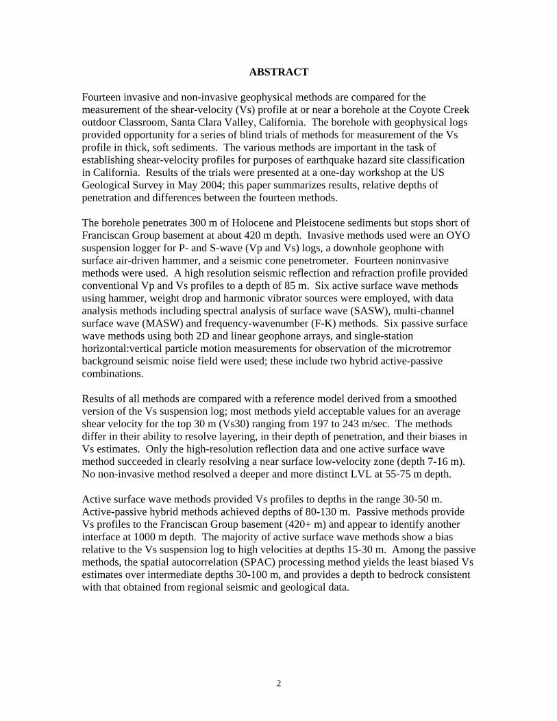
Fourteen invasive and non-invasive geophysical methods are compared for the measurement of the shear-velocity (Vs) profile at or near a borehole at the Coyote Creek outdoor Classroom, Santa Clara Valley, California. The borehole with geophysical logs provided opportunity for a series of blind trials of methods for measurement of the Vs profile in thick, soft sediments. The various methods are important in the task of establishing shear-velocity profiles for purposes of earthquake hazard site classification in California. Results of the trials were presented at a one-day workshop at the US Geological Survey in May 2004; this paper summarizes results, relative depths of penetration and differences between the fourteen methods. The borehole penetrates 300 m of Holocene and Pleistocene sediments but stops short of Franciscan Group basement at about 420 m depth. Invasive methods used were an OYO suspension logger for P- and S-wave (Vp and Vs) logs, a downhole geophone with surface air-driven hammer, and a seismic cone penetrometer. Fourteen noninvasive methods were used. A high resolution seismic reflection and refraction profile provided conventional Vp and Vs profiles to a depth of 85 m. Six active surface wave methods using hammer, weight drop and harmonic vibrator sources were employed, with data analysis methods including spectral analysis of surface wave (SASW), multi-channel surface wave (MASW) and frequency-wavenumber (F-K) methods. Six passive surface wave methods using both 2D and linear geophone arrays, and single-station horizontal:vertical particle motion measurements for observation of the microtremor background seismic noise field were used; these include two hybrid active-passive combinations. Results of all methods are compared with a reference model derived from a smoothed version of the Vs suspension log; most methods yield acceptable values for an average shear velocity for the top 30 m (Vs30) ranging from 197 to 243 m/sec. The methods differ in their ability to resolve layering, in their depth of penetration, and their biases in Vs estimates. Only the high-resolution reflection data and one active surface wave method succeeded in clearly resolving a near surface low-velocity zone (depth 7-16 m). No non-invasive method resolved a deeper and more distinct LVL at 55-75 m depth. Active surface wave methods provided Vs profiles to depths in the range 30-50 m. Active-passive hybrid methods achieved depths of 80-130 m. Passive methods provide Vs profiles to the Franciscan Group basement (420+ m) and appear to identify another interface at 1000 m depth. The majority of active surface wave methods show a bias relative to the Vs suspension log to high velocities at depths 15-30 m. Among the passive methods, the spatial autocorrelation (SPAC) processing method yields the least biased Vs estimates over intermediate depths 30-100 m, and provides a depth to bedrock consistent with that obtained from regional seismic and geological data.

3

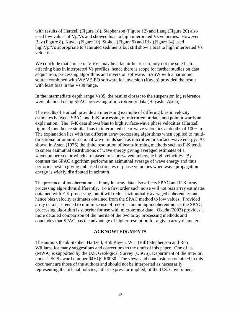
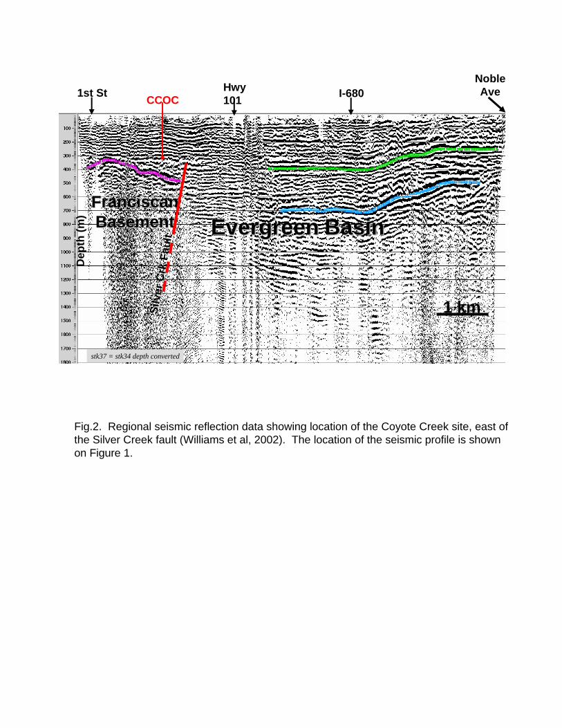
INTRODUCTION Measurement or estimation of the shear-velocity (Vs) profile of sediments overlying geological basement is a vital part of site zonation studies for earthquake hazard prediction, and more generally for geotechnical studies. A series of boreholes drilled in the Santa Clara Valley Water District provide opportunity for the comparison of geophysical methods with known geological data. This paper compares the shear-wave velocity profiles obtain from fourteen invasive and non-invasive methodologies obtained in and near a single 300 m borehole. The selected site is CCOC (the Coyote Creek Outdoor Classroom). The geology and hydrology is summarized by Hanson et al (2002). The site is within 200 m of the William Street Park which provides abundant open space for layout of seismic arrays used in the comparisons described herein. Figure 1 (from Wentworth and Tinsley, 2005) and Figure 2 (from Williams et al, 2002) show the site relative to the Valley and the nearest basement structure. The comparisons are grouped into four categories for invasive measurements, active-source seismic measurements, combined active-passive seismic, and passive seismic (ie microtremor) methods, totaling fourteen techniques listed in Table 1 below. Results are plotted as both Vs and shear-slowness (Ss) in order to accommodate the needs of both convention (NEHRP standards, see eg. Dobry et al., 2000; BSSC, 2001) and of wave physics (slowness is the “natural” parameter affecting seismic energy travel times, and site response, as pointed out by Brown et al, 2002). While the site of the borehole forming the reference for the study is the Coyote Creek Outdoor Classroom, the majority of surface-wave measurements were conducted (for access and space reasons) at the William Street Park, located 200 m south-west of the CCOC borehole (Figure 3). There is obvious potential for variation in seismic properties over this distance, but comparison of two active methods at both sites suggests variation in shear velocity in the top 30 m is below the uncertainty in estimates of the shear-velocity profile. On a larger scale, the William Street Park site is along strike from the CCOC borehole (where strike is defined by the NW-SE trending Silver Creek fault shown in Figure 1). When comparing results (in this case Vs or Ss) derived from different methodologies the additional question arises as to which (if any) method should be used as a “reference”. For the purposes of this study we have adopted a smoothed version of the shear-wave suspension log as a reference, since it has depth coverage to 293 m, and has higher vertical resolution than all other tools. However that does not necessarily imply that it is the most “correct” representation of the shear-wave velocity profile; as Glenn Rix (personal communication) points out, “each type of seismic measurement is very different and captures a different aspect of the properties at the site. For example, the suspension PS logger, downhole test and surface wave test sample increasingly larger

4

volumes of soil. If the soil conditions are heterogeneous (which they most certainly are), each test will measure different values of velocity”.

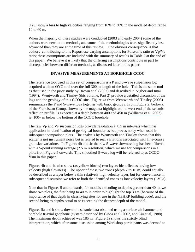
TABLE 1

SUMMARY OF SEISMIC METHODS APPLIED TO SHEAR-VELOCITY STUDIES AT THE COYOTE CREEK & WILLIAM ST PARK SITES

Method Personnel Description Location

# INVASIVE METHODS1 CCOC Geological summary Carl Wentworth, John Tinsley & Suspension log & Rob Steller P and S-wave logs from surface to 300m, 0Coy. Creek borehole2 Surface source, downhole receiver Jim Gibbs Coy. Creek borehole2 Reinterpretation for detail Gibs and Boore Coy. Creek borehole3 SCPT Tom Holzer Data collected at CCOC and WSP CCOC, WSP

ACTIVE SEISMIC METHODS4 High-resolution reflection/refraction Rob Williams 60-channel linear array, 3 meter spacing CCOC - in William St. Park (WSP)5 SASW James Bay, J. Gilbert Spec analysis of surface waves (SASW) CCOC, WSP6 SASW Rob Kayen SASW with harmonic source WSP7 MASW Bill Stephenson CCOC, GUAD boreholes, WSP8 SASW Ken Stokoe & Yin-Cheng Lin CCOC, WSP

ACTIVE & PASSIVE SEISMIC METHODS COMBINED9 MASW Koichi Hayashi Multichannel analysis of surface waves Coy. Creek-- park, 46m line

& MAM with SPAC processing & microtremor array method (MAM) Coy. Creek-- park, 40m triangle10 FK processing Sungsoo Yoon, Glenn Active test with linear array WSP

Rix & Rob Kayen & Passive tests with circular arrays WSP

PASSIVE MICROTREMOR METHODS11 MMSPAC Michael Asten Interpretation of data collected by Coy. Creek-- borehole, 60m triangle

R. Sell, H. Flores Coy. Creek-- park, 60m triangle ditto Coy. Creek-- park, 300m triangle

12 Single-station HVSR Dominic Lang Horizontal/vertical particle motion ratio Coy Ck & WSP13 FK and SPAC Steve Hartzell, D. Carve10-station array,100m embedded triangle aCoy. Creek-- park14 ReMi Bill Stephenson Microtremors observed with linear array CCOC, GUAD boreholes, other?

ACRONYMSSASW Spectral analysis of surface waves MASW Multichannel analysis of surface waves MAM Microtremor array methodSPAC Spatial AutoCorrelation method of processing seismic array data MMSPAC Multi-mode SPACF-K Frequency-wavenumber method of processing seismic array data HVSR Horizontal/Vertical spectral ratio method (on single station microtremor data)ReMi Refraction microtremor methodCCOC Coyote Creek Outdoor ClassroomWSP William Street Park

It is well known that Rayleigh-wave phase velocities are most strongly affected by Vs and thicknesses in a layered earth, with Vp and densities having a sufficiently small effect that these latter parameters are generally assumed as fixed values by interpreters rather than included as variables in an inversion scheme. However the choice of Vp does have a non-negligible influence on the outcome of inversions. Brown (1998) shows a comparison between Vs profiles computed from SASW data in sediments at strong motion sites in California using Vp computed from a fixed Poisson’s ratio of 0.25 (equivalently a Vp/Vs ratio of 1.73), and using Vp (more correctly) set at a value of 1524 m/sec typical of saturated unconsolidated sediments. The interpreted Vs profiles, when using the erroneously low values Vp computed from the assumed fixed Poisson’s ratio of

5

0.25, show a bias to high velocities ranging from 10% to 30% in the modeled depth range 10 to 60 m. When the majority of these studies were conducted (2003 and early 2004) some of the authors were new to the methods, and some of the methodologies were significantly less advanced than they are at the time of this review. One obvious consequence is that authors contributing to this Report use varying assumptions for Poisson’s ratio or Vp/Vs ratio; these assumptions are included with the summary of results in Table 2 at the end of this paper. We believe it is likely that the differing assumptions contribute in part to discrepancies between different methods, as discussed later in this paper.

INVASIVE MEASUREMENTS AT BOREHOLE CCOC The reference tool used in this set of comparisons is a P and S-wave suspension log, acquired with an OYO tool over the full 300 m length of the hole. This is the same tool as that used in the prior study by Brown et al (2002) and described in Nigbor and Imai (1994). Wentworth and Tinsley (this volume, Part 2) provide a detailed discussion of the logs and the geology of this CCOC site. Figure 4a from Wentworth and Tinsley (2005) summarizes the P and S-wave logs together with basic geology. From Figure 2, bedrock of the Franciscan Group, shown by the magenta highlight on the west end of the seismic reflection profile, is expected at a depth between 400 and 450 m (Williams et al, 2002), ie. 100+ m below the bottom of the CCOC borehole. The raw Vp and Vs suspension logs provide resolution at 0.5 m intervals which has application in identification of geological boundaries but proves noisy when used in subsequent comparison plots. The analysis by Wentworth and Tinsley shows that this scatter is not instrument noise but is related to real variations associated with fine-coarse grainsize variations. In Figures 4b and 4c the raw S-wave slowness log has been filtered with a 5-point running average (2.5 m resolution) which we use for comparisons in all plots from Figure 5 onwards. This smoothed S-wave log will be referred to as CCOC-Vsm in this paper. Figures 4b and 4c also show (as yellow blocks) two layers identified as having low-velocity (high slowness). The upper of these two zones (depth 7 to 16 m) could equally be described as a layer below a thin relatively high velocity layer, but for convenience in subsequent discussion we refer to both the identified zones as low velocity layers (LVLs). Note that in Figures 5 and onwards, for models extending to depths greater than 40 m, we show two plots, the first being to 40 m in order to highlight the top 30 m (because of the importance of that depth in classifying sites for use in the NEHRP building code), and the second being to depths equal to or exceeding the deepest depth of the model. Figures 5a and b show downhole seismic data obtained using a surface air-hammer and borehole triaxial geophone (system described by Gibbs et al, 2002, and Liu et al, 1988). The maximum depth achieved was 185 m. Figure 5a shows the strictly blind interpretation, which after some discussion among Workshop participants was deemed to

6

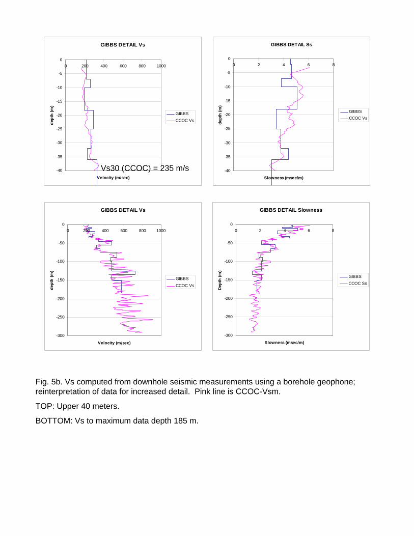
have insufficient detail. A reinterpretation of the raw data was undertaken to provide more detail (see Gibbs and Boore, this volume, Part 3) Figure 5b shows the results of the reinterpretation; being done after May 2004 these data are not a blind test in the strictest sense. The correspondence between derived Vs and CCOC-Vsm shows a bias to high velocities in the upper 15 m, but is unbiased relative to CCOC-Vsm from 15 m to 185 m. The reinterpretation shows that the method achieves on the order of 5 m resolution in the upper 50 m, and 10 m resolution elsewhere. In particular the deeper of the two LVLs (55 to 75 m depth) is clearly resolved. The seismic cone penetrometer (SCPT) method is described by Holzer et al (2005). The method is invasive while having the advantage of avoiding the cost of drilling a hole, but has a limitation that cone penetration depth may be limited if gravels or cemented sands are encountered. SCPT measurements were made at the CCOC hole, and at the William Street Park, reaching depths of 38 m and 20 m respectively. Figure 6 shows (SCPT) the interpretation of data acquired at the CCOC hole site. The measured Vs follows the CCOC-Vsm trend with resolution limited to 5-10 m in this example. Velocities appear biased of order 15 % high relative to CCOC-Vsm.

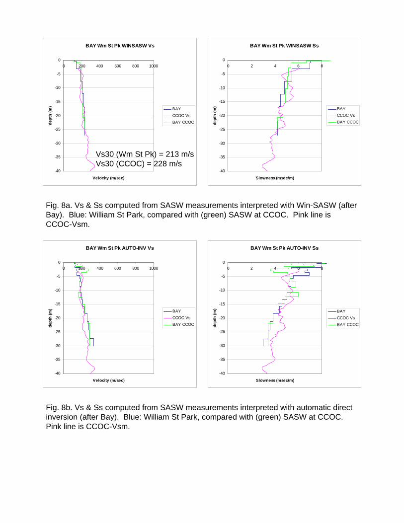
ACTIVE-SOURCE SEISMIC METHODS The active source methods were conducted in the William Street Park (200 m SE of the CCOC hole). A conventional seismic reflection/refraction survey was conducted with a spread of length 180 m, 3 m sensor spacing and 1 msec sample interval. Figure 7 shows the results plotted to depths of 30 m and 80 m (the depth to the deepest detected reflector) (Williams et al, this volume, Part 2). The plotted Vs shows no obvious bias relative to CCOC-Vsm, and successfully resolves a thin LVL at 7-16 m depth. However it does not detect the lower LVL identified on Figure 4b (55-75 m). Figures 8 and 9 show interpretations for active SASW methods performed by two different practitioners at both the William Street Park site and the CCOC borehole site. The results from the pair of sites support the statement made earlier that there is no significant difference in Vs profile between the sites at depths between about 5 m and at least 30 m. Figure 8 shows results from a SASW survey conducted using a weight-drop source and a linear array of geophones spaced at intervals from 3.3 to 15 m (Bay et al, this Volume, Part 2 and Part 3). Data were acquired both at the William Street Park and at the CCOC site. Observed dispersion data were processed both by iterative forward modelling using the Win-SASW software, and by direct inversion. Figure 8a shows the former which gives the preferred interpreted Vs profiles, and is depth-limited at 28 m. Within the uncertainty of the data there is no evidence for any significant difference between the Vs profiles at the two sites at depths greater than 3 to 5 m. The plotted Vs profiles show no obvious bias relative to CCOC-Vsm, but do not appear to resolve any detail of low or high velocity layers.

7

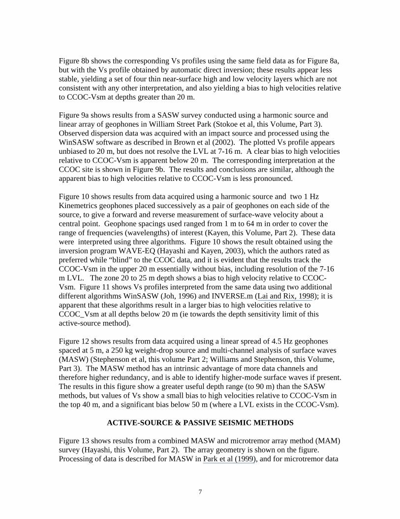
Figure 8b shows the corresponding Vs profiles using the same field data as for Figure 8a, but with the Vs profile obtained by automatic direct inversion; these results appear less stable, yielding a set of four thin near-surface high and low velocity layers which are not consistent with any other interpretation, and also yielding a bias to high velocities relative to CCOC-Vsm at depths greater than 20 m. Figure 9a shows results from a SASW survey conducted using a harmonic source and linear array of geophones in William Street Park (Stokoe et al, this Volume, Part 3). Observed dispersion data was acquired with an impact source and processed using the WinSASW software as described in Brown et al (2002). The plotted Vs profile appears unbiased to 20 m, but does not resolve the LVL at 7-16 m. A clear bias to high velocities relative to CCOC-Vsm is apparent below 20 m. The corresponding interpretation at the CCOC site is shown in Figure 9b. The results and conclusions are similar, although the apparent bias to high velocities relative to CCOC-Vsm is less pronounced. Figure 10 shows results from data acquired using a harmonic source and two 1 Hz Kinemetrics geophones placed successively as a pair of geophones on each side of the source, to give a forward and reverse measurement of surface-wave velocity about a central point. Geophone spacings used ranged from 1 m to 64 m in order to cover the range of frequencies (wavelengths) of interest (Kayen, this Volume, Part 2). These data were interpreted using three algorithms. Figure 10 shows the result obtained using the inversion program WAVE-EQ (Hayashi and Kayen, 2003), which the authors rated as preferred while “blind” to the CCOC data, and it is evident that the results track the CCOC-Vsm in the upper 20 m essentially without bias, including resolution of the 7-16 m LVL. The zone 20 to 25 m depth shows a bias to high velocity relative to CCOC-Vsm. Figure 11 shows Vs profiles interpreted from the same data using two additional different algorithms WinSASW (Joh, 1996) and INVERSE.m (Lai and Rix, 1998); it is apparent that these algorithms result in a larger bias to high velocities relative to CCOC_Vsm at all depths below 20 m (ie towards the depth sensitivity limit of this active-source method). Figure 12 shows results from data acquired using a linear spread of 4.5 Hz geophones spaced at 5 m, a 250 kg weight-drop source and multi-channel analysis of surface waves (MASW) (Stephenson et al, this volume Part 2; Williams and Stephenson, this Volume, Part 3). The MASW method has an intrinsic advantage of more data channels and therefore higher redundancy, and is able to identify higher-mode surface waves if present. The results in this figure show a greater useful depth range (to 90 m) than the SASW methods, but values of Vs show a small bias to high velocities relative to CCOC-Vsm in the top 40 m, and a significant bias below 50 m (where a LVL exists in the CCOC-Vsm).

ACTIVE-SOURCE & PASSIVE SEISMIC METHODS Figure 13 shows results from a combined MASW and microtremor array method (MAM) survey (Hayashi, this Volume, Part 2). The array geometry is shown on the figure. Processing of data is described for MASW in Park et al (1999), and for microtremor data

8

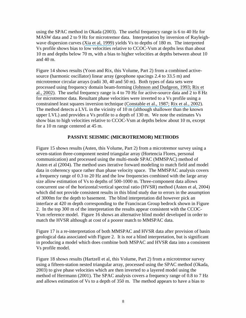
using the SPAC method in Okada (2003). The useful frequency range is 6 to 40 Hz for MASW data and 2 to 9 Hz for microtremor data. Interpretation by inversion of Rayleigh-wave dispersion curves (Xia et al, 1999) yields Vs to depths of 180 m. The interpreted Vs profile shows bias to low velocities relative to CCOC-Vsm at depths less than about 10 m and depths below 70 m, with a bias to higher velocities at depths between about 10 and 40 m. Figure 14 shows results (Yoon and Rix, this Volume, Part 2) from a combined active-source (harmonic oscillator) linear array (geophone spacings 2.4 to 33.5 m) and microtremor circular arrays (radii 30, 40 and 50 m). Both types of data sets were processed using frequency domain beam-forming (Johnson and Dudgeon, 1993; Rix et al., 2002). The useful frequency range is 4 to 70 Hz for active-source data and 2 to 8 Hz for microtremor data. Resultant phase velocities were inverted to a Vs profile using a constrained least squares inversion technique (Constable et al., 1987; Rix et al., 2002). The method detects a LVL in the vicinity of 10 m (although shallower than the known upper LVL) and provides a Vs profile to a depth of 130 m. We note the estimates Vs show bias to high velocities relative to CCOC-Vsm at depths below about 10 m, except for a 10 m range centered at 45 m.

PASSIVE SEISMIC (MICROTREMOR) METHODS Figure 15 shows results (Asten, this Volume, Part 2) from a microtremor survey using a seven-station three-component nested triangular array (Hortencia Flores, personal communication) and processed using the multi-mode SPAC (MMSPAC) method of Asten et al (2004). The method uses iterative forward modeling to match field and model data in coherency space rather than phase velocity space. The MMSPAC analysis covers a frequency range of 0.3 to 20 Hz and the low frequencies combined with the large array size allow estimation of Vs to depths of 500-1000 m. Three-component data allows concurrent use of the horizontal:vertical spectral ratio (HVSR) method (Asten et al, 2004) which did not provide consistent results in this blind study due to errors in the assumption of 3000m for the depth to basement. The blind interpretation did however pick an interface at 420 m depth corresponding to the Franciscan Group bedrock shown in Figure 2. In the top 300 m of the interpretation the results appear consistent with the CCOC-Vsm reference model. Figure 16 shows an alternative blind model developed in order to match the HVSR although at cost of a poorer match to MMSPAC data. Figure 17 is a re-interpretation of both MMSPAC and HVSR data after provision of basin geological data associated with Figure 2. It is not a blind interpretation, but is significant in producing a model which does combine both MSPAC and HVSR data into a consistent Vs profile model. Figure 18 shows results (Hartzell et al, this Volume, Part 2) from a microtremor survey using a fifteen-station nested triangular array, processed using the SPAC method (Okada, 2003) to give phase velocities which are then inverted to a layered model using the method of Herrmann (2001). The SPAC analysis covers a frequency range of 0.8 to 7 Hz and allows estimation of Vs to a depth of 350 m. The method appears to have a bias to

9

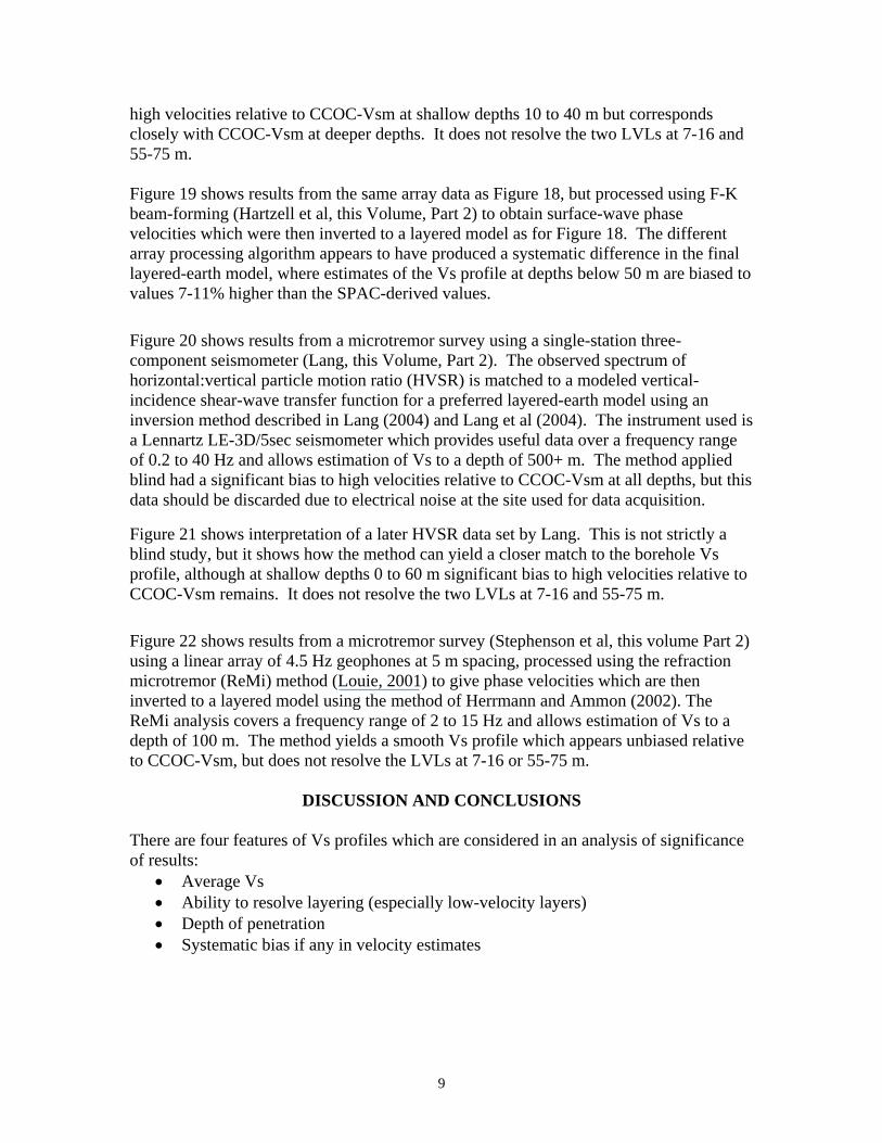
high velocities relative to CCOC-Vsm at shallow depths 10 to 40 m but corresponds closely with CCOC-Vsm at deeper depths. It does not resolve the two LVLs at 7-16 and 55-75 m. Figure 19 shows results from the same array data as Figure 18, but processed using F-K beam-forming (Hartzell et al, this Volume, Part 2) to obtain surface-wave phase velocities which were then inverted to a layered model as for Figure 18. The different array processing algorithm appears to have produced a systematic difference in the final layered-earth model, where estimates of the Vs profile at depths below 50 m are biased to values 7-11% higher than the SPAC-derived values. Figure 20 shows results from a microtremor survey using a single-station three-component seismometer (Lang, this Volume, Part 2). The observed spectrum of horizontal:vertical particle motion ratio (HVSR) is matched to a modeled vertical-incidence shear-wave transfer function for a preferred layered-earth model using an inversion method described in Lang (2004) and Lang et al (2004). The instrument used is a Lennartz LE-3D/5sec seismometer which provides useful data over a frequency range of 0.2 to 40 Hz and allows estimation of Vs to a depth of 500+ m. The method applied blind had a significant bias to high velocities relative to CCOC-Vsm at all depths, but this data should be discarded due to electrical noise at the site used for data acquisition.

Figure 21 shows interpretation of a later HVSR data set by Lang. This is not strictly a blind study, but it shows how the method can yield a closer match to the borehole Vs profile, although at shallow depths 0 to 60 m significant bias to high velocities relative to CCOC-Vsm remains. It does not resolve the two LVLs at 7-16 and 55-75 m. Figure 22 shows results from a microtremor survey (Stephenson et al, this volume Part 2) using a linear array of 4.5 Hz geophones at 5 m spacing, processed using the refraction microtremor (ReMi) method (Louie, 2001) to give phase velocities which are then inverted to a layered model using the method of Herrmann and Ammon (2002). The ReMi analysis covers a frequency range of 2 to 15 Hz and allows estimation of Vs to a depth of 100 m. The method yields a smooth Vs profile which appears unbiased relative to CCOC-Vsm, but does not resolve the LVLs at 7-16 or 55-75 m.

DISCUSSION AND CONCLUSIONS There are four features of Vs profiles which are considered in an analysis of significance of results:

• Average Vs • Ability to resolve layering (especially low-velocity layers) • Depth of penetration • Systematic bias if any in velocity estimates

10

TABLE 2SUMMARY OF RESULTS OF SHEAR-VELOCITY STUDIES AT THE COYOTE CREEK & WILLIAM ST PARK SITES

# Method Personnel Maximum Source of Vp Vs30 Vs85 Vs185 Vs293 Depth (m/s) (m/s) (m/s) (m/s)

(m)INVASIVE METHODS

1 CCOC Geological summary Carl Wentworth, John Tinsley measured & Suspension log & Rob Steller 293 206 284 374 4412 Surface source, downhole receiver Jim Gibbs 185 measured 235 302 3912 Reinterpretation for detail Gibbs and Boore * 185 measured 233 3013 SCPT at CCOC Tom Holzer 37 measured 236

ACTIVE SEISMIC METHODS4 Hi-res reflection/refraction Rob Williams 85 measured 219 3055 SASW James Bay, J. Gilbert 30 Prat*=0.30 above WT** at 7.6 m. 213 WSP

30 Prat=0.30 above WT at 5.8 m. 228 CCOC

6 SASW Rob Kayen 32 Prat=0.33 above WT, =.48 below WT 1977 MASW Bill Stephenson 100 Prat=0.33 220 3468 SASW Ken Stokoe & Yin-Cheng Lin 38 Prat=0.33 above WT, Vp=1524 below WT 205-231 WSP

( depth to wt varies from 2 to 3.2m) 202-211 CCOCACTIVE & PASSIVE SEISMIC METHODS COMBINED

9 MASW Koichi Hayashi 80 Prat ranging from 0.497 at surface 209 292& MAM with SPAC processing to 0.473 at bottom of model

10 FK processing Sungsoo Yoon, Glenn 130

Prat = 0.20 above 6 m and 0.48 below 6 m, where 6 m is an assumed depth to the top of the water table 222 321

Rix & Rob Kayen Prat = 0.20 above 6 m and 0.48 below 6 mwhere 6 m is assumed depth to WT

PASSIVE MICROTREMOR METHODS11 Multi-mode Spatial AutoCorrelation Michael Asten 500 Prat=0.33 above assumed water table at 10 m 233 303 405 488

(MMSPAC) * 1000 Prat ranges from 0.49 at 10 m to 0.33 at 420 m 230 298 401 484

12 Single-station HVSR Dominic Lang 512 Prat=0.25 341 452 574 722* 512 Prat increases from negative values in top 4 m 280 336 429 491

to 0.41at 171m, then decr to 0.25 at 521 m13 SPAC Steve Hartzell, D. Carver 350 Prat=0.33 243 327 422 494

FK 350 Prat=0.33 263 343 453 534

14 Refraction-microtremor Bill Stephenson 100 Prat=0.33 224 311* Result is a re-interpretation, ie. not strictly blind

*Prat = Poisson's Ratio**WT = Water Table

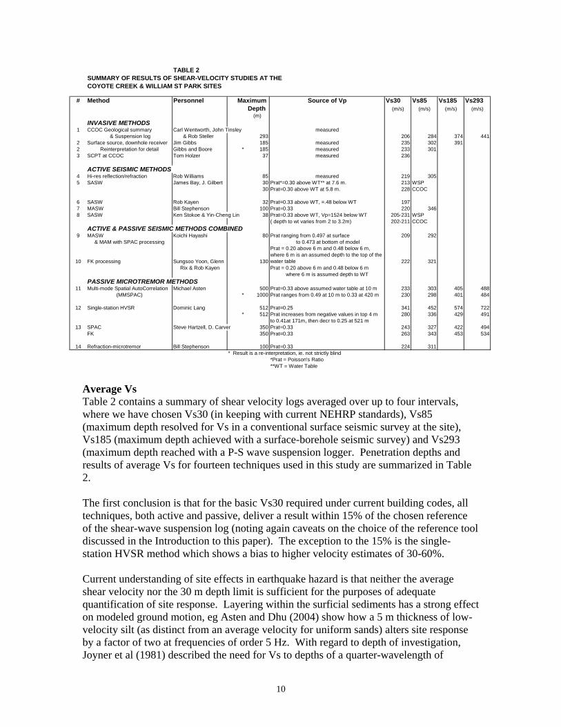
Average Vs Table 2 contains a summary of shear velocity logs averaged over up to four intervals, where we have chosen Vs30 (in keeping with current NEHRP standards), Vs85 (maximum depth resolved for Vs in a conventional surface seismic survey at the site), Vs185 (maximum depth achieved with a surface-borehole seismic survey) and Vs293 (maximum depth reached with a P-S wave suspension logger. Penetration depths and results of average Vs for fourteen techniques used in this study are summarized in Table 2. The first conclusion is that for the basic Vs30 required under current building codes, all techniques, both active and passive, deliver a result within 15% of the chosen reference of the shear-wave suspension log (noting again caveats on the choice of the reference tool discussed in the Introduction to this paper). The exception to the 15% is the single-station HVSR method which shows a bias to higher velocity estimates of 30-60%. Current understanding of site effects in earthquake hazard is that neither the average shear velocity nor the 30 m depth limit is sufficient for the purposes of adequate quantification of site response. Layering within the surficial sediments has a strong effect on modeled ground motion, eg Asten and Dhu (2004) show how a 5 m thickness of low-velocity silt (as distinct from an average velocity for uniform sands) alters site response by a factor of two at frequencies of order 5 Hz. With regard to depth of investigation, Joyner et al (1981) described the need for Vs to depths of a quarter-wavelength of

11

seismically relevant frequencies, which is of order 500 m at the CCOC site (frequency 0.3 Hz). It is therefore appropriate to review the results in terms of both resolution of layering, and total depth of penetration. Detection of LVL It is apparent from both the suspension log and the downhole receiver survey (Figure 5) that the CCOC hole contains two dominant low velocity layers of thickness 9 m and 20 m with tops at 7 and 50 m depths respectively. Three of the non-invasive seismic methods resolved the upper LVL, being high-resolution surface seismic reflection-refraction (Williams), SASW with a harmonic source and WAVE-EQ software (Kayen), and the use of a harmonic source with F-K analysis and direct inversion of the dispersion curve (Rix). The last of these may be questionable being depth-shifted and too shallow by 3 m (30%). The lower LVL at 55 m depth is beyond range of the purely active surface-wave methods. None of the non-invasive seismic methods employed here succeeded in resolving either this LVL or the thin high-velocity layer of coarse gravels overlying it. Depth of penetration Obtaining shear-velocity data to depths of order 100 m was achieved by hi-res surface seismic (Williams), possibly by MASW (Stephenson) although bias is evident at depths greater than 50 m, and clearly by use of each of the passive methods. While information to 100 m is highly desirable, it is evident that the technology in active surface-wave methods as applied at this site is generally insufficient for obtaining Vs100. Passive microtremor array methods using 2D arrays all proved effective in gaining depth penetration to 300+ m. The combination of an array of 300 m diameter, SPAC processing, and HVSR measurements correctly resolved Franciscan Group bedrock at a depth of 420-550 m, and may have resolved a further basement boundary at 1000 m depth (Asten), although no deeper P-wave impedance boundaries were imaged in the seismic profile at the projected location of CCOC (Figure 2). . Bias in array estimates and shear-velocity measurements Among the active methods, significant bias to high velocities in the 15-30 m depth range affects the majority of active methods (Bay, Kayen, Stokoe, Rix, Stephenson MASW). The cause of discrepancies could lie with any or all of the source type (impulsive or harmonic), the processing algorithm, the surface-wave phase- velocity inversion algorithms used, and assumptions made regarding the P-wave velocity profile. The potential importance of the P-wave velocity profile as established by Brown (1998) is noted in the Introduction of this paper. Table 2 includes a summary of assumptions regarding Poisson’s ratio made by each author. Actual Vp/Vs ratios in the depth interval 10 to 40 m (Figure 4b) range from 8 to 5, and trend downwards with depth reducing to ratios of order 3 at the base of the hole. This would suggest that bias associated with use of low values of Vp/Vs will be greatest in the interval 10 to 40 m, a prediction consistent

12

with results of Hartzell (Figure 18). Stephenson (Figure 12) and Lang (Figure 20) also used low values of Vp/Vs and showed bias to high interpreted Vs velocities. However Bay (Figure 8), Kayen (Figure 10), Stokoe (Figure 9) and Rix (Figure 14) used highVp/Vs appropriate to saturated sediments but still show a bias to high interpreted Vs velocities. We conclude that choice of Vp/Vs may be a factor but is certainly not the sole factor affecting bias in interpreted Vs profiles, hence there is scope for further studies on data acquisition, processing algorithms and inversion software. SASW with a harmonic source combined with WAVE-EQ software for inversion (Kayen) provided the result with least bias in the Vs30 range. In the intermediate depth range Vs85, the results closest to the suspension log reference were obtained using SPAC processing of microtremor data (Hayashi, Asten). The results of Hartzell provide an interesting example of differing bias in velocity estimates between SPAC and F-K processing of microtremor data, and point towards an explanation. The F-K data shows bias to high surface-wave phase velocities (Hartzell figure 3) and hence similar bias in interpreted shear-wave velocities at depths of 100+ m. The explanation lies with the different array processing algorithms when applied to multi-directional or omni-directional wave fields such as microtremor surface-wave energy. As shown in Asten (1976) the finite resolution of beam-forming methods such as F-K tends to smear azimuthal distributions of wave energy giving averaged estimates of a wavenumber vector which are biased to short wavenumbers, ie high velocities. By contrast the SPAC algorithm performs an azimuthal average of wave energy and thus performs best in giving unbiased estimates of phase velocities when wave propagation energy is widely distributed in azimuth. The presence of incoherent noise if any in array data also affects SPAC and F-K array processing algorithms differently. To a first order such noise will not bias array estimates obtained with F-K processing, but it will reduce azimuthally averaged coherencies and hence bias velocity estimates obtained from the SPAC method to low values. Provided array data is screened to minimize use of records containing incoherent noise, the SPAC processing algorithm is superior for use with microtremor data. Okada (2003) provides a more detailed comparison of the merits of the two array processing methods and concludes that SPAC has the advantage of higher resolution for a given array diameter.

ACKNOWLEDGMENTS The authors thank Stephen Hartzell, Rob Kayen, W.J. (Bill) Stephenson and Rob Williams for many suggestions and corrections to the draft of this paper. One of us (MWA) is supported by the U.S. Geological Survey (USGS), Department of the Interior, under USGS award number 04HQGR0030. The views and conclusions contained in this document are those of the authors and should not be interpreted as necessarily representing the official policies, either express or implied, of the U.S. Government.

13

REFERENCES Asten, M.W., (1976). The use of microseisms in geophysical exploration, PhD Thesis,

Macquarie University, Sydney. Asten, MW, and Dhu, T., (2004). Site response in the Botany area, Sydney, using

microtremor array methods and equivalent linear site response modelling . Australian Earthquake Engineering in the New Millennium, Proceedings of a conference of the Australian Earthquake Engineering Soc., Mt Gambier South Australia, Paper 33.

Asten,M.W., Dhu, T., and Lam,N., (2004). Optimised array design for microtremor array studies applied to site classification; observations, results and future use: Proceedings of the 13th World Conference of Earthquake Engineering, Vancouver, August 2004.

Brown, L.T., (1998). Comparison of Vs profiles from SASW and borehole measurements at strong motion sites in southern California. MSc thesis, University of Texas, Austin.

Brown, L.T., Boore, D.M., and Stoke, K.H., (2002). Comparison of shear-wave slowness profiles at ten striong-motion sites from non-invasive SASW measurements and measurements made in boreholes. Bull. Seism. Soc. Am. 92, 3116-3133.

BSSC (2001). NEHRP recommended provisions for seismic regulations for new buildings and other structures, 2000 Edition, Part 1: Provisions, prepared by the Building Seismic Safety Council for the Federal Emergency Management Agency (Report No. FEMA 368), Washington, D.C.

Constable, S.C., Parker, R.L., and Constable, C.G. (1987). "Occam's Inversion: A Practical Algorithm for Generating Smooth Models from Electromagnetic Sounding Data", Geophysics, 52, 289-300.

Dobry, R., R. D. Borcherdt, C. B. Crouse, I. M. Idriss, W. B. Joyner, G. R. Martin, M. S. Power, E. E. Rinne, and R. B. Seed (2000). New site coefficients and site classification system used in recent building seismic code provisions: Earthquake Spectra 16, 41–67.

Gibbs, J.F., John C. Tinsley,J.C. and Boore, D.M., (2002). Borehole velocity measurements at five sites that recorded the Cape Mendocino, California earthquake of 25 April, 1992: U.S. Geological Survey Open-File Report OF 02 -203.

Hanson, R.T., (2002). Santa Clara Valley Water District multi-acquifer monitoring-well site, Coyote Creek Outdoor Classroom, San Jose, California, USGS Open File Report #02-369.

Hayashi, K. and Kayen, R. (2003). Comparative test of three surface wave methods at William Street Park in San Jose, USA. Paper S051-009, 2003 Joint Meeting of Japan Earth and Planetary Science , University of Tokyo, Tokyo, Japan 2003 Joint Meeting, May 26-29, 2003.

Herrmann, R.B., (2001). Computer programs in seismology - an overview of synthetic seismogram computation Version 3.1, Department of Earth and Planetary Sciences, St Louis Univ.

Herrmann, R.B., and Ammon, C.J. (2002). Computer programs in seismology version 3.2: surface waves, receiver functions and crustal structure, St Louis Univ., Missouri.

Holzer, T.L., Bennett, M.J., Noce, T.E., and Tinsley, J.C., III, (2005). Shear-wave velocity of surficial geologic sediments in Northern California: Statistical distributions and depth dependence: Earthquake Spectra, v. 21(1), xx-xx. (In press).

14

Joh, S.-H. (1996). Advances in Interpretation and Analysis Techniques for Spectral-Analysis-of-Surface-Waves (SASW) Measurements, Ph.D. Dissertation, University of Texas at Austin, Austin, TX.

Johnson, D.H., and Dudgeon, D.E. (1993). Array Signal Processing; Concepts and Techniques, PTR Prentice-Hall, New Jersey, 533 pp.

Joyner, W. B., R. E. Warrick, and T. E. Fumal (1981). The effect of Quaternary alluvium on strong ground motion in the Coyote Late, California, earthquake of 1979, Bull. Seism. Soc. Am. 71, 1333–1349.

Lai, C.G., and G. J. Rix (1998). Simultaneous Inversion of Rayleigh Phase Velocity and Attenuation for Near-Surface Site Characterization," Report No. GIT-CEE/GEO-98-2, Georgia Institute of Technology, School of Civil and Environmental Engineering, 258 pp.

Lang D.H. (2004). Damage potential of seismic ground motion considering local site effects. Scientific technical reports Vol. 01 (2004), Earthquake Damage Analysis Center, Bauhaus-University Weimar, 293 pp. (PhD thesis)

Lang, D.H., Schwarz, J., Ende, C. (2004). Subsoil classification of strong-motion recording sites in Turkish earthquake regions. Schriften der Bauhaus-Universität Weimar 116 (2004): 79--89.

Liu, H.-P., R.E. Warrick, R.E. Westerlund, J.B. Fletcher, and G.L. Maxwell (1988). An air-powered impulsive shear-wave source with repeatable signals, Bull. Seism. Soc. Am. 78, 355–369.

Louie, J. N. (2001). Faster, better: shear-wave velocity to 100 meters depth from refraction microtremor arrays, Bull. Seism. Soc. Am., 91, 347–364.

Nigbor, R. L., and T. Imai (1994). The suspension P-S velocity logging method, in Geophysical Characterization of Sites, Technical Committee for XIII ICSMFE, A. A. Balkema, Rotterdam, The Netherlands, 57–61.

Okada, H. (2003). The Microseismic Survey Method, Society of Exploration Geophysicists of Japan. Translated by Koya Suto, Geophysical Monographs, Vol 12, Society of Exploration Geophysicists, Tulsa.

Park, C. B., Miller, R. D., and Xia, J., (1999). Multimodal analysis of high frequency surface waves : Proceedings of the symposium on the application of geophysics to engineering and environmental problems '99, 115-121.

Rix, G. J., Hebeler, G. L., and Orozco, M. C. (2002). Near-Surface Vs Profiling in the New Madrid Seismic Zone Using Surface Wave Methods, Seismological Research Letters, 73(3), 380-392.

Wentworth, C.M., and Tinsley, J.C., (2005). Detailed stratigraphy and velocity structure of Quaternary alluvial sediments, Santa Clara Valley, California: paper presented at the Annual Northern California Earthquake Hazards Workshop January 18-19,2005, USGS, Menlo Park.

Williams, R.A., Stephenson, W.J., Wentworth, C.M., Odum, J.K., Hanson, R.T., and R.C. Jachens, (2002). Definition of the Silver Creek fault and Evergreen Basin sediments from seismic reflection data, San Jose, California: EOS Transactions, Fall AGU meeting, v. 83, no. 47, p. F1313.

Xia, J., Miller, R. D., and Park, C. B. (1999). Configuration of near surface shear wave velocity by inverting surface wave : Proceedings of the symposium on the application of geophysics to engineering and environmental problems '99, 95-104.

Fig. 1. Location of the Coyote Creek site, east of the Silver Creek fault, Santa Clara Valley (from Wentworth and Tinsley, 2005). The purple seismic line located north and north-east of the CCOC borehole is the location of the seismic section shown in Figure 2.

stk37 = stk34 depth converted

FranciscanFranciscanBasementBasement EvergreenEvergreen BasinBasin

Silv

er C

rkFa

ult

1 km

1st St Hwy 101 I-680

NobleAve

Dep

th (m

)

CCOC

Fig.2. Regional seismic reflection data showing location of the Coyote Creek site, east of the Silver Creek fault (Williams et al, 2002). The location of the seismic profile is shown on Figure 1.

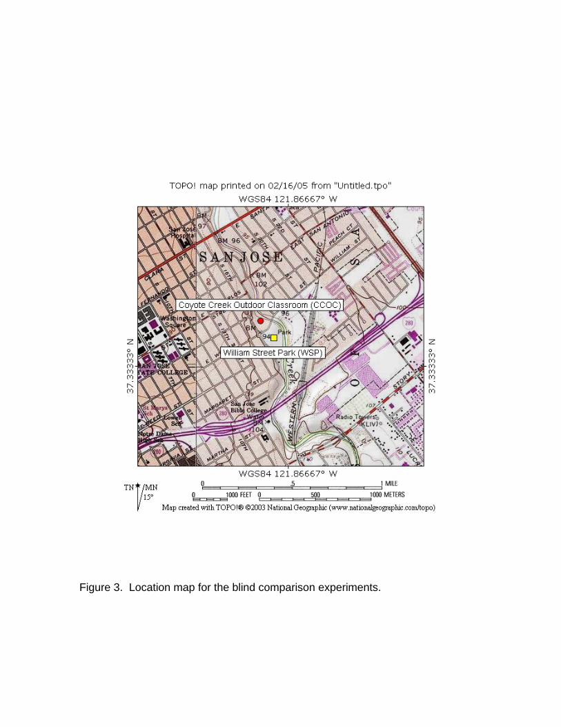
Figure 3. Location map for the blind comparison experiments.

Coyote Creek Suspension Vs Velocity Log and smoothed Vp/Vs ratio

-300-290-280-270-260-250-240-230-220-210-200-190-180-170-160-150-140-130-120-110-100-90-80-70-60-50-40-30-20-10

00 2 4 6 8

Slowness Ss

Depth

(m)

Ss-rawSs5

Vp/Vs

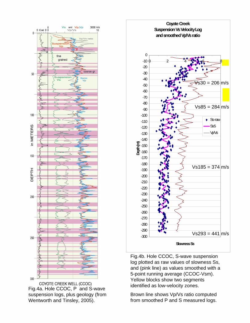
Fig.4a. Hole CCOC, P and S-wave suspension logs, plus geology (from Wentworth and Tinsley, 2005).

Fig.4b. Hole CCOC, S-wave suspension log plotted as raw values of slowness Ss, and (pink line) as values smoothed with a 5-point running average (CCOC-Vsm). Yellow blocks show two segments identified as low-velocity zones.

Brown line shows Vp/Vs ratio computed from smoothed P and S measured logs.

Vs30 = 206 m/s

Vs85 = 284 m/s

Vs185 = 374 m/s

Vs293 = 441 m/s

Fig.4c. The top 40 m of Hole CCOC, S-wave suspension log plotted as raw values of slowness Ss, and (pink line) as values smoothed with a 5-point running average (CCOC-Vsm). Yellow block shows the upper of two segments identified as low-velocity zones.

Brown line shows Vp/Vs ratio computed from smoothed P and S measured logs.

Coyote Creek Suspension Vs Velocity Log and smoothed Vp/Vs ratio

-40

-35

-30

-25

-20

-15

-10

-5

00 2 4 6 8

Slowness Ss

Depth

(m)

Ss-raw

Ss5Vp/Vs

Vs30 = 206 m/s

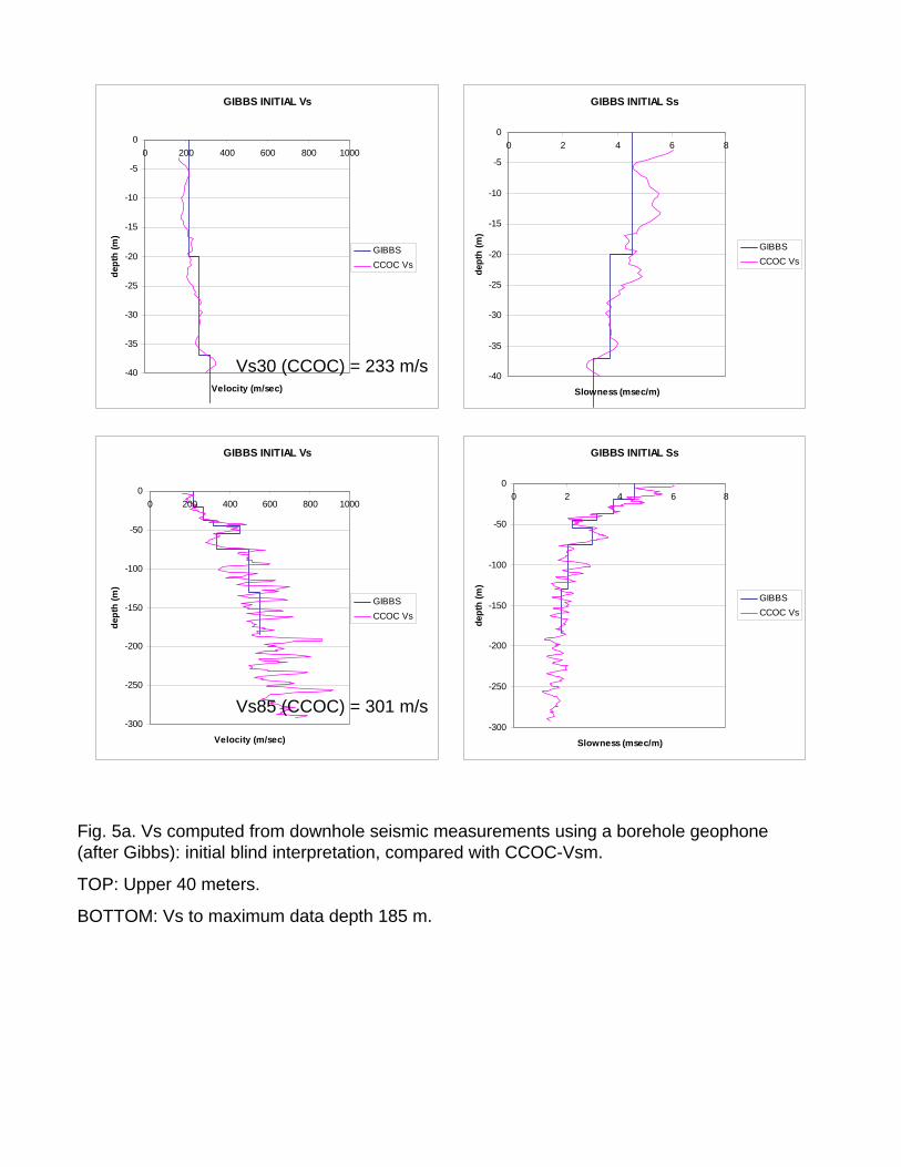
Fig. 5a. Vs computed from downhole seismic measurements using a borehole geophone (after Gibbs): initial blind interpretation, compared with CCOC-Vsm.

TOP: Upper 40 meters.

BOTTOM: Vs to maximum data depth 185 m.

Vs30 (CCOC) = 235 m/s

GIBBS INITIAL Vs

-40

-35

-30

-25

-20

-15

-10

-5

00 200 400 600 800 1000

Velocity (m/sec)

dept

h (m

)

GIBBSCCOC Vs

GIBBS INITIAL Ss

-40

-35

-30

-25

-20

-15

-10

-5

00 2 4 6 8

Slowness (msec/m)

dept

h (m

)

GIBBSCCOC Vs

GIBBS INITIAL Vs

-300

-250

-200

-150

-100

-50

00 200 400 600 800 1000

Velocity (m/sec)

dept

h (m

)

GIBBSCCOC Vs

GIBBS INITIAL Ss

-300

-250

-200

-150

-100

-50

00 2 4 6 8

Slowness (msec/m)

dept

h (m

)

GIBBSCCOC Vs

Vs30 (CCOC) = 233 m/s

Vs85 (CCOC) = 301 m/s

GIBBS DETAIL Vs

-300

-250

-200

-150

-100

-50

00 200 400 600 800 1000

Velocity (m/sec)

dept

h (m

)

GIBBSCCOC Vs

GIBBS DETAIL Slowness

-300

-250

-200

-150

-100

-50

00 2 4 6 8

Slowness (msec/m)

Dep

th (m

)

GIBBSCCOC Ss

Vs185 (CCOC) = 391 m/s

GIBBS DETAIL Vs

-40

-35

-30

-25

-20

-15

-10

-5

00 200 400 600 800 1000

Velocity (m/sec)

dept

h (m

)

GIBBSCCOC Vs

GIBBS DETAIL Ss

-40

-35

-30

-25

-20

-15

-10

-5

00 2 4 6 8

Slowness (msec/m)

dept

h (m

)

GIBBSCCOC Vs

Fig. 5b. Vs computed from downhole seismic measurements using a borehole geophone; reinterpretation of data for increased detail. Pink line is CCOC-Vsm.

TOP: Upper 40 meters.

BOTTOM: Vs to maximum data depth 185 m.

Vs30 (CCOC) = 235 m/s

HOLZER SCPT CCOC Vs

-40

-35

-30

-25

-20

-15

-10

-5

00 200 400 600 800 1000

Velocity (m/sec)

dept

h (m

)

HOLZERCCOC Vs

HOLZER SCPT CCOC Ss

-40

-35

-30

-25

-20

-15

-10

-5

00 2 4 6 8

Slowness (msec/m)

dept

h (m

)

HOLZERCCOC Vs

Vs30 (CCOC) = 236 m/s

Fig. 6. Vs computed from SCPT measurements (after Holzer), compared with CCOC-Vsm.

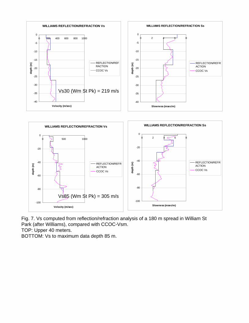
Fig. 7. Vs computed from reflection/refraction analysis of a 180 m spread in William St Park (after Williams), compared with CCOC-Vsm.TOP: Upper 40 meters.BOTTOM: Vs to maximum data depth 85 m.

WILLIAMS REFLECTION/REFRACTION Vs

-40

-35

-30

-25

-20

-15

-10

-5

00 200 400 600 800 1000

Velocity (m/sec)

dept

h (m

) REFLECTION/REFRACTIONCCOC Vs

WILLIAMS REFLECTION/REFRACTION Ss

-40

-35

-30

-25

-20

-15

-10

-5

00 2 4 6 8

Slowness (msec/m)

dept

h (m

) REFLECTION/REFRACTIONCCOC Vs

WILLIAMS REFLECTION/REFRACTION Vs

-100

-80

-60

-40

-20

00 500 1000

Velocity (m/sec)

dept

h (m

) REFLECTION/REFRACTIONCCOC Vs

WILLIAMS REFLECTION/REFRACTION Ss

-100

-80

-60

-40

-20

00 2 4 6 8

Slowness (msec/m)

dept

h (m

) REFLECTION/REFRACTIONCCOC Vs

Vs30 (Wm St Pk) = 219 m/s

Vs85 (Wm St Pk) = 305 m/s

BAY Wm St Pk WINSASW Vs

-40

-35

-30

-25

-20

-15

-10

-5

00 200 400 600 800 1000

Velocity (m/sec)

dept

h (m

) BAYCCOC VsBAY CCOC

BAY Wm St Pk WINSASW Ss

-40

-35

-30

-25

-20

-15

-10

-5

00 2 4 6 8

Slowness (msec/m)

dept

h (m

) BAYCCOC VsBAY CCOC

Fig. 8a. Vs & Ss computed from SASW measurements interpreted with Win-SASW (after Bay). Blue: William St Park, compared with (green) SASW at CCOC. Pink line is CCOC-Vsm.

Fig. 8b. Vs & Ss computed from SASW measurements interpreted with automatic direct inversion (after Bay). Blue: William St Park, compared with (green) SASW at CCOC. Pink line is CCOC-Vsm.

BAY Wm St Pk AUTO-INV Vs

-40

-35

-30

-25

-20

-15

-10

-5

00 200 400 600 800 1000

Velocity (m/sec)

dept

h (m

) BAYCCOC VsBAY CCOC

BAY Wm St Pk AUTO-INV Ss

-40

-35

-30

-25

-20

-15

-10

-5

00 2 4 6 8

Slowness (msec/m)

dept

h (m

) BAYCCOC VsBAY CCOC

Vs30 (Wm St Pk) = 213 m/sVs30 (CCOC) = 228 m/s

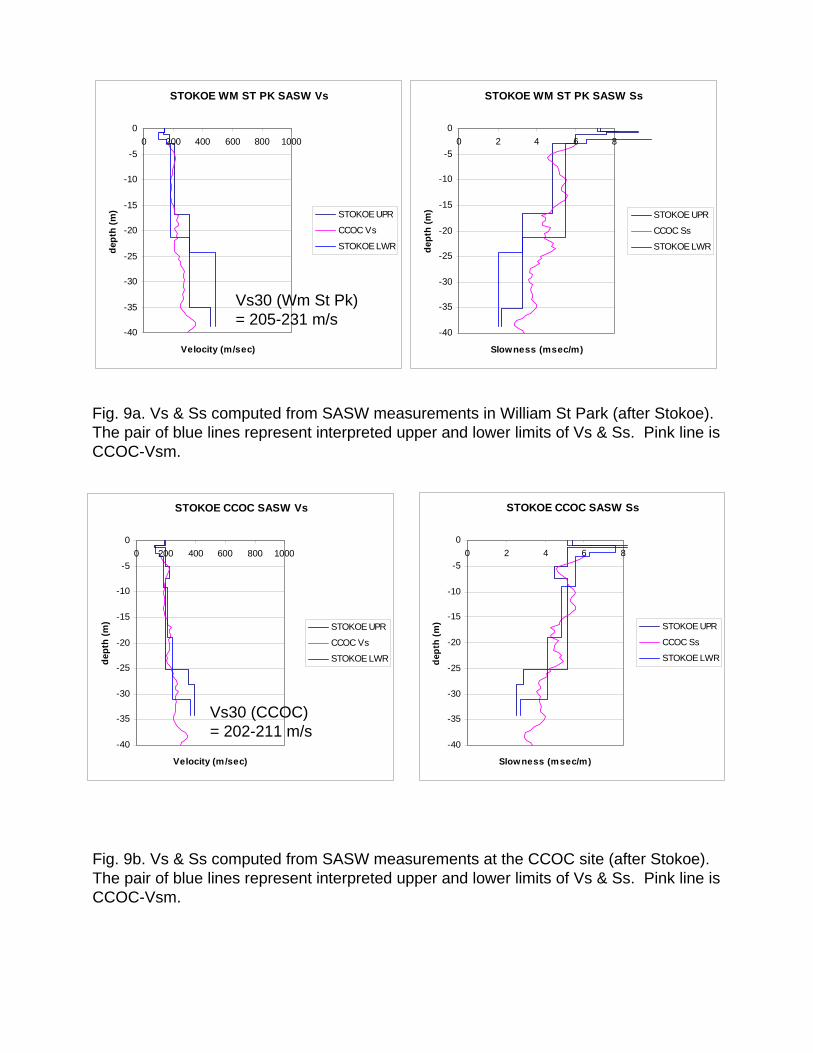
Fig. 9a. Vs & Ss computed from SASW measurements in William St Park (after Stokoe). The pair of blue lines represent interpreted upper and lower limits of Vs & Ss. Pink line is CCOC-Vsm.

Fig. 9b. Vs & Ss computed from SASW measurements at the CCOC site (after Stokoe). The pair of blue lines represent interpreted upper and lower limits of Vs & Ss. Pink line is CCOC-Vsm.

STOKOE CCOC SASW Vs

-40

-35

-30

-25

-20

-15

-10

-5

00 200 400 600 800 1000

Velocity (m/sec)

dept

h (m

) STOKOE UPR

CCOC Vs

STOKOE LWR

STOKOE CCOC SASW Ss

-40

-35

-30

-25

-20

-15

-10

-5

00 2 4 6 8

Slowness (msec/m)

dept

h (m

) STOKOE UPR

CCOC Ss

STOKOE LWR

Vs30 (CCOC) = 202-211 m/s

STOKOE WM ST PK SASW Vs

-40

-35

-30

-25

-20

-15

-10

-5

00 200 400 600 800 1000

Velocity (m/sec)

dept

h (m

) STOKOE UPR

CCOC Vs

STOKOE LWR

STOKOE WM ST PK SASW Ss

-40

-35

-30

-25

-20

-15

-10

-5

00 2 4 6 8

Slowness (msec/m)

dept

h (m

) STOKOE UPR

CCOC Ss

STOKOE LWR

Vs30 (Wm St Pk) = 205-231 m/s

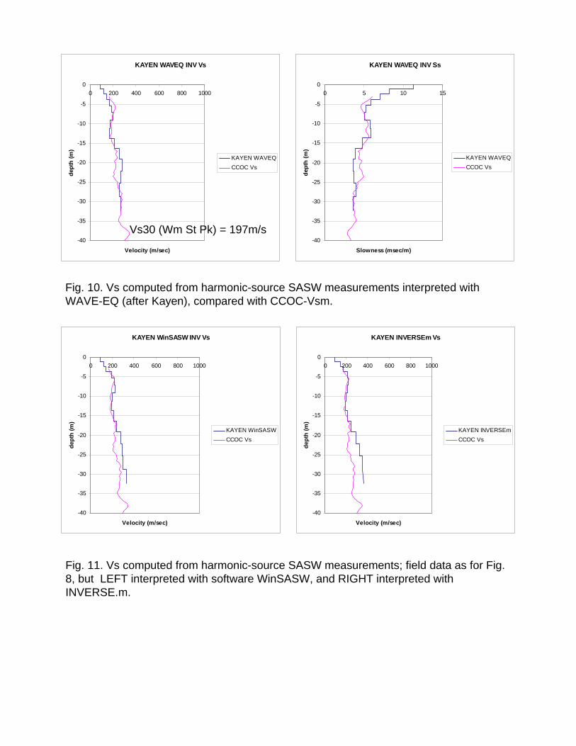
Fig. 10. Vs computed from harmonic-source SASW measurements interpreted with WAVE-EQ (after Kayen), compared with CCOC-Vsm.

Fig. 11. Vs computed from harmonic-source SASW measurements; field data as for Fig. 8, but LEFT interpreted with software WinSASW, and RIGHT interpreted with INVERSE.m.

KAYEN WAVEQ INV Vs

-40

-35

-30

-25

-20

-15

-10

-5

00 200 400 600 800 1000

Velocity (m/sec)

dept

h (m

)

KAYEN WAVEQCCOC Vs

KAYEN WAVEQ INV Ss

-40

-35

-30

-25

-20

-15

-10

-5

00 5 10 15

Slowness (msec/m)

dept

h (m

)

KAYEN WAVEQCCOC Vs

Vs30 (Wm St Pk) = 197m/s

KAYEN WinSASW INV Vs

-40

-35

-30

-25

-20

-15

-10

-5

00 200 400 600 800 1000

Velocity (m/sec)

dept

h (m

)

KAYEN WinSASWCCOC Vs

KAYEN INVERSEm Vs

-40

-35

-30

-25

-20

-15

-10

-5

00 200 400 600 800 1000

Velocity (m/sec)

dept

h (m

)

KAYEN INVERSEmCCOC Vs

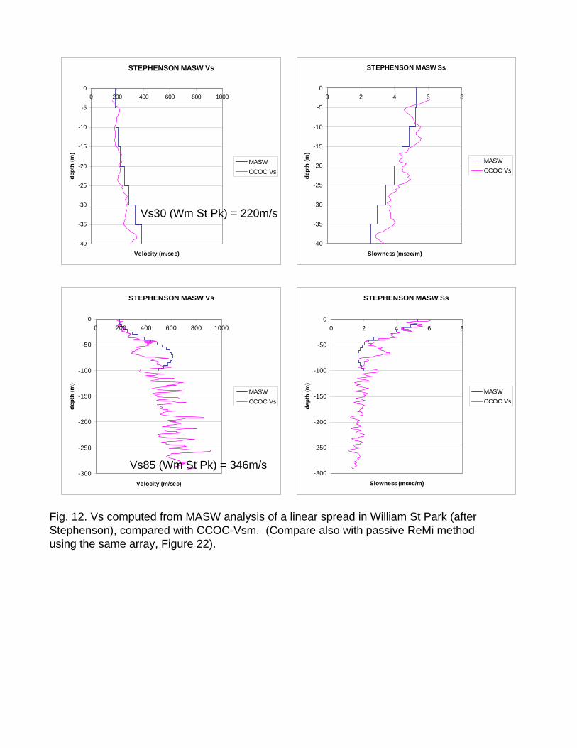
Fig. 12. Vs computed from MASW analysis of a linear spread in William St Park (after Stephenson), compared with CCOC-Vsm. (Compare also with passive ReMi method using the same array, Figure 22).

STEPHENSON MASW Vs

-40

-35

-30

-25

-20

-15

-10

-5

00 200 400 600 800 1000

Velocity (m/sec)

dept

h (m

)

MASWCCOC Vs

STEPHENSON MASW Ss

-40

-35

-30

-25

-20

-15

-10

-5

00 2 4 6 8

Slowness (msec/m)

dept

h (m

)

MASWCCOC Vs

STEPHENSON MASW Vs

-300

-250

-200

-150

-100

-50

00 200 400 600 800 1000

Velocity (m/sec)

dept

h (m

)

MASWCCOC Vs

STEPHENSON MASW Ss

-300

-250

-200

-150

-100

-50

00 2 4 6 8

Slowness (msec/m)

dept

h (m

)

MASWCCOC Vs

Vs85 (Wm St Pk) = 346m/s

Vs30 (Wm St Pk) = 220m/s

Fig. 13. Vs computed from combined MASW and passive MAM (after Hayashi) compared with CCOC-Vsm. Figure at top left shows the survey line used for MASW (2 m geophone spacings, 2 m hammer source positions) and the layout of a ten-station nested triangular array for microtremor measurements.

HAYASHI MASW & MAM Vs

-30

-25

-20

-15

-10

-5

00 200 400 600 800 1000

Velocity (m/sec)

dept

h (m

) HAYASHI MASW &MAMCCOC Vs

HAYASHI MASW & MAM Ss

-30

-25

-20

-15

-10

-5

00 2 4 6 8 10

Slowness (msec/m)

dept

h (m

) HAYASHI MASW &MAMCCOC Vs

HAYASHI MASW & MAM Vs

-300

-250

-200

-150

-100

-50

00 200 400 600 800 1000

Velocity (m/sec)

dept

h (m

) HAYASHI MASW &MAMCCOC Vs

HAYASHI MASW & MAM Ss

-300

-250

-200

-150

-100

-50

00 2 4 6 8 10

Slowness (msec/m)

dept

h (m

) HAYASHI MASW &MAMCCOC Vs

40m

MASW

Vs30 (Wm St Pk) = 209 m/s

Vs85 (Wm St Pk) = 292 m/s

Fig. 14. Vs computed from FK analysis of combined linear spread with active source, plus circular array with microtremor (passive) source (after Rix) compared with CCOC-Vsm. Figure at top left shows the survey line used for the linear array of 15 geophones (variable spacings from 2.4 to 33.5 m) and the layout of a 16-station circular array (radii 30 to 50 m) for microtremor measurements.

RIX FK Ss

-30

-25

-20

-15

-10

-5

00 2 4 6 8 10

Slowness (msec/m)

dept

h (m

)

FKCCOC Vs

RIX FK Vs

-30

-25

-20

-15

-10

-5

00 200 400 600 800 1000

Velocity (m/sec)

dept

h (m

)

FKCCOC Vs

RIX FK Vs

-300

-250

-200

-150

-100

-50

00 200 400 600 800 1000

Velocity (m/sec)

dept

h (m

)

FKCCOC Vs

RIX FK Ss

-300

-250

-200

-150

-100

-50

00 2 4 6 8 10

Slowness (msec/m)

dept

h (m

)

FKCCOC Vs

Active source & array

Vs30 (Wm St Pk) = 223 m/s

Vs85 (Wm St Pk) = 321 m/s

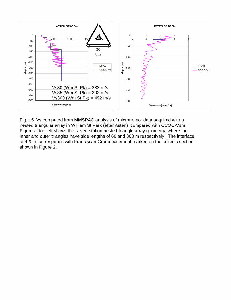
Fig. 15. Vs computed from MMSPAC analysis of microtremor data acquired with a nested triangular array in William St Park (after Asten) compared with CCOC-Vsm. Figure at top left shows the seven-station nested-triangle array geometry, where the inner and outer triangles have side lengths of 60 and 300 m respectively. The interface at 420 m corresponds with Franciscan Group basement marked on the seismic section shown in Figure 2.

ASTEN SPAC Vs

-600

-550

-500

-450

-400

-350

-300

-250

-200

-150

-100

-50

00 500 1000 1500

Velocity (m/sec)

dept

h (m

)

SPACCCOC Vs

ASTEN SPAC Ss

-300

-250

-200

-150

-100

-50

00 2 4 6 8

Slowness (msec/m)

dept

h (m

)

SPACCCOC Vs

300m

Vs30 (Wm St Pk) = 233 m/sVs85 (Wm St Pk) = 303 m/sVs300 (Wm St Pk) = 492 m/s

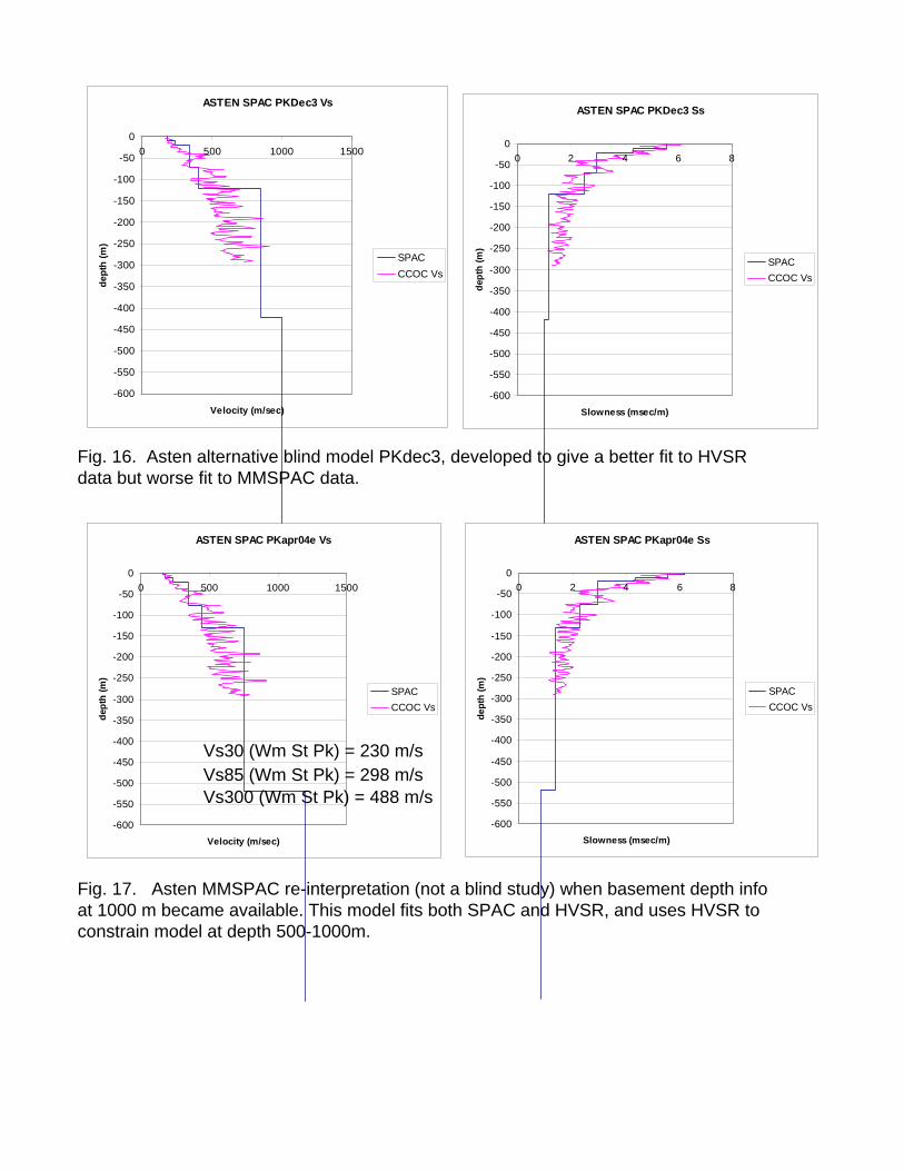
Fig. 17. Asten MMSPAC re-interpretation (not a blind study) when basement depth info at 1000 m became available. This model fits both SPAC and HVSR, and uses HVSR to constrain model at depth 500-1000m.

ASTEN SPAC PKDec3 Vs

-600

-550

-500

-450

-400

-350

-300

-250

-200

-150

-100

-50

00 500 1000 1500

Velocity (m/sec)

dept

h (m

)

SPACCCOC Vs

ASTEN SPAC PKDec3 Ss

-600

-550

-500

-450

-400

-350

-300

-250

-200

-150

-100

-50

00 2 4 6 8

Slowness (msec/m)

dept

h (m

)

SPACCCOC Vs

Fig. 16. Asten alternative blind model PKdec3, developed to give a better fit to HVSR data but worse fit to MMSPAC data.

ASTEN SPAC PKapr04e Vs

-600

-550

-500

-450

-400

-350

-300

-250

-200

-150

-100

-50

00 500 1000 1500

Velocity (m/sec)

dept

h (m

)

SPACCCOC Vs

ASTEN SPAC PKapr04e Ss

-600

-550

-500

-450

-400

-350

-300

-250

-200

-150

-100

-50

00 2 4 6 8

Slowness (msec/m)

dept

h (m

)

SPACCCOC Vs

Vs30 (Wm St Pk) = 230 m/sVs85 (Wm St Pk) = 298 m/sVs300 (Wm St Pk) = 488 m/s

Fig. 18. Vs computed from SPAC analysis of microtremor data acquired with an array of three concurrent circles (or equivalently, nested triangles) in William St Park (after Hartzell) compared with CCOC-Vsm. Figure at top left shows the fifteen-station nested-triangle array geometry, where the three circles have radii 19, 33 and 57 m respectively.

HARTZELL SPAC Vs

-30

-25

-20

-15

-10

-5

00 200 400 600 800 1000

Velocity (m/sec)

dept

h (m

)

SPACCCOC Vs

HARTZELL SPAC Ss

-30

-25

-20

-15

-10

-5

00 2 4 6 8

Slowness (msec/m)

dept

h (m

)

SPACCCOC Vs

HARTZELL SPAC Vs

-600

-550

-500

-450

-400

-350

-300

-250

-200

-150

-100

-50

00 200 400 600 800 1000

Velocity (m/sec)

dept

h (m

)

SPACCCOC Vs

HARTZELL SPAC Ss

-300

-250

-200

-150

-100

-50

00 2 4 6 8

Slowness (msec/m)

dept

h (m

)

SPACCCOC Vs

40m

MASW

Vs30 (Wm St Pk) = 243 m/s

Vs85 (Wm St Pk) = 327 m/sVs300 (Wm St Pk) = 494 m/s

Vs30 (Wm St Pk) = 243 m/s

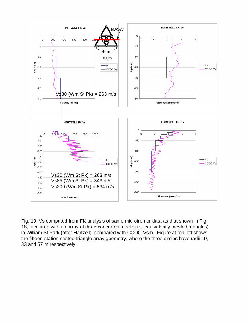
Fig. 19. Vs computed from FK analysis of same microtremor data as that shown in Fig. 18, acquired with an array of three concurrent circles (or equivalently, nested triangles) in William St Park (after Hartzell) compared with CCOC-Vsm. Figure at top left shows the fifteen-station nested-triangle array geometry, where the three circles have radii 19, 33 and 57 m respectively.

HARTZELL FK Vs

-30

-25

-20

-15

-10

-5

00 200 400 600 800 1000

Velocity (m/sec)

dept

h (m

)

fkCCOC Vs

100m

HARTZELL FK Ss

-30

-25

-20

-15

-10

-5

00 2 4 6 8

Slowness (msec/m)

dept

h (m

)

FKCCOC Vs

HARTZELL FK Vs

-600

-550

-500

-450

-400

-350

-300

-250

-200

-150

-100

-50

00 200 400 600 800 1000

Velocity (m/sec)

dept

h (m

)

FKCCOC Vs

HARTZELL FK Ss

-300

-250

-200

-150

-100

-50

00 2 4 6 8

Slowness (msec/m)

dept

h (m

)

FKCCOC Vs

40m

MASW

Vs85 (Wm St Pk) = 343 m/sVs300 (Wm St Pk) = 534 m/s

Vs30 (Wm St Pk) = 263 m/s

Vs30 (Wm St Pk) = 263 m/s

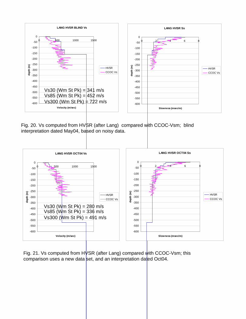
Fig. 20. Vs computed from HVSR (after Lang) compared with CCOC-Vsm; blind interpretation dated May04, based on noisy data.

Fig. 21. Vs computed from HVSR (after Lang) compared with CCOC-Vsm; this comparison uses a new data set, and an interpretation dated Oct04.

LANG HVSR BLIND Vs

-600

-550

-500

-450

-400

-350

-300

-250

-200

-150

-100

-50

00 500 1000 1500

Velocity (m/sec)

dept

h (m

)

HVSRCCOC Vs

LANG HVSR Ss

-600

-550

-500

-450

-400

-350

-300

-250

-200

-150

-100

-50

00 2 4 6 8

Slowness (msec/m)

dept

h (m

)

HVSRCCOC Vs

LANG HVSR OCT04 Vs

-600

-550

-500

-450

-400

-350

-300

-250

-200

-150

-100

-50

00 500 1000 1500

Velocity (m/sec)

dept

h (m

)

HVSRCCOC Vs

LANG HVSR OCT04 Ss

-600

-550

-500

-450

-400

-350

-300

-250

-200

-150

-100

-50

00 2 4 6 8

Slowness (msec/m)

dept

h (m

)

HVSRCCOC Vs

Vs85 (Wm St Pk) = 452 m/sVs300 (Wm St Pk) = 722 m/s

Vs30 (Wm St Pk) = 341 m/s

Vs85 (Wm St Pk) = 336 m/sVs300 (Wm St Pk) = 491 m/s

Vs30 (Wm St Pk) = 280 m/s

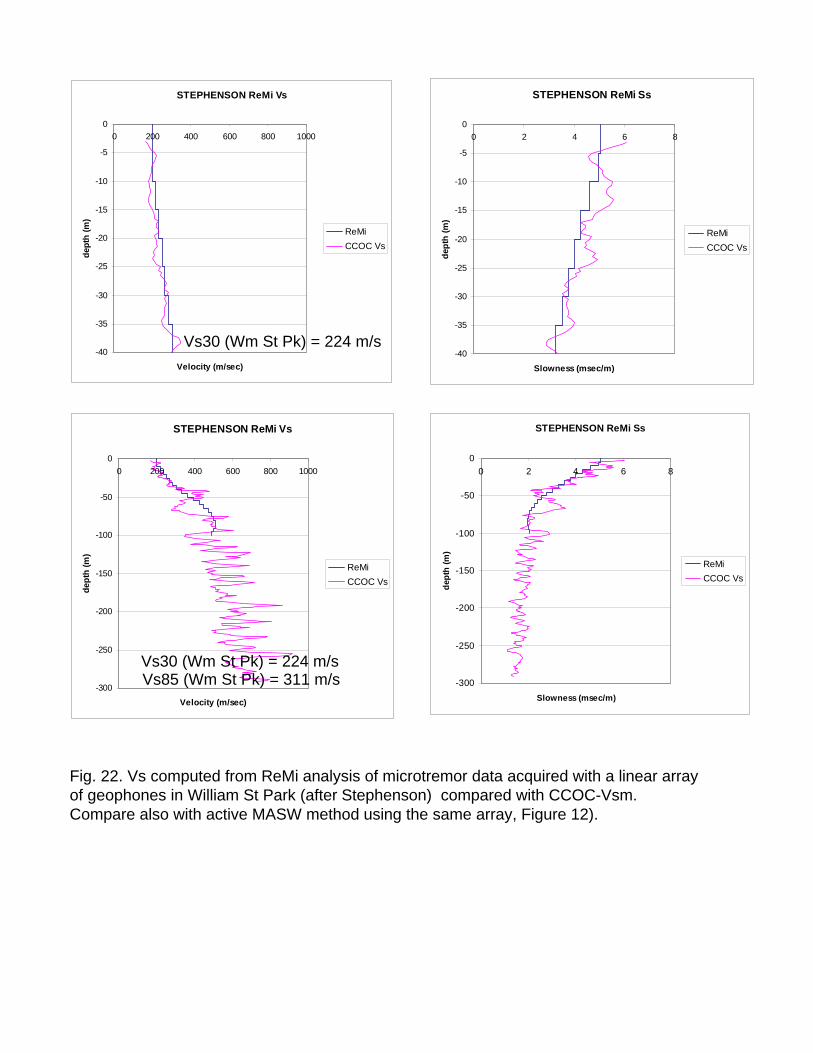
Fig. 22. Vs computed from ReMi analysis of microtremor data acquired with a linear array of geophones in William St Park (after Stephenson) compared with CCOC-Vsm. Compare also with active MASW method using the same array, Figure 12).

STEPHENSON ReMi Vs

-40

-35

-30

-25

-20

-15

-10

-5

00 200 400 600 800 1000

Velocity (m/sec)

dept

h (m

)

ReMiCCOC Vs

STEPHENSON ReMi Ss

-40

-35

-30

-25

-20

-15

-10

-5

00 2 4 6 8

Slowness (msec/m)

dept

h (m

)

ReMiCCOC Vs

STEPHENSON ReMi Vs

-300

-250

-200

-150

-100

-50

00 200 400 600 800 1000

Velocity (m/sec)

dept

h (m

)

ReMiCCOC Vs

STEPHENSON ReMi Ss

-300

-250

-200

-150

-100

-50

00 2 4 6 8

Slowness (msec/m)

dept

h (m

)

ReMiCCOC Vs

Vs85 (Wm St Pk) = 311 m/sVs30 (Wm St Pk) = 224 m/s

Vs30 (Wm St Pk) = 224 m/s