Comparing two genetic overproduce-and-choose strategies for fuzzy rule-based multiclassification...

International Journal of Hybrid Intelligent Systems 7 (2010) 45–64 45DOI 10.3233/HIS-2010-0104IOS Press

Comparing two geneticoverproduce-and-choose strategies for fuzzyrule-based multiclassification systemsgenerated by bagging and mutualinformation-based feature selection

Oscar Cordon and Arnaud Quirin∗,1European Centre for Soft Computing, Edificio Cient ıfico-Tecnologico, planta 3. Gonzalo Gutierrez Quiros, s/n,33600 - Mieres (Asturias), Spain

Abstract. In [14] we proposed a scheme to generate fuzzy rule-based multiclassification systems by means of bagging, mutualinformation-based feature selection, and a multicriteria genetic algorithm for static component classifier selection guided by theensemble training error. In the current contribution we extend the latter component by making use of the bagging approach’scapability to evaluate the accuracy of the classifier ensemble using the out-of-bag estimates. An exhaustive study is developedon the potential of the two multicriteria genetic algorithms respectively considering the classical training error and the out-of-bagerror fitness functions to design a final multiclassifier with an appropriate accuracy-complexity trade-off. Several parametersettings for the global approach are tested when applied to nine popular UCI datasets with different dimensionality.

1. Introduction

Multiclassification systems (MCSs) (also called mul-ticlassifiers or classifier ensembles) have been shown asvery promising tools to improve the performance of sin-gle classifiers when dealing with complex, high dimen-sional classification problems in the last few years [28].This research topic has become especially active in theclassical machine learning area, considering decisiontrees or neural networks to generate the componentclassifiers, but also some work has been done usingdifferent kinds of fuzzy classifiers (see Section 2.2).

In a previous study [13], we described how fuzzyrule-based multiclassification systems (FRBMCSs)

∗Corresponding author. E-mail: [email protected].

1This work has been supported by the Spanish Ministry ofEducation and Science, under grants TIN2005-08036-C05-05 andTIN2006-00829.

could be generated from classical MCS design ap-proaches such as bagging [4] and random subspace [23]with a basic, heuristic fuzzy classification rule gen-eration method [25]. Later, we analyzed how moreadvanced feature selection approaches based on theuse of mutual information measures – the classicalBattiti’s mutual information feature selection (MIFS)method [3], a greedy heuristic, and its extensionto a greedy randomized adaptive search procedure(GRASP) [19]— allowed us to obtain better performingFRBMCSs [14].

The latter generation approach was embedded intoan overproduce-and-choose strategy [36] with the aimto both reduce the final multiclassifier complexity andeven try to increase its accuracy by eliminating redun-dant classifiers. To do so, we proposed a multicriteriagenetic algorithm (GA) [9] for static component clas-sifier selection guided by the training error which al-lowed us to generate linguistic fuzzy rule-based clas-

1448-5869/10/$27.50 2010 – IOS Press. All rights reserved

46 O. Cordon and A. Quirin / Comparing two genetic overproduce-and-choose strategies

sification system (FRBCS) ensembles with differentaccuracy-complexity trade-offs in a single run.

The resulting FRBMCS design technique thus be-long to the genetic fuzzy systems family, one of themost successful approaches to hybridize fuzzy systemswith learning and adaptation methods in the last fifteenyears [11,12]. It is also quite novel in the fuzzy systemsarea since no previous work has been done on baggingFRBCSs up to our knowledge.

The aim of the current contribution is to take a stepahead on those first developments by paying more at-tention to the genetic classifier selection stage. To doso, we will make use of another of the bagging inherentadvantages, its ability to test the accuracy of the ensem-ble without the need of removing any pattern from thedata set (i.e., no need to use a validation set) by meansof the “Out-Of-Bag” Error (OOBE) [6]. Hence, a newvariant of the multicriteria genetic component classifierselection technique will be proposed by adapting thewhole FRBMCS design framework in order the latterstage can be guided by the OOBE. In principle, theoriginal fitness function based on the use of the train-ing error could lead to the generation of overfitted FR-BCS ensembles due to the use of the same patterns forthe individual classifier generation and MCS selectionstages. Proceeding in the former way, the FRBCS en-semble configurations selected by the OOBE-guidedGA will be evaluated on those instances not consideredto learn the component classifiers, i.e., not chosen bythe bagging resampling to be included in each bag. Weaim to check if the new GA fitness function will allowus to reduce the possible overfitting while still beingcompetitive in terms of accuracy regarding to the initialensemble.

An exhaustive study will be developed to test the twoGA variants based on the use of the two fitness func-tions guided by the classical training error and OOBE,respectively, on nine popular data sets from the UCImachine learning repository with different characteris-tics of dimensionality (i.e., with different numbers ofexamples and features). Several parameter settings forthe global approach (e.g., different granularity levelsfor the fuzzy partitions) will be tested and the perfor-mance of the two kinds of genetically selected FRBM-CSs will be compared between them, as well as to boththe individual FRBCSs and the initial FRBCS ensem-bles.

This paper is set up as follows. In the next section,the preliminaries required for a good understanding ofour work (popular classifier ensemble design approach-es, fuzzy MCSs, the need of classifier selection, and the

existing GA-based methods to perform it) are reviewed.Section 3 recalls our approach for designing FRBM-CSs considering bagging and feature selection, whileSection 4 describes the proposed multicriteria GA forcomponent classifier selection. The experiments devel-oped and their analysis are shown in Section 5. Specif-ically, an example of the analysis of one chromosomeregarding the FRBCS ensemble accuracy-complexitytrade-off is presented in Section 6. Finally, Section 7collects some concluding remarks and future researchlines.

2. Background and related work

This section explores the current literature relatedto the generation of a FRBMCS. The techniques usedto generate MCSs and FRBCSs are described in Sec-tions 2.1 and section 2.2 respectively. Some ways toreduce the size of the ensembles are described in Sec-tion 2.3. The use of GAs, for this purpose, is exploredin Section 2.4.

2.1. Related work on MCSs

A MCS is the result of the combination of the outputsof a group of individually trained classifiers in order toget a system that is usually more accurate than any ofits single components [28].

According to the existing literature, there are dif-ferent methods to generate a MCS, all of them basedon altering the training process in such way there isdisagreement between the component classifiers. Dif-ferent taxonomies can be considered, but it is usuallyagreed that there is a well known group comprising ap-proaches considering data resampling to obtain differ-ent training sets to derive each individual classifier, i.e.bagging and boosting:

1. Bagging [4]: In the bootstrap aggregation ap-proach, the individual classifiers are independent-ly learnt from resampled training sets (“bags"),which are randomly selected with replacementfrom the original training data set, following thestatistical bootstrapping procedure. In this way,bagging must be used in combination with “un-stable” learning algorithms where small changesin the training set result in large changes in thepredictions given by the classifier [5].

O. Cordon and A. Quirin / Comparing two genetic overproduce-and-choose strategies 47

2. Boosting [43]: Boosting is a family of differentmethods following the same operation mode: theindividual classifiers are generated sequentiallyby selecting the training set for each of them basedon the performance of the previous classifier(s)in the series. Opposed to bagging, the resam-pling process gives a higher probability of selec-tion to the incorrectly predicted examples by theprevious classifiers.

These methods have gain a large acceptance inthe machine learning community during the last twodecades due to their high performance. Decision treesare the most usual classifier structure considered bythem and much work has been done on the topic, al-though they can be used with any type of classifier (theuse of neural networks is also very extended, see forexample [35]).

On the other hand, a second group can be found com-prised by a more diverse set of approaches which in-duct the individual classifier diversity using some waysdifferent from resampling [52]. Feature selection playsa key role in many of them where each classifier is de-rived by considering a different subset of the originalfeatures. random subspace [23], where each featuresubset is randomly generated, is one of the most repre-sentative methods of this kind. Although it was initiallyproposed for decision tree ensembles, it can be clearlyused with any kind of classifier inductor in the sameway that resampling approaches. Other generic ap-proaches considering more advanced feature selectionstrategies can be found in [49,51].

Finally, there are some advanced proposals that canbe considered as combinations of the two groups. Themost extended one could be random forests [6], wherethe individual classifiers are decision trees learnt froma resampled “bag" of examples, a subset of randomvariables is selected at each construction step, and thebest split for those selected variables is chosen for thatnode.

The interested reader is referred to [2,35] for tworeviews for the case of decision tree ensembles (both)and neural networks (the latter), including exhaustiveexperimental studies. The next subsection reviews thecase of the fuzzy MCSs.

2.2. Previous work on fuzzy MCSs

The use of boosting for the design of fuzzy classifi-er ensembles has been considered in some works, tak-ing the weak learners as fuzzy variants of neural net-

works [37,50]: as granular models [38], as neuro-fuzzysystems [45], as well as single fuzzy rules [16,24,40].

However, only a few contributions for bagging fuzzyclassifiers have been proposed considering, fuzzy adap-tive neural networks [37], fuzzy clustering-based clas-sifiers [48], and neuro-fuzzy systems [7] as componentclassifier structures. Up to our knowledge, no proposalhas been made considering FRBCSs.

Two advanced GFS-based contributions are worthyto be mentioned. On the one hand, an FRBMCS de-sign technique is proposed in [1] based on the use ofsome niching GA-based feature selection methods togenerate the diverse component classifiers, and of an-other GA for classifier fusion by learning the combina-tion weights. On the other hand, another interval andFRBCS ensemble design method based on the use of asingle- and multi-objective genetic rule selection is in-troduced in [33]. In this case, the coding scheme allowsan initial set of either intervals or fuzzy rules, consider-ing the use of different features in their antecedents, tobe distributed among different component classifiers,trying to make them as diverse as possible by meansof two accuracy and one entropy measures. Besides,the same authors presented a previous proposal in [26],where a multi-objective GA generated a Pareto set ofFRBCSs with different accuracy-complexity trade-offsto be combined into an ensemble.

Finally, some works making use of fuzzy techniquesfor classifier ensemble fusion have also been proposed,but they are out out of the scope of the current contri-bution.

The next two subsections reviews the techniquesused to optimize the ensemble size.

2.3. Determination of the optimal set of componentclassifiers in the MCS

Typically an ensemble of classifiers is post-processedin such a way only a subset of them are kept for thefinal decision. It is a well known fact that the size ofthis MCS is an important issue for its trade-off betweenaccuracy and complexity [2,35] and that most of theerror reduction occurs with the first few additional clas-sifiers [4,35]. Furthermore, the selection process alsoparticipates in the elimination of the duplicates or thepoor-performing classifiers.

While in the first studies on MCSs a very small num-ber (around ten) of component classifiers was consid-ered as appropriate to sufficiently reduce the test setprediction error, later research on boosting (that alsoholds for bagging) suggested that error can be signifi-


cantly reduced by largely exceeding this number [44].This has caused the use of very large ensemble sizes(for example comprised by 1,000 individual classifiers)in the last few years [2].

Hence, the determination of the optimal size of theensemble is an important issue for obtaining both thebest possible accuracy in the test data set without over-fitting it, and a good accuracy-complexity trade-off. Inpure bagging and boosting approaches, the optimal en-sembles are directly composed of all the componentclassifiers generated until an specific stopping point,which is determined according to different means (val-idation data set errors, likelihood, . . .). For example,in [2] it is proposed an heuristic method to determinethe optimal number guided by the “OOBE" error.

However, there is the chance that the optimal ensem-ble is not comprised by all the component classifiersfirst generated but on a subset of them carrying a larg-er degree of disagreement/diversity. This is why dif-ferent classifier selection methods [15] has been pro-posed. They could be mainly grouped in two kinds ofstrategies. The first one is named the overproduce-and-choose strategy (OCS) [36], also known as the test-and-select methodology [47] or the static strategy [42]in the literature. In this strategy, a large set of classi-fiers is produced and then selected to extract the bestperforming subset. The second one is named the dy-namic classifier selection approach (DCS) [21]. In thisapproach, the accuracy of each classifier surroundingthe region of the feature space where the unknown pat-tern to be classified is located is previously estimated,and the best ones are selected to classify that specificpattern.

GAs have been commonly used for the both strate-gies as we will show in the following subsection.

2.4. Related work on genetic selection of FRBMCSs

GAs are a popular technique used to select the classi-fiers, especially within the OCS strategy. Usually, per-formance, complexity and diversity measures consid-ered used as search criteria. Complexity measures areemployed to increase the interpretability of the systemwhereas diversity measures are used to avoid overfit-ting.

Among the different genetic OCS proposals, we canremark the following ones. In [34], a hierarchical multi-objective GA (MOGA) algorithm, performing featureselection at the first level and classifier selection at thesecond level, is presented which outperforms classi-cal methods for two handwritten recognition problems.

The MOGA allows both performance and diversity tobe considered for MCS selection. In [22] a GA is usedto select from seven diversity heuristics for k-meanscluster-based ensembles and the ensemble size is alsoencoded in the genome. Even if the experiments con-ducted on 18 datasets showed that no particular combi-nation of heuristics have been chosen by the GA acrossall the datasets, this study dealt with the three fami-lies of criteria: performance, complexity and diversi-ty. Another extensive comparison between 15 differentclassifiers, 27 datasets, 7 search methods (among themthree evolutionary algorithms) and 16 selection crite-ria (diversity measures and classifier error) is presentedin [39], but the conclusion does not agree with the otherstudies: the diversity measures seem not to be usefulto improve the error rate. In the study of Mart inez-Munoz et al. [31], a GA is compared to five other tech-niques for ensemble selection. Even if the performanceof the GA was the worst obtained, they showed thatwhile selecting a small subset of classifiers, the gen-eralization error was significantly decreased. In [20],the authors developed a multidimensional GA to opti-mize two weight-based models, in which the weightsare assigned to each classifier or to each class. Theyapplied their system to 6 different classifiers (only lin-ear and quadratic classifiers are explored), but on onlytwo small datasets and without comparing to the re-sults obtained on a single classifier. Another study [27]aimed to develop a weighted-based GA for combiningdiverse classifiers, driven from machine-learning tech-niques or human experts. The authors obtained promis-ing results, but they applied their methodology only ona small dataset, due to the difficulty of collecting a largeexpert dataset. Our own previous studies [13,14] alsoconsider a multicriteria GA for the ensemble selectionin an OCS fashion, with performance (training error)and complexity as criteria to guide the GA.

Some conclusions drawn in the cited papers are sim-ilar to all of them: in general, the performance obtainedafter the genetic selection of an ensemble outperformsthe initial MCS, while quite drastically simplifying thesystem. But in all of them, the error rate is measuredon the initial training set or a pre-defined validation set.The aim of the current contribution is to analyze a newselection methodology based on the use of the OOBEto select the ensembles by the means of a GA, takingadvantage of the bagging approach.

The other strategy, the DCS approach, is still lessextended in the specialized literature. One of the avail-able studies, presented in [41], is a comparison of asingle-objective GA and a MOGA for 14 different ob-


jective functions of the mentioned three families of cri-teria (12 diversity measures, the training error, and thenumber of classifiers as a complexity measure). Theauthors applied their study on only one dataset, a digithandwritten recognition problem with 10 classes and118,735 instances. They conclude saying that the train-ing error is the best criterion for a single GA and a com-bination of training error and one diversity measure isthe best criterion for a MOGA. In [42], the two OCSand DCS strategies are combined to form a dynamicoverproduce-and-choose strategy to allow, respective-ly, the generation of a set of highly accurate ensembles,and to select the one with the highest degree of confi-dence, in a two-step process. This strategy outperformsboth a static strategy and the initial ensemble of clas-sifiers on seven datasets. In [18], the authors proposeda GA selecting the votes of each classifier in an en-semble for its reliability to classify each class, insteadof discarding the classifiers at a whole. They obtainedgood results with respect to static strategies, but theytested their proposal on only one application. In [30],an ensemble of neural networks are evolved using anevolutionary algorithm based on negative correlation,in order they learn different parts of the training set.Very competitive results are presented, but in only twodatasets.

We can also notice that GAs are also popular tech-niques for feature selection. For instance, in [49], a GAis compared to four other techniques for feature selec-tion on a high number of datasets (21) and using differ-ent diversity measures. For all the experimentations,the GA outperformed the remaining methods regardingthe MCS test accuracy.

3. Bagging and feature selection-based FRBMCSs

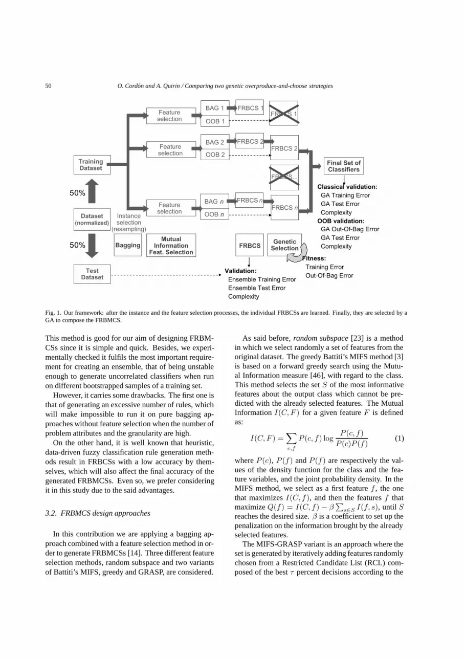
In this section we will both detail how the individualclassifiers and the FRBMCSs are designed. Figure 1shows the framework of the whole approach. A nor-malized dataset is split into two parts, a training set anda test set. The training set is submitted to an instanceselection and a feature selection procedure in order toprovide individual training sets (the so-called bags) totrain simple FRBCSs (through the method describedin Section 3.1). The instance selection and the featureselection procedures are described in Section 3.2. Af-ter the training, we got an initial MCS, which is vali-dated using the training and the test errors (EnsembleTraining Error and Ensemble Test Error), as well as ameasure of complexity based on the total number of

rules in the FRBCSs. This ensemble is selected usinga GA (described in Section 4) using either the TrainingError or the OOBE. The final MCS is validated usingdifferent accuracy (Training Error, OOBE, Test Error)and complexity measures (number of classifiers, totalnumber of rules).

3.1. Individual FRBCS composition and designmethod

The FRBCSs considered in the ensemble will bebased on fuzzy rules with a class Cj and a certaintydegree CFj in the consequent:

Rule Rj : If x1 is Aj1 and . . . and xn is Ajn

then Class Cj with CFj ; j = 1, 2, ..., N,

and they will take their decisions by means of thesingle-winner method, which gives as classifier outputthe class associated to the rule with the largest valuefor the product of its firing degree and the certainty de-gree [10,25]. The and conjunctive operator in the ruleantecedent is modeled by the product T-Norm. Thisfuzzy reasoning method has been selected due to itshigh simplicity and interpretability. The use of othermore advanced ones [10] is left for future works.

To derive the fuzzy knowledge bases, one of theheuristic methods proposed by Ishibuchi et al. in [25]is considered. All the fuzzy rule derivation methodsin this family start from a fuzzy partition definition foreach variable, and are based on generating a fuzzy ruleRj for each fuzzy input subspace Aj where at leasta training example is located. The consequent classCj and certainty degree CFj are statistically computedfrom all the examples located in the specific subspaceD(Aj) (grid-based methods, see [8]).

In the chosen method, Cj is computed as the class hwith maximum confidence according to the rule com-patible training examples D(Aj) = {x1, . . . , xm}.That confidence value for every class is computed as:

c(Aj ⇒ Class h) =|D(Aj)

⋂D(Class h)|

|D(Aj)| =

=

∑p∈Class h µAj (xp)∑m

p=1 µAj (xp)h = 1, 2, . . . , M ;

CFj is obtained as the difference between the confi-dence of the consequent class and the sum of the con-fidences of the remainder (called CF IV

j in [25]):

CFj = c(Aj ⇒ Class Cj) −m∑

h=1;h �=Cj

c(Aj ⇒ Class h).


TrainingDataset

Dataset

TestDataset

(normalized)

Bagging GeneticSelection

Final Set ofClassifiers

FRBCSMutual

InformationFeat. Selection

50%

50%

n

n

n

n

BAG 1 FRBCS 1

FRBCS 2FRBCS 2

FRBCSFRBCS

BAG

OOB 1

OOB 2

OOB

BAG 2

Featureselection

Featureselection

Instanceselection

(resampling)

Featureselection

nn

Validation: Ensemble Training Error Ensemble Test Error Complexity

Classical validation: GA Training Error GA Test Error ComplexityOOB validation: GA Out-Of-Bag Error GA Test Error Complexity

Fitness: Training Error Out-Of-Bag Error

FRBCS 1

FRBCS...

Fig. 1. Our framework: after the instance and the feature selection processes, the individual FRBCSs are learned. Finally, they are selected by aGA to compose the FRBMCS.

This method is good for our aim of designing FRBM-CSs since it is simple and quick. Besides, we experi-mentally checked it fulfils the most important require-ment for creating an ensemble, that of being unstableenough to generate uncorrelated classifiers when runon different bootstrapped samples of a training set.

However, it carries some drawbacks. The first one isthat of generating an excessive number of rules, whichwill make impossible to run it on pure bagging ap-proaches without feature selection when the number ofproblem attributes and the granularity are high.

On the other hand, it is well known that heuristic,data-driven fuzzy classification rule generation meth-ods result in FRBCSs with a low accuracy by them-selves, which will also affect the final accuracy of thegenerated FRBMCSs. Even so, we prefer consideringit in this study due to the said advantages.

3.2. FRBMCS design approaches

In this contribution we are applying a bagging ap-proach combined with a feature selection method in or-der to generate FRBMCSs [14]. Three different featureselection methods, random subspace and two variantsof Battiti’s MIFS, greedy and GRASP, are considered.

As said before, random subspace [23] is a methodin which we select randomly a set of features from theoriginal dataset. The greedy Battiti’s MIFS method [3]is based on a forward greedy search using the Mutu-al Information measure [46], with regard to the class.This method selects the set S of the most informativefeatures about the output class which cannot be pre-dicted with the already selected features. The MutualInformation I(C, F ) for a given feature F is definedas:

I(C, F ) =∑

c,f

P (c, f) logP (c, f)

P (c)P (f)(1)

where P (c), P (f) and P (f) are respectively the val-ues of the density function for the class and the fea-ture variables, and the joint probability density. In theMIFS method, we select as a first feature f , the onethat maximizes I(C, f), and then the features f thatmaximize Q(f) = I(C, f) − β

∑s∈S I(f, s), until S

reaches the desired size. β is a coefficient to set up thepenalization on the information brought by the alreadyselected features.

The MIFS-GRASP variant is an approach where theset is generated by iteratively adding features randomlychosen from a Restricted Candidate List (RCL) com-posed of the best τ percent decisions according to the


Q measure. Parameter τ is used to control the amountof randomness injected in the MIFS selection. Withτ = 0, we get the original MIFS method, while withτ = 1, we get the random subspace method.1

For the bagging approach, the bags are generatedwith the same size as the original training set, as com-monly done. In every case, all the classifiers will con-sider the same fixed number of features.

Finally, no weights will be considered to combinethe outputs of the component classifiers to take thefinal MCS decision, but a pure voting approach will beapplied: the ensemble class prediction will directly bethe most voted class in the component classifiers outputset.

4. A multicriteria genetic-based MCS selectionmethod

As described in Section 2.3, several studies havedemonstrated most of the gain in a MCS’s performancecomes in the first few classifiers combined [2,35], andseveral proposals have been made either to determinewhen enough component classifiers have been generat-ed for the ensemble or to select a subset of them witha large degree of disagreement. In the current contri-bution we propose to use a multicriteria GA in orderto be able not only to obtain a single solution, i.e., aclassifier ensemble composition, but a list of possibleMCS designs, ranked by their quality, from a singlechromosome.

In one of our previous studies [13], we used this GAapproach considering the likelihood instead of the train-ing error as the fitness function guiding criterion, as itseems to be more appropriate when basic feature selec-tion methods are used. In this extension of the studypublished in [14], we are comparing two approachesfor the fitness function. In the first one, we use thesame training set as the one used to generate the bagson which each single classifier are trained. In the fol-lowing, we will refer to it as the Training Error-basedFitness Function (TEFF).

This training error is computed as follows. Leth1(x), h2(x), . . . , hl(x) be the outputs of the com-

1We should note that, although this procedure is called MIFS-GRASP, it does not completely match the usual GRASP structure [19]since it does not include a second stage with a local optimizer. Inour case, the use of only the first randomized greedy stage is a betterchoice since more diverse feature subsets (and thus more diverseindividual classifiers) will be obtained at a lowest computational cost.

ponent classifiers of the selected ensemble for an in-put value x = (x1, . . . , xn). For a given sample{(xk, Ck)}k∈{1...m}, the training error of that MCS is:

1m

· #{k | Ck �= argj∈{1...M} hj(xk)} (2)

In the second one, we allow the GA to compute theerror measure of an ensemble by using only the “Out-Of-Bag" instances of each classifier, i.e. the equationabove is computed considering only the instances xk

not found into the bag k (see Fig. 1). In the follow-ing, we will refer to it as the Out-Of-Bag Error-basedFitness Function (OOBEFF). Not only these Out-Of-Bag instances have not been seen during the learning ofeach individual classifier, thus leading to less overfit-ting, but also the size of the datasets used for the genet-ic selection is reduced as only a 37% of the instancesfrom the original training set is comprised in the Out-Of-Bags in average [4], thus improving the selectionstage computation time.

The GA looks for an optimal ordering of the com-ponent classifiers, so that the most relevant classifiershave the lowest indexes and those redundant membersthat can be safely discarded are in the last places. Thecoding scheme is thus based on an order-based repre-sentation, a permutation Π = {j1, j2, . . . , jl} of the loriginally generated individual classifiers. In this way,each chromosome encodes l different solutions to theproblem, based on considering a “basic” MCS com-prised by a single classifier, that one stored in the firstgene; another one composed of two classifiers, those inthe first and the second genes, and so forth.

The degree to which a permutation fulfills this goalis measured by means of the cumulative error of theensemble, defined as the vector containing the trainingor Out-Of-Bag error values (depending on the consid-ered approach) of the first classifier; the subset formedby the first and the second; and so on. The fitnessfunction is thus multicriteria, being composed of anarray of l values, Li = L′

{j1,j2,...,ji}, corresponding tothe cumulative error of the l mentioned MCS designs.The best chromosome is that member in the populationwith the lowest minimum cumulative error. Then, thefinal design is the MCS comprising the classifiers fromthe first one to the one having the minimum cumula-tive error value (although any other design not havingthe optimal error but, for example, showing a lowestcomplexity can also be directly extracted, see Fig. 7 inSection 6).

Instead of using a Pareto-based approach [9], a lex-icographical order is considered to deal with the mul-


Table 1Data sets considered

Data set #attr. #examples #classes

Pima 8 768 2Glass 9 214 7Vehicle 18 846 4Sonar 60 208 2Breast 9 699 2Heart 13 270 2Yeast 8 1,484 10Phoneme 5 5,404 2P-Blocks 10 5,473 5

ticriteria optimization, since we think it better match-es our scenario. When comparing two chromosomes,one is better than the other if it takes a better (lower)minimum value of the cumulative error. In case of tie,the first positions of the fitness arrays are compared.If both first positions are of equal value, the secondpositions are compared, and so on.

To increase its convergence rate, the GA works fol-lowing a steady-state approach. The initial populationis composed of randomly generated permutations. Ineach generation, a tournament selection of size 3 is per-formed, and the two winners are crossed over to obtaina single offspring that directly substitutes the loser. Inthis study, we have considered OX crossover and theusual exchange mutation [32].

5. Experiments and analysis of results

In this section, we discuss the performance obtainedby a single FRBCS, an FRBMCS and two GA-selectedFRBMCSs on nine chosen data sets.

5.1. Experimental setup

To evaluate the performance of the FRBMCSs gen-erated, we have selected nine data sets from the UCImachine learning repository (see Table 1). In orderto compare the accuracy of the considered classifiers,we used Dietterichs 5 × 2-fold cross-validation (5 ×2-cv), which is considered to be superior to paired k-fold cross validation in classification problems [17]. In5 × 2-cv, five stratified two-fold cross-validations areperformed. The data set is randomly broken into twohalves, and one is used for training and the other fortesting and vice versa. The procedure is repeated fivetimes, each with a new half/half partition, and a sin-gle index is finally computed by averaging the ten testerrors.

Three different granularities, 3, 5 and 7, are testedfor the single FRBCS derivation method, for feature

sets of size 5 selected by means of three approach-es: the greedy Battiti’s MIFS filter feature selectionmethod [3], the Battiti’s method with GRASP (withτ equal to 0.5, see Section 3.2), and random sub-space [23]. Battiti’s method has been run by consider-ing a discretization of the real-valued attribute domainsin ten parts and setting the β parameter to 0.1.

The FRBMCSs generated are initially comprised by50 classifiers. The GA for the component classifierselection works with a population of 50 individuals andruns during 50 generations. The mutation probabilityconsidered is 0.05.

All the experiments have been run in an Intel quadri-core Pentium 2.4 GHz computer with 2 GBytes ofmemory, under the Linux operating system.

5.2. Single FRBCS vs. bagging + feature selectionFRBMCSs

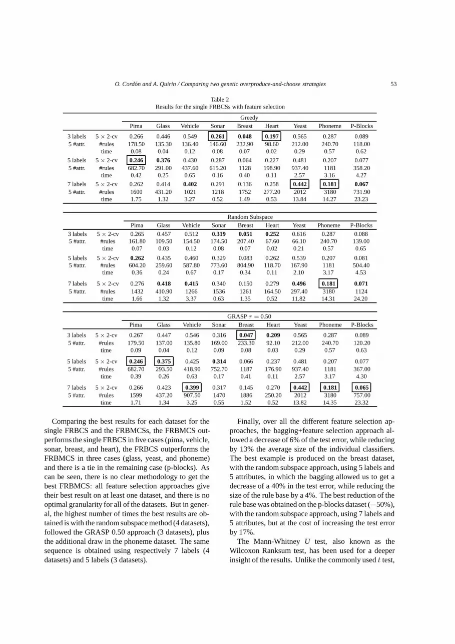
The statistics (5 × 2-cv error, number of rules,and run time required for each run, expressed in sec-onds) for the single FRBCSs are collected in Table 2.There are three subtables for each feature selectionmethod considered: Battiti’s method (greedy), Battiti’smethod combined with GRASP with 50% of random-ness (GRASP 0.50), and the random subspace method.The best results for a given feature selection method areshown in bold and the best values overall are outlined.

In our previous study [13], we showed that the bestresults for the four datasets considered in that contribu-tion were obtained using 5 labels for the smaller prob-lems (pima and glass), and 7 labels for the largest ones(vehicle and sonar). This is not the case with this largerstudy as sonar and some other problems with a higherdimension (breast and heart) give their best results with3 labels using respectively the GRASP 0.50 and thegreedy approaches. For the largest problems (yeast,phoneme, and p-blocks), the best performance is stillobtained with the largest number of labels.

Overall, the best single FRBCS results were obtainedwith GRASP 0.50 for four datasets, and with the greedyapproach for only two datasets (in the remaining threedatasets, these two approaches gave the same results).Pure random subspace only achieves a draw in the bestresults for a single dataset. This confirms the fact thatcontrolled randomness in the feature selection processis useful when combined with FRBCSs.

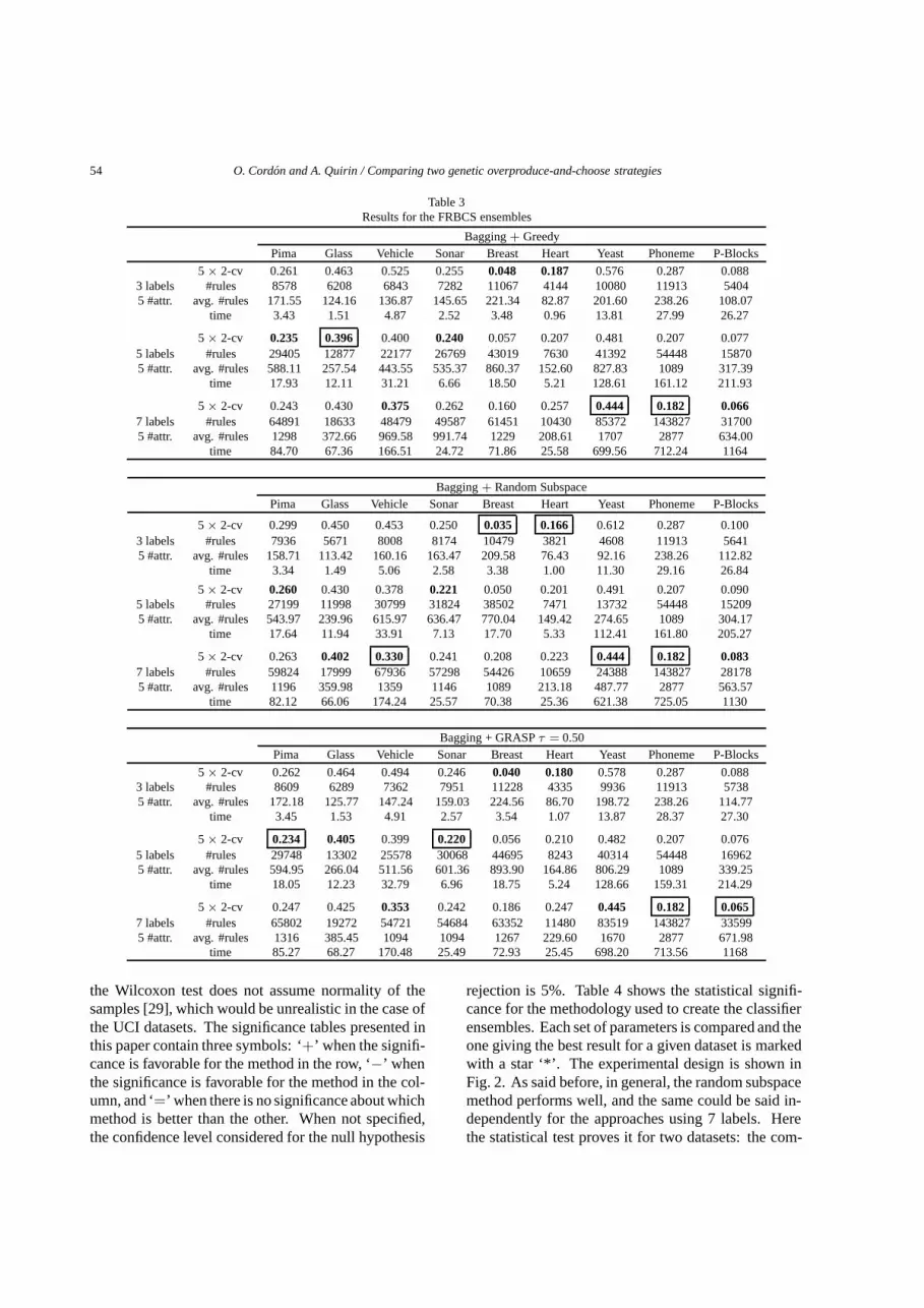
The results for the FRBMCSs of 50 classifiers gener-ated from the three different feature selection approach-es considered are shown in Table 3, which present thesame structure than Table 2.


Table 2Results for the single FRBCSs with feature selection

GreedyPima Glass Vehicle Sonar Breast Heart Yeast Phoneme P-Blocks

3 labels 5 × 2-cv 0.266 0.446 0.549 0.261 0.048 0.197 0.565 0.287 0.0895 #attr. #rules 178.50 135.30 136.40 146.60 232.90 98.60 212.00 240.70 118.00

time 0.08 0.04 0.12 0.08 0.07 0.02 0.29 0.57 0.62

5 labels 5 × 2-cv 0.246 0.376 0.430 0.287 0.064 0.227 0.481 0.207 0.0775 #attr. #rules 682.70 291.00 437.60 615.20 1128 198.90 937.40 1181 358.20

time 0.42 0.25 0.65 0.16 0.40 0.11 2.57 3.16 4.27

7 labels 5 × 2-cv 0.262 0.414 0.402 0.291 0.136 0.258 0.442 0.181 0.0675 #attr. #rules 1600 431.20 1021 1218 1752 277.20 2012 3180 731.90

time 1.75 1.32 3.27 0.52 1.49 0.53 13.84 14.27 23.23

Random SubspacePima Glass Vehicle Sonar Breast Heart Yeast Phoneme P-Blocks


time 0.07 0.03 0.12 0.08 0.07 0.02 0.21 0.57 0.65

5 labels 5 × 2-cv 0.262 0.435 0.460 0.329 0.083 0.262 0.539 0.207 0.0815 #attr. #rules 604.20 259.60 587.80 773.60 804.90 118.70 167.90 1181 504.40

time 0.36 0.24 0.67 0.17 0.34 0.11 2.10 3.17 4.53

7 labels 5 × 2-cv 0.276 0.418 0.415 0.340 0.150 0.279 0.496 0.181 0.0715 #attr. #rules 1432 410.90 1266 1536 1261 164.50 297.40 3180 1124

time 1.66 1.32 3.37 0.63 1.35 0.52 11.82 14.31 24.20

GRASP τ = 0.50Pima Glass Vehicle Sonar Breast Heart Yeast Phoneme P-Blocks


time 0.09 0.04 0.12 0.09 0.08 0.03 0.29 0.57 0.63

5 labels 5 × 2-cv 0.246 0.375 0.425 0.314 0.066 0.237 0.481 0.207 0.0775 #attr. #rules 682.70 293.50 418.90 752.70 1187 176.90 937.40 1181 367.00

time 0.39 0.26 0.63 0.17 0.41 0.11 2.57 3.17 4.30

7 labels 5 × 2-cv 0.266 0.423 0.399 0.317 0.145 0.270 0.442 0.181 0.0655 #attr. #rules 1599 437.20 907.50 1470 1886 250.20 2012 3180 757.00

time 1.71 1.34 3.25 0.55 1.52 0.52 13.82 14.35 23.32

Comparing the best results for each dataset for thesingle FRBCS and the FRBMCSs, the FRBMCS out-performs the single FRBCS in five cases (pima, vehicle,sonar, breast, and heart), the FRBCS outperforms theFRBMCS in three cases (glass, yeast, and phoneme)and there is a tie in the remaining case (p-blocks). Ascan be seen, there is no clear methodology to get thebest FRBMCS: all feature selection approaches givetheir best result on at least one dataset, and there is nooptimal granularity for all of the datasets. But in gener-al, the highest number of times the best results are ob-tained is with the random subspace method (4 datasets),followed the GRASP 0.50 approach (3 datasets), plusthe additional draw in the phoneme dataset. The samesequence is obtained using respectively 7 labels (4datasets) and 5 labels (3 datasets).

Finally, over all the different feature selection ap-proaches, the bagging+feature selection approach al-lowed a decrease of 6% of the test error, while reducingby 13% the average size of the individual classifiers.The best example is produced on the breast dataset,with the random subspace approach, using 5 labels and5 attributes, in which the bagging allowed us to get adecrease of a 40% in the test error, while reducing thesize of the rule base by a 4%. The best reduction of therule base was obtained on the p-blocks dataset (−50%),with the random subspace approach, using 7 labels and5 attributes, but at the cost of increasing the test errorby 17%.

The Mann-Whitney U test, also known as theWilcoxon Ranksum test, has been used for a deeperinsight of the results. Unlike the commonly used t test,


Table 3Results for the FRBCS ensembles

Bagging + GreedyPima Glass Vehicle Sonar Breast Heart Yeast Phoneme P-Blocks

5 × 2-cv 0.261 0.463 0.525 0.255 0.048 0.187 0.576 0.287 0.0883 labels #rules 8578 6208 6843 7282 11067 4144 10080 11913 54045 #attr. avg. #rules 171.55 124.16 136.87 145.65 221.34 82.87 201.60 238.26 108.07

time 3.43 1.51 4.87 2.52 3.48 0.96 13.81 27.99 26.27

5 × 2-cv 0.235 0.396 0.400 0.240 0.057 0.207 0.481 0.207 0.0775 labels #rules 29405 12877 22177 26769 43019 7630 41392 54448 158705 #attr. avg. #rules 588.11 257.54 443.55 535.37 860.37 152.60 827.83 1089 317.39

time 17.93 12.11 31.21 6.66 18.50 5.21 128.61 161.12 211.93

5 × 2-cv 0.243 0.430 0.375 0.262 0.160 0.257 0.444 0.182 0.0667 labels #rules 64891 18633 48479 49587 61451 10430 85372 143827 317005 #attr. avg. #rules 1298 372.66 969.58 991.74 1229 208.61 1707 2877 634.00

time 84.70 67.36 166.51 24.72 71.86 25.58 699.56 712.24 1164

Bagging + Random SubspacePima Glass Vehicle Sonar Breast Heart Yeast Phoneme P-Blocks


time 3.34 1.49 5.06 2.58 3.38 1.00 11.30 29.16 26.84


time 17.64 11.94 33.91 7.13 17.70 5.33 112.41 161.80 205.27

5 × 2-cv 0.263 0.402 0.330 0.241 0.208 0.223 0.444 0.182 0.0837 labels #rules 59824 17999 67936 57298 54426 10659 24388 143827 281785 #attr. avg. #rules 1196 359.98 1359 1146 1089 213.18 487.77 2877 563.57

time 82.12 66.06 174.24 25.57 70.38 25.36 621.38 725.05 1130

Bagging + GRASP τ = 0.50Pima Glass Vehicle Sonar Breast Heart Yeast Phoneme P-Blocks


time 3.45 1.53 4.91 2.57 3.54 1.07 13.87 28.37 27.30


time 18.05 12.23 32.79 6.96 18.75 5.24 128.66 159.31 214.29

5 × 2-cv 0.247 0.425 0.353 0.242 0.186 0.247 0.445 0.182 0.0657 labels #rules 65802 19272 54721 54684 63352 11480 83519 143827 335995 #attr. avg. #rules 1316 385.45 1094 1094 1267 229.60 1670 2877 671.98

time 85.27 68.27 170.48 25.49 72.93 25.45 698.20 713.56 1168

the Wilcoxon test does not assume normality of thesamples [29], which would be unrealistic in the case ofthe UCI datasets. The significance tables presented inthis paper contain three symbols: ‘+’ when the signifi-cance is favorable for the method in the row, ‘−’ whenthe significance is favorable for the method in the col-umn, and ‘=’ when there is no significance about whichmethod is better than the other. When not specified,the confidence level considered for the null hypothesis

rejection is 5%. Table 4 shows the statistical signifi-cance for the methodology used to create the classifierensembles. Each set of parameters is compared and theone giving the best result for a given dataset is markedwith a star ‘*’. The experimental design is shown inFig. 2. As said before, in general, the random subspacemethod performs well, and the same could be said in-dependently for the approaches using 7 labels. Herethe statistical test proves it for two datasets: the com-


Tabl

e4

Stat

istic

alte

stfo

rth

eco

mpa

riso

nof

the

FRB

MC

Sde

sign

met

hodo

logi

es(s

eeFi

g.2)

.Fo

rea

chda

tase

t,th

ebe

stm

etho

dis

mar

ked

(‘*’

)an

dth

eot

hers

are

com

pare

dto

it

App

roac

hG

reed

yG

RA

SPτ

=0.

50R

ando

mSu

bspa

ce3

labe

ls5

labe

ls7

labe

ls3

labe

ls5

labe

ls7

labe

ls3

labe

ls5

labe

ls7

labe

ls

Pim

aµ±

σ0.

261±

0.02

200.

235±

0.01

560.

243±

0.01

670.

262±

0.02

330.

234±

0.01

90.

247±

0.01

560.

299±

0.02

840.

260±

0.02

200.

263±

0.01

38Sy

mbo

l+

==

+*

=+

++

Gla

ssµ±

σ0.

463±

0.04

910.

396±

0.05

680.

430±

0.05

840.

464±

0.04

890.

405±

0.04

60.

425±

0.06

480.

450±

0.07

020.

430±

0.06

210.

402±

0.05

19Sy

mbo

l+

*=

+=

=+

==

Veh

icle

µ±

σ0.

525±

0.02

470.

400±

0.02

670.

375±

0.01

500.

494±

0.03

40.

399±

0.03

390.

353±

0.02

390.

453±

0.02

090.

378±

0.02

440.

330±

0.01

79Sy

mbo

l+

++

++

++

+*

Sona

rµ±

σ0.

255±

0.03

550.

240±

0.03

010.

262±

0.03

230.

246±

0.06

050.

220±

0.04

450.

242±

0.03

560.

250±

0.04

60.

221±

0.03

360.

241±

0.04

83Sy

mbo

l=

=+

=*

==

==

Bre

ast

µ±

σ0.

0478

±0.

0092

0.05

75±

0.01

600.

160±

0.01

870.

0403

±0.

0096

50.

0561

±0.

0148

0.18

6±

0.02

450.

0355

±0.

0046

80.

0503

±0.

0095

90.

209±

0.02

14Sy

mbo

l+

++

=+

+*

++

Hea

rtµ±

σ0.

187±

0.03

220.

207±

0.03

760.

257±

0.05

410.

180±

0.03

310.

210±

0.03

500.

247±

0.04

690.

166±

0.03

350.

201±

0.03

50.

223±

0.05

13Sy

mbo

l=

++

=+

+*

++

Yea

stµ±

σ0.

576±

0.04

450.

481±

0.01

990.

444±

0.01

310.

578±

0.04

770.

482±

0.01

980.

445±

0.01

440.

612±

0.03

140.

491±

0.02

040.

444±

0.01

24Sy

mbo

l+

+=

++

=+

+*

Phon

eme

µ±

σ0.

287±

0.00

570.

207±

0.00

614

0.18

2±

0.00

933

0.28

7±

0.00

570.

207±

0.00

614

0.18

2±

0.00

933

0.28

7±

0.00

570.

207±

0.00

614

0.18

2±

0.00

933

Sym

bol

++

*+

+=

++

=P-

Blo

cks

µ±

σ0.

0882

±0.

0024

70.

077±

0.00

347

0.06

61±

0.00

319

0.08

76±

0.00

285

0.07

57±

0.00

437

0.06

53±

0.00

310

0.10

0±

0.00

331

0.08

97±

0.00

576

0.08

34±

0.00

636

Sym

bol

++

=+

+*

++

+


For each dataset

Output Wilcoxon(0.05)

For each parameter(granularity, #features), foreach feat. sel. approach

5x2 cv

For each ensemble approach

Get the best one(using the mean)

5x2 cv

G et the 9 (5x2cvtesterror) results

For each dataset

5x2 cv

For each ensemble approach

5x2 cv

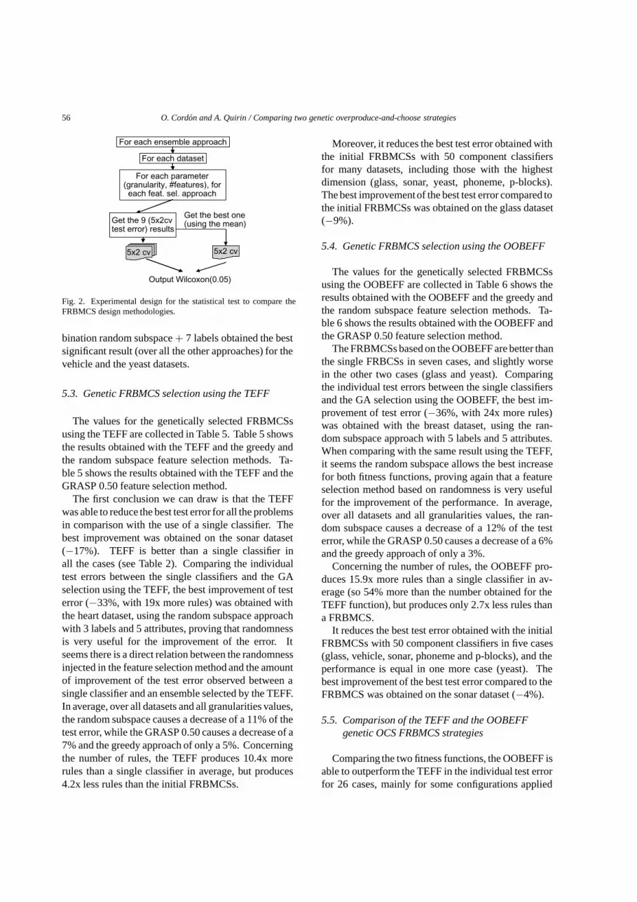
Get the 9 (5x2cvtest error) results

Fig. 2. Experimental design for the statistical test to compare theFRBMCS design methodologies.

bination random subspace + 7 labels obtained the bestsignificant result (over all the other approaches) for thevehicle and the yeast datasets.

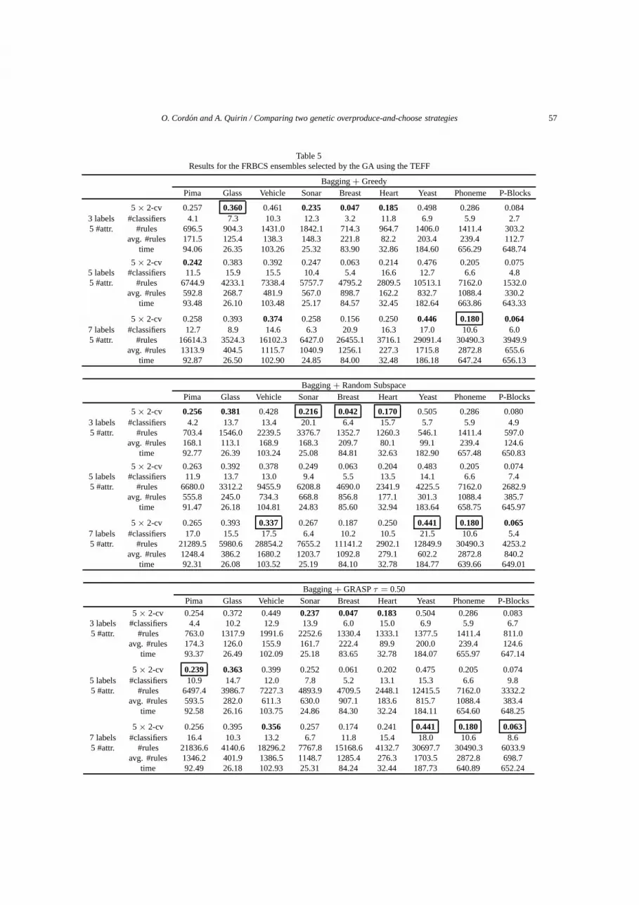
5.3. Genetic FRBMCS selection using the TEFF

The values for the genetically selected FRBMCSsusing the TEFF are collected in Table 5. Table 5 showsthe results obtained with the TEFF and the greedy andthe random subspace feature selection methods. Ta-ble 5 shows the results obtained with the TEFF and theGRASP 0.50 feature selection method.

The first conclusion we can draw is that the TEFFwas able to reduce the best test error for all the problemsin comparison with the use of a single classifier. Thebest improvement was obtained on the sonar dataset(−17%). TEFF is better than a single classifier inall the cases (see Table 2). Comparing the individualtest errors between the single classifiers and the GAselection using the TEFF, the best improvement of testerror (−33%, with 19x more rules) was obtained withthe heart dataset, using the random subspace approachwith 3 labels and 5 attributes, proving that randomnessis very useful for the improvement of the error. Itseems there is a direct relation between the randomnessinjected in the feature selection method and the amountof improvement of the test error observed between asingle classifier and an ensemble selected by the TEFF.In average, over all datasets and all granularities values,the random subspace causes a decrease of a 11% of thetest error, while the GRASP 0.50 causes a decrease of a7% and the greedy approach of only a 5%. Concerningthe number of rules, the TEFF produces 10.4x morerules than a single classifier in average, but produces4.2x less rules than the initial FRBMCSs.

Moreover, it reduces the best test error obtained withthe initial FRBMCSs with 50 component classifiersfor many datasets, including those with the highestdimension (glass, sonar, yeast, phoneme, p-blocks).The best improvementof the best test error compared tothe initial FRBMCSs was obtained on the glass dataset(−9%).

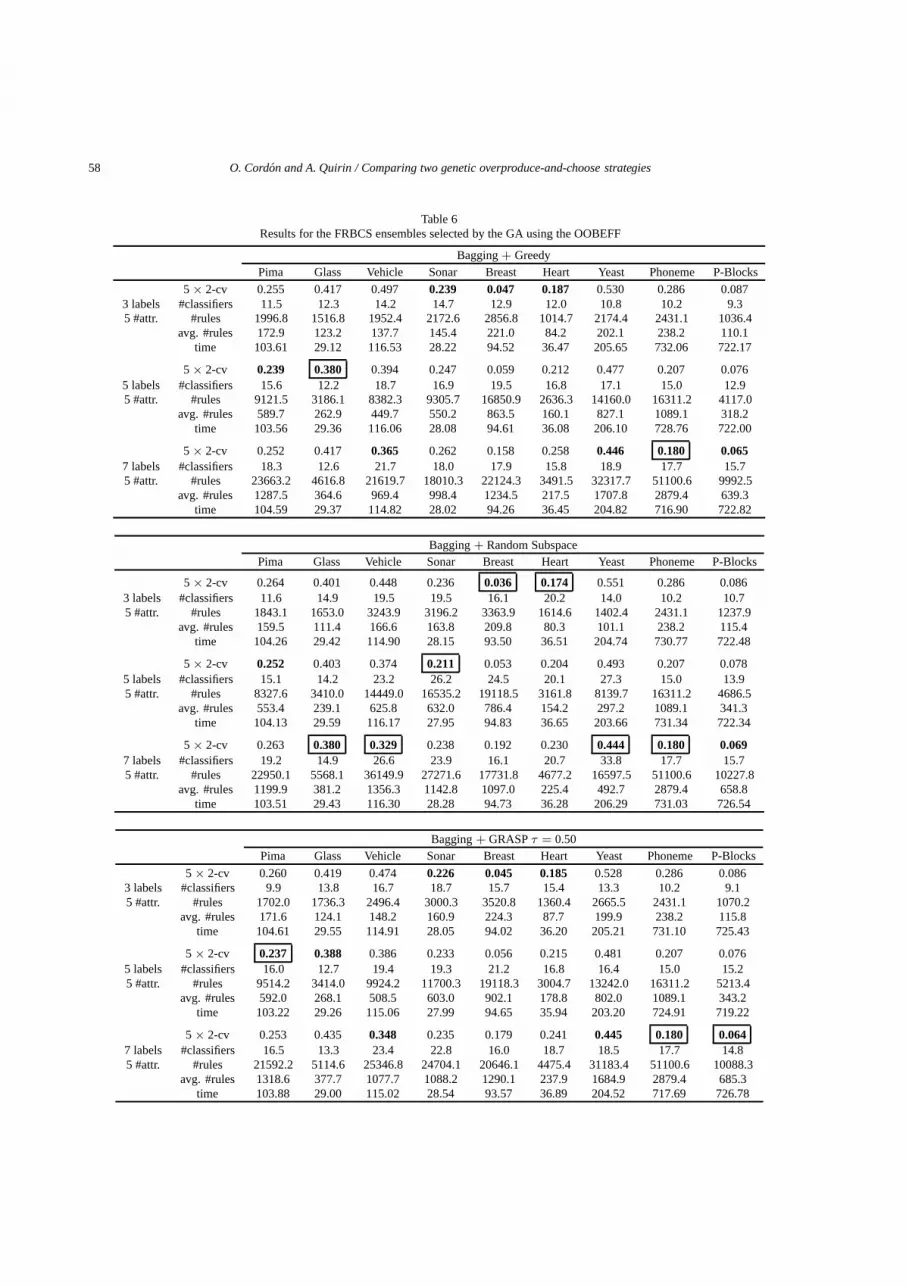
5.4. Genetic FRBMCS selection using the OOBEFF

The values for the genetically selected FRBMCSsusing the OOBEFF are collected in Table 6 shows theresults obtained with the OOBEFF and the greedy andthe random subspace feature selection methods. Ta-ble 6 shows the results obtained with the OOBEFF andthe GRASP 0.50 feature selection method.

The FRBMCSs based on the OOBEFF are better thanthe single FRBCSs in seven cases, and slightly worsein the other two cases (glass and yeast). Comparingthe individual test errors between the single classifiersand the GA selection using the OOBEFF, the best im-provement of test error (−36%, with 24x more rules)was obtained with the breast dataset, using the ran-dom subspace approach with 5 labels and 5 attributes.When comparing with the same result using the TEFF,it seems the random subspace allows the best increasefor both fitness functions, proving again that a featureselection method based on randomness is very usefulfor the improvement of the performance. In average,over all datasets and all granularities values, the ran-dom subspace causes a decrease of a 12% of the testerror, while the GRASP 0.50 causes a decrease of a 6%and the greedy approach of only a 3%.

Concerning the number of rules, the OOBEFF pro-duces 15.9x more rules than a single classifier in av-erage (so 54% more than the number obtained for theTEFF function), but produces only 2.7x less rules thana FRBMCS.

It reduces the best test error obtained with the initialFRBMCSs with 50 component classifiers in five cases(glass, vehicle, sonar, phoneme and p-blocks), and theperformance is equal in one more case (yeast). Thebest improvement of the best test error compared to theFRBMCS was obtained on the sonar dataset (−4%).

5.5. Comparison of the TEFF and the OOBEFFgenetic OCS FRBMCS strategies

Comparing the two fitness functions, the OOBEFF isable to outperform the TEFF in the individual test errorfor 26 cases, mainly for some configurations applied


Table 5Results for the FRBCS ensembles selected by the GA using the TEFF


5 × 2-cv 0.257 0.360 0.461 0.235 0.047 0.185 0.498 0.286 0.0843 labels #classifiers 4.1 7.3 10.3 12.3 3.2 11.8 6.9 5.9 2.75 #attr. #rules 696.5 904.3 1431.0 1842.1 714.3 964.7 1406.0 1411.4 303.2

avg. #rules 171.5 125.4 138.3 148.3 221.8 82.2 203.4 239.4 112.7time 94.06 26.35 103.26 25.32 83.90 32.86 184.60 656.29 648.74


avg. #rules 592.8 268.7 481.9 567.0 898.7 162.2 832.7 1088.4 330.2time 93.48 26.10 103.48 25.17 84.57 32.45 182.64 663.86 643.33


avg. #rules 1313.9 404.5 1115.7 1040.9 1256.1 227.3 1715.8 2872.8 655.6time 92.87 26.50 102.90 24.85 84.00 32.48 186.18 647.24 656.13



avg. #rules 168.1 113.1 168.9 168.3 209.7 80.1 99.1 239.4 124.6time 92.77 26.39 103.24 25.08 84.81 32.63 182.90 657.48 650.83


avg. #rules 555.8 245.0 734.3 668.8 856.8 177.1 301.3 1088.4 385.7time 91.47 26.18 104.81 24.83 85.60 32.94 183.64 658.75 645.97


avg. #rules 1248.4 386.2 1680.2 1203.7 1092.8 279.1 602.2 2872.8 840.2time 92.31 26.08 103.52 25.19 84.10 32.78 184.77 639.66 649.01



avg. #rules 174.3 126.0 155.9 161.7 222.4 89.9 200.0 239.4 124.6time 93.37 26.49 102.09 25.18 83.65 32.78 184.07 655.97 647.14


avg. #rules 593.5 282.0 611.3 630.0 907.1 183.6 815.7 1088.4 383.4time 92.58 26.16 103.75 24.86 84.30 32.24 184.11 654.60 648.25


avg. #rules 1346.2 401.9 1386.5 1148.7 1285.4 276.3 1703.5 2872.8 698.7time 92.49 26.18 102.93 25.31 84.24 32.44 187.73 640.89 652.24


Table 6Results for the FRBCS ensembles selected by the GA using the OOBEFF



avg. #rules 172.9 123.2 137.7 145.4 221.0 84.2 202.1 238.2 110.1time 103.61 29.12 116.53 28.22 94.52 36.47 205.65 732.06 722.17


avg. #rules 589.7 262.9 449.7 550.2 863.5 160.1 827.1 1089.1 318.2time 103.56 29.36 116.06 28.08 94.61 36.08 206.10 728.76 722.00


avg. #rules 1287.5 364.6 969.4 998.4 1234.5 217.5 1707.8 2879.4 639.3time 104.59 29.37 114.82 28.02 94.26 36.45 204.82 716.90 722.82



avg. #rules 159.5 111.4 166.6 163.8 209.8 80.3 101.1 238.2 115.4time 104.26 29.42 114.90 28.15 93.50 36.51 204.74 730.77 722.48


avg. #rules 553.4 239.1 625.8 632.0 786.4 154.2 297.2 1089.1 341.3time 104.13 29.59 116.17 27.95 94.83 36.65 203.66 731.34 722.34


avg. #rules 1199.9 381.2 1356.3 1142.8 1097.0 225.4 492.7 2879.4 658.8time 103.51 29.43 116.30 28.28 94.73 36.28 206.29 731.03 726.54



avg. #rules 171.6 124.1 148.2 160.9 224.3 87.7 199.9 238.2 115.8time 104.61 29.55 114.91 28.05 94.02 36.20 205.21 731.10 725.43


avg. #rules 592.0 268.1 508.5 603.0 902.1 178.8 802.0 1089.1 343.2time 103.22 29.26 115.06 27.99 94.65 35.94 203.20 724.91 719.22


avg. #rules 1318.6 377.7 1077.7 1088.2 1290.1 237.9 1684.9 2879.4 685.3time 103.88 29.00 115.02 28.54 93.57 36.89 204.52 717.69 726.78


0

0.1

0.2

0.3

0.4

0.5

0.6

Pima

GlassVehicle

Sonar

Breast

Heart

Yeast

Phoneme

P-Blocks

Tes

t Err

or R

ates

Datasets

Test Error Comparison

Single classifierInitial ensemble

GA Training Error FitnessGA Out-Of-Bag Error Fitness

Fig. 3. Comparison of the average test errors of a single classifier, the initial FRBMCS, and those generated using the TEFF and the OOBEFF-basedgenetic selection.

on the smallest datasets (pima, glass, vehicle, sonar,breast, and heart). The best individual improvementobserved was on the breast dataset (−16%), with ran-dom subspace (again!) with 5 labels and 5 attributes.We have compared the average improvement over thefeature selection approaches, over all the datasets, andonly the random subspace shows an improvement withthe OOBEFF (−0.52%), while an increase of 0.86%with GRASP 0.50 and of 1.42% with the greedy ap-proach are found. Comparing the number of labels, re-gardless the datasets and the feature selection approach-es, it seems that the best test error improvement wasobtained with 5 labels (−1.2%, +3.1% with 3 labelsand −0.1% with 7 labels). For all the remaining cases,it seems the OOBEFF is a little worst than the TEFF,but the results are still better than those obtained bythe initial pool. This little decrease in the classificationaccuracy could be explained by the fact the GA is usingless instances (in general, the bootstrapping producea 37% of instances in the “Out-Of-Bags", this means63% less instances in average).

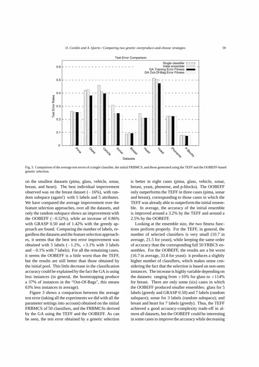
Figure 3 shows a comparison between the averagetest error (taking all the experiments we did with all theparameter settings into account) obtained on the initialFRBMCS of 50 classifiers, and the FRBMCSs derivedby the GA using the TEFF and the OOBEFF. As canbe seen, the test error obtained by a genetic selection

is better in eight cases (pima, glass, vehicle, sonar,breast, yeast, phoneme, and p-blocks). The OOBEFFonly outperforms the TEFF in three cases (pima, sonarand breast), corresponding to those cases in which theTEFF was already able to outperform the initial ensem-ble. In average, the accuracy of the initial ensembleis improved around a 3.2% by the TEFF and around a2.5% by the OOBEFF.

Looking at the ensemble size, the two fitness func-tions perform properly. For the TEFF, in general, thenumber of selected classifiers is very small (10.7 inaverage, 21.5 for yeast), while keeping the same orderof accuracy than the corresponding full 50 FRBCS en-sembles. For the OOBEFF, the results are a bit worst(16.7 in average, 33.8 for yeast): it produces a slightlyhigher number of classifiers, which makes sense con-sidering the fact that the selection is based on non-seeninstances. The increase is highly variable depending onthe datasets: ranging from +10% for glass to +114%for breast. There are only some (six) cases in whichthe OOBEFF produced smaller ensembles: glass for 5labels (greedy and GRASP 0.50) and 7 labels (randomsubspace); sonar for 3 labels (random subspace); andbreast and heart for 7 labels (greedy). Thus, the TEFFachieved a good accuracy-complexity trade-off in al-most all datasets, but the OOBEFF could be interestingin some cases to improve the accuracy while decreasing


0

10

20

30

40

50

Pima

GlassVehicle

Sonar

Breast

Heart

Yeast

Phoneme

P-Blocks

Com

plex

ity (

# of

cla

ssifi

ers)

Datasets

Complexity Comparison

Single classifierInitial ensemble

GA Training Error FitnessGA Out-Of-Bag Error Fitness

Fig. 4. Comparison of the average complexity (# of classifiers) between the selected FRBMCSs using the TEFF and those generated using theOOBEFF-based genetic selection.

For the single classifier

For each dataset




5x2 cv

For the GA selectedensembles

Output Wilcoxon(0.05)



For each parameter(granularity, #features), for

each feat. sel. approach, forthe two fitnesses

For the ensemble




5x2 cv

5x2 cv

5x2 cv

5x2 cv

5x2 cv

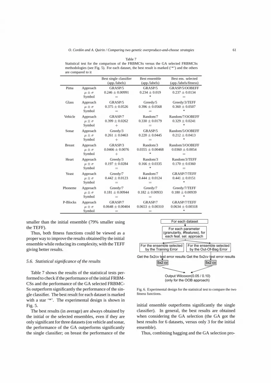
Fig. 5. Experimental design for the statistical test to compare the selected FRBMCS design methodologies.

the complexity (e.g., on glass, 5 labels, 5 attributes andthe greedy approach, the ensemble is reduced by a 23%while still decreasing the test error).

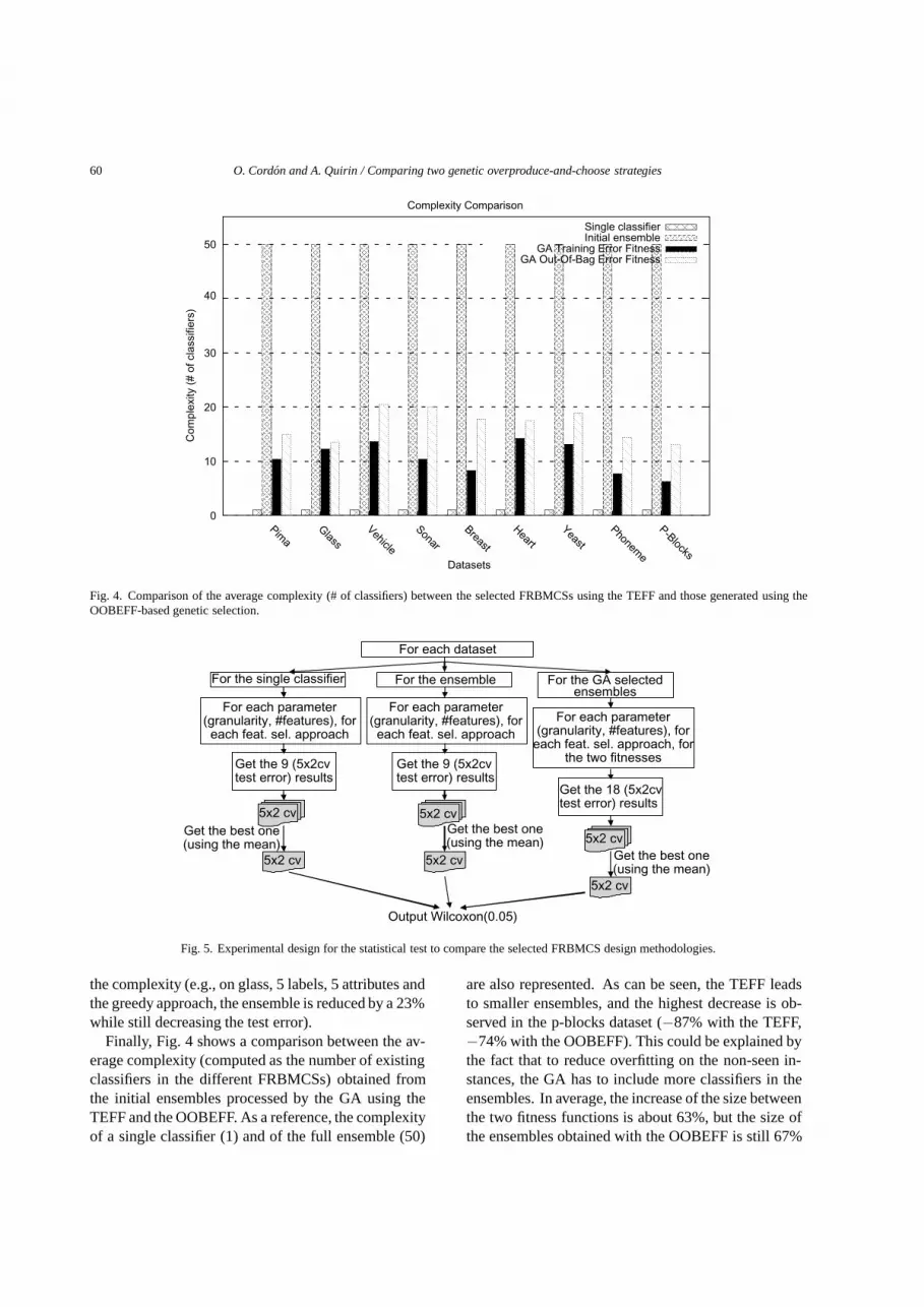
Finally, Fig. 4 shows a comparison between the av-erage complexity (computed as the number of existingclassifiers in the different FRBMCSs) obtained fromthe initial ensembles processed by the GA using theTEFF and the OOBEFF. As a reference, the complexityof a single classifier (1) and of the full ensemble (50)

are also represented. As can be seen, the TEFF leadsto smaller ensembles, and the highest decrease is ob-served in the p-blocks dataset (−87% with the TEFF,−74% with the OOBEFF). This could be explained bythe fact that to reduce overfitting on the non-seen in-stances, the GA has to include more classifiers in theensembles. In average, the increase of the size betweenthe two fitness functions is about 63%, but the size ofthe ensembles obtained with the OOBEFF is still 67%


Table 7Statistical test for the comparison of the FRBMCSs versus the GA selected FRBMCSsmethodologies (see Fig. 5). For each dataset, the best result is marked (‘*’) and the othersare compared to it

Best single classifier Best ensemble Best ens. selected(app./labels) (app./labels) (app./labels/fitness)

Pima Approach GRASP/5 GRASP/5 GRASP/5/OOBEFFµ ± σ 0.246 ± 0.00991 0.234 ± 0.019 0.237 ± 0.0134

Symbol = * =

Glass Approach GRASP/5 Greedy/5 Greedy/3/TEFFµ ± σ 0.375 ± 0.0526 0.396 ± 0.0568 0.360 ± 0.0507

Symbol = = *

Vehicle Approach GRASP/7 Random/7 Random/7/OOBEFFµ ± σ 0.399 ± 0.0262 0.330 ± 0.0179 0.329 ± 0.0241

Symbol + = *

Sonar Approach Greedy/3 GRASP/5 Random/5/OOBEFFµ ± σ 0.261 ± 0.0463 0.220 ± 0.0445 0.212 ± 0.0413

Symbol + = *

Breast Approach GRASP/3 Random/3 Random/3/OOBEFFµ ± σ 0.0466 ± 0.0076 0.0355 ± 0.00468 0.0360 ± 0.0054

Symbol + * =

Heart Approach Greedy/3 Random/3 Random/3/TEFFµ ± σ 0.197 ± 0.0284 0.166 ± 0.0335 0.170 ± 0.0360

Symbol = * =

Yeast Approach Greedy/7 Random/7 GRASP/7/TEFFµ ± σ 0.442 ± 0.0123 0.444 ± 0.0124 0.441 ± 0.0151

Symbol = = *

Phoneme Approach Greedy/7 Greedy/7 Greedy/7/TEFFµ ± σ 0.181 ± 0.00944 0.182 ± 0.00933 0.180 ± 0.00939

Symbol = = *

P-Blocks Approach GRASP/7 GRASP/7 GRASP/7/TEFFµ ± σ 0.0648 ± 0.00404 0.0653 ± 0.00310 0.0634 ± 0.00318

Symbol = = *

smaller than the initial ensemble (79% smaller usingthe TEFF).

Thus, both fitness functions could be viewed as aproper way to improve the results obtained by the initialensemble while reducing its complexity, with the TEFFgiving better results.

5.6. Statistical significance of the results

Table 7 shows the results of the statistical tests per-formed to check if the performance of the initial FRBM-CSs and the performance of the GA selected FRBMC-Ss outperform significantly the performance of the sin-gle classifier. The best result for each dataset is markedwith a star ‘*’. The experimental design is shown inFig. 5.

The best results (in average) are always obtained bythe initial or the selected ensembles, even if they areonly significant for three datasets (on vehicle and sonar,the performance of the GA outperforms significantlythe single classifier; on breast the performance of the

For the ensemble selectedby the Training Error

For the ensemble selectedby the Out-Of-Bag Error

For each dataset

Output Wilcoxon(0.05 / 0.10)(only for the OOB approach)


5x2 cv

Get the 5x2cv test error results Get the 5x2cv test error results

5x2 cv

Fig. 6. Experimental design for the statistical test to compare the twofitness functions.

initial ensemble outperforms significantly the singleclassifier). In general, the best results are obtainedwhen considering the GA selection (the GA got thebest results for 6 datasets, versus only 3 for the initialensemble).

Thus, combining bagging and the GA selection pro-


Table 8Statistical test for the comparison of the two GA fitness functions (see Fig. 6). Foreach dataset, the OOBEFF is compared to the TEFF for each approach (‘+’ meansthe OOBEFF is significantly better). The results are shown with a confidenceof 5 and 10%. Only the datasets/approaches with have statistically significantdifferences are listed

Approach Greedy GRASP τ = 0.50 Random SubspaceDatasets 3 labels 3 labels 7 labels 3 labels 5 labels 7 labels

Glass – =/– =/–Vehicle =/–Sonar +Breast =/+Yeast – – –

P-Blocks =/– – – –

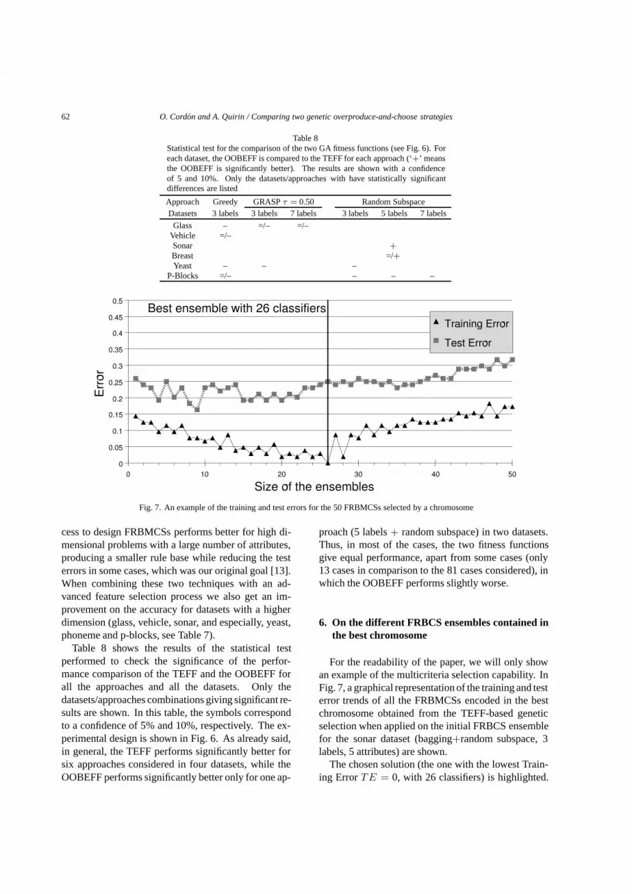
Fig. 7. An example of the training and test errors for the 50 FRBMCSs selected by a chromosome

cess to design FRBMCSs performs better for high di-mensional problems with a large number of attributes,producing a smaller rule base while reducing the testerrors in some cases, which was our original goal [13].When combining these two techniques with an ad-vanced feature selection process we also get an im-provement on the accuracy for datasets with a higherdimension (glass, vehicle, sonar, and especially, yeast,phoneme and p-blocks, see Table 7).

Table 8 shows the results of the statistical testperformed to check the significance of the perfor-mance comparison of the TEFF and the OOBEFF forall the approaches and all the datasets. Only thedatasets/approaches combinations giving significant re-sults are shown. In this table, the symbols correspondto a confidence of 5% and 10%, respectively. The ex-perimental design is shown in Fig. 6. As already said,in general, the TEFF performs significantly better forsix approaches considered in four datasets, while theOOBEFF performs significantly better only for one ap-

proach (5 labels + random subspace) in two datasets.Thus, in most of the cases, the two fitness functionsgive equal performance, apart from some cases (only13 cases in comparison to the 81 cases considered), inwhich the OOBEFF performs slightly worse.

6. On the different FRBCS ensembles contained inthe best chromosome

For the readability of the paper, we will only showan example of the multicriteria selection capability. InFig. 7, a graphical representation of the training and testerror trends of all the FRBMCSs encoded in the bestchromosome obtained from the TEFF-based geneticselection when applied on the initial FRBCS ensemblefor the sonar dataset (bagging+random subspace, 3labels, 5 attributes) are shown.

The chosen solution (the one with the lowest Train-ing Error TE = 0, with 26 classifiers) is highlighted.


Notice that the ensemble of 9 classifiers has a better testerror and is actually smaller; and how bigger ensembleslead to bigger training and test errors.

We leave for future works the study of this capabilityof our algorithm and the analysis of its interrelationwith the two fitness functions.

7. Conclusions and future works

We have proposed the use of bagging and featureselection approaches like random subspace and greedyand GRASP-based Battiti’s methods, together witha TEFF and a OOBEFF-guided multicriteria GA, todesign FRBMCS ensembles with a good accuracy-complexity trade-off. The resulting FRBCS ensembleshave shown to be able to deal with classification prob-lems with a large number of features (up to 60) and alarge number of instances (up to 5,400). The resultsobtained in some popular data sets of high dimensionare quite promising.

Our future work will be concentrated on the study ofthe influence of other parameters (the GA parametersfor instance), on the design of more advanced genet-ic MCS selection techniques (for example, the use ofPareto-based algorithms), on the use of more advancedfuzzy reasoning mechanisms both in the componentFRBCSs and in the ensemble, on the analysis of themulticriteria GA potentials, and on the design of MCSsof more accurate FRBCSs.

References

[1] J.J. Aguilera, M. Chica, M.J. del Jesus and F. Herrera, Nichinggenetic feature selection algorithms applied to the design offuzzy rule based classification systems, In IEEE Internation-al Conference on Fuzzy Systems (FUZZ-IEEE), pages 1794–1799, London, 2007.

[2] R.E. Banfield, L.O. Hall, K.W. Bowyer and W.P. Kegelmeyer,A comparison of decision tree ensemble creation techniques,IEEE Transactions on Pattern Analysis and Machine Intelli-gence 29(1) (2007), 173–180.

[3] R. Battiti, Using mutual information for selecting features insupervised neural net learning, IEEE Transactions on NeuralNetworks 5(4) (1994), 537–550.

[4] L. Breiman, Bagging predictors, Machine Learning 24(2)(1996), 123–140.

[5] L. Breiman, Stacked regressions, Machine Learning 24(1)(1996), 49–64.

[6] L. Breiman, Random forests, Machine Learning 45(1) (2001),5–32.

[7] J. Canul-Reich, L. Shoemaker and L.O. Hall, Ensembles ofFuzzy Classifiers, In IEEE International Conference on FuzzySystems (FUZZ-IEEE), pages 1–6, London, 2007.

[8] J. Casillas, O. Cordon and F. Herrera, COR: A methodologyto improve ad hoc data-driven linguistic rule learning methodsby inducing cooperation among rules, IEEE Transactions onSystems, Man, and Cybernetics, Part B: Cybernetics 32(4)(2002), 526–537.

[9] C.A. Coello, G.B. Lamont and D.A. Van Veldhuizen, Evo-lutionary Algorithms for Solving Multi-Objective Problems,(2nd Edition), Springer, 2007.

[10] O. Cordon, M.J. del Jesus and F. Herrera, A proposal onreasoning methods in fuzzy rule-based classification systems,International Journal of Approximate Reasoning 20 (1999),21–45.

[11] O. Cordon, F. Gomide, F. Herrera, F. Hoffmann and L. Mag-dalena, Ten years of genetic fuzzy systems: Current frame-work and new trends, Fuzzy Sets and Systems 141(1) (2004),5–31.

[12] O. Cordoon, F. Herrera, F. Hoffmann and L. Magdalena, Ge-netic Fuzzy Systems, Evolutionary Tuning and Learning ofFuzzy Knowledge Bases, World Scientific, 2001.

[13] O. Cordon, A. Quirin and L. Sanchez, A first Study on BaggingFuzzy Rule-Based Classification Systems with multicriteriagenetic selection of the Component Classifiers, In IEEE Inter-national Workshop on Genetic and Evolving Fuzzy Systems(GEFS), pages 11–16, Germany, 2008.

[14] O. Cordon, A. Quirin and L. Sanchez, On the Use of Bag-ging, Mutual Information-Based Feature Selection and Multi-criteria Genetic Algorithms to Design Fuzzy Rule-Based Clas-sification Ensembles, In International Conference on HybridIntelligent Systems (HIS), pages 549–554, Barcelona, 2008.

[15] B.V. Dasarathy and B.V. Sheela, A composite classifier sys-tem design: Concepts and methodology, Proceedings of IEEE67(5) (1979), 708–713.

[16] M.J. del Jesus, F. Hoffmann, L.J. Navascues and L. Sanchez,Induction of fuzzy-rule-based classifiers with evolutionaryboosting algorithms, IEEE Transactions on Fuzzy Systems12(3) (2004), 296–308.

[17] T.G. Dietterich, Approximate statistical test for comparing su-pervised classification learning algorithms, Neural Computa-tion 10(7) (1998), 1895–1923.

[18] N. Dimililer, E. Varoglu and H. Altincay, Classifier subsetselection for biomedical named entity recognition, AppliedIntelligence 31(3) (December 2009), 267–282.

[19] T.A. Feo and M.G.C. Resende, Greedy randomized adaptivesearch procedures, Journal of Global Optimization 6 (1995),109–133.

[20] B. Gabrys and D. Ruta, Genetic algorithms in classifier fusion,Applied Soft Computing 6(4) (2006), 337–347.

[21] G. Giacinto and F. Roli, Dynamic classifier selection basedon multiple classifier behaviour, Pattern Recognition 34(9)(2001), 1879–1881.

[22] S.T. Hadjitodorov and L.I. Kuncheva, Selecting diversifyingheuristics for cluster ensembles, Lecture Notes in ComputerScience 4472 (2007), 200–209.

[23] T. Ho, The random subspace method for constructing decisionforests, IEEE Transactions on Pattern Analysis and MachineIntelligence 20(8) (1998), 832–844.

[24] F. Hoffmann, Combining boosting and evolutionary algo-rithms for learning of fuzzy classification rules, Fuzzy Setsand Systems 141(1) (2004), 47–58.

[25] H. Ishibuchi, T. Nakashima and M. Nii, Classification andModeling With Linguistic Information Granules, Springer,2005.

[26] H. Ishibuchi and Y. Nojima, Evolutionary multiobjective op-timization for the design of fuzzy rule-based ensemble classi-


fiers, International Journal of Hybrid Intelligent Systems 3(3)(2006), 129–145.

[27] M. Kim, S. Min and I. Han, An evolutionary approach to thecombination of multiple classifiers to predict a stock priceindex, Expert Systems with Applications 31 (2006), 241–247.

[28] L. Kuncheva, Combining Pattern Classifiers: Methods andAlgorithms, Wiley, 2004.

[29] E. Lehmann, Nonparametric Statistical Methods Based onRanks, McGraw-Hill, New-York, 1975.

[30] Y. Liu, X. Yao and T. Higuchi, Evolutionary ensembles withnegative correlation learning, IEEE Transactions on Evolu-tionary Computation 4 (2000), 380–387.

[31] G. Martınez-Munoz, D. Hernandez-Lobato and A. Suarez,Selection of decision stumps in bagging ensembles, LectureNotes in Computer Science 4668 (2007), 319–328.

[32] Z. Michalewicz, Genetic Algorithms + Data Structures =Evolution Programs, Springer, 1996.

[33] Y. Nojima and H. Ishibuchi, Genetic rule selection with amulti-classifier coding scheme for ensemble classifier de-sign, International Journal of Hybrid Intelligent Systems 4(3)(2007), 157–169.

[34] L.S. Oliveira, M. Morita, R. Sabourin and F. Bortolozzi, Multi-objective genetic algorithms to create ensemble of classifiers,Lecture Notes in Computer Science 3410 (2005), 592–606.

[35] D. Optiz and R. Maclin, Popular ensemble methods: An em-pirical study, Journal of Artificial Intelligence Research 11(1999), 169–198.

[36] D. Partridge and W.B. Yates, Engineering multiversion neural-net systems, Neural Computation 8 (4) (1996), 869–893.

[37] W. Pedrycz, A. Breuer and N.J. Pizzi, Fuzzy adaptive logicnetworks as hybrid models of quantitative software engineer-ing, Intelligent Automation and Soft Computing 12(2)(2006),189–209.

[38] W. Pedrycz and K.C. Kwak, Boosting of granular models,Fuzzy Sets and Systems 157(22) (2006), 2934–2953.

[39] D. Ruta and B. Gabrys, Classifier selection for majority voting,Information Fusion 6(1) (2005), 63–81.

[40] L. Sanchez and J. Otero, Boosting fuzzy rules in classificationproblems under single-winner inference, International Jour-nal of Intelligent Systems 22(9) (2007), 1021–1034.

[41] E.M. Dos Santos, R. Sabourin and P. Maupin, Single andMulti-Objective Genetic Algorithms for the Selection of En-semble of Classifiers, In International Joint Conference onNeural Networks (IJCNN), pages 3070–3077, Vancouver,2006.

[42] E.M. Dos Santos, R. Sabourin and P. Maupin, A dynamicoverproduce-and-choose strategy for the selection of classifierensembles, Pattern Recognition 41(10) (2008), 2993–3009.

[43] R. Schapire, The strength of weak learnability, MachineLearning 5(2) (1990), 197–227.

[44] R. Schapire, Y. Freund, P. Bartlett and W. Lee, Boosting theMargin: A new Explanation for the Effectiveness of VotingMethods, In International Conference on Machine Learning,pages 322–330, Nashville, 1997.

[45] R. Scherer, Boosting ensemble of relational neurofuzzy sys-tems, Lecture Notes in Computer Science 4029 (2006), 306–313.

[46] C.E. Shannon and W.Weaver, The Mathematical Theory ofCommunication, University of Illlinois Press, 1949.

[47] A.J.C. Sharkey and N.E. Sharkey, The Test and Select Ap-proach to Ensemble Combination, In InternationalWorkshopon Multiclassifier Systems, pages 30–44, Cagliari, 2000.

[48] C.-A. Tsai, T.-C. Lee, I.-C. Ho, U.-C. Yang, C.-H. Chen andJ.J. Chen, Multi-class clustering and prediction in the analysisof microarray data, Mathematical Biosciences 193(1) (2005),79–100.

[49] A. Tsymbal, M. Pechenizkiy and P. Cunningham, Diversity insearch strategies for ensemble feature selection, InformationFusion 6(1) (2005), 83–98.

[50] S.J. Verzi, G.L. Heileman and M. Georgiopoulos, BoostedARTMAP: Modifications to fuzzy ARTMAP motivated byboosting theory, Neural Networks 19(4) (2006), 446–468.

[51] L. Xu, A. Krzyzak and C.Y. Suen, Methods of combiningmultiple classifiers and their application to handwriting recog-nition, IEEE Transactions on Systems, Man, and Cybernetics22(3) (1992), 418–435.

[52] Z.H. Zhou, Ensembling local learners through multimodal per-turbation, IEEE Transactions of Systems, Man, and Cybernet-ics, Part B: Cybernetics 35(4) (2005), 725–735.

Comparing two genetic overproduce-and-choose strategies for fuzzy rule-based multiclassification...

Documents

Transcript of Comparing two genetic overproduce-and-choose strategies for fuzzy rule-based multiclassification...