Three-dimensional Density Structure of the Earth:Limits to Astrophysical and Seismological Approaches

by

Chaincy Kuo

B.A. (University of California at Berkeley) 1991

A dissertation submitted in partial satisfaction of the

requirements for the degree of

Doctor of Philosophy

in

Geophysics

in the

GRADUATE DIVISION

of the

UNIVERSITY of CALIFORNIA at BERKELEY

Committee in charge:

Professor Barbara Romanowicz, ChairProfessor Raymond JeanlozProfessor Gilbert Shapiro

1999

The dissertation of Chaincy Kuo is approved:

Chair Date

Date

Date

University of California at Berkeley

1999

1

Abstract

Three-dimensional Density Structure of the Earth:

Limits to Astrophysical and Seismological Approaches

by

Chaincy Kuo

Doctor of Philosophy in Geophysics

University of California at Berkeley

Professor Barbara Romanowicz, Chair

Large scale density structure of the Earth’s interior is investigated. Two

widely differing approaches to retrieving density structure are examined: through

astrophysical and geophysical means. The theoretical framework of measuring

the Earth’s radial density profile from very high energy (TeV) neutrino attenu-

ation measurements is presented. Celestial objects such as active galaxies and

quasars are assumed to be sources of very high energy neutrinos, and theoreti-

cal fluxes are calculated. Using detector parameters, attenuation values of the

very high neutrinos after they have traversed through the Earth are estimated.

On the order of two decades’ worth of measurements from the proposed neu-

trino sources would be required for a statistically significant observation of the

Earth’s core, given the current neutrino detector capabilities. Next, the more

traditional approach of seismology is utilized. Earth normal mode theory is

2

presented and the linearization of the seismogram relation to Earth structure

is formulated, including corrections for mode coupling. Inversions of normal

mode spectra directly for Earth structure are performed. Earth models, param-

eterized in terms of seismic velocity and density perturbations and topography

on the core-mantle boundary, are presented. Comparisons of the seismic veloc-

ity models with those derived from body wave studies show good agreement.

The core-mantle boundary topography pattern indicates correspondence with

PcP and PKPab analyses of undulations at this boundary. The resolution for

density perturbations is analyzed carefully in the last chapter. Contamination

effects between seismic velocity model parameters and density model parameters

are examined by using resolution matrices computed from data kernels, and by

inverting synthetic spectra computed from realistic input Earth models. These

resolution tests indicate that density structure retrieved from normal mode data

are not reliable, to date.

Approved:

Barbara Romanowicz, Chair Date

iii

In loving memory of my uncles,

John S. Tsang and Paul J. Tsang,

who celebrate this with me in my heart.

iv

Contents

v

List of Figures

vi

List of Tables

vii

Acknowledgements

Barbara Romanowicz’s expertise and guidance were essential for the Earth

free oscillation studies, which comprise the bulk of this dissertation. Much of

my code for this work has foundations from programs written by Xiang-Dong

Li. Joseph Durek also provided me with guidance in the earlier stages of the

normal mode research.

I extend my gratitude to Gil Shapiro and Raymond Jeanloz for serving on

my dissertation committee.

Without Hank Crawford’s continued faith in me since I was an undergraduate

researcher under his supervision, my desire to engage in scientific research would

not have been fulfilled. I am most grateful to him and Gil Shapiro for introducing

me to and guiding me in high energy particle astrophysics, and for sending me

to the work in the harsh environment of the experimental site for DUMAND

;-). The neutrino study resulted in a published article, and I’d like to thank

the publisher, Elsevier Science, and my co-authors: Hank Crawford, Raymond

Jeanloz, Barbara Romanowicz, Gil Shapiro and Lynn Stevenson. As co-authors,

we thank Ralph Becker-Szendy, Mark Bukowinski, John Learned, John Mitchell,

and Victor Stenger for helpful discussions.

The particle physicists on the ’5th’ floor of Building 50, Lawrence Berkeley

Lab, gave me valuable perspectives on my geophysics research by scrutinizing

my results: Jack Engelage, Brian Fujikawa, Leo Greiner, Eleanor Judd, Maria

viii

Perillo-Isaac, Collin Okada, Mou Roy, and Gil Shapiro. I thank Carl Penny-

packer for first hiring me into my first research position as an undergraduate

summer intern for the Center for Particle Astrophysics in 1989. I would never

have made it this far without the support and friendships of Hank, Jack, and

Leo, which they have been giving me since I began working with them that

summer.

The course of my graduate studies at U.C. Berkeley was not devoid of difficult

experiences. My warmest heartfelt thanks to my friends who were there for me,

especially Patty Seifert, Matteo Melani, Jennie Cullen, Bettina Spillar, Bruno

Kaelin, my parents and my brother Augie.

I am also extremely grateful to my friends with whom I could find distraction

from science. Many stories were shared with Patty, and Maria P.-I. I will never

forget mountain biking, climbing, and wind-surfing with Patty, Jennifer M.,

Marzio, and Alex P., getting lost in the snowy Sierras with Matteo, Paola M.,

and the Scout, ski trips year after year with the bellos, and Saturday morning

coffee and pitstops with Erika. Glamour queens Florence and Tashi kept me on

my toes.

Lastly, but perhaps the most importantly, I thank my mother, who has

always encouraged me, and who believes that are no limits to a woman’s ability

in any endeavor.

1

Chapter 1

Introduction

Knowledge of the Earth’s density distribution is important for understanding

many physical aspects of the Earth’s interior, in terms of composition, geody-

namics, and mineral physics. Relating radially symmetric density models with

cosmic abundances has been instrumental in our early understanding of the bulk

composition of the Earth’s interior. Three-dimensional density variations cause

the buoyancy forces which drive convection in the mantle and the core. Models

of lateral variations in density could provide valuable information on proper-

ties of Earth materials by analyzing correlations of density perturbations with

models of bulk velocity and/or shear velocity perturbations.

Estimation of the Earth’s radial density distribution began with the mea-

surements on the mass and moment of inertia of the Earth. The problem then

proceeded to take into account the density equation of state by considering the

seismic bulk velocity (Williamson and Adams, 1923) and the Earth’s tempera-

ture gradient. In the 1960’s, eigenfrequencies of fundamental terrestrial oscilla-

2

tions were used to constrain the Earth’s radial density profile even further.

To date, inferences on the three-dimensional density structure have, on the

most part, been made from seismic velocity observations, from which density

variations have been extrapolated by assuming thermal relations to velocity per-

turbations. Tanimoto, 1991 measured the density of the shallow upper mantle

by waveform inversion of high order fundamental modes. Geodynamicists (eg.,

Lithgow-Bertelloni and Richards, 1998; Ricard et al., 1994) have been quite suc-

cessful predicting the Earth’s gravitational potential field using forward models

of tectonic plate motions and convection studies. An update of the radial den-

sity profile has been documented by Kennett, 1998 by analyzing a number of

normal mode central frequency estimates. More recently, Ishii and Tromp, 1999

have reported their measurements of the three-dimensional density structure

based on normal mode ’splitting coefficients’ (Giardini et al., 1988), which are a

processed form of normal mode spectra. Measurement techniques for the three-

dimensional density structure of the Earth’s interior are explored in this thesis,

by astrophysical and geophysical observations. Portions of the research in this

thesis have been conducted contemporaneously with that of Ishii and Tromp,

1999, in which normal mode spectra are analyzed for three-dimensional density.

In Chapter 2, the feasibility of measuring density structure in the Earth by

observations of extraterrestrial neutrinos is investigated. Attenuation of neutri-

nos as they pass through the Earth is examined theoretically. This method of

3

non-invasive imaging is analogous to medical X-ray computed tomography. Neu-

trinos are chargeless elementary particles with little mass which interact weakly

with matter, and only very high energy neutrinos (≥ 1012TeV) are attenuated

by the atomic densities relevant to the Earth’s deep interior. Unfortunately, for

neutrinos at these high energies, the construction of detectors is cost-limiting,

and the probable count rate of measurements for these high energy neutrinos is

deficient for making density measurements of the Earth in a reasonable lifetime

of a geophysicist.

Next, we propose to take advantage of seismic data collected from digital

broadband seismometers, with a large dynamic range, which were emplaced

around the globe in the early 1990’s. Two great seismic events in 1994, the

Bolivia event on June 9, and Kurile event on October 4, incited seismologists

to analyze the eigenfrequency perturbations of the Earth’s free oscillations of-

fered by the new data from the digital instruments. The eigenperiods of the

Earth’s oscillations have sensitivity to the Earth’s density structure. This thesis

will outline the investigation for three-dimensional density structure and seismic

velocity structure from free-oscillation spectra. In Chapter 3 the theory of the

Earth’s normal modes and the method by which we expect to unravel density,

as well as seismic velocity perturbations, from the data is defined. Chapter 4

outlines the inverse methods used in this analysis.

In Chapter 5, we describe in detail the process by which we extract our

4

models of seismic velocity perturbations and density perturbations, as derived

from our normal mode spectral measurements. Our models are presented, and

we find good agreement in our velocity models with other previously published

work (Li and Romanowicz, 1996; Dziewonski et al., 1997; Masters et al., 1996;

Vasco and Johnson, 1997). We also parameterize our models to investigate the

topography of the core mantle boundary, and find that the pattern of boundary

undulations are similar to results from PcP travel time studies (Obayashi and

Fukao, 1997; Rodgers and Wahr, 1993). Density perturbations appear in almost

all depths of the mantle which correspond to expected locations for slabs sinking

in a non-layered, convecting mantle.

Finally, the stability and robustness of our models are assessed in Chapter

6. We compare and contrast three types of density models: 1) our density

models derived from normal mode spectra, 2) the density model published in

Ishii and Tromp, 1999 derived from normal mode splitting coefficients, and 3)

artifact density models computed from our resolution tests which result from

contamination of compressional and shear velocity heterogeneity.

5

Chapter 2

Neutrino tomography for Earth structure

2.1 Abstract

Astrophysical sources of very high-energy neutrinos may offer a novel means

of imaging the Earth’s internal structure. Likewise, occultation by our planet’s

core-mantle structure can help constrain the locations of extragalactic neutrino

sources. Neutrino observations from the Earth’s surface thus motivate new levels

of collaboration between astrophysics and geophysics.

2.2 Introduction

The Earth’s internal structure is primarily defined by the seismologically

observed variations in density and elastic-wave velocities at depth. Among the

measured properties of the interior, density plays a special role because it is

the most readily interpreted in terms of composition and state, the distinction

between the Earth’s silicate shell (mantle plus crust) and iron-alloy core being

a case in point. In addition, it is the lateral variations in density that con-

6

trol the thermal and tectonic evolution of the interior. These represent the

buoyancy forces driving mantle convection, plate tectonics and, indeed, most

of the global-scale geological processes in the planet. At present, seismological

determinations of the Earth’s free-oscillation modes, complemented by geode-

tic measurements, provide the only means of obtaining the density distribution

within the mantle and core [Dziewonski and Anderson, 1981]. In detail, this

represents a complex inverse problem, and the radial density distribution is re-

solved to a fraction of one percent only when averaged over depth intervals of

several hundred to 1000 kilometers or more [Gilbert et al., 1973]. Because of its

geophysical significance, however, there is considerable motivation to enhance

determinations of the Earth’s internal density structure. Improved spatial res-

olution, especially in lateral directions, and even a redundant measurement of

internal densities obtained by independent, non-seismological methods would be

of great value. Recent interest in observing very-high energy (∼TeV-PeV) neu-

trinos emitted from Active Galactic Nuclei and other extraterrestrial sources

suggests that astrophysical observations may provide independent constraints

on the Earth’s internal density structure [Wilson, 1984; Roberts, 1992; Berezin-

ski’i et al., 1986]. Unlike the well-known solar or supernova neutrinos, which

are much lower in energy (∼keV-MeV) and pass through the Earth essentially

unattenuated, the very-high energy (VHE) neutrinos are significantly absorbed

by the planetary interior (Figure 2.1). Specifically, a muon-neutrino νµis ab-

7

sorbed when it interacts with a nucleon N by charged-current interactions, and

changes into a muon :

νµ + Nn → µ− + Xn+1 (2.1)

where X represents the remaining products of the interaction, and n is the charge

of the nucleon; a similar process yields electrons from interactions of electron-

neutrinos with nucleons. Since the neutrino-nucleon scattering cross section, the

probability of neutrino interaction with a nucleon, rises linearly with energy up

to nearly 10 TeV [Quigg et al., 1986], the cross section is sufficiently high for neu-

trinos of TeV-PeV energies to be significantly absorbed within the Earth. The

resulting absorption of VHE neutrinos is proportional to the nucleon number,

hence the integrated mass density along the neutrino path through the Earth

(Figure 2.1). In addition to the potential for an independent measurement of the

Earth’s density structure, recent developments motivate our analysis: the obser-

vation of candidate extraterrestrial sources of VHE neutrinos, the construction

of detector arrays designed to observe these astrophysical neutrinos within the

next few years, and updated neutrino-nucleon scattering cross sections [Frichter

et al, 1995]. With these, we consider the determination of the internal density

variations through the direct absorption of these natural VHE neutrinos. This

approach distinguishes our study and Wilson’s [Wilson, 1984] from other’s [De

Rujula et al, 1983; Askar’yan, 1984; Borisov et al., 1986; Tsarev and Chechin,

1986], in which the use of accelerator-produced neutrinos has been considered.

8

0.001

0.01

0.1

1

1 07 1 09 1 01 1 1 01 3 1 01 5

®

®

®

®

®

Abs

orpt

ion

Neutrino Energy (eV)

Earth along Earth diameter

= 4.5 g/cm3, L = 102 km

= 4.5 g/cm3, L = 103 km

= 13 g/cm3, L = 102 km= 13 g/cm3, L = 103 km

Figure 2.1: Calculated absorption as a function of energy for neutrinos passingthrough material of given density and thickness (Absorption = 1 indicates totalabsorption). The neutrino-nucleon scattering cross section [Frichter et al., 1995]is used for this calculation. The solid line corresponds to a path directly throughthe center of the Earth, whereas dashed lines show the neutrino absorption forpaths through regions of specified thicknesses and average densities: ρ = 4.5and 13g/cm3 are typical densities for the Earth’s mantle and core, respectively.The present study focuses on the very-high energy (VHE) range of ∼TeV-PeV(1012 − 1015 electron volts).

9

2.3 Neutrino Sources

The main sources of neutrinos considered here are thought to be associated

with the highest known energy processes in the universe: Active Galactic Nuclei

(AGNs), black holes, quasars, pulsars, and gamma-ray bursters. The primary

mechanism creating the extragalactic neutrinos is one whereby protons are ac-

celerated near the dense, matter-accreting cores of celestial objects [Stecker et al,

1992]. The high-energy protons (p) collide with ultraviolet photons (γ), exciting

a baryon resonance (∆+) that decays into: i) a charged pi-meson (π+) plus a

neutron (n), ultimately creating neutrinos (Neutrino Branch); or ii) a neutral

pi-meson (πo) plus a proton, finally decaying to gamma-rays (γ) (Gamma-Ray

Branch).

p + γ → ∆+ →

Neutrino Branch n + π+

↓

νµ + µ+

↓

e+ + νe + νµ

Gamma − Ray Branch p + πo

↓

γ + γ

Decay via the Neutrino Branch, which occurs half as often as via the Gamma-

10

Ray Branch, results in a muon neutrino daughter and a muon antineutrino

granddaughter product, as well as an electron neutrino (νe). Since this mech-

anism produces neutrinos and γ-rays at similar energies, strong γ-ray sources

are considered as potentially strong sources of VHE neutrinos. The observation

of VHE cosmic rays provides support for this VHE neutrino production model,

the centers of active galaxies being the most probable sites in which cosmic

rays could be accelerated to such high energies [Cronin, 1990]. New measure-

ments obtained from the Compton Gamma Ray Observatory (GRO) reveal the

existence of high-flux gamma-ray emitters, ”blazars,” that may be promising

neutrino sources for our purposes [Fichtel, 1994]. Specifically, the gamma-ray

spectrum has been found in a number of cases to decrease more slowly with

energy than previously expected. Referring to the photon spectral index (α)

(the negative of the logarithmic derivative of the gamma-ray flux F with re-

spect to energy E), sources with spectral indices as low as α = -dlnF/dlnE =

1.5 have now been found (Table 2.1). Previous values all lay above α = 2, so

the new data imply a larger flux at the higher energies pertinent to our study

than had been estimated in the past. The neutrino fluxes from these sources

are expected to be as much as 200 times higher than the gamma-ray fluxes at

equivalent energies, since the neutrinos are not affected by the electromagnetic

interactions attenuating the gamma-rays traversing photon fields and matter

in the AGNs and in interstellar space [Berezinsky and Learned, 1992; Bassani

11

Table 2.1: a Sources identified by right ascension (h hours, m minutes) anddeclination (d tenths of degrees) as hhmmdd. [15] b The effective DUMANDarea used for this calculation is 20,000 m2. c Assumed ratio of neutrino flux togamma-ray flux emitted from the source (see text). d see Stenger, 1992.

Gamma-Ray Blazars as VHE Neutrino Sources

Sourcea Gamma-RayFlux forE > 0.1 GeV(10−6cm−2s−1)

PhotonSpectral In-dex (α =−dlnF/dlnE)

Muon eventsper year atDUMANDb

for Eµ > 10TeV(ν/γ = 1)c,d

Muon eventsper year atDUMANDb

for Eµ > 10TeV(ν/γ = 200)c

0208-512 0.4 to 0.9 1.7 ± 0.10446+112 1.0 ± 0.2 1.8 ± 0.30716+714 0.20 ± 0.06 1.8 ± 0.21622-253 0.2 to 0.4 1.9 ± 0.52022-077 0.7 ± 0.1 1.5 ± 0.21101+384(Mrk 421)

0.14 ± 0.03 1.9 ± 0.1 0.67 137

1253-055(3C 279)

2.7 ± 0.1 1.9 ± 0.1 4.2 840

12

and Dean, 1981; Jelley, 1966]. Although the new estimates of VHE neutrino

fluxes are significantly higher than in the past, they remain well below the ap-

parent upper limit set by measurements using the Irvine-Michigan-Brookhaven

(IMB) detector [Becker-Szendy, 1991]. Still, being higher than Wilson’s [Wilson,

1984], the recent estimates of neutrino fluxes yield a more optimistic progno-

sis for imaging the Earth’s internal structure. The gamma-ray fluxes from the

”blazars” have been observed to be variable. If the neutrino source intensity

is proportional to these measured gamma-ray fluxes, then the neutrino fluxes

may also vary with time. However, as long as the variation of neutrino source

intensity does not have a significant Fourier component at a frequency of once

per sidereal day, or exact multiples thereof, the source variability should cancel

out when the transmission of neutrinos is averaged over many cycles of rotation

of the Earth. As noted below, monitoring the gamma-ray fluxes and using more

than one neutrino detector array can also serve to calibrate the neutrino fluxes

as a function of time. Extragalactic neutrinos are not limited to coming from

point sources. A diffuse spectrum of high-energy neutrinos emitted from AGNs

and massive black holes spread quasi-uniformly over the sky could also serve

to map the Earth’s internal density structure; many of these sources may not

be detectable optically [Stecker and Salamon, 1993]. The neutrinos would be

incident at the detector from all directions, thus providing a volume scan of the

Earth that is self-calibrating. That is, the patch of sky viewed when it is tangent

13

to the Earth is compared to observation when it is behind the Earth. Spatial

resolution of the internal density structure is then limited only by the angular

sensitivity of the detector array, typically ∼ 1 [Roberts, 1992]; for comparison,

the core subtends ±30 about the nadir as observed from the Earth’s surface.

In addition to the extragalactic sources, interactions of very-high energy cosmic

rays with the atmosphere produce a diffuse flux of neutrinos [Wilson, 1984].

These neutrinos come mostly from the horizon, following a secant(θ) angular

distribution [Flatte et al., 1971], but represent a source that is not self- cal-

ibrating. Moreover, the atmospheric neutrinos have a steep energy spectrum

(α > 2), implying a diminished flux at the energies of interest here. Because

the atmospheric neutrinos seem less promising for our application, and little is

yet known about the spectrum and flux of the diffuse extragalactic source, we

focus the remaining discussion onto point sources of VHE neutrinos.

2.4 Neutrino Detectors

Astrophysical interest in the extragalactic sources of neutrinos, further height-

ened by the recent gamma-ray observations, has motivated the construction of

several neutrino observatories at the Earth’s surface. At least four such detector

arrays have been contemplated, planned or constructed: AMANDA [Barwick et

al., 1993] in the ice of Antarctica, DUMAND II [Roberts, 1992] in the Pacific

Ocean off the coast of Hawaii, NESTOR [Resvanis et al., 1992] in the Mediter-

14

ranean Sea off the coast of Greece, and the Neutrino Telescope [Belolaptikov et

al., 1994] in Lake Baikal, Siberia. All of these detector arrays are designed to

measure the incoming neutrino flux indirectly, by recording the muons created

from muon-neutrinos interacting with terrestrial matter through the charged-

current weak interactions (Equation 2.1). Each muon created in this manner

continues along essentially the trajectory of the original neutrino. The muon

either stops within the Earth or, if it has enough energy, escapes from the solid

Earth out the opposite end of the chord where the neutrino entered (see inset,

Figure 2.2). The muons eventually lose energy via electromagnetic interactions.

For the energies of interest to this study, muons can travel many kilometers

in solid or liquid matter before they are stopped: a 1 TeV muon travels 5 km

through the crust, for example. It is the Cherenkov radiation produced in water

or ice by the muons escaping the solid Earth that is recorded by the detector

arrays. Muons traversing the effective area of the array in an upward direction

are thus interpreted as originating from neutrino-nucleon interactions. Briefly,

using the DUMAND II (Deep Underwater Muon and Neutrino Detector II) ar-

ray as an example, nine 350 m long strings holding 24 photomultiplier tubes

each were to be anchored at 4.8 km depth in the ocean [Roberts, 1994]. The

water encompassed by the array acts as the detector for the neutrino-generated

muons. Although DUMAND II would enclose a volume of 2× 106m3, the effec-

tive volume of the detector reaches 2 × 108m3, depending on the energy of the

15

muon. From the arrival time of Cherenkov photons at the different photomulti-

plier tubes, the direction and, to a more limited extent, the energy of the original

neutrino can be inferred. In its final configuration, the array was designed to

have directional resolution of ≤ 0.5−1, and to be sensitive to neutrinos having

energies between 50 GeV and at least 100 TeV [Roberts, 1992].

2.5 Geophysical Application: Implementation and Reso-

lution

As a consequence of the Earth’s rotation, only one extraterrestrial source and

one detector array at a single site are sufficient to sample the Earth’s density

profile. As the planet rotates, the neutrino source sweeps across the detector’s

downward field of view (through the Earth), with the neutrino beam intersect-

ing the mantle and core in a continuous set of chord paths. Monitoring the

neutrino flux as a function of time then reveals the variations in neutrino trans-

mission due to the Earth’s internal density structure. Results for sources at

three representative declinations, as observed from the DUMAND array, are

shown in Figure 2.2. The relative intensity of transmitted neutrinos, I/I0 (I0 is

the incident intensity), is calculated assuming the spherically symmetric density

distribution obtained from seismology [Dziewonski and Anderson, 1981]: I/I0

= exp(-σnN ), where σ is the neutrino-nucleon scattering cross section and nN

is the integrated nucleon number density along the neutrino path through the

16

0.7

0.8

0.9

1

6 7 8 9 1 0 1 1 1 2

TTTTrrrraaaannnnssssmmmmiiiissssssssiiiioooonnnn ooooffff 11110000 TTTTeeeeVVVV nnnneeeeuuuuttttrrrriiiinnnnoooossss aaaatttt DDDDUUUUMMMMAAAANNNNDDDD

∂ = +15.8fi ∂ = -51.2fi ∂ = -25.3fi

Tra

nsm

issi

on (

I/I0)

Time (Hour)

670 km discontinuity

core-mantle boundary

inner core boundary

¨

¨

¨

Figure 2.2: Calculated neutrino transmission as a function of sidereal time forsources observed from the DUMAND location (Hawaii) and located at declina-tions of δ = +15.8,−51.2, and −25.3.

Earth [Wilson, 1984]. The boundaries of large density contrast, such as the core-

mantle boundary, are characterized by changes in the slope of each transmission

curve versus time.

The curves illustrate the effects on the neutrino transmission of sources being

occulted only by the upper and lower mantle (δ = 15.8,−25.3 and −51.2); by

the mantle and outer core (δ = −25.3 and −51.2); and by the mantle, outer

core and inner core (δ = −25.3). The Earth’s density profile is thus revealed

17

down to the depth of maximum penetration by the neutrino paths,

zmax = Re(1 − sin|δ + λ|) (2.2)

with δ, λ and Re being, respectively, the source declination, detector latitude

and Earth’s radius. Consequently, the spherically averaged density structure

can in principle be fully determined from one detector-source pair with a path

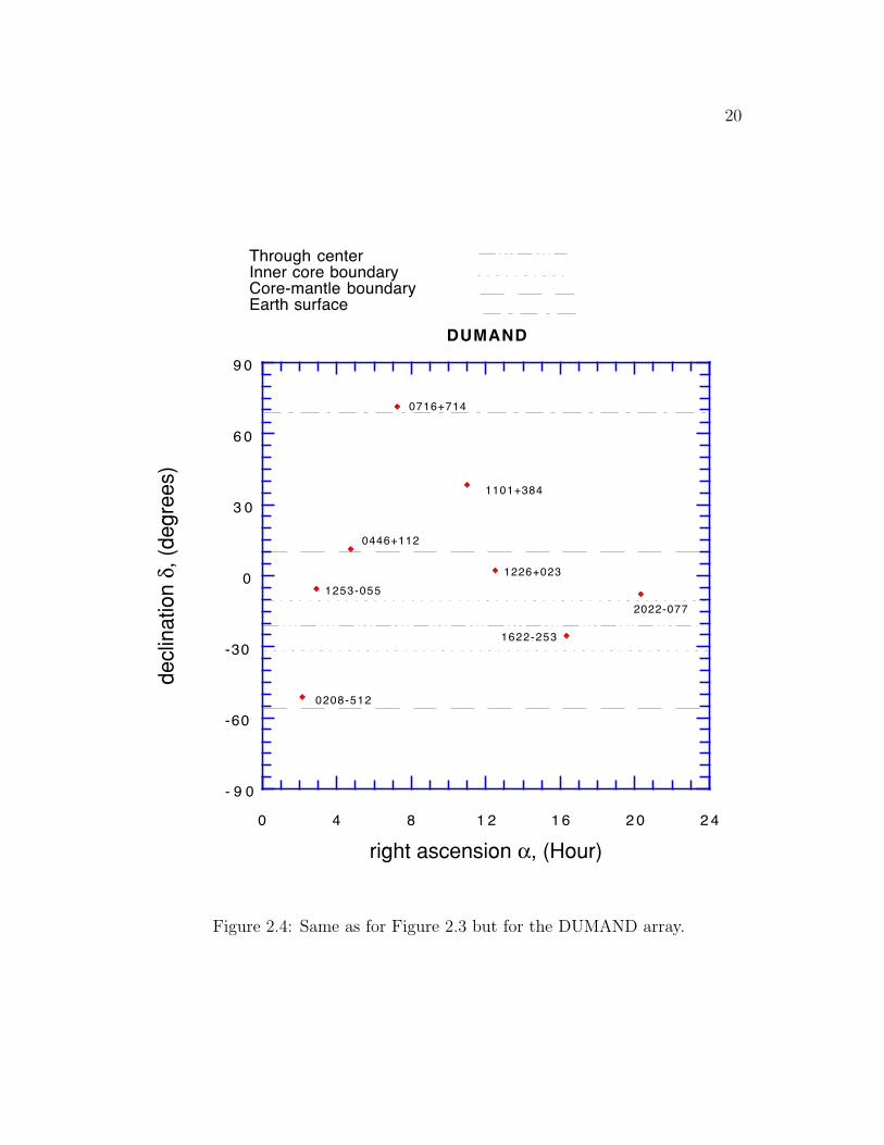
traversing the center of the planet; this requires δ = −λ. Figures 2.3 through

2.5 summarize the locations, hence maximum penetration depths, of potential

VHE neutrino sources as seen from the sites of the AMANDA, DUMAND and

NESTOR arrays (cf. Table 2.1). Because of their low latitudes, the latter

two sites are advantageous for mapping the deepest structure of the planet.

If observed from both DUMAND and NESTOR, for example, source 1622-253

yields redundant determinations of inner-core density, whereas sources 1253-055,

2022-077 and 0208-512 provide independent measurements of outer-core densi-

ties (Figures 2.4, and 2.5). The AMANDA site, near the South Pole, offers

complementary advantages due to its high latitude. First, because the sources

just mentioned are not occulted by the Earth, the AMANDA array can moni-

tor the temporal stability of their neutrino fluxes (Figure 2.3). A combination

of redundant observations from several neutrino observatories and of gamma-

ray measurements from satellite-borne detectors (e.g., GRO) can additionally

serve as monitors of source stability. Second, because the transmission curves

at AMANDA are essentially flat if density depends only on radius (Figure 2.6),

18

any deviations from constant transmission observed at this site can be directly

ascribed to lateral variations in the Earth’s density structure. Indeed, such mea-

surements may provide the first clear indication of horizontal density structure

at specific depths in the mantle and core. At the same time, neutrino determi-

nations of average densities at these individual depths, given by the individual

source declinations δ, are best constrained by the (nearly) flat transmission

curves obtained at AMANDA. Imaging the Earth’s density structure can in

principle be extended to three dimensions, if more than one detector array is

used and if sources of high enough flux are found at a sufficient number of dis-

tinct locations. For example, a diffuse extragalactic source of neutrinos impinges

on the Earth isotropically, and can thus provide the required source geometry

for three-dimensional imaging. However, this approach is no doubt limited by

the neutrino flux, as we next discuss. The spatial dimension and density con-

trast of internal structure that is resolved depends on the number of detected

muons generated from neutrinos that pass through the regions or features of

interest. As an example, we summarize current estimates of neutrino-generated

muon event rates at DUMAND in Table 2.1; the neutrino fluxes on which these

values are based are set at 1-200 times the gamma-ray fluxes emanating from

the sources, as noted above [Stenger, 1992]. Thus, for the single source 1253-

055 (3C 279), the number of >10 TeV neutrino-generated muons detectable at

the nine-string DUMAND array is estimated to lie between 4.2 and 840 per

19

- 9 0

-60

-30

0

3 0

6 0

9 0

0 4 8 1 2 1 6 2 0 2 4

AMANDA

decl

inat

ion

∂, (

degr

ees)

right ascension å, (Hour)

0208-512

0446+112

0716+714

1622-253

2022-077

1101+384

1226+023

1253-055

Through centerInner core boundaryCore-mantle boundaryEarth surface

Figure 2.3: Sky maps of some potential VHE neutrino sources, as observedfrom the sites of the AMANDA array. For comparison, the main structuralboundaries of the Earth are projected onto the maps according to Eq. (2.2).Sources located between boundary lines are occulted by the specified layer ofthe Earth.

20

- 9 0

-60

-30

0

3 0

6 0

9 0

0 4 8 1 2 1 6 2 0 2 4

DUMAND

decl

inat

ion

∂, (

degr

ees)

right ascension å, (Hour)

0208-512

0446+112

0716+714

1622-253

2022-077

1101+384

1226+023

1253-055

Through centerInner core boundaryCore-mantle boundaryEarth surface

Figure 2.4: Same as for Figure 2.3 but for the DUMAND array.

21

- 9 0

-60

-30

0

3 0

6 0

9 0

0 4 8 1 2 1 6 2 0 2 4

NESTOR

decl

inat

ion

∂, (

degr

ees)

right ascension å, (Hour)

0208-512

0446+112

0716+714

1622-253

2022-077

1101+384

1226+023

1253-055

Through centerInner core boundaryCore-mantle boundaryEarth surface

Figure 2.5: Same as for Figure 2.3 but for the NESTOR array.

22

0.7

0.8

0.9

1

0 2 4 6 8 1 0 1 2

TTTTrrrraaaannnnssssmmmmiiiissssssssiiiioooonnnn ooooffff 11110000 TTTTeeeeVVVV nnnneeeeuuuuttttrrrriiiinnnnoooossss aaaatttt AAAAMMMMAAAANNNNDDDDAAAA

∂ = +11.2fi ∂ = +38.2fi ∂ = +71.4fiT

rans

mis

sion

(I/I

0)

Time (Hour)

¨

¨¨

Figure 2.6: Neutrino transmission versus sidereal time for three sources observedfrom a site located near the South Pole (AMANDA). The curves are calculated asin Fig. 2.2, assuming the spherically symmetric (horizontally averaged) densitystructure obtained from seismology [Dziewonski and Anderson, 1981], and theyare flat because of the constant path length of neutrinos coming from sourcesof declination δ > 0 (see inset). For source declinations of δ = 11.2, 38.4, and71.4, respectively, neutrino paths pass through the upper mantle alone; throughthe upper mantle and lower mantle; and through the entire mantle and outercore, narrowly missing the inner core (cf. Fig. 2.2).

23

year (Table 2.1). Assuming the factor of 200 enhancement of neutrinos over

gamma-rays, 10 years’ observation of ten sources is expected to yield 104 − 105

recordable muon events having energies above 10 TeV. To determine the res-

olution of the density structure that can be measured by neutrino absorption,

we imagine dividing the array field of view into bins of width equal to 1/3 the

transit time required for the source point to traverse past the density feature.

For instance, a source at δ = −25 is occulted by the 6980 km diameter core

for roughly 4 hours out of the ∼14 hours each day it is in the DUMAND field

of view. This gives 8 bins, 1.6 hours long each, during 3 of which only 75-80

out of 100 neutrinos can be observed, for 10 TeV neutrinos (20-25% absorption

by the core: Figure 2.2). The statistical uncertainty corresponds to a standard

deviation less than 801/2 = 8.9, indicating the core density is constrained to

an accuracy of ∼10% with just 100 counts for paths going through this region.

Evidently, such a count rate, hence resolution, is feasible in less than 1 year

with one well-placed source (e.g., 1622-253) having sufficiently high flux (e.g.,

1253-055). However, neither the number of neutrino sources nor the number

of detector arrays is limited to one. Multiple observations of more than one

source serve two important purposes: they can drastically reduce the number of

years required to obtain density measurements with reduced uncertainties, and

also can provide redundancy to the signal in the event that a particular time

variable source is viewed during its minimum cycle. Figure 2.7 summarizes the

24

0.01

0.1

1

0.1

1

1 0

0.1 1 1 0

FFFFeeeeaaaattttuuuurrrreeee SSSSiiiizzzzeeee RRRReeeessssoooolllluuuuttttiiiioooonnnn

1 0

10

1 0

101010

ή/

® m (

® m =

4.5

g/c

m3 )

ή (g/cm

3)

Feature Thickness (x 103 km)

2 20 TeV Neutrinos3 20 TeV Neutrinos4 20 TeV Neutrinos

Figure 2.7: Number of neutrinos required to establish, to one standard deviation,the presence of a feature of given thickness and differential density (∆ρ) withrespect to surrounding material.

tradeoff between size and density contrast for features to be resolved to within

one standard deviation by a given number of cross-cutting neutrinos. Fewer

than 100 detected events due to core-traversing neutrinos suffice to establish

the presence of this region, for example (radius rcore= 3480 km and density

ρcore∼= 10.6gcm−3, versus ρmantle

∼= 4.5gcm−3), where the densities given are

characteristic of the region. In contrast, constraining either the density jump

across the inner core - outer core boundary (∆ρ ∼= 0.6gcm−3, ρIC = 1220 km)

25

or the possible density variations due to mantle-core intermixing in the D” zone

at the base of the mantle (δρ ∼= 6gcm−3, thickness≤200 km) requires about

104 − 105 events. This is prospectively achievable at more than one detector

array over a decade’s observations.

2.6 Location of Neutrino Sources by Core Occultation

In addition to the geophysical applications, neutrino absorption by the Earth’s

internal structure may serve the astrophysical community interested in precisely

determining the locations of VHE neutrino point sources. Because the radius of

the outer core is known to better than 0.1% from seismology [Dziewonski and

Anderson, 1981], we can take advantage of occultation by the Earth’s core to

locate an extraterrestrial point source of neutrinos. First, the right ascension

of the source is determined absolutely by the sidereal time of occultation in the

transmission curve (e.g., Figure 2.2). Second, the source declination is obtained

from the total amount of time spent behind the core, which varies with δ (Figure

2.2). Clearly, the technique of using core occultation to locate neutrino point

sources works best with detector arrays sited at low latitudes (cf. Figures 2.2

and 2.6). Furthermore, the occultation is most sensitive to declination when

the source is located such that its neutrinos pass near the edge of the core:

zmax ≈ 2885km, the depth to the core-mantle boundary (Equation 2.2), rather

than straight through the core. For example, it is easier at DUMAND to dis-

26

1

1.5

2

2.5

3

3.5

4

4.5

- 5 0 -40 -30 -20 -10 0 1 0Cor

e O

ccul

tatio

n D

urat

ion

(Hou

rs)

Source declination ∂ (degrees)

Figure 2.8: Core occultation duration as a function of source declination calcu-lated for neutrinos detected at a site of latitude λ = 21 (e.g., DUMAND). Theoccultation duration is highly sensitive to source declinations for δ ≈ −50 and+5.

tinguish between sources of declination 0 and 5, than between sources of −20

and −25 (Figure 2.8).

Thus, both DUMAND and NESTOR are most sensitive to locating sources at

declinations near −5 to +10 and −55 to −70 through occultation by the core-

mantle boundary (Figures 2.4 and 2.5). If the inner core–outer core boundary

can be similarly used (Figure 2.2), source declinations near −10 and −30, and

near −25 and −70 are resolved by DUMAND and NESTOR, respectively.

27

2.7 Conclusion

Observations of astrophysically-produced Very High Energy (∼TeV-PeV)

neutrinos, using one or more detector arrays at the Earth’s surface, may yield

significant new constraints on the density structure of the planetary interior.

Current estimates of VHE neutrino fluxes from extragalactic point sources sug-

gest that geophysically interesting results can be obtained over time periods of

years to decades (Table 2.1). At the same time, precise seismological infor-

mation on the Earth’s internal structure, such as the depth to the core-mantle

boundary, can be used to obtain refined locations of neutrino point sources. De-

tector arrays now under construction will test the feasibility of these applications

over the next few years.

28

Chapter 3

Normal Mode Theory

3.1 Normal Modes of the Earth

Seismic waves radiated from a large earthquake source coherently interfere

to produce standing waves in the Earth. The elastic Earth continues to deform

hours to days after the excitation provided by a strong earthquake source has

died out, in the form of free oscillations, or standing waves.

Seismologists generally work starting from a reference Earth model, which

has the following properties:

1. spherically symmetric;

2. non-rotating ;

3. elastic ;

4. isotropic,

is given the nomenclature ’SNREI Earth model.’ In such a model, the equation

29

of motion for displacement in the Earth is given by

ρ0d2x

dt2= ∇ · τ + F (3.1)

where ρ0 is the density of the reference Earth model, x is the point displacement

vector, τ is the total stress tensor, and F is the body force per unit volume. In

the quiescent state, x=0, F is the gravitational body force F = ρ0g = −ρ0∇φ0,

and the stress distribution τ is the hydrostatic pressure due to rock overburden

τ0 = −p0I where p0 is hydrostatic pressure, and I is the identity tensor.

When F includes an excitation term, the SNREI Earth undergoes infinites-

imal time dependent deformations. A particulate of Earth material initially at

position r0 displaces to position r by

r(r0, t) = r0 + x(r0, t). (3.2)

Due to the elastic properties of the material, stresses will act on the deformation

to restore the particulate back to its original position. For an isotropic Earth,

the elastic stress tensor is

τE = 2µε + λ(∇ · x)I (3.3)

where ε is the elastic strain tensor given by

ε = 1/2(∇x + (∇x)T ). (3.4)

The density field and gravitational potential field are also perturbed by the

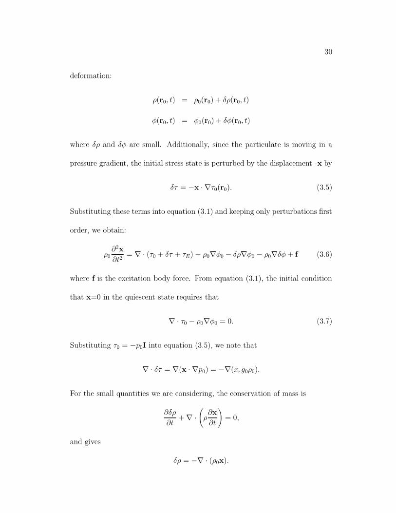
30

deformation:

ρ(r0, t) = ρ0(r0) + δρ(r0, t)

φ(r0, t) = φ0(r0) + δφ(r0, t)

where δρ and δφ are small. Additionally, since the particulate is moving in a

pressure gradient, the initial stress state is perturbed by the displacement -x by

δτ = −x · ∇τ0(r0). (3.5)

Substituting these terms into equation (3.1) and keeping only perturbations first

order, we obtain:

ρ0∂2x

∂t2= ∇ · (τ0 + δτ + τE) − ρ0∇φ0 − δρ∇φ0 − ρ0∇δφ + f (3.6)

where f is the excitation body force. From equation (3.1), the initial condition

that x=0 in the quiescent state requires that

∇ · τ0 − ρ0∇φ0 = 0. (3.7)

Substituting τ0 = −p0I into equation (3.5), we note that

∇ · δτ = ∇(x · ∇p0) = −∇(xrg0ρ0).

For the small quantities we are considering, the conservation of mass is

∂δρ

∂t+ ∇ ·

(

ρ∂x

∂t

)

= 0,

and gives

δρ = −∇ · (ρ0x).

31

Equation (3.6) is then further simplified to

ρ0∂2x

∂t2= ∇ · τE − ρ0∇δφ + rg0∇ · (ρ0x) −∇(xrg0ρ0) + f . (3.8)

The gravitational potential satisfies Poisson’s Equation, thus we have an addi-

tional equation defining δφ,

∇2δφ = 4πGδρ = −4πG∇ · (ρ0x) (3.9)

where G is the gravitational constant. Equations (3.8) and (3.9) are the fun-

damental equations governing the behavior of small deformations of the SNREI

model.

At times after the excitation body force f has ceased to act, f=0 in equation

(3.8), which then becomes the equation of motion for free oscillations of the

SNREI model. By seeking solutions for point displacement of the form

x(r, t) = xkeiωkt,

equation (3.8) becomes an eigenproblem

−ρ0ω2kxk = ∇ · τE − ρ0∇δφ + rg0∇ · (ρ0xk) −∇(xk rg0ρ0). (3.10)

The free oscillations of an SNREI Earth model can be characterized by solving

the eigenproblem written in symbolic form as

H0xmk = ρ0ω

2kx

mk , (3.11)

where H0 is a Hermitian differential operator defined as the negative of the

right hand side of equation (3.10), ω2k is the squared eigenfrequency of a free

32

oscillation mode, and xmk is a vector field of elastic displacement for the mode,

and has the form

xmk = |n q l m〉 ≡ nU q

l (r)Y ml (θ, φ)r + nV q

l (r)∇1Yml (θ, φ)

− nW ql (r)r×∇1Y

ml (θ, φ). (3.12)

The bracket notation for an eigenmode |n q l m〉 is adopted from quantum me-

chanics, where n is the overtone number, l is the angular order, and m is the

azimuthal order of a type q (spheroidal or toroidal) mode. In an SNREI Earth

model, 2l + 1 modes, or “singlets”, of different m but the same n, q and l os-

cillate at the same degenerate eigenfrequency ωk, and make up the ’multiplet’

k ≡ |n q l〉. nU ql (r), nV q

l (r), and nW ql (r) are functions of radius r, are character-

istic of each multiplet and can be computed from the explicit form of equation

(3.11) for an SNREI Earth. nU ql (r) = nV q

l (r) = 0 for toroidal modes (q=T), and

nW ql (r) = 0 for spheroidal modes (q=S). ∇1 ≡ θ∂θ +csc θφ∂φ, and r, θ and φ are

unit vectors in the spherical coordinate system. Y ml (θ, φ) are complex spherical

harmonics, completely normalized following the convention in Edmonds, 1960:

Y ml (θ, φ) =

(−1)l+m

2ll!

[

(2l + 1)(l − m)!

4π(l + m)!

] 1

2

·(sinθ)m

[

∂

∂(cosθ)

]l+m

(sinθ)2leimφ. (3.13)

The inner product by which the eigenfunctions xkm are normalized is defined

by (Woodhouse, 1980)

〈k′ m′|ρ0|k m〉 ≡∫

Vρ0x

k′∗m′ · xk

mdV = δkk′δmm′ (3.14)

33

where the integration is over the volume V of the Earth, ρ is the density dis-

tribution in the SNREI Earth, the * denotes complex conjugation and δkk′ and

δmm′ are Kronecker deltas. Together, all the modes of Earth oscillation form a

complete set, so that any vector field u may be written as

u =∑

k m

|k m〉〈k m|ρ0|u〉 (3.15)

3.2 Normal Mode Splitting

When considering the realistic aspherical structure of the Earth, the degen-

eracy of the eigenfrequencies ωk is removed. Considering only first order per-

turbations to the SNREI Earth, (Dahlen, 1969, 1974; Woodhouse and Dahlen,

1978; Woodhouse, 1980), the eigenfunctions and eigenfrequencies of each singlet

can be derived using perturbation theory. The perturbed eigenvalue equation

to first order written in standard form is

[H0 + εH1 − (ρ0 + ερ1)$2]u = 0 (3.16)

where $2 is the eigenvalue of the perturbed system, and u is the associated

eigenfunction. εH1 is the perturbing operator, and ερ1 is the perturbation in

density, for small factors ε. u can be expressed following equation (3.15) to

obtain

∑

k m

[ε(H1 − ρ1$2) + (H0 − ρ0$

2)]|k m〉〈k m|ρ0|u〉 = 0 (3.17)

34

By taking the product with |k′ m′〉∗ and using equation (3.11), we can then

integrate over V for

∑

k m

〈k′ m′|[ε(H1 − ρ1$2)|k m〉 + ρ0(ω

2k − $2)δkk′δmm′ ]〈k m|ρ0|u〉 = 0. (3.18)

The eigenvalue of the perturbed system is approximately equal to that of the

eigenvalue of the spherical system, and for multiplets which are well-separated

in the frequency band, that is, uncoupled and deemed ’isolated’, we can simply

consider $2 = ω2k + εω2

k. The first order terms of equation (3.18) are then

∑

k m

〈k′ m′|ε(H1 − ρ1ω2k)|k m〉 + ρ0(ω

2k − $2)δkk′δmm′ ]〈k m|ρ0|u〉 = 0, (3.19)

leading to the expression for the perturbation in eigenvalue

εω2kmm′ = 〈k m′|ε(H1 − ρ1ω

2k)|k m〉. (3.20)

The term on the left hand side of equation (3.20) refers to elements of a (2l +1)

dimensional square matrix of perturbations in eigenvalue ω2k resulting from the

coupling, due to aspherical structure, of singlets m and m′ belonging to multiplet

k. Each singlet |k m〉 in the multiplet k has an associated eigenvalue ω2k +εω2

kmm,

and thus the aspherical structure splits the reference degenerate eigenvalue ω2k

for multiplet k into (2l + 1) eigenvalues associated with multiplet k.

Relating the small quantity ε → δ, εω2 → δ(ω2) = 2ωδω. Likewise, εH1 and

ερ1 can be expressed as perturbations to the spherical operator H0 and density

ρ0 by εH1 → δH and ερ1 → δρ.

δωkmm′ = 〈k m′|Hkk|k m〉 (3.21)

35

gives the (2l + 1) square matrix of eigenfrequency perturbations where

Hkk ≡δH− δρω2

k

2ωk

. (3.22)

3.2.1 Splitting of Coupled Multiplets

A set K of multiplets may couple in the aspherical Earth if the multiplets

k ∈ K resonate at very similar eigenfrequencies, and if non-zero values of the

eigenfunctions of k ∈ K overlap in depth (Dahlen, 1969; Luh, 1973; Woodhouse,

1980). Then, in the coupled oscillation, the k ∈ K multiplets share the same

beat frequency ωK, where for each k ∈ K, ω2K − ω2

k = O(ε). In this case, we

can write $2 = ω2K + εω2. In this thesis, we only consider coupling between two

modes, i.e. k, k′ ∈ K, and a more general form of equation (3.20) is

εω2kk′mm′ = 〈k′ m′|ε(H1 − ρ1ω

2K)|k m〉 − (ω2

K − ω2k)δkk′δmm′ , (3.23)

where for k = k′, equation (3.23) is reduced to equation (3.20). Then

δωkk′mm′ = 〈k′ m′|Hkk′|k m〉 − (ω2K − ω2

k)δkk′δmm′/2ωK (3.24)

is the matrix of eigenfrequency perturbations for a coupled multiplet system

where

Hkk′ ≡δH− δρω2

K

2ωK. (3.25)

The dimension of matrices δω and Hkk′ is (2l′ +1)× (2l+1) where the rows are

labeled by −l ≤ m ≤ l, and the columns are labeled by −l′ ≤ m′ ≤ l′.

36

The second term on the right hand side of equation (3.24) is much less than

O(ε), and therefore may be neglected. Aspherical Earth structure is then related

to δωkk′mm′ ≡ 〈k′ m′|Hkk′|k m〉 by (Woodhouse, 1980)

〈k′ m′|Hkk′|k m〉 ≡ Hmm′

kk′

= (Ωmβδll′ + ε)δmm′ +l+l′∑

s=|l−l′|

s∑

t=−s

γmm′tll′s ct

ll′s (3.26)

where

ctll′s =

∫ a

0Mkk′

s (r) · δmts(r)r

2dr −∑

d

Hsdδhtsdr

2. (3.27)

The first term on the right-hand side of equation (3.26) is the shift due to

Coriolis force; Ω is the rotational angular velocity and β is the Coriolis splitting

parameter. ε includes the contribution from the Earth’s hydrostatic ellipticity.

The coefficient

γmm′tll′s ≡

∫ 2π

0

∫ π

0Y m∗

l (θ, φ)Y ts (θ, φ)Y m′

l′ (θ, φ)sinθdθdφ, (3.28)

where Y ml (φ, θ),Y m′

l′ (φ, θ), and Y ts (φ, θ) are spherical harmonic functions. In

equation ( 3.27), δmts represents the relative perturbation of structure m with

respect to the reference one-dimensional model. Mkk′

s (r) represents sensitivity

kernels for the modes (k, k′) and a is the radius of the Earth. Topographical vari-

ations are represented by δhtsd, where the index d refers to discontinuities within

the earth (in our case we consider the sea floor, Moho, 670 km discontinuity,

and core-mantle boundary) and Hsd is the associated kernel for the undulation

of boundary d. The extraction of structure variations m and boundaries d in

37

the mantle from normal mode spectral observations is the motivation of this

thesis, while the remaining variables in equation ( 3.26) are considered to be

well understood.

The splitting due to Coriolis coupling and the aspherical structure of the

Earth’s ellipticity of figure are accurately known and can be computed theoret-

ically (Dahlen, 1968, 1976; Woodhouse and Dahlen, 1978; Woodhouse, 1980).

Eigenfrequency splitting by Coriolis coupling and the Earth’s hydrostatic ellip-

ticity of figure is computed to first order from an SNREI Earth model in this

study. The expressions for β and ε in equation ( 3.26), generalized for coupled

multiplets (k 6= k′), can be found in Woodhouse 1980.

The product of the coefficient γmm′tll′s , and the weighted integral of structure

heterogeneity contribute to the eigenfrequency perturbation in the second term

in equation ( 3.26). The integral represented by γmm′tll′s (equation 3.28), may also

be written in terms of Wigner 3-j symbols (Edmonds, 1960, equation [4.6.3])

γmm′tll′s ≡

[

(2l + 1)(2s + 1)(2l′ + 1)

4π

]1/2

l s l′

0 0 0

l s l′

−m t m

. (3.29)

Symmetry properties of γmm′tll′s , commonly known as Clebsch-Gordon coefficients

in quantum mechanics, are well-documented (eg., Rose, 1957; Edmonds, 1960).

By virtue of the symmetry relation (equation [3.7.6], Edmonds, 1960)

l s l′

m t m′

= (−1)l+s+l′

l s l′

−m −t −m′

, (3.30)

38

it is required that (−1)l+s+l′ = 1 for m = t = m′ = 0 so that

l s l′

0 0 0

= 0 unless l + s + l′ is even. (3.31)

The γmm′tll′s coefficients represent the interaction strength between singlets |n q l m〉

and |n′ q′ l′ m′〉, coupled by heterogeneity size, which is represented by spherical

harmonic coefficient of degree s and azimuthal order t. For coupled multiplets

|n q l〉 and |n′ q′ l′〉, the relation between l, s, and l′ required by equation ( 3.31)

and vector addition determine the selection rules:

|l − l′|, |l − l′| + 2, . . . ≤ s ≤ . . . , l + l′ − 2, l + l′

and

−s ≤ t ≤ s.

This implies that isolated multiplets (k = k′) coupling with themselves then are

only sensitive to even harmonic degrees s of heterogeneity, where 0 ≤ s ≤ 2l.

On the other hand, for multiplets k 6= k′ which resonate at nearly equivalent

frequencies, the singlets couple within their own multiplet in addition to cross-

coupling with singlets of the nearly resonant multiplet partner. Self-coupling

(k = k, k′ = k′ within K) provides sensitivity to even harmonic degrees s, and

cross-multiplet coupling (k 6= k′ within K) may provide additional sensitivity

to odd harmonic degrees s if l + l′ or equivalently, |l − l′|, is odd.

39

3.3 Spectral Splitting

The contribution of a particular isolated multiplet k to the observed surface

displacement can be written as (Woodhouse and Girnius, 1982)

u(t) = <[exp(iωkt)Rk · exp(iHt) · Sk] (3.32)

where Rk is the receiver vector and Sk is the source vector, and ωk is the complex

reference frequency of the mode with respect to an SNREI model of the Earth.

Rk describes the instrument response and location and Sk characterizes the

excitation of singlets evaluated at the source. These (2l+1) dimensional vectors

may be expressed as

Rk = Rmk (θr, φr) =

1∑

N=−1

RkNY Nml (θr, φr) (3.33)

Sk = Smk (θs, φs) =

2∑

N=−2

SkNY Nm∗l (θs, φs) (3.34)

where Y Nml are generalized spherical harmonics (Phinney and Burridge, 1973),

where l is the angular order of the multiplet k, m is the azimuthal order −l <

m < l, θr, φr, θs, and φs are the receiver and source colatitudes and longitudes.

In the case where modes are closely spaced in frequency, and their respective

eigenfunctions sample similar depths in the Earth, the contribution to the dis-

placement on the surface is formulated as a linear combination of equation(3.32)

for each of the multiplets, and there is additional contribution to the seismo-

gram from the cross-multiplet coupling of singlets. We can then express the

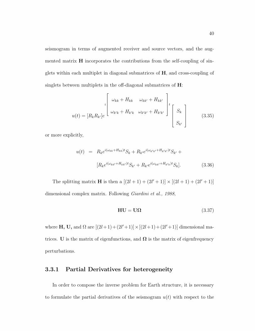
40

seismogram in terms of augmented receiver and source vectors, and the aug-

mented matrix H incorporates the contributions from the self-coupling of sin-

glets within each multiplet in diagonal submatrices of H, and cross-coupling of

singlets between multiplets in the off-diagonal submatrices of H:

u(t) = [RkRk′]e

i

ωkk + Hkk ωkk′ + Hkk′

ωk′k + Hk′k ωk′k′ + Hk′k′

t

Sk

Sk′

(3.35)

or more explicitly,

u(t) = Rkei(ωkk+Hkk)tSk + Rk′ei(ωk′k′+Hk′k′ )tSk′ +

[Rkei(ωkk′+Hkk′ )tSk′ + Rk′ei(ωkk′+Hk′k)tSk]. (3.36)

The splitting matrix H is then a [(2l + 1) + (2l′ + 1)] × [(2l + 1) + (2l′ + 1)]

dimensional complex matrix. Following Giardini et al., 1988,

HU = UΩ (3.37)

where H, U, and Ω are [(2l+1)+(2l′+1)]× [(2l+1)+(2l′+1)] dimensional ma-

trices. U is the matrix of eigenfunctions, and Ω is the matrix of eigenfrequency

perturbations.

3.3.1 Partial Derivatives for heterogeneity

In order to compose the inverse problem for Earth structure, it is necessary

to formulate the partial derivatives of the seismogram u(t) with respect to the

41

coefficients of structure perturbation, mts. We first note that equation (3.36) is

non-linear in H, and from equation (3.26), it follows that u(t) has a non-linear

relationship to the coefficients ctll′s as well. First, we derive the linearized ex-

pression for ∂u(t)/∂ctll′s, expanded from the treatment of Giardini et al., 1991,

to include coupled multiplet pairs. The coefficients ctll′s in equation (3.27) are

linear in structure perturbations mts, and it is then trivial to compute the par-

tial derivatives relating seismogram to structure perturbations for a linearized,

iterative inverse problem.

Using the notation of Woodhouse and Girnius, 1982, a wave propagation

operator P(t) may be defined as P(t) ≡ eiHt. Taking the first time derivative,

and stating initial conditions, we have

dP(t)

dt= iHP; P(0) = I (3.38)

where I is the unit matrix. Perturbing this equation, we find a differential

equation linear in δP(t)

dδP(t)

dt= iδHP(t) + iHδP(t); δP(0) = 0, (3.39)

the solution to which is

δP(t) =∫ t

0(iδHP(t′) + iHδP(t′))dt′

=∫ t

0P(t − t′)iδHP(t′)dt′. (3.40)

Then using

P(t) = eiHt = UeiΩtU−1 (3.41)

42

we can express each element of the matrix in the left hand side of equation (3.40)

as

δPij(t) =∑

pqmm′

∫ t

0iUipe

iΩpp(t−t′)U−1pmδHkk′

mm′Um′qeiΩqqt′U−1

qj dt′. (3.42)

In the case of singlet coupling within an isolated multiplet (k = k′), the indices

−m ≤ i, j, p, q ≤ m, and in the case of non-isolated multiplets (k 6= k′), the rows

are indexed by −m ≤ i, p ≤ m and the columns by −m′ ≤ j, q ≤ m′.

Taking the derivative of equation (3.42) with respect to Hkk′

mm′ , and keeping

in mind the indexing as described above,

∂exp(iHt)ij

∂Hkk′

mm′

=∑

pqmm′

i∫ t

0Uipe

iΩpp(t−t′)UpmUm′qeiΩqqt′Uqjdt′

=∑

pqmm′

iUipU−1pmUm′qU

−1qj

[

eiΩqqt − eiΩppt

Ωqq − Ωpp

]

. (3.43)

This leads to a linearized form of equation (3.36):

δu(t) =4∑

ζ=1

<

∑

pqst

∑

i

riUip

∑

mm′

U−1pmUm′qγ

mm′tll′s

∑

j

U−1qj sje

iωkk′ t

×eiΩqqt − eiΩppt

Ωqq − Ωppδct

ll′s

]

ζ

(3.44)

where ζ indexes over the combinations of mode coupling: 1≡ 〈km|km〉, 2≡

〈k′m′|k′m′〉, 3≡ 〈km|k′m′〉, and 4≡ 〈k′m′|km〉.

For q6=p,

∑

pq

eiΩqqt − eiΩppt

Ωqq − Ωpp=∑

pq

eiΩqqt

Ωqq − Ωpp+∑

qp

eiΩqqt

Ωqq − Ωpp(3.45)

For q=p,

limΩqq→Ωpp

eiΩqqt − eiΩppt

Ωqq − Ωpp= iteiΩqqt (3.46)

43

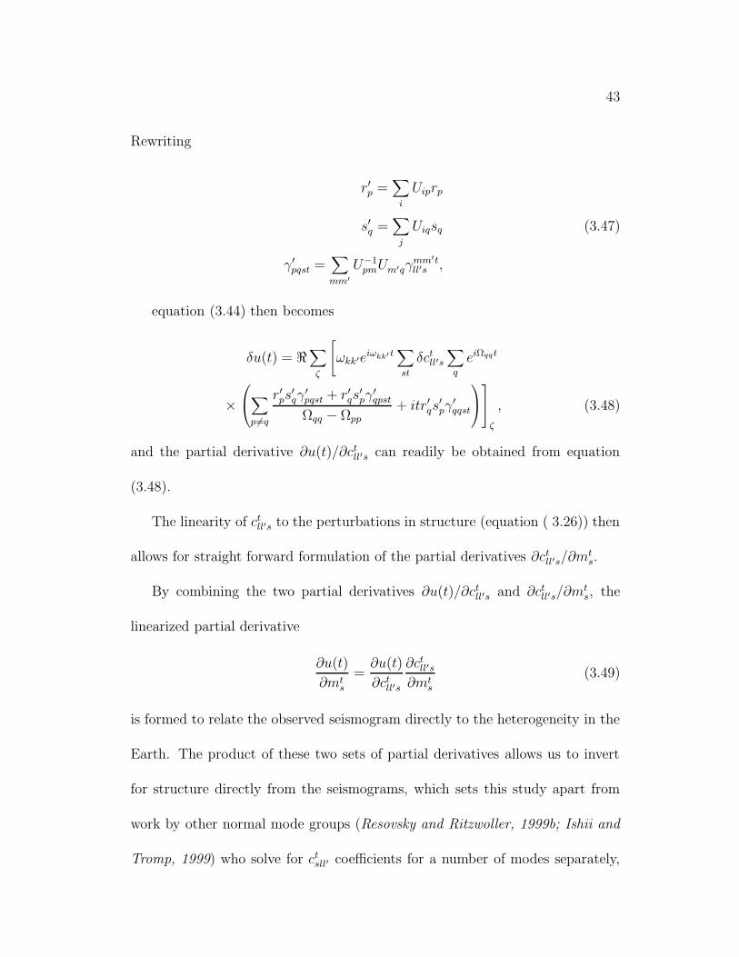
Rewriting

r′p =∑

i

Uiprp

s′q =∑

j

Uiqsq (3.47)

γ′pqst =

∑

mm′

U−1pmUm′qγ

mm′tll′s ,

equation (3.44) then becomes

δu(t) = <∑

ζ

[

ωkk′eiωkk′ t∑

st

δctll′s

∑

q

eiΩqqt

×

∑

p6=q

r′ps′qγ

′pqst + r′qs

′pγ

′qpst

Ωqq − Ωpp+ itr′qs

′pγ

′qqst

ζ

, (3.48)

and the partial derivative ∂u(t)/∂ctll′s can readily be obtained from equation

(3.48).

The linearity of ctll′s to the perturbations in structure (equation ( 3.26)) then

allows for straight forward formulation of the partial derivatives ∂ctll′s/∂mt

s.

By combining the two partial derivatives ∂u(t)/∂ctll′s and ∂ct

ll′s/∂mts, the

linearized partial derivative

∂u(t)

∂mts

=∂u(t)

∂ctll′s

∂ctll′s

∂mts

(3.49)

is formed to relate the observed seismogram directly to the heterogeneity in the

Earth. The product of these two sets of partial derivatives allows us to invert

for structure directly from the seismograms, which sets this study apart from

work by other normal mode groups (Resovsky and Ritzwoller, 1999b; Ishii and

Tromp, 1999) who solve for ctsll′ coefficients for a number of modes separately,

44

and then combine these coefficients to perform a linear inversion for structure.

The advantage gained from the direct inversion approach is that the inverse

problem is more regularized, by which we mean that all the mode data spectra

are inverted simultaneously for a consistent model of Earth structure.

3.4 Normal Mode Kernels

3.4.1 Kernels for volumetric heterogeneity

Heterogeneity in the Earth can be described by different sets of physical prop-

erties, and specifically for seismology, Earth structure may be characterized by

its elastic properties and density. Neglecting the effects of anisotropy, the per-

turbations in normal mode eigenfrequencies have been specified by perturbations

in shear modulus δµ(r, θ, φ), bulk modulus δκ(r, θ, φ), density ρ(r, θ, φ), and the

boundary topography δh(θ, φ) in Woodhouse, 1980.

We choose to describe the heterogeneity in terms of perturbations in com-

pressional velocity, vP , shear velocity, vS, and density ρ so that the term δmts in

equation ( 3.27) is

δmts =

[

δv tPs

vP,δv t

Ss

vS,δρt

s

ρ

]

(3.50)

where the numerators are spherical harmonic components of angular degree s

and azimuthal order t of the perturbation, and the denominators are evaluated

at the relevant depth in the spherical reference model. When the effects of

attenuation are included, δv tPs and δv t

Ss may be complex.

45

For this description of heterogeneity, the kernel Mkk′

s (r) can then be defined

as

Mkk′

s (r) = [P skk′(r), Ss

kk′(r), Rskk′(r)]. (3.51)

The kernels weight, as a function of radius r, the contribution which hetero-

geneity of degree s gives to the eigenfrequency perturbation. Kernels P skk′(r), Ss

kk′(r),

and Rskk′(r) are functions of the eigenfunctions of the coupling multiplets (k, k′)

for the spherical reference model (equation (3.12)), and can be formulated in

terms of the equations (A36), (A37), and (A38) given in Woodhouse, 1980, for

which the kernels are cast for bulk modulus κ, shear modulus µ and density ρ,

are, respectively:

ωkk′P kk′

s (r) = 2vP ρKs

= 2[(κ +4

3µ)ρ]1/2Ks (3.52)

ωkk′Skk′

s (r) = 2vSρ(Ms −4

3Ks)

= 2[µρ]1/2(Ms −4

3Ks) (3.53)

ωkk′Rkk′

s (r) = [(v2P −

4

3v2

S)Ks + v2SMs + R(1)

s ]

=1

ρ(κKs + µMs + ρR(1)

s ) (3.54)

We have replaced l′′, in the notation of Woodhouse, 1980, by s here, and the

dependence of Ks, Ms and Rs on radius r is understood.

46

3.4.2 Kernel coefficients for boundary topography

The undulations δhtsd of a boundary d at radius r give rise to eigenfrequency

perturbations through the kernel coefficients evaluated at the boundary radius.

If δhtsd in equation (3.26) is defined as topography normalized by the boundary

radius, then the corresponding kernel can be expressed as

ωkk′Hs = rρ[(v2P −

4

3v2

S)Ks + v2SMs + R(1)

s ]+−

= r[κKs + µMs + ρ0R(1)s ]+− (3.55)

where Ks, Ms, and R(1)s are given in (A27), (A28), and (A38) of Woodhouse,

1980, respectively. The notation [·]+− is used to signify the discontinuity jump

of the enclosed quantity across the boundary, where the positive contribution

corresponds to the positive r side of the boundary.

47

Chapter 4

Inverse Theory

The physical properties of the Earth’s interior cannot always be measured

directly. Assuming that a mathematical representation is valid, inverse the-

ory is used to estimate the model parameter values, given a set of data and a

model theory. Also encompassed in inverse theory is the estimation of resolution

and uncertainty in model parameters. The inverse formulation for the problem

specified in this thesis, and solution evaluation schemes are discussed below.

4.1 Formulation of the Inverse Problem

In this thesis, the three-dimensional structure in density, and compressional

and shear velocity are the physical properties which we wish to quantify. From

a collection of observed seismograms u(t), we invert for three-dimensional struc-

ture in compressional velocity δ ln αts(r), shear velocity δ ln βt

s(r), density δ ln ρts(r)

and boundary undulations δhdst. The digital seismograms u(t) are discretely tab-

ulated, and the solutions for three-dimensional structure are discretized in the

48

form of polynomial expansion coefficients, as described in Section 5.5. Defining

mts(r) to be the vector of three-dimensional model structure coefficients, it is

clear from equation (3.49) that solving for mts(r) from the collection of data,

u(t), is a non-linear inverse problem.

We seek solutions for our model parameters m from the following relation:

d = f(m) + e (4.1)

where d is the N -dimensional vector of data, f is a non-linear function, m is the

M -dimensional vector of model parameters, and e is the vector of errors in d.

Assuming that the noise in the data has a white spectrum, errors in e are then

normally distributed with a zero mean and a variance σ2e . The data covariance

matrix C e is then a matrix in which the diagonal elements are equal to σ2e .

We also make the assumption that the probability distributions of the model

parameters in m are Gaussian. The variables in m then have a priori mean

values m 0, and covariance defined in the matrix C m. m 0 represents values of a

starting model which we expect values of our final model to be close to, and the

covariance matrix C m reflects the strength of our expectations. Combining the

probability distribution of errors and a priori probability distribution of model

parameters with the our model equation d=f(m), the probability distribution

of the model vector m is

P (m) ∝ exp[−1

2(d − f(m))TC−1

e (d − f(m))] ×

49

exp[−1

2(m − m0)

TC−1m (m − m0)]. (4.2)

The maximum likelihood solution to d=f(m)+e is then the minimum of the

argument of the exponential in (4.2). The objective function which must be

minimized is given by

Φ(m) = (d − f(m))TC−1e (d − f(m)) + (m − m0)

TC−1m (m − m0). (4.3)

The minimum of the objective function Φ(m) is found by applying the following

in an iterative fashion:

mi+1 = mi + (ATi C−1

e Ai + C−1m )−1[AT

i C−1e (d− f(mi))−C−1

m (mi −m0)] (4.4)

where Ai is an N × M matrix of partial derivatives

Ai =

[

∂f(m)

∂m

]

m=mi

, (4.5)

and is expressed explicitly by equation (3.49), and i is the index of iteration.

To avoid obtaining solutions in m which may be biased towards pre-existing

three-dimensional models, particularly by seismic velocities models derived from

higher frequency data, the a priori model vector m 0 has been set to zero,i.e,

PREM, for the inversions in this study. We have been seeking solutions for

perturbations from a spherical model of the Earth, namely PREM (Dziewonski

and Anderson, 1981), in order to investigate the heterogeneities to which the

normal mode spectra are sensitive. The inversion relation for the model thus

50

becomes

mi+1 = mi + (ATi C−1

e Ai + C−1m )−1[AT

i C−1e (d − f(mi)) − C−1

m mi]. (4.6)

In what follows, we discuss the model covariance matrix Cm, and the error

estimates which constitute the diagonal of the matrix Ce.

4.2 Model Covariance Matrix

The normal modes used in this study sample the mantle structure given by

the model kernel sensitivity (equations (3.53)-(3.54)). For each mode, there are

spectral measurements from a number of stations and events. We have required

that the dimension of the model vector be inferior to the dimension of the

data vector to ensure that our inversions are not underdetermined. However,

the model parameterization has global extent while the modes do not have

uniform sensitivity throughout the depths in the mantle, as discussed in Section

5.5. Also, our mode data set primarily has sensitivity to even degrees s of

heterogeneity, the details of which will be outlined in Section 5.5.1. This data

coverage, for the model parameterization we chose, defines a mixed-determined

inverse problem, and we wish to determine our solutions in terms of minimizing

the prediction error e = d − f(m) and solution length L = m − m0, in which

we impose a priori assumptions and/or constraints about the behavior of the

solution model parameters m with respect to a starting model m0. The a priori

information is introduced in the model covariance matrix Cm, and imposed on

51

the model parameters in the form mTC−1m m (Tarantola and Valette, 1982; Li

and Romanowicz, 1996).

Following the description in Li and Romanowicz, 1996, we specify the ele-

ments of model vector m as coefficients of polynomial expansions laterally and

radially in the following fashion:

δm(r, θ, φ)

m(r)=

pmax∑

p

smax∑

s

s∑

t=−spm

ts fp(r) Y t

s (θ, φ), (4.7)

where pmts are coefficients of expansion for radial functions fp(r), and spherical

harmonics Y ts (θ, φ). We can then define the model covariance matrix Cm so that

mTC−1m m has the form

mTC−1m m =

∫ ∫

η1m2 + η2

(

∂m

∂r

)2

+ η3

(

∂2m

∂r2

)2

+ η4|∇1m|2

drdΩ

+∫

[η5i(δri)2 + η6i|∇1ri|

2]dΩ. (4.8)

The η1 term penalizes the amplitudes of the model. Values for η1 are located

along the diagonal of the model covariance matrix. The η2 and η3 terms im-

pose radial smoothness, and η4 terms require horizontal smoothness. Imposing

η2, η3, and η4 terms correspond to placing damping values in the off-diagonal

elements of Cm, corresponding to covariance between parameters. The term

η5i reduces the amplitudes of specific boundary undulations i, and η6i requires

horizontal smoothness on the boundaries. We find that the terms η5i and η6i

have interchangeable effects on the boundary amplitudes.

52

4.3 Error Estimates and Model Significance

Uncertainty in the mode spectral measurement can be estimated by consid-

ering the noise floor of the seismic trace, the time window chosen before applying

the Fourier transform which affects the signal power and resolution, and the fre-

quency window bounds for each spectral measurement, which may incorporate

signal from neighboring modes.

There are approximations imposed on the theoretical formulation which we

employ, and they further limit the accuracy of the tomographic technique. These

approximations in the theory include utilizing a spherically stratified elastic

reference Earth model (e.g.. PREM) and extending the representation of the

spherical structure to perturbations of only first order. The eigenfunctions and

reference eigenfrequencies are computed from the spherically stratified elastic

Earth model. Accuracy in spectra prediction could be increased by applying

higher order perturbation theory (eg. Lognonne and Romanowicz, 1990), com-

puting reference eigenfunctions and eigenfrequencies from a 3-D model, and up-

dating the reference eigenfunctions and eigenfrequencies with each iteration of

inversion for 3-D structure until convergence is reached ( Clevede and Lognonne,

1994). This higher order method is computationally laborious, but would allow

for wave propagation effects to be modelled such as focusing and defocusing due

to 3-D structure, which we here neglect. We also neglect departures from a sim-

ple Q-model as described by PREM. By choosing a time window for the seismic

53

trace which does not exceed 1.1 Q-cycles (Dahlen, 1982) we assume, however,

that spectral peak broadening is dominated by 3D elastic effects.

For a perfect model m ⊕ of the Earth, the measurement error σ2e represents

the difference between our ability to predict the spectrum from the theory and

the observed spectrum. We can define ε as some percentage of noise with respect

to the observed data. Then, we can consider that the diagonal of the matrix C e

is populated by

σ2e = εdTd = (d − f(m⊕))T (d − f(m⊕)) (4.9)

We assume that the measurement error is at least as good as what we can predict

from theory. From spectral records of well-excited modes in which noise is so

minimal as to appear absent, we find that this error is about 1% of the size of

the record, that is, ε=0.01.

The residual variance ratio of squared misfit to squared data is defined as

follows:

ς2 =(d − f(m))T (d − f(m))

dTd(4.10)

Since the number of model parameters varies between experiments, it is neces-

sary to take into account ν = N − M , the number of degrees of freedom, when

considering fits to the data. An a posteriori estimation can be made of the errors

and used to assess the significance of a model, with respect to the number of

54

model parameters M . The data variance σ2d can be computed by

σ2d =

(d − f(m))T (d − f(m))

N − M(4.11)

For two different realizations, M1 and M2, of the N data, if M2 gives a better

fit than M1, then the F-ratio defined by σ2d1/σ

2d2 is greater than 1.

55

Chapter 5

Heterogeneity in the Earth from Normal Mode

Spectra

5.1 Abstract

Mantle heterogeneity from normal mode studies has been generally derived

from ”splitting coefficients”, which represent an integration, over depth, of the

lateral heterogeneity weighted in depth by the mode’s sensitivity. The splitting

coefficients, measured from individual mantle modes from observed spectra, are

then inverted for mantle structure from this linear relationship. In contrast,

we forego this intermediate stage of solving for splitting coefficients and invert

directly for mantle structure from the spectral data for a sweep of mantle modes.

In this manner, the inverse problem for structure becomes more constrained than

the dual-stage inversion approach.

Previous models determined from normal mode data were parameterized in

terms of δ ln Vs, where aspherical structure in Vp and ρ were scaled to Vs struc-

ture, based on proportionality constants from mode studies . We demonstrate

56

that this assumption is inadequate, and by preserving it, the final S-wave velocity

model is contaminated by P-wave velocity and density structure. By setting the

scaling relationships free, the model solutions resulting from independently and

jointly inverting for δ ln Vs, δ ln Vp, and δ ln ρ improve the correlation of S-wave

velocity models with the existing Berkeley model derived from surface wave and

body wave studies. We present and discuss our models of Vs, Vp and density (ρ)

perturbations in the mantle. The Vs and Vp models compare well with results

from other studies. The density model is consistently robust, presents features

in the mantle which are in accordance with interpretations of denser slabs sink-

ing in the mantle in the circum-Pacific region. A reliable heterogeneous mantle

density model would provide a significant contribution to our understanding of

mantle convection.

5.2 Introduction

Observations of the Earth’s free oscillations have been a valuable complement

to seismic body and surface wave data in constraining material properties and

their lateral variations in the deep Earth. For example, normal mode data pro-

vided the first confirmation of the solidity of the inner core (Dziewonski, 1971).

Along with the mass and moment of inertia of the earth, they provide the best

constraints on the radial density distribution (e.g. Masters and Gubbins, 1979;

Bolt 1972; Dziewonski and Anderson, 1981; Kennett, 1998). Normal mode split-

57

ting data have been used to infer the patterns of low degree heterogeneity in the

mantle (Woodhouse and Giardini, 1985; Ritzwoller et al., 1986,1988; Giardini et

al., 1987; Li et al., 1991). They have also been incorporated, along with other

data sets, into recent 3D tomographic mantle models to constrain the lowest

degree structure (e.g. Masters et al., 1996; Resovsky and Ritzwoller, 1999b).

The analysis of modes sensitive to core structure has also lead to constraints

on inner core anisotropy (e.g. Woodhouse et al., 1986; Li et al., 1991; Tromp,

1995; Romanowicz et al., 1996; Durek and Romanowicz, 1999).

While in principle mantle mode data provide information on the V s, V p and

ρ in the mantle, the sensitivity to V s is dominant, and most studies to-date have

assumed an a-priori scaling between the 3 elastic parameters, and inverted for V s

alone (Giardini et al., 1987; Li et al., 1991a; Resovsky and Ritzwoller, 1998). In

particular, the density structure is thought to be rather poorly resolved. On the

other hand, several studies have shown that the assumption of proportionality

between V p and V s breaks down in the mid-mantle, based on the comparison

of V p and V s models derived from P and S travel time data respectively, or

the simultaneous inversion of such data (Robertson and Woodhouse, 1995,1996;

Vasco and Johnson, 1998). Cast in terms of bulk modulus κ and shear modulus

µ, instead of seismic velocities, such comparisons indicate anticorrelation in the

lowermost mantle (Su and Dziewonski, 1997).

With the accumulation of high quality data from global digital seismic net-

58

works, and the recent occurrence of several very large deep earthquakes (in

particular the Mw 8.2 06/09/94 Bolivia, and Mw 8.3 10/10/94 Kurile events), a

new data set, greatly improved in quality, is currently available (e.g. Resovsky

and Ritzwoller, 1995; He and Tromp, 1997) and has been used to improve 3D

models of the mantle (e.g.Resovsky and Ritzwoller, 1999b; Ishii and Tromp,

1998; Kuo et al., 1998). In what follows, we describe our efforts in this direc-

tion, using a somewhat different inversion approach from other studies, and a

data set of spheroidal mode spectra.

Most normal mode inversions are cast in terms of a two-step formalism, in

which ”splitting functions” (Woodhouse et al., 1986) are first computed for each

mode in the data set. In the second step, splitting functions are simultaneously

inverted for the distribution of elastic parameters with depth. This is similar

to the standard phase-velocity inversion procedures for surface waves. Such a

methodology is convenient, since the 2nd step is linear, and rapidly performed.

However, there are some issues about the accuracy and uniqueness of the split-

ting function coefficients obtained in the first, non-linear step (eg. Megnin and

Romanowicz, 1995). The splitting functions may depend on the starting model

and may not be completely compatible with a unique earth model. Following Li

et al (1991a), and Durek and Romanowicz (1999), we have opted for a direct, one

step method, which inverts normal mode spectra directly for 3D earth structure.

While more time consuming, this approach is more internally consistent.

59

Also, most studies include only isolated modes in the spectral representa-

tion of seismograms, and the resulting 3D earth models therefore only include

even-order terms of lateral heterogeneity (Woodhouse, 1983; Romanowicz, 1987

Resovsky and Ritzwoller, 1995). We allow for coupling between two nearby

modes in our formalism and apply it to several mode pairs. As shown by

Resovsky and Ritzwoller (1995), this has several advantages: (1) Reducing the

bias introduced by an isolated mode approximation when 2 modes are close in

frequency, therefore increasing the available mode data set, (2) adding sensitivity

to odd-order structure.

Using this approach, we have performed inversions in which we simultane-

ously solve for V s, V p, ρ structure up to degree 4 in the mantle, for both even

and odd degrees. In what follows we present our data set and mantle models,

and we discuss the resolution achieved in the different elastic parameters.

5.3 Data selection

We have extracted high quality very long period data from GSN/IRIS and

Geoscope stations for events listed in Table 1. Events were selected according

to their size (M0 ≥ 5 × 1020 Nm) and their occurrence preceding and following

a relatively quiet period in seismicity, so that about 125 hours of data could be

obtained from each record, free of perturbations from major aftershocks or other

earthquakes with Mw ≥ 6.5 (M0 ≥ 7 × 1018 Nm ). Only vertical component

60

Table 5.1: Earthquake event information

Date Moment Mw Depth (km) Region(×1020Nm)

03/09/94 3.5 7.63 564 Fiji Islands06/09/94 30.5 8.26 637 Northern Bolivia10/04/94 33.9 8.29 33 Kurile Islands07/30/95 13.8 8.03 47 Northern Chilean Coast10/09/95 13.3 8.02 49 Coast Near Jalisco, Mexico01/01/96 8.8 7.90 33 Minahassa Peninsula02/17/96 27.5 8.23 33 West Irian Region06/17/96 8.2 7.88 587 Flores Sea

records were considered (spheroidal modes only). Deep events (h > 200 km)

were favored, since they excite mode branches sensitive to very deep structure

better than shallow earthquakes of the same size.

Each time domain record was edited to remove glitches as well as tides, the

latter using an order-50 Legendre polynomial fit (Bohn, 1994). In addition to

removing the tidal signal, this also removed the mean and trend of the data.

Small events and aftershocks were deleted from the traces, which were padded

up using linear interpolation. If, in total, more than ∼ 1 hour of data required

adjustment, the record was discarded. The edited and cleaned selected traces

were deconvolved to ground acceleration, and a tapered band-pass filter was

applied. The records were then Fourier transformed using a length of record

determined by trial and error to optimize the signal to noise ratio and the

isolation from neighboring modes. When using a Hann window, the duration

is typically targeted to be about 1.1 Q-cycles of the mode (Dahlen 1982) to

61

optimize the estimation of frequencies and decay rates of well-isolated modes.

Some target multiplets are close in frequency to low-Q neighbors, and it is

advantageous to initiate the Hann window a few hours after the origin time of

the event in order to allow the neighboring modes to decay and bring out the

signal amplitude of the target mode. The traces are then padded with zeroes

before the application of a fast Fourier transform algorithm to the frequency

domain. The frequency window limits are chosen for each mode, and do not

vary between stations and events.

Synthetic time-domain traces were calculated using the 3D SH velocity model

SAW12D (Li and Romanowicz, 1996), and source characteristics from the CMT

catalog (eg. Dziewonski et al., 1995) were assumed in the forward modeling of

the traces. For each trace, the same editing, windowing, and filtering algorithms

as used for the data were applied to the synthetic traces to compute synthetic

spectra. The synthetics were compared with the data to look for anomalous

amplitudes which could be attributed to systematic errors, such as inaccurate

instrument response functions. However, the misfit of the data compared to

the spectral prediction from the 3D model was not a strong factor in selecting

spectra, so as not to introduce potential bias towards the initial model. During

the data selection process, the spectra of Vs dominant modes, when displayed in

comparison with synthetic spectra computed from an S-velocity model, generally

have smaller misfit values than P-velocity sensitive modes. Choosing spectra for

62

minimal misfit to spectra derived from a model prediction will tend to produce

a final model which is very highly correlated to the model used for prediction.

This is done in practice in many types of inversions in order to quickly stabilize

the solution. We have found that our direct inversion method is very stable and

independent of the starting model, whether it is a spherically symmetric model

such as PREM (Dziewonski and Anderson, 1981), or a 3D Vs model such as

SAW12D (Li and Romanowicz, 1996). Structure in Vp and ρ not proportional

to Vs, such as can be predicted from SAW12D, will be lost if the criterion of

minimal misfit to spectral prediction is emphasized in data selection.

We analyze the vertical component spectra of spheroidal mantle modes whose

eigenfunctions primarily exhibit particle motion in the mantle (0S, 1S, 2S, 4S, 5S

branches, and a few in the 6S, 7S, 8S branches). Modes with significant dis-

placement in the core are not included in this study, although some mantle

modes in our data set have some sensitivity to outer core structure. The effect

of outer core sensitivity on our models of mantle structure is minimal, and this

is consistent with conclusions of Giardini et al. 1987. Models which include core

modes and parameterization in the outer core will be described in detail in a

future paper. Below 5 mHz, the mantle modes in our study are well-isolated in

frequency, which minimizes contamination by neighboring modes. On the other

hand, our analysis code is capable of taking into account the more complex ef-

fects of 3-D structure on the spectra of coupled mode pairs. In total, we have

63

chosen 30 isolated mantle modes and 7 coupled mantle mode pairs, amounting

to a total of 44 spheroidal mantle modes, and spectra from a total of 2757 in-

dividual seismograms. From each spectrum, about ∼ 10 − 20 data points are

used.

5.4 Inversion Procedure

As seen from equation (3), solving for 3D structure using normal mode ob-

servations is a non-linear inverse problem. The relation between the structure

δmm

(r, θ, φ) = ( δVp

Vp(r, θ, φ), δVs

Vs(r, θ, φ), δρ

ρ(r, θ, φ)) and the splitting coefficients ct

s

is linear, and the corresponding partial derivatives are readily obtained. The

derivation of partial derivatives of the seismogram u(t) with respect to cts’s fol-

low that of the case for isolated modes, such as in Giardini et al. 1988, but

includes the case of coupled modes in which H is augmented by cross-coupling

terms. The product of these two sets of partial derivatives allows us to invert for

structure directly from the seismograms, which sets this study apart from work

by other normal mode groups (Resovsky and Ritzwoller 1999b, and Ishii and

Tromp 1997, 1998, 1999) who solve for cts coefficients for a number of modes,

and then use these coefficients to perform a linear inversion for structure.

The expressions for the partial derivatives can be found in Durek & Ro-

manowicz (1999). We employ an iterative inversion scheme which minimizes

the objective function

64

Φ(m) = (d − f(m))T C−1e (d − f(m)) + mT C−1

m m. (5.1)

d−f(m) is the difference between synthetic spectra f(m) related non-linearly

to the model parameters m, and the data d spectra. C−1e is the data covariance

matrix. The noise, excitation of modes, and contamination of spectra by neigh-

boring modes are assessed during data selection, discarding undesirable spectra.

The data are weighted by the fractional amplitude of the data per mode over

the total amplitude of all the data:

wm =

√

√

√

√

√

1Nstn

∑Nstn

i dm 2i

1Nm

1Nstn

∑Nm

m

∑Nstn

j dm 2j

(5.2)

where wm is the weight for mode m, dmi,j is the spectrum of mode m at each

station i, j over Nstn stations, and Nm is the total number of modes in the

data set. In this manner, the modes which are strongly excited will contribute

more to the model than weakly excited modes. Li et al. (1991a) measured

the signal-to-noise ratio of each trace from a quiescent time window before each

event to compose the C−1e matrix. Other mode studies have used an a posteriori

weighting scheme in which the data are weighted according to the misfit to

the previous iteration (Resovsky & Ritzwoller, 1998; He & Tromp, 1996). The

consequence of this a posteriori weighting scheme is that the final result could

be biased towards the starting model.

The model covariance matrix C−1m represents a priori constraints, such as

model size and smoothness. The elements of Cm can be computed from imposed

65

damping parameters, and a discussion of this can be found in Li & Romanow-

icz (1996). There exists a trade-off between the variances of final models and

damping parameter values used in the inversion. Damping parameter values are

thus selected in the vicinity of the point at which the variance versus damping

parameter curve flattens out.

5.4.1 Starting model

It is a common procedure to use a starting model of heterogeneity in the

inversion process to quickly stabilize the solution, assuming that the starting

model is already close to the minimum in misfit-space. When using a laterally

heterogeneous starting model, we have employed the following schemes:

1. in inversions for a Vs model, either PREM, or models of heterogeneity in

Vs from body and surface wave studies were used as starting models.

2. for a Vs + n-parameter models, where n = Vp, ρ, two schemes were under-

taken:

(a) scaling relationships between Vs and n were used to calculate the

heterogeneities in n, or

(b) Vs models were used as starting models and no aspherical structure

in Vp or ρ was assumed.

66

We find that our final models are independent of the starting model used in

the inversion, whether we choose a spherically averaged model such as PREM

as starting model, or a laterally heterogeneous model, such as SAW12D or

S12WM13 (Su et al., 1994) for Vs, and whether the starting Vp and ρ per-

turbations are assumed to be proportional to those of Vs, or are initially set to

PREM. For either spherical or laterally heterogeneous starting models, our in-

versions converge after ∼3 iterations and produce final models which are highly

correlated in depth with each other. For this reason, we have adopted PREM

as our starting model for Vs, Vp, and ρ to obtain models of heterogeneity in the

absence of a priori knowledge of aspherical structure.

5.4.2 Model Corrections

As our goal is to study the effects of volumetric mantle heterogeneity on

the eigenfrequency spectra of normal modes, we must consider contributions to

multiplet splitting other than those from mantle heterogeneity. These include

the hydrostatic ellipticity and rotation of the Earth, and crustal structure. We

account for these by forward modeling their effects on spectral splitting. Spectral

splitting of isolated and coupled multiplets as a result of the rotation of the

Earth and consequently hydrostatic ellipticity are calculated from Woodhouse

1980 and are incorporated into α of equation 1. Splitting by heterogeneity of

the crust is computed by considering the last term in equation 2 for models of

67

surface and Moho boundary undulations from SAW12D.

5.5 Model Parameterization

5.5.1 Sensitivity to wavelength of structure

Before exploring the spatial parameterization of our models, we consider

the sensitivity of the modes used in our data set. For spheroidal modes, the

sensitivity to harmonic degree s structure goes as, in general, |l − l′| < s <

l + l′ and is governed by the coefficient γmm′tll′s which is non-zero for even values

of the sum l + l′ + s. The value of γmm′tll′s indicates the strength of coupling

between singlets. Isolated modes (n, q, l) are therefore sensitive to even degrees

of structure, s = 0, 2, . . . , 2l. Coupled modes may contribute sensitivity to odd

degree structure, in addition to even degree structure. Coupled modes may have

additional odd degree sensitivity if the difference and sum of their angular orders

(l, l′) is odd. For example, the modes 1S5 at 1.370 mHz and 2S4 at 1.379 mHz

are coupled, and have sensitivity to even degrees 0,2,4,6,8, and 10 and to odd

degrees 1,3,5,7,and 9 (Resovsky and Ritzwoller, 1995).

In order to understand the depths at which the modal data have resolving

power, we compute the combined sensitivity kernels of the 30 isolated and 14

coupled modes for each model parameter, at each harmonic degree of our model.

Sensitivity kernels represent the weight which a perturbation from spherical

structure has, at a particular depth, on the splitting of spectra. The combined

68

sensitivity of the modes to variations in mantle structure is computed as follows:

SMs(r) =1

N

(

N∑

i

M skk′ i(r)

)2

. (5.3)

where s is the index of harmonic degree, M skk′ is the sensitivity kernel P s

kk′,

Sskk′, or Rs

kk′ (equations(3.53)-(3.54)), i is the mode index up to N total modes.

The combined sensitivity of all the modes used in this study is predominantly

to Vs (Figure 5.1), but at certain depths, particularly in the shallow portions

of the lower mantle and near the core-mantle boundary, the sensitivity to Vs

is reduced, and the sensitivity to Vp dominates. Sensitivity to ρ, on the other

hand, is consistently lower than to velocity, except at the very top of the mantle.

5.5.2 Model parameter expansion

A model parameter, δ lnm=(δ ln Vs, δ ln Vp, δ ln ρ), representing a perturba-

tion in seismic velocity or density in three-dimensions, can be expressed as a

function of radius r, colatitude θ, and longitude φ, and expanded in spherical

harmonics as follows:

δm

m(r, θ, φ) =

pmax∑

p

smax∑

s

s∑

t=−spm

ts fp(r) Y t

s (θ, φ),

where pmts are coefficients of expansion for radial functions fp(r), and spherical

harmonics Y ts (θ, φ).

69

670

CMB

ic bndy

r=0

Σ Κα

Σ K β

Σ K ρ

deg 2 deg 4

2

2

2

Figure 5.1: The accumulated sensitivity of mantle modes used in the inversion.The sensitivity kernels represent the weight which heterogeneity at a particulardepth has on spectral splitting. ΣK2

α (solid line) ΣK2β (dashed line), and ΣK2

ρ

are the cumulative sensitivity of the modes to aspherical structure in compress-ibility velocity, shear velocity, and density as functions of depth, respectively,averaged over the number of modes in the data set. Shown in the left panel isthe sensitivity to degree 2 structure, and the right panel, to degree 4 structure.

70

The choice of spherical harmonic expansion laterally simplifies the computa-

tion of coupling effects, owing to the mathematical rules that govern the γmm′tll′s

coefficients. As the modes in our data set have very low frequencies, they are

sensitive to very long wavelength structure. Given that the lowest angular order

in our data set is l = 2, all the modes in the data set have sensitivity in even

degree structure up to degree 4. While many of the modes have sensitivity to

even degree structure higher than 4, we only have 4 coupled mode pairs which

have sensitivity to odd degree structure: two pairs from which odd degree 1-9

structure ( 2S4 − 1S5 and 2S5 − 1S6) can be retrieved, and two pairs from

which degrees 5-11 ( 4S3 − 2S8 and 6S3 − 3S8) can be retrieved. In the interest

of ensuring that each harmonic degree of our models is well ’sampled’, we first

limit the harmonic degree of heterogeneity in our model to a maximum value of

4 in preliminary tests of data sensitivity to model parameters. After the mode

sensitivity to model parameters has been established, we will show models ex-

tended to degree 6, in order to avoid the effects of aliasing. The polynomial

order of the radial basis functions was chosen to be roughly equivalent to the

maximum radial order of the modes used in the data set. As we reported in

Section 5.3, our data set primarily consists of modes up to radial order n = 5,

but we also include a few modes of higher radial order. Thus, we have chosen to

use Legendre polynomials up to order 7 to describe the heterogeneity radially.

71

Layered models

Using local basis functions to parameterize the model radially has the ad-

vantage over a global basis set in that strong heterogeneity located in particular

depth regions, such as D”, should remain localized in the model, rather than

possibly being smoothed out over the whole depth range by low order global

parameterization. By discretizing the mantle depths into layers, we have ob-

served that the final models are consistent with models radially parameterized

by Legendre polynomials of order 7, for harmonic degrees 2 and 4,:w both in

terms of root mean square amplitude profiles and heterogeneity patterns at var-

ious depths. For all layers, the pattern of heterogeneity retrieved in a particular

model is an average of the polynomial model patterns of structure over the

depth range of that layer. Furthermore, there is no significant degradation nor

improvement in the misfit to the data when using a layered parameterization

to describe the depth dependence of heterogeneity of Vs, Vp and ρ. Other au-

thors sometimes use splines, where the basis spline amplitudes in depth can be

weighted according to the corresponding mode data set sensitivity (Masters et

al., 1996; Megnin and Romanowicz, 1999).

5.5.3 Model structure parameterization

The contamination of a Vs model by Vp and ρ structure, when both Vp and ρ

are assumed to scale with Vs, can be illustrated by the trade-offs between models

72

derived from dependent and independent model parameters. The trade-offs

between δ ln Vs, δ ln Vp as well as δ ln ρ were tested by running three experiments:

1) one in which only δ ln Vs was retrieved, 2) one in which δ lnVs and δ ln Vp were

inverted independently, and finally, 3) one in which δ ln Vs, δ ln Vp, and δ ln ρ were

determined independently. We label the resulting models S.sclPR, PS.sclR, and

PSR.noscl, respectively. For the first experiment (S.sclPR), the perturbations

in Vp and ρ were assumed to vary with δ lnVs uniformly throughout the mantle

, according to: δ ln Vs

δ lnVp= 2.0 and δ ln Vs

δ ln ρ= 4.0. (Li et al., 1991b). In the second

experiment (PS.sclR), the perturbations to ρ were set to scale to δ ln Vs with

δ ln Vs

δ ln ρ= 4.0.

Model assessment includes correlating the S-velocity model from each ex-

periment with SAW12D, and comparing the data misfits obtained in each ex-

periment. We opt to use SAW12D as the standard for S-velocity perturbations

in the mantle as it was developed using SH waveform data, and therefore is a

purely shear model, whereas other models, which include SV data, have built-

in assumptions about relation of P to S velocity in the mantle. However, we

also show comparisons with a Harvard derived Vs model, SH12WM13 (Su et al.,

1994). The residual variance is defined as follows:

ς2 =

∑

i(di − dpi )

2

∑

i d2i

where di is the data at each station i, and dpi is the prediction from the model.

Since the number of model parameters varies between experiments, the number

73

of degrees of freedom needs to be taken into account when comparing fits to the

data. We consider the following data misfit definition:

σ2d =

1

N − M

∑

i

(di − dpi )

2

σ2i

where di and dpi are defined as above, σ2

i is the estimate of uncertainty for

each measurement of the N spectra at station i, and M is the number of model

parameters. Uncertainty in the mode spectral measurement can be estimated by

considering the noise floor of the seismic trace, the time window chosen before

Fourier transforming which affects the signal power and resolution, and the

frequency window bounds for each spectral measurement, which may incorporate

signal from neighboring modes. In addition to the weighting scheme outlined in

the data covariance matrix description, we assume that the measurement error

is at least as good as what we can predict from theory. From spectral records

of well-excited modes in which noise is so minimal as to appear absent, we find

that this error is about 1% of the size of the record. The 1% error represents

the difference between our ability to predict the spectrum from the theory and

the observed spectrum.

There are approximations imposed on the theoretical formulation which we

employ, and they further limit the accuracy of the tomographic technique. These

approximations in the theory include utilizing a spherically stratified elastic ref-

erence Earth model (e.g.. PREM) and extending the representation of the spher-

ical structure to perturbations of only first order. The eigenfunctions and refer-

74

ence eigenfrequencies are computed from the spherically stratified elastic Earth

model. Accuracy in spectra prediction could be increased by applying higher

order perturbation theory (eg. Lognonne and Romanowicz, 1990), computing

reference eigenfunctions and eigenfrequencies from a 3-D model, and updating

the reference eigenfunctions and eigenfrequencies with each iteration of inversion

for 3-D structure until convergence is reached ( Clevede and Lognonne, 1994).

This higher order method is computationally laborious, but would allow for wave

propagation effects to be modeled such as focusing and defocusing effects due

to 3-D structure, which we here neglect.

We also neglect departures from a simple Q-model as described by PREM.

Choosing a time window for the seismic trace which does not exceed 1.1 Q-cycles

(Dahlen, 1982) we assume, however, that spectral peak broadening is dominated

by 3D elastic effects.

5.6 Results of model parameterization experiments

In the following experiments, three-dimensional structure was parameterized

in terms of spherical harmonics up to degree 4 laterally, and in the radial direc-

tion, using Legendre polynomials up to degree 7. We have already mentioned

that using a layered parameterization in depth gives consistent results. Damping

parameters have not been fully explored in these preliminary experiments, but

the norm damping was set so as to produce models whose root-mean-squared

75

amplitude values in Vs are of the same order as SAW12D (Li & Romanowicz,

1996).

5.6.1 δ ln Vs models

In the first experiment, only Vs is solved for and the resulting model is labeled

S.sclPR.

After 3 iterations, the residual variance, as defined above, is 0.308. The

structure obtained in the depth range 800-1200 km and near the core-mantle

boundary for S.sclPR differs significantly from existing δ ln Vs models based on

body wave and surface wave data such as SAW12D and SH12WM13 (Su et al.,

1994), as can be seen in the correlation profiles of lateral heterogeneity in Figure

5.2 a and b (solid lines). Although it is possible that the differences reflect

differences in sampling between body-wave studies and normal modes in this

depth range, we also note that the combined sensitivity amplitude of the mode

set to Vs structure is relatively small in this depth range (Figure 5.1), whereas

the sensitivity to Vp structure is strong. The lack of correlation of S.sclPR

with SAW12D and SH12WM13 in the depth range 800-1200 km may be due to

Vp structure inadvertently being mapped into Vs structure by using inaccurate

a priori assumptions about the relationship between Vs and Vp heterogeneity

throughout the mantle. As we will see below, we favor the latter explanation.

76

0

400

800

1200

1600

2000

2400

2800

dept

h (k

m)

-1.0 -0.5 0.0 0.5 1.0

Correlation

SAW12D

correlated with

Even degrees 2 through 4

S.sclPR / PS.sclR / PSR.noscl

0

400

800

1200

1600

2000

2400

2800

dept

h (k

m)

-1.0 -0.5 0.0 0.5 1.0

Correlation

SH12_WM13

correlated with

Even degrees 2 through 4

S.sclPR / PS.sclR / PSR.noscl

a) b)

Figure 5.2: For degrees 2 and 4, correlation profiles in Vs models S.sclPR in solidline, PS.sclR in dashed line, and PSR.noscl in dotted line, to a) SAW12D and b)SH12WM13. The improvement of mode spectra inversion capability in imagingVs perturbations when relaxing scaling relationships between Vs, Vp, and ρ isdemonstrated by the dotted line, for model PSR.noscl.

77

5.6.2 δ ln Vs,δ lnVp models

In the second experiment, we invert for δ ln Vs, and δ ln Vp jointly and inde-

pendently (PS.sclR). We use the same damping of the model norms for both Vs

and Vp models in order to remain consistent with the previous experiment.

By increasing the model space from a Vs model to a joint inversion of Vs

and Vp, the variance after two iterations is reduced from 0.308 to 0.278. More

significantly, the variance per degree of freedom is decreased from S.sclPR to

PS.sclR; the ratio σ2d S.sclPR/σ2

d PS.sclR = 1.292 (equation 4.11). This implies that

the spectra are better explained by inverting separately for P-velocity and S-

velocity perturbations in the mantle. From the dashed line in Figures 5.2a and

5.2b, the correlation of the Vs perturbation from this joint inversion to that of

SAW12D is also improved somewhat in the depth range 800-1200 km, and at

the bottom of the lower mantle, but it is degraded in the transition zone. There

appears to be some trade-offs in our ability to retrieve the Vs structure in the

mid-mantle.

5.6.3 δ ln Vs,δ lnVp, and ρ models

Inverting for all three parameters independently (PSR.noscl) reduces the

variance further to 0.271. In this case, the correlation with SAW12D (Figure

5.2, dotted lines) is improved in the mid-mantle, particularly between 800-1200

km, and also in the bottom 800 km of the lower mantle. We note that the

78

improvement in correlation in the depth range 800-1200 km is less strong when

the reference model is SH12 WM13, a model derived from both SH and SV data.

By inverting separately for Vs, Vp, and ρ, we not only decrease the residual

variance, but also improve the correlation of the resulting Vs model with inde-

pendently derived tomographic Vs models. While the improvement in variance

is marginal and could, by itself, be attributed to the addition of 240 parameters,

the improved correlation indicates that there are resolvable differences between

modeling Vs, Vp, and ρ.

5.6.4 Fits to observed spectra

Figure 5.3 illustrates the fit to the spectrum and phase (solid lines) of

spheroidal mode 5S4 from various model predictions (dashed lines): a) PREM,

b) SAW12D, c) S.sclPR, d) PS.sclR, and e) PSR.noscl. S.sclPR gives a signif-

icantly better fit to 5S4 in both phase and spectrum amplitude compared to

SAW12D, an SH model developed from an independent data set of body and

surface waveforms. From f) in Figure 5.3, we see that 5S4 is predominantly

sensitive to Vp perturbations. The model with relaxed scaling between Vp and Vs

perturbations, PS.sclR, improves the fit to the spectrum even more, particularly

the amplitude. We see that the addition of density perturbations in the model

parameterization does not improve the fit for this mode. On the other hand,

Figure 5.4 shows the fits obtained to a primarily S-sensitive mode, 1S7 for the

79

different models. As seen from the bottom right panel of this figure, this mode

has some sensitivity to density in the upper-most mantle and the mid-lower

mantle. Improvements in fit from SAW12D, S.sclPR and PS.sclR are marginal.

When comparing the PS.sclR fit with that of PSR.noscl, we note a perceptible,

although not large, improvement in the amplitude of the larger peak. More

generally, fits to modes with some sensitivity to density are slightly improved

when density is inverted for independently, although one could argue that other

unmodeled factors could equally well influence the amplitudes of these modes,

at the marginal level of improvement that we observe.

Table 5.2 summarizes the fit of the three models, S.sclPR, PS.sclR, and

PSR.noscl, to the observed spectra. The residual variances decrease with in-

creasing number of model parameters, as expected. However, the significance of

the parameterization is assessed by the error per degree of freedom, σ2d (equation

(4.11)), for each model. A model parameterization M1 significantly improves the

fit to the data over M2 if σ2d1/σ

2d2 > 1 (Menke, 1989). We note from the ratios

of σ2d that although PSR.noscl does not improve the error per degree of free-

dom compared to PS.sclPR, the change in error is slight. From Figure 5.1, it

is apparent that most of the sensitivity of our mode data set is to Vs and Vp,

and there is little to density. Through these kernels, the contribution of the

density model to the spectra is small, and we do not expect the density model

to be well resolved. Nevertheless, as we will see below, our observations of den-

80

a) PREM var=0.34. b) SAW12D var=0.45

c) S.sclPR var=0.07 d) PS.sclR var=0.02

e) PSR.noscl var=0.02

deg 0 deg 2 deg 4

f) Sensitivity kernels

2.350 2.365 mHz 2.393 2.410

2.350 2.365 mHz 2.393 2.4102.350 2.365 mHz 2.393 2.410

2.350 2.365 mHz 2.393 2.410

2.350 2.365 mHz 2.393 2.410

Power spectra fits to 5S4

June 9, 1994 Mw=8.3 event

670

CMB

ICB

PAS

Figure 5.3: The fit to the spectrum and phase (solid lines) of spheroidal mode

5S4 from various model predictions (dashed lines): A) PREM, B) SAW12D, C)S.sclPR, D) PS.sclR, and E) PSR.noscl. The top panel of each plot in A)-E)shows the fit to the phase, the middle panel shows the fit to the spectrum,and the bottom panel illustrates the predicted singlet contribution to splitting.The abscissa range dimension is frequency in mHz. 5S4 is a predominantly Vp

sensitive mode, as seen in F), where the solid line indicates sensitivity to Vp,dashed to Vs, and dotted to ρ, with depth for degrees 0, 2 and 4 structure.The spectra are plotted for the June 9, 1994 Bolivia event at station PAS, inPasadena, California.

81

b) SAW12D var=0.11

Power spectra fits to 1S7June 9, 1994 Mw=8.3 event

PMG

a) PREM var=0.86

c) S.sclPR var=0.14 d) PS.sclR var=0.10

e) PSR.noscl var=0.08 f) Sensitivity kernels

670

CMB

ICB

deg 0 deg 2 deg 4

1.62 1.64 mHz 1.67 1.69 1.62 1.64 mHz 1.67 1.69

1.62 1.64 mHz 1.67 1.69 1.62 1.64 mHz 1.67 1.69

1.62 1.64 mHz 1.67 1.69

b) SAW12D var=0.11

Figure 5.4: The same as in Figure 5.3, but for mode 1S7, which has littlesensitivity to Vp, but is rather Vs and ρ sensitive, These spectra are plotted forthe same event as in Figure 5.3, but at station PMB, in Port Moresby, NewGuinea.

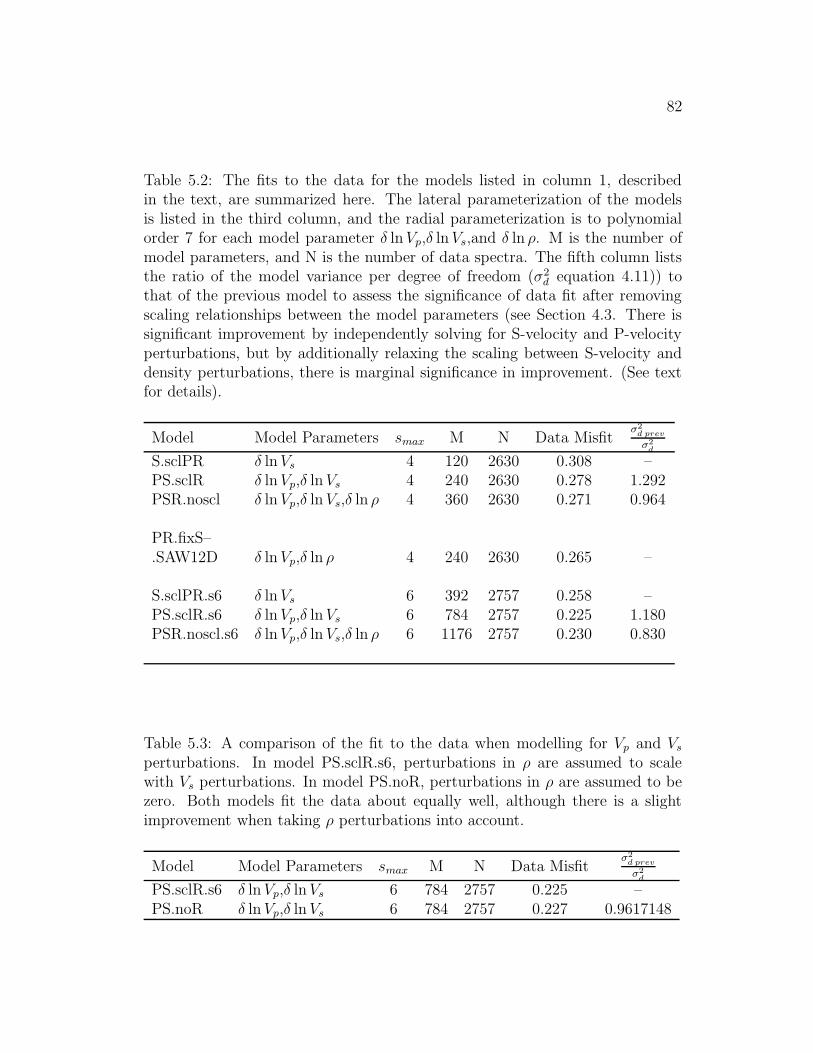
82

Table 5.2: The fits to the data for the models listed in column 1, describedin the text, are summarized here. The lateral parameterization of the modelsis listed in the third column, and the radial parameterization is to polynomialorder 7 for each model parameter δ ln Vp,δ ln Vs,and δ ln ρ. M is the number ofmodel parameters, and N is the number of data spectra. The fifth column liststhe ratio of the model variance per degree of freedom (σ2

d equation 4.11)) tothat of the previous model to assess the significance of data fit after removingscaling relationships between the model parameters (see Section 4.3. There issignificant improvement by independently solving for S-velocity and P-velocityperturbations, but by additionally relaxing the scaling between S-velocity anddensity perturbations, there is marginal significance in improvement. (See textfor details).

Model Model Parameters smax M N Data Misfitσ2

d prev

σ2

d

S.sclPR δ ln Vs 4 120 2630 0.308 –PS.sclR δ ln Vp,δ ln Vs 4 240 2630 0.278 1.292PSR.noscl δ ln Vp,δ ln Vs,δ ln ρ 4 360 2630 0.271 0.964

PR.fixS–.SAW12D δ ln Vp,δ ln ρ 4 240 2630 0.265 –

S.sclPR.s6 δ ln Vs 6 392 2757 0.258 –PS.sclR.s6 δ ln Vp,δ ln Vs 6 784 2757 0.225 1.180PSR.noscl.s6 δ ln Vp,δ ln Vs,δ ln ρ 6 1176 2757 0.230 0.830

Table 5.3: A comparison of the fit to the data when modelling for Vp and Vs

perturbations. In model PS.sclR.s6, perturbations in ρ are assumed to scalewith Vs perturbations. In model PS.noR, perturbations in ρ are assumed to bezero. Both models fit the data about equally well, although there is a slightimprovement when taking ρ perturbations into account.

Model Model Parameters smax M N Data Misfitσ2

d prev

σ2

d

PS.sclR.s6 δ ln Vp,δ ln Vs 6 784 2757 0.225 –PS.noR δ ln Vp,δ ln Vs 6 784 2757 0.227 0.9617148

83

sity heterogeneity in the mantle are consistent with geodynamical expectations.

The confidence in the density model retrieved is thus solely based on indirect

evidence. On the other hand, the importance of solving independently for Vp

heterogeneity is much clearer. In what follows, we present further tests of the

stability of the Vp and ρ models.

5.6.5 Separate inversions of Vp and Vs sensitive modes

In the following experiments, we performed two separate inversions indepen-

dently for Vs and Vp, keeping δ ln ρ scaled to δ ln Vs, using different subsets of

data:

1. PS.sclR.Smod, including only Vs sensitive modes in the data set, and

2. PS.sclR.Pmod, including only Vp sensitive modes in the data set.

The spatial and damping parameters of the models were kept the same as in the

previous experiments.

In the first inversion, 18 primarily Vs sensitive modes (Figure 5.5) were

used, and the final variance of the model (PS.sclR.Smod) is 0.255 after 2 itera-

tions. The correlation in Vs with SAW12D is comparable to that obtained with

PSR.noscl (Figure 5.6 and dashed line in Figure 5.2a). The Vs perturbations

in this model and PSR.noscl are highly correlated at all depths whereas the Vp

structure is not well correlated (Figure 5.7) in the depth range 1500-2500km,

84

directly reflecting the lack of sensitivity in this depth range to Vp in the reduced

data set of Vs sensitive modes.

In the second inversion (PS.sclR.Pmod), 11 mostly Vp sensitive modes (Fig-

ure 5.8) were used. The final variance of the model is 0.215 after 2 iterations.

The correlation of the Vp structure from this model with PSR.noscl is high ex-

cept at the very top and bottom of the mantle (Figure 5.9), due to the decrease

of Vp mode sensitivity in these regions. However, the subset of S sensitive modes

considered above compensates for this in both regions, in the combined data set,

as can be seen from Figure 5.5 and Figure 5.7.

These experiments demonstrate further that inverting separately for Vs and

Vp is justified.

5.6.6 S-velocity ”Correction” for P-velocity and density

variation

Finally, returning to our whole data set, we test the stability of our Vp and

density models by assuming that the Vs perturbations are those of SAW12D

and solving for Vp and density structure independently (PR.fixS.SAW12D). We

find that the resulting density model (which gives a residual variance of 0.265)

correlates well throughout the mantle with the density model of PSR.noscl, ex-

cept perhaps at the very top and bottom. This indicates that the density model

obtained is stable. The Vp models, on the other hand, are not as stable in this

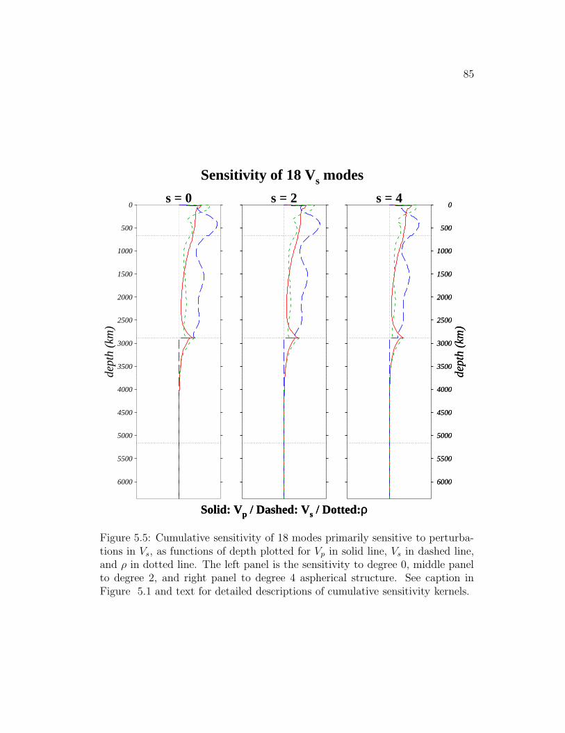
85

0

500

1000

1500

2000

2500

3000

3500

4000

4500

5000

5500

6000

dept

h (k

m)

s = 0 s = 2

Sensitivity of 18 Vs modes

Solid: Vp / Dashed: Vs / Dotted:ρSolid: Vp / Dashed: Vs / Dotted:ρ

0

500

1000

1500

2000

2500

3000

3500

4000

4500

5000

5500

6000

dept

h (k

m)

0

500

1000

1500

2000

2500

3000

3500

4000

4500

5000

5500

6000

dept

h (k

m)

s = 4

Figure 5.5: Cumulative sensitivity of 18 modes primarily sensitive to perturba-tions in Vs, as functions of depth plotted for Vp in solid line, Vs in dashed line,and ρ in dotted line. The left panel is the sensitivity to degree 0, middle panelto degree 2, and right panel to degree 4 aspherical structure. See caption inFigure 5.1 and text for detailed descriptions of cumulative sensitivity kernels.

86

0

400

800

1200

1600

2000

2400

2800

dept

h (k

m)

-1.0 -0.5 0.0 0.5 1.0

Correlation

SAW12D

correlated with

PS.sclR.Smod

Degrees 2 through 4 e

Dashed: Vs

Figure 5.6: The δ ln Vs model PS.sclR.Smod, is correlated to SAW12D as afunction of depth for degrees 2 and 4. There is good agreement with SAW12D.

87

0

400

800

1200

1600

2000

2400

2800

dept

h (k

m)

-1.0 -0.5 0.0 0.5 1.0

Correlation

PS.sclR.Smod

correlated with

PSR.noscl

Degrees 2 and 4

Solid: V p / Dashed: V s

Figure 5.7: δ ln Vp of PS.sclR.Smod correlated with δ ln Vp of PSR.noscl, a modelwith includes all the modes in the data set, in the solid line. Since the sensitivityto δ ln Vp is weak for the data included for PS.sclR.Smod, the correlation is weakin the lower mantle. The correlation of δ lnVs between the two models (dashedline) remains high. Correlation is for degrees 2 and 4.

88

0

500

1000

1500

2000

2500

3000

3500

4000

4500

5000

5500

6000

dept

h (k

m)

s = 0 s = 2

Sensitivity of 11 Vp modes

Solid: Vp / Dashed: Vs / Dotted:ρSolid: Vp / Dashed: Vs / Dotted:ρ

0

500

1000

1500

2000

2500

3000

3500

4000

4500

5000

5500

6000

dept

h (k

m)

0

500

1000

1500

2000

2500

3000

3500

4000

4500

5000

5500

6000

dept

h (k

m)

s = 4

Figure 5.8: As in Figure 5.5, but for 11 modes primarily sensitive to perturba-tions in Vp, as functions of depth.

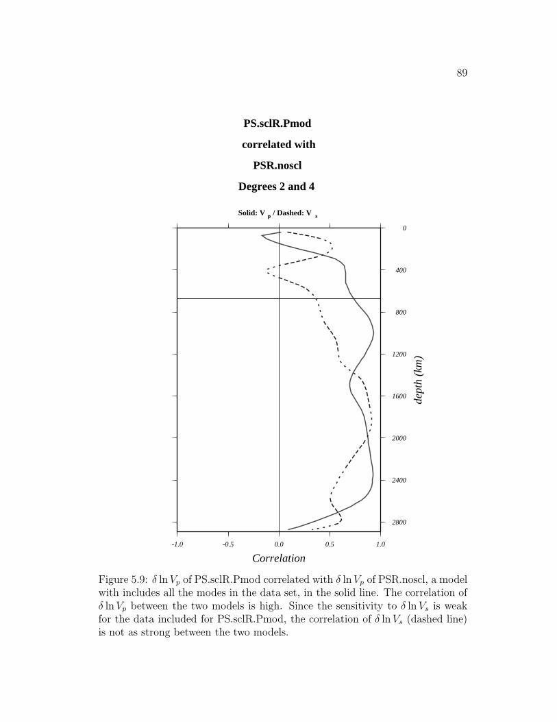
89

0

400

800

1200

1600

2000

2400

2800

dept

h (k

m)

-1.0 -0.5 0.0 0.5 1.0

Correlation

PS.sclR.Pmod

correlated with

PSR.noscl

Degrees 2 and 4

Solid: V p / Dashed: V s

Figure 5.9: δ ln Vp of PS.sclR.Pmod correlated with δ lnVp of PSR.noscl, a modelwith includes all the modes in the data set, in the solid line. The correlation ofδ lnVp between the two models is high. Since the sensitivity to δ ln Vs is weakfor the data included for PS.sclR.Pmod, the correlation of δ ln Vs (dashed line)is not as strong between the two models.

90

comparison. The correlation is particularly poor in the mid-lower mantle, but

the models agree in the lowermost mantle (Figure 5.10). This is an indication

that the mode data set may provide additional constraints to low degree struc-

ture in Vs in the mid-mantle. Indeed, by requiring that the Vs perturbations

follow those of SAW12D, we make the assumption that the mode data set has

the same sensitivity and sampling as the higher frequency body and surface

wave data. From the present experiment PR.fixS.SAW12D, it appears that the

Vp structure retrieved for the lower mantle may be biased by assuming the Vs

perturbations values of SAW12D at those depths. The final Vp solution from the

three parameter inversion (PSR.noscl) correlates well with the Vp model inverted

with primarily Vp sensitive modes (PS.sclR.Pmod)(Figure 5.9), indicating that

the modes do find a stable solution for δ ln Vp, when no a-priori constraint is

imposed on the Vs model.

In addition, we have computed the resolution matrix for the case in which Vs,

Vp, and ρ are independently retrieved which show that there are some trade-off

between Vs and Vp perturbations, as well as with ρ. In Chapter 6, the effects of a

priori constraints on model resolution, and contamination between parameters

will be discussed.

91

0

400

800

1200

1600

2000

2400

2800

dept

h (k

m)

-1.0 -0.5 0.0 0.5 1.0

Correlation

PR.fixS.SAW12D

correlated with

PSR.noscl

Degrees 2 and 4

Solid: V p / Dotted: ρ

Figure 5.10: Correlation of Vp heterogeneity between model PR.fixS.SAW12Dand PSR.noscl in the solid line, and the correlation of ρ heterogeneity from thesetwo models, in the dotted line. There are some trade-offs between our ability toresolve Vp and Vs, but there is little contamination of velocity structure into ρstructure. The correlations are for degrees 2 and 4.

92

5.7 Model Results

Having determined in the previous section that there is some value in invert-

ing independently for Vs, Vp and ρ, we now present the resulting final models,

PSR.s4.cmb and PSR.s6.cmb. In these models, we have allowed for perturba-

tions in core mantle boundary topography, and we will discuss below the signif-

icance of doing so. This model was obtained after exploring damping parameter

space. We damp the size , the second radial derivative, and the surface gradient

(equation (4.8)). The values of damping parameters are chosen by exploring a

range for each damping parameter, applying the damping to the inversion, and

plotting trade-off curves of the misfit of the resulting models against damping

parameter used in its inversion. The damping parameter value which gives the

smallest misfit is chosen.

5.7.1 Velocity models in PSR.s4.cmb

In Figure 5.11, we display our degree 4 Vp and Vs models at 6 representa-

tive depths in the mantle in the left and middle columns, respectively. Density

heterogeneity is given in the right column. We only retrieve the very large scale

features of lateral heterogeneity in degree 4, and upon inspection, we observe

anomalous equatorial high shear velocity band in the shallow mantle. At the

bottom of the mantle, shear velocity in PSR.s4.cmb also exhibits prominent high

velocity regions in the Pacific which we attribute to higher order features derived

93

from body waves, eg., SAW12D (Li and Romanowicz, 1996) or SKS12WM13

(Dziewonski et al., 1997). There is, otherwise, good correspondence with ex-

pected features of the dynamic Earth, as documented in other studies. Fast

anomalies are associated with regions of subduction, particularly in the West-

ern Pacific and are prominent under South America at 650 km depth. In the

lower mantle to 1200 km, the fast velocities are somewhat shifted for Vs, while

the Vp pattern remains stable. At the bottom of the mantle, compressional wave

velocity maps exhibit high velocity rings around a low velocity Pacific Ocean.

The anomalous high Vs features in the degree 4 model may be attributed to

aliasing, which is the effect of shorter wavelength terms becoming folded into

longer wavelength terms due to the truncation of the polynomial series of our

spatial model parameterization. In the next section, models parameterized to

degree 6 in spherical harmonics are described.

5.7.2 Velocity models in PSR.s6.cmb

By extending the lateral parameterization to spherical harmonic degree 6, we

obtain models with better resolution in which aliasing is diminished and shorter

wavelength structure is resolved, as illustrated in Figure 5.12, where the models

of heterogeneity in Vp, Vs, and ρ are displayed in the same columns as in Figure

5.11. For six depths in the mantle at 200, 650, 1200, 1800, 2200, and 2800 km,

we compare our Vs and Vp models (with and without CMB undulations) with

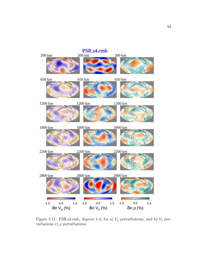
94

200 kmPSR.s4.cmb PSR.s4.cmb

650 km

1200 km

1800 km

2200 km

-1.5 0.0 1.5

δln Vp (%)

2800 km

200 km

650 km

1200 km

1800 km

2200 km

-1.5 0.0 1.5

δln Vs (%)

2800 km

200 km

650 km

1200 km

1800 km

2200 km

-1.5 0.0 1.5

δln ρ (%)

2800 km

Figure 5.11: PSR.s4.cmb, degrees 1-4, for a) Vp perturbations, and b) Vs per-turbations c) ρ perturbations.

95

independently derived published models, expanded in spherical harmonics up to

degree 6 (Figures 5.13 and 5.14). The left map at each depth section is the Vs

(respectively Vp) structure of our model PSR.s6.cmb. The maps of independently

derived heterogeneity are in the middle and right column in each depth section.

In the Vs comparison (Figure 5.13), we use SAW12D (Li and Romanowicz,

1996) and SKS12WM13 (Dziewonski et al., 1997). For Vp (Figure 5.14), we

compare our models with WE1997 (Vasco and Johnson, 1997) and P16B30

(Masters and Laske, personal communication). The model of Vp heterogeneity

from WE1997 is inverted from ISC travel time data, and P16B30 incorporates

travel time data, surface-wave phase velocities, and normal mode data in the

form of ’splitting coefficients’ for 19 spheroidal modes which have sensitivity to

lower mantle structure.

There is very good agreement between our Vs model and both SAW12D (Li

and Romanowicz, 1996) and SKS12WM13 (Dziewonski et al., 1997). The pat-

tern of Vs heterogeneity at 200 km exhibits fast velocities beneath the colder

Pacific Basin, beneath Western Australia, and beneath the American, African

and Antarctic continents. Mid-ocean ridge regions associated with warm up-

welling material are slow. At 650 km, fast velocities are prominent in regions

often referred to as subducting slabs. In the lower mantle, the patterns in our

Vs model appear to agree with those of SKS12WM13 more than with SAW12D.

SKS12WM13 is sensitive to SV perturbations, and SAW12D is a model of SH

96

200 kmPSR.s6.cmb PSR.s6.cmb

650 km

1200 km

1800 km

2200 km

-1.5 0.0 1.5

δln Vp (%)

2800 km

200 km

650 km

1200 km

1800 km

2200 km

-1.5 0.0 1.5

δln Vs (%)

2800 km

200 km

650 km

1200 km

1800 km

2200 km

-1.5 0.0 1.5

δln ρ (%)

2800 km

Figure 5.12: PSR.s6.cmb, degrees 1-6, for a) Vp perturbations, and b) Vs per-turbations c) ρ perturbations.

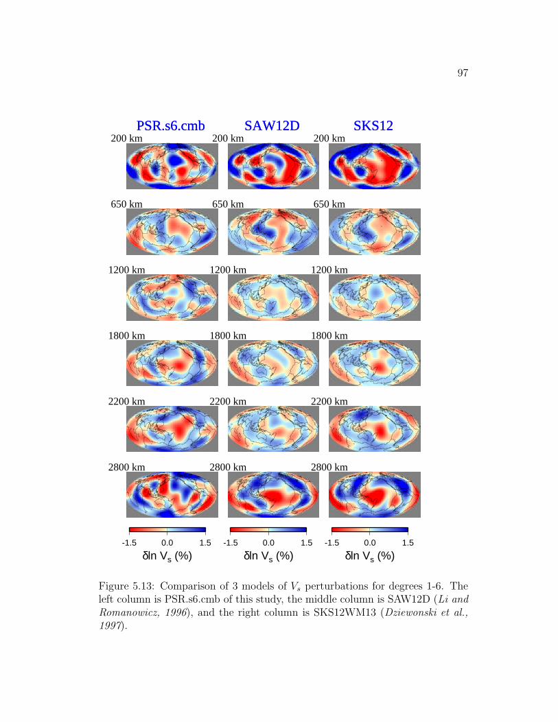
97

200 kmPSR.s6.cmb PSR.s6.cmb

650 km

1200 km

1800 km

2200 km

-1.5 0.0 1.5

δln Vs (%)

2800 km

200 kmSAW12D SAW12D

650 km

1200 km

1800 km

2200 km

-1.5 0.0 1.5

δln Vs (%)

2800 km

200 kmSKS12 SKS12

650 km

1200 km

1800 km

2200 km

-1.5 0.0 1.5

δln Vs (%)

2800 km

Figure 5.13: Comparison of 3 models of Vs perturbations for degrees 1-6. Theleft column is PSR.s6.cmb of this study, the middle column is SAW12D (Li andRomanowicz, 1996), and the right column is SKS12WM13 (Dziewonski et al.,1997).

98

200 kmPSR.s6.cmb PSR.s6.cmb

650 km

1200 km

1800 km

2200 km

-1.5 0.0 1.5

δln Vp (%)

2800 km

200 kmWE1997.P WE1997.P

650 km

1200 km

1800 km

2200 km

-1 0 1

δln Vp (%)

2800 km

200 kmP16B30 P16B30

650 km

1200 km

1800 km

2200 km

-1.5 0.0 1.5

δln Vp (%)

2800 km

Figure 5.14: Comparison of 3 models of Vp perturbations for degrees 1-6. Theleft column is PSR.s6.cmb of this study, the middle column is WE1997 (Vascoand Johnson, 1997), and the right column is P16B30 (Masters et al., 1996).

99

perturbations. The correspondence of our model with SKS12WM13 is most

likely due to the P-SV nature of particle motion for spheroidal modes. At

the bottom of the mantle, however, our Vs differs from both SAW12D and

SKS12WM13,in that our model lacks strong fast regions over Asia.

Referring to Figure 5.14, our model of Vp structure in the left column com-

pares well with WE1997 (Vasco and Johnson, 1997) in the upper mantle. The

upper mantle structure in P16B30 is constrained by a number of fundamental

mode data, many of which we do not include in our data set. There is good

agreement in the lower mantle at 1200 km, but at 1800 and 2200 km, our Vp

model differs from WE1997 and P16B30. The origin of the patterns at these

depths can be attributed to contamination from Vs, as we will discuss in Chapter

6.

5.7.3 Volumetric heterogeneity and boundary undulations

When the core-mantle boundary topography is not modeled, CMB undu-

lations may be mapped into patterns of structure in the lowermost mantle.

We compare a model PSR.s6 which assumes a smooth CMB, with PSR.s6.cmb

which includes CMB topography to try to understand the trade-off between

solutions for lower mantle structure and the CMB undulations (Figure 5.15).

Model PSR.s6.cmb includes up to harmonic degree 6 in CMB undulations, and

thus has 49 additional model parameters, compared to PSR.s6.

100

-1

0

1δln Vp (%)

PSR.s6 w/out CMB

Maps at 2800 km

δln Vp

PSR.s6.cmb with CMB

-1.5

0.0

1.5δln Vs (%)

δln Vs

-1

0

1δln ρ (%)

δln ρ

Figure 5.15: At 2800 km, Comparison of models PSR.s6, which assumes asmooth core-mantle boundary, and PSR.s6.cmb, for which boundary topographyis included in the model parameterization. Degrees 1 through 6.

101

The mantle heterogeneity in the two models is very stable, except at depths

near the very bottom of the mantle, illustrating the trade-offs between the capa-

bility of imaging volumetric structure and boundary deformation in the vicinity

of the discontinuity. Although present at shallower depths around 1600-2000

km in PSR.s6, the c22/s

22 pattern of fast S-velocity perturbations surrounding a

slow velocity central Pacific region commonly found in higher frequency seismic

tomographic models such as SAW12D, S12WM13, or S16B30 (Masters et al.,

1996) is not as clear in the model PSR.s6 at the bottom of the mantle at 2800 km

(Figure 5.15a). This c22/s

22 pattern at the bottom of the mantle is also present in

the shear-velocity model derived from normal modes data by Resovsky & Ritz-

woller 1999b, but their model has been damped to optimize consistency with

mantle models SAW12D, SKS12WM13, and S16B30. Although we have applied

damping to the model size, horizontal smoothing, and radial smoothing, we do

not retrieve a c22/s

22 pattern near the core-mantle boundary in Vs of PSR.s6.

Including topography of core-mantle boundary in our models improves the

model of S-velocity heterogeneity at the bottom of the mantle in the sense that

at 2800 km, the fast velocity band extending North-South through the Pacific

Ocean is removed. More specifically, while the even degree structure of δ ln Vs

in PSR.s6 and PSR.s6.cmb has remained somewhat consistent, the odd degrees

1 and 3 have not, and we note that most of the power of the CMB undulation

solution is in degrees 1 and 3.

102

The effect of excluding CMB topography on the δ ln Vp model of PSR.s6 can

also be seen in the lower mantle as illustrated in Figure 5.15. The pattern of

heterogeneity in the δ ln Vp model of PSR.s6.cmb exhibits fast velocities around a

slow Pacific near the CMB. In their discussion of their S-velocity model S16B30

( Masters et al., 1996), the authors confirm that the sensitivity of mode data to

boundary topography introduces a trade-off with sensitivity to structure in the

vicinity of the boundary. Stating that the boundary undulations are not well-

constrained by their data set, they choose not to solve for boundary undulations

at the time of producing S16B30 (/P16B30). With the addition of the CMB un-

dulation solution, a fast velocity region over Asia is more pronounced in δ lnVp

of PSR.s6.cmb. This fast velocity feature appears consistently in P-velocity

models P16B30, JLM4P6 (Robertson & Woodhouse 1995), the P-velocity com-

ponent of WE1997 (Vasco & Johnson 1998), and the P-velocity model derived

from MK12WM13 (Su & Dziewonski 1997).

5.7.4 ρ model of PSR.s6.cmb

Although our confidence in the retrieval of density structure is marginal, as

discussed in a previous section, we see from Figure 5.12c that the density struc-

ture retrieved from PSR.s6.cmb is not unreasonable: patterns of high density

anomalies in the mantle correspond to regions of down-going slabs in the man-

tle. High density features are present southwest of South America and Western

103

Pacific starting at about 250 km depth, in particular near the Tonga Trench.

These features surrounding the Pacific extend all the way down to the base of the

mantle. Again, we find that the density heterogeneity pattern at the base the

mantle differs when we do not include CMB topography modeling. In PSR.s6,

the density structure at 2800 km is similar to that in PSR.s6.cmb, except for the

presence of high density extending northwesterly from Western South America,

over the Hawaiian Islands, up to the Bering Sea. When the CMB topography is

included in the model, as for PSR.s6.cmb, this density high is removed and the

density pattern corresponding to the subduction of cold slabs is retained at 2800

km (Figure 5.15). There are high density features in the model which would

not appear to be thermal in origin, assuming mantle geodynamic models driven

by cold and dense downgoing slabs, and warm upwelling plumes originating at

the core-mantle boundary. For example, there is high density at 2800 km in

the region of the hypothesized origin of the Hawaiian Plume. Before concluding

that these features are chemical in origin (Ishii and Tromp, 1999), extensive

resolution tests must be analyzed for model robustness. We address resolution

issues in Chapter 6.

5.7.5 Core-Mantle Boundary Topography

Inclusion of parameterization for core-mantle boundary topography improves

our models of volumetric heterogeneity at the base of the mantle. In Figure

104

-7.5-6.0-4.5-3.0-1.5 0.0 1.5 3.0 4.5 6.0 7.5

km

PSR.s6.cmb

CMB degrees 2 and 4 CMB degrees 2 and 4

Figure 5.16: Even degrees 2 and 4 of the CMB undulations for modelPSR.s6.cmb. Positive deformations indicate elevation (light), and negative de-formations represent regions of depression (dark).

5.16, the deformations in degrees 2 and 4 on the core-mantle boundary are

displayed for model PSR.s6.cmb, where positive deformations indicate areas of

elevation, and negative deformations represent areas of depression. Only degrees

2 and 4 are shown because we have found that the degree 2 and 4 topographic

undulations are stable throughout a number of inversion experiments using a

number of various spatial parameterizations of our three-dimensional models,

while odd degrees, which are constrained by only few coupled-modes are not as

stable.

105

The prominent depressions are seen under the Philippine Sea where the

Phillipine Trench and New Guinea Trench merge at the surface of the Earth,

and over South America, west of the Peru-Chile Trench in the direction of dip.

There are two large regions of depressions, west of North America extending to

the Tonga Trench region and over Africa, for which we do not have an obvious

explanation based on surface tectonics. Nevertheless, our model of CMB to-

pography is comparable in pattern and amplitude to the CMB maps from PcP

travel time studies of Obayashi and Fukao, 1997 and Rodgers and Wahr, 1993,

particularly the depressions below South East Asia, South America, Africa, and

the dominant degree 2 zonal component (s = 2, t = 0). A depression in the Pa-

cific west of North America is expressed in the Rodgers and Wahr, 1993 CMB

model from inversions of ISC PcP travel times. We also retrieve elevated to-

pography in high northern latitudes, in agreement with Obayashi and Fukao,

1997 and Rodgers and Wahr, 1993. Obayashi and Fukao, 1997 interpret the

dominant degree 2 zonal pattern in the CMB heterogeneity as possibly related

to outer core fluid flow.

Our CMB amplitudes, ±7.5 km, are high compared to independent con-

straints of the topographic amplitudes, such as from Earth tide and nutation

measurements (e.g. Wahr and de Vries, 1989), which constrain the h02 coefficient

of CMB topography to vary between 0.5-1.0 km. However, the residual variance

of the model is essentially invariant for a range of amplitudes of the core-mantle

106

boundary undulations, and we can choose the CMB amplitude damping value

which is consistent with independent studies of core mantle boundary topo-

graphic amplitudes such as the observations of the Earth’s nutation.

The patterns of CMB topography presented by a number of authors (Morelli

and Dziewonski, 1987; Li et al., 1991b; Rodgers and Wahr, 1993; Obayashi and

Fukao, 1997) vary depending on what types of seismic data analyzed. In what

follows, we discuss the stability of our model, with respect to spatial parame-

terizations of our models. In order to test the stability of the even degrees, the

following experiments were performed: ones analogous to S.sclPR, PS.sclR, and

PSR.noscl in which the CMB topography has been included as additional model

parameters, for both even-degree only models (where coupled modes are not con-

sidered), and models which also retrieve odd degree structure. A model of Earth

heterogeneity which includes parameterization for both CMB topography and

outer core structure has also been computed to test mapping of possible outer

core structure into the CMB parameterization. The degree 2 and 4 structure is

extremely stable throughout all of these experiments.

Although the odd degree CMB topographic coefficients from the relevant

parameterization experiments have also been stable, their amplitudes are almost

two orders of magnitude too high. In what follows, we describe a resolution test,

in which we find that we can reliably retrieve a small amplitude even degree

signal. In a test of resolution, we take the product of an input model of mock

107

even degree CMB undulations with the resolution matrix constructed from our

mode kernels for the parameterization for PSR.s6.cmb. While the input CMB

model only includes even degrees 2 and 4 and zero values for odd degrees, the

output model includes both even and odd degrees. Figure 5.17 displays the

input map and output patterns in degrees 2 and 4, and demonstrates that the

even degree pattern is well preserved.

While we have demonstrated that we can reliably retrieve an input model

of CMB undulations, we’d also like to examine the trade-off between volumet-

ric heterogeneity and boundary topography, but this time, with respect to the

effects on the patterns of topography. Assuming now that the input CMB has

zero topography, we test the resolution of our data set and see that the output

model in Figure 5.18 shows depressions in the circum-Pacific region. This pat-

tern is most likely a result of contamination from seismic velocity signals, which

we will discuss in detail in Chapter 6. A comparison between the output models

in Figures 5.18 and 5.17 assures us that for our data set, we can resolve trough

and elevation peaks of the CMB over ∼ 0.75 km without being influenced by

the contaminant signal. The output model of CMB undulations in Figure 5.18

is very similar to the CMB model derived from an earlier work in inversions of

normal mode spectra for heterogeneity, Li et al., 1991b (Figure 12a). In Li et

al., 1991b, 835 pre-1990 seismic spectra of 20 mantle modes were analyzed to

invert for even degree Vs models of heterogeneity, where Vp and ρ perturbations

108

-1.00-0.75-0.50-0.250.00 0.25 0.50 0.75 1.00

km

Input

CMB resolution degrees 2 and 4 CMB resolution degrees 2 and 4

-1.00-0.75-0.50-0.250.00 0.25 0.50 0.75 1.00

km

Output

Figure 5.17: Resolution test of CMB topography. Negative values indicate de-pressions (dark) and positive values indicate elevations (light).

109

-1.00-0.75-0.50-0.250.00 0.25 0.50 0.75 1.00

km

Input

CMB resolution degrees 2 and 4 CMB resolution degrees 2 and 4

-1.00-0.75-0.50-0.250.00 0.25 0.50 0.75 1.00

km

Output

Figure 5.18: A second resolution test of CMB topography examining artifactCMB patterns. Negative values indicate depressions (dark) and positive valuesindicate elevation (light).

110

were scaled to Vs perturbations. Although they retrieve CMB amplitudes of ±3

km, we cannot make direct comparisons of threshold sensitivity to contaminant

signal amplitudes due to the differences in data set, and model parameteriza-

tion. However, the difference in pattern between our CMB model and that of Li

et al., 1991b can be explained by Figure 5.18, where we put forth the suggestion

that they may have observed contamination from Vs.

5.7.6 Odd degree sensitivity

Although our mode data set is primarily sensitive to even degree structure

from the self-coupling interaction of isolated modes, it is possible to infer odd

degree structure from cross coupled modes. We find that for Vs, our solution for

odd degree structure agrees well with that of SAW12D in the lower mantle. For

inversions up to degree 4 harmonics involving coupled modes, the sensitivity to

odd degree structure is limited to degree 1 and 3, and constrained only by two

pairs of couple modes, 1S5−2 S4 and 1S6−2 S5. The sensitivity of these two pairs

of coupled modes is strong for Vs but very weak for Vp and ρ for degree 1 and 3

structure in the lower mantle (Figure 5.19). Including the coupled modes, the

correlation of the Vs model from PSR.s6, to SAW12D in degree 1 and 3 structure

is high in the lowermost mantle where the sensitivity to Vp is very low, and the

Vs sensitivity dominates (Figure 5.20). This may suggest that because there is

little sensitivity to Vp and ρ in degrees 1 and 3, there is much less trade-off with

111

Vp and ρ in the Vs model. We also find that the even degree is stable when

odd degree structure coefficients are added to the parameterization. On the

other hand, the addition of the CMB topography to our model parameterization

degrades the correlation of the odd degree structure with that of SAW12D. The

model coefficients of the CMB topography in PSR.s6.cmb is dominated by odd

degrees, but we have demonstrated that the even degree structure is well resolved

in Figure 5.17, and contamination between even and odd degree CMB structure

is negligible.

5.7.7 Outer Core

Although our data set consists of ’mantle modes’, most of these modes also

have sensitivity in the outer core. If the model parameterization only includes

depths extending to the core-mantle boundary, outer core structure may be

mapped into the coefficients of mantle structure. The outer core is assumed

to be homogeneous because of the low viscosity and the vigorous convection

of metallic iron required to support the geodynamo; there would be no outer

core structure to contaminate the mantle models, in this case. Stevenson (1987)

concluded from fluid dynamics considerations that lateral variations in the outer

core are undetectable by seismology, but there may be limitations to the author’s

examination (S. Zatman, personal communication). Despite these assumptions,

112

1S5--2 S4 1S6--2 S5

Odd degree structure sensitivity

moho

670

CMB

ICB

r=0

deg 1 deg 3 deg 1 deg 3

KVs

KVp

Kρ

Figure 5.19: Two mode pairs in the coupled mode inversion, 1S5- 2S4 and 1S6-

2S5, are sensitive to odd degree structure. The mode pairs, 1S5-2S4 and 1S6-2S5

give sensitivity to degrees 1 and 3 for our model PSR.s6.cmb and the sensitivitykernels (KV s,V p,ρ) plotted here show that most of the amplitude in odd degreesis in δ ln Vs.

113

0

400

800

1200

1600

2000

2400

2800

dept

h (k

m)

-1.0 -0.5 0.0 0.5 1.0

Correlation

SAW12D

correlated with

Solid: PSR.s6 / Dashed: PSR.s6.cmb

degrees 1 and 3

Figure 5.20: For Vs structure in odd degrees 1 and 3, the correlation betweenSAW12D and PSR.s6 in solid line, and the correlation between SAW12D andPSR.s6.cmb in dashed line. The CMB topography in PSR.s6.cmb is strong inodd degrees.

114

0

400

800

1200

1600

2000

2400

2800

dept

h (k

m)

-1.0 -0.5 0.0 0.5 1.0

Correlation

PSR.s4.cmb

correlated with

PSR.s4.cmb+oc

Degrees 1 through 4

Solid: Vp / Dashed: Vs / Dotted:ρ

Figure 5.21: The correlation of mantle structure between a mantle model(PSR.s4.cmb) and a mantle model which includes outer core parameterization(PSR.s4.cmb+oc) for degrees 1 through 4. The solid line is the correlation inVp, dashed line: in Vs, and dotted line: in ρ.

115

we have parameterized our models to include a layer , specifically parameterized

by a zero order polynomial, in the outer core extending to ∼200 km below the

core mantle boundary. By comparing the Vp, Vs, and ρ models with and without

the outer core parameterization, we find that the mantle structure is very stable

for the seismic velocity perturbations, and that there exists a slight trade-off in

density structure (Figure 5.21). The structure which is mapped into the outer

core layer will be the subject of a future article.

5.8 Conclusions

We have shown that our data set of mode spectra has sensitivity to not only

Vs structure, but to Vp structure as well. Inverting for structure using either only

Vs or Vp sensitive modes confirms that the Vp structure obtained by jointly and

independently inverting for Vs, Vp, and ρ has more information than the ’noise’

of Vs structure. We have presented our models of large scale Vp,Vs, and density

structure. The density models are stable throughout the inversion experiments.

The final models are parameterized to degree 6 harmonics laterally and degree

7 Legendre polynomials radially, and include odd degree structure.

We find that the assumption that Vp and density variations scale uniformly

with those of Vs introduces notable contamination into the Vs modeling, when

compared to SAW12D. Our models of Vs are improved, in this sense, when

solutions to Vs, Vp and ρ inhomogeneities are found independently. The stabil-

116

ity of the resulting Vp tomographic model is demonstrated through its strong

correlation with Vp structure inverted by using a subset of P-wave velocity sen-

sitive modes with low S-wave velocity sensitivity. While it is difficult to per-

form the same type of comparison for the density models, as the amplitudes of

Vs and/or Vp sensitivity dominate that of ρ for the modes used in this study

( 0S, 1S, 2S, 4S, 5S branches), the density models remain stable throughout

the numerous inversion experiments, and display features related to subducting

slabs in the circum-Pacific.

Our density structure in the mantle does not agree with that of Ishii and

Tromp, 1999, particularly at the depths immediately above the core-mantle

boundary, although the topography of the CMB is parameterized in the model

space in both our analysis and theirs. The anomalous high density structures at

lowermost depths in the central Pacific and under Africa displayed in the Ishii

and Tromp, 1999 model is not prominent in our model. Although some of our

models display similar features, we do not find that these features are stable.

They disappear with the inclusion of CMB topography in model parameteriza-

tion, and with our choice of damping values.

Our model of CMB structure agrees with the results of PcP travel time

studies of Obayashi and Fukao, 1997 and Rodgers and Wahr, 1993. We find

that there is a dominant degree 2 zonal pattern in which polar regions are

elevated, and this observation may indicate influences of outer core fluid flow

117

on the core mantle boundary topography, as suggested by Obayashi and Fukao,

1997. Regions of depression on the core mantle boundary are located beneath

the Philippine Sea, where a junction of three trenches merge at the Earth’s

surface, and South America, in the dipping direction of the Peru-Chile Trench.

Two other large regions of depressions, west of North America and over Africa,

can not be explained by surface tectonics. The differences in pattern between

the CMB structure retrieved in our model PSR.s6.cmb and in SAT of Li et

al., 1991b for which type of data and inversion technique are essentially the

same, may be due to a contaminant signal in the model SAT. We find that the

degree 2 and 4 coefficients of our CMB topography structure to be very stable

throughout a number of model parameterizations. The issue of uncertainties

in the final density models due to a priori assumptions imposed on inversions

for density structure from normal mode splitting coefficients, as performed by

Ishii and Tromp, 1999, has been addressed by Resovsky and Ritzwoller, 1999a.

The problems induced from a priori assumptions have further impact on the

inversions for structure from splitting coefficients, as the regularization schemes

used to solve for splitting coefficients from normal mode spectra are unaccounted

for in this type of analysis, whereas the method of direct inversion from normal

mode spectra to Earth structure, as we have used, allows us to better understand

the trade-offs associated with our a priori assumptions. In the next chapter, we

will address the issues of a priori assumptions and their impact on resolvable

118

model parameters.

119

Table 5.4: For each mode in column 1, the residual variance of predicted spectrato the data spectra, computed from model PSR.s6.cmb, is reported in column3. The total residual variance for this model is 0.227. The central referencefrequency of each mode, with respect to PREM, is listed in the 2nd column.

Mode Reference Frequency (mHz) Data misfit

0S3 0.469 0.448

0S4 0.647 0.283

0S5 0.840 0.182

0S6 1.038 0.217

0S9 1.578 0.103

0S27 3.544 0.227

1S2 0.680 0.418

1S4 1.173 0.106

1S7 1.656 0.202

1S8 1.799 0.177

1S9 1.964 0.180

2S6 1.681 0.161

2S12 2.737 0.153

2S13 2.900 0.215

4S2 1.722 0.375

4S4 2.280 0.164

4S9 3.709 0.257

4S11 4.010 0.764

5S3 2.170 0.115

5S4 2.380 0.089

5S5 2.703 0.051

5S6 3.011 0.159

5S7 3.291 0.150

5S8 3.526 0.195

120

Table 5.4 continued

Mode(s) Reference Frequency (mHz) Data misfit

5S12 4.696 0.239

6S10 4.211 0.298

7S4 3.413 0.353

7S5 3.660 0.308

8S7 4.650 0.355

9S14 6.768 0.108

3S1 − 1S3 0.944, 0.940 0.184

2S4 − 1S5 1.379, 1.370 0.141

2S5 − 1S6 1.515, 1.522 0.134

4S3 − 2S8 2.049, 2.049 0.080

6S3 − 3S8 2.822, 2.820 0.269

0S7 − 2S3 1.232, 1.242 0.200

2S10 − 4S5 2.403, 2.411 0.091

121

Chapter 6

The resolution of density anomalies in the

Earth’s mantle using normal mode data

6.1 Introduction

The issue of whether lateral variations in density in the mantle can be re-

solved from normal mode data has recently received renewed attention, in par-

ticular with the work of Ishii and Tromp, 1998, 1999. In their recently pub-

lished paper, these authors present a degree 6 model of density throughout the

mantle, derived from inversion of normal mode splitting coefficients. This model

presents unexpected features in the lowermost mantle, namely two large ”blobs”

of high density material centered in the Pacific and under Africa, that, if real,

would have important consequences for the dynamics of the mantle. Ishii and

Tromp, 1999 argue for the robustness of their model, on the basis of numerous

experiments, including checkerboard resolution tests and exploration of different

parameterization schemes.

Whether lateral variations in density can be resolved from normal mode

122

data has long been the subject of debate. Resovsky and Ritzwoller, 1999 have

recently presented the results of tests which show that the retrieved density

structure is very sensitive to the regularization scheme used in the inversion.

Imposed a priori constraints on the location and size of density heterogeneity

have a strong effect on the resulting models, which, while providing equal fit to

the data, can be significantly different. Ishii and Tromp, 1999 however, argue

that their density model is weakly dependent on their starting model.

In what follows, we present the results of a series of tests in which we have

explored more fully the structure of the resolution matrix than can be done with

checkerboard tests. Because in the case of non-linear inversions, the resolution

matrix approach only allows us to investigate the problem approximately, we

also present results of tests in which we compute synthetic seismograms for

realistic Earth models and invert them under the same conditions as the real

data.

6.2 Tests with resolution matrices

6.2.1 Resolution matrix

The resolution matrix is a useful tool to assess the leakage between model

parameters in a generalized inversion framework. Indeed, the solution mest to

the inverse problem dobs = Am, where A is a linearized data kernel, dobs is the

data vector, and m the model vector, can be written as:

123

mest = (ATA + C−1m )−1ATdobs (6.1)

where C−1m is the matrix of damping parameters. The relation between the

vector of estimated model parameters mest and the true model mtrue, for a

given parameterization and underlying theory, is then:

mest = (ATA + C−1m )−1ATAmtrue. (6.2)

The M ×M model resolution matrix R, where M is the number of unknown

parameters, is defined as

R = (ATA + C−1m )−1ATA (6.3)

so that

mest = Rmtrue. (6.4)

If R = I, where I is the identity matrix, then each model parameter is perfectly

resolved. In practice, R = I has non zero off-diagonal terms, and their size

relative to each other and to the diagonal terms indicates the amount of con-

tamination (or ”covariance”) between the different parameters as determined by

inversion.

In our particular problem, we invert simultaneously for structure in VP , VS

and ρ, and wish to investigate the level of contamination between these param-

eters. The model vector is arranged as follows:

124

m = [ pVtP s, pV

tS s, pρ

ts], (6.5)

where the indices s, t, p refer to the parameterization of the model. In our stud-

ies, we have chosen spherical harmonics laterally, and Legendre polynomials

vertically. The maximum degree (smax = 6) of the spherical harmonics expan-

sion is chosen in view of the sensitivity of the particular mode data set we are

considering, given that a particular mode of angular order l is sensitive to at most

lateral heterogeneity of degree 2l. The maximum order of the radial polynomial

expansion is commensurate with the maximum radial order n of the modes in

our data set (pmax = 7). We will compare results for pmax = 7 and pmax = 10,

as it has been argued (e.g. Ishii and Tromp, 1999 that more stable results can

be obtained by overparameterizing the model and then damping more strongly.

The resolution equation is then:

pVtP s

pVtS s

pρts

est

=

RP ∅SP ∅RP

∅PS RS ∅RS

∅PR ∅SR RR

pVtP s

pVtS s

pρts

true

(6.6)

where RP , RS, and RR are resolution submatrices for pVtP s, pV

tS s, and pρ

ts re-

spectively, and non-zero values in ∅PS are the covariances which would map VP

structure into VS structure, and so on. Of course, the ∅’s are zero in an ideal

resolution matrix.

125

Imposing a priori distributions

Since the resolution matrix is a function of both the data kernels and the a

priori model covariance matrix, C−1m , it is important to carefully choose the a

priori damping parameters so as to obtain, inasmuch as possible, R ≈ I.

To do so, we consider a ”realistic” synthetic model, for which we choose

S velocity (VS) to be that of model SAW12D (Li and Romanowicz, 1996) , P

velocity (VP )to be that of P16B30 (Masters et al, 1996). A mock density model

(ρ) is constructed so that the root-mean-square amplitudes are about 25% of VS,

a common assumption in low-frequency seismology (e.g. Li et al., 1991) that

is in agreement with laboratory measurements at shallow mantle pressure and

temperatures. The mock density perturbations are constructed by permuting

and scaling (to 25%) coefficients of Vs model SAW12D so that the actual patterns

of heterogeneity are not correlated with SAW12D, and we name this model R25.

As mentioned previously, we consider two different spatial parameterizations: 1)

smax = 6, pmax = 7 (Experiment A), and 2) smax = 6, pmax = 10 (Experiment

B). The resolution matrix is computed using the data kernels corresponding to

our data set of 44 spheroidal mode spectra.

Damping parameters are defined separately for δVP , δVS, and δρ and chosen

in such a fashion as to best recover the rms amplitudes of the true model for

even degrees (2,4,6) after applying the resolution matrix. We only consider norm

damping (η1 in equation (4.8)) and we find that values of ηP1 = ηS

1 = ηR1 = 1 are

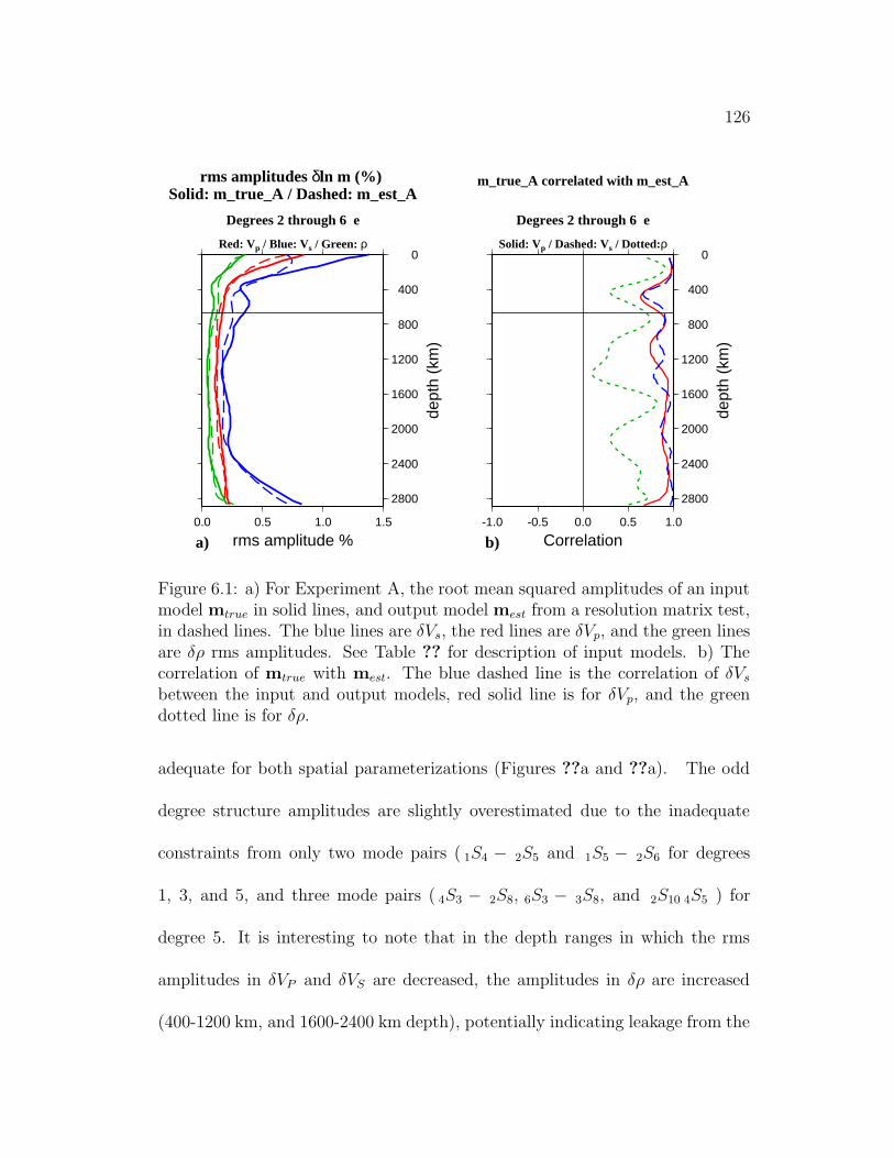
126

0

400

800

1200

1600

2000

2400

2800

dept

h (k

m)

0.0 0.5 1.0 1.5

rms amplitude %a)

rms amplitudes δln m (%) Solid: m_true_A / Dashed: m_est_A

Degrees 2 through 6 e

Red: Vp / Blue: Vs / Green: ρ0

400

800

1200

1600

2000

2400

2800

dept

h (k

m)

-1.0 -0.5 0.0 0.5 1.0

Correlationb)

m_true_A correlated with m_est_A

Degrees 2 through 6 e

Solid: Vp / Dashed: Vs / Dotted:ρ

Figure 6.1: a) For Experiment A, the root mean squared amplitudes of an inputmodel mtrue in solid lines, and output model mest from a resolution matrix test,in dashed lines. The blue lines are δVs, the red lines are δVp, and the green linesare δρ rms amplitudes. See Table ?? for description of input models. b) Thecorrelation of mtrue with mest. The blue dashed line is the correlation of δVs

between the input and output models, red solid line is for δVp, and the greendotted line is for δρ.

adequate for both spatial parameterizations (Figures ??a and ??a). The odd

degree structure amplitudes are slightly overestimated due to the inadequate

constraints from only two mode pairs ( 1S4 − 2S5 and 1S5 − 2S6 for degrees

1, 3, and 5, and three mode pairs ( 4S3 − 2S8, 6S3 − 3S8, and 2S10 4S5 ) for

degree 5. It is interesting to note that in the depth ranges in which the rms

amplitudes in δVP and δVS are decreased, the amplitudes in δρ are increased

(400-1200 km, and 1600-2400 km depth), potentially indicating leakage from the

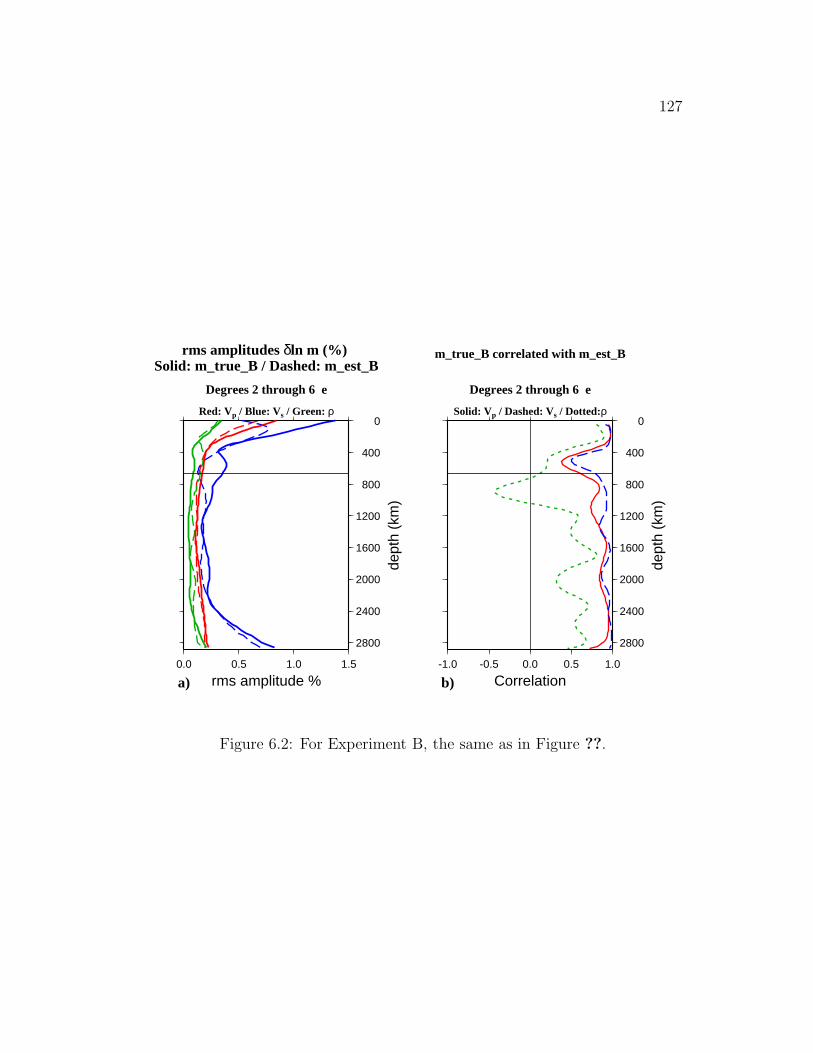
127

0

400

800

1200

1600

2000

2400

2800

dept

h (k

m)

0.0 0.5 1.0 1.5

rms amplitude %a)

rms amplitudes δln m (%) Solid: m_true_B / Dashed: m_est_B

Degrees 2 through 6 e

Red: Vp / Blue: Vs / Green: ρ0

400

800

1200

1600

2000

2400

2800de

pth

(km

)-1.0 -0.5 0.0 0.5 1.0

Correlationb)

m_true_B correlated with m_est_B

Degrees 2 through 6 e

Solid: Vp / Dashed: Vs / Dotted:ρ

Figure 6.2: For Experiment B, the same as in Figure ??.

128

former to the latter. In Figures ??b and ??b, the correlations between mtrue

and mest are plotted for spatial parameterizations smax = 6, pmax = 7, and

smax = 6, pmax = 10 respectively. We recover perturbations in VP and VS well

for the spatial parameterization smax = 6, pmax = 7, (correlation coefficients of

75%-99%), and perturbations in ρ are recovered with ∼60% correlation. For the

spatial parameterization smax = 6, pmax = 10, we can still recover perturbations

in VP and VS sufficiently, although in the depth range 400-670 km, the corre-

lation drops to ∼50%. Perturbations in ρ in the upper half of the mantle are

poorly recovered in this parameterization. Clearly, adding vertical smoothing is

necessary to compensate for overparameterization in the vertical direction.

If the perturbations in ρ in our input model mtrue, are scaled exactly to

those of our input δVS model, a resolution experiment on such an mtrue is

insufficient to assess the leakage of VS and VP structure into ρ. However, it gives

us an opportunity to examine the structure of the resolution matrix, which is

independent of the input model coefficients. The resolution matrix is presented

in Figure ??, which shows that the part of the matrix corresponding to VS and

VP has a structure close to that of an identity matrix, with strongest values

on the diagonal, and generally weak cross-terms ∅SP and ∅PS. On the other

hand, the density sub-matrix shows both much smaller values on the diagonal,

compared to VS and VP , and off-diagonal terms ∅RP , ∅RS ... which are small

but commensurate with the diagonal terms. The structure of the resolution

129

matrix indicates that density cannot be resolved as well as velocity structure.

Choosing the relative level of damping for velocities and density will therefore

have a strong effect on the level of contamination present in the retrieved density

structure.

Many authors perform checkerboard tests to assess the resolution of their

models. In this kind of test, the model vector mtrue is sparsely populated by

non zero coefficients pmts. For example, a checkerboard model of s = 4, t = 4,

and p = 7 will consist of non-zero values for pm44 and pm

−44 for 0 ≤ p ≤ 7. This

gives 16 non-zero elements in mtrue, of dimension M = 200 (M = (s+1)2(p+1)).

The remaining 184 elements of mtrue are zero. Then, many non-zero off-diagonal

elements in R can be neutralized by the product with zero elements in mtrue,

and the covariances in R may not be found by this type of test, even if it is

performed at several degrees s.

Also, one may introduce a checkerboard model for δVP only, where δVS = 0

and δρ = 0 in mtrue, to analyze the possible mapping of VP structure into VS

and ρ structure, or introduce a checkerboard pattern for δVS only to analyze the

possible mapping of VS structure into VP and ρ structure, and so on (Ishii and

Tromp, 1999). Then, for a checkerboard pattern s = 4, t = 4, and p = 7 in only

one physical parameter vector, there are 16 non-zero values populating mtrue of

dimension M = 600 (M = (s + 1)2(p + 1)× 3). Off-diagonal elements in R can

be missed, unless checkerboard tests are run for each model coefficient, which is

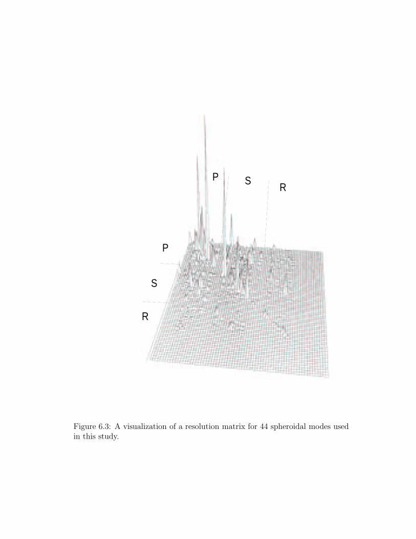
130

P SR

R

S

P

Figure 6.3: A visualization of a resolution matrix for 44 spheroidal modes usedin this study.

131

not generally done. In other words, the mapping between physical parameters

is not fully explored.

Instead of using a checkerboard model, in a first set of experiments, we choose

to fully populate δVP (respectively δVS and δρ) with coefficients of an aspherical

model, keeping the other parameters zero. We can thus test how well we can

resolve each parameter, independently of the others, and how much is mapped

into the others. Our input models are therefore, respectively mPtrue = [δVP , ∅, ∅]

mStrue = [∅, δVS, ∅] and mR

true = [∅, ∅, δρ]. The same model of heterogeneity is

used in all three cases, but the amplitudes are scaled according to VP =0.5 VS,

and ρ = 0.25 VS, to achieve realistic rms levels in the respective parameters being

tested. Resolution experiments with parameterizations A and B, as defined

above, are performed in each case.

In Figures ??– ??, we plot the results of the three resolution tests using

mPtrue, mS

true, and mRtrue respectively for smax = 6, pmax = 7. The legend scale

for heterogeneity for δ ln VP is ±1%, for δVS is ±1.5%, and for δρ is ±0.5%.

The color scale is chosen so as to correspond to expected amplitudes for each

physical parameter. Figure ?? shows that δVP is well recovered, but there is

some contamination into δVS est and δρest, as expected from the visualization of

R. The amplitude of contamination into δVS est is very small, and is well below

the level of signal obtained in real data inversions, so it should not be a problem.

The amplitude of contamination into δρest is also not very large, but patterns

132

200 km

mest=[δVp,δVs,δρ] mtrue=[δVp,0,0] smax=6, pmax=7 mtrue=[δVp,0,0] smax=6, pmax=7

650 km

1200 km

1800 km

2200 km

-1 0 1

δln Vp (%)

2800 km

200 km

650 km

1200 km

1800 km

2200 km

-1.5 1.5

δln Vs (%)

2800 km

200 km

650 km

1200 km

1800 km

2200 km

-0.5 0.0 0.5

δln ρ (%)

2800 km

Figure 6.4: The output model of perturbations in Vp, left column, Vs, middlecolumn, and ρ, right column, for an input model mtrue = [δVp, 0, 0], where δVp

is 0.5*SAW12D (Li and Romanowicz, 1996). The spatial parameterization forthe resolution matrix is smax = 6, pmax = 7.

133

200 km

mest=[δVp,δVs,δρ] mtrue=[0,δVs,0] smax=6, pmax=7 mtrue=[0,δVs,0] smax=6, pmax=7

650 km

1200 km

1800 km

2200 km

-1 0 1

δln Vp (%)

2800 km

200 km

650 km

1200 km

1800 km

2200 km

-1.5 1.5

δln Vs (%)

2800 km

200 km

650 km

1200 km

1800 km

2200 km

-0.5 0.0 0.5

δln ρ (%)

2800 km

Figure 6.5: The output model of perturbations in Vp, left column, Vs, middlecolumn, and ρ, right column, for an input model mtrue = [0, δVs, 0], where δVs

is SAW12D (Li and Romanowicz, 1996). The spatial parameterization for theresolution matrix is smax = 6, pmax = 7.

134

200 km

mest=[δVp,δVs,δρ] mtrue=[0,0,δρ] smax=6, pmax=7 mtrue=[0,0,δρ] smax=6, pmax=7

650 km

1200 km

1800 km

2200 km

-1 0 1

δln Vp (%)

2800 km

200 km

650 km

1200 km

1800 km

2200 km

-1.5 1.5

δln Vs (%)

2800 km

200 km

650 km

1200 km

1800 km

2200 km

-0.5 0.0 0.5

δln ρ (%)

2800 km

Figure 6.6: The output model of perturbations in Vp, left column, Vs, middlecolumn, and ρ, right column, for an input model mtrue = [0, 0, δρ], where δρis 0.25*SAW12D (Li and Romanowicz, 1996). The spatial parameterization forthe resolution matrix is smax = 6, and pmax = 7.

135

200 km

mtrue=[δVp,0,0] smax=6, pmax=10 mtrue=[δVp,0,0] smax=6, pmax=10

650 km

1200 km

1800 km

2200 km

-1 0 1

δln Vp (%)

2800 km

200 km

650 km

1200 km

1800 km

2200 km

-1.5 1.5

δln Vs (%)

2800 km

200 km

650 km

1200 km

1800 km

2200 km

-0.5 0.0 0.5

δln ρ (%)

2800 km

Figure 6.7: The output model of perturbations in Vp, left column, Vs, middlecolumn, and ρ, right column, for an input model mtrue = [δVp, 0, 0], where δVp

is 0.5*SAW12D (Li and Romanowicz, 1996). The spatial parameterization forthe resolution matrix is smax = 6, pmax = 10.

136

200 km

mtrue=[0,δVs,0] smax=6, pmax=10 mtrue=[0,δVs,0] smax=6, pmax=10

650 km

1200 km

1800 km

2200 km

-1 0 1

δln Vp (%)

2800 km

200 km

650 km

1200 km

1800 km

2200 km

-1.5 1.5

δln Vs (%)

2800 km

200 km

650 km

1200 km

1800 km

2200 km

-0.5 0.0 0.5

δln ρ (%)

2800 km

Figure 6.8: The output model of perturbations in Vp, left column, Vs, middlecolumn, and ρ, right column, for an input model mtrue = [0, δVs, 0], where δVs

is SAW12D (Li and Romanowicz, 1996). The spatial parameterization for theresolution matrix is smax = 6, pmax = 10.

137

200 km

mtrue=[0,0,δρ] smax=6, pmax=10 mtrue=[0,0,δρ] smax=6, pmax=10

650 km

1200 km

1800 km

2200 km

-1 0 1

δln Vp (%)

2800 km

200 km

650 km

1200 km

1800 km

2200 km

-1.5 1.5

δln Vs (%)

2800 km

200 km

650 km

1200 km

1800 km

2200 km

-0.5 0.0 0.5

δln ρ (%)

2800 km

Figure 6.9: The output model of perturbations in Vp, left column, Vs, middlecolumn, and ρ, right column, for an input model mtrue = [0, 0, δρ], where δρis 0.25*SAW12D (Li and Romanowicz, 1996). The spatial parameterization forthe resolution matrix is smax = 6, pmax = 10.

138

at certain depths, particularly at 2800 km, are reminiscent of patterns from

recent density models inverted from normal mode splitting coefficients (Ishii

and Tromp, 1999), where high density features are located over Africa, and the

Pacific basin region. In the upper mantle, there is significant contamination

of δVP patterns into δρ. In Figure ??, δVS is well resolved, with insignificant

contamination into δVP est. The contamination amplitude into δρest is somewhat

higher, and the patterns mapped into the density model appear as high densities

in areas of slab subduction in the circum-Pacific regions, especially at the bottom

of the mantle. In the upper mantle, the same patterns of contamination in δρ

from δVS appear as in Figure ??, but at somewhat stronger amplitudes. Finally,

in Figure ??, we see that δρ can be recovered in the absence of δVS and δVP

structure, and there is not significant contamination into δVP est and δVS est in

amplitude and pattern.

The results of an analogous experiment are shown in Figures ??-?? for spatial

parameterization smax = 6, pmax = 10, and the contamination effects are similar

to the effects for spatial parameterization smax = 6, pmax = 7.

6.2.2 Cumulative contamination

As seismic velocity structure in the Earth is well-documented (Su et al.,

1994; Li and Romanowicz, 1996; Masters et al, 1996; Dziewonski et al, 1997;

Vasco and Johnson, 1997;, van der Hilst et al., 1997 ), the study of cumulative

139

Experi- Spatial Para- δV truep δV true

s δρtrue

ment meterization model model models = 6 s = 6 P16B30 1 SAW12D 2 SH12- 0 R25 R50p = 7 p = 10 WM13 3

Resolution matrix tests

A ? ? ? ?B ? ? ? ?C ? ? ? ?D ? ? ? ?E ? ? ? ?F ? ? ? ?H ? ? ? ?I ? ? ? ?

Inversions w/ synthetic seismograms

J ? ? ? ?K ? ? ? ?

Table 6.1: Experiments of input mtrue = [δVp, δVs, δρ] are tabulated. For allexperiments, the same norm damping is used for δVp, δVs, δρ in the determinationof mest. The δVp and δVs models are from 1G. Masters and G. Laske, personalcommunication, 2Li and Romanowicz, 1996, 3Su and Dziewonski, 1994.

contamination of δVP and δVS into δρ can be particularly informative. To in-

vestigate the latter, we have performed a series of tests (labeled C-J), in which

we vary the depth parameterization (pmax = 7 versus pmax = 10), the input δVS

model, keeping the input model in ρ to be zero. Table ?? describes the details

of each experiment.

The comparison of the models obtained in experiments C,D (same initial

models, different depth parameterization) with those of experiments A and B

respectively, indicates that the velocity structures are well recovered, but a spu-

rious density structure is introduced in C,D. This density structure is well cor-

related with that obtained in A, B, where the starting model was a realistic

140

0

400

800

1200

1600

2000

2400

2800

dept

h (k

m)

0.0 0.5 1.0 1.5

rms amplitude %a)

rms amplitudes δln m (%) Solid: m_true_C / Dashed: m_est_C

Degrees 2 through 6 e

Red: Vp / Blue: Vs / Green: ρ0

400

800

1200

1600

2000

2400

2800

dept

h (k

m)

-1.0 -0.5 0.0 0.5 1.0

Correlationb)

m_est_C correlated with m_est_A

Degrees 2 through 6 e

Solid: Vp / Dashed: Vs / Dotted:ρ

Figure 6.10: a) For Experiment C, the root mean squared amplitudes of an inputmodel mtrue in solid lines, and output model mest from a resolution matrix test,in dashed lines. The blue lines are δVs, the red lines are δVp, and the green linesare δρ rms amplitudes. See Table ?? for description of input models. The inputδρtrue = 0 (solid green line). The retrieved δρest has rms amplitudes > 0. b)The retrieved model mC

est correlated with the retrieved model mAest. The blue

dashed line is the correlation of δVs between the two models, red solid line is forδVp, and the green dotted line is for δρ.

141

0

400

800

1200

1600

2000

2400

2800

dept

h (k

m)

0.0 0.5 1.0 1.5

rms amplitude %a)

rms amplitudes δln m (%) Solid: m_true_D / Dashed: m_est_D

Degrees 2 through 6 e

Red: Vp / Blue: Vs / Green: ρ0

400

800

1200

1600

2000

2400

2800

dept

h (k

m)

-1.0 -0.5 0.0 0.5 1.0

Correlationb)

m_est_D correlated with m_est_B

Degrees 2 through 6 e

Solid: Vp / Dashed: Vs / Dotted:ρ

Figure 6.11: For Experiment D, the root mean squared amplitudes of an inputmodel mtrue in solid lines, and output model mest from a resolution matrix test,in dashed lines. The blue lines are δVs, the red lines are δVp, and the green linesare δρ rms amplitudes. See Table ?? for description of input models. The inputδρtrue = 0 (solid green line). The retrieved δρest has rms amplitudes > 0. b)The retrieved model mD

est correlated with the retrieved model mBest. The blue

dashed line is the correlation of δVs between the two models, red solid line is forδVp, and the green dotted line is for δρ.

142

-0.30-0.24-0.18-0.12-0.060.000.060.120.180.240.30

δln ρ (%)200 km

m_est_C δln ρghost m_est_C δln ρghost

-0.30-0.24-0.18-0.12-0.060.000.060.120.180.240.30

δln ρ (%)600 km

-0.20-0.16-0.12-0.08-0.040.000.040.080.120.160.20

δln ρ (%)1300 km

-0.20-0.16-0.12-0.08-0.040.000.040.080.120.160.20

δln ρ (%)1800 km

-0.20-0.16-0.12-0.08-0.040.000.040.080.120.160.20

δln ρ (%)2300 km

-0.30-0.24-0.18-0.12-0.060.000.060.120.180.240.30

δln ρ (%)2850 km

Figure 6.12: Even degrees 2, 4, and 6 of retrieved model δρCest are shown for six

depths in the mantle. We name δρCest a ’ghost’ density model because the input

model is mtrue = [P16B30, SAW12D, 0] for smax = 6, pmax = 7.

143

-0.30-0.24-0.18-0.12-0.060.000.060.120.180.240.30

δln ρ (%)200 km

m_est_D δln ρghost m_est_D δln ρghost

-0.5-0.4-0.3-0.2-0.10.00.10.20.30.40.5

δln ρ (%)600 km

-0.20-0.16-0.12-0.08-0.040.000.040.080.120.160.20

δln ρ (%)1300 km

-0.20-0.16-0.12-0.08-0.040.000.040.080.120.160.20

δln ρ (%)1800 km

-0.20-0.16-0.12-0.08-0.040.000.040.080.120.160.20

δln ρ (%)2300 km

-0.30-0.24-0.18-0.12-0.060.000.060.120.180.240.30

δln ρ (%)2850 km

Figure 6.13: Even degrees 2, 4, and 6 of retrieved model δρDest are shown for six

depths in the mantle. We name δρDest a ’ghost’ density model because the input

model is mtrue = [P16B30, SAW12D, 0] for smax = 6, pmax = 10.

144

density model (Figures ?? and ??). The maps of ’ghost’ density patterns for

degrees 2, 4, and 6 are shown in Figures ?? and ?? for Experiments C and D.

Only the even degrees are displayed to compare directly with published density

models, even though the odd degree model parameters are not very large and

do not have much of an impact on the displayed images. High density regions

corresponding to regions of slab subduction exist at many depths. In fact, the

patterns of δρCest and δρC

est are similar to density models obtained from inversions

of spectral data, which we call R NMSPEC (Figure ??)(Kuo et al., 1998; Kuo

and Romanowicz, 1999a,1999b). The model R NMSPEC is spatially parameter-

ized to smax = 6 and pmax = 7, and no a priori assumptions are imposed for the

inversion of observed spectral data. The correspondence between Figures ?? and

?? shows that if P16B30 and SAW12D are representative of the seismic velocity

perturbations in the real Earth, the artifact density models puts into question

the confidence we have in the density models obtained from the inversions of

the normal mode spectra.

If we use SH12WM13 (Su and Dziewonski, 1994), as a starting model for δVS,

(experiments E-F), the ghost density model retrieved is somewhat different. In

Experiment F, the resulting ghost density model for a smax = 6, pmax = 10

parameterization yields patterns (Figure ??) which are strongly reminiscent of

the published density model SPRD6 of Ishii and Tromp, 1999 , particularly the

high density feature in the Pacific basin and over Africa at 2800 km. There

145

-1.0-0.8-0.6-0.4-0.20.00.20.40.60.81.0

δln ρ (%)200 km

R_NMSPEC δln ρR_NMSPEC δln ρ

-1.0-0.8-0.6-0.4-0.20.00.20.40.60.81.0

δln ρ (%)600 km

-1.0-0.8-0.6-0.4-0.20.00.20.40.60.81.0

δln ρ (%)1300 km

-1.0-0.8-0.6-0.4-0.20.00.20.40.60.81.0

δln ρ (%)1800 km

-1.0-0.8-0.6-0.4-0.20.00.20.40.60.81.0

δln ρ (%)2300 km

-1.0-0.8-0.6-0.4-0.20.00.20.40.60.81.0

δln ρ (%)2850 km

Figure 6.14: The even degrees 2, 4, and 6 of a density model (Kuo and Ro-manowicz, 1998, 1999) retrieved from normal mode spectra is shown here forsix mantle depths, for comparison with Figures ?? and ??.

146

are, however, lateral shifts in the distribution of the patterns between Figure ??

and Figure 3 in Ishii and Tromp, 1999. In Figure ??, the density patterns from

SPRD6 Ishii and Tromp, 1999 and δρFest are directly compared for six depths in

the mantle. The resemblance is striking, although the amplitudes of δρFest are

much smaller in the lower mantle. However, amplitudes retrieved from inversions

are dependent on the choice of damping parameter values. There is not so much

resemblance to the SPRD6 density model for the pmax = 7 parameterization in

Experiment E (Figure ??), but high density ghost features also appear in the

Pacific Basin at 2800 km. The source of this contamination could be attributed

to δVP (Figures ?? and ??, if one assumes that Vp is highly correlated with Vs).

While regularization schemes used in resolution tests are not directly appli-

cable to the inversion of observed data (Resovsky and Ritzwoller, 1999) due to

the effects of noise, the damping scheme which we use is quite simplistic in C−1m

and is imposed in the absence of noise. Despite this simplistic damping scheme,

we can retrieve ghost density models which mimic density models inverted from

data. Tests of model robustness by considering random noise in the data (Ishii

and Tromp, 1999) can still stably produce density models given by Figure ??

since the contamination in the density model parameter space is due to coherent

rather than random noise.

Of course, the contamination effect is more important for a low level of signal

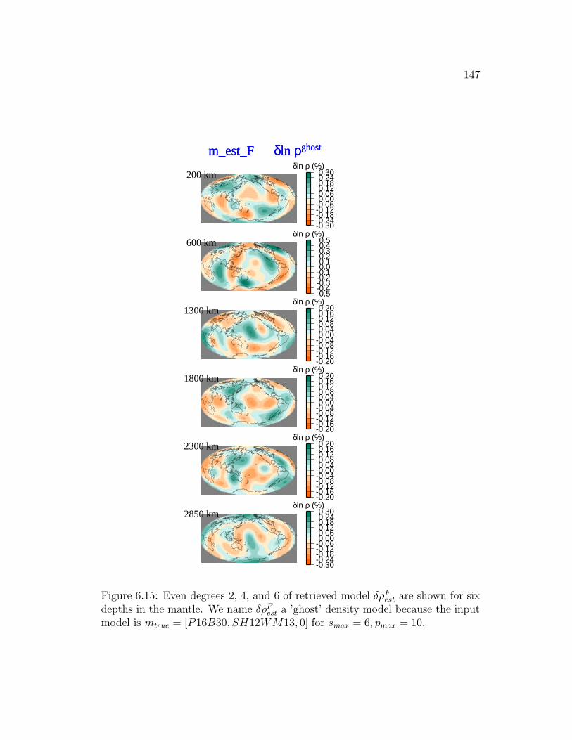
147

-0.30-0.24-0.18-0.12-0.060.000.060.120.180.240.30

δln ρ (%)200 km

m_est_F δln ρghost m_est_F δln ρghost

-0.5-0.4-0.3-0.2-0.10.00.10.20.30.40.5

δln ρ (%)600 km

-0.20-0.16-0.12-0.08-0.040.000.040.080.120.160.20

δln ρ (%)1300 km

-0.20-0.16-0.12-0.08-0.040.000.040.080.120.160.20

δln ρ (%)1800 km

-0.20-0.16-0.12-0.08-0.040.000.040.080.120.160.20

δln ρ (%)2300 km

-0.30-0.24-0.18-0.12-0.060.000.060.120.180.240.30

δln ρ (%)2850 km

Figure 6.15: Even degrees 2, 4, and 6 of retrieved model δρFest are shown for six

depths in the mantle. We name δρFest a ’ghost’ density model because the input

model is mtrue = [P16B30, SH12WM13, 0] for smax = 6, pmax = 10.

148

-0.60-0.48-0.36-0.24-0.120.000.120.240.360.480.60

δln ρ (%)50 km

SPRD6 δln ρ SPRD6 δln ρ

-0.60-0.48-0.36-0.24-0.120.000.120.240.360.480.60

δln ρ (%)200 km

-0.5-0.4-0.3-0.2-0.10.00.10.20.30.40.5

δln ρ (%)600 km

-0.5-0.4-0.3-0.2-0.10.00.10.20.30.40.5

δln ρ (%)1300 km

-0.80-0.64-0.48-0.32-0.160.000.160.320.480.640.80

δln ρ (%)2200 km

-1.0-0.8-0.6-0.4-0.20.00.20.40.60.81.0

δln ρ (%)2800 km

-0.60-0.48-0.36-0.24-0.120.000.120.240.360.480.60

δln ρ (%)50 km

m_est_F δln ρghost m_est_F δln ρghost

-0.20-0.16-0.12-0.08-0.040.000.040.080.120.160.20

δln ρ (%)200 km

-0.5-0.4-0.3-0.2-0.10.00.10.20.30.40.5

δln ρ (%)600 km

-0.20-0.16-0.12-0.08-0.040.000.040.080.120.160.20

δln ρ (%)1100 km

-0.20-0.16-0.12-0.08-0.040.000.040.080.120.160.20

δln ρ (%)2200 km

-0.20-0.16-0.12-0.08-0.040.000.040.080.120.160.20

δln ρ (%)2800 km

Figure 6.16: Comparison of the density model of SPRD6 (Ishii and Tromp,1999), left column, and ghost density model δρF

est, right column, at six mantledepths, for even degrees 2, 4, and 6. SPRD6 is inverted from normal modesplitting coefficients.

149

-0.30-0.24-0.18-0.12-0.060.000.060.120.180.240.30

δln ρ (%)200 km

m_est_E δln ρghost m_est_E δln ρghost

-0.30-0.24-0.18-0.12-0.060.000.060.120.180.240.30

δln ρ (%)600 km

-0.20-0.16-0.12-0.08-0.040.000.040.080.120.160.20

δln ρ (%)1300 km

-0.20-0.16-0.12-0.08-0.040.000.040.080.120.160.20

δln ρ (%)1800 km

-0.20-0.16-0.12-0.08-0.040.000.040.080.120.160.20

δln ρ (%)2300 km

-0.30-0.24-0.18-0.12-0.060.000.060.120.180.240.30

δln ρ (%)2850 km

Figure 6.17: Even degrees 2, 4, and 6 of retrieved model δρEest are shown for six

depths in the mantle. We name δρEest a ’ghost’ density model because the input

model is mtrue = [P16B30, SH12WM13, 0] for smax = 6, pmax = 7.

150

in δρtrue, and for larger levels of signal in ρ, it may still be possible to retrieve

some information, especially by applying an appropriate damping scheme. How-

ever, the confidence in the resulting model will always be marginal, and will have

to be supplemented by independent information, such as constraints provided

by fits to the observed geoid.

6.2.3 Tests with ρ input models of different amplitudes

Experiments A-F have demonstrated that density perturbation amplitudes

which are about 25% of δVs cannot be retrieved with confidence. The estimated

models of density in Experiments A and B, in which a mock input density model

is used, are highly correlated with the estimated densities of Experiments C and

D, for which no input density was used. The high correlation demonstrates

that contamination from seismic velocity signal swamps out the density signal

in Experiments A and B. The level of density perturbation signal in the Earth

which can be detected needs to be investigated. To do so we refer to experiments

A,B and H,I (Table ??) in which we respectively consider two input density

models which differ only by an amplitude scaling factor. The mock density

perturbations in model R50 have twice the amplitudes as in model R25.

At the level of density signal in R50, Figure ?? shows that δρHtrue is correlated

with δρHest much better than when the density signal is that of R25 (Figure ??).

Overall, this is true for the correlation of δρItrue and δρI

est in comparison with the

151

0

400

800

1200

1600

2000

2400

2800

dept

h (k

m)

0.0 0.5 1.0 1.5

rms amplitude %a)

rms amplitudes δln m (%) Solid: m_true_H / Dashed: m_est_H

Degrees 2 through 6 e

Red: Vp / Blue: Vs / Green: ρ0

400

800

1200

1600

2000

2400

2800

dept

h (k

m)

-1.0 -0.5 0.0 0.5 1.0

Correlationb)

m_true_H correlated with m_est_H

Degrees 2 through 6 e

Solid: Vp / Dashed: Vs / Dotted:ρ

Figure 6.18: For Experiment H, the same as in Figure ??

correlation of δρBtrue and δρB

est (Figures ?? and ??), but for this radial parame-

terization, pmax = 10, the density correlation in Experiment I is poor below the

transition zones down to 1200 km depth. This indicates that Experiment I is

overparameterized, leading to deficiencies in resolution.

Next, we correlate the δρest’s in Experiments H and I with ghost density

estimates from Experiments C and D. Correlation of δρHest with the ghost density

model δρCest is decreased in comparison with Figure ??, demonstrated by the left

plot in Figure ??. However, δρIest correlates above 50% with the ghost density

model δρDest in over three-fourths of the mantle, shown in right plot of Figure

152

0

400

800

1200

1600

2000

2400

2800

dept

h (k

m)

0.0 0.5 1.0 1.5

rms amplitude %a)

rms amplitudes δln m (%) Solid: m_true_I / Dashed: m_est_I

Degrees 2 through 6 e

Red: Vp / Blue: Vs / Green: ρ0

400

800

1200

1600

2000

2400

2800de

pth

(km

)-1.0 -0.5 0.0 0.5 1.0

Correlationb)

m_true_I correlated with m_est_I

Degrees 2 through 6 e

Solid: Vp / Dashed: Vs / Dotted:ρ

Figure 6.19: For Experiment I, the same as in Figure ??

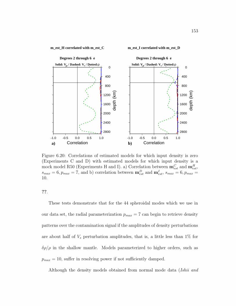
153

0

400

800

1200

1600

2000

2400

2800

dept

h (k

m)

-1.0 -0.5 0.0 0.5 1.0

Correlationa)

m_est_H correlated with m_est_C

Degrees 2 through 6 e

Solid: Vp / Dashed: Vs / Dotted:ρ0

400

800

1200

1600

2000

2400

2800

dept

h (k

m)

-1.0 -0.5 0.0 0.5 1.0

Correlationb)

m_est_I correlated with m_est_D

Degrees 2 through 6 e

Solid: Vp / Dashed: Vs / Dotted:ρ

Figure 6.20: Correlations of estimated models for which input density is zero(Experiments C and D) with estimated models for which input density is amock model R50 (Experiments H and I). a) Correlation between mC

est and mHest,

smax = 6, pmax = 7, and b) correlation between mDest and mI

est, smax = 6, pmax =10.

??.

These tests demonstrate that for the 44 spheroidal modes which we use in

our data set, the radial parameterization pmax = 7 can begin to retrieve density

patterns over the contamination signal if the amplitudes of density perturbations

are about half of Vs perturbation amplitudes, that is, a little less than 1% for

δρ/ρ in the shallow mantle. Models parameterized to higher orders, such as

pmax = 10, suffer in resolving power if not sufficiently damped.

Although the density models obtained from normal mode data (Ishii and

154

Tromp, 1999; Kuo and Romanowicz, 1999) currently resemble the ghost den-

sity patterns from Experiments C-F, we do not suggest that the Earth’s density

perturbations are not resolvable. The expected amplitudes of density perturba-

tions due to slabs at high pressures and temperatures (Panero and Jeanloz, in

preparation) is 1-2%. Therefore, the density signal may be at the limit of being

resolvable. If there is real signal in the density models derived from data, it may

very likely be overwhelmed by contamination. The plots on the left in Figures

?? and ?? show that the contaminant density amplitudes can be commensurate

with the amplitudes in R50 (left plot in Figure ??). Inversions with real data

can yield density amplitudes greater than those in R50, but before assuming

that the amplitudes are an indication of large signal, one must ensure that the

amplitudes are not due to coherent errors from contamination producing such an

amplified signal. It will be necessary to find appropriate damping parameters to

reduce the effect of the covariant elements between physical model parameters

in the resolution matrix.

6.3 Tests with synthetic seismograms

So far, we have only considered simple tests, to illustrate the sensitivity of

the retrieved density models to assumptions on damping, resulting from the

structure of the resolution matrix. However, our particular inversion scheme

is non-linear, and therefore involves several iterations, whose results may not

155

be completely represented by the resolution matrix corresponding to the first

iteration only. In what follows, we present more complete tests involving the

computation of synthetic seismograms and their iterative inversion, more accu-

rately simulating the inversion process corresponding to real spectral data.

Specifically, we are interested in the contaminant signal in density resulting

from our iterative inversion scheme. The spatial parameterization and input

models of Experiments E and F are revisited in Experiments J and K (Table ??)

whereby the estimated models mJest and mK

est are now obtained from inversions

of synthetic seismograms computed from input models mJtrue=mK

true. mJtrue and

mKtrue are composed of models P16B30 for δVp and SH12WM13 for δVs, and there

are no density perturbations. Aspherical structure up to harmonic degree 12 and

radial order 13 are included in the computation of synthetic seismograms. We

start the inversions from PREM (Anderson and Dziewonski, 1981), and damp

the second radial derivative (η3 in equation(4.8)) to ensure radial smoothness.

η3 for Vp was required to be twice as strong as for either Vs or ρ to produce a

radially smooth model. After 4 iterations, the models mJest and mK

est converge

to give 99.6% and 99.5% fits to the synthetic data respectively.

The two models mJest and mK

est are extremely similar and we believe that

this is due to the choice of damping to smooth the radial models. At present,

the radial damping η3 applied for Vp is insufficient and stronger damping should

be applied. The root-mean-squared profile for δVp est shows a large augmented

156

0

400

800

1200

1600

2000

2400

2800

dept

h (k

m)

0.0 0.5 1.0 1.5

rms amplitude %a)

rms amplitudes δln m (%) Solid: m_true_J / Dashed: m_est_J

Degrees 2 through 6 e

Red: Vp / Blue: Vs / Green: ρ0

400

800

1200

1600

2000

2400

2800de

pth

(km

)-1.0 -0.5 0.0 0.5 1.0

Correlationb)

m_true_J correlated with m_est_J

Degrees 2 through 6 e

Solid: Vp / Dashed: Vs / Dotted:ρ

Figure 6.21: For Experiment J, the same as in Figure ??

157

0

400

800

1200

1600

2000

2400

2800

dept

h (k

m)

0.0 0.5 1.0 1.5

rms amplitude %a)

rms amplitudes δln m (%) Solid: m_true_K / Dashed: m_est_K

Degrees 2 through 6 e

Red: Vp / Blue: Vs / Green: ρ0

400

800

1200

1600

2000

2400

2800de

pth

(km

)-1.0 -0.5 0.0 0.5 1.0

Correlationb)

m_true_K correlated with m_est_K

Degrees 2 through 6 e

Solid: Vp / Dashed: Vs / Dotted:ρ

Figure 6.22: For Experiment K, the same as in Figure ??

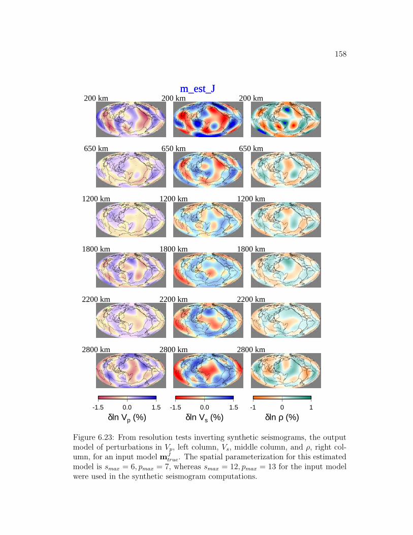
158

200 kmm_est_J m_est_J

650 km

1200 km

1800 km

2200 km

-1.5 0.0 1.5

δln Vp (%)

2800 km

200 km

650 km

1200 km

1800 km

2200 km

-1.5 0.0 1.5

δln Vs (%)

2800 km

200 km

650 km

1200 km

1800 km

2200 km

-1 0 1

δln ρ (%)

2800 km

Figure 6.23: From resolution tests inverting synthetic seismograms, the outputmodel of perturbations in Vp, left column, Vs, middle column, and ρ, right col-umn, for an input model mJ

true. The spatial parameterization for this estimatedmodel is smax = 6, pmax = 7, whereas smax = 12, pmax = 13 for the input modelwere used in the synthetic seismogram computations.

159

200 kmm_est_K m_est_K

650 km

1200 km

1800 km

2200 km

-1.5 0.0 1.5

δln Vp (%)

2800 km

200 km

650 km

1200 km

1800 km

2200 km

-1.5 0.0 1.5

δln Vs (%)

2800 km

200 km

650 km

1200 km

1800 km

2200 km

-1 0 1

δln ρ (%)

2800 km

Figure 6.24: The same as in Figure ??, for an input model mKtrue(=mJ

true).The spatial parameterization for this estimated model is smax = 6, pmax = 10,whereas smax = 12, pmax = 13 for the input model were used in the syntheticseismogram computations.

160

200 kmm_true_J m_true_J

650 km

1200 km

1800 km

2200 km

-1.5 0.0 1.5

δln Vp (%)

2800 km

200 km

650 km

1200 km

1800 km

2200 km

-1.5 0.0 1.5

δln Vs (%)

2800 km

200 km

650 km

1200 km

1800 km

2200 km

-1 0 1

δln ρ (%)

2800 km

Figure 6.25: For Experiments J and K (also E and F), the input modelmtrue = [δVp, δVs, 0] where δVp=P16B30 (Masters and Laske, personal com-munication), and δVs=SH12WM13 (Su and Dziewonski, 1994). There are nodensity perturbations in mtrue.

161

bump in the lower mantle which corresponds to a decreased correlation between

the input and output Vp models at the same depths (Figures ?? and ??).

The patterns of mJest and mK

est are shown in Figures ?? and ?? for degrees 1

through 6. The input model for mJtrue=mK

true is shown in Figure ?? for compar-

ison. Assessment of our inversions with real data, (Figure 5.12) can be made by

comparing mJest with mJ

true. In particular, we can compare the density model

obtained from normal mode spectral data (third column in Figure 5.12), with

the ghost density patterns in the third columns in Figures ?? and ?? and find

that most of the high density features from our density models can be explained

by features in the ghost density model.

6.4 Discussion and Conclusions

Current methods of retrieving three-dimensional mantle density structure

from normal mode spectra (Kuo and Romanowicz, 1999b) and normal mode

splitting coefficients (Ishii and Tromp, 1999) do not appear to yield reliable

density models. The mantle density models are affected by the contamination

of VP and VS structure into the density model space.

Resovsky and Ritzwoller, 1999 have documented the instability of ρ models

derived from normal mode splitting coefficients when using a sweep of a priori

constraints. They have shown that it is not possible to determine correlation

and/or decorrelation of δρ with seismic velocity as a function of depth. Our work

162

supports their conclusions that current methods and data sets are not sufficient

to uniquely determine the density structure of the Earth. We have shown that

it is possible to retrieve models of ρ perturbations purely due to contamination

from VS and VP structure, and that these ghost ρ models are consistent in pattern

and amplitude with published ρ models inverted from splitting coefficients (Ishii

and Tromp, 1999) , and with ρ models which we determine from normal model

spectral data. When using a spatial parameterization of s=6, w=7 for Earth

structure, the ghost density model exhibits high density features surrounding the

Pacific, much like the features which we have found in our ρ models inverted from

data. The density model SPRD6 of Ishii and Tromp, 1999, retrieved from linear

inversions of normal mode splitting coefficients, is different from density models

from our non-linear inversions of normal mode spectral data. We have found that

resolution tests involving linear products of resolution matrices with input Earth

models devoid of a density perturbations (mtrue = [Vp, Vs, 0]) produce ghost

density models which closely resemble the density structure of SPRD6. From

our performance of non-linear inversions of synthetic spectra computed from the

same input model mtrue = [Vp, Vs, 0], a ghost density pattern is produced which

resembles density models estimated from normal mode spectral data (Kuo and

Romanowicz, 1999).

Since δρ might be correlated with δVS throughout parts of the mantle, this

signal may be buried in the noise. Based on our tests of contamination, how-

163

ever, no conclusions may be drawn on the correlation of δρ with δVS. Damping

the covariant elements between physical model parameters may aid in reducing

contamination in δρ from the seismic velocities. Perhaps resolution of density

feature size should be addressed. If normal modes have little sensitivity to den-

sity perturbations to harmonic degree 6, then we propose to invert for VP , VS,

and ρ perturbations in a spatial parameterization scheme for which we may

solve for ρ parameterized to smaller degrees s than for VP and VS. The cumu-

lative contamination of covariant elements in the resolution matrix for spatial

parameterizations must be addressed.

164

Chapter 7

Outlook

Based on the astrophysical and seismological methods analysed in this disser-

tation research, we have found that reliable measurements of the Earth’s deep

interior three-dimensional density structure continue to elude the geophysics

community. Most recent theoretical calculations of very high energy neutrino

data count rates which would be measured at current detectors are prohibitively

low (Douglas Lowder, personal communication), and would require a couple of

decades’ worth of data to distinguish features such as the core from the man-

tle. We have shown that the current methods used in normal mode seismology,

which takes advantage of split spectra, do not produce credible density mod-

els. A combination of modes to include in the data set which could amplify

the density kernel sensitivity may be a useful strategy in the future, although it

may be impossible to decrease the seismic velocity kernel sensitivities. It would

be imperative to inspect resolution matrices with diagonal elements normalized

by covariant elements to understand thoroughly the tradeoffs between model

165

parameters. Perhaps with future instrumentation in which the noise floor due

to barometric pressure is reduced, even cleaner signals may allow us to extract

perturbations in density from normal model spectral splitting.

The common assumption that density perturbations scale with velocity per-

turbations is reasonable at least down to the mid-lower mantle. This assumption

can be used as an additional constraint to solve, for a scaling relationship as a

function of depth, between density and shear velocity. It is conceivable that

this approach could offer some information on the three-dimensional density

structure of the Earth’s interior.

166

References

Askar’yan,G. A., Investigation of the Earth by means of neutrinos, Neutrino

geology,Sov. Phys. Usp. , 27, 896-900, 1984.

Barwick, S. et al., AMANDA South Pole neutrino detector, in: 26th Interna-

tional Conference on High Energy Physics , American Institute of Physics

Conf. Proc. No. 272, pp. 1250-1253, 1992.

Bassani, L. and A.J. Dean, Absorption of γ-rays in active galaxies as a test for

the jet hypothesis, Nature, 294, 332-333, 1981.

Becker-Szendy, R.A., Study of Upward-going muons with the IMB detector,

University of Hawaii at Manoa High Energy Physics Report UH-511-729-

91, Honolulu, Hawaii, 1991 (Ph.D. Thesis).

Belolaptikov, I.A. et al., The lake Baikal underwater telescope NT-36: first

months of operation, in: Third Int’l Workshop on Theoretical and Phe-

nomenological Aspects of Underground Physics, Nucl. Phys. B Proc.

Suppl. , 35, pp. 290-293, 1994.

167

Berezinski’i, V.S., A.Z. Gazizov, G.T. Zatsepin, and I.L. Rozental, The passage

of high energy neutrinos through the Earth and the possibility of detect-

ing them by means of extensive air showers, Sov. J. Nucl. Phys. , 43,

406-413, 1986.

Berezinsky, V.S. and J.G. Learned, Upper bounds on Diffuse High Energy Neu-

trino Fluxes, in: High Energy Neutrino Astrophysics, V.J. Stenger, J.G.

Learned, S. Pakvasa and X. Tata, eds., pp. 43-57, World Scientific, Sin-

gapore, 1992.

Bohn, T., Time-Lapse Analysis of Core-Sensitive Free Oscillations, Master’s

thesis, University of California, Berkeley, 1994.

Bolt, B.A. and R. Uhrhammer, Resolution techniques for density and hetero-

geneity in the Earth, Geophys. J. R. Astr. Soc., 42, 419-35, 1975.

Borisov, A. B., B.A. Dolgoshein, and A.N. Kalinovski’i, direct method of deter-

mining the differential distribution of the density of the Earth by means

of high-energy neutrino scattering, Sov. J. Nucl. Phys. , 44, 442-447,

1986.

Clevede, E. and P. Lognonne, Frechet derivatives of coupled seismograms with

respect to an anelastic rotating Earth. Geophys. J. Int., 124, 456-82,

1996.

Cronin, J.W., High Energy Astrophysics, in: 1989 Int’l Symposium on Lepton

and Photon Interactions at High Energies, M. Riordan, ed., pp. 403-419,

168

World Scientific, Singapore, 1990.

Dahlen, F.A., The effect of data windows on the estimation of free oscillation

parameters, Geophys. J. R. Astr. Soc., 69, 537-49, 1982.

Dahlen, F.A., Reply, J. Geophys. Res., 81, 491, 1976.

Dahlen, F.A., The normal modes of a rotating, elliptical earth. II. near-resonance

multiplet coupling, Geophys. J. R. Astr. Soc., 18, 397-436, 1969.

Dahlen, F.A., The normal modes of a rotating, elliptical earth, Geophys. J. R.

Astr. Soc., 16, 329-367, 1968.

De Rujula, A., S. L. Glashow, R. R. Wilson and G. Charpak, Neutrino Explo-

ration of the Earth, Phys. Rep. , 99, 341-396, 1983.

Durek, J. and B. Romanowicz, Inner core anisotropy inferred by direct inversion

of normal mode spectra, In press, Geophys. J. Int., 1999.

Dziewonski, A.M., X.-F. Liu, and W.-J. Su, in Earth’s Deep Interior: the Doorn-

bos memorial volume, D. J. Crossley, ed., pp. 11-50, Gordon and Breach

Science, Newark, N.J., 1997.

Dziewonski, A.M., G. Ekstrom, and M.P. Salganik, Centroid-moment tensor so-

lutions for April-June 1994. Physics of the Earth and Planetary Interiors,

88, 69-78, 1995.

Dziewonski, A.M. and D.L Anderson, Preliminary reference Earth model, Phys.

Earth Planet. Inter., 25, 297-356, 1981.

Dziewonski, A.M. and F. Gilbert, Solidity of the inner core of the Earth inferred

169

from normal mode observations, Nature, 234, 465-6, 1971.

Edmonds, A.R., Angular Momentum in Quantum Mechanics, Princeton Univer-

sity Press, Princeton, N.J., 1960.

Fichtel, C.E. et al., The first Energetic Gamma-Ray Experiment Telescope

(EGRET) Source Catalog, Astrophys. J. Suppl. Ser. , 94, 551-581,

1994.

Flatte, S.M., R.J. Decoster, M.L. Stevenson, W.T. Toner and T.F. Zipf, Zenith-

angle Distribution of Atmospheric Muons above 1 TeV, Phys. Lett. ,

35B, 345-350, 1971.

Frichter, G.M., D.W. McKay and J.P Ralston, Small-X Quarks from HERA Pre-

dict the Ultra-High Energy Neutrino-Nucleon Scattering Cross Section,

Phys. Rev. Lett., 74, 1508-1511, 1995.

Giardini, D., X.-D. Li and J.H. Woodhouse, Splitting functions of long-period

normal modes of the Earth, J. Geophys. Res., 93, 13716-42, 1988.

Giardini, D., X.-D. Li, and J.H. Woodhouse, Three-dimensional structure of

the Earth from splitting in free-oscillation spectra, Nature, 325, 405-11,

1987.

Gilbert, F., A. Dziewonski and J. Brune, An Informative Solution to a Seis-

mological Inverse Problem,Proc. Nat. Acad. Sci. USA, 70, 1410-1413,

1973.

Gubbins, D., T.G. Masters and J.A. Jacobs, Thermal evolution of the Earth’s

170

core, Geophys. J. R. Astr. Soc., 59, 57-99, 1979.

He, X. and J. Tromp, Normal-mode constraints on the structure of the Earth,

J. Geophys. Res., 101, 20053-82, 1996.

Ishii, M. and J. Tromp, Normal-Mode and Free-Air Gravity Constraints on

Lateral Variations in Velocity and Density of Earth’s Mantle Science,

285, 1231-6, 1999.

Ishii, M. and J. Tromp, Three-dimensional modeling of mantle heterogeneity

and their implications for petrology, Eos Trans. AGU, 79, F656, 1998.

Ishii, M. and J. Tromp, Three-dimensional modeling of mantle heterogeneity

using normal-mode splitting function coefficients, Eos Trans. AGU, 78,

F460, 1997.

Jelley, J.V., Absorption of High-energy Gamma-rays within Quasars and Other

Radio Sources, Nature, 221, 472-475, 1966.

Karato, S., Importance of anelasticity in the interpretation of seismic tomogra-

phy, Geophys. Research Letters, 20, 1623-6, 1993.

Kennett, B.L.N., On the density distribution within the Earth. Geophys. J.

Int., 132, 374-82, 1998.

Kuo,C and B. Romanowicz, Three-dimensional Density Structure Obtained by

Normal Mode Spectral Measurements, Proceedings, IUGG XXII General

Assembly, A62, 1999a.

Kuo, C. and B. Romanowicz, Density and Seismic Velocity Variations Deter-

171

mined from Normal Mode Spectra, Eos Trans., AGU,80, S14, 1999b.

Kuo, C., J. Durek and B. Romanowicz, Mantle heterogeneity inferred from

normal mode spectra, Eos, Trans. AGU, 79, F627, 1998.

Kuo, C., J. Durek and B. Romanowicz, Direct inversion of normal mode spectra

for mantle heterogeneity, Eos, Trans. AGU, 78, F460, 1997.

Li, X.-D. and B. Romanowicz, Global mantle shear velocity model developed

using nonlinear asymptotic coupling theory. J. Geophys. Res., 101,

22245-72, 1996.

Li, X.-D., D. Giardini, and J.H. Woodhouse, Large-scale three-dimensional even-

degree structure of the Earth from splitting of long-period normal modes,

J. Geophys. Res., 96, 551-77, 1991a.

Li, X.-D., D. Giardini, and J.H. Woodhouse, The relative amplitudes of mantle

heterogeneity in P velocity, S velocity and density from free-oscillation

data, Geophys. J. Int., 105, 649-57, 1991b.

Lithgow-Bertelloni, C. and M.A. Richards, The dynamics of Cenozoic and Meso-

zoic plate motions. Rev. Geophys., 36, 27-78, 1998.

Lognonne, P. and B. Romanowicz, Modelling of coupled normal modes of the

Earth: the spectral method. Geophysical Journal International, 102,

365-95, 1990.

Luh, P.C., Free oscillations of the laterally inhomogeneous Earth: Quasi - de-

generate multiplet coupling, Geophys. J. R. Astr. Soc., 32, 187-202,

172

1973.

Masters, G., S. Johnson, G. Laske, and H. Bolton, A shear-velocity model of

the mantle. Philos. Trans. R. Soc. London A, 354, 1385-411, 1996.

Megnin, C. and B. Romanowicz, A 3d model of shear velocity in the mantle from

the inversion of body, surface and higher mode waveforms, submitted to

Geophys. J. Int., 1999.

Megnin, C. and B. Romanowicz, Estimation of inner core mode splitting func-

tions combining a genetic algorithm with a direct iterative inversion

scheme, Eos, Trans. AGU, 76, F355, 1995.

Menke, W., Geophysical Data Analysis: Discrete Inverse Theory, Academic

Press, Inc, San Diego, CA, 1989.

Morelli, A., A.M. Dziewonski, Topography of the core-mantle boundary and

lateral homogeneity of the liquid core, Nature, 325, 678-83, 1987.

Nicolaidis, A., M. Jannane and A. Tarantola, Neutrino Tomography of the

Earth,J. Geophys. Res. , 96, 21811-21817, 1991.

Obayashi, M. and Y. Fukao, P and PcP travel time tomography for the core-

mantle boundary, J. Geophys. Res., 102, 17825-41, 1997.

Panero W. and R. Jeanloz, Mineral phases and density of oceanic crust sub-

ducted into the Earth’s lower mantle, in preparation, 1999.

Phinney, R.A. and R. Burridge, Representation of the elastic-gravitational ex-

citation of a spherical earth model by generalized spherical harmonics,

173

Geophys. J. R. Astr. Soc., 34, 451-87, 1973.

Quigg, C., M.H. Reno and T.P. Walker, Interactions of Ultrahigh-Energy Neu-

trinos,Phys. Rev. Lett. , 57, 774-777, 1986.

Resovsky, J.S. and M.H. Ritzwoller, Regularization uncertainty in density mod-

els estimated from normal mode data, Geophys. Res. Lett., 26, 2319-22,

1999a.

Resovsky, J.S. and M.H. Ritzwoller, A degree 8 mantle shear velocity model

from normal mode observations below 3 mHz, J. Geophys. Res., 104,

993-1014, 1999b.

Resovsky, J.S. and M.H. Ritzwoller, New and refined constraints on three-

dimensional Earth structure from normal modes below 3 mHz, J. Geo-

phys. Res., 103, 783-810, 1998.

Resovsky, J.S. and M.H. Ritzwoller, Constraining odd-degree Earth structure

with coupled free-oscillations, Geophys. Res. Lett., 22, 2301-4, 1995.

Resvanis, L.K. et al., NESTOR: A neutrino particle astrophysics underwater lab-

oratory for the Mediterranean, in: High Energy Neutrino Astrophysics,

V.J. Stenger, J.G. Learned, S. Pakvasa and X. Tata, eds., pp. 325-353,

World Scientific, Singapore, 1992.

Ritzwoller, M., G. Masters, and F. Gilbert, Constraining aspherical structure

with low-degree interaction coefficients: application to uncoupled multi-

plets, J. Geophys. Res., 93, 6369-96, 1988.

174

Ritzwoller, M., G. Masters, and F. Gilbert, Observations of anomalous splitting

and their interpretation in terms of aspherical structure, J. Geophys.

Res., 91, 10203-28, 1986.

Roberts, A., The birth of high-energy neutrino astronomy: A personal history

of the DUMAND project, Rev. Mod. Phys.,64, 259-312, 1992.

Robertson, G.S. and J.H. Woodhouse, Evidence for proportionality of P and S

heterogeneity in the lower mantle, Geophys. J. Int., 123, 85-116, 1995.

Robertson, G.S.and J.H. Woodhouse, Ratio of relative S to P velocity hetero-

geneity in the lower mantle, J. Geophys. Res., 101, 20041-52, 1996.

Rodgers, A., J. Wahr, Inference of core-mantle boundary topography from ISC

PcP and PKP traveltimes, Geophys. J. Int., 115, 991-1011, 1993.

Romanowicz, B., X.-D. Li, and J. Durek, Anisotropy in the inner core: could it

be due to low-order convection?, Science, 274, 963-6, 1996.

Romanowicz, B., G. Roult, and T. Kohl, The upper mantle degree two pattern:

constraints from Geoscope fundamental spheroidal mode eigenfrequency

and attenuation measurements, Geophys. Res. Lett., 14, 1219-22, 1987.

Rose, M.E., Elementary Theory of Angular Momentum, John Wiley and Sons,

Inc., New York, 1957.

Stecker, F. W. , C. Done, M. H. Salamon and P. Sommers, High-energy neutri-

nos from active galactic nuclei,Phys. Rev. Lett. , 66, 2697-2700, 1991.

Erratum, Phys. Rev. Lett. , 69, 2738, 1992.

175

Stecker, F. W. , and M. H. Salamon, High-energy diffuse cosmic gamma-ray

background radiation from blazars, Astrophys. J. Lett. , 410, L71-74,

1993.

V.J. Stenger, High Energy Neutrino Astrophysics: Potential Sources and their

Underwater Detection, in: Proc. of the 2nd NESTOR International

Workshop, L.K. Resvanis, ed., pp. 79-100, University of Athens, Athens,

1992.

Stevenson, D.J., Limits on lateral density and velocity variations in the Earth’s

outer core, Geophys. J. R. Astr. Soc., 88, 311-319, 1987.

Su, W.-J. and A.M. Dziewonski, Simultaneous inversion for 3-D variations in

shear and bulk velocity in the mantle, Phys. Earth Planet. Inter., 100,

135-156, 1997.

Su, W.-J., R.L. Woodward, and A.M. Dziewonski, Degree 12 model of shear

velocity heterogeneity in the mantle, J. Geophys. Res., 99, 6945-80,

1994.

Tarantola, A. and B. Valette, Generalized nonlinear inverse problems solved

using the least squares criterion, Rev. Geophys., 20, 219-32, 1982.

Tsarev, V. A., and V. A. Chechin, ”Long-distance” neutrinos. Physical bases

and geophysical applications, Sov. J. Part. Nucl., 17, 167-185, 1986.

Tromp, J., Normal-mode splitting due to inner-core anisotropy. Geophys. J.

Int., 121, 963-8, 1995.

176

Van Der Hilst, R.D., S. Widiyantoro, and E.R. Engdahl, Evidence for deep

mantle circulation from global tomography, Nature, 386, 578-84, 1997.

Vasco, D.W. and L.R. Johnson, Whole Earth structure estimated from seismic

arrival times, J. Geophys. Res., 103, 2633-71, 1998.

Wahr, J. and D. de Vries, The possibility of lateral structure inside the core and

its implications for nutation and Earth tide observations. Geophys. J.

Int., 99, 511-19, 1989.

Wilson, T.L., Neutrino tomography: Tevatron mapping versus the neutrino

sky,Nature, 309, 38-42, 1984.

Woodhouse, J.H. The joint inversion of seismic wave forms for lateral variations

in Earth structure and earthquake source parameters. IN: Proceedings of

the International School of Physics ’Enrico Fermi’. Course LXXXV, H.

Kanamori and E. Boschi, eds., North-Holland, Netherlands, p. 366-97,

1983.

Woodhouse, J.H., The coupling and attenuation of nearly resonant multiplets

in the Earth’s free oscillation spectrum, Geophys. J. R. Astr. Soc., 61,

261-83, 1980.

Woodhouse, J.H. and F.A. Dahlen, The effect of a general aspherical perturba-

tion on the free oscillations of the Earth, Geophys. J. R. Astr. Soc., 53,

335-54, 1978.

Woodhouse, J.H. and A.M. Dziewonski, Mapping the upper mantle: three-

177

dimensional modeling of Earth structure by inversion of seismic wave-

forms, J. Geophys. Res., 89, 5953-86, 1984.

Woodhouse, J.H., D. Giardini, and X.-D. Li, Evidence for inner core anisotropy

from free oscillations, Geophys. Res. Lett., 13, 1549-52, 1986.

Woodhouse, J.H. and T.P. Girnius, Surface waves and free oscillations in a

regionalized Earth model, Geophys. J. R. Astr. Soc., 68, 653-73, 1982.