CODE_BRIGHT USER’S GUIDE
265
C C O O D D E E _ _ B B R R I I G G H H T T USER’S GUIDE https://www.etcg.upc.edu/recerca/webs/code_bright/code_bright June 2013
Transcript of CODE_BRIGHT USER’S GUIDE

CCOODDEE__BBRRIIGGHHTT
USER’S GUIDE
https://www.etcg.upc.edu/recerca/webs/code_bright/code_bright
June 2013
Table of contents i
TABLE OF CONTENTS
· I. CODE_BRIGHT. FOREWORD
I. 1. Introduction I. 2. System basics I. 3. Using this manual
· II. CODE_BRIGHT. PREPROCESS. PROBLEM DATA. II. 1. Problem type II. 2. CODE_BRIGHT interface
II. 2.1. Problem data II. 2.2. Materials II. 2.3. Conditions II. 2.4. Intervals data
· III. CODE_BRIGHT. PROCESS. III. 1. Calculate III. 2. Data Files III. 3. General information file ROOT_GEN.DAT III. 4. Geometrical description file ROOT_GRI.DAT III. 5. Summary-list of cards
Table of contents ii
· IV. CODE_BRIGHT. POSTPROCESS.
IV. 1. Facilities description IV. 2. Read Post-processing
· V. CODE_BRIGHT. THEORETICAL ASPECTS V. 1.Basic formulation features V. 2. Governing equations
V. 2.1 Balance equations V. 2.2 Constitutive equations and restrictions V. 2.3 Boundary conditions V. 2.4 Summary of governing equations
V. 3. Numerical Approach V. 3.1 Introduction V. 3.2 Treatment of different terms
V. 4. Theoretical approach summary V. 5. Features of CODE_BRIGHT V. 6. Parallel version of CODE_BRIGHT
V. 6.1 Matrix storage mode in CODE_BRIGHT V. 6.2 Iterative solver for nonsymmetrical linear systems of equations V. 6.3 Parallel version of CODE_BRIGHT
V. 7. Appendix 1
Table of contents iii
· VI. CODE_BRIGHT. CONSTITUTIVE LAWS
VI. a. Hydraulic and thermal constitutive laws. Phase properties
VI. b. Mechanical constitutive laws: Elastic and visco- plastic models VI. c. Mechanical constitutive laws: Damage-Elastoplastic
model for argillaceous rocks VI. d. Mechanical constitutive laws: Thermo-elastoplastic
model VI. e. Mechanical constitutive laws: Barcelona Expansive
model VI. f. Mechanical constitutive laws: CASM’s family models VI. g. Excavation/construction process
· VII. CODE_BRIGHT. REFERENCES.
___________________________________
FOREWORD I.1
CODE_BRIGHT. FOREWORD
I.1. INTRODUCTION
The program described here is a tool designed to handle coupled problems in geological media. The computer code, originally, was developed on the basis of a new general theory for saline media. Then the program has been generalised for modelling thermo-hydro-mechanical (THM) processes in a coupled way in geological media. Basically, the code couples mechanical, hydraulic and thermal problems in geological media.
The theoretical approach consists in a set of governing equations, a set of constitutive laws and a special computational approach. The code is written in FORTRAN and it is composed by several subroutines. The program does not use external libraries.
CODE_BRIGHT uses GiD system for preprocessing and post-processing. GiD is developed by the International Center for Numerical Methods in Engineering (CIMNE). GiD is an interactive graphical user interface that is used for the definition, preparation and visualisation of all the data related to numerical simulations. This data includes the definition of the geometry, materials, conditions, solution information and other parameters. The program can also generate the finite element mesh and write the information for a numerical simulation program in its adequate format for CODE_BRIGHT. It is also possible to run the numerical simulation directly from the system and to visualize the resulting information without transfer of files.
FOREWORD I.2
For geometry definition, the program works quite like a CAD (Computer Aided Design) system. The most important difference is that the geometry is developed in a hierarchical mode. This means that an entity of higher level (dimension) is constructed over entities of lower level; two adjacent entities will then share the same lower level entity.
All materials, conditions and solution parameters can also be defined on the geometry without the user having any knowledge of the mesh. The meshing is performed once the problem has been fully defined. The advantages of doing this are that, using associative data structures, modifications can be made on the geometry and all other information will be updated automatically.
Full graphic visualisation of the geometry, mesh and conditions is available for comprehensive checking of the model before the analysis run is started. More comprehensive graphic visualisation features are provided to evaluate the solution results after the analysis has been performed. This post-processing user interface is also customisable depending on the analysis type and the results provided.
A query window appears for some confirmations or selections. This feature is also extended to the end of a session, when the system prompts the user to save the changes, even when the normal ending has been superseded by closing the main window from the Window Manager, or in most cases with incorrect exits.
I.2. SYSTEM BASICS
GiD is a geometrical system in the sense that, having defined the geometry, all the attributes and conditions (i.e., material assignments, loading, conditions, etc.) are applied to the geometry without any reference or knowledge of a mesh. Only once everything is defined, should the meshing of the geometrical domain be carried out. This methodology facilitates alterations to the geometry while maintaining the attributes and conditions definitions. Alterations to the attributes or conditions can simultaneously be made without the need of reassigning to the geometry. New meshes or small modifications on the obtained mesh can
FOREWORD I.3
also be generated if necessary and all the information will be automatically assigned correctly.
The system does provide the option for defining attributes and conditions directly on the mesh once this has been generated. However, if the mesh is regenerated, it is not possible to maintain these definitions and therefore all attributes and conditions must be redefined. In general, the complete solution process can be described as:
1. Define geometry - points, lines, surfaces, volumes. · Use other facilities. · Import from CAD.
2. Define attributes and conditions. 3. Generate mesh. 4. Carry out simulation. 5. View results.
Depending upon the results in step (5) it may be necessary to return to one of the steps (1), (2) or (3) to make alterations and rerun the simulations.
Building a geometrical domain in GiD is based on the 4 geometrical levels of entities: points, lines, surfaces and volumes. Entities of higher level are constructed over entities of lower level; two adjacent entities can therefore share the same level entity.
All domains are considered in 3-dimensional space but if there is no variation in the third coordinate (into the screen) the geometry is assumed to be 2-dimensional for analysis and results visualisation purposes. Thus, to build a geometry, the user must first define points, join these to form lines, create closed surfaces from the lines and define closed volumes from the surfaces. Many other facilities are available for creating the geometrical domain; these include: copying, moving, automatic surface creation, etc.
The geometrical domain can be created in a series of layers where each one is a separate part of the geometry. Any geometrical entity (points, lines, surfaces or volumes) can belong to a particular layer. It is then possible to view and manipulate some layers and not others. The main purpose of the use of layers is to offer a visualisation and selection tool, but they are not
FOREWORD I.4
used in the analysis.
The system has the option of importing a geometry or mesh that has been created by a CAD program outside GiD; at present, this can be done via a DXF, IGES or NASTRAN interface.
Once the geometry and attributes have been defined, the mesh can be generated using the mesh generation tools supplied within the system. Structured and unstructured meshes containing triangular and quadrilateral surface meshes or tetrahedral and hexahedral volume meshes may be generated. The automatic mesh generation facility utilizes a background mesh concept for which the users are required to supply a minimum number of parameters.
Simulations are carried out by using the calculate menu. The final stage of graphic visualisation is flexible in order to allow the users to critically evaluate the results quickly and easily. The menu items are generally determined by the results supplied by the solver module: this not only reduces the amount of information stored but also allows a certain degree of user customisation. The post solver interface may be included fully into the system so that it runs automatically once the simulation run has terminated.
I.3. USING THIS MANUAL
This User Manual has been split into several differentiated parts. The part, THEORETICAL ASPECTS, contains the theoretical basis of CODE_BRIGHT, and the numerical solution. In CODE_BRIGHT. PREPROCESS. PROBLEM DATA, it is described how to enter the data of the problem, i. e. general data, constitutive laws, boundary conditions, initial conditions and interval data. The referred as CODE_BRIGHT. PROCESS is related to the calculation process. This part also contains the description of input files. The part, CODE_BRIGHT. CONSTITUTIVE LAWS contains a description of hydraulic, thermal and mechanical constitutive laws and phase properties. Finally, CODE_BRIGHT. TUTORIAL, introduces guided examples for a fast and easy familiarization with the system.
___________________________________
CODE_BRIGHT. PREPROCESS. PROBLEM DATA II.1
CODE_BRIGHT. PRE-PROCESS, PROBLEM DATA.
Problem data include all the parameters, conditions (see section Conditions), materials properties (see section Materials), problem data (see section Problem Data) and intervals data (see section Interval Data) that define the project. Conditions and materials should be assigned to geometrical entities.
II.1. PROBLEM TYPE
This option permits to select among all available problem types. When selecting a new problem type, all information about materials, conditions and other that has already been selected or defined will be lost. Select CODE_BRIGHT. If an existing project has been created with an old version of CODE_BRIGHT, use the option Transform to new problem type and data will be converted to update problem type.

CODE_BRIGHT. PREPROCESS. PROBLEM DATA II.2
II.2. CODE_BRIGHT INTERFACE
CODE_BRIGHT program reads data from two files: ROOT_GEN.DAT and ROOT_GRI.DAT. These files are identified by the ROOT argument (previously read in a file called ROOT.DAT). The information data files are estructured in 'Cards' which are described in CODE_BRIGHT. PROCESS: ‘Data files’. Working into CODE_BRIGHT interface, the information needs to be introduced in a four concept scheme:
Interface (inputs)
CONDITIONS
MATERIALS
PROBLEM DATA
INTERVAL DATA
Information Data Files (numerical program)
(File structure - obtained with CALCULATE)
ROOT.DAT
ROOT_GEN.DAT
ROOT_GRI.DAT
In order to build the data files ROOT_GEN.DAT and ROOT_GRI.DAT, data is introduced into several window statements associated with these concepts (interface inputs).
Once the geometry has been prepared, it is necessary to go through the different Interface steps, i.e. PROBLEM DATA, MATERIALS, CONDITIONS, and INTERVAL DATA. See the tutorials for a guided introduction to the interface between GiD and CODE_BRIGHT.
CODE_BRIGHT. PREPROCESS. PROBLEM DATA II.3
II.2.1. PROBLEM DATA
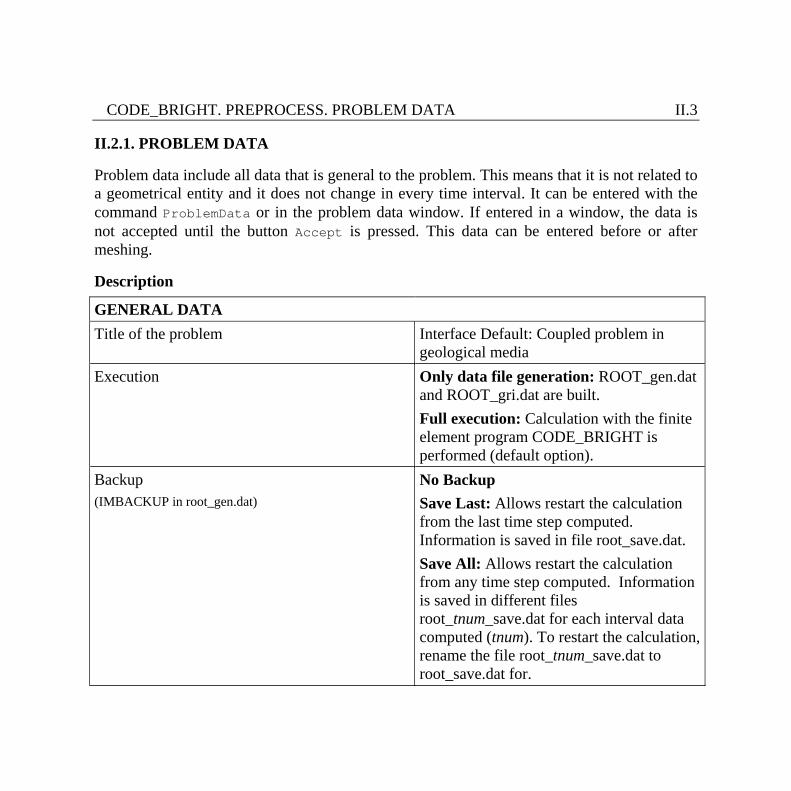
Problem data include all data that is general to the problem. This means that it is not related to a geometrical entity and it does not change in every time interval. It can be entered with the command ProblemData or in the problem data window. If entered in a window, the data is not accepted until the button Accept is pressed. This data can be entered before or after meshing.
Description
GENERAL DATA Title of the problem Interface Default: Coupled problem in
geological media Execution Only data file generation: ROOT_gen.dat
and ROOT_gri.dat are built. Full execution: Calculation with the finite element program CODE_BRIGHT is performed (default option).
Backup (IMBACKUP in root_gen.dat)
No Backup Save Last: Allows restart the calculation from the last time step computed. Information is saved in file root_save.dat. Save All: Allows restart the calculation from any time step computed. Information is saved in different files root_tnum_save.dat for each interval data computed (tnum). To restart the calculation, rename the file root_tnum_save.dat to root_save.dat for.
CODE_BRIGHT. PREPROCESS. PROBLEM DATA II.4
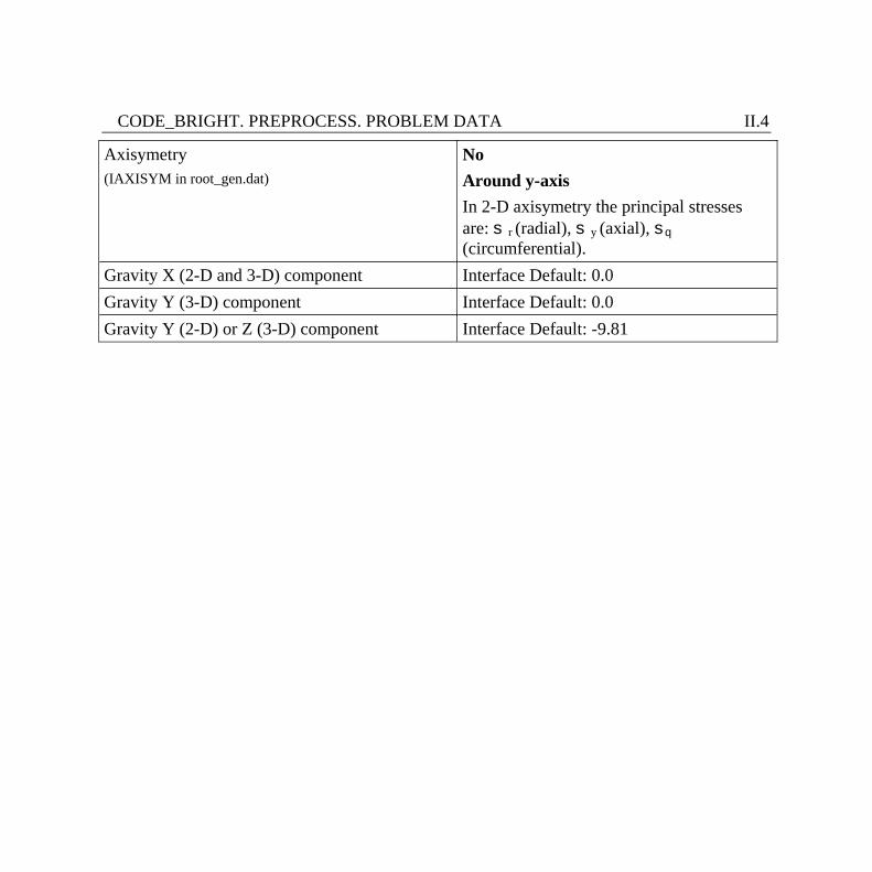
Axisymetry (IAXISYM in root_gen.dat)
No Around y-axis In 2-D axisymetry the principal stresses are: s r (radial), s y (axial), sq (circumferential).
Gravity X (2-D and 3-D) component Interface Default: 0.0 Gravity Y (3-D) component Interface Default: 0.0 Gravity Y (2-D) or Z (3-D) component Interface Default: -9.81
CODE_BRIGHT. PREPROCESS. PROBLEM DATA II.5
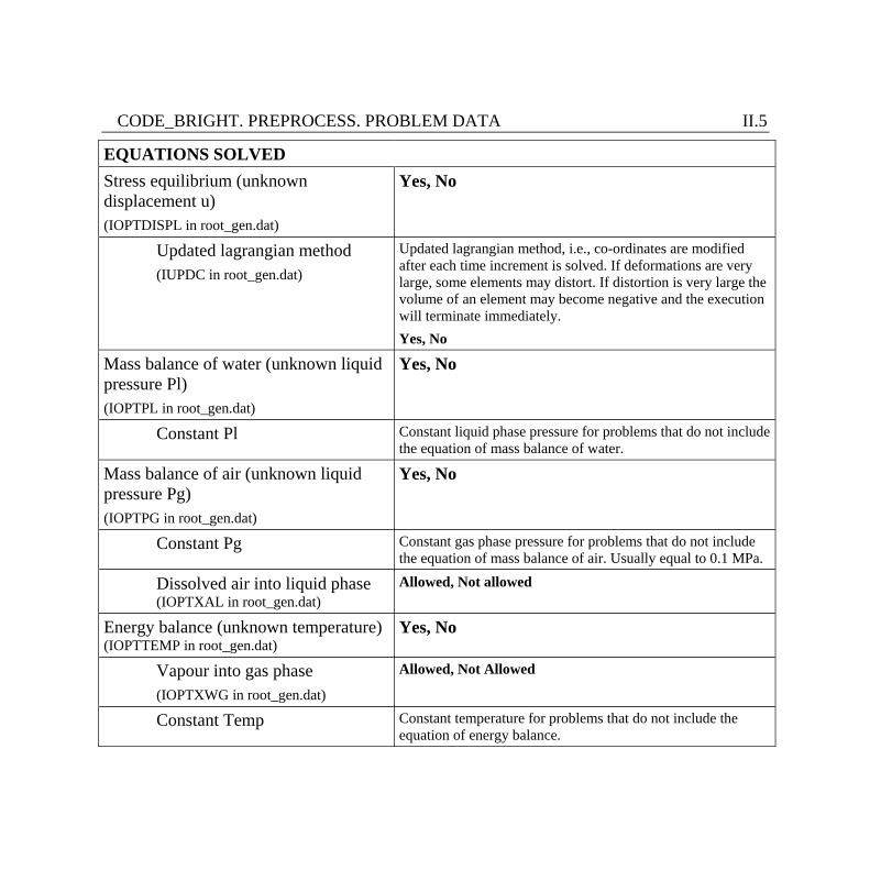
EQUATIONS SOLVED Stress equilibrium (unknown displacement u) (IOPTDISPL in root_gen.dat)
Yes, No
Updated lagrangian method (IUPDC in root_gen.dat)
Updated lagrangian method, i.e., co-ordinates are modified after each time increment is solved. If deformations are very large, some elements may distort. If distortion is very large the volume of an element may become negative and the execution will terminate immediately. Yes, No
Mass balance of water (unknown liquid pressure Pl) (IOPTPL in root_gen.dat)
Yes, No
Constant Pl Constant liquid phase pressure for problems that do not include the equation of mass balance of water.
Mass balance of air (unknown liquid pressure Pg) (IOPTPG in root_gen.dat)
Yes, No
Constant Pg Constant gas phase pressure for problems that do not include the equation of mass balance of air. Usually equal to 0.1 MPa.
Dissolved air into liquid phase (IOPTXAL in root_gen.dat)
Allowed, Not allowed
Energy balance (unknown temperature) (IOPTTEMP in root_gen.dat)
Yes, No
Vapour into gas phase (IOPTXWG in root_gen.dat)
Allowed, Not Allowed
Constant Temp Constant temperature for problems that do not include the equation of energy balance.
CODE_BRIGHT. PREPROCESS. PROBLEM DATA II.6
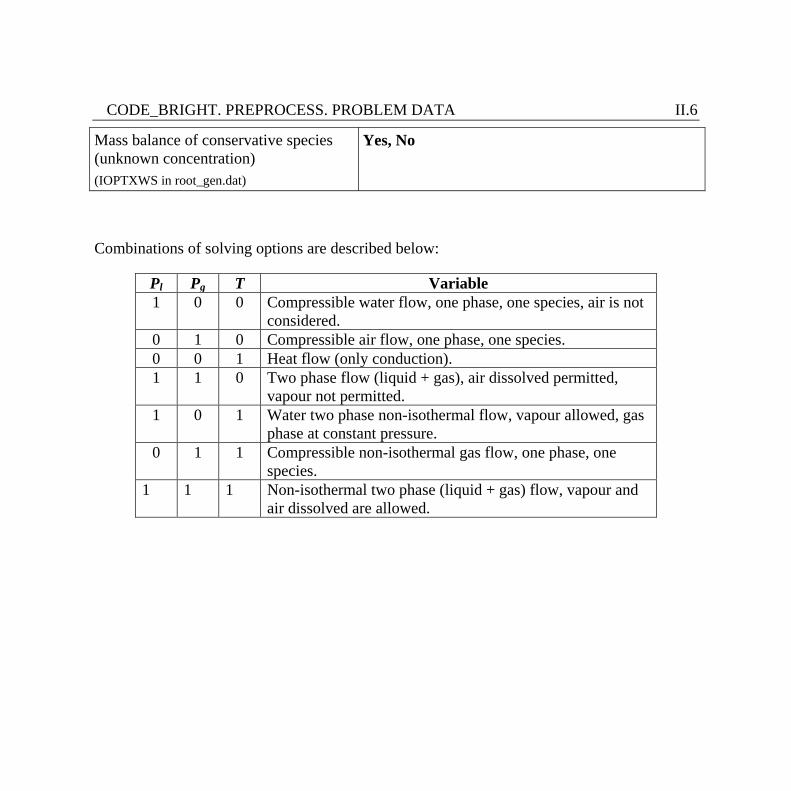
Mass balance of conservative species (unknown concentration) (IOPTXWS in root_gen.dat)
Yes, No
Combinations of solving options are described below:
Pl Pg T Variable 1 0 0 Compressible water flow, one phase, one species, air is not
considered. 0 1 0 Compressible air flow, one phase, one species. 0 0 1 Heat flow (only conduction). 1 1 0 Two phase flow (liquid + gas), air dissolved permitted,
vapour not permitted. 1 0 1 Water two phase non-isothermal flow, vapour allowed, gas
phase at constant pressure. 0 1 1 Compressible non-isothermal gas flow, one phase, one
species. 1 1 1 Non-isothermal two phase (liquid + gas) flow, vapour and
air dissolved are allowed.
CODE_BRIGHT. PREPROCESS. PROBLEM DATA II.7
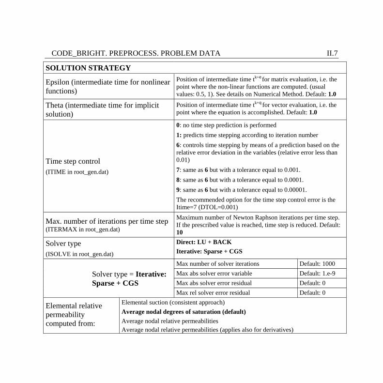
SOLUTION STRATEGY
Epsilon (intermediate time for nonlinear functions)
Position of intermediate time tk+e for matrix evaluation, i.e. the point where the non-linear functions are computed. (usual values: 0.5, 1). See details on Numerical Method. Default: 1.0
Theta (intermediate time for implicit solution)
Position of intermediate time tk+q for vector evaluation, i.e. the point where the equation is accomplished. Default: 1.0
Time step control (ITIME in root_gen.dat)
0: no time step prediction is performed 1: predicts time stepping according to iteration number 6: controls time stepping by means of a prediction based on the relative error deviation in the variables (relative error less than 0.01) 7: same as 6 but with a tolerance equal to 0.001. 8: same as 6 but with a tolerance equal to 0.0001. 9: same as 6 but with a tolerance equal to 0.00001. The recommended option for the time step control error is the Itime=7 (DTOL=0.001)
Max. number of iterations per time step (ITERMAX in root_gen.dat)
Maximum number of Newton Raphson iterations per time step. If the prescribed value is reached, time step is reduced. Default: 10
Solver type (ISOLVE in root_gen.dat)
Direct: LU + BACK Iterative: Sparse + CGS
Solver type = Iterative: Sparse + CGS
Max number of solver iterations Default: 1000 Max abs solver error variable Default: 1.e-9 Max abs solver error residual Default: 0 Max rel solver error residual Default: 0
Elemental relative permeability computed from:
Elemental suction (consistent approach) Average nodal degrees of saturation (default) Average nodal relative permeabilities Average nodal relative permeabilities (applies also for derivatives)

CODE_BRIGHT. PREPROCESS. PROBLEM DATA II.8 (IOPTPC in root_gen.dat) Maximal nodal relative permeabilty
Stress equilibrium (unknown displacement u) = yes
Max Abs Displacement (m) (DELMXU in root_gen.dat)
Maximum (absolute) displacement error tolerance (m). When correction of displacements (displacement difference between two iterations) is lower than this value, convergence has been achieved. Default: 1e-6
Max Nod Bal Forces (MN) (DELFMX in root_gen.dat)
Maximum nodal force balance error tolerance (MN). If the residual of forces in all nodes are lower than this value, convergence has been achieved. Default: 1e-10
Displacement Iter Corr (m) (DUMX in root_gen.dat)
Maximum displacement correction per iteration (m) (time increment is reduced if necessary). Default: 1e-1
Mass balance of water (unknown liquid pressure Pl) = yes
Max Abs Pl (MPa) (DELMXPL in root_gen.dat)
Maximum (absolute) liquid pressure error tolerance (MPa). Default: 1e-3
Max Nod Bal Forces (MN) (DELQWMX in root_gen.dat)
Maximum nodal water mass balance error tolerance (kg/s). Default: 1e-10
Pl Iter Corr (MPa) (DPLMX in root_gen.dat)
Maximum liquid pressure correction per iteration (MPa) (time increment is reduced if necessary). Default: 1e-1
Mass balance of air (unknown liquid pressure Pg) = yes
Max Abs Pg (MPa) (DELMXPG in root_gen.dat)
Maximum (absolute) gas pressure error tolerance (MPa). Default: 1e-3
Max Nod Air Mass (kg/s) (DELQAMX in root_gen.dat)
Maximum nodal air mass balance error tolerance (kg/s). Default: 1e-10
Pg Iter Corr (MPa) (DPGMX in root_gen.dat)
Maximum gas pressure correction per iteration (MPa) (time increment is reduced if necessary). Default: 1e-1
Energy balance (unknown temperature) = yes
Max Abs Temp (C) (DELMXT in root_gen.dat)
Maximum (absolute) temperature error tolerance (C). Default: 1e-3
Max Nod Energy (J/s) (DELQMX in root_gen.dat)
Maximum nodal energy balance error tolerance (J/s). Default: 1e-10
Temp Iter Corr (C) DTMX in root_gen.dat)
Maximum temperature correction per iteration (C) (time increment is reduced if necessary). Default: 1e-1
CODE_BRIGHT. PREPROCESS. PROBLEM DATA II.9
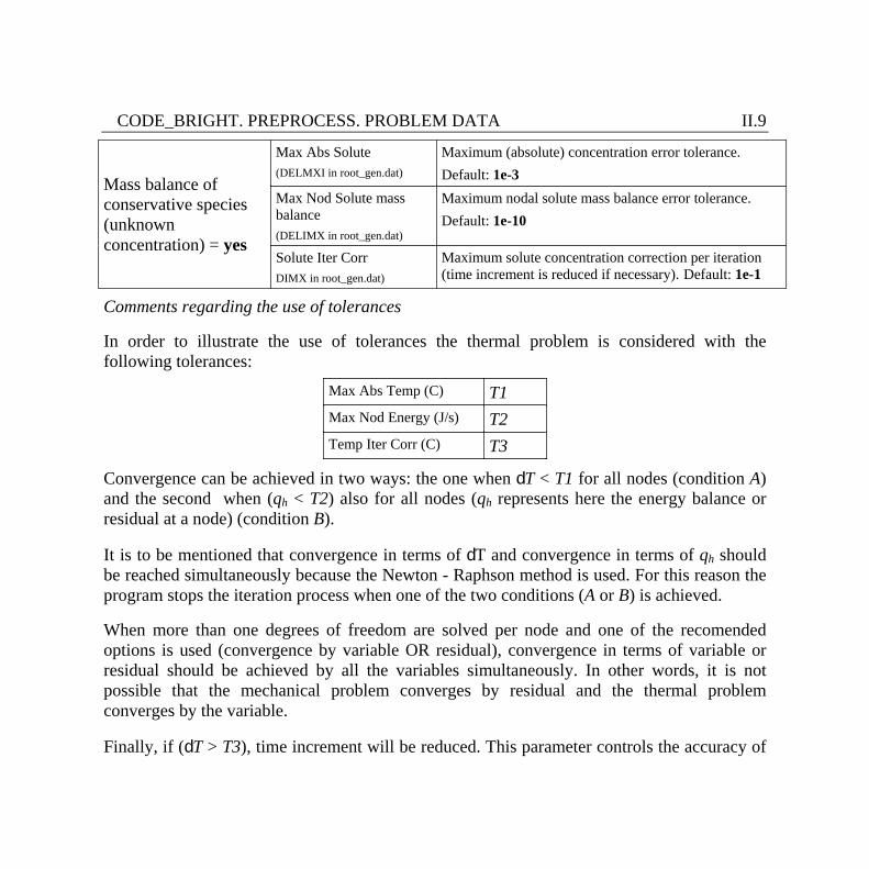
Mass balance of conservative species (unknown concentration) = yes
Max Abs Solute (DELMXI in root_gen.dat)
Maximum (absolute) concentration error tolerance. Default: 1e-3
Max Nod Solute mass balance (DELIMX in root_gen.dat)
Maximum nodal solute mass balance error tolerance. Default: 1e-10
Solute Iter Corr DIMX in root_gen.dat)
Maximum solute concentration correction per iteration (time increment is reduced if necessary). Default: 1e-1
Comments regarding the use of tolerances
In order to illustrate the use of tolerances the thermal problem is considered with the following tolerances:
Max Abs Temp (C) T1 Max Nod Energy (J/s) T2 Temp Iter Corr (C) T3
Convergence can be achieved in two ways: the one when dT < T1 for all nodes (condition A) and the second when (qh < T2) also for all nodes (qh represents here the energy balance or residual at a node) (condition B).
It is to be mentioned that convergence in terms of dT and convergence in terms of qh should be reached simultaneously because the Newton - Raphson method is used. For this reason the program stops the iteration process when one of the two conditions (A or B) is achieved.
When more than one degrees of freedom are solved per node and one of the recomended options is used (convergence by variable OR residual), convergence in terms of variable or residual should be achieved by all the variables simultaneously. In other words, it is not possible that the mechanical problem converges by residual and the thermal problem converges by the variable.
Finally, if (dT > T3), time increment will be reduced. This parameter controls the accuracy of
CODE_BRIGHT. PREPROCESS. PROBLEM DATA II.10
the solution in terms of how large time increments can be. A low value of T3 will force to use small time increments when large variations of temperature take place.
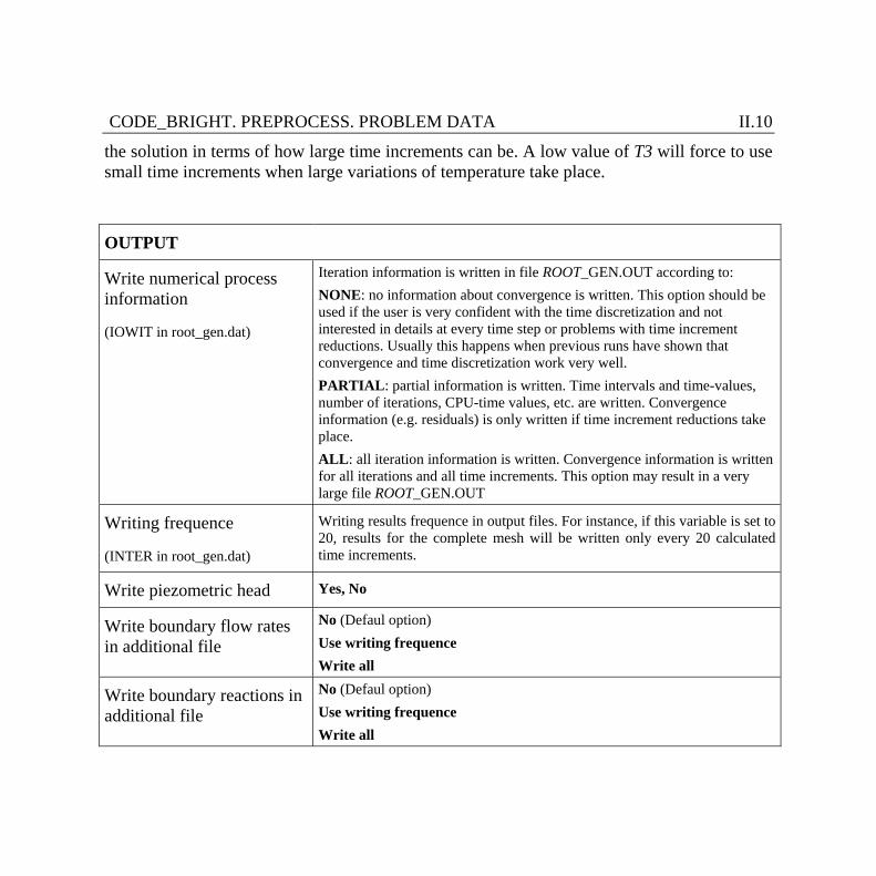
OUTPUT
Write numerical process information
(IOWIT in root_gen.dat)
Iteration information is written in file ROOT_GEN.OUT according to: NONE: no information about convergence is written. This option should be used if the user is very confident with the time discretization and not interested in details at every time step or problems with time increment reductions. Usually this happens when previous runs have shown that convergence and time discretization work very well. PARTIAL: partial information is written. Time intervals and time-values, number of iterations, CPU-time values, etc. are written. Convergence information (e.g. residuals) is only written if time increment reductions take place. ALL: all iteration information is written. Convergence information is written for all iterations and all time increments. This option may result in a very large file ROOT_GEN.OUT
Writing frequence
(INTER in root_gen.dat)
Writing results frequence in output files. For instance, if this variable is set to 20, results for the complete mesh will be written only every 20 calculated time increments.
Write piezometric head Yes, No
Write boundary flow rates in additional file
No (Defaul option) Use writing frequence Write all
Write boundary reactions in additional file
No (Defaul option) Use writing frequence Write all

CODE_BRIGHT. PREPROCESS. PROBLEM DATA II.11
Output points (IOWCONTOURS in root_gen.dat)
Nodes Gauss points: (Default option)
Write all information
(IWRALL in root_gen.dat)
Yes (default option), No If No is selected, the following option appears:
Separated output files (IPOLYFILES in root_gen.dat) : Yes, No and user go to Select output window.
SELECT OUTPUT
(If Write all information=No) Select outputs option is necessary when working with complex problems in which separated output files are used to facilitate the post-processing. The following options are available: Write Displacements Write Liquid Pressure Write Gas Pressure Write Temperature Write solute concentration Write Halite Concentration Write Vapour Concentration Write Gas Density Write Dissolved air concentration Write Liq Density Write porosity Write Liquid Saturation Degree Write heat fluxes: qT Write liquid fluxes: qL Write gas fluxes: qG Write diffusive heat fluxes: iT Write diffusive water fluxes: iL
Yes, No Yes, No Yes, No Yes, No Yes, No Yes, No Yes, No Yes, No Yes, No Yes, No Yes, No Yes, No Yes, No Yes, No Yes, No Yes, No Yes, No
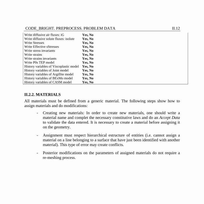
CODE_BRIGHT. PREPROCESS. PROBLEM DATA II.12 Write diffusive air fluxes: iG Write diffusive solute fluxes: isolute Write Stresses Write Effective sStresses Write stress invariants Write strains Write strains invariants Write P0s TEP model History variables of Viscoplastic model History variables of Joint model History variables of Argillite model History variables of BExMo model History variables of CASM model
Yes, No Yes, No Yes, No Yes, No Yes, No Yes, No Yes, No Yes, No Yes, No Yes, No Yes, No Yes, No Yes, No
II.2.2. MATERIALS All materials must be defined from a generic material. The following steps show how to assign materials and do modifications:
- Creating new materials: In order to create new materials, one should write a material name and complet the necessary constitutive laws and do an Accept Data to validate the data entered. It is necessary to create a material before assigning it on the geometry.
- Assignment must respect hierarchical estructure of entities (i.e. cannot assign a material on a line belonging to a surface that have just been identified with another material). This type of error may create conflicts.
- Posterior modifications on the parameters of assigned materials do not require a re-meshing process.
CODE_BRIGHT. PREPROCESS. PROBLEM DATA II.13
Constituve Laws in CODE_BRIGHT
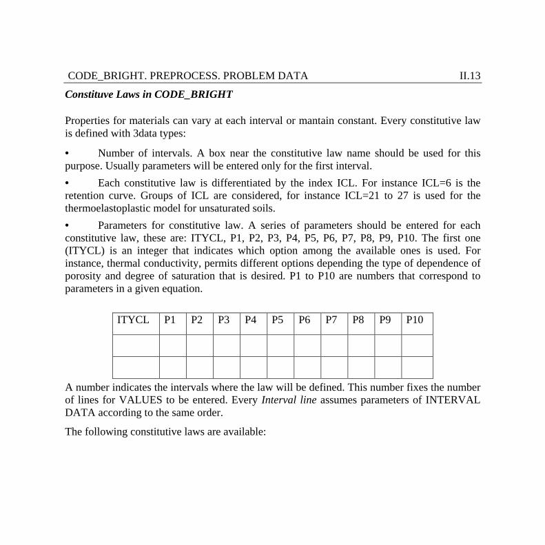
Properties for materials can vary at each interval or mantain constant. Every constitutive law is defined with 3data types:
· Number of intervals. A box near the constitutive law name should be used for this purpose. Usually parameters will be entered only for the first interval. · Each constitutive law is differentiated by the index ICL. For instance ICL=6 is the retention curve. Groups of ICL are considered, for instance ICL=21 to 27 is used for the thermoelastoplastic model for unsaturated soils. · Parameters for constitutive law. A series of parameters should be entered for each constitutive law, these are: ITYCL, P1, P2, P3, P4, P5, P6, P7, P8, P9, P10. The first one (ITYCL) is an integer that indicates which option among the available ones is used. For instance, thermal conductivity, permits different options depending the type of dependence of porosity and degree of saturation that is desired. P1 to P10 are numbers that correspond to parameters in a given equation.
ITYCL P1 P2 P3 P4 P5 P6 P7 P8 P9 P10
A number indicates the intervals where the law will be defined. This number fixes the number of lines for VALUES to be entered. Every Interval line assumes parameters of INTERVAL DATA according to the same order.
The following constitutive laws are available:
CODE_BRIGHT. PREPROCESS. PROBLEM DATA II.14
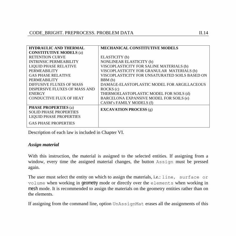
HYDRAULIC AND THERMAL CONSTITUTIVE MODELS (a) RETENTION CURVE INTRINSIC PERMEABILITY LIQUID PHASE RELATIVE PERMEABILITY GAS PHASE RELATIVE PERMEABILITY DIFFUSIVE FLUXES OF MASS DISPERSIVE FLUXES OF MASS AND ENERGY CONDUCTIVE FLUX OF HEAT
MECHANICAL CONSTITUTIVE MODELS ELASTICITY (b) NONLINEAR ELASTICITY (b) VISCOPLASTICITY FOR SALINE MATERIALS (b) VISCOPLASTICITY FOR GRANULAR MATERIALS (b) VISCOPLASTICITY FOR UNSATURATED SOILS BASED ON BBM (b) DAMAGE-ELASTOPLASTIC MODEL FOR ARGILLACEOUS ROCKS (c) THERMOELASTOPLASTIC MODEL FOR SOILS (d) BARCELONA EXPANSIVE MODEL FOR SOILS (e) CASM’s FAMILY MODELS (f)
PHASE PROPERTIES (a) SOLID PHASE PROPERTIES LIQUID PHASE PROPERTIES
GAS PHASE PROPERTIES
EXCAVATION PROCESS (g)
Description of each law is included in Chapter VI.
Assign material
With this instruction, the material is assigned to the selected entities. If assigning from a window, every time the assigned material changes, the button Assign must be pressed again.
The user must select the entity on which to assign the materials, i.e.: line, surface or volume when working in geometry mode or directly over the elements when working in mesh mode. It is recommended to assign the materials on the geometry entities rather than on the elements.
If assigning from the command line, option UnAssignMat erases all the assignments of this

CODE_BRIGHT. PREPROCESS. PROBLEM DATA II.15
particular material.
When a mesh has been already generated, and changes in the assigned materials are required, then it is necessary to re-mesh again or assign the materials directly on the mesh.
Draw material
Draws a color indicating the selected material for all the entities that have the required material assigned. It is possible to draw just one or draw all materials. To select some of them the users should use a:b and all material numbers that lie between a and b will be drawn.
When drawing materials in 3 dimensions, it may be necessary to change the viewing mode to polygons or render (see section Render) to diferenciate the front and back of the objects.
Unassign material
Command Unassign unassigns all the materials from all the entities. For only one material, use UnAssignMat (see section Assign material).
New material
When the command NewMaterial is used, a new material is created taking an existing one as a base material. Base material means that the new one will have the same fields as the base one. Then, all the new values for the fields can be entered in the command line. It is possible to redefine an existing material.
To create a new material or redefine an existing one in the materials window, write a new name or the same one and change some of the properties. Then push the command Accept.
CODE_BRIGHT. PREPROCESS. PROBLEM DATA II.16
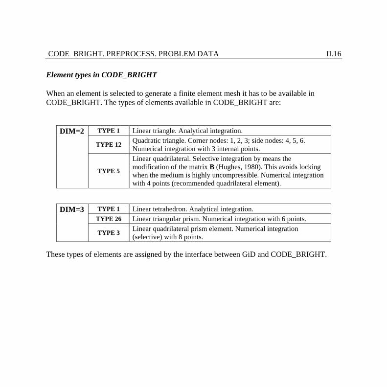
Element types in CODE_BRIGHT
When an element is selected to generate a finite element mesh it has to be available in CODE_BRIGHT. The types of elements available in CODE_BRIGHT are:
DIM=2
TYPE 1 Linear triangle. Analytical integration.
TYPE 12 Quadratic triangle. Corner nodes: 1, 2, 3; side nodes: 4, 5, 6. Numerical integration with 3 internal points.
TYPE 5
Linear quadrilateral. Selective integration by means the modification of the matrix B (Hughes, 1980). This avoids locking when the medium is highly uncompressible. Numerical integration with 4 points (recommended quadrilateral element).
DIM=3 TYPE 1 Linear tetrahedron. Analytical integration. TYPE 26 Linear triangular prism. Numerical integration with 6 points.
TYPE 3 Linear quadrilateral prism element. Numerical integration (selective) with 8 points.
These types of elements are assigned by the interface between GiD and CODE_BRIGHT.

CODE_BRIGHT. PREPROCESS. PROBLEM DATA II.17
II.2.3. CONDITIONS
Conditions are all the properties of a problem, excluding materials, that can be assigned to an entity. In this concept several types of conditions have been included: Force/Disp conditions, Flux conditions, Initial unknowns, Porosity (and other variables), Initial stress, Joint element width and time evolution location. The condition window permits to choose entities to assign on (Point, Line, Surface or Volume in geometry display mode and Node or Element in mesh display mode) and select different types of conditions. It must be taken into account that conditions assigned in mesh display mode will be unassigned in every new meshing process.
The following points should be taken into account for condition construction:
· Force/Disp conditions add up all conditions assigned at every node, except for variables Index (takes last value encountered) and Multiplier (takes the biggest). · Flux conditions, Initial unknowns, Porosity (and other variables), Initial stress and Joint element width are assigned with entities priority in the following order: Points, Lines, Surfaces and Volumes (i.e. the node takes a Flux_Point_B.C. refusing a Line_Flux_B.C. assigned previously).
If a mesh has already been generated, for any change in the condition assignments, it is necessary to re-mesh again to transfer these new conditions to the mesh.

CODE_BRIGHT. PREPROCESS. PROBLEM DATA II.18
Conditions description
II.2.3.1 Force/displacement conditions
The mechanical boundary conditions only exists if the mechanical problem is solved (Solve displacement). For each time period only the types that undergo changes should be read.
X direction force/stress Value in MPa or MPa/m2 Y direction force/stress Value in MPa or MPa/m2 Z direction force/stress Value in MPa or MPa/m2 X displacement rate prescribed Value in m/s Y displacement rate prescribed Value in m/s Z displacement rate prescribed Value in m/s
X direction prescribed = 1 means that displacement rate will be prescribed in the X direction. The value is given above.
Y direction prescribed = 1 means that displacement rate will be prescribed in the Y direction. The value is given above.
Z direction prescribed = 1 means that displacement rate will be prescribed in the Z direction. The value is given above.
g (multiplier) The units of this parameter depend on whether force or stress is applied.
Dfxo obtained as ramp loading
during the current interval.
Dfyo obtained as ramp loading
during the current interval.
Dfzo obtained as ramp loading
during the current interval.
CODE_BRIGHT. PREPROCESS. PROBLEM DATA II.19
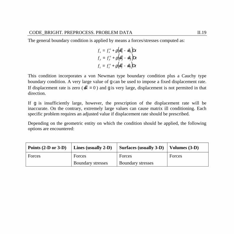
The general boundary condition is applied by means a forces/stresses computed as:
( )( )( ) tuuff
tuuff
tuuff
zzo
zz
yyoyy
xxo
xx
D-+=
D-+=
D-+=
&&
&&
&&
0
0
0
g
g
g
This condition incorporates a von Newman type boundary condition plus a Cauchy type boundary condition. A very large value of g can be used to impose a fixed displacement rate. If displacement rate is zero ( 0 0u =& ) and g is very large, displacement is not permited in that direction.
If g is insufficiently large, however, the prescription of the displacement rate will be inaccurate. On the contrary, extremely large values can cause matrix ill conditioning. Each specific problem requires an adjusted value if displacement rate should be prescribed.
Depending on the geometric entity on which the condition should be applied, the following options are encountered:
Points (2-D or 3-D) Lines (usually 2-D) Surfaces (usually 3-D) Volumes (3-D)
Forces Forces Boundary stresses
Forces Boundary stresses
Forces
CODE_BRIGHT. PREPROCESS. PROBLEM DATA II.20
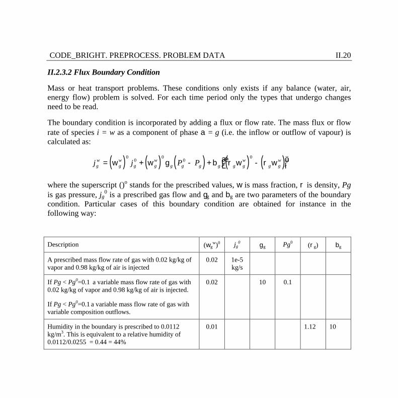
II.2.3.2 Flux Boundary Condition
Mass or heat transport problems. These conditions only exists if any balance (water, air, energy flow) problem is solved. For each time period only the types that undergo changes need to be read.
The boundary condition is incorporated by adding a flux or flow rate. The mass flux or flow rate of species i = w as a component of phase a = g (i.e. the inflow or outflow of vapour) is calculated as:
( ) ( ) ( ) ( ) ( )j j P Pgw
gw
g gw
g g g g g gw
g gw= + - + -æ
èçöø÷w w g b r w r w
00
00
0
where the superscript ()o stands for the prescribed values, w is mass fraction, r is density, Pg is gas pressure, jg
0 is a prescribed gas flow and gg and bg are two parameters of the boundary condition. Particular cases of this boundary condition are obtained for instance in the following way:
Description (wgw)0 jg
0 g g Pg0 (rg) bg
A prescribed mass flow rate of gas with 0.02 kg/kg of vapor and 0.98 kg/kg of air is injected
0.02 1e-5 kg/s
If Pg < Pg0=0.1 a variable mass flow rate of gas with 0.02 kg/kg of vapor and 0.98 kg/kg of air is injected.
If Pg < Pg0=0.1 a variable mass flow rate of gas with variable composition outflows.
0.02 10 0.1
Humidity in the boundary is prescribed to 0.0112 kg/m3. This is equivalent to a relative humidity of 0.0112/0.0255 = 0.44 = 44%
0.01 1.12 10
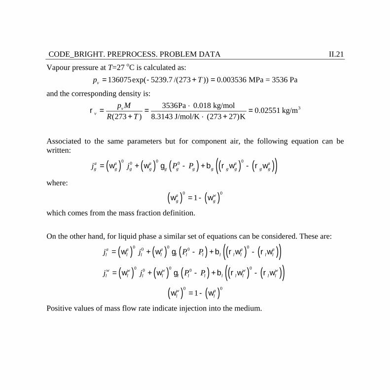
CODE_BRIGHT. PREPROCESS. PROBLEM DATA II.21
Vapour pressure at T=27 oC is calculated as: 136075exp( 5239.7 /(273 )) 0.003536 MPa = 3536 Pavp T= - + =
and the corresponding density is:
33536Pa 0.018 kg/mol 0.02551 kg/m(273 ) 8.3143 J/mol/K (273 27)K
vv
p MR T
´r = = =
+ ´ +
Associated to the same parameters but for component air, the following equation can be written:
( ) ( ) ( ) ( ) ( )( )0 0 00 0a a a a ag g g g g g g g g g g gj j P P= w + w g - + b r w - r w
where:
( ) ( )0 01a w
g gw = - w
which comes from the mass fraction definition. On the other hand, for liquid phase a similar set of equations can be considered. These are:
( ) ( ) ( ) ( ) ( )( )0 0 00 0a a a a al l l l l l l l l l l lj j P P= w + w g - + b r w - r w
( ) ( ) ( ) ( ) ( )( )0 0 00 0w w w w wl l l l l l l l l l l lj j P P= w + w g - + b r w - r w
( ) ( )0 01w a
l lw = - w
Positive values of mass flow rate indicate injection into the medium.
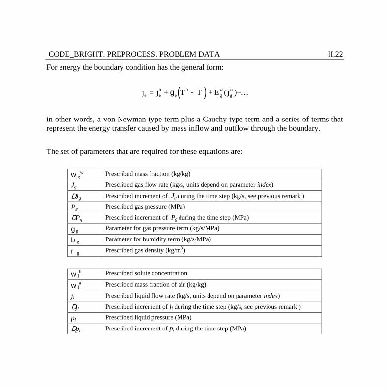
CODE_BRIGHT. PREPROCESS. PROBLEM DATA II.22
For energy the boundary condition has the general form:
( )j j T T E je e e gw
gw= + - + +0 0g ( ) ...
in other words, a von Newman type term plus a Cauchy type term and a series of terms that represent the energy transfer caused by mass inflow and outflow through the boundary. The set of parameters that are required for these equations are:
w gw Prescribed mass fraction (kg/kg)
Jg Prescribed gas flow rate (kg/s, units depend on parameter index)
DJg Prescribed increment of Jg during the time step (kg/s, see previous remark )
Pg Prescribed gas pressure (MPa)
DPg Prescribed increment of Pg during the time step (MPa)
g g Parameter for gas pressure term (kg/s/MPa)
b g Parameter for humidity term (kg/s/MPa)
r g Prescribed gas density (kg/m3)
w lh Prescribed solute concentration
w la Prescribed mass fraction of air (kg/kg)
jl Prescribed liquid flow rate (kg/s, units depend on parameter index)
Djl Prescribed increment of jl during the time step (kg/s, see previous remark )
pl Prescribed liquid pressure (MPa)
Dpl Prescribed increment of pl during the time step (MPa)
CODE_BRIGHT. PREPROCESS. PROBLEM DATA II.23
gl Parameter needed to be ¹ 0 when Pl is prescribed (kg/s/MPa)
bl Parameter needed only when mass transport problem is considered (kg/s/MPa)
rl Prescribed liquid density (kg/m3)
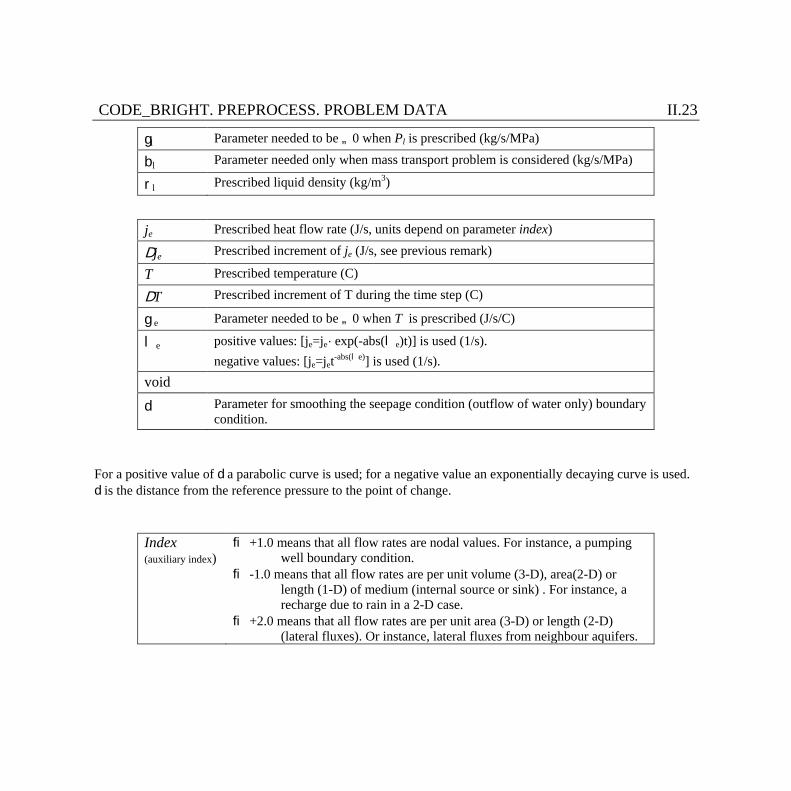
je Prescribed heat flow rate (J/s, units depend on parameter index)
Dje Prescribed increment of je (J/s, see previous remark)
T Prescribed temperature (C)
DT Prescribed increment of T during the time step (C)
g e Parameter needed to be ¹ 0 when T is prescribed (J/s/C)
l e positive values: [je=je´exp(-abs(l e)t)] is used (1/s). negative values: [je=jet-abs(l e)] is used (1/s).
void
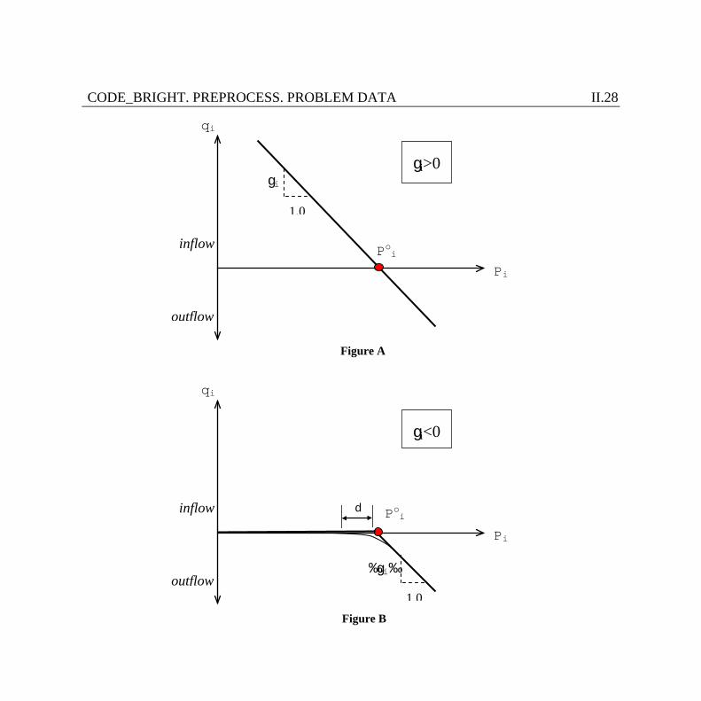
d Parameter for smoothing the seepage condition (outflow of water only) boundary condition.
For a positive value of d a parabolic curve is used; for a negative value an exponentially decaying curve is used. d is the distance from the reference pressure to the point of change.
Index (auxiliary index)
® +1.0 means that all flow rates are nodal values. For instance, a pumping well boundary condition.
® -1.0 means that all flow rates are per unit volume (3-D), area(2-D) or length (1-D) of medium (internal source or sink) . For instance, a recharge due to rain in a 2-D case.
® +2.0 means that all flow rates are per unit area (3-D) or length (2-D) (lateral fluxes). Or instance, lateral fluxes from neighbour aquifers.
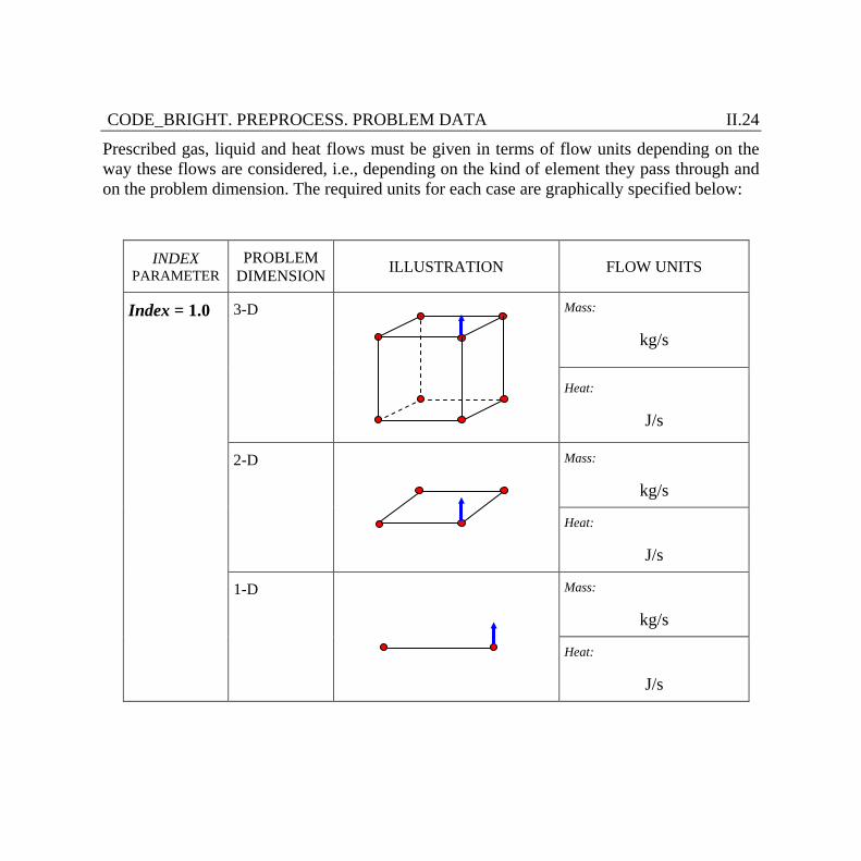
CODE_BRIGHT. PREPROCESS. PROBLEM DATA II.24
Prescribed gas, liquid and heat flows must be given in terms of flow units depending on the way these flows are considered, i.e., depending on the kind of element they pass through and on the problem dimension. The required units for each case are graphically specified below:
INDEX PARAMETER
PROBLEM DIMENSION ILLUSTRATION FLOW UNITS
Index = 1.0 3-D
Mass:
kg/s
Heat:
J/s
2-D Mass:
kg/s
Heat:
J/s
1-D
Mass:
kg/s
Heat:
J/s
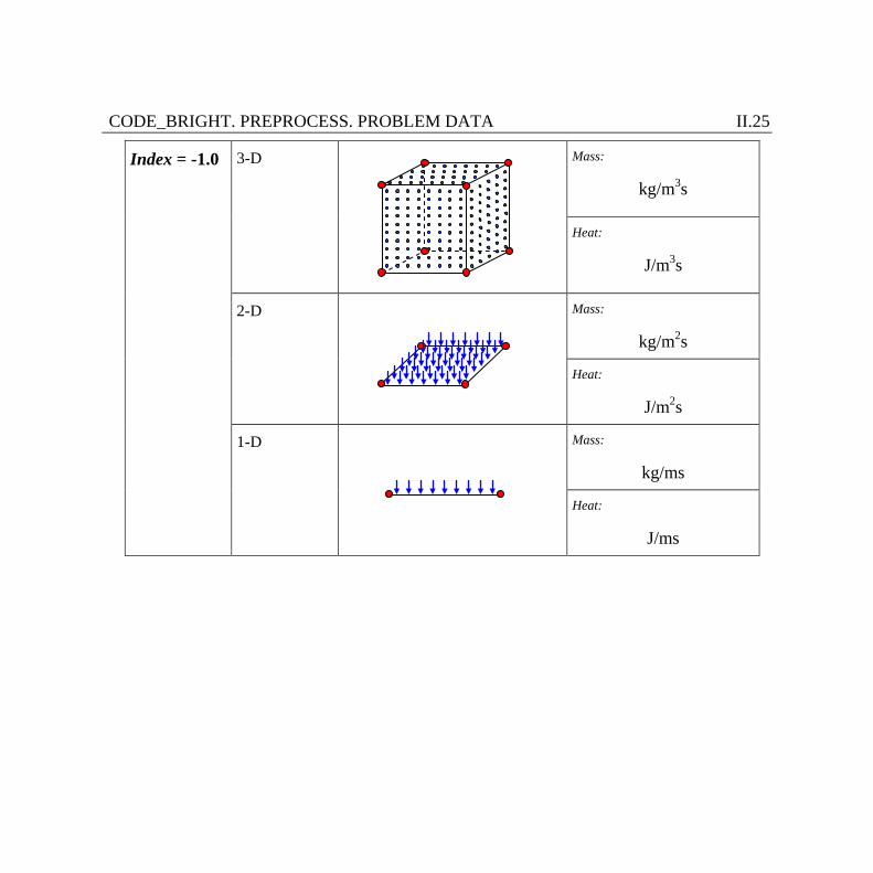
CODE_BRIGHT. PREPROCESS. PROBLEM DATA II.25
Index = -1.0 3-D Mass:
kg/m3s
Heat:
J/m3s
2-D
Mass:
kg/m2s
Heat:
J/m2s
1-D
Mass:
kg/ms
Heat:
J/ms

CODE_BRIGHT. PREPROCESS. PROBLEM DATA II.26
Index = 2.0 3-D
Mass:
kg/m2s
Heat:
J/m2s
2-D Mass:
kg/ms
Heat:
J/ms
The following table contains a summary of the units for each case:
index Problem dimension
Required units
Gas Flow Liquid Flow Heat Flow
1.0 --- kg/s kg/s J/s
-1.0
1D kg/m/s kg/m/s J/m/s
2D kg/m2/s kg/m2/s J/m2/s
3D kg/m3/s kg/m3/s J/m3/s
2.0 2D kg/m/s kg/m/s J/m/s
3D kg/m2/s kg/m2/s J/m2/s
CODE_BRIGHT. PREPROCESS. PROBLEM DATA II.27
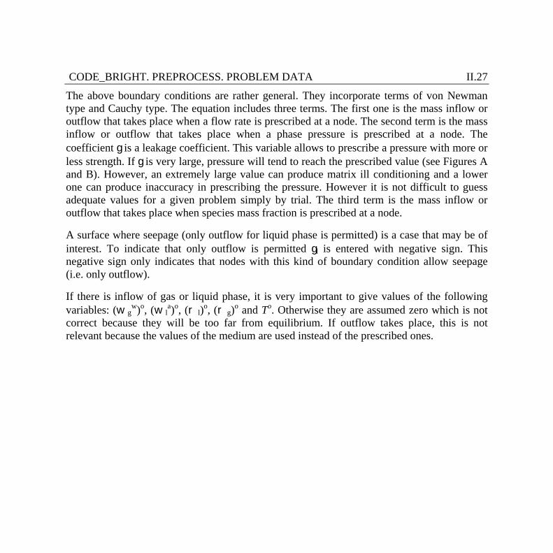
The above boundary conditions are rather general. They incorporate terms of von Newman type and Cauchy type. The equation includes three terms. The first one is the mass inflow or outflow that takes place when a flow rate is prescribed at a node. The second term is the mass inflow or outflow that takes place when a phase pressure is prescribed at a node. The coefficient g is a leakage coefficient. This variable allows to prescribe a pressure with more or less strength. If g is very large, pressure will tend to reach the prescribed value (see Figures A and B). However, an extremely large value can produce matrix ill conditioning and a lower one can produce inaccuracy in prescribing the pressure. However it is not difficult to guess adequate values for a given problem simply by trial. The third term is the mass inflow or outflow that takes place when species mass fraction is prescribed at a node.
A surface where seepage (only outflow for liquid phase is permitted) is a case that may be of interest. To indicate that only outflow is permitted gl is entered with negative sign. This negative sign only indicates that nodes with this kind of boundary condition allow seepage (i.e. only outflow).
If there is inflow of gas or liquid phase, it is very important to give values of the following variables: (w g
w)o, (w la)o, (r l)o, (r g)o and To. Otherwise they are assumed zero which is not
correct because they will be too far from equilibrium. If outflow takes place, this is not relevant because the values of the medium are used instead of the prescribed ones.
CODE_BRIGHT. PREPROCESS. PROBLEM DATA II.28
qi
Pi
Poi
gi
1.0
outflow
inflow
gi>0
Figure A
qi
Pi
Poi
½gi½
1.0
outflow
inflow
gi<0
d
Figure B

CODE_BRIGHT. PREPROCESS. PROBLEM DATA II.29
Variable flux boundary condition:
It is possible to assign a flux condition varying with time using an auxiliary file. In this case, user must assign a value of -999 to the particular variable for which a given variation want to be assigned and include an ASCII file in the GiD project folder called “root_bcf.dat” with the variation of the given flux variable with time. The structure of the “root_bcf.dat” file is illustrated in Table A.
Table A. Illustration of the format of root_bcf.dat file
Number of data (N)
Number of Flux variables (NF)
Id. variable (1) Id. variable (2) …… Id. variable (NF)
Time (1) Value Value … Value
Time (2) Value Value … Value
… … … … …
Time (N) Value Value … Value
It should be noted that the first line of the root_bcf.dat must contain the number of data (N) that has to be readed. The first column of the second line refers to the number of flux variables (NF) for which a given variation with time want to be assigned. The other columns of the second line contain a special flag (or indicator) of the flux variables to be changed, this indicator is shown in Table B. The following lines (third to N) contain the time in the same unit considered at the interval data (in the first column) and the values of the flux variables assigned to the specific time (in the other columns).
CODE_BRIGHT. PREPROCESS. PROBLEM DATA II.30
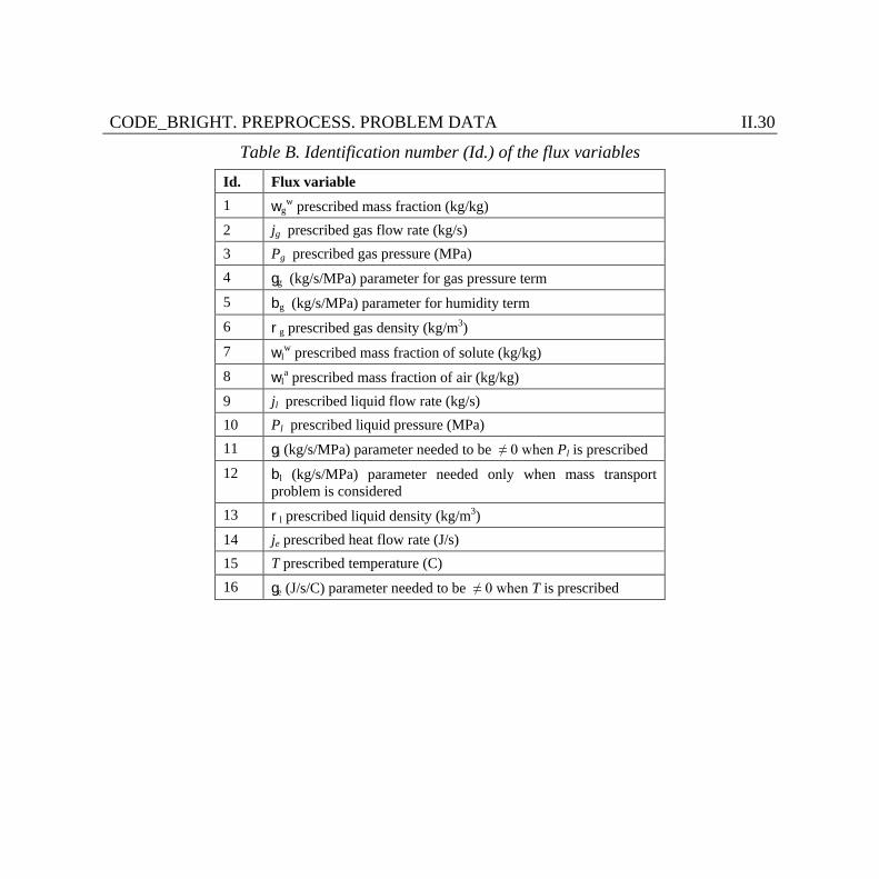
Table B. Identification number (Id.) of the flux variables Id. Flux variable 1 wg
w prescribed mass fraction (kg/kg) 2 jg prescribed gas flow rate (kg/s) 3 Pg prescribed gas pressure (MPa) 4 gg (kg/s/MPa) parameter for gas pressure term 5 bg (kg/s/MPa) parameter for humidity term 6 rg prescribed gas density (kg/m3) 7 wl
w prescribed mass fraction of solute (kg/kg) 8 wl
a prescribed mass fraction of air (kg/kg) 9 jl prescribed liquid flow rate (kg/s) 10 Pl prescribed liquid pressure (MPa) 11 gl (kg/s/MPa) parameter needed to be ≠ 0 when Pl is prescribed 12 bl (kg/s/MPa) parameter needed only when mass transport
problem is considered 13 rl prescribed liquid density (kg/m3) 14 je prescribed heat flow rate (J/s) 15 T prescribed temperature (C) 16 ge (J/s/C) parameter needed to be ≠ 0 when T is prescribed
CODE_BRIGHT. PREPROCESS. PROBLEM DATA II.31
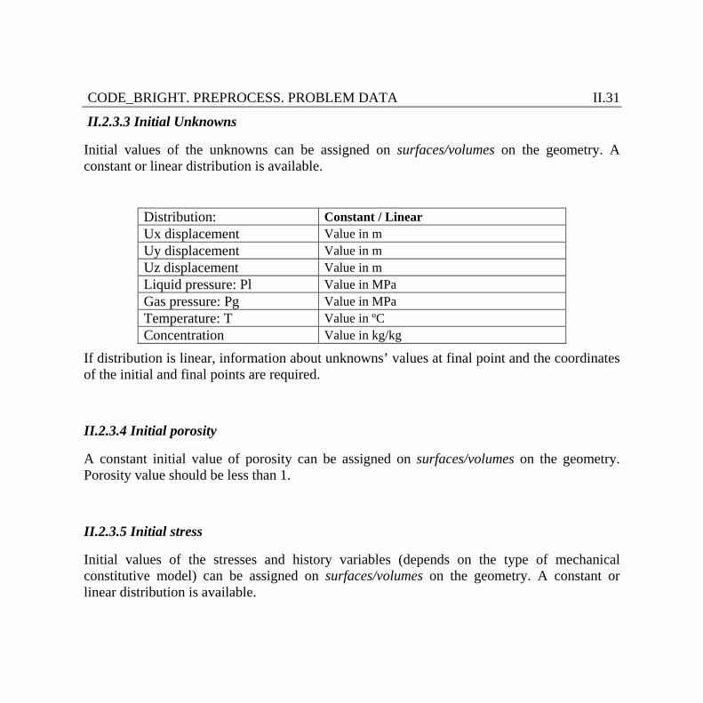
II.2.3.3 Initial Unknowns
Initial values of the unknowns can be assigned on surfaces/volumes on the geometry. A constant or linear distribution is available.
Distribution: Constant / Linear Ux displacement Value in m Uy displacement Value in m Uz displacement Value in m Liquid pressure: Pl Value in MPa Gas pressure: Pg Value in MPa Temperature: T Value in ºC Concentration Value in kg/kg
If distribution is linear, information about unknowns’ values at final point and the coordinates of the initial and final points are required.
II.2.3.4 Initial porosity
A constant initial value of porosity can be assigned on surfaces/volumes on the geometry. Porosity value should be less than 1.
II.2.3.5 Initial stress
Initial values of the stresses and history variables (depends on the type of mechanical constitutive model) can be assigned on surfaces/volumes on the geometry. A constant or linear distribution is available.

CODE_BRIGHT. PREPROCESS. PROBLEM DATA II.32
Distribution: Constant / Linear X stress Value in MPa Y stress Value in MPa Z stress Value in MPa XY stress Value in MPa XZ stress Value in MPa YZ stress Value in MPa History variable 1 (depend on the constitutive model) History variable 2 (depend on the constitutive model)
In chapter VI, the description of history variables required for elastoplastic and viscoplastic models is included.
If distribution is linear, information about stresses and history variables values at final point and the coordinates of the initial and final points are required.
II.2.3.6 Initial anisotropy.
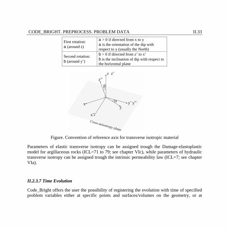
Transverse isotropy can be assigned on surfaces/volumes in a hydraulic and/or mechanical problem. The direction of orthotropy axis is indicated by the two angles shown in the figure. Transformation is done from physical plane (global axes) to anisotropy directions (local axes) First rotation is around z axis and the second rotation is around the new y’ axis.
CODE_BRIGHT. PREPROCESS. PROBLEM DATA II.33
First rotation: a (around z)
a > 0 if directed from x to y a is the orientation of the dip with respect to y (usually the North)
Second rotation: b (around y’)
b > 0 if directed from z’ to x’ b is the inclination of dip with respect to the horizontal plane
Figure. Convention of reference axis for transverse isotropic material
Parameters of elastic transverse isotropy can be assigned trough the Damage-elastoplastic model for argillaceous rocks (ICL=71 to 79; see chapter VIc), while parameters of hydraulic transverse isotropy can be assigned trough the intrinsic permeability law (ICL=7; see chapter VIa).
II.2.3.7 Time Evolution
Code_Bright offers the user the possibility of registering the evolution with time of specified problem variables either at specific points and surfaces/volumes on the geometry, or at
CODE_BRIGHT. PREPROCESS. PROBLEM DATA II.34
specific nodes and elements on the mesh. In case that nodes and elements are specified by the user, special care must be taken when remeshing, yet information regarding time evolution will be lost.
The program does not admit more than 10 nodes and 10 elements (or, if the case, points and surfaces/volumes) for time evolution registration, whatever could be read from the introduced time evolution data. These data, on the other hand, have to be given to the program as referring to the first time interval of the problem.
However, Post–process interface in GID has available the information of problem variables in all points/lines/surfaces/volumes of the geometry and nodes/elements of the mesh. Post–process offers the option to draw graphs of specified problem variables. Several graph types are available: point evolution against time, result 1 vs. result 2 over points, and result along a boundary line (see View results/graphs option of Post-process). It is possible to save or read a graph (see Files menu of Post-process). These advanced options of Post-process avoid the need to select specific points/surfaces/volumes in conditions for the time evolution, before to run the problem.
Assignment priorities
Conditions assigned on the geometry are distributed over the mesh with priorities. In general points have priority over lines, lines over surfaces and surfaces over volumes. At mesh level, nodes have priority over elements.
Mechanical boundary conditions on high entities are superimposed when they are applied to a lower entity. This means, for instance in a 2-D case, that a point that belongs to two lines will have the combination of boundary conditions coming from these two lines.
CODE_BRIGHT. PREPROCESS. PROBLEM DATA II.35
Assign condition
A condition is assigned to the entities with the given field values. If assigning from the command AssignCond, the option Change allows the definition of the field values. Do not forget to change these values before assigning. Option DeleteAll erases all the assigned entities of this particular condition. Conditions can be assigned both on the geometry and on the mesh but it is convenient to assign them on the geometry and the conditions will then be transferred to the mesh. If conditions are assigned on the mesh, any remeshing will cause the conditions to be lost.
Conditions that are to be attached to the boundary of the elements, are assigned to the elements and GiD searches the boundaries of the elements that are boundaries of the total mesh. Option Unassign inside AssignCond, permits to unassign this condition. It is also possible to unassign from only certain entities.
If a mesh has already been generated, for any change in the condition assignments, it is necessary to re-mesh again.
Draw condition
Option Draw all draws all the conditions assigned to all the entities in the graphical window. This means to draw a graphical symbol or condition number over every entity that has this condition. If one particular condition is selected, it is possible to choose between Draw and one of the fields. Draw is like Draw all but only for one particular condition. If one field is chosen, the value of this field is written over all the entities that have this condition assigned.
When the condition has any field referred to the type of axes, the latters can be visualized by means of Draw local axes.
CODE_BRIGHT. PREPROCESS. PROBLEM DATA II.36
Unassign condition
In window mode, command UnAssign lets the user to choose between unassigning this condition from the entities that owe it or unassigning all the conditions or select some entities to unassign. In command mode UnAssing, do it for all the conditions. For only one condition, use command Delete All (see section Assign condition).
Entities
Create an information window with all entities assigned including values at every one .
CODE_BRIGHT. PREPROCESS. PROBLEM DATA II.37
II.2.4. INTERVALS DATA
Intervals are a way to change some conditions and, eventually, material properties.
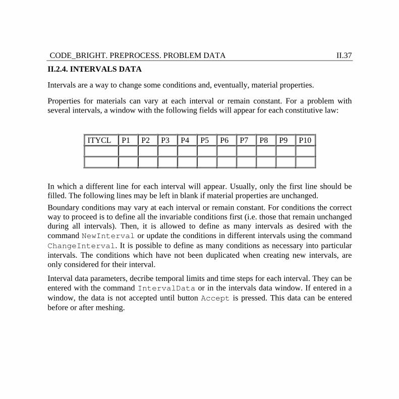
Properties for materials can vary at each interval or remain constant. For a problem with several intervals, a window with the following fields will appear for each constitutive law:
ITYCL P1 P2 P3 P4 P5 P6 P7 P8 P9 P10
In which a different line for each interval will appear. Usually, only the first line should be filled. The following lines may be left in blank if material properties are unchanged. Boundary conditions may vary at each interval or remain constant. For conditions the correct way to proceed is to define all the invariable conditions first (i.e. those that remain unchanged during all intervals). Then, it is allowed to define as many intervals as desired with the command NewInterval or update the conditions in different intervals using the command ChangeInterval. It is possible to define as many conditions as necessary into particular intervals. The conditions which have not been duplicated when creating new intervals, are only considered for their interval.
Interval data parameters, decribe temporal limits and time steps for each interval. They can be entered with the command IntervalData or in the intervals data window. If entered in a window, the data is not accepted until button Accept is pressed. This data can be entered before or after meshing.

CODE_BRIGHT. PREPROCESS. PROBLEM DATA II.38
Description
INTERVAL DATA
Units of time discretization
Time units for defined interval. Options: Seconds, Minutes, Hours, Days, Weeks, Months, Years
Initial Time (start period) (TIMEI in root_gen.dat)
Initial time for defined interval.
Initial Time Step (DTIME in root_gen.dat)
Initial time step for this time interval.
Final Time (end period) (TIMEF in root_gen.dat)
Final time for defined interval.
Partial Time (TIME1 in root_gen.dat)
Time from which time increment is kept constant.
Partial Time Step (DTIMEC in root_gen.dat)
Constant time step value.
Put displacements to 0 Yes / No
This option put displacement to zero at the beginning of the next time step.
In 'Writing results frequence', the intermittence for writing results is defined, i.e. only after a given number of time steps the results will be written. This may cause inconveniences if the user desires the results at precisely fixed times (for instance: 6 months, 1 year, 2 year, etc.). Moreover, if something changes between two runs (e.g. boundary conditions) and any time
CODE_BRIGHT. PREPROCESS. PROBLEM DATA II.39
increment should be modified, the value of the times in which results are output will not be identical between these two runs. In this case, it would be difficult to make a comparison of the two analyses because the output results correspond to different times. However, it is possible to decide the values of the times for output using a sequence of consecutive intervals. In this way, the results will be output for all 'Final time' defined, and if the user is only interested in these fixed times a very large value may be used for 'Writing results frequence' to avoid output at other times.
_________________________________
CODE_BRIGHT. PROCESS III.1
CODE_BRIGHT PROCESS III.1. CALCULATE This part deals with the stage of the process that solves the numerical problem. The system would allow to call the Finite Element program without necessity of leaving from the work environment. Pressing Calculate the user can see a Process window, and clicking on Start the solver module runs.
III.2. DATA FILES If the solver program is required to be run outside GiD enviroment, i.e. in another computer or the user needs to check the data input for calculations; it is posible to see the data files. In the work directory there are the followings files:
· Root.dat
· ROOT_GEN.DAT
· ROOT_GRI.DAT
from which the program CODE_BRIGHT reads all the necessary data.
CODE_BRIGHT. PROCESS III.2
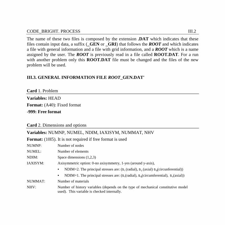
The name of these two files is composed by the extension .DAT which indicates that these files contain input data, a suffix (_GEN or _GRI) that follows the ROOT and which indicates a file with general information and a file with grid information, and a ROOT which is a name assigned by the user. The ROOT is previously read in a file called ROOT.DAT. For a run with another problem only this ROOT.DAT file must be changed and the files of the new problem will be used. III.3. GENERAL INFORMATION FILE ROOT_GEN.DAT' Card 1. Problem Variables: HEAD Format: (A40): Fixed format -999: Free format Card 2. Dimensions and options Variables: NUMNP, NUMEL, NDIM, IAXISYM, NUMMAT, NHV Format: (10I5). It is not required if free format is used NUMNP: Number of nodes NUMEL: Number of elements NDIM: Space dimensions (1,2,3) IAXISYM: Axisymmetric option: 0-no axisymmetry, 1-yes (around y-axis),
· NDIM=2. The principal stresses are: (sr (radial), sy (axial) sq(circunferential)) · NDIM=1. The principal stresses are: (sr(radial), sq(circumferential), sz(axial))
NUMMAT: Number of materials NHV: Number of history variables (depends on the type of mechanical constitutive model
used). This variable is checked internally.

CODE_BRIGHT. PROCESS III.3
Card 3. Dimensions and options Variables: NZ1, NZ2, MFRONTH, NDF, MNVAL, ISOLVE Format: (10I5). It is not required if free format is used NZ1: =MXDIFN: maximum difference between connected nodes, this variable is read for
dimensioning purposes. The node numeration of the grid is assumed to have been optimised in order to reduce the matrix band width. If q=e=0 are used in a non-mechanical problem, then MXDIFN can be 0 because a quasi-explicit approximation will be used, i.e. only a NDF-diagonal matrix is solved which contains derivatives of the storage terms. (See below for NZ=NZ1*NZ2).
NZ2: =MBANDT: total band width (geometrical for 1 variable), (MBANDT = 2(MXDIFN+1)-1, the user should provide a value but the code checks this value. So this entry is redundant.
NZ= NZ1*NZ2:
Used only for ISOLVE=5. It is the number of nonzero-blocks in the jacobian (i.e. the number of nonzeros for NDF=1). This variable is computed as NZ=NZ1*NZ2. Since this variable is checked internally, if the number of nonzeros is not known a priori, a guess can be used and the code automatically checks its validity. Otherwise, the required value is output.
MFRONTH: void NDF: Number of degrees of freedom per node. For instance a 2-dimension thermomechanical
analysis requires NDF=3. MNVAL: Maximum number of integration points in an element (default=1). For a two-dimensional
analysis with some (not necessarily all) quadrilateral elements, MNVAL=4. For a three-dimensional analysis with some (not necessarily all) quadrilateral prism elements, MNVAL=8.
ISOLVE: solve the system of equations according to different algorithms. ISOLVE=3: LU decomposition + backsubstitution (NAG subroutines, fonts
available). (recommended option for direct solution). ISOLVE=5: Sparse storage + CGS (conjugate gradients squared)

CODE_BRIGHT. PROCESS III.4
Card 4. Dimension boundary conditions Variables: NFDTYPE, NFLUXTYPE Format: (5I5). It is not required if free format is used NFDTYPE: Number of prescribed force/displacement boundary condition types.
NFDTYPE<=NUMNP because the maximum types that can be defined is limited by one per node. If IOPTDISPL > 0 then NFDTYPE>= 1.
NFLUXTYPE: Number of flux boundary condition types. NFLUXTYPE<=NUMNP. Boundary conditions for mass and energy balance problems are grouped in a single type due to practical reasons. See Cards 17 to 20 for information about the form of boundary conditions.
Boundary conditions can be applied at all nodes, even in the internal nodes. Card 5. Options. Unknowns to be calculated. Variables: IOPTDISPL, IOPTPL, IOPTPG, IOPTTEMP, IOPTXWS Format: (10I5). It is not required if free format is used IOPTDISPL: =1, solving for NDIM displacements (ux,uy,uz) IOPTPL: =1, solving for liquid pressure (Pl) (see IOPTPC) IOPTPG: =1, solving for gas pressure (Pg) IOPTTEMP: =1, solving for temperature (T) IOPTXWS: =2, solving for a solute in liquid phase (c)
CODE_BRIGHT. PROCESS III.5
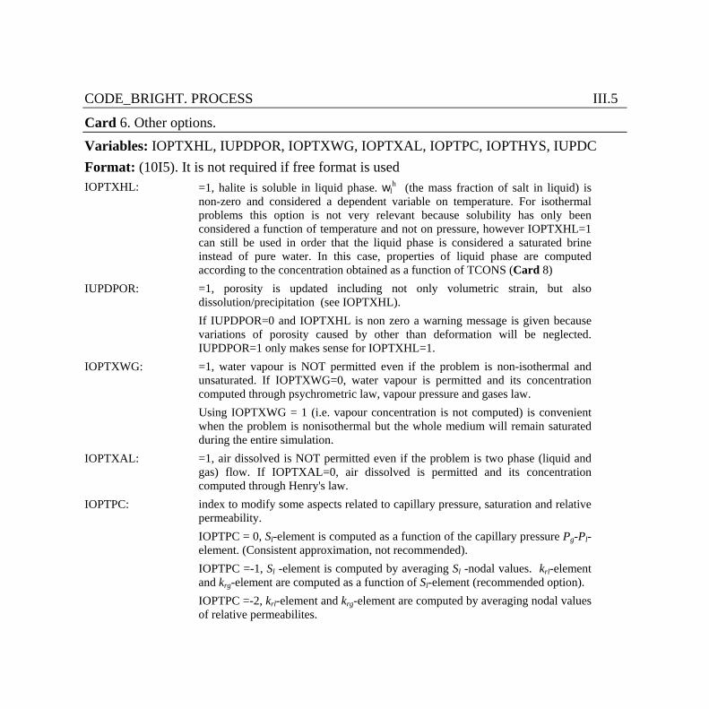
Card 6. Other options. Variables: IOPTXHL, IUPDPOR, IOPTXWG, IOPTXAL, IOPTPC, IOPTHYS, IUPDC Format: (10I5). It is not required if free format is used IOPTXHL: =1, halite is soluble in liquid phase. wl
h (the mass fraction of salt in liquid) is non-zero and considered a dependent variable on temperature. For isothermal problems this option is not very relevant because solubility has only been considered a function of temperature and not on pressure, however IOPTXHL=1 can still be used in order that the liquid phase is considered a saturated brine instead of pure water. In this case, properties of liquid phase are computed according to the concentration obtained as a function of TCONS (Card 8)
IUPDPOR: =1, porosity is updated including not only volumetric strain, but also dissolution/precipitation (see IOPTXHL). If IUPDPOR=0 and IOPTXHL is non zero a warning message is given because variations of porosity caused by other than deformation will be neglected. IUPDPOR=1 only makes sense for IOPTXHL=1.
IOPTXWG: =1, water vapour is NOT permitted even if the problem is non-isothermal and unsaturated. If IOPTXWG=0, water vapour is permitted and its concentration computed through psychrometric law, vapour pressure and gases law. Using IOPTXWG = 1 (i.e. vapour concentration is not computed) is convenient when the problem is nonisothermal but the whole medium will remain saturated during the entire simulation.
IOPTXAL: =1, air dissolved is NOT permitted even if the problem is two phase (liquid and gas) flow. If IOPTXAL=0, air dissolved is permitted and its concentration computed through Henry's law.
IOPTPC: index to modify some aspects related to capillary pressure, saturation and relative permeability. IOPTPC = 0, Sl-element is computed as a function of the capillary pressure Pg-Pl-element. (Consistent approximation, not recommended). IOPTPC =-1, Sl -element is computed by averaging Sl -nodal values. krl-element and krg-element are computed as a function of Sl-element (recommended option). IOPTPC =-2, krl-element and krg-element are computed by averaging nodal values of relative permeabilites.

CODE_BRIGHT. PROCESS III.6
IOPTPC =-3, krl-element and krg-element are computed by averaging nodal values. Derivatives of relative permeabilities are also averaged. IOPTPC =-4, krl-element and krg-element are set equal to the maximum nodal value. IOPTPC = 1: capillary pressure is used (Pc = Pg-Pl) as state variable instead of Pl. If IOPTPC is = 1 then it is necessary to use IOPTXAL=1 and IOPTXWG=1, and IOPTDISPL=0 and IOPTTEMP=0. That is, IOPTPC=1 is only available for two phase immiscible fluids.
IOPTHYS: = 1: option for hysteretic behaviour of retention curve IUPDC: = 1: updated lagrangian method, i.e., co-ordinates are modified after each time
increment is solved. If deformations are very large, some elements may distort. If distortion is very large the volume of an element may become negative and the execution would terminate immediately.
Remarks: vapour and air dissolved are considered automatically depending on options in Card 5. However, if for any reason they want not to be considered, then the auxiliary indexes IOPTXWG=1 or IOPTXAL=1 can be used. Card 7. Flags. Auxiliary options. Variables: IFLAG1, IFLAG2, IFLAG3, IFLAG4, IGLAG5 Format: (10I5). It is not required if free format is used IFLAG1: 0 IFLAG2: 0 IFLAG3: 0 IFLAG4: 0 IFLAG5: 0
These options have been introduced for programming purposes. In general users should not use them.
CODE_BRIGHT. PROCESS III.7
Card 8. Constants. Variables: EPSILON, THETA, PGCONS, TCONS, PLCONS Format: (6F10.0). It is not required if free format is used EPSILON: Position of intermediate time tk+e for matrix evaluation, i.e. the point where the non-
linear functions are computed. (frequent values: 0.5, 1) THETA: Position of intermediate time tk+q for vector evaluation, i.e. the point where the
equation is accomplished. (frequent values: 0.5, 1) PGCONS: Constant gas phase pressure for solving with IOPTPG=0, otherwise ignored. (frequent
value: 0.1 MPa = atmospheric pressure). TCONS: Constant temperature for solving with IOPTTEMP=0, otherwise this value is ignored. PLCONS: Constant liquid phase pressure for solving with IOPTPL=0, otherwise ignored. (if
PLCONS is greater than -1.0 x 10¹⁰ then wet conditions are assumed for computing viscous coefficients in creep laws. (Otherwise the medium is considered dry.)
Card 9. Void. This line should be left blank. Card 10. Options. Variables: IOWIT, INTER, ITERMAX, IOWCONTOURS, ITERMAXS, ITIME, IMBACKUP, IWRALL, IPOLYFILES Format: (10I5). It is not required if free format is used IOWIT: Iteration information is written in file ROOT_GEN.OUT according to:
IOWIT=0, no information about convergence is written. This option should be used if the user is very confident with the time discretization and not interested in details at every time step or problems with time increment reductions. Usually this happens when previous runs have shown that convergence and time discretization work very well. IOWIT=1, partial information is written. Time intervals and time-values,
CODE_BRIGHT. PROCESS III.8 number of iterations, CPU-time values, etc. are written. Convergence information is only written if time increment reductions take place. IOWIT=2, all iteration information is written. Convergence information is written for all iterations and all time increments. This option may result in a very large file ROOT_GEN.OUT
INTER: Writing results frequency in ROOT_OUT.OUT or in ROOT.FLAVIA.RES. For instance, if INTER=20 results will be written only every 20 time increments, results at intermediate points will be lost, except the values at few nodes or elements that may be requested in the ROOT_GRI.DAT file (see below).
ITERMAX: Maximum number of iterations per time increment IOWCONTOURS:
Option for writing results in files GID post processor. IOWCONTOURS=2 then files of nodal values for GiD are generated. These are ROOT.flavia.dat and ROOT.flavia.res. IOWCONTOURS=5 or 6 then files for new GiD output (nodal variables at nodes, Gauss point variables at Gauss points without smoothing) are generated. These are ROOT.post.msh and ROOT.post.res. If IOWCONTOURS=5, only one Gauss point of each element is printed (average value). IF IOWCONTOURS=6, all Gauss points are printed for all elements.
ITERMAXS: Maximum number of iterations for the solver, i.e. for Conjugate Gradients Squared solution (this variable is only required for ISOLVE=5).
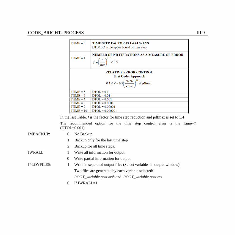
ITIME (see table: 0 No time step prediction 1 Time step prediction according to number of iterations 6 A new time step is predicted from the relative error in variables of the
previous time increment. If the relative error is less than dtol=0.01, time increment is reduced according to error deviation.
7 The same as 6, but with dtol=0.001. 8 The same as 6, but with dtol = 0.0001. 9 The same as 6, but with dtol = 0.00001. 10 The same as 6, but with dtol = 0.000001.
CODE_BRIGHT. PROCESS III.9
In the last Table, f is the factor for time step reduction and pdfmax is set to 1.4 The recommended option for the time step control error is the Itime=7 (DTOL=0.001)
IMBACKUP: 0 No Backup 1 Backup only for the last time step 2 Backup for all time steps.
IWRALL: 1 Write all information for output 0 Write partial information for output
IPLOYFILES: 1 Write in separated output files (Select variables in output window). Two files are generated by each variable selected: ROOT_variable.post.msh and ROOT_variable.post.res 0 If IWRALL=1
CODE_BRIGHT. PROCESS III.10
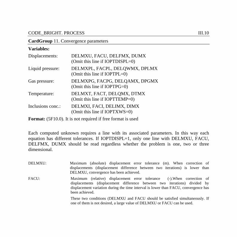
CardGroup 11. Convergence parameters Variables: Displacements: DELMXU, FACU, DELFMX, DUMX (Omit this line if IOPTDISPL=0) Liquid pressure: DELMXPL, FACPL, DELQWMX, DPLMX (Omit this line if IOPTPL=0) Gas pressure: DELMXPG, FACPG, DELQAMX, DPGMX (Omit this line if IOPTPG=0) Temperature: DELMXT, FACT, DELQMX, DTMX (Omit this line if IOPTTEMP=0) Inclusions conc.: DELMXI, FACI, DELIMX, DIMX (Omit this line if IOPTXWS=0) Format: (5F10.0). It is not required if free format is used Each computed unknown requires a line with its associated parameters. In this way each equation has different tolerances. If IOPTDISPL=1, only one line with DELMXU, FACU, DELFMX, DUMX should be read regardless whether the problem is one, two or three dimensional. DELMXU: Maximum (absolute) displacement error tolerance (m). When correction of
displacements (displacement difference between two iterations) is lower than DELMXU, convergence has been achieved.
FACU: Maximum (relative) displacement error tolerance (-).When correction of displacements (displacement difference between two iterations) divided by displacement variation during the time interval is lower than FACU, convergence has been achieved. These two conditions (DELMXU and FACU should be satisfied simultaneously. If one of them is not desired, a large value of DELMXU or FACU can be used.
CODE_BRIGHT. PROCESS III.11
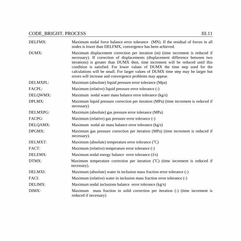
DELFMX: Maximum nodal force balance error tolerance (MN). If the residual of forces in all nodes is lower than DELFMX, convergence has been achieved.
DUMX: Maximum displacement correction per iteration (m) (time increment is reduced if necessary). If correction of displacements (displacement difference between two iterations) is greater than DUMX then, time increment will be reduced until this condition is satisfied. For lower values of DUMX the time step used for the calculations will be small. For larger values of DUMX time step may be larger but errors will increase and convergence problems may appear.
DELMXPL: Maximum (absolute) liquid pressure error tolerance (Mpa) FACPL: Maximum (relative) liquid pressure error tolerance (-) DELQWMX: Maximum nodal water mass balance error tolerance (kg/s) DPLMX: Maximum liquid pressure correction per iteration (MPa) (time increment is reduced if
necessary) DELMXPG: Maximum (absolute) gas pressure error tolerance (MPa) FACPG: Maximum (relative) gas pressure error tolerance (-) DELQAMX: Maximum nodal air mass balance error tolerance (kg/s) DPGMX: Maximum gas pressure correction per iteration (MPa) (time increment is reduced if
necessary). DELMXT: Maximum (absolute) temperature error tolerance (oC) FACT: Maximum (relative) temperature error tolerance (-) DELEMX: Maximum nodal energy balance error tolerance (J/s) DTMX: Maximum temperature correction per iteration (oC) (time increment is reduced if
necessary). DELMXI: Maximum (absolute) water in inclusion mass fraction error tolerance (-) FACI: Maximum (relative) water in inclusion mass fraction error tolerance (-) DELIMX: Maximum nodal inclusions balance error tolerance (kg/s) DIMX: Maximum mass fraction in solid correction per iteration (-) (time increment is
reduced if necessary)
CODE_BRIGHT. PROCESS III.12
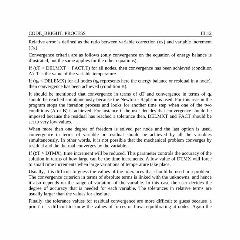
Relative error is defined as the ratio between variable correction (dx) and variable increment (Dx). Convergence criteria are as follows (only convergence on the equation of energy balance is illustrated, but the same applies for the other equations): If (dT < DELMXT + FACT.T) for all nodes, then convergence has been achieved (condition A). T is the value of the variable temperature. If (qh < DELEMX) for all nodes (qh represents here the energy balance or residual in a node), then convergence has been achieved (condition B). It should be mentioned that convergence in terms of dT and convergence in terms of qh should be reached simultaneously because the Newton - Raphson is used. For this reason the program stops the iteration process and looks for another time step when one of the two conditions (A or B) is achieved. For instance if the user decides that convergence should be imposed because the residual has reached a tolerance then, DELMXT and FACT should be set to very low values. When more than one degree of freedom is solved per node and the last option is used, convergence in terms of variable or residual should be achieved by all the variables simultaneously. In other words, it is not possible that the mechanical problem converges by residual and the thermal converges by the variable. If (dT > DTMX), time increment will be reduced. This parameter controls the accuracy of the solution in terms of how large can be the time increments. A low value of DTMX will force to small time increments when large variations of temperature take place. Usually, it is difficult to guess the values of the tolerances that should be used in a problem. The convergence criterion in terms of absolute terms is linked with the unknowns, and hence it also depends on the range of variation of the variable. In this case the user decides the degree of accuracy that is needed for each variable. The tolerances in relative terms are usually larger than the values for absolute. Finally, the tolerance values for residual convergence are more difficult to guess because 'a priori' it is difficult to know the values of forces or flows equilibrating at nodes. Again the
CODE_BRIGHT. PROCESS III.13
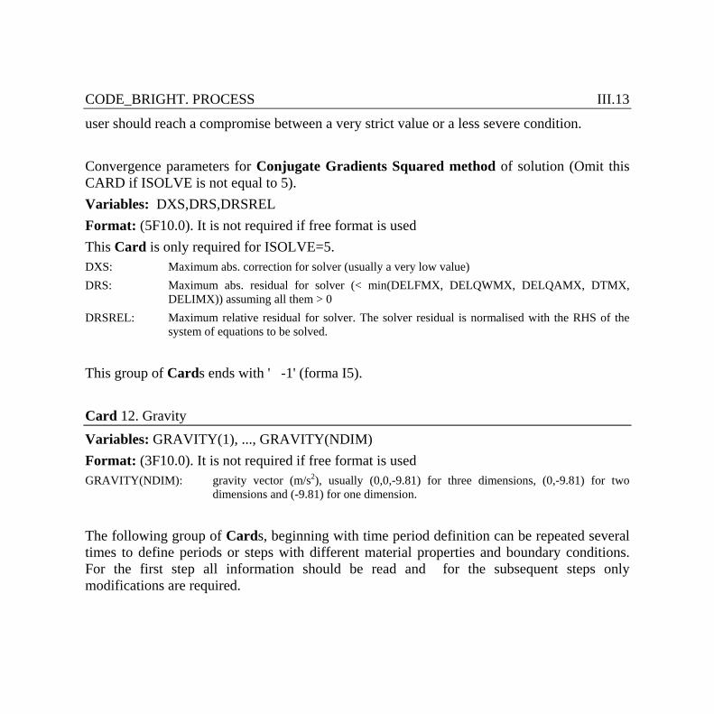
user should reach a compromise between a very strict value or a less severe condition. Convergence parameters for Conjugate Gradients Squared method of solution (Omit this CARD if ISOLVE is not equal to 5). Variables: DXS,DRS,DRSREL Format: (5F10.0). It is not required if free format is used This Card is only required for ISOLVE=5. DXS: Maximum abs. correction for solver (usually a very low value) DRS: Maximum abs. residual for solver (< min(DELFMX, DELQWMX, DELQAMX, DTMX,
DELIMX)) assuming all them > 0 DRSREL: Maximum relative residual for solver. The solver residual is normalised with the RHS of the
system of equations to be solved.
This group of Cards ends with ' -1' (forma I5). Card 12. Gravity Variables: GRAVITY(1), ..., GRAVITY(NDIM) Format: (3F10.0). It is not required if free format is used GRAVITY(NDIM): gravity vector (m/s2), usually (0,0,-9.81) for three dimensions, (0,-9.81) for two
dimensions and (-9.81) for one dimension.
The following group of Cards, beginning with time period definition can be repeated several times to define periods or steps with different material properties and boundary conditions. For the first step all information should be read and for the subsequent steps only modifications are required.
CODE_BRIGHT. PROCESS III.14
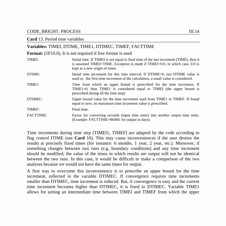
Card 13. Period time variables Variables: TIMEI, DTIME, TIME1, DTIMEC, TIMEF, FACTTIME Format: (5F10.0), It is not required if free format is used TIMEI: Initial time. If TIMEI is not equal to final time of the last increment (TIME), then it
is assumed TIMEI=TIME. Exception is made if TIMEI=0.0, in which case, 0.0 is kept as a new origin of times.
DTIME: Initial time increment for this time interval. If DTIME=0, last DTIME value is used or, the first time increment of the calculation, a small value is considered.
TIME1: Time from which an upper bound is prescribed for the time increment. If TIME1=0, then TIME1 is considered equal to TIMEI (the upper bound is prescribed during all the time step)
DTIMEC: Upper bound value for the time increment used from TIME1 to TIMEF. If found equal to zero, no maximum time increment value is prescribed.
TIMEF: Final time. FACTTIME: Factor for converting seconds (input time units) into another output time units.
(Example: FACTTIME=86400. for output in days).
Time increments during time step [TIMEI1, TIMEF] are adapted by the code according to flag control ITIME (see Card 10). This may cause inconveniences if the user desires the results at precisely fixed times (for instance: 6 months, 1 year, 2 year, etc.). Moreover, if something changes between two runs (e.g. boundary conditions) and any time increment should be modified, the value of the times in which results are output will not be identical between the two runs. In this case, it would be difficult to make a comparison of the two analyses because we would not have the same times for output. A first way to overcome this inconvenience is to prescribe an upper bound for the time increment, reflected in the variable DTIMEC. If convergence requires time increments smaller than DTIMEC, time increment is reduced. But, if convergence is easy and the current time increment becomes higher than DTIMEC, it is fixed to DTIMEC. Variable TIME1 allows for setting an intermediate time between TIMEI and TIMEF from which the upper
CODE_BRIGHT. PROCESS III.15
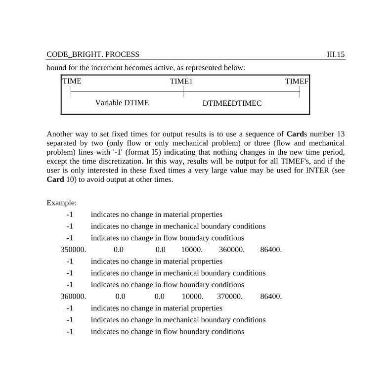
bound for the increment becomes active, as represented below:
Another way to set fixed times for output results is to use a sequence of Cards number 13 separated by two (only flow or only mechanical problem) or three (flow and mechanical problem) lines with '-1' (format I5) indicating that nothing changes in the new time period, except the time discretization. In this way, results will be output for all TIMEF's, and if the user is only interested in these fixed times a very large value may be used for INTER (see Card 10) to avoid output at other times. Example:
-1 indicates no change in material properties -1 indicates no change in mechanical boundary conditions -1 indicates no change in flow boundary conditions
350000. 0.0 0.0 10000. 360000. 86400. -1 indicates no change in material properties -1 indicates no change in mechanical boundary conditions -1 indicates no change in flow boundary conditions
360000. 0.0 0.0 10000. 370000. 86400. -1 indicates no change in material properties -1 indicates no change in mechanical boundary conditions -1 indicates no change in flow boundary conditions
TIME TIME1 TIMEF
Variable DTIME DTIME£DTIMEC
CODE_BRIGHT. PROCESS III.16
in this case for the times 350000, 360000 and 370000 the results would be written. Time step in this case would be lesser or equal than 10000. It is is possible to define at the beginning of the calculation a step for equilibration of the initial stress state. This is done by defining a time step starting from a negative value (TIMEI <0) and ending at 0 (TIMEF = 0). During this step, gravity is applied as a ramp. Greater is time step (TIMEF – TIMEMAX), smoother is the gravity ramp. Card 14. Number of material Variables: IMAT Format: (I5). It is not required if free format is used IMAT: index of material (<= NUMMAT) (if '-1' (format I5) is read, no more materials are read, and hence, parameters will be zero (or default values when defined) or the value read in a former time period) Card 15. Number and name of constitutive law Variables: ICL, TIT, ITYCL Format: (I5, A20; I5). It is not required if free format is used ICL: index of constitutive law (if '-1' (format I5) is read, no more constitutive laws are read for this
material). Each process considered needs one or more ICL's. TIT: text to identify (by the user) the constitutive law (ex: Retention curve), this text will be
reproduced on output only for the user reference but will not be used by the program. ITYCL: type of constitutive law. For each value of ICL several relationships (different values of
ITYCL) may be available.
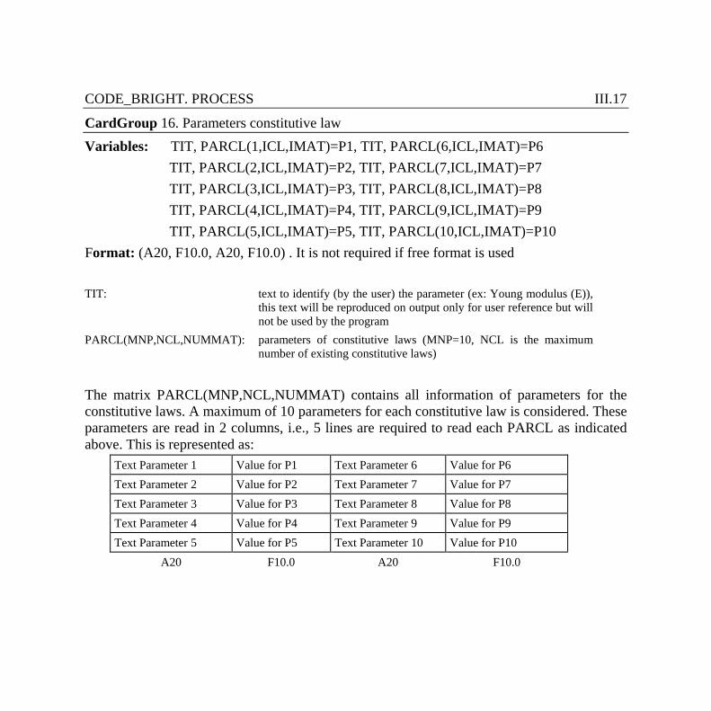
CODE_BRIGHT. PROCESS III.17
CardGroup 16. Parameters constitutive law Variables: TIT, PARCL(1,ICL,IMAT)=P1, TIT, PARCL(6,ICL,IMAT)=P6
TIT, PARCL(2,ICL,IMAT)=P2, TIT, PARCL(7,ICL,IMAT)=P7 TIT, PARCL(3,ICL,IMAT)=P3, TIT, PARCL(8,ICL,IMAT)=P8 TIT, PARCL(4,ICL,IMAT)=P4, TIT, PARCL(9,ICL,IMAT)=P9 TIT, PARCL(5,ICL,IMAT)=P5, TIT, PARCL(10,ICL,IMAT)=P10
Format: (A20, F10.0, A20, F10.0) . It is not required if free format is used TIT: text to identify (by the user) the parameter (ex: Young modulus (E)),
this text will be reproduced on output only for user reference but will not be used by the program
PARCL(MNP,NCL,NUMMAT): parameters of constitutive laws (MNP=10, NCL is the maximum number of existing constitutive laws)
The matrix PARCL(MNP,NCL,NUMMAT) contains all information of parameters for the constitutive laws. A maximum of 10 parameters for each constitutive law is considered. These parameters are read in 2 columns, i.e., 5 lines are required to read each PARCL as indicated above. This is represented as:
Text Parameter 1 Value for P1 Text Parameter 6 Value for P6 Text Parameter 2 Value for P2 Text Parameter 7 Value for P7 Text Parameter 3 Value for P3 Text Parameter 8 Value for P8 Text Parameter 4 Value for P4 Text Parameter 9 Value for P9 Text Parameter 5 Value for P5 Text Parameter 10 Value for P10
A20 F10.0 A20 F10.0
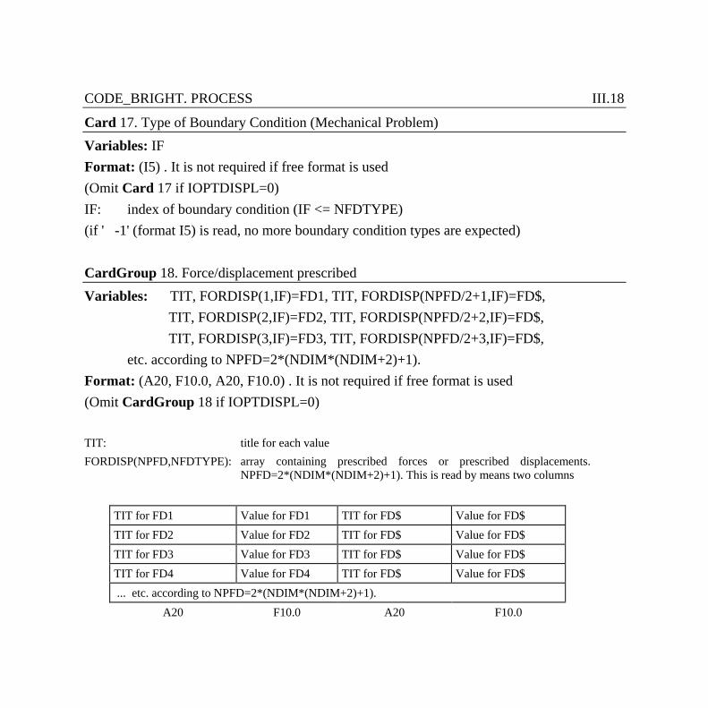
CODE_BRIGHT. PROCESS III.18
Card 17. Type of Boundary Condition (Mechanical Problem) Variables: IF Format: (I5) . It is not required if free format is used (Omit Card 17 if IOPTDISPL=0) IF: index of boundary condition (IF <= NFDTYPE) (if ' -1' (format I5) is read, no more boundary condition types are expected) CardGroup 18. Force/displacement prescribed Variables: TIT, FORDISP(1,IF)=FD1, TIT, FORDISP(NPFD/2+1,IF)=FD$,
TIT, FORDISP(2,IF)=FD2, TIT, FORDISP(NPFD/2+2,IF)=FD$, TIT, FORDISP(3,IF)=FD3, TIT, FORDISP(NPFD/2+3,IF)=FD$,
etc. according to NPFD=2*(NDIM*(NDIM+2)+1). Format: (A20, F10.0, A20, F10.0) . It is not required if free format is used (Omit CardGroup 18 if IOPTDISPL=0) TIT: title for each value FORDISP(NPFD,NFDTYPE): array containing prescribed forces or prescribed displacements.
NPFD=2*(NDIM*(NDIM+2)+1). This is read by means two columns
TIT for FD1 Value for FD1 TIT for FD$ Value for FD$ TIT for FD2 Value for FD2 TIT for FD$ Value for FD$ TIT for FD3 Value for FD3 TIT for FD$ Value for FD$ TIT for FD4 Value for FD4 TIT for FD$ Value for FD$ ... etc. according to NPFD=2*(NDIM*(NDIM+2)+1).
A20 F10.0 A20 F10.0
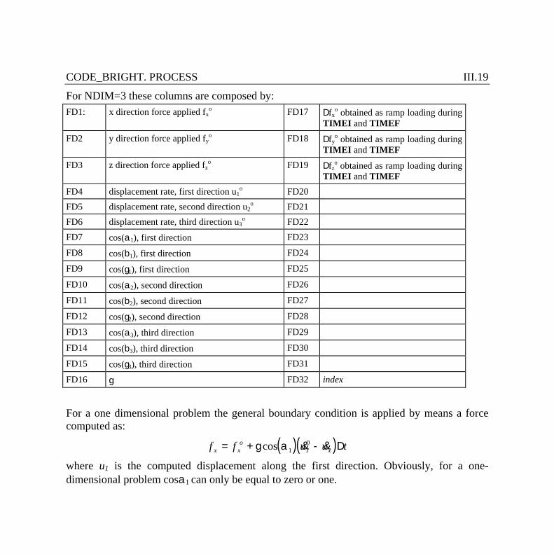
CODE_BRIGHT. PROCESS III.19
For NDIM=3 these columns are composed by: FD1: x direction force applied fx
o FD17 Dfxo obtained as ramp loading during
TIMEI and TIMEF FD2 y direction force applied fy
o FD18 Dfyo obtained as ramp loading during
TIMEI and TIMEF FD3 z direction force applied fz
o FD19 Dfzo obtained as ramp loading during
TIMEI and TIMEF FD4 displacement rate, first direction u1
o FD20 FD5 displacement rate, second direction u2
o FD21 FD6 displacement rate, third direction u3
o FD22 FD7 cos(a1), first direction FD23
FD8 cos(b1), first direction FD24
FD9 cos(g1), first direction FD25
FD10 cos(a2), second direction FD26
FD11 cos(b2), second direction FD27
FD12 cos(g2), second direction FD28
FD13 cos(a3), third direction FD29
FD14 cos(b3), third direction FD30
FD15 cos(g3), third direction FD31
FD16 g FD32 index
For a one dimensional problem the general boundary condition is applied by means a force computed as:
( )( )f f u u tx xo
x= + -g acos & &1 10 D
where u1 is the computed displacement along the first direction. Obviously, for a one-dimensional problem cosa1 can only be equal to zero or one.
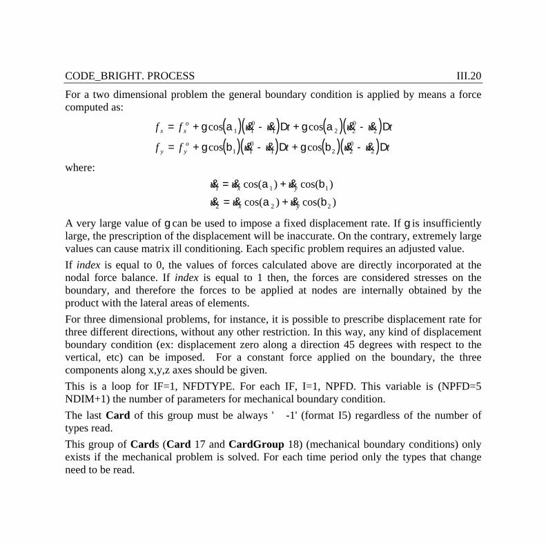
CODE_BRIGHT. PROCESS III.20
For a two dimensional problem the general boundary condition is applied by means a force computed as:
( )( ) ( )( )( )( ) ( )( )
f f u u t u u t
f f u u t u u tx x
o
y yo
= + - + -
= + - + -
g a g a
g b g b
cos & & cos & &
cos & & cos & &
1 10
1 2 20
2
1 10
1 2 20
2
D D
D D
where: & & cos( ) & cos( )& & cos( ) & cos( )u u uu u u
x y
x y
1 1 1
2 2 2
= +
= +
a b
a b
A very large value of g can be used to impose a fixed displacement rate. If g is insufficiently large, the prescription of the displacement will be inaccurate. On the contrary, extremely large values can cause matrix ill conditioning. Each specific problem requires an adjusted value. If index is equal to 0, the values of forces calculated above are directly incorporated at the nodal force balance. If index is equal to 1 then, the forces are considered stresses on the boundary, and therefore the forces to be applied at nodes are internally obtained by the product with the lateral areas of elements. For three dimensional problems, for instance, it is possible to prescribe displacement rate for three different directions, without any other restriction. In this way, any kind of displacement boundary condition (ex: displacement zero along a direction 45 degrees with respect to the vertical, etc) can be imposed. For a constant force applied on the boundary, the three components along x,y,z axes should be given. This is a loop for IF=1, NFDTYPE. For each IF, I=1, NPFD. This variable is (NPFD=5 NDIM+1) the number of parameters for mechanical boundary condition. The last Card of this group must be always ' -1' (format I5) regardless of the number of types read. This group of Cards (Card 17 and CardGroup 18) (mechanical boundary conditions) only exists if the mechanical problem is solved. For each time period only the types that change need to be read.
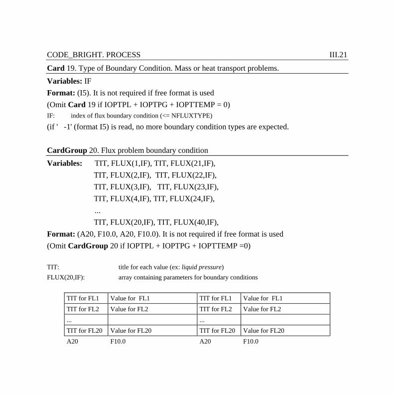
CODE_BRIGHT. PROCESS III.21
Card 19. Type of Boundary Condition. Mass or heat transport problems. Variables: IF Format: (I5). It is not required if free format is used (Omit Card 19 if IOPTPL + IOPTPG + IOPTTEMP = 0) IF: index of flux boundary condition (<= NFLUXTYPE)
(if ' -1' (format I5) is read, no more boundary condition types are expected. CardGroup 20. Flux problem boundary condition Variables: TIT, FLUX(1,IF), TIT, FLUX(21,IF),
TIT, FLUX(2,IF), TIT, FLUX(22,IF), TIT, FLUX(3,IF), TIT, FLUX(23,IF), TIT, FLUX(4,IF), TIT, FLUX(24,IF),
... TIT, FLUX(20,IF), TIT, FLUX(40,IF),
Format: (A20, F10.0, A20, F10.0). It is not required if free format is used (Omit CardGroup 20 if IOPTPL + IOPTPG + IOPTTEMP =0) TIT: title for each value (ex: liquid pressure) FLUX(20,IF): array containing parameters for boundary conditions
TIT for FL1 Value for FL1 TIT for FL1 Value for FL1 TIT for FL2 Value for FL2 TIT for FL2 Value for FL2 ... ... TIT for FL20 Value for FL20 TIT for FL20 Value for FL20 A20 F10.0 A20 F10.0
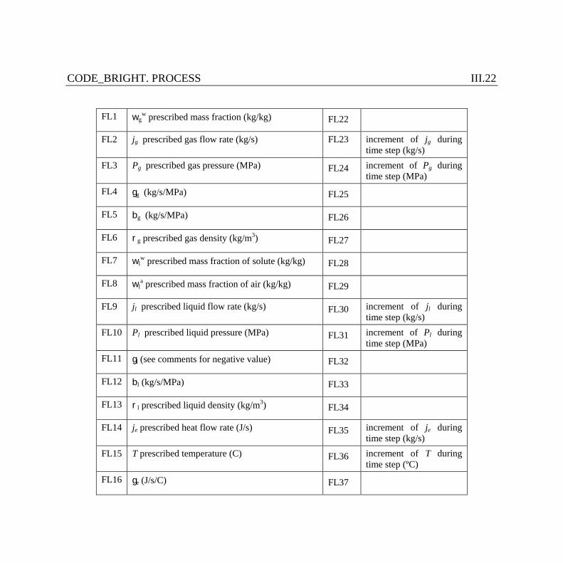
CODE_BRIGHT. PROCESS III.22
FL1 wg
w prescribed mass fraction (kg/kg) FL22 FL2 jg prescribed gas flow rate (kg/s) FL23 increment of jg during
time step (kg/s) FL3 Pg prescribed gas pressure (MPa) FL24 increment of Pg during
time step (MPa) FL4 gg (kg/s/MPa) FL25 FL5 bg (kg/s/MPa) FL26 FL6 rg prescribed gas density (kg/m3) FL27 FL7 wl
w prescribed mass fraction of solute (kg/kg) FL28 FL8 wl
a prescribed mass fraction of air (kg/kg) FL29 FL9 jl prescribed liquid flow rate (kg/s) FL30 increment of jl during
time step (kg/s) FL10 Pl prescribed liquid pressure (MPa) FL31 increment of Pl during
time step (MPa) FL11 gl (see comments for negative value) FL32 FL12 bl (kg/s/MPa) FL33 FL13 rl prescribed liquid density (kg/m3) FL34 FL14 je prescribed heat flow rate (J/s) FL35 increment of je during
time step (kg/s) FL15 T prescribed temperature (C) FL36 increment of T during
time step (ºC) FL16 ge (J/s/C) FL37
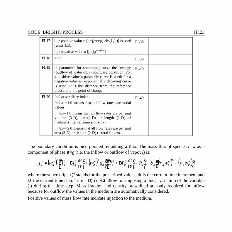
CODE_BRIGHT. PROCESS III.23
FL17 le : positive values: [je=je*exp(-abs(le)t)] is used (units 1/s). le : negative values: [je=jet-abs(le)]
FL38
FL18 void FL39 FL19 d: parameter for smoothing curve the seepage
(outflow of water only) boundary condition. For a positive value a parabolic curve is used; for a negative value an exponentially decaying curve is used. d is the distance from the reference pressure to the point of change
FL40
FL20 index: auxiliary index. index=+1.0 means that all flow rates are nodal values index=-1.0 means that all flow rates are per unit volume (3-D), area(2-D) or length (1-D) of medium (internal source or sink) index=+2.0 means that all flow rates are per unit area (3-D) or length (2-D) (lateral fluxes).
FL40
The boundary condition is incorporated by adding a flux. The mass flux of species i=w as a component of phase a=g (i.e. the inflow or outflow of vapour) is:
( ) ( ) ( ) ( )÷øöç
èæ -+÷÷
ø
öççè
æ-÷
øö
çèæ
DD++÷
øö
çèæ
DD+= w
ggwggggggg
wggg
wg
wg P
tdtPP
tdtjjj wrwrbgww
0000000
where the superscript ()o stands for the prescribed values, dt is the current time increment and Dt the current time step. Terms D(.) dt/Dt allow for imposing a linear variation of the variable (.) during the time step. Mass fraction and density prescribed are only required for inflow because for outflow the values in the medium are automatically considered. Positive values of mass flow rate indicate injection to the medium.
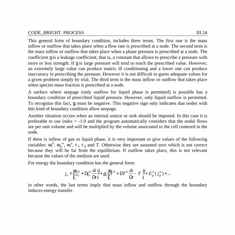
CODE_BRIGHT. PROCESS III.24
This general form of boundary condition, includes three terms. The first one is the mass inflow or outflow that takes place when a flow rate is prescribed at a node. The second term is the mass inflow or outflow that takes place when a phase pressure is prescribed at a node. The coefficient g is a leakage coefficient, that is, a constant that allows to prescribe a pressure with more or less strength. If g is large pressure will tend to reach the prescribed value. However, an extremely large value can produce matrix ill conditioning and a lower one can produce inaccuracy in prescribing the pressure. However it is not difficult to guess adequate values for a given problem simply by trial. The third term is the mass inflow or outflow that takes place when species mass fraction is prescribed at a node. A surface where seepage (only outflow for liquid phase is permitted) is possible has a boundary condition of prescribed liquid pressure. However, only liquid outflow is permitted. To recognize this fact, gl must be negative. This negative sign only indicates that nodes with this kind of boundary condition allow seepage. Another situation occurs when an internal source or sink should be imposed. In this case it is preferable to use index = -1.0 and the program automatically considers that the nodal flows are per unit volume and will be multiplied by the volume associated to the cell centered in the node. If there is inflow of gas or liquid phase, it is very important to give values of the following variables: wl
h, wgw, wl
a, rl, rg and T. Otherwise they are assumed zero which is not correct because they will be far from the equilibrium. If outflow takes place, this is not relevant because the values of the medium are used. For energy the boundary condition has the general form:
...)(0000 ++÷øö
çèæ -
DD++÷
øö
çèæ
DD+= w
gwgeeee jET
tdtTT
tdtjjj g
in other words, the last terms imply that mass inflow and outflow through the boundary induces energy transfer.

CODE_BRIGHT. PROCESS III.25
In general, this is a loop for IF=1, NFLUXTYPE. For each IF, I=1,NPFLUX. The last Card of this group must be always ' -1' (format I5). This group of Cards (Card 19 and CardGroup 20) only exists if any balance (water, air, energy flow) problem is solved. For each time period only the types that change need to be read.
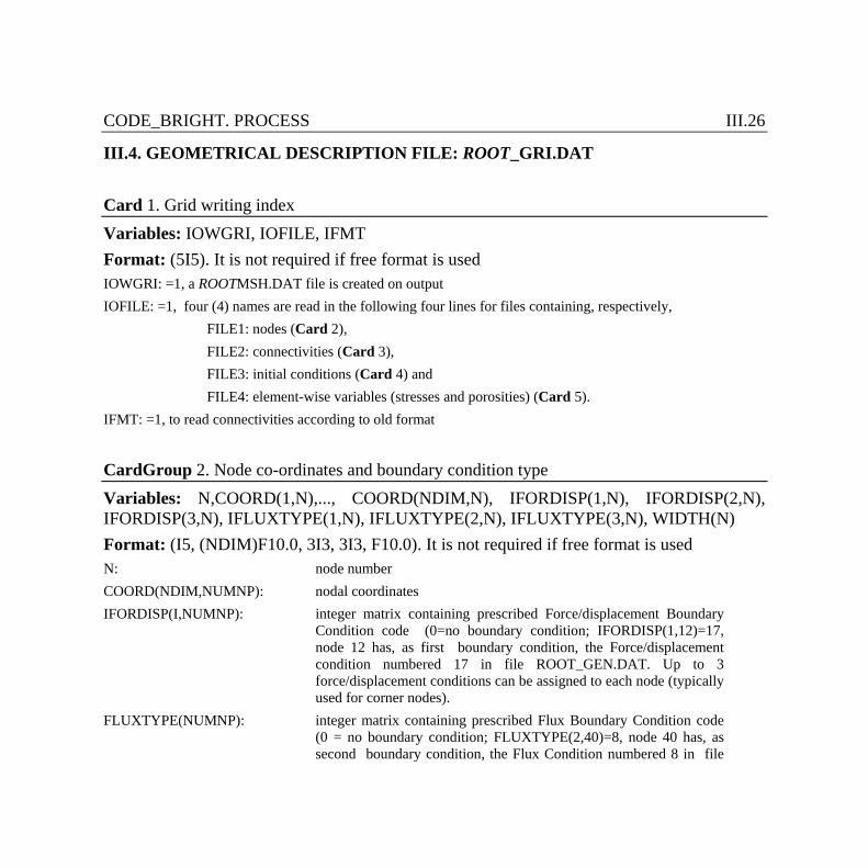
CODE_BRIGHT. PROCESS III.26
III.4. GEOMETRICAL DESCRIPTION FILE: ROOT_GRI.DAT Card 1. Grid writing index Variables: IOWGRI, IOFILE, IFMT Format: (5I5). It is not required if free format is used IOWGRI: =1, a ROOTMSH.DAT file is created on output IOFILE: =1, four (4) names are read in the following four lines for files containing, respectively,
FILE1: nodes (Card 2), FILE2: connectivities (Card 3), FILE3: initial conditions (Card 4) and FILE4: element-wise variables (stresses and porosities) (Card 5).
IFMT: =1, to read connectivities according to old format
CardGroup 2. Node co-ordinates and boundary condition type Variables: N,COORD(1,N),..., COORD(NDIM,N), IFORDISP(1,N), IFORDISP(2,N), IFORDISP(3,N), IFLUXTYPE(1,N), IFLUXTYPE(2,N), IFLUXTYPE(3,N), WIDTH(N) Format: (I5, (NDIM)F10.0, 3I3, 3I3, F10.0). It is not required if free format is used N: node number COORD(NDIM,NUMNP): nodal coordinates IFORDISP(I,NUMNP): integer matrix containing prescribed Force/displacement Boundary
Condition code (0=no boundary condition; IFORDISP(1,12)=17, node 12 has, as first boundary condition, the Force/displacement condition numbered 17 in file ROOT_GEN.DAT. Up to 3 force/displacement conditions can be assigned to each node (typically used for corner nodes).
FLUXTYPE(NUMNP): integer matrix containing prescribed Flux Boundary Condition code (0 = no boundary condition; FLUXTYPE(2,40)=8, node 40 has, as second boundary condition, the Flux Condition numbered 8 in file
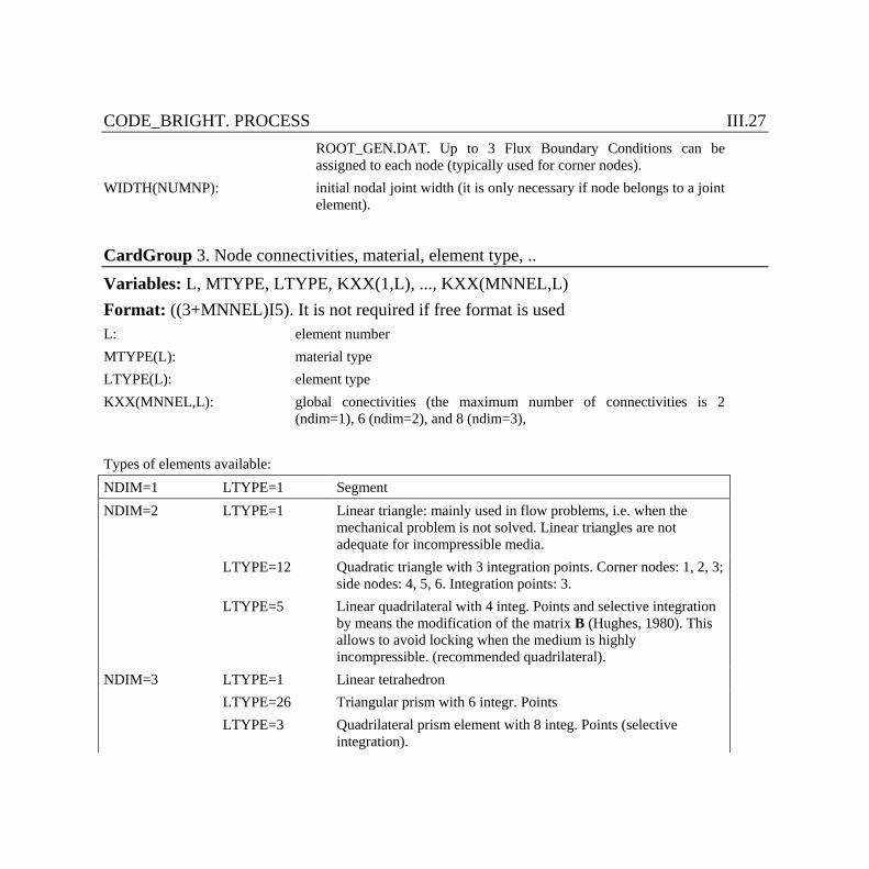
CODE_BRIGHT. PROCESS III.27 ROOT_GEN.DAT. Up to 3 Flux Boundary Conditions can be assigned to each node (typically used for corner nodes).
WIDTH(NUMNP): initial nodal joint width (it is only necessary if node belongs to a joint element).
CardGroup 3. Node connectivities, material, element type, .. Variables: L, MTYPE, LTYPE, KXX(1,L), ..., KXX(MNNEL,L) Format: ((3+MNNEL)I5). It is not required if free format is used L: element number MTYPE(L): material type LTYPE(L): element type KXX(MNNEL,L): global conectivities (the maximum number of connectivities is 2
(ndim=1), 6 (ndim=2), and 8 (ndim=3), Types of elements available: NDIM=1 LTYPE=1 Segment NDIM=2 LTYPE=1 Linear triangle: mainly used in flow problems, i.e. when the
mechanical problem is not solved. Linear triangles are not adequate for incompressible media.
LTYPE=12 Quadratic triangle with 3 integration points. Corner nodes: 1, 2, 3; side nodes: 4, 5, 6. Integration points: 3.
LTYPE=5 Linear quadrilateral with 4 integ. Points and selective integration by means the modification of the matrix B (Hughes, 1980). This allows to avoid locking when the medium is highly incompressible. (recommended quadrilateral).
NDIM=3 LTYPE=1 Linear tetrahedron LTYPE=26 Triangular prism with 6 integr. Points LTYPE=3 Quadrilateral prism element with 8 integ. Points (selective
integration).
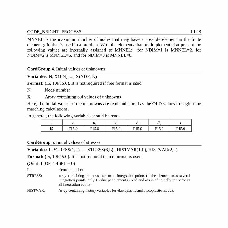
CODE_BRIGHT. PROCESS III.28
MNNEL is the maximum number of nodes that may have a possible element in the finite element grid that is used in a problem. With the elements that are implemented at present the following values are internally assigned to MNNEL: for NDIM=1 is MNNEL=2, for NDIM=2 is MNNEL=6, and for NDIM=3 is MNNEL=8. CardGroup 4. Initial values of unknowns Variables: N, X(1,N), ..., X(NDF, N) Format: (I5, 10F15.0). It is not required if free format is used N: Node number X: Array containing old values of unknowns Here, the initial values of the unknowns are read and stored as the OLD values to begin time marching calculations. In general, the following variables should be read:
n ux uy uz Pl Pg T I5 F15.0 F15.0 F15.0 F15.0 F15.0 F15.0
CardGroup 5. Initial values of stresses Variables: L, STRESS(1,L), ..., STRESS(6,L) , HISTVAR(1,L), HISTVAR(2,L) Format: (I5, 10F15.0). It is not required if free format is used (Omit if IOPTDISPL = 0) L: element number STRESS: array containing the stress tensor at integration points (if the element uses several
integration points, only 1 value per element is read and assumed initially the same in all integration points)
HISTVAR: Array containing history variables for elastoplastic and viscoplastic models
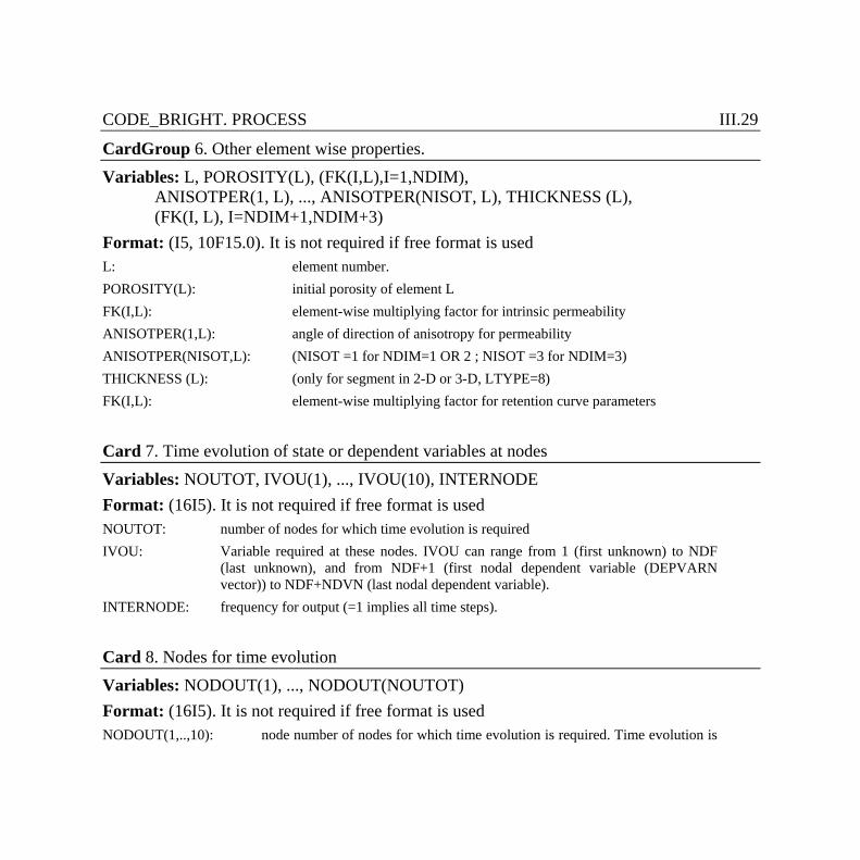
CODE_BRIGHT. PROCESS III.29
CardGroup 6. Other element wise properties. Variables: L, POROSITY(L), (FK(I,L),I=1,NDIM), ANISOTPER(1, L), ..., ANISOTPER(NISOT, L), THICKNESS (L), (FK(I, L), I=NDIM+1,NDIM+3) Format: (I5, 10F15.0). It is not required if free format is used L: element number. POROSITY(L): initial porosity of element L FK(I,L): element-wise multiplying factor for intrinsic permeability ANISOTPER(1,L): angle of direction of anisotropy for permeability ANISOTPER(NISOT,L): (NISOT =1 for NDIM=1 OR 2 ; NISOT =3 for NDIM=3) THICKNESS (L): (only for segment in 2-D or 3-D, LTYPE=8) FK(I,L): element-wise multiplying factor for retention curve parameters
Card 7. Time evolution of state or dependent variables at nodes Variables: NOUTOT, IVOU(1), ..., IVOU(10), INTERNODE Format: (16I5). It is not required if free format is used NOUTOT: number of nodes for which time evolution is required IVOU: Variable required at these nodes. IVOU can range from 1 (first unknown) to NDF
(last unknown), and from NDF+1 (first nodal dependent variable (DEPVARN vector)) to NDF+NDVN (last nodal dependent variable).
INTERNODE: frequency for output (=1 implies all time steps).
Card 8. Nodes for time evolution Variables: NODOUT(1), ..., NODOUT(NOUTOT) Format: (16I5). It is not required if free format is used NODOUT(1,..,10): node number of nodes for which time evolution is required. Time evolution is
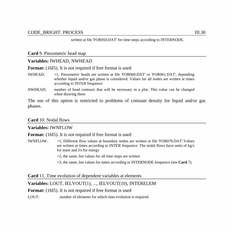
CODE_BRIGHT. PROCESS III.30 written at file 'FOR050.DAT' for time steps according to INTERNODE.
Card 9. Piezometric head map Variables: IWHEAD, NWHEAD Format: (16I5). It is not required if free format is used IWHEAD: =1, Piezometric heads are written at file 'FOR060.DAT' or 'FOR061.DAT', depending
whether liquid and/or gas phase is considered. Values for all nodes are written at times according to INTER frequence
NWHEAD: number of head contours that will be necessary in a plot. This value can be changed when drawing them
The use of this option is restricted to problems of constant density for liquid and/or gas phases. Card 10. Nodal flows Variables: IWNFLOW Format: (16I5). It is not required if free format is used IWNFLOW: =1, Different flow values at boundary nodes are written at file 'FOR070.DAT'.Values
are written at times according to INTER frequence. The nodal flows have units of kg/s for mass and J/s for energy
=2, the same, but values for all time steps are written =3, the same, but values for times according to INTERNODE frequence (see Card 7).
Card 11. Time evolution of dependent variables at elements Variables: LOUT, IELVOUT(1), ..., IELVOUT(10), INTERELEM Format: (16I5). It is not required if free format is used LOUT: number of elements for which time evolution is required.
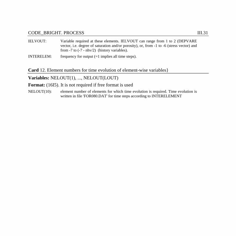
CODE_BRIGHT. PROCESS III.31
IELVOUT: Variable required at these elements. IELVOUT can range from 1 to 2 (DEPVARE vector, i.e. degree of saturation and/or porosity), or, from -1 to -6 (stress vector) and from -7 to (-7 - nhv/2) (history variables).
INTERELEM: frequency for output (=1 implies all time steps).
Card 12. Element numbers for time evolution of element-wise variables} Variables: NELOUT(1), ..., NELOUT(LOUT) Format: (16I5). It is not required if free format is used NELOUT(10): element number of elements for which time evolution is required. Time evolution is
written in file 'FOR080.DAT' for time steps according to INTERELEMENT
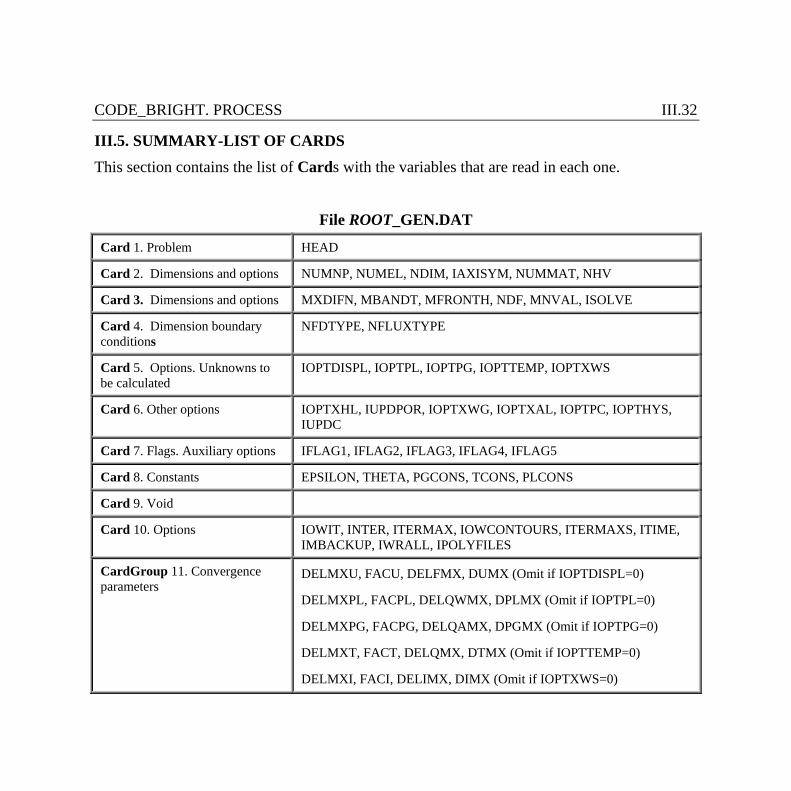
CODE_BRIGHT. PROCESS III.32
III.5. SUMMARY-LIST OF CARDS This section contains the list of Cards with the variables that are read in each one.
File ROOT_GEN.DAT
Card 1. Problem HEAD
Card 2. Dimensions and options NUMNP, NUMEL, NDIM, IAXISYM, NUMMAT, NHV
Card 3. Dimensions and options MXDIFN, MBANDT, MFRONTH, NDF, MNVAL, ISOLVE
Card 4. Dimension boundary conditions
NFDTYPE, NFLUXTYPE
Card 5. Options. Unknowns to be calculated
IOPTDISPL, IOPTPL, IOPTPG, IOPTTEMP, IOPTXWS
Card 6. Other options IOPTXHL, IUPDPOR, IOPTXWG, IOPTXAL, IOPTPC, IOPTHYS, IUPDC
Card 7. Flags. Auxiliary options IFLAG1, IFLAG2, IFLAG3, IFLAG4, IFLAG5
Card 8. Constants EPSILON, THETA, PGCONS, TCONS, PLCONS
Card 9. Void
Card 10. Options IOWIT, INTER, ITERMAX, IOWCONTOURS, ITERMAXS, ITIME, IMBACKUP, IWRALL, IPOLYFILES
CardGroup 11. Convergence parameters
DELMXU, FACU, DELFMX, DUMX (Omit if IOPTDISPL=0)
DELMXPL, FACPL, DELQWMX, DPLMX (Omit if IOPTPL=0)
DELMXPG, FACPG, DELQAMX, DPGMX (Omit if IOPTPG=0)
DELMXT, FACT, DELQMX, DTMX (Omit if IOPTTEMP=0)
DELMXI, FACI, DELIMX, DIMX (Omit if IOPTXWS=0)
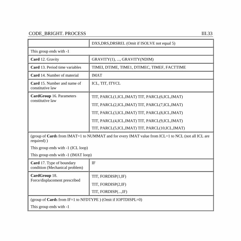
CODE_BRIGHT. PROCESS III.33
DXS,DRS,DRSREL (Omit if ISOLVE not equal 5)
This group ends with -1
Card 12. Gravity GRAVITY(1), ..., GRAVITY(NDIM)
Card 13. Period time variables TIMEI, DTIME, TIME1, DTIMEC, TIMEF, FACTTIME
Card 14. Number of material IMAT
Card 15. Number and name of constitutive law
ICL, TIT, ITYCL
CardGroup 16. Parameters constitutive law
TIT, PARCL(1,ICL,IMAT) TIT, PARCL(6,ICL,IMAT)
TIT, PARCL(2,ICL,IMAT) TIT, PARCL(7,ICL,IMAT)
TIT, PARCL(3,ICL,IMAT) TIT, PARCL(8,ICL,IMAT)
TIT, PARCL(4,ICL,IMAT) TIT, PARCL(9,ICL,IMAT) TIT, PARCL(5,ICL,IMAT) TIT, PARCL(10,ICL,IMAT)
(group of Cards from IMAT=1 to NUMMAT and for every IMAT value from ICL=1 to NCL (not all ICL are required) )
This group ends with -1 (ICL loop)
This group ends with -1 (IMAT loop)
Card 17. Type of boundary condition (Mechanical problem)
IF
CardGroup 18. Force/displacement prescribed
TIT, FORDISP(1,IF)
TIT, FORDISP(2,IF) TIT, FORDISP(...,IF)
(group of Cards from IF=1 to NFDTYPE ) (Omit if IOPTDISPL=0)
This group ends with -1
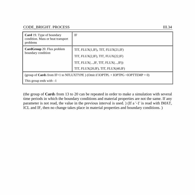
CODE_BRIGHT. PROCESS III.34
Card 19. Type of boundary condition. Mass or heat transport problems
IF
CardGroup 20. Flux problem boundary condition
TIT, FLUX(1,IF), TIT, FLUX(21,IF)
TIT, FLUX(2,IF), TIT, FLUX(22,IF)
TIT, FLUX(...,IF, TIT, FLUX(...,IF)) TIT, FLUX(20,IF), TIT, FLUX(40,IF)
(group of Cards from IF=1 to NFLUXTYPE ) (Omit if IOPTPL + IOPTPG +IOPTTEMP = 0)
This group ends with –1
(the group of Cards from 13 to 20 can be repeated in order to make a simulation with several time periods in which the boundary conditions and material properties are not the same. If any parameter is not read, the value in the previous interval is used. ) (If a '-1' is read with IMAT, ICL and IF, then no change takes place in material properties and boundary conditions. )
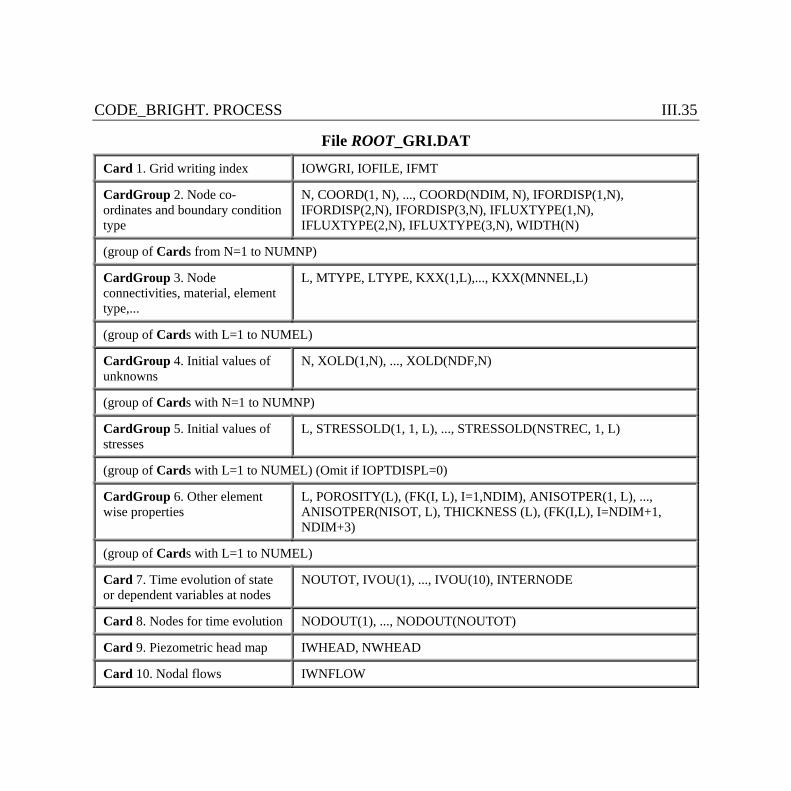
CODE_BRIGHT. PROCESS III.35
File ROOT_GRI.DAT
Card 1. Grid writing index IOWGRI, IOFILE, IFMT
CardGroup 2. Node co-ordinates and boundary condition type
N, COORD(1, N), ..., COORD(NDIM, N), IFORDISP(1,N), IFORDISP(2,N), IFORDISP(3,N), IFLUXTYPE(1,N), IFLUXTYPE(2,N), IFLUXTYPE(3,N), WIDTH(N)
(group of Cards from N=1 to NUMNP)
CardGroup 3. Node connectivities, material, element type,...
L, MTYPE, LTYPE, KXX(1,L),..., KXX(MNNEL,L)
(group of Cards with L=1 to NUMEL)
CardGroup 4. Initial values of unknowns
N, XOLD(1,N), ..., XOLD(NDF,N)
(group of Cards with N=1 to NUMNP)
CardGroup 5. Initial values of stresses
L, STRESSOLD(1, 1, L), ..., STRESSOLD(NSTREC, 1, L)
(group of Cards with L=1 to NUMEL) (Omit if IOPTDISPL=0)
CardGroup 6. Other element wise properties
L, POROSITY(L), (FK(I, L), I=1,NDIM), ANISOTPER(1, L), ..., ANISOTPER(NISOT, L), THICKNESS (L), (FK(I,L), I=NDIM+1, NDIM+3)
(group of Cards with L=1 to NUMEL)
Card 7. Time evolution of state or dependent variables at nodes
NOUTOT, IVOU(1), ..., IVOU(10), INTERNODE
Card 8. Nodes for time evolution NODOUT(1), ..., NODOUT(NOUTOT)
Card 9. Piezometric head map IWHEAD, NWHEAD
Card 10. Nodal flows IWNFLOW
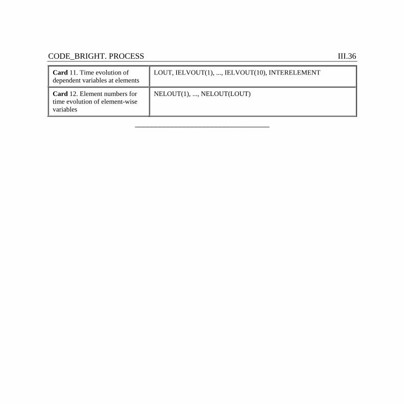
CODE_BRIGHT. PROCESS III.36
Card 11. Time evolution of dependent variables at elements
LOUT, IELVOUT(1), ..., IELVOUT(10), INTERELEMENT
Card 12. Element numbers for time evolution of element-wise variables
NELOUT(1), ..., NELOUT(LOUT)
_________________________________
CODE_BRIGHT. POSTPROCESS IV.1
CODE_BRIGHT. POSTPROCESS. IV.1. POST-PROCESSING TOOLS: SHORT DESCRIPTION The different results that the system allows to display are the following ones:
· Geometry: GiD displays the whole volumetric mesh, surface sets and boundary surfaces. It can also cut and divide them, in its original state as well as also in its deformed state, and switch them on and off. GiD displays how the meshes/sets will be deformed according to a certain vectorial variable. GiD provides two representations: on the first one all the results will then be drawn on these original or deformed meshes (Main Geomtery); on the second one, a superimposed representation (Show Geometry) is provided, that can be also deformed, but the results will still be drawn on the main representation. The user can compare the main original/deformed meshes/sets with the second representation, which can also be deformed with the same or another vector deformation, or with no deformation at all. The scaling of all the displays can be modified interactively.
· Show minimum and maximum: The minimum and maximum values of the variable for the currently viewed meshes/sets can appear, pointing all the nodes where these limits are computed, in dark blue the minimum values and in red the maximum ones.
· Vectors: GiD presents a vector distribution according to the vectorial or matrix

CODE_BRIGHT. POSTPROCESS IV.2
variables on each node, showing their magnitudes and directions. The scaling of the vectors can be modified interactively.
· Contour fields: GiD represents the variables through isosurfaces or contours that comprise all the values between two given values. GiD takes advantage of the graphical capabilities of the machine, what allows a smoothing of the results when a high number of colors is used.
· Contour lines: This representation is quite similar to the last one, but the uniform bands are substituted here by isolines, where each one ties several points with the same value.
IV.2. READ POST-PROCESSING
GiD displays a `File Open Dialog Box' and asks the user for a file. Afterwards, it looks for the files filename.msh, filename.bon and filename.res. The description of what is found and being read, sorted (if necessary) and built appears on the message bar. Sometimes, it may be useful to use the visualisation options to center and zoom the drawing on the screen, specially when the different scales affect the post-processing. All the post-processing facilities can be used for this new project, jump to the pre-processing, if desired, or go back to the previous or another project post-processings.
Other details on post-processing information are available from the GiD manual.
________________________________
CODE_BRIGHT. THEORETICAL ASPECTS V.1
CODE_BRIGHT. THEORETICAL ASPECTS
In porous media, subjected to thermal, hydraulical and mechanical conditions relevant thermo-hydro-mechanical (THM) phenomena takes place. In fact, there exist a number of mutual interactions that must be taken simultaneously into account in analyses. For instance, strains due to thermal loading will induce stress variations and changes in mass storage terms and hydraulic conductivity. The thermal expansion of the water in the pores itself causes changes in the degree of saturation or, if the material is saturated or quasi-saturated, increases of water pressure. Thermal induced vapor diffusion and the dependence of water viscosity on temperature also affect significantly the water transfer process.
On the other hand, changes in hydraulic conditions influence the temperature field via variations of thermal conductivity and affect the stress/strain field due to pore water pressure and pore gas pressure changes. Gas pressure is affected by the increase in vapour pressure with temperature. This may lead to further changes in the pattern of gas and water flow. Finally, porosity changes due to volumetric strain influence pore pressure distributions because of associated variations in storage terms and hydraulic conductivity. The effect on temperature is less important as the variations of thermal conductivity with porosity are relatively small. In Appendix 1 the most significant interactions between the various phenomena are presented in a systematic manner.
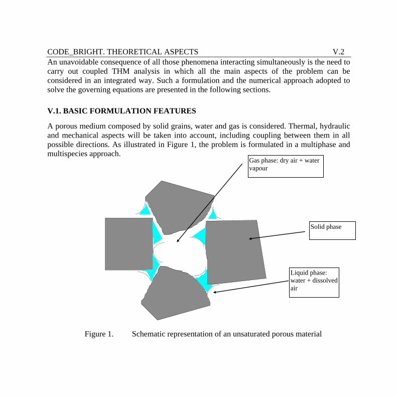
CODE_BRIGHT. THEORETICAL ASPECTS V.2
An unavoidable consequence of all those phenomena interacting simultaneously is the need to carry out coupled THM analysis in which all the main aspects of the problem can be considered in an integrated way. Such a formulation and the numerical approach adopted to solve the governing equations are presented in the following sections.
V.1. BASIC FORMULATION FEATURES
A porous medium composed by solid grains, water and gas is considered. Thermal, hydraulic and mechanical aspects will be taken into account, including coupling between them in all possible directions. As illustrated in Figure 1, the problem is formulated in a multiphase and multispecies approach.
Gas phase: dry air + water vapour
Solid phase
Liquid phase: water + dissolved air
Figure 1. Schematic representation of an unsaturated porous material

CODE_BRIGHT. THEORETICAL ASPECTS V.3
The three phases are: · solid phase (s) : mineral · liquid phase (l) : water + air dissolved · gas phase (g) : mixture of dry air and water vapour
The three species are: · solid (-) : the mineral is coincident with solid phase · water (w) : as liquid or evaporated in the gas phase · air (a) : dry air, as gas or dissolved in the liquid phase
The following assumptions and aspects are taken into account in the formulation of the problem:
· Dry air is considered a single species and it is the main component of the gaseous phase. Henry's law is used to express equilibrium of dissolved air.
· Thermal equilibrium between phases is assumed. This means that the three phases are at the same temperature
· Vapour concentration is in equilibrium with the liquid phase. Psychrometric law expresses its concentration.
· State variables (also called unknowns) are: solid displacements, u (three spatial directions); liquid pressure, Pl; gas pressure, Pg; and temperature, T.
· Balance of momentum for the medium as a whole is reduced to the equation of stress equilibrium together with a mechanical constitutive model to relate stresses with strains. Strains are defined in terms of displacements.
· Small strains and small strain rates are assumed for solid deformation. Advective terms due to solid displacement are neglected after the formulation is transformed in terms of material derivatives (in fact, material derivatives are approximated as eulerian time derivatives). In this way, volumetric strain is properly considered.
CODE_BRIGHT. THEORETICAL ASPECTS V.4
· Balance of momentum for dissolved species and for fluid phases are reduced to constitutive equations (Fick's law and Darcy's law).
· Physical parameters in constitutive laws are function of pressure and temperature. For example: concentration of vapour under planar surface (in psychrometric law), surface tension (in retention curve), dynamic viscosity (in Darcy's law), strongly depend on temperature.
V.2. GOVERNING EQUATIONS
The governing equations for non-isothermal multiphase flow of water and gas through porous deformable saline media have been presented by Olivella et al. (1994). A detailed derivation is given there, and only a brief description is included here.
The equations that govern this problem can be categorised into four main groups. These are: balance equations, constitutive equations, equilibrium relationships and definition constraints. Equations for mass balance were established following the compositional approach. That is, mass balance is performed for water, air and salt species instead of using solid, liquid and gas phases. Equation for balance of energy is established for the medium as a whole. The equation of momentum balance for the porous medium is reduced to that of stress equilibrium.
The following notation will be used in writing balance equations:
CODE_BRIGHT. THEORETICAL ASPECTS V.5
f: porosity b: body forces, r: density w: mass fraction, j: total mass flux q: mass content per unit volume of phase, i.e., q=wr, i: non-advective mass flux E: specific internal energy q: advective flux ic: conductive heat flux u: solid displacements jE: energy fluxes due to mass motion s: stress tensor Sl, Sg: degree of saturation of liquid and gaseous phases i.e., fraction of pore volume occupied
by each phase. Superscripts w and a refer to water and air, respectively Subscripts s, l and g refer to solid, liquid and gas phase, respectively.
V.2.1. Balance Equations
The compositional approach is adopted to establish the mass balance equations. Volumetric mass of a species in a phase (e.g. water in gas phase qg
w is the product of the mass fraction of that species (wg
w) and the bulk density of the phase (rg), i.e. qgw=wg
wrg.
The total mass flux of a species in a phase (e.g. flux of air present in gas phase jgw is, in
general, the sum of three terms:
· the nonadvective flux: igw, i.e. diffusive/ dispersive,
· the advective flux caused by fluid motion: qgw qg, where qg is the Darcy's flux,
· the advective flux caused by solid motion: fSgqgwdu/dt where du/dt is the vector of
solid velocities, Sg is the volumetric fraction of pores occupied by the gas phase and f is porosity.
The sum of the nonadvective and fluid motion advective fluxes is separated from the total flux in order to simplify algebraic equations. This flux is relative to the solid phase and is denoted
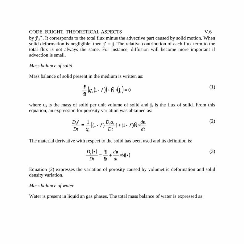
CODE_BRIGHT. THEORETICAL ASPECTS V.6
by j’gw. It corresponds to the total flux minus the advective part caused by solid motion. When
solid deformation is negligible, then j’ = j. The relative contribution of each flux term to the total flux is not always the same. For instance, diffusion will become more important if advection is small.
Mass balance of solid
Mass balance of solid present in the medium is written as:
( )( ) ( ) 01 =×Ñ+- sstjfq
¶¶
(1)
where qs is the mass of solid per unit volume of solid and js is the flux of solid. From this equation, an expression for porosity variation was obtained as:
[ )1(])1(1dtd
DtD
DtD ss
s
s u×Ñ-+-= fqf
qf
(2)
The material derivative with respect to the solid has been used and its definition is:
( )( )D
Dt tddt
s ·= + × Ñ ·
¶¶
u
(3)
Equation (2) expresses the variation of porosity caused by volumetric deformation and solid density variation.
Mass balance of water
Water is present in liquid an gas phases. The total mass balance of water is expressed as:
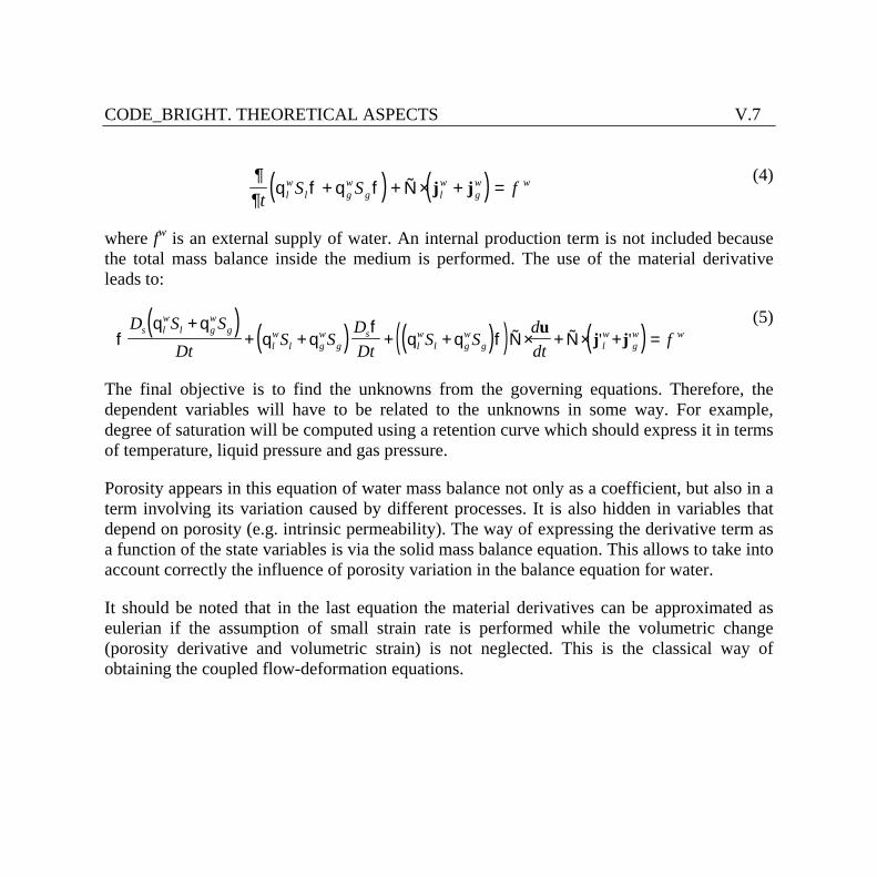
CODE_BRIGHT. THEORETICAL ASPECTS V.7
( ) ( )¶¶
q f q ft
S S flw
l gw
g lw
gw w+ + Ñ × + =j j
(4)
where fw is an external supply of water. An internal production term is not included because the total mass balance inside the medium is performed. The use of the material derivative leads to:
( ) ( ) ( )( ) ( )fq q
q qf
q q fD S S
DtS S
DDt
S Sddt
fs l
wl g
wg
lw
l gw
gs
lw
l gw
g lw
gw w
++ + + + Ñ× + Ñ× + =
uj j' '
(5)
The final objective is to find the unknowns from the governing equations. Therefore, the dependent variables will have to be related to the unknowns in some way. For example, degree of saturation will be computed using a retention curve which should express it in terms of temperature, liquid pressure and gas pressure.
Porosity appears in this equation of water mass balance not only as a coefficient, but also in a term involving its variation caused by different processes. It is also hidden in variables that depend on porosity (e.g. intrinsic permeability). The way of expressing the derivative term as a function of the state variables is via the solid mass balance equation. This allows to take into account correctly the influence of porosity variation in the balance equation for water.
It should be noted that in the last equation the material derivatives can be approximated as eulerian if the assumption of small strain rate is performed while the volumetric change (porosity derivative and volumetric strain) is not neglected. This is the classical way of obtaining the coupled flow-deformation equations.
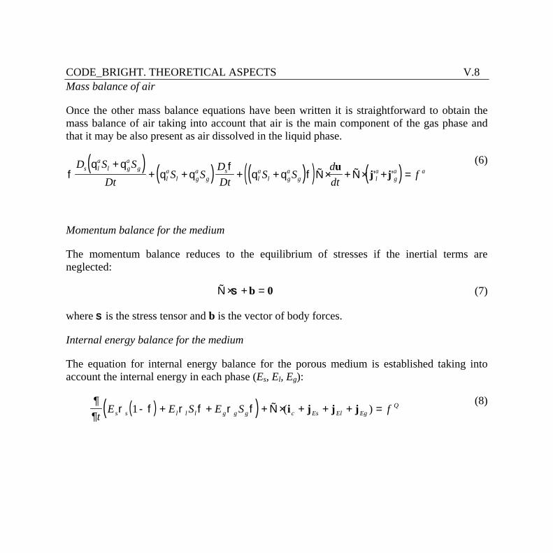
CODE_BRIGHT. THEORETICAL ASPECTS V.8
Mass balance of air
Once the other mass balance equations have been written it is straightforward to obtain the mass balance of air taking into account that air is the main component of the gas phase and that it may be also present as air dissolved in the liquid phase.
( ) ( ) ( )( ) ( )fq q
q qf
q q fD S S
DtS S
DDt
S Sddt
fs l
al g
ag
la
l ga
gs
la
l ga
g la
ga a
++ + + + Ñ× + Ñ× + =
uj j' '
(6)
Momentum balance for the medium
The momentum balance reduces to the equilibrium of stresses if the inertial terms are neglected:
Ñ × + =s b 0 (7)
where s is the stress tensor and b is the vector of body forces.
Internal energy balance for the medium
The equation for internal energy balance for the porous medium is established taking into account the internal energy in each phase (Es, El, Eg):
( )( )¶¶
r f r f r ft
E E S E S fs s l l l g g g c Es El EgQ1- + + + Ñ × + + + =( )i j j j
(8)
CODE_BRIGHT. THEORETICAL ASPECTS V.9
where ic is energy flux due to conduction through the porous medium, the other fluxes (jEs, jEl, jEg) are advective fluxes of energy caused by mass motions and fQ is an internal/external energy supply. In this case this term accounts, for instance, energy dissipation due to medium deformation which is not explicit because it is negligible in most cases. The use of the material derivative allows obtaining an equation formally similar to the mass balance of water. The reason for the similarity is that both water and internal energy, are considered present in the three phases.
Hence, only one equation is required which expresses the balance of internal energy in the porous medium as a whole. In problems involving geological materials, this equation usually reduces to the balance of enthalpy. The reason for this is that the variations of temperature produce enthalpy variations which are very large compared with the energy variations supplied from deformation work.
The fluxes in the divergence term include conduction of heat and advection of heat caused by the motion of every species in the medium. A non-advective mass flux causes an advective heat flux because a species inside a phase moves and transports energy. Contrary to what happens with the movement of a contaminant in a groundwater system, the diffusive term for heat transport (conduction of heat) is much larger than the term concerning hydromechanical dispersion (non-advective flux caused by the velocity of fluids). For this reason, this term is usually neglected.
V.2.2. Constitutive equations and equilibrium restrictions
Associated with this formulation there is a set of necessary constitutive and equilibrium laws. Table 1 is a summary of the constitutive laws and equilibrium restrictions that should be incorporated in the general formulation. The dependent variables that are computed using each of the laws are also included.
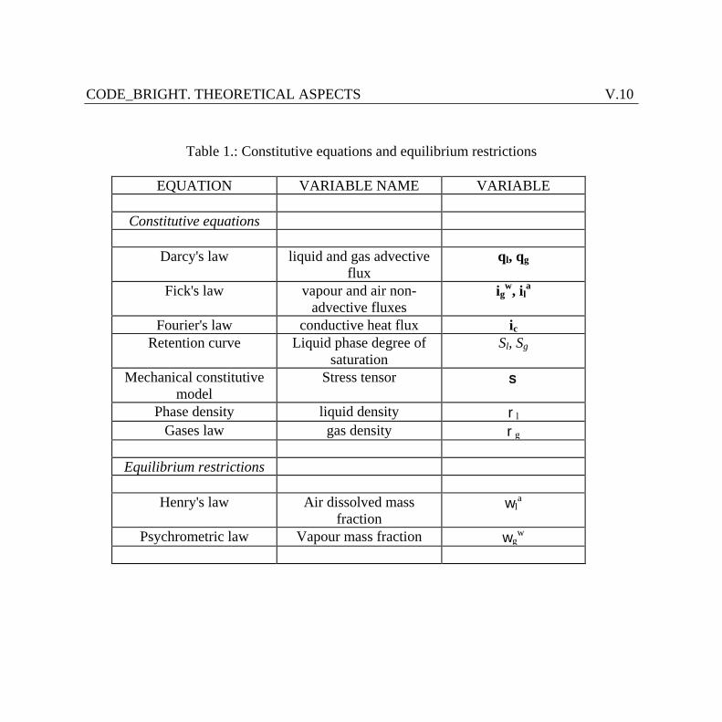
CODE_BRIGHT. THEORETICAL ASPECTS V.10
Table 1.: Constitutive equations and equilibrium restrictions
EQUATION VARIABLE NAME VARIABLE
Constitutive equations
Darcy's law liquid and gas advective flux
ql, qg
Fick's law vapour and air non-advective fluxes
igw, il
a
Fourier's law conductive heat flux ic Retention curve Liquid phase degree of
saturation Sl, Sg
Mechanical constitutive model
Stress tensor s
Phase density liquid density rl Gases law gas density rg
Equilibrium restrictions
Henry's law Air dissolved mass
fraction wl
a
Psychrometric law Vapour mass fraction wgw

CODE_BRIGHT. THEORETICAL ASPECTS V.11
The constitutive equations establish the link between the independent variables (or unknowns) and the dependent variables. There are several categories of dependent variables depending on the complexity with which they are related to the unknowns. The governing equations are finally written in terms of the unknowns when the constitutive equations are substituted in the balance equations.
Another type of relationships that relate dependent variables with unknowns are the equilibrium restrictions. They are obtained assuming chemical equilibrium for dissolution of the different species (air and vapour) in phases (liquid, gas). This assumption is sufficiently adequate because these chemical processes are fast compared to the transport processes that take place in porous media and, for this reason, they are not rate controlling.
V.2.3. Boundary conditions
Application of the Green's theorem to the divergence term (both in the balance or equilibrium of stresses equations) produces terms which represent fluxes or stresses across or on the boundaries. These terms are substituted by nodal flow rates or forces in the discretized form of the equations. For the mechanical problem, the classical approach is followed to impose external forces. Imposing displacement is made by means a Cauchy type boundary condition, i.e. a force computed as the stiffness of a spring times the displacement increment. The boundary conditions for balance equations are incorporated by means the simple addition of nodal flow rates. For instance the mass flow rate of water as a component of gas phase (i.e. vapour) is:
( ) ( ) ( ) ( ) ( )j j P Pgw
gw
g gw
g g g g g gw
g gw= + - + -æ
èçöø÷w w g b r w r w
00
00
0
(9)
where the superscript ()0 stands for prescribed values. This general form of boundary condition, includes three terms. The first one is the mass inflow or outflow that takes place when a flow rate of gas (jg
0) is prescribed. Second term is the mass inflow or outflow that takes place when gas phase pressure (Pg
0) is prescribed at a node. The coefficient gg is a
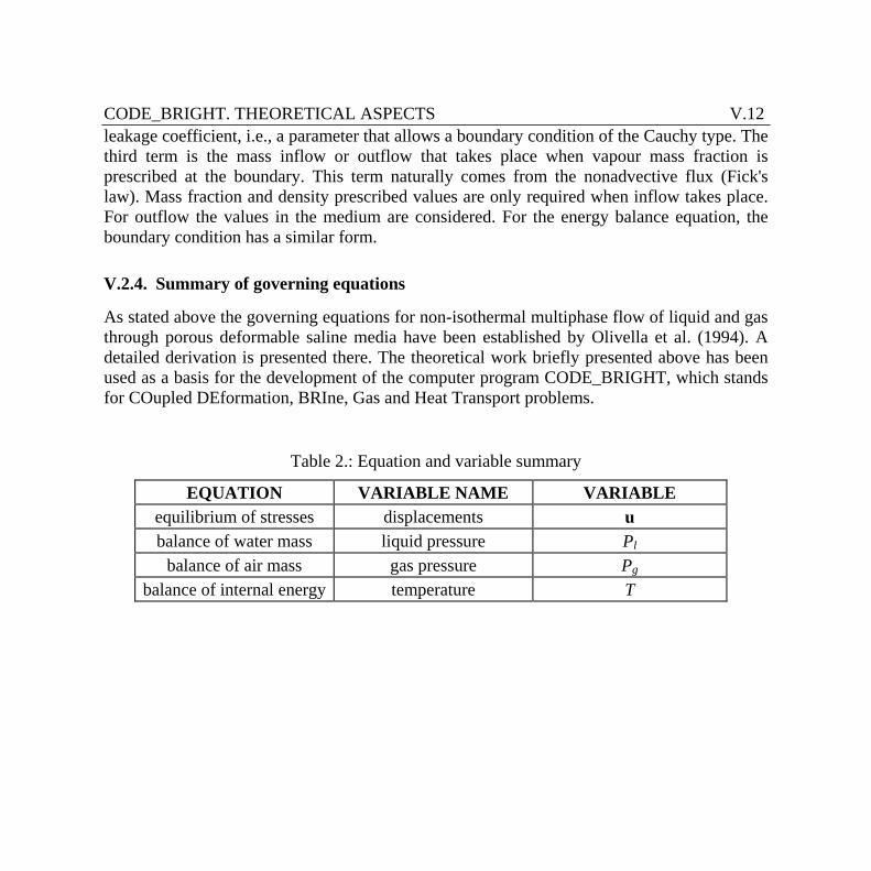
CODE_BRIGHT. THEORETICAL ASPECTS V.12
leakage coefficient, i.e., a parameter that allows a boundary condition of the Cauchy type. The third term is the mass inflow or outflow that takes place when vapour mass fraction is prescribed at the boundary. This term naturally comes from the nonadvective flux (Fick's law). Mass fraction and density prescribed values are only required when inflow takes place. For outflow the values in the medium are considered. For the energy balance equation, the boundary condition has a similar form.
V.2.4. Summary of governing equations
As stated above the governing equations for non-isothermal multiphase flow of liquid and gas through porous deformable saline media have been established by Olivella et al. (1994). A detailed derivation is presented there. The theoretical work briefly presented above has been used as a basis for the development of the computer program CODE_BRIGHT, which stands for COupled DEformation, BRIne, Gas and Heat Transport problems.
Table 2.: Equation and variable summary
EQUATION VARIABLE NAME VARIABLE equilibrium of stresses displacements u balance of water mass liquid pressure Pl
balance of air mass gas pressure Pg balance of internal energy temperature T
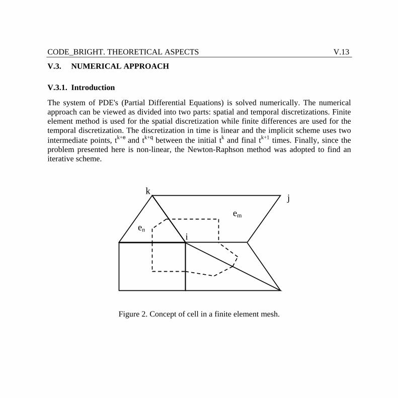
CODE_BRIGHT. THEORETICAL ASPECTS V.13
V.3. NUMERICAL APPROACH
V.3.1. Introduction
The system of PDE's (Partial Differential Equations) is solved numerically. The numerical approach can be viewed as divided into two parts: spatial and temporal discretizations. Finite element method is used for the spatial discretization while finite differences are used for the temporal discretization. The discretization in time is linear and the implicit scheme uses two intermediate points, tk+e and tk+q between the initial tk and final tk+1 times. Finally, since the problem presented here is non-linear, the Newton-Raphson method was adopted to find an iterative scheme.
Figure 2. Concept of cell in a finite element mesh.
j k
i
em
en
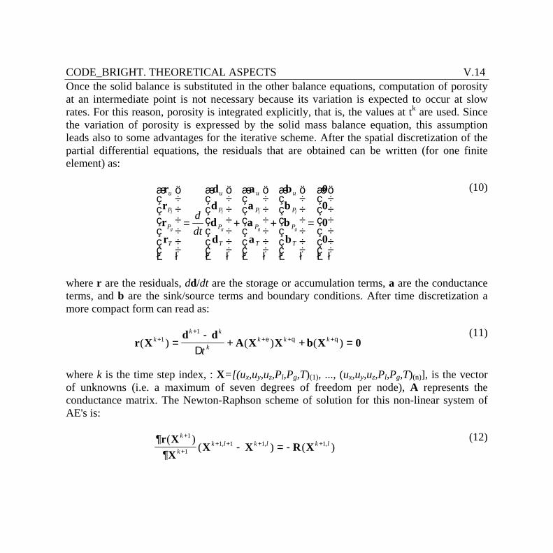
CODE_BRIGHT. THEORETICAL ASPECTS V.14
Once the solid balance is substituted in the other balance equations, computation of porosity at an intermediate point is not necessary because its variation is expected to occur at slow rates. For this reason, porosity is integrated explicitly, that is, the values at tk are used. Since the variation of porosity is expressed by the solid mass balance equation, this assumption leads also to some advantages for the iterative scheme. After the spatial discretization of the partial differential equations, the residuals that are obtained can be written (for one finite element) as:
rrrr
dddd
aaaa
bbbb
0000
u
P
P
T
u
P
P
T
u
P
P
T
u
P
P
T
l
g
l
g
l
g
l
g
ddt
æ
è
çççççç
ö
ø
÷÷÷÷÷÷
=
æ
è
çççççç
ö
ø
÷÷÷÷÷÷
+
æ
è
çççççç
ö
ø
÷÷÷÷÷÷
+
æ
è
çççççç
ö
ø
÷÷÷÷÷÷
=
æ
è
çççççç
ö
ø
÷÷÷÷÷÷
(10)
where r are the residuals, dd/dt are the storage or accumulation terms, a are the conductance terms, and b are the sink/source terms and boundary conditions. After time discretization a more compact form can read as:
r Xd d
A X X b X 0( ) ( ) ( )kk k
kk k k
t+
++ + +=
-+ + =1
1
De q q
(11)
where k is the time step index, : X=[(ux,uy,uz,Pl,Pg,T)(1), ..., (ux,uy,uz,Pl,Pg,T)(n)], is the vector of unknowns (i.e. a maximum of seven degrees of freedom per node), A represents the conductance matrix. The Newton-Raphson scheme of solution for this non-linear system of AE's is:
¶¶r X
XX X R X
( )( ) ( ), , ,
k
kk l k l k l
+
++ + + +- = -
1
11 1 1 1
(12)
CODE_BRIGHT. THEORETICAL ASPECTS V.15
where l indicates iteration.
In the present approach, the standard Galerkin method is used with some variations in order to facilitate computations. General aspects related to numerical solution of hydrogeological problems can be found in Huyakorn and Pinder (1983). As shown in the preceding section, in the mass and energy balance equations the following terms may be distinguished:
· Storage terms. These terms represent the variation of mass or energy content and therefore, they are calculated by means of variables such as degree of saturation, density, porosity, mass fraction and specific energy.
· Advective fluxes. The advective fluxes caused by motion of fluids computed using Darcy's law and, except for the coefficients, they are explicit in terms of pressure gradients.
· Nonadvective fluxes. These terms, computed through Fick's law, are proportional to gradients of mass fractions which do not belong to the set of unknowns. Fourier's law is used for the conductive heat flux and it expresses proportionality to temperature gradients.
· Volumetric strain terms. In fact, these terms are also storage terms. They are proportional to Ñ×du/dt which is equivalent to the volumetric strain rate.
· Sink/source terms.
Each of these terms requires specific treatment. This is described in detail in Olivella et al (1996).
In order to explain the treatment of the different terms and equations the following notation is introduced:
· node i: node in a finite element mesh
CODE_BRIGHT. THEORETICAL ASPECTS V.16
· e1,e2,...,em: elements that contain node i, i.e. a cell centered in node i is composed by a fraction of these elements. m is variable from node to node and it is not related to the number of nodes per element.
· nem: number of nodes in element em. For example, nem=3 for triangles, nem=4 for quadrilaterals, nem=4 for tetrahedrons, etc.
· (×)k: the quantity is computed at time tk of the temporal discretization. The same for tk+1, tk+e or tk+q
· (×)em: the quantity is computed in element em. This means at the center of the element or, in other words, using the average of nodal unknowns.
· (×)i: the quantity is computed in node i as a function of the unknowns in that node. \item--}
· (×)i,em: the quantity is computed in node i but with the material properties corresponding to element em.
· Vem: volume of element em.
· xi: shape function for node i.
V.3.2 Treatment of different terms
Treatment of storage terms
In this sub-section we refer to terms not related to volumetric strain or porosity variation. The storage or accumulation terms are computed in a mass conservative approach (Allen and Murphy, 1986; Celia et al., 1990; Milly, 1984). The conservative approach discretizes directly the accumulation terms while the capacitative approach uses the chain rule to transform time derivatives in terms of the unknowns. Milly (1984) proposes modifications of the capacitative
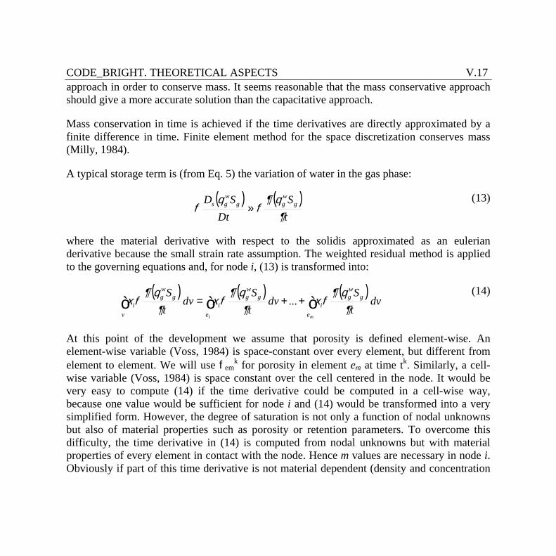
CODE_BRIGHT. THEORETICAL ASPECTS V.17
approach in order to conserve mass. It seems reasonable that the mass conservative approach should give a more accurate solution than the capacitative approach.
Mass conservation in time is achieved if the time derivatives are directly approximated by a finite difference in time. Finite element method for the space discretization conserves mass (Milly, 1984).
A typical storage term is (from Eq. 5) the variation of water in the gas phase:
( ) ( )
tS
DtSD g
wgg
wgs
¶q
fq
f » (13)
where the material derivative with respect to the solidis approximated as an eulerian derivative because the small strain rate assumption. The weighted residual method is applied to the governing equations and, for node i, (13) is transformed into:
( ) ( ) ( )dv
tS
dvtS
dvtS g
wg
ei
gwg
ei
gwg
vi
m
q¶fx
¶q
fx
q¶fx òòò ++= ...
1
(14)
At this point of the development we assume that porosity is defined element-wise. An element-wise variable (Voss, 1984) is space-constant over every element, but different from element to element. We will use fem
k for porosity in element em at time tk. Similarly, a cell-wise variable (Voss, 1984) is space constant over the cell centered in the node. It would be very easy to compute (14) if the time derivative could be computed in a cell-wise way, because one value would be sufficient for node i and (14) would be transformed into a very simplified form. However, the degree of saturation is not only a function of nodal unknowns but also of material properties such as porosity or retention parameters. To overcome this difficulty, the time derivative in (14) is computed from nodal unknowns but with material properties of every element in contact with the node. Hence m values are necessary in node i. Obviously if part of this time derivative is not material dependent (density and concentration
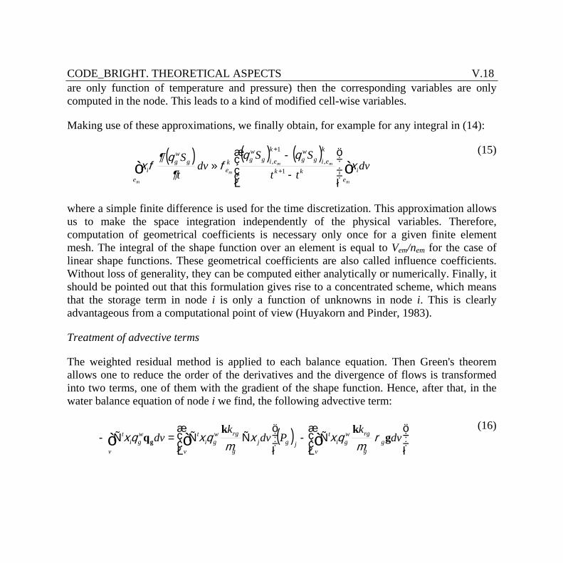
CODE_BRIGHT. THEORETICAL ASPECTS V.18
are only function of temperature and pressure) then the corresponding variables are only computed in the node. This leads to a kind of modified cell-wise variables.
Making use of these approximations, we finally obtain, for example for any integral in (14):
( ) ( ) ( ) 1
,
1
, dvtt
SSdv
tS
m
mm
m
m eikk
k
eigwg
k
eigwgk
eg
wg
ei òò ÷÷
÷
ø
ö
ççç
è
æ
-
-» +
+
xqq
f
q¶fx
(15)
where a simple finite difference is used for the time discretization. This approximation allows us to make the space integration independently of the physical variables. Therefore, computation of geometrical coefficients is necessary only once for a given finite element mesh. The integral of the shape function over an element is equal to Vem/nem for the case of linear shape functions. These geometrical coefficients are also called influence coefficients. Without loss of generality, they can be computed either analytically or numerically. Finally, it should be pointed out that this formulation gives rise to a concentrated scheme, which means that the storage term in node i is only a function of unknowns in node i. This is clearly advantageous from a computational point of view (Huyakorn and Pinder, 1983).
Treatment of advective terms
The weighted residual method is applied to each balance equation. Then Green's theorem allows one to reduce the order of the derivatives and the divergence of flows is transformed into two terms, one of them with the gradient of the shape function. Hence, after that, in the water balance equation of node i we find, the following advective term:
( ) ÷÷ø
öççè
æÑ-÷
÷ø
öççè
æÑÑ=Ñ- òòò dv
kPdv
kdv g
g
rgwg
vi
tjgj
g
rgwg
vi
twg
vi
t gkk
qg rm
qxxm
qxqx (16)
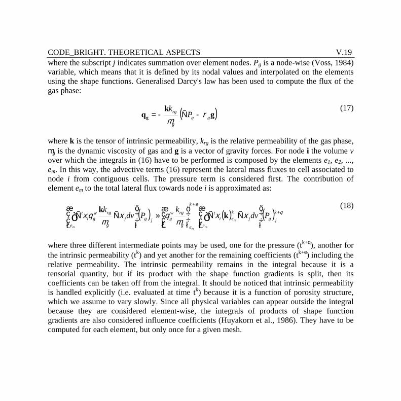
CODE_BRIGHT. THEORETICAL ASPECTS V.19
where the subscript j indicates summation over element nodes. Pg is a node-wise (Voss, 1984) variable, which means that it is defined by its nodal values and interpolated on the elements using the shape functions. Generalised Darcy's law has been used to compute the flux of the gas phase:
( ) gk
qg ggg
rg Pk
rm
-Ñ-= (17)
where k is the tensor of intrinsic permeability, krg is the relative permeability of the gas phase, mg is the dynamic viscosity of gas and g is a vector of gravity forces. For node i the volume v over which the integrals in (16) have to be performed is composed by the elements e1, e2, ..., em. In this way, the advective terms (16) represent the lateral mass fluxes to cell associated to node i from contiguous cells. The pressure term is considered first. The contribution of element em to the total lateral flux towards node i is approximated as:
( ) ( ) ( ) q
e
xxm
qxm
qx +
+
÷÷ø
öççè
æÑÑ÷
÷ø
öççè
æ»÷
÷ø
öççè
æÑÑ òò k
jgjke
ei
t
k
eg
rgwgjgj
g
rgwg
ei
t Pdvk
Pdvk
m
mmm
kk
(18)
where three different intermediate points may be used, one for the pressure (tk+q), another for the intrinsic permeability (tk) and yet another for the remaining coefficients (tk+e) including the relative permeability. The intrinsic permeability remains in the integral because it is a tensorial quantity, but if its product with the shape function gradients is split, then its coefficients can be taken off from the integral. It should be noticed that intrinsic permeability is handled explicitly (i.e. evaluated at time tk) because it is a function of porosity structure, which we assume to vary slowly. Since all physical variables can appear outside the integral because they are considered element-wise, the integrals of products of shape function gradients are also considered influence coefficients (Huyakorn et al., 1986). They have to be computed for each element, but only once for a given mesh.
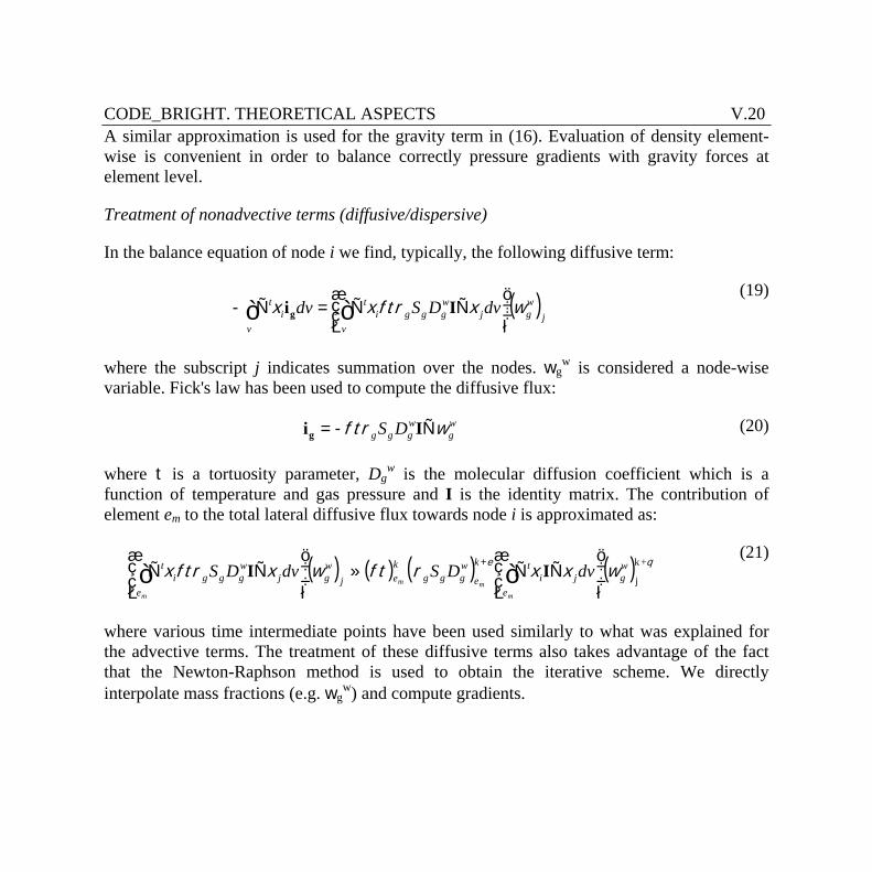
CODE_BRIGHT. THEORETICAL ASPECTS V.20
A similar approximation is used for the gravity term in (16). Evaluation of density element-wise is convenient in order to balance correctly pressure gradients with gravity forces at element level.
Treatment of nonadvective terms (diffusive/dispersive)
In the balance equation of node i we find, typically, the following diffusive term:
( ) j
wgj
wggg
vi
t
vi
t dvDSdv wxtrfxx ÷÷ø
öççè
æÑÑ=Ñ- òò Iig
(19)
where the subscript j indicates summation over the nodes. wgw is considered a node-wise
variable. Fick's law has been used to compute the diffusive flux:
wg
wggg DS wftr Ñ-= Iig (20)
where t is a tortuosity parameter, Dgw is the molecular diffusion coefficient which is a
function of temperature and gas pressure and I is the identity matrix. The contribution of element em to the total lateral diffusive flux towards node i is approximated as:
( ) ( ) ( ) ( ) +k
j
qewxxrftwxtrfx w
gje
itk
ewggg
kej
wgj
wggg
ei
t dvDSdvDSm
mm
m÷÷ø
öççè
æÑÑ»÷
÷ø
öççè
æÑÑ òò
+ II (21)
where various time intermediate points have been used similarly to what was explained for the advective terms. The treatment of these diffusive terms also takes advantage of the fact that the Newton-Raphson method is used to obtain the iterative scheme. We directly interpolate mass fractions (e.g. wg
w) and compute gradients.
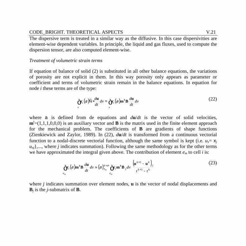
CODE_BRIGHT. THEORETICAL ASPECTS V.21
The dispersive term is treated in a similar way as the diffusive. In this case dispersivities are element-wise dependent variables. In principle, the liquid and gas fluxes, used to compute the dispersion tensor, are also computed element-wise.
Treatment of volumetric strain terms
If equation of balance of solid (2) is substituted in all other balance equations, the variations of porosity are not explicit in them. In this way porosity only appears as parameter or coefficient and terms of volumetric strain remain in the balance equations. In equation for node i these terms are of the type:
( ) ( ) dvdtddv
dtd
vi
vi
uBmu taxax òò =×Ñ (22)
where a is defined from de equations and du/dt is the vector of solid velocities, mt=(1,1,1,0,0,0) is an auxiliary vector and B is the matrix used in the finite element approach for the mechanical problem. The coefficients of B are gradients of shape functions (Zienkiewick and Zaylor, 1989). In (22), du/dt is transformed from a continuous vectorial function to a nodal-discrete vectorial function, although the same symbol is kept (i.e. ux= xj uxj},..., where j indicates summation). Following the same methodology as for the other terms we have approximated the integral given above. The contribution of element em to cell i is:
( ) ( )( )
1
1
kkj
kk
je
ike
ei
ttdvdv
dtd
m
m
m-
-»
+
++ òò
uuBmuBm tt xaax e
(23)
where j indicates summation over element nodes, u is the vector of nodal displacements and Bj is the j-submatrix of B.
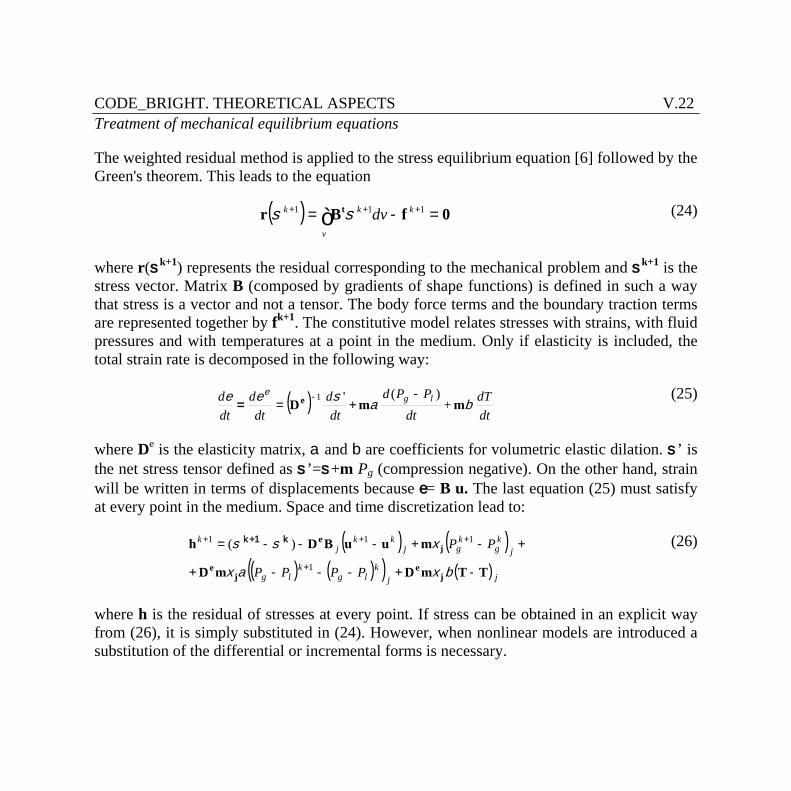
CODE_BRIGHT. THEORETICAL ASPECTS V.22
Treatment of mechanical equilibrium equations
The weighted residual method is applied to the stress equilibrium equation [6] followed by the Green's theorem. This leads to the equation
( ) ò =-= +++
v
kkk dv 111 0fBr tss (24)
where r(sk+1) represents the residual corresponding to the mechanical problem and sk+1 is the stress vector. Matrix B (composed by gradients of shape functions) is defined in such a way that stress is a vector and not a tensor. The body force terms and the boundary traction terms are represented together by fk+1. The constitutive model relates stresses with strains, with fluid pressures and with temperatures at a point in the medium. Only if elasticity is included, the total strain rate is decomposed in the following way:
( ) +)('1
dtdT
dtPPd
dtd
dtd
dtd lg basee e
mmDe -+=
-=
(25)
where De is the elasticity matrix, a and b are coefficients for volumetric elastic dilation. s’ is the net stress tensor defined as s’=s+m Pg (compression negative). On the other hand, strain will be written in terms of displacements because e= B u. The last equation (25) must satisfy at every point in the medium. Space and time discretization lead to:
( ) ( )( ) ( )( ) ( )
)(
1
111
jjk
lgk
lg
jkg
kgj
kkj
k
PPPP
PP
TTmDmD
muuBDh
je
je
je
-+---+
+-+---=
+
+++
bxax
xss k1+k
(26)
where h is the residual of stresses at every point. If stress can be obtained in an explicit way from (26), it is simply substituted in (24). However, when nonlinear models are introduced a substitution of the differential or incremental forms is necessary.

CODE_BRIGHT. THEORETICAL ASPECTS V.23
For the mechanical problem, the approximations that should be made are different from the ones used for flow problems. According to the numerical approximations proposed for the flow problems (hydraulic and thermal), we would tend to use element-wise matrices. However, the mechanical problem has some peculiarities which do not allow this kind of simplified treatment.
First, linear triangular elements (the simplest element in two dimensional analyses), which have been proven to be very adequate for flow problems, should be avoided for mechanical problems. This is because if the medium is nearly-incompressible (creep of rocks takes place with very small volumetric deformation), locking takes place (not all displacements are permitted due to element restrictions). Second, linear quadrilateral elements with element-wise variables (this is equivalent to one integration point) lead to hour-glassing (uncontrolled displacement modes appear).
In order to overcome these difficulties, the selective integration (B-bar) method is used. It consists in using a modified form of matrix B which implies that the volumetric part of deformation and the deviatoric part are integrated with different order of numerical integration (Hughes, 1980). For linear quadrilateral elements, four integration points are used to integrate the deviatoric part while one is used for volumetric strain terms. Although this approximation is different from what is proposed for the flow problem, element-wise variables or parameters are maintained (porosity, saturation,...). Stress is not element-wise and it must be computed at the integration points.
CODE_BRIGHT. THEORETICAL ASPECTS V.24
V.4. THEORETICAL APPROACH SUMMARY
The governing equations include: stress equilibrium equations (1, 2 or 3 according to the dimensions of the problem), mass balance equations (different species) and internal energy balance equation for the medium as a whole (thermal equilibrium is assumed).
The stress equilibrium equations are a simplified form of the balance of momentum for the porous medium. Mass balance of water, solid and air are established. Since the assumption of equilibrium is made, the mass of each species as present in any phase (solid, liquid or gas) is balanced for the porous medium as a whole. In this way, one equation for each species is obtained. The equilibrium assumption implies that partition functions are required to compute the fraction of each species in each phase.
Each partial differential equation is naturally associated to an unknown. These unknowns can be solved in a coupled way, i.e., allowing all possible cross coupling processes that have been implemented, or, on the contrary, any uncoupled problem to obtain a single unknown can be solved.
The balance equations that CODE_BRIGHT solves are compiled here:
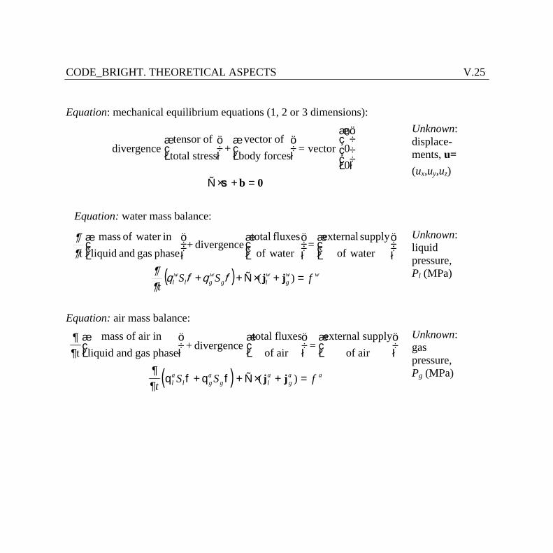
CODE_BRIGHT. THEORETICAL ASPECTS V.25
Equation: mechanical equilibrium equations (1, 2 or 3 dimensions):
divergence tensor of
total stress +vector of
body forces = vector 000
æèç
öø÷
æèç
öø÷
æ
è
ççç
ö
ø
÷÷÷
Ñ × + =s b 0
Unknown: displace-ments, u= (ux,uy,uz)
Equation: water mass balance:
( ) wwg
wlg
wgl
wl fSS
t=+×Ñ++
÷÷ø
öççè
æ÷÷ø
öççè
æ÷÷ø
öççè
æ
)(
waterof
supply external=
wateroffluxes total
divergence+phase gas and liquid
in water of masst
jjfqfq¶¶
¶¶
Unknown: liquid pressure, Pl (MPa)
Equation: air mass balance:
( )
¶¶
¶¶
q f q f
tmass of air in
liquid and gas phase + divergence total fluxes
of air =external supply
of air æèç
öø÷
æèç
öø÷
æèç
öø÷
+ + Ñ × + =t
S S fla
l ga
g la
ga a( )j j
Unknown: gas pressure, Pg (MPa)
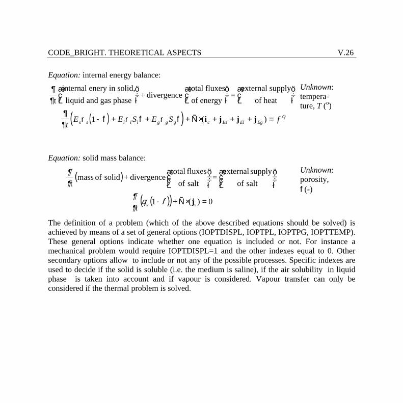
CODE_BRIGHT. THEORETICAL ASPECTS V.26
Equation: internal energy balance:
( )( )
¶¶
¶¶
r f r f r f
tinternal enery in solid,liquid and gas phase + divergence
total fluxesof energy =
external supplyof heat
æèç
öø÷
æèç
öø÷
æèç
öø÷
- + + + Ñ × + + + =t
E E S E S fs s l l l g g g c Es El EgQ1 ( )i j j j
Unknown: tempera-ture, T (o)
Equation: solid mass balance:
( )
( )( ) 0)(1
salt ofsupply external
=salt offluxes total
divergence+solid of masst
=×Ñ+-
÷÷ø
öççè
æ÷÷ø
öççè
æ
sstjfq
¶¶
¶¶
Unknown: porosity, f(-)
The definition of a problem (which of the above described equations should be solved) is achieved by means of a set of general options (IOPTDISPL, IOPTPL, IOPTPG, IOPTTEMP). These general options indicate whether one equation is included or not. For instance a mechanical problem would require IOPTDISPL=1 and the other indexes equal to 0. Other secondary options allow to include or not any of the possible processes. Specific indexes are used to decide if the solid is soluble (i.e. the medium is saline), if the air solubility in liquid phase is taken into account and if vapour is considered. Vapour transfer can only be considered if the thermal problem is solved.
CODE_BRIGHT. THEORETICAL ASPECTS V.27
V.5. FEATURES OF CODE-BRIGHT
The implementation of a coupled non-linear approach requires some especific developments and approximations. In this section the main aspects of the numerical approximation are reviewed. The program CODE_BRIGHT uses the finite element method to solve the coupled equations presented above. The main features of the numerical approach are:
· Linear interpolation functions on segments, triangles, quadrilaterals, tetrahedrons, triangular prisms and quadrilateral prisms (regular). Analytical integration is used for segments, triangles and tetrahedrons. Numerical integration is used for quadrilateral, arbitrary triangular prisms (6 points) and quadrilateral prisms (8 points). For the mechanical problem selective integration is used for quadrilateral and quadrilateral prisms (this means that the volumetric part is integrated with a reduced quadrature of 1 point). Finally, for all elements the flow equations are solved using element-wise and cell-wise approximations. This approximation is independent of the type of integration performed.
· Finite differences and implicit scheme are used for time integration. Two intermediate points are defined between the two ends of the time interval (tk, tk+1). One represents the point where the equation will be accomplished (tk+q) and the other is the point where the non-linear functions are computed (tk+e). For instance e=0 and q=1 states for a linearised problem with a fully implicit scheme of integration.
· Newton-Raphson method for solution of the non-linear system of algebraic equations that results once the space and time discretizations are applied.
· LU decomposition and backsubstitution (non-symmetric matrix) or conjugate gradients squared to solve the system of linear equations that result from the Newton-Raphson application.
CODE_BRIGHT. THEORETICAL ASPECTS V.28
· Automatic discretization of time. Increase or reduction of time increment according to convergence conditions or output requirements. Reduction of time increment may be caused by: excessive variation of unknowns per iteration, excessive number of iterations to reach convergence and correction larger than in the previous iteration.
The main features of the program CODE_BRIGHT are:
· Options that allow to solve uncoupled and coupled problems. For instance: Hydro-mechanical, Thermo-mechanical, Hydro-thermal problems can be solved if the physical situation requires one of these approaches.
· Types of analysis: One dimension (uni-axial confined strain and axi-symmetric). Two dimension (plane strain and axi-symmetric). Three dimensions.
· Several element types.
· Constitutive laws: each law defined as a set of parameters. Different types of relationships can be chosen in some cases.
· Boundary conditions:
· Mechanical problem: forces and displacement rate in any spatial direction and at any node
· Hydraulic problem: mass flow rate of water and air prescribed and liquid/gas pressure prescribed at any node
· Thermal problem: heat flow rate prescribed and temperature prescribed at any node
· Convergence criteria: Tolerances for absolute and relative error independent for each unknown. Tolerance for residual convergence of each problem (mechanical, hydraulic, etc). The node under worse conditions is used to verify the convergence condition.
CODE_BRIGHT. THEORETICAL ASPECTS V.29
· Forces/flows = e®0
· Absolute variable correction = dx®0
· Variable correction / variable increment = dx/Dx®0
· Output options: Time evolution of variables in nodes or elements. The user should decide 'a priori' the nodal or element variables that will be output at all times (absolutely all computed times will be output for a few variables). Contour maps in the solution domain. Nodal or element variables can be used to draw contour maps. However, in the second case it is required to perform an interpolation that may be difficult due to the lack of continuity of the element variables.
CODE_BRIGHT. THEORETICAL ASPECTS V.30
V.6. SOLUTION OF SYSTEM OF EQUATIONS IN CODE_BRIGHT
As described in the preceding chapters, CODE_BRIGHT is a FE-three dimensional code that solves the following equations:
· equilibrium of stresses (displacements)
· mass balance of water (liquid pressure)
· mass balance of air (gas pressure)
· balance of energy (temperature)
Associated to every equation there is a variable, i.e. the unknown that is obtained by solving the corresponding equation. The code can be used to solve problems that need only some of the equations in the list. The equations are solved together in a monolithic way. Usually problems require variable time stepping and an iterative method for the solution of non-linearities. Usually the resulting system of equations is non-symmetric.
V.6.1 Matrix storage mode in CODE_BRIGHT.
Originally, a solver using LU decomposition was implemented in the program together with a band storage mode. This alternative is still available but obviously the band storage mode is not very efficient. This is especially dramatic when more than one degrees of freedom are considered.
In principle, two possible alternatives could be considered for a more efficient storage of the matrix coefficients. These are skyline mode and sparse mode. The skyline mode seems adequate for LU-solvers because in such case filling of the matrix is important (the decomposed matrices contain more non-zero coefficients than the original matrix but the skyline structure is maintained).
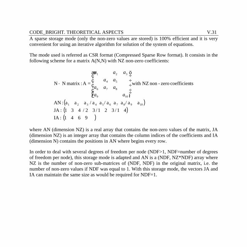
CODE_BRIGHT. THEORETICAL ASPECTS V.31
A sparse storage mode (only the non-zero values are stored) is 100% efficient and it is very convenient for using an iterative algorithm for solution of the system of equations.
The mode used is referred as CSR format (Compressed Sparse Row format). It consists in the following scheme for a matrix A(N,N) with NZ non-zero coefficients:
( )( )( )9641 :IA
41 / 321 / 32 / 431 :JAaa/ a a a/ a a / aaa :AN
tscoefficien zero-non NZ with =A :matrix NN
10987654321
109
876
54
321
÷÷÷÷÷
ø
ö
ççççç
è
æ
´
aaaaaaa
aaa
where AN (dimension NZ) is a real array that contains the non-zero values of the matrix, JA (dimension NZ) is an integer array that contains the column indices of the coefficients and IA (dimension N) contains the positions in AN where begins every row.
In order to deal with several degrees of freedom per node (NDF>1, NDF=number of degrees of freedom per node), this storage mode is adapted and AN is a (NDF, NZ*NDF) array where NZ is the number of non-zero sub-matrices of (NDF, NDF) in the original matrix, i.e. the number of non-zero values if NDF was equal to 1. With this storage mode, the vectors JA and IA can maintain the same size as would be required for NDF=1.
CODE_BRIGHT. THEORETICAL ASPECTS V.32
V.6.2 Iterative solver for nonsymmetrical linear systems of equations.
There are several alternatives for solving linear systems in an iterative way. It should be taken into account that the matrix is non-symmetric. Perhaps one of the simplest algorithms that can be used is the conjugate gradients squared method (CGS) which has been proposed by Sonneveld, 1989 and van der Vorst, 1990. This CGS method is a modification of the conjugate gradients for non-symmetric matrices. Iterative methods require some extra space and a pre-conditioner. In order to facilitate parallelism the simplest pre-conditioner that can be used is the inverse of the diagonal of the matrix (diagonal scaling). Of course this is the less efficient pre-conditioner from the point of view of a scalar machine. However Pini and Gambolatti (1990) have shown that in vectorial machines, diagonal scaling was the most efficient pre-conditioner in the majority of the applications they compared. A block diagonal scaling consists in the inversion of the NDFxNDF block corresponding to each node (block in the matrix diagonal).
Using CRS storage mode plus CGS iterative method plus block-diagonal scaling produces a quite simple structure of the solver. In fact, only vector-vector products, matrix-vector products and inversion of NDFxNDF matrices have to be performed. The requirements of extra space are only 8*N*NDF where N is the number of nodes and NDF the number of degrees of freedom per node. It should be mentioned that the matrix-vector products are easily performed with the CRS storage mode because the matrix is stored by rows.
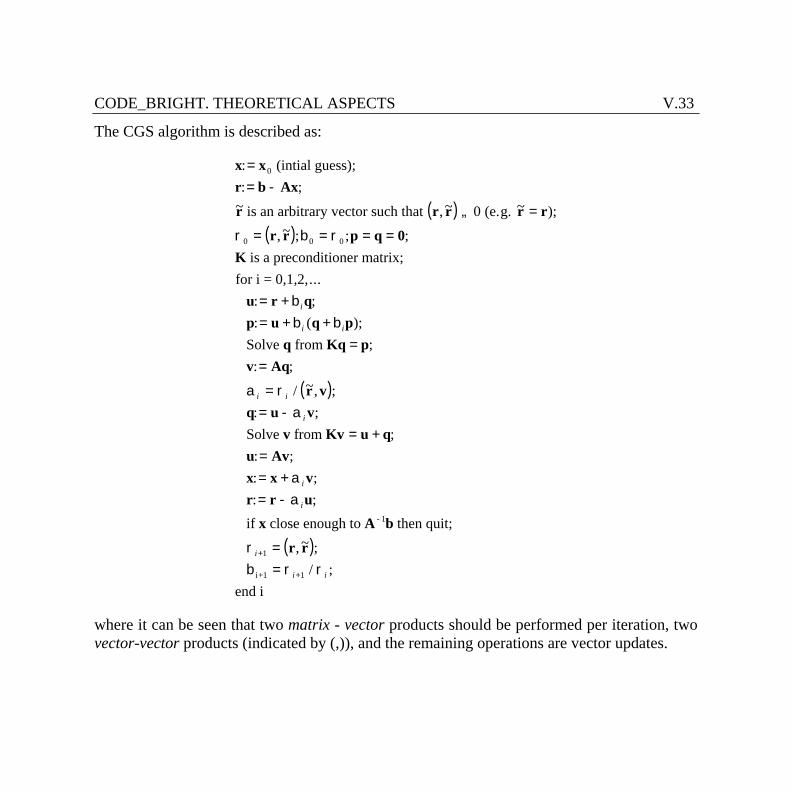
CODE_BRIGHT. THEORETICAL ASPECTS V.33
The CGS algorithm is described as:
( )( )
( )
x xr b Ax
r r r r r
r r p q 0K
u r qp u q p
q Kq pv Aq
r vq u v
v Kv u qu Avx
:: ;
~ ,~ ~ );
,~ ; ; ;
: ;: ( );
;: ;
/ ~, ;: ;
;: ;:
== -
¹ =
= = = =
= += + +
==
== -
= +==
0
0 0 0
0
(intial guess);
is an arbitrary vector such that (e.g.
is a preconditioner matrix;for i = 0,1,2,... Solve from
Solve from
r b r
bb b
a ra
i
i i
i i
i
( )
x vr r u
x A b
r r
+= -
==
-
+
+
aa
rb r r
i
i
i
i i
;: ;
, ~ ;/ ;
if close enough to then quit;
end i
i+1
1
1
1
where it can be seen that two matrix - vector products should be performed per iteration, two vector-vector products (indicated by (,)), and the remaining operations are vector updates.
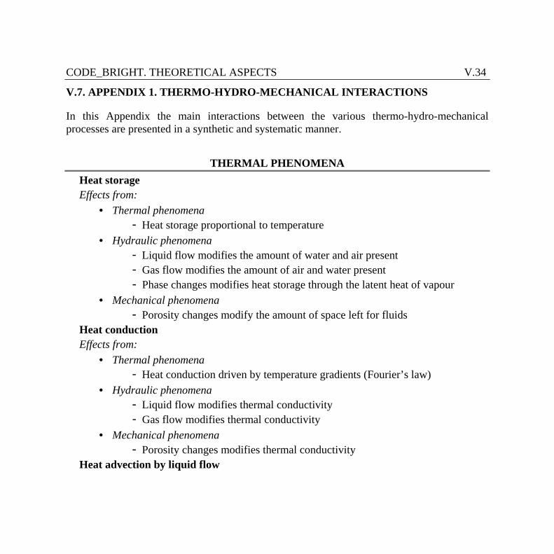
CODE_BRIGHT. THEORETICAL ASPECTS V.34
V.7. APPENDIX 1. THERMO-HYDRO-MECHANICAL INTERACTIONS
In this Appendix the main interactions between the various thermo-hydro-mechanical processes are presented in a synthetic and systematic manner.
THERMAL PHENOMENA
Heat storage Effects from:
· Thermal phenomena - Heat storage proportional to temperature
· Hydraulic phenomena - Liquid flow modifies the amount of water and air present - Gas flow modifies the amount of air and water present - Phase changes modifies heat storage through the latent heat of vapour
· Mechanical phenomena - Porosity changes modify the amount of space left for fluids
Heat conduction Effects from:
· Thermal phenomena - Heat conduction driven by temperature gradients (Fourier’s law)
· Hydraulic phenomena - Liquid flow modifies thermal conductivity - Gas flow modifies thermal conductivity
· Mechanical phenomena - Porosity changes modifies thermal conductivity
Heat advection by liquid flow
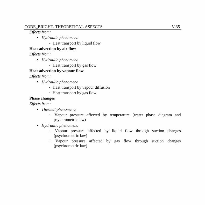
CODE_BRIGHT. THEORETICAL ASPECTS V.35
Effects from: · Hydraulic phenomena
- Heat transport by liquid flow Heat advection by air flow Effects from:
· Hydraulic phenomena - Heat transport by gas flow
Heat advection by vapour flow Effects from:
· Hydraulic phenomena - Heat transport by vapour diffusion - Heat transport by gas flow
Phase changes Effects from:
· Thermal phenomena - Vapour pressure affected by temperature (water phase diagram and
psychrometric law) · Hydraulic phenomena
- Vapour pressure affected by liquid flow through suction changes (psychrometric law)
- Vapour pressure affected by gas flow through suction changes (psychrometric law)
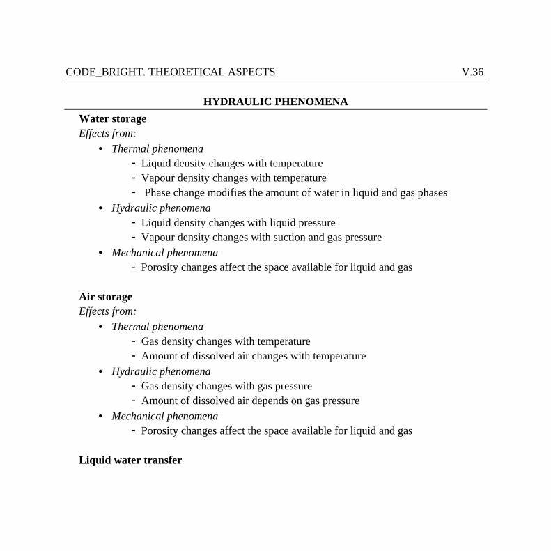
CODE_BRIGHT. THEORETICAL ASPECTS V.36
HYDRAULIC PHENOMENA
Water storage Effects from:
· Thermal phenomena - Liquid density changes with temperature - Vapour density changes with temperature - Phase change modifies the amount of water in liquid and gas phases
· Hydraulic phenomena - Liquid density changes with liquid pressure - Vapour density changes with suction and gas pressure
· Mechanical phenomena - Porosity changes affect the space available for liquid and gas
Air storage Effects from:
· Thermal phenomena - Gas density changes with temperature - Amount of dissolved air changes with temperature
· Hydraulic phenomena - Gas density changes with gas pressure - Amount of dissolved air depends on gas pressure
· Mechanical phenomena - Porosity changes affect the space available for liquid and gas
Liquid water transfer
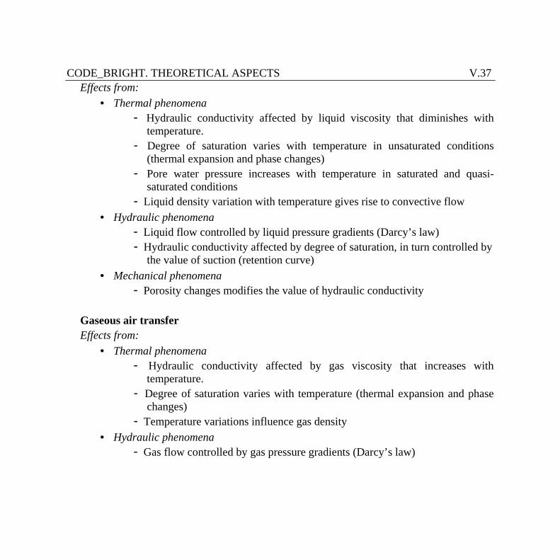
CODE_BRIGHT. THEORETICAL ASPECTS V.37
Effects from: · Thermal phenomena
- Hydraulic conductivity affected by liquid viscosity that diminishes with temperature.
- Degree of saturation varies with temperature in unsaturated conditions (thermal expansion and phase changes)
- Pore water pressure increases with temperature in saturated and quasi-saturated conditions
- Liquid density variation with temperature gives rise to convective flow · Hydraulic phenomena
- Liquid flow controlled by liquid pressure gradients (Darcy’s law) - Hydraulic conductivity affected by degree of saturation, in turn controlled by
the value of suction (retention curve) · Mechanical phenomena
- Porosity changes modifies the value of hydraulic conductivity Gaseous air transfer Effects from:
· Thermal phenomena - Hydraulic conductivity affected by gas viscosity that increases with
temperature. - Degree of saturation varies with temperature (thermal expansion and phase
changes) - Temperature variations influence gas density
· Hydraulic phenomena - Gas flow controlled by gas pressure gradients (Darcy’s law)
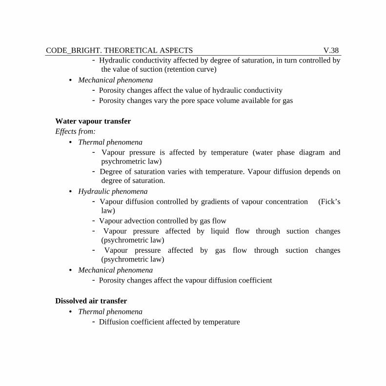
CODE_BRIGHT. THEORETICAL ASPECTS V.38
- Hydraulic conductivity affected by degree of saturation, in turn controlled by the value of suction (retention curve)
· Mechanical phenomena - Porosity changes affect the value of hydraulic conductivity - Porosity changes vary the pore space volume available for gas
Water vapour transfer Effects from:
· Thermal phenomena - Vapour pressure is affected by temperature (water phase diagram and
psychrometric law) - Degree of saturation varies with temperature. Vapour diffusion depends on
degree of saturation. · Hydraulic phenomena
- Vapour diffusion controlled by gradients of vapour concentration (Fick’s law)
- Vapour advection controlled by gas flow - Vapour pressure affected by liquid flow through suction changes
(psychrometric law) - Vapour pressure affected by gas flow through suction changes
(psychrometric law) · Mechanical phenomena
- Porosity changes affect the vapour diffusion coefficient Dissolved air transfer
· Thermal phenomena - Diffusion coefficient affected by temperature
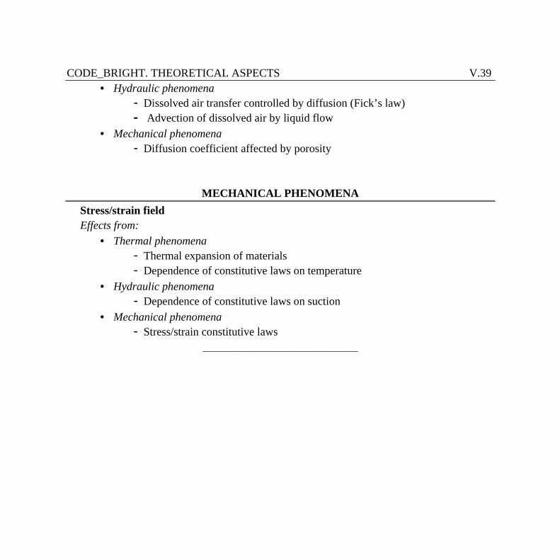
CODE_BRIGHT. THEORETICAL ASPECTS V.39
· Hydraulic phenomena - Dissolved air transfer controlled by diffusion (Fick’s law) - Advection of dissolved air by liquid flow
· Mechanical phenomena - Diffusion coefficient affected by porosity
MECHANICAL PHENOMENA Stress/strain field Effects from:
· Thermal phenomena - Thermal expansion of materials - Dependence of constitutive laws on temperature
· Hydraulic phenomena - Dependence of constitutive laws on suction
· Mechanical phenomena - Stress/strain constitutive laws
_________________________________
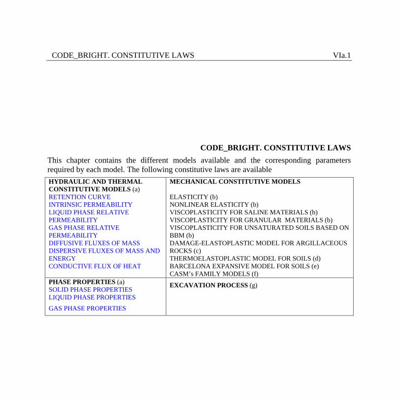
CODE_BRIGHT. CONSTITUTIVE LAWS VIa.1
CODE_BRIGHT. CONSTITUTIVE LAWS This chapter contains the different models available and the corresponding parameters required by each model. The following constitutive laws are available HYDRAULIC AND THERMAL CONSTITUTIVE MODELS (a) RETENTION CURVE INTRINSIC PERMEABILITY LIQUID PHASE RELATIVE PERMEABILITY GAS PHASE RELATIVE PERMEABILITY DIFFUSIVE FLUXES OF MASS DISPERSIVE FLUXES OF MASS AND ENERGY CONDUCTIVE FLUX OF HEAT
MECHANICAL CONSTITUTIVE MODELS ELASTICITY (b) NONLINEAR ELASTICITY (b) VISCOPLASTICITY FOR SALINE MATERIALS (b) VISCOPLASTICITY FOR GRANULAR MATERIALS (b) VISCOPLASTICITY FOR UNSATURATED SOILS BASED ON BBM (b) DAMAGE-ELASTOPLASTIC MODEL FOR ARGILLACEOUS ROCKS (c) THERMOELASTOPLASTIC MODEL FOR SOILS (d) BARCELONA EXPANSIVE MODEL FOR SOILS (e) CASM’s FAMILY MODELS (f)
PHASE PROPERTIES (a) SOLID PHASE PROPERTIES LIQUID PHASE PROPERTIES
GAS PHASE PROPERTIES
EXCAVATION PROCESS (g)
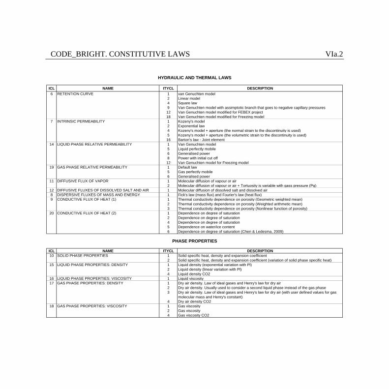
CODE_BRIGHT. CONSTITUTIVE LAWS VIa.2
ICL NAME ITYCL DESCRIPTION6 RETENTION CURVE 1 van Genuchten model
2 Linear model4 Square law9 Van Genuchten model with assimptotic branch that goes to negative capillary pressures
12 Van Genuchten model modified for FEBEX project18 Van Genuchten model modified for Freezing model
7 INTRINSIC PERMEABILITY 1 Kozeny's model2 Exponential law4 Kozeny's model + aperture (the normal strain to the discontinuity is used)5 Kozeny's model + aperture (the volumetric strain to the discontinuity is used)
16 Barton's law - Joint element14 LIQUID PHASE RELATIVE PERMEABILITY 1 Van Genuchten model
5 Liquid perfectly mobile6 Generalised power8 Power with initial cut off
12 Van Genuchten model for Freezing model19 GAS PHASE RELATIVE PERMEABILITY 1 Default law
5 Gas perfectly mobile6 Generalised power
11 DIFFUSIVE FLUX OF VAPOR 1 Molecular diffusion of vapour or air2 Molecular diffusion of vapour or air + Tortuosity is variable with gass pressure (Pg)
12 DIFFUSIVE FLUXES OF DISSOLVED SALT AND AIR 1 Molecular diffusion of dissolved salt and dissolved air8 DISPERSIVE FLUXES OF MASS AND ENERGY 1 Fick's law (mass flux) and Fourier's law (heat flux)9 CONDUCTIVE FLUX OF HEAT (1) 1 Thermal conductivity dependence on porosity (Geometric weighted mean)
2 Thermal conductivity dependence on porosity (Weighted arithmetic mean)3 Thermal conductivity dependence on porosity (Nonlinear function of porosity)
20 CONDUCTIVE FLUX OF HEAT (2) 1 Dependence on degree of saturation2 Dependence on degree of saturation4 Dependence on degree of saturation5 Dependence on water/ice content6 Dependence on degree of saturation (Chen & Ledesma, 2009)
ICL NAME ITYCL DESCRIPTION10 SOLID PHASE PROPERTIES 1 Solid specific heat, density and expansion coefficient
2 Solid specific heat, density and expansion coefficient (variation of solid phase specific heat)15 LIQUID PHASE PROPERTIES: DENSITY 1 Liquid density (exponential variation with Pl)
2 Liquid density (linear variation with Pl)4 Liquid density CO2
16 LIQUID PHASE PROPERTIES: VISCOSITY 1 Liquid viscosity17 GAS PHASE PROPERTIES: DENSITY 1 Dry air density. Law of ideal gases and Henry's law for dry air
2 Dry air density. Usually used to consider a second liquid phase instead of the gas phase3 Dry air density. Law of ideal gases and Henry's law for dry air (with user defined values for gas
molecular mass and Henry's constant)4 Dry air density CO2
18 GAS PHASE PROPERTIES: VISCOSITY 1 Gas viscosity2 Gas viscosity4 Gas viscosity CO2
HYDRAULIC AND THERMAL LAWS
PHASE PROPERTIES
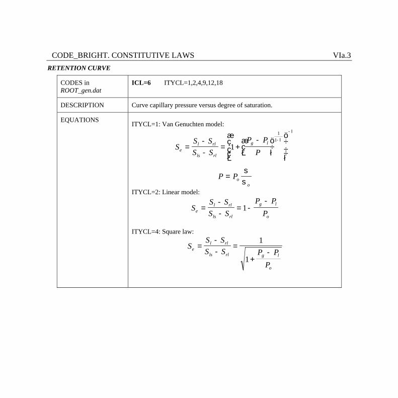
CODE_BRIGHT. CONSTITUTIVE LAWS VIa.3 RETENTION CURVE
CODES in ROOT_gen.dat
ICL=6 ITYCL=1,2,4,9,12,18
DESCRIPTION Curve capillary pressure versus degree of saturation.
EQUATIONS ITYCL=1: Van Genuchten model:
SS SS S
P PP
P P
el rl
ls rl
g l
oo
=--
= +-æ
èç
öø÷
æ
è
ççç
ö
ø
÷÷÷
=
-
-
1
11 l
l
ss
ITYCL=2: Linear model:
SS SS S
P PPe
l rl
ls rl
g l
o=
--
= --
1
ITYCL=4: Square law:
SS SS S P P
P
el rl
ls rl g l
o
=--
=
+-
1
1
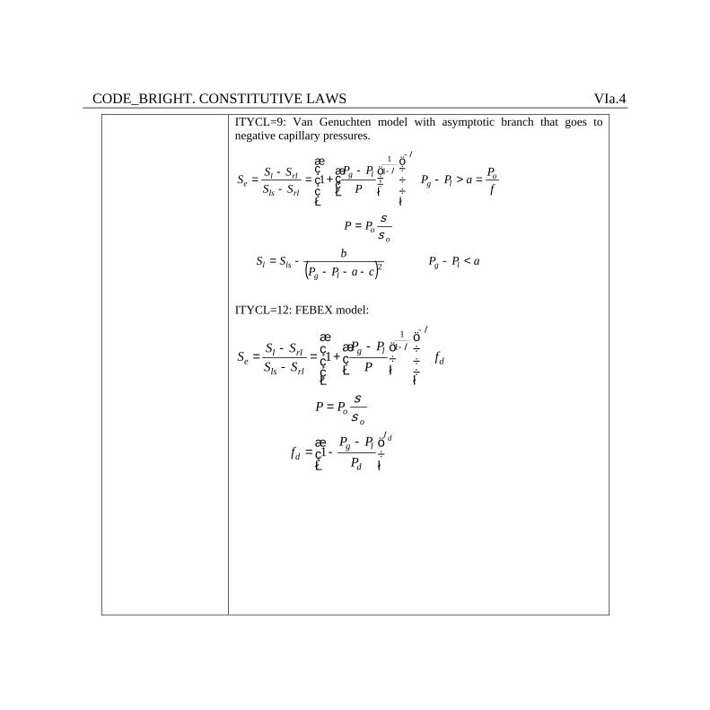
CODE_BRIGHT. CONSTITUTIVE LAWS VIa.4
ITYCL=9: Van Genuchten model with asymptotic branch that goes to negative capillary pressures.
( ) aPPcaPP
bSS
PP
fPaPP
PPP
SSSSS
lglg
lsl
oo
olg
lg
rlls
rlle
<----
-=
=
=>-÷÷÷
ø
ö
ççç
è
æ
÷÷ø
öççè
æ -+=
--
=
-
-
1
2
11
ss
l
l
ITYCL=12: FEBEX model:
11
1
1d
g ll rle d
ls rl
oo
g ld
d
P PS SS fS S P
P P
P Pf
P
l
l
l
ss
-
-æ ö
-æ ö- ç ÷= = + ç ÷ç ÷- è øç ÷è ø
=
-æ ö= -ç ÷
è ø
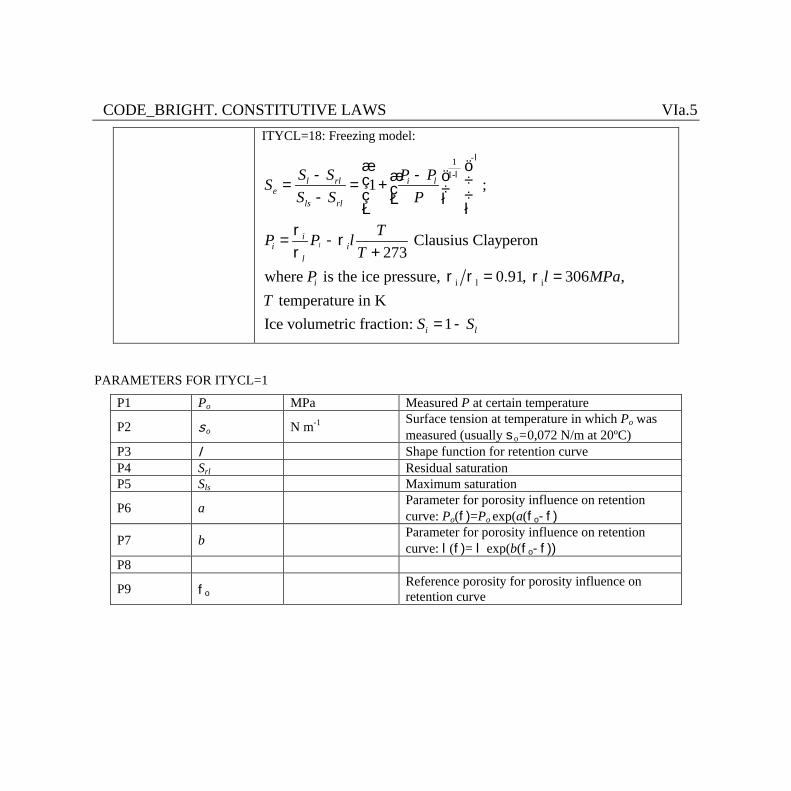
CODE_BRIGHT. CONSTITUTIVE LAWS VIa.5 ITYCL=18: Freezing model:
-11-
i l i
1 ;
Clausius Clayperon 273
where is the ice pressure, 0.91, 306 , temperature in K
Ice volumetric fraction: 1
l
l rl i le
ls rl
ii i
l
i
i l
S S P PSS S P
TP P lT
P l MPaT
S S
l
læ ö- -æ öç ÷= = + ç ÷ç ÷- è øè ø
r= - r
r +
r r = r =
= -
PARAMETERS FOR ITYCL=1
P1 Po MPa Measured P at certain temperature
P2 so N m-1 Surface tension at temperature in which Po was measured (usually so=0,072 N/m at 20ºC)
P3 l Shape function for retention curve P4 Srl Residual saturation P5 Sls Maximum saturation
P6 a Parameter for porosity influence on retention curve: Po(f)=Po exp(a(fo-f)
P7 b Parameter for porosity influence on retention curve: l(f)= l exp(b(fo-f))
P8
P9 fo Reference porosity for porosity influence on retention curve
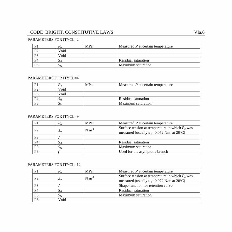
CODE_BRIGHT. CONSTITUTIVE LAWS VIa.6 PARAMETERS FOR ITYCL=2
P1 Po MPa Measured P at certain temperature P2 Void P3 Void P4 Srl Residual saturation P5 Sls Maximum saturation
PARAMETERS FOR ITYCL=4
P1 Po MPa Measured P at certain temperature P2 Void P3 Void P4 Srl Residual saturation P5 Sls Maximum saturation
PARAMETERS FOR ITYCL=9
P1 Po MPa Measured P at certain temperature
P2 so N m-1 Surface tension at temperature in which Po was measured (usually so=0,072 N/m at 20ºC)
P3 l P4 Srl Residual saturation P5 Sls Maximum saturation P6 f Used for the asymptotic branch
PARAMETERS FOR ITYCL=12
P1 Po MPa Measured P at certain temperature
P2 so N m-1 Surface tension at temperature in which Po was measured (usually so=0,072 N/m at 20ºC)
P3 l Shape function for retention curve P4 Srl Residual saturation P5 Sls Maximum saturation P6 Void
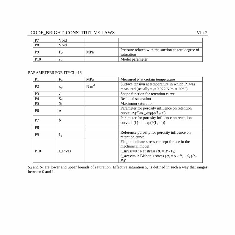
CODE_BRIGHT. CONSTITUTIVE LAWS VIa.7 P7 Void P8 Void
P9 Pd MPa Pressure related with the suction at zero degree of saturation
P10 ld Model parameter
PARAMETERS FOR ITYCL=18
P1 Po MPa Measured P at certain temperature
P2 so N m-1 Surface tension at temperature in which Po was measured (usually so=0,072 N/m at 20ºC)
P3 l Shape function for retention curve P4 Srl Residual saturation P5 Sls Maximum saturation
P6 a Parameter for porosity influence on retention curve: Po(f)=Po exp(a(fo-f)
P7 b Parameter for porosity influence on retention curve: l(f)= l exp(b(fo-f))
P8
P9 fo Reference porosity for porosity influence on retention curve
P10 i_stress
Flag to indicate stress concept for use in the mechanical model: i_stress=0 : Net stress (sn = s - Pi) i_stress=-1: Bishop’s stress (sb = s - Pi + Sr (Pi-Pl))
Srl and Sls are lower and upper bounds of saturation. Effective saturation Se is defined in such a way that ranges between 0 and 1.
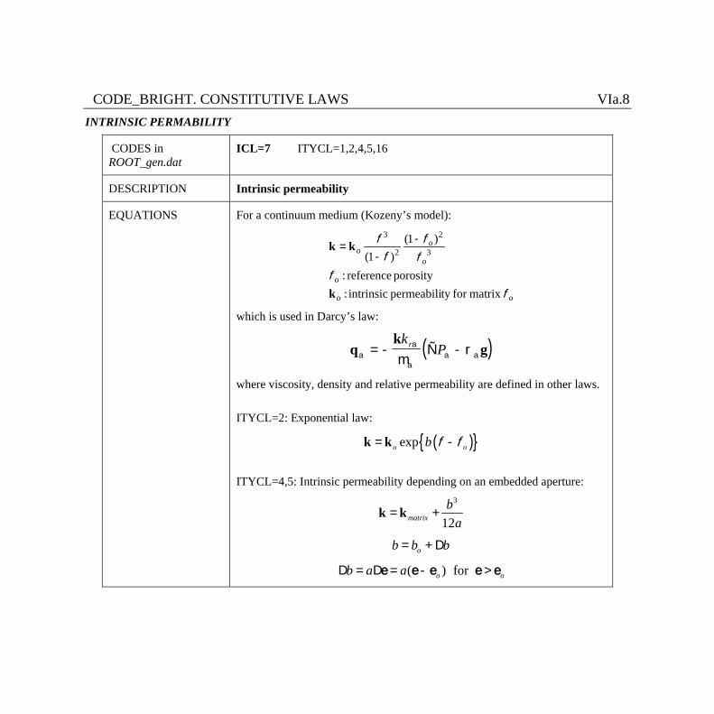
CODE_BRIGHT. CONSTITUTIVE LAWS VIa.8 INTRINSIC PERMABILITY
CODES in ROOT_gen.dat
ICL=7 ITYCL=1,2,4,5,16
DESCRIPTION Intrinsic permeability
EQUATIONS For a continuum medium (Kozeny’s model):
oo
o
o
oo
ff
ff
ff
matrix for ty permeabili intrinsic :porosity reference :
)1()1( 3
2
2
3
k
kk --
=
which is used in Darcy’s law:
( )qk
gaa
aa am
r= - Ñ -k
Pr
where viscosity, density and relative permeability are defined in other laws.
ITYCL=2: Exponential law:
( ){ }expo ob f f= -k k
ITYCL=4,5: Intrinsic permeability depending on an embedded aperture:
3
12matrixb
a= +k k
ob b b= + D
( ) for o ob a aD = D = - >e e e e e
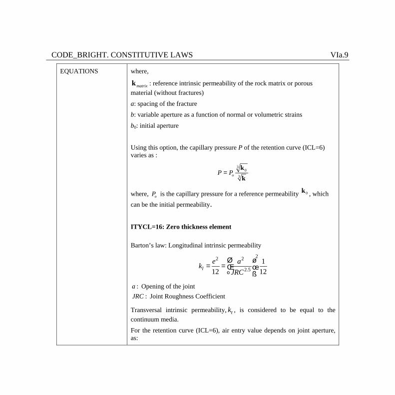
CODE_BRIGHT. CONSTITUTIVE LAWS VIa.9
EQUATIONS where,
matrixk : reference intrinsic permeability of the rock matrix or porous material (without fractures) a: spacing of the fracture
b: variable aperture as a function of normal or volumetric strains
b0: initial aperture
Using this option, the capillary pressure P of the retention curve (ICL=6) varies as :
30
3oP P=kk
where, oP is the capillary pressure for a reference permeability 0k , which can be the initial permeability.
ITYCL=16: Zero thickness element Barton’s law: Longitudinal intrinsic permeability
22 2
2.51
12 12le ak
JRCé ù
= = ê úë û
: Opening of the joint: Joint Roughness Coefficient
aJRC Transversal intrinsic permeability, tk , is considered to be equal to the continuum media.
For the retention curve (ICL=6), air entry value depends on joint aperture, as:
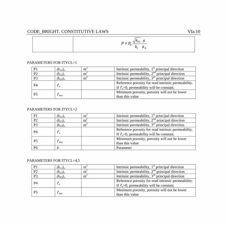
CODE_BRIGHT. CONSTITUTIVE LAWS VIa.10
00
0
l
l
kP P
kss
=
PARAMETERS FOR ITYCL=1
P1 (k11)o m2 Intrinsic permeability, 1st principal direction P2 (k22)o m2 Intrinsic permeability, 2nd principal direction P3 (k33)o m2 Intrinsic permeability, 3rd principal direction
P4 fo Reference porosity for read intrinsic permeability. If fo=0, permeability will be constant.
P5 fmin Minimum porosity, porosity will not be lower than this value
PARAMETERS FOR ITYCL=2
P1 (k11)o m2 Intrinsic permeability, 1st principal direction P2 (k22)o m2 Intrinsic permeability, 2nd principal direction P3 (k33)o m2 Intrinsic permeability, 3rd principal direction
P4 fo Reference porosity for read intrinsic permeability. If fo=0, permeability will be constant.
P5 fmin Minimum porosity, porosity will not be lower than this value
P6 b Parameter
PARAMETERS FOR ITYCL=4,5
P1 (k11)o m2 Intrinsic permeability, 1st principal direction P2 (k22)o m2 Intrinsic permeability, 2nd principal direction P3 (k33)o m2 Intrinsic permeability, 3rd principal direction
P4 fo Reference porosity for read intrinsic permeability. If fo=0, permeability will be constant.
P5 fmin Minimum porosity, porosity will not be lower than this value
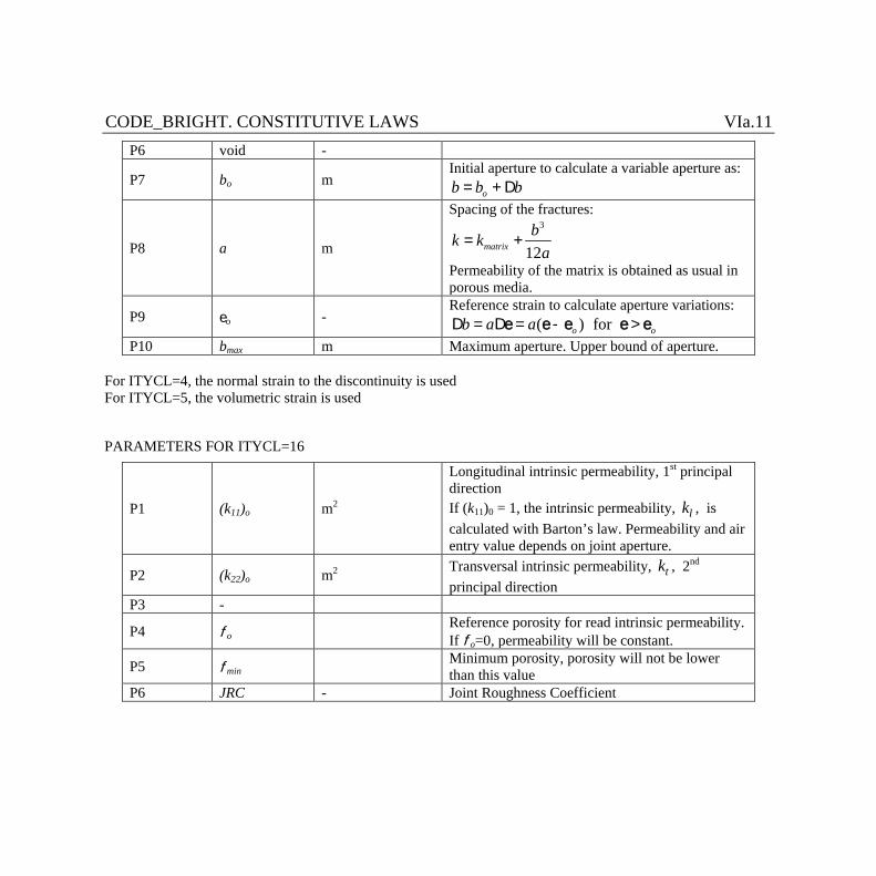
CODE_BRIGHT. CONSTITUTIVE LAWS VIa.11 P6 void -
P7 bo m Initial aperture to calculate a variable aperture as:
ob b b= + D
P8 a m
Spacing of the fractures: 3
12matrixbk k
a= +
Permeability of the matrix is obtained as usual in porous media.
P9 eo - Reference strain to calculate aperture variations:
( ) for o ob a aD = D = - >e e e e e P10 bmax m Maximum aperture. Upper bound of aperture.
For ITYCL=4, the normal strain to the discontinuity is used For ITYCL=5, the volumetric strain is used
PARAMETERS FOR ITYCL=16
P1 (k11)o m2
Longitudinal intrinsic permeability, 1st principal direction If (k11)0 = 1, the intrinsic permeability, lk , is calculated with Barton’s law. Permeability and air entry value depends on joint aperture.
P2 (k22)o m2 Transversal intrinsic permeability, tk , 2nd principal direction
P3 -
P4 fo Reference porosity for read intrinsic permeability. If fo=0, permeability will be constant.
P5 fmin Minimum porosity, porosity will not be lower than this value
P6 JRC - Joint Roughness Coefficient
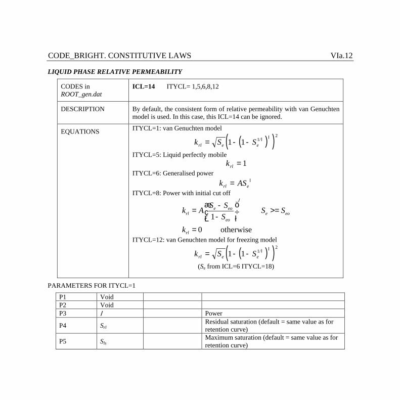
CODE_BRIGHT. CONSTITUTIVE LAWS VIa.12
LIQUID PHASE RELATIVE PERMEABILITY
CODES in ROOT_gen.dat
ICL=14 ITYCL= 1,5,6,8,12
DESCRIPTION By default, the consistent form of relative permeability with van Genuchten model is used. In this case, this ICL=14 can be ignored.
EQUATIONS ITYCL=1: van Genuchten model
( )( )k S Srl e e= - -1 1 12
/l l
ITYCL=5: Liquid perfectly mobile krl = 1
ITYCL=6: Generalised power k ASrl e= l
ITYCL=8: Power with initial cut off
1
0 otherwise
e eorl e eo
eo
rl
S Sk A S SS
k
læ ö-
= >=ç ÷-è ø=
ITYCL=12: van Genuchten model for freezing model
( )( )k S Srl e e= - -1 1 12
/l l
(Se from ICL=6 ITYCL=18)
PARAMETERS FOR ITYCL=1
P1 Void P2 Void P3 l Power
P4 Srl Residual saturation (default = same value as for retention curve)
P5 Sls Maximum saturation (default = same value as for retention curve)
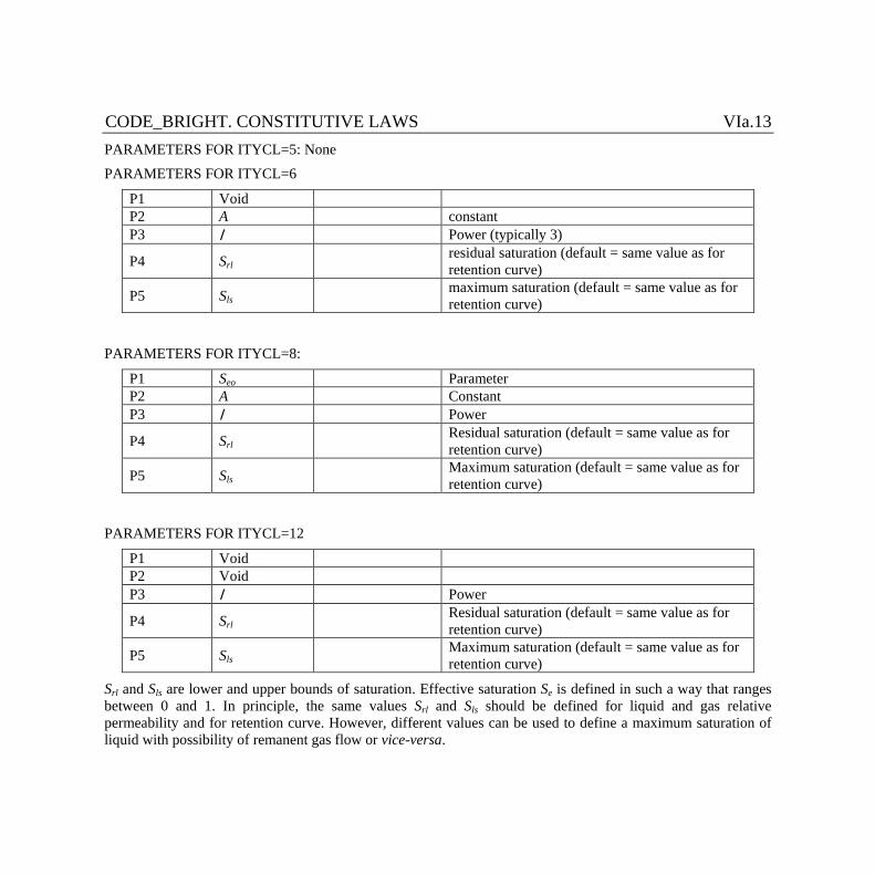
CODE_BRIGHT. CONSTITUTIVE LAWS VIa.13 PARAMETERS FOR ITYCL=5: None PARAMETERS FOR ITYCL=6
P1 Void P2 A constant P3 l Power (typically 3)
P4 Srl residual saturation (default = same value as for retention curve)
P5 Sls maximum saturation (default = same value as for retention curve)
PARAMETERS FOR ITYCL=8:
P1 Seo Parameter P2 A Constant P3 l Power
P4 Srl Residual saturation (default = same value as for retention curve)
P5 Sls Maximum saturation (default = same value as for retention curve)
PARAMETERS FOR ITYCL=12
P1 Void P2 Void P3 l Power
P4 Srl Residual saturation (default = same value as for retention curve)
P5 Sls Maximum saturation (default = same value as for retention curve)
Srl and Sls are lower and upper bounds of saturation. Effective saturation Se is defined in such a way that ranges between 0 and 1. In principle, the same values Srl and Sls should be defined for liquid and gas relative permeability and for retention curve. However, different values can be used to define a maximum saturation of liquid with possibility of remanent gas flow or vice-versa.
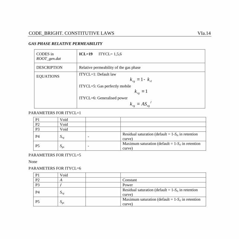
CODE_BRIGHT. CONSTITUTIVE LAWS VIa.14
GAS PHASE RELATIVE PERMEABILITY
CODES in ROOT_gen.dat
ICL=19 ITYCL= 1,5,6
DESCRIPTION Relative permeability of the gas phase
EQUATIONS ITYCL=1: Default law k krg rl= -1
ITYCL=5: Gas perfectly mobile krg = 1
ITYCL=6: Generalised power k ASrg eg= l
PARAMETERS FOR ITYCL=1
P1 Void P2 Void P3 Void
P4 Srg - Residual saturation (default = 1-Sls in retention curve)
P5 Sgs - Maximum saturation (default = 1-Srl in retention curve)
PARAMETERS FOR ITYCL=5
None
PARAMETERS FOR ITYCL=6
P1 Void P2 A Constant P3 l Power
P4 Srg Residual saturation (default = 1-Sls in retention curve)
P5 Sgs Maximum saturation (default = 1-Srl in retention curve)
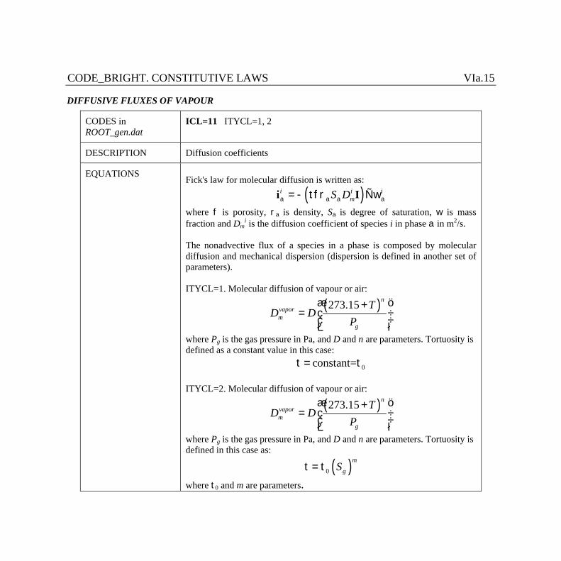
CODE_BRIGHT. CONSTITUTIVE LAWS VIa.15
DIFFUSIVE FLUXES OF VAPOUR
CODES in ROOT_gen.dat
ICL=11 ITYCL=1, 2
DESCRIPTION Diffusion coefficients
EQUATIONS Fick's law for molecular diffusion is written as:
( )i i imS Da a a a= - tfr Ñwi I
where f is porosity, ra is density, Sa is degree of saturation, w is mass fraction and Dm
i is the diffusion coefficient of species i in phase a in m2/s. The nonadvective flux of a species in a phase is composed by molecular diffusion and mechanical dispersion (dispersion is defined in another set of parameters). ITYCL=1. Molecular diffusion of vapour or air:
( )273.15 nvaporm
g
TD D
P
æ ö+= ç ÷
ç ÷è ø
where Pg is the gas pressure in Pa, and D and n are parameters. Tortuosity is defined as a constant value in this case:
0constant=t = t ITYCL=2. Molecular diffusion of vapour or air:
( )273.15 nvaporm
g
TD D
P
æ ö+= ç ÷
ç ÷è ø
where Pg is the gas pressure in Pa, and D and n are parameters. Tortuosity is defined in this case as:
( )0
m
gSt = t
where t0 and m are parameters.
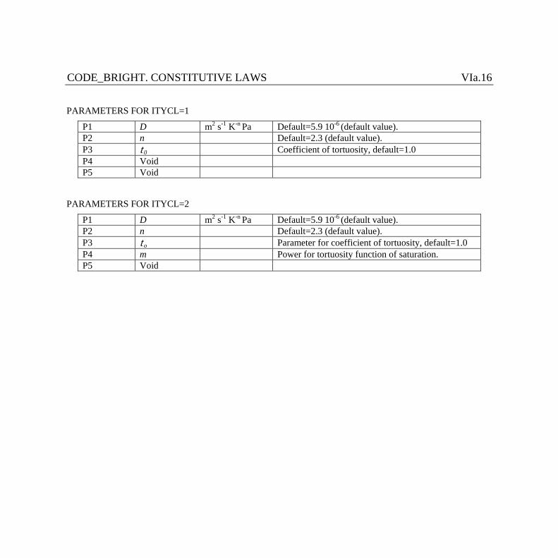
CODE_BRIGHT. CONSTITUTIVE LAWS VIa.16 PARAMETERS FOR ITYCL=1
P1 D m2 s-1 K-n Pa Default=5.9 10-6 (default value). P2 n Default=2.3 (default value). P3 t0 Coefficient of tortuosity, default=1.0 P4 Void P5 Void
PARAMETERS FOR ITYCL=2
P1 D m2 s-1 K-n Pa Default=5.9 10-6 (default value). P2 n Default=2.3 (default value). P3 to Parameter for coefficient of tortuosity, default=1.0 P4 m Power for tortuosity function of saturation. P5 Void
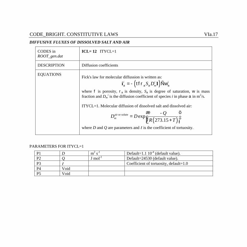
CODE_BRIGHT. CONSTITUTIVE LAWS VIa.17 DIFFUSIVE FLUXES OF DISSOLVED SALT AND AIR
CODES in ROOT_gen.dat
ICL= 12 ITYCL=1
DESCRIPTION Diffusion coefficients
EQUATIONS Fick's law for molecular diffussion is written as:
( )i i imS Da a a a= - tfr Ñwi I
where f is porosity, ra is density, Sa is degree of saturation, w is mass fraction and Dm
i is the diffusion coefficient of species i in phase a in m2/s. ITYCL=1. Molecular diffusion of dissolved salt and dissolved air:
( )air or solute exp
273.15mQD D
R Tæ ö-
= ç ÷ç ÷+è ø
where D and Q are parameters and t is the coefficient of tortuosity.
PARAMETERS FOR ITYCL=1
P1 D m2 s-1 Default=1.1 10-4 (default value). P2 Q J mol-1 Default=24530 (default value). P3 t Coefficient of tortuosity, default=1.0 P4 Void P5 Void
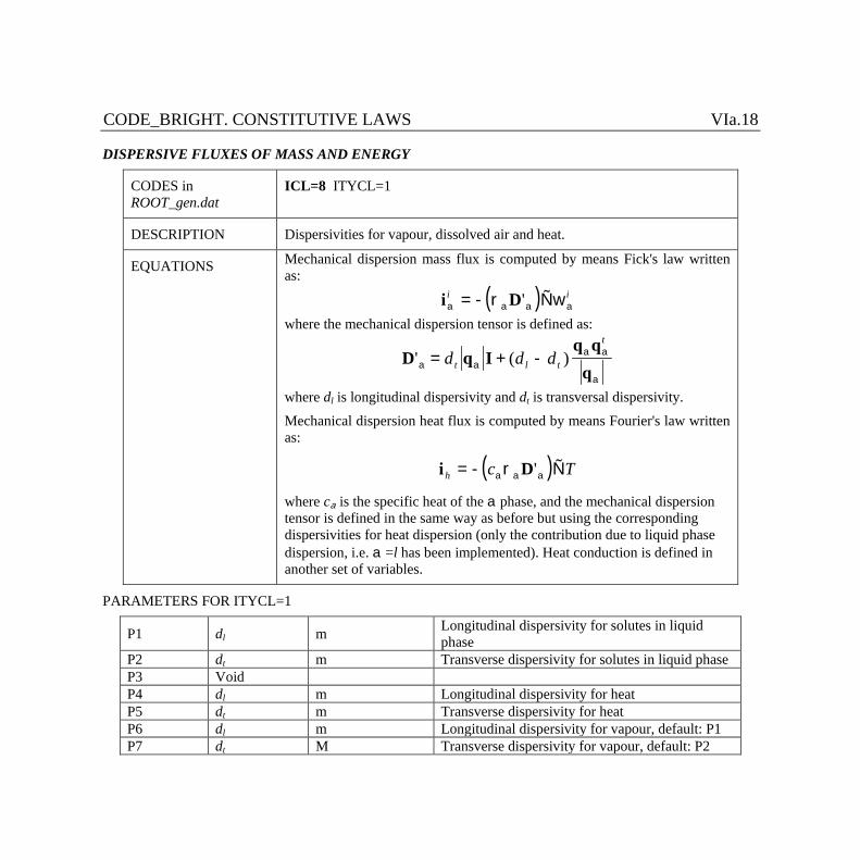
CODE_BRIGHT. CONSTITUTIVE LAWS VIa.18
DISPERSIVE FLUXES OF MASS AND ENERGY
CODES in ROOT_gen.dat
ICL=8 ITYCL=1
DESCRIPTION Dispersivities for vapour, dissolved air and heat.
EQUATIONS Mechanical dispersion mass flux is computed by means Fick's law written as:
( )i Da a a ari i= - Ñw' where the mechanical dispersion tensor is defined as:
D q Iq q
q' ( )a a
a a
a
= + -d d dt l t
t
where dl is longitudinal dispersivity and dt is transversal dispersivity. Mechanical dispersion heat flux is computed by means Fourier's law written as:
( )i Dh c T= - Ña a ar '
where ca is the specific heat of the a phase, and the mechanical dispersion tensor is defined in the same way as before but using the corresponding dispersivities for heat dispersion (only the contribution due to liquid phase dispersion, i.e. a =l has been implemented). Heat conduction is defined in another set of variables.
PARAMETERS FOR ITYCL=1
P1 dl m Longitudinal dispersivity for solutes in liquid phase
P2 dt m Transverse dispersivity for solutes in liquid phase P3 Void P4 dl m Longitudinal dispersivity for heat P5 dt m Transverse dispersivity for heat P6 dl m Longitudinal dispersivity for vapour, default: P1 P7 dt M Transverse dispersivity for vapour, default: P2
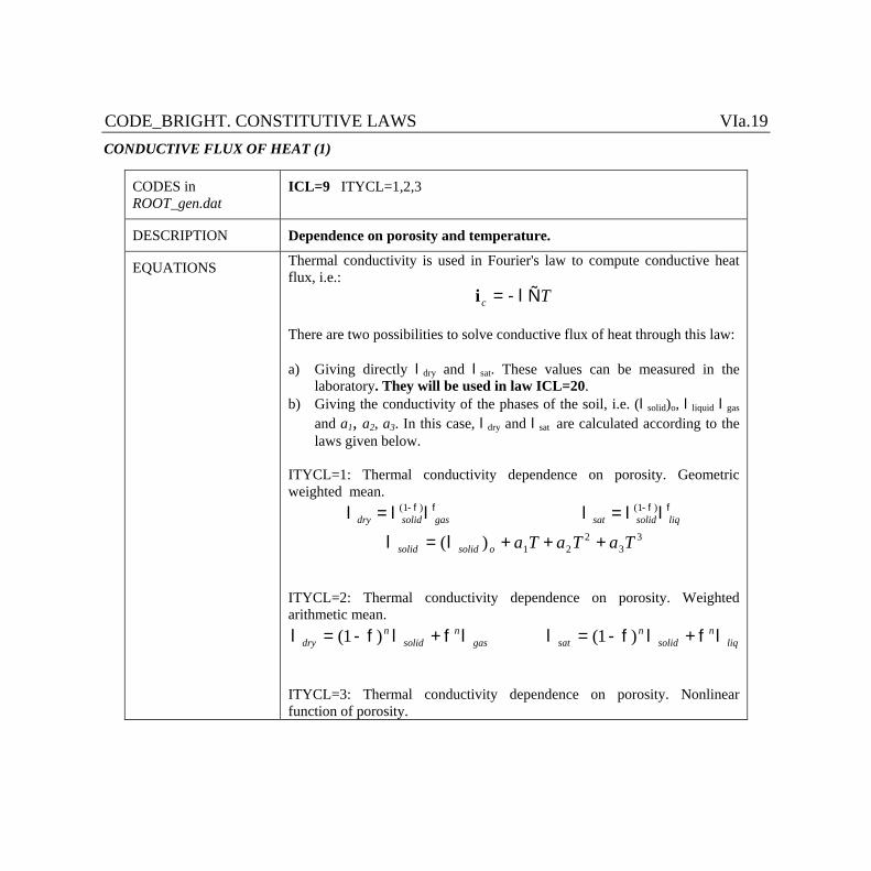
CODE_BRIGHT. CONSTITUTIVE LAWS VIa.19 CONDUCTIVE FLUX OF HEAT (1)
CODES in ROOT_gen.dat
ICL=9 ITYCL=1,2,3
DESCRIPTION Dependence on porosity and temperature.
EQUATIONS Thermal conductivity is used in Fourier's law to compute conductive heat flux, i.e.:
i c T= -lÑ There are two possibilities to solve conductive flux of heat through this law: a) Giving directly ldry and lsat. These values can be measured in the
laboratory. They will be used in law ICL=20. b) Giving the conductivity of the phases of the soil, i.e. (lsolid)o, lliquid lgas
and a1, a2, a3. In this case, ldry and lsat are calculated according to the laws given below.
ITYCL=1: Thermal conductivity dependence on porosity. Geometric weighted mean.
l l l l l lf f f fdry solid gas sat solid liq= =- -( ) ( )1 1
l lsolid solid o a T a T a T= + + +( ) 1 22
33
ITYCL=2: Thermal conductivity dependence on porosity. Weighted arithmetic mean. l f l f l l f l f ldry
nsolid
ngas sat
nsolid
nliq= - + = - +( ) ( )1 1
ITYCL=3: Thermal conductivity dependence on porosity. Nonlinear function of porosity.
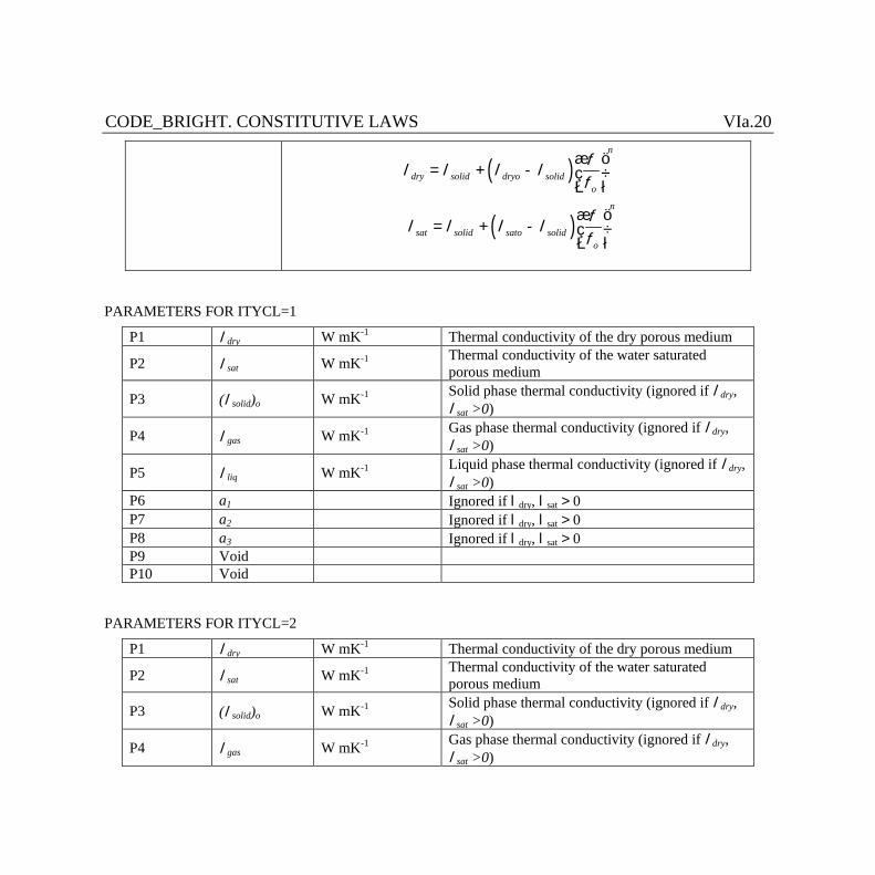
CODE_BRIGHT. CONSTITUTIVE LAWS VIa.20
( )
( )
n
dry solid dryo solido
n
sat solid sato solido
fl l l lf
fl l l lf
æ ö= + - ç ÷
è ø
æ ö= + - ç ÷
è ø
PARAMETERS FOR ITYCL=1
P1 ldry W mK-1 Thermal conductivity of the dry porous medium
P2 lsat W mK-1 Thermal conductivity of the water saturated porous medium
P3 (lsolid)o W mK-1 Solid phase thermal conductivity (ignored if ldry, lsat >0)
P4 lgas W mK-1 Gas phase thermal conductivity (ignored if ldry, lsat >0)
P5 lliq W mK-1 Liquid phase thermal conductivity (ignored if ldry, lsat >0)
P6 a1 Ignored if ldry, lsat > 0 P7 a2 Ignored if ldry, lsat > 0 P8 a3 Ignored if ldry, lsat > 0 P9 Void P10 Void
PARAMETERS FOR ITYCL=2
P1 ldry W mK-1 Thermal conductivity of the dry porous medium
P2 lsat W mK-1 Thermal conductivity of the water saturated porous medium
P3 (lsolid)o W mK-1 Solid phase thermal conductivity (ignored if ldry, lsat >0)
P4 lgas W mK-1 Gas phase thermal conductivity (ignored if ldry, lsat >0)
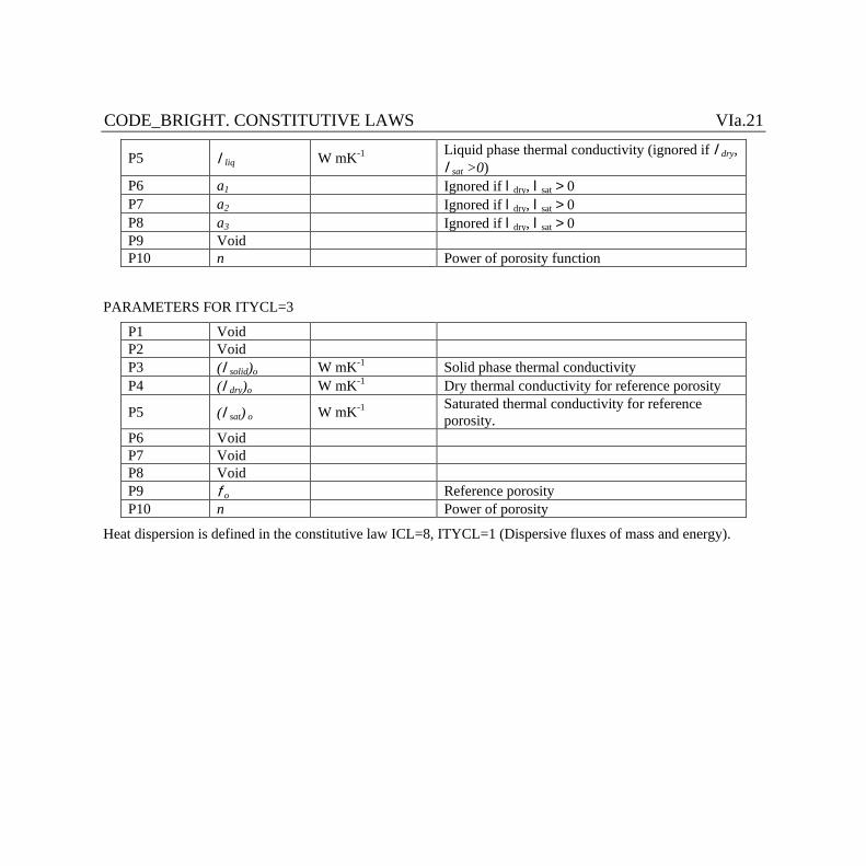
CODE_BRIGHT. CONSTITUTIVE LAWS VIa.21
P5 lliq W mK-1 Liquid phase thermal conductivity (ignored if ldry, lsat >0)
P6 a1 Ignored if ldry, lsat > 0 P7 a2 Ignored if ldry, lsat > 0 P8 a3 Ignored if ldry, lsat > 0 P9 Void P10 n Power of porosity function
PARAMETERS FOR ITYCL=3
P1 Void P2 Void P3 (lsolid)o W mK-1 Solid phase thermal conductivity P4 (ldry)o W mK-1 Dry thermal conductivity for reference porosity
P5 (lsat) o W mK-1 Saturated thermal conductivity for reference porosity.
P6 Void P7 Void P8 Void P9 fo Reference porosity P10 n Power of porosity
Heat dispersion is defined in the constitutive law ICL=8, ITYCL=1 (Dispersive fluxes of mass and energy).

CODE_BRIGHT. CONSTITUTIVE LAWS VIa.22
CONDUCTIVE FLUX OF HEAT (2)
CODES in ROOT_gen.dat
ICL= 20 ITYCL=1,2, 4,5, 6
DESCRIPTION Dependence on water content.
EQUATIONS Thermal conductivity is used in Fourier's law to compute conductive heat flux, i.e.:
i c T= -lÑ Dependence of thermal conductivity on degree of saturation can be considered in the following ways: ITYCL=1:
( )l l l= + -sat l dry lS S1 ITYCL=2:
( )l l l= -sat
Sdry
Sl l1 ITYCL=4:
( )1dry l sat lS Sl l l= - + ITYCL=5: Dependence on water/ice content. Activating this option permits to have different values for thermal conductivity depending if the soil is frozen or unfrozen.
( )1 ll SSunfrozen frozen
-l = l l Parameters are not necessary for ICL=20 and ITYCL=5
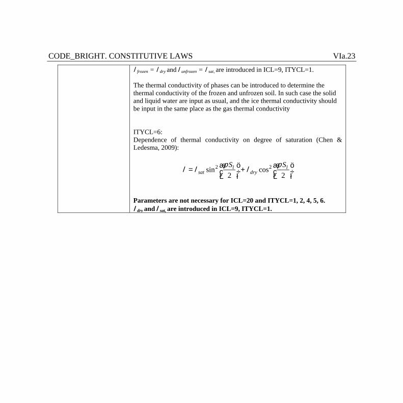
CODE_BRIGHT. CONSTITUTIVE LAWS VIa.23 lfrozen = ldry and lunfrozen = lsat, are introduced in ICL=9, ITYCL=1. The thermal conductivity of phases can be introduced to determine the thermal conductivity of the frozen and unfrozen soil. In such case the solid and liquid water are input as usual, and the ice thermal conductivity should be input in the same place as the gas thermal conductivity ITYCL=6: Dependence of thermal conductivity on degree of saturation (Chen & Ledesma, 2009):
2 2sin cos2 2
l lsat dry
S Sp pl l læ ö æ ö= +ç ÷ ç ÷
è ø è ø
Parameters are not necessary for ICL=20 and ITYCL=1, 2, 4, 5, 6. ldry and lsat, are introduced in ICL=9, ITYCL=1.
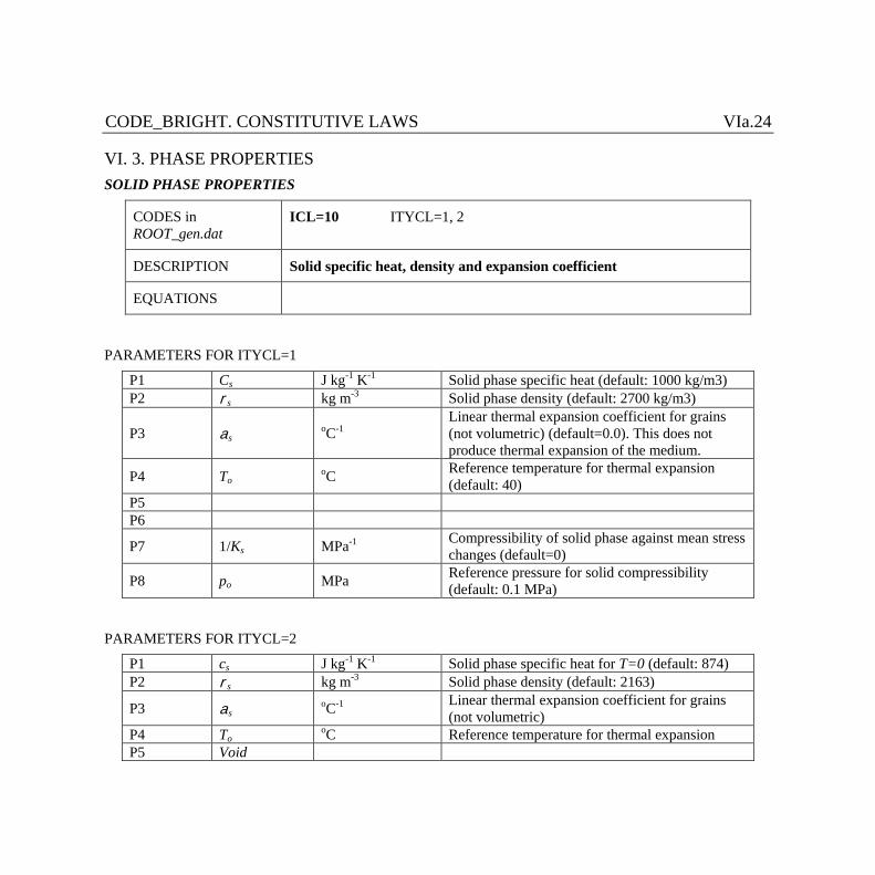
CODE_BRIGHT. CONSTITUTIVE LAWS VIa.24
VI. 3. PHASE PROPERTIES SOLID PHASE PROPERTIES
CODES in ROOT_gen.dat
ICL=10 ITYCL=1, 2
DESCRIPTION Solid specific heat, density and expansion coefficient
EQUATIONS
PARAMETERS FOR ITYCL=1
P1 Cs J kg-1 K-1 Solid phase specific heat (default: 1000 kg/m3) P2 rs kg m-3 Solid phase density (default: 2700 kg/m3)
P3 as oC-1 Linear thermal expansion coefficient for grains (not volumetric) (default=0.0). This does not produce thermal expansion of the medium.
P4 To oC Reference temperature for thermal expansion (default: 40)
P5 P6
P7 1/Ks MPa-1 Compressibility of solid phase against mean stress changes (default=0)
P8 po MPa Reference pressure for solid compressibility (default: 0.1 MPa)
PARAMETERS FOR ITYCL=2
P1 cs J kg-1 K-1 Solid phase specific heat for T=0 (default: 874) P2 rs kg m-3 Solid phase density (default: 2163)
P3 as oC-1 Linear thermal expansion coefficient for grains (not volumetric)
P4 To oC Reference temperature for thermal expansion P5 Void
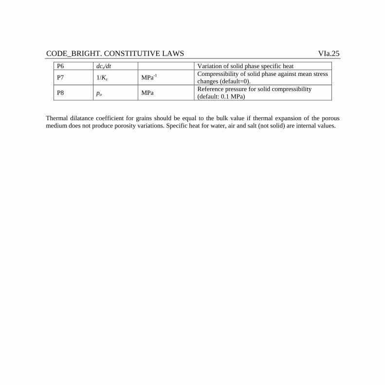
CODE_BRIGHT. CONSTITUTIVE LAWS VIa.25 P6 dcs/dt Variation of solid phase specific heat
P7 1/Ks MPa-1 Compressibility of solid phase against mean stress changes (default=0).
P8 po MPa Reference pressure for solid compressibility (default: 0.1 MPa)
Thermal dilatance coefficient for grains should be equal to the bulk value if thermal expansion of the porous medium does not produce porosity variations. Specific heat for water, air and salt (not solid) are internal values.
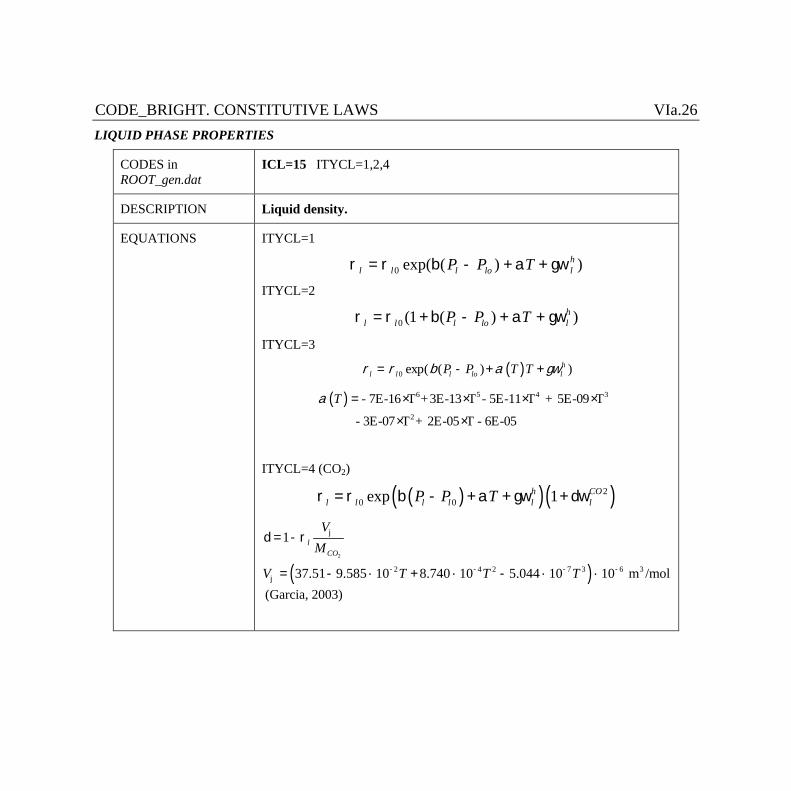
CODE_BRIGHT. CONSTITUTIVE LAWS VIa.26 LIQUID PHASE PROPERTIES
CODES in ROOT_gen.dat
ICL=15 ITYCL=1,2,4
DESCRIPTION Liquid density.
EQUATIONS ITYCL=1
r r b a gwl l l lo lhP P T= - + +0 exp( ( ) )
ITYCL=2
0 (1 ( ) )hl l l lo lP P Tr = r + b - + a + gw
ITYCL=3
( )0 exp( ( ) )hl l l lo lP P T Tr r b a gw= - + +
( ) 6 5 4 3
2
- 7E-16 T +3E-13 T - 5E-11 T + 5E-09 T
- 3E-07 T + 2E-05 T - 6E-05
Ta = × × × ×
× ×
ITYCL=4 (CO2)
( )( )( )20 0exp 1h CO
l l l l l lP P Tr = r b - + a + gw + dw
( )2
2 4 2 7 3 6 3
1
37.51 9.585 10 8.740 10 5.044 10 10 m /mol
lCO
VM
V T T T
j
- - - -j
d = - r
= - ´ + ´ - ´ ´
(Garcia, 2003)
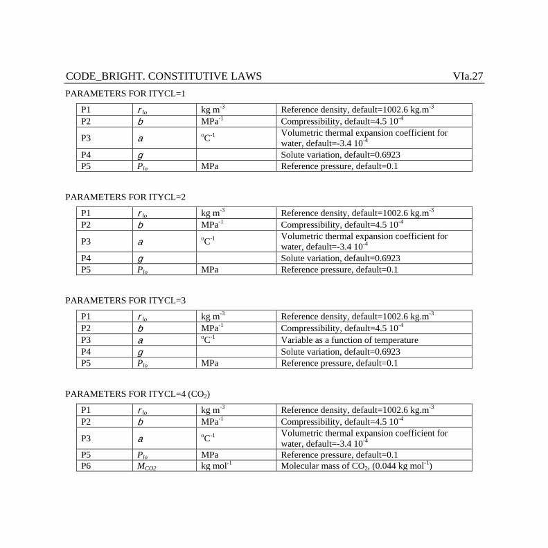
CODE_BRIGHT. CONSTITUTIVE LAWS VIa.27 PARAMETERS FOR ITYCL=1
P1 rlo kg m-3 Reference density, default=1002.6 kg.m-3 P2 b MPa-1 Compressibility, default=4.5 10-4
P3 a oC-1 Volumetric thermal expansion coefficient for water, default=-3.4 10-4
P4 g Solute variation, default=0.6923 P5 Plo MPa Reference pressure, default=0.1
PARAMETERS FOR ITYCL=2
P1 rlo kg m-3 Reference density, default=1002.6 kg.m-3 P2 b MPa-1 Compressibility, default=4.5 10-4
P3 a oC-1 Volumetric thermal expansion coefficient for water, default=-3.4 10-4
P4 g Solute variation, default=0.6923 P5 Plo MPa Reference pressure, default=0.1
PARAMETERS FOR ITYCL=3
P1 rlo kg m-3 Reference density, default=1002.6 kg.m-3 P2 b MPa-1 Compressibility, default=4.5 10-4 P3 a oC-1 Variable as a function of temperature P4 g Solute variation, default=0.6923 P5 Plo MPa Reference pressure, default=0.1
PARAMETERS FOR ITYCL=4 (CO2)
P1 rlo kg m-3 Reference density, default=1002.6 kg.m-3 P2 b MPa-1 Compressibility, default=4.5 10-4
P3 a oC-1 Volumetric thermal expansion coefficient for water, default=-3.4 10-4
P5 Plo MPa Reference pressure, default=0.1 P6 MCO2 kg mol-1 Molecular mass of CO2, (0.044 kg mol-1)

CODE_BRIGHT. CONSTITUTIVE LAWS VIa.28
CODES in ROOT_gen.dat
ICL= 16 ITYCL=1
DESCRIPTION Liquid viscosity.
EQUATIONS ITYCL=1
m l AB
T=
+æèç
öø÷exp
.27315
PARAMETERS FOR ITYCL=1
P1 A MPa s Pre-exponential parameter, default= 2.1 10-12
P2 B K Exponential parameter, default=1808.5 (only used if A=B=0, but not used if A>0 and B=0)
Remark: liquid and gas density and viscosity are not material dependents. For this reason, values should be prescribed only once. If these are multiplied defined, the code will use the values it reads first.
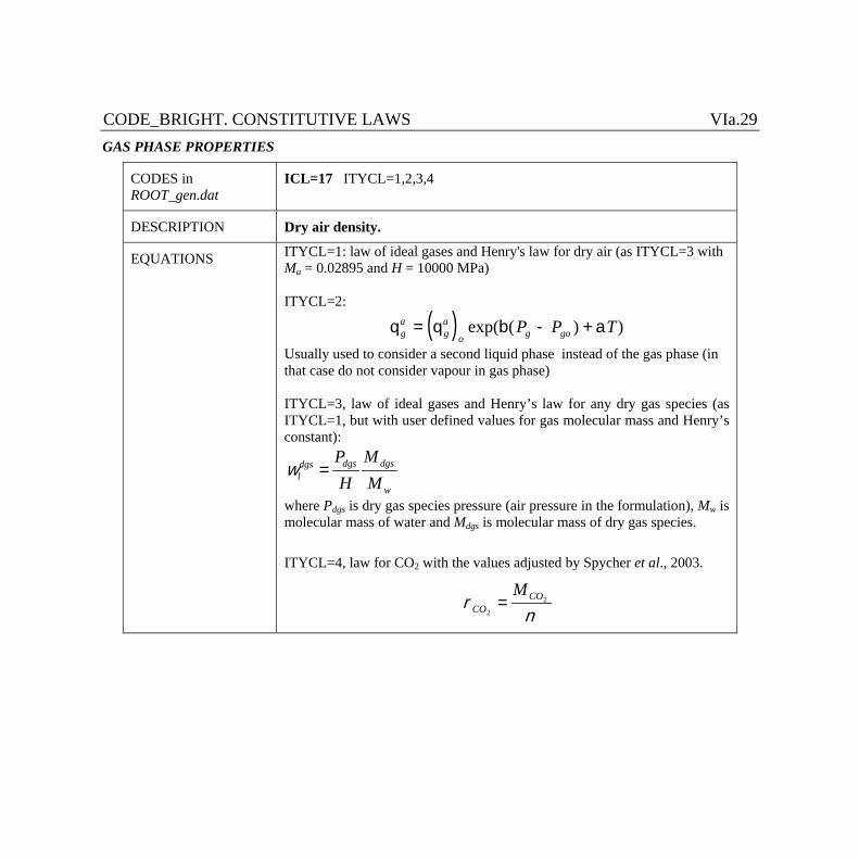
CODE_BRIGHT. CONSTITUTIVE LAWS VIa.29 GAS PHASE PROPERTIES
CODES in ROOT_gen.dat
ICL=17 ITYCL=1,2,3,4
DESCRIPTION Dry air density.
EQUATIONS ITYCL=1: law of ideal gases and Henry's law for dry air (as ITYCL=3 with Ma = 0.02895 and H = 10000 MPa) ITYCL=2:
( )q q b aga
ga
o g goP P T= - +exp( ( ) )
Usually used to consider a second liquid phase instead of the gas phase (in that case do not consider vapour in gas phase) ITYCL=3, law of ideal gases and Henry’s law for any dry gas species (as ITYCL=1, but with user defined values for gas molecular mass and Henry’s constant):
dgs dgsdgsl
w
P MH M
w =
where Pdgs is dry gas species pressure (air pressure in the formulation), Mw is molecular mass of water and Mdgs is molecular mass of dry gas species.
ITYCL=4, law for CO2 with the values adjusted by Spycher et al., 2003.
nr 2
2
COCO
M=
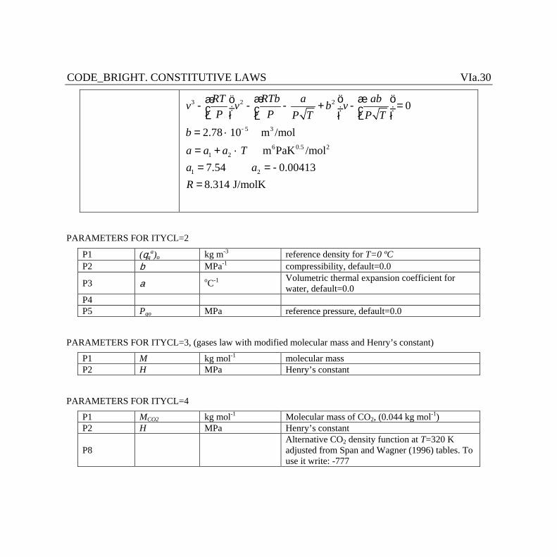
CODE_BRIGHT. CONSTITUTIVE LAWS VIa.30
5 3
6 0.5 2
2
1 2
1
3
2
2
2.78 10 m /mol m PaK /mol
7.54 0.0041
0
8.314 J/m3
olK
ba
RT RTb a abv v b vP P P T
a a
P T
R
Ta a
-
æ ö æ öæ ö- - - + - =ç ÷ ç ÷ ç ÷è ø è ø è ø=
= -=
´
= + ´=
PARAMETERS FOR ITYCL=2
P1 (qga)o kg m-3 reference density for T=0 ºC
P2 b MPa-1 compressibility, default=0.0
P3 a oC-1 Volumetric thermal expansion coefficient for water, default=0.0
P4 P5 Pgo MPa reference pressure, default=0.0
PARAMETERS FOR ITYCL=3, (gases law with modified molecular mass and Henry’s constant)
P1 M kg mol-1 molecular mass P2 H MPa Henry’s constant
PARAMETERS FOR ITYCL=4
P1 MCO2 kg mol-1 Molecular mass of CO2, (0.044 kg mol-1) P2 H MPa Henry’s constant
P8
Alternative CO2 density function at T=320 K adjusted from Span and Wagner (1996) tables. To use it write: -777

CODE_BRIGHT. CONSTITUTIVE LAWS VIa.31
CODES in ROOT_gen.dat
ICL=18 ITYCL=1,2,4
DESCRIPTION Gas viscosity.
EQUATIONS ITYCL=1:
ty)permeabili intrinsic :(
1
1
2731
273
kDkCb
Pb
TB
TA
k
g
kg
-=
+÷øö
çèæ
++
+=m
ITYCL=2:
÷øö
çèæ
+=
TBAg 15.273
expm
ITYCL=4: Viscosity function for CO2 (Altunin and Sakhabetdinov, 1972)
÷÷ø
öççè
æ= åå
= =
4
1
1
00 exp
i jj
R
iRij
g Ta r
mm
÷÷ø
öççè
æ+-= 2
5.00
66920556.46346068.162246461.27RR
R TTTm
cR T
TT = , 304=cT K c
COR r
rr 2= , 468=cr kg/m3
248566120.010 =a 004894942.011 =a
373300660.020 -=a 22753488.121 =a
363854523.030 =a 774229021.031 -=a
0639070755.040 -=a 142507049.041 =a
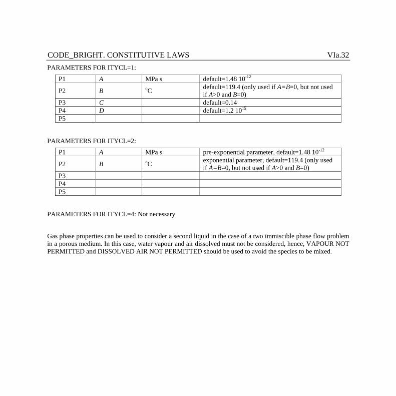
CODE_BRIGHT. CONSTITUTIVE LAWS VIa.32 PARAMETERS FOR ITYCL=1:
P1 A MPa s default=1.48 10-12
P2 B oC default=119.4 (only used if A=B=0, but not used if A>0 and B=0)
P3 C default=0.14 P4 D default=1.2 1015 P5
PARAMETERS FOR ITYCL=2:
P1 A MPa s pre-exponential parameter, default=1.48 10-12
P2 B oC exponential parameter, default=119.4 (only used if A=B=0, but not used if A>0 and B=0)
P3 P4 P5
PARAMETERS FOR ITYCL=4: Not necessary
Gas phase properties can be used to consider a second liquid in the case of a two immiscible phase flow problem in a porous medium. In this case, water vapour and air dissolved must not be considered, hence, VAPOUR NOT PERMITTED and DISSOLVED AIR NOT PERMITTED should be used to avoid the species to be mixed.
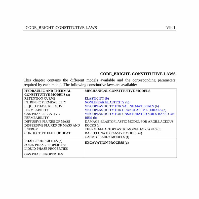
CODE_BRIGHT. CONSTITUTIVE LAWS VIb.1
CODE_BRIGHT. CONSTITUTIVE LAWS This chapter contains the different models available and the corresponding parameters required by each model. The following constitutive laws are available: HYDRAULIC AND THERMAL CONSTITUTIVE MODELS (a) RETENTION CURVE INTRINSIC PERMEABILITY LIQUID PHASE RELATIVE PERMEABILITY GAS PHASE RELATIVE PERMEABILITY DIFFUSIVE FLUXES OF MASS DISPERSIVE FLUXES OF MASS AND ENERGY CONDUCTIVE FLUX OF HEAT
MECHANICAL CONSTITUTIVE MODELS ELASTICITY (b) NONLINEAR ELASTICITY (b) VISCOPLASTICITY FOR SALINE MATERIALS (b) VISCOPLASTICITY FOR GRANULAR MATERIALS (b) VISCOPLASTICITY FOR UNSATURATED SOILS BASED ON BBM (b) DAMAGE-ELASTOPLASTIC MODEL FOR ARGILLACEOUS ROCKS (c) THERMO-ELASTOPLASTIC MODEL FOR SOILS (d) BARCELONA EXPANSIVE MODEL (e) CASM’s FAMILY MODELS (f)
PHASE PROPERTIES (a) SOLID PHASE PROPERTIES LIQUID PHASE PROPERTIES
GAS PHASE PROPERTIES
EXCAVATION PROCESS (g)
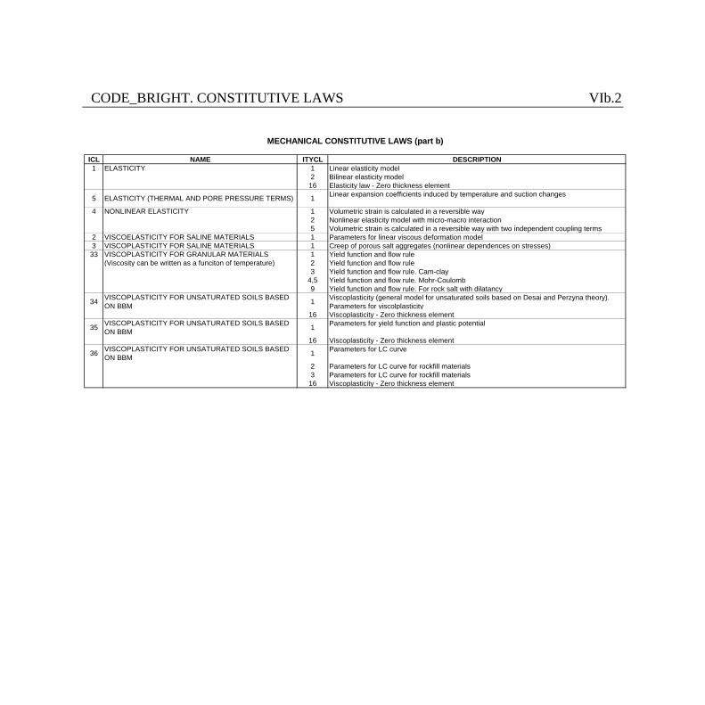
CODE_BRIGHT. CONSTITUTIVE LAWS VIb.2
ICL NAME ITYCL DESCRIPTION1 ELASTICITY 1 Linear elasticity model
2 Bilinear elasticity model16 Elasticity law - Zero thickness element
5 ELASTICITY (THERMAL AND PORE PRESSURE TERMS) 1 Linear expansion coefficients induced by temperature and suction changes
4 NONLINEAR ELASTICITY 1 Volumetric strain is calculated in a reversible way2 Nonlinear elasticity model with micro-macro interaction5 Volumetric strain is calculated in a reversible way with two independent coupling terms
2 VISCOELASTICITY FOR SALINE MATERIALS 1 Parameters for linear viscous deformation model3 VISCOPLASTICITY FOR SALINE MATERIALS 1 Creep of porous salt aggregates (nonlinear dependences on stresses)
33 VISCOPLASTICITY FOR GRANULAR MATERIALS 1 Yield function and flow rule(Viscosity can be written as a funciton of temperature) 2 Yield function and flow rule
3 Yield function and flow rule. Cam-clay4,5 Yield function and flow rule. Mohr-Coulomb9 Yield function and flow rule. For rock salt with dilatancy
34 VISCOPLASTICITY FOR UNSATURATED SOILS BASED ON BBM 1 Viscoplasticity (general model for unsaturated soils based on Desai and Perzyna theory).
Parameters for viscolplasticity16 Viscoplasticity - Zero thickness element
35 VISCOPLASTICITY FOR UNSATURATED SOILS BASED ON BBM 1 Parameters for yield function and plastic potential
16 Viscoplasticity - Zero thickness element
36 VISCOPLASTICITY FOR UNSATURATED SOILS BASED ON BBM 1 Parameters for LC curve
2 Parameters for LC curve for rockfill materials3 Parameters for LC curve for rockfill materials
16 Viscoplasticity - Zero thickness element
MECHANICAL CONSTITUTIVE LAWS (part b)
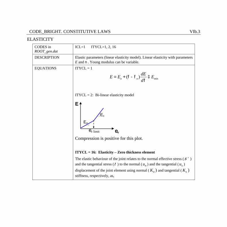
CODE_BRIGHT. CONSTITUTIVE LAWS VIb.3
ELASTICITY CODES in ROOT_gen.dat
ICL=1 ITYCL=1, 2, 16
DESCRIPTION Elastic parameters (linear elasticity model). Linear elasticity with parameters E and n . Young modulus can be variable.
EQUATIONS ITYCL = 1
min( )o odEE E Ed
= + f - f ³f
ITYCL = 2: Bi-linear elasticity model
Compression is positive for this plot.
ITYCL = 16: Elasticity – Zero thickness element
The elastic behaviour of the joint relates to the normal effective stress ( 's ) and the tangential stress (t ) to the normal ( nu ) and the tangential ( su ) displacement of the joint element using normal ( nK ) and tangential ( sK ) stiffness, respectively, as,
ev
E
ev limit
Eo
Ec
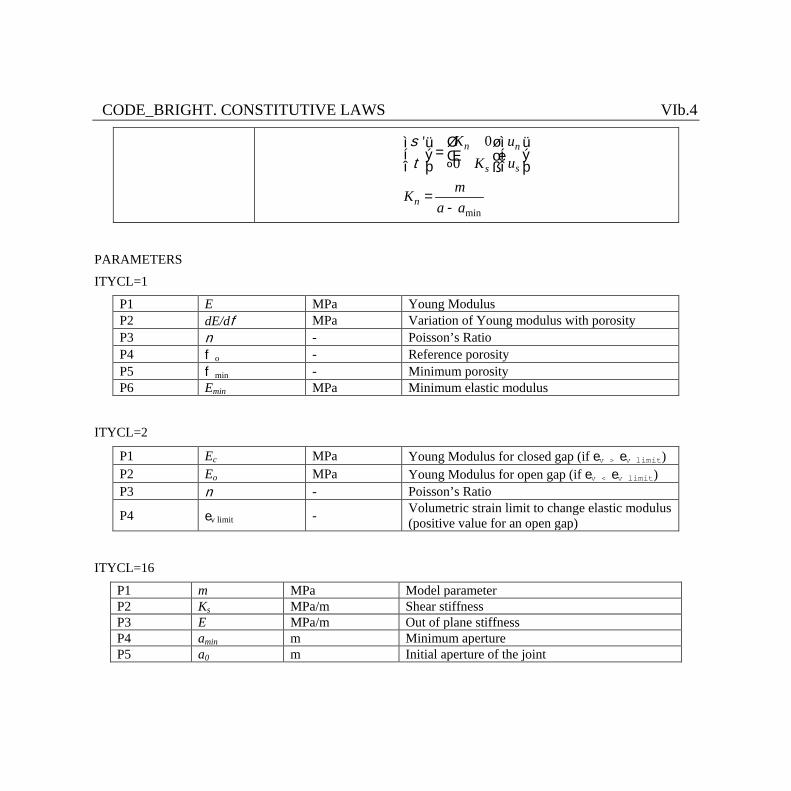
CODE_BRIGHT. CONSTITUTIVE LAWS VIb.4
min
0'0
n n
ss
n
K uuK
mKa a
st
é ù ì üì ü=í ý í ýê ú
î þ î þë û
=-
PARAMETERS
ITYCL=1
P1 E MPa Young Modulus P2 dE/df MPa Variation of Young modulus with porosity P3 n - Poisson’s Ratio P4 f o - Reference porosity P5 f min - Minimum porosity P6 Emin MPa Minimum elastic modulus
ITYCL=2
P1 Ec MPa Young Modulus for closed gap (if ev > ev limit) P2 Eo MPa Young Modulus for open gap (if ev < ev limit) P3 n - Poisson’s Ratio
P4 ev limit - Volumetric strain limit to change elastic modulus (positive value for an open gap)
ITYCL=16
P1 m MPa Model parameter P2 Ks MPa/m Shear stiffness P3 E MPa/m Out of plane stiffness P4 amin m Minimum aperture P5 a0 m Initial aperture of the joint
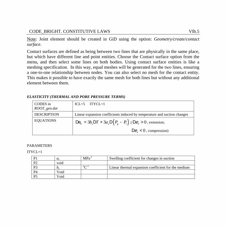
CODE_BRIGHT. CONSTITUTIVE LAWS VIb.5
Note: Joint element should be created in GiD using the option: Geometry/create/contact surface. Contact surfaces are defined as being between two lines that are physically in the same place, but which have different line and point entities. Choose the Contact surface option from the menu, and then select some lines on both bodies. Using contact surface entities is like a meshing specification. In this way, equal meshes will be generated for the two lines, ensuring a one-to-one relationship between nodes. You can also select no mesh for the contact entity. This makes it possible to have exactly the same mesh for both lines but without any additional element between them. ELASTICITY (THERMAL AND PORE PRESSURE TERMS)
CODES in ROOT_gen.dat
ICL=5 ITYCL=1
DESCRIPTION Linear expansion coefficients induced by temperature and suction changes EQUATIONS ( )3 3V s s g lb T a P PDe = D + D - ( 0>D ve , extension;
0<D ve , compression)
PARAMETERS
ITYCL=1
P1 as MPa-1 Swelling coefficient for changes in suction P2 void P3 bs oC-1 Linear thermal expansion coefficient for the medium P4 Void P5 Void
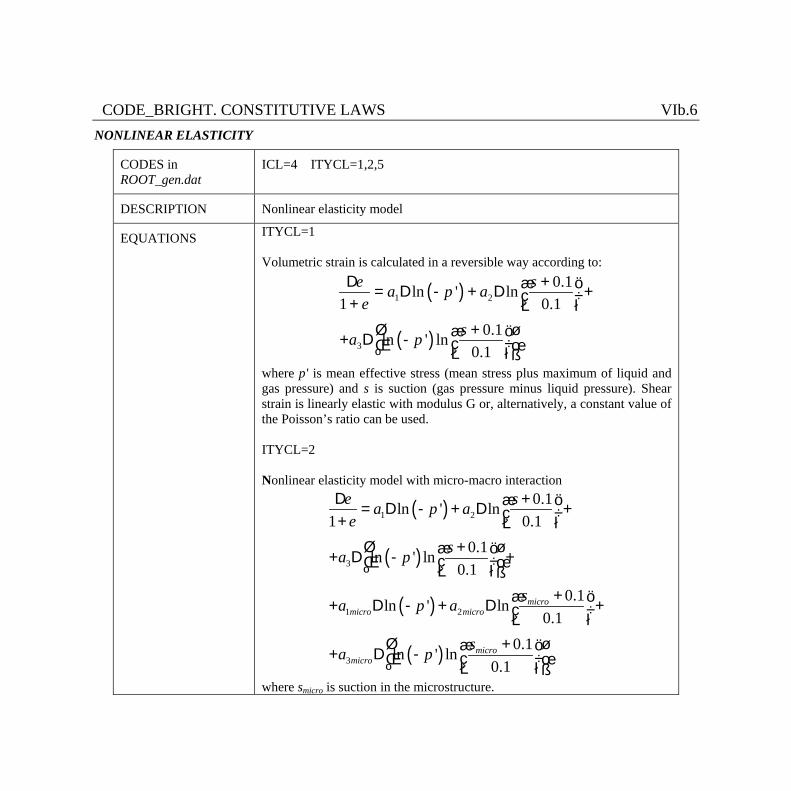
CODE_BRIGHT. CONSTITUTIVE LAWS VIb.6 NONLINEAR ELASTICITY
CODES in ROOT_gen.dat
ICL=4 ITYCL=1,2,5
DESCRIPTION Nonlinear elasticity model
EQUATIONS ITYCL=1 Volumetric strain is calculated in a reversible way according to:
( )
( )
1 2
3
0.1ln ' ln1 0.1
0.1ln ' ln0.1
e sa p ae
sa p
D +æ ö= D - + D +ç ÷+ è ø+é ùæ ö+ D - ç ÷ê úè øë û
where p' is mean effective stress (mean stress plus maximum of liquid and gas pressure) and s is suction (gas pressure minus liquid pressure). Shear strain is linearly elastic with modulus G or, alternatively, a constant value of the Poisson’s ratio can be used. ITYCL=2 Nonlinear elasticity model with micro-macro interaction
( )
( )
( )
( )
1 2
3
1 2
3
0.1ln ' ln1 0.1
0.1ln ' ln0.1
0.1ln ' ln0.1
0.1ln ' ln0.1
micromicro micro
micromicro
e sa p ae
sa p
sa p a
sa p
D +æ ö= D - + D +ç ÷+ è øé + ùæ ö+ D - +ç ÷ê úè øë û
+æ ö+ D - + D +ç ÷è ø
é + ùæ ö+ D - ç ÷ê úè øë û
where smicro is suction in the microstructure.
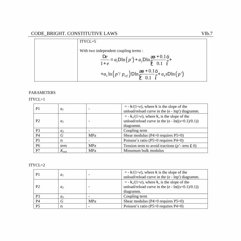
CODE_BRIGHT. CONSTITUTIVE LAWS VIb.7 ITYCL=5 With two independent coupling terms :
( )
( ) ( )
1 2
3 4
0.1ln ' ln1 0.1
0.1ln '/ ln ln '0.1ref
e sa p ae
sa p p a s p
D +æ ö= D + D +ç ÷+ è ø+æ ö+ D + Dç ÷
è ø
PARAMETERS
ITYCL=1
P1 a1 - = - k/(1+e), where k is the slope of the unload/reload curve in the (e - lnp') diagramm.
P2 a2 - = - ks/(1+e), where ks is the slope of the unload/reload curve in the (e - ln((s+0.1)/0.1)) diagramm.
P3 a3 - Coupling term P4 G MPa Shear modulus (P4>0 requires P5=0) P5 n - Poisson’s ratio (P5>0 requires P4=0) P6 tens MPa Tension term to avoid tractions (p’- tens £ 0) P7 Kmin MPa Minumum bulk modulus
ITYCL=2
P1 a1 - = - k/(1+e), where k is the slope of the unload/reload curve in the (e - lnp') diagramm.
P2 a2 - = - ks/(1+e), where ks is the slope of the unload/reload curve in the (e - ln((s+0.1)/0.1)) diagramm.
P3 a3 - Coupling term P4 G MPa Shear modulus (P4>0 requires P5=0) P5 n - Poisson’s ratio (P5>0 requires P4=0)
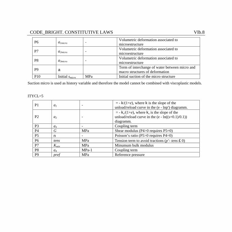
CODE_BRIGHT. CONSTITUTIVE LAWS VIb.8
P6 a1micro - Volumetric deformation associated to microestructure
P7 a2micro - Volumetric deformation associated to microestructure
P8 a3micro - Volumetric deformation associated to microestructure
P9 a Term of interchange of water between micro and macro structures of deformation
P10 Initial smicro MPa Initial suction of the micro structure
Suction micro is used as history variable and therefore the model cannot be combined with viscoplastic models.
ITYCL=5
P1 a1 - = - k/(1+e), where k is the slope of the unload/reload curve in the (e - lnp') diagramm.
P2 a2 - = - ks/(1+e), where ks is the slope of the unload/reload curve in the (e - ln((s+0.1)/0.1)) diagramm.
P3 a3 - Coupling term P4 G MPa Shear modulus (P4>0 requires P5=0) P5 n - Poisson’s ratio (P5>0 requires P4=0) P6 tens MPa Tension term to avoid tractions (p’- tens £ 0) P7 Kmin MPa Minumum bulk modulus P8 a4 MPa-1 Coupling term P9 pref MPa Reference pressure
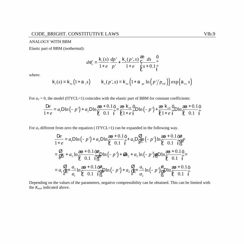
CODE_BRIGHT. CONSTITUTIVE LAWS VIb.9 ANALOGY WITH BBM
Elastic part of BBM (isothermal):
( ) ( ', )'1 ' 1 0.1
e i sv
s p sdp dsde p e s
æ ök k ç ÷e = +ç ÷+ + +è ø
where:
( )( ) 1i io is sk = k + a ( )( ) ( )( ', ) 1 ln ' exps so sp ref s sp s p p sk = k + a a
For a3 = 0, the model (ITYCL=1) coincides with the elastic part of BBM for constant coefficients:
( ) ( )0 01 2
0.1 0.1ln ' ln ln ' ln1 0.1 1 1 0.1
i se s sa p a pe e e
-k -kD + +æ ö æ öæ ö æ ö= D - + D = D - + Dç ÷ ç ÷ç ÷ ç ÷+ + +è ø è øè ø è ø
For a3 different from zero the equation ( ITYCL=1) can be expanded in the following way.
( ) ( )
( ) ( )
( ) ( )
1 2 3
1 3 2 3
3 31 2
1 2
0.1 0.1ln ' ln ln ' ln1 0.1 0.1
0.1 0.1ln ln ' ln ' ln0.1 0.1
0.1 0.11 ln ln ' 1 ln ' ln0.1 0.
e s sa p a a pe
s sa a p a a p
a as sa p a pa a
D + é + ùæ ö æ ö= D - + D + D - =ç ÷ ç ÷ê ú+ è ø è øë ûé + ù +æ ö æ ö= + D - + + - D =é ùç ÷ ç ÷ê ú ë ûè ø è øë û
é ù é ù+ +æ ö= + D - + + - Dê ú ê úç ÷è øë û ë û 1
æ öç ÷è ø
Depending on the values of the parameters, negative compressibility can be obtained. This can be limited with the Kmin indicated above.
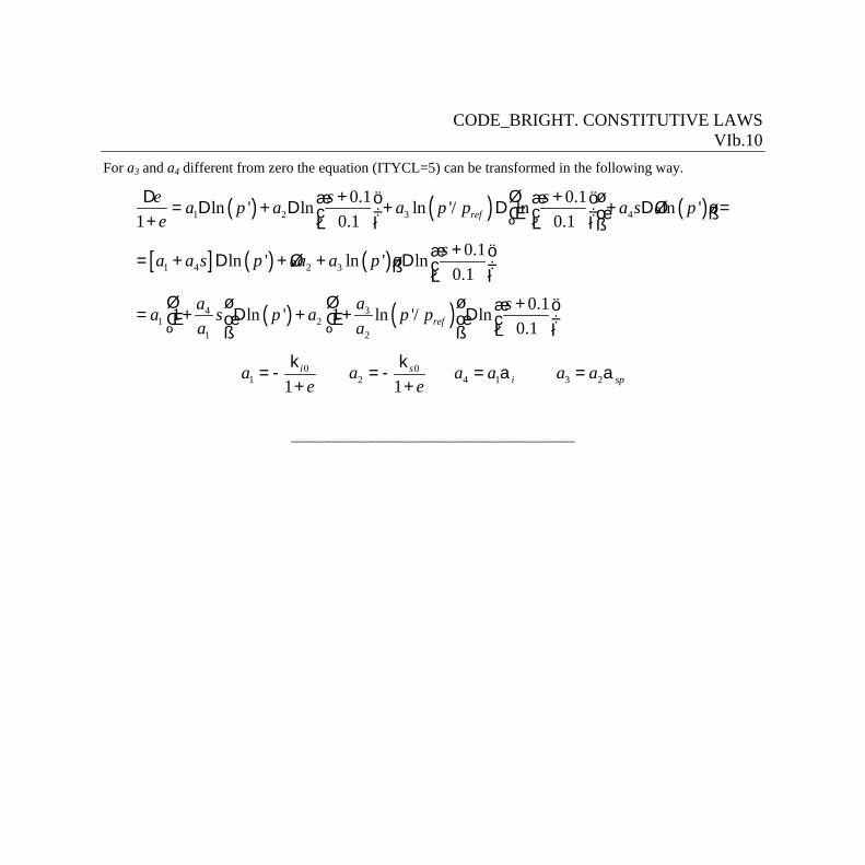
CODE_BRIGHT. CONSTITUTIVE LAWS VIb.10
For a3 and a4 different from zero the equation (ITYCL=5) can be transformed in the following way.
( ) ( ) ( )
[ ] ( ) ( )
( ) ( )
1 2 3 4
1 4 2 3
341 2
1 2
0.1 0.1ln ' ln ln '/ ln ln '1 0.1 0.1
0.1ln ' ln ' ln0.1
0.11 ln ' 1 ln '/ ln0.1
ref
ref
e s sa p a a p p a s pe
sa a s p a a p
aa sa s p a p pa a
D + é + ùæ ö æ ö= D + D + D + D =é ùç ÷ ç ÷ê ú ë û+ è ø è øë û+æ ö= + D + + Dé ù ç ÷ë û è ø
é ù é ù +æ ö= + D + + Dê ú ê ú ç ÷è øë û ë û
0 01 2 4 1 3 2
1 1i s
i spa a a a a ae e
k k= - = - = a = a
+ +
_______________________________________
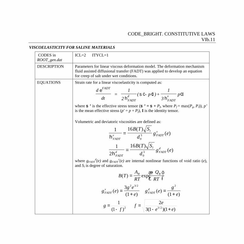
CODE_BRIGHT. CONSTITUTIVE LAWS VIb.11
VISCOELASTICITY FOR SALINE MATERIALS
CODES in ROOT_gen.dat
ICL=2 ITYCL=1
DESCRIPTION Parameters for linear viscous deformation model. The deformation mechanism fluid assisted diffusional transfer (FADT) was applied to develop an equation for creep of salt under wet conditions.
EQUATIONS Strain rate for a linear viscoelasticity is computed as:
d
dt =
1
2( - p )+
1
3p
FADT
FADTd
FADTv
e
hs
h¢ ¢ ¢I I
where s ’ is the effective stress tensor (s ’ = s + Pf, where Pf = max(Pg, Pl)), p’ is the mean effective stress (p' = p + Pf), I is the identity tensor. Volumetric and deviatoric viscosities are defined as:
1 16
12
1603
03
h
h
FADTv
lFADTv
FADTd
lFADTd
B T Sd
g e
B T Sd
g e
=
=
( )( )
( )( )
where gFADTd(e) and gFADT
v(e) are internal nonlinear functions of void ratio (e), and Sl is degree of saturation.
B TART
QRT
B B( ) exp=-æ
èçöø÷
g eg e
eg e
geFADT
vFADTd( )
( )( )
( )
/
=+
=+
31 1
2 3 2 2
)1)(1(3
2 )1(
12/32 eeef
fg
+-=
-=
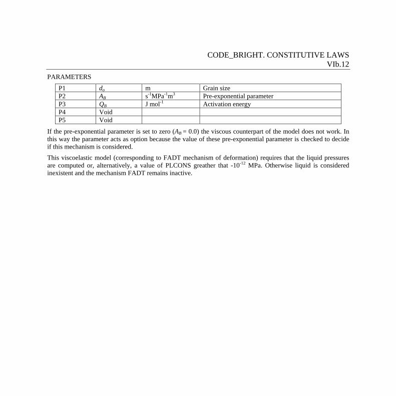
CODE_BRIGHT. CONSTITUTIVE LAWS VIb.12
PARAMETERS
P1 do m Grain size P2 AB s-1MPa-1m3 Pre-exponential parameter P3 QB J mol-1 Activation energy P4 Void P5 Void
If the pre-exponential parameter is set to zero (AB = 0.0) the viscous counterpart of the model does not work. In this way the parameter acts as option because the value of these pre-exponential parameter is checked to decide if this mechanism is considered.
This viscoelastic model (corresponding to FADT mechanism of deformation) requires that the liquid pressures are computed or, alternatively, a value of PLCONS greather that -10-12 MPa. Otherwise liquid is considered inexistent and the mechanism FADT remains inactive.
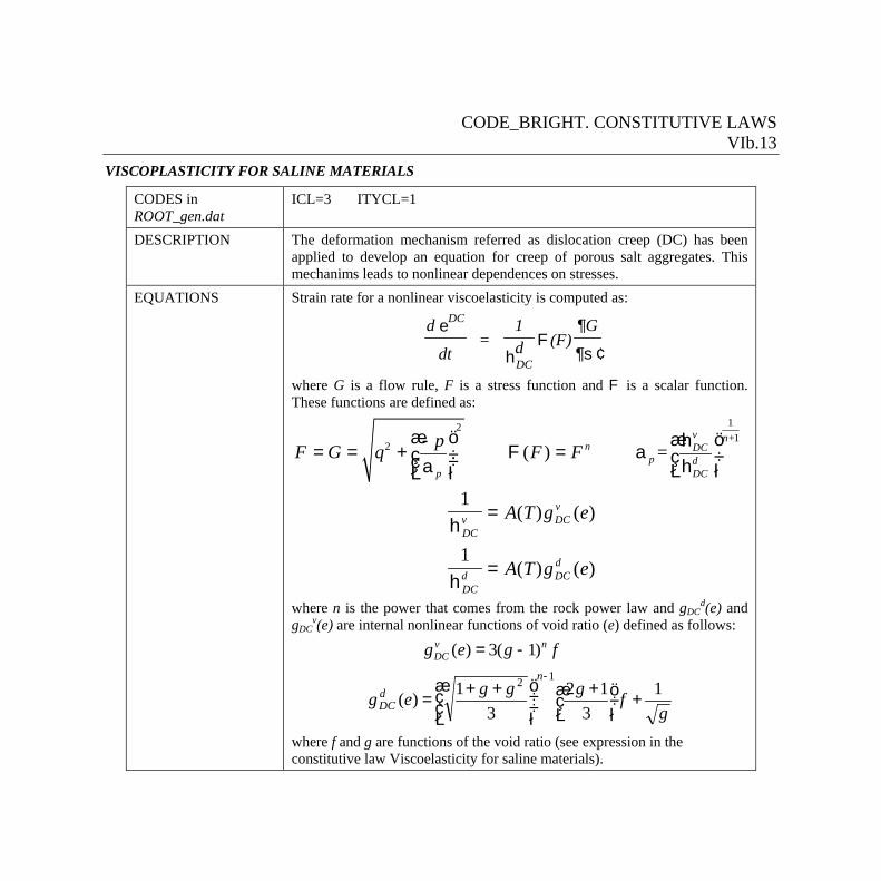
CODE_BRIGHT. CONSTITUTIVE LAWS VIb.13
VISCOPLASTICITY FOR SALINE MATERIALS
CODES in ROOT_gen.dat
ICL=3 ITYCL=1
DESCRIPTION The deformation mechanism referred as dislocation creep (DC) has been applied to develop an equation for creep of porous salt aggregates. This mechanims leads to nonlinear dependences on stresses.
EQUATIONS Strain rate for a nonlinear viscoelasticity is computed as:
d
dt =
1d (F)
G
DC
DC
e
h sF
¶ ¢
where G is a flow rule, F is a stress function and F is a scalar function. These functions are defined as:
121
2 ( ) = v n+
n DCp d
p DC
pF G q F Fæ ö æ öh-
= = + F = aç ÷ ç ÷ç ÷a hè øè ø
1
1h
h
DCv DC
v
DCd DC
d
A T g e
A T g e
=
=
( ) ( )
( ) ( )
where n is the power that comes from the rock power law and gDCd(e) and
gDCv(e) are internal nonlinear functions of void ratio (e) defined as follows:
( ) 3( 1) v nDCg e g f= -
gfgggeg
ndDC
13
123
1)(12
+÷øö
çèæ +
÷÷ø
öççè
æ ++=
-
where f and g are functions of the void ratio (see expression in the constitutive law Viscoelasticity for saline materials).
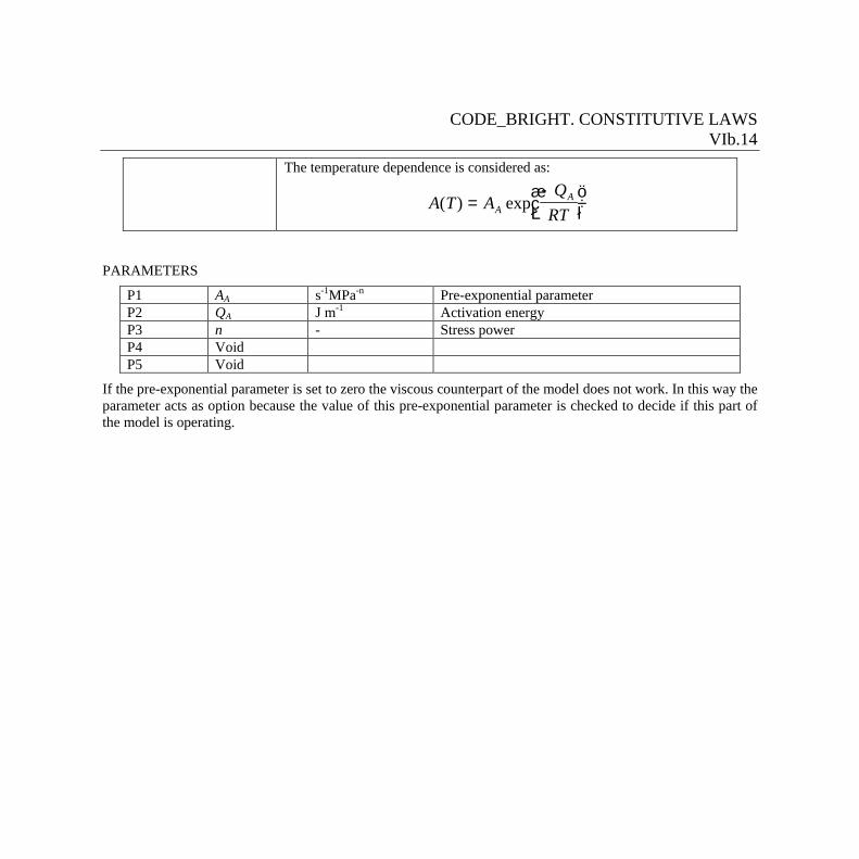
CODE_BRIGHT. CONSTITUTIVE LAWS VIb.14
The temperature dependence is considered as:
A T AQ
RTAA( ) exp=
-æèç
öø÷
PARAMETERS
P1 AA s-1MPa-n Pre-exponential parameter P2 QA J m-1 Activation energy P3 n - Stress power P4 Void P5 Void
If the pre-exponential parameter is set to zero the viscous counterpart of the model does not work. In this way the parameter acts as option because the value of this pre-exponential parameter is checked to decide if this part of the model is operating.
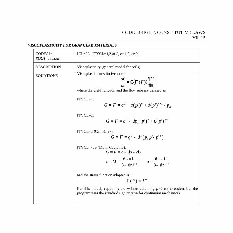
CODE_BRIGHT. CONSTITUTIVE LAWS VIb.15
VISCOPLASTICITY FOR GRANULAR MATERIALS
CODES in ROOT_gen.dat
ICL=33 ITYCL=1,2 or 3, or 4,5, or 9
DESCRIPTION Viscoplasticity (general model for soils)
EQUATIONS Viscoplastic constitutive model. ddt
FGe 
¶s= G F( )
where the yield function and the flow rule are defined as: ITYCL=1:
G F q p p pn no= = - + +2 1d d( ' ) ( ' ) /
ITYCL=2:
G F q p p pon n= = - + +2 1d d( ' ) ( ' )
ITYCL=3 (Cam-Clay):
G F q p p po= = - -2 2 2d ( ' ' ) ITYCL=4, 5 (Mohr-Coulomb):
'6sin ' 6cos '
3 sin ' 3 sin '
G F q p c
M
= = - d - bf f
d = = b =- f - f
and the stress function adopted is:
F( )F F m=
For this model, equations are written assuming p>0 compression, but the program uses the standard sign criteria for continuum mechanics)
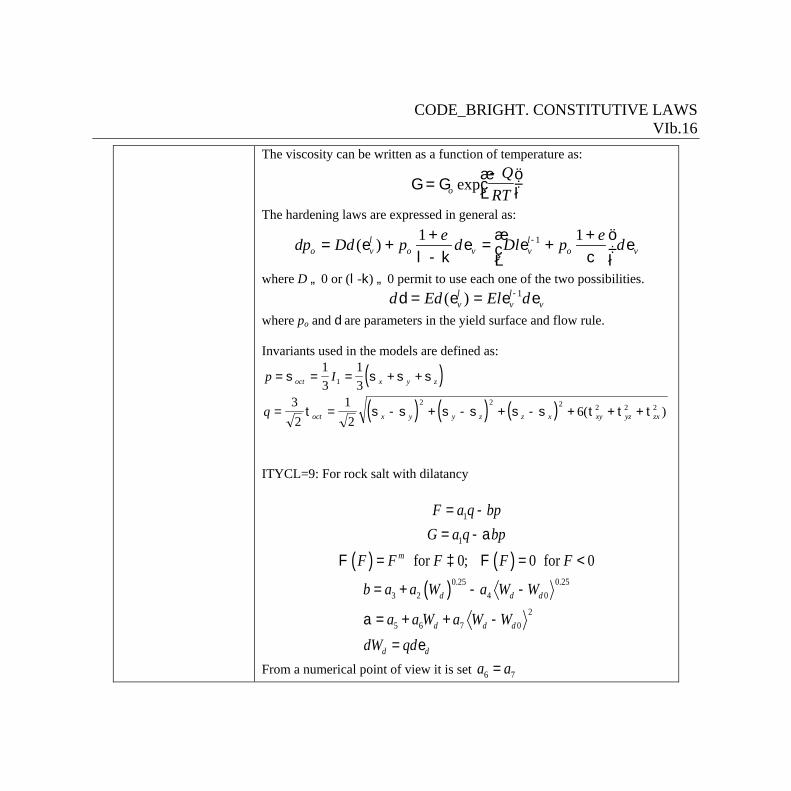
CODE_BRIGHT. CONSTITUTIVE LAWS VIb.16
The viscosity can be written as a function of temperature as:
G G=-æ
èçöø÷o
QRT
exp
The hardening laws are expressed in general as:
11 1( )l lo v o v v o v
e edp Dd p d Dl p d-æ ö+ += e + e = e + eç ÷l - k cè ø
where D ¹ 0 or (l-k) ¹ 0 permit to use each one of the two possibilities. 1( )l l
v v vd Ed El d-d = e = e e where po and d are parameters in the yield surface and flow rule. Invariants used in the models are defined as:
( )( ) ( ) ( )
p I
q
oct x y z
oct x y y z z x xy yz zx
= = = + +
= = - + - + - + + +
s s s s
t s s s s s s t t t
13
13
32
12
6
1
2 2 2 2 2 2( )
ITYCL=9: For rock salt with dilatancy
( ) ( )
1
1
for 0; 0 for 0m
F a q bpG a q bp
F F F F F
= -= - a
F = ³ F = <
( ) 0.250.253 2 4 0
25 6 7 0
d d d
d d d
d d
b a a W a W W
a a W a W WdW qd
= + - -
a = + + -
= e
From a numerical point of view it is set 6 7a a=
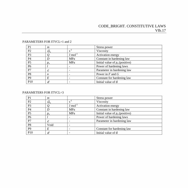
CODE_BRIGHT. CONSTITUTIVE LAWS VIb.17
PARAMETERS FOR ITYCL=1 and 2
P1 m Stress power P2 G o s-1 Viscosity P3 Q J mol-1 Activation energy P4 D MPa Constant in hardening law P5 po MPa Initial value of po (positive) P6 l - Power of hardening laws P7 c - Parameter in hardening law P8 n - Power in F and G P9 E - Constant for hardening law P10 d - Initial value of d
PARAMETERS FOR ITYCL=3
P1 m Stress power P2 G o s-1 Viscosity P3 Q J mol-1 Activation energy P4 D MPa Constant in hardening law P5 po MPa Initial value of po (positive) P6 l - Power of hardening laws P7 c - Parameter in hardening law P8 Void - P9 E - Constant for hardening law P10 d - Initial value of d
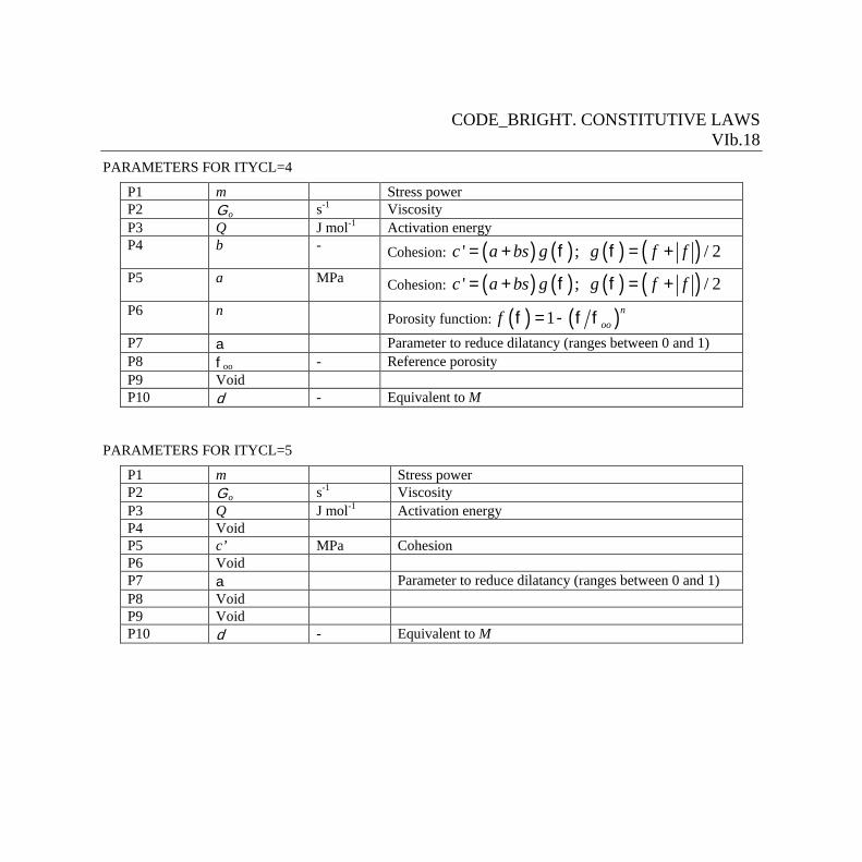
CODE_BRIGHT. CONSTITUTIVE LAWS VIb.18
PARAMETERS FOR ITYCL=4
P1 m Stress power P2 G o s-1 Viscosity P3 Q J mol-1 Activation energy P4 b - Cohesion: ( ) ( ) ( ) ( )' ; / 2c a bs g g f f= + f f = +
P5 a MPa Cohesion: ( ) ( ) ( ) ( )' ; / 2c a bs g g f f= + f f = +
P6 n Porosity function: ( ) ( )1 noof f = - f f
P7 a Parameter to reduce dilatancy (ranges between 0 and 1) P8 foo - Reference porosity P9 Void P10 d - Equivalent to M
PARAMETERS FOR ITYCL=5
P1 m Stress power P2 G o s-1 Viscosity P3 Q J mol-1 Activation energy P4 Void P5 c’ MPa Cohesion P6 Void P7 a Parameter to reduce dilatancy (ranges between 0 and 1) P8 Void P9 Void P10 d - Equivalent to M
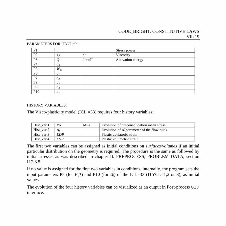
CODE_BRIGHT. CONSTITUTIVE LAWS VIb.19
PARAMETERS FOR ITYCL=9
P1 m Stress power P2 G o s-1 Viscosity P3 Q J mol-1 Activation energy P4 a6 P5 Wd0 P6 a1 P7 a2 P8 a3 P9 a4 P10 a5
HISTORY VARIABLES:
The Visco-plasticity model (ICL =33) requires four history variables:
Hist_var 1 Po MPa Evolution of preconsolidation mean stress Hist_var 2 d0 Evolution of d (parameter of the flow rule) Hist_var 3 EDP Plastic deviatoric strain Hist_var 4 EVP Plastic volumetric strain
The first two variables can be assigned as initial conditions on surfaces/volumes if an initial particular distribution on the geometry is required. The procedure is the same as followed by initial stresses as was described in chapter II. PREPROCESS, PROBLEM DATA, section II.2.3.5. If no value is assigned for the first two variables in conditions, internally, the program sets the input parameters P5 (for Po*) and P10 (for d0) of the ICL=33 (ITYCL=1,2 or 3), as initial values. The evolution of the four history variables can be visualized as an output in Post-process GID interface.
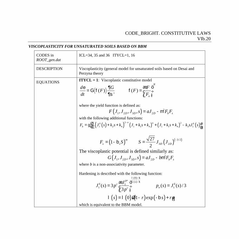
CODE_BRIGHT. CONSTITUTIVE LAWS VIb.20
VISCOPLASTICITY FOR UNSATURATED SOILS BASED ON BBM
CODES in ROOT_gen.dat
ICL=34, 35 and 36 ITYCL=1, 16
DESCRIPTION Viscoplasticity (general model for unsaturated soils based on Desai and Perzyna theory
EQUATIONS ITYCL = 1: Viscoplastic constitutive model
( ) ( )'
N
o
d G FF Fdt F
æ öe ¶= G f f = ç ÷¶s è ø
where the yield function is defined as:
( ) 21 2 3 2, , ,D D D b sF J J J s aJ F F= - m
with the following additional functions:
( )( ) ( ) ( ) ( )2 20 01 2 4 1 1 4 1 1 4 3 1
n nbF J s k s k J k s k J k s k k sJ s
-é ù= g - + + + + + + + -ê úë û
( ) ( )( )3/ 23 2
271 2
ms s D DF S S J J -= -b =
The viscoplastic potential is defined similarly as: ( ) 2
1 2 3 2, , ,D D D b sG J J J s aJ b F F= - m where b is a non-associativity parameter. Hardening is described with the following function:
(0)0* ( )
0 011 1( ) 3 ( ) ( ) / 3
3
sc
oc
JJ s p p s J sp
l -kl -kæ ö
= =ç ÷è ø
( ) ( ) ( ) ( )0 1 exps r s rl = l - -b +é ùë û
which is equivalent to the BBM model.

CODE_BRIGHT. CONSTITUTIVE LAWS VIb.21
Suction and net stress are defined as:
( )( )max ,0g ls P P= -
max( , )totaln n g lP Ps = s -
And the invariants are:
( ) 1
22
1' ' ' ' max( , ) / 3 max( , )3
1 1( : ) = ' '2 3
x y z g l g l
D
p p p p J p p
J trace q p
= s + s + s = - = -
= = s -s s s I
Hardening depends on viscoplastic volumetric strains according to:
( )( ) ( )( ) ( )*
0* * * *1 1 *
1 1 100 0
o vp vp vpov o o v v
o
dpe e edJ J d dp p d dp
+ + += e Û = e Û = e
cl - k l - k
which is equivalent to BBM model as shown. Note that:
2 2 2 2 21( , , ) 3 ( ( ) ) ( ) ( )3
n noF q p s a q p s ks p ks p ks-é ù= - m g - + + + +ë û
(using k1=3k, k2=3k, k3=0, k4=0, and Fs=1) In the same way the viscoplastic potential is described as:
2 2 2 2 21( , , ) 3 ( ( ) ) ( ) ( )3
n noG q p s a q b p s ks p ks p ks-é ù= - m g - + + + +ë û
which incorporates a parameter to allow for non-associativity conditions. Strength can be considered also a function of suction in the following way:
( ) ( ) ( ) s
satdry dry sat sat dry
dry
sæ öm
m = m - m - m m < mç ÷ç ÷mè ø
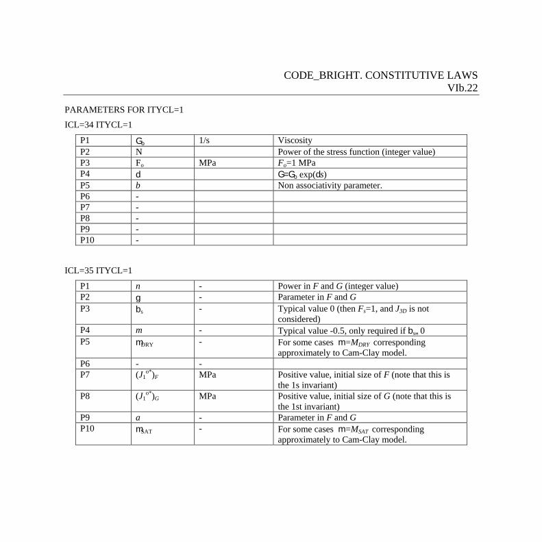
CODE_BRIGHT. CONSTITUTIVE LAWS VIb.22
PARAMETERS FOR ITYCL=1
ICL=34 ITYCL=1
P1 Go 1/s Viscosity P2 N Power of the stress function (integer value) P3 Fo MPa Fo=1 MPa P4 d G=Go exp(ds) P5 b Non associativity parameter. P6 - P7 - P8 - P9 - P10 -
ICL=35 ITYCL=1
P1 n - Power in F and G (integer value) P2 g - Parameter in F and G P3 bs - Typical value 0 (then Fs=1, and J3D is not
considered) P4 m - Typical value -0.5, only required if bs¹0 P5 mDRY - For some cases m =MDRY corresponding
approximately to Cam-Clay model. P6 - - P7 (J1
o*)F MPa Positive value, initial size of F (note that this is the 1s invariant)
P8 (J1o*)G MPa Positive value, initial size of G (note that this is
the 1st invariant) P9 a - Parameter in F and G P10 mSAT - For some cases m =MSAT corresponding
approximately to Cam-Clay model.
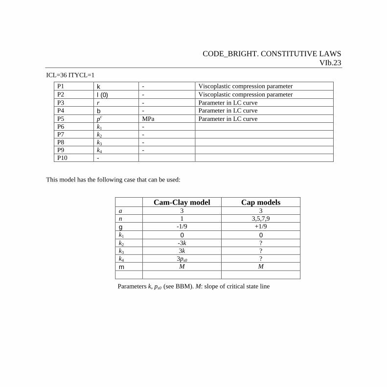
CODE_BRIGHT. CONSTITUTIVE LAWS VIb.23
ICL=36 ITYCL=1
P1 k - Viscoplastic compression parameter P2 l(0) - Viscoplastic compression parameter P3 r - Parameter in LC curve P4 b - Parameter in LC curve P5 pc MPa Parameter in LC curve P6 k1 - P7 k2 - P8 k3 - P9 k4 - P10 -
This model has the following case that can be used:
Cam-Clay model Cap models a 3 3 n 1 3,5,7,9 g -1/9 +1/9 k1 0 0 k2 -3k ? k3 3k ? k4 3ps0 ? m M M
Parameters k, ps0 (see BBM). M: slope of critical state line
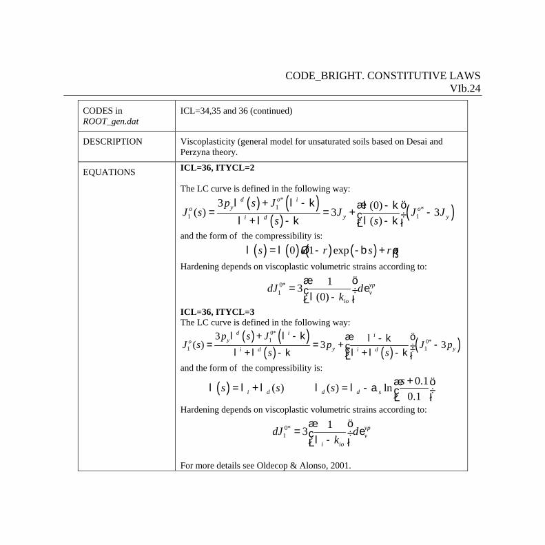
CODE_BRIGHT. CONSTITUTIVE LAWS VIb.24
CODES in ROOT_gen.dat
ICL=34,35 and 36 (continued)
DESCRIPTION Viscoplasticity (general model for unsaturated soils based on Desai and Perzyna theory.
EQUATIONS ICL=36, ITYCL=2 The LC curve is defined in the following way:
( ) ( )( ) ( )
*1 *
1 1
3 (0)( ) 3 3( )
d o iyo o
y yi d
p s JJ s J J J
s sl + l - k æ öl - k
= = + -ç ÷l + l - k l - kè ø
and the form of the compressibility is:
( ) ( ) ( ) ( )0 1 exps r s rl = l - -b +é ùë û
Hardening depends on viscoplastic volumetric strains according to:
0*1
13(0)
vpv
io
dJ dk
æ ö= eç ÷l -è ø
ICL=36, ITYCL=3 The LC curve is defined in the following way:
( ) ( )( ) ( ) ( )
0*1 0*
1 1
3( ) 3 3
d i iyo
y yi d i d
p s JJ s p J p
s sl + l - k æ öl - k
= = + -ç ÷ç ÷l + l - k l + l - kè øand the form of the compressibility is:
( ) 0.1( ) ( ) ln0.1i d d d s
ss s s +æ öl = l + l l = l - a ç ÷è ø
Hardening depends on viscoplastic volumetric strains according to:
0*1
13 vpv
i io
dJ dk
æ ö= eç ÷l -è ø
For more details see Oldecop & Alonso, 2001.
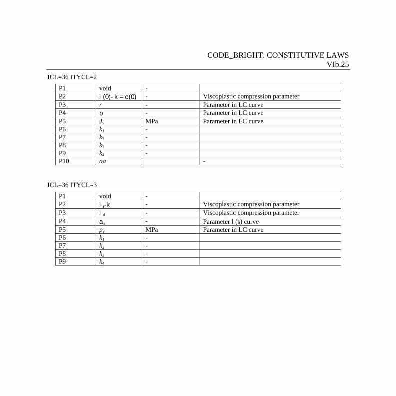
CODE_BRIGHT. CONSTITUTIVE LAWS VIb.25
ICL=36 ITYCL=2
P1 void - P2 l(0)-k = c(0) - Viscoplastic compression parameter P3 r - Parameter in LC curve P4 b - Parameter in LC curve P5 Jy
MPa Parameter in LC curve P6 k1 - P7 k2 - P8 k3 - P9 k4 - P10 aa -
ICL=36 ITYCL=3
P1 void - P2 li-k - Viscoplastic compression parameter P3 ld - Viscoplastic compression parameter P4 as - Parameter l(s) curve P5 py MPa Parameter in LC curve P6 k1 - P7 k2 - P8 k3 - P9 k4 -
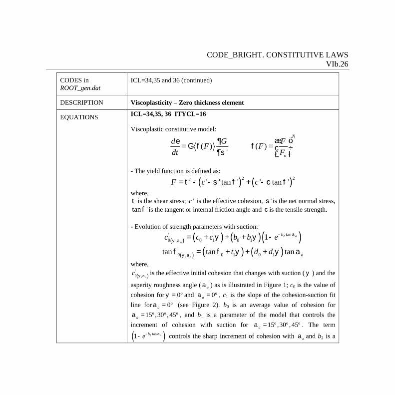
CODE_BRIGHT. CONSTITUTIVE LAWS VIb.26
CODES in ROOT_gen.dat
ICL=34,35 and 36 (continued)
DESCRIPTION Viscoplasticity – Zero thickness element
EQUATIONS ICL=34,35, 36 ITYCL=16 Viscoplastic constitutive model:
( ) ( )'
N
o
d G FF Fdt F
æ öe ¶= G f f = ç ÷¶s è ø
- The yield function is defined as:
( ) ( )2 22 ' ' tan ' ' tan 'F c c= t - - s f + - c f
where, t is the shear stress; 'c is the effective cohesion, 's is the net normal stress, tan 'f is the tangent or internal friction angle and c is the tensile strength. - Evolution of strength parameters with suction:
( ) ( ) ( )( )2 tan'0 0 1 0 1, 1 a
a
bc c c b b e- ay a = + y + + y -
( ) ( ) ( )'0 0 1 0 1,tan tan tan
a at d dy af = f + y + + y a
where,
( )'0 , a
c y a is the effective initial cohesion that changes with suction ( y ) and the
asperity roughness angle ( aa ) as is illustrated in Figure 1; c0 is the value of cohesion for 0ºy = and 0ºaa = , c1 is the slope of the cohesion-suction fit line for 0ºaa = (see Figure 2). b0 is an average value of cohesion for
15º ,30º , 45ºaa = , and b1 is a parameter of the model that controls the increment of cohesion with suction for 15º ,30º , 45ºaa = . The term
( )2 tan1 abe- a- controls the sharp increment of cohesion with aa and b2 is a
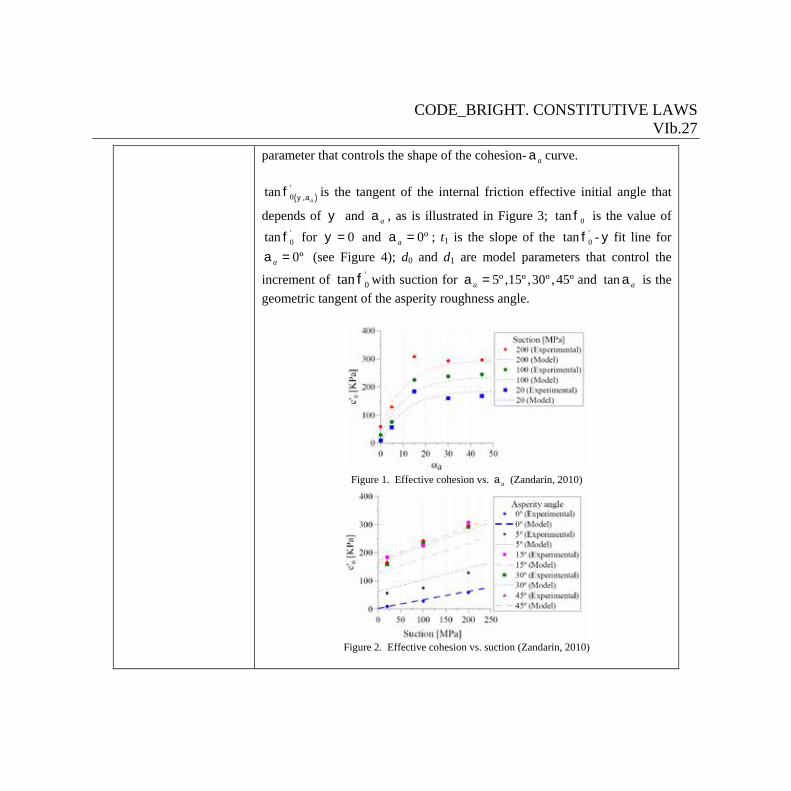
CODE_BRIGHT. CONSTITUTIVE LAWS VIb.27
parameter that controls the shape of the cohesion- aa curve.
( )'0 ,tan
ay af is the tangent of the internal friction effective initial angle that
depends of y and aa , as is illustrated in Figure 3; 0tan f is the value of '0tan f for 0y = and 0ºaa = ; t1 is the slope of the '
0tan f - y fit line for 0ºaa = (see Figure 4); d0 and d1 are model parameters that control the
increment of '0tan f with suction for 5º ,15º ,30º , 45ºaa = and tan aa is the
geometric tangent of the asperity roughness angle.
Figure 1. Effective cohesion vs. aa (Zandarin, 2010)
Figure 2. Effective cohesion vs. suction (Zandarin, 2010)
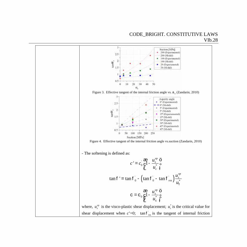
CODE_BRIGHT. CONSTITUTIVE LAWS VIb.28
Figure 3. Effective tangent of the internal friction angle vs. aa (Zandarin, 2010)
Figure 4. Effective tangent of the internal friction angle vs.suction (Zandarin, 2010)
- The softening is defined as:
'0 *' 1
vps
c
uc cu
æ ö= -ç ÷
è ø
( )' ' '0 0 *tan ' tan tan tan
vps
resuuf
f = f - f - f
0 *1vpsu
uc
æ öc = c -ç ÷ç ÷
è ø
where, vpsu is the visco-plastic shear displacement; *
cu is the critical value for shear displacement when c’=0; 'tan resf is the tangent of internal friction
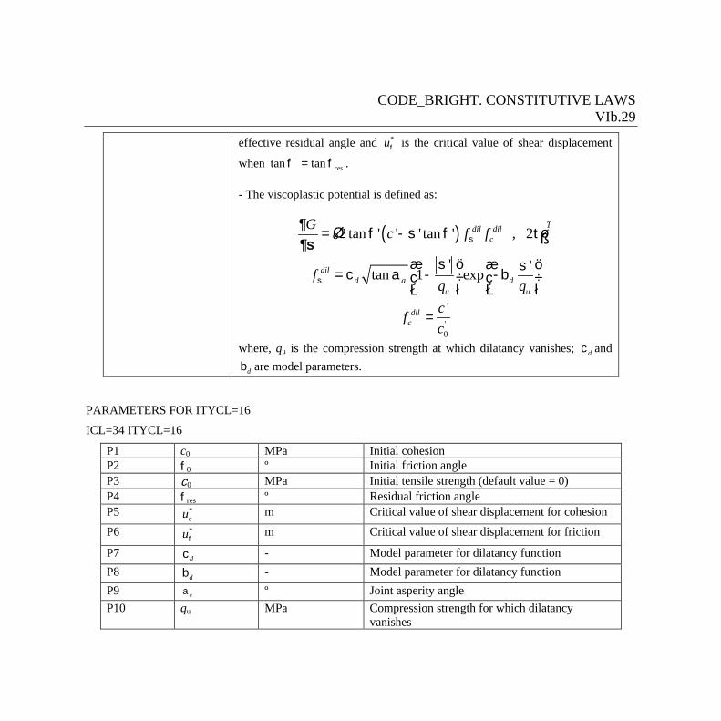
CODE_BRIGHT. CONSTITUTIVE LAWS VIb.29
effective residual angle and *uf is the critical value of shear displacement
when ' 'tan tan resf = f . - The viscoplastic potential is defined as:
( )2 tan ' ' ' tan ' , 2Tdil dil
cG c f fs
¶ é ù= f - s f të û¶s
' 'tan 1 expdild a d
u u
fq qs
æ s ö æ ös= c a - -bç ÷ ç ÷
è øè ø
'0
'dilc
cfc
=
where, qu is the compression strength at which dilatancy vanishes; dc and
db are model parameters.
PARAMETERS FOR ITYCL=16
ICL=34 ITYCL=16
P1 c0 MPa Initial cohesion P2 f0 º Initial friction angle P3 c0 MPa Initial tensile strength (default value = 0) P4 fres º Residual friction angle P5 *
cu m Critical value of shear displacement for cohesion
P6 *uf m Critical value of shear displacement for friction
P7 dc - Model parameter for dilatancy function P8 db - Model parameter for dilatancy function P9 aa º Joint asperity angle P10 qu MPa Compression strength for which dilatancy
vanishes

CODE_BRIGHT. CONSTITUTIVE LAWS VIb.30
ICL=35 ITYCL=16
P1 - P2 - P3 Go 1/s Viscosity P4 N Power of the stress function (integer value) P5 F0 MPa F0=1 MPa (Default value) P6 - P7 - P8 - P9 - P10 -
ICL=36 ITYCL=16
P1 c1 MPa Model parameter for evolution of cohesion with suction
P2 b0 MPa Model parameter for evolution of cohesion with suction
P3 b1 - Model parameter for evolution of cohesion with suction
P4 b2 - Model parameter for evolution of cohesion with suction
P5 t1 - Model parameter for evolution of friction angle with suction
P6 d0 - Model parameter for evolution of friction angle with suction
P7 d1 - Model parameter for evolution of friction angle with suction
P8 aa º Joint asperity angle P9 - P10 -
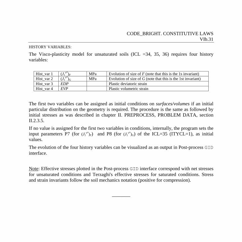
CODE_BRIGHT. CONSTITUTIVE LAWS VIb.31
HISTORY VARIABLES:
The Visco-plasticity model for unsaturated soils (ICL =34, 35, 36) requires four history variables:
Hist_var 1 (J1o*)F MPa Evolution of size of F (note that this is the 1s invariant)
Hist_var 2 (J1o*)G MPa Evolution of size of G (note that this is the 1st invariant)
Hist_var 3 EDP Plastic deviatoric strain Hist_var 4 EVP Plastic volumetric strain
The first two variables can be assigned as initial conditions on surfaces/volumes if an initial particular distribution on the geometry is required. The procedure is the same as followed by initial stresses as was described in chapter II. PREPROCESS, PROBLEM DATA, section II.2.3.5. If no value is assigned for the first two variables in conditions, internally, the program sets the input parameters P7 (for (J1
o*)F) and P8 (for (J1o*)G) of the ICL=35 (ITYCL=1), as initial
values. The evolution of the four history variables can be visualized as an output in Post-process GID interface. Note: Effective stresses plotted in the Post-process GID interface correspond with net stresses for unsaturated conditions and Terzaghi's effective stresses for saturated conditions. Stress and strain invariants follow the soil mechanics notation (positive for compression).
_________
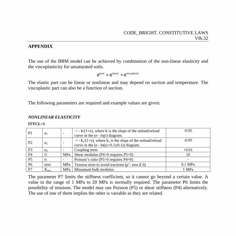
CODE_BRIGHT. CONSTITUTIVE LAWS VIb.32
APPENDIX The use of the BBM model can be achieved by combination of the non-linear elasticity and the viscoplasticity for unsaturated soils.
total elastic viscoplastice = e + e The elastic part can be linear or nonlinear and may depend on suction and temperature. The viscoplastic part can also be a function of suction. The following parameters are required and example values are given: NONLINEAR ELASTICITY ITYCL=1
P1 a1 - = - k/(1+e), where k is the slope of the unload/reload curve in the (e - lnp') diagram.
-0.05
P2 a2 - = - ks/(1+e), where ks is the slope of the unload/reload curve in the (e - ln((s+0.1)/0.1)) diagram.
-0.05
P3 a3 - Coupling term +0.01 P4 G MPa Shear modulus (P4>0 requires P5=0) 10 P5 n - Poisson’s ratio (P5>0 requires P4=0) - P6 tens MPa Tension term to avoid tractions (p’- tens £ 0) 0.1 MPa P7 Kmin MPa Minumum bulk modulus 1 MPa
The parameter P7 limits the stiffness coefficient, so it cannot go beyond a certain value. A value in the range of 1 MPa to 20 MPa is normally required. The parameter P6 limits the possibility of tensions. The model may use Poisson (P5) or shear stiffness (P4) alternatively. The use of one of them implies the other is variable as they are related.

CODE_BRIGHT. CONSTITUTIVE LAWS VIb.33
The so-called state surface is an old model for unsaturated soils is based on reversibility. The volumetric strain is calculated in a reversible way according to:
( ) ( )1 2 30.1 0.1ln ' ln ln ' ln
1 0.1 0.1e s sa p a a pe
D + é + ùæ ö æ ö= D + D + Dç ÷ ç ÷ê ú+ è ø è øë û
where p' is mean effective stress (mean stress plus maximum of liquid and gas pressure) and s is suction (gas pressure minus liquid pressure). Shear strain is linearly elastic with modulus G or, alternatively, a constant value of the Poisson’s ratio can be used. For a3 = 0, the model coincides exactly with the elastic part of BBM for constant coefficients:
( ) ( )0 01 2
0.1 0.1ln ' ln ln ' ln1 0.1 1 1 0.1
i se s sa p a pe e e
-k -kD + +æ ö æ öæ ö æ ö= D + D = D + Dç ÷ ç ÷ç ÷ ç ÷+ + +è ø è øè ø è ø
For a3 different from zero the equation can be expanded in the following way.
( ) ( )
( ) ( )
( ) ( )
1 2 3
1 3 2 3
3 31 2
1 2
0.1 0.1ln ' ln ln ' ln1 0.1 0.1
0.1 0.1ln ln ' ln ' ln0.1 0.1
0.1 0.11 ln ln ' 1 ln ' ln0.1 0.1
e s sa p a a pe
s sa a p a a p
a as sa p a pa a
D + é + ùæ ö æ ö= D + D + D =ç ÷ ç ÷ê ú+ è ø è øë ûé + ù +æ ö æ ö= + D + + D =é ùç ÷ ç ÷ê ú ë ûè ø è øë û
é ù é ù+ +æ ö æ ö= + D + + Dê ú ê úç ÷ çè ø è øë û ë û
÷
Depending on the values of the parameters, negative compressibility can be obtained. This can be limited with the Kmin indicated above.
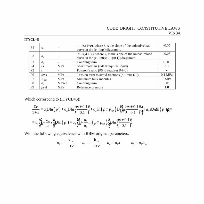
CODE_BRIGHT. CONSTITUTIVE LAWS VIb.34
ITYCL=5
P1 a1 - = - k/(1+e), where k is the slope of the unload/reload curve in the (e - lnp') diagramm.
-0.05
P2 a2 - = - ks/(1+e), where ks is the slope of the unload/reload curve in the (e - ln((s+0.1)/0.1)) diagramm.
-0.05
P3 a3 - Coupling term +0.01 P4 G MPa Shear modulus (P4>0 requires P5=0) 10 P5 n - Poisson’s ratio (P5>0 requires P4=0) - P6 tens MPa Tension term to avoid tractions (p’- tens £ 0) 0.1 MPa P7 Kmin MPa Minumum bulk modulus 1 MPa P8 a4 MPa-1 Coupling term 0.01 P9 pref MPa Reference pressure 1.0
Which correspond to (ITYCL=5):
( ) ( ) ( )
( ) ( )
1 2 3 4
341 2
1 2
0.1 0.1ln ' ln ln '/ ln ln '1 0.1 0.1
0.11 ln ' 1 ln '/ ln0.1
ref
ref
e s sa p a a p p a s pe
aa sa s p a p pa a
D + é + ùæ ö æ ö= D + D + D + D =é ùç ÷ ç ÷ê ú ë û+ è ø è øë ûé ù é ù +æ ö= + D + + Dê ú ê ú ç ÷
è øë û ë û With the following equivalence with BBM original parameters:
0 01 2 4 1 3 2
1 1i s
i spa a a a a ae e
k k= - = - = a = a
+ +
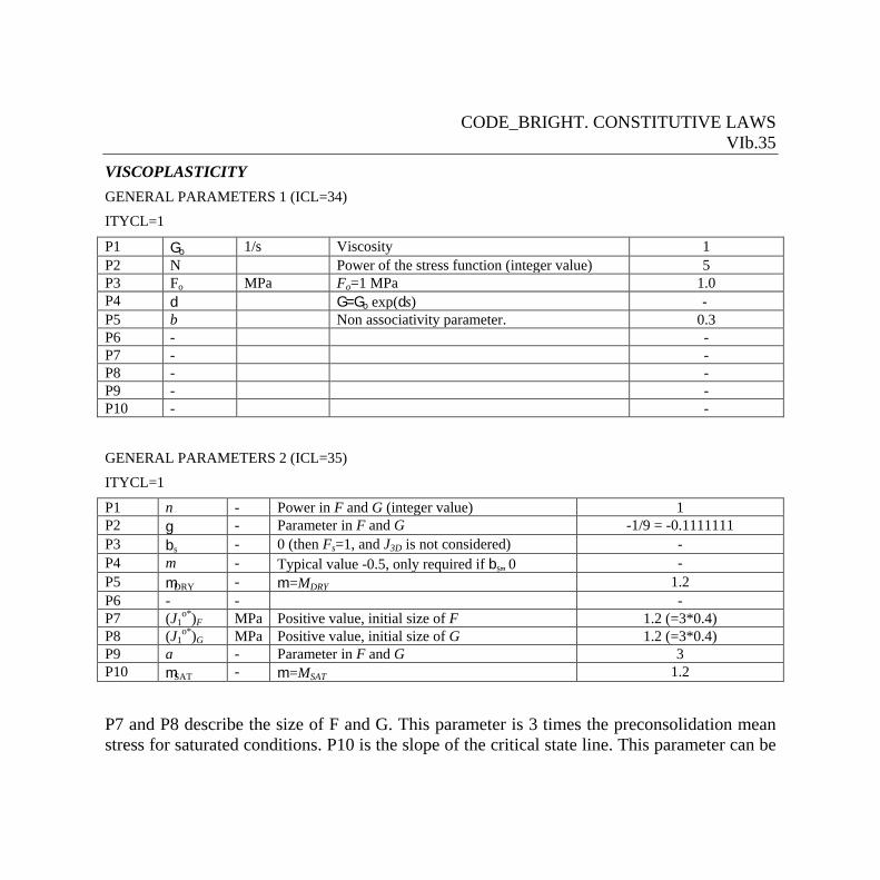
CODE_BRIGHT. CONSTITUTIVE LAWS VIb.35
VISCOPLASTICITY GENERAL PARAMETERS 1 (ICL=34)
ITYCL=1
P1 Go 1/s Viscosity 1 P2 N Power of the stress function (integer value) 5 P3 Fo MPa Fo=1 MPa 1.0 P4 d G=Go exp(ds) - P5 b Non associativity parameter. 0.3 P6 - - P7 - - P8 - - P9 - - P10 - -
GENERAL PARAMETERS 2 (ICL=35)
ITYCL=1
P1 n - Power in F and G (integer value) 1 P2 g - Parameter in F and G -1/9 = -0.1111111 P3 bs - 0 (then Fs=1, and J3D is not considered) - P4 m - Typical value -0.5, only required if bs¹0 - P5 mDRY - m =MDRY 1.2 P6 - - - P7 (J1
o*)F MPa Positive value, initial size of F 1.2 (=3*0.4) P8 (J1
o*)G MPa Positive value, initial size of G 1.2 (=3*0.4) P9 a - Parameter in F and G 3 P10 mSAT - m =MSAT 1.2
P7 and P8 describe the size of F and G. This parameter is 3 times the preconsolidation mean stress for saturated conditions. P10 is the slope of the critical state line. This parameter can be
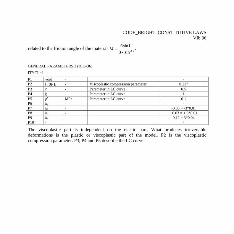
CODE_BRIGHT. CONSTITUTIVE LAWS VIb.36
related to the friction angle of the material 6sin '3 sin '
M f=
- f.
GENERAL PARAMETERS 3 (ICL=36)
ITYCL=1
P1 void - - P2 l(0)-k - Viscoplastic compression parameter 0.117 P3 r - Parameter in LC curve 0.5 P4 b - Parameter in LC curve 1 P5 pc MPa Parameter in LC curve 0.1 P6 k1 - - P7 k2 - -0.03 = -3*0.01 P8 k3 - +0.03 = + 3*0.01 P9 k4 - 0.12 = 3*0.04 P10 - -
The viscoplastic part is independent on the elastic part. What produces irreversible deformations is the plastic or viscoplastic part of the model. P2 is the viscoplastic compression parameter. P3, P4 and P5 describe the LC curve.
CODE_BRIGHT. CONSTITUTIVE LAWS VIc.1
C:\Users\jean.vaunat\Documents\My CV\Academic\Grado\UPC\Tesinas\Claudio Dias\2terço.gid
CODE_BRIGHT. CONSTITUTIVE LAWS This chapter contains the different models available and the corresponding parameters required by each model. The following constitutive laws are available: HYDRAULIC AND THERMAL CONSTITUTIVE MODELS (a) RETENTION CURVE INTRINSIC PERMEABILITY LIQUID PHASE RELATIVE PERMEABILITY GAS PHASE RELATIVE PERMEABILITY DIFFUSIVE FLUXES OF MASS DISPERSIVE FLUXES OF MASS AND ENERGY CONDUCTIVE FLUX OF HEAT
MECHANICAL CONSTITUTIVE MODELS ELASTICITY (b) NONLINEAR ELASTICITY (b) VISCOPLASTICITY FOR SALINE MATERIALS (b) VISCOPLASTICITY FOR GRANULAR MATERIALS (b) VISCOPLASTICITY FOR UNSATURATED SOILS BASED ON BBM (b) DAMAGE-ELASTOPLASTIC MODEL FOR ARGILLACEOUS ROCKS (c) THERMO-ELASTOPLASTIC MODEL FOR SOILS (d) BARCELONA EXPANSIVE MODEL FOR SOILS (e) CASM’s FAMILY MODELS (f)
PHASE PROPERTIES (a) SOLID PHASE PROPERTIES LIQUID PHASE PROPERTIES
GAS PHASE PROPERTIES
EXCAVATION PROCESS (g)
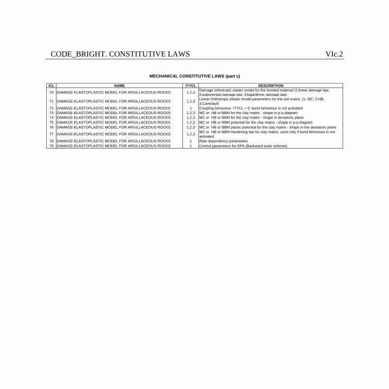
CODE_BRIGHT. CONSTITUTIVE LAWS VIc.2
ICL NAME ITYCL DESCRIPTION
70 DAMAGE-ELASTOPLASTIC MODEL FOR ARGILLACEOUS ROCKS 1,2,3 Damage orthotropic elastic model for the bonded material (1:linear damage law; 2:exponential damage law; 3:logarithmic damage law)
71 DAMAGE-ELASTOPLASTIC MODEL FOR ARGILLACEOUS ROCKS 1,2,3 Linear Orthotropic elastic model parameters for the soil matrix. (1; MC; 2:HB, 3:Camclayl)
72 DAMAGE-ELASTOPLASTIC MODEL FOR ARGILLACEOUS ROCKS 1 Coupling behaviour. ITYCL = 0: bond behaviour is not activated73 DAMAGE-ELASTOPLASTIC MODEL FOR ARGILLACEOUS ROCKS 1,2,3 MC or HB or BBM for the clay matrix - shape in p-q diagram74 DAMAGE-ELASTOPLASTIC MODEL FOR ARGILLACEOUS ROCKS 1,2,3 MC or HB or BBM for the clay matrix - shape in deviatoric plane75 DAMAGE-ELASTOPLASTIC MODEL FOR ARGILLACEOUS ROCKS 1,2,3 MC or HB or BBM potential for the clay matrix - shape in p-q diagram76 DAMAGE-ELASTOPLASTIC MODEL FOR ARGILLACEOUS ROCKS 1,2,3 MC or HB or BBM plastic potential for the clay matrix - shape in the deviatoric plane
77 DAMAGE-ELASTOPLASTIC MODEL FOR ARGILLACEOUS ROCKS 1,2,3 MC or HB or BBM Hardening law for clay matrix, used only if bond behaviour is not activated
78 DAMAGE-ELASTOPLASTIC MODEL FOR ARGILLACEOUS ROCKS 1 Rate dependency parameters79 DAMAGE-ELASTOPLASTIC MODEL FOR ARGILLACEOUS ROCKS 1 Control parameters for SPA (Backward euler scheme)
MECHANICAL CONSTITUTIVE LAWS (part c)

CODE_BRIGHT. CONSTITUTIVE LAWS VIc.3 DAMAGE-ELASTOPLASTIC MODEL FOR ARGILLACEOUS ROCKS
CODES ICL=70 to 79 ITYCL=see below
DESCRIPTION Damage-elastoplastic model for argillaceous rock This model considers the argillaceous rock as a composite material made of a clay matrix interlocked by bond. Clay matrix behaviour is modeled through an elastoplastic constitutive law, typical of soils. Bonds are modeled through a damage elastic law (Carol et al., 2001), typical of quasi-brittle materials. A coupling parameter gives the relative importance of clay and bond response for the composite material. This law applies to material having a response transitional between that of a soil and a rock.
EQUATIONS
For this model, equations are written assuming Soils Mechanics convention (p > 0, ev > 0, compression). p is the mean effective stress, J the square root of the second invariant of deviatoric stress tensor, q the Lode’ angle (-30º in triaxial compression, +30º in triaxial extension) (see ICL 21 to 27 for their definition). Clay matrix behaviour Elastic law:
M eM M pij ijkl kl kl klM
s
dsd D d dK
s e d eæ ö
= - -ç ÷è ø
Mijs are the stresses prevailing at clay particles contact, eM
ijklD is the
mechanical elastic stiffness matrix of the clay, Mklde are the strains
corresponding to the clay matrix deformation (equal to the external strains), MsK is the bulk modulus against suction changes (if any), p
klde are the plastic strains of the clay matrix. 2 elastic laws are considered: Orthotropic linear elasticity (ITYCL = 1 or 2):
eMijklD is defined by clay matrix Young’s moduli EM
h and EM
v and Poisson’s
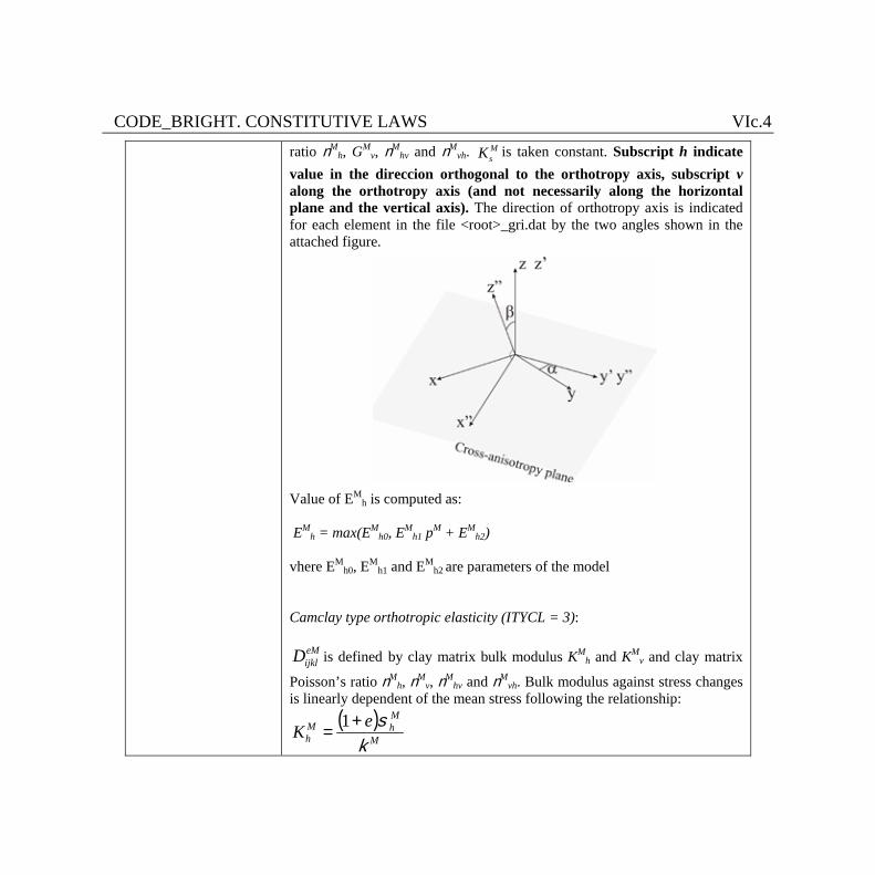
CODE_BRIGHT. CONSTITUTIVE LAWS VIc.4
ratio nMh, GM
v, nMhv and nM
vh. MsK is taken constant. Subscript h indicate
value in the direccion orthogonal to the orthotropy axis, subscript v along the orthotropy axis (and not necessarily along the horizontal plane and the vertical axis). The direction of orthotropy axis is indicated for each element in the file <root>_gri.dat by the two angles shown in the attached figure.
Value of EM
h is computed as: EM
h = max(EMh0, EM
h1 pM + EMh2)
vhere EM
h0, EMh1 and EM
h2 are parameters of the model Camclay type orthotropic elasticity (ITYCL = 3):
eMijklD is defined by clay matrix bulk modulus KM
h and KMv and clay matrix
Poisson’s ratio nMh, nM
v, nMhv and nM
vh. Bulk modulus against stress changes is linearly dependent of the mean stress following the relationship:
( )M
MhM
heK
ks+
=1
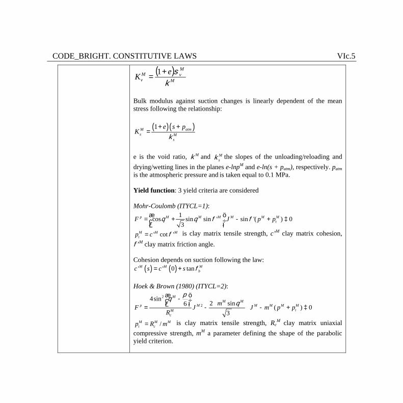
CODE_BRIGHT. CONSTITUTIVE LAWS VIc.5
( )M
MvM
veK
ks+
=1
Bulk modulus against suction changes is linearly dependent of the mean stress following the relationship:
( )( )1 atmMs M
s
e s pK
k+ +
=
e is the void ratio, Mk and M
sk the slopes of the unloading/reloading and drying/wetting lines in the planes e-lnpM and e-ln(s + patm), respectively. patm is the atmospheric pressure and is taken equal to 0.1 MPa. Yield function: 3 yield criteria are considered Mohr-Coulomb (ITYCL=1):
1cos sin sin ' sin '( ) 03
p M M M M M MtF J p pq q f fæ ö= + - + ³ç ÷
è ø
' cot 'M M Mtp c f= is clay matrix tensile strength, c’M clay matrix cohesion,
f’M clay matrix friction angle. Cohesion depends on suction following the law:
( ) ( )' ' 0 tanM M Mbc s c s f= +
Hoek & Brown (1980) (ITYCL=2):
2
24sin
2 sin6 ( ) 03
MM M
p M M M M MtM
c
mF J J m p pR
pqq
æ ö-ç ÷è ø= - - + ³
/M M Mt cp R m= is clay matrix tensile strength, Rc
M clay matrix uniaxial
compressive strength, mM a parameter defining the shape of the parabolic yield criterion.
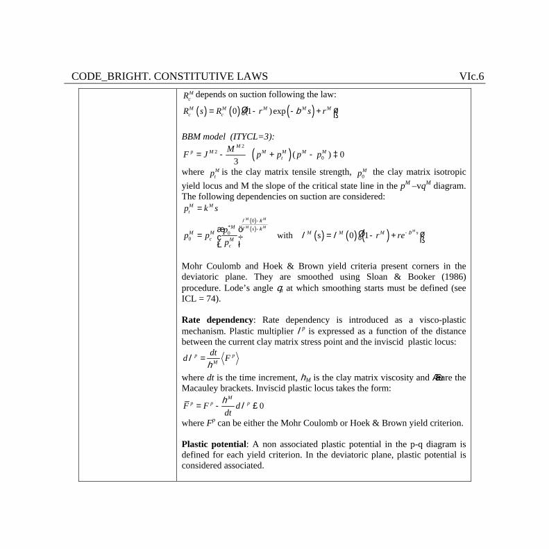
CODE_BRIGHT. CONSTITUTIVE LAWS VIc.6 McR depends on suction following the law:
( ) ( ) ( )0 (1 )expM M M M Mc cR s R r s rbé ù= - - +ë û
BBM model (ITYCL=3):
( )2
20( ) 0
3
Mp M M M M M
tMF J p p p p= - + - ³
where Mtp is the clay matrix tensile strength,
0Mp the clay matrix isotropic
yield locus and M the slope of the critical state line in the pM –vqM diagram. The following dependencies on suction are considered:
M Mtp k s=
( )( )
( ) ( ) ( )0
*0
0 with s 0 1
M M
M MM
M sM M M M M s
c Mc
pp p r rep
l kl k
bl l
-
--æ ö é ù= = - +ç ÷ ë ûè ø
Mohr Coulomb and Hoek & Brown yield criteria present corners in the deviatoric plane. They are smoothed using Sloan & Booker (1986) procedure. Lode’s angle qt at which smoothing starts must be defined (see ICL = 74). Rate dependency: Rate dependency is introduced as a visco-plastic mechanism. Plastic multiplier lp is expressed as a function of the distance between the current clay matrix stress point and the inviscid plastic locus:
p pM
dtd Flh
=
where dt is the time increment, hM is the clay matrix viscosity and áñ are the Macauley brackets. Inviscid plastic locus takes the form:
0M
p p pF F ddt
h l= - £
where Fp can be either the Mohr Coulomb or Hoek & Brown yield criterion. Plastic potential: A non associated plastic potential in the p-q diagram is defined for each yield criterion. In the deviatoric plane, plastic potential is considered associated.
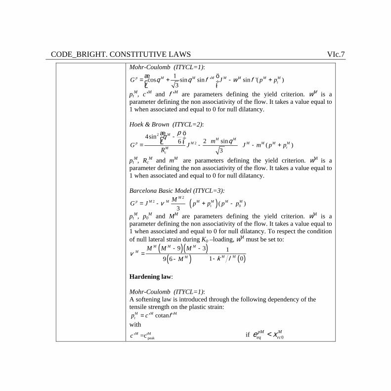
CODE_BRIGHT. CONSTITUTIVE LAWS VIc.7 Mohr-Coulomb (ITYCL=1):
1cos sin sin ' sin '( )3
p M M M M M M MtG J p pq q f w fæ ö= + - +ç ÷
è ø
ptM, c’M and f’M are parameters defining the yield criterion. wM is a
parameter defining the non associativity of the flow. It takes a value equal to 1 when associated and equal to 0 for null dilatancy. Hoek & Brown (ITYCL=2):
2
24sin
2 sin6 ( )3
MM M
p M M M M MtM
c
mG J J m p pR
pqq
æ ö-ç ÷è ø= - - +
ptM, Rc
M and mM are parameters defining the yield criterion. wM is a parameter defining the non associativity of the flow. It takes a value equal to 1 when associated and equal to 0 for null dilatancy. Barcelona Basic Model (ITYCL=3):
( )2
20( )
3
Mp M M M M M M
tMG J p p p pv= - + -
ptM, p0
M and MM are parameters defining the yield criterion. wM is a parameter defining the non associativity of the flow. It takes a value equal to 1 when associated and equal to 0 for null dilatancy. To respect the condition of null lateral strain during K0 –loading, wM must be set to:
( )( )( ) ( )
9 3 11 09 6
M M MM
M MM
M M M
Mv
k l
- -=
--
Hardening law: Mohr-Coulomb (ITYCL=1): A softening law is introduced through the following dependency of the tensile strength on the plastic strain:
M' cotan 'M Mtp c f=
with Mpeak' =c'Mc if 0
pM Meq rce x<
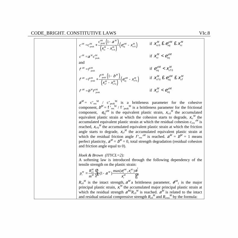
CODE_BRIGHT. CONSTITUTIVE LAWS VIc.8
( )( ) ( )MpeakM
peak 00
c' 1' =c'
MM pM M
eq rcM Mrc rc
ca
e xx x
-+ -
- if 0
M pM Mrc eq rcx e x£ £
Mpeak' = c'M Mc a if M pM
rc eqx e< and
Mpeak' = 'Mf f if 0
pM Meq rfe x<
( )( ) ( )MpeakM
peak 00
' 1' = '
MM pM M
eq rM Mr r
ff f
f bf f e x
x x
-+ -
- if 0
M pM Mr eq rf fx e x£ £
Mpeak' = 'M Mf b f if M pM
r eqfx e< aM = c’res
M / c’peakM is a brittleness parameter for the cohesive
component, bM = f’resM / f’peak
M is a brittleness parameter for the frictional component, eeq
pM is the equivalent plastic strain, xrc0M the accumulated
equivalent plastic strain at which the cohesion starts to degrade, xrcM the
accumulated equivalent plastic strain at which the residual cohesion cres’M is reached, xrf0
M the accumulated equivalent plastic strain at which the friction angle starts to degrade, xrf
M the accumulated equivalent plastic strain at which the residual friction angle f’res’M is reached. aM = bM = 1 means perfect plasticity, aM = bM = 0, total strength degradation (residual cohesion and friction angle equal to 0). Hoek & Brown (ITYCL=2): A softening law is introduced through the following dependency of the tensile strength on the plastic strain:
2
0 1max( , )1-(1 )M pM M
M Mc rt M M
r
Rpm
e xax
é ù= -ê ú
ë û
Rc0M is the intact strength, aM a brittleness parameter, epM
1 is the major principal plastic strain, xr
M the accumulated major principal plastic strain at which the residual strength aM2Rc0
M is reached. aM is related to the intact and residual uniaxial compressive strength Rc0
M and RcresM by the formula:
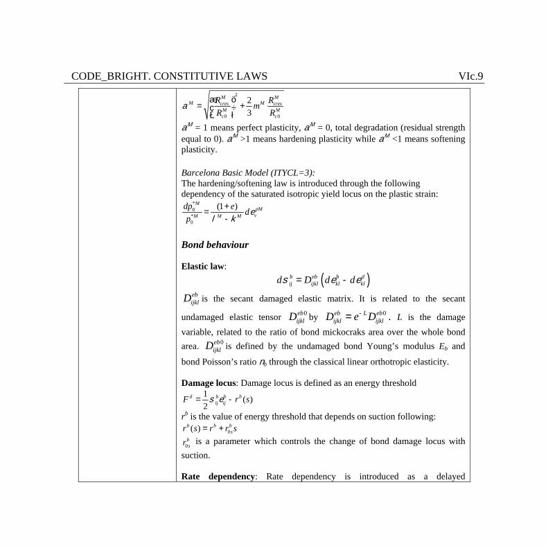
CODE_BRIGHT. CONSTITUTIVE LAWS VIc.9 2
0 0
23
M MM Mcres cres
M Mc c
R RmR R
aæ ö
= +ç ÷è ø
aM = 1 means perfect plasticity, aM = 0, total degradation (residual strength equal to 0). aM >1 means hardening plasticity while aM <1 means softening plasticity. Barcelona Basic Model (ITYCL=3): The hardening/softening law is introduced through the following dependency of the saturated isotropic yield locus on the plastic strain:
*0
*0
(1 )MpM
vM M M
dp e dp
el k
+=
-
Bond behaviour Elastic law:
( )b eb b dij ijkl kl kld D d ds e e= -
ebijklD is the secant damaged elastic matrix. It is related to the secant
undamaged elastic tensor 0ebijklD by 0eb L eb
ijkl ijklD e D-= . L is the damage variable, related to the ratio of bond mickocraks area over the whole bond area. 0eb
ijklD is defined by the undamaged bond Young’s modulus Eb and
bond Poisson’s ratio nb through the classical linear orthotropic elasticity.
Damage locus: Damage locus is defined as an energy threshold 1 ( )2
d b b bij ijF r ss e= -
rb is the value of energy threshold that depends on suction following: 0( )b b b
sr s r r s= +
0bsr is a parameter which controls the change of bond damage locus with
suction. Rate dependency: Rate dependency is introduced as a delayed
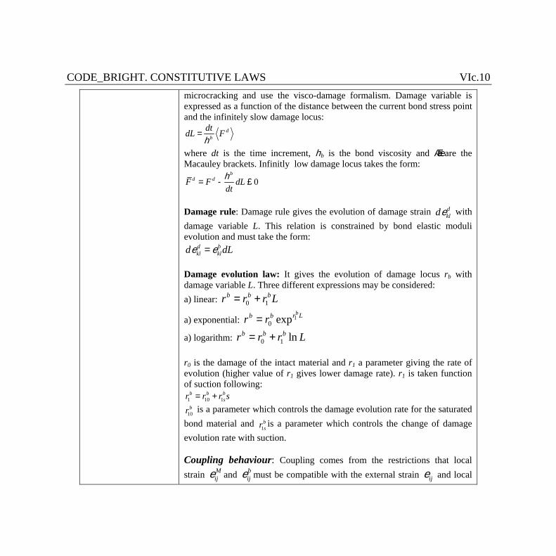
CODE_BRIGHT. CONSTITUTIVE LAWS VIc.10 microcracking and use the visco-damage formalism. Damage variable is expressed as a function of the distance between the current bond stress point and the infinitely slow damage locus:
db
dtdL Fh
=
where dt is the time increment, hb is the bond viscosity and áñ are the Macauley brackets. Infinitly low damage locus takes the form:
0b
d dF F dLdth
= - £
Damage rule: Damage rule gives the evolution of damage strain d
klde with damage variable L. This relation is constrained by bond elastic moduli evolution and must take the form:
d bkl kld dLe e=
Damage evolution law: It gives the evolution of damage locus rb with damage variable L. Three different expressions may be considered: a) linear: 0 1
b b br r r L= +
a) exponential: 10 exp
br Lb br r=
a) logarithm: 0 1 lnb b br r r L= + r0 is the damage of the intact material and r1 a parameter giving the rate of evolution (higher value of r1 gives lower damage rate). r1 is taken function of suction following:
1 10 1b b b
sr r r s= +
10br is a parameter which controls the damage evolution rate for the saturated
bond material and 1bsr is a parameter which controls the change of damage
evolution rate with suction. Coupling behaviour: Coupling comes from the restrictions that local strain M
ije and bije must be compatible with the external strain ije and local

CODE_BRIGHT. CONSTITUTIVE LAWS VIc.11
stresses Mijs and b
ijs must be in equilibrium with external stresses ijs . This restrictions read:
M bij ij ijd d de e e= +
( )1 M bij ij ijs c s cs= + + with 2
0Le-= cc
L is the damage variable and c0 a coupling parameter that gives the relative importance of bond and clay matrix behaviour in the overall response of the composite material. 00 c£ £ ¥ .
Since this model requires a substantial number of parameters, several ICL's are included:
ICL=70 contains elastic parameters for the bonding
ICL=71 contains elastic parameters for the soil matrix
ICL=72 contains parameters for the coupling between bonding and soil matrix
ICL=73 contains parameters for the shape of the yield function in the p-q plane (soil matrix)
ICL=74 contains parameters for the shape of the yield function in the deviatoric plane (soil matrix)
ICL=75 contains parameters for the shape of the plastic potential in the p-q plane (soil matrix)
ICL=76 contains parameters for the shape of the plastic potential in the deviatoric plane (soil matrix)
ICL=77 contains parameters for the hardening law (soil matrix)
ICL=78 contains parameters for the viscoplastic model (bonding and soil matrix)
ICL=79 contains parameters to control the integration of the constitutive law
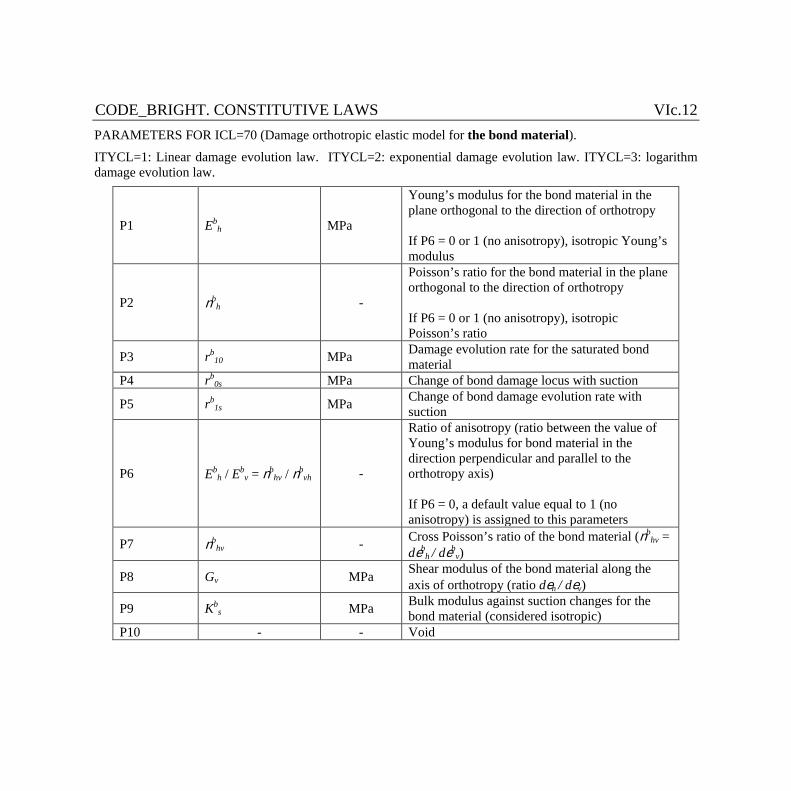
CODE_BRIGHT. CONSTITUTIVE LAWS VIc.12 PARAMETERS FOR ICL=70 (Damage orthotropic elastic model for the bond material). ITYCL=1: Linear damage evolution law. ITYCL=2: exponential damage evolution law. ITYCL=3: logarithm damage evolution law.
P1 Ebh MPa
Young’s modulus for the bond material in the plane orthogonal to the direction of orthotropy If P6 = 0 or 1 (no anisotropy), isotropic Young’s modulus
P2 nbh -
Poisson’s ratio for the bond material in the plane orthogonal to the direction of orthotropy If P6 = 0 or 1 (no anisotropy), isotropic Poisson’s ratio
P3 rb10 MPa Damage evolution rate for the saturated bond
material P4 rb
0s MPa Change of bond damage locus with suction
P5 rb1s MPa Change of bond damage evolution rate with
suction
P6 Ebh / Eb
v = nbhv / nb
vh -
Ratio of anisotropy (ratio between the value of Young’s modulus for bond material in the direction perpendicular and parallel to the orthotropy axis) If P6 = 0, a default value equal to 1 (no anisotropy) is assigned to this parameters
P7 nbhv - Cross Poisson’s ratio of the bond material (nb
hv = deb
h / debv)
P8 Gv MPa Shear modulus of the bond material along the axis of orthotropy (ratio deh / dev)
P9 Kbs MPa Bulk modulus against suction changes for the
bond material (considered isotropic) P10 - - Void
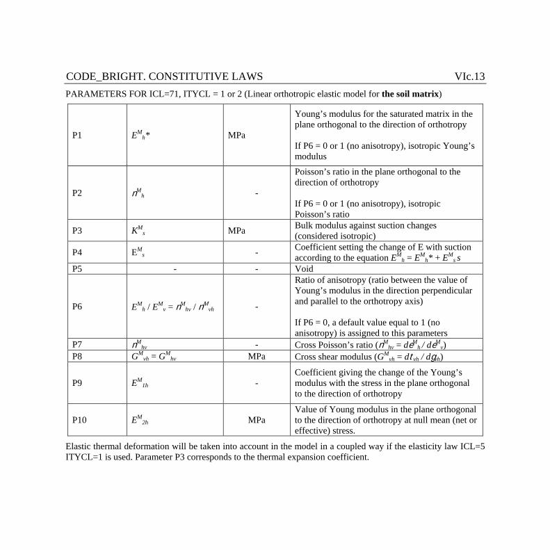
CODE_BRIGHT. CONSTITUTIVE LAWS VIc.13 PARAMETERS FOR ICL=71, ITYCL = 1 or 2 (Linear orthotropic elastic model for the soil matrix)
P1 EMh* MPa
Young’s modulus for the saturated matrix in the plane orthogonal to the direction of orthotropy If P6 = 0 or 1 (no anisotropy), isotropic Young’s modulus
P2 nMh -
Poisson’s ratio in the plane orthogonal to the direction of orthotropy If P6 = 0 or 1 (no anisotropy), isotropic Poisson’s ratio
P3 KMs MPa Bulk modulus against suction changes
(considered isotropic)
P4 EMs - Coefficient setting the change of E with suction
according to the equation EMh = EM
h* + EMs s
P5 - - Void
P6 EMh / EM
v = nMhv / nM
vh -
Ratio of anisotropy (ratio between the value of Young’s modulus in the direction perpendicular and parallel to the orthotropy axis) If P6 = 0, a default value equal to 1 (no anisotropy) is assigned to this parameters
P7 nMhv - Cross Poisson’s ratio (nM
hv = deMh / deM
v) P8 GM
vh = GMhv MPa Cross shear modulus (GM
vh = dtvh / dgvh)
P9 EM1h -
Coefficient giving the change of the Young’s modulus with the stress in the plane orthogonal to the direction of orthotropy
P10 EM2h MPa
Value of Young modulus in the plane orthogonal to the direction of orthotropy at null mean (net or effective) stress.
Elastic thermal deformation will be taken into account in the model in a coupled way if the elasticity law ICL=5 ITYCL=1 is used. Parameter P3 corresponds to the thermal expansion coefficient.
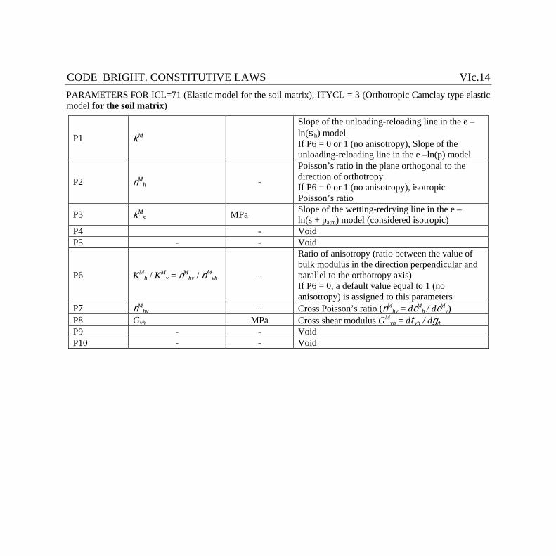
CODE_BRIGHT. CONSTITUTIVE LAWS VIc.14 PARAMETERS FOR ICL=71 (Elastic model for the soil matrix), ITYCL = 3 (Orthotropic Camclay type elastic model for the soil matrix)
P1 kM
Slope of the unloading-reloading line in the e –ln(sh) model If P6 = 0 or 1 (no anisotropy), Slope of the unloading-reloading line in the e –ln(p) model
P2 nMh -
Poisson’s ratio in the plane orthogonal to the direction of orthotropy If P6 = 0 or 1 (no anisotropy), isotropic Poisson’s ratio
P3 kMs MPa Slope of the wetting-redrying line in the e –
ln(s + patm) model (considered isotropic) P4 - Void P5 - - Void
P6 KMh / KM
v = nMhv / nM
vh -
Ratio of anisotropy (ratio between the value of bulk modulus in the direction perpendicular and parallel to the orthotropy axis) If P6 = 0, a default value equal to 1 (no anisotropy) is assigned to this parameters
P7 nMhv - Cross Poisson’s ratio (nM
hv = deMh / deM
v) P8 Gvh MPa Cross shear modulus GM
vh = dtvh / dgvh P9 - - Void P10 - - Void
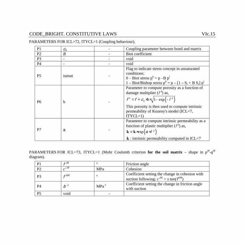
CODE_BRIGHT. CONSTITUTIVE LAWS VIc.15 PARAMETERS FOR ICL=72, ITYCL=1 (Coupling behaviour).
P1 c0 - Coupling parameter between bond and matrix P2 B - Biot coefficient P3 - - void P4 - - void
P5 iunsat -
Flag to indicate stress concept in unsaturated conditions: 0 – Biot stress pb = p –B pl 1 – Biot/Bishop stress pb = p – [1 – Sr + B Sr] pl
P6 b -
Parameter to compute porosity as a function of damage multiplier (ld) as,
( )0 1 expb dbf f c l= + × × - -
This porosity is then used to compute intrinsic permeability of Kozeny's model (ICL=7, ITYCL=1)
P7 a -
Parameter to compute intrinsic permeability as a function of plastic multiplier (lp) as,
( )exp pa l= × ×k k k : intrinsic permeability computed in ICL=7
PARAMETERS FOR ICL=73, ITYCL=1 (Mohr Coulomb criterion for the soil matrix – shape in pM-qM diagram).
P1 f’M º Friction angle P2 c’ M
MPa Cohesion
P3 f bM º Coefficient setting the change in cohesion with
suction following: c’M = s tan(fbM)
P4 b M MPa-1 Coefficient setting the change in friction angle with suction
P5 void -
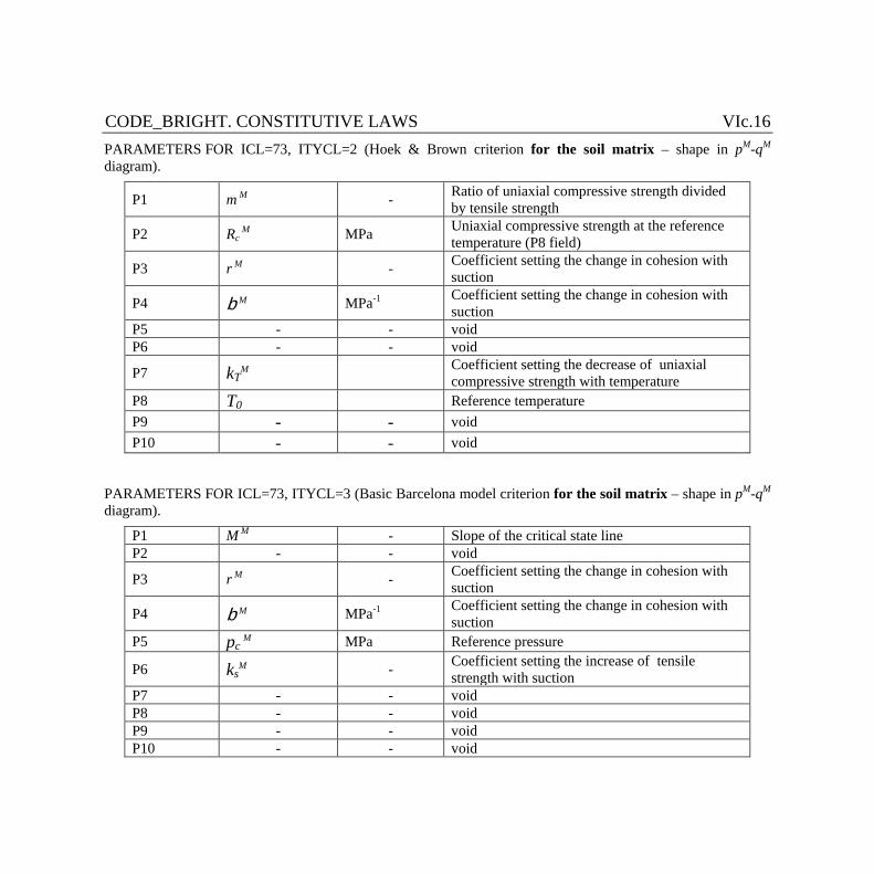
CODE_BRIGHT. CONSTITUTIVE LAWS VIc.16 PARAMETERS FOR ICL=73, ITYCL=2 (Hoek & Brown criterion for the soil matrix – shape in pM-qM diagram).
P1 m M - Ratio of uniaxial compressive strength divided by tensile strength
P2 Rc M
MPa Uniaxial compressive strength at the reference temperature (P8 field)
P3 r M - Coefficient setting the change in cohesion with
suction
P4 b M MPa-1 Coefficient setting the change in cohesion with suction
P5 - - void P6 - - void
P7 kTM Coefficient setting the decrease of uniaxial
compressive strength with temperature P8 T0 Reference temperature P9 - - void P10 - - void
PARAMETERS FOR ICL=73, ITYCL=3 (Basic Barcelona model criterion for the soil matrix – shape in pM-qM diagram).
P1 M M - Slope of the critical state line P2 - - void
P3 r M - Coefficient setting the change in cohesion with
suction
P4 b M MPa-1 Coefficient setting the change in cohesion with suction
P5 pc M MPa Reference pressure
P6 ksM - Coefficient setting the increase of tensile
strength with suction P7 - - void P8 - - void P9 - - void P10 - - void
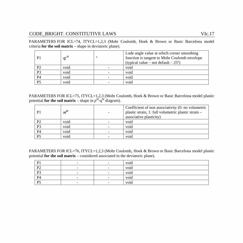
CODE_BRIGHT. CONSTITUTIVE LAWS VIc.17 PARAMETERS FOR ICL=74, ITYCL=1,2,3 (Mohr Coulomb, Hoek & Brown or Basic Barcelona model criteria for the soil matrix – shape in deviatoric plane).
P1 qt M
º Lode angle value at which corner smoothing function is tangent to Mohr Coulomb envelope (typical value – not default – 25º)
P2 void - void P3 void - void P4 void - void P5 void - void
PARAMETERS FOR ICL=75, ITYCL=1,2,3 (Mohr Coulomb, Hoek & Brown or Basic Barcelona model plastic potential for the soil matrix – shape in pM-qM diagram).
P1 wM - Coefficient of non associativity (0: no volumetric plastic strain, 1: full volumetric plastic strain –associative plasticity)
P2 void - void P3 void - void P4 void - void P5 void - void
PARAMETERS FOR ICL=76, ITYCL=1,2,3 (Mohr Coulomb, Hoek & Brown or Basic Barcelona model plastic potential for the soil matrix – considered associated in the deviatoric plane).
P1 - - void P2 - - void P3 - - void P4 - - void P5 - - void
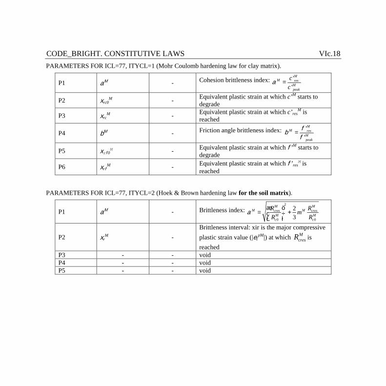
CODE_BRIGHT. CONSTITUTIVE LAWS VIc.18 PARAMETERS FOR ICL=77, ITYCL=1 (Mohr Coulomb hardening law for clay matrix).
P1 aM - Cohesion brittleness index: ''
MM res
Mpeak
cc
a =
P2 xrc0M - Equivalent plastic strain at which c’M starts to
degrade
P3 xrcM - Equivalent plastic strain at which c’res
M is reached
P4 bM - Friction angle brittleness index: '
'
MM res
Mpeak
fbf
=
P5 xrf0M - Equivalent plastic strain at which f’M starts to
degrade
P6 xrfM - Equivalent plastic strain at which f’res
M is reached
PARAMETERS FOR ICL=77, ITYCL=2 (Hoek & Brown hardening law for the soil matrix).
P1 aM - Brittleness index: 2
0 0
23
M MM Mcres cres
M Mc c
R RmR R
aæ ö
= +ç ÷è ø
P2 xrM -
Brittleness interval: xir is the major compressive plastic strain value (|e1
pM|) at which McresR is
reached P3 - - void P4 - - void P5 - - void
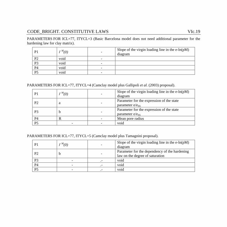
CODE_BRIGHT. CONSTITUTIVE LAWS VIc.19 PARAMETERS FOR ICL=77, ITYCL=3 (Basic Barcelona model does not need additional parameter for the hardening law for clay matrix).
P1 l M(0) - Slope of the virgin loading line in the e-ln(pM)
diagram P2 void - P3 void - P4 void - P5 void -
PARAMETERS FOR ICL=77, ITYCL=4 (Camclay model plus Gallipoli et al. (2003) proposal).
P1 l M(0) - Slope of the virgin loading line in the e-ln(pM)
diagram
P2 a - Parameter for the expression of the state parameter e/eSS
P3 b - Parameter for the expression of the state parameter e/eSS
P4 R - Mean pore radius P5 - - void
PARAMETERS FOR ICL=77, ITYCL=5 (Camclay model plus Tamagnini proposal).
P1 l M(0) - Slope of the virgin loading line in the e-ln(pM)
diagram
P2 b - Parameter for the dependency of the hardening law on the degree of saturation
P3 - .- void P4 - .- void P5 - .- void
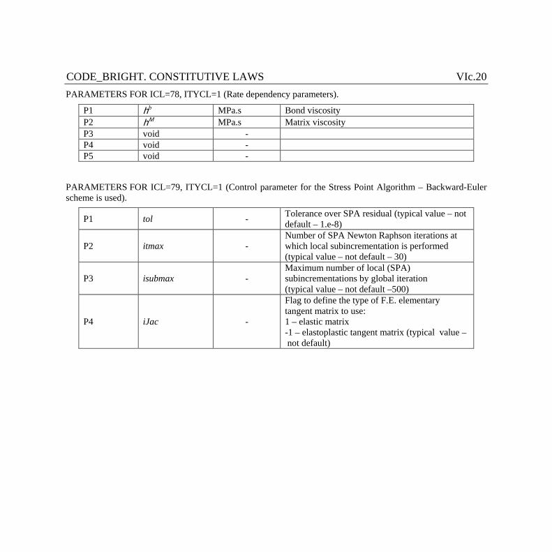
CODE_BRIGHT. CONSTITUTIVE LAWS VIc.20 PARAMETERS FOR ICL=78, ITYCL=1 (Rate dependency parameters).
P1 hb MPa.s Bond viscosity P2 hM MPa.s Matrix viscosity P3 void - P4 void - P5 void -
PARAMETERS FOR ICL=79, ITYCL=1 (Control parameter for the Stress Point Algorithm – Backward-Euler scheme is used).
P1 tol - Tolerance over SPA residual (typical value – not default – 1.e-8)
P2 itmax - Number of SPA Newton Raphson iterations at which local subincrementation is performed (typical value – not default – 30)
P3 isubmax - Maximum number of local (SPA) subincrementations by global iteration (typical value – not default –500)
P4 iJac -
Flag to define the type of F.E. elementary tangent matrix to use: 1 – elastic matrix -1 – elastoplastic tangent matrix (typical value – not default)
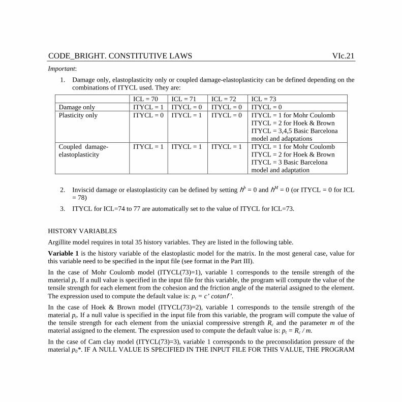
CODE_BRIGHT. CONSTITUTIVE LAWS VIc.21 Important:
1. Damage only, elastoplasticity only or coupled damage-elastoplasticity can be defined depending on the combinations of ITYCL used. They are:
ICL = 70 ICL = 71 ICL = 72 ICL = 73 Damage only ITYCL = 1 ITYCL = 0 ITYCL = 0 ITYCL = 0 Plasticity only ITYCL = 0 ITYCL = 1 ITYCL = 0 ITYCL = 1 for Mohr Coulomb
ITYCL = 2 for Hoek & Brown ITYCL = 3,4,5 Basic Barcelona model and adaptations
Coupled damage-elastoplasticity
ITYCL = 1 ITYCL = 1 ITYCL = 1 ITYCL = 1 for Mohr Coulomb ITYCL = 2 for Hoek & Brown ITYCL = 3 Basic Barcelona model and adaptation
2. Inviscid damage or elastoplasticity can be defined by setting hb = 0 and hM = 0 (or ITYCL = 0 for ICL = 78)
3. ITYCL for ICL=74 to 77 are automatically set to the value of ITYCL for ICL=73.
HISTORY VARIABLES
Argillite model requires in total 35 history variables. They are listed in the following table.
Variable 1 is the history variable of the elastoplastic model for the matrix. In the most general case, value for this variable need to be specified in the input file (see format in the Part III).
In the case of Mohr Coulomb model (ITYCL(73)=1), variable 1 corresponds to the tensile strength of the material pt. If a null value is specified in the input file for this variable, the program will compute the value of the tensile strength for each element from the cohesion and the friction angle of the material assigned to the element. The expression used to compute the default value is: pt = c’ cotanf’. In the case of Hoek & Brown model (ITYCL(73)=2), variable 1 corresponds to the tensile strength of the material pt. If a null value is specified in the input file from this variable, the program will compute the value of the tensile strength for each element from the uniaxial compressive strength Rc and the parameter m of the material assigned to the element. The expression used to compute the default value is: pt = Rc / m. In the case of Cam clay model (ITYCL(73)=3), variable 1 corresponds to the preconsolidation pressure of the material p0*. IF A NULL VALUE IS SPECIFIED IN THE INPUT FILE FOR THIS VALUE, THE PROGRAM

CODE_BRIGHT. CONSTITUTIVE LAWS VIc.22 WILL ABORT DUE TO A MATH ERROR (this ellipse of Cam clay model degenerates into a point). Variable 2 is the history variable of the damage model for the bond. In the most general case, value for this variable need to be specified in the input file (see format in the Part III). However, in many cases, this value can be set to 0. It means that damage will start for any stress changes.
Variable 3 is used internally to keep memory of the type of constitutive matrix (elastic, tangent elastoplastic, tangent damage or tangent damage elastoplastic) used to build the global tangent stiffness. No input from the user is associated to this variable.
Variable 4 is the plastic multiplier of the matrix. This variable measures the amount of plastic strain. It is usually set to 0 at the beginning of the computation and updated within the argillite subroutine. This variable is used only by the user for output visualization purposes (it provides the spatial distribution of plastic strain intensity within the mesh at any output time).
Variable 5 is the damage multiplier of the bonds. This variable measures the amount of damage. It is usually set to 0 at the beginning of the computation and updated within the argillite subroutine. This variable is used by the user for output visualization purposes only (it provides the spatial distribution of damage intensity within the mesh at any output time).
Variables 6 to 11 are the current stresses within the bonds. Variables 12 to 17 are the stresses within the matrix at time of bond formation. In the most general case, all these variables have to be specified in the input file*. However, from a practical point of view, most of the problems can be run setting these values to 0 at the beginning of the computation (in this case, the damage locus is centered on the initial stress state at the beginning of the computation).
Variables 18 to 35 contain the total, plastic and damage strain tensor components. They are usually set to 0 at the beginning of the computation and updated within the argillite subroutine. These variables are used by the user for output visualization purposes only (they provides the spatial distribution of the total, plastic and damage strain within the mesh at any output time).
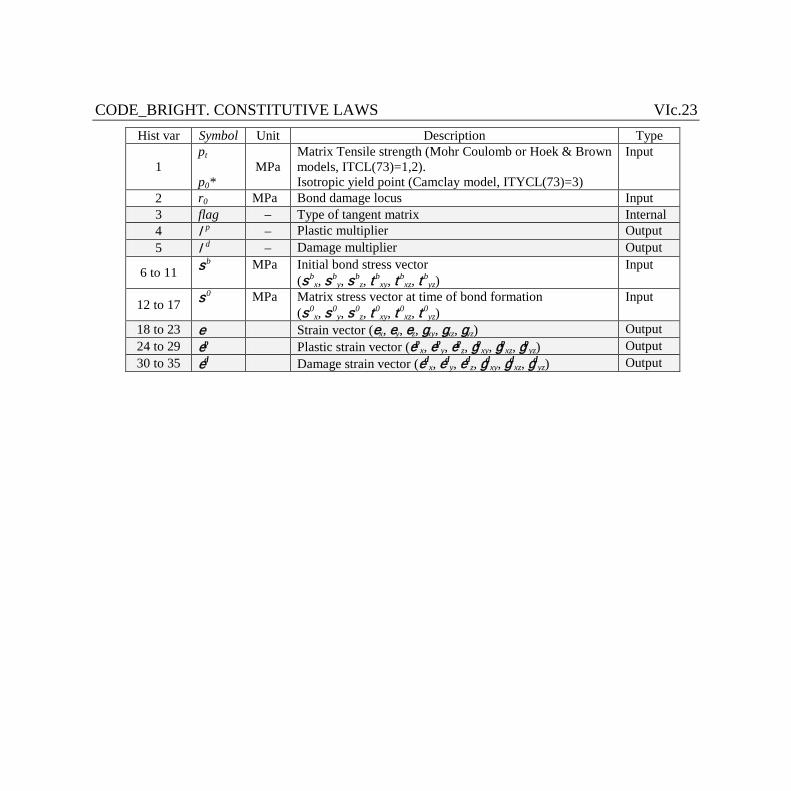
CODE_BRIGHT. CONSTITUTIVE LAWS VIc.23
Hist var Symbol Unit Description Type
1 pt p0*
MPa Matrix Tensile strength (Mohr Coulomb or Hoek & Brown models, ITCL(73)=1,2). Isotropic yield point (Camclay model, ITYCL(73)=3)
Input
2 r0 MPa Bond damage locus Input 3 flag – Type of tangent matrix Internal 4 lp – Plastic multiplier Output 5 ld – Damage multiplier Output
6 to 11 sb MPa Initial bond stress vector (sb
x, sby, sb
z, tbxy, tb
xz, tbyz)
Input
12 to 17 s0 MPa Matrix stress vector at time of bond formation (s0
x, s0y, s0
z, t0xy, t0
xz, t0yz)
Input
18 to 23 e Strain vector (ex, ey, ez, gxy, gxz, gyz) Output 24 to 29 ep Plastic strain vector (ep
x, epy, ep
z, gpxy, gp
xz, gpyz) Output
30 to 35 ed Damage strain vector (edx, ed
y, edz, gd
xy, gdxz, gd
yz) Output
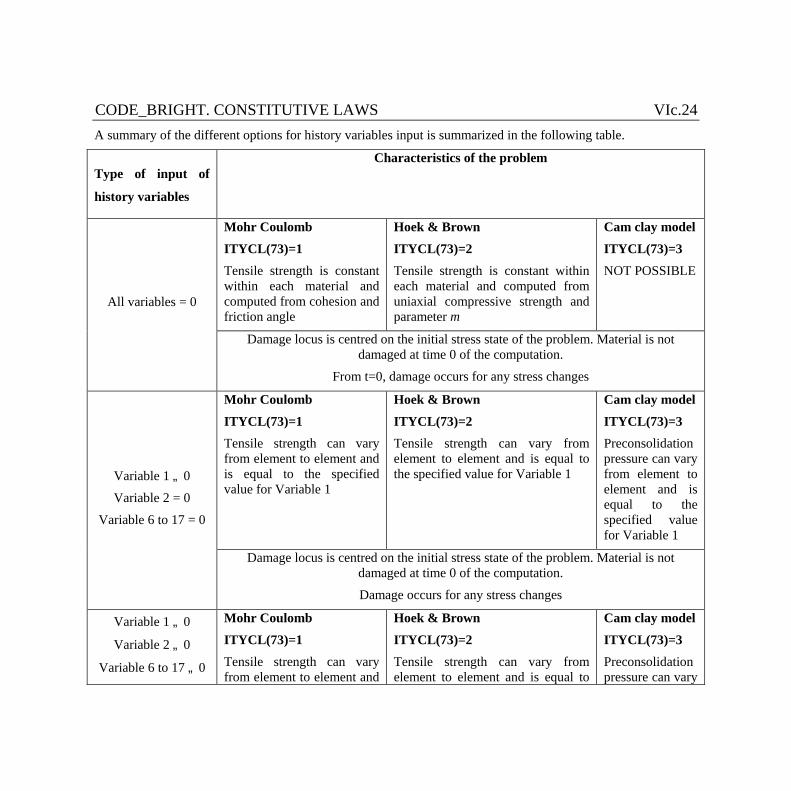
CODE_BRIGHT. CONSTITUTIVE LAWS VIc.24 A summary of the different options for history variables input is summarized in the following table.
Type of input of
history variables
Characteristics of the problem
All variables = 0
Mohr Coulomb ITYCL(73)=1 Tensile strength is constant within each material and computed from cohesion and friction angle
Hoek & Brown ITYCL(73)=2 Tensile strength is constant within each material and computed from uniaxial compressive strength and parameter m
Cam clay model ITYCL(73)=3 NOT POSSIBLE
Damage locus is centred on the initial stress state of the problem. Material is not damaged at time 0 of the computation.
From t=0, damage occurs for any stress changes
Variable 1 ¹ 0
Variable 2 = 0
Variable 6 to 17 = 0
Mohr Coulomb ITYCL(73)=1 Tensile strength can vary from element to element and is equal to the specified value for Variable 1
Hoek & Brown ITYCL(73)=2 Tensile strength can vary from element to element and is equal to the specified value for Variable 1
Cam clay model ITYCL(73)=3 Preconsolidation pressure can vary from element to element and is equal to the specified value for Variable 1
Damage locus is centred on the initial stress state of the problem. Material is not damaged at time 0 of the computation.
Damage occurs for any stress changes
Variable 1 ¹ 0
Variable 2 ¹ 0
Variable 6 to 17 ¹ 0
Mohr Coulomb ITYCL(73)=1 Tensile strength can vary from element to element and
Hoek & Brown ITYCL(73)=2 Tensile strength can vary from element to element and is equal to
Cam clay model ITYCL(73)=3 Preconsolidation pressure can vary
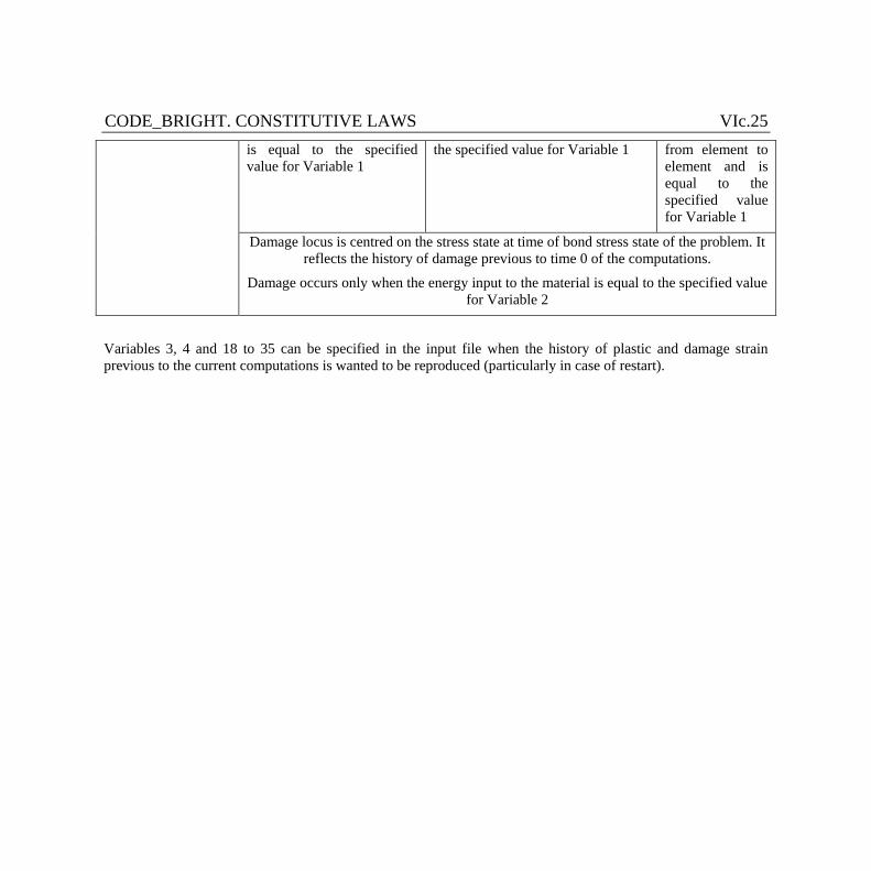
CODE_BRIGHT. CONSTITUTIVE LAWS VIc.25 is equal to the specified value for Variable 1
the specified value for Variable 1 from element to element and is equal to the specified value for Variable 1
Damage locus is centred on the stress state at time of bond stress state of the problem. It reflects the history of damage previous to time 0 of the computations.
Damage occurs only when the energy input to the material is equal to the specified value for Variable 2
Variables 3, 4 and 18 to 35 can be specified in the input file when the history of plastic and damage strain previous to the current computations is wanted to be reproduced (particularly in case of restart).
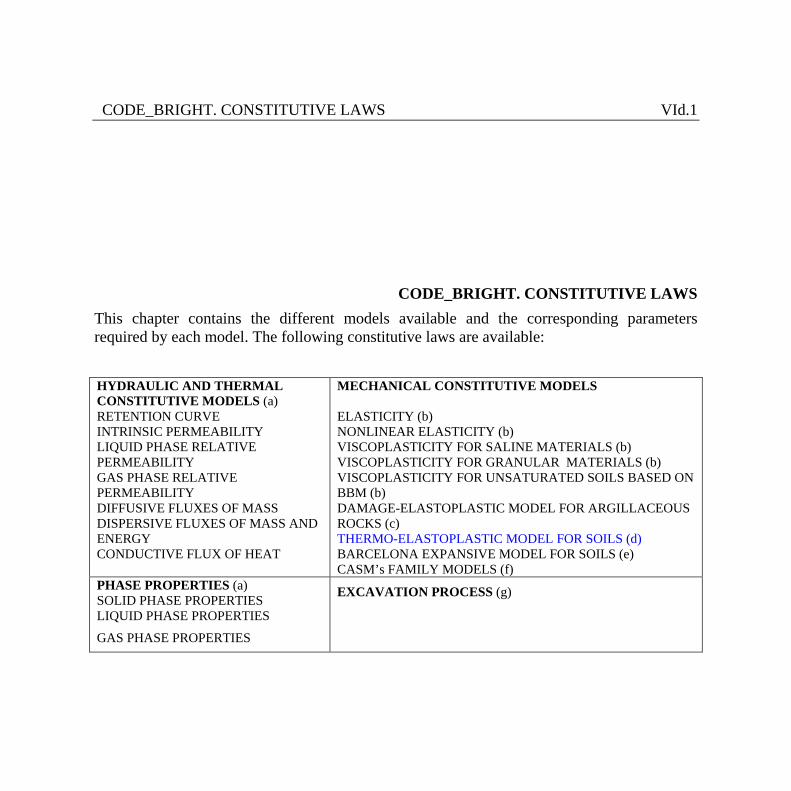
CODE_BRIGHT. CONSTITUTIVE LAWS VId.1
CODE_BRIGHT. CONSTITUTIVE LAWS This chapter contains the different models available and the corresponding parameters required by each model. The following constitutive laws are available: HYDRAULIC AND THERMAL CONSTITUTIVE MODELS (a) RETENTION CURVE INTRINSIC PERMEABILITY LIQUID PHASE RELATIVE PERMEABILITY GAS PHASE RELATIVE PERMEABILITY DIFFUSIVE FLUXES OF MASS DISPERSIVE FLUXES OF MASS AND ENERGY CONDUCTIVE FLUX OF HEAT
MECHANICAL CONSTITUTIVE MODELS ELASTICITY (b) NONLINEAR ELASTICITY (b) VISCOPLASTICITY FOR SALINE MATERIALS (b) VISCOPLASTICITY FOR GRANULAR MATERIALS (b) VISCOPLASTICITY FOR UNSATURATED SOILS BASED ON BBM (b) DAMAGE-ELASTOPLASTIC MODEL FOR ARGILLACEOUS ROCKS (c) THERMO-ELASTOPLASTIC MODEL FOR SOILS (d) BARCELONA EXPANSIVE MODEL FOR SOILS (e) CASM’s FAMILY MODELS (f)
PHASE PROPERTIES (a) SOLID PHASE PROPERTIES LIQUID PHASE PROPERTIES
GAS PHASE PROPERTIES
EXCAVATION PROCESS (g)
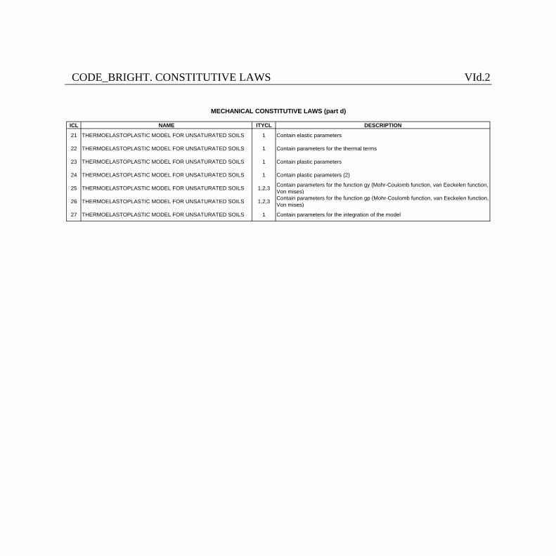
CODE_BRIGHT. CONSTITUTIVE LAWS VId.2
ICL NAME ITYCL DESCRIPTION
21 THERMOELASTOPLASTIC MODEL FOR UNSATURATED SOILS 1 Contain elastic parameters
22 THERMOELASTOPLASTIC MODEL FOR UNSATURATED SOILS 1 Contain parameters for the thermal terms
23 THERMOELASTOPLASTIC MODEL FOR UNSATURATED SOILS 1 Contain plastic parameters
24 THERMOELASTOPLASTIC MODEL FOR UNSATURATED SOILS 1 Contain plastic parameters (2)
25 THERMOELASTOPLASTIC MODEL FOR UNSATURATED SOILS 1,2,3 Contain parameters for the function gy (Mohr-Coulomb function, van Eeckelen function, Von mises)
26 THERMOELASTOPLASTIC MODEL FOR UNSATURATED SOILS 1,2,3 Contain parameters for the function gp (Mohr-Coulomb function, van Eeckelen function, Von mises)
27 THERMOELASTOPLASTIC MODEL FOR UNSATURATED SOILS 1 Contain parameters for the integration of the model
MECHANICAL CONSTITUTIVE LAWS (part d)

CODE_BRIGHT. CONSTITUTIVE LAWS VId.3 THERMO-ELASTOPLASTIC MODEL FOR SOILS
CODES in ROOT_gen.dat
ICL=21 to 27 ITYCL=see below
DESCRIPTION Thermo-elastoplastic model for unsaturated soils
EQUATIONS
For this model, equations are written assuming Soils Mechancis compression (p > 0, ev > 0, compression). The mechanical constitutive equation takes the incremental general form:
d d dss e'= +D h This equation is derived from:
1( ) ''
e p e Gd d d d ds- ¶= + = + a + L
¶De e e s I
s
where an elasto-plastic constitutive law has been selected that is based on a generalized yield surface that depends not only on stresses but on suction as well:
( )', ,pvF F s= s e
Volumetric strain is defined as:
e e e ev x y z= + +
and e vp is the plastic volumetric strain. Using stress invariants this equation depends on:
( )F F p J svp= ' , , , ,q e
where:
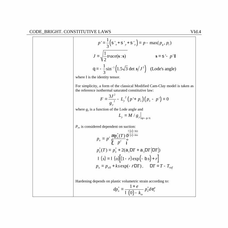
CODE_BRIGHT. CONSTITUTIVE LAWS VId.4
( )
( )1 3
1' ' ' ' max( , )3
1 ( : ) ' '21 sin 1.5 3 det (Lode's angle)3
x y z g lp p p p
J trace p
J-
= s + s + s = -
= = s -
q = -
s s s I
s
where I is the identity tensor. For simplicity, a form of the classical Modified Cam-Clay model is taken as the reference isothermal saturated constitutive law:
( ) ( )2
22
3 ' ' 0y s oy
JF L p p p pg
= - + - =
where gy is a function of the Lode angle and
/ 6/y yL M g
q=-p=
Po, is considered dependent on suction:
( )( )*
* *1 3
( )
( ) 2( )
o kios kio
c oo c
o o
p Tp pp
p T p T T T
l -l -æ ö
= ç ÷è ø
= + a D + a D D
( ) ( ) ( ) ( )[ ]l l bs o r s r= - - +1 exp
)exp(0 Tskpp ss D-+= r , refTTT -=D Hardening depends on plastic volumetric strain according to:
( )* *1
0p
o o vio
edp p dk
+= e
l -
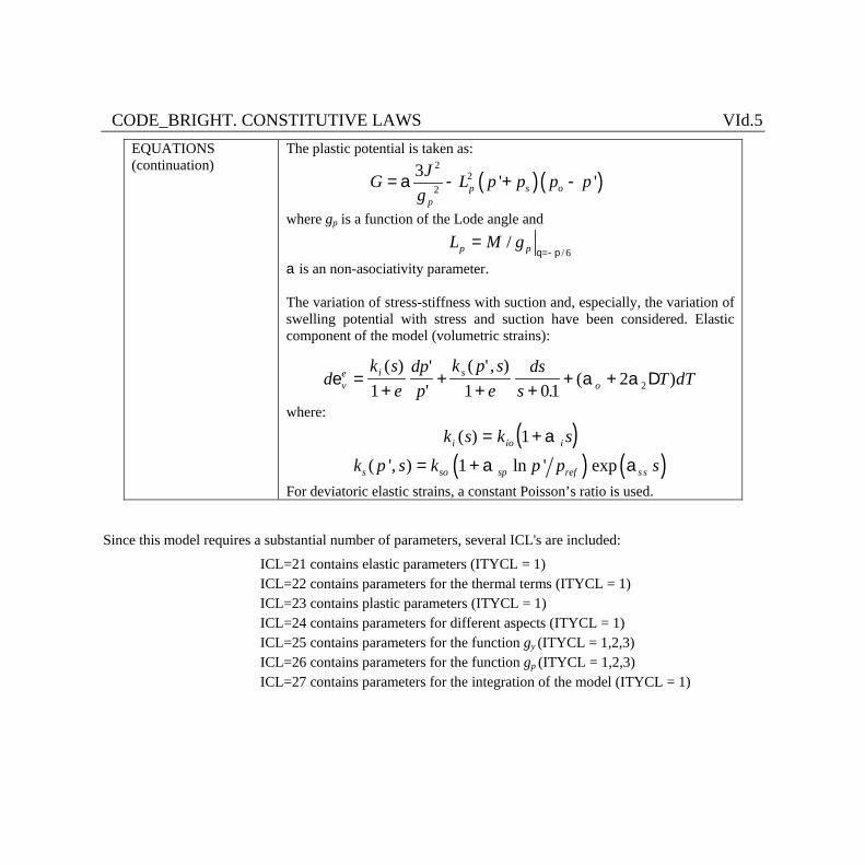
CODE_BRIGHT. CONSTITUTIVE LAWS VId.5 EQUATIONS (continuation)
The plastic potential is taken as:
( )( )2
22
3 ' 'p s op
JG L p p p pg
= a - + -
where gp is a function of the Lode angle and
/ 6/p pL M g
q=-p=
a is an non-asociativity parameter. The variation of stress-stiffness with suction and, especially, the variation of swelling potential with stress and suction have been considered. Elastic component of the model (volumetric strains):
dk s
edpp
k p se
dss
T dTve i s
oe a a=+
++ +
+ +( ) '
'( ' , )
.( )
1 1 012 2 D
where:
( )k s k si io i( ) = +1 a
( ) ( )( ', ) 1 ln ' exps so sp ref s sk p s k p p s= + a a
For deviatoric elastic strains, a constant Poisson’s ratio is used.
Since this model requires a substantial number of parameters, several ICL's are included:
ICL=21 contains elastic parameters (ITYCL = 1) ICL=22 contains parameters for the thermal terms (ITYCL = 1) ICL=23 contains plastic parameters (ITYCL = 1) ICL=24 contains parameters for different aspects (ITYCL = 1) ICL=25 contains parameters for the function gy (ITYCL = 1,2,3) ICL=26 contains parameters for the function gp (ITYCL = 1,2,3) ICL=27 contains parameters for the integration of the model (ITYCL = 1)

CODE_BRIGHT. CONSTITUTIVE LAWS VId.6 PARAMETERS FOR ICL=21 (TEP Elastic Parameters), ITYCL=1
P1 k io - Initial (zero suction) elastic slope for specific volume-mean stress
P2 k so - Initial (zero suction) elastic slope for specific volume-suction
P3 Kmin MPa Minimum bulk module P4 Void P5 n - Poisson’s ratio P6 a ss - Parameter for ks (only for expansive material) P7 Void P8 a i - Parameter for ki (only for expansive material) P9 a sp - Parameter for ks (only for expansive material) P10 pref MPa Reference mean stress (only for expansive material)
PARAMETERS FOR ICL=22 (TEP Thermal Parameters), ITYCL=1
P1 a o oC-1 Parameter for elastic thermal strain
P2 a 1 MPa oC-1 Parameter for plastic thermal strain P3 a 2
oC-2 Parameter for elastic thermal strain P4 a 3 MPaoC-2 Parameter for plastic thermal strain P5 Tref oC Reference temperature
PARAMETERS FOR ICL=23 (TEP Plastic Parameters 1), ITYCL=1
P1 l (0) Slope of void ratio - mean stress curve at zero suction
P2 r Parameter defining the maximum soil stiffness P3 b MPa-1 Parameter controlling the rate of increase of soil
stiffness with suction P4 r oC-1 Parameter that takes into account decrease of
tensile strength due to temperature P5 k Parameter that takes into account increase of
tensile strength due to suction P6 ps0 MPa Tensile strength in saturated conditions
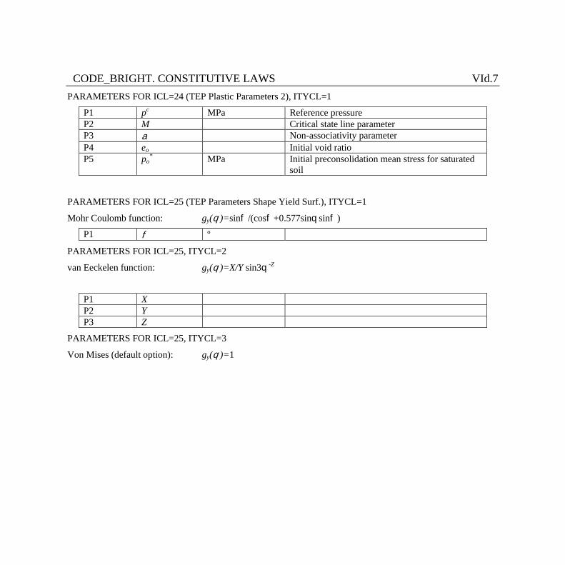
CODE_BRIGHT. CONSTITUTIVE LAWS VId.7 PARAMETERS FOR ICL=24 (TEP Plastic Parameters 2), ITYCL=1
P1 pc MPa Reference pressure P2 M Critical state line parameter P3 a Non-associativity parameter P4 eo Initial void ratio P5 po
* MPa Initial preconsolidation mean stress for saturated soil
PARAMETERS FOR ICL=25 (TEP Parameters Shape Yield Surf.), ITYCL=1
Mohr Coulomb function: gy(q )=sinf /(cosf +0.577sinq sinf )
P1 f º
PARAMETERS FOR ICL=25, ITYCL=2
van Eeckelen function: gy(q )=X/Y sin3q -Z
P1 X P2 Y P3 Z
PARAMETERS FOR ICL=25, ITYCL=3
Von Mises (default option): gy(q )=1
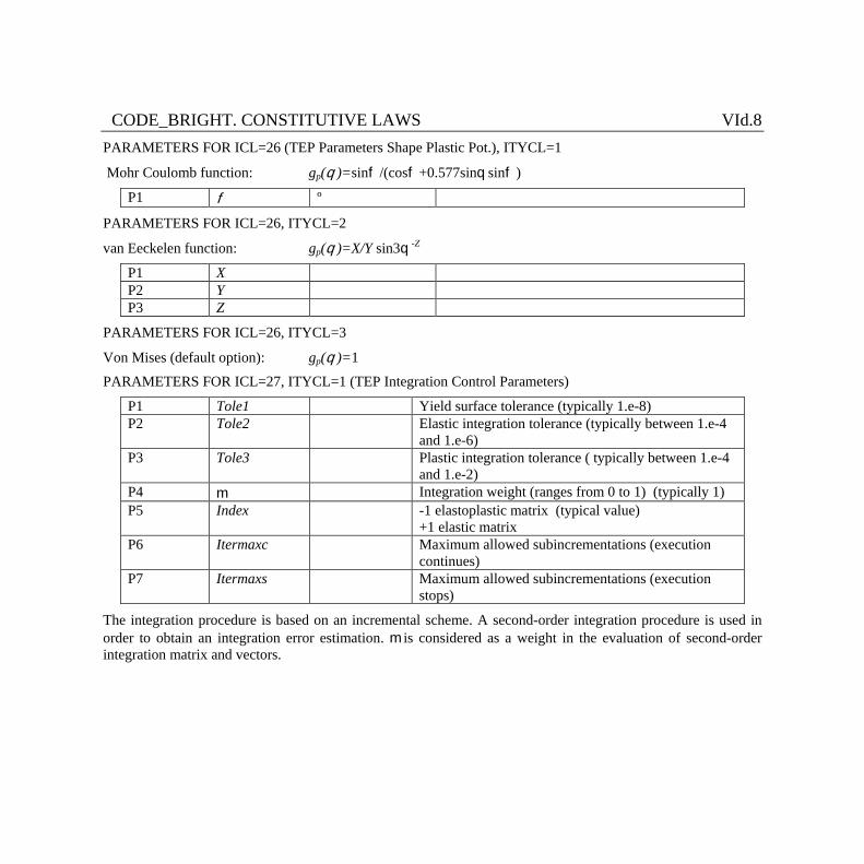
CODE_BRIGHT. CONSTITUTIVE LAWS VId.8 PARAMETERS FOR ICL=26 (TEP Parameters Shape Plastic Pot.), ITYCL=1
Mohr Coulomb function: gp(q )=sinf /(cosf +0.577sinq sinf )
P1 f º
PARAMETERS FOR ICL=26, ITYCL=2
van Eeckelen function: gp(q )=X/Y sin3q -Z
P1 X P2 Y P3 Z
PARAMETERS FOR ICL=26, ITYCL=3
Von Mises (default option): gp(q )=1
PARAMETERS FOR ICL=27, ITYCL=1 (TEP Integration Control Parameters)
P1 Tole1 Yield surface tolerance (typically 1.e-8) P2 Tole2 Elastic integration tolerance (typically between 1.e-4
and 1.e-6) P3 Tole3 Plastic integration tolerance ( typically between 1.e-4
and 1.e-2) P4 m Integration weight (ranges from 0 to 1) (typically 1) P5 Index -1 elastoplastic matrix (typical value)
+1 elastic matrix P6 Itermaxc Maximum allowed subincrementations (execution
continues) P7 Itermaxs Maximum allowed subincrementations (execution
stops)
The integration procedure is based on an incremental scheme. A second-order integration procedure is used in order to obtain an integration error estimation. m is considered as a weight in the evaluation of second-order integration matrix and vectors.

CODE_BRIGHT. CONSTITUTIVE LAWS VId.9 HISTORY VARIABLES:
The Thermo-elastoplastic (ICL=21 to 27) model requires two history variables:
Hist_var 1 Po* MPa Evolution of preconsolidation mean stress for saturated soil Hist_var 2 eo Evolution of void ratio
These variables can be assigned as initial conditions on surfaces/volumes if an initial particular distribution on the geometry is required. The procedure is the same as followed by initial stresses as was described in chapter II. PREPROCESS, PROBLEM DATA, section II.2.3.5. If no value is assigned for these variables in conditions, internally, the program sets the input parameters P4 (for e0) and P5 (for Po*) of the ICL=24, as initial values. The evolution of Po* can be visualized as an output in Post-process GID interface. Note: Effective stresses plotted in the Post-process GID interface correspond with net stresses for unsaturated conditions and Terzaghi's effective stresses for saturated conditions. Stress and strain invariants follow the soil mechanics notation (positive for compression). ______
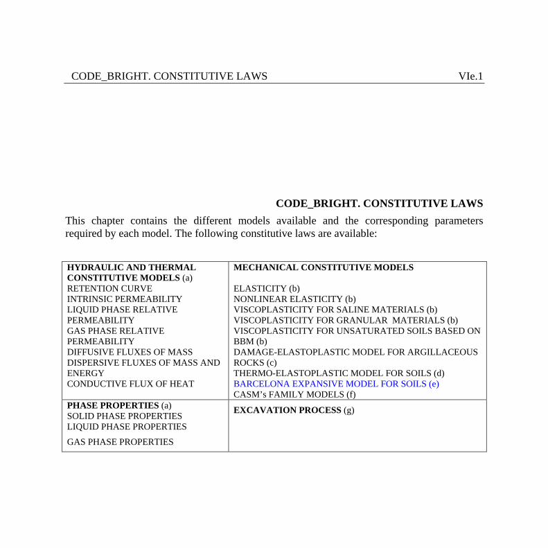
CODE_BRIGHT. CONSTITUTIVE LAWS VIe.1
CODE_BRIGHT. CONSTITUTIVE LAWS This chapter contains the different models available and the corresponding parameters required by each model. The following constitutive laws are available: HYDRAULIC AND THERMAL CONSTITUTIVE MODELS (a) RETENTION CURVE INTRINSIC PERMEABILITY LIQUID PHASE RELATIVE PERMEABILITY GAS PHASE RELATIVE PERMEABILITY DIFFUSIVE FLUXES OF MASS DISPERSIVE FLUXES OF MASS AND ENERGY CONDUCTIVE FLUX OF HEAT
MECHANICAL CONSTITUTIVE MODELS ELASTICITY (b) NONLINEAR ELASTICITY (b) VISCOPLASTICITY FOR SALINE MATERIALS (b) VISCOPLASTICITY FOR GRANULAR MATERIALS (b) VISCOPLASTICITY FOR UNSATURATED SOILS BASED ON BBM (b) DAMAGE-ELASTOPLASTIC MODEL FOR ARGILLACEOUS ROCKS (c) THERMO-ELASTOPLASTIC MODEL FOR SOILS (d) BARCELONA EXPANSIVE MODEL FOR SOILS (e) CASM’s FAMILY MODELS (f)
PHASE PROPERTIES (a) SOLID PHASE PROPERTIES LIQUID PHASE PROPERTIES
GAS PHASE PROPERTIES
EXCAVATION PROCESS (g)
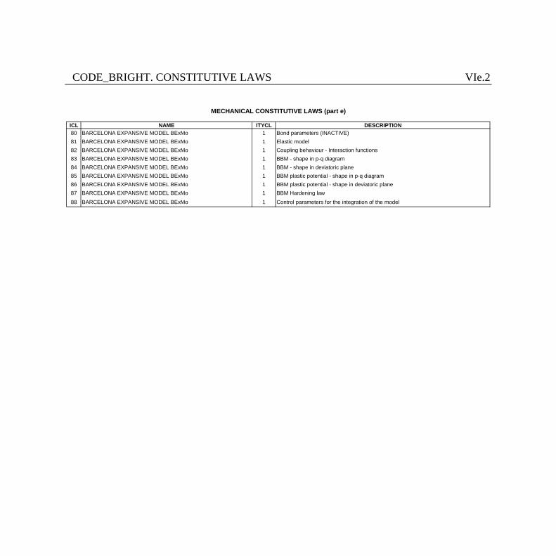
CODE_BRIGHT. CONSTITUTIVE LAWS VIe.2
ICL NAME ITYCL DESCRIPTION80 BARCELONA EXPANSIVE MODEL BExMo 1 Bond parameters (INACTIVE)81 BARCELONA EXPANSIVE MODEL BExMo 1 Elastic model82 BARCELONA EXPANSIVE MODEL BExMo 1 Coupling behaviour - Interaction functions83 BARCELONA EXPANSIVE MODEL BExMo 1 BBM - shape in p-q diagram84 BARCELONA EXPANSIVE MODEL BExMo 1 BBM - shape in deviatoric plane85 BARCELONA EXPANSIVE MODEL BExMo 1 BBM plastic potential - shape in p-q diagram86 BARCELONA EXPANSIVE MODEL BExMo 1 BBM plastic potential - shape in deviatoric plane87 BARCELONA EXPANSIVE MODEL BExMo 1 BBM Hardening law88 BARCELONA EXPANSIVE MODEL BExMo 1 Control parameters for the integration of the model
MECHANICAL CONSTITUTIVE LAWS (part e)
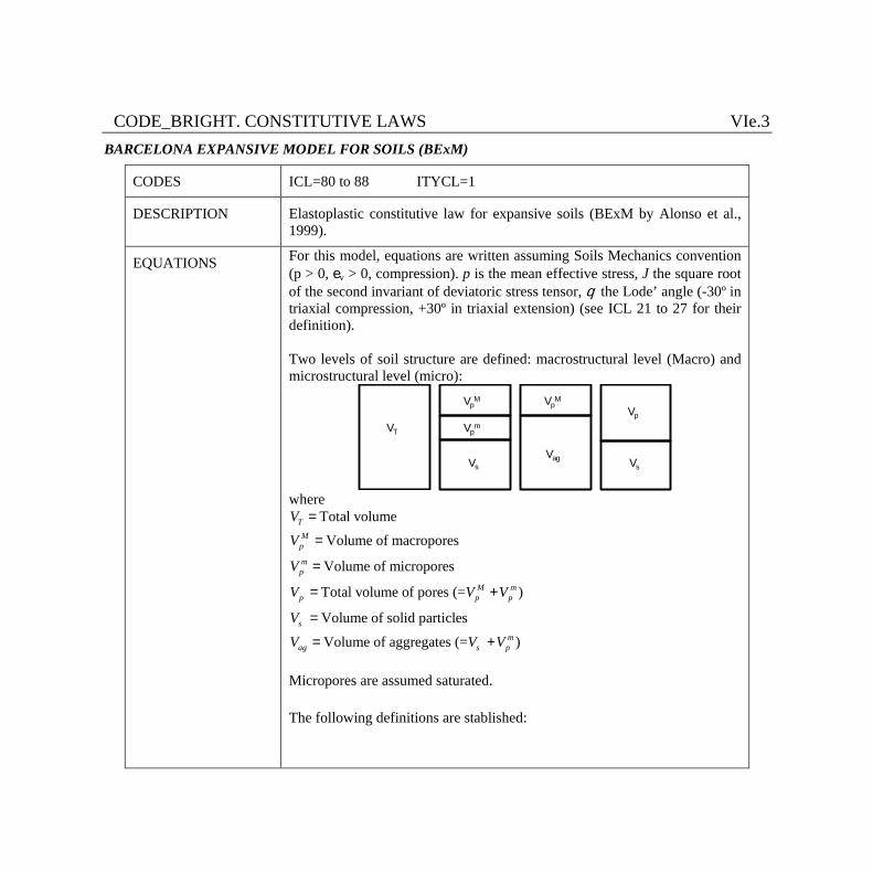
CODE_BRIGHT. CONSTITUTIVE LAWS VIe.3 BARCELONA EXPANSIVE MODEL FOR SOILS (BExM)
CODES ICL=80 to 88 ITYCL=1
DESCRIPTION Elastoplastic constitutive law for expansive soils (BExM by Alonso et al., 1999).
EQUATIONS
For this model, equations are written assuming Soils Mechanics convention (p > 0, ev > 0, compression). p is the mean effective stress, J the square root of the second invariant of deviatoric stress tensor, q the Lode’ angle (-30º in triaxial compression, +30º in triaxial extension) (see ICL 21 to 27 for their definition). Two levels of soil structure are defined: macrostructural level (Macro) and microstructural level (micro):
VT
Vs
Vpm
VpM Vp
M
Vs
Vp
Vag
where
Total volume
Volume of macropores
Volume of micropores
Total volume of pores (= )
Volume of solid particles
Volume of aggregates (= )
TM
p
mp
M mp p p
sm
ag s p
VV
V
V V V
V
V V V
=
=
=
= +
=
= +
Micropores are assumed saturated. The following definitions are stablished:
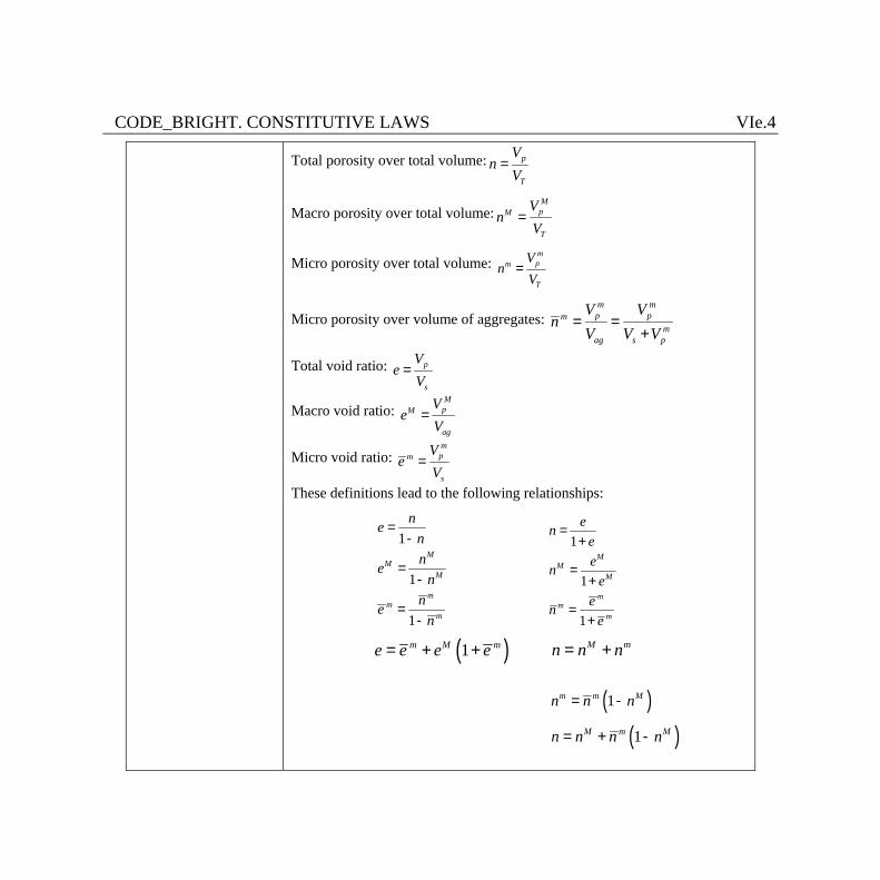
CODE_BRIGHT. CONSTITUTIVE LAWS VIe.4 Total porosity over total volume: p
T
Vn
V=
Macro porosity over total volume:M
pM
T
Vn
V=
Micro porosity over total volume: mpm
T
Vn
V=
Micro porosity over volume of aggregates: m mp pm
mag s p
V Vn
V V V= =
+
Total void ratio: p
s
Ve
V=
Macro void ratio: M
pM
ag
Ve
V=
Micro void ratio: mpm
s
Ve
V=
These definitions lead to the following relationships:
1
1
1
MM
M
mm
m
nenne
nne
n
=-
=-
=-
1
1
1
MM
M
mm
m
eneen
een
e
=+
=+
=+
( )1m M me e e e= + + M mn n n= +
( )1m m Mn n n= -
( )1M m Mn n n n= + -
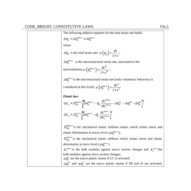
CODE_BRIGHT. CONSTITUTIVE LAWS VIe.5 The following additive equation for the total strain rate holds:
Macro microkl kl kld d d= +e e e
where
klde is the total strain rate: ( ) 1kldetr
e=
+e ;
Macroklde is the macrostructural strain rate, associated to the
macroskeleton: ( ) 1
MMacrokl M
detre
=+
e ;
microklde is the microstructural strain rate (only volumetric behaviour is
considered at this level): ( ) 1
mMicrokl m
detre
=+
e
Elastic law:
3
3
MacroMacro Macro LC SD SI
ij ijkl kl kl kl kl klMacros
micromicro micro
ij ijkl kl kl micros
dsd D d d d dK
dsd D dK
s e d e e e
s e d
æ ö= - - - -ç ÷
è øæ ö
= -ç ÷è ø
MacroijklD is the mechanical elastic stiffness matrix which relates stress and
elastic deformation at macro level ( Macroklde );
microijklD is the mechanical elastic stiffness which relates stress and elastic
deformation at micro level ( microklde ).
MacrosK is the bulk modulus against macro suction changes and micro
sK the bulk modulus against micro suction changes.
LCklde are the macro plastic strains if LC is activated. SDklde and SI
klde are the macro plastic strains if SD and SI are activated,
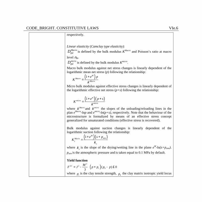
CODE_BRIGHT. CONSTITUTIVE LAWS VIe.6 respectively. Linear elasticity (Camclay type elasticity):
MacroijklD is defined by the bulk modulus KMacro and Poisson’s ratio at macro
level nM. microijklD is defined by the bulk modulus Kmicro.
Macro bulk modulus against net stress changes is linearly dependent of the logarithmic mean net stress (p) following the relationship:
( )1 MMacro
Macro
e pK
+=
k
Micro bulk modulus against effective stress changes is linearly dependent of the logarithmic effective net stress (p+s) following the relationship:
( )( )1 mmicro
micro
e p sK
+ +=
k
where Macrok and microk the slopes of the unloading/reloading lines in the plan eMacro-lnp and emicro-ln(p+s), respectively. Note that the behaviour of the microstructure is formalized by means of an effective stress concept generalized for unsaturated conditions (effective stress is recovered). Bulk modulus against suction changes is linearly dependent of the logarithmic suction following the relationship:
( )( )1 MatmMacro
ss
e s pK
+ +=
k
where sk is the slope of the drying/wetting line in the plane eM-ln(s+patm). patm is the atmospheric pressure and is taken equal to 0.1 MPa by default. Yield function
( )2
20( ) 0
3LC
tMF J p p p p= - + - £
where tp is the clay tensile strength,
0p the clay matrix isotropic yield locus
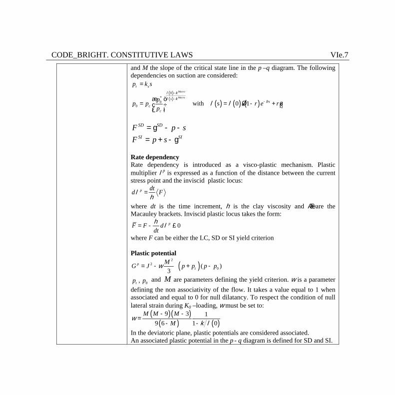
CODE_BRIGHT. CONSTITUTIVE LAWS VIe.7 and M the slope of the critical state line in the p –q diagram. The following dependencies on suction are considered:
t sp k s= ( )( )
( ) ( ) ( )0
*0
0 with s 0 1
Macro
Macross
cc
pp p r e rp
-
--æ ö
é ù= = - +ç ÷ ë ûè ø
l kl k
bl l
SD SDF p s= g - - SI SIF p s= + - g
Rate dependency Rate dependency is introduced as a visco-plastic mechanism. Plastic multiplier lp is expressed as a function of the distance between the current stress point and the inviscid plastic locus:
p dtd Flh
=
where dt is the time increment, h is the clay viscosity and áñ are the Macauley brackets. Inviscid plastic locus takes the form:
0pF F ddth l= - £
where F can be either the LC, SD or SI yield criterion Plastic potential
( )2
20( )
3p
tMG J p p p pw= - + -
0,tp p and M are parameters defining the yield criterion. w is a parameter defining the non associativity of the flow. It takes a value equal to 1 when associated and equal to 0 for null dilatancy. To respect the condition of null lateral strain during K0 –loading, w must be set to:
( )( )( ) ( )
9 3 19 6 1 0
M M MM
wk l
- -=
- -
In the deviatoric plane, plastic potentials are considered associated. An associated plastic potential in the p - q diagram is defined for SD and SI.
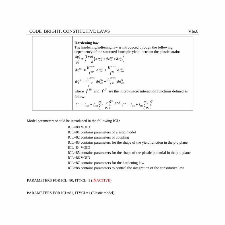
CODE_BRIGHT. CONSTITUTIVE LAWS VIe.8 Hardening law: The hardening/softening law is introduced through the following dependency of the saturated isotropic yield locus on the plastic strain:
( )*0
*0
(1 ) LC SD SIvol vol vol
dp e d d dp
+= + +
-e e e
l k
micro microSD SD SI
vol volSD SI
K Kd d df f
g = e + e
micro microSI SD SI
vol volSD SI
K Kd d df f
g = e + e
where SDf and SIf are the micro-macro interaction functions defined as follow:
0 10
1SDn
SDSD SD
pf f fp
æ ö= + -ç ÷
è ø and
0 10
SInSI
SI SIpf f fp
æ ö= + ç ÷
è ø
Model parameters should be introduced in the following ICL:
ICL=80 VOID ICL=81 contains parameters of elastic model ICL=82 contains parameters of coupling ICL=83 contains parameters for the shape of the yield function in the p-q plane ICL=84 VOID ICL=85 contains parameters for the shape of the plastic potential in the p-q plane ICL=86 VOID ICL=87 contains parameters for the hardening law ICL=88 contains parameters to control the integration of the constitutive law
PARAMETERS FOR ICL=80, ITYCL=1 (INACTIVE)
PARAMETERS FOR ICL=81, ITYCL=1 (Elastic model)
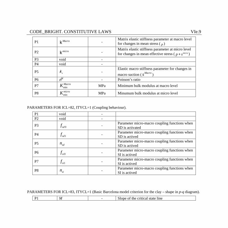
CODE_BRIGHT. CONSTITUTIVE LAWS VIe.9
P1 Macrok - Matrix elastic stiffness parameter at macro level for changes in mean stress ( p )
P2 microk - Matrix elastic stiffness parameter at micro level for changes in mean effective stress ( microp s+ )
P3 void - P4 void -
P5 sk - Elastic macro stiffness parameter for changes in macro suction ( Macros )
P6 nM - Poisson’s ratio P7 min
MacroK MPa Minimum bulk modulus at macro level
P8 minmicroK MPa Minumum bulk modulus at micro level
PARAMETERS FOR ICL=82, ITYCL=1 (Coupling behaviour).
P1 void - P2 void -
P3 0sdf - Parameter micro-macro coupling functions when SD is activated
P4 1sdf - Parameter micro-macro coupling functions when SD is actived
P5 sdn - Parameter micro-macro coupling functions when SD is actived
P6 0sif - Parameter micro-macro coupling functions when SI is actived
P7 1sif - Parameter micro-macro coupling functions when SI is actived
P8 sin - Parameter micro-macro coupling functions when SI is actived
PARAMETERS FOR ICL=83, ITYCL=1 (Basic Barcelona model criterion for the clay – shape in p-q diagram).
P1 M - Slope of the critical state line
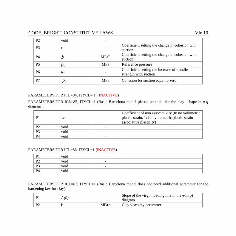
CODE_BRIGHT. CONSTITUTIVE LAWS VIe.10 P2 void - -
P3 r - Coefficient setting the change in cohesion with
suction
P4 b MPa-1 Coefficient setting the change in cohesion with suction
P5 pc MPa Reference pressure
P6 ks - Coefficient setting the increase of tensile strength with suction
P7 0tp MPa Cohesion for suction equal to zero
PARAMETERS FOR ICL=84, ITYCL= 1 (INACTIVE)
PARAMETERS FOR ICL=85, ITYCL=1 (Basic Barcelona model plastic potential for the clay– shape in p-q diagram).
P1 w - Coefficient of non associativity (0: no volumetric plastic strain, 1: full volumetric plastic strain –associative plasticity)
P2 void - P3 void - P4 void -
PARAMETERS FOR ICL=86, ITYCL=1 (INACTIVE)
P1 void - P2 void - P3 void - P4 void -
PARAMETERS FOR ICL=87, ITYCL=1 (Basic Barcelona model does not need additional parameter for the hardening law for clay).
P1 l (0) - Slope of the virgin loading line in the e-ln(p)
diagram P2 h MPa.s Clay viscosity parameter
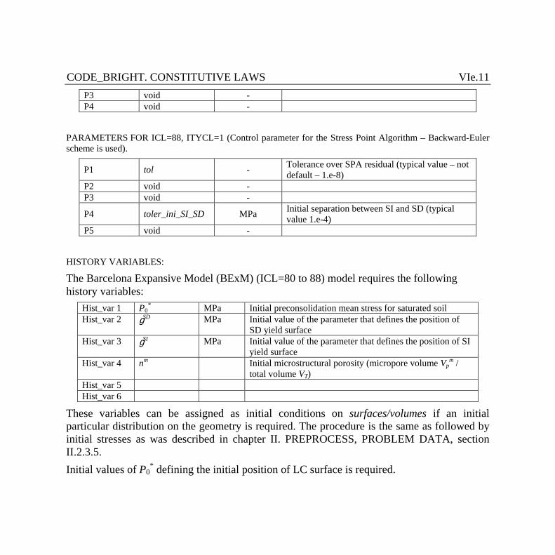
CODE_BRIGHT. CONSTITUTIVE LAWS VIe.11 P3 void - P4 void -
PARAMETERS FOR ICL=88, ITYCL=1 (Control parameter for the Stress Point Algorithm – Backward-Euler scheme is used).
P1 tol - Tolerance over SPA residual (typical value – not default – 1.e-8)
P2 void - P3 void -
P4 toler_ini_SI_SD MPa Initial separation between SI and SD (typical value 1.e-4)
P5 void -
HISTORY VARIABLES:
The Barcelona Expansive Model (BExM) (ICL=80 to 88) model requires the following history variables:
Hist_var 1 P0* MPa Initial preconsolidation mean stress for saturated soil
Hist_var 2 gSD MPa Initial value of the parameter that defines the position of SD yield surface
Hist_var 3 gSI MPa Initial value of the parameter that defines the position of SI yield surface
Hist_var 4 nm Initial microstructural porosity (micropore volume Vpm /
total volume VT) Hist_var 5 Hist_var 6
These variables can be assigned as initial conditions on surfaces/volumes if an initial particular distribution on the geometry is required. The procedure is the same as followed by initial stresses as was described in chapter II. PREPROCESS, PROBLEM DATA, section II.2.3.5. Initial values of P0
* defining the initial position of LC surface is required.
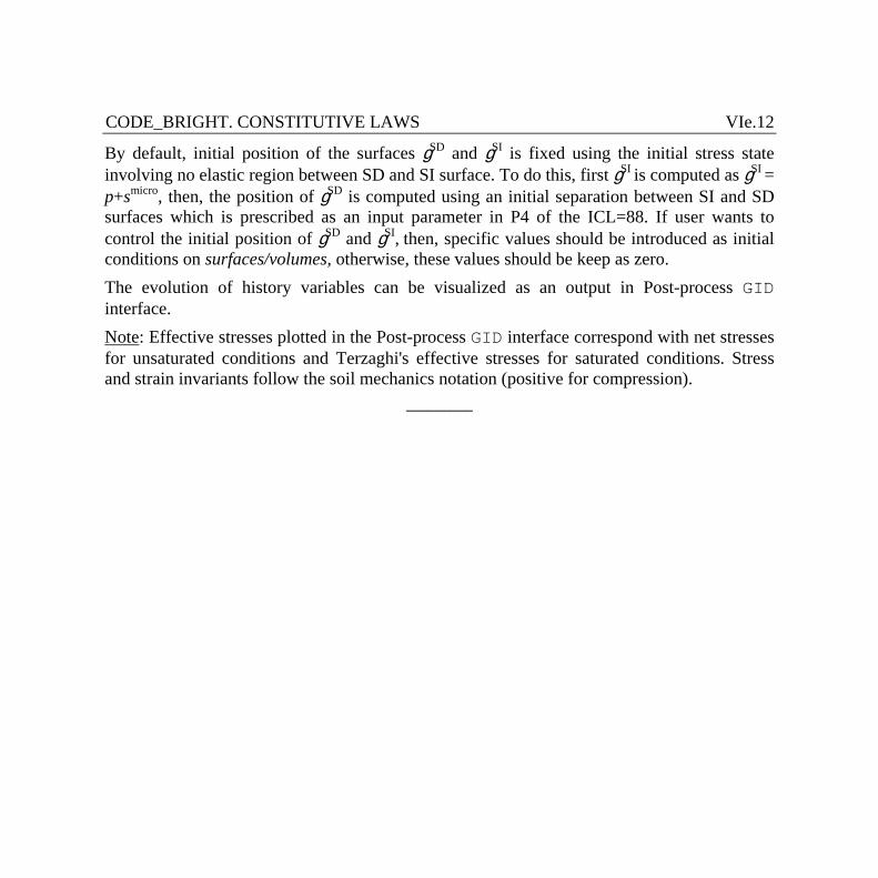
CODE_BRIGHT. CONSTITUTIVE LAWS VIe.12
By default, initial position of the surfaces gSD and gSI is fixed using the initial stress state involving no elastic region between SD and SI surface. To do this, first gSI is computed as gSI = p+smicro, then, the position of gSD is computed using an initial separation between SI and SD surfaces which is prescribed as an input parameter in P4 of the ICL=88. If user wants to control the initial position of gSD and gSI, then, specific values should be introduced as initial conditions on surfaces/volumes, otherwise, these values should be keep as zero. The evolution of history variables can be visualized as an output in Post-process GID interface. Note: Effective stresses plotted in the Post-process GID interface correspond with net stresses for unsaturated conditions and Terzaghi's effective stresses for saturated conditions. Stress and strain invariants follow the soil mechanics notation (positive for compression).
_________

CODE_BRIGHT. CONSTITUTIVE LAWS VIf.1
CODE_BRIGHT. CONSTITUTIVE LAWS This chapter contains the different models available and the corresponding parameters required by each model. The following constitutive laws are available: HYDRAULIC AND THERMAL CONSTITUTIVE MODELS (a) RETENTION CURVE INTRINSIC PERMEABILITY LIQUID PHASE RELATIVE PERMEABILITY GAS PHASE RELATIVE PERMEABILITY DIFFUSIVE FLUXES OF MASS DISPERSIVE FLUXES OF MASS AND ENERGY CONDUCTIVE FLUX OF HEAT
MECHANICAL CONSTITUTIVE MODELS ELASTICITY (b) NONLINEAR ELASTICITY (b) VISCOPLASTICITY FOR SALINE MATERIALS (b) VISCOPLASTICITY FOR GRANULAR MATERIALS (b) VISCOPLASTICITY FOR UNSATURATED SOILS BASED ON BBM (b) DAMAGE-ELASTOPLASTIC MODEL FOR ARGILLACEOUS ROCKS (c) THERMO-ELASTOPLASTIC MODEL FOR SOILS (d) BARCELONA EXPANSIVE MODEL FOR SOILS (e) CASM’s FAMILY MODELS (f)
PHASE PROPERTIES (a) SOLID PHASE PROPERTIES LIQUID PHASE PROPERTIES
GAS PHASE PROPERTIES
EXCAVATION PROCESS (g)
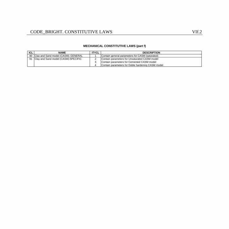
CODE_BRIGHT. CONSTITUTIVE LAWS VIf.2
ICL NAME ITYCL DESCRIPTION90 Clay and Sand model (CASM): GENERAL 1 Contain general parameters for CASM (saturated)91 Clay and Sand model (CASM):SPECIFIC 2 Contain parameters for Unsaturated CASM model
3 Contain parameters for Cemented CASM model4 Contain parameters for Doble hardening CASM model
MECHANICAL CONSTITUTIVE LAWS (part f)
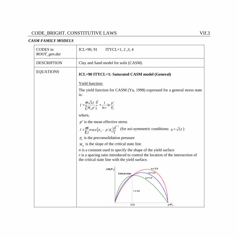
CODE_BRIGHT. CONSTITUTIVE LAWS VIf.3 CASM FAMILY MODELS
CODES in ROOT_gen.dat
ICL=90, 91 ITYCL=1, 2 ,3, 4
DESCRIPTION Clay and Sand model for soils (CASM)
EQUATIONS ICL=90 ITYCL=1: Saturated CASM model (General) Yield function: The yield function for CASM (Yu, 1998) expressed for a general stress state is:
nJ pf
M p r Pq
æ ö= +ç ÷
è ø'
0
3 1 'ln
' ln
where, p’ is the mean effective stress
( )ij ijJ trace ps dæ ö= -ç ÷è ø
1/21'
2 (for axi-symmetric conditions: 3q J= )
P '0 is the preconsolidation pressure
Mq is the slope of the critical state line n is a constant used to specify the shape of the yield surface r is a spacing ratio introduced to control the location of the intersection of the critical state line with the yield surface.
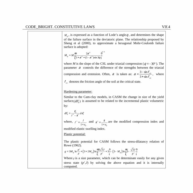
CODE_BRIGHT. CONSTITUTIVE LAWS VIf.4
Mq , is expressed as a function of Lode’s angleq , and determines the shape of the failure surface in the deviatoric plane. The relationship proposed by Sheng et al (2000), to approximate a hexagonal Mohr-Coulomb failure surface is adopted:
M Mqa
a a qæ ö
= ç ÷+ + -è ø
1/44
4 4
21 (1 )sin 3
where M is the slope of the CSL under triaxial compression (q = -30º ). The parameter a controls the difference of the strengths between the triaxial
compression and extension. Often, a is taken as: cs
cs
fa
f-
=+
3 sin3 sin
, where
csf denotes the friction angle of the soil at the critical state.
Hardening parameter:
Similar to the Cam-clay models, in CASM the change in size of the yield surface dP '
0( ) is assumed to be related to the incremental plastic volumetric by:
PdP de
l k=
-
'' p0
0 v* *
where, e
ll =+
*
01 and
ekk =+
*
01are the modified compression index and
modified elastic swelling index.
Plastic potential: The plastic potential for CASM follows the stress-dilatancy relation of Rowe (1962).
( ) ( )p J Jg M M Mp pq q qz
æ ö æ ö= + + + - - -ç ÷ ç ÷
è ø è ø
' 2 3 33 ln 3 2 ln 3 3 ln 3
' '
Wherez is a size parameter, which can be determinate easily for any given stress state (p’,J) by solving the above equation and it is internally computed.
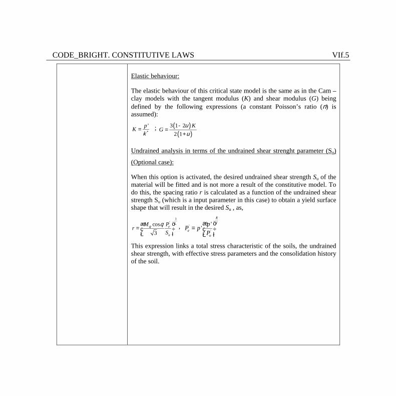
CODE_BRIGHT. CONSTITUTIVE LAWS VIf.5
Elastic behaviour:
The elastic behaviour of this critical state model is the same as in the Cam –clay models with the tangent modulus (K) and shear modulus (G) being defined by the following expressions (a constant Poisson’s ratio (n) is assumed):
pKk
= *
' ; ( )( )
3 1 22 1
KG
uu
-=
+
Undrained analysis in terms of the undrained shear strenght parameter (Su)
(Optional case):
When this option is activated, the desired undrained shear strength Su of the material will be fitted and is not more a result of the constitutive model. To do this, the spacing ratio r is calculated as a function of the undrained shear strength Su (which is a input parameter in this case) to obtain a yield surface shape that will result in the desired Su , as,
e
u
M Pr
Sq q Læ ö
= ç ÷è ø
1'cos
3,
eo
pP pP
klæ ö
= ç ÷è ø
''
''
This expression links a total stress characteristic of the soils, the undrained shear strength, with effective stress parameters and the consolidation history of the soil.
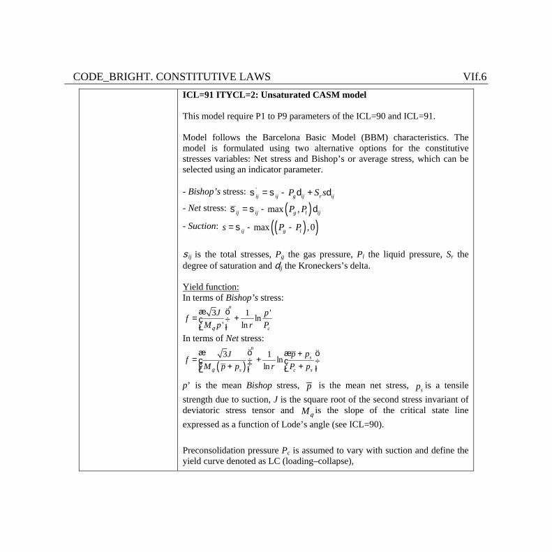
CODE_BRIGHT. CONSTITUTIVE LAWS VIf.6 ICL=91 ITYCL=2: Unsaturated CASM model This model require P1 to P9 parameters of the ICL=90 and ICL=91. Model follows the Barcelona Basic Model (BBM) characteristics. The model is formulated using two alternative options for the constitutive stresses variables: Net stress and Bishop’s or average stress, which can be selected using an indicator parameter. - Bishop’s stress: '
ij ij g ij r ijP S ss = s - d + d - Net stress: ( )max ,ij ij g l ijP Ps = s - d - Suction: ( )( )max ,0ij g ls P P= s - -
sij is the total stresses, Pg the gas pressure, Pl the liquid pressure, Sr the degree of saturation and dij the Kroneckers’s delta. Yield function: In terms of Bishop’s stress:
3 1 'ln
' ln
n
c
J pfM p r Pq
æ ö= +ç ÷
è ø
In terms of Net stress:
( )3 1
lnln
n
s
s c s
p pJfM p p r P pq
æ ö æ ö+= +ç ÷ ç ÷ç ÷+ +è øè ø
p’ is the mean Bishop stress, p is the mean net stress, sp is a tensile strength due to suction, J is the square root of the second stress invariant of deviatoric stress tensor and Mq is the slope of the critical state line expressed as a function of Lode’s angle (see ICL=90).
Preconsolidation pressure Pc is assumed to vary with suction and define the yield curve denoted as LC (loading–collapse),
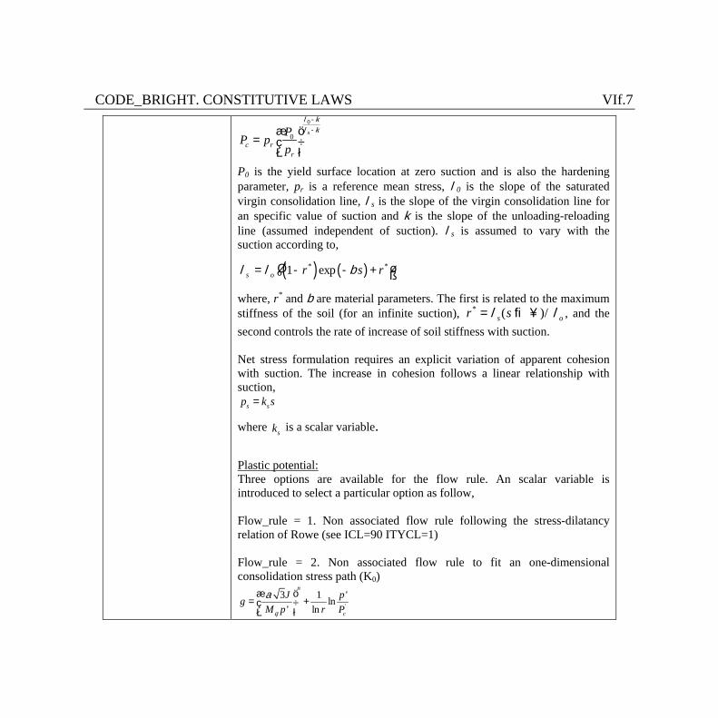
CODE_BRIGHT. CONSTITUTIVE LAWS VIf.7
s
c rr
PP pp
l kl k
--æ ö
= ç ÷è ø
0
0
P0 is the yield surface location at zero suction and is also the hardening parameter, pr is a reference mean stress, l0 is the slope of the saturated virgin consolidation line, ls is the slope of the virgin consolidation line for an specific value of suction and k is the slope of the unloading-reloading line (assumed independent of suction). ls is assumed to vary with the suction according to,
( ) ( )* *1 exps o r s rl l bé ù= - - +ë û
where, r* and b are material parameters. The first is related to the maximum stiffness of the soil (for an infinite suction), * ( )/s or sl l= ® ¥ , and the second controls the rate of increase of soil stiffness with suction. Net stress formulation requires an explicit variation of apparent cohesion with suction. The increase in cohesion follows a linear relationship with suction,
s sp k s= where sk is a scalar variable.
Plastic potential: Three options are available for the flow rule. An scalar variable is introduced to select a particular option as follow, Flow_rule = 1. Non associated flow rule following the stress-dilatancy relation of Rowe (see ICL=90 ITYCL=1) Flow_rule = 2. Non associated flow rule to fit an one-dimensional consolidation stress path (K0)
'
3 1 'ln
' ln
n
c
J pgM p r Pq
aæ ö= +ç ÷
è ø
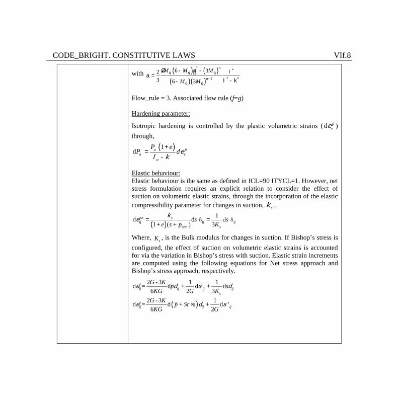
CODE_BRIGHT. CONSTITUTIVE LAWS VIf.8
with ( ) ( )( )( )
*
1 * *
6 323 6 3
n n
n
M M M
M Mq q q
-q q
é ù- - lë ûa =l - k-
Flow_rule = 3. Associated flow rule (f=g) Hardening parameter:
Isotropic hardening is controlled by the plastic volumetric strains ( pved )
through,
( ) poo v
o
P eP de
l k+
=-1
d
Elastic behaviour: Elastic behaviour is the same as defined in ICL=90 ITYCL=1. However, net stress formulation requires an explicit relation to consider the effect of suction on volumetric elastic strains, through the incorporation of the elastic compressibility parameter for changes in suction, sk ,
( )e,sij
1d d δ d δ
1 ( ) 3s
ij ijatm s
s se s p K
ke = =
+ +
Where, sK , is the Bulk modulus for changes in suction. If Bishop’s stress is configured, the effect of suction on volumetric elastic strains is accounted for via the variation in Bishop’s stress with suction. Elastic strain increments are computed using the following equations for Net stress approach and Bishop’s stress approach, respectively.
2 - 3 1 1d = d d d
6 2 3eij ij ij ij
s
G K p sKG G K
e d s d+ +
( )2 - 3 1d = d d '
6 2eij ij ij
G K p Sr sKG G
e d s+ × +
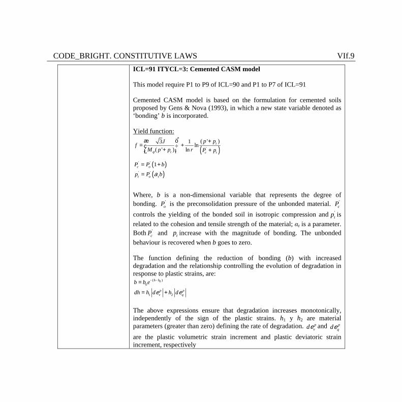
CODE_BRIGHT. CONSTITUTIVE LAWS VIf.9 ICL=91 ITYCL=3: Cemented CASM model This model require P1 to P9 of ICL=90 and P1 to P7 of ICL=91 Cemented CASM model is based on the formulation for cemented soils proposed by Gens & Nova (1993), in which a new state variable denoted as ‘bonding’ b is incorporated. Yield function:
( )'
( ' )3 1ln
( ' ) ln
n
t
t c t
p pJfM p p r P pq
æ ö += +ç ÷
+ +è ø
( )( )
c o
t o t
P P b
p P ba
= +
=
' '
' '
1
Where, b is a non-dimensional variable that represents the degree of bonding. oP ' is the preconsolidation pressure of the unbonded material. cP ' controls the yielding of the bonded soil in isotropic compression and tp ' is related to the cohesion and tensile strength of the material; αt is a parameter. Both cP ' and tp increase with the magnitude of bonding. The unbonded behaviour is recovered when b goes to zero. The function defining the reduction of bonding (b) with increased degradation and the relationship controlling the evolution of degradation in response to plastic strains, are:
0( )0
1 2
h h
p pv q
b b e
dh h d h de e
- -=
= +
The above expressions ensure that degradation increases monotonically, independently of the sign of the plastic strains. h1 y h2 are material parameters (greater than zero) defining the rate of degradation. p
vde and pqde
are the plastic volumetric strain increment and plastic deviatoric strain increment, respectively
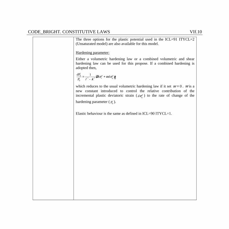
CODE_BRIGHT. CONSTITUTIVE LAWS VIf.10 The three options for the plastic potential used in the ICL=91 ITYCL=2 (Unsaturated model) are also available for this model. Hardening parameter: Either a volumetric hardening law or a combined volumetric and shear hardening law can be used for this propose. If a combined hardening is adopted then,
'0' * *
0
1 p pv q
dPd d
Pe w e
l ké ù= +ë û-
which reduces to the usual volumetric hardening law if it set w = 0 . w is a new constant introduced to control the relative contribution of the incremental plastic deviatoric strain ( p
qde ) to the rate of change of the hardening parameter ( P '
0 ).
Elastic behaviour is the same as defined in ICL=90 ITYCL=1.

CODE_BRIGHT. CONSTITUTIVE LAWS VIf.11 ICL=91 ITYCL=4: Double hardening soil model (DHSM) This model require P1 to P9 of ICL=90 and P1 to P8 of ICL=91 The model involves two plastic mechanisms: a plastic volumetric-driven mechanism with isotropic hardening, by means of the use of the CASM yield surface (ICL=90), and a plastic shear-driven mechanism that gives rise to a nonlinear stress-strain relationship of a hyperbolic type, by the use of a shear yield surface based on the Hardening Soil Model (HSM) (Schanz et al., 1999). Yield functions: - Volumetric yield surface: CASM surface (see ICL=1, ITYCL=1) - Shear yield surface:
s p
ur
a
J JfE EJ
J
g= - -æ ö
-ç ÷è ø
50
1 2
1
with: ( )' ' cot ' ( ) sin ' and ( ) sin sin 'cos
3
fa
f f
J p c gJ g
R Rf q fq q fq
+= = =
+
aJ is the asymptotic value of the shear strength, Rf stands for the relation between the ultimate deviatoric stress, fJ , and the asymptotic stress, a
standard setting is Rf = 0.9. pg is the hardening parameter of the shear yield
surface and corresponds to the plastic deviatoric strain ( pde ), as is described
in the next section.
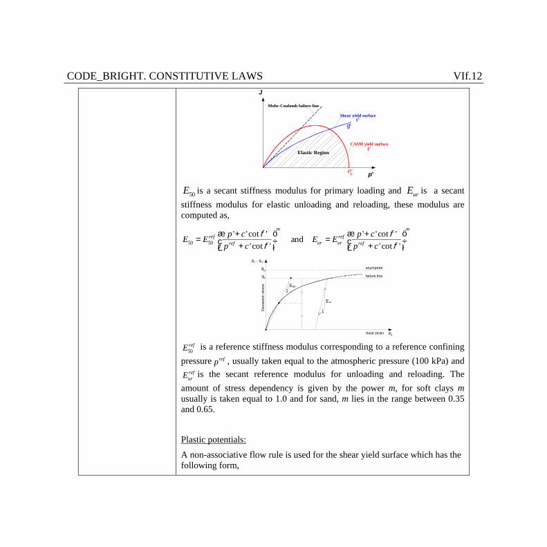
CODE_BRIGHT. CONSTITUTIVE LAWS VIf.12
p'
J
P'o
Elastic Region
CASM yield surface
Shear yield surface
Mohr-Coulomb failure line
f s
f c
gp
50E is a secant stiffness modulus for primary loading and urE is a secant stiffness modulus for elastic unloading and reloading, these modulus are computed as,
50 50' ' cot ' ' ' cot '
and ' cot ' ' cot '
m mref ref
ur urref refp c p cE E E E
p c p cf ff f
æ ö æ ö+ += =ç ÷ ç ÷+ +è ø è ø
Axial strain e
Dev
iato
ric s
tress
s - s
1
Eur
150E
1
1 3
qa
fq
asymptote
failure line
refE50
is a reference stiffness modulus corresponding to a reference confining pressure refp , usually taken equal to the atmospheric pressure (100 kPa) and
refurE is the secant reference modulus for unloading and reloading. The
amount of stress dependency is given by the power m, for soft clays m usually is taken equal to 1.0 and for sand, m lies in the range between 0.35 and 0.65.
Plastic potentials:
A non-associative flow rule is used for the shear yield surface which has the following form,
CODE_BRIGHT. CONSTITUTIVE LAWS VIf.13
( )p pv md g de y g=
where, ( )mg y , is a function of mobilized dilatancy angle, my , and Lode’s angle, q , as,
mm
mg
yy q y
q=
+
sin( ) sin sin
cos3
The mobilized dilatancy angle, my , is defined as,
m csm
m cs
f fy
f f-
=-
sin sinsin
1 sin sin
csf is the friction angle at the critical state and mf is the mobilized friction angle. Material contracts for small stress ratios m csf f< , while dilatancy occurs for high stress ratios m csf f> . Considering dense materials contraction is excluded by taking 0my = for a mobilized friction angle m csf f< .
The volumetric surface uses a non-associated flow rule, the plastic potential is defined in the ICL=90 ITYCL=1.
Hardening parameters:
The hardening parameter of the shear surface, pg , is the plastic deviatoric strain p p
dg e= . The plastic deviatoric strain rate is calculated as,
22pdd dJ ee =
( ) ( ) ( ){ }1/22 22 2 2 22
3p p p p p p p
d x y x z y z xy xz yzd d d d d d d d d de e e e e e e g g gé ù é ù= - + - + - + + +ë ûê úë û
where, J e2
is the second strain invariant of deviatoric strain tensor, pg is the integral of plastic deviatoric strain rates.
The hardening parameter of the volumetric yield surface is the so-called
CODE_BRIGHT. CONSTITUTIVE LAWS VIf.14
preconsolidation pressure ( P '0 ) defined in the ICL=90, ITYCL=1.
The two surfaces can be activated simultaneously and move together as in a multi-surface plasticity problem, if the stress path reaches the intersection between both surfaces.
Elastic behaviour of the DHSM is the same as in basic CASM model defined in the ICL=90, ITYCL=1.
Enhanced model (E –DHSM): For stiff materials an enhanced model (E-DHSM) can be used, which allows the evolution of the shear yield surface until the volumetric yield surface is engaged on the dry side of the critical state, providing the simulation of softening controlled by the hardening/softening law of the CASM. In this case, a simple linear variation of the strength parameters with plastic deviatoric strain, p
de , is employed, as, '' p
d csAff e f= + '' p
c d resc A ce= + where, Af
and cA are two input parameters. It these parameters are zero the basic DHSM is recovered.

CODE_BRIGHT. CONSTITUTIVE LAWS VIf.15 PARAMETERS FOR ICL = 90 ITYCL=1 (General: required for ICL=91, ITYCL=2,3,4)
P1 n - Poisson ratio P2 k - Slope of unload/reload compression curve P3 l - Slope of the normal compression curve P4 r - Spacing ratio P5 n - Shape parameter P6 M - Slope of Critical State Line
P7 fcs º Friction angle at CS (computed as a function of M). If fcs=0, the shape of the YS plots as a circle in the deviatoric plane)
P8 - P9 - P10 Su MPa Undrained shear strength (optional). By default = 0
PARAMETERS FOR ICL = 91 ITYCL=2 (Unsaturated)
P1 Pr MPa Reference mean stress (LC curve) P2 r Parameter to control infinite suction (LC curve) P3 b MPa-1 Parameter to control stiffness (LC curve) P4 ks Elastic stiffness due to suction
P5 ks - Parameter to account tensile strength due to suction
P6 iunsat - Indicator of stress option: (0: net stress; 1: Bishop’s stress)
P7 pt MPa Tensile strength for saturated conditions
P8 flow_rule -
Flow rule indicator: 1: Non-associated: Rowe 2: Non-associated: K0 fit. Parameter a is required 3: Associated
P9 a - Non-associated parameter in case of flow_rule option equal to 2.
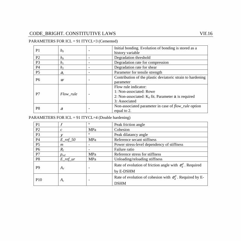
CODE_BRIGHT. CONSTITUTIVE LAWS VIf.16 PARAMETERS FOR ICL = 91 ITYCL=3 (Cemented)
P1 b0 - Initial bonding. Evolution of bonding is stored as a history variable
P2 h0 - Degradation threshold P3 h1 - Degradation rate for compression P4 h2 - Degradation rate for shear P5 at - Parameter for tensile strength
P6 w - Contribution of the plastic deviatoric strain to hardening parameter
P7 Flow_rule -
Flow rule indicator: 1: Non-associated: Rowe 2: Non-associated: K0 fit. Parameter a is required 3: Associated
P8 a - Non-associated parameter in case of flow_rule option equal to 2.
PARAMETERS FOR ICL = 91 ITYCL=4 (Double hardening)
P1 f º Peak friction angle P2 c MPa Cohesion P3 y º Peak dilatancy angle P4 E_ref_50 MPa Reference secant stiffness P5 m - Power stress-level dependency of stiffness P6 Rf - Failure ratio P7 pref MPa Reference stress for stiffness P8 E_ref_ur MPa Unloading/reloading stiffness
P9 Af - Rate of evolution of friction angle with pde . Required
by E-DSHM
P10 Ac - Rate of evolution of cohesion with pde . Required by E-
DSHM
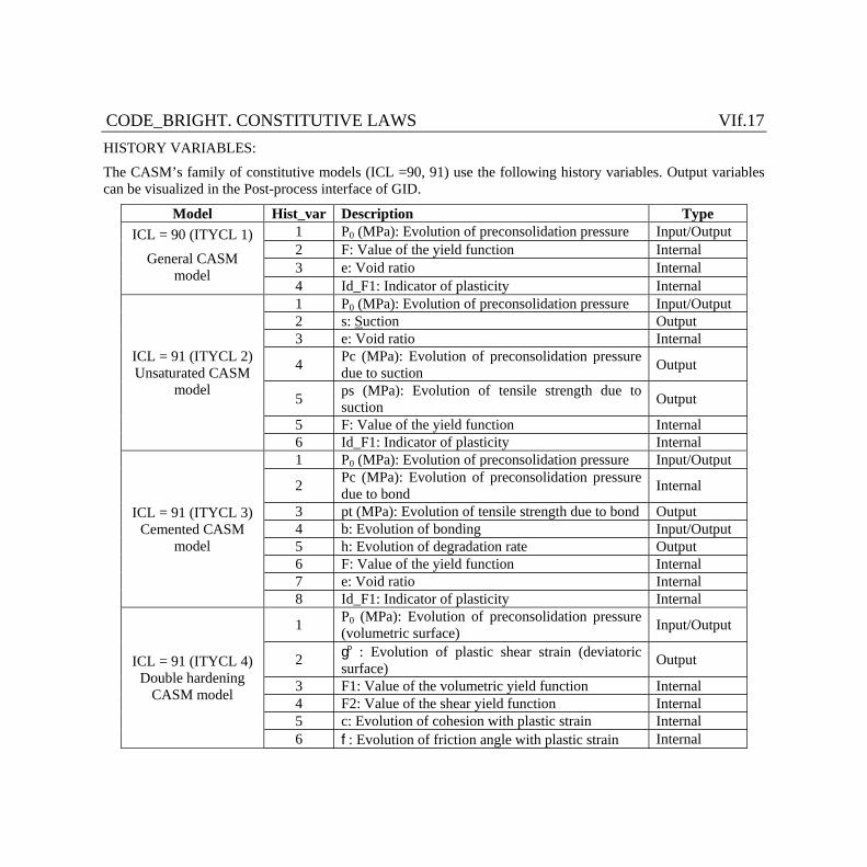
CODE_BRIGHT. CONSTITUTIVE LAWS VIf.17 HISTORY VARIABLES:
The CASM’s family of constitutive models (ICL =90, 91) use the following history variables. Output variables can be visualized in the Post-process interface of GID.
Model Hist_var Description Type ICL = 90 (ITYCL 1)
General CASM model
1 P0 (MPa): Evolution of preconsolidation pressure Input/Output 2 F: Value of the yield function Internal 3 e: Void ratio Internal 4 Id_F1: Indicator of plasticity Internal
ICL = 91 (ITYCL 2) Unsaturated CASM
model
1 P0 (MPa): Evolution of preconsolidation pressure Input/Output 2 s: Suction Output 3 e: Void ratio Internal
4 Pc (MPa): Evolution of preconsolidation pressure due to suction Output
5 ps (MPa): Evolution of tensile strength due to suction Output
5 F: Value of the yield function Internal 6 Id_F1: Indicator of plasticity Internal
ICL = 91 (ITYCL 3) Cemented CASM
model
1 P0 (MPa): Evolution of preconsolidation pressure Input/Output
2 Pc (MPa): Evolution of preconsolidation pressure due to bond Internal
3 pt (MPa): Evolution of tensile strength due to bond Output 4 b: Evolution of bonding Input/Output 5 h: Evolution of degradation rate Output 6 F: Value of the yield function Internal 7 e: Void ratio Internal 8 Id_F1: Indicator of plasticity Internal
ICL = 91 (ITYCL 4) Double hardening
CASM model
1 P0 (MPa): Evolution of preconsolidation pressure (volumetric surface) Input/Output
2 gp : Evolution of plastic shear strain (deviatoric surface) Output
3 F1: Value of the volumetric yield function Internal 4 F2: Value of the shear yield function Internal 5 c: Evolution of cohesion with plastic strain Internal 6 f: Evolution of friction angle with plastic strain Internal
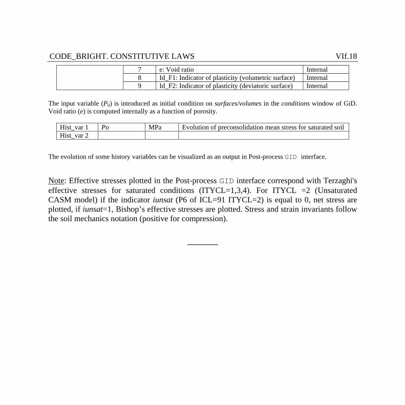
CODE_BRIGHT. CONSTITUTIVE LAWS VIf.18 7 e: Void ratio Internal 8 Id_F1: Indicator of plasticity (volumetric surface) Internal 9 Id_F2: Indicator of plasticity (deviatoric surface) Internal
The input variable (P0) is introduced as initial condition on surfaces/volumes in the conditions window of GiD. Void ratio (e) is computed internally as a function of porosity.
Hist_var 1 Po MPa Evolution of preconsolidation mean stress for saturated soil Hist_var 2
The evolution of some history variables can be visualized as an output in Post-process GID interface.
Note: Effective stresses plotted in the Post-process GID interface correspond with Terzaghi's effective stresses for saturated conditions (ITYCL=1,3,4). For ITYCL =2 (Unsaturated CASM model) if the indicator iunsat (P6 of ICL=91 ITYCL=2) is equal to 0, net stress are plotted, if iunsat=1, Bishop’s effective stresses are plotted. Stress and strain invariants follow the soil mechanics notation (positive for compression).
_________
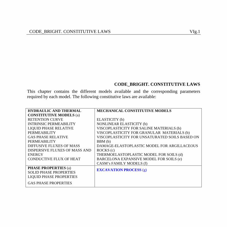
CODE_BRIGHT. CONSTITUTIVE LAWS VIg.1
CODE_BRIGHT. CONSTITUTIVE LAWS This chapter contains the different models available and the corresponding parameters required by each model. The following constitutive laws are available: HYDRAULIC AND THERMAL CONSTITUTIVE MODELS (a) RETENTION CURVE INTRINSIC PERMEABILITY LIQUID PHASE RELATIVE PERMEABILITY GAS PHASE RELATIVE PERMEABILITY DIFFUSIVE FLUXES OF MASS DISPERSIVE FLUXES OF MASS AND ENERGY CONDUCTIVE FLUX OF HEAT
MECHANICAL CONSTITUTIVE MODELS ELASTICITY (b) NONLINEAR ELASTICITY (b) VISCOPLASTICITY FOR SALINE MATERIALS (b) VISCOPLASTICITY FOR GRANULAR MATERIALS (b) VISCOPLASTICITY FOR UNSATURATED SOILS BASED ON BBM (b) DAMAGE-ELASTOPLASTIC MODEL FOR ARGILLACEOUS ROCKS (c) THERMOELASTOPLASTIC MODEL FOR SOILS (d) BARCELONA EXPANSIVE MODEL FOR SOILS (e) CASM’s FAMILY MODELS (f)
PHASE PROPERTIES (a) SOLID PHASE PROPERTIES LIQUID PHASE PROPERTIES
GAS PHASE PROPERTIES
EXCAVATION PROCESS (g)
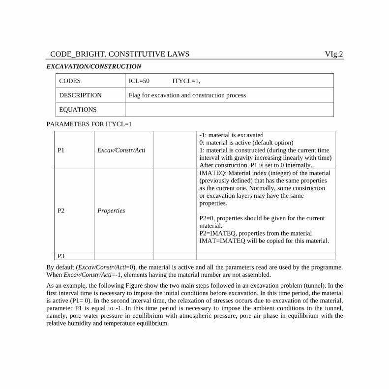
CODE_BRIGHT. CONSTITUTIVE LAWS VIg.2 EXCAVATION/CONSTRUCTION
CODES ICL=50 ITYCL=1,
DESCRIPTION Flag for excavation and construction process
EQUATIONS
PARAMETERS FOR ITYCL=1
P1 Excav/Constr/Acti
-1: material is excavated 0: material is active (default option) 1: material is constructed (during the current time interval with gravity increasing linearly with time) After construction, P1 is set to 0 internally.
P2 Properties
IMATEQ: Material index (integer) of the material (previously defined) that has the same properties as the current one. Normally, some construction or excavation layers may have the same properties. P2=0, properties should be given for the current material. P2=IMATEQ, properties from the material IMAT=IMATEQ will be copied for this material.
P3
By default (Excav/Constr/Acti=0), the material is active and all the parameters read are used by the programme. When Excav/Constr/Acti=-1, elements having the material number are not assembled.
As an example, the following Figure show the two main steps followed in an excavation problem (tunnel). In the first interval time is necessary to impose the initial conditions before excavation. In this time period, the material is active (P1= 0). In the second interval time, the relaxation of stresses occurs due to excavation of the material, parameter P1 is equal to -1. In this time period is necessary to impose the ambient conditions in the tunnel, namely, pore water pressure in equilibrium with atmospheric pressure, pore air phase in equilibrium with the relative humidity and temperature equilibrium.
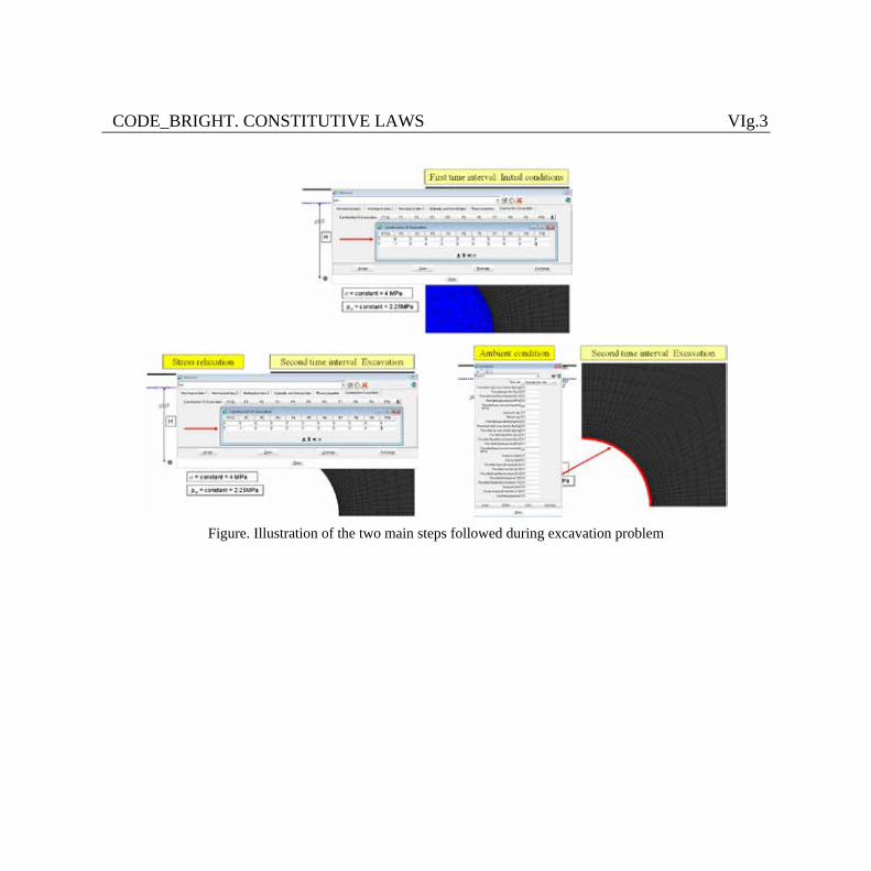
CODE_BRIGHT. CONSTITUTIVE LAWS VIg.3
Figure. Illustration of the two main steps followed during excavation problem
REFERENCES VII.1
CODE_BRIGHT. REFERENCES Formulation and numerical methods
Allen, M.B. and Murphy C.L. (1986): A Finite-Element Collocation Method for Variably Saturated Flow in Two Space Dimensions, Water Resources Research, 22, no. 11: 1537:1542.
Altunin, VV & Sakhabetdinov, MA (1972). Viscosity of liquid and gaseous carbon dioxide at temperatures 220-1300 K and pressure up to 1200 bar. Teploenergetika, 8:85-89.
Celia, M.A., Boulotas, E.T. and Zarba, R. (1990): A General Mass Conservative Numerical Solution for the Unsaturated Flow Equation, Water Resources Research, 26, no. 7: 1483:1496.
Chen, G., Ledesma, A. (2009). Coupled Thermohydromechanical Modeling of the Full-Scale In Situ Test "Prototype Repository. Journal of geotechnical and geoenvironmental engineering, vol. 135, núm. 1, p. 121-132.
Garcia, J.E. (2003). Fluid Dynamics of Carbon Dioxide Disposal into Saline Aquifers. PhD thesis, University of California, Berkeley.
Hughes, T. J. R. (1980): Generalisation of Selective Integration Procedures to Anisotropic and Nonlinear Media, Int. J.Num. Meth. Eng. 15, 1413-1418.
Huyakorn, P.S. and Pinder, G.F. (1983): Computational Methods in Subsurface Flow,
REFERENCES VII.2
Academic Press, Inc. ISBN 0-12-363480-6.
Huyakorn, P.S., Springer, E.P., Guvanasen, V. and Wadsworth, T.D.(1986): A Three-dimensional Finite-Element Model for Simulating Water Flow in Variably Saturated Porous Media, Water Resources Research, 22, no. 13 : 1790:1808 }
Milly, P.C.D. (1984): A mass-conservative procedure for time stepping in models of unsaturated flow, in Proceedings Fifth International Conference on Finite Elements in Water Resources, edited by J. P. Laible et al., Springer-Verlag, New York: 103-112.
Olivella, S., J. Carrera, A. Gens, E. E. Alonso, (1994). Non-isothermal Multiphase Flow of Brine and Gas through Saline media. Transport in Porous Media, 15, 271:293
Olivella, S., A. Gens, J. Carrera, E. E. Alonso, (1996), Numerical Formulation for a Simulator (CODE_BRIGHT) for the Coupled Analysis of Saline Media, Engineering Computations, Vol. 13, No 7, , pp: 87-112.
Olivella, S., J. Carrera, A. Gens, E. E. Alonso. (1996) Porosity Variations in Saline Media Caused by Temperature Gradients Coupled to Multiphase Flow and Dissolution/Precipitation. Transport in Porous Media, 25:1-25.
Pini, G. and Gambolatti, G. (1990), Is a simple diagonal scaling the best pre-conditioner for conjugate gradients on super-computers?, Advances in Water Resources.
Sonnelveld, P., (1989), CGS, A fast Lanczos-type solver for non-symmetric linear systems, SIAM J. Sci. Stat. Comput., 10, 36-52.
Spycher, N, Pruess, K & Ennis-king, J (2003). CO2-H2O Mixtures in the Geological Sequestration of CO2. I. Assessment and calculation of mutual solubilities from 12 to 100°C and up to 600 bar. Geochim. Cosmochim. Acta, 67:3015-3031.
Voss, C.I. (1984): SUTRA Users's Guide, U.S. Geological Survey, Water Resources investigations, Report 48-4369.
Van der Vorst, Henk (1990), Iterative methods for the solution of large systems of equations on super-computers, Advances in Water Resources, Vol. 13, No. 3, 137-146.
REFERENCES VII.3
Viscous/creep models Olivella, S.; A. Gens, J. Carrera, and E. E. Alonso (1993): Behaviour of Porous Salt
Aggregates. Constitutive and Field Equations for a Coupled Deformation, Brine, Gas and Heat Transport Model. The Mechanical Behaviour of Salt III, Trans Tech Publications, pp. 269:283. ISBN 0-87849-100-7.
Olivella, S., A. Gens, J. Carrera, E. E. Alonso (1996) Analysis of Creep Deformation of Galleries Backfilled with Porous Salt Aggregates. The Mechanical Behaviour of Salt IV, Trans Tech Publications, 379:386.
State surface approach Fredlund, D.G., Morgenstern, N.R., 1977. Stress state variables for unsaturated soils. J
Geotech Engng Div, 103(GT5):447-466. Lloret, A. & Alonso, E., 1985. State surfaces for partially saturated soils. Proc. 11th Int. Conf.
Soil Mech. Fdn Engng, San Franciso, vol. 2, pp. 557-562. Matyas, E.L. & Radhakrishna, H.S., 1968. Volume change characteristics of partially
saturated soils, Géotechnique, 18(4):432-448. Elastoplastic model for unsaturated soils Alonso, E.E., Gens, A., Josa, A., 1990. A constitutive model for partially saturated soils.
Géotechnique 40(3):405-430. Gens, A., Potts, D.M., 1988. Critical state models in computational geomechanics. Eng
Comp, 5(3):178-197. Ledesma, A., Chan, A.H.C, Vaunat, J., Gens, A., 1995. Finite Element formulation of an
elasto-plastic model for partially saturated soils. In: Owen, D.R.J., Oñate, E. (Eds.) Proc. 4th Int. Conf. on Computational Plasticity, Pineridge Press, Swansea, pp. 1677-1688.
Maâtouk, A., Leroueil, S., La Rochelle, P., 1995. Yielding and critical state of a collapsible unsaturated silty soil. Géotechnique, 45(3):465-477.
REFERENCES VII.4
Ohmaki, S., 1982. Stress-strain behaviour of anisotropically, normally consolidated cohesive soil. In: Dungar, R., Pande, G.N., Studer, J.A. (Eds), Proc. 1st Int. Symp. on Num. Models in Geomechanics, Balkema, Rotterdam, pp. 250-269.
Roscoe, K.H., Burland, J.B., 1968. On the generalized stress-stain behaviour of the 'wet' clay. In: Heyman, J.,Leckie, F.A. (Eds.), Engineering Plasticity, Cambridge University Press, Cambridge, pp. 535-609.
Sloan, S.W., 1987. Substepping schemes for the numerical integration of elastoplastic stress-
strain relations. Int J Num Methods Engrg, 24(5), 893-911. Wheeler, S.J., Sivakumar, V., 1995. A elasto-plastic critical state framework for unsaturated
soil. Géotechnique 45(1):35-53. Wood, D.M., 1990. Soil behaviour and critical state soil mechanics. Cambridge University
Press, Cambridge. Thermoelastoplastic model for unsaturated soils Hueckel, T. & Borsetto, M. 1990. Thermoplasticity of saturated soils and shales: constitutive
equations. Jnl. Geot. Eng. ASCE, 116: 1765-1777. Hueckel,T.& Baldi, G. 1990.Thermoplasticity of saturated clays: experimental constitutive
study. Jnl. Geot. Eng.ASCE,116:1778-1796. Hueckel,T. & Pellegrini,R.(1991). Thermo-plastic modelling of untrained failure of saturated
clay due to heating. Soils and Found., 3:1-16. García Molina. A., Gens, Añ & Olivella, O. 1996. Un modelo constitutivo para suelos no
saturados sometidos a variaciones térmicas: formulación, implementació y aplicaciones. In Doblaré, M., Correas, J.M., Alarcón E., Gavete, L. & Pastor, M. (Eds): Proc. III Congreso de Métodos Numéricoas en Ingeniería, pp.502-512.
Gens, A. 1995. Constitutive laws. In Gens, A., Jouanna, P. & Schrefler, B. (Eds): Modern issues in non-saturated soils, Springer-Verlag.
REFERENCES VII.5
Visco-plastic model for unsaturated soils Perzyna, J.K. (1966). Fundamental problems in viscoplasticity. Adv. Appl. Math. 9, 243–
377. Desai, C.S and Zhang, D. (1987. Viscoplastic model for geologic materials with generalized
flow rule. Int. J. Num. Anal. Methods in Geomech. Vol 11, issue 6, pp. 603-260. Sánchez, Marcelo. 1997. Implementation of VP model by Desai in CB. Used to simulate
triaxial tests under drained conditions. Master’s thesis, UPC, January 1997. Molist, Jordi. 1997. Extension of the VP model by Desai to unsaturated soils. Graduation
thesis. UPC. September 1997. Oldecop, L.A. and Alonso, E.E. 2001 A constitutive model for rockfill compressibility.
Géotechnique 51, No.2, pp 127-239. Zandarin, Maria Teresa. 2010. Thermo-hydro-mechanical analysis of joints a theoretical and
experimental study. PhD Thesis. UPC. Barcelona. Damage-elastoplastic model for argillaceous rocks Carol, I., Rizzi E. & Willam K. 2001. “On the formulation of anisotropic elastic degradation.
1. Theory based on a pseudo-logarithmic damage tensor rate”, Int. J. Solids Struct., 38: 491-518.
Hoek, E. & Brown, E. T. 1980. “Empirical strength criterion for rock masses”, Journal of the Geotechnical Engineering Division, 106: 1013-1035 .
Sloan, S. W. & Booker, J. R. 1986. Removal of singularities in Tresca and Mohr-Coulomb yield functions. Communications in Applied Numerical Methods, 2: 173-179.
Vaunat, J. & Gens, A. 2003. Bond degradation and irreversible strains in soft argillaceous rock. In: Cullighan, P.J., Einstein, H.H. & Whittle, A. (Eds.) “Proceedings of 12th Panamerican Conference on Soil Mechanics and Geotechnical Engineering”, 23th –25th June 2003, Boston, United-State, Pub. VGE, ISBN 3-7739-5985-0, vol. 1, pp. 479-484.
REFERENCES VII.6
Barcelona expansive model (BExMo) Alonso, E.E., Vaunat, J., & Gens, A. 1999. “Modelling the mechanical behaviour of
expansive soils ”, Engng. Geol. 54 Nos 1-2, 173-183. Pinyol, N., Vaunat, J., & Alonso, E.E. 2007. “A constitutive model for soft clayey rocks that
includes weathering effects”. Géotechnique 57, No.2, 137-151. CASM’s family models Alonso, E.E., Gens, A., Josa, A., 1990. A constitutive model for partially saturated soils.
Géotechnique 40(3):405-430. Gens, A. & Nova, R. (1993). Conceptual bases for a constitutive model for bonded soils and
weak rocks. In Geotechnical Engineering of Hard Soils-Soft Rocks, Athens, Greece, Anagnostopoulos et al. (eds.) Rotterdam: Balkema, 577-583.
González, N.A. (2011). Development of a family of constitutive models for Getoechnical applications. PhD Thesis. UPC. Barcelona.
Schanz, T., Vermeer, P.A. & Bonnier, P.G. (1999). Formulation and verification of the Hardening-Soil Model. Beyond 2000 in Computational Geotechnics, pages 281–290. Balkema, Rotterdam.
Sheng, D., Sloan S.W., & Yu, H.S. (2000). Aspects of finite element implementation of critical state models. Computational Mechanics 26, 185-196.
Yu, H.S. (1988). CASM: A unified state parameter model for clay and sand. International Journal of Numerical and Analytical Methods in Geomechanics, 22, 621-653.
Other Gens, A. , A.J. Garcia-Molina, S. Olivella, E. E. Alonso, F. Huertas. (1998) Analysis of Full Scale In-situ Heating Test Simulating Repository Conditions. Int. Journal for Numerical and Analitical Methods in Geomechanics. 22:515-548.
___________________________________