Coalition Formation to Provide Public Goodsunder Weakest-link Technology

Alejandro CaparrósConsejo Superior de Investigaciones Cientícas (CSIC),

Institute for Public Goods and Policies (IPP),Albasanz 26, 28037 Madrid, Spain.E-mail: alejandro.caparros@csic.es

Michael FinusUniversity of Bath

Department of EconomicsBath, BA2 7AY, UK

E-mail: m.nus@bath.ac.uk

Abstract: We analyze the canonical coalition formation model of international envi-ronmental agreements (IEAs) under a weakest-link technology and compare it with thewell-known summation technology. That is, benets from the provision of a public gooddo not depend on the sum but on the minimum of individual contributions, an assumptionappropriate for many regional and global public goods, like ghting a re which threatensseveral communities, compliance with minimum standards in marine law, protecting specieswhose habitat cover several countries, scal convergence in a monetary union and curbingthe spread of an epidemic. Compared to the summation technology, we demonstrate thatmany more general results can be obtained and under much more general assumptions. Weshow, for the standard assumption of symmetric players, that policy coordination is not nec-essary. For asymmetric players, without transfers, though all coalitions are Pareto-optimal,no coalition with a provision level above the non-cooperative equilibrium is stable. However,if an optimal transfer is used, an e¤ective non-trivial coalition exists. We show how variousforms of asymmetry relate to stability and the welfare gains from cooperation. We nd aparadox: asymmetries which are conducive to stability of coalitions imply low welfare gainsfrom cooperation and vice versa.

Key words: public goods, weakest-link technology, coalition formationJEL classication: C71, C72, H41

1

1 Introduction

There are many cases of global and regional public goods for which the decision in one juris-

diction has consequences for other jurisdictions and which are not internalized via markets.

Reducing global warming and the thinning of the ozone layer are examples in case. As

Sandler (1998), p. 221, points out: “Technology continues to draw the nations of the world

closer together and, in doing so, has created novel forms of public goods and bads that have

diminished somewhat the relevancy of economic decisions at the nation-state level.” The

stabilization of financial markets, the fighting of contagious diseases and the efforts of non-

proliferation of weapons of mass destruction have gained importance through globalization

and the advancement of technologies.

A central aspect in the theory of public goods is to understand the incentive structure

that typically leads to the underprovision of public goods as well as the possibilities of recti-

fying this. Historically, the analysis has developed along two strands, almost independently,

the literature on public good provision and the literature on international environmental

agreements (IEAs) where the latter is an application of a broader literature on coalition

formation in the presence of externalities. In this paper, we combine ideas and concepts

from both strands which we discuss subsequently.

The literature on public goods provision suggests three fundamental features for the

provision or underprovision of public goods: a) the degree of excludability1 , b) the degree

of rivalry2 and c) the aggregation technology. This paper focuses on the last of these three

1The degree of excludability relates to the proportion of the benefits which are privately and publiclyenjoyed and has two dimensions. Technical excludability, which is defined by the intrinsic properties of agood, and socially constructed excludability, which is defined by the properties assigned by society to them(Kaul and Mendoza 2003). Whereas the degree of technical excludability can be regarded as given, at leastin the short and mid-term (e.g. through physical exclusion devices, such as barbed wire fences and electronicsensing devices in the fight against international terrorism), socially constructed excludability is determinedby the establishment and enforcement of property rights. A formal analysis of the degree of excludabilityand its impacts on the success of coalition formation is for instance provided in Finus et al. (2011) in thecontext of a fishery model and in Finus and Rübbelke (2013) in the context of climate change.

2The degree of rivalry relates to the distinction between public goods, club goods, congested goods,private goods and common pool resources (Sandler and Arce 2002). According to the classic definition,there is no rivalry for public goods, and the same applies for the members of a club, but congested goodsexhibit some rivalry and private goods and common property resources strong rivalry. Sandler and Arce

2

features, which originates from Hirschleifer (1983).

Aggregation technologies, which have also been called social composition functions by

Hirschleifer (1983), comprise summation technology (with equal or unequal weights), best-

and better-shot technology and weakest- and weaker-link technology. The classic public

good model assumes that the benefits from public good provision depend only on the sum of

individual contributions. Classical examples with equal weights are contributions to reduce

climate change and the depletion of the ozone layer. The canonical example with unequal

weights is transboundary emission reductions in the acid rain game as effective contributions

depend on wind patterns and weights depend on the transportation matrix (Mäler 1994

and Sandler 1998). A best-shot technology means that the benefits from the public good

depend on the maximum of all individual provision levels. Examples include asteroid pro-

tection, finding a cure for the Ebola and AIDS virus, developing antibiotic-resistant against

tuberculosis, and developing a breakthrough technology for safely storing highly radioactive

materials or a shield for missile protection (Arce 2001, Arce and Sandler 2001 and Sandler

1998). Weakest-link is just the opposite of best-shot in that only the smallest individual pro-

vision level matters for the benefits of public good provision.3 Examples include the classical

example of Hirschleifer (1983) of building dykes against flooding, fighting a fire which threat-

ens several communities, air-traffi c control, compliance with minimum standards in marine

law, compliance with targets for fiscal convergence in a monetary union, measures against

money laundering within the European Union, disease eradication, curbing the spread of an

epidemic and maintaining the integrity of a network (Arce 2001 and Sandler 1998). Biodi-

versity may have features of best shot and weakest link: efforts to protect a species whose

(2003) conjecture that it would be easier to establish joint action for public goods than joint inaction forcommon pool resources. In Finus et al. (2011) it is suggested that this claim cannot be sustained formallyand in fact the formal analysis in Sandler and Arce (2003) also does not lend support for their conjecture.This is also supported by the literature on IEAs from which it is evident that it does not matter whetherone talks of providing a public good or ameliorating a public bad. See Rubio and Ulph (2006) and morerecently Hong and Karp (2013).

3Better shot (weaker link) is a modification of the best shot (weakest link) technology where the marginaleffect of an individual contribution on the global provision level decreases (increases) with the level of thecontribution. For a formal exposition, see for instance Cornes (1993) and Cornes and Hartely (2007a,b).

3

habitat covers several countries is best described as a weakest-link public good, and saving

one particular species from extinction is a best-shot public good if one out of several areas

is enough to ensure the subsistence of the species. In this paper, we focus on the weakest-

link technology and stress similarities and differences to the public good model with equal

weights.

The public goods literature has taken basically three approaches in order to understand

the incentive structure of the weakest-link technology in comparison to the summation tech-

nology.

The first approach is informal and argues that the least interested player in the public

good provision is essentially the bottleneck, which defines the equilibrium provision and

which is matched by all others who mimic the smallest effort (e.g. Sandler and Arce 2002

and Sandler 2006). Moreover, it is argued that either a third party or the most well-off

players should have an incentive to support the least well-off through monetary or in-kind

transfers in order to increase the provision level. The intuitive approach is useful in placing

the debate in the policy context and in formulating hypotheses, but by its informal nature,

it needs to be complemented by a formal analysis.

The second approach is a formal approach (Cornes 1993, Cornes and Hartley 2007a,b,

Vicary 1990, and Vicary and Sandler 2002). Typically, it is shown that there is no unique

Nash equilibrium for the weakest-link technology, though Nash equilibria can be Pareto

ranked. It is demonstrated that except if players are symmetric, Nash equilibria are Pareto

ineffi cient. Cooperation is modelled by considering monetary transfers between players that

change players’endowments. This may change players’equilibrium strategies in the Nash

equilibrium because income neutrality does no longer hold (as this is the case under the

summation technology) for the weakest-link technology. If players have suffi ciently different

preferences, then the Nash equilibrium provision level, determined by the weakest player,

can be increased through transfers and this may constitute a Pareto improvement to all

players. In some models (e.g. Cornes and Hartley 2007b and Vicary and Sandler 2002),

4

which allow for different prices across players (the marginal opportunity costs in the form

of giving up consumption of the private good), this is reinforced if the recipients face a

lower price than the donor. In Vicary and Sandler (2002) it is also investigated how the

Nash equilibrium provision level changes if monetary transfers are either substituted or

complemented by in-kind transfers.4 This approach, though useful and interesting, faces

at least two shortcomings. First, the degree of underprovision and how it changes through

“cooperation”is not really measured. Though in Cornes (1993) a kind of physical measure

(Allais-Debreu measure of waste) is proposed, the degree of underprovision is not measured in

welfare terms. Second, cooperation is only considered in a rudimentary form as no departure

from Nash behavior is investigated. We can address both shortcomings with our model,

though admittedly, this is easier in our IEA-coalition framework, which assumes transferable

utility. That is, in our model, equilibrium strategies are not affected by monetary transfer

and aggregate welfare can easily be measured and benchmarked in the Nash and a coalitional

equilibrium against the social optimum. Moreover, our model allows not only for different

marginal costs but also non-constant marginal costs of public good provision.

The third approach considers various forms of formal and informal cooperative agree-

ments, established for instance through a correlation device implemented by a third party

institution, leadership and evolutionary stable strategies (e.g. Arce 2001, Arce and Sandler

2001, Sandler 1998 and Holzinger 2001). The advantage of this approach is that it takes

up the research question already posed by Cornes (1993), namely how cooperative institu-

tions develop endogenously under different aggregation technologies. The disadvantage is

that these papers are based on examples, matrix games (e.g. prisoners’dilemma, chicken

or assurance games) with discrete strategies for which it is not evident whether results hold

generally or whether they are an artefact of their particular assumptions.5

4We consider monetary transfers in our model but not in-kind transfers as they basically transform theweakest-link technology into a summation technology.

5Coalition formation, though not necessarily of the weakest-link technology, has been considered byonly few papers in this literature, e.g. Arce and Sandler (2003) and Sandler (1999). However, they usea cooperative game theory approach where the focus is not on enforcement but on sharing the gains fromcooperation in the grand coalition. A similar approach has been used by Chander and Tulkens (1997) in the

5

The second strand of literature on IEAs, which can be traced back to Barrett (1994),

Carraro and Siniscalco (1993) and Hoel (1992) and which is summarized in Barrett (2003)

and Finus (2003), and coalition formation in general as summarized in Bloch (2003) and Yi

(1997), has stressed that the size of stable coalitions depends on the institutional features of

coalition formation and the properties of the underlying economic problem. The institutional

features of most coalition formation games, can be related to a two-stage process in which

players choose their membership strategies in the first stage and their economic strategies in

the second stage. Regarding the first stage, features like a) simultaneous versus sequential

membership choice (e.g. Finus and Rundshagen 2006), b) open versus exclusive membership

(e.g. Finus and Rundshagen 2009) and c) single versus multiple coalitions (e.g. Carraro

and Marchiori 2003 and Finus and Rundshagen 2003) may matter. Regarding the second

stage, features like a) Nash-Cournot versus Stackelberg leadership (Finus 2003) b) ambitious

versus modest targets (e.g. Barrett 2002 and Finus and Maus 2008) and c) no transfers

versus transfers (e.g. Fuentes-Albero and Rubio 2010 and Weikard 2009) may matter. Re-

garding the underlying economic problem, it has been shown that problems can be broadly

categorized into positive versus negative externalities (Bloch 2003 and Yi 1997). In positive

(negative) externality games, players not involved in the enlargement of coalitions are better

(worse) off through such a move. Hence, in positive externalities games, typically, only small

coalitions are stable, as players have an incentive to stay outside coalitions. Typical examples

of positive externalities include output and price cartels and the provision of public goods

under the summation technology. Firms not involved in an output cartel benefit from lower

output by the cartel via higher market prices. This is also the driving force in price cartels

where the cartel raises prices above non-cooperative levels. Agents not involved in a public

good agreement benefit from higher provision levels of participants. In contrast, in negative

externality games, outsiders have an incentive to join coalitions and therefore most coalition

models predict the grand coalition as a stable outcome. Examples include for instance trade

IEA literature. In contrast, our model is based on the non-cooperative coalition formation approach.

6

agreements, which impose tariffs on imports from outsiders or R&D-collaboration among

firms in imperfectly competitive markets where members gain a comparative advantage over

outsiders if the benefits from R&D accrue exclusively to coalition members.

Until now, the analysis of public goods in the tradition of the IEA literature has exclu-

sively focused on the summation technology, by and large with equal weights. Even though

the bulk of the papers has assumed symmetric agents, the analysis has been conducted to

a large extent based on simulations. This is even more true for asymmetric agents where

hardly any general results have been obtained.6 Therefore, we investigate the success of

coalition formation for the weakest-link technology in the canonical IEA model, the car-

tel formation game, reflecting the standard assumptions of a two-stage coalition formation

game. In section 4, we briefly consider what changes if we modify some assumptions. It will

become apparent that for the weakest-link technology many more general conclusions un-

der much more general assumptions can be derived compared to the summation technology.

Moreover, we stress similarities and differences to the summation technology along the way

of our analysis.

In the following, we set out our model and provide some basic definitions in section 2.

Section 3 derives our main results and section 4 summarizes our main findings and concludes.

2 Model and Definitions

We consider the following payoff function of player i ∈ N :

Vi(Q, qi) = Bi(Q)− Ci(qi) (1)

Q = mini∈Nqi

where N denotes the set of players and Q denotes the public good provision level, which

is the minimum over all players under the weakest-link technology. The individual provision

6For an analysis of cooperation with asymmetric agents based on simulations see McGinty (2007); ananalytical analysis is provided in Caparrós et al. (2011).

7

level of player i is qi. Payoffs comprise benefits, Bi(Q), and costs, Ci(qi). Externalities across

players are captured through Q on the benefit side.

In order to appreciate some features of the weakest-link technology, we will occasionally

relate some results to the classical assumption of a summation technology. The subsequent

description of the model and its assumptions are general enough to apply two both technolo-

gies. For the classical assumption, payofffunction (1) is still valid, except thatQ =∑

j∈N qj.7

Important results of the classical case are compactly derived and summarized in Appendix

A in order to facilitate a comparison.

Regarding the components of the payoff function, we make the following assumptions

where primes denoting derivatives.

Assumption 1. For all i ∈ N : B′i > 0, B′′i ≤ 0, C ′i > 0, C ′′i ≥ 0 , assuming that if

B′′i = 0, then C ′′i > 0 and, vice versa, if C ′′i = 0, then B′′i < 0, i.e. not both functions can be

linear. Furthermore, we assume Bi(0) = Ci(0) = 0 and limQ→0B′i(Q) > limq→0C

′i(q) > 0.

The assumptions are very general and ensure the strict concavity of the payoff function

and interior equilibria as explained below. For the following definitions, it is convenient

to abstract from the aggregation technology and simply write Vi(q), stressing that payoffs

depend on the entire vector of contributions, q = (q1, q2, ..., qN), which may also be written

as q = (qi, q−i) where the superscript of q−i indicates that this is not a single entry but a

vector, comprising all provision levels except that of player i, qi.

Following d’Aspremont et al. (1983), the coalition formation process unfolds as follows:

Definition 1 Cartel Formation Game. Let an individual player be denoted by i or

j and the set of all players be denoted by N . In the first stage, each individual player

simultaneously chooses a membership strategy mi ∈ 0, 1. All players who announce mj = 0

act as single players and are called non-signatories or non-members, and all players who

announce mi = 1 form coalition S and are called signatories or members. In the second7More precisely, we mean a summation technology with equal weights, which we assume throughout the

paper and therefore will not stress it explicitly anymore.

8

stage, simultaneously, all non-signatories maximize their individual payoff Vj(q), and all

signatories jointly maximize their aggregate payoff∑

i∈S Vi(q).

Note that due to the simple nature of the cartel formation game, a coalition structure, i.e.

a partition of players, is completely characterized by coalition S as all players not belonging

to S act as singletons. The coalition de facto acts like a meta player, internalizing the

externality among its members. The assumption of joint welfare maximization of coalition

members implies a transferable utility framework (TU-framework). The cartel formation

game is solved by backwards induction, assuming that players play a Nash equilibrium in

each stage and hence a subgame-perfect equilibrium with respect to the entire game. In order

to save on notation, we assume in this section that the second stage equilibrium for every

coalition S ⊆ N (denoted by q∗(S) in the subsequent Definition1 below) is a unique interior

equilibrium, even though this is established later in Section 3, in particular in Subsection

3.1.

Definition 2 Subgame-perfect Equilibrium in the Cartel Formation Game

(i) Second Stage:

For a given coalition S that has formed in the first stage, let q∗(S) denote the (unique)

simultaneous solution to

∑i∈S

Vi(q∗(S)) ≥

∑i∈S

Vi(qS(S), q−S∗(S))

Vj(q∗(S)) ≥ Vj(qj(S), q−j∗(S)) ∀j /∈ S

for all qS(S) 6= qS∗(S) and qj(S) 6= q∗j (S) with qS(S) denoting the provision vector of coali-

tion S, q−S(S), the provision vector of all players not in S, qj(S) the provision level of a

single player j not in S and q−j(S) the provision vector of all players different from j.

a) In the case of no monetary transfers, equilibrium payoffs are given by Vi(q∗(S)) or V ∗i (S)

for short.

b) In the case of monetary transfers, equilibrium payoffs, V ∗Ti (q∗(S)), or V ∗Ti (S) for short,

9

for all signatories i ∈ S are given by V ∗Ti (S) = V ∗i (S)+γiσS(S) with σS(S) :=∑

i∈S(V ∗i (S)−

V ∗i (S \i)) , γi ≥ 0 and∑

i∈S γi = 1 and for all non-signatories j /∈ S by V ∗Tj (S) = V ∗j (S).

(ii) First stage:

a) Assuming no monetary transfers in the second stage, coalition S is called stable if

internal stability: V ∗i (S) ≥ V ∗i (S \ i)∀i ∈ S and

external stability: V ∗j (S) ≥ V ∗j (S ∪ j)∀j /∈ S hold simultaneously.

b) Assuming monetary transfers in the second stage, coalition S is called stable if

internal stability : V ∗Ti (S) ≥ V ∗Ti (S \ i)∀i ∈ S and

external stability : V ∗Tj (S) ≥ V ∗Tj (S ∪ j)∀j /∈ S hold simultaneously.

First note that with respect to the second stage, the equilibrium provision vector is

a Nash equilibrium between coalition S, de facto acting as single player, and all the sin-

gle players in N \ S. Only because of our assumption of uniqueness, we are allowed to

write V ∗i (S) instead of Vi(q∗(S)). Second, as we assume a TU-game, monetary transfers

do not affect equilibrium provision levels. Monetary transfers are only paid among coali-

tion members, exhausting all (without wasting any) resources generated by the coalition.

Non-signatories do neither pay nor receive monetary transfers. Third, note that the "all

singleton coalition structure", i.e. all players act as singletons, subsequently denoted by

i, j, ...z, replicates the non-cooperative or Nash equilibrium provision vector known

from games without coalition formation. It emerges if either only one player or no player

announcesmi = 1. By the same token, the grand coalition, i.e. the coalition which comprises

all players, is identical to the socially optimal provision vector, sometimes also called the full

10

cooperative outcome, subsequently denoted by N. Hence, our coalition game covers these

two well-known benchmarks, apart from partially cooperative outcomes where neither the

grand coalition nor the all singleton coalition structure forms. Fourth, the monetary transfer

scheme which we consider is the optimal monetary transfer scheme proposed by Eyckmans

and Finus (2004).8 Every coalition member receives his free-rider payoff plus a share γi of

the total surplus σS(S), which is the difference between the total payoff of coalition S and

the sum over all free-rider payoffs if a player i leaves coalition S. In other words, σS(S) is the

sum of individual coalition member’s incentive to stay in (σi(S) ≥ 0) or leave (σi(S) < 0)

coalition S, σi(S) := V ∗i (S) − V ∗i (S \ i), which must be positive for internal stability at

the aggregate, i.e. σS(S) =∑

i∈S σi ≥ 0. Thus, the transfer scheme has some resemblance

with the Nash bargaining solution in TU-games, though the threat point payoffs are not the

Nash equilibrium payoffs but the payoffs if a player leaves coalition S. The shares γi can be

interpreted as weights, reflecting bargaining power. They matter for the actual payoffs of

individual coalition members, but do not matter for the stability (or instability) of coalition

S because stability only depends on σS(S). The properties of this transfer scheme will be

discussed in the context of the first stage of coalition formation below. Fifth, note with re-

spect to the first stage that internal and external stability define a Nash equilibrium in terms

of membership strategies. All players who have announced mi = 1 should have no incentive

to announce mi = 0 instead (internal stability) and all players who have announced mj = 0

should have no incentive to announce mj = 1 instead, given the equilibrium announcements

of all other players. Due to the fact that the singleton coalition structure can always be

supported as Nash equilibrium in the membership game if all players announce mi = 0 (as

a change of the strategy by one player makes no difference), existence of a stable coalition

is guaranteed. We denote a coalition which is internally and externally stable and hence

stable by S∗. Sixth, in the case of the monetary transfer scheme considered here, it is easy

to see that, by construction, if σS ≥ 0, then coalition S is internally stable and if σS < 0,

8Similar notions have been considered by Fuentes-Albero and Rubio (2010), McGinty (2007) and Weikard(2009).

11

then neither this transfer scheme nor any other scheme could make coalition S internally

stable. Seventh, internal and external stability are linked: if coalition S is not externally

stable because player i has an incentive to join, then coalition coalition S ∪ i is internally

stable. Eighth, loosely speaking, the transfer scheme considered here is optimal subject to

the constraint that coalitions have to be stable. Clearly, for symmetric payoff functions,

optimal transfers will have no impact on stability. However for asymmetric payoff functions,

it is easy to show that every coalition S which is internally stable without transfers will also

be internally stable with optimal transfers. However, the reverse is not true. There may be

coalitions which are not internally stable without transfers (in particular large coalitions),

but they may be stable with transfers. Thus, if we can show that the coalition game exhibits

a property called full cohesiveness, i.e. the aggregate welfare over all players increases with

the enlargement of coalitions, then the aggregate payoff of the stable coalition with the high-

est aggregate welfare among the set of stable coalitions under an optimal transfer scheme

is (weakly) higher than without transfers (or any other transfer scheme). Hence, optimal

transfers have the potential to improve upon global welfare of stable coalitions. This poten-

tial is particular relevant for economic problems where the grand coalition is not stable due

to too strong free-rider incentives.9

In the following, we introduce some properties which are useful in evaluating the success

and incentive structure of coalition formation.10

Definition 3 Effectiveness of a Coalition. A coalition S is (strictly) effective with

respect to coalition S#, S# ⊂ S, if Q∗(S) ≥ (>) Q∗(S#).

9All properties of the optimal transfer scheme are proved in Eyckmans et al. (2012).10Note that for the subsequent definitions, transfers are not important as we look at the aggregate payoff

over all players or the aggregate payoff over all coalition members. Also for the payoffs of non-signatories,transfers do not matter, as they do not pay or receive transfers by assumption.

12

Definition 4 Superadditivity, Positive Externality and Cohesiveness.

(i) A coalition game is (strictly) superadditive if for all S ⊆ N and all i ∈ S:

∑i∈S

V ∗i (S) ≥ (>)∑

i∈S\i

V ∗i (S \ i) + Vi(S \ i)

(ii) A coalition game exhibits a (strict) positive externality if for all ∀S ⊆ N and for all

j ∈ N \ S :

V ∗j (S) ≥ (>)V ∗j (S \ i).

(iii) A game is (strictly) cohesive if for all S ⊂ N :

∑i∈N

V ∗i (N) ≥ (>)∑i∈S

V ∗i (S) +∑j∈N\S

V ∗j (S)

(iv) A game is (strictly) fully cohesive if for all S ⊆ N :

∑i∈S

V ∗i (S) +∑j∈N\S

V ∗j (S) ≥ (>)∑

i∈S\i

V ∗i (S \ i) +∑

j∈N\S∪i

V ∗j (S \ i).

All four properties are related to each other. For instance, a coalition game which is

superadditive and exhibits positive externalities is fully cohesive and a game which is fully

cohesive is cohesive (see Cornet 1998 and Montero 2006 for applications). Typically, a game

with externalities is cohesive, with the understanding that in a game with externalities the

strategy of at least one player has an impact on the payoff of at least one other player. The

reason is that the grand coalition internalizes all externalities by assumption.11 Cohesiveness

also motivates the choice of the social optimum as a normative benchmark, and it appears to

be the basic motivation to investigate stability and outcomes of cooperative arrangements. A

stronger motivation is related to full cohesiveness, as it provides a sound foundation for the

11Cohesiveness could fail if there are diseconomies of scale from cooperation, e.g. due transactions costswhich increase in the number of cooperating players. Our model abstracts from such complications.

13

search for large stable coalitions even if the grand coalition is not stable due to large free-rider

incentives. The fact that large coalitions, including the grand coalition, may not be stable in

coalition games with the positive externality property is well-known in the literature (e.g. see

the overviews by Bloch 2003 and Yi 1997). Examples of positive externality problems include

public good games with summation technology and other economic problems like output and

price cartels or R&D-cooperation among firms. The positive externality can be viewed as

a non-excludable benefit accruing to outsiders from cooperation. This property makes it

attractive to stay outside the coalition. This may be true despite superadditivity holds, a

property which makes joining a coalition attractive. In the context of a public good game

with summation technology, stable coalitions are typically small because with increasing

coalitions, the "push factor" positive externality dominates the "pull factor" superadditivity

(e.g. see the overviews by Barrett 2003 and Finus 2003).12 Whether this is also the case in

the context of the weakest-link technology is the key research question of this paper.

We close this section with a simple observation, which is summarized in the following

lemma.

Lemma 1 Individual Rationality and Stability. Let a payoff be called individually ra-

tional if V ∗i (S) ≥ V ∗i (i, j, ...z) in the case of no transfers, respectively, V ∗Ti (S) ≥

V ∗Ti (i, j, ...z) in the case of transfers. In a game which exhibits a positive external-

ity, a necessary condition for internal stability of coalition S is that for all i ∈ S individual

rationality must hold.

Proof. Applying the definition of internal stability and positive externality, V ∗i (S) ≥

V ∗i (S \ i ≥ V ∗i (i, j, ...z) follows with the obvious modification for transfers.

Note that in negative externality games, this conclusion could not be drawn.13 A player

in coalition S may be worse off than in the all singleton coalition structure, but still better12This is quite different in negative externality games. In Eyckmans et al. (2012) it is shown that in

a coalition game with negative externalities and superadditivity the grand coalition is the unique stableequilibrium, using the optimal transfer scheme in the case of asymmetric payoff functions.13Examples of coalition games with negative externalities are provided in Bloch (2003) and Yi (1997).

14

off than when leaving the coalition.

3 Results

In this section, we derive results according to the sequence of backwards induction.

3.1 Part I

Recall that we denote the equilibrium in the second stage by q∗(S), assuming that some

coalition S has formed in the first stage. It is helpful for the subsequent discussion to think

of S as a none trivial coalition, meaning that at least two players have formed a coalition.

We refer to this as partial cooperation. If S is empty or contains only a single player, i.e.

the all singleton coalition structure forms, we talk about no cooperation. We also normally

assume that S is not the grand coalition. If S comprises all players, we talk about the social

optimum or full cooperation.

Generally speaking, q∗(S) can be a vector with different entries. However, for coalition

members, it can never be rational to choose different provision levels as any provision level

larger than the smallest provision level within the coalition would not affect benefits but

would only increase costs. In the absence of any outsider, their optimal, or as we call it au-

tarky provision level, is given by qAS , which follows from max∑

i∈S Vi(qS) =⇒∑

i∈S B′i(q

AS ) =∑

i∈S C′i(q

AS ) in an interior equilibrium which is ensured by Assumption 1. Non-signatories’

autarky provision levels, qAj , follow from maxVj(qj) =⇒ B′j(q

Aj ) = C

′j(q

Aj ). In order to solve

for the overall equilibrium, some basic considerations are suffi cient. Neither the coalition nor

the singleton players have an incentive to provide more than the smallest provision level over

all players, Q = mini∈N qi, as this would not affect their benefits but only increase their

costs. They also have no incentive to provide less than Q as long as Q < qAj , respectively,

Q < qAS , as they are at the upward sloping part of their strictly concave payoff function.

Strict concavity follows from our assumptions about benefit and the cost functions, as sum-

15

marized in Assumption 1 above. In the case of the coalition, we just have to note that the

sum of strictly concave functions is strictly concave. Finally, players can veto any provision

level above their autarky level. Thus, all players match Q as long as this is weakly smaller

than their autarky level.

The replacement functions, qi = Ri(Q), as introduced by Cornes and Hartley (2007a,b)

as a convenient and elegant way of displaying optimal responses in the case of more than

two players, a variation of best reply functions, qi = ri(q−i), look like drawn in Figure

1.14 ,15 The figure assumes a coalition with replacement function RS, and two single players

1 and 2 with replacement functions R1 and R2, respectively. All replacement functions start

at the origin and slope up along the 45O-line up to the autarky level of a player. At the

autarky level, replacement functions have a kink and become horizontal lines, as no player

can be forced to provide more than his autarky level. Hence, public good provision levels are

strategic complements from the origin of the replacement functions up to the point where

replacement functions kink.16 Consequently, all points on the 45O-line up to the lowest

autarky level qualify as second stage equilibria (thick bold line). Thus, different from the

summation technology, the second stage equilibrium is not unique.17 However, due to the

strict concavity of all payoff functions, the smallest autarky level strictly Pareto-dominates

14Bergstrom et al. (1986) use Brouwer’s fixed point theorem to proof existence in the canonical public goodmodel with summation technology. They also proof uniqueness, but use what the authors call an “undulyopaque”proof in a follow- up paper (Bergstrom et al., 1992). In this follow- up paper, they also improvetheir original proof in response to concerns raised by Fraser (1992). Exploiting the aggregative structure ofBergstrom et al.’s (1986) model, Corners and Hartley (2007a) greatly simplify the proof of existence anduniqueness for the summation technology. Essentially, their proof boils down to a graphical argument: ifthe aggregate replacement function starts at a positive level on the abscissa, is continuous and decreasingover the entire strategy space, it will intersect with the 45o-line, and does this only once. Corners andHartley (2007b) also analyze the weakest-link case, showing that any non-negative level of the public goodnot exceeding any individually preferred level is an equilibrium (and thus that the game has a continuum ofPareto ranked equilibria). As their argument only requires convex preferences, it also holds in our framework(see their Proposition 4.1 and 4.2). We only need to interpret coalition S as a single player for whom theaggregate preferences (as the sum of individual members’preferences) are convex.15Reaction functions would also be upward sloping.16In the case of the summation technology, replacement functions would start at some positive level on

the vertical qi-axis in Figure 1 and would be downward sloping in south-easterly direction to the horizontalQ-axis; provision levels would be strategic substitutes. Reaction functions would also be downward sloping.See Appendix A.17Appendix A summarizes the conditions under which the second stage equilibrium is unique for the

summation technology.

16

all provision levels which are smaller. Therefore, is seems natural to assume that players

play the Pareto-optimal equilibrium.18 Consequently, we henceforth assume this to be the

unique second stage equilibrium.

[Figure 1 about here]

Proposition 1 Second Stage Equilibrium Provision Levels. Suppose some coalition

S has formed in the first stage. The second stage equilibrium provision levels are given by

the interval q∗i (S) ∈ [0, QA(S)], QA(S) = minqAi , qAj , ..., qAm, qAS and q∗i (S) = q∗j (S) = q∗S(S)

∀i 6= j; i, j /∈ S. Public good provision levels are strategic complements up to the minimum

autarky level QA(S). The unique Pareto-optimal second stage equilibrium among the set of

equilibria is q∗i (S) = q∗j (S) = q∗S(S) = QA(S) = Q∗(S) ∀i 6= j; i, j /∈ S.

Proof. Follows from the discussion above, including footnote 8.

Assumption 2. Among the set of second stage equilibria, the (unique) Pareto-optimal

equilibrium is played in the second stage.

On the way of deriving various properties of coalition formation, the following two lemmas

are useful.

Lemma 2 Coalition Formation and Autarky Provision Level. Consider a coalition

S with autarky level qAS and a player i with autarky level qAi . If coalition S and player i

merge, such that S ∪ i forms, then for the autarky level of the enlarged coalition, qAS∪i,

maxqAS , qAi ≥ qAS∪i ≥ minqAS , qAi holds.

Proof. The maximum of the summation of two strictly concave payoff functions is between

the maxima of the two individual payoff functions.

Lemma 2 is illustrated in Figure 1 with the replacement function of the enlarged coalition

denoted by RS∪1, assuming player 1 merges with coalition S. Note that merging of several

players can be derived as sequence of single accessions to coalition S.18The discussion of selecting the Pareto-optimal equilibrium would be very similar as discussed in

Hirschleifer (1983) and Vicary (1990) in the context of a Nash equilibrium without coalition formation.

17

Lemma 3 Coalition Formation and Effectiveness. Consider a coalition S which

mergers with a player i, then coalition S∪i is effective with respect to S, i.e. Q∗(S∪i) ≥

Q∗(S).

Proof. Case 1: Suppose that Q∗(S) is the autarky level of a player who does not belong

to S ∪ i. Then the equilibrium provision level will not change through the merger. Case

2: Suppose that Q∗(S) = qAi initially. Therefore, qAi ≤ qAS and hence q

Ai ≤ qAS∪i due to

Lemma 2. Thus, regardless whether Q∗(S ∪i) is equal to the autarky level of the enlarged

coalition, qAS∪i, or equal to the autarky level of some other non-signatory j, qAj , and hence

qAj ≥ qAi , Q∗(S ∪ i) ≥ Q∗(S) must be true. Case 3: Suppose that Q∗(S) = qAS before the

enlargement, then the same argument applies as in Case 2.

Lemma 3 is useful in that it tells us that the public good provision level never decreases

through a merger but may increase. It will strictly increase if the enlarged coalition contains

the (strictly) weakest-link player (either the single player who joins the coalition or the

original coalition) whose autarky level before the merger was strictly below that of any other

player. This property is helpful in proving the next Proposition.

Proposition 2 Positive Externality, Superadditivity and Full Cohesiveness. The

coalition formation game with the weakest-link aggregation technology exhibits the properties

positive externality, superadditivity and full cohesiveness.

Proof. Positive Externality: From Lemma 3 we know that Q∗(S ∪ i) ≥ Q∗(S). Let

j /∈ S ∪ i. Player j can veto any provision level above his autarky level qAj , and for

qAj > Q∗(S∪i) he must be at the upward sloping part of his strictly concave payoff function

and hence V ∗j (S ∪ i) ≥ V ∗j (S). Superadditivity: If the expansion from S to S ∪ i is not

strictly effective, weak superadditivity holds. If it is strictly effective, Q∗(S ∪ i) > Q∗(S),

then either i or S must determine Q∗(S) before the merger. Then qAS∪i(S ∪ i) > Q∗(S)

from Lemma 2. Since the enlarged coalition S ∪ i can veto any provision level above

18

qAS∪i(S∪i), starting from level Q∗(S) and gradually increasing the provision level towards

qAS∪i(S ∪ i), this must imply a move along the upward sloping part of the aggregate

welfare function of the enlarged coalition and hence the enlarged coalition as a whole must

have strictly gained. Full Cohesiveness: Positivity externality and superadditivity together

are suffi cient conditions for full cohesiveness.

Lemma 3 and Proposition 2 are interesting in itself but can be even more appreciated

when comparing them with the summation technology. For the summation technology,

replacement and reaction functions are downward sloping, i.e. provision levels are strate-

gic substitutes. The slopes are less than 1 in absolute terms. This implies that though

non-signatories will reduce their contributions to the public good due to an increase of the

provision levels of the enlarged coalition, the total provision level will strictly increase. In

other words, there is leakage, but it is less than 100%. Consequently, the corresponding

Lemma 3 would hold with a strict inequality sign, i.e. Q∗(S ∪ i) > Q∗(S), Q =∑

j∈N qj.

Also the positive externality would hold with a strict inequality sign (see Definition 4):

every non-signatory would be strictly better off through the expansion as benefits will have

increased through the higher total provision level but costs decreased through a lower indi-

vidual provision level. The leakage effect is responsible that superadditivity may not hold

generally for the summation technology, which is particularly true if the slopes of reaction

functions are steep and coalitions are small so that free-riding is particularly pronounced.19

It is for this reason that is diffi cult to establish generally full cohesiveness for the summation

technology, at least we are not aware of any proof which is not based on the combination

of superadditivity and positive externalities.20Overall, stable coalitions tend to be small be-

cause, as pointed out already in Section 2, even if the superadditivity effect is positive it

19An example when superadditivity fails is provided in Appendix A. For the summation technology itis diffi cult to derive general conditions when superadditivity holds. For the special case of linear benefitfunctions superadditivity is established in Appendix A.20It is somehow disturbing that the non-cooperative coalition formation literature analyzes ways to estab-

lish large stable coalitions without clarifying whether full cohesiveness holds. This shortcoming is valid forpositive and negative externality problems.

19

may fall short of the positive externality effect for large coalitions.

In the case of the weakest-link technology, we have seen above that public good provision

levels are strategic complements, at least below individual autarky levels. It is for this rea-

son that superadditivity holds generally. Intuitively, one would expect that this facilitates

more cooperation compared to the summation technology. However, like for the summation

technology, also the positive externality holds generally, providing an incentive to free-ride.

Hence, overall, it is not obvious whether coalition formation becomes easier and more suc-

cessful under the weakest-link compared to the summation technology. Nevertheless, this is

the central question which we try to answer in this paper.21

3.2 Part II

On the way to answering this question, it is informative to start with the assumption of

symmetric players which is widespread in the literature due to the complexity of coalition

formation (see e.g. Bloch 2003 and Yi 1997 for overview articles on this topic). Symmetry

means that all players have the same payoff function, an assumption which is sometimes also

called ex-ante symmetry because, depending whether players are coalition members or non-

members, they may be ex-post asymmetric, i.e. have different equilibrium payoffs. We follow

the mainstream assumption and ignore transfer payments for ex-ante symmetric players.22

For the summation technology, despite symmetry, partial cooperation makes a difference to

no cooperation and full cooperation is different to partial cooperation. This is very different21Note that convexity does not hold for the public good coalition game, neither for the summation tech-

nology (see Appendix A) nor for the weakest-link technology (see Appendix B). Convexity is a strongerproperty than superadditivity and implies that the gains from cooperation increase more than proportionalwhen coalitions become larger. Hence, convexity facilitates cooperation, an assumption frequently made incooperative coalition theory, though, obviously, not appropriate in our context.22For most economic problems and ex-ante symmetric players, in equilibrium, all players belonging to

the group of signatories and all players belonging to the group of non-signatories chose the same economicstrategies in the second stage (though signatories and non-signatories choose different strategies; see Bloch2003 and Yi 1997). Thus, all signatories receive the same payoff, and the same is true among the group ofnon-signatories. Consequently, transfers among signatories would create an asymmetry, which, though intheory possible, would be diffi cult to justify on economic terms. For the weakest-link technology transferswould be even more diffi cult to justify for ex-ante symmetric players because all players, regardless whetherthey are signatories or non-signatories, choose the same equilibrium strategy as established in Proposition 3below.

20

for the weakest-link technology as summarized in our next result.

Proposition 3 Symmetry and Stable Coalitions. Assume payoff function (1) to be the

same for all players, i.e. all players are ex-ante symmetric, then, all players (signatories

and non-signatories) are ex-post symmetric if coalition S forms, V ∗i (S) = V ∗j (S) for all

i 6= j. Moreover, q∗(S) = q∗(S#) for all possible coalitions S 6= S#, S, S# ⊆ N and hence

V ∗i (S) = V ∗i (S#) for all i ∈ N . Therefore, all coalitions are Pareto-optimal, socially optimal

and stable, though all non-trivial coalitions are not strictly effective with respect to the all

singleton coalition structure.

Proof. Follows directly from Lemma 2 and applying the conditions of internal and external

stability.

Though Proposition 3 may seem obvious, it implies - quite different from the summation

technology - that there is no need for cooperation for ex-ante symmetric players. Thus, to

render the analysis interesting, we henceforth consider asymmetric payoff functions.

In the general context of asymmetric players, it is interesting that one part of Proposition

3 carries over directly.

Proposition 4 Pareto-optimality of Coalitions (No Monetary Transfers). Assume

no monetary transfers. Then all coalitions are Pareto-optimal, i.e. moving from a coalition

S to any coalition S# ⊆ N , S 6= S#, it is not possible to strictly improve the payoff of at

least one player without decreasing the payoff of at least one other player.

Proof. The case of symmetry follows from Proposition 3. Asymmetry implies that autarky

levels can be ranked as follows: qA1 ≤ qA2 ≤ ... ≤ qAN , with at least one inequality sign being

strict. Case 1: Consider a player i joining coalition S such that S ∪ i. For a move to

strictly benefit at least one player, it needs to be strictly effective (Q∗(S ∪ i) > Q∗(S))

which requires that either qAi = Q∗(S) or qAS = Q∗(S) before the merger. If it was player

i who determined the equilibrium, then he must be worse off as qAi maximizes his payoff.

21

If it was coalition S, aggregate welfare of coalition S must have decreased (qAS maximizes

the aggregate welfare of S) and hence the payoff of at least one member in S must have

decreased. Case 2: Consider a player i leaving coalition S such that S \i. For this to have

an effect, we need Q∗(S) > Q∗(S \i). Thus, either qAi = Q∗(S \i) or qAS\i = Q∗(S \i).

In the former case, player i will have gained because Q∗(S \ i) = qAi < Q∗(S) but at least

one player j ∈ S must be worse off because qAj > qAS > Q∗(S). In the latter case, player i

must be worse off because qAi > qAS , otherwise qAS\i = Q∗(S \ i) is not possible.

For the summation technology, in contrast, such a general conclusion cannot be drawn.

Usually, the set of Pareto-optimal coalitions is only a subset of all coalitions. In particular,

the all singleton coalition structure is usually Pareto-dominated by some other coalition

structures. Almost a corollary of Proposition 4 is the following statement about the stability

of coalitions in the absence of transfers.

Proposition 5 Asymmetry and Instability of Effective Coalitions (No Monetary

Transfers). Let qA1 ≤ qA2 ≤ ... ≤ qAN , with at least one inequality sign being strict. All

strictly effective coalitions with respect to the all singleton coalition structure are not stable

in the absence of transfers and all coalitions which are not strictly effective are stable.

Proof. First, a strictly effective coalition requires the membership of the player with the

lowest autarky level, say player i, and this player will be strictly worse off in any strictly

effective coalition because qAi = Q∗(S) < Q∗(S ∪ i). Instability follows from Lemma 1.

Second, leaving a not strictly effective coalition with respect to no cooperation means that

Q∗(S) = Q∗(S \ i) and hence internal stability follows trivially. External stability follows

because either joining S such that S ∪ j forms is ineffective with respect to S or if it is

strictly effective, then qAj = Q∗(S) must be true and hence j is worse off in S ∪ j than as

a single player, as just explained above. Hence, S is externally stable.

Given this negative result, i.e. no coalition which strictly improves upon no cooperation

is stable, we consider transfers in the form of the optimal transfer scheme as introduced in

22

section 2. At the most basic level, we can ask the question: will optimal transfers strictly

improve upon no transfers? The answer is affi rmative.

Proposition 6 Asymmetry and Existence of an Effective Stable Coalition (Mon-

etary Transfers). Let qA1 ≤ qA2 ≤ ... ≤ qAN with at least one inequality sign being strict.

Assume monetary transfers. Then there exists at least one strictly effective coalition S with

respect to the all singleton coalition structure with also strictly higher total payoffs.

Proof. Consider a two-player coalition S including player 1 and a second player i with qA1 <

qAi . This coalition is strictly effective and the formation of S entails strict superadditivity, a

weak or strong positive externality and hence a strict total payoff increase, noting that strict

superadditivity coincides with σS =∑

i∈S σi > 0 for two players and hence internal stability

holds. Now suppose S is externally stable and we are done. If S is not externally stable

with respect to the accession of an outsider j, then coalition S ∪ j is internally stable.

If it is also externally stable we are done, otherwise the same argument is repeated, noting

that eventually one enlarged coalition will be externally stable because the grand coalition

is externally stable by definition.23

Note that for the summation technology such general statements as summarized in Propo-

sition 5 and 6 would not be possible. Asymmetry is not suffi cient to predict instability of

any non-trivial coalition without monetary transfers (Proposition 5) and establishing exis-

tence of a non-trivial coalition with transfers is not straightforward because superadditivity

does not hold generally (Proposition 6).24 However, determining which specific coalitions are

stable for the weakest-link technology is also not straightforward at this level of generality.

In the following, we lay out the basic analysis for determining stable coalitions in Part III

and further detail the analysis in Part IV.

23Note that the argument of this proof follows Eyckmans et al. (2012).24See Appendix A for examples which support this statement.

23

3.3 Part III

In the context of the provision of a public good, it seems natural to worry more about

players leaving a coalition than joining it and hence one is mainly concerned about internal

stability. This is even more true because if coalition S is internally stable with transfers,

but not externally stable, then a coalition S ∪ j is internally stable, with total welfare

strictly higher than before.25 Hence, we focus on this dimension of stability. Moreover, we

consider only strictly effective coalitions because all other coalitions are anyway stable as

stated in Proposition 5. In the presence of monetary transfers, we know from Section 2

that internal stability of coalition S requires that σS(S) =∑

i∈S σi(S) ≥ 0, with σi(S) =

V ∗i (S) − V ∗i (S \ i). In order to fix ideas suppose as a start that S is the grand coalition

with autarky level qAS and hence qAS = Q∗(S). The grand coalition will be strictly effective as

there are no outsiders left, assuming as before at least a minimum of asymmetry, i.e. qA1 ≤ qA2

≤ ... ≤ qAN , with at least one inequality sign being strict and therefore qA1 < qAS = Q∗(S)

by applying Lemma 2. More generally, qAi < qAS = Q∗(S) < qAj , with at least one player i

and one player j. Therefore, when a player with an autarky level below qAS leaves the grand

coalition, then he will determine the new equilibrium as a singleton, qAi = Q∗(S\i) as qAi <

qAS implies qAi < qAS\i by Lemma 2. We call players for whom qAi < qAS holds "weak players".

For weak players, we can write σi(S) = Vi(qAS )− Vi

(qAi)with the understanding that these

are equilibrium provision levels if coalition S and S \ i form, respectively, recalling that in

equilibrium all players match their provision levels. We know that σi(S) < 0 as qAi maximizes

player i’s payoff. Thus, weak players benefit from leaving coalition S. In contrast, we call

a player for whom qAj > qAS holds a "strong player". If a strong player leaves coalition S,

the remaining coalition will determine the new equilibrium qAS\j = Q∗(S \ i), as qAj >

qAS\j and therefore σj(S) = Vj(qAS ) − Vj(q

AS\j) > 0. That is, strong players would loose

from leaving coalition S. In other words, they benefit from being inside the coalition, as the

25If Q∗(S) = Q∗(S ∪ j), then coalition S is externally stable. Hence, external instability requiredQ∗(S) < Q∗(S ∪ j) and hence the move from S to S ∪ j would be strictly fully cohesive by Proposition2.

24

coalition provides a provision level that is closer to their optimum, qAj , than the level that

would be provided by a coalition without them. In what follows, we denote the set of weak

players by S1 and the set of strong players by S2, using index i to denote a player in S1 and

index j for a player in S2. Clearly, there could be also "neutral players" in a group S3 for

which qAl = qAS and hence Q∗(S) = Q∗(S \ i) so that they neither benefit nor loose from

leaving coalition S.

Thus, the grand coalition is internally stable if and only if:

σS(S) =∑k∈S

Vk(qAS , q

AS )−

∑i∈S1

Vi(qAi)−∑j∈S2

Vj(qAS\j)−

∑l∈S3

Vl(qAS)≥ 0 (2)

or to ease interpretation, summarizing strong and weak players such that S = S1 + S2 and

noticing that the players in S3 are indifferent between staying in the coalition or leaving it,

we can write:

σS(S) =∑

j∈S\S1

[Vj(q

AS )− Vj(qAS\j)

]−∑i∈S1

[Vi(qAi)− Vi(qAS )

]≥ 0 (3)

stressing that what strong players gain by staying inside the coalition (first term) must be

larger than what weak players lose by staying inside the coalition (second term). When is

this condition likely to hold? Consider first the first term in (3) above. Intuitively, for the

S \ S1 group of strong players, a large difference between qAj and qAS implies a large drop

from qAS to qAS\j when they leave the coalition. Hence, q

AS and q

AS\j are at the steep part

of the upward sloping part of a strong players’strictly concave payoff function Vj. Hence,

the difference Vj(qAS ) − Vj(qAS\j) is large if the distance between q

AS and q

Aj is large. For

the S1 group of weak players, we require just the opposite: the closer qAi to qAS , the smaller

the second term in (3). Thus, roughly speaking, we are looking for a positively skewed

distribution of autarky levels of the players in coalition S: the weak players with an autarky

level close to the autarky level of the coalition and the strong players with an autarky level

well above the coalitional autarky level. In Part IV, we have a closer look how this relates

25

to the underlying parameters and structure of the benefit and cost functions.

At this stage we note that although we have focused on the grand coalition to simplify the

discussion, condition (2), respectively (3), is actually valid for any coalition S smaller than

the grand coalition that determines the equilibrium, i.e. qAS = Q∗(S) ≤ qAm = minqAN\S

,

S ⊂ N . When country i leaves coalition S, we know that either (i) qAi < qAS\i, which

implies qAi < qAS < qAm = minqAN\S

or (ii) qAS\i < qAi , which implies q

AS\i < qAS < qAm =

minqAN\S

. Thus, outsiders to the initial coalition S never define the minimum. Hence, in

order to know whether coalition S is internally stable, we need to check if (3) holds (case (i)

corresponds to S1 players and case (ii) to S \ S1 players).

An alternative procedure is required provided a player outside of coalition S is deter-

mining the initial equilibrium, i.e. qAS > qAm = minqAN−S

= Q∗(S). There are potentially

three types of players in coalition S: (i) those determining the new equilibrium if they leave,

Q∗(S \i) = qAi < qAm, qAS\i, (ii) those for which the remaining coalition would be determin-

ing the new equilibrium if they leave, Q∗(S \j) = qAS\j < qAj , qAm, and (iii) those for which

the outsider would continue to be the weakest-link if they leave, Q∗(S\l) = qAm < qAi , qAS\l.

The three types of players correspond to the types of players denoted S1, S2 and S3, above,

though it is important to note that the actual set of players may differ from above. For a

given S because qAm < qAS , there maybe more players in S2 and less in S1. Taken together,

using the definition of internal stability, we have:

σS(S) =∑k∈S

Vk(qAm)−

∑i∈S1

Vi(qAi )−

∑j∈S2

Vj(qAS\j)−

∑l∈S3

Vl(qAm) ≥ 0 . (4)

However, as the players in S3 are indifferent between staying in the coalition or leaving

it, and again summarizing players in S1 and S2 such that S = S1 + S2, we have:

σS(S) =∑

j∈S\S1

[Vj(q

Am)− Vj(qAS\j)

]−∑i∈S1

[Vi(qAi)− Vi(qAm)

]≥ 0 . (5)

Thus, in order to check whether coalition S is internally stable, we only need to focus on

26

the subset of players in S for which the outsider would loose its weakest-link status if they

left the coalition. Conditions that favor internal stability are similar as discussed above in

the context of the grand coalition. The autarky levels of the weak players in S1 should be

as close as possible to the initial equilibrium which is now the autarky level of the outsider,

qAm; and the autarky levels of the strong players in S \ S1 should be as far away as possible

from qAm. Thus, simply speaking, again positively skewed autarky levels in coalition S favour

internal stability.

Note that at this level of generality it is not possible to say whether it is easier to satisfy

inequality (3) or (5) for a given coalition S. All players who where called weak (strong)

players above if the coalition determines the equilibrium provision level if S forms gain

(loose) now less from leaving the coalition if an outsider determines the equilibrium and all

neutral players above are still neutral players now. Trivially, of course, for the benchmark

qAm = qAS , both inequalities coincide.

3.4 Part IV

From Part III, it became evident that positive skewness of autarky levels of the players in

coalition S is conducive for internal stability. In this section, we want to illustrate how this

relates to the characteristics of the payoff functions. For this, we consider a payoff function

which has slightly more structure than our general payoff function (1), but which is still

far more general than what is typically considered in the literature on coalition formation

and public good provision, assuming a summation technology (see for example Barrett 1994,

McGinty 2007, Rubio and Ulph 2006 and Dimantoudi and Sartzetakis 2006). We use the

notation vi(Q, qi) to indicate the difference to our general payoff function (1) which used

Vi(Q, qi):

vi(Q, qi) = biB(Q)− ciC(qi) (6)

Q = mini∈Nqi

27

where the properties of B and C are those summarized in Assumption 1. That is, we assume

that all players share a common function B and C but differ in the scalars bi and ci.26 In

addition, in order to simplify the subsequent analysis, we assume C ′′′ ≥ 0 and B′′′ ≤ 0 (or,

if B′′′ > 0, that B′′′ is suffi ciently small).27

The following lemma shows the key advantage of the functional form used, i.e. it allows

us to characterize the autarky provision of any trivial or non-trivial coalition S, based on a

single parameter.

Lemma 4 Consider payoff function (6). The autarchy equilibrium abatement level of a

coalition S is given by qAS = h (θS) , where h is a strictly increasing and strictly concave

function implicitly defined by C′(q)B′(q) = θS, with θS =

∑i∈S bi∑i∈S ci

.

Proof: See Appendix B.1.

Lemma 4 allows to rank players according to their autarky levels based on their parameter

values θi through the function h.28 Players with higher parameters θi will have higher autarky

levels. We say a player k is "stronger" than a player l if θk > θl and "weaker" if the opposite

relation holds. According to our analysis in Part III, assuming that coalition S is determining

the equilibrium provision level Q∗(S), i.e. qAS = Q∗(S), weak players are coalition members

for which θi < θS holds, strong players for which θj > θS holds and neutral players for which

26The weakest-link version of the "quadratic-quadratic" payoff function, which has been extensively usedin the analysis of the summation technology and international environmental agreements, is obtained bysetting B(Q) = a1(Q) − a2

2 (Q)2 and C(qi) = a3qi +

a42 q

2i , with aj ≥ 0 for j = 1, 2, 3, 4 . For example,

Barrett (1994) and Courtois and Haeringer (2012) assume identical players and a particular case of thisfunctional form. In order to replicate their payoff function, we would need to set a1 = a, a2 = 1, a3 = 0,a4 = 1, bi = b ∀i ∈ N, ci = c ∀i ∈ N and Q =

∑i∈N qi). McGinty (2007) analyzes, using simulations, a game

with asymmetric players with similar functions. In order to retrieve his function, we would need to set aj forj = 1, 2, 3, 4 as in Barrett’s game but bi = bαi and ci = ci. For other payoff functions, including the linearbenefit function considered for instance in Ray and Vohra (2001) or Finus and Maus (2008) a similar linkcould be established. This is also true for Rubio and Ulph (2006) and Dimantoudi and Sartzetakis (2006)although they analyze the dual problem to the public good provision game, namely an emission game.27If B′′′(q) > 0, a suffi cient condition for the subsequent results to hold is B′′′(q) < −2B′′(q)C ′′(q)/C ′(q).28For the "quadratic-quadratic" payoff function mentioned in footnote 26 we obtain: h(θ) = θa1−a3

θa2+a4.

28

θl = θS holds. Accordingly, condition (3) can be written as follows:

σS(S,Θ) =∑

j∈S\S1

[vj(θS)− vj

(θS\j)

)]−∑i∈S1

[vi (θi)− vi(θS)] (7)

with σS(S,Θ) indicating that internal stability of coalition S depends on the distribution of

θi-values, Θ. We know ask the question how σS(S,Θ) changes if we change the θi-values of

the players in S, assuming the same θS, but considering different distributions Θ.

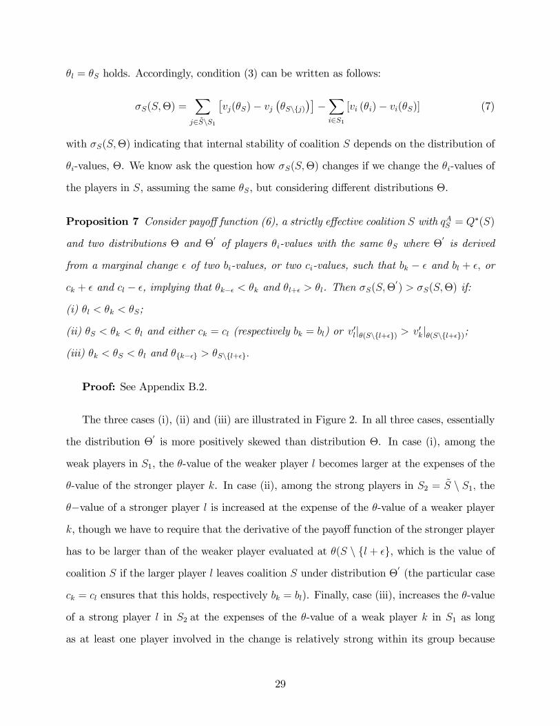
Proposition 7 Consider payoff function (6), a strictly effective coalition S with qAS = Q∗(S)

and two distributions Θ and Θ′of players θi-values with the same θS where Θ

′is derived

from a marginal change ε of two bi-values, or two ci-values, such that bk − ε and bl + ε, or

ck + ε and cl − ε, implying that θk−ε < θk and θl+ε > θl. Then σS(S,Θ′) > σS(S,Θ) if:

(i) θl < θk < θS;

(ii) θS < θk < θl and either ck = cl (respectively bk = bl) or v′l|θ(S\l+ε) > v′k|θ(S\l+ε);

(iii) θk < θS < θl and θk−ε > θS\l+ε.

Proof: See Appendix B.2.

The three cases (i), (ii) and (iii) are illustrated in Figure 2. In all three cases, essentially

the distribution Θ′is more positively skewed than distribution Θ. In case (i), among the

weak players in S1, the θ-value of the weaker player l becomes larger at the expenses of the

θ-value of the stronger player k. In case (ii), among the strong players in S2 = S \ S1, the

θ−value of a stronger player l is increased at the expense of the θ-value of a weaker player

k, though we have to require that the derivative of the payoff function of the stronger player

has to be larger than of the weaker player evaluated at θ(S \ l + ε, which is the value of

coalition S if the larger player l leaves coalition S under distribution Θ′(the particular case

ck = cl ensures that this holds, respectively bk = bl). Finally, case (iii), increases the θ-value

of a strong player l in S2 at the expenses of the θ-value of a weak player k in S1 as long

as at least one player involved in the change is relatively strong within its group because

29

this ensures θk−ε > θS\l+ε, where θS\l+ε is the θ-value of coalition S if player l leaves

coalition S under distribution Θ′.

[Figure 2 about here]

Taking the three cases together, and noting that a distribution Θ′′can be generated

through a sequence of marginal changes as described in Proposition 7, starting from a distri-

bution Θ (with different θ-values), the "ideal" distribution Θ′′to support internal stability

has all small players with a similar θ-value and only one strong player with a θ-value as

distant as possible from θs.29 Clearly, such a continuous sequence of marginal changes makes

Θ′′as positively skewed as possible and hence fosters internal stability through an increase

in σS(S,Θ).

An alternative view arises when recalling that for symmetric players, all coalitions are

stable. In the context of payoff function (6), players do not need to be symmetric in such a

strict sense, all players just need to have the same θi-values, but they could differ in their bi-

and ci-values as long their ratios are equal. We denote a distribution with equal θi-values

ΘΨfor reference reason. Now, when moving to asymmetry, the "ideal" distribution in terms

of internal stability of a coalition S with #S-members, increases one player’s θ-value by

4θ and reduces the θ-value of all remaining players uniformly by 4θ/(#S − 1), choosing

the maximum 4θ subject to the condition that the average θ-value, θS, remains unchanged

and θi > 0 for all small players. Let us call such a distribution ΘAfor reference reason.

Moreover, let us note that we could also generate a kind of a mirror image distribution, ΘB,

being extremely negatively skewed where we increase all θ-values of all players uniformly by

4θ/(#S−1) at the expenses of one player with −4 θ, again maximizing 4θ, subject to θS

remaining unchanged and θi > 0 of the small player. In terms of internal stability, ΘBwould

be a "bad" distribution. Finally, we could think of generating a symmetric distribution, like

29If the initial distribution has only one player in S2, case (ii) becomes irrelevant (and hence conditionv′l|S\l+ε > v′k|S\l+εis not binding). If there is more than one player initially in S2, the ideal changesimply to increase the θ-value of the strongest player in S2 (as long as it also has the largest v′l|S\l+ε) and tobring all the other players in S2 as close as possible to the average θ-value, i.e. θS , to make them "irrelevant"(as they are indifferent between the coalition and their autarky level). Finally, note that having all smallplayers with a similar θ-value and only one strong player generally implies θk−ε > θS\l+ε.

30

a normal or uniform distribution, which may call ΘΩ. Then, in terms of internal stability,

we could rank these distributions as follows: ΘΨ> Θ

A> Θ

Ω> Θ

Bby applying Proposition

7. Hence, if players have a different benefit-cost ratio, and provided an optimal transfer

scheme is employed to balance asymmetric payoffs, it is not so conducive for stability if all

signatories’θi-values are symmetrically distributed. It is much better if all coalition members

have a similar cost-benefit ratio except one player. This ensures that there is no weakest-link

outlier at the bottom and one very strong player with a benefit-cost ratio far above all other

signatories who compensates all other signatories for participating in cooperation.

Interestingly, from an economic point view the conclusion is quite different. Let us define

the gain from cooperation as the difference between the aggregate welfare if coalition S forms

and the aggregate welfare if all players act as singletons. We know from Proposition 3 that

for symmetric players, requiring here only that all θi-values are the same, i.e. distribution

ΘΨ, the gains from cooperation are zero. Now one can analyze the question how this welfare

gain compares across the three alternative distributions which we have defined above and

find the following.

Proposition 8 Consider payoff function (6), a strictly effective coalition S with qAS = Q∗(S)

and the four distributions defined above in the text: ΘΨ, Θ

Ω, Θ

Aand Θ

B, all with the same

θS. Let the stability function be given by σS(S,Θ) as defined in (7) and define the welfare

gain from cooperation for distribution Θ be given by

4W (S,Θ) =∑i∈N

vi(S,Θ)−∑i∈N

vi(i, j, z,Θ),

then we have:

(i) σS(S,ΘΨ

) ≥ 0; σS(S,ΘΨ

) > σS(S,ΘA) > σS(S,ΘΩ) > σS(S,ΘB);

(ii) 4W (S,ΘΨ

) = 0; 4W (S,ΘΨ

) < 4W (S,ΘA) < 4W (S,ΘΩ) < 4W (S,ΘB).

Proof. (i) follows from an application of Proposition 7 and (ii) follows from some basic

algebra.

31

Note that for all four distributions, welfare if coalition S forms,∑

i∈N vi(S,Θ), is the same.

In what distributions differ is the welfare if there is not cooperation,∑

i∈N vi(i, j, z,Θ).

The crucial point defining aggregate welfare is the value of the bottleneck country, θi, which

is the lowest under distribution ΘB and therefore leads to the lowest aggregate welfare under

no cooperation and hence the total gain from cooperation is the highest. Thus, the "paradox

of cooperation", a term coined by Barrett (1994) in the context of the summation technology,

also holds for the weakest-link technology: situations favoring stable cooperation are those

for which the gains from cooperation are modest.

4 Summary and Conclusion

In this paper, we have analyzed the canonical coalition formation model of international

environmental agreements (IEAs) under a weakest-link aggregation technology. This tech-

nology is relevant for a large bunch of important regional or global public goods, such as

fighting a fire which threatens several communities, compliance with minimum standards in

marine law, protecting species whose habitat cover several countries, compliance with tar-

gets for fiscal convergence in a monetary union, air-traffi c control or curbing the spread of

an epidemic.

The analysis of IEAs under the summation technology has typically been conducted

assuming identical players and highly specific functional forms (mainly the linear-quadratic

or the quadratic-quadratic payoff function). Moreover, very few papers analyzed the role of

asymmetric players and those are mainly based on simulations. Changing the focus of the

analysis to the weakest-link technology has proven fruitful, as we were able to establish a

large set of analytical results for general payoff functions (even the more restrictive functional

form assumed in Part IV was still far more general than the form used in previous game-

theoretic analyses of IEAs). Superadditivity or full cohesiveness are important features of a

game, which could generally be established for the weakest-link technology. In contrast , we

32

are unaware of an equivalent proof for the summation technology.

The analysis of the common assumption of symmetric players turned out to produce

rather trivial results for the weakest-link technology: policy coordination proved unnecessary

as all coalitions are stable and lead to the same Paret0 optimal outcome. Hence, the bulk

of the paper was devoted to the analysis of the role of asymmetric players. We showed

that without transfers, though all coalitions are Pareto-optimal, no coalition is stable which

departs from non-cooperative levels. However, if an optimal transfer is used to balance

asymmetries, a non-trivial coalition exists, associated with a provision level strictly above

the non-cooperative level. Furthermore, we showed the kind of asymmetry that is more

conducive to cooperation: a set of relatively similar weak players and one strong player.

This ensures that there is no weakest-link outlier at the bottom and one very strong player,

with a benefit-cost ratio far above all other signatories, who compensates all other signatories

for their contributions to cooperation. Unfortunately, this also implied that the "paradox

of cooperation" continues to hold for this technology: asymmetries which are conducive to

stability of coalitions yield low welfare gains from cooperation, and vice versa.

References

[1] Arce, M. (2001), Leadership and the aggregation of international collective action. Ox-

ford Economic Papers, vol. 53, pp. 114-137.

[2] Arce, M. and T. Sandler (2001), Transnational public goods: strategies and institutions.

European Journal of Political Economy, vol. 17, pp. 493—516.

[3] Barrett, S. (1994), Self-enforcing international environmental agreements. Oxford Eco-

nomic Papers, vol. 46, pp. 878-894.

[4] Barrett, S. (2002), Consensus Treaties. Journal of Institutional and Theoretical Eco-

nomics, vol. 158(4), pp. 529-547.

33

[5] Barrett, S. (2003), Environment and Statecraft: The Strategy of Environmental Treaty-

making. Oxford University Press, New York.

[6] Bergstrom, T.C., L. Blume and H. Varian (1986), On the private provision of public

goods. Journal of Public Economics, vol. 29, pp. 25—49.

[7] Bergstrom, T.C., L. Blume and H. Varian (1992), Uniqueness of Nash equilibrium in

private provision of public goods: an improved proof. Journal of Public Economics, vol.

49, pp. 391—392.

[8] Bloch, F. (2003), Non-Cooperative Models of Coalition Formation in Games with

Spillovers. In: Carraro, C. (ed.), The Endogenous Formation of Economic Coalitions.

Edward Elgar, Cheltenham, UK et al., ch. 2, pp. 35—79.

[9] Caparrós, A., E. Giraud-Héraud, A. Hammoudi, and T. Tazdaït (2011), Coalition sta-

bility with heterogeneous agents. Economics Bulletin, vol. 31(1), pp. 286-296.

[10] Carraro, C. and C. Marchiori (2003), Stable Coalitions. In: Carraro, C. (ed.), The

Endogenous Formation of Economic Coalitions. Edward Elgar, Cheltenham, UK et al.,

ch. 5, pp. 156-198.

[11] Carraro, C. and D. Siniscalco (1993), Strategies for the international protection of the

environment. Journal of Public Economics, vol. 52(3), pp. 309-328.

[12] Cornet, M.F. (1998), Game Theoretic Models of Bargaining and Externalities, Tinber-

gen Institute Research Series 176, Thesis Publishers, Amsterdam.

[13] Cornes, R.C. (1993), Dyke maintenance and other stories: some neglected types of

public goods. Quarterly Journal of Economics, vol. 107, pp. 259—271.

[14] Cornes, R.C. and R. Hartley (2007a), Weak links, good shots and other public good

games: building on BBV. Journal of Public Economics, vol. 91, pp. 1684-1707.

34

[15] Cornes, R.C. and R. Hartley (2007b), Aggregative public good games. Journal of Public

Economic Theory, vol. 9(2), pp. 201—219.

[16] Courtois, P. and G. Haeringer (2012), Environmental cooperation: ratifying second-best

agreements. Public Choice, vol. 151, pp. 565—584.

[17] d’Aspremont, C., A. Jacquemin, J. J. Gabszewicz and J. A. Weymark (1983), On the

stability of collusive price leadership, Canadian Journal of Economics, vol. 16(1), pp.

17—25.

[18] Diamantoudi, E. and E.S. Sartzetakis (2006), Stable international environmental agree-

ments: an analytical approach. Journal of Public Economic Theory, vol. 8(2), pp. 247-

263.

[19] Eyckmans, J. and M. Finus (2004), An Almost Ideal Sharing Scheme for Coalition

Games with Externalities. CLIMNEG Working Paper No. 62, University of Leuven

(K.U.L.), Belgium.

[20] Eyckmans, J., M. Finus and Lina Mallozzi (2012), A New Class of Welfare Maximiz-

ing Sharing Rules for Partition Function Games with Externalities. Bath Economics

Research Paper 6-2012.

[21] Finus, M. (2003), Stability and Design of International Environmental Agreements: The

Case of Global and Transboundary Pollution. In: Folmer, H. and T. Tietenberg (eds.),

International Yearbook of Environmental and Resource Economics 2003/4. Edward El-

gar, Cheltenham, UK et al., ch. 3, pp. 82-158.

[22] Finus, M. and S. Maus (2008), Modesty may pay! Journal of Public Economic Theory,

vol. 10(5), pp. 801-826.

[23] Finus, M. and D.T.G. Rübbelke (2013), Coalition formation and the ancillary benefits

of climate policy. Environmental and Resource Economics, vol. 56, pp. 211-222.

35

[24] Finus, M. and B. Rundshagen (2003), Endogenous Coalition Formation in Global Pol-

lution Control: A Partition Function Approach. In: Carraro, C. (ed.), The Endogenous

Formation of Economic Coalitions. Edward Elgar, Cheltenham, UK et al., ch. 6, pp.

199-243.

[25] Finus, M. and B. Rundshagen (2006), Participation in international environmental

agreements: the role of timing and regulation. Natural Resource Modeling, vol. 19(2),

pp. 165-200.

[26] Finus, M. and B. Rundshagen (2009), Membership rules and stability of coalition struc-

tures in positive externality games. Social Choice and Welfare, vol. 32, pp. 389-406.

[27] Finus, M. R. Schneider and P. Pintassilgo (2011), The Incentive Structure of Impure

Public Good Provision: The Case of International Fisheries. Working Paper 11/03,

University of Exeter, UK.

[28] Fraser, C.D. (1992), The uniqueness of Nash equilibrium in the private provision of

public goods: an alternative proof. Journal of Public Economics, vol. 49, pp. 389—390.

[29] Fuentes-Albero, C. and S.J. Rubio (2010), Can international environmental cooperation

be bought? European Journal of Operational Research, vol. 202, 255—264.

[30] Hirshleifer, J. (1983), From weakest-link to best-shot: The voluntary provision of public

goods, Public Choice, vol. 41, 371-386.

[31] Holzinger, K. (2001), Aggregation technology of common goods and its strategic conse-

quences: Global warming, biodiversity and siting conflicts. European Journal of Political

Research, vol. 40, pp. 117-138

[32] Hoel, M. (1992), International environment conventions: the case of uniform reductions

of emissions. Environmental and Resource Economics, vol. 2(2), pp. 141-159.

36

[33] Hong, F. and L. Karp (2013), International Environmental Agreements with Exogenous

and Endogenous Risk. Mimeo.

[34] I. Kaul and R. U. Mendoza (2003), Advancing the Concept of Public Goods. In: Kaul, I.

(ed), Providing Global Public Goods: Managing Globalization, Oxford University Press,

Oxford, UK.

[35] K.-G. Mäler (1994), Acid Rain in Europe: a Dynamic Perspective on the Use of Eco-

nomic Incentives. In: H. Folmer and E. van Ierland (eds.), International Environmental

Economics, Elsevier, Amsterdam, The Netherlands.

[36] McGinty, M. (2007), International environmental agreements among asymmetric na-

tions, Oxford Economic Papers, vol. 59, 45—62.

[37] Montero, M. (2006), Coalition Formation in Games with Externalities, mimeo, Univer-

sity of Nottingham, School of Economics.

[38] Weikard, H.-P. (2009), Cartel stability under an optimal sharing rule, Manchester

School, vol. 77(5), 575—593.

[39] Ray, D. and R. Vohra (2001), Coalitional power and public goods. Journal of Political

Economy, vol. 109(6), pp. 1355-1384.

[40] Rubio, S.J. and A. Ulph (2006), Self-enforcing international environmental agreements

revisited. Oxford Economic Papers, vol. 58(2), pp. 233-263.

[41] Sandler, T. (1998), Global and regional public goods: a prognosis for collective action,

Fiscal Studies, vol. 19, pp. 221-247.

[42] Sandler, T. (2006), Regional public goods and international organizations. Review of

International Organizations, vol. 1, p. 5-25.

[43] Sandler, T. and D. Arce (2002), A conceptual framework for understanding global and

transnational public goods for health, Fiscal Studies, vol. 23(2), pp. 195-222.

37

[44] Sandler, T. and D. Arce (2003), Pure public goods versus commons: benefit-cost duality,

Land Economics vol. 79, pp. 355-368 (2003)

[45] Vicary, S. (1990), Transfers and the weakest link: an extension of Hirshleifer’s analysis.

Journal of Public Economics, vol. 43, pp. 375—394.

[46] Vicary, S. and T. Sandler (2002), Weakest-link public goods: giving in-kind or transfer-

ring money. European Economic Review, vol. 46, pp. 1501—1520.

[47] Yi, S.-S. (1997), Stable coalition structures with externalities. Games and Economic

Behavior, vol. 20(2), pp. 201-237.

A Summation Technology: Results and Proofs

To be written.

B Weakest-Link Technology: Proofs

B.1 Lemma 4

The first order conditions in an interior equilibrium are c∂C∂q

= b∂B∂qwhere b =

∑i∈S bi and

c =∑

i∈S ci. Thus, we can define functions f and h as follows:

f(q) =C ′(q)

B′(q)=b

c=b

c= θS ,

qAS = f−1 (θS) = h (θS) .

38

To show that h is strictly concave and strictly increasing, we show that f is strictly increasing

and strictly convex:

∂f(q)

∂q=

B′(q)C ′′(q)− C ′(q)B′′(q)(B′(q))2 > 0 ,

∂2f (q)

∂q∂q=

C ′′′(q) (B′(q))2 + 2C ′(q) (B′′(q))2 − 2C ′′(q)B′(q)B′′(q)− C ′(q)B′(q)B′′′(q)(B′(q))3 > 0

which is true due to the assumptions about the first and second derivatives summarized

in Assumption 1 and the assumptions about the third derivatives mentioned in section 3.4,

namely, C ′′′ ≥ 0 and B′′′ ≤ 0 (or if B′′′ > 0, B′′′(q) < −2B′′(q)C ′′(q)/C ′(q)).

B.2 Proposition 7

Before proving the proposition itself, we proof a lemma that is useful for the subsequent

analysis.

Lemma 5 The function ki (θ) = vi(h(θ)) is strictly concave and increasing in θ, θ ∈ [0, θAi ].

Proof. k′i (θ) = v′i(h(θ))h′(θ) is increasing if v′i(h(θ)) = ∂v(q)∂q

> 0, as we have shown in

Lemma 4 that h(θ) is strictly concave and increasing and we thus have h′(θ) > 0. Due to

Assumption 1, v is a strictly concave function with respect to qi that has its maximum at

qAi = h(θAi ), and it is therefore increasing for qi ∈ [0, qAi ]. As h(θi) is increasing everywhere

we also know that vi(h(θi)) is increasing for θi ∈ [0, θAi ] because for any θi ∈ [0, θAi ] we know

that qi = h(θi) ≤ qAi . Thus, we have v′i(h(θ)) = ∂v(q)

∂q> 0.

For k to be strictly concave, we need:

k′′ (θ) = v′′(h(θ)) (h′(θ))2

+ v′(h(θ))h′′(θ) < 0. (B.1)

We have just shown that v′i(h(θ)) = ∂v(q)∂q

> 0 in θi ∈ [0, θAi ], and by the strict concavity of

v with respect to q = h(θ), due to Assumption 1, and that of h with respect to θ, shown in

in Lemma 4, we know v′′(h(θ)) < 0 and h′′(θ) < 0. Hence, k′′ (θ) < 0 and k (θ) is strictly

concave.

39

We now proceed to proof Proposition (7). After the marginal changes in the distribution

mentioned in the Proposition, bk becomes bk−ε and bl becomes bl+ε (respectively ck becomes

ck + ε and cl becomes cl − ε). These changes do not affect θS =∑

i∈S bi/∑

i∈S ci. Focusing

on the case where the b values change, the three possibilities to be considered are:

(i) θl < θk < θS. As both players are part of S1, the third sum in σS(θ), see equation (2) in

the main text, remains unchanged. In the first sum in σS(θ), θS remains unchanged but the

valuation function has changed for players k and l. We denote the new valuation function

by vMj . However, the aggregate value of the first sum in σS(θ) has not changed because

vk (θS) + vl (θS) = vMk (θS) + vMl (θS) as

bkB(h(θS))− ckC(h(θS)) + blB(h(θS))− clC(h(θS))

= (bk − ε)B(h(θS))− ckC(h(θS)) + (bl + ε)B(h(θS))− clC(h(θS).

Thus, only the second sum of σS(θ) has changed, and to have σS(θ) < σS(θM), we need

∑i∈S1

vi (θi) >∑i∈S1

vMi(θMi)

or, as as nothing has changed for the remaining players (slightly abusing notation by denoting

θk−ε and θl+ε the two values that have changed in θM):

vk (θk) + vl (θl) > vMk(θk−ε

)+ vMl

(θl+ε

)or

[bkB(h(θk))− ckC(h(θk))]−[bkB(h(θk−ε))− ckC(h(θk−ε))

](B.2)

+ε[B(h(θk−ε))−B(h(θl+ε)

]>

[blB(h(θl+ε))− clC(h(θl+ε)

]− [blB(h(θl))− clC(h(θl))] .

40

Recalling the definition of derivatives, dividing both sides by ε and taking the limit ε → 0,

equation (B.2) becomes:

[B(h(θk−ε))−B(h(θl+ε)

]+ v′k (θ)|θk−ε ≥ v′l (θ)|θl . (B.3)

For ε → 0, θk > θl implies θk−ε > θl+ε and therefore the first term on the L.H.S of (B.3) is

positive. Thus, (B.3) always holds as we have v′k (θ)|θk−ε & v′k (θ)|θk = 0 and v′l (θ)|θl = 0,

given that θk−ε < θk, θk and θl maximize vk and vl, respectively, and vi(θ) is an increasing

and strictly concave function for θ ∈ [0, θAi ] by Lemma (5).

(ii) θS < θk < θl. Both players are part of S \ S1 and as there is no change for the players

in S1, the second sum in σS(θ) remains unchanged. In the first sum in σS(θ), θS remains

unchanged but the valuation function has changed for players k and l. However, as before,

the aggregate value has not changed. Thus, only the third sum in σS(θ) has changed, and

to have σS(θ) < σS(θM) we need:

∑j∈S\S1

vj(θS\j

)>∑

j∈S\S1

vMj(θMS\j

)or

[blB(h(θS\l))− clC(h(θS\l))

]−[blB(h(θS\l+ε))− clC(h(θS\l+ε)

](B.4)

+ε[B(h(θS−k−ε))−B(h(θS\l+ε)

]>

[bkB(h(θS−k−ε))− ckC(h(θS−k−ε))

]−[bkB(h(θS\k))− ckC(h(θS\k))

].

Noting that θS\l+ε < θS\l and θS\k < θS−k−ε, we have that θS\l+ε < θS−k−ε and the

third term on the L.H.S. of (B.4) is positive. Thus, a suffi cient condition for this to hold is:

[blB(h(θS\l))− clC(h(θS\l))

]−[blB(h(θS\l+ε))− clC(h(θS\l+ε)

]>

[bkB(h(θS−k−ε))− ckC(h(θS−k−ε))

]−[bkB(h(θS\k))− ckC(h(θS\k))

]

41

and dividing both sides by ε and taking the limit ε→ 0 this becomes:

v′l (θ)|S\l+ε > v′k (θ)|S\k . (B.5)

As we have

v′j (θ) = v′j(h(θ))h′(θ) = [bjB′(h(θ))− cjC ′(h(θ))]h′(θ) > 0

equation (B.5) can be written as:

[blB

′(h(θS\l+ε))− clC ′(h(θS\l+ε))]h′(θS\l+ε) >

[bkB

′(h(θS\k))− ckC ′(h(θS\k))]h′(θS\k).

As θl > θk, we also know that if cl = ck (or, alternatively, if v′l (θ)|S\l+ε > v′k (θ)|S\l+ε)

[blB

′(h(θS\l+ε))− clC ′(h(θS\l+ε))]h′(θS\l+ε) >

[bkB

′(h(θS\l+ε))− ckC ′(h(θS\l+ε))]h′(θS\l+ε).

Hence, a suffi cient condition for (B.5) to hold is

[bkB

′(h(θS\l+ε))− ckC ′(h(θS\l+ε))]h′(θS\l+ε) >

[bkB

′(h(θS\k))− ckC ′(h(θS\k))]h′(θS\k)

or

v′k (θ)|S\l+ε > v′k (θ)|S\k .

And this holds, with θS\l+ε < θS\k < θAk , as vk(θ) is an increasing and strictly concave

function for θ ∈ [0, θAi ] by Lemma (5).

(iii) θk < θS < θl. Player k belongs to S1 and player l to S \ S1. As before, the aggregate

value of the first sum in σS(θ) remains unchanged. Hence, to have σS(θ) < σS(θM), we need:

∑i∈S1

vi (θi) +∑

j∈S\S1

vj(θS\j

)>∑i∈S1

vMi(θMi)

+∑

j∈S\S1

vMj(θMS\j

)or, as as nothing has changed for the remaining players:

[blB(h(θS\l))− clC(h(θS\l))

]−[blB(h(θS\l+ε))− clC(h(θS\l+ε)

](B.6)

+ε[B(h(θk−ε))−B(h(θS\l+ε)

]>

[bkB(h(θk−ε))− ckC(h(θk−ε))

]− [bkB(h(θk))− ckC(h(θk))] .

42

If θk−ε > θS\l+ε, the third term on the L.H.S. in (B.6) is positive and a suffi cient condition

for (B.6) to hold is:

[blB(h(θS\l))− clC(h(θS\l))

]−[blB(h(θS\l+ε))− clC(h(θS\l+ε)

]+ [bkB(h(θk))− ckC(h(θk))]−

[bkB(h(θk−ε))− ckC(h(θk−ε))

]> 0 .

Noting that θS\l+ε < θS\l, dividing both sides by ε and taking the limit ε→ 0, this becomes:

v′l (θ)|S\l+ε + v′k (θ)|k−ε > 0 .

And this holds, with θS\l+ε < θAl and θk−ε < θAk , as vi(θ) is an increasing and strictly

concave function for θ ∈ [0, θAi ] by Lemma (5).

43

Figure 1: Replacement Functions and Equilibria for the Weakest-link Technology

Q

45º

Figure 2: Illustration of Proposition 7

θS θk θk-ε θl θl+ε

(i)

(ii)

θS θk θk-ε θl θl+ε

θS θk θk-ε θl θl+ε

(iii)

θS\l+ε