
Charming New Physics in Beautiful Processes?
250
Charming New Physics in Beautiful Processes? Matthew John Kirk A Thesis presented for the degree of Doctor of Philosophy Institute for Particle Physics Phenomenology Department of Physics Durham University United Kingdom August 2018
-
Upload
khangminh22 -
Category
Documents
-
view
0 -
download
0
Transcript of Charming New Physics in Beautiful Processes?

Charming New Physics inBeautiful Processes?
Matthew John Kirk
A Thesis presented for the degree ofDoctor of Philosophy
Institute for Particle Physics PhenomenologyDepartment of PhysicsDurham UniversityUnited Kingdom
August 2018


Charming New Physics inBeautiful Processes?
Matthew John Kirk
Submitted for the degree of Doctor of PhilosophyAugust 2018
Abstract: In this thesis we study quark flavour physics and in particular observablesrelating to B meson mixing and lifetimes. Meson mixing arises due to the natureof the weak interaction, and leads to several related observables that are highlysuppressed in the Standard Model (SM). Alongside meson mixing, lifetimes providean insight into rare B processes which can shed light on possible new physics.
Both calculations are based on an Effective Field Theory (EFT) framework, inparticular the Weak Effective Theory. This framework allows us to separate the highscale effects which are calculable in perturbation theory from the low energy matrixelement which are determined through other means. Within this framework, theobservables are expanded using the Heavy Quark Expansion (HQE) technique, whichutilises the relatively large masses of b and c quarks to reveal a further hierarchyof corrections. The basics of EFTs and the HQE are explored in detail as an entrypoint to the majority of the work in this thesis.
In the rest of the thesis, we take aim at pushing the accuracy of our SM predictionsfurther: by testing the underlying assumption of Quark-Hadron duality in the HQE;by studying possible new physics models that can explain the long standing problemof dark matter as well as recently seen anomalies; and by using alternative approachesto determining the low energy constants associated with mixing and lifetimes in orderto provide independent and state-of-the-art results.


Contents
Declaration 11
Acknowledgements 13
1 Introduction 15
1.1 The Standard Model . . . . . . . . . . . . . . . . . . 15
1.1.1 QCD . . . . . . . . . . . . . . . . . . . . . 16
1.1.2 Electroweak Theory and the Higgs Mechanism . . . . . 17
1.2 Flavour . . . . . . . . . . . . . . . . . . . . . . 19
1.2.1 CKM . . . . . . . . . . . . . . . . . . . . . 20
1.2.2 CP Violation . . . . . . . . . . . . . . . . . . 22
1.3 Beyond the Standard Model? . . . . . . . . . . . . . . 23
1.3.1 Dark Matter . . . . . . . . . . . . . . . . . . 24
1.3.2 Matter-Antimatter Asymmetry . . . . . . . . . . . 27
1.3.3 Neutrino Masses . . . . . . . . . . . . . . . . 29
1.3.4 Flavour Anomalies . . . . . . . . . . . . . . . . 30
1.4 Remainder of the thesis . . . . . . . . . . . . . . . . . 31
2 Theoretical Tools 33
2.1 Effective Field Theories . . . . . . . . . . . . . . . . . 33
2.2 Heavy Quark Expansion . . . . . . . . . . . . . . . . 34
2.3 Heavy Quark Effective Theory . . . . . . . . . . . . . . 36
2.4 Example calculations . . . . . . . . . . . . . . . . . 38
2.4.1 Matching and RG running . . . . . . . . . . . . . 38
2.4.2 Bs mixing . . . . . . . . . . . . . . . . . . . 47
2.5 B mixing observables . . . . . . . . . . . . . . . . . 53

6 Contents
3 Quark-Hadron Duality 55
3.1 Introduction . . . . . . . . . . . . . . . . . . . . . 55
3.2 Duality violation . . . . . . . . . . . . . . . . . . . 56
3.2.1 B mixing . . . . . . . . . . . . . . . . . . . 60
3.2.2 Duality bounds from lifetime ratios . . . . . . . . . . 66
3.3 Numerical Updates of Standard Model Predictions . . . . . . . 70
3.4 D mixing . . . . . . . . . . . . . . . . . . . . . . 74
3.5 Summary . . . . . . . . . . . . . . . . . . . . . . 78
4 Charming Dark Matter 81
4.1 Introduction . . . . . . . . . . . . . . . . . . . . . 81
4.1.1 The DMFV Model . . . . . . . . . . . . . . . . 84
4.2 Relic Density . . . . . . . . . . . . . . . . . . . . 86
4.2.1 Relic Density with coannihilations . . . . . . . . . . 86
4.2.2 The Generation of Mass Splitting . . . . . . . . . . 87
4.3 Flavour Constraints . . . . . . . . . . . . . . . . . . 88
4.3.1 Mixing Observables . . . . . . . . . . . . . . . 88
4.3.2 Rare Decays . . . . . . . . . . . . . . . . . . 89
4.4 Direct Detection Constraints . . . . . . . . . . . . . . . 91
4.5 Indirect Detection Constraints . . . . . . . . . . . . . . 94
4.5.1 Basics of Indirect Detection . . . . . . . . . . . . 94
4.5.2 Gamma rays (and other mono-chromatic lines) . . . . . 96
4.6 Collider Constraints . . . . . . . . . . . . . . . . . . 97
4.6.1 EFT Limit . . . . . . . . . . . . . . . . . . . 98
4.6.2 LHC bounds . . . . . . . . . . . . . . . . . . 98
4.6.3 Collider Constraints within DMFV . . . . . . . . . . 102
4.7 Results . . . . . . . . . . . . . . . . . . . . . . . 104
4.7.1 Constrained Scenarios . . . . . . . . . . . . . . 109
4.8 Summary . . . . . . . . . . . . . . . . . . . . . . 115

Contents 7
5 Charming new physics in rare Bs decays and mixing? 117
5.1 Introduction . . . . . . . . . . . . . . . . . . . . . 1175.2 Charming new physics scenario . . . . . . . . . . . . . . 1185.3 Rare B decays . . . . . . . . . . . . . . . . . . . . 1195.4 Mixing and lifetime observables . . . . . . . . . . . . . . 1205.5 Rare decays versus lifetimes – low-scale scenario . . . . . . . 1225.6 High-scale scenario and RGE . . . . . . . . . . . . . . . 123
5.6.1 RG enhancement of ∆Ceff9 . . . . . . . . . . . . . 123
5.6.2 Phenomenology for high NP scale . . . . . . . . . . 1245.6.3 Implications for UV physics . . . . . . . . . . . . 126
5.7 Prospects and summary . . . . . . . . . . . . . . . . 127
6 Dimension-six matrix elements from sum rules 129
6.1 Introduction . . . . . . . . . . . . . . . . . . . . . 1296.2 QCD-HQET matching for ∆B = 2 operators . . . . . . . . . 131
6.2.1 Setup . . . . . . . . . . . . . . . . . . . . 1316.2.2 Results . . . . . . . . . . . . . . . . . . . . 1336.2.3 Matching of QCD and HQET bag parameters . . . . . . 134
6.3 HQET sum rule . . . . . . . . . . . . . . . . . . . 1366.3.1 The sum rule . . . . . . . . . . . . . . . . . . 1366.3.2 Spectral functions at NLO . . . . . . . . . . . . . 1376.3.3 Sum rule for the bag parameters . . . . . . . . . . . 139
6.4 Results for ∆B = 2 operators . . . . . . . . . . . . . . 1426.4.1 Details of the analysis . . . . . . . . . . . . . . 1426.4.2 Results and comparison . . . . . . . . . . . . . . 1446.4.3 Bs and Bd mixing observables . . . . . . . . . . . . 146
6.5 ∆B = 0 operators and ratios of B meson lifetimes . . . . . . . 1486.5.1 Operators and matrix elements . . . . . . . . . . . 1486.5.2 Results for the spectral functions and bag parameters . . . 1496.5.3 Results for the lifetime ratios . . . . . . . . . . . . 152
6.6 Matrix elements for charm and the D+ − D0 lifetime ratio . . . . 1546.6.1 Matrix elements for D mixing . . . . . . . . . . . . 1546.6.2 Matrix elements for D lifetimes and τ(D+)/τ(D0 ) . . . . 156
6.7 Summary . . . . . . . . . . . . . . . . . . . . . . 157

8 Contents
7 One constraint to kill them all? 161
7.1 Introduction . . . . . . . . . . . . . . . . . . . . . 161
7.2 Bs mixing in the SM . . . . . . . . . . . . . . . . . . 161
7.3 Bs mixing beyond the SM . . . . . . . . . . . . . . . . 163
7.3.1 Impact of Bs mixing on NP models for B-anomalies . . . . 164
7.3.2 Model building directions for ∆MNPs < 0 . . . . . . . . 169
7.4 Summary . . . . . . . . . . . . . . . . . . . . . . 171
8 Conclusions 173
A Fierz transformations 181
B Feynman Rules 183
C Four Quark Matrix Elements 185
D Additional information from “Quark-Hadron Duality” 189
D.1 Inputs and detailed view of uncertainties . . . . . . . . . . 190
D.2 Proof of ∆Γ ≤ 2|Γ12| . . . . . . . . . . . . . . . . . . 195
E Additional information from “Charming Dark Matter” 197
E.1 Rare decays . . . . . . . . . . . . . . . . . . . . . 197
E.2 Direct Detection . . . . . . . . . . . . . . . . . . . 198
E.2.1 LUX . . . . . . . . . . . . . . . . . . . . . 198
E.2.2 CDMSlite . . . . . . . . . . . . . . . . . . . 199
E.3 Feynman Diagrams for collider searches . . . . . . . . . . . 199
E.3.1 Monojet processes . . . . . . . . . . . . . . . . 199
E.3.2 Dijet processes . . . . . . . . . . . . . . . . . 201
F Additional information from “Charming new physics in rare Bs
decays and mixing?” 203

Contents 9
G Additional information from “Dimension-six matrix elements fromsum rules” 205
G.1 Basis of evanescent operators and ADMs . . . . . . . . . . 206
G.1.1 ∆B = 2 operators . . . . . . . . . . . . . . . . 206
G.1.2 ∆B = 0 operators . . . . . . . . . . . . . . . . 208
G.2 Inputs and detailed overview of uncertainties . . . . . . . . . 209
H Additional information from “One constraint to kill them all?” 213
H.1 Numerical input for theory predictions . . . . . . . . . . . 213
H.2 Error budget of the theory predictions . . . . . . . . . . . 213
H.3 Non-perturbative inputs . . . . . . . . . . . . . . . . 215
H.4 CKM-dependence . . . . . . . . . . . . . . . . . . . 216
Bibliography 219


Declaration
The work in this thesis is based on research carried out in the Institute for ParticlePhysics Phenomenology at Durham University. No part of this thesis has beensubmitted elsewhere for any degree or qualification. This thesis is partly based onjoint research as noted below.
• Chapter 3 is based on the article “On the Ultimate Precision of Meson MixingObservables” published in Nuclear Physics B [1].
• Chapter 4 is based on the article “Charming Dark Matter” published in theJournal of High Energy Physics [2].
• Chapter 5 is based on the article “Charming new physics in rare B decays andmixing?” published in Physical Review D [3].
• Chapter 6 is based on the article “Dimension-six matrix elements for mesonmixing and lifetimes from sum rules” published in the Journal of High EnergyPhysics [4].
• Chapter 7 is based on the article “One constraint to kill them all?” published(as “Updated Bs-mixing constraints on new physics models for b → s`+`−”) inPhysical Review D [5].
Copyright © 2018 Matthew John Kirk.The copyright of this thesis rests with the author. No quotation from it should bepublished without the author’s prior written consent and information derived fromit should be acknowledged.


Acknowledgements
I would like to thank my supervisor Alex Lenz, for his expert guidance, advice, andsupport throughout my PhD, without which I would not have reached this stage.He has been an invaluable guide in the world of flavour physics, and he has been anoutstanding supervisor over the last four years.
I must also thank the IPPP for offering me the chance to continue studying thesubject I love, and STFC for the funding that enabled me to do so.
Throughout my PhD, my work has been done in collaboration with others and so Imust extend my thanks to Gilberto Tetlalmatzi Xolocotzi, Thomas Jubb, SebastianJäger, Kirsty Leslie, Thomas Rauh, and Luca Di Luzio for being enjoyable to workwith. Along with Alex, they have helped shape this thesis. I must also single out andthank Alex, Rachael, Danny, Andrew, Jonny, and Duncan for agreeing to proofreadparts of this thesis, large or small.
Over my time in Durham, my fellow students at the IPPP (and in particular myoffice mates past and present) have made it a joy to come to work everyday. Whilethe atmosphere of the office has changed over the last three years, it has always beengreat. I make my apologies to those in other offices (particularly OC118) who havebeen subjected to my bored wanderings.
Beyond work, I cannot begin to describe in this short space how much I have enjoyedmy time as part of Grey MCR. It has shaped me, and made these last few yearssome of the best of my life. It has been a pleasure and a privilege to be a part of theamazing community at Grey, both on the MCR Exec and otherwise – I hope I have,in one way or another, conveyed this to everybody I have met here. I cannot nameyou all, but I feel I must pick out and thank a few individually. Bear: for everythingfrom your passing suggestion of dinner to our many hours of gaming. Darren: forthe sheer joy physics inspires in you 24 hours a day, your mad banter, and the manyhelpful conversations. Sarah: for being such an amazing friend. And Rachael: forthese last ten months.
Finally of course, my parents, for supporting me my entire life.


Chapter 1
Introduction
Particle physics can be described as the area of physics which concerns itself withdescribing the fundamental building blocks of the universe. Its aim is no less loftythan the construction of a model that can, with minimal input, generate correctpredictions for the interactions on the smallest scales, and allow us to build upphysical laws we can use to describe our world. Our current best working modelof this type is known as the Standard Model (SM) – the nature of the SM willbe described in the rest of this chapter, alongside a brief historical overview of itsconstruction. Finding ways to clearly test the SM and probe possible extensions toit is the work which the remainder of this thesis consists of.
1.1 The Standard Model
The SM, as a complete theory, has been developed over an extended period oftime. The start of the journey could well be considered to be the development ofQuantum Electrodynamics (QED) over several decades, from Dirac [6] to Tomon-aga [7], Schwinger [8, 9], Feynman [10–12], and many others. The other majorconstituent parts of the SM were developed in the 1960s and 1970s – the Brout-Englert-Higgs (BEH) mechanism [13–15]; the unified theory of electroweak interac-tions by Glashow [16], Weinberg [17], and Salam [18]; the Quantum Chromodynamics(QCD) Lagrangian by Fritzsch, Gell-Mann, and Leutwyler [19], and the nature ofasymptotic freedom in QCD by Gross and Wilczek [20], and Politzer [21].
The SM is formulated as a quantum field theory (QFT) – the dynamics of thetheory are characterised by the Lagrangian density LSM.1 The SM Lagrangian can
1Typically referred to as just the Lagrangian, which we will do from here on out.

16 Chapter 1. Introduction
Field SU(3)c SU(2)L U(1)YQL 3 2 1/6uR 3 1 2/3dR 3 1 −1/3LL 1 2 −1/2eR 1 1 −1H 1 2 1/2
Table 1.1: Field content of the SM.
be written rather succinctly in the form1
LSM =− 14FµνF
µν
+ iψ /Dψ
+ ψiyijψjH + h.c.+ |DµH |2 − V (H ) ,
(1.1.1)
where successive lines describe, respectively, the kinetic and self-interactions ofgauge fields; the kinetic terms of fermions and their interaction with gauge fields; theinteractions of the fermions with the Higgs field; and the kinetic and self-interactionsof the Higgs field. The SM is a gauge theory, with the Lagrangian having a SU(3)c×SU(2)L × U(1)Y gauge symmetry. It is also Lorentz invariant, as is required tobe consistent with special relativity. The power of symmetries can be appreciatedhere – given we want a renormalisable theory which has SU(3)c × SU(2)L × U(1)Ygauge symmetries, SO(1, 3) Lorentz symmetry, and the field content in Table 1.1,Equation 1.1.1 is the only possible Lagrangian we can write.2
In the next two sections, we will break the SM Lagrangian down differently to showthe different gauge groups and their properties.
1.1.1 QCD
QCD is a non-abelian gauge theory, meaning the generators of the symmetry don’tcommute. The symmetry is SU(3)c, where the subscript stands for colour – the labelwe use for the gauge charges of QCD. Quarks live in the fundamental representationof SU(3), while gluons live in the adjoint (from which we need only take that thereare three colours of quarks, but eight colours of gluon).
1Available on t-shirts, mugs, etc. from all good gift shops.2The issue of a possible right handed neutrino νR, which could in principle be added, is briefly
discussed later in Section 1.3.3.

1.1. The Standard Model 17
Singling out the pure QCD parts of Equation 1.1.1, we have two relatively simpleparts: the QCD gauge field tensor and the covariant derivative that couples quarksto the gluon field. The gauge field tensor in QCD can be written as
Gaµν = ∂µG
aν − ∂νGa
µ + gsfabcGb
µGcν ,
where Ga is a gluon field, gs is the coupling constant of QCD (also called the strongcoupling constant), and fabc is the antisymmetric structure constant of SU(3). Thecovariant derivative for QCD, acting on quarks which exist in the fundamentalrepresentation of SU(3), is
(Dµ)ij = ∂µδij − igsGaµtaij , (1.1.2)
where ta are the generators of SU(3) which obey the following useful relations:
taijtajk = CF δij ≡
N2c − 12Nc
δij ,
taijtakl = 1
2
(δilδkj −
1Nc
δijδkl
).
(The second result can be thought of as a Fierz relation in colour space, see Ap-pendix A for details.)
1.1.2 Electroweak Theory and the Higgs Mechanism
The other half of the SM is the electroweak sector – the unification of the weakand electromagnetic interactions into a SU(2)L × U(1)Y gauge group, where thesubscript L stands for left and the subscript Y for weak hypercharge. The respectivegauge field strengths are
W aµν = ∂µW
aν − ∂νW a
µ + gεabcW bµW
cν ,
where εabc is the standard three dimensional Levi-Civita tensor, and
Bµν = ∂µBν − ∂νBµ .
The SU(2) group is labelled left as the electroweak sector explicitly distinguishesbetween left and right chiralities – left handed fermions sit in the doublet repre-sentation of SU(2), while right handed fermions are SU(2) singlets; and as seenin Table 1.1 the left and right handed fields have different charges under the U(1)group. This makes the SM a parity violating theory – we will discuss this more inSections 1.2.2 and 1.3.2.

18 Chapter 1. Introduction
Since the different chiralities sit in different representations of the group, the covariantderivative acts differently on them – for left handed particles, it takes the form
Dµ = ∂µ − igW aµ
σa
2 − ig′YLBµ , (1.1.3)
where σa are the Pauli matrices, while for right handed particles only the weakhypercharge field acts and it takes the form
Dµ = ∂µ − ig′YRBµ , (1.1.4)
and we have explicitly distinguished the weak hypercharge YL,R for left and righthanded fields to remind the reader that they are not equal. The chiral nature of theelectroweak theory means that a standard Dirac mass term like mψLψR cannot besimply included, as the left and right handed fields transform differently under thegauge symmetry. Mass terms for the vector bosons W a
µ and Bµ, like M2V VµV
µ, arealso not gauge invariant; and yet we know the W and Z bosons are definitely notmassless. The resolution of both these problems is the BEH mechanism [13–15]. Byadding a complex scalar field with a particularly shaped potential, we can arrangefor the field to acquire a vacuum expectation value (VEV), spontaneously breakingthe symmetry obeyed by the SM Lagrangian down to SU(3)c × U(1)EM.
A form of potential that achieves our aims is
V (H ) = −µ2(H †H ) + λ(H †H )2 ,
with µ2, λ > 0 – often known as the “Mexican hat” potential. It is easily seen thatwith those choices for the sign of the Higgs potential parameters, the field has aminimum at
|H | = v, where v =õ2
2λ 6= 0 and has dimensions of mass .
The non-zero VEV breaks the electroweak symmetry SU(2)L × U(1)Y down toU(1)EM, i.e. just the symmetry associated with the conservation of electric charge.After symmetry breaking we can, in the unitary gauge, write the Higgs doublet inthe form
H = 1√2
0v + h
, (1.1.5)
where h is the field associated with the Higgs boson. In this form, it is moststraightforward to see the origin of the fermion and gauge boson mass terms. Weleave the discussion of the origin of fermion masses to Section 1.2.1 as this is a crucialpart of the broad spectrum of flavour phenomenology. For the gauge bosons, if weexpand the covariant derivative terms in the broken Higgs phase, we find terms with

1.2. Flavour 19
two gauge fields and factors of v, g, g′ as coefficients – these look exactly like gaugeboson mass terms. With this procedure we find mixed terms however, like v2W 3
µBµ.
If we diagonalise the mass matrix for the Bµ and W 3,µ fields, we find one masslesseigenstate and one massive eigenstate, which we will suggestively call Aµ and Zµ
respectively. Defining also the combination W±µ ≡ 1√
2(W 1µ ∓ iW 2
µ), we end up withthe following mass terms:
LSM ⊃ −v2g2
4 W +µW−µ −
v2(g2 + g′2)4 ZµZµ
= −v2g2
4 W +µW−µ −
v2g2
8 cos2 θWZµZµ
≡ −M2WW +µW−
µ −M2
Z
2 ZµZµ .
As seen in experiment, we have massive W and Z bosons while the photon staysmassless.
As a final point to round out this brief discussion, we mention the different gaugechoices for the Higgs field. While unitary gauge (which leaves us the form shownin Equation 1.1.5) is convenient for demonstrating the mass generation mechanism,for calculational purposes Feynman gauge is generally better, as it improves theconvergence of diagrams with virtual massive electroweak bosons. In this gauge,along with the W± and Z bosons we also have charged Goldstone scalars φ± anda neutral Goldstone scalar φZ . These couple to fermions in a similar way as thecorresponding W± and Z bosons, and so are important for loop corrections; in thecalculation of meson mixing for example (see Section 2.4.2 for more detail) it isimportant to consider the Goldstone diagrams.
1.2 Flavour
While the field content of the SM as detailed in Table 1.1 might at first glance seemrelatively modest, there is an complication. We have found an extra two copies of theup, down, electron, and electron neutrino particles, whose fundamental propertiesare exactly the same except for their masses. We say that there are three generationsof quarks and leptons, and refer1 to the six different types of quarks and leptonsas flavours. The different generations give rise to a huge variety of phenomenology,and the study of quark flavour will be the primary focus of this thesis (althoughsee Section 1.3.4 and Chapter 7 for some interesting signs involving different lepton
1After a fortuitous trip to a Baskin-Robbins shop [22, 23] by Harald Fritzsch and MurrayGell-Mann.

20 Chapter 1. Introduction
flavours). In flavour physics, processes that change the flavour of particles can occurthrough tree-level interactions of the charged W± bosons, or through rarer, so calledFlavour Changing Neutral Current (FCNC), interactions. Why FCNCs are not seenat tree level in the SM, and are instead much rarer due to being loop-suppressed isa result of the specific nature of how the BEH mechanism arises in the SM, and wewill discuss this in the next section.
1.2.1 CKM
The method by which fermions gain their mass via the BEH mechanism is slightlymore complex than that for the Z and W bosons, due to the existence of multiplegenerations. The generic form of the Yukawa interaction [24] between the Higgs fieldand quarks is
L ⊃ Y uijQ
iLH ujR + Y d
ijQiLH djR + h.c.
⊃ v√2Y uijuiLujR + v√
2Y dijd iLdjR + h.c.
(1.2.1)
where H = iσ2H ∗, i, j are indices in generation space, and we have replaced theHiggs field with its form in the unitary gauge (see Equation 1.1.5) and droppedterms without the VEV. As Y u,d need not be diagonal (and certainly not bothsimultaneously), we use singular value decomposition to rotate to the basis of quarkmass eigenstates
Mu = v√2UuLY
u(UuR)† , Md = v√
2UdLY
d(UdR)† , (1.2.2)
where Uu,dL,R are four unitary matrices,1 and the mass matrices Mu,d are diagonal in
the quark masses: Mu = diag(mu,mc,mt), Md = diag(md,ms,mb). Now that ourmass Lagrangian is diagonal, what effect does this have on the other terms in the SMLagrangian? The gluon, photon, and Z boson fields only couple fermions to theirconjugate states, and so our change of basis has no effect. For photons and gluon,this result is a consequence of gauge invariance – up and down type quarks exist indifferent gauge representations and so they cannot be coupled together in the kineticterm, where interactions with the gauge bosons arise. For Z bosons, the story isslightly trickier since the Z is a gauge boson of a broken symmetry. But in the SMthe Z coupling is a combination of electric charge and weak isospin; electric charge isan unbroken symmetry, and all particles with the same weak isospin happen to havethe same electric charge; hence no FCNC arise for the Z boson. This is why there
1We get four, rather than two as might be expected from standard matrix diagonalisation, aswe are doing singular value decomposition since we need our mass eigenvalues to be ≥ 0.

1.2. Flavour 21
are no FCNCs at tree level – the form of the SM prevents them. Extending thisvery specific flavour structure to BSM models is the principal of Minimal FlavourViolation (MFV) [25,26] – all new flavour changing effects follow the pattern shownin the SM, and are governed by the known Yukawa and CKM structures.
On the contrary, the charged W bosons couple up and down quarks together, andso the change of basis looks like
uLγµdLW+µ → uL(Uu
L)γµ(UdL)†dLW+
µ ≡ uiLγµVijdjLW +
µ
where we have defined the matrix V ≡ UuL(Ud
L)†. This matrix is known as theCabibbo–Kobayashi–Maskawa or CKM matrix [27, 28]. Since the indices of thematrix are related to the quark generations, we often write the elements of V as
V =
Vud Vus Vub
Vcd Vcs Vcb
Vtd Vts Vtb
≈
0.97 0.23 0.0037e−1.1i
−0.22 0.97 0.0420.0086e−0.39i −0.041 1
, (1.2.3)
where we show the approximate size of the elements of the CKM matrix using arecent [29] set of inputs from the CKMfitter group [30,31].1 There are two commonways of parameterising the CKM matrix – the “standard” parameterisation [34] andthe “Wolfenstein” parameterisation [35]. A general 3 × 3 unitary matrix has nine“degrees of freedom” in total, which can be broken down into six phases and three realparameters. However, we can absorb all but one of the phases into the quark fields,leaving us with just four independent parameters. The standard parameterisation isgiven in terms of three mixing angles θ12, θ13, θ23 and one phase δ13:
V =
c12c13 s12c13 s13e
−iδ13
−s12c23 − c12s23s13eiδ13 c12c23 − s12s23s13e
iδ13 s23c13
s12s23 − c12c23s13eiδ13 −c12s23 − s12c23s13e
iδ13 c23c13
(1.2.4)
where sij = sin θij and cij = cos θij, while the Wolfenstein parameterisation uses thefour parameters λ,A, ρ, η:
V =
1− λ2/2 λ Aλ3(ρ− iη)−λ 1− λ2/2 Aλ2
Aλ3(1− ρ− iη) −Aλ2 1
+O(λ4). (1.2.5)
The Wolfenstein parameterisation was originally conceived as an expansion in thesmall parameter Vus ≈ 0.2, and nicely shows off several features of the CKM matrixthat are seen numerically in Equation 1.2.3:
1The UTfit collaboration [32, 33] also produces similar results, using a different statisticalapproach to the fit – in this work we use the CKMfitter results throughout.

22 Chapter 1. Introduction
1. It is close to the identity matrix – so transitions between same generationflavours are the least suppressed.
2. There is the most mixing between the first and second generation, and theleast between the first and third.
3. The complex elements are O(λ3), so CP violation is highly suppressed.
Since this parameterisation is not exact, it should not be used for detailed calcula-tions.
Now that we have seen how flavour changing interactions arise, we make note ofanother interesting feature of the SM. Since FCNCs don’t appear at tree level, theyarise at loop level through loops involving the flavour changing W vertices. Butthey are suppressed even beyond this. If we consider the amplitude for a loop levelFCNC, changing a quark from flavour i to flavour j, we see it will (schematically atleast) behave like
iM∼∑q
ViqV∗jq × f(mq) .
In the limit of equal quark masses, the unitarity of the CKM guarantees this ampli-tude vanishes since if f does not depend on q, we simply get∑q ViqV
∗jq = ∑
q(V V †)ij =0 for i 6= j. This is known as the GIM mechanism [36]1 – loop flavour changingprocesses get suppressed as long as they have a weak dependence on the mass of thequarks in the loop.
The multiple sources of suppression in the flavour sector of the SM for FCNCs meansthat they can be ideal places to search for NP – any difference in flavour structurewill likely lift the strong suppression, and greatly enhance the rate for these rareprocesses.
1.2.2 CP Violation
In the previous section, we made the point that while the CKM matrix has non-realelements, they are very small. Why are complex couplings interesting? Becausethe CP operator has the effect of replacing coupling constants with their complexconjugate, and so non-real couplings imply a theory is not CP invariant.
We make a quick aside here about the discrete symmetries of the SM. It has longbeen known that the CPT theorem holds for most quantum field theories [37–39] –which means that any Lorentz invariant local quantum field theory with a Hermitian
1In that work they predicted the existence of the charm quark through the non-observation ofK0 → µ+µ−.

1.3. Beyond the Standard Model? 23
Hamiltonian must obey CPT symmetry (i.e. symmetry under the combined effects ofthe charge conjugation C, parity inversion P , and time reversal T operators). For along time, it was assumed that these each held individually as well, until the idea ofa parity violating theory was proposed by Lee and Yang in 1956 [40] and discoveredby Wu, Ambler, Hayward, Hoppes, and Hudson [41] a year later, and CP violationwas found in 1964 by Christenson, Cronin, Fitch, and Turlay [42]. As a result of theCPT theorem, these results mean that C, P and T must all be violated individuallyin nature.
As we will discuss in Section 1.3.2, CP violation is required to reproduce variousobserved features of the universe. It is interesting to note that if we had just twogenerations of quarks, there would be no physical phases in the CKM matrix (as theycould all be absorbed by rephasing of the quark fields), and so no CP violation couldbe present in the flavour sector. Hence the question of why there are (at least) threegenerations is intimately tied up with the origin of CP violation in our universe.
It can be shown that the amount of CP violation in the SM can be represented in aparameterisation independent way by the Jarlskog invariant, which comes from thecommutator of the two quark Yukawa matrices. The original definition [43] (in ournotation) is
det(−i[Mu
mt
,Md
mb
])= − 2
m3tm
3b
(mt −mc)(mt −mu)(mc −mu)×
(mb −ms)(mb −md)(ms −md)J (1.2.6)
with (∑mn
εikmεjln
)J = Im(VijVklV ∗ilV ∗kj) . (1.2.7)
Nowadays, it is more common to discuss the modified invariant, first proposed in [44],defined by
det(−i[(Mu)2, (Md)2
])= −2(m2
t −m2c)(m2
t −m2u)(m2
c −m2u)×
(m2b −m2
s)(m2b −m2
d)(m2s −m2
d)J , (1.2.8)
which has the advantage of removing the unphysical sensitivity to the sign of thequark masses.
1.3 Beyond the Standard Model?
The Standard Model as detailed in Section 1.1 is, alongside being the most compre-hensive theoretical description of the fundamental nature of reality, one of the most

24 Chapter 1. Introduction
well tested and predictive physical theories ever devised. As an example of this, wetake from ATLAS [45] and CMS [46] Figures 1.1 and 1.2, which summarise crosssection measurements for a variety of different production processes at the LHC andcompare them to the corresponding theoretical prediction. In these measurements,which span many orders of magnitude, no significant (by which we mean > 5σ)deviations been observed. This is true across almost the entirety of high energyparticle physics.
However the SM is not (and cannot be) the final theory – there a few areas whereit fails. Notably, the SM does not incorporate gravity and so must inevitably besuperseded one day by a model that combines a full quantum theory of gravity withthe strong and electroweak forces. But even beyond this fundamental weakness, thereare a small number of well known questions in particle physics alone that cannot beunderstood in the SM – that of dark matter, the matter-antimatter asymmetry andneutrino masses.
1.3.1 Dark Matter
The existence of dark matter has a long history in physics, and was one of the earliestsigns of new physics to be found – in fact the history is so long it predates the SM. Oneof the earliest suggestions of dark matter can be found in the work of Zwicky, who inthe 1930s used the virial theorem to calculate the mass of the Coma Cluster [47,48],and found a calculated mass of around 500 times that which was expected basedon the luminosity. This difference he attributed to non-luminous matter or darkmatter. A similar problem, of a discrepancy in the behaviour of astrophysical objects,appeared in the 1970s following the development of more advanced instruments.Observations of galactic rotation curves by Rubin and Ford [49] showed that starsorbiting far out from the centre of galaxies were moving much faster than would beexpected from the observed distribution of matter. With the confirmation of thesefindings over the rest of that decade, and more detailed studies since then [50–52],dark matter became an established part of the scientific scenery.
Further astrophysical observations that reinforce the need for dark matter have notbeen slow to arise. On the largest scales, we have seen evidence for DM in theCosmic Microwave Background (CMB) [53]. Studying the power spectrum allows usto infer the relative amounts of regular matter (which interacted with the photonsthat formed the CMB) and dark matter which only interacts gravitationally (at leastto a first approximation). Observations of gravitational lensing effects also providean insight into dark matter (see [54] for a review) – these kinds of measurementsprovide a clear insight into the location of mass within observed objects, and one

1.3. Beyond the Standard Model? 25
pp
500µ
b−1
80µ
b−1
WZ
ttt
t-ch
an
WW
Htota
l
ttH
VB
F
VH
Wt2.
0fb−1
WZ
ZZ
t
s-ch
an
ttW
ttZ
tZj
10−11101
102
103
104
105
106
1011
σ[pb]
Sta
tus:
Mar
ch20
18
ATL
AS
Pre
limin
ary
Run
1,2√ s
=7,
8,13
TeV
Theo
ry
LHC
pp√ s
=7
TeV
Dat
a4.5−4
.9fb−1
LHC
pp√ s
=8
TeV
Dat
a20.2−2
0.3
fb−1
LHC
pp√ s
=13
TeV
Dat
a3.2−3
6.1
fb−1
Sta
ndar
dM
odel
Tota
lPro
duct
ion
Cro
ssS
ectio
nM
easu
rem
ents
Figu
re1.1:
ATLA
Ssummaryplot
show
ingvario
ustheoretic
alpredictio
nsagainstexpe
rimentald
ata[45].

26 Chapter 1. Introduction
[pb] σ Production Cross Section,
4−10
3−10
2−10
1−10
110
210
310
410
510
CM
S P
relim
inar
yJa
nuar
y 20
18
All
resu
lts a
t: ht
tp://
cern
.ch/
go/p
Nj7
Wn je
t(s)
≥
Zn je
t(s)
≥
γW
γZ
WW
WZ
ZZ
µll,
l=e,
→, Zνl
→E
W: W
qqW
EW
ZE
WW
W→γγγ
qqW
EW
ssW
W E
Wγ
qqZ
EW
qqZ
ZE
Wγ
WV
γγZ
γγW
tt
=n
jet(
s) t-ch
ttW
s-ch
tγtt
tZq
ttWttZ
tttt
σ∆ in
exp
. Hσ∆
Th.
gg
Hqq
HV
BF
VH
WH
ZH
ttHH
H
CM
S 9
5%C
L lim
its a
t 7, 8
and
13
TeV
)-1
5.0
fb≤
7 T
eV C
MS
mea
sure
men
t (L
)-1
19.
6 fb
≤8
TeV
CM
S m
easu
rem
ent (
L )
-1 3
5.9
fb≤
13 T
eV C
MS
mea
sure
men
t (L
The
ory
pred
ictio
n
Figu
re1.2:
CMSsummaryplot
show
ingvario
ustheoretic
alpredictio
nsagainstexpe
rimentald
ata[46].

1.3. Beyond the Standard Model? 27
particularly famous example is that of the Bullet Cluster. This name refers to twocolliding clusters of galaxies (of which the smaller is the actual Bullet Cluster) wheregravitational lensing techniques clearly show two widely separated mass distributions,while X-ray emissions coming from the hot interacting gas are centred in the middle.
There are a wide variety of ideas that have been put forward for explaining darkmatter over the years, from Massive Compact Halo Objects (MACHOs) and WeaklyInteracting Massive Particles (WIMPs), to more out of the box ideas like modifiedgravity theories. We will not go into detail here on the full landscape of options,but simply say that, for the last few decades, WIMPs (or WIMP-like) have beenthe favoured explanation. This is part due to the so-called “WIMP miracle”, whichcomes from the seemingly strange coincidence that a weakly interacting (in the senseof the electroweak force) particle, with a mass around the electroweak scale, naturallygives the correct relic abundance to be DM. Our work in Chapter 4 fits roughly intothis paradigm.
We have not attempted here to provide a fully comprehensive view of dark matter,nor fully cover the spectrum of evidence and possible explanations. For a much morecomplete overview of the history of dark matter and more details on the variety ofastrophysical evidence for it, see the recent review by Bertone and Hooper [55].
1.3.2 Matter-Antimatter Asymmetry
The existence of a measured matter-antimatter asymmetry in our universe cutsright to the heart of the question of our existence. At the time of the discoveryof antimatter, it was assumed to be an exact mirror image of matter, and so itwas reasonable to believe that antimatter would behave in exactly the same wayas matter and should have been created equally at the beginning of the universe.However, this leads to a question about the observed asymmetry – if matter andantimatter were created equally at the beginning of the universe, why does the worldwe see around us seem to be made almost entirely of matter?
The baryon asymmetry is a measure of this asymmetry – it measures the differencebetween the number of baryons and antibaryons, normalised to the number ofphotons:
ηB = nB − nBnγ
.
It can be determined through studies of Big Bang Nucleosynthesis (BBN) [56,57] orthe CMB [53] – both give a measured asymmetry of around ηB ∼ 6× 10⁻¹⁰.
How can such an asymmetry have come about? We have two options:

28 Chapter 1. Introduction
1. Have a non-zero asymmetry as an initial condition of the universe, i.e. ηB(t =0) 6= 0
2. Generate an asymmetry dynamically during the evolution of the universe, i.e.ηB(t = 0) = 0 =⇒ ηB(t > 0) 6= 0
At first sight, the first options seems rather unnatural, but without a full under-standing of the physics of the Big Bang it is hard to rule it out. However, this optionhas bigger problems. All the evidence currently points towards a inflationary phaseat very early times, where the size of the universe increased by a factor of arounde60 ≈ 1026 [58]. This means that any initial asymmetry will be “washed out” to amuch smaller value.
So we must find a way for the asymmetry to be generated dynamically (known asbaryogenesis) – the three conditions that must be fulfilled are known as the Sakharovconditions [59]:
1. C and CP violation
2. Baryon number violation
3. An out of thermal equilibrium phase
Given our current knowledge, is it possible these conditions were fulfilled in ouruniverse?
1. Currently we know that these are not good symmetries of the SM. As weexplained earlier in Section 1.2.2, we have observed P and CP violation, andhence C must also be violated as well.
2. It has been shown that a baryon number violating process exists as a non-perturbative solution to the SM electroweak field equations [60] (this solutionis generally known as a sphaleron).
3. In first order phase transitions, parameters can change discontinuously, andthis allows an out of thermal equilibrium situation to arise – the breaking of theelectroweak symmetry via the BEH mechanism constitutes a phase transition,so it seems possible such a situation can occur.
It seems we can fulfil all of the three conditions – however, it is not as good as itlooks at first glance. If we assume that electroweak symmetry breaking is whenbaryogenesis occurs, we have a problem. As discussed in Section 1.2.2, the Jarlskog

1.3. Beyond the Standard Model? 29
invariant characterises the amount of CP violation in the SM. Normalising it to theelectroweak scale, we find that
det(−i[(Mu)2, (Md)2
])v12 ∼ 7× 10⁵ GeV12
(246GeV)12 ∼ 10−23 ηB (1.3.1)
and so there is not enough CP violation in SM to account for the measured asymmetry.On top of this, given the mass of the Higgs boson it is believed (e.g. [61]) that thephase transition associated with the breaking of electroweak symmetry is secondrather than first order (meaning phase parameters change continuously) and so therewould have been no out of equilibrium phase.
As you might suspect from the positioning of this section, we are left with theconclusion that there must be BSM physics in order to explain the observed matter-antimatter asymmetry.
1.3.3 Neutrino Masses
While the issue of neutrino masses will bear no further relevance for the work inthis thesis, it is worth remarking briefly upon them as they may be considered theclearest sign of BSM physics that we have yet discovered.
Neutrinos were first posited as a solution to the different energies of electrons emittedin β decays – a two body decay of a neutron to a proton and an electron has fixedkinematics, and so the energy and momentum of the electron should always be thesame. Observationally, electrons with a range of energies were detected, and Pauliproposed that it was in fact a three body decay – proton to neutron, electron andneutrino – such that the electron and neutrino could share the released energy in avariety of ways.
It was for a long time presumed that the neutrino was massless, until the discovery ofneutrino oscillations through various experiments [62–65]. Neutrino oscillations canonly occur if the three flavours of neutrino have different masses, as the oscillationprobability is proportional to the mass differences. In order to give mass to neutrinosin the same way as the other fermions (through interactions with the Higgs field), aright-handed neutrino is needed. However, such a particle would be a singlet underall the SM gauge groups, and hence would have no interactions except through theHiggs mechanism – for this reason, the SM does not contain such a field, as it wasunnecessary for massless neutrinos. There is an alternative way to give the neutrinomass – as the only massive neutral fundamental particle, it is possible that it is itsown antiparticle. In QFT terms, the neutrino field is Majorana rather than Dirac.

30 Chapter 1. Introduction
Either solution involves extending the SM (albeit possibly in a very minimal way)and so the observed masses are the first sign of BSM physics.
1.3.4 Flavour Anomalies
While all direct searches for new physics (NP) at the LHC have so far drawn ablank, there is intriguing evidence of a serious anomaly emerging in rare B mesondecays. The story started back in 2013 when the LHCb collaboration reported adiscrepancy, with a local significance of 3.7σ, in an analysis of angular observablesin B0 → K∗µ+µ− decays [66], making use of less form factor dependent observablesdefined in [67] (including the famous P ′5). A complete theory analysis of thesedecays was done in [68]. That result was based on 1 fb−1 of data, and has sincebeen replicated with more data by the LHCb [69, 70], as well as by CMS [71, 72],ATLAS [73], BaBar [74], Belle [75,76] collaborations in various similar decay modes.
Since that initial result, there have been more measurements across a variety ofchannels and observables – the common thread is the underlying decay b → s``.The significance of the effect is still under discussion because of the difficulty ofdetermining the exact size of the hadronic contributions (see e.g. [77–83]). Estimatesof the combined significance of all these deviations range between three and almostsix standard deviations.
The picture developed still further with the measurement of the ratios
RK (∗) = B(B → K (∗)µ+µ−)B(B → K (∗)e+e−)
, (1.3.2)
which test lepton flavour universality (LFU), by LHCb [84, 85].1 Such ratios werefirst suggested as ideal testing grounds for NP in [87], and recent SM predictions canbe found in [88]. The results are highly suggestive of some non-universal physics atplay, i.e. that the universality of lepton couplings that exists in the SM is violatedby BSM physics.
There have been many global fits to all the relevant data [89–100], and what hasemerged is probably the most coherent sign yet from LHC results – a single NPeffect, contributing to the operator (sγµPLb)(µγµµ), can reduce the tension in allthe anomalies.
Since then there has been a flood of interest from theorists attempting to explainthe results – see for example [101–130] for an arbitrary set of papers investigatingZ ′ models alone. In Chapter 5 we examine how a lepton flavour universal effect
1These ratios were also measured much earlier by Belle [86], but with a larger uncertainty.

1.4. Remainder of the thesis 31
could be generated at 1-loop by effective operators, while in Chapter 7 we take themeasurements of LFU violation seriously and study how models that explain it arestrongly constrained by Bs mixing measurements.
1.4 Remainder of the thesis
The remainder of this thesis will concern the study of quark flavour physics, startingwith Chapter 2 where we study methods that will form the basis of some of thecalculations in the following chapters. Having worked on our theoretical foundations,we try and answer some of the questions raised in Section 1.3, namely is thereanything beyond the Standard Model, and if so where might we see it and what isit like? In order to tackle this we take a three pronged approach: we assess someof the underlying assumptions of our calculational tools; we look for new physics inboth model independent and model dependent ways; and attempt to improve theprecision of vital input parameters to our calculations.
Starting in Chapter 3, we examine quark-hadron duality and how well it can betested using the current precision of B mixing observables, and how a small violationof the duality could improve the status of D mixing calculations. Following this, inChapter 4 we study a specific model of dark matter that can produce interestingeffects in the up type quark sector and attempt to see what parameter space canbe ruled out by a mix of different constraints. Still looking at new physics, we takean effective theory approach in Chapter 5 and look at a full set of new four quarkoperators of the form (sb)(cc) and how a small set of precision observables canrule out or confirm new effects in this sector. We then move on to improving theprecision of our calculations – so-called “bag” parameters are an important inputparameter in many of our calculations, and in Chapter 6 we provide an independentand state-of-the-art calculation of these parameters as a cross-check on other, older,calculations. Our final study, in Chapter 7, is of how a whole class of new physicsmodel that aim to explain the anomalies we introduced in Section 1.3.4 can be verystrongly constrained by Bs mixing observables given recent improvements to thecalculation. Finally we wrap up by discussing our conclusions from this body ofwork in Chapter 8.


Chapter 2
Theoretical Tools
In this chapter we explore some of the concepts, tools and methods which will beused in the rest of the thesis. The idea of effective field theories (EFTs) is oneof the most powerful in physics, and we will explain them in Section 2.1, alongwith a specific example of an EFT in Section 2.3. Another omnipresent tool is theHeavy Quark Expansion, which we see in Section 2.2. Finally, we will explore twosimple examples of operator matching and renormalisation – the construction of theWeak Effective Theory (WET) and the calculation of a Bs mixing observable – inSection 2.4.
2.1 Effective Field Theories
The basic idea of an effective field theory is simple – that a problem can be successfullyanalysed only making reference to the physics that is most relevant. To talk about abasic mechanics problem of e.g. balls colliding, we don’t need to know the details ofthe individual atoms in the ball, only that the total effect is to make the balls bounceoff each other elastically. We have chosen a description with only the relevant degreesof freedom – in our example, Newtonian mechanics can do the job most effectively.An EFT is simply a formalised version of this principle, applied to field theoriesas our computational tool. If we have a theory with some high energy degrees offreedom, but want to calculate at low energies (or equivalently larger scales), we canproduce a new theory with the irrelevant parts removed, and do it in a consistentway such that we understand how to include corrections in a systematic fashion.
There are two approaches to constructing an EFT – generally called top down andbottom up. In the bottom up approach, you take a model that is known to workwell at some energy scale and build up all the new higher dimensional operatorsfrom the fields you know while respecting your low energy symmetries – an example

34 Chapter 2. Theoretical Tools
of such an EFT is the SMEFT (Standard Model Effective Field Theory) [131,132].Alternatively, you can take the top down approach. Start with a theory you know(or believe) to be valid at a high scale, and integrate out the irrelevant degrees offreedom such that you end up with a simpler theory that is more useful for certainclasses of problems. Two examples are shown in the remainder of this chapter –Heavy Quark Effective Theory, which we describe in Section 2.3, and the WeakEffective Theory, the basic derivation of which we show in Section 2.4.1.
The principle of the EFT formalism (separating out the scales of a problem) providesanother benefit for our computations. One central aspect of QCD is the runningbehaviour of the coupling constant – αs becomes larger at lower energies, diverging atthe scale ΛQCD. As such, QCD corrections become increasingly large. An EFT allowsus to separate out the matrix elements (which are determined by long distance, lowenergy behaviour) from the effective coupling constants (which come from high energyinteractions). As we will see, the low energy matrix elements can be determinedthrough lattice QCD calculations, while we determine the effective coupling constantsusing perturbation theory. This separation can be seen in the Lagrangian, whichtakes the form
L ∼ C(µ)O(µ) ,
where µ is the scale of our calculation (which we will see more of later in this chapter).Both the effective coupling constant C and the operator O are individually scaledependent, but their product (which is directly related to a physical observable) isnot – the scale variation cancels between them.
2.2 Heavy Quark Expansion
The Heavy Quark Expansion (HQE) is a tool for studying inclusive decays of heavyhadrons, particularly the decay of b mesons. In an inclusive decay we calculate aquark level process, but don’t worry about the details of how the final state quarkscan hadronise into many different hadrons. The corresponding experimental result isfound by measuring and summing over all the possible hadronic end products. (Theopposite would be exclusive decays, where a single hadronic decay mode is studiedand the theoretical calculation is challenging.)
The HQE is an operator product expansion (OPE), in inverse powers of mb.1 (See[133–140] for the pioneering papers and [141] for a recent review.) The reason for
1In the case of the total lifetime and Γ12, you also find that an overall factor of√
1−M2f /m
2b ,
where Mf is the total mass of the final state quarks, appears in the calculations.

2.2. Heavy Quark Expansion 35
such an expansion can be seen schematically in the following way. The decay widthof a B meson can be written in the form
Γ(B → X) = 12MB
∑X
∫p.s.
(2π)4δ4(pB − pX)|iM(B → X)|2 (2.2.1)
where∫p.s. stands for an integration over the phase space of the final state particles.
Making use of the optical theorem,1 we can rewrite this as
Γ(B) = 1MB
Im(M(B → B)) . (2.2.2)
An alternative formulation is more common, using the Taylor expansion of theS-matrix in terms of time-ordered products of the Hamiltonian:
Γ(B) = 1MB
Im 〈B|T |B〉 where T = i∫d4xT (H(x)H(0)) . (2.2.3)
The OPE tells us that since mb is large in this context, the integral is dominated bysmall distances x ∼ m−1
b , and we can expand T as a series of local operators.
If we consider operators that can mediate the B → B process, we can see what thepower series looks like.
• The smallest dimension operator we can write down is bb, with mass dimensionthree.
• At first glance, it would seem we could write down b /Db as a dimension-fouroperator (where /D is the QCD+QED covariant derivative), but this can bereduced to bb using the corresponding equations of motion, and so is notindependent.
• The next independent operator has dimension five: bσµνGµνb.
• At dimension six, there is (bΓq)(bΓ′q) – notice this is the first time we have acoupling to the second quark that makes up the meson, whereas for the lowerdimensional operators this other quark is a spectator to the decay.
We can expand the width in terms of these operators and their (dimensionless)
1In the language of amplitudes, the optical theorem can be written in the form
iM(i→ f) + [iM(f → i)]∗ = −(2π)4∑X
∫p.s.
[iM(f → X)]∗ iM(i→ X) .

36 Chapter 2. Theoretical Tools
Particle Lifetime / ps Lifetime ratio (τ(X)/τ(Bd))Bd(= bd) 1.520± 0.004 1Bs(= bs) 1.509± 0.004 0.993± 0.004B+(= bu) 1.638± 0.004 1.076± 0.004B+
c (= bc) 0.507± 0.009 0.334± 0.006 †Λb(= bdu) 1.470± 0.010 0.967± 0.007Ξ 0b(= bsu) 1.479± 0.031 0.97± 0.02 †
Ξ−b (= bsd) 1.571± 0.040 1.03± 0.26 †Ω−b (= bss) 1.64+0.18
−0.17 1.08+0.12−0.11 †
Table 2.1: Lifetime data for B mesons and baryons, taken from theHFLAV [142,143] 2018 results [144]. Those marked witha † are not directly given by HFLAV, and are my owncalculation.
coefficients as
Γ(B) ∼ Cbb〈B|bb|B〉MB
+CbGb
m2b
〈B|bσµνGµνb|B〉MB
+Cbqbq
m3b
〈B|(bΓq)(bΓ′q)|B〉MB
+ . . . ,
(2.2.4)which is the Heavy Quark Expansion. It is interesting to note two properties weexpect from the HQE – the corrections to free b quark decay arise at O
(1/m2
b
), and
the spectator quark only gets involved at O(1/m3
b
)(although some of the O
(1/m3
b
)terms get a numerical enhancement of the order 16π2 as they arise from 1-loop ratherthan 2-loop diagrams). This is realised in the experimental data, where we can seefrom Table 2.1 that many B mesons and baryons have a lifetime of approximately1.5 ps, and e.g. the lifetime ratio τ(Bs)/τ(Bd) deviates from 1 at the sub-percentlevel.
We have focused on the HQE for B mesons here, but it is worth a small discussionabout the charm sector. Since mc ≈ mb/3, it is not clear that the HQE willconverge as well for D mesons as it does for B. The simplest way to test this is tomake predictions for D lifetimes and see how they compare to data. However, thisapproach has been hindered by the lack of availability of non-perturbative matrixelement determinations, leaving us reliant on the Vacuum Saturation Approximation(VSA). Our work in Chapter 6 provides some of the first results in this area, and isencouraging in terms of the reliability of the HQE for these calculations.
2.3 Heavy Quark Effective Theory
As we discussed in Section 2.1 the basic idea of an EFT is that given a scale that iswidely separated from all others in a problem, we can remove the isolated scale to

2.3. Heavy Quark Effective Theory 37
construct a simpler theoretical description. For the Heavy Quark Effective Theory,the heavy quark mass is the isolated scale. (See [140,145–154] for some of the earlydevelopment of the HQET, or [155,156] for in depth reviews.) What do we mean bya “heavy” quark? In many processes with a single bottom or charm quark, the otherrelevant scales are that of the QCD scale and/or the lighter (i.e. s, d, u) quark massesand momenta, which are both on the order of 100MeV. Since ΛQCD/mb,c 1, wehave the basis for our EFT.
The formulation of HQET can be thought of in the following way: we work in aframe where the heavy quark is almost at rest,
p = mQv + p, (with v · v = 1) (2.3.1)
where the residual momentum is small (p ∼ ΛQCD). Although choosing such a framebreaks Lorentz invariance, it is possible to write the theory in a Lorentz covariantfashion. In this frame, the heavy quark acts as a static source of the QCD potential.A more physical understanding can be seen by analogy to the case of the electroncloud surrounding a proton in a hydrogen atom. At first approximation, we model theproton at rest and talk about the electrons moving around in a fixed electromagnetic(QED) potential – this gives rise to the measurable spectra of hydrogen atoms.Corrections to this picture arise at O
(1/mQ
), in the same way that the spectrum of
different isotopes of hydrogen differ only in their hyperfine structure. A final pointto note about HQET is that the heavy quark and antiquark fields are separate – wesee that in the frame where the heavy quark is at rest, there is not enough energyto create an antiquark where none existed before.
Feynman Rules
The Feynman rules for HQET can be found in Table B.1 of Appendix B, but webriefly outline here how their form can be derived. Since HQET is based on thelarge quark mass, we can get an idea of the behaviour by considering mQ → ∞.By taking this limit of the QCD Feynman rules, we can see, for example, that theHQET heavy quark propagator will look like:
i(/p+m)p2 −m2 = im(/v + 1) + i/p
m2v · v + 2mv · p+ p2 −m2
= im(/v + 1) + i/p
2mv · p+ p2
= i(/v + 1)2v · p +O
(p
m
).

38 Chapter 2. Theoretical Tools
LL NLL NNLL N3LL
Tree-level 1 − − −1-loop αs ln αs − −2-loop α2
s ln2 α2s ln α2
s −3-loop α3
s ln3 α3s ln2 α3
s ln α3s
Table 2.2: Coefficients in a perturbative expansion.
2.4 Example calculations
As a round off to this section, we aim to show in detail two particular calculations,including some points that are often less well elaborated on. To start, we will showthe calculation of the Wilson coefficients for the first two operators of the WET andhow the renormalisation and renormalisation group running works. As a follow up,we detail the calculation of the mass difference arising from Bs mixing, hopefullyilluminating the origin of many of the more obscure factors.
2.4.1 Matching and RG running
Matching is the procedure by which we relate two field theories with different regionsof applicability (generally a more fundamental theory to its low energy effectiveversion) to each other – we calculate some process in both the EFTs, and set theWilson coefficients by requiring that we get the same answer in both (in generalmany processes may be necessary to specify all the unknown coefficients). Oncewe go beyond tree level, a scale dependence will appear in our calculation – this isthe “matching scale” and there is a certain amount of freedom in our choice of thisscale as it is unphysical (by which we mean that any observable quantity cannotdepend on it). As we have said, often the idea of EFTs is to allow us to calculate atan energy scale that is very far removed from some fundamental scale in our “full”theory. Once we have our Wilson coefficients as a function of our matching scale, µm,can we just set this scale to whatever low scale we want to work at? Mathematically,yes perhaps, but if we do that we see that large logarithms arise in our results –generally of the form ln(scale of removed physics/scale of calculation), which breakthe validity of our perturbation series. Naively this might be solved by going tohigher orders in the calculation, as this is “well-known” as the technique to reducescale variation (which amounts to calculating more rows in Table 2.2). A bettersolution is to use renormalisation group (RG) improved perturbation theory to sumup these large logs to all orders – this corresponds to calculating column by columnin Table 2.2.

2.4. Example calculations 39
Figure 2.1: QCD correction diagrams in the SM (symmetric dia-grams not shown).
The process we study in this example is biuj → ckd l, which can arise from two∆F = 1 operators in the WET:
Q1 = (ciγµPLbj)(djγµPLui), Q2 = (ciγµPLbi)(djγµPLuj) (2.4.1)
(there is an alternative way of defining the two operators in terms of colour singletsand octets, which can be related to our definition using the Fierz relation Equa-tion A.0.1). The numbering of these two operators is convention dependent – ourchoice matches that of [157]. At tree level only one operator would be needed (Q2),but QCD corrections generate the other colour structure.
In this example we match onto the WET at LO+LL accuracy – this means calculatingthe matching at 1-loop as this is where the leading order QCD corrections comein. We keep terms that are O (αs ln) since these will turn out to be large, whilediscarding terms that are simply O (αs) – looking at Table 2.2 we see that theseterms count at NLL accuracy. We can choose our external quarks to all have equal,off-shell momentum p (with p2 < 0), despite this obviously being unphysical, aswell as further approximating our external states as massless. The previous twochoices have no effect on the resulting Wilson coefficients (as only the infrared (IR)behaviour is affected, and our Wilson coefficients come from the different ultraviolet(UV) behaviour of the two theories) but greatly simplify the calculation.
SM calculation
In addition to the tree-level diagram the QCD corrections give us another six dia-grams, some of which are shown in Figure 2.1. The amplitude for the tree diagramis simple:
iMSM,(0) = −i4GF√2VcbV
∗ud(ucγµPLub)(udγµPLuu)δkiδlj ≡ −i
4GF√2VcbV
∗ud 〈Q2〉tree ,

40 Chapter 2. Theoretical Tools
where we have defined the tree-level insertion in what will be a sensible way whenwe come to the WET calculation, and the Fermi constant GF is given by
GF√2≡ g2
8M2W
. (2.4.2)
The 1-loop diagrams are where the interesting results come in – we will see thatdifferent colour structures are generated by the exchange of gluons between the twosets of fermion lines. (In the following, the subscripts on iM refer to the left, middleand right diagrams in Figure 2.1 respectively.)
iMSM,(1)1 =
∫ ddk
(2π)d
[(uc · igstakmγα ·
i(/p− /k)(p− k)2 ·
ig√2γµPL ·
i(/p− /k)(p− k)2 · igst
amiγ
β · ub)
(ud ·
ig√2δjlγ
νPL · uu)× −igµν−M2
W
× −igαβk2 × VcbV ∗ud
]
= −i4GF√2VcbV
∗udδkiδlj
αs4πCF
[(ucγµPLub)(udγµPLuu)
(1ε
+ ln(µ2
−p2
)+ 1
)
− 2p2 (uc/pPLub)(ud/pPLuu)
]
and now dropping terms that don’t contribute at leading log accuracy we find
= −i4GF√2VcbV
∗ud(ucγµPLub)(udγµPLuu)δkiδlj
[αs4πCF
(1ε
+ ln(µ2
−p2
))]
= −i4GF√2VcbV
∗ud
[αs4πCF
(1ε
+ ln(µ2
−p2
))]〈Q2〉tree .
iMSM,(1)2 =
∫ ddk
(2π)d
[(uc ·
ig√2γµPL ·
i(/p− /k)(p− k)2 · igst
akiγ
α · ub)
(ud ·
ig√2γνPL ·
i(/p+ /k)(p+ k)2 · igst
aljγ
β · uu)
× −igµνk2 −M2
W
× −igαβk2 × VcbV ∗ud
]
= −i8GF√2VcbV
∗ud(ucγµPLub)(udγµPLuu)
(1Nc
δkiδlj − δkjδli)[
αs4π ln
(M2
W
−p2
)]
= −i8GF√2VcbV
∗ud
[αs4π ln
(M2
W
−p2
)](1Nc
〈Q2〉tree − 〈Q1〉tree).

2.4. Example calculations 41
iMSM,(1)3 =
∫ ddk
(2π)d
[(uc ·
ig√2γµPL ·
i(/p+ /k)(p+ k)2 · igst
akiγ
α · ub)
(ud · igstaljγβ ·
i(/p+ /k)(p+ k)2 ·
ig√2γνPL · uu
)
× −igµνk2 −M2
W
× −igαβk2 × VcbV ∗ud
]
= i2GF√
2VcbV
∗ud(ucγµPLub)(udγµPLuu)
(1Nc
δkiδlj − δkjδli)[
αs4π ln
(M2
W
−p2
)]
= −i2GF√2VcbV
∗ud
[αs4π ln
(M2
W
−p2
)](〈Q1〉tree −
1Nc
〈Q2〉tree).
The symmetric diagrams give the same results as their corresponding diagrams, andso we find
iMSM = iMSM,(0) + 2(iMSM,(1)1 + iMSM,(1)
2 + iMSM,(1)3 )
= −i4GF√2VcbV
∗ud
[(1 + αs
4π
[2CF
1ε
+ ln(µ2
−p2
)+ 3Nc
ln(M2
W
−p2
)])〈Q2〉tree
+(αs4π
[−3 ln
(M2
W
−p2
)])〈Q1〉tree
]
WET calculation
We define our effective Hamiltonian as
Heff = 4GF√2VcbV
∗ud(C1Q1 + C2Q2) + h.c. (2.4.3)
where we have already included some prefactors for convenience.
The diagrams which contribute in the effective theory are just those of the SM(see Figure 2.1) with the W propagator contracted to a point. At tree level, theamplitude is just
iMWET,(0) = −i4GF√2VcbV
∗ud(ucγµPLub)(udγµPLuu)(C1δkiδlj + C2δkjδli)
≡ −i4GF√2VcbV
∗ud(C1 〈Q1〉tree + C2 〈Q2〉tree)
which justifies our earlier definition of the tree-level insertion.

42 Chapter 2. Theoretical Tools
The 1-loop QCD corrections are:
iMWET,(1)1 =
∫ ddk
(2π)d
[(uc · igstakmγα ·
i(/p− /k)(p− k)2 · γ
µPL ·i(/p− /k)(p− k)2 · igst
aniγ
β · ub)
× (ud · γµPL · uu)
× −igαβk2 ×−i4GF√
2VcbV
∗ud(C1δmjδln + C2δmnδlj)
]
= −i4GF√2VcbV
∗ud
[αs4π
(1ε
+ ln(µ2
−p2
))]×[(
C12 + CFC2
)〈Q2〉tree −
C12Nc
〈Q1〉tree].
iMWET,(1)2 =
∫ ddk
(2π)d
[ (uc · γµPL ·
i(/p− /k)(p− k)2 · igst
amiγ
α · ub)
×(ud · γµPL ·
i(/p+ /k)(p+ k)2 · igst
anjγ
β · uu)
× −igαβk2 ×−i4GF√
2VcbV
∗ud(C1δkmδln + C2δknδlm)
]
= −i8GF√2VcbV
∗ud
[αs4π
(1ε
+ ln(µ2
−p2
))]×[(
C1Nc
− C2
)〈Q1〉tree +
(C2Nc
− C1
)〈Q2〉tree
].
iMWET,(1)3 =
∫ ddk
(2π)d
[(uc · γµPL ·
i(/p− /k)(p− k)2 · igst
amiγ
β · ub)
×(ud · igstalnγα ·
i(/p− /k)(p− k)2γ
µPL · ·uu)
× −igαβk2 ×−i4GF√
2VcbV
∗ud(C1δkjδnm + C2δkmδnj)
]
= −i4GF√2VcbV
∗ud
[αs4π
(1ε
+ ln(µ2
−p2
))]×[(
C22 + CFC1
)〈Q1〉tree −
C22Nc
〈Q2〉tree].
As in the SM, the symmetric diagrams give the same result, and hence the total

2.4. Example calculations 43
result for our EFT calculation is
iMWET = iMWET,(0) + 2(iMWET,(1)1 + iMWET,(1)
2 + iMWET,(1)3 )
= −i4GF√2VcbV
∗ud
〈Q1〉tree(
C1
1 + αs
4π
(1ε
+ ln(µ2
−p2
))(2CF + 3
Nc
)
− 3C2
αs4π
(1ε
+ ln(µ2
−p2
)))
+ 〈Q2〉tree(
+ C2
1 + αs
4π
(1ε
+ ln(µ2
−p2
))(2CF + 3
Nc
)
− 3C1
αs4π
(1ε
+ ln(µ2
−p2
))) .Comparing iMSM with iMWET, we see that the effective amplitude has extra di-vergences compared to the full theory. This is related to the fact that our effectivetheory is non-renormalisable – both have the same IR behaviour but the UV be-haviour is worse in the WET. By setting iMSM = iMWET, we can find the Wilsoncoefficients needed such that the two theories give the same result as the calculatedorder: 1
C1 = −3αs4π
(1ε
+ ln(µ2
M2W
)),
C2 = 1− 3Nc
αs4π
(1ε
+ ln(µ2
M2W
)).
We see that the result still has divergences – as expected they did not all cancel inthe matching, only those common to both theories. The Wilson coefficients can berenormalised by a two by two matrix, which in our case will be non-diagonal sincethe QCD corrections generate one operator from the other.
Cbarei = Zij(µ)Cren
j (µ) (2.4.4)
The renormalisation constants Zij can be expanded perturbatively in αs, and it iseasy to read off that the matrix
Z = 1 + αs4π
1ε
0 30 − 3
Nc
renders our Wilson coefficients finite, with the following form:
C1(µ) = −3αs4π ln(µ2
M2W
),
1Note that the explicit µ dependence in this result cancels with that of αs (from Equation 2.4.8)to give a µ independent result for C1 and C2, as expected since these are bare coefficients.

44 Chapter 2. Theoretical Tools
C2(µ) = 1− 3Nc
αs4π ln
(µ2
M2W
).
There is a slight problem, however – the Zi1 elements of our renormalisation matrixdrop out of the calculation at this order since C1 only appears at O (αs). Hence wehave an ambiguity in the result – any constant times αs could be added here withoutaffecting the renormalisation property. This ambiguity can be resolved by a differentchoice of operator basis, e.g. if we use Q± (as defined later in this section). Doing so,we can then transform back into the Q1,2 basis and find the renormalisation matrixfor the Wilson coefficients C1,2 is
Z = 1 + αs4π
1ε
− 3Nc
33 − 3
Nc
. (2.4.5)
It is also worth noting that we can instead consider renormalising the operatorsQ1,2 themselves to remove the new UV divergence, and this process gives us a non-ambiguous renormalisation matrix, which is related to the one we have found asfollows: let
Cbarei = ZijC
renj and Qbare
i = ZQijQ
renj
such that(Cbare
i )TQbarei = (Cren
j )TZjiZQikQ
renk = (Cren
i )TQreni
where the second equality holds since we can equally well formulate our theory interms of renormalised or bare constituents. As such, we must have
ZjiZQik = δjk ⇒ ZQ
ij = Z−1ji . (2.4.6)
Renormalisation Group Evolution
In principle we can now use our EFT to make calculations at low (µ ∼ mb ) scales,as we have a perturbative expression for our coupling constants as a function of thescale. But looking at the numbers, it is not quite so simple – if we set our scale tothe b quark mass, what do we find? Our expansion parameter, rather than beingαs(mb) ∼ 0.2, is instead αs lnm2
b/M2W ∼ 1 – the entire basis of perturbation theory,
that successive corrections get smaller, seems to have broken down. Including allthe factors we find our Wilson coefficients are then C1 ∼ −0.3, C2 ∼ 1.1 – not quiteas worrying, but still a relatively large change from tree level.
How do we resolve this crisis? Going to higher orders will not help – looking atTable 2.2 we see at n-loops we have terms that look like (αs ln)n which still breakthe convergence of the perturbative series. We have to sum up these terms to allorders – i.e. calculate column by column rather than row by row in Table 2.2. The

2.4. Example calculations 45
tool to do this is renormalisation group improved perturbation theory, which we willnow demonstrate.
If we recall our renormalised Wilson coefficients are defined as ~Cbare = Z · ~Cren, andthat the bare coefficients should be independent of the scale µ, we can write
d~Cbare
dµ= 0 = dZ
dµ· ~Cren + Z · d
~Cren
dµ.
Rearranging this equation, we get
µd~Cren
dµ= −Z−1 · µdZ
dµ· ~Cren
d~Cren
d lnµ ≡ γT · ~Cren (2.4.7)
which defines the anomalous dimension matrix γ (the transpose in the definition isconventional).
The simplest way to solve this differential equation is to move to a basis of Wilsoncoefficients (or equivalently operators) where the renormalisation matrix is diagonal.Defining new operators Q± = 1
2(Q2 ±Q1), we find the following result
Cbare± = Z±C
ren± with Z± = 1± 3
Nc
αs4π
1ε(Nc ∓ 1)
for which our now diagonal anomalous dimension matrix is
γ± = − 1Z±
dZ±d lnµ .
The running of αs is given by the QCD beta function, defined in the following way:
dαsd lnµ ≡ β(αs) = −2αs
(ε+ αs
4πβ0 +(αs4π
)2β1 + . . .
), (2.4.8)
where we have included the O (ε) term as well. The βi coefficients are determined byan i-loop calculation – in our notation, β0 = 11− 2nf/3. Using this, we can expand

46 Chapter 2. Theoretical Tools
our anomalous dimension matrix as
γ± = − 1Z±
dZ±dαs
dαsd lnµ
= −(
1± 3Nc
αs4π
1ε(Nc ∓ 1)
)−1
× d
dαs(1± 3
Nc
αs4π
1ε(Nc ∓ 1))× β(αs)
= −(
1∓ 3Nc
αs4π
1ε(Nc ∓ 1)
)(± 3Nc
14π
1ε(Nc ∓ 1)
)(−2αs
(ε+ αs
4πβ0
))+O
(α2s
)= −αs4π
6Nc
(1∓Nc)
≡ αs4πγ
(0)± .
We can now solve the RG equation for the evolution of our Wilson coefficients, inthe following way:
dC±d lnµ = γ±C±
1C±
dC±dαs
= γ±β(αs)
C±(µ)∫C±(µ0)
dC±C±
=αs(µ)∫
αs(µ0)
αs4πγ
(0)±
−2αs(αs4πβ0)dαs
ln(C±(µ)C±(µ0)
)= −γ
(0)±
2β0
αs(µ)∫αs(µ0)
dαsαs
ln(C±(µ)C±(µ0)
)= −γ
(0)±
2β0ln(αs(µ)αs(µ0)
)
⇒ C±(µ) = C±(µ0)[αs(µ)αs(µ0)
]− γ(0)±
2β0
where µ0 is some scale close to the matching scale of our EFT. From the start of ourcalculation, and our definition C± = C2 ± C1, we have
C±(µ) = 1− 3Nc
(1±Nc)αs4π ln
(µ2
M2W
)
and so our full result is
C±(µ) =(
1− 3Nc
(1±Nc)αs4π ln
(µ2
0
M2W
))[αs(µ)αs(µ0)
]− γ(0)±
2β0(2.4.9)
Before continuing, a brief interlude about the above result. The first term (in roundbrackets) is a fixed order calculation at some high scale µ0, which displays the poorconvergence behaviour we discussed earlier. The second term (in square brackets) is

2.4. Example calculations 47
the result of summing up all large logs, which arise when we take µ very differentfrom µ0.
Our final step is to revert back to the original basis of C1,2 coefficients. We have thefreedom to choose the matching scale µ0 (which acts as a boundary condition onour RGE equations) to be anything of the order of MW , such that large logs don’tappear. The simplest solution is to set µ0 = MW , as at this scale the logs vanish atthis order, and we are left with a simpler result. Plugging in all the numbers, wefind as our final result
C1(µ) = 12
[ αs(µ)αs(MW )
]− 623
−[αs(µ)αs(MW )
] 1223 , (2.4.10)
C2(µ) = 12
[ αs(µ)αs(MW )
]− 623
+[αs(µ)αs(MW )
] 1223 . (2.4.11)
2.4.2 Bs mixing
The formalism of meson mixing can be understood as a “simple”1 application oftime-dependent perturbation theory with two discrete eigenstates of the unperturbedHamiltonian, plus a continuum of lighter states. They are unstable particles, whichcan transition into other quantum states through the decay process. Treating theparticles as quantum mechanical states, and applying the Wigner-Weisskopf method(see Appendix I of [158] for the details of this), we can show that the time evolutioncan be written as
∂
∂t
Bs
Bs
=M − i
2ΓBs
Bs
(2.4.12)
where M and Γ are both Hermitian matrices. Because of the weak interaction thesetwo matrices are not diagonal, and the eigenstates of the Hamiltonian can be foundby diagonalising M and Γ. This gives
(∆M)2 − 14(∆Γ)2 = 4|M12|2 − |Γ12|2 , (2.4.13)
∆M ·∆Γ = −4 Re(M12Γ∗12) , (2.4.14)
where M12 and Γ12 are the off-diagonal elements of M and Γ, and ∆M and ∆Γ cor-respond to the mass and width difference of the two mass eigenstates, conventionallylabelled BH ,BL (heavy and light) such that
∆M ≡MBH −MBL , ∆Γ ≡ ΓBL − ΓBH . (2.4.15)
1i.e. not at all

48 Chapter 2. Theoretical Tools
It has been experimentally measured that the ratio ∆Γ/∆M is small, and it is alsotrue that in the SM we have |Γ12/M12| 1.1 Expanding in either of these smallparameters, we find
∆M ≈ 2|M12|, ∆Γ ≈ 2|Γ12| cosφ12, with φ12 = arg(−M12/Γ12) , (2.4.16)
where we have neglected terms of O(|Γ12/M12|2
).
In order to predict ∆M , we see that we must calculateM12. The quantum mechanicalcalculation2 tells us that the off diagonal element M12 is given by
M12 = 〈Bs|H ′|Bs〉 ,
where H ′ is the weak Hamiltonian (note that this is actually the Hamiltonian here,not the density) that acts as the perturbation. Since in QFT states are normalisedsuch that 〈i|i〉 = 2EiV (where V is the volume of a hypothetical finite spacetime),compared to the unit normalisation 〈Bs|Bs〉 = 1 in QM, this expression becomes
M12 =〈Bs|H ′|Bs〉
2MBsV
=〈Bs|
∫d4xH(x)|Bs〉2MBsV
=〈Bs|H|Bs〉
2MBs, (2.4.17)
where we have used the translational invariance of the Hamiltonian density to canceloff the volume factor.
In our above expression, what is the Hamiltonian we must use? Since we wantto calculate the overlap between two hadronic states, it seems reasonable that theHamiltonian must be one that is most appropriate for that scale, i.e. ∼ mb – so weshould use an effective Hamiltonian.
So a rough outline of the calculation is
1. Match the SM onto the WET (which we will do using the process bisj → bksl)
2. (RG run the Wilson coefficients down to ∼ mb)
3. Find a way to evaluate the matrix element of our low scale Hamiltonian.
The matching process proceeds similarly to that done in the previous section.1Note that while this hierarchy is true for B and Bs mesons, they do not hold for D mixing.2A full account of this calculation can be found in Chapter 1.2.1 of [159].

2.4. Example calculations 49
b
s
s
b
b
s
s
b
Figure 2.2: Leading order diagrams for Bs mixing in the weak effec-tive theory.
WET calculation
It can be shown that the appropriate basis of operators for ∆B = 2 processes is theso-called “SUSY” basis [160], which contains eight operators (see Appendix C for alist). For our purposes, we need only one however (as it is the only one that arisesin the SM):
O1 = (s iγµPLbi)(sjγµPLbj)
which means our effective Hamiltonian is
Heff = C1O1 + h.c.
(note that there is a factor of four and a hermitian conjugation relative to e.g.FLAG [161,162].).
There are two diagrams that contribute in the WET (at leading order), shown inFigure 2.2.
The amplitude in the effective theory is
iMWET = (−iC) · 2(vγµPLu)(uγµPLv)δijδkl − (−iC) · 2(vγµPLv)(uγµPLu)δilδkj= −2iC
[(vγµPLu)(uγµPLv)δijδkl − (vγµPLv)(uγµPLu)δilδkj
]. (2.4.18)
The factor of two comes from being able to contract the external legs multiple waysin the diagram (this would normally be cancelled out by a normalisation factor inthe Lagrangian, like e.g. the 4! factor in scalar φ4 theory), and the minus sign fromthe different orientation of the fermion lines. Both these factors can be most easilyseen by doing the Wick contraction by hand.
SM calculation
In the SM there are many more diagrams, two of which are shown in Figure 2.3.We have to sum over the possible internal quarks (u, c, t), and in Feynman gauge

50 Chapter 2. Theoretical Tools
b
s
s
b
b
s
s
b
Figure 2.3: Box diagrams that contribute to Bs mixing in the SM.
you can also substitute either of the W bosons for a charged Goldstone boson. Intotal, this gives us 2× 4× 3× 3 = 72 diagrams. However, what seems like a largecomputation can be simplified by examining the structure of the amplitudes.
For each diagram, we get a result like iM∼ ∑q,q′ λqλq′F (xq, xq′) where λq ≡ VqbV∗qs,
xq ≡ mq/MW and F is the function resulting from the loop integral, which we havewritten as a function of the dimensionless quark mass ratios rather than the massesalone. Using the unitarity of the CKM matrix, the above sum can be written in thefollowing form
iM = λ2u [F (xu, xu)− 2F (xc, xu) + F (xc, xc)]
+ 2λuλc [F (xc, xc)− F (xc, xu)− F (xt, xc) + F (xt, xu)]+ λ2
t [F (xt, xt)− 2F (xt, xu) + F (xu, xu)] .
(2.4.19)
There are two sources of suppression in this expression, GIM and CKM. GIMsuppression (see the end of Section 1.2.1) comes from the fact that if the quarkmasses were equal, each set of terms in the square brackets would vanish, whileCKM suppression can be seen from examining size of the prefactors:
λ2t ∼ 10−3, λtλu ∼ 10−5, λ2
u ∼ 10−7 . (2.4.20)
While obviously the approximation mt = mc = mu is not a good one, setting mc =mu = 0 is much better, and so we will drop the first two terms in Equation 2.4.19,leaving us with
iM = λ2t [F (xt, xt)− 2F (xt, 0) + F (0, 0)] . (2.4.21)
(The terms we are dropping by doing this are of the order 10−4 which is much lessthan both the current experimental and theoretical precision.)
To separate out the calculation, we label the left and right diagrams in Figure 2.3by a and b respectively, and the diagrams with virtual W W ,Wφ, φW , φφ by 1-4respectively. It is worth noting that in Feynman gauge, the loop integrals are finite,

2.4. Example calculations 51
and so we set d = 4 from the start.
iMSM1a = λ2
t
∫ d4k
(2π)4
[(v · ig√
2γµPL ·
i(/k +mq)k2 −m2
q
· ig√2γνPL · u
)(u · ig√
2γαPL ·
i(/k +mq′)k2 −m2
q′· ig√
2γβPL · v
)
× −igµνk2 −M2
W
× −igαβk2 −M2
W
× δijδkl]
= δijδklλ2t
g4
16(vγµγαγνPLu)(uγνγαγµPLv)×∫ d4k
(2π)4k2
(k2 −m2q)(k2 −m2
q′)(k2 −M2W )2 .
For the diagrams with virtual Goldstone bosons, since the Goldstone coupling isproportional to the quark mass, we need only calculate the result for the case whereboth virtual quarks are tops, as the others give zero contribution in our approximationmc = mu = 0.
iMSM2a = iMSM
3a = λ2t
∫ d4k
(2π)4
[(v · ig√
2mt
MW
PR ·i(/k +mt)k2 −m2
t
· ig√2γµPL · u
)(u · ig√
2γνPL ·
i(/k +mt)k2 −m2
t
· ig√2mt
MW
PL · v)
× −igµνk2 −M2
W
× i
k2 −M2W
× δijδkl]
= −δijδklλ2t
g4
4m4t
M2W
(vγµPLu)(uγµPLv)×∫ d4k
(2π)41
(k2 −m2t )2(k2 −M2
W )2 ,
iMSM4a = λ2
t
∫ d4k
(2π)4
[(v · ig√
2mt
MW
PR ·i(/k +mt)k2 −m2
t
· ig√2mt
MW
PL · u)
(u · ig√
2mt
MW
PR ·i(/k +mt)k2 −m2
t
· ig√2mt
MW
PL · v)
× i
k2 −M2W
× i
k2 −M2W
× δijδkl]
= −δijδklλ2t
g4
16m4t
M4W
(vγµPLu)(uγµPLv)∫ d4k
(2π)4k2
(k2 −m2t )2(k2 −M2
W )2 .
The b diagrams give the same result, up to a relative minus sign1 (which will matchthe sign difference in the effective theory), and having the opposite spinor structure((vv)(uu) instead of (vu)(uv)) and colour structure (δilδkj instead of δijδkl).
1See for example [163] for a set of Feynman rules which make this sign clear.

52 Chapter 2. Theoretical Tools
Putting our results together, and using the Fierz identity Equation A.0.3 (whichallows us to relate the two different Dirac structures), we find
iMSM = −iG2F
2π2M4Wλ
2tS0(xt)
[(vγµPLu)(uγµPLv)δijδkl − (vγµPLv)(uγµPLu)δi,lδk,j
]where
S0(xt) = 4xt − 11x2t + x3
t
4(x2t − 1)
+ 3x3t ln xt
2(x2t − 1)
(2.4.22)
is the Inami-Lim function [164].
∆B = 2 Matching
Setting iMWET = iMSM, we can read off the coefficient of our effective Hamiltonianto be
C = G2F
4π2M2Wλ
2tS0(xt) .
Hence,
M12 = G2F
4π2λ2tM
2WS0(xt)×
12MBs
〈Bs|O1|Bs〉
= G2F
12π2λ2tM
2WS0(xt)f 2
BsMBsB
where B, known as a bag parameter, parameterises the deviation from the VSA (seeAppendix C for details).
In principle we must also consider the RG group running of our operator and Wilsoncoefficient – we will not go into detail here, but simply state the effects. Havingmatched at the scale µt ∼MW ,mt, we run down to the scale µb ∼ mb. It turns outthat QCD corrections, in contrast to our other EFT case study, do not bring in anyother operators, and so we simply find
M12(µt, µb) = G2F
12π2λ2tM
2WS0
(m2t (µt)M2
W
)η2B(µt, µb)f 2
BsMBsB(µb)
where at leading order the correction factor is
η2B =(αs(µt)αs(µb)
)6/23
.
(Note that in e.g. [165], this quantity is denoted ηB.) At higher orders, it is seen thatη2B is only very weakly dependent on µt if we set our matching scale to be close to thetop mass, as the logarithmic terms are of the form lnµt/mt [166]. Traditionally, theµb dependence is absorbed into the bag parameter, which then formally cancels its

2.5. B mixing observables 53
scale and scheme dependence, and this parameter then gets called B – this notationis widely used by lattice groups. We then can write
M12 = G2F
12π2λ2tM
2WS0
(m2t (mt)M2
W
)η2B(mt)f 2
BsMBsB , (2.4.23)
with η2B ≈ 0.55. (In the literature, since the mt dependence of η2B is so small, themt dependence is often dropped.) It is useful to convert between the “hatted” and“unhatted” bag parameters, so we quote here the NLO conversion factor [166]:
B = αs(µb)−623
(1 + αs(µb)
4π51653174
)B(µb) ≈ 1.5B(µb) (2.4.24)
from which we can find η2B ≈ 0.84.
With all this in place, we can finally make a prediction for ∆M – using a recent setof input (circa 2015) parameters, we find
∆Ms = (18.3± 2.7) ps−1
as the SM prediction [165]. This has been the standard result for the last few years,but in Chapter 7 we update this in light of new inputs, and examine the consequencesfor certain classes of NP model.
2.5 B mixing observables
Following on from our in depth discussion of the calculation of ∆Ms, now seems anappropriate time to give an overview of the other observables that arise from mesonmixing.
The width difference ∆Γ is calculated in a similar way to ∆M , but with the differencethat we only include diagrams where the intermediate particles can go on shell. Asimple way to understand this is by considering ∆Γ written in the form
∆Γ = ΓBL − ΓBH =∑f
|〈f |H|BL〉|2 −
∑f
|〈f |H|BH〉|2 ,
where f denotes final states common to Bs and Bs – the lifetime calculation can onlyinvolve on shell final states.
In the HQE Γ12 can be expanded in powers of Λ/mb
Γ12 = Λ3
m3b
(Γ(0)
3 + αs4πΓ(1)
3 + . . .)
+ Λ4
m4b
(Γ(0)
4 + . . .)
+ . . . . (2.5.1)

54 Chapter 2. Theoretical Tools
The leading term Γ(0)3 was calculated quite some time ago by [167–172], the NLO-
QCD corrections Γ(1)3 were determined in [173–175] and subleading mass corrections
were done in [176–178]. Lattice values for the corresponding operators were deter-mined by [179–182].
Alongside ∆M and ∆Γ, there is another main observable associated with mixing –the semileptonic asymmetry or asl. This is defined by
asl ≡Γ(B(t)→ f )− Γ(B(t)→ f )Γ(B(t)→ f ) + Γ(B(t)→ f )
, (2.5.2)
where f is a flavour-specific final state, i.e. B → f and B → f are forbidden withoutmixing.1 Expanding in our small parameters as we did in Equation 2.4.16 we find
asl ≈ Im(
Γ12M12
), (2.5.3)
where as before we have dropped terms of O(|Γ12/M12|2
). This ratio expression is
nice from a calculational point of view, as various factors which are less preciselyknown cancel out when we take the ratio, allowing us to make a more preciseprediction. Something similar can be done for the mass and width differences, wherewe find that at the same level of accuracy the real part of the ratio is
Re(
Γ12M12
)≈ − ∆Γ
∆M . (2.5.4)
1For this reason, asl is often referred to as the flavour specific asymmetry, or afs.

Chapter 3
Quark-Hadron Duality
3.1 Introduction
In Chapter 1 we discussed how flavour physics is an ideal testing ground for searchesfor new physics, as there are many observables which are highly suppressed in theSM but could easily be enhanced by new physics, as well as many observables forwhich a high experimental precision is available – meson mixing observables satisfyboth these criteria. In order to make use of this fact, we must be sure that hadronicuncertainties are under control in our theoretical calculations, as otherwise we cannottell for certain if we are seeing anything new. In this chapter we aim to tackle onepart of this question.
Many current theory predictions rely on the HQE and we will examine how theidea of quark-hadron duality – which is a basic assumption of the HQE – canbe tested. In order to do this, we use current data from B mixing and B mesonlifetimes to constrain violations of quark-hadron duality, and then see how this affectsthe predicted values of other observables. As part of this, we discuss how futureimprovements in theory and experiment could further constraint duality violations,and what level of precision could allow us to properly distinguish genuine new physicsfrom some non-perturbative contribution to the SM calculation. We also investigatehow the current trouble with inclusive predictions of mixing in the charm sector canbe explained through a mild violation of quark-hadron duality.
Our work in this chapter is organised as follows: in Section 3.2 we explain the basicideas of duality violation in the HQE, then we introduce in Section 3.2.1 a simpleparameterisation for duality violation in B mixing and we derive bounds on itspossible size. The lifetime ratio τ(Bs)/τ(Bd) can provide complementary boundson duality violation, and so we discuss this in Section 3.2.2. The bounds in the Bsystem depend strongly on the theory uncertainties, hence we present in Section 3.3

56 Chapter 3. Quark-Hadron Duality
a numerical update of the mixing observables with an aggressive error estimate forthe input parameters. In Section 3.4 we study possible effects of duality violation inD mixing. We summarise our findings in Section 3.5 and discuss the outlook for thefuture.
3.2 Duality violation
In 1979 the notion of duality was introduced by Poggio, Quinn and Weinberg [183]for the process e+e− → hadrons.1 The basic assumption is that this process can bewell approximated by a quark level calculation of e+e− → qq . In this work we willinvestigate duality in the case of decays of heavy hadrons, which are described bythe HQE (see Section 2.2 for an overview and references to the early works). TheHQE assumes quark-hadron duality, i.e. that the hadron decays can be describedat the quark level. A violation of duality could correspond to non-perturbativeterms like exp(−mb/Λ) (where Λ is the numerator in the HQE) which give vanishingcontributions when Taylor expanded around Λ/mb = 0 (see e.g. [186] and also [187]for a detailed discussion of duality, its violations and some possible models forduality violations). To estimate the possible size of these non-perturbative termswe note that in the case of lifetimes and mixing, the expansion parameter of theHQE is not Λ/mb but the hadronic scale Λ normalised to the momentum release√M2
i −M2f , where Mi is the mass of the initial state and Mf the sum of the final
state masses. As such, the expansion parameter for the quark-level decay b → ccs,Λ/√m2b − 4m2
c , is considerably larger than for the decay b → uuu, where it is Λ/mb.Put another way, the less phase space that is accessible in the final state, the worsethe convergence property of the HQE for this class of decays, and the larger mightbe the hypothetical duality violating terms. The remaining phase space for Bs decayinto light mesons (e.g. Bs → K−π+, via b → uud), due to the dominant quark leveldecay (e.g. Bs → D−s π+, via b → cud) and into the leading contribution to ∆Γs(e.g. Bs → D+
s D−s , via b → ccs) reads
MBs −MK −Mπ = 4.73GeV , (3.2.1)
MBs −MD+s−Mπ = 3.26GeV , (3.2.2)
MBs − 2MD(∗)+s
= 1.43(1.15)GeV . (3.2.3)
The crucial question is whether the phase space in Bs → D(∗)+s D(∗)−
s is still largeenough to ensure quark-hadron duality.
1The concept of duality was already used in 1970 for electron proton scattering by Bloom andGilman [184,185].

3.2. Duality violation 57
Channel Expansion parameter (= x) Value of x exp(−1/x)
b → ccs Λ√m
2b−4m2
c
≈ Λmb
(1 + 2m
2c
m2b
)0.054–0.58 9.4× 10⁻⁹–0.18
b → cus Λ√m
2b−m
2c
≈ Λmb
(1 + 1
2m
2c
m2b
)0.045–0.49 1.9× 10⁻¹⁰–0.13
b → uus Λ√m
2b−4m2
u
= Λmb
0.042–0.48 4.2× 10⁻¹¹–0.12
Table 3.1: Value of the HQE expansion parameter for a range ofvalues of Λ, mb and mc.
To get some idea of the possible values of the expansion parameter and the non-perturbative terms in inclusive b quark decays, we vary Λ within 0.2 and 2GeV,1
mb within 4.18 and 4.78GeV, and mc within 0.975 and 1.67GeV – the resultingnumerics are shown in Table 3.1. From this simple numerical exercise we find thatduality violating terms could easily be of a similar size as the expansion parameter ofthe HQE. Moreover decay channels like b → ccs might be more strongly affected byduality violations compared to e.g. b → uus. This agrees with the naive expectationthat decays with a smaller final state phase space might be more sensitive to dualityviolation.
Obviously duality cannot be proved directly because this would require a completesolution of QCD and a subsequent comparison with the HQE expectations, which isclearly not possible. To make statements about duality violation, in principle thereare two strategies that could be performed:
1. Study simplified models for QCD, e.g. the ’t Hooft model (a two-dimensionalmodel for QCD, see e.g. [186, 187, 189–192]) and develop models for dualityviolations, like instanton-based and resonance-based models (see e.g. [186,187]).
2. Use a pure phenomenological approach, by comparing experiment with HQEpredictions.
In this chapter we will follow the second strategy and use a simple parameterisationfor duality violation in mixing observables and lifetime ratios, which will be mostpronounced for the b → ccs channel.
At this stage it is interesting to note that for many years there have been problemsrelated to applications of the HQE for inclusive b hadron decays and most of themseemed to be related to the b → ccs channel:
• For quite some time the experimental value for the Λb lifetime was considerablylower than early theory predictions [193], which indicated a value quite close
1This is twice the scale one finds in ∆Γs, where Λ/mb ≈ 1/5 [188].

58 Chapter 3. Quark-Hadron Duality
to the Bd lifetime (see [141] for a detailed review). These results triggeredtheoretical attempts to explain the discrepancy with a failure of the HQE, seee.g. the discussion in [194], where a simple model for a modification of theHQE was suggested in order to explain experiment, see also [195] and [196].The dominant contribution to the Λb lifetime is given by the b → cud andb → ccs transitions. To a large extent the Λb lifetime problem has nowbeen solved experimentally, see the detailed discussion in [141], mostly by newmeasurements from LHCb [197–199] and the new data confirm the early theoryestimates [193]. However, there is still a large theory uncertainty remainingdue to unknown non-perturbative matrix elements that could be calculatedwith current lattice QCD techniques.
• For quite some time the values of the inclusive semi-leptonic branching ratio ofB mesons as well as the average number of charm quarks per b decay (missingcharm puzzle) disagreed between experiment and theory, see e.g. [200–203].Modifications of the decay b → ccs were considered as a potential candidatefor solving this problem. This issue has been improved considerably by newdata and new calculations [204]. Again, there still a considerable uncertaintyremains due to unknown NNLO QCD corrections. First estimates suggest thatsuch corrections could be large [205].
• Because of a cancellation of weak annihilation contributions it is theoreticallyexpected (based on the HQE) that the Bs lifetime is more or less equal to theBd lifetime, see e.g. an early estimate from 1986 [193] or the review [141] for up-dated values. For quite some time experiment found deviations of τ(Bs)/τ(Bd)from one – we have plotted the experimental averages from HFLAV [143] from2003 onwards in Figure 3.1. Currently there is still a small difference betweendata and the HQE prediction, which will be discussed further in Section 3.2.2.Here again a modification of the b → cud and/or the b → ccs transitionsmight solve the problem.
All of these problems have softened considerably since being recognised and hugeduality violations are now ruled out by experiment [206], in particular by the mea-surement of the decay rate difference of neutral Bs mesons, ∆Γs, which is to a goodapproximation a b → ccs transition. But there is still space for a small amount ofduality violation – which will be quantified in this chapter. We will thus investigatethe decay rate difference ∆Γs in more detail.
We show in Table 3.2 the theory and experimental values we use in the rest ofthis chapter. The most recent numerical update for the mixing quantities is givenin [165] (superseding the numerical predictions in [207,208]) which is where we take

3.2. Duality violation 59
2003 2005 2007 2009 2011 2013 2015 2017
0.90
0.92
0.94
0.96
0.98
1.00
Year
Figure 3.1: Historical values of the lifetime ratio τ(Bs)/τ(Bd) as re-ported by HFLAV [143] since 2003. The solid line showsthe central value and the shaded line indicates the 1σregion, the dotted line corresponds to the theory predic-tion, which is essentially one, with a tiny uncertainty.
Observable SM Experiment∆Ms / ps−1 18.3± 2.7 17.757± 0.021∆Γs / ps−1 0.088± 0.020 0.082± 0.006assl / 10−5 2.22± 0.27 170± 300∆Γs/∆Ms / 10−4 48.10± 8.32 46.2± 3.4∆Md / ps−1 0.528± 0.078 0.5055± 0.0020∆Γd / 10−3 ps−1 2.61± 0.59 0.66± 6.60adsl / 10−4 −4.7± 0.6 −15± 17∆Γd/∆Md / 10−4 49.4± 8.5 13± 130
Table 3.2: SM predictions and experimental measurements that willbe used for the work in this chapter.
our SM predictions from, and can be compared to the experimental values fromHFLAV [209, 210] (except the experimental average for assl which has been takenfrom [211]). The theory prediction uses conservative ranges for the input parameters– we will present a more aggressive estimate in Section 3.3. Experiment and theoryagree very well for the quantities ∆Mq and ∆Γs. The semileptonic asymmetriesand the decay rate difference in the Bd system have not been observed yet. Moreprofound statements about the validity of the theory can be made by comparing theratio of ∆Γs and ∆Ms, where some theoretical uncertainties cancel and we get(
∆Γs∆Ms
)exp(
∆Γs∆Ms
)SM = 0.96± 0.22 . (3.2.4)

60 Chapter 3. Quark-Hadron Duality
The central value shows a very good agreement of experiment and HQE predictions.The remaining uncertainty leaves some space for new physics effects or for violationsof duality. We have taken here the 2σ range of the experimental value, while weconsider the theory range to cover all allowed values. Thus we conclude that in themost sensitive decay channel, b → ccs, duality seems to be violated by at most 22%.In the next section we try to investigate these possibilities in more detail.
3.2.1 B mixing
For the discussion in the rest of this section, it will be useful to separate out theCKM dependence of M12 and Γ12. We can write
Γs12 = −∑x=u,c
∑y=u,c
λxλyΓs,xy12 , M s12 = λ2
tMs12 . (3.2.5)
where λq = V ∗qsVqb. For simplicity we give only the expressions for Bs mesons whenmodifications for Bd mesons are obvious, and we will explicitly present expressions forthe Bd sector only when they are non-trivial. As we saw in Section 2.5, the physicalobservables ∆Ms, ∆Γs and assl are related to the ratio Γs12/M
s12 via Equations 2.5.3
and 2.5.4. Using the unitarity of the CKM matrix we can write
− Γs12M s
12= Γs,cc12
M s12
+ 2λuλt
Γs,cc12 − Γs,uc12
M s12
+(λuλt
)2 Γs,cc12 − 2Γs,uc12 + Γs,uu12
M s12
(3.2.6)
= −10−4
c+ aλuλt
+ b
(λuλt
)2 . (3.2.7)
The a, b and c notation of Equation 3.2.7 comes from [175]. The way of writingΓs12/M
s12 in Equations 3.2.6 and 3.2.7 can be viewed as a Taylor expansion in the
small CKM parameter λu/λt, for which we get (using the input parameters of [165])
Bs : λuλt
= (−8.05 + 18.1i)× 10−3,
(λuλt
)2
= (−2.63− 2.91i)× 10−4 .
Bd : λuλt
= (7.55− 405i)× 10−3,
(λuλt
)2
= (−164− 6.11i)× 10−3 .
(3.2.8)
In addition to the CKM suppression a pronounced GIM cancellation arises in thecoefficients a and b in Equation 3.2.7. With the input parameters described in [165]we get for the numerical values of a, b and c:
Bs : c = −48.0± 8.3, a = 12.3± 1.4, b = 0.79± 0.12 .Bd : c = −49.5± 8.5, a = 11.7± 1.3, b = 0.24± 0.06 .
(3.2.9)
From this hierarchy we see that (to a very good approximation) ∆Γq/∆Mq is given

3.2. Duality violation 61
Observable Bs Bd
∆Γ∆M 48.1(1 + 3.95δ)× 10−4 49.5(1 + 3.76δ)× 10−4
∆Γ 0.0880(1 + 3.95δ)ps−1 2.61(1 + 3.76δ)× 10−3 ps−1
asl 2.225(1− 22.3δ)× 10−5 −4.74(1− 24.5δ)× 10−4
Table 3.3: Dependence on δ of the mixing observables. The expres-sions for ∆Γq were obtained by simply multiplying thetheory ratio ∆Γq/∆Mq with the theoretical values of themass difference, as given in Table 3.2.
by −c× 10−4 and aqsl by Im(λu/λt)× a× 10−4.
We now introduce our simple phenomenological model for duality violation. As sucheffects are expected to be inversely proportional to the phase space of a decay, as weobserved in Section 3.2, we write to a first approximation:1
Γs,cc12 → Γs,cc12 (1 + 4δ) , (3.2.10)Γs,uc12 → Γs,uc12 (1 + δ) , (3.2.11)Γs,uu12 → Γs,uu12 (1 + 0δ) . (3.2.12)
It is already obvious at this stage that such a model will soften the GIM cancellationsin the ratio Γs12/M
s12 – we get
Γs12M s
12= 10−4
[c(1 + 4δ) + λu
λt(a+ δ(6c+ a)) + λ2
u
λ2t
(b+ δ(2c+ a))]. (3.2.13)
From our earlier observations we expect ∆Γs/∆Ms ≈ −c(1 + 4δ)× 10−4, but moreinterestingly the semi-leptonic CP asymmetries will be approximately given byassl ≈ Im(λu/λt) [a+ δ(6c+ a)] × 10−4 – the duality violating coefficient δ is GIMenhanced by (6c + a) compared to the leading term a. As such, an agreement be-tween experiment and theory for the semileptonic CP asymmetries could providevery strong constraints on duality violation. Using the values of a, b and c fromEquation 3.2.9 and the CKM elements from Equation 3.2.8, we get the dependenceon the duality violating parameter δ of the mixing observables that is shown inTable 3.3. As expected we find that the duality violating parameter δ has a decentleverage on ∆Γq and a sizeable one on aqsl.
Comparing experiment and theory for the ratio of the decay rate difference ∆Γs andthe mass difference ∆Ms we found in Equation 3.2.4 an agreement with a deviationof at most 22%. Thus the duality violation – i.e. the factor 1 + 3.95δ in Table 3.3 –
1Similar models have been used in [212–214] for penguin insertions with a cc-loop.

62 Chapter 3. Quark-Hadron Duality
has to be smaller than this uncertainty:
1 + 3.95δ ≤ 0.96± 0.22⇒ δ ∈ [−0.066, 0.046] , (3.2.14)
Equivalently this bound tells us that the duality violation in the cc-channel is atmost +18.2%, or −26.3% if the effect turns out to be negative. If experiment andtheory would also agree to within 22% for the semileptonic asymmetry assl, then wecould shrink the bound to δ down to 0.01, but for the moment experiment is stillfar away from the SM prediction (see Table 3.2). However, we can turn around theargument: even in the most pessimistic scenario – i.e. having a duality violation thatlifts GIM suppression – the theory prediction of assl can at most be in the range
assl ∈ [−0.06, 5.50]× 10−5 . (3.2.15)
In the Bd system, making a similar comparison of experiment and theory for ∆Γ/∆Mturns out to be tricky, since ∆Γd is not yet measured. Because of this large uncer-tainty in the current experimental bound on ∆Γd, we would get artificially largebounds on δ. If we look at the structure of the loop contributions necessary to calcu-late Γd12 and Γs12, we find very similar cc-, uc-, cu- and uu-contributions. Our dualityviolation model is based on the phase space differences of decays like Bs → DsDs
(cc), Bs → DsK (uc), (cu) and Bs → πK (uu), which are very pronounced. Onthe other hand we find that the phase space differences of Bs and Bd decays arenot very pronounced, i.e. the difference between e.g. Bs → DsDs vs. Bd → DsD issmall, compared to the above differences due to different internal quarks. As such,we conclude that applying the duality violation bounds from the Bs system to theBd system is a good approximation. With the Bs bound we find that the theoryprediction of adsl and ∆Γd can be altered due to duality violations to at most
adsl ∈ [−12.4,−0.6]× 10−4 , (3.2.16)∆Γd ∈ [1.96, 3.06]× 10−3 ps−1 . (3.2.17)
These numbers can be compared to the SM values shown in Table 3.2. In principleany measurement of these observables outside the ranges in Equations 3.2.15 to 3.2.17would be a clear indication of new physics.
Since our conclusions (new physics or unknown hadronic effects) are quite far-reaching, we try to be as conservative as possible and from now on use a likelihoodratio test to set a 95% confidence limit on our duality violating parameters. Ourmore conservative bound for δ is now given by
δ ∈ [−0.12, 0.10] . (3.2.18)

3.2. Duality violation 63
This more conservative statistical method doubles the allowed region for δ. Insertingthese values into the predictions for ad,ssl and ∆Γd we see that duality violation cangive at most the following ranges for the mixing observables:
assl ∈ [−2.8, 8.2]× 10−5 , (3.2.19)adsl ∈ [−18.7, 6.9]× 10−4 , (3.2.20)
∆Γd ∈ [1.4, 3.6]× 10−3 ps−1 . (3.2.21)
The second modification to ensure that our estimates are conservative concerns ourad-hoc ansatz in Equations 3.2.10 to 3.2.12, where we assumed that the cc-part isaffected by duality violations four times as much as the cu-part and the uu-part isnot affected at all; we can obtain more general results with the following modification
Γs,cc12 → Γs,cc12 (1 + δcc) , (3.2.22)Γs,uc12 → Γs,uc12 (1 + δuc) , (3.2.23)Γs,uu12 → Γs,uu12 (1 + δuu) , (3.2.24)
with δcc ≥ δuc ≥ δuu and the requirement that all δs must have the same sign. Nowwe get for the observables
∆Γs∆Ms
= 48.1(1 + 0.982δcc + 0.0187δuc − 0.000326δuu)× 10−4 , (3.2.25)
∆Γd = 26.1(1 + 0.852δcc + 0.350δuc − 0.202δuu)× 10−4 ps−1 , (3.2.26)assl = 2.225(1− 7.75δcc + 8.67δuc + 0.0780δuu)× 10−5 , (3.2.27)adsl = −4.74(1− 8.52δcc + 9.60δuc − 0.0787δuu)× 10−4 . (3.2.28)
In the case of ∆Γs/∆Ms, which will be used to determine the size of the dualityviolating δs, the coefficients of the uu component are suppressed by more thanthree orders of magnitude compared to the rest and therefore neglected. For thesemileptonic CP asymmetries the uu duality violating component is about two ordersof magnitude lower than the rest, and again we neglect the uu component in thefollowing. This might lead to an uncertainty of about 20% in the duality boundsfor ∆Γd, which we will keep in mind.
Considering only δcc and δuc we get with the likelihood ratio test the bounds depictedin Figure 3.2. In the figure we see that a duality violation of no more than 60%is allowed in either Γscc or in Γsuc. We also see that it is in principle possible tosee duality violation in ∆Γs but not in assl and vice versa. Moreover we find fromthe functional form of assl, that this quantity achieves a maximum (minimum) whenδuc = 0 and δcc < 0 (> 0). Our generalised parameterisation of duality violation

64 Chapter 3. Quark-Hadron Duality
-2.5
-1.25
0
1.25
2.5
3.75
5
-0.6 -0.4 -0.2 0.0 0.2 0.4
-0.6
-0.4
-0.2
0.0
0.2
0.4
Figure 3.2: 95% confidence limits on δcc and δuc for the Bs sys-tem from a comparison of the experimentally allowedregion of ∆Γs/∆Ms with the theory expression in Equa-tion 3.2.25. The allowed regions for the δs are shadedblue. A deviation of the δs from zero will also affect thetheory prediction of assl in Equation 3.2.27. The mod-ification factors of assl/as,SMsl are denoted by the blacklines.
gives now the most conservative bounds on the mixing observables
assl ∈ [−6.7, 12.5]× 10−5 , (3.2.29)adsl ∈ [−29, 16]× 10−4 , (3.2.30)
∆Γd ∈ [0.7, 4.2]× 10−3 ps−1 . (3.2.31)
The duality bound on adsl overlaps largely with the current experimental bound onthis observable – in this case a future improvement in the measurement of adsl willgive an additional bound on duality violation.
We are now in a position to make a strong statement: any measurement outside thisrange is very unlikely to be due to duality violation, and so must be considered as astrong signal for new physics.
Since the ranges in Equations 3.2.29 to 3.2.31 are considerably larger than theuncertainties of the corresponding SM prediction given in Table 3.2, we now discussthe question of how to further shrink our bounds on duality violation. Currentlythe bound comes entirely from ∆Γs/∆Ms, where the combined experimental andtheoretical uncertainty comes to 22%. Any improvement on this uncertainty willshrink the allowed regions on δ. In Section 3.3 we will discuss a more aggressive

3.2. Duality violation 65
Future Scenario
SMDuality Violation
Experiment
-5 0 5-60 -40 -20 0 20
-200
0
200
400
600
SM
Figure 3.3: On the left, a comparison of SM prediction (green), SM+ duality violation (yellow), SM + duality violationin future (red) and current experimental (blue) boundfor ∆Γd. On the right, the experimental bounds on adsl(green) and assl (blue) are shown in comparison to theirtheory values. The uncertainties of the SM predictionsare too small to be resolved, the regions allowed byduality violation are shown in yellow (assl) and red (adsl).Any measurement outside these duality allowed theoryregions will be a clear indication for new physics. Foradsl the duality allowed region (red) has a pronouncedoverlap with the experimental one, while in the futurethis region could be shrink to the dark blue region. Thetheory uncertainties for the future duality region of asslare so small, that they cannot be resolved in the plot.
estimate of the theory predictions for the mixing observable, indicating that a theoryuncertainty of about 10% or even 5% in ∆Γs/∆Ms might come into sight. Alsoincluding possible improvements in experiment, this indicates a region for δ could befound that is considerably smaller than the ones given in Equations 3.2.29 to 3.2.31.The current (and a possible future) situation is summarised in Figure 3.3. Onthe left ∆Γd is investigated. The current experimental bound is given by the blueregion, which can be compared to the SM prediction (green). As we have seenabove, because of still sizeable uncertainties in ∆Γs duality violation of up to 60%cannot currently be excluded – this leads to an extended region (yellow) for the SMprediction including the effects of duality violation. If in future ∆Γs were knownwith a precision of about 5% in both theory and experiment, then the yellow regionwill shrink to the red one – obviously in this scenario the intrinsic precision of the SMvalue will be reduced. In other words: currently any measurement of ∆Γd outsidethe yellow region will be a clear signal of new physics, in the future any measurementoutside the red region will be a signal of new physics. The same logic is appliedfor the right of Figure 3.3, where adsl and assl are investigated simultaneously. For

66 Chapter 3. Quark-Hadron Duality
b
q b
q
y
xb
q q
b
y
x
Figure 3.4: Diagrams contributing to the Γq12 (left) and diagramscontributing to the lifetime of a Bq meson (right).
assl still any measurement outside the bounds in Equation 3.2.29 would be a clearindication of new physics. This bound is denoted in Figure 3.3 by the tiny yellowregion. For adsl the current experimental region is given by the green area, whichis slightly smaller than the red region, which is indicating the theory predictionincluding duality violation. Future improvement in experiment and theory for ∆Γswill reduce the red region to the purple one and then any measurement outside thedark blue region will be a clear signal of new physics.
Following this discussion, we now turn to the question of if there are more observablesthat will be affected by the duality violations. An obvious candidate is the lifetimeratio τ(Bs)/τ(Bd), where the dominant diagrams are very similar to the mixing ones,and this observable will be studied further in Section 3.2.2.
3.2.2 Duality bounds from lifetime ratios
Very similar diagrams to the ones in Γq12 arise in the lifetime ratio τ(Bs)/τ(Bd), aswe see from Figure 3.4. The obvious difference between the two diagrams is thetrivial exchange of b and q lines at the right end of the diagrams. A more subtleand more important difference lies in the possible intermediate states, which comesfrom cutting the diagrams down the middle. In the case of lifetimes all possibleintermediate states that can originate from a xy quark pair can appear, while in thecase of mixing, we have only the subset of all intermediate states into which bothBq and B q can decay. Because of the larger set of intermediate states, one wouldexpect that duality works better in the lifetimes than in mixing. Independent of thisobservation, our initial argument that the phase space for intermediate cc-statesis smaller than the one for intermediate uc-states, which is again smaller that theuu-case, still holds. Hence we assume that the xy-loop for the lifetime ratio, has thesame duality violating factor δxy as the xy-loop for Γq12. It turns out that the largestweak annihilation contribution to the Bs lifetime is given by a cc-loop, while for theBd lifetime a uc-loop is dominating. This tells us that duality will not drop out in

3.2. Duality violation 67
the lifetime ratio, because the dominating contributions for Bs and Bd are affecteddifferently. Using our previously described model and modifying the cc-loop witha factor 1 + 4δ and the uc-loop with a factor 1 + δ, we get with the expressionsin [141,195,196,215]
τ(Bs)τ(Bd) = 1.00050± 0.00108− 0.0225 δ . (3.2.32)
A detailed estimate of the theoretical error is given in Table D.1, since the previousSM prediction from [141] had an error twice as large. Unfortunately the SM predic-tion relies strongly on lattice calculations that are 17 years old [216], and the onlyupdate since then is our work in Chapter 6 (a more detailed discussion of the statusof lifetime predictions can be found in [141]). Despite this, we find that the dualityviolating factor δ can have a large impact on the final result; a value of δ = 0.1would give corrections of the same size as the SM uncertainty.
Our theory prediction can be compared to the current experimental value for thelifetime ratio [210]
τ(Bs)τ(Bd) = 0.990± 0.004 . (3.2.33)
If the deviation between theory and experiment is attributed to duality violation,then we get an allowed range for δ of
δ ∈ [0.13, 0.80] . (3.2.34)
There is currently a discrepancy of about 2.5σ between experiment (Equation 3.2.33)and theory (Equation 3.2.32) and this difference could stem from new physics ora sizeable duality violation of δ ≈ 0.5 in lifetimes. Of course it is also worthbearing in mind the historical evolution of the experimental values, as seen inFigure 3.1, when considering this deviation. The allowed region of the dualityviolating parameter δ can be read off Figure 3.5, where the current experimentalbound from Equation 3.2.33 is given by the blue region and theory predictionincluding hypothetical duality violation by the red region. Since 2.5σ is not enough tojustify profound statements, we consider next future scenarios where the experimentaluncertainty of the lifetime ratio will be reduced to 0.1%.
• Scenario I: the central value will stay at the current slight deviation from one:
τ(Bs)τ(Bd)
Scenario I
= 0.990± 0.001 . (3.2.35)
This scenario corresponds to a clear sign of duality violation or new physics in

68 Chapter 3. Quark-Hadron Duality
Current experiment
Scenario I
Scenario II
Theory
-0.2 0.0 0.2 0.4 0.6 0.8 1.00.980
0.985
0.990
0.995
1.000
Figure 3.5: Duality bounds extracted from the lifetime ratioτ(Bs)/τ(Bd). The red band shows the theoretical ex-pected value, with the δ dependence given in Equa-tion 3.2.32. The current experimental bound is givenby the blue region and the overlap of both gives thecurrent allowed region δ, indicated in Equation 3.2.34.The future scenarios are indicated by the purple band(Scenario I) and the green band (Scenario II). Again theoverlap of the future scenarios with the theory predic-tion gives future allowed regions for δ – in this figure thenaive overlap of both regions is shown, this correspondsto a linear addition of uncertainties and leads thus toslightly bigger ranges of δ compared to the main text(Equations 3.2.36 and 3.2.38).

3.2. Duality violation 69
the lifetime ratio. Assuming the first one, we get a range of δ of
δ ∈ [0.34, 0.60] . (3.2.36)
Thus the lifetime ratio requires large values of δ. Our final conclusions dependnow on the future developments of ∆Γs. Currently ∆Γs requires small valuesof δ, which is in contrast to scenario I. Thus we have to assume additionalnew physics effects – either in mixing or in lifetimes – that might solve thediscrepancy. Alternatively, if in the future the theory value of ∆Γs goes upor the experimental value goes down, then mixing might also require a bigvalue of δ and we then would have duality violation as a simple solution forexplaining discrepancies in both lifetimes and Bs mixing.
• Scenario II: the central value will go up to the SM expectation:
τ(Bs)τ(Bd)
Scenario II
= 1.000± 0.001 , (3.2.37)
In that case we will find only a small allowed region for δ around zero
δ ∈ [−0.11, 0.15] . (3.2.38)
The above region is, however, still larger than the one obtained from ∆Γs. Newlattice determinations of lifetime matrix elements might change this pictureand in the end the lifetime ratio might also lead to slightly stronger dualityviolating bounds than ∆Γs. Again our final conclusion depends on futuredevelopments related to ∆Γs. If both experiment and theory for mixing stayat their current central values, we simply get very strong bounds on δ. Iftheory or experiment will change in future, when we could have indicationsfor deviations in mixing, which have to be compared to the agreement ofexperiment and theory for lifetimes in Scenario II.
In Section 3.3 we will discuss a possible future development of future theory predic-tions for mixing observables.
Before we proceed let us make a comment about our duality model. In principlewe also could generalise our duality ansatz in the same way as we did for Γ12. Thiswould leave to the following expression
τ(Bs)τ(Bd) = 1 + 0.0005(1− 13.4δcc + 8.92δuc) (3.2.39)
Here we see a pronounced cancellation of the cc and the uc contribution, if we allowδcc to be close in size to δuc. This is not what we expect from our phase space

70 Chapter 3. Quark-Hadron Duality
estimates for duality violation, and would allow an unphysically large upper limiton duality violation, and so we use for the lifetime ratio only our simple model andthe corresponding result given in Equation 3.2.32.
3.3 Numerical Updates of Standard ModelPredictions
We have already pointed out that more precise values of ∆Γs are needed to derivemore stringent bounds on duality violation in the B system. Very recently the Fer-milab MILC collaboration presented a comprehensive study of the non-perturbativeparameters that enter B mixing [217].1 A brief summary of their results reads:
• Improved numerical values for the matrix elements of the operators O1−5 andR0 that are necessary for ∆Γq and ∆Mq.2 With these results, we have numericalvalues for all operators that arise up to dimension seven in the HQE, except〈R2〉 and 〈R3〉 which are still unknown and can only be estimated by assumingthe vacuum saturation approximation.
• The numerical values of f 2BqB are larger than in most previous lattice calcula-
tions.
• We have a very strong confirmation of the vacuum saturation approximation,since all their bag parameters turn out to be in the range 0.8–1.2.
Based on these new results we perform a more aggressive numerical analysis of theSM predictions, where we try to push the current theory uncertainties to the limits.(These results also form part of the basis of our work in Chapter 7.) In particularwe will modify the predictions in [165] by doing the following:
1. We use the most recent (at time of writing) values of the CKM parameter fromCKMfitter [219]..
2. We take the new Fermilab MILC results for the bag parameters of 〈O1〉, 〈O3〉,〈O4〉, 〈O5〉 and 〈R0〉. (Note that they quote values for the bag parameters ofthe operators R1, R1 which are proportional to those for O4,O5, and it is thesewe use these in our calculation.) We do not try to average with other latticeresults, e.g. the values given by FLAG [220].
1A numerical analysis with these new inputs was already performed in [218], but the authors putemphasis on the implications for the correlation between ∆Ms,d and εK in models with constrainedMFV and the implications for ∆Γs,d were not been analysed.
2R0 is a 1/mb suppressed operator which is a linear combination of O1,2,3 [176,207].

3.3. Numerical Updates of Standard Model Predictions 71
Observable SM (conservative) SM (agressive) Experiment∆Ms / ps−1 18.3± 2.7 20.11± 1.37 17.757± 0.021∆Γs / ps−1 0.088± 0.020 0.098± 0.014 0.082± 0.006assl / 10−5 2.22± 0.27 2.27± 0.25 170± 300∆Γs∆Ms
/ 10−4 48.1(1± 0.173) 48.8(1± 0.125) 46.2(1± 0.073)
∆Md / ps−1 0.528± 0.078 0.606± 0.056 0.5055± 0.0020∆Γd / 10−3 ps−1 2.61± 0.59 2.99± 0.52 0.66± 6.60adsl / 10−4 −4.7± 0.6 −4.90± 0.54 −15± 17∆Γd∆Md
/ 10−4 49.4(1± 0.172) 49.3(1± 0.149) 13(1± 10)
Table 3.4: New predictions for mixing observables with “aggressive”input choices, with a comparison to the usual SM pre-dictions and experimental measurements.
3. We assume the vacuum saturation approximation for R2 and R3 with a smalluncertainty of B = 1 ± 0.2. We note that this is the most aggressive changeas no calculation of these bag parameters has yet been done.
4. We use results derived from equations of motion BR3 = 7/5BR3 − 2/5BR2 andBR2 = −BR2 [176].
All our inputs are listed in Table D.2. We first note a few things: that the overallnormalisation due to f 2
BqB seems to be considerably enhanced now, so we expect
enhancements in ∆Mq and ∆Γq individually (but that will cancel in the ratio); thatthe uncertainty in the bag parameter ratio B3/B1 is larger than e.g. in [165]; andthat the dominant uncertainty due to R2 and R3 will now be dramatically reduced.
Putting everything together, we show in Table 3.4 our updated predictions with thenew parameters for the two neutral B systems, which are compared with the moreconservative theory predictions [165] and the experimental values from HFLAV [210]which were already given in Table 3.2.
The new theory values for ∆Mq and ∆Γq are larger than the ones presented in [165]and they are further from experiment. For the ratios ∆Γq/∆Mq and aqsl the centralvalues are only slightly enhanced. The overall error shrinks by about a factor oftwo for ∆Ms and also sizeably for ∆Md, ∆Γq and the ratios ∆Γq/∆Mq. For thesemileptonic asymmetries the effect is less pronounced. A detailed breakdown of theerrors is given in Tables D.3 to D.10.
It is now interesting to consider the ratios of the new SM predictions normalised tothe experimental numbers.
∆M exps
∆MSM (agr.)s
= 0.88(1± 0.060(theory)± 0.001(exp)) (3.3.1)

72 Chapter 3. Quark-Hadron Duality
= 0.88(1± 0.06) , (3.3.2)∆Γexp
s
∆ΓSM (agr.)s
= 0.836(1± 0.12(theory)± 0.06(exp)) (3.3.3)
= 0.84(1± 0.13) , (3.3.4)(∆Γs∆Ms
)exp(
∆Γs∆Ms
)SM (agr.) = 0.947(1± 0.12(theory)± 0.07(exp)) (3.3.5)
= 0.95(1± 0.14) , (3.3.6)∆M exp
d
∆MSM (agr.)d
= 0.83(1± 0.08(theory)± 0.003(exp)) (3.3.7)
= 0.83(1± 0.08) . (3.3.8)
Here one clearly sees the enhancements of the mass differences, which are up to 20%or more than two standard deviations above the experimental value. The decay ratedifference ∆Γs is also enhanced by about 20% above the measured value; due tolarger uncertainties, this is statistically less significant. The dominant source for thisenhancement is the new value of 〈O1〉. The ratio ∆Γs/∆Ms is slightly lower thanbefore, but still consistent with the corresponding experimental number.
Taking the deviations above seriously, we can think about several possible interpre-tations:
1. Since duality violations do not affect ∆M , they alone cannot explain thedeviations. Statistical fluctuations in the experimental results of the orderof three standard deviations might explain the deviation in ∆Γs, while thedeviation in ∆Ms cannot be explained by a fluctuation in the experiment.
2. The lattice normalisation for f 2BB is simply too high, future investigations will
bring down the value and there is no NP in mixing. Currently there is noreason to favour this possibility, but we try to leave no stone unturned. Sincef 2BB cancels in the ratio of mass and decay rate difference, we can use the new
values to give the most precise SM prediction of ∆Γs via
∆Γs∆Ms
· 17.757 ps−1(≡ ∆M exps ) = (0.087± 0.010) ps−1 . (3.3.9)
Now the theory error is very close to the experimental one and it would bedesirable to have more precise values in both theory and experiment. Inthat case we also get an indication of the short-term perspectives for dualityviolating bounds. The above numbers indicate an uncertainty of ±0.145 for theratio ∆Γs/∆Ms, which corresponds (if we had perfect agreement of experimentand theory) to a bound on δ of ±0.037. This would already be a considerable

3.3. Numerical Updates of Standard Model Predictions 73
improvement compared to the current situation.
3. Finally the slight deviation might be a first hint for NP effects.
(a) To explain the deviation in the decay rate difference we need new physicseffects in tree-level decays, while the deviation in M12 could be solved bynew physics effects in loop contributions.
(b) In principle there is also the possibility of new tree-level effects that modifyboth ∆Γs and ∆Ms, but which cancels in the ratio. (∆Ms is affected bya double insertion of the new tree-level operators.) Following the strategydescribed in e.g. [221], we found, however, that the possible effects on themass difference are much too small.
(c) Finally there is also the possibility of a duality violation of about 20%in ∆Γs, while the deviation in ∆Ms is due to new physics at loop level.This possibility can be tested in the future by more precise investigationsof the lifetime ratio τ(Bs)/τ(Bd).
In order to draw any definite conclusions about these interesting possibilities, weneed improvements in several sectors: from experiment we need more precise valuesfor ∆Γs and τ(Bs)/τ(Bd), as well as a first measurement of ∆Γd which would also bevery helpful. A measurement of the semileptonic asymmetries outside the duality-allowed regions would already be a clear manifestation of new physics in the mixingsystem. From the theory side we need (in ranked order):
1. A first principle determination of the dimension-seven operators BR2,3 and thecorresponding colour-rearranged ones.
2. Independent non-perturbative determinations (lattice, sum rules) of the matrixelements 〈O1〉, 〈O2〉, 〈O3〉, 〈O4〉, 〈O5〉 and 〈R0〉. We provide a sum ruledetermination of all these operators except R0 in Chapter 6.
3. NNLO QCD calculations for the perturbative part of Γ12. First steps in thisdirection have been done in [222].
4. An updated result for the dimension-six operators for meson lifetimes. We usesum rules to calculate these in Chapter 6, but a lattice calculation would stillbe desirable.
These improvements seem possible in the next few years and they might lead toa reduction of the theory error as low as 5% (see Chapter 7 where we achieve aprecision of around 6% in ∆Ms) and thus might be the path to a detection of newphysics effects in meson mixing.

74 Chapter 3. Quark-Hadron Duality
3.4 D mixing
Mixing in D mesons is by now experimentally well established and the values of themixing parameters are quite well measured [223]:
x = (0.37± 0.16)× 10−2 , (3.4.1)y = (0.66+0.07
−0.10)× 10−2 . (3.4.2)
Using τ(D0) = 0.4101 ps [224], this can be translated into
∆MD = x
τ(D0)= 0.0090 ps−1 , (3.4.3)
∆ΓD = 2 y
τ(D0)= 0.032 ps−1 . (3.4.4)
When trying to compare these numbers with theory predictions, we face the problemthat it is not obvious if our theory tools also work in the D system (see also thediscussion in Section 2.2). The mixing quantities have been estimated via bothinclusive and exclusive approaches. Inclusive HQE calculations work very well in theB system, but their naive application to the D system gives results that are severalorders of magnitude lower than the experimental result [225, 226]. The exclusiveapproach is mostly based on phase space and SU(3)F -symmetry arguments, see forexample [227,228]. Within this approach values for x and y of the order of 1% canbe obtained. So while it is not a real first principles approach, this method seemsto be our best currently available tool to describe D mixing. Given this status, itseems we are left with some of the following options:
• The HQE is simply not valid in the charm system. This obvious solution mighthowever, be challenged by the fact that the tiny theoretical D mixing resultis solely caused by an extremely effective GIM cancellation [36] (see e.g. thediscussion in [229]), and not by the smallness of the first terms of the HQEexpansion. A breakdown of the HQE in the charm system could best be testedby investigating the lifetime ratio of D mesons. From the theory side, theNLO QCD corrections for the lifetime ratio have been determined in [230]and it seems that the experimental measured values can be reproduced. Todraw a definite conclusion about the agreement of experiment and theory forlifetimes and thus about the convergence of the HQE in the charm system,lattice evaluations of the unknown charm lifetime matrix elements are urgentlyneeded. We make an initial calculation of these matrix elements in Chapter 6using sum rules and at first sight it seems that the HQE is working.
• Bigi and Uraltsev pointed out in 2000 [231] that the extreme GIM cancellation

3.4. D mixing 75
in D mixing might be lifted by higher terms in HQE. There are indications forsuch an effect (see [229,232]) but it is not yet clear whether the effect is largeenough to explain the experimental mixing values. To make further progress inthat direction we need the perturbative calculation of the higher order terms ofthe OPE and an idea of how to estimate the matrix elements of the operatorsthat arise.
• The deviation of theory and experiment could of course also be due to newphysics effects. Bounds on new physics models have been studied in e.g. [233],where they determined the NP contribution to D mixing, while more or lessneglecting the SM contributions.
In this work we will investigate the related question of whether relatively smallduality violating effects in inclusive charm decays could explain the deviation betweenexperiment and the inclusive approach. We consider the decay rate difference ∆ΓDfor this task. According to the relation
∆ΓD ≤ 2|Γ12| , (3.4.5)
(see Appendix D.2 for a derivation) we will only study |Γ12| and test whether it canbe enhanced close to the experimental value of the decay rate difference. This is ofcourse a necessary, but not sufficient condition for an agreement of experiment andtheory. A complete answer would also require a calculation of M12, which is beyondthe scope of this work.
Γ12 consists again of three CKM contributions
Γ12 = −(λ2sΓss12 + 2λsλdΓsd12 + λ2
dΓdd12), (3.4.6)
with the CKM elements λd = VcdV∗ud and λs = VcsV
∗us. Using as before the unitarity
of the CKM matrix (λd + λs + λb = 0) we get
Γ12 = −λ2s
(Γss12 − 2Γsd12 + Γdd12
)+ 2λsλb
(Γsd12 − Γdd12
)− λ2
bΓdd12 . (3.4.7)
The CKM-factor have now a very pronounced hierarchy, they read
λ2s = (4.82− 0.0003i)× 10−2 , (3.4.8)
2λsλb = (2.50 + 5.91i)× 10−5 , (3.4.9)λ2b = (−1.49 + 1.53i)× 10−8 . (3.4.10)

76 Chapter 3. Quark-Hadron Duality
The expressions for Γxy12 can be expanded in powers of zs = (ms(mc)/mc(mc))2 ≈0.0092.
Γss12 = 1.8696− 5.5231zs − 13.8143z2 +O(z3), (3.4.11)
Γsd12 = 1.8696− 2.7616zs − 7.4906z2 +O(z3), (3.4.12)
Γdd12 = 1.8696 . (3.4.13)
Looking at the expressions in Equation 3.4.7 we see an extreme GIM cancellation inthe CKM-leading term, while the last term without any GIM cancellation is stronglyCKM suppressed. We get
Γss12 − 2Γsd12 + Γdd12 = 1.17z2 − 59.5z3 + . . . , (3.4.14)Γsd12 − Γdd12 = −2.76z + . . . . (3.4.15)
Using our simplest duality violating model
Γss12 → Γss12(1 + 4δ) , (3.4.16)Γsd12 → Γsd12(1 + δ) , (3.4.17)Γdd12 → Γdd12(1 + 0δ) , (3.4.18)
we find
Γss12 − 2Γsd12 + Γdd12 = 1.17z2 − 59.5z3 + . . .
+ δ(3.7392− 16.5692z − 40.276z2 + . . . ) ,(3.4.19)
Γsd12 − Γdd12 = −2.76z + · · ·+ δ(1.8696− 2.7616z − 7.4906z2 + . . .
).
(3.4.20)
Equation 3.4.20 shows that our duality violating model completely lifts the GIMcancellation and that even tiny values of δ will lead to an overall result that is muchbigger than the usual SM predictions within the inclusive approach. For our finalconclusions we will use the generalised duality violating model
Γss12 → Γss12(1 + δss) , (3.4.21)Γsd12 → Γsd12(1 + δsd) , (3.4.22)Γdd12 → Γdd12(1 + δdd) , (3.4.23)
with δss ≥ δsd ≥ δdd. Next we test for what values of δ the inclusive approach canreproduce the experimental results for ∆ΓD. The corresponding allowed regions forδss,sd,dd are given as shaded areas in Figure 3.6. As expected, very small values ofδ cannot give an agreement between HQE and experiment, however surprisingly

3.4. D mixing 77
-0.3 -0.2 -0.1 0.0 0.1 0.2 0.3-0.3
-0.2
-0.1
0.0
0.1
0.2
0.3
0.18 0.190.17
0
0.01
Figure 3.6: Limits on δss, δsd and δdd for the D system from a com-parison of the experimentally allowed region of ∆ΓDwith the theory prediction based on the HQE. The al-lowed regions for the δs are shaded. Depending on thevalues of δdd, different colours are used. As expected,for small values of δ the experimental value of ∆ΓDcan not be reproduced and thus the area in the centreis free. Starting from values of about 20% on dualityviolation can explain the difference between experimentand HQE. To see more precisely where the smallest pos-sible value of δ lies, we have zoomed into the overlapregion.

78 Chapter 3. Quark-Hadron Duality
values as low as δss ≈ 0.18 can explain the current difference. So a duality violationof the order of 20% in the HQE for the charm system is sufficient to explain thehuge discrepancy between a naive application of the HQE and the measured valuefor ∆ΓD.
3.5 Summary
In this chapter we have explored the possibility of duality violations in heavy mesondecays. Since the direct measurement of ∆Γs in 2012 by the LHCb collaboration hugeduality violating effects are excluded [206], but there is still space for duality violatingeffects of the order of 20%. Because of the constantly improving experimentalprecision in flavour physics it is crucial to consider corrections of the order of 20%and to investigate whether, and how, such a bound can be improved.
To do so, we introduced in Equations 3.2.10 to 3.2.12 a simple parameterisation ofduality violating effects, that relies solely on phase space arguments: the smallerthe remaining phase space is in a heavy hadron decay, the larger duality violationsmight be. In such a model, decay rate differences depend moderately on the dualityviolating parameter δ, whereas semi-leptonic asymmetries have a strong δ depen-dence, as can be seen from our results in Table 3.3. Currently we get the strongestbound on δ from Equation 3.2.4(
∆Γs∆Ms
)exp(
∆Γs∆Ms
)SM = 0.96± 0.22⇒ |δ| . 0.1. (3.5.1)
If there were agreement to a similar precision between experiment and theory forthe semileptonic asymmetries then the bound on δ would go down to ±0.01. Unfor-tunately, the semileptonic asymmetries have not yet been observed – we have onlyexperimental bounds.
The same is true for the decay rate difference ∆Γd, and so we used our bounds onδ from ∆Γs to determine the maximal possible size of aqsl and ∆Γd, if duality isviolated. These regions are compared with current experimental ranges in Figure 3.3.Any measurement outside the region allowed by duality violation is a clear signalfor new physics. We also show a future scenario in which the duality violation isfurther constrained by more precise values of ∆Γs both in experiment and theory.
We have shown that the duality violating parameter δ will also affect the lifetimeratio τ(Bs)/τ(Bd), where at the time of writing there was a deviation of about 2.5σbetween experiment and theory. Looking at the historical development of this ratioas depicted in Figure 3.1, one might be tempted to assume a statistical fluctuation

3.5. Summary 79
in the data (see also Table 2.1 as well as our new calculation in Chapter 6 and theupdated experimental value quoted there). Taking that deviation seriously however,it is either a hint for new physics or for a sizeable duality violations of the orderof δ ∼ 0.5, which is inconsistent with our bounds on δ derived from ∆Γs. Here afuture reduction of the experimental error of τ(Bs)/τ(Bd) will give us valuable insightinto the correct answer. We have studied two future scenarios in Figure 3.5, whichwould either point towards new physics and duality violations or stronger bounds onduality violation. It is very important to note that the theory prediction has a verystrong dependence on almost unknown lattice parameters. In particular, we can seefrom our error budget for the lifetime ratio in Table D.1 that any new calculationof the bag parameters ε1,2 would bring large improvements in the theory predictionfor τ(Bs)/τ(Bd). We make a new calculation in Chapter 6, but our overall error isworse than in this chapter, due to larger uncertainties than the old lattice results forthese colour suppressed operators.
As we have mentioned several times, improvements in both experiment and theoryfor mixing observables and in particular for ∆Γs would be extremely helpful in thisarea. Therefore we presented an update of the SM predictions for the observables∆Γ, ∆M , and asl in both the Bs and Bd systems, based on the recent Fermilab-MILClattice results [217] for non-perturbative matrix elements, CKM parameters fromCKMfitter [219], and an aggressive error estimate on the unknown bag parametersof dimension-seven operators. With this input the current theory error in themixing observables could be reduced by a half for ∆Ms or a third for ∆Md, ∆Γsand ∆Γs/∆Ms. In our aggressive scenario, we get for our fundamental relation toestablish the possible size of duality violation(
∆Γs∆Ms
)exp(
∆Γs∆Ms
)SM (agr.) = 0.95± 0.14 . (3.5.2)
As expected, the overall uncertainty drops considerably, with a theory uncertaintythat comes close to the experimental one – if this can be realised more precision inthe experimental values of ∆Γs would be most helpful. Along with this improvementin precision, we found in this new analysis that the central values of the massdifferences and decay rate differences are enhanced to values of about 20% abovethe measurements with a significance of around 2 standard deviations. To find outwhether this enhancement is real, we need several ingredients: 1) an independentconfirmation of the larger values of the matrix element 〈O1〉 found by [217]. (SeeChapter 6 for our sum rule calculation, and Appendix H.3 for how that resultcombined with a sum rule decay constant result affects the mass difference centralvalue). 2) a first principle calculation of 〈R2,3〉 – triggered by the results of [217] we

80 Chapter 3. Quark-Hadron Duality
simply assumed small deviations from vacuum saturation approximation. If the newcentral values turn out to be correct, there will be profound implications for newphysics effects and duality violation in the B system. For a further improvement ofthe theory uncertainties beyond what we have considered, NNLO QCD correctionsfor mixing have to be calculated.
We finally focussed on the charm system, where a naive application of the HQE givesresults that are several orders of magnitude below the experimental values. We foundthe unexpected result that duality violating effects as low as 20% could solve thisdiscrepancy. Such a result might have profound consequences on the applicability ofthe HQE. As a decisive test we suggest a lattice calculation of the matrix elementsarising in the ratio of charm lifetimes – this ratio is free of any GIM cancellation,which are very severe in mixing, and so allows us to separate the reliability of theunderlying HQE from numerical cancellations.

Chapter 4
Charming Dark Matter
4.1 Introduction
As discussed in Section 1.3.1, dark matter has a long history, but the interactions ofDM (outside of its gravitational influence) remain elusive, despite concerted efforts.These range from attempts to measure its scattering in terrestrial targets (known asdirect detection), its annihilation or decay products in the galaxy or beyond (indirectdetection), or through its direct production in colliders (collider searches). A briefhistory and overview of direct detection (DD) and indirect detection (ID) can befound in [55] and [234].
One property of DM that is known to high precision is its abundance in the Universetoday. The evolution of the structure of the Universe is well modelled [235] andso the starting point for building a model of a particle DM is to consider how itsinteractions influence its relic abundance. This leads to the concept of a thermalWIMP, in which the DM achieves its relic abundance by decoupling from thermalequilibrium due to its annihilations or decay into SM particles.
Under the assumption of a WIMP particle interpretation of DM, we have no concreteindications of its mass, spin or interactions, which leaves tremendous freedom whenbuilding models. Although many concrete models, e.g. supersymmetric theories,predict the existence of a DM candidate, so far these theories remain unverifiedand the phenomenology is often complicated by the large parameter spaces. Thisrepresents a top-down approach in which DM arises naturally from a UV completemodel.
An alternative approach to DM model building is from the bottom up, where a classof simple low energy models or interactions are considered simultaneously. With notheoretical guiding principle, except Lorentz symmetry, on which to build such mod-els, one must consider all possible models within a framework of a few assumptions.

82 Chapter 4. Charming Dark Matter
This is most easily done using a set of EFT (see Section 2.1) operators. Althoughan EFT may be perfectly valid for low energy experiments such as direct or indirectdetection, they face problems with collider searches where the EFT approximationbreaks down when heavy (O (TeV)) states become energetically accessible.
To ensure the model is valid up to high energies (or at least above the reach ofcolliders) a commonly used tool is simplified models, where often the mediatorbetween the dark sector and the SM is included as a propagating mode. Simplifiedmodels arose first in the context of collider searches for missing energy [236–242], buthave recently been applied more widely to indirect and direct detection [236,243,244],they allow for a much more broad study since the models themselves are sufficientlysimple to contain only a few parameters which dominate the phenomenology of theDM. This approach is not without criticism, and can at times be too simple, forexample neglecting gauge symmetries and perturbative unitarity [245–247].
Given the remarkable agreement between the SM and experimentally measuredflavour observables it is natural for NP models to enforce the MFV assumption tosuppress large NP effects [25,26]. This assumption limits any quark flavour breakingterms to be at most proportional to the Yukawa couplings, which are responsible forthe small violation of the flavour symmetry in the SM. This suppresses FCNCs andavoids strong constraints from rare decays and neutral meson mixing. Nonetheless,some such observables are not reproduced by SM calculations and hence allow roomfor violations of MFV, for example D0 mixing which we discuss in Section 4.3.1.
Some recent studies of simplified models have begun to go beyond the MFV as-sumptions. This has been done in the context of down type couplings [248], leptoniccouplings [249], and more recently top-like [250], or top and charm-like couplings [251].Such models allow a continuous change from the MFV assumption to strong MFVbreaking and can quantify the degree of MFV breaking permitted by the flavourconstraints. Similar scenarios have been studied in [252], taking an overview of bothlepton and quark flavoured DM and as well as a more focused study on top DM [253],both in the MFV limit.
In this chapter, we extend the work of [250], taking a more general approach to thesekinds of beyond MFV models – by placing fewer restrictions on the parameters ofthe model we include models with dominant up and charm type couplings, whichgive non-trivially different exclusion regions for different flavours of DM. We notethat a similar scenario, except with scalar dark matter and a fermionic mediator hasbeen studied in [254]. We aim to present statistically robust bounds from the entireparameter space based on a Markov Chain Monte Carlo (MCMC) approach.
We consider the following constraints in detail:

4.1. Introduction 83
• Relic Density (Section 4.2): We calculate the relic density of all three DMparticles, including their widths and important coannihilation effects.
• Flavour Bounds (Section 4.3): We provide bounds on the model from neutralcharm meson mixing, ensuring that the new physics does not exceed the 1σupper bound of the experimental measurement of the mass difference betweenthe heavy and light state of the D0 . We assess the possibility for constraints onrare decays like D+ → π+`` but find that the NP is relatively unconstrainedcompared to mixing.
• Direct Detection (Section 4.4): We calculate the event rate for the most exclud-ing DD experiments (LUX and CDMSlite) over a large range of DM masses,including all relevant contributions up to one loop order (including gluon, pho-ton, Z and Higgs exchange) and matching to a full set of non-relativistic formfactors.
• Indirect Detection (Section 4.5): We include a large collection of constraintsfrom the literature on the thermally averaged annihilation cross section 〈σv〉for annihilation into various search targets such as photons, electrons, andprotons. We also include a study of gamma ray line searches, generated at theone-loop level in our model.
• Collider Searches (Section 4.6): We perform a robust simulation of the dom-inant signals for a series of monojet, dijet and stop searches for ATLAS andCMS, including the widths of the particles.
We also compute constraints coming from electroweak precision observables, andperturbative unitarity. We calculate the Peskin-Takeuchi parameters [255, 256] asthese characterise the NP effects in much of the parameter space of our model, andreplicate the literature result for a charged singlet scalar [257]. We find that theS, T, U parameters provide no additional constraints beyond those previously de-scribed, and similarly perturbative unitarity calculations prove to be unconstrainingand so we make no further mention of them.
Including the various constraints named above we can carry out an MCMC scan inorder to identify the parameter space left open to the model – our results are collectedin Section 4.7. We find that current data can be used to restrict the parameter spacewhere DM of this kind can exist, and go beyond the results of [250] by showinghow renormalisation group mixing and running can dramatically improve the directdetection constraints, disfavouring attempts to avoid these limits by predominantlycoupling to top quarks.

84 Chapter 4. Charming Dark Matter
U(3)uR U(3)χ U(3)c U(1)EMuR 3 1 3 2/3χ 1 3 1 0φ 1 1 3 2/3
λ 3 3 1 0
Table 4.1: The representation for the relevant symmetries of theparticles introduced in the DMFV model, along with thecoupling matrix λ and the SM right-handed quarks.
4.1.1 The DMFV Model
The SM (without Yukawa couplings) has a flavour symmetry amongst the quarks –there are no flavour violating effects such as FCNCs at tree level. Minimal FlavourViolation (MFV) is then the statement that the only flavour symmetry breakingterms in the BSM model are the Yukawa terms [26].
In the model of Dark Minimal Flavour Violation (DMFV) originally proposed in [248],the SM quark flavour symmetry is increased by the inclusion of a U(3) symmetry inthe dark sector,
Sflavour = U(3)QL × U(3)uR × U(3)dR × U(3)χ , (4.1.1)
and the DMFV hypothesis is that this enlarged flavour symmetry is broken only byterms involving the quark Yukawas and a new coupling matrix λ. In the originalwork [248] λ coupled the DM to right-handed down type quarks, whereas in thiswork we couple the DM to right-handed up type quarks (the choice of right-handedquarks avoids having to introduce any non-trivial SU(2) structure). In this model,we introduce four new particles – a scalar φ that is colour and electrically charged,and a flavour triplet χi that is a singlet under the SM gauge groups (which allows itto have a standard Dirac mass term). In Table 4.1 we detail the behaviour of the newparticles and the coupling matrix under various symmetry groups (and their electriccharge) – the idea of λ “transforming” under the U(3) flavour symmetries is to beunderstood by considering λ as a spurion field [26]. The new physics Lagrangianreads
LNP = χ(i/∂ −mχ)χ+Dµφ(Dµφ)† −mφφ†φ− (λijuR,iχjφ+ h.c.) , (4.1.2)
giving the vertices shown in Figure 4.1. Note that a coupling between the mediatorand the Higgs as well as a mediator self-coupling are allowed by the symmetries ofthe model, but we neglect them in this work. It was shown in [248] that coupling

4.1. Introduction 85
φ
χj
qi
∼ iλijPL φ∗
χj
qi
∼ iλ∗ijPR
Figure 4.1: Feynman rules for the interaction in Equation 4.1.2.
matrix can be written in the form
λ = UλDλ (4.1.3)
with the matrices Dλ and Uλ parameterised as (defining cij ≡ cos θij, sij ≡ sin θij)
Uλ =
c12c13 s12c13e
−iδ12 s13e−iδ13
−s12c23eiδ12 − c12s23s13e
i(δ13−δ23) c12c23 − s12s23s13ei(δ13−δ12−δ23) s23c13e
−iδ23
s12s23ei(δ12+δ23) − c12c23s13e
iδ13 −c12s23eiδ23 − s12c23s13e
i(δ13−δ12) c23c13
,
(4.1.4)
Dλ =
D11 0 00 D22 00 0 D33
,
where θij ∈ [0, π/4] to avoid double counting the parameter space, and we requireDii < 4π for a perturbative theory.
The presence of complex couplings (δij 6= 0) creates a violation of CP symmetry (notethis is also permissible in the MFV assumption, so long as the complex phases areflavour-blind [258]). Due to the stringent constraints from electric dipole moments(EDM) in the presence of CP violation [26] we will set δij = 0 throughout. In totalwe then have a 10 dimensional parameter space:
mχ,1,mχ,2,mχ,3,mφ, θ12, θ13, θ23, D11, D22, D33 . (4.1.5)
Other than those mentioned above, the only other limit we place on our parametersis mχ,mφ & 1GeV, so that the DM is a conventional WIMP candidate and themediator is sufficiently heavy to decay to at least the up and charm quarks.
Although the masses of the DM fields and mediator field are in principle arbitraryfree parameters, one must impose mχ,min < mφ + mq (where mq is the lightestquark to which mχ,min couples) to ensure χ cannot decay. Similarly we must havemφ > mχ,min +mq, which ensures the mediator has at least one decay channel andprevents it obtaining a relic abundance itself.

86 Chapter 4. Charming Dark Matter
It can be shown additionally that a residual Z3 symmetry exists in the model[248,259], which prevents either χ or φ decaying into purely SM particles. This usefulsymmetry argument ensures the relic DM (the lightest of the three) is completelystable even once non-renormalisable effects are considered. It is possible for theheavier χ fields to decay to the lightest χ (DM) – in fact the rate of such decays arealways large enough to totally erase the relic density of the heaviest two DM.
Finally we briefly mention some interesting behaviour of the widths of our newparticles. First, the mediator width Γφ can be shown to be very narrow, withΓφ/mφ ≤ 9
128π . 1% even in the limit of non-perturbative couplings. Secondly, forsmall mass splittings (mχi
= mχj(1 + ε)) the decay rate χi → χj + qq scales as
ε5, which is important when we consider the relic abundance of the different DMspecies.
4.2 Relic Density
4.2.1 Relic Density with coannihilations
As mentioned in the introduction, the relic density (RD) of DM is currently measuredto a very high accuracy by the Planck collaboration [53], and reproducing this is amust for any DM model.
In our model with three possible DM candidates, with potentially almost degeneratemasses, we follow the results of [260] – Section III in particular deals with the effectsof coannihilations (processes with χiχj → SM, i 6= j). In that work, the authorsdescribe how coannihilations can be very important, and can be included in the“standard” computation [261–263] of relic density through the use of an effectiveannihilation cross-section 〈σv〉eff, defined in eq. (12) of [260]. We will not reproduceall the detail from that paper here, but summarise the key results.
To compute the relic density, one first finds the freeze-out temperature xf ≡ m/Tf
by solving the equation
exf =√
458geffmχMpl 〈σv〉eff
2π3g1/2∗ x
1/2f
, (4.2.1)
with geff an effective number of degrees of freedom of the near-degenerate DMcandidates, Mpl the Planck mass, g∗ the total number of relativistic degrees offreedom at freeze-out. The relic density itself can then be written
Ωh2 = 2× 1.04× 109 xf√g∗Mpl
(aiiIa + 3biiIb/xf
) , (4.2.2)

4.2. Relic Density 87
where aii and bii are the s-wave and p-wave terms of 〈σv〉ii (the cross section for therelic, plus any particles with degenerate mass), and Ia,b are temperature integrals.
These results are found through certain simplifications of the full Boltzmann equa-tions, and follow the full numerical calculation very closely.
4.2.2 The Generation of Mass Splitting
Almost degenerate DM masses mean the mass splittings (∆m = mχi−mχj
) betweenthe different χi are important to determining the true value of the DM relic density.
We can follow two regimes which distinguish the various possibilities by the dominanteffect on the signals they generate:
1. The mass splitting is non-zero, the lightest of the χi survives as the relic. Thisholds as long as the splitting is large enough to accommodate any kind ofdecay.
2. The masses are truly degenerate, equivalent to a degeneracy which is suffi-ciently small to prevent decay, i.e. ∆m ≤ 4MeV. In this case, the three DMparticles obtain equal relic abundances, with the total affected primarily bytheir coannihilations.
The difference between the effective cross-section method mentioned above and a fullsolution of the coupled Boltzmann equations, and the effect of degenerate massesis shown on the left of Figure 4.2. We see that the effective cross section approachcorrectly reproduces the relic density of the lightest candidate at late times, andthat relic density constraints are not hugely sensitive to the mass splitting if it isnon-zero.
As the final relic density depends sensitively on whether a mass splitting in thecandidates exists or not, we briefly talk about how such a splitting can arise. Split-tings can arise from two sources – a tree-level contribution where mχi
and mχjare
split by mass terms of the form O (1) × (λ†λ)ii, or a loop-level contribution fromrenormalisation where the coefficient is instead of the order Nc/(16π2) log(µ2/Λ2)multiplied by the tree-level couplings (λ†λ)ii with Λ some high scale at which themasses are universal, and µ a low scale at which we wish to use the mass (e.g. fordirect detection this could well be the nuclear scale of around 1GeV). Explicitly,the resulting shift in the DM mass will be given by
mχi(µ) = mχ(Λ)
(1 + Nc
16π2 (λ†λ)ii log(
Λµ
)+O
((λ†λ)2
ii
)). (4.2.3)

88 Chapter 4. Charming Dark Matter
100
101
102
103
104
10-5
10-3
10-1
101
103
105
107
109
x
(Ωh2) i
100
101
102
103
104
101
102
103
104
mχ=mϕ
Figure 4.2: Illustration of relic density over time (x = mχ/T ) asfreeze out occurs (left), and the RD bounds with masssplitting calculated with the effective method mentionedin the main text (hatched regions for which the DMFVmodels allows the correct relic abundance) (right).
Note that because of our parameterisation of the coupling matrix, λ†λ is diagonal,with elements D2
ii
Relatively large splittings can be generated this way – with a high scale of 100TeV,then the coefficient of (λλ†)ii can be as large as ∼ 0.35. We explore the effect ofmass splitting in our work by manually setting the mass splitting (∆m/mχ) to alarge (15%) and small (2%) value.
4.3 Flavour Constraints
4.3.1 Mixing Observables
Since our model introduces couplings to the up type quarks, we would expect newphysics effects in the charm meson sector – in particular in neutral D0 mesons.For the case of D mesons mixing, the current experimental averages from HFLAVare [264]
x ≡ ∆MΓ = (0.32± 0.14)% ,
y ≡ ∆Γ2Γ = (0.69+0.06
−0.07)% .
(4.3.1)
On the theory side however, things are not so well developed, a point which wediscussed in Section 3.4. To summarise that discussion, in the exclusive approachvalues of x and y on the order of 1% are believed to be possible, while for the

4.3. Flavour Constraints 89
inclusive calculation huge GIM and CKM suppression leads to a prediction that isorders of magnitudes below the experimental values. We then showed that a smallbreakdown (O (20%)) of quark-hadron duality could enhance the predicted value ofy up to its experimental value. Because of these difficulties we have some freedomin the treatment of the SM contributions to ∆M and ∆Γ when constraining theallowed BSM contribution by comparison to experiment. One possibility [265] is torequire that
xNP = 2|MNP12 |
ΓD≤ xexp, upper limit , (4.3.2)
taking the 1σ upper limit reported by HFLAV (Equation 4.3.1). This is the limitthat would be derived if the NP and SM contributions have roughly the same phase,so that
|MNP12 +MSM
12 | = |MNP12 |+ |MSM
12 | , (4.3.3)
since ∆M ≤ 2|M12|. Our NP contribution to M12 is given by
MNP12 = −f
2DBDMD
384m2φπ
2
3∑i,j=1
F
m2χi
m2φ
,m2χj
m2φ
λ1iλ1jλ∗2iλ∗2j (4.3.4)
where we take the decay constant fD from FLAG [161,266,267], the D mixing bagparameter BD from [268], and the loop function F is given by
F (xi, xj) = 1(1− xi)(1− xj)
+ x2i log xi
(xi − xj)(1− xi)2 −x2j log xj
(xi − xj)(1− xj)2 .
The important result is that M12 ∝ ((λλ†)12)2 for degenerate DM masses. Thematrix (λλ†) is diagonal if Dii are all equal, or if θij = 0 (no mixing between quarkflavours) and then the flavour constraints disappear.
Using the upper 1σ value of the experimentally measured xD leads to bounds asshown on the left of Figure 4.3, these bounds can be very strong and significantlyexclude almost all massesm . 1TeV for large couplings λ & 0.1 unless one fine-tunesthe model to remove (λλ†)12.
4.3.2 Rare Decays
We consider the semileptonic decay D+ → π+µ+µ−, whose short distance contribu-tion comes from the quark level decay c → uµ+µ−. This decay is loop and GIMsuppressed in the SM, and so should have good sensitivity to new physics. In our

90 Chapter 4. Charming Dark Matter
Dii < 0.1
Dii < 0.05
Dii < 0.01
100
101
102
103
104
101
102
103
104
mχ=mϕ
100
101
102
103
100
101
102
103
mχ=mϕ
Figure 4.3: Excluded regions (hatched) for which the value of ∆Mfrom DMFV diagrams exceeds the +1σ contour of theexperimental result (left). The bounds are the mostconstraining possible given the limits on Dii, and canbe made arbitrarily small by adjusting the values (forexample with equal values Dii = D). The exclusionsfrom |C ′9| < 1.3 varying (λλ†)12 (right).
model contributions are no longer GIM suppressed, coming from electroweak penguindiagrams with our new particles in the loop.
In [269] rare charm decays are examined to provide limits on the Wilson coefficientsof an effective theory – they look at D → µ+µ− as well as D+ → π+µ+µ− andfind the latter to place the strongest bounds for the coefficients relevant in ourmodel. Matching onto their EFT, and neglecting the Z penguin since the momentumtransfer is small, we find only the C ′7, C ′9 coefficients are non-zero, corresponding tothe operators
Q′7 = emc
16π2 (uσµνPLc)F µν , Q′9 = e2
16π2 (uγµPRc)(`γµ`) , (4.3.5)
(our full expressions for the Wilson coefficients can be found in Appendix E.1).
Since the SM branching ratios for the D0 decay suffer from a strong GIM cancellation,we would expect strong constraints on the flavour breaking terms of the DMFV model.As with the mixing observables, the rare decay process is primarily sensitive to (λλ†)12
in the limit of degenerate DM mass. On the right of Figure 4.3 we show the boundscoming from limits on the Wilson coefficients for (λλ†)12 = 1, 2 and 4. The boundson the individual Wilson coefficients are |Ci| ∼ 1 (see Table II of [269]). Mediatorsup to mφ ∼ 50GeV can be ruled out for couplings Dii ∼ (λλ†)12 ∼ O (1). Theseconstraints are therefore substantially weaker than from meson mixing observables.
The rare flavour-changing decays t → u/cγ have been measured by ATLAS [270],

4.4. Direct Detection Constraints 91
but we find that the current limits are again not constraining on our model.
4.4 Direct Detection Constraints
Direct detection experiments are one of the most powerful ways of searching for DM,and operate by searching for DM scattering from atomic nuclei. The calculation ofthe scattering rate is done via an effective theory, where all heavy degrees of freedom(save the DM) have been integrated out, and then amplitudes are matched onto fourfermion operators.
We choose to examine data from LUX [271,272] and CDMSlite [273], which together(at the time of this work) provided the best constraints over the range of DM masseswe are looking at. LUX uses liquid xenon as a target, which detects DM withmasses above 5GeV while scattering from DM masses below this is kinematicallyimpossible; CDMSlite is a germanium detector, and best constrains particles withmasses between 1.6GeV and 5.5GeV. Details of our exact method can be found inAppendix E.2 – here we merely state that we use a Poisson probability distributionfor both, comparing the number of observed events in each bin to our predictedsignal plus background.
At tree level, the only EFT operator which arises from our model is given by adiagram with t-channel φ exchange. We only consider the scattering amplitudesin which the incoming and outgoing DM (and quark) are the same flavour, as thisavoids the computation of (possibly unknown) hadronic matrix elements of quarkcurrents q iΓqj for i 6= j. The operator in question is
LEFT = Cij(χiLγµχiL)(q jRγµqjR) , Cij(µ ∼ mφ) = λjiλ∗ji
2((mχ −mq)2 −m2φ)
(4.4.1)
where the Mandelstam variable t has been replaced by its low velocity expansionand we have performed a Fierz transform (see Appendix A).
Vector and axial-vector currents probe the valence quark content and spin distri-bution respectively of the scattered nucleon, and so would naively be small fornon-valence quarks (i.e. c and t). However, there are 1-loop diagrams (see Fig-ure 4.4) that mix operators with heavy quarks into those with up and down quarks,and in the case of heavy mediators RG running down to the direct detection scale(µ ∼ 1GeV) also alters the relative coupling to nuclei. This calculation has beendone in [274,275], and we find (see Figure 4.5) that DM that couples to heavy quarksat the mediator scale will mix into up quark coupling at the low scale with up to10% of its high scale coupling strength; tree-level scattering is therefore substantial
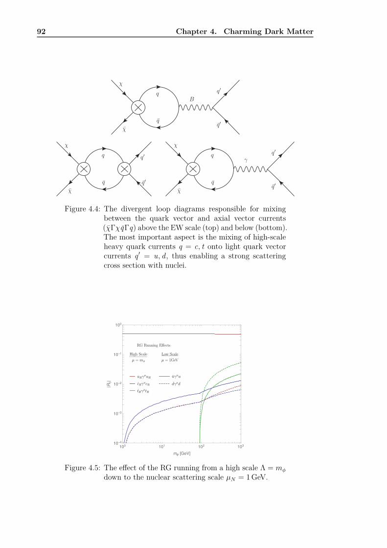
92 Chapter 4. Charming Dark Matter
χ
χq′
B
q
q q′
χ
χ
q′q
q q′
χ
χq′
γ
q
q q′
Figure 4.4: The divergent loop diagrams responsible for mixingbetween the quark vector and axial vector currents(χΓχqΓq) above the EW scale (top) and below (bottom).The most important aspect is the mixing of high-scaleheavy quark currents q = c, t onto light quark vectorcurrents q ′ = u, d, thus enabling a strong scatteringcross section with nuclei.
100 101 102 10310-4
10-3
10-2
10-1
100
mϕ [GeV]
|Rij|
Figure 4.5: The effect of the RG running from a high scale Λ = mφ
down to the nuclear scattering scale µN = 1GeV.

4.4. Direct Detection Constraints 93
100
101
102
103
104
101
102
103
104
105
mχ=mϕ
100
101
102
103
104
101
102
103
104
105
mχ=mϕ
100
101
102
103
104
101
102
103
104
105
mχ=mϕ
mϕ = mχ + mt
Figure 4.6: The DD bounds for three coupling choices – χ1 exclu-sively coupling to u quarks, χ2 to c, and χ3 to t. Boundsfor LUX (CDMSlite) are solid (dashed), and the filledregion shows the parameters which give the correct relicabundance. Constraints are based on the dominant tree-level contribution to scattering.

94 Chapter 4. Charming Dark Matter
(as can be seen in Figure 4.6), even in the case of only coupling to heavy quarks.The spin-averaged cross section is parameterised by a series of nuclear form factorsF
(N,N ′)ij [276], which are functions of the incident DM velocity squared v2 and the
momentum transfer q2,
〈|M|2〉 ∼∑
i,j,N,N′C
(N)i C
(N ′)j F
(N,N ′)ij (v2, q2) (4.4.2)
where we sum over the form factors and the nucleons N,N ′ = p, n. The nucleoncoefficients above are related to our Wilson coefficients by
C(p),i1 (µ ∼ 1GeV) = 4mimN
∑j
(2Rju +Rjd)Cij(mφ) (4.4.3)
C(n),i1 (µ ∼ 1GeV) = 4mimN
∑j
(2Rjd +Rju)Cij(mφ) (4.4.4)
where Rju (Rjd) gives the magnitude of the running of operator q jRγµqjR onto uγµu
(dγµd), and we have quoted the i = j = 1 relation since the corresponding formfactor has the dominant scaling behaviour. i and j run over the DM and quarkflavours respectively. The dependence of the Rjq parameters on the high scale (whichwe take to be the mediator mass) is shown in Figure 4.5.
At loop-level, there are various new operators that arise – in general these are highlysuppressed, but we include them both because they can become dominant in particu-lar regions of parameter space (see Figure 4.7) and for completeness. The operatorswe consider are photon operators [277,278] (which in the non-relativistic limit cor-respond to the charge-radius, magnetic dipole moment, and anapole moment); Zpenguins [277]; and those for DM-gluon [279–281] scattering. We reproduced thequoted literature results as a check.
The more recent null results from XENON1T [282] and PandaX-II [283] push theconstraining potential of direct detection even further – nearly an order of magnitudestronger in cross-section, which translates into a factor of ∼ 2 in mediator mass.
4.5 Indirect Detection Constraints
4.5.1 Basics of Indirect Detection
Indirect detection experiments looks for signs of annihilating and/or decaying DMcoming from astrophysical sources, such as the centre of galaxies where DM densityis largest. The constraints are based around limits on the annihilation cross-sectionof DM to SM particles – in our model the main limits come from annihilation to

4.5. Indirect Detection Constraints 95
10-6
10-5
10-4
10-3
10-10
10-9
10-8
10-7
10-6
10-5
10-4
10-3
10-2
10-1
100
101
102
103
104
10-6
10-5
10-4
10-3
10-10
10-9
10-8
10-7
10-6
10-5
10-4
10-3
10-2
10-1
100
101
102
103
104
Figure 4.7: The differential scattering rate in recoil energy for DM-nuclear scattering at LUX. Each of the quark contribu-tion are plotted separately, the rates are also separatedaccording to the way in which they scatter. The rightplot represents a model with almost complete degen-eracy between the DM and mediator mass, where theloop level interactions become important.
quark pairs
〈σv〉χiχj→q lqm≈ Ncm
2χ
32π(m2χ +m2
φ)2
(λmjλ
∗li
)2+O
(v2). (4.5.1)
There is a bounty of possible search avenues for this annihilation signal; the energeticquarks will hadronise and decay into stable particles (photons, electrons, protons,and their anti-particles, which make up some part of the measured cosmic ray flux),which can be measured directly as they arrive at the earth (in the case of photonsespecially, which suffer very little energy loss to galactic or inter-galactic material),or indirectly through their influence on cosmic rays (for example photons producedby electrons/protons diffusing through the galaxy). We also have great freedom inwhere to look; generally anywhere where there is a cosmic overdensity of dark matter– close to home in the galactic centre or further afield in dwarf spheroidal (dSph)galaxies, galaxy clusters or the CMB.
Underlying all these is Equation 4.5.1 and so ID constraints are frequently quotedas confidence limits on the thermally averaged annihilation cross section 〈σv〉f f intofermions of the same flavour, covering a mass range in mχ from 1GeV to 100TeV.The ID signals from heavy quarks (q = c, b, t) are very similar (see Fig. 3 and 4in [284]), and it is uncommon to find constraints on c, t final states (more commonis the b). The primary spectra of electrons, positrons, anti-protons, deuteron andneutrinos are extremely similar between c, b, t quarks, and thus any constraints

96 Chapter 4. Charming Dark Matter
100
101
102
103
104
105
10-28
10-27
10-26
10-25
10-24
10-23
101
102
103
104
105
10-27
10-26
10-25
10-24
10-23
Figure 4.8: The constraints on 〈σv〉qq for q = u, d, s (left) and q = b(right) which is representative of q = c, t for mχ > mc,t.The constraints are taken from many different sources(DSph, galactic centre, clusters) and targets (gammarays, radio waves, positron, anti-protons).
which look for these particles from DM annihilations will be approximately heavy-flavour independent. The situation is depicted in Figure 4.8.
It should be noted that the relative strength of these constraints is not robust;different authors use different halo profiles, different astrophysical parameters andare subject to varying degrees of uncertainty, some significantly larger than others,it is beyond the scope of this work to accommodate all these effects and compareconstraints on a like-for-like basis and so what we present should be taken as represen-tative but not precise. We will use the bb final state as representative for constraintsbased on dSph [285] and anti-proton measurements of AMS-02 [286] which dominateother constraints such as those based on other particle targets, such as the positronfraction [287] or neutrinos [288] and also those based on the galactic centre [289], orgalaxy clusters [290].
4.5.2 Gamma rays (and other mono-chromatic lines)
At the one-loop level, the pair production of quarks from annihilating DM can pairproduce photons at a fixed energy Eγ = mχ/2 via a box diagram. We calculate thiscross-section using an EFT where the mediator has been integrated out, in whichlimit only the axial vector operator (χγµγ5χ)(qγµγ5q) contributes to the s-waveannihilation, with cross section
〈σv〉γγ = 16α2s
9468(m2χ −m2
φ)2π4
(1 + 2m2
fC0)2, (4.5.2)

4.6. Collider Constraints 97
100 101 102 103 104101
102
103
104
100 101 102 103 104101
102
103
104
Figure 4.9: The ID constraints on DMFV model, with ‘maximal’mixing θij = π/4 (left), or for couplings to top quarksonly (right), assuming degenerate DM masses. Boundsare produced on individual final states, and thereforescale with the dominant annihilation channel, somewhatsurprisingly the top quark channel gives stronger con-straints due to the extremely sensitive γ-ray search byH.E.S.S [289].
where s ≈ 2m2χ is the centre of mass energy of the annihilating DM, and C0 is the
scalar integral C0(0, 0, s;m2f ,m
2f ,m
2f ) in LoopTools notation [291].
As well as γγ final states, there will be γX final states where X = Z, h for exampleand these also provide constraints. The presence of a massive particle recoilingagainst the photon shifts the energy to Eγ = mχ(1−m2
X/4m2χ), but still creates a
mono-energetic line signature. We show some results from the indirect searches inFigure 4.9 – we see that indirect searches can be quite powerful, especially in thecase of large coupling to top quarks.
4.6 Collider Constraints
Our DMFV model contains a new particle with colour charge, and so we expect thereto be significant limits coming from collider experiments. In addition we also haveDM which can be searched for in final states with missing energy, and current LHCdata can also place limits on the mass of invisible particles. In the past, DM modelbuilders have used effective field theories (EFTs) to analyse NP at colliders, but inrecent years it has become clear that the regions of validity of these EFTs at highenergy machines such as the LHC are so small as to be almost useless [236,243,244].We briefly detail in the next section this point for our particular model, before

98 Chapter 4. Charming Dark Matter
101
102
103
101
102
103
104
Figure 4.10: The EFT approximation breaks down beneath thedashed lines (which are the RΛ = 0.5 contours withg . 4π), while ATLAS excludes below the solid lines,and so only the shaded regions can robustly be ex-cluded using the EFT.
moving on to a more complete analysis.
4.6.1 EFT Limit
In [292] the validity of the EFT approximation for t-channel mediators is quantifiedby RΛ, which they define as the ratio of the cross section with the constraint t < Λ2
applied to the total cross section (i.e. the total proportion of the cross section whichis valid under the EFT assumption). The lines of RΛ = 0.50 are plotted alongside theEFT limits taken from ATLAS [293] (the RΛ contour assumes |η| < 2 and pT < 2TeV,the ATLAS results assumed the same range of η, but allow pT . 1.2TeV). It isworth noting that the authors of [292] produce results with the limit g . 1, thebounds become significantly weaker by using g . 4π which then permit a smallregion of validity as shown in Figure 4.10. The EFT breaks down entirely for g . 1.Thus the EFT approximation cannot be justified in our analysis and we turn to thesimulation of the full cross section.
4.6.2 LHC bounds
To try and cover a large range of constraints, we look at three different LHC processesthat could place limits on our model – monojet with missing energy searches, wherea single jet recoils off DM pair production; dijet searches with missing energy; and

4.6. Collider Constraints 99
g
u, c
qu, c
χj
χi u, c
u, c φ
φ
χi
Figure 4.11: Example Feynman diagram for the monojet (left) anddijet (right) processes.
stop searches. The latter are relevant to our model as we have a coloured scalarcoupling to top quarks and DM, in analogy with the e.g. stop-top-neutralino vertexin many supersymmetric theories, and so provide sensitivity to the φ-t coupling D33.
In Figure 4.11 one example Feynman diagram that generates monojet and dijetsignals is shown – in the dijet case the decay of the mediator into quark plus DM isnot shown. Other diagrams that contribute can be seen in Appendix E.3.
We produce our collider constraints using MadGraph [294], replicating, except wherenoted below, the experimental cuts used by the experiments.
Monojet searches
In our analysis, we use the most recent monojet search by ATLAS [295] (which usesthe Run 2 data (
√s = 13TeV and L = 3.2 fb−1)), along with a similar analysis
performed by CMS [296] with the Run 1 data (√s = 8TeV and L = 19.7 fb−1).
The total cross section as a function of mφ for a benchmark scenario is shown inFigure 4.12 with the ATLAS limits overlaid, and the constraints on our model areshown in the top of Figure 4.13.
Dijet searches
Moving on to dijet searches, we use a Run 1 and Run 2 search by ATLAS [297,298]looking for multiple jets plus missing energy – we restricted our comparison to the2-jet searches which should provide the strongest constraint. In our model, theprocess pp → φφ → χχjj provides the dominant contribution to this signal.
We replicate all the main selection cuts for both analyses, in particular for the Run 1comparison: Emiss
t > 160GeV, pT,(1,2) > 130, 60GeV, ∆φ > 0.4 (between the jets andmissing momentum), and for Run 2 similar cuts are applied (full detail in Table 2of [298]). The different signals regions (tjl, tjm, tjt) also include a minimum

100 Chapter 4. Charming Dark Matter
102
103
10-3
10-2
10-1
100
101
Figure 4.12: Total cross section for the seven signal regions of theATLAS monojet search [295] for two DM masses.
SR Nobs NSM Nn.p. σobs / fbtjl 12 315 13 000± 1000 15–704 60tjm 715 760± 50 15–59 4.3tjt 133 125± 10 22–50 1.9tjl 263 283± 24 12–37 16tjm 191 191± 21 15–58 15tjt 26 23± 4 10–22 5.2
Table 4.2: Lower limits (at 95% CL) on the visible cross section forthree signal regions (SR) in the Run 1 ATLAS dijet plusmissing ET search [297] (top), and ATLAS dijet searchfrom Run 2 [298] (bottom).

4.6. Collider Constraints 101
Cut tN_diag tN_med tN_high tN_boost
EmissT / GeV 100 200 320 315
pjT,i / GeV 60, 60, 40, 25 80, 60, 40, 25 100, 80, 40, 25 75, 65, 40, 25mT / GeV 60 140 200 175∆R(b, l) 0.4 0.4 0.4 0.4∆φ(j1,2, p
missT ) 60 140 200 175
Bound σvis / fb 1.8–2.9 0.4 0.3 0.3
Table 4.3: The four relevant signal regions from [299] and the cutswe have implemented.
requirement for meff and ET/√HT , which are defined as
HT = |pT,1|+ |pT,2| ,meff = HT + ET ,
which we implement in MadGraph manually (again, see the respective papers for thecuts in each case). The constraints this places on our model parameters are shownin the bottom left of Figure 4.13 for the case of no mixing and strong couplings forall DM particles.
ATLAS 2014 Stop Search
Lastly, a study by ATLAS [299] considers a set of cuts optimized for the detectionof stops – the signal consists of a lepton in the final state along with four or morejets. There are four relevant signal regions tN_diag, tN_med, tN_high, tN_boost,each requiring a single lepton with plT > 25GeV, and cuts in Table 4.3.1
We find that the production of the φ pair is dominated by t-channel χ exchange ands-channel gluons; the photon and Z mediated diagrams are neglected. We calculatein MadGraph the cross-section for a single final state ((bb)(du) + e−), and thenmultiply this by four to account for the different top quark decay options (the pTcut means the different masses have a negligible effect). Although the cross sectionis predominantly controlled by the size of D33, the light quark couplings D11, D22
have a mild affect by reducing the branching ratio φ → tχi and hence suppressingthe cross section.
We also examined constraints from a similar ATLAS search for scharms [300] ratherthan stops, searching for c-tagged jets plus missing energy in the region where the
1We do not include the cuts on the parameters amT2 and mτT2. From the published cut flows
it can be seen that the effect of these cuts is of the order 10% and 2% respectively (although theformer cut can have a more pronounced effect ∼ 30% on the tN_med cut choice).

102 Chapter 4. Charming Dark Matter
0 200 400 600 8000
500
1000
1500
2000
0 200 400 600 8000
500
1000
1500
2000
0 200 400 600 8000
500
1000
1500
2000
0 100 200 300 400 5000
200
400
600
800
Figure 4.13: Exclusion regions for different signal regions in the AT-LAS (top left) and CMS (top right) monojet analyses,ATLAS dijet searches (bottom left), and ATLAS stopsearches (bottom right).
branching ratio φ→ cχi is large. The limits on mφ,χ are similar to the stop search,and thus do not warrant further attention when compared to the dijet searches.
4.6.3 Collider Constraints within DMFV
We have now looked at three classes of analysis: monojet searches, dijet searches,and searches optimised for a stop. Within our model we have couplings to u, c, t(which we denote here by λu,c,t) and the relative strengths of these dictate whichsignals will be dominant.
Compared to λu, the monojet and dijet processes are suppressed by pure λc (dueto the charm parton distribution function (PDF)), but generally are enhanced bymixtures of λu,c. The coupling λt reduces the signals since they dominantly comefrom s-channel φ resonances and thus the branching ratio to u and c jets is ∝ (D33)−2

4.6. Collider Constraints 103
if λt λu,c. The stop search only becomes relevant for large λt with λt/λu,c > 1,and increasing λu,c suppresses the signal as the branching fraction to top quarks isreduced.
• Mostly up type: The dominant signal will come from the monojet processeswhich have the least QCD suppression and which require an up quark in theinitial state. Dijet searches are also sensitive but it tends to be the monojetwhich sets the better constraint.
• Mostly charm type: The monojet processes are enhanced by the presence ofcharm couplings, however as the up coupling is reduced the monojet processesbecome suppressed because of the charm PDF by around a factor 10–100.The dijet processes are very similar as for u quarks but the largest contribut-ing diagram is again suppressed by the charm PDF. Both searches provideconstraints.
• Mostly top type: The monojet signal depends primarily on λu,c, only indi-rectly on λt though the widths. λt can be probed through stop searches withjet multiplicities of ≥ 4.
Colliders provide very powerful exclusions (up to the TeV scale in mediator mass), andcover the full model parameter space in coupling, although these can be significantlyweakened by, for example, strong top couplings. The DM is produced on shell, andso the constraints are comparatively weak at high DM mass when compared withsearches which depend on the cosmic abundance of DM; on the other hand the factthat the DM is produced in the collider releases any dependence on its abundancein the universe, thus allowing more powerful constraints on DM which has onlya fraction of the full relic abundance (or none at all). Similarly, low mass DM isstrongly excluded, whereas the most powerful astrophysical probe (direct detection)cannot detect much below the GeV scale due to kinematics.
When compared with the strongest direct detection limits, the collider limits arenot as constraining, and this is not likely to change even with more luminosity andhigher energy beams.
It is very difficult for a given parameter choice to determine the strongest boundfrom colliders, except in the extreme cases above, and one should therefore checkall available searches as we have done. Due to the interplay between 1 and 2 jetprocesses, there is no obvious scaling behaviour of the cross section with the couplingparameters, these factors make implementing collider searches in an MCMC scandifficult and slow as each cross section must be numerically computed at each pointin phase space.

104 Chapter 4. Charming Dark Matter
Parameter Range Priormχ / GeV 1–105 Log-Uniformmφ / GeV 1–105 Log-Uniformθij 0–π4 UniformDii 10−2–4π Log-Uniform
Table 4.4: Allowed ranges for the parameters used in the MCMCscan, along with the assumed prior likelihood, which isuniform on either a linear or logarithmic scale.
4.7 Results
We have aimed to produce a robust statistical analysis of the eight dimensionalparameter space of the DMFV model, using the Bayesian inference tool Multi-Nest [301–303] and its Python interface PyMultiNest [304] with 5000 live points.The motivation for carrying out this analysis is twofold, firstly from a practical stand-point it enables very quick and efficient algorithms for scanning a large dimensionalparameter space, allowing us to include all parameters in one analysis. Secondly, arudimentary “hit-or-miss” analysis leaves a large region of parameter space allowed,which is not surprising given the flexibility of 8 free parameters, with a statisticalresult we can quantify the regions of parameter space which are allowed but veryimprobable given the errors of the experimental data. For clarity, we represent theallowed parameters as contours containing credible regions, using the method of [305];using the posterior probability density function. The 1 and 2 sigma contours give anindication of the allowed parameter range, with containment probabilities of 68%and 95% respectively.
Regarding the use of priors: We make one note of caution regarding the results;the credible regions depend sensitively on the choice of priors for the parameters.This is not surprising since our constraints allow large regions of parameter spaceto be equally well allowed, and so the use of priors which bias the parameters tolower values (i.e. log-uniform compared with linearly uniform) is reflected in the finalresult. Nonetheless, we are careful to limit the statements made in the text to thosewhich are independent of the choice of priors. In all figures the log-uniform priorshave been used for the masses and for Dii, as this represents the more conservativechoice. The ranges and priors for the parameters of the scan are summarized inTable 4.4.
Our results are summarized in Figures 4.14 to 4.16 as 2σ contours, and in Table 4.5as one-dimensional 1σ intervals. We consider three separate samples in which theDM (the lightest χ) is the first, second and third member of the triplet (denoted ‘up’,

4.7. Results 105
‘charm’ and ‘top’ DM). Within each sample we present a low and high mass splitting(2% and 15%), which primarily distinguish the effects caused by coannihilation inthe calculation of relic density, but affect all other bounds to some extent as we haveexplicitly included the masses in each.
As we see from Figure 4.14, the masses of the DM and mediator are both requiredto be in the TeV range, with upper limits in the tens of TeV. The DM and mediatormasses are strongly correlated with the Dii, as in Figure 4.14, due to the relic densityand mixing bounds which both scale approximately as (D/m)4 in the high masslimit. Masses in the TeV range favour the Dii to be & O (1). The mixing angles arenot well constrained in general; θij = 0 is favoured, but the full range of angles areusually allowed with 2σ credibility.
TheDii themselves are highly correlated from the mixing constraints (see Figures 4.15and 4.16) which depend on (λλ†)12 which is approximately
(λλ†)12 ≈(s13s23(D2
22 −D211) + s12(D2
33 −D211)), (4.7.1)
and so we see D11 ∼ D33 (and less strongly D11 ∼ D22. Because the correlationbetween D22 and D33 is less pronounced, the RD bound controls the behaviour andproduces an anti-correlation, since the annihilation cross section scales like
〈σv〉eff ∝ (D211 +D2
22 +D233)2 ∼ 3× 10⁻²⁶ cm3 s−1 (4.7.2)
due to coannihilations, as such the trend is most pronounced for small mass splitting.This is seen in the range of D22 for the small splitting data in Figure 4.16.
In all cases, increasing the mass splitting reduces the available parameter space ofthe masses and couplings of the DM since the coannihilations and annihilationsof the heavy particles have a reduced effect on the relic density (scaling with aBoltzmann factor exp(−∆m)). This allows less flexibility in the DM parameterswhilst potentially opening up the allowed parameters of the heavy particles, sincetheir couplings are out of reach of the astronomical constraints (indirect and directsearches) which are proportional to the relic density of the lightest χ (scaling as Ω2
and Ω respectively). This effect can be clearly seen in the right panels of Figure 4.14,where the 2% splitting allows much smaller DM couplings compared with the 15%splitting, contrastingly in Figure 4.15 (middle right panel) the non DM couplingspace opens up with a larger splitting. Of course, since we have fixed the masssplitting by hand, the heavy particle parameters are not totally free, and so theparameter space is still reduced by the constraints we consider.
Top quark threshold effects are absent in the MCMC scan, due to the high masses(mχ & mt). Since mχ,mφ mt the three quarks are kinematically equivalent, and

106 Chapter 4. Charming Dark Matter
100
101
102
103
104
105
100
101
102
103
104
105
10-2
10-1
100
101
100
101
102
103
104
105
100
101
102
103
104
105
100
101
102
103
104
105
10-2
10-1
100
101
100
101
102
103
104
105
100
101
102
103
104
105
100
101
102
103
104
105
10-2
10-1
100
101
100
101
102
103
104
105
Figure 4.14: Credible regions (2σ contours) in the mχ −mφ plane(left) and Dii −mφ (right) where the DM is χ1 (top),χ2 (middle) or χ3 (bottom). Two values of a mass split-ting are chosen, shown with solid and dashed contoursrespectively.

4.7. Results 107
10-2
10-1
100
101
10-2
10-1
100
101
10-2
10-1
100
101
10-2
10-1
100
101
10-2
10-1
100
101
10-2
10-1
100
101
10-2
10-1
100
101
10-2
10-1
100
101
10-2
10-1
100
101
10-2
10-1
100
101
10-2
10-1
100
101
10-2
10-1
100
101
Figure 4.15: As for Figure 4.14 but for the D11 − D22 plane (left)and D11−D33 (right), for two values of mass splitting(dashed shaded, and solid darker shaded respectively).

108 Chapter 4. Charming Dark Matter
10-2
10-1
100
101
10-2
10-1
100
101
10-2
10-1
100
101
10-2
10-1
100
101
10-2
10-1
100
101
10-2
10-1
100
101
Figure 4.16: As for Figure 4.14 but for the D22 −D33 plane.

4.7. Results 109
so the bounds are not strongly dependent on the flavour of DM. The main differencesarise due to the quarks SM interactions which impact the DD and ID limits.
As described in Section 4.6, we have studied collider bounds on our model, butthese were not directly incorporated into our MultiNest routine as these boundsare much more computationally intensive than the others. However, as we see fromFigure 4.13, the collider bounds only rule out sub-TeV scale masses, even at largecouplings and so we do not expect that a full likelihood function incorporating theLHC constraints would give significantly different results. As a test, we checked asample of the points inside the 68% (1σ) credible regions and found only a smallminority (of order 1%) that would be excluded by collider data. We produce, foreach parameter, a marginalized posterior integrated over the remaining 7 parameters.From this distribution we find the 1σ credible interval. The results are shown inTable 4.5. This contains results for both uniform and log-uniform priors on Dii, mχ
and mφ; when the two cases are discrepant by > 1σ this is due to a flat posterior,and using the 2σ band instead the two agree.
4.7.1 Constrained Scenarios
We consider two extensions to the previous results:
1. In Section 4.2.2 we found that the mass splitting which is generated throughRG running of the DM self-energy is approximately proportional to D2
ii, thismotivates us to consider a scenario in which the couplings Dii are correlatedwith the masses (thus introducing a coupling splitting ∆Dii/Dχ ∝ ∆mij/mχ).The reduced parameter space enforces almost degenerate couplings which leadsto two important effects; firstly, it subjects all three χ to the astrophysicalconstraints of indirect and direct detection, despite the heavier particles havingno relic density. By this we mean that, upon fixing the mass splitting, anylimits on the coupling strength of the relic particle are translated to restrictthe non-relic particles. Secondly, because the Dii are equal the mixing effectsare naturally small and as a result the mixing angles are much less constrainedas they do not need to be small to counteract flavour effects.
This scenario is representative of a model in which MFV is broken only slightly,since the couplings to quark flavours are roughly equal, differing due to themixing angles and the small differences in the Dii. It is actually only slightlyless constrained in both mass and couplings than models in which flavourviolation is allowed, which counteracts the naive assumption that withoutMFV, flavour observables restrict NP very high scales (O (100TeV)).

110 Chapter 4. Charming Dark Matter
100
101
102
103
104
105
100
101
102
103
104
105
100
101
102
103
104
105
100
101
102
103
104
105
100
101
102
103
104
105
100
101
102
103
104
105
100
101
102
103
104
105
100
101
102
103
104
105
100
101
102
103
104
105
100
101
102
103
104
105
100
101
102
103
104
105
100
101
102
103
104
105
Figure 4.17: Comparison between 2σ contours of the full MCMCscan and two extensions discussed in the text, for amass splitting of 2% (left) or 15% (right).
4.7. Results 111
2. When compared with the down type quark sector, flavour bounds are weakerdue to D0 being less well measured and our conservative treatment in whichwe assume the SM contribution to D0 mixing is zero and the experimentalvalue comes entirely from the new physics. This is not entirely unreasonable,since current short distance calculations of the observable are known to notreproduce the experimental result, nor is it completely reasonable, since longdistance calculations are able to bring the SM into agreement.
To cover this caveat we consider a future scenario in which the SM calculationreproduces the experimental number (but the precision of the measurementstays at its current value). This is also conservative, since any interferenceterms between the SM and DMFV amplitude are likely to be large. Theconstraints on the mixing angles are more pronounced
Results for these two further scenarios are shown in Figure 4.17, and the 1σ intervalsin Tables 4.6 and 4.7.

112 Chapter 4. Charming Dark Matterθ 1
2θ 1
3θ 2
3
0.0.
20.
40.
60.
0.2
0.4
0.6
0.0.
20.
40.
6
D11
D22
D33
10-
210
-1
100
101
10-
210
-1
100
101
10-
210
-1
100
101
mχ/GeV
mφ/GeV
100
101
102
103
104
105
100
101
102
103
104
105
Table4.5:
The
1D1σ
credible
intervalsforall8
parametersof
theMCMC
scan
.Colou
rsdeno
tetheDM
flavo
ur(red,
greenan
dblue
forup
,cha
rman
dtopDM
respectiv
ely).The
twopriorchoiceson
Diian
dthemasses(lo
g-un
iform
vsun
iform
)are
show
nas
lines
andshad
edregion
srespe
ctively
,the
mod
alaverag
eof
thelog-un
iform
priorchoice
isshow
nas
ado
t.The
twomasssplittin
gcasesarecontainedin
diffe
rent
panels.

4.7. Results 113
θ 12
θ 13
θ 23
0.0.
20.
40.
60.
0.2
0.4
0.6
0.0.
20.
40.
6
Dii
mχ/GeV
mφ/GeV
10-
210
-1
100
101
100
101
102
103
104
105
100
101
102
103
104
105
Table4.6:
The
1D1σ
credible
intervalsforthe6pa
rametersof
constrainedscenario
inwhich
theDiisplittin
gare
prop
ortio
naltothe
∆m/m
χ.C
olou
rsde
note
theDM
flavo
ur(red
,green
andblue
foru
p,charm
andtopDM
respectiv
ely).The
twopriorchoiceson
Diian
dthemasses(lo
g-un
iform
vsun
iform
)areshow
nas
lines
and
shad
edregion
srespectiv
ely,
themod
alaverageof
thelog-un
iform
priorchoice
isshow
nas
ado
t.The
two
masssplittin
gcasesarecontainedin
diffe
rent
panels.

114 Chapter 4. Charming Dark Matterθ 1
2θ 1
3θ 2
3
0.0.
20.
40.
60.
0.2
0.4
0.6
0.0.
20.
40.
6
D11
D22
D33
10-
210
-1
100
101
10-
210
-1
100
101
10-
210
-1
100
101
mχ/GeV
mφ/GeV
100
101
102
103
104
105
100
101
102
103
104
105
Table4.7:
The
1D1σ
credible
intervalsforafuture
scenario
inwhich
theSM
predictio
nforthemixingmatches
theexpe
rimentalv
alue.Colou
rsdeno
tetheDM
flavo
ur(red,g
reen
andblue
forup
,cha
rman
dtopDM
respectiv
ely).The
twopriorchoiceson
Diian
dthemasses(lo
g-un
iform
vsun
iform
)areshow
nas
lines
and
shad
edregion
srespectiv
ely,
themod
alaverageof
thelog-un
iform
priorchoice
isshow
nas
ado
t.The
two
masssplittin
gcasesarecontainedin
diffe
rent
panels.

4.8. Summary 115
4.8 Summary
In this chapter we have analysed a model of dark matter, based on [248] but couplingto up type quarks, that goes beyond MFV in order to allow potentially large neweffects in the flavour sector, and have seen how the combination of a wide range ofconstraints can be used to place limits on models of this type. We approached thistask of combining many different constraints using the MCMC tool Multinest, whichallowed us to place limits on the high dimensional parameter space of our particularmodel.
As we can see from Figure 4.14, the MCMC places lower bounds on the new particlemasses of at least 1TeV for Top DM, and a few hundred GeV for Up and CharmDM in certain cases. Our collider bounds (Figure 4.13) cannot further exclude TopDM, even in the case of strong couplings, but could remove a small area of allowedparameter space from the bottom end of the mass range in the case of Up/CharmDM.
In [250] the authors consider this model, but examined the region of parameterspace with dominant top quark couplings. Our results in general agree with theirconclusions if we look at their more focused parameter space. For example, they findstrong constraints on θ12 except in the case of some degeneracy in the Dii, whichwe replicate. Similarly the strong constraints on DM mass from relic density anddirect detection are reproduced. In their work, they explain how loop-level diagramscontributing to direct detection favour the dominant top coupling – however as weexplain in Section 4.4, RG effects mean even when DM doesn’t couple to up quarksdirectly, the mixing is substantial enough to weaken this conclusion (as long as themediator mass is large enough).
Given the current level of data, the model we examine of flavoured DM couplingto up type quarks has large sections of its parameter space still allowed, so long asone considers large mass new particles. However, even without the complimentarycollider results, the lower mass, phenomenologically interesting, regions of parameterspace are disfavoured by flavour, relic density, and direct detection considerations.
The MFV assumption is frequently invoked in simplified models in order to evadepotentially large flavour-violating effects. The level of robustness of this assumptionvaries considerably between up type and down type quark couplings in the DMFVmodel; for RH down type quarks strong flavour bounds do ensure that the assumptionis a good one. However for couplings to RH up type quarks we have seen that in factthe flavour bounds are avoided in a large region of MFV-breaking parameter space.
One particular future development could alter this picture however – if a precisetheoretical prediction of D0 mixing observables could be obtained then either (a) a

116 Chapter 4. Charming Dark Matter
significant discrepancy requiring new physics is present, or (b) the SM predictionsare reproduced with a high precision. The former would motivate the explorationof models which go beyond MFV, and the latter would make the MFV assumptiona necessary assumption of the DMFV simplified model if one wants to avoid somefine-tuning.

Chapter 5
Charming new physics in rare Bsdecays and mixing?
5.1 Introduction
As we have discussed in Section 1.2, flavour processes such as rare B decays areexcellent probes of new physics at the electroweak scale and beyond, due to theirstrong suppression in the SM. We also mentioned (in Section 1.3.4) how there areinteresting signs of a BSM effect in B → K (∗)µ+µ−, caused by a contact interactionof the form (sγµPLb)(µγµµ). Explaining the effect requires destructive interferencefrom BSM to reduce the Wilson coefficient C9 by O (20%). As was mentioned, awide variety of models with new particles have been proposed (see e.g. [101–109,115,117, 118, 121–126, 306–320]), which might in turn be part of a more comprehensivesector of new dynamics. Since the early signs of the anomalies (i.e. before RK (∗))suggested a flavour universal interaction, and noting that in the SM about half ofC9 comes from (short-distance) virtual-charm contributions, in this chapter we askwhether new physics affecting the quark-level b → ccs transitions could cause theanomalies by affecting rare B decays through a loop The bulk of these effects wouldalso be captured through an effective shift ∆C9(q2), with a possible dependence onthe dilepton mass q2. At the same time, such a scenario offers the exciting prospectof confirming the rare B decay anomalies through correlated effects in hadronic Bdecays into charm, with mixing observables such as the Bs meson width differencestanding out as precisely measured [199,321–323] and under reasonable theoreticalcontrol. This is in contrast with the Z ′ and leptoquark models usually considered,where correlated effects are typically restricted to other rare processes and are highlymodel dependent. Specific scenarios of hadronic new physics in the B widths havebeen considered previously [221,324–326], while the possibility of virtual charm BSM

118 Chapter 5. Charming new physics in rare Bs decays and mixing?
physics in rare semileptonic decay has been raised in [327] (see also [328]). As wewill show, viable scenarios exist which can mimic a shift ∆C9 = −O (1) while beingconsistent with all other observables. In particular, very strong renormalisation-group effects can generate large shifts in the (low-energy) effective C9 coupling fromsmall b → ccs couplings at a high scale without conflicting with the measuredB → Xsγ branching ratio [329–336].
5.2 Charming new physics scenario
We consider a scenario where new physics affects the b → ccs transitions. This couldbe the case in models containing new scalars or new gauge bosons, or strongly couplednew physics. Such models will typically affect other observables, but in a model-dependent manner. For this paper, we restrict ourselves to studying the new effectsinduced by modified b → ccs couplings, leaving construction and phenomenology ofconcrete models for future work. We refer to this as the “charming BSM” (CBSM)scenario. As long as the mass scale M of new physics satisfies M mB, themodifications to the b → ccs transitions can be accounted for through a localeffective Hamiltonian,
Hcceff = 4GF√
2V ∗csVcb
10∑i=1
(CciQ
ci + Cc′
i Qc′i ) . (5.2.1)
We choose our operator basis and renormalisation scheme to agree with [337] uponthe substitution d → b, s → c, u → s:
Qc1 = (c iγµPLbj)(sjγµPLci), Qc
2 = (c iγµPLbi)(sjγµPLcj) ,Qc
3 = (c iPLbj)(sjPRci), Qc4 = (c iPLbi)(sjPRcj) ,
Qc5 = (c iγµPRbj)(sjγµPLci), Qc
6 = (c iγµPRbi)(sjγµPLcj) ,Qc
7 = (c iPRbj)(sjPRci), Qc8 = (c iPRbi)(sjPRcj) ,
Qc9 = (c iσµνPRbj)(sjσµνPRci), Qc
10 = (c iσµνPRbi)(sjσµνPRcj) .
(5.2.2)
The Qc′i are obtained by changing all the quark chiralities. These chirality flipped
operators do not give any effect in C9, and so we discard the Qc′i below. We split
the Wilson coefficients into SM and BSM parts,
Cci (µ) = Cc,SM
i (µ) + ∆Ci(µ) , (5.2.3)
where Cc,SMi = 0 except for i = 1, 2 and µ is the renormalisation scale.

5.3. Rare B decays 119
b
s
s(b)
b(s)
c
c
b s
γq µ−
µ+
Figure 5.1: Leading CBSM contributions to rare decays (left), andto width difference ∆Γs and lifetime ratio τ(Bs)/τ(Bd)(right).
5.3 Rare B decays
The leading-order (LO), one-loop CBSM effects in radiative and rare semileptonic de-cays may be expressed through “effective” Wilson coefficient contributions ∆Ceff
9 (q2)and ∆Ceff
7 (q2) in an effective local Hamiltonian
Hrsleff = −4GF√
2VtsVtb
(Ceff
7 (q2)Q7γ + Ceff9 (q2)Q9V
), (5.3.1)
where q2 is the dilepton mass and
Q7γ = emb
16π2 (sσµνPRb)F µν , Q9V = α
4π (sγµPLb)(`γµ`) .
For small q2 (in particular, well below the charm resonances), ∆Ceff9 (q2) and ∆Ceff
7 (q2)govern the theoretical predictions for both exclusive (B → K (∗)`+`−, Bs → φ`+`−,etc.) and inclusive B → Xs`
+`− decay, up to O (αs) QCD corrections and powercorrections to the heavy quark limit that we neglect in our leading-order analy-sis. Similarly, ∆Ceff
7 (0) determines radiative B decay rates. We will neglect thesmall CKM combination V ∗usVub, implying V ∗csVcb = −V ∗tsVtb, and focus on real (CP-conserving) values for the Cc
i . From the diagram shown in Figure 5.1 (left) we thenobtain
∆Ceff9 (q2) =
(Cc
1,2 −Cc
3,4
2
)h− 2
9Cc3,4 , (5.3.2)
∆Ceff7 (q2) = mc
mb
[(4Cc
9,10 − Cc7,8)y + 4Cc
5,6 − Cc7,8
6
], (5.3.3)
with Ccx,y = 3∆Cx + ∆Cy and the loop functions
h(q2,mc, µ) = −49
[ln m
2c
µ2 −23 + (2 + z)a(z)− z
], (5.3.4)

120 Chapter 5. Charming new physics in rare Bs decays and mixing?
y(q2,mc, µ) = −13
[ln m
2c
µ2 −32 + 2a(z)
], (5.3.5)
where a(z) =√|z − 1| arctan 1√
z−1 and z = 4m2c/q
2. Our numerical evaluationemploys the charm pole mass.
We note that only the four Wilson coefficients ∆C1−4 enter ∆Ceff9 (q2). Conversely,
∆Ceff7 (q2) is given in terms of the other six Wilson coefficients ∆C5−10. The appear-
ance of a one-loop, q2-dependent contribution to Ceff7 is a novel feature in the CBSM
scenario. Numerically, the loop function a(z) equals one at q2 = 0 and vanishes atq2 = (2mc)2. The constant terms and the logarithm accompanying y(q2,mc) par-tially cancel the contribution from a(z) and they introduce a sizeable dependence onthe renormalisation scale µ and the charm quark mass. Since a shift of ∆Ceff
7 (q2) isstrongly constrained by the measured B → Xsγ decay rate, we do not consider thecoefficients ∆C5−10 in the remainder and focus on the four coefficients ∆C1−4, whichdo not contribute to B → Xsγ at 1-loop order. Higher-order contributions can beimportant if new physics generates ∆Ci at the weak scale or beyond, as is typicallyexpected. In this case large logarithms lnM/mB occur, requiring resummation. Toleading-logarithmic accuracy, we find
∆Ceff7 = 0.02∆C1 − 0.19∆C2 − 0.01∆C3 − 0.13∆C4 , (5.3.6)
∆Ceff9 = 8.48∆C1 + 1.96∆C2 − 4.24∆C3 − 1.91∆C4 , (5.3.7)
if ∆Ci are understood to be renormalized at µ = MW and ∆Ceff7,9 at µ = 4.2GeV. It
is clear that ∆C1 and ∆C3 contribute (strongly) to rare semileptonic decay but onlyweakly to B → Xsγ.
5.4 Mixing and lifetime observables
A distinctive feature of the CBSM scenario is that non-zero ∆Ci affect not onlyradiative and rare semileptonic decays, but also tree-level hadronic b → ccs transi-tions. While the theoretical control over exclusive b → ccs modes is very limited atpresent, the decay width difference ∆Γs and the lifetime ratio τ(Bs)/τ(Bd) stand outas being calculable in the HQE, via the diagrams shown in Figure 5.1 (right). Forboth observables, the heavy quark expansion gives rise to an operator product expan-sion in terms of local ∆B = 2 (for the width difference) or ∆B = 0 (for the lifetimeratio) operators. For the Bs width difference, we have ∆Γs = 2|Γs,SM12 + Γcc12| cosφs12,

5.4. Mixing and lifetime observables 121
where the phase φs12 is small. Neglecting the strange quark mass, we find
Γcc12 =−G2F (V ∗csVcb)2m2
bMBsf2Bs
√1− 4x2
c
576π × [16(1− x2
c)(4Cc,22 + Cc,2
4 )
+8(1− 4x2c)(12Cc,2
1 + 8Cc1C
c2 + 2Cc
3Cc4 + 3Cc,2
3 )−192x2
c(3Cc1C
c3 + Cc
1Cc4 + Cc
2Cc3 + Cc
2Cc4)]B1
+2(1 + 2x2c)(
MBs
mb +ms
)2
×
(4Cc,22 − 8Cc
1Cc2 − 12Cc,2
1 − 3Cc,23 − 2Cc
3Cc4 + Cc,2
4 )B3
,
(5.4.1)
with xc = mc/mb. B1 and B3 are defined as in Equation C.0.2 with values taken from[220]. For our numerical evaluation of Γcc12, we split the Wilson coefficients accordingto Equation 5.2.3, subtract from the LO expression (Equation 5.4.1) the pure SMcontribution and add the NLO SM expressions from [173–177, 207]. In general, amodification of Γcc12 also affects the semi-leptonic CP asymmetries. However, sincewe consider CP-conserving new physics in this paper and since the correspondingexperimental uncertainties are still large, the semi-leptonic asymmetries will not leadto an additional constraint.
In a similar manner, for the lifetime ratio we find
τ(Bs)τ(Bd) =
(τ(Bs)τ(Bd)
)SM
+(τ(Bs)τ(Bd)
)NP
, (5.4.2)
where the SM contribution is taken from [215] and
(τ(Bs)τ(Bd)
)NP
= G2F |VcbVcs|2m2
bMBsf2BsτBs
√1− 4x2
c
144π ×(1− x2
c)[(4Cc,2
1,2 + Cc,23,4)B1 + 6(4Cc,2
2 + Cc,24 )ε1
]− 12x2
c
[Cc
1,2Cc3,4B1 + 6Cc
2Cc4ε1]
− (1 + 2x2c)(
MBs
mb +ms
)2
×[(4Cc,2
1,2 + Cc,23,4)B2 + 6(4Cc,2
2 + Cc,24 )ε2
],
(5.4.3)
subtracting the SM part and defining B1, B2, ε1, ε2 as in Equations C.0.3 and C.0.4with values taken from our work in Chapter 6. We interpret the quark masses asMS parameters at µ = 4.2GeV.

122 Chapter 5. Charming new physics in rare Bs decays and mixing?
0
-1
-1
-2
-1.0 -0.5 0.0 0.5 1.0-1.0
-0.5
0.0
0.5
1.0
0 -1
-1
-2
-1.0 -0.5 0.0 0.5 1.0-1.0
-0.5
0.0
0.5
1.0
Figure 5.2: Mixing observables versus rare decays in the CBSMscenario, in the ∆C1−∆C2 plane (left) and ∆C3−∆C4plane (right). All Wilson coefficients are renormalizedat µ = 4.2GeV and those not corresponding to eitheraxis set to zero. The black dot corresponds to the SM,i.e. ∆Ci = 0. The measured central value for the widthdifference is shown as brown (solid) line together withthe 1σ allowed region. The lifetime ratio measurementis depicted as green (dashed) line and band. Overlaidare contours of ∆Ceff
9 (5GeV2) = −1,−2 (black, dashed)and ∆Ceff
9 (2GeV2) = −1,−2 (red, dotted), as computedfrom Equation 5.3.2, and of ∆Ceff
9 = 0 (black, solid).
5.5 Rare decays versus lifetimes – low-scalescenario
We are now in a position to confront the CBSM scenario with rare decay andmixing observables, as long as we consider renormalisation scales µ ∼ mB. Thenthe logarithms inside the h function entering Equation 5.3.2 are small and ourleading-order calculation should be accurate. Such a scenario is directly applicableif the mass scale M of the physics generating the ∆Ci is not too far above mB,such that ln(M/mB) is small. Figure 5.2 (left) shows the experimental 1σ allowedregions for the width difference [338] and lifetime ratio [339] in the ∆C1−∆C2 plane.The central values are attained on the brown (solid) and green (dashed) curves,respectively. The measured lifetime ratio and the width difference measurementcan be simultaneously accommodated for different values of the Wilson coefficients:in the ∆C1 − ∆C2 plane, we find the SM solution, as well as a solution around∆C1 = −0.5 and ∆C2 ≈ 0. In the ∆C3 − ∆C4 plane, we have a relatively broadallowed range, roughly covering the interval [−0.9,+0.7] for ∆C3 and [−0.6,+1.1]for ∆C4. For further conclusions, a considerably higher precision in experiment and

5.6. High-scale scenario and RGE 123
theory is required for ∆Γs and τ(Bs)/τ(Bd). Also shown in the plot are contourlines for the contribution to the effective semileptonic coefficient ∆Ceff
9 (q2), both forq2 = 2GeV2 and q2 = 5GeV2. We see that sizeable negative shifts are possible whilerespecting the measured width difference and the lifetime ratio. For example, a shift∆Ceff
9 ∼ −1 as data may suggest could be achieved through ∆C1 ∼ −0.5 alone. Sucha value for ∆C1 may well be consistent with CP-conserving exclusive b → ccs decaydata, where no accurate theoretical predictions exist. On the other hand, ∆Ceff
9
only exhibits a mild q2-dependence. Distinguishing this from possible long-distancecontributions would require substantial progress on the theoretical understanding ofthe latter.
We can also consider other Wilson coefficients, such as the pair (∆C3,∆C4) (rightpanel in Figure 5.2). A shift ∆Ceff
9 ∼ −1 is equally possible and consistent with thewidth difference, requiring only ∆C3 ∼ 0.5.
5.6 High-scale scenario and RGE
5.6.1 RG enhancement of ∆Ceff9
If the CBSM operators are generated at a high scale then large logarithms lnM/mB
appear. Their resummation is achieved by evolving the initial (matching) conditionsCi(µ0 ∼ M) to a scale µ ∼ MB according to the coupled renormalisation-groupequations (RGE),
µdCjdµ
(µ) = γij(µ)Ci(µ) , (5.6.1)
where γij is the anomalous dimension matrix. As is well known, the operators Qci
mix not only with Q7 and Q9, but also with the 4 QCD penguin operators P3−6
and the chromodipole operator Q8g (defined as in [340]), which in turn mix into Q7.Hence the index j runs over 11 operators with ∆B = −∆S = 1 flavour quantumnumbers in order to account for all contributions to C7(µ) that are proportional to∆Ci(µ0). Most entries of γij are known at LO [337, 340–354]; our novel results are(i = 3, 4)
γ(0)Qci Q9
=(4
3 ,49
)i, γ
(0)QciP4
=(
0,−23
)i, γ
eff(0)QciQ7
=(
0, 22481
)i, (5.6.2)
where Q9 = (4π/αs)Q9V (µ) and γeff(0)QciQ7
requires a two-loop calculation. (See Ap-pendix F for further technical information.) Solving the RGE for µ0 = MW ,

124 Chapter 5. Charming new physics in rare Bs decays and mixing?
µ = 4.2GeV, and αs(MZ) = 0.1181 results in the CBSM contributions
∆C1(µ)∆C2(µ)∆C3(µ)∆C4(µ)∆Ceff
7 (µ)∆Ceff
9 (µ)
=
1.12 −0.27 0 0−0.27 1.12 0 0
0 0 0.92 00 0 0.33 1.91
0.02 −0.19 −0.01 −0.138.48 1.96 −4.24 −1.19
∆C1(µ0)∆C2(µ0)∆C3(µ0)∆C4(µ0)
. (5.6.3)
A striking feature are the large coefficients in the ∆Ceff9 case, which are O (1/αs) in
the logarithmic counting. The largest coefficients appear for ∆C1 and ∆C3, whichat the same time practically do not mix into Ceff
7 . This means that small values∆C1 ∼ −0.1 or ∆C3 ∼ 0.2 can generate ∆Ceff
9 (µ) ∼ −1 while having essentially noimpact on the B → Xsγ decay rate. Conversely, values for ∆C2 or ∆C4 that leadto ∆Ceff
9 ∼ −1 lead to large effects in Ceff7 and B → Xsγ.
5.6.2 Phenomenology for high NP scale
The situation in various two-parameter planes is depicted in Figure 5.3, where the1σ constraint from B → Xsγ is shown as blue, straight bands. (We implement it bysplitting B(B → Xsγ) into SM and BSM parts and employ the numerical result andtheory error from [355] for the former. The experimental result is taken from [356].)The top row corresponds to Figure 5.2, but contours of given ∆C9 lie much closerto the origin. All six panels testify to the fact that the SM is consistent with alldata when leaving aside the question of rare semileptonic B decays – the largest pullstems from the fact that the experimental value for τ(Bs)/τ(Bd) is just under 1.5standard deviations below the SM expectation, such that the black (SM) point isless than 0.5σ outside the green area. Our main question now is: can we have a newcontribution ∆Ceff
9 ∼ −1 to rare semileptonic decays, while being consistent withthe bounds stemming from b → sγ, ∆Γs and τ(Bs)/τ(Bd)? This is clearly possible(indicated by the yellow star in the plots) if we have a new contribution ∆C3 ≈ 0.2,see the three plots of the ∆Ci − ∆C3 planes in Figure 5.3 (right on the top row,left on the middle row and left on the lower row). In these cases, the ∆Ceff
9 ∼ −1solution is even favoured compared to the SM solution. A joint effect in ∆C2 ≈ −0.1and ∆C4 ≈ 0.3 can also accommodate our desired scenario (see the right plot on thelower row), while new BSM effects in the pairs ∆C1,∆C2 and ∆C1,∆C4 alone areless favoured. One could also consider three or all four ∆Ci simultaneously.

5.6. High-scale scenario and RGE 125
0-1-2
-0.4 -0.2 0.0 0.2 0.4
-0.4
-0.2
0.0
0.2
0.4 0 -1 -2
-0.4 -0.2 0.0 0.2 0.4
-0.4
-0.2
0.0
0.2
0.4
0-1-2
-0.4 -0.2 0.0 0.2 0.4
-0.4
-0.2
0.0
0.2
0.4
0-1-2
-0.4 -0.2 0.0 0.2 0.4
-0.4
-0.2
0.0
0.2
0.4
0
-1
-2
-0.4 -0.2 0.0 0.2 0.4
-0.4
-0.2
0.0
0.2
0.4
0
-1
-2
-0.4 -0.2 0.0 0.2 0.4
-0.4
-0.2
0.0
0.2
0.4
Figure 5.3: Mixing observables versus rare decays, for ∆Ci renor-malized at µ0 = MW . Colour coding as in Figure 5.2,B → Xsγ constraint shown in addition (straight bluebands).

126 Chapter 5. Charming new physics in rare Bs decays and mixing?
5.6.3 Implications for UV physics
Our model-independent results are well suited to study the rare B decay and lifetimephenomenology of UV completions of the Standard Model. Any such completion mayinclude extra UV contributions to C7(M) and C9(M), correlations with other flavourobservables, collider phenomenology, etc.; the details are highly model-dependentand beyond the scope of our model-independent analysis. Here we restrict ourselvesto some basic sanity checks.
Taking the case of ∆C1(M) ∼ −0.1 corresponds to a naive ultraviolet scale
Λ ∼(
4GF√2|V ∗csVcb| × 0.1
)−1/2
∼ 3TeV .
This effective scale could arise in a weakly-coupled scenario from tree-level exchangeof new scalar or vector mediators, or at loop level in addition from fermions; orthe effective operator could arise from strongly-coupled new physics. For a tree-level exchange, Λ ∼ M/g∗ where g∗ = √g1g2 is the geometric mean of the relevantcouplings. For weak coupling g∗ ∼ 1, this then gives M ∼ 3TeV. Particles ofsuch mass are certainly allowed by collider searches if they do not couple (or onlysufficiently weakly) to leptons and first-generation quarks. Multi-TeV weakly coupledparticles are also not generically in violation of electroweak precision tests of the SM.Loop-level mediation would require mediators close to the weak scale which may beproblematic and would require a specific investigation; this is of course unsurprisinggiven that b → ccs transitions are mediated at tree level in the SM. The samewould be true in a BSM scenario that mimics the flavour suppressions in the SM(such as MFV models). Conversely, in a strongly-coupled scenario we would haveM ∼ g∗Λ ∼ 4πΛ ∼ 30TeV. This is again safe from generic collider and precisionconstraints, and a model-specific analysis would be required to say more.
Finally, as all CBSM effects are lepton-flavour-universal, they cannot on their ownaccount for departures of the lepton flavour universality parameters R
K(∗) [87] from
the SM values as suggested by current experimental measurements [84, 85, 357].However, even if those departures are real, they may still be caused by direct UVcontributions to ∆C9. For example, as shown in [96], a scenario with a muon-specificcontribution ∆Cµ
9 = −∆Cµ10 ∼ −0.6 and in addition a lepton-universal contribution
∆C9 ∼ −0.6, which may have a CBSM origin, is perfectly consistent with all rare Bdecay data, and in fact marginally preferred.

5.7. Prospects and summary 127
0-1-2
-0.4 -0.2 0.0 0.2 0.4
-0.4
-0.2
0.0
0.2
0.4 0-1-2
-0.4 -0.2 0.0 0.2 0.4
-0.4
-0.2
0.0
0.2
0.4
Figure 5.4: Future prospects for mixing observables. Dashed: con-tours of constant width difference, dotted: contours ofconstant lifetime ratio. See text for discussion.
5.7 Prospects and summary
The preceding discussion suggests that a precise knowledge of width difference andlifetime ratio, as well as B(B → Xsγ), can have the potential to identify and dis-criminate between different CBSM scenarios, or rule them out altogether. This isillustrated in Figure 5.4, showing contour values for future precision both in mix-ing and lifetime observables. In each panel, the solid (brown and green) contourscorrespond to the SM central values of the width difference and lifetime ratio (re-spectively). The spacing of the accompanying contours is such that the area betweenany two neighbouring contours corresponds to a prospective 1σ-region, assuminga combined (theoretical and experimental) error on the lifetime ratio of 0.001 anda combined error on ∆Γs of 5% (theory is already there for the lifetime ratio, andexperiment for ∆Γ). The assumed future errors are ambitious but seem feasible withexpected experimental and theoretical progress. Overlaid is the (current) B → Xsγ
constraint (blue). The figure indicates that a discrimination between the SM andthe scenario where ∆C9 ≈ −1, while B(B → Xsγ) is SM-like is clearly possible. Acrucial role is played by the lifetime ratio τ(Bs)/τ(Bd): in e.g. the ∆C3 −∆C4 casea 1σ deviation of the lifetime ratio almost coincides with the ∆C9 = −1 contourline; a further precise determination of ∆Γs could then identify the point on this linechosen by nature. Further progress on B → Xsγ in the Belle II era would providecomplementary information.
In summary, we have given a comprehensive, model-independent analysis of BSMeffects in partonic b → ccs transitions (CBSM scenario) in the CP-conserving case,focusing on those observables that can be computed in a heavy quark expansion.

128 Chapter 5. Charming new physics in rare Bs decays and mixing?
An effect in rare semileptonic B decays compatible with hints from current LHCband B-factory data can be generated, while satisfying the B → Xsγ constraint.It can originate from different combinations of b → ccs operators. The requiredWilson coefficients are so small that constraints from B decays into charm are noteffective, particularly if new physics enters at a high scale; then large renormalisation-group enhancements are present. Likewise, there are no obvious model-independentconflicts with collider searches or electroweak precision observables. A more precisemeasurement of mixing observables and lifetime ratios, at a level achievable at LHCb,may be able to confirm (or rule out) the CBSM scenario, and to discriminate betweendifferent BSM couplings. Finally, all CBSM effects are lepton-flavour-universal; thecurrent RK and RK
∗ anomalies would either have to be mismeasurements or requireadditional lepton-flavour-specific UV contribution to C9; such a combined scenariohas been shown elsewhere [96] to be consistent with all rare B decay data and alsopresents the most generic way for UV physics to affect rare decays. With the statedcaveats, our conclusions are rather model independent. It would be interesting toconstruct concrete UV realizations of the CBSM scenario, which almost certainlywill affect other observables in a correlated, but model-dependent manner.

Chapter 6
Dimension-six matrix elementsfrom sum rules
6.1 Introduction
As we have seen in Section 2.4.2, the SM contribution to meson mixing arises at the1-loop level and is both CKM and GIM suppressed. This makes these observableshighly sensitive to new physics contributions (an issue which we will explore furtherin Chapter 7), and so a precise knowledge of the theoretical predictions is veryimportant. The SM calculation can be factorised into a perturbative calculation ofthe Wilson coefficients and a non perturbative part coming from the matrix elementsof effective operators that contribute to mixing. While the perturbative part (ofwhich we showed the leading order calculation at the start of this thesis) is knownup to NLO in QCD, and the first steps towards the NNLO QCD corrections haverecently been done [222], the dominant uncertainty comes from the non perturbativepart of the calculation. These hadronic matrix elements are usually determined bylattice simulations and results for the leading dimension-six operators are availablefrom several collaborations [181, 217, 358]. Using the most recent result [217], asmall tension at the level of 2σ arises for Bs mixing (see [217] and Chapters 3and 7). Given the important nature of Bs mixing observables in constraining newphysics with a non-trivial flavour structure, it is important to try and settle thisissue. An independent determination of the matrix elements is an important step inthis direction, which we will take in this chapter.
QCD sum rules [359,360] provide an alternative way to determine hadronic quantities– this approach employs quark-hadron duality and the analyticity of Green functions,as opposed to a numerical solution of the QCD path integral as done by lattice

130 Chapter 6. Dimension-six matrix elements from sum rules
groups. Since its sources of uncertainty are entirely different from lattice simulations,sum rule analyses can provide truly independent results.
We determine the hadronic matrix elements of the dimension-six ∆B = 2 operatorsfor B mixing from a sum rule for three-point correlators first introduced in [361].Since the sum rule is valid at scales µρ ∼ 1.5GeV which are much smaller than thebottom quark mass, we formulate the sum rule in HQET. We then run the HQETmatrix elements up to a scale µm of the order of the bottom quark mass where thematching to QCD can be performed without introducing large logarithms. Earliersum rule results are available for the SM operator Q1 [362, 363] and condensatecorrections have been computed for dimension-six [363–366] and dimension-seven[364] operators. We can apply the same technique for a variety of other operators,and so we also study dimension-six operators that contribute to mixing in the charmsector and to the lifetimes of B and D mesons, since, as we explain below, these aremuch needed results.
The theory calculation for the mixing induced width differences and the mesonlifetimes are based on the HQE, which was covered in Section 2.2. As we saw inChapter 3, violations of quark-hadron duality in the HQE are currently limited toaround 20% by the current agreement between experiment and theory. As wasdiscussed there as well, lifetimes provide an excellent testing ground for the HQE,but this is hindered by the availability of up to date calculations of the relevantnon-perturbative parameters as these are the dominant uncertainties here (for areview of the calculation of meson lifetimes, see e.g. [367]). For B mesons, the mostrecent calculation comes from a conference proceedings in 2001 [216], while for Dmesons the calculation has never been done and so the corresponding SM predictionhas a very large uncertainty [230].
In the charm sector the validity of the HQE is rather uncertain due to the smallercharm mass (mc ∼ mb/3). The direct translation of the predictions for B mixing failsby several orders of magnitude [229], but it has been argued that higher-dimensionalcontributions can lift the severe GIM suppression and potentially explain the sizeof mixing observables [225, 226, 229, 231, 232]. For D meson lifetimes, while theuncertainty is large, the central value agrees well with experiment and so there is noimmediate sign of a breakdown of the HQE.
The outline of this chapter is as follows: In Section 6.2 we describe the details of theQCD-HQET matching computation focussing on ∆B = 2 operators. The sum ruleand the calculation of the three-point correlators are discussed in Section 6.3. Ourresults for the matrix elements are presented in Section 6.4 and compared to otherrecent works. In Section 6.5 we study ∆B = 0 operators and ratios of B mesonlifetimes. We determine the matrix elements of ∆C = 0, 2 operators in Section 6.6

6.2. QCD-HQET matching for ∆B = 2 operators 131
and update the HQE result for the D+−D0 lifetime ratio using these results. Finally,we summarise our results in Section 6.7.
6.2 QCD-HQET matching for ∆B = 2 operators
We perform the matching computation between QCD and HQET operators at the1-loop level. The details of the computation are described in Section 6.2.1 for the∆B = 2 operators. Our results for the matching of the operators and bag parametersare given in Section 6.2.2 and Section 6.2.3, respectively.
6.2.1 Setup
The matching calculation for the SM operator Q1 appearing in ∆Ms has beenperformed in [368–370]. We compute the matching coefficients of the full dimension-six ∆B = 2 operator basis needed for ∆Ms in BSM theories and for ∆Γs in the SM.We work in dimensional regularization with d = 4 − 2ε and an anti-commuting γ5
(NDR scheme). We consider the following operators in QCD
Q1 = (biγµ(1− γ5)qi)(bjγµ(1− γ5)qj) ,Q2 = (bi(1− γ5)qi)(b(1− γ5)b) , Q3 = (bi(1− γ5)qj)(bj(1− γ5)qi) ,Q4 = (bi(1− γ5)qi)(b(1 + γ5)b) , Q5 = (bi(1− γ5)qj)(bj(1 + γ5)qi) .
(6.2.1)
To fix the renormalisation scheme we also have to specify a basis of evanescentoperators [371–373] – we do this following [173]. Evanescent operators are thosewith Dirac structures that vanish in d = 4 dimensions, but whose matrix elements donot necessarily vanish beyond tree-level. The explicit form of our choice of evanescentoperators can be found in Appendix G.1. On the HQET side, we have the operators
Q1 = (h(+)i γµ(1− γ5)qi)(h
(−)j γµ(1− γ5)qj) ,
Q2 = (h(+)i (1− γ5)qi)(h
(−)j (1− γ5)qj) ,
Q4 = (h(+)i (1− γ5)qi)(h
(−)j (1 + γ5)qj) ,
Q5 = (h(+)i (1− γ5)qj)(h
(−)j (1 + γ5)qi) ,
(6.2.2)
where the HQET field h(+)(x) annihilates a bottom quark, h(−)(x) creates an anti-bottom and we have introduced the notation
(h(+)ΓAq)(h(−)ΓBq) = (h(+)ΓAq)(h(−)ΓBq) + (h(−)ΓAq)(h(+)ΓBq) . (6.2.3)
Note that no operator Q3 appears on the HQET side because it is not linearlyindependent, just like its QCD equivalent at leading order in 1/mb [176]. We define

132 Chapter 6. Dimension-six matrix elements from sum rules
bα dδ
bγdβ
D2
bα dδ
bγdβ
D3
bα dδ
bγdβ
D4
bα dδ
bγdβ
D1
bα dδ
bγdβ
E2
bα dδ
bγdβ
E3
bα dδ
bγdβ
E4
bα dδ
bγdβ
E1
Figure 6.1: QCD (Di) and HQET (Ei) diagrams that enter thematching. Symmetric diagrams are not shown.
the evanescent HQET operators up to three constants ai with i = 1, 2, 3 which allowus to keep track of the scheme dependence. Again the explicit basis of the evanescentoperators can be found in Appendix G.1.
The matching condition for the ∆B = 2 operators is given by
〈Qi〉 (µ) =∑
CQiQj(µ) 〈Qj〉 (µ) +O(
1mb
), (6.2.4)
where 〈A〉 = 〈B |A|B〉. The matching coefficients can be expanded in perturbationtheory and take the form
CQiQj(µ) = C(0)QiQj
+ αs(µ)4π C
(1)QiQj
(µ) + . . . . (6.2.5)
The partonic QCD matrix elements are
〈Q〉 = δαβδγδNc
ZOSb ZOS
q ZQO
Obα dδ
bγdβ O
bα dδ
bγdβ
+
+O (αs)
, (6.2.6)
where we sum over O, including all physical and evanescent operators, and the coloursinglet initial and final state have been projected out.
The two tree-level contractions appear with a relative minus sign, as we saw inEquation 2.4.18. The gluon corrections are shown in Figure 6.1 and do not containself-energy insertions on the external legs, since the quark fields are renormalizedin the on-shell scheme. The HQET matrix elements follow from the replacementsQ→ Q, O → O, ZOS
b → ZOSh and using HQET propagators instead of the full QCD

6.2. QCD-HQET matching for ∆B = 2 operators 133
ones for the bottom quark. The heavy quark on-shell renormalisation constants are
ZOSb = 1− αsCF
4π
(3ε
+ 4 + 3 ln µ2
m2b
)+O
(α2s
), ZOS
h = 1 . (6.2.7)
The light quark renormalisation is trivial in the massless case: ZOSq = 1. For the
renormalisation of the physical operators the MS scheme is used. In accordancewith [371–373] the evanescent operators are renormalized by a finite amount suchthat their physical matrix elements vanish. Consequently the Wilson coefficientsCQiEj are not required for the determination of the hadronic matrix elements andare omitted in the results shown below. However, in the matching computationitself the matrix elements are taken between external on-shell quark states and aretherefore not IR finite. While the IR divergences cancel in the matching of theQCD to the HQET operators there are non-vanishing contributions to the physicalmatching coefficients CQQ from matrix elements of the evanescent operators thatare multiplied by IR poles since the evanescent operators are defined differently inQCD and HQET (see Appendix G.1).
We also find that the NLO matching coefficients C(1)Q3Qj
of the operator Q3 areaffected by the finite renormalisation of the evanescent operator E2 which containscontributions proportional to the physical operators. This usually only happens atNNLO (as is the case for the other operators) but is already present here at NLObecause the tree-level matching coefficient C(0)
Q3E2of this operator is non-vanishing
and, therefore, the NLO matrix element of the evanescent HQET operator E2 alreadyappears at NLO in the matching calculation.
In the computation we have used both a manual approach and an automated setuputilizing QGRAF [374] and Mathematica to generate the amplitudes. The Diracalgebra has been performed with a customized version of TRACER [375] as well aswith Package-X [376, 377] and the QCD loop integrals have been evaluated usingPackage-X. We have also checked our results by performing the calculation with agluon mass as an IR regulator and found full agreement.
6.2.2 Results
We write the LO QCD anomalous dimension matrix (ADM) as
γ(0) =γ(0)
QQ γ(0)QE
γ(0)EQ γ
(0)EE
, (6.2.8)
where γ(0)QQ is the ADM for the physical set of operators (Equation 6.2.1), γ(0)
QE de-scribes the mixing of the physical operators into the evanescent ones (Equation G.1.1),

134 Chapter 6. Dimension-six matrix elements from sum rules
γ(0)EQ vanishes (see [373]) and γ(0)
EE is not required. We decompose the LO HQET ADMγ(0) analogously. Our results for the non-vanishing entries are given in Appendix G.1.
The non-vanishing Wilson coefficients at LO are
C(0)Q1Q1
= 1 , C(0)Q2Q2
= 1 , C(0)Q3Q1
= −12 ,
C(0)Q3Q2
= −1 , C(0)Q4Q4
= 1 , C(0)Q5Q5
= 1 .(6.2.9)
The NLO corrections to the matching coefficients read
C(1)QQ
=
−413 + a2
12 − 6Lµ −8 0 032 −
a112 + Lµ 8 + 4Lµ 0 0
5 + 2a1−a224 + 4Lµ 4 + 4Lµ 0 0
0 0 8− a324 + 9Lµ
2 −4 + a38 −
3Lµ2
0 0 4 + a38 + 3Lµ
2 −8− a324 −
9Lµ2
, (6.2.10)
where Lµ = ln(µ2/m2b) and we have set Nc = 3 to keep the results compact.
6.2.3 Matching of QCD and HQET bag parameters
We define the QCD bag parameters BQ as
〈Q(µ)〉 = AQf2BM
2BBQ(µ) , (6.2.11)
where the coefficients read
AQ1 = 2 + 2Nc
,
AQ2 = M2B
(mb +mq)2
(−2 + 1
Nc
), AQ3 = M2
B
(mb +mq)2
(1− 2
Nc
),
AQ4 = 2 M2B
(mb +mq)2 + 1Nc
, AQ5 = 2Nc
M2B
(mb +mq)2 + 1 ,
(6.2.12)
and the B meson decay constant fB is defined as
〈0|bγµγ5q|B(p)〉 = ifBpµ , (6.2.13)
which match our definitions in Appendix C (up to a factor four due to the normali-sation of the PL,R projection operators). We note that the quark masses appearingin Equation 6.2.12 are not MS masses which is the usual convention today [207,217],but pole masses. We prefer the definition in Equation 6.2.11 for the analysis be-cause the use of MS masses makes the LO ADM of the bag parameters explicitlyµ-dependent and prohibits an analytic solution of the RGE. At the end we convert

6.2. QCD-HQET matching for ∆B = 2 operators 135
our results to the convention of [207,217] which we denote as
〈Q(µ)〉 = AQ(µ)f 2BM
2BBQ(µ) , (6.2.14)
where the AQ(µ) follow from AQ with the replacements mb → mb(µ) and mq →mq(µ). Similar to Equation 6.2.11, we use for the HQET operators
〈〈Q(µ)〉〉 = AQ F2(µ)BQ(µ) , (6.2.15)
where
AQ1= 2 + 2
Nc
, AQ2= −2 + 1
Nc
, AQ4= 2 + 1
Nc
, AQ5= 1 + 2
Nc
, (6.2.16)
and the matrix elements have been taken between non-relativistically normalizedstates 〈〈Qi(µ)〉〉 ≡ 〈B|Qi(µ)|B〉 with
|B(p)〉 =√
2MB |B(v)〉+O (1/mb) , (6.2.17)
such that〈B(v′)|B(v)〉 = v0
M3B
(2π)3δ(3)(v′ − v) . (6.2.18)
The parameter F (µ) is defined as
〈0|h(−)γµγ5q|B(v)〉 = iF (µ)vµ , (6.2.19)
and related to the decay constant by
fB =√
2MB
C(µ)F (µ) +O (1/mb) , (6.2.20)
with [149]
C(µ) = 1− 2CFαs(µ)
4π +O(α2s
). (6.2.21)
From Equations 6.2.11 and 6.2.15, we obtain (by use of Equations 6.2.4, 6.2.17and 6.2.20)
BQi(µ) =
∑j
AQjAQi
CQiQj(µ)C2(µ)
BQj(µ) +O (1/mb) . (6.2.22)
The HQET bag parameters BQ are determined from a sum rule analysis, which wedescribe in the next section.

136 Chapter 6. Dimension-six matrix elements from sum rules
6.3 HQET sum rule
The HQET sum rule is introduced in Section 6.3.1. We give results for the double-discontinuity of the three-point correlators in Section 6.3.2 and describe the deter-mination of HQET and QCD bag parameters in Section 6.3.3.
6.3.1 The sum rule
We define the three-point correlator
KQ(ω1, ω2) =∫ddx1 d
dx2 eip1·x1−ip2·x2 〈0|T
[+(x2)Q(0)−(x1)
]|0〉 , (6.3.1)
where ω1,2 = p1,2 · v and
+ = qγ5h(+) , − = qγ5h(−) , (6.3.2)
are interpolating currents for the pseudoscalar B and B mesons. The correlator(Equation 6.3.1) is analytic in ω1,2 apart from discontinuities for positive real ω.This allows us to construct a dispersion relation
KQ(ω1, ω2) =∞∫0
dη1 dη2ρQ(η1, η2)
(η1 − ω1)(η2 − ω2) + subtraction terms , (6.3.3)
where ρQ is the double discontinuity of KQ in ω1 and ω2. The second term on theright originates from the integration of KQ along the circle at infinity in the complexη1 and/or η2 planes and is therefore polynomial in ω1 and/or ω2. The correlator KQ
can be computed by means of an OPE
KOPEQ (ω1, ω2) = Kpert
Q(ω1, ω2) +K
〈qq〉Q
(ω1, ω2) 〈qq〉
+K〈αsG
2〉Q
(ω1, ω2) 〈αsG2〉+ . . .(6.3.4)
for values of ω1,2 that lie far away from the physical cut. Assuming quark-hadronduality, we can equate the correlator KOPE
Q with its hadronic counterpart
KhadQ (ω1, ω2) =
∞∫0
dη1 dη2ρhadQ (η1, η2)
(η1 − ω1)(η2 − ω2) + subtraction terms , (6.3.5)
which is obtained from integration over the hadronic spectral function
ρhadQ (ω1, ω2) = F 2(µ)〈〈Q(µ)〉〉δ(ω1 − Λ)δ(ω2 − Λ) + ρcontQ (ω1, ω2) . (6.3.6)
We use a double Borel transformation with respect to ω1,2 to remove the contributionfrom the integration over the circle at infinity and to suppress the sensitivity to the

6.3. HQET sum rule 137
Q j+j−
q
qh(−)
h(+)
Figure 6.2: Leading order diagram for the three-point HQET corre-lator (Equation 6.3.1). The sum over the two possiblecontractions of the operator Q is implied.
continuum part ρcontQ of the spectral function, which yields the sum rule
∞∫0
dω1 dω2 e−ω1t1−ω2t2 ρOPE
Q (ω1, ω2) =∞∫0
dω1 dω2 e−ω1t1−ω2t2 ρhadQ (ω1, ω2) . (6.3.7)
In principle one can proceed by modelling the continuum ρcontQ . The desired matrixelement of the operator Q between the mesonic ground state can then be disen-tangled by varying the Borel parameters. However, the continuum contribution isexponentially suppressed in the Borel sum rule and it is safe to simply “cut off” thesum rule by assuming that
ρcontQ (ω1, ω2) = ρOPEQ (ω1, ω2) [1− θ(ωc − ω1)θ(ωc − ω2)] , (6.3.8)
which directly yields a finite-energy sum rule for the matrix elements
F 2(µ)〈〈Q(µ)〉〉e−Λt1− Λt2 =
ωc∫0
dω1 dω2 e−ω1t1−ω2t2 ρOPE
Q (ω1, ω2) . (6.3.9)
From this expression, we see that a determination of the HQET bag parametersrequires the computation of the spectral functions ρOPE
Q . The leading condensatecorrections have been determined in [364]. We compute the O(αs) corrections to theperturbative contribution below.
6.3.2 Spectral functions at NLO
We determine the spectral functions by first computing the correlator
KpertQ
(ω1, ω2) = K(0)Q
(ω1, ω2) + αs4πK
(1)Q
(ω1, ω2) + . . . (6.3.10)
and then taking its double discontinuity. At LO we have to evaluate the diagram inFigure 6.2 which factorizes into two two-point functions.

138 Chapter 6. Dimension-six matrix elements from sum rules
Figure 6.3: Diagrams contributing to the three-point HQET corre-lator (Equation 6.3.1) at NLO. Symmetric diagrams arenot shown.
We obtain1
K(0)Qi
(ω1, ω2) =(AQi − δi1
2εNc
)Π(0)(ω1)Π(0)(ω2) , (6.3.11)
whereΠ(0)(ω) = − 4Nc
(4π)2−ε µ2ε (−2ω)2−2ε Γ(2− ε)Γ(−2 + 2ε) (6.3.12)
is the LO result for the two-point correlator
Π(ω) = i∫ddx eip·x 〈0|T
[†+(0)+(x)
]|0〉 , (6.3.13)
where ω = p · v and the use of µ2 = µ2 exp(γE)/(4π) corresponds to the MS scheme.
The bare NLO correction K(1),bareQ
is given by the diagrams shown in Figure 6.3. Atthis order we get corrections that do not factorize due to gluon exchange betweenthe left and right-hand side. These genuine three-loop contributions – given by thediagrams in the second row of Figure 6.3 – are the most computationally challenging.The Dirac traces have been evaluated with both TRACER and Package-X. We use thecode FIRE [378–380] to find IBP relations [381] between the three-loop integrals andto reduce them to a set of master integrals via the Laporta algorithm [382]. Therelevant master integrals have been computed analytically in [363,383].
The renormalized NLO correlators are given by
K(1)Qi
= K(1),bareQi
+ 12ε
[(2γ(0)
δij + γ(0)QiQj
)K
(0)Qj
+ γ(0)QiEj
K(0)Ej
]. (6.3.14)
where γ(0) = −3CF is the LO anomalous dimension of the currents ±. The con-
tributions from the evanescent operators modify the double discontinuities of thecorrelators by a finite amount and introduce a dependence in the correlator on the
1As discussed below the sum rule reproduces the VSA at LO. Therefore the factors AQiappear
at leading order in the expansion of the results in ε. However, the correlator is computed in ddimensions and corrections can appear. We find that this happens only for Q1 where the contractionof the two γ matrices inside the trace yields a d-dimensional factor.

6.3. HQET sum rule 139
choice of basis of the HQET evanescent operators. This dependence propagates to theHQET bag parameters extracted in the sum rule and cancels with the HQET evanes-cent scheme dependence of the matching coefficients (as seen in Equation 6.2.10) inthe matching equation (Equation 6.2.22) for the QCD bag parameters.
Methods to compute the double discontinuities of the correlators have been describedin [363,384]. The results take the form
ρpertQi
(ω1, ω2) = AQiρΠ(ω1)ρΠ(ω2) + ∆ρQi , (6.3.15)
where
ρΠ(ω) ≡ Π(ω + i0)− Π(ω − i0)2πi
= Ncω2
2π2
[1 + αsCF
4π
(17 + 4π2
3 + 3 ln µ2
4ω2
)+O
(α2s
)] (6.3.16)
is the discontinuity of the two-point correlator (Equation 6.3.13) up to two-looporder [385–387]. The non-factorizable contributions are
∆ρQi ≡NcCF
4ω2
1ω22
π4αs4πrQi(x, Lω) , (6.3.17)
where x = ω2/ω1, Lω = ln(µ2/(4ω1ω2)) and we obtain
rQ1(x, Lω) = 8− a2
2 −8π2
3 ,
rQ2(x, Lω) = 25 + a1
2 −4π2
3 + 6Lω + φ(x) ,
rQ4(x, Lω) = 16− a3
4 −4π2
3 + 3Lω + φ(x)2 ,
rQ5(x, Lω) = 29− a3
2 −8π2
3 + 6Lω + φ(x) ,
(6.3.18)
where
φ(x) =
x2 − 8x+ 6 ln(x), x ≤ 1 ,
1x
2 − 8x− 6 ln(x), x > 1 .
(6.3.19)
Taking a2 = −4 in accordance with [363] we reproduce their result for rQ1up to a
factor of 2 which is due to the different normalization of the HQET operators.
6.3.3 Sum rule for the bag parameters
Inserting the decomposition given in Equation 6.3.15 into the sum rule in Equa-tion 6.3.9 allows us to subtract the factorized contribution, by making use of the

140 Chapter 6. Dimension-six matrix elements from sum rules
sum rule [385–387] for the HQET decay constant
F 2(µ)e−Λt =
ωc∫0
dωe−ωt ρΠ(ω) + . . . . (6.3.20)
The factorizable part of Equation 6.3.15 exactly reproduces the VSA for the matrixelements. After subtracting it, we obtain a sum rule for the deviation ∆BQ = BQ−1from the VSA. In the traditional sum rule approach this gives
∆BQi= 1AQiF (µ)4
ωc∫0
dω1 dω2 eΛ−ω1t1
+ Λ−ω2t2 ∆ρQi(ω1, ω2) (6.3.21)
= 1AQi
ωc∫0dω1 dω2 e
−ω1t1−ω2t2 ∆ρQi(ω1, ω2)(
ωc∫0dω1 e
−ω1t1 ρΠ(ω1)
)(ωc∫0dω2 e
−ω2t2 ρΠ(ω2)
) . (6.3.22)
The stability of the sum rule in Equation 6.3.22 can then be assessed numerically byvariation of the cutoff ωc and the Borel parameters ti (see e.g. [384,386]).
In our analysis we instead follow a different approach that allows us to obtain analyticresults for the HQET bag parameters. We exploit the fact that the dispersion relationgiven in Equation 6.3.3 is not violated by the introduction of an arbitrary weightfunction w(ω1, ω2) in the integration, as long as w is chosen such that no additionaldiscontinuities appear in the complex plane.1 In the presence of such a weightfunction w, the square of the sum rule for the decay constant (Equation 6.3.20) takesthe form
F 4(µ)e−Λt1− Λt2w(Λ,Λ) =
ωc∫0
dω1 dω2 e−ω1t1−ω2t2 w(ω1, ω2)ρΠ(ω1)ρΠ(ω2) + . . . . (6.3.23)
Since the condensate contributions have already been taken into account in [363,364]and are in the sub-percent range we only focus on the perturbative contribution tothe sum rule. By using Equation 6.3.23 with the choice2
wQi(ω1, ω2) =∆ρpert
Qi(ω1, ω2)
ρpertΠ (ω1)ρpertΠ (ω2)= CFNc
αs4π rQi(x, Lω) , (6.3.24)
we can remove the integration in Equation 6.3.21 altogether and find the simple1The arbitrariness of the weight function is a mathematical statement which holds for the
dispersion relation. The sum rule in Equation 6.3.7 does however also assume quark-hadron dualityand breaks down if pathological weight functions are used, e.g. rapidly oscillating ones. In thefollowing we only use slowly varying weight functions with support on the complete integrationdomain.
2This choice, while technically original, is a relatively straightforward modification of the previoususage of weight functions in sum rule calculations.

6.3. HQET sum rule 141
result∆Bpert
Qi(µρ) = CF
NcAQi
αs(µρ)4π rQi
(1, log µ2
ρ
4Λ2
). (6.3.25)
This sum rule is valid at a low scale µρ ∼ 2ωi ∼ 2Λ where the logarithms that appearin the spectral functions are small. From there we have to evolve the results for thebag parameters up to the scale µm ∼ mb where the matching (which we describedin Section 6.2.3) to the QCD bag parameters can be performed without introducinglarge logarithms. From Equation 6.2.15 and the running of the HQET operatorsand decay constant
d ~Q
d lnµ = −ˆγQQ~Q ,
dF (µ)d lnµ = −γF (µ) , (6.3.26)
we obtain the RG equations for the HQET bag parameters
d ~BQ
d lnµ = −(A−1Q
ˆγQQAQ − 2γ)~BQ ≡ −ˆγB ~BQ , (6.3.27)
where AQ is the diagonal matrix with entries AQ given in Equation 6.2.16. The LOsolution to Equation 6.3.27 takes the form
~BQ(µ) = U(0)B
(µ, µ0) ~BQ(µ0) . (6.3.28)
Here U (0)B
is the LO evolution matrix
U(0)B
(µ, µ0) =(αs(µ)αs(µ0)
) ˆγ(0)B
2β0= V
(αs(µ)αs(µ0)
) ~γ(0)B
2β0V −1 , (6.3.29)
with V the transformation that diagonalizes the ADM ˆγ(0)B
ˆγ(0),DB
= V −1 ˆγ(0)BV , (6.3.30)
and the vector ~γ(0)B
contains the diagonal entries of ˆγ(0),DB
. As part of our erroranalysis we allow the matching scale µm to differ from mb(mb) and then evolve theQCD bag parameters back to mb(mb). The LO evolution matrix has the same formas its HQET counterpart (Equation 6.3.29) while the anomalous dimension matrixof the QCD bag parameters is given by
γB = A−1Q γQQAQ . (6.3.31)
We only resum the leading logarithms because the NLO anomalous dimensions inHQET are currently not known. This implies that dependence of the QCD matrixelements on the basis of evanescent HQET operators does not fully cancel. As

142 Chapter 6. Dimension-six matrix elements from sum rules
discussed below, we use variation of the parameters ai to estimate the effects of NLLresummation. We expect this effect to be small since the scales µρ and µm are notvery widely separated and so ln(µm/µρ) ∼ O (1).
6.4 Results for ∆B = 2 operators
We describe our analysis in Section 6.4.1, then give the results for the bag parameters,together with a comparison with other works, in Section 6.4.2. In Section 6.4.3 theresults for the mixing observables with our bag parameters are shown.
6.4.1 Details of the analysis
We determine the HQET bag parameters from the sum rule in Equation 6.3.25 withthe central values µρ = 1.5GeV and Λ = 0.5GeV. We use RunDec [388,389] to evolveαs(MZ) = 0.1181 [390] down to the bottom quark MS mass mb(mb) = 4.203GeV[391, 392] with five-loop accuracy [393–397]. From there we use two-loop runningwith four and five flavours in HQET and QCD, respectively. The decoupling of thebottom quark is trivial at this accuracy.
The HQET bag parameters are then evolved from the scale µρ up to the scaleµm = mb(mb) using Equation 6.3.28. There the matching to the QCD bag parametersis performed. The factors CQiQj(µ)/C2(µ) are expanded in αs and truncated afterthe linear term. We also expand the ratios AQj/AQi strictly in Λ/mb and mq/mb.Up to higher order perturbative corrections, this is equivalent to the use of the VSAfor the power-suppressed HQET operators that arise in the QCD-HQET matching(Equation 6.2.4).
A small dependence on the choice of basis for the evanescent HQET operators remainsin the QCD bag parameters because the RG evolution of the HQET bag parametersis only known at the LL level. We have checked that the ai-dependence fully cancelswhen the scales µρ and µm are identified and the matching (Equation 6.2.22) isstrictly expanded in the strong coupling, which serves as a strong cross-check ofour calculation. For different scales µρ and µm the remaining ai-dependence can beremoved by a future computation of the NLO ADMs.
Finally, we convert the QCD bag parameters BQ to the usual convention BQ de-fined in Equation 6.2.14. This is done by expanding the ratios of the prefactorsAQ/AQ(mb(mb)) in αs and truncating them after the linear term.
To estimate the errors of the bag parameters we take the following sources of uncer-tainties into account:

6.4. Results for ∆B = 2 operators 143
• The uncertainty in the analytic form of the sum rule given in Equation 6.3.25is estimated through variation of the residual mass Λ in the range 0.4–0.6GeV.In addition we include an intrinsic sum rule uncertainty of 0.02 in the HQETbag parameters. This numerical value is determined by comparing the analyticvalues from Equation 6.3.25 with results obtained from the traditional sumrule approach (Equation 6.3.22).
• The condensate contributions to BQ1and BQ2
are taken from [364] and are inthe sub-percent range. For BQ4
and BQ5, which have not been determined in
that work, we therefore add an additional error of ±0.01 to the perturbativeresults.
• To assign an uncertainty from the unknown α2s contributions to the spectral
densities we vary the scale µρ in the range 1–2GeV.
• As discussed above we implicitly include higher-order corrections in 1/mb inthe VSA approximation. The non-factorizable corrections of this kind are ofthe order (αs/π)× (Λ/mb) ∼ 0.01, which we take as an estimate for the error.
• Higher order perturbative contributions to the QCD-HQET matching relationand the RG evolution of the bag parameters are estimated through variation ofµm in the range 3–6GeV and variation of the ai in the range ±10. The QCDbag parameters are then evolved to the central scale mb(mb) with LL accuracyas described in Section 6.3.3. The variation of µm by the usual factors of 1/2and 2 would lead to a doubling of the matching uncertainty estimates givenbelow, which would significantly exceed the effect of the NLO matching at thecentral scale. We therefore use a less conservative range but cannot excludelarger matching effects at NNLO at present, while a full calculation is notavailable.
• The parametric uncertainty from αs(MZ) is in the 0.1% range and is henceneglected.
The individual errors are then summed in quadrature. We also divide the uncertain-ties into a sum rule uncertainty which contains the first three items in the list aboveand a matching uncertainty which contains the remaining three.

144 Chapter 6. Dimension-six matrix elements from sum rules
6.4.2 Results and comparison
From the sum rule we obtain the HQET bag parameters
BQ1(1.5GeV) = 0.910+0.023
−0.031
= 0.910+0.000−0.000(Λ) +0.020
−0.020(intr.) +0.005−0.005(cond.) +0.011
−0.024(µρ) ,BQ2
(1.5GeV) = 0.923+0.029−0.035
= 0.923+0.016−0.020(Λ) +0.020
−0.020(intr.) +0.004−0.004(cond.) +0.013
−0.020(µρ) ,BQ4
(1.5GeV) = 1.009+0.024−0.023
= 1.009+0.007−0.006(Λ) +0.020
−0.020(intr.) +0.010−0.010(cond.) +0.003
−0.003(µρ) ,BQ5
(1.5GeV) = 1.004+0.030−0.028
= 1.004+0.020−0.016(Λ) +0.020
−0.020(intr.) +0.010−0.010(cond.) +0.004
−0.006(µρ) ,
(6.4.1)
where we have set ai = 0 in order to uniquely specify a basis of evanescent HQEToperators. The individual uncertainties were determined as described above andadded in quadrature. The corrections to the VSA for scales in the range 1–2GeV areat the level of 5–11% for Q1,2 and 0–4% for Q4,5. We find that the total sum ruleuncertainties of the bag parameters are quite small. This is because the sum rule(Equation 6.3.25) is formulated for the deviation from the VSA and the substantialrelative uncertainties of the sum rule itself are small in comparison with the VSAcontribution to the bag parameters.
Following the steps outlined in Section 6.4.1 we obtain the following results for theQCD bag parameters
BQ1(mb(mb)) = 0.868+0.051−0.050
= 0.868+0.021−0.029(sum rule) +0.046
−0.041(matching) ,BQ2(mb(mb)) = 0.842+0.078
−0.073
= 0.842+0.028−0.033(sum rule) +0.073
−0.065(matching) ,BQ3(mb(mb)) = 0.818+0.162
−0.159
= 0.818+0.126−0.132(sum rule) +0.102
−0.087(matching) ,BQ4(mb(mb)) = 1.049+0.092
−0.084
= 1.049+0.025−0.025(sum rule) +0.089
−0.080(matching) ,BQ5(mb(mb)) = 1.073+0.083
−0.075
= 1.073+0.028−0.026(sum rule) +0.078
−0.070(matching) .
(6.4.2)
The evolution to the scale mb(mb)) and the matching to QCD increase the deviationsfrom the VSA to up to 18%. With the exception of BQ3 the uncertainties of thebag parameters are dominated by the matching. A detailed list of the uncertainties

6.4. Results for ∆B = 2 operators 145
BQ1 BQ2
BQ3 BQ4
BQ5
0.6
0.8
1.0
1.2
1.4
This work
HPQCD’07
ETM’14FNAL/MILC’16
GKMP’16FLAG’16 (2)
FLAG’16 (2+1)FLAG’16 (2+1)
Figure 6.4: Comparison of our results for the ∆B = 2 bag pa-rameters at the scale mb(mb) to the lattice values ofHPQCD’07 [358], ETM’14 [181] and FNAL/MILC’16[217], the FLAG averages [161] and the sum rule resultGKMP’16 [363].
can be found in Appendix G.2.
In Figure 6.4 we compare our results to other recent determinations from latticesimulations [161,181,217,358] and sum rules [363]. We find excellent agreement forthe bag parameters of the operators Q1, Q2 and Q3. The uncertainties of our sum ruleanalysis are similar to those obtained on the lattice. We observe that the uncertaintyof the bag parameter BQ3 is significantly larger than those of BQ1 and BQ2 . Thisis related to the small colour factor AQ3 = 1/3 +O (1/mb) which implies that thesum rule uncertainties get enhanced by the factors AQ1
/AQ3 = 8 + O (1/mb) andAQ2
/AQ3 = −5 +O (1/mb) when we match from HQET to QCD (Equation 6.2.22) –the absolute sum rule uncertainty of the matrix element of Q3 is of a similar size asthat of the other operators.
The tiny difference of the central value of BQ1 compared to the sum rule determina-tion [363] is mostly due to different scale choices. Since BQ1 does not run at the LLorder, [363] sets all scales equal to the bottom quark mass. We on the other hand,evaluate the sum rule at a lower scale µρ ∼ 1.5GeV where the strong coupling islarger and causes a bigger deviation from the VSA.
Only two previous lattice results [181, 217] exist for the matrix elements of theoperators Q4 and Q5, and they differ at the level of more than two sigma. Ourresults are in very good agreement with those of [217] and show an even higher levelof tension with [181] in BQ5 .

146 Chapter 6. Dimension-six matrix elements from sum rules
6.4.3 Bs and Bd mixing observables
In this section, we consider the observables ∆Ms, ∆Γs, and assl (see Equations 2.4.16and 2.5.2 for definitions). Using our values for the bag parameters, we give predictionsfor these observables and compare them to the current experimental averages givenby HFLAV [339]. In our sum rule determination we have assumed the light quark qin the Bq meson to be massless – the corrections to Equation 6.3.25 from a non-zerostrange quark mass are of the order (αs/π)(ms/(2Λ)) ≈ 0.02, and so we add anotheruncertainty of ±0.02 in quadrature to the results (Equation 6.4.2) to account forthese unknown corrections. (This point has recently been discussed in more detailin [398].) The effect on the total uncertainty is small.
We find excellent agreement between experiment and the SM prediction for the massdifference:
∆M exps = (17.757± 0.021) ps−1 ,
∆MSMs =
(18.1+1.9
−1.8)ps−1
=(18.1+1.3
−1.2(had.)± 0.1(scale)+1.4−1.3(param.)
)ps−1 ,
(6.4.3)
where we have used the input values given in Appendix G.2. The 10% uncertainty ofthe SM prediction is dominated by the hadronic and parametric CKM uncertaintieswhich are of the same size. We also give results for the mass difference in the Bd
system
∆M expd = (0.5065± 0.0019) ps−1 ,
∆MSMd = (0.61± 0.09) ps−1
= (0.61± 0.04(had.)± 0.00(scale)± 0.08(param.)) ps−1 ,
(6.4.4)
where the agreement is at the level of 1.1σ.
We determine the decay rate difference and the semileptonic decay asymmetry in theMS, PS [399], 1S [400] and kinetic [401] mass schemes with the mass values given inAppendix G.2. The MS charm quark mass at the scale of the bottom quark mass

6.4. Results for ∆B = 2 operators 147
has been used throughout. We obtain
∆Γexps = (0.090± 0.005) ps−1 ,
∆ΓMSs =
(0.080+0.018
−0.023)ps−1
=(0.080± 0.016(had.)+0.006
−0.015(scale)± 0.006(param.))ps−1 ,
∆ΓPSs =
(0.079+0.020
−0.026)ps−1
=(0.079± 0.018(had.)+0.007
−0.018(scale)± 0.006(param.))ps−1 ,
∆Γ1Ss =
(0.075+0.021
−0.028)ps−1
=(0.075± 0.019(had.)+0.008
−0.020(scale)± 0.006(param.))ps−1 ,
∆Γkins = (0.076+0.020
−0.027) ps−1
=(0.076± 0.018(had.)+0.008
−0.019(scale)± 0.006(param.))ps−1 ,
(6.4.5)
andas,expsl = (−60± 280)× 10−5 ,
as,MSsl = (2.1± 0.3)× 10−5
=(2.1± 0.1(had.)+0.0
−0.1(scale)+0.2−0.3(param.)
)× 10−5 ,
as,PSsl = (2.0+0.2−0.3)× 10−5
=(2.0± 0.1(had.)+0.0
−0.1(scale)± 0.2(param.))× 10−5 ,
as,1Ssl = (2.0+0.2−0.3)× 10−5
=(2.0± 0.0(had.)+0.0
−0.1(scale)± 0.2(param.))× 10−5 ,
as,kinsl = (2.0+0.2−0.3)× 10−5
=(2.0± 0.1(had.)+0.0
−0.1(scale)± 0.2(param.))× 10−5 .
(6.4.6)
The different mass schemes are in good agreement with each other and we adopt thePS mass scheme as our central result. The SM value for the decay rate difference is ingood agreement with the experimental average. The theory uncertainty is currentlyat the level of 30%, and is dominated by the matrix elements of the dimension-seven operators, in particular the VSA estimate BR2 = 1.0± 0.5 which contributes±0.016 ps−1 to the uncertainty. The second largest contribution is the scale variation.A detailed overview is given in Appendix G.2. To achieve a significant reduction ofthe combined uncertainties, a determination of the dimension-seven matrix elementsand a NNLO calculation of the perturbative matching are needed (see [398,402] forthe first work in this direction).
The experimental uncertainty for the semileptonic decay asymmetry is two ordersof magnitude larger than the SM prediction, making it a clear null test for theSM [403], while the decay rate difference and the semileptonic decay asymmetry inthe Bd system have not yet been measured. The current experimental averages and

148 Chapter 6. Dimension-six matrix elements from sum rules
our predictions are
∆Γexpd = (−1.3± 6.6)× 10−3 ps−1 ,
∆ΓPSd =
(2.7+0.8−0.9
)× 10−3 ps−1
=(2.7+0.6−0.6(had.)+0.2
−0.6(scale)+0.4−0.4(param.)
)× 10−3 ps−1 ,
ad,expsl = (−21± 17)× 10−4 ,
ad,PSsl = (−4.0± 0.5)× 10−4
=(−4.0± 0.1(had.)+0.2
−0.1(scale)± 0.5(param.))× 10−4 .
(6.4.7)
The results obtained in different mass schemes are compatible and the relativeuncertainties of the predictions are of the same magnitude as in the Bs system.
6.5 ∆B = 0 operators and ratios of B mesonlifetimes
The dominant contribution to lifetime differences between the mesons Bq with q =u, d, s is due to spectator effects which first appear as dimension-six contributions inthe HQE (see the bullet points in Section 2.2). The NLO Wilson coefficients havebeen computed in [215,404,405]. The dimension-seven contributions are known atLO [230,406]. We define the set of operators in Section 6.5.1 and present the resultsfor their bag parameters in Section 6.5.2. The updated HQE results for the B mesonlifetime ratios are given in Section 6.5.3.
6.5.1 Operators and matrix elements
The following QCD operators enter at dimension six:
Qq1 = (bγµ(1− γ5)q)(qγµ(1− γ5)b) ,
Qq2 = (b(1− γ5)q)(qγµ(1 + γ5)b) ,
T q1 = (bγµ(1− γ5)taq)(qγµ(1− γ5)tab) ,T q2 = (b(1− γ5)taq)(q(1 + γ5)tab) .
(6.5.1)
On the HQET side they match onto
Qq1 = (hγµ(1− γ5)q)(qγµ(1− γ5)h) ,
T q1 = (hγµ(1− γ5)taq)(qγµ(1− γ5)tah) ,Qq
2 = (h(1− γ5)q)(q(1 + γ5)h) ,T q2 = (h(1− γ5)taq)(q(1 + γ5)tah) .
(6.5.2)

6.5. ∆B = 0 operators and ratios of B meson lifetimes 149
j− j†−
q
Q
q′
h(−) h(−)
Figure 6.5: Leading order eye contraction.
Our basis of evanescent operators and the results of the matching computation canbe found in Appendix G.1.2. We only consider the isospin-breaking combinations ofoperators
Qi = Qui −Qd
i , Ti = T ui − T di , (6.5.3)
and their analogues in HQET. This implies that the eye contractions displayed inFigure 6.5 cancel in the limit of exact isospin symmetry.
The matrix elements are
〈Qi(µ)〉 = Ai f2BM
2B Bi(µ) , 〈Ti(µ)〉 = Ai f
2BM
2B εi(µ) , (6.5.4)
where 〈Q〉 = 〈B−|Q|B−〉, the coefficients read
A1 = 1 , A2 = M2B
(mb +mq)2 , (6.5.5)
and Bi = 1, εi = 0 corresponds to the VSA approximation, matching our definitionsin Equations C.0.3 and C.0.4. Similarly we obtain for the HQET operators
〈〈Qi(µ)〉〉 = Ai F2(µ) Bi(µ) , 〈〈Ti(µ)〉〉 = Ai F
2(µ) εi(µ) , (6.5.6)
whereA1 = 1 , A2 = 1 . (6.5.7)
6.5.2 Results for the spectral functions and bagparameters
For the ∆B = 0 operators we use the same conventions for the decomposition ofthe three-point correlator and the sum rule as for the ∆B = 2 operators above. We

150 Chapter 6. Dimension-six matrix elements from sum rules
obtain for the double discontinuities of the non-factorizable contributions
rQi(x, Lω) = 0 ,
rT1(x, Lω) = −8 + a1
8 + 2π2
3 −32Lω −
14φ(x) ,
rT2(x, Lω) = −29
4 + a28 + 2π2
3 −32Lω −
14φ(x) .
(6.5.8)
The leading condensate contributions have been determined in [365]. From theirresults we deduce that
ρcondQi(ω1, ω2) = 0 + . . . ,
ρcondT1(ω1, ω2) =
⟨gsqσµνG
µνq⟩
128π2 [δ(ω1) + δ(ω2)] + . . . ,
ρcondT2(ω1, ω2) = − 1
64π2
[⟨αsπG2⟩
+⟨gsqσµνG
µνq⟩
[δ(ω1) + δ(ω2)]]
+ . . . ,
(6.5.9)
where the dots indicate factorizable contributions, αs corrections and contributionsfrom condensates of dimension six and higher. To determine the condensate con-tributions to the HQET parameters we have used the traditional form of the sumrule, because the appearance of the δ-functions prevents the application of a weightfunction analogous to Equation 6.3.24. We find
∆B condi (1.5GeV) = 0.000± 0.002 ,
∆ε cond1 (1.5GeV) = −0.005± 0.003 ,
∆ε cond2 (1.5GeV) = 0.006± 0.004 .
(6.5.10)
The associated errors were determined from an uncertainty of ±0.002 for missinghigher-dimensional condensates, variations of the Borel parameters and the contin-uum cutoff and the uncertainty in the condensates⟨
αsπG2⟩
= (0.012± 0.006)GeV4 ,⟨gsqσµνG
µνq⟩
= (−0.011± 0.002)GeV5 .(6.5.11)
We note that our results for the contributions of the condensate corrections to thedeviation of the bag parameters from the VSA are much smaller than those of [365].This is mostly due to the choice of the Borel parameter. We use t ∼ 1GeV wherethe sum rule is stable against variations of the Borel parameter, while the Borelregion of [365] translates to t = 0.35–0.5GeV, where the sum rule becomes unstableas can be seen in their plots. Our choice is also preferred by other modern sum ruleanalyses [364,407,408].
Following the same analysis strategy for the perturbative contributions as described

6.5. ∆B = 0 operators and ratios of B meson lifetimes 151
for the ∆B = 2 bag parameters in Section 6.4.1, we find the HQET bag parameters
B1(1.5GeV) = 1.000+0.020−0.020
= 1.000+0.000−0.000(Λ)+0.020
−0.020(intr.)+0.002−0.002(cond.)+0.000
−0.001(µρ) ,B2(1.5GeV) = 1.000 +0.020
−0.020
= 1.000+0.000−0.000(Λ)+0.020
−0.020(intr.)+0.002−0.002(cond.)+0.000
−0.001(µρ) ,ε1(1.5GeV) = −0.016 +0.021
−0.022
= −0.016+0.007−0.008(Λ)+0.020
−0.020(intr.)+0.003−0.003(cond.)+0.003
−0.003(µρ) ,ε2(1.5GeV) = 0.004+0.022
−0.022
= 0.004+0.007−0.008(Λ)+0.020
−0.020(intr.)+0.004−0.004(cond.)+0.002
−0.002(µρ) .
(6.5.12)
where we have set a1 = a2 = 0. At the considered order, there is no deviation fromthe VSA for the bag parameters of the colour singlet operators, as can be seen fromEquations 6.5.8 and 6.5.9, because the corresponding colour factors vanish. Thedeviations for the colour octet operators are in the range 0–2% for scales µρ between1GeV and 2GeV. In QCD we obtain
B1(µ = mb(mb)) = 1.028+0.064−0.056
= 1.028+0.019−0.019(sum rule)+0.061
−0.053(matching) ,B2(µ = mb(mb)) = 0.988+0.087
−0.079
= 0.988+0.020−0.020(sum rule)+0.085
−0.077(matching) ,ε1(µ = mb(mb)) = −0.107+0.028
−0.029
= −0.107+0.023−0.024(sum rule)+0.015
−0.017(matching) ,ε2(µ = mb(mb)) = −0.033+0.021
−0.021
= −0.033+0.018−0.018(sum rule)+0.011
−0.011(matching) .
(6.5.13)
The RG evolution and the perturbative matching cause larger deviations from theVSA, but these do not exceed 11%.
In Figure 6.6 we compare our results to previous ones from sum rules [365,366] andthe lattice [216,409]. The results of [365,366,409] were obtained within HQET. Forthe comparison we match their results to QCD at tree level while expanding factorsof Ai/AQ(mb(mb)) in 1/mb. As discussed in Section 6.4.1 this effectively includes1/mb corrections in the VSA approximation.
The Bi are in good agreement, with the exception of the value for B2 from [216],which differs from the other results and the VSA by a factor of about two. While theother sum rule results for the εi agree reasonably well with ours, the lattice resultsfor ε1 show significantly smaller deviations from the VSA. The similarity betweenthe sum rule results [365,366] and ours appears to be mostly coincidental, because

152 Chapter 6. Dimension-six matrix elements from sum rules
B1 B2 ε1 ε2
0.4
0.6
0.8
1.0
1.2
This work
-0.2
-0.1
0.0
0.1
BLLS’98
CY’98
UKQCD’98
Becirevic’01Becirevic’01
Figure 6.6: Comparison of our results for the ∆B = 0 bag parame-ters at the scale mb(mb) to the HQET sum rule resultsBLLS’98 [365] and CY’98 [366], and the lattice valuesof UKQCD’98 [409] and Becirevic’01 [216].
of the following reasons. We find that the bulk of the deviation from the VSA inthe εi is due to the RG running and matching, while the latter was not consideredin [365,366]. In their analyses, there is instead a sizeable deviation at the hadronicscale, originating from the condensate contributions. In comparison with [365] wefind that this is due to the choice of very small values of the Borel parameter whichlie outside of the stability region as discussed above. To properly assess the origin ofthe smallness of the lattice results [216,409] for the εi would need comparison witha state-of-the-art lattice simulation which currently does not exist, as many of theapproximations made in [216,409], like quenching, have since been reappraised.
6.5.3 Results for the lifetime ratios
Using our results in Equation 6.5.13 for the dimension-six bag parameters, and theVSA for the dimension-seven bag parameters (as defined in [230]) with uncertainties

6.5. ∆B = 0 operators and ratios of B meson lifetimes 153
ρi = 1± 1/12, σi = 0± 1/6, we find
τ(B+)τ(Bd)
∣∣∣∣∣exp
= 1.076± 0.004 ,
τ(B+)τ(Bd)
∣∣∣∣∣MS
= 1.078+0.021−0.023
= 1.078+0.020−0.019(had.)+0.002
−0.011(scale)± 0.006(param.) ,τ(B+)τ(Bd)
∣∣∣∣∣PS
= 1.082+0.022−0.026
= 1.082± 0.021(had.)+0.000−0.015(scale)± 0.006 (param.) ,
τ(B+)τ(Bd)
∣∣∣∣∣1S
= 1.082+0.023−0.028
= 1.082+0.022−0.021(had.)+0.001
−0.017(scale)+0.007−0.006(param.) ,
τ(B+)τ(Bd)
∣∣∣∣∣kin
= 1.081+0.022−0.027
= 1.081± 0.021(had.)+0.001−0.016(scale)± 0.006(param.) ,
(6.5.14)
as our predictions for the lifetime ratio – showing excellent agreement with theexperimental value and very good consistency between different mass schemes. Thebiggest contributions to the total uncertainty are still from the hadronic matrixelements, specifically from ε1 with±0.015 and σ3 with±0.013. In the future, they canbe reduced with an independent determination of the dimension-six bag parametersand a sum-rule determination of the dimension-seven bag parameters.
We also update the prediction for the lifetime ratio τ(Bs)/τ(Bd) in the MS scheme,by using Equation 117 from [367]:
τ(Bs)τ(Bd)
∣∣∣∣∣exp
= 0.994± 0.004 ,
τ(Bs)τ(Bd)
∣∣∣∣∣MS
= 0.9994± 0.0025
= 0.9994± 0.0014(had.)± 0.0006(scale) ± 0.0020(1/m4b) ,
(6.5.15)
where we have added an uncertainty estimate for the spectator effects at order 1/m4b
which have not been considered in [367]. With respect to our determination inChapter 3, the difference between the theory prediction and the experimental valuefor τ(Bs)/τ(Bd) is reduced from 2.5σ to 1.1σ.

154 Chapter 6. Dimension-six matrix elements from sum rules
6.6 Matrix elements for charm and the D+ −D0
lifetime ratio
The HQET sum rule analysis can easily be adapted to the charm sector. It is commonto quote the matrix elements for the charm sector at the scale 3 GeV instead ofthe charm quark mass (see [268, 410, 411]), and we adopt that convention for easeof comparison. Consequently we also use 3GeV as the central matching scale. Inthe error analysis it is varied between 2GeV and 4GeV. To account for the lowervalue of charm quark mass we assume that the uncertainty due to power correctionsis 0.03 instead of 0.01 for the bottom sector. Otherwise, we use the same analysisstrategy as in the bottom sector which is outlined in Section 6.4.1.
6.6.1 Matrix elements for D mixing
The latest lattice QCD study [411] for D mixing only gives results for the matrixelements and not for the bag parameters. We do the same here and obtain, usingthe value of the D meson decay constant from Appendix G.2,
〈Q1(3GeV)〉 / GeV4 = 0.265+0.024−0.021
= 0.265+0.006−0.010(s.r.) +0.019
−0.014(matching)+0.013−0.012(fD) ,
−〈Q2(3GeV)〉 / GeV4 = 0.502 +0.124−0.092
= 0.502+0.094−0.078(s.r.)+0.076
−0.044(matching)+0.024−0.023 (fD) ,
〈Q3(3GeV)〉 / GeV4 = 0.135 +0.037−0.029
= 0.135 +0.031−0.026(s.r.)+0.019
−0.010(matching)+0.006−0.006(fD) ,
〈Q4(3GeV)〉 / GeV4 = 0.792 +0.175−0.122
= 0.792 +0.116−0.093(s.r.)+0.125
−0.070 (matching)+0.038−0.037(fD) ,
〈Q5(3GeV)〉 / GeV4 = 0.340 +0.060−0.039
= 0.340 +0.027−0.021(s.r.)+0.051
−0.029 (matching)+0.016−0.016(fD) .
(6.6.1)
The relative uncertainties in the charm sector are consistently larger than those inthe bottom sector because of larger perturbative corrections due to a larger value ofαs at the smaller scales and larger power corrections. This effect is most pronouncedfor Q2, Q4 and Q5 where the relative uncertainty is larger by a factor of order two.In the matrix elements we have an additional uncertainty from the value of the decayconstant which is added in quadrature.
We compare our results to those from the lattice in Figure 6.7. There is a consistenthierarchy with decreasing values from the results of the FNAL/MILC collaboration

6.6. Matrix elements for charm and the D+ −D0 lifetime ratio 155
3⟨Q1
⟩−3/2
⟨Q2
⟩6⟨Q3
⟩ ⟨Q4
⟩5/2⟨Q5
⟩0.6
0.8
1.0
1.2
1.4
GeV
4
This work (f expD )
This work (f latticeD )
ETM’14
ETM’15FNAL/MILC’17FNAL/MILC’17
Figure 6.7: Comparison of our results for the ∆C = 2 matrixelements at the scale 3 GeV to the lattice values ofETM’14 [268], ETM’15 [410] and FNAL/MILC’17 [411].The values for the matrix elements of the ETM collab-oration are extracted from Figure 16 of [411].
[411], those of the ETM collaboration [268,410] and ours. The only exception is thevalue of 〈Q5〉 from [410] which lies below ours. If we use the lattice average [390] forthe decay constant f latticeD = (211.9± 1.1)MeV in place of the experimental averagef expD = (203.7± 4.8)MeV [390], we find very good agreement between our resultsand those of ETM and the remaining differences with respect to the FNAL/MILCresults are comfortably below 2σ. We prefer the experimental average of the decayconstant since it is in significantly better agreement with recent sum rule results [407,408,412,413]. On the other hand, using the lattice value yields a more meaningfulcomparison with the lattice results since the quantities we determine with the sumrule are the bag parameters and the decay constant cancels out in the comparison ifthe same value is used on both sides. We therefore conclude that our sum rule resultsfor the non-factorizable contributions to the bag parameters are in good agreementwith lattice simulations. An investigation of the differences in the numerical valuesof the decay constant is beyond the scope of this work.

156 Chapter 6. Dimension-six matrix elements from sum rules
6.6.2 Matrix elements for D lifetimes and τ (D+)/τ (D0)
Our results for the ∆C = 0 bag parameters are
B1(3GeV) = 0.902+0.077−0.051
= 0.902+0.018−0.018(sum rule)+0.075
−0.048(matching) ,B2(3GeV) = 0.739+0.124
−0.073
= 0.739+0.015−0.015(sum rule)+0.123
−0.072(matching) ,ε1(3GeV) = −0.132+0.041
−0.046
= −0.132+0.025−0.026(sum rule)+0.033
−0.038(matching) ,ε2(3GeV) = −0.005+0.032
−0.032
= −0.005+0.011−0.012(sum rule)+0.030
−0.030(matching) .
(6.6.2)
While the uncertainties in B1,2 are similar to those in the B sector we find thatthose in ε1,2 are larger by about 50%. The latter ones are dominated by the non-factorizable power correction and the intrinsic sum rule errors which are both basedon somewhat ad-hoc estimates. As such, our values for the uncertainties of ε1,2 shouldbe taken with a grain of salt and lattice results for the ∆C = 0 bag parameterscould provide an important consistency check. As an alternative, it should also bepossible to reduce the dominant error due to non-factorizable 1/mc corrections byperforming the operator matching up to the order 1/mc and determine the matrixelements of the subleading HQET operators using sum rules.
We update our result for the D meson lifetime ratio from [230] using the dimension-six bag parameters (Equation 6.6.2) and the VSA for the dimension-seven bagparameters, with uncertainties ρi = 1± 1/12, σi = 0± 1/6. We have converted theMS value of the charm quark mass to the PS mass at µf = 1GeV and the 1S mass atfour-loop accuracy using RunDec. The kinetic mass at the scale 1GeV is determinedwith two-loop accuracy using an unpublished version of the QQbar_Threshold code[414,415]. The central value for the scales µ1 and µ0 is fixed to 1.5GeV for all mass

6.7. Summary 157
schemes and varied between 1GeV and 3GeV. We find
τ(D+)τ(D0 )
∣∣∣∣∣exp
= 2.536± 0.019 ,
τ(D+)τ(D0 )
∣∣∣∣∣MS
= 2.61+0.72−0.77
= 2.61+0.70−0.66(had.)+0.12
−0.38(scale)± 0.09(param.) ,τ(D+)τ(D0 )
∣∣∣∣∣PS
= 2.70+0.74−0.82
= 2.70+0.72−0.68(had.)+0.11
−0.45(scale)± 0.10(param.) ,τ(D+)τ(D0 )
∣∣∣∣∣1S
= 2.56+0.81−0.99
= 2.56+0.78−0.74(had.)+0.22
−0.65(scale)± 0.10(param.) ,τ(D+)τ(D0 )
∣∣∣∣∣kin
= 2.53+0.72−0.76
= 2.53+0.70−0.66(had.)+0.13
−0.37(scale)± 0.10(param.) ,
(6.6.3)
which is in very good agreement. The various mass schemes are all consistentand we again take the PS result as our preferred value. The dominant sourcesof uncertainties are the bag parameters ε1 and σ3 which both contribute ±0.5 tothe error budget of the lifetime ratio. Both errors can be reduced in the futurewith a lattice determination of the dimensions-six matrix elements and a sum-ruledetermination of the dimension-seven bag parameters, respectively. In the PS scheme,the radiative corrections are of the order +27%, and the power corrections of theorder −34%, which indicate good convergence behaviour. We therefore concludethat the HQE provides a good description of the lifetime ratio τ(D+)/τ(D0 ).
6.7 Summary
We have determined the matrix elements of the dimension-six ∆F = 0, 2 operatorsfor the bottom and charm sector using HQET sum rules. Our findings for the∆F = 2 matrix elements are in good agreement with recent lattice [181,217,268,358,410,411] and sum rule [363] results. Our ∆F = 0 results are the first state-of-the-artvalues for the matrix elements required for B and D meson lifetime ratios. Theuncertainties in our analyses for the bag parameters are similar to those of recentlattice determinations in the B sector and somewhat larger in the D sector. Thissuggests that the uncertainty of the ∆C = 0 matrix elements could be reduced bya lattice simulation. In most cases, the dominant errors in our approach stem fromthe matching of QCD to HQET operators, see Appendix G.2. These errors could

158 Chapter 6. Dimension-six matrix elements from sum rules
HFLAV
This work
FNAL/MILC
-5 0 5 10 15 20 25
0.00
0.05
0.10
No mixing
hypothesis
HFLAV
This work
FNAL/MILC
-0.2 0.0 0.2 0.4 0.6 0.8-10
-5
0
5
No mixing
hypothesis
Figure 6.8: Comparison of our predictions for the mass and decayrate difference in the Bs (left) and Bd (right) system withthe present experimental averages (error bars). We alsoshow the results obtained with the lattice results of [217]for f 2
BqBQi
and the matrix element 〈R0〉 and the valuesgiven in Appendix G.2 for the other input parameters.The PS mass scheme for the bottom quarks has beenused in both cases.
be reduced substantially by performing the matching calculation at NNLO. Firststeps towards this goal have recently been taken in [398,402]. Consequently, in thefuture, sum rules will continue to be competitive with lattice simulations in thedetermination of four quark operators.
Our predictions for the mixing observables and lifetime ratios in the B sector arein good agreement with the experimental averages as summarized in Figures 6.8and 6.9. In particular, the small tensions that follow from using the FNAL/MILCresults [217] for the matrix elements are not confirmed by our results. We note thatthe predictions based on matrix elements from sum rules and from lattice simulationsare compatible and lead to overall uncertainties of the same size. Taking the naiveaverage of the bag parameters, the relative uncertainties of the mass and decayrate difference are only reduced by about 9% and 6% respectively, because othersources of uncertainties (e.g. the matrix elements of dimension-seven operators) aredominant.
We find that the experimental value for the lifetime ratio τ(D+)/τ(D0 ) can bereproduced within the HQE. This is a strong indication that the HQE does notbreak down in the charm sector. However, due to sizeable hadronic uncertainties,we cannot exclude large duality violations at the level of 20–30% yet. On the otherhand, the D mixing observables are very sensitive to duality violations and mightoffer a handle on a better quantitative understanding of these effects [231].

6.7. Summary 159
1.00 1.05 1.10 1.15 1.20Lifetime ratio (B system)
τ(Bs)/τ(Bd)HFLAV: 0.994± 0.004 HQE: 0.9994± 0.0025
τ(B +)/τ(Bd)HFLAV: 1.076± 0.004 HQE: 1.082+0.022
−0.026
τ(B +)/τ(Bd)HFLAV: 1.076± 0.004 HQE: 1.082+0.022
−0.026
1.0 1.5 2.0 2.5 3.0 3.5 4.0 4.5 5.0Lifetime ratio (D system)
τ(D +)/τ(D 0)HFLAV: 2.536± 0.019 HQE: 2.7+0.74
−0.82
τ(D +)/τ(D 0)HFLAV: 2.536± 0.019 HQE: 2.7+0.74
−0.82
Figure 6.9: Comparison of our predictions for the lifetime ratios ofheavy mesons with the present experimental averages.


Chapter 7
One constraint to kill them all?
7.1 Introduction
As we have discussed in Section 1.3.4, there are many intriguing anomalies in the bquark sector, for which a variety of possible classes of new physics model have beenproposed. However, any new bs-coupling immediately gives tree-level contributionsto Bs mixing, which is strongly constrained by experiment. For many years, the SMprediction for ∆Ms (see Equation 7.2.1) has perfectly agreed with the experimentalmeasurement. Recently, there has been an updated average provided by FLAG of theimportant input parameter fBsB, and this increases the SM prediction by around10% to a value considerably above experiment. In this chapter, we investigatethe consequences of this updated theory prediction. We will find that the allowedparameter space for Z ′ and leptoquark models that can explain the B anomaliesis severely reduced by this change. Remarkably, for Z ′ models the upper boundon the Z ′ mass approaches dangerously close to the energy scales already probedby the LHC. We finally identify some directions for model building in order toalleviate the tension with Bs mixing. More details of the SM prediction and errorbreakdown, along with a critical discussion of the theoretical uncertainties can befound in Appendix H.
7.2 Bs mixing in the SM
Having discussed in detail the theory of Bs mixing in Section 2.4.2, we move straightinto our updated prediction of the mass difference.

162 Chapter 7. One constraint to kill them all?
Two commonly used SM predictions of ∆Ms are
∆MSM,2011s = (17.3± 2.6) ps−1 ,
∆MSM,2015s = (18.3± 2.7) ps−1 ,
(7.2.1)
given in [208] and [165] respectively, which both give very good agreement with theexperimental measurement [142]:
∆M exps = (17.757± 0.021) ps−1 . (7.2.2)
In 2016 Fermilab/MILC presented a new calculation [217], which gave considerablylarger values for the non-perturbative input fBsB, resulting in values around 20ps−1
for the mass difference [217, 218, 416, 417] which are much larger than experiment.An independent confirmation of these large values would of course be desirable; afirst step in that direction is our work in Chapter 6 which is in agreement withFermilab/MILC for the bag parameters.
Using the most recent numerical inputs (as listed in Appendix H.1) we predict themass difference of the neutral Bs mesons to be1
∆MSM,2017s = (20.01± 1.25) ps−1 . (7.2.3)
As in previous calculations, the dominant uncertainty in this result comes from thelattice predictions for the non-perturbative parameters B and fBs , giving a relative er-ror of 5.8%, while the next-to-leading contribution comes from the uncertainty in theCKM elements. A detailed discussion of the error budget is given in Appendix H.2.
The updated central value for the mass difference in Equation 7.2.3 is 1.8σ abovethe experimental one given in Equation 7.2.2, which has profound implications forNP models that predict sizeable positive contributions to Bs mixing. As the SMprediction depends strongly on the non-perturbative input as well as the valuesof the CKM elements, we take our values from the relevant groups in those fields,FLAG and CKMfitter respectively. In general, the presence of BSM physics canaffect the determination of the CKM elements, and hence the SM prediction of ∆Mcan in general differ from the one we use – see e.g. the case of a fourth chiral fermiongeneration [418]. In the following, we will assume that NP effects do not invokesizeable shifts in the CKM elements. Further discussion of the lattice and CKMdependencies can be found in Appendices H.3 and H.4.
1A more conservative determination of the SM value of the mass difference using only tree-levelinputs for the CKM parameters can be found in Equation H.4.6.

7.3. Bs mixing beyond the SM 163
7.3 Bs mixing beyond the SM
To determine the allowed space for NP effects in Bs mixing we compare the experi-mental measurement of the mass difference with the SM prediction plus some NPcomponent:
∆M exps = 2
∣∣∣MSM12 +MNP
12
∣∣∣ = ∆MSMs
∣∣∣∣∣1 + MNP12
MSM12
∣∣∣∣∣ . (7.3.1)
A simple estimate shows that the change in the SM prediction from Equation 7.2.1to Equation 7.2.3 can have a drastic impact on the size of the allowed BSM effectson Bs mixing. For a generic NP model we can introduce the parameterisation
∆M exps
∆MSMs
=∣∣∣∣∣1 + κ
Λ2NP
∣∣∣∣∣ , (7.3.2)
where ΛNP denotes the mass scale of the NP mediator and κ is a dimensionfulquantity which encodes NP couplings and the SM contribution. If κ > 0, which isoften the case in BSM scenarios considered in the literature,1 the 2σ bound on ΛNP
scales like
Λ2017NP
Λ2015NP
=
√√√√√√√∆Mexp
s
(∆MSMs −2δ∆MSM
s )2015 − 1
∆Mexps
(∆MSMs −2δ∆MSM
s )2017 − 1' 5.2 , (7.3.3)
where δ∆MSMs denotes the 1σ error of the SM prediction. Hence in models where
κ > 0, the limit on the mass of the NP mediators is strengthened by a factor 5. Onthe other hand, if the tension between the SM prediction and ∆M exp
s increases in thefuture, a NP contribution with κ < 0 would be required in order to accommodatethe discrepancy.
A typical example where κ > 0 is that of a purely left-handed (LH) vector-currentoperator, which arises from the exchange of a single mediator featuring real couplings(see Section 7.3.1 for an example). In such a case, the short distance contribution toBs mixing is described by the effective Lagrangian
LNP∆B=2 = −4GF√2
(VtbV ∗ts)2CLLbs
(sLγµbL
)2+ h.c. , (7.3.4)
where CLLbs is a Wilson coefficient to be matched with UV models, and which enters
Equation 7.3.1 as∆M exp
s
∆MSMs
=∣∣∣∣∣1 + CLL
bs
RloopSM
∣∣∣∣∣ , (7.3.5)
1See for example the papers by Blanke and Buras [218, 419] where they show that so-calledCMFV models always lead to κ > 0.

164 Chapter 7. One constraint to kill them all?
whereRloop
SM =√
2GFM2W η2BS0(xt)
16π2 = 1.3397× 10⁻³ . (7.3.6)
In the rest of this chapter, we will show how the updated bound from ∆Ms impactsthe parameter space of simplified models (with κ > 0) that have been put forth to theexplain the recent discrepancies in semileptonic B physics data (Section 7.3.1), andthen discuss some model-building directions in order to achieve κ < 0 (Section 7.3.2).
7.3.1 Impact of Bs mixing on NP models for B-anomalies
A useful application of the refined SM prediction in Equation 7.2.3 is in the contextof the recent hints of LFU violation in both neutral and charged current semileptonicB meson decays. Focussing first on neutral current anomalies, the main observablesare the LFU violating ratios (which we defined in Equation 1.3.2), together withthe angular distributions of B → K (∗)µ+µ− [69–76,86,420] and the branching ratiosof hadronic b → sµ+µ− decays [69, 71, 421]. As hinted at by various recent globalfits [95–100] (and in order to simplify the discussion), we assume NP contributionsonly in purely LH vector currents involving muons. The generalisation to differenttype of operators is straightforward. The effective Lagrangian for semileptonicb → sµ+µ− transitions contains the terms
LNPb→sµµ ⊃4GF√
2VtbV
∗ts (∆Cµ
9Oµ9 + ∆Cµ
10Oµ10) + h.c. , (7.3.7)
with
Oµ9 = α
4π (sLγµbL)(µγµµ) , (7.3.8)
Oµ10 = α
4π (sLγµbL)(µγµγ5µ) . (7.3.9)
Assuming purely LH currents and real Wilson coefficients the best-fit of RK and RK∗
yields (from e.g. [98]): Re(∆Cµ9 ) = −Re(∆Cµ
10) ∈ [−0.81,−0.48] ([−1.00,−0.32])at 1σ (2σ). Including also the data on B → K (∗)µ+µ− angular distributions andother b → sµ+µ− observables1 improves the statistical significance of the fit, butdoes not necessarily imply larger deviations of Re(∆Cµ
9 ) from zero (see e.g. [97]). Inthe following we will limit ourselves to the RK and RK
∗ observables and denote thisbenchmark as “R
K(∗)”.
1These include for instance B(Bs → µ+µ−) which is particularly constraining in the case ofpseudo-scalar mediated quark transitions (see e.g. [422]).

7.3. Bs mixing beyond the SM 165
Z′
A paradigmatic NP model for explaining the B-anomalies in neutral currents is thatof a Z ′ dominantly coupled via LH currents. Here we focus only on the part of theLagrangian relevant for b → sµ+µ− transitions and Bs mixing, namely
LZ′ = 12M
2Z′(Z ′µ)2 +
(λQij d iLγµdjL + λLαβ `
αLγ
µ`βL)
Z ′µ , (7.3.10)
where d i and `α denote down quark and charged lepton mass eigenstates, and λQ,L arehermitian matrices in flavour space. Of course, any full-fledged (i.e. SU(2)L×U(1)Ygauge invariant and anomaly free) Z ′ model attempting an explanation of R
K(∗) via
LH currents can be mapped into Equation 7.3.10. After integrating out the Z ′ attree level, we obtain the effective Lagrangian
LeffZ′ = − 12M2
Z′
(λQij d iLγµdjL + λLαβ `
αLγµ`
βL
)2
⊃ − 12M2
Z′
[(λQ23)2
(sLγµbL
)2+ 2λQ23λ
L22(sLγµbL)(µLγµµL) + h.c.
].
Matching with Equations 7.3.4 and 7.3.7 we get
∆Cµ9 = −∆Cµ
10 = − π√2GFM
2Z′α
(λQ23λ
L22
VtbV∗ts
), (7.3.11)
and
CLLbs =
ηLL(MZ′)4√
2GFM2Z′
(λQ23VtbV
∗ts
)2
, (7.3.12)
where ηLL(MZ′) encodes the RG running down to the bottom mass scale using NLOanomalous dimensions [337, 423] – e.g. for MZ′ ∈ [1–10]TeV we find ηLL(MZ′) ∈[0.79, 0.75].
Here we consider the case of a real coupling λQ23, so that CLLbs > 0 and ∆Cµ
9 = −∆Cµ10
is also real. This assumption is consistent with the fact that nearly all of the groupsperforming global fits [89–100] (see however [424] for an exception) have so farassumed real Wilson coefficients in Equation 7.3.7, and also follows the standardapproach adopted in the literature for the Z ′ models aiming at an explanation ofthe b → sµ+µ− anomalies (for an incomplete list, see [101–130]). In fact, complexZ ′ couplings can arise via fermion mixing, but are subject to additional constraintsfrom CP-violating observables (see Section 7.3.2).
The impact of the improved SM calculation of Bs mixing on the parameter space of

166 Chapter 7. One constraint to kill them all?
0 2 4 6 8 10 120.00
0.02
0.04
0.06
0.08
0.10
Figure 7.1: Bounds from Bs mixing on the parameter space of thesimplified Z ′ model of Equation 7.3.10, for real λQ23 andλL22 = 1. The blue and red shaded areas correspondrespectively to the 2σ exclusions from ∆MSM,2015
s and∆MSM,2017
s , while the solid (dashed) black curves encom-pass the 1σ (2σ) best-fit region from R
K(∗) .
the Z ′ explanation of RK
(∗) is displayed in Figure 7.1 for the reference value λL22 = 1.1
Note that the old SM determination, ∆MSM,2015s , allowed for values of M ′
Z up to≈ 10TeV in order to explain R
K(∗) at 1σ. In contrast, our updated ∆MSM,2017
s
now implies M ′Z . 2TeV. Remarkably, even for λL22 =
√4π, which saturates the
perturbative unitarity bound [427, 428], we find that the updated limit from Bs
mixing requiresM ′Z . 8TeV for the 1σ explanation of R
K(∗) . However, whether a Z ′
of mass a few TeV is ruled out or not by direct searches at LHC depends on the detailsof the Z ′ model. For instance, the stringent constraints from di-lepton searches [429]are relaxed in models where the Z ′ couples mainly third generation fermions (as e.g.in [129]). This notwithstanding, the updated limit from Bs mixing cuts dramaticallyinto the parameter space allowed for a Z ′ explanation of the b → sµ+µ− anomalies,with important implications for the sensitivity of LHC direct searches and futurecolliders [430] in discovering or ruling out models of this kind.
Leptoquarks
Another popular class of simplified models which has been proposed in order toaddress the b → sµ+µ− anomalies consists of leptoquark mediators (see e.g. [307–
1For MZ′ . 1TeV the coupling λL22 is bounded by the Z → 4µ measurement at LHC and byneutrino trident production [425]. See for instance Figure 1 in [426] for a recent analysis.

7.3. Bs mixing beyond the SM 167
311, 313, 314, 316, 319, 320, 431–438]). Although Bs mixing is generated at one loop[439, 440],1 and hence the constraints are expected to be milder compared to theZ ′ case, the connection with the anomalies is more direct due to the structureof the leptoquark couplings. For instance, let us consider the scalar leptoquarkS3 ∼ (3,3)1/3,2 with the Lagrangian
LS3 = −M2S3 |S
a3 |2 + yQLiα Q
ci(εσa)Lα Sa3 + h.c. , (7.3.13)
where σa (for a = 1, 2, 3) are the Pauli matrices, ε = iσ2, and Qi = (V ∗jiujL d iL)T andLα = (ναL`αL)T are the quark and lepton doublet representations respectively (V beingthe CKM matrix). The contribution to the Wilson coefficients in Equation 7.3.7 ispresent at tree level and reads
∆Cµ9 = −∆Cµ
10 = π√2GFM
2S3α
(yQL32 y
QL∗22
VtbV∗ts
), (7.3.14)
while that to Bs mixing in Equation 7.3.4 is induced at one loop [442]
CLLbs =
ηLL(MS3)4√
2GFM2S3
564π2
(yQL3α y
QL∗2α
VtbV∗ts
)2
, (7.3.15)
where the sum over the leptonic index α = 1, 2, 3 is understood. In order to comparethe two observables we consider in Figure 7.2 the case in which only the couplingsyQL32 y
QL∗22 (namely those directly connected to R
K(∗)) contribute to Bs mixing, and
further assume real couplings so that we can use the results of global fits which applyto real ∆Cµ
9 = −∆Cµ10.
The bound on MS3 from Bs mixing is strengthened by a factor of 5 due to our newdetermination of ∆Ms, which requires MS3 . 22TeV to explain R
K(∗) at 1σ (see
Figure 7.2).
On the other hand, in flavour models predicting a hierarchical structure for theleptoquark couplings one expects yQLi3 yQLi2 , so that the dominant contributionto ∆Ms is given by yQL33 y
QL∗23 . For example, yQLi3 /yQLi2 ∼
√mτ/mµ ≈ 4 in the partial
compositeness framework of [308], so that the upper bound on MS3 is strengthenedby a factor yQL33 y
QL∗23 /yQL32 y
QL∗22 ∼ 16. The latter can then easily approach the limits
from LHC direct searches which implyMS3 & 900GeV, e.g. for a QCD pair-producedS3 dominantly coupled to third generation fermions [443].
1The scalar leptoquark model proposed in [434] is a notable exception.2Similar considerations apply to the vector leptoquarks Uµ1 ∼ (3,1)2/3 and Uµ3 ∼ (3,3)2/3,
which also provide a good fit for RK
(∗) . The case of massive vectors is however subtler, since thecalculability of loop observables depends upon the UV completion (for a recent discussion, seee.g. [441]).

168 Chapter 7. One constraint to kill them all?
0 10 20 30 40 500.0
0.5
1.0
1.5
2.0
Figure 7.2: Bounds from Bs mixing on the parameter space of thescalar leptoquark model of Equation 7.3.13, for realyQL32 y
QL∗22 couplings. Meaning of shaded areas and curves
as in Figure 7.1.
Combined RK
(∗) and RD
(∗) explanations
Another set of intriguing anomalies in B physics data are those related to the LFUviolating ratios R
D(∗) ≡ B(B → D(∗)τν)/B(B → D(∗)`ν) (here, ` = e, µ), which are
observed to be larger than the SM [444–446]. Notably, in this case NP competes witha tree-level SM charged current, thus requiring a sizeably larger effect comparedto that needed to explain the neutral current anomalies. The conditions underwhich a combined explanation of R
K(∗) and R
D(∗) can be obtained, while being
compatible with a plethora of other indirect constraints (such as e.g. those pointedout in [447,448]), have been recently reassessed at the EFT level in [449]. RegardingBs mixing, dimensional analysis (see e.g. Equation (6) in [449]) shows that modelswithout some additional dynamical suppression (compared to semileptonic operators)are already severely constrained by the old ∆Ms value. For instance, solutions basedon a vector triplet V ′ ∼ (1,3)0 [450], where Bs mixing arises at tree level, arein serious tension with data unless one invokes e.g. a percent level cancellationfrom extra contributions [449]. The updated value of ∆Ms in Equation 7.2.3 onlyincreases the tuning required. On the other hand, leptoquark solutions (e.g. thevector Uµ
1 ∼ (3,1)2/3) comply better with the bound due to the fact that Bs mixingarises at one loop, but the contribution to ∆Ms should be addressed in specific UVmodels whenever calculable [320].

7.3. Bs mixing beyond the SM 169
7.3.2 Model building directions for ∆MNPs < 0
Given the fact that ∆MSMs > ∆M exp
s at about 2σ, it is interesting to considerpossible ways to obtain a negative NP contribution to ∆Ms, thus relaxing thetension between the SM and the experimental measurement.
Sticking to the simplified models of Section 7.3.1 (Z ′ and leptoquarks coupled onlyto LH currents), an obvious solution to achieve CLL
bs < 0 is to allow for complexcouplings (see Equation 7.3.11 and Equation 7.3.15). For instance, in Z ′ models thiscould happen as a consequence of fermion mixing if the Z ′ does not couple universallyin the gauge-current basis. A similar mechanism could occur for vector leptoquarksarising from a spontaneously broken gauge theory, while scalar-leptoquark couplingsto SM fermions are in general complex even before transforming to the mass basis.
Extra phases in the couplings are constrained by CP-violating observables, that wediscuss now. In order to quantify the allowed parameter space for a generic, complexcoefficient CLL
bs in Equation 7.3.4, we parameterise NP effects in Bs mixing via
MSM + NP12
MSM12
≡ |∆| eiφ∆ , (7.3.16)
where|∆| =
∣∣∣∣∣1 + CLLbs
RloopSM
∣∣∣∣∣ , φ∆ = arg(
1 + CLLbs
RloopSM
). (7.3.17)
The former is constrained by ∆M exps /∆MSM
s = |∆|, while the latter by the mixing-induced CP asymmetry [165,207]1
AmixCP (Bs → J/ψφ) = sin (φ∆ − 2βs) , (7.3.18)
where AmixCP = −0.021± 0.031 [142], βs = 0.01852± 0.00032 [29], and we neglected
penguin contributions [165]. The combined 2σ constraints on the Wilson coefficientCLLbs are displayed in Figure 7.3.
For arg(CLLbs ) = 0 we recover the 2σ bound
∣∣∣CLLbs
∣∣∣ /RloopSM . 0.014, which corresponds
to the case discussed in Section 7.3.1 where we assumed a nearly real CLLbs (up to
a small imaginary part due to Vts). On the other hand, a non-zero phase of CLLbs
allows relaxation of the bound from ∆Ms, or even accommodation of ∆Ms at 1σ(region between the red dashed lines in Figure 7.3), and compatibility with the 2σallowed region from Amix
CP (blue shaded region in Figure 7.3). For arg(CLLbs ) ≈ π
values of∣∣∣CLL
bs
∣∣∣ /RloopSM as high as 0.21 are allowed at 2σ, relaxing the bound on the
modulus of the Wilson coefficient by a factor 15 with respect to the arg(CLLbs ) = 0
1The semileptonic CP asymmetries for flavour-specific decays, assl, cannot generate competitiveconstraints as the experimental errors are currently still too large [165].

170 Chapter 7. One constraint to kill them all?
0.0 0.5 1.0 1.5 2.00.0
0.1
0.2
0.3
0.4
0.5
Figure 7.3: Combined constraints on the complex Wilson coefficientCLLbs . The blue shaded area is the 2σ allowed region
from AmixCP , while the solid (dashed) red curves enclose
the 2σ (1σ) allowed regions from ∆MSM,2017s .
case. Note, however, that the limit arg(CLLbs ) = π corresponds to a nearly imaginary
∆Cµ9 = −∆Cµ
10 which likely spoil the fit of RK
(∗) , as the interference with the SMcontribution would be strongly suppressed. Nevertheless, it would be interestingto perform a global fit of R
K(∗) together with ∆Ms and Amix
CP while allowing fornon-zero values of the phase in order to see whether a better agreement with thedata can be obtained. Non-zero weak phases can potentially reveal themselves viatheir contribution to triple product CP asymmetries in B → K (∗)µ+µ− angulardistributions [424].
An alternative way to achieve a negative contribution for ∆MNPs is to go beyond the
simplified models of Section 7.3.1 and consider generalised chirality structures. Letus choose, for definiteness, the case of a Z ′ coupled both to LH and RH down quarkcurrents
LZ′ ⊃12M
2Z′(Z ′µ)2 +
(λQij d iLγµdjL + λdij d iRγµdjR
)Z ′µ . (7.3.19)
Upon integrating out the Z ′ one obtains
LeffZ′ ⊃ −
12M2
Z′
[(λQ23)2
(sLγµbL
)2+ (λd23)2
(sRγµbR
)2
+ 2λQ23λd23(sLγµbL)(sRγµbR) + h.c.
].
(7.3.20)
The left-right (LR) vector operator can clearly have either sign, even for real cou-plings. Moreover, since it gets enhanced by renormalisation-group effects comparedto LL and RR vector operators [451], it can dominate the contribution to ∆MNP
s .

7.4. Summary 171
Note, however, that λd23 contributes to RK
(∗) via RH quark currents whose presenceis disfavoured by global fits, since they break the approximate relation RK ≈ RK∗
that is observed experimentally (see e.g. [99]). Hence a careful study would also berequired in this case in order to assess the simultaneous explanation of RK (∗) and∆Ms.
7.4 Summary
In this chapter we made an updated SM prediction for the Bs mixing observable ∆Ms
(Equation 7.2.3) using the most recent values for the input parameters, in particularnew results from the lattice averaging group FLAG. Our update shifts the centralvalue of the SM theory prediction upwards and away from experiment by 13%,while reducing the theory uncertainty compared to the previous SM determinationby a factor of two – which when combined result in a 1.8σ discrepancy betweenexperiment and theory.
We further discussed an important application of the ∆Ms update for NP modelsaimed at explaining the recent anomalies in semileptonic Bs decays. The lattertypically predict a positive shift in the NP contribution to ∆Ms, thus making thediscrepancy with respect to the experimental value even worse. We have showngenerically that whenever the NP contribution to ∆Ms is positive, the upper limiton the mass of the NP mediators that must be invoked to explain any of the anomaliesis reduced by a factor of five (for a given size of couplings) compared to using the2015 SM calculation for ∆Ms.
In particular, we considered two representative examples of NP models featuringpurely LH current and real couplings – that of a Z ′ with the minimal couplingsneeded to explain R
K(∗) anomalies, and a scalar (SU(2)L triplet) leptoquark model.
For the Z ′ case we get an upper bound on the Z ′ mass of 2TeV (for unit Z ′ couplingto muons, see Figure 7.1), an energy scale that is already being probed by directsearches at LHC. On the other hand, the bounds on leptoquark models from Bs
mixing are generally milder, as the contributions to mixing are loop suppressed. Forinstance, taking only the contribution of the couplings needed to fit RK (∗) for theevaluation of ∆Ms we find that the upper bound on the scalar leptoquark massis brought down to about 20TeV (see Figure 7.2). This limit gets strengthened,however, in flavour models predicting a hierarchical structure of the leptoquarkcouplings to SM fermions and can then easily approach the region probed by theLHC. Solving the deviations in R
D(∗) in addition to RK (∗) implies very severe bounds
from Bs mixing as well, since the overall scale of NP must be lowered compared tothe case of only neutral current anomalies.

172 Chapter 7. One constraint to kill them all?
Given the current status of a higher theory value for ∆Ms compared to experiment,we also have looked at possible ways in which NP can provide a negative contributionthat lessens the tension. A non-zero phase in the NP couplings is one such way,and we have shown how extra constraints from the CP-violating observable Amix
CP
in Bs → J/ψφ decays cuts out parameter space where otherwise a significant NPcontribution could be present. However, a large phase can potentially worsen thefit for RK (∗) , increasing the need for a combined global fit of ∆Ms, Amix
CP and RK (∗) .Another possibility is to consider NP models with a generalised chirality structure. Inparticular, ∆B = 2 LR vector operators, which are renormalisation-group enhanced,can accommodate any sign for ∆MNP
s , even for real couplings. Large contributionsfrom RH currents are however disfavoured by the R
K(∗) fit, and again a more careful
analysis is needed.

Chapter 8
Conclusions
The aim of this thesis has been to focus on certain observables within particle physics,and to understand how they may lead us either to greater heights in confirming theStandard Model, or show us the way to as yet unknown physics. We have chosenon flavour physics as our target as it holds the key to many rare processes that areideal for our purpose. The structure of the SM means that a great many flavourobservables are suppressed by various means, and so any new physics that can liftthe suppression should either stand out easily or have very strong bounds placedupon it.
Within this thesis we have approached our task from several angles, in an attempt toelucidate all we can. We have looked at the basic underlying assumptions of the waywe calculate, so that we might be sure if we can distinguish a failure of the tool fromgenuine new effects; we have improved the accuracy of calculations by improving thedeterminations of crucial inputs; and studied directly a few models of BSM physicsand the limitations imposed by the current and future precision of experimental andtheoretical results.
Following on from Chapter 1 where we introduced the Standard Model, flavourphysics, and the problems facing theory today, in Chapter 2 we outlined many of thestandard tools of flavour physics used to perform calculations and make predictions.As part of that, we focussed in depth on two simple calculations – the matching ofthe SM to the weak effective theory and the leading order calculation of the massdifference ∆Ms arising from Bs mixing, both to illuminate the tools we had describedat the start of the chapter, and as a helpful guide to those who follow by includingdetails that are so often “left as an exercise to the reader”.
In Chapter 3, we studied one of the underlying assumptions of the HQE, quark-hadron duality. The HQE is an important technique for calculating in our effectivetheory, where the b quark mass is far removed from most other relevant scales,

174 Chapter 8. Conclusions
but it cannot account for any violation of the duality between inclusive quark levelcalculations and exclusive studies of fully identified hadronic decay modes. As therest of the thesis relies on the HQE for precision calculations and for identifyingpossible NP effects in flavour observables, it is of vital importance that we can trustour tools – we must be sure that our phenomenological predictions correctly reflectthe underlying theory.
We tested quark-hadron duality by constructing a simple phenomenological model ofhow duality violations could occur, which we presented in Equations 3.2.10 to 3.2.12.Using this simple model we studied how the theory prediction for mixing observables∆Γ and asl would be affected. Due to cancellations, the ratio ∆Γs/∆Ms is one of thehighest precision mixing observables, and so we used that to bound our simple model.Comparing theory and experiment, we showed that within our model, duality couldbe violated by no more than 20–25% in the cc decay channel (see Equation 3.2.14).We next examined a generalised version of our model and saw (for example inFigure 3.2) how large duality violating effects in ∆Γs could be hidden in assl. Thegeneral model allowed us to make more profound statements about possible futuremeasurements of the currently unmeasured quantities assl, adsl, and ∆Γd. Takingduality to be violated by the maximum allowed by current results, we showed inFigure 3.3 what size of measurement by a future experiment could only be explainedby new physics rather than a breakdown of the HQE. In the spirit of looking forward,we took recent lattice results of greatly improved precision and briefly examinedhow they would affect our conclusions, and how far the limits might conceivably bepushed. Our brief adventure saw the possibility of constraining duality violation atclose to the 5% level.
Since the structure of the HQE and processes that contribute to the lifetime ratioτ(Bs)/τ(Bd) are similar to those in ∆Γ, we took a slight detour to see whetherthat observable could be affected by duality violations. The results are shown inFigure 3.5 – currently we cannot make any further statement beyond what we havealready learned, but future scenarios could be very enlightening depending on thedirection experiment takes.
While in the B sector the agreement between theory and experiment for mixingallows us to bound duality violations, in the D sector we saw that opposite istrue. Currently it is not clear how well the HQE works for the simple reason that1/mb 1/mc, and the inclusive calculation of ∆M and ∆Γ for D mixing seemsto totally disagree with experiment, at least with the current level of calculatedcorrections. However a small duality violation, of roughly the same size as currentlyallowed in Bs mesons can bring the HQE calculation into agreement by breaking theextremely effective GIM cancellation that arises in the standard calculation.

175
What we learned from this chapter is that while current precision does place limits onviolations of quark-hadron duality, there are a few areas where swift progress couldbe made. The major uncertainty in most of our calculations comes from the matrixelements of dimension-six and dimension-seven operators, and future improvementthere would be very meaningful – our work in Chapter 6 is an example of what canbe done here.
In Chapter 4 we study the problem of dark matter that was first discussed inSection 1.3.1. As we explained there, the existence of dark matter has been knownfor many decades now, but our knowledge of the nature of dark matter is effectivelystill limited to its abundance in the universe and the interactions with our currentdetectors. With so much unknown about the dark sector, it is tempting to makeuse of effective field theories as these can be sufficiently general as to assume almostnothing about the undiscovered particles. Yet there is an issue with these – whilevalid at low scales, they break down once experiments start to probe close to the scaleassociated with the new physics. This is a problem as the search for dark matteris currently proceeding from three directions: direct detection, indirect detectionand collider searches. Since there are some theoretical reasons to believe that atleast part of the dark sector should be close to the energy scale of the LHC, an EFTapproach cannot be used to include all current searches for dark matter.
Once this became clear to the community, so-called simplified models gained pop-ularity as a tool for dark matter investigations. In these models, a minimal set ofdark sector particles are kept as dynamical degrees of freedom, allowing the correctbehaviour at LHC energy scales to be reproduced. As we have seen in this thesis,the flavour sector of the SM has a non-trivial structure, and so the question arises ofhow to proceed with any interaction with dark matter. In our work, we chose to gobeyond the MFV hypothesis to study a dark sector with a coloured mediator andthree dark sector particles (of which the lightest will be DM) with complex (in thesense of not simple) couplings to the quark sector. Since we know that the currenttheory predictions for mixing in the up type sector are not in agreement with theexperimental results, we looked at dark matter with couplings to right handed uptype quarks to see how it might contribute.
We approached it using an MCMC to deal with our large parameter space and themany constraints. MCMC techniques not only allowed us to probe the relatively highdimensional parameter space efficiently, but also to get a statistical handle on theallowed regions that we found. Looking at Figure 4.14, we see that the MCMC tellsus that for dark matter coupling predominantly to top quarks, both the mediatorand dark matter are, at 2σ, forbidden from having masses below O (1TeV). On thecontrary, for predominant charm quark coupling we can go lighter in mass for both

176 Chapter 8. Conclusions
particles and, by allowing a small mass splitting between the flavour triplet darkparticles, push this bound down to almost 100GeV. We note that collider constraintscan rule out most of this low mass range if we allow roughly equal coupling to allquarks, as the LHC searches for stop dijet production are constraining at thismass range. There are few searches (aimed at e.g. scharm production) which wouldconstrain the charming dark matter scenario, so we maintain our result that allowingcoupling to multiple up type quarks can allow what might otherwise be consideredexcluded parameter space.
In the SM there are many rare B processes that are highly suppressed, which makesthem ideal probes of BSM physics. We introduced in Section 1.3.4 how rare B decayshave thrown up intriguing signs of new physics. The first signs of these NP effectswere in B → K`` decays and were interpreted as lepton flavour universal effects inthe Wilson coefficient C9. In the SM, around half of the effect in this operator isgenerated by a 1-loop diagram involving b → ccs transitions. As such, it seemedplausible that a relatively small NP contribution here could account for the observeddeviations.
We studied this possibility in Chapter 5, since these four quark operators showup in the Bs mixing and lifetime calculations, as well as the radiative decay modeB → Xsγ. All these observables are well measured experimentally, and are underdecent theoretical control – a correlated effect between all these could provide adistinct signature. We looked at operators of the form (sb)(cc) with the full setof possible Dirac structures, and used the aforementioned observables to constrainthe NP Wilson coefficients. As part of our calculation, we computed the leadingorder mixing of our chosen effective operators into the full set of ∆B = −∆S = 1operators.
We use our computation to show how, if these effective operators are generatedat the weak scale or beyond, strong renormalisation-group effects can enhance theimpact on the semileptonic decays b → s`` while leaving radiative B decay largelyunaffected. Meanwhile, if they are generated by low scale NP the resulting effect inC9 has a non-trivial dependence on q2 (the invariant mass of the lepton pair), whichis contrary to the prevailing wisdom in much of the literature. As a result of ourstudy, we showed that there are certain contributions within this scenario where theoverall fit between theory and experiment can be improved in the SM for our chosenobservables. This can be seen from Figure 5.3, where we have marked with a goldstar points in parameter space where the C9 shift can be accommodated alongsideimprovements in at least some of our observables. An obvious caveat to our resultsin this chapter is the non universality shown in R
K(∗) , as our loop level contribution
to the rare decay anomalies must be lepton flavour universal without some extra

177
model-dependent NP.
As a final study in that chapter, we examined how future prospects for the mixingand lifetime observables would alter our conclusions, and allow us to discriminatebetween different BSM effects.
As we saw in Chapter 3, precision flavour calculations are heavily reliant on latticecalculations of the matrix elements of effective operators, and advances in this areacan bring a wealth of benefits. In Chapter 6, we used sum rule techniques tocalculate the bag parameters for the dimensions-six operators contributing to mixingand lifetime calculations, in both the bottom and charm sector. These types ofcalculation are typically not as precise as lattice, but for the bag parameters we havea unique situation where competitive results are possible. Since these inputs are ofvital importance to theory, for both precision calculations and for constraining newphysics (as we saw in Chapter 7), an independent determination is vital. Sum ruleshave completely different systematics to lattice calculations, and so they can providethis independent checks of lattice results.
The technical aspect of our work came in three parts – we formulated our sum rules atlow scales using HQET, then calculated the anomalous dimensions of the operatorsso as to RG run them up to the b mass scale, and then matched from HQET to QCDat 1-loop. Our main results are given in Equations 6.4.2, 6.5.13, 6.6.1 and 6.6.2. The∆B = 2 results show (see Figure 6.4) a competitive precision compared to currentlattice calculations – this is achievable because we have formulated the sum rulefor the quantity ∆B = B − 1, i.e. the deviation from the VSA, and so the overallerror is reduced for the full bag parameter result. For ∆C = 2 (Figure 6.7), ouruncertainties are still slightly behind lattice, as the lower charm scale increases thesize of the perturbative corrections.
For the lifetime operators (∆F = 0), our work is of even more significance. Theoperators needed for B lifetime calculations have not been updated since 2001 andso our result (seen in Figure 6.6) stands as the only state-of-the-art determinationavailable today. In the calculation of D meson lifetimes, up until now there has onlybeen the VSA to rely upon as no lattice study has ever been done. Our new resultallows the first real test of the HQE for D lifetimes, which is shown in the top sectionof Figure 6.9. The central result for the lifetime ratio τ(D+)/τ(D0 ) agrees very wellwith experiment, which is a major improvement, but there is still significant roomfor improvement in both.
With our new results many of the dominant uncertainties are now due to dimension-seven operators, which are currently undetermined. Our sum rules method can beextended to these subleading contributions, and could allow a substantial reductionin theoretical uncertainties.

178 Chapter 8. Conclusions
In recent years, it has become clear that something is going on in a variety ofrare b → s`` decays, and that NP might well be the explanation. The most likelyeffective theory scenario is one in which new physics couples to the SM in form ofthe operator (sγµPLb)(µγµµ). Since the quark part of this operator matches the“square root” of the SM operator that generates Bs mixing, many of the proposedexplanations have profound implications for the theoretical prediction for mixing,and so in Chapter 7 we looked at how these models are affected by changes in theSM prediction. Following on from our initial look in Chapter 3, we take the mostrecent set of lattice averages and consider them seriously in terms of their effect on∆Ms.
Our first result was the updated calculation for ∆Ms, which is given in Equation 7.2.3.It shows a 1.8σ deviation from the experimental result, as a result of both an enlargedcentral value and a greater than 50% reduction in the uncertainty. The lattice resultwe first discussed in Chapter 3 plays a large role in this, but there is also a majorimprovement in the precision of Vcb from the CKM fitting community. Our nextresult is that this updated SM prediction strengthens the mass constraints by afactor of five for any NP model that provides a positive contribution to ∆Ms, and wedemonstrate this explicitly for Z ′ models in Figure 7.1 and leptoquarks in Figure 7.2.This means that a minimal Z ′ that doesn’t increase the tension in the mixing sectorto unreasonable levels cannot also explain the flavour anomalies unless it is lighterthan around 2–3TeV.
In light of these tight bounds, we thought about how a NP model could reduce thetension in mixing alongside the tension in b decays. We presented a solution where theZ ′ off-diagonal couplings are complex, allowing for a negative contribution to ∆Ms,and showed a CP-violating observable that would come into play. An alternativedirection was also pursued, where allowing multiple chiralities in the quark couplingmight allow for reduced tension in the mass difference, and we discussed that RGeffects could play an important role here. Our final thought was that assumingall the anomalies, in both decays and mixing, hold up under further inspection, acareful study of these possibilities would be something worth pursuing. Particularlyfor the mixing result, a confirmation of our calculation (by further lattice groupsconfirming the large FNAL/MILC results for the four quark matrix elements, aswell as a definite solution of the Vcb puzzle) would give further confidence in theextraordinary strength of the bounds we found.
Over the course of this thesis, we have aimed to study how flavour physics observablescan be used to test the Standard Model as well as being used as a search space forbeyond the Standard Model effects. Following our initial look at some underlyingassumptions, we identified areas where progress could be made, and worked towards

179
these in the rest of the thesis, following interesting hints when they appeared. Wehope that the steps laid out here have provided a useful improvement in the areas ofB mixing and lifetimes, as well as searches for new physics. We are optimistic thatthe study of flavour physics and the lines of enquiry within this thesis will continueto be fruitful in the years ahead.


Appendix A
Fierz transformations
Fierz identities are often considered in the context of particular relationships betweenpairs of fermion bilinears – probably the most well known is
(γµPL)ij(γµPL)kl = −(γµPL)il(γνPL)kj
which is often useful in flavour physics calculations and also in e.g. the calculationof the MSW [452,453] effect for neutrino propagation in matter.
However they can instead be considered (perhaps more correctly) as a set of identitiesthat can be found for any complete set of square matrices, which arise simply as aconsequence of completeness relations over this basis set.
In general, if we have some matrix vector space which is spanned by the basis setM i, then we can write identities of the form
M i ⊗M j = Mk ⊗M l .
In this way, the colour rearrangement identity
taijtakl = 1
2
(δilδkj −
1Nc
δijδkl
)(A.0.1)
can be viewed as a Fierz identity, since the space of 3 × 3 matrices is spanned bythe set ta of generators of SU(3) plus the identity matrix.
A useful introduction to generalised Fierz identities and how to calculate themis [454]. We will use the notation of that paper (itself taken from Takahashi [455])in the rest of this appendix, where we list some identities that are used in thisthesis. It is important to note that when these identities are used in conjunctionwith fermionic operators rather than spinors, an extra minus sign will arise from theanti-commuting nature of the operators.
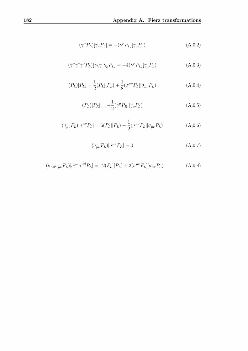
182 Appendix A. Fierz transformations
(γµPL)[γµPL] = −(γµPL][γµPL) (A.0.2)
(γµγνγλPL)[γλγνγµPL] = −4(γµPL][γµPL) (A.0.3)
(PL)[PL] = 12(PL][PL) + 1
8(σµνPL][σµνPL) (A.0.4)
(PL)[PR] = −12(γµPR][γµPL) (A.0.5)
(σµνPL)[σµνPL] = 6(PL][PL)− 12(σµνPL][σµνPL) (A.0.6)
(σµνPL)[σµνPR] = 0 (A.0.7)
(σαβσµνPL)[σµνσαβPL] = 72(PL][PL) + 2(σµνPL][σµνPL) (A.0.8)

Appendix B
Feynman Rules
Our SM Feynman rules can be found by taking those in [456] and setting η = ηs =η′ = ηe = −1 and ηZ = ηθ = ηY = 1. (Note that in that work all particles areconsidered incoming in Feynman diagrams.) These match the conventions of [457].
In Table B.1 below, we show the Feynman rules for heavy quarks in HQET.

184 Appendix B. Feynman Rules
i j
µ, a
∼ igsvµtaji
j i
µ, a
∼ −igsvµtaji
p = mv + p
∼ i(1+/v)2v·p
p = mv + p
∼ i(1−/v)2v·p
Table B.1: HQET Feynman rules.

Appendix C
Four Quark Matrix Elements
In phenomenological calculations matrix elements of four quark operators oftenarise, and so knowing these matrix elements is of vital importance to being able tomake theoretical predictions. However these are non-perturbative objects and socalculating them is non-trivial. Nowadays, lattice QCD has progressed to the pointof being able to provide precision determinations, but historically other techniqueswere used. In particular the Vacuum Saturation Approximation (VSA) is a simpleway of analytically approximating the result, and current data shows it even holdsnumerically at the 10–20% level [161,162]. The VSA approximates the four quarkmatrix elements as a product of decay to vacuum operators, and so gives us anestimate in terms of meson decay constants plus various colour factors. Below weshow an example of a VSA calculation, and then we list the results for differentoperators.
Note that we show results in this appendix for Bs-Bs mixing and Bs lifetime calcula-tions – the generalisation to Bd , D, etc. mesons can be found by making the obvioussubstitutions.
VSA Calculation Example
If we take the operator O1 = (biγµPLsi)(bjγµPLsj), there are four ways to contractthis with an incoming Bs and outgoing Bs state – two for the b quarks and two forthe s quarks. Making use of the Fierz identities stated in Equations A.0.1 and A.0.2,

186 Appendix C. Four Quark Matrix Elements
we can write the matrix element 〈Bs|O1|Bs〉 ≡ 〈O1〉 as
〈O1〉 = 〈Bs|(biγµPLsi)(bjγµPLsj)|Bs〉
= 2[ (〈Bs| b
iγµPLsi
) (bjγµPLsj |Bs〉
)+(〈Bs| b
iγµPLsj
) (bjγµPLsi |Bs〉
) ]= 2
[ (1 + 1
Nc
)(〈Bs| b
iγµPLsi
) (bjγµPLsj |Bs〉
)+2
(〈Bs| b
iγµPLt
aijsj
) (bkγµPLtaklsl |Bs〉
) ],
where the round brackets fix the operator contraction. (The factor of two is the sameas seen in Equation 2.4.18.) We then take the completeness relation I = ∑
X |X〉 〈X|and insert it into the middle of the four quark operator:
〈O1〉 = 2∑X
[ (1 + 1
Nc
)〈Bs|b
iγµPLsi|X〉 〈X|bjγµPLsj|Bs〉
+2 〈Bs|biγµPLt
aijsj|X〉 〈X|b
kγµPLt
aklsl|Bs〉
].
The VSA amounts to assuming the vacuum state dominates this sum, and so we canwrite
〈O1〉VSA= 2
[ (1 + 1
Nc
)〈Bs|b
iγµPLsi|0〉 〈0|bjγµPLsj|Bs〉
+2 〈Bs|biγµPLt
aijsj|0〉 〈0|b
kγµPLt
aklsl|Bs〉
].
The second term goes to zero as the colour octet operator cannot annihilate a coloursinglet meson, while for the first term we can use the definitions of the meson decayconstant
〈0|bγµs|Bs(p)〉 = 0〈0|bγµγ5s|Bs(p)〉 = ipµfBs
⇒ 〈0|bγµPL,Rs|Bs(p)〉 = ∓ i2pµfBs (C.0.1)
to give our result
〈O1〉VSA= 2
(1 + 1
Nc
)(− i2p
µfBs
)† (− i2pµfBs
)
= 12
(1 + 1
Nc
)M2
Bsf2Bs .
Since the VSA is only an approximation, we introduce an extra correction factor,known as the bag parameter,1 to account for deviations from this behaviour and
1The term “bag” dates back to the MIT bag model of hadrons.

187
write the matrix element as
〈Bs|O1|Bs〉 = 23f
2BsM
2BsB1 .
∆F = 2 operators
For ∆F = 2 operators, we can use Fierz relations to reduce the set of possibledimension-six operators which can arise to a minimal basis set, which are shownbelow:
O1 = (bαγµPLsα)(bβγµPLsβ) ,
O2 = (bαPLsα)(bβPLsβ) ,
O3 = (bαPLsβ)(bβPLsα) ,
O4 = (bαPLsα)(bβPRsβ) ,
O5 = (bαPLsβ)(bβPRsα) ,
O1 = (bαγµPRsα)(bβγµPRsβ) ,
O2 = (bαPRsα)(bβPRsβ) ,
O3 = (bαPRsβ)(bβPRsα) .
This minimal set was first derived in the context of supersymmetric extensions of theSM [160], and so is often referred to as the “SUSY basis”. Since parity is a symmetryof QCD, 〈O〉 = 〈O〉 holds as long as we don’t consider electroweak corrections to thematrix elements. At dimension seven, there are several more operators that arise –see [176] for details.
The matrix elements of the SUSY basis can be written in the form (notation takenfrom [217])
〈O1〉 = c1f2BsM
2BsB1 ,
〈Oi〉 = cif2BsM
2Bs
(MBs
mb +ms
)2
Bi (i = 2, 3) ,
〈Oi〉 = cif2BsM
2Bs
( MBs
mb +ms
)2
+ di
Bi (i = 4, 5) ,
(C.0.2)
where ci = 2/3,−5/12, 1/12, 1/2, 1/6, d4 = 1/6, and d5 = 3/2. These prefactors can bederived in the same way as in the above example, making use of Equations A.0.4and A.0.5, as well as the following two further relations involving the decay constant.

188 Appendix C. Four Quark Matrix Elements
We can show〈0|bPL,Rs|Bs(p)〉 = ± i2
MBs
mb +ms
fBs
by contracting the meson momentum pµ with our result in Equation C.0.1 (seeSection 4.3 of [458]); we must also have
〈0|bσµνs|Bs(p)〉 = 0
since we cannot construct an antisymmetric Lorentz tensor out of a single 4-momentum.
∆F = 0 operators
For ∆F = 0 operators, the standard set considered (which are those which arise inthe SM) is
Q1 = (bγµPLq)(qγµPLb)Q2 = (bPLq)(qPLb)T1 = (bγµtaPLq)(qγµtaPLb)T2 = (btaPLq)(qtaPLb)
which have matrix elements
〈Qi〉 = Aif2BsM
2BsBi
〈Ti〉 = Aif2BsM
2Bsεi
(C.0.3)
where Bi = 1 and εi = 0 in the VSA and
A1 = 14 , A2 = 1
4
(MBs
mb +ms
)2
. (C.0.4)
Appendix D
Additional information from“Quark-Hadron Duality”
In this appendix we present more information on the work in Chapter 3.
In Table D.1, we show the error breakdown for our updated lifetime ratio calcula-tion in Equation 3.2.32, which has an error smaller than the current experimentalmeasurement by a factor of four, and the previous SM calculation by a factor two.
In Table D.2, we present the inputs for our “aggressive” SM calculation in Section 3.3.
In Tables D.3 to D.10 we present the error breakdown for our updated predictions.
Finally in Appendix D.2 we show the proof of the inequality used in Section 3.4.

190 Appendix D. “Quark-Hadron Duality”
D.1 Inputs and detailed view of uncertainties
Parameter Error contributionδ(ε1) 0.0710%δ(ε2) 0.0510%δ(fBs) 0.0290%δ(µ2
G(Bs)/µ2G(Bd)) 0.0280%
µ2π(Bs)− µ2
π(Bd)) 0.0230%δ(fBd) 0.0230%δ(c3) 0.0230%δ(µ) 0.0160%δ(B1) 0.0140%δ(µ2
G(Bd)) 0.0130%δ(B2) 0.0100%δ(cG) 0.007%δ(mb) 0.004%δ(|Vcb|) 0.003%δ(mc) 0.001%δ(τBs) < 0.001%δ(MBs
) < 0.001%δ(MBd
) < 0.001%δ(|Vus|) < 0.001%δ(γ) < 0.001%δ(|Vub/Vcb|) < 0.001%∑δ 0.108%
Table D.1: Error breakdown for the SM prediction for τ(Bs)/τ(Bd)given in Equation 3.2.32.

D.1. Inputs and detailed view of uncertainties 191
Parameter This work ABL 2015 [165]
fBs
√B (0.223± 0.007)GeV (0.215± 0.015)GeV
fBd
√B (0.185± 0.008)GeV (0.175± 0.012)GeV
B3/B (Bs) 1.15± 0.16 1.07± 0.06B3/B (Bd) 1.17± 0.24 1.04± 0.12BR0/B (Bs) 0.54± 0.55 1.00± 0.3BR0/B (Bd) 0.35± 0.80 1.00± 0.3BR1/B (Bs) 1.61± 0.10 1.71± 0.26BR1/B (Bd) 1.72± 0.15 1.71± 0.26BR1
/B (Bs) 1.223± 0.093 1.27± 0.16BR1
/B (Bd) 1.31± 0.14 1.27± 0.16|Vcb| 0.04180+0.00033
−0.00068 0.04117+0.00090−0.00114
|Vub/Vcb| 0.0889± 0.0019 0.0862± 0.0044γ 1.170+0.015
−0.035 1.171+0.017−0.038
|Vus| 0.22542+0.00042−0.00031 0.22548+0.00068
−0.00034
Table D.2: Input parameters used in the “aggressive” determinationof Section 3.3, compared to the previous SM calculation.
Error contributionParameter This work ABL 2015 [165]
δ(fBs
√B) 0.0635% 0.139%
δ(|Vcb|) 0.0240% 0.049%δ(mt) 0.0066% 0.007%δ(ΛQCD) 0.0013% 0.001%δ(γ) 0.0009% 0.001%δ(mb) 0.0005% < 0.001%δ(|Vub/Vcb|) 0.0004% 0.001%∑δ 0.0682% 0.148%
Table D.3: Error breakdown for the mass difference ∆Ms.
Error contributionParameter This work ABL 2015 [165]
δ(fBd
√B) 0.0872% 0.137%
δ(|Vcb|) 0.0240% 0.049%δ(mt) 0.0066% 0.001%δ(ΛQCD) 0.0013% 0.0%δ(γ) 0.0208% 0.002%δ(mb) 0.0005% 0.0%δ(|Vub/Vcb|) 0.0001% 0.0%∑δ 0.0931% 0.148%
Table D.4: Error breakdown for the mass difference ∆Md.

192 Appendix D. “Quark-Hadron Duality”
Error contributionParameter This work ABL 2015 [165]δ(µ) 0.0889% 0.084%δ(fBs) 0.0635% 0.139%δ(BR2) 0.0604% 0.148%δ(B3) 0.0539% 0.021%δ(BR0) 0.0301% 0.021%δ(|Vcb|) 0.0240% 0.049%δ(z) 0.0109% 0.011%δ(mb) 0.0080% 0.008%δ(BR1
) 0.0038% 0.007%δ(ms) 0.0024% 0.001%δ(BR3) 0.0023% 0.002%δ(BR1) 0.0018% 0.005%δ(γ) 0.0010% 0.001%δ(ΛQCD) 0.0010% 0.001%δ(|Vub/Vcb|) 0.0004% 0.001%δ(mt) 0% < 0.001%∑δ 0.1421% 0.228%
Table D.5: Error breakdown for the width difference ∆Γs.
Error contributionParameter This work ABL 2015 [165]δ(µ) 0.0929% 0.079%δ(fBd ) 0.0872% 0.137%δ(B3) 0.0809% 0.04%δ(BR2) 0.0623% 0.144%δ(BR0) 0.0533% 0.025%δ(|Vcb|) 0.0240% 0.049%δ(γ) 0.0233% 0.002%δ(z) 0.0109% 0.011%δ(mb) 0.0076% 0.008%δ(BR3) 0.0023% 0.005%δ(ΛQCD) 0.0009% 0.001%δ(|Vub/Vcb|) 0.0008% 0.001%δ(BR1
) 0.0% 0.0%δ(md) — —δ(BR1) 0.0% 0.0%∑δ 0.175% 0.227%
Table D.6: Error breakdown for the width difference ∆Γd.

D.1. Inputs and detailed view of uncertainties 193
Parameter Error contributionδ(µ) 0.0889%δ(BR2) 0.0604%δ(B3) 0.0539%δ(BR0) 0.0301%δ(z) 0.0109%δ(mb) 0.0080%δ(mt) 0.0066%δ(BR1) 0.0038%δ(ms) 0.0024%δ(ΛQCD) 0.0023%δ(BR3) 0.0023%δ(BR1) 0.0018%δ(γ) 0.0001%δ(|Vub/Vcb|) 0%δ(|Vcb|) 0%∑δ 0.125%
Table D.7: Error breakdown for the ratio ∆Γs/∆Ms.
Parameter Error contributionδ(µ) 0.0929%δ(B3) 0.0809%δ(BR2) 0.0623%δ(BR0) 0.0533%δ(z) 0.0109%δ(mb) 0.0076%δ(mt) 0.0066%δ(γ) 0.0025%δ(BR3) 0.0023%δ(ΛQCD) 0.0022%δ(|Vub/Vcb|) 0.0009%δ(BR1) 0.0%δ(md) 0.0%δ(BR1) 0.0%δ(|Vcb|) 0.0%∑δ 0.149%
Table D.8: Error breakdown for the ratio ∆Γd/∆Md.

194 Appendix D. “Quark-Hadron Duality”
Parameter Error contributionδ(µ) 0.0946%δ(z) 0.0463%δ(Vub/Vcb) 0.0211%δ(γ) 0.0118%δ(BR3) 0.0106%δ(mb) 0.0101%δ(mt) 0.0066%δ(BS) 0.0078%δ(ΛQCD) 0.0053%δ(BR2) 0.0039%δ(BR1) 0.0030%δ(BR0) 0.0026%δ(ms) 0.0021%δ(BR1) 0.0002%δ(Vcb) 0%∑δ 0.1098%
Table D.9: Error breakdown for assl.
Parameter Error contributionδ(µ) 0.0937%δ(z) 0.0487%δ(|Vub/Vcb|) 0.0215%δ(mb) 0.0129%δ(B3) 0.0123%δ(BR3) 0.0115%δ(γ) 0.0105%δ(mt) 0.0066%δ(ΛQCD) 0.0054%δ(BR0) 0.0049%δ(BR2) 0.0042%δ(BR1) 0.0%δ(md) 0.0%δ(BR1) 0.0%δ(|Vcb|) 0.0%∑δ 0.111%
Table D.10: Error breakdown for adsl.

D.2. Proof of ∆Γ ≤ 2|Γ12| 195
D.2 Proof of ∆Γ ≤ 2|Γ12|
In the B system we get the very simple expression Equation 2.4.16 for the mixingobservables ∆M and ∆Γ in terms of M12 and Γ12, by expanding in the smallparameter ∆Γ/∆M . In the D system ∆Γ and ∆M are of the same order and so onewould have to exactly solve the two defining equations. One can find however, theinequality ∆Γ ≤ 2|Γ12|, which gives us the opportunity to calculate only Γ12 and togive an upper bound on ∆Γ.
We start with the two fundamental equations for the mixing observables:
(∆M)2 − 14(∆Γ)2 = 4|M12|2 − |Γ12|2 , (D.2.1)
∆M∆Γ = 4|M12||Γ12| cosφ12 . (D.2.2)
Next we eliminate ∆M by substituting Equation D.2.2 into Equation D.2.1, andthen solve for |M12|.
16|M12|2|Γ12|2 cos2 φ12
(∆Γ)2 − 14(∆Γ)2 = 4|M12|2 − |Γ12|2
|M12|2(
16|Γ12|2 cos2 φ12
(∆Γ)2 − 4)
= 14(∆Γ)2 − |Γ12|2
|M12|2 =14(∆Γ)2 − |Γ12|2(16|Γ12|
2 cos2φ12
(∆Γ)2 − 4) .
(D.2.3)
Since |M12|2 ≥ 0, we can say that the numerator and denominator on the right handside of the last line of Equation D.2.3 must have the same sign.
First, assume both terms are ≥ 0:
14(∆Γ)2 − |Γ12|2 ≥ 0 and 16|Γ12|2 cos2 φ12
(∆Γ)2 − 4 ≥ 0 (D.2.4)
=⇒ (∆Γ)2 ≥ 4|Γ12|2 and (∆Γ)2 ≤ 4Γ212 cos2 φ12 . (D.2.5)
These inequalities are only consistent in the case cos2 φ12 = 1 and ∆Γ = 2|Γ12|.
Now, assume both terms are ≤ 0:
14(∆Γ)2 − |Γ12|2 ≤ 0 and 16|Γ12|2 cos2 φ12
(∆Γ)2 − 4 ≤ 0 (D.2.6)
=⇒ (∆Γ)2 ≤ 4|Γ12|2 and 4Γ212 cos2 φ12 ≤ (∆Γ)2 . (D.2.7)
As 0 ≤ cos2 φ12 ≤ 1, these inequalities are consistent for either a) cos2 φ12 = 1 whichgives ∆Γ = 2|Γ12| or b) 2|Γ12|| cosφ12| ≤ ∆Γ ≤ 2|Γ12|.

196 Appendix D. “Quark-Hadron Duality”
We see that for either assumption the inequality ∆Γ ≤ 2|Γ12| holds. A similar lineof reasoning shows that the inequality ∆M ≤ 2|M12| also holds.

Appendix E
Additional information from“Charming Dark Matter”
In this appendix we present more information on the work in Chapter 4.
In Appendix E.1 we explicitly give the Wilson coefficients that arise when consideringcontributions to rare D decays, in Appendix E.2 we give more information onour technique for calculating constraints from direct detection experiments, and inAppendix E.3 we show some of the Feynman diagrams that contribute to collidersignatures for dark matter.
E.1 Rare decays
The non-zero Wilson coefficients arise from electroweak penguins (shown in Fig-ure E.1) and (neglecting Z penguins since the small momentum transfer means they
γ, Z
l l
c
χi
u
φ
γ, Z
l l
u
c
u
χi
φ
γ, Z
l l
c
c
uχi
φ
Figure E.1: The DMFV model contribution to the effective opera-tors governing rare decays of charm mesons, includingexplicit self-energy corrections to the external quarklegs as explained in the text. The γ,Z couple to alepton pair.

198 Appendix E. “Charming Dark Matter”
amount to an O (1%) correction) we find
C ′7 =∑i
λ1iλ∗2i
6√
2GF
[C1(m2
c , q2, 0,m2
χi,m2
φ,m2φ) + C11(m2
c , q2, 0,m2
χi,m2
φ,m2φ)
+C12(m2c , q
2, 0,m2χi,m2
φ,m2φ)], (E.1.1)
C ′9 =∑i
λ1iλ∗2i
3√
2GF q2
[B1(m2
c ,m2χi,m2
φ) + 2C00(m2c , q
2, 0,m2χi,m2
φ,m2φ)
+m2c
C1(m2
c , q2, 0,m2
χi,m2
φ,m2φ) + C11(m2
c , q2, 0,m2
χi,m2
φ,m2φ)
+C12(m2c , q
2, 0,m2χi,m2
φ,m2φ)]
, (E.1.2)
where B and C are loop functions using LoopTools [291] notation.
E.2 Direct Detection
E.2.1 LUX
For situations where we have both a measured event count Nobsk (binned into energy
bins labelled by k), and theoretical background Nbckk , we can use the likelihood
ratio test, a method based on a hypothesis test between a background only, andbackground+signal model, with likelihoods L,Lbck respectively [459].
The likelihood of observing the data, D, assuming a particular set of parametersλ, is denoted L(D|λ). The likelihood of each bin is a Poisson distributionPoiss(Nobs, N th(λ)) where N th
k are the predicted number of signal events (includingbackground):
L(Nobs|λ) =∏k
(N thk
)Nobsk
Nobsk !
exp[−N th
k
](E.2.1)
and where N th(λ) = NDM(λ) + Nbck. The background only model is identical butwith N th = Nbck. Then the test statistic
TS(λ) = −2 log(LLbck
)≈ 2
∑k
(N thk −Nobs
k log[N thk +Nbck
k
Nbckk
])(E.2.2)
follows a χ2 distribution – the cumulative probability density function of χ2(x)represents the probability that we observe the data given the model parameters λ.The value of x such that χ2(x) = C (i.e. the C% confidence limit) depends on thenumber of parameters λ – for only one parameter for example one can look upthat χ2(2.71) = 0.9, which means that the 90% confidence bounds on λ are givenby TS(λ) = 2.71.

E.3. Feynman Diagrams for collider searches 199
u, c
u, cχi
χj
φ
Figure E.2: The above diagram must include initial/final state ra-diation from external legs or internal bremsstrahlungfrom the mediator. The contribution is roughly equalamongst these emissions.
E.2.2 CDMSlite
For CDMSlite, we use a conservative method based on the statement that the 90%confidence limit is such that there is a probability of 0.9 that if the model were true,then the experiment would have measured more events (n) than have been measured(nobs). Using the Poisson distribution this probability is
P (n > nobs|µ) =∞∑
n=nobs
µn
n! exp(−µ) ≈∞∫
nobs
1√2πµ exp
(−(t− µ)2
2µ
)dt = 0.9 (E.2.3)
and in the limit nobs 1, this can be approximated by
P (n > nobs|µ) = 12
(Erfc
(nobs − µ√
2µ
))= 0.9 . (E.2.4)
This equation is numerically solvable for µ giving a required signal µ = 109+51−50, 88±
14, 635±37 and 207±20 events for energy bins 1 to 4 respectively. This is conservativesince a large portion of the measured events are background, and the resulting limitsare slightly weaker than those given by the CDMSlite collaboration.
E.3 Feynman Diagrams for collider searches
E.3.1 Monojet processes
The dominant diagrams contributing to the pure monojet process are shown here.Each processes scales as σ ∝ (λλ†)αs and can become extremely large for large λ.The cross section is dominated by the diagrams containing a heavy φ resonance.

200 Appendix E. “Charming Dark Matter”
g
u χi
φ
φ
q
χj g
u, c χi
φ
χj
q
g
u, c
qu, c
χj
χi
Figure E.3: The s-channel φ resonance is responsible for top leftand bottom dominating over top right, and the addi-tional enhancement due to the gluon pdf over Figure E.2makes these the overall dominant monojet contribution.For very heavy mediators top left is suppressed due tothe two propagators.

E.3. Feynman Diagrams for collider searches 201
g
g φ
φ g
g φ
φ
g
g φ
φ
Figure E.4: Gluon fusion dijet processes σ ∝ α2s.
u, c
u, c φ
φ
χi
u, c
u, c φ
φ
Figure E.5: The left (right) process has σ ∝ (λλ†)2(α2s) and so the
dominance depends on the size of the new couplings –for couplings which are large enough to be excluded itis usually the left diagram which dominates.
E.3.2 Dijet processes
The dominant processes contributing to the production of on-shell φ, which decayφ→ qiχj producing a dijet signal, are shown here. In monojet analyses, this providesa subdominant contribution compared with pure monojet processes (Figures E.2and E.3) in most of the parameter space.


Appendix F
Additional information from“Charming new physics in rare Bsdecays and mixing?”
In this appendix we provide additional information on the technical aspects ofour results for the anomalous dimensions entering in the RGE (Equation 5.6.1) inChapter 5.
A set of Wilson coefficients that contains C7, C9, and Cc1...4 and is closed under
renormalisation necessarily also contains four QCD-penguin coefficients CPi mul-tiplying the operators P3...6 (we define them as in [340]) and the chromodipolecoefficient C8g, resulting in an 11×11 anomalous dimension matrix γ. If the rescaledsemileptonic operator Q9(µ) = (4π/αs(µ))Q9V (µ) is used, then to leading orderγij(µ) = αs(µ)/(4π)γ(0)
ij , with constant γ(0)ij . As is well known, this matrix is already
scheme-dependent at LO [347–349]. A scheme-independent matrix γeff(0) can beachieved by replacing C7 and C8 by the scheme-independent combinations
Ceff7 = C7 +
∑i
yiCi , (F.0.1)
Ceff8 = C8 +
∑i
ziCi , (F.0.2)
where
〈sγ|Qi|b〉 = yi〈sγ|Q7γ|b〉 , (F.0.3)〈sg|Qi|b〉 = zi〈sγ|Q8g|b〉 , (F.0.4)
to lowest order and the sums run over all four-quark operators. We find that yi and zivanish forQc
1...4, leaving only the known coefficients yPi = (−1/3,−4/9,−20/3,−80/9)iand zPi = (1,−1/6, 20,−10/3)i (i = 3 . . . 6) [340]. The BSM correction ∆Ceff
9 in

204 Appendix F. “Charming new physics . . . ”
Equations 5.3.2 and 5.3.7 coincides with the (BSM correction to the) coefficient C9
of Q9V to LL accuracy.
Many of the elements of γeff(0) are known [337, 341–348], except for γeff(0)QciQ7γ
, γeff(0)QciQ8g
,γeff(0)QciPj
, and γeff(0)Qci Q9
, for i = 3, 4. The latter can be read off from the logarithmic termsin Equation 5.3.2, and the mixing into Pi follows from substituting gauge couplingand colour factors in the diagram shown on the left of Figure 5.1. This gives
γ(0)Qci Q9
=(−8
3 ,−89 ,
43 ,
49
)i, γ
(0)QciP4
=(
0, 43 , 0,−
23
)i,
for i = 1, 2, 3, 4, with the mixing into CP3,5,6 vanishing.
The leading mixing into Ceff7 arises at two loops [350–353] and is the technically
most challenging aspect of our results. Our calculation employs the 1PI (off-shell)formalism and the method of [354] for computing UV divergences, which involvesan infrared-regulator mass and the appearance of a set of gauge-non-invariant coun-terterms. The result is
γeff(0)QciQ7
=(
0, 41681 , 0,
22481
)i
(i = 1, 2, 3, 4) .
Our stated results for i = 1, 2 agree with the results in [340,345], which constitutesa cross-check of our calculation.
We have not obtained the 2-loop mixing of Cc3,4 into C8g and set these anomalous
dimension elements to zero. For the case of Cc1,2 where this mixing is known, the
impact of neglecting γeff(0)i8 on ∆Ceff7 (µ) is small (the only change being −0.19∆C2 →
−0.18∆C2 in Equation 5.3.6). We expect a similarly small error in the case of ∆C3,4.

Appendix G
Additional information from“Dimension-six matrix elementsfrom sum rules”
In this appendix we provide additional information relating to our work in Chapter 6.
In Appendix G.1 we provide our choice of basis for the evanescent operators forboth the ∆B = 2 and ∆B = 0 sectors, along with the corresponding anomalousdimension matrices.
In Appendix G.2 we show our choice of input parameters (Table G.1) as well asa detailed breakdown of the uncertainties associated with our results for the bagparameters (Tables G.2 to G.5).
Finally in Tables G.6 to G.9 we provide a breakdown of the errors in our mixing andlifetime ratio observables.

206 Appendix G. “Dimension-six matrix . . . ”
G.1 Basis of evanescent operators and ADMs
G.1.1 ∆B = 2 operators
Our choice of basis for the evanescent operators is given by
E1 = biγµ(1− γ5)qj bjγµ(1− γ5)qi −Q1 ,
E2 = biγµγν(1− γ5)qi bjγµγν(1− γ5)qj − (8− 4ε)Q2 − (8− 8ε)Q3 ,
E3 = biγµγν(1− γ5)qj bjγµγν(1− γ5)qi − (8− 8ε)Q2 − (8− 4ε)Q3 ,
E4 = biγµγνγρ(1− γ5)qi bjγµγνγρ(1− γ5)qj − (16− 4ε)Q1 ,
E5 = biγµγνγρ(1− γ5)qj bjγµγνγρ(1− γ5)qi − (16− 4ε)(Q1 + E1) ,E6 = biγµ(1− γ5)qi bjγµ(1 + γ5)qj + 2Q5 ,
E7 = biγµ(1− γ5)qj bjγµ(1 + γ5)qi + 2Q4 ,
E8 = biγµγν(1− γ5)qi bjγµγν(1 + γ5)qj − 4Q4 ,
E9 = biγµγν(1− γ5)qj bjγµγν(1 + γ5)qi − 4Q5 ,
(G.1.1)
for QCD and
E1 = h(+)i γµ(1− γ5)qj h(−)
j γµ(1− γ5)qi − Q1 ,
E2 = 12Q1 + Q2 + h
(+)i (1− γ5)qj h(−)
j (1− γ5)qi ,
E3 = h(+)i γµγν(1− γ5)qi h(−)
j γµγν(1− γ5)qj + (4 + a1ε)Q1 ,
E4 = h(+)i γµγν(1− γ5)qj h(−)
j γµγν(1− γ5)qi + (4 + a1ε)(Q1 + E1) ,E5 = h
(+)i γµγνγρ(1− γ5)qi h(−)
j γµγνγρ(1− γ5)qj − (16 + a2ε)Q1 , (G.1.2)E6 = h
(+)i γµγνγρ(1− γ5)qj h(−)
j γµγνγρ(1− γ5)qi − (16 + a2ε)(Q1 + E1) ,E7 = h
(+)i γµ(1− γ5)qi h(−)
j γµ(1 + γ5)qj + 2Q5 ,
E8 = h(+)i γµ(1− γ5)qj h(−)
j γµ(1 + γ5)qi + 2Q4 ,
E9 = h(+)i γµγν(1− γ5)qi h(−)
j γµγν(1 + γ5)qj − (4 + a3ε)Q4 ,
E10 = h(+)i γµγν(1− γ5)qj h(−)
j γµγν(1 + γ5)qi − (4 + a3ε)Q5 ,
for HQET. It is straightforward to verify that the evanescent operators vanish infour dimensions by using the Fierz identities Equations A.0.2, A.0.4 and A.0.5 alongwith the relation
γµγνγρ = gµνγρ + gνργµ − gµργν − iεµνρλγλγ5. (G.1.3)
A useful strategy to simplify expressions with two Dirac matrices is to use projectionidentities, e.g.
h(±)γµγν(1− γ5)q = ±h(±)/vγµγν(1− γ5)q, (G.1.4)

G.1. Basis of evanescent operators and ADMs 207
and then reduce the number of Dirac matrices with Equation G.1.3.
In the decomposition shown in Equation 6.2.8 the LO QCD ADM is
γ(0)QQ =
6(Nc−1)Nc
0 0 0 0
0 −2(3N2c−4Nc−1)Nc
4Nc−8Nc
0 00 4(Nc−2)(Nc+1)
Nc
2(Nc+1)2
Nc0 0
0 0 0 −6(N2c−1)Nc
00 0 0 −6 6
Nc
, (G.1.5)
γ(0)QE =
6 0 0 − 1Nc
1 0 0 0 00 − 1
Nc1 0 0 0 0 0 0
0 12
Nc2 −
1Nc
0 0 0 0 0 00 0 0 0 0 0 0 − 1
Nc1
0 0 0 0 0 0 0 12
Nc2 −
1Nc
. (G.1.6)
In HQET we find
γ(0)QQ
=
3Nc− 3Nc 0 0 0
1 + 1Nc
−3Nc + 4 + 7Nc
0 00 0 6
Nc− 3Nc −3
0 0 −3 6Nc− 3Nc
, (G.1.7)
γ(0)QE
=
0 0 0 0 − 1
4Nc14 0 0 0 0
−1 −4 − 14Nc
14 0 0 0 0 0 0
0 0 0 0 0 0 0 0 − 14Nc
14
0 0 0 0 0 0 0 0 14 − 1
4Nc
. (G.1.8)
Our result (Equation G.1.5) with Nc = 3 differs from the results of [460,461] becausewe have only used the replacements implied by the basis of evanescent operators(Equation G.1.1) to simplify products of Dirac matrices. We can reproduce theirresult by applying 4-dimensional Fierz identities that relate Q1, Q2 and Q3. Theupper left 2× 2 sub-matrix of Equation G.1.7 agrees with [369].

208 Appendix G. “Dimension-six matrix . . . ”
G.1.2 ∆B = 0 operators
We define the basis of evanescent operators in QCD following [404]:
Eq1 = bγµγνγρ(1− γ5)q qγργνγµ(1− γ5)b− (4− 8ε)Qq
1 ,
Eq2 = bγµγν(1− γ5)q qγνγµ(1 + γ5)b− (4− 8ε)Qq
2 ,
Eq3 = bγµγνγρ(1− γ5)TAq qγργνγµ(1− γ5)TAb− (4− 8ε)T q1 ,
Eq4 = bγµγν(1− γ5)TAq qγνγµ(1 + γ5)TAb− (4− 8ε)T q2 .
(G.1.9)
In HQET we again introduce parameters a1,2 to keep track of the scheme dependence.
Eq1 = hγµγνγρ(1− γ5)q qγργνγµ(1− γ5)h− (4 + a1ε)Qq
1 ,
Eq2 = hγµγν(1− γ5)q qγνγµ(1 + γ5)h− (4 + a2ε)Qq
2 ,
Eq3 = hγµγνγρ(1− γ5)TAq qγργνγµ(1− γ5)TAh− (4 + a1ε)T q1 ,
Eq4 = hγµγν(1− γ5)TAq qγνγµ(1 + γ5)TAh− (4 + a2ε)T q2 .
(G.1.10)
The isospin breaking combinations of the evanescent operators are defined in analogyto Equation 6.5.3. The LO ADM in QCD takes the form
γ(0)QQ =
0 0 12 00 6
Nc− 6Nc 0 0
3− 3N
2c
0 − 12Nc
00 0 0 6
Nc
, (G.1.11)
γ(0)QE =
0 0 −2 00 0 0 −2
12N2
c
− 12 0 2
Nc− Nc
2 00 1
2N2c
− 12 0 2
Nc− Nc
2
. (G.1.12)
The HQET result is given by
γ(0)QQ
=
3Nc− 3Nc 0 6 00 3
Nc− 3Nc 0 6
32 −
32N2
c
0 − 3Nc
00 3
2 −3
2N2c
0 − 3Nc
, (G.1.13)
γ(0)QE
=
0 0 −1
2 00 0 0 −1
21
8N2c
− 18 0 1
2Nc− Nc
4 00 1
8N2c
− 18 0 1
2Nc− Nc
4
. (G.1.14)

G.2. Inputs and detailed overview of uncertainties 209
Our result in Equation G.1.11 is in agreement with [337,423] and Equation G.1.13reproduces the result of [196].1 The results in Equations G.1.12 and G.1.14 are new.The matching coefficients read
C(0)QiQj
= δij (G.1.15)
at LO and
C(1)QiQj
=
−4Lµ − 32
3163 −a1
4 − 3Lµ − 13 −20 4Lµ + 16
3 −32 −a2
4 + 3Lµ − 1−a1
18 −2Lµ
3 −269 −4
9 −7a124 + 3Lµ
2 + 76 −3
−13 −a2
18 + 2Lµ3 −
29 −1
4 −7a224 −
3Lµ2 −
296
(G.1.16)
at NLO where we have set Nc = 3 for brevity.
G.2 Inputs and detailed overview ofuncertainties
Parameter Value Source
mb(mb)(4.203+0.016
−0.034)GeV [391,392]
mPSb (2GeV)
(4.532+0.013
−0.039)GeV [391,392]
m1Sb
(4.66+0.04
−0.03)GeV [390]
mkinb (1GeV) (4.553± 0.020)GeV [462]
mc(mc) (1.279± 0.013)GeV [463]αs(MZ) 0.1181± 0.0011 [390]Vus 0.2248± 0.0006 [390]Vub 0.004 09± 0.000 39 [390]Vcb 0.0405± 0.0015 [390]γCKM
(73.2+6.3
−7.0)° [390]
fB (189± 4)MeV [390]fBs (227.2± 3.4)MeV [390]fD (203.7± 4.8)MeV [390]
Table G.1: Input values for parameters. Note that for fB we usethe mean of fB and fB+ , while for fD we use the “ex-perimental” value instead of the lattice average, sincethe former is in significantly better agreement with sumrule results [407,408,412,413].
1Note that [196] contains a misprint that has been identified in [405].

210 Appendix G. “Dimension-six matrix . . . ”
Λ intrinsic SR condensates µρ 1/mb µm ai
BQ1+0.001−0.002 ±0.018 ±0.004 +0.011
−0.022 ±0.010 +0.045−0.039
+0.007−0.007
BQ2+0.014−0.017 ±0.020 ±0.004 +0.012
−0.019 ±0.010 +0.071−0.062
+0.015−0.015
BQ3+0.060−0.074 ±0.107 ±0.023 +0.016
−0.008 ±0.010 +0.086−0.069
+0.053−0.052
BQ4+0.007−0.006 ±0.021 ±0.011 +0.003
−0.003 ±0.010 +0.088−0.079
+0.005−0.006
BQ5+0.019−0.015 ±0.018 ±0.009 +0.004
−0.006 ±0.010 +0.077−0.068
+0.012−0.012
Table G.2: Individual errors for the bag parameters of the ∆B = 2matrix elements.
Λ intrinsic SR condensates µρ 1/mb µm ai
B1+0.003−0.002 ±0.019 ±0.002 +0.002
−0.002 ±0.010 +0.060−0.052
+0.002−0.003
B2+0.001−0.001 ±0.020 ±0.002 +0.000
−0.001 ±0.010 +0.084−0.076
+0.001−0.002
ε1+0.006−0.007 ±0.022 ±0.003 +0.003
−0.003 ±0.010 +0.010−0.012
+0.006−0.007
ε2+0.005−0.006 ±0.017 ±0.003 +0.002
−0.001 ±0.010 +0.001−0.002
+0.003−0.004
Table G.3: Individual errors for the bag parameters of the ∆B = 0matrix elements.
Λ intrinsic SR condensates µρ 1/mc µm ai
BQ1+0.001−0.002 ±0.013 ±0.003 +0.009
−0.021 ±0.030 +0.039−0.021 ±0.003
BQ2+0.011−0.014 ±0.015 ±0.003 +0.010
−0.016 ±0.030 +0.092−0.050 ±0.012
BQ3+0.037−0.045 ±0.059 ±0.013 +0.016
−0.016 ±0.030 +0.116−0.059 ±0.016
BQ4+0.006−0.005 ±0.017 ±0.009 +0.003
−0.003 ±0.030 +0.131−0.071 ±0.004
BQ5+0.014−0.012 ±0.014 ±0.007 +0.004
−0.005 ±0.030 +0.127−0.069 ±0.004
Table G.4: Individual errors for the bag parameters of the ∆C = 2matrix elements.
Λ intrinsic SR condensates µρ 1/mc µm ai
B1+0.004−0.003 ±0.017 ±0.002 +0.002
−0.002 ±0.030 +0.068−0.037
+0.003−0.005
B2+0.001−0.000 ±0.015 ±0.001 +0.000
−0.000 ±0.030 +0.120−0.065
+0.000−0.001
ε1+0.007−0.008 ±0.024 ±0.004 +0.003
−0.004 ±0.030 +0.012−0.022
+0.006−0.008
ε2+0.003−0.004 ±0.011 ±0.002 +0.001
−0.001 ±0.030 +0.000−0.000
+0.001−0.002
Table G.5: Individual errors for the bag parameters of the ∆C = 0matrix elements.

G.2. Inputs and detailed overview of uncertainties 211
Error contribution
Parameter ∆MSMs / ps−1 ∆ΓPS
s / ps−1 as,PSsl / 10−5
δ(BQ1) ±1.1 ±0.005 ±0.01δ(BQ3) ±0.0 ±0.005 ±0.01δ(BR0) ±0.0 ±0.003 ±0.00δ(BR1) ±0.0 ±0.000 ±0.00δ(BR
′1) ±0.0 ±0.000 ±0.00
δ(BR2) ±0.0 ±0.016 ±0.00δ(BR3) ±0.0 ±0.001 ±0.02δ(BR
′3) ±0.0 ±0.000 ±0.05
δ(fBs) ±0.5 ±0.002 ±0.00δ(µ1) ±0.0 +0.007
−0.018+0.04−0.08
δ(µ2) ±0.1 +0.000−0.002 ±0.01
δ(mb) ±0.0 +0.000−0.001 ±0.01
δ(mc) ±0.0 +0.000−0.001 ±0.06
δ(αs) ±0.0 ±0.000 ±0.04δ(CKM) +1.4
−1.3 ±0.006 +0.21−0.22
Table G.6: Individual errors for the Bs mixing observables.
Error contribution
Parameter ∆MSMd / ps−1 ∆ΓPS
d / 10−3 ps−1 ad,PSsl / 10−4
δ(BQ1) +0.04−0.03 ±0.16 ±0.02
δ(BQ3) ±0.00 +0.17−0.16 ±0.03
δ(BR0) ±0.00 ±0.11 ±0.01δ(BR1) ±0.00 ±0.01 ±0.00δ(BR
′1) ±0.00 ±0.01 ±0.00
δ(BR2) ±0.00 ±0.54 ±0.00δ(BR3) ±0.00 ±0.00 ±0.04δ(BR
′3) ±0.00 ±0.01 ±0.09
δ(fB) ±0.03 ±0.11 ±0.00δ(µ1) ±0.00 +0.24
−0.62+0.17−0.07
δ(µ2) ±0.00 +0.00−0.08
+0.01−0.03
δ(mb) ±0.00 +0.01−0.03
+0.01−0.03
δ(mc) ±0.00 +0.01−0.02 ±0.13
δ(αs) ±0.00 ±0.01 ±0.08δ(CKM) ±0.08 +0.38
−0.37+0.47−0.44
Table G.7: Individual errors for the Bd mixing observables.

212 Appendix G. “Dimension-six matrix . . . ”
Parameter Error contributionδ(B1) ±0.002δ(B2) ±0.000δ(ε1) +0.016
−0.015δ(ε2) ±0.004δ(ρ3) ±0.001δ(ρ4) ±0.000δ(σ3) ±0.013δ(σ4) ±0.000δ(fB) +0.004
−0.003δ(µ1) +0.000
−0.013δ(µ0) +0.000
−0.006δ(mb) +0.000
−0.001δ(mc) ±0.000δ(αs) ±0.002δ(CKM) ±0.006
Table G.8: Individual errors for the ratio τ(B+)/τ(B0 ) in the PSmass scheme.
Parameter Error contributionδ(B1) +0.07
−0.05δ(B2) ±0.00δ(ε1) +0.52
−0.47δ(ε2) ±0.017δ(ρ3) ±0.05δ(ρ4) ±0.00δ(σ3) ±0.46δ(σ4) ±0.00δ(fD) ±0.08δ(µ1) +0.07
−0.40δ(µ0) +0.08
−0.21δ(mc) ±0.08δ(ms) ±0.00δ(αs) +0.07
−0.06δ(CKM) ±0.00
Table G.9: Individual errors for the ratio τ(D+)/τ(D0 ) in the PSmass scheme.

Appendix H
Additional information from “Oneconstraint to kill them all?”
In this appendix, we break down our updated SM calculation in Chapter 7 byshowing the inputs used and the resulting error breakdown. We also discuss in moredetail the dependence of ∆Ms on inputs from lattice QCD and the CKM matrixelements.
H.1 Numerical input for theory predictions
The inputs we use in our numerical evaluations are shown in Table H.1. The valuesare taken from the PDG [224,464], from non-relativistic sum rules (NRSR) [391,392],from the CKMfitter group [29] and the non-perturbative parameters from FLAG(July 2017 online update [162]). For αs we use RunDec [389] with 5-loop accuracy[393–397], running from MZ down to the bottom mass scale. At the low scale weuse 2-loop accuracy to determine Λ(5).
H.2 Error budget of the theory predictions
In this section we compare the error budget of our new SM prediction for ∆MSMs
with the ones given in 2015 by [165], in 2011 by [208] and 2006 by [207] – the resultsare shown in Table H.2.
We observe a considerable improvement in accuracy and a sizeable shift compared tothe 2015 prediction, mostly stemming from the new lattice results for fBs
√B, which
is still responsible for the largest error contribution of about 6%. The next importantuncertainty is the accuracy of the CKM element Vcb, which contributes about 2% to

214 Appendix H. “One constraint to . . . ”
Parameter Value SourceMBs (5.366 89± 0.000 19)GeV PDG 2017mt (173.1± 0.6)GeV PDG 2017mt(mt) (165.65± 0.57)GeV own evaluationmb(mb) (4.203± 0.025)GeV NRSRαs(MZ) 0 1181(11) PDG 2017αs(mb) 0 2246(21) own evaluationΛ(5) (0.2259± 0.0068)GeV own evaluationVus 0.22508+0.00030
−0.00028 CKMfitterVcb 0.04181+0.00028
−0.00060 CKMfitter|Vub/Vcb| 0 0889(14) CKMfitterγCKM 1.141+0.017
−0.020 CKMfitterfBs
√B (274± 8)MeV FLAG
Table H.1: Input parameters for our update of ∆Ms.
Error contributionParameter This work ABL 2015 [165] LN 2011 [208] LN 2006 [207]
δ(fBs√B) 5.8% 13.9% 13.5% 34.1%
δ(|Vcb|) 2.1% 4.9% 3.4% 4.9%δ(mt) 0.7% 0.7% 1.1% 1.8%δ(αs) 0.1% 0.1% 0.4% 2%δ(γCKM) 0.1% 0.1% 0.3% 1%δ(|Vub/Vcb|) < 0.1% 0.1% 0.2% 0.5%δ(mb) < 0.1% < 0.1% 0.1% —∑δ 6.2% 14.8% 14.0% 34.6%
Table H.2: Individual contributions to the theoretical error of themass difference ∆Ms within the SM and comparisonwith the values obtained in [165, 207, 208]. In the lastrow the errors are summed in quadrature.

H.3. Non-perturbative inputs 215
Source fBs
√B ∆MSM
s
HPQCD14 [182] (247± 12)MeV (16.2± 1.7) ps−1
ETMC13 [181] (262± 10)MeV (18.3± 1.5) ps−1
HPQCD09 [465] = FLAG13 [220] (266± 18)MeV (18.9± 2.6) ps−1
FLAG17 [161] (274± 8)MeV (20.01± 1.25) ps−1
Fermilab16 [217] (274.6± 8.8)MeV (20.1± 1.5) ps−1
HQET-SR [4,408](278+28
−24)MeV
(20.6+4.4
−3.4)ps−1
HPQCD06 [358] (281± 20)MeV (21.0± 3.0) ps−1
RBC/UKQCD14 [466] (290± 20)MeV (22.4± 3.4) ps−1
Fermilab11 [180] (291± 18)MeV (22.6± 2.8) ps−1
Table H.3: Predictions for the non-perturbative parameter fBs
√B
and the corresponding SM prediction for ∆Ms. Thecurrent FLAG average is dominated by the FERMI-LAB/MILC value from 2016. Note that the HQET-SRresult is found by combining our result for the bag pa-rameter (Equation 6.4.2, which was published in [4])with a separate sum rule calculation of the decay con-stant.
the error budget. The CKM parameters were determined assuming unitarity of the3×3 CKM matrix – if this assumption is relaxed, then the uncertainties can increase.The uncertainties due to the remaining parameters are subleading. In total we areleft with an overall uncertainty of about 6%, in comparison to the experimentaluncertainty of about 0.1%.
H.3 Non-perturbative inputs
As a word of caution we present in Table H.3 a wider range of non-perturbativedeterminations of the matrix elements of the four-quark operators alongside thecorresponding predictions for the mass difference.
HPQCD presented in 2014 preliminary results for Nf = 2+1 [182] – for our numericalestimate in Table H.3 we extracted the numbers from Figure 3 in those proceedings.When finalised, this new calculation will supersede the 2006 [358] and 2009 [465]values. The ETMC Nf = 2 number stems from 2013 [181], it is obtained withonly two active flavours in the lattice simulation. The Fermilab/MILC Nf = 2 + 1number is from 2016 [217] and it supersedes the 2011 value [180]. This value currentlydominates the FLAG average. The numerical effect of these new inputs on mixingobservables was partially studied in Chapter 3. The previous FLAG average from2013 [220] was considerably lower. There is also a large Nf = 2 + 1 value from

216 Appendix H. “One constraint to . . . ”
RBC-UKQCD presented at LATTICE 2015 (update of [466]). However, this numberis obtained in the static limit and currently missing 1/mb corrections are expectedto be very sizeable.1 The HQET sum rules estimate for the bag parameter fromChapter 6 can also be combined with the decay constant from lattice.
It would be very desirable to see a convergence of these determinations, and inparticular an independent confirmation of the Fermilab/MILC result which currentlydominates the FLAG average.
H.4 CKM-dependence
The second most important input parameter for the prediction of ∆Ms is the CKMparameter Vcb. There is a long-standing discrepancy between the inclusive determina-tion and values obtained from studying exclusive B decays, see [467]. Recent studieshave found that a problem with the use of a certain form factor parameterisation inthe experimental analysis might be the cause of the low exclusive value. The formfactor models are denoted by CLN [468] and BGL [469]. Traditionally experimentshad used CLN, but it appears that this might underestimate some uncertainties.Using the BGL parameterisation instead one finds (see [470–473]) values that lieconsiderably closer to the inclusive one. Currently, there are various determinationsof Vcb available:
V Inclusivecb = 0.04219± 0.00078 [142]V
B→Dcb = 0.03918± 0.00094± 0.00031 [142]
VB→D∗, CLNcb = 0.03871± 0.00047± 0.00059 [142]
VB→D∗, BGLcb = 0.0419+0.0020
−0.0019 [470] .
In Figure H.1 we plot the dependence of the SM prediction of ∆Ms on Vcb, andshow the regions predicted by the above inclusive and exclusive determinations. Weuse the CKMfitter result for Vcb (see Table H.1) for our new SM prediction of ∆Ms
(see Equation 7.2.3 and the (upper) horizontal dashed line denoted with “SM”),and the corresponding error band is shown in orange. The predictions obtained byusing the inclusive value of Vcb only are given by the blue region. For completenesswe also show the regions obtained by using the various exclusive extractions of Vcb.The disfavoured CLN values result in much lower values for the mass difference(hatched areas), while the BGL value agrees well with the inclusive region, albeitwith a higher uncertainty. The experimental value of ∆Ms is shown by the (lower)
1Private communication with Tomomi Ishikawa.

H.4. CKM-dependence 217
Exp
SM
0.038 0.039 0.040 0.041 0.042 0.043 0.04416
17
18
19
20
21
22
Figure H.1: Dependence of the SM prediction of ∆Ms on the valueof Vcb.
horizontal dashed line denoted with “Exp”.
The preference for the inclusive determination agrees with the value obtained fromthe CKM fit (which we use in our SM estimate), as well as with the fit value that isfound if the direct measurements of Vcb are not included in the fit [29]:
VCKMfitter (no direct)cb = 0.04235+0.00074
−0.00069 . (H.4.1)
We also note that the CKMfitter determinations take into account loop-mediatedprocesses, where potentially NP could be present and affect the determination.Taking only tree-level inputs, they find:1
|Vus| = 0.22520+0.00012−0.00038 , (H.4.2)
|Vcb| = 0.04175+0.00033−0.00172 , (H.4.3)
|Vub/Vcb| = 0.092+0.004−0.005 , (H.4.4)
γCKM = 1.223+0.017−0.030 , (H.4.5)
and using these inputs we find
∆MSM,2017 (tree)s = (19.9± 1.5) ps−1 , (H.4.6)
which shows an overall consistency with the prediction in Equation 7.2.3.
1Private communication with Sébastien Descotes-Genon.


Bibliography
[1] T. Jubb, M. Kirk, A. Lenz and G. Tetlalmatzi-Xolocotzi, On the ultimateprecision of meson mixing observables, Nucl. Phys. B915 (2017) 431–453,[1603.07770].
[2] T. Jubb, M. Kirk and A. Lenz, Charming Dark Matter, JHEP 12 (2017) 010,[1709.01930].
[3] S. Jäger, K. Leslie, M. Kirk and A. Lenz, Charming new physics in rareB-decays and mixing?, Phys. Rev. D97 (2018) 015021, [1701.09183].
[4] M. Kirk, A. Lenz and T. Rauh, Dimension-six matrix elements for mesonmixing and lifetimes from sum rules, JHEP 12 (2017) 068, [1711.02100].
[5] L. Di Luzio, M. Kirk and A. Lenz, One constraint to kill them all?, Phys.Rev. D97 (2018) 095035, [1712.06572].
[6] P. A. M. Dirac, The quantum theory of the electron, Proc. Roy. Soc. Lond.A117 (1928) 610–624.
[7] S. Tomonaga, On a relativistically invariant formulation of the quantumtheory of wave fields, Prog. Theor. Phys. 1 (1946) 27–42.
[8] J. S. Schwinger, On Quantum electrodynamics and the magnetic moment ofthe electron, Phys. Rev. 73 (1948) 416–417.
[9] J. S. Schwinger, Quantum electrodynamics. I A covariant formulation, Phys.Rev. 74 (1948) 1439.
[10] R. P. Feynman, Space - Time Approach to Quantum Electrodynamics, Phys.Rev. 76 (1949) 769–789.
[11] R. P. Feynman, The Theory of positrons, Phys. Rev. 76 (1949) 749–759.
[12] R. P. Feynman, Mathematical formulation of the quantum theory ofelectromagnetic interaction, Phys. Rev. 80 (1950) 440–457.
[13] F. Englert and R. Brout, Broken Symmetry and the Mass of Gauge VectorMesons, Phys. Rev. Lett. 13 (1964) 321–323.
[14] P. W. Higgs, Broken Symmetries and the Masses of Gauge Bosons, Phys. Rev.Lett. 13 (1964) 508–509.

220 Bibliography
[15] G. S. Guralnik, C. R. Hagen and T. W. B. Kibble, Global Conservation Lawsand Massless Particles, Phys. Rev. Lett. 13 (1964) 585–587.
[16] S. L. Glashow, Partial Symmetries of Weak Interactions, Nucl. Phys. 22(1961) 579–588.
[17] S. Weinberg, A Model of Leptons, Phys. Rev. Lett. 19 (1967) 1264–1266.
[18] A. Salam, Weak and Electromagnetic Interactions, Conf. Proc. C680519(1968) 367–377.
[19] H. Fritzsch, M. Gell-Mann and H. Leutwyler, Advantages of the Color OctetGluon Picture, Phys. Lett. 47B (1973) 365–368.
[20] D. J. Gross and F. Wilczek, Ultraviolet Behavior of Nonabelian GaugeTheories, Phys. Rev. Lett. 30 (1973) 1343–1346.
[21] H. D. Politzer, Reliable Perturbative Results for Strong Interactions?, Phys.Rev. Lett. 30 (1973) 1346–1349.
[22] H. Fritzsch, The Physics of flavor is the flavor of physics, in Flavor physics.Proceedings, International Conference, ICFP 2001, Zhang-Jia-Jie, China,May 31-June 6, 2001, pp. 453–462, 2001, hep-ph/0111051, DOI.
[23] H. Fritzsch, The Physics of flavor: Challenge for the future, J. Korean Phys.Soc. 45 (2004) S297–S300, [hep-ph/0407069].
[24] H. Yukawa, On the Interaction of Elementary Particles I, Proc. Phys. Math.Soc. Jap. 17 (1935) 48–57.
[25] A. J. Buras, P. Gambino, M. Gorbahn, S. Jäger and L. Silvestrini, Universalunitarity triangle and physics beyond the standard model, Phys. Lett. B500(2001) 161–167, [hep-ph/0007085].
[26] G. D’Ambrosio, G. F. Giudice, G. Isidori and A. Strumia, Minimal flavorviolation: An Effective field theory approach, Nucl. Phys. B645 (2002)155–187, [hep-ph/0207036].
[27] N. Cabibbo, Unitary Symmetry and Leptonic Decays, Phys. Rev. Lett. 10(1963) 531–533.
[28] M. Kobayashi and T. Maskawa, CP Violation in the Renormalizable Theoryof Weak Interaction, Prog. Theor. Phys. 49 (1973) 652–657.
[29] CKMfitter collaboration, “ICHEP 2016 results.”http://ckmfitter.in2p3.fr/www/results/plots_ichep16/num/ckmEval_results_ichep16.html.
[30] CKMfitter collaboration, J. Charles, A. Hocker, H. Lacker, S. Laplace,F. R. Le Diberder, J. Malcles et al., CP violation and the CKM matrix:Assessing the impact of the asymmetric B factories, Eur. Phys. J. C41 (2005)1–131, [hep-ph/0406184].

Bibliography 221
[31] CKMfitter collaboration. http://ckmfitter.in2p3.fr/.
[32] UTfit collaboration, M. Bona et al., The Unitarity Triangle Fit in theStandard Model and Hadronic Parameters from Lattice QCD: A Reappraisalafter the Measurements of ∆ms and BR(B → τντ ), JHEP 10 (2006) 081,[hep-ph/0606167].
[33] UTfit collaboration. http://www.utfit.org/UTfit/WebHome.
[34] L.-L. Chau and W.-Y. Keung, Comments on the Parametrization of theKobayashi-Maskawa Matrix, Phys. Rev. Lett. 53 (1984) 1802.
[35] L. Wolfenstein, Parametrization of the Kobayashi-Maskawa Matrix, Phys.Rev. Lett. 51 (1983) 1945.
[36] S. L. Glashow, J. Iliopoulos and L. Maiani, Weak Interactions withLepton-Hadron Symmetry, Phys. Rev. D2 (1970) 1285–1292.
[37] G. Luders, On the Equivalence of Invariance under Time Reversal and underParticle-Antiparticle Conjugation for Relativistic Field Theories, Kong. Dan.Vid. Sel. Mat. Fys. Med. 28N5 (1954) 1–17.
[38] W. Pauli in Niels Bohr and the Development of Physics: Essays Dedicated toNiels Bohr on the Occasion of His Seventieth Birthday (W. Pauli, ed.).McGraw-Hill, 1955.
[39] J. S. Bell, Ph.D. thesis, University of Birmingham, 1954.
[40] T. D. Lee and C.-N. Yang, Question of Parity Conservation in WeakInteractions, Phys. Rev. 104 (1956) 254–258.
[41] C. S. Wu, E. Ambler, R. W. Hayward, D. D. Hoppes and R. P. Hudson,Experimental Test of Parity Conservation in Beta Decay, Phys. Rev. 105(1957) 1413–1414.
[42] J. H. Christenson, J. W. Cronin, V. L. Fitch and R. Turlay, Evidence for the2π Decay of the K0
2 Meson, Phys. Rev. Lett. 13 (1964) 138–140.
[43] C. Jarlskog, Commutator of the Quark Mass Matrices in the StandardElectroweak Model and a Measure of Maximal CP Violation, Phys. Rev. Lett.55 (1985) 1039.
[44] C. Jarlskog, A Basis Independent Formulation of the Connection BetweenQuark Mass Matrices, CP Violation and Experiment, Z. Phys. C29 (1985)491–497.
[45] ATLAS collaboration, “Summary plots from the ATLAS Standard Modelphysics group.” https://atlas.web.cern.ch/Atlas/GROUPS/PHYSICS/CombinedSummaryPlots/SM/.
[46] CMS collaboration, “Summaries of CMS cross section measurements.” https://twiki.cern.ch/twiki/bin/view/CMSPublic/PhysicsResultsCombined.

222 Bibliography
[47] F. Zwicky, Die Rotverschiebung von extragalaktischen Nebeln, Helv. Phys.Acta 6 (1933) 110–127.
[48] F. Zwicky, On the Masses of Nebulae and of Clusters of Nebulae, Astrophys.J. 86 (1937) 217–246.
[49] V. C. Rubin and W. K. Ford, Jr., Rotation of the Andromeda Nebula from aSpectroscopic Survey of Emission Regions, Astrophys. J. 159 (1970) 379–403.
[50] K. G. Begeman, A. H. Broeils and R. H. Sanders, Extended rotation curves ofspiral galaxies: dark haloes and modified dynamics, Mon. Not. Roy. Astron.Soc. 249 (1991) 523.
[51] D. S. Davis and R. E. White, III, Rosat temperatures and abundances for acomplete sample of elliptical galaxies, Astrophys. J. 470 (1996) L35,[astro-ph/9607052].
[52] S. W. Allen, D. A. Rapetti, R. W. Schmidt, H. Ebeling, G. Morris and A. C.Fabian, Improved constraints on dark energy from Chandra X-rayobservations of the largest relaxed galaxy clusters, Mon. Not. Roy. Astron.Soc. 383 (2008) 879–896, [0706.0033].
[53] Planck collaboration, P. A. R. Ade et al., Planck 2015 results. XIII.Cosmological parameters, Astron. Astrophys. 594 (2016) A13, [1502.01589].
[54] R. Massey, T. Kitching and J. Richard, The dark matter of gravitationallensing, Rept. Prog. Phys. 73 (2010) 086901, [1001.1739].
[55] G. Bertone and D. Hooper, A History of Dark Matter, Submitted to: Rev.Mod. Phys. (2016) , [1605.04909].
[56] Particle Data Group collaboration, “Big-Bang Nucleosynthesis.” http://pdg.lbl.gov/2017/reviews/rpp2017-rev-bbang-nucleosynthesis.pdf.
[57] R. H. Cyburt, B. D. Fields, K. A. Olive and T.-H. Yeh, Big BangNucleosynthesis: 2015, Rev. Mod. Phys. 88 (2016) 015004, [1505.01076].
[58] Particle Data Group collaboration, “Inflation.”http://pdg.lbl.gov/2018/reviews/rpp2018-rev-inflation.pdf.
[59] A. D. Sakharov, Violation of CP Invariance, C asymmetry, and baryonasymmetry of the universe, Pisma Zh. Eksp. Teor. Fiz. 5 (1967) 32–35.
[60] F. R. Klinkhamer and N. S. Manton, A Saddle Point Solution in theWeinberg-Salam Theory, Phys. Rev. D30 (1984) 2212.
[61] K. Kajantie, M. Laine, K. Rummukainen and M. E. Shaposhnikov, Is there ahot electroweak phase transition at m(H) larger or equal to m(W)?, Phys. Rev.Lett. 77 (1996) 2887–2890, [hep-ph/9605288].
[62] R. Davis, Jr., D. S. Harmer and K. C. Hoffman, Search for neutrinos from thesun, Phys. Rev. Lett. 20 (1968) 1205–1209.

Bibliography 223
[63] Super-Kamiokande collaboration, Y. Fukuda et al., Evidence foroscillation of atmospheric neutrinos, Phys. Rev. Lett. 81 (1998) 1562–1567,[hep-ex/9807003].
[64] Double Chooz collaboration, Y. Abe et al., Indication of Reactor νeDisappearance in the Double Chooz Experiment, Phys. Rev. Lett. 108 (2012)131801, [1112.6353].
[65] OPERA collaboration, N. Agafonova et al., Observation of a first ντcandidate in the OPERA experiment in the CNGS beam, Phys. Lett. B691(2010) 138–145, [1006.1623].
[66] LHCb collaboration, R. Aaij et al., Measurement ofForm-Factor-Independent Observables in the Decay B0 → K∗0µ+µ−, Phys.Rev. Lett. 111 (2013) 191801, [1308.1707].
[67] S. Descotes-Genon, J. Matias, M. Ramon and J. Virto, Implications fromclean observables for the binned analysis of B → K ∗ µ+µ− at large recoil,JHEP 01 (2013) 048, [1207.2753].
[68] J. Matias, F. Mescia, M. Ramon and J. Virto, Complete Anatomy ofBd → K∗0(→ Kπ)l+l− and its angular distribution, JHEP 04 (2012) 104,[1202.4266].
[69] LHCb collaboration, R. Aaij et al., Angular analysis and differentialbranching fraction of the decay B0
s → φµ+µ−, JHEP 09 (2015) 179,[1506.08777].
[70] LHCb collaboration, R. Aaij et al., Angular analysis of the B0 → K∗0µ+µ−
decay using 3 fb−1 of integrated luminosity, JHEP 02 (2016) 104,[1512.04442].
[71] CMS collaboration, V. Khachatryan et al., Angular analysis of the decayB0 → K∗0µ+µ− from pp collisions at
√s = 8 TeV, Phys. Lett. B753 (2016)
424–448, [1507.08126].
[72] CMS collaboration, A. M. Sirunyan et al., Measurement of angularparameters from the decay B0 → K∗0µ+µ− in proton-proton collisions at√s = 8 TeV, Phys. Lett. B781 (2018) 517–541, [1710.02846].
[73] ATLAS collaboration, M. Aaboud et al., Angular analysis of B0d → K∗µ+µ−
decays in pp collisions at√s = 8 TeV with the ATLAS detector, 1805.04000.
[74] BaBar collaboration, J. P. Lees et al., Measurement of angular asymmetriesin the decays B → K∗`+`−, Phys. Rev. D93 (2016) 052015, [1508.07960].
[75] Belle collaboration, A. Abdesselam et al., Angular analysis ofB0 → K∗(892)0`+`−, in Proceedings, LHCSki 2016 - A First Discussion of 13TeV Results: Obergurgl, Austria, April 10-15, 2016, 2016, 1604.04042, https://inspirehep.net/record/1446979/files/arXiv:1604.04042.pdf.
[76] Belle collaboration, S. Wehle et al., Lepton-Flavor-Dependent AngularAnalysis of B → K∗`+`−, Phys. Rev. Lett. 118 (2017) 111801, [1612.05014].

224 Bibliography
[77] S. Jäger and J. Martin Camalich, On B → V `` at small dilepton invariantmass, power corrections, and new physics, JHEP 05 (2013) 043, [1212.2263].
[78] S. Jäger and J. Martin Camalich, Reassessing the discovery potential of theB → K∗`+`− decays in the large-recoil region: SM challenges and BSMopportunities, Phys. Rev. D93 (2016) 014028, [1412.3183].
[79] S. Descotes-Genon, L. Hofer, J. Matias and J. Virto, On the impact of powercorrections in the prediction of B → K∗µ+µ− observables, JHEP 12 (2014)125, [1407.8526].
[80] M. Ciuchini, M. Fedele, E. Franco, S. Mishima, A. Paul, L. Silvestrini et al.,B → K∗`+`− decays at large recoil in the Standard Model: a theoreticalreappraisal, JHEP 06 (2016) 116, [1512.07157].
[81] V. G. Chobanova, T. Hurth, F. Mahmoudi, D. Martinez Santos andS. Neshatpour, Large hadronic power corrections or new physics in the raredecay B → K∗µ+µ−?, JHEP 07 (2017) 025, [1702.02234].
[82] B. Capdevila, S. Descotes-Genon, L. Hofer and J. Matias, Hadronicuncertainties in B → K∗µ+µ−: a state-of-the-art analysis, JHEP 04 (2017)016, [1701.08672].
[83] C. Bobeth, M. Chrzaszcz, D. van Dyk and J. Virto, Long-distance effects inB → K∗`` from Analyticity, Eur. Phys. J. C78 (2018) 6, [1707.07305].
[84] LHCb collaboration, R. Aaij et al., Test of lepton universality usingB+ → K+`+`− decays, Phys. Rev. Lett. 113 (2014) 151601, [1406.6482].
[85] LHCb collaboration, R. Aaij et al., Test of lepton universality withB0 → K∗0`+`− decays, JHEP 08 (2017) 055, [1705.05802].
[86] Belle collaboration, J. T. Wei et al., Measurement of the DifferentialBranching Fraction and Forward-Backword Asymmetry for B → K(∗)`+`−,Phys. Rev. Lett. 103 (2009) 171801, [0904.0770].
[87] G. Hiller and F. Kruger, More model-independent analysis of b→ s processes,Phys. Rev. D69 (2004) 074020, [hep-ph/0310219].
[88] M. Bordone, G. Isidori and A. Pattori, On the Standard Model predictions forRK and RK
∗ , Eur. Phys. J. C76 (2016) 440, [1605.07633].
[89] S. Descotes-Genon, J. Matias and J. Virto, Understanding the B → K∗µ+µ−
Anomaly, Phys. Rev. D88 (2013) 074002, [1307.5683].
[90] F. Beaujean, C. Bobeth and D. van Dyk, Comprehensive Bayesian analysis ofrare (semi)leptonic and radiative B decays, Eur. Phys. J. C74 (2014) 2897,[1310.2478].
[91] W. Altmannshofer and D. M. Straub, New physics in b→ s transitions afterLHC run 1, Eur. Phys. J. C75 (2015) 382, [1411.3161].

Bibliography 225
[92] S. Descotes-Genon, L. Hofer, J. Matias and J. Virto, Global analysis ofb→ s`` anomalies, JHEP 06 (2016) 092, [1510.04239].
[93] T. Hurth, F. Mahmoudi and S. Neshatpour, On the anomalies in the latestLHCb data, Nucl. Phys. B909 (2016) 737–777, [1603.00865].
[94] W. Altmannshofer, C. Niehoff, P. Stangl and D. M. Straub, Status of theB → K∗µ+µ− anomaly after Moriond 2017, Eur. Phys. J. C77 (2017) 377,[1703.09189].
[95] M. Ciuchini, A. M. Coutinho, M. Fedele, E. Franco, A. Paul, L. Silvestriniet al., On Flavourful Easter eggs for New Physics hunger and Lepton FlavourUniversality violation, Eur. Phys. J. C77 (2017) 688, [1704.05447].
[96] L.-S. Geng, B. Grinstein, S. Jäger, J. Martin Camalich, X.-L. Ren and R.-X.Shi, Towards the discovery of new physics with lepton-universality ratios ofb→ s`` decays, Phys. Rev. D96 (2017) 093006, [1704.05446].
[97] B. Capdevila, A. Crivellin, S. Descotes-Genon, J. Matias and J. Virto,Patterns of New Physics in b→ s`+`− transitions in the light of recent data,JHEP 01 (2018) 093, [1704.05340].
[98] W. Altmannshofer, P. Stangl and D. M. Straub, Interpreting Hints for LeptonFlavor Universality Violation, Phys. Rev. D96 (2017) 055008, [1704.05435].
[99] G. D’Amico, M. Nardecchia, P. Panci, F. Sannino, A. Strumia, R. Torreet al., Flavour anomalies after the RK
∗ measurement, JHEP 09 (2017) 010,[1704.05438].
[100] A. K. Alok, B. Bhattacharya, A. Datta, D. Kumar, J. Kumar and D. London,New Physics in b→ sµ+µ− after the Measurement of RK
∗ , Phys. Rev. D96(2017) 095009, [1704.07397].
[101] A. J. Buras and J. Girrbach, Left-handed Z ′ and Z FCNC quark couplingsfacing new b→ sµ+µ− data, JHEP 12 (2013) 009, [1309.2466].
[102] R. Gauld, F. Goertz and U. Haisch, An explicit Z’-boson explanation of theB → K∗µ+µ− anomaly, JHEP 01 (2014) 069, [1310.1082].
[103] A. J. Buras, F. De Fazio and J. Girrbach, 331 models facing new b→ sµ+µ−
data, JHEP 02 (2014) 112, [1311.6729].
[104] W. Altmannshofer, S. Gori, M. Pospelov and I. Yavin, Quark flavortransitions in Lµ − Lτ models, Phys. Rev. D89 (2014) 095033, [1403.1269].
[105] A. Crivellin, G. D’Ambrosio and J. Heeck, Explaining h→ µ±τ∓,B → K∗µ+µ− and B → Kµ+µ−/B → Ke+e− in a two-Higgs-doublet modelwith gauged Lµ − Lτ , Phys. Rev. Lett. 114 (2015) 151801, [1501.00993].
[106] A. Crivellin, G. D’Ambrosio and J. Heeck, Addressing the LHC flavoranomalies with horizontal gauge symmetries, Phys. Rev. D91 (2015) 075006,[1503.03477].

226 Bibliography
[107] A. Celis, J. Fuentes-Martin, M. Jung and H. Serôdio, Family nonuniversal Z ′models with protected flavor-changing interactions, Phys. Rev. D92 (2015)015007, [1505.03079].
[108] G. Belanger, C. Delaunay and S. Westhoff, A Dark Matter Relic From MuonAnomalies, Phys. Rev. D92 (2015) 055021, [1507.06660].
[109] A. Falkowski, M. Nardecchia and R. Ziegler, Lepton Flavor Non-Universalityin B-meson Decays from a U(2) Flavor Model, JHEP 11 (2015) 173,[1509.01249].
[110] A. Carmona and F. Goertz, Lepton Flavor and Nonuniversality from MinimalComposite Higgs Setups, Phys. Rev. Lett. 116 (2016) 251801, [1510.07658].
[111] B. Allanach, F. S. Queiroz, A. Strumia and S. Sun, Z? models for the LHCband g − 2 muon anomalies, Phys. Rev. D93 (2016) 055045, [1511.07447].
[112] C.-W. Chiang, X.-G. He and G. Valencia, Z? model for b?s?? flavoranomalies, Phys. Rev. D93 (2016) 074003, [1601.07328].
[113] S. M. Boucenna, A. Celis, J. Fuentes-Martin, A. Vicente and J. Virto,Non-abelian gauge extensions for B-decay anomalies, Phys. Lett. B760 (2016)214–219, [1604.03088].
[114] E. Megias, G. Panico, O. Pujolas and M. Quiros, A Natural origin for theLHCb anomalies, JHEP 09 (2016) 118, [1608.02362].
[115] S. M. Boucenna, A. Celis, J. Fuentes-Martin, A. Vicente and J. Virto,Phenomenology of an SU(2)× SU(2)× U(1) model with lepton-flavournon-universality, JHEP 12 (2016) 059, [1608.01349].
[116] W. Altmannshofer, S. Gori, S. Profumo and F. S. Queiroz, Explaining darkmatter and B decay anomalies with an Lµ − Lτ model, JHEP 12 (2016) 106,[1609.04026].
[117] A. Crivellin, J. Fuentes-Martin, A. Greljo and G. Isidori, Lepton FlavorNon-Universality in B decays from Dynamical Yukawas, Phys. Lett. B766(2017) 77–85, [1611.02703].
[118] I. Garcia Garcia, LHCb anomalies from a natural perspective, JHEP 03(2017) 040, [1611.03507].
[119] D. Bhatia, S. Chakraborty and A. Dighe, Neutrino mixing and RK anomalyin U(1)X models: a bottom-up approach, JHEP 03 (2017) 117, [1701.05825].
[120] J. M. Cline, J. M. Cornell, D. London and R. Watanabe, Hidden sectorexplanation of B-decay and cosmic ray anomalies, Phys. Rev. D95 (2017)095015, [1702.00395].
[121] S. Baek, Dark matter contribution to b→ sµ+µ− anomaly in local U(1)Lµ−Lτmodel, Phys. Lett. B781 (2018) 376–382, [1707.04573].

Bibliography 227
[122] J. M. Cline and J. Martin Camalich, B decay anomalies from nonabelian localhorizontal symmetry, Phys. Rev. D96 (2017) 055036, [1706.08510].
[123] S. Di Chiara, A. Fowlie, S. Fraser, C. Marzo, L. Marzola, M. Raidal et al.,Minimal flavor-changing Z ′ models and muon g − 2 after the RK
∗
measurement, Nucl. Phys. B923 (2017) 245–257, [1704.06200].
[124] J. F. Kamenik, Y. Soreq and J. Zupan, Lepton flavor universality violationwithout new sources of quark flavor violation, Phys. Rev. D97 (2018) 035002,[1704.06005].
[125] P. Ko, Y. Omura, Y. Shigekami and C. Yu, LHCb anomaly and B physics inflavored Z ′ models with flavored Higgs doublets, Phys. Rev. D95 (2017)115040, [1702.08666].
[126] P. Ko, T. Nomura and H. Okada, Explaining B → K(∗)`+`− anomaly byradiatively induced coupling in U(1)µ−τ gauge symmetry, Phys. Rev. D95(2017) 111701, [1702.02699].
[127] R. Alonso, P. Cox, C. Han and T. T. Yanagida, Anomaly-free local horizontalsymmetry and anomaly-full rare B-decays, Phys. Rev. D96 (2017) 071701,[1704.08158].
[128] J. Ellis, M. Fairbairn and P. Tunney, Anomaly-Free Models for FlavourAnomalies, Eur. Phys. J. C78 (2018) 238, [1705.03447].
[129] R. Alonso, P. Cox, C. Han and T. T. Yanagida, Flavoured B − L LocalSymmetry and Anomalous Rare B Decays, Phys. Lett. B774 (2017) 643–648,[1705.03858].
[130] A. Carmona and F. Goertz, Recent B Physics Anomalies - a First Hint forCompositeness?, 1712.02536.
[131] W. Buchmuller and D. Wyler, Effective Lagrangian Analysis of NewInteractions and Flavor Conservation, Nucl. Phys. B268 (1986) 621–653.
[132] B. Grzadkowski, M. Iskrzynski, M. Misiak and J. Rosiek, Dimension-SixTerms in the Standard Model Lagrangian, JHEP 10 (2010) 085, [1008.4884].
[133] V. A. Khoze and M. A. Shifman, HEAVY QUARKS, Sov. Phys. Usp. 26(1983) 387.
[134] M. A. Shifman and M. B. Voloshin, Preasymptotic Effects in Inclusive WeakDecays of Charmed Particles, Sov. J. Nucl. Phys. 41 (1985) 120.
[135] I. I. Y. Bigi and N. G. Uraltsev, Gluonic enhancements in non-spectatorbeauty decays: An Inclusive mirage though an exclusive possibility, Phys. Lett.B280 (1992) 271–280.
[136] I. I. Y. Bigi, N. G. Uraltsev and A. I. Vainshtein, Nonperturbative correctionsto inclusive beauty and charm decays: QCD versus phenomenological models,Phys. Lett. B293 (1992) 430–436, [hep-ph/9207214].

228 Bibliography
[137] B. Blok and M. A. Shifman, The Rule of discarding 1/N(c) in inclusive weakdecays. 1., Nucl. Phys. B399 (1993) 441–458, [hep-ph/9207236].
[138] B. Blok and M. A. Shifman, The Rule of discarding 1/N(c) in inclusive weakdecays. 2., Nucl. Phys. B399 (1993) 459–476, [hep-ph/9209289].
[139] J. Chay, H. Georgi and B. Grinstein, Lepton energy distributions in heavymeson decays from QCD, Phys. Lett. B247 (1990) 399–405.
[140] M. E. Luke, Effects of subleading operators in the heavy quark effective theory,Phys. Lett. B252 (1990) 447–455.
[141] A. Lenz, Lifetimes and heavy quark expansion, Int. J. Mod. Phys. A30 (2015)1543005, [1405.3601].
[142] HFLAV collaboration, Y. Amhis et al., Averages of b-hadron, c-hadron, andτ -lepton properties as of summer 2016, Eur. Phys. J. C77 (2017) 895,[1612.07233].
[143] HFLAV collaboration. https://hflav.web.cern.ch.
[144] HFLAV collaboration, “B Lifetime and Oscillation Parameters, PDG 2018.”http://www.slac.stanford.edu/xorg/hflav/osc/PDG_2018/.
[145] E. Eichten and F. Feinberg, Spin Dependent Forces in QCD, Phys. Rev. D23(1981) 2724.
[146] W. E. Caswell and G. P. Lepage, Effective Lagrangians for Bound StateProblems in QED, QCD, and Other Field Theories, Phys. Lett. 167B (1986)437–442.
[147] H. D. Politzer and M. B. Wise, Leading Logarithms of Heavy Quark Massesin Processes with Light and Heavy Quarks, Phys. Lett. B206 (1988) 681–684.
[148] H. D. Politzer and M. B. Wise, Effective Field Theory Approach to ProcessesInvolving Both Light and Heavy Fields, Phys. Lett. B208 (1988) 504–507.
[149] E. Eichten and B. R. Hill, An Effective Field Theory for the Calculation ofMatrix Elements Involving Heavy Quarks, Phys. Lett. B234 (1990) 511–516.
[150] E. Eichten and B. R. Hill, STATIC EFFECTIVE FIELD THEORY: 1/mCORRECTIONS, Phys. Lett. B243 (1990) 427–431.
[151] B. Grinstein, The Static Quark Effective Theory, Nucl. Phys. B339 (1990)253–268.
[152] H. Georgi, An Effective Field Theory for Heavy Quarks at Low-energies, Phys.Lett. B240 (1990) 447–450.
[153] A. F. Falk, H. Georgi, B. Grinstein and M. B. Wise, Heavy MesonForm-factors From QCD, Nucl. Phys. B343 (1990) 1–13.
[154] A. F. Falk, B. Grinstein and M. E. Luke, Leading mass corrections to theheavy quark effective theory, Nucl. Phys. B357 (1991) 185–207.

Bibliography 229
[155] H. Georgi, Heavy quark effective field theory, in Theoretical Advanced StudyInstitute in Elementary Particle Physics (TASI 91): Perspectives in theStandard Model Boulder, Colorado, June 2-28, 1991, pp. 0589–630, 1991,http://www.people.fas.harvard.edu/~hgeorgi/tasi.pdf.
[156] M. Neubert, Heavy quark symmetry, Phys. Rept. 245 (1994) 259–396,[hep-ph/9306320].
[157] A. J. Buras, Weak Hamiltonian, CP violation and rare decays, in Probing thestandard model of particle interactions. Proceedings, Summer School inTheoretical Physics, NATO Advanced Study Institute, 68th session, LesHouches, France, July 28-September 5, 1997. Pt. 1, 2, pp. 281–539, 1998,hep-ph/9806471.
[158] O. Nachtmann, Elementary Particle Physics: Concepts and Phenomena.1990.
[159] M. Bóna, Analysis of two-body charmless decays for branching ratio andCP-violating asymmetry measurements with the BaBar experiment, Ph.D.thesis, Universita’ di Torino, 2001.http://inspirehep.net/record/923685/files/cer-002642923.pdf.
[160] F. Gabbiani, E. Gabrielli, A. Masiero and L. Silvestrini, A Complete analysisof FCNC and CP constraints in general SUSY extensions of the standardmodel, Nucl. Phys. B477 (1996) 321–352, [hep-ph/9604387].
[161] S. Aoki et al., Review of lattice results concerning low-energy particle physics,Eur. Phys. J. C77 (2017) 112, [1607.00299].
[162] FLAG collaboration. http://flag.unibe.ch/MainPage.
[163] M. Srednicki, Quantum field theory. Part 2. Spin one half, hep-th/0409036.
[164] T. Inami and C. S. Lim, Effects of Superheavy Quarks and Leptons inLow-Energy Weak Processes KL → µµ, K+ → π+νν and K0 ←→ K0, Prog.Theor. Phys. 65 (1981) 297.
[165] M. Artuso, G. Borissov and A. Lenz, CP violation in the B0s system, Rev.
Mod. Phys. 88 (2016) 045002, [1511.09466].
[166] A. J. Buras, M. Jamin and P. H. Weisz, Leading and Next-to-leading QCDCorrections to ε Parameter and B0 − B0 Mixing in the Presence of a HeavyTop Quark, Nucl. Phys. B347 (1990) 491–536.
[167] J. R. Ellis, M. K. Gaillard, D. V. Nanopoulos and S. Rudaz, ThePhenomenology of the Next Left-Handed Quarks, Nucl. Phys. B131 (1977)285.
[168] J. S. Hagelin, Mass Mixing and CP Violation in the B0 − B0 system, Nucl.Phys. B193 (1981) 123–149.
[169] E. Franco, M. Lusignoli and A. Pugliese, Strong Interaction Corrections toCP Violation in B0 Anti-b0 Mixing, Nucl. Phys. B194 (1982) 403.

230 Bibliography
[170] L.-L. Chau, Quark Mixing in Weak Interactions, Phys. Rept. 95 (1983) 1–94.
[171] A. J. Buras, W. Slominski and H. Steger, B0-B0 Mixing, CP Violation andthe B-Meson Decay, Nucl. Phys. B245 (1984) 369–398.
[172] V. A. Khoze, M. A. Shifman, N. G. Uraltsev and M. B. Voloshin, On InclusiveHadronic Widths of Beautiful Particles, Sov. J. Nucl. Phys. 46 (1987) 112.
[173] M. Beneke, G. Buchalla, C. Greub, A. Lenz and U. Nierste, Next-to-leadingorder QCD corrections to the lifetime difference of Bs mesons, Phys. Lett.B459 (1999) 631–640, [hep-ph/9808385].
[174] M. Ciuchini, E. Franco, V. Lubicz, F. Mescia and C. Tarantino, Lifetimedifferences and CP violation parameters of neutral B mesons at thenext-to-leading order in QCD, JHEP 08 (2003) 031, [hep-ph/0308029].
[175] M. Beneke, G. Buchalla, A. Lenz and U. Nierste, CP asymmetry in flavorspecific B decays beyond leading logarithms, Phys. Lett. B576 (2003) 173–183,[hep-ph/0307344].
[176] M. Beneke, G. Buchalla and I. Dunietz, Width Difference in the Bs − Bs
System, Phys. Rev. D54 (1996) 4419–4431, [hep-ph/9605259].
[177] A. S. Dighe, T. Hurth, C. S. Kim and T. Yoshikawa, Measurement of thelifetime difference of Bd mesons: Possible and worthwhile?, Nucl. Phys. B624(2002) 377–404, [hep-ph/0109088].
[178] A. Badin, F. Gabbiani and A. A. Petrov, Lifetime difference in Bs mixing:Standard model and beyond, Phys. Lett. B653 (2007) 230–240, [0707.0294].
[179] D. Becirevic, V. Gimenez, G. Martinelli, M. Papinutto and J. Reyes,B-parameters of the complete set of matrix elements of ∆B = 2 operatorsfrom the lattice, JHEP 04 (2002) 025, [hep-lat/0110091].
[180] C. M. Bouchard, E. D. Freeland, C. Bernard, A. X. El-Khadra, E. Gamiz,A. S. Kronfeld et al., Neutral B mixing from 2 + 1 flavor lattice-QCD: theStandard Model and beyond, PoS LATTICE2011 (2011) 274, [1112.5642].
[181] ETM collaboration, N. Carrasco et al., B-physics from Nf = 2 tmQCD: theStandard Model and beyond, JHEP 03 (2014) 016, [1308.1851].
[182] R. J. Dowdall, C. T. H. Davies, R. R. Horgan, G. P. Lepage, C. J. Monahanand J. Shigemitsu, B-meson mixing from full lattice QCD with physical u, d,s and c quarks, 1411.6989.
[183] E. C. Poggio, H. R. Quinn and S. Weinberg, Smearing the Quark Model,Phys. Rev. D13 (1976) 1958.
[184] E. D. Bloom and F. J. Gilman, Scaling, Duality, and the Behavior ofResonances in Inelastic electron-Proton Scattering, Phys. Rev. Lett. 25 (1970)1140.

Bibliography 231
[185] E. D. Bloom and F. J. Gilman, Scaling and the Behavior of NucleonResonances in Inelastic electron-Nucleon Scattering, Phys. Rev. D4 (1971)2901.
[186] M. A. Shifman, Quark hadron duality, in At the frontier of particle physics.Handbook of QCD. Vol. 1-3, (Singapore), pp. 1447–1494, World Scientific,World Scientific, 2001, hep-ph/0009131, DOI.
[187] I. I. Y. Bigi and N. Uraltsev, A Vademecum on quark hadron duality, Int. J.Mod. Phys. A16 (2001) 5201–5248, [hep-ph/0106346].
[188] A. J. Lenz, A simple relation for Bs mixing, Phys. Rev. D84 (2011) 031501,[1106.3200].
[189] B. Grinstein, Global duality in heavy flavor decays in the ’t Hooft model, Phys.Rev. D64 (2001) 094004, [hep-ph/0106205].
[190] B. Grinstein, Non-local duality in B decays in the t’Hooft model, PoSHEP2001 (2001) 099.
[191] R. F. Lebed and N. G. Uraltsev, Precision studies of duality in the ’t Hooftmodel, Phys. Rev. D62 (2000) 094011, [hep-ph/0006346].
[192] I. I. Y. Bigi, M. A. Shifman, N. Uraltsev and A. I. Vainshtein, Heavy flavordecays, OPE and duality in two-dimensional ’t Hooft model, Phys. Rev. D59(1999) 054011, [hep-ph/9805241].
[193] M. A. Shifman and M. B. Voloshin, Hierarchy of Lifetimes of Charmed andBeautiful Hadrons, Sov. Phys. JETP 64 (1986) 698.
[194] G. Altarelli, G. Martinelli, S. Petrarca and F. Rapuano, Failure of localduality in inclusive nonleptonic heavy flavor decays, Phys. Lett. B382 (1996)409–414, [hep-ph/9604202].
[195] N. G. Uraltsev, On the problem of boosting nonleptonic b baryon decays, Phys.Lett. B376 (1996) 303–308, [hep-ph/9602324].
[196] M. Neubert and C. T. Sachrajda, Spectator effects in inclusive decays ofbeauty hadrons, Nucl. Phys. B483 (1997) 339–370, [hep-ph/9603202].
[197] LHCb collaboration, R. Aaij et al., Precision measurement of the Λb baryonlifetime, Phys. Rev. Lett. 111 (2013) 102003, [1307.2476].
[198] LHCb collaboration, R. Aaij et al., Precision measurement of the ratio of theΛ0b to B0 lifetimes, Phys. Lett. B734 (2014) 122–130, [1402.6242].
[199] LHCb collaboration, R. Aaij et al., Measurements of the B+, B0, B0s meson
and Λ0b baryon lifetimes, JHEP 04 (2014) 114, [1402.2554].
[200] I. I. Y. Bigi, B. Blok, M. A. Shifman and A. I. Vainshtein, The Bafflingsemileptonic branching ratio of B mesons, Phys. Lett. B323 (1994) 408–416,[hep-ph/9311339].

232 Bibliography
[201] A. F. Falk, M. B. Wise and I. Dunietz, Inconclusive inclusive nonleptonic Bdecays, Phys. Rev. D51 (1995) 1183–1191, [hep-ph/9405346].
[202] G. Buchalla, I. Dunietz and H. Yamamoto, Hadronization of b→ ccs, Phys.Lett. B364 (1995) 188–194, [hep-ph/9507437].
[203] A. Lenz, Some comments on the missing charm puzzle, in Heavy flavours andCP violation. Proceedings, 8th UK Phenomenology Workshop, Durham, UK,September 19-24, 2000, 2000, hep-ph/0011258.
[204] F. Krinner, A. Lenz and T. Rauh, The inclusive decay b→ ccs revisited, Nucl.Phys. B876 (2013) 31–54, [1305.5390].
[205] A. Czarnecki, M. Slusarczyk and F. V. Tkachov, Enhancement of the hadronicb quark decays, Phys. Rev. Lett. 96 (2006) 171803, [hep-ph/0511004].
[206] A. Lenz, Theoretical update of B-Mixing and Lifetimes, in 2012 ElectroweakInteractions and Unified Theories: Proceedings of the 47th Rencontres deMoriond on Electroweak Interactions and Unified Theories, La Thuile, March3-10, 2012, 2012, 1205.1444,https://inspirehep.net/record/1113760/files/arXiv:1205.1444.pdf.
[207] A. Lenz and U. Nierste, Theoretical update of Bs − Bs mixing, JHEP 06(2007) 072, [hep-ph/0612167].
[208] A. Lenz and U. Nierste, Numerical Updates of Lifetimes and MixingParameters of B Mesons, in CKM unitarity triangle. Proceedings, 6thInternational Workshop, CKM 2010, Warwick, UK, September 6-10, 2010,2011, 1102.4274,http://inspirehep.net/record/890169/files/arXiv:1102.4274.pdf.
[209] Heavy Flavor Averaging Group (HFAG) collaboration, Y. Amhiset al., Averages of b-hadron, c-hadron, and τ -lepton properties as of summer2014, 1412.7515.
[210] HFLAV collaboration, “B Lifetime and Oscillation Parameters, Summer2015.” http://www.slac.stanford.edu/xorg/hflav/osc/summer_2015/.
[211] LHCb collaboration, R. Aaij et al., Measurement of the CP asymmetry inB0s −B0
s mixing, Phys. Rev. Lett. 117 (2016) 061803, [1605.09768].
[212] W. F. Palmer and B. Stech, Inclusive nonleptonic decays of B and D mesons,Phys. Rev. D48 (1993) 4174–4182.
[213] I. Dunietz, J. Incandela, F. D. Snider and H. Yamamoto, Large charmlessyield in B decays and inclusive B decay puzzles, Eur. Phys. J. C1 (1998)211–219, [hep-ph/9612421].
[214] A. Lenz, U. Nierste and G. Ostermaier, Penguin diagrams, charmless Bdecays and the missing charm puzzle, Phys. Rev. D56 (1997) 7228–7239,[hep-ph/9706501].

Bibliography 233
[215] E. Franco, V. Lubicz, F. Mescia and C. Tarantino, Lifetime ratios of beautyhadrons at the next-to-leading order in QCD, Nucl. Phys. B633 (2002)212–236, [hep-ph/0203089].
[216] D. Becirevic, Theoretical progress in describing the B meson lifetimes, PoSHEP2001 (2001) 098, [hep-ph/0110124].
[217] Fermilab Lattice, MILC collaboration, A. Bazavov et al., B0(s)-mixing
matrix elements from lattice QCD for the Standard Model and beyond, Phys.Rev. D93 (2016) 113016, [1602.03560].
[218] M. Blanke and A. J. Buras, Universal Unitarity Triangle 2016 and thetension between ∆Ms,d and εK in CMFV models, Eur. Phys. J. C76 (2016)197, [1602.04020].
[219] CKMfitter collaboration, “EPS-HEP 2015 results.” http://ckmfitter.in2p3.fr/www/results/plots_eps15/num/ckmEval_results_eps15.html.
[220] S. Aoki et al., Review of lattice results concerning low-energy particle physics,Eur. Phys. J. C74 (2014) 2890, [1310.8555].
[221] C. Bobeth, U. Haisch, A. Lenz, B. Pecjak and G. Tetlalmatzi-Xolocotzi, Onnew physics in ∆Γd, JHEP 06 (2014) 040, [1404.2531].
[222] H. M. Asatrian, A. Hovhannisyan, U. Nierste and A. Yeghiazaryan, Towardsnext-to-next-to-leading-log accuracy for the width difference in the Bs − Bs
system: fermionic contributions to order (mc/mb)0 and (mc/mb)1, JHEP 10(2017) 191, [1709.02160].
[223] HFLAV collaboration, “Global Fit for D0 -D0 Mixing, CHARM15.”http://www.slac.stanford.edu/xorg/hflav/charm/CHARM15/results_mix_cpv.html.
[224] Particle Data Group collaboration. http://pdg.lbl.gov/.
[225] H. Georgi, D-D mixing in heavy quark effective field theory, Phys. Lett. B297(1992) 353–357, [hep-ph/9209291].
[226] T. Ohl, G. Ricciardi and E. H. Simmons, D - anti-D mixing in heavy quarkeffective field theory: The Sequel, Nucl. Phys. B403 (1993) 605–632,[hep-ph/9301212].
[227] A. F. Falk, Y. Grossman, Z. Ligeti and A. A. Petrov, SU(3) breaking and D0
- D0 mixing, Phys. Rev. D65 (2002) 054034, [hep-ph/0110317].
[228] A. F. Falk, Y. Grossman, Z. Ligeti, Y. Nir and A. A. Petrov, The D0 - D0
mass difference from a dispersion relation, Phys. Rev. D69 (2004) 114021,[hep-ph/0402204].
[229] M. Bobrowski, A. Lenz, J. Riedl and J. Rohrwild, How Large Can the SMContribution to CP Violation in D0 − D0 Mixing Be?, JHEP 03 (2010) 009,[1002.4794].

234 Bibliography
[230] A. Lenz and T. Rauh, D-meson lifetimes within the heavy quark expansion,Phys. Rev. D88 (2013) 034004, [1305.3588].
[231] I. I. Y. Bigi and N. G. Uraltsev, D0 - D0 oscillations as a probe of quarkhadron duality, Nucl. Phys. B592 (2001) 92–106, [hep-ph/0005089].
[232] M. Bobrowski, A. Lenz and T. Rauh, Short distance D0 - D0 mixing, inProceedings, 5th International Workshop on Charm Physics (Charm 2012):Honolulu, Hawaii, USA, May 14-17, 2012, 2012, 1208.6438.
[233] E. Golowich, S. Pakvasa and A. A. Petrov, New Physics contributions to thelifetime difference in D0-D0 mixing, Phys. Rev. Lett. 98 (2007) 181801,[hep-ph/0610039].
[234] Particle Data Group collaboration, “Dark Matter.”http://pdg.lbl.gov/2017/reviews/rpp2017-rev-dark-matter.pdf.
[235] V. Springel et al., Simulating the joint evolution of quasars, galaxies and theirlarge-scale distribution, Nature 435 (2005) 629–636, [astro-ph/0504097].
[236] J. Abdallah et al., Simplified Models for Dark Matter and Missing EnergySearches at the LHC, 1409.2893.
[237] LHC New Physics Working Group collaboration, D. Alves, SimplifiedModels for LHC New Physics Searches, J. Phys. G39 (2012) 105005,[1105.2838].
[238] J. Alwall, P. Schuster and N. Toro, Simplified Models for a FirstCharacterization of New Physics at the LHC, Phys. Rev. D79 (2009) 075020,[0810.3921].
[239] ATLAS collaboration, M. Aaboud et al., Search for new phenomena inevents with a photon and missing transverse momentum in pp collisions at√s = 13 TeV with the ATLAS detector, JHEP 06 (2016) 059, [1604.01306].
[240] A. De Simone and T. Jacques, Simplified models vs. effective field theoryapproaches in dark matter searches, Eur. Phys. J. C76 (2016) 367,[1603.08002].
[241] J. Goodman and W. Shepherd, LHC Bounds on UV-Complete Models ofDark Matter, 1111.2359.
[242] H. Dreiner, D. Schmeier and J. Tattersall, Contact Interactions ProbeEffective Dark Matter Models at the LHC, EPL 102 (2013) 51001,[1303.3348].
[243] D. Abercrombie et al., Dark Matter Benchmark Models for Early LHC Run-2Searches: Report of the ATLAS/CMS Dark Matter Forum, 1507.00966.
[244] G. Busoni et al., Recommendations on presenting LHC searches for missingtransverse energy signals using simplified s-channel models of dark matter,1603.04156.

Bibliography 235
[245] D. Goncalves, P. A. N. Machado and J. M. No, Simplified Models for DarkMatter Face their Consistent Completions, Phys. Rev. D95 (2017) 055027,[1611.04593].
[246] F. Kahlhoefer, K. Schmidt-Hoberg, T. Schwetz and S. Vogl, Implications ofunitarity and gauge invariance for simplified dark matter models, JHEP 02(2016) 016, [1510.02110].
[247] C. Englert, M. McCullough and M. Spannowsky, S-Channel Dark MatterSimplified Models and Unitarity, Phys. Dark Univ. 14 (2016) 48–56,[1604.07975].
[248] P. Agrawal, M. Blanke and K. Gemmler, Flavored dark matter beyondMinimal Flavor Violation, JHEP 10 (2014) 72, [1405.6709].
[249] M.-C. Chen, J. Huang and V. Takhistov, Beyond Minimal Lepton FlavoredDark Matter, JHEP 02 (2016) 060, [1510.04694].
[250] M. Blanke and S. Kast, Top-Flavoured Dark Matter in Dark Minimal FlavourViolation, JHEP 05 (2017) 162, [1702.08457].
[251] S. Baek, P. Ko and P. Wu, Heavy Quarks Flavored Real Scalar Dark Matter,1709.00697.
[252] P. Agrawal, S. Blanchet, Z. Chacko and C. Kilic, Flavored Dark Matter, andIts Implications for Direct Detection and Colliders, Phys. Rev. D86 (2012)055002, [1109.3516].
[253] C. Kilic, M. D. Klimek and J.-H. Yu, Signatures of Top Flavored DarkMatter, Phys. Rev. D91 (2015) 054036, [1501.02202].
[254] B. Bhattacharya, D. London, J. M. Cline, A. Datta and G. Dupuis,Quark-flavored scalar dark matter, Phys. Rev. D92 (2015) 115012,[1509.04271].
[255] M. E. Peskin and T. Takeuchi, A New constraint on a strongly interactingHiggs sector, Phys. Rev. Lett. 65 (1990) 964–967.
[256] M. E. Peskin and T. Takeuchi, Estimation of oblique electroweak corrections,Phys. Rev. D46 (1992) 381–409.
[257] W. Grimus, L. Lavoura, O. M. Ogreid and P. Osland, The Oblique parametersin multi-Higgs-doublet models, Nucl. Phys. B801 (2008) 81–96, [0802.4353].
[258] G. Isidori and D. M. Straub, Minimal Flavour Violation and Beyond, Eur.Phys. J. C72 (2012) 2103, [1202.0464].
[259] B. Batell, J. Pradler and M. Spannowsky, Dark Matter from Minimal FlavorViolation, JHEP 08 (2011) 038, [1105.1781].
[260] K. Griest and D. Seckel, Three exceptions in the calculation of relicabundances, Phys. Rev. D43 (1991) 3191–3203.

236 Bibliography
[261] G. Busoni, A. De Simone, T. Jacques, E. Morgante and A. Riotto, Makingthe Most of the Relic Density for Dark Matter Searches at the LHC 14 TeVRun, JCAP 1503 (2015) 022, [1410.7409].
[262] G. Bertone, D. Hooper and J. Silk, Particle dark matter: Evidence, candidatesand constraints, Phys. Rept. 405 (2005) 279–390, [hep-ph/0404175].
[263] P. Gondolo and G. Gelmini, Cosmic abundances of stable particles: Improvedanalysis, Nucl. Phys. B360 (1991) 145–179.
[264] HFLAV collaboration, “Global Fit for D0 -D0 Mixing, CKM16.” http://www.slac.stanford.edu/xorg/hflav/charm/CKM16/results_mix_cpv.html.
[265] E. Golowich, J. Hewett, S. Pakvasa and A. A. Petrov, Implications of D0 -D0 Mixing for New Physics, Phys. Rev. D76 (2007) 095009, [0705.3650].
[266] H. Na, C. T. H. Davies, E. Follana, G. P. Lepage and J. Shigemitsu, |Vcd|from D Meson Leptonic Decays, Phys. Rev. D86 (2012) 054510, [1206.4936].
[267] Fermilab Lattice, MILC collaboration, A. Bazavov et al., B- andD-meson decay constants from three-flavor lattice QCD, Phys. Rev. D85(2012) 114506, [1112.3051].
[268] N. Carrasco et al., D0 - D0 mixing in the standard model and beyond from Nf
=2 twisted mass QCD, Phys. Rev. D90 (2014) 014502, [1403.7302].
[269] S. Fajfer and N. Košnik, Prospects of discovering new physics in rare charmdecays, Eur. Phys. J. C75 (2015) 567, [1510.00965].
[270] CMS collaboration, V. Khachatryan et al., Search for anomalous single topquark production in association with a photon in pp collisions at
√s = 8 TeV,
JHEP 04 (2016) 035, [1511.03951].
[271] LUX collaboration, D. S. Akerib et al., First results from the LUX darkmatter experiment at the Sanford Underground Research Facility, Phys. Rev.Lett. 112 (2014) 091303, [1310.8214].
[272] LUX collaboration, D. S. Akerib et al., Improved Limits on Scattering ofWeakly Interacting Massive Particles from Reanalysis of 2013 LUX Data,Phys. Rev. Lett. 116 (2016) 161301, [1512.03506].
[273] SuperCDMS collaboration, R. Agnese et al., New Results from the Searchfor Low-Mass Weakly Interacting Massive Particles with the CDMS LowIonization Threshold Experiment, Phys. Rev. Lett. 116 (2016) 071301,[1509.02448].
[274] A. Crivellin, F. D’Eramo and M. Procura, New Constraints on Dark MatterEffective Theories from Standard Model Loops, Phys. Rev. Lett. 112 (2014)191304, [1402.1173].
[275] F. D’Eramo and M. Procura, Connecting Dark Matter UV Complete Modelsto Direct Detection Rates via Effective Field Theory, JHEP 04 (2015) 054,[1411.3342].

Bibliography 237
[276] A. L. Fitzpatrick, W. Haxton, E. Katz, N. Lubbers and Y. Xu, The EffectiveField Theory of Dark Matter Direct Detection, JCAP 1302 (2013) 004,[1203.3542].
[277] A. Ibarra and S. Wild, Dirac dark matter with a charged mediator: acomprehensive one-loop analysis of the direct detection phenomenology, JCAP1505 (2015) 047, [1503.03382].
[278] F. Kahlhoefer and S. Wild, Studying generalised dark matter interactions withextended halo-independent methods, JCAP 1610 (2016) 032, [1607.04418].
[279] M. Drees and M. Nojiri, Neutralino - nucleon scattering revisited, Phys. Rev.D48 (1993) 3483–3501, [hep-ph/9307208].
[280] J. Hisano, R. Nagai and N. Nagata, Effective Theories for Dark MatterNucleon Scattering, JHEP 05 (2015) 037, [1502.02244].
[281] P. Gondolo and S. Scopel, On the sbottom resonance in dark matterscattering, JCAP 1310 (2013) 032, [1307.4481].
[282] XENON collaboration, E. Aprile et al., First Dark Matter Search Resultsfrom the XENON1T Experiment, Phys. Rev. Lett. 119 (2017) 181301,[1705.06655].
[283] PandaX-II collaboration, X. Cui et al., Dark Matter Results From54-Ton-Day Exposure of PandaX-II Experiment, Phys. Rev. Lett. 119 (2017)181302, [1708.06917].
[284] M. Cirelli, G. Corcella, A. Hektor, G. Hutsi, M. Kadastik, P. Panci et al.,PPPC 4 DM ID: A Poor Particle Physicist Cookbook for Dark MatterIndirect Detection, JCAP 1103 (2011) 051, [1012.4515].
[285] Fermi-LAT, MAGIC collaboration, J. Rico, M. Wood, A. Drlica-Wagnerand J. Aleksić, Limits to dark matter properties from a combined analysis ofMAGIC and Fermi-LAT observations of dwarf satellite galaxies, PoSICRC2015 (2016) 1206, [1508.05827].
[286] M. Boudaud, A fussy revisitation of antiprotons as a tool for Dark Mattersearches, 1510.07500.
[287] M. Di Mauro and A. Vittino, AMS-02 electrons and positrons: astrophysicalinterpretation and Dark Matter constraints, PoS ICRC2015 (2016) 1177,[1507.08680].
[288] IceCube collaboration, M. G. Aartsen et al., All-flavour Search forNeutrinos from Dark Matter Annihilations in the Milky Way withIceCube/DeepCore, Eur. Phys. J. C76 (2016) 531, [1606.00209].
[289] H.E.S.S. collaboration, V. Lefranc and E. Moulin, Dark matter search in theinner Galactic halo with H.E.S.S. I and H.E.S.S. II, PoS ICRC2015 (2016)1208, [1509.04123].

238 Bibliography
[290] Fermi-LAT collaboration, M. Ackermann et al., Search for extendedgamma-ray emission from the Virgo galaxy cluster with Fermi-LAT,Astrophys. J. 812 (2015) 159, [1510.00004].
[291] T. Hahn and M. Perez-Victoria, Automatized one loop calculations infour-dimensions and D-dimensions, Comput. Phys. Commun. 118 (1999)153–165, [hep-ph/9807565].
[292] G. Busoni, A. De Simone, T. Jacques, E. Morgante and A. Riotto, On theValidity of the Effective Field Theory for Dark Matter Searches at the LHCPart III: Analysis for the t-channel, JCAP 1409 (2014) 022, [1405.3101].
[293] ATLAS collaboration, G. Aad et al., Search for new phenomena in finalstates with an energetic jet and large missing transverse momentum in ppcollisions at
√s =8 TeV with the ATLAS detector, Eur. Phys. J. C75 (2015)
299, [1502.01518].
[294] J. Alwall, R. Frederix, S. Frixione, V. Hirschi, F. Maltoni, O. Mattelaer et al.,The automated computation of tree-level and next-to-leading order differentialcross sections, and their matching to parton shower simulations, JHEP 07(2014) 079, [1405.0301].
[295] ATLAS collaboration, M. Aaboud et al., Search for new phenomena in finalstates with an energetic jet and large missing transverse momentum in ppcollisions at
√s = 13 TeV using the ATLAS detector, Phys. Rev. D94 (2016)
032005, [1604.07773].
[296] CMS collaboration, V. Khachatryan et al., Search for dark matter, extradimensions, and unparticles in monojet events in proton–proton collisions at√s = 8 TeV, Eur. Phys. J. C75 (2015) 235, [1408.3583].
[297] ATLAS collaboration, G. Aad et al., Search for squarks and gluinos with theATLAS detector in final states with jets and missing transverse momentumusing
√s = 8 TeV proton–proton collision data, JHEP 09 (2014) 176,
[1405.7875].
[298] ATLAS collaboration, M. Aaboud et al., Search for squarks and gluinos infinal states with jets and missing transverse momentum at
√s = 13 TeV with
the ATLAS detector, Eur. Phys. J. C76 (2016) 392, [1605.03814].
[299] ATLAS collaboration, G. Aad et al., Search for top squark pair production infinal states with one isolated lepton, jets, and missing transverse momentumin√s =8 TeV pp collisions with the ATLAS detector, JHEP 11 (2014) 118,
[1407.0583].
[300] ATLAS collaboration, G. Aad et al., Search for Scalar Charm Quark PairProduction in pp Collisions at
√s = 8 TeV with the ATLAS Detector, Phys.
Rev. Lett. 114 (2015) 161801, [1501.01325].
[301] F. Feroz and M. P. Hobson, Multimodal nested sampling: an efficient androbust alternative to MCMC methods for astronomical data analysis, Mon.Not. Roy. Astron. Soc. 384 (2008) 449, [0704.3704].

Bibliography 239
[302] F. Feroz, M. P. Hobson and M. Bridges, MultiNest: an efficient and robustBayesian inference tool for cosmology and particle physics, Mon. Not. Roy.Astron. Soc. 398 (2009) 1601–1614, [0809.3437].
[303] F. Feroz, M. P. Hobson, E. Cameron and A. N. Pettitt, Importance NestedSampling and the MultiNest Algorithm, 1306.2144.
[304] J. Buchner, A. Georgakakis, K. Nandra, L. Hsu, C. Rangel, M. Brightmanet al., X-ray spectral modelling of the AGN obscuring region in the CDFS:Bayesian model selection and catalogue, Astron. Astrophys. 564 (2014) A125,[1402.0004].
[305] A. Fowlie and M. H. Bardsley, Superplot: a graphical interface for plotting andanalysing MultiNest output, Eur. Phys. J. Plus 131 (2016) 391, [1603.00555].
[306] A. Datta, M. Duraisamy and D. Ghosh, Explaining the B → K∗µ+µ− datawith scalar interactions, Phys. Rev. D89 (2014) 071501, [1310.1937].
[307] G. Hiller and M. Schmaltz, RK and future b→ s`` physics beyond thestandard model opportunities, Phys. Rev. D90 (2014) 054014, [1408.1627].
[308] B. Gripaios, M. Nardecchia and S. A. Renner, Composite leptoquarks andanomalies in B-meson decays, JHEP 05 (2015) 006, [1412.1791].
[309] I. de Medeiros Varzielas and G. Hiller, Clues for flavor from rare lepton andquark decays, JHEP 06 (2015) 072, [1503.01084].
[310] D. Bečirević, S. Fajfer and N. Košnik, Lepton flavor nonuniversality inb→ sµ+µ− processes, Phys. Rev. D92 (2015) 014016, [1503.09024].
[311] R. Alonso, B. Grinstein and J. Martin Camalich, Lepton universality violationand lepton flavor conservation in B-meson decays, JHEP 10 (2015) 184,[1505.05164].
[312] B. Gripaios, M. Nardecchia and S. A. Renner, Linear flavour violation andanomalies in B physics, JHEP 06 (2016) 083, [1509.05020].
[313] M. Bauer and M. Neubert, Minimal Leptoquark Explanation for the RD
(∗) ,RK , and (g − 2)g Anomalies, Phys. Rev. Lett. 116 (2016) 141802,[1511.01900].
[314] S. Fajfer and N. Košnik, Vector leptoquark resolution of RK and RD
(∗) puzzles,Phys. Lett. B755 (2016) 270–274, [1511.06024].
[315] P. Arnan, L. Hofer, F. Mescia and A. Crivellin, Loop effects of heavy newscalars and fermions in b→ sµ+µ−, JHEP 04 (2017) 043, [1608.07832].
[316] D. Bečirević, S. Fajfer, N. Košnik and O. Sumensari, Leptoquark model toexplain the B-physics anomalies, RK and RD, Phys. Rev. D94 (2016) 115021,[1608.08501].
[317] J. M. Cline, B decay anomalies and dark matter from vectorlike confinement,Phys. Rev. D97 (2018) 015013, [1710.02140].

240 Bibliography
[318] J. Kawamura, S. Okawa and Y. Omura, Interplay between the b→ s``anomalies and dark matter physics, Phys. Rev. D96 (2017) 075041,[1706.04344].
[319] A. Crivellin, D. Müller and T. Ota, Simultaneous explanation of R(D(∗)) andb→ sµ+µ−: the last scalar leptoquarks standing, JHEP 09 (2017) 040,[1703.09226].
[320] L. Di Luzio, A. Greljo and M. Nardecchia, Gauge leptoquark as the origin ofB-physics anomalies, Phys. Rev. D96 (2017) 115011, [1708.08450].
[321] ATLAS collaboration, G. Aad et al., Measurement of the CP-violating phaseφs and the B0
s meson decay width difference with B0s → J/ψφ decays in
ATLAS, JHEP 08 (2016) 147, [1601.03297].
[322] CMS collaboration, V. Khachatryan et al., Measurement of the CP-violatingweak phase φs and the decay width difference ∆Γs using theB0s → J/ψφ(1020) decay channel in pp collisions at
√s = 8 TeV, Phys. Lett.
B757 (2016) 97–120, [1507.07527].
[323] LHCb collaboration, R. Aaij et al., Precision measurement of CP violationin B0
s → J/ψK+K− decays, Phys. Rev. Lett. 114 (2015) 041801, [1411.3104].
[324] C. Bobeth, M. Gorbahn and S. Vickers, Weak annihilation and new physics incharmless B →MM decays, Eur. Phys. J. C75 (2015) 340, [1409.3252].
[325] J. Brod, A. Lenz, G. Tetlalmatzi-Xolocotzi and M. Wiebusch, New physicseffects in tree-level decays and the precision in the determination of the quarkmixing angle γ, Phys. Rev. D92 (2015) 033002, [1412.1446].
[326] C. W. Bauer and N. D. Dunn, Comment on new physics contributions to Γs12,Phys. Lett. B696 (2011) 362–366, [1006.1629].
[327] J. Lyon and R. Zwicky, Resonances gone topsy turvy - the charm of QCD ornew physics in b→ s`+`−?, 1406.0566.
[328] X.-G. He, J. Tandean and G. Valencia, Probing New Physics in CharmCouplings with FCNC, Phys. Rev. D80 (2009) 035021, [0904.2301].
[329] CLEO collaboration, S. Chen et al., Branching fraction and photon energyspectrum for b→ sγ, Phys. Rev. Lett. 87 (2001) 251807, [hep-ex/0108032].
[330] Belle collaboration, K. Abe et al., A Measurement of the branching fractionfor the inclusive B → X(s)γ decays with BELLE, Phys. Lett. B511 (2001)151–158, [hep-ex/0103042].
[331] BaBar collaboration, B. Aubert et al., Measurement of the B → Xsγbranching fraction and photon energy spectrum using the recoil method, Phys.Rev. D77 (2008) 051103, [0711.4889].
[332] Belle collaboration, A. Limosani et al., Measurement of Inclusive RadiativeB-meson Decays with a Photon Energy Threshold of 1.7-GeV, Phys. Rev. Lett.103 (2009) 241801, [0907.1384].

Bibliography 241
[333] BaBar collaboration, J. P. Lees et al., Precision Measurement of theB → Xsγ Photon Energy Spectrum, Branching Fraction, and Direct CPAsymmetry ACP (B → Xs+dγ), Phys. Rev. Lett. 109 (2012) 191801,[1207.2690].
[334] BaBar collaboration, J. P. Lees et al., Measurement of B(B → Xsγ), theB → Xsγ photon energy spectrum, and the direct CP asymmetry inB → Xs+dγ decays, Phys. Rev. D86 (2012) 112008, [1207.5772].
[335] BaBar collaboration, J. P. Lees et al., Exclusive Measurements of b→ sγTransition Rate and Photon Energy Spectrum, Phys. Rev. D86 (2012) 052012,[1207.2520].
[336] Belle collaboration, T. Saito et al., Measurement of the B → XsγBranching Fraction with a Sum of Exclusive Decays, Phys. Rev. D91 (2015)052004, [1411.7198].
[337] A. J. Buras, M. Misiak and J. Urban, Two loop QCD anomalous dimensionsof flavor changing four quark operators within and beyond the standard model,Nucl. Phys. B586 (2000) 397–426, [hep-ph/0005183].
[338] HFLAV collaboration, “B Lifetime and Oscillation Parameters, Spring 2016.”http://www.slac.stanford.edu/xorg/hflav/osc/spring_2016/.
[339] HFLAV collaboration, “B Lifetime and Oscillation Parameters, Summer2017.” http://www.slac.stanford.edu/xorg/hflav/osc/summer_2017/.
[340] K. G. Chetyrkin, M. Misiak and M. Munz, Weak radiative B meson decaybeyond leading logarithms, Phys. Lett. B400 (1997) 206–219,[hep-ph/9612313].
[341] M. K. Gaillard and B. W. Lee, ∆ I = 1/2 Rule for Nonleptonic Decays inAsymptotically Free Field Theories, Phys. Rev. Lett. 33 (1974) 108.
[342] G. Altarelli and L. Maiani, Octet Enhancement of Nonleptonic WeakInteractions in Asymptotically Free Gauge Theories, Phys. Lett. 52B (1974)351–354.
[343] F. J. Gilman and M. B. Wise, Effective Hamiltonian for ∆S = 1 WeakNonleptonic Decays in the Six Quark Model, Phys. Rev. D20 (1979) 2392.
[344] M. A. Shifman, A. I. Vainshtein and V. I. Zakharov, Nonleptonic Decays of KMesons and Hyperons, Sov. Phys. JETP 45 (1977) 670.
[345] F. J. Gilman and M. B. Wise, K → πe+e− in the Six Quark Model, Phys.Rev. D21 (1980) 3150.
[346] B. Guberina and R. D. Peccei, Quantum Chromodynamic Effects and CPViolation in the Kobayashi-Maskawa Model, Nucl. Phys. B163 (1980)289–311.

242 Bibliography
[347] M. Ciuchini, E. Franco, G. Martinelli, L. Reina and L. Silvestrini, Schemeindependence of the effective Hamiltonian for b→ sγ and b→ sg decays,Phys. Lett. B316 (1993) 127–136, [hep-ph/9307364].
[348] M. Ciuchini, E. Franco, G. Martinelli, L. Reina and L. Silvestrini, b→ sγ andb→ sg: A Theoretical reappraisal, Phys. Lett. B334 (1994) 137–144,[hep-ph/9406239].
[349] M. Ciuchini, E. Franco, L. Reina and L. Silvestrini, Leading order QCDcorrections to b→ sγ and b→ sg decays in three regularization schemes, Nucl.Phys. B421 (1994) 41–64, [hep-ph/9311357].
[350] S. Bertolini, F. Borzumati and A. Masiero, QCD Enhancement of Radiative bDecays, Phys. Rev. Lett. 59 (1987) 180.
[351] B. Grinstein, R. P. Springer and M. B. Wise, Effective Hamiltonian for WeakRadiative B Meson Decay, Phys. Lett. B202 (1988) 138–144.
[352] B. Grinstein, R. P. Springer and M. B. Wise, Strong Interaction Effects inWeak Radiative B Meson Decay, Nucl. Phys. B339 (1990) 269–309.
[353] M. Misiak, QCD corrected effective Hamiltonian for the b→ sγ decay, Phys.Lett. B269 (1991) 161–168.
[354] K. G. Chetyrkin, M. Misiak and M. Munz, Beta functions and anomalousdimensions up to three loops, Nucl. Phys. B518 (1998) 473–494,[hep-ph/9711266].
[355] M. Misiak et al., Updated NNLO QCD predictions for the weak radiativeB-meson decays, Phys. Rev. Lett. 114 (2015) 221801, [1503.01789].
[356] HFLAV collaboration, “Rare B Decay Parameters, 2014.”http://www.slac.stanford.edu/xorg/hflav/rare/2014/radll/OUTPUT/HTML/radll_table3.html.
[357] LHCb collaboration, R. Aaij et al., Measurement of the ratio of branchingfractions B(B+
c → J/ψτ+ντ )/B(B+c → J/ψµ+νµ), Phys. Rev. Lett. 120
(2018) 121801, [1711.05623].
[358] E. Dalgic, A. Gray, E. Gamiz, C. T. H. Davies, G. P. Lepage, J. Shigemitsuet al., B0
s − B0s mixing parameters from unquenched lattice QCD, Phys. Rev.
D76 (2007) 011501, [hep-lat/0610104].
[359] M. A. Shifman, A. I. Vainshtein and V. I. Zakharov, QCD and ResonancePhysics. Theoretical Foundations, Nucl. Phys. B147 (1979) 385–447.
[360] M. A. Shifman, A. I. Vainshtein and V. I. Zakharov, QCD and ResonancePhysics: Applications, Nucl. Phys. B147 (1979) 448–518.
[361] K. G. Chetyrkin, A. L. Kataev, A. B. Krasulin and A. A. Pivovarov,CALCULATION OF THE K0-K0 MIXING PARAMETER VIA THE QCDSUM RULES AT FINITE ENERGIES, Phys. Lett. B174 (1986) 104,[hep-ph/0103230].

Bibliography 243
[362] J. G. Korner, A. I. Onishchenko, A. A. Petrov and A. A. Pivovarov, B0-B0
mixing beyond factorization, Phys. Rev. Lett. 91 (2003) 192002,[hep-ph/0306032].
[363] A. G. Grozin, R. Klein, T. Mannel and A. A. Pivovarov, B0 − B0 mixing atnext-to-leading order, Phys. Rev. D94 (2016) 034024, [1606.06054].
[364] T. Mannel, B. D. Pecjak and A. A. Pivovarov, Sum rule estimate of thesubleading non-perturbative contributions to Bs − Bs mixing, Eur. Phys. J.C71 (2011) 1607, [hep-ph/0703244].
[365] M. S. Baek, J. Lee, C. Liu and H. S. Song, Four quark operators relevant to Bmeson lifetimes from QCD sum rules, Phys. Rev. D57 (1998) 4091–4096,[hep-ph/9709386].
[366] H.-Y. Cheng and K.-C. Yang, Nonspectator effects and B meson lifetimesfrom a field theoretic calculation, Phys. Rev. D59 (1999) 014011,[hep-ph/9805222].
[367] A. Lenz, Lifetimes and heavy quark expansion, Int. J. Mod. Phys. A30 (2015)1543005, [1405.3601].
[368] J. M. Flynn, O. F. Hernandez and B. R. Hill, Renormalization of fourfermion operators determining B anti-B mixing on the lattice, Phys. Rev.D43 (1991) 3709–3714.
[369] G. Buchalla, Renormalization of ∆B = 2 transitions in the static limit beyondleading logarithms, Phys. Lett. B395 (1997) 364–368, [hep-ph/9608232].
[370] M. Ciuchini, E. Franco and V. Gimenez, Next-to-leading orderrenormalization of the ∆B = 2 operators in the static theory, Phys. Lett.B388 (1996) 167–172, [hep-ph/9608204].
[371] J. C. Collins, Renormalization, vol. 26 of Cambridge Monographs onMathematical Physics. Cambridge University Press, Cambridge, 1986.
[372] A. J. Buras and P. H. Weisz, QCD Nonleading Corrections to Weak Decays inDimensional Regularization and ’t Hooft-Veltman Schemes, Nucl. Phys. B333(1990) 66–99.
[373] S. Herrlich and U. Nierste, Evanescent operators, scheme dependences anddouble insertions, Nucl. Phys. B455 (1995) 39–58, [hep-ph/9412375].
[374] P. Nogueira, Automatic Feynman graph generation, J. Comput. Phys. 105(1993) 279–289.
[375] M. Jamin and M. E. Lautenbacher, TRACER: Version 1.1: A Mathematicapackage for γ algebra in arbitrary dimensions, Comput. Phys. Commun. 74(1993) 265–288.
[376] H. H. Patel, Package-X: A Mathematica package for the analytic calculationof one-loop integrals, Comput. Phys. Commun. 197 (2015) 276–290,[1503.01469].

244 Bibliography
[377] H. H. Patel, Package-X 2.0: A Mathematica package for the analyticcalculation of one-loop integrals, Comput. Phys. Commun. 218 (2017) 66–70,[1612.00009].
[378] A. V. Smirnov, Algorithm FIRE – Feynman Integral REduction, JHEP 10(2008) 107, [0807.3243].
[379] A. V. Smirnov and V. A. Smirnov, FIRE4, LiteRed and accompanying toolsto solve integration by parts relations, Comput. Phys. Commun. 184 (2013)2820–2827, [1302.5885].
[380] A. V. Smirnov, FIRE5: a C++ implementation of Feynman IntegralREduction, Comput. Phys. Commun. 189 (2015) 182–191, [1408.2372].
[381] K. G. Chetyrkin and F. V. Tkachov, Integration by Parts: The Algorithm toCalculate beta Functions in 4 Loops, Nucl. Phys. B192 (1981) 159–204.
[382] S. Laporta, High precision calculation of multiloop Feynman integrals bydifference equations, Int. J. Mod. Phys. A15 (2000) 5087–5159,[hep-ph/0102033].
[383] A. G. Grozin and R. N. Lee, Three-loop HQET vertex diagrams for B0 -anti-B0 mixing, JHEP 02 (2009) 047, [0812.4522].
[384] P. Ball and V. M. Braun, Next-to-leading order corrections to meson massesin the heavy quark effective theory, Phys. Rev. D49 (1994) 2472–2489,[hep-ph/9307291].
[385] D. J. Broadhurst and A. G. Grozin, Operator product expansion in staticquark effective field theory: Large perturbative correction, Phys. Lett. B274(1992) 421–427, [hep-ph/9908363].
[386] E. Bagan, P. Ball, V. M. Braun and H. G. Dosch, QCD sum rules in theeffective heavy quark theory, Phys. Lett. B278 (1992) 457–464.
[387] M. Neubert, Heavy meson form-factors from QCD sum rules, Phys. Rev. D45(1992) 2451–2466.
[388] K. G. Chetyrkin, J. H. Kuhn and M. Steinhauser, RunDec: A Mathematicapackage for running and decoupling of the strong coupling and quark masses,Comput. Phys. Commun. 133 (2000) 43–65, [hep-ph/0004189].
[389] F. Herren and M. Steinhauser, Version 3 of RunDec and CRunDec, Comput.Phys. Commun. 224 (2018) 333–345, [1703.03751].
[390] Particle Data Group collaboration, C. Patrignani et al., Review ofParticle Physics, Chin. Phys. C40 (2016) 100001.
[391] M. Beneke, A. Maier, J. Piclum and T. Rauh, The bottom-quark mass fromnon-relativistic sum rules at NNNLO, Nucl. Phys. B891 (2015) 42–72,[1411.3132].

Bibliography 245
[392] M. Beneke, A. Maier, J. Piclum and T. Rauh, NNNLO determination of thebottom-quark mass from non-relativistic sum rules, PoS RADCOR2015(2016) 035, [1601.02949].
[393] P. A. Baikov, K. G. Chetyrkin and J. H. Kühn, Five-Loop Running of theQCD coupling constant, Phys. Rev. Lett. 118 (2017) 082002, [1606.08659].
[394] F. Herzog, B. Ruijl, T. Ueda, J. A. M. Vermaseren and A. Vogt, The five-loopbeta function of Yang-Mills theory with fermions, JHEP 02 (2017) 090,[1701.01404].
[395] T. Luthe, A. Maier, P. Marquard and Y. Schroder, Complete renormalizationof QCD at five loops, JHEP 03 (2017) 020, [1701.07068].
[396] T. Luthe, A. Maier, P. Marquard and Y. Schroder, The five-loop Betafunction for a general gauge group and anomalous dimensions beyondFeynman gauge, JHEP 10 (2017) 166, [1709.07718].
[397] K. G. Chetyrkin, G. Falcioni, F. Herzog and J. A. M. Vermaseren, Five-looprenormalisation of QCD in covariant gauges, JHEP 10 (2017) 179,[1709.08541].
[398] A. G. Grozin, T. Mannel and A. A. Pivovarov, Towards aNext-to-Next-to-Leading Order analysis of matching in B0-B0 mixing, Phys.Rev. D96 (2017) 074032, [1706.05910].
[399] M. Beneke, A Quark mass definition adequate for threshold problems, Phys.Lett. B434 (1998) 115–125, [hep-ph/9804241].
[400] A. H. Hoang, Z. Ligeti and A. V. Manohar, B decay and the Upsilon mass,Phys. Rev. Lett. 82 (1999) 277–280, [hep-ph/9809423].
[401] I. I. Y. Bigi, M. A. Shifman, N. Uraltsev and A. I. Vainshtein, High power nof mb in beauty widths and n = 5→∞ limit, Phys. Rev. D56 (1997)4017–4030, [hep-ph/9704245].
[402] A. G. Grozin, T. Mannel and A. A. Pivovarov, B0-B0 mixing: matching toHQET at NNLO, 1806.00253.
[403] S. Laplace, Z. Ligeti, Y. Nir and G. Perez, Implications of the CP asymmetryin semileptonic B decay, Phys. Rev. D65 (2002) 094040, [hep-ph/0202010].
[404] M. Beneke, G. Buchalla, C. Greub, A. Lenz and U. Nierste, The B+-B0d
lifetime difference beyond leading logarithms, Nucl. Phys. B639 (2002)389–407, [hep-ph/0202106].
[405] M. Ciuchini, E. Franco, V. Lubicz and F. Mescia, Next-to-leading order QCDcorrections to spectator effects in lifetimes of beauty hadrons, Nucl. Phys.B625 (2002) 211–238, [hep-ph/0110375].
[406] F. Gabbiani, A. I. Onishchenko and A. A. Petrov, Spectator effects andlifetimes of heavy hadrons, Phys. Rev. D70 (2004) 094031, [hep-ph/0407004].

246 Bibliography
[407] W. Lucha, D. Melikhov and S. Simula, OPE, charm-quark mass, and decayconstants of D and Ds mesons from QCD sum rules, Phys. Lett. B701 (2011)82–88, [1101.5986].
[408] P. Gelhausen, A. Khodjamirian, A. A. Pivovarov and D. Rosenthal, Decayconstants of heavy-light vector mesons from QCD sum rules, Phys. Rev. D88(2013) 014015, [1305.5432].
[409] UKQCD collaboration, M. Di Pierro and C. T. Sachrajda, A Lattice study ofspectator effects in inclusive decays of B mesons, Nucl. Phys. B534 (1998)373–391, [hep-lat/9805028].
[410] ETM collaboration, N. Carrasco, P. Dimopoulos, R. Frezzotti, V. Lubicz,G. C. Rossi, S. Simula et al., ∆S = 2 and ∆C = 2 bag parameters in thestandard model and beyond from Nf=2+1+1 twisted-mass lattice QCD, Phys.Rev. D92 (2015) 034516, [1505.06639].
[411] A. Bazavov et al., Short-distance matrix elements for D0-meson mixing forNf = 2 + 1 lattice QCD, Phys. Rev. D97 (2018) 034513, [1706.04622].
[412] Z.-G. Wang, Analysis of the masses and decay constants of the heavy-lightmesons with QCD sum rules, Eur. Phys. J. C75 (2015) 427, [1506.01993].
[413] S. Narison, A fresh look into mc,b and precise fD(s),B(s) from heavy-light QCDspectral sum rules, Phys. Lett. B718 (2013) 1321–1333, [1209.2023].
[414] M. Beneke, Y. Kiyo, A. Maier and J. Piclum, Near-threshold production ofheavy quarks with QQbar_threshold, Comput. Phys. Commun. 209 (2016)96–115, [1605.03010].
[415] M. Beneke, A. Maier, T. Rauh and P. Ruiz-Femenia, Non-resonant andelectroweak NNLO correction to the e+e− top anti-top threshold, JHEP 02(2018) 125, [1711.10429].
[416] A. J. Buras and F. De Fazio, 331 Models Facing the Tensions in ∆F = 2Processes with the Impact on ε′/ε, Bs → µ+µ− and B → K∗µ+µ−, JHEP 08(2016) 115, [1604.02344].
[417] W. Altmannshofer, S. Gori, D. J. Robinson and D. Tuckler, The Flavor-lockedFlavorful Two Higgs Doublet Model, JHEP 03 (2018) 129, [1712.01847].
[418] M. Bobrowski, A. Lenz, J. Riedl and J. Rohrwild, How much space is left fora new family of fermions?, Phys. Rev. D79 (2009) 113006, [0902.4883].
[419] M. Blanke and A. J. Buras, Lower bounds on ∆Ms,d from constrainedminimal flavour violation, JHEP 05 (2007) 061, [hep-ph/0610037].
[420] CDF collaboration, T. Aaltonen et al., Measurements of the AngularDistributions in the Decays B → K(∗)µ+µ− at CDF, Phys. Rev. Lett. 108(2012) 081807, [1108.0695].

Bibliography 247
[421] LHCb collaboration, R. Aaij et al., Differential branching fractions andisospin asymmetries of B → K(∗)µ+µ− decays, JHEP 06 (2014) 133,[1403.8044].
[422] E. Golowich, J. Hewett, S. Pakvasa, A. A. Petrov and G. K. Yeghiyan,Relating Bs Mixing and Bs → µ+µ− with New Physics, Phys. Rev. D83(2011) 114017, [1102.0009].
[423] M. Ciuchini, E. Franco, V. Lubicz, G. Martinelli, I. Scimemi andL. Silvestrini, Next-to-leading order QCD corrections to ∆F = 2 effectiveHamiltonians, Nucl. Phys. B523 (1998) 501–525, [hep-ph/9711402].
[424] A. K. Alok, B. Bhattacharya, D. Kumar, J. Kumar, D. London and S. U.Sankar, New physics in b→ sµ+µ−: Distinguishing models throughCP-violating effects, Phys. Rev. D96 (2017) 015034, [1703.09247].
[425] W. Altmannshofer, S. Gori, M. Pospelov and I. Yavin, Neutrino TridentProduction: A Powerful Probe of New Physics with Neutrino Beams, Phys.Rev. Lett. 113 (2014) 091801, [1406.2332].
[426] A. Falkowski, S. F. King, E. Perdomo and M. Pierre, Flavourful Z ′ portal forvector-like neutrino Dark Matter and R
K(∗) , 1803.04430.
[427] L. Di Luzio and M. Nardecchia, What is the scale of new physics behind theB-flavour anomalies?, Eur. Phys. J. C77 (2017) 536, [1706.01868].
[428] L. Di Luzio, J. F. Kamenik and M. Nardecchia, Implications of perturbativeunitarity for scalar di-boson resonance searches at LHC, Eur. Phys. J. C77(2017) 30, [1604.05746].
[429] ATLAS collaboration, M. Aaboud et al., Search for new high-massphenomena in the dilepton final state using 36 fb−1 of proton-proton collisiondata at
√s = 13 TeV with the ATLAS detector, JHEP 10 (2017) 182,
[1707.02424].
[430] B. C. Allanach, B. Gripaios and T. You, The case for future hadron collidersfrom B → K(∗)µ+µ− decays, JHEP 03 (2018) 021, [1710.06363].
[431] R. Barbieri, G. Isidori, A. Pattori and F. Senia, Anomalies in B-decays andU(2) flavour symmetry, Eur. Phys. J. C76 (2016) 67, [1512.01560].
[432] D. Bečirević, N. Košnik, O. Sumensari and R. Zukanovich Funchal, PalatableLeptoquark Scenarios for Lepton Flavor Violation in Exclusive b→ s`1`2modes, JHEP 11 (2016) 035, [1608.07583].
[433] G. Hiller and I. Nisandzic, RK and RK∗ beyond the standard model, Phys.
Rev. D96 (2017) 035003, [1704.05444].
[434] D. Bečirević and O. Sumensari, A leptoquark model to accommodateRexpK < RSM
K and RexpK∗ < RSM
K∗ , JHEP 08 (2017) 104, [1704.05835].
[435] I. Doršner, S. Fajfer, D. A. Faroughy and N. Košnik, The role of the S3 GUTleptoquark in flavor universality and collider searches, 1706.07779.

248 Bibliography
[436] N. Assad, B. Fornal and B. Grinstein, Baryon Number and LeptonUniversality Violation in Leptoquark and Diquark Models, Phys. Lett. B777(2018) 324–331, [1708.06350].
[437] L. Calibbi, A. Crivellin and T. Li, A model of vector leptoquarks in view ofthe B-physics anomalies, 1709.00692.
[438] M. Bordone, C. Cornella, J. Fuentes-Martin and G. Isidori, A three-site gaugemodel for flavor hierarchies and flavor anomalies, Phys. Lett. B779 (2018)317–323, [1712.01368].
[439] S. Davidson, D. C. Bailey and B. A. Campbell, Model independent constraintson leptoquarks from rare processes, Z. Phys. C61 (1994) 613–644,[hep-ph/9309310].
[440] I. Doršner, S. Fajfer, A. Greljo, J. F. Kamenik and N. Košnik, Physics ofleptoquarks in precision experiments and at particle colliders, Phys. Rept. 641(2016) 1–68, [1603.04993].
[441] C. Biggio, M. Bordone, L. Di Luzio and G. Ridolfi, Massive vectors and loopobservables: the g − 2 case, JHEP 10 (2016) 002, [1607.07621].
[442] C. Bobeth and A. J. Buras, Leptoquarks meet ε′/ε and rare Kaon processes,JHEP 02 (2018) 101, [1712.01295].
[443] CMS collaboration, A. M. Sirunyan et al., Search for third-generation scalarleptoquarks and heavy right-handed neutrinos in final states with two tauleptons and two jets in proton-proton collisions at
√s = 13 TeV, JHEP 07
(2017) 121, [1703.03995].
[444] BaBar collaboration, J. P. Lees et al., Measurement of an Excess ofB → D(∗)τ−ντ Decays and Implications for Charged Higgs Bosons, Phys. Rev.D88 (2013) 072012, [1303.0571].
[445] LHCb collaboration, R. Aaij et al., Measurement of the ratio of branchingfractions B(B0 → D∗+τ−ντ )/B(B0 → D∗+µ−νµ), Phys. Rev. Lett. 115 (2015)111803, [1506.08614].
[446] Belle collaboration, S. Hirose et al., Measurement of the τ leptonpolarization and R(D∗) in the decay B → D∗τ−ντ , Phys. Rev. Lett. 118(2017) 211801, [1612.00529].
[447] F. Feruglio, P. Paradisi and A. Pattori, Revisiting Lepton Flavor Universalityin B Decays, Phys. Rev. Lett. 118 (2017) 011801, [1606.00524].
[448] F. Feruglio, P. Paradisi and A. Pattori, On the Importance of ElectroweakCorrections for B Anomalies, JHEP 09 (2017) 061, [1705.00929].
[449] D. Buttazzo, A. Greljo, G. Isidori and D. Marzocca, B-physics anomalies: aguide to combined explanations, JHEP 11 (2017) 044, [1706.07808].
[450] A. Greljo, G. Isidori and D. Marzocca, On the breaking of Lepton FlavorUniversality in B decays, JHEP 07 (2015) 142, [1506.01705].

Bibliography 249
[451] A. J. Buras, S. Jäger and J. Urban, Master formulae for ∆F = 2 NLO QCDfactors in the standard model and beyond, Nucl. Phys. B605 (2001) 600–624,[hep-ph/0102316].
[452] S. P. Mikheyev and A. Yu. Smirnov, Resonance Amplification of Oscillationsin Matter and Spectroscopy of Solar Neutrinos, Sov. J. Nucl. Phys. 42 (1985)913–917.
[453] L. Wolfenstein, Neutrino Oscillations in Matter, Phys. Rev. D17 (1978)2369–2374.
[454] C. C. Nishi, Simple derivation of general Fierz-like identities, Am. J. Phys.73 (2005) 1160–1163, [hep-ph/0412245].
[455] Y. Takahashi, THE FIERZ IDENTITIES, in PROGRESS IN QUANTUMFIELD THEORY (H. Ezawa and S. Kamefuchi, eds.), pp. 121–132.North-Holland, 1986.
[456] J. C. Romao and J. P. Silva, A resource for signs and Feynman diagrams ofthe Standard Model, Int. J. Mod. Phys. A27 (2012) 1230025, [1209.6213].
[457] M. E. Peskin and D. V. Schroeder, An Introduction to Quantum Field Theory.Addison-Wesley, Reading, USA, 1995.
[458] P. Tanedo, One-Loop MSSM predictions for Bs,d → `+`− at low tan β ,Master’s thesis, Durham University, 2009.http://etheses.dur.ac.uk/2040/. See also https://www.physics.uci.edu/~tanedo/files/documents/TanedoMSc.pdf for anon-scanned version.
[459] M. Cirelli, E. Del Nobile and P. Panci, Tools for model-independent bounds indirect dark matter searches, JCAP 1310 (2013) 019, [1307.5955].
[460] E. Gamiz, J. Shigemitsu and H. Trottier, Four Fermion Operator Matchingwith NRQCD Heavy and AsqTad Light Quarks, Phys. Rev. D77 (2008)114505, [0804.1557].
[461] C. Monahan, E. Gámiz, R. Horgan and J. Shigemitsu, Matching lattice andcontinuum four-fermion operators with nonrelativistic QCD and highlyimproved staggered quarks, Phys. Rev. D90 (2014) 054015, [1407.4040].
[462] A. Alberti, P. Gambino, K. J. Healey and S. Nandi, Precision Determinationof the Cabibbo-Kobayashi-Maskawa Element Vcb, Phys. Rev. Lett. 114 (2015)061802, [1411.6560].
[463] K. G. Chetyrkin, J. H. Kuhn, A. Maier, P. Maierhofer, P. Marquard,M. Steinhauser et al., Charm and Bottom Quark Masses: An Update, Phys.Rev. D80 (2009) 074010, [0907.2110].
[464] Particle Data Group collaboration, C. Patrignani et al., Review ofParticle Physics, Chin. Phys. C40 (2016) 100001.

250 Bibliography
[465] HPQCD collaboration, E. Gamiz, C. T. H. Davies, G. P. Lepage,J. Shigemitsu and M. Wingate, Neutral B Meson Mixing in UnquenchedLattice QCD, Phys. Rev. D80 (2009) 014503, [0902.1815].
[466] Y. Aoki, T. Ishikawa, T. Izubuchi, C. Lehner and A. Soni, Neutral B mesonmixings and B meson decay constants with static heavy and domain-wall lightquarks, Phys. Rev. D91 (2015) 114505, [1406.6192].
[467] Particle Data Group collaboration, “Semileptonic B-Hadron Decays,Determination of Vcb, Vub.”http://pdg.lbl.gov/2017/reviews/rpp2017-rev-vcb-vub.pdf.
[468] I. Caprini, L. Lellouch and M. Neubert, Dispersive bounds on the shape ofanti-B → D(*) lepton anti-neutrino form-factors, Nucl. Phys. B530 (1998)153–181, [hep-ph/9712417].
[469] C. G. Boyd, B. Grinstein and R. F. Lebed, Constraints on form-factors forexclusive semileptonic heavy to light meson decays, Phys. Rev. Lett. 74 (1995)4603–4606, [hep-ph/9412324].
[470] B. Grinstein and A. Kobach, Model-Independent Extraction of |Vcb| fromB → D∗`ν, Phys. Lett. B771 (2017) 359–364, [1703.08170].
[471] D. Bigi, P. Gambino and S. Schacht, R(D∗), |Vcb|, and the Heavy QuarkSymmetry relations between form factors, JHEP 11 (2017) 061, [1707.09509].
[472] F. U. Bernlochner, Z. Ligeti, M. Papucci and D. J. Robinson, Tensions andcorrelations in |Vcb| determinations, Phys. Rev. D96 (2017) 091503,[1708.07134].
[473] S. Jaiswal, S. Nandi and S. K. Patra, Extraction of |Vcb| from B → D(∗)`ν`and the Standard Model predictions of R(D(∗)), JHEP 12 (2017) 060,[1707.09977].