Characterization of E. coli levels at 63rd Street Beach

Characterization of E. coli levels at 63rd Street Beach

Prepared for

City of Chicago

By R. L. Whitman, T.G. Horvath, M.L. Goodrich and M.B. Nevers,

U.S. Geological Survey Lake Michigan Ecological Research Station

1100 N. Mineral Springs Rd. Porter, Indiana 46304

M.J. Wolcott

U.S. Geological Survey National Wildlife Disease Center

S.K. Haack

U.S. Geological Survey Water Resource Division, Michigan District

September 27, 2001

1

Table of Contents List of Figures ................................................................................................................................. 3 List of Tables .................................................................................................................................. 4 Acknowledgements......................................................................................................................... 7 Summary ......................................................................................................................................... 8

Introduction................................................................................................................................. 8 Methods....................................................................................................................................... 8 Results......................................................................................................................................... 9 Conclusions............................................................................................................................... 10

Methods......................................................................................................................................... 12 Study Area ................................................................................................................................ 12

Results and Discussion ................................................................................................................. 21 Statistical Data Distribution...................................................................................................... 21 Sands ......................................................................................................................................... 22 Water......................................................................................................................................... 22 Water vs. sediments .................................................................................................................. 24 Replicate patterns and sampling confidence............................................................................. 24 Diurnal Patterns ........................................................................................................................ 26 Spatial Patterns.......................................................................................................................... 37 Multiple regression of suspected factors................................................................................... 42 Effects of raking........................................................................................................................ 45 Beach renovation. ..................................................................................................................... 47 Factors linking E. coli occurrence ............................................................................................ 49 Morphology and Remediation .................................................................................................. 56 Gull Distribution ....................................................................................................................... 57 Gull and E. coli distribution...................................................................................................... 59 Results of Harbor Sediment Testing ......................................................................................... 61

DNA, MAR, and Chemical Analysis............................................................................................ 63 E. coli DNA Fingerprints.............................................................................................................. 64

Overall analysis......................................................................................................................... 64 August E. coli DNA fingerprints. ............................................................................................. 68

Enterococci Phenotypes ................................................................................................................ 71 Evidence for other sources........................................................................................................ 73

Conclusions................................................................................................................................... 82 References..................................................................................................................................... 84

2

LIST OF FIGURES Figure 1. Sampling locations at 63rd Street Beach: transects 1-5, lagoon outflow (LO), harbor

(H), north revetment (N), offshore (O). ................................................................................ 12 Figure 2. Sampling schedule: "-" = regular sampling day, "R"= replicate sampling day, "H"=

hourly sampling day.............................................................................................................. 14 Figure 3. Normal probability plots for log10-transformed E. coli abundances from water (am, pm

and 45, 90 cm deep) and sediments (foreshore and submerged). ......................................... 21 Figure 4. Mean log-transformed hourly E. coli data at 45 cm from 10 different sampling days.

Solid lines correspond to time-series regressions with p < 0.05 for slope and intercept...... 28 Figure 5. Mean log-transformed hourly E. coli data at 90 cm from 10 different sampling days.

Solid lines correspond to time-series regressions with p < 0.05 for slope and intercept...... 29 Figure 6. Hourly E. coli measurements from 45 cm water averaged over 10 sampling days. Error

bars show mean + 1 SE......................................................................................................... 30 Figure 7. Hourly E. coli measurements from 90 cm water averaged over 10 sampling days. Error

bars show mean + 1 SE......................................................................................................... 31 Figure 8. Measurements of UV and PPF (umol/(m^2)s) over time from above and below the

water surface on 18 September. UV measurements are displayed at 10x. .......................... 32 Figure 9. Measurements of UV and PPF (umol/(m^2)s) over time from above and below the

water surface on 25 September. UV measurements are displayed at 10x. .......................... 33 Figure 10. Above-water PPF measurements and hourly average E. coli on 18 September. E. coli

concentrations are averaged from 5 samples at 45 cm and displayed in cfu/100 ml. PPF is displayed in umol/(m2s). ...................................................................................................... 34

Figure 11. Mean E. coli over time in light bags, dark bags, and ambient conditions. Error bars show mean ± 1 SE................................................................................................................. 35

Figure 12. Mean E. coli per 100 ml in water and sand. All numbers are log transformed. Error bars are ± 1 SE. ..................................................................................................................... 38

Figure 13. E. coli concentrations over the course of the study at 45 cm and 90 cm water in the morning and afternoon.......................................................................................................... 38

Figure 14. Weekly average of E. coli concentrations in foreshore, submerged sands and swimming waters of 63rd Street Beach. ............................................................................... 41

Figure 15. Dendrogram showing cluster analysis based on Pearson correlation of E. coli concentrations at specific sampling sites .............................................................................. 42

Figure 16. Linear regression of E. coli concentration in 45 cm water AM and foreshore sands. Upper and lower lines represent 95% mean prediction interval. .......................................... 44

Figure 17. Linear regression of E. coli concentration in 90 cm water AM and foreshore sands. Upper and lower lines represent 95% mean prediction interval. .......................................... 44

Figure 18. Regression of gull droppings and E. coli concentration of morning 45 cm water. Upper and lower lines represent 95% mean prediction interval. .......................................... 45

Figure 19. Number of gull droppings, log transformed E. coli in foreshore sands and morning 45 cm water for raked and unraked beaches. Error bars show mean ± 1 SE............................ 46

Figure 20. Concentrations of E. coli before and after beach renewal. Error bars show + 1 SE. . 49 Figure 21. Centroid cluster analysis of various factors associated with E. coli concentrations at

63rd Street Beach.................................................................................................................. 50

3

Figure 22. Centroid dendrogram of major factors associated with E. coli concentrations, all data considered. ............................................................................................................................ 51

Figure 23. Centroid cluster analysis of factors associated with E. coli concentrations for waves greater than season mean (9 cm)........................................................................................... 52

Figure 24. Centroid cluster analysis of factors associated with E. coli concentrations for waves less than season mean (9 cm)................................................................................................ 53

Figure 25. Number of gulls and concentration E. coli in of foreshore sands. .............................. 55 Figure 26. Number of gulls in transects 1-5 at 63rd St. Beach, AM. ........................................... 58 Figure 27. Number of gulls in transects 1-5 at 63rd St. Beach, PM. ............................................ 58 Figure 28. Number of bathers in transects 1-5 at 63rd St. Beach. ................................................ 60 Figure 29. Cluster diagram for rep-PCR DNA fingerprints for all isolates.................................. 65 Figure 30. Different rep-PCR profiles for seagulls, June and August. ......................................... 67 Figure 31. Cluster diagram of rep-PCR DNA fingerprints for all June isolates........................... 69 Figure 32. Cluster diagram of rep-PCR DNA fingerprints for all August isolates....................... 70 Figure 33. Cluster diagram of enterococci from seagulls (June and August) and water and

sediments (June).................................................................................................................... 72 Figure 34. Salmonella isolates from 63rd Street Beach................................................................ 79 Figure 35. Cluster analysis of water samples from near the Indiana Dunes................................. 81 LIST OF TABLES Table 1. Antimicrobial Agents Tested .......................................................................................... 18 Table 2 Phenotypic characteristics................................................................................................ 20 Table 3. Two-sided p values from comparisons of E. coli abundances from water samples in

morning at 45 cm, morning at 90 cm, afternoon at 45 cm, and afternoon at 90 cm. P values were calculated from Z numbers of the Wilcoxon Signed-Rank Test. Pcritical = 0.005 ..... 23

Table 4. Repeated-measures ANOVA for sediment and water E. coli. P=normal probability, G-G=Greenhouse-Geisser probability, and H-F=Huynh-Feldt probability. Bonferroni-adjusted Pcritical of 0.0125 used for multiple comparisons (maximum 4) of the same data. ............ 24

Table 5. Estimated sample sizes required to achieve 95% Confidence Limits ± d % of the mean. Estimates were calculated using Elliott’s (1977) equation for small sample size. Numbers in each column are for AM and PM data sets. .......................................................................... 26

Table 6. Results from time-series regressions of log-transformed mean hourly E. coli data. The model equation is ln(conc) = ß0 + ß1*time, where conc=number of colony forming units per 100 ml, time=time of day in hours, and ßi are parameters to be estimated .................... 27

Table 7. Weather observations on days with the highest and lowest E. coli counts..................... 36 Table 8. Matrix of two-sided probabilities based on Z numbers calculated from Wilcoxon

Signed-Rank Test. Pcritical = 0.005 because of Bonferroni adjustment. Bold p values indicate significance and sign indicates difference between row vs. column heading. ........ 37

Table 9. Mean separation of locations at 63rd Street Beach. Lines which are connected are not significantly different at a=0.033. Overall means are given under each location name...... 37

Table 10. Hydraulic gradients, seepage fluxes, and E. coli concentrations in seepage waters..... 39 Table 11. Spearman correlation matrix for tests of relationships between sites........................... 40 Table 12. ANOVA analysis of E. coli concentrations in 45 cm AM water vs E. coli

concentrations in foreshore sand and number of gull droppings. ......................................... 43

4

Table 13. Partial correlation coefficients for average # gull droppings and E. coli concentrations in foreshore sand and 45 cm AM water. ............................................................................... 46

Table 14. Mann-Whitney Test of E. coli concentration during periods with and without beach raking. ................................................................................................................................... 47

Table 15. Mann-Whitney test of mean differences two weeks before and after new beach sand placement on May 24-25, 2000. ........................................................................................... 48

Table 16. Correlations when wave heights <9 cm........................................................................ 52 Table 17. Correlations when wave heights >9 cm........................................................................ 53 Table 18. Correlations of # of gulls against foreshore sand E. coli concentrations before and after

lagging foreshore sand by one day........................................................................................ 56 Table 19. Pearson correlation between bird counts in north and south transects (LNBRDPM,

LSBRDPM) and E. coli in north and south foreshore sand transects (LNSED0, LSED0). Sediments were lagged by one day....................................................................................... 59

Table 20. Pearson Partial Correlation for Bather Frequency versus E. coli at 45 and 90 cm depths. ................................................................................................................................... 61

Table 21. Numbers of total coliform bacteria, E. coli, and enterococci for 63rd Street Beach samples on the two sampling dates....................................................................................... 63

Table 22. Numbers of total coliforms, E. coli and enterococci in seagull feces........................... 64 Table 23. Concentrations of detected wastewater constituents in mg/L....................................... 74 Table 24. Resistance to antibiotics................................................................................................ 76

5

INTRODUCTION The City of Chicago, the United States Geological Survey (USGS), and the Chicago Park District developed a cooperative relationship in early 2000 to provide information on the nearshore waters of the Chicago area. In particular, the City wanted a more thorough understanding of excessive E. coli occurrences at 63rd Street Beach, near Jackson Park. Chicago historically complies with monitoring rules on a voluntary basis in the interest of public heath and recreational enjoyment. In fact, Chicago has one of the most intensive monitoring programs in the Great Lakes region. Chicago’s hope was that with a thorough understanding of the nature and source of E. coli problems, they could begin to address remediation. Further, Chicago desired information on factors that related to these exceedances for purposes of developing real-time prediction models that could eventually augment or even replace traditional monitoring approaches. USGS, in turn, desired the opportunity to gather intensive information on the spatial-temporal distributions and population characteristics of E. coli in order to understand how environmental conditions, sources, and bacteria concentrations interact. This, in turn, would help USGS provide information for better management of public swimming areas in the Great Lakes area. Specifically, Chicago wanted to:

1. Identify suspected sources that may be contributing to the elevated E. coli levels at 63rd St. Beach and quantify to what extent these sources are contributing to the E. coli levels;

2. Determine the efficacy of proposed mitigation measures by monitoring the post-effects of city-implemented measures;

3. Develop a more efficient testing and analysis protocol using a forecast model in order to alert the public of beach closures in a more timely manner;

To this end, we assembled a team of experts and support staff that could attend to these questions. Five senior scientists (Drs. Haack, Horvath, Olyphant, Whitman and Wolcott) and 9 supporting staff (Ms./Mr. Berlowskii, Goodrich, Gutzman, Laplante, Nevers, Price, Reynolds, Shiu, and Stenftenagel) worked actively on this project. Four institutions were involved: Lake Michigan Ecological Research Station, Great Lakes Science Center, USGS; National Wildlife Heath Center, USGS; Michigan Water Resources Division, USGS; and Indiana University. We believe this report goes far in achieving the goals set above. Some of the methods used to address these objectives included looking at the effects of routine beach raking and the May 24 beach renovation on E. coli concentrations. Examining the efficacy of pumping water across Casino Pier lies outside the scope of this report. In this report, we also briefly discuss some of the factors contributing to E. coli exceedances and some hypothetical options that might alleviate high E. coli concentrations. The Chicago 63rd Street project has clearly taught us that even a small confined system such as 63rd Street beach is far more complex and varied than imagined. Even when we employ many of the available modern scientific tools (intensive descriptive statistics, modeling, advance biochemistry, genetic fingerprinting, biotyping, antibiotic resistance profiling), it is difficult to determine all the factors affecting E. coli on the beach. We now know that there is no single factor, or even set of factors, that can be universally relied on to predict specific concentrations

6

of E. coli. We understand, thanks to this project, that sampling depth and time are critical sampling considerations and will greatly affect results. In short, the Chicago 63rd Street study has shown us that there is much we didn’t know; has taught us a lot about how the system works and has clearly laid the foundation for further studies both in the interest of Chicago and the Great Lakes.

ACKNOWLEDGEMENTS

We especially thank Mayor Richard M. Daley for his support of this project and his commitment to maintaining healthy beaches. We also thank the Chicago Park District for their valuable assistance in carrying out this project. We thank the support staff that made this project possible, including Yvette Shiu and Jessie Stenftenagel, who worked diligently from June through September collecting water samples and transporting them to the Jardine Water Treatment Laboratory. Justin LaPlante and Valerie Price had the challenging job of sampling in April and May. Charles Bowling and Ellen Flanagan provided invaluable data on E. coli concentrations in sand and water throughout the study. They worked long stressful hours in the interest of the Chicago public. The field crew and laboratory formed the foundation of the project and we are indebted. Ellen Oberdick helped prepare several of the graphs and arranged data for this report. Naren Prasad and Christine Wolski were truly valued associates whose patience, commitment and energy made this project possible. Pam Thomas and Marcia Jimenez were instrumental in conceptual development of the project, providing administrative support and logistics. The assistance of Jean Adams, Angel Gochee and Evert Ting was greatly appreciated in reviewing this report.

7

SUMMARY Introduction To characterize the distribution and possible sources of E. coli at 63rd Street Beach, Chicago, an intensive study was undertaken between April and September 2000. Swimmability has been affected by high concentrations of E. coli in the past several years and in particular during the summer of 1999. Beach closures are enforced to protect the public from possible harmful illness associated with contamination. Most strains of E. coli are harmless, but it is typically associated with more harmful bacteria that can cause illness. The City of Chicago wanted to eliminate E. coli contamination at the beach in order to increase swimming safety and reduce beach closures. In order to accomplish this, sources of E. coli and the movement of E. coli within the system had to be determined. Methods

Daily Sampling Over the course of six months, water samples and sand samples were collected. In April,

water samples were collected at two depths (45 cm and 90 cm) along five transects three days each week, and onshore and submerged sand samples were collected in these transects. Additional water samples were collected off the north revetment, at the end of Casino pier, near the mouth of the Jackson Harbor, and from the Jackson Lagoon outflow. One additional sand sample was collected where the density of seagulls on the beach was observed to be the highest. Between May and September, an additional set of water samples was collected in the afternoon at the same locations along the five transects. Field observations were also noted in the morning, including the number of gulls on the beach, wind speed and direction, air and water temperature, and wave height at 45 cm depth.

Replication and Hourly Sampling On ten randomly selected days, replicate water samples were collected. Two water samples were collected at each sampling site, and ten samples were collected at the 90 cm site in one transect. During ten other randomly selected days, samples were collected at the usual ten sites hourly from 7:00 a.m. to 3:00 p.m.

Sunlight In order to test a hypothesis about E. coli survival during normal sunlight exposure, an experiment was conducted on-site using clear and dark bags containing lake water. The experiment was conducted on September 18, 2000 between 8:00 a.m. and 3:00 p.m.

Groundwater Testing Seepage meters and piezometers were deployed on two separate days to determine the direction of water flow between the beach and the lake. Seepage meters were placed either in the lake bed or in the beach swash zone. Water movement was recorded, and samples were collected for E. coli analysis.

Source Testing Additional tests conducted included DNA analysis of gull droppings to determine potential sources of E. coli at the beach. Water, sand, and fecal samples were analyzed for E.

8

coli and Salmonella spp. using rep-PCR and pulsed gel electrophoresis. Isolates were also analyzed for antibiotic resistance of E. coli and Enterococci.

An analysis of harbor water and sediment was conducted once to determine potential E. coli sources. Samples were collected in Jackson Harbor and analyzed for E. coli concentrations. Finally, water samples from each transect and the lagoon were tested for wastewater compounds in order to determine potential sources of E. coli. The water was analyzed for chemicals that would indicate human influence.

Modeling Weather data were collected throughout the study at a weather station located on Casino Pier. Data collected included wind speed and direction, barometric pressure, temperature, rainfall, and solar radiation. Ambient water conditions were tested simultaneously throughout the sampling period using a multiprobe water quality monitoring instrument. Temperature, pH, conductivity, dissolved oxygen, turbidity, chlorophyll a, nitrate, and ammonium were measured every fifteen minutes at a remote platform located in 1.25-m-deep water. Using these data and E. coli results from water and sediment sampling, models were developed to predict elevated E. coli concentrations at the beach. Results

Daily Sampling E. coli concentrations in water samples at both depths and times collected were correlated with each other, and similarly, E. coli in sand samples at foreshore and submerged sites were correlated. Comparing the two water depths, E. coli concentrations were lower in the deeper water (90 cm) than in the shallow water (45 cm), and counts in the offshore water (off the pier) were lower than both shallow (45 cm) and deep (90 cm) water. E. coli concentrations were higher in morning water samples than in afternoon samples. Overall, E. coli concentrations were considerably higher in the sand samples than in the water samples. E. coli concentrations were highest in sand samples collected near the highest density of seagulls on the beach. Time of day and location of collection are clearly important considerations for beach monitoring with the amount of variation found in this study.

Replication and Hourly Sampling Results of replicate sampling indicate that a single sample is not sufficient for accurately

estimating E. coli concentration in the water—the technique used by most E. coli monitoring programs.

Hourly sampling results indicate a dramatic decrease in E. coli concentration over the course of the day. E. coli concentrations exceeding the safe limit in the morning typically dropped off to concentrations below the safe limit in the afternoon. On days when samples were collected twice, afternoon samples were significantly lower than morning samples. The samples collected in 90 cm of water showed a smoother decrease over the course of the day than water collected from 45 cm depth. Samples collected on the ten instances of hourly sampling extended this result. E. coli concentrations decreased exponentially between 8:00 and 15:00.

9

Sunlight Light readings clearly supported the hourly sampling results. Over the course of the day

on September 18 and 25, both visible and UV increased between 7:30 and 13:00 and then appeared to fall off slightly. Submerged probes indicated that water severely impeded UV penetration, more so than visible light. Results of the light/dark bag experiments supported the hourly sampling E. coli results. E. coli concentrations decreased throughout the day in the bags exposed to sunlight and in ambient lake water while concentrations in bags shielded from light decreased only slightly through the day.

Groundwater Testing Groundwater studies indicated that the general movement of water was downward into the sand except for the swash zone, where the gradient was directed from the sand to the lake. Seepage flux was always limited, but the E. coli concentrations in seepage water were highly variable.

Source Testing Bird density and location was also compared with E. coli concentration to examine any

correlations. In the morning, gull numbers increased from May to peak in July and then began to decrease. In the afternoon, gull numbers increased consistently from May to September. During both time periods, gulls typically occupied the north end of the beach. Lagged bird counts were correlated with sand and water. Number of bathers was not correlated with E. coli concentrations in the water.

Jackson Harbor sediments and water apparently were not important sources of E. coli to the beach because concentrations were relatively low. Lagoon water concentrations were also low. Seagulls are a source of E. coli, but other sources are possible. Fingerprinting of seagull DNA isolates indicated that E. coli and Enterococci at the beach were partly derived from the resident seagull population. DNA analysis of Salmonella spp. indicated a relatively close match between gull droppings, water, and sand samples, but some Salmonella spp. could have been transferred from other birds. E. coli and Salmonella were both highly susceptible to antibiotics, indicating a non-human source. These results were supported by the chemical analysis of water samples. Although numerous anthropogenic biochemicals were present, they are likely derived from storm and wastewater rather than sewage.

Modeling Efforts to model the occurrence and prevalence of E. coli met with some success. There were correlations between elevated E. coli levels and storm events and the associated high winds and waves. There was no single factor that could be used to predict accurately the concentration of E. coli. The best predictors overall were rainfall, wave height, wind speed (northern component only), air temperature and solar radiation, lake stage (level), water turbidity, and chlorophyll a concentration of the lake water. Conclusions The goal of this study was to determine the potential sources and distribution of E. coli at the 63rd Street Beach. Because of the unique structure of the beach, it is likely that E. coli may be moving south into the area of 63rd Street beach, where it becomes trapped due to shallow depths and the presence of a large pier. With such a scenario, E. coli levels could originate from any number of sources along the Chicago lakefront. Although all sources were not identified in

10

the course of this study, it was determined that seagulls and sand E. coli are among the largest contributors. In order to protect beach visitors from high E. coli levels, sources ultimately need to be determined and eliminated. Because the problem still persists, personnel must continue to monitor the beaches for excessive concentrations of E. coli. Although the Chicago Park District’s monitoring plan far exceeds national standards for testing, statistical analysis shows that ten replicate samples are needed to get a reliable indication of the E. coli concentration. Predictive models that were developed over the course of this study may alleviate shortfalls in sampling precision and timely reporting. Using ambient conditions, a model was developed that can predict excessive E. coli contamination most of the time. We suggest a more comprehensive validation and calibration of this model in 2001. The complexity of the 63rd Street Beach system and the interacting factors associated with a beach in a metropolitan area make source determinations difficult. The results of this study illuminate some of the factors involved and eliminate others. With more information about other beaches and influences along the Lake Michigan shoreline, E. coli levels may eventually be minimized.

11

Figure 1. Sampling locations at 63rd Street Beach: transects 1-5, lagoon outflow (LO), harbor (H), north revetment (N), offshore (O).

METHODS Study Area The study area was located on the southwest shore of Lake Michigan in Cook County, Illinois, at 63rd Street Beach, Chicago. This public swimming beach is on the south side of Chicago, approximately 8 miles from the downtown area. Breakwaters extend into the lake north and south of the beach and partially enclose the beach basin. Stone revetment covers the north half of the basin shoreline. Figure 1 shows the study area and sample sites. Five transects were established 100 m apart perpendicular to the shore (T1-T5). Three sites were set along each transect. One site was located onshore one meter from the furthest extent of the waves. The other two sites were located at approximately 45 cm and 90 cm water depths (as estimated by field technicians). Other sample sites were located at the Jackson Lagoon outflow (lagoon) and Jackson Harbor (harbor) north of the beach, along the north shore revetment, and offshore at the end of the Casino Pier (offshore). The lagoon outflow is a small cascade from the dam at the west end of 59th Street Harbor. It drains a series of lagoons west of the beach that was suspected as a possible E. coli contamination source. Harbor samples were obtained at the mouth of 59th

12

St. Harbor where it connects to Lake Michigan immediately north of 63rd St. Beach. The north revetment site was located in approximately 45 cm water off the center of the stone revetment in the north part of the 63rd St. Beach basin. Offshore samples were obtained approximately 500 m from shore, from the end of Casino Pier. Collection of E. coli. Water samples were taken in the transects by dipping a sterile 500 ml polyethylene bag below the water surface at the 45 cm and 90 cm sites according to the protocol in Nevers and Whitman (2000). Samples were collected in the same way from the north revetment. An ethanol-sterilized bucket attached to a rope was used to obtain lagoon, harbor, and offshore samples.

Sediment samples were taken by pushing a 2.3 cm x 30 cm AMS slotted soil recovery probe with an ethanol-sterilized butyrate liner at least 20 cm into the sediments at the submerged and foreshore sites. Upon extraction any overlying water was decanted and the liner was capped and removed from the probe. One additional sediment sample was collected onshore from a site with the greatest density of gull droppings, as judged by field technician (gull sand). All water and sediment samples were immediately placed on ice in a cooler and transported to the Jardine Filtration Plant’s microbiology laboratory for analysis of E. coli concentration. Field Observations. Field crew collected information on wind speed and direction, air and water temperature, wave height at 45 cm, and general weather observations. Distance to the water’s edge was measured from two fixed points, one each on the north and south ends of the beach. Bathers were counted in a 5x5 m area around the 45 cm and 90 cm sampling sites. Larus spp., mostly Ring-bill gulls, were counted in a 100-m-wide swath centered on each transect. Onshore gull droppings were counted at each transect in 3 randomly placed 1x1m quadrats 1-6 m from the furthest extent of the waves (15 quadrats total). Sampling Schedule. Samples were collected three days per week, generally from Monday through Wednesday or Tuesday through Thursday, from April through September 2000 (Figure 2). During April, sampling took place at 08:00 each day. Sampling occurred twice each day during May, at 08:00 and 13:00. From June through September sampling occurred at 07:00 and 13:00 each day. In the afternoon, water samples were only collected from the transect sites and no sediment samples were collected. Gull droppings were not counted in the afternoon. All other sampling and measuring procedures remained the same for afternoon sampling.

Replicate water sampling to measure sample variability was conducted on ten randomly chosen days. The only modification to the original sampling procedure was that every morning and afternoon water sample was collected in duplicate, except for the 90 cm site on transect 3. This site was sampled 10 times.

Hourly water sampling to measure temporal variability was conducted on another ten randomly chosen days. Samples were taken hourly at all transect sites from 07:00 through 15:00. Wave heights were measured hourly; all other measurements and samples were collected according to the usual sampling schedule.

13

April May

Sun Mon Tue W ed Thu Fri Sat Sun Mon Tue W ed Thu Fri Sat1 1 2 3 4 5 6

- - -2 3 4 5 6 7 8 7 8 9 10 11 12 13

- - - - - -9 10 11 12 13 14 15 14 15 16 17 18 19 20

- - - - - R16 17 18 19 20 21 22 21 22 23 24 25 26 27

- - - - H -23 24 25 26 27 28 29 28 29 30 31

- - - - -30

June July

Sun Mon Tue W ed Thu Fri Sat Sun Mon Tue W ed Thu Fri Sat1 2 3 1R

4 5 6 7 8 9 10 2 3 4 5 6 7 8- R - R - -

11 12 13 14 15 16 17 9 10 11 12 13 14 15H - - - H R

18 19 20 21 22 23 24 16 17 18 19 20 21 22- - R - - -

25 26 27 28 29 30 23 24 25 26 27 28 29H - - H R -

30 31-

August Septem ber

Sun Mon Tue W ed Thu Fri Sat Sun Mon Tue W ed Thu Fri Sat1 2 3 4 5 1 2H -

6 7 8 9 10 11 12 3 4 5 6 7 8 9H R - - - -

13 14 15 16 17 18 19 10 11 12 13 14 15 16- - H R - -

20 21 22 23 24 25 26 17 18 19 20 21 22 23- - R H - -

27 28 29 30 31 24 25 26 27 28 29 30- - - H - -

Figure 2. Sampling schedule: "-" = regular sampling day, "R"= replicate sampling day, "H"= hourly

ight/Dark Bag Experiment. This experiment was conducted to measure the effect of light on

m.

n

m water approx d 5

sampling day.

LE. coli in lake water. It took place at 63rd St. Beach and occurred simultaneously with the 9/18/00 hourly sampling. An ethanol-sterilized 20 l carboy was filled with water from 45 cFrom this sample 80 sterile polyethylene bags were filled with 175 ml sub-samples. Half of thebags were covered with opaque silver tape and half remained transparent. Prior experimentationindicated that the transparent polyethylene blocked less than 1% of photosynthetic photon flux (PPF) and ultra violet radiation (UV). Onset StowAway TidbiT Temp Logger temperature sensors were placed in two additional filled sub-sample bags (one each clear and taped). Teblanks were prepared with 175 ml of sterile buffered water (5 bags taped, 5 clear).

All bags were randomly distributed 20 cm apart on a wire suspended in 45 cimately 15 cm above the sediment surface. Every hour from 08:00 to 15:00 5 taped an

clear sub-sample bags were retrieved. These were transported to the laboratory for E. coli

14

analysis with the normal hourly samples. At 15:00 the blanks and temperature sensors were retrieved along with the final sub-sample bags. Blanks were analyzed for E. coli.

Readings for PPF and UV were recorded at 5-minute intervals during the experiment using an Apogee Micrologger datalogger and two each of Apogee models QSO and UVS light meters attached to a rebar post. One set of meters was positioned above the water and the other in 45 cm water approximately 20 cm above the sediment surface.

Additional Harbor Testing. Additional sampling was conducted at 59th St. Harbor to assess the presence and/or magnitude of E. coli storage in the harbor sediments. Sampling took place on 19 July. Water and sediment samples were collected from a total of three points located at the ends of the three easternmost floating piers in the harbor.

The water samples were collected first to avoid contamination from sediments. Water samples were obtained using a plexiglass Wildco vertical Kemmerer water sampler. The sampler was rinsed between samples with 95% ethanol followed by distilled water. Two water samples were taken at each point. The first was taken from just below the water surface; the second was taken from just above the sediment surface. A small amount of water was released to clear the sampler spout, and then 500 ml of sample was collected in a sterile polyethylene bag and placed on ice.

Sediment samples were collected using a Wildco petite Ponar. This sampler was also rinsed between samples with 95% ethanol followed by distilled water. One sediment sample was taken at each point and emptied into a sterilized bucket. The sampler retained a large amount of water, so each sample consisted of approximately 50% sediment and 50% overlying water. This was swirled vigorously for 30 seconds and then 500 ml of the overlying water was emptied into a sterile polyethylene bag and placed on ice.

All samples were analyzed for E. coli concentration according to EPA/600/4-85 076 (USEPA, 1985) as described previously (0.1, 1.0, and 4.0 ml dilutions for sediment, 1.0, 10.0, and 50.0 ml dilutions for water). The only exception was that no urea substrate was used prior to counting. Sample analysis took place at the Lake Michigan Ecological Research Station instead of at the Jardine Water Plant. Ambient Water Conditions. Physical and chemical parameters were measured from June through September at a platform in 1.25 m water in the northern portion of the basin. Parameters measured include temperature, pH, oxidation-reduction potential, conductivity, dissolved oxygen, turbidity, chlorophyll a, nitrate, and ammonium. A YSI sonde, model 6600, powered by marine battery took these readings every 15 minutes.

The YSI platform was constructed of metal plates and grating attached to an oil drum. Cement blocks and steel cables stabilized the platform. The sonde was suspended in the water column from a post in the center of the platform. Once during the study, the platform was repositioned because it was sinking. By September, submerged parts of the platform were covered with algal growth. The YSI sonde was initially deployed on June 7. It was removed approximately every two weeks, or when a potential problem developed, for cleaning, calibration, and data transfer. These procedures were performed on site, and the sonde was re-programmed and immediately returned to the platform. The wipers on the turbidity and chlorophyll probes were replaced once during the season.

15

Test of E. coli Concentration. Water samples were tested for E. coli according to EPA/600/4-85 076 (USEPA, 1985), with the exception that buffered dilution water was prepared according to APHA, 9050 C (1998). Briefly, samples were tested at three dilutions (generally 1, 10, and 50 ml) by membrane filtration onto mTEC agar (Acumedia, Baltimore, MD, or Difco Laboratories, Detroit, MI). Yellow colonies were confirmed as E. coli by transferring membranes to urea substrate following incubation. Counts were taken and results calculated from plates with 20 to 80 colonies; otherwise results were estimated from the plate closest to that range. Results were calculated and reported as colony forming units (CFU) per 100 ml. Sediment samples required extra preparation prior to E. coli analysis. Total sample volume was calculated from measurement of sediment height in the core liner (nearest 1 cm). The liner was then emptied and contents rinsed into a sterile 250 ml polypropylene bottle using 100 ml of sterile buffered dilution water. All sample bottles were simultaneously shaken for 5 minutes at 210 rpm on an Eberbach platform shaker. The supernatant liquid was allowed to settle for a few minutes before sample volumes were removed by pipette. Testing was conducted according to EPA/600/4-85 076 (USEPA, 1985) as summarized above (dilutions of 0.1, 1.0, and 4.0 ml). Groundwater Studies. Seepage meters and mini-piezometers were installed along the five study transects on August 21-22 and September 7-8, 2000 in an effort to evaluate transfers of water that were taking place between the lake, the lake bed sediments, and the foreshore. The mini-piezometers and seepage meters followed the design of Lee and Cherry (1978). Mini-piezometers were placed 34 cm below the sand surface where the lake water was 0.5 m deep. Mini-piezometers were also placed 40 cm below the crest of the berm on the foreshore at each transect. On our first visit (August 21-22), we placed four of the seepage meters in the lake bed below 0.5 meters of water and one in the swash zone at the base of the berm. On our second visit (September 7-8), we placed all of the seepage meters in the swash zone at the base of the berm. On August 21-22, samples were collected from the mini-piezometers and the seepage meters using a vacuum pump that purged each apparatus thoroughly before filling a whirl-pac sample bag for eventual analysis of E. coli concentrations. On September 7-8, the vacuum pump again was used to extract the samples from the mini-piezometers, but the seepage meters were allowed to collect samples of water passively. After collection of all seepage meter samples for laboratory analysis, an additional sample was collected from one of the seepage meters using the vacuum pump. This was done to compare samples collected using the two methods. The seepage meters were installed for a third time on September 12-13 in an effort to collect samples of seepage water for E. coli concentrations in association with a storm. On that occasion, no mini-piezometers were installed and only 2 of the seepage meters yielded any samples. DNA Fingerprinting of E. coli. Water (45 cm, lagoon, harbor, north and south breakwaters) and sediment (onshore) samples were split from the normal daily samples and collected for DNA analysis on June 26 and August 21. In addition, gull droppings were swabbed for analysis. Coliform bacteria were quantified and E. coli isolates were obtained and confirmed following procedures 9222 B, 9222 G, and 9225 D outlined in APHA (1998). Total coliform bacteria were quantified using membrane filtration on mENDO agar medium (Hach Company, Loveland, CO or Difco Laboratories, Detroit, MI) at two dilutions. A blank sample was processed for each environmental sample. Representative positive coliform colonies from filters with optimum counts (20-80 colonies) were transferred to Nutrient Agar (Difco) containing 4-

16

methylumbelliferyl-ß-D-glucuronide (NA-MUG medium). All blue fluorescent colonies were tentatively identified as E. coli. These were confirmed using 3 physiologic tests [cytochrome oxidase, ß-D-galactosidase (ONPG) and indole tests] as well as continued fluorescence on NA-MUG. About 10% were additionally confirmed using multiple physiologic assay test strips (Enterotubes: BBL Becton Dickson or API20E: bioMérieux, Hazelwood, MO).

DNA fingerprints of confirmed E. coli isolates were characterized by rep-PCR profiling. Rep-PCR procedures were slightly revised from those described by Versalović et al., 1991. Primers used were REP 1R and REP 2I (Genosys Biotechnologies, The Woodlands, TX) and these were diluted in TE (10 mM Tris, pH 8.0, 1 mM EDTA). The rep-PCR reaction components consisted of: 1 X PCR reaction buffer (100 mM Tris-HCl pH 8.5, 500 mM KCl) (Gibco BRL, Gaithersburg, NY), 3.3 mM MgCl2, 125 µM of each dNTP (Pharmacia, Piscataway, NJ), 0.25 µg BSA (Boehringer Mannheim, Indianapolis, IN), 10% DMSO, 2 nM of each primer, 2U Taq DNA Polymerase (Gibco BRL), 1µl of a 1:10 diluted E. coli culture (18-24 hr culture in LB broth), and sterile tissue culture water to bring the volume up to 25 µl. Cultures used for the PCR were streaked onto EMB (Difco Laboratories, Detroit, MI) and TSA with 5% sheep blood (BBL Becton Dickinson) to be sure the culture was pure. Reactions were carried out in a Perkin Elmer 2400 Gene Amp PCR system (Perkin Elmer-Cetus, Norwalk, CT) with the following conditions: 95° for 7 min; 34 cycles of: 94°C for 3 sec, 92°C for 30 sec, 40°C for 1 min, 65°C for 8 min; a final elongation of 16 min at 65°C; and a final hold at 4°C. PCR products (7 µl) were electrophoresed on a 2% agarose gel for 100 min at 75V in a Wide Mini-Sub Cell GT system (Bio-Rad Laboratories, Hercules, CA). Gels were visualized by ethidium bromide staining. Isolate DNA banding patterns were grouped based on similarity (UPGMA based on Pearson product moment correlation with global (2.85%) or fine (3.25%) optimization) using GelCompar version 4.0 (Applied Maths, Kortrijk, Belgium). An E. coli control sample was run in quadruplicate on one gel and as an internal standard on each subsequent gel to establish the similarity level at which identities can be determined for the library of all isolates. Antibiotic Resistance Testing of E. coli. Escherichia coli isolates were grown and maintained on 5% sheep blood agar (Becton Dickinson, Cockeysville, MD) for short duration studies. Stock cultures of each isolate were prepared in TSB with 50% glycerol (NWHC) and maintained at approximately -70 °C for long-term storage. Overnight growth of isolates was identified and antimicrobial susceptibilities determined using the GNI+ and GNS-207 test systems, respectively, of the Vitek (bioMerieux, St. Louis, Missouri, USA) according to manufacturer’s instructions. Antimicrobial minimum inhibitory concentrations (MIC) were determined for 17 antimicrobial agents (Table 1). MIC data was translated into binary data for analysis where breakpoint MIC data was converted into 0 for susceptible and 1 for intermediate or resistant reactions to the antimicrobial agent based on NCCLS M2-A7 Performance Standards for Antimicrobial Disk Susceptibility Tests, Approved Standard —Seventh Edition interpretive data (National Committee for Clinical Laboratory Standards, Inc., 940 West Valley Road, Suite 1400 Wayne, PA 19087-1898). Antimicrobial susceptibilities (antibiotic resistance) similarity patterns were determined by cluster analysis using UPGMA (unweighted pair group methods arithmetic averages) using simple matching of binary data (BioNumerics, Applied Maths, Kortrijk, Belgium).

17

Table 1. Antimicrobial Agents Tested

Amikacin Amoxicillin Ampicillin Carbenicillin Ceftazidime Ceftiofur Cephalothin Chloramphenicol Ciprofloxacin Enrofloxacin Gentamicin Nitrofurantoin Piperacillin Tetracycline Ticarcillin Tobramycin Trimethoprim-sulfamethoxasol Antibiotic Resistance Testing of Enterococci. Enterococci were quantified using membrane filtration on mEI agar as described in EPA/821/R-97/004 (USEPA, 2000). Enterococci with representative morphologies were isolated and confirmed using multiple physiologic assays (Rapid ID 32Strep, bioMérieux). Selected enterococci isolates from seagulls, sediments and water were tested for resistance to the antibiotics vancomycin, gentamycin, ampicillin, tetracycline, and streptomycin using the Etest® (AB Biodisk, Piscataway, NJ). DNA fingerprinting of Salmonella. Samples analyzed included water, sediment, and fecal material. Portions of the samples were initially enriched using Rappaport-Vassiliadis Medium (RV) and Dulcitol-Selenite Broth (DS) (NWHC, Madison, WI) incubated at 42±0.5 EC for 16 to 18 hours. For the water samples, approximately 500 ml was added to double concentrated enrichment broths. For the sediment samples, approximately 1 ml of the overlying water from a well-mixed sample was added to each enrichment broth. After incubation, a portion of each enrichment was transferred to XLT4 Agar (Difco Laboratories, Detroit MI) and Brilliant Green Agar (Becton Dickinson, Cockeysville, MD). Both media were incubated at 35-37oC for 18 to 24 hours. Passage of each enrichment broth into a second enrichment broth set was occasionally done to enhance recovery from samples that failed to yield suspect Salmonella isolates on first passage. All bacterial colonies were screened to identify Salmonella spp., and those matching morphological and biochemical characters were subcultured on 5% sheep blood agar (Becton Dickinson, Cockeysville, MD). Suspected Salmonella isolates were biochemically characterized by either the API-20E or Vitek systems (bioMerieux, St. Louis, MO). Isolates yielding Salmonella identification were screened using a polyvalent antisera for Salmonella (Becton Dickinson, Cockeysville, MD) before being serotyped for confirmation at USDA National Veterinary Services Laboratory (Ames, IA).

18

Pulsed field gel electrophoresis (PFGE) of the Salmonella isolates was done essentially as previously described (Thong et al. 1994, Olsen et al. 1997). Briefly, an overnight growth of each Salmonella isolate was lysed in InCert agar (BioWhittaker Molecular Applications, Rockland, ME) before being digested with XbaI enzyme (Promega, Madison, WI) for 1.5 to 2 hours. The digested plugs were loaded into a SeaKem Gold (BioWhittaker Molecular Applications, Rockland, ME) gel which was electrophoresed for 18 hours at 6 volts with an initial switch time of 2.2 seconds and a final switch time of 63.8 seconds in 0.5X TBE running buffer using a CHEF-DR II system (BioRad, Hercules, CA). The gel was then stained with either ethidium bromide for 30 minutes before being visualized on a Foto/Analyst Investigator system (Fotodyne, Hartland, WI) or with Vistra Green (Amersham Pharmacia Biotech, Piscataway, NJ) for 30 minutes before being visualized on a Flourimager (Molecular Dynamics, Sunnyvale, CA). The electronic images of the gels were analyzed using Dice coefficient on band patterns with an optimization setting of 3% and a position tolerance of 2% (BioNumerics, Applied Maths, Kortrijk, Belgium). Antibiotic resistance testing of Salmonella. Antimicrobial minimum inhibitory concentrations (MIC) were determined for 17 antimicrobial agents (Table 1). MIC data was translated into binary data for analysis where breakpoint MIC data was converted into 0 for susceptible and 1 for intermediate or resistant reactions to the antimicrobial agent based on NCCLS M2-A7 Performance Standards for Antimicrobial Disk Susceptibility Tests, Approved Standard —Seventh Edition, interpretive data (National Committee for Clinical Laboratory Standards, Inc., 940 West Valley Road, Suite 1400 Wayne, PA 19087-1898). Antimicrobial susceptibilities (antibiotic resistance) similarity patterns were determined by cluster analysis using UPGMA (unweighted pair group methods arithmetic averages) using simple matching of binary data (BioNumerics, Applied Maths, Kortrijk, Belgium). Phenotypic analysis of Salmonella and E. coli. Phenotypic data was translated into binary data for analysis based on the presence (1) or absence (0) of the characteristic. The phenotypic characteristics for 30 attributes (Table 2) were then analyzed by cluster analysis using UPGMA (unweighted pair group methods arithmetic averages) based on Pearson product moment correlation (BioNumerics, Applied Maths, Kortrijk, Belgium).

19

https://www.researchgate.net/publication/14076153_Genomic_relationships_between_selected_phage_types_of_Salmonella_enterica_susp_enterica_serotype_Typhimurium_defined_by_ribotyping_IS200_typing_and_PFGE?el=1_x_8&enrichId=rgreq-f74ea15b-4a29-4b79-a3eb-13bd508433f1&enrichSource=Y292ZXJQYWdlOzIzODc2MzQ3NTtBUzoxMzU0ODU1NDQ0NzI1NzZAMTQwOTMxMzY3OTYxNA==

Table 2 Phenotypic characteristics

DP-300 fermentation DP3 Glucose, oxidative utilization OFG Growth control GC Acetamide utilization ACE Esculin hydrolysis ESC Plant indican reaction PLI Urea utilization URE Citrate utilization CIT Malonate utilization MAL Tryptophan deaminase TDA Polymixin B growth PXB Lactose oxidation LAC Maltose oxidation MLT Mannitol oxidation MAN Xylose oxidation XYL Raffinose utilization RAF Sorbitol utilization SOR Sucrose utilization SUC Inositol utilization INO Adonitol utilization ADO p-Coumaric fermentation COU Hydrogen sulfide production H2S Ortho-nitophenol galactopyranoside hydrolysis

ONP

Rhamnose utilization RHA L-Arabinose utilization ARA Glucose fermentation GLU Arginine dihydrolation ARG Lysine decarboxylation LYS Decarboxylation control NC Ornithine decarboxylation ORN

Chemical Tests for Wastewater Compounds. Chemical testing was conducted at the lagoon and all five 45 cm transect sites. These locations were analyzed for wastewater chemicals (solvents, pesticides, detergent by-products, cholesterol, caffeine and cleaning agents) that can only result from human influence and may indicate the potential for presence of hormones, pharmaceuticals and other emerging contaminants. These constituents were analyzed by the US Geological Survey’s National Water Quality Laboratory in Arvada, CO using gas chromatography mass spectral analysis (GCMS) in the selective ion mode on 1 L samples extracted with methylene chloride (Seiler et al. 1999). This method provides estimates of the concentrations of approximately 40 compounds with detection limits in the range of 10 ng/L to 1 µg/L.

20

https://www.researchgate.net/publication/280778628_Caffeine_and_pharmaceuticals_as_indicators_of_waste_water_contamination_in_wells?el=1_x_8&enrichId=rgreq-f74ea15b-4a29-4b79-a3eb-13bd508433f1&enrichSource=Y292ZXJQYWdlOzIzODc2MzQ3NTtBUzoxMzU0ODU1NDQ0NzI1NzZAMTQwOTMxMzY3OTYxNA==

RESULTS AND DISCUSSION Statistical Data Distribution. Normal data distribution is a requirement for many of the statistical analyses we desired to perform. To describe the general distribution of the data, we first separated the data by medium type (i.e., water and sediment), by depth (i.e., foreshore and submerged sand, and 45 and 90 cm water) and then further divided the water into morning and afternoon. Each data set was then checked for outliers using the Stem and Leaf Plot procedure (Wilkinson 1999). The major outliers were removed from the data, and data were plotted on a normal probability plot and checked for normal distribution using the Kolmogorov-Smirnov Lilliefors test. Analyses were run first on raw data, and then on log10-transformed data.

Abundance of E. coli in morning water at 45 cm deep fit the normal distribution once it was log10 transformed (Lilliefors p = 0.243). Likewise, the afternoon water dataset at this depth also best fit the normal distribution after log10 transformation (Lilliefors p = 0.038). The morning data at the 90 cm site was not adequately described by typical transformations, although the best probability was achieved after log10 transformation (Lilliefors p = 0.008). The afternoon data fit the distribution well after log10 transformation (Lilliefors p = 0.242). Both of the sand data sets were normalized after log10 transformation (Lilliefors p = 0.096 for foreshore, Lilliefors p = 0.515 for submerged). When water or sand data was partitioned by wave conditions above or below the seasonal log transformed mean normality was notably improved.

-5 0 5 10 15

TRANAM45

-3

-2

-1

0

1

2

3

Exp

ecte

d V

alue

for N

orm

al D

istri

butio

n

0 2 4 6 8 10 12

TRANPM45

-3

-2

-1

0

1

2

3

Exp

ecte

d V

alue

for N

orm

al D

istri

butio

n

-5 0 5 10

TRANPM90

-3

-2

-1

0

1

2

3E

xpec

ted

Val

ue fo

r Nor

mal

Dis

tribu

tion

0 1 2 3 4 5 6 7 8 9 10

TRANAM90

-3

-2

-1

0

1

2

3

Exp

ecte

d V

alue

for N

orm

al D

istri

butio

n

0 5 10 15

TRANFORE

-3

-2

-1

0

1

2

3

Exp

ecte

d V

alue

for N

orm

al D

istri

butio

n

4 5 6 7 8 9 10 11 12

TRANSED45

-3

-2

-1

0

1

2

3

Exp

ecte

d V

alue

for N

orm

al D

istri

butio

n

Figure 3. Normal probability plots for log10-transformed E. coli abundances from water (am, pm and 45, 90 cm deep) and sediments (foreshore and submerged).

21

Sands Wilcoxon Signed-Rank Test was used to test for E. coli concentration differences in foreshore and submerged sands among transects. The Wilcoxon Signed-Rank Test was used because it is a distribution-free test and does not depend on normally distributed data. Levene test of similarity of variance on log-transformed data indicated that foreshore sands had equal variances (p = 0.296) while submerged sands had significantly different variances (p=0.033). The gull sand (defined as a sediment samples taken near the physical center of the flock) was added to the data set when analyzing the foreshore transects. Pcritical was Bonferroni-adjusted to compensate for the increase in procedure-wise error rate due to the multiple comparisons (Sokal and Rohlf 1981).

Repeated-measures ANOVA (rmANOVA) was used to compare E. coli abundances in sands between the two depths (i.e., foreshore versus submerged) because the sampling dates were close enough together in time that we felt abundances may not be completely independent among dates. Because of the limitations of the computer and because sampling methods changed between April and May, only the dates from May to September could be run. The data needed to be log10 transformed to achieve normality, but transformation did not completely normalize the data. However, in no cases did the violations exceed 10% of the cells, and because ANOVAs are generally robust to small violations to normality (Underwood 1981), we believe the results of the tests to be valid. E. coli abundance was significantly higher in the foreshore sand than in the submerged sand (F65,520 = 1.683, Huynh-Feldt p = 0.011). Paired t-test on log-transformed data confirms that foreshore sands were significantly higher than submerged sands in E. coli concentration (p < 0.001). Water Wilcoxon Signed-Rank Test was used to test for differences in water E. coli abundance (45 cm and 90 cm deep) among transects (i.e., spatial differences). This test was used because it is a distribution-free test and is not affected when data is not normally distributed. This test compares paired data, and the abundance for each transect/depth couple was paired by date. No transformations were needed for this test (Wilkinson 1999). No significant differences were detected among transects for E. coli abundance from water samples (Table 3).

22

https://www.researchgate.net/publication/202001306_Techniques_of_analysis_of_variance_in_experimental_marine_biology_and_ecology_Oceanogr_Mar_Biol_Ann_Rev?el=1_x_8&enrichId=rgreq-f74ea15b-4a29-4b79-a3eb-13bd508433f1&enrichSource=Y292ZXJQYWdlOzIzODc2MzQ3NTtBUzoxMzU0ODU1NDQ0NzI1NzZAMTQwOTMxMzY3OTYxNA==

Table 3. Two-sided p values from comparisons of E. coli abundances from water samples in morning at 45 cm, morning at 90 cm, afternoon at 45 cm, and afternoon at 90 cm. P values were calculated from Z numbers of the Wilcoxon Signed-Rank Test. Pcritical = 0.005

45 cm AM Transect1 Transect2 Transect3 Transect4 Transect2 0.749 Transect3 0.455 0.829 Transect4 0.766 0.935 0.507 Transect5 0.527 0.891 0.342 0.526 90 cm AM Transect1 Transect2 Transect3 Transect4 Transect2 0.577 Transect3 0.869 0.378 Transect4 0.538 0.121 0.524 Transect5 0.886 0.819 0.779 0.852 45 cm PM Transect1 Transect2 Transect3 Transect4 Transect2 0.176 Transect3 0.028 0.132 Transect4 0.372 0.867 0.219 Transect5 0.084 0.470 0.271 0.612 90 cm PM Transect1 Transect2 Transect3 Transect4 Transect2 0.557 Transect3 0.904 0.213 Transect4 0.674 0.747 0.235 Transect5 0.331 0.030 0.192 0.010

We used repeated-measures ANOVA (mANOVA) to compare E. coli abundances in water between the two depths (i.e., 45 cm versus 90 cm deep) at each time of day (morning and afternoon) because the sampling dates were close enough together in time that we felt abundances may not be completely independent among dates. Because of the limitation of the computer (it could handle only 66 repeating measures) and because sampling methods changed between April and May, only the dates from May to September could be run. The data needed to be log10 transformed to achieve normality. Normality was tested using the one-sample Kolmogorov-Smirnov Lilliefors test on the residuals of the mANOVA (Wilkinson 1999). Simple log10 transformation did not completely normalize the data. However, because only 6% of the cells violated normality, and because ANOVAs are generally robust to small violations to normality (Underwood 1981), we believe the results of the tests to be valid. Morning E. coli abundance was significantly higher in 45 cm than in 90 cm morning waters (F65,520 = 3.075, Huynh-Feldt, p = 0.001). Afternoon E. coli abundances also differed significantly (F65,520 = 2.577, Huynh-Feldt p = 0.005). Similar mANOVA analyses were used to compare morning and afternoon E. coli abundances at each depth. Morning E. coli abundances were higher than afternoon at 45 cm (F65,520 =14.287, Huynh-Feldt p < 0.001) and at 90 cm (F65,520 =13.885,

23


Huynh-Feldt p < 0.001). For both morning and afternoon, paired t-test on transformed data shows that E. coli concentration in 45 cm water was significantly higher than E. coli concentration in 90 cm water, and both concentrations were correlated with one another (p < 0.001). Water vs. sediments Similar mANOVA analyses were performed to test for differences between water and sand E. coli abundances. Comparisons included foreshore and submerged sand vs. morning water at both 45 cm and 90 cm deep, foreshore and submerged sand vs. afternoon water at both 45 cm and 90 cm deep. Differences between sand and water E. coli abundances, regardless of the sand or water sample, were always highly significant (Table 4), with sand abundances always higher than water abundances. Table 4. Repeated-measures ANOVA for sediment and water E. coli. P=normal probability, G-G=Greenhouse-Geisser probability, and H-F=Huynh-Feldt probability. Bonferroni-adjusted Pcritical of 0.0125 used for multiple comparisons (maximum 4) of the same data.

Comparison df F P G-G H-F Foreshore-am, 45 cm 65,520 3.799 < 0.001 0.006 < 0.001 Foreshore-am, 90 cm 65,520 4.960 < 0.001 0.001 < 0.001 Foreshore-pm, 45 cm 65,520 4.469 < 0.001 0.002 < 0.001 Foreshore-pm, 90 cm 65,520 5.426 < 0.001 0.001 < 0.001 Submerged- am, 45 cm 65,520 3.975 < 0.001 0.003 < 0.001 Submerged- am, 90 cm 65,520 5.067 < 0.001 < 0.001 < 0.001 Submerged- pm, 45 cm 65,520 3.942 < 0.001 0.003 < 0.001 Submerged- pm, 90 cm 65,520 5.331 < 0.001 < 0.001 < 0.001 The implications for future monitoring are great. For one, the time of day has an important effect on E. coli abundance. This point is more thoroughly discussed under the hourly samplings and the light/dark bag experiments. Both analyses indicate that abundances are higher in the morning than in the afternoon. Naturally, if a sampling regime were to consider a single sampling time during the day, the earlier sample will be the most conservative with regards to public safety. In addition, the depth of sampling affects the E. coli abundance at this beach. This means the physical location of the sampling may be important in future monitoring at this and other beaches. Replicate patterns and sampling confidence

Confidence intervals (CI, 95%) were calculated for the 10-sample site for each replicate day (total of 20 CIs were calculated). For each 10-sample group, 100 samples were chosen randomly with replacement. The percent of samples falling within the 95% CI was calculated. Only 57% of the samples on average would fall within the 95% CI for that day-depth sampling. This suggests that the variation within a date is high and that the interpretation of any single sample has to be tempered. The range of percentages was 75 (min. = 18%, max. = 93%), so it appears that temporal effects are present.

24

Wilcoxon Signed-Rank Test was used to test for differences in variance among transects (i.e., spatial differences) because a paired test was necessary since no true replicates existed for each transect. This test was used because it is a distribution-free test. This test compares paired data, and the average variance at each transect/depth couple was paired by date. No transformations were needed for this test (Wilkinson 1999). Wilcoxon Signed-Rank Test also was used to test for differences in variance between morning and afternoon for beach water. ANOVA was used to test for differences in variance between sites (harbor, lagoon, north revetment, offshore, 45-cm water, and 90-cm water) for each time of day (morning and afternoon). Harbor, lagoon, north revetment and offshore sites were only sampled in the morning. We did not expect a priori effects of date because the dates of sampling were randomly selected and fortuitously were well-spaced in time. Date was added nevertheless to the model as a covariate to determine if date had a significant effect (i.e., temporal differences in variance). Variance for each replicated sample was calculated and standardized to the mean. The third transect data were deleted to maintain a balanced design in the analyses and variance was log +10 transformed (only for the ANOVA) to help normalize the data. When data were separated by depth and time of day, no spatial differences (i.e., among transects) in variance existed in the data (Wilcoxon Signed-Rank Test, all two-sided p > 0.1). Variance was higher in the morning beach-water samples than in the afternoon samples (Wilcoxon Signed-Rank Test, two-sided p = 0.02). Variance was not significantly different (F5,112 = 1.907, p = 0.099) among sites in the morning. Using date as a covariate suggested that date did not have a significant effect (F1,112 = 1.012, p = 0.317). However, variance was significantly higher in the 45 cm water than in the 90 cm water (F1,77 = 4.560, p = 0.036) in the afternoon, and again date had no significant effect (F1,77 = 0.060, p = 0.807) in the model.

Based on variance from each 10-sample data set, we calculated the number of samples needed to find a value with a confidence limit ± some % of the mean using n = 10 and α = 0.05. We used the formula from Elliott (1977),

22

22

Yd

Stn =

where n is the number of replicates required, t is the value from the Student’s t distribution with n degrees of freedom (here 9), S2 is sample variance calculated from each 3-sample data set, d is the relative error as percent Confidence Limit (CL) of Y and Y is the sample mean from each 10-sample data set.

25

Table 5. Estimated sample sizes required to achieve 95% Confidence Limits ± d % of the mean. Estimates were calculated using Elliott’s (1977) equation for small sample size. Numbers in each column are for AM and PM data sets.

Date d=20% d=30% d=40%

18-May 526, 91 234, 41 132, 23 1-June 103, 11 46, 5 26, 3 6-June 18, 35 8, 16 5, 8 21-June 17, 46 8, 21 5, 12 5-July 25, 50 12, 22 7, 13 12-July 14, 22 7, 10 4, 6 25-July 12, 19 5, 9 3, 5 8-August 6, 3 3, 1 2, 1 23-August 11, 7 5, 3 3, 2 11-September 63, 14 28, 6 16, 4

Taking 10 samples is adequate to achieve a value within a relative error of 30% of the mean most of the time. To achieve a relative error of 20%, an average of 80 samples would have to be taken in the morning or 30 samples in the afternoon. Much of the error is skewed by the May 18 samples, which were extremely variable. If those data are removed as outliers, 30 samples in the morning and 23 samples in the afternoon would be needed to achieve 20% accuracy. Taking a single sample is not recommended, and any replicate number <5 likely will not give a very precise value. Diurnal Patterns

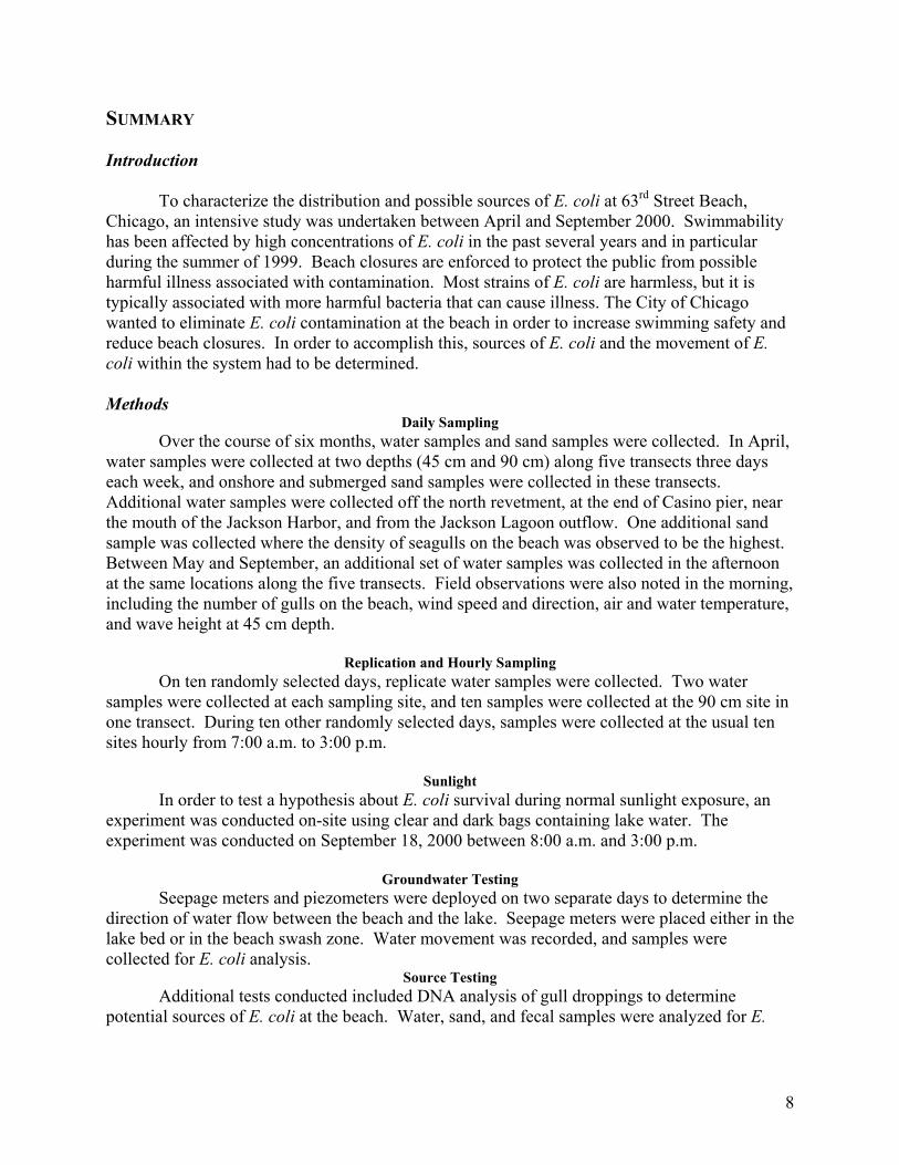
E. coli abundance generally declined exponentially throughout the day. Data were log-transformed to allow construction of linear regression models. Separate time-series regression models were fit on the log-transformed abundance for each day and depth (Table 6). No significant change in E. coli abundance was detected in seven cases: 25 May 45 and 90 cm, 24 July 45 cm, 1 August 45 and 90 cm and 25 September 45 and 90 cm. E. coli abundance remained relatively constant on these days. In general, change in E. coli abundance over time is reasonably well explained by the model (Table 6). Some dates had relatively low R-values, such as 25 May at 90 cm. Spikes caused by a few individual samples were responsible for breaks in the exponential decline (and thus the low R).

26

Table 6. Results from time-series regressions of log-transformed mean hourly E. coli data. The model equation is ln(conc) = ß0 + ß1*time, where conc=number of colony forming units per 100 ml, time=time of day in hours, and ßi are parameters to be estimated

depth t-ratio t-ratio p-value p-value date

(cm) R df ß0 ß1 ß0 ß1 ß0 ß1

25-May 45 0.759 5 6.51 -0.38 3.20 -2.18 <.02 <.10

90 0.577 5 1.31 -0.08 2.45 -1.78 <.10 <.20 12-Jun 45 0.990 6 12.37 -0.48 32.83 -14.31 <.001 <.001

90 0.982 6 11.18 -0.44 28.00 -11.84 <.001 <.001 26-Jun 45 0.953 6 5.66 -0.21 19.69 -8.11 <.001 <.001

90 0.969 6 6.28 -0.36 13.97 -8.61 <.001 <.001 11-Jul 45 0.877 6 9.22 -0.23 11.07 -3.16 <.001 <.05

90 0.942 6 9.60 -0.30 10.21 -3.48 <.001 <.02 24-Jul 45 0.900 6 4.43 -0.02 5.62 -0.23 <.001 >.50

90 0.928 6 6.13 -0.29 12.19 -6.10 <.001 <.001 1-Aug 45 0.474 6 4.72 -0.01 13.88 -0.34 <.001 >.50

90 0.949 6 4.73 -0.03 12.78 -1.00 <.001 <.50 7-Aug 45 0.989 6 12.86 -0.59 37.67 -19.43 <.001 <.001

90 0.968 6 10.60 -0.52 20.09 -10.48 <.001 <.001 16-Aug 45 0.969 6 10.93 -0.46 17.29 -8.21 <.001 <.001

90 1.000 6 9.96 -0.39 101.75 -42.86 <.001 <.001 18-Sep 45 0.908 6 7.16 -0.25 11.92 -4.78 <.001 <.005

90 0.960 6 6.53 -0.26 10.48 -4.47 <.001 <.005 25-Sep 45 0.958 6 4.01 0.02 18.09 0.93 <.001 <.50

90 0.612 6 4.09 -0.03 8.49 -0.75 <.001 <.50 When log-transformed data were plotted against time, regression lines clearly showed that on most days E. coli abundance declined over time (Figures 4 and 5). On four dates (12 June, 11 July, 7 August, and 16 August) E. coli abundance was between 1000 and 7000 cfu/100 ml at 7:00, well over the EPA limit of 235 cfu/100ml. These levels declined rapidly on all four days so that at 15:00 E. coli abundance was near or below 235 cfu/100 ml. On all other days E. coli abundances were moderate at 7:00, falling between 50 and 235 cfu/100 ml (with the exception of very low readings between 0-10 cfu/100 ml for 25 May 90 cm). In about half of these cases, E. coli declined from this level over the course of the day. E. coli abundance appeared to remain steady for other days. Rates of decline (slope) were usually similar at 45 and 90 cm for each day, as shown by Figures 4 and 5, and the slope (ß1) values in Table 6.

27

01 May 25 02 June 12 03 June 26 04 July 11 05 July 24

06 August 1 07 August 7 08 August 16 09 September 18 10 September 25

Date

8.00 10.00 12.00 14.00

time of day

2.00

4.00

6.00

8.00

mea

n ln

CFU

/100

ml

A A

A A

A

A A A

A A A

A

A A A A

A A

A A A

A A A

A A A A

A A

A A

A A

A A A

A A

A A

A

A A

A A A A A A

A

A A A

A A AA

A A A A A A A

AA

A A A A A

A A A

A

A

A A

A A

A A

A A

A A

A

A

Figure 4. Mean log-transformed hourly E. coli data at 45 cm from 10 different sampling days. Solid lines correspond to time-series regressions with p < 0.05 for slope and intercept.

28

01 May 25 02 June 12 03 June 26 04 July 11 05 July 24

06 August 1 07 August 7 08 August 16 09 September 18 10 September 25

Date

8.00 10.00 12.00 14.00

time of day

0.00

2.00

4.00

6.00

8.00 m

ean

ln C

FU/1

00

lA

A A A

A A

A A

A

A A

A A A

A A

A

AA

A A

A

A A A

A A

A A A

A A A

A

A A

A A A

A A

A

A A A

A A

A A A A A A

A A

A A

A

A

A A A A

A A

A A

A A A A A A

A

A

A A

A

A A

A

A A A A A A

A A

Figure 5. Mean log-transformed hourly E. coli data at 90 cm from 10 different sampling days. Solid lines correspond to time-series regressions with p < 0.05 for slope and intercept.

Average raw E. coli abundance data for 90 cm showed a smooth exponential decline, but

data at 45 cm appeared to follow this model less closely (Figures 6 and 7). As E. coli abundance declined over time, the magnitude of the standard error for the untransformed data also decreased. Regardless of how high morning E. coli abundance was, as the day progressed levels appeared to converge to a relatively narrow range. Wide daily variability made it difficult to use one equation to describe the variation for any given day.

29

8 10 12 14

time of day (hour)

0.00

1000.00

2000.00 m

ean

E. c

oli (

cfu/

100

ml)

at 4

5 cm

]

] ]

]

] ] ] ] ]

Figure 6. Hourly E. coli measurements from 45 cm water averaged over 10 sampling days. Error bars show mean + 1 SE

30

8 10 12 14

time of day (hour)

0.00

500.00

1000.00

1500.00

mea

n E.

coli

(cfu

/100

ml)

at 9

0 cm

]

]

] ]

] ] ] ] ]

Figure 7. Hourly E. coli measurements from 90 cm water averaged over 10 sampling days. Error bars show mean + 1 SE.

E. coli abundance changed with time of day. Morning abundances were usually much

higher than afternoon, with a steady decline throughout the day. Thus samples taken early in the morning will tend to be the most conservative in regards to public safety, but they may not necessarily reflect the conditions experienced by the majority of recreational users.

Light Readings Measurements from submerged and atmospheric UV and PPF sensors on 18 September and 25 September showed an overall increase in light intensity over time until approximately 13:00 (Figures 8 and 9). At this point light readings appeared to level off or decrease. Atmospheric UV and PPF behaved very similarly, though UV was generally 10x lower than PPF. Submerged UV was substantially more than 10x lower than submerged PPF, indicating that UV passage through the water column was more severely impeded than PPF. Overall, the disparity between atmospheric and submerged light intensity for UV and PPF appears to increase over the course of the day. This could possibly be affected by an increase in water turbidity as wind and waves increase throughout the day.

Light intensity was generally much higher on 18 September than on 25 September. In particular, UV intensity remained nearly flat all day on 25 September. This may be a result of low incoming light and high water turbidity. Light intensity increased very erratically on 18 September, with a particularly large jump registered on all sensors between 12:30 and 13:00.

31

This is likely the result of shifting cloud cover. For the most part atmospheric and submerged light readings track each other very well, suggesting that atmospheric light readings are a reasonable surrogate for submerged light readings when assessing the effect of light on E. coli.

PPF atmosphere PPF submerged UV atmosphere (x10) UV sumberged (x10)

sensor

7:30 8:30 9:30 10:30 11:30 12:30 13:30 14:30

time of day (hour)

0.00

400.00

800.00

1200.00

umol

/(m2 s)

Figure 8. Measurements of UV and PPF (umol/(m^2)s) over time from above and below the water surface on 18 September. UV measurements are displayed at 10x.

32

PPF t hPPF b dUV atmosphere (x10)

UV sumberged (x10)

sensor

7:30 8:30 9:30 10:30 11:30 12:30 13:30 14:30

time of day (hour)

0.00

400.00

800.00

1200.00

umol

/(m2 s)

Figure 9. Measurements of UV and PPF (umol/(m^2)s) over time from above and below the water surface on 25 September. UV measurements are displayed at 10x.

33

cfu PPF atmosphere

7:30 8:30 9:30 10:30 11:30 12:30 13:30 14:30

time of day (hour)

0.00

250.00

500.00

750.00

1000.00

cfu/

100

ml o

r um

ol/(m

^2)s

Figure 10. Above-water PPF measurements and hourly average E. coli on 18 September. E. coli concentrations are averaged from 5 samples at 45 cm and displayed in cfu/100 ml. PPF is displayed in umol/(m2s).

Increases in light intensity on 18 September were accompanied by a corresponding decline in E. coli (Figure 10). Particularly, as atmospheric PPF started to climb rapidly after 10:00, E. coli density quickly fell off to near zero. Though this is one isolated example, it does suggest that light has some deleterious effect on the colony-forming ability of E. coli.

Light/Dark Bag experiment. Mean (n=5) log transformed E. coli (CFU/100ml) data were plotted against time of day for light (clear) bags, dark (taped) bags, and the ambient water at 45 cm (Figure 11). E. coli concentrations were nearly equal in both light and dark bags at 08:00; after 11:00 E. coli concentration in the light bags declines rapidly. The dark bags retained a relatively constant concentration of E. coli throughout the course of the experiment. Final E. coli concentrations after 8 hours of exposure were greater than 1 log unit different between light and dark bags.

Ambient E. coli concentrations at 45 cm started out and remained higher than either bag type until 11:00. The ambient E. coli concentration began to decline markedly after 10:00; at 15:00, ambient E. coli concentration was between the final concentrations of the light and dark

34

bags. The manner of decline in E. coli concentration appears to be similar for both light bags and ambient water.

A Light Bag A Dark Bag A Ambient Water

Treatment

8.00 10.00 12.00 14.00

Time of Day (hour)

1.00

1.50

2.00

2.50

Mea

n E.

col

i (lo

g(C

FU/1

00m

l + 1

)) V

V V

V

V V V

V

V

V

V V V

V

V

V

V

V

V

V

V

V

V

V

V

A A

A A

A A

A A

A A A

A A A A

A

A A

A A

A

A

A A

A

Figure 11. Mean E. coli over time in light bags, dark bags, and ambient conditions. Error bars show mean ± 1 SE

All statistics were performed on log-transformed data. Two outliers were removed from the ambient data and replaced with the mean of the remaining data for that time and treatment. One value at 10:00 was more than 4X the value of the mean of the remaining raw data; the other value at 15:00 was more than 36X the mean of the remaining data. These data far exceeded all ambient water data for this day, giving rise to the suspicion that contamination during sampling may have caused non-representative values.

Repeated measures testing of the data showed that the within-subjects effect of time of day had a significant effect on E. coli concentration (P<0.01). Interaction between time of day and treatment was also significant (P<0.01). All treatments were significantly different in their effect on E. coli concentration (Tukey’s HSD, P<0.01). However, Pearson correlations demonstrated a 0.84 correlation coefficient for E. coli concentration in ambient water and light

35

bags (P=0.01). E. coli concentration in dark bags was not significantly correlated with concentration in either light bags or ambient water. Temperature was significantly different in the two types of bags (paired t-test, P<0.01). The sensor in the light bag registered an average of 0.32° C higher than that in the dark bag during the course of the experiment. This small difference is likely caused by slight variations in the physical conditions surrounding each bag or a lag in temperature change caused by the tape on the dark bag. The temperature difference is likely not biologically significant.

These results suggest that exposure to light may be a dominant factor in the decline of apparent E. coli concentrations over the course of the day. This could suggest that on bright sunny days (when the beach is more likely to be in use) high E. coli concentrations may diminish rapidly. A cursory review of weather observations reveals some interesting patterns regarding the highest and lowest E. coli counts over the course of the summer. When the highest 20% and lowest 20% of daily E.coli concentrations in water are separated, some interesting patterns appear in weather observations (Table 7). Those days during the summer on which the highest counts of E. coli were collected are cloudy, overcast, or rainy days. The days on which the highest E. coli concentrations were collected were almost all sunny and clear. The data should be subject to some rigorous testing, but some patterns clearly emerge. Because E. coli is being used for beach monitoring as an indicator of contamination, it cannot be assumed that other health impacts associated with fecal contamination decline in the same way during exposure to sunlight. Therefore, early morning samples are the most conservative and perhaps the most appropriate when using E. coli for water quality monitoring.

Table 7. Weather observations on days with the highest and lowest E. coli counts.

Highest 20 percentile E. coli in PM, 45 cm Lowest 20 percentile E. coli in PM, 45 cm

Date AM PM Date AM PM 5/9 rainy/overcast partly sunny/raining 5/2 sunny, clear sunny, clear

5/11 cloudy cloudy/rainy 5/3 sunny, clear sunny, clear

5/17 partly cloudy cloudy 5/4 sunny sunny

5/18 partly cloudy cloudy,foggy, rainy 5/25 sunny, clear sunny, clear

6/12 drizzle mixed clouds 5/30 overcast overcast, thunderstorm

6/13 cloudy/fog rainy 6/1 sunny and hazy partly cloudy

6/20 rain rainy 6/6 sunny sunny

7/6 hazy sunny 6/7 sunny, calm sunny, hazy, breezy

7/11 cloudy partly cloudy 6/14 mostly sunny partly cloudy

8/23 cloudy cloudy/windy 7/7 overcast, windy sunny

9/12 rain sun/windy 9/18 sunny sunny

9/20 cloudy/rain wind/rain 9/19 sunny sunny

9/26 sunny sunny

36

Spatial Patterns

Among site comparisons were made using Wilcoxon Signed-Rank Test to avoid questions of normality of data (Wilkinson 1999). Multiple comparisons were made (45 comparisons) so that a Bonferroni correction of Pcritical of 0.005 was used for test significance. Data were paired by date with averages from the 5 transects being used for each date for the sediment (by depth) and water (by depth and time of day) samples. The offshore site had significantly lower E. coli abundances compared to all other sites except the 90 cm water samples in the afternoon (Table 8). Submerged sands<foreshore sands<gull sand were all significantly different than one another and from water samples. The 45 cm water sites in the morning were generally higher in E. coli than other water sites, except for the lagoon (Table 8). The E. coli abundances in the lagoon and the harbor were not significantly different than at the other sites, except the previously mentioned sites (Table 8). Log10-transformed means are depicted on the histogram below (Figure 12). Table 8. Matrix of two-sided probabilities based on Z numbers calculated from Wilcoxon Signed-Rank Test. Pcritical = 0.005 because of Bonferroni adjustment. Bold p values indicate significance and sign indicates difference between row vs. column heading.

Northshore Offshore Lagoon Harbor W_am_45 Offshore - < 0.001 Lagoon 0.694 + < 0.001 Harbor - 0.002 + < 0.001 - 0.004 W_am_45 + < 0.001 + < 0.001 0.015 + < 0.001 W_pm_45 0.896 + < 0.001 0.863 + 0.003 - < 0.001 W_am_90 0.830 + < 0.001 0.790 + 0.002 - < 0.001 W_pm_90 - 0.003 0.091 - 0.002 0.081 - < 0.001 Foreshore + < 0.001 + < 0.001 + < 0.001 + < 0.001 + < 0.001 Submerged + < 0.001 + < 0.001 + < 0.001 + < 0.001 + < 0.001 Offshore W_pm_45 W_am_90 W_pm_90 Sed_Fore W_am_90 0.356 W_pm_90 - < 0.001 - < 0.001 Foreshore + < 0.001 + < 0.001 + < 0.001 Submerged + < 0.001 + < 0.001 + < 0.001 - < 0.001

Table 9. Mean separation of locations at 63rd Street Beach. Lines which are connected are not significantly different at a=0.033. Overall means are given under each location name. offshore 90 cm PM harbor 90cm AM lagoon Nrevetment 45cm PM 45cmAM submerged foreshore gull sand 21.26 30.81 54.98 66.16 7402 78.84 84.78 158.07 735.21 4845.19 9303.65 ___________________ _________________ ____________________________________________ _______________________________ _________ ________ _______

37

1.00

2.00

3.00

4.00

Log Mean E. coli per 100 ml of water or sand

Knee deep water pm

Waist deep water pm

Knee deep water am

foreshore sands

Northshore water

submerged sands

Waist deep water am

Harbor Water

Lagoon Outfall

2.08

1.62

2.33

4.02

1.92

3.13

1.93

1.75

1.87

]

]

]

]

]

]

]

]

]

A

A

A

A

A

A A

A

A

A

A A

A A

A

A

A

A

A

A

A

A

A

A A

AA

A

A

A AA

A

A

A

A

A

A A

A

A

Figure 12. Mean E. coli per 100 ml in water and sand. All numbers are log transformed. Error bars are ± 1 SE.

Knee deep water am Knee deep water pm

A Waist deep water am A Waist deep water pm

4/04

4/11

4/18

4/25

5/02

5/09

5/16

5/24

5/30

6/05

6/12

6/19

6/26

7/05

7/10

7/17

7/24

7/31

8/07

8/14

8/21

8/28

9/05

9/11

9/18

9/25

1.0

2.0

3.0

4.0

Log

mea

n E.

col

i (C

FU/1

00 m

l)

A A

A A

A

A A A

A

A

AAA

A

A A

A

A A

A

A A AA A

A A A

A A

A

A A

A

A A

A

A A

A

A

A A A

A

AA A A A A

A

A A

A A A

A

A

A A

A

A

A

A

A A

A A

A

A

A

A

A A A

A A

A

A

A A

A A

A

A A

A

A

A

A A

A A

A

A

A

A

A

A A A A

A A A A

A

A A A

A A A A A A

A

A

A A A A

A

A A

A

A

A

A A AA A

A

A

A A

A

A A A

A A A

A

A A

A A

A

A A A

A

A A

A

A A

A

A

A A

A

A

A

A A

A A A

A A

A

A A A

A A A

A A

A

A A A A A A

A

A

A

A A A A A A A

A

A A A

A

A

A A

A

A

A

AA

A

A

A

A

A

A

A A

A

A

A

A

A

A

A

A

A

AA

A

A

A

A

AA

A

A

A AA

A

A

A A

A

A

Figure 13. E. coli concentrations over the course of the study at 45 cm and 90 cm water in the morning and afternoon.

38

Groundwater Studies. The data in Table 10 indicate that over most of the lake bed, the hydraulic gradient was directed downward into the sand, but in a narrow zone close to the shore face (swash zone), the gradient was directed from the sand into the lake. The measured seepage fluxes were consistently small, but the E. coli concentrations in the seepage water were highly variable. The water collected from the seepage meter near the shore face on August 22 had a very high bacterial concentration, and this was consistent with an extremely high concentration (> 50,000 cfu/100 ml) in the sample that was collected that same day from the mini-piezometer on the berm. In contrast, the bacterial concentrations in seepage meter samples collected on September 7 were very low. On that day, samples collected from the mini-piezometers on the berm had concentrations of E. coli that were consistently less than 100 cfu/ 100ml. [Note that a vacuum sample collected on September 7 also had a low bacterial concentration of 46 cfu/ 100 ml.]. Finally, the samples of seepage collected in association with the stormy period of August 9 also had elevated bacteria concentrations. Although there is clearly need for more extensive sampling of seepage waters, it appears that the concentration of E. coli in such waters can be very high, and that the concentration can vary over orders of magnitude depending on prevailing conditions. Table 10. Hydraulic gradients, seepage fluxes, and E. coli concentrations in seepage waters.

Date ∆h

shorea (cm)

∆h lake bedb (cm)

Seepage flux Shorec (L m-2 h-1)

Seepage flux lake bedc (L m-2 h-1)

E. coli shore (cfu/100ml)

E. coli lake bed (cfu/100ml)

8/21-22 2 – 9 (6)

∼ 0 0.19 -0.01 – [-0.30] (-0.22)

3,000d 190 – 3,000 (250)d

9/7-8 4 – 8 (6)

n.d. 0.04 – 0.96 (0.30)

n.d 13 – 67 (41) e

n.d.

9/12-13 n.d. n.d. 0.03 n.d. 3,100 – 4,800 3,900 e

n.d.

Notes: Upper entries in table cells are observed ranges, numbers in parentheses are averages; n.d. indicates no data. ahydraulic gradient existing between the water table in shore sediment and the lake surface. bhydraulic gradient existing between the lake surface and the saturated sand beneath the lake. cpositive flux indicates lake is gaining water from sand, negative flux indicates lake is discharging into sand. dwater samples were collected using a vacuum pump. ewater samples were collected passively by letting hydraulic gradient fill the sample container. Spatial Relationship. Spearman correlations were used to determine relationships between distinctive sampling sites. This nonparametric test was used because the non-normality of the data does not affect the test (Wilkinson 1999). This Spearman correlation used the average E. coli abundance for the 5 transects for the water (by depth and time) and sand (by depth). The data from the others sites (offshore, north revetment, lagoon, and harbor) were the single datum collected per day. Correlation coefficients are shown in Table 11. Although many coefficients are relatively high (e.g., E. coli abundance in 45 cm and 90 cm AM water, R2 = 0.793), some increased errors in these comparisons are expected due to the high number of comparisons.

39

Table 11. Spearman correlation matrix for tests of relationships between sites. Foreshore W_45_am W_45_pm W_90_am W_90_pm SED_SUB

M Spearman'

s rho Foreshore Correlation

Coefficient 1.000 .482 .317 .450 .400 .395

Sig. (2-tailed)

. .000 .000 .000 .000 .000

N 390 389 330 388 330 390 W_45_am Correlation

Coefficient .482 1.000 .595 .793 .620 .431

Sig. (2-tailed)

.000 . .000 .000 .000 .000

N 389 389 329 388 329 389 W_45_pm Correlation

Coefficient .317 .595 1.000 .534 .687 .328

Sig. (2-tailed)

.000 .000 . .000 .000 .000

N 330 329 330 329 330 330 W_90_am Correlation

Coefficient .450 .793 .534 1.000 .716 .363

Sig. (2-tailed)

.000 .000 .000 . .000 .000

N 388 388 329 388 329 388 W_90_pm Correlation

Coefficient .400 .620 .687 .716 1.000 .339

Sig. (2-tailed)

.000 .000 .000 .000 . .000

N 330 329 330 329 330 330 SED_SUB

M Correlation Coefficient

.395 .431 .328 .363 .339 1.000

Sig. (2-tailed)

.000 .000 .000 .000 .000 .

N 390 389 330 388 330 390 ** Correlation is significant at the .01 level (2-tailed).

40

foreshore sands Knee deep water am Knee deep water pm submerged sands Waist deep water am Waist deep water pm

0.00 7.00 14.00 21.00 28.00

week

0.00

2.00

4.00

6.00

Log

mea

n E.

col

i (cf

u/10

0 m

l)

Figure 14. Weekly average of E. coli concentrations in foreshore, submerged sands and swimming waters of 63rd Street Beach.

The best correlations among sampling sites and times were between water depths sampled at the same time of day (Figure 14). Those, in turn, are correlated to one another and more loosely correlated to foreshore sands. Harbor waters and offshore waters are correlated as expected, considering the similarity of source water for both locations. The lagoon and submerged sands formed a very weak correlation that lacks hydrological justification. North revetment E. coli concentrations were not well correlated with other bacteria samples taken.

41

Rescaled Distance Cluster Combine C A S E 0 5 10 15 20 25 Label Num +---------+---------+---------+---------+---------+ WAT45 AM 3 òûòòòòòòòòòø WAT90 AM 8 ò÷ ùòòòòòòòòòòòø WAT45 PM 4 òòòûòòòòòòò÷ ùòòòø WAT90 PM 9 òòò÷ ó ùòòòòòòòòòòòòòòòòòòòø FORESHORE 1 òòòòòòòòòòòòòòòòòòòòòòò÷ ó ó HARBOR 2 òòòòòòòòòòòòòòòòòòòûòòòòòòò÷ ùòø OFFSHORE 6 òòòòòòòòòòòòòòòòòòò÷ ó ó LAGOON 5 òòòòòòòòòòòòòòòòòòòòòòòòòòòòòòòòòòòûòòòòòòòòòòò÷ ó SUBMERGED 7 òòòòòòòòòòòòòòòòòòòòòòòòòòòòòòòòòòò÷ ó NREVETMENT 10 òòòòòòòòòòòòòòòòòòòòòòòòòòòòòòòòòòòòòòòòòòòòòòòòò÷

Figure 15. Dendrogram showing cluster analysis based on Pearson correlation of E. coli concentrations at specific sampling sites

Multiple regression of suspected factors. One of the most important objectives of this study was to understand the factors that influence E. coli concentrations and how these elements might relate to swimming beach results gathered by the Chicago Park District (CPD). It is also important to hypothesize what best explains the nature and sources of E. coli fluctuation. Although this is somewhat related to predictive modeling elsewhere presented in this report, the emphasis here is to discover important phenomena affecting E. coli occurrence and to explore factors that may be contributing to the source of E. coli at tested locations. Statistically, inferences are drawn based on data collected, and hypotheses are rejected (or not rejected) with a certain level of confidence, in this case 95% (α = 0.05). Multiple linear regression was used first to determine what factors best explained variation of E. coli concentrations at 45 cm depth in the morning—the same depth at which the CPD takes samples on weekdays. Of the factors considered in this report, those thought to have the greatest potential to affect E. coli concentration were: Density of gull droppings on the beach Number of Gulls Morning Wave Height Morning Width at north revetment and offshore Morning Wind Speed Concentration of E. coli at the Lagoon Concentration of E. coli at the Harbor

42

Concentration of E. coli within the foreshore sands Concentration of E. coli within the submerged sands Concentration of E. coli at the offshore site Table 12. ANOVA analysis of E. coli concentrations in 45 cm AM water vs E. coli concentrations in foreshore sand and number of gull droppings.

ANOVA

Model Sum of Squares

df Mean Square

F Sig.

1 Regression 11.580 1 11.580 33.456 .000 Residual 21.461 62 .346 Total 33.041 63

2 Regression 13.753 2 6.877 21.748 .000 Residual 19.288 61 .316 Total 33.041 63

a Predictors: (Constant), Foreshore sand b Predictors: (Constant), Foreshore sand, Gull Droppings c Dependent Variable: morning 45 cm water There were significant relationships between E. coli concentrations within the foreshore sands and 45 cm AM water (P < 0.001) (Table 12). Linear regressions of E. coli concentration in 45 cm water and 90 cm water against E. coli concentration in foreshore sands showed that E. coli in foreshore sands accounts for the same amount of variation at both water depths (R2 = 0.43) (Figures 16 and 17). This means that 43% of the variation shown in either 45 cm or 90 cm water can be accounted for by the concentration of E. coli in the sand and 57% of the variation is related to other factors. Only gull droppings contributed significantly to the model. Closer inspection shows that gull droppings only contributed an R2 change of 6.6% to the model and that gull droppings and submerged sands or water were inversely related. The importance of gull droppings alone is minimal without any further considerations such as beach grooming and seasonality.

43

2.00 3.00 4.00 5.00 6.00

Log mean E. coli in foreshore sands (cfu/100ml)

1.00

2.00

3.00

4.00

Log

mea

n E.

col

i in

45 c

m w

ater

am

(c

fu/1

00m

l) A

A A

Knee deep water am = -0.71 + 0.75 * sed_fore R-Square = 0.43

A

A A

A A

A

A

A

A

A A A

A A

A

A

A

A

A

A A

A A

A

A

A

A

A A

A

A A

A

A

A

A A

A

A

A A

A A

A A

A

A

A A A

A A A

A

A A A A

A

A

A

A A A

A A

A

A

A

A A

A

A A

A

A

A

A

A A

A

A

A

A

A A

A

A A

A

A

A A

A A

A

A A

A

A

A

A A

A A

A

A

A

A

A

A

A A

A

A A A

A

A A A

A A A A A A

A

A

A A

A A

A

A A

A

A

A

A A

A A A

A

A

A A

A

A A A

Figure 16. Linear regression of E. coli concentration in 45 cm water AM and foreshore sands. Upper and lower lines represent 95% mean prediction interval.

2.00 3.00 4.00 5.00 6.00

Log mean E. coli in foreshore sands (cfu/100ml)

0.00

1.00

2.00

3.00

4.00

Log

mea

n E.

col

i in

90 c

m w

ater

am

(c

fu/1

00m

l)

A

Waist deep water am = -0.99 + 0.73 * sed_fore R-Square = 0.43

Figure 17. Linear regression of E. coli concentration in 90 cm water AM and foreshore sands. Upper and lower lines represent 95% mean prediction interval.

44

0.00 0.20 0.40 0.60

Mean # gull droppings per m2

0.00

1.00

2.00

3.00

4.00

Mea

n E.

col

i 45

cm w

ater

am

(c

fu/1

00m

l)

A Knee deep water am = 2.79 + -2.87 * gulldrop R-Square = 0.25

A A A

A

A

A A A

A

A

A

A

A

A

A

A

A

A

A A

A

A

A

A

A A

A

A A

A A

A

A A

A

A

A A

A A

A A

A A

A A

A A A A

A

A A A

A

A

A

A

A

A A A A

A

A

A

A

A A

A

A

A A

A

Figure 18. Regression of gull droppings and E. coli concentration of morning 45 cm water. Upper and lower lines represent 95% mean prediction interval.

Effects of raking. The inverse relationship of gull droppings and E. coli concentration may have more to do with the beach raking (grooming, combing) schedule than original contamination. A student t-test showed that both gull counts and morning E. coli counts differed between periods of grooming and non-grooming (p = 0.017 and 0.015, when equal variance are not assumed) (Figure 19).

45

Not raked raked

Raking of Beach

# gull droppings foreshore sands Knee deep water am

1.00

2.00

3.00

4.00

Mea

n lo

g E.

col

i per

100

ml

Mea

n gu

ll dr

oppi

ngs

per s

q m

eter

]

]

]

]

]

]

Figure 19. Number of gull droppings and log transformed E. coli in foreshore sands and morning 45 cm water for raked and unraked beaches. Error bars show mean ± 1 SE.

Thus, it becomes important to consider the number of gull droppings relative to raking treatment. This can be done by partial correlations, which take into account the effect of raking by holding it constant relative to the other parameters evaluated. With this done, the correlation matrix (Table 13) shows that gull droppings are an even more significant factor (p < 0.001) although still inverse. The significance of the correlation between E. coli concentrations in foreshore sand and 45 cm water also increases (p < 0.001).

Table 13. Partial correlation coefficients for average # gull droppings and E. coli concentrations in foreshore sand and 45 cm AM water.

Controlling for.. RAKING W_45_AM FORESHORE GULLDROP W_45_AM 1.0000 .6190 -.4461 ( 0) ( 72) ( 72) P= . P= .000 P= .000 FORESHORE 1.0000 -.2905 ( 0) ( 72) P= .012 (Coefficient / (D.F.) / 2-tailed Significance)

46

Initially, the inverse relationship between raking, gull droppings, and E. coli concentrations seem counterintuitive. It is clear that raking breaks up the droppings rendering them uncountable by the field technician. But why would raking increase E. coli concentration in the sand and water? Raking, while increasing the aesthetics of the beach, likely does little to reduce the E. coli that was associated with the droppings. In fact, raking might enhance E. coli survival because the fecal material is now dispersed and buried below the surface sands protecting the bacteria from two of its most lethal threats, desiccation and irradiation Further, raking may make it easier for dispersed bacteria to mobilize in the swash zone. To test this hypothesis, we did a Mann Whitney Test of foreshore and submerged sands and of water on a raked and un-raked beach. We selected a non-parametric test because some of the parameters inspected showed significant difference in variances when raked and un-raked sands were compared (critical value = 0.05, Levene Test). Foreshore sands, submerged sands, 45 cm morning water, 90 cm morning water, north revetment waters and number of gulls were significantly higher during the raking period Table 14). These results further support the idea that E. coli concentrations are enhanced in both sands and water during periods of raking. A controlled experiment would be necessary to confirm this phenomenon.

Table 14. Mann-Whitney Test of E. coli concentration during periods with and without beach raking.

Test Statistics

Fore- shore sands

Submerged sands

Offshore water

45 cm am

45 cm pm

90 cm am

90 cm pm

# of gulls Gull Droppings

North Revetment

Mann-Whitney U

387.000 290.500 469.000 403.500 344.500 427.000 320.500 386.000 465.000 441.500

Wilcoxon W 793.000 696.500 794.000 809.500 480.500 833.000 456.500 711.000 1740.000 847.500 Z -3.261 -4.266 -1.755 -3.089 -.830 -2.844 -1.190 -2.687 -1.806 -2.693

Asymp. Sig. (2-tailed)

.001 .000 .079 .002 .406 .004 .234 .007 .071 .007

The confounding problem with this hypothesis is the cofactor correlation of seasonality on E. coli abundance. Raking was done during the summer months when E. coli would be expected to be higher (Whitman et al.1999). Thus, temperature and raking might be covariant factors. Pearson analysis shows no correlation between gull droppings and temperature (p = 0.218) and the significance levels between E. coli in foreshore sands, submerged sands, and 45 cm water are only slightly improved when partials are adjusted for raking as well as temperature. Beach renovation. In preparation for the swimming season, 63rd Street Beach foreshore sands were removed to a depth of 8-15 cm and replaced with fresh sands from North Avenue and Montrose beaches on May 24-25, 2000. A few sand samples were taken from the hauling trucks and found to be very low in E. coli content. Fortunately for our project, this created a near experimental condition in which we could examine differences between old foreshore and new foreshore sand E. coli and possibly clarify influences of foreshore sands on associated aqueous E. coli. The statistics demonstrate that foreshore sands, offshore water, 45 cm afternoon water, 90 cm afternoon water were significantly higher before new sand placement (Table 14). There were not significant differences in mean concentration *p>0.05) between number of gulls, gull droppings, and morning E. coli concentrations in the water and submerged sands. This suggests that the new

47

sand may have temporarily reduced the E. coli for foreshore sands, and afternoon and offshore waters. Yet, these differences were only statistically significant in the afternoon. Post-treatment morning E. coli means at north revetment, 45 cm and 90 cm waters all ranked lower but failed to show a significant difference mainly due to higher statistical variation associated with increased morning E. coli concentration (Figure 19). A treatment control would be needed to confirm that sand renewal reduced foreshore and water E. coli. Other factors such as weather and antecedent conditions may have explained the pre- and post-treatment effects. Waves were not significantly different during the treatment (p=0.05), but air temperature was significantly warmer for the two weeks following new sand placement (p = 0.001). E. coli in sand and water appeared to stabilize after this two week period since the next two weeks were not significantly different ( p > 0.05) even though the first two-week period was relatively warmer. Table 15. Mann-Whitney test of mean differences two weeks before and after new beach sand placement on May 24-25, 2000.

foreshore

sands Sub-

merged sands

Offshore water

45 cm am

45 cm pm

90 cm am

90 cm pm

# of Gull Drop gullsPings

North revetment

Mann-Whitney U

5.000 18.000 4.500 9.000 3.000 7.000 5.000 17.500 12.000 6.000

Wilcoxon W

26.000 39.000 25.500 30.000 24.000 28.000 26.000 38.500 33.000 27.000

Z -2.082 .000 -2.169 -1.441 -2.402 -1.764 -2.082 -.080 -.982 -1.922 Asymp. Sig. (2-tailed)

.037 1.000 .030 .150 .016 .078 .037 .936 .326 .055

Exact Sig. [2*(1-tailed

Sig.)]

.041 1.000 .026 .180 .015 .093 .041 .937 .394 .065

a Not corrected for ties. b Grouping Variable: Beach Renewal

48

66 66 66 66N =

Concentration of E. coli

Before and After Beach Renewal

Beach Renewal

AfterBefore

Log

E. c

oli M

ean

+- 1

SE

5

4

3

2

1

0

Offshore water

Knee deep water pm

Waist deep water pm

foreshore sands

Figure 20. Concentrations of E. coli before and after beach renewal. Error bars show + 1 SE. Factors linking E. coli occurrence Another way to analyze the relationship between various factors affecting beach E. coli is through hierarchical cluster analysis. This procedure shows the relational homogeneity between variables using a selected grouping formula. The distance between variables reflects the relative similarities between the factors being considered. We elected to analyze the average linkage between groups using a centroid algorithm. The cluster (Figure 20) shows clear similarities between foreshore and submerged sediments, 45 cm and 90 cm water E. coli for afternoon and morning, morning and afternoon wave heights, gull droppings and north revetment E. coli concentration, and harbor E. coli and shore width. Secondary linkages are suggested between foreshore and submerged sediments and afternoon 45 cm and 90 cm water, between number of droppings and north revetment E. coli, between harbor E. coli and shore width and gull numbers, between morning water and offshore E. coli concentration. We expect similarities between offshore waters and shallower water samples since all were taken at the same time. The similarity between shore width and harbor E. coli can be attributed to lake stage because it drives water in and out of the harbor hydrosystem. It is interesting that north revetment E. coli were similar to bird dropping counts even though the two factors were not statistically correlated.

49

Rescaled Distance Cluster Combine C A S E 0 5 10 15 20 25 Label Num +---------+---------+---------+---------+---------+ FORESHORE 3 òûòòòòòòòòòòòòòòòòòòòòòòòòòòòø SUBMERGED 6 ò÷ ùòòòòòòòòòòòø DROPPING 1 òòòòòûòòòòòòòòòòòòòòòòòòòòòòò÷ ó NREVETMENT 10 òòòòò÷ ùòòòòòòòø HARBOR 9 òûòòòòòòòòòòòòòòòòòòòòòòòòòø ó ó AVGSWALL 14 ò÷ ùòòòòòòòòòòòòò÷ ó #GULLS 2 òòòòòòòòòòòòòòòòòòòòòòòòòòò÷ ó WAVEAM 12 òòòûòòòòòòòòòòòòòòòòòòòòòòòòòòòòòòòòòòòòòòòòòø ó WAVEPM 13 òòò÷ ùòòò÷ W_45_PM 5 òûòòòòòòòòòòòòòòòòòòòòòòòòòòòòòòòø ó W_90_PM 8 ò÷ ùòòòòòòòòòòò÷ W_45_AM 4 òûòòòòòòòòòòòòòòòø ó W_90_AM 7 ò÷ ùòòòòòòòòòòòòòòò÷ OFFSHORE 11 òòòòòòòòòòòòòòòòò÷

Figure 21. Centroid cluster analysis of various factors associated with E. coli concentrations at 63rd Street Beach.

For sake of simplicity and for exploratory purposes, the cluster analysis was restricted to potential sources of E. coli (Figure 21). The interrelationship between E. coli in the water and the foreshore E. coli becomes clear as the cluster shows that E. coli in the foreshore sand is similar to afternoon waters. This is consistent with the beach renewal relationships discussed earlier under the beach renewal section. In separate clusters using Pearson correlation or cosine method, morning waters were secondarily clustered with afternoon waters as well. The similarity between bird droppings and shore width is interesting, suggesting that rising water either excludes birds or washes away droppings. Correlations between droppings, shore width and number of gulls were not significant (p>0.10).

50

Rescaled Distance Cluster Combine C A S E 0 5 10 15 20 25 Label Num +---------+---------+---------+---------+---------+ FORESHORE 4 òûòòòòòòòòòòòòòòòòòòòòòòòòòòòòòòòø SUBMERGED 8 ò÷ ùòòòòòòòòòòòø W_45_PM 6 òûòòòòòòòòòòòòòòòòòòòòòòòòòòòòòòò÷ ó W_90_PM 10 ò÷ ùòòòø W_45_AM 5 òûòòòòòòòòòòòòòòòòòòòòòòòòòø ó ó W_90_AM 9 ò÷ ùòòòòòòòòòòòòòòòòò÷ ó AVEWAVES 3 òòòòòòòòòòòòòòòòòòòòòòòòòòò÷ ó DROPPING 1 òòòûòòòòòòòòòòòòòòòòòòòòòòòòòø ó AVGSWALL 7 òòò÷ ùòòòòòòòòòòòòòòòòòòò÷ #GULL 2 òòòòòòòòòòòòòòòòòòòòòòòòòòòòò÷

Figure 22. Centroid dendrogram of major factors associated with E. coli concentrations, all data considered. Wave height appears to be one of the most important and revealing factors influencing E. coli at 63rd Street Beach. It integrates wind speed, wind direction, fetch, and water depth and often translates itself to shore width and swash energy. This, in turn, translates into hydrological energy, which has the potential to mobilize and suspend E. coli-laden exposed or submerged sediments. To illustrate this, we compared parameters when waves were above and below the study mean (9 cm). The resulting dendrogram shows very similar results for all clusters except that there is a greater similarity between E. coli in submerged and foreshore sands and wave heights during periods of increased wave height (>9 cm). Spearman’s statistics show positive correlation between PM waves and 90 cm PM water; foreshore sands and 90 cm AM water; 45 cm and 90 cm AM water; and 45 cm and 90 cm PM water. Submerged sand was not correlated with water or foreshore sand. For waves greater than 9 cm, foreshore sands were positively correlated (critical p < 0.002 with Bonferonni adjustment) with submerged sands, 45 cm morning and afternoon water and 90 cm afternoon water. Submerged sands were positively correlated with 45 cm and 90 cm morning water. There was a positive correlation between gull droppings and 45 cm PM water. Negative correlation between gull droppings and E. coli concentration is discussed elsewhere. These statistics emphasize the greater importance of resuspended E. coli-laden shallow and foreshore sediments during increased wave action.

51

Table 16. Correlations when wave heights <9 cm. foreshore

sands Gull Droppings

submerged sands

90 cm pm

PM wave

45 cm am

90 cm water am

90 cm water pm

Spearman's rho

foreshore sands Correlation Coefficient

1.000 -.034 .176 .321 -.059 .442 .534 .443

Sig. (2-tailed) . .852 .327 .069 .745 .010 .001 .010 N 33 33 33 33 33 33 33 33 Gull Droppings Correlation

Coefficient -.034 1.000 -.035 -.170 -.240 -.205 -.268 -.340

Sig. (2-tailed) .852 . .845 .343 .178 .253 .131 .053 N 33 33 33 33 33 33 33 33 submerged

sands Correlation Coefficient

.176 -.035 1.000 .253 -.114 .171 .061 .025

Sig. (2-tailed) .327 .845 . .155 .526 .341 .736 .888 N 33 33 33 33 33 33 33 33 Knee deep water

pm Correlation Coefficient

.321 -.170 .253 1.000 .148 .681 .479 .709

Sig. (2-tailed) .069 .343 .155 . .410 .000 .005 .000 N 33 33 33 33 33 33 33 33 PMWAVE Correlation

Coefficient -.059 -.240 -.114 .148 1.000 .422 .332 .176

Sig. (2-tailed) .745 .178 .526 .410 . .015 .059 .326 N 33 33 33 33 33 33 33 33 Knee deep water

am Correlation Coefficient

.442 -.205 .171 .681 .422 1.000 .692 .676

Sig. (2-tailed) .010 .253 .341 .000 .015 . .000 .000 N 33 33 33 33 33 33 33 33 Waist deep water

am Correlation Coefficient

.534 -.268 .061 .479 .332 .692 1.000 .673

Sig. (2-tailed) .001 .131 .736 .005 .059 .000 . .000 N 33 33 33 33 33 33 33 33 Waist deep water

pm Correlation Coefficient

.443 -.340 .025 .709 .176 .676 .673 1.000

Sig. (2-tailed) .010 .053 .888 .000 .326 .000 .000 . N 33 33 33 33 33 33 33 33

** Correlation is significant at the .01 level (2-tailed). * Correlation is significant at the .05 level (2-tailed). Rescaled Distance Cluster Combine C A S E 0 5 10 15 20 25 Label Num +---------+---------+---------+---------+---------+ W_45_AM 5 òûòòòòòòòòòòòòòòòòòòòòòòòòòòòòòø W_90_AM 9 ò÷ ùòòòòòòòòòòòòòòòòòø W_45_PM 6 òûòòòòòòòòòòòòòòòòòòòòòòòòòòòòò÷ ó W_90_PM 10 ò÷ ó FORESHORE 4 òûòòòòòòòòòòòòòòòòòø ó SUBMERGED 8 ò÷ ùòòòòòòòòòòòòòòòòòòòòòòòø ó AVEWAVES 3 òòòòòòòòòòòòòòòòòòò÷ ùòòòòò÷ DROPPING 1 òûòòòòòòòòòòòòòòòòòòòòòòòòòòòòòòòø ó AVGSWALL 7 ò÷ ùòòòòòòòòò÷ #GULL 2 òòòòòòòòòòòòòòòòòòòòòòòòòòòòòòòòò÷

Figure 23. Centroid cluster analysis of factors associated with E. coli concentrations for waves greater than season mean (9 cm).

52

Table 17. Correlations when wave heights >9 cm. foreshore

sands Gull Droppings

submerged sands

45 cm water pm

PM wave

45 cm water am

90 cm water am

90 cm water pm

Spearman's rho

foreshore sands Correlation Coefficient

1.000 -.355 .472 .344 .149 .622 .518 .542

Sig. (2-tailed) . .042 .006 .050 .407 .000 .002 .001 N 33 33 33 33 33 33 33 33 Gull Droppings Correlation

Coefficient -.355 1.000 -.446 -.272 -.245 -.538 -.483 -.559

Sig. (2-tailed) .042 . .009 .126 .170 .001 .004 .001 N 33 33 33 33 33 33 33 33 submerged

sands Correlation Coefficient

.472 -.446 1.000 .460 .115 .535 .447 .535

Sig. (2-tailed) .006 .009 . .007 .524 .001 .009 .001 N 33 33 33 33 33 33 33 33 Knee deep

water pm Correlation Coefficient

.344 -.272 .460 1.000 .039 .607 .573 .762

Sig. (2-tailed) .050 .126 .007 . .828 .000 .000 .000 N 33 33 33 33 33 33 33 33 PMWAVE Correlation

Coefficient .149 -.245 .115 .039 1.000 .311 .367 .295

.407 .170 .524 .828 . .078 .035 .095 N 33 33 33 33 33 33 33 33 Knee deep

water am Correlation Coefficient

.622 -.538 .535 .607 .311 1.000 .906 .763

Sig. (2-tailed) .000 .001 .001 .000 .078 . .000 .000 N 33 33 33 33 33 33 33 33 Waist deep

water am Correlation Coefficient

.518 -.483 .447 .573 .367 .906 1.000 .747

Sig. (2-tailed) .002 .004 .009 .000 .035 .000 . .000 N 33 33 33 33 33 33 33 33 Waist deep

water pm Correlation Coefficient

.542 -.559 .535 .762 .295 .763 .747 1.000

Sig. (2-tailed) .001 .001 .001 .000 .095 .000 .000 . N 33 33 33 33 33 33 33 33

Sig. (2-tailed)

Rescaled Distance Cluster Combine C A S E 0 5 10 15 20 25 Label Num +---------+---------+---------+---------+---------+ FORESHORE 4 òûòòòòòòòòòòòòòòòòòòòòòòòòòòòòòø SUBMERGED 8 ò÷ ùòòòòòòòòòòòòòòòòòø DROPPING 1 òòòûòòòòòòòòòòòòòòòòòòòòòòòòòòò÷ ó AVGSWALL 7 òòò÷ ó #GULL 2 òòòòòòòòòòòòòòòûòòòòòòòòòòòòòòòòòòòòòòòòòø ó AVEWAVES 3 òòòòòòòòòòòòòòò÷ ùòòòòòòò÷ W_45_AM 5 òûòòòòòòòòòòòòòòòòòòòòòòòòòòòòòø ó W_90_AM 9 ò÷ ùòòòòòòòòò÷ W_45_PM 6 òòòûòòòòòòòòòòòòòòòòòòòòòòòòòòò÷ W_90_PM 10 òòò÷

Figure 24. Centroid cluster analysis of factors associated with E. coli concentrations for waves less than season mean (9 cm).

53

When non-parametric statistics are used, we discover that number of gulls is positively correlated with E. coli concentrations in foreshore sands (p = 0.012) but not submerged sands. Foreshore sands are positively correlated to submerged sands. Gulls are not correlated with E. coli in either water or sand. We then hypothesize that it takes at least a day for the gulls to influence the sand E. coli concentration. To test this theory, gull populations were lagged one day and then tested using a Spearman’s rho correlation matrix. Lagged gull populations were correlated with E. coli concentrations in foreshore sands, 45 cm water AM, 90 cm water AM, harbor water and offshore sands. E. coli concentrations in 90 cm water PM were nearly significant (p=0.008, which exceeded Bonferonni critical value of 0.006). Submerged sands and 45 cm water PM were not correlated with lagged gull samples. There may be evidence that gulls and foreshore sand E. coli interact with one another and with swimming water.

54

foreshore sandsnumber of gullssubmerged sands

4/04

4/11

4/18

4/25

5/02

5/09

5/16

5/24

5/30

6/05

6/12

6/19

6/26

7/05

7/10

7/17

7/24

7/31

8/07

8/14

8/21

8/28

9/05

9/11

9/18

9/25

2.00

3.00

4.00

5.00

6.00

Log

Mea

nE.

col

i p

er 1

00 m

lLo

g #

of g

ulls

(ave

rage

AM

+PM

)

Figure 25. Number of gulls and concentration E. coli in of foreshore sands.

55

Table 18. Correlations of # of gulls against foreshore sand E. coli concentrations before and after lagging foreshore sand by one day.

#gulls Lagged

#gulls Unlagged

Sig. (2-tailed)

Sig. (2-tailed)

#gulls Lagged

. .341

#gulls Unlagged

.341 .

foreshore sands

.000 .133

45 cm water am

.004 .224

45 cm water pm

.167 .916

90 cm water am

.001 .037

90 cm water pm

.008* .432

Harbor Water

.000 .899

North Rev water

.101 .381

Offshore water

.000 .265

submerged sands

.046 .972

Critical p value Bonferroni corrected =0.006 Morphology and Remediation

Beach and adjacent morphology may be an important aspect of water quality at 63rd Street Beach. Morphology directly affects circulation patterns, waves, sediment deposition, resuspension, and entrainment of contaminants and helps control the export or dilution of pollutants such as E. coli. The bounding of 63rd Street Beach by the Jackson Harbor breakwater and the doglegged Casino Pier forms an embayment. To develop a confident understanding of the hydrodynamics of the 63rd Street Beach ‘embayment’, circulation tracing and hydrodynamic models would have to be employed. Nonetheless, there are some approximate intuitive assumptions that can be made by the morphological setting at the beach. With a northerly longshore current created by high winds, suspended contaminants might be captured by Casino Pier. Because of the geometry of the embayment, wind-generated internal circulation during calmer periods might be favored, thus retarding exportation, dilution, and externally and internally introduced E. coli. Sand and fine sediments with associated E. coli become trapped in the embayment. Accrual of sediments accounts for the beach’s shallowness, the increased silty nature of the sand and the more abundant natural and anthropogenic debris along the beach relative to other observed nearby beaches. The north and south breakwaters also act as protection against wind by reducing fetch. The increased calmness may translate itself into

56

reduced exportation and dilution of internal or external loadings of bacteria and anthropogenic chemicals that were found in this study. On the other hand, the walls increase the total energy in the area during certain flow conditions because wave energy is reflected rather than absorbed. This energy may act to keep material suspended long enough for some of it to be exported from the beach area. The shallowness of the beach compounds the problem by further decreasing circulation and by allowing less volume of water for dilution of bacteria. Bacteria tend to be associated with detritus and fine sediments (i.e. silts and clays). In deeper water this bacteria-laden material eventually settles to the bottom, and the bacteria eventually dies. This may be why offshore water, and even 90-cm water or harbor water, was lower in E. coli content than 45-cm water. If assumptions concerning the negative effects of morphology and hydrodynamics on bacteria concentration are correct, increasing circulation could be desirable. These hydrodynamic questions lie beyond the scope of the current study but need to be answered before significant funds and effort are made toward remediation. Some of the remediation options that might be considered are: 1) dredging just beyond the swimming area to increase circulation and increase volume, 2) allowing water to move more freely through Casino Pier or 3) creating a sand shunt under the Pier. Evaluating the efficacy of remediation approaches needs to be attended to systematically by hydrologists/engineers working closely with environmental scientists that know this beach system. Remediation approaches will likely have secondary environmental or cultural impacts. These effects need to be clearly identified before any corrective action is undertaken. Gull Distribution By using the factors of time (AM, PM) and space (transects 1 to 5) for comparison, several similarities and differences may be found in the distribution of gulls on the 63rd Street Beach. In general, there was no significant difference between morning and afternoon bird populations when the entire season was inspected (paired t-test, p = 0.296), although morning and afternoon were significantly correlated (p=0.001). Graphs with the date versus the number of gulls in each transect for AM and PM allow descriptive comparisons to be made (Figures 25 and 26). The peak in total number of gulls on the beach for AM is in early July, and it is in mid-September for PM. The structures of these peaks differ as well. The AM gull numbers stay low throughout April and May, peak in July, and gradually decrease through September. On the other hand, the PM numbers begin small and increase over time to the maximum in September. The total number of gulls for the sampling period tends to be higher for the PM. A second comparison is between AM/PM and the location on the beach that the gulls occupy. For the AM, the gulls are most often in transects 2 and 3, while in the PM the gulls are in 1 and 2. Overall, the gulls seem to prefer the north end of the beach during June to September. In May, however, the gulls occupy transect 5 almost exclusively in both the AM and PM. This shift in location preference may be due to the presence of bathers beginning in June, and thus, the presence of food litter.

57

Number of Gulls in Transect 1-5 in AM

Date

09/25/2000

09/11/2000

08/28/2000

08/14/2000

07/31/2000

07/17/2000

07/05/2000

06/19/2000

06/05/2000

05/24/2000

05/09/2000

04/25/2000

04/11/2000

Gul

l Num

bers

1600

1400

1200

1000

800

600

400

200

0

Transect

5

4

3

2

1

Figure 26. Number of gulls in transects 1-5 at 63rd St. Beach, AM.

Number of Gulls in Transect 1-5 in PM

Date

09/19/2000

09/06/2000

08/22/2000

08/08/2000

07/25/2000

07/11/2000

06/27/2000

06/13/2000

05/31/2000

05/17/2000

05/02/2000

Num

ber o

f Gul

ls

1600

1400

1200

1000

800

600

400

200

0

Transect

5

4

3

2

1

Figure 27. Number of gulls in transects 1-5 at 63rd St. Beach, PM.

58

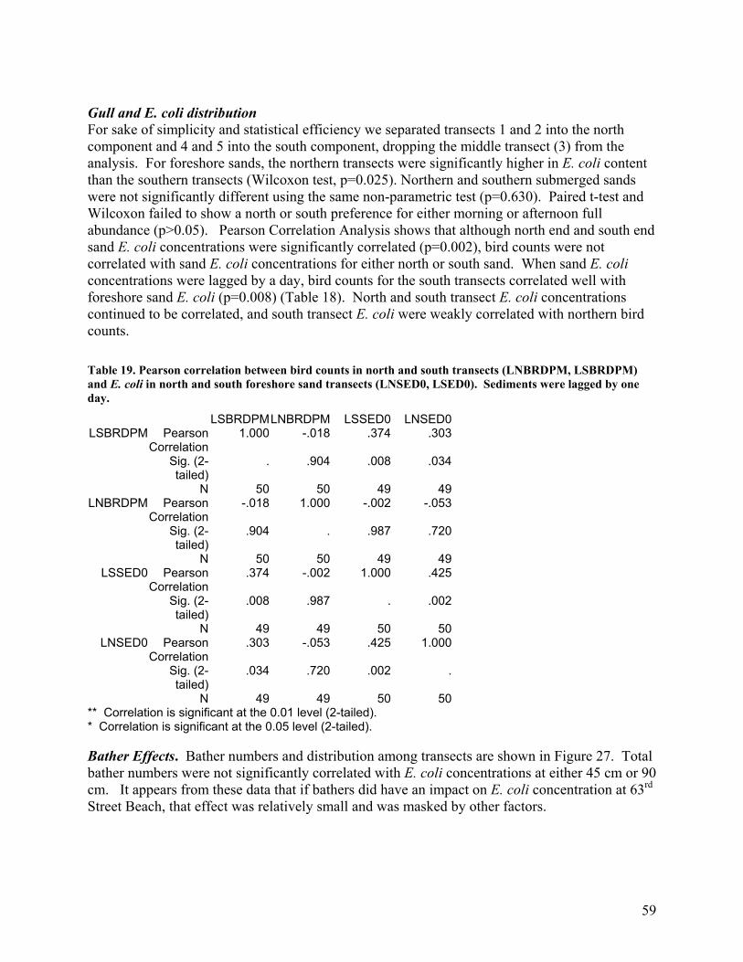
Gull and E. coli distribution For sake of simplicity and statistical efficiency we separated transects 1 and 2 into the north component and 4 and 5 into the south component, dropping the middle transect (3) from the analysis. For foreshore sands, the northern transects were significantly higher in E. coli content than the southern transects (Wilcoxon test, p=0.025). Northern and southern submerged sands were not significantly different using the same non-parametric test (p=0.630). Paired t-test and Wilcoxon failed to show a north or south preference for either morning or afternoon full abundance (p>0.05). Pearson Correlation Analysis shows that although north end and south end sand E. coli concentrations were significantly correlated (p=0.002), bird counts were not correlated with sand E. coli concentrations for either north or south sand. When sand E. coli concentrations were lagged by a day, bird counts for the south transects correlated well with foreshore sand E. coli (p=0.008) (Table 18). North and south transect E. coli concentrations continued to be correlated, and south transect E. coli were weakly correlated with northern bird counts. Table 19. Pearson correlation between bird counts in north and south transects (LNBRDPM, LSBRDPM) and E. coli in north and south foreshore sand transects (LNSED0, LSED0). Sediments were lagged by one day.

LSBRDPM LNBRDPM LSSED0 LNSED0 LSBRDPM Pearson

Correlation 1.000 -.018 .374 .303

Sig. (2-tailed)

. .904 .008 .034

N 50 50 49 49 LNBRDPM Pearson

Correlation -.018 1.000 -.002 -.053

Sig. (2-tailed)

.904 . .987 .720

N 50 50 49 49 LSSED0 Pearson

Correlation .374 -.002 1.000 .425

Sig. (2-tailed)

.008 .987 . .002

N 49 49 50 50 LNSED0 Pearson

Correlation .303 -.053 .425 1.000

Sig. (2-tailed)

.034 .720 .002 .

N 49 49 50 50 ** Correlation is significant at the 0.01 level (2-tailed). * Correlation is significant at the 0.05 level (2-tailed). Bather Effects. Bather numbers and distribution among transects are shown in Figure 27. Total bather numbers were not significantly correlated with E. coli concentrations at either 45 cm or 90 cm. It appears from these data that if bathers did have an impact on E. coli concentration at 63rd Street Beach, that effect was relatively small and was masked by other factors.

59

Number of Bathers in Afternoon

in Transects 1-5

Date

09/07/2000

08/29/2000

08/21/2000

08/09/2000

08/01/2000

07/24/2000

07/12/2000

07/06/2000

06/26/2000

06/14/2000

No.

of B

athe

rs

100

80

60

40

20

0

TRANSECT

5

4

3

2

1

Figure 28. Number of bathers in transects 1-5 at 63rd St. Beach.

60

Table 20. Pearson Partial Correlation for Bather Frequency versus E. coli at 45 and 90 cm depths.

- - - P A R T I A L C O R R E L A T I O N C O E F F I C I E N T S - - - Controlling for.. W_90_PM BATHERPM W_45_PM BATHERPM 1.0000 .0942 ( 0) ( 48) P= . P= .515 W_45_PM .0942 1.0000 ( 48) ( 0) P= .515 P= . (Coefficient / (D.F.) / 2-tailed Significance) " . " is printed if a coefficient cannot be computed - - - P A R T I A L C O R R E L A T I O N C O E F F I C I E N T S - - - Controlling for.. W_45_PM BATHERPM W_90_PM BATHERPM 1.0000 -.1472 ( 0) ( 48) P= . P= .308 W_90_PM -.1472 1.0000 ( 48) ( 0) P= .308 P= . (Coefficient / (D.F.) / 2-tailed Significance) " . " is printed if a coefficient cannot be computed

Results of Harbor Sediment Testing Additional sampling was conducted at Jackson Harbor to assess the presence and/or magnitude of E. coli storage in the harbor sediments relative to the overlying water. Sampling took place on 19 July. Water and sediment samples were collected from a total of three points located at the ends of the three easternmost floating piers in the harbor. Means of cfu/100 ml for all three sample types were very similar. Mean E. coli concentration was highest (before correction) in sediment samples (367 + 79 cfu/100 ml), followed by subsurface water (327 +46 cfu/100 ml)

61

and then water from just above the sediment surface (287 + 54 cfu/100 ml). Sample means failed to show a statistically significant difference (p>0.05). The elutriation water for the sediment samples was harbor water, so E. coli concentrations from overlying water have to be subtracted to get a true estimation of sediment E. coli concentrations (367-287=80 cfu/100 ml). Therefore sediment E. coli concentrations actually appear to be lower than concentrations in the water. This makes it unlikely that the harbor sediments are storing large amounts of E. coli or contributing significantly to E. coli concentrations in the harbor water.

62

DNA, MAR, AND CHEMICAL ANALYSIS Samples for source determination were collected on June 26, 2000 and August 21, 2000.

Environmental conditions for these two dates place them in the low to average wave height category. Seagull populations on each date were typical. All samples were collected in the morning. The population numbers for E. coli and enterococci varied between these two sets of samples (Table 21). Estimates of population numbers were generally comparable between laboratories. Numbers of E. coli and enterococci were generally lower for the August 21 samples. Numbers of enterococci in sediments were dramatically lower for the August 21 samples (Table 21). Numbers of E. coli and enterococci in seagull feces varied between samples (Table 22) with no apparent relation to date of collection. Table 21. Numbers of total coliform bacteria, E. coli, and enterococci for 63rd Street Beach samples on the two sampling dates.

USGS Total

Coliforms USGS E. coli Chicago E. coli USGS Enterococci

Sample ID per 100 ml per 100 ml per 100 ml per 100 ml June 26 August 21 June 26 August 21 June 26 August 21 June 26 August 21

T1 W 45cm 160 ND 90 ND 100 34 14 0 T2 W 45cm 190 ND 50 ND 120 84 37 1 T3 W 45cm 50 ND 17 ND 32 140 11 1 T4 W 45cm 270 ND 130 ND 140 160 13 0 T5 W 45 cm 310 ND 160 ND 160 180 26 1

North Revet. 420 ND 130 ND 600 120 5 0

Offshore 2 ND 3 ND 14 4 2 0 Lagoon 1000 ND 800 ND 3100 280 42 2 Harbor 270 ND 90 ND 110 38 41 0

T1 S foreshore 1.4 x 105 TNTC 6.0 x 104 TNTC 2.7 x 104 TNTC 4.0 x 103 5

3369/cm3*

NA 1444/cm3 NA 650/cm3 NA 96/cm3 <1/cm3

T2 S foreshore 3.0 x 103 3.3 x 104 7.0 x 103 1.0 x 104 7.2 x 103 9.0 x 103 1.5 x 104 0 60/cm3 456/cm3 140/cm3 14/cm3 144/cm3 125/cm3 301/cm3 <1/cm3




Gull Sand 1.4 x 104 1.0 x 103 1.3 x 104 4.0 x 103 9.0 x 103 NA 9.0 x 103 1 198/cm3 NA 184/cm3 NA 127/cm3 NA 127/cm3 <1/cm3

*The volume of sediment suspended in 100 mL buffer was determined from the inner diameter of the core tube and the recorded length of the core. ND, not determined. NA, not available.

63

Table 22. Numbers of total coliforms, E. coli and enterococci in seagull feces. USGS Total

Coliforms USGS E. coli USGS Enterococci

Seagull ID per 100 mla per 100 mla per 100 mla June 26

SGA 1.9 x 107 3.1 x 106 4.5 x 107 SGB 2.9 x 107 6.0 x 106 6.0 x 105 SGC 2.8 x 106 2.7 x 106 TNTC SGD 1.3 x 109 1.0 x 109 TNTC SGE 0 0 TNTC SGF 2.5 x 106 0 5.0 x 106

August 21b

SGA 1.9 x 109 (1.9 x 109 per g

feces)

1.9 x 109 (1.9 x 109 per g feces)

4.1 x 106 (4.0 x 106 per g feces)

SGB 2.3 x 107 (9.2 x 107 per g

feces)

2.3 x 107 (9.2 x 107 per g feces)

7.0 x 104 (2.8 x 105 per g feces)

SGC 1.9 x 107 (9.3 x 106 per g

feces)

1.9 x 107 (9.3 x 106 per g feces)

1.3 x 108 (6.5 x 107 per g feces)

SGD 5.0 x 106 (4.0 x 106 per g

feces)

5.0 x 106 (4.0 x 106 per g feces)

2.5 x 105 (2.0 x 104 per g feces)

TNTC, too numerous to count; aNumbers are reported per 100 mL of resuspension buffer. Weight of feces was not determined; bThe wet weight of the August feces was determined. E. COLI DNA FINGERPRINTS Overall analysis DNA fingerprints were obtained for 136 isolates on the two dates: June: 26 water, 20 sediment, 20 seagull; and August: 33 water, 20 sediment, 18 seagull. Cluster analysis was conducted on these samples (Figure 29); the vertical red line indicates the minimum similarity of the control E. coli. Any isolates that group at a similarity greater than this level are considered indistinguishable given the variability in the method. The green vertical lines drawn at approximately 0.5 kilobases (a measure of the size of DNA; Kb), 1.1 Kb and 1.5 Kb indicate major bands that, together with groups of other bands, result in the clusters depicted. Certain clusters are marked for discussion. The large cluster A1 contains isolates that generally possess all three major bands. In addition, groups of bands (2 around 1.3-1.4 Kb and several > 2 Kb) define subsets of cluster A1. Cluster A2 retains some features of the A1 group but not the entire set of features that would allow members of this group to cluster more closely with A1 members. Anything not in clusters A1 or A2 is designated as “B.” The group B members usually lack one of the major bands, and/or have a new feature that is not found in the A1 or A2 clusters. For example, B1 possesses a unique band around 0.8 Kb, B2 lacks two of the major bands and B3 possesses a group of 3 bands between 0.5 and 0.7 Kb that makes a unique feature.

64

Figure 29. Cluster diagram for rep-PCR DNA fingerprints for all isolates.

65

Some aspects of this large cluster analysis are noteworthy. First, of 40 sediment samples

analyzed for both dates, 30 are in the A1-A2 group. On the other hand, of 32 beach water samples, 19 (10 June and 9 August) are in the A1-A2 group and 13 (4 June and 9 August) are in the B group. One interpretation may be that the sediment isolates are a more homogeneous population than the water isolates and are less susceptible to date-to-date variation. Since the cores aggregate material from land surface to the water table, there is a possibility that different populations are aggregated as well. If, as prior studies indicate, the majority of the sediment E. coli occur at shallow ground water (near the water table) then these may be a separate population or bacteria earlier derived from groundwater inputs or through-flow over time from materials applied to the surface of beach sand. Seepage tests of through-flow E. coli delivery was inconclusive. Core samples of sands which include the groundwater at 1 meter would not necessarily be related to E. coli populations in surface waters sampled at the same time. This would be especially true during periods of lake calm when entrainment of E. coli laden sands in the swash zone is less.

Seagull isolates (20 tested in June and 18 in August) are about equally distributed between the A(16) and B(22) groups (Figure 29). However, group A contains 12 seagull isolates from August and only 4 from June and vice versa for group B. This has a significant effect on the June and August results (discussed separately below) and suggests temporal population differences in E. coli in seagulls. Temporal E. coli population variability in seagull feces may be supported by ecological information suggesting a shift in seagull species from mostly adult Ring-bill gulls in the early summer to adult and juvenile Ring-bill gulls, Herring gulls and migrants in early fall. Therefore, we may have sampled different birds in August. Alternatively, they may have been the same birds on both dates, but food sources or other behavioral differences may account for fecal bacterial population shifts. Finally, it is possible that the analysis of only a few fecal samples on each date may have resulted in an under-representation of E. coli types from this source on any given date. If so, then there may have been no true difference in E. coli populations between dates, and the observed difference would be attributed to sampling error. A plot of cumulative total rep-PCR profiles against isolates for all seagull isolates indicates a linear relationship (Figure 30) with no asymptote, suggesting that more E. coli types would have been found in additional samples. Since the total number of E. coli rep-PCR fingerprint types is unknown, it is not possible to state how representative the E. coli analyzed were of all those possibly found on the beach. On the other hand, enterococci (see below) and Salmonella suggest adequate sampling for these particular species.

66

Figure 30. Different rep-PCR profiles for seagulls, June and August.

June and August Seagull Profiles

0

5

10

15

20

25

0 10 20 30 4

Number of seagull isolates

Cum

ulat

ive

tota

l of

diffe

rent

rep-

PCR

pro

files

0

67

June E. coli DNA fingerprints. DNA fingerprints were obtained for 26 water E. coli isolates (14 from the beach transects), 20 sediment isolates and 20 seagull isolates (Figure 31). Only two samples, both sediments (4SA and 5SA), can be construed to match a seagull (Figure 29). The red line again marks the similarity criterion for the control E. coli. All but one June seagull has the “B” fingerprint pattern while most water samples have the “A” fingerprint pattern. Seagull fingerprints were only identical within a seagull. There were no identities among seagulls. Within-site identical fingerprints occurred at several locations: H, L, N, 4SA, and 1SA. There is no apparent spatial pattern to isolates designated as identical using our criterion. For example, five clusters representing identical isolates are marked (Figure 31). Each cluster includes isolates from very different parts of the beach and from both sediments and water. Using our identity criterion, six foreshore beach sediment isolates are identical to an isolate from beach water. On the other hand, six foreshore beach sediment isolates are identical to an isolate from the harbor, lagoon, offshore or north revetment areas. Likewise, eight water isolates from 45 cm can be related to an isolate from the harbor, lagoon, or offshore or north revetment areas. The June results suggest little influence of seagulls on the E. coli found in foreshore sediments or knee-deep waters. Interestingly there was some limited overlap between beach sand strains and genotypes recovered from lagoon, harbor, or north revetment samples. August E. coli DNA fingerprints. DNA fingerprints were obtained for 33 water E. coli isolates (18 from the beach transects), 20 sediment isolates, and 18 seagull isolates (Figure 32). There was a seagull match, using our identity criterion, for 26 samples (14 water and 12 sediment). There was no seagull match for any water sample from site 5 or LO and only one of four north revetment samples matched a seagull. For water from the beach transects, 10 of 18 isolates could be matched to a seagull. Of the remaining eight samples, five presented unique profiles: one matched an LO isolate and two matched each other. There were no identities among seagulls. There were several within-site identities at 2SA, 4SA, and 2WA. In addition, there was a very close match between 1SA and 4WA and between 2WA and 4WA. Again, there is no apparent spatial pattern to isolates that cluster within identity groups.

68

Figure 31. Cluster diagram of rep-PCR DNA fingerprints for all June isolates.

69

Figure 32. Cluster diagram of rep-PCR DNA fingerprints for all August isolates.

70

ENTEROCOCCI PHENOTYPES Enterococci were isolated from seagull feces in June and August and from water and sediment (June only) at the 63rd Street Beach (Figure 33). Enterococci numbers in water and sediment in August were very low, which precluded their isolation from the August samples. The enterococci grouped in two major clusters (A and B, Figure 33). Cluster A contains 22 (of 25) August seagull isolates, while Cluster B contains the majority of the June seagull isolates (23 of 24). Nine sediment isolates and 10 water isolates from June were also analyzed. The sediment isolates fall primarily (8 of 9) in Cluster B, and the water isolates fall primarily (9 of 10) into group A. Within their respective clusters, most of the June water and sediment isolates do not group closely with isolates from seagulls (see sub-group X Figure 33). The identities of selected sub-clusters are indicated on Figure 33. The most likely species for the June water and sediment group X suggests that they are indeed different from the closest related seagull isolate. Other groups equally separated in these clusters are also likely different species, however the test method employed does not permit a definitive naming of all enterococci species.

71

Figure 33. Cluster diagram of enterococci from seagulls (June and August) and water and sediments (June).

72

These results indicate that populations of enterococci in seagull feces were different for the June and August samplings. This result is consistent with the E. coli DNA-fingerprinting results for seagull isolates as discussed above. This would suggest that the differences in rep-PCR DNA fingerprints for seagull isolates on the two dates were most likely the result of true fecal bacterial population differences, and not an artifact of sampling. Another important finding from the enterococci tests is that June sediment and water isolates may arise largely from a source other than seagulls. This result is again consistent with the E. coli DNA-fingerprinting results from June, which showed very little correlation between E. coli in seagulls and those in beach water and sand on that date. The numbers of enterococci in seagull feces did not vary substantially between the two dates (Table 22). However, the absence of enterococci in sediments and the lower numbers in water for August, as compared to June (Table 21), suggests that hydrologic or environmental conditions were different on the two dates and affected the enterococci differently than the E. coli. One possibility is that the enterococci are delivered to the sediments and water by a process that was present during or prior to the June sampling but not the August sampling. Since the enterococci in water and sediment in June were not similar to those in seagulls, we must assume there is another source of these bacteria to the system. That source may have been present (or had lingering effects) in June, but not in August. Evidence for other sources Water samples were analyzed for a variety of constituents associated with human wastewater (Table 23). These constituents include a variety of chemicals used (detergents, fumigants, solvents, polycyclic aromatic hydrocarbons, an insect repellent, fire-retardants); consumed (caffeine, cotinine—a by-product of nicotine); or produced (cholesterol, coprostanol) by humans. These constituents commonly occur in water influenced by human activities through the addition of storm water or sanitary waste. Results indicate that beach water contained some of these target chemicals on September 11, 2000. This sampling date followed a significant rainfall event. The results suggest that storm water runoff affects the beach water under such conditions. The chemicals detected are not especially suggestive of human sanitary waste since the detergents and human metabolites such as cholesterol and coprostanol were not detected. Rather, the combination of chemicals detected could conceivably arise from water washing off parking lots or picnic areas.

73

Table 23. Concentrations of detected wastewater constituents in mg/L.

Sample ID

Caffeine

N,N,-diethyl-

toluamide

Tri (2-

chloroethyl) phosphate

Ethanol, 2-

butoxy-, phosphate

5-methyl-1H- benzotriazole

Triclosan

Cotinine

(µg/L)

LO nd 0.138 0.060 nd 0.147 nd 0.052

1WA 0.618 Nd 0.052 nd nd nd nd

2WA 0.588 0.135 0.052 nd nd 0.070 nd

3WA nd Nd 0.052 1.6 nd nd nd

4WA 0.096 Nd 0.050 nd nd 0.070 nd

5WA nd Nd nd nd nd nd nd

Nd, no detection; N,N, diethyltoluamide, DEET (an insect repellant); tri (2-chloroethyl) phosphate (a fire retardant); ethanol, 2-butoxy-, phosphate (a plasticizer), 5-methyl-1H-benzotraizole (antioxidant used in antifreeze), triclosan (major ingredient of antibacterial soaps), cotinine (a by-product of nicotine metabolism). These results suggest that E. coli isolates identical or very similar to those found in seagulls occur in beach water and beach sediment at the 63rd Street Beach. However, the impact of seagulls is apparently different on different dates, and seagulls did not account for the majority of beach water or sediment isolates on either of the two dates. Instead, approximately one-half the August beach water and sediment isolates and virtually all June beach water and sediment isolates appear to originate from other sources. This conclusion is also supported by the enterococci results. Finally, the presence of human-generated chemicals in beach water indicates that sources other than seagulls affect the system. Other sources may include:

Storm-water runoff Bacteria associated with aquatic plants or detritus brought to the beach by long-shore drift Bacteria associated with septic or sewage waste brought to the site by long-shore currents

that may originate from gray water waste from boats or domestic effluents Groundwater or through-flow inputs (e.g., seepage from the lagoon, or harbors or washing-in

of bacteria on the “hill” separating the lagoon and beach which would then be transported to the shallow water table).

The hydrologic connection between the lagoon and/or harbor and specific sites on the beach through human infrastructure and geologic heterogeneities also may present potential contamination channels. In addition, there may be currents that affect the movement of water along the beach and may provide unanticipated connections between sites. Since the chemicals found are generally persistent, they may have been in the system for quite some time with origins that are relatively distant to Chicago.

74

Source determination sampling was conducted on two dates that represent average to low wave height for the 63rd Street Beach. Under such conditions, numbers of E. coli in foreshore beach sands may not be as strongly correlated with numbers in knee-deep water. In addition, seagull droppings are not correlated with the numbers of E. coli in foreshore sands or water. Finally, as demonstrated earlier, there appears to be a statistically significant lag time in the influence of seagulls on beach waters and sands. These factors and correlations were not known at the outset of the study, so could not have been included in the present sampling design. However, future studies should make use of the environmental information and should attempt to conduct source determination studies under more varying environmental conditions. A number of scientific issues are also raised by this research. The difference in fecal bacterial populations on the two sampling dates was not anticipated, and indeed this research represents the first report of this phenomenon. This is an important finding that will allow better design of future source-determination studies. However, further information will be needed on the temporal scale over which fecal bacterial population shifts take place. Secondly, the source determination studies have identified some E. coli and enterococci at 63rd Street Beach not related to those found in seagull feces. As discussed, these results are inconclusive and in need of more rigorous sampling. Further testing is warranted. The presence of chemicals indicative of human-influenced storm or wastewater in beach waters is significant. This is the first report of such detections in ambient lake waters and may indeed be common at many urban beaches. However, this influence will have to be taken into consideration as mitigation strategies to improve recreational water quality at the 63rd Street Beach are undertaken. Further investigation of the frequency of such detections and the source(s) of these chemicals may be warranted.

E. coli MAR

Antibiotic testing results (n=274) were grouped into four clusters. The vast majority of the isolates were susceptible to all antibiotic agents tested (n=254; ~93%). One group of isolates (n=8; ~3%) was susceptible to only one antibiotic (tetracycline) while another group (n=8; ~3%) was resistant only to Cephalothin. Four isolates (~1%) were resistant to multiple antibiotics. Of the isolates resistant to a single antibiotic agent, three were from seagulls (~1%), nine were from sediments (3.3%), and four were from water (1.5%). Of the isolates resistant to multiple antibiotic agents (MAR), two were from water (0.7%), and two were from sediment (0.7%); no isolates from seagulls were resistant to multiple antibiotic agents. No significant temporal trends were noted. Of the MAR isolates from water, both were from sources distant from the actual beach area (sample sites NB and LO). Of the MAR from sediment, both isolates, one from June and one from August, were from the sample site 2893 (5 Sediment A). There was some agreement between MAR results of the north revetment and lagoon outfall suggesting a linkage. We do not know if this implies a hydrological connection or reflects E. coli that is ubiquitous to the general area.

75

Multiple antibiotic resistance has been used to determine or speculate on host populations (human vs. animal) in an effort to determine sources of E. coli (Parveen et al. 1997, Harwood et al. 2000). Human resistance to single antibiotics varies by antibiotic and population sampled but there are typical expected resistances (Table 24). Multiple antibiotic resistance of E. coli from humans is typically considered to be more prevalent than multiple antibiotic resistance of E. coli from animal sources. The low percentage of ambient MAR E. coli coupled with the complete absence of seagull MAR supports the use of this parameter for source determination. It follows that the MAR results imply reduced frequency of human derived E. coli, which would intrinsically have higher MAR values.

Table 24. Resistance to antibiotics.

Antibiotic agent % E. coli susceptible

Amikacin 99

Amoxicillin-Clav. Acid 82

Ampicillin 66

Carbenicillin 68

Cefonicid 94

Ceftriaxone 100

Cephalothin 88

Ciprofloxacin 97

Gentamicin 89

Nalidixic Acid 95

Nitrofuntoin 99

Pipercillin 91

Tetracycline 87

Trimethoprim-sulfamethoxasole

90

E. coli Biotyping

The biotyping cluster analysis results of the E. coli isolates shows that overall there are eleven distinct groups of isolates (with 2 isolates not grouping with other isolates) based on the significance of the Dice correlation coefficient for the phenotypic data. Generalizations on these data suggest that the E. coli isolates from this study are phenotypically well distributed. Within the two main clusters there is fairly equal distribution between the three sources of isolates

76

https://www.researchgate.net/publication/12356467_Classification_of_Antibiotic_Resistance_Patterns_of_Indicator_Bacteria_by_Discriminant_Analysis_Use_in_Predicting_the_Source_of_Fecal_Contamination_in_Subtropical_Waters?el=1_x_8&enrichId=rgreq-f74ea15b-4a29-4b79-a3eb-13bd508433f1&enrichSource=Y292ZXJQYWdlOzIzODc2MzQ3NTtBUzoxMzU0ODU1NDQ0NzI1NzZAMTQwOTMxMzY3OTYxNA==


https://www.researchgate.net/publication/14007860_Association_of_multiple_antibiotic_resistance_profiles_with_point_and_nonpoint_sources_of_E_coli_in_Appalachicola_Bay?el=1_x_8&enrichId=rgreq-f74ea15b-4a29-4b79-a3eb-13bd508433f1&enrichSource=Y292ZXJQYWdlOzIzODc2MzQ3NTtBUzoxMzU0ODU1NDQ0NzI1NzZAMTQwOTMxMzY3OTYxNA==

(water, sediment, and seagull). One cluster is composed entirely of isolates from seagulls (n=6; ~2%). Three primary phenotypic clusters form when examining the seagull isolates alone: two of which do not cluster with any other isolates. The clusters support the suggestion that a temporal distribution of isolates exists because one cluster is predominately from the August samples (~74%), another is primarily from June samples (~63%), and the other cluster is solely from June samples. Applying similar analysis to June sampling, there are four distinct clusters of E. coli. The first cluster is solely composed of isolates from seagulls (the same isolates that were clustered in the cluster of the seagull isolates) whereas other clusters were heterogeneous with all three sources of isolates represented. In the cluster analysis of the isolates from the August sampling, there were five distinct clusters of E. coli. Within the two predominant clusters, representation of all three sources of isolates was again seen. There were 38 distinct biotyping patterns based on the phenotypic data from these isolates. While the overall phenotypic data permutations that would result in an identity of E. coli is not known, it is suspected that these biotypes represent only a fraction of the possible E. coli biotypes possible. The biotyping data show that E. coli from the seagulls constitutes a significant portion (typically one-third) of each of the groups of E. coli isolates, consistent with their overall contribution to the data. Only one group (n=2) did not have a phenotypic pattern consistent with an E. coli isolated from a seagull. This suggests that other sources of E. coli, such as human sources, do not seem to be uniquely represented in these data. This lends strong support to the hypothesis that seagulls are a significant source of E. coli in this location. Antibiotic resistance testing resulted in the determination that all Salmonella isolated were susceptible to all antibiotics tested. Salmonella was isolated from samples representative of each sample type collected. Of the approximately 80 fecal samples collected, ten isolates of Salmonella were recovered. From the five samples of water, four yielded isolates of Salmonella. From ten samples of sediment, five isolates of Salmonella were obtained. On serotyping the isolates, only one serotype was obtained: Salmonella enterica subsp. enterica ser. Typhimurium. S. Typhimurium is the second most predominant isolate associated with human gastroenteritis, accounting for typically 20% of all reported salmonellosis outbreaks (Koneman et al. 1997). In wildlife, S. Typhimurium has typically accounted for over 40% of the wildlife mortality due to salmonellosis (NWHC unpublished data). With over 2000 serotypes of Salmonella and S. Typhimurium typically accounting for only about 20% of the human cases, the isolation of only S. Typhimurium from all the samples (although probably not statistically significant) probably indicates contributing sources. The cluster analysis results of the Salmonella isolates from the 63rd Street Beach shows that there are three distinct groups of isolates at the $85% coefficient (Figure 34). Typically, a Dice coefficient of $90% is considered to have good genetic relatedness, however, this analysis suggested a broader latitude in determining relatedness. All the Salmonella isolated from sediment samples (n=5) grouped well within the first group. The Salmonella isolated from the water (n=4), however, was split equally between two groups. The Salmonella isolated from

77

https://www.researchgate.net/publication/200156696_Color_Atlas_an_Textbook_of_Diagnostic_Microbiology?el=1_x_8&enrichId=rgreq-f74ea15b-4a29-4b79-a3eb-13bd508433f1&enrichSource=Y292ZXJQYWdlOzIzODc2MzQ3NTtBUzoxMzU0ODU1NDQ0NzI1NzZAMTQwOTMxMzY3OTYxNA==

seagulls (n=10) were represented with isolates in all three groups and included one isolate that was distinct enough to not group with any other isolates. Based on the diversity of S. Typhimurium isolated from seagulls, the similarity of seagull isolates to isolates obtained from the water and sediment strongly suggest that seagulls are potentially the source of Salmonella isolated from the water and sediment samples. Although Salmonella spp. have been reported to remain viable for long periods of time in water, it is most likely, given the similarity of isolates within each group, that the sediment and water Salmonella isolates originated from the seagulls frequenting the beach. The cluster analysis of the Chicago derived Salmonella isolates suggests three groups of genetically related S. Typhimurium, but the strength of those relationships must be determined. Water samples from the area in and around Indiana Dunes were also tested for the presence of Salmonella spp. From the samples submitted, seven isolates of S. Typhimurium were obtained, including a repeat sample from the 63rd Street area. In addition, S. Typhimurium isolates from diverse human sources (Wisconsin State Laboratory of Hygiene, Madison, WI) and other sources including wildlife (NWHC) were also included in a cluster analysis. Using a Dice coefficient of $85%, five related clusters were evident with five isolates that were not closely related to other isolates (Figure 35). One cluster was not previously seen, based on the Chicago isolates alone, and includes only wildlife isolates not obtained as part of the study. One sediment and one water isolate from the Chicago isolates that previously grouped with the sediment and seagull (Figure 34, group I) were shifted into a cluster that was strong enough to stand alone (Figure 35, group IV) and was composed of isolates obtained from both wildlife and Indiana Dunes. Interestingly, however, a water sample obtained from the 63rd Street site included with the Indiana Dunes samples also clustered in this group, significantly away from the other water and sediment samples. The inclusion of S. Typhimurium from human cases of salmonellosis, however, leaves open the possibility of human source contamination of the Chicago beach, either through beach users or through sewage contamination. Of six distinct human isolates included, four clustered with the isolates from water and seagulls (Figure 35, group IV). While contamination of the Chicago beach with human sources of S. Typhimurium is a possibility, it is not considered the most likely because: 1) humans are not typically considered reservoirs on Salmonella (except S. typhi) (Bopp et al. 1999, Koneman et al. 1997) 2) human salmonellosis is not restricted to a single serotype such as S. Typhimurium 3) salmonellosis from seagulls has been previously well established (Levesque et al. 2000, Literak et al. 1992).

78

https://www.researchgate.net/publication/223015210_Study_of_the_bacterial_content_of_Ring-billed_Gull_droppings_in_relation_to_recreational_water_quality?el=1_x_8&enrichId=rgreq-f74ea15b-4a29-4b79-a3eb-13bd508433f1&enrichSource=Y292ZXJQYWdlOzIzODc2MzQ3NTtBUzoxMzU0ODU1NDQ0NzI1NzZAMTQwOTMxMzY3OTYxNA==

https://www.researchgate.net/publication/250174931_Examinations_of_Young_Black-headed_Gulls_Larus_ridibundus_for_the_Detection_of_Salmonellae_in_the_Environment?el=1_x_8&enrichId=rgreq-f74ea15b-4a29-4b79-a3eb-13bd508433f1&enrichSource=Y292ZXJQYWdlOzIzODc2MzQ3NTtBUzoxMzU0ODU1NDQ0NzI1NzZAMTQwOTMxMzY3OTYxNA==


D ic e ( O p t: 3 .0 0 % ) (T o l 2 . 0 % - 2 .0 % ) ( H > 0 . 0 % S > 0 .0 % ) [0 . 0 % - 1 0 0 . 0 % ]

C h ic a g o S a l m o n e ll a P r o je c t

10

0

95

90

85

80

75

70

65

60

C h i c a g o S a l m o n e ll a P r o j e c t

1 4 7 4 5 - 3 A

3 0 1 7 - 3 0 4 5 0 A

3 0 1 3 - 3 0 4 1 9

S B e a c h 1

S e a G u l l 4 4

S e d im e n t 2 8 .



S e a G u l l 1 8

S e a g u ll 1 8


D o u g la s # 1

6 1 8 4

5 7 8 6

S e a G u l l 1 7

O O B C - 6 1 7 2

S e a G u l l 1 8

5 W A

2 W A

6 0 3 1

N B e a c h

S B e a c h 3

S e a G u l l 4 5


1 W A

1 0 9 7 0 - 2

1 5 6 6 3 - 9

3 W A

3 0 1 7 - 3 0 4 5 0

1 5 6 7 6 - 1

1 3 7 1 7 - 1

1 3 6 4 5 - 1

9 6 7 3 - 1

1 4 2 8 3 - 2

D o u g la s

W . B e a c h

L a k e v ie w

6 3 d s t r e e t

D u n b a r

S e a G u l l 4 2

M t B a ld y

O O B C - 6 0 9 3

6 0 3 2

S . T y p h im u r iu m



S . T y p h im u r iu m (C o .











S . T y p h im u r iu m m o n .





























G r o s .

G u ll , .

G u ll , .

G u ll

G u ll

S e d i.

S e d i.

S e d i.

G u ll

G u ll

S e d i.

w a t e r

H u m .

H u m .

G u ll

H u m .

G u ll

W a t e r

W a t e r

H u m .

G u ll

G u ll

G u ll

S e d i.

W a t e r

G u ll , r .

S is k i n .

w a t e r

G u ll , .

S is k i n .

S is k i n .

S is k i n .

G u ll , r .

S is k i n .

W a t e r

W a t e r

W a t e r

W a t e r

W a t e r

G u ll

W a t e r

H u m .

H u m .

N V S .

D y n a l

B P W

V

IV

III

II

I

Figure 34. Salmonella isolates from 63rd Street Beach.

79

80

Dice (> 50% MEAN)pheno

100

989694929088868482pheno

DP

3

OFG

GC

AC

E

ES

C

PLI

UR

E

CIT

MA

L

TDA

PXB

LAC

MLT

MA

N

XYL

RA

F

SO

R

SU

C

INO

AD

O

CO

U

H2S

ON

P

RH

A

AR

A

GLU

AR

G

LYS

NC

OR

N

.

.

.

.

.

.

.

.

.

.

.

.

.

.

.

.

.

.

.

.

.

.

.

.

.

.

.

.

.

.

.

.

.

.

.

.

.

.

.

.

.

.

.

.

.

.

.

.

.

.

.

.

.

.

.

.

.

.

.

.

.

.

.

.

.

.

.

.

.

.

.

.

.

.

.

.

.

.

.

.

.

.

.

.

.

.

.

.

.

.

.

.

.

.

.

.

.

.

.

.

.

.

1W A

4W A

SGD-2

SGD-5

SGD-4

SGD-6

SGD-7

4SA

4SA

5W A

5W A

2SA-10

1SA-9

1SA-8

SGC-AG-2

SGC-AG-5

SGC-AG-4

1SA-10

1SA-6

1W A-3

4SA-5

SGB-1

SGC-1

2W A

5W A

4W A-8

5SA-9

2W A

5SA

5SA-8

SGB-3

SGB-AG-5

SGC-AG-1

SGB-AG-3

SGC-AG-8

2SA-9

4W A-7

2SA

1SA

4SA

4SA

4SA

4SA

5SA

2SA

1W A

1W A

2W A

2W A

4W A

4W A

5W A

5W A

5SA-6

SGA-AG-1

SGA-AG-5

SGA-AG-4

SGA-AG-7

SGA-AG-8

SGA-AG-6

SGB-AG-2

SGB-AG-4

SGB-AG-6

SGA-AG-2

1SA-7

1W A-1

2W A-4

4SA-11

2W A-2

4SA-9

4W A-4

5SA-4

5W A-4

Sediment, Gull.

Sediment, Gull.

SGA-3

SGA-2

SGA-1

SGB-4

Sediment, Gull.

4W A-3

4W A-2

4W A-6

4W A-5

SGD-1

1W A-4

5SA-2

Sediment, Gull.

5SA

5SA-7

1W A-2

4W A

2W A

4W A

SGA-AG-3

SGC-4

SGC-6

SGC-7

SGC-5

SGC-2

SGC-3

4SA

.

.

.

.

.

.

.

.

.

.

.

.

.

.

.

.

.

.

.

.

.

.

.

.

.

.

.

.

.

.

.

.

.

.

.

.

.

.

.

.

.

.

.

.

.

.

.

.

.

.

.

.

.

.

.

.

.

.

.

.

.

.

.

.

.

.

.

.

.

.

.

.

.

.

.

.

.

.

.

.

.

.

.

.

.

.

.

.

.

.

.

.

.

.

.

.

.

.

.

.

.

.

.

.

.

.

.

.

.

.

.

.

.

.

.

.

.

.

.

.

.

.

.

.

.

.

.

.

.

.

.

.

.

.

.

.

.

.

.

.

.

.

.

.

.

.

.

.

.

.

.

.

.

.

.

.

.

.

.

.

.

.

.

.

.

.

.

.

.

.

.

.

.

.

.

.

.

.

.

.

.

.

.

.

.

.

.

.

.

.

.

.

.

.

.

.

.

.

.

.

.

.

.

.

.

.

.

.

.

.

.

.

.

.

.

.

.

.

.

.

.

.

.

.

.

.

.

.

.

.

.

.

.

.

.

.

.

.

.

.

.

.

.

.

.

.

.

.

.

.

.

.

.

.

.

.

.

E . coli

E . coli

E . coli

E . coli

E . coli

E . coli

E . coli

E . coli

E . coli

E . coli

E . coli

E . coli

E . coli

E . coli

E . coli

E . coli

E . coli

E . coli

E . coli

E . coli

E . coli

E . coli

E . coli

E . coli

E . coli

E . coli

E . coli

E . coli

E . coli

E . coli

E . coli

E . coli

E . coli

E . coli

E . coli

E . coli

E . coli

E . coli

E . coli

E . coli

E . coli

E . coli

E . coli

E . coli

E . coli

E . coli

E . coli

E . coli

E . coli

E . coli

E . coli

E . coli

E . coli

E . coli

E . coli

E . coli

E . coli

E . coli

E . coli

E . coli

E . coli

E . coli

E . coli

E . coli

E . coli

E . coli

E . coli

E . coli

E . coli

E . coli

E . coli

E . coli

E . coli

E . coli

E . coli

E . coli

E . coli

E . coli

E . coli

E . coli

E . coli

E . coli

E . coli

E . coli

E . coli

E . coli

E . coli

E . coli

E . coli

E . coli

E . coli

E . coli

E . coli

E . coli

E . coli

E . coli

E . coli

E . coli

E . coli

E . coli

E . coli

E . coli

sorb. - (.

2892

2892

no resis.

sorb. - (.

2893

no resis.

2890

2889

2892

2892

2892

2893

2890

no resis.

2893

O157:H.

possible.

2892

.

.

.

.

.

.

.

.

.

.

.

.

.

.

.

.

.

.

.

.

.

.

.

.

.

.

.

.

.

.

.

.

.

.

.

.

.

.

.

.

.

.

.

.

.

.

.

.

.

.

.

.

.

.

.

.

.

.

.

.

.

.

.

.

.

.

.

.

.

.

.

.

.

.

.

.

.

.

.

.

.

.

.

.

.

.

.

.

.

.

.

.

.

.

.

.

.

.

.

.

.

.

water

water

gull

gull

gull

gull

gull

sediment

sediment

water

water

sediment

sediment

sediment

gull

gull

gull

sediment

sediment

water

sediment

gull

gull

water

water

water

sediment

water

sediment

sediment

gull

gull

gull

gull

gull

sediment

water

sediment

sediment

sediment

sediment

sediment

sediment

sediment

sediment

water

water

water

water

water

water

water

water

sediment

gull

gull

gull

gull

gull

gull

gull

gull

gull

gull

sediment

water

water

sediment

water

sediment

water

sediment

water

sediment

sediment

gull

gull

gull

gull

sediment

water

water

water

water

gull

water

sediment

sediment

sediment

sediment

water

water

water

water

gull

gull

gull

gull

gull

gull

gull

sediment

Aug

Aug

June

June

June

June

June

Aug

Aug

Aug

Aug

June

June

June

Aug

Aug

Aug

June

June

June

June

June

June

Aug

Aug

June

June

Aug

Aug

June

June

Aug

Aug

Aug

Aug

June

June

Aug

Aug

Aug

Aug

Aug

Aug

Aug

Aug

Aug

Aug

Aug

Aug

Aug

Aug

Aug

Aug

June

Aug

Aug

Aug

Aug

Aug

Aug

Aug

Aug

Aug

Aug

June

June

June

June

June

June

June

June

June

June

June

June

June

June

June

June

June

June

June

June

June

June

June

June

Aug

June

June

Aug

Aug

Aug

Aug

June

June

June

June

June

June

Aug

Yes

Yes

Yes

Yes

Yes

Yes

Yes

Yes

Yes

Yes

Yes

Yes

Yes

Yes

Yes

Yes

Yes

Yes

Yes

Yes

Yes

Yes

Yes

Yes

Yes

Yes

Yes

Yes

Yes

Yes

Yes

Yes

Yes

Yes

Yes

Yes

Yes

Yes

Yes

Yes

Yes

Yes

Yes

Yes

Yes

Yes

Yes

Yes

Yes

Yes

Yes

Yes

Yes

Yes

Yes

Yes

Yes

Yes

Yes

Yes

Yes

Yes

Yes

Yes

Yes

Yes

Yes

Yes

Yes

Yes

Yes

Yes

Yes

Yes

Yes

Yes

Yes

Yes

Yes

Yes

Yes

Yes

Yes

Yes

Yes

Yes

Yes

Yes

Yes

Yes

Yes

Yes

Yes

Yes

Yes

Yes

Yes

Yes

Yes

Yes

Yes

Yes

Di ce (> 50 % MEA N)pheno

100

989694

92

9088

p he no

DP

3

OF

G

GC

ACE

ESC

PLI

URE

CIT

MAL

TDA

PXB

LAC

MLT

MA

N

XYL

RAF

SOR

SUC

INO

AD

O

CO

U

H2S

ON

P

RH

A

ARA

GLU

ARG

LYS

NC OR

N

.

.

.

.

.

.

.

.

.

.

.

.

.

.

.

.

.

.

.

.

.

.

.

.

.

.

.

.

.

.

.

.

.

.

.

.

.

SG B-AG-5

SG C-A G-1

SG B-AG-3

SG C-A G-8

SG A-AG-1

SG A-AG-5

SG A-AG-4

SG A-AG-7

SG A-AG-8

SG A-AG-6

SG B-AG-2

SG B-AG-4

SG B-AG-6

SG A-AG-2

SG A-3

SG A-2

SG A-1

SG B-4

SG D-1

SG D-2

SG D-5

SG D-4

SG D-6

SG D-7

SG C-A G-2

SG C-A G-5

SG C-A G-4

SG B-1

SG C-1

SG A-AG-3

SG C-4

SG C-6

SG C-7

SG C-5

SG C-2

SG C-3

SG B-3

E. coli

E. coli

E. coli

E. coli

E. coli

E. coli

E. coli

E. coli

E. coli

E. coli

E. coli

E. coli

E. coli

E. coli

E. coli

E. coli

E. coli

E. coli

E. coli

E. coli

E. coli

E. coli

E. coli

E. coli

E. coli

E. coli

E. coli

E. coli

E. coli

E. coli

E. coli

E. coli

E. coli

E. coli

E. coli

E. coli

E. coli

.

.

.

.

.

.

.

.

.

.

.

.

.

.

.

.

.

.

.

.

.

.

.

.

.

.

.

.

.

.

.

.

.

.

.

.

.

gu ll

gu ll

gu ll

gu ll

gu ll

gu ll

gu ll

gu ll

gu ll

gu ll

gu ll

gu ll

gu ll

gu ll

gu ll

gu ll

gu ll

gu ll

gu ll

gu ll

gu ll

gu ll

gu ll

gu ll

gu ll

gu ll

gu ll

gu ll

gu ll

gu ll

gu ll

gu ll

gu ll

gu ll

gu ll

gu ll

gu ll

Aug

Aug

Aug

Aug

Aug

Aug

Aug

Aug

Aug

Aug

Aug

Aug

Aug

Aug

June

June

June

June

June

June

June

June

June

June

Aug

Aug

Aug

June

June

Aug

June

June

June

June

June

June

June

Figure 35. Cluster analysis of water samples from near the Indiana Dunes.

81

CONCLUSIONS

1. The statistical distribution of E. coli concentration does not tend to be normal. Normalization was improved when data were partitioned by high and low wave conditions.

2. E. coli concentrations in foreshore sands were higher than in submerged sands that in turn were higher than in water samples. Sands taken near gull flocks were highest in E. coli.

3. Shallow water (45 cm depth) had higher E. coli than deeper water (90 cm). Offshore water generally had lower E. coli concentrations than nearshore water.

4. Replicate sampling shows that a high degree of variation can be expected in E. coli samples, especially during periods of increased concentrations. In general, taking ten samples is adequate to achieve a value within a relative error of 30% of the mean most of the time.

5. In general, populations of E. coli rapidly decrease during the morning and early afternoon in an exponential pattern. There is a significant difference in morning and afternoon E. coli levels. The decrease appears to be caused by exposure to sunlight.

6. Morning, afternoon, 45 cm, and 90 cm water E. coli concentrations were generally correlated with one another. Foreshore and submerged sands were correlated with each other.

7. Stepwise regression shows that foreshore sand was the best prediction factor for 45 or 90 cm AM water E. coli concentrations, accounting for about 43% of the variation.

8. Water moves into the lake bed a few meters offshore but wells up along the narrow band in the swash zone at 63rd Street Beach

9. The E. coli content of the upwelling water varies considerably depending on wave conditions and retrieval technique. More information is needed to offer generalities about the contribution of upwelling water to beach E. coli levels.

10. E. coli concentrations in submerged and foreshore sands are more closely associated with water E. coli concentrations during periods of increased wave height (>9 cm).

11. When number of gulls is lagged by one day it correlates significantly with E. coli in 45 and 90 cm water.

12. Morphology of 63rd Street Beach has embayment conditions that may affect E. coli loading and retention.

13. Seagulls showed no spatial preference on the beach, although there were some seasonal tendencies. When seagull counts were lagged by a day, their densities were correlated with water and foreshore sand E. coli concentration.

14. No significant relationships existed between number of bathers and E. coli concentrations for the weekdays inspected.

15. E. coli concentrations in Jackson Harbor sands were not particularly high, suggesting that this bottom material is not an important reservoir of E. coli.

16. DNA fingerprinting of Salmonella spp. isolates from sand and water show a reasonably good match with gull feces isolates, but other birds also could act as Salmonella vectors.

17. E. coli and Salmonella isolates were highly susceptible to all antibiotics tested. This reduces the discrimination capacity of the tests but also increases the possibility that the E. coli isolates originate generally from non-human sources.

82

18. E. coli fingerprinting suggests that seagulls contribute to bacteria in the water and sand but that E. coli also comes from other sources. E. coli populations varied substantially between the two times tested. Enterococci fingerprinting results were consistent with conclusions reached with E. coli observations.

19. Anthropogenic biochemicals found in 63rd Street beach water may implicate storm or wastewater inputs, but not necessarily direct sewage introduction.

20. A statistical model was developed that successfully predicted regulatory monitoring exceedances for E. coli concentrations 79% of the time.

21. Remediation options need to be evaluated carefully by hydrologists and engineers working closely with environmental scientists.

22. 63rd Street Beach E. coli problem needs to be examined within the context of the entire Chicago lakefront in order to understand its idiosyncrasies.

83

REFERENCES [APHA] American Public Health Association. 1998. Standard Methods for the Examination of Water and Wastewater, 20th ed. American Public Health Association, Washington, D.C. 1162 p. Baudaart J., K. Lemarchand, A. Brisabois, P. Lebaron. 2000. Diversity of Salmonella strains isolated from the aquatic environment as determined by serotyping and amplification of the ribosomal DNA spacer regions. Applied and Environmental Microbiology 66(4): 1544-52. Bopp C. A., F. W. Brenner, J. G. Wells, N. A. Strockbine. 1999 Escherichia, Shigella, and Salmonella. In: P.R. Murray, E. J. Baron, M. A. Pfaller, F. C. Tenover, R. H. Yolken, Eds. Manual of Clinical Microbiology. 7th ed. ASM Press, Washington, D.C. p. 459-74. Elliott. 1977. Some methods for the statistical analysis of samples of benthic invertebrates, 2nd edition. Freshwater Biological Association Scientific Publication No. 25, Cumbria UK. Harwood, V. J., J. Whitlock, V. Withington. 2000. Classification of antibiotic resistance patterns of indicator bacteria by discriminant analysis: use in predicting the source of fecal contamination in subtropical waters. Applied and Environmental Microbiology 66(9): 3698-704. Koneman E. W., S. D. Allen, W. M. Janda, P. C. Schreckenberg, W. C. Winn Jr. 1997. Color atlas and textbook of diagnostic microbiology. 5th ed. Lippincott, New York. Levesque B., P Brousseau, F. Bernier, E. Dewailly, J. Joly. 2000. Study of the bacterial content of ring-billed gull dropping in relation to recreational water quality. Water Research 34(4): 1089-96. Literak I., A. Cizek, M Honza. 1992. Using examination of young black-headed gulls (Larus ridibundus) for the detection of Salmonellae in the environment. Acta Vetrinaria Brno 61: 141-6. Manero, A. and A.R. Blanch. 1999. Identification of Enterococcus spp. with a biochemical key. Applied and Environmental Microbiology 65:4425-4430. Nevers, M. N. and R. L. Whitman. 2000. Lake Monitoring Field Manual. In review. Olsen, J. E., M. N. Skov, O. Angen, E. J. Threlfall, and M. Bisgaard. 1997. Genomic relationships between selected phage types of Salmonella enterica subsp. enterica serotype typhimurium defined by ribotyping, IS200 typing and PFGE. Microbiology 143: 1471-79. Parveen S., R. L. Murphree, L. Edmiston, C. W. Kaspar, K. M. Portier, J. L. Tamplin. 1997. Association of multiple-antibiotic-resistance profiles with point and nonpoint sources of Escherichia coli in Apalachicola Bay. Applied and Environmental Microbiology 63(7): 2607-12 Seiler, R. L., S. D. Zaugg, J. M. Thomas and D. L. Howcroft. 1999. Caffeine and pharmaceuticals as indicators of wastewater contamination in wells. Ground Water 37: 405-410.

84

https://www.researchgate.net/publication/12792534_Identification_of_Enterococcus_spp_with_a_biochemical_key?el=1_x_8&enrichId=rgreq-f74ea15b-4a29-4b79-a3eb-13bd508433f1&enrichSource=Y292ZXJQYWdlOzIzODc2MzQ3NTtBUzoxMzU0ODU1NDQ0NzI1NzZAMTQwOTMxMzY3OTYxNA==

https://www.researchgate.net/publication/12792534_Identification_of_Enterococcus_spp_with_a_biochemical_key?el=1_x_8&enrichId=rgreq-f74ea15b-4a29-4b79-a3eb-13bd508433f1&enrichSource=Y292ZXJQYWdlOzIzODc2MzQ3NTtBUzoxMzU0ODU1NDQ0NzI1NzZAMTQwOTMxMzY3OTYxNA==

https://www.researchgate.net/publication/12574555_Diversity_of_Salmonella_Strains_Isolated_from_the_Aquatic_Environment_as_Determined_by_Serotyping_and_Amplification_of_the_Ribosomal_DNA_Spacer_Regions?el=1_x_8&enrichId=rgreq-f74ea15b-4a29-4b79-a3eb-13bd508433f1&enrichSource=Y292ZXJQYWdlOzIzODc2MzQ3NTtBUzoxMzU0ODU1NDQ0NzI1NzZAMTQwOTMxMzY3OTYxNA==





















https://www.researchgate.net/publication/284410703_Some_Methods_for_the_Statistical_Analysis_of_Samples_of_Benthic_Invertebrates?el=1_x_8&enrichId=rgreq-f74ea15b-4a29-4b79-a3eb-13bd508433f1&enrichSource=Y292ZXJQYWdlOzIzODc2MzQ3NTtBUzoxMzU0ODU1NDQ0NzI1NzZAMTQwOTMxMzY3OTYxNA==

https://www.researchgate.net/publication/284410703_Some_Methods_for_the_Statistical_Analysis_of_Samples_of_Benthic_Invertebrates?el=1_x_8&enrichId=rgreq-f74ea15b-4a29-4b79-a3eb-13bd508433f1&enrichSource=Y292ZXJQYWdlOzIzODc2MzQ3NTtBUzoxMzU0ODU1NDQ0NzI1NzZAMTQwOTMxMzY3OTYxNA==

Sokal, R. R., and F. J. Rohlf. 1981. Biometry. W. H. Freeman and Company, New York Thong, K. L., Y. M. Cheong, S. Puthucheary, C. L. Koh, and T. Pang. 1994. Epidemiologic analysis of sporadic Salmonella typhi isolates and those from outbreaks by pulsed-field gel electrophoresis. Journal of Clinical Microbiology 32: 1135-41. Underwood, A. J. 1981. Techniques of analysis of variance in experimental marine biology and ecology. Oceanogr Mar Biol Ann Rev 19: 513-605. USEPA. 1985. E. coli and Enterococci in Water – Membrane Filter. Office of Science and Technology, Washington, D.C. EPA/600/4-85 076 USEPA. 2000. Improved enumeration methods for the recreational water quality indicators: enterococci and Escherichia coli. Office of Science and Technology, Washington, D.C. EPA/821/R-97/004 Versalovic, J., T. Koeuth, and JR Lupski. 1991. Distribution of repetitive DNA sequences in eubacteria and application to fingerprinting of bacterial genomes. Nucleic Acids Research 19:6823-6831. Whitman, R. L., M. B. Nevers, P. J. Gerovac. 1999. Interaction of ambient conditions and fecal coliform bacteria in southern Lake Michigan waters: monitoring program implications. Natural Areas Journal 19:166-171. Wilkinson, L. 1999. SYSTAT 9: Statistics I & II. SPSS Inc., Chicago, Illinois.

85

https://www.researchgate.net/publication/21392704_Distribution_of_repetitive_DNA_sequences_in_eubacteria_and_application_to_fingerprinting_of_bacterial_genomes_Nucleic_Acids_Res?el=1_x_8&enrichId=rgreq-f74ea15b-4a29-4b79-a3eb-13bd508433f1&enrichSource=Y292ZXJQYWdlOzIzODc2MzQ3NTtBUzoxMzU0ODU1NDQ0NzI1NzZAMTQwOTMxMzY3OTYxNA==



https://www.researchgate.net/publication/15285435_Epidemiologic_analysis_of_sporadic_Salmonella_Typhi_isolates_and_those_from_outbreaks_by_pulsed-field_gel_electrophoresis?el=1_x_8&enrichId=rgreq-f74ea15b-4a29-4b79-a3eb-13bd508433f1&enrichSource=Y292ZXJQYWdlOzIzODc2MzQ3NTtBUzoxMzU0ODU1NDQ0NzI1NzZAMTQwOTMxMzY3OTYxNA==






https://www.researchgate.net/publication/279549573_Interaction_of_ambient_conditions_and_fecal_coliform_bacteria_in_southern_Lake_Michigan_beach_waters_Monitoring_program_implications?el=1_x_8&enrichId=rgreq-f74ea15b-4a29-4b79-a3eb-13bd508433f1&enrichSource=Y292ZXJQYWdlOzIzODc2MzQ3NTtBUzoxMzU0ODU1NDQ0NzI1NzZAMTQwOTMxMzY3OTYxNA==



Characterization of E. coli levels at 63rd Street Beach

Documents

Transcript of Characterization of E. coli levels at 63rd Street Beach