1

Chapter submitted to Landauer, McNamara, Dennis, & Kintsch (Eds.), LSA: A Road to Meaning.

Strengths, Limitations, and Extensions of LSA

Xiangen Hu

Zhiangqiang Cai

Peter Wiemer-Hastings

Art C. Graesser

Danielle S. McNamara

University of Memphis

2

Abstract

The strength of Latent Semantic Analysis (LSA) (Deerwester, Dumais, Furnas, Landauer,&

Harshman,1990, Landauer & Dumais,1997) has been demonstrated in many applications, many of

which are described in this book. This chapter briefly describes how LSA has been effectively

integrated in some of the applications developed at the Institute for Intelligent Systems, the

University of Memphis. The chapter subsequently identifies some weaknesses of the current use of

LSA and proposes a few methods to overcome these weaknesses. One problem addresses

statistical properties of an LSA space when it is used as a measure of similarity, while the second

problem addresses the limited use of dimensional information in the vector representation. With

respect to the statistical aspect of LSA, we propose using the standardized value of cosine matches

for similarity measurements between documents. Such standardization is based on both the

statistical properties of the LSA space and the properties of the specific application. With respect

to the dimensional information in LSA vectors, we propose three different methods of using LSA

vectors in computing similarity between documents. The three methods adapt to (1) learner

perspective, (2) context, and (3)conversational history. These adaptive methods are assessed by

examining the relationship between LSA similarity measure and keyword-match based similarity

measures. We argue that LSA can be more powerful if such extensions are appropriately used in

applications.

3

Introduction As the title indicates, this chapter addresses three goals. The first goal is to identify some

important strengths of LSA whereas the second is to identify some weaknesses. The third goal is to

propose a few alternative quantitative models of representation with high-dimensional semantic

spaces. As amply demonstrated by the range of applications described in other chapters of this

book, there is no need to address the practical strength of LSA. Instead, we approach the first goal

by presenting some basic facts about LSA in terms of simple algebra and demonstrate how

powerfully this “data-mining” method captures human intuition. Limitations of LSA are observed

from two perspectives: empirical evaluations of LSA in applications and formal analysis of LSA

algorithms and procedures. Regarding the third goal, we position LSA in a more general

framework and then examine possible extensions. These extensions include three methods which

adapt (1) to learner perspective (2) context, and (3) conversational history.

Comparing text similarity

The primary task that LSA performs in most applications is to compute the semantic

similarity of any two texts. To approach LSA from a different angle, we consider two other text

similarity metrics: word-based and context-based measures of text similarity. The discussion of

these relatively simple measures will facilitate the introduction of a denotation that allows the

consideration of LSA in a new framework.

Word-based Similarity Keyword matching is the most frequently used method to measure similarity between two

texts. There are many different techniques for keyword matching. We list a few in the order of

simplicity.

Word Matching: The simplest technique is word matching. In this case, all words are of

4

equal importance and the calculation is based on how many words the two texts share. This

method does not depend on context or domain knowledge. The similarity measure is a function of

the total words and the shared words, which can readily be depicted in a Venn diagram

(http://www-groups.dcs.st-and.ac.uk/~history/Mathematicians/Venn.html). The most often-used

formula for the computation is the ratio of the shared words to the total words, which restricts the

similarity measure between 0 (completely different) and 1 (completely identical). The advantages

of word matching are its intuitiveness and computational simplicity. One disadvantage of this

method is the lack of emphasis on important words. The next method improves the word matching

method by considering which words contribute most to the distinct meaning of the text.

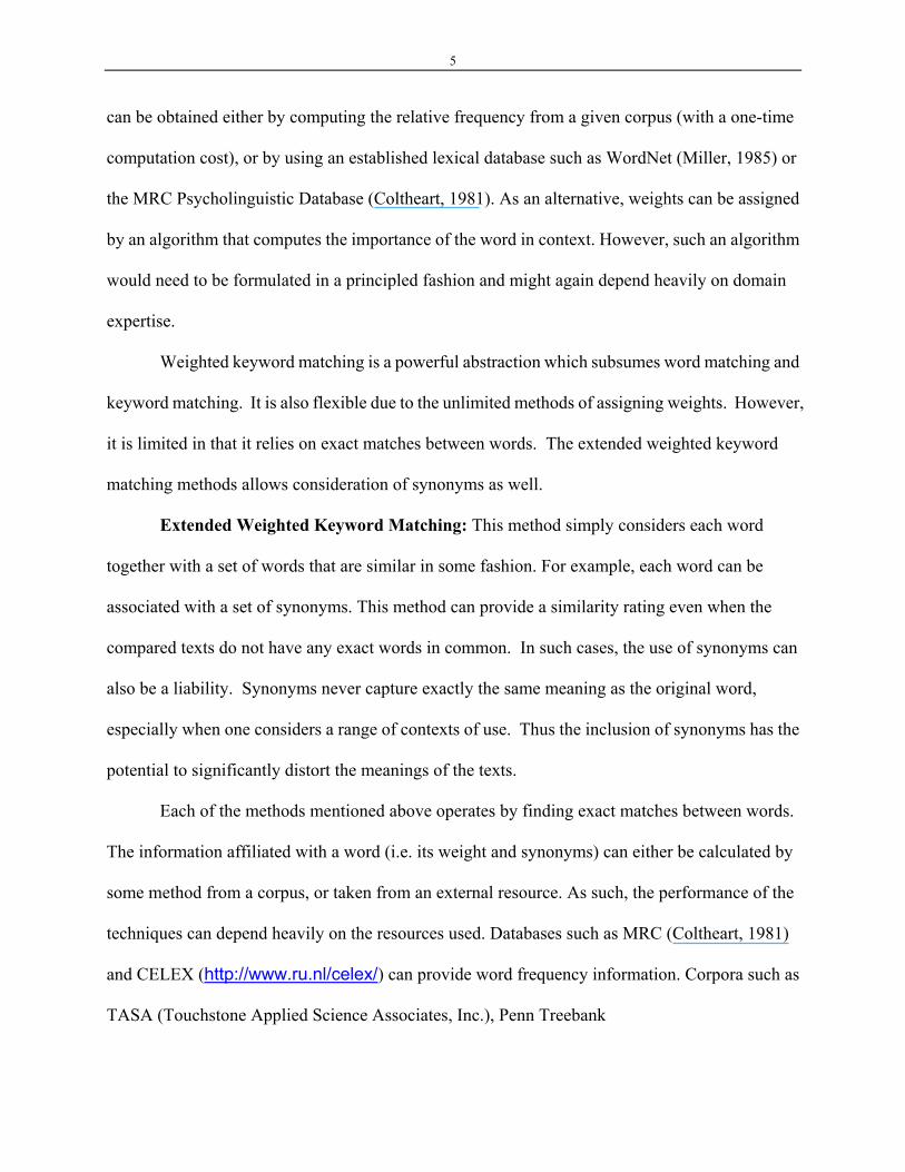
Keyword Matching: In this case, only keywords are considered. Common words or

function words like it, is, or the are ignored (Graesser, Hu, Person, Jackson, and Toth, 2004). This

is the most widely used method in document retrieval. The advantage of this method is that it

considers the importance of the words’ semantic contributions. Some additional requirements

need to be satisfied in order to have this method work well, especially in narrowly-defined

domains. For example, which words are identified as keywords largely depends on the domain. In

most cases, the list of keywords is simply the list of glossary items and therefore is domain

dependent. One weakness of this method is that it does not consider differential importance as to

how much information a particular word may carry. The following method addresses this problem

by differentially weighting the keywords.

Weighted Keyword Matching: The advantage of weighting keywords is to emphasize the

degree to which a particular word is important to a particular domain. The challenge lies in how to

assign the weights, which is often domain dependent. For example, weights can reflect how often a

word is used in ordinary written language or spoken language (Graesser, Hu, et., 2004). Such data

5

can be obtained either by computing the relative frequency from a given corpus (with a one-time

computation cost), or by using an established lexical database such as WordNet (Miller, 1985) or

the MRC Psycholinguistic Database (Coltheart, 1981). As an alternative, weights can be assigned

by an algorithm that computes the importance of the word in context. However, such an algorithm

would need to be formulated in a principled fashion and might again depend heavily on domain

expertise.

Weighted keyword matching is a powerful abstraction which subsumes word matching and

keyword matching. It is also flexible due to the unlimited methods of assigning weights. However,

it is limited in that it relies on exact matches between words. The extended weighted keyword

matching methods allows consideration of synonyms as well.

Extended Weighted Keyword Matching: This method simply considers each word

together with a set of words that are similar in some fashion. For example, each word can be

associated with a set of synonyms. This method can provide a similarity rating even when the

compared texts do not have any exact words in common. In such cases, the use of synonyms can

also be a liability. Synonyms never capture exactly the same meaning as the original word,

especially when one considers a range of contexts of use. Thus the inclusion of synonyms has the

potential to significantly distort the meanings of the texts.

Each of the methods mentioned above operates by finding exact matches between words.

The information affiliated with a word (i.e. its weight and synonyms) can either be calculated by

some method from a corpus, or taken from an external resource. As such, the performance of the

techniques can depend heavily on the resources used. Databases such as MRC (Coltheart, 1981)

and CELEX (http://www.ru.nl/celex/) can provide word frequency information. Corpora such as

TASA (Touchstone Applied Science Associates, Inc.), Penn Treebank

6

(http://www.cis.upenn.edu/~treebank/home.html), and the British National Corpus (BNC,

http://www.natcorp.ox.ac.uk/) provide samples of actual texts from which word information can

be derived. A lexicon like WordNet (http://wordnet.princeton.edu/)can provide synonyms. The

information derived from different lexical databases or corpora may be appropriate for the domain

of interest, but it may also be misleading if there is a misalignment between the corpus and the

application. The quality of this information can have a large effect on the overall success of the

technique.

Formal definition of similarity between texts The various types of word matching methods can be represented within a unified

mathematical formalism. First, consider that the collection of all possible terms in a given

language is a set with m elements. If one indexes all the terms from 1 to m, then each term ti (where

i=1,…m) can be represented by an m-dimensional row vector with only one nonzero element. This

is captured in expressions 1 and 2 below, with bold letters depicting vectors.

( ) ,1

mjiji u=

=t (1)

where

. (2) ⎩⎨⎧ =

=otherwise

jiuij 0

1

In other words, ti is a vector which is 0 everywhere except for the ith element which is 1. With this

notation, for any text T with K words (not necessarily distinct), there is an m dimensional vector

representation T, as expressed in equation Eq(3) in which there are K term vectors in the

summation:

.iii

n tT ∑= (3)

where ni is the number of occurrences of the ith word in the text T.

7

The word match similarity between two texts, T1 and T2 is computed as the cosine between the two

document vectors:

( ) .,cos2211

2121 TT

T

TTTTTTTT = (4)

Notice that T1 and T2 are row vectors, so there is a transpose needed for T2 in Eq(4).

Assembling all the term vectors together, a diagonal matrix U can be obtained, as

expressed in Eq(5).

(5) ( )mmij

mm

un

n

×⎟⎟⎟

⎠

⎞

⎜⎜⎜

⎝

⎛==

t

tU Μ

11

With this definition of U, we are able to have similar formulas for different types of similarity

measures.

Keyword matching and weighted keyword matching

Consider an m x m diagonal matrix, W = diag{wi}, where all diagonal elements are

non-negative. In this case, the similarity measure based on both keyword matching and weighted

keyword matching can be computed with Eq(4), where the term vector ti is multiplied by the

number of occurrence to form the ith row of WU. In other words, the matrix WU contains term

vectors ti multiplied by the occurrences and then weighted by wi (i = 1,…m). Note that keyword

matching corresponds to the case where elements of W only have the value of 0 or 1. A weight of

0 for a common word essentially removes it from consideration.

Extended Weighted Keyword Matching

The similarity measure corresponds to extended weighted keyword matching can be

computed as the as Eq(4), where T=WUE and E=(eij)mxm is a matrix with all elements either 0 or 1.

When eij = 1, terms indexed as i and j are synonyms of each other.

8

We find the above notations very useful. We can extend the similarity measures from word

matching to context matching.

Context-based Similarity In the word-based methods, the only way that one could obtain a nonzero similarity

measure between two distinct terms is when they are somehow related. This occurs, for example,

when there is extended weighted keyword matching and the two terms are synonyms. A similarity

measure based on context is different from the keyword-based similarity measure. Consider a

corpus, with all of the documents indexed from 1,2,…,n. Term ti, i=1,…m, in the corpus is

represented as the n-dimensional vector expressed in Eq(6),

( ) ,1

njiji f=

=t (6)

where fij is the number of times term ti appears in document j. Denote ( )nmijf

×=F . The similarity

measure of any two texts based on context can again be computed with Eq(4), where ti is the ith row

of F. As with the word-based measures, we can also apply weighting to terms and documents. In

this case, term weights form a diagonal matrix and document weights form a diagonal

matrix The similarity measures between two texts is the same as Eq(4), except that the term

vector t

mm×W

.nn×Λ

i is obtained as the ith row of .ΛWF This method of denotation allows us to consider LSA

in a new framework, as discussed in the next section.

LSA

The two similarity measures introduced previously have one important common

characteristic: the terms are represented as multidimensional vectors. The computational formulas

are the same, namely Eq(4). However, the vector representations of the terms differ between the

approaches. As we have observed, for all the methods introduced, we always assume the existence

9

of a high dimensional vector representation. This assumption will bring some difficulty when they

are implemented in real applications due to the computational complexity.

Representing terms as vectors and comparing similarity between texts using vector algebra

has been a common methodology in several applications. For example, HAL (Hyperspace Analog

to Language) uses co-occurrence of word pairs in a corpus to build word vector representations

(Burgess, 1998). NLS (Non-Latent Similarity) uses similarities between explicit word pairs to

build word vector representations (Cai, McNamara, Louwerse, Hu, Rowe & Graesser, 2004).

Latent Semantic Analysis (LSA) is the most well known example of such methods that use vectors

to represent terms. Instead of using high dimensional vectors (usually, the number of words is in

the neighborhood of 105 and the number of documents is about the same scale), LSA represents

each term as a real vector (of up to 500 dimensions), and the similarity between any two texts is

computed using the formula in Eq(4).

Basic Steps in LSA The difference between LSA and other methods that we have introduced previously

(Martin and Berry, this volume) is the mechanism by which the term vectors are obtained. We

briefly summarize the LSA procedures for obtaining term vectors: data acquisition, singular value

decomposition, and dimension reduction.

Data Acquisition: The process starts by collecting a massive amount of text data in

electronic form. With such data, we prepare the nm× matrix in Eq(7),

( ) ( )( )nmij jiLiGf

×××= ,A (7)

where m is the number of terms and n is the number of documents (usually m and n are very large,

and for now, assume ), the value of fmn ≥ ij is a function of the number of times term i appears in

document j, L(i,j) is a local weighting of term i in document j, and G(i) is the global weighting for

10

term i. Such a weighting function is used to differentially treat terms and documents to reflect

knowledge that is beyond the collection of the documents (see Martin and Berry, this volume for

detail) . Notice the fact that if L(i,j) is multiplicative, namely L(i, j) can be written as,

( ) ( ) ( ),, jlikjiL = (8)

where k(i) is a weight for the ith term and l(j) is a weight for the jth document, then Eq(7) is a matrix

(fij) multiplied by a diagonal matrix diag{k(i)G(i)} on the left and another diagonal matrix

diag{l(j)} on the right, the same form as ΛWF in the context-based similarity measure.

Singular Value Decomposition (SVD): Singular value decomposition (SVD)

decomposes the matrix A into three matrices

(9) TVUA Σ=

where U is and V is square matrices, such that UUmm × nn× T = I ; VVT=I (orthonormal

matrices), and is an diagonal matrix with singular values on the diagonal. In addition, the

singular values are non-negative and are ordered from largest to smallest in the diagonal of

Σ nm×

Σ

(see Martin and Berry, this volume for detail of SVD).

Dimension Reduction: By removing dimensions corresponding to small singular values

and keeping the dimensions corresponding to larger singular values, the representation of each

term is reduced to a smaller vector with only k dimensions. The original SVD Eq(9) becomes

Eq(10).

(10) Tkkkkk VUA ×= Σ

The new term vectors (rows in the reduced U matrix, Uk ) are no longer orthogonal, but the

advantage of this is that only the most important dimensions that correspond to larger singular

values are kept. This operation is believed to remove redundant information in the matrix A and

reduce noise from semantic information. In the LSA procedure described above, the Data

11

Acquisition and the Dimension Reduction parts are the most intuitive. The most mysterious part is

the SVD. Why and how it works is a very deep mathematical / philosophical question and is

beyond the scope of this chapter. For more details, see Martin and Berry (this volume).

Basic facts about LSA After Uk is obtained, each term has a unique k -dimensional vector representation.

Furthermore, any text containing one or more terms will also have a corresponding vector with the

same number of dimensions. The vector for a text can be computed as a function of the term

vectors. Text vectors are computed differently for different applications. The formula for the text

vector is in the same form as Eq(3), except that ti is the ith row of ,ΛkWU where W=diag{wi} is a

diagonal matrix and wi is the weight for term i }{ jdiag λ=Λ is a diagonal matrix where jλ is the

weight of dimension j. The similarity between any two texts is calculated by the formula in Eq(4).

The procedure outlined above is relatively simple. There are several advantages to using

LSA, but two of them are primary:

1) It picks up the word importance score from the information provided by the corpus.

2) It sets up semantic similarity between words. This widely extends the synonym relation

between words.

In addition to the advantages, there are several key elements in LSA that are not directly obvious.

These are listed below.

a) The computation of weights G(i) and L(i, j) in Eq(7) is nontrivial. G(i) is a measure of how

important a term is in the entire collection of texts. In order to obtain G(i) and L(i,j), one needs

to process the entire corpus first to get some kind of importance measure such as frequency of

appearance A direct consequence of this is that the entire matrix A needs to be recalculated

whenever some more documents are put into the corpus, because word frequencies are

12

changed. It presumably encodes the weighting of term i in document j and the importance of

document j. Such parameters are needed during the data acquisition/encoding phase. It is very

important to note that the influence of the parameters can only be evaluated after the three steps

and it is very hard to set the parameters because of the massive amount of computation needed

to reach the last step.

b) Selection of the number of dimensions (k) is a challenging task. One needs to specify k before

the computation. There is no intuitive way to determine the best k, other than by repeated

empirical evaluations (Zha and Zhang, 1999).

c) The computation of Eq(4) is task dependent. For example, if one only wants to compare the

similarity between two texts, then Λ is an identity matrix ( kjj ,...,1,1 ==λ ). If one wants to

retrieve a document from the original corpus and obtain the closest vector in V, then Λ is the

inverse of the singular values from the SVD (Berry, 1992). The former similarity computation

is called the term method, wherein the later computation is called the document method (see

http://lsa.colorado.edu/).

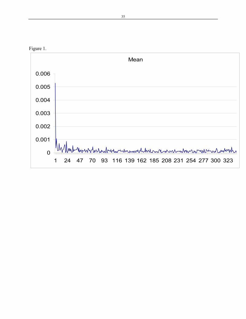
d) The first dimension is problematic. Because all entries of the original matrix A are

non-negative, the first dimension of Uk always has the same sign (Hu, Cai, Franceschetti,

Penumatsa, Graesser, Louwerse, McNamara & TRG, 2003) and the mean of the first

dimension values is much larger than that of other dimensions. This trend is illustrated in

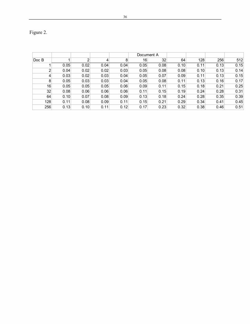
Figure 1. As a result of this, the cosine value between any two documents, if one uses the term

method, is monotonically related to number of words contained in the documents. This fact

was observed by Buckley, Singhal, Mitra, and Salton (1996). Such trend is illustrated in

Figure 2.

Insert Figures 1 and 2 about here

13

e) The vector representations for the terms are not fully used. Up to now, their contribution is

essentially in the computation of similarities between terms. In other words, in the computation

of text similarity, LSA only provides the information about “term similarity”. A little

mathematics can help to make this clear. Denote T1 = (t11+ t12,…,+t1I) and T2 = (t21+

t22,…,+t2I) then

( )T

jiJj

Ji

Tji

Ij

Ii

Tji

Jj

Ii

TT

T

22111111

2111

2211

2121,cos

tttt

tt

TTTTTTTT

∑∑∑∑

∑∑==

====

== , (11)

where t1itT2j, t1itT

1j, and t2itT2j, i=1,2,…I, j=1,2,…J are dot products of the term vectors. In

other words, the obtained matrix, nn × ( ) ,nnijs

×=P where sij = titT

j, i, j = 1,2, …, n is the

similarity (un-normalized) between term i and term j. Eq(11) gives a way to compute text

similarities based on the term similarity matrix. However, we need an to save the

un-normalized term similarities. The advantage of vector representation of terms here is the

saving of storage space (from to

nn×

nn× kn× real numbers). It may be a significant saving,

when n is greater than k. One drawback is the lost of flexibility in constructing the term

similarity matrix (Cai, et al. 2004).

We end this section by proving a theorem that relates LSA and weighted keyword

matching (Hu, et al. 2003). This theorem will help to develop other sections of the chapter.

Theorem Assume k equals the number of nonzero singular values, then

1. If and L(i, j) is multiplicative, as in Eq(8), then Eq(4) is weighted context

matching.

,kk×Σ=Λ

2. If then Eq(4) is weighted keyword matching. ,kkI ×=Λ

Based on our discussions in this section, we observed that there are some facts about LSA

that is none trivial (facts d) and e), for example). In the next section, we will examine the use of

14

LSA in several applications and point out some weaknesses of LSA.

Limitations of LSA In order to understand the limitations that we point out here, we briefly describe two

applications that use LSA. For details about these two applications, the reader may find more in

other chapters in this book (see Graesser et al., this volume; McNamara, Cai, & Louwerse, this

volume).

AutoTutor: AutoTutor is a natural language tutoring system that teaches conceptual

physics and computer literacy via the Internet (Graesser, Wiemer-Hastings, Wiemer-Hastings,,

Harter, Person, & TRG. 2000). One challenge for this system is to assess the quality of the

student's response to the system. LSA cosine match is used to compare the student's response with

the expected answers stored in a curriculum script. The values are used to help AutoTutor provide

appropriate feedback for the student.

Coh-Metrix: Coh-Metrix is a web tool that analyzes texts and provides up to 250 measures

of cohesion and language characteristics (Graesser, McNamara, Louwerse, & Cai, 2004). Some of

the cohesion measures consist of density scores for particular types of cohesion links between text

constituents, such as paragraphs, sentences, clauses, or even words. LSA is used in this system to

assess the conceptual relatedness of constituents (i.e., the more related, the more cohesive) and to

assess co-referential cohesion (i.e., the extent to which content words refer to other constituents in

the text).

The Statistical Nature of LSA values As we have pointed out previously, the first dimension of all the term vectors have the

same sign. This indicates that if one uses the term method to compute the similarity, the value

computed by Eq(4) is directly influenced by the number of words in the texts. A simple simulation

15

shows that the cosine value between two texts monotonically increases as a function of the number

of terms in the two documents (see Figure 2). This property of the term method makes it very hard

to interpret text similarity measures without considering the sizes of the texts (Hu, Cai et al, 2003).

In the case of AutoTutor, students’ contributions are compared with stored expectations.

AutoTutor selects a fixed value between 0 and 1. If the cosine match between students’

contribution and the stored expectation exceed such value, AutoTutor assumes the expectation is

covered. The fixed value for this purpose is called a threshold. The issue here is how to set the

threshold. The threshold should be a function of the number of terms contained in the student’s

contribution and the individual expectations. This limitation is not relevant in the case where

similarity is computed using the document method, where the influence of the first dimension is

minimized, nor in the case where the similarity is used for information retrieval, where only the

ordinal property of the similarity value is used (Graesser et al., 2004).

The use of detailed dimensional information The procedure outlined in the previous section has demonstrated that the original U matrix

from the SVD and the truncated Uk are substantially influenced by the information contained in the

original corpus. We further observed that even with the remaining k dimensions, LSA only has

limited use. In fact, all the remaining dimensions are used only to obtain dot-products between

terms, as it was shown in Eq(11). In the next few sections, we demonstrate that the vector

representations of terms and documents contain more information. The information contained in

the dimensions can be further used to extend the usefulness of LSA.

Extending LSA Two observed weaknesses of LSA motivated us to propose two extensions of LSA that

address the observations. One extension is to use the statistical characteristics to reduce the text

16

size effect in the LSA similarity computation. The other extension is to make more use of the

dimensional information contained in the vector representation.

Statistical Characteristics of LSA LSA was originally used as a tool for information retrieval (IR) (Graesser, Hu, et al., 2004)

where recall was more emphasized than precision in most of the applications. In IR, the influence

of the first dimension is not as strong as in similarity measure. This is because (1) the query vector

is computed from WUkΛ where Λ=Σ-1 so the first dimension was weighted inversely by the largest

singular value and (2) the document vector is from Vk where the rows are normalized before they

are truncated. Furthermore, only the ordinal nature of the cosine value is used in IR because the

main goal is to fetch the most relevant document to the query. As a consequence, consideration of

the statistical nature of the cosine values is not necessary. In the case of the similarity measure,

however, the query vector is computed from WUk so the first dimension is always the most

influential. Furthermore, in some applications, such as AutoTutor, the cosine values are compared

with a threshold. As indicated in Figure 2 and proven by Hu et al. (2003), the cosine values are

always a monotonic function of the texts’ size. For example, a cosine value of 0.2 between two

terms may indicate a high degree of similarity but may not indicate any similarity at all between

texts with over 200 terms. This analysis suggests that when using LSA cosine values for the

measures of similarity between texts, one needs to consider the sizes of the texts (Buckley et

al,1996; Hu, Cai et al 2003).

Given the weighted term matrix WUk, one can always obtain some basic statistical

information such as the average cosine ( )21,nnµ and the standard deviation ( 21,nn )σ of any two

texts with n1 and n2 terms respectively. Furthermore, if the distribution of all possible cosine

values between two texts is normally distributed, one can obtain the relative cosine values between

17

two texts using the following simple formula

( ) ( ) ( )( )21

212121 ,

,,cos,

nnnn

Sσ

µ−=

TTTT , (12)

where n1 and n2 are the number of terms in T1 and T2 respectively.

Adaptive Methods of LSA As we have pointed out in the previous section, the vector representation of terms in LSA

space has been used only to produce a numerical value (vector dot product) between two terms.

We argue that there are several other ways of using the dimensional information contained in the

vector representation. We call this approach the "adaptive method" of LSA. For the purpose of

later sections, we briefly review a few concepts in linear algebra.

Some basic concept in linear algebra Linear Combination: A vector b is a linear combination of the vectors v1, v2…, vn , if b =

c1v1+ c2v2+,…, + cnvn, where c1, c2…, cn are scalars.

Span: Suppose v1, v2…, vn are vectors in a vector space V. These vectors are said to span V

if every vector v in V can be expressed as a linear combination of these vectors.

Linear Dependence: A set of vectors v1,v2…, vn are linearly dependent if it is possible to

express one of the vectors as the others; that is, for some k ,

ii

kini

k vav ∑≠≤≤

=1

Linear Independence: A set of vectors v1, v2…, vn are linearly independent if it is

impossible to express any one of the vectors as the others.

Basis: A set of vectors v1, v2…, vn in V is a basis for V if the vectors are linearly

independent and span V.

18

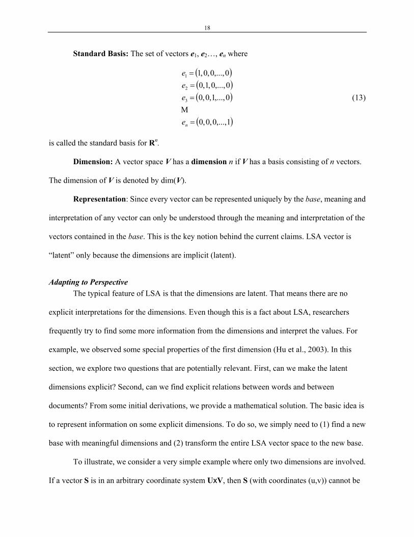
Standard Basis: The set of vectors e1, e2…, en where

( )( )(

( )1,...,0,0,0

0,...,1,0,00,...,0,1,00,...,0,0,1

3

2

1

=

===

ne

eee

Μ) (13)

is called the standard basis for Rn.

Dimension: A vector space V has a dimension n if V has a basis consisting of n vectors.

The dimension of V is denoted by dim(V).

Representation: Since every vector can be represented uniquely by the base, meaning and

interpretation of any vector can only be understood through the meaning and interpretation of the

vectors contained in the base. This is the key notion behind the current claims. LSA vector is

“latent” only because the dimensions are implicit (latent).

Adapting to Perspective The typical feature of LSA is that the dimensions are latent. That means there are no

explicit interpretations for the dimensions. Even though this is a fact about LSA, researchers

frequently try to find some more information from the dimensions and interpret the values. For

example, we observed some special properties of the first dimension (Hu et al., 2003). In this

section, we explore two questions that are potentially relevant. First, can we make the latent

dimensions explicit? Second, can we find explicit relations between words and between

documents? From some initial derivations, we provide a mathematical solution. The basic idea is

to represent information on some explicit dimensions. To do so, we simply need to (1) find a new

base with meaningful dimensions and (2) transform the entire LSA vector space to the new base.

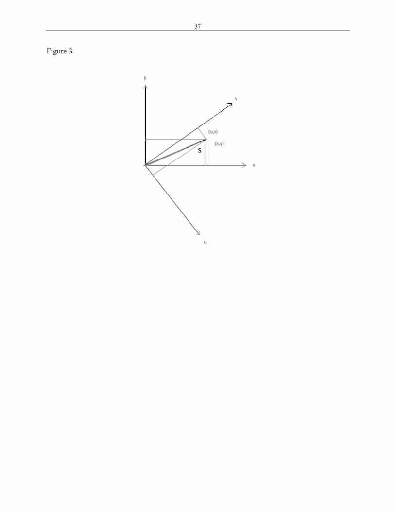
To illustrate, we consider a very simple example where only two dimensions are involved.

If a vector S is in an arbitrary coordinate system UxV, then S (with coordinates (u,v)) cannot be

19

easily interpreted without an explicit interpretation of U and V. However, if a new system XxY is

introduced where X is the horizontal axis and Y is vertical axis, S can be interpreted easily, due to

the obvious interpretation of X and Y (see Fig. 3).

Figure 3 is about here

To generalize the above intuitive example, we derive a general algorithm that can be used

in LSA space with k dimensions. Consider the LSA term matrix Λkkm WUH =× with m term

vectors. Furthermore, we may assume b1, b2, …, bk are any set of independent vectors that serve

as a base of the space. For example, the base could be k words that represent k distinct categories,

or a centroid of some categories that can be interpreted. From linear algebra, for any row in ,

h

km×H

i = (hi1, hi2…, hik) there is a unique nonzero vector (ei1, ei2 …, eik), such that

(14) . 1

jij

k

ji e bh ∑

=

=

In this case, ei = (ei1, …, eik) is the new representation under new base B=(b1, b2 …, bk). To

illustrate, suppose in the original LSA space, two terms are represented by two rows in h,km×H s =

(hs1, hs2… hsk) and ht = (ht1, ht2…, htk) . There exist unique cs = (cs1, cs2… csk) and ct = (ct1, ct2… ctk) ,

for hs= csBT and ht= ctBT, respectively, where csBT and ctBT are inner products of vectors. The

cosine in the original space is

( )( ) ( )ts

ts

ts

tkttskss

ts

ts hhhhhhhh

cBBchhhh

hh TTTT

==...,,...,, 2121 ,

where • is the length of a vector. On the other hand, since ( ) 1−= TBhc ss and , the

cosine under the new base can be obtained by

( ) 1−= TBhc tt

( )( ) ( ) ( )( )ts

ts

ts

Ttkttskss

ts

Tts cccccc

cchBBh

cccccc TT 11

2121 ...,,...,, −−

== .

20

The interesting question is whether we can find a meaningful base. The answer is yes and

the construction of such bases can be very simple. For example, we can choose k key terms that we

think are most relevant to our task. If the corresponding term vectors are linearly independent, then

these k term vectors form a base. Then, any term in the space can be linearly expressed by these

selected k term vectors. By definition, these k term vectors form a base of the k-dimensional space.

In the above description, we have used (b1, b2…,bk) where k is the rank of .Λkkm WUH =×

In fact, from the derivation above, we can prove that it is not necessary to specify all k

vectors for the base. One could simply specify a few meaningful vectors (b1, b2…, bk0) and select

(k – k0) vectors from the old base from Eq(13).

Adapting to context In AutoTutor, every input from student is compared to several expectations. LSA is used to

decide whether each of the expectations is covered. It turned out that some of the expectations

have similar LSA vectors. When this occurs, it would be ideal to adjust AutoTutor so that it can

detect small differences between the expectations. The process of adjusting LSA to this task is

outlined below. We call this the method of “adapting to context.”

Before we derive the formal method, consider the following keyword match example to

help understand our basic claims. Assume that the two target expectations are A: "The horizontal

speed is constant for the moving body" and B: "The vertical speed is zero for the moving body".

Assume that the student's input is C: "The moving body will move forward with constant speed.".

To distinguish A from B, there are some common words (the, is, for, the, moving, body) shared by

A and B; they will not add much value in discriminating the two alternative expectations. In this

case, one can either include common words or exclude common words. When common words are

included, the similarity between A and C is 0.556 whereas the similarity between B and C is 0.444.

21

When common words are excluded, the similarity between A and C is 0.258 whereas the similarity

between B and C is 0.

Table 1 is about here

As shown from this example, one might prefer the exclusion method so that C is relatively

more similar to A than B. In essence, the differences between A and B would be magnified and this

would be reflected in the similarity between C and A versus B (See Table 1). There needs to be a

method to implement this context-sensitive magnification to LSA, where each expectation is

represented as an LSA vector. Assume the two target expectations have vectors A and B, and that

the student's input is vector C.

( )( )( )k

k

k

cccbbbaaa

...,,

...,,...,,

21

21

21

===

CBA

,

Further assume that nA, nB and nC are the number of words in A , B and C , respectively, and that we

have identified statistical properties of the LSA space. That is, for each column of ,ΛkWU such

as column x, there is the mean xµ and standard deviation xσ , x = 1,2 …, k. Given these statistics

and the number of words in A , B, and C , the expected values and variability (standard deviation)

of the xth elements of A , B, and C are ( ),, xAxA nn σµ ( )xBxB nn σµ , , and ( )., xCxC nn σµ With

these values computed, we can then decide the difference between A and B by comparing

quantities computed based on Eq(15) for all x = 1, …, k.

x

xBxA

xBxA znn

nn=

+

−22 σσ

µµ (15)

The final comparison between A and B versus B and C is computed in Eq(16),

22

( ) ( )

( ) ( )

( ) ( )

( ) ( )

,

,

21

21

1

21

21

1

⎪⎪⎩

⎪⎪⎨

⎧

∑∑∑=′

∑∑∑=′

==

=

==

=

xxk

xxxk

x

xxxk

x

xxk

xxxk

x

xxxk

x

czfbzf

cbzf

czfazf

cazf

S

S

CB

CA, (16)

where f(z) is a function such that ( ) ( )"zfzf ≥′ if ".zz >′ The simplest case for the function f(z) is

the function captured in Eq(17).

(17) ( )⎩⎨⎧

≤>

=δδ

zz

zf01

The function Eq(17) was used in the simulation that we describe next.

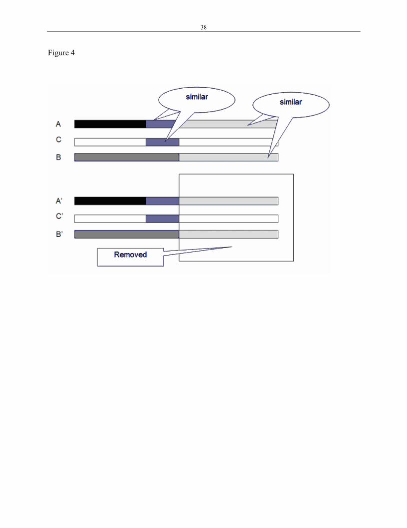
Simulation We explored the above analysis by a simple simulation (see Fig. 4 as an illustration) where A, B,

and C are generated random vectors with 300 dimensions. In the simulation, two set of vectors that

are “similar” at dimension x if zx=0. A and B are similar for 150 of the dimensions while A and C

are similar for those 37 of the 150 dimensions for which A and B are different. Thus, similarity is

based on those dimensions that differentiate A and B, not all dimensions.

Figure 4 is about here

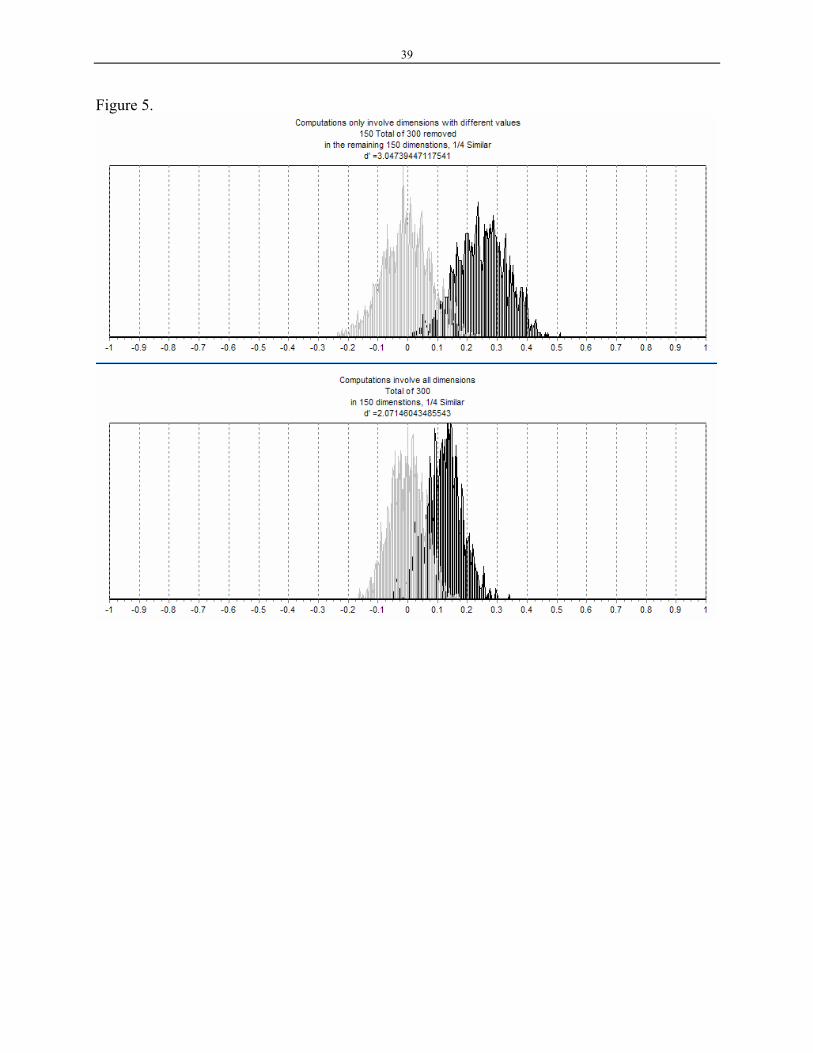
We obtained all simulated values of Eq(16), both with and without using the weighting

function Eq(17). We observed the difference between ( )CA,S ′ and ( )CB,S ′ is larger with Eq(17)

(upper picture of Fig. 5, ) than the case in which Eq(17) was not used (lower picture of

Fig. 5, ).

05.3=′d

07.2=′d

Figure 5 is about here

From the above analysis and simulation, we argue that when using LSA similarity to select

one option from multiple alternatives (such as using C to select one of A and B, as in the example

and simulation), considering detailed dimensional information will help the selection. In this

method, context constrained and narrows down the alternatives at the level of detailed dimensions.

23

We call this the method of "adapting to context."

Adapting to dialog history This is a method especially appropriate in situations where LSA is used to evaluate

sequence of contributions. Consider AutoTutor when the tutor's goal is to help the student produce

an answer to a question. The student typically gives one piece of information at a time. To furnish

a complete answer to a question, the student needs to produce multiple pieces of information. In

order for the tutor to be helpful and effective, the tutor needs to evaluate every contribution of the

student and to help the student every time a contribution is made. We assume that AutoTutor is

suppose to give feedback based on student's contribution towards the answer and that AutoTutor is

suppose to give four different context-sensitive feedbacks at every contribution:

Table 2 is about here

Similar to the analysis of the previous method, we first consider what AutoTutor would do

if the evaluation method were keyword matching. For an ordered sequence of statements, S1, S2, …,

SN and a target statement S0 , for any given i ( )ni ≤≤2 , one can decompose Si into the four

different bags of words, as specified below:

• Words that overlap with words in S0 (relevant)

• Appeared in S1, S2 … , Si-1 (old)

• Never appeared in S1, S2 … , Si-1 (new)

• Words that do not overlap with words in S0 (irrelevant)

• Appeared in S1, S2 … , Si-1 (old)

• Never appeared in S1, S2 … , Si-1 (new)

Having established relations between keyword match and LSA in the previous section, the

similar decomposition can be achieved in the present case. Denote si = siWUk , I = 0,1, …, n. For

24

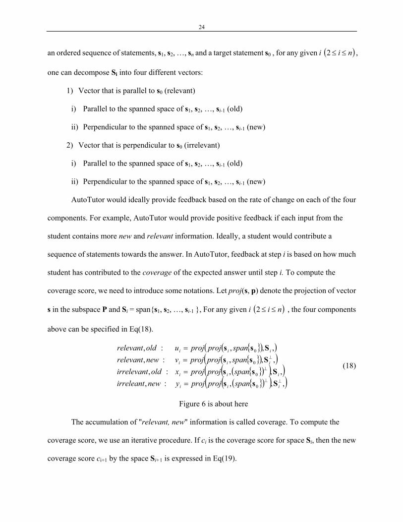
an ordered sequence of statements, s1, s2, …, sn and a target statement s0 , for any given i ( )ni ≤≤2 ,

one can decompose Si into four different vectors:

1) Vector that is parallel to s0 (relevant)

i) Parallel to the spanned space of s1, s2, …, si-1 (old)

ii) Perpendicular to the spanned space of s1, s2, …, si-1 (new)

2) Vector that is perpendicular to s0 (irrelevant)

i) Parallel to the spanned space of s1, s2, …, si-1 (old)

ii) Perpendicular to the spanned space of s1, s2, …, si-1 (new)

AutoTutor would ideally provide feedback based on the rate of change on each of the four

components. For example, AutoTutor would provide positive feedback if each input from the

student contains more new and relevant information. Ideally, a student would contribute a

sequence of statements towards the answer. In AutoTutor, feedback at step i is based on how much

student has contributed to the coverage of the expected answer until step i. To compute the

coverage score, we need to introduce some notations. Let proj(s, p) denote the projection of vector

s in the subspace P and Si = span{s1, s2, …, si-1 }, For any given i ( )ni ≤≤2 , the four components

above can be specified in Eq(18).

{ }( )( ){ }( )( ){ }( )(({ }( )( )( ),,,:,

,,,:,,,,:,,,,:,

0

0

0

0

⊥⊥

⊥

⊥

====

iii

iii

iii

iii

spanprojprojynewirreleantspanprojprojxoldirrelevant

spanprojprojvnewrelevantspanprojprojuoldrelevant

SssSss

SssSss

) ) (18)

Figure 6 is about here

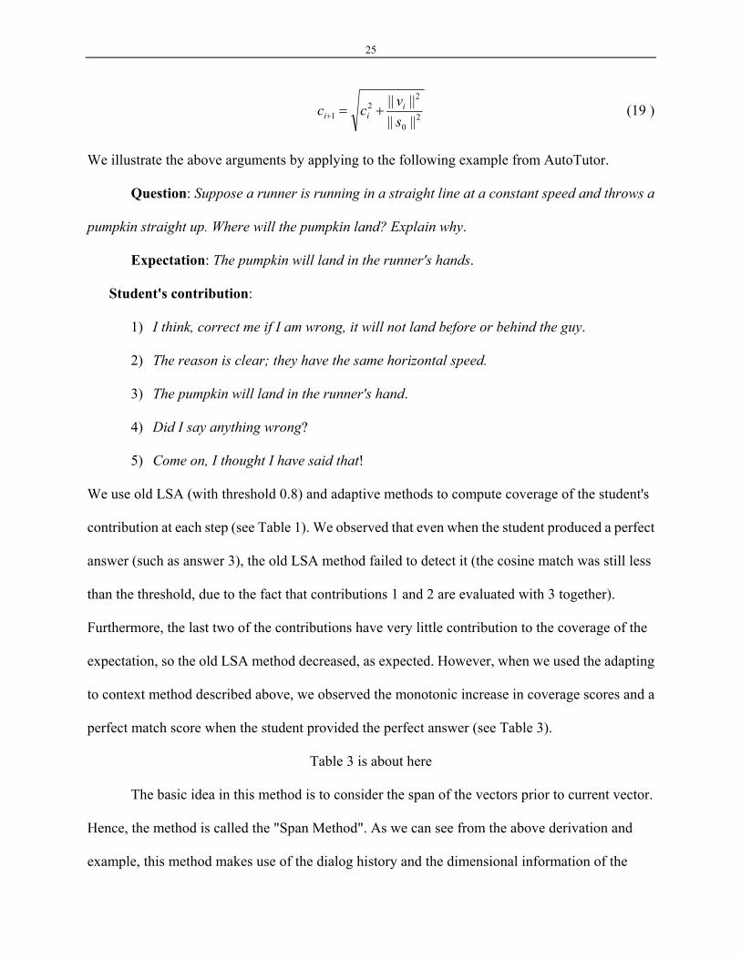
The accumulation of "relevant, new" information is called coverage. To compute the

coverage score, we use an iterative procedure. If ci is the coverage score for space Si, then the new

coverage score ci+1 by the space Si+1 is expressed in Eq(19).

25

20

22

1 ||||||||

svcc i

ii +=+ (19 )

We illustrate the above arguments by applying to the following example from AutoTutor.

Question: Suppose a runner is running in a straight line at a constant speed and throws a

pumpkin straight up. Where will the pumpkin land? Explain why.

Expectation: The pumpkin will land in the runner's hands.

Student's contribution:

1) I think, correct me if I am wrong, it will not land before or behind the guy.

2) The reason is clear; they have the same horizontal speed.

3) The pumpkin will land in the runner's hand.

4) Did I say anything wrong?

5) Come on, I thought I have said that!

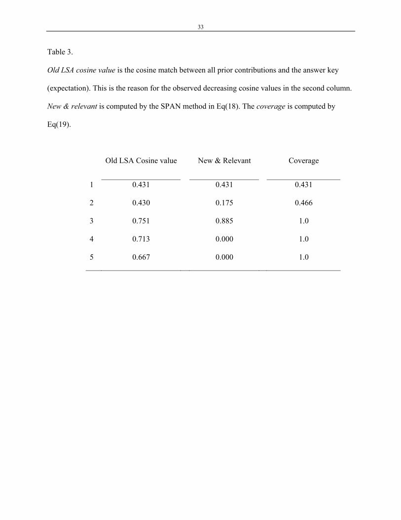
We use old LSA (with threshold 0.8) and adaptive methods to compute coverage of the student's

contribution at each step (see Table 1). We observed that even when the student produced a perfect

answer (such as answer 3), the old LSA method failed to detect it (the cosine match was still less

than the threshold, due to the fact that contributions 1 and 2 are evaluated with 3 together).

Furthermore, the last two of the contributions have very little contribution to the coverage of the

expectation, so the old LSA method decreased, as expected. However, when we used the adapting

to context method described above, we observed the monotonic increase in coverage scores and a

perfect match score when the student provided the perfect answer (see Table 3).

Table 3 is about here

The basic idea in this method is to consider the span of the vectors prior to current vector.

Hence, the method is called the "Span Method". As we can see from the above derivation and

example, this method makes use of the dialog history and the dimensional information of the

26

vector representation. One could imagine that Tutor's feedback could be based on other

components also. For example, when the student provides old and irrelevant information,

AutoTutor may detect that persistent misconceptions are driving the answers. AutoTutor's

feedback is largely determined by the values of ui, vi, xi, yi at any step i. The overall performance is

computed as an accumulation score, as in the case of Eq(19).

Conclusions In this chapter, we have pointed out two limitations of LSA: 1) limited use of statistical

information of LSA space and 2) limited use of dimensional information in the vector

representation of the terms. Based on these observations, we have proposed a few extensions.

These include a modified cosine match (as shown in Eq(12)) as similarity measures and adaptive

methods that intelligently select dimensional information of the vector representations. We have

concentrated large portion of the chapter developing the adaptive methods. We have proposed

three adaptive methods: 1) adapting to perspective, 2) adapting to context, and 3) adapting to

dialog history. All three adaptive methods are developed in the context of the application of

AutoTutor with LSA cosine match being used as similarity measure. In this paper, we primarily

concentrated on mathematical derivations and explained the extensions at the conceptual level

with simple simulations. The next step is to implement the extensions in real applications.

27

Acknowledgements

This research was supported by grants from the Institute for Education Sciences (IES

R3056020018-02), the National Science Foundation (SBR 9720314, REC 0106965, REC

0126265, ITR 0325428), and the DoD Multidisciplinary University Research Initiative (MURI)

administered by ONR under grant N00014-00-1-0600. . The Tutoring Research Group (TRG) is an

interdisciplinary research team comprised of approximately 35 researchers from psychology,

computer science, physics, and education (visit http://www.autotutor.org). Any opinions, findings,

and conclusions or recommendations expressed in this material are those of the authors and do not

necessarily reflect the views of IES, NSF, DoD, or ONR.

28

References

Berry, M. W. (1992). Large scale singular value computations. International Journal of

Supercomputer Applications 6(1), 13-49.

Buckley, C., Singhal, A., Mitra, M., and Salton, G. (1996). New Retrieval Approaches Using

SMART: TREC 4. In Proceedings of the Fourth Text Retrieval Conference, NIST Special

Publication 500-236, 25-48, 1996.

Burgess, C. (1998). From simple associations to the building blocks of language: Modeling

meaning in memory with the HAL model. Behavior Research Methods, Instruments, &

Computers, 30, 188-198

Cai, Z., McNamara, D.S., Louwerse, M.M., Hu, X., Rowe, M.P., & Graesser, A.C. (2004). NLS: A

non-latent similarity algorithm. In K.D. Forbus, D. Gentner, T. Regier (Eds.), Proceedings of

the Twenty-Sixth Annual Conference of the Cognitive Science Society (pp. 180-185).

Mahwah, NJ: Erlbaum.

Coltheart, M. (1981). The MRC Psycholinguistic Database. Quarterly Journal of Experimental

Psychology, 33, 497-505

Deerwester, S., Dumais, S. T., Furnas, G. W., Landauer, T. K., & Harshman, R. (1990). Indexing

By Latent Semantic Analysis. Journal of the American Society for Information Science, 41,

391-407.

Graesser, A.C., McNamara, D.S., Louwerse, M.M., & Cai, Z. (2004). Coh-Metrix: Analysis of

text on cohesion and language. Behavior Research Methods, Instruments, and Computers,

36, 193-202.

29

Graesser, A. C., Hu, X., Person, P., Jackson, T., & Toth, J (2004). Modules and information

retrieval facilities of the Human Use Regulatory Affairs Advisor (HURAA). International

Journal on eLearning, October-November, 29-39.

Graesser, A., Wiemer-Hastings, P., Wiemer-Hastings, K., Harter, D., Person, N., & the Tutoring

Research Group. (2000). Using latent semantic analysis to evaluate the contributions of

students in AutoTutor. Interactive Learning Environments, 8, 149-169.

Graesser, A., Penumatsa, P., Ventura, M., Cai, Z., & Hu, X. (in press). Using LSA in AutoTutor:

learning through mixed-initiative dialogue in natural language. In T. Landauer, D.S.,

McNamara, S. Dennis, & W. Kintsch (Eds.), LSA: A Road to Meaning. Mahwah, NJ:

Erlbaum.

Hu, X., Cai, Z., Louwerse, M., Olney, A., Penumatsa, P., Graesser, A.C., & TRG (2003). A revised

algorithm for Latent Semantic Analysis. Proceedings of the 2003 International Joint

Conference on Artificial Intelligence (pp. 1489-1491).

Hu, X., Cai, Z., Franceschetti, D., Penumatsa,P., Graesser, A.C., Louwerse, M.M., McNamara,

D.S., & TRG (2003). LSA: The first dimension and dimensional weighting. In R. Alterman

and D. Hirsh (Eds.), Proceedings of the 25rd Annual Conference of the Cognitive Science

Society (pp. 1-6). Boston, MA: Cognitive Science Society.

Landauer, T.K., & Dumais, S.T. (1997). A solution to Plato’s problem: The latent semantic

analysis theory of acquisition, induction, and representation of knowledge. Psychological

Review, 104, 211-240.

McNamara, D.S., Kintsch, E., Songer, N.B., & Kintsch, W. (1996). Are good texts always better?

Text coherence, background knowledge, and levels of understanding in learning from text.

Cognition and Instruction, 14, 1-43.

30

McNamara, D. S., Cai, Z., & Louwerse, M. M. (in press). Comparing latent and non-latent

measures of cohesion. In T. Landauer, D.S., McNamara, S. Dennis, & W. Kintsch (Eds.),

LSA: A Road to Meaning. Mahwah, NJ: Erlbaum.

Miller, George A. ``WordNet: a dictionary browser.'' In: Proceedings of the First International

Conference on Information in Data, University of Waterloo, Waterloo, 1985.

Hongyuan Z., & Zhenyue, Z. (1999). Matrices with Low-Rank-Plus-Shift Structure: Partial SVD

and Latent Semantic Indexing. SIAM J. Matrix Anal. Appl. 21, 522-536.

31

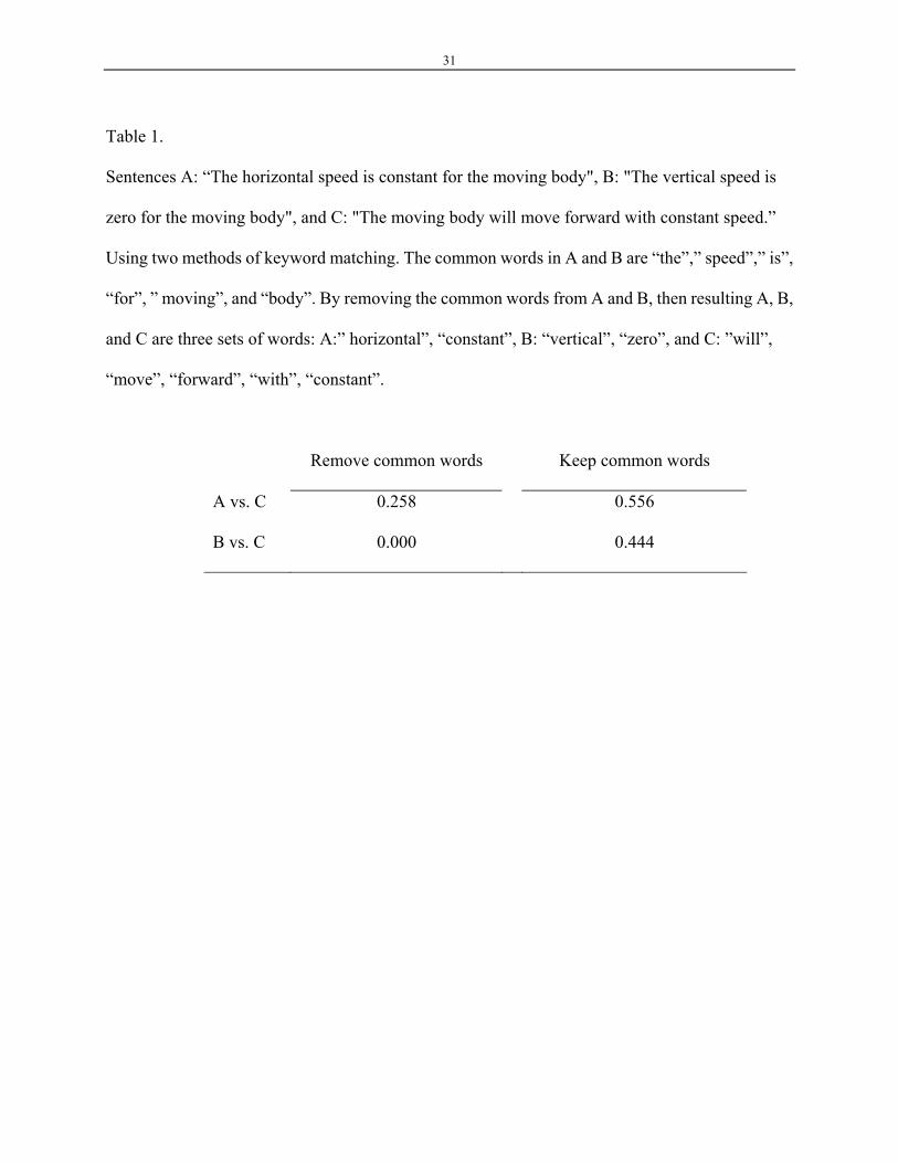
Table 1.

Sentences A: “The horizontal speed is constant for the moving body", B: "The vertical speed is

zero for the moving body", and C: "The moving body will move forward with constant speed.”

Using two methods of keyword matching. The common words in A and B are “the”,” speed”,” is”,

“for”, ” moving”, and “body”. By removing the common words from A and B, then resulting A, B,

and C are three sets of words: A:” horizontal”, “constant”, B: “vertical”, “zero”, and C: ”will”,

“move”, “forward”, “with”, “constant”.

Remove common words Keep common words

A vs. C 0.258 0.556

B vs. C 0.000 0.444

32

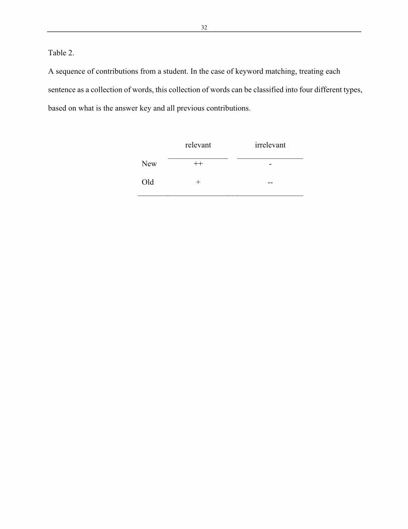
Table 2.

A sequence of contributions from a student. In the case of keyword matching, treating each

sentence as a collection of words, this collection of words can be classified into four different types,

based on what is the answer key and all previous contributions.

relevant irrelevant

New ++ -

Old + --

33

Table 3.

Old LSA cosine value is the cosine match between all prior contributions and the answer key

(expectation). This is the reason for the observed decreasing cosine values in the second column.

New & relevant is computed by the SPAN method in Eq(18). The coverage is computed by

Eq(19).

Old LSA Cosine value New & Relevant Coverage

1 0.431 0.431 0.431

2 0.430 0.175 0.466

3 0.751 0.885 1.0

4 0.713 0.000 1.0

5 0.667 0.000 1.0

34

Figure Captions

Figure 1: First dimension always has the same sign and its mean is larger than all other dimensions.

Figure 2. Cosine matches of two documents (i.e., Doc A and B) is a monotonic function of the

document size (number of words in each of the two documents).

Figure 3. Vector (u,v) in an arbitrary system cannot be interpreted due to the arbitrariness of the

coordinates system U and V. However, it can be interpreted if a new system (coordinates system X

and Y) is used. The vector (x,y) can be obtained from the relations between the two systems,

namely, U-V coordinates system and X-Y coordinates system.

Figure 4. This is an illustration of the simulation. Vectors A, B, and C are generated base on the

following rule: A and B are similar 50% ; A and C are similar 25% among the dimensions where A

and B are different. In the first simulation, all dimensions are used in the simulation. In the second

simulation, the dimensions that A and B are similar are removed.

Figure 5. Darker distribution is the cosine between A and C, and lighter distribution is the cosine

between B and C. The difference between the two distribution is d’=2.07 for the case where all

dimensions are used and d’=3.047 when the common dimensions are removed.

Figure 6. A vector si is decomposed into components in the direction of the target vector s0 and its

perpendicular direction. The components are further decomposed in the direction of the ith span Si

and its perpendicular direction.

35

Figure 1.

Mean

0

0.001

0.002

0.003

0.004

0.005

0.006

1 24 47 70 93 116 139 162 185 208 231 254 277 300 323

36

Figure 2.

Doc B 1 2 4 8 16 32 64 128 2561 0.05 0.02 0.04 0.04 0.05 0.08 0.10 0.11 0.13 0.152 0.04 0.02 0.02 0.03 0.05 0.08 0.08 0.10 0.13 0.144 0.03 0.02 0.03 0.04 0.05 0.07 0.09 0.11 0.13 0.158 0.05 0.03 0.03 0.04 0.05 0.08 0.11 0.13 0.16 0.17

16 0.05 0.05 0.05 0.06 0.09 0.11 0.15 0.18 0.21 0.2532 0.08 0.06 0.06 0.06 0.11 0.15 0.19 0.24 0.28 0.3164 0.10 0.07 0.08 0.09 0.13 0.18 0.24 0.28 0.35 0.39

128 0.11 0.08 0.09 0.11 0.15 0.21 0.29 0.34 0.41 0.45256 0.13 0.10 0.11 0.12 0.17 0.23 0.32 0.38 0.46 0.51

Document A512

37

Figure 3

38

Figure 4

39

Figure 5.

40

Figure 6.

si

s0proj(si, span{s0})

proj(si, span{s0} ⊥ )

vi

yi Si

ui

xi