Chapter 4The TheorThe TheorThe TheorThe TheorThe Theory of the Fy of the Fy of the Fy of the Fy of the Firmirmirmirmirm

under Punder Punder Punder Punder Perererererfect Competitionfect Competitionfect Competitionfect Competitionfect Competition

In the previous chapter, we studied concepts related to a firm’sproduction function and cost curves. The focus of this chapter isdifferent. Here we ask : how does a firm decide how much toproduce? Our answer to this question is by no means simple oruncontroversial. We base our answer on a critical, if somewhatunreasonable, assumption about firm behaviour – a firm, wemaintain, is a ruthless profit maximiser. So, the amount that afirm produces and sells in the market is that which maximises itsprofit. Here, we also assume that the firm sells whatever it producesso that ‘output’ and quantity sold are often used interchangebly.

The structure of this chapter is as follows. We first set up andexamine in detail the profit maximisation problem of a firm. Then,0we derive a firm’s supply curve. The supply curve shows the levelsof output that a firm chooses to produce at different market prices.Finally, we study how to aggregate the supply curves of individualfirms and obtain the market supply curve.

4.1 PERFECT COMPETITION: DEFINING FEATURES

In order to analyse a firm’s profit maximisation problem, we mustfirst specify the market environment in which the firm functions.In this chapter, we study a market environment called perfectcompetition. A perfectly competitive market has the followingdefining features:1. The market consists of a large number of buyers and sellers2. Each firm produces and sells a homogenous product. i.e., the

product of one firm cannot be differentiated from the productof any other firm.

3. Entry into the market as well as exit from the market are freefor firms.

4. Information is perfect.The existence of a large number of buyers and sellers means

that each individual buyer and seller is very small compared tothe size of the market. This means that no individual buyer orseller can influence the market by their size. Homogenous productsfurther mean that the product of each firm is identical. So a buyercan choose to buy from any firm in the market, and she gets thesame product. Free entry and exit mean that it is easy for firms toenter the market, as well as to leave it. This condition is essential

2021–22

54

Introd

uct

ory

Micro

econ

omics

for the large numbers of firms to exist. If entry was difficult, or restricted, thenthe number of firms in the market could be small. Perfect information impliesthat all buyers and all sellers are completely informed about the price, qualityand other relevant details about the product, as well as the market.These features result in the single most distinguishing characteristic of perfectcompetition: price taking behaviour. From the viewpoint of a firm, what doesprice-taking entail? A price-taking firm believes that if it sets a price above themarket price, it will be unable to sell any quantity of the good that it produces.On the other hand, should the set price be less than or equal to the market price,the firm can sell as many units of the good as it wants to sell. From the viewpointof a buyer, what does price-taking entail? A buyer would obviously like to buythe good at the lowest possible price. However, a price-taking buyer believes thatif she asks for a price below the market price, no firm will be willing to sell to her.On the other hand, should the price asked be greater than or equal to the marketprice, the buyer can obtain as many units of the good as she desires to buy.

Price-taking is often thought to be a reasonable assumption when the markethas many firms and buyers have perfect information about the price prevailingin the market. Why? Let us start with a situation where each firm in the marketcharges the same (market) price. Suppose, now, that a certain firm raises itsprice above the market price. Observe that since all firms produce the same goodand all buyers are aware of the market price, the firm in question loses all itsbuyers. Furthermore, as these buyers switch their purchases to other firms, no“adjustment” problems arise; their demand is readily accommodated when thereare so many other firms in the market. Recall, now, that an individual firm’sinability to sell any amount of the good at a price exceeding the market price isprecisely what the price-taking assumption stipulates.

4.2 REVENUE

We have indicated that in a perfectly competitive market, a firm believes that itcan sell as many units of the good as it wants by setting a price less than or equalto the market price. But, if this is the case, surely there is no reason to set a pricelower than the market price. In other words, should the firm desire to sell someamount of the good, the price that it sets is exactly equal to the market price.

A firm earns revenue by selling the good that it produces in the market. Letthe market price of a unit of the good be p. Let q be the quantity of the goodproduced, and therefore sold, by the firm at price p. Then, total revenue (TR) ofthe firm is defined as the market price of the good (p) multiplied by the firm’soutput (q). Hence,

TR = p × q

To make matters concrete, consider the following numerical example. Let themarket for candles be perfectly competitive and let the market price of a box ofcandles be Rs 10. For a candle manufacturer,Table 4.1 shows how total revenue is related tooutput. Notice that when no box is sold,TR is equal to zero; if one box of candles is sold,TR is equal to 1×Rs 10= Rs 10; if two boxes ofcandles are produced, TR is equal to 2 × Rs 10= Rs 20; and so on.

We can depict how the total revenue changesas the quantity sold changes through a TotalRevenue Curve. A total revenue curve plots

Boxes sold TR (in Rs)

Table 4.1: Total Revenue

0 01 102 203 304 405 50

2021–22

55

The T

heory of th

e Firm

under P

erfect Com

petitionthe quantity sold or output on theX-axis and the Revenue earned onthe Y-axis. Figure 4.1 shows thetotal revenue curve of a firm. Threeobservations are relevant here.First, when the output is zero, thetotal revenue of the firm is alsozero. Therefore, the TR curvepasses through point O. Second,the total revenue increases as theoutput goes up. Moreover, theequation ‘TR = p × q’ is that of astraight line because p is constant.This means that the TR curve isan upward rising straight line.Third, consider the slope of thisstraight line. When the output isone unit (horizontal distance Oq

1

in Figure 4.1), the total revenue(vertical height Aq

1 in Figure 4.1)

is p × 1 = p. Therefore, the slope ofthe straight line is Aq

1/Oq

1 = p.

The average revenue ( AR ) ofa firm is defined as total revenueper unit of output. Recall that if afirm’s output is q and the marketprice is p, then TR equals p × q.Hence

AR = TRq =

p q

q

× = p

In other words, for a price-takingfirm, average revenue equals themarket price.

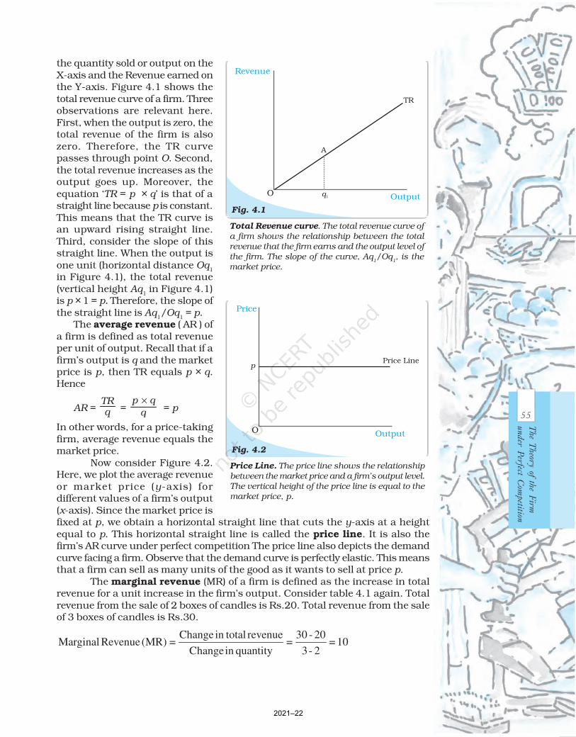
Now consider Figure 4.2.Here, we plot the average revenueor market price (y-axis) fordifferent values of a firm’s output(x-axis). Since the market price isfixed at p, we obtain a horizontal straight line that cuts the y-axis at a heightequal to p. This horizontal straight line is called the price line. It is also thefirm’s AR curve under perfect competition The price line also depicts the demandcurve facing a firm. Observe that the demand curve is perfectly elastic. This meansthat a firm can sell as many units of the good as it wants to sell at price p.

The marginal revenue (MR) of a firm is defined as the increase in totalrevenue for a unit increase in the firm’s output. Consider table 4.1 again. Totalrevenue from the sale of 2 boxes of candles is Rs.20. Total revenue from the saleof 3 boxes of candles is Rs.30.

Change in total revenue 30 - 20Marginal Revenue(MR) = = = 10

Changein quantity 3- 2

Price Line. The price line shows the relationship

between the market price and a firm’s output level.

The vertical height of the price line is equal to the

market price, p.

Fig. 4.2

Price

Price Line

O Output

p

Total Revenue curve. The total revenue curve of

a firm shows the relationship between the total

revenue that the firm earns and the output level of

the firm. The slope of the curve, Aq1/Oq

1, is the

market price.

Fig. 4.1

Revenue

TR

O Output

A

q1

2021–22

56

Introd

uct

ory

Micro

econ

omics

Is it a coincidence that this is the same as the price? Actually it is not. Considerthe situation when the firm’s output changes from q

1 to q

2. Given the market

price p,MR = (pq

2 –pq

1)/ (q

2 –q

1)

= [p (q2 –q

1)]/ (q

2 –q

1)

= pThus, for the perfectly competitive firm, MR=AR=p

In other words, for a price-taking firm, marginal revenue equals the marketprice.

Setting the algebra aside, the intuition for this result is quite simple. When afirm increases its output by one unit, this extra unit is sold at the market price.Hence, the firm’s increase in total revenue from the one-unit output expansion –that is, MR – is precisely the market price.

4.3 PROFIT MAXIMISATION

A firm produces and sells a certain amount of a good. The firm’s profit, denotedby π 1, is defined to be the difference between its total revenue (TR) and its total

cost of production (TC ). In other words

π= TR – TC

Clearly, the gap between TR and TC is the firm’s earnings net of costs.A firm wishes to maximise its profit. The firm would like to identify the quantity

q0 at which its profits are maximum. By definition, then, at any quantity other

than q0, the firm’s profits are less than at q

0. The critical question is: how do we

identify q0?

For profits to be maximum, three conditions must hold at q0:

1. The price, p, must equal MC2. Marginal cost must be non-decreasing at q

0

3. For the firm to continue to produce, in the short run, price must be greaterthan the average variable cost (p > AVC); in the long run, price must be greaterthan the average cost (p > AC).

4.3.1 Condition 1

Profits are the difference between total revenue and total cost. Both total revenueand total cost increase as output increases. Notice that as long as the change intotal revenue is greater than the change in total cost, profits will continue toincrease. Recall that change in total revenue per unit increase in output is themarginal revenue; and the change in total cost per unit increase in output is themarginal cost. Therefore, we can conclude that as long as marginal revenue isgreater than marginal cost, profits are increasing. By the same logic, as long asmarginal revenue is less than marginal cost, profits will fall. It follows that forprofits to be maximum, marginal revenue should equal marginal cost.

In other words, profits are maximum at the level of output (which we havecalled q

0) for which MR = MC

For the perfectly competitive firm, we have established that the MR = P. So thefirm’s profit maximizing output becomes the level of output at which P=MC.

4.3.2 Condition 2

Consider the second condition that must hold when the profit-maximising outputlevel is positive. Why is it the case that the marginal cost curve cannot slope

1It is a convention in economics to denote profit with the Greek letter π .

2021–22

57

The T

heory of th

e Firm

under P

erfect Com

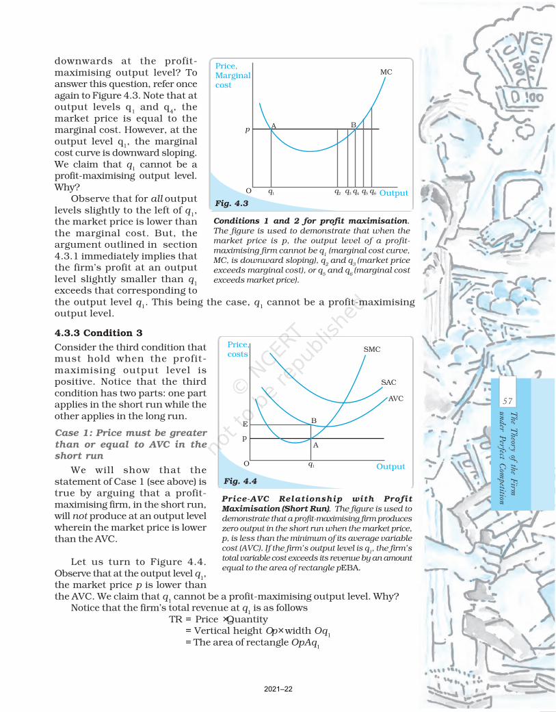
petitiondownwards at the profit-maximising output level? Toanswer this question, refer onceagain to Figure 4.3. Note that atoutput levels q

1 and q

4, the

market price is equal to themarginal cost. However, at theoutput level q

1, the marginal

cost curve is downward sloping.We claim that q

1 cannot be a

profit-maximising output level.Why?

Observe that for all outputlevels slightly to the left of q

1,

the market price is lower thanthe marginal cost. But, theargument outlined in section4.3.1 immediately implies thatthe firm’s profit at an outputlevel slightly smaller than q

1

exceeds that corresponding tothe output level q

1. This being the case, q

1 cannot be a profit-maximising

output level.

4.3.3 Condition 3

Consider the third condition thatmust hold when the profit-maximising output level ispositive. Notice that the thirdcondition has two parts: one partapplies in the short run while theother applies in the long run.

Case 1: Price must be greaterthan or equal to AVC in theshort run

We will show that thestatement of Case 1 (see above) istrue by arguing that a profit-maximising firm, in the short run,will not produce at an output levelwherein the market price is lowerthan the AVC.

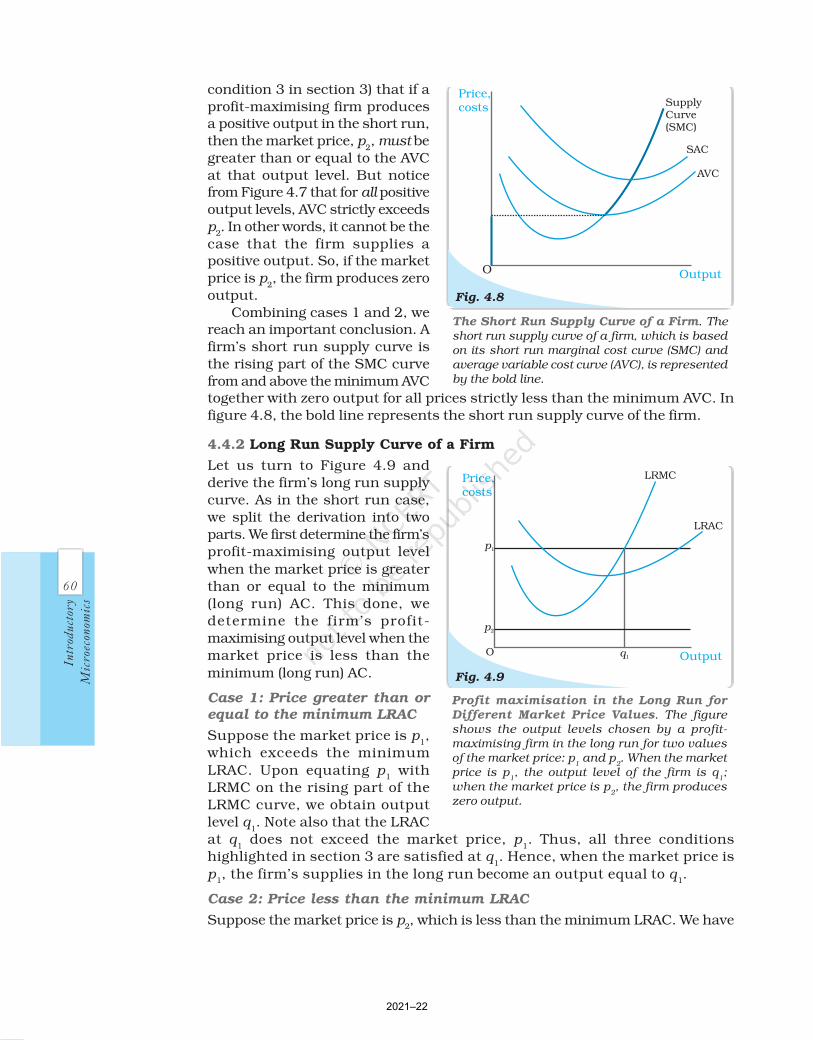
Let us turn to Figure 4.4.Observe that at the output level q

1,

the market price p is lower thanthe AVC. We claim that q

1 cannot be a profit-maximising output level. Why?

Notice that the firm’s total revenue at q1 is as follows

TR = Price × Quantity= Vertical height Op × width Oq

1

= The area of rectangle OpAq1

Price-AVC Relationship with ProfitMaximisation (Short Run). The figure is used to

demonstrate that a profit-maximising firm produces

zero output in the short run when the market price,

p, is less than the minimum of its average variable

cost (AVC). If the firm’s output level is q1, the firm’s

total variable cost exceeds its revenue by an amount

equal to the area of rectangle pEBA.

Fig. 4.4

Price,costs

O Outputq1

A

E

SMC

B

p

SAC

AVC

Conditions 1 and 2 for profit maximisation.

The figure is used to demonstrate that when the

market price is p, the output level of a profit-

maximising firm cannot be q1 (marginal cost curve,

MC, is downward sloping), q2 and q

3 (market price

exceeds marginal cost), or q5 and q

6 (marginal cost

exceeds market price).

2021–22

58

Introd

uct

ory

Micro

econ

omics

Similarly, the firm’s total variable cost at q1 is as follows

TVC = Average variable cost × Quantity= Vertical height OE × Width Oq

1

= The area of rectangle OEBq1

Now recall that the firm’s profit at q1 is TR – (TVC + TFC); that is, [the area of

rectangle OpAq1] – [the area of rectangle OEBq

1] – TFC. What happens if the firm

produces zero output? Since output is zero, TR and TVC are zero as well. Hence,the firm’s profit at zero output is equal to – TFC. But, the area of rectangle OpAq

1

is strictly less than the area of rectangle OEBq1. Hence, the firm’s profit at q

1 is

[(area EBAp)-TFC], which is strictly less than what it obtains by not producing atall. So, the firm will choose not toproduce at all, and exit from themarket.

Case 2: Price must be greaterthan or equal to AC in thelong run

We will show that the statement ofCase 2 (see above) is true byarguing that a profit-maximisingfirm, in the long run, will not

produce at an output levelwherein the market price is lowerthan the AC.

Let us turn to Figure 4.5.Observe that at the output level q

1,

the market price p is lower thanthe (long run) AC. We claim thatq

1 cannot be a profit-maximising

output level. Why?Notice that the firm’s total

revenue, TR, at q1 is the area of the

rectangle OpAq1 (the product of

price and quantity) while the firm’stotal cost, TC , is the area of therectangle OEBq

1 (the product of

average cost and quantity). Sincethe area of rectangle OEBq

1 is

larger than the area of rectangleOpAq

1, the firm incurs a loss at the

output level q1. But, in the long

run set-up, a firm that shuts downproduction has a profit of zero.Again, the firm chooses to exit inthis case.

4.3.4 The Profit MaximisationProblem: GraphicalRepresentation

Using the material in sections 3.1,3.2 and 3.3, let us graphicallyrepresent a firm’s profit

Price-AC Relationship with ProfitMaximisation (Long Run). The figure is used to

demonstrate that a profit-maximising firm

produces zero output in the long run when the

market price, p, is less than the minimum of its

long run average cost (LRAC). If the firm’s output

level is q1, the firm’s total cost exceeds its revenue

by an amount equal to the area of rectangle pEBA.

Fig. 4.5

Price,costs

O Outputq1

A

E

LRMC

B

p

LRAC

Geometric Representation of ProfitMaximisation (Short Run). Given market

price p, the output level of a profit-maximising

firm is q0. At q

0, the firm’s profit is equal to the

area of rectangle EpAB.

2021–22

59

The T

heory of th

e Firm

under P

erfect Com

petitionmaximisation problem in the short run. Consider Figure 4.6. Notice that themarket price is p. Equating the market price with the (short run) marginalcost, we obtain the output level q

0. At q

0, observe that SMC slopes upwards

and p exceeds AVC. Since the three conditions discussed in sections 3.1-3.3are satisfied at q

0, we maintain that the profit-maximising output level of the

firm is q0.

What happens at q0? The total revenue of the firm at q

0 is the area of

rectangle OpAq0 (the product of price and quantity) while the total cost at q

0 is

the area of rectangle OEBq0 (the product of short run average cost and quantity).

So, at q0, the firm earns a profit equal to the area of the rectangle EpAB.

4.4 SUPPLY CURVE OF A FIRM

A firm’s ‘supply’ is the quantity that it chooses to sell at a given price, giventechnology, and given the prices of factors of production. A table describing thequantities sold by a firm at various prices, technology and prices of factorsremaining unchanged, is called a supply schedule. We may also represent theinformation as a graph, called a supply curve. The supply curve of a firm showsthe levels of output (plotted on the x-axis) that the firm chooses to producecorresponding to different values of the market price (plotted on the y-axis),again keeping technology and prices of factors of production unchanged. Wedistinguish between the short run supply curve and the long run supplycurve.

4.4.1 Short Run Supply Curve of a Firm

Let us turn to Figure 4.7 and derive a firm’s short run supply curve. We shallsplit this derivation into two parts. We first determine a firm’s profit-maximisingoutput level when the market price is greater than or equal to the minimumAVC. This done, we determine the firm’s profit-maximising output level whenthe market price is less than the minimum AVC.

Case 1: Price is greater thanor equal to the minimum AVC

Suppose the market price is p1,

which exceeds the minimum AVC.We start out by equating p

1 with

SMC on the rising part of the SMCcurve; this leads to the output levelq

1. Note also that the AVC at q

1

does not exceed the market price,p

1. Thus, all three conditions

highlighted in section 3 aresatisfied at q

1. Hence, when the

market price is p1, the firm’s

output level in the short run isequal to q

1.

Case 2: Price is less than theminimum AVC

Suppose the market price is p2,

which is less than the minimum

AVC. We have argued (see

Market Price Values. The figure shows the

output levels chosen by a profit-maximising firm

in the short run for two values of the market price:

p1 and p

2. When the market price is p

1, the output

level of the firm is q1; when the market price is

p2, the firm produces zero output.

Fig. 4.7

Price,costs

O Outputq1

p1

SMC

SAC

AVC

p2

2021–22

60

Intr

odu

ctor

y

Mic

roec

onom

ics

condition 3 in section 3) that if a

profit-maximising firm producesa positive output in the short run,

then the market price, p2, must be

greater than or equal to the AVC

at that output level. But noticefrom Figure 4.7 that for all positive

output levels, AVC strictly exceeds

p2. In other words, it cannot be the

case that the firm supplies apositive output. So, if the market

price is p2, the firm produces zero

output.

Combining cases 1 and 2, wereach an important conclusion. A

firm’s short run supply curve is

the rising part of the SMC curve

from and above the minimum AVCtogether with zero output for all prices strictly less than the minimum AVC. In

figure 4.8, the bold line represents the short run supply curve of the firm.

4.4.2 Long Run Supply Curve of a Firm

Let us turn to Figure 4.9 and

derive the firm’s long run supply

curve. As in the short run case,

we split the derivation into two

parts. We first determine the firm’s

profit-maximising output level

when the market price is greater

than or equal to the minimum

(long run) AC. This done, we

determine the firm’s profit-

maximising output level when the

market price is less than the

minimum (long run) AC.

Case 1: Price greater than orequal to the minimum LRAC

Suppose the market price is p1,

which exceeds the minimum

LRAC. Upon equating p1 with

LRMC on the rising part of the

LRMC curve, we obtain output

level q1. Note also that the LRAC

at q1 does not exceed the market price, p

1. Thus, all three conditions

highlighted in section 3 are satisfied at q1. Hence, when the market price is

p1, the firm’s supplies in the long run become an output equal to q

1.

Case 2: Price less than the minimum LRAC

Suppose the market price is p2, which is less than the minimum LRAC. We have

The Short Run Supply Curve of a Firm. The

short run supply curve of a firm, which is based

on its short run marginal cost curve (SMC) and

average variable cost curve (AVC), is represented

by the bold line.

Fig. 4.8

Price,costs

O Output

SupplyCurve(SMC)

SAC

AVC

Profit maximisation in the Long Run forDifferent Market Price Values. The figure

shows the output levels chosen by a profit-

maximising firm in the long run for two values

of the market price: p1 and p

2. When the market

price is p1, the output level of the firm is q

1;

when the market price is p2, the firm produces

zero output.

Fig. 4.9

Price,costs

O Outputq1

p1

LRMC

LRAC

p2

2021–22

61

The T

heory of th

e Firm

under P

erfect Com

petitionargued (see condition 3 in section

3) that if a profit-maximising firm

produces a positive output in the

long run, the market price, p2,

must be greater than or equal to

the LRAC at that output level. But

notice from Figure 4.9 that for all

positive output levels, LRAC

strictly exceeds p2. In other words,

it cannot be the case that the firm

supplies a positive output. So,

when the market price is p2, the

firm produces zero output.Combining cases 1 and 2, wereach an important conclusion. Afirm’s long run supply curve is therising part of the LRMC curve fromand above the minimum LRACtogether with zero output for allprices less than the minimum LRAC. In Figure 4.10, the bold line represents thelong run supply curve of the firm.

4.4.3 The Shut Down Point

Previously, while deriving the supply curve, we have discussed that in the shortrun the firm continues to produce as long as the price remains greater than orequal to the minimum of AVC. Therefore, along the supply curve as we movedown, the last price-output combination at which the firm produces positiveoutput is the point of minimum AVC where the SMC curve cuts the AVC curve.Below this, there will be no production. This point is called the short run shutdown point of the firm. In the long run, however, the shut down point is theminimum of LRAC curve.

4.4.4 The Normal Profit and Break-even Point

The minimum level of profit that is needed to keep a firm in the existing businessis defined as normal profit. A firm that does not make normal profits is notgoing to continue in business. Normal profits are therefore a part of the firm’stotal costs. It may be useful to think of them as an opportunity cost forentrepreneurship. Profit that a firm earns over and above the normal profit iscalled the super-normal profit. In the long run, a firm does not produce if itearns anything less than the normal profit. In the short run, however, it mayproduce even if the profit is less than this level. The point on the supply curve atwhich a firm earns only normal profit is called the break-even point of the firm.The point of minimum average cost at which the supply curve cuts the LRACcurve (in short run, SAC curve) is therefore the break-even point of a firm.

The Long Run Supply Curve of a Firm. The

long run supply curve of a firm, which is based on

its long run marginal cost curve (LRMC) and long

run average cost curve (LRAC), is represented by

the bold line.

Fig. 4.10

Price,costs

O Output

Supply Curve(LRMC)

LRAC

Opportunity cost

In economics, one often encounters the concept of opportunity cost.Opportunity cost of some activity is the gain foregone from the second bestactivity. Suppose you have Rs 1,000 which you decide to invest in your familybusiness. What is the opportunity cost of your action? If you do not invest

2021–22

62

Intr

odu

ctor

y

Mic

roec

onom

ics

4.5 DETERMINANTS OF A FIRM’S SUPPLY CURVE

In the previous section, we have seen that a firm’s supply curve is a part of itsmarginal cost curve. Thus, any factor that affects a firm’s marginal cost curve isof course a determinant of its supply curve. In this section, we discuss twosuch factors.

4.5.1 Technological Progress

Suppose a firm uses two factors of production – say, capital and labour – toproduce a certain good. Subsequent to an organisational innovation by the firm,the same levels of capital and labour now produce more units of output. Putdifferently, to produce a given level of output, the organisational innovation allowsthe firm to use fewer units of inputs. It is expected that this will lower the firm’smarginal cost at any level of output; that is, there is a rightward (or downward)shift of the MC curve. As the firm’s supply curve is essentially a segment of theMC curve, technological progress shifts the supply curve of the firm to the right.At any given market price, the firm now supplies more units of output.

4.5.2 Input Prices

A change in input prices also affects a firm’s supply curve. If the price of aninput (say, the wage rate of labour) increases, the cost of production rises. Theconsequent increase in the firm’s average cost at any level of output is usuallyaccompanied by an increase in the firm’s marginal cost at any level of output;that is, there is a leftward (or upward) shift of the MC curve. This means that thefirm’s supply curve shifts to the left: at any given market price, the firm nowsupplies fewer units of output.

this money, you can either keep it in the house-safe which will give you zeroreturn or you can deposit it in either bank-1 or bank-2 in which case you getan interest at the rate of 10 per cent or 5 per cent respectively. So the maximumbenefit that you may get from other alternative activities is the interest fromthe bank-1. But this opportunity will no longer be there once you invest themoney in your family business. The opportunity cost of investing the moneyin your family business is therefore the amount of forgone interest from thebank-1.

Impact of a unit tax on supply

A unit tax is a tax that the government imposes per unit sale of output. Forexample, suppose that the unit tax imposed by the government is Rs 2.Then, if the firm produces and sells 10 units of the good, the total tax thatthe firm must pay to the government is 10 × Rs 2 = Rs 20.

How does the long run supply curve of a firm change when a unit tax isimposed? Let us turn to figure 4.11. Before the unit tax is imposed, LRMC0

and LRAC0 are, respectively, the long run marginal cost curve and the longrun average cost curve of the firm. Now, suppose the government puts inplace a unit tax of Rs t. Since the firm must pay an extra Rs t for each unitof the good produced, the firm’s long run average cost and long run marginalcost at any level of output increases by Rs t. In Figure 4.11, LRMC1 andLRAC1 are, respectively, the long run marginal cost curve and the long runaverage cost curve of the firm upon imposition of the unit tax.

2021–22

63

The T

heory of th

e Firm

under P

erfect Com

petition

4.6 MARKET SUPPLY CURVE

The market supply curve shows the output levels (plotted on the x-axis) thatfirms in the market produce in aggregate corresponding to different values ofthe market price (plotted on the y-axis).

How is the market supply curve derived? Consider a market with n firms:firm 1, firm 2, firm 3, and so on. Suppose the market price is fixed at p. Then,the output produced by the n firms in aggregate is [supply of firm 1 at price p]+ [supply of firm 2 at price p] + ... + [supply of firm n at price p]. In other words,the market supply at price p is the summation of the supplies of individualfirms at that price.

Let us now construct the market supply curve geometrically with just twofirms in the market: firm 1 and firm 2. The two firms have different cost structures.

Firm 1 will not produce anything if the market price is less than 1p while firm 2

will not produce anything if the market price is less than 2p . Assume also that

2p is greater than 1p .

In panel (a) of Figure 4.13 we have the supply curve of firm 1, denoted byS

1; in panel (b), we have the supply curve of firm 2, denoted by S

2. Panel (c) of

Figure 4.13 shows the market supply curve, denoted by Sm. When the market

price is strictly below 1p , both firms choose not to produce any amount of the

good; hence, market supply will also be zero for all such prices. For a market

Recall that the long run supply curve of a firm is the rising part of theLRMC curve from and above the minimum LRAC together with zero outputfor all prices less than the minimum LRAC. Using this observation in Figure4.12, it is immediate that S0 and S1 are, respectively, the long run supplycurve of the firm before and after the imposition of the unit tax. Notice thatthe unit tax shifts the firm’s long run supply curve to the left: at any givenmarket price, the firm now supplies fewer units of output.

Cost Curves and the Unit Tax. LRAC0

and LRMC0 are, respectively, the long run

average cost curve and the long run

marginal cost curve of a firm before a unit

tax is imposed. LRAC1 and LRMC1 are,

respectively, the long run average cost

curve and the long run marginal cost curve

of a firm after a unit tax of Rs t is imposed.

Fig. 4.11

Costs

O Output

p0

LRMC1

LRAC0

LRMC0

LRAC1

p t0+

q0

t

Supply Curves and Unit Tax. S0 is the

supply curve of a firm before a unit tax

is imposed. After a unit tax of Rs t isimposed, S1 represents the supply curve

of the firm.

Fig. 4.12

Price

Output

S1

S0

O

p0

p t0+

q0

2021–22

64

Intr

odu

ctor

y

Mic

roec

onom

ics

price greater than or equal to 1p but strictly less than 2p , only firm 1 will produce

a positive amount of the good. Therefore, in this range, the market supply curvecoincides with the supply curve of firm 1. For a market price greater than or

equal to 2p , both firms will have positive output levels. For example, consider a

situation wherein the market price assumes the value p3 (observe that p

3

exceeds 2p ). Given p3, firm 1 supplies q

3 units of output while firm 2 supplies q

4

units of output. So, the market supply at price p3 is q

5, where q

5 = q

3 + q

4. Notice

how the market supply curve, Sm, in panel (c) is being constructed: we obtain S

m

by taking a horizontal summation of the supply curves of the two firms in themarket, S

1 and S

2.

The Market Supply Curve Panel. (a) shows the supply curve of firm 1. Panel (b) shows the

supply curve of firm 2. Panel (c) shows the market supply curve, which is obtained by taking

a horizontal summation of the supply curves of the two firms.

Fig. 4.13

Price

O Output

p1

O O

S1

q3q4 q5

S2

Sm

p2

p3

(a) (b) (c)

It should be noted that the market supply curve has been derived for a fixednumber of firms in the market. As the number of firms changes, the marketsupply curve shifts as well. Specifically, if the number of firms in the marketincreases (decreases), the market supply curve shifts to the right (left).

We now supplement the graphical analysis given above with a relatednumerical example. Consider a market with two firms: firm 1 and firm 2. Let thesupply curve of firm 1 be as follows

S1(p) =

0 : 10

– 10 : 10

p

p p

<

≥

Notice that S1(p) indicates that (1) firm 1 produces an output of 0 if the market

price, p, is strictly less than 10, and (2) firm 1 produces an output of (p – 10) ifthe market price, p, is greater than or equal to 10. Let the supply curve of firm 2be as follows

S2(p) =

0 : 15

– 15 : 15

p

p p

<

≥

The interpretation of S2(p) is identical to that of S

1(p), and is, hence, omitted.

Now, the market supply curve, Sm(p), simply sums up the supply curves of the

two firms; in other words

Sm(p) = S

1(p) + S

2(p)

2021–22

65

Th

e Th

eory of the F

irm

un

der P

erfect Com

petition

But, this means that Sm(p) is as follows

Sm(p) =

0 : 10

– 10 : 10 15

( – 10) ( – 15) 2 – 25 : 15

p

p p and p

p p p p

<

≥ < + = ≥

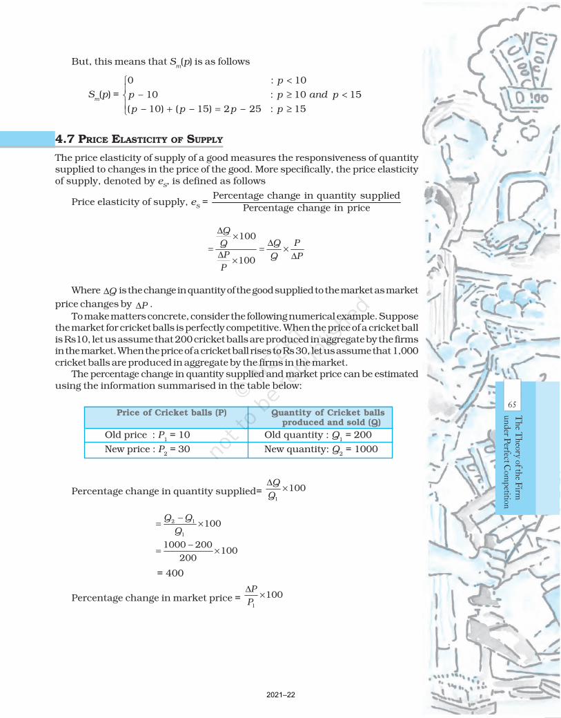
4.7 PRICE ELASTICITY OF SUPPLY

The price elasticity of supply of a good measures the responsiveness of quantitysupplied to changes in the price of the good. More specifically, the price elasticityof supply, denoted by e

S, is defined as follows

Price elasticity of supply, eS =

Percentage change in quantity supplied

Percentage change in price

100

100

Q

Q PQ

P Q P

P

∆×

∆= = ×

∆ ∆×

Where Q∆ is the change in quantity of the good supplied to the market as market

price changes by P∆ .

To make matters concrete, consider the following numerical example. Supposethe market for cricket balls is perfectly competitive. When the price of a cricket ballis Rs10, let us assume that 200 cricket balls are produced in aggregate by the firmsin the market. When the price of a cricket ball rises to Rs 30, let us assume that 1,000cricket balls are produced in aggregate by the firms in the market.

The percentage change in quantity supplied and market price can be estimatedusing the information summarised in the table below:

Percentage change in quantity supplied= 1

100Q

Q

∆×

2 1

1

100

1000 200100

200

Q Q

Q

−= ×

−= ×

= 400

Percentage change in market price = 1

100P

P

∆×

Price of Cricket balls (P) Quantity of Cricket balls produced and sold (Q)

Old price : P1 = 10 Old quantity : Q

1 = 200

New price : P2 = 30 New quantity: Q

2 = 1000

2021–22

66

Intr

odu

ctor

y

Mic

roec

onom

ics

2 1

1

100

30 10100

10

P P

P

−= ×

−= ×

= 200

Therefore, price elasticity of supply, eS

4002

200= =

When the supply curve is vertical, supply is completely insensitive to priceand the elasticity of supply is zero. In other cases, when supply curve ispositively sloped, with a rise in price, supply rises and hence, the elasticity ofsupply is positive. Like the price elasticity of demand, the price elasticity ofsupply is also independent of units.

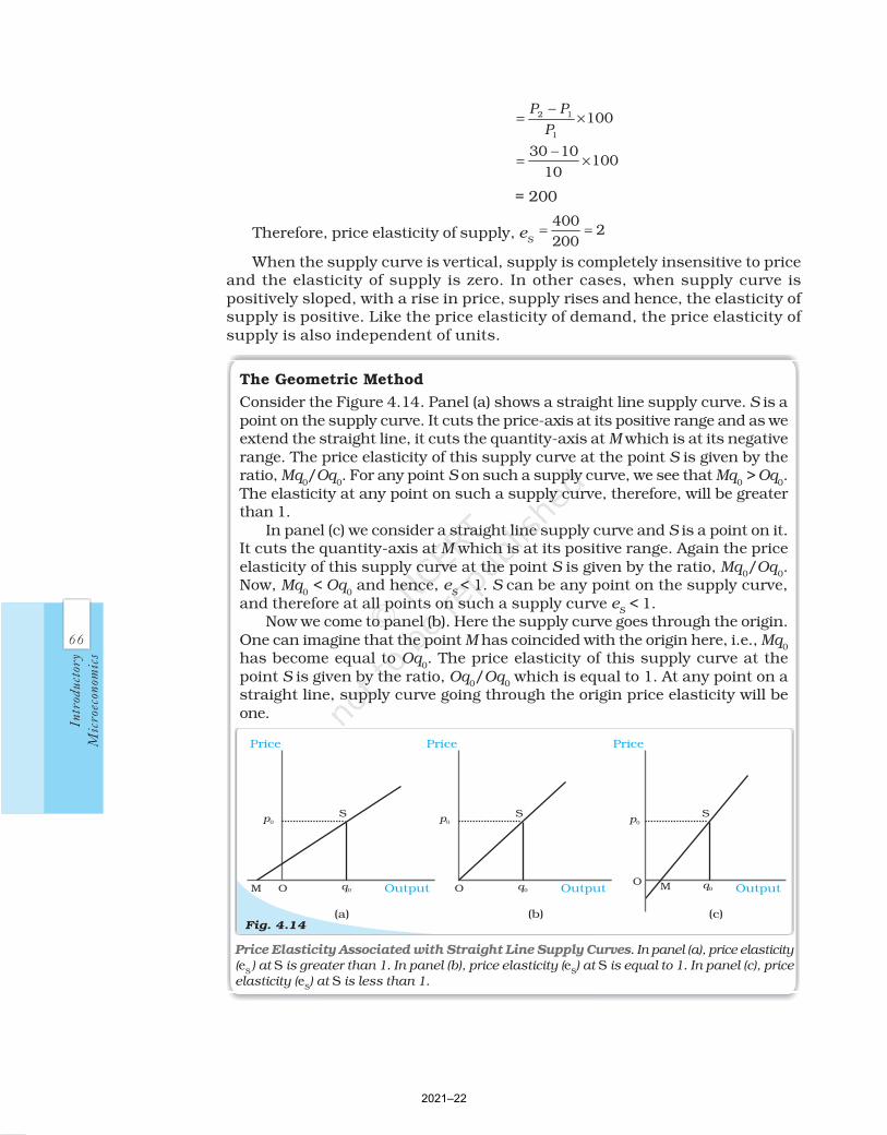
The Geometric Method

Consider the Figure 4.14. Panel (a) shows a straight line supply curve. S is apoint on the supply curve. It cuts the price-axis at its positive range and as weextend the straight line, it cuts the quantity-axis at M which is at its negativerange. The price elasticity of this supply curve at the point S is given by theratio, Mq

0/Oq

0. For any point S on such a supply curve, we see that Mq

0 > Oq

0.

The elasticity at any point on such a supply curve, therefore, will be greaterthan 1.

In panel (c) we consider a straight line supply curve and S is a point on it.It cuts the quantity-axis at M which is at its positive range. Again the priceelasticity of this supply curve at the point S is given by the ratio, Mq

0/Oq

0.

Now, Mq0 < Oq

0 and hence, e

S < 1. S can be any point on the supply curve,

and therefore at all points on such a supply curve eS < 1.

Now we come to panel (b). Here the supply curve goes through the origin.One can imagine that the point M has coincided with the origin here, i.e., Mq

0

has become equal to Oq0. The price elasticity of this supply curve at the

point S is given by the ratio, Oq0/Oq

0 which is equal to 1. At any point on a

straight line, supply curve going through the origin price elasticity will beone.

Fig. 4.14(a) (b) (c)

Price Price Price

Output Output Output

p0 p0 p0

q0 q0q0

S S S

M O OO M

Price Elasticity Associated with Straight Line Supply Curves. In panel (a), price elasticity

(eS) at S is greater than 1. In panel (b), price elasticity (e

S) at S is equal to 1. In panel (c), price

elasticity (eS) at S is less than 1.

2021–22

67

The T

heory of th

e Firm

under P

erfect Com

petition• In a perfectly competitive market, firms are price-takers.

• The total revenue of a firm is the market price of the good multiplied by the firm’soutput of the good.

• For a price-taking firm, average revenue is equal to market price.

• For a price-taking firm, marginal revenue is equal to market price.

• The demand curve that a firm faces in a perfectly competitive market is perfectlyelastic; it is a horizontal straight line at the market price.

• The profit of a firm is the difference between total revenue earned and total costincurred.

• If there is a positive level of output at which a firm’s profit is maximised in theshort run, three conditions must hold at that output level

(i) p = SMC

(ii) SMC is non-decreasing

(iii) p ≥ AV C.

• If there is a positive level of output at which a firm’s profit is maximised in thelong run, three conditions must hold at that output level

(i) p = LRMC

(ii) LRMC is non-decreasing

(iii) p ≥ LRAC.

• The short run supply curve of a firm is the rising part of the SMC curve from andabove minimum AVC together with 0 output for all prices less than the minimumAVC.

• The long run supply curve of a firm is the rising part of the LRMC curve from andabove minimum LRAC together with 0 output for all prices less than the minimumLRAC.

• Technological progress is expected to shift the supply curve of a firm to the right.

• An increase (decrease) in input prices is expected to shift the supply curve of afirm to the left (right).

• The imposition of a unit tax shifts the supply curve of a firm to the left.

• The market supply curve is obtained by the horizontal summation of the supplycurves of individual firms.

• The price elasticity of supply of a good is the percentage change in quantitysupplied due to one per cent change in the market price of the good.

Su

mm

ar

yS

um

ma

ry

Su

mm

ar

yS

um

ma

ry

Su

mm

ar

yE

xer

cise

sE

xer

cise

sE

xer

cise

sE

xer

cise

sE

xer

cise

s 1. What are the characteristics of a perfectly competitive market?

2. How are the total revenue of a firm, market price, and the quantity sold by thefirm related to each other?

3. What is the ‘price line’?

4. Why is the total revenue curve of a price-taking firm an upward-sloping straightline? Why does the curve pass through the origin?

KKKK Key

C

once

pts

ey

Con

cepts

ey

Con

cepts

ey

Con

cepts

ey

Con

cepts Perfect competition Revenue, Profit

Profit maximisation Firms supply curve

Market supply curve Price elasticity of supply

?

?

2021–22

68

Intr

odu

ctor

y

Mic

roec

onom

ics

5. What is the relation between market price and average revenue of a price-taking firm?

6. What is the relation between market price and marginal revenue of a price-taking firm?

7. What conditions must hold if a profit-maximising firm produces positive outputin a competitive market?

8. Can there be a positive level of output that a profit-maximising firm producesin a competitive market at which market price is not equal to marginal cost?Give an explanation.

9. Will a profit-maximising firm in a competitive market ever produce a positivelevel of output in the range where the marginal cost is falling? Give anexplanation.

10. Will a profit-maximising firm in a competitive market produce a positive level ofoutput in the short run if the market price is less than the minimum of AVC?Give an explanation.

11. Will a profit-maximising firm in a competitive market produce a positive level ofoutput in the long run if the market price is less than the minimum of AC?Give an explanation.

12. What is the supply curve of a firm in the short run?

13. What is the supply curve of a firm in the long run?

14. How does technological progress affect the supply curve of a firm?

15. How does the imposition of a unit tax affect the supply curve of a firm?

16. How does an increase in the price of an input affect the supply curve of a firm?

17. How does an increase in the number of firms in a market affect the marketsupply curve?

18. What does the price elasticity of supply mean? How do we measure it?

19. Compute the total revenue, marginalrevenue and average revenue schedulesin the following table. Market price of eachunit of the good is Rs 10.

20. The following table shows thetotal revenue and total costschedules of a competitivefirm. Calculate the profit ateach output level. Determinealso the market price of thegood.

Quantity Sold TR (Rs) TC (Rs) Profit

0 0 5

1 5 7

2 10 10

3 15 12

4 20 15

5 25 23

6 30 33

7 35 40

Quantity Sold TR MR AR

0

1

2

3

4

5

6

2021–22

69

The T

heory of th

e Firm

under P

erfect Com

petition21. The following table shows the total cost schedule

of a competitive firm. It is given that the priceof the good is Rs 10. Calculate the profit at eachoutput level. Find the profit maximising level ofoutput.

22. Consider a market with twofirms. The following tableshows the supply schedulesof the two firms: the SS

1

column gives the supplyschedule of firm 1 and theSS

2 column gives the supply

schedule of firm 2. Computethe market supply schedule.

23. Consider a market with twofirms. In the following table,columns labelled as SS

1

and SS2 give the supply

schedules of firm 1 and firm2 respectively. Compute themarket supply schedule.

24. There are three identical firms in a market. Thefollowing table shows the supply schedule of firm1. Compute the market supply schedule.

Price (Rs) SS1 (units) SS

2 (units)

0 0 0

1 0 0

2 0 0

3 1 1

4 2 2

5 3 3

6 4 4

Price (Rs) SS1 (kg) SS

2 (kg)

0 0 0

1 0 0

2 0 0

3 1 0

4 2 0.5

5 3 1

6 4 1.5

7 5 2

8 6 2.5

Price (Rs) SS1 (units)

0 0

1 0

2 2

3 4

4 6

5 8

6 10

7 12

8 14

Output TC (Rs)

0 5

1 15

2 22

3 27

4 31

5 38

6 49

7 63

8 81

9 101

10 123

2021–22

70

Intr

odu

ctor

y

Mic

roec

onom

ics

25. A firm earns a revenue of Rs 50 when the market price of a good is Rs 10. Themarket price increases to Rs 15 and the firm now earns a revenue of Rs 150.What is the price elasticity of the firm’s supply curve?

26. The market price of a good changes from Rs 5 to Rs 20. As a result, the quantitysupplied by a firm increases by 15 units. The price elasticity of the firm’s supplycurve is 0.5. Find the initial and final output levels of the firm.

27. At the market price of Rs 10, a firm supplies 4 units of output. The market priceincreases to Rs 30. The price elasticity of the firm’s supply is 1.25. What quantitywill the firm supply at the new price??

?

2021–22