Changing institutions in the European market: the impact on mark-ups and rents allocation

Temi di Discussione(Working Papers)

Changing institutions in the European market: the impact on mark-ups and rents allocation

by Antonio Bassanetti, Roberto Torrini and Francesco Zollino

Num

ber 781D

ecem

ber

201

0

Temi di discussione(Working papers)

Changing institutions in the European market: the impact on mark-ups and rents allocation

by Antonio Bassanetti, Roberto Torrini and Francesco Zollino

Number 781 - December 2010

The purpose of the Temi di discussione series is to promote the circulation of workingpapers prepared within the Bank of Italy or presented in Bank seminars by outside economists with the aim of stimulating comments and suggestions.

The views expressed in the articles are those of the authors and do not involve the responsibility of the Bank.

Editorial Board: MARCELLO PERICOLI, SILVIA MAGRI, LUISA CARPINELLI, EMANUELA CIAPANNA, DANIELA MARCONI, ANDREA NERI, MARZIA ROMANELLI, CONCETTA RONDINELLI,TIZIANO ROPELE, ANDREA SILVESTRINI.

Editorial Assistants: ROBERTO MARANO, NICOLETTA OLIVANTI.

CHANGING INSTITUTIONS IN THE EUROPEAN MARKET: THE IMPACT ON MARK-UPS AND RENTS ALLOCATION

by Antonio Bassanetti,* Roberto Torrini** and Francesco Zollino*

Abstract

We investigate whether the completion of the Single Market Programme has enhanced competition on the product markets across European countries, taking into account the companion structural reforms undertaken by the member countries, particularly in the labour market and the institutional setting of important industries (i.e. network industries). We test for a break in both mark-ups and the division of rent between capital and labour based on a statistical model incorporating efficient bargaining in the labour market. Using industry data for ten EU countries we find that, without controlling for changes in the rent sharing, mark-up estimates tend to increase in the 1990s. However, once we assume efficient bargaining in the labour market, mark-ups remain virtually unchanged or, in some sectors or groups of countries, even decrease; this reflects the declining shares of rents accruing to workers as a result of their diminished bargaining power. The evidence is particularly strong for high and medium-tech manufacturing, for construction and for those activities that went through deep institutional changes and privatization programmes.

JEL Classification: D40, J50, L50. Keywords: institutional changes, mark-up, rent-sharing .

Contents 1. Introduction.......................................................................................................................... 5 2. The model and the links to the literature ............................................................................. 6 3. The data ............................................................................................................................. 12 4. Estimates for changing structural parameters.................................................................... 14

4.1 Results at the aggregate level ..................................................................................... 16 4.2 Results at the industry level........................................................................................ 20

5. Conclusions........................................................................................................................ 23 References .............................................................................................................................. 25 Appendix I .............................................................................................................................. 27 Appendix II............................................................................................................................. 31 Appendix III ........................................................................................................................... 33

_______________________________________

* Bank of Italy, Economic Outlook and Monetary Policy Department.

** Bank of Italy, Structural Economic Analysis Department.

1 Introduction1

Since the early nineties, economies in the European Union (EU) have gone through deep structural

changes driven by widespread institutional reforms and the evolution of the international context.

The implementation of the Single Market Programme and several EU directives on network in-

dustries and other highly regulated activities reshaped goods and service markets in an e¤ort to

enhance competition while reforms at the country level greatly increased labour market �exibility.

At the same time, the surge of new competitors at global level added to the competitive pressures

on European �rms and necessitated an intense reorganization of their production processes.

A large body of research has investigated the actual impact of these trends across EU countries.

In particular, following the approaches to mark-up estimation put forward by Hall (1988) and Roger

(1995), recent contributions have focused on detecting the pro-competitive impact of the Single

Market Programme. However, most studies are limited to the manufacturing sector and do not

come up with clear-cut evidence of declining market power (Oliveira Martins et al., 1996; Allen

et al., 1998; Bottasso and Sembenelli, 2001; Sauner-Leroy, 2003; Gri¢ th et al., 2010). Badinger

(2007) even �nds an unexpected increase in mark-ups in most service activities.

Unfortunately, this literature disregards the contemporaneous labour market reforms, which

enhanced �exibility and job-creation in the EU and are deemed to account for a large share of

the employment increase since the mid-1990s (European Commission, 2004; Bassanini and Duval,

2006; Dew-Becker and Gordon, 2008). Developments in the labour markets likely reduced the

unions�bargaining power, leading to a decline of rents accrued to workers and thus explaining part

of the fall in the labour share of total value added observed in most European countries (Blanchard,

1997 and 2000; Blanchard and Giavazzi, 2003).2 Controlling for these trends is particularly relevant

for mark-up estimation; otherwise, a rise in �rms�pro�tability due to rent redistribution could be

wrongly interpreted as an increase in market power, even though the overall amount of rents is

declining thanks to stronger product market competition.

In the empirical literature on mark-up estimation the issue of simultaneous imperfections on

1We are grateful for comments and suggestions received on an earlier version of the paper by participants inthe EU KLEMS �nal conference on "Productivity in the European Union: A Comparative Industry Approach"at the University of Groningen, the European Economic Association conference at the Barcelona Graduate Schoolof Economics, the European Association of Labour Economists at the University College London, the seminarsin the Bank of Italy and the European Commission. The views expressed in the paper are those of the authorsand do not involve the responsibility of the Bank of Italy. Correspondence to: [email protected];[email protected] and [email protected].

2Additionally, the privatization of public �rms shifted management incentives towards increasing the shareholdervalues (Torrini, 2005; Azmat et al., 2007). This factor proved particularly strong in network utilities.

5

the product and the labour markets has been addressed only in a few recent contributions, which

embed e¢ cient bargaining between �rms and unions within the standard approach set out by Hall

(Bughin, 1996; Crépon et al., 2007; Neven et al., 2002; Dobbelaere, 2004; Dobbelaere and Mairesse,

2007). They show that mark-up estimates tend to be downward biased when the rent allocation

is not explicitly taken into account.

We move from this strand of literature to investigate to what extent the changes in the unions�

power can a¤ect the assessment of the break in mark-ups expected from the completion of the

Single Market Programme. In particular, the aim of the paper is to provide estimates of the

evolution of mark-ups in Europe since the nineties, by taking explicitly into account the e¤ects of

changes in the division of rent between labour and capital inputs. For this purpose, we embed the

e¢ cient bargaining model within the dual approach put forward by Roeger (1995), which makes

it possible to get consistent OLS estimates of key parameters and to work with current price

variables, thus avoiding the bias caused by errors in the measurement of volumes.

We provide estimates at both the aggregate and the industry level by exploiting the EU KLEMS

dataset covering the whole business sector, including such highly regulated industries as energy,

telecommunications and �nance, which have recently gone through major institutional changes.

We concentrate on a set of countries broadly representing the European Union, though we also

provide results for the subset of those belonging to the euro area and for clusters of countries

de�ned by the intensity of the regulatory changes.

Among our main �ndings, we show that without controlling for changes in rent sharing, mark-

up estimates tend to increase in the 1990s. However, once we assume e¢ cient bargaining in the

labour market, mark-ups remain virtually unchanged or even decrease in some sectors or groups

of countries; this result stems from the declining shares of rents accruing to workers due to a fall

in their bargaining power.

In the remaining part of the paper, we �rst sketch the model and discuss our paper�s links

to the received literature. After a description of the dataset, we comment on our main empirical

�ndings and conclude with some �nal observations.

2 The model and the links to the literature

In this section we sketch the model adopted for the estimation of mark-ups and rent sharing

between capital and labour. In the literature two approaches are usually followed for mark-up

estimation, both relying on the assumption that employment levels are determined by the labour

demand schedule: the seminal model developed by Hall (1988), which starts out from the solution

6

of the primal optimization problem of the �rm, and the one put forward by Roeger (1995) which

combines the primal and the dual solutions. In particular, by computing a suitable measure of

the user cost of capital, Roeger provides a strategy to get rid of the unobservable TFP term that

poses serious problems for the empirical implementation of Hall�s approach.

Hall�s approach has recently been extended to the case that �rms and workers divide rents

according to e¢ cient bargaining on both wages and labour input (Dobbelaere, 2004). Indeed,

the e¢ cient bargaining model has been receiving renewed attention in the literature addressing

the recent decline in the labour share of total value added across most industrial countries, since

in such a model the institutional changes a¤ecting bargaining power can explain part of that

reduction (Blanchard and Giavazzi, 2003; Torrini, 2005; Azmat et al., 2007). This feature also

proves relevant for mark-up estimation, as Hall�s and Roeger�s standard approaches both su¤er

from misspeci�cation when rents are shared according to e¢ cient bargaining. In fact, the observed

wage rate absorbs part of the rents that �rms are able to elicit in the product market, so that

the observed price-cost margin underestimates the overall amount of rents and thus the market

power of �rms. Instead the relevant margin to detect the actual market power of �rms (the Lerner

index) should be measured with respect to the reservation wage of workers. Since both Hall�s and

Roeger�s original models look at the wedge between the price and the observed wage rate, any rise

(fall) in the price-cost margin due to a decrease (increase) in the workers�rent share is wrongly

interpreted as a rise (fall) in the market power of �rms. We consider this a major drawback of the

standard models when applied to assess the evolution of the �rms�market power in Europe during

the nineties, since the labour market went through important structural changes that probably

a¤ected the bargaining power of unions.

In what follows, after sketching the standard approaches to mark-up estimation and the ex-

tension put forward by Dobbelaere to include e¢ cient bargaining in Hall�s model, we show how

e¢ cient bargaining can also be embedded in Roeger�s. This provides us with a new model to

be estimated, whose results can be compared with the evidence found by Badinger (2007), who

applied Roeger�s standard approach to study the changes in mark-ups following the completion of

the Single Market Programme.

The standard models. Hall�s empirical strategy to estimate price mark-ups on marginal costs

can be seen as a rearrangement of the Solow residual, once the assumption of perfect competition

on the product markets is removed. The basic equation in growth accounting is the following:3

�q = "Q;N�n+ "Q;M�m+ "Q;K�k +�e (1)

3Time subscripts are dropped for simplicity�s sake.

7

where q is the log of gross output, n is the log of labour input, m is the log of intermediate inputs,

k is the log of capital input, �e is technical progress, and the parameters "Q;f (f = N; M; K)

represent output elasticities with respect to labour, intermediate and capital inputs. Under the

assumptions of perfect competition on both output and input markets and of constant returns

to scale, the output elasticities are just the input shares of total output. Hall showed that with

imperfect competition on the output market, these elasticities are given by the product of input

shares and the mark-up, so that equation (1) can be rewritten as follows (details in Appendix I):

�q = ��N�n+ ��M�m+ ��K�k +�e (2)

where �f are the input shares of output (f = N; M; K) and the mark-up � is de�ned as the ratio

of the output price to marginal cost.

Assuming constant returns to scale, equation (2) can be rearranged to obtain:

�q = ��N�n+ ��M�m+ (1� ��N � ��M)�k +�e (3)

and de�ning � = 1=(1�B), it follows that

�q � �N�n� �M�m� (1� �N � �M)�k = B(�q ��k) + (1�B)�e (4)

which in the right-hand side gives a decomposition of the standard Solow residual shown in the

left-hand side.

This equation can be estimated to retrieve B and therefore �. However, given that the e¢ ciency

term (1�B)�e is not observed, instrumental variables are required to obtain consistent estimates.Roeger (1995) worked out an ingenious way to get rid of the unobservable e¢ ciency term, by

combining the primal and the dual solution to the �rm�s program. He showed that the following

equations holds (see Appendix I for the derivation):

(�q +�p)� �N (�n+�w)� �M (�m+�j)� (1� �N � �M) (�k +�r)= B[(�q +�p)� (�k +�r)] (5)

where (�q +�p), (�n+�w), (�m+�j) and (�k +�r) represent, respectively, the growth rate

of nominal output and input compensation (p; w; j; r being the logs of output and input prices).

The term on the left-hand side can be de�ned as the nominal Solow residual (NSR), which only

depends on the changes in the revenue-capital ratio expressed in nominal terms. Unlike Hall�s

model, which requires instrumental variables, this equation can be estimated simply through OLS.

8

Moreover, once a suitable user cost of capital r is computed, it only includes nominal variables

and it is not a¤ected by possible biases in the measurement of input and output de�ators.

The e¢ cient bargaining model. A number of recent contributions (Dobbelaere, 2004; Dobbe-

laere and Mairesse, 2007; Crépon et al., 2007; Abraham et al., 2009) have modi�ed Hall�s model

by introducing the hypothesis that �rms and unions bargain over labour input and wages in order

to share existing rents. In this setting both the labour share and the elasticity of output to labour

input become a function of the bargaining power of unions (see Blanchard and Giavazzi, 2003),

whose estimate is thus needed (together with that of the mark-up �) in order to retrieve the correct

value of the output elasticity.4

More speci�cally, following Dobbelaere (2004) and Abraham et al. (2009) it is assumed that

�rms and workers, while taking the other factors of production as given, choose W and N by

solving the standard e¢ cient bargaining problem de�ned as follows:

maxW;N

�NW + (N �N

�W �NW )�(R�WN)1�� (6)

or

maxW;N

(NW �NW )�(R�WN)1��

where W is the reservation wage, N is trade union membership, R is the �rm�s revenue; � is the

unions�bargaining power.

The �rst order condition for N leads to:

W = RN + �R�RNN

N= (1� �)RN + �

R

N(7)

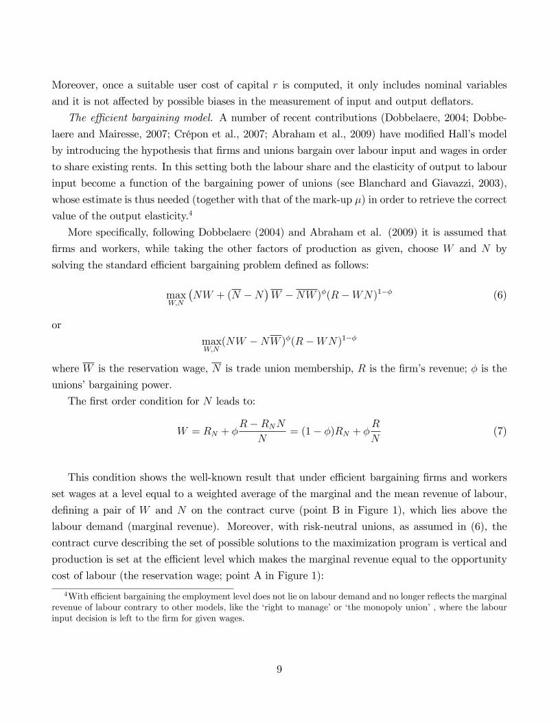
This condition shows the well-known result that under e¢ cient bargaining �rms and workers

set wages at a level equal to a weighted average of the marginal and the mean revenue of labour,

de�ning a pair of W and N on the contract curve (point B in Figure 1), which lies above the

labour demand (marginal revenue). Moreover, with risk-neutral unions, as assumed in (6), the

contract curve describing the set of possible solutions to the maximization program is vertical and

production is set at the e¢ cient level which makes the marginal revenue equal to the opportunity

cost of labour (the reservation wage; point A in Figure 1):

4With e¢ cient bargaining the employment level does not lie on labour demand and no longer re�ects the marginalrevenue of labour contrary to other models, like the �right to manage�or �the monopoly union�, where the labourinput decision is left to the �rm for given wages.

9

RN = W (8)

R/N

RN

N

W

W

A

B

Contract curve

C

Figure 1 - E¢ cient bargaining solution

Under imperfect competition and assuming an isoelastic demand for output, we can use the

following results:

P = Q�1� , R = PQ = Q1�

1� , RN = (1�

1

�)Q�

1�@Q

@N=1

�P (Q)

@Q

@N,

N

Q

@Q

@N= "Q;N

and rewrite equation (8) as follows:

� =P�

W= @Q@N

� (9)

Accordingly, under e¢ cient bargaining the price strategy of �rms depends on the reservation

wageW , so that the relevant price-cost margin measuring �rms�market power has to be computed

with respect to the reservation wage instead of the observed wage W: This correctly measures the

overall rent to be shared, which is not a¤ected by changes in the bargaining power of unions.

Hall�s and Roeger�s models with e¢ cient bargaining. Hall�s model can be adjusted by plugging

into equation (1) the new expression for the elasticity of output to labour that follows from rewriting

equation (7) as:

WN

PQ=N

Q

@Q

@N

1

�+ �� N

Q

@Q

@N

1

�

10

since NQ@Q@N= "Q;N , we get:

�N = (1� �)"Q;N�

+ � (10)

and the elasticity of output to labour turns out to be a function of the labour share, the mark-up

and union bargaining power:

"Q;N = ��N + ��

1� �(�N � 1) (11)

Thus with e¢ cient bargaining and assuming constant returns to scale, the whole set of output

elasticities with respect to inputs becomes:58><>:"Q;N = ��N + �

�1��(�N � 1)

"Q;M = ��M

"Q;K = [1� ��M � ��N � � �1��(�N � 1)]

(12)

By de�ning = �1�� and substituting for output elasticities (12) in equation (1), Dobbelaere

(2004) and Abraham et al. (2009) obtained a modi�ed version of Hall�s equation:

�q � �N�n� �M�m� (1� �N � �M)�k= B(�q ��k) + (�N � 1)(�n��k) + (1�B)�e (13)

where an extra term (�N � 1)(�n��k) shows up. Omitting this additional term would lead to

biased estimates of both B and the mark-up �:

Following the same approach, we modi�ed Roeger�s model to obtain (see Appendix I for the

derivation):

(�q +�p)� �N(�n+�w)� �M(�m+�j)� (1� �N � �M)(�k +�r)= B[(�q +�p)� (�k +�r)] + (�N � 1)[(�n+�w)� (�k +�r)] (14)

While controlling for the extra term (�N � 1)(�n � �k), we can estimate this equation byOLS, bene�ting from the advantages of Roeger�s original approach.

5It should be noticed that in the �right to manage�or in the �monopoly union�model, where employment ischosen by �rms on the labour demand, the usual �rst order condition for pro�t maximization RN = W continuesto hold true, although W is no longer set at the competitive level. In this case Hall�s results would not be modi�ed,as the elasticity of output with respect to labour would remain "Q;N = ��N ; moreover, the bargaining power ofworkers would not show up in the equation to be estimated and therefore would not a¤ect the estimation of themark-up either.

11

More speci�cally, our empirical model is given by:

NSRi;t = �0 + �1XMARKi;t + �2V BARGi;t + ui;t (15)

where, by dropping subscripts: NSR = [(�q + �p) � �N(�n + �w) � �M(�m + �j) � (1 ��N � �M)(�k +�r)] is the nominal Solow residual; XMARK = [(�q +�p)� (�k +�r)] is thenominal change in the output to capital ratio, whose coe¢ cient is linked to the mark-up through

the equation � = 1=(1��1); V BARG = (�N�1)[(�n+�w)�(�k+�r)] is the weighted nominalchange in the labour to capital ratio and its coe¢ cient gives us the bargaining power of unions

through � = �2=(1 + �2).

3 The data

Our empirical analysis is based on the EU KLEMS Growth and Productivity Accounts, which

in the release of March 2008 provide a comprehensive and coherent dataset for most European

countries with annual statistics at industry level on hours worked by skills, net capital stock by

main assets, intermediate inputs and gross production.6 However, as data are not available with

the same level of sectoral disaggregation for all countries, we decided to work with a selection

of 15 industries belonging to the non-farm business sector in 10 European countries: Austria,

Belgium, Denmark, Finland, France, Germany, Italy, Netherlands, United Kingdom and Spain.

Again to avoid an unbalanced panel, we restricted our analysis to the period spanning 1982-2005.

We also drew on supplementary estimates to make the dataset fully suitable for our investigation.

First, for Belgium, France and Spain data on real capital stock, gross �xed capital formation and

consumption of �xed capital, not included in the EU KLEMS dataset, were taken from the STAN-

OECD database.7 Second, for all countries the user cost of capital was estimated by multiplying the

gross �xed capital formation price index by the rental rate of capital, which, in turn, is measured

by the sum of the real interest rate and the depreciation rate, net of the expected capital gains.8

As for the selection of sectors of activity, we did not include agriculture and mining, for which

data are missing for a large number of countries for the early years in the sample, public adminis-

tration, health care and education, where State supply play a predominant role in most European

6http://www.euklems.net/7For Spain the consumption of �xed capital was also missing in the STAN-OECD database and therefore it was

calculated implicitly for each sector as CFKt = Kt�1�Kt+GFKFt, where CFK is consumption of �xed capital,K is net capital stock and GFKF is gross �xed capital formation.

8For each sector in a given country, we have calculated the depreciation rate at time t as the contemporaneousratio of the consumption of �xed capital to the net capital stock; the expected capital gains at time t are proxiedby a moving average of three terms (t, t-1, t-2 ) of the rate of growth of the gross �xed capital formation de�ator.

12

countries; moreover, in the public sector the concepts of pro�t and mark-up make little sense,

given that only labour compensation and capital depreciation contribute to value added. We also

excluded housing services, which is mostly made up of imputed rents pertaining to owner-occupied

dwellings.

Equations (5) and (15) have been estimated for the entire dataset and separately for distinct

aggregates of industries, which we believe could have been a¤ected in di¤erent ways by the institu-

tional changes that occurred since the early nineties. In particular, we focused on manufacturing

industries (further split in high, medium-tech and traditional industries), construction, highly reg-

ulated services (energy, gas and water supply; transport, storage and communication; �nancial

intermediation) and other (remaining) services (Table 1). Regarding manufacturing industries,

given the importance of international trade for this sector, one could expect a sizeable impact of

the implementation of the Single Market Programme; on the other hand, since this sector was

already exposed to high levels of international competition, one could argue that there was little

room for further improvement. In regulated industries, public ownership and regulation tradition-

ally limited competitive pressure; however, several EU directives have been issued to harmonize

the regulatory framework across member countries and foster competition. Moreover, in a number

of countries privatization programmes have deeply changed their market organization. Finally,

other business services remain quite closed to international competition; the Directive on services

was subsequently passed and in a watered-down version that still awaits a full implementation.

Accordingly, the Single Market Programme is expected to play a minor role in these activities,

even if they might have been a¤ected by the labour market reforms like the rest of the business

sector.

The empirical counterparts to the theoretical variables in equations (5) and (15) are given by

the following:9 Qt is real gross output and Pt refers to its price index; Nt is total hours worked by

employees and Wt is hourly labour compensation;10 Mt is the volume index of intermediate inputs

and Jt refers to its price index; Kt is net real �xed capital stock; Rt is the user cost of capital.

In a �rst stage, the shares of labour and intermediate inputs were calculated as �0N = WN=PQ

and �0M = JM=PQ, respectively; further, since we assume constant returns to scale, the capital

share was obtained as �0K = (1 � �0N � �0M). Unfortunately, as outlined also in the EU KLEMSmethodology, the capital share happens to be negative in some cases. Instead of restricting the

negative values to zero, as suggested by the EU KLEMS consortium,11 since we believe it is

9The description of the variables is valid for each sector in the dataset, although for brevity we do not report asu¢ x to identify it.10In the EU KLEMS dataset it is assumed that, at the industry level, the compensation per hour of self-employed

is equal to the compensation per hour of employees.11See �EU KLEMS Growth and productivity accounts �Part I Methodology�, page 41.

13

reasonable to posit a minimum return to capital we proceeded as follows: �rst, we calculated

the implicit return on capital as rimp = (�0KPQ)=K; second, where it turns negative, rimp was

substituted with the minimum positive rimp across sectors for the same year and country; third,

the �nal adjusted capital share was calculated as �K = (rimp�PQ)=K and, on the assumption that

the sign inconvenience described above was due to an improper measurement of the intermediate

inputs, the �nally adjusted share of the latter was obtained as �M = (1 � �K � �N), with anunchanged labour share �N = �0N .

198690 200105 198690 200105 198690 200105 198690 200105 198690 200105

1 Food, beverages and tobacco 8.42 5.85 4.04 3.44 8.34 8.95 15.14 16.81 76.5 74.242 Textile, leather and footwear 3.28 1.79 4.09 1.95 8.55 7.03 27.51 25.26 63.93 67.713 Pulp, paper, printing and publishing 3.63 2.84 2.75 2.22 11.97 12.54 26.19 24.49 61.84 62.974 Chemical, rubber and plastics 8.13 7.49 3.71 2.89 12.89 11.66 17.63 15.29 69.47 73.055 Basic metals and fabricated metal 6.06 4.76 4.84 4.01 10.8 8.72 24.98 24.81 64.21 66.476 Machinery, n.e.c. 4.65 3.98 3.83 2.89 10.01 8.69 29.65 26.25 60.34 65.067 Electrical and optical equipment 4.73 4.18 4.04 2.83 11.33 9.15 30.21 23.79 58.45 67.068 Transport equipment 4.86 5.32 3.06 2.35 6.28 5.87 23.5 17.92 70.22 76.219 Electricity, gas and water supply 3.55 3.19 1.34 0.89 30.51 28.81 17.94 13.15 51.55 58.04

10 Construction 10.53 9.81 12.19 12.15 8.86 8.66 32.09 31.13 59.05 60.2111 Wholesale and retail trade 14.54 15.06 24.21 23.69 13.98 15.01 43.67 38.06 42.35 46.9312 Hotels and restaurants 3.21 3.78 6.24 7.66 7.04 9.18 41.15 39.78 51.81 51.0413 Transport, storage and communication 9.07 11.22 10.12 9.83 17.99 18.68 36.64 26.96 45.37 54.3614 Financial intermediation 6.3 7.07 4.89 4.59 20.41 22.42 40.27 30.61 39.32 46.9715 Renting of m.&eq. and other business activities 9.07 13.65 10.61 18.62 13.59 12.96 43.26 43.34 43.15 43.7

… … … … … … … … … … … … … … … … … … … … … … … … … … … … … … … … … … … … … … … … … … … … … … … … … … … … … … … … … … … … … … … … … … … … … … … … … … … … … … .

1 to 8 Manufacturing 43.76 36.21 30.38 22.56 10.02 9.08 24.35 21.83 65.63 69.099, 13, 14 Regulated Services 18.92 21.48 1.34 0.89 30.51 28.81 17.93 13.15 51.56 58.0411, 12, 15 Other Services 26.72 31.95 36.97 42.65 13.64 14.48 39.51 34.98 46.85 50.54

Aggregations:

Shares on total grossproduction

Shares on total workedhours

Factor shares on industry gross productionCapital Labour IntermediateIndustries

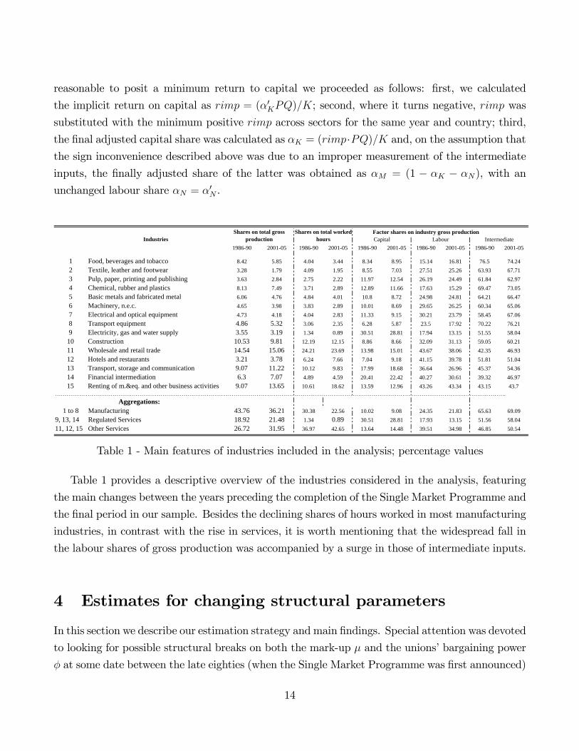
Table 1 - Main features of industries included in the analysis; percentage values

Table 1 provides a descriptive overview of the industries considered in the analysis, featuring

the main changes between the years preceding the completion of the Single Market Programme and

the �nal period in our sample. Besides the declining shares of hours worked in most manufacturing

industries, in contrast with the rise in services, it is worth mentioning that the widespread fall in

the labour shares of gross production was accompanied by a surge in those of intermediate inputs.

4 Estimates for changing structural parameters

In this section we describe our estimation strategy and main �ndings. Special attention was devoted

to looking for possible structural breaks on both the mark-up � and the unions�bargaining power

� at some date between the late eighties (when the Single Market Programme was �rst announced)

14

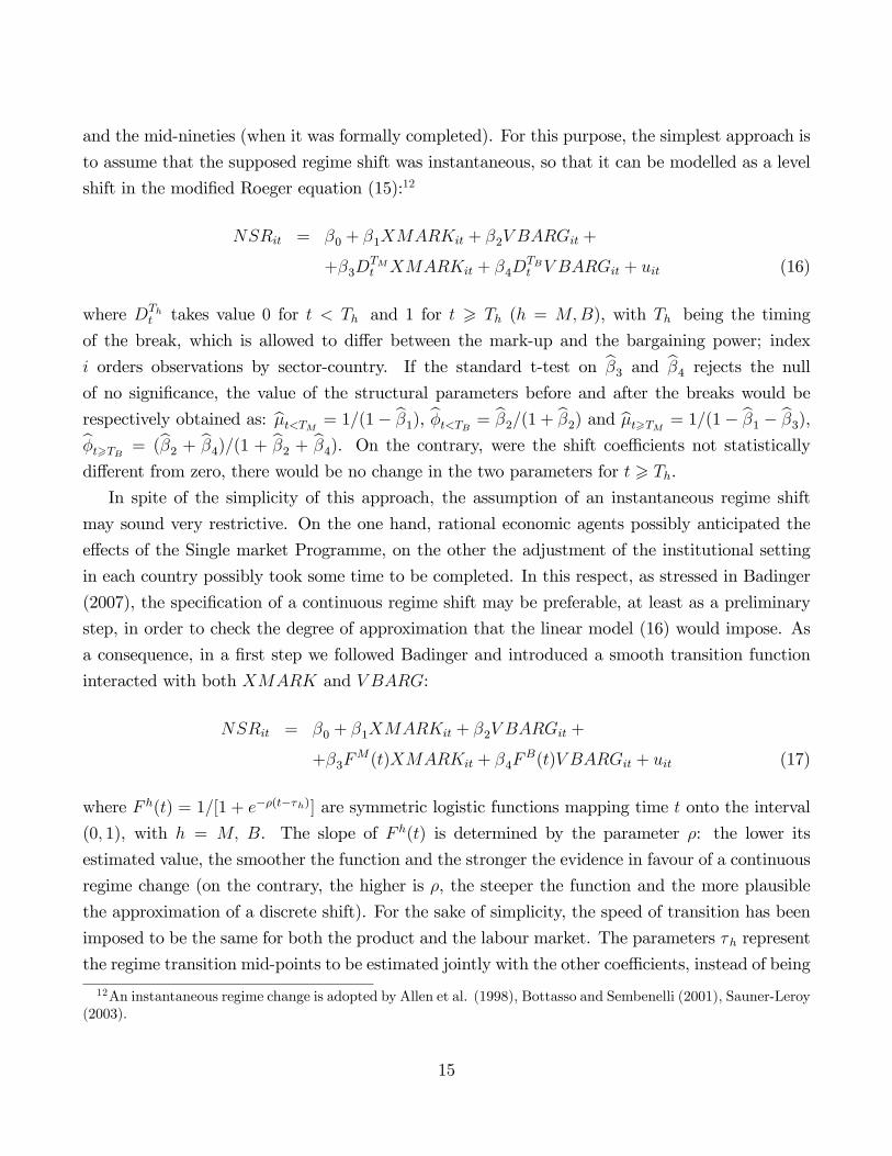
and the mid-nineties (when it was formally completed). For this purpose, the simplest approach is

to assume that the supposed regime shift was instantaneous, so that it can be modelled as a level

shift in the modi�ed Roeger equation (15):12

NSRit = �0 + �1XMARKit + �2V BARGit +

+�3DTMt XMARKit + �4D

TBt V BARGit + uit (16)

where DTht takes value 0 for t < Th and 1 for t > Th (h = M;B), with Th being the timing

of the break, which is allowed to di¤er between the mark-up and the bargaining power; index

i orders observations by sector-country. If the standard t-test on b�3 and b�4 rejects the nullof no signi�cance, the value of the structural parameters before and after the breaks would be

respectively obtained as: b�t<TM = 1=(1� b�1), b�t<TB = b�2=(1 + b�2) and b�t>TM = 1=(1� b�1 � b�3),b�t>TB = (b�2 + b�4)=(1 + b�2 + b�4). On the contrary, were the shift coe¢ cients not statisticallydi¤erent from zero, there would be no change in the two parameters for t > Th.In spite of the simplicity of this approach, the assumption of an instantaneous regime shift

may sound very restrictive. On the one hand, rational economic agents possibly anticipated the

e¤ects of the Single market Programme, on the other the adjustment of the institutional setting

in each country possibly took some time to be completed. In this respect, as stressed in Badinger

(2007), the speci�cation of a continuous regime shift may be preferable, at least as a preliminary

step, in order to check the degree of approximation that the linear model (16) would impose. As

a consequence, in a �rst step we followed Badinger and introduced a smooth transition function

interacted with both XMARK and V BARG:


+�3FM(t)XMARKit + �4F

B(t)V BARGit + uit (17)

where F h(t) = 1=[1 + e��(t��h)] are symmetric logistic functions mapping time t onto the interval

(0; 1), with h = M; B. The slope of F h(t) is determined by the parameter �: the lower its

estimated value, the smoother the function and the stronger the evidence in favour of a continuous

regime change (on the contrary, the higher is �, the steeper the function and the more plausible

the approximation of a discrete shift). For the sake of simplicity, the speed of transition has been

imposed to be the same for both the product and the labour market. The parameters �h represent

the regime transition mid-points to be estimated jointly with the other coe¢ cients, instead of being

12An instantaneous regime change is adopted by Allen et al. (1998), Bottasso and Sembenelli (2001), Sauner-Leroy(2003).

15

imposed exogenously as in (16).13

Equation (17) has been estimated through non-linear least squares (detailed results in Appendix

II), con�rming the evidence found in Badinger (2007) of very high values for �. More speci�cally,

the speed of transition validates an instantaneous break in most of the largest industrial sectors

(manufacturing, construction and non-regulated �"Other" �services); as for the total dataset and

the regulated services, the value of � proves relatively smaller. All in all, the simpler option of

discrete breaks, equation (16), turns out to be a plausible approximation. As for the dating, we

retained the break years endogenously selected as transition mid-points when we estimated (17),

and we accordingly set the shift dummies DTht ; we maintained some limited degree of �exibility

just in the choice of the breaks years where we found evidence of a slightly lower speed of transition

(total dataset and regulated services).

4.1 Results at the aggregate level

The modi�ed Roeger equation (16) was estimated through OLS with country-sector �xed e¤ects.

First we concentrated on the total dataset, exploiting all sample variations over time; then we

looked at the evidence for main industries.

In order to check for endogeneity problems potentially coming from measurement errors, we

performed GMM estimates (in system speci�cation), �nding results invariably in line with the OLS

counterparts (Appendix II).

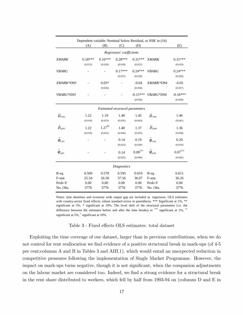
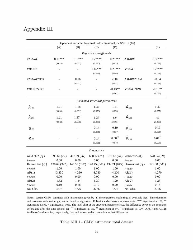
Starting with the total dataset, in the Columns A to D of Table 3 we report as a benchmark

the results that we obtained by setting the break at year 1993, just after the restrictions on the

free circulation of goods and factors across the EU were de�nitively removed. Column E describes

our favourite model (though results are quite similar), where the level shift was postponed to 1994

in line with our estimates of the non-linear equation (17) (Table AII.1 in Appendix II).

In line with the received empirical evidence mostly based on Hall�s approach, in our frame-

work the assumption of e¢ cient bargaining signi�cantly raises the estimated size of the mark-up.

Speci�cally, it appears to be 15 per cent higher when estimated by explicitly controlling for rent

allocation (columns A and C in Table 3 and Table AIII.1 in Appendix III).14 Indeed, rents prove

reasonably larger when they are measured ex ante, before a share of them is distributed to workers.

13As Badinger outlined, equation (16) is nested in equation (17) that collapses into a linear model with aninstantaneous break at � = t when �!1.14Standard errors for structural parameters reported in the tables are computed according to the delta-method.

In general, when the reduced form parameter is statistically signi�cant, the structural parameter is signi�cant aswell. The same holds true for tests on strutural breaks.

16

(A) (B) (C) (D) (E)

XMARK 0.18*** 0.16*** 0.28*** 0.31*** XMARK 0.31***(0.013) (0.016) (0.018) (0.021) (0.019)

VBARG 0.17*** 0.24*** VBARG 0.24***(0.031) (0.030) (0.029)

XMARK*D93 0.05* 0.04 XMARK*D94 0.05(0.026) (0.036) (0.037)

VBARG*D93 0.15*** VBARG*D94 0.16***(0.056) (0.058)

1.22 1.19 1.40 1.45 1.46(0.019) (0.023) (0.035) (0.043) (0.041)

1.22 1.27†† 1.40 1.37 1.36(0.019) (0.031) (0.036) (0.055) (0.058)

0.14 0.19 0.20(0.023) (0.020) (0.019)

0.14 0.08††† 0.07†††

(0.023) (0.040) (0.042)

Rsq. 0.569 0.578 0.595 0.610 Rsq. 0.611Fstat. 25.54 26.50 37.56 36.07 Fstat. 36.26Prob>F 0.00 0.00 0.00 0.00 Prob>F 0.00No. Obs. 3776 3776 3776 3776 No. Obs. 3776

Notes: time dummies and economy wide output gap are included as regressors. OLS estimateswith countrysector fixed effects; robust standard errors in parenthesis. *** Significant at 1%, **significant at 5%, * significant at 10%. The level shift of the structural parameters (i.e. thedifference between the estimates before and after the time breaks) is: ††† significant at 1%, ††

significant at 5%, † significant at 10%.

Regressors' coefficients

Estimated structural parameters

Diagnostics

Dependent variable: Nominal Solow Residual, or NSR in (16)

93<̂tµ

93≥̂tµ

93<̂tφ

93≥̂tφ

94<̂tµ

94≥̂tµ

94<̂tφ

94≥̂tφ

Table 3 - Fixed e¤ects OLS estimates: total dataset

Exploiting the time coverage of our dataset, larger than in previous contributions, when we do

not control for rent reallocation we �nd evidence of a positive structural break in mark-ups (of 4-5

per cent;columns A and B in Tables 3 and AIII.1), which would entail an unexpected reduction in

competitive pressures following the implementation of Single Market Programme. However, the

impact on mark-ups turns negative, though it is not signi�cant, when the companion adjustments

on the labour market are considered too. Indeed, we �nd a strong evidence for a structural break

in the rent share distributed to workers, which fell by half from 1993-94 on (columns D and E in

17

Tables 3 and AIII.1).

Regressions meet the usual diagnostic checks; results prove robust across estimation meth-

ods and controlling for non-spherical errors due to the endogeneity issues raised in Hylleberg and

Jorgensen (1998).15 Moreover, as a robustness check we dropped, in turn, each of the countries

included in the dataset: outcomes remained almost unchanged, irrespective of the sample com-

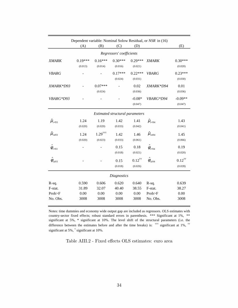
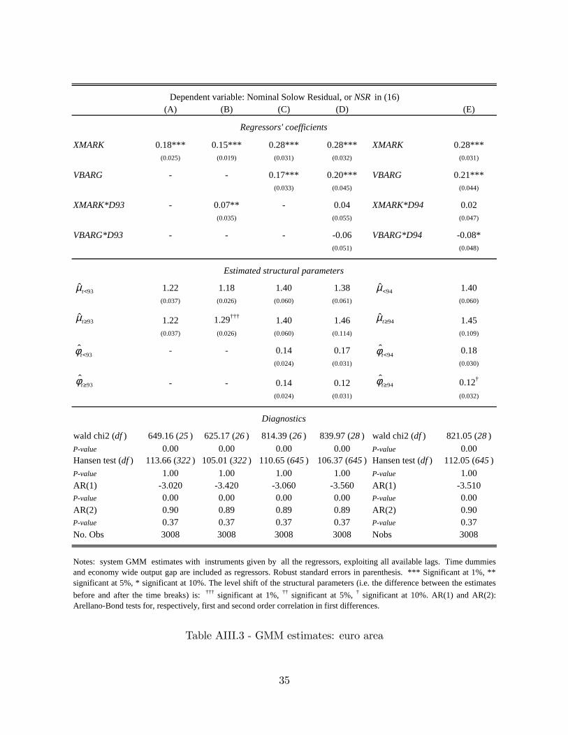
position. The same evidence broadly emerged also when we concentrated only on the subset of

countries belonging to the euro area, as reported in Tables AIII.2 and AIII.3 in Appendix III.16

Tentatively, considering the remaining possible measurement issues, it follows that con�ning

attention to the product market may result in the missing of important ingredients in the appraisal

of both the extent and the transmission channel of the competitive impulse exerted by the Single

Market Programme. Our evidence suggests that institutional changes have mainly a¤ected the

equilibrium on the labour market through a reduction in workers�bargaining power, while the

impact on the pricing rules in the product market is more controversial. Even if we assume that

the total amount of rents tends to decrease, �rms�pro�t margins could well remain unchanged or

even increase due to the fall in the share of rents distributed to workers.

We believe that the result does not stem only from the Single Market Programme, whose

implementation came hand in hand with broader innovation in the institutional and productive

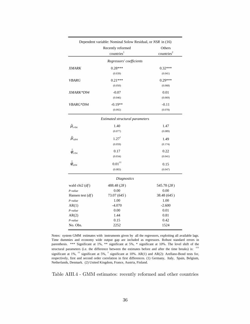
set-up that was spurred in part by privatization and increasing globalization. In order to inves-

tigate in more detail this �rst set of results, we grouped our countries according to the intensity

of the regulatory changes since the beginning of the nineties. For this purpose, we adopted the

OECD indicators regarding employment protection legislation (EPL) and product market regula-

tion (PMR).

15In each regression we added a country-speci�c output gap measure to control for aggregate cyclical e¤ects thatare not captured by the coe¢ cients of the time dummies estimated for the whole sample. However results did notchange when the output gap variable was not included.16In this case the break years were set equal to those adopted for the total dataset.

18

2

1.5

1

0.5

0

0.5

4 3.5 3 2.5 2

change in PMR, 19902005

chan

ge in

EP

L, 1

990

2003

ukfra

finaut

spanld

dnk ger

bel

ita

Figure 2 - OECD indicators of changes in employment protection legislation (EPL) and product

market regulation (PMR)

Figure 2 shows that the total sample can be split quite clearly into two groups, one (lower

left area of the graph) made up of countries that underwent a sizeable reduction in both product

and labour market regulations (Italy, Germany, Belgium, Denmark, the Netherlands and Spain),

the other (upper right area) comprising countries characterized by less pronounced deregulation

(Austria and Finland), France, with persistently high labour market protection, and the UK,

which endorsed signi�cant reforms before the implementation of the Single Market Programme.

Estimating the modi�ed Roeger equation (16) separately for the two subgroups, we �nd that the

outcomes just described for the total dataset are driven exclusively by the "recently reformed"

countries, which since the mid-nineties have registered a signi�cant decline both in mark-ups and

in the share of rent distributed to workers (Table 4 and Table AIII.4 in Appendix III). We interpret

this as corroborating evidence that the identi�ed breaks have to be linked to the reform e¤ort of

the last decade.

19

Recently reformed Otherscountries1 countries2

XMARK 0.31*** 0.32***(0.024) (0.032)

VBARG 0.23*** 0.29***(0.034) (0.052)

XMARK*D94 0.10*** 0.02(0.040) (0.059)

VBARG*D94 0.22*** 0.10(0.079) (0.081)

1.45 1.47(0.051) (0.070)

1.26††† 1.51(0.050) (0.113)

0.18 0.22(0.023) (0.031)

0.01††† 0.16(0.070) (0.044)

Rsq. 0.630 0.600Fstat. 25.34 16.97Prob>F 0.00 0.00No. Obs. 2252 1524




Diagnostics

Notes: time dummies and economy wide output gap are included as regressors. OLS estimates withcountrysector fixed effects; robust standard errors in parenthesis. *** Significant at 1%, **significant at 5%, * significant at 10%. The level shift of the structural parameters (i.e. the differencebetween the estimates before and after the time breaks) is: †††significant at 1%, ††significant at 5%,† significant at 10%. (1) Germany, Italy, Spain, Belgium, Netherlands, Denmark. (2) UnitedKingdom, France, Austria, Finland.

94<̂tµ

94≥̂tµ

94<̂tφ

94≥̂tφ

Table 4 - Fixed e¤ects OLS estimates: recently reformed and other countries

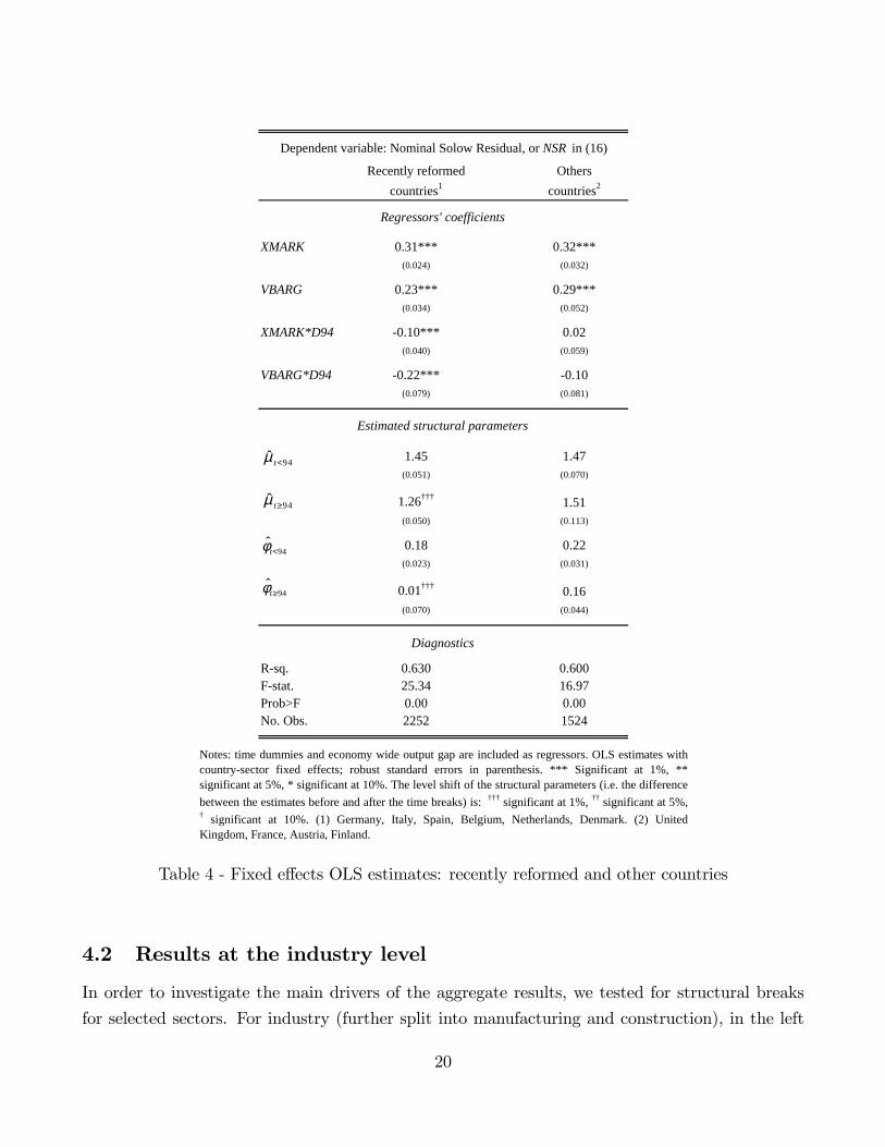
4.2 Results at the industry level

In order to investigate the main drivers of the aggregate results, we tested for structural breaks

for selected sectors. For industry (further split into manufacturing and construction), in the left

20

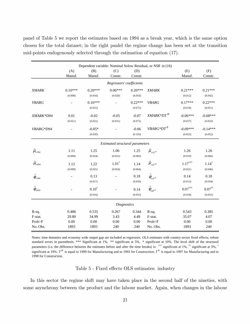
panel of Table 5 we report the estimates based on 1994 as a break year, which is the same option

chosen for the total dataset; in the right panlel the regime change has been set at the transition

mid-points endogenously selected through the estimation of equation (17).

(A) (B) (C) (D) (E) (F)Manuf. Manuf. Constr. Constr. Manuf. Constr.

XMARK 0.10*** 0.20*** 0.06*** 0.20*** XMARK 0.21*** 0.21***(0.008) (0.016) (0.020) (0.054) (0.012) (0.042)

VBARG 0.16*** 0.22*** VBARG 0.17*** 0.22***(0.022) (0.075) (0.018) (0.051)

XMARK*D94 0.01 0.02 0.05 0.07 XMARK*DT M 0.06*** 0.08***(0.011) (0.021) (0.031) (0.072) (0.017) (0.033)

VBARG*D94 0.05* 0.06 VBARG*DT B 0.09*** 0.14***(0.030) (0.103) (0.023) (0.052)

1.11 1.25 1.06 1.25 1.26 1.26(0.009) (0.024) (0.022) (0.083) (0.019) (0.066)

1.12 1.22 1.01† 1.14 1.17††† 1.14†

(0.009) (0.021) (0.024) (0.064) (0.021) (0.046)

0.13 0.18 0.14 0.18(0.017) (0.050) (0.013) (0.034)

0.10† 0.14 0.07††† 0.07††

(0.016) (0.055) (0.018) (0.055)

Rsq. 0.486 0.535 0.267 0.344 Rsq. 0.543 0.385Fstat. 29.80 34.99 3.43 4.49 Fstat. 35.07 4.07Prob>F 0.00 0.00 0.00 0.00 Prob>F 0.00 0.00No. Obs. 1893 1893 240 240 No. Obs. 1893 240

Notes: time dummies and economy wide output gap are included as regressors. OLS estimates with countrysector fixed effects; robuststandard errors in parenthesis. *** Significant at 1%, ** significant at 5%, * significant at 10%. The level shift of the structuralparameters (i.e. the difference between the estimates before and after the time breaks) is: ††† significant at 1%, †† significant at 5%, †

significant at 10%. T M is equal to 1999 for Manufacturing and to 1993 for Construction; T B is equal to 1997 for Manufacturing and to1998 for Construction.

Diagnostics




94≥̂tµ

94<̂tµ

94<̂tφ

94≥̂tφ

MTt<µ̂

MTt≥µ̂

BTt<φ̂

BTt≥φ̂

Table 5 - Fixed e¤ects OLS estimates: industry

In this sector the regime shift may have taken place in the second half of the nineties, with

some asynchrony between the product and the labour market. Again, when changes in the labour

21

market are not controlled for, there is no evidence of any signi�cant break in the product market

(left panel of Table 5 and Table AIII.5 in Appendix III); on the contrary, once e¢ cient bargaining

is allowed for and break years are properly selected, outcomes point to a signi�cant decrease in

mark-up and union bargaining power (right panel of Tables 5 and AIII.5).

(A) (B) (C) (D) (E) (F)Regul. Regul. Others Others Regul. Others

XMARK 0.25*** 0.37*** 0.17*** 0.39*** XMARK 0.36*** 0.39***(0.017) (0.039) (0.013) (0.047) (0.033) (0.044)

VBARG 0.21*** 0.38*** VBARG 0.20*** 0.38***(0.067) (0.083) (0.055) (0.077)

XMARK*D94 0.08*** 0.01 0.05*** 0.00 XMARK*DT M 0.01 0.00(0.030) (0.083) (0.019) (0.085) (0.029) (0.060)

VBARG*D94 0.16 0.07 VBARG*DT B 0.16*** 0.07(0.123) (0.144) (0.046) (0.102)

1.33 1.58 1.21 1.64 1.57 1.64(0.031) (0.097) (0.019) (0.126) (0.082) (0.118)

1.49††† 1.56 1.15†† 1.64 1.60 1.64(0.053) (0.174) (0.018) (0.199) (0.108) (0.160)

0.17 0.28 0.17 0.28(0.046) (0.044) (0.038) (0.040)

0.04 0.31 0.04†† 0.31(0.094) (0.058) (0.061) (0.047)

Rsq. 0.804 0.814 0.546 0.659 Rsq. 0.821 0.659Fstat. 32.09 29.07 16.32 21.75 Fstat. 34.36 21.50Prob>F 0.00 0.00 0.00 0.00 Prob>F 0.00 0.00No. Obs. 720 720 923 923 No. Obs. 720 923

Notes: time dummies and economy wide output gap are included as regressors. OLS estimates with countrysector fixed effects; robuststandard errors in parenthesis. *** Significant at 1%, ** significant at 5%, * significant at 10%. The level shift of the structuralparameters (i.e. the difference between the estimates before and after the time breaks) is: ††† significant at 1%, †† significant at 5%, †

significant at 10%. T M is equal to 1994 for both Regulated and Other services; T B is equal to 1996 for Regulated services and to 1995for Other services.




Diagnostics

94<̂tµ

94≥̂tµ

94<̂tφ

94≥̂tφ

MTt<µ̂

MTt≥µ̂

BTt<φ̂

BTt≥φ̂

Table 6 - Fixed e¤ects OLS estimates: services

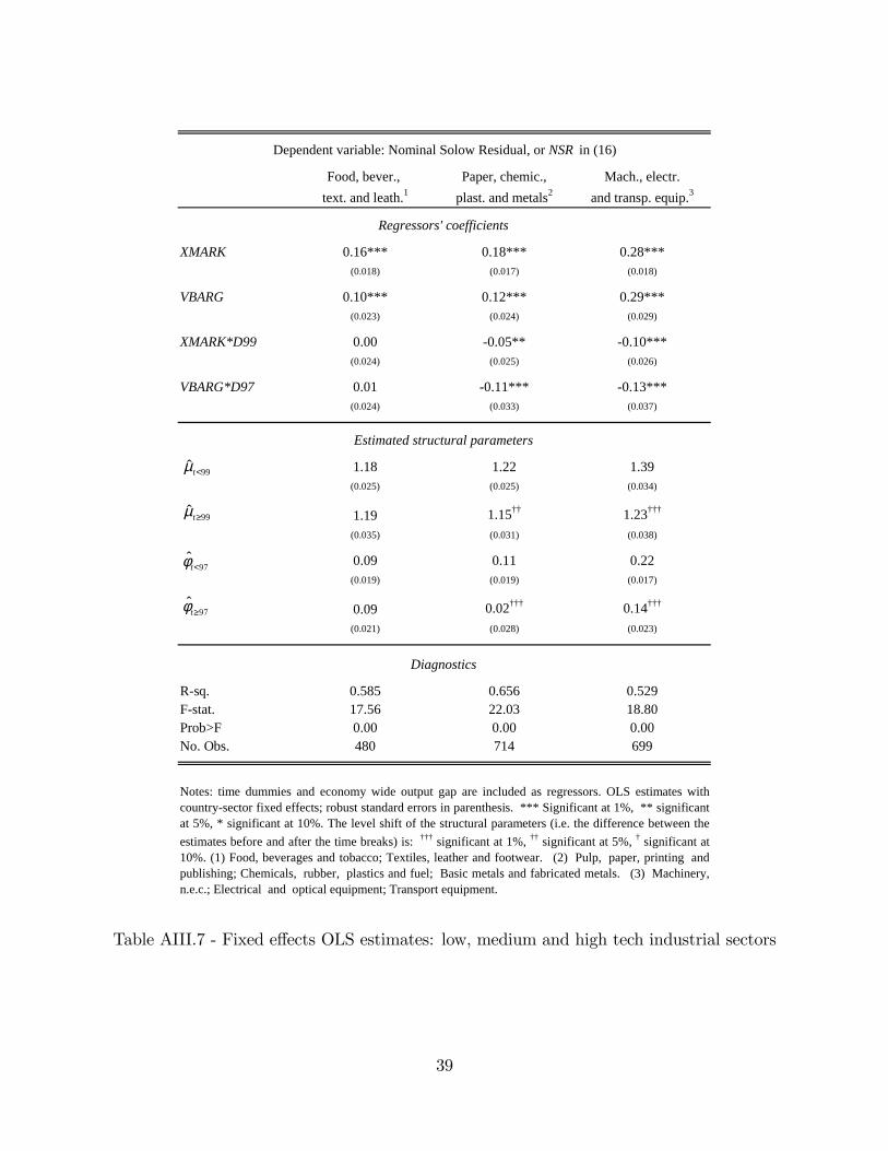
By disaggregating further the manufacturing sector, signi�cant and sizeable shifts in para-

meters are detected in medium and high-tech industries, grouped in the two aggregates "Paper,

chemicals, plastics and metals" and "Machinery, electrical and transport equipment". Both sub-

groups experienced a reduction in mark-ups and union bargaining power (Tables AIII.7 and AIII.8

22

in Appendix III); on the contrary, traditional industries such as "Food, beverages, textiles and

leather" do not show statistical evidence of a regime change.

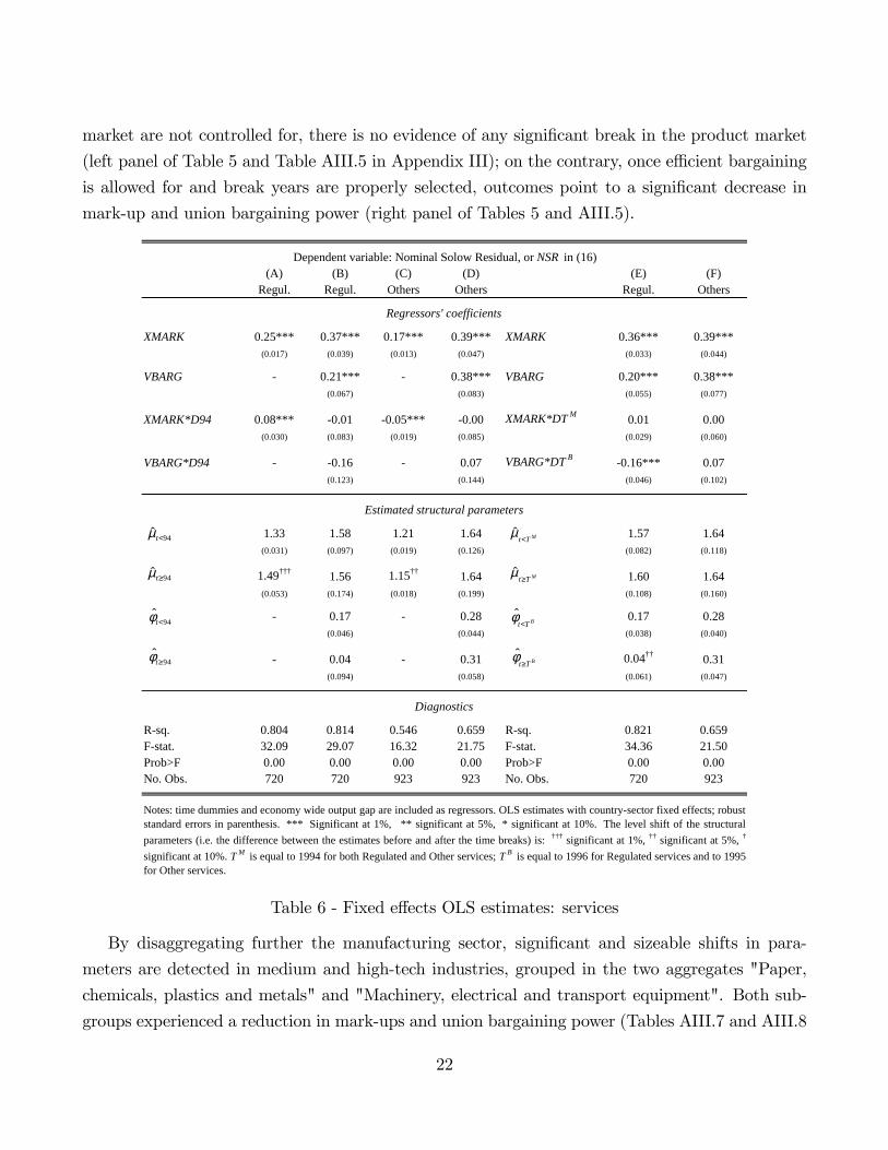
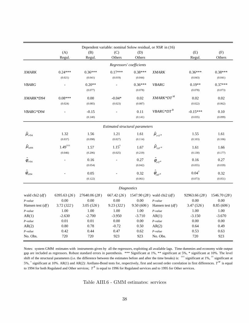
In the service sector, without controlling for imperfect labour markets we �nd a signi�cant rise

in mark-ups in regulated industries (by more than 10 per cent) and a decline in other services

(by around 5 per cent; left panel in Table 6 and Table AIII.6 in Appendix III). However, when

rent sharing is taken into account, the shift becomes statistically insigni�cant in both groups of

activities, and we �nd strong evidence of a drop in bargaining power only in the sole regulated

sectors (right panel in Tables 6 and AIII.6 in Appendix III). This is consistent with results in

Torrini (2005) and Azmat et al. (2007), showing that the main outcome of privatizations and

changes in regulation in some sectors, notably in network industries, was a reallocation of rents -

from labour to capital - rather than a reduction in their amount. This would be due to either a

shift in the managers�objectives from politically related targets to pro�t maximization or a decline

in union power after ownership is transferred from the government to private shareholders.

Summing up, in manufacturing and construction there is clear evidence of a reduction in both

mark-ups and workers rent shares around the mid-nineties; in highly regulated industries, mark-

ups remained roughly unchanged while workers�bargaining power declined signi�cantly; in other

business services, both mark-ups and rent sharing remained virtually unchanged.

5 Concluding remarks

We investigate the extent to which the EU Single Market Programme has a¤ected �rms mark-

ups over marginal costs. Since the Programme went hand in hand with structural reforms in the

labour market and in the institutional setting of important industries (i.e. network industries), we

control for a simultaneous break in the mark-ups and rent sharing between capital and workers by

encompassing the hypothesis of e¢ cient bargaining in the labour market both in the theoretical

and in the empirical model. Using industry data for ten EU countries, at the aggregate level we

�nd that the mark-up tended to increase in the nineties when we do not control for rent sharing.

However, once we assume e¢ cient bargaining in the labour market, the mark-up remain virtually

unchanged while the share of rents accruing to workers declined. Disregarding the fall in the

unions�bargaining power, a rise in �rms�pro�tability due to rent reallocation could be wrongly

interpreted as a reduction in competitive pressures in the product markets. At the sector level, the

evidence proves particularly clear for manufacturing, construction and highly regulated industries,

which went through deep institutional changes and privatization programmes. Our �ndings of

both a sustained di¤erence between prices and marginal costs on the product markets and a

23

declining hedge between wages and labour productivity have further implications for the correct

measurement of total factor productivity under imperfect markets. In our research agenda, we

plan to undertake TFP estimation by explicitly taking into account our estimates of the mark-ups

and unions�bargaining power in order to make the Solow residual a closer proxy for disembodied

technical progress.

24

References

[1] Abraham F., J. Konings and S. Vanormelingen (2009), �The E¤ect of Globalization on Union

Bargaining and Price-Cost Margins of Firms�, Review of World Economics, 145, pp. 14-36.

[2] Allen, C., M. Gasiorek and A. Smith (1998), �European Single Market: How the Programme

Has Fostered Competition�, Economic Policy, 27, pp. 441-486.

[3] Azmat G., A. Manning and J. Van Reenen. (2007), �Privatization, Entry Regulation and

the Decline of Labor�s Share of GDP: A Cross-Country Analysis of the Network Industries�,

Centre for Economic Performance Discussion Paper, 806, London School of Economics.

[4] Badinger, H. (2007), �Has the EU�s Single Market Programme Fostered Competition? Test-

ing for a Decrease in Mark-up Ratios in EU Industries�, Oxford Bulletin of Economics and

Statistics, 69, pp. 497-519.

[5] Bassanini, A. and R. Duval (2006), �The Determinants of Unemployment across OECD Coun-

tries: Reassessing the Role of Policies and Institutions�, OECD Economic Studies, 42.

[6] Blanchard, O. (1997), �The Medium Run�, Brookings Papers on Economic Activity, 28, pp.

89-158.

[7] Blanchard O. (2000), �The Economics of Unemployment. Shocks, Institutions, and Interac-

tions�, Lionel Robbins Lecture, MIT mimeo.

[8] Blanchard, O. and F. Giavazzi (2003), �Macroeconomic E¤ects of Regulation and Deregulation

in Goods and Labour Markets�, The Quarterly Journal of Economics, 118, pp. 879-907.

[9] Bottasso, A. and A. Sembenelli (2001), �Market Power, Productivity and the EU Single

Market Programme: Evidence from a Panel of Italian Firms�, European Economic Review,

45, pp. 167-186.

[10] Bughin, J. (1996), �Trade Unions and Firms�Product Market Power�, The Journal of Indus-

trial Economics, 44, pp. 289-307.

[11] Crépon, B., R. Desplatz and J. Mairesse (2007), �Price-Cost Margins and Rent Sharing:

Evidence from a Panel of French Manufacturing Firms�, mimeo, CREST.

[12] Dobbelaere, S. (2004), �Estimation of Price-Cost Margins and Union Bargaining Power for

Belgian Manufacturing�, International Journal of Industrial Organization, 22, pp. 1381-1398.

25

[13] Dobbelaere, S. and J. Mairesse (2007), �Panel Data Estimates of the Production Function and

Product and Labour Market Imperfections�, European Central Bank Working Paper, 782.

[14] Dew-Becker, I. and R.J. Gordon (2008), �The Role of Labour Market Changes in the Slowdown

of European Productivity Growth�, CEPR Discussion Paper, 6722.

[15] European Commission (2004), �The EU Economy: 2004 Review�, European Economy, 6.

[16] Gri¢ th, R., R. Harrison and H. Simpson (2010), �Product Market Reform and Innovation in

the EU�, Scandinavian Journal of Economics, 112, pp. 389-415

[17] Hall, R.E. (1988), �The Relations Between Price and Marginal Cost in US Industry�, Journal

of Political Economy, 96, pp. 921-947.

[18] Hylleberg, S. and R.W. Jorgensen (1998), �A Note on the Estimation of Markup Pricing in

Manufacturing�, Centre for Non-linear Modelling in Economics Working Paper, 6, University

of Aarhus, Denmark.

[19] Oliveira Martins, J., S. Scarpetta and D. Pilat (1996), �Mark-Up Ratios in Manufacturing

Industries. Estimates for OECD countries�, OECD Economic Department Working Paper,

162.

[20] Neven, D.J., L. Röller and Z. Zhang (2002), �Endogenous Costs and Price-Costs Margins�,

DIW Berlin Discussion Paper, 294, German Institute for Economic Research, Berlin.

[21] Roeger, W. (1995), �Can Imperfect Competition Explain the Di¤erence between Primal and

Dual Productivity Measures? Estimates for US Manufacturing�, Journal of Political Econ-

omy, 103, pp. 316-330.

[22] Sauner-Leroy, J.B. (2003), �The Impact of the Implementation of the Single Market Pro-

gramme on Productive E¢ ciency and on Mark-Ups in the European Union Manufacturing

Industry�, European Economy, European Commission Directorate-General for Economic and

Financial A¤airs, Economic Papers, 192.

[23] Torrini, R. (2005), �Pro�t Share and the Returns on Capital Stock in Italy: The Role of

Privatization Behind the Rise in the1990s�, Centre for Economic Performance Discussion

Paper, 671, London School of Economics.

26

Appendix IHall�s standard model. The basic equation in growth accounting is the following:17

�q = "Q;N�n+ "Q;M�m+ "Q;K�k +�e (A.1)

where q is the log of gross output, n is the log of labour input, m is the log of intermediate inputs,

k is the log of capital input, �e is technical progress, and the parameters "Q;f (f = N; M; K)

represent output elasticities with respect to labour, intermediate and capital inputs. Under the

assumption of perfect competition and constant returns to scale, the output elasticities are just

the input shares of total output. With imperfect competition these elasticities are given by the

product of input shares and the mark-up term. This can be easily seen by expressing the marginal

cost in the following way:

x =W�N +R�K + J�M

�Q��eQ (A.2)

whereW, R and J are, respectively, the price of labour, capital and intermediate goods. This can

be rearranged in the following way:

�Q

Q=WN

xQ

�N

N+JM

xQ

�M

M+RK

xQ

�K

K+�e (A.3)

by log-approximation:

�q =WN

xQ�n+

JM

xQ�m+

RK

xQ�k +�e (A.4)

Since the mark up � is equal to P=x (that is output price over marginal cost), we obtain:

�q = ��N�n+ ��M�m+ ��K�k +�e (A.5)

where �f are the input shares of output (f = N; M; K).

As shown in section 2, assuming constant returns to scale this can be rearranged as:

�q = ��N�n+ ��M�m+ (1� ��N � ��M)�k +�e (A.6)

Rede�ning � = 1=(1�B), we obtain:

�q � �N�n� �M�m� (1� �N � �M)�k = B(�q ��k) + (1�B)�e (A.7)

17Time subscripts dropped for simplicity.

27

which gives a decomposition (right hand side) of the standard Solow residual (the left hand side).

This equation can be estimated to retrieve B and therefore �. However, given that the e¢ ciency

term (1�B)�e is not observable, instrumental variables are required to obtain consistent estimates.

Roeger�s standard model. Roeger (1995) combines the primal and the dual solution to the �rm�s

program to get rid of the unobservables. Starting from cost minimization, price variation can be

expressed as:

�p = "Q;N�w + "Q;M�j + (1� "Q;N � "Q;M)�r ��e (A.8)

where �w;�j;�r are, respectively, the � log of input prices. This can be written as:

�p =WN

C�w +

JM

C�j + (1� WN

C� JM

C)�r ��e (A.9)

where C is the total cost,WN and JM are the cost of labour and intermediate inputs. Cost shares

represent both the output elasticities with respect to inputs and the cost and price elasticities with

respect to the price of inputs. With perfect competition, for each production factor output share

and cost share coincide; with imperfect competition, cost shares can be expressed as the product

of the mark-up and the output shares, or, taking labour as an example:

�N =WN

PQ, P =

1

1�Bx =) WN

C=

�N1�B

Equation (A.8) can be written:

�p =�N1�B�w +

�M1�B�j + (1�

�N1�B �

�M1�B )�r ��e (A.10)

Rearranging we obtain:

�p� �N�w � �M�j � (1� �N � �M)�r = B(�p��r)� (1�B)�e (A.11)

This can be used to substitute for (1�B)�e in equation (7) to get:

[�q � �N�n� �M�m� (1� �N � �M)�k] + [�p� �N�w � �M�j � (1� �N � �M)�r](A.12)

= B[(�q ��k) + (�p��r)] (18)

As outlined in section 2, this equation, unlike Hall�s, can be estimated through OLS, with the

possibility of expressing all the variables in nominal terms, once a suitable user cost of capital is

28

computed; in fact, rearranging:

(�q +�p)� �N (�n+�w)� �M (�m+�j)� (1� �N � �M) (�k +�r) (A.13)

= B[(�q +�p)� (�k +�r)] (19)

where (�q +�p), (�n+�w), (�m+�j) and (�k +�r) represent, respectively, the growth rate

of nominal output and of nominal inputs compensation.

Hall�s and Roeger�models with e¢ cient bargaining. As shown in the main text, by assuming

that �rms and workers take other factors of production as given and choose W and N by solving

a standard e¢ cient bargaining problem, the elasticities of output with respect to inputs become

(under the hypothesis of constant returns to scale):8><>:"Q;N = ��N + �

�1��(�N � 1)

"Q;M = ��M

"Q;K = [1� ��M � ��N � � �1��(�N � 1)]

(A.16)

De�ning = �1�� and using (A.16) to substitute for output elasticities in equation (A.1), we get

the modi�ed version of Hall�s equation adopted by Dobbelaere (2004) and Abraham et al. (2009):

�q � �N�n� �M�m� (1� �N � �M)�k (A.17)

= B(�q ��k) + (�N � 1)(�n��k) + (1�B)�e (20)

In order to get a correspondingly modi�ed Roeger model, we can now substitute (A.16) in

equation (A.8), obtaining a new version of equation (A.11):

�p� �N�w � �M�j � (1� �N � �M)�r (A.18)

= B(�p��r) + (�N � 1)(�w ��r)� (1�B)�e (21)

Finally, combining equations (A.17) and (A.18) we obtain the modi�ed version of Roeger�s equa-

tion:

[�q � �N�n� �M�m� (1� �N � �M)�k] + [�p� �N�w � �M�j � (1� �N � �M)�r](A.19)

= B[(�q ��k) + (�p��r)] + (�N � 1)(�n��k +�w ��r) (22)

29

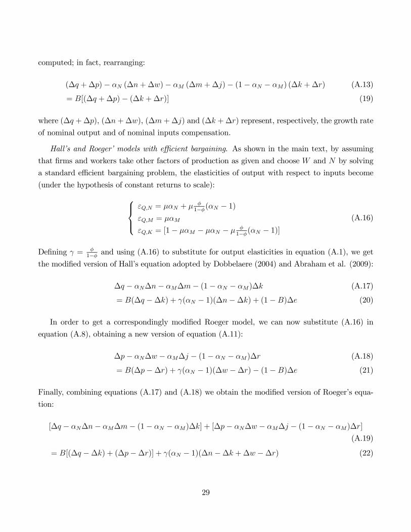
Rearranging it can be written as:

(�q +�p)� �N(�n+�w)� �M(�m+�j)� (1� �N � �M)(�k +�r) (A.20)

= B[(�q +�p)� (�k +�r)] + (�N � 1)[(�n+�w)� (�k +�r)] (23)

which is equation (14) in the main text.

30

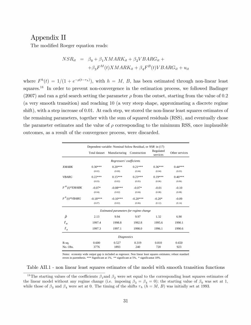
Appendix IIThe modi�ed Roeger equation reads:


+�3FM(t)XMARKit + �4F

B(t)V BARGit + uit

where F h(t) = 1=(1 + e��(t��h)), with h = M; B, has been estimated through non-linear least

squares.18 In order to prevent non-convergence in the estimation process, we followed Badinger

(2007) and ran a grid search setting the parameter � from the outset, starting from the value of 0:2

(a very smooth transition) and reaching 10 (a very steep shape, approximating a discrete regime

shift), with a step increase of 0:01. At each step, we stored the non-linear least squares estimates of

the remaining parameters, together with the sum of squared residuals (RSS), and eventually chose

the parameter estimates and the value of � corresponding to the minimum RSS, once implausible

outcomes, as a result of the convergence process, were discarded.

XMARK 0.30*** 0.20*** 0.21*** 0.36*** 0.44***(0.02) (0.00) (0.04) (0.04) (0.03)

VBARG 0.22*** 0.15*** 0.23*** 0.19*** 0.46***(0.03) (0.02) (0.05) (0.06) (0.06)

F M (t)*XMARK 0.07* 0.08*** 0.07* 0.01 0.10(0.04) (0.02) (0.04) (0.08) (0.08)

F B (t)*VBARG 0.18*** 0.10*** 0.20*** 0.20* 0.09(0.07) (0.02) (0.06) (0.12) (0.14)

2.13 9.94 9.97 1.32 6.90

1997.4 1998.8 1992.8 1995.6 1990.1

1997.3 1997.1 1998.0 1996.1 1990.6

Rsq. 0.600 0.527 0.319 0.810 0.650No. Obs. 3776 1893 240 720 923

ManufacturingTotal dataset

Estimated parameters for regime change

Regulatedservices Other servicesConstruction

Diagnostics



Notes: economy wide output gap is included as regressor. Non linear least squares estimates; robust standarderrors in parenthesis. *** Significant at 1%, ** significant at 5%, * significantat 10%.

ρ̂

Mτ̂

Bτ̂

Table AII.1 - non linear least squares estimates of the model with smooth transition functions

18The starting values of the coe¢ cients �1and �2 were set equal to the corresponding least squares estimates ofthe linear model without any regime change (i.e. imposing �3 = �4 = 0); the starting value of �0 was set at 1,while those of �3 and �4 were set at 0. The timing of the shifts �h (h =M; B) was initially set at 1993.

31

In Table AII.1, besides the ��s coe¢ cients for XMARK, XBARG and their relative smooth

transition variables, we report the estimated transition mid-points �h (h =M;B) and the value of

� minimizing RSS as the outcome of the grid search. The value of � has been selected among those

implying transition mid-points falling between the end of the eighties and the end of the nineties,

that is, the time range in which the actual regime shift towards the Single Market Programme

settings most plausibly took place.

32

Appendix III

(A) (B) (C) (D) (E)

XMARK 0.17*** 0.15*** 0.27*** 0.29*** XMARK 0.30***(0.023) (0.023) (0.030) (0.029) (0.028)

VBARG 0.16*** 0.23*** VBARG 0.23***(0.041) (0.040) (0.039)

XMARK*D93 0.06 0.02 XMARK*D94 0.04(0.037) (0.051) (0.048)

VBARG*D93 0.13** VBARG*D94 0.15**(0.062) (0.062)

1.21 1.18 1.37 1.41 1.42(0.033) (0.031) (0.056) (0.058) (0.057)

1.21 1.27†† 1.37 1.37 1.35

(0.033) (0.036) (0.056) (0.093) (0.090)

0.14 0.19 0.19(0.031) (0.027) (0.026)

0.14 0.08†† 0.07††

(0.031) (0.048) (0.050)

wald chi2 (df ) 399.62 (25 ) 407.89 (26 ) 608.12 (26 ) 578.67 (28 ) wald chi2 (df ) 578.04 (28 )Pvalue 0.00 0.00 0.00 0.00 Pvalue 0.00Hansen test (df ) 138.69 (322 ) 145.59 (322 ) 140.45 (645 ) 132.21 (645 ) Hansen test (df ) 126.08 (645 )Pvalue 1.00 1.00 1.00 1.00 Pvalue 1.00AR(1) 3.830 4.360 3.780 4.300 AR(1) 4.270Pvalue 0.00 0.00 0.00 0.00 Pvalue 0.00AR(2) 1.32 1.34 1.30 1.29 AR(2) 1.33Pvalue 0.19 0.18 0.19 0.20 Pvalue 0.18No. Obs. 3776 3776 3776 3776 No. Obs. 3776

Notes: system GMM estimates with instruments given by all the regressors, exploiting all available lags. Time dummiesand economy wide output gap are included as regressors. Robust standard errors in parenthesis. *** Significant at 1%, **significant at 5%, * significant at 10%. The level shift of the structural parameters (i.e. the difference between the estimatesbefore and after the time breaks) is: ††† significant at 1%, †† significant at 5%, † significant at 10%. AR(1) and AR(2):ArellanoBond tests for, respectively, first and second order correlation in first differences.




Diagnostics

93<̂tµ

93≥̂tµ

93<̂tφ

93≥̂tφ

94<̂tµ

94≥̂tµ

94<̂tφ

94≥̂tφ

Table AIII.1 - GMM estimates: total dataset

33

(A) (B) (C) (D) (E)

XMARK 0.19*** 0.16*** 0.30*** 0.29*** XMARK 0.30***(0.013) (0.014) (0.016) (0.021) (0.020)

VBARG 0.17*** 0.22*** VBARG 0.23***(0.024) (0.031) (0.030)

XMARK*D93 0.07*** 0.02 XMARK*D94 0.01(0.024) (0.036) (0.036)

VBARG*D93 0.08* VBARG*D94 0.09**(0.047) (0.047)

1.24 1.19 1.42 1.41 1.43(0.020) (0.020) (0.033) (0.042) (0.041)

1.24 1.29††† 1.42 1.46 1.45(0.020) (0.023) (0.033) (0.061) (0.066)

0.15 0.18 0.19(0.018) (0.021) (0.020)

0.15 0.12†† 0.12††

(0.018) (0.026) (0.028)

Rsq. 0.590 0.606 0.620 0.640 Rsq. 0.639Fstat. 31.89 32.07 40.40 38.55 Fstat. 38.27Prob>F 0.00 0.00 0.00 0.00 Prob>F 0.00No. Obs. 3008 3008 3008 3008 No. Obs. 3008

Notes: time dummies and economy wide output gap are included as regressors. OLS estimates withcountrysector fixed effects; robust standard errors in parenthesis. *** Significant at 1%, **significant at 5%, * significant at 10%. The level shift of the structural parameters (i.e. thedifference between the estimates before and after the time breaks) is: ††† significant at 1%, ††

significant at 5%, † significant at 10%.

Diagnostics




93<̂tµ

93≥̂tµ

93<̂tφ

93≥̂tφ

94<̂tµ

94≥̂tµ

94<̂tφ

94≥̂tφ

Table AIII.2 - Fixed e¤ects OLS estimates: euro area

34

(A) (B) (C) (D) (E)

XMARK 0.18*** 0.15*** 0.28*** 0.28*** XMARK 0.28***(0.025) (0.019) (0.031) (0.032) (0.031)

VBARG 0.17*** 0.20*** VBARG 0.21***(0.033) (0.045) (0.044)

XMARK*D93 0.07** 0.04 XMARK*D94 0.02(0.035) (0.055) (0.047)

VBARG*D93 0.06 VBARG*D94 0.08*(0.051) (0.048)

1.22 1.18 1.40 1.38 1.40(0.037) (0.026) (0.060) (0.061) (0.060)

1.22 1.29††† 1.40 1.46 1.45(0.037) (0.026) (0.060) (0.114) (0.109)

0.14 0.17 0.18(0.024) (0.031) (0.030)

0.14 0.12 0.12†

(0.024) (0.031) (0.032)

wald chi2 (df ) 649.16 (25 ) 625.17 (26 ) 814.39 (26 ) 839.97 (28 ) wald chi2 (df ) 821.05 (28 )Pvalue 0.00 0.00 0.00 0.00 Pvalue 0.00Hansen test (df ) 113.66 (322 ) 105.01 (322 ) 110.65 (645 ) 106.37 (645 ) Hansen test (df ) 112.05 (645 )Pvalue 1.00 1.00 1.00 1.00 Pvalue 1.00AR(1) 3.020 3.420 3.060 3.560 AR(1) 3.510Pvalue 0.00 0.00 0.00 0.00 Pvalue 0.00AR(2) 0.90 0.89 0.89 0.89 AR(2) 0.90Pvalue 0.37 0.37 0.37 0.37 Pvalue 0.37No. Obs 3008 3008 3008 3008 Nobs 3008

Notes: system GMM estimates with instruments given by all the regressors, exploiting all available lags. Time dummiesand economy wide output gap are included as regressors. Robust standard errors in parenthesis. *** Significant at 1%, **significant at 5%, * significant at 10%. The level shift of the structural parameters (i.e. the difference between the estimatesbefore and after the time breaks) is: ††† significant at 1%, †† significant at 5%, † significant at 10%. AR(1) and AR(2):ArellanoBond tests for, respectively, first and second order correlation in first differences.

Diagnostics




93<̂tµ

93≥̂tµ

93<̂tφ

93≥̂tφ

94<̂µ

94≥̂tµ

94<̂tφ

94≥̂tφ

Table AIII.3 - GMM estimates: euro area

35

Recently reformed Otherscountries1 countries2

XMARK 0.28*** 0.32***(0.039) (0.041)

VBARG 0.21*** 0.29***(0.050) (0.068)

XMARK*D94 0.07 0.01(0.046) (0.069)

VBARG*D94 0.19** 0.11(0.092) (0.078)

1.40 1.47(0.077) (0.089)

1.27† 1.49(0.059) (0.174)

0.17 0.22(0.034) (0.041)

0.01†† 0.15(0.083) (0.047)

wald chi2 (df ) 488.48 (28 ) 545.78 (28 )Pvalue 0.00 0.00Hansen test (df ) 73.07 (645 ) 38.48 (645 )Pvalue 1.00 1.00AR(1) 4.070 2.600Pvalue 0.00 0.01AR(2) 1.44 0.81Pvalue 0.15 0.42No. Obs. 2252 1524



Diagnostics


Notes: system GMM estimates with instruments given by all the regressors, exploiting all available lags.Time dummies and economy wide output gap are included as regressors. Robust standard errors inparenthesis. *** Significant at 1%, ** significant at 5%, * significant at 10%. The level shift of thestructural parameters (i.e. the difference between the estimates before and after the time breaks) is: †††

significant at 1%, †† significant at 5%, † significant at 10%. AR(1) and AR(2): ArellanoBond tests for,respectively, first and second order correlation in first differences. (1) Germany, Italy, Spain, Belgium,Netherlands, Denmark. (2) United Kingdom, France, Austria, Finland.

94<̂tµ

94≥̂tµ

94<̂tφ

94≥̂tφ

Table AIII.4 - GMM estimates: recently reformed and other countries

36

(A) (B) (C) (D) (E) (F)Manuf. Manuf. Constr. Constr. Manuf. Constr.

XMARK 0.09*** 0.18*** 0.06*** 0.18*** XMARK 0.19*** 0.19***(0.010) (0.021) (0.023) (0.057) (0.019) (0.054)

VBARG 0.14*** 0.18** VBARG 0.15*** 0.20**(0.029) (0.083) (0.027) (0.084)

XMARK*D94 0.02 0.00 0.04** 0.04 XMARK*DT M 0.05*** 0.08***(0.012) (0.021) (0.017) (0.035) (0.017) (0.018)

VBARG*D94 0.03 0.01 VBARG*DT B 0.08*** 0.14***(0.030) (0.061) (0.026) (0.027)

1.10 1.21 1.07 1.21 1.23 1.24(0.012) (0.031) (0.026) (0.083) (0.029) (0.083)

1.12 1.21 1.02†† 1.15 1.16†† 1.13(0.013) (0.027) (0.023) (0.091) (0.025) (0.078)

0.12 0.15 0.13 0.16(0.023) (0.060) (0.020) (0.059)

0.10 0.14 0.07†† 0.05(0.022) (0.077) (0.024) (0.089)

wald chi2 (df ) 794.27 (26 ) 1263.57 (28 ) 129.11 (26 ) 1065.50 (28 ) wald chi2 (df ) 1268.20 (28 ) 221.99 (28 )Pvalue 0.00 0.00 0.00 0.00 Pvalue 0.00 0.00Hansen test (df ) 60.89 (322 ) 62.97 (645 ) 0 (187 ) 0 (205 ) Hansen test (df ) 58.17 (645 ) 0 (205 )Pvalue 1.00 1.00 1.00 1.00 Pvalue 1.00 1.00AR(1) 4.340 4.250 2.660 2.590 AR(1) 4.280 2.640Pvalue 0.00 0.00 0.01 0.01 Pvalue 0.00 0.01AR(2) 0.26 0.27 0.50 0.56 AR(2) 0.07 0.05Pvalue 0.80 0.79 0.62 0.58 Pvalue 0.95 0.96No. Obs. 1893 1893 240 240 No. Obs. 1893 240

Notes: system GMM estimates with instruments given by all the regressors, exploiting all available lags. Time dummies and economywide output gap are included as regressors. Robust standard errors in parenthesis. *** Significant at 1%, ** significant at 5%, *significant at 10%. The level shift of the structural parameters (i.e. the difference between the estimates before and after the time breaks)is: ††† significant at 1%, †† significant at 5%, † significant at 10%. AR(1) and AR(2): ArellanoBond tests for, respectively, first andsecond order correlation in first differences. T M is equal to 1999 for Manufacturing and to 1993 for Construction; T B is equal to 1997 forManufacturing and to 1998 for Construction.



Diagnostics


94<̂tµ

94≥̂tµ

94<̂tφ

94≥̂tφ

MTt<µ̂

BTt≥φ̂

MTt≥µ̂

BTt<φ̂

Table AIII.5 - GMM estimates: industry

37

(A) (B) (C) (D) (E) (F)Regul. Regul. Others Others Regul. Others

XMARK 0.24*** 0.36*** 0.17*** 0.38*** XMARK 0.36*** 0.38***(0.021) (0.041) (0.019) (0.044) (0.043) (0.041)

VBARG 0.20** 0.36*** VBARG 0.19** 0.37***(0.077) (0.078) (0.078) (0.073)

XMARK*D94 0.08*** 0.00 0.04* 0.02 XMARK*DT M 0.02 0.02(0.024) (0.085) (0.023) (0.087) (0.022) (0.062)

VBARG*D94 0.15 0.11 VBARG*DT B 0.15*** 0.10(0.140) (0.141) (0.035) (0.099)

1.32 1.56 1.21 1.61 1.55 1.61(0.037) (0.098) (0.027) (0.114) (0.103) (0.106)

1.49††† 1.57 1.15† 1.67 1.61 1.66(0.046) (0.206) (0.025) (0.219) (0.130) (0.177)

0.16 0.27 0.16 0.27(0.054) (0.042) (0.055) (0.039)

0.05 0.32 0.04† 0.32(0.122) (0.061) (0.073) (0.051)

wald chi2 (df ) 6395.63 (26 ) 27640.06 (28 ) 667.42 (26 ) 1547.90 (28 ) wald chi2 (df ) 92963.66 (28 ) 1546.70 (28 )Pvalue 0.00 0.00 0.00 0.00 Pvalue 0.00 0.00Hansen test (df ) 3.72 (322 ) 3.05 (526 ) 9.23 (322 ) 9.50 (606 ) Hansen test (df ) 3.47 (526 ) 8.85 (606 )Pvalue 1.00 1.00 1.00 1.00 Pvalue 1.00 1.00AR(1) 2.630 2.700 3.950 3.710 AR(1) 3.150 3.670Pvalue 0.01 0.01 0.00 0.00 Pvalue 0.00 0.00AR(2) 0.80 0.78 0.72 0.50 AR(2) 0.64 0.49Pvalue 0.42 0.44 0.47 0.62 Pvalue 0.53 0.63No. Obs. 720 720 923 923 No. Obs. 720 923

Notes: system GMM estimates with instruments given by all the regressors, exploiting all available lags. Time dummies and economy wide outputgap are included as regressors. Robust standard errors in parenthesis. *** Significant at 1%, ** significant at 5%, * significant at 10%. The levelshift of the structural parameters (i.e. the difference between the estimates before and after the time breaks) is: †††significant at 1%, ††significant at5%, †significant at 10%. AR(1) and AR(2): ArellanoBond tests for, respectively, first and second order correlation in first differences. T M is equalto 1994 for both Regulated and Other services; T B is equal to 1996 for Regulated services and to 1995 for Other services.


Diagnostics

Dependent variable: nominal Solow residual, or NSR in (16)


94<̂tµ

94≥̂tµ

94<̂tφ

94≥̂tφ

MTt<µ̂

MTt≥µ̂

BTt≥φ̂

BTt<φ̂

Table AIII.6 - GMM estimates: services

38

Food, bever., Paper, chemic., Mach., electr.text. and leath.1 plast. and metals2 and transp. equip.3

XMARK 0.16*** 0.18*** 0.28***(0.018) (0.017) (0.018)

VBARG 0.10*** 0.12*** 0.29***(0.023) (0.024) (0.029)

XMARK*D99 0.00 0.05** 0.10***(0.024) (0.025) (0.026)

VBARG*D97 0.01 0.11*** 0.13***(0.024) (0.033) (0.037)

1.18 1.22 1.39(0.025) (0.025) (0.034)

1.19 1.15†† 1.23†††

(0.035) (0.031) (0.038)

0.09 0.11 0.22(0.019) (0.019) (0.017)

0.09 0.02††† 0.14†††

(0.021) (0.028) (0.023)

Rsq. 0.585 0.656 0.529Fstat. 17.56 22.03 18.80Prob>F 0.00 0.00 0.00No. Obs. 480 714 699

Notes: time dummies and economy wide output gap are included as regressors. OLS estimates withcountrysector fixed effects; robust standard errors in parenthesis. *** Significant at 1%, ** significantat 5%, * significant at 10%. The level shift of the structural parameters (i.e. the difference between theestimates before and after the time breaks) is: ††† significant at 1%, †† significant at 5%, † significant at10%. (1) Food, beverages and tobacco; Textiles, leather and footwear. (2) Pulp, paper, printing andpublishing; Chemicals, rubber, plastics and fuel; Basic metals and fabricated metals. (3) Machinery,n.e.c.; Electrical and optical equipment; Transport equipment.



Diagnostics


99<̂tµ

99≥̂tµ

97<̂tφ

97≥̂tφ

Table AIII.7 - Fixed e¤ects OLS estimates: low, medium and high tech industrial sectors

39

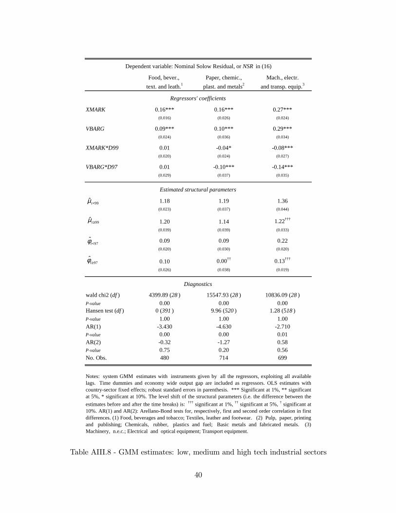
Food, bever., Paper, chemic., Mach., electr.text. and leath.1 plast. and metals2 and transp. equip.3

XMARK 0.16*** 0.16*** 0.27***(0.016) (0.026) (0.024)

VBARG 0.09*** 0.10*** 0.29***(0.024) (0.036) (0.034)

XMARK*D99 0.01 0.04* 0.08***(0.020) (0.024) (0.027)

VBARG*D97 0.01 0.10*** 0.14***(0.029) (0.037) (0.035)

1.18 1.19 1.36(0.023) (0.037) (0.044)

1.20 1.14 1.22†††

(0.039) (0.039) (0.033)

0.09 0.09 0.22(0.020) (0.030) (0.020)

0.10 0.00†† 0.13†††

(0.026) (0.038) (0.019)

wald chi2 (df ) 4399.89 (28 ) 15547.93 (28 ) 10836.09 (28 )Pvalue 0.00 0.00 0.00Hansen test (df ) 0 (391 ) 9.96 (520 ) 1.28 (518 )Pvalue 1.00 1.00 1.00AR(1) 3.430 4.630 2.710Pvalue 0.00 0.00 0.01AR(2) 0.32 1.27 0.58Pvalue 0.75 0.20 0.56No. Obs. 480 714 699


Notes: system GMM estimates with instruments given by all the regressors, exploiting all availablelags. Time dummies and economy wide output gap are included as regressors. OLS estimates withcountrysector fixed effects; robust standard errors in parenthesis. *** Significant at 1%, ** significantat 5%, * significant at 10%. The level shift of the structural parameters (i.e. the difference between theestimates before and after the time breaks) is: ††† significant at 1%, †† significant at 5%, † significant at10%. AR(1) and AR(2): ArellanoBond tests for, respectively, first and second order correlation in firstdifferences. (1) Food, beverages and tobacco; Textiles, leather and footwear. (2) Pulp, paper, printingand publishing; Chemicals, rubber, plastics and fuel; Basic metals and fabricated metals. (3)Machinery, n.e.c.; Electrical and optical equipment; Transport equipment.



Diagnostics

99<̂tµ

99≥̂tµ

97<̂tφ

97≥̂tφ

Table AIII.8 - GMM estimates: low, medium and high tech industrial sectors

40

(*) Requestsforcopiesshouldbesentto:Bancad’Italia–ServizioStudidistrutturaeconomicaefinanziaria–DivisioneBibliotecaeArchiviostorico–ViaNazionale,91–00184Rome–(fax00390647922059).TheyareavailableontheInternetwww.bancaditalia.it.

RECENTLYPUBLISHED“TEMI”(*)

N. 757 – A note on rationalizability and restrictions on belief, by Giuseppe Cappelletti(April2010).

N. 758 – A non-parametric model-based approach to uncertainty and risk analysis of macroeconomic forecasts,byClaudiaMianiandStefanoSiviero(April2010).

N. 759 – Financial innovation and risk: the role of information,byRobertoPiazza (June2010).

N. 760 – Switching costs in local credit markets,byGuglielmoBarone,RobertoFeliciandMarcelloPagnini(June2010).

N. 761 – The determinants of teacher mobility. Evidence from a panel of Italian teachers,byGiannaBarbieri,ClaudioRossettiandPaoloSestito(June2010).

N. 762 – A public guarantee of a minimum return to defined contribution pension scheme members,byGiuseppeGrandeandIgnazioVisco(June2010).

N. 763 – Debt restructuring and the role of lending technologies,byGiacintoMicucciandPaolaRossi(June2010).

N. 764 – Disentangling demand and supply in credit developments: a survey-based analysis for Italy,byPaoloDelGiovane,GinetteEramoandAndreaNobili(June2010).

N. 765 – Information uncertainty and the reaction of stock prices to news,byPaoloAngeliniandGiovanniGuazzarotti(July2010).

N. 766 – With a little help from abroad: the effect of low-skilled immigration on the female labor supply,byGuglielmoBaroneandSauroMocetti(July2010).

N. 767 – Real time forecasts of inflation: the role of financial variables,byLiberoMonteforteandGianlucaMoretti(July2010).

N. 768 – The effect of age on portfolio choices: evidence from an Italian pension fund, byGiuseppeG.L.Cappelletti,GiovanniGuazzarottiandPietroTommasino(July2010).

N. 769 – Does investing abroad reduce domestic activity? Evidence from Italian manufacturing firms,byRaffaelloBronzini(July2010).

N. 770 – The EAGLE. A model for policy analysis of macroeconomics interdependence in the euro area,bySandraGomes,PascalJacquinotandMassimilianoPisani(July2010).

N. 771 – Modelling Italian potential output and the output gap, by Antonio Bassanetti,MicheleCaivanoandAlbertoLocarno(September2010).

N. 772 – Relationship lending in a financial turmoil,byStefaniaDeMitri,GiorgioGobbiandEnricoSette(September2010).

N. 773 – Firm entry, competitive pressures and the US inflation dynamics, by MartinaCecioni(September2010).

N. 774 – Credit ratings in structured finance and the role of systemic risk,byRobertoVioli(September2010).

N. 775 – Entrepreneurship and market size. The case of young college graduates in Italy,bySabrinaDiAddarioandDanielaVuri(September2010).

N. 776 – Measuring the price elasticity of import demand in the destination markets of Italian exports,byAlbertoFelettighandStefanoFederico(October2010).

N. 777 – Income reporting behaviour in sample surveys,byAndreaNeriandRobertaZizza(October2010).

N. 778 – The rise of risk-based pricing of mortgage interest rates in Italy,bySilviaMagriandRaffaellaPico(October2010).

N. 779 – On the interaction between market and credit risk: a factor-augmented vector autoregressive (FAVAR) approach, by Roberta Fiori and Simonetta Iannotti(October2010).

"TEMI" LATER PUBLISHED ELSEWHERE

2008

P. ANGELINI, Liquidity and announcement effects in the euro area, Giornale degli Economisti e Annali di Economia, v. 67, 1, pp. 1-20, TD No. 451 (October 2002).

P. ANGELINI, P. DEL GIOVANE, S. SIVIERO and D. TERLIZZESE, Monetary policy in a monetary union: What role for regional information?, International Journal of Central Banking, v. 4, 3, pp. 1-28, TD No. 457 (December 2002).

F. SCHIVARDI and R. TORRINI, Identifying the effects of firing restrictions through size-contingent Differences in regulation, Labour Economics, v. 15, 3, pp. 482-511, TD No. 504 (June 2004).

L. GUISO and M. PAIELLA,, Risk aversion, wealth and background risk, Journal of the European Economic Association, v. 6, 6, pp. 1109-1150, TD No. 483 (September 2003).

C. BIANCOTTI, G. D'ALESSIO and A. NERI, Measurement errors in the Bank of Italy’s survey of household income and wealth, Review of Income and Wealth, v. 54, 3, pp. 466-493, TD No. 520 (October 2004).

S. MOMIGLIANO, J. HENRY and P. HERNÁNDEZ DE COS, The impact of government budget on prices: Evidence from macroeconometric models, Journal of Policy Modelling, v. 30, 1, pp. 123-143 TD No. 523 (October 2004).

L. GAMBACORTA, How do banks set interest rates?, European Economic Review, v. 52, 5, pp. 792-819, TD No. 542 (February 2005).

P. ANGELINI and A. GENERALE, On the evolution of firm size distributions, American Economic Review, v. 98, 1, pp. 426-438, TD No. 549 (June 2005).

R. FELICI and M. PAGNINI, Distance, bank heterogeneity and entry in local banking markets, The Journal of Industrial Economics, v. 56, 3, pp. 500-534, No. 557 (June 2005).

S. DI ADDARIO and E. PATACCHINI, Wages and the city. Evidence from Italy, Labour Economics, v.15, 5, pp. 1040-1061, TD No. 570 (January 2006).

S. SCALIA, Is foreign exchange intervention effective?, Journal of International Money and Finance, v. 27, 4, pp. 529-546, TD No. 579 (February 2006).

M. PERICOLI and M. TABOGA, Canonical term-structure models with observable factors and the dynamics of bond risk premia, Journal of Money, Credit and Banking, v. 40, 7, pp. 1471-88, TD No. 580 (February 2006).

E. VIVIANO, Entry regulations and labour market outcomes. Evidence from the Italian retail trade sector, Labour Economics, v. 15, 6, pp. 1200-1222, TD No. 594 (May 2006).

S. FEDERICO and G. A. MINERVA, Outward FDI and local employment growth in Italy, Review of World Economics, Journal of Money, Credit and Banking, v. 144, 2, pp. 295-324, TD No. 613 (February 2007).

F. BUSETTI and A. HARVEY, Testing for trend, Econometric Theory, v. 24, 1, pp. 72-87, TD No. 614 (February 2007).

V. CESTARI, P. DEL GIOVANE and C. ROSSI-ARNAUD, Memory for prices and the Euro cash changeover: an analysis for cinema prices in Italy, In P. Del Giovane e R. Sabbatini (eds.), The Euro Inflation and Consumers’ Perceptions. Lessons from Italy, Berlin-Heidelberg, Springer, TD No. 619 (February 2007).

B. H. HALL, F. LOTTI and J. MAIRESSE, Employment, innovation and productivity: evidence from Italian manufacturing microdata, Industrial and Corporate Change, v. 17, 4, pp. 813-839, TD No. 622 (April 2007).

J. SOUSA and A. ZAGHINI, Monetary policy shocks in the Euro Area and global liquidity spillovers, International Journal of Finance and Economics, v.13, 3, pp. 205-218, TD No. 629 (June 2007).

M. DEL GATTO, GIANMARCO I. P. OTTAVIANO and M. PAGNINI, Openness to trade and industry cost dispersion: Evidence from a panel of Italian firms, Journal of Regional Science, v. 48, 1, pp. 97-129, TD No. 635 (June 2007).

P. DEL GIOVANE, S. FABIANI and R. SABBATINI, What’s behind “inflation perceptions”? A survey-based analysis of Italian consumers, in P. Del Giovane e R. Sabbatini (eds.), The Euro Inflation and Consumers’ Perceptions. Lessons from Italy, Berlin-Heidelberg, Springer, TD No. 655 (January

2008).

R. BRONZINI, G. DE BLASIO, G. PELLEGRINI and A. SCOGNAMIGLIO, La valutazione del credito d’imposta per gli investimenti, Rivista di politica economica, v. 98, 4, pp. 79-112, TD No. 661 (April 2008).

B. BORTOLOTTI, and P. PINOTTI, Delayed privatization, Public Choice, v. 136, 3-4, pp. 331-351, TD No. 663 (April 2008).

R. BONCI and F. COLUMBA, Monetary policy effects: New evidence from the Italian flow of funds, Applied Economics , v. 40, 21, pp. 2803-2818, TD No. 678 (June 2008).

M. CUCCULELLI, and G. MICUCCI, Family Succession and firm performance: evidence from Italian family firms, Journal of Corporate Finance, v. 14, 1, pp. 17-31, TD No. 680 (June 2008).

A. SILVESTRINI and D. VEREDAS, Temporal aggregation of univariate and multivariate time series models: a survey, Journal of Economic Surveys, v. 22, 3, pp. 458-497, TD No. 685 (August 2008).

2009

F. PANETTA, F. SCHIVARDI and M. SHUM, Do mergers improve information? Evidence from the loan market, Journal of Money, Credit, and Banking, v. 41, 4, pp. 673-709, TD No. 521 (October 2004).

M. BUGAMELLI and F. PATERNÒ, Do workers’ remittances reduce the probability of current account reversals?, World Development, v. 37, 12, pp. 1821-1838, TD No. 573 (January 2006).

P. PAGANO and M. PISANI, Risk-adjusted forecasts of oil prices, The B.E. Journal of Macroeconomics, v. 9, 1, Article 24, TD No. 585 (March 2006).

M. PERICOLI and M. SBRACIA, The CAPM and the risk appetite index: theoretical differences, empirical similarities, and implementation problems, International Finance, v. 12, 2, pp. 123-150, TD No. 586 (March 2006).

U. ALBERTAZZI and L. GAMBACORTA, Bank profitability and the business cycle, Journal of Financial Stability, v. 5, 4, pp. 393-409, TD No. 601 (September 2006).

S. MAGRI, The financing of small innovative firms: the Italian case, Economics of Innovation and New Technology, v. 18, 2, pp. 181-204, TD No. 640 (September 2007).

V. DI GIACINTO and G. MICUCCI, The producer service sector in Italy: long-term growth and its local determinants, Spatial Economic Analysis, Vol. 4, No. 4, pp. 391-425, TD No. 643 (September 2007).

F. LORENZO, L. MONTEFORTE and L. SESSA, The general equilibrium effects of fiscal policy: estimates for the euro area, Journal of Public Economics, v. 93, 3-4, pp. 559-585, TD No. 652 (November 2007).

R. GOLINELLI and S. MOMIGLIANO, The Cyclical Reaction of Fiscal Policies in the Euro Area. A Critical Survey of Empirical Research, Fiscal Studies, v. 30, 1, pp. 39-72, TD No. 654 (January 2008).

P. DEL GIOVANE, S. FABIANI and R. SABBATINI, What’s behind “Inflation Perceptions”? A survey-based analysis of Italian consumers, Giornale degli Economisti e Annali di Economia, v. 68, 1, pp. 25-52, TD No. 655 (January 2008).

F. MACCHERONI, M. MARINACCI, A. RUSTICHINI and M. TABOGA, Portfolio selection with monotone mean-variance preferences, Mathematical Finance, v. 19, 3, pp. 487-521, TD No. 664 (April 2008).

M. AFFINITO and M. PIAZZA, What are borders made of? An analysis of barriers to European banking integration, in P. Alessandrini, M. Fratianni and A. Zazzaro (eds.): The Changing Geography of Banking and Finance, Dordrecht Heidelberg London New York, Springer, TD No. 666 (April 2008).

A. BRANDOLINI, On applying synthetic indices of multidimensional well-being: health and income inequalities in France, Germany, Italy, and the United Kingdom, in R. Gotoh and P. Dumouchel (eds.), Against Injustice. The New Economics of Amartya Sen, Cambridge, Cambridge University Press, TD No. 668 (April 2008).

G. FERRERO and A. NOBILI, Futures contract rates as monetary policy forecasts, International Journal of Central Banking, v. 5, 2, pp. 109-145, TD No. 681 (June 2008).

P. CASADIO, M. LO CONTE and A. NERI, Balancing work and family in Italy: the new mothers’ employment decisions around childbearing, in T. Addabbo and G. Solinas (eds.), Non-Standard Employment and Qualità of Work, Physica-Verlag. A Sprinter Company, TD No. 684 (August 2008).

L. ARCIERO, C. BIANCOTTI, L. D'AURIZIO and C. IMPENNA, Exploring agent-based methods for the analysis of payment systems: A crisis model for StarLogo TNG, Journal of Artificial Societies and Social Simulation, v. 12, 1, TD No. 686 (August 2008).

A. CALZA and A. ZAGHINI, Nonlinearities in the dynamics of the euro area demand for M1, Macroeconomic Dynamics, v. 13, 1, pp. 1-19, TD No. 690 (September 2008).

L. FRANCESCO and A. SECCHI, Technological change and the households’ demand for currency, Journal of Monetary Economics, v. 56, 2, pp. 222-230, TD No. 697 (December 2008).

G. ASCARI and T. ROPELE, Trend inflation, taylor principle, and indeterminacy, Journal of Money, Credit and Banking, v. 41, 8, pp. 1557-1584, TD No. 708 (May 2007).

S. COLAROSSI and A. ZAGHINI, Gradualism, transparency and the improved operational framework: a look at overnight volatility transmission, International Finance, v. 12, 2, pp. 151-170, TD No. 710 (May 2009).

M. BUGAMELLI, F. SCHIVARDI and R. ZIZZA, The euro and firm restructuring, in A. Alesina e F. Giavazzi (eds): Europe and the Euro, Chicago, University of Chicago Press, TD No. 716 (June 2009).

B. HALL, F. LOTTI and J. MAIRESSE, Innovation and productivity in SMEs: empirical evidence for Italy, Small Business Economics, v. 33, 1, pp. 13-33, TD No. 718 (June 2009).

2010

A. PRATI and M. SBRACIA, Uncertainty and currency crises: evidence from survey data, Journal of Monetary Economics, v, 57, 6, pp. 668-681, TD No. 446 (July 2002).

S. MAGRI, Debt maturity choice of nonpublic Italian firms , Journal of Money, Credit, and Banking, v.42, 2-3, pp. 443-463, TD No. 574 (January 2006).

R. BRONZINI and P. PISELLI, Determinants of long-run regional productivity with geographical spillovers: the role of R&D, human capital and public infrastructure, Regional Science and Urban Economics, v. 39, 2, pp.187-199, TD No. 597 (September 2006).

E. IOSSA and G. PALUMBO, Over-optimism and lender liability in the consumer credit market, Oxford Economic Papers, v. 62, 2, pp. 374-394, TD No. 598 (September 2006).

S. NERI and A. NOBILI, The transmission of US monetary policy to the euro area, International Finance, v. 13, 1, pp. 55-78, TD No. 606 (December 2006).

A. CIARLONE, P. PISELLI and G. TREBESCHI, Emerging Markets' Spreads and Global Financial Conditions, Journal of International Financial Markets, Institutions & Money, v. 19, 2, pp. 222-239, TD No. 637 (June 2007).

M. IACOVIELLO and S. NERI, Housing market spillovers: evidence from an estimated DSGE model, American Economic Journal: Macroeconomics, v. 2, 2, pp. 125-164, TD No. 659 (January 2008).

F. D'AMURI, O. GIANMARCO I.P. and P. GIOVANNI, The labor market impact of immigration on the western german labor market in the 1990s, European Economic Review, v. 54, 4, pp. 550-570, TD No. 687 (August 2008).

A. ACCETTURO, Agglomeration and growth: the effects of commuting costs, Papers in Regional Science, v. 89, 1, pp. 173-190, TD No. 688 (September 2008).

S. NOBILI and G. PALAZZO, Explaining and forecasting bond risk premiums, Financial Analysts Journal, v. 66, 4, pp. 67-82, TD No. 689 (September 2008).

A. B. ATKINSON and A. BRANDOLINI, On analysing the world distribution of income, World Bank Economic Review , v. 24, 1 , pp. 1-37, TD No. 701 (January 2009).

R. CAPPARIELLO and R. ZIZZA, Dropping the Books and Working Off the Books, Labour, v. 24, 2, pp. 139-162 ,TD No. 702 (January 2009).

C. NICOLETTI and C. RONDINELLI, The (mis)specification of discrete duration models with unobserved heterogeneity: a Monte Carlo study, Journal of Econometrics, v. 159, 1, pp. 1-13, TD No. 705 (March 2009).

V. DI GIACINTO, G. MICUCCI and P. MONTANARO, Dynamic macroeconomic effects of public capital: evidence from regional Italian data, Giornale degli economisti e annali di economia, v. 69, 1, pp. 29-66, TD No. 733 (November 2009).

F. COLUMBA, L. GAMBACORTA and P. E. MISTRULLI, Mutual Guarantee institutions and small business finance, Journal of Financial Stability, v. 6, 1, pp. 45-54, TD No. 735 (November 2009).

A. GERALI, S. NERI, L. SESSA and F. M. SIGNORETTI, Credit and banking in a DSGE model of the Euro Area, Journal of Money, Credit and Banking, v. 42, 6, pp. 107-141, TD No. 740 (January 2010).

M. AFFINITO and E. TAGLIAFERRI, Why do (or did?) banks securitize their loans? Evidence from Italy, Journal of Financial Stability, v. 6, 4, pp. 189-202, TD No. 741 (January 2010).

S. FEDERICO, Outsourcing versus integration at home or abroad and firm heterogeneity, Empirica, v. 37, 1, pp. 47-63, TD No. 742 (February 2010).

V. DI GIACINTO, On vector autoregressive modeling in space and time, Journal of Geographical Systems, v. 12, 2, pp. 125-154, TD No. 746 (February 2010).

A. DI CESARE and G. GUAZZAROTTI, An analysis of the determinants of credit default swap spread changes before and during the subprime financial turmoil, Journal of Current Issues in Finance, Business and Economics, v. 3, 4, pp., TD No. 749 (March 2010).

A. BRANDOLINI, S. MAGRI and T. M SMEEDING, Asset-based measurement of poverty, Journal of Policy Analysis and Management, v. 29, 2 , pp. 267-284, TD No. 755 (March 2010).

FORTHCOMING

L. MONTEFORTE and S. SIVIERO, The Economic Consequences of Euro Area Modelling Shortcuts, Applied Economics, TD No. 458 (December 2002).

M. BUGAMELLI and A. ROSOLIA, Produttività e concorrenza estera, Rivista di politica economica, TD No. 578 (February 2006).

G. DE BLASIO and G. NUZZO, Historical traditions of civicness and local economic development, Journal of Regional Science, TD No. 591 (May 2006).

F. SCHIVARDI and E. VIVIANO, Entry barriers in retail trade, Economic Journal, TD No. 616 (February 2007).

G. FERRERO, A. NOBILI and P. PASSIGLIA, Assessing excess liquidity in the Euro Area: the role of sectoral distribution of money, Applied Economics, TD No. 627 (April 2007).

Y. ALTUNBAS, L. GAMBACORTA and D. MARQUÉS, Securitisation and the bank lending channel, European Economic Review, TD No. 653 (November 2007).

E. CIAPANNA, Directed matching with endogenous markov probability: clients or competitors?, The RAND Journal of Economics, TD No. 665 (April 2008).

F. BALASSONE, F. MAURA and S. ZOTTERI, Cyclical asymmetry in fiscal variables in the EU, Empirica, TD No. 671 (June 2008).

M. BUGAMELLI and F. PATERNÒ, Output growth volatility and remittances, Economica, TD No. 673 (June 2008).

P. SESTITO and E. VIVIANO, Reservation wages: explaining some puzzling regional patterns, Labour, TD No. 696 (December 2008).

L. FORNI, A. GERALI and M. PISANI, Macroeconomic effects of greater competition in the service sector: the case of Italy, Macroeconomic Dynamics, TD No. 706 (March 2009).

Y. ALTUNBAS, L. GAMBACORTA, and D. MARQUÉS-IBÁÑEZ, Bank risk and monetary policy, Journal of Financial Stability, TD No. 712 (May 2009).

L. FORNI, A. GERALI and M. PISANI, The macroeconomics of fiscal consolidations in euro area countries, Journal of Economic Dynamics and Control, TD No. 747 (March 2010).

A. DI CESARE and G. GUAZZAROTTI, An analysis of the determinants of credit default swap spread changes before and during the subprime financial turmoil, in C. V. Karsone (eds.), Finance and Banking Developments, Nova Publishers, New York., TD No. 749 (March 2010).

G. GRANDE and I. VISCO, A public guarantee of a minimum return to defined contribution pension scheme members, Journal of Risk, TD No. 762 (June 2010).

S. MAGRI and R. PICO, The rise of risk-based pricing of mortgage interest rates in Italy, Journal of Banking and Finance, TD No. 696 (October 2010).

Changing institutions in the European market: the impact on mark-ups and rents allocation

Documents

Transcript of Changing institutions in the European market: the impact on mark-ups and rents allocation