ivc04_resgate.docx 1

Corner detection and matching for visual

tracking during power line inspection.

Ian Golightly and Dewi Jones

both formerly with

School of Electronic Engineering

University of Wales, Bangor

Dr D I Jones

GWEFR Cyf

Pant Hywel

Penisarwaun

Gwynedd LL55 3PG

United Kingdom

Tel: +44 (0)1286 400250

E-mail: dewi@gwefr.co.uk

Mr I T Golightly

Senior Controls Engineer

Brush Turbogenerators

Leicester

United Kingdom

Abstract:

Power line inspection from a helicopter using video surveillance techniques demands

that the camera be automatically pointed at the object of interest, in order to

compensate for the helicopter’s movement. The possibility of using corner detection

and matching to maintain the fixation point in the image is investigated here. An

attractive feature of corner-based methods is that they are invariant to camera focal

length, which can vary widely during inspection. The paper considers the selection,

parameter determination and testing of a customised method for detecting corners

present in images of pole-tops. The method selected uses gradient computation and

dissimilarity measures evaluated along the gradient to find clusters of corners, which

are then aggregated to individual representative points. Results are presented for its

detection and error rates. The stability of the corner detector in conjunction with a

basic corner matcher is evaluated on image sequences produced on a laboratory test

rig. Examples of its response to background clutter and change of illumination are

given. Overall the results support the use of corners as robust, stable beacons suitable

for use in this application.

Keywords: corner detection, corner matching, visual tracking

This is the pre-publication version of the paper published in:

“Image and Vision Computing”, 21 (9), 2003, 827-840.

ivc04_resgate.docx 1

Introduction.

In this paper, it is shown how techniques for zoom-invariant tracking, whose low-level

processing is based on corner detection and matching, can be applied to a problem that arises

when power lines are inspected from a helicopter using a video camera. The question that is

addressed is whether a visual servo technique can maintain the object to be inspected within

the field of view of a stabilised camera mounted on the helicopter, despite the helicopter’s

motion. Detailed inspection requires the focal length of the lens to be changed during object

tracking; this causes a model-based tracking algorithm to fail.

In the United Kingdom, the distribution of electricity in rural areas is primarily by means of

11kV and 33kV overhead lines whose typical construction consists of 2 or 3 bare conductors

supported on ceramic insulators mounted on a steel cross-arm at the top of a wood pole.

Inspection of approximately 150,000km of overhead line and 1.5 million poles must take

place at regular intervals and it is now common to do so by direct observation from low-

flying helicopters. A wide variety of items are inspected for defects ranging from large scale

items, such as sagging spans and tree encroachment, to small scale items such as broken or

chipped insulators and discoloration due to corroded joints on conductors. As described by

Whitworth et al [24], the overall goal is to partially automate the inspection process by using

video surveillance techniques, instead of manual observation, to obtain full coverage of high

quality, retrievable data on the state of the overhead line network. During airborne inspection,

the apparent target motion is quite fast [11] and manual adjustment of the camera sightline is

impractical, particularly at high lens magnification [10].

To date, it has been shown that initial acquisition of a support pole into the camera’s field of

view can be accomplished using its (approximately) known position and the helicopter’s

position using GPS measurement. The required fixation point is the intersection of the pole

and its cross-arm (the ‘pole-top’) and it has also been shown that this point can be located

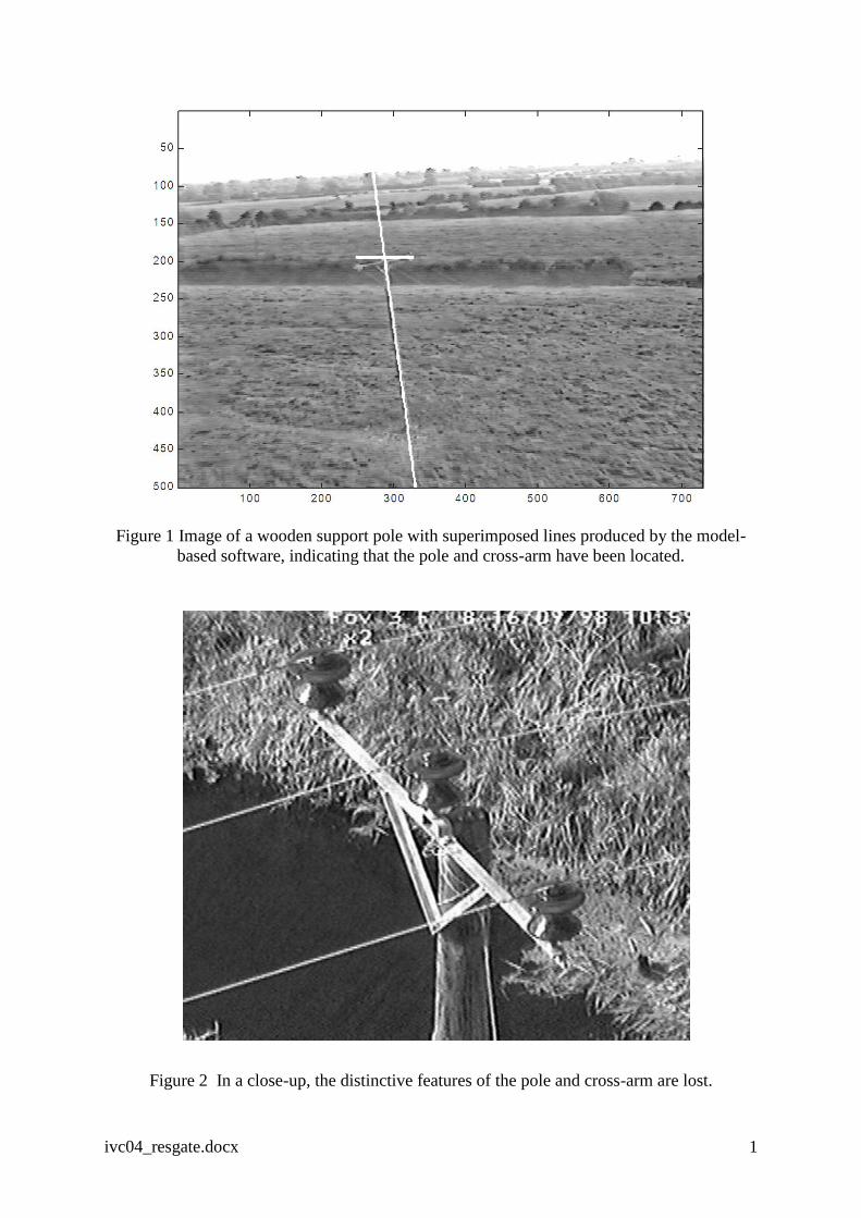
using an algorithm which discriminates for the characteristic features of a pole. Figure 1 is a

typical aerial scene showing a pole and its cross-arm being located; this has been achieved

with a 65 – 92% rate of success on real imagery [24] . Further, provided the camera remains

at a wide field of view, it has been demonstrated (in the laboratory) that closed loop visual

tracking on the pole-top is possible. However, this algorithm has limited resilience to zoom

effects and loses the target as magnification is increased. The problem is that its model-based

ivc04_resgate.docx 2

feature extraction is not zoom-invariant - the target object at high magnification bears little

resemblance to the ‘template’ for a support pole used for object matching, as shown in Figure

2. Similarly, the algorithm is not viewpoint invariant. As the helicopter approaches the post,

the cross-arm rotates in the image and the solution for the point of intersection becomes

increasingly ill-conditioned. When the helicopter is immediately opposite the post, the cross-

arm and post are co-linear. It is concluded that this algorithm is excellent for the initial

acquisition of the target and the early stages of visual servoing but is not suitable for smooth

tracking.

Promising new approaches to tracking while zooming [8], [9], [15] based on affine transfer

have appeared relatively recently. Zoom-invariant methods are described for maintaining

fixation of arbitrary objects using point and line correspondences in affine views, i.e. when

the field of view is small and the variation in depth of the scene along the optical axis is small

compared to its distance from the lens, as is the case in the application considered here. The

low-level processing which underpins these methods is the generation of image trajectories

based on corner detection, a 'corner' being a point at which a 2-dimensional intensity change

occurs in the image. If these methods are to be used, it is essential that corners are detected

and matched which serve as stable, robust beacons in a sequence of images. As a minimum,

any four corner correspondences in three consecutive frames allows the position of the

fixation point to be determined in the third frame, provided its co-ordinates in the first two

frames are known [8]. It should be possible, first, to run the initial acquisition algorithm so

that the pole-top is placed near the centre of the image, then to define the fixation point from

the co-ordinates of two frames in this sequence and thereafter to switch to a corner-based

algorithm for smooth tracking.

Selection of corner detection method

Over the last twenty years, a profusion of corner detectors has been described in the

literature. Notable examples, which new methods often use as a basis for comparison, are

those of Kitchen & Rosenfeld [12], Harris & Stephens [7] (commonly known as the Plessey

detector), Wang & Brady [23] and SUSAN [18]. New corner detection methods continue to

be produced, often with an emphasis on suitability for some method of implementation or

area of application. For instance, Tzionas [22] describes corner detection by means of a

cellular automaton which is specifically intended for VLSI implementation while Quddus &

ivc04_resgate.docx 3

Gabbouj [14] consider a wavelet-based technique for detecting corners at a natural scale in

the image, which is applicable to content-based image retrieval systems. It is desirable to

choose a corner detector which is well matched to the application but this is not

straightforward in view of the wide variety of proposed methods and tests used for

comparison purposes. The corner detector used in this work is due to Cooper, Venkatesh and

Kitchen [4], which was selected because it is claimed to be fast, robust to image noise and

straightforward to program. In particular, results in [4] show that the Cooper, Venkatesh,

Kitchen (CVK) method produces fewer false negative corners than the well-known Kitchen

& Rosenfeld (KR) and Plessey methods, even in the presence of modest or substantial image

noise, as well as being computationally less expensive.

The approach of the CVK detector is first to find contours on the image which have a steep

intensity gradient and then compute a dissimilarity measure for patches taken along the

direction of the contour. If a patch is sufficiently dissimilar to ones on either side then its

centre pixel is deemed to be a corner. The dissimilarity measure itself is due to Barnea and

Silverman [2] and is defined as the sum of the absolute values of intensity differences

between corresponding pixels in the two patches, which is much faster to compute than other

measures such as correlation. During the dissimilarity comparison, additional conditions are

applied which can cause the test to terminate before all pixel differences between the patches

have been accumulated. This ‘early jump-out’ technique reduces the execution time of the

method significantly. Despite its apparent merits, the CVK method does not appear to have

joined the ‘standard list’ of comparators in the literature so it is difficult to compare it with

later methods. However, some indication of its relative performance may be inferred from

work on new corner detection methods available in recent literature, specifically publications

by Trajković and Hedley [21], Bae et al [1] and Shen & Wang [16]. These also provide

useful summaries of previous literature on corner detectors.

The method due to Trajković and Hedley, known as “minimum intensity change” (MIC), is

optimised for fast corner detection and is aimed towards tracking and estimation of structure

from motion. Drawing on the USAN concept, it defines a quadratic corner response function

on a straight line that passes through the USAN nucleus and joins two opposing points on the

periphery of the window that bounds the USAN. It is then observed that, if the nucleus is a

corner point, the variation of image intensity (and hence the response function) will be high

along any such line in the window. Conversely, if the nucleus is within the USAN, there will

ivc04_resgate.docx 4

be at least one line which yields a low response and the nucleus is not a corner point. These

simple rules are used to distinguish rapidly whether a point in the image is a corner or not,

although further tests are required to eliminate false corner responses in the limiting case

where the nucleus is on an edge. The method of Bae et al [1] also uses the USAN concept.

They note that the MIC method is simple and fast but state that it is highly sensitive to noise

and sometimes gives false responses on straight lines. Instead they propose a more complex

method which makes use of two oriented cross operators, which they call “crosses as oriented

pairs” (COP). The COP masks are used to generate the inverted USAN area (defined as the

number of pixels dissimilar to the mask’s nucleus) over a window surrounding the point of

interest. A set of simple rules is then used to link these COP responses to a number of

elementary shapes associated with different types of corner. The method then proceeds to

smooth the responses by ‘resolving’ the components of the elementary shapes determined at

each point in the window into just four dominant directions. Corner candidates must have at

least two dominant directions. Shen & Wang [16] base their method on a definition of a

corner as the intersection of two straight lines. The image is scanned by a window which is

treated as a local co-ordinate system with the central pixel as its origin. Designating the

central pixel to be a corner requires two conditions to be satisfied : (a) it must be an edge

pixel, which is determined by computing the intensity gradient and (b) two straight lines must

pass through it, which is determined by means of a modified Hough transform.

Trajković and Hedley’s broad conclusions are that the localisation accuracy of the Plessey,

Wang-Brady (WB), SUSAN and MIC methods are comparable when tested on a selection of

synthetic and real images. In terms of speed, MIC is clearly superior, being about twice as

fast as the WB and SUSAN detectors and about four times as fast as the Plessey. With respect

to stability, i.e. their capacity to track corresponding corners through a time-sequence of

images, they conclude that the Plessey performs best, the MIC performs well while WB

struggles and SUSAN is inferior. Detection rates and false corner rates are not quantified in

the paper but it is clear from comments in the text that the performance of MIC is comparable

to the other methods in this respect. The results presented by Bae et al show that the

localisation accuracy and stability measure for their COP method are satisfactory but they do

not provide comparisons with other methods on these criteria. A detection rate of 85% is

quoted for COP, compared to 82% for SUSAN, 74% for KR and 67% for Plessey. At 25%,

the false corner rate for COP is better than SUSAN (28%), KR (29%) and Plessey (32%). The

execution rate of COP is determined to be faster than SUSAN and Plessey but slower than

ivc04_resgate.docx 5

KR. Shen & Wang (SW) test their method against WB, SUSAN and Plessey on one synthetic

image and three images of natural scenes with varying amounts of contrast, texture and

rounded or well-defined corners. Their conclusions on localisation accuracy are narrative but

indicate a modest superiority to their method in respect of localisation accuracy, detection

error and false corner rate. This, however, is obtained at the expense of execution speed,

which is about ¼ that of SUSAN and about ⅔ that of WB, although 3 times faster than

Plessey. Tracking stability is not considered.

While the preceding is by no means a systematic evaluation, the principal impression is that

no consistent pattern of superiority is discernible amongst the corner detectors considered.

The results for the COP and SW methods tend to emphasise their advantages with respect to

localisation accuracy and their ability to detect corners other than type ‘L’, but this is not of

primary importance in this application. The detection rates of COP and SW seem to be 10 –

15% better than KR or Plessey but they are slower to compute. On the other hand, CVK has a

lower rate of false corner detection than KR and Plessey and is faster too. MIC is fast and

claimed to be good on all measures but is reported to be susceptible to noise, whereas CVK is

said to be robust to noise. MIC and Plessey have proven qualities of stability whereas

SUSAN and WB are reported in [21] to struggle; no results are available for CVK. In the

absence of a standard set of assessments conducted under controlled conditions and where

different methods may be expected to be optimal for different criteria, the decision to

investigate CVK for this application seems reasonable.

Parameter selection for the CVK method.

The response of the CVK detector is determined by four parameters :

G – the gradient threshold

S – the dissimilarity threshold

L – the size of the image patch used to calculate dissimilarity

D – the distance between successive image patches along a contour

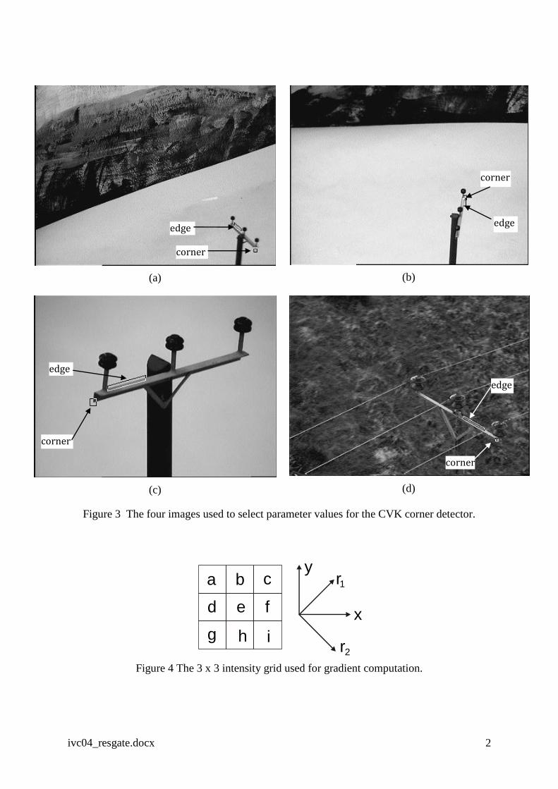
The four 384 x 288 greyscale images shown in Figure 3 were used to determine suitable

value for these parameters. Figure 3(a) - (c) were taken from a laboratory test rig while (d)

was taken during flight trials. Figure 3(a) and (b) show a model pole top against a plain

background with the camera set on wide field of view while (c) shows the same object at

ivc04_resgate.docx 6

higher lens magnification. Each image has two small rectangles superimposed on it, which

define edge and corner areas used as benchmarks during the parameter sensitivity tests.

Gradient threshold (G)

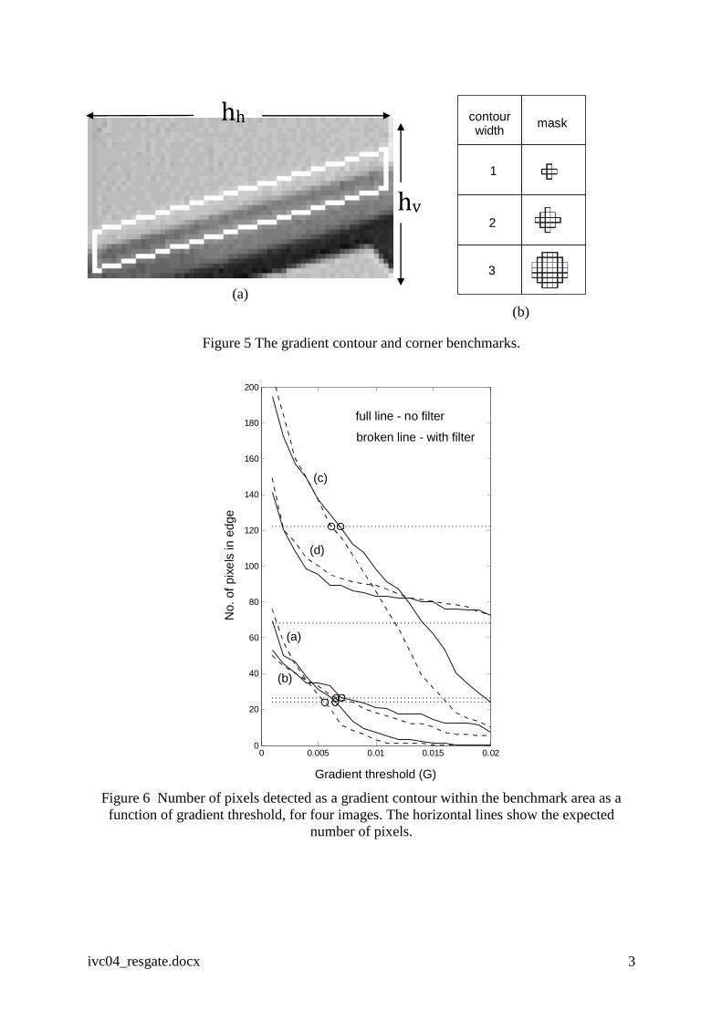
The first stage of the CVK method computes the intensity gradient across the image. Suppose

that the intensities over a 3 x 3 grid are as shown in Figure 4, then the gradient components at

the centre pixel in the 0° and ±45° directions are:

2

df

x

I x

221

1 gc

r

Ir

222

2 ai

r

Ir

(1)

Resolving the diagonal components, the average intensity gradient in the horizontal direction

is:

8844

1

4

1

2

1 21 aigcdf

x

I

x

I

x

I

x

I rrx (2)

Similarly, the average gradient in the vertical direction is:

884

iagchb

y

I (3)

Finally. the gradient is:

22

y

I

x

II (4)

The gradient contour benchmark was set at two pixels thickness so that, as illustrated in

Figure 5a, the expected number of pixels in a portion of edge is 2h, where h = hv if hv > hh or

h = hh if hh > hv. The number of pixels within the benchmark area whose gradient value

exceeded the threshold was determined for 0.001 < G < 0.02. This was done for the four raw

images and for the same images pre-filtered with a 3x3 Gaussian filter of = 0.5; the results

are presented in Figure 6. The intersection of the curves with the expected number of pixels

has been marked and for images (a) – (c) is seen to occur in the range 0.005 < G < 0.008. For

the real image (d), which has a lower edge contrast, the intersection occurs at G > 0.02. The

results exhibit only a slight sensitivity to pre-filtering, possibly because of the averaging

which takes place within the gradient expression (4). For the remainder of the parameter

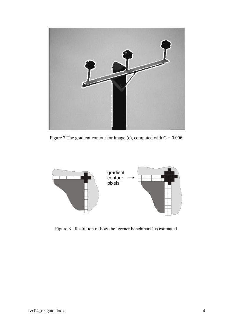
sensitivity tests, the gradient threshold was fixed at G = 0.006 and Figure 7 shows the well-

defined gradient contour obtained when applied to image (c).

ivc04_resgate.docx 7

Dissimilarity threshold (S)

As will be explained in Section 4, the dissimilarity threshold is typically exceeded at several

pixel locations near a corner on the gradient contour. The number of points contained in such

a ‘cluster’ depends in practice on image resolution, image ‘noise’, the size of the detection

window and the thickness of the gradient contour as well as the dissimilarity threshold. The

‘corner benchmark’ acts as a basis for comparison and is an estimate of how many points a

cluster would be expected to contain. The estimate is made by placing a circular mask, whose

radius is the width of the gradient contour (see Figure 5b), at the true corner. The expected

number of pixels in the corner is then defined as the number of contour pixels within the

mask. The principle is illustrated in Figure 8 on an ideal ‘L’ type corner for gradient contours

of width 1 and 2, where the corner benchmark evaluates to 3 and 6 pixels, respectively.

The dissimilarity measure (d) is given by [2]:

2

1

L

pqjk IId (5)

where (j, k) and (p, q) are the centre coordinates of the original and displaced patches of size

L x L and the intensity is normalised to 0 ≤ I ≤1. The number of pixels within the benchmark

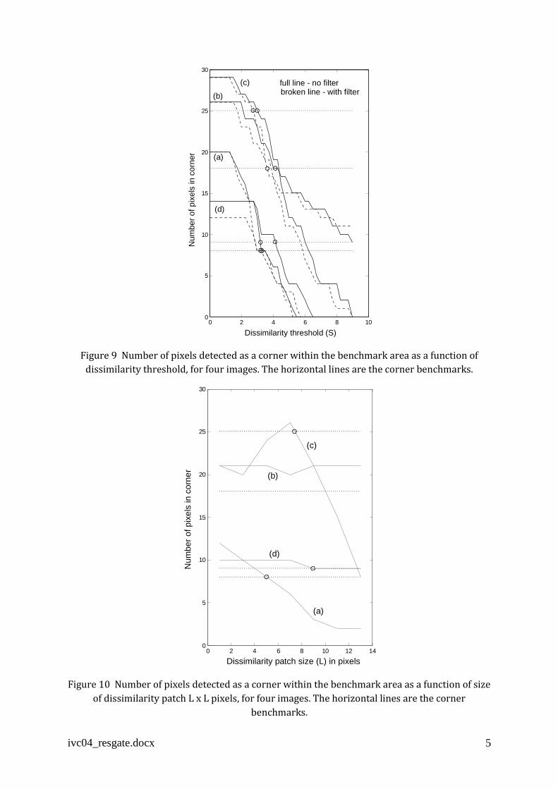
corner areas whose dissimilarity value exceeded the threshold was determined for 0 < S < 9,

for the same set of four raw and pre-filtered images. The result is given in Figure 9 which

shows that the intersections with the corner benchmark values lie in the range 2.7 < S < 4.2

with an average value of S = 3.3. The tests were performed with a dissimilarity patch size of

5 x 5 pixels so the maximum value of dissimilarity for L = 5 is 25 if the pixels in one patch

are all white and in the other are all black. Thus a value of S = 3.3 represents roughly a

dissimilarity of %1325

3.3 . Again, the results are not sensitive to pre-filtering.

Size of dissimilarity patch (L)

The variation of the number of pixels detected as a corner within the benchmark areas was

determined as a function of dissimilarity patch size for the images in Figure 3. The results are

shown in Figure 10. Graphs (b) and (d) exhibit negligible dependence on L and graph (c) has

no clear pattern. Intersections with the corner benchmarks occur at 5, 7.2 and 9. The lowest

value of L = 5 was selected on the pragmatic grounds that it needs least computation.

ivc04_resgate.docx 8

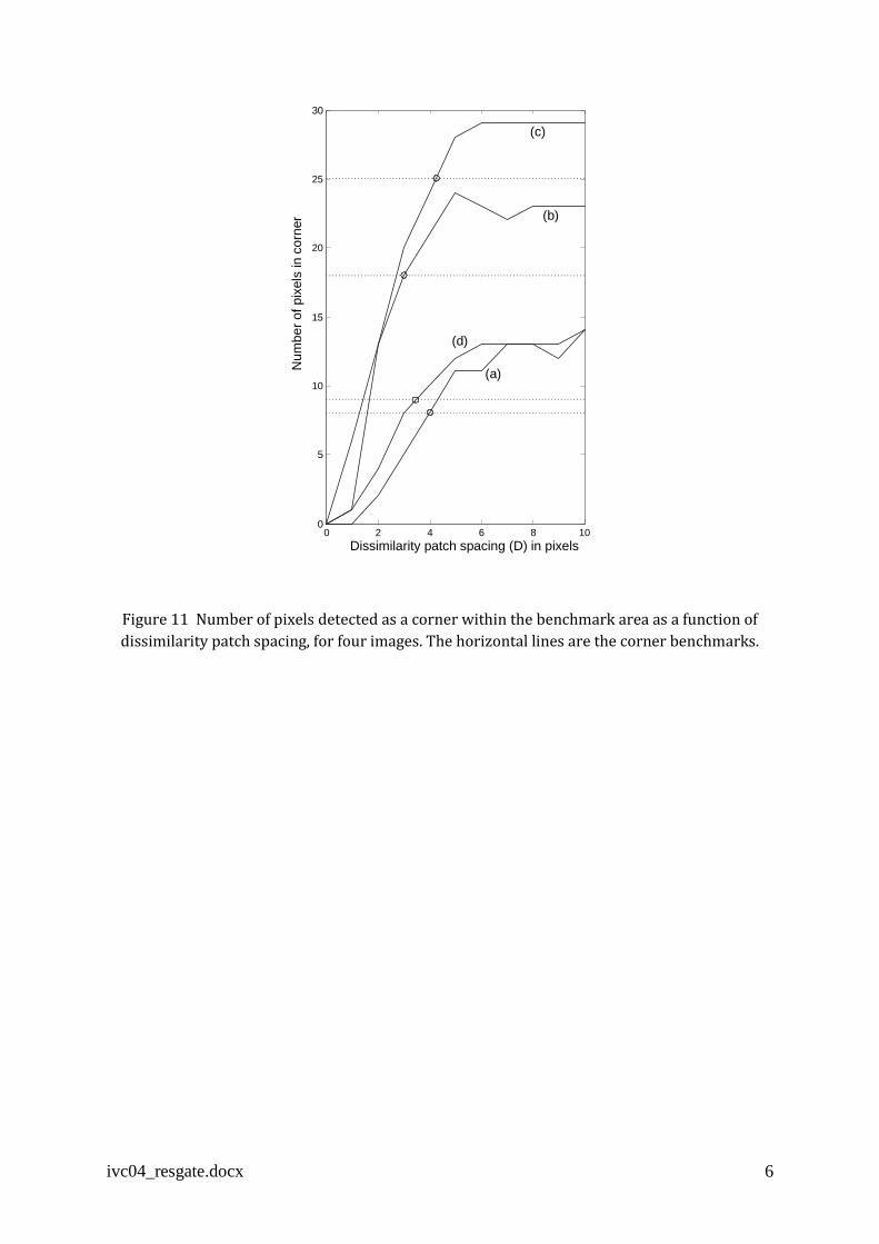
Distance between successive image patches (D)

Finally, the number of pixels detected as a corner within the benchmark areas was determined

as a function of dissimilarity patch spacing and the results are shown in Figure 11. Here, the

intersections with the corner benchmarks are confined to a relatively narrow range 3 < D <

4.2. The nearest integer value is D = 4.

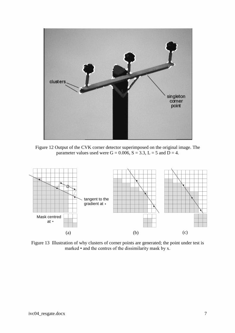
Result of corner detection

A typical corner map produced by the detector with the selected parameter values is shown in

Figure 12 where distinct clusters of ‘corner’ pixels are seen to be associated with the corners

in the physical object. There are also several example of singleton corner points which need

to be removed and this is done by cluster aggregation.

Cluster aggregation and detector performance.

The aggregation method.

The dissimilarity measure of equation (5) is calculated at all points on the gradient contour

and this tends to generate clusters of corner points around a real corner. Why this happens is

explained in the case of an idealised corner in Figure 13. Suppose that, in Figure 13(a), the

pixel marked • is on the gradient contour and generates the dissimilarity mask shown. The

dissimilarity is calculated when the mask is centred at the two points marked x, displaced D

pixels (here D = 4) on either side along the tangent to the contour. For the left hand position,

no pixels differ from the mask while 5 pixels (out of 9) differ at the right hand position. The

detector deems the test point to be a corner if the dissimilarity threshold is exceeded at either

or both positions on the tangent, so this test point is marked as a corner point. Considering the

same procedure applied to Figure 13(b), it is seen that a dissimilarity of 4 pixels is recorded at

both positions on the tangent and the test point is again marked a corner. Similarly, the case

in Figure 13(c) causes pixel differences of 5 and 6 and is marked as a third corner point. In

practice, then, a cluster of corner points surrounds the real corner. Because they are all

associated with the same physical feature, it is sufficient to represent all the corners in a

cluster by a single point, thus improving localisation accuracy and avoiding superfluous

computation at the corner-matching stage. This is done by means of an aggregation

algorithm.

ivc04_resgate.docx 9

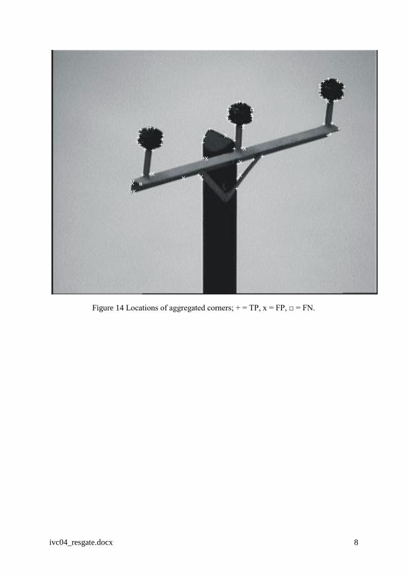
The first stage of the aggregation algorithm removes any singleton corners by applying a

3 x 3 window centred in turn on all the detected corner points in the image. If no adjacent

corner lies within the window, the centre corner is rejected as spurious. The second stage

applies a 5 x 5 window to all the corners belonging to a particular cluster. The number of

corners which lie within each of these windows is counted and the one which contains most

corners is selected as the ‘representative’ window. The average of the co-ordinates of all the

corners in the representative window is then calculated and the pixel location nearest to this

value is taken as the clustered corner point. Because it rejects the influence of corners at the

periphery of the cluster almost entirely, this aggregation procedure selects a representative

point very effectively. It is also quick, because it only takes account of the number of pixels

within a window, not their location.

A typical result following aggregation is shown in Figure 14. The aggregated corner points in

Figure 14b are classified as two types – those detected within a 3 pixel radius of a real corner

are classified true positive (TP) while those detected outside this radius are false positive

(FP). Where there is more than one corner within the 3 pixel radius, only the nearest is

categorised TP and the remainder are FP. Also shown in Figure 14b are points in the image

where a corner exists but has not been detected – these are classified false negative (FN).

Two common indicators of quality are:

Detection rate: FNTP

TPRD

(6)

and

Error rate : FNFPTP

FNFPRF

(7)

For the result in Figure 14 these evaluate to RD = 97% and RF = 18%.

Performance tests.

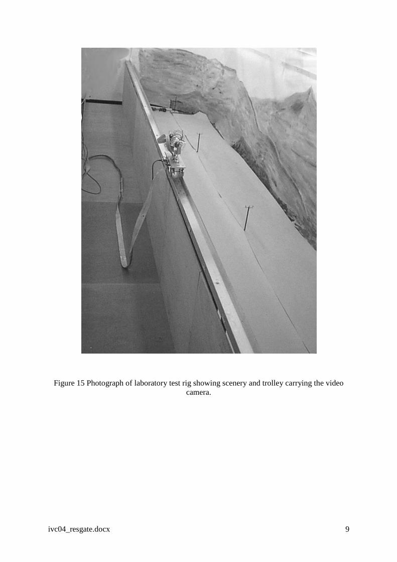
To obtain a broader estimate of the corner detector’s performance, a number of sample

images were produced using the laboratory test rig of Figure 15. The rig consists of a 30:1

scale model of an overhead line set against a painted background. Images are produced by a

Sony colour CCD video camera mounted in an azimuth/elevation gimbal and steered by

precision dc motors. The gimbal is mounted on a wheeled trolley running along an 8m long

track that is located above and to one side of the scenery. This represents the helicopter’s

ivc04_resgate.docx 10

movement. The camera has a built-in 12x optical zoom and its video output is digitised using

a Matrox Meteor frame-grabber. The camera’s 256 bit grey-scale images were normalised to

unity and reduced in size to 384 x 288 pixels; processing was done off-line in Matlab. Figure

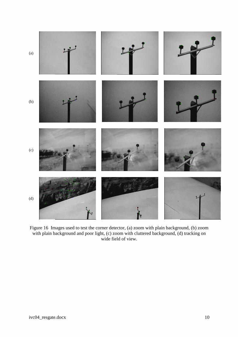
16 shows the 4 sequences, of 3 images each, used for testing the corner detector. Note that, in

sequence (d), the camera sightline was fixed onto the pole-top (using odometric information

and co-ordinate transformation) as the trolley was traversed. This was done in order to

emulate approximately the tracking that would occur during visual servoing. RD and RF were

evaluated for the 12 images and the results are presented in Table 1.

Table 1 Detection and error rates measured for the corner detector.

Image RD(%) RF(%) Mean RD(%) Mean RF(%)

(a) 1 77 35

2 96 20

3 97 18 90 24

(b) 1 86 30

2 87 13

3 91 17 88 20

(c) 1 76 28

2 85 25

3 77 29 80 27

(d) 1 93 11

2 89 14

3 85 27 89 17

Both the detection and error rates compare favourably with those reported by others [1], [16]

although this may be at the expense of some loss in localisation accuracy, which has not been

quantified here. The classification of some FP and FN points requires subjective assessment

but it is estimated that in sequences (a) – (c) no more than 1 FN and 2 FP points have been

wrongly classified. Using these estimates gives bounds of approximately ±2% on RD and

±3% on RF. However, it should be noted that the curved insulators generate many corner

clusters, which have all been recorded as TP (e.g. Figure 14); this tends to give a favourable

ivc04_resgate.docx 11

bias to both the detection and error rates. A small reduction in detection rate is seen as a

consequence of the poorer ambient light in sequence (b) while the background in sequence

(c) causes a substantial reduction in detection rate and an increased error rate. The detection

rate for sequence d(1) is very high because of the large number of corner points generated in

the background, which were all coded TP and this is also true, to some extent, for d(2).

Overall, the results indicate the CVK method with aggregation to be a very satisfactory

corner detector for this application.

Corner Matching

Corner matching methods.

Having established a method for obtaining corners from a single image, the next question is

whether correspondence exists, i.e. can it be established that a corner occurring in two (or

more) successive frames is associated with the same point on a physical object? If so, then it

is the ‘same’ corner and affords information about the motion of the object during the time

interval between the frames. A brief review of work on the motion correspondence problem,

which goes back at least to the mid-1970s, is given by Shapiro [15] who also describes a

specific corner-matching algorithm, a modified version of which is used here. If there are N

and N’ corners respectively in two successive images then there are potentially NN’ pairs to

examine. The motion of objects in the real world is limited by physical laws and corner

matching methods therefore impose corresponding constraints to limit the allowable motion

of corners between images; only a small proportion of the NN’ pairs then have to be

considered. At a basic level, the matching process usually imposes rules such as uniqueness,

which prevents a corner in the first image being matched with two corners in the second, or

similarity which prevents two corners derived from completely different image features being

matched together or maximum velocity which prevents two very distant corners being

matched. Even at this level, a great variety of techniques exist. Smith et al [17], for instance,

cite seven different measures of similarity which could be used (which does not include (5))

and propose the use of a median flow filter as a velocity constraint. Building upon these basic

properties, a wide variety of higher order techniques have been developed which, broadly

speaking, attempt to reduce the computational effort and improve the robustness of the

matcher by embedding more a priori information about the nature of the image into the

algorithm. Model-based tracking introduces knowledge about the expected shape and

ivc04_resgate.docx 12

appearance of the object of interest in the image, generated from a known geometric model

and sometimes including adjustment for the camera’s viewpoint. A recent example of

tracking complex objects in real-time is given by Drummond & Cipolla [6] who project the

edges of a 3 dimensional model of a welded assembly into an image where it is matched with

intensity discontinuities. Another example is the initial acquisition phase for this application,

described in Section 1, which finds the overhead line support pole in an image. An alternative

approach is to avoid a priori object models and instead infer potential objects from distinctive

patterns of point features occurring in the image; Shapiro [15] for instance presents a

technique for grouping points on the basis of their structure and motion. A complementary

strategy (see for example Yao & Chellapa [25]) is to introduce knowledge about the expected

(or assumed) motion of the target object and the ego-motion of the camera. Typically a

dynamic model of the motion is used as the basis for a Kalman filter which is then used to

predict the probable position of a feature point in the next image. The match window can then

be placed at this point. The error between the predicted and measured position of the feature

is then used to update the Kalman filter so that predictions are a function of both the model

and past motion. There are many variations on this theme such as adaptively varying the size

of the match window with the size of the object of interest [3] or taking into account the

quality of an individual feature (which can vary with illumination or contrast) as an indication

of its reliability for analysing object motion [13]. A method which has attracted attention

lately is ‘multiple hypothesis testing’ (MHT) which is used to track multiple objects moving

independently in a scene. Emerging originally from the field of radar signal processing, an

efficient version suitable for vision processing was derived by Cox et al [5]. The problem is

that multiple trajectories for the objects being tracked may intersect leading to ambiguity as

to whether features detected at this point belong to existing trajectories, are new trajectories

or just false alarms. MHT generates different hypotheses, associating the detected points with

the various possibilities and proceeds to test these hypotheses by assigning probabilities to

them, thus resolving the conflict. Recent work extends this principle to track features with

varied motion by admitting multiple motion models [20].

Asserting Occam’s razor, it was decided that a very simple matching method should be used

in the first instance. The targets are fixed and rigid and motion in the image is due only to the

ego-motion of the camera and its zoom. Moreover, a fixation point at or near the target is

maintained by visual servoing. It was also desirable not to obscure the assessment of the

ivc04_resgate.docx 13

corner detector’s stability over an image sequence by employing an over-elaborate matcher,

which is the viewpoint adopted in [21].

Based on the method in [15], corner matching is done in two stages, producing ‘strong’

matches followed by ‘forced’ matches. To search for a strong match, a 41 x 41 pixel window

is centred on a corner in the first frame and all corners lying within the corresponding

window in the second frame are considered to be candidates for a match. Again, the

dissimilarity measure (5) is calculated between the corner in the first frame and each

candidate corner in the second frame using 5 x 5 image patches centred on the corners. The

candidate corner with least dissimilarity is chosen as the ‘best’ matching corner. This

procedure is repeated, working backward from the second frame to the first. A corner where

there is agreement on the best match in both directions is designated a strong match; this

method is known as ‘mutual consent pruning’.

Typically, this leaves corners in frame 1 that are unmatched and these need to be fed forward

into frame 2, the assumption being that they have temporarily disappeared and need the

opportunity to be recovered in future frames. The method for forced matches resembles that

for strong matches and begins by centring an image patch on an unmatched corner in the first

frame. Now, however, all pixels that are not corners within the corresponding area in the

second frame are considered to be candidates for a match. Again, the dissimilarity measure

with the first patch is calculated for patches centred on every candidate point and the one with

least dissimilarity is simply designated a forced corner match. Forced matches have a limited

lifetime and are terminated if a strong match is not recovered. This is done by assigning a

value of unity to all detected corners. A value associated with a forced corner is decremented

by a fixed ‘retirement factor’ at successive frames and any corner whose value falls below a

given threshold (0.5 in this case) is eliminated.

During initial testing of the corner matcher, it was noticed that a significant number of strong

matches occurred to corners in the second frame that were further from the reference corner

in the first frame than the correct match. This occurred at low magnifications in particular. It

was therefore decided to include a simple distance measure in the algorithm in order to

discriminate against matching to far-away corners. The effective dissimilarity measure deff is:

dR

deff

31 (8)

ivc04_resgate.docx 14

where R is the distance between the reference corner and its match candidates. In effect, (8)

places bounds on the expected velocity of corners between frames without resort to a

dynamic target motion model. This eliminated almost all widely-separated false matches.

Corner matching tests

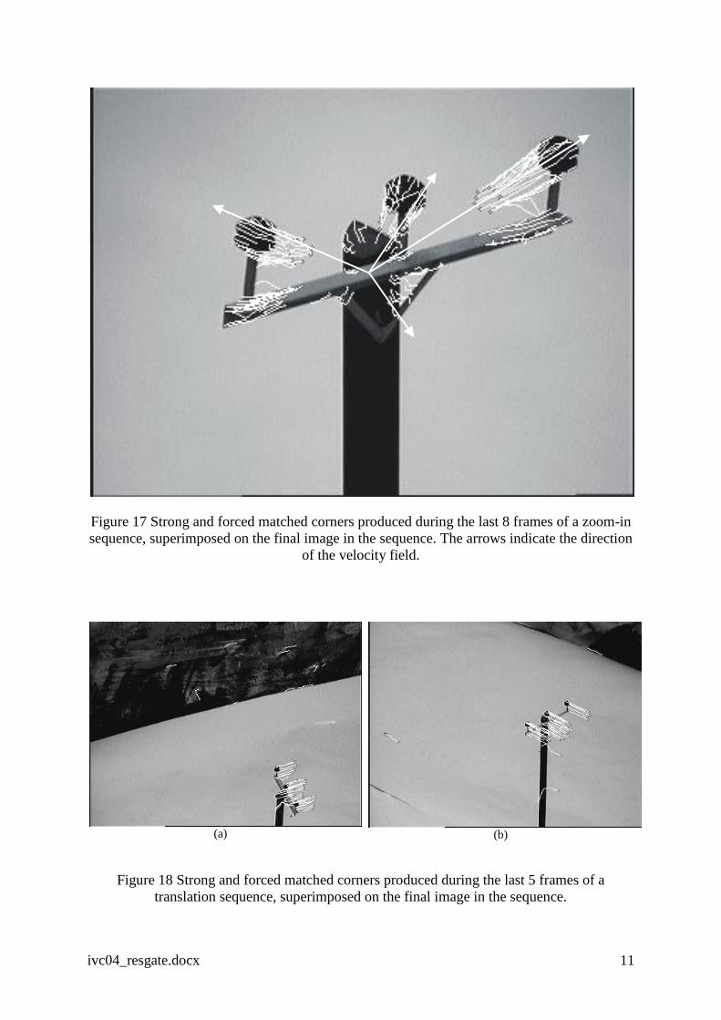
Figure 17 shows both strong and forced matches over the last 8 frames of a sequence where

the camera is zooming in, superimposed on the last frame. The period between frames is

approximately 250ms. The trajectories clearly show the expected form of a divergence field

and the shapes of the cross-arm and insulators are clearly defined by their start points.

Similarly, Figure 18 shows two examples of trajectories produced when the camera is

translating and its focal length is fixed. The post-top is moving from right to left in the image

and the trajectories form slightly convergent straight lines as the size of the target reduces

with increasing distance from the camera.

Trajković and Hedley [21] note that there is no standard procedure for assessing the stability

of corner detectors and therefore propose the following measure:

c

m

N

N (9)

where: Nm = number of corners that are reliably matched over 3 consecutive pairs of frames

in the sequence;

Nc = number of corners in the first frame (of the sequence of 3).

A high value of indicates a corner detector with good stability.

Tissainayagam & Suter [19] also state that there is limited literature on performance analysis

techniques for tracking algorithms for computer vision related applications and that which

does exist is confined to a narrow band of applications. They note two criteria for tracking

performance – the track purity which is the average percentage of correctly associated

corners in each track and the Probability of Correct Association (PCA) which is the

probability, at any given frame, that the tracker will make a correct correspondence of corners

in the presence of clutter. The latter concept is useful for deriving analytical expressions to

predict the performance of trackers with different motion models.

ivc04_resgate.docx 15

Noting that the velocity field for the image sequences considered here is known (a divergent

field in Figure 17 and an uniform field in Figure 18), it is possible to refine the ‘match rate’

(9) by extending the definitions in section 5.1 to include true and false matches, where a true

match (TM) is one whose direction agrees with the local velocity field and a false match

(FM) is one whose direction is contrary to the local velocity field. Accordingly, there are 4

types of match – a Strong True Match (STM), a Strong False Match (SFM), a Forced True

Match (FTM) and a Forced False Match (FFM). The measures of interest are:

Strong match rate FFMFTMSFMSTM

SFMSTMRs

matches ofnumber total

matchesstrongofnumber (10)

True match rate FFMFTMSFMSTM

FTMSTMRT

matches ofnumber total

matches trueofnumber (11)

These measures were calculated for four of the cases shown in Figure 16 and the results are

presented in Table 2.

Table 2 Corner matcher performance.

Case Number of matches Match rates

STM SFM FTM FFM RS (%) RT (%)

A. Fig 16(a)-3 65 3 53 11 52 89

B. Fig 16(b)-3 50 7 38 4 58 89

C. Fig 16(c)-2 26 5 203 89 10 71

D. Fig 16(c)-3 37 2 36 1 52 96

In Case A there is a large number of strong matches into the previous frame, as would be

expected for a well-defined object against a plain background. There is a similar number of

forced matches, most of which are true. This indicates that, whether fed through from the

preceding frame or generated in the second frame, they are consistent with the known image

motion. In this sense they are ‘true’ matches even though a reciprocating match has not been

found in the alternate frame. The number of false matches, indicating corners moving in a

manner that is inconsistent with the known motion, is very small. These comments are

substantially true for Case B too, although fewer corners are detected overall because of the

poorer illumination. In Case C, the amorphous dark area to the left of the pole top is heavily

textured and produces many corners. Rather few of these are classified as strong matches,

leading to a low value of RS. About 1/3 of the forced matches are classified false because the

background produces inconsistent motion. By the next frame (Case D), much of the textured

background has left the scene and RS is restored to a value similar to cases A and B. The

ivc04_resgate.docx 16

STM matches in Case C are almost all associated with the pole top, indicating that the corner

detector is stable and can provide meaningful matches in the presence of clutter, even when

using a basic matching algorithm.

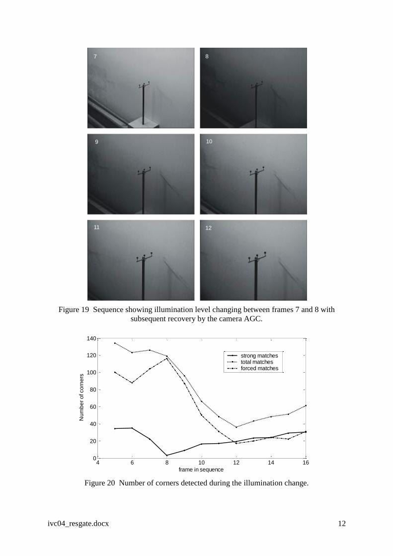
The effect of a sharp change in illumination on stability was investigated by switching off the

laboratory lights during a zoom sequence. Figure 19 shows the 6 frames which include this

event, where the camera’s AGC is seen to restore the average intensity with a time constant

of about ½ second. The number of corners detected during this sequence is shown in Figure

20. Initially, there is a large number of forced corners produced by the textured area in the

bottom left hand corner of the scene which diminishes as the zoom progressively removes it

from the field of view. At frame 8, the number of strong matches reduces sharply and the

forced matches increases correspondingly but they recover their former levels as the AGC

reacts. In operational terms, such a rapid change in illumination would be rare and has not

been observed in several hours of video footage recorded during flight trials. Nevertheless, a

visual servo loop which includes a model for the apparent motion of the target (e.g. observer

or Kalman filter) would probably recover from a brief lapse in the quality of the data,

provided the apparent target velocity is not excessive. Finally, the slow increase in the total

number of corners detected in frames 12-16 of Figure 20 is due to the increasing detail of the

pole top as the lens magnification increases. A better visualisation of how the corner maps

and the set of matched corners change, from one frame to the next, can be obtained from the

short animations available at http://gwefr.co.uk/corner_tracking/cnrdetec.htm.

Conclusions

Through the judicious adoption and modification of known techniques and ideas, a new

corner detection and matching procedure has been derived which is customised to the

application of power line inspection. A brief survey of current literature suggested that no

clear pre-eminence has been established amongst corner detector methods and that the CVK

method has desirable attributes for this application. Before testing this corner detector, its

parameters were carefully chosen by reference to edge and corner benchmarks. It was found

that the method produced clusters of small-scale corner points in the vicinity of a physical

corner and that an aggregation algorithm was necessary to reduce these to single

representative points. Tests showed that the detection and error rates are very good and

comparable with other methods described in the literature.

ivc04_resgate.docx 17

The stability of the CVK detector when used as a corner matcher does not appear to have

been evaluated previously. The detection method was combined with a basic corner matcher

and tests undertaken using typical image sequences for power line inspection, including

camera translation and zoom, changing illumination and background clutter. The results

showed that the method has sound stability properties.

Because the camera mount is dynamically balanced and the ‘jitter’ of the optical axis is

stabilised to approximately 100r [10], the effect of motion blur due to vibration and other

high frequency helicopter motion is small. Although running the gimbal rate controller,

which includes an observer to estimate the apparent velocity of the target in the image, at a

relatively high sample rate of 25Hz helps to maintain smooth tracking, the fixation servo loop

does introduce a small amount of motion blur. On the laboratory test rig, the vision loop is

updated 5 – 10 times per second and some blurring is caused by the rapid sightline

corrections which occur at these times, particularly at the lower update rates. It has been

observed that the corner tracking algorithm can accommodate the loss of contrast over these

relatively short periods but produces fewer strong matches, as found with the experiment on

changing illumination.

Overall, this work has shown that there is an excellent prospect of using corners as robust,

stable beacons to track the movement of a pole top. The next stage of the work is real-time

implementation and testing of the corner detector and matcher, followed by prediction and

affine transfer routines. The method will then be integrated with the overall pole-top tracking

system.

Acknowledgements

The help and encouragement of Mr Graham Earp of EA Technology Ltd and a bursary for Mr

Golightly from the Nuffield Foundation (NUF-URB/00355/G) are gratefully acknowledged.

ivc04_resgate.docx 18

References

[1] S.C. Bae, I.S. Kweon, C.D. Yoo, COP : a new corner detector, Pattern Recognition Lett,

2002, 23, 1349-1360.

[2] D.I. Barnea, H.F. Silverman, A class of algorithms for fast digital image registration,

IEEE Trans Computers, 1972, C-21(2), 179-186.

[3] S. Chien, S. Sung, Adaptive window method with sizing vectors for reliable correlation-

based target tracking., Pattern Recognition, 2000, 33, 237-249.

[4] J. Cooper, S. Venkatesh, L. Kitchen, Early jump-out corner detectors, IEEE Trans Pattern

Analysis & Machine Intelligence, 1993, PAMI-15(8), 823-828.

[5] I.J. Cox, S.L. Hingorani, An efficient implementation of Reid's multiple hypothesis

tracking algorithm and its evaluationfor the purpose of visual tracking., IEEE Trans

Pattern Analysis & Machine Intelligence, 1996, 18(2), 138-150.

[6] T. Drummond, R. Cipolla, Real-time tracking of complex structures with on-line camera

calibration., Image and Vision Computing, 2002, 20, 427-433.

[7] C. Harris, M. Stephens, A combined corner and edge detector, in Proc 4th Alvey Vision

Conf, 1988, 189-192.

[8] E. Hayman, I.E. Reid, D.W. Murray, Zooming while tracking using affine transfer, in

Proc. BMVC'96, 1996, 395-404.

[9] E. Hayman, T. Thorallson, D.W. Murray, Zoom-invariant tracking using points and lines

in affine views, in Proc Int Conf Computer Vision, 1999.

[10] D.I. Jones, Aerial inspection of overhead power lines using video : estimation of image

blurring due to vehicle and camera motion., Proc IEE Vision, Image and Signal

Processing, 2000, 147(2), 157-166.

[11] D.I. Jones, G.K. Earp, Camera sightline pointing requirements for aerial inspection of

overhead power lines, Electric Power Systems Research, 2001, 57(2), 73-82.

[12] L. Kitchen, A. Rosenfeld, Gray level corner detector, Pattern Recognition Lett, 1982, 1,

95-102.

[13] K. Nickels, S. Hutchinson, Estimating uncertainty in SSD-based feature tracking., Image

and Vision Computing, 2002, 20, 47-58.

[14] A. Quddus, M. Gabbouj, Wavelet-based corner detection technique using optimal scale,

Pattern Recognition Lett, 2002, 23, 215-220.

[15] L.S. Shapiro, Affine analysis of image sequences, 1995, Cambridge University Press.

[16] F. Shen, H. Wang, Corner detection based on modified Hough transform, Pattern

Recognition Lett, 2002, 23, 1039-1049.

[17] P. Smith, et al., Effective corner matching, in Proc 9th British Machine Vision

Conference, P.H. Lewis and M.S. Nixon, Editors, 1998, Southampton, 545-556.

[18] S.M. Smith, M. Brady, SUSAN - a new approach to low level image processing, Int Jour

Computer Vision, 1997, 23(1), 45-78.

[19] P. Tissainayagam, D. Suter, Performance prediction analysis of a point feature tracker

based on different motion models., Computer Vision and Image Understanding, 2001, 84,

104-125.

[20] P. Tissainayagam, D. Suter, Visual tracking with automatic motion model switching,

Pattern Recognition, 2001, 34, 641-660.

[21] M. Trajkovic, M. Hedley, Fast corner detection, Image and Vision Computing, 1998, 16,

75-87.

[22] P. Tzionas, A cellular automaton processor for line and corner detection in gray-scale

images, Real-Time Imaging, 2000, 6, 462-470.

[23] H. Wang, M. Brady, Real-time corner detection algorithm for motion estimation, Image

and Vision Computing, 1995, 16, 75-87.

ivc04_resgate.docx 19

[24] C.C. Whitworth, et al., Aerial video inspection of power lines, Power Engineering

Journal, 2001, 15(1), 25-32.

[25] Y. Yao, R. Chellappa, Tracking a dynamic set of feature points., IEEE Trans Image

Processing, 1995, 4(10), 1382-1395.

ivc04_resgate.docx 1

Figure 1 Image of a wooden support pole with superimposed lines produced by the model-

based software, indicating that the pole and cross-arm have been located.

Figure 2 In a close-up, the distinctive features of the pole and cross-arm are lost.

ivc04_resgate.docx 2

(a)

(b)

(c)

(d)

Figure 3 The four images used to select parameter values for the CVK corner detector.

Figure 4 The 3 x 3 intensity grid used for gradient computation.

a b c

d e f

g h i

x

yr1

r2

corner

edge

corner

edge

corner

edge

corner

edge

ivc04_resgate.docx 3

(a)

(b)

Figure 5 The gradient contour and corner benchmarks.

Figure 6 Number of pixels detected as a gradient contour within the benchmark area as a

function of gradient threshold, for four images. The horizontal lines show the expected

number of pixels.

contourwidth

mask

1

2

3

0 0.005 0.01 0.015 0.020

20

40

60

80

100

120

140

160

180

200

Gradient threshold (G)

No. of

pix

els

in e

dge

(c)

(d)

(a)

(b)

full line - no filter

broken line - with filter

hh

hv

ivc04_resgate.docx 4

Figure 7 The gradient contour for image (c), computed with G = 0.006.

Figure 8 Illustration of how the ‘corner benchmark’ is estimated.

gradientcontourpixels

ivc04_resgate.docx 5

Figure 9 Number of pixels detected as a corner within the benchmark area as a function of

dissimilarity threshold, for four images. The horizontal lines are the corner benchmarks.

Figure 10 Number of pixels detected as a corner within the benchmark area as a function of size

of dissimilarity patch L x L pixels, for four images. The horizontal lines are the corner

benchmarks.

0 2 4 6 8 100

5

10

15

20

25

30

Dissimilarity threshold (S)

Num

be

r o

f p

ixe

ls in c

orn

er

full line - no filterbroken line - with filter

(c)

(d)

(b)

(a)

Nu

mb

er

of p

ixe

ls in

co

rne

r

0 2 4 6 8 10 120

5

10

15

20

25

30

Dissimilarity patch size (L) in pixels

14

(d)

(c)

(a)

(b)

ivc04_resgate.docx 6

Figure 11 Number of pixels detected as a corner within the benchmark area as a function of

dissimilarity patch spacing, for four images. The horizontal lines are the corner benchmarks.

Nu

mb

er

of

pix

els

in c

orn

er

Dissimilarity patch spacing (D) in pixels0 2 4 6 8 10

0

5

10

15

20

25

30

(c)

(b)

(d)

(a)

ivc04_resgate.docx 7

Figure 12 Output of the CVK corner detector superimposed on the original image. The

parameter values used were G = 0.006, S = 3.3, L = 5 and D = 4.

(a)

(b)

(c)

Figure 13 Illustration of why clusters of corner points are generated; the point under test is

marked • and the centres of the dissimilarity mask by x.

D

Mask centredat

tangent to thegradient at

ivc04_resgate.docx 8

Figure 14 Locations of aggregated corners; + = TP, x = FP, □ = FN.

x

x

x+

++

++++

+

+++

++

++++++++ ++

+++++

++

+++

++

+

+

+

++

+

++++++

++

+

++++

+

+++++++

++

x

x

x

x

x

x

x

xx

ivc04_resgate.docx 9

Figure 15 Photograph of laboratory test rig showing scenery and trolley carrying the video

camera.

ivc04_resgate.docx 10

(a)

(b)

(c)

(d)

Figure 16 Images used to test the corner detector, (a) zoom with plain background, (b) zoom

with plain background and poor light, (c) zoom with cluttered background, (d) tracking on

wide field of view.

ivc04_resgate.docx 11

Figure 17 Strong and forced matched corners produced during the last 8 frames of a zoom-in

sequence, superimposed on the final image in the sequence. The arrows indicate the direction

of the velocity field.

(a)

(b)

Figure 18 Strong and forced matched corners produced during the last 5 frames of a

translation sequence, superimposed on the final image in the sequence.

ivc04_resgate.docx 12

Figure 19 Sequence showing illumination level changing between frames 7 and 8 with

subsequent recovery by the camera AGC.

Figure 20 Number of corners detected during the illumination change.

7 8

9 10

11 12

4 6 8 10 12 14 160

20

40

60

80

100

120

140

frame in sequence

Nu

mb

er

of co

rne

rs

strong matchestotal matchesforced matches