California’sCOVID-19economicshutdownrevealsthefingerprintofsystemicenvironmentalracism

RichardBluhm1,2+(bluhm@mak.uni-hannover.de)PascalPolonik3+(ppolonik@ucsd.edu)KyleS.Hemes4+(khemes@stanford.edu)LukeC.Sanford2,5+(lcsanford@ucsd.edu)SusanneA.Benz5+(sabenz@ucsd.edu)MorganC.Levy3,5+(mclevy@ucsd.edu)KatharineRicke3,5(kricke@ucsd.edu)JenniferA.Burney5∗(jburney@ucsd.edu)1LeibnizUniversityHannover,Germany2DepartmentofPoliticalScience,UCSanDiego,USA3ScrippsInstitutionofOceanography,UCSanDiego,USA4StanfordWoodsInstitutefortheEnvironment,StanfordUniversity,USA5SchoolofGlobalPolicyandStrategy,UCSanDiego,USA +Theseauthorscontributedequally.∗Communicatingauthor:jburney@ucsd.edu

This paper is a preprint submitted to OSF. It is not yet formally under review, and as such, during the submission and review process, future versions of this manuscript may vary slightly. If accepted, the final version of this manuscript will be linked here. We welcome your feedback.

California’s COVID-19 economic shutdown reveals the fingerprint

of systemic environmental racism

Richard Bluhm1,2+, Pascal Polonik3+, Kyle S. Hemes4+, Luke C. Sanford2,5+, Susanne A.Benz5+, Morgan C. Levy3,5+, Katharine Ricke3,5, Jennifer A. Burney5⇤

1Leibniz University Hannover, Germany2Department of Political Science, UC San Diego, USA3Scripps Institution of Oceanography, UC San Diego, USA4Stanford Woods Institute for the Environment, Stanford University, USA5School of Global Policy and Strategy, UC San Diego, USA

+These authors contributed equally.⇤Communicating author: jburney@ucsd.edu

Abstract: Racial and ethnic minorities in the United States often experience higher-than-average exposures to air pollution. However, the relative contribution of embedded institutionalbiases to these disparities can be di�cult to disentangle from physical environmental drivers,socioeconomic status, and cultural or other factors that are correlated with exposures understatus quo conditions. Over the spring and summer of 2020, rapid and sweeping COVID-19 shelter-in-place orders around the world created large perturbations to local and regionaleconomic activity that resulted in observable changes in air pollution concentrations,compositions, and distributions. Here, we use the pandemic-related emergency order andsubsequent economic slowdown, together with a di↵erences-in-di↵erences approach, to causallyestimate pollution exposure disparities in California. Using both public ground-based sensor dataand a citizen-science network of monitors for respirable particulate matter (PM2.5), along withsatellite records of nitrogen dioxide (NO2), we show that the initial sheltering-in-place periodproduced disproportionate air pollution reduction benefits for Asian, Hispanic/Latinx, and low-income communities. By linking these pollution data with weather, geographic, socioeconomic,and mobility data in di↵erence-in-di↵erences models, we demonstrate that these disparatepollution reductions cannot be explained by environmental conditions, geography, income, orlocal economic activity and are instead driven by non-local activity. This study thus providescausally-identified evidence of systemic racial and ethnic bias in pollution control under business-as-usual conditions.

1

There exist substantial concerns in the United States about the pervasive harms of racism, which1

modern scholarship conceptualizes as either active or passive normalization of racial or ethnic2

inequities (1).⇤ Particularly worrisome is the potential for institutionalized (or systemic) racism –3

in the form of policies, regulations, and norms that favor certain racial or ethnic groups (2) – to4

perpetuate such harm via democratic processes. Rigorous quantitative evidence of institutional5

racism can be di�cult to come by, because the e↵ects of various social and institutional processes6

that embed bias (for example urban planning and environmental regulation) often overlap in7

space and time, and thus stymie attempts at more specific attribution (e.g., (3)). This in turn8

makes policy proposals that address racism head-on more di�cult to justify. This has long been9

the case with “environmental injustice” or the manifestation of systemic racism in environmental10

policymaking and enforcement (4).†11

Disparities in air pollution exposure provide a clear example of this attribution problem (5–7).12

Air pollution is linked to a wide range of negative health consequences (8) and is estimated to13

cause nearly 9 million premature deaths globally per year (9). On average, these health e↵ects14

are not distributed evenly among di↵erent demographic groups (10–13), running counter to15

the notion that society’s environmental burdens should be equally shared (5–7, 14). However,16

despite observable exposure gradients across racial and ethnic groups, causally ascribing such17

inequities to bias in environmental policy has proven di�cult.‡ Economic and other social18

policymaking (e.g., housing, transportation, education) over generations has created the modern19

geography of who lives where. Over time, myriad physical and social confounds (12) – including20

variable atmospheric transport processes (15), economic inequalities (11), and neighborhood21

⇤Here we use racism in the modern descriptive sense that does not hinge on the intent of theperpetrator(s): that is, actions and policies that promote race-based inequities are racist, whether or notsuch an outcome is intended.

†The term environmental injustice is often used more broadly to describe disparities across multipledemographic dimensions, including, but not limited to, race and ethnicity. Here, for clarity, we use thismore specific definition with a primary focus on racism and racial disparities in environmental policy.

‡Here we consider ‘environmental policy’ to be the full landscape of policies, laws, statutes,regulations, and enforcement mechanisms governing environmental quality. This definition includes gaps;that is, existing loopholes, lack of regulation, and non-enforcement of rules are also forms of policy.

2

demographics – have become correlated with present-day pollution exposures. As such, moving22

beyond simple observations of disparate but confounded exposures in contemporary cross-sections23

to causal attribution of environmental injustice thus requires a perturbation to the status24

quo (16). Such a shock to the policy regime was provided by the initial COVID-19 economic25

shutdown in California (17).26

In early 2020, governments implemented unprecedented policies to limit the public health27

impacts of the COVID-19 pandemic (18), including stay-at-home orders and travel limitations,28

with California instituting some of the most aggressive lock-down measures in the U.S. (19).29

The well-known side-e↵ect of these policies was widespread economic slowdown: businesses30

closed, factories shuttered, and employees temporarily discontinued their daily commutes31

(20). Because pollutants like particulate matter (PM2.5) and nitrogen dioxide (NO2) are32

produced by transportation, industrial processes, energy production, and agriculture (21),33

pollutant concentrations tend to track aggregate economic activity (22–24). Thus, the economic34

slowdown corresponded to reductions in satellite and ground station observations of NO2 and35

PM2.5 concentrations, particularly in transportation-heavy metropolitan regions (25–27). This36

period thus provides a baseline for a more equitable distribution of pollutants to which the non-37

shutdown exposures can be compared.38

Here we leverage the shutdowns at the early stages of the COVID-19 pandemic (March-April39

2020) as a natural experiment that partially disentangles the confounding underlying legacy40

of historical social and economic policy from air pollution exposures. Because the COVID-1941

shutdowns generated a large local economic shock, the time period provides a clearer look into42

racial and ethnic disparities in air pollution generation and associated pollution control policies43

that are obscured within the status-quo California economy.§ We employ established statistical44

§California is uniquely well-suited context for this study: it is the fifth largest economy in the world(28, 29); it is one of the most racially and ethnically diverse states in the country (30), and one of only ahandful in which non-Hispanic whites make up less than half the population(31); it is home to four of thetop 20 most populous U.S. cities (32); and despite improvements in air quality in the late 1900s and early2000s (33, 34), several California cities still regularly rank as having the most polluted air in the United

3

di↵erences-in-di↵erence methods to quantify declines in ambient concentrations of two criteria45

pollutants (PM2.5 and NO2) during the economic shutdown, and to test for the existence of46

heterogeneous e↵ects associated with the racial and ethnic composition of neighborhoods. We47

utilize data from a relatively new network of low-cost particulate matter monitors that are48

predominantly privately-owned and deployed outside homes, along with data from state-run air49

quality sensors, satellite measurements, demographic and socioeconomic information, geographic50

data, and cell phone-based location data. By combining these datasets, we disentangle the51

contribution of local conditions (income, mobility, urban geography, weather) to local air52

pollution exposures. Data on mobility – defined as the extent to which individuals spend time53

away from their homes – are particularly important because they characterize variability in the54

shutdown’s e↵ect on the local economic activity of di↵erent communities, as essential worker55

status and economic insecurity are associated with less time spent at home (37, 38).56

We interpret statistically larger reductions in air pollution exposure for select disadvantaged57

racial and ethnic groups, conditional on other confounding factors (e.g., weather, income,58

geography, mobility), as evidence of embedded bias in how the economy generates and59

government controls pollution in the status quo. To our knowledge, this is the first study that60

uses these unique conditions to quantify racial inequities in air quality exposure underlying61

business-as-usual economic activity. Our novel approach also reveals complementary inequities62

in the monitoring of pollution – an insight that highlights a path towards pro-actively addressing63

the identified inequities through air pollution monitoring policy that is itself environmentally64

just.65

States(35). Finally, California citizens live under a historically rich tapestry of environmental regulation –from the Clean Air Act and its amendments at the federal level to local district level rules – that controlair pollution from essentially every source in the state. California also has a long history of environmentalactivism by and on behalf of disadvantaged communities, which have historically experienced higherpollution exposures (36). As such, it is a favorable location for trying to tease apart environmental racismfrom the legacy of economic policy and other confounds that might also lead to disparate environmentalexposures.

4

Results66

We describe our approach to parsing pollution exposure inequities and their local and non-local67

components in a conceptual schematic (Figures 1G and S1). Using daily and weekly pollution68

observations, along with demographic, geographic, and mobility data, we estimate how much69

race and ethnicity alone explain the changes in air pollution exposures experienced during the70

COVID-19 shutdown in California. We account for time-varying (e.g., local mobility, weather,71

seasonality), and relatively static factors (e.g., population density, income, proximity to roads)72

known to contribute to heterogeneous pollution exposure in di↵erent areas.73

Our study area and data are summarized in Figure 1. Aerosol PM2.5 measurements are drawn74

from a network of 826 monitors (106 public monitors from the California Air Resources Board75

(CARB), and 720 privately-owned PurpleAir monitors; Figure S2A), and cover the period76

from Jan 1 to April 30, for both 2019 and 2020 (to facilitate comparison across economic77

conditions at the same time of year). The PurpleAir sensors are low-cost and often privately78

owned; they have been shown to correlate well with research-grade mass-based sensors, though79

they tend to have a high bias, which we have corrected before analysis (see Methods). The80

PM2.5 monitors are located in 746 unique census block groups across California. Satellite-derived81

tropospheric NO2 (Figure 1B) measurements from the TROPOMI instrument cover all 2321282

census block groups of California, but at a ⇠weekly time scale, due to the overpass frequency83

of the Sentinel-5 precursor satellite. Local social, demographic, and geographic characteristics84

(Figure 1C-F), including income and population shares for race and Hispanic/Latinx ethnicity,85

are heterogeneously distributed across the state: for example, income tends to be higher in86

coastal communities and cities, and the southeast and Central Valley regions have higher87

Hispanic/Latinx population shares. Population shares by race are also somewhat spatially88

clustered: Asian population share is highest in Los Angeles and the San Francisco Bay Area, but89

census block groups with larger Black population shares are more widely distributed, especially90

5

in the southern part of the state.¶ This complex human geography demonstrates the importance91

of rich measurement networks in addressing questions of environmental justice: the PurpleAir92

monitors provide a 7-fold increase in the number of sampled census block groups, although this93

increase still only represents 3.2% of all California block groups. (For more detail, please see the94

supplemental information, which includes a detailed mapping toolk.)95

In 2019 (the year prior to the pandemic), without controlling for other sources of heterogeneity,96

areas with lower income and larger Black and Hispanic/Latinx population shares were exposed97

to higher-than-average concentrations of both PM2.5 and NO2 than wealthier and white, non-98

Hispanic communities (for PM2.5 this corresponded to: -1.883 µgm3 for each unit increase in99

ln(median income); 0.065 µgm3 for each percent increase in share Hispanic/Latinx; 0.052 µg

m3 for100

each percent increase in share Black; and no significant trend for share Asian. For NO2 this101

corresponded to: -8.778 µmolm2 for each unit increase in ln(median income); 0.740 µmol

m2 for each102

percent increase in share Hispanic/Latinx; 0.809 µmolm2 for each percent increase in share Black;103

and 0.400 µmolm2 for each percent increase in share Asian) (Figure S4). Such descriptive air quality104

di↵erences have long been noted by environmental justice scholars and advocates (36, 39–45),105

but these relationships are confounded by other contributors to variations in pollution exposure106

(Figure S1). Hence, it is di�cult to separate the relationship of these measures with demographic107

groupings themselves from the social and economic characteristics of these groups, including the108

policies that generated those groupings (e.g., redlining).(46)109

The COVID-19 pandemic temporarily removed a large portion of this confounding economic110

geography by ‘turning o↵’ most economic activity in the state, with some variation in local111

activity across communities, thus facilitating a glimpse into the relative distribution of locally112

versus non-locally generated pollutants. Figure 2 shows the depth and dimensions of this natural113

experiment across the state. The unique response to the spread of COVID-19, including stay-114

¶Hispanic/Latinx ethnicity is tallied independently of other race information in the U.S., and istherefore not mutually exclusive from race (see Methods; Figure S3).

khttps://sabenz.users.earthengine.app/view/covid-ej

6

at-home orders, precipitate a steep decline in the average fraction of the day that people spent115

away from their homes (hereafter, mobility), a decline which took a little under two weeks after116

the state-wide emergency declaration (March 4, 2020) to fully emerge (Figure 2A). Importantly,117

reductions in time away from home did not occur equally for all state residents. Census block118

groups with relatively high Hispanic/Latinx population fractions both had higher baseline119

mobility and much smaller mobility reductions during the shutdown than those with relatively120

low Hispanic/Latinx populations (Figure 2B). This is likely due the greater designation of121

essential jobs and economic vulnerability to Hispanic/Latinx populations, relative to non-122

Hispanic/Latinx populations, that precludes being able to work from home (47). This disparity123

is present, though much less pronounced, for census block groups with high and low Black124

population shares, and the pre- and post- shutdown di↵erences are reversed for high and low125

Asian population shares. We account for these di↵erent responses in the statistical framework126

described below.127

Using a series of statistical di↵erence-in-di↵erences models (see Methods), we estimate the128

relative magnitudes of the reductions in PM2.5 and NO2 concentrations before and after the129

shutdown across di↵erent demographic gradients (we show and discuss PM2.5 results in the130

main text, with NO2 results in the SI, for brevity). The best-fit coe�cients for these models,131

plotted in Figure 3 and Figure S6), correspond to the statistically identifiable expected changes132

in air pollution, across the COVID-19 shutdown window, for either a 0 vs. 100% share of a133

given demographic group at the census block group level or roughly a doubling of non-share134

variables (e.g., income, road density, population density).⇤⇤ These coe�cients show that lower-135

income neighborhoods in California experienced greater reductions in PM2.5 concentration136

(Figure 3A); the positive and statistically significant coe�cient for income indicates that lower137

incomes were strongly associated with more negative shutdown pollutant levels. For example,138

⇤⇤We note that estimating the population average change, on the other hand, would require a strongerstatistical assumption than we make about the similarity of other (i.e. seasonality) conditions in 2019 and2020 (See Methods.)

7

our estimates indicate that a block group with an average income that is half that of a wealthier139

block group would have experienced a -1µg/m3 greater reduction in PM2.5 exposures. Changes140

in mobility, road density, and population density at the level of a census block group are only141

weakly associated with changes in PM2.5 concentrations (Figure 3A).142

We consider mobility to be a proxy for local pollution-causing economic activity, and assume that143

decreased mobility directly corresponded to reduced vehicle emissions along with a suite of local144

business-related emissions (e.g., restaurants were forced to close). Therefore, the relationship145

between the relative decline in local mobility and the relative decline in local air pollution gives146

insight into the pollution impacts of a block group’s own economic activity. Figure 3B shows that147

residents in lower-income neighborhoods reduced their mobility less than richer neighborhoods148

during the shutdown period. Combined with the fact that lower-income areas experienced a149

larger drop in PM2.5 concentrations, this finding suggests that local activity is not the primary150

driver of disparate exposures across the income gradient in California.151

To further probe potential heterogeneity in the magnitude of shutdown impacts, we examine152

exposure changes across neighborhood demographic gradients – with and without accounting153

for various local characteristics (Figure 3C). We identify substantial racial and ethnic disparities154

in air quality improvements, even when accounting for income, road and population density,155

and very fine-grained di↵erences in weather over space and time that strongly a↵ect surface156

pollutant concentrations (see Methods and Supplement). A ten percentage point (pp) increase157

in the Hispanic/Latinx population of a census block group is associated with a -0.28 µg/m3

158

reduction in PM2.5 concentration after the shutdown. This falls to about -0.24 µg/m3 once we159

include local mobility and allow for heterogeneous e↵ects of the shutdown in terms of income,160

road density, and population density (mobility impacts are shown directly in Figure 3D). This is161

evidence of a disproportionate pollution burden experienced by predominantly Hispanic/Latinx162

communities under business-as-usual conditions — only about a seventh of which is explained by163

di↵erences in incomes and other location characteristics. We observe a nearly identical change164

8

of -0.22 µg/m3 in PM2.5 concentration for every ten pp increase in the Asian population of a165

block group after accounting for heterogeneous e↵ects in location characteristics. Di↵erences166

in PM2.5 concentration for Black communities are statistically insignificant across all model167

specifications. This may be due to a smaller Black population share overall (around 7%) and the168

fact that there are relatively few majority Black census block groups in California (Figure 1F).169

These findings are largely consistent with an analogous set of models run using weekly satellite-170

derived NO2 concentrations as the outcome, although some small di↵erences between the two171

reflect both coverage discrepancies and the distributions of PM2.5 and NO2 sources in the state172

(Figure S6).173

Consistent with other research (48–51), we find large di↵erences in mobility across di↵erent174

income and racial groups. Census block groups with high Hispanic/Latinx and Black populations175

had smaller mobility reductions during the shutdown than predominantly white neighborhoods176

(0.8 pp for every 10 pp increase in the population share). However, these di↵erences can be177

completely accounted for by allowing for heterogeneous e↵ects in income. This suggests that178

mobility during the pandemic is mainly a function of the economic ability to stay home and the179

probability of belonging to the essential workforce, rather than other characteristics associated180

with di↵erent neighborhoods. This does not hold for block groups with a greater share of the181

Asian population. Here we estimate a -0.20 pp decrease in mobility for a 10 pp increase in182

the census block group Asian population share. The e↵ect falls to -0.14 pp but remains highly183

significant even after allowing for heterogeneous responses to other block group characteristics.184

Hispanic/Latinx and Asian are the two largest racial and ethnic minority groups in the state,185

making up about 39% and 16% of the population respectively. However, beyond the minority186

designation, these two groups are very di↵erent in their political histories and socioeconomic187

attributes. Asian Californians are predominately concentrated in urban areas and have on188

average higher incomes and education, whereas Hispanic/Latinx populations are more skewed189

towards rural areas, and have on average lower incomes and education.(31) Moreover, as190

9

described above, the two groups had opposite mobility responses to the shutdown. Despite these191

large circumstantial di↵erences, we show that their disproportionate exposure to economy-scale192

pollution is substantially similar, providing strong, albeit indirect, evidence of the influence of193

systemic racism in the mechanisms and institutions responsible for pollution control.194

While our results (Figure 3) show that racial and ethnic disparities in pollutant exposure195

are robust, and not fully explained by local mobility, income, or other characteristics, a196

key remaining concern is sampling bias. Ground-based monitors might be placed in a non-197

representative sub-sample of census block groups, as CARB stations are relatively sparse, and198

PurpleAir monitors are privately purchased and placed. We find that CARB monitor placement199

appears to better represent California’s disadvantaged communities – these public monitors200

are more likely to be placed in poorer, more rural, and more racially and ethnically diverse201

neighborhoods (Figure 4). The PurpleAir network is unsurprisingly slanted towards wealthier202

locations and under-represents the Hispanic/Latinx population of California.203

We therefore derive a set of weightings from these distributions (see Methods and Figure S2B)204

to combine measurements and better represent statewide demographics in unmeasured census205

block groups; we use these weightings in our main estimates (i.e. Figure 3). We also re-estimate206

impacts using several subsets of census block groups, including only CARB monitors, only207

PurpleAir monitors, and both networks combined with and without weighting (Figure 4). The208

significant racial disparities calculated from our weighted sample are consistent with most209

estimates from the unweighted samples (Figure 4). The CARB-only estimates have much larger210

uncertainties, due in part to the vastly smaller sample size. The bias towards more rural areas in211

the state’s CARB network manifests in larger magnitude estimates for the role of population and212

road densities in determining air pollution disparities.213

10

Discussion214

Here we provide new causal estimates of inequality in air pollution exposure and identify a215

unique fingerprint of systemic racial and ethnic bias in environmental policy in the status quo216

generation and control of pollutants in the California economy. While this finding is robust217

to various specifications and data subsets, and consistent across surface- and satellite-based218

data, our analysis nevertheless requires some contextualization, and care in interpretation.219

Importantly, while we note that exposure disparities are not explained by local mobility, the220

ability to fully distinguish local and non-local economic activity is limited; representative221

spatial scales of local versus non-local may vary (e.g., geographically, culturally, seasonally).222

We additionally note that while we focus on the non-local drivers of exposure disparities, local223

mobility-related pollution generation may nevertheless be caused by structurally unjust policy224

in other sectors (e.g., housing, transportation). More broadly, it is important to recognize that225

contemporary and historical biases in other policy areas can lead to disparate average exposures,226

even if environmental policy were unbiased. This may be what explains our finding of higher227

average pollution exposures, but no disproportionate air quality benefit from the COVID-19228

shutdowns for Black communities in California.229

We also consistently identified that lower income communities in the state are disproportionately230

a↵ected by economy-scale pollution. While income is primarily employed as a control in our231

analysis, this income disparity presents an important environmental justice concern in and of232

itself, and presents policy challenges that are unique from those associated with combating233

institutional racism. California has one of the highest rankings for income inequality among U.S.234

states (31), and our findings provide additional evidence both that wealthier communities are235

able to both buy environmental quality (i.e., higher housing prices embed air quality) and can236

a↵ord to stay at home more fully during a pandemic.237

Our analysis reveals not only disparities in pollution exposure, but inequality in local air238

11

pollution information itself. Because air pollution monitoring networks are sparse, researchers239

have increasingly used Chemical Transport Models (CTMs) to model pollutant exposures and240

map them to local socio-economic and demographic characteristics. While CTMs have become241

ever more powerful and accurate, they require accurate emissions inventories as inputs; although242

rapidly improving for long-lived greenhouse gases (e.g., (52)), such inventories for air pollution,243

unfortunately, are notoriously uncertain over short time scales and under abnormal economic244

conditions.(53) Statistical studies like ours also have shortcomings: while they draw on high-245

frequency data of actual ground-level (or atmospheric column) pollution and thus avoid the need246

for emissions inventories, they nevertheless require accurate and unbiased characterization of247

the system under study. While we do not explicitly account for point source emissions or wind248

in this study, we use areal road density summaries (see Methods), and detailed temperature,249

precipitation, and relative humidity controls (see Figure S7), which should capture much of250

this variation. Additionally, because our analysis focuses on di↵erences in the same block group251

over time, the average influences of these and other unobserved factors are taken into account.252

Still, we cannot rule out that some of our measured e↵ects may be driven by either variations253

in emissions or meteorological conditions that are correlated with both the demographic254

characteristics of a neighborhood and the COVID-related shutdown. Future studies could focus255

on more thoroughly accounting for natural seasonal swings in air pollution and the full range256

of its spatial and temporal variability through the inclusion of more years of data.(17) This was257

not possible here due to the short timescale of PurpleAir data availability. Nevertheless, our use258

of 2019 as a comparison for 2020, and similar estimates made with pre and post-shutdown 2020259

data alone (see Table S1), underscore that the exposure disparities we estimate are not likely to260

be systematically changed by inclusion of more years of observations.261

These findings have important implications for air pollution measurement strategies to address262

environmental injustice. As we show, monitor placement matters for detection of disparate263

exposures. CARB recently re-focused air quality monitoring in designated environmental justice264

12

communities (54), and its monitor placement has resulted in a more accurate sample of the265

state’s Hispanic/Latinx population distribution than (e.g.) PurpleAir. The PurpleAir monitoring266

network, established through the individual purchase and placement of (relatively) low-cost267

sensors, shows both that citizen science networks can be exceedingly useful for increasing the268

amount of public data, but that those networks are unlikely to be optimally placed for addressing269

environmental justice questions, nor do they accurately reflect the spatial distribution of di↵erent270

sub-populations. PurpleAir sensors also require care in correcting biases compared to monitoring-271

grade instruments (55). On the public monitoring side, local governments that are responsible for272

choosing locations of sensors mandated by the Clean Air Act (i.e. CARB) may also strategically273

place sensors to improve their chances of being in attainment (56, 57). This strategic placement274

reduces the ability of those sensor networks to detect environmental injustice (58) and makes275

adjustments for sampling bias, like those proposed here, relevant for the larger literature. Lastly,276

while we show that satellite-based observations can be helpful in understanding the spatial277

distribution of pollutants that underlies ground-based monitoring network samples, satellite data278

are spatially coarse compared to the average census block group, and are limited temporally.279

As such, satellites may not be able to replace ground-based monitoring when high spatial and280

temporal resolution are required. While a more spatially dense ground measurement network281

would vastly improve the ability to detect and address environmental injustice, reliability, cost,282

distribution, and data curation would need to be considered in choosing a scale-up strategy283

(59, 60). Our weighting approach can be used to leverage all available (high quality) ground284

sensors, no matter which placement mechanism is driving their spatial distribution.285

The use of California as a study region makes interpretation of our results more straightforward286

than might be the case in other regions, or over a larger region. First, California’s mild climate287

and predictable seasonality makes it easier to compare two years of observations than would be288

the case in more variable climates. Second, the lack of coal and fuel heating oil use in California289

means that the regional (anthropogenic) aerosol chemistry is relatively simple – California’s290

13

PM2.5 includes primary carbonaceous aerosols produced by transportation, and secondary291

nitrates produced by transportation and agriculture (61). There are relatively few other primary292

sources of particulate matter in California compared to other regions, particularly outside of293

the state’s summer-fall wildfire season, which contributes a large organic carbon burden to the294

region (62). Our study location and timing also mean that satellite-based NO2 observations295

are more highly correlated with PM2.5 than they would be in other locations, because the same296

emissions sources contribute to both in the state (predominantly transportation and agriculture).297

Studies in more complicated climates, and with a more diverse set of aerosol particulate matter298

(and precursor) emissions will potentially require more sophisticated statistical techniques to299

address potential unobserved sources of heterogeneity and to assess whether changes in pollution300

chemical composition di↵er across population subgroups.301

Our analysis demonstrates that the generation and control of pollution from California’s302

economy-at-large disproportionately a↵ect the state’s largest racial and ethnic minority303

communities. Our unconditional finding of disparate shutdown-related decreases for Asian and304

Hispanic/Latinx communities is evidence of environmental racism, even if it were entirely driven305

by income di↵erences. However, when we take a more narrow definition of racism and partial306

out the impacts of many other variables like income, we still find the same or stronger e↵ects.307

While this complicates their interpretation, it makes clear that these groups are environmentally308

disadvantaged through environmental policy failures, beyond what we would expect on the basis309

of income, roads, weather, etc.310

This has several implications for potential policy responses. Many state and federal regulatory311

impact analyses mandate assessment of impacts to disadvantaged and vulnerable groups312

(e.g., (63, 64)). While this sets a clear precedent for including analysis of the distribution of313

regulatory impacts across socioeconomic groups, best practices for quantitative distributional314

analysis are not codified to the extent of those for (e.g.) benefit-cost analysis typically used315

in environmental regulation (65). Furthermore, there is no standard assessment criterion for316

14

justifying interventions to mitigate inequities (e.g., placement of air pollution monitoring that317

addresses racial disparities) along the lines of the net benefit criterion (the simple objective that318

regulatory benefits exceed costs). If racial equity is a matter of concern for decision makers,319

future revisions to regulatory impact analysis mandates should include protocols with provisions320

for clear, quantitative standards for equity in regulation and analytical practices for evaluating321

progress. Finally, we note that public policy interventions are considered most e↵ective when322

targeted to address a known market failure, and many tools of environmental regulation focus on323

e�ciently reducing these failures. However, when systemic bias is driving adverse outcomes, in324

the absence of amelioration of the unequal representation in political institutions, public policy325

intervention focused narrowly on addressing market failures may eventually result in reversion to326

inequality.(66)327

15

Data and Methods328

Data329

PM2.5 Data: Surface station measurements of particulate matter with diameter smaller than330

2.5 µm (PM2.5) were downloaded from publicly available databases from PurpleAir and the331

California Air Resources Board (CARB) (Figure S8). We downloaded all outdoor PurpleAir332

data available (1891 individual stations) for Jan-Apr 2019 and 2020. PurpleAir sensors are333

relatively inexpensive and are usually privately owned, but much of the data is publicly available.334

The quality of these data are lower than data from regulatory monitors, but PurpleAir sensors335

provide unprecedented spatial coverage. Most PurpleAir sensors contain two Particulate Matter336

Sensor (PMS) 5003 sensors (Plantower, Beijing, China), which measure particle counts in 6337

size bins. Counts are converted to PM2.5 using two proprietary conversions, one intended for338

indoor use and the other for outdoor use; here we use the outdoor conversion as recommended339

and tested by Tryner et al. (2020) (67). We also average the two sensors (when available) and340

exclude days when daily PM2.5 measurements within the same unit di↵er by at least 5 µm m�3341

and at least 16% (55). In limited field evaluations, PurpleAir sensors have been shown to have342

strong correlations with high-quality sensors (67–70)). Tryner et al. also proposed a correction343

for e↵ects of relative humidity, which we do not apply in part because we consider daily data344

rather than sub-daily. We do, however, apply an correction developed by the EPA, which tends345

to slightly over-correct the high bias of the PurpleAir instruments, meaning the presented results346

from these sensors are conservative (Figure S9) (55).347

We downloaded (May 1, 2020) all hourly CARB PM2.5 data in California available for Jan-Apr348

2019 and 2020 using CARB’s Air Quality and Meteorological Information System (AQMIS),349

and calculated the daily mean (150 individual stations). Professional instruments and oversight,350

particularly for calibration, provide higher confidence in the data quality of the CARB sites.351

However, there are an order of magnitude fewer CARB stations than PurpleAir sensors in352

16

California, which means studies using the government data are statistically limited by a relatively353

small sample size. Unlike PurpleAir sensors, CARB sites often o↵er a wide variety of air354

pollutant measurements, though we only use hourly PM2.5 aggregated to the daily mean. For355

both CARB and PurpleAir data, days with mean PM2.5 equal to zero or greater than 500 µg356

m�3 are removed as outliers. Sites for which we remove more than 10% of data are excluded357

from the entire analysis. Sites with less than 80% data coverage during our study period are358

also excluded. For models that require 2019 and 2020 data, we apply these requirements to both359

years independently. This quality filtering removed 5.9% of daily CARB PM2.5 data, and 11.4%360

of daily PurpleAir data resulting in data from 1664 individual stations (119 CARB and 1545361

Purple Air). However, only 826 of those (106 CARB and 720 PurpleAir) include data for 2019362

and 2020 for the pre-shutdown and shutdown period, and were therefore used in our empirical363

statistical analysis.364

NO2 Data: We used the Copernicus Sentinel-5 Precursor TROPOspheric Monitoring365

Instrument (TROPOMI) O✏ine tropospheric NO2 column number density (71) for mean366

NO2 concentrations of the developed areas of each census block group. TROPOMI has a367

resolution of 0.01 arc degrees. Data were collected for Jan-Apr 2019 and 2020 and only for368

developed areas based on the U.S. Geological Survey (USGS) National Land Cover Database369

(NLCD) 2016 (72). For this study, all data was prepared using the Google Earth Engine Python370

API (73) and formatted as weekly means for each census block group. Weekly means were chosen371

to counteract the high frequency of missing data, particularly in northern California (Figure372

S10).373

Climate Data: To gather information on temperature, precipitation, and relative humidity374

we relied on the Gridded Surface Meteorological dataset (GridMet) (74). GridMet provides375

daily information in a 4-km resolution across the continental USA. For this study, data376

were aggregated in Google Earth Engine (73) in its original daily frequency for each377

PM2.5 measurement station, and as a weekly mean for the NO2-Data for each census block378

17

group. The weekly mean data was only collected for developed areas based on the U.S.379

Geological Survey (USGS) National Land Cover Database (NLCD) 2016 (72).380

Mobility Data: We use SafeGraph’s Social Distancing Metrics, which were made available381

for research as part of the company’s COVID-19 response. SafeGraph collects and cleans GPS382

pings from about 45 million mobile devices. The data are available daily at census block group383

resolution and are close to a random sample of the population. Our primary measure of mobility,384

not social distancing, is the percent of time spent away from home. We calculate this measure385

based on the median time (in minutes) that a device was observed at its geohash-7 (about386

153 m ⇥ 153 m) home location, which SafeGraph determines as the night time residence of the387

device in the 6-weeks prior. The data cover the entire period of observation from Jan 1, 2019388

until the end of April 2020.389

Demographic Data: We downloaded census block groups level demographic information390

from the U.S. Census Bureau 2018 5-year American Community Survey (ACS) for all CBGs391

in California using the tidycensus package (75) for the R programming environment (76)392

(June 29, 2020). Demographic features included ACS sample-based CBG-level estimates of:393

population count; white race count (alone or in combination with one or more other races), or394

“white”; Black or African American race count (alone or in combination with one or more other395

races), or “Black”; Asian race count (alone or in combination with one or more other races),396

or “Asian”; Hispanic or Latino origin (of any race) count, or “Hispanic/Latinx”; and median397

income. Other race and ethnic groups represent a substantially lower share of the California398

population, and were therefore excluded from our analysis due to small sample sizes. The CBG-399

level “share” of these groups was calculated by dividing the CBG count by the CBG population.400

Population density was calculated as the CBG population divided by the area of the CBG.401

Because Hispanic/Latinx is a separate designation from race in the ACS (i.e., those categorized402

as Hispanic/Latinx may also be of any race), we evaluated how distinct Hispanic/Latinx was403

from race variables of interest (Figure S3). On average, less than 1% of those identified at the404

18

CBG level as Hispanic/Latinx were also identified as Black or Asian; 61% of Hispanic/Latinx405

were White. Thus, Hispanic/Latinx is e↵ectively distinct from Asian and Black categorizations,406

and we consider Hispanic/Latinx, Asian, and Black designations to be unique demographic407

indicators in our model.408

Geographic Data: We calculated road density (m / km2) using The Global Roads409

Inventory Project (GRIP4) (77) vector dataset for North America, downloaded at410

https://www.globio.info/download-grip-dataset (April 4, 2020). The GRIP4 dataset harmonizes411

global geospatial datasets on road infrastructure, including road features that can be categorized412

as highways, primary roads, secondary roads, tertiary roads and local roads. It is consistent with413

primary and secondary road classifications from the U.S. Census TIGER/Line shapefiles for414

roads. To calculate road density for each CBG, we summed road lengths within the area of the415

CBG, and divided by the area of the CBG. Calculations were done using the sf package (78) in416

the R programming environment (76).417

Methods418

Study period: We consider three periods between Jan 1 and April 30 in 2019 and 2020. The419

first period is “pre-shutdown,” followed by a “transition,” and then “shutdown.” The transition420

is defined as the period between the state-wide emergency declaration (March 4, 2020) and the421

state-wide stay-at-home order (March 19, 2020). The mobility data demonstrate that activity422

declined throughout this period (Figure 2). This is consistent with recent literature which shows423

that fear was a potent driver of the decline in mobility and often preempted county-wide legal424

restrictions (79). The shutdown period begins with the stay-at-home order and ends at the end425

of our study period. We exclude the transition from the model analyses described below.426

Empirical Strategy: In our statistical analyses, our main dependent variable is an (average)427

measure of air quality (PM2.5 or NO2) in census block group i at day (or week) t. We focus428

19

on block groups to minimize the influence of aggregation bias or the “ecological fallacy”429

(80) and study temporal variation in air quality across block groups using a di↵erences-in-430

di↵erences design. Di↵erences-in-di↵erences methods are commonly used to study causal431

e↵ects in economics (81). Our objective is to estimate the heterogeneity in the e↵ect of the432

shutdown across di↵erent communities, rather than the overall e↵ect of the shutdown. We433

focus on the racial composition of California’s three biggest racial and ethnic minority groups434

(Hispanic/Latinx, Asian,and Black) to first establish the existence of an air pollution exposure435

inequity and then include observed characteristics of minority populations to document the racial436

inequities that remain after accounting for di↵erences in mobility, income and location (82).437

A key concern is that di↵erences in air quality are driven by interannual cycles in pollution438

and particle concentration unrelated to the shutdown. We address this issue in several ways.439

First, we subtract observed air quality in 2019 from the 2020 value. All annual di↵erences, after440

aligning the weekdays, are denoted by yit = yit � yi,t�364. Second, we flexibly control for local441

weather conditions in 2020 and 2019. Finally, we allow for a rich set of day or week fixed-e↵ects442

which capture the remaining di↵erences in synoptic scale weather patterns. We estimate the443

heterogeneous e↵ect of the shutdown using variants of the following specification444

yit =KX

k=1

�k

⇣dt ⇥ x

ki

⌘+ ✓Mit + f

2020 (T,RH,P )it + f2019 (T,RH,P )it + �t + µi + eit (1)

where dt is an indicator for the post-shutdown period, xki are the population shares of the three445

minority groups or other time-invariant location characteristics at the census block group level,446

Mit is the annual di↵erence in mobility, f2020 (·)it and f2019 (·)it approximate the non-linear447

response of pollution and particle concentration to weather with interacted fixed e↵ects for each448

decile of temperature, relative humidity and precipitation in the corresponding year, �t are day449

(or week) fixed e↵ects, µi are census block group fixed e↵ects (capturing changes in the number450

20

of stations in a block group across years), and eit is an error term. We cluster all standard errors451

on the county level, as stay-at-home and local health ordinances are spatially and temporally452

correlated at this level.453

We are interested in �k which captures the heterogeneous impact of the shutdown across di↵erent454

demographic gradients (see SI text for a derivation). The baseline e↵ect of the shutdown, dt,455

is not statistically identified without the assumption constant seasonal emissions patterns, as456

that baseline e↵ect occurs simultaneously for all block groups in California and is therefore457

collinear with seasonal shifts in air quality that are unrelated to the COVID-19 shutdowns.458

Heterogeneous impacts are identified by variation among block groups experiencing a COVID-19459

shutdown-related air pollution change only, and can be interpreted as the e↵ect of the shutdown460

relative to some baseline. This requires a weaker assumption: that the inter-annual di↵erences461

in pollution are not simultaneously correlated with the timing of the shutdown and the spatial462

distribution of race and income. Our weather controls make this a plausible assumption by463

accounting for systematic di↵erences in temperature, humidity, and rainfall across di↵erent464

parts of the state. We interpret the coe�cient on dt ⇥ % Hispanic/Latinx as the di↵erence in465

PM2.5 concentration for a block group which is 100% Hispanic/Latinx, relative to a block group466

which is 0% Hispanic/Latinx. Di↵erences in air pollution concentrations across the shutdown467

window are typically reductions in air pollution, which we consider to be equivalent to the468

expected increase after a return to “business-as-usual” conditions.469

Software: All data processing and analysis other than acquisition, and pre-processing of470

mobility information was done using the R programming environment (76) and the python API471

for Google Earth Engine (73).472

21

Acknowledgments473

S.A.B. is supported by the Big Pixel Initiative at UC San Diego, J.A.B., M.C.L., and S.A.B.474

are supported by NSF/USDA NIFA INFEWS T1 #1619318; J.A.B. and P.P. are supported by475

NSF CNH-L #1715557. R.B. is supported by the Alexander von Humboldt Foundation. K.S.H is476

supported by the Stanford Woods Institute for the Environment.477

Author Contributions478

K.S.H., P.P., J.A.B., M.C.L, S.A.B., L.C.S., R.B. designed study. S.A.B., M.C.L., K.S.H., P.P.,479

and R.B. prepared data and code for analyses; R.B. and L.C.S. ran statistical models. All480

authors interpreted results, prepared figures, wrote, and edited the manuscript together.481

References482

[1] Ibram X Kendi. How to be an antiracist. One world, 2019.483

[2] Joe Feagin. Systemic racism: A theory of oppression. Routledge, 2013.484

[3] Nancy Krieger, Gretchen Van Wye, Mary Huynh, Pamela D Waterman, Gil Maduro,485

Wenhui Li, R Charon Gwynn, Oxiris Barbot, and Mary T Bassett. Structural racism,486

historical redlining, and risk of preterm birth in new york city, 2013–2017. American Journal487

of Public Health, (0):e1–e8, 2020.488

[4] David N Pellow. Environmental inequality formation: Toward a theory of environmental489

injustice. American behavioral scientist, 43(4):581–601, 2000.490

[5] Robert D Bullard. The legacy of american apartheid and environmental racism. . John’s J.491

Legal Comment., 9:445, 1993.492

[6] Robert J. Brulle and David N. Pellow. Environmental Justice: Human Health and493

Environmental Inequalities. Annual Review of Public Health, 27(1):103–124, 2006.494

[7] Spencer Banzhaf, Lala Ma, and Christopher Timmins. Environmental justice: The495

economics of race, place, and pollution. Journal of Economic Perspectives, 33(1):185–208,496

February 2019.497

22

[8] Gerard Hoek, Ranjini M. Krishnan, Rob Beelen, Annette Peters, Bart Ostro, Bert498

Brunekreef, and Joel D. Kaufman. Long-term air pollution exposure and cardio- respiratory499

mortality: a review. Environmental Health, 12(1):43, May 2013.500

[9] Richard Burnett, Hong Chen, Mieczys law Szyszkowicz, Neal Fann, Bryan Hubbell, C Arden501

Pope, Joshua S Apte, Michael Brauer, Aaron Cohen, Scott Weichenthal, et al. Global502

estimates of mortality associated with long-term exposure to outdoor fine particulate503

matter. Proceedings of the National Academy of Sciences, 115(38):9592–9597, 2018.504

[10] Michael Jerrett. Global Geographies of Injustice in Tra�c-Related Air Pollution Exposure.505

Epidemiology, 20(2):231–233, March 2009.506

[11] Anthony Nardone, Joan A. Casey, Rachel Morello-Frosch, Mahasin Mujahid, John R.507

Balmes, and Neeta Thakur. Associations between historical residential redlining and current508

age-adjusted rates of emergency department visits due to asthma across eight cities in509

California: an ecological study. The Lancet Planetary Health, 4(1):e24–e31, January 2020.510

[12] Christopher W. Tessum, Joshua S. Apte, Andrew L. Goodkind, Nicholas Z. Muller,511

Kimberley A. Mullins, David A. Paolella, Stephen Polasky, Nathaniel P. Springer, Sumil K.512

Thakrar, Julian D. Marshall, and Jason D. Hill. Inequity in consumption of goods and513

services adds to racial–ethnic disparities in air pollution exposure. Proceedings of the514

National Academy of Sciences, 116(13):6001–6006, March 2019.515

[13] Ihab Mikati, Adam F. Benson, Thomas J. Luben, Jason D. Sacks, and Jennifer Richmond-516

Bryant. Disparities in Distribution of Particulate Matter Emission Sources by Race and517

Poverty Status. American Journal of Public Health, 108(4):480–485, April 2018.518

[14] U.S. Environmental Protection Agency. Environmental Justice, November 2014.519

[15] Nelson L Seaman. Meteorological modeling for air-quality assessments. Atmospheric520

environment, 34(12-14):2231–2259, 2000.521

[16] Kenneth Y. Chay and Michael Greenstone. The Impact of Air Pollution on Infant Mortality:522

Evidence from Geographic Variation in Pollution Shocks Induced by a Recession. The523

Quarterly Journal of Economics, 118(3):1121–1167, August 2003.524

[17] Noah S Di↵enbaugh, Christopher B Field, Eric A Appel, Ines L Azevedo, Dennis D525

Baldocchi, Marshall Burke, Jennifer A Burney, Philippe Ciais, Steven J Davis, Arlene M526

Fiore, et al. The covid-19 lockdowns: a window into the earth system. Nature Reviews Earth527

& Environment, pages 1–12, 2020.528

[18] Solomon Hsiang, Daniel Allen, Sebastien Annan-Phan, Kendon Bell, Ian Bolliger, Trinetta529

Chong, Hannah Druckenmiller, Luna Yue Huang, Andrew Hultgren, Emma Krasovich, et al.530

23

The e↵ect of large-scale anti-contagion policies on the COVID-19 pandemic. Nature, pages531

1–9, 2020.532

[19] State of California. Stay home Q&A, August 2020.533

[20] Corinne Le Quere, Robert B. Jackson, Matthew W. Jones, Adam J. P. Smith, Sam534

Abernethy, Robbie M. Andrew, Anthony J. De-Gol, David R. Willis, Yuli Shan, Josep G.535

Canadell, Pierre Friedlingstein, Felix Creutzig, and Glen P. Peters. Temporary reduction536

in daily global CO 2 emissions during the COVID-19 forced confinement. Nature Climate537

Change, 10(7):647–653, July 2020.538

[21] Jing Cai, Yihui Ge, Huichu Li, Changyuan Yang, Cong Liu, Xia Meng, Weidong Wang,539

Can Niu, Lena Kan, Tamara Schikowski, et al. Application of land use regression to assess540

exposure and identify potential sources in pm2. 5, bc, no2 concentrations. Atmospheric541

Environment, 223:117267, 2020.542

[22] Mary E. Davis. Recessions and Health: The Impact of Economic Trends on Air Pollution in543

California. American Journal of Public Health, 102(10):1951–1956, August 2012.544

[23] Bryan N Duncan, Lok N Lamsal, Anne M Thompson, Yasuko Yoshida, Zifeng Lu, David G545

Streets, Margaret M Hurwitz, and Kenneth E Pickering. A space-based, high-resolution546

view of notable changes in urban nox pollution around the world (2005–2014). Journal of547

Geophysical Research: Atmospheres, 121(2):976–996, 2016.548

[24] Sumil K. Thakrar, Srinidhi Balasubramanian, Peter J. Adams, Ines M. L. Azevedo,549

Nicholas Z. Muller, Spyros N. Pandis, Stephen Polasky, C. Arden Pope, Allen L. Robinson,550

Joshua S. Apte, Christopher W. Tessum, Julian D. Marshall, and Jason D. Hill. Reducing551

Mortality from Air Pollution in the United States by Targeting Specific Emission Sources.552

Environmental Science & Technology Letters, July 2020. Publisher: American Chemical553

Society.554

[25] Zander S. Venter, Kristin Aunan, Sourangsu Chowdhury, and Jos Lelieveld. COVID-19555

lockdowns cause global air pollution declines. Proceedings of the National Academy of556

Sciences, July 2020.557

[26] M Bauwens, S Compernolle, T Stavrakou, J-F Muller, J Van Gent, H Eskes,558

Pieternel Felicitas Levelt, R van der A, JP Veefkind, J Vlietinck, et al. Impact of559

coronavirus outbreak on no2 pollution assessed using tropomi and omi observations.560

Geophysical Research Letters, 47(11):e2020GL087978, 2020.561

[27] Fei Liu, Aaron Page, Sarah A. Strode, Yasuko Yoshida, Sungyeon Choi, Bo Zheng, Lok N.562

Lamsal, Can Li, Nickolay A. Krotkov, Henk Eskes, Ronald van der A, Pepijn Veefkind,563

24

Pieternel F. Levelt, Oliver P. Hauser, and Joanna Joiner. Abrupt decline in tropospheric564

nitrogen dioxide over China after the outbreak of COVID-19. Science Advances,565

6(28):eabc2992, July 2020.566

[28] U.S. Bureau of Economic Analysis (BEA). Gross Domestic Product by State: 4th Quarter567

and Annual 2019.568

[29] International Monetary Fund. Report for Selected Countries and Subjects, October 2019.569

[30] U.S. News and World Reports. Majority of U.S. Cities are Becoming More Diverse, New570

Analysis Shows, January 2020.571

[31] US Census Bureau. ACS Provides New State and Local Income, Poverty and Health572

Insurance Statistics, September 2019.573

[32] US Census Bureau. City and Town Population Totals: 2010-2019, May 2020.574

[33] David D Parrish, Jin Xu, Bart Croes, and Min Shao. Air quality improvement in los575

angeles—perspectives for developing cities. Frontiers of Environmental Science &576

Engineering, 10(5):11, 2016.577

[34] Erika Garcia, Robert Urman, Kiros Berhane, Rob McConnell, and Frank Gilliland. E↵ects578

of policy-driven hypothetical air pollutant interventions on childhood asthma incidence in579

southern california. Proceedings of the National Academy of Sciences, 116(32):15883–15888,580

2019.581

[35] American Lung Association. State of the Air 2020. Technical report, American Lung582

Association, Chicago, Illinois, 2020.583

[36] Manuel Pastor Jr, Rachel Morello-Frosch, and James L Sadd. The air is always cleaner on584

the other side: Race, space, and ambient air toxics exposures in california. Journal of urban585

a↵airs, 27(2):127–148, 2005.586

[37] Joakim A. Weill, Matthieu Stigler, Olivier Deschenes, and Michael R. Springborn. Social587

distancing responses to COVID-19 emergency declarations strongly di↵erentiated by income.588

Proceedings of the National Academy of Sciences, July 2020.589

[38] Giovanni Bonaccorsi, Francesco Pierri, Matteo Cinelli, Andrea Flori, Alessandro Galeazzi,590

Francesco Porcelli, Ana Lucia Schmidt, Carlo Michele Valensise, Antonio Scala, Walter591

Quattrociocchi, and Fabio Pammolli. Economic and social consequences of human mobility592

restrictions under COVID-19. Proceedings of the National Academy of Sciences, 117(27),593

July 2020.594

25

[39] Susan A Perlin, R Woodrow Setzer, John Creason, and Ken Sexton. Distribution of595

industrial air emissions by income and race in the united states: an approach using the toxic596

release inventory. Environmental Science & Technology, 29(1):69–80, 1995.597

[40] Susan A Perlin, Ken Sexton, and David WS Wong. An examination of race and poverty for598

populations living near industrial sources of air pollution. Journal of Exposure Analysis &599

Environmental Epidemiology, 9(1), 1999.600

[41] R Charon Gwynn and George D Thurston. The burden of air pollution: impacts among601

racial minorities. Environmental health perspectives, 109(suppl 4):501–506, 2001.602

[42] Julian D Marshall. Environmental inequality: air pollution exposures in california’s south603

coast air basin. Atmospheric Environment, 42(21):5499–5503, 2008.604

[43] Nam P Nguyen and Julian D Marshall. Impact, e�ciency, inequality, and injustice of urban605

air pollution: variability by emission location. Environmental Research Letters, 13(2):024002,606

2018.607

[44] Lara P Clark, Dylan B Millet, and Julian D Marshall. National patterns in environmental608

injustice and inequality: outdoor no 2 air pollution in the united states. PloS one,609

9(4):e94431, 2014.610

[45] Lara P Clark, Dylan B Millet, and Julian D Marshall. Changes in transportation-related air611

pollution exposures by race-ethnicity and socioeconomic status: Outdoor nitrogen dioxide in612

the united states in 2000 and 2010. Environmental health perspectives, 125(9):097012, 2017.613

[46] Anthony Nardone, Joan A Casey, Rachel Morello-Frosch, Mahasin Mujahid, John R Balmes,614

and Neeta Thakur. Associations between historical residential redlining and current age-615

adjusted rates of emergency department visits due to asthma across eight cities in california:616

an ecological study. The Lancet Planetary Health, 4(1):e24–e31, 2020.617

[47] Misael Galdamez, Charlotte Kesteven, and Aaron Melaas. In a vulnerable state.618

[48] Giovanni Bonaccorsi, Francesco Pierri, Matteo Cinelli, Andrea Flori, Alessandro Galeazzi,619

Francesco Porcelli, Ana Lucia Schmidt, Carlo Michele Valensise, Antonio Scala, Walter620

Quattrociocchi, et al. Economic and social consequences of human mobility restrictions621

under covid-19. Proceedings of the National Academy of Sciences, 117(27):15530–15535,622

2020.623

[49] Michael S Warren and Samuel W Skillman. Mobility changes in response to covid-19. arXiv624

preprint arXiv:2003.14228, 2020.625

26

[50] Caroline O Buckee, Satchit Balsari, Jennifer Chan, Merce Crosas, Francesca Dominici, Urs626

Gasser, Yonatan H Grad, Bryan Grenfell, M Elizabeth Halloran, Moritz UG Kraemer, et al.627

Aggregated mobility data could help fight covid-19. Science (New York, NY), 368(6487):145,628

2020.629

[51] Serina Chang, Emma Pierson, Pang Wei Koh, Jaline Gerardin, Beth Redbird, David Grusky,630

and Jure Leskovec. Mobility network models of covid-19 explain inequities and inform631

reopening. Nature, pages 1–6, 2020.632

[52] Zhu Liu, Philippe Ciais, Zhu Deng, Ruixue Lei, Steven J Davis, Sha Feng, Bo Zheng, Duo633

Cui, Xinyu Dou, Biqing Zhu, et al. Near-real-time monitoring of global co 2 emissions634

reveals the e↵ects of the covid-19 pandemic. Nature communications, 11(1):1–12, 2020.635

[53] Rachel M Hoesly, Steven J Smith, Leyang Feng, Zbigniew Klimont, Greet Janssens-636

Maenhout, Tyler Pitkanen, Jonathan J Seibert, Linh Vu, Robert J Andres, Ryan M Bolt,637

et al. Historical (1750-2014) anthropogenic emissions of reactive gases and aerosols from the638

community emission data system (ceds). Geoscientific Model Development, 11:369–408, 2018.639

[54] California State Assembly. Ab-617: Nonvehicular air pollution: criteria air pollutants and640

toxic air contaminants. 2017.641

[55] K. Johnson, B. Gantt, I. VonWald, and A. Clements. Pm2.5 performance across the u.s.642

2019.643

[56] Luke Fowler. Local Governments: The “Hidden Partners” of Air Quality Management. State644

and Local Government Review, 48(3):175–188, September 2016.645

[57] Nicholas Z. Muller and Paul A. Ruud. What Forces Dictate the Design of Pollution646

Monitoring Networks? Environmental Modeling & Assessment, 23(1):1–14, February 2018.647

[58] Corbett Grainger and Andrew Schreiber. Discrimination in Ambient Air Pollution648

Monitoring? AEA Papers and Proceedings, 109:277–282, May 2019.649

[59] Dorothy L Robinson. Accurate, low cost pm2. 5 measurements demonstrate the large spatial650

variation in wood smoke pollution in regional australia and improve modeling and estimates651

of health costs. Atmosphere, 11(8):856, 2020.652

[60] Thomas Becnel, Kyle Tingey, Jonathan Whitaker, Tofigh Sayahi, Katrina Le, Pascal Go�n,653

Anthony Butterfield, Kerry Kelly, and Pierre-Emmanuel Gaillardon. A distributed low-cost654

pollution monitoring platform. IEEE Internet of Things Journal, 6(6):10738–10748, 2019.655

[61] S. Hasheminassab, N. Daher, A. Sa↵ari, D. Wang, B. D. Ostro, and C. Sioutas. Spatial656

and temporal variability of sources of ambient fine particulate matter (pm2.5) in california.657

Atmospheric Chemistry and Physics, 14(22):12085–12097, 2014.658

27

[62] Dan Ja↵e, William Hafner, Duli Chand, Anthony Westerling, and Dominick Spracklen.659

Interannual variations in pm2. 5 due to wildfires in the western united states. Environmental660

science & technology, 42(8):2812–2818, 2008.661

[63] Executive Order 12866: Regulatory Planning and Review, volume 58. 1993.662

[64] Executive Order 12898: Federal actions to address environmental justice in minority663

populations and low-income populations, volume 59. 1994.664

[65] O�ce of Management and Budget. Circular a-4: Regulatory analysis. 2003.665

[66] Tseming Yang. Melding civil rights and environmentalism: Finding environmental justice’s666

place in environmental regulation. Harvard Environmental Law Review, 26:1, 2002.667

[67] Jessica Tryner, Christian L’Orange, John Meha↵y, Daniel Miller-Lionberg, Josephine C668

Hofstetter, Ander Wilson, and John Volckens. Laboratory evaluation of low-cost purpleair669

pm monitors and in-field correction using co-located portable filter samplers. Atmospheric670

Environment, 220:117067, 2020.671

[68] T Sayahi, A Butterfield, and KE Kelly. Long-term field evaluation of the plantower pms672

low-cost particulate matter sensors. Environmental Pollution, 245:932–940, 2019.673

[69] Jianzhao Bi, Avani Wildani, Howard H Chang, and Yang Liu. Incorporating low-cost sensor674

measurements into high-resolution pm2. 5 modeling at a large spatial scale. Environmental675

Science & Technology, 54(4):2152–2162, 2020.676

[70] Iasonas Stavroulas, Georgios Grivas, Panagiotis Michalopoulos, Eleni Liakakou, Aikaterini677

Bougiatioti, Panayiotis Kalkavouras, Kyriaki Maria Fameli, Nikolaos Hatzianastassiou,678

Nikolaos Mihalopoulos, and Evangelos Gerasopoulos. Field evaluation of low-cost pm679

sensors (purple air pa-ii) under variable urban air quality conditions, in greece. Atmosphere,680

11(9):926, 2020.681

[71] J.P. Veefkind, I. Aben, K. McMullan, H. Forster, J. de Vries, G. Otter, J. Claas, H.J.682

Eskes, J.F. de Haan, Q. Kleipool, M. van Weele, O. Hasekamp, R. Hoogeveen, J. Landgraf,683

R. Snel, P. Tol, P. Ingmann, R. Voors, B. Kruizinga, R. Vink, H. Visser, and P.F. Levelt.684

TROPOMI on the ESA sentinel-5 precursor: A GMES mission for global observations of685

the atmospheric composition for climate, air quality and ozone layer applications. Remote686

Sensing of Environment, 120:70–83, May 2012.687

[72] Limin Yang, Suming Jin, Patrick Danielson, Collin Homer, Leila Gass, Stacie M. Bender,688

Adam Case, Catherine Costello, Jon Dewitz, Joyce Fry, Michelle Funk, Brian Granneman,689

Greg C. Liknes, Matthew Rigge, and George Xian. A new generation of the united states690

national land cover database: Requirements, research priorities, design, and implementation691

28

strategies. ISPRS Journal of Photogrammetry and Remote Sensing, 146:108–123, December692

2018.693

[73] Noel Gorelick, Matt Hancher, Mike Dixon, Simon Ilyushchenko, David Thau, and Rebecca694

Moore. Google earth engine: Planetary-scale geospatial analysis for everyone. Remote695

Sensing of Environment, 2017.696

[74] John T. Abatzoglou. Development of gridded surface meteorological data for ecological697

applications and modelling. International Journal of Climatology, 33(1):121–131, December698

2011.699

[75] Kyle Walker. tidycensus: Load US Census Boundary and Attribute Data as ’tidyverse’ and700

’sf ’-Ready Data Frames, 2020. R package version 0.9.9.5.701

[76] R Core Team. R: A Language and Environment for Statistical Computing. R Foundation for702

Statistical Computing, Vienna, Austria, 2020.703

[77] Johan R. Meijer, Mark A. J. Huijbregts, Kees C. G. J. Schotten, and Aafke M. Schipper.704

Global patterns of current and future road infrastructure. Environmental Research Letters,705

13(6):064006, May 2018.706

[78] Edzer Pebesma. Simple Features for R: Standardized Support for Spatial Vector Data. The707

R Journal, 10(1):439–446, 2018.708

[79] Austan Goolsbee and Chad Syverson. Fear, lockdown, and diversion: Comparing drivers709

of pandemic economic decline 2020. Working Paper 27432, National Bureau of Economic710

Research, June 2020.711

[80] Brett M. Baden, Douglas S. Noonan, and Rama Mohana R. Turaga. Scales of justice:712

Is there a geographic bias in environmental equity analysis? Journal of Environmental713

Planning and Management, 50(2):163–185, 2007.714

[81] Je↵rey M. Wooldridge. Asymptotic properties of weighted m-estimators for variable715

probability samples. Econometrica, 67(6):1385–1406, 1999.716

[82] Spencer Banzhaf, Lala Ma, and Christopher Timmins. Environmental Justice: The717

Economics of Race, Place, and Pollution. Journal of Economic Perspectives, 33(1):185–208,718

February 2019.719

29

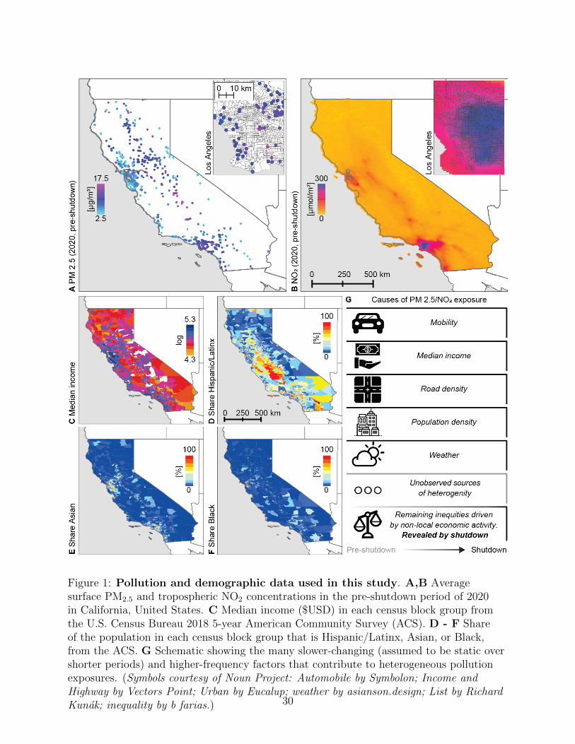
Figure 1: Pollution and demographic data used in this study. A,B Averagesurface PM2.5 and tropospheric NO2 concentrations in the pre-shutdown period of 2020in California, United States. C Median income ($USD) in each census block group fromthe U.S. Census Bureau 2018 5-year American Community Survey (ACS). D - F Shareof the population in each census block group that is Hispanic/Latinx, Asian, or Black,from the ACS. G Schematic showing the many slower-changing (assumed to be static overshorter periods) and higher-frequency factors that contribute to heterogeneous pollutionexposures. (Symbols courtesy of Noun Project: Automobile by Symbolon; Income and

Highway by Vectors Point; Urban by Eucalup; weather by asianson.design; List by Richard

Kunak; inequality by b farias.) 30

Figure 2: The COVID-19 “Mobility Shock”. A Shows the percentage point di↵erencein time spent at home pre-shutdown and during the shutdown at the census blockgroup level in CA, with an inset for the Los Angeles region. B Shows the unequalmobility reductions for the median of the upper and lower 10 percentiles of three di↵erentpopulation subsets. Shading indicates the 25th and 75th percentiles within each group.Vertical lines indicate the beginning and end of the transition (March 4, 2020 and March19, 2020) period excluded from our dynamic analysis.

31

Figure 3: Impact of the economic slowdown on (left) PM2.5 concentrations

and (right) mobility. Points show heterogeneous changes across census block groupdemographics estimated from di↵erences-in-di↵erences models, along with 95% confidenceintervals. Intervals that include zero indicate that there was no di↵erential reduction inexposures across the given gradient. A Changes in daily PM2.5 concentration across theshutdown estimated for various socioeconomic variables. The coe�cient for mobility isthe estimated di↵erence between 0 and 100% of time spent at home; the coe�cients for(ln) income, road, and population density each represent the impact of an approximatedoubling for each variable. C Changes in PM2.5 concentrations over the shutdown periodacross di↵erent racial and ethnic population shares, estimated with di↵erent physicaland socioeconomic control variables (labels on right). The coe�cients correspond to theexpected changes between 0 and 100% population share at the census block group level.B and D show similar estimates, but with mobility as the outcome instead of PM2.5. Allfour panels compare the post-shutdown di↵erence from 2020 to 2019 to the pre-shutdowndi↵erence to account for seasonality. Additionally, estimates were weighted to reflect thedistribution of incomes, population shares and other location characteristics across allblock groups in California, and correct for the endogenous sampling of ground stationlocations (see Figure S2B, Methods, and Supporting Information.)

32

Figure 4: Monitor locations, weighting, and influence on impact estimates. Thepublic (CARB) and private (PurpleAir) PM2.5 sensor networks used in this study arenot evenly distributed across the state, which a↵ects how di↵erent census block groupscontribute to estimated impacts. On the left we show post-shutdown concentrationchanges across various census block group gradients (as in Figure 3), but estimated usingdi↵erent samples – the public CARB network only (green), the private PurpleAir networkonly (purple), both together but unweighted (brown), and both together and weighted(red). (These weighted estimates correspond to the estimates presented in Figure 3.) Thepanels on the right show the representation of demographic and geographic features due tosensor placement by the di↵erent sensor networks. Compared to the distribution of thesefeatures by all census block groups in California (black lines), the distribution of censusblock groups with CARB or PurpleAir monitors can be quite di↵erent. The distributionof CARB and PurpleAir combined after weighting (red) matches the all-group state-widedistribution much more closely (see Methods).

33

Supplemental Information

This supplement contains:

• Supplemental Text (5 pages)

• Supplemental Figures S1-S10

• Supplemental Tables S1-S3

Supplemental Text

Data and Methodology Details

Overview of why the COVID-19 related economic slowdown o↵ers new insight into questions

of environmental justice. Figure S1 compares several quantitative approaches to questions of

environmental justice present in the literature. Many environmental justice studies note, as

in Figure S1A or B, that at any given moment in time (a cross-sectional analysis), ambient

pollutant concentrations are higher for communities of color. Here, a best-fit line to cross-sectional

observations would lead to an estimate of �, or the expected di↵erence in exposure between a 100%

Hispanic/Latinx community and a 100% non-Hispanic/Latinx community. Accounting for slower-

moving confounds in a multi-dimensional analysis, as in B, can change the estimate of �. In the case

shown, accounting for income can increase the estimate of �, if Hispanic/Latinx households tend

to have lower incomes than non-Hispanic/Latinx households. Many time-varying factors can also

confound this relationship. Importantly, expanding to panel (observations across time) analysis, as

in Figure S1C, allows inclusion of weather variables, and various time cycles known to contribute

to changes in pollution, like day-of-week and seasonal e↵ects.

While panel studies allow for inclusion of time-varying covariates, it is still the case that the

economy (including both point and mobile sources that emit pollutants like primary PM and other

precursors that contribute to secondary PM formation), geography (where humans live, including

factors like population density and proximity to roads and other steady-state emissions locations),

and climate (annual weather cycle and associated daily and seasonal emissions) typically exist

together over a fairly narrow set of conditions. Populations change slowly over time, as does the

34

general structure of the economy. As such, even in panel analyses, it remains di�cult to account for

enough factors such that residual exposure disparities can be confidently attributed to the broader

scale economy.

A large perturbation to the system, as the COVID-19 pandemic has created, moves one piece

of the system (the local and non-local in-person economy) far outside the historical experienced

conditions. This allows for a much more robust attribution of the change between pre- and

post- slowdown conditions to economic factors. The ability to additionally account for own

mobility further allows disaggregation of experienced disparities into those that might be caused

by geographic conditions (e.g., communities of color may need to commute more in general, or may

be more likely to be essential workers who cannot work from home) and general influence of the

broader scale economy. We explain how this intuition also maps to a statistically well-identified

question.

Identification of heterogeneous treatment e↵ects. Consider a simplified version of our

specifications in the main text with a single interaction of the treatment status (post-shutdown),

dit, with a binary, cross-sectional measure of di↵erential exposure to the treatment, xi:

yit = ⌧dit + �(dit ⇥ xi) + zit + µi + �t + uit. (2)

where zit captures the e↵ects of weather and other observed unit by time variation. All else is

defined as before, but note that yit is now in levels to further simplify the exposition. Using annual

di↵erences does not fundamentally alter these results but changes all di↵erences-in-di↵erences (DID)

interpretations to a triple DID which allows for more complex forms of unobserved heterogeneity.

This set-up allows us to make two points:

1) With staggered treatment (dit 6= dt for all i) and no heterogeneity in the treatment e↵ect

(� = 0), ⌧ is a standard DID estimate. Di↵erencing over time, rearranging and taking expectation

delivers

⌧ = E[�yit|�dit = 1]� E[�yit|�dit = 0] = (⌧ + �zit + ��t)� (�zit + ��t) = ⌧ (3)

which can be written as �ytreat � �ycontrol. However, the overall treatment e↵ect ⌧ is not

statistically identified in our setting, where all observations after a particular calendar date are

treated, so that dit = dt for all i, and we do not observe any unit with �dit = 0. Hence, dt and

�t are perfectly collinear. Omitting the time e↵ects, �t would lead us to be able to estimate ⌧ but

would also lead us to mistakenly attribute state-wide shocks, ��t, to the treatment e↵ect.

2) Without staggered treatment but heterogeneity in the treatment e↵ect (� 6= 0), we can

only identify the e↵ect of the heterogeneous exposure, �, relative to some baseline exposure captured

35

by ⌧ . The treatment e↵ect for each observation now becomes ⌧ + �xi but ⌧ is still collinear with

�t. With binary xi, the heterogeneous treatment e↵ect is captured by

� = E[�yit|�dit = 1, xi = 1]� E[�yit|�dit = 1, xi = 0]

� {E[�yit|�dit = 0, xi = 1]� E[�yit|�dit = 0, xi = 0]}

= E[�yit|�dit = 1, xi = 1]� E[�yit|�dit = 1, xi = 0]

=(⌧ + � + zit + ��t)� (⌧ + zit + ��t) = �

which is another DID estimate that compares the e↵ect of the treatment in groups with xi = 1

to those with xi = 0. With continuous xi this becomes a generalized DID estimate, where we,

for example, compare the e↵ect of the shutdown in block groups with a positive share of the

Hispanic/Latinx population to those without any Hispanic/Latinx residents.

Weighting. Ground-based monitor placement is endogenous to several of the variables we

interact with the shutdown in order to investigate heterogeneous treatment e↵ects. PurpleAir

monitors are privately installed by a non-representative subset of the population which is, among

other di↵erences, less racially diverse and lives in higher income neighborhoods than the state-wide

average (Figure 4A-F). CARB sensors are often set up to explicitly monitor pollution exposure in

vulnerable groups and, hence, tend to be placed in more diverse, less wealthy and more rural block

groups (Figure 4A-F). Such choice-based sampling implies that monitor placement is correlated

with the error term of our regression equation. Estimation which ignores endogenous sampling

is generally biased, but consistent estimates can be obtained by weighting the regression function

with the inverse probability of selection (81).

We use iterative proportional fitting—a standard post-stratification procedure—to match

the marginal distributions of the endogenous sample of monitors to known census population

margins. We determine the marginal distributions of the population by computing the cell

frequencies for each of the ACS variables used in the analysis (the Hispanic/Latinx, Asian, and

Black population shares, as well as income, road density and population density) per vigintile (20

bins) of the census data. A process called ”raking” then finds post-stratification weights which

adjust the endogenous sample such that it resembles the set of target distributions (Figure 4A-F).

The process is able to fit individual distributions in our data very well, but involves some trade-o↵s

in terms of how well it matches any particular distribution when more than one target variable is

used. Calculating the inverse probability of selection directly on a large contingency table would

require a much coarser portioning of the data, resulting in a substantially worse fit. All fixed e↵ects

regressions in the main text which use ground-based monitors are estimated using weighted least

squares if not otherwise noted.

We include a brief investigation into what the weighting tells us about the potential for

36

each set of monitors to provide information on disparities. Figure S2C shows the distribution

of weights across CARB and PurpleAir sensor types and shows that more CARB sensors are

highly upweighted by our weighting process than PurpleAir sensors. This makes sense–given the

endogenous placement of sensors discussed above and in the main text–we should expect some

CARB sensors to be deliberately placed where there are few other monitors or in locations where

residents would be unlikely to purchase a PurpleAir sensor.

Selection of weather controls We have included variables to control for temperature, relative

humidity, and precipitation in the same day (PM2.5 ) or week (NO2 ) as the dependent variable

measurement. Most importantly, if correctly specified these controls help reduce the variability

caused by weather di↵erences between 2019 and 2020. For example, if areas with larger Asian

populations also received more rainfall in 2020 after the shutdown, we might mis-attribute the

subsequent reduction in PM2.5 concentrations to the shutdown rather than to the weather. The

form of the function which maps these three variables onto concentrations is unknown to us, so

we searched for a specification which had good out-of-sample performance, didn’t use too many

degrees of freedom, and where interacted fixed e↵ects specifications contained few bins with only

one observation (e↵ectively dummying out that observation). This exercise sought to find a well-

fitting but not overfit specification that left enough observations for the main models to work well,

and that did not accidentally remove observations from geographic areas with extremes in one or

more of the variables.

Tables S2 and S3 as well as figure S7 show the results of these specification searches. The

categories of functional forms that we tried included interacted fixed-width fixed e↵ects (one, two,

five, ten, 20) of native units, fixed e↵ects created to split the data into evenly sized groups (decile,

vigintile), a cubic spline, polynomial fits (first, second, and third degree), uninteracted fixed e↵ects,

and a specification with no adjustment. In the tables, we show each of the first four classes of

models using both 2019 and 2020 weather variables or only 2020 weather variables, meaning we

included one or both of f2020 (T,RH,P )it + f2019 (T,RH,P )it. To test the performance of each

specification we ran a regression of weather variables on pollutant using a randomly chosen 70% of

CBGs and tested the performance on the remaining 30%. Tables S2 and S3 show the average out

of sample mean squared error (MSE) for each specification across 100 random splits, the standard

deviation of those estimates (sd), the degrees of freedom used by each specification (df), and the

number of observations which are dummied out because they singularly correspond to a fixed e↵ect

(lost). Both tables are sorted from lowest to highest MSE.

Figure S7 panel B shows the distribution of MSE estimates across 100 70%/30% cross-

validations for each specification for PM2.5 and NO2. Panel A shows the coe�cients from our

main model using a subset of the weather specifications. Our preferred specification is vigintile

fixed e↵ects, interacted, for both 2019 and 2020. This specification minimized MSE in the

37

PM2.5 regressions and was second in NO2 regressions, while drastically reducing the degrees

of freedom used and the observations dummied out.

38

Supplemental Figures

Figure S1: Why the COVID-19 related ‘mobility shock’ o↵ers new insight into

questions of environmental justice. For simplicity, imagine 5 communities across(e.g.) a state, represented by the five colors here. These locations each have a di↵erentracial/ethnic composition, represented here for simplicity in one dimension, as the shareof the population that is Hispanic/Latinx. Many observations of environmental injusticerely on cross-sectional analyses, either without (A) or accounting for potential slower-moving confounds (B). However, many high-frequency variables contribute to ambientpollution levels and might be correlated with geography and socioeconomic variables. Apanel analysis with repeat observations over time (C) allows for inclusion of these typesof covariates, and the ability to account for the contribution that (e.g.) natural weatherpatterns make to exposure disparities. However, even a panel analysis is subject topotential confounding, and interpretation of residual exposure disparities as environmentalinjustice caused by the economy remains problematic. The COVID-19 economic shockcreates a large perturbation that “turns o↵” a portion of the economy, and thus revealsthe footprint of pollution caused by economic activity (D). The ability to account formobility in this framework (E) further allows the separation of very local activity frombroader economic activity (see Supplemental Text).

39

Figure S2: PM2.5 networks and weights. A Location of public (California AirResources Board (CARB) and United States Environmental Protection Agency (EPA))PM2.5 monitors, as well as privately-owned PurpleAir PM2.5 monitors used in this study.B Weights used in the model to better represent the Californian population. Each dotrepresents one census block group. C Distribution of weights generated by the rakingprocess, across sensor types.

40

Figure S3: Summary of origin and race for California census block groups.

Distributions of (left panel) the percents of the total population categorized as White,Black, Asian, and Hispanic/Latinx, and (right panel) the percents of either theHispanic/Latinx or non-Hispanic/Latinx portion of the total population categorized asWhite, Black, and Asian at the census block group (CBG) level according to the CensusBureau’s American Community Survey (ACS). The total number of CBGs was 23,212.Statistical outliers were included in the distribution calculation, but excluded from thevisualization.

41

Figure S4: January-April 2019 PM2.5 and NO2 with increasing shares of census blockgroup income and racial makeup, without controlling for other sources of heterogeneity.The line represents the best linear fit.

42

Figure S5: Maps of observed di↵erences-in-di↵erences. A Observed di↵erences(shutdown - pre-shutdown) in the di↵erences (2020 - 2019) in PM2.5. A low percentile/redcolor indicates a greater reduction in PM2.5. B Same as A for NO2.

43

Figure S6: Same as Figure 3, but for weekly NO2 models. Since NO2measurements arefrom the TROPOMI satellite instrument, they cover all census block groups in California.Qualitative di↵erences between NO2 estimates (A,C) and Figure 3A,C thus represent acombination of coverage, and di↵erences in PM2.5 and NO2 distributions. Di↵erences inmobility between these estimates (B,D) and Figure 3B,D are due to coverage di↵erencesbetween the satellite and the ground-based monitoring networks and weekly or ratherdaily analysis.

44

Figure S7: Choice of, and sensitivity to, weather controls specification. A

Sensitivity of main results (Figure 3 to di↵erent functional forms of climate variables(temperature, precipitation, and relative humidity). B Mean squared error (MSE) ofmodels fit with di↵erent functional forms of weather controls and no other covariates,cross-validated, for both PM2.5 and NO2 models (for additional details see the theSelection of weather controls section in the supplement). Tables S3 and S2 show the MSEstatistics for each specification, and the number of observations dropped (due to uniqueweather controls values). We selected interacted vigintile fixed e↵ects as the optimalstructure for this analysis based on the combination of lowest MSE for PM2.5and veryfew dropped observations, even with full interactions of temperature, precipitation, andrelative humidity bins.

45

Figure S8: Daily mean PM2.5 measurements from CARB and PurpleAir sensornetworks during the study period, in 2019 and 2020, after quality control filtering.

46

Figure S9: Regression slopes of nearly co-located (< 100m) PurpleAir and

CARB PM2.5 measurements (2019 and 2020 Jan-Apr outdoor in CA) as a

function of distance between the PurpleAir and CARB sensors. Color indicatesthe correlation coe�cient. Marker size indicates the number of points used for theregression. The dashed horizontal line indicates the median. Point size indicates numberof points available for the sensor pairs. The three panels show the same comparison withno correction (left), the RH correction proposed in Tryner et al. (2020), and the EPAcorrection used in the study (right). The RH correction may not be su�cient in ourcase because we use daily mean data. The EPA correction we implement is conservative.Several PurpleAir sensors are paired with the same CARB sensors (in one case as many as32). 29 unique CARB sensors are represented here, meaning they have a PurpleAir sensorwithin 100m. Three sensor pairs were excluded from the figure because the correlation wasvery low (< 0.2).

47

Figure S10: Percentage of Data missing due to low quality or clouds from the

TROPOMI NO2product. For the time periods pre-shutdown and shutdown for 2019and 2020 the percentage of data missing is shown for each pixel (resolution 1 km).

48

Supplemental Tables

49

Dependent variable:

Di↵erence PM2.5 2020 PM2.5

(1) (2) (3) (4) (5) (6)

Mobility �0.217 �0.107 �0.221 �0.307(0.139) (0.158) (0.172) (0.191)

% HispanicLatinx �2.645⇤⇤⇤ �2.288⇤⇤⇤ �2.386⇤⇤⇤ �3.238⇤⇤⇤ �1.765⇤⇤⇤ �1.873⇤⇤⇤

(0.268) (0.293) (0.321) (0.478) (0.496) (0.554)

% Asian �0.949 �1.595⇤⇤⇤ �2.244⇤⇤⇤ �0.508 �0.529 �1.436⇤⇤

(0.572) (0.396) (0.357) (0.865) (0.553) (0.580)

% Black �0.639 �0.548 0.022 �2.288 �0.615 �1.107(0.962) (0.955) (0.799) (1.399) (1.232) (1.426)

Income 0.423⇤⇤⇤ 0.544⇤⇤⇤ 1.069⇤⇤⇤ 1.348⇤⇤⇤

(0.129) (0.176) (0.192) (0.294)

Road density 0.004 �0.004 0.013 �0.001(0.022) (0.017) (0.033) (0.026)

Population density 0.052 0.081 �0.228⇤⇤⇤ �0.120⇤⇤

(0.040) (0.055) (0.049) (0.059)

Weighted No No Yes No No YesCBG FEs Yes Yes Yes Yes Yes YesDay FEs Yes Yes Yes Yes Yes YesP(T,RH,P) 2019 Yes Yes Yes No No NoP(T,RH,P) 2020 Yes Yes Yes Yes Yes YesObservations 72,953 72,953 72,953 72,953 72,953 72,953

Note:⇤p<0.1; ⇤⇤p<0.05; ⇤⇤⇤p<0.01

Table S1: PM2.5 2020-2019 di↵erence vs 2020 values for all of California. Results of threePM2.5 regressions: without controls or weights, with controls and without weights, andwith both controls and weights. The first three columns correspond to the estimates inthe paper, the second three columns estimate the same quantities using only 2020 data.The dependent variable is the level of PM2.5 rather than the inter-annual di↵erence,and Mobility corresponds to the level of mobility rather than the di↵erence. We onlyinclude 2020 weather variables in columns 3-6 rather than the both years. The estimateshave slight di↵erences in magnitude but are the same sign and significance level in bothspecifications. This has two implications. First, the weather controls do a good enough jobthat di↵erencing out the previous year does not make an enormous di↵erence, though itdoes add precision to the estimates. Second, it is possible to consistently estimate thesee↵ects without access to previous years data.

50

model MSE (1e-11) sd (1e-11) df lost1 by 1 144.0 2.2 14567 42692 by vigintile 184.0 2.7 7467 6123 by 2 216.1 3.0 3870 8654 by decile 246.4 3.5 1350 265 by vigintile 2020 295.7 4.2 3659 3156 by 1 2020 299.1 14.8 5458 14537 uninteracted 317.1 4.3 317 88 by 5 320.0 4.3 519 489 by decile 2020 344.8 4.9 668 1310 cubic spline 2020 357.3 11.0 43 011 by 2 2020 388.8 5.6 1310 20912 by 10 390.6 5.5 107 513 by 5 2020 422.7 6.2 168 1314 by 10 2020 442.9 6.5 34 215 by 20 447.8 6.6 29 016 cubic spline 457.3 13.9 22 017 Poly 1 460.0 6.2 7 018 by 20 2020 461.3 7.0 11 019 Poly 2 2020 479.8 6.9 10 020 Poly 1 2020 488.3 7.6 4 021 base 489.5 7.6 1 022 Poly 3 2020 503.6 6.7 19 023 Poly 3 800.3 13.8 64 024 Poly 2 815.8 16.1 28 0

Table S2: NO2 selection of weather controls specification

51

model MSE sd df lost1 by vigintile 22.2 1.3 4116 4182 by decile 22.6 1.3 739 133 by 2 22.8 1.2 6111 24344 by 5 23.4 1.4 1114 2595 cubic spline 23.8 1.4 22 06 uninteracted 23.8 1.4 482 407 by 1 23.8 1.2 16477 89828 by 10 23.9 1.4 269 349 by vigintile 2020 25.2 1.4 2040 16010 by 2 2020 25.5 1.4 2181 91111 by 20 25.6 1.5 62 612 by 1 2020 25.7 1.4 6152 367413 by decile 2020 25.7 1.5 362 714 by 5 2020 26.0 1.5 407 9115 cubic spline 2020 26.1 1.5 43 016 by 10 2020 26.3 1.5 97 1217 Poly 1 26.6 1.4 7 018 by 20 2020 26.8 1.5 25 319 Poly 2 2020 27.0 1.5 10 020 Poly 3 2020 27.2 1.4 19 021 Poly 1 2020 27.9 1.6 4 022 base 29.0 1.6 1 023 Poly 2 32.1 2.4 28 024 Poly 3 34.1 2.4 71 0

Table S3: PM 2.5 selection of weather controls specification

52