AE-279UDC 539.125.523.348

621.039.51.12

O)INCMLU< Calculations of Neutron Flux Distributions

by Means of Integral Transport Methods

I. Carlvik

AKTIEBOLAGET ATOMENERGI

STOCKHOLM, SWEDEN 1967

AE -279

CALCULATIONS OF NEUTRON FLUX DISTRIBUTIONS BY MEANS OF

INTEGRAL TRANSPORT METHODS

I Carlvik

SUMMARY

Flux distributions have been calculated, mainly in one energy

group, for a number of systems representing geometries interesting

for reactor calculations. Integral transport methods of two kinds were

utilised, collision probabilities (CP) and the discrete method (DIT).

The geometries considered comprise the three one-dimensional geo­

metries, plane, spherical, and annular, and further a square cell with

a circular fuel rod and a rod cluster cell with a circular outer boundary.

For the annular cells both methods (CP and DIT) were used and the re­

sults were compared.

The purpose of the work is twofold, firstly to demonstrate the

versatility and efficacy of integral transport methods and secondly to

sefrve as a guide for anybody who wants to use the methods.

Printed and distributed in May 1967

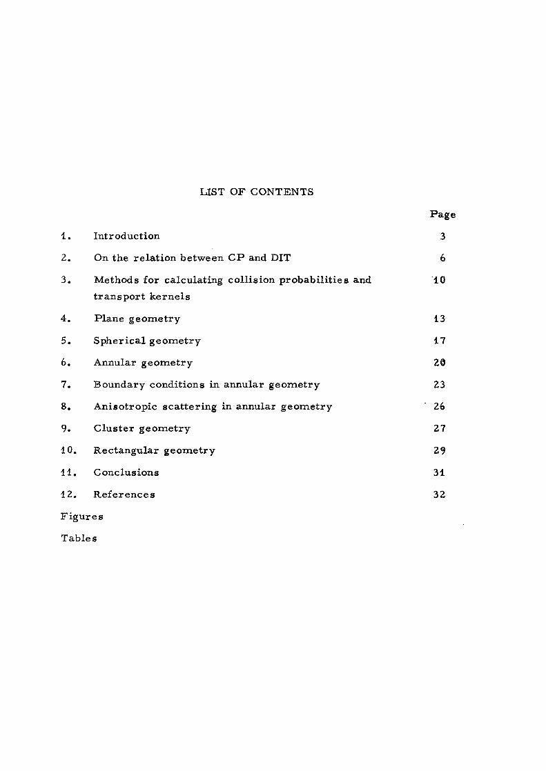
LIST OF CONTENTS

Page

1. Introduction 3

2. On the relation between CP and DIT 6

3. Methods for calculating collision probabilities and 10

transport kernels

4. Plane geometry 13

5. Spherical geometry 17

6. Annular geometry 20

7. Boundary conditions in annular geometry 23

8. Anisotropic scattering in annular geometry ' 26

9. Cluster geometry 27

10. Rectangular geometry 29

11. Conclusions 31

12. References 32

Figures

Tables

- 3 -

1. INTRODUCTION

During the last five or ten years there has been an increasing

interest in integral transport methods, that is methods for calculating

neutron flux distributions that are based on the integral form of the

transport equation. These methods are suitable for systems, where

the characteristic dimension is less than say, ten mean free paths. In

such small systems, e.g. reactor lattice cells, they are often superior

in accuracy and speed of computation to other transport methods such

as the spherical harmonics method and the Carlson method, which are

based on the integro-differential equation which represents the usual

form of the Boltzmann equation.

Considerable effort has been devoted to the development of in­

tegral transport methods at AB Atomenergi. In fact methods of this

kind have been incorporated in all current cell codes produced at the

establishment. Even the standard cell burnup code, REBUS, which

utilises the Westcott formalism, determines the intracell thermal flux

distribution by means of a complete integral transport calculation.

Two different formulations have been studied. The first one is

the most common form of integral transport methods, the one that uses

flat source collision probabilities. It will be called CP for short. The

second method uses a point-wise representation of space, and it de­

scribes the neutron transport by means of transport kernels. This

form together with the use of Gaussian integration over the space co­

ordinate was first suggested by Kobayashi and Nishihara [ l] . We have

suggested that the method be called DIT for Discrete Integral Transport.

The next two paragraphs contain some general remarks on in­

tegral transport methods, and give a short survey of methods for cal­

culating collision probabilities and transport kernels. However, the

main content of the paper is a collection of sample calculations using

either CP or DIT. The purpose is first of all to demonstrate the ver­

satility and efficacy of the methods, but it is also hoped that the col­

lection can serve as a guide for users of the codes, and therefore such

things as the effect of varying the distribution of points and regions are

investigated. The relationship between the accuracy achieved and the

computer time used is studied in some detail, since it is this which

- 4 -

determines the usefulness of a method. All computing times given refer

to calculations on an IBM 7044 computer.

In a complete cell programme using integral transport methods

there are three main parts which determine the speed of a calculation,

1) the evaluation of the transport matrices, one for each energy, 2) the

solution of the system of linear equations, and 3) the administration of

the programme and particularly the handling of a large amount of cross

section data. Only the first part will be considered here. The main in­

terest is directed to the method used for evaluating transport matrices.

It is then superfluous to keep the energy dependence, and consequently

most of the calculations refer to one-group problems with an external

source.

The major part of the calculations also refer to one-dimensional

systems, plane, annular, and spherical. In all three geometries

examples of DIT calculations are shown. The annular cases considered

have also been calculated by means of CP, and the results are compared.

The important parameter is the number of space points or regions neces­

sary to reach a certain accuracy. This is of particular importance in a

multi-group code, both for the speed of part 2) above and for the necessary

capacity of the fast memory. It is shown that in general CP is superior if

the flux variations in the system are small and vice versa.

Integral transport methods are most advantageous when it is pos­

sible to assume isotropic scattering. If anisotropic scattering must be

considered, it is necessary to carry one more flux moment in the calcu­

lation for each added term in the expansion of the scattering cross section.

There are also other difficulties, for example in annular geometry the

azimuth angle varies along a neutron path, and if CP is used, this is

somewhat in contradiction to the flat source assumption. It is, however, possible to use suitable averages over segments of neutron paths [ 2] . In

the DIT method this difficulty does not exist", although there are others

related to the problem of finding suitable diagonal elements. The DIT

method has been applied to linear anisotropic scattering in annular geo­

metry, and sample calculations are shown. In plane geometry there are

no particular difficulties with anisotropic scattering in the DIT method.

- 5 “

It may be fruitful to attack two- or three-dimensional problems

by means of a generalised DIT-method, but so far the applications have

been to one-dimensional geometries with the exception that problems

including so called pole-fluxes in annular geometry could be classified

as two-dimensional.

Another ’’restricted two-dimensional” system, which we hope to

be able to work on in the future is the annular system with an axial

buckling, that is with an axial cosine variation of the flux. A main dif­

ficulty in this problem is to develop a fast computer routine for the

generalised Bickley function

Je~x cosh u----------- ------ cos (y sinh u) du

cosh u o

In more complicated two-dimensional geometries CP seems to

be the only alternative to Monte Carlo methods.

Fuel elements for heavy water reactors usually consist of rod

bundles. This cluster geometry is very difficult to handle by means of

conventional methods, and most cell programmes consider only a

homogeneous mixture of fuel, cladding, and coolant. However, using

collision probabilities it is by no means impossible to manage calcu­

lations in cluster geometry. It has even been possible to make multi­

group calculations and obtain good agreement with measured detailed activation distributions inside the rod cluster [ 3] . One-group calcu­

lations on a cluster are shown here;,, and the accuracy that can be

achieved is demonstrated.

Another two-dimensional case, which we have considered, is

that of a one-group flux distribution in a square lattice cell with a

single fuel rod. The resulting distribution is compared with the one

obtained in a calculation for the corresponding circular Wigner-Seitz

cell. The results give a contribution to the discussion of suitable

boundary conditions in the Wigner-Seitz cell.

Beyond the particular geometrical configurations investigated

in this report there are others that could be well worth studying. For

example,when considering annular cells with several tubes and voided

- 6 -

regions surrounding the fuel one could suspect that the approximations

to the Bickley functions used here would not be sufficient. Another

case is an annular system with azimuthal flux variation, for which an

important question is what boundary conditions should be used under

various conditions. It would, however, take too much time and money

to cover all possible types of system.

The ultimate test of a computational method is a comparison

with experiments. There are no such comparisons in this paper. This

is because only the transport in space is considered. A comparison

with experiments demands a full physical model, and what should be

checked in that context is the physical model, not the numerical accu­

racy of the calculations inside the model. Therefore, the various parts

of the calculations should be checked in accuracy, one at a time, by

comparisons with more exact calculations as is done in this paper. In

this manner one makes sure that an agreement with measured results

has something to say about the physical model, rather than indicating

that errors in the model happen to be compensated by numerical errors

in the calculations.

The author tried to make the material as complete as possible,

and it could not be avoided that the report contains a multitude of nu­

merical results. It may be appropriate to apologise for the great

number of tables in the report.

2. ON THE RELATION BETWEEN CP AND DIT

The two formulations are naturally closely related; they differ

only in_that they employ different schemes for the integration over space.

Since CP is unwieldy in treating anisotropic scattering, all neutron

sources, both external sources, scattering sources, and fission sources,

are assumed to be isotropic in this paragraph to make the discussion

more perspicuous.

If $ (jr) is the flux density and ^ (r) the total source density (in­

cluding scattering and fission) both for a certain energy, the spatial part

of the transport equation is [ 4 J

- 7 -

2.1

2.2

is the optical distance between jr and jri. £ (r) is the macroscopic total

cross section at _r.

The system under consideration is assumed to consist of a

number of homogeneous regions.

The DIT method uses an integration formula of Gaussian type

for the integral in equation 2.1. If i and j are used for numbering the

points of the point set, the equation can be written

4>. = S 4>. V. T. . 2.31 j J J

Vj is the product of the volume of one of the homogeneous

regions and a suitable weight, and it can be formally interpreted as a

subregion of the corresponding homogeneous region.

In a general three-dimensional system one has

(r) = ^ dr* 4* (r• ) >- P(l,r' )

4ir I r - r1allspace

where

I r - r» I

P (£>£') = J S (r' + s,) ds

Ti,j 4ir |r. - r.-i -j

2 2.4

In a two-dimensional system T^ ^ is calculated as an average

over two curves and in a one-dimensional system as an average over

two surfaces.

The approximation scheme is a little different in the CP

method. The homogeneous regions are divided into subregions, which

are chosen in such a way that the source density ip varies little inside

a subregion. The size of a subregion is denoted by W, and k and t

- 8 -

are used for numbering the subregions. Then the approximation to

equation 2.1 is

<P (r) = Se'P

4ir,|_£ - jr< I ^2.5

Equation 2. 5 is integrated over subregion k to give the average

flux in W,

J dr <t> (r) = J dr J dr. P2.6

The collision probability ^ from l to k can be obtained from

equation 2. 6 as ^ for ip^ = in subregion l and ip = 0 in all

other subregions. The result is the following well-known expression

2. 7

l ~ W. *k

Combining equations 2.6 and 2.7 one obtains the usual spatial

equation in the CP formalism.

2.8

An alternative form is obtained if equation 2.8 is divided by

skwk

*k = S vp, W, kj l2kWk 2.9

The last equation is completely equivalent to equation 2.3 of the

DIT method. A computer routine devised for solving group fluxes and

- 9 -

possibly also an eigenvalue for one of the methods can be used for the

other as well.

In practical problems it often happens that certain regions, e.g.

gas channels, can be considered as voided. This does not cause any

difficulty in the DIT method, since T. . can always be calculated. If1» J

CP in the form of equation 2. 8 is used, the result of the calculation

does not give any flux density in the voided regions, because the pri­

marily calculated quantity, the collision density S^^^is zero in the

void region. If, however, the equations for the group fluxes are

written in the form of equation 2. 9, the calculation gives the flux den­

sities also in the empty regions. It must be observed that if £, = 0,Pk l

also P. . = 0, and the matrix element v *.y— k, c 3bi_W,_ must be calculated as a

limit. k k

It should be born in mind, when a multi-group code is written,p

that both matrices, T. .of equation 2. 3 and ^ of equation 2. 9 are

symmetric.

A few words can be said about what the approximations mean

in the explicit physical model. The assumption in the CP method is

the flat source approximation. Consider neutrons that have collided in

a certain subregion. Some of them are scattered and start again, but

before they are started, they are spread out uniformly over the sub­

region. This means a neutron transport from points with higher flux

to points with lower flux, and consequently the CP method will tend to

give too small flux variations in a system.

The collision probabilities utilised in the well-known THERMOS code [ 5] are not the usual flat source collision probabilities, but in­

stead they refer to neutrons that start from a central point of a sub­

region. In the physical picture neutrons that have collided inside a

certain region are concentrated to the central point before they start

again. This should make the coupling between the subregions too

small, and it has also been observed that THERMOS tends to give too

high flux variations.

There is another disadvantage with this type of collision pro­

bability. In a system where one knows that the flux density is almost

constant in a large zone it is possible to use very large subregions if

- 10 -

the flat source collision probabilities are used. However, in the

THERMOS scheme the subregions must still be so small that the escape

probability from the central point is representative for the escape pro­

bability from the subregion.

It is not so easy to see how the approximation in the DIT method

works. However, at least if the number of space points is small, it

seems that the coupling between various parts of the system should be

too small in the calculation, so that the flux variation over the system

should be too large. This has also been found in the calculations in an­

nular geometry, where CP and DIT are compared. The moderator to

fuel flux ratios converge from above in the DIT method and from below

in the CP method.

3. METHODS FOR CALCULATING COLLISION PROBABILITIES ANDTRANSPORT KERNELS

A key problem in the application of integral transport methods is

the calculation of the collision probabilities or the transport kernels.

Various methods have been proposed. They will not be discussed in de­

tail here, but a short survey will be given.

A majority of the literature on the subject deals with the calcu­

lation of collision probabilities in annular geometry. Formulae for

multi-region collision probabilities (in some papers only two or three regions) have ibfeen given by Takahashi [ 6], Millier [ 7] , Kiesewetter [ 8] , Di Pasqbdmtonio [ 9] , Pennington [ 10] , and Carlvik [ 11 ] among

others.

Application of the correct formulae must necessarily use up

some computer time and memory space. Considerable efforts have

been devoted to the derivation of approximate collision probabilities

that are easy to calculate but still accurate enough to allow the calcu­

lation of flux densities of sufficient accuracy.

A frequently used approximation is the assumption that neutrons

that have crossed a boundary between two adjacent annuli have a cosine

distribution. With this assumption it is possible to uncouple any an­

nulus from the others except the two adjacent ones, and only the self

- 11 -

collision probability and certain transmission probabilities have to be

calculated for each annulus. This method has been employed by Mtiller

and Linnartz [ 12] , and they have derived polynomial approximations

that give the probabilities conveniently. The same assumption has been

used by Kalnaes et al. [ 13] .

With this assumption - that neutrons have a cosine distribution

after crossing a region boundary - it seems probable, although it has

not been proved, that if the number of regions is increased, the solu­

tion should converge towards the DPq solution, that is the solution of

the double spherical harmonics method of order zero.

The assumptions regarding the angular distribution are less severe in the approximation scheme of Bonalumi [ 14]. Bonalumi's

method has been developed further by Jons son [ 15], and it has also

been generalised to linearly anisotropic sources by Hyslop [ 16].

A drawback with this kind of approximation is that one cannot be

certain that the solution converges towards the correct solution, when

the number of regions increases. If accurate results are desired, it is necessary to use the exact formulae. This was done by Honeck [ 5] in

the THERMOS code for the particular type of collision probabilities

discussed in paragraph 2. The same method for calculating collision

probabilities was employed by Stamm'ler [ 17]. The probability that

neutrons starting at a certain point collide in the different annuli is

calculated by means of a Gaussian integration over the azimuth angle.

The integration scheme developed by Wexler for the MINOTAUR

code [l8] calculates the ordinary volume-to-volume collision proba­

bilities. It is more elaborate, and it takes into account the discon­

tinuities of the derivative of the integrand.Kobayashi and Nishihara [ 1 ] employ the straight forward in­

tegration over the azimuth angle for the calculation of transport kernels

in annular geometry.

The method we have used for the calculations in the present

paper is also based on the exact formulae, but the scheme for per­

forming the integration over the azimuth angle is different from the

one used by other authors and seems to be more efficient. In fact we

have found that the gain in computing time when using an approximate

- 12 -

method is not very large. Our scheme has been described in reference [4] for collision probabilities and in reference [ 11 ] for transport

kernels. The former reference regarding collision probabilities is a

little brief, but the latter one is more detailed, and the modification of

the scheme when going from transport kernels to collision probabilities

is obvious. .

There has been less interest in collision probabilities in spheri­

cal geometry, because this geometry is not so important from a practi­

cal point of view. In plane geometry collision probabilities and transport

kernels can be expressed directly in exponential integrals, and no par­

ticular schemes are needed to calculate them.

The two-dimensional geometry of a square or hexagonal cell with

a cylindrical fuel rod is more complicated, and calculations will neces­

sarily take longer than for one-dimensional geometries. Honeck [ 19]

has considered this geometry. He calculates collision probabilities for

neutrons starting at a representative point in each region by Gaussian

integration over the azimuth angle as in the annular case. The division

of the cell into subregions is quite general.

Two-region collision probabilities for the same geometry have been calculated, both from exact expressions by Fukai [ 20] and by

means of approximative assumptions by Sauer [ 21 ]. Sauer extended his

method by including a third region, the cladding of the rod. Fukai

generalised his method to a multi-region cell consisting of concentric

annuli plus one more region made up of the remaining corners of the cell

[22]. Willis has used a Monte Carlo technique to calculate collision

probabilities in the three-region cell, fuel, cladding, moderator [23].

The general method developed independently by Beardwood, Clayton and Pull [24] and by Carlvik [ 11 ], which was originally intended

for cluster geometry, can be used for square or hexagonal cells as well.

For the calculation of collision probabilities sets of parallel, equidistant

lines are drawn over the system in a number of directions, intersections

with region boundaries are determined, and collision probabilities are

obtained as combinations of Bickley functions of optical distances

between intersections.

- 13 -

Even for cluster geometry, simpler methods have been pro­posed. Leslie and Jons son [ 25] developed a scheme, which relies on

the use of approximate analytic expressions for the collision proba­

bilities in the cluster.

The Bickley functions are vital for integral transport theory in

general cylindrical geometry, one-dimensional or two-dimensional. The original paper by Bickley and Nayler [ 26 ] gives the most im­

portant formulae and a short table. Larger tables for the closely re­lated functions Kj have been given by Muller [ 27] . However, what is

needed in computer codes is numerical approximations that can be

used for quick subroutines. Such approximations can be found in papers by Fukai [ 20] , Danielsen et al. [ 28] and Clayton [ 29] .

The approximations we have used are due to Tellander [ 30] .

4. PLANE GEOMETRY

The calculations in plane geometry were made by means of the

DIT code PLUS LA, which calculates the flux distribution in one group

for an external source. The programme allows anisotropic scattering,

but the calculations reported here assume isotropic scattering.

The basic functions for the calculation of transport kernels in

plane geometry are the exponential integrals. With isotropic scattering00C -xu

only the first order function E^ (x) = ^ —-— du is needed. Approxi-

1'mations for E, were taken from the Handbook of Mathematical Functions1[ 31 ] , formulae 5. 1.53 and 5. 1. 56. The maximum absolute error of the

- 7 - 8approximation is 2x10 in the interval 0 < x < 1 and 2x10 for 1 < x < oo.

In plane geometry, in contrast to annular or spherical geometry,

the transport kernel is expressed directly in known functions (the expo­

nential integral) and no integrations are needed. On the other hand in a

lattice one must perform a summation over all cells in the lattice. The

FLUSLA code terminates the summation, when the optical distance

between the field point and the source point is larger than a prescribed

number, OPMAX. The values 6, 8, and 10 have been used in the cal­

culations.

- 14 -

The effect of the uncertainty in the exponential integral can be in­

vestigated in the following manner. Consider a case, where the source

density ip at any point is equal to the local macroscopic cross section.

The flux density at a point x is then equal to

+oo y +oo* (x) = -| J Ei { • J £ (t) dt I j- £ (y) dy = -| J E4 (| u | ) du = E2 (0) = 1

-oo X -eo

(4.1)

The maximum absolute error caused by the uncertainty in E^ and by the

fact that the integration is terminated at OPMAX is

1 OPMAX , ooMmax(x)= ( 2 x 10'7 dT + J 2 x 10"8 dT + j (t) d T

m X o 1 OPMAX

= 2 x 10"7 + (OPMAX - 1) x 2 x 10'8 + E^ (OPMAX) (4. 2)

Thus in this case the relative error in the flux density is less than 3.2x10 ^ if OPMAX=6, and less than 4.2x10 8 if OPMAX=10. In practical

cases the source density varies, but this calculation shows that the error

caused by the inaccuracy of E^ can in general be neglected.

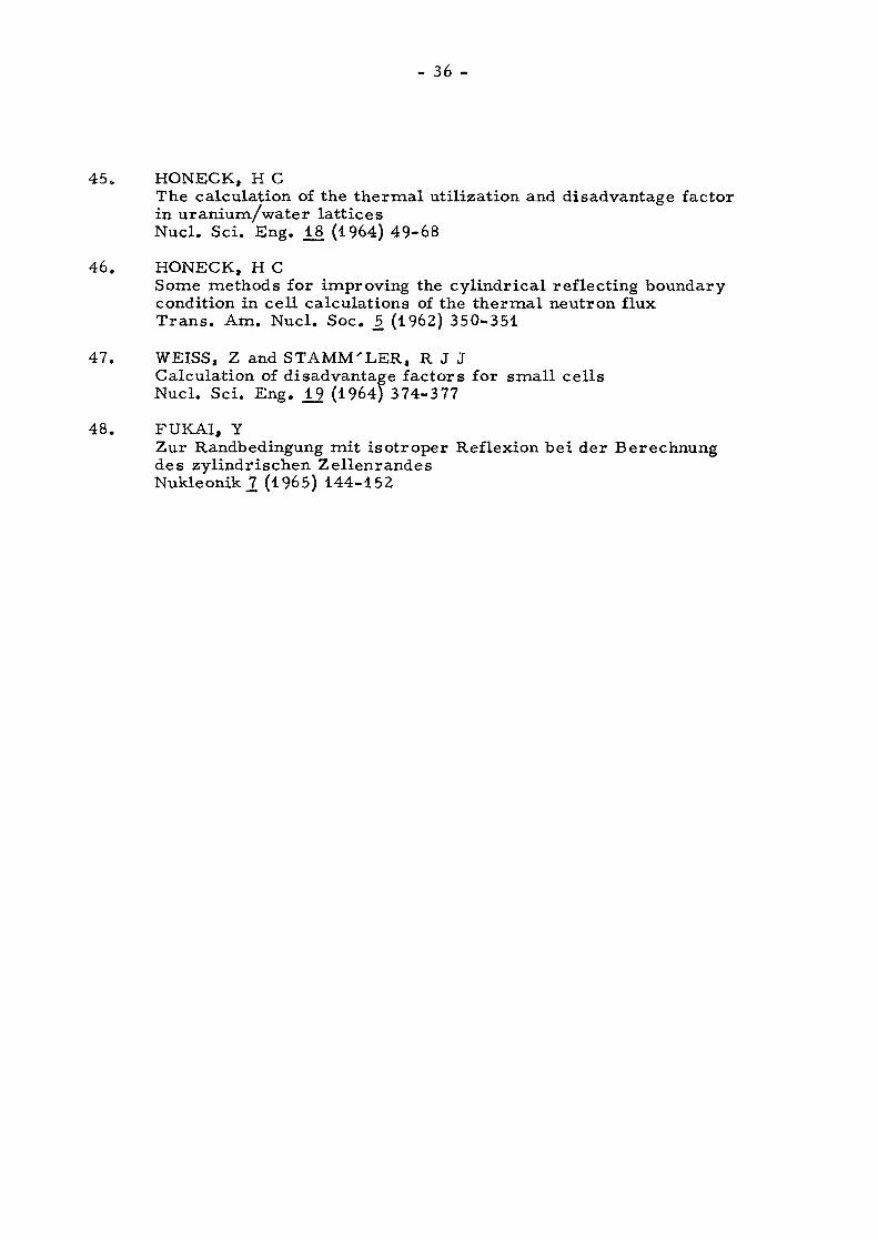
Two series of lattices were studied. The first one, typical for light water reactors, has been considered by Theys [ 32 j and the second

one, typical for fast reactor lattices of the Z PR-III type, by Meneghetti [ 33 ]. Geometrical data and macroscopic cross sections of the lattices

are given in figure 4.1.

Neither the paper by Theys nor a later paper by Ferziger and Robinson [ 34], in which the same lattices were considered, quote an

absorption cross section for the light water moderator, so we thought

that the absorption cross section had been neglected. Later we found [35] that the calculations of these authors had used the value

=0.0195. The corresponding change in the flux ratio is quite

small, 0.00002 in the thinnest cell and 0. 0093 in the thickest one, and it

does not in any way influence the conclusions of the general investigations

of accuracy and computing times. However, for the comparison with the

- 15 -

result of other authors we repeated a series of calculations, so that the

data for the results of table 4.4 and figure 4.4 are the same as those

used by the other authors.

In the calculations on the four lattices of Theys the distribution

of the space points and the value of OPMAX were varied in order to study

the effect on accuracy and computing time.

First the four lattices were calculated with 12 space points in the

half-cell and with the space points divided between the two regions in

various ways. For the thickest lattice a similar series was done with

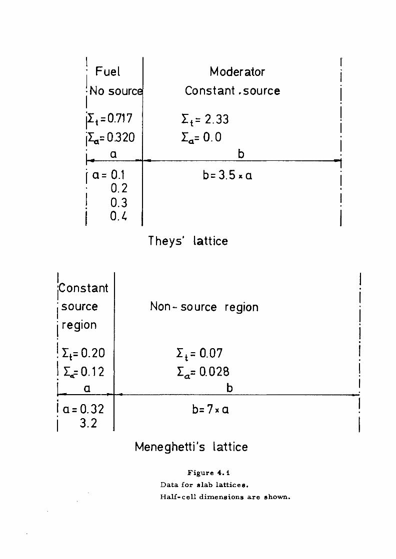
16 space points. The resulting flux ratios, that is the ratio average flux

in moderator to average flux in fuel, are given in table 4.1 and shown

graphically in figure 4. 2.

The flux ratio converges towards the correct value from above.

Thus the most suitable distribution of the 12 points is 3 in the fuel and 9

in the moderator for the first three lattices, and 2 and 10 respectively

for the thickest lattice. In the case of 16 points in the thickest lattice

the best division is 3 points in the fuel and 13 in the moderator. How­

ever, the division is not critical.for the result.

A simple way to distribute points would be to assign to each

region a number of points proportional to the optical thickness of the

region. The ratio between the optical thicknesses of the two regions is

a little over 11, the same for all four lattices. However, in the cases

investigated the ratio.between the number of points in the optimum

distributions is 3 to 5, low in thin cells and high in thick cells. A

qualitative conclusion is that the distribution of points between regions

should be more even than proportional to the optical thicknesses, the

more even the thinner the cells.

Then the influence of OPMAX was investigated in calculations

on the thickest and the thinnest cell with 8, 12, 15, and 20 space

points. Three values for OPMAX were used, 6, 8, and 10. The cal­

culated flux ratios are given in table 4. 2. The difference in the flux

ratios for OPMAX=6 and OPMAX=10 is about 0.00012 for the thin cell

and 0. 00006 for the thick cell. The difference for OPMAX=8 and

OPMAX=10 is about 0.000004 for the thin cell, but for the thick cell it

happens that the same number of cells is considered for both values

-16-

of OPMAX, so the calculations are identical. These results indicate

that OPMAX=10 can be used with confidence, and also that OPMAX=6

is sufficient in most practical calculations.

Finally the total number of space points was varied. All four

Theys lattices were calculated with 8, 12, 15, and 20 points and with

OPMAX=10. The results are given in table 4.3 and the convergence of

the flux ratio with the number of points is also shown in figure 4. 3. The

calculation with 20 points gives something like four correct decimals for

the thin cell (optical thickness 1.7744) and three correct decimals for

the thick cell (optical thickness 7. 0976). However, the computing time

is considerably longer for the thin cell.

The lattices of Theys have also been calculated by Ferziger and

Robinson [ 34] by means of the eigenfunction expansion method. A com­

parison of the results is shown in table 4.4 and in figure 4.4, where

also results by P^ calculations and by the method of Theys (similar to

the Amoyal-Benoist method for annular geometry) are shown. The DIT

results agree with the results from the eigenfunction expansion method,

and an Sg -calculation by K. Lathrop (not shown in the figure) is very

close. As could be expected the flux ratios of the diffusion theory are

much too low, and use of the method of Theys means a considerable im­

provement over diffusion theory.

The Meneghetti lattices were calculated with 5, 10, and 20 space

points and with OPMAX=6, 8, and 10. The calculated flux ratios are

given in table 4. 5 and shown graphically in figure 4. 5. The conclusions

that can be drawn are similar to those from the calculations on the

Theys lattices.

Finally a few words should be said about computing times. The

number of -functions that has to be calculated for a case is proportional

to the squarfe of the number of points, and also about proportional to the

ratio OPMAX/(optical thickness of the cell). In a case with many points

and a thin cell the computing time is about proportional to this number,

since the calculation of E^-functions takes the major part of the time. In

the opposite case, few points and a thick cell, other parts of the calcu­

lation dominate the time. The computing times in the tables show this

general behaviour. However, one can also see that the computing time

- 17 -

for a certain accuracy does not vary much from cell to cell, A thick

cell needs more points than a thin one, but this is compensated by the

fact that fewer cells have to be taken into account. An accuracy of

0.1 % can be obtained in about 1 second for all cells.

If an accuracy of this order is considered as sufficient, it is

possible to calculate the transport matrices for e. g. a 30-group cal­

culation in less than 30 seconds. If desired this time could be reduced

considerably if a simpler E ^ - routine were used. The one used here

contains a rational expression with altogether 6 or 10 terms in nu­

merator and denominator and further either a log function or an expo­nential function. A maximum absolute error of something like 5x10 ^

in the E^-function would be more compatible with a relative error of

0.1 % in the flux, and this could certainly be achieved by a faster

routine.

5. SPHERICAL GEOMETRY

No spherical one-group DIT code exists, and the calculations

in this paragraph were made by means of the multi-group DIT code

FLUB AG. The routine for evaluating the transport kernels was de­

veloped at AB Atomenergi, but the solution of the fluxes is achieved

by means of a slightly changed version of the British PIP routine [ 36]. FLUB AG can accomodate 16 energy groups and 40 space points,

and it is possible to make either an eigenvalue calculation or a fixed

source calculation.

Calculations in spherical geometry are of interest for fast

reactors rather than for reactor lattice cells. However, integral

transport methods are not suitable for large systems, so the FLUB AG

code is of interest mainly for small fast reactors. In fact the code

was composed mainly because only some small changes were needed

to convert the corresponding annular multi-group code to a spherical

one.

The basic function needed for the calculation of transport ker­

nels in spherical geometry is the ordinary exponential function, so no

special functions had to be built in.

- 18 -

It was not possible to analyse one-group problems in detail re­

garding computing times with FLUBAG as was done in plane geometry

and also in annular geometry. When a simple one-group problem is

calculated by means of a multi-group code, the real computing time is

short as compared to the time spent on administration and link

changes. '

Two types of calculations in spherical geometry will be ac­

counted for. The first is the classical test problem for a spherical

transport code, the determination of the critical parameter c2g + y

(c =---- s-------- ) for a bare homogeneous critical sphere in one energy^tot

group. Three spheres were calculated with the radii 1, 2, and 4 mean

free paths. For each radius calculations were performed with 4, 6, 8,

10, 12, 16, and 20 space points.

The results are given in table 5.1 and shown graphically in

figure 5.1. The values labelled "exact" in the table were calculated by means of a variational method [ 37] . The latter is equivalent to the

usual variational method using powers of the radius as test functions*

although in this case Legendre polynomials were used instead. In this

way it was easy to use a high order approximation.

Figure 5.1 shows the c-values from the FLUBAG calculations,

and also the c - value s from the variational method as functions of the

order of the polynomial used. For this particular problem the varia­

tional method shows a much better convergence, but also the DIT

method gives c with an accuracy better than 0.1 % with less than 10

points. Of course, the DIT method shows its strength in more com­

plicated systems, containing regions with different compositions.

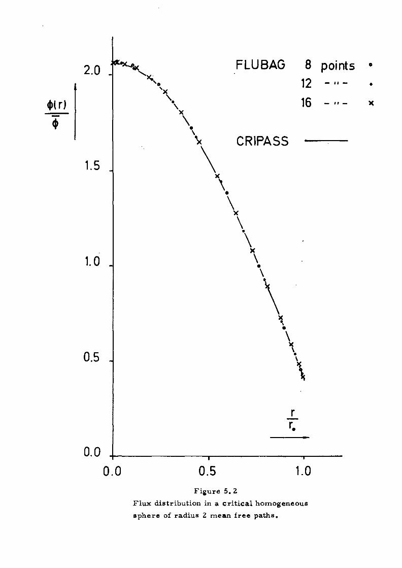
I may be of interest to compare the flux distributions obtained.

This is done for the sphere of radius 2 m. f. p. in figure 5.2. The full

line gives the distribution obtained in a variational calculation with a

polynomial of the order 10. Flux values are also given for FLUBAG

calculations with 8, 12, and 16 points. The points agree quite well

with the curve, although the 8-point values are a little high near the

center of the sphere.

In spherical geometry, as well as in annular, the transport

matrix is evaluated by means of integrations. The accuracy is deter-

- 19 -

mined by two parameters IA and IM, which are' defined in reference [4]

The number of Gauss points in the integrations varies between IA and IM

according to the size of the interval. Standard values in FLUB AG are

IA=2, IM=5. The effect of the parameters was investigated in a series

of calculations for all three spheres. Each sphere was calculated with

10 and 20 Gauss points, and the result for IA=2, IM=5 was compared

with the result for IA=4, IM=10. This comparison is shown in table 5. 2.

The largest change in c is 4x10 so the values IA=2, IM=5, which

were used in the calculations of table 5.1 should be sufficient for the 5

decimals given there.

In another series of calculations the effective multiplication

factor of the fast zero-power reactor FR-0 was calculated. FR-0 is

similar to the ZPR-III reactor or the British Vera reactor. In this

particular loading the core of radius 17 cm contains 20 % enriched

uranium and some structural material, and the reflector of radius

47 cm consists of copper. The calculation was performed in three

energy groups. The group data, table 5.3, were provided by Haggblom [38].

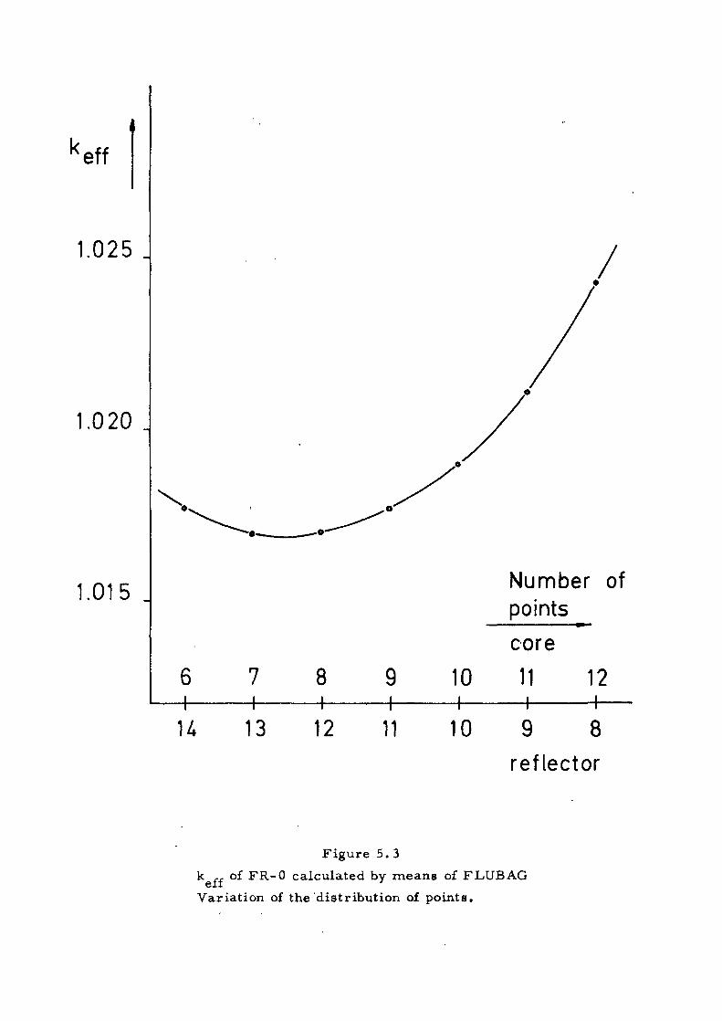
In the first series of calculations the space-points, 20 in all,

were divided in different ways between core and reflector. The results

are given in table 5.4 and figure 5. 3. The best division is 7 points in

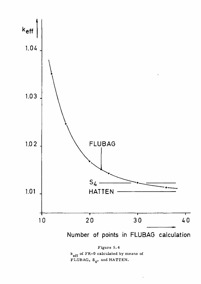
the core and 13 in the reflector. Then a series of calculations was

performed with different total numbers of points, table 5.5 and figure

5.4. Some of the values were also calculated with higher accuracy in

the transport kernels, IA=4, IM=10, instead of IA=2, IM=5.

Apparently also for this larger system IA=2, IA=5 is sufficient.

The use of the more accurate integration gives a change in of the

order of 10 The accuracy in k^^ that can be obtained with the number of points available in the code, 40, is about 10 \

Values for k^^ obtained by means of two other methods are

given in table 5.5. Also the computing times of the FLUB AG calcu­

lations are included.The code HATTEN was developed by Haggblom [ 38] . It uti­

lises an integral transform of the P^-equations.

- 20 -

The radius of the system considered here is 22 mean free paths

with group 3 cross sections and 9.4 mean free paths with group 1 cross

sections. The calculations show that the DIT method can indeed be used

for problems of this size, but it probably represents the limit, and for

larger systems one should use differential methods, S or P or a method

such as HATTEN.

6. ANNULAR GEOMETRY

The application of DIT to annular geometry has been studied in

more detail than the application to the other two one-dimensional geo­

metries. The calculations were performed by means of the one-group

code FLURIG-4. It is rather general, and it allows the study of the

following things, although only one at a time: a) linear anisotropic scat­

tering, b) azimuthal flux variation, c) the effect of a perfectly reflecting

cell boundary (the standard boundary condition being a white boundary).

With isotropic scattering and a white boundary the albedo of the boundary

may have any value, even negative.

As in the case of spherical geometry the transport kernel is

evaluated by means of integrations, and the accuracy in the integrations

is determined by the parameters IA and IM.

The basic functions in the annular case are the Bickley functions[ 26 ] . In our calculations we have used approximations to the Bickley

functions Ki^, Ki^» and Ki^, that have been derived by Toll and er [ 30 ] .

They are very fast but have a limited accuracy, the maximum absolute -5error being 3x10 .

The effect of the inaccuracy of the routines for the Bickley

functions can be estimated in the same manner as was used for the in­

accuracy of the routine for the exponential integrals in the plane case.

Using the kernel for a line source instead of the kernel for a plane

source, equation 4.1 for the plane case is now replaced by

- 21 -

2ir oo r oo4> (°) = ^ da ^ 2“ Ki4 J £ (ri) dr« S(r) rdr = J Ki1 (p) d p =

= Ki^ (o) = 1 (6.1)

The approximations for the Bickley functions assume that

Ki (x) = 0 for x > 10. Thus one obtains for the maximum absolute error

i n the flux

a4>

10 00(o) = j 3x10 ^dp + j Ki^ (r) dp = 3 x 10 ^ + Ki^ (10) =

10

= 3. 2 x 10-4 (6. 2)

The true error is on the average considerably smaller since - 53x10 is the maximum absolute error of the Bickley approximations,

and the error varies between the two extreme values as the argument

varies. If one tries to converge the solution of a calculation by in­

creasing the number of points, one could expect that the result would

start oscillating, when the error caused by other sources comes down-4below say 10 . However, some of our results seem to have converged

to an accuracy of about 10 ^ and no oscillations have occurred, so the

errors have probably been well smoothed out in the integrations. The

accuracy of the Bickley approximations is certainly sufficient for most

practical applications.

Some calculations of disadvantage factors in annular geometry have been reported earlier [ 39]. For the present more detailed in­

vestigation we have chosen two particular cells. The first, which is a

typical heavy water cell is the same as the heavy water cell considered

in the previous paper. The second one is the third of the six Thie cells [40], also considered in the previous paper. Data for both cells

are given in table 6. 1

First both cells were calculated using 10 and 20 radial points

in all, but with the points divided in different ways between regions.

These calculations gave the disadvantage factors of table 6. 2 and

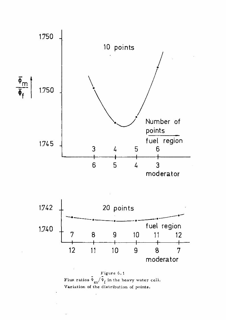
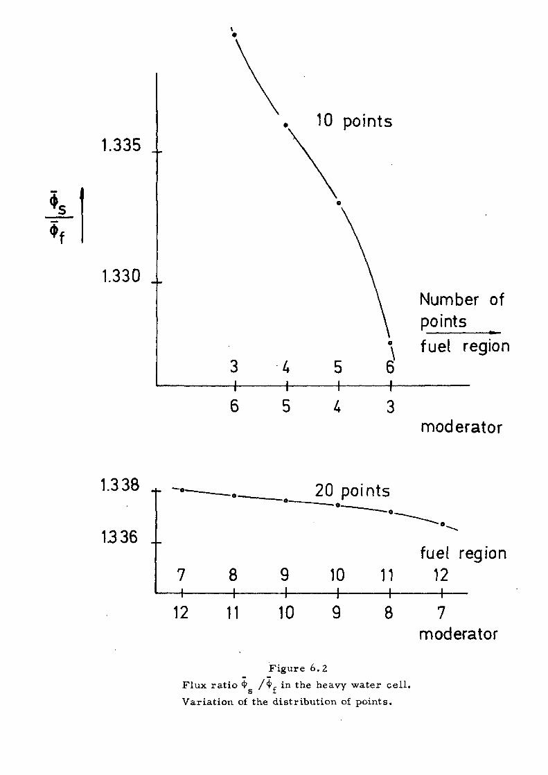
table 6.3. The results are also shown in figure 6.1 to 6.3. It was

- 22 -

found for the heavy water cell that the most accurate flux ratios were

obtained with equal number of points in the fuel region and in the

moderator. As pointed out in paragraph 2, the DIT method gives an

overall flux variation in the cell that is too large, and consequently the

moderator to fuel flux ratio, which represents the overall flux varia­

tion, has a minimum for a certain distribution of the points in figure

6.1. On the other hand the shroud to fuel flux ratio has a monotonic

variation, figure 6.2. This can be explained as follows. The thin

shroud region will be coupled most closely to that of the two main

regions with the most points. As a consequence the flux in the shroud

will be too close to the fuel flux, that is too low, if most of the points

are in the fuel region, and vice versa.

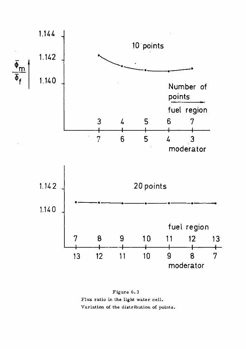
The minima for the flux ratio in the light water cell are

shallow, figure 6. 3, and also for this cell we used in the rest of the

calculations the same number of points in the fuel and in the moderator,

although the minimum does not come exactly at that point.

Next the effect of varying the accuracy parameters IA and IM

was investigated, and the results are shown in tables 6.4 and 6.5.

The flux ratios from calculations using IA=0, IM=5, which are the

values that were used in most annular calculations, do not differ by

more than 0. 03 % from more accurate values.

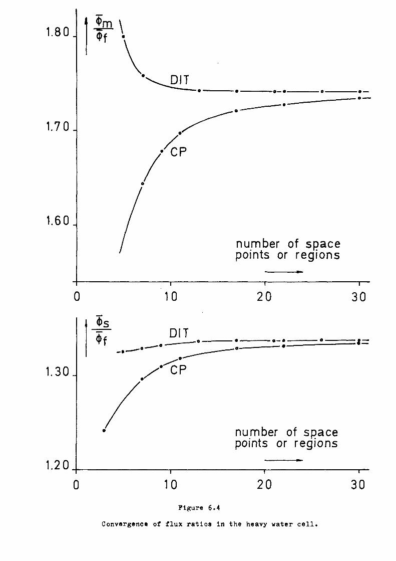
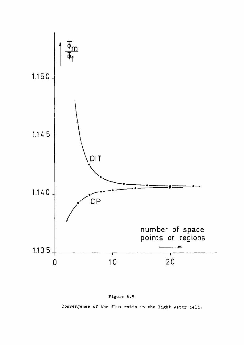
Finally calculations were performed with an increasing num­

ber of radial points, tables 6.6 and 6.7. The convergence of the flux

ratios is shown graphically in figures 6.4 and 6.5.

Similar calculations were also performed by means of a

collision probability code FLURIG-2, and results are given in tables

6. 8 and 6. 9, and they are drawn in the same diagrams as the DIT

results for comparison, figures 6.4 and 6.5. The abscissa is the

number of points for the DIT calculation and the number of regions

for the CP calculation.

The CP code FLURIG-2 does not print out the computing times

as the DIT code FLURIG-4 does, but equal numbers of points and

regions give about equal computing times.

Looking now at figures 6.4 and 6.5, one can see that both

methods converge well. For equal numbers of points or regions the

- 23 -

DIT calculations are more accurate in the case of the heavy water cell.

For the light water cell the CP results are more accurate, except if one

goes to a very large number of points or regions. The explanation of

this is the flat source approximation of the CP method. The approxi­

mation is good, if the source is nearly constant, and this is what

happens in the light water cell, where the disadvantage factor is only1.14. The total variation of the flux over the cell, /<& . , whichmax' mincan be found from the calculations, is about 1.35. For this cell even a

two region CP calculation gives the flux ratio with an accuracy of 0. 2 %.

In the heavy water cell the total flux variation is considerably larger,

about 2.5, and the flat source approximation is worse.

One can see from tables 6. 6 and 6. 7 that an accuracy of 0.1 %

in the flux ratios can be obtained by means of the DIT method in about

1.5 seconds for the heavy water cell, and in less than 0.5 seconds for

the light water cell. This is the same order of magnitude as the 1.0

second found in the plane case. One would think that the plane cal­

culation would be much faster, because there are no integrations in the

calculation of the transport kernel. One fact that compensates partly

for this difference is the summation over cells that is needed in the

plane case but not in the annular case, if a white boundary is used.

Another point is the fact that the approximations we have used for the

basic functions, exponential integrals and Bickley functions respective­

ly, are much more accurate and consequently slower in the plane case

than in the annular case.

7. BOUNDARY CONDITIONS IN ANNULAR GEOMETRY

The annular Wigner-Seitz cell is an approximation to a square,

triangular or hexagonal lattice cell. The correct boundary condition

of the true cell in an infinite lattice is perfect reflection of neutrons

that reach the boundary. It was earlier customary to retain the pro­

perty of perfect reflection, when the true boundary was replaced by the

circular boundary in the process of forming the Wigner-Seitz cell. Newmarch showed [ 41 ] that this boundary condition gives serious

errors in the flux ratio for small cells, and that it even gives wrong

— 24 —

flux ratio in the limit, when the size of the cell approaches zero. The

effect has been discussed in relation to specific cells by Thie [40] .

Several other authors have considered the problem of the boundary con­dition in Wigner-Seitz cells [ 20, 42-45] .

It is now generally agreed that it is better to use a ’'white" bounda­

ry in the Wigner-Seitz cell, that is neutrons returning through the bounda­

ry have a cos 6 distribution, with 9 equal to the angle between the neutron

direction and the inward normal of the boundary surface [46, 47, 48] .

We will not discuss this point in detail here, but it will be illus­

trated by some FLURIG-4 calculations and by two-dimensional collision

probability calculations in a square cell. The former calculations treat

the two annular cells considered in the preceding paragraph, but the

latter calculation refers only to the light water cell.

The calculations on the two annular cells were performed by

means of FLURIG-4 using the option of perfectly reflecting boundary,

table 7.1 and 7. 2. Calculations with a white boundary were described in

paragraph 6, and the two-dimensional calculations on the light water cell

are described in paragraph 10. The flux ratios obtained in the calcu­

lations are shown in table 7.3. The values in the table from ABH, and Sn calculations were given by Thie [40] .

The results for the heavy water cell are very little dependent on

the boundary conditions. This indicates that the boundary is not important

in a cell with a radius of several mean free paths.

In the light water cell on the other hand there is a large difference

in flux ratio between the calculations for the two boundary conditions.

Assuming that the two-dimensional calculation is correct one finds that

the use of a white boundary makes the calculated flux ratio about 1 % too

small, while the use of a perfectly reflecting boundary makes it about

11 % too large. Thus the assumption that the white boundary is better is

confirmed for this cell.

The flux distributions of the two cells with the two boundary con­

ditions are shown in figures 7.1 and 7.2, and it can be seen there how

the use of another boundary condition does not affect the distribution

very much in the heavy water cell but causes a great change in the light

water cell.

25 -

The figures also show clearly that neither boundary condition

gives a zero flux gradient at the boundary. In both cells a white

boundary gives a negative slope and a perfectly reflecting boundary gives a positive slope. Thus the supposition of Fukai [48]., that the

white boundary in integral transport theory should give a zero flux

gradient at the boundary, is not confirmed.

If the computing times of tables 7.1 and 7.2 are compared

with those of tables 6.6 and 6. 7, it is found that the calculations using

a white boundary are considerably faster. With perfect reflection it

is necessary to follow the neutron path through a number of reflections,

and many more Bickley functions have to be calculated. Kobayashi and Nishihara [ 1 ] summed the contributions of the consecutive re­

flections, but with that method it is no longer possible to use Bickley

functions. One more numerical integration must be carried out, and

there is no gain in speed. Thus not only does the white boundary give

better flux ratios, but it also allows a faster calculation.

Finally a few words will be said about our findings concerning

the variation of the flux ratio in close packed lattices, when the den­sity of the moderator is decreased. Clendenin [ 42 ] assumed that

the flux ratio should decrease monotonically with the decreasing

moderator density. Weiss and Stamm'ler [ 47] found in calculations

with K7- TRANSPO that the flux ratio has a minimum and then in­

creases again for very low moderator density. They also gave a

proof of the existence of this effect utilising approximate expressions

for collision probabilities. We calculated all six lattices of Thie and added two more with lower moderator density [ 39] . The results of

the K7-TRANSPO calculations and the FLURIG-4 calculations are

shown in table 7.4. Although there is a slight difference in the

values for the sixth lattice, our results confirm the conclusion of

Weiss and Stamm'ler about the minimum in the flux ratio.

The existence of a minimum is not in contradiction to the fact

that the flux ratio converges towards unity when the dimensions of

the cell decrease. In the calculations described above the fuel rod

radius and the fuel density were constant. It is clear that even with

no moderator present the flux ratio is larger than unity, if

the neutron source is located in the empty space between the rods.

— 26 -

8. ANISOTROPIC SCATTERING IN ANNULAR GEOMETRY

Neutron scattering in the laboratory system is in general ani­

sotropic, but to take due account of more than the isotropic part of

scattered neutrons in a calculation often implies complications. It is

customary to use the so called transport correction, that is the

scattering cross section is reduced by the factor (1-p), where |i is the

average of the cosine of the scattering angle. This measure is unam-

bigous in a one-group problem, but in multi-group problems it is not

immediately clear how one single transport correction could be applied.

We shall not, however, discuss this last problem, but instead we shall

study how the transport correction works in one-group cell calculations.

The annular code FLURIG-4 allows linear anisotropic scattering.

This option was used for both the cells defined earlier. The one-group

data refer to a thermal group, and in order to demonstrate the effect of

anisotropic scattering {1 of the moderator (and of the coolant in the heavy

water cell) was varied rather arbitrarily from 0 to i/3 in the heavy

water cell and from 0 to 2/3 in the light water cell. The transport cross

section was kept constant, that is Sgo was varied so that (l-|i)l!go was

constant. In this way the calculations would give a constant flux ratio,

independent of |i, if the transport correction gave exact results.

The results of the calculations are given in tables 8.1 and 8.2.

Regarding accuracy it is found that IA=0, IM=5 is sufficient for four

correct decimals in the flux ratio. However, the convergence with the

number of points is slower when |i is larger, so the flux ratios obtained

are less accurate than before.

Figure 8.1 shows the variation of the flux ratios with (i. The

ratios are not constant, but the variation is less than 2 %.

Anisotropic scattering has been taken into account in multi­

group calculations on light water cells by Takahashi (2). He used gene­

ralised first-flight collision probabilities in the code FIRST II, which

can be considered as a generalisation of the THERMOS code to cover

linear anisotropic scattering. Takahashi calculated the disadvantage

factor for dysprosium activation in a series of uranium-water lattices.

In all cases results from the calculations with linear anisotropy and

calculations using the so called Honeck's transport correction agree

quite well, the difference being less than 1.5 %

- 27 -

Thus - regarding the effect of linearly anisotropic scattering in

the thermal region - both Takahashi's calculations and ours indicate

that for practical reactor calculations the use of transport corrected

cross sections in a method assuming isotropic scattering should be

sufficient.

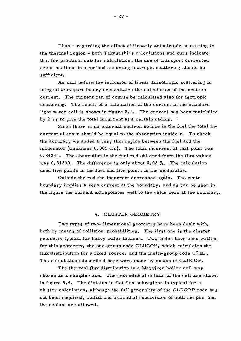
As said before the inclusion of linear anisotropic scattering in

integral transport theory necessitates the calculation of the neutron

current. The current can of course be calculated also for isotropic

scattering. The result of a calculation of the current in the standard

light water cell is shown in figure 8. 2. The current has been multiplied

by 2 rr r to give the total incurrent at a certain radius. '

Since there is no external neutron source in the fuel the total in­

current at any r should be equal to the absorption inside r. To check

the accuracy we added a very thin region between the fuel and the

moderator (thickness 0. 001 cm). The total incurrent at that point was

0.81244. The absorption in the fuel rod obtained from the flux values

was 0.81230. The difference is only about 0.02 %. The calculation

used five points in the fuel and five points in the moderator.

Outside the rod the incurrent decreases again. The white

boundary implies a zero current at the boundary, and as can be seen in

the figure the current extrapolates well to the value zero at the boundary.

9. CLUSTER GEOMETRY

Two types of two-dimensional geometry have been dealt with, both by means of collision probabilities. The first one is the cluster

geometry typical for heavy water lattices. Two codes have been written

for this geometry, the one-group code CLUCOP, which calculates the

flux distribution for a fixed source, and the multi-group code CLEF.

The calculations described here were made by means of CLUCOP.

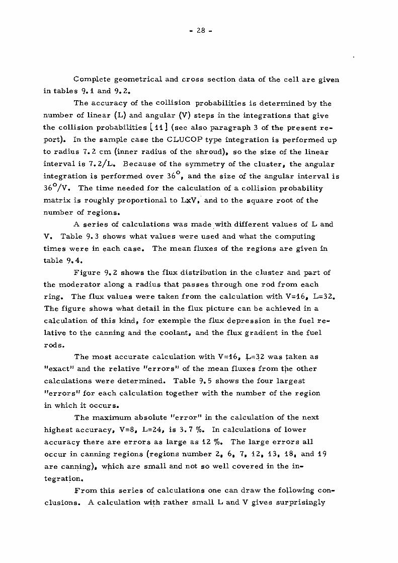
The thermal flux distribution in a Marviken boiler cell was

chosen as a sample case. The geometrical details of the cell are shown

in figure 9.1. The division in flat flux subregions is typical for a

cluster calculation, although the full generality of the CLUCOP code has

not been required, radial and azimuthal subdivision of both the pins and

the coolant are allowed.

“ 28 -

Complete geometrical and cross section data of the cell are given

in tables 9.1 and 9.2.

The accuracy of the collision probabilities is determined by the

number of linear (L) and angular (V) steps in the integrations that give the collision probabilities [ 11 ] (see also paragraph 3 of the present re­

port). In the sample case the CLUCOP type integration is performed up

to radius 7.2 cm (inner radius of the shroud), so the size of the linear

interval is 7. 2/L. Because of the symmetry of the cluster, the angular integration is performed over 36°, and the size of the angular interval is

36°/V. The time needed for the calculation of a collision probability

matrix is roughly proportional to LxV, and to the square root of the

number of regions.

A series of calculations was made with different values of L and

V. Table 9.3 shows what values were used and what the computing

times were in each case. The mean fluxes of the regions are given in

table 9. 4.

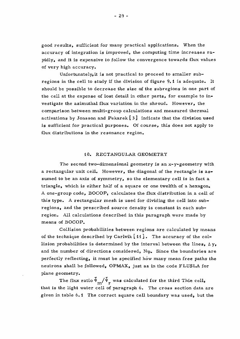
Figure 9.2 shows the flux distribution in the cluster and part of

the moderator along a radius that passes through one rod from each

ring. The flux values were taken from the calculation with V=l6, L=32.

The figure shows what detail in the flux picture can be achieved in a

calculation of this kind, for exemple the flux depression in the fuel re­

lative to the canning and the coolant, and the flux gradient in the fuel

rods.The most accurate calculation with V=l6, J-.= 32 was taken as

"exact" and the relative "errors" of the mean fluxes from t]ie other

calculations were determined. Table 9.5 shows the four largest

"errors" for each calculation together with the number of the region

in which it occurs.

The maximum absolute "error" in the calculation of the next

highest accuracy, V=8, L=24, is 3.7 %. In calculations of lower

accuracy there are errors as large as 12 %. The large errors all

occur in canning regions (regions number 2, 6, 7, 12, 13, 18, and 19

are canning), which are small and not so well covered in the in­

tegration.

From this series of calculations one can draw the following con­

clusions. A calculation wifh rather small L and V gives surprisingly

- 29 -

good results, sufficient for many practical applications. When the

accuracy of integration is improved, the computing time increases ra­

pidly, and it is expensive to follow the convergence towards flux values

of very high accuracy.

Unfortunately,it is not practical to proceed to smaller sub­

regions in the cell to study if the division of figure 9.1 is adequate. It

should be possible to decrease the size of the subregions in one part of

the cell at the expense of lost detail in other parts, for example to in­

vestigate the azimuthal flux variation in the shroud. However, the

comparison between multi-group calculations and measured thermal activations by Jons son and Pekarek [ 3 ] indicate that the division used

is sufficient for practical purposes. Of course, this does not apply to

flux distributions in the resonance region.

10. RECTANGULAR GEOMETRY

The second two-dimensional geometry is an x-y-geometry with

a rectangular unit cell. However, the diagonal of the rectangle is as­

sumed to be an axis of symmetry, so the elementary cell is in fact a

triangle, which is either half of a square or one twelfth of a hexagon.

A one-group code, BOCOP, calculates the flux distribution in a cell of

this type. A rectangular mesh is used for dividing the cell into sub­

regions, and the prescribed source density is constant in each sub­

region. All calculations described in this paragraph were made by

means of BOCOP.

Collision probabilities between regions are calculated by means of the technique described by Carlvik [ 11 ] . The accuracy of the col­

lision probabilities is determined by the interval between the lines, Ay,

and the number of directions considered, Ncp. Since the boundaries are

perfectly reflecting, it must be specified how many mean free paths the

neutrons shall be followed, OPMAX, just as in the code FLUSLA for

plane geometry.The flux ratio $ /$ was calculated for the third Thie cell,

m rthat is the light water cell of paragraph 6. The cross section data are

given in table 6.1 The correct square cell boundary was used, but the

- 30 -

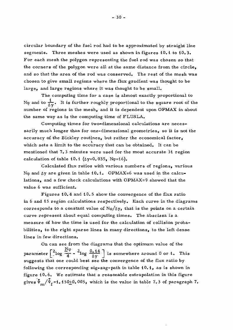
circular boundary of the fuel rod had to be approximated by straight line

segments. Three meshes were used as shown in figures 10.1 to 10.3.

For each mesh the polygon representing the fuel rod was chosen so that

the corners of the polygon were all at the same distance from the circle,

and so that the area of the rod was conserved. The rest of the mesh was

chosen to give small regions where the flux gradient was thought to be

large, and large regions where it was thought to be small.

The computing time for a case is almost exactly proportional to

Ncp and to ^. It is further roughly proportional to the square root of the

number of regions in the mesh, and it is dependent upon OPMAX in about

the same way as is the computing time of FLUSLA.

Computing times for two-dimensional calculations are neces­

sarily much longer than for one-dimensional geometries, so it is not the

accuracy of the Bickley routines, but rather the economical factor,\

which sets a limit to the accuracy that can be obtained. It can be

mentioned that 7. 3 minutes were used for the most accurate 31 region

calculation of table 10.1 (Ay=0. 035, Ncp=l6).

Calculated flux ratios with various numbers of regions, various

Ncp and Ay are given in table 10.1. OPMAX=6 was used in the calcu­

lations, and a few check calculations with OPMAX=9 showed that the

value 6 was sufficient.

Figures 10.4 and 10.5 show the convergence of the flux ratio

in 6 and 15 region calculations respectively. Each curve in the diagrams

corresponds to a constant value of Ncp/Ay, that is the points on a certain

curve represent about equal computing times. The abscissa is a

measure of how the time is used for the calculation of collision proba­

bilities, to the right sparse lines in many directions, to the left dense

lines in few directions.

On can see from the diagrams that the optimum value of the

parameter j^log Ncp- log 0.14 ]*is somewhere around 0 or 1. This4 & Ay

suggests that one could best see the convergence of the flux ratio by

following the corresponding zig-zag-path in table 10.1, as is shown in

figure 10. 6. We estimate that a reasonable extrapolation in this figure gives $m/=1.150+0. 005, which is the value in table 7.3 of paragraph 7.

- 31 -

The flux ratio is not very sensitive to the number of regions, 6,

15, or 31. This is because the overall variation of the flux density in

the cell is small (compare the calculation with collision probabilities of

paragraph 6, where only two regions gave the flux ratio with an accura­

cy of 0. 2 %).

11. CONCLUSIONS

We hope that most of what can be learned from the present work

has been pointed out in the preceeding paragraphs. Only a few summing

inferences will be drawn here.

It has been found that integral transport methods are very useful

for calculating neutron flux distributions in several types of reactor

lattice cells. A typical computing time for one-group flux ratios in a

cell with a fixed source is one second on IMB 7044 for an accuracy of

0.1 %, if the calculation is performed in a one-dimensional geometry

and with assumed isotropic scattering (with transport corrected cross

sections).

Integral transport methods are also applicable to systems with

more complex geometry, although computing times will necessarily be

longer. These methods are, in general, to be preferred to Monte Carlo

methods, if the geometry is not too complicated.

— 32 —

12. REFERENCES

1. KOBAYASHI, K and NISHIHARA, HThe solution of the integral transport equations in cylindrical geometry using the Gaussian quadrature formula J. Nucl. Energy A/B JJ3 (1964) 513-522 ,

2. TAKAHASHI, HThe generalized first-flight collision probability in the cylindri-calized lattice systemNucl. Sci. Eng. 24 (1966) 60-71

3. JONSSON, A and PEKAREK, HMulti-group collision probability theory in cluster geometry. Comparison with experimentsPaper to ’’Reactor Physics in the Resonance and Thermal Regions’’ANS National Topical Meeting, San Diego 7-9.2.1965

4. CARLVIK, 1Integral transport theory in one-dimensional geometries. 1966. (AE-227)

5. HONECK, H CThe distribution of thermal neutrons in space and energy in reactor lattices. Part I: Theory Nucl. Sci. Eng. 8 (i960) 193-202

6. TAKAHASHI, HFirst flight collision probability in lattice systems Reactor Science (J. Nucl. Energy, A).dJL (I960) 1-15

7. MOTHER, AStosswahrscheinlichkeiten in Zylindergeometrie Nukleonik^4 (1962) 53-56

8. KIESEWETTER, HZur Berechnung der Stosswahr scheinlichkeiten in regularen StabgitternKernenergie j6 (1963) 106-113

9. Di PASQUANTONIO, FCalculation of first-collision probabilities for heterogeneous lattice cells composed of n mediaReactor Sci. Tech. (J. Nucl. Energy A/b) 17 (1963) 67-81

10. PENNINGTON, E MCollision probabilities in cylindrical lattices Nucl. Sci. Eng. 19 (1964) 215-220

11. CARLVIK, IA method for calculating collision probabilities in general cylindrical geometry with applications to flux distributions and Dane off factorsU.N. Int. Gonf. on the Peaceful Uses of Atomic Energy,Geneva, 3. 1964. Vol. 2. Geneva 1965, p. 225

- 33 -

12. MULLER, A and LINNARTZ, EZur Berechnung des the r mi sc hen Nutzfaktors einer zylindrischen Zelle aus mehreren konzentrischen Zonen Nukleonik _5 (l 963) 23-27

13. KALNAES, O, NELTRUP, H and 0LGAARD, P LA recipe for heavy-water lattice calculations. 1964 (Ris/ Report No. 81)

14. BONALUMI, RNeutron first collision probabilities in reactor physics Energia Nucleare _8 (l961) 326-336

15. JONSSON, AOne-group collision-probability calculations for annular systems by the method of BonalumiReactor Sci. Techn. (J. Nucl. Energy A/b) 17 (1963) 511-518

16. HYSLOP, JFirst-collision probabilities associated with linearly anisot­ropic flux distributions in cylindrical geometry Reactor Sci. Techn. (J. Nucl. Energy A/B) _17 (1963) 237-244

17. STAMM'LER, R J JK-7 THERMOS (Neutron thermalization in a heterogeneouscylindrical!/ symmetric reactor cell). 1963(KR-47)

18. WEXLER, GBlackness and collision probabilities in complex fuel elements II. 1963(TNPG/PD1. 571)

19. HONECK, H CThe calculation of the thermal utilization and disadvantage factor in uranium water latticesLight Water Lattices, Vienna 1962, IAEA Technical Reports Ser. No. 12) 233-265

20. FUKAI, YFirst-flight collision probability in moderator-cylindrical fuel

' systemReactor Sci. Techn. F7 (1963) 115-120

21. SAUER, AThermal utilization in the square lattice cell J. Nucl. Energy A/B _18 (1964) 425-447

FUKAI, YValidity of the cylindrical cell approximation in lattice cal­culationsJ. Nucl. Energy A/B 18 (1964) 241-259

22.

- 34 -

23. WILLIS, I JA method for determining mean thermal flux ratios in a reactor lattice using first-flight collision probabilities J. Nucl. Energy A/B 1_9 (1965) 7-16

24. BEARD WOOD, J E, CLAYTON, A J and PULL, I CThe solution of the transport equation by collision probability methodsProceedings of the Conference on the Application of Computing Methods to Reactor Problems, May 1965 (ANL-7050)

25. LESLIE, D C and JONSSON, AThe calculation of collision probabilities in cluster-type fuel elementsNuclear Sci. Eng. _23 (1965) 272-290

26. BICKLEY, W G and NAYLER, JA short table of the functions Ki (x) from n=l to n=l6 Phil. Mag. Ser. 7, 20 (1935) 349-347

27. MULLER, G M , z«xTable of the function Kj (x)=— \ u nK (u) d u. 1954 (HW-30323) n xn Jo °

28. DANIELSEN, T M, HA VIE, T and STAMM'LER, R J J On the numerical calculation on Bickley functions. 1963 (KR-55)

29. CLAYTON, A JSome rational approximations for the KL and Ki, functions J. Nucl. Energy A/B, _18 (1964) 82-84

30. TOLLANDER, B Private communication

31. ABRAMOWITZ, M and STEGUN, I A (eds)Handbook of mathematical functions with formulas, graphsand mathematical tables. Wash. D. C. 1964(National Bureau of Standards, Appl. Mathematics Ser. 55)

32. THEYS, M HIntegral transport theory of thermal utilization factor in in­finite slab geometry Nucl. Sci. Eng. J7 (i960) 58-63

33. MENEGHETTI, DDiscrete ordinate quadratures for thin slab cells Nucl. Sci. Eng. 14 (1962) 295-303

34. FERZIGER, J H and ROBINSON, A HTransport calculations of the disadvantage factor Trans. Am. Nucl. Soc. _7 (1964) 12-13

— 35 —

35. ROBINSON, APrivate communication (1966)

36. PULL, I CThe solution of equations arising from the use of collision pro­babilities. 1963 (AEEW-M 355)

CLAYTON, A JThe programme PIP1 for the solution of the multigroup equations of the method of collision probabilities. 1964 (AEEW-R 326)

37. CARLVIK, IMonoenergetic critical parameters and decay constants for small spheres and thin slabs, 1967 (AE-273) ,

38. HAGGBLOM, HPrivate communication

39. CARLVIK, IOn the use of integral transport theory for the calculation ofthe neutron flux distribution in a Wigner-Seitz cell Nukleonik 8 (1966) 226-227

40. THIE, J AFailure of neutron transport approximations in small cells incylindrical geometryNucl. Sci. Eng. 9 (1961) 286-287

41. NEWMARCH, D AErrors due to the cylindrical cell approximation in lattice calculations. I960 (AEEW-R 34)

42. C LEND ENIN, W WEffect of zero gradient boundary conditions on cell calculationsin cylindrical geometryNucl. Sci. Eng. 14 (1962) 103-104

43. POMRANING, G CThe Wigner-Seitz cell: a discussion and a simple calculational methodNucl. Sci. Eng. 1J (1963) 311-314

44. SIMMS, R, KAPLAN, I, THOMPSON, T J and LANNING, D D The failure of the cell cylindricalization approximation in closely packed uranium/heavy-water latticesTrans. Am. Nucl. Soc. _7 (1964) 9

- 36 -

45* HONECK, H CThe calculation of the thermal utilization and disadvantage factor in uranium/water lattices Nucl. Sci. Eng. _18 (1964) 49-68

46. HONECK, H CSome methods for improving the cylindrical reflecting boundary condition in cell calculations of the thermal neutron flux Trans. Am. Nucl. Soc. j> (1962) 350-351

47. WEISS, Z and STAMM'LER, R J JCalculation of disadvantage factors for small cells Nucl. Sci. Eng. 19 (1964) 374-377

48. FUKAI, YZur Randbedingung mit isotroper Reflexion bei der Berechnung des zylindrischen Zellenrandes Nukleonik J7 (1965) 144-152

: FuelI

Moderator j!No source1

Constant .source j

jXt = 0.717 It= 2.33 |

jX«=0320 r ii o o

L a b !

r a = 0.1 b= 3.5 * a j, 02

iI 0.3 ij 0.4 1

Theys' lattice

[Constant !1j source Non - source region ;j region iI, = 0.20 It= 0.071^0.12 Ia= 0.028 i

iL a . . b

o = 0.32 3.2

b= 7 x ai

Meneghetti’s lattice

Figure 4.1

Data for slab lattices.

Half-cell dimensions are shown.

1.0982Fuel half thickness

1.09800.1 cm

1.2332

1.23300.2 cm

1.4126

1.412 2

1.411 8

1.6420

1.6410

1.6400

/

2 3 4 5 Fuel—1------------------1--------------- 1--------------- 1-----------------------------

10 9 8 7 Moderator

Figure 4. 2

Flux ratios in the lattices of Theys.

Variation of the distribution of points.

Fuel half thickness

0.1 cm

1.099

1.098

1.234

1.232

1.414

1.412

0.2cm

0.3cm

1.644

1.642

1.640

1.638

0.4 cm

Number of points

8 12 15 20J I I I—

Figure 4. 3

Flux ratios in the lattices of Theys.

Variation of the number of points.

f

Ferziger- Robinson

Diffusiontheory

. Fuel half thickness

Figure 4. 4

Flux ratios in the lattices of Theys by various methods.

1.123

1.121\ Thin cell

e

*s$ns

2.815

2.810

2.805

2.800

2.795

2.790

2.785

Thick cell

Number of points

5 10 20 J____________ I---------------------------------------- L_

Figure 4. 5

Flux ratios in the lattices of Meneghetti.

1.989_|

1.988.

1.987.

1.397,

1.396.

1.395.

1.394.

1.140,

1.139.

1.138 .

1.137 .

0

\CRIPASS

FLUBAG

Radius in m.fp.

1.0

/

\\CRIPASS

• — .o....— o •—

/■ FLUBAG2.0

/

\X^RIPASS

FLUBAG4.0

Number of points or order of polynomial

10 20

Figure 5.1

Critical parameter* of homogeneous sphere*.

FLU BAG2.0 . v

v\

\

81216

CRIPASS

1.5

1.0 .

0.5 .

0.00.0 0.5

X

r.

1.0Figure 5. 2

Flux distribution in a critical homogeneous

sphere of radius 2 mean free paths.

points

1.025 „

1.020 _

Number of points

1.015 „

core

14 13 12 11 10 9 8reflector

Figure 5. 3

of FR-0 calculated by means of FLUBAG

Variation of the distribution of points.

1.04 .

1.03 .

FLUBAG1.0 2 .

S4--------

HATTEN

Number of points in FLUBAG calculation

Figure 5. 4

°f FR-0 calculated by means of

FLUBAG, S4, and HATTEN.

1.750

V1.750

1.745

10 points

fuel region 3 4 5 6H------------ 1--------------- 1---------------- 1------------------

6 5 4 3moderator

1742

17407 8

h--------------- h

12 11

20 points

fuel region 9 10 11 12

10 9 8 7moderator

Figure 6. 1Flux ratios 4* /9, in the heavy water cell,m i 1Variation of the distribution of points.

\

10 points

1.330 __Number of pointsfuel region

moderator

1.338 ^ 20 points

fuel region

moderator

Figure 6. 2Flux ratio 4>g /4^ in the heavy water cell.

Variation of the distribution of points.

1.144 I

1.142 .

1.140 _

1.142 _

1.140 _

10 points

Number of points

fuel region3 4 5 6 7

H----------- 1---------1---------1-------- 1------7 6 5 4 3

moderator

20 points

fuel region7 8 9 10 11 12 13H----------- 1------------ 1--------- 1------------1------ h---------h13 12 11 10 9 8 7

moderator

Figure 6. 3Flux ratio in the light water cell.

Variation of the distribution of points.

1.80.

1.70

1.60.

0

o

10

number of space points or regions

—I------------------------------------ r-

20 30

/• CP1.30.

number of space points or regions

Figure 6.4

Convergence of flux ratios in the heavy water cell.

£m

1.150.

1.14 5.

1.13 5..

0

number of space points or regions

—i-----------------------------------r~

10 20

Figure 6.5

Convergence of the flux ratio in the light water cell.

Reflecting

ShroudWhite

ModeratorCanningCoolant

Radius

Figure 7. 1Flux distribution in the heavy water cell with

white and perfectly reflecting boundary.

Reflecting

White

Moderator

0.6 cm

Radius

Figure 7. 2

Flux distribution in the light water cell with

white and perfectly reflecting boundary.

1.74 _

$5

ff

1.73 „

1.72 „

Heavy water cell

1.13 .

1------------------------------ 1------------------------------ 1------------------------------ 1------------------------------ 1------------------------------ 1---------------------------- 1—

0/9 1/9 2/9 3/9 4/9 5/9 6/9Light water cell

Figure 8.1

Flux ratios in the heavy water and light water cells.

Variation with while keeping the transport cross

section constant.

2TTrJ(r)<|>(r),

Moderator

0.81244

= 0.81230

Radius

0.9

0.8

0.6

0.4

0.2

0.0

Figure 8. 2

Flux and incurrent in the light water cell.

T33O

CO

<u3

LL

7

zcnc*cc0$o

<L>-4—'

c<uO

<u4->

V)3u

Figure 9. 2

Flux distribution in the inner part of the cluster cell

0.5715

0.2348

CO

inoo CN COd d d

Figure 10.16 region mesh of square cell.

0.57

15

0.5715

0.1894

CDon CDo o o Oo cxi CXjo o' o O d

Figure 10. 215 region me eh of square cell.

0.57

15

0.5715

0.2522

0.1627

CXIo

o cr> CO CD If) COo o CM CM COo CD CD CD CD CD

CO

o

Figure 10. 331 region mesh of square cell.

0.57

15

014Ay

Figure 10. 4Flux ratio in square cell calculated for 6 regions.

Figure 10. 5Flux ratio in square cell calculated for 15 regions.

Figure 10. 6

Convergence of the flux ratio in the square cell.

Table 4.1

Flux ratios ^/♦j. i* the lattices of Theys

Variation of the distribution of points.

Half thickness of fuel

(cm)

0PMAX Number of points 5^moderator*fuel

Computingtime

(millimins)Total Fuel Mode­

rator

0.1 10.0 12 2 10 1.098163 393 9 1.098082 404 8 1.098116 38

5 7 1.098198 40

0.2 12 2 10 1.233120 23

3 9 1.232969 254 8 1.233066 24

5 7 . 1.233278 23

0.3 12 2 10 1.411996 20

3 9 1.411839 194 8 1.412117 19

5 7 1.412644 19

0.4 12 2 10 1.639596 16

3 9 1.639620 174 8 1.640382 17

5 7 1.641704 16

0.4 16 2 14 1.638765 28

3 13 1.638343 274 12 1.638433 28

5 11 1.638669 28

Table 4.2

Flux ratios in the lattices of Theys

Variation of OFMAX

Half thickness of fuel

(cm)

OFMAX Number of points ^moderator^fuel

Computingtime

(millimins)Total Fuel Mode­

rator

0.1 6.0 8 2 6 1.098542 148.0 1.098426 16

10.0 1.098423 18

6.0 12 3 9 1.098201 298.0 1.098086 36

10.0 1.098082 39

6.0 15 3 12 1.098155 438.0 1.098039 55

10.0 1.098036 6l

6.0 20 4 16 1.098122 778.0 1.098006 98

10.0 1.098002 106

0.4 6.0 8 2 6 1.644370 88.0 1.644311 8

10.0 1.644311 8

6.0 12 3 9 1.639676 158.0 1.639620 17

10.0 1.639620 17

6.0 15 3 12 1.638574 228.0 1.638516 25

10.0 1.638516 25

6.0 20 4 16 1.638006 388.0 1.637947 43

10.0 1.637947 42

Table 4.3

Flux ratios in the lattices of Theys

Variation of the number of points

Half thickness of fuel

(cm)

OFMAX Number of points ^moderator^fuel

Computingtime

(millimins)Total Fuel Mode­

rator

0.1 10.0 8 2 6 1.098423 18

12 3 9 1.098082 39

15 3 12 1.098036 6l

20 4 16 1.098002 106

0.2 8 2 6 1.233815 12

12 3 9 1.232969 24

15 3 12 1.232832 37

20 4 16 1.232743 64

0.3 8 2 6 1.413813 9

12 3 9 1.411839 19

15 3 12 1.4ll44l 29

20 4 16 1.411217 50

0.4 8 2 6 1.644311 8

12 3 9 1.639620 17

15 3 12 1.638516 25

20 4 16 1.637947 42

Table 4.1+

Flux ratios $m/?£. in the lattices of Theys

by various methods

Method Half thickness of fuel (cm)0.1 0.2 0.3 0.4

Diffusion appr. 1.03 1.11 1.24 1.43

Theys (ABH) 1.08 1.20 1.36 1.58

Lathrop, Sg 1.090 1.231 1.410 1.632

Ferziger-Robinson Eigen-function expansion

1.094 1.227 1.401 1.623

Carlvik, BIT 1.0979 1.2318 1.408 1.629

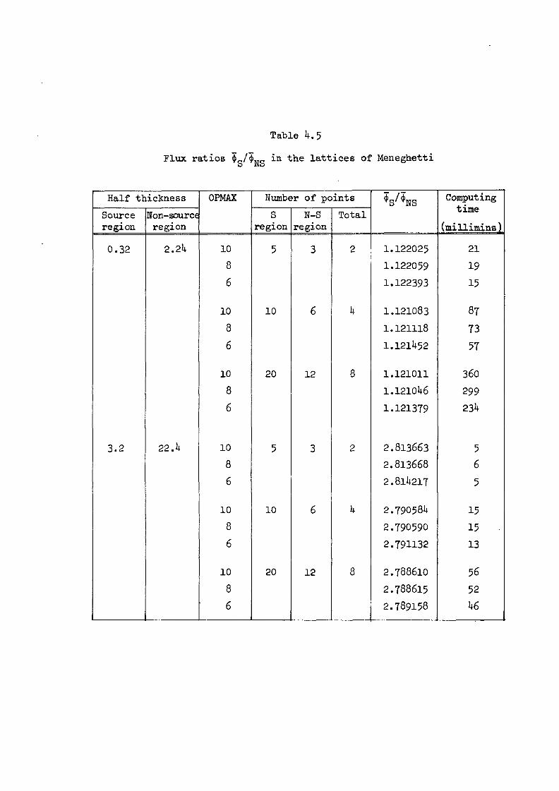
Table 4.5

Flux ratios 4>g/i^g in the lattices of Meneghetti

Half thickness OPMAX Number of points *S^NS Computingtime

(millimins)Sourceregion

Non-sourceregion

Sregion

N-Sregion

Total

0.32 2.24 10 5 3 2 1.122025 218 1.122059 196 1.122393 15

10 10 6 4 1.121083 878 1.121118 736 1.121452 57

10 20 12 8 1.121011 3608 1.121046 2996 1.121379 234

3.2 22.4 10 5 3 2 2.813663 58 2.813668 66 2.814217 5

10 10 6 4 2.790584 158 2.790590 15 •6 2.79H32 13

10 20 12 8 2.788610 568 2.788615 526 2.789158 46

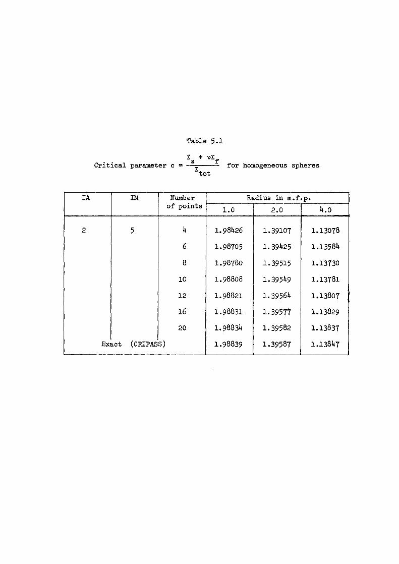
Table $.1

Critical parameter c =Es + vEf

totfor homogeneous spheres

IA IM Number of points

Radius in m.f.p.1.0 2.0 4.0

2 5 4 1.98426 1.39107 1.13078

6 1.98705 1.39425 1.13584

8 I.9878O 1.39515 1.13730

10 1.98808 1.39549 1.13781

12 1.98821 1.39564 1.13807

16 1.98831 1.39577 1.13829

20 1.98834 1.39582 1.13837

Extict (CRIPASs) 1.98839 1.39587 1.13847

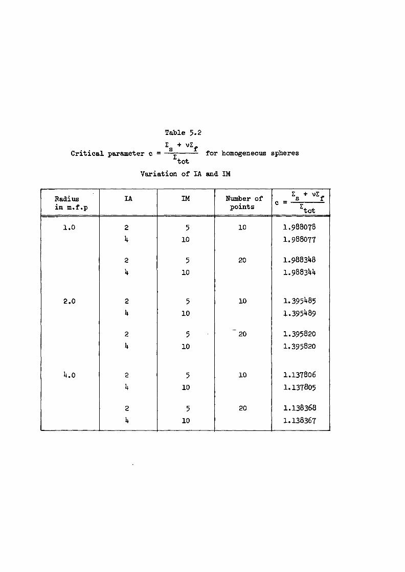
Table 5.2

Zs + vlCritical parameter c = —z-------- for homogeneous spheres

totVariation of IA and IM

Radius in m.f.p

IA IM Number of points =. vu£f

tot

1.0 2 5 10 1.988078

4 10 1.988077

2 5 20 1.9883484 10 1.988344

2.0 2 5 10 1.3954854 10 1.395489

2 5 ~ 20 1.395820

4 10 1.395820

4.0 2 5 10 1.1378064 10 1.137805

2 5 20 1.138368

4 10 1.138367

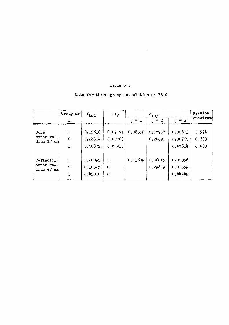
Table 5.3

Data for three-group calculation on FR-0

Group nr Ztot vZf _________Fissionspectrumi j = 1 j = 2 j = 3

Core ‘ 1 0.19836 0.07791 0.08552 0.07767 0.00623 0.574outer ra­dius 17 cm 2 0.28614 0.02766 0.26091 0.00765 0.393

3 0.50872 0.03915 0.47814 0.033

Reflector 1 0.20095 0 0.13609 0.06045 0.00356outer ra­dius U7 cm 2 0.30525 0 0.29819 0.00559

3 0.45010 0 0.44449

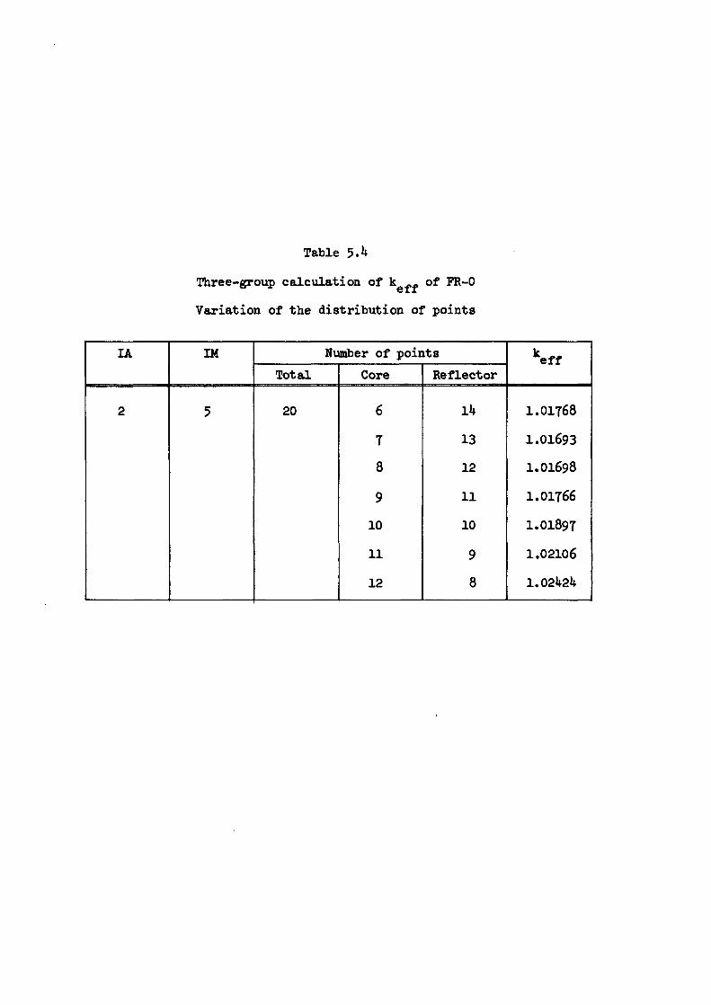
Table 5.4

Three-group calculation of keff of FR-0

Variation of the distribution of points

IA IM Number of points keffTotal Core Reflector

2 5 20 6 lit 1.01768

7 13 1.01693

8 12 I.OI698

9 11 1.01766

10 10 1.01897

11 9 1.02106

12 8 1.02424

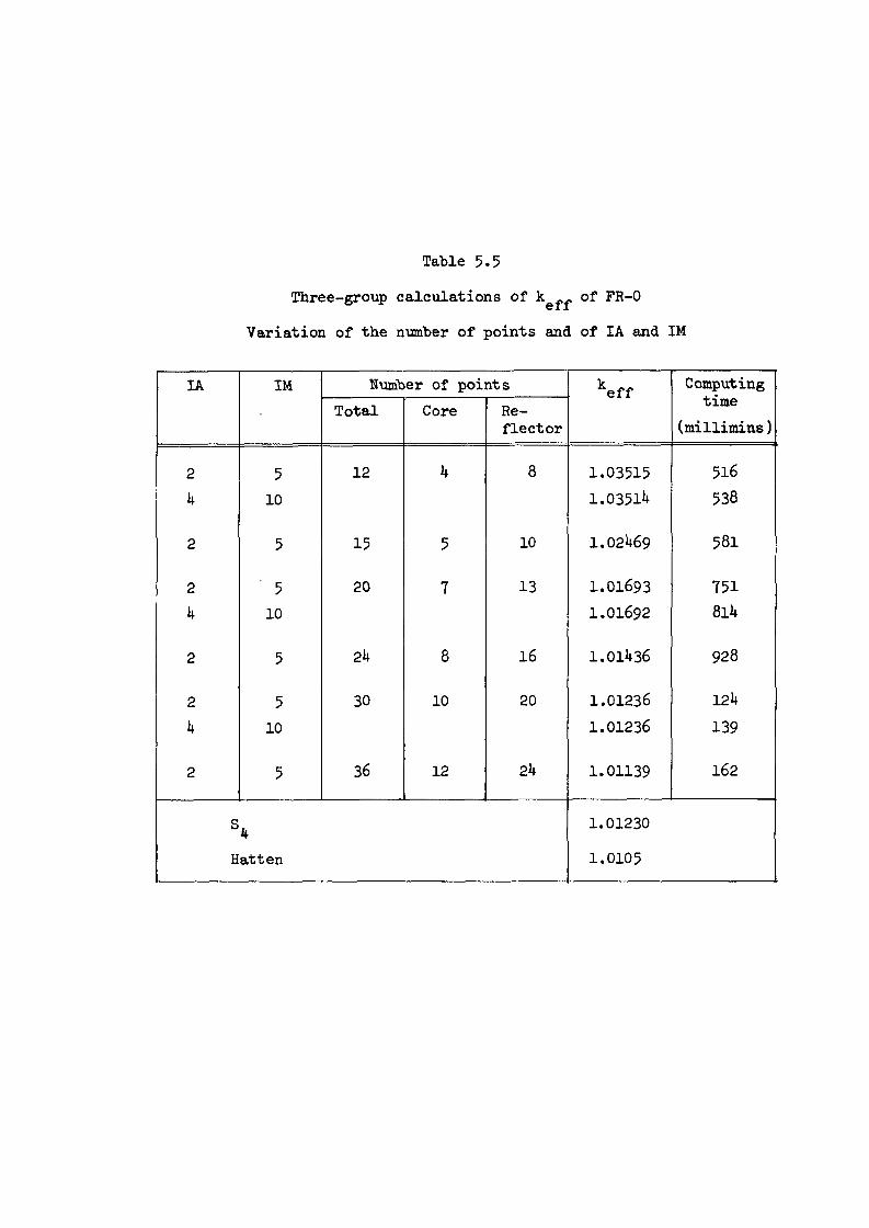
Table 5.5

Three-group calculations of kef^ of FR-0

Variation of the number of points and of IA and IM

IA IM Number of points keff Computingtime

(millimins)Total Core Re­

flector

2 5 12 4 8 1.03515 516

4 10 1.03514 538

2 5 15 5 10 1.02469 581

2 5 20 7 13 1.01693 7514 10 1.01692 8l4

2 5 2k 8 16 1.01436 928

2 5 30 10 20 1.01236 124

4 10 1.01236 139

2 5 36 12 2k 1.01139 162

S 4 1.01230

Hatten 1.0105

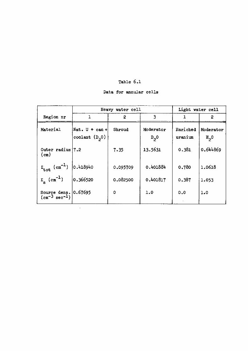
Table 6.1

Data for annular cells

Heavy water cell Light water cellRegion nr 1 2 3 1 2

Material Nat. U + can + Shroud Moderator Enriched Moderatorcoolant (DgO) D2° uranium H2°

Outer radius (cm)

7.2 7.35 13.5631 0.381 0.644869

Etot O.ltlSpUO 0.095709 0.401884 0.780 1.0618

Zs (cm-1) 0.366520 0.082500 0.401817 0.387 1.053

Source dens, (cm-3 gec"l)

0.67695 0 1.0 0.0 1.0

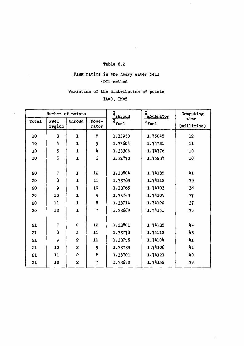
Table 6.2

Variation of the distribution of points IA=0, IM=5

Flux ratios in the heavy water cell• DIT-method

Number of points 4Yshroud^fuel

^moderator

*fuel

Computingtime

(millimins)Total Fuel

regionShroud Mode­

rator

10 3 1 6 1.33950 1.75045 12

10 4 1 5 1.33604 1.74721 11

10 5 1 4 1.33306 1.74776 10

10 6 1 3 1.32770 1.75237 10

20 7 1 12 1.33804 1.74135 4l

20 8 1 11 1.33783 1.74112 3920 9 1 10 1.33765 1.74103 38

20 10 1 9 1.33743 1.74105 3720 11 1 8 1.33714 1.74120 3720 12 ; 7 1.33669 1.74151 35

21 7 2 12 1.33801 1.74135 44

21 8 2 11 1.33778 1.74112 43

21 9 2 10 1.33758 1.74104 4i

21 10 2 9 1.33733 1.74106 4l

21 11 2 8 1.33701 1.74121 40

21 12 2 7 1.33652 1.74152 39

Table 6.3

Variation of the distribution of points

IA=0, IM=5

Flux ratios in the light water cellDIT-method

Number of points 2^moderator^fuel

Computingtime

(millimins)Total Fuel Moderator

10 3 7 1.14240 11

4 6 1.14145 11

5 5 1.14110 10

6 4 1.14103 11

7 3 1.14124 10

20 7 13 1.14083 4i

8 12 1.14079 4o

9 11 1.14077 4o

10 10 1.14075 3911 9 1.14075 3812 8 1.14075 38

13 7 1.14075 37

Table 6.4

Variation of Ik and IM

Flux ratios in the heavy water cellDIT-method

IA IM Number of points^shroud 5

moderator Computingtime

(millimins)Total Fuel

regionShroud Mode­

rator *fuel *fuel

0 5 11 5 1 5 1.33556 1.74544 13

2 5 1.33550 1.74535 150 8 1.33546 1.74544 13

2 8 1.33552 1.74535 17

0 5 22 10 2 10 1.33751 1.74091 45

2 5 1.33751 1.74090 53

0 8 1.33722 1.74092 54

2 8 1.33722 1.74091 63

Variation of IA and IM

Table 6.5

Flux ratios in the light water cellDIT-method

IA IM Number of points^moderator^fuel

Computing

Total Fuel Mode­rator

time(millimins)

0 5 10 5 5 l.lUllO 10

2 5 l.l4o86 130 8 l.lUllO 11

2 8 1.14085 14

0 5 20 10 10 1.14075 392 5 1.14073 430 8 1.14075 472 8 1.14073 55

3

5

7

913

172122

26

30

3k

35

Table 6.6

Variation of the number of points

IA«0, IM*5

Flux ratios in the heavy water cellDIT-method

Number of points A _Tshroud^fuel

♦ . . Computingtime

(millimins)Fuelregion

Shroud Mode­rator

moderator^fuel

1 1 1 1.960U5 3.10756 It '

2 1 2 1.32626 1.80053 It

3 1 3 1.32936 1.75907 6

k 1 k 1.333^5 1.7k9k9 9

6 1 6 1.33656 1.7k339 16

8 1 8 1.33735 1.7kl60 27

10 1 10 1.33758 1.7k09l kl

10 2 10 1.33751 1.7k09l k5

12 2 12 1.33763 1.7k059 6k

lk 2 lk 1.33768 1.7k0k2 87

16 2 16 1.33769 1.7k032 113

16 3 16 1.3377% 1.7k032 122

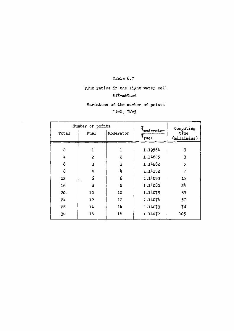
Variation of the number of points

IA=0, IM=5

Table 6.7

Flux ratios in the light water cell

DIT-method

Number of points(4moderator

^fuel

Computingtime

(millimins)Total Fuel Moderator

2 1 1 1.19564 34 2 2 1.14625 36 3 3 1.14262 58 1* 4 1.14152 7

12 6 6 1.14093 1516 8 8 l.l4o8o 24

20, 10 10 1.14075 392k 12 12 1.14074 5728 14 Ik 1.14073 78

32 16 16 1.14072 105

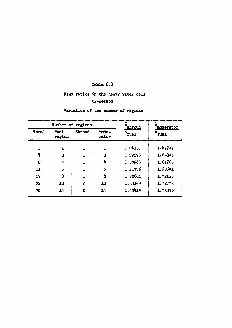
Table 6.8

Variation of the number of regions

Flux ratios in the heavy water cellCP-method

Number of regions *shroud*fuel

^moderator*fuelTotal Fuel

regionShroud Mode­

rator

3 1 1 1 1.24131 1.47747

7 3 1 3 1.29596 1.64345

9 4 1 4 1.30986 1.67765

11 5 1 5 1.31796 1.69691

17 8 1 8 1.32861 1.7213522 10 2 10 1.33149 1.72773

30 14 2 14 1.33419 1.73359

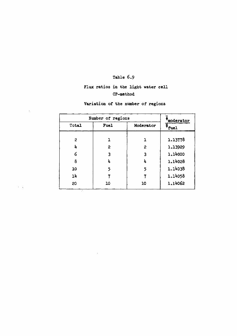
Variation of the number of regions

Table 6.9

Flux ratios in the light water cellCP-method

Number of regions ^moderator

^fuelTotal Fuel Moderator

2 1 1 1.13778

It 2 2 1.139296 3 3 1.14000

8 4 4 1.14028

10 5 5 1.14038

14 7 7 1.14058

20 10 10 1.14062

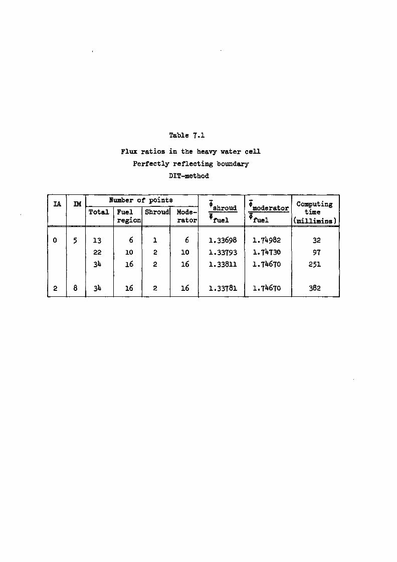
Table 7.1

Flux ratios in the heavy water cell

Perfectly reflecting boundary

DIT-method

IA IM Number of points ATshroud

Amoderator Computing

time(millimins)

Total Fuelregion

Shroud Mode­rator *fUel ^fuel

0 5 13 6 1 6 1.33698 1.74982 32

22 10 2 10 1.33793 1.74730 9734 16 2 16 1.33811 1.74670 251

2 8 34 16 2 16 1.33781 1.74670 382

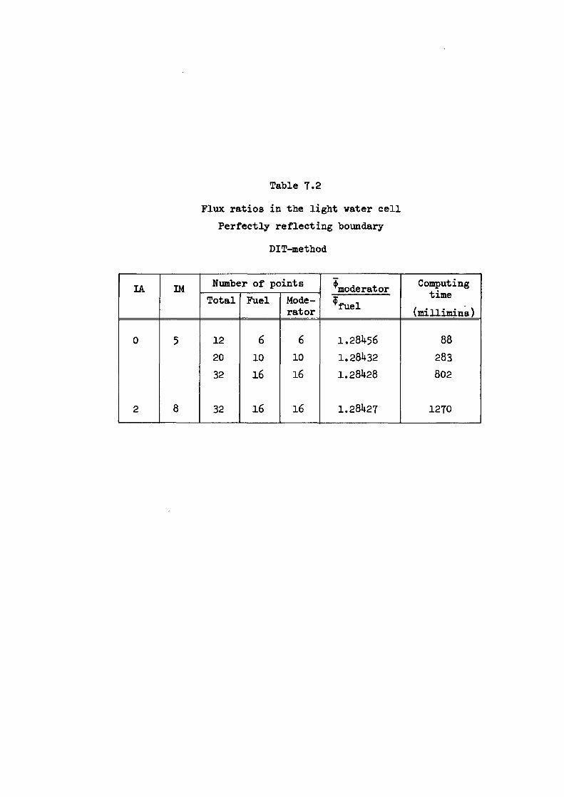
Table 7.2

Flux ratios in the light water cell Perfectly reflecting boundary

DIT-method

IA IM Number of points ^moderator Computingtime

(millimins)Total Fuel Mode­

rator^fuel

0 5 12 6 6 1.28456 8820 10 10 1.28432 28332 l6 16 1.28428 802

2 8 32 16 16 1.28427 1270

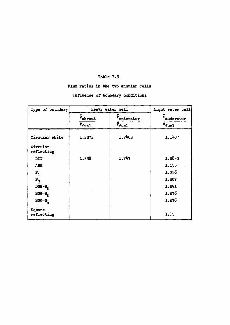
Table 7.3

Flux ratios in the two annular cells Influence of boundary conditions

Type of boundary Heavy water cell Light water cell$moderator^fuel

*shroud^fuel

Amoderator^fuel

Circular white 1.3373 1.7W3 1.1U07

CircularreflectingDIT 1.338 1.7^7 1.281*3

ABH 1.155 .

P1 1.036

P3 1.207

DSN-Sq 1.291SNG-Sq 1.276

SNG-S^ 1.276

Squarereflecting 1.15

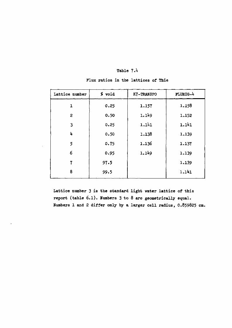
Table 7.4

Flux ratios in the lattices of Thie

Lattice number % void K7-TRANSP0 FLURIG-4

1 0.25 1.157 1.158

2 0.50 1.149 1.152

3 0.25 l.l4l i.l4i

4 0.50 1.138 1.139

5 0.75 1.136 1.137

6 0.95 1.149 1.139

7 97.5 1.139

8 99.5 l.l4i

Lattice number 3 is the standard light water lattice of this

report (table 6.1). Numbers 3 to 8 are geometrically equal.

Numbers 1 and 2 differ only by a larger cell radius, 0.859825 cm.

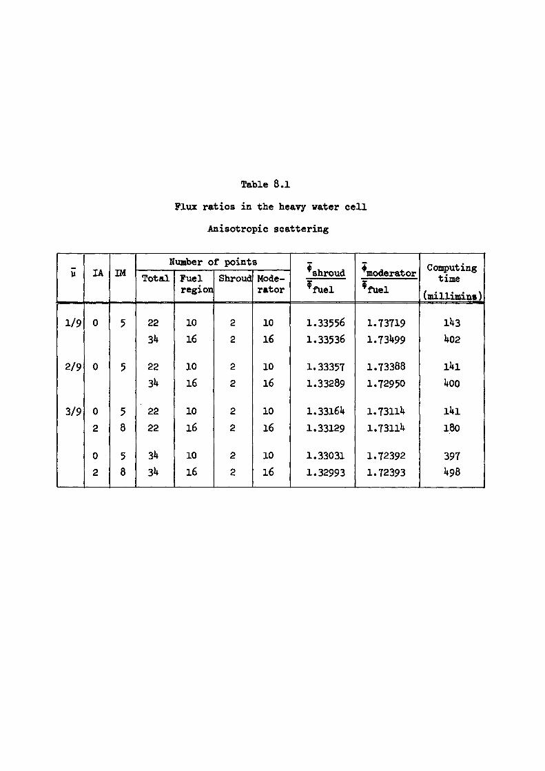
Table 8.1

Flux ratios in the heavy water cell

Anisotropic scattering

a IA IMNumber of points I

shroud ^moderator Computingtime

(millimins)

Total Fuelregion

Shroud Mode­rator ^fuel ^fuel

1/9 0 5 22 10 2 10 1.33556 1.73719 143

34 16 2 16 1.33536 1.73499 402

2/9 0 5 22 10 2 10 1.33357 1.73388 l4l

34 16 2 16 1.33289 1.72950 400

3/9 0 5 22 10 2 10 1.33164 1.73114 l4l

2 8 22 16 2 16 1.33129 1.73114 180

0 5 34 10 2 10 1.33031 1.72392 3972 8 34 16 2 16 1.32993 1.72393 498

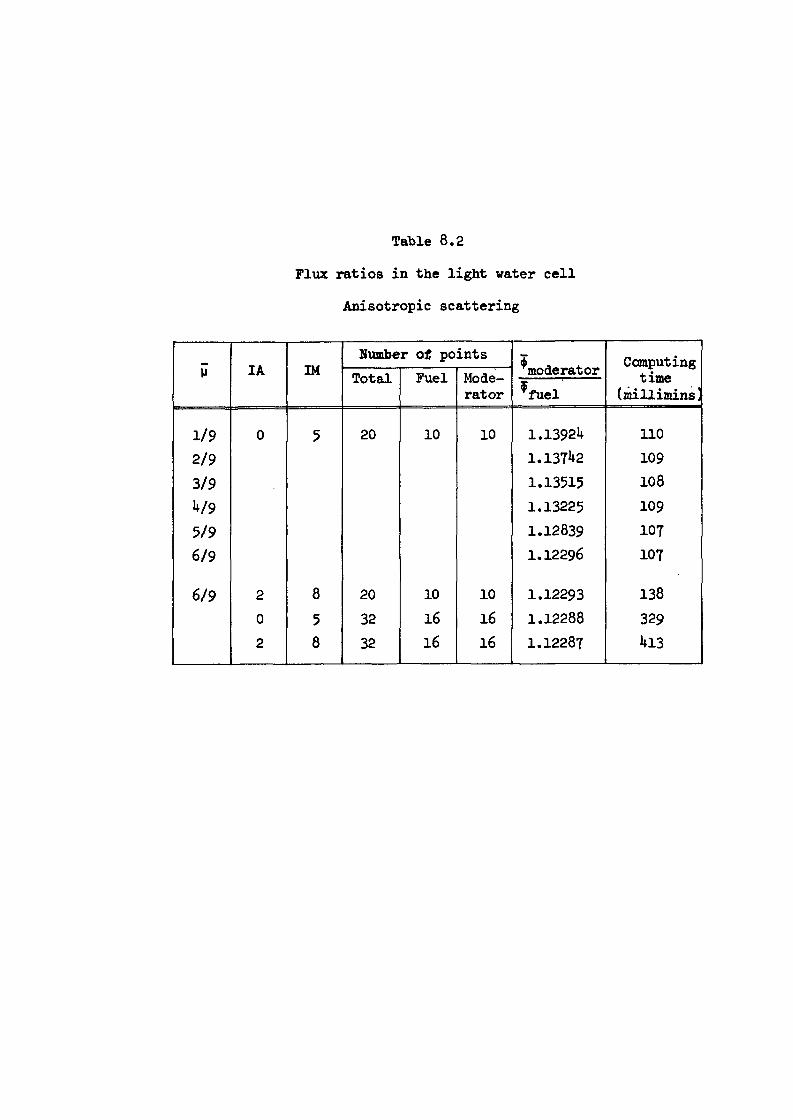
Table 8.2

Flux ratios in the light water cell

Anisotropic scattering

V IA IMNumber of points I

moderator Computingtime

(millimins!Total Fuel Mode­

rator ffuel

1/9 0 5 20 10 10 1.13924 110

2/9 1.13742 109

3/9 1.13515 108

4/9 1.13225 109

5/9 1.12839 107

6/9 1.12296 107

6/9 2 8 20 10 10 1.12293 138

0 5 32 16 16 1.12288 329

2 8 32 16 16 1.12287 413

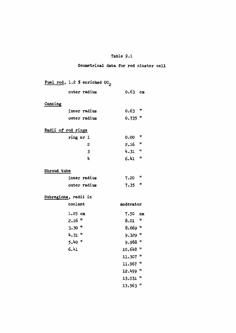
Table 9.1

Geometrical data for rod cluster cell

Fuel rod, 1.2 % enriched UO,

outer radius 0.63 cm

Canning

inner radius 0.63 It

outer radius 0.735 M

Radii of rod rings

ring nr 1 0.00 II

2 2.16 Tl

3 4.31 IV

4 6.4l II

Shroud tube

inner radius 7.20 IV

outer radius 7.35 II

Subregions, radii in

coolant moderator

1.25 cm 7.50 cm2.16 " 8.01 II

3.30 " 8.669 II

4.31 " 9.329 II

5.40 " 9.988 II

6.4l 10.648 II

11.307 II

11.967 It

12.499 II

13.031 n

13.563 tr

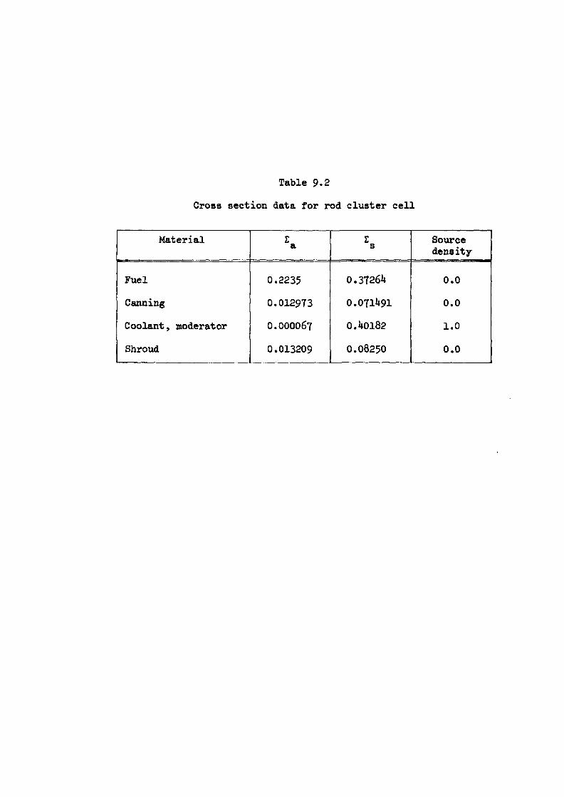
Table 9.2

Cross section data for rod cluster cell

Material %a Zs Sourcedensity

Fuel 0.2235 0.37264 0.0

Canning 0.012973 0.071491 0.0

Coolant, moderator 0.000067 0.40182 1.0

Shroud 0.013209 0.08250 0.0

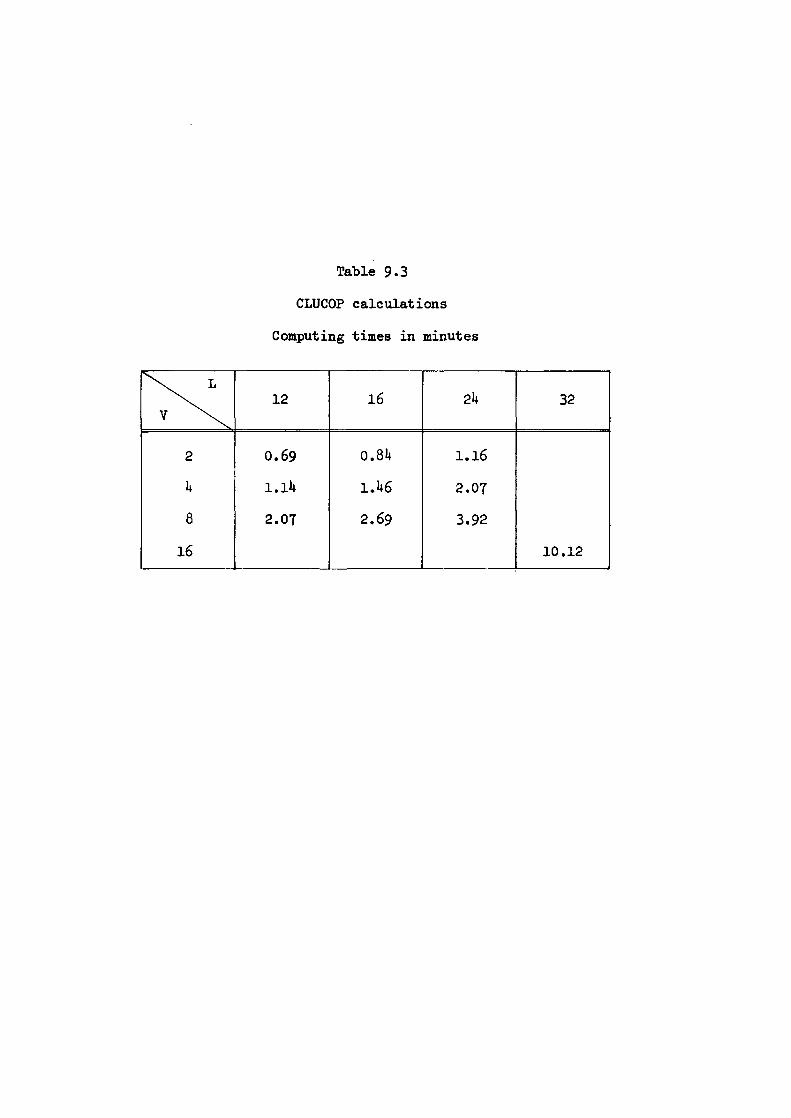
Table 9.3

CLUCOP calculations

Computing times in minutes

L

V12 16 24 32

2 0.69 0.84 1.16

4 l.l4 1.46 2.07

8 2.07 2.69 3.92

16 10.12

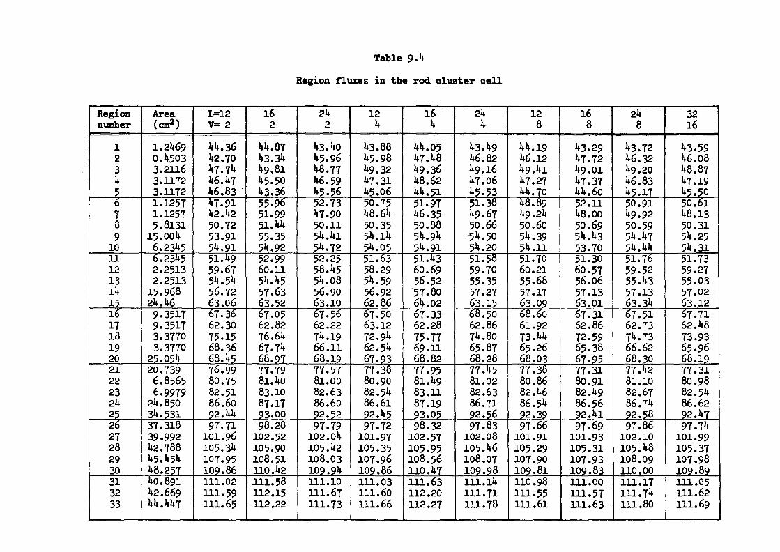
Table 9*4

Region fluxes in the rod cluster cell

Region Area L=12 16 24 12 16 24 12 16 24 32number (cm2) V= 2 2 2 4 4 4 8 8 8 16

1 1.2469 44.36 44.87 43.40 43.88 44.05 43.49 44.19 43.29 43.72 43.592 0.4.503 42.70 43.34 45.96 45.98 47.48 46.82 46.12 47.72 46.32 46.083 3.2116 47.74 49.81 48.77 49.32 49.36 49.16 49.4i 49.01 49.20 48.874 3.1172 46.47 45.50 46.59 47.31 48.62 47.06 47.27 47.37 46.83 47.195 3.1172 46.83 43.36 45.56 45.06 44.51 45.53 44.70 44.60 45.17 45.50 6 1.1257 47.91 55.96 52.73 50.75 51.97 51.38 48.89 52.11 50.91 50.617 1.1257 42.42 51.99 47.90 48.64 46.35 49.67 49.24 48.00 49.92 48.138 5.8131 50.72 51.44 50.11 50.35 50.88 50.66 50.60 50.69 50.59 50.319 15.004 53.91 55.35 54.4i 54.14 54.94 54.50 54.39 54.43 54.47 54.25

10 6.2345 54.91 54.92 54.72 54.05 54.91 54.20 54.11 53.70 54.44 54.3111 “ 6.2345 51.49 52.99 52.25 51.63 51.43 51.58 51.70 51.30 51.76 51.7312 2.2513 59.67 60.ll 58.45 58.29 60.69 59.70 60.21 60.57 59.52 59.2713 2.2513 54.54 54.45 54.08 54.59 56.52 55.35 55.68 56.06 55.43 55.03l4 15.968 56.72 57.63 56.90 56.92 57-80 57.27 57.17 57.13 57.13 57.0215 24.46 63.06 63.52 63.10 62.86 64.02 63.15 63.09 63.01 63.34 63.1216 9.3517 67.36 67.05 67.56 67.50 67.33 68.50 68.60 67.31 67.51 67.7117 9.3517 62.30 62.82 62.22 63.12 62.28 62.86 61.92 62.86 62.73 62.4818 3.3770 75.15 76.64 74.19 72.94 75.77 74.80 73.44 72.59 74.73 73.9319 3.3770 68.36 67.74 66.11 62.54 69.11 65.87 65.26 65.38 66.62 65.9620 25.054 68.45 68.97 68.19 67.93 68.82 68.28 68.03 67.95 68.30 68.1921 20.739 76.99 77.79 77.57 77.38 77.95 77.45 77.38 77.31 77.42 77.3122 6.8565 80.75 81.40 81.00 80.90 81.49 81.02 80.86 80.91 81.10 80.9823 6.9979 82.51 83.10 82.63 82.54 83.11 82.63 82.46 82.49 82.67 82.5424 24.850 86.60 87.17 86.60 86.61 87.19 86.71 86.54 86.56 86.74 86.6225 34.531 92.44 93.00 92.52 92.45 93.05 92.56 92.39 92.41 92.58 92.4726 37.318 97.71 98.28 97-79 97.72 98.32 97.83 97-66 97.69 97.86 97.7427 39.992 101.96 102.52 102.04 101.97 102.57 102.08 101.91 101.93 102.10 101.9928 42.788 J-05.34 105.90 105.42 105.35 105.95 105.46 105.29 105.31 105.48 105.3729 45.454 107.95 108.51 108.03 107.96 108.56 108.07 107.90 107.93 108.09 107.9830 48.257 109.86 110.42 109.94 109.86 110.47 109.98 109.81 109.83 110.00 109.8931 40.891 111.02 111.58 111.10 111.03 111.63 111.14 110.98 111.00 111.17 111.0532 42.669 111.59 112.15 111.67 111.60 112.20 111.71 111.55 111.57 111.74 111.6233 44.447 111.65 112.22 111.73 111.66 112.27 111.78 111.61 111.63 111.80 111.69

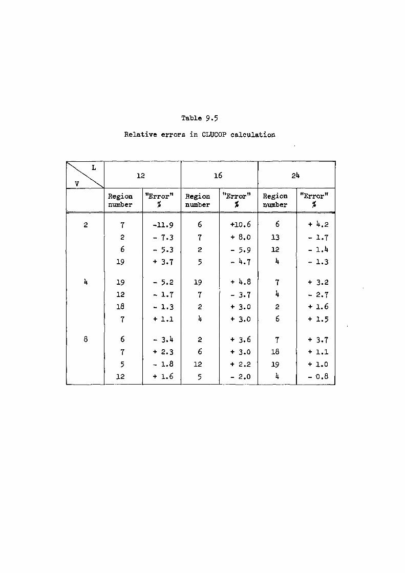
Table 9-5

Relative errors in CLUCOP calculation

X\ L

V \12 l6 24

Regionnumber

"Error"%

Regionnumber

"Error"%

Regionnumber

"Error"%

2 7 -11.9 6 +10.6 6 + 4.2

2 - 7.3 7 + 8.0 13 - 1.76 - 5.3 2 - 5.9 12 - 1.4

19 + 3.7 5 - 4.7 4 - 1.3

4 19 - 5.2 19 + 4.8 7 + 3.2

12 - 1.7 7 - 3.7 4 - 2.718 - 1.3 2 + 3.0 2 + 1.6

7 + 1.1 4 + 3.0 6 + 1.5

8 6 - 3.4 2 + 3.6 7 + 3.7

7 + 2.3 6 + 3.0 18 + 1.1

5 - 1.8 12 + 2.2 19 + 1.0

12 + 1.6 5 - 2.0 4 - 0.8

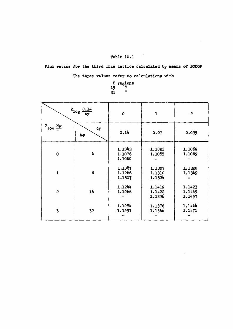
Table 10.1

Flux ratios for the third Thie lattice calculated by means of B0C0P

The three values refer to calculations with6 regions

1531

nii

0 1 2

Ay0.14 0.07 0.035

1.1043 1.1023 1.10690 4 1.1076 1.1085 1.1089

1.1080 - -

1.1087 1.1307 1.13201 8 1.1266 1.1310 1.1349

1.1307 1.1324 -

1.1244 1.1419 1.14232 16 1.1266 1.1422 1.1449

- 1.1396 1.1457

1.1284 1.1376 1.14443 32 1.1251 1.1366 1.1471

** — —

LIST OF PUBLISHED AE-REPORTS

1—200. (See the back cover earlier reports.)

201. Heat transfer analogies. By A. Bhattacharyya. 1965. 55 p. Sw. cr. 8:—.202. A study of the ”384” KeV complex gamma emission from plutonium-239.

By R. S. Forsyth and N. Ronqvist. 1965. 14 p. Sw. cr. 8:—.203. A scintillometer assembly for geological survey. By E. Dissing and O.

Landstrom. 1965. 16 p. Sw. cr. 8:—.204. Neutron-activation analysis of natural water applied to hydrogeology. By

O. Landstrom and C. G. Wenner. 1965. 28 p. Sw. cr. 8:—.205. Systematics of absolute gamma ray transition probabilities in deformed

oad-A nuclei. By S. G. Malmskog. 1965. 60 p. Sw. cr. 8:-. k206. Radiation induced removal of stacking faults in quenched aluminium. By

U. Bergenlid. 1965. 11 p. Sw. cr. 8:—.207. Experimental studies on assemblies 1 and 2 of the fast reactor FRO. Part 2.

By E. Hellstrand, T. Andersson, B. Brunfelter, J. Kockum, S-O. London and L. I. TirSn. 1965. 50 p. Sw. cr. 8:—.

208. Measurement of the neutron slowing-down time distribution at 1.46 eV and its space dependence in water. By E. Moller. 1965. 29 p. Sw. cr. 8:—.

209. Incompressible steady flow with tensor conductivity leaving a transverse magnetic field. By E. A. Witalis. 1965. 17 p. Sw. cr. 8:-.

210. Methods for the determination of currents and fields In steady two­dimensional MHD flow with tensor conductivity. By E. A. Witalis. 1965. 13 p. Sw. cr. 8:-.

211. Report on the personnel dosimetry at AB Atomenergi during 1964. By K. A. Edvardsson. 1966. 15 p. Sw. cr, 8:-.

212. Central reactivity measurements on assemblies 1 and 3 of the fast reactor FRO. By S-O. Londen. 1966. 58 p. Sw. cr. 8:-.

213. Low temperature irradiation applied to neutron activation analysis of mercury in human whole blood. By D. Brune. 1966. 7 p. Sw. cr. 8:—.

214. Characteristics of linear MHD generators with one or a few loads. By E. A. Witalis. 1966. 16 p. Sw. cr. 8:-.

215. An automated anion-exchange method for the selective sorption of five groups of trace elements in neutron-irradiated biological material. By K. Samsahl. 1966. 14 p. Sw. cr. 8:—.

216. Measurement of the time dependence of neutron slowing-down and therma- lization in heavy water. By E. Moller. 1966. 34 p. Sw. cr. 8:—.

217. Electrodeposition of actinide and lanthanide elements. By N-E. Barring. 1966. 21 p. Sw. cr. 8:-.

218. Measurement of the electrical conductivity of He* plasma induced by neutron irradiation. By J. Braun and K, Nygaard. 1966. 37 p. Sw. cr. 8:-.

219. Phytoplankton from Lake Magelungen, Central Sweden 1960—1963. By T. Willen. 1966. 44 p. Sw. cr. 8:—.

220. Measured and predicted neutron flux distributions in a material surround­ing av cylindrical duct. By J. Nilsson and R. Sandlin. 1966. 37 p. Sw. cr. 8:—.

221. Swedish work on brittle-fracture problems in nuclear reactor pressure vessels. By M. Grounes. 1966. 34 p. Sw. cr. 8:-.

222. Total cross-sections of U, UOa and ThOi for thermal and subthermal neutrons. By S. F. Beshai. 1966. 14 p. Sw. cr. 8:—.

223. Neutron scattering in hydrogenous moderators, studied by the time de­pendent reaction rate method. By L. G. Larsson, E, Moller and S. N. Purohit. 1966. 26 p. Sw. cr. 8:—.

224. Calcium and strontium in Swedish waters and fish, and accumulation of strontium-90. By P-O. Agnedal. 1966. 34 p. Sw. cr. 8:-.

225. The radioactive waste management at Studsvik. By R. Hedlund and A. Lindskog. 1966. 14 p. Sw. cr. 8:—.

226. Theoretical time dependent thermal neutron spectra and reaction rates in H2O and DzO. S. N. Purohit. 1966. 62 p. Sw. cr. 8:-.

227. Integral transport theory in one-dimensional geometries. By I. Carlvik. 1966. 65 p. Sw. cr. 8:—.

228. Integral parameters of the generalized frequency spectra of moderators. By S. N. Purohit. 1966. 27 p. Sw. cr. 8:—.

229. Reaction rate distributions and ratios in FRO assemblies 1, 2 and 3. By T. L. Andersson. 1966. 50 p. Sw. cr. 8:—.

230. Different activation techniques for the study of epithermal spectra, app­lied to heavy water lattices of varying fuel-to-moderator ratio. By E. K. Sokolowski. 1966. 34 p. Sw. cr. 8:-.

231. Calibration of the failed-fuel-element detection systems In the Agesta reactor. By O. Strindehag. 1966. 52 p. Sw. cr. 8:—.

232. Progress report 1965. Nuclear chemistry. Ed. by G. Carleson. 1966. 26 p. Sw. cr. 8:—.

233. A summary report on assembly 3 of FRO. By T. L. Andersson, B. Brun­felter, P. F. Cecchi, E. Hellstrand, J. Kockum, S-O. Londen and L. I. Tiren. 1966. 34 p. Sw. cr. 8:—.

234. Recipient capacity of Tvaren, a Baltic Bay. By P.-O. Agnedal and S. O. W. Bergstrom. 1966. 21 p. Sw. cr. 8:-.

235. Optimal linear filters for pulse height measurements in the presence of noise. By K. Nygaard. 1966. 16 p. Sw. cr. 8:-.

236. DETEC, a subprogram for simulation of the fast-neutron detection pro­cess in a hydro-carbonous plastic scintillator. By B. Gustafsson and O. Aspelund. 1966. 26 p. Sw. cr. 8:—.

237. Microanalys of fluorine contamination and its depth distribution in zircaloy by the use of a charged particle nuclear reaction. By E. Moller and N. Starfelt. 1966. 15 p. Sw. cr. 8:—.

238. Void measurements in the regions of sub-cooled and low-quality boiling.P. 1. By S. Z. Rouhani. 1966. 47 p. Sw. cr. 8:—.

239. Void measurements In the regions of sub-cooled and low-quality boiling. P. 2. By S. Z. Rouhani. 1966. 60 p. Sw. cr. 82—.

240. Possible odd parity in U8Xe. By L. Broman and S. G. Malmskog. 1966. 10 p. Sw. cr. 8:-.

241. Burn-up determination by high resolution gamma spectrometry: spectra from slightly-irradiated uranium and plutonium between 400-830 keV. By R. S. Forsyth and N. Ronqvist, 1966. 22 p. Sw. cr. 8:—.

242. Half life measurements in 1S5Gd. By S. G. Malmskog. 1966. 10 p. Sw. cr. 8:—.

243. On shear stress distributions for flow in smooth or partially rough annuli. By B. Kjellstrom and S. Hedberg. 1966. 66 p. Sw. cr. 8:-.

244. Physics experiments at the Agesta power station. By G. Apelqvist, P.-A. Bliselius, P. E. Blomberg, E. Jonsson and F. Akerhielm. 1966. 30 p. Sw. cr. 8:-.

245. Intercrystalline stress corrosion cracking of inconel 600 inspection tubes in the Agesta reactor. By B. Gronwall, L. Ljungberg, W. Htibner and W. Stuart. 1966. 26 p. Sw. cr. 8:-.

246. Operating experience at the Agesta nuclear power station. By S. Sand- strom. 1966. 113 p. Sw. cr. 8:—.

247. Neutron-activation analysis of biological material with high radiation levels. By K. Samsahl. 1966. 15 p. Sw. cr. 8:-.

248. One-group perturbation theory applied to measurements with void. By R. Persson. 1966. 19 p. Sw. cr. 82-.

249. Optimal linear filters. 2. Pulse time measurements in the presence of noise. By K. Nygaard. 1966. 9 p. Sw. cr. 8:-.

250. The interaction between control rods as estimated by second-order one- group perturbation theory. By R. Persson. 1966. 42 p. Sw. cr. 82-.

251. Absolute transition probabilities from the 453.1 keV level in 183W. By S. G. Malmskog. 1966. 12 p. Sw. cr. 8:-.

252. Nomogram for determining shield thickness for point and line sources of gamma rays. By C. Jonemalm and K. Malen. 1966. 33 p. Sw. cr. 8:—.

253. Report on the personnel dosimetry at AB Atomenergi during 1965. By K. A. Edwardsson. 1966. 13 p. Sw. cr. 8:-.

254 Buckling measurements up to 250°C on lattices of Agesta clusters and on DaO alone in the pressurized exponential assembly TZ. By R. Persson, A. J. W. Andersson and C.-E. Wikdahl. 1966. 56 p. Sw. cr. 6:—.

255 Decontamination experiments on intact pig skin contaminated with beta- gamma-emitting nuclides. By K. A. Edwardsson, S. HagsgSrd and A. Swens- son. 1966. 35 p. Sw. cr. 8:—.

256. Perturbation method of analysis applied to substitution measurements of buckling. By R. Persson. 1966. 57 p. Sw. cr. 8:—.

257. The Dancoff correction in square and hexagonal lattices. By I. Carlvik. 1966. 35 p. Sw. cr. 8:-.

258. Hall effect influence on a highly conducting fluid. By E. A. Witalis, 1966. 13 p. Sw. cr. 8:-.

259. Analysis of the quasi-elastic scattering of neutrons in hydrogenous liquids. By S. N. Purohit. 1966. 26 p. Sw, cr. 8:—.

260. High temperature tensile properties of unirradiated and neutron irradiated 20Cr—35Ni austenitic steel By R B Roy and B Solly. 1966. 25 p. Sw. cr. 8:-.

261. On the attenuation of neutrons and photons in a duct filled with a helical plug. By E. Aalto and A. Krell, 1966. 24 p. Sw. cr. 82-.

262. Design and analysis of the power control system of the fast zero energy reactor FR-O. By N. J. H. Schuch. 1966. 70 p. Sw. cr. 8:—.

263. Possible deformed states in 115ln and ,17ln. By A. Backlin, B. Fogelberg and S. G. Malmskog. 1967. 39 p. Sw. cr. 10:-.

264. Decay of the 16.3 min. mTa isomer. By M. Hojeberg and S. G. Malmskog. 1967. 13 p. Sw. cr. 10:-.

265. Decay properties of ,<7Nd. By A. Backlin and S. G. Malmskog. 1967. 15 p. Sw. cr. 10: -.

266. The half life of the 53 keV level in 197Pt. By S. G. Malmskog. 1967. 10 p. Sw. cr. 10:-.

267. Burn-up determination by hight resolution gamma spectrometry: Axial and diametral scanning experiments. By R. S. Forsyth, W. H. Blackadder and N. Ronqvist. 1967. 18 p. Sw. cr. 10:-.

268. On the properties of the s,y2 ------>- d3y2 transition in mAu. By A. Backlinand S. G. Malmskog. 1967, 23 p. Sw. cr. 10:—.

269. Experimental equipment for physics studies in the Agesta reactor. By G. Bernander, P. E. Blomberg and P.-O. Dubois. 1967. 35 p. Sw. cr. 10:-.

270. An optical model study of neutrons elastically scattered by iron, nickel, cobalt, copper, and indium in the energy region 1.5 to 7.0 MeV. By B. Holmqvist and T. Wiedling. 1967. 20 p. Sw. cr. 10:-.

271. Improvement of reactor fuel element heat transfer by surface roughness. By B. Kjellstrom and A. E. Larsson. 1967. 94 p. Sw. cr. 10:-.

272. Burn-up determination by high resolution gamma spectormetry Fission pro­duct migration studies. By R. S. Forsyth, W. H. Blackadder and N. Ron­qvist. 1967. 19 p. Sw. cr. 10:-.

273. Monoenergetic critical parameters and decay constants for small spheres and thin slabs. By I. Carlvik. 24 p. Sw. cr. 10:-.

274. Scattering of neutrons by an enharmonic crystal. By T. Hogberg, L. Bohlin and I. Ebosjo. 1967. 38 p. Sw. cr. 10:—.

275. The IAKI=1, E1 transitions in odd-A isotopes of Tb and Eu. By S. G. Malm­skog, A. Marelius and S. Wahlborn. 1967. 24 p. Sw. cr. 10:-.

276. A burnout correlation for flow of boiling water in vertical rod bundles. By Kurt M. Becker. 1967. 102 p. Sw. cr. 10:-.

277. Epithermal and thermal spectrum indices in heavy water lattices. By E. K. Sokolowski and A. Jonsson. 1967. 44 p. Sw. cr. 10:-.

278. On the d^2<-"^97/2 transitions in odd mass Pm nuclei. By A. Backlin and S. G. Malmskog. 1967. 14 p. Sw. cr. 10:-.

279. Calculations of neutron flux distributions by means of integral transport methods. By I. Carlvik. 1967. 94 p. Sw. cr. 10:-.

Forteckning over publicerade AES-rapporter

1. Analys medelst gamma-spektrometri. Av D. Brune. 1961. 10 s. Kr 6:-.2. Bestr&lningsforandringar och neutronatmosfar i reaktortrycktankar — nfigra

synpunkter. Av M. Grounes. 1962. 33 s. Kr 6:—.3. Studium av strackgransen i mjukt st8I. Av G. Ostberg och R, Attermo.

1963. 17 s. Kr 6:-.4. Teknisk upphandling inom reaktoromrSdet. Av Erik Jonson. 1963. 64 s.

Kr 8:-.5. Agesta Kraftvarmeverk. Sammanstallning av tekniska data, beskrivningar

m. m. for reaktordelen. Av B. Lilliehook, 1964. 336 s. Kr 15:—.6. Atomdagen 1965. Sammanstallning av foredrag och diskussioner. Av S.

Sandstrom. 1966. 321 s. Kr 15:—.Additional copies available at the library of AB Atomenergi, Studsvik, Ny- koping, Sweden. Micronegatives of the reports are obtainable through Film- produkter, Gamla landsvagen 4, Ektorp, Sweden.

EOS-tryckerierna, Stockholm 1967