University of New England

School of Economics

Calculating Developer Charges For Urban Infrastructure: A Feasible Method For Applying Marginal Cost Pricing

by

Judith McNeill and Brian Dollery

No. 2003-7

Working Paper Series in Economics

ISSN 1442 2980

http://www.une.edu.au/febl/EconStud/wps.htm

Copyright © 2003 by Judith McNeill and Brian Dollery. All rights reserved. Readers may make verbatim copies of this document for non-commercial purposes by any means, provided this copyright notice appears on all such copies. ISBN 1 86389 844 1

2

Calculating Developer Charges For Urban Infrastructure: A Feasible Method

For Applying Marginal Cost Pricing

Judith McNeill and Brian Dollery∗∗

Abstract

This paper considers the application of marginal cost pricing to the calculation of developer charges, also termed exactions or impact fees, in the contemporary urban environment. We derive an “ideal” measure of long-run marginal capacity cost (MCC) of urban infrastructure expansion. Given practical difficulties in estimating MCC, we develop an alternative Adjusted Amortization Method (AAM) with less onerous data requirements. Using a simulation model we compare the magnitudes of developer charges derived from the ideal MCC measure, our AAM method and three other common approaches to the measurement of MCC. Our results show that an adjusted version of the AAM formula performs very well.

∗∗ Judith McNeill is a Research Fellow in the Institute of Rural Futures, University of New England and Brian Dollery is Professor of Economics at the School of Economics, University of New England. Contact information: School of Economics, University of New England, Armidale, NSW 2351, Australia. Email: bdollery@pobox.une.edu.au.

3

INTRODUCTION

In common with other realms of economic endeavor, marginal cost pricing is socially optimal in guiding

both the use of existing local public services as well as investment in these services (Baumol and Bradford

[2]). But urban infrastructure, such as water supply, sewerage and drainage, has a number of idiosyncratic

features, like lumpiness, uncertainty over demand, and inherited systems, which make the determination of

marginal cost in the real world extremely difficult. Turvey [15] argued that in these circumstances

marginal costs center on “central system costs” that can be thought of as the “headworks” and major capital

works of an infrastructure service network that are characterized by longevity, lumpiness and excess

capacity.

Each infrastructure service provider is envisaged as having a schedule of investment plans into the

future that optimizes production and investment timing. Put differently, the schedule minimizes the

expected present worth of all avoidable costs and no change in the way planned output is produced will

lower the present worth of these future costs. If we postulate that demand for the service unexpectedly, but

permanently, rises (or falls) by a given amount, then output must also adjust to accommodate this

permanent increment. This means that planned future investments will have to be rescheduled. Perhaps a

rescheduling of the whole program will be necessary, but at a minimum, the timing of some future

expansions of capacity will have to be brought forward. This implies that there will be a new present worth

of the stream of future costs that now takes the permanent increment into account. Turvey [13] defined

marginal cost as the difference between these two cost streams.

If we accept the convention of excluding expected running costs from developer charges, then we

can define an ideal developer charge for headworks and major works of some infrastructural service by

applying the Turvey [15] concept of marginal cost. An ideal charge would equal the MCC of the permanent

output increment required by the development, measured as follows: The present worth of the least-cost

investment expenditure stream with the permanent output increment that a development will occasion less

the present worth of the least-cost investment expenditure stream without the increment due to

development.

4

PRAGMATIC CONSIDERATIONS

Notwithstanding the theoretical rectitude in using marginal cost pricing in the provision of public services,

governments and other real-world public infrastructure service providers have been extremely reluctant to

employ these pricing techniques (Littlechild [5]; Rees [10]). For example, the American Water Works

Association [1] has argued that the development of marginal cost pricing is “complex and costly” and “a

controversial approach not commonly used in the water industry”. Given the extensive amount of detail on

forward expenditure estimates based on hypothetical demand and supply scenarios, there is a strong

possibility that infrastructure service providers will also find the data demands of the “ideal” method of

calculating marginal capacity costs for developer charges (sometimes also known as exactions or impact

fees) prohibitive. This raises important theoretical questions: Can alternative “second-best” measures exist

that reduce data requirements but nevertheless retain these general principles? If so, to what extent would

the costs measured by the simpler methods depart from the ideal and how would they vary under differing

conditions? We now turn our attention to these questions.

ALTERNATIVE MARGINAL COST MEASURES

Five alternative measures of marginal capacity cost are briefly outlined below and then subjected to

simulation exercises.

Present Worth of Incremental System Cost (PWISC)

Herrington [3] has argued that the PWISC represents the “best method” of calculating MCC because it is

closest to Turvey's [15] ideal definition. The measure is defined as follows:

PWISC =

Present worth (PW) of system - PW of system costs with a costs with one planned expansion different planned expansion

PW of difference in quantities of output

The PWISC formula may be understood as follows: if capacity expansion could take place instantaneously

and in “divisible” amounts, then the marginal (capacity) cost of an increment in output required by a

development site would simply represent the cost of providing the extra capacity to facilitate exactly the

output increase needed. But when capacity expansion is “lumpy” and contains many years worth of excess

5

capacity, the problem becomes one of finding ways of allocating a lump-sum amount over the years until

excess capacity is eliminated. Annuitizing the lump-sum amount equally over the number of years of

excess capacity is one rational way of achieving this, and is appropriate if the take-up of excess capacity

occurs at the same rate each year. If the take-up rate varies over the years to full capacity, then what is

required is an annuity in a year which is proportional to the take-up rate in that year, and which still sums

over all years to the lump-sum amount. In other words, what is required of the measure of marginal cost in

a year is a constant amount, say X, which, when multiplied by the output in that year, and then discounted

back to the present, for each of the years of excess capacity, will sum to equal the present worth of the

planned investment (i.e. the lump-sum being allocated). In mathematical terms, the amount of the present

worth of the planned investment (I) to be allocated to any year (t) of excess capacity is:

A t =X.Ot1 + i( )t (1)

where At is the amount of the lump-sum cost of investment expenditure allocated to year t; X (=MCC) is a

constant amount expressed in dollars per unit of output; Ot is the demand for the output of the

infrastructure service in year t; and i is the discount rate.

The amount X is calculated such that when summed over all years of excess capacity, t = i, ..., j, the result

equals the present worth of the investment expenditure. If, for clarity, we substitute MCC for X, then we

get:

MCC.Ot

1 + i( )t = PW(I)t=1

j

∑ (2)

Since MCC is a constant, equation (2) can be rearranged as:

MCCOt

1 + i( )t = PW(I)t=1

j

∑

and since PW(O) = Ot

1 + i( )tt=1

j

∑ , equation (2) becomes:

6

MCC =PW(I)PW(O)

(3)

One advantage of annuitizing the cost of I is that the interest (or “holding”) costs of the excess

capacity fall equally on all developers regardless of whether they arrive well before, or close to the end, of

the period of excess capacity. Moreover, the unit of demand for output (0) is not expressed directly in terms

of the units of use (such as megalitres of water) but in terms of a “standard residential unit” (SRU) or an

“equivalent tenement” (ET) or some equivalent measure. As a pragmatic device for calculating PWISC, an

output increment (or SRU increase) can be postulated of a size sufficient to bring forward by one year the

planned investment program numerator in PWISC then becomes the difference between the present worth

of each investment stream and the denominator is the “present worth” of the postulated output increment.

Adjusted Amortization Method (AAM)

Parmenter and Webb [8] have suggested a somewhat different approach inspired by Turvey [14] when he

observed that “since in the absence of system interdependence, marginal cost equals the first-year unit

running cost of new capacity plus its first-year amortization per unit of output, it is clear that first-year

amortization epitomizes the complex of expectations and calculations about the future which are central to

the notion of marginal cost”, thus, “in principle, an intelligent guess at first-year amortization could furnish

a quick route to an intelligent guess at marginal cost”. When adapted to developer charges, this method

involves four steps: (1) Estimate the economic value of the asset based on current estimates of the period to

full take-up of capacity; (2) Amortize the resultant value over the same period. If a constant annual take-up

rate represents a reasonable assumption, then a constant annuity is calculated. If it is known that something

other than a constant rate is likely, then an annuity which is weighted in this manner can be calculated; (3)

Calculate a constant developer charge per unit of output. For example, $X per SRU, by dividing the

constant annuity by the SRU take-up rate if the latter is assumed constant, or by dividing the present worth

of the value of the asset by the present worth of the number of SRUs, (i.e. PW(I)PW(O)

as in equation (3)

above if the take-up rate is not constant). This method will produce a charge of $X per SRU which will be

equal for all developers irrespective of when they arrive to take-up a share of capacity; and (4) Monitor the

7

asset value regularly for unanticipated changes in future costs or demand, and exercise broad judgment in

adjusting asset values accordingly. Then recalculate the charge per SRU.

There are at least two reasons why the simulation results calculated here will underrate AAM

compared to other measures of marginal cost. Firstly, the calculation of AAM for the simulation uses the

initial value of the cost of the current expansion program as the economic value of the asset and does not

attempt step (4) above. The subjective element in step (4) is not something that can be objectively

simulated; but leaving this step out does have a useful purpose in that it demonstrates by how much AAM

will deviate from alternative methods of measuring MCC, if costs do change in the future. Secondly, the

simulation (in effect) assumes only one large headworks asset that requires expansion from time to time.

AAM is a method that lends itself to separate calculations of amortization for each type of asset. Because of

this it will, in practice, reflect more accurately the cost of the individual assets on which a development will

draw, compared to other methods.

Average Incremental Cost (AIC)

Both the OECD (Herrington [3]) and the World Bank (Saunders [12]) have employed AIC defined as

follows:

AIC =

The present worth of the least cost investment expenditures (those sensitiveto quantity of water use)The present worth of the incremental output resulting from this investmentstream

In the specific circumstances of developer charges, “incremental output” will be measured in output units

(such as SRUs or ETs). AIC does require knowledge of a least-cost stream of forward investment, but not

the two alternative streams required by PWISC. By its nature this method “smooths out” lumps in planned

capital expenditures. In sum, it is an average cost for all planned capacity expansions.

Method Suggested by Sydney Water Corporation (SWC)

The Sydney Water Corporation has produced an SWC method of calculating developer charges, especially

when it is not administratively feasible to separate assets and attribute them to specific geographic areas.

8

The SWC method lumps all output sensitive capital expenditures together for both past and future

investment, and averages out the costs of capacity expansions over a lengthy period. The method is the

same as AIC except that past trends are included in the charge in addition to estimated future costs. From a

theoretical point of view the inclusion of past trends is somewhat surprising since prices or charges should

signal future rather than past trends.

Textbook Long Run Incremental Cost (TLRIC)

Where there are no extended plans and estimates of expansion costs of the whole system, both the OECD

(Herrington [3]) and World Bank (Saunders [12]) suggest the use of TLRIC. The MCC component of

TLRIC can be defined as follows:

TLRIC =r.Ik

Ok+1 − O k (4)

where Ik is the cost of the next major lump of investment; r is the capital recovery factor (equal to the

annuity that will repay a $1 loan over the period to full capacity with compound interest equal to the

opportunity cost of capital on the unpaid balance); and Ok, Ok+1 represents output (e.g. SRUs) produced in

year k and year k+1 respectively. Thus, during the years through to k, the TLRIC formula in equation (4)

remains constant and reflects the annual equivalent of the MCC for the next lump of investment. As soon as

that investment has taken place, k is redesignated to the subsequent large lump of investment. In one sense,

TLRIC might be envisaged as a “mirror image” of AAM; since whereas AAM annuitizes current asset

value based on assessments of future cost conditions, TLRIC takes the estimate of the cost of the next

investment and annuitizes it “back” to the present day. Charges calculated using TLRIC would “jump” (or

drop) immediately following an expansion of capacity depending on the per unit capacity cost of

expansion.

Montgomery Watson (MW) Method

The MW method is a typical example of a method that is often recommended to municipalities by private

consultants. This genre of methods can be summarized in the following five steps [6]: (1) Identify

9

the assets requiring extension in order to service a development site and cost the necessary amplification

works (e.g. say, $400,000 worth of capital works); (2) Recognize that amplification works should contain

an excess capacity component for later development, determine the share of the capacity of the asset

required by the developer under consideration (e.g. 50 ETs of an ultimate capacity of 290 ETs); (3) Council

should then determine “a period of cost recoupment” (e.g. 17 years); (4) Decide on an appropriate interest

rate and calculate an annuity which repays the capital cost over the period of recoupment. For example, if

the capital cost is $400,000, the interest rate, i, is 8% and the period of recoupment is 17 years, the annuity,

A, is calculated as: A =400 000(0.08)1- (1+.08)-17 = $43 852 ; and (5) Determine the developer's share of

payments by working out what proportion of repayments are directly attributable. For example, 50290

(17)

= 2.93 (two full repayments and 0.93 of a third). The developer's share is then calculated as follows [6]:

DC = (1.08−1).43852 + (1.08−2 ).43852 +1.08−3 (.93)(43852)= $100 574

One problem with this method compared to the other methods discussed so far is that the developer

charge per ET will vary depending on the number of ETs a developer takes up; the larger the number of

ETs, the smaller the resultant charge per ET. For instance, in the example above, the developer taking up

50 ETs will pay a per ET charge of $2201, whereas the developer who takes up 17 ETs in this development

pays $2580 per ET. An additional problem is that the constant annuity ($43,852 in the example) includes a

component for interest that would accumulate over the 17 years calculated on the assumption that

developers take-up capacity at a constant rate over that period. If development does not take place at a

constant rate (because, say, one developer comes in immediately and buys 80% of the capacity), then the

interest burden to be spread amongst developers is likely to be much lower overall. In this respect, the

holding costs imposed on developers are thus somewhat arbitrary.

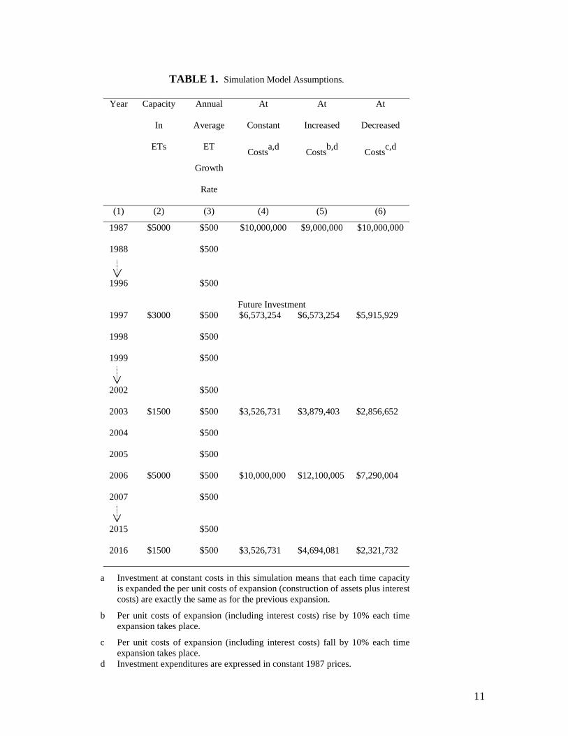
THE SIMULATION MODEL ASSUMPTIONS

Key assumptions in the simulation model that will be used to compare alternative measures of MCC are set

out in TABLE 1. The model itself spans a hypothetical period of 30 years from 1987 to 2016. The “current”

10

year is 1997 (year 0). Measured in ETs, the rate of output grows annually at an average rate of $500 a year

(column (3)). Up to 1997, this has been met by an initial investment in 1987 that has facilitated 5000 ETs

of growth but further expansion is required in 1997. A least-cost stream of future investment has been

determined which includes expansions in 2003, 2006 and 2016, in addition to 1997. The costs of each

expansion (indicated in columns (4), (5) and (6)) are presented in constant 1987 dollars. For simplicity, it is

assumed that there is no growth in demand for service from existing development. That is, all of the

capacity expansions are required to meet demand from new development so that it is not necessary to

apportion out sections of capacity to meet existing development. A real interest rate of

5% is assumed initially in the simulation.

11

TABLE 1. Simulation Model Assumptions.

Year Capacity

In

ETs

Annual

Average

ET

Growth

Rate

At

Constant

Costsa,d

At

Increased

Costsb,d

At

Decreased

Costsc,d

(1) (2) (3) (4) (5) (6)

1987 $5000 $500 $10,000,000 $9,000,000 $10,000,000

1988 $500

1996 $500

Future Investment 1997 $3000 $500 $6,573,254 $6,573,254 $5,915,929

1998 $500

1999 $500

2002 $500

2003 $1500 $500 $3,526,731 $3,879,403 $2,856,652

2004 $500

2005 $500

2006 $5000 $500 $10,000,000 $12,100,005 $7,290,004

2007 $500

2015 $500

2016 $1500 $500 $3,526,731 $4,694,081 $2,321,732

a Investment at constant costs in this simulation means that each time capacity is expanded the per unit costs of expansion (construction of assets plus interest costs) are exactly the same as for the previous expansion.

b Per unit costs of expansion (including interest costs) rise by 10% each time expansion takes place.

c Per unit costs of expansion (including interest costs) fall by 10% each time expansion takes place.

d Investment expenditures are expressed in constant 1987 prices.

12

Alternative measures of MCC are compared under three scenarios. Firstly, in the constant cost case,

each time an expansion of capacity takes place, the total capital costs of that expansion (i.e. construction

costs and the interest costs that will be incurred until capacity is exhausted) are such that per unit costs

remain constant (column (4)). In other words, the annuity that will repay each of the investments indicated

over each period to full capacity is constant (at $1,295,046) each year. Second, in the increasing cost case,

total capital costs rise by 10% each time expansion of capacity takes place. Thirdly, in the decreasing cost

case, total capital costs fall by 10% with each capacity expansion. (Details on calculations are contained in

the Appendix.)

It is also assumed for clarity in the simulation exercise that headworks assets can be aggregated so

that they appear to be one major asset that requires expansion in the clearly identifiable “jumps” indicated

in TABLE 1. It is recognized that in reality headworks systems will have multiple assets that will require

expansion at varying times. However, a more realistic depiction of this feature would obscure the discrete

increases that are required in the simulation in order to compare qualitative differences between methods

(i.e. those dealing only with the next “jump”; those which average out the “jumps”, etc.).

SIMULATION RESULTS

The developer charges per ET that result from each of the different measures under the constant costs,

increasing cost and decreasing cost assumptions are shown in TABLE 2. With the exception of the MW

method (calculated as a per ET charge for 20 lots), all charges calculated under constant costs turn out the

same at $2590 per ET. This result arises because, under constant costs per unit, costs will not vary over

time and averages and marginals will always be equal. That is to say, even though each of these measures

“searches out” and gives different emphasis to different periods over the 30-year time period, if costs over

all periods are everywhere the same, the measures must coincide.

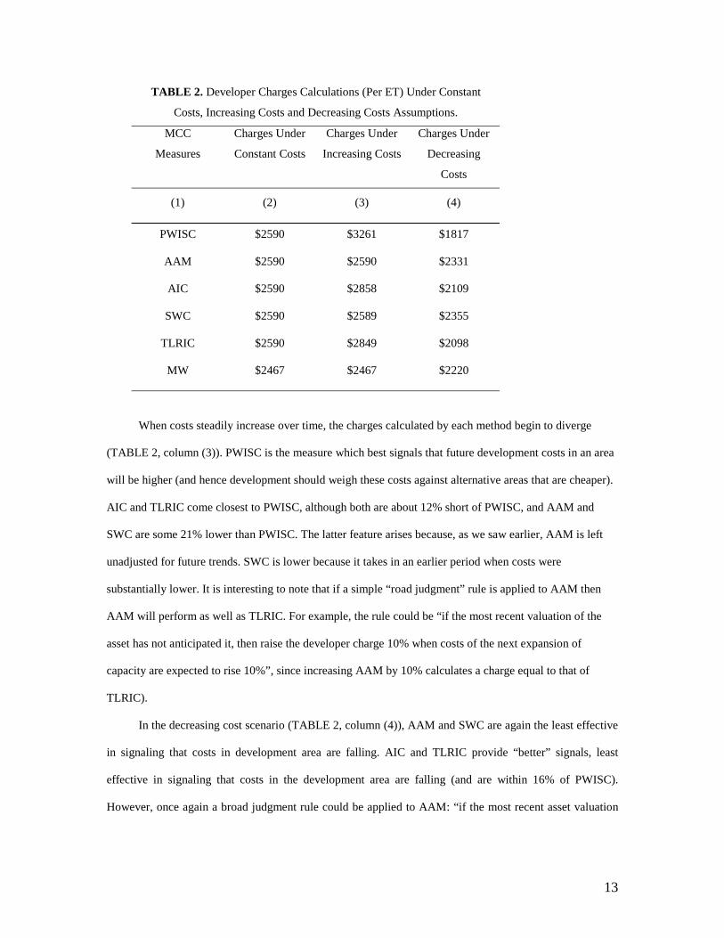
13

TABLE 2. Developer Charges Calculations (Per ET) Under Constant

Costs, Increasing Costs and Decreasing Costs Assumptions.

MCC

Measures

Charges Under

Constant Costs

Charges Under

Increasing Costs

Charges Under

Decreasing

Costs

(1) (2) (3) (4)

PWISC $2590 $3261 $1817

AAM $2590 $2590 $2331

AIC $2590 $2858 $2109

SWC $2590 $2589 $2355

TLRIC $2590 $2849 $2098

MW $2467 $2467 $2220

When costs steadily increase over time, the charges calculated by each method begin to diverge

(TABLE 2, column (3)). PWISC is the measure which best signals that future development costs in an area

will be higher (and hence development should weigh these costs against alternative areas that are cheaper).

AIC and TLRIC come closest to PWISC, although both are about 12% short of PWISC, and AAM and

SWC are some 21% lower than PWISC. The latter feature arises because, as we saw earlier, AAM is left

unadjusted for future trends. SWC is lower because it takes in an earlier period when costs were

substantially lower. It is interesting to note that if a simple “road judgment” rule is applied to AAM then

AAM will perform as well as TLRIC. For example, the rule could be “if the most recent valuation of the

asset has not anticipated it, then raise the developer charge 10% when costs of the next expansion of

capacity are expected to rise 10%”, since increasing AAM by 10% calculates a charge equal to that of

TLRIC).

In the decreasing cost scenario (TABLE 2, column (4)), AAM and SWC are again the least effective

in signaling that costs in development area are falling. AIC and TLRIC provide “better” signals, least

effective in signaling that costs in the development area are falling (and are within 16% of PWISC).

However, once again a broad judgment rule could be applied to AAM: “if the most recent asset valuation

14

has not anticipated it, then lower the developer charge by the same amount that costs in the next investment

are expected to fall”. This again would produce better results for AAM, matching it to TLRIC.

The two scenarios are useful in that they enable a judgment to be made about which measures will

err in what direction, given an expectation about the future, and perhaps even enable a ranking to be

determined about the extent to which each will deviate relative to the others. One question that naturally

arises is what is the most likely scenario in real-world circumstances? It is, of course, true that future

technologies tend to lower costs per unit. However, it is interesting to note that notwithstanding this

offsetting factor, there are some recent commentators who believe that average costs of supplying

infrastructure, such as water services to urban areas, may well rise over time [7]. For example, Rees [10]

observed that “it is now being recognized that the marginal costs of providing new water supplies will

increase markedly in the next decade or so, because the period of low cost source extraction is now at an

end”. If these views are correct, and TABLE 2, column (3) is the likely scenario, then all alternative

methods of calculation will understate the MCC as indicated by PWISC.

SENSITIVITY TESTS

Each of the measures of MCC was subjected to sensitivity tests in the key parameters affecting their

calculation. The results of these sensitivity tests are discussed below.

Sensitivity of MCC Measures to Changes in Interest Rates

The results of charges of changes in the real rate of interest are presented in TABLE 3. The first parameter

change considered was a 20% increase in the real rate of interest, from 5% to 6%, using the same cost

figures as were employed in the constant cost simulation (TABLE 1, column (4)). The effect on the charges

calculated by each measure was small, ranging between increases of 3.3% and 4.3%. Increases of similar

limited magnitude occurred when the investment figures were substituted for the increasing cost

simulation. Compared to the same charges calculated for 5% (TABLE 3, column (4)), the effect of a 20%

rise in the rate to 6% was still marginal (TABLE 3, column (5)).

15

TABLE 3. Developer Charges Calculationsa Under Varying Real

Interest Rates - Selected Scenarios.

MCC

Measures

5%

Constant

Cost

6%

Constant

Cost

5%

Increased

Cost

6%

Increased

Cost

10%

Constant

Cost

(1) (2) (3) (4) (5) (6)

PWISC $2590 $2668 $3261 $3331 $3030

AAM $2590 $2674 $2590 $2674 $3019

AIC $2590 $2685 $2858 $2952 $3061

SWB $2590 $2702 $2589 $2678 $3188

TLRIC $2590 $2673 $2849 $2902 $3018

a Charges are calculated per ET.

A second interest rate test raised the real rate further, from 5% to 10%. This had a greater effect on

the charges calculated, but overall, a 100% increase in the interest rate increased the charges by between

17 and 23% (TABLE 3, column (6) compared to column (2)).

Further tests revealed that the sensitivity of MCC measures with respect to interest rates rose

according to two factors. The first of these is the size of the rate before the change; that is, the higher the

original rate, the higher the sensitivity of charges to changes in this rate. For example, doubling the rate

from 5% to 10% produced changes in the calculations averaging around 18%. A further doubling of the

rate of 10% to a real rate of interest of 20% produced an increase in AAM of 31%, although by contrast

increases in PWISC and TLRIC, for instance, were still quite small at around 11%. In explaining why

AAM moved further than the other measures, it is clear that PWISC and TLRIC draw on future trends more

than AAM (since step (4) of AAM is not attempted). Since these other measures draw on what is happening

to interest costs in the future, it is apparent that because of the shorter period to full capacity of the next

investment expansion ($3,526,731 for three years, as in TABLE 1, column (4) compared to six years for the

1997 expansion on which AAM draws) the lower interest burden compared to the 1997-2002 period

reduces the sensitivity to interest rate changes of these measures.

16

The second factor increasing the sensitivity of charges to alterations in the interest rate is the length

of the excess capacity period. If the costs for the 1997 expansion of $6,573,254 are spread over a period to

full capacity of six years, then doubling the real interest rate from 10% to 20% will produce a change in

AAM of 31%. On the other hand, if that same capital cost is spread over 15 years, then doubling the

interest rate from 5% to 10% causes a rise of 63% in AAM.

High real interest rates combined with long periods to full capacity indicate a greater sensitivity of

the AAM charge to interest rates than is apparent with the excess capacity periods used in the simulation.

The same would be true of the other measures if the investment streams simulated had had significantly

longer periods to full capacity.

The higher sensitivity to interest rate changes at high real rates combined with long excess capacity

periods arises because the interest burden of holding excess capacity for many years starts to become a

significant factor in overall capital costs. In choosing the optimal scale of expansion, the economies of

scale of larger capacity need to be weighed, amongst other things, against the higher interest burden of long

periods of unused capacity. In examining various types of developer charges in the United States, Peiser [9]

observed that the high holding costs of long periods of excess capacity may have been overlooked. Peiser

[9] argued that “while the results depend on the particular assumptions, they demonstrate that economies of

scale must be substantial for users to realize net benefits” and thus his results “suggest that planners should

temper traditional engineering approaches in favor of larger systems to take advantages of economies of

scale; they need to understand the costs for carrying excess capacity”.

In sum, the interest rate sensitivity tests appear to suggest that the “extreme sensitivity” requires

unusually high interest rates combined with long periods of unused capacity. Over shorter excess capacity

periods and lower real rates of interest there is much less sensitivity of charges to changes in interest rates,

and little variation between the alternative measures in the extent to which they demonstrate this

conclusion. If high real rates of interest do prevail and periods of excess capacity are longer than, say,

15 years, holding costs become a significant component of expansion costs and must be weighed against

the benefits of economies of scale in large investment programs.

17

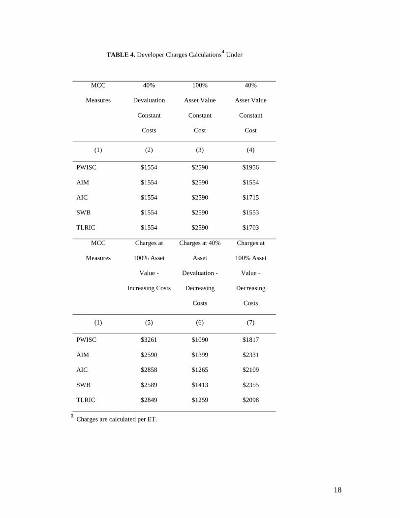
Sensitivity of MCC Measures to Changes in Asset Valuations

A second series of sensitivity tests examined the effect on charges of variations in the valuations of

headworks assets on which the calculations are based. Using the investment cost figures for all three

scenarios of constant cost, increasing cost and decreasing cost, all assets were devalued 40%. The results

are presented in TABLE 4.

The results in TABLE 4 show that irrespective of whether costs are constant, increasing or

decreasing over time, a change in asset value leads to a directly proportionate change in the charge

calculated by all measures.

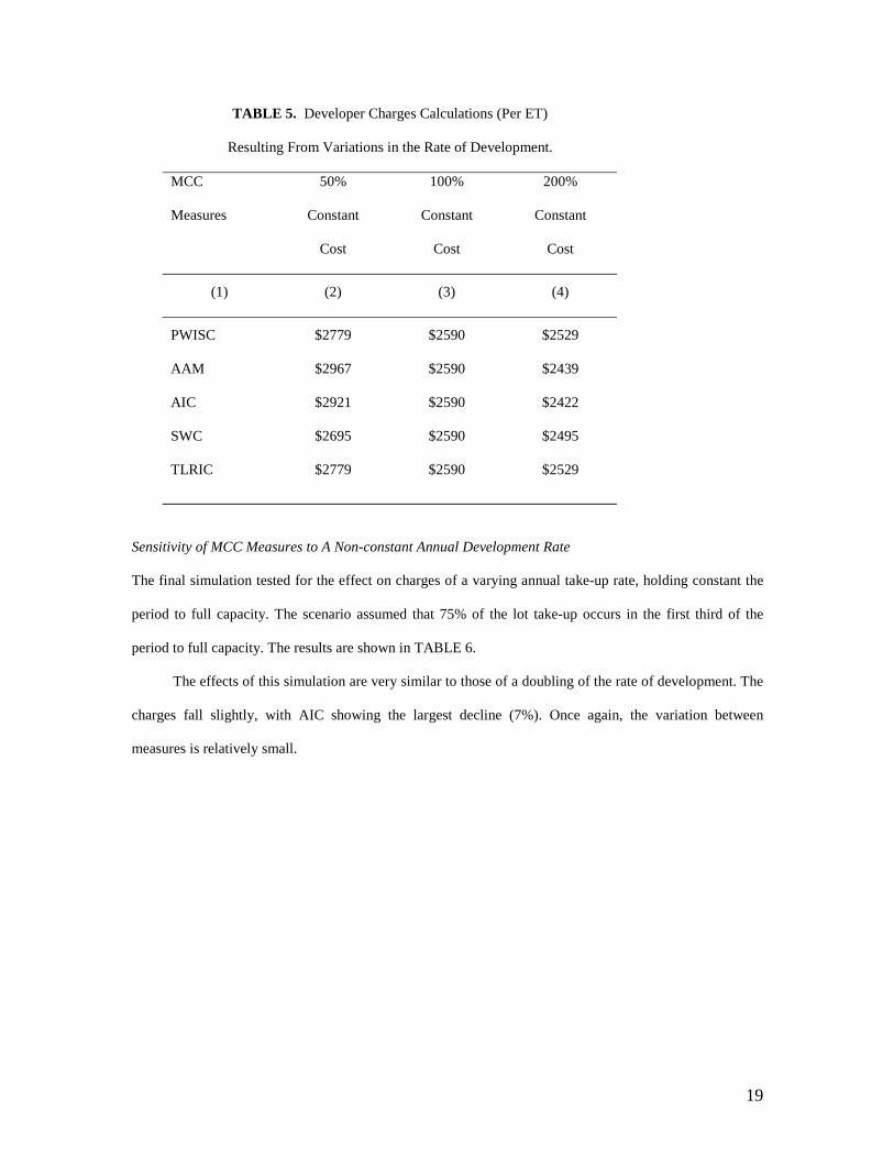
Sensitivity of MCC Measures to Changes in the Lot Take-up Rates

In a further series of sensitivity tests, the effects on charges of changes in the rates at which developers

take-up lots (measured as ETs) were examined. In the first test, lot take-up rate was halved as from 1997. In

effect this means that in the simulation, annual output each year from 1997 is halved and the periods to full

capacity are doubled. In the second test, the lot take-up rate was doubled. This has the converse effect in

the simulation; annual output each year is doubled, and the periods to full capacity are halved. The results

of these simulations are presented in TABLE 5.

In TABLE 5 all charges rise as a result of a 100% fall in the rate of development since the holding

costs of longer periods to full capacity are now proportionately greater. However, it is again somewhat

surprising how small the effect of a dramatic drop in the lot take-up is on the developer charges (TABLE 5,

column (2) compared to column (3)). AAM moves up the most (by 15%) and AIC is second at 13%. Both

these measures are most affected by the (now) 12-year period to full capacity of the 1997 investment.

PWISC and TLRIC are most influenced by events in the 2003 investment period (now a six-year period)

where the holding costs are proportionately less, whilst SWC is least affected because it draws significantly

on a period where no change occurs.

18

TABLE 4. Developer Charges Calculationsa Under

MCC

Measures

40%

Devaluation

Constant

Costs

100%

Asset Value

Constant

Cost

40%

Asset Value

Constant

Cost

(1) (2) (3) (4)

PWISC $1554 $2590 $1956

AIM $1554 $2590 $1554

AIC $1554 $2590 $1715

SWB $1554 $2590 $1553

TLRIC $1554 $2590 $1703

MCC

Measures

Charges at

100% Asset

Value -

Increasing Costs

Charges at 40%

Asset

Devaluation -

Decreasing

Costs

Charges at

100% Asset

Value -

Decreasing

Costs

(1) (5) (6) (7)

PWISC $3261 $1090 $1817

AIM $2590 $1399 $2331

AIC $2858 $1265 $2109

SWB $2589 $1413 $2355

TLRIC $2849 $1259 $2098

a Charges are calculated per ET.

19

TABLE 5. Developer Charges Calculations (Per ET)

Resulting From Variations in the Rate of Development.

MCC

Measures

50%

Constant

Cost

100%

Constant

Cost

200%

Constant

Cost

(1) (2) (3) (4)

PWISC $2779 $2590 $2529

AAM $2967 $2590 $2439

AIC $2921 $2590 $2422

SWC $2695 $2590 $2495

TLRIC $2779 $2590 $2529

Sensitivity of MCC Measures to A Non-constant Annual Development Rate

The final simulation tested for the effect on charges of a varying annual take-up rate, holding constant the

period to full capacity. The scenario assumed that 75% of the lot take-up occurs in the first third of the

period to full capacity. The results are shown in TABLE 6.

The effects of this simulation are very similar to those of a doubling of the rate of development. The

charges fall slightly, with AIC showing the largest decline (7%). Once again, the variation between

measures is relatively small.

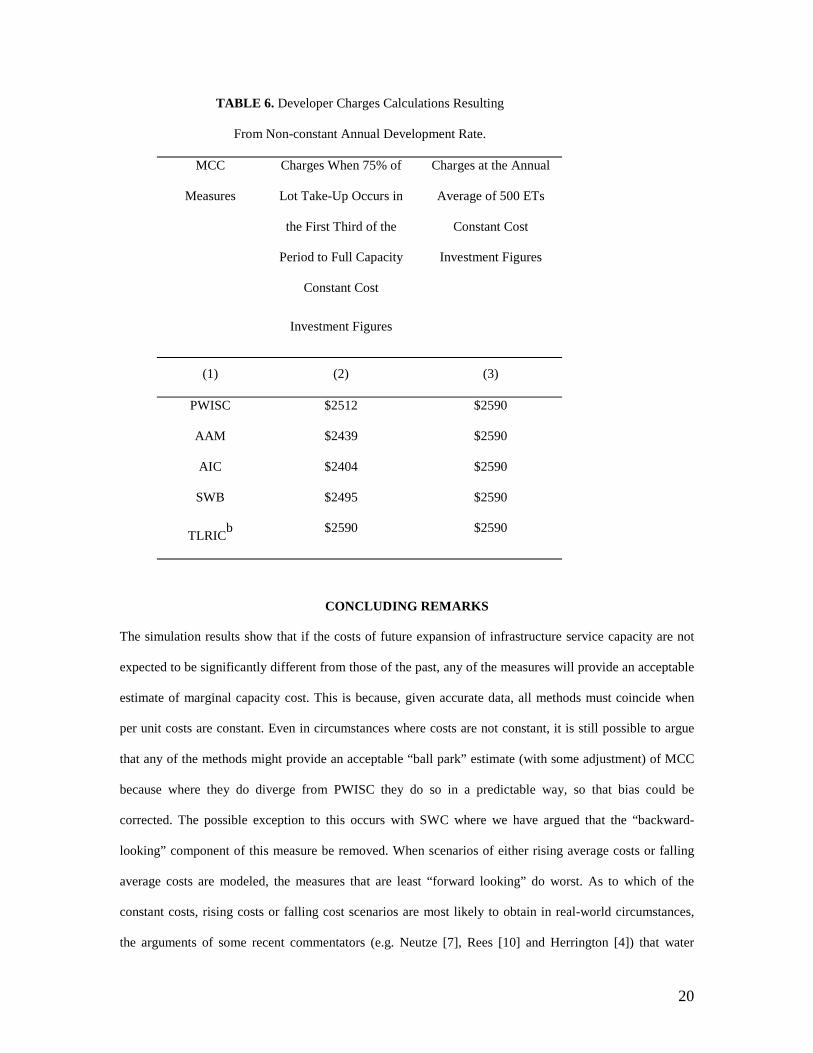
20

TABLE 6. Developer Charges Calculations Resulting

From Non-constant Annual Development Rate.

MCC

Measures

Charges When 75% of

Lot Take-Up Occurs in

the First Third of the

Period to Full Capacity

Constant Cost

Investment Figures

Charges at the Annual

Average of 500 ETs

Constant Cost

Investment Figures

(1) (2) (3)

PWISC $2512 $2590

AAM $2439 $2590

AIC $2404 $2590

SWB $2495 $2590

TLRICb $2590 $2590

CONCLUDING REMARKS

The simulation results show that if the costs of future expansion of infrastructure service capacity are not

expected to be significantly different from those of the past, any of the measures will provide an acceptable

estimate of marginal capacity cost. This is because, given accurate data, all methods must coincide when

per unit costs are constant. Even in circumstances where costs are not constant, it is still possible to argue

that any of the methods might provide an acceptable “ball park” estimate (with some adjustment) of MCC

because where they do diverge from PWISC they do so in a predictable way, so that bias could be

corrected. The possible exception to this occurs with SWC where we have argued that the “backward-

looking” component of this measure be removed. When scenarios of either rising average costs or falling

average costs are modeled, the measures that are least “forward looking” do worst. As to which of the

constant costs, rising costs or falling cost scenarios are most likely to obtain in real-world circumstances,

the arguments of some recent commentators (e.g. Neutze [7], Rees [10] and Herrington [4]) that water

21

supply costs may rise in the future seem plausible. If this is true, then our results indicate that all alternative

methods will understate marginal capacity costs of supplying the service compared with PWISC. If the

average costs of future expansions fall, all measures will overstate the appropriate charge and would have

to be adjusted downwards.

If we discard SWC because of its backward-looking focus, and compare AAM to TLRIC and AIC,

then several reasons emerge for recommending AAM as the most effective and practical option. First, it

can achieve at least the same degree of accuracy of estimation of MCC as TLRIC. Secondly, AAM can

measure the MCC of individual assets that are specific to a site. A method such as AIC tends to average the

forward investment plans over a wide area and hence average out some locational variation in costs.

Thirdly, there is the pragmatic consideration that TLRIC and AIC (and of course PWISC) all require

reliable forward estimates of the costs of capacity expansion. On the other hand, AAM can avoid this

demand for detailed data by using only broad judgment about future costs and demand conditions.

Fourthly, the AAM approach can be used to calculate charges for distribution assets as well as headworks

and major works. Since distribution assets tend to have a smaller excess capacity and demand for these

services is not expected to grow indefinitely (requiring capacity expansions), AIC and TLRIC cannot be

applied. Finally, with AAM, the interest rate burden over the expected period to full take-up of capacity is

spread evenly over all developers. Early developers gain no interest cost advantage, but neither is

development stifled by higher interest costs later on.

REFERENCES

[1] AMERICAN WATER WORKS ASSOCIATION (AWWA) 1991, AWWA Manual M34, AWWA,

1991.

[2] BAUMOL, W.J. and C. BRADFORD, “Optimal Departures from Marginal Cost Pricing”, American

Economic Review, Vol. 60, No. 3, pp. 472-481, June 1970.

[3] HERRINGTON, P., Pricing of Water Services, OECD, 1987.

[4] HERRINGTON, P., “Pricing Water Properly”, in Ecotaxation, ed. T. O'Riordan, Earthscan,

pp. 263-286, 1997.

22

[5] LITTLECHILD, S., Elements of Telecommunications Economics, Peter Peregrinus, 1979.

[6] MONTGOMERY WATSON (MW), Armidale City Council Water Supply and Sewerage

Development Strategy Study, report to Armidale City Council, November, 1995.

[7] NEUTZE, M., Funding Urban Services, Allen and Unwin, 1997.

[8] PARMENTER, B. and L. WEBB, “Amortization and Public Pricing Policies”, Australian Economic

Papers, Vol. 15, No. 28, pp. 11-27, 1976.

[9] PEISER, R., “Calculating Equity-neutral Water and Sewer Impact Fees”, Journal of the American

Planning Association, Vol. 54, No. 1, pp. 38-48, Winter, 1988.

[10] REES, J., “Toward Implementation Realities”, in Ecotaxation, ed. T. O'Riordan, Earthscan,

pp. 287-303, 1997.

[11] ROSS, S., S. THOMSON, M. CHRISTENSEN, R. WESTERFIELD and B. JORDAN, Student

Problem Manual for Use with Fundamentals of Corporate Finance (First Australian Edition), Irwin,

1994.

[12] SAUNDERS, R., J. WARFORD and P. MANN, Alternative Concepts of Marginal Cost for Public

Utility Pricing: Problems of Application in the Water Supply Sector, World Bank Staff Working

Paper No.259, World Bank, May, 1977.

[13] TURVEY, R., Optimal Pricing and Investment in Electricity Supply, Allen and Unwin, 1968.

[14] TURVEY, R., “Marginal cost”, Economic Journal, Vol. 79, No. 2, pp. 282-299, 1969.

[15] TURVEY, R., Economic Analysis and Public Enterprises, Allen and Unwin, 1971.

23

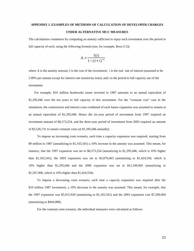
APPENDIX 1. EXAMPLES OF METHODS OF CALCULATION OF DEVELOPER CHARGES

UNDER ALTERNATIVE MCC MEASURES

The calculations commence by computing an annuity sufficient to repay each investment over the period to

full capacity of each, using the following formula (see, for example, Ross [11]):

A =I(i)

1− (1+ i)−t

where A is the annuity amount; I is the cost of the investment; i is the real rate of interest (assumed to be

5.00% per annum except for interest rate sensitivity tests); and t is the period to full capacity use of the

investment.

For example, $10 million headworks assets invested in 1987 amounts to an annual equivalent of

$1,295,046 over the ten years to full capacity of this investment. For the “constant cost” case in the

simulation, the construction and interest costs combined of each future expansion was assumed to remain at

an annual equivalent of $1,295,046. Hence the six-year period of investment from 1997 required an

investment amount of $6,573,254, and the three-year period of investment from 2003 required an amount

of $3,526,731 to ensure constant costs (at $1,295,046 annually).

To impose an increasing costs scenario, each time a capacity expansion was required, starting from

$9 million in 1987 (annuitizing to $1,165,541) a 10% increase in the annuity was assumed. This meant, for

instance, that the 1997 expansion was set to $6,573,254 (annuitizing to $1,295,046, which is 10% higher

than $1,165,541); the 2003 expansion was set to $3,879,403 (annuitizing to $1,424,550, which is

10% higher than $1,295,046 and the 2006 expansion was set to $12,100,005 (annuitizing to

$1,567,006, which is 10% higher than $1,424,550).

To impose a decreasing costs scenario, each time a capacity expansion was required after the

$10 million 1987 investment, a 10% decrease in the annuity was assumed. This meant, for example, that

the 1997 expansion was $5,915,929 (annuitising to $1,165,541) and the 2003 expansion cost $7,290,004

(annuitising to $944,088).

For the constant costs scenario, the individual measures were calculated as follows:

24

PWISC:

PWISC =

Present worth (PW) of system - PW of system costs with acosts with one planned expansion different planned expansion

PW of the difference in quantities of output

An output increment of 500 was assumed, sufficient to necessitate the investment program to move forward

by one year. The only difference between the present worth of the investment stream with and without this

increment, will be that an additional $1,295,046 will be required in period 5. Hence:

PW of 1 295 046 in period 5

PW of 500 in period 5= 1 295 046 (1 + i)5

500 (1+ i)5

Developer Charge for PWISC = $2590 per ET

Calculating the charge for PWISC under increasing and decreasing costs required additional adjustments in

later years because of differences in the annuities for each investment. For example, PWISC under

increasing costs required an additional $1,424,550 in period 5 plus a difference of [$1,567,006 –

$1,424,550] in period 8 plus a difference of [$1,723,707 – $1,567,006] in period 18.

AAM:

AAM = Present worth of an updated value of the current assetPresent worth of output over the period to full capacity

.

At time t = 0 (1997), the updated value of $6,573,254 is $6,573,254. Thus:

AAM =

6 573 2545001.05( )

+ 5001.05( )2 K

5001.05( )6

=6 573 254

2537.9

Developer Charge for AAM = $2590 per ET.

Because the simulation assumes a constant rate of output of 500 ETs per year, an alternative calculation

method for AAM is to divide the constant annuity for $6,573,254 by 500:

25

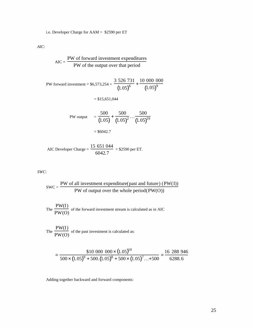
i.e. Developer Charge for AAM = $2590 per ET

AIC:

AIC = PW of forward investment expenditures

PW of the output over that period

PW forward investment = $6,573,254 + 3 526 731

1.05( )6 +10 000 000

1.05( )9

= $15,651,044

PW output =

5001.05( ) +

5001.05( )2 K

5001.05( )19

= $6042.7

AIC Developer Charge = 15 651 044

6042.7 = $2590 per ET.

SWC:

SWC = PW of all investment expenditure(past and future) (PW(I))

PW of output over the whole period(PW(O))

The PW(I)PW(O)

of the forward investment stream is calculated as in AIC

The PW(I)PW(O)

of the past investment is calculated as:

=

$10 000 000 × 1.05( )10

500 × 1.05( )9 + 500. 1.05( )8 + 500 × 1.05( )7K+500=

16 288 9466288.6

Adding together backward and forward components:

26

=15 651 044 +16 288 946

6042.7 + 6288.6=

31 939 99012331.3

Developer charge for SWB = $2590 per ET.

TLRIC:

TLRIC = r.Ik

Ok +1 − Ok=

Annuitisation of the next lump of IAnnual ET output

The next lump of investment is $3,526,731, which annuitizes to $1,295,046 over a

three-year period to full capacity:

∴ Developer charge for TLRIC = 1 295 046

500 = $2590 per ET.

MW:

The MW methodology is explained in the text.

For the increasing and decreasing cost scenarios the same procedures were followed using the

altered investment figures as described above.

For the interest rate sensitivity tests the same procedures were again followed, except that the

interest rate of i = 0.05 was replaced by i = 0.06 and i = 0.1 respectively.

For the sensitivity to changes in asset valuation using the constant cost investment figures, the

sequence of investment costs of $10,000,000 (10 periods); $6,573,254 (6 periods); $3,526,731 (3 periods);

$10,000,000 (10 periods) and $3,526,731 (3 periods) were replaced by $6,000,000 (10 periods); $3,943,952

(6 periods); $3,526,731 (3 periods); $6,000,000 (10 periods); and $2,116,039 (3 periods) respectively.

The increasing cost investment figures were also reduced by 40% in a second test of asset valuation

sensitivity. For testing sensitivity to a halving of the lot take-up rate, the annual output was reduced to 250

ETs and the 1997 investment program became the equivalent of $741,630 a year for 12 years and the 2003

investment program shifted to 2009, becoming the equivalent of $694,828 over

six years. The 2006 expansions program of $10,000,000 was shifted to 2015, annuitizing to $802,426 for

20 years. Doubling the lot take-up rate changed the annual output rate to 1000 ETs and brought forward all

27

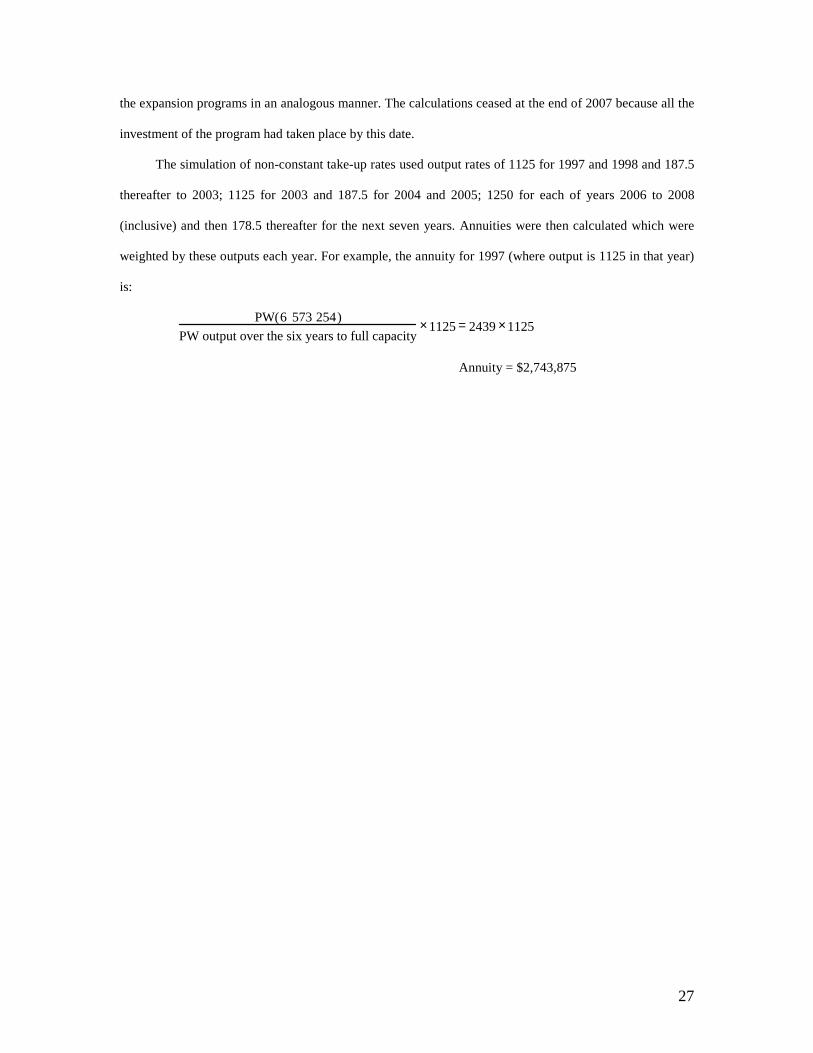
the expansion programs in an analogous manner. The calculations ceased at the end of 2007 because all the

investment of the program had taken place by this date.

The simulation of non-constant take-up rates used output rates of 1125 for 1997 and 1998 and 187.5

thereafter to 2003; 1125 for 2003 and 187.5 for 2004 and 2005; 1250 for each of years 2006 to 2008

(inclusive) and then 178.5 thereafter for the next seven years. Annuities were then calculated which were

weighted by these outputs each year. For example, the annuity for 1997 (where output is 1125 in that year)

is:

PW(6 573 254)PW output over the six years to full capacity

×1125 = 2439 ×1125

Annuity = $2,743,875