By Jessica Nicole Fitzsimmons B.A., Boston University, 2008
275
1 THE MARINE BIOGEOCHEMISTRY OF DISSOLVED AND COLLOIDAL IRON By Jessica Nicole Fitzsimmons B.A., Boston University, 2008 Submitted in partial fulfillment of the requirements for the degree of Doctor of Philosophy at the MASSACHUSETTS INSTITUTE OF TECHNOLOGY and the WOODS HOLE OCEANOGRAPHIC INSTITUTION September 2013 © 2013 Jessica N. Fitzsimmons All rights reserved. The author hereby grants to MIT and WHOI permission to reproduce and to distribute publicly paper and electronic copies of this thesis document in whole or in part in any medium now known or hereafter created. Author:_________________________________________________________________ Jessica N. Fitzsimmons Joint Program in Chemical Oceanography Massachusetts Institute of Technology and Woods Hole Oceanographic Institution August 22nd, 2013 Certified by:_____________________________________________________________ Edward A. Boyle Professor of Ocean Geochemistry, MIT Thesis Supervisor Accepted by:_____________________________________________________________ Elizabeth B. Kujawinski Associate Scientist in Marine Chemistry & Geochemistry, WHOI Chair, Joint Committee for Chemical Oceanography
-
Upload
khangminh22 -
Category
Documents
-
view
4 -
download
0
Transcript of By Jessica Nicole Fitzsimmons B.A., Boston University, 2008

1
THE MARINE BIOGEOCHEMISTRY OF DISSOLVED AND COLLOIDAL IRON
By
Jessica Nicole Fitzsimmons
B.A., Boston University, 2008
Submitted in partial fulfillment of the requirements for the degree of
Doctor of Philosophy
at the
MASSACHUSETTS INSTITUTE OF TECHNOLOGY
and the
WOODS HOLE OCEANOGRAPHIC INSTITUTION
September 2013
© 2013 Jessica N. Fitzsimmons All rights reserved.
The author hereby grants to MIT and WHOI permission to reproduce and to distribute publicly paper and electronic copies of this thesis document in whole or in part in any
medium now known or hereafter created.
Author:_________________________________________________________________ Jessica N. Fitzsimmons
Joint Program in Chemical Oceanography Massachusetts Institute of Technology and Woods Hole Oceanographic Institution
August 22nd, 2013
Certified by:_____________________________________________________________ Edward A. Boyle
Professor of Ocean Geochemistry, MIT Thesis Supervisor
Accepted by:_____________________________________________________________ Elizabeth B. Kujawinski
Associate Scientist in Marine Chemistry & Geochemistry, WHOI Chair, Joint Committee for Chemical Oceanography

2

3
The Marine Biogeochemistry of Dissolved and Colloidal Iron
By Jessica Nicole Fitzsimmons
Submitted to the MIT/WHOI Joint Program in Oceanography in August, 2013, in partial fulfillment of the requirements for the degrees of Doctor of Philosophy
Abstract
Iron is a redox active trace metal micronutrient essential for primary production and nitrogen acquisition in the open ocean. Dissolved iron (dFe) has extremely low concentrations in marine waters that can drive phytoplankton to Fe limitation, effectively linking the Fe and carbon cycles. Understanding the marine biogeochemical cycling and composition of dFe was the focus of this thesis, with an emphasis on the role of the size partitioning of dFe (<0.2µm) into soluble (sFe<0.02µm) and colloidal (0.02µm<cFe<0.2µm) size fractions. This was accomplished through the measurement of the dFe distribution and size partitioning along basin-scale transects experiencing a range of biogeochemical influences. dFe provenance was investigated in the tropical North Atlantic and South Pacific Oceans. In the North Atlantic, elevated dFe (>1 nmol/kg) concentrations coincident with the oxygen minimum zone were determined to be caused by remineralization of a high Fe:C organic material (vertical flux), instead of a laterally advected low oxygen-high dFe plume from the African margin. In the South Pacific Ocean, dFe maxima near 2000m were determined by comparison with dissolved manganese and 3He to be caused by hydrothermal venting. The location of these stations hundreds to thousands of kilometers from the nearest vents confirms the "leaky vent" hypothesis that enough dFe escapes precipitation at the vent site to contribute significantly to abyssal dFe inventories. The size partitioning of dFe was also investigated in order to trace the role of dFe composition on its cycling. First, the two most commonly utilized methods of sFe filtration were compared: cross flow filtration (CFF) and Anopore filtration. Both were found to be robust sFe collection methods, and sFe filtrate through CFF (10 kDa) was found to be only 74±21% of the sFe through Anopore (0.02µm) filters at 28 locations, a function of both pore size differences and the natural variability in distribution of 10kDa-0.02µm colloids. In the North Atlantic, a colloidal-dominated partitioning was observed in the surface ocean underlying the North African dust plume, in and downstream of the TAG hydrothermal system, and along the western Atlantic margin. However, cFe was depleted or absent at the deep chlorophyll maximum. A summary model of dFe size partitioning in the North Atlantic open ocean is presented in conclusion, hypothesizing that a constant dFe exchange between soluble and colloidal pools modulates the constant partitioning of nearly 50% dFe into the colloidal phase throughout the subsurface North Atlantic Ocean, while sFe and cFe cycle independently in the upper ocean. Thesis supervisor: Edward A. Boyle, Professor of Ocean Geochemistry, MIT

4

5
Acknowledgements First and foremost, I would like to thank my advisor, Ed, for his guidance and support for this thesis project. Ed allowed me independence in my science, which I never knew I wanted but now I know I could never live without. He provided me with endless support and incredible opportunities: as long as I could back-up my ideas with sound reasoning, he acted as if he didn't know the word "no." I was so lucky to travel internationally not only on six research cruises but also to many conferences worldwide. Ed was eternally optimistic, and when he had to criticize or remind me to relax, he always did it gently, which I appreciated so much. I also thank my committee, who not only provided me professional advice and mentorship but also gave me incredible inspiration. I realize that students in other disciplines have anxiety over their thesis committee meetings, but I was always excited for mine. I knew that I would leave that room more invigorated about my science than when I entered. My committee improved the quality and direction of my work so much, and to them I am very grateful. I am also very grateful to the numerous collaborators and field teams who made this journey so much fun. I thank the U.S. GEOTRACES family, to whom I owe much of my training in trace metal sampling and analysis and cruise leadership, and especially Pete, Randie, Sara, Kaitlin, Chris, Katharina, and Geo for the endless laughter. I was also lucky enough to be a part of the C-MORE family, who provided me with luxurious cruise opportunities and the freedom to explore in detail things I might not have had time for on other cruises. This was a particularly rewarding learning experience. I also owe a HUGE thanks to the Boyle lab and Joint Program. Rick, Jong-Mi, Ruifeng, Yolanda, Gonzalo, Rene, Abigail, and Simone - I was so lucky to develop a special friendship with each of you, and while you all taught me something about science, more importantly you taught me how to be a better me, both personally and professionally. Thanks so much for picking me up on my lowest days and reminding me how great research can be! Special thanks also to my Joint Program friends, especially Meagan, Emily, Britta, and Evan, and to my MIT buddies Sara, Anthony, and Oscar - you all made grad school a fun place to be. Also to the JP Academic Programs Office and the E25 Administrative Assistants (especially Julia, Meg, and Mary) - you gals were incredible. Not only were you there each and every time I had a stupid bureaucratic question, but you were always good for a pick-me-up. You are the ladies who make things happen, and I would have been lost with you. Finally, I thank my parents, Nick and Jade, Dana, the 3rd Floor Girls (Irina, Erin, Sarah, Smita, and Julia), Alli, and most importantly, my husband. What do I thank you for? EVERYTHING. For the daily laughter, love, care, support, and fun times. You all reminded me to breathe when I was down, shook me when I was crazy, danced with me when I needed a smile, and floated with me when I was sky high. To my parents: you always told me that I could do anything if I worked hard enough, and you were by my side every step of this journey with all the love and support you could muster. Thank you, and I love you guys so much. And to my huband: I would never have made it through this journey without you, nor would I have wanted to. You are my rock, my everything, and I can't wait for our next adventure. I love you. Funding for this research was provided by an MIT Presidential Fellowship, an NSF Graduate Research Fellowship (# 0645960), a fellowship from the Martin Family Society of Fellows for Sustainability, several NSF Chemical Oceanography grants (OCE-0751409, OCE-07020278, OCE-0926204, and OCE-0926197), and the Center for Microbial Oceanograhy: Research and Education (NSF OIA #EF-0424599).

6
Table of Contents Chapter 1: Introduction 13 1.1 Dissolved Fe composition and biogeochemistry 14 1.2 Marine colloid chemistry 19 1.3 The bioavailability of colloidal Fe 22 1.4 Marine colloidal Fe distributions and biogeochemistry 23 1.5 Dissertation outline and chapter descriptions 26 References for Chapter 1 30 Chapter 2: An intercalibration between the GEOTRACES GO-FLO and the MITESS/Vanes sampling systems for dissolved iron concentration analyses (and a closer look at adsorption effects) 39 2.1 Introduction 40 2.2 Methods 42 2.2.1 Cleaning procedures 42 2.2.2 Sample collection 43 2.2.3 Adsorption experiment 43 2.2.4 Headspace experiment 44 2.2.5 dFe analyses 44 2.3 Assessment 45 2.3.1 Adsorption experiment 46 2.3.2 Headspace - CO2 loss experiment 49 2.4 Discussion 50 2.5 Comments and Recommendations 52 References for Chapter 2 52 Chapter 3: Dissolved iron in the tropical North Atlantic Ocean 55 3.1 Introduction 56 3.2 Methods 57 3.2.1 Seawater sampling 57 3.2.2 Nutrient measurements 57 3.2.3 dFe measurement 57 3.2.4 Dissolved manganese measurement 58 3.3 Results and Discussion 58 3.3.1 Surface dFe distribution 58 3.3.2 Water column dFe distribution 59 3.3.2.1 Regional circulation of the tropical North Atlantic 59 3.3.2.2 Upper 1000 m dFe distribution 60 3.3.2.3 Station 13 full water column dFe distribution 61 3.3.3 dFe provenance in the tropical North Atlantic OMZ 64 3.3.4 Effects of future deoxygenation on dFe in the tropical North Atlantic OMZ 66 3.4. Conclusions 66

7
References for Chapter 3 67 Supplementary Material 3A: 1-D Fe model including scavenging 69 Supplementary Material 3B: Data from Chapter 3 74 Chapter 4: Distal transport of dissolved hydrothermal iron in the deep South Pacific Ocean 79 4.1 Introduction, Results, and Discussion 80 4.2 Methods 86 References for Chapter 4 89 Supplementary Material for Chapter 4 95 Chapter 5: Assessment and comparison of Anopore™ and cross flow filtration methods for the determination of dissolved iron size fractionation into soluble/colloidal phases in seawater 107 5.1 Introduction 111 5.2 Methods 113 5.2.1 Anopore™ filtration 113 5.2.2 Cross flow filtration (ultrafiltration) 114 5.2.3 Sample collection 116 5.2.4 Fe analyses 117 5.3 Assessment 118 5.3.1 Anopore™ filtration 118 5.3.2 Cross flow filtration (ultrafiltration) 121 5.3.3 Comparison of Anopore filtration with CFF 125 5.4 Discussion 129 5.5 Conclusions and recommendations 131 References for Chapter 5 134 Chapter 6: Both soluble and colloidal iron phases control dissolved iron variability in the tropical North Atlantic Ocean 145 6.1 Introduction 149 6.2 Sampling & Analysis Methodology 151 6.3 Results & Discussion 152 6.3.1 Surface distribution 152 6.3.2 Water column profiles 155 6.3.2.1 Euphotic zone 155 6.3.2.2 Upper 1000m 157 6.3.2.3 Deep ocean 159 6.3.3 Controls on dissolved Fe variability 160 6.4 Conclusions 164 References for Chapter 6 165 Supplemental Data from Chapter 6 174

8
Chapter 7: Partitioning of dissolved iron into soluble and colloidal phases along the U.S. GEOTRACES North Atlantic Zonal transect 177 7.1 Introduction 178 7.2 Methods 180 7.3 Results & Discussion 182 7.3.1 dFe size partitioning from the major Fe sources 183 7.3.1.1 Aerosol deposition: the surface ocean 183 7.3.1.2 Eastern margin: Mauritanian oxygen minimum zone 187 7.3.1.3 Western boundary (Line W) 188 7.3.1.4 TAG hydrothermal system 191 7.3.2 dFe size partitioning due to internal ocean dFe cycling 193 7.3.2.1 Deep chlorophyll maximum 194 7.3.2.2 Remineralization 197 7.3.2.3 Deep ocean 199 7.3.3 Consensus on dFe partitioning in the North Atlantic 201 7.4 Conclusions 206 References for Chapter 7 208 Appendix I: Dissolved iron distribution, size partitioning, and stable isotopes in the Southeast Pacific Ocean 229 References for Appendix I 237 Appendix II: Iron chemistry at the TAG hydrothermal field 243 Introduction 243 Methods 244 Results and Discussion 245 References for Appendix II 251 Appendix III: Size partitioned dissolved iron isotopes and ligands in the North Atlantic Ocean 253 Introduction 253 Site selection and methodology 255 Results and Discussion 257 Size partitioning of Fe-binding ligands 258 Size fractionated dissolved Fe isotopes 261 Referneces for Appendix III 267 Appendix IV: Temporal variability of dissolved iron at Station ALOHA 271 References for Appendix IV 275

9
List of Figures Chapter 1 Figure 1. The marine Fe cycle 15
Figure 2. Summary of the size partitioning of Fe into soluble, colloidal, and particulate size fractions 21
Chapter 2 Figure 1. Sampling devices used in the intercalibration 41 Figure 2. Experimental design flowchart 44
Figure 3. dFe profile intercalibration using MITESS/Vanes and GEOTRACES GO-FLO bottles at the SAFe station 46
Figure 4. Kinetics of adsorption to bottle walls results 48 Figure 5. Headspace Experiment results 49
Chapter 3 Figure 1. Tropical North Atlantic cruise transect 57 Figure 2. Surface water dFe distribution and literature review 58 Figure 3. 3-D visualization of the dFe distribution 60 Figure 4. Temperature-salinity diagram for the cruise transect 61 Figure 5. 2-D visualization of the dFe distribution 62 Figure 6. dFe distribution near the Cape Verde Islands 63 Figure 7. Profile of dFe, dMn, phosphate, and dissolved oxygen (Station 13) 63 Figure 8. dFe-AOU correlation across the transect 63 Figure 9. dMn distribution 64 Figure 10. Non-dimensionalized results of the dFe-dissolved oxygen model 65 Figure 11. dFe as a function of dissolved oxygen along the cruise transect 66 Figure S1. Modeled vs. measured dissolved oxygen concentrations at 500m 70 Figure S2. Modeleled vs. measured dFe at 500m (no scavenging) 71 Figure S3. Modeled vs. measured dFe at 500m (with scavenging) 72 Chapter 4 Figure 1. dFe, 3He, and dMn profiles at three Pacific Ocean stations 92 Figure 2. Size partitioning of dFe into soluble and colloidal phases 93 Figure 3. Distal hydrothermal dFe/3He ratios 94 Figure S1. Map of South Pacific station locations 95 Figure S2. Fe-AOU relationships in the South Pacific 97 Chapter 5 Figure 1. Station locations and filter type of all published dFe size partitioning studies in the global ocean 139

10
Figure 2. Anopore™ and cross flow filtration geometries 140 Figure 3. Results from the Anopore™ clog experiment 141 Figure 4. Results from the Anopore™ blank experiment 141 Figure 5. Cross flow filtration mass balances (by volume and flow rate) 142 Figure 6. Soluble Fe comparison using CFF and Anopore™ filtration 142
Figure 7. Soluble Fe comparison using CFF and Anopore™ filtration at TENATSO 143
Chapter 6 Figure 1. Tropical North Atlantic cruise track with size partitioning stations indicated 169 Figure 2. dFe size partitioning in the surface ocean by longitude 170 Figure 3. Euphotic zone dFe size partitioning in the subtropical gyre and OMZ 170 Figure 4. dFe size partitioning to 1000m in the tropical North Atlantic 171 Figure 5. dFe and sFe concentrations at 500m depth by oxygen concentration 172
Figure 6. Full depth profile of dFe size partitioning at Station 13 and comparison to the size partitioning profile of Bergquist et al. (2007) 173
Figure 7. dFe-sFe-cFe partitioning plots 174 Chapter 7 Figure 1. GEOTRACES North Atlantic Zonal Transect station map 214 Figure 2. Distributions of dFe, sFe, cFe, and %cFe across GEOTRACES NAZT 215 Figure 3. Surface dFe size partitioning and Fe(II) concentrations 216 Figure 4. Mauritanian OMZ transect distributions of dFe, sFe, cFe, and %cFe 217 Figure 5. dFe size partitioning comparison of CFF and Anopore™ filtration at
TENATSO 218 Figure 6. dFe size partitioning and Fe(II) at Station 14, northwest of TAG 219 Figure 7. dFe size partitioning at the deep chlorophyll maximum 220 Figure 8. dFe, sFe, and cFe relationships with AOU 221 Figure 9. Full depth profiles of dFe size partitioning 222 Figure 10. dFe-sFe-cFe partitioning plots 223 Figure 11. Proposed model of dFe size partitioning in the North Atlantic 225 Appendix I Figure 1. Map of BiG RAPA station locations 230 Figure 2. Salinity and water mass distribution along BiG RAPA 231 Figure 3. Hydrography and nutrient distribution along BiG RAPA 232 Figure 4. dFe distribution in the upper 400m of BiG RAPA 233 Figure 5. Surface dFe distribution and size partitioning 234 Figure 6. Station 1 OMZ Fe chemistry and hydrography 235 Figure 7. dFe distribution in the upper 1000m of BiG RAPA 236 Figure 8. dFe relationships with oxygen and AOU 236

11
Figure 9. dFe isotopes at Stations 1, 4, and 7 along BiG RAPA 237 Appendix II Figure 1. TAG transmissometry, dFe, and dMn data 248 Figure 2. Fe chemistry at TAG as a function of dMn (dilution proxy) 249 Figure 3. Fe physico-chemical speciation at TAG 250 Appendix III Figure 1. The size partitioning of dFe and dFe-binding ligands 264 Figure 2. Measured sFe/dFe vs. modeled sFe/dFe 265 Figure 3. Hydrography, dFe size partitioning, and dFe isotope partitioning 266 Appendix IV Figure 1. Surface dFe concentration time-series at Station ALOHA 272 Figure 2. Euphotic zone profile of dFe at Station ALOHA 273 Figure 3. dFe isotopic composition in intermediate waters of Station ALOHA 274

12
List of Tables Chapter 2 Table 1. MITES/Vanes vs. GO-FLO dFe intercalibration results 45 Table 2. Adsorption kinetics results 47 Table 3. Estimated contribution of bottle adsorption during the Headspace Experiment 51 Chapter 3 Table 1. Summary of Fe:C ratios and pre-formed dFe 64 Table S1. Measured data and estimated constant used in the model 73 Table SB. Chapter 3 data summary 74 Chapter 4 Table S1. Chapter 4 data summary 102 Chapter 5 Table 1. Effect of cFe calculation equation on dFe partitioning 138 Table 2. Summary recommendations for Anopore vs. CFF usage 138 Chapter 6 Table S1. Chapter 6 data summary 175 Chapter 7 Table 1. Analytical merits of dFe and sFe methodology 226 Table 2. dFe:C, sFe:C and pre-formed Fe summary 227 Appendix III Table 1. Surface dFe, sFe, and cFe concentrations and isotopes 262

13
Chapter 1
Introduction
Iron (Fe) is an essential micronutrient for marine phytoplankton, required for
enzymes involved in nitrogen assimilation, remineralization, and the photosynthetic
apparatus (MOREL et al., 2003). Though it is the fourth most abundant element in the
Earth's crust, Fe has very low (picomolar to nanomolar) concentrations in the ocean
because of its low solubility in oxygenated waters. This has led to model estimates that
nearly 40% of surface ocean phytoplankton growth is limited by Fe (MOORE and
BRAUCHER, 2008; MOORE et al., 2002). As a result, marine Fe concentrations directly
impact global climate by modulating the productivity of the phytoplankton that fix carbon
dioxide and sequester carbon into the abyssal oceans. It is therefore imperative to study
and understand the chemical form, bioavailability, and cycling of Fe in ocean in order to
understand how external sources and sinks and internal cycling of Fe may affect the
ocean ecosystem and global climate.
Over the last three decades, the chemical oceanography community has made
great strides in the exploration of marine Fe distributions and cycling. Before this, marine
Fe data were plagued by contamination acquired during both sample collection and
analysis, since ubiquitous dust and the ships/equipment used to sample seawater can all
be Fe rich. These contamination problems were overcome with the use of non-metal
sampling bottles and hydrowires at sea, and HEPA-filters were added to trace metal
laboratories to produce a clean working environment during analysis. While these efforts
allowed for the first high-quality marine Fe datasets, our exploration of marine dFe was
still prohibitively data-poor, since only single profiles offering limited global
applicability were produced by the time-consuming early trace metal analytical methods
(BRULAND and RUE, 2001). Over the last 20 years with the advancements in inductively-
coupled plasma mass spectrometry (ICP-MS) detection limits and precision (BILLER and

14
BRULAND, 2012; LAGERSTROM et al., 2013; LEE et al., 2011; WU and BOYLE, 1998) and
the development of automated flow-injection methods for both Fe extraction (MILNE et
al., 2010) and Fe detection (MEASURES et al., 1995; OBATA et al., 1993), Fe
measurements in seawater today are relatively routine, require less sample volume, and
have high-throughput capacity. The accuracy and precision of marine Fe data are at their
zenith as a result of the development of appropriate standard reference materials by the
SAFe and GEOTRACES intercalibration projects (JOHNSON et al., 2007). Even sample
collection is less spatially limited with the success of the international GEOTRACES
program, which seeks to map the global distribution of marine trace elements and
isotopes and identify the processes that regulate those distributions.
In this thesis, sampling was focused on state-of-the-art, basin-scale transects and
high-throughput Fe analysis using ICP-MS in order to explore marine dFe
biogeochemistry. Three dFe transects were acquired: the OC449-2 tropical North Atlantic
transect (Chapter 3 and 6), the BiG RAPA Southeast Pacific transect (Chapter 4 and
Appendix I), and the GEOTRACES North Atlantic Zonal transect (Chapter 7 and
Appendices II and III). Opportunistic sampling, methods development, and experiments
were also conducted at Station ALOHA and the SAFe station on the GEOTRACES
Pacific Intercalibration cruise (Chpater 2, 5, and Appendix IV). This thesis aimed to
identify dFe sources along the three cruise transects, as well as explore the composition
and cycling of dFe through the use of the size partitioning of dFe into soluble and
colloidal fractions. These topics are introduced in this section, first providing a review of
marine dFe biogeochemistry and composition, followed by a discussion of marine
colloids and colloidal Fe biogeochemistry. Finally, the aims and results of each of the
chapters in this thesis are outlined.
1.1 Dissolved Fe composition and biogeochemistry
The exploration of the marine dFe cycle was motivated by the development of the
Fe hypothesis, which posited that in multiple regions of the global ocean called high-
nutrient, low-chlorophyll zones (HNLC zones), macronutrient (nitrate, phosphate)

15
concentrations are high but chlorophyll concentrations are low because Fe limits primary
production (MARTIN, 1990; MARTIN and FITZWATER, 1988; MARTIN et al., 1990). Since
Martin's Fe hypothesis, fertilization experiments where Fe was added to large swaths of
HNLC ocean resulted in massive phytoplankton blooms, confirming that Fe is indeed the
micronutrient limiting primary production in HNLC waters (reviewed in BOYD et al.,
2007). Fe research since has revealed a very complex biogeochemistry, involving
multiple sources, aggregation and scavenging, redox chemistry, photochemistry,
biological utilization and remineralization, sorption onto particles, organic complexation,
a wide size distribution including soluble and colloidal phases, and a low solubility
(Figure 1). dFe is classified as a "hybrid-type" element (BRULAND and LOHAN, 2003)
because it experiences both nutrient-type processes (biological uptake in the euphotic
Figure 1: The marine Fe cycle
DUST
Biological uptakeScavenging
(De‐)/AggregationRegeneration
RIVERS
Dust dissolution into dFe
Burial
Export
Scavenging
BENTHIC RESUSPENSION/MARGIN FLUX
Bottom of euphotic zone
Burial
Lateral advection
Mixing
Photochemistry
Scavenging/Redoxchemistry
Upwelling/Vertical mixing
Remineralization
HYDRO‐THERMALVENTS
Advection
Mixing
Fe oxyhydroxide/sulfide precipitation/deposition
dFe transport by“leaky vents”

16
zone and remineralization with depth) and scavenging-type processes with a short
residence time that results in no buildup of Fe along thermohaline circulation. Fe(II) is
the more soluble of the two oxidation states of Fe and is thought to be the most
biologically available Fe phase (MOREL et al., 2008; SALMON et al., 2006; SHAKED et al.,
2005); however, Fe(III) is the thermodynamically favored oxidation state in oxygenated
waters, and thus most marine Fe is Fe(III). Fe(III) has a very low solubility in seawater
(<0.1 nmol/kg at pH 8), which leads to significant Fe scavenging and precipitation to
particulate phases (KUMA et al., 1996; LIU and MILLERO, 1999; LIU and MILLERO, 2002).
Thus, marine residence times of dFe are as short as 6-62 days in the dust-rich surface
North Atlantic Ocean (CROOT et al., 2004; JICKELLS, 1999) and are longer at 70-270
years in the deep ocean (BERGQUIST and BOYLE, 2006; BRULAND et al., 1994).
Fe sources to the ocean include atmospheric dust fluxes, rivers, continental
margin fluxes, and hydrothermal vents (Figure 1). While rivers are relatively insignificant
Fe inputs to the global ocean because of estuarine flocculation (BOYLE et al., 1977),
atmospheric dust inputs are traditionally considered the most significant Fe input (DUCE
and TINDALE, 1991; JICKELLS et al., 2005; MAHOWALD et al., 2005). In the last decade,
however, several studies have shown that continental margin fluxes of Fe can be
important in some regions (ELROD et al., 2004; LAM and BISHOP, 2008), potentially
rivaling aerosol sources in those areas (MOORE and BRAUCHER, 2008). In fact, I
investigate a dust vs. continental margin Fe source in the tropical North Atlantic in
Chapter 3. The final source of Fe to the ocean is hydrothermal vents, which release
millimolar concentrations of Fe into the ocean (six orders of magnitude greater than in
deep ocean seawater) at high flow rates. Despite these high concentrations, however,
vented Fe was long thought to precipitate quantitatively near the vent site and thus was
not believed to contribute significantly to marine dFe budgets (GERMAN et al., 1991).
Recently, the "leaky vent" hypothesis has suggested that some hydrothermal-dFe does
escape the vent site to contribute significantly to the ocean dFe inventory (TONER et al.,
2012), and I explore whether hydrothermal vents can impact distal dFe concentrations in
the abyssal ocean in Chapter 4.

17
The major sink of Fe from the ocean is scavenging to the particulate phase.
Several metal loss mechanisms are encompassed by the term "scavenging," including
adsorption/surface complexation to particulate species, precipitation into particles, as
well as aggregation into successively larger particles. Even biological uptake of dFe into
cells of particulate size could be encompassed by scavenging, since it moves Fe from the
dissolved to the particulate phase. Scavenging processes can be abiotic, biological,
associated with Fe inputs such as dust and continental margin fluxes, and even induced
by redox processes in oxygen minimum zones, margin sediments, near hydrothermal
vents, and during photochemical processing in the surface ocean. It is this scavenging
that prevents dFe from accumulating higher concentrations along thermohaline
circulation (BRULAND et al., 1994).
However, we've known since the earliest high-quality marine Fe datasets that dFe
can significantly exceed its Fe(III) solubility of ~0.1 nmol/kg, so how is marine dFe kept
from being scavenged? Using competitive ligand exchange adsorptive cathodic stripping
voltammetry (CLE-ACSV), it was shown that seawater contains ubiquitous organic
compounds with a very high affinity to bind Fe (RUE and BRULAND, 1995; VAN DEN
BERG, 1995; WU and LUTHER, 1995). The concentrations of these Fe-binding ligands are
usually in excess of dFe concentrations (BUCK and BRULAND, 2007), and assuming
equilibrium between the electrochemically characterized ligand pool and dFe, it can be
calculated that >99.9% of marine dFe is organically bound. This organic chelation not
only buffers dFe concentrations above Fe(III) mineral solubility, but it also allows for
dFe to be much more available to the phytoplankton that compete for the short dFe
supply.
Because Fe-binding ligands are only a small fraction of the seemingly countless
different organic compounds in seawater, it has thus far been analytically impossible to
separate and identify the chemical composition of the specific ligands that bind dFe.
Early studies demonstrating elevated strong-ligand concentrations near the surface ocean
where microorganisms are abundant, as well as the similar binding constants of marine
Fe ligands with known bacterially-produced Fe-ligands called siderophores, lent to

18
hypotheses that marine dFe was bound by biologically produced siderophores and/or
biological degradation products such as porphyrins (RUE and BRULAND, 1995). Using
laboratory cultures of marine organisms, several biologically produced siderophores have
been isolated (ITO and BUTLER, 2005; MARTINEZ and BUTLER, 2007; MARTINEZ et al.,
2003; MARTINEZ et al., 2000; TRICK, 1989; TRICK et al., 1983a; TRICK et al., 1983b); the
hydroxamate, catecholate, and carboxylate functional groups are common to these
siderophores and are thought to be responsible for chelating the Fe. Only hydroxamate
siderophores have been isolated from natural seawater, and these have been found at
(sub-) picomolar concentrations comprising only 0.5-5% of total dFe pools (MAWJI et al.,
2008; MAWJI et al., 2011; VELASQUEZ et al., 2011). Analytical methods pursuing the
chemical composition of these ligands is developing rapidly (GLEDHILL and BUCK,
2012a), with advancements in high-pressure liquid chromotagraphy coupled to ICP-MS
(BOITEAU et al., 2013), high-resolution mass spectrometry (VELASQUEZ et al., 2011), and
flow-field flow fractionation coupled to ICP-MS (STOLPE et al., 2010; STOLPE and
HASSELOV, 2010).
One discovery, however, changed our perception of marine dFe composition from
a siderophore-focused composition to a more varied composition: dFe has a dynamic size
distribution ranging from truly dissolved "soluble" Fe complexes (sFe typically less than
0.02 µm) to very small particulate "colloidal" Fe complexes (cFe between 0.02 µm and
0.2 µm, WU et al., 2001). Bacterially-produced siderophores discovered to date are small
chemicals that should easily fall into the soluble size fraction, so the significant presence
of "colloidal" species (as much as 90% in some regions) indicated that dFe complexation
must be more diverse than previously thought. Recently, it has been hypothesized that
much of this cFe is bound to less well-defined organic compounds persisting in the
"ligand soup" of the open ocean (HUNTER and BOYD, 2007), with humic-like substances
(BATCHELLI et al., 2010; LAGLERA et al., 2011) and exopolymeric saccharides (EPS,
HASSLER et al., 2011a; HASSLER et al., 2011b) as likely candidates. Inorganic Fe
(nanoparticles) may also contribute to this cFe pool, as shown in hydrothermal fluids

19
(YUCEL et al., 2011) and in Southern Ocean surface waters underlying the Patagonian
dust plume (VON DER HEYDEN et al., 2012).
It is the cycling of colloidal Fe that is the focus of this dissertation. Due to their
larger size, cFe might be expected to cycle differently than truly dissolved (soluble) Fe
species. Scavenging models have shown theoretically (HONEYMAN and SANTSCHI, 1989)
and experimentally (HONEYMAN and SANTSCHI, 1991) that Fe colloids are an important
intermediary between the dissolved and particulate phases (Figure 2). However, there is
still much we do not understand about the role colloidal Fe plays in dFe biogeochemistry,
ranging from fundamental questions about Fe colloids such as their composition,
distribution, and partitioning, to more advanced questions of their cycling, including their
rates of coagulation and relative bioavailability. I review below what has been learned
about colloidal Fe thus far.
1.2 Marine colloid chemistry
Colloids are a group of compounds defined operationally by their size; they are
collected by sequential filtrations with an upper size limit of 0.2-0.4 μm and a lower size
limit of 1-10 kDa or 0.02 μm (GUO and SANTSCHI, 1997). More important than their
operational definition, however, colloids have a theoretical definition. Colloids exist
between the dissolved and sinking particulate fractions; their lower limit is described as
the smallest dimension at which a compound is separated from the surrounding media
(composing a surface, usually ~1nm), while their upper limit marks the size at which
gravity becomes the principal force acting on the compound (WELLS, 2002). Thus,
colloids are non-sinking particles found operationally in the “dissolved” fraction. It is this
"theoretical" difference between soluble and colloidal phases that defines their variable
biogeochemistries.
Early studies using ultra-centrifugation and transmission electron microscopy
(TEM) suggested that marine colloids are mostly composed of organic, not inorganic,
material (ISAO et al., 1990; WELLS, 2002; WELLS and GOLDBERG, 1991; 1992). Some
inorganic crystalline material composed largely of Fe is present in the colloidal class in

20
estuarine and coastal waters, but inorganic colloids are rare in open ocean waters
(WELLS, 2002). An exception to this, however, is the report of colloidal-sized magnetite
in surface waters of the Southern Ocean underlying the Patagonian dust plume (VON DER
HEYDEN et al., 2012), indicating that there may be select regions where nanoparticulate
cFe (defined in this dissertation as colloidal-sized Fe of inorganic composition) might be
prevalent, even in the open ocean. Colloids are chemically heterogeneous and can be
enriched in trace elements such as Fe and Al (WELLS and GOLDBERG, 1991). Colloids are
also physically heterogeneous, comprised of smaller 2-5nm sized granules that are joined
together (WELLS and GOLDBERG, 1992), which has led to the conclusion that the major
source of colloids to the ocean is in situ production by aggregation and coagulation of
smaller material. Sediment resuspension (GUO et al., 1996), delivery by estuaries
(BENNER et al., 1992), hydrothermal vents (SANDS et al., 2012), and atmospheric dust
inputs (AGUILAR-ISLAS et al., 2010) are also colloidal inputs to the ocean. Photochemical
oxidation, disaggregation to the dissolved phase, and biological degradation are all sinks
of colloids from the ocean, although progressive aggregation of colloids into larger
particles is thought to be the major output (WELLS and GOLDBERG, 1994).
In 1989, HONEYMAN and SANTSCHI developed a theoretical model by which
solutes are transferred from the dissolved to the sinking particle fraction via colloidal
intermediaries (Figure 2). They named this model the “colloidal pumping” hypothesis,
whereby metals first bind to colloids in a rapid equilibrium step, and then the colloids
aggregate into larger particles via a slower, rate-limiting step until they eventually sink
out of the system as particulate species. This model brought colloids to the forefront of
marine geochemical research, since scavenging and burial in marine sediments is the
dominant output for many metals in the oceans (LI, 1981). The colloidal pumping model
was verified by the reproduction of the slow scavenging rates observed for Th isotopes in
the ocean (BACON and ANDERSON, 1982), which could not be explained by the physico-
chemical theories prevalent at the time; colloidal pumping was also confirmed by its
ability to explain the counterintuitive “particle-concentration effect” (ANDERSON, 2007).

21
Figure 2: The size partitioning of Fe into soluble, colloidal, and particulate size fractions. sFe and cFe combine to make dFe. From top to bottom, this figure summarizes the "theoretical" definitions of these size fractions, their operational size definitions based on filtration, the proposed mechanisms that relate these size fractions (HONEYMAN and SANTSCHI, 1989), the potential chemical composition of these fractions, and their relative bioavailabilities.
Laboratory tests finally proved the "colloidal pumping" hypothesis using radio-labeled
metals (HONEYMAN and SANTSCHI, 1991; STORDAL et al., 1996; WEN et al., 1997), and
colloid turnover rates with respect to aggregation were estimated using colloidal 234Th to
be on the order of 10 days in the ocean (MORAN and BUESSELER, 1992).
Although marine colloids are primarily organic, they are very important to marine
inorganic biogeochemistry because of their chemical proclivity to scavenge other metals,
leading to a significant output of metals from the surface ocean. Metal interactions with
colloidal organic matter are characterized by ligand association reactions where the
positively charged metals associate with electronegative or negatively charged functional
groups on the organic colloid. In estuarine and coastal waters, a significant portion of
SOLUBLE PARTICULATECOLLOIDAL
sFe < 0.02‐0.05 µm or < 1‐10 kDa
0.02‐0.05 µm < cFe < 0.2‐0.4 µm1‐10 kDa < cFe < 0.2‐0.4 µm
pFe > 0.2 µm or 0.4 µm
“truly dissolved” “very small suspended particles”“suspended &
sinking particles”
· · . · . .· · · . . ·. .·· . · ·· . . · .·· . . · ·
· . .. ·· . . . · · .
Adsorption
Desorption
Aggregation
Disaggregation
Fe2+, Fe3+, Fe’Soluble‐sized FeL
Colloidal‐sized FeLFe adsorbed to colloidal OM
Nanoparticulate Fe
Fe attached to/in particulate OM;
Mineral Fe
Directly bioavailable Indirectly bioavailable
Predominately unavailable
Aggregation/Disaggregation

22
dissolved bioactive metals exist in the colloidal fraction: ~70-100% of Fe, ~65-90% of
Cu, up to ~75% of Ni and Cd, and 5-32% of Co (WELLS, 2002, and references therein;
WEN et al., 1996). Zn and Mn, in contrast, are predominantly soluble. There are far fewer
studies of colloidal metals in open ocean waters (GREENAMOYER and MORAN, 1996; GUO
et al., 2000), except for colloidal Fe which has been studied most significantly and will be
discussed more explicitly in section 1.4 below.
1.3 The bioavailability of colloidal Fe
The bioavailability of colloidal Fe is a question of utmost importance in
motivating future studies of marine Fe colloid distributions and cycling. If Fe colloids do
make up a majority of the variable dissolved Fe fraction in the global ocean (BERGQUIST
et al., 2007) but this fraction is only moderately bioavailable (CHEN et al., 2003; WANG
and DEI, 2003), then current models linking dissolved Fe distributions and nutrient
limitation may be overestimating the bioavailability of Fe (LEFEVRE and WATSON, 1999;
MOORE et al., 2009; MOORE et al., 2002), and more of the surface ocean may be Fe
limited than presently believed.
Early studies suggested that cell-adsorbed colloidal ferric hydroxides were
available for direct uptake by diatoms (GOLDBERG, 1952; HARVEY, 1937; HAYWARD,
1968). However, this idea was disproven when pulse-chase experiments using radio-
labeled Fe showed that Fe was principally transported into the cell from solution, not
from the adsorbed fraction (ANDERSON and MOREL, 1982). Even inorganic colloids as
small as 6-50 Fe atoms per colloid were not available for direct uptake by diatoms (RICH
and MOREL, 1990). Only mixotrophic flagellates have been shown to be capable of direct
ingestion of Fe colloids (small bacteria and inorganic Fe colloids) by phagotrophy
(MARANGER et al., 1998; NODWELL and PRICE, 2001).
It is now understood, however, that dissolved Fe, including the colloidal fraction,
is mostly bound to organic compounds. Following this, studies of Fe bioavailability
quickly expanded to show that certain species preferred specific Fe-ligand complexes
over others (HASSLER and SCHOEMANN, 2009; MALDONADO and PRICE, 1999; SORIA-

23
DENGG and HORSTMANN, 1995; WELLS, 1999). In general, eukaryotes prefer porphyrin-
like complexes, while prokarytoes prefer siderophore complexes, in accordance with their
Fe uptake mechanisms (HUTCHINS et al., 1999). Incubations using natural colloidal Fe
assemblages, which are composed of an undetermined amount of organic and inorganic
material, demonstrated that phytoplankton can in fact access the natural colloidal Fe
fraction, although they prefer the soluble fraction and take it up much faster (CHEN and
WANG, 2001). These results indicate that colloidal Fe may need to dissociate from the
colloid via cell surface reduction or photoreduction before it can be taken up, although it
is still indirectly bioavailable (Figure 2). In follow-up studies, diatoms were shown to
prefer coastal and oceanic colloidal Fe over estuarine colloidal Fe (CHEN et al., 2003),
while cyanobacteria were shown to prefer estuarine and oceanic colloidal Fe over coastal
colloidal Fe (WANG and DEI, 2003). On the contrary, during studies specifically
investigating the bioavailability of colloidal Fe bound to exopolymeric saccharides
(EPS), Fe-EPS was found to be highly available, preferred even over some soluble-sized
Fe-siderophore complexes (HASSLER et al., 2011). Thus, it appears that colloidal Fe
bioavailability is quite complex, varying with both species and colloid composition, both
of which change significantly over the global ocean.
1.4 Marine colloidal Fe distributions and biogeochemistry
The distributions of soluble and colloidal Fe are important to constrain because
these distributions determine 1) whether an element is available for biological uptake,
and 2) whether Fe is likely to remain dissolved or be moved to the particle phase that is
exported from the system (i.e. the residence time of dFe). There have been very limited
studies of colloidal Fe distributions (shown in map view in Chapter 5, Figure 1), and
most of these existing studies contain single profiles of dFe partitioning; there is an
extreme dearth of colloidal Fe studies along transects, which have the potential to provide
us much more information about factors controlling the observed partitioning. In general,
the dissolved Fe size fraction (dFe) is defined as the amount of Fe passing through a 0.2
or 0.4μm filter, and the soluble Fe fraction (sFe) is defined as the amount of Fe passing

24
through a 0.02μm filter or collected in the permeate of a 1-10kDa cross flow filtration
(CFF) apparatus. The colloidal Fe class (cFe) is calculated as cFe = dFe – sFe. Here I
review by depth the patterns of dFe size partitioning and resulting theories of cFe
biogoechemical cycling discovered up until the writing of this thesis. A note of caution:
in addition to the biogeochemical mechanisms described, some of the variability in dFe
partitioning discussed below can be attributed to differences in the filter pore sizes used
in each of the studies; however, given the relative deficiency of size fractionated dFe data
globally and the complete absence of an intercalibration of filter types, a global
comparison of all current data remains useful as an introduction to colloidal Fe
biogeochemistry.
Surface concentrations of colloidal Fe range were nearly negligible (0-0.1 nM) in
the Southern Ocean (BOYE et al., 2010; CHEVER et al., 2010), North Pacific (NISHIOKA et
al., 2001), and subtropical South Atlantic (BERGQUIST et al., 2007), while colloidal Fe
concentrations were as high as 0.4-0.7 nM in the North Atlantic . WELLS (2003) noted a
pattern between colloidal loading and sFe filtration mechanism, and he suggested that
these regional differences might simply be an artifact of the sFe filtration methods used
(Anopore filtration providing high colloidal Fe, CFF providing low colloidal Fe).
However, this geographic pattern also matches a range of dust fluxes to the surface
ocean, with higher dust deposition in the North Atlantic underlying the North African
dust plume, and much lower dust deposition in the Southern Ocean, subarctic North
Pacific, and subtropical South Atlantic (MAHOWALD et al., 2005); this might suggest that
dust deposits colloidal Fe into the surface ocean. A study by USSHER et al. (2010)
supports this theory by reporting a complete range in surface %cFe (=cFe/dFe) between
0% and 72%, where higher %cFe corresponded with higher dissolved aluminum (Al)
concentrations, a proxy for dust deposition (Figure 4, KRAMER et al., 2004; MEASURES
and VINK, 2000). BERGQUIST et al. (2007) found similar spatial variation in %cFe
(between 0% and 66%) in a north-south transect in the western North Atlantic, again with
highest %cFe coincident with high dissolved Al. This led to their hypothesis that dust
releases Fe preferentially into the colloidal fraction.

25
Directly below the cFe surface maximum, BERGQUIST et al. (2007) reported that
in the mixed layer (30-70m) cFe decreased to negligible concentrations at all Atlantic
stations examined. This pattern was also observed in the western (WU et al., 2001) and
eastern (USSHER et al., 2010) North Atlantic and in the subarctic Northeast Pacific
(NISHIOKA et al., 2001). It was hypothesized that the drop in colloidal Fe is caused by
either downward mixing of a transient dust deposition event with water of lower cFe
below or colloidal Fe removal by aggregation or biological uptake (BERGQUIST et al.,
2007).
At intermediate depths, the contribution of cFe to total dFe is spatially variable
(compare 20% cFe in the Southern Ocean with 88% cFe in the Northeast Atlantic,
CHEVER et al., 2010; THUROCZY et al., 2010). NISHIOKA et al. (2001) also found temporal
variation in nutricline dFe partitioning at a single station over several years. In this depth
range, remineralization has the potential to release Fe into the soluble or colloidal size
fraction, depending on the size of the organic compound to which the released Fe is
bound and to what extent ligand exchange occurs upon release. Furthermore, colloidal
aggregation and subsequent particle sinking in this depth range could serve to
significantly reduce the %cFe present in the dFe fraction. Therefore, depending on the
biological, chemical, and physical characteristics of the nutricline, dissolved Fe
partitioning might change quite dramatically. BERGQUIST et al. (2007) found that %cFe
was highest at the station with the most severe oxygen minimum, leading them to
hypothesize that remineralization releases Fe preferentially into the colloidal size
fraction. In contrast, BOYE et al. (2010) suggested that remineralization releases Fe into
both soluble and colloidal phases.
Very few studies have examined dissolved Fe partitioning in deep waters. The
first investigation showed that dFe in both the North Atlantic and North Pacific abyssal
oceans was 30-70% colloidal Fe (WU et al., 2001), and deepwater values in most studies
since then have fit that description (BERGQUIST et al., 2007; BOYE et al., 2010; CHEVER et
al., 2010; THUROCZY et al., 2010). North Atlantic Deep Water (NADW) sFe was
measured to be 0.3-0.4nM by WU et al. (2001), and using the cFe decrease between the
26
North and South Atlantic NADW, cFe was calculated to have a scavenging residence
time of 140 years (BERGQUIST et al., 2007). The abyssal ocean, however, is still relatively
unexplored for dFe size partitioning.
BERGQUIST et al. (2007) summarized dFe partitioning in the North Atlantic by
showing that the variability in dissolved Fe concentrations with depth is dominated by
variation in colloidal Fe; soluble Fe, in contrast, maintains a nutrient-like profile with a
near-constant concentration below remineralization depths (Figure 5). Much more global
data is required to determine the global applicability of this dFe partitioning pattern, yet
the potential impacts of independently cycling sFe and cFe pools are immense. For
instance, where we believe Fe to be replete for biouptake because of high dFe
concentrations, Fe may actually be limiting if the dFe is dominated by relatively
unavailable cFe. Moreover, where we believe Fe to be dissolved and stable, it might
actually have a very short residence time if the fraction is dominated by scavenging-
prone cFe.
1.5 Dissertation outline and chapter descriptions
The primary objective of this dissertation was to explore the biogeochemical
cycling and composition of dFe through both an assessment of the sources and sinks
controlling dFe distributions worldwide as well as an examination of the composition and
cycling of dFe resulting from its size partitioning into soluble and colloidal fractions. The
field data for this thesis are concentrated in Chapters 3 and 6 for the tropical North
Atlantic, Chapter 4 and Appendix I for the eastern South Pacific, and Chapter 7 and
Appendices II and III for the subtropical North Atlantic. Chapters 2 and 5 shift the
research focus toward intercalibration and experimental constraints on sample collection
and processing methodology.
Chapter 2 (FITZSIMMONS and BOYLE, 2012) contains dFe data comparing the two
methods of seawater sample collection used throughout this dissertation: the
MITESS/Vanes system (BELL et al., 2002) and the U.S. GEOTRACES GO-FLO rosette
system (CUTTER and BRULAND, 2012). This intercalibration proved that the two sampling

27
systems produce identically uncontaminated samples for dFe and can be used
interchangeably. Also in this chapter, the kinetics of dFe adsorption to bottle walls is
constrained, which is important for studies of dFe size partitioning because of the double
filtration required: seawater filtered for dFe (0.2 or 0.4 µm size cutoff) must sit in a
holding bottle before sFe filtration, during which time dFe can adsorb to bottle walls and
bias the resulting dFe partitioning. Sorption kinetics were discovered to be dependent on
the time in the holding bottle as well as the bottle's size/volume.
In Chapter 3, the dFe distribution along a 27-station transect in the tropical North
Atlantic is reported and modeled (FITZSIMMONS et al., 2013). dFe was found to have
enhanced concentrations >1 nmol/kg near 500m depth coincident with the oxygen
minimum zone (OMZ) near the Cape Verde Islands. While this dFe enhancement might
be interpreted as arising from lateral transport of African margin dFe, constant Fe/AOU
ratios across the transect and along all depths sampled indicated instead that this elevated
dFe arose from the remineralization of high Fe:C organic material.
Chapter 4 contains an evaluation of the distal impact of hydrothermal venting on
the dFe distribution and dFe size partitioning of the abyssal South Pacific Ocean. Three
stations located hundreds to thousands of kilometers from the nearest known vent sites
exhibited dFe concentration anomalies at 2000m depth (between 0.4-1.0 nmol/kg above
background dFe concentrations), and dissolved manganese and 3He maxima at coincident
depths verify that this dFe enrichment is hydrothermally derived. This distal transport
confirms the "leaky vent" hypothesis in the South Pacific Ocean, which posits that
instead of all Fe being precipitated near the vent site, some hydrothermal Fe is retained in
the dissolved phase and is transported sufficiently far from the vent site to contribute
significantly to the global dFe budget.
Chapter 5 is the first chapter that focuses exclusively on dFe size partitioning into
soluble and colloidal phases. It contains an evaluation and comparison of the two most
commonly used methods for collecting size fractionated dFe samples: cross flow
filtration (CFF; 10kDa pore size) and Anopore™ filtration (0.02 µm pore size). Both
methods were found to be robust for the collection of sFe samples, and the advantages

28
and disadvantages of each are reviewed. Moreover, the first comparison of these two
filtration systems on identical seawater samples demonstrated that sFe filtered using CFF
was only 74±21% that collected with Anopore filtration, a difference attributed to both a
smaller effective pore size in the CFF system as well as a natural variability in the 10 kDa
- 0.02 µm size fraction with location and depth.
Chapter 6 is a follow-up to Chapter 3, containing the dFe size partitioning results
from seven stations along the tropical North Atlantic cruise transect. dFe partitioning
patterns are described as a function of depth, including the preferential partitioning of
dust-derived surface dFe into the colloidal size fraction and the disappearance of cFe at
the deep chlorophyll maximum. The overall partitioning observed in these stations
surprisingly reflected that both sFe and cFe contribute to dFe variability, opposing the
previous hypothesis that North Atlantic dFe variability is controlled by a dynamic
colloidal phase alone (BERGQUIST et al., 2007).
The final chapter, Chapter 7, includes a report of the dFe partitioning along the
U.S. GEOTRACES North Atlantic Zonal Transect, which with 28 stations sampled at 25-
37 depths each is the highest spatial and depth resolution of dFe size fractionation
sampled to date. The partitioning resulting from the four major dFe inputs to the North
Atlantic (dust, hydrothermal vents, the western continental margin, and the eastern OMZ)
are discussed, as well as the partitioning in the deep chlorophyll maximum,
remineralization depths, and the abyssal ocean. To conclude, a model is presented that
explains how both sFe and cFe might cycle synchronously below the deep chlorophyll
maximum in the North Atlantic, with a "remineralization-driven" partitioning controlling
the observed dFe size fractionation away from external dFe sources.
The four appendices contain reports of additional projects not complete at the
time of writing this dissertation. Appendix I includes a discussion of the dFe
biogeochemistry in the upper 1000m of the eastern South Pacific Ocean (same transect as
Chapter 4), encompassing the most oligotrophic of all global subtropical gyres as well as
one of the most productive oxygen minimum zones in the global ocean. Appendix II
contains an analysis of the Fe chemistry (dissolved, soluble, colloidal, particulate, and

29
Fe(II)) in the TAG hydrothermal plume collected during the U.S. GEOTRACES North
Atlantic cruise. Appendix III includes size fractionated Fe-ligand and dFe isotope data
collected on the U.S. GEOTRACES North Atlantic cruise. Surprisingly, most ligands
detected were soluble, despite the partitioning of most of the dFe into the colloidal phase,
and the surface ocean soluble Fe isotopes were isotopically enriched compared to dFe
isotopes, supporting the hypothesis that the two size fractions cycle independently in the
upper ocean. Finally, Appendix IV contains a time-series of surface dFe at the
oligotrophic Station ALOHA north of Oahu where we hope to record the influence of
Loihi hydrothermal vents, seasonal trends of biological population composition and
productivity, and changes in the physical circulation near Hawai'i on the temporal
variability of dFe.

30
References for Chapter 1 Aguilar-Islas, A. M., Wu, J., Rember, R., Johansen, A. M., and Shank, L. M., 2010. Dissolution
of aerosol-derived iron in seawater: Leach solution chemistry, aerosol type, and colloidal iron fraction. Marine Chemistry 120, 25-33.
Anderson, M. A. and Morel, F. M. M., 1982. The influence of aqueous iron chemistry on the uptake of iron by the coastal diatom Thalassiosira weisflogii. Limnology and Oceanography 27, 789-813.
Anderson, R. F., 2007. Chemical Tracers of Particle Transport. In: Turekian, K. K. and Holland, H. D. Eds.), Treatise on Geochemistry. Elsevier Science Ltd., Cambridge, UK.
Bacon, M. P. and Anderson, R. F., 1982. Distribution of thorium isotopes between dissolved and particulate forms in the deep-sea. Journal of Geophysical Research Oceans and Atmospheres 87, 2045-2056.
Batchelli, S., Muller, F. L. L., Chang, K. C., and Lee, C. L., 2010. Evidence for Strong but Dynamic Iron-Humic Colloidal Associations in Humic-Rich Coastal Waters. Environmental Science & Technology 44, 8485-8490.
Bell, J., Betts, J., and Boyle, E., 2002. MITESS: a moored in situ trace element serial sampler for deep-sea moorings. Deep-Sea Research Part I-Oceanographic Research Papers 49, 2103-2118.
Benner, R., Chin-Leo, C., Gardner, W., Eadie, B., and Cotner, J., 1992. The fates and effects of riverine and shelf-derived DOM on Mississippi River Plume/gulf shelf processes, Nutrient Enhanced Coastal Ocean Productivity, NECOP workshop Proceedings, October 1991, TAMU-SG-92-109. Texas A&M University Sea Grant Program, College Station, TX.
Bergquist, B. A. and Boyle, E. A., 2006. Dissolved iron in the tropical and subtropical Atlantic Ocean. Global Biogeochemical Cycles 20, 14.
Bergquist, B. A., Wu, J., and Boyle, E. A., 2007. Variability in oceanic dissolved iron is dominated by the colloidal fraction. Geochimica et Cosmochimica Acta 71, 2960-2974.
Biller, D. V. and Bruland, K. W., 2012. Analysis of Mn, Fe, Co, Ni, Cu, Zn, Cd, and Pb in seawater using the Nobias-chelate PA1 resin and magnetic sector inductively coupled plasma mass spectrometry (ICP-MS). Marine Chemistry 130-131, 12-20.
Boiteau, R. M., Fitzsimmons, J. N., Repeta, D. J., and Boyle, E. A., 2013. Detection of Iron Ligands in Seawater and Marine Cyanobacteria Cultures by High-Performance Liquid Chromatography-Inductively Coupled Plasma-Mass Spectrometry. Analytical Chemistry 85, 4357-4362.
Boyd, P. W., Jickells, T., Law, C. S., Blain, S., Boyle, E. A., Buesseler, K. O., Coale, K. H., Cullen, J. J., de Baar, H. J. W., Follows, M., Harvey, M., Lancelot, C., Levasseur, M., Owens, N. P. J., Pollard, R., Rivkin, R. B., Sarmiento, J., Schoemann, V., Smetacek, V., Takeda, S., Tsuda, A., Turner, S., and Watson, A. J., 2007. Mesoscale iron enrichment experiments 1993-2005: Synthesis and future directions. Science 315, 612-617.
Boye, M., Nishioka, J., Croot, P., Laan, P., Timmermans, K. R., Strass, V. H., Takeda, S., and de

31
Baar, H. J. W., 2010. Significant portion of dissolved organic Fe complexes in fact is Fe colloids. Marine Chemistry 122, 20-27.
Boyle, E. A., Edmond, J. M., and Sholkovitz, E. R., 1977. The mechanism of iron removal in estuaries. Geochimica et Cosmochimica Acta 41, 1313-1324.
Bruland, K. W. and Lohan, M. C., 2003. Controls of Trace Metals in Seawater. In: Turekian, K. K. and Holland, H. D. Eds.), Treatise On Geochemistry. Elsevier Science Ltd., Cambridge, United Kingdom.
Bruland, K. W., Orians, K. J., and Cowen, J. P., 1994. Reactive trace metals in the stratified central North Pacific. Geochimica et Cosmochimica Acta 58, 3171-3182.
Bruland, K. W. and Rue, E. L., 2001. Analytical Methods for the Determination of Concentrations and Speciation of Iron. In: Turner, D. R. and Hunter, K. A. Eds.), The Biogeochemistry of Iron in Seawater. John Wiley & Sons Ltd.
Buck, K. N. and Bruland, K. W., 2007. The physicochemical speciation of dissolved iron in the Bering Sea, Alaska. Limnology and Oceanography 52, 1800-1808.
Chen, M., Dei, R. C. H., Wang, W.-X., and Guo, L., 2003. Marine diatom uptake of iron bound with natural colloids of different origins. Marine Chemistry 81, 177-189.
Chen, M. and Wang, W. X., 2001. Bioavailability of natural colloid-bound iron to marine plankton: Influences of colloidal size and aging. Limnology and Oceanography 46, 1956-1967.
Chever, F., Bucciarelli, E., Sarthou, G., Speich, S., Arhan, M., Penven, P., and Tagliabue, A., 2010. Physical speciation of iron in the Atlantic sector of the Southern Ocean along a transect from the subtropical domain to the Weddell Sea Gyre. J. Geophys. Res. 115, C10059.
Croot, P. L., Streu, P., and Baker, A. R., 2004. Short residence time for iron in surface seawater impacted by atmospheric dry deposition from Saharan dust events. Geophysical Research Letters 31, L23S08.
Cutter, G. A. and Bruland, K. W., 2012. Rapid and noncontaminating sampling system for trace elements in a global ocean surveys. Limnology & Oceanography: Methods 10, 425-436.
Duce, R. A. and Tindale, N. W., 1991. Atmospheric transport of iron and its deposition in the ocean. Limnology and Oceanography 36, 1715-1726.
Elrod, V. A., Berelson, W. M., Coale, K. H., and Johnson, K. S., 2004. The flux of iron from continental shelf sediments: a missing source for global budgets. Geophysical Research Letters 31, L12307.
Fitzsimmons, J. N. and Boyle, E. A., 2012. An intercalibration between the GEOTRACES GO- FLO and the MITESS/Vanes sampling systems for dissolved iron concentration analyses (and a closer look at adsorption effects). Limnology & Oceanography: Methods 10, 437-450.
Fitzsimmons, J. N., Zhang, R., and Boyle, E. A., 2013. Dissolved iron in the tropical North Atlantic oxygen minimum zone. Marine Chemistry 154, 87-99.
German, C. R., Campbell, A. C., and Edmond, J. M., 1991. Hydrothermal scavenging at the Mid- Atlantic Ridge: Modification of trace element dissolved fluxes. Earth and Planetary Science Letters 107, 101-114.

32
Gledhill, M. and Buck, K. N., 2012. The organic complexation of iron in the marine environment: a review. Frontiers in Microbiology 3, 69.
Goldberg, E. D., 1952. Iron assimilation by marine diatoms. Biological Bulletin 102, 243-248. Greenamoyer, J. M. and Moran, S. B., 1996. Evaluation of an Osmonics spiral-wound cross-flow
filtration system for sub-um sampling of Cd, Cu and Ni in seawater. Marine Chemistry 55, 153-163.
Guo, L. and Santschi, P. H., 1997. Composition and cycling of colloids in marine environments. Rev. Geophys. 35, 17-40.
Guo, L., Santschi, P. H., and Warnken, K. W., 2000. Trace metal composition of colloidal organic material in marine environments. Marine Chemistry 70, 257-275.
Guo, L. D., Santschi, P. H., Cifuentes, L. A., Trumbore, S., and Southon, J., 1996. Cycling of high molecular weight dissolved organic matter in the Middle Atlantic Bight as revealed by carbon isotopic (13C and 14C) signatures. Limnology and Oceanography 41.
Harvey, H. W., 1937. The supply of iron to diatoms. Journal of the Marine Biological Association of the United Kingdom 22, 205-217.
Hassler, C. S., Alasonati, E., Mancuso Nichols, C. A., and Slaveykova, V. I., 2011a. Exopolysaccharides produced by bacteria isolated from the pelagic Southern Ocean: Role in Fe binding, chemical reactivity, and bioavailability. Marine Chemistry 123, 88-98.
Hassler, C. S. and Schoemann, V., 2009. Bioavailability of organically bound Fe to model phytoplankton of the Southern Ocean. Biogeosciences 6, 2281-2296.
Hassler, C. S., Schoemann, V., Nichols, C. M., Butler, E. C. V., and Boyd, P. W., 2011b. Saccharides enhance iron bioavailability to Southern Ocean phytoplankton. Proceedings of the National Academy of Sciences 108, 1076-1081.
Hayward, J., 1968. Studies on the growth of Phaeodactylum tricornutum .3. Effect of iron on growth. Journal of the Marine Biological Association of the United Kingdom 48, 295-302.
Honeyman, B. D. and Santschi, P. H., 1989. A Brownian-pumping model for oceanic trace metal scavenging: Evidence from Th isotopes. Journal of Marine Research 47, 951-992.
Honeyman, B. D. and Santschi, P. H., 1991. Coupling adsorption and particle aggregation: Laboratory studies of "Colloidal pumping" using 59Fe-labeled hematite. Environmental Science & Technology 25, 1739-1747.
Hunter, K. A. and Boyd, P. W., 2007. Iron-binding ligands and their role in the ocean biogeochemistry of iron. Environmental Chemistry 4, 221-232.
Hutchins, D. A., Witter, A. E., Butler, A., and Luther III., G. W., 1999. Competition among marine phytoplankton for different chelated iron species. Nature 400, 858-861.
Isao, K., Hara, S., Terauchi, K., and Kogure, K., 1990. Role of sub-micrometre particles in the ocean. Nature 345, 242-244.
Ito, Y. and Butler, A., 2005. Structure of synechobactins, new siderophores of the marine cyanobacterium Synechococcus sp PCC 7002. Limnology & Oceanography 50, 1918-1923.
Jickells, T. D., 1999. The inputs of dust derived elements to the Sargasso Sea; a synthesis. Marine Chemistry 68, 5-14.

33
Jickells, T. D., An, Z. S., Andersen, K. K., Baker, A. R., Bergametti, G., Brooks, N., Cao, J. J., Boyd, P. W., Duce, R. A., Hunter, K. A., Kawahata, H., Kubilay, N., laRoche, J., Liss, P. S., Mahowald, N., Prospero, J. M., Ridgwell, A. J., Tegen, I., and Torres, R., 2005. Global iron connections between desert dust, ocean biogeochemistry, and climate. Science 308, 67-71.
Johnson, K. S., Boyle, E. A., Bruland, K. W., Coale, K., Measures, C., Moffett, J., Aguilar-Islas, A., Barbeau, K., Bergquist, B., Bowie, A., Buck, K., Cai, Y., Chase, Z., J. Cullen, Doi, T., Elrod, V., Fitzwater, S., Gordon, M., King, A., Laan, P., Laglera-Baquer, L., Landing, W., Lohan, M., Mendez, J., Milne, A., Obata, H., Ossiander, L., Plant, J., Sarthou, G., Sedwick, P., Smith, G. J., Sohst, B., Tanner, S., Berg, S. V. D., and Wu, J., 2007. Developing standards for dissolved iron in seawater. EOS Transactions America Geophysical Union 88, 131-132.
Kramer, J., Laan, P., Sarthou, G., Timmermans, K. R., and de Baar, H. J. W., 2004. Distribution of dissolved aluminium in the high atmospheric input region of the subtropical waters of the North Atlantic Ocean. Marine Chemistry 88, 85-101.
Kuma, K., Nishioka, J., and Matsunaga, K., 1996. Controls on iron(III) hydroxide solubility in seawater: The influence of pH and natural organic chelators. Limnology and Oceanography 41, 396-407.
Lagerstrom, M. E., Field, M. P., Seguret, M., Fischer, L., Hann, S., and Sherrell, R. M., 2013. Automated on-line flow-injection ICP-MS determination of trace metals (Mn, Fe, Co, Ni, Cu and Zn) in open ocean seawater: Application to the GEOTRACES program. Marine Chemistry 155, 71-80.
Laglera, L. M., Battaglia, G., and van den Berg, C. M. G., 2011. Effect of humic substances on the iron speciation in natural waters by CLE/CSV. Marine Chemistry 127, 134-143.
Lam, P. J. and Bishop, J. K. B., 2008. The continental margin is a key source of iron to the HNLC North Pacific Ocean. Geophysical Research Letters 35, L07608.
Lee, J.-M., Boyle, E. A., Echegoyen-Sanz, Y., Fitzsimmons, J. N., Zhang, R., and Kayser, R. A., 2011. Analysis of trace metals (Cu, Cd, Pb, and Fe) in seawater using single batch Nitrilotriacetate resin extraction and isotope dilution inductively coupled plasma mass spectrometry. Analytica Chimica Acta 686, 93-101.
Lefevre, N. and Watson, A. J., 1999. Modeling the geochemical cycle of iron and its impact on atmospheric CO2 concentrations. Global Biogeochemical Cycles 13, 727-736.
Li, Y.-H., 1981. Ultimate removal mechanisms of elements from the ocean. Geochimica et Cosmochimica Acta 45, 1159-1164.
Liu, X. and Millero, F. J., 1999. The solubility of iron hydroxide in sodium chloride solutions. Geochimica et Cosmochimica Acta 63, 3487-3497.
Liu, X. and Millero, F. J., 2002. The solubility of iron in seawater. Marine Chemistry 77, 43-54. Mahowald, N., Baker, A. R., Bergametti, G., Brooks, N., Duce, R. A., Jickells, T., Kubilay, N.,
Prospero, J. M., and Tegen, I., 2005. Atmospheric global dust cycle and iron inputs to the ocean. Global Biogeochemical Cycles 19, GB4025.
Maldonado, M. T. and Price, N. M., 1999. Utilization of iron bound to strong organic ligands by

34
plankton communities in the subarctic Pacific Ocean. Deep Sea Research Part II: Topical Studies in Oceanography 46, 2447-2473.
Maranger, R., Bird, D. F., and Price, N. M., 1998. Iron acquisition by photosynthetic marine phytoplankton from ingested bacteria. Nature 396, 248-251.
Martin, J. H., 1990. Glacial-interglacial CO2 change: The iron hypothesis. Paleoceanography 5, 1-13.
Martin, J. H. and Fitzwater, S. E., 1988. Iron deficiency limits phytoplankton growth in the north- east Pacific subarctic. Nature 331, 341-343.
Martin, J. H., Gordon, R. M., and Fitzwater, S. E., 1990. Iron in Antarctic waters. Nature 345, 156-158.
Martinez, J. S. and Butler, A., 2007. Marine amphiphilic siderophores: marinobactin structure, uptake, and microbial partitioning. Journal of Inorganic Biochemistry 101, 1692-1698.
Martinez, J. S., Carter-Franklin, J. N., Mann, E. L., Martin, J. D., Haygood, M. G., and Butler, A., 2003. Structure and membrane affinity of a suite of amphiphilic siderophores produced by a marine bacterium. Proceedings of the National Academy of Sciences 2003, 3754-3759.
Martinez, J. S., Zhang, G. P., Holt, P. D., Jung, H.-T., Carrano, C. J., Haygood, M. G., and Butler, A., 2000. Self-assembling amphiphilic siderophores from marine bacteria. Science 287, 1245-1247.
Mawji, E., Gledhill, M., Milton, J. A., Tarran, G. A., Ussher, S., Thompson, A., Wolff, G. A., Worsfold, P. J., and Achterberg, E. P., 2008. Hydroxamate siderophores: occurrence and importance in the Atlantic Ocean. Environmental Science and Technology 42, 8675-8680.
Mawji, E., Gledhill, M., Milton, J. A., Zubkov, M. V., Thompson, A., Wolff, G. A., and Achterberg, E. P., 2011. Production of siderophore type chelates in Atlantic Ocean water enriched with different carbon and nitrogen sources. Marine Chemistry 124, 90-99.
Measures, C. I. and Vink, S., 2000. On the use of dissolved aluminum in surface waters to estimate dust deposition to the ocean. Global Biogeochem. Cycles 14, 317-327.
Measures, C. I., Yuan, J., and Resing, J. A., 1995. Determination of iron in seawater by flow injection-analysis using in-line preconcentration and spectrophotometric detection. Marine Chemistry 50, 3-12.
Milne, A., Landing, W., Bizimis, M., and Morton, P., 2010. Determination of Mn, Fe, Co, Ni, Cu, Zn, Cd and Pb in seawater using high resolution magnetic sector inductively coupled mass spectrometry (HR-ICP-MS). Analytica Chimica Acta 665, 200-207.
Moore, C. M., Mills, M. M., Achterberg, E. P., Geider, R. J., LaRoche, J., Lucas, M. I., McDonagh, E. L., Pan, X., Poulton, A. J., Rijkenberg, M. J. A., Suggett, D. J., Ussher, S. J., and Woodward, E. M. S., 2009. Large-scale distribution of Atlantic nitrogen fixation controlled by iron availability. Nature Geosci 2, 867-871.
Moore, J. K. and Braucher, O., 2008. Sedimentary and mineral dust sources of dissolved iron to the world ocean. Biogeosciences 5, 631-656.
Moore, J. K., Doney, S. C., Glover, D. M., and Fung, I. Y., 2002. Iron cycling and nutrient-

35
limitation patterns in surface waters of the World Ocean. Deep Sea Research Part II: Topical Studies in Oceanography 49, 463-507.
Moran, S. B. and Buesseler, K. O., 1992. Short residence time of colloids in theupper ocean estimated from 238U-234Th disequilibria. Nature 359, 221-223.
Morel, F. M. M., Kustka, A. B., and Shaked, Y., 2008. The role of unchelated Fe in the iron nutrition of phytoplankton. Limnology and Oceanography 53, 400-404.
Morel, F. M. M., Milligan, A. J., and Saito, M. A., 2003. Marine Bioinorganic Chemistry: The Role of Trace Metals in the Oceanic Cycles of Major Nutrients. In: Turekian, K. K. and Holland, H. D. Eds.), Treatise On Geochemistry. Elsevier Science Ltd., Cambridge, United Kingdom.
Nishioka, J., Takeda, S., Wong, C. S., and Johnson, W. K., 2001. Size-fractionated iron concentrations in the northeast Pacific Ocean: distribution of soluble and small colloidal iron. Marine Chemistry 74, 157-179.
Nodwell, L. M. and Price, N. M., 2001. Direct use of inorganic colloidal iron by marine mixotrophic phytoplankton. Limnology and Oceanography 46, 765-777.
Obata, H., Karatani, H., and Nakayama, E., 1993. Automated determination of iron in seawater by chelating resin concentration and chemiluminescence. Analytical Chemistry 65, 1524-1528.
Rich, H. W. and Morel, F. M. M., 1990. Availability of well-defined iron colloids to the marine diatom Thalassiosira weissflogii. Limnology and Oceanography 35, 652-662.
Rue, E. L. and Bruland, K. W., 1995. Complexation of iron(III) by natural organic ligands in the Central North Pacific as determined by a new competitive ligand equilibration/adsorptive cathodic stripping voltammetric method. Marine Chemistry 50, 117-138.
Salmon, T. P., Rose, A. L., Neilan, B. A., and Waite, T. D., 2006. The FeL model of iron acquisition: Nondissociative reduction of ferric complexes in the marine environment. Limnology and Oceanography 51, 1744-1754.
Sands, C. M., Connelly, D. P., Statham, P. J., and German, C. R., 2012. Size fractionation of trace metals in the Edmond hydrothermal plume, Central Indian Ocean. Earth and Planetary Science Letters 319-320, 15-22.
Shaked, Y., Kustka, A. B., and Morel, F. M. M., 2005. A general kinetic model for iron acquisition by eukaryotic phytoplankton. Limnology and Oceanography 50, 872-882.
Soria-Dengg, S. and Horstmann, U., 1995. Ferrioxamines B and E as iron sources for the marine diatom Phaeodactylum tricornutum. Marine Ecology Progress Series 127, 269-277.
Stolpe, B., Guo, L., Shiller, A. M., and Hassellöv, M., 2010. Size and composition of colloidal organic matter and trace elements in the Mississippi River, Pearl River and the northern Gulf of Mexico, as characterized by flow field-flow fractionation. Marine Chemistry 118, 119-128.
Stolpe, B. and Hassellov, M., 2010. Nanofibrils and other colloidal biopolymers binding trace elements in coastal seawater: Significance for variations in element size distributions. Limnology & Oceanography 55, 187-202.
Stordal, M. C., Santschi, P. H., and Gill, G. A., 1996. Colloidal pumping: Evidence for the

36
coagulation process using natural colloids tagged with 203Hg. Environmental Science & Technology 30, 3335-3340.
Thuróczy, C. E., Gerringa, L. J. A., Klunder, M. B., Middag, R., Laan, P., Timmermans, K. R., and de Baar, H. J. W., 2010. Speciation of Fe in the Eastern North Atlantic Ocean. Deep Sea Research Part I: Oceanographic Research Papers 57, 1444-1453.
Toner, B. M., Marcus, M. A., Edwards, K. J., Rouxel, O., and German, C. R., 2012. Measuring the form of iron in hydrothermal plume particles. Oceanography 25, 209-212.
Trick, C. G., 1989. Hydroxamate-siderophore production and utilization by marine eubacteria. Current Microbiology 18, 375.
Trick, C. G., Andersen, R. J., Gillam, A., and Harrison, P. J., 1983a. Prorocentrin: an extracellular siderophore produced by the marine dinoflagellate Prorocentrum minimum. Science 219, 306.
Trick, C. G., Andersen, R. J., Price, N. M., Gillam, A., and Harrison, P. J., 1983b. Examination of hydroxamate-siderophore production by neritic eukaryotic marine phytoplankton. Marine Biology 75, 9.
Ussher, S. J., Achterberg, E. P., Sarthou, G., Laan, P., de Baar, H. J. W., and Worsfold, P. J., 2010. Distribution of size fractionated dissolved iron in the Canary Basin. Marine Environmental Research 70, 46-55.
van den Berg, C. M. G., 1995. Evidence for organic complexation of iron in seawater. Marine Chemistry 50, 139-157.
Velasquez, I., Nunn, B. L., Ibisanmi, E., Goodlet, D. R., Hunter, K. A., and Sander, S. G., 2011. Detection of hydroxamate siderophores in coastal and sub-Antarctic waters off the South Eastern coast of New Zealand. Marine Chemistry 126, 97-107.
von der Heyden, B. P., Roychoudhury, A. N., Mtshali, T. N., Tyliszczak, T., and Myneni, S. C. B., 2012. Chemically and Geographically Distinct Solid-Phase Iron Pools in the Southern Ocean. Science 338, 1199-1201.
Wang, W. X. and Dei, R. C. H., 2003. Bioavailability of iron complexed with organic colloids to the cyanobacteria Synechococcus and Trichodesmium. Aquatic Microbial Ecology 33, 247-259.
Wells, M. L., 1999. Manipulating iron availability in nearshore waters. Limnology and Oceanography 44, 1002-1008.
Wells, M. L., 2002. Marine Colloids and Trace Metals. In: Dennis, A. H. and Carlson, C. A. Eds.), Biogeochemistry of Marine Dissolved Organic Matter. Academic Press, San Diego.
Wells, M. L., 2003. The level of iron enrichment required to initiate diatom blooms in HNLC waters. Marine Chemistry 82, 101-114.
Wells, M. L. and Goldberg, E. D., 1991. Occurrence of small colloids in sea water. Nature 353, 342-344.
Wells, M. L. and Goldberg, E. D., 1992. Marine submicron particles. Marine Chemistry 40, 5-18. Wells, M. L. and Goldberg, E. D., 1994. The distribution of colloids in the North Atlantic and
Southern Oceans. Limnology and Oceanography 39, 286-302. Wen, L.-S., Santschi, P. H., and Tang, D., 1997. Interactions between radioactively labeled

37
colloids and natural particles: Evidence for colloidal pumping. Geochimica et Cosmochimica Acta 61, 2867-2878.
Wen, L.-S., Stordal, M. C., Tang, D., Gill, G. A., and Santschi, P. H., 1996. An ultraclean cross- flow ultrafiltration technique for the study of trace metal phase speciation in seawater. Marine Chemistry 55, 129-152.
Wu, J. and Boyle, E. A., 1998. Determination of iron in seawater by high-resolution isotope dilution inductively coupled plasma mass spectrometry after Mg(OH)2 coprecipitation. Analytica Chimica Acta 367, 183-191.
Wu, J., Boyle, E. A., Sunda, W. G., and Wen, L., 2001. Soluble and colloidal iron in the oligotrophic North Atlantic and North Pacific. Science 293, 847-849.
Wu, J. and Luther, G. W., 1995. Complexation of Fe(III) by natural organic ligands in the Northwest Atlantic Ocean by a competitive ligand equilibration method and a kinetic approach. Marine Chemistry 50, 159-177.
Wu, J. F. and Luther, G. W., 1996. Spatial and temporal distribution of iron in the surface water of the northwestern Atlantic Ocean. Geochimica et Cosmochimica Acta 60, 2729-2741.
Yucel, M., Gartman, A., Chan, C. S., and Luther, G. W., 2011. Hydrothermal vents as a kinetically stable source of iron-sulphide-bearing nanoparticles to the ocean. Nature Geoscience 4, 367-371.

38

39
Chapter 2
An intercalibration between the GEOTRACES GO-FLO and the MITESS/Vanes sampling systems for dissolved iron concentration analyses (and a closer look at adsorption effects)
Reprinted with permission of Limnology & Oceanography: Methods (ASLO). Copyright 2013 by the Association for the Sciences of Limnology and Oceanography, Inc.
Fitzsimmons, J.N. and Boyle, E.A. 2012. An intercalibration between the GEOTRACES GO-FLO and the MITESS/Vanes sampling systems for dissolved iron concentration analyses (and a closer look at adsorption effects). Limnology & Oceanography: Methods 10: 437-450. Published 7 April 2012.
Abstract An intercalibration of dissolved iron (dFe) concentrations was conducted from samples collected on the GEOTRACES Pacific Intercalibration cruise using two different sampling devices: the GEOTRACES GO-FLO rosette system and MITESS/Vane samplers. At each depth, the dFe concentrations were identical within analytical error, except at 500 m where contamination in one bottle is suspected. dFe adsorption kinetics to bottle walls was also investigated. Over 29 h, 18% of the dFe adsorbed to the walls of 1 L bottles, whereas over 15 h, 19% adsorbed to the walls of 250 mL bottles, suggesting a relationship between dFe adsorption and sample bottle surface area to volume ratio. Contrary to expectations that refrigeration would slow adsorption, cold 250 mL bottles demonstrated a 29% dFe loss over 15 h compared to 19% loss at room temperature. Finally, we tested the hypothesis that the decreasing dFe observed in successive sub sampled bottles from the (unacidified) SAFe D1 tank was due not only to adsorption but also to pH-dependent Fe solubility changes resulting from carbon dioxide outgassing to the headspace of the 500L SAFe D1 tank. Filtered, low-pH seawater collected at 1000 m in the North Pacific was placed into bottles with variable headspace for 15-17 h. The pH rose with increasing headspace, demonstrating that carbon dioxide outgassed, and dFe decreased in magnitude similar to the SAFe D1 sample. Fe size fractionation results did not conclusively reveal an Fe loss mechanism, but estimates of wall adsorption predicted from our adsorption experiments suggest that the decrease in dFe was more than can be expected by simple adsorption.

40

41
42

43

44

45

46
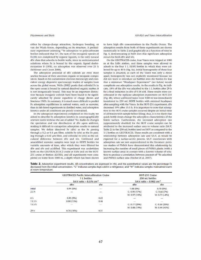
47

48

49

50

51

52

53

54

55
Chapter 3
Dissolved iron in the tropical North Atlantic Ocean
Reprinted with permission of Marine Chemistry.
Fitzsimmons, J.N., Zhang, R., and Boyle, E.A. 2013. Dissolved iron in the tropical North Atlantic Ocean. Marine Chemistry 154: 87-99.
Abstract Seawater from27 stations was sampled in a zig-zag transect across the tropical North Atlantic from Barbados to the Cape Verde Islands, 7–20°N and 21–58°W. Under the Northwest African dust plume, surface dissolved Fe (dFe) was elevated, averaging 0.55 ± 0.29 nmol/kg (1SD), but showed a wide range from 0.12 to 1.31 nmol/kg with no clear longitudinal or latitudinal gradients. A subsurface dFe maximum in excess of 1 nmol/kg was evident coincident with the oxygen minimum zone. Our goal was to determine whether this maximum occurred as a result of remineralization of high Fe:C organic material formed in the dust-laden (Fe-rich) surface ocean or as a result of lateral mixing of a coastal Fe signal from the African margin. We found that dFe is directly related to apparent oxygen utilization (AOU)with the same slope across all depths sampled, which implies a remineralization source throughout the water column. A continental margin dFe supply was discounted because a modeled margin Fe source should cause curvature in the Fe–AOU relationship that was not observed. We also did not see a significant dissolved manganese (dMn) plume emanating from the margin. Regenerated Fe:C ratios calculated from the dFe:AOU relationships ranged from 9.6 to 12.4 μmol Fe/mol C, which is much higher than ratios found in HNLC and dust-poor regions. Deep waters measured at one station in the eastern tropical North Atlantic reflected typical NADW concentrations until 4000 m, where the dFe increased to 0.82 nmol/kg in four discrete samples down to 5000m. We propose that this increase in dFe may reflect dFe inputs to deep waters as they traverse the Mid-Atlantic Ridge and enter the eastern basin.

56

57

58

59

60
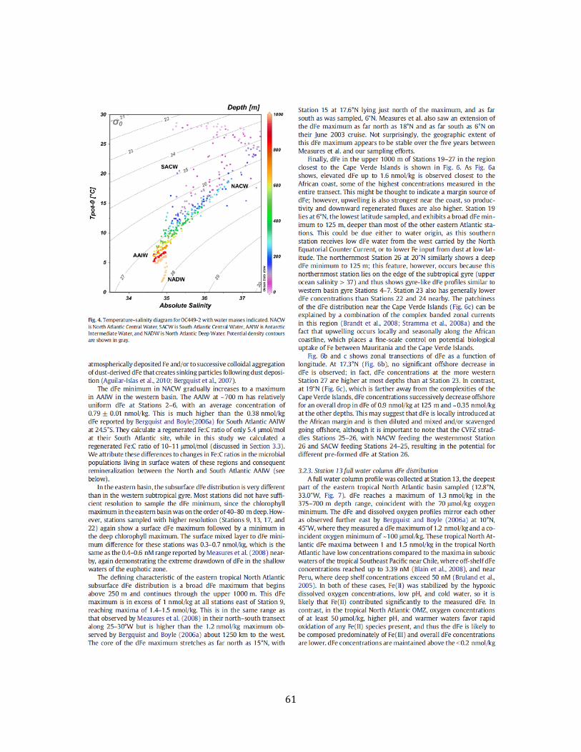
61

62

63

64

65

66
67

68
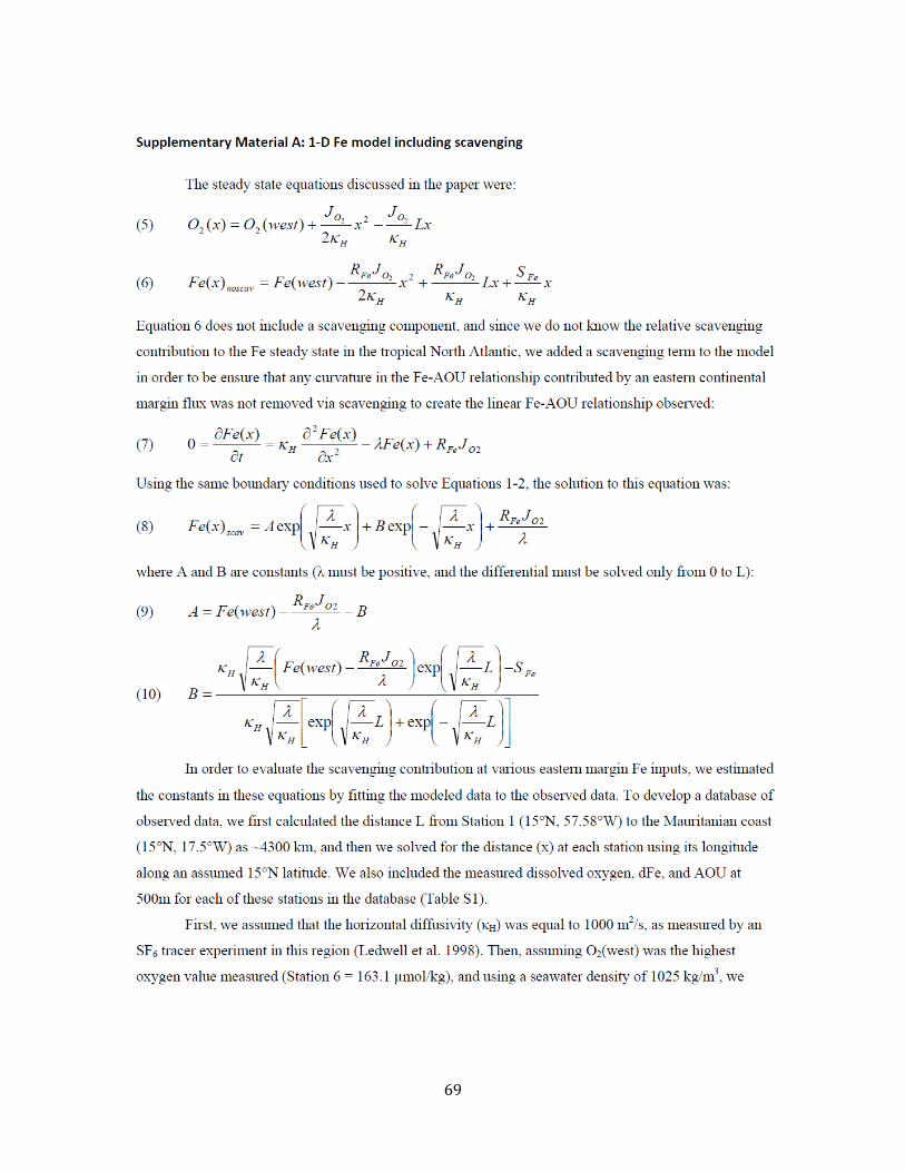
69
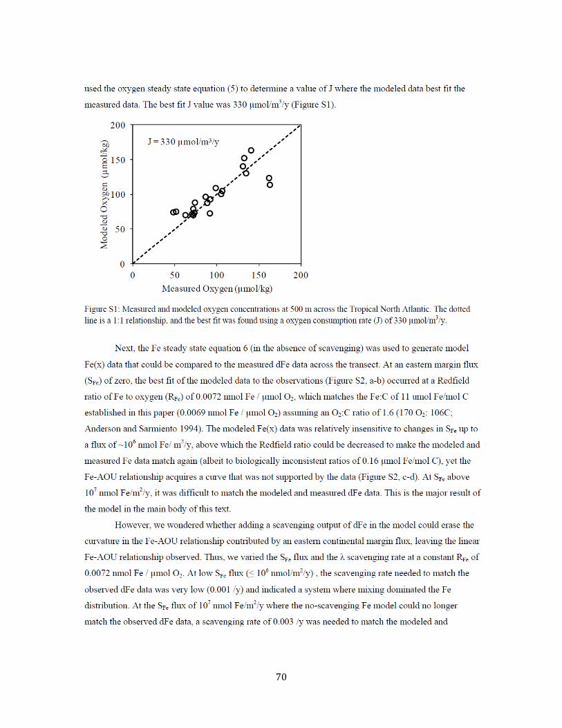
70

71
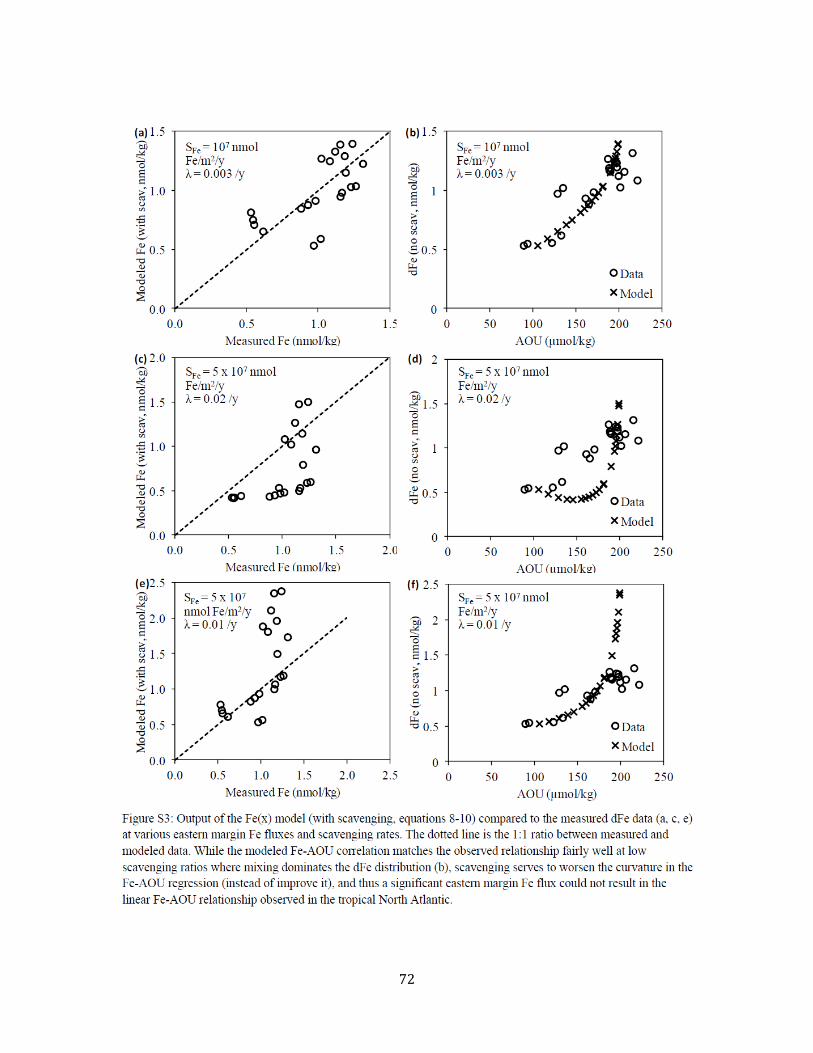
72

73

74

75

76

77

78

79
Chapter 4
Distal transport of dissolved hydrothermal iron in the deep South Pacific Ocean
Submitted to Nature Geoscience.
Fitzsimmons, J.N., Boyle, E.A., and Jenkins, W.J. in review. Distal transport of dissolved
hydrothermal iron in the deep South Pacific Ocean. Nature Communications.
Abstract Until recently, hydrothermal vents were not considered an important source in marine dissolved Fe (dFe) budgets because hydrothermal Fe was believed to precipitate quantitatively at the vent site. Based on recent abyssal dFe data, however, the "leaky vent" hypothesis argues that some hydrothermal Fe survives in the dissolved phase, contributing a significant flux of dFe to the global ocean. We show here the first measurements of dFe from the abyssal Southeast and Southwest Pacific Ocean, where observed correlations of dFe with primordial 3He support the hypothesis that dFe enrichments near 2000m are hydrothermally-derived. Remarkably this dFe is transported beyond the local vent site hundreds to thousands of kilometers away, where dFe is still enriched at 1.0-1.5 nmol/kg. The size partitioning of this hydrothermal dFe into soluble/colloidal phases further indicates that dFe transformations continue to occur at great distance from the vent source. This study provides observational evidence in support of "leaky vent" models and confirms that hydrothermal vents can have far-field impacts on the global dFe inventory, potentially providing an abyssal dFe source comparable in magnitude to dust-derived remineralization, with disproportionately large impacts on global climate after upwelling into the Fe-limited Southern Ocean.

80
Distal transport of dissolved hydrothermal iron in the deep South Pacific Ocean
Jessica N. Fitzsimmons1,2*, Edward A. Boyle2, and William J. Jenkins3
1MIT/WHOI Joint Program in Chemical Oceanography, Cambridge, MA 02139
2MIT, Department of Earth, Atmospheric and Planetary Sciences, Cambridge, MA 02139 3Woods Hole Oceanographic Institution, Marine Chemistry and Geochemistry, Woods
Hole, MA 02543
*Corresponding author: [email protected]
Submitted to Nature Communications on July 15, 2013
Acknowledgements:
We thank Jong-Mi Lee and Rick Kayser for collecting and filtering samples on the BiG
RAPA cruise, as well as Dan Repeta, and Jon Zehr and Joe Montoya, who served as
Chief Scientists on the Melville BiG RAPA and KM0703 SPEEDO cruises, respectively.
Finally, we thank the officers and crew of the R/V Kilo Moana and the R/V Melville for
their efforts on our behalf. This work was funded by a National Science Foundation
Graduate Research Fellowship (NSF Award #0645960) and the Center for Microbial
Oceanography: Research and Education (NSF-OIA Award #EF-0424599). E.A.B.’s
participation in the SPEEDO cruise was funded by a Gordon and Betty Moore
Foundation grant to Jon Zehr.
Author Contributions:
J.N.F and E.A.B. designed the sampling strategy and performed the dissolved iron
analyses. E.A.B. did the seagoing work on the KM0703 SPEEDO cruise. W.J.J.
interpolated He-3 from the WOCE data. J.N.F. drafted the manuscript, and all authors
contributed to data analysis, interpretation of results, and editing of the manuscript.

81
Until recently, hydrothermal vents were not considered an important source
in marine dissolved Fe (dFe) budgets because hydrothermal Fe was believed to
precipitate quantitatively at the vent site1. Based on recent abyssal dFe data2-7,
however, the "leaky vent" hypothesis8 argues that some hydrothermal Fe survives
in the dissolved phase, contributing a significant flux of dFe to the global ocean. We
show here the first measurements of dFe from the abyssal Southeast and Southwest
Pacific Ocean, where observed correlations of dFe with primordial 3He support the
hypothesis that dFe enrichments near 2000m are hydrothermally-derived.
Remarkably this dFe is transported beyond the local vent site hundreds to
thousands of kilometers away, where dFe is still enriched at 1.0-1.5 nmol/kg. The
size partitioning of this hydrothermal dFe into soluble/colloidal phases further
indicates that dFe transformations continue to occur at great distance from the vent
source. This study provides observational evidence in support of "leaky vent"
models and confirms that hydrothermal vents can have far-field impacts on the
global dFe inventory, potentially providing an abyssal dFe source comparable in
magnitude to dust-derived remineralization9,10, with disproportionately large
impacts on global climate after upwelling into the Fe-limited Southern Ocean11.
Hydrothermal fluids can have Fe concentrations six orders of magnitude greater
than typical deep ocean values12, so a small fraction of hydrothermal Fe escaping
precipitation into Fe sulfides or oxyhydroxides could significantly impact oceanic dFe
distributions. Nonetheless, previous marine dFe models9 have neglected this possible
source and instead focused on Fe inputs from atmospheric dust and continental margin
fluxes. In recent years, however, hotspots of enhanced dFe concentration have been
detected near known vent sites in all of the major oceans2-7, demonstrating that
hydrothermal vents impact deep ocean dFe concentrations nearby the vent source. What
has not been clear is whether this impact is confined locally or whether vent-derived dFe
is carried far enough away from the vent source to contribute to the global marine dFe
inventory. Following the early description by Boyle and Jenkins3, we address this
question by reporting deep ocean dFe in the South Pacific Ocean, where hydrothermal

82
Fe(II) lifetimes are near their longest in the global ocean because oxygen concentrations
are low, having been significantly consumed along thermohaline circulation13. Moreover,
abyssal southern hemisphere water masses upwell into the Southern Ocean, so enriched
dFe from hydrothermal vents in the South Pacific has the potential to fuel increased
biological productivity and carbon export in the Fe-limited Southern Ocean11, making the
South Pacific region we explored an important area to determine the influence of
hydrothermal venting on ocean productivity and climate. No measurements of dFe
concentration deeper than 1000m in the South Pacific have been reported previously9.
We observed enhanced dFe concentrations (1.0-1.5 nmol/kg) centered at ~2000m
at three stations in the South Pacific: KM0703 SPEEDO Station 19 (20°S, 170°W) in the
western Pacific, and Melville BiG RAPA Stations 4 (23.5°S, 88.75°W) and 7 (26.25°S,
104°W) in the eastern Pacific (Figure 1; station map is Figure S1). These dFe
concentrations are elevated above North Pacific2,14 and Atlantic15 deep ocean
concentrations of 0.4-0.6 nmol/kg and thus indicate a clear dFe anomaly. The dFe
maxima are not coincident with apparent oxygen utilization (AOU) maxima at 500-
1000m and thus are not likely caused by the remineralization of Fe from sinking organic
material (Fe-AOU correlations shown in Figure S2). Instead, the dFe profiles show
striking similarities to profiles of excess 3He, which is derived from primordial degassing
at hydrothermally active sites16. Thus, the associated 3He and dFe maxima at 2000m
suggest a hydrothermal Fe source. A concomitant enrichment in dissolved manganese
(dMn) at 2000m further corroborates the hypothesis of hydrothermal influence, as Mn is
also released from vents at high concentrations12,17 but otherwise has low deep ocean
concentrations18 (Fe/Mn discussed in Supplementary Information). These correlated dFe,
dMn, and 3He profiles demonstrate that hydrothermal venting enriches dFe by 0.4-0.9
nmol/kg above background concentrations in the abyssal South Pacific Ocean, which is
even larger than the 0.1-0.5 nmol/kg enrichments estimated by a recent model of
hydrothermal Fe delivery to the deep ocean11.
What is truly remarkable about these South Pacific dFe measurements, however,
is that they are sampled from locations hundreds to thousands of kilometers from the

83
nearest known vent source, and they still demonstrate high dFe concentrations of 1.0-1.5
nmol/kg. While we cannot constrain exactly which vents contributed to the observed
distal dFe maxima, we can compare the station locations to the sites of known
hydrothermal venting19 in light of deep South Pacific circulation (reviewed in
Supplementary Information). Transit times (t) from the vent sites are also estimated,
assuming a conservatively slow abyssal South Pacific current speed20 of 2 mm/s, to be
compared to typical deep ocean dFe residence times with respect to scavenging of 70-270
years14,21. KM0703 SPEEDO Station 19 in the western South Pacific is downstream of
EPR hydrothermal vents more than 6000 km to the east (t>95y) at 2000-3500 m depth.
This station may also be influenced in the 1000-2000 m depth range by Lau Basin vent
sources only 600-700 km away (t~10y). Melville BiG RAPA Stations 4 and 7 in the
Southeast Pacific are affected by hydrothermal sources from the west (southern EPR);
circulation studies using steric height estimations22 have determined that the enhanced
abyssal 3He as well as enriched Fe/Mn oxides in sediments of the Peru/Chile Basins are
caused by eastward advection16 across the EPR south of 20°S. Thus, an eastward flowing
EPR Fe source at 25°S would have to travel at least 800km to influence Station 7
(t=12.5y) and over 2400km to influence Station 4 (t=38y), although we cannot confirm
that hydrothermal dFe at Stations 4 and 7 are derived from the same vent site. Thus, in
the South Pacific, hydrothermal Fe is not only maintained in the dissolved phase locally
at the vent site, but it is able to escape rapid scavenging and become transported hundreds
to thousands of kilometers from the vent site at high dFe concentrations.
How is this dissolved phase Fe stabilization achieved? Two hypotheses have been
proposed, and perhaps both contribute to vent Fe stabilization. First, pyrite nanoparticles
between 4-200nm have been shown to account for 5-25% of the dFe in global vent
fluids23. These colloids would pass through the 0.4 µm filter used to operationally define
dissolved Fe in this study, and due to their small size they would sink very slowly,
providing a mechanism by which inorganic dFe might be carried away from vents in the
“dissolved” fraction. Alternatively, organic ligands may bind the Fe(III) formed after
oxidation of vent-derived Fe(II) upon mixing of vent fluids with oxic seawater24,25. This

84
organic chelation protects the Fe from precipitation and stabilizes it in the dissolved
fraction as Fe is advected away from the vent site.
To further investigate the mechanism of dFe stabilization, we measured the size
partitioning of dFe between soluble Fe (sFe, <0.02 µm) and colloidal Fe phases (0.02
µm<cFe<0.4 µm; cFe = dFe - sFe). sFe is considered to be truly dissolved, while cFe is
composed of particles so small that they remain suspended in solution and are circulated
and collected along with the dissolved Fe pool; both inorganic and organically-bound dFe
can be present in both size fractions. The results shown in Figure 2 suggest that when
hydrothermally-derived dFe is high (Station 7), colloidal Fe is the major dFe fraction
(cFe composes 76% of dFe), while a more diluted/scavenged dFe signal (Stations 19 and
4) has a more soluble Fe-rich dFe pool (50% soluble, 50% colloidal Fe). Thus, assuming
a similarly partitioned Fe source among the three stations studied here, colloidal Fe
appears to compose most of the dFe near the vent site (Station 7) and is transformed into
a soluble Fe maximum (Station 4) as the dFe is scavenged away. These observations are
consistent with the only published near-field Fe size partitioning study, which
demonstrated that within 100m of a vent site in the Indian Ocean colloidal Fe was the
primary dissolved Fe phase26.
In the Southeast Pacific, not only does the % sFe increase with distance from the
vents, but the absolute sFe concentration also increases with distance from the vent,
rising from 0.35 nmol/kg at Melville BiG RAPA Station 7 to a maximum of 0.51
nmol/kg at Station 4. This Station 4 sFe concentration and the 0.44 nmol/kg sFe at
Station 19 are well above background deep water sFe concentrations in the Pacific Ocean
of 0.2-0.3 nmol/kg27 and must have been transferred from the particulate (pFe) or
colloidal fraction. This downstream sFe increase leads us to conclude that Fe
transformations between phases occur not only at the local site of hydrothermal venting
but continue hundreds to thousands of kilometers from the vent source. The nature of
these pFe, sFe, and cFe transformations are unknown, but one potential mechanism that
could explain the observed pattern is the conversion of Fe from inorganic colloids to truly
soluble, organically-bound complexes over time/distance.
85
Using the excess 3He concentrations measured on nearby WOCE sections
interpolated onto the depths of the measured dFe data (see Supplementary Information
for 3He profile station locations), dFe/3He ratios were determined; only depths near the
hydrothermally-derived dFe maxima were included in the regression calculation (Figure
3, closed circles). Resulting dFe/3He ratios ranged from 0.9-2.7x10⁶ mol Fe / mol 3He,
much lower than the 2-10x108 mol/mol values found in high-temperature vent fluids
(both at EPR 19°S and in the Western Pacific vents11). Thus, only 0.02-1.0% of total
vented hydrothermal Fe survives transport hundreds to thousands of kilometers away in
the dissolved phase. Even within the three far-field stations of this study, the highest
dFe/3He ratios were found at the station closest to the vent source, while the lower ratios
represent a more distally-persistent, scavenging-affected hydrothermal signal.
It is worth noting that in the Southwest Pacific the 3He and dFe profiles are nearly
identical, while in the Southeast Pacific the 3He remains enriched to the ocean floor but
dFe decreases to background concentrations below 2500-3000m. An elevated 3He signal
in the absence of any Fe enrichment suggests Fe scavenging. The depth range of this dFe-3He separation (3000-4000m) is below the typical sill depth of the southern EPR and
Chile Ridge (2500-3000m), and thus we hypothesize that the 3He measured below those
depths may actually be relic 3He that reached those depths after long circulation times
during which hydrothermal dFe was scavenged (deep ocean residence time of dFe is 70-
270 years14,21).
The results of this study support a “leaky vent" model of dFe inputs to the abyssal
South Pacific Ocean and also demonstrate transport of hydrothermal Fe in the dissolved
phase hundreds to thousands of kilometers from the vent source. If the dFe/3He ratio of
0.9x10⁶ mol/mol is indicative of the amount of vent-derived dFe "persisting" in the deep
ocean, using the estimated annual loss rate of 3He from the ocean28 of 750±200 mol/y we
estimate that the flux of dFe "leaking" from global vents into the deep ocean is ~7x10⁸
mol/y. This value is twice the hydrothermal flux reported based on Fe-binding ligand
measurements near the Mid-Atlantic Ridge24 and is nearly 3% of the estimated 2.36x10¹⁰
mol/y aerosol inputs of dissolved Fe into the surface ocean9.

86
While this might seem to be a relatively insignificant marine Fe source compared
to dust, we know that abyssal South Pacific waters eventually upwell in the Fe-limited
Southern Ocean11 where upper ocean productivity plays a significant role in global
carbon export29. Thus the relatively small percentage of open ocean dFe contributed by
hydrothermal vents calculated here may play a disproportionately large role in global
climate by its influence in the Fe-limited Southern Ocean. If this "persistent"
hydrothermal dFe were to reach the surface and fertilize phytoplankton with an Fe:C ratio
of 6 µmol Fe per mol carbon (typical of diatoms in the Fe-limited Southern Ocean30),
then this dFe could support ~1x10¹⁴ mol/y of new carbon, which is comparable in
magnitude to global new production (4x10¹⁴ mol/y)10. This estimate, however, has both
positive and negative uncertainties. dFe/3He ratios vary globally as a function of bedrock
geology and ridge spreading rate, and values along the slow-spreading Mid-Atlantic
Ridge31 are higher by orders of magnitude than those in the Pacific, indicating that the
hydrothermally-supported new production may be biased too low. In contrast, this
production estimate may be biased high because it assumes full biological availability of
the hydrothermal dFe, which may not be true if the dFe is in inorganic nanoparticulate
form32, and also assumes that no additional scavenging of the "persistent" hydrothermal
dFe occurs before upwelling to the surface ocean. We know that the residence time of
abyssal dFe with respective to scavenging onto sinking particles is 100-300 years14,21, so
scavenging of some of this "persistent" dFe before upwelling is likely. Future research
must focus on distal hydrothermal dFe transformation pathways and scavenging rates in
order to constrain the spatial and temporal extent of this aybssal dFe source, and global
Fe and climate models that have neglected hydrothermal Fe inputs require its inclusion in
the future.
Methods
Station 19 in the Southwest Pacific was sampled on the R/V Kilo Moana in April
2007 on the Center for Microbial Oceanography: Research & Education (C-MORE)
SPEEDO cruise, and Stations 4 and 7 in the Southeast Pacific were sampled on the R/V

87
Melville in November-December 2010 on the C-MORE BiG RAPA cruise. Trace metal-
uncontaminated seawater on KM0703 was collected using the MITESS system, which
employed both Teflon and HDPE bottles during sample collection (Teflon vs. HDPE
indicated in Supplementary Information data table), followed by filtration through 0.4 µm
Nuclepore filters into HDPE bottles by previously established methods33. Soluble Fe
samples were subsequently collected after filtration through a 0.02 µm Anodisc filter. On
the Melville BiG RAPA cruise, seawater was collected using the MITESS/Vanes system
employing HDPE bottles, followed by filtration through 0.4 µm Nuclepore filters into
HDPE bottles33. Soluble Fe samples were collected using a cross flow ultrafiltration
system in static mode employing a 10 kDa nominal molecular weight cutoff regenerated
cellulose filter (Millipore: Pellicon XL, PLCGC) after conditioning with 350mL of
filtered sample seawater. Detailed methodological descriptions and an intercalibration
between the two soluble Fe sample collection methods used in this study have been
described previously34.
Samples were analyzed in triplicate for their Fe concentration by isotope dilution
inductively-coupled plasma mass spectrometry (ID-ICP-MS) on a hexapole collision cell
IsoProbe ICP-MS. The ID-ICP-MS method employs an 54Fe-spike and batch pre-
concentration with nitrilotriacetate resin15. Procedure blanks for the western Pacific
stations were 0.20 nmol/kg, but very stable to ±0.03 nmol/kg because they derived
quantitatively from the constant amount of NTA superflow resin used to pre-concentrate
the Fe. Procedure blanks over the six analytical sessions for the Eastern Pacific stations
were much lower, ranging from 0.025-0.060 nmol/kg, and the detection limit (three times
the standard deviation of the procedure blanks for each analytical session) averaged 0.025
nmol/kg. Comprehensive lab analyses of SAFe D2 standard for dFe during the period of
these analyses averaged 0.99±0.03 nmol/kg (Bottle 242, ±1SD, n=8) and 0.92±0.01
nmol/kg (Bottle 446, ±1SD, n=8), which agrees well with the current consensus value of
0.933±0.023 nmol/kg (May 2013 consensus:www.geotraces.org/science/intercalibration).
Dissolved manganese (dMn) was extracted from filtered seawater by a modified
version of an automated flow injection pre-concentration method35 followed by dMn

88
concentration analysis using quadrupole ICP-MS and standard addition calibrations. 12
mL filtered and acidified samples were aliquoted into acid cleaned 50 mL Corning
centrifuge tubes. 60, 120, and 180 µL of 100 nM Mn standard were added to SAFe
surface water in order to generate standard curves throughout the run; this allowed for
final Mn standard concentrations of 0.5, 1.0, and 1.5 nM, respectively. The pH of each
sample was brought to 6.0±0.2 with ammonium acetate buffer (pH 8.9) before being
pumped through the extraction system. The extraction system was identical to that
described by Milne et al., except that the micro-column was filled with Nobias-chelate
PA1 resin (ESI). After elution through the column in 1.0 mL of 1M distilled nitric acid,
extracted samples were analyzed for dMn by ICP-MS on a VG/Fisons PQ2+. The SAFe
D1 standard reference seawater was found to have a dMn concentration of 0.352±0.020
nmol/kg (n=8; ±1 SD of replicate analyses), agreeing exactly with the SAFe D2
consensus value of 0.35±0.05 nmol/kg. dMn procedure blanks were less than 0.01
nmol/kg.
The excess 3He data were obtained from http://cchdo.ucsd.edu/ (see also the
measurement protocols described at
http://cchdo.ucsd.edu/manuals/pdf/91_1/jenknew.pdf) and the stations in the vicinity of
the dFe stations (Figure S1) were used to interpolate onto the dFe station data in the
following manner. First, excess 3He was computed using the reported the helium isotope
ratio anomaly and helium concentration, correcting for helium solubility isotope
fractionation for equilibrium with air, then each 3He station was vertically interpolated
onto neutral density surfaces. Next, each isopycnal surface was interpolated to the
geographic location of the dFe stations. Finally, the resultant profiles of 3He vs. neutral
density were interpolated to the sampling depths of the dFe profiles. The statistical
uncertainties associated with this interpolation were small relative the variance in the
dFe:3He relationships subsequently derived.

89
References for Chapter 4
1 German, C. R., Campbell, A. C. & Edmond, J. M. Hydrothermal scavenging at
the Mid-Atlantic Ridge: Modification of trace element dissolved fluxes. Earth and Planetary Science Letters 107, 101-114 (1991).
2 Boyle, E. A., Bergquist, B. A., Kayser, R. A. & Mahowald, N. Iron, manganese, and lead at Hawaii Ocean Time-series station ALOHA: Temporal variability and an intermediate water hydrothermal plume. Geochimica et Cosmochimica Acta 69, 5165-5166, doi:10.1016/j.gca.2005.03.006 (2005).
3 Boyle, E. A. & Jenkins, W. K. Hydrothermal iron in the deep western South Pacific. Geochimica et Cosmochimica Acta 72, A107 (2008).
4 Klunder, M. B., Laan, P., Middag, R., de Baar, H. J. W. & Bakker, K. Dissolved iron in the Arctic Ocean: Important role of hydrothermal sources, shelf input and scavenging removal. J. Geophys. Res. 117, C04014, doi:10.1029/2011jc007135 (2012).
5 Klunder, M. B., Laan, P., Middag, R., De Baar, H. J. W. & van Ooijen, J. C. Dissolved iron in the Southern Ocean (Atlantic sector). Deep Sea Research Part II: Topical Studies in Oceanography 58, 2678-2694 (2011).
6 Nishioka, J., Obata, H. & Tsumune, D. Evidence of an extensive spread of hydrothermal dissolved iron in the Indian Ocean. Earth and Planetary Science Letters 361, 26-33, doi: http://dx.doi.org/10.1016/j.epsl.2012.11.040 (2013).
7 Wu, J., Wells, M. L. & Rember, R. Dissolved iron anomaly in the deep tropical- subtropical Pacific: Evidence for long-range transport of hydrothermal iron. Geochimica et Cosmochimica Acta 75, 460-468 (2011).
8 Toner, B. M., Marcus, M. A., Edwards, K. J., Rouxel, O. & German, C. R. Measuring the form of iron in hydrothermal plume particles. Oceanography 25, 209-212 (2012).
9 Moore, J. K. & Braucher, O. Sedimentary and mineral dust sources of dissolved iron to the world ocean. Biogeosciences 5, 631-656 (2008).
10 Shaffer, G. Biogeochemical cycling in the global ocean 2. New proudction, Redfield ratios, and remineralization in the organic pump. Journal of Geophysical
Research 101, 3723-2745 (1996). 11 Tagliabue, A. et al. Hydrothermal contribution to the oceanic dissolved iron
inventory. Nature Geosci 3, 252-256 (2010). 12 Von Damm, K. L. et al. Chemistry of submarine hydrothermal solutions at 21°N,
East Pacific Rise. Geochimica et Cosmochimica acta 49, 2197-2220 (1985). 13 Field, M. P. & Sherrell, R. M. Dissolved and particulate Fe in a hydrothermal
plume at 9°45'N, East Pacific Rise: Slow Fe (II) oxidation kinetics in Pacific plumes. Geochimica et Cosmochimica Acta 64, 619-628 (2000).
14 Bruland, K. W., Orians, K. J. & Cowen, J. P. Reactive trace metals in the

90
stratified central North Pacific. Geochimica et Cosmochimica Acta 58, 3171-3182 (1994).
15 Lee, J.-M. et al. Analysis of trace metals (Cu, Cd, Pb, and Fe) in seawater using single batch Nitrilotriacetate resin extraction and isotope dilution inductively coupled plasma mass spectrometry. Analytica Chimica Acta 686, 93-101 (2011).
16 Lupton, J. Hydrothermal helium plumes in the Pacific Ocean. J. Geophys. Res. 103, 15853-15868, doi:10.1029/98jc00146 (1998).
17 Edmond, J. M., Von Damm, K. L., McDuff, R. E. & Measures, C. I. Chemistry of hot springs on the East Pacific Rise and their effluent dispersal. Nature 297, 187-191 (1982).
18 Martin, J. H., Knauer, G. A. & Broenkow, W. W. VERTEX: the lateral transport of manganese in the northeast Pacific. Deep Sea Research Part A. Oceanographic Research Papers 32, 1405-1427, doi:http://dx.doi.org/10.1016/0198-0149(85)90056-1 (1985).
19 Beaulieu, S. E. InterRidge Global Database of Active Submarine Hydrothermal Vent Fields: prepared for InterRidge, Version 2.0, <http://www.interridge.org/IRvents> (2010).
20 Hautala, S. L. & Riser, S. C. A nonconservative b-spiral determination of the deep circulation in the Eastern South Pacific. Journal of Physical Oceanography 23, 1975-2000 (1993).
21 Bergquist, B. A. & Boyle, E. A. Dissolved iron in the tropical and subtropical Atlantic Ocean. Global Biogeochemical Cycles 20, 14 (2006).
22 Reid, J. L. On the total geostrophic circulation of the South Pacific Ocean: Flow Patterns, tracers, and transports. Progress in Oceanography 16, 1-61 (1986).
23 Yucel, M., Gartman, A., Chan, C. S. & Luther, G. W. Hydrothermal vents as a kinetically stable source of iron-sulphide-bearing nanoparticles to the ocean. Nature Geoscience 4, 367-371 (2011).
24 Bennett, S. A. et al. The distribution and stabilisation of dissolved Fe in deep-sea hydrothermal plumes. Earth and Planetary Science Letters 270, 157-167 (2008).
25 Sander, S. G. & Koschinsky, A. Metal flux from hydrothermal vents increased by organic complexation. Nature Geoscience 4, 145-150 (2011).
26 Sands, C. M., Connelly, D. P., Statham, P. J. & German, C. R. Size fractionation of trace metals in the Edmond hydrothermal plume, Central Indian Ocean. Earth and Planetary Science Letters 319-320, 15-22 (2012).
27 Wu, J., Boyle, E. A., Sunda, W. G. & Wen, L. Soluble and colloidal iron in the oligotrophic North Atlantic and North Pacific. Science 293, 847-849 (2001).
28 Craig, H., Clarke, W. B. & Beg, M. A. Excess 3He in deep water on the East Pacific Rise. Earth and Planetary Science Letters 26, 125-132 (1975).
29 Honjo, S., Manganini, S. J., Krishfield, R. A. & Francois, R. Particulate organic carbon fluxes to the ocean interior and factors controlling the biological pump: A synthesis of global sediment trap programs since 1983. Progress in Oceanography 76, 217-285, (2008).

91
30 Twining, B. S., Baines, S. B. & Fisher, N. S. Element stoichiometries of individual plankton cells collected during the southern ocean iron experiment (SOFeX). Limnology & Oceanography 49, 2115-2128 (2004).
31 Saito, M. A. et al. A South Atlantic hydrothermal iron plume and implications for global iron cycling. Nature Geoscience (in press).
32 Rich, H. W. & Morel, F. M. M. Availability of well-defined iron colloids to the marine diatom Thalassiosira weissflogii. Limnology and Oceanography 35, 652-662 (1990).
33 Fitzsimmons, J. N. & Boyle, E. A. An intercalibration between the GEOTRACES GO-FLO and the MITESS/Vanes sampling systems for dissolved iron concentration analyses (and a closer look at adsorption effects). Limnology & Oceanography: Methods 10, 437-450 (2012).
34 Fitzsimmons, J. N. & Boyle, E. A. The assessment and intercalibration of Anopore™ and cross flow filtration methods for the determination of dissolved iron size fractionation into soluble/colloidal phases in seawater. Limnology & Oceanography: Methods (in review).
35 Milne, A., Landing, W., Bizimis, M. & Morton, P. Determination of Mn, Fe, Co, Ni, Cu, Zn, Cd and Pb in seawater using high resolution magnetic sector inductively coupled mass spectrometry (HR-ICP-MS). Analytica Chimica Acta 665, 200-207, doi:10.1016/j.aca.2010.03.027 (2010).

92
34 35 36
0
1000
2000
3000
4000
5000
0 10 20 30
Salinity
Temperature (°C)
0 0.2 0.4 0.6
0 0.2 0.4 0.6 0.8 1
dMn (nmol/kg)
dFe (nmol/kg)
0 1 2 3 4
0 100 200
Phosphate (µmol/L)
AOU (µmol/kg)
0 0.3 0.6 0.9 1.2
excess 3He (fmol/kg)
34 35 36
0
500
1000
1500
2000
2500
0 10 20 30
Salinity
Temperature (°C)
0.0 0.5 1.0 1.5
0.0 0.4 0.8 1.2 1.6
dMn (nmol/kg)
dFe (nmol/kg)
0 1 2 3
0 100 200
Phosphate (µmol/L)
AOU (µmol/kg)
0 0.3 0.6 0.9 1.2
excess 3He (fmol/kg)
34 35 36
0
500
1000
1500
2000
2500
3000
3500
4000
0 10 20
Salinity
Temperature (°C)
0.0 0.5 1.0 1.5
0.0 0.3 0.6 0.9 1.2
dMn (nmol/kg)
dFe (nmol/kg)
0 1 2 3
0 75 150 225
Phosphate (µmol/L)
AOU (µmol/kg)
0 0.2 0.4 0.6 0.8 1
excess 3He (fmol/kg)
(a) KM0703 Station 19 (Southwest Pacific: 20°S, 170°W)
(b) Melville BiG RAPA Station 7 (Southeast Pacific: 26°S, 104°W)
(c) Melville BiG RAPA Station 4 (Southeast Pacific: 23.5°S, 88.5°W)

93
Figure 1: Oceanographic profiles showing a hydrothermal influence on dFe, 3He, and dMn at 2000 m. Relevant profiles taken from (a) SPEEDO-KM0703 Station 19 in the Southwest Pacific, (b) Melville BiG RAPA Station 7 in the Southeast Pacific, and (c) Melville BiG RAPA Station 4 in the Southeast Pacific. Temperature, AOU, and dFe are shown as solid lines, while salinity, phosphate, and dMn are shown as open circles and dotted lines. The average excess 3He data is shown as a solid line at the depths where dFe measurements were made, while the data used to generate those average values are shown as grey crosses.
Figure 2: The size partitioning of dFe into soluble and colloidal phases demonstrates continued Fe transformations at great distance from vents. dFe (closed circles, solid line; dFe < 0.4 µm) is partitioned into soluble Fe (open circles, dashed line; sFe < 0.02µm or 10kDa) and colloidal Fe (the difference between the two lines) fractions at (a) Station 19 in the Southwest Pacific, (b) Station 7 in the Southeast Pacific, and (c) Station 4 in the Southeast Pacific. Note that the Fe concentration scale changes in each of the three panels.
0
1000
2000
3000
4000
5000
0 0.5 1
Depth(m
)
Fe (nmol/kg)
0 0.5 1
Fe (nmol/kg)
0 0.5 1 1.5
Fe (nmol/kg)
(a) KM0703 Sta. 19 (b) BiG RAPA Sta. 7 (c) BiG RAPA Sta. 4
dFe
sFe
sFe
dFe
dFe
sFe

94
Figure 3: Distal hydrothermal dFe/3He ratios. Station locations are (a) Station 19 in the Southwest Pacific, (b) Station 7 in the Southeast Pacific, and (c) Station 4 in the Southeast Pacific. Data shallower than 1000m is excluded from the regression calculation (open circles). Deepest samples at Stations 4 and 7 where dFe appears to have been scavenged while 3He remains elevated are also excluded (open circles).
Slope = 0.90±0.06 x 10⁶
(mol Fe/mol 3He)
0
0.4
0.8
1.2
1.6
0.0 0.5 1.0
dFe
(nmol/kg) Slope = 1.13±0.10 x 10⁶
(mol Fe/mol 3He)
0.0 0.5 1.0
Slope = 2.70±0.59 x 10⁶
(mol Fe/mol 3He)
0.0 0.5 1.0
Excess 3He (fmol/kg)
(a) KM0703 Sta. 19 (b) BiG RAPA Sta. 7 (c) BiG RAPA Sta. 4

95
Supplementary Material for
Distal transport of dissolved hydrothermal iron in the deep South Pacific Ocean
Jessica N. Fitzsimmons*, Edward A. Boyle, and William J. Jenkins
*To whom correspondence should be addressed. Email: [email protected]
This file contains: Text (1882 words) Figure S1 - S2; Figure captions (185 words) Table S1 24 References Locations and general circulation of sample stations
Figure S1 shows a map of the three stations sampled for dissolved iron (dFe), along with
the reference stations used to interpolate profiles of excess 3He at our stations and known
sites of hydrothermal venting near the sampling sites (both active and confirmed)1.
Figure S1: Map of study locations. (a) shows the Southwest Pacific where KM0703 SPEEDO Station 19 (20°S, 170°W) is indicated in red, and the Kermadec/Tonga Arc is indicated as a topographic high along 175°W. (b) shows the Southeast Pacific where Melville BiG RAPA Stations 7 (26.25°S, 104°W) and 4 (23.5°S, 88.75°W) are indicated in red, and the East Pacific Rise (EPR) is shown as the topographic high along 113°W. Shown as squares are stations where historical 3He data exists that was used to interpolate the average 3He profiles onto this study's sampling locations (3He data from https://cchdo.ucsd.edu). Shown as crosses are sites of confirmed or inferred hydrothermal venting (deeper than 1000m)1.
96
Enhanced dFe at 2000m is not a result of remineralization: Fe-AOU relationships
The dFe maxima at the three sampling stations at 2000m depth are not associated
with maxima in AOU (Figure 1) and thus should not be attributed to remineralization. In
fact, at all stations there is a ferricline at 400-500m depth that corresponds exactly with
the depths of increasing AOU and phosphate concentrations, and dFe, AOU, and
phosphate reach relative maxima by 1000m. This shallow ferricline depth also matches
the ferricline depths recorded in prior studies of the Southeast2 and Equatorial Pacific3
and is attributed to remineralization of sinking organic matter. Remineralization dFe
signals stabilize between 500-1000m at concentrations of 0.3 nmol/kg at Stations 19 and
7 and 0.6 nmol/kg at Station 4. Along these depths, dFe and AOU have a linear
relationship (Figure S2) that result in Fe:C ratios between 2.4-4.5 µmol/mol, falling in the
overall range of 1.4-4.7 found in the North and equatorial Pacific4.
At Stations 19 and 7, the anomalously enriched dFe data (shown as crosses in
Figure S2) fall off a linear relationship of dFe:AOU, suggesting that the high Fe
concentrations are not produced by remineralization. Accordingly if these enriched dFe
data are included in the Fe:C ratio estimates, not only do the linear correlations between
dFe and AOU become less significant, but the resulting Fe:C ratios (designated as
"Fe:C(all)" in Figure S2) also increase to 5.1-9.2 µmol/mol, which is higher than has ever
been recorded in the open ocean Pacific. Both of these facts suggest that the deep dFe
enrichment at 2000m is not a result of remineralization.

97
Figure S2: Fe-AOU relationships for each of the three stations. In circles are the stations included in the regression and the Fe:C calculation, while the crosses show the sample depths that we suggest are affected by hydrothermal Fe. When all points (circles and crosses) are included in the regression, the resulting Fe:C ratio is indicated as "Fe:C (all)." Fe:C ratios are calculated using an AOU:C ratio5 of 1.6 and are in units of µmol/mol.
dMn data and Fe/Mn ratios
Hydrothermally-derived dissolved Mn maxima were detected at 2000m in our
open ocean samples at all three stations, ranging from 0.32-1.18 nmol/kg in the profile
peaks (compared to 0.1-0.2 nmol/kg dMn backgrounds in typical abyssal seawater).
Station 7 in the eastern South Pacific had the highest dMn concentration, in accordance
with highest dFe concentrations. Station 4 (23.5°S, 88.75°W) had a peak dMn
concentration of 0.40 nmol/kg, which is much lower than the 1.77 nmol/kg total
dissolved Mn (dissolved + particulate) measured in 1986 at a nearby station (24.64°S,
94.04°W) at 2579m depth6. Assuming similar hydrothermal Mn delivery at the two
sampling stations today and in 1986, there must be a large particulate Mn component at
these stations that was not monitored in this study, potentially suggesting that both
particulate and dissolved Mn are transported hundreds-thousands of kilometers from the
vent source in the hydrothermal plume. This particulate Mn inference requires further
investigation to confirm.
Because of its slow scavenging kinetics7 and sluggish re-equilibration after
temperature alteration in the buyoant plume8, dissolved Mn is believed to behave
conservatively in vent fluids on the timescale of hours-days. Following this assumption
BiG RAPA Sta. 4y = 0.0027x + 0.031
Fe:C = 4.3±0.7
Fe:C (all) = 5.1±1.1
0.0
0.1
0.2
0.3
0.4
0.5
0.6
0.7
0.8
0.9
1.0
0 50 100 150 200
BiG RAPA Sta. 7y = 0.0026x ‐ 0.035Fe:C = 4.1±0.5
Fe:C (all) = 9.2±2.9
0.0
0.2
0.4
0.6
0.8
1.0
1.2
1.4
1.6
0 50 100 150 200
AOU µmol/kg
KM0703 Sta. 19y = 0.0015x + 0.086
Fe:C = 2.4±0.7
Fe:C (all) = 6.2±1.0
0.0
0.1
0.2
0.3
0.4
0.5
0.6
0.7
0.8
0.9
1.0
0 50 100 150 200
[Fe] nmol/kg

98
of Mn conservation, dFe/dMn ratios have been used in vent fluid samples to calculate the
extent of plume dilution9,10 and the temperature of the hydrothermal reaction chamber11.
Since our samples are taken from the distal hydrothermal plume at a very minimum of
several days from the vent source, we believe that an analysis of vent fluid dilution using
the dissolved Mn data is not appropriate because dissolved Mn no longer behaves
conservatively, and 3He is instead used as the conservative tracer of vent fluids in this
paper.
However, there is still useful information to be gleaned from the Fe/Mn ratios
with distance from the plume, although background deep-ocean concentrations must be
subtracted from the hydrothermal concentration anomalies in order to compare the distal
hydrothermal Fe/Mn ratios to near-field hydrothermal ratios. We made these corrections
by subtracting the non-hydrothermal, deep-ocean dFe and dMn concentrations of 0.4
nmol/kg and 0.15 nmol/kg, respectively12. The resulting Fe/Mn ratios at the depths of
maximum hydrothermal influence are Station 19: 2.65±0.5, Station 7: 1.16±0.2, and
Station 4: 2.21±0.6. Assuming both Fe and Mn behave non-conservatively in the far-field
plume, these ratios inform us about the relative scavenging precipitation potential of Fe
and Mn in the distal hydrothermal plume. If we assume a similar hydrothermal source for
Stations 4 and 7, with Station 4 simply ~1500km farther along the distal plume, then the
increase in dFe/dMn ratio from 1.16 at Station 7 to 2.21 at Station 4 suggests that dMn is
scavenged to a greater extent in the distal plume than dFe, presumably because more of
the "scavenge-able" dFe has already been removed in the near-field plume. While dFe
removal pathways along the distal plume are abiotically-driven, including oxidation of
remaining dissolved Fe2+ or pyrite nanoparticles and aggregation/scavenging of colloidal
Fe to the particulate phase, dMn removal pathways include both an abiotic component
(oxidation of dissolved Mn2+ to particulate Mn4+) as well as a biotic component that is
microbially mediated13. This microbial Mn scavenging was the dominant Mn removal
pathway in distal (15-20 km from vent) samples, compared to a larger abiotic scavenging
component in proximal vent samples (0-3 km from vent) near the Juan de Fuca Ridge7.

99
Possible sources of hydrothermal vent input to the study locations
With the data shown here, it is impossible to identify vent sources for the
hydrothermally-derived dFe observed at the three study locations; it is also very probable,
given that the study sites are situated far away from a large array of known hydrothermal
vents, that multiple vents contribute to the cumulative hydrothermal dFe and 3He
anomalies measured at the three stations. We review here the hydrothermal vent fields
that may have contributed to the observed dFe enrichment, in light of the recently
assembled global hydrothermal vent database1 as well as published articles from the
literature.
Southwest Pacific: KM0703 SPEEDO Station 19 (20°S, 170°W)
The hydrothermal dFe, dMn, and excess 3He anomalies at Station 19 are both
greatest over a depth range from 1000-3500m, with coincident maxima at 2000m.
Although the nearest identified hydrothermal sources occur in the Tonga-Fiji region just
to the west of this station14 the predominant flow pattern over this depth range is from the
southeast, organized as a zonally elongated anticyclonic gyre extending perhaps as far
eastward as the East Pacific Rise according to Reid15. This suggests that the fast
spreading centers along the southern EPR described by Lupton and Craig16 may be the
origin of the 3He and dFe anomalies. Moreover, the direction of this circulation is
consistent with the beta-plume dynamics earlier described by Stommel17 that arise from
the mid-depth injection of buoyancy at these sites. However, we cannot completely rule
out an additional contribution from the Tonga-Fiji venting sites, even though they occur
“downstream” of Station 19 (a 3He plume has been observed14 north and west of Station
19, centered at 1750m near 15°S, 175°W, emanating westward toward the Coral Sea). A
detailed examination of the data from Lupton et al.14 shows that the zonal 3He section is
characterized by nearly vertical 3He contours between 173° and 176°W, supporting the
hypothesis of little influence of Tonga-Fiji vents on the dFe and 3He profiles at Station
19.

100
Southeast Pacific: Melville BiG RAPA Stations 4 (23.5°S, 88.75°W) and 7 (26.25°S,
104°W)
The hydrothermal 3He and dFe anomalies at Stations 4 and 7 in the Southeast
Pacific both have maxima at 2000m depth, with Station 7 having >50% more dFe than
Station 4 at their maxima, although the 3He anomalies are roughly comparable in
magnitude at the two stations. The highly elevated dFe concentrations of >1.5 nmol/kg at
2000m at Station 7 might suggest the presence of a proximal Fe source. This station is
also located on the topographic high of the Easter Seamount Chain, which might also
support the premise of a nearby hydrothermal site. However, no venting has been
confirmed or even inferred from CTD casts anywhere along the Easter Seamount Chain
(as shown in Figure S1). The Sala y Gomez hotspot, which formed the Eastern Seamount
Chain during the last 30 million years18,19, is currently believed to be somewhere between
Easter Island (540 km away from Station 7) and Sala y Gomez Island (145 km away),
likely nearer to Sala y Gomez Island. No modern seamount derived from this hotspot has
been identified, and as a result no volcanic activity or associated venting has been
inferred. If the Sala y Gomez hotspot is found to be the major dFe source to the Peru
Basin at some later date, however, the elevated dFe at Station 4 still implies long range
transport of dFe from distal hydrothermal sources because there are no known vents (or
even topographic rises that might support vents) near Station 4.
The EPR is the most probable source of dFe and 3He at Melville BiG RAPA
Station 7. The well-known 3He plume initially discovered at ~15°S between 2000-3000m
is advected westward from the EPR, away from the Peru/Chile basins16, but there is still
elevated δ3He (28-30%) at 15-30°S in the Peru Basin east of the EPR through and along
88°W20 (the longitude of Station 4). Despite being east of the EPR, Lupton20 attributed
this 88°W δ3He distribution to an EPR source, since steric height calculations infer
eastward transport of water at 2500m depth across the EPR and into the Peru/Chile
basins21. In fact, the 3He distribution along 32°S very clearly shows eastward transport of
a 3He plume from the southern EPR22. This eastward aybssal flow south of 15°S has also
been used to explain the enhanced Fe and Mn in surface sediments of the Peru/Chile

101
Basins at 25°S23 and the enhanced total dissolved Mn concentrations (from unfiltered
samples) collected at 18-25°S, 94°W near Station 4 of our study6. As shown in Figure S1,
there are many hydrothermal vents between 20-32°S, reported by Baker et al.24, that
could source this enhanced dFe, dMn, and 3He along the Nazca Ridge, most of which
vent at the appropriate depths of 2000-3000m to produce the observed signal. These EPR
vents are a minimum of 860 km from Station 7 and thus indicate that dFe can be stably
transported quite far from the vent source.
The geostrophic flow patterns proposed by Reid15 at Station 4 come from the
north and northwest at 2000-2500m depth, instead of from due west, as at Station 7.
Thus, although it is still likely that Station 4 dFe is derived from the EPR, it may also
receive hydrothermal influence from the northern EPR. As a hydrothermal plume extends
away from its vent site, it typically shoals along isopycnal surfaces, and consequently 3He
plumes near 32°S, 80°W in the Chile Basin were hypothesized by Jenkins22 to have
originated in the North Pacific and then shoaled during transport to the South Pacific,
since the South Pacific enhanced 3He was at a shallower isopycnal than southern EPR-
derived vent plumes. It is not clear whether a hydrothermal dFe signal from the North
Pacific would survive long transit times to the South Pacific, but it is possible that North
Pacific vents may contribute a portion of the accumulated hydrothermal signal observed
in the Southeast Pacific. Station 4 is at a minimum of 2400 km from southern EPR vents,
and hydrothermal signals would have had to transit even farther if derived from northern-
EPR vents.
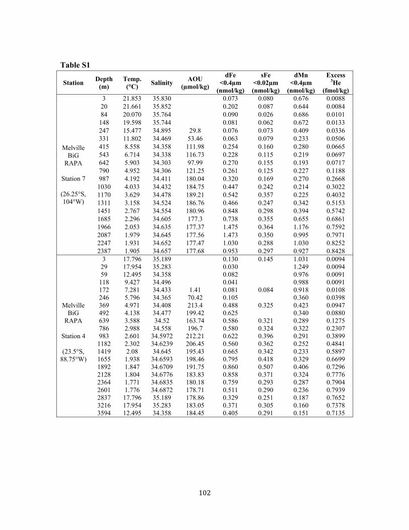
102
Table S1
Station Depth
(m) Temp. (°C)
Salinity AOU
(µmol/kg)
dFe <0.4µm
(nmol/kg)
sFe <0.02µm (nmol/kg)
dMn <0.4µm
(nmol/kg)
Excess 3He
(fmol/kg)
Melville BiG
RAPA
Station 7
(26.25°S, 104°W)
3 21.853 35.830 0.073 0.080 0.676 0.0088 20 21.661 35.852 0.202 0.087 0.644 0.0084 84 20.070 35.764 0.090 0.026 0.686 0.0101
148 19.598 35.744 0.081 0.062 0.672 0.0133 247 15.477 34.895 29.8 0.076 0.073 0.409 0.0336 331 11.802 34.469 53.46 0.063 0.079 0.233 0.0506 415 8.558 34.358 111.98 0.254 0.160 0.280 0.0665 543 6.714 34.338 116.73 0.228 0.115 0.219 0.0697 642 5.903 34.303 97.99 0.270 0.155 0.193 0.0717 790 4.952 34.306 121.25 0.261 0.125 0.227 0.1188 987 4.192 34.411 180.04 0.320 0.169 0.270 0.2668 1030 4.033 34.432 184.75 0.447 0.242 0.214 0.3022 1170 3.629 34.478 189.21 0.542 0.357 0.225 0.4032 1311 3.158 34.524 186.76 0.466 0.247 0.342 0.5153 1451 2.767 34.554 180.96 0.848 0.298 0.394 0.5742 1685 2.296 34.605 177.3 0.738 0.355 0.655 0.6861 1966 2.053 34.635 177.37 1.475 0.364 1.176 0.7592 2087 1.979 34.645 177.56 1.473 0.350 0.995 0.7971 2247 1.931 34.652 177.47 1.030 0.288 1.030 0.8252 2387 1.905 34.657 177.68 0.953 0.297 0.927 0.8428
Melville BiG
RAPA
Station 4
(23.5°S, 88.75°W)
3 17.796 35.189 0.130 0.145 1.031 0.0094 29 17.954 35.283 0.030 1.249 0.0094 59 12.495 34.358 0.082 0.976 0.0091
118 9.427 34.496 0.041 0.988 0.0091 172 7.281 34.433 1.41 0.081 0.084 0.918 0.0108 246 5.796 34.365 70.42 0.105 0.360 0.0398 369 4.971 34.408 213.4 0.488 0.325 0.423 0.0947 492 4.138 34.477 199.42 0.625 0.340 0.0880 639 3.588 34.52 163.74 0.586 0.321 0.289 0.1275 786 2.988 34.558 196.7 0.580 0.324 0.322 0.2307 983 2.601 34.5972 212.21 0.622 0.396 0.291 0.3899 1182 2.302 34.6239 206.45 0.560 0.362 0.252 0.4841 1419 2.08 34.645 195.43 0.665 0.342 0.233 0.5897 1655 1.938 34.6593 198.46 0.795 0.418 0.329 0.6699 1892 1.847 34.6709 191.75 0.860 0.507 0.406 0.7296 2128 1.804 34.6776 183.83 0.858 0.371 0.324 0.7776 2364 1.771 34.6835 180.18 0.759 0.293 0.287 0.7904 2601 1.776 34.6872 178.71 0.511 0.290 0.236 0.7939 2837 17.796 35.189 178.86 0.329 0.251 0.187 0.7652 3216 17.954 35.283 183.05 0.371 0.305 0.160 0.7378 3594 12.495 34.358 184.45 0.405 0.291 0.151 0.7135
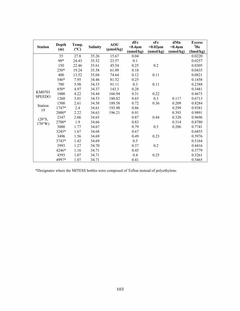
103
Station Depth
(m) Temp. (°C)
Salinity AOU
(µmol/kg)
dFe <0.4µm
(nmol/kg)
sFe <0.02µm (nmol/kg)
dMn <0.4µm
(nmol/kg)
Excess 3He
(fmol/kg)
KM0703 SPEEDO
Station
19
(20°S, 170°W)
35 27.8 35.26 15.67 0.04 0.0220 90* 24.43 35.52 23.57 0.1 0.0257 150 22.46 35.61 45.54 0.25 0.2 0.0305 250* 19.24 35.58 61.09 0.18 0.0435 400 13.52 35.04 74.64 0.12 0.11 0.0821 546* 7.95 34.46 81.52 0.25 0.1458 700 5.98 34.33 91.11 0.3 0.11 0.2388 850* 4.97 34.37 143.3 0.28 0.3481 1000 4.22 34.44 166.94 0.31 0.22 0.4673 1260 3.01 34.53 180.82 0.65 0.3 0.117 0.6713 1500 2.61 34.58 189.58 0.72 0.36 0.209 0.8284
1747* 2.4 34.61 193.98 0.86 0.299 0.9381 2000* 2.22 34.63 196.21 0.91 0.393 0.9891 2347 2.06 34.65 0.87 0.44 0.320 0.9696
2700* 1.9 34.66 0.83 0.314 0.8780 3000 1.77 34.67 0.79 0.3 0.206 0.7741
3245* 1.67 34.68 0.67 0.6855 3496 1.56 34.69 0.49 0.23 0.5976
3743* 1.42 34.69 0.5 0.5164 3993 1.27 34.70 0.37 0.2 0.4416
4246* 1.16 34.71 0.45 0.3779 4593 1.07 34.71 0.4 0.25 0.3261
4997* 1.07 34.71 0.41 0.3465
*Designates where the MITESS bottles were composed of Teflon instead of polyethylene.

104
References for Chapter 4 Supplementary Information
1 Beaulieu, S. E. InterRidge Global Database of Active Submarine Hydrothermal Vent
Fields: prepared for InterRidge, Version 2.0, <http://www.interridge.org/IRvents> (2010).
2 Blain, S., Bonnet, S. & Guieu, C. Dissolved iron distribution in the tropical and sub tropical South Eastern Pacific. Biogeosciences 5, 269-280 (2008).
3 Wu, J., Wells, M. L. & Rember, R. Dissolved iron anomaly in the deep tropical- subtropical Pacific: Evidence for long-range transport of hydrothermal iron. Geochimica et Cosmochimica Acta 75, 460-468 (2011).
4 Sunda, W. G. Control of dissolved iron concentrations in the world ocean, A comment. Marine Chemistry 57, 169-172 (1997).
5 Martin, J. H., Knauer, G. A., Karl, D. M. & Broenkow, W. W. VERTEX: carbon cycling in the northeast Pacific. Deep Sea Research Part A. Oceanographic Research Papers 34, 267-285 (1987).
6 Klinkhammer, G. & Hudson, A. Dispersal patterns for hydrothermal plumes in the South Pacific using manganese as a tracer. Earth and Planetary Science Letters 79, 241-249, doi:http://dx.doi.org/10.1016/0012-821X(86)90182-2 (1986).
7 Cowen, J. P., Massoth, G. J. & Feely, R. A. Scavenging rates of dissolved manganese in a hydrothermal vent plume. Deep Sea Research Part A. Oceanographic Research Papers 37, 1619-1637, doi:http://dx.doi.org/10.1016/0198-0149(90)90065-4 (1990).
8 Seewald, J. S. & Seyfried, W. E. The effect of temperature on metal mobility in subseafloor hydrothermal systems: constraints from basalt alteration experiments. Earth and Planetary Science Letters 101, 388-403 (1990).
9 Field, M. P. & Sherrell, R. M. Dissolved and particulate Fe in a hydrothermal plume at 9°45'N, East Pacific Rise: Slow Fe (II) oxidation kinetics in Pacific plumes. Geochimica et Cosmochimica Acta 64, 619-628 (2000).
10 James, R. H. & Elderfield, H. Dissolved and particulate trace metals in hydrothermal plumes at the Mid-Atlantic Ridge. Geophysical Research Letters 23, 3499-3502, doi:10.1029/96gl01588 (1996).
11 Pester, N. J., Rough, M., Ding, K. & Seyfried, W. E. A new Fe/Mn geothermometer for hydrothermal systems: Implications for high-salinity fluids at 13°N on the East Pacific Rise. Geochimica et Cosmochimica Acta 75, 7881-7892 (2011).
12 Bruland, K. W., Orians, K. J. & Cowen, J. P. Reactive trace metals in the stratified central North Pacific. Geochimica et Cosmochimica Acta 58, 3171-3182 (1994).
13 Cowen, J. P., Massoth, G. J. & Baker, E. T. Bacterial scavenging of Mn and Fe in a mid- to far-field hydrothermal particle plume. Nature 322, 169-171 (1986).
14 Lupton, J. E., Pyle, D. G., Jenkins, W. J., Greene, R. & Evans, L. Evidence for an

105
extensive hydrothermal plume in the Tonga-Fiji region of the South Pacific. Geochemistry, Geophysics, Geosystems 5, Q01003, doi:10.1029/2003gc000607 (2004).
15 Reid, J. L. On the total geostrophic circulation of the south Pacific Ocean: Flow patterns, tracers and transports. Progress in Oceanography 39, 263-352 (1997).
16 Lupton, J. E. & Craig, H. A major helium-3 source at 15S on the East Pacific Rise. Science 214, 13-18 (1981).
17 Stommel, H. Is the South Pacific helium-3 plume dynamically active? Earth and Planetary Science Letters 61, 63-67 (1982).
18 Ray, J. S. et al. Chronology and geochemistry of lavas from the Nazca Ridge and Easter Seamount Chain: an ~30 Myr hostpot record. Journal of Petrology 53, 1417-1448 (2012).
19 Kingsley, R. H., Blichert-Toft, J., Fontignie, D. & Schilling, J. G. Hafnium, neodymium, and strontium isotope and parent-daughter element systematics in basalts from the plume-ridge interaction system of the Salas y Gomez Seamount Chain and Easter Microplate. Geochem. Geophys. Geosyst. 8, 28, doi:Q04005 10.1029/2006gc001401 (2007).
20 Lupton, J. Hydrothermal helium plumes in the Pacific Ocean. J. Geophys. Res. 103, 15853-15868, doi:10.1029/98jc00146 (1998).
21 Reid, J. L. On the total geostrophic circulation of the South Pacific Ocean: Flow Patterns, tracers, and transports. Progress in Oceanography 16, 1-61 (1986).
22 Jenkins, W. J. in International WOCE Newsletter Vol. 23 6-11 (1996). 23 Boström, K., Peterson, M. N. A., Joensuu, O. & Fisher, D. E. Aluminum-poor
ferromanganoan sediments on active oceanic ridges. Journal of Geophysical Research 74, 3261-3270, doi:10.1029/JB074i012p03261 (1969).
24 Baker, E. T. et al. Hydrothermal venting along Earth's fastest spreading center: East Pacific Rise, 27.5°-32.3°S. Journal of Geophysical Research 107, doi:10.1029/2001JB000651 (2002).

106

107
Chapter 5
Assessment and comparison of Anopore™ and cross flow filtration methods for the determination of dissolved iron size fractionation into soluble/colloidal phases in seawater Submitted to Limnology & Oceanography: Methods
Fitzsimmons, J.N. and Boyle, E.A. in review. Assessment and comparison of Anopore™ and cross flow filtration methods for the determination of dissolved iron size fractionation into soluble/colloidal phases in seawater. Limnology & Oceanography: Methods.
Abstract The two most frequently used methods for determining the size fractionation of dissolved iron (dFe) in seawater, 0.02 µm Anopore membrane filtration and cross flow filtration using a 10 kDa regenerated cellulose filter, were evaluated and compared. Anopore filtration was found to produce consistent soluble Fe (sFe) concentrations in the filtrate after >1L of unfiltered seawater was filtered, indicating that clogging is not an issue for typical open ocean filtration volumes. Cross flow filtration (CFF) only achieved a 70-75% mass balance regardless of flow rate and seawater pre-conditioning. However, Fe losses were determined to arise only from the colloidal (not soluble) size fraction, and Fe loss was constrained to Fe clogging in/on the CFF membrane. Both Anopore and cross flow filtration methods were found to be equally robust for the size fractionation of dFe in seawater samples. Additionally, sFe arising from these two filtration methods were compared for the first time using seawater samples across multiple depths from the North Pacific and Atlantic Oceans. sFe separated by CFF was almost always lower than sFe separated by Anopore filtration, with the sFe in CFF/Anopore filtration averaging 74±21%. This sFe difference is attributed to a combination of the smaller effective pore size of the CFF system and the natural variability in the size distribution of dFe. Finally, the advantages and disadvantages of each method (pore size, filtration time, sample volume requirements, cost, experience necessary, etc.) are reviewed to offer users a suite of factors with which to choose their ideal filtration method.

108
Assessment and comparison of Anopore and cross flow filtration methods for the
determination of dissolved iron size fractionation into soluble/colloidal phases in
seawater
Jessica N. Fitzsimmons1* and Edward A. Boyle2
1. MIT/WHOI Joint Program in Chemical Oceanography, MIT E25-615, 45 Carleton St,
Cambridge, Massachusetts 02142, USA; [email protected]; +1-617-324-0283
2. Massachusetts Institute of Technology; MIT E25-619; 45 Carleton St, Cambridge,
Massachusetts 02142, USA; [email protected]; +1-617-253-3388
* Corresponding author
Keywords: iron, colloids, size fractionation, cross flow filtration, GEOTRACES
Running head: Anopore and CFF evaluation & comparison
Submitted to Limnology & Oceanography: Methods on 28 May 2013

109
Acknowledgements:
We thank Susan Curless, Craig Nosse, and Dave Karl for the opportunity to sail
on the HOT-231 cruise to Station ALOHA, as well as Simone Moos, Sam Wilson, and
the rest of the HOE-DYLAN V team for help with the MITESS Vanes at sea. We also
owe extreme gratitude to Gonzalo Carrasco for completing many of the filtrations on the
GEOTRACES cruises. We also thank Pete Morton, Randie Bundy, Chris Measures,
Mariko Hatta, and Ana Aguilar-Islas for their help collecting trace metal-clean seawater
samples on the GEOTRACES cruises and Jingfeng Wu for demonstrating his CFF
system. Finally, we thank Phoebe Lam and Carl Lamborg for useful discussions about
marine colloidal Fe and especially Mark Wells for early comments and discussions on
this manuscript. Excellent marine support was offered by the officers and crew of the
R/V Knorr and R/V Kilo Moana. J.N. Fitzsimmons was funded by a National Science
Foundation Graduate Research Fellowship (NSF Award #0645960), and this work was
funded by NSF grants OCE-0926204 and OCE-0926197 and the Center for Microbial
Oceanography: Research and Education (NSF-OIA Award #EF-0424599).

110
Abstract
The two most frequently used methods for determining the size fractionation of
dissolved iron (dFe) in seawater, 0.02 µm Anopore membrane filtration and cross flow
filtration using a 10 kDa regenerated cellulose filter, were evaluated and compared.
Anopore filtration was found to produce consistent soluble Fe (sFe) concentrations in the
filtrate after >1L of unfiltered seawater was filtered, indicating that clogging is not an
issue for typical open ocean filtration volumes. Cross flow filtration (CFF) only achieved
a 70-75% mass balance regardless of flow rate and seawater pre-conditioning. However,
Fe losses were determined to arise only from the colloidal (not soluble) size fraction, and
Fe loss was constrained to Fe clogging in/on the CFF membrane. Both Anopore and cross
flow filtration methods were found to be equally robust for the size fractionation of dFe
in seawater samples. Additionally, sFe arising from these two filtration methods were
compared for the first time using seawater samples across multiple depths from the North
Pacific and Atlantic Oceans. sFe separated by CFF was almost always lower than sFe
separated by Anopore filtration, with the sFe in CFF/Anopore filtration averaging
74±21%. This sFe difference is attributed to a combination of the smaller effective pore
size of the CFF system and the natural variability in the size distribution of dFe. Finally,
the advantages and disadvantages of each method (pore size, filtration time, sample
volume requirements, cost, experience necessary, etc.) are reviewed to offer users a suite
of factors with which to choose their ideal filtration method.

111
5.1 Introduction
Iron (Fe) is an essential micronutrient for photosynthesis and nitrogen fixation in
the ocean (MOREL et al., 2003), and because of its low seawater concentrations, Fe
controls primary production in a large portion of the global ocean (MARTIN and
FITZWATER, 1988; MOORE et al., 2009; MOORE et al., 2002). Fe(III) is the
thermodynamically favored redox state in the modern oxic ocean, yet inorganic Fe(III)
solubility is depressed to potentially biologically limiting concentrations of <0.1 nM in
seawater (KUMA et al., 1996; LIU and MILLERO, 1999). In natural seawater, however,
electrochemical methods indicate that >99.9% of dissolved Fe (dFe) is bound to organic
Fe-binding ligands that raise the solubility (RUE and BRULAND, 1995; VAN DEN BERG,
1995; WU and LUTHER, 1995). These organic ligands comprise a portion of the dissolved
organic carbon (DOC) pool but have a high binding capacity for Fe. As for DOC, we
know little about the chemical composition and structure of Fe-binding ligands (reviewed
in GLEDHILL and BUCK, 2012b); therefore we rely mostly on electrochemical
measurements of ligand concentration and binding strength to interpret how the
organically-bound nature of dFe impacts its biogeochemical cycling.
Because Fe is bound to organic ligands, however, we can use clues about the
characteristics of DOC to inform us about Fe. For instance, like marine DOC, oceanic
dFe is partitioned between both truly dissolved and colloidal species (WU et al., 2001). In
fact, it is thought that the organically-bound nature of dFe is what causes its observed size
partitioning (as opposed to its potential for inorganic hydrolysis) because other
hydrolyzable metals such as aluminum and titanium do not exhibit the same colloidal
presence in the open ocean (DAMMSHAUSER and CROOT, 2012). The size fractionation of
dFe has been investigated globally (Figure 1), and the colloidal contribution to dFe has
been found to range from 0% in the shallow South Atlantic and Southern Oceans
(BERGQUIST et al., 2007; BOYE et al., 2010) to ~90% in the surface ocean of the tropical
North Atlantic (FITZSIMMONS and BOYLE, in prep). Like size fractionated DOC pools
(GUO and SANTSCHI, 1997), the soluble, or low molecular weight, dFe fraction is thought
to be the more biologically labile fraction (CHEN and WANG, 2001), while the colloidal

112
(high molecular weight) dFe fraction is believed to be more easily removed to the
particulate phase via aggregation and/or adsorption onto particles (HONEYMAN and
SANTSCHI, 1989). Thus, the partitioning of dFe into these two size fractions may have a
major influence on the biogeochemical fate of dFe across the global ocean.
In these dFe size fractionation studies, the sizes of the soluble and colloidal Fe
define their "identity" in the ocean, and thus these size classifications drive our
interpretation of how the marine compounds behave. Ideally, soluble compounds are
those that are truly dissolved and cannot be differentiated from the surrounding solvent
molecules. Ideal colloids can also be defined: their lower size limit is the molecular
dimension at which the compound is large enough to establish a "surface" that separates
it from the rest of the solution, while their upper size limit is the dimension at which the
molecule is large enough for gravity to cause it to sink (WELLS, 2002). Thus, despite that
colloids fall operationally in the dissolved phase, "classical" colloidal material is
comprised of particles so small that they do not sink. Only when other compounds in
solution interact with these colloids at their surface (sorption/aggregation) might they
become large enough to sink, moving them into the particulate phase. This idealized
framework defines what we might consider to be bioavailable (generally, the soluble
phase), aggregating (the colloidal phase), and sinking (the particulate phase) fractions in
seawater.
Ultimately, however, our measurement of these size fractions are operationally
defined by the filtration techniques we use, and operational definitions don't necessarily
match classical definitions. Historically, marine colloids have been counted using a
combination of ultracentrifugation and transmission electron microscopy (WELLS and
GOLDBERG, 1991; 1992; 1993) or atomic force microscopy (SANTSCHI et al., 1998), as
well as light scattering methods including photon correlation spectroscopy (CHIN et al.,
1998) and nanoparticle tracking analysis (TARTARKIEWICZ et al., 2012). Separations of
the two size fractions for elemental quantification has been completed by a myriad of
techniques including ultrafiltration methods such as cross flow filtration (BUESSELER et
al., 1996; NISHIOKA et al., 2001) and Vivaspin ultracentrifugation (SCHLOSSER et al., in

113
press), small-pore size membrane filtration (WU et al., 2001), flow field flow
fractionation (BAALOUSHA et al., 2011; STOLPE et al., 2010), and various chromatography
techniques (BURGESS et al., 1996; CHIN and GSCHWEND, 1991). In the last decade, two
methods have emerged as the dominant systems used for size partitioning studies of
marine trace metals: cross flow filtration and small-pore sized membrane filtration using
Anopore™ filters. A growing number of studies have used one of these two methods to
quantify open ocean distributions of both soluble and colloidal Fe (Figure 1), yet the two
methods have never been compared on the same samples. Because there is no reason to
expect that the two systems should make the same operational separation of soluble and
colloidal dFe, it is difficult to make comparisons between literature studies using the two
methods, and thus our global understanding of dFe size partitioning is limited to regions
where only one operational definition has been used.
This study seeks to evaluate these two most common methods for collecting size
fractionated dissolved Fe samples and outline the advantages and disadvantages of each,
with the ultimate goal of offering a recommendation for when it might be ideal to use one
method over the other. We will also compare these two methods in order to begin to
resolve the literature divide between studies using the two methodologies.
5.2 Methods
5.2.1 Anopore™ filtration - Anopore™ filter membranes (Whatman) are
manufactured electrochemically by the anodic oxidation of aluminum and contain 0.02
µm pores composed of a single-layer honeycomb structure (FURNEAUX et al., 1989);
operationally defined "soluble Fe" (sFe<0.02 µm) passes through the pores, while
colloidal Fe is retained on the filter (0.02 µm<cFe<0.4 µm) and can be calculated as:
cFe = dFe - sFe (1)
where dFe is the iron passing through a 0.4 µm (or sometimes 0.2 µm) filter. Anopore™
filters are available as individual membranes (called Anodisc™ membranes) to be used
on a filtration rig, as in this study, or as syringe filters (called Anotop™ filters). In both

114
of these cases, a traditional filtration geometry is employed where fluid is pushed parallel
to (through) the membrane pores by differential pressure (Figure 2).
The methods we employed to collect soluble Fe samples through Anopore™
filtration are summarized in FITZSIMMONS and BOYLE (2012). Briefly, an untreated
47mm Anodisc™ 0.02 µm filter was loaded into a pre-cleaned PFA filter rig (Savillex)
for cleaning immediately before sample filtration (filters were not cleaned in advance of
the cruise because the acid treatment decomposes the alumina filter in the week after
cleaning). Each filter was rinsed with >50 mL of pH 1.5 trace metal-grade hydrochloric
acid (HCl), followed by a rinse of >50 mL of trace metal clean water. Finally, >50 mL of
seawater sample collected using trace metal clean techniques (see Sample Collection
methods below) was used to pre-condition the filter, followed by the soluble Fe filtrate
collection after a single sub-sample bottle rinse. Filtrates were collected in 30 mL HDPE
bottles pre-cleaned using the bottle cleaning procedures outlined in FITZSIMMONS and
BOYLE 2012, and typically two 30 mL bottles of sFe were filled for each seawater
sample. In total, only about 150 mL of seawater was needed to collect two 30 mL soluble
Fe samples.
5.2.2 Cross flow filtration (ultrafiltration) - Cross flow filtration (or
ultrafiltration) was completed using a Millipore Pellicon XL (PLCGC) filter made of
regenerated cellulose with a nominal molecular weight cutoff of 10 kDa (surface area of
50 cm2) and was pumped using a Cole Parmer Masterflex peristaltic pump fed with FEP
tubing. Feed solution flow rate was calibrated at 12 mL min-1, half of the maximum
recommended flow rate of 25 mL min-1 through the Pellicon XL filter. The feed solution
bottle, permeate bottle, and retentate bottle were held in an ISO 5 (formerly Class 100)
flow bench and were fed by Teflon tubing that was rinsed in pH 2 trace metal grade HCl
before contacting any new solutions. Permeate and retentate flow rates were calibrated to
be identical at 6 mL/min each. New Pellicon filters arrive pre-loaded with glycerine and
preservatives that were washed out in the lab before use at sea with several liters of trace
metal-clean water, followed by 4 L of 0.25N trace metal grade HCl to pre-clean the
system of trace metals. The low blank of the system after initial cleaning was verified by

115
ultrafiltering ~800 mL of 0.4 µm-filtered seawater that had been acidified to pH 2
through the system once, and then ultrafiltering the resulting permeate fraction again as a
"new" sample (see methods for treatment of new samples below). The two resulting
permeate solutions were then analyzed for their Fe concentration to ensure that the
solution ultafiltered twice ([Fe] = 0.31±0.04 nmol/kg, n=3) did not acquire additional
contaminant Fe after its first ultrafiltration ([Fe] = 0.29±0.02 nmol/kg, n=4); these two
solutions did not have statistically different Fe concentrations (p=0.61, Student's T-test,
two-tailed), and thus the CFF system was assumed to be clean.
At sea, cross flow filtration (CFF) was completed on 0.2 or 0.4 µm pre-filtered
seawater samples as quickly as possible after sample collection (see Sample Collection
methods below); previous experiments have shown that Fe sorbs to bottle walls on as
short a timescale as 3 hours, depending on the surface area-to-volume ratio of the bottle
(FITZSIMMONS and BOYLE, 2012). At the start of any day of CFF, 1 L of pH 1.5 trace
metal grade HCl was flushed through the system as an initial rinse, and flow rates were
calibrated. Before any new seawater was ultrafiltered (including between samples), 500
mL of pH 1.5 trace metal grade HCl was used to rinse the system. Then 300-350 mL of
pre-filtered sample seawater was used to condition the system before permeate and
retentate solutions were collected in 30 mL HDPE bottles after a single rinse each.
Relative permeate/retentate flow rates were also monitored after sample collection. The
system was stored in pH 2.5 trace metal grade HCl after flushing with the pH 1.5 HCl
rinse solution. About 500mL of seawater is needed to collect two 30 mL soluble Fe
samples through the CFF system.
After cross flow filtration, Fe concentrations can be measured in the permeate,
retentate, and total dissolved (feed solution) fractions. In this system, soluble Fe is equal
to the concentration of Fe in the permeate fraction (sFe < 10 kDa). Colloidal Fe is
operationally defined as the fraction between 10 kDa and the 0.2 or 0.4 µm filter used to
pre-filter the seawater samples. In addition to the colloidal Fe, the retentate fraction also
contains a portion of soluble Fe that is carried along in the aqueous carrier solution; this
is monitored using the concentration factor (CF; BUESSELER et al., 1996):

116
CF = initial sample volume
final retentate volume
permeate volume + retentate volume
retentate volume (2)
Thus, in our static CFF system where permeate and retentate volumes are calibrated to be
identical, the CF is equal to 2.0. Under ideal permeation conditions where the membrane
does not preferentially retain any soluble compounds (permeation coefficient = 1,
SCHLOSSER and CROOT, 2008), the amount of Fe in both permeate and retentate solutions
should be the same in a sample with no colloidal Fe. However, in solutions containing
colloidal Fe, the amount of Fe in the retentate solution must be corrected for the presence
of soluble Fe and the degree of concentration in order to calculate the true colloidal Fe
concentration:
cFe = Fe]retentate Fe]permeate
CF (3)
This method only involves Fe measurement in the permeate and retentate fractions (not
the total dissolved feed solution). Alternatively, the total dissolved feed solution Fe
concentration can be measured in place of the retentate fraction, and equation 1 can be
used to calculate colloidal Fe. Under 100% mass balance in the CFF system and ideal
membrane permeability, the colloidal Fe calculated using equations 1 and 3 should be
identical, and both have been used in the literature to define cFe concentrations (see the
Intercalibration section of the Assessment below for more information on choosing which
colloidal Fe equation to use). The recovery of Fe in a measured mass balance can be
calculated as:
Recovery = sFe + cFe
dFe100% (4)
where sFe is the concentration in the permeate solution, cFe is calculated using equation
3, and dFe is the concentration of Fe in the sample fed into the CFF system.
5.2.3 Sample collection - Samples used in this methods
assessment/intercalibration were collected and analyzed from four different cruises: the
U.S. GEOTRACES North Atlantic cruise Leg 1 in late October-November 2010 (Station
8 at 20.59°N, 22.0°W; Station 12 at the TENATSO time-series station at 17.0°N,
24.0°W), the HOT-231 cruise at Station ALOHA (22.75°N, 158.0°W) in the North
Pacific subtropical gyre in April 2011, the U.S. GEOTRACES North Atlantic cruise Leg

117
2 in November 2011 (Station 24 at the TENATSO time-series station), and the HOE-
DYLAN cruise led by the Center for Microbial Oceanography: Research and Education
program at Station ALOHA in July 2012. On both GEOTRACES cruises, trace metal-
clean seawater was collected using the U.S. GEOTRACES GO-FLO carousel (CUTTER
and BRULAND, 2012) and was pre-filtered using 0.2 µm Pall Acropak-200™ Supor®
capsule filters. Filtration protocols were identical to those described by FITZSIMMONS and
BOYLE (2012), except that the Acropak filters were pre-cleaned by soaking overnight in
filtered surface seawater that had been acidified to pH 2 using trace metal grade HCl,
after which they were flushed with 5L of unacidified surface seawater and stored empty
in the refrigerator until use. On the Station ALOHA cruises, trace metal-clean seawater
was collected using the MITESS Vanes system; MITESS stands for Moored In situ Trace
Element Sampler System and is an autonomous sampler whose exterior is made entirely
of metal-free ultra-high molecular weight polyethylene and contains an internal
electronics board and motor that are used to open and close a sample bottle for clean
seawater collection at a designated time at depth (BELL et al., 2002). The deployment of
MITESS in the Vanes mode, as well as the subsequent pre-filtration of the seawater using
0.4 µm Nuclepore™ polycarbonate track-etched filters, are described in FITZSIMMONS
and BOYLE (2012). It should be noted that in the Anopore Clog and Anopore Blank
experiments from the Station ALOHA cruises, seawater was not pre-filtered so that
potential clogging and contamination of the membrane was maximized. All samples were
acidified at sea to pH 2 with 6N trace metal grade HCl.
5.2.4 Fe analyses - At least one month after acidification, samples were analyzed
in triplicate for their Fe concentration by isotope dilution inductively-coupled plasma
mass spectrometry (ID-ICP-MS) with a hexapole collision cell IsoProbe multiple
collector-ICP-MS. The ID-ICP-MS method employs an 54Fe-spike and batch pre-
concentration with nitrilotriacetate resin (LEE et al., 2011). Procedure blanks during the
six analytical sessions ranged from 0.025-0.060 nmol/kg, and the detection limit (three
times the standard deviation of the procedure blanks for each analytical session) averaged
0.025 nmol/kg. Comprehensive lab analyses of SAFe D2 standard for dFe during the

118
period of these analyses averaged 0.99±0.03 nmol/kg (Bottle 242, ±1SD, n=8) and
0.92±0.01 nmol/kg (Bottle 446, ±1SD, n=8), in close agreement with the current
consensus value of 0.933±0.023 nmol/kg (updated May 2013;
http://www.geotraces.org/science/intercalibration).
5.3 Assessment
The two most commonly used filtration methods for measuring the size
fractionation of dFe in the open ocean were assessed in this study: traditional membrane
filtration using Anopore™ filters with a pore size of 0.02 µm and cross flow filtration
using a regenerated cellulose membrane with a 10 kDa molecular weight cutoff. These
two filtration mechanisms have inherently different filtration geometries (Figure 2),
where cross flow filtration is assumed to be a more "gentle" approach because of its
tangential filtration geometry that is less likely to clog the filter membrane and create
filtration artifacts in the resulting size distribution. Anopore™ filtration, in contrast, has a
traditional direct-flow geometry that is more likely to suffer filter fouling but requires
much lower sample volumes that can be filtered more rapidly. The experiments executed
on each of these, as well as the comparison between them, are discussed below.
5.3.1 Anopore™ filtration - Anopore™ filters were first used to examine the
marine distribution of dFe size fractions by WU et al. (2001), who modified this
microfiltration approach for open ocean dFe size partitioning after the Fe solubility
studies of KUMA and MILLERO (KUMA et al., 1996; LIU and MILLERO, 1999). In open
ocean studies, Anopore™ filtration has two significant advantages over other methods.
First, it requires very little seawater volume for filtration and allows for fast filtration
times when small volumes are filtered. Second, Anopore™ filters can be used on the
same filter rig that is used for the 0.2-0.4 µm pre-filtrations or in a small syringe and thus
are less cumbersome to set up and manage at sea than CFF systems. These two benefits
have allowed for sFe to be measured across several ocean basins in moderately high
spatial resolution using Anopore™ filtration (Figure 1).
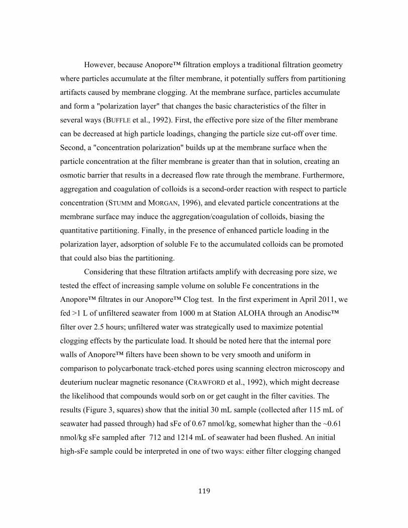
119
However, because Anopore™ filtration employs a traditional filtration geometry
where particles accumulate at the filter membrane, it potentially suffers from partitioning
artifacts caused by membrane clogging. At the membrane surface, particles accumulate
and form a "polarization layer" that changes the basic characteristics of the filter in
several ways (BUFFLE et al., 1992). First, the effective pore size of the filter membrane
can be decreased at high particle loadings, changing the particle size cut-off over time.
Second, a "concentration polarization" builds up at the membrane surface when the
particle concentration at the filter membrane is greater than that in solution, creating an
osmotic barrier that results in a decreased flow rate through the membrane. Furthermore,
aggregation and coagulation of colloids is a second-order reaction with respect to particle
concentration (STUMM and MORGAN, 1996), and elevated particle concentrations at the
membrane surface may induce the aggregation/coagulation of colloids, biasing the
quantitative partitioning. Finally, in the presence of enhanced particle loading in the
polarization layer, adsorption of soluble Fe to the accumulated colloids can be promoted
that could also bias the partitioning.
Considering that these filtration artifacts amplify with decreasing pore size, we
tested the effect of increasing sample volume on soluble Fe concentrations in the
Anopore™ filtrates in our Anopore™ Clog test. In the first experiment in April 2011, we
fed >1 L of unfiltered seawater from 1000 m at Station ALOHA through an Anodisc™
filter over 2.5 hours; unfiltered water was strategically used to maximize potential
clogging effects by the particulate load. It should be noted here that the internal pore
walls of Anopore™ filters have been shown to be very smooth and uniform in
comparison to polycarbonate track-etched pores using scanning electron microscopy and
deuterium nuclear magnetic resonance (CRAWFORD et al., 1992), which might decrease
the likelihood that compounds would sorb on or get caught in the filter cavities. The
results (Figure 3, squares) show that the initial 30 mL sample (collected after 115 mL of
seawater had passed through) had sFe of 0.67 nmol/kg, somewhat higher than the ~0.61
nmol/kg sFe sampled after 712 and 1214 mL of seawater had been flushed. An initial
high-sFe sample could be interpreted in one of two ways: either filter clogging changed

120
the measured dFe size partitioning by decreasing the effective pore size, or the Anodisc™
filter was not sufficiently cleaned by the time the first sample was collected, resulting in
an anomalously high dFe concentration in the first sample. Statistically, the first sFe
sample collected was significantly higher in concentration (p=0.025 and 0.019 when the
second and third sFe samples, respectively, were compared to the first sFe sample
collected: Student's T-test, two-tailed), but practically an external reproducibility of at
least 0.05 nmol/kg is common in marine Fe analyses (contributed by random sample
handling/bottle contamination and analytical uncertainties) and thus we repeated this
experiment to verify whether our initial enhanced sFe was a true filter artifact.
The Anopore Clog experiment was repeated at Station ALOHA in July 2012 with
unfiltered seawater collected from 800m. A similar total volume was filtered over 2
hours, but sub-samples were collected over smaller volume steps to increase the
resolution. In contrast to the initial experiment, the results (Figure 3, circles) showed no
decreasing sFe trend with increasing volume filtered, despite the initial sample being
collected earlier in the filtration process (90 mL seawater filtered) than in the April 2011
study (115 mL filtered). Thus, >1 L of unfiltered deep ocean seawater is insufficient to
noticeably reduce flow rate through the filter or cause significant changes in the effective
pore size of the Anodisc filter. This makes Anopore™ filtration a promising tool for
quantitative estimates of dFe partitioning in unfiltered deep-water samples, since modern
analytical techniques for trace metal concentration measurement require much less than 1
L volume for sample analysis (BILLER and BRULAND, 2012; LEE et al., 2011; MILNE et
al., 2010; OBATA et al., 1993). However, if larger volumes are required (for instance, for
metal isotopes or metal-binding ligand measurements) or samples are collected with
significantly higher particulate/colloidal loading (estuarine or coastal waters), this
experiment should be repeated to prove that filtration artifacts are not biasing the
measured partitioning. Pre-filtering the seawater samples with a coarse 0.2 or 0.4 µm
filter to first separate the dissolved from particulate phases is also recommended before
Anopore™ filtration to reduce particle loadings on the filter that could promote filtration
artifacts. However, the decision to pre-filter must be weighed against total filtration time,

121
which should be minimized because dFe sorbs significantly to bottle walls in as short a
time as three hours (dependent on bottle surface area to volume ratio, FITZSIMMONS and
BOYLE, 2012), and Fe speciation/partitioning can change in the <4 hours before filtration
(WEN et al., 1996).
Untreated Anopore™ membranes are a significant source of Fe to seawater
filtrates, so we investigated the degree of acid cleaning required to yield uncontaminated
samples in our Anopore Blank experiment. Replicate filters were rinsed with increasing
volumes of pH 1.5 HCl before processing unfiltered seawater from 800 m at Station
ALOHA. The findings show that any contaminant Fe is fully removed with as little as a
20 mL rinse with pH 1.5 HCl clean water (Figure 4), with rinse volumes up to 125 mL
having no substantial effect on the filtrate Fe concentrations (800m Station ALOHA
water sFe averaged 0.480±0.022 nmol/kg). It must be noted, however, that this acid
rinsing only removes potential contamination affecting the filtrate, and particulate Fe
contamination (that no longer leaches Fe into the filtrate) may still be present. In fact, a
closer inspection of Anopore filters by synchrotron Fe-XANES analysis (Brandy Toner,
personal communication) showed that an acid-rinsed filter maintained the same
particulate Fe inclusions as an unrinsed filter, resulting in a potentially significant Fe
background in any analysis of the colloidal Fe on the Anopore filter.
From the Anopore Blank experiment, there was also no indication that the
relatively strong pH 1.5 HCl rinse sufficiently attacked the aluminum oxide filters to the
point that they increased the pore size; no increases in sFe concentrations were observed
with as much as 130mL of acid rinse. However, longer storage under acidic conditions is
not recommended as it may still significantly change the effective pore size of the filter.
It is also important to note that the results of this blank evaluation highlight the excellent
sFe reproducibility over the 10 individual Anodisc™ filters, with multiple membranes
yielding very uniform sFe concentrations from the same seawater sample.
5.3.2 Cross flow filtration (ultrafiltration) - Cross flow filtration (CFF) has been
used for years to separate high- and low-molecular weight DOC phases (reviewed in
BUESSELER et al., 1996; GUO and SANTSCHI, 1997; WELLS, 2002). As shown in Figure 2,

122
the sample stream of a CFF system flows tangentially to the membrane pores, so flow of
soluble compounds through the pores into the permeate solution is driven by a pressure
difference across the membrane, and the colloids are continually swept into the retentate
solution. The major advantage of this filtration geometry is that concentration
polarization effects at the membrane surface are reduced because fluid shear strips
colloids away from the membrane surface, reducing the likelihood of clogging relative to
filtration systems of normal geometry. Furthermore, extraction efficiencies of CFF
systems are typically high, filtration of large volumes is relatively rapid compared to
other filtration systems, and the colloidal phase is concentrated in the retentate solution of
recirculating CFF systems for easy analysis (GUO and SANTSCHI, 1997), making this the
most popular method for separating colloid-sized fractions for direct analysis.
However, an analysis of the integrity of these CFF systems was made during the
"Colloid Cookout" in the mid-1990s (BUESSELER et al., 1996), where several groups used
their own pre-treatment and sample processing methods to size fractionate identical
seawater samples using identically rated CFF membranes (1kDa molecular weight size
cutoff, polysulfone, although different manufacturers' membranes were allowed). The
results showed two major patterns for DOC measurements. First, DOC blanks measured
in Q-water were highly variable, indicating that membrane material, system cleaning, and
sample handling protocols were critical. Second, the retention ratings used by various
manufacturers is not uniform, and even membranes rated for the same molecular weight
cutoff (1kDa in this case) do not have the same "effective pore sizes" (GUSTAFFSON et al.,
1996). For example, Amicon membranes retained the most colloidal material while those
manufactured by Membrex retained the least. A more rigorous discussion of "effective
pore sizes" is found in the next section on Intercalibration.
REITMEYER et al. (1996) reported the results of the aluminum (Al) and Fe
intercalibration from the Colloid Cookout and showed that most systems showed high
contamination for Al and significant (up to 80%) scavenging/loss of Fe by sorption to the
CFF system. Although there have been very few analyses of the size partitioning of
marine Al since, studies of Fe size partitioning using CFF have continued (as seen in

123
Figure 1), many with surprisingly little consideration for establishing Fe mass balance.
Notable exceptions to this are the Fe fertilization study by WELLS (2003), where mass
balance >90% was achieved (Filtron polysulfone membrane, 1 kDa size cutoff), and the
Fe solubility study by SCHLOSSER and CROOT (2008), where nearly 100% of the Fe was
recovered after a dilute hydrochloric acid rinse (Vivaflow polyethersulfone membrane,
10 kDa size cutoff).
For the cross flow filtration evaluation in this study, several steps were taken to
optimize the mass balance for Fe. First, regenerated cellulose was chosen as an
alternative membrane material to the typical polysulfone in hopes that it might be less
likely to sorb Fe compounds, and a small membrane surface area was selected despite the
slower flow rate in order to reduce the area to which Fe could sorb. The ultrafiltration
system was also run in static mode (where retentate is collected immediately after
filtration and is not sent back to the sample feed) instead of the more classical
recirculation mode (where retentate is recycled through the CFF system multiple times)
in order to avoid potential Fe contamination or sorptive losses as well as any potential
size partitioning changes during recycling. Finally, the CFF system was conditioned by
processing ~350mL of sample seawater before sample collection to minimize sorptive
losses of Fe to the system during sample collection.
The mass balance results from the Station ALOHA test are shown in Figure 5 and
indicate that, despite these efforts, only 75.0±2.5% of the Fe was recovered from the CFF
system. The 25% Fe lost might reflect sorption to the walls of the CFF system (tubing or
membrane walls), accumulation on the CFF membrane (i.e., concentration polarization),
or retention of colloidal fragments within the pores of the CFF membrane. To determine
which of these was the major Fe loss, we collected filtrate samples at multiple time points
during the processing of a large sample volume. We hypothesized that if Fe sorption to
the walls of the CFF system was responsible, then this effect would diminish with
prolonged filtration as the active sites became saturated with Fe, at which point the mass
balance should improve. The mass balances, however, did not significantly improve with
volume filtered (Figure 5a), indicating that the pre-conditioning of the system with ~350
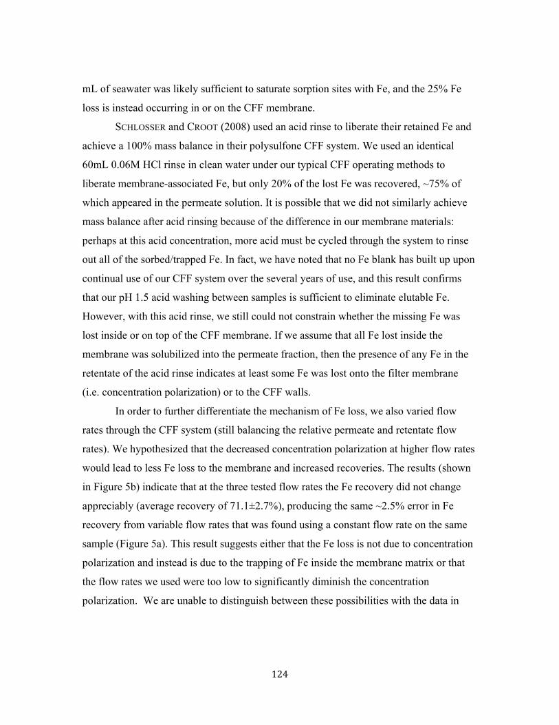
124
mL of seawater was likely sufficient to saturate sorption sites with Fe, and the 25% Fe
loss is instead occurring in or on the CFF membrane.
SCHLOSSER and CROOT (2008) used an acid rinse to liberate their retained Fe and
achieve a 100% mass balance in their polysulfone CFF system. We used an identical
60mL 0.06M HCl rinse in clean water under our typical CFF operating methods to
liberate membrane-associated Fe, but only 20% of the lost Fe was recovered, ~75% of
which appeared in the permeate solution. It is possible that we did not similarly achieve
mass balance after acid rinsing because of the difference in our membrane materials:
perhaps at this acid concentration, more acid must be cycled through the system to rinse
out all of the sorbed/trapped Fe. In fact, we have noted that no Fe blank has built up upon
continual use of our CFF system over the several years of use, and this result confirms
that our pH 1.5 acid washing between samples is sufficient to eliminate elutable Fe.
However, with this acid rinse, we still could not constrain whether the missing Fe was
lost inside or on top of the CFF membrane. If we assume that all Fe lost inside the
membrane was solubilized into the permeate fraction, then the presence of any Fe in the
retentate of the acid rinse indicates at least some Fe was lost onto the filter membrane
(i.e. concentration polarization) or to the CFF walls.
In order to further differentiate the mechanism of Fe loss, we also varied flow
rates through the CFF system (still balancing the relative permeate and retentate flow
rates). We hypothesized that the decreased concentration polarization at higher flow rates
would lead to less Fe loss to the membrane and increased recoveries. The results (shown
in Figure 5b) indicate that at the three tested flow rates the Fe recovery did not change
appreciably (average recovery of 71.1±2.7%), producing the same ~2.5% error in Fe
recovery from variable flow rates that was found using a constant flow rate on the same
sample (Figure 5a). This result suggests either that the Fe loss is not due to concentration
polarization and instead is due to the trapping of Fe inside the membrane matrix or that
the flow rates we used were too low to significantly diminish the concentration
polarization. We are unable to distinguish between these possibilities with the data in

125
hand. Regardless, the findings show that flow rates between 12-25 mL/min are
acceptable, but all result in a 25-30% Fe loss to the CFF membrane.
The most vexing aspect of this Fe loss is that it is not clear which Fe fraction is
lost to the membrane. Although it would make sense for the lost Fe to be comprised of
colloidal species (i.e., colloidal Fe becomes entwined in the membrane), the Fe loss may
also reflect soluble Fe species sorbing strongly to a limited number of membrane surface
sites or to the trapped colloidal species themselves. The identity of the lost Fe fraction is
discussed further in the Intercalibration section.
5.3.3 Comparison of Anopore filtration with CFF - When interpreting the effect
of soluble/colloidal Fe partitioning on the biogeochemistry of marine dFe, it is often
assumed that the "classical" definitions of soluble and colloidal Fe phases apply (as
discussed in the Introduction), yet the measured partitioning between the two size
fractions is actually operationally defined by the filter type used, which can be very
different from the "classical" description. As Figure 1 shows, marine studies of dFe size
fractionation have used two filtration systems (CFF and Anopore™ filtration) with
several nominal pore size cutoffs, and thus our definition of the "colloidal contribution"
to dFe partitioning is actually quite fluid depending on which study you are reading.
Additionally, a comparison of data among studies (e.g., to calculate scavenging rates
along a water mass trajectory) is impossible unless the same filter types are used. Only
one study has attempted a comparison between the two methodologies. An endnote in the
WU et al. (2001) study reported a comparison of cFe separated by Anopore™ and CFF
filtration and found them to be identical within error. It must be noted, however, that the
cFe concentrations discussed were only ~0.1 nM, too low a concentration to detect
significant changes between filtration methods, especially given the reported 0.03nM
external error, and thus this was not a very robust comparison effort.
A key issue for a comparison of colloid separation methods is the assessment of
the accuracy, precision, and reproducibility of the nominal pore size cutoffs both within a
given filter and among replicate filters. The anodizing voltage of the electrochemical
fabrication method for Anopore™ membranes generates a very reproducible pore size,

126
even at small dimensions, and a high pore density, both of which are desirable for
synthetic filters. The pore size distribution of Anopore™ filters was measured by atomic
force microscopy to cover a small range of only 0.0119-0.0278 µm, averaging
0.0188±0.0035 µm over 108 replicates (BOWEN et al., 1996), demonstrating that the
nominal 0.02 µm pore size defined by Whatman is both accurate and precise. We did not
confirm these dimensions in this study, but it is reasonable to expect similar
specifications for the membranes used here.
Most CFF filters, in contrast, are depth filters that contain a wider range of
effective pore sizes. As a consequence, in some cases retention of compounds smaller
than the nominal molecular weight size cutoff occurs, while in other cases compounds
larger than the size cutoff pass through to the permeate. The nominal molecular weight
cutoff is defined by the manufacturers using standard compounds of a known molecular
weight, and they report the percentage of those molecular weight standards that are
retained by the filter (for example, a rating requirement might be that 90% of 10 kDa
compounds are retained by a 10 kDa membrane). The variability in manufacturers'
ratings, tested under different conditions with different standards, is what largely
contributed to the variable permeation behavior of the filters used in the Colloid Cookout
(BUESSELER et al., 1996). Moreover, the standard compounds chosen for the membrane
ratings are optimized for biomedical or industrial water treatment applications (the most
frequent users of CFF membranes) and thus are frequently proteins or polysaccharides;
there are no equivalent standards for dilute solutions composed of natural compounds. In
any filtration, molecular shape, electrostatics, and other physicochemical characteristics
of the compounds in solution allow for intermolecular or membrane interactions that can
change the retention characteristics of different molecules, so at best CFF can only be
nominally defined, and individual filters (especially those from separate fabrication
batches) may act differently than others that are identically rated.
Acknowledging the inherent differences in membranes, we compared the soluble
Fe filtered through Anodisc™ membranes with the sFe filtered through our 10 kDa CFF
membrane (results shown in Figure 6). Assuming a common conversion of 1kDa ≈ 1nm

127
and that molecular weight increases nonlinearly much faster than molecular size, the
nominal molecular weight cutoff of an Anopore filter would be at least 20kDa (and
perhaps much greater), overall larger than the nominal 10kDa size cutoff of our CFF.
Thus, we expected the sFe collected through the Anodisc™ filter to be greater than that
filtered through the 10 kDa CFF membrane, and this was true at every location we
intercalibrated. A study by CHEN et al. (2004) reported that the actual molecular weight
cutoff of Anopore™ filters determined using standard molecules was approximately 3
kDa. The results of our comparison, however, do not support this assessment; our results
suggest instead that the pore size of Anopore™ filters are at least greater than the 10kDa
nominal molecular weight cutoff of the CFF filter membrane with which we compared.
The initial comparison from Station ALOHA in the North Pacific Ocean and a
North Atlantic station near the Cape Verde Islands indicated that CFF sFe concentrations
were 68±15% of that measured in the Anodisc™ filtrate (Figure 6). Much of this
difference in sFe concentrations can be attributed to a difference in the pore sizes of the
two filtration systems. However, the 44-84% spread in sFe ratio between
CFF/Anopore™ is also a function of the natural variations in the size distribution of dFe
compounds, which allows the difference between the effective pore sizes of the two filter
types to be more apparent at some locations than at others. Additionally, the composition
of these colloids plays a role as well; for instance, if some of the colloids are comprised
of loosely associated gels, they could fall apart during Anopore filtration and be observed
as sFe, while these same compounds may stay composed during the gentler CFF filtration
and be measured as colloidal. So although a 68±15% correction factor may be a
reasonable first order approximation for reconciling CFF and Anopore datasets, it is clear
that more comparisons in different water masses are needed to refine this correction
factor.
Two separate samplings at the TENATSO time-series station a year apart (Nov.
2010 and Dec. 2011) provided an opportunity to assess the reproducibility of these
methods and the consistency of their differences (Figure 7). The CFF sFe was measured
at six identical depths in both years, and the concentrations were statistically identical at

128
all depths except 235m (p-values of the Student's t-test are mostly >0.05, Figure 7a). This
finding provided evidence that there were no significant natural changes in Fe
concentration or partitioning at TENATSO during the two years, making it a good
comparison site. Additionally, this proved that the (same) CFF membrane provides a
stable platform for size fractioning colloidal materials, despite the inherent caveats
mentioned above, and thus CFF produces dFe partitioning data of high integrity.
The sFe concentrations measured in Anopore filtrates were substantially higher at
almost all depths than measured in CFF permeates in 2010 and 2011 (Figure 7b). The
three exceptions were 185m, 2750m, and 3200m: p-values = 0.87, 0.31, and 0.23
respectively using a Student's T-test, two-tailed). A treatment of the implications of this
data comparison on the natural size partitioning of dFe in the North Atlantic will be made
elsewhere (Fitzsimmons et al. in prep). The average CFF/Anopore™ sFe ratio was
75±22% for the 23 TENATSO samples, bringing the total average CFF/Anopore™ sFe
ratio to 74±21% for all 28 samples analyzed in this intercalibration, similar to the
68±15% findings at Station ALOHA.
There was close agreement between the sFe concentrations from both filter types
in the deepest 4 samples between 2750-3500m, and this indicates that there were
negligible contributions of colloidal Fe in the 10kDa-0.02µm size fraction at these
depths. This agreement in sFe would be impossible if there was a significant sorptive loss
of soluble Fe to the CFF membrane. This finding then indicates that the 20-30% Fe loss
to the CFF system (described in the Cross Flow Filtration section above) is due to
retention of colloidal Fe, and accordingly it is reasonable to interpret permeate Fe from
this CFF membrane as equivalent to sFe for our comparison with Anopore filtrates.
Ideally, CFF systems should attain 100% recovery of Fe in the permeate and
retentate solutions; however, the results of this study and all other studies using CFF to
measure dFe fractionation in seawater (Figure 1) have shown that this is nearly
impossible without lengthy and aggressive treatments (such as post-filtration acid
leaching that renders the remaining colloidal material useless for further
characterization). To escape the consequences of poor mass balance, we proved in our

129
CFF system that the Fe recovery was very reproducible for a single sample and that all of
the retained Fe was colloidal. This has implications for the ideal equation to use to
calculate true cFe concentrations by CFF. As discussed in the methods section, the cFe
can be calculated using the permeate and retentate concentrations (Equation 3) or using
the permeate and total dissolved (feed solution) fractions (Equation 1). Any difference
between the cFe calculated by these two methods depends entirely on the CFF recovery.
An example of the resulting range in cFe concentrations using the two equations is shown
in Table 1 as a function of recovery. We recommend the use of Equation 1 for our CFF
system because it attributes all of the lost Fe to the colloidal fraction, which we
confirmed for our system. Equation 3, in contrast, neglects any Fe that is lost to the CFF
system, which can falsely bias the % sFe high when recovery is low. For other CFF
systems where it is not clear which fraction of Fe is being lost or where it is expected that
permeation is non-ideal, Equation 3 might be a better estimate, although every effort
should be made to constrain the phase of Fe loss or the permeation coefficient.
5.4 Discussion
Generally, it was found that both CFF and Anopore™ filtration methods
reproducibly size fractionated dFe concentrations in open ocean seawaters, but the two
methods produced different soluble Fe concentrations from the same seawater sample,
likely due to differences in their effective pore sizes. However, the size separations
defined here are valid only for the conditions outlined in this study, and we do not know
whether the integrity of these methods for marine dFe persists for other metals.
Furthermore, the dFe separations by the two systems are quite arbitrary, since they cannot
be verified by any independent method, and the use of standard compounds of known
molecular weight is not appropriate because they do not match seawater compounds,
characteristics, or conditions. Despite these overwhelming limitations, the operational
size separations explored here provide a useful insight into the broader issues of trace
metal biogeochemistry and are the state-of-the-art methods to this day. In this section, we
will review the advantages and disadvantages for each method and offer a framework

130
with which the best method for a given scientific question and sampling plan can be
chosen.
First and foremost, as discussed in the Introduction, it would be ideal to match the
"operational" definition of soluble/colloidal material to the "classical" definition that we
use to interpret the oceanographic significance of the observed partitioning. In this case,
CFF would be the better filtration method because it has a smaller pore size; very tiny
colloids can pass through an Anopore™ filter and be measured as truly soluble, distorting
oceanographic interpretations of the resulting partitioning data.
However, there are basic sampling restrictions that might preclude the use of CFF
and favor Anopore filtration. For instance, if only small seawater volumes are available,
Anopore™ filtration is ideal because CFF requires at least 300mL of seawater to
condition the filter, increasing the seawater volume requirement to ~500mL to generate
just 60mL of sFe sample. In contrast, Anopore™ filters only require ~150mL of seawater
to condition and collect the same sized sFe sample. If these small sFe samples are
adequate (for concentration analyses, for example), Anopore™ filtration is also faster
than CFF and thus better suited for high-throughput work, such as that undertaken by the
GEOTRACES program. Alternatively, if larger sample volumes (1L or more) are
required, CFF is the only practical method because it takes too long to filter a large
volume sample through an Anopore™ filter, and it is not clear that the effective pore size
would remain unchanged after a >1L sample was flushed through a single Anopore™
membrane. Additionally, unfiltered samples cannot be processed through CFF systems
because the larger particles have the potential to clog the pumped system, raising the
back-pressure and causing the pressure fittings to fail; thus, if pre-filtering the samples is
inconvenient, Anopore™ filtration would be the better filtration choice.
There are also several advantages and disadvantages to each filtration system for
applications of dissolved phase size partitioning studies beyond Fe. For instance, the
recovery issues with CFF might become limiting for size partitioning of particle-reactive
elements such as thorium and protactinium (as observed in, for example, DAI and
BENITEZ-NELSON, 2001), and thus low-surface area Anopore™ filtration might be

131
preferable in these cases. Furthermore, certain chemical characterization methods might
require the colloidal material to be in the aqueous phase, in which a recirculating CFF
system would be ideal, whereas others might require the colloidal material to be dried on
a membrane, in which case Anopore™ filtration might be best.
Finally, several miscellaneous factors can influence the two filtration setups such
that one technique might be favored over the other. The first of these factors is cost: CFF
methods have a high initial cost but are reusable, reducing spending over the long term,
while Anopore™ filters are individually less expensive but accumulate expense quickly
when many samples need to be filtered because each filter can only be used once.
Second, the physical footprint of these two methods can be quite different, depending on
the extent of automation. Anopore™ filtration can be completed in a syringe filter that
has no physical footprint and negligible weight, while cross flow filtration requires a
peristaltic pump, clean tubing, and a clean working area. However, filtration through
Anopore filters requires a high level of expertise, while CFF is semi-automated and thus
is much more straightforward for a person trained in trace metal techniques. CFF can be
run unattended for some periods of time while it cleans or conditions itself, which may be
beneficial for multi-tasking users, while Anopore™ filtration largely requires constant
attention.
In summary, there is no straightforward recommendation for a single filtration
system, as there are many reasons why either filtration system might be preferable
(summarized in Table 2). The major conclusion from this study, however, is that either
filtration method produces reproducible data and is scientifically robust, and thus the
choice between the two filtration methods is truly a matter of the question being asked,
technical requirements in the field sampling, and/or convenience.
5.5 Conclusions and Recommendations
Our work aimed to evaluate the popular Anopore™ and cross flow filtration
techniques for colloidal fractionation of seawater Fe samples. Anopore™ filtration has
the advantage of small seawater volume requirements and rapid/convenient filtration for

132
small volumes, but also has the potential for filtration artifacts as a result of filter fouling.
The Anopore™ experiments showed, however, that even after >1L of unfiltered
oligotophic seawater had been processed, the sFe collected in the filtrate was constant,
indicating that there was not sufficient filter clogging to change the effective pore size of
the filter over the volume studied. Our findings show that pre-cleaning the filter with
≥20mL of pH 1.5 HCl in clean water is sufficient to eliminate measurable filter-derived
Fe blanks. We also recommend that when possible all samples be pre-filtered (0.2-0.4
µm) to reduce the potential for filter fouling, as long as it does not unduly delay the
Anopore filtration process, given that Fe loss to container walls and size
partitioning/speciation changes can occur on short timescales.
Our cross flow filtration system was designed to minimize Fe sorption by having
a low CFF filter surface area, running without recirculation, and conditioning with
seawater before the size fractionated filtrate was collected. Nonetheless, 20-30% of the
Fe was consistently lost to the CFF system, despite altering sample volumes and flow
rates. A major portion of this Fe was not released from the membrane even with a small
volume of 0.06N hydrochloric acid. However, results from laboratory testing, and more
importantly the close agreement between sFe concentrations in the permeate and
Anopore filtrates in near-bottom waters, implies that the vast majority of the CFF loss is
due to retention of colloidal matter rather than simple sorption of soluble Fe species. We
therefore feel it is appropriate to assign the permeate Fe as equivalent to sFe with this
CFF system. We recommend calculation of cFe concentration as the difference between
the measured dFe and sFe concentrations, instead of using the retentate Fe concentration
that neglects the lost Fe phase, although we can recommend this only for users of our
same hardware and sample handling procedures. In any situation where sFe can be lost or
permeation is non-ideal, an analysis of Fe in the retentate solution is required. In general,
we note that low CFF system blanks and proper seawater conditioning of the filter before
sample collection are critical to obtaining reproducible sFe samples by CFF, and we
recommend quantification of Fe recovery on any CFF used in trace metal oceanography.

133
A comparison of sFe from 28 depths across the Atlantic and Pacific Oceans
showed that sFe collected using CFF was 74±21% of that collected using Anopore™
filtration, a result reflecting the larger effective pore size of Anopore™ filters as well as
the natural variability of the size distribution of dFe across the two oceans. This
CFF/Anopore™ sFe ratio can be used to preliminarily combine the bodies of literature on
dFe size partitioning using the two methods that up until now have not been comparable
because of the unknown differences in effective pore size between the two filter types.
Finally, we concluded that both filtration methods provide robust and
reproducible size fractionation of sFe from dFe in seawater, each with distinct advantages
and disadvantages. These were reviewed, and when deciding between the filtration
systems each user should consider the full suite of factors that differentiate them
including pore size, filtration time, sample volume requirements, cost, and user
experience required. With this final note, we emphasize that careful trace metal clean
techniques were used in the generation of all data in this study, and our results
demonstrated that reliably low filter blanks and rapid filtration processing (FITZSIMMONS
and BOYLE, 2012) were critical to the reproducibility of the data.
134
References for Chapter 5 Baalousha, M., B. Stolpe, and J. R. Lead. 2011. Flow field-flow fractionation for the analysis and
characterization of natural colloids and manufactured nanoparticles in environmental systems: A critical review. Journal of Chromatography A 1218: 4078-4103.
Bell, J., J. Betts, and E. Boyle. 2002. MITESS: a moored in situ trace element serial sampler for deep-sea moorings. Deep-Sea Research Part I-Oceanographic Research Papers 49: 2103-2118.
Bergquist, B. A., J. Wu, and E. A. Boyle. 2007. Variability in oceanic dissolved iron is dominated by the colloidal fraction. Geochimica et Cosmochimica Acta 71: 2960-2974.
Biller, D. V., and K. W. Bruland. 2012. Analysis of Mn, Fe, Co, Ni, Cu, Zn, Cd, and Pb in seawater using the Nobias-chelate PA1 resin and magnetic sector inductively coupled plasma mass spectrometry (ICP-MS). Marine Chemistry 130-131: 12-20.
Bowen, W. R., N. Hilal, R. W. Lovitt, and P. M. Williams. 1996. Atomic force microscope studies of membranes: Surface pore structures of Cyclopore and Anopore membranes. Journal of Membrane Science 110: 233-238.
Boye, M. and others 2010. Significant portion of dissolved organic Fe complexes in fact is Fe colloids. Marine Chemistry 122: 20-27.
Boye, M., J. Nishioka, P. L. Croot, P. Laan, K. R. Timmermans, and H. J. W. De Baar. 2005. Major deviations of iron complexation during 22 days of a mesoscale iron enrichment in the open Southern Ocean. Marine Chemistry 96: 257-271.
Buesseler, K. O. and others 1996. An intercomparison of cross-flow filtration techniques used for sampling marine colloids: Overview and organic carbon results. Marine Chemistry 55: 1-31.
Buffle, J., D. Perret, and M. Newman. 1992. The use of filtration and ultrafiltration for size fractionation of aquatic particles, colloids, and macromolecules, p. 171-230. In J. Buffle and H. P. van Leeuwen [eds.], Environmental Particles. IUPAC Series on Environmental Analytical and Physical Chemistry. Lewis Publishers.
Burgess, R. M., R. A. Mckinney, W. A. Brown, and J. G. Quinn. 1996. Isolation of marine sediment colloids and associated polychlorinated biphenyls: An evaluation of ultrafiltration and reverse-phase chromatography. Environmental Science and Technology 30: 1923-1932.
Chen, M., W.-X. Wang, and L. Guo. 2004. Phase partitioning and solubility of iron in natural seawater controlled by dissolved organic matter. Global Biogeochemical Cycles 18: GB4013.
Chen, M., and W. X. Wang. 2001. Bioavailability of natural colloid-bound iron to marine plankton: Influences of colloidal size and aging. Limnology and Oceanography 46: 1956-1967.
Chever, F. and others 2010. Physical speciation of iron in the Atlantic sector of the Southern Ocean along a transect from the subtropical domain to the Weddell Sea Gyre. J. Geophys. Res. 115: C10059.
Chin, W.-C., M. V. Orellana, and P. Verdugo. 1998. Spontaneous assembly of marine dissolved

135
organic matter into polymer gels. Nature 391: 568-572. Chin, Y.-P., and P. M. Gschwend. 1991. The abundance, distribution, and configuration of
porewater organic colloids in recent sediments. Geochimica et Cosmochimica Acta 55: 1309-1317.
Crawford, G. P. and others 1992. Characterization of the cylindrical cavities of Anopore and Nuclepore membranes. The Journal of Chemical Physics 96: 7788-7796.
Cutter, G. A., and K. W. Bruland. 2012. Rapid and noncontaminating sampling system for trace elements in a global ocean surveys. Limnology & Oceanography: Methods 10: 425-436.
Dai, M., and C. R. Benitez-Nelson. 2001. Colloidal organic carbon and 234Th in the Gulf of Maine. Marine Chemistry 74: 181-196.
Dammshauser, A., and P. L. Croot. 2012. Low colloidal associations of aluminium and titanium in surface waters of the tropical Atlantic. Geochimica et Cosmochimica Acta 96: 304-318.
Fitzsimmons, J. N., and E. A. Boyle. 2012. An intercalibration between the GEOTRACES GO- FLO and the MITESS/Vanes sampling systems for dissolved iron concentration analyses (and a closer look at adsorption effects). Limnology & Oceanography: Methods 10: 437-450.
---. in prep. Dynamic soluble and colloidal iron phases both control dissolved iron variability in the tropical North Atlantic Ocean. Geochimica et Cosmochimica Acta.
Furneaux, R. C., W. R. Rigby, and A. P. Davidson. 1989. The formation of controlled-porosity membranes from anodically oxidized aluminum. Nature 337: 147-149.
Gledhill, M., and K. N. Buck. 2012. The organic complexation of iron in the marine environment: a review. Frontiers in Microbiology 3: 69.
Guo, L., and P. H. Santschi. 1997. Composition and cycling of colloids in marine environments. Rev. Geophys. 35: 17-40.
Gustafsson, Ö., K. O. Buesseler, and P. M. Gschwend. 1996. On the integrity of cross-flow filtration for collecting marine organic colloids. Marine Chemistry 55: 93-111.
Honeyman, B. D., and P. H. Santschi. 1989. A Brownian-pumping model for oceanic trace metal scavenging: Evidence from Th isotopes. Journal of Marine Research 47: 951-992.
Kuma, K., J. Nishioka, and K. Matsunaga. 1996. Controls on iron(III) hydroxide solubility in seawater: The influence of pH and natural organic chelators. Limnology and Oceanography 41: 396-407.
Lee, J.-M., E. A. Boyle, Y. Echegoyen-Sanz, J. N. Fitzsimmons, R. Zhang, and R. A. Kayser. 2011. Analysis of trace metals (Cu, Cd, Pb, and Fe) in seawater using single batch Nitrilotriacetate resin extraction and isotope dilution inductively coupled plasma mass spectrometry. Analytica Chimica Acta 686: 93-101.
Liu, X., and F. J. Millero. 1999. The solubility of iron hydroxide in sodium chloride solutions. Geochimica et Cosmochimica Acta 63: 3487-3497.
Martin, J. H., and S. E. Fitzwater. 1988. Iron deficiency limits phytoplankton growth in the north- east Pacific subarctic. Nature 331: 341-343.
Milne, A., W. Landing, M. Bizimis, and P. Morton. 2010. Determination of Mn, Fe, Co, Ni, Cu,

136
Zn, Cd and Pb in seawater using high resolution magnetic sector inductively coupled mass spectrometry (HR-ICP-MS). Analytica Chimica Acta 665: 200-207.
Moore, C. M. and others 2009. Large-scale distribution of Atlantic nitrogen fixation controlled by iron availability. Nature Geosci 2: 867-871.
Moore, J. K., S. C. Doney, D. M. Glover, and I. Y. Fung. 2002. Iron cycling and nutrient- limitation patterns in surface waters of the World Ocean. Deep Sea Research Part II: Topical Studies in Oceanography 49: 463-507.
Morel, F. M. M., A. J. Milligan, and M. A. Saito. 2003. Marine Bioinorganic Chemistry: The Role of Trace Metals in the Oceanic Cycles of Major Nutrients, p. 113-143. In K. K. Turekian and H. D. Holland [eds.], Treatise On Geochemistry. Elsevier Science Ltd.
Nishioka, J., H. Obata, and D. Tsumune. 2013. Evidence of an extensive spread of hydrothermal dissolved iron in the Indian Ocean. Earth and Planetary Science Letters 361: 26-33.
Nishioka, J. and others 2005. Changes in the concentration of iron in different size fractions during an iron enrichment experiment in the open Southern Ocean. Marine Chemistry 95: 51-63.
---. 2003. Size-fractionated iron distributions and iron-limitation processes in the subarctic NW Pacific. Geophysical Research Letters 30.
Nishioka, J., S. Takeda, C. S. Wong, and W. K. Johnson. 2001. Size-fractionated iron concentrations in the northeast Pacific Ocean: distribution of soluble and small colloidal iron. Marine Chemistry 74: 157-179.
Obata, H., H. Karatani, and E. Nakayama. 1993. Automated determination of iron in seawater by chelating resin concentration and chemiluminescence. Analytical Chemistry 65: 1524-1528.
Reitmeyer, R., R. T. Powell, W. M. Landing, and C. I. Measures. 1996. Colloidal aluminum and iron in seawater: An intercomparison between various cross-flow ultrafiltration systems. Marine Chemistry 55: 75-91.
Rue, E. L., and K. W. Bruland. 1995. Complexation of iron(III) by natural organic ligands in the Central North Pacific as determined by a new competitive ligand equilibration/adsorptive cathodic stripping voltammetric method. Marine Chemistry 50: 117-138.
Santschi, P. H., E. Balnois, K. J. Wilkinson, J. Zhang, and J. Buffle. 1998. Fibrillar polysaccharides in marine macromolecular organic matter as imaged by atomic force microscopy and trasnission electron microscopy. Limnology and Oceanography 43: 896-908.
Schlosser, C., and P. L. Croot. 2008. Application of cross-flow filtration for determining the solubility of iron species in open ocean seawater. Limnology and Oceanography-Methods 6: 630-642.
Schlosser, C., P. Streu, and P. L. Croot. in press. Vivaspin ultrafiltration: A new approach for high resolution measurements of colloidal and soluble iron species. Limnology & Oceanography: Methods.
Stolpe, B., L. Guo, A. M. Shiller, and M. Hassellöv. 2010. Size and composition of colloidal

137
organic matter and trace elements in the Mississippi River, Pearl River and the northern Gulf of Mexico, as characterized by flow field-flow fractionation. Marine Chemistry 118: 119-128.
Stumm, W., and J. J. Morgan. 1996. Aquatic Chemistry: Chemical Equilibria and Rates in Natural Waters, 3rd ed. John Wiley & Sons.
Tatarkiewicz, J., R. A. Reynolds, and D. Stramski. 2012. Counting and sizing of colloidal particles in the Arctic Ocean. Ocean Sciences Meeting.
Thuróczy, C. E. and others 2010. Speciation of Fe in the Eastern North Atlantic Ocean. Deep Sea Research Part I: Oceanographic Research Papers 57: 1444-1453.
Ussher, S. J., E. P. Achterberg, G. Sarthou, P. Laan, H. J. W. De Baar, and P. J. Worsfold. 2010. Distribution of size fractionated dissolved iron in the Canary Basin. Marine Environmental Research 70: 46-55.
Van Den Berg, C. M. G. 1995. Evidence for organic complexation of iron in seawater. Marine Chemistry 50: 139-157.
Wells, M. L. 2002. Marine Colloids and Trace Metals, p. 367-404. In A. H. Dennis and C. A. Carlson [eds.], Biogeochemistry of Marine Dissolved Organic Matter. Academic Press.
---. 2003. The level of iron enrichment required to initiate diatom blooms in HNLC waters. Marine Chemistry 82: 101-114.
Wells, M. L., and E. D. Goldberg. 1991. Occurrence of small colloids in sea water. Nature 353: 342-344.
---. 1992. Marine submicron particles. Marine Chemistry 40: 5-18. ---. 1993. Colloid aggregation in seawater. Marine Chemistry 41: 353-358. Wen, L.-S., K.-T. Jiann, and P. H. Santschi. 2006. Physicochemical speciation of bioactive trace
metals (Cd, Cu, Fe, Ni) in the oligotrophic South China Sea. Marine Chemistry 101: 104-129.
Wen, L.-S., M. C. Stordal, D. Tang, G. A. Gill, and P. H. Santschi. 1996. An ultraclean cross- flow ultrafiltration technique for the study of trace metal phase speciation in seawater. Marine Chemistry 55: 129-152.
Wu, J., E. A. Boyle, W. G. Sunda, and L. Wen. 2001. Soluble and colloidal iron in the oligotrophic North Atlantic and North Pacific. Science 293: 847-849.
Wu, J., and G. W. Luther. 1995. Complexation of Fe(III) by natural organic ligands in the Northwest Atlantic Ocean by a competitive ligand equilibration method and a kinetic approach. Marine Chemistry 50: 159-177.

138
Figure and Tables for Chapter 5:
Calculated using Eq (1) Calculated using Eq (3)
Recovery Depth
(m) dFe sFe
Retentate Fe
cFe % sFe % cFe cFe % sFe % cFe
53% 1099 1.022 0.356 0.704 0.666 34.8% 65.2% 0.182 66.2% 33.8%
61% 2998 0.466 0.231 0.329 0.234 49.7% 50.3% 0.051 81.9% 18.1%
70% 1999 0.728 0.331 0.656 0.396 45.6% 54.4% 0.170 66.2% 33.8%
72% 71 0.218 0.112 0.203 0.109 51.4% 48.6% 0.045 71.1% 28.9%
Table 1: Comparison of cFe concentrations and dFe partitioning percentages calculated using two different calculations (Equation 1 and Equation 3). Recovery is calculated using Equation 4. All Fe concentrations are in nmol/kg. Data are taken from the 2012 U.S. GEOTRACES cruise at TENATSO (Station 24) using CFF. When recovery is low, the difference in % cFe between the two methods is significant.
Anopore™ filtration is recommended when: CFF is recommended when:
Only a small seawater volume is available
Only unfiltered seawater is available
Easy filtration setup is desired
Rapid filtering times (for small volumes) is desired
Colloidal material is desired in solid phase
Highly sorptive elements are of interest
"Ideal" soluble/colloidal definitions are desired (CFF has smallest pore size)
Large sFe samples are required
Colloidal material is desired in the aqueous phase/preconcentrated
An automated filtration system is desired, or little attention can be paid to filtration
Table 2: Summarized recommendations for when to use Anopore™ or CFF to generate size fractionated samples of dissolved elements.

139
Figure 1: A map reviewing the locations of all of the studies of dFe size partitioning in the open ocean. Studies using Anopore™ filtration are shown as diamonds, while studies using cross flow filtration (CFF) are shown as squares. The numbers indicate the publications where discussions of these studies can be found: 1Bergquist et al. (2007) using Anotop™ filters; 2Boye et al. (2005), Boye et al. (2010), and Nishioka et al. (2005) using a 200 kDa CFF membrane; 3Chever et al. (2010) using Anotop™ filters, 4Fitzsimmons and Boyle (in prep) using Anodisc™ filters; 5Fitzsimmons et al. (in prep) using 10 kDa CFF membranes; 6Fitzsimmons et al. (in prep) using Anodisc™ and 10 kDa CFF membranes (18 total stations); 7Nishioka et al. (2001) using a 200 kDa CFF membrane; 8Nishioka et al. (2003) using a 200 kDa CFF membrane; 9Nishioka et al. (2013) using a 1000 kDa CFF membrane; 10Thurόczy et al. (2010) using a 1000 kDa CFF membrane; 11Ussher et al. (2010) using Anotop™ filters (10 total stations); 12Wells (2003) using a 1kDa CFF membrane; 13Wen et al. (2006) using a 1 kDa CFF membrane; 14Wu et al. (2001) using Anotop™ filters.

140
Figure 2: Anopore™ and cross flow filtration (CFF) geometries. The filter membrane is shown in black, assuming an equal pore size in the two filtration types (note that CFF actually has a smaller pore size than Anopore™ membranes in this comparison). Anopore™ filtration uses a traditional filtration geometry where the solution flows parallel (through) the membrane pores; particulate material accumulates at the membrane surface. CFF uses a tangential geometry where the solution enters perpendicular to the membrane pores; soluble material flows through the pores into the permeate, while both soluble and colloidal material exit perpendicular to the pores in the retentate solution.

141
Figure 3: Results from the Anopore™ clog experiment, where soluble Fe that had passed through a single Anopore™ filter was measured as a function of the total volume of unfiltered seawater passed through the filter. Seawater is from Station ALOHA at 1000m (April 2011) and 800m (July 2012). Error bars represent one standard deviation of replicate analyses of the same sample.
Figure 4: Results from the Anopore™ blank experiment, where soluble Fe was measured after being passed through a different Anopore™ filter, after the filter with variable acid (pH 1.5 HCl) rinse volumes. Seawater is from Station ALOHA at 800m (July 2012). Error bars represent one standard deviation of replicate analyses of the same sample.
0.0
0.1
0.2
0.3
0.4
0.5
0.6
0.7
0 500 1000 1500
Soluble Fe (nmol/kg)
Total unfiltered seawater filtered through
an Anopore membrane (mL)
4/2011: 1000m
7/2012: 800m
0.0
0.2
0.4
0.6
0 50 100 150
Soluble Fe (nmol/kg)
Volume pH 1.5 HCl used to rinse
Anopore filter (mL)

142
Figure 5: Cross flow filtration mass balance assessments made at Station ALOHA (a) at 1000m in 4/2011 and (b) at 800m in 7/2012. (a) Mass balance examined as a function of seawater volume flushed through the filter. (b) Mass balance examined as a function of CFF flow rate. Error bars represent 1σ standard deviations on replicate analyses of the same sample. Colloidal Fe concentrations are calculated using Equation 3, and the italicized percentages shown indicate the Fe recovery calculated with Equation 4.
Figure 6: Comparison of the soluble Fe collected using cross flow filtration (CFF; black bars) and Anopore™ filtration (white bars). Seawater samples were collected at Station ALOHA on the HOT-231 cruise (April 2011) and on the GEOTRACES (GT) cruise in 2010 at Station 8 at several depths. Error bars represent 1σ standard deviations on replicate analyses of the same sample. The italicized percentages shown indicate the percent of sFe collected using Anopore™ filtration that is collected using CFF.
0.0
0.1
0.2
0.3
0.4
0.5
0.6
0.7
0.8
0.9
12 17.5 25
Fe (nmol/kg)
CFF sample feed flow rate (mL/min)
0.0
0.2
0.4
0.6
0.8
1.0
1.2
0 L 0.4 L 1.4 L 2.4 L
Fe (nmol/kg)
Total seawater volume flushed through CFF
dFe
sFe
cFe
sFe + cFe
(a) (b)
78%73%
75%69%
75% 70%
0.0
0.1
0.2
0.3
0.4
0.5
0.6
0.7
0.8
0.9
1.0
HOT 2011
1000m
GT 2010‐08
90m (DCM)
GT 2010‐08
235m
GT 2010‐08
665m
GT 2010‐08
1200m
[sFe] nmol/kg
CFF filtered
Anopore filtered
68%
44%
84%
65%
78%
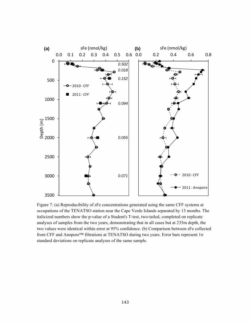
143
Figure 7: (a) Reproducibility of sFe concentrations generated using the same CFF systems at occupations of the TENATSO station near the Cape Verde Islands separated by 13 months. The italicized numbers show the p-value of a Student's T-test, two-tailed, completed on replicate analyses of samples from the two years, demonstrating that in all cases but at 235m depth, the two values were identical within error at 95% confidence. (b) Comparison between sFe collected from CFF and Anopore™ filtrations at TENATSO during two years. Error bars represent 1σ standard deviations on replicate analyses of the same sample.
0.0 0.2 0.4 0.6 0.8
sFe (nmol/kg)
2010 ‐CFF
2011 ‐Anopore
0
500
1000
1500
2000
2500
3000
3500
0.0 0.1 0.2 0.3 0.4 0.5 0.6
Depth (m)
sFe (nmol/kg)
2010 ‐CFF
2011 ‐CFF
(a) (b)
0.502
0.018
0.152
0.094
0.055
0.071

144

145
Chapter 6
Both soluble and colloidal iron phases control dissolved iron variability in the tropical North Atlantic Ocean Submitted to Geochimica et Cosmochimica Acta
Fitzsimmons, J.N. and Boyle, E.A. in review. Both soluble and colloidal iron phases control dissolved iron variability in the tropical North Atlantic Ocean. Geochimica et Cosmochimica Acta. Abstract The size fractionation of dissolved iron (dFe, <0.4 μm) between soluble (sFe, <0.02 μm) and colloidal (0.02 μm<cFe<0.4 μm) phases was investigated at seven stations in the tropical North Atlantic Ocean, and the results are compared to the dFe size partitioning study of Bergquist et al. (2007) in the same region. Downwind of the North African dust plumes, cFe comprised 80±7% of the surface dFe pool at six stations, supporting the hypothesis that atmospherically-derived Fe is maintained in the colloidal size fraction. In the deep chlorophyll maximum, colloidal Fe had minimum concentrations or was completely absent, suggesting that cFe was either preferentially taken up by microbes and/or scavenged/aggregrated at these depths. sFe was the dominant phase at remineralization depths both in the subtropical gyre-like stations (76% sFe; [sFe] = 0.42±0.03 nmol/kg) and in the oxygen minimum zone (56% sFe; [sFe] = 0.65±0.03 nmol/kg); only at remineralization depths of stations with intermediate oxygen concentrations (100-110 µmol/kg) did colloidal Fe dominate (contributing 58% of dFe). North Atlantic Deep Water (NADW) had a sFe concentration of 0.34±0.05 nmol/kg, and in the deepest samples composed of a NADW/Antarctic Bottom Water mixture where the bottom water may have attained a ~0.1 nmol/kg hydrothermal Fe input during transit past the Mid-Atlantic Ridge, sFe did not increase coincidentally with dFe, indicating that any potential hydrothermal contribution was comprised of colloidal Fe only. In general, the results of this study counter the previous hypothesis of BERGQUIST et al. (2007) that the colloidal Fe fraction predominately controls dFe variability and instead suggest that both soluble and colloidal Fe are variable and contribute to the observed dFe distribution throughout this region. To reconcile the results of both studies, we suggest one of two partitioning mechanisms persists: (1) the nearly constant sFe concentration with depth found in previous studies represents a "steady state" dFe partitioning pattern due to Fe exchange between the soluble and colloidal size fractions, over which regional Fe sources and unique Fe partitioning mechanisms are overlain, or (2), the partitioning of Fe-binding ligands between the two size fractions is variable in the open ocean and directly controls dFe partitioning.

146
Both soluble and colloidal iron phases control dissolved iron variability in the
tropical North Atlantic Ocean
Jessica N. Fitzsimmonsa* and Edward A. Boyleb
a. MIT/WHOI Joint Program in Chemical Oceanography, MIT E25-615, 45 Carleton St,
Cambridge, MA 02142, USA; [email protected]; +1-617-324-0283
b. Massachusetts Institute of Technology; MIT E25-619; 45 Carleton St, Cambridge, MA 02142,
USA; [email protected]; +1-617-253-3388
* Corresponding author

147
Abstract:
The size fractionation of dissolved iron (dFe, <0.4 μm) between soluble (sFe,
<0.02 μm) and colloidal (0.02 μm<cFe<0.4 μm) phases was investigated at seven stations
in the tropical North Atlantic Ocean, and the results are compared to the dFe size
partitioning study of Bergquist et al. (2007) in the same region. Downwind of the North
African dust plumes, cFe comprised 80±7% of the surface dFe pool at six stations,
supporting the hypothesis that atmospherically-derived Fe is maintained in the colloidal
size fraction. In the deep chlorophyll maximum, colloidal Fe had minimum
concentrations or was completely absent, suggesting that cFe was either preferentially
taken up by microbes and/or scavenged/aggregrated at these depths. sFe was the
dominant phase at remineralization depths both in the subtropical gyre-like stations (76%
sFe; [sFe] = 0.42±0.03 nmol/kg) and in the oxygen minimum zone (56% sFe; [sFe] =
0.65±0.03 nmol/kg); only at remineralization depths of stations with intermediate oxygen
concentrations (100-110 µmol/kg) did colloidal Fe dominate (contributing 58% of dFe).
North Atlantic Deep Water (NADW) had a sFe concentration of 0.34±0.05 nmol/kg, and
in the deepest samples composed of a NADW/Antarctic Bottom Water mixture where the
bottom water may have attained a ~0.1 nmol/kg hydrothermal Fe input during transit past
the Mid-Atlantic Ridge, sFe did not increase coincidentally with dFe, indicating that any
potential hydrothermal contribution was comprised of colloidal Fe only. In general, the
results of this study counter the previous hypothesis of BERGQUIST et al. (2007) that the
colloidal Fe fraction predominately controls dFe variability and instead suggest that both
soluble and colloidal Fe are variable and contribute to the observed dFe distribution
throughout this region. To reconcile the results of both studies, we suggest one of two
partitioning mechanisms persists: (1) the nearly constant sFe concentration with depth
found in previous studies represents a "steady state" dFe partitioning pattern due to Fe
exchange between the soluble and colloidal size fractions, over which regional Fe sources
and unique Fe partitioning mechanisms are overlain, or (2), the partitioning of Fe-binding
ligands between the two size fractions is variable in the open ocean and directly controls
dFe partitioning.

148
Acknowledgements:
We thank Ruifeng Zhang for his help with the dissolved iron measurements as well as
Richard Kayser for his efforts maintaining and deploying the MITESS units. We would
also like to thank Phoebe Lam, Mark Wells, and Carl Lamborg for useful discussions
about marine colloidal Fe. Excellent marine support was offered by the officers and crew
of the R/V Oceanus. Finally, we thank Reiner Schlitzer and his group for sharing the
Ocean Data View graphics program. J.N. Fitzsimmons was funded by a National Science
Foundation Graduate Research Fellowship (NSF Award #0645960), and this work was
funded by NSF OCE-07020278 and the Center for Microbial Oceanography: Research
and Education (NSF-OIA Award #EF-0424599).
149
6.1 Introduction
For decades our understanding of the limitation of marine primary productivity by
the micronutrient iron (Fe, MARTIN and FITZWATER, 1988; MOREL et al., 2003) has been
hampered by our scant knowledge of the global distribution of Fe. With the advent of the
international GEOTRACES program, however, global transects of dissolved Fe (dFe) are
being collected, and this information will improve our understanding of the sources and
sinks of this trace element that has the potential regulate ocean productivity and climate.
This maturation of our knowledge will shift our research focus from establishing the
distribution of these metals throughout the oceans to determining the processes that lead
to those distributions. The transfer of metals from the dissolved pool into the sinking
particulate pool ("scavenging”) is in particular need of illumination. Several metal loss
mechanisms are encompassed by the term "scavenging," including adsorption/surface
complexation, precipitation, and aggregation into successively larger particles, as well as
microbiological uptake.
Colloids, the focus of this study, are an understudied physico-chemical group of
materials defined as particles so small that they are operationally included in the
dissolved size fraction, but they retain their status as particles since they are physically
distinct from the fluid. Because of their diminutive size, colloids remain suspended until
they aggregate to a size experiencing significant gravitational settling. Colloids thus serve
the important role of transporting material between the dissolved and particulate phases,
thereby coupling two of the aforementioned "scavenging" processes: a rapid initial
adsorption of metal onto colloidal/particulate material in solution, followed by a slow
aggregation of the colloids into particulate material of filterable size (the Brownian-
pumping model, HONEYMAN and SANTSCHI, 1989). Additionally, while suspended,
colloidal material can mediate chemical processes that further alter the bulk seawater
solution including sorption of solutes, ligand exchange, surface redox reactions, and
photochemical reactions.
For Fe, a hybrid-type element demonstrating both nutrient-type profile shapes as
well as scavenged-type surface maxima and concentration loss along global thermohaline

150
circulation (BRULAND and LOHAN, 2003), scavenging plays an important role in its
marine biogeochemical cycle. Under oxic conditions, Fe(III) has a very low inorganic
solubility in seawater (MILLERO, 1998), and most of the dissolved Fe found in the ocean
is complexed by natural organic ligands that sustain dFe concentrations above the <0.1
nM solubility observed in UV-irradiated seawater (KUMA et al., 1996; LIU and MILLERO,
2002); excess Fe above ligand concentrations is quickly transformed into the particulate
phase. Early studies of marine colloidal Fe distributions indicated that a large fraction,
often 30-70% and as high as 80%, of the dissolved Fe in the ocean exists in the colloidal
size fraction (WU et al., 2001), which was operationally defined as the dFe between
0.02µm and 0.4µm (cFe, "colloidal Fe", and "Fe colloids" will be used interchangeably in
this paper; soluble Fe, sFe, is the Fe passing through a 0.02µm filter; sFe + cFe = dFe).
Thus, a significant portion of the dissolved Fe that many imagine to be bound to
siderophore-like organic ligands in seawater is actually composed of tiny particles that
may have a different chemical composition and behavior than truly dissolved (soluble)
Fe.
Using transmission electron microscopy imaging and energy dispersive
spectroscopy composition analyses, it was concluded that colloidal Fe is organically
bound in the open ocean (WELLS and GOLDBERG, 1991; WELLS and GOLDBERG, 1992).
This is consistent with electrochemical measurements of Fe ligand concentration and
binding strength indicating that >99% of marine dFe, which contains the colloidal
fraction, is bound by organic Fe-binding ligands (GLEDHILL and BUCK, 2012; RUE and
BRULAND, 1995). However, due to their differences in size and chemical composition,
soluble and colloidal Fe have unique behaviors that affect the Fe biogeochemical cycle in
two ways. First, because soluble and colloidal Fe undergo different chemical
transformations (sFe experiencing sorption, while cFe experiences aggregation), the two
phases may have an inherently different residence times. This size partitioning could
impact, for instance, whether new dFe sources escape abiotic scavenging long enough to
be taken up by microbes, and thus modelers must understand this size distribution of dFe
in order to best predict downstream dFe concentrations.

151
Second, and even more important to studies of micronutrient limitation, soluble
and colloidal Fe may not be equally bioavailable. Laboratory experiments have
conclusively shown that inorganic Fe colloids (here named nanoparticles) as small as 6-
50 Fe atoms per colloid are not directly bioavailable to diatoms (RICH and MOREL, 1990).
Since most marine colloidal Fe is thought to be organically bound, however, incubations
using natural, organic-dominated colloidal Fe assemblages were executed to reflect more
realistic marine compounds, and the results indicated that natural colloidal Fe is only
indirectly bioavailable, requiring first a dissociation from the colloid into the soluble
phase before being taken into the cell; the smaller soluble Fe fraction, in contrast, was
always taken up much faster and thus thought to be preferred (CHEN and WANG, 2001).
An assessment of the bioavailability of natural colloidal Fe is essential in order to ensure
that nutrient limitation models are not underestimating the geographic extent of Fe
limitation simply because they parameterize the bioavailable Fe pool as dFe instead of
sFe.
BERGQUIST et al. (2007) indicated that much of the dFe variability in the tropical
and subtropical Atlantic Ocean is due to a dynamic colloidal fraction, while the soluble
Fe concentration remained relatively constant with depth. This highlighted the
importance of studying dFe size partitioning, as it suggested that the cycling of the two
size fractions is distinct. Here, we have measured dFe size partitioning at several more
stations across the tropical North Atlantic, reaching further along the southwestern
boundary of the subtropical gyre and east into the heart of the oxygen minimum zone
(OMZ). We find that both the soluble and colloidal fractions determine the dissolved Fe
variability in this broader region, instead of just the colloidal fraction as in BERGQUIST et
al.'s study. In this paper we will establish the similarities and differences between the
BERGQUIST et al. study and the present one, and we will attempt to establish the major
facets of dFe size partitioning and its contribution to Fe biogeochemistry in the tropical
North Atlantic.

152
6.2 Sampling & Analysis Methodology
In August 2008, trace metal clean seawater samples were collected aboard the R/V
Oceanus (cruise OC449-2 sailing from Bridgetown, Barbados, to Mindelo, Cape Verde
Islands) in the tropical North Atlantic (see cruise track in Figure 1). A review of the
sample collection and Fe analysis protocols for this cruise can be found in FITZSIMMONS
et al. (2013, Chapter 3), which discusses the major processes controlling the dFe
distribution along this track. Briefly, the Moored In situ Trace Element Serial Samplers
(MITESS, BELL et al., 2002) were used to collected profile seawater samples in the
"Vane" mode using deployment procedures described in FITZSIMMONS and BOYLE
(2012). Near-surface samples (~5 m depth) were collected using the Automated Trace
Element ("ATE") sampler, which is a single MITESS unit deployed manually off the side
of the ship using a plastic-coated line. Seawater was vacuum-filtered (0.5 atm.) through
0.4μm Nuclepore™ filters on a Savillex™ fluorocarbon filter rig directly into acid-
cleaned 30 mL HDPE sub-sampling bottles after two rinses. MITESS Vane sample
collection produced dFe concentrations indistinguishable from those collected by the U.S.
GEOTRACES GO-FLO carousel system (FITZSIMMONS and BOYLE, 2012).
To collect sFe samples, a 0.02 μm Anodisc filter was pre-cleaned on a Teflon
filter rig first with >100 mL pH 1.5 HCl (distilled 4x in a Vycor still and tested for trace
metal purity), followed by >100 mL trace metal-clean distilled water, and finally ~50mL
unfiltered seawater sample, after which unfiltered seawater was passed through the clean
Anodisc filter and collected as sFe in acid-cleaned 30 mL HDPE sub-sampling bottles
after one bottle rinse. Samples were acidified at sea to pH 2, and at least six months after
acidification they were analyzed in triplicate for their Fe content by isotope dilution
inductively-coupled plasma mass spectrometry (ID-ICP-MS) on a hexapole collision cell
IsoProbe multiple collector-ICP-MS. The ID-ICP-MS method employs an 54Fe-spike and
batch pre-concentration with nitrilotriacetate resin (LEE et al., 2011). Comprehensive lab
analyses of SAFe D2 standard for dFe during the period of these analyses averaged
0.95±0.05 nmol/kg (Bottle 33, ±1SD, n=38) and 0.90±0.02 nmol/kg (Bottle 446, ±1SD,

153
n=10), which agree well with the current consensus value of 0.933±0.032 nmol/kg
(consensus update: May 2013; www.geotraces.org/science/intercalibration).
6.3 Results and Discussion
6.3.1 Surface distribution - The surface ocean distributions of dFe and sFe as a
function of longitude are shown in Figure 2. As discussed in FITZSIMMONS et al. (2013,
Chapter 3), dFe in the tropical North Atlantic exhibited concentration maxima at the
surface, in accordance with expectations of high aerosol Fe deposition downwind of
North African deserts along 10-20°N (MAHOWALD et al., 2005). dFe was highest in the
west and lower in the east, despite closer proximity to the African dust source; this likely
reflects a combination of spatially variable factors including dust source/solubility, dust
deposition patterns (seasonal), biological uptake of metals in the surface ocean, and
mixed layer depth. NOAA HYSPLIT backwards trajectories calculated using the GDAS
Meteorological data indicate that the air masses over all of the stations in Figure 2
originated in NW Africa/Europe, except for Stations 9 & 11 (37-41°W), which had South
American sources. It is reasonable to assume that over the 1.5-5 months residence time of
dFe in surface waters of the tropical North Atlantic (BERGQUIST and BOYLE, 2006), most
of the dFe is derived from North African desert sources.
What is most striking from Figure 2, however, is that soluble Fe concentrations
remained low across the transect (at all but one station) despite a factor-of-two variability
in dFe, with sFe ≤ 0.2nmol/kg at most stations. Thus, most of the elevated surface dFe
was partitioned into the colloidal Fe size fraction (%cFe averaged 80±7%, with Station 6
removed). This reinforces the hypothesis that atmospherically derived Fe is preferentially
maintained in the colloidal pool, which was suggested by WU et al. (2001) using data
near Bermuda and Hawaii and corroborated by BERGQUIST et al. (2007) in the tropical
North Atlantic. It is possible that both soluble and colloidal Fe were released by dust and
then only sFe was preferentially taken up by microorganisms, leaving the observed
majority of aerosol dFe in the colloidal phase. However, the preferential release of dust-
derived Fe into the colloidal, not soluble, size fraction is supported experimentally by

154
direct leaching of aerosols from diverse oceanic regions in filtered seawater with natural
organic Fe-binding ligand assemblages (AGUILAR-ISLAS et al., 2010), although one can
be concerned whether excess Fe binding ligands are saturated during these dust leaching
experiments, which would generate colloidal Fe oxyhydroxides and bias the resulting size
partitioning. Dust-derived Fe colloids could be composed of organically bound Fe-ligand
complexes that fall in the colloidal size fraction, colloidal-sized dust particles, and/or
inorganic Fe-colloids formed in situ during the dust solubilization process.
In contrast at the northernmost station of our transect (Station 6: 20°N, 45°W),
sFe had a much higher concentration of 0.48 nmol/kg, which exceeded the cFe of 0.33
nmol/kg (59% of the dFe was sFe). If dust is assumed to partition into the colloidal
fraction, then the decreased cFe contribution at Station 6 could indicate that dust
deposition at this northernmost station was reduced. This hypothesis would be supported
by a majority partitioning into the soluble phase in the surface ocean of other low-dust
regions such as the South Atlantic (BERGQUIST et al., 2007), subarctic North Pacific
(NISHIOKA et al., 2003), and the Southern Ocean (BOYE et al., 2010; CHEVER et al.,
2010). However, the dFe concentration at Station 6 was relatively high (0.8 nmol/kg) and
thus requires a recent Fe input. While we cannot exclude that the Station 6 sFe sample
might have been contaminated, we also know that dFe is stabilized by organic ligands,
and thus the size partitioning of surface Fe-binding ligands at any individual location may
be directly controlling the observed partitioning of surface dFe. Only one study has
recorded the size partitioning of organic Fe-binding ligands in the tropical North Atlantic
(CULLEN et al., 2006), with surface water samples taken at one station in the tropical
North Atlantic (3.5°N, 44.5°W) and one station in the North Atlantic subtropical gyre
(36.1°N, 65°W). At the tropical North Atlantic station, 50-62% of the dissolved ligands
fell into the soluble fraction, while in the subtropical gyre station, 72-100% of the
dissolved ligands were soluble. That study demonstrates that ligand partitioning is
spatially variable and supports the premise that significant ligand partitioning into the
soluble fraction might be predicted in the subtropical gyre at our Station 6, which lies
closer to the gyre center (with a high surface salinity >37.5 and depressed mixed layer,

155
chlorophyll max, and isopycnals) than any of the other stations sampled on our cruise
track. More studies of the size partitioning of Fe-binding ligands across the global ocean
would be useful for assessing the impact of the ligand size distribution on the solubility
and size partitioning of dFe, especially when comparing high- and low-dust regions.
Nevertheless, the predominance of surface colloidal Fe only in regions of significant dust
(inorganic Fe) input may imply that there is a contribution of inorganically bound Fe
colloids (nanoparticles) to this dust-derived cFe that is not present in low-dust regions.
6.3.2 Water column profiles - Figures 3-6 show all of the subsurface dFe and sFe
samples collected on OC449-2. Despite the fact that these samples were collected in a
relatively narrow 12° latitudinal band, the stations situated farther north and west in the
subtropical gyre had very different dFe profiles than those stations farther south and east
in the OMZ (FITZSIMMONS et al., 2013). BERGQUIST et al. (2007) made a similar
designation of a subtropical gyre (30°N, 45°W) and an OMZ (10°N, 45°W) station, and
that same nomenclature will be applied to the stations in this study's cruise track.
Subtropical gyre (3 & 6) and OMZ (9-22) stations were distinguished using salinity
profiles (Figure 4) with subtropical gyre sites having a deeper pycnocline than OMZ
stations. Notably, the stations formed the same groups when sorted by dFe distribution as
by pycnocline depth (Figure 4 c&d), indicating that the biogeochemical signature of each
water mass was a determining factor for dFe size partitioning in the tropical North
Atlantic.
Dissolved Fe generally displayed a nutrient-type profile with a dust-derived
surface maximum, a minimum near the deep chlorophyll maximum (DCM), a maximum
in the OMZ, and typical North Atlantic deep water values (FITZSIMMONS et al., 2013).
The different pools of dFe (cFe and sFe), however, demonstrated unique features with
depth. Throughout the open ocean, dFe partitioning can be interpreted as a function of
two processes: unique Fe partitioning resulting from individual Fe transformations,
inputs, or outputs occurring at the location of interest, and/or a unique Fe ligand
partitioning (presumably regulated by microorganisms) that directly regulates the
observed dFe partitioning. We will discuss the balance of these two partitioning

156
mechanisms throughout the transect starting in the euphotic zone and extending down to
the abyssal ocean.
6.3.2.1 Euphotic Zone - In the euphotic zone, cFe and sFe had very different
profile structures (Figure 3), suggesting that cFe and sFe behave uniquely in the upper
ocean. At all stations, the surface dFe maximum decreased with depth to a minimum near
the DCM (Figure 3). In the subtropical gyre stations, dFe was relatively split between
soluble and colloidal fractions (Figure 3a: Station 6 had 56% cFe), while at the OMZ
stations 9 and 13, colloidal Fe disappeared completely in the DCM (Figure 3 b&c). This
lack of cFe in the DCM was also observed by BERGQUIST et al. (2007) at their OMZ
station and by USSHER et al. (2010) near the Canary Islands. CHEVER et al. (2010) also
found a cFe minimum in Southern Ocean Antarctic Circumpolar Current (ACC) surface
waters that persisted through the upper 100-200m.
The disappearance of cFe in the DCM can be interpreted as occurring either
because of a unique Fe-ligand partitioning in the DCM that is different from that at other
depths or as a result of unique Fe transformations occurring in the DCM. If size
fractionation of Fe-binding ligands were to explain the observed pattern, the DCM must
have had either higher soluble ligand concentrations than colloidal or substantially
stronger soluble ligands that outcompeted colloidal ligands for Fe in the DCM. Very few
studies have reported the size distribution of Fe-binding ligands at the DCM, but one
study in the Southern Ocean ACC found that 92±3% (n=7) of Fe-binding ligands were
soluble in the upper 100m of water (BOYE et al., 2010). This is in contrast to a study in
the North Pacific near Hawaii that detected almost no soluble ligands in upper 100m
waters (WU et al., 2001). Regardless, it is generally believed that organic Fe-binding
ligands, especially in the upper ocean, are biologically produced (HUNTER and BOYD,
2007), and several studies have shown that marine microbes produce "siderophore-like"
ligands that would fall into the soluble size fraction (MARTINEZ et al., 2003; MARTINEZ et
al., 2001; WILHELM and TRICK, 1994). Thus, it might make sense that strong,
"siderophore-like" ligands in the soluble class might be produced at the DCM that
outcompete any colloidal ligands present for Fe.
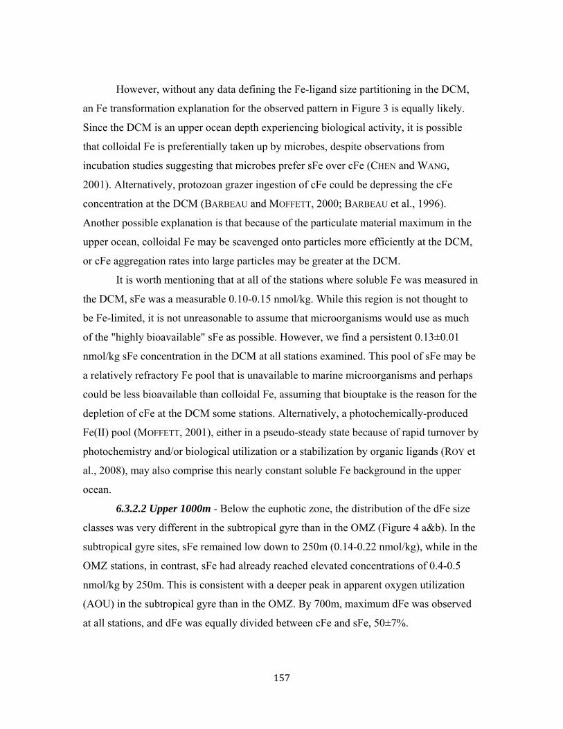
157
However, without any data defining the Fe-ligand size partitioning in the DCM,
an Fe transformation explanation for the observed pattern in Figure 3 is equally likely.
Since the DCM is an upper ocean depth experiencing biological activity, it is possible
that colloidal Fe is preferentially taken up by microbes, despite observations from
incubation studies suggesting that microbes prefer sFe over cFe (CHEN and WANG,
2001). Alternatively, protozoan grazer ingestion of cFe could be depressing the cFe
concentration at the DCM (BARBEAU and MOFFETT, 2000; BARBEAU et al., 1996).
Another possible explanation is that because of the particulate material maximum in the
upper ocean, colloidal Fe may be scavenged onto particles more efficiently at the DCM,
or cFe aggregation rates into large particles may be greater at the DCM.
It is worth mentioning that at all of the stations where soluble Fe was measured in
the DCM, sFe was a measurable 0.10-0.15 nmol/kg. While this region is not thought to
be Fe-limited, it is not unreasonable to assume that microorganisms would use as much
of the "highly bioavailable" sFe as possible. However, we find a persistent 0.13±0.01
nmol/kg sFe concentration in the DCM at all stations examined. This pool of sFe may be
a relatively refractory Fe pool that is unavailable to marine microorganisms and perhaps
could be less bioavailable than colloidal Fe, assuming that biouptake is the reason for the
depletion of cFe at the DCM some stations. Alternatively, a photochemically-produced
Fe(II) pool (MOFFETT, 2001), either in a pseudo-steady state because of rapid turnover by
photochemistry and/or biological utilization or a stabilization by organic ligands (ROY et
al., 2008), may also comprise this nearly constant soluble Fe background in the upper
ocean.
6.3.2.2 Upper 1000m - Below the euphotic zone, the distribution of the dFe size
classes was very different in the subtropical gyre than in the OMZ (Figure 4 a&b). In the
subtropical gyre sites, sFe remained low down to 250m (0.14-0.22 nmol/kg), while in the
OMZ stations, in contrast, sFe had already reached elevated concentrations of 0.4-0.5
nmol/kg by 250m. This is consistent with a deeper peak in apparent oxygen utilization
(AOU) in the subtropical gyre than in the OMZ. By 700m, maximum dFe was observed
at all stations, and dFe was equally divided between cFe and sFe, 50±7%.
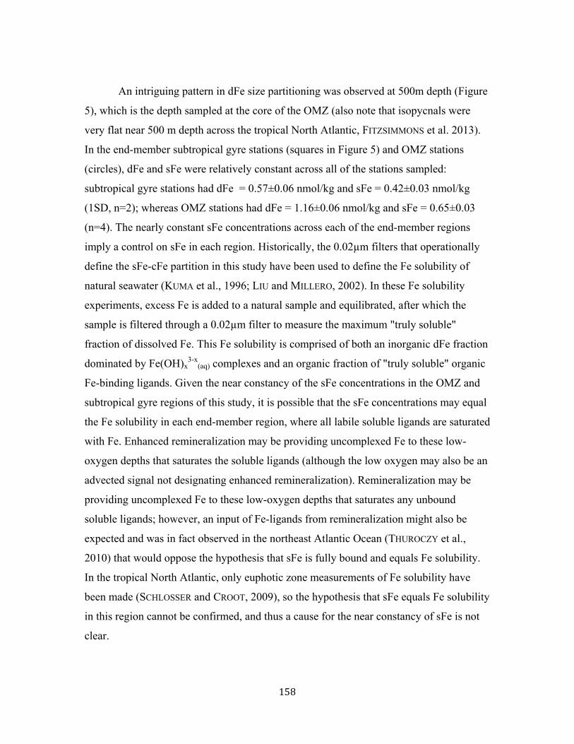
158
An intriguing pattern in dFe size partitioning was observed at 500m depth (Figure
5), which is the depth sampled at the core of the OMZ (also note that isopycnals were
very flat near 500 m depth across the tropical North Atlantic, FITZSIMMONS et al. 2013).
In the end-member subtropical gyre stations (squares in Figure 5) and OMZ stations
(circles), dFe and sFe were relatively constant across all of the stations sampled:
subtropical gyre stations had dFe = 0.57±0.06 nmol/kg and sFe = 0.42±0.03 nmol/kg
(1SD, n=2); whereas OMZ stations had dFe = 1.16±0.06 nmol/kg and sFe = 0.65±0.03
(n=4). The nearly constant sFe concentrations across each of the end-member regions
imply a control on sFe in each region. Historically, the 0.02µm filters that operationally
define the sFe-cFe partition in this study have been used to define the Fe solubility of
natural seawater (KUMA et al., 1996; LIU and MILLERO, 2002). In these Fe solubility
experiments, excess Fe is added to a natural sample and equilibrated, after which the
sample is filtered through a 0.02µm filter to measure the maximum "truly soluble"
fraction of dissolved Fe. This Fe solubility is comprised of both an inorganic dFe fraction
dominated by Fe(OH)x3-x
(aq) complexes and an organic fraction of "truly soluble" organic
Fe-binding ligands. Given the near constancy of the sFe concentrations in the OMZ and
subtropical gyre regions of this study, it is possible that the sFe concentrations may equal
the Fe solubility in each end-member region, where all labile soluble ligands are saturated
with Fe. Enhanced remineralization may be providing uncomplexed Fe to these low-
oxygen depths that saturates the soluble ligands (although the low oxygen may also be an
advected signal not designating enhanced remineralization). Remineralization may be
providing uncomplexed Fe to these low-oxygen depths that saturates any unbound
soluble ligands; however, an input of Fe-ligands from remineralization might also be
expected and was in fact observed in the northeast Atlantic Ocean (THUROCZY et al.,
2010) that would oppose the hypothesis that sFe is fully bound and equals Fe solubility.
In the tropical North Atlantic, only euphotic zone measurements of Fe solubility have
been made (SCHLOSSER and CROOT, 2009), so the hypothesis that sFe equals Fe solubility
in this region cannot be confirmed, and thus a cause for the near constancy of sFe is not
clear.

159
Notably, however, only at intermediate oxygen concentrations (triangles in Figure
5), did colloidal Fe dominate dFe at 500m. The two "intermediate" samples were taken
from OC449-2 station 9 and from the OMZ station (10°N, 45°W) station of BERGQUIST
et al. (2007), where dissolved oxygen concentrations were between 100-110 µmol/kg. At
both stations, sFe was depressed to "gyre-like" concentrations, while dFe remained
elevated to "OMZ" levels. What is driving this unique dFe size partitioning as OMZ
waters meet subtropical gyre waters? We exclude a redox explanation, despite its clear
link to oxygen concentrations, since at all stations of this study dissolved oxygen
(minimum of ~50 µmol/kg) was high enough to favor Fe(III) over Fe(II). Alternatively,
remineralization and ligand-partitioning may actually be the cause for this change in dFe
size partitioning: if the population of microorganisms is unique at intermediate oxygen
concentrations or in the surface waters above these regions, then the size partitioning of
new, remineralization-produced Fe ligands may also be changing as a function of the
biological population, perhaps driving the formation of enhanced organically-bound dFe
into the colloidal size fraction. On the other hand, this pattern may be an abiotic function
of the mixing of lower-oxygen OMZ waters with higher-oxygen subtropical gyre waters.
It is clear that sFe concentrations remained depressed to subtropical gyre levels in these
intermediate stations, and if sorption/aggregation rates transforming soluble Fe into
colloidal Fe were higher than desoprtion/disaggregation in this mixing zone, then cFe
would be favored. This could be motivated by an increase in particle concentrations or a
change in particle composition at these mixing stations around the edge of the OMZ.
Regardless of the cause, colloids may be serving as a conduit of dFe loss during mixing
of high dFe waters of the OMZ with the low dFe waters of the gyre. If the colloidal phase
is actively aggregating, as suggested by the model of HONEYMAN and SANTSCHI (1989),
the partitioning of the remineralized fraction could affect the efficiency of Fe recycling,
since if cFe aggregated to the particulate phase before it was upwelled to the surface
ocean, it would result in a "leak" in the Fe recycling system that might not be present if
the mixing zone comprised less cFe.

160
6.3.2.3 Deep ocean - We determined the deep water size partitioning of dFe at
one station in the deepest part of the eastern tropical North Atlantic basin (Station 13:
12.8°N, 33.0°W, Figure 6a). As described in FITZSIMMONS et al. (2013), Antarctic
Intermediate Water (AAIW) was the main water mass near 1000m, North Atlantic Deep
Water (NADW) dominated from 1500-4000m, and Antarctic Bottom Water (AABW)
was mixed with NADW below 4000m. In the deepest samples from 4000-5000m,
FITZSIMMONS et al. (2013) observed a 0.1 nmol/kg increase in dFe compared to the
shallower NADW-only depths, which they suggested might have been acquired from
hydrothermal vent Fe inputs during deep water transit through the Vema Fracture Zone.
As can be seen in Figure 6a, sFe concentrations at these AABW-influenced depths were
not significantly different from those at the shallower, NADW-only depths, and thus the
increase in dFe was contributed only by the colloidal Fe phase (composing 65±2% of the
dFe in the deepest samples, n=2). If this 0.1 nmol/kg excess dFe is hydrothermally
derived, it is unknown whether it is composed of organically bound colloidal Fe, as
would traditionally be assumed in deep ocean waters, or whether an inorganic Fe
colloidal phase potentially precipitated during venting also contributes. Regardless, this
cFe would have had to escape scavenging over the >1200 km transit from the Vema
Fracture Zone to Station 13.
In the mid-depth NADW at this site, sFe constituted 48±11% of the dFe pool, and
sFe concentrations were 0.34±0.05 nmol/kg (n=2), which compares well with the
0.35±0.05 nmol/kg values reported by BERGQUIST et al. (2007) in the North (Figure 6b)
and South Atlantic as well as the ~0.32 nmol/kg values reported by WU et al. (2001) near
Bermuda. Even in the Atlantic sector of the Southern Ocean, at depths where NADW is
recognized by enhanced salinity, the same sFe values of 0.35±0.02 nmol/kg were
observed (CHEVER et al., 2010). This is in contrast to measurements in the northeast
Atlantic off Portugal where sFe was only measured to be 0.16-0.21 nmol/kg in NADW
(THUROCZY et al., 2010). These samples, however, were collected using a different
operational definition of the sFe size fraction, a 1000 kDa membrane in a cross-flow
filtration apparatus, and thus cannot be directly compared to the sFe concentrations in this

161
study, which were collected using 0.02 µm Anopore filtration (FITZSIMMONS and BOYLE,
in review).
6.3.3 Controls on dissolved Fe size partitioning in the tropical North Atlantic -
In their study on dFe size partitioning in the Atlantic Ocean, BERGQUIST et al. (2007)
suggested that it is the variability in colloidal Fe that determines dFe concentration
variability in the open ocean, with soluble Fe remaining relatively invariant with depth.
This pattern is clear in their data, which is reproduced in Figure 6b: sFe is relatively
constant at 0.3-0.4 nmol/kg below the euphotic zone, while dFe is at high concentration
and variable, with most of the variability contributed by changes in the colloidal phase. In
contrast, however, the full-depth profile data from Station 13 of this study (Figure 6a)
shows that where dissolved Fe is enhanced in the OMZ, soluble Fe is also enhanced, and
as a result both soluble and colloidal fractions contribute to the variability in the dFe
profile. In fact, the sFe concentrations from all stations of OC449-2 were generally more
variable than in the two stations measured by BERGQUIST et al. (2007; Figure 4 c-d), and
at no stations in OC449-2 could sFe be considered to remain constant with depth. At the
subtropical gyre site of BERGQUIST et al. (2007), sFe concentrations were nearly constant
through the upper 1000m, averaging 0.34±0.04 nmol/kg (1SD, n=12) over all depths
sampled, while OC449-2 subtropical gyre stations reached lower minima in sFe in the
upper ocean (0.12-0.22 nmol/kg) and higher maxima in the deeper waters (0.4-0.5
nmol/kg; Figure 4c). The same is true of the OMZ stations where OC449-2 stations
reached a lower sFe near the chlorophyll maximum (0.1-0.15 nmol/kg) and higher sFe
maxima in OMZ waters (0.6-0.7 nmol/kg) than the nearly constant 0.40±0.06 nmol/kg
(n=9) measured by BERGQUIST et al. (2007) at their OMZ site (Figure 4d).
Relatively invariant sFe below the euphotic zone was a major finding of the
BERGQUIST et al. (2007) study, and combined with the dominance of cFe in the upper
waters underlying dust deposition led them to conclude that colloidal Fe dominates dFe
variability throughout the ocean (Figure 7a). The tropical North Atlantic OC449-2
stations, however, show a reliance of dFe variability on both sFe and cFe concentrations
(Figure 7b). Why do these two studies show different patterns in dFe size partitioning?

162
One possibility is that Station 13 is farther into the OMZ than BERGQUIST et al.'s OMZ
station and thus might receive more of a "uniquely partitioned" OMZ Fe input that is
enriched in more soluble Fe than colloidal Fe. FITZSIMMONS et al. (2013) used several
proxies to apportion the Fe sources to the OMZ and concluded that the most likely
mechanism for the enriched Fe was enhanced remineralization of high Fe:C organic
material formed in the dust-laden surface waters above rather than advection/mixing out
of an African margin Fe source. If this is true, then for a remineralization-derived "source
partitioning signature" to explain the difference between dFe partitioning in the Figure 6
profiles, there must be a difference in the microbial communities between Station 13 and
BERGQUIST et al.'s OMZ station that would cause a change in the partitioning of
remineralized Fe in the OMZ. Alternatively, the partitioning of free ligands that bind this
newly remineralized material in the OMZ could be different between the two sites.
However, the dFe dependence on both sFe and cFe phases in OC449-2 is not
isolated only to the OMZ stations in Figure 7b: both size fractions are variable across the
entire tropical North Atlantic Ocean. The data of BERGQUIST et al. (2007) shows a
narrower range in sFe concentrations despite a wide range in dFe concentrations, and thus
only a dFe-cFe relationship can be deduced from their data. Across a wider span of
oceanographic conditions in the tropical North Atlantic, however, sFe also contributes to
dFe variability where it did not in the more restricted sampling of BERGQUIST et al. We
believe that the dFe partitioning pattern where both sFe and cFe contributions to dFe
variability is more representative of the general tropical North Atlantic Ocean (as shown
by the numerous stations emcompassed by this study's data). We hypothesize that this
more equivalent partitioning is attributed to an equal partitioning of Fe-binding ligands in
the two size fractions that controls dFe size distributions, or that following
remineralization the exchange rates between soluble and colloidal Fe
(aggregation/disaggregation, sorption/desorption, or ligand exchange) set a "steady state"
dFe partitioning that is more equivalent between the two size fractions. We further
explore the processes controlling this "steady state" partitioning in Chapter 7. We believe
that the >0.8 nmol/kg dFe data of Bergquist et al. data in Figure 7a fall off the linear dFe-

163
sFe trend because they do not reach a steady state between aggregation/disaggregation
due to their location in waters of "intermediate" oxygen concentration after mixing of
OMZ and gyre waters (as discussed in section 6.3.2.2).
The slopes of the dFe-cFe (1.261±0.156, ±1SE) and dFe-sFe (1.235±0.140)
relationships in Figure 7 are statistically identical, indicating that within the scatter of the
regressions, soluble and colloidal Fe contribute equally to dissolved Fe variability. These
slopes are also not significantly different from the dFe-cFe slopes cited by BERGQUIST et
al. (2007) for their Atlantic Ocean data (1.18) or THUROCZY et al. (2010) for their
Northeast Atlantic data (1.16). Notably, neither of these studies produced statistically
significant regressions between dFe-sFe, and there was also no significant dFe-sFe
correlation in the Southern Ocean study of CHEVER et al. (2010). This reinforces the
conclusion that soluble Fe is playing a greater role in dFe variability in the tropical North
Atlantic than previously thought.
The near-equal slopes between dFe-sFe and dFe-cFe also suggest that the average
partitioning of marine dFe is 50-50% to the soluble and colloidal pools (when using a
0.02 µm filter), driven either by control of the dFe size distribution by equally partitioned
Fe-binding ligands or by a constant exchange rate between soluble-colloidal Fe pools.
Regional Fe inputs or processes may impart additional Fe sources of one of the phases on
top of this "steady state" partitioning, while scavenging/output processes may detract
from it, to produce the observed variable partitioning. We believe that the data of
Bergquist et al. (2007) is, in fact, out of steady state because of unique processes
occurring in the OMZ-gyre mixing zone. Whether it is the partitioning of organic ligands
that controls this background dFe partitioning, and if so which Fe-ligands are most
important and where do they come from, remains to be determined. The "steady state
partitioning" model is supported by near equal contributions of soluble and colloidal Fe
to deep ocean dFe partitioning in the Atlantic, Pacific, and Southern Oceans (BERGQUIST
et al., 2007; BOYE et al., 2010; CHEVER et al., 2010; WU et al., 2001).
It is clear from this and similar studies that the partitioning of dFe between
soluble and colloidal phases is variable, even within the tropical North Atlantic alone, yet

164
this partitioning has a major impact on Fe biogeochemical cycling, potentially affecting
dFe bioavailability, solubility, and residence times. Unfortunately, we know very little
about the chemical composition of dFe in the ocean, but it is clear from this and other
size fractionation studies that soluble and colloidal Fe species cycle independently to
some extent and warrant further study, both in exploration of their distribution as well as
in experimental constraint of their bioavailability and scavenging potential. We rely
heavily on the assumption that the partitioning of organic Fe-binding ligands drives the
observed dFe partitioning, yet of the three published studies that have measured the size
fractionation of ligands using electrochemical techniques (BOYE et al., 2010; CULLEN et
al., 2006; THUROCZY et al., 2010), none have found that ligand partitioning actually
predicts the observed dFe partitioning. This either indicates that electrochemical
measurements are missing a fraction of Fe-binding ligands that are active in the open
ocean, or that there is a missing link between our kinetically-limited measurements of Fe-
binding ligand concentration and binding strength and our thermodynamic understand of
organic ligand-binding of Fe in the open ocean. We still have much to learn about the
chemical environment of dFe in the open ocean that will help us predict how Fe is
solubilized and made available to marine microbes yet also is eventually scavenged to the
particulate phase.
6.4 Conclusions
In this study, we investigated the partitioning of dFe between soluble and
colloidal size fractions in the tropical North Atlantic and compared the distributions to
the study of dFe size partitioning completed previously in the western portion of this
region (BERGQUIST et al., 2007). We found that in the surface ocean underlying the
Saharan dust plume that dFe was composed predominately of colloidal Fe, supporting the
hypothesis that dust-derived Fe may be preferentially retained in the colloidal size
fraction (AGUILAR-ISLAS et al., 2010; WU et al., 2001). At the chlorophyll maximum,

165
colloidal Fe was minimized or disappeared completely, which is likely due to a
combination of biological uptake of colloidal Fe and/or the scavenging/aggregation of
cFe at this depth. In the deep ocean, dFe size partitioning averaged 50-50% between the
soluble and colloidal phases. Typical NADW sFe concentrations were observed, and in
deeper waters including an AABW component that appear to have acquired Fe from
hydrothermal activity or some other source during passage through the Vema Fracture
Zone (FITZSIMMONS et al., 2013), soluble Fe did not increase coincidently, indicating that
any new Fe source was contributed by the colloidal phase.
Most significantly, the results of this study oppose the premise that colloidal Fe
alone controls the dissolved Fe variability in the open ocean. We instead propose that
both soluble and colloidal Fe control dFe concentration variability and that the near-
constancy of sFe with depth found in previous studies either represents a "steady state"
open ocean dFe partitioning pattern over which regional Fe sources with unique dFe
partitioning are overlain to explain the observed partitioning, or that Fe-binding ligand
partitioning between the two size fractions is variable in the open ocean and directly
controls dFe partitioning. This distinction warrants future exploration in studies where the
size fractionation of both the Fe-binding ligands and dFe are measured together
throughout the water column. In general, this study confirms that soluble and colloidal Fe
have unique patterns of cycling in different ocean regions and depths, and the two size
classes cycle independently to some extent. These global dFe partitioning distributions
impact both the bioavailability and scavenging residence time of dFe in the open ocean.

166
References for Chapter 6
Aguilar-Islas, A. M., Wu, J., Rember, R., Johansen, A. M., and Shank, L. M., 2010. Dissolution
of aerosol-derived iron in seawater: Leach solution chemistry, aerosol type, and colloidal iron fraction. Marine Chemistry 120, 25-33.
Barbeau, K. and Moffett, J. W., 2000. Laboratory and field studies of colloidal iron oxide dissolution as mediated by phagotrophy and photolysis. Limnology & Oceanography 45, 827-835.
Barbeau, K., Moffett, J. W., Caron, D. A., Croot, P. L., and Erdner, D. L., 1996. Role of protozoan grazing in relieving iron limitation of phytoplankton. Nature Geosci 380, 61-64.
Bell, J., Betts, J., and Boyle, E., 2002. MITESS: a moored in situ trace element serial sampler for deep-sea moorings. Deep-Sea Research Part I-Oceanographic Research Papers 49, 2103-2118.
Bergquist, B. A. and Boyle, E. A., 2006. Dissolved iron in the tropical and subtropical Atlantic Ocean. Global Biogeochemical Cycles 20, 14.
Bergquist, B. A., Wu, J., and Boyle, E. A., 2007. Variability in oceanic dissolved iron is dominated by the colloidal fraction. Geochimica et Cosmochimica Acta 71, 2960-2974.
Boye, M., Nishioka, J., Croot, P., Laan, P., Timmermans, K. R., Strass, V. H., Takeda, S., and de Baar, H. J. W., 2010. Significant portion of dissolved organic Fe complexes in fact is Fe colloids. Marine Chemistry 122, 20-27.
Bruland, K. W. and Lohan, M. C., 2003. Controls of Trace Metals in Seawater. In: Turekian, K. K. and Holland, H. D. Eds.), Treatise On Geochemistry. Elsevier Science Ltd., Cambridge, United Kingdom.
Chen, M. and Wang, W. X., 2001. Bioavailability of natural colloid-bound iron to marine plankton: Influences of colloidal size and aging. Limnology and Oceanography 46, 1956-1967.
Chever, F., Bucciarelli, E., Sarthou, G., Speich, S., Arhan, M., Penven, P., and Tagliabue, A., 2010. Physical speciation of iron in the Atlantic sector of the Southern Ocean along a transect from the subtropical domain to the Weddell Sea Gyre. J. Geophys. Res. 115, C10059.
Cullen, J. T., Bergquist, B. A., and Moffett, J. W., 2006. Thermodynamic characterization of the partitioning of iron between soluble and colloidal species in the Atlantic Ocean. Marine Chemistry 98, 295-303.
Fitzsimmons, J. N. and Boyle, E. A., 2012. An intercalibration between the GEOTRACES GO- FLO and the MITESS/Vanes sampling systems for dissolved iron concentration analyses (and a closer look at adsorption effects). Limnology & Oceanography: Methods 10, 437-450.
Fitzsimmons, J. N. and Boyle, E. A., in review. The assessment and intercalibration of

167
Anopore™ and cross flow filtration methods for the determination of dissolved iron size fractionation into soluble/colloidal phases in seawater. Limnology & Oceanography: Methods.
Fitzsimmons, J. N., Zhang, R., and Boyle, E. A., 2013. Dissolved iron in the tropical North Atlantic oxygen minimum zone. Marine Chemistry 154, 87-99.
Gledhill, M. and Buck, K. N., 2012. The organic complexation of iron in the marine environment: A review. Frontiers in Microbiology: Microbiological Chemistry 3, Article 69.
Honeyman, B. D. and Santschi, P. H., 1989. A Brownian-pumping model for oceanic trace metal scavenging: Evidence from Th isotopes. Journal of Marine Research 47, 951-992.
Hunter, K. A. and Boyd, P. W., 2007. Iron-binding ligands and their role in the ocean biogeochemistry of iron. Environmental Chemistry 4, 221-232.
Kuma, K., Nishioka, J., and Matsunaga, K., 1996. Controls on iron(III) hydroxide solubility in seawater: The influence of pH and natural organic chelators. Limnology and Oceanography 41, 396-407.
Lee, J.-M., Boyle, E. A., Echegoyen-Sanz, Y., Fitzsimmons, J. N., Zhang, R., and Kayser, R. A., 2011. Analysis of trace metals (Cu, Cd, Pb, and Fe) in seawater using single batch
Nitrilotriacetate resin extraction and isotope dilution inductively coupled plasma mass spectrometry. Analytica Chimica Acta 686, 93-101.
Liu, X. and Millero, F. J., 2002. The solubility of iron in seawater. Marine Chemistry 77, 43-54. Mahowald, N., Baker, A. R., Bergametti, G., Brooks, N., Duce, R. A., Jickells, T., Kubilay, N.,
Prospero, J. M., and Tegen, I., 2005. Atmospheric global dust cycle and iron inputs to the ocean. Global Biogeochemical Cycles 19, GB4025.
Martin, J. H. and Fitzwater, S. E., 1988. Iron deficiency limits phytoplankton growth in the north- east Pacific subarctic. Nature 331, 341-343.
Martinez, J. S., Carter-Franklin, J. N., Mann, E. L., Martin, J. D., Haygood, M. G., and Butler, A., 2003. Structure and membrane affinity of a suite of amphiphilic siderophores produced by a marine bacterium. Proceedings of the National Academy of Sciences 2003, 3754-3759.
Martinez, J. S., Haygood, M. G., and Butler, A., 2001. Identification of a natural desferrioxamine siderophore produced by a marine bacterium. Limnology & Oceanography 46, 420-424.
Millero, F. J., 1998. Solubility of Fe(III) in seawater. Earth and Planetary Science Letters 154, 323-329.
Moffett, J. W., 2001. Transformations among different forms of iron in the ocean. In: Turner, D. R. and Hunter, K. A. Eds.), The Biogeochemistry of Iron in Seawater. John Wiley & Sons, West Sussex, England.
Morel, F. M. M., Milligan, A. J., and Saito, M. A., 2003. Marine Bioinorganic Chemistry: The Role of Trace Metals in the Oceanic Cycles of Major Nutrients. In: Turekian, K. K. and Holland, H. D. Eds.), Treatise On Geochemistry. Elsevier Science Ltd., Cambridge, United Kingdom.
Nishioka, J., Takeda, S., Kudo, I., Tsumune, D., Yoshimura, T., Kuma, K., and Tsuda, A., 2003. Size-fractionated iron distributions and iron-limitation processes in the subarctic NW Pacific. Geophysical Research Letters 30.

168
Rich, H. W. and Morel, F. M. M., 1990. Availability of well-defined iron colloids to the marine diatom Thalassiosira weissflogii. Limnology and Oceanography 35, 652-662.
Roy, E. G., Wells, M. L., and King, D. W., 2008. Persistence of iron(II) in surface waters of the western subarctic Pacific. Limnology and Oceanography 53, 89-98.
Rue, E. L. and Bruland, K. W., 1995. Complexation of iron(III) by natural organic ligands in the Central North Pacific as determined by a new competitive ligand equilibration/adsorptive cathodic stripping voltammetric method. Marine Chemistry 50, 117-138.
Schlosser, C. and Croot, P. L., 2009. Controls on seawater Fe(III) solubility in the Mauritanian upwelling zone. Geophysical Research Letters 36, L18606.
Thuróczy, C. E., Gerringa, L. J. A., Klunder, M. B., Middag, R., Laan, P., Timmermans, K. R., and de Baar, H. J. W., 2010. Speciation of Fe in the Eastern North Atlantic Ocean. Deep Sea Research Part I: Oceanographic Research Papers 57, 1444-1453.
Ussher, S. J., Achterberg, E. P., Sarthou, G., Laan, P., de Baar, H. J. W., and Worsfold, P. J., 2010. Distribution of size fractionated dissolved iron in the Canary Basin. Marine Environmental Research 70, 46-55.
Wells, M. L. and Goldberg, E. D., 1991. Occurrence of small colloids in sea water. Nature 353, 342-344.
Wells, M. L. and Goldberg, E. D., 1992. Marine submicron particles. Marine Chemistry 40, 5-18. Wells, M. L. and Goldberg, E. D., 1993. Colloid aggregation in seawater. Marine Chemistry 41,
353-358. Wilhelm, S. W. and Trick, C. G., 1994. Iron-limited growth of cyanobacteria - Multiple
siderophore production is a common response. Limnology and Oceanography 39, 1979-1984.
Wu, J., Boyle, E. A., Sunda, W. G., and Wen, L., 2001. Soluble and colloidal iron in the oligotrophic North Atlantic and North Pacific. Science 293, 847-849.

169
Figures for Chapter 6
Figure 1: OC449-2 cruise track with the six stations sampled for dFe size partitioning indicated in bolded black. Color contours indicate the distribution of dissolved oxygen at 500m taken from the eWOCE dataset (small dots). Colors inside the station dots indicate the dissolved oxygen concentrations at 500m measured on OC449-2. The two triangles designate the subtropical gyre station (30°N, 45°W) and the OMZ station (10°N, 35°W) from Bergquist et al. (2007). The dashed red line designates the cut-off used in this study between the assigned "subtropical gyre stations" (3 & 6) and "OMZ stations" (9, 11, 13, 17, & 22).

170
Figure 2: dFe and sFe in the surface ocean as a function of longitude, with station numbers and biogeochemical province indicated at the top. Station locations are indicated in Figure 1. Italicized percentages indicate the %cFe contribution to dFe. Error bars are shown for all points and represent 1σ standard deviation of analytical replicates.
Figure 3: Euphotic zone dissolved Fe partitioning in the subtropical gyre at (a) Station 6 and in the OMZ at (b) Station 9 and (c) Station 13. dFe is shown in the filled circles (solid line), while sFe is shown in the open circles (dotted line). CTD fluorescence (V) is shown as the gray line to indicate the location of the deep chlorophyll maximum. At the OMZ stations, cFe (= dFe - sFe) goes to zero at the chlorophyll maximum.
0.00
0.20
0.40
0.60
0.80
1.00
1.20
-60 -50 -40 -30 -20
[Fe]
nm
ol/k
g
Longitude (°W)
dFe
sFe
82% 41% 87%
87% 80% 67% 79%
Station: 3 6 9 11 13 17 22
SubtropicalGyre OMZ

171
Figure 4: Dissolved Fe size partitioning to 1000m in the subtropical gyre (a, c) and the OMZ (b, d). Data is shown for individual stations in (a) and (b) with salinity indicated in gray. In (c) and (d) sFe and dFe profiles from multiple stations are shown together for comparison. Error bars in (a) and (b) show 1σ standard deviations of replicates analyzed. *Data taken from Bergquist et al. (2007).

172
Figure 5: Dissolved and soluble Fe concentrations at 500m depth as a function of oxygen concentration. OMZ stations are designated as circles, subtropical gyre stations are designated as squares, and stations with intermediate oxygen concentration are shown as triangles. Note that the datapoints at 100 μmol/kg are taken from Bergquist et al. (2007) at 10°N, 45°W. The percentage of dFe composed of soluble or colloidal Fe for each of the three regions is also designated.
0.0
0.2
0.4
0.6
0.8
1.0
1.2
1.4
40 60 80 100 120 140 160 180
[Fe]
nm
ol/k
g
Dissolved oxygen (µmol/kg)
27±3% cFe
73±3% sFe
44±4% cFe
56±4% sFe
58±2% cFe
42±2% sFe
dFe
sFe
Subtropical GyreOMZ Intermediate

173
Figure 6: (a) Full-depth profile of dissolved Fe partitioning at Station 13 in the deepest part of the eastern tropical North Atlantic basin. (b) Full-depth profile of dissolved Fe partitioning in the OMZ station from Bergquist et al. (2007), shown for comparison. In both cases, error bars designate ±1 standard deviation.
0
1000
2000
3000
4000
5000
0.0 0.5 1.0 1.5
Dep
th (m
)Station 13: 12.8°N, 33°W
Fe (nmol/kg)
dFe
sFe
0
1000
2000
3000
4000
5000
0.0 0.5 1.0 1.5
Dep
th (m
)
Bergquist et al. 2007: 10°N, 45°WFe (nmol/kg)
dFe
sFe
(a) (b)

174
Figure 7: Dissolved Fe as a function of soluble Fe (left) and colloidal Fe (right) in the North Atlantic stations of Bergquist et al. (2007) in (a) and this study (b). The error in the slopes and intercepts from this study's data are ± SE. There is no relationship between dFe and sFe in the data of Bergquist et al. (2007), while there is a dFe-sFe relationship in the stations of this study.
0.0
0.2
0.4
0.6
0.8
1.0
1.2
1.4
0.0 0.2 0.4 0.6 0.8 1.0
dF
e (n
mol
/kg)
sFe (nmol/kg)
0.0
0.2
0.4
0.6
0.8
1.0
1.2
1.4
0.0 0.2 0.4 0.6 0.8 1.0
dF
e (n
mol
/kg)
cFe (nmol/kg)
dFe = (1.235±0.140)*sFe+ (0.335±0.061)
R² = 0.64
0.0
0.2
0.4
0.6
0.8
1.0
1.2
1.4
1.6
0.0 0.2 0.4 0.6 0.8 1.0
dF
e (n
mol
/kg)
sFe (nmol/kg)
dFe = (1.261±0.156)*cFe+ (0.278±0.073)
R² = 0.60
0.0
0.2
0.4
0.6
0.8
1.0
1.2
1.4
1.6
0.0 0.2 0.4 0.6 0.8 1.0
dF
e (n
mol
/kg)
cFe (nmol/kg)
(a) Tropical (10°N) and subtropical (30°N) North Atlantic stations of Bergquist et al. (2007)
(b) All data from this study's OC449‐2 stations

175
Supplementary Data Table
Sta. Lat. (°N)
Long. (°W)
Depth (m)
dFe nmol/kg
1 SD
n sFe
nmol/kg 1
SD n
cFe (nmol/kg)
sFe/dFe (%)
cFe/dFe (%)
3 16.49 52.35 5 1.11 0.02 2 0.21 0.01 2 0.91 19 81 3 16.49 52.35 122 0.62 0.02 2 0.12 0.00 2 0.50 20 80 3 16.49 52.35 245 0.34 0.01 4 0.14 0.01 3 0.19 43 57 3 16.49 52.35 489 0.62 0.02 2 0.44 0.03 2 0.18 71 29 3 16.49 52.35 685 0.80 0.04 2 0.50 0.02 2 0.30 62 38 3 16.49 52.35 978 0.80 0.01 2 0.49 0.01 2 0.31 62 38 6 19.96 45.08 5 0.81 0.01 4 0.48 0.01 2 0.33 59 41 6 19.96 45.08 126 0.29 0.01 2 0.13 0.01 2 0.16 44 56 6 19.96 45.08 251 0.33 0.01 3 0.22 0.01 3 0.10 68 32 6 19.96 45.08 503 0.53 0.01 2 0.40 0.01 2 0.13 75 25 6 19.96 45.08 703 0.79 0.01 3 0.36 0.01 2 0.42 46 54 6 19.96 45.08 1005 0.70 0.00 2 0.29 0.01 2 0.41 42 58 9 13.07 40.63 5 0.82 0.02 4 0.11 0.01 3 0.71 13 87 9 13.07 40.63 125 0.27 0.00 3 0.15 0.02 3 0.12 56 44 9 13.07 40.63 250 0.97 0.04 2 0.57 0.03 2 0.40 59 41 9 13.07 40.63 500 0.98 0.02 2 0.42 0.00 2 0.56 43 57 9 13.07 40.63 700 1.08 0.02 6 0.51 0.02 3 0.57 47 53 9 13.07 40.63 1000 0.87 0.04 4 0.45 0.01 2 0.42 52 48
11 8.04 37.63 5 0.59 0.02 2 0.08 0.02 3 0.51 13 87 11 8.04 37.63 124 0.84 0.03 2 0.49 0.01 3 0.36 58 42 11 8.04 37.63 248 1.12 0.03 4 0.51 0.02 3 0.61 46 54 11 8.04 37.63 496 1.17 0.02 2 0.65 0.01 2 0.51 56 44 11 8.04 37.63 694 0.89 0.03 3 0.46 0.04 5 0.43 51 49 11 8.04 37.63 991 0.85 0.03 4 0.63 0.02 5 0.22 74 26
13 12.81 33.02 5 0.45 0.01 4 0.09 0.03 2 0.36 20 80 13 12.81 33.02 28 0.41 0.00 2 0.08 0.02 2 0.33 19 81 13 12.81 33.02 74 0.15 0.03 3 0.13 0.02 3 0.03 83 17 13 12.81 33.02 97 0.47 0.00 2 0.19 0.03 3 0.28 41 59 13 12.81 33.02 116 1.01 0.00 3 0.42 0.02 4 0.59 42 58 13 12.81 33.02 162 1.14 0.03 2 0.57 0.03 2 0.58 50 50 13 12.81 33.02 247 1.15 0.03 2 0.75 0.03 7 0.40 65 35 13 12.81 33.02 370 1.30 0.03 4 0.59 0.01 2 0.72 45 55 13 12.81 33.02 493 1.23 0.02 3 0.66 0.02 6 0.57 53 47 13 12.81 33.02 690 1.25 0.03 3 0.56 0.02 3 0.69 45 55 13 12.81 33.02 854 1.19 0.01 5 0.67 0.01 2 0.52 56 44 13 12.81 33.02 1005 0.92 0.02 3 0.57 0.01 2 0.35 62 38 13 12.81 33.02 1256 0.71 0.05 3 0.39 0.00 2 0.32 55 45 13 12.81 33.02 1759 ?1.19 0.01 3 0.34 0.01 3 ?0.85 13 12.81 33.02 2408 ?1.52 0.06 3 ?0.44 0.02 4 ?1.08 13 12.81 33.02 3111 0.71 0.03 3 0.28 0.01 2 0.42 40 60 13 12.81 33.02 3833 0.81 0.02 2 0.30 0.02 2 0.51 37 63 13 12.81 33.02 4958 0.81 0.04 3 0.27 0.01 3 0.53 34 66

176
Sta. Lat. (°N)
Long. (°W)
Depth (m)
dFe nmol/kg
1 SD
n sFe
nmol/kg 1
SD n
cFe (nmol/kg)
sFe/dFe (%)
cFe/dFe (%)
17 11.71 26.84 5 0.63 0.01 2 0.21 0.02 2 0.43 33 67 17 11.71 26.84 496 1.08 0.03 6 0.67 0.02 3 0.42 62 38
22 14.57 21.88 5 0.65 0.02 3 0.14 0.01 3 0.51 21 79 22 14.57 21.88 126 1.37 0.02 3 0.59 0.02 3 0.78 43 57 22 14.57 21.88 503 1.16 0.05 6 0.61 0.01 2 0.55 52 48

177
Chapter 7
Partitioning of dissolved iron into soluble and colloidal phases along the U.S. GEOTRACES North Atlantic Zonal transect In prep for the GEOTRACES North Atlantic special issue of Deep-Sea Research II.
Jessica N. Fitzsimmons*1,2, Gonzalo G. Carrasco2, Jingfeng Wu3, Mariko Hatta4, Christopher I. Measures4, and Edward A. Boyle2
1MIT/WHOI Joint Program in Chemical Oceanography, MIT E25-615, 45 Carleton St., Cambridge, MA 02142; 1-617-324-0283; [email protected]
2Department of Earth Atmospheric and Planetary Sciences, MIT, 45 Carleton St., Cambridge, MA 02142; [email protected]; [email protected]; 1-617-253-3388
3Rosenstiel School for Marine and Atmospheric Sciences, University of Miami, 4600 Rickenbacker Causeway, Miami, FL 33149; 1-305-421-4714; [email protected]
4School of Ocean and Earth Science and Technology, University of Hawai'i at Manoa,
1000 Pope Road, Honolulu, HI 96822; [email protected]; [email protected]; 1-808-956-8693
* designates the corresponding author

178
7.1 Introduction
The international GEOTRACES program endeavors to determine the global
distribution of trace elements and their isotopes while also constraining the fluxes and
processes controlling these distributions. One of the highest priority metals investigated
by GEOTRACES is dissolved iron (dFe), which is known to be an essential micronutrient
for photosynthesis and nitrogen fixation (Morel et al., 2003). However, the
thermodynamically favored redox state of dFe in the oxic open ocean, Fe(III), is largely
insoluble, causing dFe concentrations to fall to levels that limit phytoplankton growth in
nearly 40% of the surface ocean (Moore et al., 2002). Based on electrochemical data,
strong organic Fe-binding ligands are thought to bind >99.9% of marine dFe, buffering
its concentration above biologically limiting levels in many regions of the global ocean
(Rue and Bruland, 1995). However, the identity of these ligands is largely unknown
(Gledhill and Buck, 2012). One of our greatest motivators for studying Fe is to link
external Fe fluxes to biological uptake of Fe as a micronutrient, and our ambiguous
understanding of Fe speciation limits our ability to understand these chemical
transformations.
One tool we can use to explore the form, composition, and cycling of dFe in the
ocean is the size partitioning of dissolved Fe species. We know that dFe (here defined as
<0.2 µm) is composed of both soluble (sFe < 0.02 µm) and colloidal (0.02 µm < cFe <
0.2 µm) size fractions, and the partitioning across both geographic locations and depths is
highly variable, with colloids contributing 0-90% of the dFe phase (Bergquist et al.,
2007; Fitzsimmons and Boyle, in review-b; Wu et al., 2001). Colloidal Fe comprises
particles so small that they do not sink yet pass through the 0.2 µm filter separating
dissolved from particulate Fe, while soluble Fe largely comprises truly dissolved Fe
species. Resolving this physical description of dFe size partitioning with the chemical
composition of dFe composition is, however, a greater challenge. Since nearly all dFe is
assumed to be organically bound in the open ocean (Rue and Bruland, 1995), as a first
assumption we can assume this holds for sFe and cFe as well. This assessment is our best
guess of the speciation of the two dFe size fractions, as not many studies actually
179
measuring the chemical binding environment of Fe have been completed; some energy
dispersive spectroscopy measurements on colloids imaged by electron microscopy
supported the hypothesis that marine colloidal Fe is organically bound, while estuarine
and coastal colloidal Fe had an inorganic Fe oxyhydroxide component not observed in
the open ocean (Wells and Goldberg, 1992). However, recent studies have found
exceptions to the general assumption that dFe is organically bound. Using synchrotron
technology, von der Heyden et al. (2013) found that colloidal and particulate Fe in the
surface Southern Ocean had an inorganic magnetite component. We will return to the
idea of an inorganic colloidal Fe component (here termed "nanoparticulate") later in the
discussion. For the purposes of this paper, unless otherwise indicated or discussed we
will assume that both sFe and cFe are organically-bound in the open ocean, since most
evidence supports this conclusion (Rue and Bruland, 1995; Wells and Goldberg, 1992).
The size partitioning of dFe affects marine Fe biogeochemistry in two important
ways. First, colloidal Fe has been shown to be composed of discrete bits of material that
have aggregated into or been trapped by a particle of colloidal size (Wells and Goldberg,
1992); thus, colloidal Fe has been hypothesized to be an actively aggregating pool that
links the soluble and particulate phases of Fe via initial sorption followed by successive
aggregation (Honeyman and Santschi, 1989). Not only does this size partitioning have
implications for the chemical composition of the dFe pool, but it also can impact the fate
and lifetime of dFe in any given location, depending on the relative rates of
sorption/desoprtion and aggregation/disaggregation between the various Fe fractions.
Secondly, the speciation of Fe has a direct impact on the bioavailability of Fe, with
different species preferring different forms of dFe (Hassler and Schoemann, 2009;
Hutchins et al., 1999). While very few studies have assessed the bioavailability of dFe
from various size fractions, preliminary results indicate that soluble Fe is preferred, and
colloidal Fe is only indirectly bioavailable after equilibration through the sFe pool (Chen
and Wang, 2001; Wang and Dei, 2003); inorganic Fe colloids as small as 6-50 Fe atoms
were not bioavailable to diatoms (Rich and Morel, 1990). If these studies are taken as
representative of total dFe bioavailability in the open ocean, then an understanding of the

180
dFe partitioning between soluble and colloidal phases is required in order to best assess
dFe bioavailability.
In this paper, we describe the size partitioning of dFe between soluble and
colloidal species across the U.S. GEOTRACES North Atlantic Transect. While several
studies have investigated the size fractionation of dFe in the North Atlantic (see summary
in Fitzsimmons and Boyle, in review-a), there is no consensus on the dFe partitioning
pattern. Bergquist et al. (2007) reported that sFe concentrations in the central Atlantic
were relatively constant with depth near 0.35 nmol/kg, while cFe concentrations were
highly variable, concluding that a dynamic colloidal phase controls dFe variability
alongside relatively invariant sFe. With better spatial coverage in the tropical North
Atlantic, Fitzsimmons and Boyle (in review-b) found sFe to be more variable than seen
by Bergquist et al. and concluded that both sFe and cFe play an active role in controlling
dFe distributions. The new data presented here is the first full ocean-basin transect of dFe
size partitioning ever obtained, with higher spatial and depth resolution than any prior
study. This transect also encompasses several unique Fe inputs and biogeochemical
regimes that highlight changes in dFe size partitioning, including the North African dust
flux to the surface ocean, the TAG hydrothermal plume, and the Mauritanian oxygen
minimum zone (OMZ). We will assess the influence of each of these sources on the
observed dFe size partitioning, as well as offer a consensus of the general partitioning
pattern of dFe in the North Atlantic Ocean.
7.2 Methods
dFe size partitioning was measured at 28 stations in the North Atlantic Ocean
aboard the R/V Knorr on the U.S. GEOTRACES North Atlantic Zonal Transect (NAZT;
station locations in Figure 1). Sampling took place on two cruise legs: the 2010 cruise
(USGT10) sailed from Lisbon, Portugal, to Mindelo, Cape Verde Islands, from 14
October to 4 November, 2010, and the 2011 cruise (USGT11) sailed from Woods Hole,
MA, to Praia, Cape Verde Islands, from 6 November to 11 December, 2011.

181
Uncontaminated seawater was collected using the U.S. GEOTRACES GO-FLO
rosette by the methods described in Cutter and Bruland (2012). After successful rosette
deployment, GO-FLO bottles were carried individually into an ISO 5-rated clean van,
where the seawater was filtered through 0.2 µm Pall Acropak-200™ Supor® capsule
filters under ~0.4 atm of HEPA-filtered air. Filtration protocols were identical to those
described by Fitzsimmons and Boyle (2012), except that the Acropak filters were pre-
cleaned by soaking overnight in filtered surface seawater acidified to pH 2, after which
they were flushed with 5 L of unacidified 0.2 µm-filtered surface seawater and stored
empty in the refrigerator until use. Surface samples were collected using the GeoFish
system of the Bruland lab, which employs all PFA tubing attached to a vane that coasts at
~3 m depth suspended from a boom off the starboard side of the ship during forward
motion at up to 12 knot ship speeds. An all-PFA diaphragm pump sips clean seawater at
~8 psi pressure first through a 0.45 µm Osmonics (PFA) filter and then through a 0.2 µm
PCTE filter mesh held in a polyproylene housing. The filtrates for sFe analyses were
filtered into 500 mL HDPE bottles after three bottle rinses; the secondary sFe filtration is
described below. The filtrates for dFe analyses (<0.2 µm) were taken into 1L LDPE
bottles and were analyzed in the laboratory of Jingfeng Wu at the RSMAS at the
University of Miami by the methods described in Wu and Boyle (1998). Fe procedure
blanks and reported detection limits for the RSMAS method are shown in Table 1, along
with comprehensive lab analyses of SAFe standard reference materials.
A different sFe filtration method was used on each of the two cruises, and these
two methods are described, summarized, and intercalibrated in Fitzsimmons and Boyle
(in review-a). In 2010, a cross flow filtration (CFF) technique using a Millipore Pellicon
XL (PLCGC) regenerated cellulose membrane with a 10kDa nominal molecular weight
cutoff (Pellicon) was used in static mode to collect sFe samples after the system was
conditioned with 300-350mL of sample seawater. In 2011, we instead used 47mm
Anopore membrane filters made of alumina with 0.02 µm pores on an offline, all-Teflon
filter rig (Savillex) to collect sFe samples after the filters were rinsed with acid, clean
water, and sample seawater. While the amount of sFe passing through both filter types is
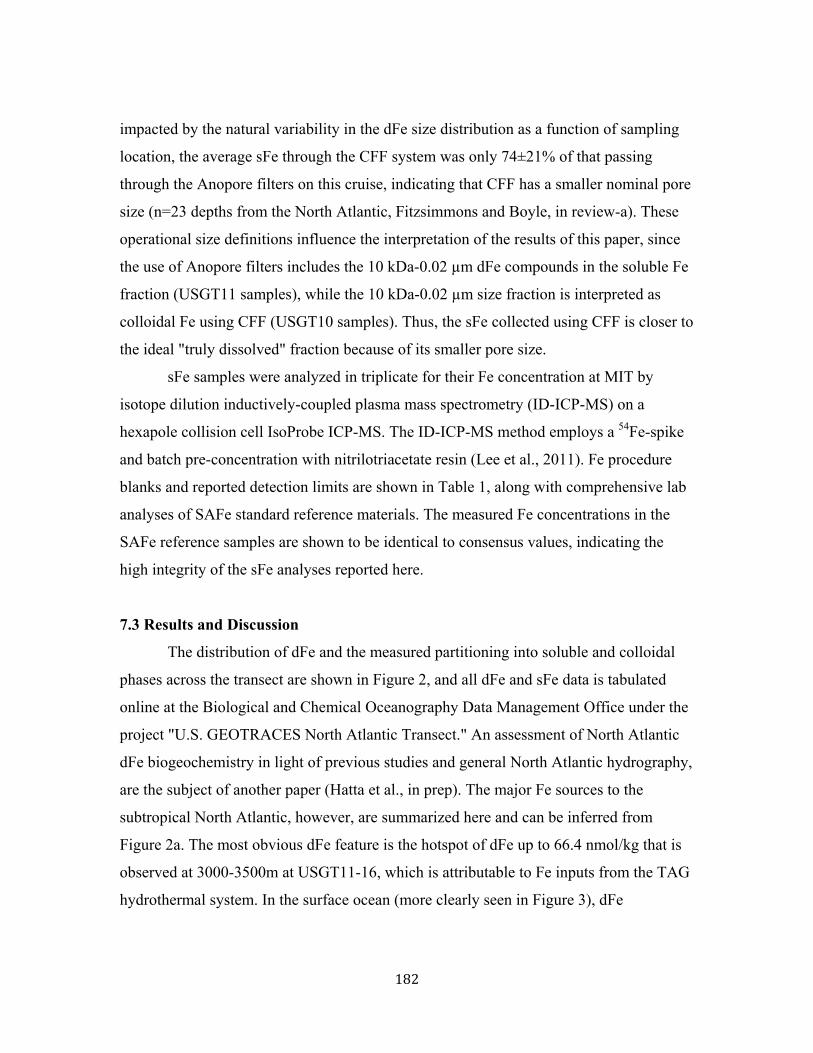
182
impacted by the natural variability in the dFe size distribution as a function of sampling
location, the average sFe through the CFF system was only 74±21% of that passing
through the Anopore filters on this cruise, indicating that CFF has a smaller nominal pore
size (n=23 depths from the North Atlantic, Fitzsimmons and Boyle, in review-a). These
operational size definitions influence the interpretation of the results of this paper, since
the use of Anopore filters includes the 10 kDa-0.02 µm dFe compounds in the soluble Fe
fraction (USGT11 samples), while the 10 kDa-0.02 µm size fraction is interpreted as
colloidal Fe using CFF (USGT10 samples). Thus, the sFe collected using CFF is closer to
the ideal "truly dissolved" fraction because of its smaller pore size.
sFe samples were analyzed in triplicate for their Fe concentration at MIT by
isotope dilution inductively-coupled plasma mass spectrometry (ID-ICP-MS) on a
hexapole collision cell IsoProbe ICP-MS. The ID-ICP-MS method employs a 54Fe-spike
and batch pre-concentration with nitrilotriacetate resin (Lee et al., 2011). Fe procedure
blanks and reported detection limits are shown in Table 1, along with comprehensive lab
analyses of SAFe standard reference materials. The measured Fe concentrations in the
SAFe reference samples are shown to be identical to consensus values, indicating the
high integrity of the sFe analyses reported here.
7.3 Results and Discussion
The distribution of dFe and the measured partitioning into soluble and colloidal
phases across the transect are shown in Figure 2, and all dFe and sFe data is tabulated
online at the Biological and Chemical Oceanography Data Management Office under the
project "U.S. GEOTRACES North Atlantic Transect." An assessment of North Atlantic
dFe biogeochemistry in light of previous studies and general North Atlantic hydrography,
are the subject of another paper (Hatta et al., in prep). The major Fe sources to the
subtropical North Atlantic, however, are summarized here and can be inferred from
Figure 2a. The most obvious dFe feature is the hotspot of dFe up to 66.4 nmol/kg that is
observed at 3000-3500m at USGT11-16, which is attributable to Fe inputs from the TAG
hydrothermal system. In the surface ocean (more clearly seen in Figure 3), dFe

183
enrichments often in excess of 1 nmol/kg are attributed to the solubilization of aerosol Fe
blown in from continental sources, including the North African continent and
industrialized North America and Europe. Finally, there appear to be sources of dFe
emanating from both margins. The western dFe maximum from 1000-2500m in excess of
1 nmol/kg corresponds to the depth range of Labrador Sea Water (LSW), extending
across the western boundary to the Bermuda Atlantic Time Series (BATS) station
(USGT11-10). The eastern dFe maximum also in excess of 1 nmol/kg is coincident with
the Mauritanian OMZ and is not thought to derive from a margin Fe source but rather to
remineralization of high Fe:C organic material (Fitzsimmons et al., 2013).
In this paper, we will focus on the size partitioning of dFe into soluble and
colloidal phases across the GEOTRACES NAZT, and we oganize our discussion as
follows. In section 3.1, we discuss dFe partitioning in each of the major Fe source
regions, and then in Section 3.2, we describe how internal oceanic cycling of dFe impacts
the observed dFe size fractionation. Finally, in Section 3.3 we propose a new model of
the patterns and mechanisms determining the dFe size fractionation that synthesizes all
existing data on dFe size partitioning in the North Atlantic Ocean.
7.3.1 dFe size partitioning from the major Fe sources
7.3.1.1 Aerosol deposition: the surface ocean - The North Atlantic Ocean is
directly downwind of North African dust sources and is thus predicted to receive the
highest dust loadings on the planet (Jickells et al., 2005). As 3.5% of dust by weight is
composed of Fe (Taylor and McLennan, 1985), high dust loadings should result in high
Fe inputs to the surface ocean, and accordingly the literature includes several reports of
elevated surface dFe concentrations in the North Atlantic (Bergquist and Boyle, 2006;
Croot et al., 2004; Fitzsimmons et al., 2013; Measures et al., 2008; Rijkenberg et al.,
2008; Rijkenberg et al., 2012). On the GEOTRACES NAZT, aerosol measurements
(Shelley and Landing, 2013) recorded a range of Fe loadings from 1-5000 ng of Fe per
m3 of air, and the Fe solubility also varied across the four aerosol end-members (North
Africa, North America, Europe, and "marine"). Thus, high surface dFe concentrations
over much of the GEOTRACES transect were expected, and elevated surface ocean dFe

184
concentrations ≥1.0 nmol/kg during the NAZT confirmed these expectations (Hatta et al.,
in prep).
The size partitioning of surface dFe is shown in Figure 3. Despite the surface
enrichment of dFe, soluble Fe occurred at low concentrations averaging 0.16±0.05
nmol/kg during USGT11, and the colloidal contribution to dFe (hereafter referred to as
%cFe) was 79±6%. This high colloidal contribution is identical to the %cFe of 80±7%
determined from six stations in the tropical North Atlantic (Fitzsimmons and Boyle, in
review-b, station locations in Figure 1) and thus appears to be representative of dFe size
partitioning in the surface tropical and subtropical Atlantic underlying the North African
dust plume. It seems, then, that aerosol Fe is preferentially maintained in the colloidal
size fraction, which has been observed previously by others (Bergquist et al., 2007;
Fitzsimmons and Boyle, in review-b; Wu et al., 2001). It is possible that aerosols directly
release Fe into both soluble and colloidal size fractions, after which most of the sFe is
taken up rapidly by microorganisms so that it is nearly absent in the mixed layer.
However, perhaps surprisingly given the variability in surface primary production from
the gyre to the upwelling region along Mauritania, we do not find sFe > 0.22 nmol/kg in
the surface at any stations except USGT10-07, in which case it might be simpler to
assume that aerosol Fe is deposited directly into the colloidal size fraction. Lab-based
aerosol leaching experiments are also consistent with preferential aerosol Fe deposition
directly into the colloidal-sized dFe pool (Aguilar-Islas et al., 2010), although one can be
concerned whether excess Fe binding ligands are saturated during these dust leaching
experiments, which would generate colloidal Fe oxyhydroxides and bias the resulting size
partitioning. Our data cannot resolve these two mechanisms but only indicate that
following dust input colloidal Fe often composes much of the resulting dFe surface
maximum, while lower dust regions such as the Subarctic Pacific (Nishioka et al., 2001b)
and Southern Ocean (Boye et al., 2010) do not have these cFe surface maxima. Finally, it
is also noteworthy that dFe size partitioning at station USGT11-03, which is influenced
by (presumably anthropogenic) North American aerosol sources (as determined by

185
Shelley and Landing, 2013), shows the same surface dFe partitioning into the colloidal
phase as locations receiving dFe inputs from North African aerosols.
The surface colloidal Fe maximum could be composed of any of three possible
forms: Fe bound by colloidal-sized organic ligands after solubilization from dust,
colloidal-sized bits of dust that physically separated from the dust particles upon
impacting the surface ocean (resulting in an inorganic, nanoparticulate cFe composition),
or Fe that was initially solubilized from dust in the surface ocean but then re-precipitated
in situ (also resulting in a nanoparticulate cFe composition, likely amorphous Fe
oxyhydroxides). An exploration of which of these processes might be dominant along
this North Atlantic transect is the subject of another study (Fitzsimmons et al., in prep-a).
Nonetheless, which of these cFe forms comprises the surface cFe pool has
important implications for its availability to phytoplankton. Early experiments suggested
that natural orgnically-bound colloidal Fe is less bioavailable than soluble Fe (Chen et al.,
2003; Chen and Wang, 2001; Wang and Dei, 2003). However, recent studies have
suggested that certain organically-bound colloidal Fe compounds might be highly
bioavailable, for instance colloidal-sized Fe bound to saccharides and biologically-
produced exopolysaccharides (Hassler et al., 2011a; Hassler et al., 2011b). Inorganic
colloidal Fe (nanoparticles) as small as 6-50 Fe atoms, in contrast, is not available to
diatoms (Rich and Morel, 1990). There is some evidence of an inorganic component to
the colloidal Fe pool in the surface ocean: von der Heyden et al. (2012) found that in the
Southern Ocean Subantarctic Front underlying Patagonian dust plumes, particulate and
colloidal Fe speciation was dominated by inorganic magnetite. A large inorganic
component to surface colloidal Fe would significantly impact our understanding of dFe
bioavailability and warrants further study. We will return to the question of the
composition of the surface cFe pool in section 7.3.3.
It is noteworthy that soluble Fe, while always at low concentrations of 0.1-0.2
nmol/kg, was never depleted to zero (Figure 3), which is somewhat unexpected in the
mixed layer if we are correct in assuming that sFe is the more bioavailable fraction.
Fitzsimmons and Boyle (in review-b: Chapter 6) hypothesized that this sFe might be

186
relatively refractory, potentially bound by ligands so strongly that the Fe is not
accessible. Alternatively, this sFe could be so available that we are measuring a pseudo-
"steady state" sFe concentration that is rapidly biologically cycled such that it is always
measurable. However, an equally likely explanation is that the sFe pool is composed of
Fe(II) produced photochemically in the surface ocean. Sunlight can reduce Fe(III) to
Fe(II) (Moffett, 2001), and because marine Fe(II) has never been shown to be bound by
organic ligands, our primary hypothesis is that Fe(II) would fall into the smaller soluble
Fe size fraction. While organically-bound cFe could also undergo photoreduction,
perhaps with the Fe(II) remaining trapped inside the colloidal organic matrix to result in a
colloidal Fe(II) species, we suggest that much of the non-zero soluble Fe in the surface
ocean of the North Atlantic might be composed of photochemically-sustained Fe(II). Up
to 50% of the dFe in the western subarctic Pacific was found to be composed of Fe(II) at
mid-day (Roy et al., 2008), and similarly we might expect that a significant portion of the
smallest Fe size fraction, sFe, may be composed of Fe(II) in the North Atlantic.
7.3.1.2 Eastern margin: Mauritanian oxygen minimum zone (OMZ) - Nearest
the African coast, a dFe maximum within the oxygen minimum zone (OMZ) reached
concentrations of 1.0-1.85 nmol/kg and extended westward past the TENATSO time-
series station (station USGT10-12, reoccupied as USGT11-24) to station USGT11-22
(Figure 2a, Figure 4). This dFe maximum was centered between 350-500m depth,
coincident with the OMZ that had oxygen concentrations as low as 40 µmol/kg near
Mauritania (Hatta et al., in prep), but extended to 1500 m depth. dFe enrichments in the
tropical North Atlantic OMZ have been reported previously (Bergquist and Boyle, 2006;
Fitzsimmons et al., 2013; Measures et al., 2008; Rijkenberg et al., 2012). While it might
appear as if this OMZ dFe plume emanates from the African margin, we do not see
evidence of Fe(II), dissolved manganese, or 228Ra reaching far beyond station USGT10-
10, all of which would be expected from a reducing sediments source (Hatta et al., in
prep). Linear Fe:AOU correlations instead indicate that this dFe enrichment is caused by
remineralization of high Fe:C organic material (Fitzsimmons et al., 2013, Hatta et al., in
prep).

187
Thus, the observed dFe size fractionation along the Mauritanian transect (stations
USGT10-09 through USGT10-12) reveals the effects of OMZ remineralization on dFe
size partitioning (Figure 4). Both soluble and colloidal Fe have maxima coincident with
the dFe maximum, suggesting that remineralization partitions regenerated Fe into both
soluble and colloidal size fractions. The partitioning pattern is clearest in the distribution
of %cFe in Figure 4d: the %cFe is nearly constant at 50-70% across this transect, and
thus remineralization drives a nearly constant dFe partitioning in this region. The 50-70%
cFe along the Mauritanian transect is higher than the 40-60% cFe at stations USGT11-22
and USGT11-24 (Figure 2d), despite being in the same region, because of the change in
methodology used to collect sFe samples on the two cruises; the 0.02 µm Anodisc
membranes used on USGT11 have a larger pore size than the 10kDa CFF filter used on
USGT10 (Fitzsimmons and Boyle, in review-a), resulting in a higher %cFe on the 2010
sections than on the 2011 sections. The effects of remineralization on dFe partitioning
will be further discussed in sections 7.3.2.2 and 7.3.3.
Fitzsimmons and Boyle (in review-b, Chapter 6) suggested that along the edges of
the North Atlantic OMZ, where oxygen concentrations are 100-110 µmol/kg at their
minimum, that a unique dFe partitioning favors the formation of excess colloids
(compared to the end-members) when subtropical gyre waters mix with OMZ waters. We
only sampled one station that satisfied this intermediate oxygen concentration, USGT11-
22. In the OMZ depths of this station, however, the sFe was 0.375±0.014 nmol/kg (n=3),
identical to the ~0.4 nmol/kg reported by Fitzsimmons and Boyle, and cFe composed 55-
60% of dFe, identical to the 58±2% in Fitzsimmons and Boyle. Thus, our GEOTRACES
data on the more northern edge of the OMZ than sampled by Fitzsimmons and Boyle
captures the same excess of colloidal Fe. While only an assessment of the Fe content in
sediments along the edge of the OMZ could confirm this, the excess cFe could be serving
as an output pathway for dFe from the OMZ. This has been shown in sediments
surrounding the Peruvian OMZ where Fe redox chemistry plays a role in driving
precipitation and loss of OMZ Fe(II) (Scholz et al. 2013). A non-redox mechanism would

188
need to be implicated in the North Atlantic, though the colloidal Fe excess implies a role
of increased aggregation.
Also, the occupation of the TENATSO time series station on both cruise legs
(stations 2010-12 and 2011-24) afforded us an opportunity to compare the two filtration
methods used in this project over a full-depth profile. dFe concentrations were relatively
constant over the two sampling years (Figure 5a), so natural variability in dFe was not an
issue during this comparison (see more on the TENATSO time-series in Hatta et al., in
prep). At the 24 depths sampled at TENATSO, sFe collected using CFF (USGT10) was
on average 75±21% of that collected by Anopore filtration (USGT11; Figure 5b), and the
majority of this difference is attributed to a change in the effective pore sizes of the two
filters used (Fitzsimmons and Boyle, in review-a).
However, the 21% standard deviation in this ratio of sFe concentrations results
from the natural variability in the size distribution and/or composition of dFe (variability
in the 10kDa - 0.02 µm size fraction), which is currently unknown, providing an
oceanographic application to this comparison effort. There are two main depth ranges
where the CFF/Anopore filtration sFe ratio falls below 50% (Figure 5c), indicating where
there was a large component of 10kDa-0.02µm (smallest colloidal Fe) material: the deep
chlorophyll maximum (DCM) at 70m and the upper portion of the oxygen minimum zone
(235m). Three processes could result in an enhanced abundance of small colloids at these
depths: (1) a direct input of small colloids, (2) increased aggregation/disaggregation into
the small colloid fraction, or (3) a unique ligand partitioning that forced dFe to favor the
smallest colloid sizes. The low dFe concentrations at the DCM make the likelihood of an
analytical artifact quite high, so we will not consider the DCM partitioning comparison
further. At 235m, however, dFe concentrations have begun to increase (Hatta et al., in
prep) and also the suspended particulate Ba, Fe, and Al reach their maxima (Ohnemus
and Lam, 2013), indicating the depths at which disaggregation of large particles is
occurring. Thus, the enrichment in small-colloidal Fe at 235m is likely a result of particle
disaggregation, all the way to the smallest 10kDa-0.02µm size. In contrast, small colloids
in the 10kDa-0.02µm size fraction are negligible in the abyssal ocean (2500-3500m),

189
despite the abundance of larger colloids (0.02-0.2 µm) at concentrations of 0.35-0.55
nmol/kg.
7.3.1.3 Western boundary (Line W) - A dFe maximum of 0.8-1.2 nmol/kg is
apparent in the western region of the transect (USGT11-02 through -10), extending
throughout the Line W transect at 400-2500m depth, reaching even the BATS station
from 900-2000m depth (Figure 2a). As described in Hatta et al. (in prep), this dFe feature
is coincident with enhanced CFCs present in Labrador Sea Water (LSW, Smethie et al.,
2013); LSW has been found to circulate along the deep western boundary current at the
continental slope (Talley and McCartney, 1982) as well as into the subtropics via an
interior pathway east of the Grand Banks (Bower et al., 2011; Bower et al., 2009). This
Line W dFe enrichment could be a pre-formed Fe signal advected from the surface of the
Labrador Sea; however, the observation of enhanced 228Ra in these waters indicates that
this water mass has been in contact with sediments during the last ~30 years (Charette et
al., 2013), and LSW may also have acquired excess dFe during transport along slope
sediments.
This western basin dFe enrichment is largely partitioned into the colloidal size
fraction, with only 20-40% contributed by the soluble phase (Figure 2b-d). As a first
approximation, the cFe concentration input by external sources (excluding
remineralization) to LSW can be calculated by assuming a 40-60% sFe-cFe%
remineralization ratio (see Section 7.3.2.2) and that all of the sFe measured in LSW was
remineralized: the resulting excess of cFe is 0.05-0.30 nmol/kg in LSW. This excess is
either pre-formed cFe from the surface ocean of the Labrador Sea or cFe acquired from
margin sediments during LSW transit. The SF6 age of this LSW is approximately 25
years since contact with the surface ocean (Smethie et al., 2013), which is shorter than
estimates of cFe scavenging residence times in North Atlantic Deep Water (NADW) of
140±100 years (Bergquist et al., 2007). This indicates that a pre-formed Labrador Sea cFe
could escape scavenging during transit to the subtropics so long as the scavenging
residence times in LSW and tropical NADW are the same (debatable since the chemical
compositions of high-Fe LSW and abyssal ocean Fe could be very different). When

190
considering the possibility of a pre-formed Labrador Sea cFe signal, it is important to
note that models of dust input to the global ocean do not predict large dust loadings in the
Labrador Sea (Jickells et al., 2005; Mahowald et al., 2005), although surface Labrador
Sea waters could acquire Fe enrichments from other sources such as sea ice or glacial
meltwaters (Bhatia et al., 2013; Lannuzel et al., 2007). Unfortunately, there are no
published dFe measurements in the surface of the Labrador Sea to confirm or deny these
hypotheses. Following the 228Ra data (Charette et al., 2013), we instead hypothesize that
LSW cFe was acquired during passage along continental shelf and slope sediments.
In addition to LSW, however, the entire Line W water column (USGT11-01 to
USGT11-10) has an enhanced %cFe of 60-70% (Figure 2d), which is in contrast to the
rest of the GEOTRACES transect that has a %cFe of 40-60%. The upper 500m of Line
W is composed of Shelf/Slope Waters (USGT11-01 through USGT11-06), which flow
southward along the continental margin, and Gulf Stream Waters (USGT11-08), which
flow northward farther offshore (Joyce et al., 2005). Only the most nearshore stations
USGT11-01 and USGT11-02 carried significantly elevated dFe concentrations greater
than 0.4 nmol/kg (Figure 2a), but waters from both regions contained a ≥60% colloidal
Fe composition. We hypothesize that, similar to LSW, this colloidal Fe may be lithogenic
(nanoparticulate) Fe acquired from the continental margin during transport. This is not
difficult to believe for the Shelf/Slope Waters, which are in contact with margin
sediments and could easily obtain continental Fe, as shown by lithogenic contribution of 232Th in Shelf/Slope Waters at USGT11-02 through USGT11-06 (Anderson et al., 2013).
The Gulf Stream %cFe maximum, however, is more difficult to explain since it is not in
contact with margin sediments at Line W latitudes, and Gulf Stream waters are not
thought to mix freely with cFe-rich Slope Waters (only mild interweaving observed;
Bower et al., 1985). The Gulf Stream may carry continental cFe from the Florida Straits,
where it was last in contact with margin sediments, or there could have been increased
aerosol Fe deposition near USGT11-08 that was preferentially maintained in the colloidal
Fe phase (see section 7.3.1.1) to produce the high %cFe observed.

191
Finally, there was an enhancement of %cFe to 60-70% below the LSW layer from
2500-5000m along Line W. dFe concentrations were somewhat lower in these depths
(~0.6 nmol/kg) compared to LSW waters, and sFe remained consistently low (0.2-0.3
nmol/kg), so it would not have taken much of a cFe input to increase the %cFe. There is
no clear dFe enrichment associated with the particulate Fe nepheloid layers at stations
USGT11-04, -08, and -10 (Lam and Ohnemus, 2013) relative to shallower depths,
although there may be a subtle effect on Fe concentrations that contributes to the
enhanced %cFe observed in the deep ocean along Line W. Wells and Goldberg (1994)
found evidence for increased colloid volume in deep waters off the Scotian shelf, very
near the Line W stations, which they hypothesized was a result of episodic high-flow
"storm" events that pushed sediments containing colloidal material into the deep water
column (Gross et al., 1988).
In summary, continental dFe sources appear to dominate dFe partitioning along
Line W and create an enrichment in colloidal Fe throughout much of the water column in
the Western North Atlantic, reaching far beyond the continental slope. Since this
enrichment is largely colloidal and presumably derived from contact with margin
sediments, there is a possibility that this cFe is inorganic (nanoparticulate) in
composition, perhaps colloidal-sized Fe oxyhydroxides swept up during the flow of
waters along the continental margin and slope. Previous studies have also suggested that
in coastal and nearshore environments, a portion of the colloidal Fe phase is inorganic
(Wells and Goldberg, 1992, 1994), so while these results are not surprising, they must be
considered when interpreting the distribution of North Atlantic dFe. The proposition that
a portion of dissolved Fe is comprised of inorganic colloids strays from the prevailing
consensus, which posits that organic ligands bind the vast majority of dissolved Fe in the
open ocean (Rue and Bruland, 1995). An inorganic portion of dissolved Fe would also
have considerable implications for dFe bioavailability, since even very small inorganic Fe
colloids are not thought to be bioavailable (Rich and Morel, 1990).
7.3.1.4 TAG hydrothermal system - Station USGT11-16 targeted the location of
the TAG hydrothermal field in order to sample the proximal impacts of hydrothermal

192
venting on the geochemistry of the deep North Atlantic water column. The TAG
hydrothermal field is located on the eastern wall of the slow-spreading (<2 cm/y) Mid-
Atlantic Ridge rift valley in 3650m water depth (Rona et al., 1986). TAG black smoker
vents have been found to release fluids with high dFe concentrations of ~5.0-5.5 mM
(Chiba et al., 2001). A decrease in light transmission at USGT11-16 indicates that we
encountered the particle-rich TAG plume, capturing a dFe maximum of 66.4 nmol/kg at
USGT11-16 that appears to be composed almost entirely of colloidal Fe(II); details of the
Fe chemistry and speciation in the near-field non-buoyant TAG plume are described in
another paper (Appendix 2: Fitzsimmons et al., in prep-b) However, we also sampled two
stations (Stations USGT11-14 and USGT11-18) that were each approximately 500km
away from TAG (to the northwest and southeast, Figure 1), which afforded us the
opportunity to determine whether hydrothermal-derived dFe is transported away from the
MAR vent system in the dissolved phase, and if so which size fraction of dFe persists.
The distal hydrothermal dFe partitioning is the focus of this section.
While no hydrothermal dFe excess was recorded at USGT11-18 to the southeast
of TAG, Hatta et al. (in prep) did record a hydrothermal signal of ~1 nmol/kg dFe at
USGT11-14 (500 km northwest of TAG) at a slightly shallower depth of 2500m
compared to the ~66.4 nmol/kg signal at TAG USGT11-16 at 3250m depth (Figure 6).
This demonstrates distal transport of dFe and confirms the "leaky vent" hypothesis
(Toner et al., 2012) in the North Atlantic that Fe is transported beyond the immediate
MAR vent sites, contributing to broad scale deep ocean dFe. Subtracting background
NADW dFe concentrations of ~0.6 nmol/kg, there is an excess of ~0.4 nmol/kg
hydrothermally-derived dFe at Station USGT11-14.
Of this ~0.4 nmol/kg dFe excess between 2100-3000m at the distal USGT11-14
site, soluble Fe contributed 9-18% (subtracting background sFe of 0.265 nmol/kg). This
sFe contribution is higher than the 4-11% soluble Fe proximal to the TAG site at
USGT11-16 (Appendix II: Fitzsimmons et al., in prep-b). Thus, while both soluble and
colloidal hydrothermal Fe are lower at USGT11-14 than at USGT11-16 because of
precipitation/scavenging, the percent of dFe that is truly soluble is higher with increasing

193
distance from vent fields. This has also been observed in the eastern South Pacific for dFe
released from East Pacific Rise hydrothermal vents (Fitzsimmons et al., in review). This
pattern may imply that the soluble fraction "leaks" more from hydrothermal vents,
providing a clue about the mechanism of hydrothermal dFe preservation. However, we
cannot tell whether the dFe maximum observed at USGT11-14 is derived from TAG or
represents distal hydrothermal impacts from other hydrothermal vents along the MAR
(vent distributions in Beaulieu, 2010), as a different vent source could partition dFe
differently than at TAG and produce the observed USGT11-14 Fe size distribution
without preferable persistence of sFe.
7.3.2 dFe size partitioning due to internal ocean dFe cycling
As can be seen in the colloidal Fe distribution in Figure 2c, the dFe size
partitioning in the North Atlantic are cannot be due solely to uniquely partitioned Fe
sources because cFe concentrations in the ocean interior are also quite variable; thus,
marine dFe partitioning must also be impacted by internal ocean processes that transform
dFe between different size fractions. As described in section 3.3,
aggregation/disaggregation (or sorption/desorption) between soluble and colloidal phases
can explain a portion of this variability in size partitioning, potentially driven abiotically
by the physical circulation and mixing of the oceans or by the interaction of marine
particles. Alternatively, the internal ocean dFe partitioning could be driven by the
biological pump. There are two places where biological aggregation/disaggregation might
be most likely to occur: in the mixed layer/deep chlorophyll maximum (DCM) regions of
the upper ocean where abundant microorganisms are active and at depths where oxygen
minima (or apparent oxygen utilization, AOU, maxima) indicate that remineralization is
occurring. We discuss each of these below, as well as the abyssal ocean dFe partitioning
pattern.
7.3.2.1 Deep chlorophyll maximum (DCM) - Several studies of dFe size
partitioning in the North Atlantic have shown colloidal Fe minima in the deep
chlorophyll maxima (DCM; Bergquist et al., 2007; Fitzsimmons and Boyle, in review-b;
Ussher et al., 2010). Similarly, along the US GEOTRACES North Atlantic Transect we

194
found that colloidal Fe concentrations at most stations were at an absolute minimum in
the DCM, and at many stations colloidal Fe disappeared completely (Figure 7). An
exception to this was the Line W section (Figure 7a), where cFe was high throughout the
upper ocean, presumably reflecting an external margin source of colloidal Fe (see Section
3.1.3). However, at most open ocean stations colloidal Fe disappeared altogether (Figure
7b-e), even along the more northern stations of USGT10 nearer to Europe (Figure 7e,
USGT10-05 example shown).
Notably, however, despite the structure in the upper ocean cFe profile (surface
maximum, DCM minimum, increasing cFe below DCM), soluble Fe was relatively
invariant from the surface through the DCM at concentrations of 0.05-0.20 nmol/kg
(Figure 7). The measurable sFe despite biological uptake was discussed in the surface
dFe partitioning section 7.3.1.1, however, the data through the DCM shows that the nonz-
ero sFe concentrations are also nearly constant in concentration until below the DCM.
This could be either a relatively refractory sFe phase that is biologically inaccessible and
thus persists in the upper ocean at relatively constant concentrations, a "steady state" sFe
concentration persisting via rapid biological recycling, or an Fe(II) phase produced
photochemically in the upper ocean.
We suggest several possible explanations for the absence of colloidalFe in the
DCM:
(1) Colloidal Fe is bioavailable and is taken up by microorganisms in the DCM.
Experimental studies have shown that natural soluble Fe is biologically preferred over
colloidal Fe (Chen et al., 2003; Chen and Wang, 2001; Wang and Dei, 2003). However,
some colloidal Fe may actually be utilized by microorganisms, either directly or
indirectly after conversion through the sFe pool. A controlled ecosystem enclosure
experiment by Nishioka et al. (2001a) showed that colloidal Fe decreased the most out of
all dFe size fractions during a simulated phytoplankton bloom, some of which was
attributed to biological uptake of colloidal Fe species (although also to cFe aggregation).
Studies of Fe bound to colloidal-sized exopolymeric saccharides (EPS) have found this
Fe-EPS to be highly bioavailable (Hassler et al., 2011a; Hassler et al., 2011b), supporting
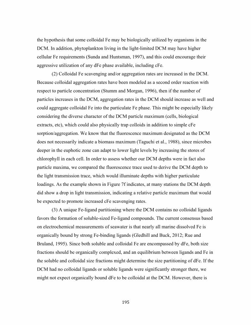
195
the hypothesis that some colloidal Fe may be biologically utilized by organisms in the
DCM. In addition, phytoplankton living in the light-limited DCM may have higher
cellular Fe requirements (Sunda and Huntsman, 1997), and this could encourage their
aggressive utilization of any dFe phase available, including cFe.
(2) Colloidal Fe scavenging and/or aggregation rates are increased in the DCM.
Because colloidal aggregation rates have been modeled as a second order reaction with
respect to particle concentration (Stumm and Morgan, 1996), then if the number of
particles increases in the DCM, aggregation rates in the DCM should increase as well and
could aggregate colloidal Fe into the particulate Fe phase. This might be especially likely
considering the diverse character of the DCM particle maximum (cells, biological
extracts, etc), which could also physically trap colloids in addition to simple cFe
sorption/aggregation. We know that the fluorescence maximum designated as the DCM
does not necessarily indicate a biomass maximum (Taguchi et al., 1988), since microbes
deeper in the euphotic zone can adapt to lower light levels by increasing the stores of
chlorophyll in each cell. In order to assess whether our DCM depths were in fact also
particle maxima, we compared the fluorescence trace used to derive the DCM depth to
the light transmission trace, which would illuminate depths with higher particulate
loadings. As the example shown in Figure 7f indicates, at many stations the DCM depth
did show a drop in light transmission, indicating a relative particle maximum that would
be expected to promote increased cFe scavenging rates.
(3) A unique Fe-ligand partitioning where the DCM contains no colloidal ligands
favors the formation of soluble-sized Fe-ligand compounds. The current consensus based
on electrochemical measurements of seawater is that nearly all marine dissolved Fe is
organically bound by strong Fe-binding ligands (Gledhill and Buck, 2012; Rue and
Bruland, 1995). Since both soluble and colloidal Fe are encompassed by dFe, both size
fractions should be organically complexed, and an equilibrium between ligands and Fe in
the soluble and colloidal size fractions might determine the size partitioning of dFe. If the
DCM had no colloidal ligands or soluble ligands were significantly stronger there, we
might not expect organically bound dFe to be colloidal at the DCM. However, there is

196
very little data on the size partitioning of Fe ligands, especially with sufficient depth
resolution to capture the DCM. The few size-fractionated Fe-ligand samples collected on
the GEOTRACES NAZT cruise show a predominance of soluble Fe ligands throughout
the entire upper ocean, with no particular change in ligand partitioning at the DCM
(Appendix III: Fitzsimmons et al., in prep-a). Thus, the existing data do not support the
hypothesis that ligand partitioning produces a unique dFe size partitioning at the DCM.
(4) Similar to a mechanism proposed for suspended particulate Fe (Ohnemus and
Lam, 2013), colloidal Fe "short-circuits" the DCM via transport in large sinking
aggregates. Suspended particulate Fe (pFe) also reaches a minimum in the DCM. This
might not be expected to occur if the absence of cFe was explained by biological uptake
or scavenging into the particulate phase (although the pFe minimum is non-zero and thus
may include scavenged or biologically utilized cFe, and thus we retain hypotheses 1-
2).Ohnemus and Lam (2013) proposed that a DCM pFe minimum results when dust-
derived pFe is incorporated into large aggregates in the mixed layer that sink through the
DCM to disaggregate below, resulting in low pFe in the DCM; importantly, this pattern
only results when the DCM is located below the mixed layer depth (excluding Line W
stations). Since the difference between colloidal (0.02-0.2 µm) and suspended particulate
(0.8-0.51 µm) Fe is operational (they are near each other in the Fe size spectrum), it is
possible that suspended particulate and colloidal Fe cycle similarly in the upper ocean
and that the lack of cFe is simply related to cFe aggregation into sinking particulates
above the DCM and disaggregation below it.
7.3.2.2 Remineralization - In order to assess the impact of remineralization on
dFe partitioning, we examined the relationship between dFe species and the apparent
oxygen utilization (AOU), which is a measure of the integrated oxygen loss due to
remineralization in a water parcel since it was last in contact with the atmosphere. We
show the correlation between dFe, cFe, and sFe with AOU in Figure 8 (Type-I
regressions) for Central Waters (potential density 25.8-27.1) and Intermediate Waters
(potential density 27.1-27.5) across the three North Atlantic sections: Line W (a), the
subtropical gyre (b), and the 2010 stations including the Mauritanian transect (c). We

197
then converted the resulting Fe:AOU slopes to Fe:C slopes using an AOU:C ratio of 1.6
(Martin et al., 1987), as in previous studies of dFe biogeochemistry in the North Atlantic
(Bergquist and Boyle, 2006; Fitzsimmons et al., 2013). The Fe:C (slope) and pre-formed
Fe (y-intercept) for both dFe and sFe are tabulated in Table 2.
Hatta et al. (in prep) showed that the dFe:C ratio was 7-8.5 µmol/mol in Central
Waters (mostly North Atlantic Central Water) and Intermediate Waters (Antarctic
Intermediate Water and Mediterranean Outflow Water) of the North Atlantic subtropical
gyre using data from the 2011 cruise (Figure 8 a-b, Table 2). In contrast, the dFe:C ratio
increased to >10 µmol/mol in the 2010 cruise samples along the eastern North Atlantic
and Mauritanian upwelling zone (Figure 8c, Table 2). By analogy to dFe:C, we might
have expected to observe a similar increase in sFe:C in the 2010 Mauritanian section
stations compared to the 2011 subtropical gyre, assuming the partitioning was similar in
the two regions. However, the results show that the sFe:C ratio was not significantly
different in the 2010 and 2011 subtropical gyre sections (Figure 8 b-c, Table 2). While
we cannot exclude the possibility that dFe size partitioning is truly different in the
Mauritanian section than in the gyre, we established previously (Section 7.3.1.2;
Fitzsimmons et al., 2013; Hatta et al., in prep) that in both regions dFe distributions are
controlled by remineralization, and thus the partitioning should be similar. Instead, we
attribute the similarity in sFe:C ratios to the smaller sFe pore size used to distinguish sFe
in 2010, which likely obscured the higher sFe:C near Mauritania (less sFe is observed
using the 2010 <10 kDa size cutoff than in the same water using the 2011 <0.02 µm
cutoff, Figure 5b). Nonetheless, we see a higher (though not significantly different) sFe:C
ratio of 4.72±0.53 in the Mauritanian transect (USGT10-09 through USGT10-12)
compared to the rest of the 2010 stations (sFe:C 4.27±0.35) in the Central Waters,
consistent with a similar increase in the dFe:C ratio (Table 2).
The ratio of sFe:C to dFe:C, however, provides useful information about the dFe
partitioning resulting from remineralization (tabulated in Table 2). While this ratio might
be interpreted as simply an average %sFe, it is actually a %sFeREMIN resulting from
remineralization, since any "pre-formed" sFe or dFe (the y-intercept of the Fe:AOU plot)

198
is not included in the slope-calculated percentage. Across the broadest swath of the North
Atlantic (2011 cruise, Figure 8b), the slope of the sFe-AOU plot produced a sFe:C ratio
of 4.13±0.27 µmol/mol that was almost exactly 50% of the dFe:C ratio of 8.18±0.42
µmol/mol. Thus, the %sFeREMIN of ~50% indicates that the partitioning resulting from
remineralization and the subsequent scavenging, ligand exchange and sorption/desorption
with the colloidal pool is is half of the dFe in the soluble phase and half in the colloidal
phase. Along the Line W section (Figure 8a), the %sFeREMIN was 41%, indicating that
remineralization and the summed re-partitioning afterward partitioned more dFe into the
colloidal size fraction than in the subtropical gyre. Finally, in the eastern North Atlantic
2010 cruise samples where the smaller 10kDa sFe-cFe size cutoff was used (Figure 8b),
the slope of the sFe-AOU plot produced a sFe:C ratio of 4.27±0.35 µmol/mol that was
~35% the dFe:C ratio, some of which is likely related to the smaller 10kDa sFe size
cutoff used on the 2010 cruise. These %sFeREMIN values in the Central and Intermediate
Waters fall within the total sub-DCM deep ocean dFe size partitioning distributions of
40-60% cFe in the 2011 abyssal ocean (Figure 2d) and 50-70% cFe in the Mauritanian
section (Figure 4d), indicating that remineralization and the re-partitioning processes
occurring immediately thereafter likely control the dFe partitioning in the abyssal ocean
away from new dFe inputs. We return to this idea in section 7.3.3.
The difference between %sFeREMIN and total %sFe in a given water mass is the
%sFe in the pre-formed fraction, which can be explored using the y-intercepts of the Fe-
AOU relationships. As can be seen in Table 2, the 2011 cruise Central Water was the
only water mass to have a statistically significant pre-formed dFe of 0.16 nmol/kg and
sFe of 0.07 nmol/kg. Central Waters along this transect are composed of Madeira Mode
Waters, which form southwest of Madeira, and 18° Mode Waters, which subduct in the
Sargasso Sea (Talley et al., 2011), and both regions receive Fe inputs from North African
dust plumes that could generate pre-formed dFe. NACW pre-formed Fe derived from the
upper portion of the water mass (upper-NACW: potential density 25.8-26.6 kg/m3), with
statistically insignificant pre-formed dFe below (lower-NACW: potential density range

199
26.6-27.1). It is noteworthy than the %sFePF pre-formed matched the %sFeREMIN within
error when pre-formed Fe was detectable (Table 2).
7.3.2.3 Deep ocean - The deep ocean circulation is described in Hatta et al. (in
prep) using the neutral density limits of LeBel et al. (2008), showing that the core of
NADW is in the depth range of 1000-4000m and is composed of four water masses:
Upper Labrador Sea Waters and Classical Labrador Sea Waters (1000-2000m), Iceland-
Scotland Overflow Waters (2000-3000m in the western basin, to the bottom in the eastern
basin), and Denmark Strait Overflow Waters (3000-4500m in the western basin only).
Typical NADW dFe concentrations were ~0.6 nmol/kg over these depths, with the
western margin CLSW, the TAG plume, and a portion of the Mauritanian OMZ carrying
higher dFe concentrations (Hatta et al., in prep). Soluble Fe along NADW was
consistently between 0.25-0.35 nmol/kg, agreeing well with the nearly-constant, ~0.30
nmol/kg sFe concentrations previously reported for NADW in the North Atlantic
(Fitzsimmons and Boyle, in review-b; Wu et al., 2001) through the South Atlantic
(Bergquist et al., 2007) and into the Southern Ocean (Chever et al., 2010). Similar to dFe,
enhanced sFe concentrations in NADW are attributed to the TAG plume at Stations
USGT11-14 and USGT11-16, CLSW along Line W, and the OMZ along the Mauritanian
section. As can be seen in Figure 2d, NADW dFe was on average 50% cFe (in white),
except along Line W in the CLSW trace eastward to USGT11-12 and at the TAG station
where colloidal Fe dominated.
At station USGT11-12 (Figure 9b), an AABW influence below 5000m depth is
evident by a drop in potential temperature below 1.8°C (McCartney, 1992) and elevated
concentrations of dissolved silica (53 µmol/kg). The relative contribution of DSOW and
AABW at these deepest depths is unclear, as some authors indicate a dominance of
AABW below ~4500m depth in the subtropics (LeBel et al., 2008; Tomczak and
Godfrey, 2003) and others estimate a much lower AABW contribution of only ~10%
(Johnson, 2008). Using a [Si] of ~120 µmol/kg in AABW and ~20 µmol/kg in NADW,
we calculate that the 5000+ m depths of USGT11-12 are comprised of ~33% AABW. In
these AABW-influenced waters, dFe dropped from ~0.52 nmol/kg in DSOW to ~0.43

200
nmol/kg, with the colloidal Fe component always staying constant at ~50% (52% in
DSOW, 46% in AABW depths). sFe concentrations below 5000m were 0.20-0.25
nmol/kg, which is lower than the 0.33 nmol/kg sFe found upstream in AABW-influenced
waters near 25°S (Bergquist et al., 2007), which are thought to have much less diluted
AABW according to their higher dissolved silicate concentration (118 µmol/kg) than the
USGT11-12 AABW samples (53 µmol/kg). The drop in sFe of 0.1 nmol/kg from 25°S to
30°N cannot be attributed solely to increasing dilution with DSOW because DSOW has a
higher sFe (0.25 nmol/kg) than the most dilute 30°N data deeper than 5000m (0.23
nmol/kg). This sFe decrease must also be attributed to scavenging or aggregation. Note
that cFe increased by the same ~0.10 nmol/kg that sFe decreased, from 0.10 nmol/kg at
25°S to ~0.20 nmol/kg at USGT11-12; this pattern points to a mechanism of
sorption/aggregation. In summary, in abyssal waters we find rather consistent %cFe
along NADW flow paths and decreasing cFe concentrations along AABW flow paths.
These patterns imply that transformations between soluble, colloidal, and particulate Fe
pools are dynamic in the deep ocean, involving active exchange between soluble and
colloidal pools via both aggregation and disaggregation, and thus calculations of the
scavenging residence times of individual Fe size fractions along these abyssal water
masses may be misleading.
7.3.3 Consensus on dFe size partitioning in the North Atlantic
The North Atlantic Ocean has been sampled more extensively for the size
fractionation of dFe into soluble and colloidal phases than any other ocean basin (see
global map of previous studies in Fitzsimmons and Boyle, in review-a), yet a consensus
on the factors controlling dFe size partitioning has not emerged. We believe that the U.S.
GEOTRACES NAZT captures most of the major dFe inputs into the North Atlantic that
might impact dFe partitioning and also provides the highest spatial and depth resolution
yet sampled for size fractionated dFe in the Atlantic. Thus, this GEOTRACES dataset is
optimally suited for updating conclusions about the processes controlling the size
partitioning of marine dFe in the Atlantic Ocean.

201
First, we review the findings of previous North Atlantic dFe size partitioning
studies (cruise locations indicated on the Figure 1 map). Bergquist et al. (2007) posited
that variability in the colloidal Fe phase was responsible for most of the variability in
North Atlantic dFe, while sFe remained relatively constant with depth at ~0.3 nmol/kg;
this partitioning pattern is apparent in a reproduction of their size fractionated dFe data in
Figure 10a (crosses), where dFe was well correlated with cFe but was not correlated with
invariant sFe. In contrast, over a larger swath of stations in the tropical North Atlantic,
Fitzsimmons and Boyle (in review-b) found that both sFe and cFe contributed dFe
variability (Figure 10b, open circles). They concluded that either the size partitioning of
organic Fe-binding ligands controlled the overall partitioning of dFe in the North Atlantic
or that North Atlantic dFe had a "steady state" dFe partitioning pattern overlain by a
series of Fe inputs with uniquely size-fractionated Fe.
To discriminate between these alternatives, we focused on correlations between
different dFe size fractions from the GEOTRACES transect for the 2011 (c-d) and 2010
(e) cruises (Figure 10, closed circles). Since both sFe and cFe increase as dFe increases,
both size fractions contribute to dFe variability, and thus we conclude that Bergquist et
al.’s hypothesis does not apply broadly across the North Atlantic. We also discount the
suggestion of Fitzsimmons and Boyle (in review-b) that the size partitioning of organic
Fe-binding ligands directly controls the size partitioning of dFe, since the excess ligand
partitioning at stations USGT11-10 and USGT11-23 did not match the observed
partitioning of dFe (Appendix III: Fitzsimmons et al., in prep-a). In fact, in those samples
the partitioning of excess Fe-binding ligands predicted a predominance of sFe at depths
where cFe clearly dominated dFe partitioning. Similar data from the North Atlantic by
Cullen et al. (2006) were interpreted as being caused by a missing "inert" colloidal Fe-
binding ligand fraction not detected electrochemically. Since the ligand partitioning
studies have been largely in the upper ocean where unique dFe partitioning exists
separate from the subsurface ocean, we must leave open the possibility that in the
intermediate and deep ocean ligand size partitioning does control dFe size partitioning.

202
However, the data reported thus far does not support this view (Boye et al., 2010; Cullen
et al., 2006; Thuróczy et al., 2010).
We propose a dFe partitioning model for all depths below the DCM (Figure 11a)
based on the hypothesis of Fitzsimmons and Boyle (in review-b) that there is a "steady
state" dFe partitioning into soluble and colloidal phases that is constant for a given
region. New dFe inputs cannot impart the constant dFe partitioning observed in the
subsurface ocean because most of the Fe inputs to the North Atlantic are heavily colloidal
(section 7.3.1), while the deep ocean has a near 50-50% sFe-cFe partitioning. Instead, we
know that deep water attains elevated dFe concentrations via remineralization. Thus, we
must consider whether remineralization directly partitions dFe equally into sFe and cFe
pools in the subtropical North Atlantic gyre. While we have no direct evidence against
this, any subsequent scavenging or exchange of Fe between size fractions would change
the observed dFe size partitioning, and the results in Figure 10b-e instead indicate a
constant subsurface partitioning in each region of the North Atlantic. Thus, we suggest
that the constant partitioning is driven by a "steady state" of the sum of dFe exchange
processes potentially following remineralization (including ligand exchange,
sorption/desorption, and aggregation/disaggregation, indicated with solid black arrows in
Figure 11a); in other words, the rates of these processes are constant and result in
constant partitioning. Thus, rather than dFe in a given seawater parcel having a fixed
concentration of sFe and a variable concentration of cFe that determines the magnitude of
dFe, the dFe in a given water parcel will have a fixed percentage of sFe and cFe set by
the relative rates of exchange between sFe and cFe fractions. This explains the near
constancy of the relative partitioning along water mass trajectories (as discussed in
section 7.3.2.3).
This "steady state" model of dFe partitioning is supported by the fact that the
%sFeREMIN derived from the Fe-AOU relationships (section 7.3.2.2) is very similar to the
total %sFe inferred from Figure 2d, and partitioning patterns and mechanisms in each of
the North Atlantic regions can be derived. Total %sFe below the DCM in the subtropical
gyre is ~50% (white in Figure 2d), which is the same as the ~50% sFeREMIN derived in
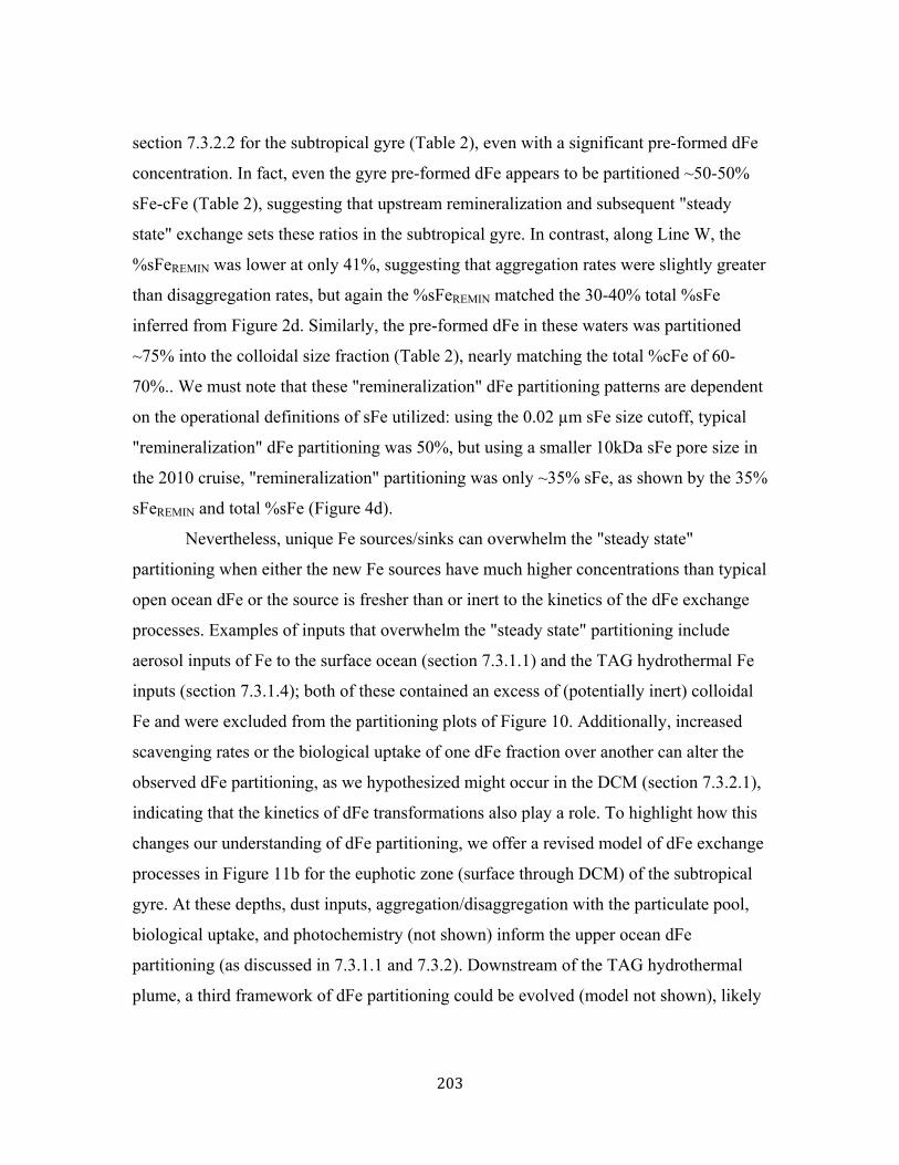
203
section 7.3.2.2 for the subtropical gyre (Table 2), even with a significant pre-formed dFe
concentration. In fact, even the gyre pre-formed dFe appears to be partitioned ~50-50%
sFe-cFe (Table 2), suggesting that upstream remineralization and subsequent "steady
state" exchange sets these ratios in the subtropical gyre. In contrast, along Line W, the
%sFeREMIN was lower at only 41%, suggesting that aggregation rates were slightly greater
than disaggregation rates, but again the %sFeREMIN matched the 30-40% total %sFe
inferred from Figure 2d. Similarly, the pre-formed dFe in these waters was partitioned
~75% into the colloidal size fraction (Table 2), nearly matching the total %cFe of 60-
70%.. We must note that these "remineralization" dFe partitioning patterns are dependent
on the operational definitions of sFe utilized: using the 0.02 µm sFe size cutoff, typical
"remineralization" dFe partitioning was 50%, but using a smaller 10kDa sFe pore size in
the 2010 cruise, "remineralization" partitioning was only ~35% sFe, as shown by the 35%
sFeREMIN and total %sFe (Figure 4d).
Nevertheless, unique Fe sources/sinks can overwhelm the "steady state"
partitioning when either the new Fe sources have much higher concentrations than typical
open ocean dFe or the source is fresher than or inert to the kinetics of the dFe exchange
processes. Examples of inputs that overwhelm the "steady state" partitioning include
aerosol inputs of Fe to the surface ocean (section 7.3.1.1) and the TAG hydrothermal Fe
inputs (section 7.3.1.4); both of these contained an excess of (potentially inert) colloidal
Fe and were excluded from the partitioning plots of Figure 10. Additionally, increased
scavenging rates or the biological uptake of one dFe fraction over another can alter the
observed dFe partitioning, as we hypothesized might occur in the DCM (section 7.3.2.1),
indicating that the kinetics of dFe transformations also play a role. To highlight how this
changes our understanding of dFe partitioning, we offer a revised model of dFe exchange
processes in Figure 11b for the euphotic zone (surface through DCM) of the subtropical
gyre. At these depths, dust inputs, aggregation/disaggregation with the particulate pool,
biological uptake, and photochemistry (not shown) inform the upper ocean dFe
partitioning (as discussed in 7.3.1.1 and 7.3.2). Downstream of the TAG hydrothermal
plume, a third framework of dFe partitioning could be evolved (model not shown), likely
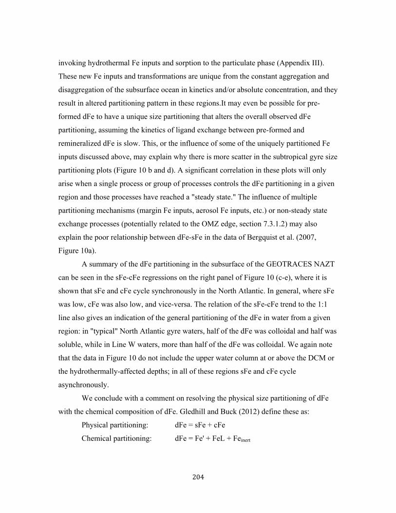
204
invoking hydrothermal Fe inputs and sorption to the particulate phase (Appendix III).
These new Fe inputs and transformations are unique from the constant aggregation and
disaggregation of the subsurface ocean in kinetics and/or absolute concentration, and they
result in altered partitioning pattern in these regions.It may even be possible for pre-
formed dFe to have a unique size partitioning that alters the overall observed dFe
partitioning, assuming the kinetics of ligand exchange between pre-formed and
remineralized dFe is slow. This, or the influence of some of the uniquely partitioned Fe
inputs discussed above, may explain why there is more scatter in the subtropical gyre size
partitioning plots (Figure 10 b and d). A significant correlation in these plots will only
arise when a single process or group of processes controls the dFe partitioning in a given
region and those processes have reached a "steady state." The influence of multiple
partitioning mechanisms (margin Fe inputs, aerosol Fe inputs, etc.) or non-steady state
exchange processes (potentially related to the OMZ edge, section 7.3.1.2) may also
explain the poor relationship between dFe-sFe in the data of Bergquist et al. (2007,
Figure 10a).
A summary of the dFe partitioning in the subsurface of the GEOTRACES NAZT
can be seen in the sFe-cFe regressions on the right panel of Figure 10 (c-e), where it is
shown that sFe and cFe cycle synchronously in the North Atlantic. In general, where sFe
was low, cFe was also low, and vice-versa. The relation of the sFe-cFe trend to the 1:1
line also gives an indication of the general partitioning of the dFe in water from a given
region: in "typical" North Atlantic gyre waters, half of the dFe was colloidal and half was
soluble, while in Line W waters, more than half of the dFe was colloidal. We again note
that the data in Figure 10 do not include the upper water column at or above the DCM or
the hydrothermally-affected depths; in all of these regions sFe and cFe cycle
asynchronously.
We conclude with a comment on resolving the physical size partitioning of dFe
with the chemical composition of dFe. Gledhill and Buck (2012) define these as:
Physical partitioning: dFe = sFe + cFe
Chemical partitioning: dFe = Fe' + FeL + Feinert

205
where dFe is categorized by size into soluble and colloidal phases (as in this study) and
by chemical composition as labile inorganic Fe complexes (Fe'), complexes of Fe to
organic ligands labile on the order of <1 day (FeL), and relatively refractory Fe
complexes (Feinert). Because different analytical methods are used to distinguish these two
dFe descriptions, it is difficult to reconcile them. However, it is reasonable to assume that
Fe' falls entirely into the soluble phase, FeL is found in both soluble and colloidal
fractions, and Feinert might encompass both size fractions as well, with very strongly-
bound FeL complexes of soluble size appearing inert and also inorganically-bound
colloidal Fe (Fe nanoparticles) appearing refractory by electrochemical speciation
techniques.
We raise this distinction because our data in the surface ocean and downstream of
TAG revealed an excess cFe pool that did not exchange with our "remineralization" dFe
partitioning, and we also found an excess of cFe along Line W that was different from the
subtropical gyre partitioning. While we know nothing about the chemical composition of
this cFe from the observed size partitioning alone, we do know that dFe in these locations
was derived from continental sources (see sections 7.3.1.1, 7.3.1.3, and 7.3.1.4), and thus
our data is consistent with a hypothesis that this additional colloidal Fe fraction may be
inorganic (nanoparticulate) Fe that is so small that it remains suspended in the dFe
(colloidal) phase. This nanoparticulate cFe might also be "inert" to biological processes
and even have separate exchange rates between the Fe size fractions than typical marine
dFe. Others have previously suggested that nanoparticulate dFe could be
stabilized/trapped inside colloidal-sized organics such as transparent exopolymer
compounds (Stolpe and Hassellov, 2010). While a nanoparticulate component to dFe
would be no surprise in hydrothermal plumes where nanoparticulate pyrite has already
been posited to exist in the dFe size fraction (Yucel et al., 2011), a significant
nanoparticulate component of dFe in the surface ocean or along Line W would contradict
the prevailing view that >99.9% of marine dFe is bound by organic ligands. However,
our hypothesis is consistent with Fe-ligand size partitioning studies in the surface North
Atlantic Ocean that report nearly no excess colloidal Fe ligands, despite there being a

206
surface excess of cFe over sFe (Cullen et al., 2006): potentially much of this "inert" cFe
is nanoparticulate Fe that does not have an "unbound" ligand pool capable of being
analyzed electrochemically (Appendix III: Fitzsimmons et al., in prep-a). With the size
partitioning data reported here, we cannot confirm a nanoparticulate dFe composition.
For confirmation, we look toward future analyses of the colloidal Fe phase by
synchrotron (similar to von der Heyden et al., 2012) and flow-field flow fractionation
methods (Stolpe et al., 2010) to resolve the physical and chemical classifications of dFe.
7.4. Conclusions
We sampled 28 stations across the North Atlantic Ocean for the size partitioning
of dFe into soluble and colloidal phases with the highest depth resolution explored to
date, and assisted by the multidimensional range of U.S. GEOTRACES tracers, we have
reached a new view of dFe partitioning in the North Atlantic Ocean. Previously dFe was
thought to have a constant soluble Fe concentration, while colloidal Fe was variable and
controlled the magnitude of the measured dFe concentration (Bergquist et al., 2007). sFe
was believed to be the more "nutrient-like" phase, while cFe had a more dynamic
distribution related to new Fe inputs. Following this, we expected to find a relatively
uniform sFe concentration in the intermediate and deep North Atlantic Ocean. Instead,
we found that both soluble and colloidal Fe were variable in the North Atlantic Ocean,
and both contributed to dFe variability, which we hypothesize occurs via a "steady state"
partitioning driven by constant exchange between the Fe pools following
remineralization. We observe a near 50-50% dFe partitioning into soluble (<0.02 µm)
and colloidal (0.02 - 0.2 µm) fractions in the subtropical gyre below the deep chlorophyll
maximum and a partitioning favoring 60% colloidal Fe along Line W. Using a smaller
definition of sFe (<10kDa), we found a 65% partitioning into colloidal Fe along the
eastern North Atlantic (2010 stations).

207
Several regions had clear exceptions to this "remineralization" dFe partitioning,
however, either because of a uniquely partitioned dFe source that overwhelmed the
"steady state" partitioning or because of the presence of a unique Fe partitioning process
or one with with unique kinetics. Examples of these exceptions include colloidal Fe
dominance in the surface ocean underlying the North African dust plume and in waters
downstream of the TAG hydrothermal plume. We suggest that there may be a significant
nanoparticulate (inorganic) cFe component in these continentally-derived Fe sources. In
contrast, colloidal Fe disappears in the deep chlorophyll maximum as a result of
increased cFe biological uptake and/or scavenging/aggregation to the particulate Fe phase
in upper ocean waters. Thus, we have found that sFe and cFe cycle synchronously
through much of the North Atlantic open ocean, except in the upper ocean and in regions
experiencing significant continental cFe inputs, where cFe cycles independently of sFe to
a large extent. This size partitioning should be incorporated into future models of dFe
biogeochemistry in order to better predict Fe limitation and downstream dFe
concentrations, since the two size fractions potentially behave uniquely during biouptake
and scavenging. We also look forward to future studies that better combine size
partitioning perspectives with analyses resolving the chemical composition of the dFe
pool in order to better constrain the composition and chemistry of the soluble and
colloidal Fe fractions.
208
References for Chapter 7
Aguilar-Islas, A.M., Wu, J., Rember, R., Johansen, A.M., Shank, L.M., 2010. Dissolution of
aerosol-derived iron in seawater: Leach solution chemistry, aerosol type, and colloidal iron fraction. Marine Chemistry 120 (1-4), 25-33.
Anderson, R.F., Fleisher, M., Hayers, C., Robinson, L., Huang, K.-F., Edwards, L., Cheng, H., Lu, Y., Moran, B., 2013. GA03: Dissolved and particulate 232Th, 230Th, and 231Pa: Tracers of TEI supply, removal, and internal cycling. U.S. GEOTRACES post-cruise data workshop, Old Dominion Unversity, Norfolk, VA.
Beaulieu, S.E., 2010. InterRidge Global Database of Active Submarine Hydrothermal Vent Fields: prepared for InterRidge, Version 2.0. http://www.interridge.org/IRvents.
Bergquist, B.A., Boyle, E.A., 2006. Dissolved iron in the tropical and subtropical Atlantic Ocean. Global Biogeochemical Cycles 20 (1), 14.
Bergquist, B.A., Wu, J., Boyle, E.A., 2007. Variability in oceanic dissolved iron is dominated by the colloidal fraction. Geochimica et Cosmochimica Acta 71 (12), 2960-2974.
Bhatia, M.P., Kujawinski, E.B., Das, S.B., Breier, C.F., Henderson, P.B., Charette, M.A., 2013. Greenland meltwater as a significant and potentially bioavailable source of iron to the ocean. Nature Geosci 6 (4), 274-278.
Bower, A., Lozier, S., Gary, S., 2011. Export of Labrador Sea Water from the subpolar North Atlantic: A Lagrangian perspective. Deep Sea Research Part II: Topical Studies in Oceanography 58 (17-18), 1798-1818.
Bower, A.S., Lozier, M.S., Gary, S.F., Boning, C.W., 2009. Interior pathways of the North Atlantic meridional overturning circulation. Nature 459 (7244), 243-247.
Bower, A.S., Rossby, H.T., Lillibridge, J.L., 1985. The Gulf Stream: Barrier or Blender? Journal of Physical Oceanography 15 (1), 24-32.
Boye, M., Nishioka, J., Croot, P., Laan, P., Timmermans, K.R., Strass, V.H., Takeda, S., de Baar, H.J.W., 2010. Significant portion of dissolved organic Fe complexes in fact is Fe colloids. Marine Chemistry 122 (1-4), 20-27.
Charette, M.A., Henderson, P., Morris, P., Moore, W.S., 2013. Radium isotope distributions: GEOTRACES NAT Legs 1 & 2 and historical data. U.S. GEOTRACES post-cruise data workshop, Old Dominion University, Norfolk, VA.
Chen, M., Dei, R.C.H., Wang, W.-X., Guo, L., 2003. Marine diatom uptake of iron bound with natural colloids of different origins. Marine Chemistry 81 (3-4), 177-189.
Chen, M., Wang, W.X., 2001. Bioavailability of natural colloid-bound iron to marine plankton: Influences of colloidal size and aging. Limnology and Oceanography 46 (8), 1956-1967.
Chever, F., Bucciarelli, E., Sarthou, G., Speich, S., Arhan, M., Penven, P., Tagliabue, A., 2010. Physical speciation of iron in the Atlantic sector of the Southern Ocean along a transect from the subtropical domain to the Weddell Sea Gyre. J. Geophys. Res. 115 (C10), C10059.
Chiba, H., Masuda, H., Lee, S., Y, Fujioka, K., 2001. Chemistry of hydrothermal fluids at the

209
TAG Active Mound, MAR 26°N, in 1998. Geophysical Research Letters 28 (15), 2919-2922.
Croot, P.L., Streu, P., Baker, A.R., 2004. Short residence time for iron in surface seawater impacted by atmospheric dry deposition from Saharan dust events. Geophysical Research Letters 31 (23), L23S08.
Cullen, J.T., Bergquist, B.A., Moffett, J.W., 2006. Thermodynamic characterization of the partitioning of iron between soluble and colloidal species in the Atlantic Ocean. Marine Chemistry 98 (2-4), 295-303.
Cutter, G.A., Bruland, K.W., 2012. Rapid and noncontaminating sampling system for trace elements in a global ocean surveys. Limnology & Oceanography: Methods 10, 425-436.
Fitzsimmons, J.N., Boyle, E.A., 2012. An intercalibration between the GEOTRACES GO-FLO and the MITESS/Vanes sampling systems for dissolved iron concentration analyses (and a closer look at adsorption effects). Limnology & Oceanography: Methods 10, 437-450.
Fitzsimmons, J.N., Boyle, E.A., in review-a. The assessment and intercalibration of Anopore™ and cross flow filtration methods for the determination of dissolved iron size fractionation into soluble/colloidal phases in seawater. Limnology & Oceanography: Methods.
Fitzsimmons, J.N., Boyle, E.A., in review-b. Both soluble and colloidal iron phases control dissolved iron variability in the tropical North Atlantic Ocean. Geochimica et Cosmochimica Acta.
Fitzsimmons, J.N., Bundy, R.M., Conway, T.M., John, S.G., Boyle, E.A., and others, in prep-a. The composition of dissolved iron in the dusty surface ocean: an exploration using size-fractionated iron-binding ligands and iron isotopes.
Fitzsimmons, J.N., Hatta, M., Measures, C.I., Sedwick, P.N., Boyle, E.A., and others, in prep-b. Iron chemistry near the TAG hydrothermal field. Geophysical Research Letters.
Fitzsimmons, J.N., Jenkins, W.J., Boyle, E.A., in review. Distal transport of dissolved hydrothermal iron in the deep South Pacific Ocean. Nature Geoscience.
Fitzsimmons, J.N., Zhang, R., Boyle, E.A., 2013. Dissolved iron in the tropical North Atlantic oxygen minimum zone. Marine Chemistry 154, 87-99.
Gledhill, M., Buck, K.N., 2012. The organic complexation of iron in the marine environment: a review. Frontiers in Microbiology 3, 69.
Gross, T.F., Williams, A.J., Newell, A.R.M., 1988. A deep-sea sediment transport storm. Nature 331 (6156), 518-521.
Hassler, C.S., Alasonati, E., Mancuso Nichols, C.A., Slaveykova, V.I., 2011a. Exopolysaccharides produced by bacteria isolated from the pelagic Southern Ocean: Role in Fe binding, chemical reactivity, and bioavailability. Marine Chemistry 123, 88-98.
Hassler, C.S., Schoemann, V., 2009. Bioavailability of organically bound Fe to model phytoplankton of the Southern Ocean. Biogeosciences 6 (10), 2281-2296.
Hassler, C.S., Schoemann, V., Nichols, C.M., Butler, E.C.V., Boyd, P.W., 2011b. Saccharides enhance iron bioavailability to Southern Ocean phytoplankton. Proceedings of the National Academy of Sciences 108 (3), 1076-1081.
Hatta, M., Measures, C.I., Wu, J., Fitzsimmons, J.N., and others, in prep. Dissolved Fe and Mn
210
concentrations in the North Atlantic Ocean during the U.S. GEOTRACES 2010-2011 cruises. Deep-Sea Research II.
Honeyman, B.D., Santschi, P.H., 1989. A Brownian-pumping model for oceanic trace metal scavenging: Evidence from Th isotopes. Journal of Marine Research 47, 951-992.
Hutchins, D.A., Witter, A.E., Butler, A., Luther III., G.W., 1999. Competition among marine phytoplankton for different chelated iron species. Nature 400, 858-861.
Jickells, T.D., An, Z.S., Andersen, K.K., Baker, A.R., Bergametti, G., Brooks, N., Cao, J.J., Boyd, P.W., Duce, R.A., Hunter, K.A., Kawahata, H., Kubilay, N., laRoche, J., Liss, P.S., Mahowald, N., Prospero, J.M., Ridgwell, A.J., Tegen, I., Torres, R., 2005. Global iron connections between desert dust, ocean biogeochemistry, and climate. Science 308 (5718), 67-71.
Johnson, G.C., 2008. Quantifying Antarctic Bottom Water and North Atlantic Deep Water volumes. Journal of Geophysical Research: Oceans 113 (C5), C05027.
Joyce, T.M., Dunworth-Baker, J., Pickart, R.S., Torres, D., Waterman, S., 2005. On the Deep Western Boundary Current south of Cape Cod. Deep-Sea Research II 52, 615-625.
Lam, P.J., Ohnemus, D.C., 2013. Size-fractionated particle mass and composition during the U.S. GEOTRACES North Atlantic Zonal Transect. U.S. GEOTRACES post-cruise data workshop, Old Dominion University, Norfolk, VA.
Lannuzel, D., Schoemann, V.r., de Jong, J., Tison, J.-L., Chou, L., 2007. Distribution and biogeochemical behaviour of iron in the East Antarctic sea ice. Marine Chemistry 106 (1-2), 18-32.
LeBel, D.A., Smethie Jr, W.M., Rhein, M., Kieke, D., Fine, R.A., Bullister, J.L., Min, D.-H., Roether, W., Weiss, R.F., Andrie, C., Smythe-Wright, D., Peter Jones, E., 2008. The formation rate of North Atlantic Deep Water and Eighteen Degree Water calculated from CFC-11 inventories observed during WOCE. Deep Sea Research Part I: Oceanographic Research Papers 55 (8), 891-910.
Lee, J.-M., Boyle, E.A., Echegoyen-Sanz, Y., Fitzsimmons, J.N., Zhang, R., Kayser, R.A., 2011. Analysis of trace metals (Cu, Cd, Pb, and Fe) in seawater using single batch Nitrilotriacetate resin extraction and isotope dilution inductively coupled plasma mass spectrometry. Analytica Chimica Acta 686, 93-101.
Mahowald, N., Baker, A.R., Bergametti, G., Brooks, N., Duce, R.A., Jickells, T., Kubilay, N., Prospero, J.M., Tegen, I., 2005. Atmospheric global dust cycle and iron inputs to the ocean. Global Biogeochemical Cycles 19, GB4025.
Martin, J.H., Knauer, G.A., Karl, D.M., Broenkow, W.W., 1987. VERTEX: carbon cycling in the northeast Pacific. Deep Sea Research Part A. Oceanographic Research Papers 34 (2), 267-285.
McCartney, M.S., 1992. Recirculating components to the deep boundary current of the northern North Atlantic. Progress in Oceanography 29, 283-383.
Measures, C.I., Landing, W.M., Brown, M.T., Buck, C.S., 2008. High-resolution Al and Fe data from the Atlantic Ocean CLIVAR-CO2 Repeat Hydrography A16N transect: Extensive linkages between atmospheric dust and upper ocean geochemistry. Global Biogeochem. Cycles 22, GB1005.

211
Moffett, J.W., 2001. Transformations among different forms of iron in the ocean. In: Turner, D.R., Hunter, K.A. (Eds.), The Biogeochemistry of Iron in Seawater. John Wiley & Sons, West Sussex, England, pp. 343-372.
Moore, J.K., Doney, S.C., Glover, D.M., Fung, I.Y., 2002. Iron cycling and nutrient-limitation patterns in surface waters of the World Ocean. Deep Sea Research Part II: Topical Studies in Oceanography 49 (1-3), 463-507.
Morel, F.M.M., Milligan, A.J., Saito, M.A., 2003. Marine Bioinorganic Chemistry: The Role of Trace Metals in the Oceanic Cycles of Major Nutrients. In: Turekian, K.K., Holland, H.D. (Eds.), Treatise On Geochemistry. Elsevier Science Ltd., Cambridge, United Kingdom, pp. 113-143.
Nishioka, J., Takeda, S., Wong, C.S., 2001a. Change in the concentrations of iron in different size fractions during a phytoplankton bloom in controlled ecosystem enclosures. Journal of Experimental Marine Biology and Ecology 258 (2), 237-255.
Nishioka, J., Takeda, S., Wong, C.S., Johnson, W.K., 2001b. Size-fractionated iron concentrations in the northeast Pacific Ocean: distribution of soluble and small colloidal iron. Marine Chemistry 74 (2-3), 157-179.
Ohnemus, D.C., Lam, P.J., 2013. Particulate metals in the North Atlantic GEOTRACES section. U.S. GEOTRACES post-cruise data workshop, Old Dominion University, Norfolk, VA.
Rich, H.W., Morel, F.M.M., 1990. Availability of well-defined iron colloids to the marine diatom Thalassiosira weissflogii. Limnology and Oceanography 35 (3), 652-662.
Rijkenberg, M.J.A., Powell, C.F., Dall'Osto, M., Nielsdottir, M.C., Patey, M.D., Hill, P.G., Baker, A.R., Jickells, T.D., Harrison, R.M., Achterberg, E.P., 2008. Changes in iron speciation following a Saharan dust event in the tropical North Atlantic Ocean. Marine Chemistry 110 (1-2), 56-67.
Rijkenberg, M.J.A., Steigenberger, S., Powell, C.F., Haren, H.v., Patey, M.D., Baker, A.R., Achterberg, E.P., 2012. Fluxes and distribution of dissolved iron in the eastern (sub-) tropical North Atlantic. Global Biogeochemical Cycles 26, GB3004.
Rona, P.A., Klinkhammer, G., Nelsen, T.A., Trefry, J.H., Elderfield, H., 1986. Black smokers, massive sulphides and vent biota at the Mid-Atlantic Ridge. Nature 321 (6065), 33-37.
Roy, E.G., Wells, M.L., King, D.W., 2008. Persistence of iron(II) in surface waters of the western subarctic Pacific. Limnology and Oceanography 53 (1), 89-98.
Rue, E.L., Bruland, K.W., 1995. Complexation of iron(III) by natural organic ligands in the Central North Pacific as determined by a new competitive ligand equilibration/adsorptive cathodic stripping voltammetric method. Marine Chemistry 50 (1-4), 117-138.
Scholz, F., Hensen, C., Severmann, S., Noffke, A., Haley, B., McManus, J., Schneider, R., Wallmann, K., 2012. Spatial and temporal trends of iron and iron isotope cycling in the Peruvian Oxygen Minimum Zone. Mineralogical Magazine 76 (6), 2343.
Sedwick, P.N., Sohst, B., Bowie, A., 2013. U.S. GEOTRACES North Atlantic section: Dissolved Fe and Fe(II). U.S. GEOTRACES post-cruise data workshop, Old Dominion University, Norfolk, VA.
Shelley, R.U., Landing, W., 2013. North Atlantic aerosol TEIs. U.S. GEOTRACES post-cruise data workshop, Old Dominion University, Norfolk, VA.

212
Smethie, W., Gorman, E., Lee, H., 2013. SF6 and CFC measurements on the U.S. North Atlantic GEOTRACES cruises. U.S. GEOTRACES post-cruise data workshop, Old Dominion University, Nofolk, VA.
Stolpe, B., Guo, L., Shiller, A.M., Hassellöv, M., 2010. Size and composition of colloidal organic matter and trace elements in the Mississippi River, Pearl River and the northern Gulf of Mexico, as characterized by flow field-flow fractionation. Marine Chemistry 118 (3-4), 119-128.
Stolpe, B., Hassellov, M., 2010. Nanofibrils and other colloidal biopolymers binding trace elements in coastal seawater: Significance for variations in element size distributions. Limnology & Oceanography 55 (1), 187-202.
Stumm, W., Morgan, J.J., 1996. Aquatic Chemistry: Chemical Equilibria and Rates in Natural Waters. John Wiley & Sons, New York.
Sunda, W.G., Huntsman, S.A., 1997. Interrelated influence of iron, light and cell size on marine phytoplankton growth. Nature 390, 389-392.
Taguchi, S., DiTullio, G.R., Laws, E.A., 1988. Physiological characteristics and production of mixed layer and chlorophyll maximum phytoplankton populations in the Caribbean Sea and western Atlantic Ocean. Deep Sea Research Part A. Oceanographic Research Papers 35 (8), 1363-1377.
Talley, L.D., McCartney, M.S., 1982. Distribution and circulation of Labrador Sea Water. Journal of Physical Oceanography 12, 1189-1205.
Talley, L.D., Pickard, G.L., Emery, W.J., Swift, J.H., 2011. Descriptive Physical Oceanography. Elsevier Ltd.
Taylor, S.R., McLennan, S.M., 1985. The Continental Crust: Its Composition and Evolution. Blackwell, Malden, MA.
Thuróczy, C.E., Gerringa, L.J.A., Klunder, M.B., Middag, R., Laan, P., Timmermans, K.R., de Baar, H.J.W., 2010. Speciation of Fe in the Eastern North Atlantic Ocean. Deep Sea Research Part I: Oceanographic Research Papers 57 (11), 1444-1453.
Tomczak, M., Godfrey, J.S., 2003. Regional Oceanography: An Introduction. Published online. Toner, B.M., Fakra, S.C., Manganini, S.J., Santelli, C.M., Marcus, M.A., Moffett, J., Rouxel, O.,
German, C.R., Edwards, K.J., 2009. Preservation of iron(II) by carbon-rich matrices in a hydrothermal plume. Nature Geoscience 2 (3), 197-201.
Toner, B.M., Marcus, M.A., Edwards, K.J., Rouxel, O., German, C.R., 2012. Measuring the form of iron in hydrothermal plume particles. Oceanography 25 (1), 209-212.
Ussher, S.J., Achterberg, E.P., Sarthou, G., Laan, P., de Baar, H.J.W., Worsfold, P.J., 2010. Distribution of size fractionated dissolved iron in the Canary Basin. Marine Environmental Research 70 (1), 46-55.
Ussher, S.J., Yaqoob, M., Achterberg, E.P., Nabi, A., Worsfold, P.J., 2005. Effect of Model Ligands on Iron Redox Speciation in Natural Waters Using Flow Injection with Luminol Chemiluminescence Detection. Analytical Chemistry 77 (7), 1971-1978.
von der Heyden, B.P., Roychoudhury, A.N., Mtshali, T.N., Tyliszczak, T., Myneni, S.C.B., 2012. Chemically and Geographically Distinct Solid-Phase Iron Pools in the Southern Ocean. Science 338 (6111), 1199-1201.
213
Wang, W.X., Dei, R.C.H., 2003. Bioavailability of iron complexed with organic colloids to the cyanobacteria Synechococcus and Trichodesmium. Aquatic Microbial Ecology 33, 247-259.
Wells, M.L., Goldberg, E.D., 1992. Marine submicron particles. Marine Chemistry 40, 5-18. Wells, M.L., Goldberg, E.D., 1994. The distribution of colloids in the North Atlantic and
Southern Oceans. Limnology and Oceanography 39 (2), 286-302. Wu, J., Boyle, E.A., 1998. Determination of iron in seawater by high-resolution isotope dilution
inductively coupled plasma mass spectrometry after Mg(OH)2 coprecipitation. Analytica Chimica Acta 367 (1-3), 183-191.
Wu, J., Boyle, E.A., Sunda, W.G., Wen, L., 2001. Soluble and colloidal iron in the oligotrophic North Atlantic and North Pacific. Science 293, 847-849.
Yucel, M., Gartman, A., Chan, C.S., Luther, G.W., 2011. Hydrothermal vents as a kinetically stable source of iron-sulphide-bearing nanoparticles to the ocean. Nature Geoscience 4, 367-371.

214
Figure 1: Station map. Stations from the 2010 cruise are shown in red, and stations from the 2011 cruise are in blue. The TENATSO crossover station was occupied on both cruises (station USGT10-12 and station USGT11-24). The locations of the Line W stations (USGT11-2 through USGT11-8), BATS station (USGT11-10), TAG hydrothermal station (USGT11-16), and the Mauritanian transect (USGT10-09 through USGT10-12) are also indicated. Stations from the literature that are referenced in this paper are also indicated as open symbols (Bergquist et al., 2007; Fitzsimmons and Boyle, in review-b).

215

216
Figure 2: Sections from the 2011 cruise of (a) dissolved Fe <0.2µm analyzed by the Mg co-precipitation method of Wu and Boyle (1998), (b) soluble Fe <0.02µm analyzed by the NTA method of Lee et al. (2011), (c) colloidal Fe calculated as dFe-sFe, and (d) %cFe calculated as cFe/dFe. Station numbers are shown at the bottom of each panel.
Figure 3: Surface dFe partitioning and Fe(II) concentrations as a function of longitude from (a) the 2011 cruise and (b) the 2010 cruise. Colloidal Fe can be calculated as dFe - sFe; recall that sFe is defined as <0.02 µm in (a) and <10 kDa in (b). In (b), the gray points at -22°W are from USGT10-07, which lies somewhat north of the other three stations indicated (Mauritanian transect USGT10-10 through USGT10-12). Error bars show ±1 standard deviation error on analytical replicates.
0.0
0.2
0.4
0.6
0.8
1.0
1.2
‐80 ‐70 ‐60 ‐50 ‐40 ‐30 ‐20
Surface [Fe] (nmol/kg)
Longitude (°W)
GEOTRACES 2011
dFe
sFe
cFe
0.0
0.2
0.4
0.6
0.8
1.0
1.2
‐26 ‐24 ‐22 ‐20
[Fe] (nmol/kg)
Longitude (°W)
GEOTRACES 2010
dFe
sFe
Station: 2 8 10 12 14 16 18 22 24 Station: 12 11 7 10
(a) (b)

217
Figure 4: Sections from the 2010 cruise along the Mauritanian transect of (a) dissolved Fe <0.2µm, (b) soluble Fe <0.02µm, (c) colloidal Fe calculated as dFe-sFe, and (d) %cFe calculated as cFe/dFe. Station numbers are shown at the bottom of each panel.

218
Figure 5: A comparison of dFe size partitioning during the two years of cruises at TENATSO. (a) dFe (<0.2 µm) over the two years. (b) sFe over the two years, with the 2010 sampling occurring by CFF (<10 kDa) and the 2011 sampling occurring by Anopore filtration (<0.02 µm). (c) A ratio of the 2010 sFe collected by CFF divided by the 2011 sFe collected by Anopore filtration. Depths where this ratio is particularly low indicate depths where there is a significant component of dFe in the 10kDa - 0.02µm size fraction. The dotted line at 70m is the deep chlorophyll maximum as recorded by the CTD fluorometer, and the shaded region includes depths where the dissolved oxygen concentration is <100 µmol/kg (the OMZ). Error bars indicate ±1 standard deviation in replicate analyses of the same sample.
0
500
1000
1500
2000
2500
3000
3500
0.0 0.5 1.0 1.5
Depth (m)
dFe (nmol/kg)
2010
2011
(b)(a)
0% 20% 40% 60% 80% 100% 120%
sFe CFF/Anopore
0.0 0.2 0.4 0.6 0.8
sFe (nmol/kg)
2010 ‐CFF
2011 ‐Anopore
(c)

219
Figure 6: dFe speciation and size partitioning at station USGT11-14, which is ~500km to the northwest of the TAG site. The USGT11-16 hydrothermal maximum dFe partitioning data is discussed separately in Fitzsimmons et al. (in prep-b). Colloidal Fe (cFe) can be taken as the difference between dFe and sFe points at any depth. sFe comprises 9-18% of the dFe at USGT11-14, compared to only 4-11% of the dFe at TAG USGT11-16.
0
500
1000
1500
2000
2500
3000
3500
4000
4500
0 0.2 0.4 0.6 0.8 1 1.2 1.4Depth (m
)[Fe] nmol/kg
USGT11‐14
dFe
sFe

220
Figure 7: The speciation and size distribution of dissolved Fe in the upper 200m on (a-c) the 2011 cruise where sFe is defined as <0.02 µm and on (d-e) the 2010 cruise where sFe is defined as <10kDa. The deep chlorophyll maximum (DCM) is designated as the fluorescence maximum in grey. Note that colloidal Fe (dFe - sFe) goes to zero at the DCM, except along the western North Atlantic margin (a, USGT11-06). Not surprisingly, the DCM also appears to be a depth of maximum particle loading, as the light transmission shows a coincident minimum with the DCM at many stations (f).
0 0.2 0.4 0.6
4.4 4.5 4.6 4.7
Fluorescence
Transmissometry (V)
USGT10‐09
0 0.2 0.4 0.6
0.0 0.3 0.6 0.9 1.2 1.5 1.8
Fluorescence
Fe (nmol/kg)
USGT10‐09
dFe
sFe
0 0.1 0.2
0
20
40
60
80
100
120
140
160
180
200
0.0 0.1 0.2 0.3
Fluorescence
Depth (m
)
Fe (nmol/kg)
USGT10‐05
dFe
sFe
0 0.05 0.1 0.15
0.0 0.2 0.4 0.6
Fluorescence
Fe (nmol/kg)
USGT11‐20
dFe
sFe
0 0.05 0.1 0.15
0.0 0.2 0.4 0.6 0.8 1.0
Fluorescence
Fe (nmol/kg)
USGT11‐16 (TAG)
dFe
sFe
0 0.05 0.1 0.15 0.2
0
20
40
60
80
100
120
140
160
180
200
0.0 0.2 0.4 0.6 0.8
Fluorescence
Depth (m
)
Fe (nmol/kg)
USGT11‐06
dFe
sFe
(a) (b) (c)
(e) (f)(d)

221
Figure 8: dFe partitioning resulting from remineralization in the Central Water layer (potential density layer 25.8-27.1 kg/m3), shown as a function of AOU for (a) Line W USGT11-02 to -08 where the sFe size cutoff is 0.02 µm, (b) the subtropical gyre stations USGT11-10 to -24 where the sFe size cutoff is 0.02 µm, and (c) the 2010 cruise stations USGT10-07 to -12 where the sFe size cutoff is 10kDa. Filled circles show dFe (<0.2 µm), open circles show sFe (<0.02 µm in (a-b), <10 kDa in (b)), and crosses show cFe (dFe - sFe). sFe and cFe each contribute ~50% to the dFe:AOU ratio in the subtropical gyre, while sFe contributes only ~35-40% in the 2010 cruise and Line W sections.
dFe:C = 8.18
sFe:C = 4.13
cFe:C = 4.130.0
0.4
0.8
1.2
1.6
0 50 100 150 200 250
Fe nmol/kg
AOU µmol/kg
dFe:C = 12.24
sFe:C = 4.27
cFe:C = 8.16
0.0
0.5
1.0
1.5
2.0
0 50 100 150 200 250 300
Fe nmol/kg
AOU µmol/kg
dFe:C = 8.32
sFe:C = 3.52
cFe:C = 4.96
0.0
0.4
0.8
1.2
0 50 100 150 200
Fe nmol/kg
AOU µmol/kg
(a)Line W
USGT11‐02 to ‐08
Subtropical GyreUSGT11‐10 to ‐24
(b)
2010 cruiseUSGT10‐07 to ‐12
(c)

222
Figure 9: Full-depth ocean profiles of dissolved Fe (<0.2 µm, closed circles) and soluble Fe (<0.02 µm). Station locations are (a) USGT11-06, (b) USGT11-10 (BATS), and (c) USGT11-20. Note that the depth range in (c) is different than in (a-b).
0
500
1000
1500
2000
2500
3000
3500
4000
4500
5000
0 0.25 0.5 0.75 1
Depth (m)
[Fe] nmol/kg
USGT11‐06
dFe
sFe
0
1000
2000
3000
4000
5000
6000
0 0.25 0.5 0.75 1
Depth (m)
[Fe] nmol/kg
USGT11‐12
dFe
sFe
0
1000
2000
3000
4000
5000
6000
0 0.25 0.5 0.75 1
Depth (m)
[Fe] nmol/kg
USGT11‐20
dFe
sFe
(a) (b) (c)
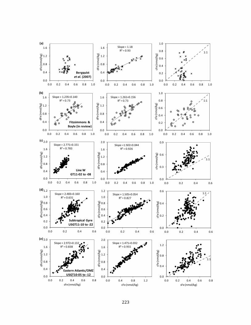
223
Slope = 1.235±0.140R² = 0.73
0.0
0.4
0.8
1.2
1.6
0.0 0.2 0.4 0.6 0.8 1.0
dFe (nmol/kg)
Slope = 1.261±0.156R² = 0.73
0.0
0.4
0.8
1.2
1.6
0.0 0.2 0.4 0.6 0.8 1.0
dFe (nmol/kg)
0.0
0.2
0.4
0.6
0.8
1.0
0.0 0.2 0.4 0.6 0.8 1.0
cFe (nmol/kg)
(b)
1:1
Fitzsimmons &Boyle (in review)
0.0
0.4
0.8
1.2
0.0 0.2 0.4 0.6 0.8
cFe (nmol/kg)
sFe (nmol/kg)
Slope = 2.972±0.132 R² = 0.838
0.0
0.4
0.8
1.2
1.6
2.0
0.0 0.2 0.4 0.6 0.8
dFe (nmol/kg)
sFe (nmol/kg)
Slope = 1.471±0.032R² = 0.955
0.0
0.4
0.8
1.2
1.6
2.0
0.0 0.4 0.8 1.2
dFe (nmol/kg)
cFe (nmol/kg)
0.0
0.2
0.4
0.6
0.0 0.2 0.4 0.6
cFe (nmol/kg)
Slope = 2.483±0.160R² = 0.631
0.0
0.2
0.4
0.6
0.8
1.0
1.2
0.0 0.2 0.4 0.6
dFe (nmol/kg)
Slope = 1.505±0.054R² = 0.827
0.0
0.2
0.4
0.6
0.8
1.0
1.2
0.0 0.2 0.4 0.6
dFe (nmol/kg)
Slope =1.502±0.044R² = 0.926
0.0
0.4
0.8
1.2
1.6
2.0
0.0 0.2 0.4 0.6 0.8 1.0
dFe (nmol/kg)
Slope = 2.771±0.151R² = 0.783
0.0
0.4
0.8
1.2
1.6
2.0
0.0 0.2 0.4 0.6 0.8 1.0
dFe (nmol/kg)
0.0
0.3
0.6
0.9
0.0 0.2 0.4 0.6
cFe (nmol/kg)
0.0
0.4
0.8
1.2
1.6
0.0 0.2 0.4 0.6 0.8 1.0
dFe (nmol/kg)
Slope = 1.18R² = 0.93
0.0
0.4
0.8
1.2
1.6
0.0 0.2 0.4 0.6 0.8 1.0
dFe (nmol/kg)
0.0
0.2
0.4
0.6
0.8
1.0
0.0 0.2 0.4 0.6 0.8 1.0
cFe (nmol/kg)
(a)
(c)
Line WGT11‐02 to ‐08
Subtropical GyreUSGT11‐10 to ‐22
(d)
Eastern Atlantic/OMZUSGT10‐05 to ‐12
(e)
1:1
1:1
1:1
1:1
Bergquistet al. (2007)

224
Figure 10: Relationships between dFe, sFe, and cFe in (a) Bergquist et al. (2007), (b) Fitzsimmons and Boyle (in review-b), (c) Line W stations USGT11-02 through USGT11-08, (d) North Atlantic subtropical gyre stations USGT11-10 through USGT11-22, and (e) stations USGT10-05 through USGT10-12 from the 2010 eastern North Atlantic cruise including the Mauritanian/OMZ section. Only depths below the deep chlorophyll maximum are included, station USGT11-16 is excluded altogether, as well as the TAG-influenced depths at Station USGT11-14. Regressions are Type-II regressions, and in (a) the regressions are taken from Bergquist et al. (2007). The dashed line on the right panels shows the 1:1 sFe:cFe line.

225
(a) Fe exchange model for the subsurface ocean: sFe and cFe cycle synchronously
(b) Fe exchange model for the upper ocean: sFe and cFe cycle independently
Figure 11: Model of Fe size partitioning, focused on the processes controlling dFe partitioning into soluble and colloidal fractions (box size has no relation to relative Fe pool size in this figure) for (a) the subsurface ocean (below the deep chlorophyll maximum) and (b) the upper ocean (surface through the deep chlorophyll maximum). Measurable quantities are shown in the gray rectangles (sFe, cFe, dFe, pFe), and exchange rates are shown as arrows. The black arrows and bolded processes indicate the mechanism(s) driving the dominant partitioning pattern expressed in the partitioning plots of Figure 10 for each depth range.
CELL
SOLUBLE IRON
COLLOIDAL IRON
External dissolved iron inputs(dust, resuspended sediments,
hydrothermal vents, etc.)
BiouptakeRemineralization
Ligand Exchange
DISSO
LVED
IRON
DISSO
LVED
IRON
PARTICULATE IRON
PARTICULATE IRON
Amorphous/crystalline material,particulate‐sized organic material
AggregationDisaggregation
Aggregation
DisaggregationSorption
Desorption
SorptionDesorption

226
Parameter or SRM Consensus [Fe] [dFe] 2010 [sFe] 2011 [sFe]
Procedure blank range
-- 0.078±0.008
(n=11 sessions) 0.009-0.019
(n=11 sessions) 0.006-0.026
(n=18 sessions)
Detection limit (3σ) -- 0.03-0.05 0.027 0.030
SAFe D2 0.90±0.02 0.950±0.035 0.931±0.046
(n=28) 0.930±0.042
(n=43)
SAFe surface underway (Boyle-lab
internal standard)
0.093±0.008 (assume SAFe S)
-- 0.083±0.035
(n=39) 0.079±0.050
(n=73)
SAFe S 0.093±0.008 0.103±0.010 --
0.094±0.007 (n=3)
0.108±0.002 (n=3)
Table 1: Reported procedure blanks, detection limits, and comprehensive lab analyses of the SAFe standard reference materials over the analytical sessions. dFe concentrations were analyzed in the Wu laboratory at RSMAS by the method described in Wu and Boyle (1998). sFe concentrations were analyzed in the Boyle laboratory at MIT by the methods described in Lee et al. (2011). All Fe concentrations are in units of nmol/kg, and consensus values are taken from http://www.geotraces.org/science/intercalibration as of May 2013. The detection limit is calculated as three times the standard deviation of the procedure blank for each analytical session.

227
Water mass: σθ (kg/m3)
Year Sta.
Dissolved Fe Soluble Fe %sFeREM
dFe:C (µmol/mol)
Pre-formed dFe
(nmol/kg)
sFe:C (µmol/mol)
Pre-formed sFe
(nmol/kg)
sFe:C / dFe:C
Central Water:
25.8-27.1
2010 5-12 12.24 ± 0.78 0 4.27 ± 0.35 0 34.9% 9-12 13.50 ± 1.40 0 4.72 ± 0.53 0 35.0%
2011 1-24 8.18 ± 0.42 0.16 ± 0.02 4.13 ± 0.27 0.07 ± 0.01 50.5% 1-8 8.38 ± 0.87 0.20 ± 0.04 3.46 ± 0.46 0.05 ± 0.02 41.3%
10-24 8.04 ± 0.46 0.14 ± 0.02 4.17 ± 0.28 0.08 ± 0.01 51.9%
Intermed Waters:
27.1-27.5
2010 5-12 12.68 ± 2.86 0 4.99 ± 1.12 0 39.4% 9-12 - 0 - 0
2011 1-24 6.78 ± 1.44 0 4.82 ± 0.78 0 71.1% 1-8 - 0 - 0
10-24 8.57 ± 1.05 0 4.52 ± 0.84 0 52.7%
Table 2: dFe:C and sFe:C relationships (in µmol/mol ) and pre-formed dFe and sFe (in nmol/kg) for various water masses. The %sFeREMIN attributed to remineralization is calculated as the ratio of sFe:C to dFe:C. The cruise year and stations used are designated. Fe:C values are calculated from a Type-I regression of Fe and AOU, and the Fe:AOU slope was converted to an Fe:C using the AOU:C ratio of 1.6 (Martin et al., 1987). Error values are ±1 standard error from the calculated regression.

228

229
Appendix I
Dissolved iron distribution, size partitioning, and stable isotopes in the Southeast Pacific Ocean Collaborators: Jong-Mi Lee, Rick Kayser, Edward Boyle, Timothy Conway, Seth John The Southeast Pacific Ocean is one of the most understudied regions of the global ocean, yet it encompasses enormous biogeochemical diversity (CLAUSTRE et al., 2008). Two opposing biogeochemical regimes share this region: the Southeast Pacific subtropical gyre and the permanent upwelling and oxygen minimum zone (OMZ) occurring along the Chilean cost. The Southeast Pacific subtropical gyre is the largest of the world's gyres and also the most oligotrophic, with the lowest marine chlorophyll-a concentrations ever reported (0.019 mg Chl-a m-3) found near Eastern Island (CLAUSTRE et al., 2008). In contrast, the wind-driven upwelling along the Chilean coast fuels some of the highest rates of primary production in the ocean (CARR, 2001). This organic material sinks and is remineralized at high rates, depleting the oxygen inventory, which combined with poor ventilation produces an OMZ reaching nearly complete anoxia (FUENZALIDA et al., 2009). Thus, across the Southeast Pacific, chlorophyll-a concentrations range over two orders of magnitude, and the redox gradient spans from complete to extinct oxygenation, providing an impressive gradient in biogeochemical features ripe for study.
In addition, the Southeast Pacific Ocean is one of the most understudied regions in the global ocean for trace metals, with no reported dissolved iron (dFe) measurements below 500m depth (MOORE and BRAUCHER, 2008). This dearth in dFe data exists despite that microorganisms in the Southeast Pacific subtropical gyre have been modeled to be limited by Fe (MOORE et al., 2002). Only one study has produced dFe data in this region and only above 400m depth (BLAIN et al., 2008), but their data showed, as expected, high dFe concentrations (>2 nmol/kg) in the OMZ and very low dFe concentrations (0.05-0.10 nmol/kg) in the subtropical gyre. Incubation studies also completed on this cruise confirmed Fe limitation in the Southeast Pacific but surprisingly not in the heart of the gyre; only the edges of the gyre were found to be Fe limited, while in the heart of the gyre nitrogen concentrations controlled primary production (BONNET et al., 2008). Despite these studies, many questions remain about dFe biogeochemistry in the Southeast Pacific including controls of oxygen on dFe distributions, the influence of the OMZ on Fe distributions throughout the region, and of course the biogeochemistry of dFe in the abyssal Southeast Pacific.

230
As a part of the Center for Microbial Oceanography: Research and Educate (C-MORE), we collected trace metal-uncontaminated seawater samples from seven stations in the Southeast Pacific Ocean on the BiG RAPA cruise (Biogeochemical Gradients: Role in Arranging Planktonic Assemblages) in Nov-Dec 2010. The cruise track (Figure 1) was sampled using both the MITESS/Vanes system described in Chapter 2 (BELL et al., 2002; FITZSIMMONS and BOYLE, 2012) and also the Saito-lab Niskin-X rosette deployed on a Kevlar hydrowire (NOBLE et al., 2012). Stations 1, 4, and 7 were sampled to the ocean bottom, while stations 2-3 and 5-6 were sampled to 1200m only. Samples were filtered through 0.4 µm Nuclepore filters using an offline, all-Teflon filter rig and were acidified to pH 2 for a year before analysis. Fe analyses were made using the isotope dilution ICP-MS method of LEE et al. (2011). Replicate analyses of the SAFe D2 standard reference material, 0.925±0.041 nmol/kg (n=23), were in good agreement with the consensus value of 0.933±0.023 nmol/kg (www.geotraces.org/science/intercalibration).
Figure 1: Map of the BiG RAPA stations sampled for trace metals. Red dots show the stations sampled to the ocean bottom, while the black dots show intermediate stations sampled to depths of 1200m. The BIOSOPE stations of BLAIN et al. (2008) are indicated as open diamonds.
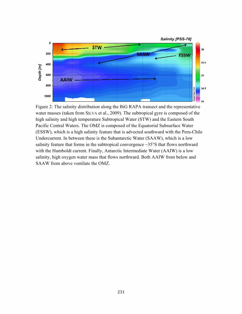
231
Figure 2: The salinity distribution along the BiG RAPA transect and the representative water masses (taken from SILVA et al., 2009). The subtropical gyre is composed of the high salinity and high temperature Subtropical Water (STW) and the Eastern South Pacific Central Waters. The OMZ is composed of the Equatorial Subsurface Water (ESSW), which is a high salinity feature that is advected southward with the Peru-Chile Undercurrent. In between these is the Subantarctic Water (SAAW), which is a low salinity feature that forms in the subtropical convergence ~35°S that flows northward with the Humboldt current. Finally, Antarctic Intermediate Water (AAIW) is a low salinity, high oxygen water mass that flows northward. Both AAIW from below and SAAW from above ventilate the OMZ.

232
Figure 3: The hydrography and nutrient distribution of the BiG RAPA cruise transect. The oxygen minimum zone at Station 1 reaches from 100-400m and is well represented in the oxygen distribution, with concentrations as low as 2 µmol/kg. This OMZ is ventilated from above by SAAW and below by AAIW (both fully oxygenated). The OMZ also presents a clear nitrite maximum, with concentrations >6 µM, indicating the severity of the oxygen depletion and corresponding change in redox state of the water column. The nitrate+nitrite and phosphate concentrations demonstrate the upwelling at Station 1 near the Chilean coast as well as the severe nutrient depletion in the upper 200-300m of the subtropical gyre.

233
Figure 4: The dFe distribution (colors, in nM) in the upper 400m of the BiG RAPA transect, with potential density contour lines. dFe concentrations were highest in the OMZ (~3.5 nM) and lowest in the subtropical gyre (<0.1 nM). This distribution was nearly identical to that reported by BLAIN et al. (2008). They reported maximum concentrations of 3.4 nM dFe in the OMZ and subtropical gyre concentrations of 0.05-0.10 nM. They also found the ferricline of the subtropical gyre to lie in the 26.4-26.6 kg/m3 potential density layer, which was exactly the same on the BiG RAPA transect. This indicates that the dFe dynamics are very similar up and down the Chilean coast (20-35°S).

234
Figure 5: Surface dFe concentrations at the seven stations (where dFe <0.4 µm and sFe < 10 kDa) were ≤ 0.25 nM except for Station 1. Station 1 likely had high Fe concentrations from a combination of upwelling and dFe transport from reducing sediments along the margin. ~1 nM dFe was observed at the surface along the narrow continental margin off of Peru (BRULAND et al., 2005), which is similar to the narrow continental margin near Station 1, indicating that advection and mixing of Fe(II) from margin sediments (as off Peru) may be sufficient to generate the Chilean Station 1 surface dFe concentration. If there was atmospheric deposition along the transect anywhere it would have been at Station 1 (HYSPLIT back trajectory shows transport from the South American continent), although the presence of coastal mountain ranges makes this questionable. Otherwise, atmospheric deposition to the Southeast Pacific Ocean is minimal, with measured Fe deposition rates from aerosols on the BIOSOPE cruise of only 0.11 nmol/m2/day (WAGENER et al., 2008); this is contrast to the high rates of deposition in the North Atlantic near Bermuda of 0.45-27.8 nmol/m2/day (SEDWICK et al., 2007). The minimal aerosol deposition is reflected in the very low concentrations of dFe measured in the surface waters. Much of this Fe was associated with the soluble Fe phase (<10 kDa), instead of the colloidal phase as in high-dust regions (Chapter 6 and 7). This sFe is likely Fe that is rapidly recycled by biology in the surface ocean of the subtropical gyre.
0.0
0.2
0.4
0.6
0.8
1.0
1.2
250 260 270 280 290
dFe (nM)
Longitude (degrees east)
dFe
sFe

235
Figure 6: Station 1 chemistry and hydrography. (a) dFe concentrations were highly elevated (3.5 nmol/kg) from 100-300m, coincident with the OMZ. This is identical to that found in Blain et al. (2008) and also very typical of dFe concentrations found in low-oxygen marine environments such as the 1.5-2 nM dFe found in the Arabian Sea OMZ (MOFFETT et al., 2007). This OMZ dFe is likely comprised mostly of Fe(II) that is stabilized by the low oxygen concentrations. However, it was very surprising to find the concentration of dFe nearly double between Event 12 and Event 37, which were ~2 days apart in time. This was not noticeably true of the nitrite concentrations (another redox-sensitive compound) over the same time period (b). Oxygen concentrations (c) did change over that time period, but the high oxygen concentrations, which would be expected to be associated with lower dFe, were associated with the higher dFe, and thus redox chemistry (more oxidation of Fe2+ in Event 12) cannot explain the observed dFe. Instead, the temperature and salinity diagram (d) shows that a different water mass moved into the region of Station 1 between these two days, with a clear anomaly in T-S at ~120m very clear in the T-S diagram. Thus, there must be some advected component to the dFe measured at Station 1, although some of it may also be generated in situ.

236
Figure 7: dFe distribution in the upper 1000m (colors) with dissolved oxygen contours (lines). Oxygen is clearly a determining factor in the dFe distribution, as the contour lines largely match the color contours. This distribution clearly shows that the elevated dFe in the OMZ does not make it very far offshore, indicating that scavenging is significant.
Figure 8: dFe is controlled by dissolved oxygen (a) and AOU (b). The relationship with oxygen in (a) clearly shows that when dissolved oxygen concentrations are low enough, dFe can be elevated as a result of the stabilization of Fe(II) species. In (b), the strong relationship between dFe and AOU shows that subsurface Fe concentrations are largely biologically controlled by uptake and remineralization, and the dFe:AOU slope can be converted to an Fe:C ratio using the AOU:C ratio of 1.6 (MARTIN et al., 1987). The resulting Fe:C ratio of ~4 µmol/mol is a bit lower than the 1.6-2.4 µmol/mol ratios found in the Equatorial Pacific Fe-limited region (SUNDA, 1997) but is within the range of 2.6-6.1 µmol/mol measured in the subarctic North Pacific Fe-limited region (MARTIN et al., 1993; MARTIN et al., 1989). These Fe:C ratios are much lower than those measured in the tropical North Atlantic (~9-11 µmol/mol, Chapter 3, FITZSIMMONS et al., 2013).
0.0
0.5
1.0
1.5
2.0
2.5
3.0
3.5
4.0
0 100 200 300
dFe (nM)
Dissolved Oxygen (µmol/kg)
Sta 1, 0‐400m
Sta 2‐7, 0‐400m
y = 0.0025x + 0.041R² = 0.8208
Fe:C ~ 4µmol/mol
0.0
0.1
0.2
0.3
0.4
0.5
0.6
0.7
0.8
0 100 200 300
dFe (nM)
AOU (µmol/kg)
Sta 2‐7 200‐1400m

237
Figure 9: Fe stable isotopes, referenced to the IRMM-014 standard in ‰, at the three full-depth stations on the BiG RAPA cruise (note that the depth range changes in each profile). Error bars show the 2σ standard error on the isotope measurement. The parentheses indicate questionable Fe isotope values, and we will not interpret these data until they are re-analyzed. These measurements were made in the John laboratory at University of South Carolina by a 57-58Fe double spike method (CONWAY et al., in press). The main purpose of these analyses was to detect the Fe isotope signature associated with hydrothermal Fe (Chapter 5) near 2000m at Stations 4 and 7 and the enriched Fe in the OMZ of Station 1. We will not comment on the OMZ Fe isotopes because the values were so variable, which is not oceanographically consistent, and thus the data is potentially untrustworthy. However, the hydrothermally-influenced samples were undeniably enriched at ~+0.5‰. This was surprising given that hydrothermal vent fluids have always been found to have a depleted Fe isotope signature (-0.69 to -0.21‰) both along the Mid-Atlantic Ridge and the East Pacific Rise (ROUXEL et al., 2004; SEVERMANN et al., 2004). Even with a contribution of a third to half of the dFe measured at these stations as "background" dFe advected along the water mass or remineralized at depth, which in the Atlantic has an Fe isotopic composition of between 0 and +0.5‰ (JOHN and ADKINS, 2012; RADIC et al., 2011), we would not have expected such an enriched Fe isotope composition unless the hydrothermal vent Fe had undergone further fractionation since venting. Four processes fractionate Fe isotopes during and after hydrothermal venting. First, basalt alteration results in isotopically enriched altered basalts and isotopically
0
200
400
600
800
1000
1200
1400
1600
1800
‐1.0 0.0 1.0
Depth (m
)
δ56Fe (‰)
BiG RAPA Sta 1
0
500
1000
1500
2000
2500
3000
3500
4000
‐1.0 0.0 1.0
Depth (m
)
δ56Fe (‰)
BiG RAPA Sta 4
0
500
1000
1500
2000
2500
3000
‐1.0 0.0 1.0
Depth (m
)
δ56Fe (‰)
BiG RAPA Sta 7
( )
( ) ( )

238
depleted fluids, indicating that the production of high-metal hydrothermal fluids itself is a fractionating process (ROUXEL et al., 2003; ROUXEL et al., 2004; SEVERMANN et al., 2004). Second, the precipitation of Fe sulfides has a kinetic isotope effect Δ56FeFe(II)-FeS of +0.60‰, where the sulfide is depleted and the remaining Fe(II) becomes enriched (BENNETT et al., 2009; ROUXEL et al., 2008). Third, during Fe(II) oxidation, the Fe(III) becomes enriched and the Fe(II) is depleted (BULLEN et al., 2001; WELCH et al., 2003). Finally, during ligand binding of free Fe(III) in seawater, the heavier the Fe-ligand complex, the more enriched the Fe becomes, presumably by an equilibrium isotope effect (MORGAN et al., 2010). All of these processes would result in the conversion of an initially depleted hyrdothermal fluid to a more enriched hydrothermally-derived dissolved Fe phase. The hydrothermal portion of dFe at stations 4 and 7 is at minimum several hundred kilometers from the vent source (Chapter 5), indicating that it has undergone extensive chemical reactions before reaching the sampling location. If the southern-EPR vent fluid originally had depleted Fe, it would have first undergone sulfide precipitation at the vent site, which would have left the vent fluid relatively enriched. Then with increasing distance from the vents, the remaining Fe(II) should have been oxidized to Fe(III), which according to the oxidation kinetics predicted for the Pacific should have happened within hours of venting (FIELD and SHERRELL, 2000), well before reaching the sampling location years after venting; this oxidation would have further enriched the hydrothermal dissolved Fe. With all of these effects, plus the further enriching effect of ligand binding and the mixing with "background" dFe that is enriched, it might no longer be surprising that the distal hydrothermal dFe was isotopically enriched. These profiles also show non-anomalous dFe isotope features that are valuable given the relative dearth of marine dFe isotope data in the Pacific Ocean. The surface dFe are depleted to -0.4‰ at the more nearshore stations 1 and 4, indicating that the Fe at these stations may have been derived from the reducing sediments along the coast, which have depleted Fe isotopic signatures (SEVERMANN et al., 2006; SEVERMANN et al., 2010). This is no surprise at Station 1 but is potentially surprising at Station 4, which is ~2000 km offshore. At station 7, however, the surface δ56Fe was enriched to +0.43‰, which is more typical of the surface ocean (JOHN and ADKINS, 2012; RADIC et al., 2011). Furthermore, AAIW at both Stations 4 and 7 had a δ56Fe near -0.1 to -0.2‰, which is likely a preformed Fe isotope signature since POC stocks ripe for remineralization in the subtropical gyre are so lean.

239
References for Appendix I Bell, J., Betts, J., and Boyle, E., 2002. MITESS: a moored in situ trace element serial
sampler for deep-sea moorings. Deep-Sea Research Part I-Oceanographic Research Papers 49, 2103-2118.
Bennett, S. A., Rouxel, O., Schmidt, K., Garbe-Schonberg, D., Statham, P. J., and German, C. R., 2009. Iron isotope fractionation in a buoyant hydrothermal plume, 5S Mid-Atlantic Ridge. Geochimica et Cosmochimica Acta 73, 5619-5634.
Blain, S., Bonnet, S., and Guieu, C., 2008. Dissolved iron distribution in the tropical and sub tropical South Eastern Pacific. Biogeosciences 5, 269-280.
Bonnet, S., Guieu, C., Bruyant, F., Prasil, O., Van Wambeke, F., Raimbault, P., Moutin, T., Grob, C., Gorbunov, M. Y., Zehr, J. P., Masquelier, S. M., Garczarek, L., and Claustre, H., 2008. Nutrient limitation of primary productivity in the Southeast Pacific (BIOSOPE cruise). Biogeosciences 5, 215-225.
Bruland, K. W., Rue, E. L., Smith, G. J., and DiTullio, G. R., 2005. Iron, macronutrients and diatom blooms in the Peru upwelling regime: brown and blue waters of Peru. Marine Chemistry 93, 81-103.
Bullen, T. D., White, A. F., Childs, C. W., Vivit, D. V., and Schulz, M. S., 2001. Demonstration of significant abiotic iron isotope fractionation in nature. Geology 29, 699-702.
Carr, M.-E., 2001. Estimation of potential productivity in Eastern Boundary Currents using remote sensing. Deep Sea Research Part II: Topical Studies in Oceanography 49, 59-80.
Claustre, H., Sciandra, A., and Vaulot, D., 2008. Introduction to the special section bio- optical and biogeochemical conditions in the South East Pacific in late 2004: the BIOSOPE program. Biogeosciences 5, 679-691.
Conway, T. M., Rosenberg, A. D., Adkins, J. F., and John, S. G., in press. A new method for precise determination of iron, zinc, and cadmium stable isotope ratios in seawater by double-spike mass spectrometry. Analytica Chimica Acta.
Field, M. P. and Sherrell, R. M., 2000. Dissolved and particulate Fe in a hydrothermal plume at 9°45'N, East Pacific Rise: Slow Fe (II) oxidation kinetics in Pacific plumes. Geochimica et Cosmochimica Acta 64, 619-628.
Fitzsimmons, J. N. and Boyle, E. A., 2012. An intercalibration between the GEOTRACES GO-FLO and the MITESS/Vanes sampling systems for dissolved iron concentration analyses (and a closer look at adsorption effects). Limnology & Oceanography: Methods 10, 437-450.
Fitzsimmons, J. N., Zhang, R., and Boyle, E. A., 2013. Dissolved iron in the tropical North Atlantic oxygen minimum zone. Marine Chemistry 154, 87-99.
Fuenzalida, R., Schneider, W., Garces-Vargas, J., Bravo, L., and Lange, C., 2009. Vertical and horizontal extension of the oxygen minimum zone in the eastern South Pacific Ocean. Deep-Sea Research II 56, 992-1003.
John, S. G. and Adkins, J., 2012. The vertical distribution of iron stable isotopes in the

240
North Atlantic near Bermuda. Global Biogeochem. Cycles 26, GB2034. Lee, J.-M., Boyle, E. A., Echegoyen-Sanz, Y., Fitzsimmons, J. N., Zhang, R., and
Kayser, R. A., 2011. Analysis of trace metals (Cu, Cd, Pb, and Fe) in seawater using single batch Nitrilotriacetate resin extraction and isotope dilution inductively coupled plasma mass spectrometry. Analytica Chimica Acta 686, 93-101.
Martin, J. H., Fitzwater, S. E., Michael Gordon, R., Hunter, C. N., and Tanner, S. J., 1993. Iron, primary production and carbon-nitrogen flux studies during the JGOFS North Atlantic bloom experiment. Deep Sea Research Part II: Topical Studies in Oceanography 40, 115-134.
Martin, J. H., Goron, R. M., Fitzwater, S., and Broenkow, W. W., 1989. VERTEX: phytoplankton/iron studies in the Gulf of Alaska. Deep-Sea Research 36, 649-680.
Martin, J. H., Knauer, G. A., Karl, D. M., and Broenkow, W. W., 1987. VERTEX: carbon cycling in the northeast Pacific. Deep Sea Research Part A. Oceanographic Research Papers 34, 267-285.
Moffett, J. W., Goepfert, T. J., and Naqvi, S. W. A., 2007. Reduced iron associated with secondary nitrite maxima in the Arabian Sea. Deep Sea Research Part I: Oceanographic Research Papers 54, 1341-1349.
Moore, J. K. and Braucher, O., 2008. Sedimentary and mineral dust sources of dissolved iron to the world ocean. Biogeosciences 5, 631-656.
Moore, J. K., Doney, S. C., Glover, D. M., and Fung, I. Y., 2002. Iron cycling and nutrient-limitation patterns in surface waters of the World Ocean. Deep Sea Research Part II: Topical Studies in Oceanography 49, 463-507.
Morgan, J. L. L., Wasylenki, L. E., Nuester, J., and Anbar, A. D., 2010. Fe isotope fractionation during equilibration of Fe-organic complexes. Environmental Science & Technology 44, 6095-6101.
Noble, A. E., Lamborg, C. H., Ohnemus, D. C., Lam, P. J., Goepfert, T. J., Measures, C. I., Frame, C. H., Casciotti, K. L., DiTullio, G. R., Jennings, J., and Saito, M. A., 2012. Basin-scale inputs of cobalt, iron, and manganese from the Benguela-Angola front to the South Atlantic Ocean. Limnology & Oceanography 57, 989-1010.
Radic, A., Lacan, F., and Murray, J. W., 2011. Iron isotopes in the seawater of the equatorial Pacific Ocean: New constraints for the oceanic iron cycle. Earth and Planetary Science Letters 306, 1-10.
Rouxel, O., Dobbek, N., Ludden, J. N., and Fouquet, Y., 2003. Iron isotope fractionation during oceanic crust alteration. Chemical Geology 202, 155-182.
Rouxel, O., Fouquet, Y., and Ludden, J. N., 2004. Subsurface processes at the lucky strike hydrothermal field, Mid-Atlantic ridge: evidence from sulfur, selenium, and iron isotopes. Geochimica et Cosmochimica Acta 68, 2295-2311.
Rouxel, O., Shanks Iii, W. C., Bach, W., and Edwards, K. J., 2008. Integrated Fe- and S-isotope study of seafloor hydrothermal vents at East Pacific Rise 9-10°N. Chemical Geology 252, 214-227.
Sedwick, P. N., Sholkovitz, E. R., and Church, T. M., 2007. Impact of anthropogenic combustion

241
emissions on the fractional solubility of aerosol iron: Evidence from the Sargasso Sea. Geochem. Geophys. Geosyst. 8, 21.
Severmann, S., Johnson, C. M., Beard, B. L., German, C. R., Edmonds, H. N., Chiba, H., and Green, D. R. H., 2004. The effect of plume processes on the Fe isotope composition of hydrothermally derived Fe in the deep ocean as inferred from the Rainbow vent site, Mid-Atlantic Ridge, 36 degrees 14' N. Earth and Planetary Science Letters 225, 63-76.
Severmann, S., Johnson, C. M., Beard, B. L., and McManus, J., 2006. The effect of early diagenesis on the Fe isotope compositions of porewaters and authigenic minerals in continental margin sediments. Geochimica et Cosmochimica Acta 70, 2006-2022.
Severmann, S., McManus, J., Berelson, W. M., and Hammond, D. E., 2010. The continental shelf benthic iron flux and its isotope composition. Geochimica et Cosmochimica Acta 74, 3984-4004.
Silva, N., Rojas, N., and Fedele, A., 2009. Water masses in the Humboldt Current System: Properties, distribution, and the nitrate deficit as a chemical water mass tracer for Equatorial Subsurface Water off Chile. Deep-Sea Research II 56, 1004-1020.
Sunda, W. G., 1997. Control of dissolved iron concentrations in the world ocean, A comment. Marine Chemistry 57, 169-172.
Wagener, T., Guieu, C., Losno, R., Bonnet, S., and Mahowald, N., 2008. Revisiting atmospheric dust export to the Southern Hemisphere ocean: Biogeochemical implications. Global Biogeochem. Cycles 22, GB2006.
Welch, S. A., Beard, B. L., Johnson, C. M., and Braterman, P. S., 2003. Kinetic and equilibrium Fe isotopic fractionation between aqueous Fe(II) and Fe(III). Geochimica et Cosmochimica Acta 67, 4231-4250.

242

243
Appendix II
Iron chemistry at the TAG hydrothermal field Collaborators: Mariko Hatta, Christopher Measures, Gonzalo Carrasco, Peter Sedwick, Edward Boyle (and soon to join: Sara Rauschenberg and Benjamin Twining) The Trans-Atlantic Geotraverse (TAG) hydrothermal field is a well-studied hydrothermal vent system in the Atlantic Ocean around 26°N. TAG is located on the eastern wall of the slow-spreading (<2 cm/y) Mid-Atlantic Ridge (MAR) rift valley in 3650m water depth (RONA et al., 1986) and is comprised of a large mound that contains multiple black and white smoker vents (TIVEY et al., 1995). The vent fluids have been studied since 1985 over several Alvin dives (CAMPBELL et al., 1988) that explored the temporal and spatial variability of TAG hydrothermal venting (GAMO et al., 1996). These studies demonstrated that the TAG system vents fluid with very high dFe concentrations of ~5.0-5.5 mM that were stable in Fe concentration over the 12 years of study (CHIBA et al., 2001), despite Ocean Drilling Program (ODP) drilling nearby in the early 1990s (EDMONDS et al., 1996). This stability in vent-fluid Fe chemistry, along with the thorough characterization of both the physics of TAG plume dynamics (RUDNICKI and ELDERFIELD, 1992; SPEER and RONA, 1989) and North Atlantic Fe chemistry (BERGQUIST and BOYLE, 2006; FITZSIMMONS et al., 2013; MEASURES et al., 2008), makes TAG an ideal model system for an exploration of Fe chemistry in MAR hydrothermal vents. The Fe chemistry in the TAG buoyant plume has been modeled as a two-stage process where in the initial 15 seconds of venting (~8 m plume rise) half of the Fe precipitates as sulfides, followed by precipitation of the rest of the Fe as oxyhydroxides (by ~150m plume rise) with an oxidation half-life of ~2.1 minutes (RUDNICKI and ELDERFIELD, 1993). However, JAMES AND ELDERFIELD (1996) found that up to 50% of the Fe in TAG plume was still dissolved (<0.4 µm) upon reaching plume neutral buoyancy, opposing the hypothesis of quantitative precipitation in the buoyant plume. Instead they hypothesized that much of their "dissolved Fe" was not actually composed of reduced Fe2+ but was instead composed of the Fe precipitates proposed by RUDNICKI
AND ELDERFIELD that simply fell into the colloidal (instead of particulate) size fraction. On the GEOTRACES North Atlantic Zonal Transect 2011 cruise (described in Chapter 7), we sampled in the region of the TAG hydrothermal vent field (Station GT11-16) using CTD/GO-FLO rosette operations. We were able to capture a portion of the proximal TAG non-buoyant plume, which we confirmed with the measurement of a drop in light transmission as well as an increase in helium (He) concentrations associated with

244
an enriched δ3He signature vented from the Earth's mantle at TAG. In this paper, we aim to re-evaluate the Fe chemistry occurring in and around the TAG hydrothermal vent field using the combined measurements of dissolved (dFe < 0.2 µm), particulate (pFe > 0.4 µm), and soluble (sFe < 0.02 µm, which derives a colloidal component as cFe = dFe - sFe) Fe size fractions, as well as an assessment of the Fe(II) concentration in the dissolved phase, and we compare our results with those of JAMES AND ELDERFIELD
(1996) to derive an updated description of Fe chemistry in the TAG plume. The proximal hydrothermal TAG Fe chemistry is explored here, while the distal effects of TAG hydrothermal venting on the dFe distribution of the North Atlantic Ocean are explored in Hatta et al. (in prep) and Chapter 7. Methods Three casts at TAG (26.137°N, 44.826°W) were completed on the GEOTRACES NAZT cruise. Cast 1 (28 Nov, 20:00-midnight) used the custom-built US GEOTRACES trace metal clean rosette (GTC) consisting of an epoxy-painted aluminum rosette frame containing 24 x 12 L GO-FLO bottles (CUTTER and BRULAND, 2012); this cast was used to collect trace metal-uncontaminated seawater samples, as all zinc anodes were replaced on the rosette, the GO-FLO bottles were all-Teflon and contained no metal springs, and filtration was completed under ISO5-rated clean air (see Chapter 7 for more sampling details). Casts 2 (29 Nov, midnight-3:00) and 4 (29 Nov, 12:30-15:00) used a Niskin rosette and CTD provided by the Oceanographic Data Facility (ODF) at Scripps. This rosette contained 12 x 30L Niskin bottles with Nylon-coated internal stainless steel springs and Viton o-rings mounted on a powder-coated aluminum frame; this package was not designed for trace metal sample collection and thus likely contributed some contamination to the seawater samples collected from it. It is important to note that dissolved Fe from the ODF rosette was filtered using an AcroPak-500 filter with a paired 0.8/0.45 µm membrane filtration; this is different than the GTC seawater samples, which were filtered using AcroPak-200 filters with a 0.2 µm pore size. The ODF samples were also collected at the end of the filtration process after all other samples had been collected, while the GTC dFe samples were collected early in the filtration process.
To estimate the mixing ratio between the high-temperature vent fluid and the abyssal seawater surrounding it, we followed JAMES and ELDERFIELD (1996) and used the concentration of dMn as dilution index:
Dilution factor Mn
Mn (1)
where [Mn]vent is the concentration of dMn in the black smoker TAG vent fluids (680 µM, EDMOND et al., 1995), [Mn]SW is the concentration of dMn in abyssal North Atlantic seawater (0.1 nM, STATHAM et al., 1998), and [Mn]sample is the concentration of dMn in the sample of interest. This dilution factor estimate assumes that Mn is a conservative

245
tracer of plume dilution, which is contingent on the slow oxidation kinetics of Mn in the TAG plume relative to Fe, and is valid on the timescale of hours to days; after this, Mn is also non-conservatively precipitated/scavenged. Minimal dilution factors for GTC and ODF casts were 3.7-4.0 x 10⁴, which are greater than the calculated 1.2±0.2 x 10⁴ dilution factors at the top of the TAG buoyant plume (based on simple plume theory: JAMES and ELDERFIELD, 1996; RUDNICKI and ELDERFIELD, 1992), suggesting that the plume samples collected on GEOTRACES were located some distance away from the main axis of the non-buoyant plume.
dFe and dissolved manganese (dMn) were measured at sea by the Measures lab using the Flow Injection Analysis methods of MEASURES et al. (1995) and RESING and MOTTL (1992), respectively. sFe was measured in the Boyle laboratory at MIT using the methods of LEE et al. (2011). cFe is calculated as dFe - sFe. Fe(II) was measured at sea by the Sedwick lab (SEDWICK et al. 2013). Particulate Fe will be analyzed in the laboratory of Benjamin Twining at Bigelow Laboratory for Ocean Sciences, and the data is soon to come. Results and Discussion High concentrations of dFe (35.7-66.4 nmol/kg) and dMn (11.2 nM - 18.1 nmol/kg) were observed between 3200-3600m, coincident with a decrease in light transmission associated with large particulate loadings from metal precipitation at TAG, indicating that these elevated dFe and dMn concentrations were derived from the TAG hydrothermal plumes (Figure 1). The variable depth range and intensity of the light transmission feature over the three casts indicate that either the ship and/or the plume itself drifted over the 19 hours of plume sampling; either mechanism requires the non-buoyant plume to have significant heterogeneity. dMn was nearly constant in the hydrothermal maximum over the three casts, which supports our assumption that dMn is an appropriate conservative tracer of plume dilution. dFe concentration, in contrast, varied by a factor of three in the hydrothermal maximum between casts. While we might expect Fe contamination in the ODF rosette casts because the Niskin bottles contain stainless steel springs (at 3000m, the ODF samples' dFe concentrations are 1.5-2.0 nmol/kg higher in concentration than the GTC sample), the ODF dFe concentrations were actually lower than the GTC dFe concentrations in the hydrothermal maximum. This pattern also occurred despite a larger dFe pore size cutoff in the ODF cast (<0.45 µm) than in the GTC cast (<0.2 µm). The higher dFe concentration during the GTC casts casts may reflect the fact that the wire time and timing of filtration were critical for the observed Fe partitioning. For instance, Fe may have precipitated into the particulate phase in the ODF Niskin bottles during rosette ascent (multiple additional depths tripped upon ascent) and filtration of all other chemical parameters (Fe was one of the last
246
filtrates sampled), while the GTC cast was recovered immediately after the hydrothermal samples were taken, and dFe was one of the first chemicals sampled during filtration, perhaps allowing for the maintenance of higher Fe concentrations in the dissolved phase. We observed the same pattern when we examined dFe as a function of dMn, a proxy for plume dilution with ambient seawater (Figure 2). There was a positive relationship between these two metals, as expected since pure vent fluid contains high concentrations of both Mn and Fe. However, the fact that all of the GETORACES dFe regression lines fell below the conservative mixing line between black smoker vent fluids and ambient seawater means that Fe precipitated or was scavenged to a greater extent than Mn in these hydrothermally-influenced waters. The seawater samples from the two ODF casts had even lower slopes than the GTC samples, indicating that they experienced further Fe precipitation/scavenging before sample collection. Using the GTC samples only, we took a closer look at the composition of the Fe pool near the TAG vent (Figure 3) in an attempt to confirm the hypothesis of JAMES and ELDERFIELD (1996) that the dFe in the non-buoyant plume was composed of colloidal Fe as opposed to Fe2+. We found two major results. First, we confirmed that 89-96% of the dFe fell in the colloidal size fraction (sFe concentrations only reached as high as 7.4 nmol/kg). This confirms the hypothesis of JAMES and ELDERFIELD (1996) that a large fraction of total Fe in the non-buoyant plume is dissolved instead of particulate because the dFe fraction includes small particles (colloids). Most surprising, however, was that ~75-100% of the dFe was composed of Fe(II). This was primarily unexpected because of the short oxidation half-life of Fe(II), measured to be as short as 2.1 minutes in the TAG buoyant plume (RUDNICKI and ELDERFIELD, 1993) or estimated to be as long as 27 minutes near TAG using the pH and oxygen concentrations of abyssal North Atlantic waters (FIELD and SHERRELL, 2000). Either half-life estimate would predict that most of the Fe2+ should be oxidized in the ~40 minutes it takes for the TAG plume to reach neutral buoyancy (RUDNICKI and ELDERFIELD, 1992). Secondarily, however, the Fe(II) dominance of non-buoyant plume TAG dissolved Fe is surprising because Fe(II) is typically thought to be truly dissolved. While we did not take strides to preserve deep water conditions before the colloidal 0.02 µm filtration, and thus our observed colloidal composition may contain some Fe aggregation during the 1-2 hours it took to filter our samples, we instead propose that the Fe(II) is indeed truly colloidal and that this colloidal composition is actually what stabilizes the Fe(II) beyond its predicted oxidation half-life. Pyrite nanoparticles as small as 4nm have been observed in hydrothermal vent fluids along the East Pacific Rise, near Lau Basin, and also at TAG (GARTMAN et al., 2012; YUCEL et al., 2011), an d this nano-pyrite aggregates into colloidal-sized nanoframboids of 50-350 nm diameter that could

247
dominate the dissolved Fe pool in the proximity of TAG. YUCEL et al. (2011) suggest that it is the nanoparticulate nature of this Fe(II) that allows it to escape oxidation longer than truly dissolved Fe(II). Alternatively, the colloidal Fe in the diluted hydrothermal samples we sampled could have an organically-bound component. TONER et al. (2009)have shown that colloidal and particulate Fe(II) near the East Pacific Rise at 9°N is stabilized by organic carbon-rich material thought to be of biological origin from near the vent site. Additionally, a non-hydrothermal study in the mixed layer of the Southern Ocean has also shown that colloidal and particulate Fe(II) is associated with organic matrices (VON
DER HEYDEN et al., 2012) and thus may indicate a pattern of Fe(II) "protection" against oxidation through organic colloid stabilization. Notably, the >1µm particulate Fe at our TAG site was found by synchrotron analysis to be comprised of ferrihydrite, and no particulate Fe(II) component was observed (LAM and OHNEMUS, 2013).

248
Figure 1: Data from the TAG station (GT11-16) on the 2011 GEOTRACES North Atlantic Zonal Transect cruise (26.137°N, 44.826°W) on GTC rosette cast (black) and the two ODF rosette casts (cast 2: red, cast 4: blue). Light transmission is shown on the left, dFe in the middle, and dMn on the right. The dissolved fraction is defined as < 0.2 µm in the GTC cast (black) and < 0.45 µm in the ODF cast (red and blue).
0 5 10 15 20
[Mn] nmol/kg
GTC Cast 1
ODF Cast 2
ODF Cast 4
0 20 40 60 80
[Fe] nmol/kg
GTC Cast 1
ODF Cast 2
ODF Cast 4
4.55 4.57 4.59
2000
2200
2400
2600
2800
3000
3200
3400
3600
3800
4000
4.7 4.71 4.72 4.73
ODF rosette light transmission
Depth (m)
GTC light transmission (V)
GTC Cast 1
ODF Cast 2
ODF Cast 4

249
Figure 2: Fe chemistry as a function of dMn (plume dilution) at TAG. The Black Smoker line depicts conservative mixing between abyssal North Atlantic seawater (dMn of 0.1 nmol/kg, dFe of 0.6 nmol/kg) and TAG black smoker vent fluids (dMn of 680 µmol/kg, dFe of 5590 µmol/kg; EDMOND et al., 1995). The thin black, red, and blue lines are the regressions of the dFe data for the GTC Cast 1 (black), ODF Cast 2 (red), and ODF Cast 4 (blue) deployments, fit to go through the abyssal North Atlantic seawater data.
y = 3.29x + 0.27
R² = 0.63
y = 1.61x + 0.44R² = 0.78
y = 1.22x + 0.48
R² = 0.87
0
10
20
30
40
50
60
70
0 5 10 15 20
Fe (nmol/kg)
dMn (nmol/kg)
dFe ‐ GTC Cast 1
dFe ‐ ODF Cast 2
dFe ‐ ODF Cast 4
Black Smoker

250
Figure 3: Fe physico-chemical speciation in the TAG hydrothermal non-buoyant plume (diluted 26000-60000 times with ambient seawater, according to equation 1).
2800
3000
3200
3400
3600
0 20 40 60 80
Depth (m)
Fe (nmol/kg)
dFe<0.2µm
sFe<0.02µm
0.02µm<cFe<0.2µm
Fe(II)

251
References for Appendix II Bergquist, B. A. and Boyle, E. A., 2006. Dissolved iron in the tropical and subtropical Atlantic
Ocean. Global Biogeochemical Cycles 20, 14. Campbell, A. C., Palmer, M. R., Klinkhammer, G. P., Bowers, T. S., Edmond, J. M., Lawrence, J.
R., Casey, J. F., Thompson, G., Humphris, S., Rona, P., and Karson, J. A., 1988. Chemistry of hot springs on the Mid-Atlantic Ridge. Nature 335, 514-519.
Chiba, H., Masuda, H., Lee, S., Y, and Fujioka, K., 2001. Chemistry of hydrothermal fluids at the TAG Active Mound, MAR 26°N, in 1998. Geophysical Research Letters 28, 2919-2922.
Cutter, G. A. and Bruland, K. W., 2012. Rapid and noncontaminating sampling system for trace elements in a global ocean surveys. Limnology & Oceanography: Methods 10, 425-436.
Edmond, J. M., Campbell, A. C., Palmer, M. R., Klinkhammer, G. P., German, C. R., Edmonds, H. N., Elderfield, H., Thompson, G., and Rona, P., 1995. Time series of vent fluids from the TAG and MARK sites (1986-1990) Mid-Atlantic Ridge: a new solution chemistry model and a mechanism for Cu/Zn zonation in massive sulfide orebodies. In: Parson, L. M., Walker, C. L., and Dixon, D. R. Eds.), Hydrothermal Vents and Processes. Geological Society Special Publication No. 87.
Edmonds, H. N., German, C. R., Green, D. R. H., Huh, Y., Gamo, T., and Edmond, J. M., 1996. Continuation of the hydrothermal fluid chemistry time series at TAG, and the effects of ODP drilling. Geophysical Research Letters 23, 3487-3489.
Field, M. P. and Sherrell, R. M., 2000. Dissolved and particulate Fe in a hydrothermal plume at 9°45'N, East Pacific Rise: Slow Fe (II) oxidation kinetics in Pacific plumes. Geochimica et Cosmochimica Acta 64, 619-628.
Fitzsimmons, J. N., Zhang, R., and Boyle, E. A., 2013. Dissolved iron in the tropical North Atlantic oxygen minimum zone. Marine Chemistry 154, 87-99.
Gamo, T., Chiba, H., Masuda, H., Edmonds, H. N., Fujioka, K., Kodama, Y., Nanba, H., and Sano, Y., 1996. Chemical characteristics of hydrothermal fluids from the TAG Mound of the Mid-Atlantic Ridge in August 1994: Implications for spatial and temporal variability of hydrothermal activity. Geophysical Research Letters 23, 3483-3486.
Gartman, A., Yucel, M., and Luther, G. W., 2012. Hydrothermal vents as a source of pyrite and trace metal-containing mineral nanoparticles to the ocean. AGU Fall Meeting, San Francisco, California.
James, R. H. and Elderfield, H., 1996. Dissolved and particulate trace metals in hydrothermal plumes at the Mid-Atlantic Ridge. Geophysical Research Letters 23, 3499-3502.
Lam, P. J. and Ohnemus, D. C. 2013. Size-fractionated particle mass and composition during the U.S. GEOTRACES North Atlantic Zonal Transect. U.S. GEOTRACES post-cruise data workshop, Old Dominion University, Norfolk, VA.
Lee, J.-M., Boyle, E. A., Echegoyen-Sanz, Y., Fitzsimmons, J. N., Zhang, R., and Kayser, R. A., 2011. Analysis of trace metals (Cu, Cd, Pb, and Fe) in seawater using single batch Nitrilotriacetate resin extraction and isotope dilution inductively coupled plasma mass spectrometry. Analytica Chimica Acta 686, 93-101.
Measures, C. I., Landing, W. M., Brown, M. T., and Buck, C. S., 2008. High-resolution Al and

252
Fe data from the Atlantic Ocean CLIVAR-CO2 Repeat Hydrography A16N transect: Extensive linkages between atmospheric dust and upper ocean geochemistry. Global Biogeochem. Cycles 22, GB1005.
Measures, C. I., Yuan, J., and Resing, J. A., 1995. Determination of iron in seawater by flow injection-analysis using in-line preconcentration and spectrophotometric detection. Marine Chemistry 50, 3-12.
Resing, J. A. and Mottl, M. J., 1992. Determination of manganese in seawater using flow injection analysis with on-line preconcentration and spectrophotometric detection. Analytical Chemistry 64, 2682-2687.
Rona, P. A., Klinkhammer, G., Nelsen, T. A., Trefry, J. H., and Elderfield, H., 1986. Black smokers, massive sulphides and vent biota at the Mid-Atlantic Ridge. Nature 321, 33-37.
Rudnicki, M. D. and Elderfield, H., 1992. Theory applid to the Mid-Atlantic Ridge hydrothermal plumes: The finite difference approach. Journal of Volcanology and Geothermal Research 50, 161-172.
Rudnicki, M. D. and Elderfield, H., 1993. A chemical model of the buoyant and neutrally buoyant plume above the TAG vent field, 26 degrees N, Mid-Atlantic Ridge. Geochimica et Cosmochimica Acta 57, 2939-2957.
Sedwick, P.N., Sohst, B., Bowie, A., 2013. U.S. GEOTRACES North Atlantic section: Dissolved Fe and Fe(II). U.S. GEOTRACES post-cruise data workshop, Old Dominion University, Norfolk, VA.
Speer, K. G. and Rona, P. A., 1989. A model of an Atlantic and Pacific hydrothermal plume. Journal of Geophysical Research 94, 6213-6220.
Statham, P. J., Yeats, P. A., and Landing, W. M., 1998. Manganese in the eastern Atlantic Ocean: processes influencing deep and surface water distributions. Marine Chemistry 61, 55-68.
Tivey, M. K., Humphris, S. E., Thompson, G., Hannington, M. D., and Rona, P. A., 1995. Deducing patterns of fluid flow and mixing within the TAG active hydrothermal mound using mineralogical and geochemical data. Journal of Geophysical Research: Solid Earth 100, 12527-12555.
Toner, B. M., Fakra, S. C., Manganini, S. J., Santelli, C. M., Marcus, M. A., Moffett, J., Rouxel, O., German, C. R., and Edwards, K. J., 2009. Preservation of iron(II) by carbon-rich matrices in a hydrothermal plume. Nature Geoscience 2, 197-201.
von der Heyden, B. P., Roychoudhury, A. N., Mtshali, T. N., Tyliszczak, T., and Myneni, S. C. B., 2012. Chemically and Geographically Distinct Solid-Phase Iron Pools in the Southern Ocean. Science 338, 1199-1201.
Yucel, M., Gartman, A., Chan, C. S., and Luther, G. W., 2011. Hydrothermal vents as a kinetically stable source of iron-sulphide-bearing nanoparticles to the ocean. Nature Geoscience 4, 367-371.

253
Appendix III
The composition of dissolved iron in the dusty surface ocean: an exploration using size-fractionated iron-binding ligands and iron isotopes Collaborators: Randelle Bundy, Gonzalo Carrasco, Edward Boyle, Timothy Conway, and Seth John
Since iron (Fe) is estimated to be the limiting nutrient in up to 40% of the surface ocean (MOORE et al., 2002), linking Fe fluxes in the surface ocean to the biological uptake of dissolved Fe (dFe) by microorganisms is a major motivation of much of the exploration of marine dFe biogeochemistry. The biological utilization of dFe during photosynthesis, nitrogen fixation, and remineralization (MOREL et al., 2003) is what ties dFe biogeochemistry to the global carbon cycle and ultimately climate. However the transformation of "new" dFe from its input flux to its potential biological utilization is ultimately controlled by its chemical composition: both the scavenging residence time and the bioavailability of these new dFe species are impacted by their various chemical forms dFe assumes.
We have learned quite a bit about the composition of dFe over the last several decades. We know that dFe (here defined as <0.2 µm) has a broad size distribution comprised of both "truly dissolved" soluble Fe (sFe <10kDa) and "small particulate" colloidal Fe (10 kDa < cFe < 0.2 µm) size fractions (BERGQUIST et al., 2007; CHEVER et al., 2010; FITZSIMMONS and BOYLE, in review-b; NISHIOKA et al., 2001; USSHER et al., 2010; WU et al., 2001). Incubation studies have shown that while both size fractions can be biologically utilized, soluble Fe is much preferred over colloidal Fe (CHEN et al., 2003; CHEN and WANG, 2001; WANG and DEI, 2003), and inorganic colloidal Fe (nanoparticles) is not biologically available at all (RICH and MOREL, 1990). In addition, studies using competitive ligand exchange electrochemical measurements have suggested that >99.9% of marine dFe is bound by organic ligands (RUE and BRULAND, 1995; VAN DEN BERG, 1995; WU and LUTHER, 1995) that maintain marine dFe above its ~0.1 nM inorganic solubility in pH 8 seawater (LIU and MILLERO, 2002; MILLERO, 1998). While a few of these organic ligands have been identified as hydroxamate siderophores (MAWJI et al., 2011; VELASQUEZ et al., 2011; VRASPIR and BUTLER, 2009), chemically characterized ligands only comprise a small percentage of the total dFe pool, as the identity of marine Fe-binding ligands is largely unknown (GLEDHILL and BUCK, 2012).

254
However, the hypothesis that nearly all marine dFe is organically bound relies on an assumption of thermodynamic equilibrium between dFe and dissolved Fe-binding ligands in the open ocean. Additionally, electrochemical characterization of Fe-binding ligands is somewhat limiting, as only the Fe-binding ligands kinetically labile over the period of equilibrium with added ligand can be detected, and thus a relatively refractory portion of free Fe-binding ligands would not be detected by these methods. Despite these points, hardly any studies explicitly measuring the chemical composition of dFe species have been completed, largely because of analytical hurdles. One analysis of colloidal Fe composition by energy dispersive spectroscopy showed that open ocean cFe is organically bound (WELLS and GOLDBERG, 1992), while a recent study using synchrotron technology demonstrated that a portion of the surface colloidal Fe underlying dust plumes in the Southern Ocean is nanoparticulate, composed of tiny bits of magnetite (VON DER HEYDEN et al., 2012). Thus, while our best guess of the chemical composition of dFe is that the overwhelming majority is bound by strong organic Fe-binding ligands, there is a possibility that some dFe, especially in the colloidal phase, is inorganically bound (nanoparticulate in nature). This might be especially true in regions where continental Fe sources are known to be significant (underlying dust plumes, downstream of hydrothermal vents, near the continental margin, in regions with abundant glacial meltwater, etc).
The chemical composition of dFe has the greatest impact on biological uptake in the upper ocean where phytoplankton are most active, and the surface ocean is also the location where atmospheric dust deposition, arguably the most significant Fe input to the ocean (JICKELLS et al., 2005; MAHOWALD et al., 2005), occurs. The solubility of aerosol Fe is variable and depends on a suite of factors including aerosol composition, source (anthropogenic or crustal), and size, as well as seawater pH and Fe-binding ligand concentration (BAKER and CROOT, 2010). One pattern, however, is reproducible in all studies: in the surface ocean underlying dust plumes, dFe is preferentially maintained in the colloidal size fraction (Chapter 7; BERGQUIST et al., 2007; FITZSIMMONS and BOYLE, in review-b; USSHER et al., 2010; WU et al., 2001), while in low-dust surface ocean regions, the smaller soluble size fraction dominates the dFe pool (BOYE et al., 2010; CHEVER et al., 2010; NISHIOKA et al., 2003; WELLS, 2003). Colloidal Fe has also been shown to be the dominant Fe size fraction yielded in leaches of natural dust (AGUILAR-ISLAS and MEHALEK, 2013; AGUILAR-ISLAS et al., 2010).
This raises two important questions: what is the binding environment of dFe in the surface ocean after recent dust deposition, and is this dust-derived dFe bioavailable? We envision that dust-derived colloidal Fe could assume any of three possible compositions: Fe bound by colloidal-sized organic ligands after Fe solubilization from dust, colloidal-sized bits of dust that physically separated from the dust particles upon

255
impacting the surface ocean (resulting in a nanoparticulate cFe composition of the same composition as the dust), or Fe that was initially solubilized from dust in the surface ocean but then re-precipitated in situ in and aggregated into colloidal size (also resulting in a nanoparticulate cFe composition, likely amorphous Fe oxyhydroxides). Which of these comprises the majority of surface dFe underlying dust plumes has a significant impact on surface dFe residence time and bioavailability, and thus the distinction between these is at the crux of the problem linking dust deposition to biological uptake of dFe.
In this paper, we explore the binding environment of dFe in the surface of the high-dust North Atlantic Ocean using an analysis of the Fe-binding ligand concentration and strength, as well as the Fe isotope signature, of both the soluble and dissolved Fe pools. We aimed to consider whether there could be a natural nanoparticulate component to the dissolved Fe pool of the surface ocean, which would contradict the prevailing view that >99.9% of dFe is believed to be bound by organic ligands. We based our research on two hypotheses:
1. If the size partitioning of surface Fe-binding ligands into soluble and colloidal fractions predicts the observed surface dFe size partitioning, then surface dFe is likely bound by organic ligands.
2. If the Fe isotope signature of colloidal Fe is significantly different from crustal isotopic values, then a dust-derived nanoparticulate component of dFe is unlikely without the implication of significant fractionation processes yet to be discovered.
Site Selection and Methodology
Seawater samples were collected from four stations on the US North Atlantic Zonal Transect 2011 cruise (Nov-Dec 2011): USGT11-10 at 31.933°N, -64.733°W (the Bermuda Atlantic Time Series, BATS, station), USGT11-11 at 30.817°N, -60.775°W (~400 km to the southeast of BATS), USGT11-21 at 20.83°N, -32.625°W (surface sample only), and USGT11-23 at 18.39°N, -26.765°W (near the Cape Verde Islands). These locations were chosen for two reasons. First, we wanted to sample variable dust loading/composition in the surface ocean. USGT11-10 and -11 near Bermuda had 1-2 ng/m3 Fe loadings with a "marine" back-trajectory (HYSPLIT) and an Fe solubility of ~7%, while USGT11-21 and -23 near Cape Verde had much higher total aerosol Fe loadings >1000 ng/m3 Fe with a "North African" back-trajectory and a lower Fe solubility of ~0.4% (SHELLEY and LANDING, 2013). Second, we wanted to sample variable biogeochemistries in the upper 1000m (Figure 3). USGT11-11 was situated more in the subtropical gyre and thus experienced a deeper pycnocline (500-900m based on the salinity trace) and an oxygen minimum of only 150 µmol/kg near 800m depth, while USGT11-23 was situated south of the gyre with a much shallower pycnocline (beginning

256
as shallow as 100m) and much lower minimum oxygen concentrations of ~80 µmol/kg from 300-500m near the Mauritanian oxygen minimum zone (OMZ).
Trace metal uncontaminated seawater was collected using the U.S. GEOTRACES GO-FLO rosette by the methods described in CUTTER and BRULAND (2012). GO-FLO bottles were carried individually into an ISO 5-rated clean van, where the seawater was filtered through pre-cleaned 0.2 µm Pall Acropak-200™ Supor® capsule filters under ~0.4 atm of HEPA-filtered air. Surface samples were collected using the GeoFish system of the Bruland lab, which employs all-PFA tubing attached to a vane that coasts at ~3m depth suspended from a boom off the starboard side of the ship during forward ship motion at up to 12 knots. An all-PFA diaphragm pump sipped clean seawater through this system at ~8 psi pressure, and filtration was completed first through a 0.45 µm Osmonics (PFA) filter and then through a 0.2 µm PCTE filter mesh held in a polypropylene housing. Filtrates were taken into acid cleaned 4L LDPE bottles after three bottle rinses. Sub-samples of this 4L were taken into 1L HDPE bottles for dFe isotope analysis and 500 mL fluorinated polyethylene (FLPE) bottles for the dFe-binding ligand sample; FLPE bottles had been conditioned with trace ultra-clean MilliQ for more than a month before sample collection to remove all acid residue. To collect the soluble Fe fraction, the rest of the 4L filtrates were immediately filtered again through an all-Teflon cross-flow filtration (CFF) system in static mode (FITZSIMMONS and BOYLE, in review-a). A Millipore Pellicon XL (PLCGC) 10 kDa regenerated cellulose CFF membrane was employed, and 300-350mL of sample seawater was first flushed through the system to condition the membrane and CFF tubing against Fe sorption. After filtration, Fe-binding ligand samples were frozen unacidified, and 1 L Fe isotope samples were acidified to pH 2 with trace metal grade hydrochloric acid.
dFe and sFe samples were analyzed in triplicate for their Fe concentration at MIT by isotope dilution inductively-coupled plasma mass spectrometry (ID-ICP-MS) on a hexapole collision cell IsoProbe ICP-MS. The ID-ICP-MS method employs a 54Fe-spike and batch pre-concentration with nitrilotriacetate resin (LEE et al., 2011). Procedure blanks averaged 0.044 nmol/kg with a typical standard deviation over a single day's analysis of 0.009 nmol/kg; thus, the reported detection limit was 0.027 nmol/kg. Comprehensive lab analyses of the SAFe S seawater for dFe during the period of these analyses averaged 0.101±0.009 nmol/kg (Bottles 17 and 318, n=6), which agrees well with the consensus value of 0.093±0.008 nmol/kg. Similarly, SAFe D2 standard for dFe during the period of these analyses averaged 0.911±0.018 nmol/kg (Bottle 446, ±1SD, n=15), which also agree well with the consensus value of 0.933±0.032 nmol/kg. Consensus values were updated in May 2013 (www.geotraces.org/science/intercalibration).
257
Measurements of Fe-binding ligand concentration and binding strength were made by competitive ligand exchange-adsorptive cathodic stripping voltammetry (CLE-ACSV) on a BioAnalytical Systems (BASi) Controlled Growth Mercury Electrode coupled to a BASi Epsilon ε2 voltammetric analyzer in the Barbeau lab at Scripps by the methods described in BUCK et al. (2007). Briefly, 10 mL sample aliquots were buffered to pH 8.2 with a borate-ammonium buffer in PFA Savillex vials that had been previously conditioned to the anticipated Fe addition. Titration Fe additions were made at concentrations ranging from 0-7.5 nM and were allowed to equilibrate for 2 hours before the addition of the added ligand, salicylaldoxime (SA), at concentrations of 25 µM (αFe(SA)2 = 60). After a 15 minute equilibration with SA, samples were adsorbed to the mercury drop at zero potential for 2-5 minutes and then stripped at 0.03 V/s using differential pulse mode to a final potential of -0.85V. Raw titration data were interpreted for their Fe-binding ligand concentration ([L]) and ligand conditional stability constants (Kcond
FeL/Fe') using the van den Berg/Ružić (RUŽIĆ, 1982; VAN DEN BERG, 1982) and the Scatchard (MANTOURA and RILEY, 1975; SCATCHARD, 1949) linearization techniques, the results of which were averaged to obtain the reported values and error estimates. Sesnitivities were determined by internal calibration at the end of the titration, where all ligands are titrated. An αFe' of 1010 was assumed in the Fe speciation calculations.
Measurement of Fe isotopes in the marine dissolved Fe was measured in the John laboratory at the University of South Carolina by the methods of CONWAY et al. (in press), employing a 57-58Fe double spike. Samples were preconcentrated at pH 2 (unbuffered), and δ56Fe values are referenced to the IRMM-014 standard.
Results and Discussion
We collected large volume seawater samples containing the dissolved (<0.2 µm) and soluble (<10 kDa) Fe size fractions in two regions of the North Atlantic Ocean: the high North African dust flux OMZ region near the Cape Verde Islands (USGT11-21 and -23) and the low marine dust flux subtropical gyre region near Bermuda (USGT11-10 and -11) in order to explore the composition of the dissolved Fe pools in different biogeochemical regimes, as well as to assess whether sFe and cFe might be differentially fractionated as a result of various Fe transformations. A complete discussion of North Atlantic dFe biogeochemistry along the GEOTRACES NAZT can be found in the relevant papers for dFe distribution (HATTA et al., in prep), the distribution of dFe size partitioning (Chapter 7), aerosol Fe composition, fluxes, and solubility (SHELLEY and LANDING, 2013), organic Fe-binding ligand concentration and strength distribution (BUCK et al., 2013), and dissolved Fe isotope distribution (CONWAY et al., 2013).
We must note that in the analysis thus far, we assume that CFF does not fractionate sFe isotopes, since we showed previously that sFe is 100% recovered using

258
this CFF system (Chapter 5: FITZSIMMONS and BOYLE, in review-a). We also assume that soluble Fe-binding ligands are similarly 100% recovered; both of these assumptions will be tested in an upcoming Station ALOHA cruise (HOE-PhoR-2). Size partitioning of Fe-binding ligands
We evaluated the size-partitioning of Fe-binding ligands in the upper 150m of USGT11-10 and USGT11-23 in order to explore whether dust-derived dFe might be bound to organic ligands or have a nanoparticulate form. As shown in Figure 1, dFe concentrations were elevated <0.4 nM in the surface ocean of both stations and were ~80% partitioned into the colloidal size fraction (10kDa < cFe < 0.2µm). This is consistent with other studies in the North Atlantic demonstrating that in regions where atmospheric dust input is significant, surface dFe is largely maintained in the cFe pool (BERGQUIST et al., 2007; FITZSIMMONS and BOYLE, in review-b; WU et al., 2001); this surface partitioning pattern favoring cFe was certainly relevant over the GEOTRACES NAZT (Chapter 7). Below, at the 70-90m deep chlorophyll maximum (DCM), cFe decreased to a minimum concentration, another feature typical of North Atlantic dFe size partitioning (Chapter 7).
Organic Fe-binding ligands, however, were overwhelmingly partitioned into the soluble size fraction. Fe ligand concentrations in both pools exceeded the Fe concentrations in each pool, and thus most of the Fe ligand concentrations reported are free ligands. Two ligand pools were detected at each of the depths measured (L1 is the stronger ligand class, and L2 is weaker), and both ligand classes were preferentially partitioned into the soluble phase: soluble L1 ligands averaged 77±17% of the L1 ligands at USGT11-10 and 75±13% of the L1 ligands at USGT11-23, and total soluble ligands averaged 78±7% of the total ligands at USGT11-10 and 86±5% of the total ligands at USGT11-23. Colloidal ligands comprised the greatest portion of total dissolved ligands at the DCM of USGT11-10, but this pattern was not reproducible at the DCM of USGT11-23. To a first degree, this data demonstrates that the size partitioning of Fe ligands into soluble and colloidal fractions is variable with depth and location, but to a second degree, this data shows the dominance of soluble ligands in the excess ligand pool, a result also observed in the upper 200m by BOYE et al. (2010) in the Southern Ocean (200kDa filter used), by THUROCZY et al. (2010) in the Northeast Atlantic Ocean (1000 kDa filter used), and by CULLEN et al. (2006) in the Atlantic Oceans (0.02 µm filter used). The Kcond
FeL/Fe' values for the two ligand classes had variable size partitioning patterns both within each station and across the two stations (Figure 1). At USGT11-10, logK values were not significantly different between the two size fractions, except near the DCM where logK1 was greater at ~13 for the soluble size fraction and nearer to ~12 for the total dissolved size fraction, indicating that colloidal ligands were much weaker. At USGT11-23, logK2 values were identical between the two size fractions, while logK1

259
values were slightly higher in the colloidal fraction than in the soluble fraction at most depths. Using this size partitioned Fe-ligand binding strength and concentration data together, we determined the capacity for the free Fe-binding ligands in each size fraction to bind Fe, αFeL': αFeL' = ( [xsL1] * K1 ) + ( [L2] * K2 ) (1) where the concentration of excess [L1] ([xsL1]) is the L1 that is not bound to Fe: [xsL1] = [L1] - [Fe] (2) This αFeL' was calculated for each size fraction and is shown in Figure 1. The total dissolved αFeL' was greater at most depths across both stations than the soluble αFeL', indicating that the colloidal ligands had at least some capacity to bind Fe. The first exception to this pattern was the surface of USGT11-10 and the deepest (140m) depth of USGT11-23, where the dissolved αFeL' was the same as the soluble αFeL;, indicating that the colloidal ligands had no capacity to bind new Fe. The second exception was the DCM of USGT11-10, where the soluble αFeL' was greater than the dissolved αFeL'; this was related to the greater logK values calculated for the soluble ligands than the total dissolved ligands at these depths.
The purpose of this study, however, was to determine whether the size partitioning of organic Fe-binding ligands in the upper ocean could predict the observed size partitioning of dFe. Thus, following CULLEN et al. (2006), we modeled the fraction of total dFe expected to exist in the soluble phase as:
Fesol
Fediss
FeL' sol
FeL' diss
∗ xs ∗ sol
∗ xs ∗ diss
If dFe is organically bound to ligands with the same concentration and strength as calculated using the αFeL' value of the free ligands, then the modeled partitioning should match the observed dFe partitioning (in this case, the left-most and the right-most panels of Figure 1 should match). We also compare the model and observed soluble Fe partitioning fractions in Figure 2, and the observed sFe fractions all fall below the modeled-observed 1:1 line, indicating that the size partitioning of organic ligands as measured by electrochemistry, do not predict the observed dFe size partitioning in the upper ocean of either station. What are the implications of these results for the influence of Fe-binding ligands on dFe in the upper ocean and the chemical composition of surface dFe? To evaluate these questions, we must return to the assumptions involved in the electrochemical measurements of Fe binding ligands. First, CLE-ACSV can only detect the fraction of ligands that can exchange with Fe on the timescale of analytical equilibrium (in this case, 2 hours with added Fe and 15 minutes with SA). Thus, any kinetically inhibited ligands would not be detected in this method, and the CLE-ACSV equilibrium may not reflect

260
natural seawater conditions (should equilibrium be reached or not). Second, and perhaps more important, all dFe is assumed to be organically bound, and the strength of the "bound" dFe is reflected in the log K1. Using these assumptions, we conclude that the size partitioning of labile organic Fe-binding ligands does not predict the size partitioning of dFe in the surface ocean or in the DCM of the North Atlantic Ocean. But what results would we expect to see if a portion of colloidal Fe was nanoparticulate? As we mentioned, dust-derived surface dFe tends to be colloidal, and while it could be bound by organic ligands of colloidal size, it could also be composed of nanoparticulate bits of dust physically eroded away or nanoparticulate Fe oxyhydroxides precipitated and/or aggregated in situ after aerosol Fe dissolves. This nanoparticulate cFe would not be expected to adsorb to the electrochemical mercury drop or exchange Fe with the added ligand, and thus electrochemistry interprets this cFe as organically bound by a strong ligand. In this paper we modeled the predicted size partitioning of dFe using the size partitioning of the "excess" Fe-binding ligands; however, nanoparticulate Fe does not have an "excess" or "free" ligand pool. In other words, electrochemistry cannot capture the " potential" to form nanoparticulate cFe that an unbound colloidal-sized ligand would present. Thus, we would expect that if a significant portion of cFe was nanoparticulate, then we might see the same results that are observed in Figure 2, where ligand partitioning predicts that the surface dFe should be mostly soluble, while much of the dFe is actually colloidal. CULLEN et al. (2006) observed the same pattern (but to a lesser extent) in surface waters of the tropical North Atlantic, and they concluded that electrochemistry was missing an "inert" pool of colloidal Fe ligands. However, our data cannot distinguish whether this inert pool is nanoparticulate or organic in nature. If it is bound to Fe, electrochemistry will see it as a strong L1 ligand, whether the cFe is nanoparticulate or organically-bound. Yet, unbound ligands can only be detected if they are kinetically labile. Thus while our Figure 2 results indicating a missing "inert" fraction of colloidal ligands that could be interpreted as nanoparticulate cFe, the same Figure 2 results are also consistent with an interpretation that cFe is bound by relatively inert organic ligands of colloidal size that are also not detected electrochemically. These ligands would have to be 1) unbound in the sample (or CLE-ACSV would detect them), 2) have the potential to bind Fe in nature (presumably composing a portion of the existing dFe), but 3) bind Fe slower than the timescale of CLE-ACSV equilibration (which is why they were not detected). In addition to a chemical lability hindrance, a steric hindrance may also prevent these cFe ligands from being detected. In (1994), Mackey and Zirino presented their "onion model" in which trace metals in the ocean are bound by concentric layers of organic compounds held together by hydrogen and other coordination bonds. Thus, Fe may become sterically "trapped" inside a colloidal-sized organic matrix (which it does not even have to bound

261
particularly strongly to) that passes through our 0.2 µm filters and so is detected as dFe but is physically prevented from exchanging with the added ligand. While they might bind Fe in nature given time and the physical mixing of the surface ocean, these same "onion" organic compounds in their unbound form in our samples might not bind Fe strongly enough during electrochemical analysis to reveal their true binding "potential" in nature. Thus, our size partitioning Fe ligand results showed that in surface locations underlying the North African dust plume, the labile organic Fe-binding ligands detected by CLE-ACSV were overwhelmingly partitioned into the soluble size fraction and do not predict the colloidal Fe composition of dFe observed. This suggests that the "binding potential" of a significant colloidal Fe fraction is missed by current electrochemical techniques. We hypothesize that this "missing cFe" is composed either of nanoparticulate cFe (eroded dust fragments or in situ precipitated Fe oxyhydroxide aggregates) that has no way to demonstrate an "excess ligand"-like binding potential via electrochemistry or a kinetically-slow or sterically-hindered organic ligand of colloidal size. In short, attempting to anticipate the chemical composition of new Fe upon external Fe inputs (such as dust fluxes) is challenging using electrochemical techniques because several colloidal Fe forms cannot demonstrate their natural "binding potential" by CLE-ACSV. Size-fractionated dissolved Fe isotopes We also evaluated the Fe isotope signatures of the size partitioned dissolved (< 0.2µm) and soluble (<10 kDa) Fe pools in the upper 1000m of three stations: USGT11-11 in the subtropical gyre near Bermuda and USGT11-21 and -23 (which we present together) near the Cape Verde Islands (Figure 3). USGT11-11 is situated in the subtropical gyre with a deep pycnocline and a relatively standard open ocean oxygen depletion to ~150 µmol/kg near ~800m, while USGT11-21 and -23 are situated near the Mauritanian OMZ(Chapter 7; HATTA et al., in prep) with much more significant oxygen depletion to ~80 µmol/kg at 300-500m depth. Our primary goal was to determine whether the Fe isotope signature of surface colloidal Fe is consistent with a hypothesis of a significant nanoparticulate component of surface cFe in regions of high dust loadings. Thus, we calculated by mass balance the surface colloidal Fe concentration and isotope ratio by the following mass balance equations: dFe = sFe + cFe (4) [dFe]*δ56FedFe = [sFe]* δ56FesFe + [cFe]*δ56FecFe (5)
The surface dFe and sFe concentrations and isotope ratios, as well as the mass balance colloidal Fe results, are tabulated in Table 1 below. The surface dFe had an 85% colloidal Fe composition at USGT11-11 and a 56% colloidal Fe composition at USGT11-

262
21, which fits the pattern of surface dFe partitioning into the colloidal phase in regions of high dust inputs (Chapter 7; BERGQUIST et al., 2007; FITZSIMMONS and BOYLE, in review-b; WU et al., 2001). The calculated Fe isotope signatures of the surface water colloidal Fe pools were +0.38±0.12‰ at USGT11-11 and -0.36±0.24‰ at USGT11-21, both of which are near the crustal Fe isotopic composition of aerosols of 0 to +0.1‰ (BEARD et al., 2003; WAELES et al., 2007). Our community has not constrained the magnitude of any isotopic fractionation that Fe might undergo during dFe solubilization from aerosols; however, if a portion of the cFe is physically eroded bits of dust, we would imagine that this cFe would have a crustal Fe isotopic signature (0 to +0.1). We must also consider, though, that the surface cFe pool is likely quite heterogeneous, both in composition and in isotopic signature. Thus the cFe ratios we calculate likely include some solubilized Fe of colloidal size (either ligand-bound cFe, potentialy advected, or re-precipitated cFe nanoparticulate aggregates), which would likely have somewhat fractionated, non-crustal isotopic compositions. Thus, our data does not preclude the hypothesis that a portion of surface cFe is nanoparticulate, and much more information on the isotopic processes controlling aerosol Fe solubilization is required.
Station [dFe]
(nmol/kg) δ56FedFe
(‰) [sFe]
(nmol/kg) δ56FesFe
(‰) [cFe]
(nmol/kg) δ56FecFe
(‰) USGT11-11 0.699±0.007 +0.52±0.06 0.105±0.041 +1.33±0.11 0.594±0.042 +0.38±0.12
USGT11-21 0.412±0.003 +0.45±0.07 0.181±0.022 +1.49±0.18 0.231±0.022 -0.36±0.24
Table 1: The concentration and Fe isotopic composition of surface dFe pools at USGT11-11 and USGT11-21. Concentration errors are ± 1 SD, and isotope errors are ± 2σ standard errors. Unexpectedly, surface soluble Fe, while low in concentration (only 15-45% of total surface dFe), was quite enriched isotopically, with δ56Fe values > +1.0 ‰. These values are higher than ever recorded in dissolved Fe in seawater. So why might sFe have such an enriched Fe isotope composition? Binding of Fe by organic ligands has been shown to produce an enriched FeL pool (DIDERIKSON et al., 2008), and preliminary laboratory experiments with known ligands have indicated that the stronger the ligand binds, the more enriched the Fe isotopic composition of the FeL (MORGAN et al., 2010). Thus, if surface sFe is bound by very strong Fe-binding ligands, the sFe isotopic composition might be expected to be quite enhanced. Additionally, there may be an isotope effect associated with the (abiotic) solubilization of Fe from dust. This is supported by the fact that typical surface dFe (including both soluble and colloidal size fractions) from the North Atlantic Ocean has an isotopic composition of +0.3 to +0.7 (CONWAY et al., 2013; JOHN and ADKINS, 2012), and thus solubilization from dust with an isotopic composition of 0 to +0.1 ‰ must have an isotope effect enhancing dFe isotopic values. In contrast, surface dFe from the lower-dust Pacific and Southern Oceans

263
have a wider range from -0.4 to +0.56 ‰ (Appendix II; JOHN et al., 2012; LACAN et al., 2008), implicating the presence of other fractionation processes on potentially advected Fe sources. Finally, other Fe transformations occurring in the surface ocean may impart an isotope effect for Fe in the North Atlantic Ocean, including biological Fe utilization and photoreduction processes; the potential isotope effects associated with both of these processes have yet to be constrained. While the subsurface dFe isotopic composition is used to quantify dFe provenance in CONWAY et al. (2013), we compared the subsurface sFe and dFe isotopic compositions in order to discriminate whether variable Fe transformations impact the soluble and colloidal fractions in the subsurface open ocean. As Figure 3 shows, the subsurface sFe and dFe isotopic compositions were very similar at all depths measured at both stations. This consistency occurred despite water mass changes, potentially with different advected or pre-formed dFe contributions, and despite the two biogeochemical regimes occurring at the two stations sampled. Hatta et al. (in prep) showed that the elevated dFe in the OMZ near the Cape Verde Islands (here at USGT11-23 of 1.05 nmol/kg) was due to remineralization of high-Fe:C organic material instead of a horizontally advected reduced Fe source from the African margin. Thus, remineralization presumably controls the subsurface dFe size partitioning at both USGT11-11 and USGT11-23 (as discussed in Chapter 7), and appropriately the isotopic compositions of both dFe size fractions are identical. This would be expected if similar isotope effects (in this case related to remineralization or ligand exchange following remineralization) influence both dFe size fractions. Thus, the Fe isotopic compositions of the soluble and dissolved Fe pools collected during the GEOTRACES NAZT support our previously proposed model of dFe size partitioning in the North Atlantic (Chapter 7). The different isotope ratios in the soluble and colloidal fractions of surface seawater indicate that sFe and cFe cycle uniquely underneath the North African dust plume, with each size fraction receiving different Fe sources and/or undergoing differentially fractionating processes. Our results do not eliminate the possibility that the surface cFe pool contains a nanoparticulate component, but they do not prove this either, due to lack of knowledge on surface ocean Fe fractionating processes. Surface soluble Fe, additionally, must undergo a strong positively fractionating process in the surface ocean, possibly via abiotic dust solubilization and/or binding by organic ligands. In the subsurface, in contrast, the identical isotope ratios in the soluble and colloidal fractions support the "remineralization-driven" partitioning model (of Chapter 7), as the identical isotope compositions suggest that sFe and cFe cycle synchronously below the deep chlorophyll maximum.

264
Figure 1: T
he partitioning of dFe and dissolved Fe-binding ligands in the dissolved (<
0.2 µm
, solid circles, solid line) and soluble (<
10 kDa, open circles, dotted lines) at (a) U
SG
T11-10 (B
AT
S) and (b) U
SG
T11-23 (near
Cape V
erde). The gray line is the fluorescence trace, and the m
aximum
fluorescence is designated as the deep chlorophyll m
aximum
(DC
M). A
ll error bars are ±1 standard deviation.

265
Figure 2: Measured sFe/dFe vs. modeled sFe/dFe at USGT11-10 (BATS, filled circles) and UST11-23 (crosses). Modeled sFe/dFe was derived by dividing αsoluble/αdissolved.
y = x
0.0
0.5
1.0
1.5
2.0
0.0 1.0 2.0 3.0 4.0 5.0
Observed: sFe/dFe
Modeled sFe/dFe (from ligand data)
USGT11‐10 (BATS)
USGT11‐23

266
Figure 3: The hydrography (left), dFe and sFe concentrations (middle) and dFe and sFe isotopic composition (right) at USGT11-11 near Bermuda (a) and USGT11-23 near the Cape Verde Islands (b). In the hydrographic panels, salinity is shown in black, and oxygen is shown in gray. In the Fe panels, dFe (< 0.2 µm) is shown as filled black dots and solid lines, while sFe (< 10 kDa) is shown as open black dots and dashed lines. Errors on the Fe concentrations are ±1 standard deviation during replicate analyses, and errors on the δ56Fe values are ± 2σ standard error.
‐1.0 ‐0.5 0.0 0.5 1.0 1.5
δ56Fe (‰)
USGT11‐21 and ‐23
‐1.0 ‐0.5 0.0 0.5 1.0 1.5
δ56Fe (‰)
USGT11‐11
0.0 0.2 0.4 0.6 0.8
Fe (nM)
USGT11‐11
0 50 100 150 200 250
0
100
200
300
400
500
600
700
800
900
35.0 35.5 36.0 36.5 37.0
Oxygen (µmol/kg)
Depth (m
)Salinity
USGT11‐11(a)
0.0 0.2 0.4 0.6 0.8 1.0 1.2
Fe (nM)
USGT11‐21 and ‐23
0 50 100 150 200 250
0
100
200
300
400
500
600
700
800
900
34.5 35.5 36.5 37.5
Oxygen (µmol/kg)
Depth (m
)
SalinityUSGT11‐23(b)

267
References for Appendix III Aguilar-Islas, A.M., Mehalek, A., 2013. Aerosol Fe solubility from field and lab-based leaching
protocols. U.S. GEOTRACES post-cruise data workshop, Old Dominion University, Norfolk, VA.
Aguilar-Islas, A.M., Wu, J., Rember, R., Johansen, A.M., Shank, L.M., 2010. Dissolution of aerosol-derived iron in seawater: Leach solution chemistry, aerosol type, and colloidal iron fraction. Marine Chemistry 120 (1-4), 25-33.
Baker, A.R., Croot, P.L., 2010. Atmospheric and marine controls on aerosol iron solubility in seawater. Marine Chemistry 120, 4-13.
Beard, B.L., Johnson, C.M., Von Damm, K.L., Poulson, R.L., 2003. Iron isotope constraints on Fe cycling and mass balance in oxygenated Earth oceans. Geology 31 (7), 629-632.
Bergquist, B.A., Wu, J., Boyle, E.A., 2007. Variability in oceanic dissolved iron is dominated by the colloidal fraction. Geochimica et Cosmochimica Acta 71 (12), 2960-2974.
Boye, M., Nishioka, J., Croot, P., Laan, P., Timmermans, K.R., Strass, V.H., Takeda, S., de Baar, H.J.W., 2010. Significant portion of dissolved organic Fe complexes in fact is Fe colloids. Marine Chemistry 122 (1-4), 20-27.
Buck, K.N., Lohan, M.C., Berger, C.J.M., Bruland, K.W., 2007. Dissolved iron speciation in two distinct river plumes and an estuary: Implications for riverine iron supply. Limnology and Oceanography 52 (2), 843-855.
Buck, K.N., Sedwick, P., Sohst, B., 2013. U.S. GEOTRACES North Atlantic: Organic complexation of dissolved Fe. U.S. GEOTRACES post-cruise data workshop, Old Dominion University, Norfolk, VA.
Chen, M., Dei, R.C.H., Wang, W.-X., Guo, L., 2003. Marine diatom uptake of iron bound with natural colloids of different origins. Marine Chemistry 81 (3-4), 177-189.
Chen, M., Wang, W.X., 2001. Bioavailability of natural colloid-bound iron to marine plankton: Influences of colloidal size and aging. Limnology and Oceanography 46 (8), 1956-1967.
Chever, F., Bucciarelli, E., Sarthou, G., Speich, S., Arhan, M., Penven, P., Tagliabue, A., 2010. Physical speciation of iron in the Atlantic sector of the Southern Ocean along a transect from the subtropical domain to the Weddell Sea Gyre. J. Geophys. Res. 115 (C10), C10059.
Conway, T.C., John, S.G., Rosenberg, A., 2013. Iron isotopes from the NAZT. U.S. GEOTRACES post-cruise data workshop, Old Dominion University, Norfolk, VA.
Conway, T.M., Rosenberg, A.D., Adkins, J.F., John, S.G., in press. A new method for precise determination of iron, zinc, and cadmium stable isotope ratios in seawater by double-spike mass spectrometry. Analytica Chimica Acta.
Cullen, J.T., Bergquist, B.A., Moffett, J.W., 2006. Thermodynamic characterization of the partitioning of iron between soluble and colloidal species in the Atlantic Ocean. Marine Chemistry 98 (2-4), 295-303.
Cutter, G.A., Bruland, K.W., 2012. Rapid and noncontaminating sampling system for trace elements in a global ocean surveys. Limnology & Oceanography: Methods 10, 425-436.
Dideriksen, K., Baker, J.A., Stipp, S.L.S., 2008. Equilibrium Fe isotope fractionation between

268
inorganic aqueous Fe(III) and the siderophore complex, Fe(III)-desferrioxamine B. Earth and Planetary Science Letters 269, 280-290.
Fitzsimmons, J.N., Boyle, E.A., in review-a. The assessment and intercalibration of Anopore™ and cross flow filtration methods for the determination of dissolved iron size fractionation into soluble/colloidal phases in seawater. Limnology & Oceanography: Methods.
Fitzsimmons, J.N., Boyle, E.A., in review-b. Both soluble and colloidal iron phases control dissolved iron variability in the tropical North Atlantic Ocean. Geochimica et Cosmochimica Acta.
Gledhill, M., Buck, K.N., 2012. The organic complexation of iron in the marine environment: a review. Frontiers in Microbiology 3, 69.
Hatta, M., Measures, C.I., Wu, J., Fitzsimmons, J.N., others, a., in prep. Dissolved Fe and Mn concentrations in the North Atlantic Ocean during the U.S. GEOTRACES 2010-2011 cruises. Deep-Sea Research II.
Jickells, T.D., An, Z.S., Andersen, K.K., Baker, A.R., Bergametti, G., Brooks, N., Cao, J.J., Boyd, P.W., Duce, R.A., Hunter, K.A., Kawahata, H., Kubilay, N., laRoche, J., Liss, P.S., Mahowald, N., Prospero, J.M., Ridgwell, A.J., Tegen, I., Torres, R., 2005. Global iron connections between desert dust, ocean biogeochemistry, and climate. Science 308 (5718), 67-71.
John, S.G., Adkins, J., 2012. The vertical distribution of iron stable isotopes in the North Atlantic near Bermuda. Global Biogeochem. Cycles 26 (2), GB2034.
John, S.G., Mendez, J., Moffett, J., Adkins, J., 2012. The flux of iron and iron isotopes from San Pedro Basin sediments. Geochimica et Cosmochimica Acta 93, 14-29.
Lacan, F., Radic, A., Jeandel, C., Poitrasson, F., Sarthou, G., Pradoux, C., Freydier, R., 2008. Measurement of the isotopic composition of dissolved iron in the open ocean. Geophysical Research Letters 35 (24), 5.
Lee, J.-M., Boyle, E.A., Echegoyen-Sanz, Y., Fitzsimmons, J.N., Zhang, R., Kayser, R.A., 2011. Analysis of trace metals (Cu, Cd, Pb, and Fe) in seawater using single batch Nitrilotriacetate resin extraction and isotope dilution inductively coupled plasma mass spectrometry. Analytica Chimica Acta 686, 93-101.
Liu, X., Millero, F.J., 2002. The solubility of iron in seawater. Marine Chemistry 77, 43-54. Mackey, D.J., Zirino, A., 1994. Comments on trace metal speciation in seawater or do "onions"
grow in the sea? Analytica Chimica Acta 284, 635-647. Mahowald, N., Baker, A.R., Bergametti, G., Brooks, N., Duce, R.A., Jickells, T., Kubilay, N.,
Prospero, J.M., Tegen, I., 2005. Atmospheric global dust cycle and iron inputs to the ocean. Global Biogeochemical Cycles 19, GB4025.
Mantoura, R.F.C., Riley, J.P., 1975. The use of gel filtration in the study of metal binding by humic acids and related compounds. Analytica Chimica Acta 78, 193-200.
Mawji, E., Gledhill, M., Milton, J.A., Zubkov, M.V., Thompson, A., Wolff, G.A., Achterberg, E.P., 2011. Production of siderophore type chelates in Atlantic Ocean water enriched with different carbon and nitrogen sources. Marine Chemistry 124, 90-99.
Millero, F.J., 1998. Solubility of Fe(III) in seawater. Earth and Planetary Science Letters 154,

269
323-329. Moore, J.K., Doney, S.C., Glover, D.M., Fung, I.Y., 2002. Iron cycling and nutrient-limitation
patterns in surface waters of the World Ocean. Deep Sea Research Part II: Topical Studies in Oceanography 49 (1-3), 463-507.
Morel, F.M.M., Milligan, A.J., Saito, M.A., 2003. Marine Bioinorganic Chemistry: The Role of Trace Metals in the Oceanic Cycles of Major Nutrients. In: Turekian, K.K., Holland, H.D. (Eds.), Treatise On Geochemistry. Elsevier Science Ltd., Cambridge, United Kingdom, pp. 113-143.
Morgan, J.L.L., Wasylenki, L.E., Nuester, J., Anbar, A.D., 2010. Fe isotope fractionation during equilibration of Fe-organic complexes. Environmental Science & Technology 44 (16), 6095-6101.
Nishioka, J., Takeda, S., Kudo, I., Tsumune, D., Yoshimura, T., Kuma, K., Tsuda, A., 2003. Size- fractionated iron distributions and iron-limitation processes in the subarctic NW Pacific. Geophysical Research Letters 30 (14).
Nishioka, J., Takeda, S., Wong, C.S., Johnson, W.K., 2001. Size-fractionated iron concentrations in the northeast Pacific Ocean: distribution of soluble and small colloidal iron. Marine Chemistry 74 (2-3), 157-179.
Rich, H.W., Morel, F.M.M., 1990. Availability of well-defined iron colloids to the marine diatom Thalassiosira weissflogii. Limnology and Oceanography 35 (3), 652-662.
Rue, E.L., Bruland, K.W., 1995. Complexation of iron(III) by natural organic ligands in the Central North Pacific as determined by a new competitive ligand equilibration/adsorptive cathodic stripping voltammetric method. Marine Chemistry 50 (1-4), 117-138.
Ružić, I., 1982. Theoretical aspects of the direct titration of natural waters and its information yield for trace metal speciation. Analytica Chimica Acta 140, 99-113.
Scatchard, G., 1949. The attractions of proteins for small molecules and ions. Annals of the New York Academy of Sciences 51, 660-672.
Shelley, R.U., Landing, W., 2013. North Atlantic aerosol TEIs. U.S. GEOTRACES post-cruise data workshop, Old Dominion University, Norfolk, VA.
Thuróczy, C.E., Gerringa, L.J.A., Klunder, M.B., Middag, R., Laan, P., Timmermans, K.R., de Baar, H.J.W., 2010. Speciation of Fe in the Eastern North Atlantic Ocean. Deep Sea Research Part I: Oceanographic Research Papers 57 (11), 1444-1453.
Ussher, S.J., Achterberg, E.P., Sarthou, G., Laan, P., de Baar, H.J.W., Worsfold, P.J., 2010. Distribution of size fractionated dissolved iron in the Canary Basin. Marine Environmental Research 70 (1), 46-55.
van den Berg, C.M.G., 1982. Determination of copper complexation with natural organic ligands in sea water by equilibrium with MnO2: I. Theory. Analytica Chimica Acta 11, 307-312.
van den Berg, C.M.G., 1995. Evidence for organic complexation of iron in seawater. Marine Chemistry 50 (1-4), 139-157.
Velasquez, I., Nunn, B.L., Ibisanmi, E., Goodlet, D.R., Hunter, K.A., Sander, S.G., 2011. Detection of hydroxamate siderophores in coastal and sub-Antarctic waters off the South Eastern coast of New Zealand. Marine Chemistry 126, 97-107.
von der Heyden, B.P., Roychoudhury, A.N., Mtshali, T.N., Tyliszczak, T., Myneni, S.C.B., 2012.

270
Chemically and Geographically Distinct Solid-Phase Iron Pools in the Southern Ocean. Science 338 (6111), 1199-1201.
Vraspir, J., Butler, A., 2009. Chemistry of marine ligands and siderophores. Annual Review of Marine Science 1, 43-63.
Waeles, M., Baker, A.R., Jickells, T., Hoogewerff, J., 2007. Global dust teleconnections: aerosol iron solubility and stable isotope composition. Environmental Chemistry 4 (4), 233-237.
Wang, W.X., Dei, R.C.H., 2003. Bioavailability of iron complexed with organic colloids to the cyanobacteria Synechococcus and Trichodesmium. Aquatic Microbial Ecology 33, 247-259.
Wells, M.L., 2003. The level of iron enrichment required to initiate diatom blooms in HNLC waters. Marine Chemistry 82 (1-2), 101-114.
Wells, M.L., Goldberg, E.D., 1992. Marine submicron particles. Marine Chemistry 40, 5-18. Wu, J., Boyle, E.A., Sunda, W.G., Wen, L., 2001. Soluble and colloidal iron in the oligotrophic
North Atlantic and North Pacific. Science 293, 847-849. Wu, J., Luther, G.W., 1995. Complexation of Fe(III) by natural organic ligands in the Northwest
Atlantic Ocean by a competitive ligand equilibration method and a kinetic approach. Marine Chemistry 50 (1-4), 159-177.

271
Appendix IV
Temporal variability of dissolved iron at Station ALOHA Collaborators: Gonzalo Carrasco, Abigail Noble, Simone Moos, Rick Kayser, Edward Boyle, Timothy Conway, and Seth John In summer 2012, we participated in the HOE-DYLAN project (Hawaii Ocean Experiment - Dynamics of Light and Nutrients) in association with the Center for Microbial Oceanography: Research and Education (C-MORE). HOE-DYLAN aimed to occupy Station ALOHA consistently from May to September 2012 over ~9 HOE and Hawaii Ocean Time Series (HOT) cruises. Our goal was to use this project to follow up on the study of BOYLE et al. (2005), which described the dissolved iron (dFe) biogeochemistry at Station ALOHA, with an investigation of the temporal variability of their observed dFe features. We had three primary goals:
1. Record the temporal variability of dFe in the surface on a daily timescale to investigate both the short-scale variability in a single location (never before shown for dFe) as well as the impact of sporadic dust events on the dFe distribution at ALOHA.
2. Record the temporal variability of dFe profiles in the euphotic zone of Station ALOHA, in response to changes in both hydrography and microbial populations.
3. Explore the potential distal contribution of the Loihi hydrothermal plume on the dFe distribution at 1100m at Station ALOHA through the use of Fe isotopes and the dFe variability over several months.
We used the MITESS/Vanes system and the surface ATE (described in detail for
HOE-DYLAN in Chapter 5; BELL et al., 2002; FITZSIMMONS and BOYLE, 2012) to sample seawater for dFe profiles and the surface time-series, respectively. The primary filtration defining dFe was a 0.4 µm filtration using Nuclepore filter membranes on an offline, all-Teflon filter rig. A subset of these samples were analyzed for their dFe concentration using the isotope dilution ICP-MS method of LEE et al. (2011) over a single analytical session. The SAFe D2 standard was found to have a dFe concentration of 0.914±0.020 nmol/kg (n=5), which is in good agreement with the consensus value of 0.933±0.023 nmol/kg (www.geotraces.org/science/intercalibration). Fe stable isotope measurements were analyzed in the laboratory of Seth John at the University of South Carolina by the double spike ICP-MS method of CONWAY et al. (in press).

272
Figure 1: Surface dFe timeseries at Station ALOHA in the <0.4 µm fraction. Error bars show the 1σ standard deviation of replicate analyses. The datapoint in parenthesis is questionable. dFe concentrations were typically between 0.2-0.4 nM. While we might have expected surface dFe concentrations to be quite high in May, which is the tail end of the high-Asian dust season for the Hawaiian region (BOYLE et al., 2005 and references therein), the single May dFe concentration did not have significantly higher concentrations that the rest of the data. BOYLE et al. (2005) also found surface dFe concentrations near Hawaii ranging from 0.3-0.7 nM in May, so this low concentration was not unprecedented. The elevated dFe concentrations to 0.7-1.0 nM in early-mid August, however, were surprising. Reanalysis of this data is required to ensure these values truly represent the concentration of the collected seawater, and even if the data quality is high there is a chance that there was random contamination during this period of the cruise; however, at this stage we consider this pattern to represent true variability, given the reproducibility of these concentrations over four days. While we cannot exclude a sporadic dust input at this time (this will be explored in the future using 232Th, CHRIS HAYES, personal communication), dust input is predicted to be low in August near Hawaii (BOYLE et al., 2005), and there was no qualitative record of a dust storm at this time of the cruise. Coincident with this high-surface dFe period, however, was the passing of an anticyclonic eddy (as detected by satellite sea-height anomaly) that has been identified as a mode-water eddy (SAM WILSON, personal communication). Eddies have previously been reported to impact trace metal distributions (JOHNSON et al., 2005; NOBLE et al., 2008). More investigation will be required to resolve the cause of the August enrichment in surface dFe.

273
Figure 2: Euphotic zone profile of dFe (< 0.4 µm) sampled on 27 August 2012 at Station ALOHA. This is one of six euphotic zone profiles collected over the summer to record the temporal variability of euphotic zone dFe at this station. A similar short-timescale sampling study was conducted near Bermuda by SEDWICK et al. (2005) along the track of a single eddy. They recorded variability in the dFe concentrations in the surface ocean, 150m, and 300m depths, which they hypothesize are related to variability in wet deposition, spatial variability in dFe (below the eddy depths), and/or temporal changes in biological dFe uptake. Similar to SEDWICK et al. (2005) and BOYLE et al. (2005), we detect a minimum in dFe at extremely low concentrations of 0.06 nM dFe coincident with the deep chlorophyll maximum (DCM). Presumably this is related to increased biological uptake/scavenging in the DCM. SEDWICK et al. hypothesized that Fe limitation may exist in the DCM in the late summer near Bermuda; similar limitation may exist at ALOHA in late summer.
0 0.5 1
0
50
100
150
200
0.0 0.2 0.4 0.6
Chlorophyll‐a (µg/L)
Depth (m
)
Fe (nM)
27‐Aug 2012
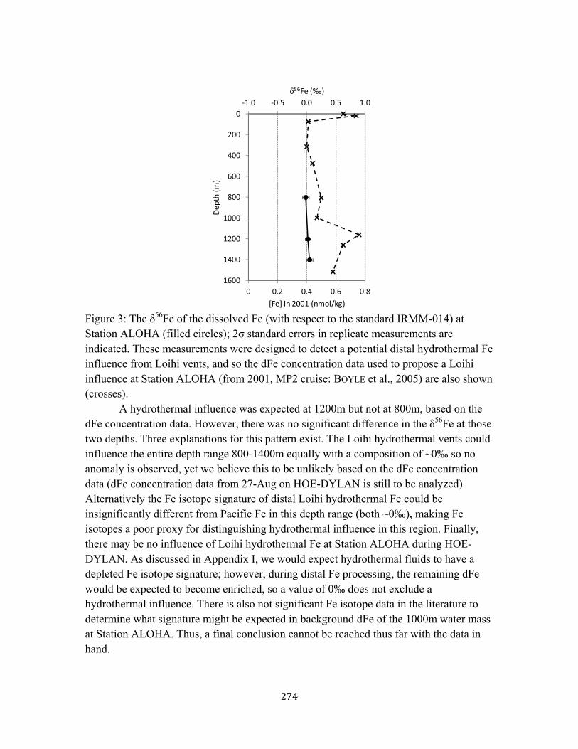
274
Figure 3: The δ56Fe of the dissolved Fe (with respect to the standard IRMM-014) at Station ALOHA (filled circles); 2σ standard errors in replicate measurements are indicated. These measurements were designed to detect a potential distal hydrothermal Fe influence from Loihi vents, and so the dFe concentration data used to propose a Loihi influence at Station ALOHA (from 2001, MP2 cruise: BOYLE et al., 2005) are also shown (crosses).
A hydrothermal influence was expected at 1200m but not at 800m, based on the dFe concentration data. However, there was no significant difference in the δ56Fe at those two depths. Three explanations for this pattern exist. The Loihi hydrothermal vents could influence the entire depth range 800-1400m equally with a composition of ~0‰ so no anomaly is observed, yet we believe this to be unlikely based on the dFe concentration data (dFe concentration data from 27-Aug on HOE-DYLAN is still to be analyzed). Alternatively the Fe isotope signature of distal Loihi hydrothermal Fe could be insignificantly different from Pacific Fe in this depth range (both ~0‰), making Fe isotopes a poor proxy for distinguishing hydrothermal influence in this region. Finally, there may be no influence of Loihi hydrothermal Fe at Station ALOHA during HOE-DYLAN. As discussed in Appendix I, we would expect hydrothermal fluids to have a depleted Fe isotope signature; however, during distal Fe processing, the remaining dFe would be expected to become enriched, so a value of 0‰ does not exclude a hydrothermal influence. There is also not significant Fe isotope data in the literature to determine what signature might be expected in background dFe of the 1000m water mass at Station ALOHA. Thus, a final conclusion cannot be reached thus far with the data in hand.
0 0.2 0.4 0.6 0.8
0
200
400
600
800
1000
1200
1400
1600
‐1.0 ‐0.5 0.0 0.5 1.0
[Fe] in 2001 (nmol/kg)
Depth (m
)
δ56Fe (‰)

275
References for Appendix IV Bell, J., Betts, J., and Boyle, E., 2002. MITESS: a moored in situ trace element serial
sampler for deep-sea moorings. Deep-Sea Research Part I-Oceanographic Research Papers 49, 2103-2118.
Boyle, E. A., Bergquist, B. A., Kayser, R. A., and Mahowald, N., 2005. Iron, manganese, and lead at Hawaii Ocean Time-series station ALOHA: Temporal variability and an intermediate water hydrothermal plume. Geochimica et Cosmochimica Acta 69, 5165-5166.
Conway, T. M., Rosenberg, A. D., Adkins, J. F., and John, S. G., in press. A new method for precise determination of iron, zinc, and cadmium stable isotope ratios in seawater by double-spike mass spectrometry. Analytica Chimica Acta.
Fitzsimmons, J. N. and Boyle, E. A., 2012. An intercalibration between the GEOTRACES GO-FLO and the MITESS/Vanes sampling systems for dissolved iron concentration analyses (and a closer look at adsorption effects). Limnology & Oceanography: Methods 10, 437-450.
Johnson, W. K., Miller, L. A., Sutherland, N. E., and Wong, C. S., 2005. Iron transport by mesoscale Haida eddies in the Gulf of Alaska. Deep Sea Research Part II: Topical Studies in Oceanography 52, 933-953.
Lee, J.-M., Boyle, E. A., Echegoyen-Sanz, Y., Fitzsimmons, J. N., Zhang, R., and Kayser, R. A., 2011. Analysis of trace metals (Cu, Cd, Pb, and Fe) in seawater using single batch Nitrilotriacetate resin extraction and isotope dilution inductively coupled plasma mass spectrometry. Analytica Chimica Acta 686, 93-101.
Noble, A. E., Saito, M. A., Maiti, K., and Benitez-Nelson, C. R., 2008. Cobalt, manganese, and iron near the Hawaiian Islands: A potential concentrating mechanism for cobalt within a cyclonic eddy and implications for the hybrid-type trace metals. Deep-Sea Research II 55, 1473-1490.
Sedwick, P. N., Church, T. M., Bowie, A. R., Marsay, C. M., Ussher, S. J., Achilles, K. M., Lethaby, P. J., Johnson, R. J., Sarin, M. M., and McGillicuddy, D. J., 2005. Iron in the Sargasso Sea (Bermuda Atlantic Time-series Study region) during summer: Eolian imprint, spatiotemporal variability, and ecological implications. Global Biogeochem. Cycles 19, GB4006.