HAL Id: tel-03092293https://tel.archives-ouvertes.fr/tel-03092293

Submitted on 2 Jan 2021

HAL is a multi-disciplinary open accessarchive for the deposit and dissemination of sci-entific research documents, whether they are pub-lished or not. The documents may come fromteaching and research institutions in France orabroad, or from public or private research centers.

L’archive ouverte pluridisciplinaire HAL, estdestinée au dépôt et à la diffusion de documentsscientifiques de niveau recherche, publiés ou non,émanant des établissements d’enseignement et derecherche français ou étrangers, des laboratoirespublics ou privés.

Business continuity of energy systems : a quantitativeframework for dynamic assessment and optimization

Jinduo Xing

To cite this version:Jinduo Xing. Business continuity of energy systems : a quantitative framework for dynamic assessmentand optimization. Chemical and Process Engineering. Université Paris Saclay (COmUE), 2019.English. �NNT : 2019SACLC087�. �tel-03092293�

Business continuity of energy systems: a quantitative framework for dynamic

assessment and optimization

Thèse de doctorat de l'Université Paris-Saclay préparée à Centralesupeléc

École doctorale n°573 interfaces : approches interdisciplinaires, fondements, applications et innovation (Interfaces)

Spécialité de doctorat : sciences et technologies industrielles

Thèse présentée et soutenue à Gif-sur-Yvette, le 03 décembre 2019, par

Mme Jinduo XING Composition du Jury: Anne Barros Professeur, CentraleSupélec, Université Paris-Saclay Président

Francesco Di Maio Professeur associé, Politecnico di Milano Rapporteur

Emmanuel Remy Chercheur, EDF R&D Examinateur Sébastien Travadel Professeur associé, Mines ParisTech Rapporteur

Hong Xia Professeur, Harbin Engineering University Examinatrice

Enrico Zio Professeur, Politecnico di Milano Directeur de thèse

NN

T : 2

019

SA

CLC

087

i

Acknowledgement

I would like to devote my deepest respect and gratitude to my supervisor, Professor Enrico Zio. Thank him for

giving me this precious opportunity to come to France for pursuing this diploma. Thanks for his trust and tolerance.

Thank him for forgiving my additional eight-year doctoral life- my punishment of taking a chocolate from him at a

picnic. Thank him, seriously, for setting an idol for my research life with his seriousness and enthusiasm for scientific

career.

I would like to extend my sincere gratitude to my co-supervisor, Dr. Zhiguo Zeng, for his help and efforts on

this thesis. Thank him for his advice, patience and great support during my PhD study.

My deepest appreciation goes to all the jury members: Professor Anne Barros, Professor Francesco Di Maio,

Professor Emmanuel Remy, Professor Sébastien Travadel, Professor Hong Xia. Thanks for their invaluable

comments that help to improve this thesis.

I would like to thank my friends and colleagues in LGI who give me a lot of help to make my life in France

easily. Particularly, great thanks for my colleagues in the Chair on System Science and the Energy Challenges (SSEC),

Jie Liu, Yanhui Lin, Xing Liu, Fangyuan Han, Mengfei Fan, Yiping Fang, Tasneem Bani-Mustafa, Zhiyi Wang,

Islam F. ABDIN, Hoang-Phuong NGUYEN, Hongping Wang, Daogui Tang. I would like to thank them for their

encouragement and help whenever I needed help. It has been a pleasure to work with such wonderful persons.

I would also like to thank the financial support from the China Scholarship Council.

Last but not the least, I would like to offer my special thanks to my family for their love, support. Especially,

for my elder sister, who devotes a lot for my family when I am abroad. I also want to thank my boyfriend Dr. Meng,

thanks for his encouragement, support, and help in my PhD life.

ii

iii

Abstract

Concerns over disruptive events on the operation of energy systems have increased significantly during the past

decades. This creates considerable demands on accurate business continuity assessment and effective management

techniques for these systems. New opportunities for this come from using online-collected data and information to

assess risk (dynamic risk assessment) and business continuity (dynamic business continuity assessment), and from

using the assessment results for improving the optimal design of the system to achieve maximal business continuity.

With this perspective in the present thesis, first, a dynamic risk assessment (DRA) framework is developed to

capture the time-dependent degradation behaviour of safety barriers by integrating both condition monitoring data

and inspection data. Condition monitoring data are online-collected by sensors and assumed to indirectly relate to

component degradation; inspection data are recorded in physical inspections that are assumed to directly measure the

component degradation. A Hidden Markov Gaussian Mixture Model (HM-GMM) is developed for modelling the

condition monitoring data and a Bayesian network (BN) is developed to integrate the two data sources for DRA. Risk

updating and prediction are exemplified on an Event Tree (ET) risk assessment model. A numerical case study and a

real-world application on a Nuclear power plant (NPP) are performed to demonstrate the application of the proposed

work.

Then, a dynamic business continuity assessment (DBCA) framework is proposed to capture time-dependent

behaviours and integrate the information on the conditions of components and system in the business continuity

assessment (BCA). Specifically, a particle filtering (PF)-based method is developed to integrate condition monitoring

data on the safety barriers installed for system protection and predict their reliability as their health states change due

to ageing. An instalment model and a stochastic price model are also employed to quantify the time-dependent

revenues and tolerable losses during the operation of the system. A simulation model is developed to evaluate

dynamic business continuity metrics originally introduced. A case study regarding a NPP risk scenario is worked out

to demonstrate the applicability of the proposed approach.

Finally, a joint optimization model is developed to optimally design safety barriers of different natures, including

prevention, mitigation, emergency and recovery barriers to enhance the business continuity of the system. The joint

iv

optimization is guided by a business continuity metrics called expected business continuity values (EBCV). A

physics-of-failure model is developed to model the effectiveness of prevention safety barriers. An ET model is

developed to describe the potential accident evolution process. A redundancy allocation model is, then, used to

consider the efforts to enhance the mitigation and emergency barriers. Recovery measures are also considered by a

widely used logarithmic function model. A mixed-integer genetic algorithm is employed to obtain optimal solutions

of the joint optimisation model. The developed framework is applied on a case study of steam generator tube rupture

accident in a NPP.

Overall, through the research of this thesis, we have established a framework that allows making BCA using

online-collected information. We have also showed how to optimize the business continuity of a system through a

joint optimization model. These findings demonstrate the prospects of applying BCM in accident prevention,

mitigation, emergency, recovery, to better support the operation of energy systems by ensuring its business continuity.

Keywords: Dynamic risk assessment, Dynamic business continuity assessment, Condition monitoring data,

Inspection data, Event tree, Hidden Markov-Gaussian Mixture model, Particle filtering, Stochastic electricity model,

Joint optimization, Mixed integer genetic algorithm

v

Résumé

Les inquiétudes suscitées par des événements perturbateurs sur le fonctionnement des systèmes énergétiques ont

considérablement augmenté au cours des dernières décennies. Cela crée des exigences considérables en matière

d'évaluation de la continuité des opérations et de techniques de gestion efficaces pour ces systèmes. Les nouvelles

opportunités à cet égard proviennent de l’utilisation des données et des informations collectées en ligne pour évaluer

les risques (évaluation dynamique des risques) et la continuité de l’activité (évaluation dynamique de la continuité

des activités), ainsi que de l’utilisation des résultats de l’évaluation pour améliorer la conception optimale du système

et atteindre une continuité maximale des activités.

Dans cette perspective dans la présente thèse, un cadre d’évaluation dynamique des risques (DRA) est développé

pour capturer le comportement de dégradation dépendant du temps des barrières de sécurité en intégrant à la fois des

données de surveillance des conditions et des données d’inspection. Les données de surveillance des conditions sont

collectées en ligne par des capteurs et supposées être indirectement liées à la dégradation des composants; les données

d'inspection sont enregistrées lors d'inspections physiques censées mesurer directement la dégradation du composant.

Un modèle de mélange gaussien caché de Markov (HM-GMM) est développé pour modéliser les données de

surveillance de l'état et un réseau bayésien (BN) est développé pour intégrer les deux sources de données pour la

DRA. La mise à jour et la prévision des risques sont illustrées dans un modèle d'évaluation des risques de l'arbre des

événements. Une étude de cas numérique et une application réelle sur une centrale nucléaire (centrale nucléaire) sont

réalisées pour démontrer l'application du travail proposé.

Ensuite, un cadre d'évaluation dynamique de la continuité des opérations (DBCA) est proposé pour capturer les

comportements dépendant du temps et intégrer l'information sur les conditions des composants et du système dans

l'évaluation de la continuité des opérations (BCA). Plus précisément, une méthode basée sur le filtrage de particules

(PF) est développée pour intégrer les données de surveillance des conditions sur les barrières de sécurité installées

pour la protection des systèmes et prévoir leur fiabilité lorsque leur état de santé évolue en raison du vieillissement.

Un modèle de versement et un modèle de prix stochastique sont également utilisés pour quantifier les revenus et les

pertes tolérables en fonction du temps pendant le fonctionnement du système. Un modèle de simulation est développé

vi

pour évaluer les mesures de continuité d'activité dynamiques introduites à l'origine. Une étude de cas concernant un

scénario de risque de centrale nucléaire est élaborée pour démontrer l'applicabilité de l'approche proposée.

Enfin, un modèle d’optimisation commun est élaboré pour concevoir de manière optimale des barrières de

sécurité de différentes natures, notamment des barrières de prévention, d’atténuation, d’urgence et de reprise, afin

d’améliorer la continuité des opérations du système. L'optimisation conjointe est guidée par une métrique de

continuité d'activité appelée valeurs de continuité d'activité attendues (EBCV). Un modèle de physique de défaillance

est développé pour modéliser l'efficacité des barrières de sécurité préventives. Un modèle ET est développé pour

décrire le processus d'évolution des accidents potentiels. Un modèle d'allocation de redondance est donc utilisé pour

prendre en compte les efforts visant à renforcer les barrières d'atténuation et d'urgence. Les mesures de récupération

sont également prises en compte par un modèle de fonction logarithmique largement utilisé. Un algorithme génétique

à nombres entiers mixtes est utilisé pour obtenir des solutions optimales du modèle d'optimisation conjointe. Le cadre

développé est appliqué à une étude de cas d'accident de rupture de tube de générateur de vapeur dans une centrale

nucléaire.

Globalement, à travers la recherche de cette thèse, nous avons établi un cadre qui permet de créer une BCA en

utilisant des informations collectées en ligne. Nous avons également montré comment optimiser la continuité

d'activité d'un système grâce à un modèle d'optimisation commun. Ces résultats démontrent les perspectives

d'application de la BCM dans la prévention, l'atténuation, les urgences et la récupération des accidents, afin de mieux

soutenir le fonctionnement des systèmes énergétiques en assurant la continuité de ses activités.

Mots-clés: Evaluation dynamique des risques, Evaluation dynamique de la continuité des opérations, Données

de surveillance des conditions, Données de contrôle, Arbre des événements, Modèle de mélange caché markov-

gaussien, Filtrage de particules, Modèle d'électricité stochastique, Optimisation d'articulation, Algorithme génétique

d'entiers mixtes

vii

Contents

Abstract ........................................................................................................................................................................ i

List of Figures ............................................................................................................................................................ xi

List of Tables ............................................................................................................................................................ xiii

Acronyms ................................................................................................................................................................... xv

Notation ................................................................................................................................................................... xvii

Appended papers ..................................................................................................................................................... xix

Chapter 1 Introduction ....................................................................................................................................... 1

1.1 Business continuity management ............................................................................................................. 2

1.2 Open issues............................................................................................................................................... 3

1.2.1 Dynamic risk assessment ........................................................................................................... 3

1.2.2 Dynamic business continuity assessment ................................................................................... 4

1.2.3 Joint optimization ....................................................................................................................... 5

1.3 Research objectives and contributions ..................................................................................................... 6

1.4 Structure of the thesis ............................................................................................................................... 6

Chapter 2 Dynamic risk assessment using condition monitoring data and inspection data ......................... 9

2.1 State of the art .......................................................................................................................................... 9

2.2 Problem definition .................................................................................................................................. 10

2.3 A HM-GMM for modelling condition monitoring data ......................................................................... 11

2.3.1 Model formulation ................................................................................................................... 12

2.3.2 Degradation states estimation based on condition monitoring data ......................................... 13

2.4 Data integration for DRA ....................................................................................................................... 17

2.4.1 A Bayesian network model for data integration ....................................................................... 17

2.4.2 Dynamic risk assessment ......................................................................................................... 19

2.5 Application ............................................................................................................................................. 20

2.5.1 System description ................................................................................................................... 20

viii

2.5.2 Dynamic risk assessment ......................................................................................................... 21

2.5.3 Results ...................................................................................................................................... 23

2.6 Conclusion ............................................................................................................................................. 24

Chapter 3 Dynamic business continuity assessment using condition monitoring data ............................... 27

3.1 State of the art ........................................................................................................................................ 27

3.2 Numerical metrics for dynamic continuity assessment .......................................................................... 29

3.3 An integrated framework for dynamic business continuity assessment ................................................. 30

3.3.1 The integrated modeling framework ........................................................................................ 31

3.3.2 Loss modeling .......................................................................................................................... 32

3.3.3 Tolerable losses modeling ........................................................................................................ 34

3.4 Case study .............................................................................................................................................. 35

3.4.1 System description ................................................................................................................... 35

3.4.2 Particle filtering and loss modeling .......................................................................................... 37

3.4.3 Tolerable loss modeling ........................................................................................................... 39

3.4.4 Results ...................................................................................................................................... 41

3.5 Conclusion ............................................................................................................................................. 44

Chapter 4 Joint optimization for enhancing business continuity .................................................................. 45

4.1 State of the art ........................................................................................................................................ 45

4.2 Joint optimization ................................................................................................................................... 47

4.3 Solution method ..................................................................................................................................... 48

4.4 Case study .............................................................................................................................................. 49

4.4.1 Event modelling ....................................................................................................................... 49

4.4.2 Business continuity modelling ................................................................................................. 50

4.4.3 Joint optimization ..................................................................................................................... 53

4.4.4 Results and sensitivity analysis ................................................................................................ 55

4.5 Conclusion ............................................................................................................................................. 62

Chapter 5 Conclusion and future work ........................................................................................................... 63

ix

5.1 Conclusion ............................................................................................................................................. 63

5.2 Perspectives ............................................................................................................................................ 64

Reference ................................................................................................................................................................... 65

Paper I ....................................................................................................................................................................... 71

Paper II .................................................................................................................................................................... 108

Paper III .................................................................................................................................................................. 140

x

xi

List of Figures

Figure 1-1. A conceptual scheme of the business continuity process [11]. ......................................................... 2

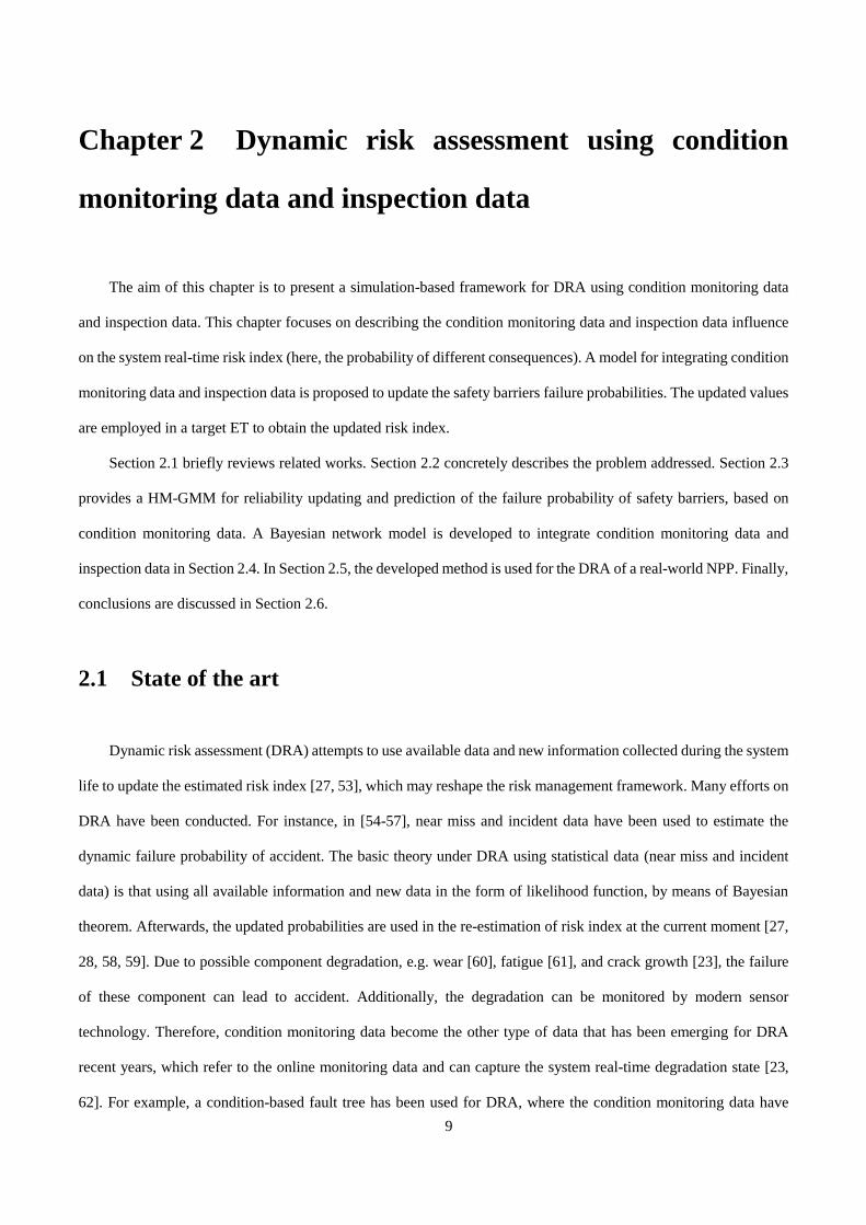
Figure 2-1. Illustrative Event Tree model. ......................................................................................................... 11

Figure 2-2. Description of the HM-GMM. ........................................................................................................ 13

Figure 2-3. Degradation state estimation based on condition monitoring data. ................................................. 14

Figure 2-4. A BN model for data integration. .................................................................................................... 18

Figure 2-5. ET for the ATWS. ........................................................................................................................... 21

Figure 2-6. Extracted degradation indicators. .................................................................................................... 22

Figure 2-7. The results of risk updating and prediction. .................................................................................... 24

Figure 3-1. An integrated model for DBCA. ..................................................................................................... 32

Figure 3-2. ET for SGTR accident [59]. ............................................................................................................ 36

Figure 3-3 Crack growth process. ...................................................................................................................... 38

Figure 3-4 RUL Prediction results ..................................................................................................................... 38

Figure 3-5. Profit trajectory at different estimation points. ............................................................................... 41

Figure 3-6. Business continuity metrics at t=1 year........................................................................................... 42

Figure 3-7. Business continuity metrics at t=10 years. ...................................................................................... 43

Figure 3-8. Business continuity metrics at t=40 years. ...................................................................................... 43

Figure 4-1. Schematic ET model of SGTR accident ( 2 5C C core damage) [115]. ........................................ 50

Figure 4-2 Schematic of MIGA. ........................................................................................................................ 55

Figure 4-3 Results comparison for proposed joint optimization and prevention only ( 8000(k€)totalc = ). ........ 57

Figure 4-4 Behavioural indexes in prevention, mitigation & emergency, and recovery phases. ....................... 58

Figure 4-5 Comparison of EBCV with different cost effectiveness parameters. ............................................... 60

Figure 4-6 Comparison EBCV with different cost-budget. ............................................................................... 61

Figure 4-7 Schematic of changing failure probability of mitigation measures (70%~130%) under budget

8000k€.totalC = .................................................................................................................................................. 61

xii

xiii

List of Tables

Table 2-1. Values of ( )CMP S S . ........................................................................................................................ 23

Table 3-1. Safety barriers in the target system [90, 91]. .................................................................................... 36

Table 3-2. Initial intervals for the parameters. ................................................................................................... 38

Table 3-3. Values of the recovery model parameters. ....................................................................................... 39

Table 3-4. Values of the seasonal component parameters of the spot prices. .................................................... 39

Table 3-5. Parameters in the stochastic electricity model [99]. ......................................................................... 40

Table 4-1 Parameters of the NPP. ...................................................................................................................... 49

Table 4-2. Classification of consequences. ........................................................................................................ 50

Table 4-3. Parameters of the MIGA algorithm. ................................................................................................. 55

Table 4-4 Parameter values used in the case study. ........................................................................................... 56

Table 4-5 Comparison results for business continuity under different strategies. ............................................. 57

xiv

xv

Acronyms

ATWS Anticipated Transient without scram

BCA Business continuity assessment

BCM Business continuity management

BCV Business continuity value

BN Bayesian Network

DRA Dynamic risk assessment

DBCA Dynamic business continuity assessment

DBN Dynamic Bayesian Network

EM Expectation Maximization

EBCV Expected business continuity value

ET Event tree

FT Fault tree

MIGA Mixed-integer genetic algorithm

HM-GMM Hidden Markov-Gaussian Mixture Model

IE Initialling Event

NPP Nuclear power plant

PF Particle Filtering

PRA Probabilistic risk assessment

PDF Probability density function

QRA Quantitative risk assessment

RA Risk assessment

RUL Remaining useful life

RCS Reactor coolant system

RDS Reactor depressurization system

xvi

RWST Refuelling water storage tank

SGTR Steam generator tube rupture

xvii

Notation

a Crack length

π Initial state distribution of the Markov degradation process

( )ib x Probability distribution of the degradation indicator x when the degradation state is iS

iC The -i th consequence in the ET

c ( )i kt Condition monitoring data from the -i th safety barrier at kt t=

( ) ( )k

Tr tc Condition monitoring data from the -k th training sample at t

( )d Euclidean distance

( )ETf ET model

inL Indirect loss

dL Direct loss

K Number of safety barriers with time-dependent failure probabilities

M Number of safety barriers in a system

N Number of consequences in the ET

SN Sample size of PF

featuren Number of features extracted from condition monitoring data

Trn Number of samples in the training data set

iCP Probability that consequence i occurs, given that the IE has occurred

, ( )kCM t CMP S Posterior distribution of the estimated degradation state from condition monitoring data, evaluated

at kt

, ( )kINT tP S Posterior distribution of the estimated degradation state by integrating condition monitoring data

and inspection data, evaluated at kt

xviii

Q Number of health states

INR Reliability of the inspection

MSBR Reliability of the M − th safety barrier

CMS Estimated degradation state from condition monitoring data

,CM MAPS Most likely degradation state given the condition monitoring data

INS Estimated degradation state from inspection data

S True degradation state

Trt Length of the observation period for the training samples

recvt Recovery time

W Working set that contains all the working states

( ) ( )k

Tr tx Health indicator of -k th training data at t

( )tx Health indicator of safety barrier at t

μ Vector of the mean values of the multivariate Gaussian distribution

Σ Covariance matrices of the multivariate Gaussian distribution

( )t iS Forward variable

( )t iS Backward variable

xix

Appended papers

Paper I: J. Xing, Z. Zeng, E. Zio. A framework for dynamic risk assessment with condition monitoring data and

inspection data. Reliability Engineering and System Safety, 2019, 191, 106552.

Paper II: J. Xing, Z. Zeng, E. Zio. Dynamic business continuity assessment using condition monitoring data.

International Journal of Disaster Risk Reduction, 2019, 41, 101334.

Paper III: J. Xing, Z. Zeng, E. Zio. Joint optimization of safety barriers against steam generator tube rupture to

enhance business continuity of nuclear power plants. Reliability Engineering and System Safety, 2019. (Under

review).

xx

1

Chapter 1 Introduction

Business operations of energy systems, such as nuclear power plants (NPPs), electricity transmission systems,

are threatened by a number of hazards [1-4]. These should be properly managed [5]. Conventionally, risk assessment

and management are employed to protect the business from disruptive events. In risk assessment, possible

consequences and associated likelihoods are considered for accidents potentially developing from the identical

hazards [6]. On the other hand, the process of recovering from an accident has a significant influence on business

operations, as it directly affects downtime. Recently, a holistic method known as business continuity management

(BCM) has been put forth, which integrates protection, mitigation, emergency and recovery to ensure the continuous

operation of a business.

Many questions and challenges arise in the application of BCM to energy systems. For instance, as sensor

technologies and computing resources advance, data and information can be collected online, as the system operates.

How to use these data and information to support proactive and real-time quantitative risk assessment (QRA) and

business continuity assessment (BCA) is an opportunity, and, at the same time, a challenging issue in BCM. Another

challenging issue is how to optimize business continuity, considering the components and safety barriers of different

nature that make up the system. Objective of this thesis is to address the aforementioned questions by providing a

quantitative framework for the safe and continuous business operation of energy systems. The focus is on the

quantitative assessment of business continuity for energy systems under disruptive events (e.g., steam generator tube

rupture (SGTR) [7], anticipated transient without scram (ATWS) accidents [8]). An integrated framework for BCA

is proposed first, where four stages named preventive stage, mitigation stage, emergency stage and recovery stage

are comprehensively considered and integrated. Due to the vital role of risk assessment in BCM, a dynamic risk

assessment (DRA) framework is proposed, capable of incorporating both inspection data and condition monitoring

data. Finally, the optimization of business continuity is considered by developing a joint optimization model.

In the following of this chapter, we present a brief introduction of the context of the research and open issues in

Section 1.1 and Section 1.2, respectively. The research objective and main contributions are discussed in Section 1.3.

Finally, Section 1.4 shows the structure of the thesis.

2

1.1 Business continuity management

BCM is defined by the international organization of standards (ISO) as “the holistic management process that

identifies potential threats to an organization and the impacts to business operations those threats, if realized might

cause, and which provides a framework for building organizational resilience with the capability of an effective

response that safeguards the interest of its key stakeholders, reputation, brand and value-creating activities”[9]. In a

nutshell, BCM is a comprehensive method that integrates pre-event and post-event management together to ensure

the resilience and continuous operation of system business. Compared to conventional risk analysis method, BCM

not only focuses on the potential hazards and their impacts, but also considers how to mitigate the consequence and

quickly recover from the disruption.

BCM aims at developing appropriate methods in order to prevent and resume system business to an acceptable

predefined level [10]. Usually, pre-disruptive and post-disruptive measures are considered in a system with respect

to system resilience and business continuity [11]. The former aims at identifying potential hazards and reducing their

possibility. The latter is associated with resuming system business in the aftermath of disruptive event to reduce

potential losses [12].

A conceptual model is presented in Figure 1-1 to illustrate the different processes involved in BCM. Business

continuity measures the ability of an organization to resist, mitigate and recover to an acceptable state given a

disruptive event.

Figure 1-1. A conceptual scheme of the business continuity process [13].

For the pre-event stage, protection measures are installed in advance to resist to the potential event, i.e. by

reducing the probability of occurrence of the accident event. Next comes the mitigation phase, where safety barriers

are usually activated to mitigate the consequences of the disruptive event once occurred. The purpose of the mitigation

3

phase is to contain the evolution of the accident consequences [14, 15]. Emergency measures act to cope with the

accident evolution and human intervention is often required [16]. Finally, recovery actions are taken to bring system

business back to operation.

Most existing researches on BCM are, however, based on qualitative BCA [17-22]. This situation impedes the

quantitative analysis of business continuity and its effective application. Thus, a quantitative framework for the

assessment and optimization of the business continuity process is needed.

1.2 Open issues

Risk assessment plays a fundamental role in BCM. How to improve risk assessment accuracy with the help of

different knowledge, information and data is the first research topic in this thesis. In Section 1.2.1, we review the

related works on this topic. In Section 1.2.2, we review the researches related to a quantitative BCA considering

available time-variant factors. Section 1.2.3 reviews the related research efforts on optimization models for enhancing

business continuity.

1.2.1 Dynamic risk assessment

Traditional risk assessment methods, like event tree (ET) and fault tree (FT), mainly treat the failure probabilities

of safety barriers as constant values, without explicitly modelling degradation and aging processes [23]. In practice,

operational and environmental conditions of the system change with time, and this generally causes time-dependent

behaviours of the safety barriers [24-26]. To account for the time-dependent characteristic of safety barriers, a number

of DRA frameworks have been developed, which employ data and information collected during the system operation

to update the estimated risk indexes [27]. The goal of DRA is to obtain an estimate of system’s risk updated in real

time with the accumulated information and data [28]. Bayesian theory has been used to update the probabilities of

the events in an ET [29, 30]. A condition-based risk assessment has been performed in [24] for a spontaneous SGTR

accident. A data-driven DRA model has been developed for offshore drilling operations, where real-time operational

data have been employed to update the probability of kick events [31]. In [32], statistical failure data and condition

monitoring data have been integrated in a hierarchical Bayesian model for DRA.

4

The data used by existing DRA methods can be broadly grouped into two categories: statistical data and

condition monitoring data. Statistical failure data refer to counts of accidents, incidents or near misses collected in

the field. Condition monitoring data are the online monitoring data collected by sensors that are installed in the system

for monitoring the degradation process of the safety barriers. Uncertainty may exist in condition monitoring data due

to possible noise during the monitoring process. Apart from these two data types, inspection data can also be collected

by physical inspections performed by maintenance personnel [33], and might serve as another data source for online

reliability assessment. In [34], a Bayesian method has been developed to merge experts’ judgments with continuous

and discontinuous inspection data for the reliability assessment of multi-state systems. A two-stage recursive

Bayesian approach has been developed in [35], in order to update system reliability based on imperfect inspection

data. Condition monitoring data and inspection data on wind turbine blades have been used separately for remaining

useful life estimation in [36]. Inspection data directly measure the component degradation and provide valuable

information complementary to condition monitoring data for DRA. In this thesis, we aim at developing new DRA

methods that allow integrating condition monitoring data with inspection data, for real-time risk estimates update.

1.2.2 Dynamic business continuity assessment

Most of the existing methods for quantitative BCA focus on time-static problems [37], where the analysis is

done before operation and is not updated to consider aging and degradation of components and systems. For instance,

a statistical model integrating Cox’s model and Bayesian networks has been proposed to model the BCM process

[38]. In [12], the BCM outsourcing and insuring strategies have been compared based on the organization

characteristics and the relevant data through a two-step fuzzy cost-benefit analysis. Two probabilistic programming

models have been developed in [39] to determine appropriate business continuity plans given epistemic uncertainty

in the input data. In [40], a new model for integrated business continuity and disaster recovery planning has been

presented, considering multiple disruptive incidents that might occur simultaneously. An integrated framework has

been developed for quantitative business continuity analysis, where four numerical metrics were proposed to quantify

the business continuity level based on the potential loss caused by the disruptive event [14].

However, in practice, various time-dependent factors might affect the business continuity, e.g., the degradation

of safety barriers, the dynamic behaviour of profits and losses. On the other hand, as sensor technologies and

computing resources advance, it is possible to capture these dynamic factors even in real-time, based on online-

5

collected condition monitoring data [41, 42]. For example, a condition-based fault tree has been used for dynamic

risk assessment (DRA) [43], where condition monitoring data are used to update the failure rates of specific

components and predict the reliability. In [44], a Bayesian reliability updating method has been proposed for

dependent components by using condition monitoring data. Therefore, in this thesis, we investigate how to use the

online collected data and information to support dynamic business continuity assessment (DBCA), with time-

dependent contributing factors.

1.2.3 Joint optimization

In general, the resources an organization can invest to safeguard the continuous operation of a system are limited.

How to allocate and arrange the limited resources among the prevention, mitigation, emergency and recovery

measures is an important topic to address. Some studies have developed methods to allocate resources to improve

system resilience for a specific disaster. For instance, multi-systems’ joint restoration processes modeling has been

addressed and the effectiveness of five different restoration strategies has been compared in [45] regarding hurricane

hazard. In [46], a two-stage mixed-integer programming resource allocation model for lifeline systems has been

proposed to improve the efficiency of restoration. A multi-objective optimization model of emergency organization

allocation for sustainable disaster supply chains has been developed to design optimized strategies of emergency

organization allocation [47], with the objective of minimizing the expected outage duration of loads. A scenario-

based two-states stochastic optimization for minimizing outage duration in distribution damage and road network

damage has been exploited in [48]. In [49], a restoration resource allocation model has been proposed to enhance

resilience of interdependent infrastructure systems. A resilience-based optimization methodology has been performed

over the set of feasible restoration policies, information investments and human resource availability to determine

optimal customer and system-wide monetary utility [50]. A stochastic optimization technique has been developed to

allocate scarce national resources to cope with multiple simultaneous disasters occurring across the nation [51].

Most existing research, as reviewed above, considers the safety barriers separately. In this work, we aim to

develop a joint optimization model that aims to assure an holistic optimal performance, considering all the safety

barriers.

6

1.3 Research objectives and contributions

The focus of this thesis is to develop methods that support DBCA, based on the online-collected data and

information. Besides, we also aim to develop a joint optimization model for maximizing system business continuity,

through optimally allocating resources among prevention, mitigation, emergency and recovery measures.

The main contributions of the thesis can be summarized as follows:

(1) A new DRA framework is developed, which allows integrating condition monitoring data and inspection

data for online assessment;

(2) An integrated DBCA model is proposed, which allows updating the business continuity in real time, using

the online-collected data and information;

(3) A joint optimization is developed to optimize the business continuity considering the prevention, mitigation,

emergency and recovery phases.

1.4 Structure of the thesis

This thesis includes two parts. The first part contains five chapters, introducing the research context and

describing the problems addressed, approaches proposed, and related results.

Chapter 2 begins with a state of art on DRA and continues with the roles of condition monitoring data and

inspection data for risk and reliability analysis. A HM-GMM is developed for modelling the condition monitoring

data and a Bayesian network (BN) is proposed to integrate the two data sources for DRA. A real-world application

on a NPP [52] is conducted to demonstrate the use of the proposed framework.

Chapter 3 firstly reviews researches related to BCA, which are grouped into qualitative methods and quantitative

methods. To capture the time-variant factors in BCA, a particle filtering (PF)-based method is developed to predict

the reliability of the safety barriers in time. Moreover, an instalment model and a stochastic price model are also

employed to model the time-dependent revenues and tolerable losses of the organization. Finally, a case study on a

NPP is performed to demonstrate the applicability of the proposed approach.

Chapter 4 focuses on the joint optimization of business continuity. An optimization model is developed for

resource allocation on system safety barriers to enhance business continuity, considering all the phases from pre-

7

disruption protection to post-disruption response and recovery. The optimal solution is obtained by a Mix-integer

genetic algorithm (MIGA), which aims at maximizing system business continuity over a finite time horizon. To

investigate the utility of the optimization model, a case study on a nuclear power plant (NPP) is performed to

maximize expected business continuity value (EBCV) against threat of SGTR.

Chapter 5 draws conclusions of the thesis and points out the potential future works.

The second part contains a collection of three papers, describing the research work performed during the PhD,

where readers can refer to for further technical details. In paper I, condition monitoring data and, inspection data are

integrated to conduct DRA (corresponding to Chapter 2). In paper II, a dynamic BCA is proposed employing PF and

the instalment model (corresponding to Chapter 3). In paper III, a joint optimization of the resources on safety barriers

for enhancing system business continuity is proposed (corresponding to Chapter 4).

8

9

Chapter 2 Dynamic risk assessment using condition

monitoring data and inspection data

The aim of this chapter is to present a simulation-based framework for DRA using condition monitoring data

and inspection data. This chapter focuses on describing the condition monitoring data and inspection data influence

on the system real-time risk index (here, the probability of different consequences). A model for integrating condition

monitoring data and inspection data is proposed to update the safety barriers failure probabilities. The updated values

are employed in a target ET to obtain the updated risk index.

Section 2.1 briefly reviews related works. Section 2.2 concretely describes the problem addressed. Section 2.3

provides a HM-GMM for reliability updating and prediction of the failure probability of safety barriers, based on

condition monitoring data. A Bayesian network model is developed to integrate condition monitoring data and

inspection data in Section 2.4. In Section 2.5, the developed method is used for the DRA of a real-world NPP. Finally,

conclusions are discussed in Section 2.6.

2.1 State of the art

Dynamic risk assessment (DRA) attempts to use available data and new information collected during the system

life to update the estimated risk index [27, 53], which may reshape the risk management framework. Many efforts on

DRA have been conducted. For instance, in [54-57], near miss and incident data have been used to estimate the

dynamic failure probability of accident. The basic theory under DRA using statistical data (near miss and incident

data) is that using all available information and new data in the form of likelihood function, by means of Bayesian

theorem. Afterwards, the updated probabilities are used in the re-estimation of risk index at the current moment [27,

28, 58, 59]. Due to possible component degradation, e.g. wear [60], fatigue [61], and crack growth [23], the failure

of these component can lead to accident. Additionally, the degradation can be monitored by modern sensor

technology. Therefore, condition monitoring data become the other type of data that has been emerging for DRA

recent years, which refer to the online monitoring data and can capture the system real-time degradation state [23,

62]. For example, a condition-based fault tree has been used for DRA, where the condition monitoring data have

10

been used to update the failure rates of the specific components and predict the reliability [43, 63]. Particle filtering

(PF) has been used for DRA based on condition monitoring data from a nonlinear non-Gaussian process [64]. In [23],

condition monitoring data from a passive safety system have been used for DRA, without considering the uncertainty

in the condition monitoring data.

2.2 Problem definition

In this chapter, we consider the DRA by integrating two data sources, i.e., condition monitoring data and

inspection data. Condition monitoring data refer to the online monitoring data collected by sensors that are installed

in the target system for monitoring the degradation process of the safety barrier [65]. Inspection data are collected by

physical inspections performed by maintenance personnel. More specifically, the problem is formulated below.

Without loss of generality, we consider a generic Event Tree (ET) model for DRA, but the framework is

applicable to other risk assessment models as well. Let IE represent the initialling event of the ET and assume that

there are M safety barriers (SB) in the ET, denoted by , 1,2, , ,iSB i M= whose states can be working or failure.

The sequences that emerge from the IE depend on the states of the SBs and lead to N possible consequences,

denoted by 1 2, , , .NC C C The generic risk index considered in this chapter is the conditional probability that a

specific consequence iC occurs, given that the IE has occurred:

{ occurs has occured}, 1,2, , .iC iP P C IE i N= = (2.1)

Conditioning on the occurrence of the these probabilities are functions of the reliabilities , 1,2, ,iSBR i M=

of the safety barriers along the specific sequences:

1 2

( , , , ), 1,2, , .i MC ET SB SB SBP f R R R i N= = (2.2)

where ( )ETf is the ET model function. For example, in the ET in Figure 2-1, the risk index 2CP of the consequence

2C of the second accident sequence, in which the IE occurs with certainty, the first 1SB functions successfully and

the second 2SB fails to provide its function, can be calculated as:

2 1 2

1 2

( , )

(1 ).

C ET SB SB

SB SB

P f R R

R R

=

= − (2.3)

11

Figure 2-1. Illustrative Event Tree model.

Without loss of generality, we assume that in the ET:

(1) Safety barriers 1 2, , , KSB SB SB are subject to degradation processes and, therefore, their reliability

functions are time-dependent, whereas 1 2, , ,K K MSB SB SB+ +

do not degrade and have constant reliability

values;

(2) Condition monitoring data are collected for 1 2, , , KSB SB SB at predefined time instants

, 1,2, ;kt t k q= =

(3) The collected condition monitoring data on the -i th safety barrier at kt t= are denoted by c ( ),i kt

where 1,2, , , 1,2, ,i K k q= = and 1 2( ) [ ( ), ( ), , ( )]i i i i qt c t c t c t=c is a vector containing all the signals that

are monitored, where q is the length of the time series;

(4) At ,Int t= inspections are performed on the safety barriers , 1,2, , .iSB i K= The inspection data

are denoted by , , 1,2, , .IN iS i K=

2.3 A HM-GMM for modelling condition monitoring data

In this section, we develop a HM-GMM to model condition monitoring data. In section 2.3.1, we formally define

the HM-GMM. Then, in section 2.3.2, we show how to use the developed HM-GMM to estimate the degradation

state of a safety barrier using condition monitoring data. The estimated degradation states are, then, used in section

2.4 for data integration in DRA.

12

2.3.1 Model formulation

Without loss of generality, we illustrate the HM-GMM using the -i th safety barrier in the ET. For simplicity of

presentation, we drop the subscript i in the notations. An illustration of the model is given in Figure 2-2. It is assumed

that the safety barrier degrades during its lifetime and the degradation process follows a discrete state discrete time

Markov model ( )S t with a finite state space 1 2( ) { , , , },QS t S S S where ( )S t represents the health state of the

safety barrier, Q is the number of health states, and 1 2, , , QS S S are in descending order of health (1S is the perfect

functioning state, QS is the failure state). The evolution of the degradation process is characterized by the transition

probability matrix of the Markov process, denoted by ,A where { }ijA a= and

( )1( ) ( ) , 1,2, , ,1 , .ij k j k ia P S t S S t S k q i j Q+= = = = The initial state distribution of the Markov process is

denoted by 1 2 ,Q = π where ( )0( ) ,1 .i iP S t S i Q = = It should be noted that repairs are not

considered in this chapter. Therefore, ( )S t can only transit to a worse state and cannot move backwards. Besides,

the failure state QS is an absorbing state, such that ( )1( ) ( ) 1k k Qp S t i S t S+ = = = if and only if Qi S= and

( )1( ) ( ) 0k k Qp S t i S t S+ = = = for other values of .i

The discrete time discrete state Markov process model is chosen because it is widely applied for quantitatively

describing discrete state degradation processes in many practical applications [66]. For example, a discrete state

Markov model has been used to model the bearing degradation process in [67]. The degradation process of a safety

instrumented system is modelled by a Markov model for availability analysis [68, 69]. Although only Markov

process-based degradation models are discussed in this chapter, the developed methods for data integration into DRA

can be easily extended to other degradation models.

13

Figure 2-2. Description of the HM-GMM.

2.3.2 Degradation states estimation based on condition monitoring data

In this section, we show how to estimate the degradation states of the safety barriers based on the developed

HM-GMM of the condition monitoring data. As shown in Figure 2-3, the estimation is made by an offline step and

an online step. In the offline step, a HM-GMM is trained based on training data from a population of similar systems.

The trained HM-GMM model, is, then, used in the online step for degradation state estimation based on the condition

monitoring data.

The offline step starts from collecting training data, denoted by ( )

1 2( ), 1,2, , , , , , .k

Tr Tr Trt k n t t t t= =c The

training data comprise of historical measurements of the degradation signals from a population of similar systems.

To ensure the accuracy of HM-GMM training, it is required to collect as many as possible training samples, i.e., the

sample size Trn should be as large as possible. The raw training data are preprocessed in a feature extraction step, as

shown in Figure 2-3, to extract the health indicators ( )

1 2( ), 1,2, , , , , , .k

Tr Tr Trt k n t t t t= =x Depending on the nature of

the degradation process condition, different feature extraction methods, e.g., time-domain, frequency domain, time-

frequency analyses, etc., can be used [70]. Next, in the HM-GMM training step, the extracted degradation indicators

are used to estimate the parameters { , , , }A=λ μ Σ of the trained HM-GMM. In this chapter, the Expectation

Maximization (EM) algorithm [71] is employed for training the HM-GMM (see section 2.3.2.1 for details). The

parameters λ is the output of the offline step.

14

The online step starts from collecting the condition monitoring data for the safety barrier, denoted by

( ), 1,2, , .kt k q=c The condition monitoring data should be of the same type and collected by the same sensors, as

in the offline step. Then, the raw degradation signals are preprocessed and the health indicators ( ), 1,2, ,kt k q=x

of the target safety barrier are extracted, following the same procedures as in the offline step. Next, the degradation

state of the safety barrier is estimated, based on the HM-GMM trained in the offline step. In this chapter, we use the

forward algorithm for degradation state estimation [71], as presented in details in section 2.3.2.2. The estimated

degradation state based on only condition monitoring data, denoted by ( ),CM kS t is, then, integrated with inspection

data for DRA in Section 2.4.

Figure 2-3. Degradation state estimation based on condition monitoring data.

2.3.2.1 HM-GM training

In this section, we present in detail how to do HM-GMM training in the offline step. The parameters

{ , , , }A=λ μ Σ are estimated by maximizing the likelihood of observing the ( )

1 2( ), 1,2, , , , , , :k

Tr Tr Trt k n t t t t= =x

( )

( )

( )(1) (2)

( )

1

arg max ( ), ( ), , ( )

arg max ( )

Tr

Tr

n

Tr Tr Tr

n

k

Tr

k

P t t t

P t=

=

=

λ

λ

λ x x x λ

x λ (2.4)

Let ( )( )

1

( )Trn

k

Tr

k

L P t=

x λ be the likelihood function of the observation data. Directly solving (2.4) is not possible

in practice, as the likelihood function in equation (2.4) contains unobservable variables (the true degradation states

( )S t in this case). Expectation Maximization (EM) algorithm [71] is applied to solve this problem, where the

maximum likelihood estimator is found in an iterative way: the current values of the parameters are used to estimate

the unobservable variables (Expectation phase); then, the estimated values of the unknown variables are substituted

15

into the likelihood function to update the maximum likelihood estimators of the parameters (Maximization phase).

The iterative procedures are repeated until the maximum likelihood estimators converge.

To apply the EM algorithm to the HM-GMM model, two auxiliary variables need to be defined first, i.e., forward

variable ( )t iS and backward variable ( ).t iS The forward variable is defined as the probability of observing the

health indicators up to the current time t and that the true degradation state ( ) ,iS t S= given a known HM-GMM :λ

1 2( ) ( ( ), ( ), , ( ), ( ) ).t i iS P t t t S t S = =x x x λ (2.5)

It is easy to verify that

1 1

1 +1

1

( ) π ( ( )),

( ) ( ) ( ) ,1 ,1 ,1 -1,

i i i

Q

t j j t t i ij Tr

i

S b t

S b S a i Q j Q t t

+

=

=

=

x

x (2.6)

where Trt represents the observation time length and all the elements in πi

are zero, except the one that corresponds

to the -i th element being one.

The backward probability ( )t iS is defined as the probability of observing the health indicator

( 1), ( 2), , ( )Trt t t+ +x x x from 1t + to the end of the observations, given that ( ) iS t S= and the model parameters

are :λ

( ) ( ( 1), ( 2), , ( ) ( ) , ).t i Tr iS P t t t S t S = + + =x x x λ (2.7)

It is easy to verify that 1

1

( ) ( ( 1)) ( ),1 ,1 , ( ) 1, 1, 2, ,1.Tr

Q

t j j ij t j t Tr Tr

i

S b t a S i j Q i t t t +

=

= + = = − − x

The iterative estimators for the transition probabilities, denoted by ,ija can, then, be derived as follows [72]:

( )

,

1 1

( )

,

1 1

( , )

,

( )

Tr Tr

Tr Tr

n tk

Tr t i j

k t

ij n tk

Tr t i

k t

S S

a

S

= =

= =

=

(2.8)

where ( )

, ( , )k

Tr t i jS S represents the probability of the -k th sample being in iS at time t and state jS at time 1,t +

and is calculated by [72]:

( )( ) ( )

,

( ) ( ) ( ) ( )

, , , 1

( )

,

( , ) ( ) , ( 1) ( 1),

( ) ( ( 1)) ( ),

( )

k k

Tr t i j i j Tr

k k k k

Tr t i ij Tr j Tr Tr t j

k

Tr t i

S S P S t S S t S t

S a b t S

S

+

= = + = +

+=

x λ

x (2.9)

16

where ( )

, ( )k

Tr t iS represents the probability of being in iS at time t given the health indicator ( ) ( )k

Tr tx and λ for the

-k th training sample:

( ) ( ) ( ) ( )

, , , ,( )

, ( )( ) ( )

, ,

1

( ) ( ) ( ) ( )( ) .

( ( ) )( ) ( )

k k k k

Tr t i Tr t i Tr t i Tr t ik

Tr t i Qkk kTr

Tr t i Tr t i

i

S S S SS

p tS S

=

= =

x λ

(2.10)

The estimator for the initial state probability π , 1,2, ,i

i Q= is calculated by [71]:

( )

,

1

( )

π .

Tr

i

nk

Tr t i

k

Tr

S

n

==

(2.11)

The estimators of the mean value vectors are derived as [72]:

( ) ( )

,

1 1

( )

,

1 1

( ) ( )

.

( )

Tr Tr

Tr Tr

n tk k

Tr t i Tr

k t

i n tk

Tr t i

k t

S t

S

= =

= =

=

x

μ (2.12)

Similarly, the covariance matrices of the Gaussian output are calculated by [72]:

( ) ( ) ( ) '

, ,

1 1

( )

,

1 1

( )( ( ) )( )

.

( )

Tr Tr

Tr Tr

n tk k k

Tr t i Tr Tr ti i

k t

i n tk

Tr t i

k t

S t

S

= =

= =

− −

=

x μ x μ

Σ (2.13)

2.3.2.2 Degradation state estimation

In this chapter, the forward algorithm [71] is employed to estimate the degradation state of the safety barriers in

the online step. Let CMS denote the estimated degradation state from condition monitoring data and

( ),P , 1,2, ,kCM t CMS k q= represent the posterior distribution of

CMS given the condition monitoring data up to :kt

( ) ( ), 1 2P ( ) ( ), ( ) , ( ),kCM t CM i k i kS S P S t S t t t= = = x x x λ (2.14)

The posterior probabilities defined in (2.14) can be easily calculated from the forward probabilities defined in

(2.15):

17

( )( )( )

1 2

,

1 2 2

1

( ) , ( ), ( ) , ( )P =

( ), ( ), ( ) , ( )

( ).

( )

k

k

k

k i k

CM t CM i

k

t i

Q

t i

i

P S t S t t tS S

P t t t t

S

S

=

==

=

x x x λ

x x x x λ

(2.15)

In practice, the ( )kt iS in (2.15) is calculated recursively, based on (2.5).

At each ,kt t= the most likely degradation state, denoted by , ( ),CM MAP kS t is, then, determined by finding the

state with maximal posterior probability:

( ), ,1

( ) argmax P ,1 .kCM MAP k CM t CM i

i Q

S t S S k q

= = (2.16)

2.4 Data integration for DRA

In this section, we first show how to integrate the condition monitoring data with inspection data for reliability

updating and prediction of the safety barriers (section 2.4.1). Then, in section 2.4.2, we develop a DRA method based

on the updated and predicted reliabilities.

2.4.1 A Bayesian network model for data integration

As in the previous sections, we illustrate the developed data integration method using the -i th safety barrier at

.kt t= For simplicity and to avoid confusion, we drop the i and kt in the notations. To update and predict the

reliability, one needs to estimate the degradation state first. Let INS denote the degradation state estimated from

inspection data and S denote the true degradation state. In practice, INS is subject to uncertainty due to potential

imprecision in the inspection and recording by the maintenance personnel. To model such uncertainty, in this chapter,

we assume that the reliability of inspection is ,INR and that the maintenance personnel correctly identify the true

degradation state with a probability ,INR whereas an inspection error can occur with probability (1 ).INR− When an

inspection error occurs, it is further assumed that the probabilities for each of the possible degradation states being

erroneously identified as the true degradation state are equal to each other:

18

,

( ) 1, ,

1

IN i

IN i IN

i

R S S

P S S S RS S

Q

=

= = − −

(2.17)

where Q is the number of degradation state. It should be noted that other inspection models might also be assumed,

depending on the actual problem setting.

In this chapter, a BN is developed to describe the dependencies among , , ,IN CMS S S as shown in Figure 2-4. The

BN in Figure 2-4 is constructed based on the assumption that given the true degradation state ,S the estimated

degradation state from condition monitoring data and inspection data are conditional-independent.

Figure 2-4. A BN model for data integration.

Based on the BN in Figure 2-4, we have

( ) ( ) ( ) ( ), , .IN CM IN CMP S S S P S S P S S P S= (2.18)

In (2.18), ( )P S measures the prior belief of the analysts on the current degradation states. We assume that is a

uniform distribution over all the possible degradation states, indicating that there is no further information to

distinguish the states. ( )P S

The conditional probability distribution ( )INP S S describes the uncertainty in the inspections and is derived

based on (2.17). In (2.17), the reliability of the inspection can be estimated from historical data or assigned based on

expert judgments. The conditional probability distribution ( )CMP S S measures the trust one has on the estimated

degradation state based on condition monitoring data. Its values can be estimated from validation test data. However,

in practice, as validation tests are not always available, ( )CMP S S might also be assigned by experts considering the

measurement uncertainty of the sensors and the distance between the neighbouring degradation states.

Once the condition monitoring data and inspection data are available, the observed values of INS and

CMS are

known. Suppose we have CM jS S= and .IN iS S= It should be noted that we choose the state with maximal posterior

probability from (2.16) as the observation value of .CMS The two data sources can be naturally integrated by

19

calculating the posterior distribution of S given the two data sources, denoted by ( ).INTP S Based on the BN in Figure

2-4, we have:

( )( )( )

( ) ( ) ( )

( )

( ) ,

, ,

,

,

INT IN i CM j

IN i CM j

IN i CM j

IN i CM j

IN i CM j

P S P S S S S S

P S S S S S

P S S S S

P S S S P S S S P S

P S S S S

= =

= ==

= =

= ==

= =

(2.19)

Given the estimated posterior distribution in (2.19), the reliability of the safety barrier can be updated. Suppose

the current time is ,kt the updated reliability can be calculated by:

( ),( ) P ,kSB k INT tS W

R t S

= (2.20)

where W is the working set that contains all the working states; ( ),PkINT t S is the posterior probability of the true

degradation state after integrating the two data sources at kt t= and is calculated from (2.19).

Furthermore, at ,kt t= we can also predict the reliability of the safety barriers at a future time .Futt For this, the

distribution of the degradation states at Futt t= is predicted first, using Chapman-Kolmogorov equation [73] and the

trained model from the offline step:

( )

, ,( ) ( ) .Fut k

Fut k

t t

INT t INT tP S P S A−

= (2.21)

The reliability at ,kt t= can be predicted as:

,( ) ( ).

FutSB Fut INT tS WR t P S

= (2.22)

2.4.2 Dynamic risk assessment

The updated reliabilities from (2.20), can, then, be substituted into (2.2) for DRA:

1 2 1

( ) ( ( ), ( ), , ( ), , , ), 1,2, , ,i K K MC k ET SB k SB k SB k SB SBr t f R t R t R t R R IE i N

+= = (2.23)

where in (2.23), ( )iSB kR t is calculated by (2.20). Similarly, the risk index at a future time

Futt can be predicted by:

1 2 1

( ) ( ( ), ( ), , ( ), , , ), 1,2, , ,i K K MC Fut ET SB Fut SB Fut SB Fut SB SBr t f R t R t R t R R IE i N

+= = (2.24)

where ( )iSB FutR t is calculated by (2.21) and (2.22).

20

2.5 Application

In this section, the developed method is applied for DRA of an ATWS accident of a NPP [52]. The description

of the case study is briefly introduced in section 2.5.1. Then, in section 2.5.2, the developed HM-GMM and the data

integration process are presented. The results of the DRA are presented and discussed in section 2.5.3.

2.5.1 System description

ATWS is an accident that can happen in a NPP. In this accident, the scram system, which is designed to shut

down the reactor during an abnormal event (anticipated transient), fails to work [74]. An ET has been developed for

PRA of the ATWS for a NPP in China [52], as shown in Figure 2-5. In Figure 2-5, T1ACM represents the failure of

the automatic scram system and is the initialling event (IE) considered. Eleven safety barriers (1 11SB SB ) are

designed to contain the accident Depending on the states of the safety barriers, 23 sequences can be generated (

01 23SE SE− ) [52, 75]. The consequences of the sequences are grouped into two categories, based on their severity;

the first group,

03 06 07 08 09 12 13 14 15 18 19 20 21 22 23{ , , , , , , , , , , , , , , },sC SE SE SE SE SE SE SE SE SE SE SE SE SE SE SE= (2.25)

represents the event sequences with severe consequences, whereas the remaining event sequences have non-severe

consequences [75]. The risk index Risk considered in this chapter is the conditional probability of having severe

consequences, given the initialling event (1IE T ACM= ):

1 2 1( ) ( , , , ),

MS ET SB SB SBRisk P C IE f R R R T ACM= (2.26)

where the model function ( )ETf is determined from the ET in Figure 2-5 and 1 2, , ,

MSB SB SBR R R are the reliabilities

of the safety barriers, calculated based on the component failure probabilities. It should be noted that the failure

probabilities for 7SB and

8SB change depending on the event sequence that occurs.

21

Figure 2-5. ET for the ATWS.

The condition monitoring data of the bearing come from the bearing degradation dataset from university of

Cincinnati [76]. The dataset contains four samples and for each sample, raw condition monitoring data are collected

in real time by measuring the vibration acceleration signals. On the other hand, the inspection can be performed at

some given time instants to identify the different degradation states. In this case study, we consider four states

(healthy, minor degradation, medium degradation, sever degradation).

2.5.2 Dynamic risk assessment

DRA of the ATWS is carried out following the procedures in Figure 2-3, where the real data set from [76] is

used as historical training data. In the offline step, feature extraction needs to be conducted first. Three features are

extracted from the vibration signals using the time domain method:

1

1

1

2

1

( , )1

2

2

( , )1

3

( , )1

1( )

( )

1( ) ( )

( )

1( )

( )

i i

i i

i i

i j

j t ti i

i j

j t ti i

i j

j t ti i

x t ct t f

x t c ct t f

x t ct t f

−

−

−

−

−

−

=

−

= −−

=

−

(2.27)

22

where 1x is the average power of vibration,

2x is the root mean square, 3x is the mean value of vibration. In (2.27)

, f is the sampling frequency, 1( )i it t f−− is the number of sampling points in time interval 1[ , ],i it t−

and jc is the

vibration signal. The results of data process are shown in Figure 2-6.

(a)

1( ) :x t average power of vibration (b) 2 ( ) :x t root mean square

(c)

3 ( ) :x t mean value of vibration

Figure 2-6. Extracted degradation indicators.

The estimated degradation state INS and

CMS are, then, integrated using (2.19). Note that in (2.17), the

reliability of the inspection data is set to 0.8.INR = Then, the value of ( )INP S S in (2.19) can be derived easily from

(2.17). The values of ( )CMP S S are assigned by considering the distance between the neighbouring degradation

states: the closer the states are, the more likely a misclassification might happen. For example, the normalized distance

between 2S and 3S is:

( )

( )

2 3

4

3

1

,0.4807,

,i

i

d

d=

=

μ μ

μ μ

(2.28)

and the normalized distance between 3S and 4S is:

23

( )

( )

4 3

4

3

1

,0.1108,

,i

d

d=

=

i

μ μ

μ μ

(2.29)

where ( )d is the Euclidean distance. Thus, we set 2 3( ) 0.1CMP S S S S= = = and 4 3( ) 0.2.CMP S S S S= = = The

value of the other elements in ( )CMP S S are determined in a similar way and reported in Once the integrated

estimation of the degradation state is obtained, risk updating and prediction can be performed by (2.23) and (2.24),

respectively.

Table 2-1. Values of ( )CMP S S .

1S S= 2S S=

3S S= 4S S=

1( )CMP S S S= 0.9 0 0 0

2( )CMP S S S= 0.05 0.9 0.1 0.1

3( )CMP S S S= 0.05 0.1 0.9 0.1

4( )CMP S S S= 0 0 0 0.8

2.5.3 Results

The results of risk updating and prediction at 30,35t = and 50( )d are given in Figure 2-7. In Figure 2-7, we

also show the results from using only condition monitoring data and inspection data, for comparison.

(a) 30 ( )t d= (b) 35 ( )t d=

24

(c) 50 ( )t d=

Figure 2-7. The results of risk updating and prediction.

As shown in Figure 2-7(a), at 30 ( ),t d= the results from all the three methods are close to each other. However,

when compared to the true risk values, the updated and predicted risks from all the three methods show relatively

large discrepancies. This discrepancy is mainly due to the estimation errors in the offline step, as we have only four

samples in the training data set. A possible way to increase the accuracy of risk updating is, then, to increase the

sample size of the training data in the offline step.

At 35 ( ),t d= the inspection data give correct information on the current degradation state while condition

monitoring data do not. From Figure 2-7(b), it can be seen that the developed data-integration method improves the

DRA results from the condition monitoring data-based method, as it integrates the correct information from

inspection data. On the other hand, when the inspection data fail to give the correct information ( 50 ( )),t d= it can

be seen from Figure 2-7(c) that the developed data integration method can also correct the misleading results obtained

from using only the inspection data. Hence, in general, applying the developed data integration method can achieve

a more robust DRA result than using the two data sources individually.

2.6 Conclusion

In this chapter, a novel framework has been presented to integrate condition monitoring data and inspection data

in DRA. A HM-GMM has been developed to estimate the degradation states of the safety barriers based on the

condition monitoring data. The estimated degradation states are integrated with the inspection data for DRA by a BN

model. A real-word application on a NPP accident risk assessment model (an ET) has been conducted. The results

25

show that, as expected, integrating the two data sources into the DRA gives more accurate and robust results than

using any one of the two individual data sources.

26

27

Chapter 3 Dynamic business continuity assessment

using condition monitoring data

Business organizations are faced with threats from various disruptive events, such as natural disaster, malicious

attacks and equipment failures, etc. Business continuity management (BCM) has been demonstrated as a

comprehensive and proactive method to prevent disruptive events from impacting the business operation and reduce

the potential losses. However, most existing BCM models are developed for time-static problems, where the factors

related to business continuity indexes are considered not varying over time. On the contrary, in practice, various time-

dependent factors influence business continuity, such as the degradation of safety barriers, the dynamic behaviour of

profits and losses, etc. The aim of this chapter is to develop a simulation-based scheme for dynamic business

continuity assessment (DBCA) using condition monitoring data, accounting for the time-variant factors in the BCA

process.

The reminder of this chapter is arranged as follows. Section 3.1 briefly reviews the business continuity

assessment methods. Section 3.2 presents the proposed numerical metrics for DBCA. Section 3.3 presents an

integrated framework of DBCA. Section 3.4 shows an application of the proposed framework on a NPP. Section 3.5

summarizes this chapter.

3.1 State of the art

Most existing researches on BCA only focus on qualitative analysis [17]. For instance, the necessity and benefit

of implementing BCM in a supply chain has been discussed in [18]. In [77], a framework for the design,

implementation and monitoring of BCM programs has been exploited. A framework that integrates business

continuity and disaster recovery planning for efficiently resuming critical operation has been proposed in [10]. In

[78], BCM has been compared with the conventional risk management methods, showing that BCM considers not

only the protection of the system against the disruptive event, but also the recovery process during and after the

accident. In [20], a framework for information system continuity management has been introduced. Standards

28

concerning BCM of the Brazilian gas supply chain have been discussed in [79]. In [21], the conceptual foundation

of business continuity management has been presented in the context of societal safety.

From an engineering point of view, it is needed to define numerical indexes that support quantitative BCA. A

few numerical indexes have been defined in [9]. e.g., maximum tolerable period of disruption (MTPD), minimum

business continuity objective (MBCO) and recovery time objective (RTO). However, these numerical indexes are

usually directly estimated based on expert judgements. Only a few attempts exist concerning developing quantitative

models to evaluate these numerical indexes. For example, a statistical model integrating Cox’s model and Bayesian

networks has been proposed to model the business continuity process [38]. In [80], the BCM outsourcing and insuring

strategies have been compared based on the organization characteristics and the relevant data through a two-step

fuzzy cost-benefit analysis. Two probabilistic programming models have been developed to determine appropriate

business continuity plans given epistemic uncertainty of input data in [39]. In [40], a new model for integrated

business continuity and disaster recovery planning has been presented, considering the multiple disruptive incidents

that might happen simultaneously. An integrated framework was developed for quantitative business continuity

analysis, where four numerical metrics were proposed to quantify the business continuity level based on the potential

loss caused by the disruptive event [14].

As shown in the reviews above, the existing quantitative BCM approaches only apply for time-static problems.

On the contrary, in practice, various time-dependent factors influence the business continuity, such as the degradation

of safety barriers, the dynamic behaviour of profits and losses, etc. On the other hand, as sensor technologies and

computing resources advance, it is possible to capture these dynamic factors even in real-time, based on online-

collected condition monitoring data [42, 81]. For example, a condition-based fault tree has been used for dynamic

risk assessment (DRA) [43], where the condition monitoring data are used to update the failure rates of specific

components and predict the reliability. In [44], a Bayesian reliability updating method has been developed for

dependent components by using condition monitoring data. In [32], a holistic framework that integrates the condition

monitoring data and statistical data has been proposed for DRA. A sequential Bayesian approach has been developed

in [82] for dynamic reliability assessment and remaining useful life prediction for dependent competing failure

processes.

29

3.2 Numerical metrics for dynamic continuity assessment

An integrated, quantitative framework for modeling BC has been developed in [14], based on the potential losses

caused by the disruptive events. The business process is divided into four sequential stages: preventive stage,

mitigation stage, emergency stage and recovery stage. Various safety measures are designed in different stages to

guarantee the continuity of the business process. Business continuity value (BCV) was formally defined as [14]:

tol

([0, ])([0, ]) 1

L TBCV T

L= − (3.1)

where L denotes the loss in [0, ]T from the disruptive event; T is the evaluation horizon for the assessment (e.g.,

the lifetime of the system); tolL is the maximum loss that can be tolerated by an organization. Equation (3.1) measures

the relative distance to a financially dangerous state by taking into account the possible losses generated by the

business disruption. It should be noted that only one business process is considered in this chapter, while in practice,

an organization might be involved in multiple business processes at the same time. For multiple-business system, the

developed framework can be naturally extended based on the potential losses and profit generated by the different

business processes together.

The business continuity metrics discussed above are time-static in nature. In practice, however, various factors

influencing the business continuity are time-dependent. These dynamic influencing factors can be grouped into

internal factors and external factors. Internal factors are related to the safety barriers within the system of interest,

such as the dynamic failure behavior of the safety barriers (e.g., corrosion, fatigue crack and wear [60]). External

factors refer to the influence from external environment. For example, variations in the price of products will affect

the accumulated revenue of the organization, and, then, the tolerable loss in Equation (3.1). To consider these factors,

the business continuity metrics are extended to the dynamic cases:

tol

([ , ])([ , ])=1- ,

( )

L t T tDBCV t t T

L t

++ (3.2)

where t is the time instant when the dynamic business continuity assessment is carried out; ([ , ])DBCV t t T+

represents the business continuity value evaluated at time ,t for a given evaluation horizon of ;T ([ , ])L t t T+

represents the potential losses in [ , ];t t T+ tol ( )L t denotes the maximal amount of losses that the company can

tolerate at ,t before having troubles in recovery. The physical meaning of DBCV is the relative distance to a financial

dangerous state at time ,t by considering the possible losses in [ , ]t t T+ due to business disruption; it measures the

30

dynamic behavior of business continuity in a time interval of interest [ , ].t t T+ By calculating the DBCV at different

,t the dynamic behavior of business continuity can be investigated.

In [14], two kinds of losses need to be considered when calculating ([ , ]) :L t t T+ direct loss and indirect loss

Direct loss, denoted by d ([ , ]),L t t T+ represents the losses that are caused directly by the disruptive event. For

example, in a NPP leakage event, d[ , ]L t t T+ includes all equipment damage directly caused by the event. Indirect

loss, denoted by in ([ , ]),L t t T+ is the revenue loss suffered during the shutdown of the plant in the recovery process.

Hence, the total loss is calculated by:

d in([ , ]) ([ , ]) ([ , ]).L t T T L t t T L t t T+ = + + + (3.3)

The DBCV defined in (3.2) is a random variable. Three numerical metrics are, then, proposed for its

quantification:

EDBCV E DBCV= (3.4)

BI ([ , ]) Pr( 1, )P t t T BCV t+ = (3.5)

BF ([ , ]) Pr( 0, )P t t T BCV t+ = (3.6)

where EDBCV denotes the expected value of the dynamic business continuity value. A higher value EDBCV

indicates higher business continuity. BI ([ , ])P t t T+ represents the probability that at least one disruptive event causes

business interruption in time interval [ , ];t t T+ BF ([ , ])P t t T+ is the probability of business failure [ , ],t t T+ meaning

that the losses caused by the disruptive event are beyond the system tolerable losses. It measures the risk that a

business cannot recover from disruptive events, if a plant with an age of t continues operation for other T units of

time.

3.3 An integrated framework for dynamic business continuity

assessment

In this section, we first present an integrated modeling framework for the dynamic business continuity metrics

defined in Section 3.2. Then, particle filtering (PF) is used to estimate the potential loss tolL in real time using

condition monitoring data (section 3.3.1). The quantification of tolerable losses tolL is, then, discussed Section 3.3.2.

31

3.3.1 The integrated modeling framework

To model the dynamic business continuity, we make the following assumptions:

(1) The evolution of the disruptive event is modeled by an ET. The possible consequences of the

disruptive event are classified as , 1,2 ,iC i n= based on the severity of the consequence.

(2) Some safety barriers in the ET are subject to degradation failure processes. Condition monitoring

data are available for these safety barriers at predefined time instants , 1,2, , .kt k q=

(3) The other safety barriers have constant failure probabilities.

(4) Recovery means repairing the failed component and restarting the business. The time from the

recovery for consequence iC is a random variable

, ,recv it with a probability density function (PDF) , .recv if

An integrated framework for DBCA is presented in Figure 3-1. The DBCA starts from collecting condition

monitoring data, denoted as ,kc which is collected from sensors and can be used to characterize the degradation states

of the component. The degradation of the safety barriers is estimated based on the condition monitoring data and

used to update the estimated losses. Then, the potential profits are predicted and used to calculate the tolerable losses.

Finally, the dynamic business continuity metrics can be calculated.

32

Figure 3-1. An integrated model for DBCA.

3.3.2 Loss modeling

To capture the dynamic failure behavior of the safety barrier, PF is employed to estimate its degradation and

predict its remaining useful life (RUL) [83-86]. Suppose the degradation process of a safety barrier can be described

by Equation (3.7), in which the current state kx at the k − th time step depends on the previous state

1.kx − Here,

f is a non-linear function and k represents process noise that follows a known distribution. In practice, Equation

(3.7) is often determined based on physics-of-failure models [83, 87]:

1( , )k k kf −=x x (3.7)

A sequence of condition monitoring data kz is assumed to be collected at predefined time points .kt The

sequence of measurement values is assumed to follow an observation function:

( , )k k kh=z x σ (3.8)

where h is the observation function (possibly nonlinear), kσ is the observation noise vector sequence of known

distribution. The measurement data kz are assumed to be conditionally independent given the state process .kx

Equation (3.8) quantifies the observation noise from the sensors.

The PF follows two steps [88]:

33

1) Filtering step, where the available condition monitoring data zk are used to estimate the current

degradation state of the system.

2) Prediction step, in which the RUL is predicted based on the estimated degradation state and the

condition monitoring data.

In the filtering step, the posterior PDF of variable kx is approximated by the sum of weighted particles

( ) ( ), :i i

k kx

( ) ( )

1 2

1

( , , , ) ( )sN

i i

k k k k k

i

p z z z =

−x x x

(3.9)

where 1 2( , , , )k kp z z zx is the estimated posterior PDF of ,kx is the Dirac Delta function, ( )i

k is the weight

assigned to particle ( )i

kx and is generated by sequential importance sampling [87]. When the new measurement kz

is available, the required posterior distribution of the current state kx can be obtained by updating the prior

distribution:

1

1

( ) ( )( )

( ) ( )

k k k k

k k

k k k k k

p z pp

p z p d

−

−

=

x x zx z

x x z x (3.10)

where ( )k kp z x is the likelihood function that can be derived from the observation function (3.8). Generally, if the

samples ( )i

kx are drawn from the sampling distribution ( ),k kp x z then, the particle weight can be updated with a

new observation ,kz as follows [32]:

( ) ( ) ( )

1( )

1

0: 1

(z ) ( ).

( , )

i i i

k k k ki i

k k i i

k k k

p p

p

−

−

−

=x x x

x x z

（） (3.11)

Note that the weights are normalized as ( )

1

1.sN

i

k

i

=

=

Then, in the prediction step, the RUL associated to the i− th particle at kt t= can be estimated through state

function (3.7) by simulating the evolution trajectory of the particles until they reach the failure threshold :thz

( ) ( )

( ) ( )

1( 1 ) , ,i i

th th

i i

k th th thT TRUL T k x z x z

−= − − (3.12)

34

where ( )i

thT is the first time the particle reaches the threshold .thz Thus, the PDF of the RUL can be generated by:

( ) ( ) ( )

1

, ( ).sN

i i

k th k k

i

p RUL z RUL RUL =

−z (3.13)

The predicted ( ) , 1,2, ,i

k sRUL i N= can, then, be used in a simulation process to generate samples of the total

loss ,L according to Equation (3.3). The procedures are summarized in Algorithm 2, where IDP is the indirect loss

per unit of time.

3.3.3 Tolerable losses modeling

Budget limitations are the primary driver of resilience-enhancing investments [89], which influence protection,

prevention, and recovery capabilities of system. Tolerable losses tolL depend on the cash flow of the company and

also the risk appetite of the decision maker [9]. Therefore, we assume that the tolerable loss at kt is proportional to

the cash flow ( )kQ t of the company at ,kt

( ) ( )tol k kL t Q t = (3.14)

For example, 0.1 = means 10% of the current cash flow can be used to withstand potential losses caused by

a disruptive event.

We make the following assumptions to model the dynamic behavior of cash flows:

(1) At 0,t = there is an initial capital of 0Q .

(2) Installment is used for the company to purchase the asset, where an equal repayment of pC is payed each

month for PN months.

It is noteworthy that the cash flow ( )Q t depends on the profit earned by the normal operation of the asset:

0

1

( ) ( ) ( ) ( )),k

k k o k p i

i

Q t Q I t C t C t(=

= + − − (3.15)

where 0Q is the initial capital, ( )kI t is the accumulated revenues of the organizations up to

kt by selling the product

of the asset. For example, in a NPP, ( )kI t is determined by the electricity price [90], in the oil exploitation, ( )kI t

depends on the petroleum price [91]. ( )o kC t is the operational cost in [0, ],kt ( )p iC t is the amount of repayment of

the installment in 1[ , ],i it t−

which can be modeled by [92]:

35

tol

p

( )(1 ) ,P

p N

p

IN DC

N

−= + (3.16)

where tolIN denotes the total investment and equals the whole value of the system, pD represents the down payment,

is the interest rate, is an indicator function:

1,

,0,

Pif t N

otherwise

=

(3.17)

where PN is the repayment period.

3.4 Case study

In this section, we consider a NPP for the DBCA, as a case study [62]. The developed methods are utilized to

evaluate the business continuity of the NPP at different ages 1,2, ,40t = (year) and different evaluation horizons

1,2, ,60T = (year). The evaluation is made with reference to a specific risk scenario, SGTR event.

The targeted system is briefly introduced in section 3.4.1. Subsequently, Section 3.4.2 presents the RUL

prediction for a SGTR and the modeling of the potential losses. The time-dependent tolL is calculated in section 3.4.3.

Section 3.4.4 presents the results and discussions.

3.4.1 System description

For illustrative purposes, it is assumed that the NPP has one reactor with a capacity of 550 MW. It is also

assumed that the NPP is subject to the threat of only one disruptive event, the SGTR. The whole value of the NPP is

910 € and the operator purchases the NPP using an installment, where the down payment is 85 10 € and the

repayment period is 10 years with an interest rate of 2%.

SGTR is a potential accident that is induced by the degradation of the tubes in the steam generator, which can

lead to tube cracking and rupture [93]. Steam generator tubes transfer the heat from the reactor core to the cooling

water that is transformed into steam to drive turbines and produce electricity [62]. The steam generator tube is often

manufactured with alloy material to attain the high structural integrity and prevent leakage of radioactive materials.

An ET has been developed for probabilistic risk assessment (PRA) of the SGTR for a NPP in South Korea, as shown

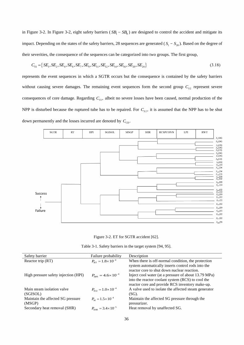
36

in Figure 3-2. In Figure 3-2, eight safety barriers (1 8SB SB ) are designed to control the accident and mitigate its

impact. Depending on the states of the safety barriers, 28 sequences are generated (1 28S S ). Based on the degree of

their severities, the consequence of the sequences can be categorized into two groups. The first group,

1 1 2 4 6 7 9 11 12 14 16 20 24, , , , , , , , , , ,SC SE SE SE SE SE SE SE SE SE SE SE SE= (3.18)

represents the event sequences in which a SGTR occurs but the consequence is contained by the safety barriers

without causing severe damages. The remaining event sequences form the second group 2SC represent severe

consequences of core damage. Regarding 1,SC albeit no severe losses have been caused, normal production of the

NPP is disturbed because the ruptured tube has to be repaired. For 2 ,SC it is assumed that the NPP has to be shut

down permanently and the losses incurred are denoted by CD .C

Figure 3-2. ET for SGTR accident [62].

Table 3-1. Safety barriers in the target system [94, 95].

Safety barrier Failure probability Description

Reactor trip (RT) 4

RT 1.8 10P −= When there is off-normal condition, the protection

system automatically inserts control rods into the

reactor core to shut down nuclear reaction.

High pressure safety injection (HPI) 4

HPI 4.6 10P −= Inject cool water (at a pressure of about 13.79 MPa)

into the reactor coolant system (RCS) to cool the

reactor core and provide RCS inventory make-up.

Main steam isolation valve

(SGISOL)

4

SGI 1.0 10P −= A valve used to isolate the affected steam generator

(SG).

Maintain the affected SG pressure

(MSGP)

4

M 1.5 10P −= Maintain the affected SG pressure through the

pressurizer.

Secondary heat removal (SHR) 5

SHR 3.4 10P −= Heat removal by unaffected SG.

37

Reactor coolant system pressure

control (RCSPCON)

2

RCSM 1.0 10P −= Open the turbine bypass valve to control the secondary

side pressure.

Low pressure safety injection (LPI) 4

LPI 4.6 10P −= Inject cool water (at a pressure of about 1.03MPa) to

cool down the RCS and provide RCS inventory make-

up.

Refill RWT (RWT) 8

RWT 2.4 10P −= Refill water storage tank.

The crack growth process that leads to SGTR can be monitored through non-destructive inspection (e.g.,

ultrasonic testing [96], eddy current testing [97]). In practice, this is done during planned shutdowns of the NPP,

often during the refueling stage. The condition monitoring data collected from these inspections are, then, used for

the dynamic business continuity assessment.

3.4.2 Particle filtering and loss modeling

The first step is to update the occurrence probability of the initiating event, based on the condition monitoring

data. For illustrative purposes, the evolution of the tube crack growth process is assumed to follow the Paris-Erdogan

model, which has been applied to model SGTR in [24, 95],

d

( ) , ,d

maC K K a

t = = (3.19)

where a is the crack length, C and m are constant parameters related to the component material properties, K is

the stress intensity factor, is the stress range. The model can be rewritten in the form of a state transition function

[98]:

1( ) dkm

k k k ka C a t a −= + (3.20)

The crack size ka at

kt t= is obtained from non-destructive inspection, such as ultrasonic testing; the

corresponding observation kz is:

,k k kz a = + (3.21)

where k is the observation noise.

PF is used to estimate the degradation state and predict the RUL. The results are shown in Figure 3-3 and Figure

3-4, respectively. The number of particles simulated is 5000.sN = It should be noted that for the tube degradation

process, the state vector x includes the crack size a and the model parameter variables ,C .m The initial values for

these variables are drawn uniformly from the intervals of values listed in Table 3-2.

2

1

2

1

(0, ).

(0, )

k k c

k k m

C C N

m m N

−

−

= +

= + (3.22)

38

Table 3-2. Initial intervals for the parameters.

Parameters Initial interval

C [0.1,0.2]

m [1.1,1.3]

c 3 2[0.9 10 ,0.2 10 ]− −

m 3 2[0.9 10 ,0.2 10 ]− −

o [0.65,0.85]

The results of PF are shown in Figure 3-4, where we find that the RUL prediction results become more accurate

when more condition monitoring data are available.

Figure 3-3 Crack growth process.

Figure 3-4 RUL Prediction results.

Afterwards, the loss ([ , ])L t t T+ in Equation (3.1) can be calculated. The losses caused by a SGTR event,

include the direct losses and indirect losses. In this case study, the direct losses, denoted by d ,L equal to the value of

the damaged equipment. For the consequence 1SC ,

dL is identical to the value of the ruptured tube. For the

consequence 2 ,SC L equals the whole value of the NPP production since the NPP needs to be shutdown. In this

chapter, we assume that if 2SC occurs, we have 95 10L = € [90].

The indirect losses inL are calculated considering the revenue losses during the recovery process, which depends

on the recovery time and electricity price. Due to the common use of lognormal distribution for modeling the repair

process [99-101], we also assume that the recovery time follows a lognormal distribution with the parameters

summarized in Table 3-3, where and are parameters of the lognormal distribution, whose PDF is

39

2

2

(ln( ) )

21, 0

( ) 2

0, 0.

recvt

recvrecv recv

recv

e tf t t

t

−−

=

(3.23)

Then, the value of inL is calculated by Monte Carlo simulation [102].

Table 3-3. Values of the recovery model parameters.

Parameter Description Value

The mean value of the lognormal

distribution.

1 year

The variance value of the lognormal

distribution.

0.1 year2

3.4.3 Tolerable loss modeling

As discussed in Section 3.3, the tolerable loss is proportional to the cash flow and should be modeled through

Equation (3.15). For the NPP, ( )kI t depends on the electricity price, which often exhibits large variabilities. In this

chapter, we use the following model to simulate the stochastic behavior of the electricity price [103]:

d ( )( )d ( )d dt p t t tx t x t t W Z = − + + (3.24)

where tx is the electricity price at , 0t and p is the mean value of the price,

tW is a standard Brownian motion

and tZ is a compound Poisson process with levy measure (d ) ( )d ,x g x x = is the jump intensity and g is the

density of the jump size distribution, ( )t is a positive stochastic process which satisfies:

( ) ( ) ( )t s t t = + (3.25)

where ( )s t is a deterministic, time-dependent and positive seasonal component, which is often modeled by a

trigonometric function:

2 41 1 3 5

2π 2π( ) sin( ) ( ) .

5 251

a t a tS t a a a

+ += + + (3.26)

The values of the seasonal component parameters are shown in Table 3-4.

Table 3-4. Values of the seasonal component parameters of the spot prices.

Parameter Value

1a 0.41

40

2a 1.90

3a 0.40

4a 43.11

5a 0.29

( )t is a stochastic process, representing the stochastic part of the time change. The Cox-Ingersoll-Ross process [104]

is used to model ( ),t

2 2d ( ) ( ( ))d ( ) d ( ).t t t t W t = − + (3.27)

By using Itô's lemma [103], Equation (3.24) can be solved and we can derive the following form:

0 0 0

( ) (0) ( ( ))d ( )d ( ) d ( ).

t t t

x t x x t t t B t Z t = + − + + (3.28)

The parameters of the stochastic electricity model are tabulated in Table 3-5, which is estimated from the

German EEX1 (a market platform for energy and commodity products), from 12.03.2009 until 31.12.2013. The

interested readers may refer to details and derivations in [103].

Table 3-5. Parameters in the stochastic electricity model [103].

Parameter Value

0x 40

ɵ 0.22

μ 50

σ 5.98

dt 1

λ 0.12

1 1.02

1 1.35

Eventually, the generated stochastic electricity price trajectory can be used to model the profit and potential

losses. The operation cost ( )o kC t in Equation (3.15) is set as constant 20€/MWh, which includes the cost of uranium

fuel and the cost of disposing used fuel and wastes [105]. Finally, the cash flow at different time points is shown in

Figure 3-5. We can see that the accumulated profit is small at the beginning. This is because this period is still under

1 https://www.eex.com, accessed 2019-09-12

41

the repayment period and a large amount of the revenue is used for repaying the installment. After 10t = years, the

repayment is paid off and, thus, the profit increases significantly.

Figure 3-5. Profit trajectory at different estimation points.

3.4.4 Results

The results from the time-static and time-dependent business continuity analyses are compared in Figure 3-6,

Figure 3-7 and Figure 3-8, where the true value is generated based on a theoretical model with known parameters.

Abscissa axis shows the estimation horizon ,T and the vertical axis stands for the different BCV indexes. Therefore,

these results show the business continuity of NPPs at different age ( ),t if it is operated for different lengths of time

( ).T It can be seen from the Figures that:

(a) EDBCV (b)

BFP

42

(c)

BIP

Figure 3-6. Business continuity metrics at t=1 year.

(a) EDBCV (b)BFP

(c) BIP

43

Figure 3-7. Business continuity metrics at t=10 years.

(a) EDBCV (b)BFP

(c) BIP

Figure 3-8. Business continuity metrics at t=40 years.

(1) At each t with the increase of the estimation horizon T the DBCV decreases. This means that

regardless of the age t of the NPP, the longer the NPP is operated, the worse its business continuity. This is

logical as it is primarily caused by the tube’s degradation process. No rupture is supposed to occur at the

beginning of system operation. Subsequently, as the crack grows, rupture will occur eventually and lead to

system failure. In addition, the dynamic business continuity (DBC) indexes curves drop significantly after a

certain value. In practice, intervention measures like overhauls need to be taken before this ,T in order to

prevent serious losses from occurring failures and ensure the business continuity.

(2) For the same estimation horizon ,T with the increase of NPP age t the EDBCV moves toward left,

which means the financial safety margin is narrowing overtime .t This is because the steam generator tube is

getting closer to a dangerous state as the NPP ages.

(3) The comparison between DBC and static business continuity shows that the results from the DBCA

44

using condition-monitoring data are closer to the true BCV than those of the static business continuity. This is

because the DBC using condition monitoring data can capture the time-dependent behaviour of SGTR

degradation. Moreover, with more condition monitoring data the DBCV estimation results are more accurate.

(4) Confidence interval quantifies the level of confidence that the BCV metrics are captured by the

interval. From Figures Figure 3-6~Figure 3-8, we can see that with more data available, the width of

confidence interval is narrowing. That is because that with more condition monitoring, more precise of the

component state estimation and less uncertainty of the BCA results.

3.5 Conclusion

In this chapter, a dynamic business continuity assessment method that integrates condition monitoring data is

proposed. Two factors that influence the dynamic behaviour of business continuity are considered explicitly. The

first one is the dynamics of the degradation-to-failure process affecting the safety barriers. Condition monitoring data

are used to update and predict the time-dependent failure behaviour by PF. The second factor is the time-dependent

profit and tolerable losses. This is quantified by applying a stochastic price model and an installment model. A

simulation-based framework is developed to calculate the time-dependent business continuity metrics originally

introduced. A case study regarding the analysis of an accident initiated by SGTR in a NPP shows that the proposed

framework allows capturing the dynamic character of business continuity. The outcomes of such dynamic analysis

can provide insights to stakeholders and decision-makers, that can help them to identify when best to take actions for

preventing serious losses and ensuring business continuity.

45

Chapter 4 Joint optimization for enhancing business

continuity

In this chapter, a joint optimization model for business continuity that considers prevention, mitigation,

emergency and recovery processes is proposed. Generally, the resources to guarantee a system’s continuity are often

limited. How to allocate and arrange the limited resources to keep the continuous service of the target system is a

paramount issue. Conventionally, organizations treat the different phases in BCA separately. In order to capture the

coordination of the four phases and extract useful information on resource allocation, a joint optimization model is

developed. A case study of the SGTR in a NPP is conducted to illustrate the utility of the joint resource allocation

model.

The remainder of this chapter is organized as follows. Section 4.1 presents a brief literature review on the optimal

allocation of loss-reduction resources. Section 4.2 elaborates the joint optimization framework. Section 4.3 shows

the MIGA method that is used for solving the resource allocation problem. Section 4.4 illustrates the utility of the

proposed framework through a NPP case study. Finally, Section 4.5 concludes this chapter.

4.1 State of the art

Most of research for improving system reliability, safety and resilience concentrates on individual or partial

stages, especially for the situation under limited resources. Some attempts focus on resource allocation for preventive

stage. For example, in [106], optimization of preventive upgrading interventions on the bridges of a highway network

has been conducted to improve the bridge reliability under earthquake disruption. In addition, a combination of the

knapsack problem and a risk matrix has been presented to carry out a cost-benefits analysis to efficiently make

prevention investment decision within a predefined budget in [107]. An optimal portfolio of prevention measures for

time-dependent accident scenarios has been proposed in [108], using Dynamic Bayesian network (DBN) represent

the temporal evolution of component failure. These model concentrates on risk prevention, in other words, reducing

frequency of disruptive event.

46

In [109, 110], a multi-objective multi-decisionmaker resource allocation framework has been represented to

model resource allocation process within large-scale hierarchical systems, aiming at mitigating the risks from the

viewpoint of subsystem and overall system. Additionally, some studies have developed to allocate the system

resources to improve system resilience for a specific disaster. For instance, multi-systems’ joint restoration processes

resilience modeling has been addressed and the effectiveness of five different restoration strategies has been

compared in [45]. In [46], a two-stage mixed-integer programming resource allocation model for lifeline system has

been proposed to improve the efficiency of restoration. A multi-objective optimization model of emergency

organization allocation for sustainable disaster supply chain has been developed to design optimized strategies of

emergency organization allocation [47]. with the objective of minimizing the expected outage duration of loads,

multiple microgrids have been used to real-time optimize resources and restore critical loads [48]. In [49], a

restoration resource allocation model has been proposed to enhance resilience of interdependent infrastructure

systems. A resiliency-based optimization methodology has been performed over the set of feasible restoration policies,

information investments, and human resource availability to determine optimal customer and system-wide monetary

utility [50]. A stochastic optimization technique has been developed to allocate scarce national resources to coping

with multiple simultaneous disasters happening across the nation [51]. All of the above-mentioned researches concern

post-disruption decision making, assuming the disruption has happened.

The objective of resource allocation in business continuity is searching an integrated optimization method to

improve the system continuity level, with consideration of the necessary measures in the whole stage, including pre-

disruption and post-disruption. As a matter of fact, this problem has not been sufficiently addressed in the available

literature and we are motivated to fill the above gaps by mathematically formulating the business continuity

enhancing based resource allocation problem and developing a joint optimization approach to identify the system

resource allocation on four phases. With respect to system business continuity, we adopt the quantitative metrics

proposed in [14]. Regarding the solution of optimization, MIGA is applied to solve the joint optimization model due

to its parallel searching and efficient interactions characteristics [111, 112].

47

4.2 Joint optimization

BCM starts from hazard identification, and follows with event evolvement analysis, as well as safety barriers

identification. The concrete definitions, functions and the characteristics of the four stages addressed in BCM are

shown as follows:

(1) Prevention stage often takes inherent safety measures to lower the probability of disruptive event [16].

(2) Mitigation phase is usually equipped with passive strategies, aiming at minimizing consequence of

disruptive events. The designer’s choice of business continuity maximization on mitigation phase is

captured by redundancy design, especially for the safety barriers arrangement which are used to

mitigate the system consequence induced by a disruptive event [113]. Regarding a corresponding

redundant system, if one component collapses, corresponding redundant system will substitute it to

work for a period of time. Redundancy allocation problem is an important topic in system reliability

design, and also plays a key role in engineering resilience[114-116].

(3) Emergency phase starts after the mitigation phase and prior to the recovery phase. Corresponding

emergency safety measures are activated when mitigation measures fail to contain damage. sometimes

human intervention are required in this phase [14].

(4) Recovery phase mainly focuses on restoring a system timely to normal operation following disruptive

events [117]. Recovery ability refers to the ability of a system repairing itself [118]. The cost of this

phase mainly focuses on system investment on repair crews, vehicles, equipment and replacement

components [119].

The overall cost (based on the cost of deployment of safety barriers on prevention phase, mitigation, emergency

and recovery phase) must not exceed a budget constrain. Considering the system business continuity, one paramount

objective of BCM is maximizing BC given limited budget or resources.

As reviewed in Section 3.2, the metric of EBCV directly reflect business continuity level which can be used as

an objective for the optimizing system resource allocation.

A joint optimization framework considering all safety barriers and corresponding cost in four phases is presented

in Figure 1-1. Prevention cost, redundancy arrangement and recovery investment are used to minimize the loss level

in BCM [19, 120].

48

max EBCV= ( , , , )P M E RSB SB SB SBf C C C C (4.1)

. . P M E RSB SB SB SB totals t C C C C C+ + + (4.2)

0, 0, 0, 0.P M E RSB SB SB SBC C C C (4.3)

The objective function maximizes system business continuity under SGTR over T time periods. where ,PSBC

, , ,M E RSB SB SBC C C are the cost allocated in preventive, mitigation, emergency and recovery stage, respectively.

totalC

denotes total resource budget. The first constraint in the joint optimization model is the constrain on the maximal

allowable resource budget. With limited budget, it is essential to allocate resource budget in an effective way, in order

to maximize system business continuity.

4.3 Solution method

In this section, the solution of this joint optimization issue is presented. The joint optimization model shown by

Equation (4.1) can be solved with methods such as Lagrange multiplier. However, due to the computation complexity

of parameters and the nonlinear characteristic of the function, hereby, MIGA is used to solving the model. MIGA is

a powerful stochastic search algorithm that has been successfully used in literature for solving optimization problems

in critical infrastructure resilience [45]. The procedures to search for an optimal solution to the joint optimization

problem can be described by following steps [121, 122].

(1) Encoding. Express each solution of cost allocation by a genotype 1 2 7( , , , ) .Te e e e= The different

combinations of structured cost make up different chromosomes. The initial solution is randomly

generated according to constraint conditions in Equations (4.2) and (4.3).

(2) Fitness assessment. Calculate the fitness value of each genotype. The fitness value of each genotype

represents the business continuity value of the system of interests [123].

(3) Selection, crossover and mutation. Offsprings are produced by these three types of operator, and then

return to the second step until the maximum generation is reached. The section operator chooses a

genotype with a probability depending on its fitness value. Two selected genotypes produce two

descendants by using crossover operator that exchange substrings of the codes of the two chosen

genotypes. Then, each descendant generates an offspring by using the mutation operator with a mutation

49

probability. The genotype in the final generation with the maximum EBCV corresponds to the optimum

resource allocation.

With abovementioned steps, the genotype is selected according to their fitness value in each generation. The

rule for stop is the convergence of the optimal fitness value between two generations. When the algorithm stops, the

genotype corresponding to the minimal fitness value is the optimal solution for the budget allocation model.

4.4 Case study

A Zion PWR NPP is considered to illustrate the developed model. It is assumed that the NPP has one SG that is

equipped with a bundle of 3592 inverted U tubes. Each U tube has a mean outside diameter of 22.23 mm and a mean

wall thickness of 1.27 mm and is subject to SGTR caused by diverse degradation mechanisms like stress corrosion

cracking (SCC), fatigue, pitting corrosion and fretting wear. A detail list of the NPP parameter values is presented in

Table 4-1 Parameters of the NPP.

Parameter Value

Capacity of NPP ( C ) 1100 Mwh

Number of tubes (tuben ) 3592

Outer diameter ( d ) N (22.23,0.1667) mm

Pressure different ( P ) N (8.3,0.33) Mpa

Thickness ( b ) N (1.27, 0.0592) mm

4.4.1 Event modelling

For illustrative purposes, it is assumed that the NPP is only subject to the threat of one disruptive event, SGTR.

SGTR is a potential accident that is induced by the degradation of tubes in steam generator, which can further lead

to tube cracking and rupture event. In principal, steam generator tube is designed for transferring heat produced by

steam generator to drive turbine for producing electricity [124]. To analyze business continuity of the NPP

considering SGTR, a schematic event tree (ET) on SGTR is investigated, as shown in Figure 4-1.

50

Figure 4-1. Schematic ET model of SGTR accident ( 2 5C C core damage) [120].

Depending on the performance of different safety barriers, six consequences, i.e., 1 2 6, , ,C C C can result from

the SGTR event. These consequences can be grouped into three categories based on their severity: no incident IC ,

incident IIC and core damage

IIIC as tabulated in Table 4-2. Different consequences are formulated based on the

variant performances of safety barrier.

Table 4-2. Classification of consequences.

Consequences Group Meaning

6C IC No SGTR occurs, the NPP is operating normally.

1C IIC SGTR occurs, but the consequence is successfully controlled by

the mitigation and emergency barriers. The power generation

business is temporarily terminated.

2 5C C IIIC Core damage is caused by SGTR, the power generation

business is terminated for a long time.

4.4.2 Business continuity modelling

The aim of this section is determining the different measures on the four phases and their functions on NPP

business continuity, as well as the corresponding costs.

51

4.4.2.1 Prevention phase

The main prevention measures for crack growth are regular inspection on the crack size, and, also the timely

preventive maintenance, such as plugging the cracked tube. Additionally, the rupture probability depends on the

inspection interval and plugging threshold, as formulated in:

, ( , ).rupt tube thp f x y= (4.4)

The costs in this preventive stage include inspection cost and plugging cost. In practice, the inspection is

conducted regularly during the NPP refueling process. The tube crack size usually is measured by eddy current test

and once the crack reaches a given threshold ,thy the associated tube is plugged to prevent occurrence of tube rupture

[24].

A two-stage crack model is used to simulate the crack progression. For the first stage, it is assumed that from

the initial crack to the critical length of 0.1 mm, which indicates after this critical length the crack propagates faster.

The duration of first stage is described through a lognormal distribution [24]. The propagation stage can be formulated

through a scott model [95], which is an empirical model that illustrate the crack growth rate as a function of stress:

( ) ,m

th

daK K

dt= − (4.5)

,2

aK F

= (4.6)

2

P d

b

= (4.7)

where da

dt is the crack growth rate, a is the crack length, ,

thK and m are constant parameters related to the

component material properties, is the stress at the crack tip, P denotes the pressure difference. In this case study,

Alloy 600 material is considered for the steam generator tube. Based on the material properties, the values for

parameters in Equations (4.5)-(4.7) can be determined.

Therefore, the cost in prevention phase can be formulated as:

,

PSB insp insp tube plug plug

insp tube plug plug

C C n n p C

TC n p C

x

= +

= + (4.8)

52

where T denotes the time horizon of business continuity assessment; inspC is the cost of a single inspection of the

health of the tube; plugC is the unit price for plugging one tube; and plugp is the plugging rate of the tube, which is

also dependent on the values of x and ,thy can be further calculated through simulation.

4.4.2.2 Mitigation & emergency phase

Failures of safety barriers in mitigation phase can increase accident severity. In this regard, redundancy system

or component are often considered to improve reliability and availability of these component. Evidently, as the

number of redundancy augments, the cost of the whole system proportionally grows. In this context, achieving an

optimal number of redundancy components by which total costs of the system is minimized could by interesting.

From the event tree model in Figure 4-1, the losses generated from different consequences 1 6C C can be

quantified as a function of the event probabilities along the sequences:

1 2 3 4( , , , , )iC ET SGTRp f p p p p p= (4.9)

where SGTRp is the probability of a single tube rupture,

1 2 3 4, , ,p p p p represent the failure probability of RTS, RDS,

RWST and RCS, respectively.

The performance of mitigation & emergency measures, i.e., RTS, RDS, RWST and RCS in Figure 4-1, can be

represented by their failure probabilities. Redundancy design can be an appropriate way used for reducing failure

probabilities. In this chapter, we assume that parallel redundancy suing the same type of equipment is considered for

the four mitigation and emergency safety barriers. It is easy to show that the failure probability of the i − th measure

becomes:

1

,( ) in

i i bp p+

= (4.10)

where ,i bp is the failure probability of the i − th safety barrier system and in is the number of redundant system

added to the original system.

The cost for improving mitigation and emergency performance can, then, calculated by:

4

,

1MSB R i i

i

C C n=

= (4.11)

where ,R iC is the price for adding one i − th redundancy measure.

53

4.4.2.3 Recovery phase

Afterwards, the analysis goes to the recovery phase. That means when consequence BC and

CC occur, the NPP

becomes temporarily unavailable for producing electricity, until the recovery measures are applied to the system to

restore the system to normal operation. It is assumed that the basic recovery time , ,ibs CT where , ,i I II III= follow

lognormal distributions [99, 101] whose probability density function is:

2,

2

(ln( ) )

2

,

, ,

,

1, 0

( ) 2

0, 0

recv Ci i

i

i

i i

i

T

recv C

recv C i recv C

recv C

e Tf T T

T

−

=

(4.12)

where ( )f is the probability density function (PDF) of , ;irecv CT

i and i are the mean value and standard deviation

value of the lognormal distribution, respectively. The values of i and

i are depends on the recovery ability of the

target organization. It is noting that the more serious consequence ,i the smaller of , .e ic

In practice, given the budget on BCM, with more resources allocated on recovery process, the recovery rate will

be improved, and, then, lead to more efficient recovery process to reduce the potential indirect losses in system

operation. The allocated resources on the recovery process is often assumed following logarithmic function [125,

126], which is defined as Equation (4.13),

,

, .1 ln(1 )

i

R

recv C

recv i

e SB

TT

c C=

+ + (4.13)

where ,recv iT is a random variable that represents the time needed to recover from the i − th consequence; , irecv CT

denotes the basic recovery time for consequence ,iC which is dependent on the basic requirement on recovery time,

RSBC denotes the resources invested on the recovery process and ec is the effective parameters of resources on −

th consequence; denotes the relationship between different cost-effective parameters for different consequences;

Its value should be set by decision makers based on the capability of the organization.

4.4.3 Joint optimization

To formulate the objective EBCV, the indirect losses caused in the recovery process can, be modelled by:

, , ,i iIn C e recv CL P C T= (4.14)

54

where , iin CL represents the indirect losses in the recovery process for consequence ;iC eP is the unit electricity price;

C is the generation capacity of the NPP; , irecv CT denotes the recovery time for the i − th consequence.

Then, the EBCV in Equation (4.1) can be formulated by:

3

1

3

, ,

1

, , , ,

( ([0, ])) ( ([0, ]))

( )

( ( )) ( ( )).

i i

i i i

II II II III III III

C C

i

d C in C C

i

C d C e recv C C d C e recv C

E L T E L T p

E L L p

p L P C E T p L P C E T

=

=

=

= +

= + + +

(4.15)

According to the cost analysis in whole process, the explicit form of the resource allocation model is given as:

1 2 3 4max EBCV= ( , , , , , , )Rth SBf x y n n n n C (4.16)

. . ,P M RSB SB SB Ths t C C C C+ + (4.17)

, , 0,P M RSB SB SBC C C (4.18)

[6,7,8, ,17,18]x (4.19)

,plug thp p (4.20)

,1 1 ,1 1

,2 2 ,2 2

,3 3 ,3 3

,4 4 ,4 4

,

,

,

,

L U

L U

L U

L U

n n n n N

n n n n N

n n n n N

n n n n N

(4.21)

The first constrain in Equation (4.17) regards the total budget on all safety barriers which cannot exceeds a

limited value .thC In Equation (4.17), the cost , ,P M RSB SB SBC C C are further calculated by Equations (4.8), (4.11) and

(4.13). The constrain in Equation (4.19) defines the possible value of inspection interval (in months). In this work, it

is assumed that the inspection can reveal the exact state of the tube. The constraint in Equation (4.20) means the total

number of plugged tubes can exceed a maximum value. The value of thp is determined based on the power generation

efficiency requirement of the NPP. According to the nuclear regulations, a steam generator of the type employed in

Zion PWR NPP can tolerate up to 30% plugged tubes before a significant reduction in efficiency occurs [127].

Therefore, here, we see 0.3.thp = The last constraint in Equation (4.21) describes the minimal and maximal number

of redundant system for the mitigation measures and is employed to describe the redundancy number of mitigation

measures.

55

MIGA is applied to solve the previously defined joint optimization problem. And the flowchart of MIGA is

shown in Figure 4-2. The parameters of the algorithm are tabulated in Table 4-3.

Figure 4-2 Schematic of MIGA.

Table 4-3. Parameters of the MIGA algorithm.

Parameters Values

Population size 40

Crossover rate 0.9

Mutation rate 0.5

Maximum generation 500

4.4.4 Results and sensitivity analysis

In this section, we firstly present comparative results on single phase resource allocation and joint optimization

within predefined budget. Subsequently, sensitivity analysis on budget, cost-effectiveness parameter as well as failure

probability of mitigation barriers are carried out to discuss the influence of these variables on EBCV.

4.4.4.1 Results

The optimization problem is solved numerically through the MIGA described in Section 4.3 to show insights on

resource allocation under budget constraint. Parameter values used in this case study are tabulated in Table 4-4.

56

Through simulation on crack onset and propagation, we can obtain the probability that the crack onset time outside

of T is 0.6498.

Table 4-4 Parameter values used in the case study.

Parameter Meaning Value

C Capacity of NPP 1100 (Mw)

tolL Tolerable losses 65 10 (k€)

inspC Cost for one inspection 500 (k€)

1C Cost for adding one redundant RTS 20 (k€)

2C Cost for adding one redundant RDS 4 (k€)

4C Cost for adding one redundant RWST 11 (k€)

4C Cost for adding one redundant RCS 5 (k€)

plugC Cost for plugging one tube 5 (k€)

ec Cost effectiveness parameter for consequence

𝐶𝐼𝐼 0.001

The relationship of cost-effectiveness

parameter between IIC and

IIIC

0.5

,1recvT Basic recovery time for consequence IIC ( ) ( )Lognormal 3.9828,0.4724 days

,2recvT Basic recovery time for consequence IIIC ( ) ( )Lognormal 6.5922,0.4724 days

eP Unit price of electricity 50€/MWh

,1 ,2 ,3 ,4, , ,L L L Ln n n n Lower bound of mitigation measures’ number

0

,1 ,2 ,3 ,4, , ,U U U Un n n n Upper bound of mitigation measures’ number

4

totalC Total budget 8000 (k€)

To investigate the effectiveness of the joint optimization method based on business continuity, a comparison

among individual optimization of the three phase is conducted. We program the joint optimization model 10 times

and consider all the results of the objective during the 10 times, and the results are shown in Figure 4-3, where green

circle means the EBCV calculated from spend all the resources on prevention phase and boxplot is the 10 times

simulation results for the proposed model. We can see that the joint optimization works better targeting maximizing

EBCV than the strategy only investing all the budget on preventive stage.

57

Figure 4-3 Results comparison for proposed joint optimization and prevention only ( 8000(k€)totalc = ).

The details on one of the simulation results is shown in Table 4-5. It is worth noting that a tolerance level

41.0 10 −= is enforced for MIGA. It can be seen that the joint optimal design solution requires to do a periodical

inspection of the steam generation tube every 15 months and the tube will be plugged when crack length exceeds

7.8780(mm). Additionally, redundancy design for mitigation & emergency measures is 1 2 3 41, 4, 4, 4.n n n n= = = =

For the recovery stage, additional resources ( )108.2384 k€RSBC = are allocated to improve the recovery efficiency

and reduce the indirect losses .inL

Table 4-5 Comparison results for business continuity under different strategies.

Variable Joint optimization Prevention measures only Mitigation & emergency Recovery (only)

x 1.25 (year) 1 (year) / /

thy 7.8780 (mm) 14.1347(mm) / /

1n 1 / 4 0

2n 4 / 4 0

3n 4 / 4 0

4n 4 / 4 0

PSBC 7792.2 (k€) 7990.05(k€) 0 0

MSBC 90 (k€) 0 120 (k€) 0

58

RSBC 108.2384 (k€) 0 0 8000 (k€)

,costotal tC 7990.4 (k€) 7999.05 (k€) 120 (k€) 8000 (k€)

EBCV 0.9963 0.9597 -20.06 -44.63

We pick the best solution among the 10 trails to show the details of the simulation result. The behavioral indexes

proposed Section 4.2 are shown in Figure 4-4. We can see that the probability of SGTR dramatically decrease after

jointly optimizing resource allocation comparing with only spend the budget on mitigation and recovery phase. For

the mitigation & emergency phase, the best option is spent all the budget only for mitigation phase. Regarding the

recovery phase, as expected, if all the budget is spent on recovery phase, the recovery time will be significantly

reduced (both regarding consequences IIC and

IIIC ).

(a) Probability of SGTR. (b) Failure probability of mitigation system.

(c) PDF of recovery time for consequence .IIC (d) PDF of recovery time for consequence .IIIC

Figure 4-4 Behavioural indexes in prevention, mitigation & emergency, and recovery phases.

59

It can be seen from Figure 4-4 that if all the budget totalC is spent on the preventive phase, the SGTR occurrence

probability can be reduced from 46.9998 10− to 42.9998 10− comparing with the joint optimization model.

However, the respective EBCV is lower than the joint optimization model. This is because in the preventive phase

only considered model the total cost is invested to prevent crack growth. The mitigation & emergency and recovery

processes are ignored, becoming bottlenecks to the business continuity of the NPP. Similar results can be found in

Figure 4-4 (b), (c) and (d): although the solution obtained from the joint optimization model not be optimal with

respect to each safety barrier, it can achieve an overall optimal performance with respect to business continuity. That

is because that the proposed joint optimization method takes all the factors into account, thus, there is not any special

shortcoming/bottleneck in the resource allocation process.

4.4.4.2 Sensitivity analysis

In this context, one major engineering interests lie in the quantification of the sensitivity of the business

continuity of the system with respect to the different parameters of basic variables. Because sensitivity analysis on

parameters provides insights on how these parameters affect the optimal allocation of budgets. In this work, a

sensitivity analysis is conducted in terms of system total budget, failure probability of mitigation measures and the

cost-effectiveness parameter in recovery stage. For each parameter sensitivity investigated, the other parameter values

are kept the same. The problem size is limited due to the significant computations required by the optimization models

to obtain joint optimal solutions [128].

For the changing budget’s effect on system business continuity, the result is presented in Figure 4-5. As expected,

with the growth of total budget, corresponding EBCV increases. This is due to more available resources allocated to

keep system business continuity, the higher preventive ability, mitigation & emergency ability and recovery ability.

Subsequently, the less loss in the evaluated time horizon [0, ],T and eventually, the higher business continuity.

Additionally, when the total budget is bigger than 8000k€, the changing on EBCV is small, indicating marginal

degradation of the budget. This is mainly because the limitations on the plugging rate, mitigation measures

redundancy. This result can provide insights on how many budgets should be arranged to keep system business

continuity.

Through the comparison results showed in Figure 4-5, we find that when total budget is relative less, the value

of cost-effectiveness has more significant influence on system business continuity. This is mainly probably caused

60

by the fact when the budget is small, the cost-effectiveness parameter ec plays a more important role in budget

allocation. Higher cost-effectiveness makes budget allocated on recovery stage more effective, and then, effectively

reduce the system indirect losses.

Figure 4-5 Comparison of EBCV with different cost effectiveness parameters.

To investigate the influence of cost-effective parameter on the joint optimization model, a comparison among

total budget with 7500k€ and 8000k€ are studied respectively. Figure 4-6 shows the results of the EBVC comparison

as a function of the changing cost-effective parameter. As can be seen from Figure 4-6, the smaller the budget, the

more sensitive of cost-effectiveness parameters on business continuity, which is also verified in Figure 4-5. Moreover,

when the cost-effectiveness parameter increases from 0.001 to 0.006, the corresponding EBCV increase. Additionally,

when the cost-effectiveness parameter increases from 0.006 to 0.01, the change in system EBCV is relatively small

due to the marginal decreasing rate of EBCV with increase of cost-effectiveness.

61

Figure 4-6 Comparison EBCV with different cost-budget.

Figure 4-7 Schematic of changing failure probability of mitigation measures (70%~130%) under budget

8000k€.totalC =

To test the influences of mitigation measures’ failure probability on the budget allocation, we do a sensitivity

analysis by changing mitigation failure probability from 70% PF to 130% PF ( where

[ , , , ]RTS RDS RWST RCSPF p p p p= ). As shown in Figure 4-7, with increase of failure probability of mitigation measure,

62

the proportion of mitigation cost increases accordingly. This is a strait forward conclusion: more redundant safety

systems are needed if the safety system has higher failure probability.

4.5 Conclusion

A mathematical model is formulated in this chapter to jointly optimize system limited resources for enhancing

system business continuity. The joint optimization model is based on the proposed BCA metrics, which aims at

calculating system business continuity level given an estimation horizon. The proposed joint model considers

reducing system potential loss under a given disruptive event from a comprehensive viewpoint. The case study on a

NPP against SGTR event demonstrates the utility of the model in decision making. Through this case study, we can

see that the proposed joint optimization model works better than the other models that deal with four phases

individually. Through the results of sensitivity analysis, we can infer that: (1) larger resource budget can result in

higher business continuity; the change of EBCV is marginally decreasing with the increase of the budget; there is an

optimal budget for the given NPP; (2) higher failure probability of the safety measures in mitigation phase, less

redundancy is needed; (3) the smaller the budget, the more sensitive of cost-effectiveness parameters on business

continuity. The optimization method can jointly provide a better scheme than separative optimization strategies for

decision makers under limited budget or resources.

63

Chapter 5 Conclusion and future work

5.1 Conclusion

This dissertation aims at developing an integrated framework and computational tools for the assessment and

optimization of system business continuity. More particularly, the works in this dissertation can be summarized as

follows.

Firstly, a framework for DRA was developed to integrate condition monitoring data and inspection data. A HM-

GMM was developed to estimate the degradation states of the safety barriers based on the condition monitoring data.

The estimated degradation states were integrated with inspection data for DRA by a BN model. An application

showed that integrating two data sources into the DRA gives more robust results than using the two data sources

individually.

Secondly, a simulation-based DBCA method was developed to analyse system business continuity that allows

considering the time-dependent feature of safety barriers’ states and target system revenues. A PF model was used to

predict the RUL of the safety barriers from condition monitoring data. The time-dependent revenue was modelled by

an instalment model. The proposed DBCA framework was applied to a NPP, taking into account a SGTR event. The

results of the case study showed that the proposed framework allows capturing the dynamic behaviour of business

continuity and can aid decision-makers.

Thirdly, a mathematical model was formulated to jointly optimize the system limited resources for enhancing

business continuity. The model aims at reducing the system potential loss from a comprehensive viewpoint in which

prevention, mitigation, emergency, and recovery phases are considered jointly. MIGA was employed to obtain the

optimal solution of the comprehensive model. A comparative study was carried out to verify the effectiveness of the

proposed BCA based decision-making. A sensitivity analysis was done on the cost-effectiveness parameter, budget,

failure probability of mitigation measures.

In summary, the findings of this work demonstrate the feasibility and the importance of the developed methods

for risk-informed analysis and BCM of energy systems, taking into account different available knowledge,

information, and data. More specifically, the original contributions of this thesis include: (1) the developed data-

64

integrated method in DRA can achieve a more robust DRA results than using the two data sources individually, which

is all-important for safety critical system; (2) the proposed quantitative DBA method taking into account the time-

dependent factors in BCM provides a robust indicator on when to do maintenance, overhaul etc; (3) the four stages

in accident evolution process are integrally considered in the resource allocation process which can provide a better

performance in BCM to energy system.

5.2 Perspectives

Some limitations still exist on the methods developed in this thesis, which deserve potential future work.

Firstly, an ET is applied in our study (Chapter 2) for modelling the disruptive event evolution process, and

describing the protection, mitigation, emergency and recovery phases. ET is mainly a static method, which cannot

capture the time-dependent of the behaviour of the safety barriers. Advanced modelling method, such as BN, dynamic

fault tree, can be applied in the business continuity modelling framework.

Secondly, the proposed BCM framework (Chapter 3) only considers one kind of disruptive event. In practice,

the increasing number of hazards is forcing organizations to build BCM against numerous types of disruptions and

their consequences [40, 119]. Therefore, multi-event based BCM can be investigated in future work, where business

continuity under multiple hazards and multi-objective optimization considering multiple disruptions can be

extensively investigated.

Lastly, in the modelling process of DBA, the current method considers a discrete-time discrete state Markov

model as the degradation model. A potential future work might be to extend the developed framework to other

degradation models, e.g. the Brownian motion model [129], Gamma process model [130], etc. Moreover, in the

current framework, the parameters of HM-GMM are estimated offline; in the future, online updating of the parameters

can be considered, aiming to improve the accuracy of the DRA.

65

Reference

[1] Zio, E., An introduction to the basics of reliability and risk analysis. Vol. 13. 2007: World scientific.

[2] Zubair, M. and G. Heo, Advancement in living probabilistic safety assessment to increase safety of nuclear

power plants. Proceedings of the Institution of Mechanical Engineers, Part O: Journal of Risk and Reliability, 2013.

227(5): p. 534-539.

[3] Zio, E., Challenges in the vulnerability and risk analysis of critical infrastructures. Reliability Engineering

& System Safety, 2016. 152: p. 137-150.

[4] Zio, E., The future of risk assessment. Reliability Engineering & System Safety, 2018. 177: p. 176-190.

[5] Nosworthy, J., A practical risk analysis approach: managing BCM risk. Computers & security, 2000. 19(7):

p. 596-596.

[6] Khan, F., S. Rathnayaka, and S. Ahmed, Methods and models in process safety and risk management: Past,

present and future. Process Safety and Environmental Protection, 2015. 98: p. 116-147.

[7] Hoseyni, S.M., F. Di Maio, and E. Zio, Condition-based probabilistic safety assessment for maintenance

decision making regarding a nuclear power plant steam generator undergoing multiple degradation mechanisms. Reliability Engineering & System Safety, 2019. 191: p. 106583.

[8] Rebollo, M.J., C. Queral, K. Fernández-Cosials, J. Sánchez-Torrijos, and J.M. Posada, Development of

phenomena identification ranking table for LONF-ATWS sequences in a Westinghouse PWR. Annals of Nuclear

Energy, 2019. 131: p. 156-170.

[9] ISO, ISO 22301, in Societal Security- Business Continuity Management Systems- Requirements2012,

International Organization for Standardization: Switzerland.

[10] Sahebjamnia, N., S.A. Torabi, and S.A. Mansouri, Integrated business continuity and disaster recovery

planning: Towards organizational resilience. European Journal of Operational Research, 2015. 242(1): p. 261-273.

[11] Liu, X., E. Ferrario, and E. Zio, Identifying resilient-important elements in interdependent critical

infrastructures by sensitivity analysis. Reliability Engineering & System Safety, 2019. 189: p. 423-434.

[12] Rabbani, M., H.R. Soufi, and S. Torabi, Developing a two-step fuzzy cost–benefit analysis for strategies to

continuity management and disaster recovery. Safety science, 2016. 85: p. 9-22.

[13] Xing, J. and E. Zio. An integrated framework for business continuity management of critical infrastructures.

in 26th European Safety and Reliability Conference-ESREL 2016. 2016. Glasgow: CRC Press.

[14] Zeng, Z. and E. Zio, An integrated modeling framework for quantitative business continuity assessment.

Process Safety and Environmental Protection, 2017. 106: p. 76-88.

[15] De Lira-Flores, J.A., A. López-Molina, C. Gutiérrez-Antonio, and R. Vázquez-Román, Optimal plant layout

considering the safety instrumented system design for hazardous equipment. Process Safety and Environmental

Protection, 2019. 124: p. 97-120.

[16] Lees, F., Lees' Loss prevention in the process industries: Hazard identification, assessment and control.

2012: Butterworth-Heinemann.

[17] Tammineedi, R.L., Business continuity management: A standards-based approach. Information Security

Journal: A Global Perspective, 2010. 19(1): p. 36-50.

[18] Zsidisin, G.A., S.A. Melnyk, and G.L. Ragatz, An institutional theory perspective of business continuity

planning for purchasing and supply management. International journal of production research, 2005. 43(16): p. 3401-

3420.

[19] Gibb, F. and S. Buchanan, A framework for business continuity management. International Journal of

Information Management, 2006. 26(2): p. 128-141.

[20] Järveläinen, J., IT incidents and business impacts: Validating a framework for continuity management in information systems. International Journal of Information Management, 2013. 33(3): p. 583-590.

[21] Hassel, H. and A. Cedergren, Exploring the Conceptual Foundation of Continuity Management in the Context of Societal Safety. Risk Analysis, 2019. 39(7): p. 1503-1519.

[22] Lin, C.S., S. Kao, and L.S. Chen, A proactive operational framework for business continuity in the

semiconductor industry. Quality and Reliability Engineering International, 2012. 28(3): p. 307-320.

[23] Kim, H., S.-H. Lee, J.-S. Park, H. Kim, Y.-S. Chang, and G. Heo, Reliability data update using condition

monitoring and prognostics in probabilistic safety assessment. Nuclear Engineering and Technology, 2015. 47(2): p. 204-211.

66

[24] Di Maio, F., F. Antonello, and E. Zio, Condition-based probabilistic safety assessment of a spontaneous

steam generator tube rupture accident scenario. Nuclear Engineering and Design, 2018. 326: p. 41-54.

[25] Zhao, X., X. Guo, and X. Wang, Reliability and maintenance policies for a two-stage shock model with self-healing mechanism. Reliability Engineering & System Safety, 2018. 172: p. 185-194.

[26] Groth, K.M., M.R. Denman, M.C. Darling, T.B. Jones, and G.F. Luger, Building and using dynamic risk-

informed diagnosis procedures for complex system accidents. Proceedings of the Institution of Mechanical Engineers,

Part O: Journal of Risk and Reliability, 2018: p. 1748006X18803836.

[27] Villa, V., N. Paltrinieri, F. Khan, and V. Cozzani, Towards dynamic risk analysis: a review of the risk

assessment approach and its limitations in the chemical process industry. Safety science, 2016. 89: p. 77-93.

[28] Kalantarnia, M., F. Khan, and K. Hawboldt, Dynamic risk assessment using failure assessment and Bayesian

theory. Journal of Loss Prevention in the Process Industries, 2009. 22(5): p. 600-606.

[29] Paltrinieri, N., F. Khan, P. Amyotte, and V. Cozzani, Dynamic approach to risk management: application

to the Hoeganaes metal dust accidents. Process Safety and Environmental Protection, 2014. 92(6): p. 669-679.

[30] Abimbola, M., F. Khan, and N. Khakzad, Dynamic safety risk analysis of offshore drilling. Journal of Loss

Prevention in the Process Industries, 2014. 30: p. 74-85.

[31] Adedigba, S.A., O. Oloruntobi, F. Khan, and S. Butt, Data-driven dynamic risk analysis of offshore drilling operations. Journal of Petroleum Science and Engineering, 2018. 165: p. 444-452.

[32] Zeng, Z. and E. Zio, Dynamic Risk Assessment Based on Statistical Failure Data and Condition-Monitoring

Degradation Data. IEEE Transactions on Reliability, 2018. 67(2): p. 609-622.

[33] Dann, M.R. and M.A. Maes, Stochastic corrosion growth modeling for pipelines using mass inspection data.

Reliability Engineering & System Safety, 2018. 180: p. 245-254.

[34] Liu, Y., P. Lin, Y.-F. Li, and H.-Z. Huang, Bayesian reliability and performance assessment for multi-state systems. IEEE Transactions on Reliability, 2015. 64(1): p. 394-409.

[35] Liu, Y. and C.-J. Chen, Dynamic Reliability Assessment for Nonrepairable Multistate Systems by Aggregating Multilevel Imperfect Inspection Data. IEEE Transactions on Reliability, 2017.

[36] Nielsen, J.S. and J.D. Sørensen, Bayesian Estimation of Remaining Useful Life for Wind Turbine Blades.

Energies, 2017. 10(5): p. 664.

[37] Rezaei Soufi, H., S.A. Torabi, and N. Sahebjamnia, Developing a novel quantitative framework for business

continuity planning. International Journal of Production Research, 2019. 57(3): p. 779-800.

[38] Bonafede, E., P. Cerchiello, and P. Giudici, Statistical models for business continuity management. Journal

of Operational Risk, 2007. 2(4): p. 79-96.

[39] Rezaei Soufi, H., S.A. Torabi, and N. Sahebjamnia, Developing a novel quantitative framework for business

continuity planning. International Journal of Production Research, 2018: p. 1-22.

[40] Sahebjamnia, N., S.A. Torabi, and S.A. Mansouri, Building organizational resilience in the face of multiple

disruptions. International Journal of Production Economics, 2018. 197: p. 63-83.

[41] An, D., N.H. Kim, and J.-H. Choi, Practical options for selecting data-driven or physics-based prognostics

algorithms with reviews. Reliability Engineering & System Safety, 2015. 133(Supplement C): p. 223-236.

[42] Zubair, M. and Z. Zhijian, Reliability Data Update Method (RDUM) based on living PSA for emergency

diesel generator of Daya Bay nuclear power plant. Safety Science, 2013. 59: p. 72-77.

[43] Aizpurua, J.I., V.M. Catterson, Y. Papadopoulos, F. Chiacchio, and G. Manno, Improved dynamic dependability assessment through integration with prognostics. IEEE Transactions on Reliability, 2017. 66(3): p.

893-913.

[44] Liu, J. and E. Zio, System dynamic reliability assessment and failure prognostics. Reliability Engineering &

System Safety, 2017. 160: p. 21-36.

[45] Ouyang, M. and Z. Wang, Resilience assessment of interdependent infrastructure systems: With a focus on joint restoration modeling and analysis. Reliability Engineering & System Safety, 2015. 141: p. 74-82.

[46] Zhang, C., X. Liu, Y. Jiang, B. Fan, and X. Song, A two-stage resource allocation model for lifeline systems

quick response with vulnerability analysis. European Journal of Operational Research, 2016. 250(3): p. 855-864.

[47] Cao, C., C. Li, Q. Yang, and F. Zhang, Multi-Objective Optimization Model of Emergency Organization

Allocation for Sustainable Disaster Supply Chain. Sustainability, 2017. 9(11): p. 2103.

[48] Lei, S., J. Wang, C. Chen, and Y. Hou, Mobile emergency generator pre-positioning and real-time allocation

for resilient response to natural disasters. IEEE Transactions on Smart Grid, 2018. 9(3): p. 2030-2041.

[49] Zhang, C., J.-j. Kong, and S.P. Simonovic, Restoration resource allocation model for enhancing resilience of interdependent infrastructure systems. Safety Science, 2018. 102: p. 169-177.

[50] Figueroa-Candia, M., F.A. Felder, and D.W. Coit, Resiliency-based optimization of restoration policies for

electric power distribution systems. Electric Power Systems Research, 2018. 161: p. 188-198.

67

[51] Doan, X.V. and D. Shaw, Resource allocation when planning for simultaneous disasters. European Journal

of Operational Research, 2019. 274(2): p. 687-709.

[52] Huang, D., T. Chen, and M.-J.J. Wang, A fuzzy set approach for event tree analysis. Fuzzy sets and systems,

2001. 118(1): p. 153-165.

[53] Jinduo, X., Z. Zhiguo, and E. Zio. An integrated framework for condition-informed probabilistic risk

assessment. in 27th European Safety and Reliability Conference-ESREL 2017. 2017. Slovenia.

[54] Meel, A. and W.D. Seider, Plant-specific dynamic failure assessment using Bayesian theory. Chemical

Engineering Science, 2006. 61(21): p. 7036-7056.

[55] Meel, A., L.M. O’Neill, J.H. Levin, W.D. Seider, U. Oktem, and N. Keren, Operational risk assessment of chemical industries by exploiting accident databases. Journal of Loss Prevention in the Process Industries, 2007.

20(2): p. 113-127.

[56] Khakzad, N., F. Khan, and N. Paltrinieri, On the application of near accident data to risk analysis of major

accidents. Reliability Engineering & System Safety, 2014. 126: p. 116-125.

[57] Abaei, M.M., E. Arzaghi, R. Abbassi, V. Garaniya, M. Javanmardi, and S. Chai, Dynamic reliability assessment of ship grounding using Bayesian Inference. Ocean Engineering, 2018. 159: p. 47-55.

[58] Zarei, E., A. Azadeh, N. Khakzad, M.M. Aliabadi, and I. Mohammadfam, Dynamic safety assessment of natural gas stations using Bayesian network. Journal of hazardous materials, 2017. 321: p. 830-840.

[59] Yuan, Z., N. Khakzad, F. Khan, and P. Amyotte, Domino effect analysis of dust explosions using Bayesian

networks. Process Safety and Environmental Protection, 2016. 100: p. 108-116.

[60] Compare, M., F. Martini, S. Mattafirri, F. Carlevaro, and E. Zio, Semi-Markov model for the oxidation

degradation mechanism in gas turbine nozzles. IEEE Transactions on Reliability, 2016. 65(2): p. 574-581.

[61] Chiachío, J., M. Chiachío, S. Sankararaman, A. Saxena, and K. Goebel, Condition-based prediction of time-dependent reliability in composites. Reliability Engineering & System Safety, 2015. 142: p. 134-147.

[62] Kim, H., J.T. Kim, and G. Heo, Failure rate updates using condition-based prognostics in probabilistic safety assessments. Reliability Engineering & System Safety, 2018. 175: p. 225-233.

[63] Shalev, D.M. and J. Tiran, Condition-based fault tree analysis (CBFTA): a new method for improved fault

tree analysis (FTA), reliability and safety calculations. Reliability Engineering & System Safety, 2007. 92(9): p.

1231-1241.

[64] Zadakbar, O., F. Khan, and S. Imtiaz, Dynamic Risk Assessment of a Nonlinear Non‐Gaussian System Using a Particle Filter and Detailed Consequence Analysis. The Canadian Journal of Chemical Engineering, 2015. 93(7):

p. 1201-1211.

[65] Diez-Olivan, A., J. Del Ser, D. Galar, and B. Sierra, Data fusion and machine learning for industrial

prognosis: Trends and perspectives towards industry 4.0. Information Fusion, 2019. 50: p. 92-111.

[66] Shahraki, A.F., O.P. Yadav, and H. Liao, A Review on Degradation Modelling and Its Engineering

Applications. International Journal of Performability Engineering, 2017. 13(3): p. 299.

[67] Soualhi, A., H. Razik, G. Clerc, and D.D. Doan, Prognosis of bearing failures using hidden Markov models

and the adaptive neuro-fuzzy inference system. IEEE Transactions on Industrial Electronics, 2014. 61(6): p. 2864-

2874.

[68] Alizadeh, S. and S. Sriramula, Unavailability assessment of redundant safety instrumented systems subject

to process demand. Reliability Engineering & System Safety, 2018. 171: p. 18-33.

[69] Jiang, H., J. Chen, and G. Dong, Hidden Markov model and nuisance attribute projection based bearing

performance degradation assessment. Mechanical Systems and Signal Processing, 2016. 72-73: p. 184-205.

[70] Javed, K., R. Gouriveau, N. Zerhouni, and P. Nectoux, Enabling health monitoring approach based on

vibration data for accurate prognostics. IEEE Transactions on Industrial Electronics, 2015. 62(1): p. 647-656.

[71] Rabiner, L.R., A tutorial on hidden Markov models and selected applications in speech recognition. Proceedings of the IEEE, 1989. 77(2): p. 257-286.

[72] Le, T.T., F. Chatelain, and C. Bérenguer, Multi-branch hidden Markov models for remaining useful life

estimation of systems under multiple deterioration modes. Proceedings of the Institution of Mechanical Engineers,

Part O: Journal of Risk and Reliability, 2016. 230(5): p. 473-484.

[73] Tsai, C.W., N.-K. Wu, and C.-H. Huang, A multiple-state discrete-time Markov chain model for estimating suspended sediment concentrations in open channel flow. Applied Mathematical Modelling, 2016. 40(23): p. 10002-

10019.

[74] Yang, S.H., Y.J. Chung, H.C. Kim, and S.Q. Zee, Performance evaluation of an advanced integral reactor against an anticipated transient without scram. Annals of Nuclear Energy, 2006. 33(8): p. 655-663.

[75] Baraldi, P. and E. Zio, A combined Monte Carlo and possibilistic approach to uncertainty propagation in event tree analysis. Risk Analysis, 2008. 28(5): p. 1309-1326.

68

[76] NASA, Prognostic Data Repository: Bearing Data Set NSF I/UCRC Center for Intelligent Maintenance

Systems, 2010.

[77] Forbes Gibb, S.B., A framework for business continuity management. International Journal of Information

Management, 2006. 26: p. 128-141.

[78] Snedaker, S., Business continuity and disaster recovery planning for IT professionals. 2013: Newnes.

[79] Faertes, D., Reliability of supply chains and business continuity management. Procedia Computer Science,

2015. 55: p. 1400-1409.

[80] Rabbani, M., H.R. Soufi, and S.A. Torabi, Developing a two-step fuzzy cost–benefit analysis for strategies

to continuity management and disaster recovery. Safety Science, 2016. 85: p. 9-22.

[81] An, D., N.H. Kim, and J.-H. Choi, Practical options for selecting data-driven or physics-based prognostics

algorithms with reviews. Reliability Engineering & System Safety, 2015. 133: p. 223-236.

[82] Fan, M., Z. Zeng, E. Zio, R. Kang, and Y. Chen, A Sequential Bayesian Approach for Remaining Useful Life

Prediction of Dependent Competing Failure Processes. IEEE Transactions on Reliability, 2018. 68(1): p. 317-329.

[83] Zio, E. and G. Peloni, Particle filtering prognostic estimation of the remaining useful life of nonlinear components. Reliability Engineering & System Safety, 2011. 96(3): p. 403-409.

[84] Si, X.-S., C.-H. Hu, Q. Zhang, and T. Li, An integrated reliability estimation approach with stochastic filtering and degradation modeling for phased-mission systems. IEEE transactions on cybernetics, 2017. 47(1): p.

67-80.

[85] Corbetta, M., C. Sbarufatti, M. Giglio, and M.D. Todd, Optimization of nonlinear, non-Gaussian Bayesian filtering for diagnosis and prognosis of monotonic degradation processes. Mechanical Systems and Signal

Processing, 2018. 104: p. 305-322.

[86] Cadini, F., C. Sbarufatti, M. Corbetta, F. Cancelliere, and M. Giglio, Particle filtering‐based adaptive

training of neural networks for real‐time structural damage diagnosis and prognosis. Structural Control and Health

Monitoring, 2019: p. e2451.

[87] Arulampalam, M.S., S. Maskell, N. Gordon, and T. Clapp, A tutorial on particle filters for online nonlinear

non-gaussian Bayesian tracking. IEEE Transactions on Signal Processing, 2002. 50(2): p. 174-188.

[88] Hu, Y., P. Baraldi, F.D. Maio, and E. Zio, Online Performance Assessment Method for a Model-Based Prognostic Approach. IEEE Transactions on reliability, 2016. 65(2): p. 718-735.

[89] Hosseini, S. and K. Barker, Modeling infrastructure resilience using Bayesian networks: A case study of inland waterway ports. Computers & Industrial Engineering, 2016. 93: p. 252-266.

[90] Zhu, L., A simulation based real options approach for the investment evaluation of nuclear power.

Computers & Industrial Engineering, 2012. 63(3): p. 585-593.

[91] Lanza, A., M. Manera, and M. Giovannini, Modeling and forecasting cointegrated relationships among

heavy oil and product prices. Energy Economics, 2005. 27(6): p. 831-848.

[92] Sullivan, W.G., E.M. Wicks, and J.T. Luxhoj, Engineering economy. Vol. 12. 2003: Prentice Hall Upper

Saddle River, NJ.

[93] Auvinen, A., J. Jokiniemi, A. Lähde, T. Routamo, P. Lundström, H. Tuomisto, J. Dienstbier, S. Güntay, D.

Suckow, and A. Dehbi, Steam generator tube rupture (SGTR) scenarios. Nuclear engineering and design, 2005.

235(2-4): p. 457-472.

[94] Mercurio, D., L. Podofillini, E. Zio, and V.N. Dang, Identification and classification of dynamic event tree scenarios via possibilistic clustering: Application to a steam generator tube rupture event. Accident Analysis &

Prevention, 2009. 41(6): p. 1180-1191.

[95] Lewandowski, R., R. Denning, T. Aldemir, and J. Zhang, Implementation of condition-dependent

probabilistic risk assessment using surveillance data on passive components. Annals of Nuclear Energy, 2016. 87:

p. 696-706.

[96] Narayanan, M., A. Kumar, S. Thirunavukkarasu, and C. Mukhopadhyay, Development of ultrasonic guided

wave inspection methodology for steam generator tubes of prototype fast breeder reactor. Ultrasonics, 2019. 93: p.

112-121.

[97] Buck, J.A., P.R. Underhill, J.E. Morelli, and T.W. Krause, Simultaneous multiparameter measurement in

pulsed eddy current steam generator data using artificial neural networks. IEEE Transactions on Instrumentation

and Measurement, 2016. 65(3): p. 672-679.

[98] An, D., J.-H. Choi, and N.H. Kim, Prognostics 101: A tutorial for particle filter-based prognostics algorithm

using Matlab. Reliability Engineering & System Safety, 2013. 115: p. 161-169.

[99] Arif, A., S. Ma, Z. Wang, J. Wang, S.M. Ryan, and C. Chen, Optimizing service restoration in distribution

systems with uncertain repair time and demand. IEEE Transactions on Power Systems, 2018. 33(6): p. 6828-6838. [100] Ananda, M.M., Confidence intervals for steady state availability of a system with exponential operating time

and lognormal repair time. Applied Mathematics and Computation, 2003. 137(2-3): p. 499-509.

69

[101] Ferrario, E. and E. Zio, Assessing nuclear power plant safety and recovery from earthquakes using a system-

of-systems approach. Reliability Engineering & System Safety, 2014. 125: p. 103-116.

[102] Zio, E., System Reliability and Risk Analysis, in The Monte Carlo Simulation Method for System Reliability and Risk Analysis. 2013, Springer. p. 7-17.

[103] Borovkova, S. and M.D. Schmeck, Electricity price modeling with stochastic time change. Energy

Economics, 2017. 63: p. 51-65.

[104] Hefter, M. and A. Herzwurm, Strong convergence rates for Cox–Ingersoll–Ross processes—full parameter

range. Journal of Mathematical Analysis and Applications, 2018. 459(2): p. 1079-1101.

[105] Zhu, L. and Y. Fan, Optimization of China's generating portfolio and policy implications based on portfolio theory. Energy, 2010. 35(3): p. 1391-1402.

[106] Augusti, G., A. Borri, and M. Ciampoli, Optimal allocation of resources in reduction of the seismic risk of highway networks. Engineering Structures, 1994. 16(7): p. 485-497.

[107] Reniers, G.L. and K. Sörensen, An approach for optimal allocation of safety resources: Using the knapsack

problem to take aggregated cost‐efficient preventive measures. Risk Analysis, 2013. 33(11): p. 2056-2067.

[108] Mancuso, A., M. Compare, A. Salo, and E. Zio, Portfolio optimization of safety measures for the prevention

of time-dependent accident scenarios. Reliability Engineering & System Safety, 2019: p. 106500.

[109] Yan, Z. and Y.Y. Haimes, Risk‐based multiobjective resource allocation in hierarchical systems with

multiple decisionmakers. Part I: Theory and methodology. Systems Engineering, 2011. 14(1): p. 1-16.

[110] Yan, Z. and Y.Y. Haimes, Risk‐based multiobjective resource allocation in hierarchical systems with multiple decisionmakers. Part II. A case study. Systems Engineering, 2011. 14(1): p. 17-28.

[111] Rebello, S., H. Yu, and L. Ma, An integrated approach for real-time hazard mitigation in complex industrial processes. Reliability Engineering & System Safety, 2019.

[112] Acosta, J.S. and M.C. Tavares, Multi-objective optimization of overhead transmission lines including the

phase sequence optimization. International Journal of Electrical Power & Energy Systems, 2020. 115: p. 105495.

[113] Zhao, X., J. Zhang, and X. Wang, Joint optimization of components redundancy, spares inventory and

repairmen allocation for a standby series system. Proceedings of the Institution of Mechanical Engineers, Part O:

Journal of Risk and Reliability, 2019. 233(4): p. 623-638.

[114] Cai, B., M. Xie, Y. Liu, Y. Liu, and Q. Feng, Availability-based engineering resilience metric and its

corresponding evaluation methodology. Reliability Engineering & System Safety, 2018. 172: p. 216-224.

[115] Tohidi, H., S. Chavoshi, and A. Bahmaninezhad, A continuous-time Markov chain model for redundancy

allocation problem: An economic analysis. Quality and Reliability Engineering International, 2019.

[116] Hamada, M.S., A. Wilson, C.S. Reese, and H. Martz, Bayesian reliability. 2008: Springer Science &

Business Media.

[117] Losada, C., M.P. Scaparra, and J.R. O’Hanley, Optimizing system resilience: a facility protection model with recovery time. European Journal of Operational Research, 2012. 217(3): p. 519-530.

[118] Cincotta, S., N. Khakzad, V. Cozzani, and G. Reniers, Resilience-based optimal firefighting to prevent

domino effect in process plants. Journal of Loss Prevention in the Process Industries, 2019.

[119] Ouyang, M., L. Dueñas-Osorio, and X. Min, A three-stage resilience analysis framework for urban

infrastructure systems. Structural Safety, 2012. 36-37: p. 23-31.

[120] Zeng, Z. and E. Zio. Joint Optimization of Business Continuity by Designing Safety Barriers for Accident Prevention, Mitigation and Emergency Responses. in 2018 3rd International Conference on System Reliability and

Safety (ICSRS). 2019. IEEE.

[121] Coit, D.W. and E. Zio, The Evolution of System Reliability Optimization. Reliability Engineering & System

Safety, 2018.

[122] Deb, K., An efficient constraint handling method for genetic algorithms. Computer methods in applied

mechanics and engineering, 2000. 186(2-4): p. 311-338.

[123] Deep, K., K.P. Singh, M.L. Kansal, and C. Mohan, A real coded genetic algorithm for solving integer and mixed integer optimization problems. Applied Mathematics and Computation, 2009. 212(2): p. 505-518.

[124] P. E. MacDonald, V.N.S., L. W. Ward, P. G. Ellison, Steam generator tube failure, 1996, International

Atomic Energy Agency.

[125] Dillon, R.L., M.-E. Paté-Cornell, and S.D. Guikema, Optimal use of budget reserves to minimize technical

and management failure risks during complex project development. IEEE Transactions on Engineering Management,

2005. 52(3): p. 382-395.

[126] MacKenzie, C.A. and C.W. Zobel, Allocating resources to enhance resilience, with application to

Superstorm Sandy and an electric utility. Risk Analysis, 2016. 36(4): p. 847-862. [127] Lewandowski, R., Incorporation of Corrosion Mechanisms into a State-dependent Probabilistic Risk

Assessment, 2013, The Ohio State University.

70

[128] Park, Y.-B., J.-S. Yoo, and H.-S. Park, A genetic algorithm for the vendor-managed inventory routing

problem with lost sales. Expert Systems with Applications, 2016. 53: p. 149-159.

[129] Zhai, Q. and Z.-S. Ye, RUL prediction of deteriorating products using an adaptive Wiener process model. IEEE Transactions on Industrial Informatics, 2017. 13(6): p. 2911-2921.

[130] Zhai, Q. and Z.-S. Ye, Robust degradation analysis with non-Gaussian measurement errors. IEEE

Transactions on Instrumentation and Measurement, 2017. 66(11): p. 2803-2812.

71

Paper I

J. Xing, Z. Zeng, E. Zio. A framework for dynamic risk assessment with condition

monitoring data and inspection data. Reliability Engineering and System Safety

(2019), 191, 106552.

72

A framework for dynamic risk assessment with condition monitoring data and inspection data

Jinduo Xing 1, Zhiguo Zeng 1, Enrico Zio 1,2,3

1 Chair System Science and the Energy Challenge, Fondation Electricité de France (EDF), CentraleSupélec,

Université Paris Saclay, Gif-sur-Yvette, France

2 Energy Department, Politecnico di Milano, Milan, Italy

3 Department of Nuclear Engineering, College of Engineering, Kyung Hee University, Republic of Korea

jinduo.xing@centralesupelec.fr, zhiguo.zeng@centralesupelec.fr, enrico.zio@ecp.fr

Abstract

In this paper, a framework is proposed for integrating condition monitoring and inspection data in Dynamic Risk

Assessment (DRA). Condition monitoring data are online-collected by sensors and indirectly relate to component

degradation; inspection data are recorded in physical inspections that directly measure the component degradation.

A Hidden Markov Gaussian Mixture Model (HM-GMM) is developed for modelling the condition monitoring data

and a Bayesian network (BN) is developed to integrate the two data sources for DRA. Risk updating and prediction

are exemplified on an Event Tree (ET) risk assessment model. A numerical case study and a real-world application

on a Nuclear Power Plant (NPP) are performed to demonstrate the application of the proposed framework.

Keywords

Dynamic risk assessment (DRA), Condition monitoring data, Inspection data, Hidden Markov Gaussian Mixture

model (HM-GMM), Bayesian network (BN), Probabilistic Risk Assessment (PRA), Prognostic and Health

Management (PHM), Event Tree (ET), Nuclear Power Plant (NPP).

73

Acronyms

ATWS Anticipated Transient Without Scram

BN Bayesian Network

DRA Dynamic Risk Assessment

EM Expectation Maximization

ETA Event Tree Analysis

FTA Fault Tree Analysis

HM-GMM Hidden Markov Gaussian Mixture Model

IE Initialling Event

NPP Nuclear Power Plant

PF Particle Filtering

Notation

Transition probability matrix

Initial state distribution of the Markov degradation process

Probability distribution of the degradation indicator when the degradation state is

The th consequence in the ET

Condition monitoring data from the th safety barrier at

Condition monitoring data from the th training sample at

Euclidean distance

ET model

Number of safety barriers with time-dependent failure probabilities

Number of safety barriers in a system

Number of consequences in the ET

Number of features extracted from condition monitoring data

Number of samples in the training data set

Probability that consequence occurs, given that the initialing event has occurred

A

π

( )ib x x iS

iC -i

c ( )i kt -ikt t=

( ) ( )k

Tr tc -k t

( )d

( )ETf

K

M

N

featuren

Trn

iCP i

74

Posterior distribution of the estimated degradation state from condition monitoring data, evaluated at

Posterior distribution of the estimated degradation state by integrating condition monitoring data and

inspection data, evaluated at

Number of health states

Reliability of the inspection

Reliability of the th safety barrier

Estimated degradation state from condition monitoring data

Most likely degradation state given the condition monitoring data

Estimated degradation state from inspection data

True degradation state

Length of the observation period for the training samples

Working set that contains all the working states

Health indicator of th training data at

Health indicator of safety barrier at

Vector of the mean values of the multivariate Gaussian distribution

Covariance matrices of the multivariate Gaussian distribution

Forward variable

Backward variable

, ( )kCM t CMP S

kt

, ( )kINT tP S

kt

Q

INR

MSBR -M

CMS

,CM MAPS

INS

S

Trt

W

( ) ( )k

Tr tx -k t

( )tx t

μ

Σ

( )t iS

( )t iS

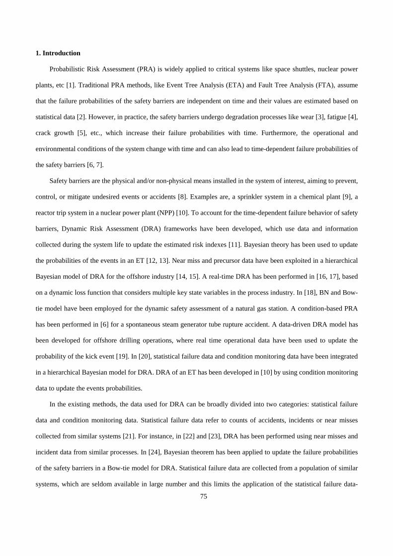
75

1. Introduction

Probabilistic Risk Assessment (PRA) is widely applied to critical systems like space shuttles, nuclear power

plants, etc [1]. Traditional PRA methods, like Event Tree Analysis (ETA) and Fault Tree Analysis (FTA), assume

that the failure probabilities of the safety barriers are independent on time and their values are estimated based on

statistical data [2]. However, in practice, the safety barriers undergo degradation processes like wear [3], fatigue [4],

crack growth [5], etc., which increase their failure probabilities with time. Furthermore, the operational and

environmental conditions of the system change with time and can also lead to time-dependent failure probabilities of

the safety barriers [6, 7].

Safety barriers are the physical and/or non-physical means installed in the system of interest, aiming to prevent,

control, or mitigate undesired events or accidents [8]. Examples are, a sprinkler system in a chemical plant [9], a

reactor trip system in a nuclear power plant (NPP) [10]. To account for the time-dependent failure behavior of safety

barriers, Dynamic Risk Assessment (DRA) frameworks have been developed, which use data and information

collected during the system life to update the estimated risk indexes [11]. Bayesian theory has been used to update

the probabilities of the events in an ET [12, 13]. Near miss and precursor data have been exploited in a hierarchical

Bayesian model of DRA for the offshore industry [14, 15]. A real-time DRA has been performed in [16, 17], based

on a dynamic loss function that considers multiple key state variables in the process industry. In [18], BN and Bow-

tie model have been employed for the dynamic safety assessment of a natural gas station. A condition-based PRA

has been performed in [6] for a spontaneous steam generator tube rupture accident. A data-driven DRA model has

been developed for offshore drilling operations, where real time operational data have been used to update the

probability of the kick event [19]. In [20], statistical failure data and condition monitoring data have been integrated

in a hierarchical Bayesian model for DRA. DRA of an ET has been developed in [10] by using condition monitoring

data to update the events probabilities.

In the existing methods, the data used for DRA can be broadly divided into two categories: statistical failure

data and condition monitoring data. Statistical failure data refer to counts of accidents, incidents or near misses

collected from similar systems [21]. For instance, in [22] and [23], DRA has been performed using near misses and

incident data from similar processes. In [24], Bayesian theorem has been applied to update the failure probabilities

of the safety barriers in a Bow-tie model for DRA. Statistical failure data are collected from a population of similar

systems, which are seldom available in large number and this limits the application of the statistical failure data-

76

based DRA methods in practice. Also, statistical data refer to a population of similar systems and do not necessarily

capture the plant-specific features of the target system. To address these issues, condition monitoring data are often

used in DRA. Condition monitoring data refer to the online monitoring data collected by sensors that are installed in

the target system for monitoring the degradation process of the safety barrier. For example, a condition-based fault

tree has been used for DRA, where the condition monitoring data have been used to update the failure rates of the

specific components and predict the reliability [25, 26]. Particle filtering (PF) has been used for DRA based on

condition monitoring data from a nonlinear non-Gaussian process [27]. In [28], a Bayesian reliability updating

method has been developed by using condition monitoring data considering the dependencies between two

components. In [5], condition monitoring data from a passive safety system have been used for DRA, without

considering the uncertainty in the condition monitoring data.

Inspection data are collected by physical inspections performed by maintenance personnel [29]. They have been

widely used for online reliability assessment. For example, a Bayesian method has been developed to merge experts’

judgment with continuous and discontinuous inspection data for the reliability assessment of multi-state systems [30].

A two-stage recursive Bayesian approach has been developed in [31], in order to update system reliability based on

imperfect inspection data. Condition monitoring data and inspection data on wind turbine blades have been used

separately for remaining useful life estimation in [32]. As inspections directly measure the component degradation,

they provide valuable information complementary to condition monitoring data for DRA and can help reducing the

impact of the uncertainty in the condition monitoring data on the result of DRA. However, to the best of our

knowledge, no previous work has considered integrating condition monitoring data and inspection data for DRA.

In this paper, we develop a new framework to integrate condition monitoring data and inspection data in DRA.

Compared to the existing works, the original contributions lie in:

(1) a Hidden Markov-Gaussian Mixture Model is developed for modeling condition monitoring data;

(2) a Bayesian network model is developed to integrate condition monitoring data and inspection data for DRA;

(3) a real-world application is performed.

The rest of the paper is organized as follows. Sect. 2 introduces the engineering motivation and formally defines

the problem. In Sect. 3, a HM-GMM is developed for reliability updating and prediction of the failure of safety

barriers based on condition monitoring data. A Bayesian network model is developed in Sect. 4 to integrate the

inspection data and condition monitoring data for DRA. The framework is tested in Sect. 5 through a numerical

77

example. In Sect. 6, it is applied for the DRA of a real-world NPP. Finally, conclusions and potential future works

are discussed in Sect. 7.

2. Problem definitions

The framework developed in this paper is motivated by real-world PRA practices. We consider an event tree

model developed for the PRA of an Anticipated Transient Without Scram (ATWS) accident of a NPP [2]. The

occurrence probabilities of the basic events, associated to the reliability of the safety barriers in the ET, are estimated

from statistical data and assumed to remain constant throughout the life of the NPP [2]. However, the safety barriers

in practice degrade. For example, a safety barrier in the aforementioned ET is the recirculation pump [2]; according

to [33], most failures of the recirculation pump are caused by the degradation of the bearings, which makes the

reliability of the pump time-dependent. DRA is best suited to capture such time-dependencies.

Two types of data can be used for the DRA of the ATWS accident. The first is inspection data. Take the bearing

mentioned above as an example: through inspections, the degradation state of the bearing can be identified, e.g.,

healthy, minor degradation (e.g., outer race defect), medium degradation (e.g., roller element defect), severe

degradation (e.g., inner race defect), etc. (see Figure 1). The second type of data is condition monitoring data: some

observable signals, e.g., temperature, vibration, etc., that contain information on the degradation process are measured

and used to infer the degradation state. For example, the vibration signals of bearings are often used as condition

monitoring data to estimate the degradation state and update the reliability of bearings [34]. Inspection data usually

give discrete degradation states, with uncertainty due to state classification by the maintenance operator. Condition

monitoring data are subject to uncertainty due to observation noises and degradation state estimation errors. In this

paper, a new framework is proposed to integrate condition monitoring data and inspection data for improving the

accuracy and reducing the uncertainty of the risk assessment.

(a) healthy state (b) minor degradation

(outer race defect)

(c) medium degradation

(roller element defect)

(d) severe degradation

(inner race defect)

78

Figure 1 Degradation states of bearing [35].

Without loss of generality, we consider a generic Even Tree (ET) model for DRA, but the framework is

applicable to other risk assessment models as well. Let represent the initialing event of the ET and assume that

there are safety barriers ( ) in the ET, denoted by whose states can be working or failure.

The sequences that emerge from the depend on the states of the and lead to possible consequences,

denoted by The generic risk index considered in this paper is the conditional probability that a specific

consequence occurs, given that the has occurred:

(1)

Conditioning on the occurrence of the these probabilities are functions of the reliabilities

of the safety barriers along the specific sequences:

(2)

where is the ET model function. For example, in the ET in Figure 2, the risk index of the consequence

of the second accident sequence, in which the occurs with certainty, the first functions successfully and

the second fails to provide its function, can be calculated as:

(3)

Figure 2 Illustrative Event Tree model.

Without loss of generality, we assume that in the ET:

(5) Safety barriers are subject to degradation processes and, therefore, their reliability

functions are time-dependent, whereas do not degrade and have constant reliability

IE

M SB , 1,2, , ,iSB i M=

IE SBs N

1 2, , , .NC C C

iC IE

{ occurs has occured}, 1,2, , .iC iP P C IE i N= =

,IE , 1,2, ,iSBR i M=

1 2( , , , ), 1,2, , .

i MC ET SB SB SBP f R R R i N= =

( )ETf 2CP

2C IE1SB

2SB

2 1 2

1 2

( , )

(1 ).

C ET SB SB

SB SB

P f R R

R R

=

= −

1 2, , , KSB SB SB

1 2, , ,K K MSB SB SB+ +

79

values;

(6) Condition monitoring data are collected for at predefined time instants

(7) The collected condition monitoring data on the th safety barrier at are denoted by where

and is a vector containing all the signals that are

monitored, where is the length of the time series;

(8) At inspections are performed on the safety barriers The inspection data are

denoted by

The DRA tasks are formally defined as:

(1) risk updating: at time update the estimated risk indexes at the current time based

on the integration of condition monitoring and inspection data available up to

(2) risk prediction: at time predict the values of the risk indexes at future times, based on the integration

of condition monitoring and inspection data available up to

3. A Hidden Markov Gaussian Mixture Model for modeling condition monitoring data

In this section, we develop a HM-GMM to model condition monitoring data. In Sect. 3.1, we formally define

the HM-GMM. Then, in Sect 3.2, we show how to use the developed HM-GMM to estimate the degradation state of

a safety barrier using condition monitoring data. The estimated degradation states are, then, used in Sect. 4 for data

integration in DRA.

3.1 Model formulations

Without loss of generality, we illustrate the HM-GMM using the th safety barrier in the ET. For simplicity of

presentation, we drop the subscript in the notations. An illustration of the model is given in Figure 3. It is assumed

that the safety barrier degrades during its lifetime and the degradation process follows a discrete state discrete time

Markov model with a finite state space where represents the health state of the

safety barrier, is the number of health states, and are in descending order of health ( is the perfect

functioning state, is the failure state). The evolution of the degradation process is characterized by the transition

probability matrix of the Markov process, denoted by where and

1 2, , , KSB SB SB , 1,2, ;kt t k q= =

-ikt t= c ( ),i kt

1,2, , , 1,2, ,i K k q= = 1 2( ) [ ( ), ( ), , ( )]i i i i qt c t c t c t=c

q

,Int t= , 1,2, , .iSB i K=

, , 1,2, , .IN iS i K=

, 1,2, , ,kt t k q= = ,kt

;kt

,kt t=

.kt

-i

i

( )S t 1 2( ) { , , , },QS t S S S ( )S t

Q1 2, , , QS S S 1S

QS

,A { }ijA a=

80

The initial state distribution of the Markov process is denoted

by where It should be noted that repairs are not considered in

this paper, just to simplify the calculation. Then, can only transit to a worse state and cannot move backwards

to a better state. Besides, the failure state is an absorbing state, such that if and only

if and for all other values of However, the model accommodates the case of

repairable components, where the transition matrix has non-zero entries also for backward state transitions, which

represent the repairs of the safety barriers. The developed algorithms, can, then, be extended naturally.

The discrete time discrete state Markov process model is chosen because it is widely applied for quantitatively

describing discrete state degradation processes in many practical applications [36]. For example, a discrete state

Markov model has been used to model the bearing degradation process in [35]. The degradation process of a safety

instrumented system is modeled by a Markov model for availability analysis [37, 38]. Although only Markov process-

based degradation models are discussed in this paper, the developed methods for data integration into DRA can be

easily extended to other degradation models.

Figure 3 Description of the HM-GMM.

As described in Sect. 2.1, condition monitoring data are available at In practice,

contains only raw signals, which cannot be directly used for degradation modeling and analysis. Feature extraction,

( )1( ) ( ) , 1,2, , ,1 , .ij k j k ia P S t S S t S k q i j Q+= = = =

1 2 ,Q = π ( )0( ) ,1 .i iP S t S i Q = =

( )S t

QS ( )1( ) ( ) 1k k Qp S t i S t S+ = = =

Qi S= ( )1( ) ( ) 0k k Qp S t i S t S+ = = = .i

( )tc , 1,2, , .kt t k q= = ( )tc

81

as shown in Figure 3, is needed to extract degradation features from . For example, vibration signals are usually

used as condition monitoring data for bearings [24]. The raw vibration signals, however, need to be preprocessed to

extract features for degradation characterization. The commonly used degradation features include entropy, root mean

square (RMS), kurtosis, etc [39]. In this paper, we refer to these extracted features as degradation indicators and

denote them by where and is the number of the degradation features.

As the safety barrier degrades, the degradation indicator exhibits distinct patterns. To capture such patterns

and the uncertainty associated with them, it is assumed that at each degradation state the values of the

degradation indicators follow a multivariate Gaussian distribution

as shown in Figure 3. The mean values vector captures the

degradation pattern at each degradation state, while the covariance matrix captures the uncertainty in the

condition monitoring data. An overall picture of the HM-GMM is given in Figure 3. Conceptually, we denote the

HM-GMM compactly as where is the initial state distribution, is the transition probability

matrix, is a vector of the mean values and is a collection of the covariance

matrices of the multivariate Gaussian distribution, respectively.

3.2 Degradation states estimation based on condition monitoring data

In this section, we show how to estimate the degradation states of the safety barriers based on the developed

HM-GMM of the condition monitoring data. As shown in Figure 4, the estimation is made by an offline step and an

online step. In the offline step, a HM-GMM is trained based on training data from a population of similar systems.

The trained HM-GMM model, is, then, used in the online step for degradation state estimation based on the condition

monitoring data.

The offline step starts from collecting training data, denoted by The training

data comprise of historical measurements of the degradation signals from a population of similar systems. To ensure

the accuracy of HM-GMM training, it is required to collect as many as possible training samples, i.e., the sample size

should be as large as possible. The raw training data are preprocessed in a feature extraction step, as shown in

Figure 4, to extract the health indicators Depending on the nature of the

degradation process condition, different feature extraction methods, e.g., time-domain, frequency domain, time-

( )tc

( ),tx 1 2( ) ( ), ( ), , ( )featurent x t x t x t =

x featuren

( )tx

,1 ,iS i Q

x

( ) ( )( ) ( ( ) ) ( , ), 1,2, , ,i i

i ib p S t S N i Q= = = =x x x μ Σ( )i

μ

( )iΣ

={ , , },Aλ π μ Σ, π A

1 2= , , Q μ μ μ μ

(1) (2) ( ), , , Q = Σ

( )

1 2( ), 1,2, , , , , , .k

Tr Tr Trt k n t t t t= =c

Trn

( )

1 2( ), 1,2, , , , , , .k

Tr Tr Trt k n t t t t= =x

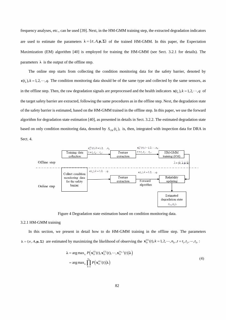
82

frequency analyses, etc., can be used [39]. Next, in the HM-GMM training step, the extracted degradation indicators

are used to estimate the parameters of the trained HM-GMM. In this paper, the Expectation

Maximization (EM) algorithm [40] is employed for training the HM-GMM (see Sect. 3.2.1 for details). The

parameters is the output of the offline step.

The online step starts from collecting the condition monitoring data for the safety barrier, denoted by

The condition monitoring data should be of the same type and collected by the same sensors, as

in the offline step. Then, the raw degradation signals are preprocessed and the health indicators of

the target safety barrier are extracted, following the same procedures as in the offline step. Next, the degradation state

of the safety barrier is estimated, based on the HM-GMM trained in the offline step. In this paper, we use the forward

algorithm for degradation state estimation [40], as presented in details in Sect. 3.2.2. The estimated degradation state

based on only condition monitoring data, denoted by is, then, integrated with inspection data for DRA in

Sect. 4.

Figure 4 Degradation state estimation based on condition monitoring data.

3.2.1 HM-GMM training

In this section, we present in detail how to do HM-GMM training in the offline step. The parameters

are estimated by maximizing the likelihood of observing the

(4)

{ , , , }A=λ μ Σ

λ

( ), 1,2, , .kt k q=c

( ), 1,2, ,kt k q=x

( ),CM kS t

{ , , , }A=λ μ Σ( )

1 2( ), 1,2, , , , , , :k

Tr Tr Trt k n t t t t= =x

( )

( )

( )(1) (2)

( )

1

arg max ( ), ( ), , ( )

arg max ( )

Tr

Tr

n

Tr Tr Tr

n

k

Tr

k

P t t t

P t=

=

=

λ

λ

λ x x x λ

x λ

83

Let be the likelihood function of the observation data. Directly solving (4) is not possible in

practice, as the likelihood function in (4) contains unobservable variables (the true degradation states in this

case). Expectation Maximization (EM) algorithm [40] is applied to solve this problem, where the maximum

likelihood estimator is found in an iterative way: the current values of the parameters are used to estimate the

unobservable variables (Expectation phase); then, the estimated values of the unknown variables are substituted into

the likelihood function to update the maximum likelihood estimators of the parameters (Maximization phase). The

iterative procedures are repeated until the maximum likelihood estimators converge.

To apply the EM algorithm to the HM-GMM model, two auxiliary variables need to be defined first, i.e., forward

variable and backward variable The forward variable is defined as the probability of observing the

health indicators up to the current time and that the true degradation state given a known HM-GMM

(5)

It is easy to verify that

(6)

where represents the observation time length and all the elements in are zero, except the one that corresponds

to the th element being one.

The backward probability is defined as the probability of observing the health indicator

from to the end of the observations, given that and the model parameters are

(7)

It is easy to verify that

The iterative estimators for the transition probabilities, denoted by can, then, be derived as follows [41]:

( )( )

1

( )Trn

k

Tr

k

L P t=

x λ

( )S t

( )t iS ( ).t iS

t ( ) ,iS t S=

:λ

1 2( ) ( ( ), ( ), , ( ), ( ) ).t i iS P t t t S t S = =x x x λ

1 1

1 +1

1

( ) π ( ( )),

( ) ( ) ( ) ,1 ,1 ,1 -1,

i i i

Q

t j j t t i ij Tr

i

S b t

S b S a i Q j Q t t

+

=

=

=

x

x

Trt πi

-i

( )t iS

( 1), ( 2), , ( )Trt t t+ +x x x 1t + ( ) iS t S=

:λ

( ) ( ( 1), ( 2), , ( ) ( ) , ).t i Tr iS P t t t S t S = + + =x x x λ

1

1

( ) ( ( 1)) ( ),1 ,1 , ( ) 1, 1, 2, ,1.Tr

Q

t j j ij t j t Tr Tr

i

S b t a S i j Q i t t t +

=

= + = = − − x

,ija

84

(8)

where represents the probability of the th sample being in at time and state at time

and is calculated by [41]:

(9)

where represents the probability of being in at time given the health indicator and for the

th training sample:

(10)

The estimator for the initial state probability is calculated by [40]:

(11)

The estimators of the mean value vectors are derived as [41]:

(12)

Similarly, the covariance matrices of the Gaussian output are calculated by [41]:

(13)

Algorithm 1 below summarizes the procedures for training the HM-GMM based on the EM algorithm. In

Algorithm 1, measures the distance between the current and the previous estimators. In this paper, we use the

absolute value for its calculation, and is the tolerance of the error. In this paper, we set

( )

,

1 1

( )

,

1 1

( , )

,

( )

Tr Tr

Tr Tr

n tk

Tr t i j

k t

ij n tk

Tr t i

k t

S S

a

S

= =

= =

=

( )

, ( , )k

Tr t i jS S -kiS t jS 1,t +

( )( ) ( )

,

( ) ( ) ( ) ( )

, , , 1

( )

,

( , ) ( ) , ( 1) ( 1) ,

( ) ( ( 1)) ( ),

( )

k k

Tr t i j i j Tr

k k k k

Tr t i ij Tr j Tr Tr t j

k

Tr t i

S S P S t S S t S t

S a b t S

S

+

= = + = +

+=

x λ

x

( )

, ( )k

Tr t iSiS t

( ) ( )k

Tr tx λ

-k

( ) ( ) ( ) ( )

, , , ,( )

, ( )( ) ( )

, ,

1

( ) ( ) ( ) ( )( ) .

( ( ) )( ) ( )

k k k k

Tr t i Tr t i Tr t i Tr t ik

Tr t i k Qk kTr

Tr t i Tr t i

i

S S S SS

p tS S

=

= =

x λ

π , 1,2, ,i

i Q=

( )

,

1

( )

π .

Tr

i

nk

Tr t i

k

Tr

S

n

==

( ) ( )

,

1 1

( )

,

1 1

( ) ( )

.

( )

Tr Tr

Tr Tr

n tk k

Tr t i Tr

k t

i n tk

Tr t i

k t

S t

S

= =

= =

=

x

μ

( ) ( ) ( ) '

, ,

1 1

( )

,

1 1

( )( ( ) )( )

.

( )

Tr Tr

Tr Tr

n tk k k

Tr t i Tr Tr ti i

k t

i n tk

Tr t i

k t

S t

S

= =

= =

− −

=

x μ x μ

Σ

tol 41 10 .tol −=

85

Algorithm 1: HM-GMM training based on EM algorithm.

Inputs:

Outputs:

Step 1:

Step 2: Expectation phase: calculate the forward and backward variables, based on (5) and (7), respectively, using

the current value of

Step 3: Maximization phase: update based on (8), (11)-(13), respectively;

Step 4: If End;

Else, go to Step 2.

3.2.2 Degradation state estimation

In this paper, the forward algorithm [40] is employed to estimate the degradation state of the safety barriers in

the online step. Let denote the estimated degradation state from condition monitoring data and

represent the posterior distribution of given the condition monitoring data up to

(14)

The posterior probabilities defined in (14) can be easily calculated from the forward probabilities defined in (15):

(15)

In practice, the in (15) is calculated recursively, based on (5).

At each the most likely degradation state, denoted by is, then, determined by finding the

state with maximal posterior probability:

(16)

Algorithm 2 below summarizes the major steps used for estimating the degradation state.

( )(1) (2)

0 0 0 0 0={ , , }, ( ), ( ), , ( );Trn

Tr Tr TrA t t tλ π μ Σ x x x,

={ , , };Aλ μ Σ,

0 ;=λ λ

;λ

λ

,prev tol− λ λ

,prev =λ λ

CMS

( ),P , 1,2, ,kCM t CMS k q=

CMS :kt

( ) ( ), 1 2P ( ) ( ), ( ) , ( ),kCM t CM i k i kS S P S t S t t t= = = x x x λ

( )( )( )

1 2

,

1 2 2

1

( ) , ( ), ( ) , ( )P =

( ), ( ), ( ) , ( )

( ).

( )

k

k

k

k i k

CM t CM i

k

t i

Q

t i

i

P S t S t t tS S

P t t t t

S

S

=

==

=

x x x λ

x x x x λ

( )kt iS

,kt t= , ( ),CM MAP kS t

( ), ,1

( ) arg max P ,1 .kCM MAP k CM t CM i

i Q

S t S S k q

= =

86

Algorithm 2 Forward algorithm for degradation state estimation at

Input:

Output:

Step 1: Calculate by (6);

Step 2: Calculate the posterior probability by (15);

Step 3: Estimate the degradation state by (16).

4. Integrating condition monitoring data with inspection data for DRA

In this section, we first show how to integrate the condition monitoring data with inspection data for reliability

updating and prediction of the safety barriers (Sect. 4.1). Then, in Sect. 4.2, we develop a DRA method based on the

updated and predicted reliabilities.

4.1. A Bayesian network model for data integration

As in the previous sections, we illustrate the developed data integration method using the th safety barrier at

For simplicity and to avoid confusion, we drop the and in the notations. To update and predict the

reliability, one needs to estimate the degradation state first. Let denote the degradation state estimated from

inspection data and denote the true degradation state. In practice, is subject to uncertainty due to potential

imprecision in the inspection and recording by the maintenance personnel. To model such uncertainty, in this paper,

we assume that the reliability of inspection is and that the maintenance personnel correctly identify the true

degradation state with a probability whereas an inspection error can occur with probability When an

inspection error occurs, it is further assumed that the probabilities for each of the possible degradation states being

erroneously identified as the true degradation state are equal to each other:

(17)

where is the number of degradation states. It is should be noted that other inspection models might also be

assumed, depending on the actual problem setting.

.kt t=

1{ , , }, ( ), 1,2, , , ( );

kt i kA S i Q t −

= =λ μ Σ x,

( ), ,P , ( );kCM t CM CM MAP kS S t

( ), 1,2, , ,kt iS i Q =

( ),PkCM t CMS

, ( )CM MAP kS t

-i

.kt t= ikt

INS

S INS

,INR

,INR (1 ).INR−

,

( ) 1, ,

1

IN i

IN i IN

i

R S S

P S S S RS S

Q

=

= = − −

Q

87

In this paper, a BN is developed to describe the dependencies among as shown in Figure 5. The BN

in Figure 5 is constructed based on the assumption that given the true degradation state the estimated degradation

state from condition monitoring data and inspection data are conditional-independent.

Figure 5 A BN model for data integration.

Based on the BN in Figure 5, we have

(18)

In (18), measures the prior belief of the analysts on the current degradation states. We assume that is a

uniform distribution over all the possible degradation states, indicating that there is no further information to

distinguish the states.

The conditional probability distribution describes the uncertainty in the inspections and is derived

based on (17). In (17), the reliability of the inspection can be estimated from historical data or assigned based on

expert judgments. The conditional probability distribution measures the trust one has on the estimated

degradation state based on condition monitoring data. Its values can be estimated from validation test data. However,

in practice, as validation tests are not always available, might also be assigned by experts considering the

measurement uncertainty of the sensors and the distance between the neighboring degradation states. We give an

example of how to determine in the case study of Sect. 6.

Once the condition monitoring data and inspection data are available, the observed values of and are

known. Suppose we have and It should be noted that we choose the state with maximal posterior

probability from (16) as the observation value of The two data sources can be naturally integrated by calculating

the posterior distribution of given the two data sources, denoted by Based on the BN in Figure 5, we

have:

, , ,IN CMS S S

,S

( ) ( ) ( ) ( ), , .IN CM IN CMP S S S P S S P S S P S=

( )P S ( )P S

( )INP S S

( )CMP S S

( )CMP S S

( )CMP S S

INS CMS

CM jS S= .IN iS S=

.CMS

S ( ).INTP S

88

(19)

Given the estimated posterior distribution in (19), the reliability of the safety barrier can be updated. Suppose

the current time is the updated reliability can be calculated by:

(20)

where is the working set that contains all the working states; is the posterior probability of the true

degradation state after integrating the two data sources at and is calculated from (19).

Furthermore, at we can also predict the reliability of the safety barriers at a future time For this, the

distribution of the degradation states at is predicted first, using Chapman-Kolmogorov equation [42] and the

trained model from the offline step:

(21)

The reliability at can be predicted as:

(22)

4.2. Dynamic risk assessment

The updated reliabilities from (20), can, then, be substituted into (2) for DRA:

(23)

where in (23), is calculated by (20). Similarly, the risk index at a future time can be predicted by:

(24)

where is calculated by (21) and (22).

Figure 6 summarizes the major steps for the developed DRA method by integrating condition monitoring data

with inspection data. It should be noted that in Figure 6, the risk updating is made at , while risk prediction is

made for a given future time

( )( )( )

( ) ( ) ( )

( )

( ) ,

, ,

,

,

INT IN i CM j

IN i CM j

IN i CM j

IN i CM j

IN i CM j

P S P S S S S S

P S S S S S

P S S S S

P S S S P S S S P S

P S S S S

= =

= ==

= =

= ==

= =

,kt

( ),( ) P ,kSB k INT tS W

R t S

=

W ( ),PkINT t S

kt t=

,kt t= .Futt

Futt t=

( )

, ,( ) ( ) .Fut k

Fut k

t t

INT t INT tP S P S A−

=

,kt t=

,( ) ( ).FutSB Fut INT tS W

R t P S

=

1 2 1( ) ( ( ), ( ), , ( ), , , ), 1,2, , ,

i K K MC k ET SB k SB k SB k SB SBr t f R t R t R t R R IE i N+

= =

( )iSB kR t

Futt

1 2 1( ) ( ( ), ( ), , ( ), , , ), 1,2, , ,

i K K MC Fut ET SB Fut SB Fut SB Fut SB SBr t f R t R t R t R R IE i N+

= =

( )iSB FutR t

kt t=

.Futt

89

Figure 6 Procedures for DRA based on condition monitoring and inspection data.

5. Numerical case study

In this section, we apply the DRA framework for data integration (see Sect. 4.1) on a numerical case study. The

purpose is to test the updating and prediction of safety barrier reliability. Hence, only reliability updating and

prediction are considered. The application of the overall DRA framework is done in Sect. 6 on a real-world case.

Consider a component whose degradation process follows a discrete state discrete time Markov chain with

four discrete degradation states where have increasing degrees of degradation from perfect

state, to failure state. The condition monitoring data are generated from a HM-GMM with known parameters

values:

( )S t

1 2 3 4, , , ,S S S S 1 4S S 1S

4S

90

(25)

The degradation indicator comprises of three features, denoted by and respectively. The size of the

generated training data is and are the time instants of data collection. Then, the training data can

be represented as where The training data are

used in the offline step for estimating the model parameters. Then, another sample, denoted by

is generated from the HM-GMM in (25) and used as condition monitoring data collected on the safety barrier

monitored in the online step, as shown in Figure 7.

Figure 7 The generated condition monitoring data for the monitored safety barrier.

Based on the generated condition monitoring data, the reliability updating and prediction can be done using

Algorithm 1 and equations (20) and (22). Due to the noise in the condition monitoring data, the updated reliability is

subject to uncertainty. The method in Figure 6 is applied to solve this problem by integrating condition monitoring

data with inspection data. In this section, we test the performance of the developed data integration method under

three possible scenarios:

(1) Both condition monitoring data and inspection data correctly estimate the degradation state: this scenario

( )

0.6 0.2 0.1 0.1

0 0.5 0.25 0.25A= ,

0 0 0.5 0.5

0 0 0 1

1 0 0 0 ,

0.0588 0.1424 0.1842 1

0.1268 0.1597 0.2432 1 ,

0.0946 0.9744 0.8648 0.8449

0.001 0 0

0 0.001 0 , with 1,2,3,4.

0 0 0.001

i i

=

=

= =

π

μ

Σ

1 2,x x 3 ,x

4101 2 23, , ,t t t t=

( ) 4

1 2 23( ), 1,2, ,10 , , , , ,k

Tr t k t t t t= =x( ) ( ) ( ) ( )

,1 ,2 ,3( ) ( ), ( ), ( ) .k k k k

Tr Tr Tr Trt x t x t x t = x

( ), 1,2, , ,CM CMt t t=x

91

is represented by choosing the time point where the estimated degradation state from condition

monitoring data and the true degradation state are both The inspection data at is generated to be

exactly

(2) Condition monitoring data correctly estimate the degradation state, but inspection data do not: this scenario

is represented by choosing the time point where the estimated degradation state from condition

monitoring data and the true state are both whereas the inspection data at is randomly sampled from

The state from the inspection data is

(3) Inspection data correctly estimate the degradation state, but condition monitoring data do not: this scenario

is generated by choosing the time point where the estimated degradation state from condition

monitoring data is whereas the true degradation state is The inspection data at

are generated to be

In subsections 5.1-5.3, we apply the developed data integration method on the three scenarios above.

5.1 Scenario Ⅰ: Both data sources are reliable

The reliability updating and prediction processes are conducted following the procedures in Figure 6, at

The updated and predicted reliability are compared to those calculated based on only condition monitoring data and

only inspection data, respectively. The comparison is shown in Figure 8. We also show the relative errors of the three

methods with respect to the true values in Table 1.

3= ,t t

2 .S kt

3 2( ) .INS t S=

7= ,t t

3 ,S 7t

, 1, , , 3.kS k Q k= 3 2( ) .INS t S=

5= ,t t

5 2( ) ,CMS t S= 5 3( ) .S t S= 5t

5 5 3( ) ( ) .INS t S t S= =

3.t t=

92

Figure 8 Updated and predicted reliability at (scenario Ⅰ).

Table 1 Relative errors of the scenario I

Condition monitoring data-based method 0 4.8% 9.7% 14.5% 19% 23% 27% 31%

Inspection data-based method 0 1.34% 0.9% 4.6% 8.7% 12.9% 17% 21%

Integrated method 0 1.2% 0.9% 4.3% 7% 11.7% 15% 18.6%

As shown in Figure 8 and Table 1, the proposed method provides a more accurate estimation and prediction of

the reliability than the other two methods. This is because condition monitoring data are affected by noise from the

data collection process, which results in uncertainty in the estimated degradation state. In this case, the state

distribution estimated by the condition monitoring data is

(26)

whereas the one estimated by integrating the two data sources is

(27)

It can be seen that integrating the two data sources reduces the uncertainty in the degradation state estimation (note

that at the true degradation state is ). Therefore, the updated and predicted reliabilities are more accurate

than only using condition monitoring data.

On the other hand, the transition probability matrix estimated from the offline step is

3t t=

3t t= 4t t= 5t t= 6t t= 7t t= 8t t= 9t t= 10t t=

3, ( ) [0 0.8263 0.1737 0],CM t CMP S =

3, ( ) [0.01 0.98 0.01 0].INT tP S =

3 ,t t= 2S

A

93

(28)

Comparing (28) to the true values in (25), it can be seen that when the current state is the estimated tends to

underestimate the reliability as it overestimates the transition probabilities to the failure states. As the inspection data

estimate that the system is in using only inspection data tends to underestimate the reliability. Integrating the two

data sources, as shown in (27), predicts that the safety barrier is also likely to be in which compensates the errors

in the estimated and results in more accurate reliability estimates.

5.2 Scenario II: Condition monitoring data are reliable but inspection data are not

The reliability updating and prediction processes are conducted following the procedures in Figure 6, at

The updated and predicted reliability are compared to those calculated based on only condition monitoring data and

only inspection data, respectively. The comparison is shown in Figure 9. We also present the relative error of the

three methods by comparing them to the true values in Table 2.

Figure 9 Updated and predicted reliability at (scenario II).

Table 2 Relative errors of the scenario II.

0.6010 0.2125 0.0865 0.1

0 0.4483 0.3121 0.2395.

0 0 0.4938 0.5062

0 0 0 1

A

=

2 ,S A

2 ,S

1,S

λ

7 .t t=

7t t=

7t t= 8t t= 9t t= 10t t= 11t t= 12t t= 13t t= 14t t=

94

Condition monitoring data-based method 0 12% 22% 33% 39% 46% 52% 57%

Inspection data-based method 0 52% 98% 138% 173% 204% 232% 255%

Integrated method 6% 34% 71% 96% 105% 137% 158% 197%

As shown in Figure 9 and Table 2, the results obtained by the inspection-data based method have the largest

estimation error. The proposed data integration method provides more accuracy than the inspection data-based

method. This is expected, as in this case the inspection data fail to correctly estimate the degradation state. By

integrating condition monitoring data, the incorrect information from inspection data can be somewhat corrected. On

the contrary, the estimation error of the data integration method is larger than that of the condition monitoring data-

based method. This is because the data integration method is affected by the incorrect information from the inspection

data. Trustworthiness of the inspection becomes essential, then.

5.3 Scenario III: Inspection data are reliable but condition monitoring data are not

The reliability updating and prediction are conducted following the procedures in Figure 6, at The updated

and predicted reliability are compared to those calculated based on only condition monitoring data and only inspection

data, respectively. The comparison is shown in Figure 10. We also present the relative errors of the three methods by

comparing them to the true values in Table 3.

Figure 10 Updated and predicted reliability at (scenario III).

Table 3 Relative errors of the scenario III.

Condition monitoring data-based method 0 16% 26% 14.5% 33% 38.5% 43% 46%

Inspection data-based method 0 1.39% 2.9% 4.6% 8.6% 12.9% 16.9% 21%

5.t t=

5t t=

5t t= 6t t= 7t t= 8t t= 9t t= 10t t= 11t t= 12t t=

95

Integrated method 2% 10% 14% 17% 20% 23% 25% 27%

As shown in Figure 10 and Table 3, the results obtained by the condition monitoring data-based method have

the largest estimation errors. This is expected as in this case, the condition monitoring data fail to correctly estimate

the degradation state. The proposed data integration method provides a more accurate result than the condition

monitoring data-based method. This is because, by integrating inspection data, the incorrect estimation from the

condition monitoring data can be compensated. However, the estimation error is larger than that of the inspection

data-based method. This is because the data integration method also considers the incorrect information from the

condition monitoring data.

In practical operation, the developed method can help the stakeholder/decision-makers to determine when to

perform preventive maintenance on critical safety barriers. This is done by setting a minimum acceptable value for

reliability and calculating the first time the reliability drops below this value. However, the reliability estimation can

sometimes be imprecise. The developed method, can, then, provide a more realistic assessment to support decision

making regarding when a preventive replacement is needed.

6. Application

In this section, the developed method is applied for DRA of an Anticipated Transient Without Scram (ATWS)

accident of a NPP [2]. The description of the case study is briefly introduced in Sect. 6.1. Then, in Sect. 6.2, the

developed HM-GMM and the data integration process are presented. The results of the DRA are presented and

discussed in Sect. 6.3.

6.1 System description

ATWS is an accident that can happen in a NPP. In this accident, the scram system, which is designed to shut

down the reactor during an abnormal event (anticipated transient), fails to work [43]. An ET has been developed for

PRA of the ATWS for a NPP in China [2], as shown in Figure 11. In Figure 11, T1ACM represents the failure of the

automatic scram system and is the initialing event (IE) considered. Eleven safety barriers ( ) are designed

to contain the accident (Table 4). Depending on the states of the safety barriers, 23 sequences can be generated (

) [2, 44]. The consequences of the sequences are grouped into two categories, based on their severity; the

first group,

(29)

1 11SB SB

01 23SE SE−

03 06 07 08 09 12 13 14 15 18 19 20 21 22 23{ , , , , , , , , , , , , , , },sC SE SE SE SE SE SE SE SE SE SE SE SE SE SE SE=

96

represents the event sequences with severe consequences, whereas the remaining event sequences have non-severe

consequences [44]. The risk index considered in this paper is the conditional probability of having severe

consequences, given the initialing event ( ):

(30)

where the model function is determined from the ET in Figure 11 and are the reliabilities of

the safety barriers, calculated based on the component failure probabilities in Table 4. It should be noted that the

failure probabilities for and change depending on the event sequence that occurs (see, e.g., and

in Figure 11 and Table 4).

Figure 11 ET for the ATWS [44]; at each branching, the upper branch corresponds to the non-failure of the safety

barrier and the low branch corresponds to the failure of the safety barrier.

In this original ETA of the ATWS, the failure probabilities in Table 4 are assumed to be constant values. In

practice, however, these probabilities might change due to various degradation mechanisms. Take the recirculation

pump as an example. According to [33], most field failures of the recirculation pump are caused by the degradation

Risk

1IE T ACM=

1 2 1( ) ( , , , ),MS ET SB SB SBRisk P C IE f R R R T ACM=

( )ETf1 2, , ,

MSB SB SBR R R

7SB 8SB7

(1)

,f SBP

7

(2)

,f SBP

97

of the bearing inside the pump, which makes the failure probability of the recirculation pump time-dependent. In this

paper, we make a DRA on the ET in Figure 11, considering the degradation of the bearing in the recirculation pump.

The condition monitoring data of the bearing come from the bearing degradation dataset from university of

Cincinnati [45]. The dataset contains four samples and for each sample, raw condition monitoring data are collected

in real time by measuring the vibration acceleration signals. An illustration of the raw data is given in Figure 12. On

the other hand, the inspection can be performed at some given time instants to identify the different degradation

states. As shown in Figure 1, we distinguish from four degradation states in this case study.

Table 4 Safety barriers in the target system [2].

Safety barrier Failure probability

Description

Recirculation pump (

) Once the plant fails to scram, the recirculation pump is activated

and used to limit power generation of the NPP.

Safety valve ( ) Safety valves are opened to prevent over-pressurization of the

reactor.

Boron injection ( ) Liquid boron should be injected manually by the operator within

the allowable time to shut down the reactor safely.

Automatic

Depressurization

System (ADS) inhibit (

)

ADS is designed to decrease the pressure of the reactor in order

to start the low-pressure system.

Early high-pressure

makeup ( )

The system is supposed to work automatically when automatic

actuation alarm appears, indicating that the water level is

lowering to level 2.

Long-term high-

pressure makeup (

)

The long-term high-pressure system is used to maintain the water

level in the vessel 24 hours after the start.

Manual reactor

depressurization ( )

The operator depressurizes the vessel manually to avoid core

melt-down. In the failure probability is

whereas, in the failure probability is

Reactor inventory

makeup at low pressure

( )

If the low pressure system fails as well as the high-pressure

system, then the reactor inventory makeup at lower pressure

needs to be activated. In the failure probability is

while, in the failure probability is In

the failure probability is

Vessel overfill

prevention ( ) The operator needs to monitor the water level and make sure the

level is not too high to cause core melt-down.

Long-term heat removal

( )

The long-term heat removal system is initialized to cool down

the suppression pool and containment in order to maintain the

other supporting systems in working states.

( )fP

1SB31.96 10−

2SB 51.01 10−

3SB 51 10−

4SB

21.37 10−

5SB28.45 10−

6SB 32.13 10−

7SB7

7

(1)

,

(2)

,

0.45,

0.9

f SB

f SB

P

P

=

=04 09 ,SE SE−

7

(1)

, ,f SBP

10 15 ,SE SE−7

(2)

, .f SBP

8SB

8

8

8

(1) 6

,

(2) 6

,

(3) 5

,

1.12 10 ,

3.4 10 ,

9.49 10

f SB

f SB

f SB

P

P

P

−

−

−

=

=

=

04 07 ,SE SE−

8

(1)

, ,f SBP10 14 ,SE SE−

8

(2)

, .f SBP

16 20 ,SE SE−8

(3)

, .f SBP

9SB0.875

10SB52.03 10−

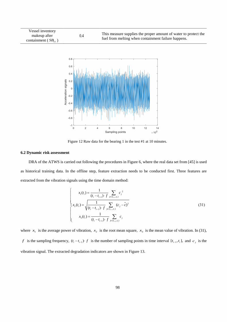
98

Vessel inventory

makeup after

containment ( )

This measure supplies the proper amount of water to protect the

fuel from melting when containment failure happens.

Figure 12 Raw data for the bearing 1 in the test #1 at 10 minutes.

6.2 Dynamic risk assessment

DRA of the ATWS is carried out following the procedures in Figure 6, where the real data set from [45] is used

as historical training data. In the offline step, feature extraction needs to be conducted first. Three features are

extracted from the vibration signals using the time domain method:

(31)

where is the average power of vibration, is the root mean square, is the mean value of vibration. In (31),

is the sampling frequency, is the number of sampling points in time interval and is the

vibration signal. The extracted degradation indicators are shown in Figure 13.

11SB

0.4

1

1

1

2

1

( , )1

2

2

( , )1

3

( , )1

1( )

( )

1( ) ( )

( )

1( )

( )

i i

i i

i i

i j

j t ti i

i j

j t ti i

i j

j t ti i

x t ct t f

x t c ct t f

x t ct t f

−

−

−

−

−

−

=

−

= −−

=

−

1x 2x 3x

f 1( )i it t f−− 1[ , ],i it t− jc

99

(a) average power of vibration (b) root mean square

(c) mean value of vibration

Figure 13 Extracted degradation indicators.

Algorithm 1 is applied to train a HM-GMM with four discrete degradation states based on the extracted

degradation indicators:

1( ) :x t 2 ( ) :x t

3 ( ) :x t

100

(32)

The online condition monitoring data are generated using the bootstrap sampling: bootstrap samples are

generated from the training data set. A HM-GMM is, then, trained based on these samples using Algorithm 1:

(33)

The HM-GMM in (33) is, then, treated as the true degradation model and used to generate the condition monitoring

data for the bearing that is monitored in the online step. The generated condition monitoring data are shown in Figure

14.

(1)

0.5 0.5 0 0

0 0.9354 0.0646 0= , 1 0 0 0 ,

0 0 0.9565 0.0435

0 0 0 1

0.0412 0.1176 0.2002 1.0000

0.0916 0.1184 0.2634 1.0000 ,

0.0579 0.9168 0.8672 0.8446

0.0108 0.0018 0.0007

0.0018 0.0137 0.0014

0.0007 0.0014

A

=

=

=

μ

Σ(2)

(3) (4)

0.0111 0.0020 0.0012

, 0.0020 0.0134 0.0019 ,

0.0121 0.0012 0.0019 0.0137

0.0129 0.0039 0.0002 0.01 0 0

0.0039 0.0153 0.0002 , 0 0.01 0 .

0.0002 0.0002 0.0106 0 0 0.01

=

= =

Σ

Σ Σ

410

λ

(1)

0.5 0.5 0 0

0 0.9613 0.0387 0A= , 1 0 0 0 ,

0 0 0.7150 0.2849

0 0 0 1

0.0446 0.1338 0.2339 0.7809

0.0974 0.2004 0.3087 0.8062 ,

0.0764 0.9744 0.8779 0.8584

0.0105 0.0010 0.0005

0.0010 0.0122 0.0009

0.0005 0.0009

=

=

=

μ

Σ(2)

(3) (4)

0.0109 0.0016 0.0007

, 0.0016 0.0128 0.0010 ,

0.0118 0.0007 0.0010 0.0128

0.0123 0.0030 0.0000 0.0111 0.0013 0.0001

0.0030 0.0141 0.0001 , 0.0013 0.0116 0.0001

0.0002 0.0001 0.0105

=

= − = −

Σ

Σ Σ .

0.0001 0.0001 0.0100

λ

101

Figure 14 The generated condition monitoring data.

Inspections are conducted at three time instants, i.e., and respectively. The

inspection data at the three time instants are given in Table 5. In Table 5, we also show the true degradation states

obtained from the true degradation model in (33) and the estimated degradation states using condition monitoring

data and Algorithm 2.

The estimated degradation state and are, then, integrated using (19). Note that in (17), the reliability

of the inspection data is set to Then, the value of in (19) can be derived easily from (17). The

values of are assigned by considering the distance between the neighboring degradation states: the closer

the states are, the more likely a misclassification might happen. For example, the normalized distance between

and is:

(34)

and the normalized distance between and is:

(35)

where is the Euclidean distance. Thus, we set and The

values of the other elements in are determined in a similar way and reported in Table 6. Once the integrated

estimation of the degradation state is obtained, risk updating and prediction can be performed by (23) and (24),

respectively.

30( ),t d= 35( )t d= 50( ),t d=

INS CMS

0.8.INR = ( )INP S S

( )CMP S S

2S

3S

( )

( )

2 3

4

3

1

,0.4807,

,i

i

d

d=

=

μ μ

μ μ

3S 4S

( )

( )

4 3

4

3

1

,0.1108,

,i

d

d=

=

i

μ μ

μ μ

( )d 2 3( ) 0.1CMP S S S S= = = 4 3( ) 0.2.CMP S S S S= = =

( )CMP S S

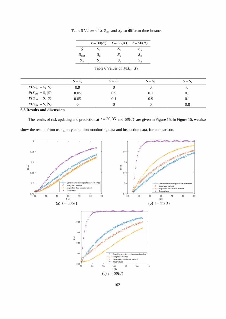
102

Table 5 Values of and at different time instants.

Table 6 Values of

0.9 0 0 0

0.05 0.9 0.1 0.1

0.05 0.1 0.9 0.1

0 0 0 0.8

6.3 Results and discussion

The results of risk updating and prediction at and are given in Figure 15. In Figure 15, we also

show the results from using only condition monitoring data and inspection data, for comparison.

(a) (b)

(c)

, CMS S INS

30( )t d= 35( )t d= 50( )t d=

S 2S 3S 3S

CMS 2S 2S 3S

INS 2S 3S 2S

( ).CMP S S

1S S= 2S S= 3S S= 4S S=

1( )CMP S S S=

2( )CMP S S S=

3( )CMP S S S=

4( )CMP S S S=

30,35t = 50( )d

30( )t d= 35( )t d=

50( )t d=

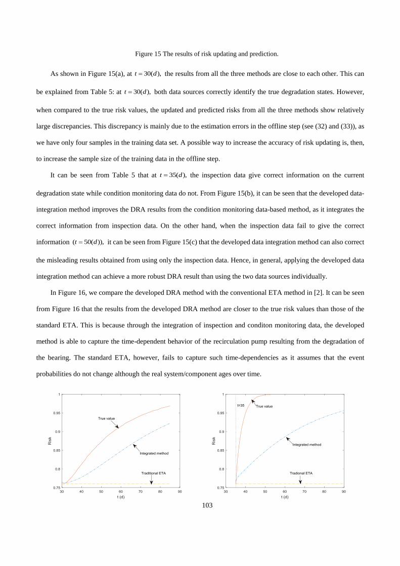
103

Figure 15 The results of risk updating and prediction.

As shown in Figure 15(a), at the results from all the three methods are close to each other. This can

be explained from Table 5: at both data sources correctly identify the true degradation states. However,

when compared to the true risk values, the updated and predicted risks from all the three methods show relatively

large discrepancies. This discrepancy is mainly due to the estimation errors in the offline step (see (32) and (33)), as

we have only four samples in the training data set. A possible way to increase the accuracy of risk updating is, then,

to increase the sample size of the training data in the offline step.

It can be seen from Table 5 that at the inspection data give correct information on the current

degradation state while condition monitoring data do not. From Figure 15(b), it can be seen that the developed data-

integration method improves the DRA results from the condition monitoring data-based method, as it integrates the

correct information from inspection data. On the other hand, when the inspection data fail to give the correct

information it can be seen from Figure 15(c) that the developed data integration method can also correct

the misleading results obtained from using only the inspection data. Hence, in general, applying the developed data

integration method can achieve a more robust DRA result than using the two data sources individually.

In Figure 16, we compare the developed DRA method with the conventional ETA method in [2]. It can be seen

from Figure 16 that the results from the developed DRA method are closer to the true risk values than those of the

standard ETA. This is because through the integration of inspection and conditon monitoring data, the developed

method is able to capture the time-dependent behavior of the recirculation pump resulting from the degradation of

the bearing. The standard ETA, however, fails to capture such time-dependencies as it assumes that the event

probabilities do not change although the real system/component ages over time.

30( ),t d=

30( ),t d=

35( ),t d=

( 50( )),t d=

104

(a) (b)

(c)

Figure 16 Comparisons of traditional ETA and DRA.

Additionally, as can be seen from Figure 16, the true risk is higher than the one estimated by the developed

method. The inaccuracy of the risk estimation is caused by the imprecise estimation of the parameters in the HM-

GMM (equation 32), which is primarily due to the small sample size in the offline training of the HM-GMM (see

Figure 4). It can be seen from equations (32) and (33) that, since we have only four samples in the offline training

phase, the estimated transition probability differs from its true value. Particularly, the probability of system remaining

in given that it enters is estimated to be which is larger than its true value This

indicates that the trained HM-GMM trends to overestimate the reliability of the safety barrier ( is the failure state

), and, hence, underestimate the risk, in this case. The inaccuracy of the estimation is caused by the fact that we have

only four samples from the real dataset, for the offline training phase. In the numerical case study (Section 5), it is

shown that with training samples, the estimation accuracy is satisfactory.

A major issue with the EM algorithm (Algorithm 1) is that, when the sample size is small, there can be large

uncertainty on the estimated parameter values. This uncertainty, if not properly addressed, might greatly impact the

estimation accuracy of the reliability of the safety barriers, and, then, the calculated risk. One way to capture the

uncertainty in the estimated risk caused by parameter estimation is to conduct a bounding risk analysis by using

Bayesian inference [20, 46, 47], where posterior distributions of the parameters, rather than point estimators, are

calculated to represent the parametric uncertainty. The uncertainty in the parameter estimation can be represented in

terms of the credible intervals. By propagating the parametric uncertainty, a credibility interval can also be obtained

for the estimated risk, which can help the decision-makers understand the confidence on the risk estimations.

30( )t d= 35( )t d=

50( )t d=

3S 3S 33 0.9565,a =33 0.7150.a =

4S

410

105

7. Conclusions

In this paper, a framework has been presented to integrate condition monitoring data and inspection data for

DRA. A HM-GMM has been developed to estimate the degradation states of the safety barriers based on the condition

monitoring data. The estimated degradation states are integrated with the inspection data for DRA by a BN model. A

numerical case study and a real-word application on a NPP accident risk assessment model (an ET) have been

conducted. The results show that, as expected, integrating the two data sources into the DRA gives more accurate

and robust results than using any one of the two individual data sources.

There are some challenges to be addressed when applying the developed model to real-life large-scale systems

(of systems). The first one is that, to ensure the accuracy of the developed method, a sufficient number of training

samples is needed. This might not be the case for real-world systems. To address this challenge, the estimation of the

values of the parameters of the HM-GMM can be embedded within a Bayesian inference framework for a bounding

analysis that gives due account to uncertainties. Other future developments should consider the extension of the

developed model to systems with multiple degrading components and repairable components.

The current method only considers a discrete time discrete state Markov model as the degradation model. A

future work is to extend the developed framework to other degradation models, e.g. the Brownian motion model [48],

Gamma process model [49], etc. Moreover, in the current framework, the parameters of HM-GMM are estimated

offline; in the future, online updating of the parameters can be considered in order to improve the accuracy of the

DRA.

References

[1] Yang, X., S. Haugen, and N. Paltrinieri, Clarifying the concept of operational risk assessment in the oil and gas

industry. Safety Science, 2018. 108: p. 259-268.

[2] Huang, D., T. Chen, and M.-J.J. Wang, A fuzzy set approach for event tree analysis. Fuzzy sets and systems, 2001.

118(1): p. 153-165.

[3] Compare, M., F. Martini, S. Mattafirri, F. Carlevaro, and E. Zio, Semi-Markov model for the oxidation degradation

mechanism in gas turbine nozzles. IEEE Transactions on Reliability, 2016. 65(2): p. 574-581.

[4] Chiachío, J., M. Chiachío, S. Sankararaman, A. Saxena, and K. Goebel, Condition-based prediction of time-

dependent reliability in composites. Reliability Engineering & System Safety, 2015. 142: p. 134-147.

[5] Kim, H., S.-H. Lee, J.-S. Park, H. Kim, Y.-S. Chang, and G. Heo, Reliability data update using condition

monitoring and prognostics in probabilistic safety assessment. Nuclear Engineering and Technology, 2015. 47(2): p. 204-

211.

[6] Di Maio, F., F. Antonello, and E. Zio, Condition-based probabilistic safety assessment of a spontaneous steam

generator tube rupture accident scenario. Nuclear Engineering and Design, 2018. 326: p. 41-54.

[7] Zhao, X., X. Guo, and X. Wang, Reliability and maintenance policies for a two-stage shock model with self-

healing mechanism. Reliability Engineering & System Safety, 2018. 172: p. 185-194.

[8] Sklet, S., Safety barriers: Definition, classification, and performance. Journal of Loss Prevention in the Process

Industries, 2006. 19(5): p. 494-506.

106

[9] Landucci, G., F. Argenti, A. Tugnoli, and V. Cozzani, Quantitative assessment of safety barrier performance in

the prevention of domino scenarios triggered by fire. Reliability Engineering & System Safety, 2015. 143: p. 30-43.

[10] Kim, H., J.T. Kim, and G. Heo, Failure rate updates using condition-based prognostics in probabilistic safety

assessments. Reliability Engineering & System Safety, 2018. 175: p. 225-233.

[11] Villa, V., N. Paltrinieri, F. Khan, and V. Cozzani, Towards dynamic risk analysis: a review of the risk assessment

approach and its limitations in the chemical process industry. Safety science, 2016. 89: p. 77-93.

[12] Paltrinieri, N., F. Khan, P. Amyotte, and V. Cozzani, Dynamic approach to risk management: application to the

Hoeganaes metal dust accidents. Process Safety and Environmental Protection, 2014. 92(6): p. 669-679.

[13] Abimbola, M., F. Khan, and N. Khakzad, Dynamic safety risk analysis of offshore drilling. Journal of Loss

Prevention in the Process Industries, 2014. 30: p. 74-85.

[14] Khakzad, N., F. Khan, and N. Paltrinieri, On the application of near accident data to risk analysis of major

accidents. Reliability Engineering & System Safety, 2014. 126: p. 116-125.

[15] Yang, M., F.I. Khan, and L. Lye, Precursor-based hierarchical Bayesian approach for rare event frequency

estimation: a case of oil spill accidents. Process safety and environmental protection, 2013. 91(5): p. 333-342.

[16] Wang, H., F. Khan, S. Ahmed, and S. Imtiaz, Dynamic quantitative operational risk assessment of chemical

processes. Chemical Engineering Science, 2016. 142: p. 62-78.

[17] Hashemi, S.J., S. Ahmed, and F. Khan, Loss functions and their applications in process safety assessment. Process

Safety Progress, 2014. 33(3): p. 285-291.

[18] Zarei, E., A. Azadeh, N. Khakzad, M.M. Aliabadi, and I. Mohammadfam, Dynamic safety assessment of natural

gas stations using Bayesian network. Journal of hazardous materials, 2017. 321: p. 830-840.

[19] Adedigba, S.A., O. Oloruntobi, F. Khan, and S. Butt, Data-driven dynamic risk analysis of offshore drilling

operations. Journal of Petroleum Science and Engineering, 2018. 165: p. 444-452.

[20] Zeng, Z. and E. Zio, Dynamic Risk Assessment Based on Statistical Failure Data and Condition-Monitoring

Degradation Data. IEEE Transactions on Reliability, 2018. 67(2): p. 609-622.

[21] Kalantarnia, M., F. Khan, and K. Hawboldt, Dynamic risk assessment using failure assessment and Bayesian

theory. Journal of Loss Prevention in the Process Industries, 2009. 22(5): p. 600-606.

[22] Meel, A. and W.D. Seider, Plant-specific dynamic failure assessment using Bayesian theory. Chemical

Engineering Science, 2006. 61(21): p. 7036-7056.

[23] Meel, A., L.M. O’Neill, J.H. Levin, W.D. Seider, U. Oktem, and N. Keren, Operational risk assessment of

chemical industries by exploiting accident databases. Journal of Loss Prevention in the Process Industries, 2007. 20(2): p.

113-127.

[24] Khakzad, N., F. Khan, and P. Amyotte, Dynamic risk analysis using bow-tie approach. Reliability Engineering

& System Safety, 2012. 104: p. 36-44.

[25] Shalev, D.M. and J. Tiran, Condition-based fault tree analysis (CBFTA): A new method for improved fault tree

analysis (FTA), reliability and safety calculations. Reliability Engineering & System Safety, 2007. 92(9): p. 1231-1241.

[26] Aizpurua, J.I., V.M. Catterson, Y. Papadopoulos, F. Chiacchio, and G. Manno, Improved dynamic dependability

assessment through integration with prognostics. IEEE Transactions on Reliability, 2017. 66(3): p. 893-913.

[27] Zadakbar, O., F. Khan, and S. Imtiaz, Dynamic Risk Assessment of a Nonlinear Non‐Gaussian System Using a

Particle Filter and Detailed Consequence Analysis. The Canadian Journal of Chemical Engineering, 2015. 93(7): p. 1201-

1211.

[28] Liu, J. and E. Zio, System dynamic reliability assessment and failure prognostics. Reliability Engineering &

System Safety, 2017. 160: p. 21-36.

[29] Nguyen, H.-P., J. Liu, and E. Zio, Dynamic-weighted ensemble for fatigue crack degradation state prediction.

Engineering Fracture Mechanics, 2018. 194: p. 212-223.

[30] Liu, Y., P. Lin, Y.-F. Li, and H.-Z. Huang, Bayesian reliability and performance assessment for multi-state

systems. IEEE Transactions on Reliability, 2015. 64(1): p. 394-409.

[31] Liu, Y. and C.-J. Chen, Dynamic reliability assessment for nonrepairable multistate systems by aggregating

multilevel imperfect inspection data. IEEE Transactions on Reliability, 2017. 66(2): p. 281-297.

[32] Nielsen, J.S. and J.D. Sørensen, Bayesian Estimation of Remaining Useful Life for Wind Turbine Blades. Energies,

2017. 10(5): p. 664.

[33] Lees, F., Lees' Loss prevention in the process industries: Hazard identification, assessment and control. 2012:

Butterworth-Heinemann.

[34] Tobon-Mejia, D.A., K. Medjaher, N. Zerhouni, and G. Tripot, A data-driven failure prognostics method based on

mixture of Gaussians hidden Markov models. IEEE Transactions on Reliability, 2012. 61(2): p. 491-503.

[35] Soualhi, A., H. Razik, G. Clerc, and D.D. Doan, Prognosis of bearing failures using hidden Markov models and

the adaptive neuro-fuzzy inference system. IEEE Transactions on Industrial Electronics, 2014. 61(6): p. 2864-2874.

[36] Shahraki, A.F., O.P. Yadav, and H. Liao, A Review on Degradation Modelling and Its Engineering Applications.

International Journal of Performability Engineering, 2017. 13(3): p. 299.

107

[37] Alizadeh, S. and S. Sriramula, Unavailability assessment of redundant safety instrumented systems subject to

process demand. Reliability Engineering & System Safety, 2018. 171: p. 18-33.

[38] Jiang, H., J. Chen, and G. Dong, Hidden Markov model and nuisance attribute projection based bearing

performance degradation assessment. Mechanical Systems and Signal Processing, 2016. 72-73: p. 184-205.

[39] Javed, K., R. Gouriveau, N. Zerhouni, and P. Nectoux, Enabling health monitoring approach based on vibration

data for accurate prognostics. IEEE Transactions on Industrial Electronics, 2015. 62(1): p. 647-656.

[40] Rabiner, L.R., A tutorial on hidden Markov models and selected applications in speech recognition. Proceedings

of the IEEE, 1989. 77(2): p. 257-286.

[41] Le, T.T., F. Chatelain, and C. Bérenguer, Multi-branch hidden Markov models for remaining useful life estimation

of systems under multiple deterioration modes. Proceedings of the Institution of Mechanical Engineers, Part O: Journal of

Risk and Reliability, 2016. 230(5): p. 473-484.

[42] Tsai, C.W., N.-K. Wu, and C.-H. Huang, A multiple-state discrete-time Markov chain model for estimating

suspended sediment concentrations in open channel flow. Applied Mathematical Modelling, 2016. 40(23): p. 10002-10019.

[43] Yang, S.H., Y.J. Chung, H.C. Kim, and S.Q. Zee, Performance evaluation of an advanced integral reactor against

an anticipated transient without scram. Annals of Nuclear Energy, 2006. 33(8): p. 655-663.

[44] Baraldi, P. and E. Zio, A combined Monte Carlo and possibilistic approach to uncertainty propagation in event

tree analysis. Risk Analysis, 2008. 28(5): p. 1309-1326.

[45] NASA, Prognostic Data Repository: Bearing Data Set NSF I/UCRC Center for Intelligent Maintenance Systems,

2010.

[46] Zhang, D., A.D. Bailey, and D. Djurdjanovic, Bayesian identification of hidden markov models and their use for

condition-based monitoring. IEEE Transactions on Reliability, 2016. 65(3): p. 1471-1482.

[47] Fan, M., Z. Zeng, E. Zio, R. Kang, and Y. Chen, A Sequential Bayesian Approach for Remaining Useful Life

Prediction of Dependent Competing Failure Processes. IEEE Transactions on Reliability, 2018. 68(1): p. 317-329.

[48] Zhai, Q. and Z.-S. Ye, RUL prediction of deteriorating products using an adaptive Wiener process model. IEEE

Transactions on Industrial Informatics, 2017. 13(6): p. 2911-2921.

[49] Zhai, Q. and Z.-S. Ye, Robust degradation analysis with non-Gaussian measurement errors. IEEE Transactions

on Instrumentation and Measurement, 2017. 66(11): p. 2803-2812.

108

Paper II

J. Xing, Z. Zeng, E. Zio. Dynamic business continuity assessment using condition

monitoring data. International Journal of Disaster Risk Reduction, 2019, 41,

101334.

109

Dynamic business continuity assessment using condition monitoring data

Jinduo Xing 1, Zhiguo Zeng 1, Enrico Zio 2,3,4

1 Chair System Science and the Energy Challenge, Fondation Electricité de France (EDF), CentraleSupélec,

Université Paris Saclay, Gif-sur-Yvette, France

2 MINES ParisTech, PSL Research University, CRC, Sophia Antipolis, France

3 Energy Department, Politecnico di Milano, Milan, Italy

4 Eminent Scholar, Department of Nuclear Engineering, College of Engineering, Kyung Hee University,

Republic of Korea

jinduo.xing@centralesupelec.fr, zhiguo.zeng@centralesupelec.fr, enrico.zio@polimi.it

Abstract

Concerns on the impacts of disruptive events of various nature on business operations have increased

significantly during the past decades. In this respect, business continuity management (BCM) has been proposed as

a comprehensive and proactive framework to prevent the disruptive events from impacting the business operations

and reduce their potential damages. Most existing business continuity assessment (BCA) models that numerically

quantify the business continuity are time-static, in the sense that the analysis done before operation is not updated to

consider the aging and degradation of components and systems which influence their vulnerability and resistance to

disruptive events. On the other hand, condition monitoring is more and more adopted in industry to maintain under

control the state of components and systems. On this basis, in this work, a dynamic and quantitative method is

proposed to integrate in BCA the information on the conditions of components and systems. Specifically, a particle

filtering-based method is developed to integrate condition monitoring data on the safety barriers installed for system

protection, to predict their reliability as their condition changes due to aging. An installment model and a stochastic

price model are also employed to quantify the time-dependent revenues and tolerable losses from operating the

system. A simulation model is developed to evaluate dynamic business continuity metrics originally introduced. A

case study regarding a nuclear power plant (NPP) risk scenario is worked out to demonstrate the applicability of the

proposed approach.

Keywords

Business continuity management (BCM), Dynamic business continuity assessment (DBCA), Condition

monitoring, Prognostic and health management (PHM), Particle filtering (PF), Event tree (ET)

110

Acronyms

BCA business continuity assessment

BCM business continuity management

BCV business continuity value

DBC dynamic business continuity

DBCA dynamic business continuity assessment

DRA dynamic risk assessment

ET event tree

MBCO minimum business continuity objective

MTPD maximum tolerable period of disruption

NPP nuclear power plant

PDF probability density function

PF particle filtering

PRA probabilistic risk assessment

RCS reactor coolant system

RTO recovery time objective

RUL remaining useful life

SGTR steam generator tube rupture

Notation

Crack size

Business continuity value at with reference to a time horizon

Operation cost

Repayment cost

First consequence

Second consequence

Down payment

Expected value of dynamic business continuity at time

a

([ , ])BCV t t T+ t T

oC

pC

1SC

2SC

pD

EDBCV t

111

State function

Event tree model

Observation function

Total investment

Direct loss

Indirect loss

Tolerable loss

Sample size of PF

Repayment period

Probability of business failure in

Probability of business interruption in

Indirect loss per unit of time

Time length of condition monitoring

Initial funding

Recovery time

Time length of BC estimation

Weight of particle

Indicator function

Interest rate

Observation noise at

Intensity of rupture event (for static business continuity)

Stress intensity factor

Stress range

( )f

( )ETf

( )h

tolIN

dL

inL

tolL

sN

PN

([ , ])BFP t t T+ [ , ]t t T+

([ , ])BIP t t T+ [ , ]t t T+

IDP

q

0Q

recvt

T

( )i

k i

k kt t=

st

K

112

1. Introduction

Business organizations are faced with threats from various disruptive events, such as natural disasters[1, 2],

intentional attacks [3] and hardware failures [4], etc. As reported in [5, 6], 43% of the companies that have suffered

from severe disruptive events have been permanently closed. Among these companies, around 30% failed within two

years. Being prepared for disruptive events, including prevention in pre-event phase and response in post-event phase,

is, then, important for modern businesses [7]. This is the reason why business continuity management (BCM) has

received increasing attention in recent years as a holistic risk management method to cope with disruptive events [8-

12]. BCM is formally defined in [13] as the “holistic management process that identifies the potential threats to an

organization and the potential impacts they may cause to business operations those threats, if realized, might cause,

and which provides a framework for building organizational resilience with the capability of an effective response

that safeguards the interest of its key stakeholders reputation, brand and value-creating activities”. Compared to

conventional risk analysis, BCM not only focuses on the hazards and potential impacts, but also considers how to

mitigate their consequence and quickly recover from disruptions. In this sense, it provides a framework for building

organizational resilience that safeguards the interests of the business stakeholders.

Most existing works mainly discuss BCM from a management perspective [14]. For instance, the necessity and

benefit of implementing BCM in a supply chain has been discussed in qualitative terms in [11]. In [15], a framework

for the design, implementation and monitoring of BCM programs has been proposed. In [16], the evolution of BCM

related to crisis management has been reviewed, in terms of practices and drivers of BCM. In [17], BCM has been

compared with conventional risk management methods, showing that BCM considers not only the protection of the

system against the disruptive event, but also the recovery process during and after the accident. The importance of

reliability and simulation in BCM has been discussed in [18]. In [19], a framework for information system continuity

management has been introduced. Standards concerning BCM of the Brazilian gas supply chain have been discussed

in [20]. A practice on BCM in Thailand has been reviewed and a few suggestions on BCM approaches have been

presented in [21]. In [22], the conceptual foundation of BCM has been presented in the context of societal safety.

For BCM effective deployment, it is necessary to define numerical indexes for the quantitative business

continuity assessment (BCA). Numerical indexes have been defined in [13], e.g., maximum tolerable period of

disruption (MTPD), minimum business continuity objective (MBCO) and recovery time objective (RTO). In the

current practice, these numerical indexes are estimated based on expert judgements. Only a few attempts exist

113

concerning developing quantitative models to evaluate these numerical indexes based on objective data [22]. For

example, a statistical model integrating Cox’s model and Bayesian networks has been proposed to model the business

continuity process [23]. In [24], a simulation model has been developed to analyze the business continuity of a

company considering an outbreak of pandemic disease, where the business continuity is characterized by the

operation rate and the plant-utilization rate. In [5], an integrated business continuity and disaster recovery planning

framework has been presented and a multi-objective mixed integer linear programing has been used to find efficient

resource allocation patterns. In [9], BCM outsourcing and insuring strategies have been compared based on the

organization characteristics and the relevant data through a two-step, fuzzy cost-benefit analysis. Moreover, in [10],

an enhanced risk assessment framework equipped with analytical techniques for BCM systems has been proposed.

Two probabilistic programming models have been developed to determine appropriate business continuity plans,

given epistemic uncertainty of input data in [25]. In [26], a new model for integrated business continuity and disaster

recovery planning has been presented, considering multiple disruptive incidents that might occur simultaneously. An

integrated framework has been developed in [12] for quantitative business continuity analysis, where four numerical

metrics have been proposed to quantify the business continuity level based on the potential losses caused by the

disruptive events.

Most quantitative BCA models mentioned above are time-static in the sense that the analysis is performed before

the system of interest comes into operation, with no further consideration of the changes that occur due to aging and

degradation. In particular, in practice, business continuity is influenced by the degradation of safety barriers. On the

other hand, the advancing of sensor technologies and computing resources has made it possible to retrieve information

on the state of components and systems, by collecting and elaborating condition monitoring data [27, 28]. For

example, a condition-based fault tree has been used for dynamic risk assessment (DRA) [29], where the condition

monitoring data are used to update the failure rates of specific components and predict their reliability. In [30], a

Bayesian reliability updating method has been developed for dependent components by using condition monitoring

data. In [4], a holistic framework that integrates the condition monitoring data and statistical data has been proposed

for DRA. A sequential Bayesian approach has been developed in [31], for dynamic reliability assessment and

remaining useful life prediction for dependent competing failure processes. Usually, information fusion can add value

for decision support [32]. A quantitative model for information risks in supply chain has been developed where the

proposed model can be updated when new data are available [33].

114

In this paper, we propose a framework for DBCA that integrates condition monitoring data and allows updating

the business continuity analysis using information collected during system operation. The focus of this paper is on

“business continuity assessment” rather than “business continuity management”, as we are concerned with

developing quantitative models to evaluate the numerical business continuity indexes which are further used in the

BCM process. The developed model contributes to the existing research on BCA in three aspects:

1) An integrated DBCA model is proposed, which can provide for BCA updating in time.

2) New dynamic business continuity metrics are introduced.

3) A simulation-based algorithm is developed to calculate the dynamic business continuity metrics.

The remainder of this paper is organized as follows. In Section 2, numerical metrics for DBCA are proposed.

An integrated framework of DBCA is developed in Section 3. Section 4 describes the application of the proposed

framework on a nuclear power plant (NPP) accident. Section 5 discusses applicability of the proposed DBCA method.

Eventually, Section 6 concludes this work.

2. Numerical metrics for dynamic business continuity assessment

A business process is a process of producing products or supporting services by an organization. The business

process of an organization can be characterized by a performance indicator, whose value reflects the degree to which

the objective of the business is satisfied. For instance, for a NPP, this indicator can be monthly electricity production.

As mentioned in Section 1, some numerical indexes exist for quantifying the continuity of a business process (MTPD,

MBCO, RTO, etc.) [13]. These numerical indexes, however, focus only on one specific phase of the whole process

at a time. For example, RTO focuses only on the post-disruption recovery phase, MBCO focuses only on the post-

disruption contingency activities. In this paper, we use the numerical business continuity indexes developed in [12],

which are defined in a more integrated sense to cover the whole process, from pre-disruption prevention to post-

disruption contingency and recovery.

In the quantitative framework developed in [12], the business continuity is quantified based on the potential

losses caused by the disruptive events. The business process is divided into four sequential stages: preventive stage,

mitigation stage, emergency stage and recovery stage. Various safety measures are designed in different stages to

guarantee the continuity of the business process. Business continuity value (BCV) was formally defined as [12]:

(1) tol

([0, ])([0, ]) 1

L TBCV T

L= −

115

where denotes the loss in from the disruptive event; is the evaluation horizon for the assessment (e.g.,

the lifetime of the system); is the maximum loss that can be tolerated by an organization, which manifests system

tolerance ability against disruptive events [34]. A negative value of BCV means that is higher than which is

unacceptable for the targeted system. When it implies that the loss is exactly what the system can

maximally tolerate. Regarding it means that no loss has been generated. Equation (1) measures the relative

distance to a financially dangerous state by taking into account the possible losses generated by the business

disruption. It should be noted that only one business process is considered in this paper, whereas in practice, an

organization might be involved in multiple-businesses processes at the same time. For multiple-businesses

organizations, the framework developed can be naturally extended based on the potential losses and profits generated

by the different business processes.

The business continuity metrics discussed above are time-static in nature. In practice, however, various factors

influencing the business continuity are time-dependent. These dynamic influencing factors can be grouped into

internal factors and external factors. Internal factors are related to the safety barriers within the system of interest,

such as the dynamic failure behavior of the safety barriers (e.g., corrosion [35], fatigue crack [36], and wear [37]).

External factors refer to the influence from external environment. For example, variations in the price of products

will affect the accumulated revenue of the organization, and, then, the tolerable loss in Equation (1). To consider

these factors, the business continuity metrics are extended to the dynamic cases:

(2)

where is the time instant when the dynamic business continuity assessment is carried out;

represents the business continuity value evaluated at time for a given evaluation horizon of

represents the potential losses in denotes the maximal amount of losses that the company can

tolerate at beyond that level of losses, it will have difficulties in recovering. It is assumed that once an organization

suffer a loss beyond it is unable to recover from the disruption. The physical meaning of DBCV is the relative

distance to a financial dangerous state at time by considering the possible losses in due to business

L [0, ]T T

tolL

L ,tolL

0,BCV =

1,BCV =

tol

([ , ])([ , ])=1- ,

( )

L t T tDBCV t t T

L t

++

t ([ , ])DBCV t t T+

,t ;T ([ , ])L t t T+

[ , ];t t T+ tol ( )L t

:t

,tolL

,t [ , ]t t T+

116

disruption; it measures the dynamic behavior of business continuity in a time interval of interest By

calculating the DBCV at different the dynamic behavior of business continuity can be investigated.

In [12], two kinds of losses need to be considered when calculating direct loss and indirect loss

Direct loss, denoted by , represents the losses that are caused directly by the disruptive event, including

structural damage of the system. For example, in a NPP leakage event, includes all equipment damage

directly caused by the event. Indirect loss, denoted by is the revenue loss suffered during the shutdown

of the plant [38]. Hence, the total loss is calculated by:

(3)

In terms of other types of accident, for instance, workplace accidents, damages to the surroundings, etc. they

may also affect the business continuity, but they are not included explicitly in the model developed in this paper.

However, the BCA framework proposed can be naturally generalized by including more initiating events in the

analysis.

The DBCV defined in (2) is a random variable. Three numerical metrics are, then, proposed for its quantification:

(4)

(5)

(6)

is the expected value of the dynamic business continuity value. A higher indicates higher

business continuity. represents the probability that at least one disruptive event causes business

interruption in time interval is the probability that business failure occurs in i.e.,

of the event that the losses caused by the disruptive event are beyond It is assumed that once an organization

suffers a loss beyond it is unable to recover from the disruption. In this work, both of current time and the

estimation horizon have influences on BCV. We manage to propose a real-time BCA by considering the time-

dependent variables.

3. An integrated framework for dynamic business continuity assessment

[ , ].t t T+

,t

([ , ]) :L t t T+

d ([ , ])L t t T+

d[ , ]L t t T+

in ([ , ]),L t t T+

d in([ , ]) ([ , ]) ([ , ]).L t T T L t t T L t t T+ = + + +

EDBCV E DBCV=

BI ([ , ]) Pr( 1, )P t t T BCV t+ =

BF ([ , ]) Pr( 0, )P t t T BCV t+ =

EDBCV EDBCV

BI ([ , ])P t t T+

[ , ];t t T+BF ([ , ])P t t T+ [ , ],t t T+

.tolL

,tolL t

T

117

In this section, we first present an integrated modeling framework for the dynamic business continuity metrics

defined in Section 2. Then, particle filtering (PF) is used to estimate the potential loss in real time using condition

monitoring data (Section 3.2). The quantification of tolerable losses is, then, discussed in Section 3.3.

3.1 The integrated modeling framework

To model the dynamic business continuity, we make the following assumptions:

(5) The evolution of the disruptive event is modeled by an event tree (ET). Depending on the states of safety

barriers, different consequences can be generated from an initialing event. These consequences can be

grouped into different categories based on their severities. Each consequence generates a certain amount

of loss. However, it should be noted that different consequences might have the same degree of loss.

According to their severities, possible consequences of a disruptive event are classified as

where is the number of severity levels. The severity and duration of the business interruption

corresponds to different losses.

(6) Some safety barriers in the ET are subject to degradation failure processes. Condition monitoring data are

available for these safety barriers at predefined time instants

(7) The other safety barriers have constant failure probabilities.

(8) Recovery means repairing the failed component and restarting the business. The time for the recovery from

consequence is a random variable with a probability density function (PDF)

An integrated framework for DBCA is presented in Figure 1. The DBCA starts from collecting condition

monitoring data, denoted as which is collected from sensors and can be used to characterize the degradation

states of the component. The degradation of the safety barriers is estimated based on the condition monitoring data

and used to update the estimated losses. Then, the potential profits are predicted and used to calculate the tolerable

losses. Finally, the dynamic business continuity metrics can be calculated.

tolL

tolL

, 1,2 , ,iC i n=

n

, 1,2, , .kt k q=

iC , ,recv it , .recv if

,kc

118

Figure 1. Integrated modeling framework for DBCA.

3.2 Loss modeling

To capture the dynamic failure behavior of a safety barrier as it ages in time, PF is employed in this work to

estimate its degradation and predict its remaining useful life (RUL) based on condition monitoring data [39-41]. PF

is applied because of its capability of dealing with the complex non-linear dynamics and non-Gaussian noises that

are often encountered in practice [42, 43].

Suppose the degradation process of a safety barrier can be described by Equation (7), in which the current state

at the th discrete time step depends on the previous state Here, is a non-linear function and

represents process noise that follows a known distribution. In practice, Equation (7) is often determined based on

physics-of-failure models [39]:

(7)

A sequence of condition monitoring data is assumed to be collected at predefined time points The

sequence of measurement values is assumed to be described by an observation function:

(8)

where is the observation function (possibly nonlinear), is the observation noise vector sequence of known

distribution. The measurement data are assumed to be conditionally independent given the state process

Equation (8) quantifies the observation noise from the sensors.

kx k − 1.kx − f k

1( , )k k kf −=x x

kz .kt

( , )k k kh=z x σ

hkσ

kz .kx

119

The PF follows two steps [44]:

3) Filtering step, where the available condition monitoring data are used to estimate the current

degradation state of the system.

4) Prediction step, in which the RUL is predicted based on the estimated degradation state and the condition

monitoring data.

In the filtering step, the posterior PDF of variable is approximated by the sum of weighted particles

(9)

where is the estimated posterior PDF of is the Dirac Delta function, is the weight

assigned to particle and is generated by sequential importance sampling [32]. When the new measurement

is available, the required posterior distribution of the current state can be obtained by updating the prior

distribution:

(10)

where is the likelihood function that can be derived from the observation function (8). Generally, if the

samples are drawn from the sampling distribution then, the particle weight can be updated with a

new observation as follows [32]:

(11)

Note that the weights are normalized as

Algorithm 1 summarizes the major steps of PF [45].

Algorithm 1: Procedures of PF.

Inputs:

zk

kx

( ) ( ), :i i

k kx

( ) ( )

1 2

1

( , , , ) ( )sN

i i

k k k k k

i

p z z z =

−x x x

1 2( , , , )k kp z z zx ,kx ( )i

k

( )i

kxkz

kx

1

1

( ) ( )( )

( ) ( )

k k k k

k k

k k k k k

p z pp

p z p d

−

−

=

x x zx z

x x z x

( )k kp z x

( )i

kx ( ),k kp x z

,kz

( ) ( ) ( )

1( )

1

0: 1

(z ) ( ).

( , )

i i i

k k k ki i

k k i i

k k k

p p

p

−

−

−

=x x x

x x z

（）

( )

1

1.sN

i

k

i

=

=

( ) ( )

1 1, , zi i

k k k− −x

120

Outputs:

For to do

using (7),

using (11),

End for

For to do

End for

If then

resample

End if

Return

Then, in the prediction step, the RUL associated to the th particle at can be estimated through state

function (7) by simulating the evolution trajectory of the particles until they reach the failure threshold

(12)

where is the first time the particle reaches the threshold Thus, the PDF of the RUL can be generated by:

(13)

The predicted can, then, be used in a simulation process to generate samples of the total

loss according to Equation (3). The procedures are summarized in Algorithm 2, where is the indirect loss per

unit of time.

Algorithm 2: Generating samples for the losses

Input:

Output:

Initial value

randomly select one element from where is selected with probability

Calculate

( ) ( )

1,

sNi i

k k i

=x

1i =sN

( ) ( )

1~ ( )i i

k k kp −x x

( ) ( ) ( )( , )i i i

k k k kp z x

1i =sN

( ) ( ) ( )

1

/sN

i i i

k k k

i

=

1

( ) 2

1

( )sN

i

eff k

i

N

−

=

eff sN N

( ) ( )

1,

sNi i

k k i

=x ( )( ) ( )

1,

sNi i

k k i

=x

( ) ( )

1,

sNi i

k k i

=x

i− kt t=

:thz

( ) ( )

( ) ( )

1( 1 ) , ,i i

th th

i i

k th th thT TRUL T k x z x z

−= − −

( )i

thT .thz

( ) ( ) ( )

1

, ( ).sN

i i

k th k k

i

p RUL z RUL RUL =

−z

( ) , 1,2, ,i

k sRUL i N=

,L IDP

( ) ( )

1,

sNi i

k k iRUL T

=，

( )i

kL( )

1 20, 0, 0, , 0;i

k kL t t T t T t= = = = + =

,pseudo kRUL ( )

1,

pNi

k kRUL

=

( )i

kRUL( );i

k

( )

,

i

k k pseudo kT t RUL= +

121

While

if

else

Using the event tree determine the consequence;

Using the generate the

If

else

end if

end if

end while

3.3 Tolerable losses modeling

Budget limitations are the primary driver of resilience-enhancing investments [46], which influence protection,

prevention, and recovery capabilities of system. Tolerable losses depend on the cash flow of the company and

also the risk attitude of the decision maker [13]. In this paper, we assume that at the organization can tolerate up

to (in percentage) of its cash flow at

(14)

For example, (as assumed in this paper) means that of the current cash flow can be used to withstand

potential losses caused by a disruptive event. In practice, the value of should be determined by the decision maker

and reflects his/her risk attitude.

We make the following assumptions to model the dynamic behavior of cash flows:

(3) At there is an initial capital of .

(4) Installment is used for the company to purchase the asset, where an equal repayment of is payed each

month for months.

It is noteworthy that the cash flow depends on the profit earned by the normal operation of the asset:

t T( )

1 1 1; ;i

kt t t t TTF= = +

1t T

( ) ( )i i

k kL L=

,recv if ;recvt

2 1 ;recvt t t= +

2t T

( ) ( )

2( )i i

k k d IDL L L T t P= + + −

2t t=

( ) ( )i i

k k d recv IDL L L t P= + +

tolL

,kt

( )kQ t :kt

( ) ( )tol k kL t Q t =

0.1 = 10%

0,t = 0Q

pC

PN

( )Q t

122

(15)

where is the initial capital, is the accumulated revenues of the organizations up to by selling the product

of the asset. For example, in a NPP, is determined by the electricity price ; in oil exploitation, depends

on the petroleum price [47]. is the operational cost in which is assumed to be not changing over time.

is the amount of repayment of the installment in which can be modeled by (see [48] for details):

(16)

where denotes the total investment and equals the whole value of the system, represents the down

payment, is the interest rate, is an indicator function:

(17)

where is the repayment period.

4. Application

In this section, we consider the development of DBCA in a case study regarding a disruptive initialing event for

a NPP [49]. The business continuity of the NPP is evaluated at different ages (year) and different

evaluation horizons (year). The evaluation is made with reference to a specific risk scenario, with the

initialing event being the steam generator tube rupture (SGTR).

The targeted system is briefly introduced in Section 4.1. Subsequently, in Section 4.2, the RUL prediction for a

SGTR and the modeling of the potential losses are conducted. The time-dependent is calculated in Section 4.3.

The results of the DBCA are presented and discussed in Section 4.4.

4.1 System description

For illustrative purposes, it is assumed that the NPP has one reactor with a capacity of MW. It is also

assumed that the NPP is subject to the threat of only one disruptive event, the SGTR. The whole value of the NPP is

and the operator purchases the NPP using an installment, where the down payment is and the repayment

period is 10 years with an interest rate of

0

1

( ) ( ) ( ) ( )),k

k k o k p i

i

Q t Q I t C t C t(=

= + − −

0Q ( )kI t kt

( )kI t ( )kI t

( )o kC t [0, ],kt

( )p iC t 1[ , ],i it t−

tol

p

( )(1 ) ,P

p N

p

IN DC

N

−= +

tolINpD

1, ,

0,

Pif t N

otherwise

=

PN

1,2, ,40t =

1,2, ,60T =

tolL

550

910 € 85 10 €

2%.

123

SGTR is a potential accident that is induced by the degradation of the tubes in the steam generator, which can

lead to tube cracking and rupture [50]. Steam generator tubes transfer the heat from the reactor core to the cooling

water that is transformed into steam to drive turbines and produce electricity [49]. The steam generator tube is often

manufactured with alloy material to attain high structural integrity and prevent leakage of radioactive materials. An

ET has been developed for the probabilistic risk assessment (PRA) of the SGTR for a NPP in South Korea, as shown

in Figure 2. In Figure 2, eight safety barriers ( ) are designed to control the accident and mitigate its impact

(Table 1). Depending on the states of the safety barriers, 28 sequences are generated ( ). Based on the degree

of their severities, the consequence of the sequences can be categorized into two groups. The first group,

(18)

represents the event sequences in which a SGTR occurs but the consequence is contained by the safety barriers

without causing severe damages. The remaining event sequences form the second group and represent severe

consequences of core damage. Regarding albeit no severe losses are caused, normal production of the NPP is

disturbed because the ruptured tube has to be repaired. For it is assumed that the NPP has to be shut down

permanently and the losses incurred are denoted by

Figure 2. ET for SGTR accident initialing event [49].

1 8SB SB

1 28S S

1 1 2 4 6 7 9 11 12 14 16 20 24, , , , , , , , , , ,SC SE SE SE SE SE SE SE SE SE SE SE SE=

2SC

1,SC

2 ,SC

CD.C

124

Table 1. Safety barriers in the target system [51, 52].

Safety barrier Failure probability Description

Reactor trip (RT) When there is off-normal condition, the protection system

automatically inserts control rods into the reactor core to

shut down the nuclear reaction.

High pressure safety injection (HPI) Inject cool water (at a pressure of about 13.79 MPa) into the

reactor coolant system (RCS) to cool the reactor core and

provide RCS inventory make-up.

Main steam isolation valve (SGISOL) A valve used to isolate the affected steam generator (SG).

Maintain the affected SG pressure

(MSGP) Maintain the affected SG pressure through the pressurizer.

Secondary heat removal (SHR) Heat removal by unaffected SG.

Reactor coolant system pressure control

(RCSPCON) Open the turbine bypass valve to control the secondary side

pressure.

Low pressure safety injection (LPI) Inject cool water (at a pressure of about 1.03MPa) to cool

down the RCS and provide RCS inventory make-up.

Refill RWT (RWT) Refill water storage tank.

The crack growth process that leads to SGTR can be monitored through non-destructive inspection (e.g.,

ultrasonic testing [53], eddy current testing [54]). In practice, this is done during planned shutdowns of the NPP,

often during the refueling stage. The condition monitoring data collected from these inspections are, then, used for

the dynamic business continuity assessment.

4.2 Particle filtering and loss modeling

The first step is to update the occurrence probability of the initiating event, based on the condition monitoring

data. Note that, due to the lack of real data, the condition monitoring data employed in the case study is generated

from a known physical model. For illustrative purposes, the evolution of the tube crack growth process is assumed

to follow the Paris-Erdogan model, which has been applied to model SGTR in [52, 55],

(19)

where is the crack length, and are constant parameters related to the component material properties,

is the stress intensity factor, is the stress range. The model can be rewritten in the form of a state transition

function [56]:

(20)

4

RT 1.8 10P −=

4

HPI 4.6 10P −=

4

SGI 1.0 10P −=

4

M 1.5 10P −=

5

SHR 3.4 10P −=

2

RCSM 1.0 10P −=

4

LPI 4.6 10P −=

8

RWT 2.4 10P −=

d( ) , ,

d

maC K K a

t = =

a C m K

1( ) dkm

k k k ka C a t a −= +

125

The crack size at is obtained from non-destructive inspection, such as ultrasonic testing; the

corresponding observation is:

(21)

where is the observation noise with

Due to environment and measurement noises, the measured crack lengths are different from the true values. In

this paper, we generate the true values of the crack in Figure 3 using a theoretical model with known parameters and

generate the observation data by adding a random noise. The purpose of using PF is to estimate the true crack length

from the noised observation data and predict the RUL. The number of particles simulated is It should be

noted that for the tube degradation process, the state vector includes the crack size and the model parameter

variables The initial values for these variables are drawn uniformly from the intervals of values listed in Table

2:

(22)

Table 2. Initial intervals for the parameters.

Parameters Initial interval

The results of PF are shown in Figure 4, where we find that the RUL prediction results become more accurate

when more condition monitoring data are available.

ka kt t=

kz

,k k kz a = +

k2(0, ).k oN

5000.sN =

x a

,C .m

2

1

2

1

(0, ).

(0, )

k k c

k k m

C C N

m m N

−

−

= +

= +

C [0.1,0.2]

m [1.1,1.3]

c3 2[0.9 10 ,0.2 10 ]− −

m3 2[0.9 10 ,0.2 10 ]− −

o [0.65,0.85]

126

Afterwards, the loss in Equation (2) can be calculated. The losses caused by a SGTR event, include

the direct losses and indirect losses. In this case study, the direct losses, denoted by equal to the value of the

damaged equipment. For the consequence , is identical to the value of the ruptured tube. For the consequence

equals the value of the NPP production since the NPP has to be shutdown. In this paper, we assume that if

occurs, we have € [57].

The indirect losses are calculated considering the revenue losses during the recovery process, which depends

on the recovery time and electricity price. Due to the common use of lognormal distribution for modeling the repair

process [58-60], we also assume that the recovery time follows a lognormal distribution with the parameters

summarized in Table 3, where and are parameters of the lognormal distribution, whose PDF is

(23)

Then, the value of is calculated by Monte Carlo simulation.

Table 3. Values of the recovery model parameters.

Parameter Description Value

The mean value of the lognormal

distribution.

1 year

The variance value of the lognormal

distribution.

0.1 year2

([ , ])L t t T+

d ,L

1SC dL

2 ,SC L

2SC95 10L =

inL

2

2

(ln( ) )

21, 0

( ) 2

0, 0.

recvt

recvrecv recv

recv

e tf t t

t

−−

=

inL

Figure 23. Crack growth process.

Figure 24. RUL prediction results.

127

4.3 Tolerable loss modeling

We assume that the decision-maker of the NPP determines that the organization can tolerate losses up to 10%

of the cash flow. Therefore, we have For the NPP, depends on the electricity price, which often

exhibits large variabilities. In this paper, we use the following model, as much as possible incorporating the features

of electricity price (such as seasonal volatility, time-varying mean reversion and seasonally occurring price spikes)

to simulate the stochastic behavior of the electricity price [61]:

(24)

where is the electricity price at and is the mean value of the price, is a standard Brownian

motion and is a compound Poisson process with levy measure is the jump intensity and

is the density of the jump size distribution, is a positive stochastic process which satisfies:

(25)

where is a deterministic, time-dependent and positive seasonal component, which is often modeled by a

trigonometric function:

(26)

The value of the seasonal component parameters are shown in Table 4.

Table 4. Values of the seasonal component parameters of the spot prices.

Parameter Value

0.41

1.90

0.40

43.11

0.29

0.1. = ( )kI t

d ( )( )d ( )d dt p t t tx t x t t W Z = − + +

tx , 0t p tW

tZ (d ) ( )d ,x g x x =

g ( )t

( ) ( ) ( )t s t t = +

( )s t

2 41 1 3 5

2π 2π( ) sin( ) ( ) .

5 251

a t a tS t a a a

+ += + +

1a

2a

3a

4a

5a

128

is a stochastic process, representing the stochastic part of the time change. The Cox-Ingersoll-Ross process [62]

is used to model

(27)

By using Itô's lemma [61], Equation (24) can be solved and we can derive the following form:

(28)

The parameters of the stochastic electricity model are tabulated in Table 5, which is estimated from the German

EEX2 (a market platform for energy and commodity products), from 12.03.2009 until 31.12.2013. The interested

readers may refer to details and derivations in [61].

Table 5. Parameters in the stochastic electricity model [61].

Parameter Value

𝑥0 40

ɵ 0.22

μ 50

σ 5.98

dt 1

λ 0.12

μ1 1.02

σ1 1.35

Eventually, the generated stochastic electricity price trajectory is shown in Figure 5.

2 https://www.eex.com, accessed 2019-9-12

( )t

( ),t

2 2d ( ) ( ( ))d ( ) d ( ).t t t t W t = − +

0 0 0

( ) (0) ( ( ))d ( )d ( ) d ( ).

t t t

x t x x t t t B t Z t = + − + +

129

Figure 5. Simulated time-varying electricity price trajectory for 1500 months.

The operation cost in Equation (15) is set as constant 20€/MWh, which includes the cost of uranium fuel

and the cost of disposing used fuel and wastes [63]. Finally, the cash flow at different time points is shown in Figure

6. We can see that the accumulated profit is small at the beginning. This is because this period is still under the

repayment period and a large amount of the revenue is used for repaying the installment. After years, the

repayment is paid off and, thus, the profit increases significantly.

Figure 6. Profit trajectory at different estimation points.

4.4 Results

A DBCA is conducted using Algorithm 2. The analyses investigate the dynamic business continuity behavior

for the plant at different ages (years) and under different evaluation horizons (years),

( )o kC t

10t =

1,2, ,40t = 1,2, ,60T =

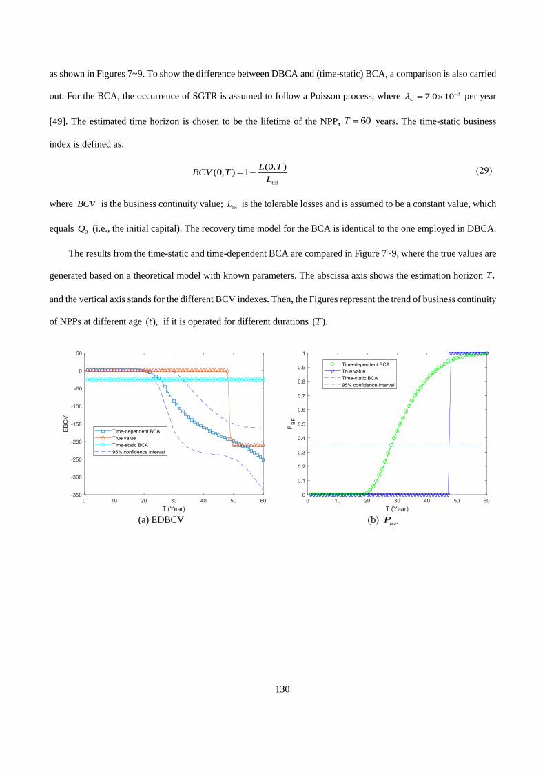
130

as shown in Figures 7~9. To show the difference between DBCA and (time-static) BCA, a comparison is also carried

out. For the BCA, the occurrence of SGTR is assumed to follow a Poisson process, where per year

[49]. The estimated time horizon is chosen to be the lifetime of the NPP, years. The time-static business

index is defined as:

(29)

where is the business continuity value; is the tolerable losses and is assumed to be a constant value, which

equals (i.e., the initial capital). The recovery time model for the BCA is identical to the one employed in DBCA.

The results from the time-static and time-dependent BCA are compared in Figure 7~9, where the true values are

generated based on a theoretical model with known parameters. The abscissa axis shows the estimation horizon

and the vertical axis stands for the different BCV indexes. Then, the Figures represent the trend of business continuity

of NPPs at different age if it is operated for different durations

(a) EDBCV (b)

37.0 10st −=

60T =

tol

(0, )(0, ) 1

L TBCV T

L= −

BCV tolL

0Q

,T

( ),t ( ).T

BFP

131

(c)

Figure 7. Business continuity metrics at t=1 year.

(a) EDBCV (b)

(c)

BIP

BFP

BIP

132

Figure 8. Business continuity metrics at t=10 years.

(a) EDBCV (b)

(c)

Figure 9. Business continuity metrics at t=40 years.

1) At each with the increase of the estimation horizon the DBCV decreases. This means that regardless

of the age of the NPP, the longer the NPP is operated, the worse its business continuity: this is logical,

as it is primarily caused by the tube’s degradation process. No rupture is supposed to occur at the beginning

of system operation. Subsequently, as the crack grows, rupture will occur eventually and lead to system

failure. In addition, the dynamic business continuity (DBC) indexes curves drop (Figure 7 (a), Figure 8 (a),

Figure 9 (a)) or rise (Figure 7 (b, c), Figure 8 (b, c), Figure 9 (b, c)) significantly after a certain value of

In practice, intervention measures like overhauls need to be taken before this in order to prevent serious

losses from occurring failures and ensure the business continuity.

BFP

BIP

,t ,T

t

.T

,T

133

2) For the same estimation horizon as the NPP age increases, the EDBCV shifts left, which means that

the financial safety margin is shrinking with This is because the steam generator tube is getting closer to

a dangerous state with age.

3) When is beyond a certain value, the business continuity metrics becomes invariant. This is mainly

because when is sufficiently long, the rupture event will surely happen and after that no loss occurs any

more.

4) There are plateau sections in the curves of EBCV (Figure 7 (a), Figure 8(a), Figure 9 (a)); the height of

these plateaus increases with time which makes sense because the system potential profits increase over

time

5) The results comparison between DBCA and time-static BCA shows that the time-static BCA grossly

underestimates the damage of SGTR on system business and, thus, underestimates the NPP’s business loss.

Moreover, the results from the DBCA using condition-monitoring data are closer to the true BCV than

those of the time-static BCA. This is because the DBCA using condition monitoring data incorporates the

time-dependent behavior of SGTR degradation.

6) the confidence intervals quantitatively express the level of confidence that the BCV metrics values are

contained in the interval. From Figures 7~9, we can see that with more data available, the widths of the

confidence intervals reduce. This is because with more condition monitoring data, the component state

estimation becomes more accurate and the uncertainty in the BCA results reduces.

5 Discussion

The method developed in this work is applied on a case study regarding NPP operation, but it can also be applied

to a wide variety of other scenarios. For systems with the following characteristics: (1) business continuity is related

to financial losses; (2) system behavior and/or profit are potentially time-dependent; (3) condition monitoring data

are available to inform on the time-dependent system behavior. For instance, in the example of oil storage tanks in

[4], the profit of the oil storage tank depends on the price of the oil and is, therefore, time-dependent; lithium batteries

are used to drive some critical safety barriers and are subject to degradation, so that the performance of the safety

barriers is also time-dependent. Besides, condition monitoring data are available from the mounted sensors and can

be used for online updating the failure probability of the safety barriers. For IT services, the profits also exhibit time-

,T t

.t

T

T

,t

.t

134

dependent behaviors, the failure behavior of the hardware in the IT infrastructure is also time-dependent due to

various degradation mechanisms, and if condition monitoring data are available to monitor the state of the hardware,

the developed DBCA method can be applied.

Compared to the original time-static BCA method, the developed model captures the time-dependent features

of both profits and system failure behaviors. Therefore, the proposed method can more precisely quantify the business

continuity that exhibits time-dependent behaviors. However, the price one needs to pay is that the model is more

complex in both development and analysis. In practice, there is the need to choose the most appropriate method based

on a tradeoff between the complexity of the modelling and the accuracy of the results, and this depends on the

characteristics of the problem and on the knowledge, information and data available for its description [64]. For

example, for systems whose failure behavior is not time-dependent or not significant for business continuity, the

traditional time-static BCA method might be sufficient. However, for safety critical systems that have significant

time-dependency, the developed method is preferred due to its potential to provide a more accurate assessment.

It should be noted that in this work we assume that the operation costs (including the inspection and maintenance

costs) do not change with time (as seen in Equation (15)). This assumption is reasonable for NPPs, because they are

usually designed with sufficient margins so that even when they reach the design life, their performance is not

degraded severely. However, these costs might be time-dependent, and typically increasing with time for other

systems: this should be considered in the modelling, then.

Moreover, to illustrate the proposed DBCA model, we use a stochastic electricity model to predict the electricity

price, considering a variety of factors contributing to electricity price variations (such as seasonal volatility, time-

varying mean reversion and seasonally occurring price spikes). The predicted electricity price is shown in Figure 5.

It should be noted that the predicted values are here used to illustrate the developed method only. There are various

factors that have a potential influence on the electricity price (such as new energy source and new consumption

patterns), which make the predicted results inevitably subject to uncertainty, especially in a long-time span of

prediction. Therefore, when the developed method is applied in practice, up-to-date electricity information should be

used, instead of the predicted value, in order to reduce the uncertainty and assessment errors.

It is noteworthy that this work considers as disruptive events only those that are caused by safety-related hazards.

In practice, however, the problem of business continuity might arise for disruptive events generated by hazards other

135

than safety-related ones, e.g., natural hazards: the method developed can be extended to capture also these disruptive

events.

6. Conclusions

In this paper, a DBCA method that integrates condition monitoring data is proposed. Two factors that influence

the dynamic behavior of business continuity are considered explicitly. The first one is the dynamics of the

degradation-to-failure process affecting the safety barriers. Condition monitoring data are used to update and predict

the time-dependent failure behavior by PF. The second factor is the time-dependent profit and tolerable losses. This

is quantified by applying a stochastic price model and an installment model. A simulation-based framework is

developed to calculate the time-dependent business continuity metrics originally introduced. A case study regarding

the analysis of an accident initiated by SGTR in a NPP shows that the proposed framework allows capturing the

dynamic character of business continuity.

The outcomes of such dynamic analysis can provide insights to stakeholders and decision-makers, that can help

them to identify when best to take actions for preventing serious losses and ensuring business continuity.

Acknowledgement

The work of Ms. Jinduo Xing is supported by China Scholarship Council (No. 201506450020). The work by

Professor Enrico Zio has been developed within the research project "SMART MAINTENANCE OF INDUSTRIAL

PLANTS AND CIVIL STRUCTURES BY 4.0 MONITORING TECHNOLOGIES AND PROGNOSTIC

APPROACHES - MAC4PRO ", sponsored by the call BRIC-2018 of the National Institute for Insurance against

Accidents at Work – INAIL in Italy.

References

[1] Zio, E., The future of risk assessment. Reliability Engineering & System Safety, 2018. 177: p. 176-190.

[2] Zhou, L., X. Wu, Z. Xu, and H. Fujita, Emergency decision making for natural disasters: An overview.

International Journal of Disaster Risk Reduction, 2018. 27: p. 567-576.

[3] Ouyang, M. and Y. Fang, A mathematical framework to optimize critical infrastructure resilience against

intentional attacks. Computer‐Aided Civil and Infrastructure Engineering, 2017. 32(11): p. 909-929.

[4] Zeng, Z. and E. Zio, Dynamic Risk Assessment Based on Statistical Failure Data and Condition-Monitoring

Degradation Data. IEEE Transactions on Reliability, 2018. 67(2): p. 609-622.

[5] Sahebjamnia, N., S.A. Torabi, and S.A. Mansouri, Integrated business continuity and disaster recovery planning:

Towards organizational resilience. European Journal of Operational Research, 2015. 242(1): p. 261-273.

[6] Cerullo, V. and M.J. Cerullo, Business continuity planning: a comprehensive approach. Information Systems

Management, 2004. 21(3): p. 70-78.

[7] Baskerville, R., P. Spagnoletti, and J. Kim, Incident-centered information security: Managing a strategic balance

between prevention and response. Information & management, 2014. 51(1): p. 138-151.

[8] Torabi, S.A., H. Rezaei Soufi, and N. Sahebjamnia, A new framework for business impact analysis in business

continuity management (with a case study). Safety Science, 2014. 68: p. 309-323.

136

[9] Rabbani, M., H.R. Soufi, and S.A. Torabi, Developing a two-step fuzzy cost–benefit analysis for strategies to

continuity management and disaster recovery. Safety Science, 2016. 85: p. 9-22.

[10] Torabi, S.A., R. Giahi, and N. Sahebjamnia, An enhanced risk assessment framework for business continuity

management systems. Safety Science, 2016. 89: p. 201-218.

[11] Zsidisin, G.A., S.A. Melnyk, and G.L. Ragatz, An institutional theory perspective of business continuity planning

for purchasing and supply management. International journal of production research, 2005. 43(16): p. 3401-3420.

[12] Zeng, Z. and E. Zio, An integrated modeling framework for quantitative business continuity assessment. Process

Safety and Environmental Protection, 2017. 106: p. 76-88.

[13] ISO, ISO 22301, in Societal Security- Business Continuity Management Systems- Requirements2012, International

Organization for Standardization: Switzerland.

[14] Tammineedi, R.L., Business continuity management: A standards-based approach. Information Security Journal:

A Global Perspective, 2010. 19(1): p. 36-50.

[15] Forbes Gibb, S.B., A framework for business continuity management. International Journal of Information

Management, 2006. 26: p. 128-141.

[16] Herbane, B., The evolution of business continuity management: A historical review of practices and drivers.

Business history, 2010. 52(6): p. 978-1002.

[17] Snedaker, S., Business continuity and disaster recovery planning for IT professionals. 2013: Newnes.

[18] Miller, H.E. and K.J. Engemann, Using reliability and simulation models in business continuity planning.

International Journal of Business Continuity and Risk Management, 2014. 5(1): p. 43-56.

[19] Järveläinen, J., IT incidents and business impacts: Validating a framework for continuity management in

information systems. International Journal of Information Management, 2013. 33(3): p. 583-590.

[20] Faertes, D., Reliability of supply chains and business continuity management. Procedia Computer Science, 2015.

55: p. 1400-1409.

[21] Kato, M. and T. Charoenrat, Business continuity management of small and medium sized enterprises: Evidence

from Thailand. International journal of disaster risk reduction, 2018. 27: p. 577-587.

[22] Hassel, H. and A. Cedergren, Exploring the Conceptual Foundation of Continuity Management in the Context of

Societal Safety. Risk Analysis, 2019.

[23] Bonafede, E., P. Cerchiello, and P. Giudici, Statistical models for business continuity management. Journal of

Operational Risk, 2007. 2(4): p. 79-96.

[24] Tan, Y. and S. Takakuwa, Use of simulation in a factory for business continuity planning. International Journal

of Simulation Modelling, 2011. 10(1): p. 17-26.

[25] Rezaei Soufi, H., S.A. Torabi, and N. Sahebjamnia, Developing a novel quantitative framework for business

continuity planning. International Journal of Production Research, 2018: p. 1-22.

[26] Sahebjamnia, N., S.A. Torabi, and S.A. Mansouri, Building organizational resilience in the face of multiple

disruptions. International Journal of Production Economics, 2018. 197: p. 63-83.

[27] Zubair, M. and Z. Zhijian, Reliability Data Update Method (RDUM) based on living PSA for emergency diesel

generator of Daya Bay nuclear power plant. Safety Science, 2013. 59: p. 72-77.

[28] Nazempour, R., M.A.S. Monfared, and E. Zio, A complex network theory approach for optimizing contamination

warning sensor location in water distribution networks. International Journal of Disaster Risk Reduction, 2018. 30: p. 225-

234.

[29] Aizpurua, J.I., V.M. Catterson, Y. Papadopoulos, F. Chiacchio, and G. Manno, Improved dynamic dependability

assessment through integration with prognostics. IEEE Transactions on Reliability, 2017. 66(3): p. 893-913.

[30] Liu, J. and E. Zio, System dynamic reliability assessment and failure prognostics. Reliability Engineering &

System Safety, 2017. 160: p. 21-36.

[31] Fan, M., Z. Zeng, E. Zio, R. Kang, and Y. Chen, A Sequential Bayesian Approach for Remaining Useful Life

Prediction of Dependent Competing Failure Processes. IEEE Transactions on Reliability, 2018. 68(1): p. 317-329.

[32] Coussement, K., D.F. Benoit, and M. Antioco, A Bayesian approach for incorporating expert opinions into

decision support systems: A case study of online consumer-satisfaction detection. Decision Support Systems, 2015. 79: p.

24-32.

[33] Sharma, S. and S. Routroy, Modeling information risk in supply chain using Bayesian networks. Journal of

Enterprise Information Management, 2016. 29(2): p. 238-254.

[34] Lawler, C.M., M.A. Harper, S.A. Szygenda, and M.A. Thornton, Components of disaster-tolerant computing:

analysis of disaster recovery, IT application downtime and executive visibility. International Journal of Business

Information Systems, 2008. 3(3): p. 317-331.

[35] Xie, Y., J. Zhang, T. Aldemir, and R. Denning, Multi-state Markov modeling of pitting corrosion in stainless steel

exposed to chloride-containing environment. Reliability Engineering & System Safety, 2018. 172: p. 239-248.

137

[36] Mayén, J., A. Abúndez, I. Pereyra, J. Colín, A. Blanco, and S. Serna, Comparative analysis of the fatigue short

crack growth on Al 6061-T6 alloy by the exponential crack growth equation and a proposed empirical model. Engineering

Fracture Mechanics, 2017. 177: p. 203-217.

[37] Compare, M., F. Martini, S. Mattafirri, F. Carlevaro, and E. Zio, Semi-Markov model for the oxidation degradation

mechanism in gas turbine nozzles. IEEE Transactions on Reliability, 2016. 65(2): p. 574-581.

[38] Franke, U., Optimal IT service availability: Shorter outages, or fewer? IEEE Transactions on Network and Service

Management, 2011. 9(1): p. 22-33.

[39] Zio, E. and G. Peloni, Particle filtering prognostic estimation of the remaining useful life of nonlinear components.

Reliability Engineering & System Safety, 2011. 96(3): p. 403-409.

[40] Si, X.-S., C.-H. Hu, Q. Zhang, and T. Li, An integrated reliability estimation approach with stochastic filtering

and degradation modeling for phased-mission systems. IEEE transactions on cybernetics, 2017. 47(1): p. 67-80.

[41] Corbetta, M., C. Sbarufatti, M. Giglio, and M.D. Todd, Optimization of nonlinear, non-Gaussian Bayesian

filtering for diagnosis and prognosis of monotonic degradation processes. Mechanical Systems and Signal Processing,

2018. 104: p. 305-322.

[42] Yu, P., J. Cao, V. Jegatheesan, and L. Shu, Activated sludge process faults diagnosis based on an improved

particle filter algorithm. Process Safety and Environmental Protection, 2019. 127: p. 66-72.

[43] Arulampalam, M.S., S. Maskell, N. Gordon, and T. Clapp, A tutorial on particle filters for online nonlinear non-

gaussian Bayesian tracking. IEEE Transactions on Signal Processing, 2002. 50(2): p. 174-188.

[44] Hu, Y., P. Baraldi, F.D. Maio, and E. Zio, Online Performance Assessment Method for a Model-Based Prognostic

Approach. IEEE Transactions on reliability, 2016. 65(2): p. 718-735.

[45] Tulsyan, A., B. Huang, R.B. Gopaluni, and J.F. Forbes, On simultaneous on-line state and parameter estimation

in non-linear state-space models. Journal of Process Control, 2013. 23(4): p. 516-526.

[46] Hosseini, S. and K. Barker, Modeling infrastructure resilience using Bayesian networks: A case study of inland

waterway ports. Computers & Industrial Engineering, 2016. 93: p. 252-266.

[47] Lanza, A., M. Manera, and M. Giovannini, Modeling and forecasting cointegrated relationships among heavy oil

and product prices. Energy Economics, 2005. 27(6): p. 831-848.

[48] Sullivan, W.G., E.M. Wicks, and J.T. Luxhoj, Engineering economy. Vol. 12. 2003: Prentice Hall Upper Saddle

River, NJ, p132-150.

[49] Kim, H., J.T. Kim, and G. Heo, Failure rate updates using condition-based prognostics in probabilistic safety

assessments. Reliability Engineering & System Safety, 2018. 175: p. 225-233.

[50] Auvinen, A., J. Jokiniemi, A. Lähde, T. Routamo, P. Lundström, H. Tuomisto, J. Dienstbier, S. Güntay, D.

Suckow, and A. Dehbi, Steam generator tube rupture (SGTR) scenarios. Nuclear engineering and design, 2005. 235(2-4):

p. 457-472.

[51] Mercurio, D., L. Podofillini, E. Zio, and V.N. Dang, Identification and classification of dynamic event tree

scenarios via possibilistic clustering: Application to a steam generator tube rupture event. Accident Analysis & Prevention,

2009. 41(6): p. 1180-1191.

[52] Lewandowski, R., R. Denning, T. Aldemir, and J. Zhang, Implementation of condition-dependent probabilistic

risk assessment using surveillance data on passive components. Annals of Nuclear Energy, 2016. 87: p. 696-706.

[53] Narayanan, M., A. Kumar, S. Thirunavukkarasu, and C. Mukhopadhyay, Development of ultrasonic guided wave

inspection methodology for steam generator tubes of prototype fast breeder reactor. Ultrasonics, 2019. 93: p. 112-121.

[54] Buck, J.A., P.R. Underhill, J.E. Morelli, and T.W. Krause, Simultaneous multiparameter measurement in pulsed

eddy current steam generator data using artificial neural networks. IEEE Transactions on Instrumentation and

Measurement, 2016. 65(3): p. 672-679.

[55] Di Maio, F., F. Antonello, and E. Zio, Condition-based probabilistic safety assessment of a spontaneous steam

generator tube rupture accident scenario. Nuclear Engineering and Design, 2018. 326: p. 41-54.

[56] An, D., J.-H. Choi, and N.H. Kim, Prognostics 101: A tutorial for particle filter-based prognostics algorithm

using Matlab. Reliability Engineering & System Safety, 2013. 115: p. 161-169.

[57] Zhu, L., A simulation based real options approach for the investment evaluation of nuclear power. Computers &

Industrial Engineering, 2012. 63(3): p. 585-593.

[58] Arif, A., S. Ma, Z. Wang, J. Wang, S.M. Ryan, and C. Chen, Optimizing service restoration in distribution systems

with uncertain repair time and demand. IEEE Transactions on Power Systems, 2018. 33(6): p. 6828-6838.

[59] Ananda, M.M., Confidence intervals for steady state availability of a system with exponential operating time and

lognormal repair time. Applied Mathematics and Computation, 2003. 137(2-3): p. 499-509.

[60] Ferrario, E. and E. Zio, Assessing nuclear power plant safety and recovery from earthquakes using a system-of-

systems approach. Reliability Engineering & System Safety, 2014. 125: p. 103-116.

[61] Borovkova, S. and M.D. Schmeck, Electricity price modeling with stochastic time change. Energy Economics,

2017. 63: p. 51-65.

138

[62] Hefter, M. and A. Herzwurm, Strong convergence rates for Cox–Ingersoll–Ross processes—full parameter range.

Journal of Mathematical Analysis and Applications, 2018. 459(2): p. 1079-1101.

[63] Zhu, L. and Y. Fan, Optimization of China's generating portfolio and policy implications based on portfolio

theory. Energy, 2010. 35(3): p. 1391-1402.

[64] Zio, E., Some challenges and opportunities in reliability engineering. IEEE Transactions on Reliability, 2016.

65(4): p. 1769-1782.

139

140

Paper III

J. Xing, Z. Zeng, E. Zio. Joint optimization of safety barriers against steam

generator tube rupture to enhance business continuity of nuclear power plants.

Reliability engineering and system safety. 2019. (Under review).

141

Joint optimization of safety barriers against steam generator tube rupture to enhance business continuity of

nuclear power plants

Jinduo Xing 1, Zhiguo Zeng 1, Enrico Zio 2,3,4

1 Chair System Science and the Energy Challenge, Laboratoire Génie Industriel (LGI), CentraleSupélec, Université

Paris Saclay, Gif-sur-Yvette, France

2 MINES ParisTech, PSL Research University, CRC, Sophia Antipolis, France

3 Energy Department, Politecnico di Milano, Milan, Italy

4 Eminent Scholar, Department of Nuclear Engineering, College of Engineering, Kyung Hee University,

Republic of Korea

jinduo.xing@centralesupelec.fr, zhiguo.zeng@centralesupelec.fr, enrico.zio@polimi.it

Abstract

In nuclear power plants (NPPs), different types of safety barriers are designed to ensure the safe and continuous

operation of the NPP against disruptive events. These safety barriers, although designed to operate in different phases

of the accidents evolution, are often optimized separately, without considering their collective effects on preventing

disruptions and quickly recovering from the disruptions. This paper develops a joint optimization model for

synthetically optimizing safety barriers of different natures, including prevention, mitigation, emergency and

recovery barriers to enhance the business continuity of the NPP, considering the threat of steam generator tube rupture

(SGTR) accidents. The joint optimization is guided by a business continuity metric called expected business

continuity value (EBCV). A physics-of-failure model is developed to describe the crack growth process of the steam

generator tube and to model the effect of the prevention barriers, i.e., periodical inspection of the crack length. An

event tree model is developed to describe the evolution of the SGTR-initiated accident and to model the effect of the

mitigation and emergency barriers. Recovery measures are also considered via a widely-used logarithmic function

model. A mixed-integer genetic algorithm (MIGA) is used to obtain optimal solutions of the joint optimization model.

The results show that the developed joint optimization model can achieve better performance in terms of business

continuity, compared to the conventional methods that optimize the safety barriers separately.

Keywords

Business continuity management (BCM), Safety barrier, Joint optimization, Event tree (ET), Mixed-integer

genetic algorithm (MIGA), Nuclear power plant (NPP), Steam generator tube rupture (SGTR).

142

Acronyms

BCM business continuity management

EBCV expected business continuity value

ET event tree

MIGA mixed-integer genetic algorithm

NPP nuclear power plant

PDF probability density function

PSA probabilistic safety assessment

RDS reactor depressurization system

RTS reactor trip system

RWST refueling water storage tank

SG steam generator

SGTR steam generator tube rupture

Notation

crack length

cost-effective parameter for th consequence

production capacity of NPP

consequence with th severity

cost in preventive phase

cost in mitigation phase

cost in recovery phase

unit price for plugging one tube

total budget

crack growth rate

stress intensity factor

potential loss in

a

ec II −

C

iC i −

PC

MC

RC

plugC

thC

da

dt

K

([0, ])L T [0, ]T

143

direct loss in

indirect loss in

maximum tolerable loss

number of tubes

vector representing the baseline value for the failure probabilities of the mitigation measures

probability of one tube rupture

estimation horizon for business continuity assessment

recovery time for the th consequence

relationship between cost-effectiveness parameters of and

([0, ])dL T [0, ]T

([0, ])inL T [0, ]T

tolL

tuben

PF

,rup tubep

T

, irecv CT i −

IIC IIIC

144

1. Introduction

Steam generator (SG) is a passive heat-exchanging system that transfers heat from the primary loop to the

secondary loop in a pressurized water reactor (PWR) to produce steam to drive the turbines [1]. One relevant safety

issue in PWR is the rupture of SG tubes, known as steam generator tube rupture (SGTR), which can be an accident

initialing event induced by a crack growth process in the SG tube [2]. SGTR accidents can cause severe consequences

related to the leakage of radioactive materials [3]. The safe operation of nuclear power plants (NPPs) is ensured by a

suite of safety barriers designed to prevent undesired events or accidents, and contain or mitigate their consequences

when they occur [4, 5].

Prevention barriers are designed to work in the pre-accident or pre-failure phases and aim at reducing the

probability of occurrence of accidents [6, 7]. In the case of SGTR accidents, one commonly adopted prevention

barriers is to make periodical inspection and timely preventive plugging of the defective tubes [8]. Mitigation and

emergency barriers intervene after the accident initiating event occurs and aim at containing the evolution of the

accident so that its consequences can be minimized. Examples of mitigation and emergency barriers for SGTR

accidents include the reactor trip system (RTS), reactor depressurization system (RDS), refueling water storage tank

(RWST), reactor cooling system (RCS), etc [9]. Recovery barriers aim at restoring to the normal operation system

functionality timely after the accident [10]. For example, in the event of a SGTR, the recovery measures could include

replacing the ruptured tube, cleaning up the contaminated area (if any), etc [11, 12].

In practice, the different safety barriers are designed separately for optimal performance, considering the

constraints of limited resources [13]. For instance, [14] has proposed the optimal design of risk-based inspections in

power and process plants. In [15], an enhanced preventive maintenance optimization model based on a three-stage

failure process has been proposed for NPP components. In [16], condition-based maintenance optimization for

deteriorating systems has been investigated by considering inspection intervals and preventive maintenance

thresholds as decision variables. Only prevention activities were taken into account in these works. There are also a

number of works considering the optimal design of emergency and mitigation barriers. For example, a simplified

probabilistic safety assessment (PSA) and a reliability allocation model have been developed to improve the safety

level of PWR by the optimal allocation of redundancies of the emergency and mitigation barriers [17]. In [18, 19], a

redundancy allocation model for series-parallel systems has been used to improve the reliability of mitigation

measures. In [20], an optimization problem is formulated and solved for the minimum average total cost of nuclear

145

fail-safe systems, where the average total system cost was subject to a restricted type I design error. The optimization

of recovery measures has also been considered in the literature. For example, in [21], economically optimal strategies

for recovering from a NPP accident have been discussed. In [22], joint restoration processes for multiple systems

have been modeled and the effectiveness of five different restoration strategies with respect to resilience has been

compared. A resilience-based optimization methodology has been proposed in [23].

Most existing research works, as reviewed above, optimize the safety barriers separately. In practical problems,

however, the safety barriers at different phases need to work jointly to ensure that the NPP can be operated

continuously and safely. In this paper, we propose a joint optimization model to ensure that the different safety

barriers can achieve holistic optimal performances. The performance of the safety barriers system is quantified

through the concept of business continuity. Defined as “the holistic management process that identifies potential

threats to an organization and the impacts to business operations those threats, if realized, might cause, and which

provides a framework for building organizational resilience with the capability of an effective response that

safeguards the interest of its key stakeholders, reputation, brand and value-creating activities” [24], business

continuity management (BCM) has received more and more attention in recent years, as a holistic requirement on the

overall performance of a system [25, 26]. A loss-based business continuity metric was defined in [5] for business

continuity assessment of an oil tank farm. In this work, we adopt the quantitative business continuity metric in [5] to

guide the joint optimization of the pre- and post-disruption barriers, and use a mixed-integer genetic algorithm

(MIGA) [27] to derive the optimal solution. The contributions of this work can be summarized as follows:

(1) A joint optimization model is proposed to enhance the business continuity of NPP.

(2) MIGA is implemented to solve the joint optimization problem.

The remaining of the paper is structured as follows. Section 2 formally defines the problem. Section 3 illustrates

the SGTR event and the corresponding safety barriers at different stages. Section 4 provides a joint optimization

model and a solution method for enhancing business continuity of the NPP. Section 5 performs a sensitivity analysis

of the parameters in the four stages. Finally, Section 6 concludes this work.

2 Problem description

One SG of a PWR is considered, which is equipped with a bundle of 3592 inverted U tubes. Each U tube has an

outside diameter Gaussian distributed with a mean of 22.23 mm and a standard deviation 0.1667mm; and a thickness

Gaussian distributed with a mean of 1.27 mm and a standard deviation of 0.0592 mm. The tubes are subject to

146

different degradation mechanisms like stress corrosion cracking (SCC), fatigue, pitting corrosion and fretting wear.

A list of the NPP parameter values is presented in Table 1 [8].

Table 1 Parameters of the NPP.

Parameter Value

Generation capacity of NPP ( ) 1100 Mwh

Number of tubes ( ) 3592

Tube outer diameter ( ) N (22.23,0.1667) mm

Tube thickness ( ) N (1.27, 0.0592) mm

Different safety barriers are presented for preventing SGTR, containing its consequences and recovering from

the possible disruptions caused. Table 2 summarizes the safety measures considered in this paper and highlights the

category they belong to: prevention, mitigation, emergency and recovery.

Table 2 Safety barriers considered in this study.

Safety barrier Category Function description

Periodic inspection and

maintenance

Prevention Periodically inspect the tubes and timely plug those defective tubes whose crack

length is beyond the maintenance threshold.

Reactor trip system (RTS) Mitigation When the reactor power exceeds a given safety operating limit, the RTS

automatically shut down the reactor, in order to prevent core damage.

Reactor depressurization

system (RDS)

Mitigation When a loss-of-coolant event is caused by the tube rupture, the RTS will work to

prevent over-pressurization of the reactor vessel.

Refueling water storage tank

(RWST)

Mitigation Store cooling water for emergency cooling of the reactor core.

Reactor cooling system (RCS) Mitigation If the reactor fails to scram, RCS will pump water into the reactor for emergency

cooling.

Repair of the damages caused

by the SGTR

Recovery Replace the ruptured tubes and restore the plant to normal operation.

3 Modelling the individual safety barriers

In this section, we present the model of the performance of each safety barrier and the associated costs.

Prevention safety barriers are discussed in Section 3.1, followed by mitigation and emergency barriers in Section 3.2,

and recovery measures in Section 3.3.

3.1 Modeling prevention safety barriers

SGTR is the break of one or more SG tubes, which can be caused by different degradation mechanisms, e.g.,

stress corrosion cracking (SCC), fatigue, pitting corrosion, fretting wear [28]. As reported in [3], a fraction of

of SGTR events is caused by SCC. For this reason, without loss of generality, in this work, the SGTR is

considered to be due only to SCC. The main prevention safety measure is to inspect the tube periodically and plug

the dangerous tubes when necessary.

C

tuben

d

b

60% 80%

147

Figure 1 Tube crack growth process.

The tube SCC growth process can be divided into two stages: onset and propagation of cracks inside the tube

wall [29], as shown in Figure 1. During the onset phase, the crack grows slowly; then, when the crack size reaches a

critical point, it begins to grow more rapidly in the propagation phase. The SCC process is often modelled by a two-

stage physics-based crack growth model. In the two-stage model, it is assumed that the critical crack length beyond

which the process enters the propagation phase (see Figure 1) is 0.1 mm. The duration of the onset phase is assumed

to follow a lognormal distribution with parameters and where denotes the mean value and is the

standard deviation [8]. Let represent the time needed for the crack to reach the length of critical size 0.1 mm.

Then, we have:

(1)

In this paper, we take the values of the parameters from [8]: years, years.

The Scott model is often used to model the propagation phase of the crack growth process (see Figure 1), in

which the crack growth rate is empirically modelled as a function of stress [30]:

(2)

(3)

(4)

c ,c c c

criticalt

2log ( , ),critical c ct normal

9.3c = 3.162c =

( ) ,m

th

daK K

dt= −

,2

aK F

=

=2

P d

b

148

where is the crack growth rate, is the crack length, and are constant parameters related to the

component material properties, is the stress at the crack tip, denotes the pressure difference. In this paper, the

material of steam generator tubes is assumed to be Alloy 600. Based on the material properties, the values for the

parameters in Equations (2)-(3) can be determined, as shown in Table 3.

Table 3 Parameter values of crack growth model.

Parameter Value

0.1

0.93

1.16

9

N (8.3,0.33) Mpa

Based on the physical model of the crack growth process, the effectiveness of the prevention safety measures

can be further modeled. It is assumed that periodical inspections are conducted every months and during each

inspection, the crack size can be measured through techniques like eddy current testing [31], ultrasonic testing [32]

), etc. If the measured crack length is beyond a given preventive maintenance threshold, denoted by the

corresponding tube is plugged to prevent further damages. The probability of SGTR, denoted by is used to

represent the performance of the prevention safety barrier: the higher the value of the worse the performance

of the prevention barrier. In our model, the probability of SGTR is formulated as a function of and

(5)

Monte Carlo simulation is used to evaluate the value of as shown in Algorithm 1.

da

dta ,

thK m

P

0a

Fm

thK

P

x

,thy

, ,rupt tubep

, ,rupt tubep

x :thy

, ( , ).rupt tube thp f x y=

. ,rupt tubep

149

Algorithm 1: calculation based on Monte Carlo simulation.

Inputs:

Outputs: ;

For

Use equation (1) to generate

If

Based on calculate the rupture time

For

If

else if

Else if and

End

End

End

End

End

where is the calculation time horizon; represents the rupture threshold; is the rupture time; implies the

crack size measured at inspection.

The cost spent in the prevention phase, represented by is a function of inspection interval and plugging

rate

(6)

where denotes the cost of a single inspection of the tube; is the unit price for plugging one tube; and

is the plugging rate of the tube, i.e., the fraction of tubes being plugged. The value of depends on the values of

and as shown in Algorithm 1.

3.2 Modeling emergency and mitigation barriers

.rup tubep

0 ., , , , , , , , , , ;th rup th sx d P b a F m K a T N

,rupt tubep

[ ,2 ,3 , , ], 1,2, , ;int x x x kx k n nx T= =

0;Index =

1: Si N=

( );criticalt i

( ) ;criticalt i T

;criticalt t=

, , , ,critical thx T t a ( );rupt i

1:k n=

( )rupt i T

;Index Index=

( ) ( 1)th in th ina a k y a k −

;Index Index=

( ) ( 1),in th ina k a a k − ( 1) ;in tha k y−

1;Index Index= +

. / .rup tube sp Index N=

Ttha rupt

ina

,PC x

:plugp

,

P insp insp tube plug plug

insp tube plug plug

C C n n p C

TC n p C

x

= +

= +

inspC plugC plugp

plugp

x ,thy

150

As shown in Table 2, the emergency and mitigation barriers include the RTS, RDS, RWST and RCS. Their

effects on containing the consequence of SGTR can be modelled using an event tree (ET), as shown in Figure 2.

Figure 2 Schematic ET model of SGTR accident.

Depending on the performance of different barriers,6 consequences i.e., can be caused by the

SGTR. These consequences can be grouped into three categories in Table 5 based on their severity. In this regard,

different consequences are caused by the variant performance of safety barrier. Based on the ET in Figure 2, the

occurrence probabilities for can be quantified as a function of the event probabilities. Conceptually, we

denote these by:

(6)

where is the occurrence probability of SGTR and can be calculated based on the models of the prevention

safety barrier, represent the failure probability of RTS, RDS, RWST and RCS, respectively.

Table 4 Classification of consequences.

Consequences Group Meaning

No SGTR occurs, the NPP is operating

normally.

SGTR occurs, but the consequence is

successfully controlled by the mitigation

and emergency barriers. The power

generation business is temporarily

terminated.

1 2 6, , ,C C C

1 6~C C

1 2 3 4( , , , , )iC ET SGTRp f p p p p p=

SGTRp

1 2 3 4, , ,p p p p

6C IC

1C IIC

151

Core damage is caused by SGTR, the

power generation business is terminated

for a long time.

The performance of the mitigation & emergency barriers is primarily determined by their failure probabilities.

One common way to reduce the failure probabilities of these barriers is to add redundancies. If one safety barrier

collapses, the redundant system will substitute it. Redundancy allocation models are often used for designing the

redundant safety systems within constraints on costs and resources [30, 31].

In this paper, we assume that parallel redundancy applying the same type of equipment is used for the four

mitigation and emergency safety barriers. It is easy to show that the failure probability of the th measure is:

(7)

where is the failure probability of the th safety barrier system and is the number of redundant system

added to the original system. The total cost associated with the redundancy design is:

(8)

where is the price for adding one th redundancy equipment.

3.3 Modeling recovery measures

Recovery ability refers to the ability of a system to be repaired and quickly restored its normal operation after

failures or disruptions [32]. The repair ability depends on a variety of factors including the training and preparedness

of repair groups, the readiness of repair materials and resources, etc. A range of models have been proposed in the

literature for the post-disruptive event recovery process [33-35]. According to these models, the performance of the

recovery process directly depends on the resources spent on the recovery processes, e.g., the investment on training

repair crews, preparing equipment and spare parts used for repairing the failed items [36]. In general, the more

budgets or resources planned for recovery process, the better recovery performances.

In this work, we use the following model for the recovery process [37]:

(9)

2 5C C IIIC

i −

1

,( ) ,in

i i bp p+

=

,i bp i − in

4

,

1

,MSB R i i

i

C C n=

=

,R iC i −

,

,

,

=1 ln(1 )

i

BR

recv C

recv i

e i S

TT

c C+ +

152

where is a random variable that represents the time needed to recover from the th consequence;

denotes the basic recovery time for consequence which is dependent on the basic requirement on recovery time,

denotes the resources invested on the recovery process and is the effective parameters of resources on

th consequence; denotes the relationship between different cost-effectiveness parameters for different severity

consequence; Its value should be set by decision makers based on the capability of the organization.

As most literatures (e.g., [5, 38, 39]) applied, we also assume that follows a lognormal distribution:

(10)

where is the probability density function (PDF) of and are the mean value and variance value of

the lognormal distribution, respectively. The values of and are depends on the recovery ability of the target

organization. It is noting that the more serious consequence the smaller of

4 Joint optimization model based on business continuity

In this Section, we develop a joint optimization model to ensure global optimal performances of the safety

barriers (prevention, mitigation, emergency and recovery). The joint optimization model is based on the objective of

maximizing the business continuity of the plant. In Section 4.1, we start from a review of the business continuity

model and numerical metrics we used to guide the optimization. The joint optimization model is presented in Section

4.2. Section 4.3 discusses how to solve this joint optimization by using a MIGA. The results of the application on the

case study of Section 2 is presented and discussed in Section 4.4.

4.1 Basics of business continuity modeling and assessment

As explained in Section 1, business continuity management (BCM) is a comprehensive method that integrates

pre-event and post-event management together to ensure the resilience and continuous operation of system business.

Compared to conventional risk analysis method, BCM not only focuses on the potential hazards and their impacts,

but also considers how to mitigate the consequence and quickly recover from the disruption. A quantitative index,

i.e., expected business continuity value (EBCV) has been developed in [5] for business continuity modeling and

assessment:

,recv iT i − , irecv CT

,iC

RSBC,e ic i −

, irecv CT

2,

2

(ln( ) )

2

,

, ,

,

1, 0

( ) 2

0, 0

recv Ci i

i

i

i i

i

T

recv C

recv C i recv C

recv C

e Tf T T

T

−

=

( )f , ;irecv CT

i i

i i

,i , .e ic

153

(11)

where is the evaluation time horizon for the business continuity assessment; is a random variable that

describes potential losses in caused by the disruptive event; denotes the maximum tolerable losses that an

organization can tolerate: beyond that level of loss, it will have difficulty to recover the corresponding business. As

can be seen from this definition, EBCV measures expected system finical risk level. A higher EBCV indicates higher

business continuity.

Two kinds of losses are considered when calculating : direct loss and indirect loss

The former one represents the losses that are caused directly by the disruptive event, including structural

damage of the system. The latter is the revenue loss suffered during the shutdown of the plant. quantified by

equipment damage and the other direct loss. For example, in the case study of SGTR in Section 2, an example of

is the direct financial due to damages caused to the assets. might be the downtime costs of the

NPP due to the maintenance and recovery process. The total loss is calculated as:

(12)

The direct losses are mainly determined by the performance of prevention, mitigation and emergency

measures, while the indirect losses are more related to the performance of the recovery process. Therefore,

the EBCV can be viewed as a global performance measures that integrates the performance of prevention, mitigation,

emergency and recovery measures.

In Figure 3, we describe a general process for business continuity modeling and assessment. The first step is to

identify the potential disruptive events. Because different disruptive events might lead to different losses and, then

result in different business continuity. Subsequently, we analyze the performance of the safety barriers and develop

models to support their evaluation. Then, the potential losses caused by the disruptive events should be modelled and

estimated through models like ET and semi-Markov process [5, 40]. Finally, the value of business continuity metrics

can be calculated based on the estimated loss.

([0, ])1

tol

E L TEBCV

L= −

T ([0, ])L T

[0, ]T tolL

([0, ])L T ([0, ])dL T

([0, ]).inL T

([0, ])dL T ([0, ])inL T

([0, ]) ([0, ]) ([0, ])in dL T L T L T= +

([0, ])dL T

([0, ])inL T

154

Figure 3 A general procedures for business continuity modelling and assessment.

4.2 The joint optimization model

In this section, we present a joint optimization model of the safety barriers in different phases, with an objective

of maximizing the EBCV [9]. As shown in Equation (11), the EBCV is determined by the direct loss and indirect

losses caused by the SGTR. The different possible consequences can be modelled by the ET model in Figure 2.

Based on their severity, these consequences were grouped into three categories in Table 5. It is assumed that for each

category, the direct losses caused by SGTR are equipment damage, such as steam generator tube, the whole NPP,

etc.

If the consequences and happen, the NPP will become temporality unavailable for producing

electricity, until the repair crew successfully handle the incident/accident and restore the normal operation of NPP.

The indirect losses caused in the recovery process can, then, be modelled by:

(13)

where represents the indirect losses in the recovery process for consequence ( as there

is no disruption for this event sequence); is the unit electricity price; is the generating capacity of the NPP;

denotes the recovery time for the th consequence and is calculated by Equation (9). Then, the can

be formulated by:

dL

inL

IIC IIIC

, , ,iIn C e recv iL P C T=

, iin CL , I, II,IIIiC i =, =0

Iin CL

eP C

,recv iT i − EBCV

155

(14)

In Equation (14), and represent the occurrence probabilities of consequences II and III, respectively.

These probabilities are calculated using the ET model in Figure 2, where the event probabilities in the ET are further

determined based on the model developed in Section 3.1 and Section 3.2. The distributions of and are

determined based on Equations (9) and (10). As shown in Equation (14), the EBCV can be conceptually as a function

of whose meanings are listed in the notation list.

Notation list:

periodic inspection time;

preventive maintenance threshold;

the redundancy of RTS, RDS, RWST, RCS, respectively;

The resource/budget allocated on recovery phase.

Hence, a joint optimization model can be set up, with maximizing EBCV as objective function:

(15)

(16)

(17)

(18)

(19)

(20)

3

1

3

, ,

1

, , , ,

( ([0, ]))

( )

( ( )) ( ( )) / .

i i

i i i

II II III III

C C

i

tol

d C in C C

i

tol

C d C e recv II C d C e recv III tol

E L T p

EBCVL

E L L p

L

p L P C E T p L P C E T L

=

=

=

+

=

= + + +

IICpIIICp

,recv IIT ,recv IIIT

1 2 3 4, , , , , , ,Rth SBx y n n n n C

x

thy

1 2 3 4, , ,n n n n

,SB RC

1 2 3 4max EBCV= ( , , , , , , )Rth SBf x y n n n n C

. . ,P M RSB SB SB Ths t C C C C+ +

, , 0,P M RSB SB SBC C C

[6,7,8 ,17,18],x

,plug thp p

,1 1 ,1 1

,2 2 ,2 2

,3 3 ,3 3

,4 4 ,4 4

,

,

,

,

L U

L U

L U

L U

n n n n N

n n n n N

n n n n N

n n n n N.

156

The objective function is only represented conceptually here. In practice, Algorithm 1 is often used to evaluate the

EBCV through Monte Carlo simulation. The first constraint in Equation (16) regards the total budget on all safety

measures: the total costs on the different safety measures cannot exceed a limited value In Equation (16), the

costs are further calculated by Equations (5), (8) and (9). The constraint in Equation (18) defines the

possible value of inspection intervals (in years). In this work, it is assumed that the inspection can reveal the exact

degradation state of the tube. The constraint in Equation (19) means that the total number of plugged tubes cannot

exceed a maximum value. The value of is determined based on the power generation efficiency requirement of

the NPP. According to the nuclear regulations, a steam generator of the type employed in Zion PWR NPP can tolerate

up to 30% plugged tubes before a significant reduction in efficiency occurs [41]. Therefore, here, we see

The last constraint in Equation (20) describes the minimal and maximal number of redundant system for the

mitigation measures. The parameter values in this paper are tabulated in Table 6.

Table 6 Parameter values used in the case study.

Parameter Meaning Value Source

Tolerable losses Assumed

Cost for one inspection 500 (k€) Assumed

Cost for adding one redundant RTS

(Equation (8))

20 (k€) Assumed

Cost for adding one redundant RDS 4 (k€) Assumed

Cost for adding one redundant RWST 11 (k€) Assumed

Cost for adding one redundant RCS 5 (k€) Assumed

Cost for plugging one tube 5 (k€) [42]

Cost effectiveness parameter for

consequence 𝐶𝐼𝐼 0.001 Assumed

The relationship of cost-

effectiveness parameter between

and

0.5 Assumed

Basic recovery time for consequence

Assumed

Basic recovery time for consequence

Assumed

.thC

, ,P M RSB SB SBC C C

thp

0.3.thp =

tolL 65 10 (k€)

inspC

1C

2C

4C

4C

plugC

,II ec

IIC IIIC

,1recvT

BC( ) ( )Lognormal 3.9828,0.4724 days

,2recvT

cC( ) ( )Lognormal 6.5922,0.4724 days

157

Unit price for electricity 50 (k€/MWh) [43]

Lower bound of mitigation

measures’ number

0 Assumed

Upper bound of mitigation

measures’ number

4 Assumed

Total budget (Equation (16)) 8000 (k€) Assumed

4.3 Mixed integer genetic algorithm

The joint optimization model in Equation (17) is a mixed integer programming problem, as some decision

variables are restricted to take integer values whereas the others can take also non-integer values. There

are a lot of methods for solving the mixed-integer programming problem, e.g., branch and bound technique [45],

Lagrange multiplier [46]. In this paper, we choose the MIGA to solve the joint optimization model for its powerful

capability to handle highly complex, nonlinear numerical models and its successful application in related areas like

optimization of critical infrastructure resilience [22, 40]. A flowchart of implementing the MIGA is shown in Figure

3. In this paper, we use the MIGA toolbox in MATLAB 2017b to solve this joint optimization model.

eP

,1 ,2 ,3 ,4, , ,L L L Ln n n n

,1 ,2 ,3 ,4, , ,U U U Un n n n

thC

1 2 3 4( , , , )n n n n

158

Figure 3 Flowchart of MIGA.

The parameter values of MIGA used in this work are shown in Table 7.

Table 7 Parameter values of MIGA.

Parameter Values

Population size 40

Crossover rate 0.9

Mutation rate 0.5

Maximum generation 300

4.4 Results and discussions

The optimization model in Equation (17) was solved numerically using the MIGA described in Section 4.3. The

MIGA was run 10 times since the MIGA tends to converge to local minimum. The optimal EBCV value for each run

is shown in Figure 4. As a comparison, the EBCV values from the individual optimization models are obtained by

Equation (17), assuming that all the budget is invested on prevention safety barriers. It can be seen that, in general,

the joint optimization works better in terms of achieving higher EBCV than the individual optimization model. More

specifically, the joint optimization method can reduce the potential total losses and achieve a higher business

159

continuity against SGTR events than only investing all the budget on the prevention phase. The same conclusions are

revealed considering the cost of investing only in the mitigation and emergency phase or in the recovery phase.

Figure 4 Comparison between the proposed joint optimization and individually optimizing the prevention barriers (

).

To further examine the differences between the different optimization strategies, we compare the optimal values

of the decision variables from different optimization models in Table 8. Note that for the joint optimization model,

the best solution among the 10 times is selected as the optimal solution to the model: it requires a periodical inspection

of the steam generation tube every 15 months and a tube should be plugged whenever its crack length exceed 7.8780

mm. The number of redundant components in mitigation and emergency barriers are

where correspond to the redundant components in the RTS, RDS, RWST, RCS, respectively. Another

is allocated for improving the performance of the recovery process.

Table 8 Comparison results for business continuity under different strategies.

Variable Joint optimization Prevention measures only Mitigation and emergency Recovery (only)

1.25 (year) 1 (year) / /

7.8780 (mm) 14.1347(mm) / /

1 / 4 0

8000k€totalC =

1 2 3 41, 4, 4, 4,n n n n= = = =

1 4

( )108.2384 k€RC =

x

thy

1n

160

4 / 4 0

4 / 4 0

4 / 4 0

7792.2 (k€) 7990.05(k€) 0 0

90 (k€) 0 120 (k€) 0

108.2384 (k€) 0 0 8000 (k€)

7990.4 (k€) 7999.05 (k€) 120 (k€) 8000 (k€)

EBCV 0.9963 0.9597 -20.06 -44.63

In Figure 5. we compare the performances of the different safety barriers under different optimization model. In

particular, the probability of SGTR is used to represent the performance of prevention safety barriers: a higher value

of SGTR probability indicates worse performance of the prevention barriers. The failure probability of mitigation

indicates the mitigation system performance, where the higher the failure probability the worse the performance of

the mitigation system. Moreover, the mean time to restore normal operation and the PDF of the recovery times show

the recovery ability, where longer recovery times indicate poorer recovery ability.

(a) Probability of SGTR. (b) Failure probability of mitigation system.

2n

3n

4n

PC

MC

RC

thC

161

(c) PDF of recovery time for consequence (d) PDF of recovery time for consequence

Figure 5 Performance indexes in prevention, mitigation & emergency, and recovery phases.

It can be seen from Figure 5(a) that the SGTR occurrence probability takes the lowest value when

all the budget is spent on the preventive measures. However, the corresponding EBCV is lower than the joint

optimization model (as shown in Table 8), indicating that the joint optimization model can achieve a better

performance globally. This is because considering the preventive measures individually might sometimes affect the

performance of the mitigation and emergency and recovery processes, as less resources can be invested on these

measures. Similar results can be found in Figure 5 (b), (c) and (d): although the solution obtained from the joint

optimization model is not optimal with respect to each safety barrier, it can achieve an overall optimal performance

with respect to business continuity.

5. Sensitivity analysis

A sensitivity analysis is conducted to investigate how does the optimal design solution changes with total budget,

basic failure probability of mitigation barriers ( in Equation (9)) and cost-effectiveness parameter ( in Equation

(11)) of improving recovery barriers. The sensitivity analysis is gradually done by changing the parameter of interest

while fixing the values of the other parameters.

Figure 6 shows how does the optimal EBCV change under different values of total budget As expected, as

the total budget grows, the optimal EBCV correspondingly increases. The error bar in Figure 6 shows the mean and

standard deviation of EBCV using the proposed joint optimization model for 10 experiments. The main reason for

this is that as the increases, more available resources can be used to enhance system business continuity.

.IIC .IIIC

-46.9998 10

,i bpec

.thC

thC

162

However, it should be noted that when exceeds 8000k€, the marginal effects on EBCV become very small. This

result shows that although increasing can improve the business continuity, increasing the budget further when it

already reaches a threshold value (8000k€ in this case) might become a waste of resources, as it cannot further

improve the business continuity. In practice, the most cost-benefit way of setting is to set the budget around this

threshold value. A dramatic change of the EBCV value can also be observed in Figure 6. This is mainly because

when the total budget is larger than 7888.2k€, the occurrence probability of SGTR will dramatically decreased.

Figure 6 Sensitivity of the optimal EBCV against the

To investigate the influence of the cost-effective parameter on the optimal solution, the optimal values of

EBCV under different values of are shown in Figure 7. Figure 7 shows the joint optimization results where the

is 7500k€ and 8000k€, respectively. As can be seen from Figure 7, the optimal EBCV value is very sensitive to

the increase of when the total budget is small (7500k€), whereas when the is large enough, the optimal EBCV

value almost does not change with the changing of This is because the partial differentiation of with respect

to is:

(23)

thC

thC

thC

.thC

ec

ec

thC

ec thC

.ec .recv iT

RC

,

1

recv i e

R e R

T c

C c C

−=

+

163

We can see that a smaller value of leads to a larger value of therefore, the smaller the total budget

(corresponding to the smaller ), the more sensitive is EBCV to the value of

Figure 7 Comparision EBCV with different cost-budgets.

RC,

:recv i

R

T

C

RC .ec

164

Figure 8 Schematic of changing failure probability of mitigation measures (70%-130%) under budget

To investigate the influence of the basic failure probabilities of mitigation barriers on the budget allocated to

improve them, we do a sensitivity analysis by changing the mitigation failure probability from 70% to 130% of the

baseline values used in Table 2 for the failure probability of the mitigation barriers. As shown in Figure 8 (where the

black lines are the minimum and maximum values among the different runs of the MIGA, the red line denote the

median values, the blue box shows the upper 75% quartile and lower 25% quartile, respectively, when the failure

probabilities of the mitigation barriers increase, the proportion of the total budget that is allocated for improving the

mitigation barriers increases accordingly, This is a straightforward conclusion: more redundant safety systems are

needed if the mitigation safety system has higher failure probability.

6. Conclusions

In this work, a joint optimization model is formulated to optimally allocate the limited resource among the

different safety barriers to enhance business continuity of NPPs against SGTR. The model allows integrated design

of prevention measure, mitigation, emergency and recovery measure. The prevention measures are modeled by a

periodical inspection model based on a physics-of-failure model. The mitigation and emergency measures are

modelled through a parallel redundancy model. The recovery measures are described by a logarithm recovery

function. An application on an NPP demonstrates the feasibility of the developed model and can provide a globally

optimal solution than optimizing the safety barriers separately. Through sensitivity analysis, we can infer that: (1)

larger resource budget can result in higher business continuity; the change of EBCV is marginally decreasing with

the increase of the budget; there is an optimal budget for the given NPP; (2) higher failure probability of the safety

measures in mitigation phase, less redundancy is needed; (3) the smaller the budget, the more sensitive of cost-

effectiveness parameters on business continuity. The optimization method can jointly provide a better scheme than

separative optimization strategies for decision makers under limited budget or resources.

This work focuses on initial trail on joint optimization based on business continuity. Our further efforts will be

devoted to utilizing the joint optimization approach proposed in this research by considering dependency of safety

barriers, using advanced method, such as Bayesian network.

Acknowledgement

8000k€.totalC =

165

The work of Ms. Jinduo Xing is supported by China Scholarship Council (No. 201506450020).

References

[1] Riznic, J., Steam Generators for Nuclear Power Plants. 2017: Elsevier Science.

[2] Kim, H., J.T. Kim, and G. Heo, Failure rate updates using condition-based prognostics in probabilistic safety

assessments. Reliability Engineering & System Safety, 2018. 175: p. 225-233.

[3] Chatterjee, K. and M. Modarres, A probabilistic physics-of-failure approach to prediction of steam generator tube

rupture frequency. Nuclear Science and Engineering, 2012. 170(2): p. 136-150.

[4] Sklet, S., Safety barriers: Definition, classification, and performance. Journal of Loss Prevention in the Process

Industries, 2006. 19(5): p. 494-506.

[5] Zeng, Z. and E. Zio, An integrated modeling framework for quantitative business continuity assessment. Process

Safety and Environmental Protection, 2017. 106: p. 76-88.

[6] Ren, F., T. Zhao, J. Jiao, and Y. Hu, Resilience Optimization for Complex Engineered Systems Based on the Multi-

Dimensional Resilience Concept. IEEE Access, 2017. 5: p. 19352-19362.

[7] ISO, ISO 17776 Petroleum and natural gas industries -- Offshore production installations -- Major accident

hazard management during the design of new installations, 2016. p. 96.

[8] Di Maio, F., F. Antonello, and E. Zio, Condition-based probabilistic safety assessment of a spontaneous steam

generator tube rupture accident scenario. Nuclear Engineering and Design, 2018. 326: p. 41-54.

[9] Zeng, Z. and E. Zio. Joint Optimization of Business Continuity by Designing Safety Barriers for Accident

Prevention, Mitigation and Emergency Responses. in 2018 3rd International Conference on System Reliability and Safety

(ICSRS). 2019. IEEE.

[10] Losada, C., M.P. Scaparra, and J.R. O’Hanley, Optimizing system resilience: A facility protection model with

recovery time. European Journal of Operational Research, 2012. 217(3): p. 519-530.

[11] Wade, K.C., Steam generator degradation and its impact on continued operation of pressurized water reactors in

the United States. Energy Information Administration/Electric Power Monthly, 1995. 66.

[12] Sato, A. and Y. Lyamzina, Diversity of concerns in recovery after a nuclear accident: a perspective from

Fukushima. International journal of environmental research and public health, 2018. 15(2): p. 350.

[13] Mancuso, A., M. Compare, A. Salo, and E. Zio, Portfolio optimization of safety measures for the prevention of

time-dependent accident scenarios. Reliability Engineering & System Safety, 2019: p. 106500.

[14] Jovanovic, A., Risk-based inspection and maintenance in power and process plants in Europe. Nuclear

Engineering and Design, 2003. 226(2): p. 165-182.

[15] Yang, R., J. Kang, and Z. Quan, An enhanced preventive maintenance optimization model based on a three-stage

failure process. Science and Technology of Nuclear Installations, 2015. 2015.

[16] Fouladirad, M., A. Grall, and L. Dieulle, On the use of on-line detection for maintenance of gradually

deteriorating systems. Reliability Engineering & System Safety, 2008. 93(12): p. 1814-1820.

[17] Yang, J.-E., M.-J. Hwang, T.-Y. Sung, and Y. Jin, Application of genetic algorithm for reliability allocation in

nuclear power plants. Reliability Engineering & System Safety, 1999. 65(3): p. 229-238.

[18] Peiravi, A., M. Karbasian, M.A. Ardakan, and D.W. Coit, Reliability optimization of series-parallel systems with

K-mixed redundancy strategy. Reliability Engineering & System Safety, 2019. 183: p. 17-28.

[19] Coit, D.W. and A.E. Smith, Reliability optimization of series-parallel systems using a genetic algorithm. IEEE

Transactions on Reliability, 1996. 45(2): p. 254-260.

[20] Pham, H. and W.J. Galyean, Reliability analysis of nuclear fail-safe redundancy. Reliability Engineering & System

Safety, 1992. 37(2): p. 109-112.

[21] Yumashev, D., P. Johnson, and P.J. Thomas, Economically optimal strategies for medium-term recovery after a

major nuclear reactor accident. Process Safety and Environmental Protection, 2017. 112: p. 63-76.

[22] Ouyang, M. and Z. Wang, Resilience assessment of interdependent infrastructure systems: With a focus on joint

restoration modeling and analysis. Reliability Engineering & System Safety, 2015. 141: p. 74-82.

[23] Figueroa-Candia, M., F.A. Felder, and D.W. Coit, Resiliency-based optimization of restoration policies for electric

power distribution systems. Electric Power Systems Research, 2018. 161: p. 188-198.

[24] ISO, ISO 22301, in Societal Security- Business Continuity Management Systems- Requirements2012, International

Organization for Standardization: Switzerland.

[25] Hassel, H. and A. Cedergren, Exploring the Conceptual Foundation of Continuity Management in the Context of

Societal Safety. Risk Analysis, 2019.

[26] Xing, J., Z. Zeng, and E. Zio, Dynamic business continuity assessment using condition monitoring data.

International Journal of Disaster Risk Reduction, 2019. 41: 101334.

[27] Rebello, S., H. Yu, and L. Ma, An integrated approach for real-time hazard mitigation in complex industrial

processes. Reliability Engineering & System Safety, 2019.

166

[28] Hoseyni, S.M., F. Di Maio, and E. Zio, Condition-based probabilistic safety assessment for maintenance decision

making regarding a nuclear power plant steam generator undergoing multiple degradation mechanisms. Reliability

Engineering & System Safety, 2019. 191: p. 106583.

[29] Blain, C., A. Barros, A. Grall, and Y. Lefebvre. Modelling of stress corrosion cracking with stochastic processes–

application to steam generators. in Risk, reliability and societal safety, Proceedings of the European safety and reliability

conference. 2007.

[30] Lewandowski, R., R. Denning, T. Aldemir, and J. Zhang, Implementation of condition-dependent probabilistic

risk assessment using surveillance data on passive components. Annals of Nuclear Energy, 2016. 87: p. 696-706.

[31] Buck, J.A., P.R. Underhill, J.E. Morelli, and T.W. Krause, Simultaneous multiparameter measurement in pulsed

eddy current steam generator data using artificial neural networks. IEEE Transactions on Instrumentation and

Measurement, 2016. 65(3): p. 672-679.

[32] Narayanan, M., A. Kumar, S. Thirunavukkarasu, and C. Mukhopadhyay, Development of ultrasonic guided wave

inspection methodology for steam generator tubes of prototype fast breeder reactor. Ultrasonics, 2019. 93: p. 112-121.

[33] Cai, B., M. Xie, Y. Liu, Y. Liu, and Q. Feng, Availability-based engineering resilience metric and its corresponding

evaluation methodology. Reliability Engineering & System Safety, 2018. 172: p. 216-224.

[34] Tohidi, H., S. Chavoshi, and A. Bahmaninezhad, A continuous-time Markov chain model for redundancy

allocation problem: An economic analysis. Quality and Reliability Engineering International, 2019.

[35] Cincotta, S., N. Khakzad, V. Cozzani, and G. Reniers, Resilience-based optimal firefighting to prevent domino

effects in process plants. Journal of Loss Prevention in the Process Industries, 2019. 58: p. 82-89.

[36] Fang, Y.-P. and E. Zio, An adaptive robust framework for the optimization of the resilience of interdependent

infrastructures under natural hazards. European Journal of Operational Research, 2019. 276(3): p. 1119-1136.

[37] Duffey, R.B. and T. Ha, The probability and timing of power system restoration. IEEE Transactions on power

Systems, 2013. 28(1): p. 3-9.

[38] MacKenzie, C.A. and C.W. Zobel, Allocating resources to enhance resilience, with application to superstorm

sandy and an electric utility. Risk Analysis, 2016. 36(4): p. 847-862.

[39] Ouyang, M., L. Dueñas-Osorio, and X. Min, A three-stage resilience analysis framework for urban infrastructure

systems. Structural Safety, 2012. 36-37: p. 23-31.

[40] Zhang, C., J.-j. Kong, and S.P. Simonovic, Restoration resource allocation model for enhancing resilience of

interdependent infrastructure systems. Safety Science, 2018. 102: p. 169-177.

[41] Ferrario, E. and E. Zio, Assessing nuclear power plant safety and recovery from earthquakes using a system-of-

systems approach. Reliability Engineering & System Safety, 2014. 125: p. 103-116.

[42] Arif, A., S. Ma, Z. Wang, J. Wang, S.M. Ryan, and C. Chen, Optimizing service restoration in distribution systems

with uncertain repair time and demand. IEEE Transactions on Power Systems, 2018. 33(6): p. 6828-6838.

[43] Lewandowski, R., Incorporation of Corrosion Mechanisms into a State-dependent Probabilistic Risk Assessment,

2013, The Ohio State University.

[44] Borovkova, S. and M.D. Schmeck, Electricity price modeling with stochastic time change. Energy Economics,

2017. 63: p. 51-65.

[45] Deep, K., K.P. Singh, M.L. Kansal, and C. Mohan, A real coded genetic algorithm for solving integer and mixed

integer optimization problems. Applied Mathematics and Computation, 2009. 212(2): p. 505-518.

[46] Bertsekas, D.P., Constrained optimization and Lagrange multiplier methods. 2014: Academic press.

Université Paris-Saclay Espace Technologique / Immeuble Discovery Route de l’Orme aux Merisiers RD 128 / 91190 Saint-Aubin, France

Titre : Un cadre quantitatif pour l'évaluation et l'optimisation dynamique de la continuité d'activité des

systèmes énergétique

Mots clés: Evaluation dynamique des risques, Evaluation dynamique de la continuité des opérations, Données de

surveillance des conditions

Résumé: La gestion de la continuité des opérations est un cadre complet visant à éviter que les événements

perturbateurs n’affectent les opérations commerciales, à rétablir rapidement les activités et à réduire les

dommages potentiels correspondants pour les systèmes énergétiques, tels que les centrales nucléaires. Cette

thèse propose des discussions sur les aspects suivants: développement de méthodes appropriées d'évaluation

des risques afin d'intégrer les données de surveillance de l'état et les données d'inspection pour une mise à

jour et des pronostics robustes et en temps réel du profil de risque. Pour tenir compte de l'incertitude des

données de surveillance de l'état, un modèle de mélange gaussien de Markov caché est développé pour

modéliser les données de surveillance de l'état. Un réseau bayésien est appliqué pour intégrer les deux sources

de données. Pour améliorer l'applicabilité de la continuité des opérations dans la pratique, les variables variant

dans le temps considèrent l'indice de continuité des opérations, par ex. la dégradation des composants, les

revenus en fonction du temps, etc. sont pris en compte dans le processus de modélisation de la continuité des

activités. Sur la base de l'indice de continuité d'activité proposé, une méthode d'optimisation conjointe prenant

en compte toutes les mesures de sécurité dans le processus d'évolution des événements, y compris les étapes

de prévention, d'atténuation, d'urgence et de récupération, est développée pour améliorer la continuité des

opérations du système avec des ressources limitées. Les méthodologies proposées sont appliquées aux

centrales nucléaires contre les événements perturbateurs.

Title: Business continuity of energy systems: a quantitative framework for dynamic assessment and

optimization

Keywords: Dynamic risk assessment, Dynamic business continuity assessment, Condition monitoring data

Business continuity management is a comprehensive framework to prevent the disruptive events from

impacting the business operations, quickly recovering business and reducing the corresponding potential

damages for energy system, such as nuclear power plants (NPPs). This dissertation provides discussions on

the following aspects: developing appropriate risk assessment methods in order to integrate condition

monitoring data and inspection data for a robust and real-time risk profile updating and prognostics. To

account for the uncertainty of condition monitoring data, a hidden Markov gaussian mixture model is

developed to model the condition monitoring data. A Bayesian network is applied to integrate the two data

sources. For improving applicability of business continuity in practice, time-variant variables regard business

continuity index, e.g. component degradation, time-dependent revenue, etc are taken into consideration in the

business continuity modelling process. Based on the proposed business continuity index, a joint optimization

method considering all the safety measures in event evolvement process including prevention stage,

mitigation stage, emergency stage and recovery stage is developed to enhance system business continuity

under limited resources. The proposed methodologies are applied to NPP against disruptive event.