TRANSPORT

ISSN 1648-4142 print / ISSN 1648-3480 online

Copyright © 2011 Vilnius Gediminas Technical University (VGTU) Press Technika

www.informaworld.com/tran

2011 Volume 26(2): 141–148

doi:10.3846/16484142.2011.584960

BUS STOP LOCATION UNDER DIFFERENT LEVELS OF NETWORK CONGESTION AND ELASTIC DEMAND

Borja Alonso1, José Luis Moura2, Luigi dell’Olio3, Ángel Ibeas4

Dept of Transportation, University of Cantabria,Santander, Av. de Los Castros s/n, 39005 Cantabria, Spain

E-mails: 1alonsobo@unican.es (corresponding author); 2mourajl@unican.es;3delloliol@unican.es; 4ibeasa@unican.es

Received 1 September 2010; accepted 20 April 2011

Abstract. e article analyses optimal bus stop locations under di#erent network congestion levels applying a bi-level optimisation model, covering an upper level minimizing an overall cost function (Social Cost) and a lower level that includes a modal split assignment model. is model is applied to Santander city (Spain) under a range of demand levels, starting from very low to high congestion, representing the evolution of variables in each case and analysing dif-ferent solutions. e optimal distances between stops obtained for each demand and congestion level indicate that very low demands produce wider spaces. However, as demand increases, accessibility to public transport service should be increased and then spacing between bus stops drops to 360 metres.

Keywords: bus stop spacing, bi-level optimization, elastic demand, congestion, transit system optimization.

1. Introduction

Traditionally, the physical and operational design of an urban transit system has been looked at from the rout-ing point of view, frequencies and necessary or available $eet size. However, the location of bus stops, especially in Europe, has been based on experience subjected to space constraints or minimizing the interaction with private tra%c.Evidently, the correct management of all these fac-

tors is essential in any e%cient usage of available re-sources, however, it is equally true that when introduc-ing a new public transport system into urban space or modifying the existing one, the location of bus stops, and therefore, walking time, takes on special relevance (Vedagiri, Arasan 2009).A rational distribution of bus stops would be ad-

vantageous not only for public transport service but probably also for the $ow of tra%c in general.Several research works in this &eld, especially in

the ‘70s and ‘80s (Vuchic, Newell 1968; Kra', Boardman 1972; Gleason 1975; Lesley 1976; Wirasinghe, Ghoneim 1981; Ceder, Wilson 1986; Ghoneim, Wirasinghe 1987), and various methodologies continued to evolve until the last decade.For example, Van Nes (2001), Van Nes and Bovy

(2000) concentrated their research on fundamental variables (spacing between stops and bus routes) in

designing a public transport network and on how ob-jectives in$uenced the resulting design values, taking into account the preferences of the traveller and budget restraints. ey considered three points of view (passen-gers, operators and local authorities) to obtain several objective functions that could be used for &xed demand design concluding that the minimization of the overall costs was the most realistic objective when taking on a problem of public transport design. In the same year, Furth and Rahbee (2000) mod-

elled the impact of modifying spacing between bus stops on a bus line. ey used a geographical model to distrib-ute demand and a dynamic programming algorithm to &nd optimal spacing between the corresponding stops which were then applied to the line in the city of Boston (USA), increasing spacing between stops from 200 to 400 metres.Saka (2001) proposed a model for determining op-

timal bus stop spacing using a detailed decomposition of bus journey times taking into account the time spent waiting at stops, acceleration, deceleration etc. and later performed sensitivity analysis of variation between bus stop spacing and its in$uence on frequency, thereby, ar-riving at optimal spacing.Sankar et al. (2003) applied multi-criteria analysis

using a GIS to consider possible bus stop locations with various parameters like distance, location importance,

user willingness to walk and junctions applied to a route in an Indian city.Chien and Qin (2004) developed a model applied

to a public transport route with demand not distributed uniformly along the entire route and more realistic than previous work, in which the number of stops was cal-culated with the minimized overall cost and performed sensitivity analysis with respect to various parameters (users’ value of time, speed of accessing service and de-mand density).Schöbel (2005) sees the problem of bus stop loca-

tion as a function that tries to maximise coverage with the least possible number of stops through a set-cover-ing problem.Dell’Olio et al. (2006) proposes a combined opti-

mization model for frequencies and bus stop spacing which, for the &rst time, considers the importance of bus capacity constraints, using a &xed and known public transport trip matrix. e same year, Alterkawi (2006) developed a com-

puter program applied to Riyadh city (Saudi Arabia) which provided optimal bus stop spacing according to passenger access distances and ‘bus weaving’ in order to reduce many public transport accidents occurring in that city due to a high number of bus stops. Bus stop interaction with tra%c was analyzed from a microscop-ic point of view in various research projects (Koshy, Arasan 2005; Zhao et al. 2007, 2008).Furth et al. (2007) applied parcel-level modelling to

analyze how the relocation of stops along public trans-port routes impacted access times. Ziari et al. (2007) in-troduced simpli&cations in the method to determine bus stop spacing traditionally used in England and suggested a way to reduce spacing between stops without increas-ing vehicle travel time.More recent research has appeared following meth-

odologies evaluating public transport systems where, even if bus stops are considered &xed, their location plays an important role in determining the quality of service (Chen et al. 2009; Shimamoto et al. 2010; Hu et al. 2010; Niewczas et  al. 2008; Jakimavičius, Burinskienė 2010; Daunoras et al. 2008; Mesarec, Lep 2009; Matis 2010).Finally, Ibeas et al. (2010) complement Dell’Olio’s

work on a bus stop location model combined with a modal distribution model and analyses changes in trav-elling habits under di#erent bus stop con&gurations on the network. e proposed model is based on one made by Ibeas

et al. (2010) performing sensitivity analysis by applying those to di#erent scenarios depending on the level of demand and network congestion. is model also com-plements preceding research that may be applied to the entire, real public transport network under any demand structure; it also considers elastic demand for evaluat-ing variations in modal split as a function of the &nal bus stop location and models congestion on the public transport system, thereby increasing its applicability.

2. Proposed Model

A bi-level optimization model is proposed to solve the problem of macroscopic bus stop locations. e upper level of the model minimizes a cost function (Z) made up of user costs (UC) and operator costs (OC); a lower level containing a modal split assignment model takes into account the in$uence of private tra%c and conges-tion on the movement of public transport vehicles (Ibeas et al. 2010).

Upper Level

User costs are made up of respective times: access (TAT), waiting (TWT), travelling, (TIVT by bus and TCTT by car) and transfer (TTT) weighted with their respective coe%cients (!). Operator costs are made up of direct costs (rolling costs (CK), personnel costs (CP), hourly costs due to standing still with the engine run-ning (CR), &xed costs (CF)) and indirect costs (exploita-tion, human resources, administrative-&nancial, depot and supplies, management and general costs) considered to be 12% (Ibeas et al. 2006) of direct cost.Rolling costs will be equal to the total number of

kilometres covered and multiplied by its unit cost per kilometre. e cost of stationary buses with the engine run-

ning will depend on the time they spend at the bus stop dealing with passengers and tra%c signals multiplied by its unit cost per hour. e total &nancial &xed costs and personnel costs

can be represented as a function of the total number of buses actually circulating and multiplied by their respec-tive unit cost per hour and bus. e cost structure presented above de&nes the up-

per level optimization problem (Ibeas et al. 2010) con-sisting of minimizing costs proposed so far (1) subjected to any operational constraint.It seems evident that as the number of bus stops in-

creases, then user access time to public transport decreas-es and operating costs increase because the time taken to turn a bus round increases requiring a larger $eet or a change in frequencies. is is why these operational constraints may include a maximum operating budget or maximum $eet size in the group of constraints (2).

! "min

1.12

a w v t

v

Z TAT TWT TIVT TTT

TCTT CK CR CP CF#

$ % & % & % & % &

% & ' & & & (1)

s.t.:

! "max

max

o o

l ll

C C

round tc h fls&

(

()

. (2)

Lower Level

A lower level is modelled using a combined Mode Choice – Assignment Model (De Cea et al. 2003) con-sidering deterministic user equilibrium (DUE) based on Wardrop’s &rst principle of choosing routes on di#er-ent modal networks of a public and private transport and a logit type model (multinomial or hierarchical) for making decisions relating to transport mode (De Cea

142 B. Alonso et al. Bus stop location under di#erent levels of network congestion and elastic demand

et al. 2003). Equilibrium $ow conditions for this prob-lem considering the application case of two transporta-tion modes (auto and bus) can be formulated using an equivalent optimization problem of the following type (De Cea et al. 2003):

& &

*+

) ), ,

))0 0

min ( ) ( )

1(ln 1)

a sf V

a sa s

m mw w

m w

c x dx c x dx

T T

(3)

,

,

. . :

, ;

, , ;

, ;

, ;

, , 0, , , , , (4)

mw

mw w

m

m mw p

p P

a p app w

s p spp w

mp s a

s t

T T w

T h w m

f h a

V h s

h V f p s a m

-

$ .

$ .

$ '/ .

$ '/ .

0 .

)

)

)

)

where: a – network link; s – route section: virtual links between bus stops within the network on which attrac-tive public transport lines run; fa – $ow on link a; Vs – passenger $ow in route section s; ca – the cost function of travelling on link a; cs  – the cost function of users travelling on public transport on route section s; m – the mode of transport; Tw – a total number of trips between O-D pair w; m

wT – a total number of trips between O-D pair w on mode m; m

wP – a group of routes associated with O-D pair w on mode m; m

ph – $ow on route p in mode m; "  – a parameter to calibrate in decision tree nest (logit); #ap – the element of the link-route incidence matrix (akes value 1 if link a is a part of the route or way p and 0 in other cases); #sp  – the element of the route-route section incidence matrix on public transport (takes value 1 if route section s is a part of the route or way p and 0 in other cases). e &rst two terms in (3) correspond to car and bus

assignments and the third term corresponds to modal split considering a multinomial logit structure. e group of constraints (4) represents trip con-

servation constraints, the relationship between $ows on routes and $ows on links, and constraints on the non negativity of $ows.

3. Solution Algorithm

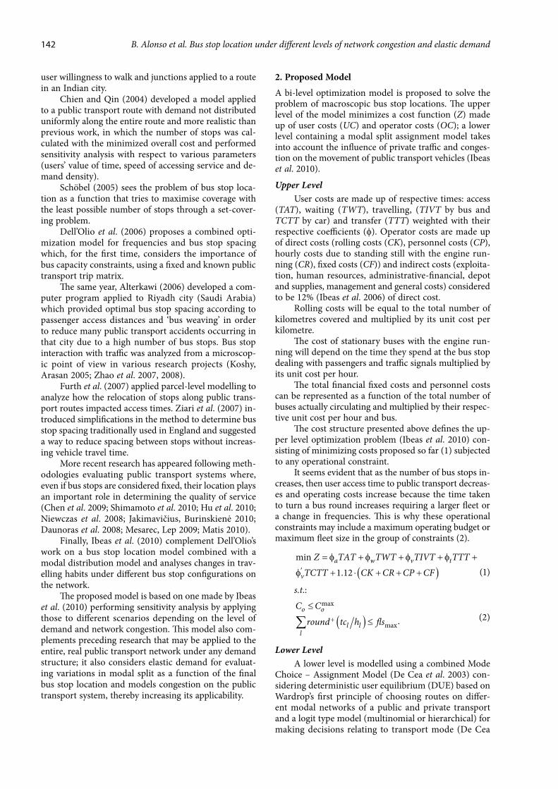
e algorithm developed to solve the optimization prob-lem is based on that developed by Ibeas et  al. (2010). is heuristic algorithm is made up of various stages (Fig. 1) over which the bi-level optimization problem is solved. e stages are described below:

Stage 0. is initial stage could be called a ‘network preparation stage’. The road network must be discretized into almost equally long links, thereby de&ning all potential candidates for lo-cating a bus stop. e study area is then divided

into a number of separate zones each of which must have the same spacing between bus stops. A  vector (∂) is thereby created with as many components as de&ning zones. Details on zon-ing criteria can be found in Ibeas et al. (2010).

Stage 1. e initial feasible bus stop spacing solution vector (∂0) is generated at the &rst iteration.

Stage 2. Given the network con&guration of bus stops de&ned by (∂i), the lower level optimization problem of the proposed model is solved at each iteration i of the algorithm and the upper level objective cost function is calculated (Zi).

Stage 3. New values of (∂i+1) are generated using the Tabu Search algorithm (Glover 1989) and the upper level problem is solved to determine the new value of Zi+1, from which we return once again to run Stage 2.

Stage 4. If 1i iZ Z& * 1 2, we return to Stage 3; however, if 1i iZ Z& * ( 2, the algorithm is stopped, where τ is a reduction in the value of the objective function established as stop criteria.

So'ware package ESTRAUSTM (De Cea et al. 2003) is used for the lower level (Mode Choice – Assignment Model) while MATLABTM (www.mathworks.com) is used for calculating the upper level cost function and for running the solution algorithm.

Fig. 1. Solution algorithm

s

Feasible Solution( )q°

Lover Level: split-Assignment Model

c X X X g T T T X T( ) ( – ) – ( ) ( – ) 0, feasible ,* * * *t t³ "

Upper Level:MATLAB Subroutine

Evaluate Z

Tabu SearchAlgorithm

( )qi +1

Z Zi i+1 – > t

End

Yes

No

q = qi i +1

Transport, 2011, 26(2): 141–148 143

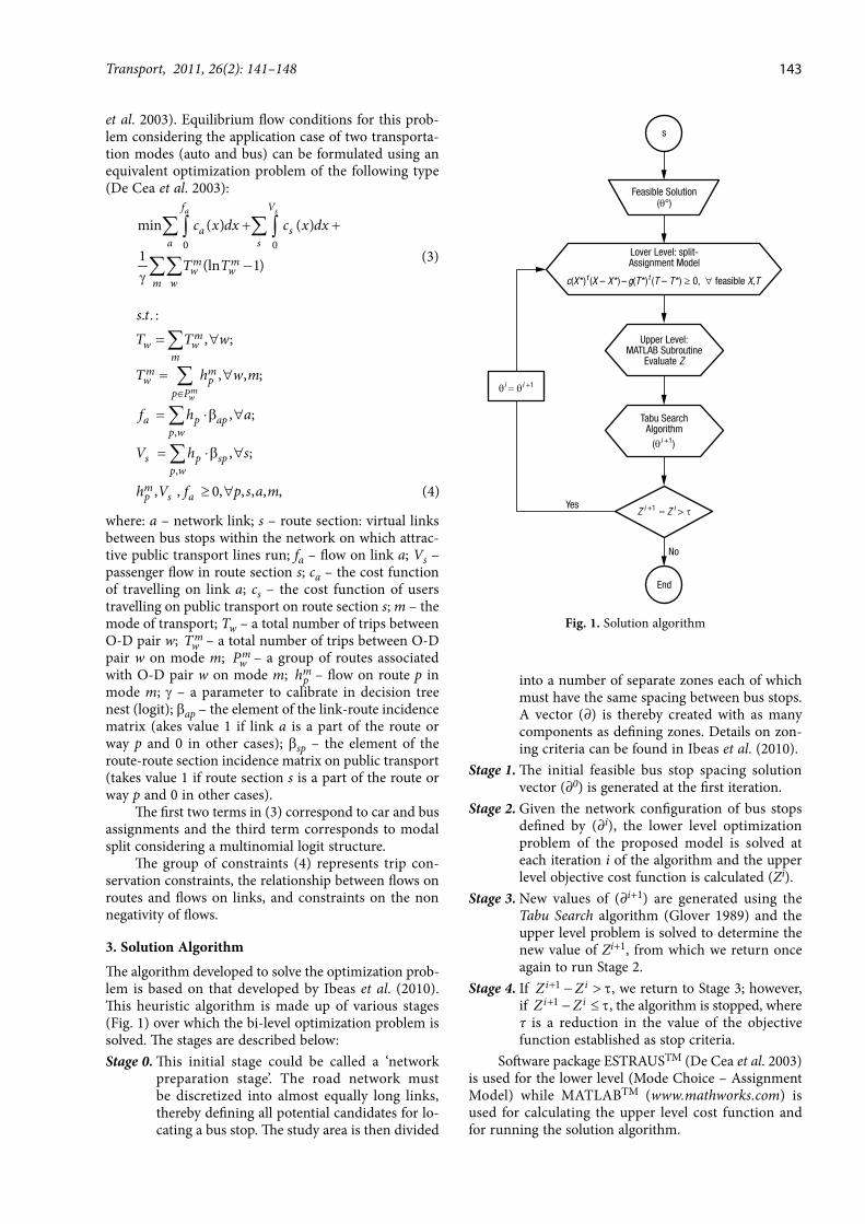
4. Application to a Real Network

To check the validity of the model presented in this arti-cle, it has been applied to a real case. e study area used was Santander city, a medium sized city, of approximate-ly 180000 inhabitants located in Northern Spain with a well established urban bus service (Fig. 2). e city is characterised by its linear structure, a well developed urban and commercial centre and various peripheral residential zones with di#ering population densities. e network had previously been discretized into

60 m long segments to be as precise as possible when locating each stop, given restrictions on so'ware. A GIS has been developed and included economic, social and demographic characteristics of each city zone as well as its more signi&cant attributes of each node: typology (junction, dummy nodes…), regulation (tra%c lights) and location (on a slope or not, the existence of resi-dential areas or special points of interest at a maximum distance if it is an ‘obligatory’ location for a stop, tun-nels, etc.). e zonal aggregation of the city was based on pop-

ulation density and commercial activity and provided &ve groups of zones with equal distancing (in metres) between stops.

5. Analysis and Discussion of Results

In order to analyse the in$uence of demand and con-gestion in the &nal solution provided by the model and the relationship between di#erent variables, the starting point was a very low level of demand, which was pro-gressively increased multiplying the O/D matrix of San-

tander by 0.5, 0.75, 1.5 and 2. In this way, we can analyse an interval range of demand varying from half to double of actual demand at peak hour.Table 1 shows the actual number of trips and their

modal split and Table 2 indicates the values of time and the operation unit used (Ibeas et al. 2010).

Table 1. Trips per hour by mode in Santander

Mode Car Bus Total

Trips per hour 48 441 4 944 53 385

Table 2. Values of time and operation unit costs

Variable

Travel time (BUS) 26.43 €/h

Waiting time (BUS) 51.29 €/h

Access time (BUS) 31.01 €/h

Transfer time (BUS) 79.77 €/h

Travel time (Car) 28.90 €/h

CK unit cost 0.4 €/km

CP unit cost 14 €/bus/h

CF unit cost 32 €/bus/h

CR unit cost 0.02 €/h

Various initial spacing vectors were used for each matrix, starting from extreme cases and the initial con-&guration for Santander to the analyses of how the vari-ables of the model evolved and interacted.

Fig. 2. Road network and public transport routes in Santander

144 B. Alonso et al. Bus stop location under di#erent levels of network congestion and elastic demand

Tables 3, 4 show the &nal solution given for each level of demand. ese tables show that for very low levels of de-

mand (0.5 and 0.75), bus stops can be uniformly well spaced apart from those throughout the city at approxi-mately every 1200÷1600 metres. ese quite high dis-tances should not be taken as rigid measurements be-tween bus stops but rather they should be looked at as the overall bus stop density. In fact, the &nal result from the model locates bus stops in the zones with higher levels of trip generation / attraction and in the highest populated areas within each zone (more speci&cally, in places where the greatest number of access links con-verge). is indicates that the loss of passengers from the bus that moves to using a private car does not cause congestion on the network (because the overall demand is very low); therefore, social cost is compensated using savings made by the operator who now requires a small-er $eet to provide the required service (remember that frequencies are kept constant in the problem). Neverthe-less, as demand increases, accessibility to public trans-port should be greater reducing spacing to 360 metres. ese results may be better understood by repre-

senting the evolution of each variable for each con&gura-tion of bus stops and each level of demand. e legend used in the graphs is the one shown in Fig. 3.Fig. 4 shows the evolution of social cost and the

number of bus passengers.Both graphs show that the sensitivity of social cost

to the number of stops (or bus stop spacing) increases with higher levels of demand and congestion. e same thing happens with the number of passengers using the public transport system.In all cases, accessibility is reduced, so does the

number of passengers the amount of which increase

along with higher bus stop densities reach a moment when an excessive number of bus stops provokes a re-duction in passenger numbers due to an increase in bus journey times. Bus passengers can also be seen to be quite sensitive to longer distances between stops.

Fig. 3. Legend

Fig. 4. e evolution of social costs and bus trips

Table 3. e &nal results of di#erent levels of demand (1)

Matrix Z Cbus Ccar CoperDistance (m)

D1 D2 D3 D4 D5Nºstops

Tripsbus

0.5 165267 39553 123560 2154 1800 1740 1800 1860 1800 68 1580

0.75 316517 52154 261952 2411 1200 1200 1200 1200 1200 84 2351

1(Santander) 707318 80805 622659 3854 360 420 540 420 780 153 5109

1.5 1374611 2859 1366816 4936 360 420 480 420 420 166 10240

2 2462995 135216 2418825 8954 360 360 360 420 360 184 12281

Table 4. e &nal results of di#erent levels of demand (2)

Matrix Cbus/pax Ccar/pax Z/pax Operator Pro&t Fleet

0.5 12.51 2.43 3.06 58.7 35

0.75 13.31 4.12 4.69 331.6 40

1(Santander) 9.95 8.54 8.73 1 825.8 61

1.5 10.27 16.23 14.55 2 232 89

2 11.01 25.28 22.81 –357.3 167

0.5 0.75 1 1.5 2

3500000

SocialC

osts(

ph)

€

3000000

2500000

2000000

1500000

1000000

500000

00 50 100 150 200 250 300

Number of bus stops

0 50 100 150 200 250 300

Number of bus stops

14000

12000

10000

8000

6000

4000

2000

0

Bustrips(tripsper

hour)

Transport, 2011, 26(2): 141–148 145

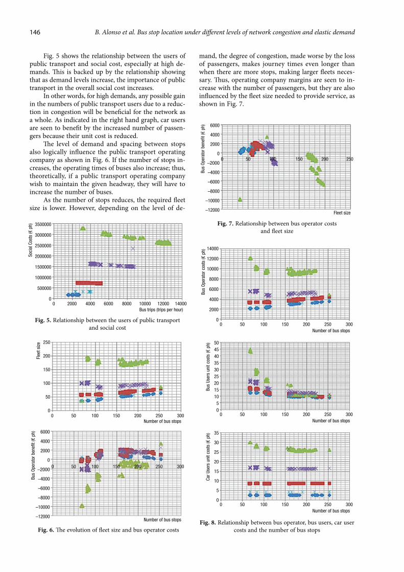
Fig. 5 shows the relationship between the users of public transport and social cost, especially at high de-mands. is is backed up by the relationship showing that as demand levels increase, the importance of public transport in the overall social cost increases.In other words, for high demands, any possible gain

in the numbers of public transport users due to a reduc-tion in congestion will be bene&cial for the network as a whole. As indicated in the right hand graph, car users are seen to bene&t by the increased number of passen-gers because their unit cost is reduced. e level of demand and spacing between stops

also logically in$uence the public transport operating company as shown in Fig. 6. If the number of stops in-creases, the operating times of buses also increase; thus, theoretically, if a public transport operating company wish to maintain the given headway, they will have to increase the number of buses.As the number of stops reduces, the required $eet

size is lower. However, depending on the level of de-

Fig. 6. e evolution of $eet size and bus operator costs

Fig. 7. Relationship between bus operator costs and $eet size

Fig. 8. Relationship between bus operator, bus users, car user costs and the number of bus stops

mand, the degree of congestion, made worse by the loss of passengers, makes journey times even longer than when there are more stops, making larger $eets neces-sary. us, operating company margins are seen to in-crease with the number of passengers, but they are also in$uenced by the $eet size needed to provide service, as shown in Fig. 7.

Fig. 5. Relationship between the users of public transport and social cost

3500000

3000000

2500000

2000000

1500000

1000000

500000

0

SocialC

osts(

ph)

€

0 2000 4000 6000 8000 10000 12000 14000

Bus trips (trips per hour)

6000

4000

2000

0

–2000

–4000

–6000

–8000

–10000

–12000

BusOperator

benefit(

ph)

€

0 50 100 150 200 250

Fleet size

0 50 100 150 200 250 300

Number of bus stops

250

200

150

100

50

0

Fleetsize

0 50 100 150 200 250 300

Number of bus stops

6000

4000

2000

0

–2000

–4000

–6000

–8000

–10000

–12000

BusOperator

benefit(

ph)

€

0 50 100 150 200 250 300

Number of bus stops

14000

12000

10000

8000

6000

4000

2000

0

BusOperator

costs(

ph)

€

0 50 100 150 200 250 300

Number of bus stops

BusUsersunitcosts(

ph)

€

0 50 100 150 200 250 300

Number of bus stops

Car

Usersunitcosts(

ph)

€

50

45

35

30

25

20

15

10

5

0

40

35

30

25

20

15

10

5

0

146 B. Alonso et al. Bus stop location under di#erent levels of network congestion and elastic demand

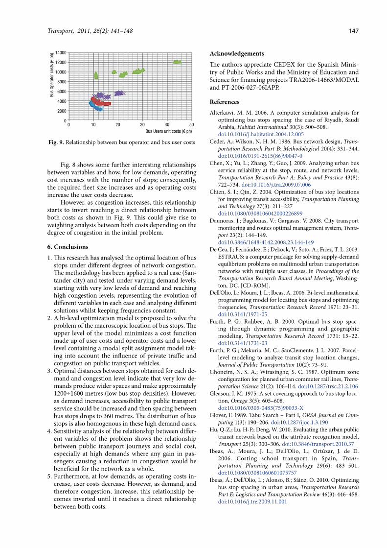
Fig. 8 shows some further interesting relationships between variables and how, for low demands, operating cost increases with the number of stops; consequently, the required $eet size increases and as operating costs increase the user costs decrease.However, as congestion increases, this relationship

starts to invert reaching a direct relationship between both costs as shown in Fig. 9. is could give rise to weighting analysis between both costs depending on the degree of congestion in the initial problem.

6. Conclusions

1. is research has analysed the optimal location of bus stops under di#erent degrees of network congestion. e methodology has been applied to a real case (San-tander city) and tested under varying demand levels, starting with very low levels of demand and reaching high congestion levels, representing the evolution of di#erent variables in each case and analysing di#erent solutions whilst keeping frequencies constant.2. A bi-level optimization model is proposed to solve the problem of the macroscopic location of bus stops. e upper level of the model minimizes a cost function made up of user costs and operator costs and a lower level containing a modal split assignment model tak-ing into account the in$uence of private tra%c and congestion on public transport vehicles.3. Optimal distances between stops obtained for each de-mand and congestion level indicate that very low de-mands produce wider spaces and make approximately 1200÷1600 metres (low bus stop densities). However, as demand increases, accessibility to public transport service should be increased and then spacing between bus stops drops to 360 metres. e distribution of bus stops is also homogenous in these high demand cases.4. Sensitivity analysis of the relationship between di#er-ent variables of the problem shows the relationship between public transport journeys and social cost, especially at high demands where any gain in pas-sengers causing a reduction in congestion would be bene&cial for the network as a whole.5. Furthermore, at low demands, as operating costs in-crease, user costs decrease. However, as demand, and therefore congestion, increase, this relationship be-comes inverted until it reaches a direct relationship between both costs.

Acknowledgements

e authors appreciate CEDEX for the Spanish Minis-try of Public Works and the Ministry of Education and Science for &nancing projects TRA2006-14663/MODAL and PT-2006-027-06IAPP.

References

Alterkawi, M. M. 2006. A computer simulation analysis for optimizing bus stops spacing: the case of Riyadh, Saudi Arabia, Habitat International 30(3): 500–508. doi:10.1016/j.habitatint.2004.12.005

Ceder, A.; Wilson, N. H. M. 1986. Bus network design, Trans-portation Research Part B: Methodological 20(4): 331–344. doi:10.1016/0191-2615(86)90047-0

Chen, X.; Yu, L.; Zhang, Y.; Guo, J. 2009. Analyzing urban bus service reliability at the stop, route, and network levels, Transportation Research Part A: Policy and Practice 43(8): 722–734. doi:10.1016/j.tra.2009.07.006

Chien, S. I.; Qin, Z. 2004. Optimization of bus stop locations for improving transit accessibility, Transportation Planning and Technology 27(3): 211–227doi:10.1080/0308106042000226899

Daunoras, J.; Bagdonas, V.; Gargasas, V. 2008. City transport monitoring and routes optimal management system, Trans-port 23(2): 144–149. doi:10.3846/1648-4142.2008.23.144-149

De Cea, J.; Fernández, E.; Dekock, V.; Soto, A.; Friez, T. L. 2003. ESTRAUS: a computer package for solving supply-demand equilibrium problems on multimodal urban transportation networks with multiple user classes, in Proceedings of the Transportation Research Board Annual Meeting, Washing-ton, DC. [CD-ROM].

Dell’Olio, L.; Moura, J. L.; Ibeas, A. 2006. Bi-level mathematical programming model for locating bus stops and optimizing frequencies, Transportation Research Record 1971: 23–31. doi:10.3141/1971-05

Furth, P. G.; Rahbee, A. B. 2000. Optimal bus stop spac-ing through dynamic programming and geographic modeling, Transportation Research Record 1731: 15–22. doi:10.3141/1731-03

Furth, P. G.; Mekuria, M. C.; SanClemente, J. L. 2007. Parcel-level modeling to analyze transit stop location changes, Journal of Public Transportation 10(2): 73–91.

Ghoneim, N. S. A.; Wirasinghe, S. C. 1987. Optimum zone con&guration for planned urban commuter rail lines, Trans-portation Science 21(2): 106–l14. doi:10.1287/trsc.21.2.106

Gleason, J. M. 1975. A set covering approach to bus stop loca-tion, Omega 3(5): 605–608. doi:10.1016/0305-0483(75)90033-X

Glover, F. 1989. Tabu Search – Part I, ORSA Journal on Com-puting 1(3): 190–206. doi:10.1287/ijoc.1.3.190

Hu, Q-Z.; Lu, H-P.; Deng, W. 2010. Evaluating the urban public transit network based on the attribute recognition model, Transport 25(3): 300–306. doi:10.3846/transport.2010.37

Ibeas, A.; Moura, J. L.; Dell’Olio, L.; Ortúzar, J. de D. 2006. Costing school transport in Spain, Trans-portation Planning and Technology 29(6): 483–501. doi:10.1080/03081060601075757

Ibeas, Á.; Dell’Olio, L.; Alonso, B.; Sáinz, O. 2010. Optimizing bus stop spacing in urban areas, Transportation Research Part E: Logistics and Transportation Review 46(3): 446–458. doi:10.1016/j.tre.2009.11.001

Fig. 9. Relationship between bus operator and bus user costs

0

Bus Users unit costs ( ph)€

14000

12000

10000

8000

6000

4000

2000

0

BusOperator

costs(

ph)

€

10 30 40 5020

Transport, 2011, 26(2): 141–148 147

Jakimavičius, M.; Burinskienė, M. 2010. Route planning meth-odology of an advanced traveller information system in Vilnius city, Transport 25(2): 171–177. doi:10.3846/transport.2010.21

Koshy, R. Z.; Arasan, V. T. 2005. In$uence of bus stops on $ow characteristics of mixed tra%c, Journal of Transportation Engineering 131(8): 640–643. doi:10.1061/(ASCE)0733-947X(2005)131:8(640)

Kra', W H.; Boardman, T. J. 1972. Location of bus stops, Jour-nal of Transportation Engineering 98(TE1): 103–116.

Lesley, L. 1976. Optimum bus stop spacing, Tra&c Engineer-ing & Control 17(10): 399–401.

Matis, P. 2010. Finding a solution for a complex street routing problem using the mixed transportation mode, Transport 25(1): 29–35. doi:10.3846/transport.2010.05

Mesarec, B.; Lep, M. 2009. Combining the grid-based spatial planning and network-based transport planning, Techno-logical and Economic Development of Economy 15(1): 60–77. doi:10.3846/1392-8619.2009.15.60-77

Niewczas, A.; Koszalka, G.; Wrona, J.; Pieniak, D. 2008. Chosen aspects of municipal transport operation on the example of the city of Lublin, Transport 23(1): 88–90. doi:10.3846/1648-4142.2008.23.88-90

Saka, A. A. 2001. Model for determining optimum bus-stop spacing in urban areas, Journal of Transportation Engineer-ing 127(3): 195–199. doi:10.1061/(ASCE)0733-947X(2001)127:3(195)

Sankar, R.; Kavitha, J.; Karthi, S. 2003. Optimization of bus stop locations using GIS as a tool for Chennai city – a case study, in Map India Conference 2003, Poster Session [CD-ROM].

Schöbel, A. 2005. Locating stops along bus or railway lines – a bicriteria problem, Annals of Operations Research 136(1): 211–227. doi:10.1007/s10479-005-2046-0

Shimamoto, H.; Murayama, N.; Fujiwara, A.; Zhang, J. 2010. Evaluation of an existing bus network using a transit network optimisation model: a case study of the Hiro-shima city bus network, Transportation 37(5): 801–823. doi:10.1007/s11116-010-9297-6

Van Nes, R. 2001. e impact of alternative access modes on urban public transport network design, European Journal of Transport and Infrastructure Research 1(2): 197–210.

Van Nes, R.; Bovy, P. H. L. 2000. Importance of objectives in urban transit-network design, Transportation Research Re-cord 1735: 25–34. doi:10.3141/1735-04

Vedagiri, P.; Arasan, V. T. 2009. Modelling modal shi' due to enhanced level of bus service, Transport 24(2): 121–128. doi:10.3846/1648-4142.2009.24.121-128

Vuchic, V. R.; Newell, G. F. 1968. Rapid transit interstation spacing for minimum travel time, Transportation Science 2(4): 303–339. doi:10.1287/trsc.2.4.303

Wirasinghe, S. C.; Ghoneim, N. S. 1981. Spacing of bus stop for many to many travel demand, Transportation Science 15(3): 210–221. doi:10.1287/trsc.15.3.210

Zhao, X.-M.; Gao, Z.-Y.; Jia, B. 2007. e capacity drop caused by the combined e#ect of the intersection and the bus stop in a CA model, Physica A: Statistical Mechanics and its Ap-plications 385(2): 645–658. doi:10.1016/j.physa.2007.07.040

Zhao, X.-M.; Gao, Z.-Y.; Li, K.-P. 2008. e capacity of two neighbour intersections considering the in$uence of the bus stop, Physica A: Statistical Mechanics and its Applica-tions 387(18): 4649–4656. doi:10.1016/j.physa.2008.03.011

Ziari, H. Keymanesh, M. R.; Khabiri, M. M. 2007. Locating sta-tions of public transportation vehicles for improving transit accessibility, Transport 22(2): 99–104.

148 B. Alonso et al. Bus stop location under di#erent levels of network congestion and elastic demand