
Ecuaciones Diferenciales - Facultad de Ciencias Químicas e ...
Upload
khangminh22Category
view
0download
0
this print for content only—size & color not accurate 7" x 9-1/4" / CASEBOUND / MALLOY(1.0625 INCH BULK -- 544 pages -- 50# Thor)
The eXPeRT’s VOIce® In sQL seRVeR
Vincent Rainardi
Building aData WarehouseWith Examples in SQL Server
BOOks fOR PROfessIOnaLs By PROfessIOnaLs®
Building a Data Warehouse: With Examples in SQL ServerDear Reader,
This book contains essential topics of data warehousing that everyone embarking on a data warehousing journey will need to understand in order to build a data warehouse. It covers dimensional modeling, data extraction from source systems, dimension and fact table population, data quality, and database design. It also explains practical data warehousing applications such as business intelligence, analytic applications, and customer relationship management. All in all, the book covers the whole spectrum of data warehousing from start to finish.
I wrote this book to help people with a basic knowledge of database systems who want to take their first step into data warehousing. People who are familiar with databases such as DBAs and developers who have never built a data ware-house will benefit the most from this book. IT students and self-learners will also benefit. In addition, BI and data warehousing professionals will be interested in checking out the practical examples, code, techniques, and architectures described in the book.
Throughout this book, we will be building a data warehouse using the Amadeus Entertainment case study, an entertainment retailer specializing in music, films, and audio books. We will use Microsoft SQL Server 2005 and 2008 to build the data warehouse and BI applications. You will gain experience designing and building various components of a data warehouse, including the architecture, data model, physical databases (using SQL Server), ETL (using SSIS), BI reports (using SSRS), OLAP cubes (using SSAS), and data mining (using SSAS).
I wish you great success in your data warehousing journey.
Sincerely,
Vincent Rainardi
Building a Data Warehouse
With Exam
ples in SQL ServerRainardi
cyan MaGenTa
yeLLOW BLack PanTOne 123 c
ISBN-13: 978-1-59059-931-0ISBN-10: 1-59059-931-4
9 781590 599310
90000
Shelve in Microsoft: SQL Server
User level: Intermediate–Advanced
www.apress.comSOURCE CODE ONLINE
Companion eBook
See last page for details
on $10 eBook version
Companion eBook Available
RELatED titLES


Vincent Rainardi
Building aData WarehouseWith Examples in SQL Server
9314fmfinal.qxd 11/15/07 1:37 PM Page i

Building a Data Warehouse: With Examples in SQL Server
Copyright © 2008 by Vincent Rainardi
All rights reserved. No part of this work may be reproduced or transmitted in any form or by any means,electronic or mechanical, including photocopying, recording, or by any information storage or retrievalsystem, without the prior written permission of the copyright owner and the publisher.
ISBN-13 (pbk): 978-1-59059-931-0
ISBN-10 (pbk): 1-59059-931-4
ISBN-13 (electronic): 978-1-4302-0527-2
ISBN-10 (electronic): 1-4302-0527-X
Printed and bound in the United States of America 9 8 7 6 5 4 3 2 1
Trademarked names may appear in this book. Rather than use a trademark symbol with every occurrenceof a trademarked name, we use the names only in an editorial fashion and to the benefit of the trademarkowner, with no intention of infringement of the trademark.
Lead Editor: Jeffrey PepperTechnical Reviewers: Bill Hamilton and Asif SayedEditorial Board: Steve Anglin, Ewan Buckingham, Tony Campbell, Gary Cornell, Jonathan Gennick,
Jason Gilmore, Kevin Goff, Jonathan Hassell, Matthew Moodie, Joseph Ottinger, Jeffrey Pepper,Ben Renow-Clarke, Dominic Shakeshaft, Matt Wade, Tom Welsh
Senior Project Manager: Tracy Brown CollinsCopy Editor: Kim WimpsettAssociate Production Director: Kari Brooks-CoponyProduction Editor: Kelly WinquistCompositor: Linda Weidemann, Wolf Creek PressProofreader: Linda MarousekIndexer: Ron StraussArtist: April MilneCover Designer: Kurt KramesManufacturing Director: Tom Debolski
Distributed to the book trade worldwide by Springer-Verlag New York, Inc., 233 Spring Street, 6th Floor,New York, NY 10013. Phone 1-800-SPRINGER, fax 201-348-4505, e-mail [email protected],or visit http://www.springeronline.com.
For information on translations, please contact Apress directly at 2855 Telegraph Avenue, Suite 600,Berkeley, CA 94705. Phone 510-549-5930, fax 510-549-5939, e-mail [email protected], or visit http://www.apress.com.
The information in this book is distributed on an “as is” basis, without warranty. Although every pre-caution has been taken in the preparation of this work, neither the author(s) nor Apress shall have anyliability to any person or entity with respect to any loss or damage caused or alleged to be caused directlyor indirectly by the information contained in this work.
The source code for this book is available to readers at http://www.apress.com.
9314fmfinal.qxd 11/15/07 1:37 PM Page ii

For my lovely wife, Ivana.
9314fmfinal.qxd 11/15/07 1:37 PM Page iii

9314fmfinal.qxd 11/15/07 1:37 PM Page iv

Contents at a Glance
About the Author . . . . . . . . . . . . . . . . . . . . . . . . . . . . . . . . . . . . . . . . . . . . . . . . . . . . . . . . . . . . . . . . . xiii
Preface . . . . . . . . . . . . . . . . . . . . . . . . . . . . . . . . . . . . . . . . . . . . . . . . . . . . . . . . . . . . . . . . . . . . . . . . . . xv
■CHAPTER 1 Introduction to Data Warehousing . . . . . . . . . . . . . . . . . . . . . . . . . . . . . . . 1
■CHAPTER 2 Data Warehouse Architecture . . . . . . . . . . . . . . . . . . . . . . . . . . . . . . . . . . 29
■CHAPTER 3 Data Warehouse Development Methodology . . . . . . . . . . . . . . . . . . . . 49
■CHAPTER 4 Functional and Nonfunctional Requirements. . . . . . . . . . . . . . . . . . . . 61
■CHAPTER 5 Data Modeling . . . . . . . . . . . . . . . . . . . . . . . . . . . . . . . . . . . . . . . . . . . . . . . . . 71
■CHAPTER 6 Physical Database Design. . . . . . . . . . . . . . . . . . . . . . . . . . . . . . . . . . . . . 113
■CHAPTER 7 Data Extraction . . . . . . . . . . . . . . . . . . . . . . . . . . . . . . . . . . . . . . . . . . . . . . . 173
■CHAPTER 8 Populating the Data Warehouse . . . . . . . . . . . . . . . . . . . . . . . . . . . . . . . 215
■CHAPTER 9 Assuring Data Quality . . . . . . . . . . . . . . . . . . . . . . . . . . . . . . . . . . . . . . . . . 273
■CHAPTER 10 Metadata . . . . . . . . . . . . . . . . . . . . . . . . . . . . . . . . . . . . . . . . . . . . . . . . . . . . . 301
■CHAPTER 11 Building Reports . . . . . . . . . . . . . . . . . . . . . . . . . . . . . . . . . . . . . . . . . . . . . . 329
■CHAPTER 12 Multidimensional Database . . . . . . . . . . . . . . . . . . . . . . . . . . . . . . . . . . . 377
■CHAPTER 13 Using Data Warehouse for Business Intelligence . . . . . . . . . . . . . . . 411
■CHAPTER 14 Using Data Warehouse for Customer Relationship Management . . . . . . . . . . . . . . . . . . . . . . . . . . . . . . . . . . . . 441
■CHAPTER 15 Other Data Warehouse Usage . . . . . . . . . . . . . . . . . . . . . . . . . . . . . . . . . 467
■CHAPTER 16 Testing Your Data Warehouse . . . . . . . . . . . . . . . . . . . . . . . . . . . . . . . . . 477
■CHAPTER 17 Data Warehouse Administration . . . . . . . . . . . . . . . . . . . . . . . . . . . . . . . 491
■APPENDIX Normalization Rules . . . . . . . . . . . . . . . . . . . . . . . . . . . . . . . . . . . . . . . . . . 505
■INDEX . . . . . . . . . . . . . . . . . . . . . . . . . . . . . . . . . . . . . . . . . . . . . . . . . . . . . . . . . . . . . . . . . . . . . . . 509
v
9314fmfinal.qxd 11/15/07 1:37 PM Page v

9314fmfinal.qxd 11/15/07 1:37 PM Page vi

Contents
About the Author . . . . . . . . . . . . . . . . . . . . . . . . . . . . . . . . . . . . . . . . . . . . . . . . . . . . . . . . . . . . . . . . . xiii
Preface . . . . . . . . . . . . . . . . . . . . . . . . . . . . . . . . . . . . . . . . . . . . . . . . . . . . . . . . . . . . . . . . . . . . . . . . . . xv
■CHAPTER 1 Introduction to Data Warehousing . . . . . . . . . . . . . . . . . . . . . . . . . . 1
What Is a Data Warehouse?. . . . . . . . . . . . . . . . . . . . . . . . . . . . . . . . . . . . . . . . 1
Retrieves Data . . . . . . . . . . . . . . . . . . . . . . . . . . . . . . . . . . . . . . . . . . . . . . 4
Consolidates Data . . . . . . . . . . . . . . . . . . . . . . . . . . . . . . . . . . . . . . . . . . . 5
Periodically . . . . . . . . . . . . . . . . . . . . . . . . . . . . . . . . . . . . . . . . . . . . . . . . . 6
Dimensional Data Store . . . . . . . . . . . . . . . . . . . . . . . . . . . . . . . . . . . . . . 7
Normalized Data Store . . . . . . . . . . . . . . . . . . . . . . . . . . . . . . . . . . . . . . . 8
History . . . . . . . . . . . . . . . . . . . . . . . . . . . . . . . . . . . . . . . . . . . . . . . . . . . . 10
Query . . . . . . . . . . . . . . . . . . . . . . . . . . . . . . . . . . . . . . . . . . . . . . . . . . . . . 11
Business Intelligence . . . . . . . . . . . . . . . . . . . . . . . . . . . . . . . . . . . . . . . 12
Other Analytical Activities. . . . . . . . . . . . . . . . . . . . . . . . . . . . . . . . . . . . 14
Updated in Batches . . . . . . . . . . . . . . . . . . . . . . . . . . . . . . . . . . . . . . . . . 15
Other Definitions . . . . . . . . . . . . . . . . . . . . . . . . . . . . . . . . . . . . . . . . . . . 16
Data Warehousing Today . . . . . . . . . . . . . . . . . . . . . . . . . . . . . . . . . . . . . . . . . 17
Business Intelligence . . . . . . . . . . . . . . . . . . . . . . . . . . . . . . . . . . . . . . . 17
Customer Relationship Management . . . . . . . . . . . . . . . . . . . . . . . . . . 18
Data Mining. . . . . . . . . . . . . . . . . . . . . . . . . . . . . . . . . . . . . . . . . . . . . . . . 19
Master Data Management (MDM). . . . . . . . . . . . . . . . . . . . . . . . . . . . . 20
Customer Data Integration . . . . . . . . . . . . . . . . . . . . . . . . . . . . . . . . . . . 23
Future Trends in Data Warehousing. . . . . . . . . . . . . . . . . . . . . . . . . . . . . . . . 24
Unstructured Data . . . . . . . . . . . . . . . . . . . . . . . . . . . . . . . . . . . . . . . . . . 24
Search . . . . . . . . . . . . . . . . . . . . . . . . . . . . . . . . . . . . . . . . . . . . . . . . . . . . 25
Service-Oriented Architecture (SOA) . . . . . . . . . . . . . . . . . . . . . . . . . . 26
Real-Time Data Warehouse . . . . . . . . . . . . . . . . . . . . . . . . . . . . . . . . . . 27
Summary . . . . . . . . . . . . . . . . . . . . . . . . . . . . . . . . . . . . . . . . . . . . . . . . . . . . . . 27
vii
9314fmfinal.qxd 11/15/07 1:37 PM Page vii

■CHAPTER 2 Data Warehouse Architecture . . . . . . . . . . . . . . . . . . . . . . . . . . . . . . 29
Data Flow Architecture . . . . . . . . . . . . . . . . . . . . . . . . . . . . . . . . . . . . . . . . . . . 29
Single DDS . . . . . . . . . . . . . . . . . . . . . . . . . . . . . . . . . . . . . . . . . . . . . . . . 33
NDS + DDS . . . . . . . . . . . . . . . . . . . . . . . . . . . . . . . . . . . . . . . . . . . . . . . . 35
ODS + DDS . . . . . . . . . . . . . . . . . . . . . . . . . . . . . . . . . . . . . . . . . . . . . . . . 38
Federated Data Warehouse . . . . . . . . . . . . . . . . . . . . . . . . . . . . . . . . . . 39
System Architecture . . . . . . . . . . . . . . . . . . . . . . . . . . . . . . . . . . . . . . . . . . . . . 42
Case Study . . . . . . . . . . . . . . . . . . . . . . . . . . . . . . . . . . . . . . . . . . . . . . . . . . . . . 44
Summary. . . . . . . . . . . . . . . . . . . . . . . . . . . . . . . . . . . . . . . . . . . . . . . . . . . . . . . 47
■CHAPTER 3 Data Warehouse Development Methodology . . . . . . . . . . . . . . 49
Waterfall Methodology . . . . . . . . . . . . . . . . . . . . . . . . . . . . . . . . . . . . . . . . . . . 49
Iterative Methodology . . . . . . . . . . . . . . . . . . . . . . . . . . . . . . . . . . . . . . . . . . . . 54
Summary. . . . . . . . . . . . . . . . . . . . . . . . . . . . . . . . . . . . . . . . . . . . . . . . . . . . . . . 59
■CHAPTER 4 Functional and Nonfunctional Requirements . . . . . . . . . . . . . 61
Identifying Business Areas. . . . . . . . . . . . . . . . . . . . . . . . . . . . . . . . . . . . . . . . 61
Understanding Business Operations . . . . . . . . . . . . . . . . . . . . . . . . . . . . . . . 62
Defining Functional Requirements . . . . . . . . . . . . . . . . . . . . . . . . . . . . . . . . . 63
Defining Nonfunctional Requirements . . . . . . . . . . . . . . . . . . . . . . . . . . . . . . 65
Conducting a Data Feasibility Study. . . . . . . . . . . . . . . . . . . . . . . . . . . . . . . . 67
Summary. . . . . . . . . . . . . . . . . . . . . . . . . . . . . . . . . . . . . . . . . . . . . . . . . . . . . . . 70
■CHAPTER 5 Data Modeling . . . . . . . . . . . . . . . . . . . . . . . . . . . . . . . . . . . . . . . . . . . . . . . 71
Designing the Dimensional Data Store . . . . . . . . . . . . . . . . . . . . . . . . . . . . . 71
Dimension Tables . . . . . . . . . . . . . . . . . . . . . . . . . . . . . . . . . . . . . . . . . . . . . . . 76
Date Dimension . . . . . . . . . . . . . . . . . . . . . . . . . . . . . . . . . . . . . . . . . . . . . . . . . 77
Slowly Changing Dimension . . . . . . . . . . . . . . . . . . . . . . . . . . . . . . . . . . . . . . 80
Product, Customer, and Store Dimensions . . . . . . . . . . . . . . . . . . . . . . . . . . 83
Subscription Sales Data Mart . . . . . . . . . . . . . . . . . . . . . . . . . . . . . . . . . . . . . 89
Supplier Performance Data Mart . . . . . . . . . . . . . . . . . . . . . . . . . . . . . . . . . . 94
CRM Data Marts. . . . . . . . . . . . . . . . . . . . . . . . . . . . . . . . . . . . . . . . . . . . . . . . . 96
Data Hierarchy . . . . . . . . . . . . . . . . . . . . . . . . . . . . . . . . . . . . . . . . . . . . . . . . . 101
Source System Mapping . . . . . . . . . . . . . . . . . . . . . . . . . . . . . . . . . . . . . . . . 102
Designing the Normalized Data Store . . . . . . . . . . . . . . . . . . . . . . . . . . . . . 106
Summary . . . . . . . . . . . . . . . . . . . . . . . . . . . . . . . . . . . . . . . . . . . . . . . . . . . . . 111
■CONTENTSviii
9314fmfinal.qxd 11/15/07 1:37 PM Page viii

■CHAPTER 6 Physical Database Design . . . . . . . . . . . . . . . . . . . . . . . . . . . . . . . . . 113
Hardware Platform . . . . . . . . . . . . . . . . . . . . . . . . . . . . . . . . . . . . . . . . . . . . . 113
Storage Considerations . . . . . . . . . . . . . . . . . . . . . . . . . . . . . . . . . . . . . . . . . 120
Configuring Databases . . . . . . . . . . . . . . . . . . . . . . . . . . . . . . . . . . . . . . . . . . 123
Creating DDS Database Structure . . . . . . . . . . . . . . . . . . . . . . . . . . . . . . . . 128
Creating the Normalized Data Store. . . . . . . . . . . . . . . . . . . . . . . . . . . . . . . 139
Using Views . . . . . . . . . . . . . . . . . . . . . . . . . . . . . . . . . . . . . . . . . . . . . . . . . . . 157
Summary Tables . . . . . . . . . . . . . . . . . . . . . . . . . . . . . . . . . . . . . . . . . . . . . . . 161
Partitioning . . . . . . . . . . . . . . . . . . . . . . . . . . . . . . . . . . . . . . . . . . . . . . . . . . . . 162
Indexes . . . . . . . . . . . . . . . . . . . . . . . . . . . . . . . . . . . . . . . . . . . . . . . . . . . . . . . 166
Summary. . . . . . . . . . . . . . . . . . . . . . . . . . . . . . . . . . . . . . . . . . . . . . . . . . . . . . 171
■CHAPTER 7 Data Extraction. . . . . . . . . . . . . . . . . . . . . . . . . . . . . . . . . . . . . . . . . . . . . 173
Introduction to ETL . . . . . . . . . . . . . . . . . . . . . . . . . . . . . . . . . . . . . . . . . . . . . 173
ETL Approaches and Architecture . . . . . . . . . . . . . . . . . . . . . . . . . . . . . . . . 174
General Considerations . . . . . . . . . . . . . . . . . . . . . . . . . . . . . . . . . . . . . . . . . 177
Extracting Relational Databases . . . . . . . . . . . . . . . . . . . . . . . . . . . . . . . . . . 180
Whole Table Every Time . . . . . . . . . . . . . . . . . . . . . . . . . . . . . . . . . . . . 180
Incremental Extract . . . . . . . . . . . . . . . . . . . . . . . . . . . . . . . . . . . . . . . . 181
Fixed Range . . . . . . . . . . . . . . . . . . . . . . . . . . . . . . . . . . . . . . . . . . . . . . 185
Related Tables . . . . . . . . . . . . . . . . . . . . . . . . . . . . . . . . . . . . . . . . . . . . 186
Testing Data Leaks . . . . . . . . . . . . . . . . . . . . . . . . . . . . . . . . . . . . . . . . 187
Extracting File Systems . . . . . . . . . . . . . . . . . . . . . . . . . . . . . . . . . . . . . . . . . 187
Extracting Other Source Types . . . . . . . . . . . . . . . . . . . . . . . . . . . . . . . . . . . 190
Extracting Data Using SSIS . . . . . . . . . . . . . . . . . . . . . . . . . . . . . . . . . . . . . . 191
Memorizing the Last Extraction Timestamp . . . . . . . . . . . . . . . . . . . . . . . . 200
Extracting from Files . . . . . . . . . . . . . . . . . . . . . . . . . . . . . . . . . . . . . . . . . . . . 208
Summary. . . . . . . . . . . . . . . . . . . . . . . . . . . . . . . . . . . . . . . . . . . . . . . . . . . . . . 214
■CHAPTER 8 Populating the Data Warehouse . . . . . . . . . . . . . . . . . . . . . . . . . . 215
Stage Loading . . . . . . . . . . . . . . . . . . . . . . . . . . . . . . . . . . . . . . . . . . . . . . . . . 216
Data Firewall . . . . . . . . . . . . . . . . . . . . . . . . . . . . . . . . . . . . . . . . . . . . . . . . . . 218
Populating NDS . . . . . . . . . . . . . . . . . . . . . . . . . . . . . . . . . . . . . . . . . . . . . . . . 219
Using SSIS to Populate NDS . . . . . . . . . . . . . . . . . . . . . . . . . . . . . . . . . . . . . 228
Upsert Using SQL and Lookup. . . . . . . . . . . . . . . . . . . . . . . . . . . . . . . . . . . . 235
Normalization . . . . . . . . . . . . . . . . . . . . . . . . . . . . . . . . . . . . . . . . . . . . . . . . . . 242
Practical Tips on SSIS . . . . . . . . . . . . . . . . . . . . . . . . . . . . . . . . . . . . . . . . . . . 249
■CONTENTS ix
9314fmfinal.qxd 11/15/07 1:37 PM Page ix

Populating DDS Dimension Tables . . . . . . . . . . . . . . . . . . . . . . . . . . . . . . . . 250
Populating DDS Fact Tables . . . . . . . . . . . . . . . . . . . . . . . . . . . . . . . . . . . . . 266
Batches, Mini-batches, and Near Real-Time ETL . . . . . . . . . . . . . . . . . . . 269
Pushing the Data In . . . . . . . . . . . . . . . . . . . . . . . . . . . . . . . . . . . . . . . . . . . . 270
Summary. . . . . . . . . . . . . . . . . . . . . . . . . . . . . . . . . . . . . . . . . . . . . . . . . . . . . . 271
■CHAPTER 9 Assuring Data Quality. . . . . . . . . . . . . . . . . . . . . . . . . . . . . . . . . . . . . . 273
Data Quality Process. . . . . . . . . . . . . . . . . . . . . . . . . . . . . . . . . . . . . . . . . . . . 274
Data Cleansing and Matching . . . . . . . . . . . . . . . . . . . . . . . . . . . . . . . . . . . . 277
Cross-checking with External Sources . . . . . . . . . . . . . . . . . . . . . . . . . . . . 290
Data Quality Rules . . . . . . . . . . . . . . . . . . . . . . . . . . . . . . . . . . . . . . . . . . . . . . 291
Action: Reject, Allow, Fix . . . . . . . . . . . . . . . . . . . . . . . . . . . . . . . . . . . . . . . . 293
Logging and Auditing . . . . . . . . . . . . . . . . . . . . . . . . . . . . . . . . . . . . . . . . . . . 296
Data Quality Reports and Notifications . . . . . . . . . . . . . . . . . . . . . . . . . . . . 298
Summary. . . . . . . . . . . . . . . . . . . . . . . . . . . . . . . . . . . . . . . . . . . . . . . . . . . . . . 300
■CHAPTER 10 Metadata . . . . . . . . . . . . . . . . . . . . . . . . . . . . . . . . . . . . . . . . . . . . . . . . . . . 301
Metadata in Data Warehousing. . . . . . . . . . . . . . . . . . . . . . . . . . . . . . . . . . . 301
Data Definition and Mapping Metadata . . . . . . . . . . . . . . . . . . . . . . . . . . . . 303
Data Structure Metadata . . . . . . . . . . . . . . . . . . . . . . . . . . . . . . . . . . . . . . . . 308
Source System Metadata . . . . . . . . . . . . . . . . . . . . . . . . . . . . . . . . . . . . . . . . 313
ETL Process Metadata . . . . . . . . . . . . . . . . . . . . . . . . . . . . . . . . . . . . . . . . . . 318
Data Quality Metadata . . . . . . . . . . . . . . . . . . . . . . . . . . . . . . . . . . . . . . . . . . 320
Audit Metadata. . . . . . . . . . . . . . . . . . . . . . . . . . . . . . . . . . . . . . . . . . . . . . . . . 323
Usage Metadata. . . . . . . . . . . . . . . . . . . . . . . . . . . . . . . . . . . . . . . . . . . . . . . . 324
Maintaining Metadata . . . . . . . . . . . . . . . . . . . . . . . . . . . . . . . . . . . . . . . . . . . 325
Summary. . . . . . . . . . . . . . . . . . . . . . . . . . . . . . . . . . . . . . . . . . . . . . . . . . . . . . 327
■CHAPTER 11 Building Reports . . . . . . . . . . . . . . . . . . . . . . . . . . . . . . . . . . . . . . . . . . . 329
Data Warehouse Reports . . . . . . . . . . . . . . . . . . . . . . . . . . . . . . . . . . . . . . . . 329
When to Use Reports and When Not to Use Them. . . . . . . . . . . . . . . . . . . 332
Report Wizard. . . . . . . . . . . . . . . . . . . . . . . . . . . . . . . . . . . . . . . . . . . . . . . . . . 334
Report Layout . . . . . . . . . . . . . . . . . . . . . . . . . . . . . . . . . . . . . . . . . . . . . . . . . . 340
Report Parameters . . . . . . . . . . . . . . . . . . . . . . . . . . . . . . . . . . . . . . . . . . . . . 342
Grouping, Sorting, and Filtering . . . . . . . . . . . . . . . . . . . . . . . . . . . . . . . . . . 351
Simplicity . . . . . . . . . . . . . . . . . . . . . . . . . . . . . . . . . . . . . . . . . . . . . . . . . . . . . 356
Spreadsheets . . . . . . . . . . . . . . . . . . . . . . . . . . . . . . . . . . . . . . . . . . . . . . . . . . 357
Multidimensional Database Reports . . . . . . . . . . . . . . . . . . . . . . . . . . . . . . 362
Deploying Reports . . . . . . . . . . . . . . . . . . . . . . . . . . . . . . . . . . . . . . . . . . . . . . 366
■CONTENTSx
9314fmfinal.qxd 11/15/07 1:37 PM Page x

Managing Reports . . . . . . . . . . . . . . . . . . . . . . . . . . . . . . . . . . . . . . . . . . . . . . 370
Managing Report Security . . . . . . . . . . . . . . . . . . . . . . . . . . . . . . . . . . 370
Managing Report Subscriptions . . . . . . . . . . . . . . . . . . . . . . . . . . . . . 372
Managing Report Execution . . . . . . . . . . . . . . . . . . . . . . . . . . . . . . . . . 374
Summary. . . . . . . . . . . . . . . . . . . . . . . . . . . . . . . . . . . . . . . . . . . . . . . . . . . . . . 375
■CHAPTER 12 Multidimensional Database . . . . . . . . . . . . . . . . . . . . . . . . . . . . . . . 377
What a Multidimensional Database Is . . . . . . . . . . . . . . . . . . . . . . . . . . . . . 377
Online Analytical Processing . . . . . . . . . . . . . . . . . . . . . . . . . . . . . . . . . . . . . 380
Creating a Multidimensional Database . . . . . . . . . . . . . . . . . . . . . . . . . . . . 381
Processing a Multidimensional Database . . . . . . . . . . . . . . . . . . . . . . . . . . 388
Querying a Multidimensional Database . . . . . . . . . . . . . . . . . . . . . . . . . . . . 394
Administering a Multidimensional Database . . . . . . . . . . . . . . . . . . . . . . . 396
Multidimensional Database Security . . . . . . . . . . . . . . . . . . . . . . . . . 397
Processing Cubes . . . . . . . . . . . . . . . . . . . . . . . . . . . . . . . . . . . . . . . . . 399
Backup and Restore . . . . . . . . . . . . . . . . . . . . . . . . . . . . . . . . . . . . . . . 405
Summary. . . . . . . . . . . . . . . . . . . . . . . . . . . . . . . . . . . . . . . . . . . . . . . . . . . . . . 409
■CHAPTER 13 Using Data Warehouse for Business Intelligence . . . . . . . . 411
Business Intelligence Reports . . . . . . . . . . . . . . . . . . . . . . . . . . . . . . . . . . . . 412
Business Intelligence Analytics . . . . . . . . . . . . . . . . . . . . . . . . . . . . . . . . . . . 413
Business Intelligence Data Mining . . . . . . . . . . . . . . . . . . . . . . . . . . . . . . . . 416
Business Intelligence Dashboards . . . . . . . . . . . . . . . . . . . . . . . . . . . . . . . . 432
Business Intelligence Alerts. . . . . . . . . . . . . . . . . . . . . . . . . . . . . . . . . . . . . . 437
Business Intelligence Portal. . . . . . . . . . . . . . . . . . . . . . . . . . . . . . . . . . . . . . 438
Summary. . . . . . . . . . . . . . . . . . . . . . . . . . . . . . . . . . . . . . . . . . . . . . . . . . . . . . 439
■CHAPTER 14 Using Data Warehouse for Customer Relationship Management . . . . . . . . . . . . . . . . . . . . . . . . . . . . . . . . 441
Single Customer View. . . . . . . . . . . . . . . . . . . . . . . . . . . . . . . . . . . . . . . . . . . 442
Campaign Segmentation . . . . . . . . . . . . . . . . . . . . . . . . . . . . . . . . . . . . . . . . 447
Permission Management . . . . . . . . . . . . . . . . . . . . . . . . . . . . . . . . . . . . . . . . 450
Delivery and Response Data . . . . . . . . . . . . . . . . . . . . . . . . . . . . . . . . . . . . . 454
Customer Analysis. . . . . . . . . . . . . . . . . . . . . . . . . . . . . . . . . . . . . . . . . . . . . . 460
Customer Support . . . . . . . . . . . . . . . . . . . . . . . . . . . . . . . . . . . . . . . . . . . . . . 463
Personalization. . . . . . . . . . . . . . . . . . . . . . . . . . . . . . . . . . . . . . . . . . . . . . . . . 464
Customer Loyalty Scheme . . . . . . . . . . . . . . . . . . . . . . . . . . . . . . . . . . . . . . . 465
Summary . . . . . . . . . . . . . . . . . . . . . . . . . . . . . . . . . . . . . . . . . . . . . . . . . . . . . 466
■CONTENTS xi
9314fmfinal.qxd 11/15/07 1:37 PM Page xi

■CHAPTER 15 Other Data Warehouse Usage . . . . . . . . . . . . . . . . . . . . . . . . . . . . . 467
Customer Data Integration. . . . . . . . . . . . . . . . . . . . . . . . . . . . . . . . . . . . . . . 467
Unstructured Data . . . . . . . . . . . . . . . . . . . . . . . . . . . . . . . . . . . . . . . . . . . . . . 470
Search in Data Warehousing . . . . . . . . . . . . . . . . . . . . . . . . . . . . . . . . . . . . . 474
Summary. . . . . . . . . . . . . . . . . . . . . . . . . . . . . . . . . . . . . . . . . . . . . . . . . . . . . . 476
■CHAPTER 16 Testing Your Data Warehouse. . . . . . . . . . . . . . . . . . . . . . . . . . . . . 477
Data Warehouse ETL Testing . . . . . . . . . . . . . . . . . . . . . . . . . . . . . . . . . . . . 478
Functional Testing . . . . . . . . . . . . . . . . . . . . . . . . . . . . . . . . . . . . . . . . . . . . . . 480
Performance Testing. . . . . . . . . . . . . . . . . . . . . . . . . . . . . . . . . . . . . . . . . . . . 482
Security Testing . . . . . . . . . . . . . . . . . . . . . . . . . . . . . . . . . . . . . . . . . . . . . . . . 485
User Acceptance Testing . . . . . . . . . . . . . . . . . . . . . . . . . . . . . . . . . . . . . . . . 486
End-to-End Testing . . . . . . . . . . . . . . . . . . . . . . . . . . . . . . . . . . . . . . . . . . . . . 487
Migrating to Production . . . . . . . . . . . . . . . . . . . . . . . . . . . . . . . . . . . . . . . . . 487
Summary. . . . . . . . . . . . . . . . . . . . . . . . . . . . . . . . . . . . . . . . . . . . . . . . . . . . . . 489
■CHAPTER 17 Data Warehouse Administration . . . . . . . . . . . . . . . . . . . . . . . . . . 491
Monitoring Data Warehouse ETL . . . . . . . . . . . . . . . . . . . . . . . . . . . . . . . . . 492
Monitoring Data Quality . . . . . . . . . . . . . . . . . . . . . . . . . . . . . . . . . . . . . . . . . 495
Managing Security . . . . . . . . . . . . . . . . . . . . . . . . . . . . . . . . . . . . . . . . . . . . . 498
Managing Databases . . . . . . . . . . . . . . . . . . . . . . . . . . . . . . . . . . . . . . . . . . . 499
Making Schema Changes . . . . . . . . . . . . . . . . . . . . . . . . . . . . . . . . . . . . . . . 501
Updating Applications . . . . . . . . . . . . . . . . . . . . . . . . . . . . . . . . . . . . . . . . . . . 503
Summary. . . . . . . . . . . . . . . . . . . . . . . . . . . . . . . . . . . . . . . . . . . . . . . . . . . . . . 503
■APPENDIX Normalization Rules . . . . . . . . . . . . . . . . . . . . . . . . . . . . . . . . . . . . . . . 505
■INDEX . . . . . . . . . . . . . . . . . . . . . . . . . . . . . . . . . . . . . . . . . . . . . . . . . . . . . . . . . . . . . . . . . . . . . . . 509
■CONTENTSxii
9314fmfinal.qxd 11/15/07 1:37 PM Page xii

About the Author
■VINCENT RAINARDI is a data warehouse architect and developer with morethan 12 years of experience in IT. He started working with data warehous-ing in 1996 when he was working for Accenture. He has been workingwith Microsoft SQL Server since 2000. He worked for Lastminute.com(part of the Travelocity group) until October 2007. He now works as a datawarehousing consultant in London specializing in SQL Server. He is amember of The Data Warehousing Institute (TDWI) and regularly writesdata warehousing articles for SQLServerCentral.com.
xiii
9314fmfinal.qxd 11/15/07 1:37 PM Page xiii

9314fmfinal.qxd 11/15/07 1:37 PM Page xiv

Preface
Friends and colleagues who want to start learning data warehousing sometimes ask me torecommend a practical book about the subject matter. They are not new to the databaseworld; most of them are either DBAs or developers/consultants, but they have never built adata warehouse. They want a book that is practical and aimed at beginners, one that containsall the basic essentials. There are many data warehousing books on the market, but they usu-ally cover a specialized topic such as clickstream, ETL, dimensional modeling, data mining,OLAP, or project management and therefore a beginner would need to buy five to six books tounderstand the complete spectrum of data warehousing. Other books cover multiple aspects,but they are not as practical as they need to be, targeting executives and project managersinstead of DBAs and developers.
Because of that void, I took a pen (well, a laptop really) and spent a whole year writingin order to provide a practical, down-to-earth book containing all the essential subjects ofbuilding a data warehouse, with many examples and illustrations from projects that are easyto understand. The book can be used to build your first data warehouse straightaway; it cov-ers all aspects of data warehousing, including approach, architecture, data modeling, ETL,data quality, and OLAP. I also describe some practical issues that I have encountered in myexperience—issues that you’ll also likely encounter in your first data warehousing project—along with the solutions.
It is not possible to show examples, code, and illustrations for all the different databaseplatforms, so I had to choose a specific platform. Oracle and SQL Server provide completeend-to-end solutions including the database, ETL, reporting, and OLAP, and after discussionswith my editor, we decided to base the examples on SQL Server 2005, while also making themapplicable to future versions of SQL Server such as 2008. I apologize in advance that the exam-ples do not run on SQL Server 2000; there is just too big a gap in terms of data warehousingfacilities, such as SSIS, between 2000 and 2005.
Throughout this book, together we will be designing and building a data warehouse fora case study called Amadeus Entertainment. A data warehouse consist of many parts, such asthe data model, physical databases, ETL, data quality, metadata, cube, application, and so on.In each chapter, I will cover each part one by one. I will cover the theory related to that part,and then I will show how to build that part for the case study. Specifically, Chapter 1 introduceswhat a data warehouse is and what the benefits are. In Chapters 2–6, we will design the archi-tecture, define the requirements, and create the data model and physical databases, includingthe SQL Server configuration. In Chapters 7–10 we will populate the data stores using SSIS, aswell as discuss data quality and metadata. Chapters 11–12 are about getting the data out byusing Reporting Services and Analysis Services cubes. In Chapters 13–15, I’ll discuss the appli-cation of data warehouse for BI and CRM as well as CDI, unstructured data, and search. I closethe book with testing and administering a data warehouse in Chapters 16–17.
xv
9314fmfinal.qxd 11/15/07 1:37 PM Page xv

The supplementary material (available on the book’s download page on the Apress website, http://www.apress.com) provides all the necessary material to build the data warehousefor the case study. Specifically, it contains the following folders:
Scripts: Contains the scripts to build the source system and the data warehouse, asexplained in Chapters 5 and 6.
Source system: Contains the source system databases required to build the data ware-house for the case study in Chapters 7 and 8.
ETL: Contains the SSIS packages to import data into the data warehouse. Chapters 7 and8 explain how to build these packages.
Report: Contains the SSRS reports explained in Chapter 11.
Cubes: Contains the SSAS projects explained in Chapter 12.
Data: Contains the backup of data warehouse database (the DDS) and Analysis Servicescube, which are used for reporting, OLAP, BI, and data mining in Chapters 11, 12, and 13.
■PREFACExvi
9314fmfinal.qxd 11/15/07 1:37 PM Page xvi

Introduction to DataWarehousing
In this chapter, I will discuss what a data warehouse is, how data warehouses are used today,and the future trends of data warehousing.
I will begin by defining what a data warehouse is. Then I’ll walk you through a diagram ofa typical data warehouse system, discussing its components and how the data flows throughthose components. I will also discuss the simplest possible form of a data warehouse. Afteryou have an idea about what a data warehouse is, I will discuss the definition in more detail.I will go through each bit of the definition individually, exploring that bit in depth. I will alsotalk about other people’s definitions.
Then, I will move on to how data warehouses are used today. I will discuss business intel-ligence, customer relationship management, and data mining as the popular applications ofdata warehousing. I will also talk about the role of master data management and customerdata integration in data warehousing.
Finally, I will talk about the future trends of data warehousing, such as unstructured data,search, real-time data warehouses, and service-oriented architecture. By the end of this chap-ter, you will have a general understanding of data warehousing.
What Is a Data Warehouse?Let’s begin by defining what a data warehouse is. A data warehouse is a system that retrievesand consolidates data periodically from the source systems into a dimensional or normalizeddata store. It usually keeps years of history and is queried for business intelligence or other ana-lytical activities. It is typically updated in batches, not every time a transaction happens in thesource system.
In the next few pages, I will discuss each of the italicized terms in the previous para-graph one by one. But for now, I’ll walk you through a diagram of a data warehouse system,discussing it component by component and how the data flows through those components.After this short walk-through, I will discuss each term in the previous definition, includingthe differences between dimensional and normalized data stores, why you store the datain the data store, and why data warehouses are updated in batches. Figure 1-1 shows a dia-gram of a data warehouse system, including the applications.
1
C H A P T E R 1
9314ch01final.qxd 11/15/07 10:24 AM Page 1

Figure 1-1. A diagram of a data warehouse system
Let’s go through the diagram in Figure 1-1, component by component, from left to right.The source systems are the OLTP systems that contain the data you want to load into the datawarehouse. Online Transaction Processing (OLTP) is a system whose main purpose is to cap-ture and store the business transactions. The source systems’ data is examined using a dataprofiler to understand the characteristics of the data. A data profiler is a tool that has the capa-bility to analyze data, such as finding out how many rows are in each table, how many rowscontain NULL values, and so on.
The extract, transform, and load (ETL) system then brings data from various sourcesystems into a staging area. ETL is a system that has the capability to connect to the sourcesystems, read the data, transform the data, and load it into a target system (the target sys-tem doesn’t have to be a data warehouse). The ETL system then integrates, transforms, andloads the data into a dimensional data store (DDS). A DDS is a database that stores the datawarehouse data in a different format than OLTP. The reason for getting the data from thesource system into the DDS and then querying the DDS instead of querying the source sys-tem directly is that in a DDS the data is arranged in a dimensional format that is moresuitable for analysis. The second reason is because a DDS contains integrated data fromseveral source systems.
When the ETL system loads the data into the DDS, the data quality rules do various dataquality checks. Bad data is put into the data quality (DQ) database to be reported and thencorrected in the source systems. Bad data can also be automatically corrected or tolerated if itis within a certain limit. The ETL system is managed and orchestrated by the control system,based on the sequence, rules, and logic stored in the metadata. The metadata is a database
CHAPTER 1 ■ INTRODUCTION TO DATA WAREHOUSING2
9314ch01final.qxd 11/15/07 10:24 AM Page 2
containing information about the data structure, the data meaning, the data usage, the dataquality rules, and other information about the data.
The audit system logs the system operations and usage into the metadata database. Theaudit system is part of the ETL system that monitors the operational activities of the ETLprocesses and logs their operational statistics. It is used for understanding what happenedduring the ETL process.
Users use various front-end tools such as spreadsheets, pivot tables, reporting tools, andSQL query tools to retrieve and analyze the data in a DDS. Some applications operate on amultidimensional database format. For these applications, the data in the DDS is loaded intomultidimensional databases (MDBs), which are also known as cubes. A multidimensionaldatabase is a form of database where the data is stored in cells and the position of each cell isdefined by a number of variables called dimensions. Each cell represents a business event, andthe values of the dimensions show when and where this event happened.
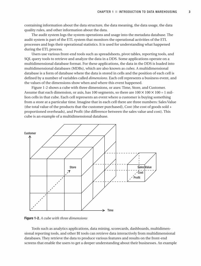
Figure 1-2 shows a cube with three dimensions, or axes: Time, Store, and Customer.Assume that each dimension, or axis, has 100 segments, so there are 100 ✕ 100 ✕ 100 = 1 mil-lion cells in that cube. Each cell represents an event where a customer is buying somethingfrom a store at a particular time. Imagine that in each cell there are three numbers: Sales Value(the total value of the products that the customer purchased), Cost (the cost of goods sold +proportioned overheads), and Profit (the difference between the sales value and cost). Thiscube is an example of a multidimensional database.
Figure 1-2. A cube with three dimensions
Tools such as analytics applications, data mining, scorecards, dashboards, multidimen-sional reporting tools, and other BI tools can retrieve data interactively from multidimensionaldatabases. They retrieve the data to produce various features and results on the front-endscreens that enable the users to get a deeper understanding about their businesses. An example
CHAPTER 1 ■ INTRODUCTION TO DATA WAREHOUSING 3
9314ch01final.qxd 11/15/07 10:24 AM Page 3

of an analytic application is to analyze the sales by time, customer, and product. The users cananalyze the revenue and cost for a certain month, region, and product type.
Not all data warehouse systems have all the components pictured previously. Even if adata warehouse system does not have a data quality mechanism, a multidimensional data-base, any analytics applications, a front-end application, a control system or audit system,metadata, or a stage, you can still call it a data warehouse system. In its simplest form, it issimilar to Figure 1-3.
Figure 1-3. Simplest form of a data warehouse system
In this case, the data warehouse system contains only an ETL system and a dimensionaldata store. The source system is not part of the data warehouse system. This is pretty much theminimum. If you take out just one more component, you cannot call it a data warehouse sys-tem anymore. In Figure 1-3, even though there is no front-end application such as reports oranalytic applications, users can still query the data in the DDS by issuing direct SQL selectstatements using generic database query tools such as the one hosted in SQL Server Manage-ment Studio. I will be discussing data warehouse architecture in Chapter 2.
Now that you have an idea about what a data warehouse system is and its components,let’s take a look at the data warehouse definition in more detail. Again, in the next few pages,I will discuss each italicized term in the following data warehouse definition one by one: adata warehouse is a system that retrieves and consolidates data periodically from the sourcesystems into a dimensional or normalized data store. It usually keeps years of history and isqueried for business intelligence or other analytical activities. It is typically updated in batches,not every time a transaction happens in the source system.
Retrieves DataThe data retrieval is performed by a set of routines widely known as an ETL system, which isan abbreviation for extract, transform, and load. The ETL system is a set of processes thatretrieve data from the source systems, transform the data, and load it into a target system. Thetransformation can be used for changing the data to suit the format and criteria of the targetsystem, for deriving new values to be loaded to the target system, or for validating the datafrom the source system. ETL systems are not only used to load data into the data warehouse.They are widely used for any kind of data movements.
Most ETL systems also have mechanisms to clean the data from the source systembefore putting it into the warehouse. Data cleansing is the process of identifying and correct-ing dirty data. This is implemented using data quality rules that define what dirty data is.After the data is extracted from the source system but before the data is loaded into the ware-house, the data is examined using these rules. If the rule determines that the data is correct,then it is loaded into the warehouse. If the rule determines that the data is incorrect, thenthere are three options: it can be rejected, corrected, or allowed to be loaded into the ware-house. Which action is appropriate for a particular piece of data depends on the situation,
CHAPTER 1 ■ INTRODUCTION TO DATA WAREHOUSING4
9314ch01final.qxd 11/15/07 10:24 AM Page 4
73ed30358d714f26dd2d9c0159f8cfe0
the risk level, the rule type (error or warning), and so on. I will go through data cleansing anddata quality in more detail in Chapter 9.
There is another alternative approach to ETL, known as extract, load, and transform(ELT). In this approach, the data is loaded into the data warehouse first in its raw format. Thetransformations, lookups, deduplications, and so on, are performed inside the data ware-house. Unlike the ETL approach, the ELT approach does not need an ETL server. This approachis usually implemented to take advantage of powerful data warehouse database engines suchas massively parallel processing (MPP) systems. I will be discussing more about the ELTapproach in Chapter 7.
Consolidates DataA company can have many transactional systems. For example, a bank may use 15 differentapplications for its services, one for loan processing, one for customer service, one for tellers/cashiers, one for ATMs, one for bonds, one for ISA, one for savings, one for private banking,one for the trading floor, one for life insurance, one for home insurance, one for mortgages,one for the call center, one for internal accounts, and one for fraud detection. Performing(for example) customer profitability analysis across these different applications would bevery difficult.
A data warehouse consolidates many transactional systems. The key difference betweena data warehouse and a front-office transactional system is that the data in the data ware-house is integrated. This consolidation or integration should take into account the dataavailability (some data is available in several systems but not in others), time ranges (data indifferent systems has different validity periods), different definitions (the term total weeklyrevenue in one system may have a different meaning from total weekly revenue in other sys-tems), conversion (different systems may have a different unit of measure or currency), andmatching (merging data based on common identifiers between different systems).
Let’s go through the previous concepts one by one:
Data availability: When consolidating data from different source systems, it is possible thata piece of data is available in one system but is not in the other system. For example, systemA may have seven address fields (address1, address2, address3, city, county, ZIP, and coun-try), but system B does not have the address3 field and the country field. In system A, anorder may have two levels—order header and order line. However, in system B, an order hasfour levels—order header, order bundle, order line item, and financial components. Sowhen consolidating data across different transaction systems, you need to be aware ofunavailable columns and missing levels in the hierarchy. In the previous examples, you canleave address3 blank in the target and set the country to a default value. In the order hierar-chy example, you can consolidate into two levels, order header and order line.
Time ranges: The same piece of data exists in different systems, but they have differenttime periods. So, you need to be careful when consolidating them. You always need toexamine what time period is applicable to which data before you consolidate the data.Otherwise, you are at risk of having inaccurate data in the warehouse because you mixeddifferent time periods. For example, say in system A the average supplier overhead cost iscalculated weekly, but in system B it is calculated monthly. You can’t just consolidatethem. In this example, you need to go back upstream to get the individual componentsthat make up the average supplier overhead cost in both systems and add them up first.
CHAPTER 1 ■ INTRODUCTION TO DATA WAREHOUSING 5
9314ch01final.qxd 11/15/07 10:24 AM Page 5

Definitions: Sometimes the same data may contain different things. In system A, a col-umn called “Total Order Value” may contain taxes, discounts, credit card charges, anddelivery charges, whereas in system B it does not contain delivery charges. In system A,the term weekly traffic may refer to unique web site visitors, whereas in system B it meansnonunique web site visitors. In this matter, you always need to examine the meaning ofeach piece of data. Just because they have the same name doesn’t mean they are thesame. This is important because you could have inaccurate data or meaningless datain the data warehouse if you consolidate data with different meanings.
Conversion: When consolidating data across different source systems, sometimes youneed to do conversion because the data in the source system is in different units of meas-ure. If you add them up without converting them first, then you will have incorrect data inthe warehouse. In some cases, the conversion rate is fixed (always the same value), but inother cases the conversion rate changes from time to time. If it changes from time to time,you need to know what time period to use when converting. For example, the conversionbetween the time in one country to another country is affected by daylight savings time,so you need to know the date to be able to do the conversion. In addition, the conversionrate between one currency and another currency fluctuates every day, so when convert-ing, you need to know when the transaction happened.
Matching: Matching is a process of determining whether a piece of data in one system isthe same as the data in another system. Matching is important because if you match thewrong data, you will have inaccurate data in the data warehouse. For example, say youwant to consolidate the data for customer 1 in system A with the data for customer 1 insystem B. In this case, you need to determine first whether those two are the same cus-tomer. If you match the wrong customers, the transaction from one customer could bemixed up with the data from another customer. The matching criteria are different fromcompany to company. Sometimes criteria are simple, such as using user IDs, customerIDs, or account IDs. But sometimes it is quite complex, such as name + e-mail address +address. The logic of determining a match can be simply based on the equation sign (=) toidentify an exact match. It can also be based on fuzzy logic or matching rules. (I will talkmore about data matching in Chapter 9.)
When building the data warehouse, you have to deal with all these data integration issues.
PeriodicallyThe data retrieval and the consolidation do not happen only once; they happen many timesand usually at regular intervals, such as daily or a few times a day. If the data retrieval happensonly once, then the data will become obsolete, and after some time it will not be useful.
You can determine the period of data retrieval and consolation based on the businessrequirements and the frequency of data updates in the source systems. The data retrievalinterval needs to be the same as the source system’s data update frequency. If the source sys-tem is updated once a day, you need to set the data retrieval once a day. There is no pointextracting the data from that source system several times a day.
On the other hand, you need to make sure the data retrieval interval satisfies the businessrequirements. For example, if the business needs the product profitability report once a week,
CHAPTER 1 ■ INTRODUCTION TO DATA WAREHOUSING6
9314ch01final.qxd 11/15/07 10:24 AM Page 6

then the data from various source systems needs to be consolidated at least once a week.Another example is when a company states to its customer that it will take 24 hours to cancelthe marketing subscriptions. Then the data in the CRM data warehouse needs to be updateda few times a day; otherwise, you risk sending marketing campaigns to customers who havealready canceled their subscriptions.
Dimensional Data StoreA data warehouse is a system that retrieves data from source systems and puts it into adimensional data store or a normalized data store. Yes, some data warehouses are in dimen-sional format, but some data warehouses are in normalized format. Let’s go through bothformats and the differences between them.
A DDS is one or several databases containing a collection of dimensional data marts.A dimensional data mart is a group of related fact tables and their corresponding dimensiontables containing the measurements of business events categorized by their dimensions.
A dimensional data store is denormalized, and the dimensions are conformed. Con-formed dimensions mean either they are exactly the same dimension table or one is thesubset of the other. Dimension A is said to be a subset of dimension B when all columns ofdimension A exist in dimension B and all rows of dimension A exist in dimension B.
A dimensional data store can be implemented physically in the form of several differentschemas. Examples of dimensional data store schemas are a star schema (shown in Figure 1-4),a snowflake schema, and a galaxy schema. In a star schema, a dimension does not have a sub-table (a subdimension). In a snowflake schema, a dimension can have a subdimension. Thepurpose of having a subdimension is to minimize redundant data. A galaxy schema is alsoknown as a fact constellation schema. In a galaxy schema, you have two or more related facttables surrounded by common dimensions. The benefit of having a star schema is that it is sim-pler than snowflake and galaxy schemas, making it easier for the ETL processes to load the datainto DDS. The benefit of a snowflake schema is that some analytics applications work betterwith a snowflake schema compared to a star schema or galaxy schema. The other benefit of asnowflake schema is less data redundancy, so less disk space is required. The benefit of galaxyschema is the ability to model the business events more accurately by using several fact tables.
■Note A data store can be physically implemented as more than one database, in other words, twodatabases, three databases, and so on. The contrary is also true: two or more data stores can be physi-cally implemented as one database. When designing the physical layer of the data store, usually you tendto implement each data store as one database. But you need to consider physical database design factorssuch as the physical data model, database platform, storage requirement, relational integrity, and backuprequirements when determining whether you will put several data stores in one database or split a datastore into several databases. Putting one data store in one database is not always the best solution. (I willdiscuss physical database design in Chapter 6.)
CHAPTER 1 ■ INTRODUCTION TO DATA WAREHOUSING 7
9314ch01final.qxd 11/15/07 10:24 AM Page 7

Figure 1-4. Star schema dimensional data store
Normalized Data StoreOther types of data warehouses put the data not in a dimensional data store but in a normal-ized data store. A normalized data store is one or more relational databases with little or nodata redundancy. A relational database is a database that consists of entity tables with parent-child relationships between them.
Normalization is a process of removing data redundancy by implementing normalizationrules. There are five degrees of normal forms, from the first normal form to the fifth normalform. A normalized data store is usually in third normal form or higher, such as fourth or fifthnormal form. I will discuss the normalization process and normalization rules in Chapter 5.
Figure 1-5 shows an example of a normalized data store. It is the normalized version ofthe same data as displayed in Figure 1-4.
CHAPTER 1 ■ INTRODUCTION TO DATA WAREHOUSING8
9314ch01final.qxd 11/15/07 10:24 AM Page 8

Figure 1-5. Normalized data store
A dimensional data store is a better format to store data in the warehouse for the purposeof querying and analyzing data than a normalized data store. This is because it is simpler (onelevel deep in all directions in star schema) and gives better query performance. A normalizeddata store is a better format to integrate data from various source systems, especially in thirdnormal form and higher. This is because there is only one place to update without data redun-dancy like in a dimensional data store.
The normalized data store is usually used for an enterprise data warehouse; from therethe data is then loaded into dimensional data stores for query and analysis purposes.Figure 1-6 shows a data warehouse system with a normalized data store used for an enter-prise data warehouse (labeled as “EDW” in the figure).
CHAPTER 1 ■ INTRODUCTION TO DATA WAREHOUSING 9
9314ch01final.qxd 11/15/07 10:24 AM Page 9

Some applications run on a DDS, that is, a relational database that consists of tables withrows and columns. Some applications run on a multidimensional database that consists ofcubes with cells and dimensions. I will go through cubes and multidimensional database con-cepts later in this chapter and in Chapter 12.
Figure 1-6. A data warehouse system that uses an enterprise data warehouse
I will discuss more about dimensional data stores, dimensional schemas, conformeddimensions, normalized data stores, the normalization process, and third normal form inChapter 5 when I talk about data modeling.
HistoryOne of the key differences between a transactional system and a data warehouse system isthe capability and capacity to store history. Most transactional systems store some history,but data warehouse systems store very long history. In my experience, transactional systemsstore only one to three years of data; beyond that, the data is purged. For example, let’s have alook at a sales order–processing system. The purpose of this system is to process customerorders. Once an order is dispatched and paid, it is closed, and after two or three years, youwant to purge the closed orders out of the active system and archive them to maintain sys-tem performance.
You may want to keep the records for, say, two years, in case the customer queries theirorders, but you don’t want to keep ten years worth of data on the active system, because thatslows the system down. Some regulations (which differ from country to country) require youto keep data for up to five or seven years, such as for tax purposes or to adhere to stockexchange regulations. But this does not mean you must keep the data on the active system.You can archive it to offline media. That’s what a typical transaction system does: it keepsonly two to three years of data in the active system and archives the rest either to an offlinemedia or to a secondary read-only system/database.
A data warehouse, on the other hand, stores years and years of history in the active sys-tem. I have seen ten years of historical data in a data warehouse. The amount of historical datato store in the data warehouse depends on the business requirements. Data warehouse tablescan become very large. Imagine a supermarket chain that has 100 stores. Each store welcomes1,000 customers a day, each purchasing 10 items. This means 100 ✕ 1000 ✕ 10 = 1 million sales
CHAPTER 1 ■ INTRODUCTION TO DATA WAREHOUSING10
9314ch01final.qxd 11/15/07 10:24 AM Page 10

order item records every day. In a year, you will have 365 million records. If you store 10 yearsof data, you will have 3.65 billion records. A high volume like this also happens in the telecom-munications industry and in online retail, especially when you store the web page visits in thedata warehouse. Therefore, it is important for a data warehouse system to be able to update ahuge table bit by bit, query it bit by bit, and back it up bit by bit. Database features such astable partitioning and parallel query would be useful for a data warehouse system. Table parti-tioning is a method to split a table by rows into several parts and store each part in a differentfile to increase data loading and query performance. Parallel query is a process where a singlequery is split into smaller parts and each part is given to an independent query-processingmodule. The query result from each module is then combined and sent back to the front-endapplication. I will go through parallel database features such as table partitioning in Chapter6, when I discuss physical database design.
Most transaction systems store the history of the transactions but not the history of themaster data such as products, customers, branches, and vehicles. When you change the prod-uct description, for example, in my experience most of the transaction systems update the olddescription with the new one; they do not store the old description. There are some exceptions,however; for example, some specialized applications such as medical and customer serviceapplications store historical master data such as old customer attributes.
In a data warehouse, on the other hand, storing the history of the master data is one ofthe key features. This is known as a slowly changing dimension (SCD). A slowly changingdimension is a technique used in dimensional modeling for preserving historical informationabout dimensional data. In SCD type 2, you keep the historical information in rows; while inSCD type 3, you keep the historical information in columns. In SCD type 1, you don’t keep thehistorical information. Please refer to Chapter 5 for more information about SCD.
Also related to history, a data warehouse stores a periodic snapshot of operationalsource systems. A snapshot is a copy of one or more master tables taken at a certain time.A periodic snapshot is a snapshot that is taken at a regular interval; for example, the bank-ing industry takes snapshots of customer account tables every day. The data warehouseapplications then compare the daily snapshots to analyze customer churns, account bal-ances, and unusual conditions. If the size of a source system is, say, 100MB, then in a yearyou would have accumulated 37GB. Storing source system daily snapshots could have aserious impact on data warehouse storage, so you need to be careful.
QueryQuerying is the process of getting data from a data store, which satisfies certain criteria. Hereis an example of a simple query: “How many customers do you have now?”1 Here is an exam-ple of a complex query: “Show me the names and revenue of all product lines that had a 10percent loss or greater in Q3 FY 2006, categorized by outlet.”
A data warehouse is built to be queried. That is the number-one purpose of its existence.Users are not allowed to update the data warehouse. Users can only query the data ware-house. Only the ETL system is allowed to update the data warehouse. This is one of the keydifferences between a data warehouse and a transaction system.
CHAPTER 1 ■ INTRODUCTION TO DATA WAREHOUSING 11
1. Note: “How many customers do you have now?” is a simple question if you have only one application,but if you have 15 applications, it could be quite daunting.
9314ch01final.qxd 11/15/07 10:24 AM Page 11

If you refer once again to Figure 1-1, you can ask yourself this question: “Why do I need toget the data from the source system into the DDS and then query the DDS? Why don’t I querythe source system directly?”
For the purpose of simple querying and reporting, you usually query the source systemdirectly. But for conducting heavy analysis such as customer profitability, predictive analysis,“what if?” scenarios, slice and dice analytical exercises, and so on, it is difficult to do it on thesource system.
Here’s why: the source system is usually a transactional system, used by many users. Oneimportant feature of a transactional system is the ability to allow many users to update andselect from the system at the same time. To do so, it must be able to perform a lot of databasetransactions (update, insert, delete, and select) in a relatively short period of time. In otherwords, it should be able to perform database transactions very quickly. If you stored the samepiece of data—say, unit price—in many different places in the system, it would take a longtime to update the data and to maintain data consistency. If you stored it in only one place, itwould be quicker to update the data, and you wouldn’t have to worry about maintaining dataconsistency between different places. Also, it would be easier to maintain the concurrency andlocking mechanism to enable many people to work together in the same database. Hence, oneof the fundamental principles of a transaction system is to remove data redundancy.
Performing a complex query on a normalized database (such as transactional systems) isslower than performing a complex query on a denormalized database (such as a data ware-house), because in a normalized database, you need to join many tables. A normalized data-base is not suitable to be used to load data into a multidimensional database for the purposeof slicing-and-dicing analysis. Unlike a relational database that contains tables with twodimensions (rows and columns), a multidimensional database consists of cubes containingcells with more than two dimensions. Then each cell is mapped to a member in each dimen-sion. To load a multidimensional database from a normalized database, you need to do amultijoin query to transform the data to dimensional format. It can be done, but it is slower.I will go through normalization in more detail in Chapter 5 and data loading in Chapter 8.
The second reason why you don’t query the source systems directly is because a companycan have many source systems or front-office transactional systems. So, by querying a sourcesystem, you get only partial data. A data warehouse, on the other hand, consolidates the datafrom many source systems, so by querying the data warehouse, you get integrated data.
Business IntelligenceBusiness intelligence is a collection of activities to understand business situations by per-forming various types of analysis on the company data as well as on external data from thirdparties to help make strategic, tactical, and operational business decisions and take neces-sary actions for improving business performance. This includes gathering, analyzing,understanding, and managing data about operation performance, customer and supplieractivities, financial performance, market movements, competition, regulatory compliance,and quality controls.
Examples of business intelligence are the following:
CHAPTER 1 ■ INTRODUCTION TO DATA WAREHOUSING12
9314ch01final.qxd 11/15/07 10:24 AM Page 12

• Business performance management, including producing key performance indicatorssuch as daily sales, resource utilization, and main operational costs for each region,product line, and time period, as well as their aggregates, to enable people to take tac-tical actions to get operational performance on the desired tracks.
• Customer profitability analysis, that is, to understand which customers are profitableand worth keeping and which are losing money and therefore need to be acted upon.The key to this exercise is allocating the costs as accurately as possible to the smallestunit of business transaction, which is similar to activity-based costing.
• Statistical analysis such as purchase likelihood or basket analysis. Basket analysis is aprocess of analyzing sales data to determine which products are likely to be purchasedor ordered together. This likelihood is expressed in terms of statistical measures such assupport and confidence level. It is mainly applicable for the retail and manufacturingindustries but also to a certain degree for the financial services industry.
• Predictive analysis such as forecasting the sales, revenue, and cost figures for the pur-pose of planning for next year’s budgets and taking into account other factors such asorganic growth, economic situations, and the company’s future direction.
According to the depth of analysis and level of complexity, in my opinion you can groupbusiness intelligence activities into three categories:
• Reporting, such as key performance indicators, global sales figures by business unit andservice codes, worldwide customer accounts, consolidated delivery status, andresource utilization rates across different branches in many countries
• OLAP, such as aggregation, drill down, slice and dice, and drill across
• Data mining, such as data characterization, data discrimination, association analysis,classification, clustering, prediction, trend analysis, deviation analysis, and similarityanalysis
Now let’s discuss each of these three categories in detail.
ReportingIn a data warehousing context, a report is a program that retrieves data from the data ware-house and presents it to the users on the screen or on paper. Users also can subscribe to thesereports so that they can be sent to the users automatically by e-mail at certain times (daily orweekly, for example) or in response to events.
The reports are built according to the functional specifications. They display the DDSdata required by the business user to analyze and understand business situations. The mostcommon form of report is a tabular form containing simple columns. There is another form ofreport known as cross tab or matrix. These reports are like Excel pivot tables, where one dataattribute becomes the rows, another data attribute becomes the columns, and each cell on thereport contains the value corresponding to the row and column attributes.
Data warehouse reports are used to present the business data to users, but they are alsoused for data warehouse administration purposes. They are used to monitor data quality, tomonitor the usage of data warehouse applications, and to monitor ETL activities.
CHAPTER 1 ■ INTRODUCTION TO DATA WAREHOUSING 13
9314ch01final.qxd 11/15/07 10:24 AM Page 13

Online Analytical Processing (OLAP)OLAP is the activity of interactively analyzing business transaction data stored in the dimen-sional data warehouse to make tactical and strategic business decisions. Typical people whodo OLAP work are business analysts, business managers, and executives. Typical functionalityin OLAP includes aggregating (totaling), drilling down (getting the details), and slicing anddicing (cutting the cube and summing the values in the cells). OLAP functionality can bedelivered using a relational database or using a multidimensional database. OLAP that usesa relational database is known as relational online analytical processing (ROLAP). OLAP thatuses a multidimensional database is known as multidimensional online analytical processing(MOLAP).
An example of OLAP is analyzing the effectiveness of a marketing campaign initiative oncertain products by measuring sales growth over a certain period. Another example is to ana-lyze the impact of a price increase to the product sales in different regions and product groupsat the same period of time.
Data MiningData mining is a process to explore data to find the patterns and relationships that describethe data and to predict the unknown or future values of the data. The key value in data min-ing is the ability to understand why some things happened in the past and to predict whatwill happen in the future. When data mining is used to explain the current or past situation,it is called descriptive analytics. When data mining is used to predict the future, it is calledpredictive analytics.
In business intelligence, popular applications of data mining are for fraud detection(credit card industry), forecasting and budgeting (finance), developing cellular/mobile pack-ages by analyzing call patterns (telecommunication industry), market basket analysis (retailindustry), customer risk profiling (insurance industry), usage monitoring (energy and utili-ties), and machine service times (manufacturing industry).
I will discuss the implementation of data warehousing for business intelligence inChapter 13.
Other Analytical ActivitiesOther than for business intelligence, data warehouses are also used for analytical activities innonbusiness purposes, such as scientific research, government departments (statistics office,weather office, economic analysis, and predictions), military intelligence, emergency anddisaster management, charity organizations, server performance monitoring, and networktraffic analysis.
Data warehouses are also used for customer relationship management (CRM). CRM isa set of activities performed by an organization (business and nonbusiness) to manage andconduct analysis about their customers, to keep in contact and communicate with their cus-tomers, to attract and win new customers, to market product and services to their customers,to conduct transactions with their customers (both business and nonbusiness transactions),to service and support their customers, and to create new ideas and new products or servicesfor their customers. I will discuss the implementation of data warehouses for CRM later in thischapter and in Chapter 14.
CHAPTER 1 ■ INTRODUCTION TO DATA WAREHOUSING14
9314ch01final.qxd 11/15/07 10:24 AM Page 14

Data warehouses are also used in web analytics. Web analytics is the activity of under-standing the behavior and characteristics of web site traffic. This includes finding out thenumber of visits, visitors, and unique visitors on each page for each day/week/month; referrersites; typical routes that visitors take within the site; technical characteristics of the visitors’browsers; domain and geographical analysis; what kind of robots are visiting; the exit rate ofeach page; and the conversion rate on the checkout process. Web analytics are especiallyimportant for online businesses.
Updated in BatchesA data warehouse is usually a read-only system; that is, users are not able to update ordelete data in the data warehouse. Data warehouse data is updated using a standard mecha-nism called ETL at certain times by bringing data from the operational source system. Thisis different from a transactional system or OLTP where users are able to update the systemat any time.
The reason for not allowing users to update or delete data in the data warehouse is tomaintain data consistency so you can guarantee that the data in the data warehouse will beconsistent with the operational source systems, such as if the data warehouse is taking datafrom two source systems, A and B. System A contains 11 million customers, system B contains8 million customers, and there are 2 million customers who exist in both systems. The datawarehouse will contain 17 million customers. If the users update the data in the data ware-house (say, delete 1 million customers), then it will not be consistent with the source systems.Also, when the next update comes in from the ETL, the changes that the users made in thewarehouse will be gone and overwritten.
The reason why data warehouses are updated in batches rather than in real time is to cre-ate data stability in the data warehouse. You need to keep in mind that the operational sourcesystems are changing all the time. Some of them change every minute, and some of themchange every second. If you allow the source system to update the data warehouse in real timeor you allow the users to update the data warehouse all the time, then it would be difficult todo some analysis because the data changes every time. For example, say you are doing adrilling-down exercise on a multidimensional cube containing crime data. At 10:07 you noticethat the total of crime in a particular region for Q1 2007 is 100. So at 10:09, you drill down bycity (say that region consists of three cities: A, B, and C), and the system displays that thecrime for city A was 40, B was 30, and C was 31. That is because at 10:08 a user or an ETLadded one crime that happened in city C to the data warehouse. The drilling-down/summing-up exercise will give inconsistent results because the data keeps changing.
The second reason for updating the data warehouse in batches rather than in real time isthe performance of the source system. Updating the data warehouse in real time means thatthe moment there is an update in the source systems, you update the data warehouse imme-diately, that is, within a few seconds. To do this, you need to either
• install database triggers on every table in the source system or
• modify the source system application to write into the data warehouse immediatelyafter it writes to the source system database.
If the source system is a large application and you need to extract from many tables (say100 or 1,000 tables), then either approach will significantly impact the performance of the
CHAPTER 1 ■ INTRODUCTION TO DATA WAREHOUSING 15
9314ch01final.qxd 11/15/07 10:24 AM Page 15

source system application. One pragmatic approach is to do real-time updates only from afew key tables, say five tables, whilst other tables are updated in a normal daily batch. It ispossible to update the data warehouse in real time or in near real time, but only for a fewselected tables.
In the past few years, real-time data warehousing has become the trend and even thenorm. Data warehouse ETL batches that in the old days ran once a day now run every hour,some of them every five minutes (this is called a mini-batch). Some of them are using the pushapproach; that is, rather than pulling the data into the warehouse, the source system pushesthe data into the warehouse. In a push approach, the data warehouse is updated immediatelywhen the data in the source system changes. Changes in the source system are detected usingdatabase triggers. In a pull approach, the data warehouse is updated at certain intervals.Changes in the source system are detected for extraction using a timestamp or identity col-umn. (I will go through data extraction in Chapter 7.)
Some approaches use messaging and message queuing technology to transport the dataasynchronously from various source systems into the data warehouse. Messaging is a datatransport mechanism where the data is wrapped in an envelope containing control bits andsent over the network into a message queue. A message queue (MQ) is a system where mes-sages are queued to be processed systematically in order. An application sends messages con-taining data into the MQ, and another application reads and removes the messages from theMQ. There are some considerations you need to be careful of when using asynchronous ETL,because different pieces of data are arriving at different times without knowing each other’sstatus of arrival. The benefit of using MQ for ETL is the ability for the source system to sendout the data without the data warehouse being online to receive it. The other benefit is thatthe source system needs to send out the data only once to an MQ so the data consistency isguaranteed; several recipients can then read the same message from the MQ. You will learnmore about real-time data warehousing in Chapter 8 when I discuss ETL.
Other DefinitionsI will close this section with data warehouse definitions from Bill Inmon and from Ralph Kim-ball, the fathers of data warehousing:
• According to Bill Inmon, a data warehouse is a subject-oriented, integrated, non-volatile, and time-variant collection of data in support of management’s decisions.2
• According to Ralph Kimball, a data warehouse is a system that extracts, cleans, con-forms, and delivers source data into a dimensional data store and then supports andimplements querying and analysis for the purpose of decision making.3
Both of them agree that a data warehouse integrates data from various operational sourcesystems. In Inmon’s approach, the data warehouse is physically implemented as a normalizeddata store. In Kimball’s approach, the data warehouse is physically implemented in a dimen-sional data store.
In my opinion, if you store the data in a normalized data store, you still need to load thedata into a dimensional data store for query and analysis. A dimensional data store is a better
CHAPTER 1 ■ INTRODUCTION TO DATA WAREHOUSING16
2. See Building the Data Warehouse, Fourth Edition (John Wiley, 2005) for more information.
3. See The Data Warehouse ETL Toolkit (John Wiley, 2004) for more information.
9314ch01final.qxd 11/15/07 10:24 AM Page 16

format to store data in the warehouse for the purpose of querying and analyzing the data,compared to a normalized data store. A normalized data store is a better format to integratedata from various source systems.
The previous definitions are amazingly still valid and used worldwide, even after 16years. I just want to add a little note. It is true that in the early days data warehouses wereused mainly for making strategic management decisions, but in recent years, especially withreal-time data warehousing, data warehouses have been used for operational purposes too.These days, data warehouses are also used outside decision making, including for under-standing certain situations, for reporting purposes, for data integration, and for CRMoperations.
Another interesting definition is from Alan Simon: the coordinated, architected, and peri-odic copying of data from various sources into an environment optimized for analytical andinformational processing.4
Data Warehousing TodayToday most data warehouses are used for business intelligence to enhance CRM and fordata mining. Some are also used for reporting, and some are used for data integration. Theseusages are all interrelated; for example, business intelligence and CRM use data mining, busi-ness intelligence uses reporting, and BI and CRM also use data integration. In the followingsections, I will describe the main usages, including business intelligence, CRM, and data min-ing. In Chapters 13 to 15, I will go through them again in more detail.
Business IntelligenceIt seems that many vendors prefer to use the term business intelligence rather than datawarehousing. In other words, they are more focused on what a data warehouse can do for abusiness. As I explained previously, many data warehouses today are used for BI. That is, thepurpose of a data warehouse is to help business users understand their business better; tohelp them make better operational, tactical, and strategic business decisions; and to helpthem improve business performance.
Many companies have built business intelligence systems to help these processes, such asunderstanding business processes, making better decisions (through better use of informationand through data-based decision making), and improving business performance (that is, man-aging business more scientifically and with more information). These systems help the busi-ness users get the information from the huge amount of business data. These systems also helpbusiness users understand the pattern of the business data and predict future behavior usingdata mining. Data mining enables the business to find certain patterns in the data and forecastthe future values of the data.
Almost every single aspect of business operations now is touched by business intelli-gence: call center, supply chain, customer analytics, finance, and workforce. Almost everyfunction is covered too: analysis, reporting, alert, querying, dashboard, and data integration.A lot of business leaders these days make decisions based on data. And a business intelligencetool running and operating on top of a data warehouse could be an invaluable support tool for
CHAPTER 1 ■ INTRODUCTION TO DATA WAREHOUSING 17
4. See http://www.datahabitat.com/datawarehouse.html for more information.
9314ch01final.qxd 11/15/07 10:24 AM Page 17

that purpose. This is achieved using reports and OLAP. Data warehouse reports are usedto present the integrated business data in the data warehouse to the business users. OLAPenables the business to interactively analyze business transaction data stored in the dimen-sional data warehouse. I will discuss the data warehouse usage for business intelligence inChapter 13.
Customer Relationship ManagementI defined CRM earlier in this chapter. A customer is a person or organization that consumesyour products or services. In nonbusiness organizations, such as universities and governmentagencies, a customer is the person who the organization serves.
A CRM system consists of applications that support CRM activities (please refer to thedefinition earlier where these activities were mentioned). In a CRM system, the followingfunctionality is ideally done in a dimensional data warehouse:
Single customer view: The ability to unify or consolidate several definitions or meaningsof a customer, such as subscribers, purchasers, bookers, and registered users, throughthe use of customer matching
Permission management: Storing and managing declarations or statements from cus-tomers so you can send campaigns to them or communicate with them includingsubscription-based, tactical campaigns, ISP feedback loops, and communicationpreferences
Campaign segmentation: Attributes or elements you can use to segregate the customersinto groups, such as order data, demographic data, campaign delivery, campaignresponse, and customer loyalty score
Customer services/support: Helping customers before they use the service or product(preconsumption support), when they are using the service or product, and after theyused the service/product; handling customer complaints; and helping them in emer-gencies such as by contacting them
Customer analysis: Various kinds of analysis including purchase patterns, price sensitivityanalysis, shopping behavior, customer attrition analysis, customer profitability analysis,and fraud detection
Personalization: Tailoring your web site, products, services, campaigns, and offers for aparticular customer or a group of customers, such as price and product alerts, personal-ized offers and recommendations, and site personalization
Customer loyalty scheme: Various ways to reward highly valued customers and buildloyalty among customer bases, including calculating the customer scores/point-basedsystem, customer classification, satisfaction survey analysis, and the schemeadministration
Other functionality such as customer support and order-processing support are betterserved by an operational data store (ODS) or OLTP applications. An ODS is a relational, nor-malized data store containing the transaction data and current values of master data from theOLTP system. An ODS does not store the history of master data such as the customer, store,
CHAPTER 1 ■ INTRODUCTION TO DATA WAREHOUSING18
9314ch01final.qxd 11/15/07 10:24 AM Page 18

and product. When the value of the master data in the OLTP system changes, the ODS isupdated accordingly. An ODS integrates data from several OLTP systems. Unlike a data ware-house, an ODS is updatable.
Because an ODS contains integrated data from several OLTP systems, it is an ideal placeto be used for customer support. Customer service agents can view the integrated data of acustomer in the ODS. They can also update the data if necessary to complement the data fromthe OLTP systems. For example, invoice data from a finance system, order data from an ERPsystem, and subscription data from a campaign management system can be consolidated inthe ODS.
I will discuss the implementation of data warehousing for customer relationship manage-ment in Chapter 14.
Data MiningData mining is a field that has been growing fast in the past few years. It is also known asknowledge discovery, because it includes trying to find meaningful and useful informationfrom a large amount of data. It is an interactive or automated process to find patterns des-cribing the data and to predict the future behavior of the data based on these patterns.
Data mining systems can work with many types of data formats: various types of data-bases (relational databases, hierarchical databases, dimensional databases, object-orienteddatabases, and multidimensional databases), files (spreadsheet files, XML files, and struc-tured text files), unstructured or semistructured data (documents, e-mails, and XML files),stream data (plant measurements, temperatures and pressures, network traffic, and telecom-munication traffic), multimedia files (audio, video, images, and speeches), web sites/pages,and web logs.
Of these various types of data, data mining applications work best with a data warehousebecause the data is already cleaned, it is structured, it has metadata that describes the data(useful for navigating around the data), it is integrated, it is nonvolatile (that is, quite static),and most important it is usually arranged in dimensional format that is suitable for variousdata mining tasks such as classification, exploration, description, and prediction. In data min-ing projects, data from the various sources mentioned in the previous paragraph are arrangedin a dimensional database. The data mining applications retrieve data from this database toapply various data mining algorithms and logic to the data. The application then presents theresult to the end users.
You can use data mining for various business and nonbusiness applications including thefollowing:
• Finding out which products are likely to be purchased together, either by analyzing theshopping data and taking into account the purchase probability or by analyzing orderdata. Shopping (browsing) data is specific to the online industry, whilst order data isgeneric to all industries.
• In the railway or telecommunications area, predicting which tracks or networks ofcables and switches are likely to have problems this year, so you can allocate resources(technician, monitoring, and alert systems, and so on) on those areas of the network.
• Finding out the pattern between crime and location and between crime rate and vari-ous factors, in an effort to reduce crime.
CHAPTER 1 ■ INTRODUCTION TO DATA WAREHOUSING 19
9314ch01final.qxd 11/15/07 10:24 AM Page 19
• Customer scoring in CRM in terms of loyalty and purchase power, based on theirorders, geographic, and demographic attributes.
• Credit scoring in the credit card industry to tag customers according to attitudes aboutrisk exposure, according to borrowing behaviors, and according to their abilities to paytheir debts.
• Investigating the relationship between types of customers and the services/productsthey would likely subscribe to/purchase in an effort to create future services/productsand to devise a marketing strategy and effort for existing services/products.
• Creating a call pattern in the telecommunication industry, in terms of time slices andgeographical area (daily, weekly, monthly, and seasonal patterns) in order to managethe network resources (bandwidth, scheduled maintenance, and customer support)accordingly.
To implement data mining in SQL Server Analysis Services (SSAS), you build a miningmodel using the data from relational sources or from OLAP cubes containing certain miningalgorithms such as decision trees and clustering. You then process the model and test how itperforms. You can then use the model to create predictions. A prediction is a forecast aboutthe future value of a certain variable. You can also create reports that query the mining mod-els. I will discuss data mining in Chapter 13 when I cover the implementation of datawarehousing for business intelligence.
Master Data Management (MDM)To understand what master data management is, we need to understand what master data isfirst. In OLTP systems, there are two categories of data: transaction data and master data.Transaction data consists of business entities in OLTP systems that record business trans-actions consisting of identity, value, and attribute columns. Master data consists of thebusiness entities in the OLTP systems that describe business transactions consisting of iden-tity and attribute columns. Transaction data is linked to master data so that master datadescribes the business transaction.
Let’s take the classic example of sales order–processing first and then look at anotherexample in public transport.
An online music shop with three brands has about 80,000 songs. Each brand has its ownweb store: Energize is aimed at young people, Ranch is aimed at men, and Essence is aimedat women. Every day, thousands of customers purchase and download thousands of differentsongs. Every time a customer purchases a song, a transaction happens. All the entities in thisevent are master data.
To understand which entities are the transaction data and which entities are the masterdata, you need to model the business process. The business event is the transaction data. Inthe online music shop example, the business event is that a customer purchases a song. Mas-ter data consists of the entities that describe the business event. Master data consists of theanswers of who, what, and where questions about a business transaction. In the previousexample, the master data is customer, product, and brand.
Here’s the second example: 1,000 bus drivers from 10 different transport companies aredriving 500 buses around 50 different routes in a town. Each route is served 20 times a day,which is called a trip. The business process here is driving one trip. That is the transaction.
CHAPTER 1 ■ INTRODUCTION TO DATA WAREHOUSING20
9314ch01final.qxd 11/15/07 10:24 AM Page 20

You have 50 ✕ 20 = 1000 transactions a day. The master data consists of the business entitiesin this transaction: the driver, the bus, and the route. How about the companies? No, the com-pany is not directly involved in the trip, so the company is not master data in this process.The company is involved in a trip through the buses and the drivers; each driver and eachbus belong to a company. The company, however, may be a master data in another businessprocess.
In the previous examples, you learned that to identify the transaction data and the masterdata in a business process, you need to identify what the business event is in the process first.Then, you identify the business entities that describe the business event.
Examples of master data are the supplier, branch, office, employee, citizen, taxpayer,assets, inventory, store, salespeople, property, equipment, time, product, tools, roads, cus-tomer, server, switch, account, service code, destination, contract, plants (as in manufacturingor oil refineries), machines, vehicles, and so on.
Now you are ready to learn about MDM, which is the ongoing process of retrieving,cleaning, storing, updating, and distributing master data. An MDM system retrieves the mas-ter data from OLTP systems. The MDM system consolidates the master data and processesthe data through predefined data quality rules. The master data is then uploaded to a masterdata store. Any changes on master data in the OLTP systems are sent to the MDM system,and the master data store is updated to reflect those changes. The MDM system then pub-lishes the master data to other systems.
There are two kinds of master data that you may not want to include when implementingan MDM system:
• You may want to exclude date and time. A date explains a business event, so by defini-tion it is master data. A date has attributes such as month name, but the attributes arestatic. The month name of 01/11/2007 is November and will always be November. It isstatic. It does not need to be maintained, updated, and published. The attributes of acustomer such as address, on the other hand, keep changing and need to be main-tained. But the attributes of a date are static.
• You may want to exclude master data with a small number of members. For example,if your business is e-commerce and you have only one online store, then it may not beworth it to maintain store data using MDM. The considerations whether to exclude orinclude a small business entity as master data or not are the number of members andfrequency of change. If the number of members is less than ten and the frequency ofchange is less than once a year, you want to consider excluding it from your MDMsystem.
Now let’s have a look at one of the most widely used types of master data: products. Youmay have five different systems in the organization and all of them have a product table, andyou need to make sure that all of them are in agreement and in sync. If in the purchase ordersystem you have a wireless router with part number WAR3311N but in the sales order systemyou have a different part number, then you risk ordering the incorrect product from your sup-plier and replenishing a different product. There is also a risk of inaccuracy of the sales reportand inventory control. It’s the same thing with the speed, protocol, color, specification, andother product attributes; they also expose you to certain risk if you don’t get them synchro-nized and corrected. So, say you have five different systems and 200,000 part numbers. Howdo you make sure the data is accurate across all systems all the time? That’s where MDMcomes into play.
CHAPTER 1 ■ INTRODUCTION TO DATA WAREHOUSING 21
9314ch01final.qxd 11/15/07 10:24 AM Page 21

An MDM system retrieves data from various OLTP systems and gets the product data. Ifthere are duplicate products, the MDM system integrates the two records. The MDM systemintegrates the two records by comparing the common attributes to identify whether the tworecords are a match. If they are a match, survivorship rules dictate which record wins andwhich record loses. The winning record is kept, and the losing record is discarded andarchived. For example, you may have two different suppliers supplying the same product butthey have different supplier part numbers. MDM can match product records based on differ-ent product attributes depending on product category and product group. For example, fordigital cameras, possible matching criteria are brand, model, resolution, optical zoom, mem-ory card type, max and min focal length, max and min shutter speed, max and min ISO, andsensor type. For books, the matching is based on totally different attributes. MDM can mergetwo duplicate records into one automatically, depending on the matching rule and survivor-ship rules that you set up. It keeps the old data so that if you uncover that the merge was notcorrect (that is, they are really two different products), then MDM can unmerge that onerecord back into two records.
Once the MDM has the correct single version of data, it publishes this data to other sys-tems. These systems use this service to update the product data that they store. If there is anyupdate on any of these applications to product data, the master store will be updated, andchanges will be replicated to all other systems.
The master data is located within OLTP systems. There are changes to this master data inthe OLTP systems from time to time. These master data changes flow from OLTP systems tothe master data store in the MDM system. There are two possible ways this data flow happens.The OLTP system sends the changes to the MDM system and the MDM system stores thechanges in the master data store, or the MDM system retrieves the master data in OLTP sys-tems periodically to identify whether there are any changes. The first approach where theOLTP system sends the master data changes to the MDM system is called a push approach.The second approach where the MDM system retrieves the master data from the OLTP sys-tems periodically is called a pull approach. Some MDM systems use the push approach, andsome MDM systems use the pull approach.
MDM systems have metadata storage. Metadata storage is a database that stores therules, the structure, and the meaning of the data. The purpose of having metadata storage inan MDM system is to help the users understand the meaning and structure of the masterdata stored in the MDM system. Two types of rules are stored in the metadata storage: sur-vivorship rules and matching rules. Survivorship rules determine which of the duplicatemaster data records from the OLTP system will be kept as the master data in the MDM sys-tem. Matching rules determine what attributes are used to identify duplicate records fromOLTP systems. The data structure stored in metadata storage explains the attributes of themaster data and the data types of these attributes.
MDM systems have a reporting facility that displays the data structure, the survivorshiprules, the matching rules, and the duplicate records from OLTP systems along with which rulewas applied and which record was kept as the master data. The reporting facility also showswhich rules were executed and when they were executed.
The master data management system for managing product data such as this is knownas product information management (PIM). PIM is an MDM system that retrieves productdata from OLTP systems, cleans the product data, and stores the product data in a masterdata store. PIM maintains all product attributes and the product hierarchy in the master data
CHAPTER 1 ■ INTRODUCTION TO DATA WAREHOUSING22
9314ch01final.qxd 11/15/07 10:24 AM Page 22

store and keeps it up-to-date by getting the product data changes from OLTP systems. PIMpublishes the product data to other systems.
It is important to remember that the master data in the MDM system’s master data storeneeds to be continuously updated. There is no point in synchronizing all the systems todaywhen next week they will be out of sync again.
Now that you understand what MDM is, how does it relate to data warehousing? It relatesfor two reasons:
• If all the master data is clean, then it would make the tasks of creating and maintaininga data warehouse much easier. The data is already integrated and cleaned. All the datawarehouse has to do is connect to this MDM store and synchronize all its dimensionswith it. Of course, you would still have to maintain the surrogate key and SCD,5 and soon, but the task is easier.
• You could use a data warehouse to store the master data. If you already have a datawarehouse in place that pulls data from many different systems, cleans them, and inte-grates them in one place, then why don’t you set up a service to publish this data andget those systems to subscribe or consume this service?
There is one more point that I need to discuss: hierarchy. Hierarchy is a structure wherethe master data is grouped into several categories, and the categories are classified intorelated levels. The top-level category has one or more second-level categories. Each of thesesecond-level categories has one or more third-level categories. The same applies for furtherlower levels. The lowest-level categories have the individual master data as their members.Hierarchy is used to determine which attributes are applicable to which data. Hierarchy isalso used when moving an item from one category to another.
For example, a product such as Canon EOS 400D belongs to a product category, suchas SLR Digital Camera. A product category belongs to a product group, such as DigitalCamera. A product group belongs to a product family, such as Camera. A product familybelongs to a product type, such as Electronics. If you want to change the Camera productfamily to Video and Photo Camera and move the Video Camera product group under it,then you can do it in one place: the MDM hub. The MDM will then distribute this newhierarchy to other systems.
It is important that an MDM system is capable of maintaining hierarchy; otherwise, theproduct data in different applications would not be in sync, and you are exposed to thoserisks. And it is not an easy task; application A can have only three levels of product hierarchy,whereas application B has four levels.
Customer Data IntegrationCustomer data integration (CDI) is the MDM for customer data. CDI is the process of retriev-ing, cleaning, storing, maintaining, and distributing customer data. A CDI system retrievescustomer data from OLTP systems, cleans it, stores it in a customer master data store, main-tains the customer data, keeps it up-to-date, and distributes the customer data to othersystems.
CHAPTER 1 ■ INTRODUCTION TO DATA WAREHOUSING 23
5. I will discuss surrogate keys and SCD in Chapter 5.
9314ch01final.qxd 11/15/07 10:24 AM Page 23
A CDI system enables you to have a cleaner, single, reliable version of customer data thatother applications in the enterprise can use. This in turn can deliver business benefits such asincreased customer satisfaction and better business analysis, and it reduces the complexity ofthe processes that use customer data. Of all the various kinds of master data management,CDI is the most widely used because every organization has customers. CDI provides cleanintegrated data for customer relationship management.
The importance of having a single accurate source of customer data is illustrated in thefollowing examples. If in the customer service system you have Carol Goodman’s date of birthas May 12, 1953, but in the policy management system it is May 12, 1973, then you are riskingunderwriting her life policy incorrectly. It’s the same thing with the address and phone num-ber, which also expose you to certain risks if you don’t get them synchronized and corrected,just like the case with the product data discussed previously. CDI has different matching crite-ria compared to products, of course; for example, it can match customer records based onname, date of birth, Social Security number, telephone number, address, credit card number,and many other attributes. This time the criteria are not different from product group to prod-uct group, but rather universal. A human being is a human being, not like products that havedifferent attributes for each product type.
Future Trends in Data WarehousingSeveral future trends in data warehousing today are unstructured data, search, service-oriented architecture, and real-time data warehousing.
Unstructured DataData that is in databases is structured; it is organized in rows and columns. I have talked ingreat length in previous sections about data warehousing using structured data; that is, thesource system is a database. It can be a relational database (tables, rows, and columns), and itmay be an object-oriented database (classes and types) or a hierarchical database (a tree-likestructure). However, they all have data structure.
Unstructured data, on the other hand, does not have a data structure such as rows andcolumns, a tree-like structure, or classes and types. Examples of unstructured data are docu-ments, images (photos, diagrams, and pictures), audio (songs, speeches, and sounds), video(films, animations), streaming data, text, e-mails, and Internet web sites. Arguably, somepeople say this kind of data is semistructured data, with the argument that there is somestructure, so it has attributes. For example, an e-mail has attributes such as from, to, date sent,date created, date received, subject, and body; a document has attributes such as title, subject,author, number of pages, number of words, creation date, and last-modified date.
How do you store unstructured data in the data warehouse? And, after you store it, howdo you get the information that you need out of this data? Well, the answer to the first ques-tion is for each unstructured data item you define the attributes and then organize these itemsaccording to the attributes. You can store the unstructured data items in a relational databaseas a binary object column, with the attributes as other columns. Or you can store the unstruc-tured data items in the file systems and just store the pointer to the file in the database.
Each type of unstructured data has different physical and content attributes. These attrib-utes can be stored in a relational or multidimensional database to enable the users to easily
CHAPTER 1 ■ INTRODUCTION TO DATA WAREHOUSING24
9314ch01final.qxd 11/15/07 10:24 AM Page 24

find a particular piece of unstructured data. The content of the unstructured data itself can beanalyzed, extracted, categorized, and stored to assist information retrieval.
For example, let’s say you have 1 million e-mails as your unstructured data. They haveattributes, such as from, to, cc, bcc, subject, date created, date sent, attachments, number ofwords in the body, host address, originator address, recipient address, and so on. You thenstore these attributes in a relational table, and the e-mails are stored as files with the file nameand location stored in the table.
In addition to the physical attribute of the e-mail, you can also uncover the contentattributes of the e-mail body. First, you do some text cleansing on the e-mail body to removenoises such as numbers and adjectives; convert past-tense verbs into present; correct plu-rals into singulars; eliminate meaningless words such as ah, the, in (well, they are not reallymeaningless, but what you are looking for are verbs and nouns); convert synonyms using adictionary; and so on. Then you can count how many times each word occurs, giving a scoredepending on how far a word is located from another word and categorizing the items to acertain hierarchy that you have created based on the words, the statistical properties ofthese words, and the score for these words. Then you can put these categories and proper-ties in those attribute columns to assist information retrieval.
It is probably not fair if we say that unstructured data is new. Text analytics have beenaround for a long time. It’s just that recently people have started realizing that most of theirdata is stored in unstructured data, especially text such as documents and e-mails, and onlya little bit of their data is structured data. So why do we spend a lot of effort storing and ana-lyzing structured data (such as numbers) and only a little effort on unstructured data? Hence,structured data has become one of the current trends in data warehousing.
SearchThis section answers the second question, how do you get the information out? The answer isby searching. To get the information out of structured data, provided that you know the struc-ture, you can do a select query, whether using a static report or manual interactive ad hocqueries. If you use a BI application, the application can go through the metadata and displaythe structure of the data and then assist you in navigating through the data to retrieve theinformation you need.
To get the information out of unstructured data, especially text data such as documents,e-mails, and web pages, you do a search. Like on the Internet, the search engine has alreadycrawled the data warehouse and indexed the unstructured data. The search engine has cate-gorized the unstructured data based on their types and their properties and, in the case of webpages, their links.
You can now type what you want to find in a search box, and the search engine will gothrough its index, find the locations of the information, and display the results. It can alsooffer predefined searches, wrapped in a nice hierarchical structure for you to navigate andchoose. It can also memorize user searches that could assist you in defining what to typewhen searching.
If the unstructured data contains links to other data—for example, hypertext documentssuch as XML or HTML—the search engine can utilize what it knows best in the Internet world,which is to use the links to score the relevance of the information when displaying the searchresults to the users. For searching images, the search engine could use the words around or
CHAPTER 1 ■ INTRODUCTION TO DATA WAREHOUSING 25
9314ch01final.qxd 11/15/07 10:24 AM Page 25

near the image to verify the title or tag of the image. This is also applicable for other multime-dia types, such as video and music.
Search in the Internet world has been around for quite a while (10 to 15) years, but indata warehousing it is relatively new (2 to 3 years). If the information in the data warehouseis huge, often it is easier to search than to browse. For example, a top international organi-zation with 100 branches located in 50 countries could have 100 data marts totaling 100terabytes for sales, purchases, finance, inventory, human resources, and a huge amount ofdocuments. This is especially true for new users who have not learned the structure of thedata warehouse, what reports are available, and how to navigate around the data using theOLAP interface. With search, you have only one box, and you can type whatever you want.What user interface could be simpler than that?
That is why currently search has become a trend in business intelligence and data ware-housing—first, because people collect their unstructured data in a huge amount, and second,because search is easier to use, even for structured data.
Service-Oriented Architecture (SOA)SOA is a method of building an application using a number of smaller, independent compo-nents that talk to each other by offering and consuming their services. These components canbe distributed; in fact, they can be located on different sides of the world.
Almost every large application can benefit from an SOA approach. You don’t build onegiant application anymore. Instead, you build many smaller pieces that talk to each other. Itis the nature of the IT industry that applications will need to be replaced every several years(I’d say every four to eight years). It could be because of obsolete technology or because ofthe functionality. Bankruptcy, mergers, and takeovers are also the other drivers to this.
If you make one giant application, it would be costly to replace it. If you make it from anumber of smaller, independent components, it is easier to replace it. SOA gives us more flexi-bility to replace the components. In other words, you can do it in stages piece by piece withoutaffecting the functionality. This is because the components are independent; that is, they don’tcare how the other components work internally as long as externally they get the responsesthey require. This enables you to rebuild one component with newer technology withoutaffecting the others.
How does this SOA relate to data warehousing? If you refer to Figure 1-1, a data ware-house system consists of many components: source systems, ETL systems, a data qualitymechanism, a metadata system, audit and control systems, a BI portal, a reporting applica-tion, OLAP/analytic applications, data mining applications, and the database system itself.You can build it as one giant application with all the components tightly coupled; that is, youcannot replace one component without affecting the other components. Or you can build it inservice-oriented architecture—you build it as a number of smaller, independent componentsthat talk to each other by offering and consuming their services.
Let’s take a look at an example: ETL. During a recent project I was involved with, theproject team built the ETL system as a service. It had various data retrieval services (forexample, getService, getAccount, and getTransaction), which retrieved the data from thesource system, wrapped it around XML messages, and sent it to a message queue. It had ascheduler service that acted as a mini-batch system; it invoked various data retrieval servicesat a certain frequency that we set, such as every 5 or 30 minutes. It had a queue management
CHAPTER 1 ■ INTRODUCTION TO DATA WAREHOUSING26
9314ch01final.qxd 11/15/07 10:24 AM Page 26

service that controlled the message queue. It had data transformation and data loading serv-ices that transformed and loaded the data into the data warehouse.
More and more data warehousing applications on all fronts are built using SOA: ETL,reporting, analytics, BI applications, data mining, metadata, data quality, and data cleansing.In the future, it would be easier to update one component without impacting the others andto connect different components that are made using different technologies.
Real-Time Data WarehouseA data warehouse, a few years ago, was usually updated every day or every week. In the pasttwo to three years, there has been more and more demand to increase the frequency of updates.The users want to see the data in the data warehouse updated every two minutes or even inreal time. A real-time data warehouse is a data warehouse that is updated (by the ETL) themoment the transaction happens in the source system.
For example, you can put triggers on the sales transaction table in the source system sothat whenever there is a transaction inserted into the database, the trigger fires and sends thenew record to the data warehouse as a message. The data warehouse has an active listenerthat captures the message the moment it arrives, cleanses it, DQs it, transforms it, and insertsit into the fact table immediately. I’m talking about a two-second time difference here,between the moment a customer purchased a product on the web site and the moment datais available in the fact table.
The other approach of implementing a real-time data warehouse is to modify the oper-ational source application to write to the data warehouse staging area, immediately after itwrites the data in its internal database. In the staging database, you place triggers thatwould be invoked every time there is a new record inserted, and these triggers update thedata warehouse.
Near real-time approaches can be implemented by using a mini-batch with two- to five-minute frequency, which pulls the data from the stage area instead of using triggers. This mini-batch also does the normal ETL job—transforming the data and loading it into the datawarehouse dimensional database. The mini-batch can also pull the data directly from thesource system, eliminating the need of modifying the source system to update the staging area.
SummaryThis chapter introduced data warehousing. I showed many examples, with the hope that theywould make the concepts easier to understand and would enrich your experience. I discusseda bit of today’s situation so you know how it is now, and a bit of the future trends so you knowwhat is coming. In the next chapter, I will discuss the architecture.
CHAPTER 1 ■ INTRODUCTION TO DATA WAREHOUSING 27
9314ch01final.qxd 11/15/07 10:24 AM Page 27

9314ch01final.qxd 11/15/07 10:24 AM Page 28

Data Warehouse Architecture
A data warehouse system has two main architectures: the data flow architecture and thesystem architecture. The data flow architecture is about how the data stores are arrangedwithin a data warehouse and how the data flows from the source systems to the users throughthese data stores. The system architecture is about the physical configuration of the servers,network, software, storage, and clients. In this chapter, I will discuss the data flow architecturefirst and then the system architecture.
Specifically, I will start this chapter by going through what the data flow architecture is,what its purpose is, and what its components are. Then I will discuss four data flow architec-tures: single DDS, NDS + DDS, ODS + DDS, and federated data warehouse. The first three usea dimensional model as their back-end data stores, but they are different in the middle-tierdata store. The federated data warehouse architecture consists of several data warehousesintegrated by a data retrieval layer.
I will then discuss the system architecture, which needs to be designed to suit the dataflow architecture. So, the data flow architecture is determined first before you design the sys-tem architecture. The system architecture affects the actual performance of a data warehousesystem delivered to the end users.
Toward the end of this chapter, I will introduce a case study that we will be using through-out the book. In subsequent chapters, I will show how to build a data warehouse for the com-pany in the case study, Amadeus Entertainment Group. You can use this case study to learn allthe data warehousing aspects covered in this book: architecture, methodology, requirements,data modeling, physical database design, ETL, data quality, metadata, reporting, multidimen-sional databases, BI, CRM, testing, and administration.
Data Flow ArchitectureIn data warehousing, the data flow architecture is a configuration of data stores within adata warehouse system, along with the arrangement of how the data flows from the sourcesystems through these data stores to the applications used by the end users. This includeshow the data flows are controlled, logged, and monitored, as well as the mechanism toensure the quality of the data in the data stores. I discussed the data flow architecturebriefly in Chapter 1, but in this chapter I will discuss it in more detail, along with four dataflow architectures: single DDS, NDS + DDS, ODS + DDS, and federated data warehouse.
The data flow architecture is different from data architecture. Data architecture is abouthow the data is arranged in each data store and how a data store is designed to reflect thebusiness processes. The activity to produce data architecture is known as data modeling. I will
29
C H A P T E R 2
9314ch02final.qxd 11/15/07 10:22 AM Page 29
not discuss data architecture and data modeling in this chapter. I will discuss those topics inChapter 5.
Data stores are important components of data flow architecture. I’ll begin the discus-sion about the data flow architecture by explaining what a data store is. A data store is one ormore databases or files containing data warehouse data, arranged in a particular format andinvolved in data warehouse processes. Based on the user accessibility, you can classify datawarehouse data stores into three types:
• A user-facing data store is a data store that is available to end users and is queried bythe end users and end-user applications.
• An internal data store is a data store that is used internally by data warehouse compo-nents for the purpose of integrating, cleansing, logging, and preparing data, and it isnot open for query by the end users and end-user applications.
• A hybrid data store is used for both internal data warehouse mechanisms and for queryby the end users and end-user applications.
A master data store is a user-facing or hybrid data store containing a complete set of datain a data warehouse, including all versions and all historical data.
Based on the data format, you can classify data warehouse data stores into four types:
• A stage is an internal data store used for transforming and preparing the dataobtained from the source systems, before the data is loaded to other data stores ina data warehouse.
• A normalized data store (NDS) is an internal master data store in the form of one ormore normalized relational databases for the purpose of integrating data from varioussource systems captured in a stage, before the data is loaded to a user-facing data store.
• An operational data store (ODS) is a hybrid data store in the form of one or more nor-malized relational databases, containing the transaction data and the most recentversion of master data, for the purpose of supporting operational applications.
• A dimensional data store (DDS) is a user-facing data store, in the form of one or morerelational databases, where the data is arranged in dimensional format for the purposeof supporting analytical queries.
I discussed the terms relational, normalized, denormalized, and dimensional in Chapter 1, but I’ll repeat the definitions here briefly:
• A relational database is a database that consists of entity tables with parent-childrelationships between them.
• A normalized database is a database with little or no data redundancy in third normalform or higher.
• A denormalized database is a database with some data redundancy that has not gonethrough a normalization process.
• A dimensional database is a denormalized database consisting of fact tables and com-mon dimension tables containing the measurements of business events, categorized by their dimensions.
CHAPTER 2 ■ DATA WAREHOUSE ARCHITECTURE30
9314ch02final.qxd 11/15/07 10:22 AM Page 30

Some applications require the data to be in the form of a multidimensional database(MDB) rather than a relational database. An MDB is a form of database where the data isstored in cells and the position of each cell is defined by a number of variables calleddimensions. Each cell represents a business event, and the value of the dimensions showswhen and where this event happened. MDB is populated from DDS.
Extract, transform, and load (ETL) is a system that has the capability to read the datafrom one data store, transform the data, and load it into another data store. The data storewhere the ETL reads the data from is called a source, and the data store that the ETL loadsthe data into is called a target.
Figure 2-1 shows a data flow architecture with four data stores: stage, ODS, DDS, and MDB.
Figure 2-1. A data flow architecture with a stage, ODS, DDS, and MDB
The arrows in Figure 2-1 show the flows of data. The data flows from the source systemsto a stage, to ODS, to DDS, and then to the applications used by the users. In Figure 2-1 thereare three ETL packages between the four data stores. A stage ETL retrieves data from thesource systems and loads it into a stage. ODS ETL retrieves data from a stage and loads itinto ODS. DDS ETL retrieves data from ODS and loads it into DDS.
An ETL package consists of several ETL processes. An ETL process is a program that ispart of an ETL package that retrieves data from one or several sources and populates one tar-get table. An ETL process consists of several steps. A step is a component of an ETL processthat does a specific task. An example of a step is extracting particular data from a source datastore or performing certain data transformations. The ETL packages in the data warehouseare managed by a control system, which is a system that manages the time each ETL packageruns, governs the sequence of execution of processes within an ETL package, and providesthe capability to restart the ETL packages from the point of failure. The mechanism to log theresult of each step of an ETL process is called ETL audit. Examples of the results logged byETL audits are how many records are transformed or loaded in that step, the time the stepstarted and finished, and the step identifier so you can trace it down when debugging or forauditing purposes. I will discuss more about ETL in Chapters 7 and 8.
The description of each ETL process is stored in metadata. This includes the source itextracts the data from, the target it loads the data into, the transformation applied, the parentprocess, and the schedule each ETL process is supposed to run. In data warehousing, meta-data is a data store containing the description of the structure, data, and processes within thedata warehouse. This includes the data definitions and mapping, the data structure of eachdata store, the data structure of the source systems, the descriptions of each ETL process, the
CHAPTER 2 ■ DATA WAREHOUSE ARCHITECTURE 31
9314ch02final.qxd 11/15/07 10:22 AM Page 31
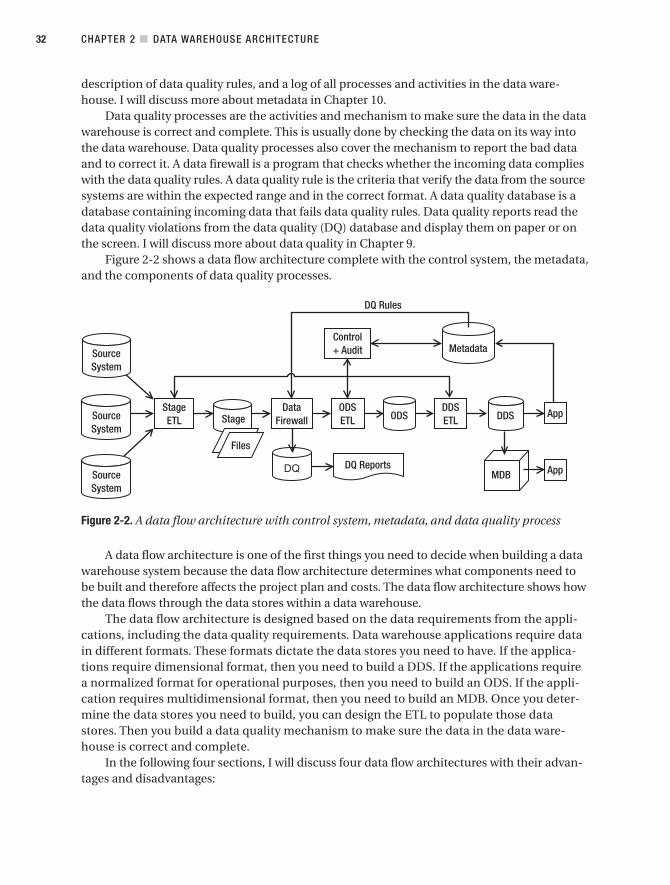
description of data quality rules, and a log of all processes and activities in the data ware-house. I will discuss more about metadata in Chapter 10.
Data quality processes are the activities and mechanism to make sure the data in the datawarehouse is correct and complete. This is usually done by checking the data on its way intothe data warehouse. Data quality processes also cover the mechanism to report the bad dataand to correct it. A data firewall is a program that checks whether the incoming data complieswith the data quality rules. A data quality rule is the criteria that verify the data from the sourcesystems are within the expected range and in the correct format. A data quality database is adatabase containing incoming data that fails data quality rules. Data quality reports read thedata quality violations from the data quality (DQ) database and display them on paper or onthe screen. I will discuss more about data quality in Chapter 9.
Figure 2-2 shows a data flow architecture complete with the control system, the metadata,and the components of data quality processes.
Figure 2-2. A data flow architecture with control system, metadata, and data quality process
A data flow architecture is one of the first things you need to decide when building a datawarehouse system because the data flow architecture determines what components need tobe built and therefore affects the project plan and costs. The data flow architecture shows howthe data flows through the data stores within a data warehouse.
The data flow architecture is designed based on the data requirements from the appli-cations, including the data quality requirements. Data warehouse applications require datain different formats. These formats dictate the data stores you need to have. If the applica-tions require dimensional format, then you need to build a DDS. If the applications requirea normalized format for operational purposes, then you need to build an ODS. If the appli-cation requires multidimensional format, then you need to build an MDB. Once you deter-mine the data stores you need to build, you can design the ETL to populate those datastores. Then you build a data quality mechanism to make sure the data in the data ware-house is correct and complete.
In the following four sections, I will discuss four data flow architectures with their advan-tages and disadvantages:
CHAPTER 2 ■ DATA WAREHOUSE ARCHITECTURE32
9314ch02final.qxd 11/15/07 10:22 AM Page 32
• The single DDS architecture has stage and DDS data stores.
• The NDS + DDS architecture has stage, NDS, and DDS data stores.
• The ODS + DDS architecture has stage, ODS, and DDS data stores.
• The federated data warehouse (FDW) architecture consists of several data warehousesintegrated by a data retrieval layer.
These four data flow architectures are just examples. When building a data warehouse,you need to design the data flow architecture to suit the data requirements and data qualityrequirements of the project. These four architectures are by no means exhaustive; you shoulddesign your own data flow architecture. For example, is it possible to have a data flow architec-ture without a stage? Yes, it is possible, if you can do the transformation on the fly in the ETLserver’s memory, especially if you have a low data volume. Can you have a data flow architec-ture without a DDS? Yes, you can have stage + NDS data stores only if you want to have a nor-malized data warehouse rather than a dimensional one. Is it possible to have two DDSs? Yes,of course you can have multiple DDSs—you can have as many as you need.
Now I’ll go through these four data flow architectures one by one.
Single DDSIn this section, you will learn about a simple data flow architecture that consists of only twodata stores: stage and DDS. In this architecture, the core data warehouse store is in dimen-sional format.
In single DDS architecture, you have a one dimensional data store. The DDS consists ofone or several dimensional data marts. A dimensional data mart is a group of related facttables and their corresponding dimension tables containing the measurements of businessevents, categorized by their dimensions. An ETL package extracts the data from differentsource systems and puts them on the stage.
A stage is a place where you store the data you extracted from the store system tem-porarily, before processing it further. A stage is necessary when the transformation iscomplex (in other words, cannot be done on the fly in a single step in memory), when thedata volume is large (in other words, not enough to be put in memory), or when data fromseveral source systems arrives at different times (in other words, not extracted by a singleETL). A stage is also necessary if you need to minimize the time to extract the data from thesource system. In other words, the ETL processes dump the extracted data on disk and dis-connect from the source system as soon as possible, and then at their own time they canprocess the data.
The physical form of a stage can be a database or files. The ETL that extracts data fromthe source system inserts the data into a database or writes them as files. A second ETL pack-age picks up the data from the stage, integrates the data from different source system, appliessome data quality rules, and puts the consolidated data into the DDS. Figure 2-3 describesa general model of this architecture.
CHAPTER 2 ■ DATA WAREHOUSE ARCHITECTURE 33
9314ch02final.qxd 11/15/07 10:22 AM Page 33

Figure 2-3. Single DDS data warehouse architecture
In Figure 2-3, the “Control + Audit” box contains the ETL control system and audit, as I discussed earlier. They manage the ETL processes and log the ETL execution results. Themetadata database contains the description of the structure, data, and processes withinthe data warehouse.
The data warehouse applications, such as business intelligence (BI) reports, read the datain the DDS and bring the data to the users. The data in the DDS can also be uploaded intomultidimensional databases, such as SQL Server Analysis Services, and then accessed by theusers via OLAP and data mining applications.
Some ETL architects prefer to combine the two ETL packages surrounding the stage inFigure 2-3 into one package, as pictured in Figure 2-4. In Figure 2-4, the stage ETL, the DDSETL, and the data quality processes are combined into one ETL. The advantage of combiningthem into one package is to have more control over the timing of when the data is written toand retrieved from the stage. In particular, you can load the data directly into the DDS withoutputting it to disk first. The disadvantage is that the ETL package becomes more complicated.
Figure 2-4. Data architecture where the stage ETL and DDS ETL are combined
An advantage of a single DDS architecture is that it is simpler than the next three architec-tures. It is simpler because the data from the stage is loaded straight into the dimensional datastore, without going to any kind of normalized store first. The main disadvantage is that it ismore difficult, in this architecture, to create a second DDS. The DDS in the single DDS archi-tecture is the master data store. It contains a complete set of data in a data warehouse,
CHAPTER 2 ■ DATA WAREHOUSE ARCHITECTURE34
9314ch02final.qxd 11/15/07 10:22 AM Page 34

including all versions and all historical data. Sometimes you need to create a smaller DDScontaining a subset of the data in the master DDS for the purpose of specific analysis whereyou want to be able to change the data or you want the data to be static. To create this smallerDDS, you would need to create a new ETL package that retrieves data from the master DDSand populates the smaller DDS. You need to build this ETL package from scratch. You cannotreuse the existing ETL package because the existing ETL package retrieves data from the stageand populates the master DDS. It’s a totally different data flow altogether.
For example, the users may require a static smaller DDS containing only order data forthe purpose of analyzing the impact of a price increase across different customer accounts.They want the BI tool (Business Objects, Cognos, or Analysis Services, for example) to run onthis smaller DDS so they can analyze the price increase. To create this smaller DDS, you needto write a new ETL package.
You would use a single DDS architecture when you need only a one dimensional storeand you don’t need a normalized data store. It is used for a simple, quick, and straightforwardanalytical BI solution where the data is used only to feed a dimensional data warehouse. Asingle DDS solution is particularly applicable when you have only one source system becauseyou don’t need additional NDS or ODS to integrate the data from different source systems.Compared to the NDS + DDS or ODS + DDS architecture, the single DDS architecture is thesimplest to build and has the quickest ETL run time because the data is loaded straight intoDDS without going into the NDS or ODS data store first.
NDS + DDSIn NDS + DDS data flow architecture, there are three data stores: stage, NDS, and DDS. Thisarchitecture is similar to the single DDS architecture, but it has a normalized data store infront of the DDS. The NDS is in third normal relational form or higher. The purpose of havingNDS is twofold. First, it integrates data from several source systems. Second, it is able to loaddata into several DDSs. Unlike the single DDS architecture, in the NDS + DDS architecture youcan have several DDSs. Figure 2-5 shows the NDS + DDS data flow architecture.
Figure 2-5. NDS + DDS data flow architecture
In the NDS + DDS architecture, NDS is the master data store, meaning NDS contains thecomplete data sets, including all historical transaction data and all historical versions of mas-ter data. Historical transaction data means the business transactions that happened in the
CHAPTER 2 ■ DATA WAREHOUSE ARCHITECTURE 35
9314ch02final.qxd 11/15/07 10:22 AM Page 35
past. Data from every single year is stored in the NDS. The DDS, on the other hand, is not themaster data store. It may not contain all transaction data for every single year. NDS containsall historical versions of master data. If there is a change in master data, the attributes are notoverwritten by new values. The new values are inserted as a new record, and the old version(the old row) is kept in the same table.
Similar to an OLTP source system, there are two types of tables in the NDS: transactiontables and master tables. A transaction table is a table that contains a business transaction orbusiness event. A master table is a table that contains the people or objects involved in thebusiness event. A sales order table is an example of a transaction table. A product table is anexample of a master table. The NDS transaction tables are the source of data for the DDS facttable. In other words, the fact tables in the DDS are populated from the transaction tables inthe NDS. The NDS master tables are the source of data for DDS dimension tables. That is, thedimension tables in the DDS are populated from the master tables in the NDS. I will discussmore about NDS in Chapter 5 when I talk about dimensional modeling.
NDS is an internal data store, meaning it is not accessible by the end user or the end-userapplications. Data from NDS is loaded into DDSs in dimensional format, and the end usersaccess these DDSs. The only application that is able to update NDS is the NDS ETL. No otherapplication should be able to update NDS.
The principles about the stage, control, audit, and metadata discussed earlier are alsoapplicable here. Some entities can fly through directly to NDS without being staged to diskfirst. In that case, the data integration/transformation is performed online in the memory ofthe ETL server. The ETL reads the data from the source system, transforms or integrates thedata in memory, and writes the data to NDS directly without writing anything to the stage.Data transformation is converting, calculating, or modifying the data to suit the target data-base. Data integration is combining the same record from several different source systemsinto one record or combining different attributes of master data or transaction data.
In the NDS + DDS architecture, the DDS ETL that loads data into the DDS is simpler thanthe one in the single DDS architecture because the data in the NDS is already integrated andcleaned. In some cases, the DDS ETL needs to feed the data only incrementally to the DDS with-out any transformation. Most, if not all, fact table calculations have been done in the NDS.
The data in the NDS is uploaded to the DDSs. The flexibility of using a centralized NDS isthat you can build a DDS that you need at any time with the scope of data as required. Theability to build a new DDS at any time is useful to satisfy requirements from projects involvingdata analysis. The ability to set the scope of data when building a new DDS means you canpick which tables, columns, and rows you want to transfer to the new DDS. For example, youcan build a DDS containing only a customer profitability data mart (one fact table and all itsdimensions) that contains only the last three months of data.
To populate a new DDS, you can use the existing DDS ETL. You just need to point the ETLto the new DDS. If you build the DDS ETL correctly, you can rebuild any DDS quickly, in otherwords, the only time we need is the time to run the ETL. You don’t have to spend days or weeksto build a new ETL package to load the new DDS. To get this flexibility, the DDS ETL needs to beparameterized; that is, the date range, the fact tables, and the dimensions to be copied acrossare all set as parameters that can easily be changed to point to a new DDS. The database con-nection details are also written as parameters. This enables you to point the ETL to anotherdatabase.
In NDS + ODS architecture, you can have several DDSs. But there is one DDS you have tobuild and maintain: the one that contains all the fact tables and all the dimensions. This one is
CHAPTER 2 ■ DATA WAREHOUSE ARCHITECTURE36
9314ch02final.qxd 11/15/07 10:22 AM Page 36
sort of obligatory; all other DDSs are optional—you build them as you need them. You need tohave this one obligatory DDS because it contains a complete set of data warehouse data and isused by all BI applications that require dimensional data stores.
The NDS tables use surrogate keys and natural keys. A surrogate key is the identifier of themaster data row within the data warehouse. In the DDS, the surrogate key is used as the pri-mary key of dimension tables. The surrogate key is a sequential integer, starting from 0. So, itis 0, 1, 2, 3, …, and so on. Using the surrogate key, you can identify a unique record on a dimen-sion table. Surrogate keys also exist in the fact tables to identify the dimension attributes for aparticular business transaction. Surrogate keys are used to link a fact table and the dimensiontables. For example, using surrogate keys, you can find out the details of the customer for aparticular order. In the NDS + DDS architecture, the surrogate keys are maintained in the NDS,not in the DDS.
A natural key is the identifier of the master data row in the source system. When loadingdata from the stage to NDS, you need to translate the natural key from the source system toa data warehouse surrogate key. You can do this by looking up the surrogate key in the NDSfor each natural key value from the source system. If the natural key exists in the NDS, itmeans the record already exists in NDS and needs to be updated. If the natural key doesn’texist in the NDS, it means the record does not exist in the NDS and needs to be created.
Only internal administrative applications access the NDS directly. These are usually appli-cations that verify the data loaded into NDS, such as data quality routines that check NDSdata against certain firewall rules. End user applications, such as BI reports, access the DDS(dimensional model) and some applications, such as OLAP applications, access the multidi-mensional databases that are built from the DDSs. You need to understand what kind of datastore is required by each application to be able to define the data flow architecture correctly.
The main advantage of this architecture is that you can easily rebuild the main DDS; inaddition, you can easily build a new, smaller DDS. This is because the NDS is the master datastore, containing a complete set of data, and because the DDS ETL is parameterized. Thisenables you to create a separate static data store for the purpose of specific analysis. The sec-ond advantage is that it is easier to maintain master data in a normalized store like the NDSand publish it from there because it contains little or no data redundancy and so you need toupdate only one place within the data store.
The main disadvantage is that it requires more effort compared to the single DDS archi-tecture because the data from the stage needs to be put into the NDS first before it is uploadedinto the DDS. The effort to build ETL becomes practically double because you need to buildtwo ETL sets, while in single DDS it is only one. The effort for data modeling would be about50 percent more because you need to design three data stores, whereas in single DDS youhave two data stores.
The NDS + DDS architecture offers good flexibility for creating and maintaining datastores, especially when creating a DDS. The NDS is a good candidate for an enterprise datawarehouse. It contains a complete set of data, including all versions of master data, and it isnormalized, with nearly no data redundancy, so data updates are more easily and quickly com-pared to the dimensional master data store. It also contains both source systems’ natural keysand data warehouse surrogate keys, enabling you to map and trace data between the sourcesystems and data warehouse.
You would use an NDS + DDS architecture when you need to make several DDSs for dif-ferent purposes containing a different set of data and when you need to integrate data in anormalized form and use the integrated data outside of the dimensional data warehouse.
CHAPTER 2 ■ DATA WAREHOUSE ARCHITECTURE 37
9314ch02final.qxd 11/15/07 10:22 AM Page 37

ODS + DDSThis architecture is similar to an NDS + DDS architecture, but it has an ODS in the place of theNDS. Like NDS, ODS is in third normal form or higher. Unlike the NDS, the ODS contains onlythe current version of master data; it has no historical master data. The structure of its entitiesis like an OLTP database. The ODS has no surrogate keys. The surrogate keys are maintained inthe DDS ETL. The ODS integrates the data from various source systems. The data in the ODS iscleaned and integrated. The data flowing into the ODS has already passed the DQ screening.Figure 2-6 shows ODS + DDS data flow architecture.
Figure 2-6. ODS + DDS data flow architecture
Like NDS, ODS contains transaction tables and master tables. The transaction tablescontain business events, and the master tables contain the people or objects involved inthe business events. The fact tables in the DDS are populated from the transaction tablesin the ODS. The dimension tables in the DDS are populated from the master tables inthe ODS. Unlike NDS, ODS’s master tables contain only the current version of master data.ODS does not contain the historical versions of master data.
Unlike NDS, which is an internal data store, ODS is a hybrid data store. This means ODSis accessible by the end users and end-user applications. In NDS + DDS applications, NDS isnot accessible by the end users and end-user applications. Unlike NDS, ODS is updatable.End-user applications can retrieve data from the ODS, but they can also update the ODS. Toensure the quality of the data in the ODS, data quality rules are also applied to these updates.The end-user application must not update the data coming from the source systems; it canupdate only the data that itself generates to complement the source systems’ data. If the ODSis used to support a CRM customer support application, data such as status and commentscan be written on ODS directly, but all the customer data is still from the source systems.
In the ODS + DDS architecture, the DDS is the master data store. Unlike an NDS + DDSarchitecture, in an ODS + DDS architecture you have only one DDS. The DDS contains a com-plete set of fact tables and the dimension tables. The DDS contains both the current versionand all historical versions of master data.
The principles about the stage, control, audit, and metadata discussed in regard to thesingle DDS architecture are also applicable here. Some entities can fly through directly to theODS without being staged first. Integration and transformation happen in the memory of theETL server. The DDS ETL is simpler than the one in the single DDS architecture because thedata in the ODS is already integrated and cleaned. In many cases, it is literally feeding DDS
CHAPTER 2 ■ DATA WAREHOUSE ARCHITECTURE38
9314ch02final.qxd 11/15/07 10:22 AM Page 38

incrementally without any transformation. Most, if not all, fact table calculations have beendone in the ODS.
In the ODS + DDS architecture, applications can access the data warehouse in threeplaces in three different formats: those that need the data in normalized form can access theODS, those that need the data in relational dimensional format can access the DDS, and thosethat need the data in multidimensional format can access the MDBs.
This architecture has these advantages:
• The third normal form is slimmer than the NDS because it contains only current values.This makes the performance of both ODS ETL and DDS ETL better than the ones in theNDS + DDS architecture.
• Like the NDS + DDS architecture, in the ODS + DDS architecture you have a centralplace to integrate, maintain, and publish master data.
• The normalized relational store is updatable by the end-user application, making itcapable of supporting operational applications at the transaction level.
The disadvantage of this architecture is that to build a new, small DDS (say, 2007 Q4 salesdata), you need to get it from the main DDS and cannot utilize the existing DDS ETL to do that.You need either to write custom queries (in other words, create table from select), which isnot preferred because of standardization and consistency reasons, or to build a new ETL, whichis not preferred either because of the effort, especially if it is a one-off, throwaway thing.
You would use an ODS + DDS architecture when you need only a one dimensional datastore and you need a centralized, normalized data store to be used for operational purposessuch as CRM. The ODS contains detailed, current-valued, integrated data that is useful fortransactional queries.
Federated Data WarehouseA federated data warehouse consists of several data warehouses with a data retrieval layer ontop of them. A federated data warehouse retrieves data from existing data warehouses usingan ETL and loads the data into a new dimensional data store. For example, because of mergerand acquisition activities, you could have three data warehouses. Perhaps the first one is adimensional data warehouse, the second one is a third normal form normalized data ware-house, and the third one is a relational data warehouse with a few big transaction tablesreferencing many reference tables. Figure 2-7 shows a federated data warehouse.
The granularity of the FDW data is the same as the highest of the granularities of sourcedata warehouses. If the granularities of the source data warehouses are G1, G2, and G3, thenthe granularity of the FDW data is the highest of (G1, G2, G3). This is because you can consoli-date data only on the same granularity and because you can transform data only from lowergranularity to higher granularity, not the reverse direction. For example, if G1 is daily, G2 isweekly, and G3 is monthly, then the granularity of FDW is monthly. This is because you cantransform G1 and G2 to monthly, but you cannot transform G3 to daily or weekly.
The ETL that extracts data from the source data warehouses needs to be aware of the tim-ing of the data. The data in the source data warehouses may not arrive at the same frequency.The FDW ETL needs to match the frequency of the source DWs. If the source DWs have differ-ent update frequencies, the FDW ETL needs to run several times to match the frequency ofeach source DW.
CHAPTER 2 ■ DATA WAREHOUSE ARCHITECTURE 39
9314ch02final.qxd 11/15/07 10:22 AM Page 39

Figure 2-7. A federated data warehouse from several data warehouses
The FDW ETL needs to integrate the data from source DWs based on business rules.The ETL needs to identify whether records from one source data warehouse are duplicatesof records from the other source data warehouses. Duplicate records need to be merged.The business rules need to be applied to determine which record should survive and whichattributes need to be updated. In addition, the FDW ETL needs to transform the data fromdifferent source DWs into a common structure and common format.
You also need to bear in mind that the number of subject areas in the FDW is probablynarrower than the number of subject areas in the source DWs. This is because the FDW is ata higher level than the source DWs, and at this level, not all subject areas are applicable anduseful for the business users. For example, in the global data warehouse, you may be inter-ested in sales and employees and leave inventory and campaigns in the regional datawarehouses.
When you have several data warehouses like this, it is possible to implement enterpriseinformation integration (EII) rather than ETL, as described in Figure 2-8, especially if thesource data warehouses are similar. EII is a method to integrate data by accessing differentsource systems online and aggregating the outputs on the fly before bringing the end result tothe user. Everything is done the moment a user requests the information. There is no storageof any form that stores the aggregated or integrated data. The main advantage of using EII isthe data freshness; in other words, the result is truly real time. In Figure 2-8, even if data ware-house DW3 was changed a second ago, the end result will still include that last second change.Even though there is no integrated data warehouse, sometimes this architecture is also calledfederated data warehouse. For example, if the organization consists of three geographicalregions, such as Asia Pacific, America, and EMEA, then each region has a different ERP systemand different IT organizations; hence, they have three data warehousing projects. But they allagreed to standardize on the same structure: dimensional data warehousing with fact anddimension tables.
Instead of integrating several data warehouses, federated data warehouse can also beimplemented when there are several nonintegrated data marts in the organization, as shownin Figure 2-9.
CHAPTER 2 ■ DATA WAREHOUSE ARCHITECTURE40
9314ch02final.qxd 11/15/07 10:22 AM Page 40

Figure 2-8. Federated data warehouse using enterprise information integration
Figure 2-9. A federated data warehouse from several data marts
The source data marts in Figure 2-9 can be in many different forms. They can be dimen-sional, normalized, or neither. These marts could be two conformed fact tables surrounded byfour to eight conformed dimensions in star schema format, properly designed using the Kim-ball dimensional modeling approach. They could be in a snowflake format where the dimen-sions are normalized. They could be in third normal form (or higher). And in many cases, theymight not be data marts at all; in other words, they don’t follow any formal data warehousingdesign approach and instead are just a collection of tables with good data inside them, andthe users call these tables data marts. You can use FDW to integrate these data marts.
The same principles described previously when integrating data warehouses are stillapplicable, specifically, level of granularity, matching/deduplicating, reformatting, dealingwith timing issues, and platform diversity. In some cases, you may want to consider bypassingsome marts and accessing the source systems directly, especially if the same source system issupplying the same data to different data marts.
You can also still use the EII approach here when integrating the data marts. That is, youdon’t have a permanent data store at the federated level but can access the source data martson the fly when users issue their requests.
CHAPTER 2 ■ DATA WAREHOUSE ARCHITECTURE 41
9314ch02final.qxd 11/15/07 10:22 AM Page 41

The main advantage of this architecture is that you can accommodate existing data ware-houses, and therefore the development time will be shorter. The main disadvantage is that,practically speaking, it is difficult to build a good-quality warehouse from such diverse stan-dards found in the source data marts or data warehouses.
You would use federated data warehouse architecture when you want to utilize existingdata warehouses or where you want to integrate data from several data marts.
System ArchitectureThe previous sections covered data flow architecture. They showed how the data is arrangedin the data stores and how the data flows within the data warehouse system. Once you havechosen a certain data flow architecture, you then need to design the system architecture,which is the physical arrangement and connections between the servers, network, software,storage system, and clients. Designing a system architecture requires knowledge about hard-ware (especially servers), networking (especially with regard to security and performanceand in the last few years also fiber networks), and storage (especially storage area networks[SANs], redundant array of inexpensive disks [RAID], and automated tape backup solutions).Figure 2-10 shows an example of a system architecture.
Figure 2-10. Example of a system architecture for data warehouse
In this example, the system architecture consists of three servers: one ETL server, onedatabase server, and one reporting server. The source system is an electronic point-of-salesystem that records retail sales in the stores running on Oracle 9.2 on Sun Solaris. The ETLserver is Informatica PowerCenter 7 installed on Red Hat Enterprise Linux. The data ware-house data stores (stage, DDS, and MDB) are hosted in the SQL Server relational databaseengine and Analysis Services, running on Windows Server 2003. The data is physically storedin a DAS consisting of fifteen 146GB disks, making the raw capacity 2TB. The disks are config-ured in RAID 1 and RAID 5 for data resilience. (I will discuss RAID in Chapter 6 when I coverphysical database design.) The reports are created and managed using SSRS installed onWindows Server 2003.
CHAPTER 2 ■ DATA WAREHOUSE ARCHITECTURE42
9314ch02final.qxd 11/15/07 10:22 AM Page 42
I chose this example because it represents a typical architecture for a medium system.We have a dedicated ETL server, separated from the database server. It’s a medium size ofdata; the raw capacity of 2TB is about 400GB to 500GB final usable database space, assum-ing we have both development and production environments. The platform is a bit of amixture, as typically found in organizations: the source system and ETL are not Microsoft.The Informatica was probably already there when the data warehouse project started, sothey have to use what they already have. Therefore, you can create a system architecturewith different platforms.
A data warehouse architect does not usually design the system architecture of a datawarehouse infrastructure, but in my opinion, it is helpful if they know these subjects—per-haps not at a very detailed level, but they need to know at a high level. For example, they don’tneed to understand how to build a four-node cluster using Windows 2003 servers, but theyneed to know what kind of high availability can be achieved using clustering technology.
To design a data warehouse system architecture, you first establish the technologystack you want to use for ETL, the database, and BI, such as Microsoft SQL Server (SSIS,SSAS, SSIS), Informatica + Oracle 9i + Cognos, and so on. This is determined based onproduct capability and based on the company standard. After you determine the technol-ogy stack, you do a high-level design on the servers, network configuration, and storageconfiguration that supports the chosen technology, including high-availability design.Then you determine the detailed technical specification of the servers, network, and stor-age. This is done based on capacity and system performance requirements. You then orderthe hardware and software and build the system in the data center together with the hard-ware and network vendor. You then install and configure the software. Designing andbuilding the environment is fundamental and critical to the performance and stability ofthe data warehouse system that you are going to build on top of it.
The other factor that greatly affects the system architecture is the choice of software inbuilding the data warehouse, such as specific versions of SQL Server, Oracle, or Teradata. Thesystem architectures required to run this software are different. For example, Teradata runs onmassively parallel processing hardware. It does not share the storage between the nodes. Onthe other hand, a SQL Server cluster uses central storage. It shares the storage between thenodes.
In terms of software, there are two different types of database software: symmetric multi-processing (SMP) and massively parallel processing (MPP). An SMP database system is a data-base system that runs on one or more machines with several identical processors sharing thesame disk storage. When an SMP database system runs on more than one machine, it is calleda clustered configuration. The database is physically located in a single disk storage system.Examples of SMP database systems are SQL Server, Oracle, DB/2, Informix, and Sybase. AnMPP database system is a database system that runs on more than one machine where eachmachine has its own disk storage. The database is physically located in several disk storagesystems that are interconnected to each other. An MPP database system is also known as aparallel database system. Examples of MPP database systems are Teradata, Neoview, Netezza,and DATAllegro.
The machines in SMP and MPP database systems are called nodes. An MPP database sys-tem is faster and more scalable than an SMP database system. In an MPP database system, atable is physically located in several nodes, each with its own storage. When you retrieve datafrom this table, all nodes simultaneously read the data from their own storage, so the process
CHAPTER 2 ■ DATA WAREHOUSE ARCHITECTURE 43
9314ch02final.qxd 11/15/07 10:22 AM Page 43

of reading the data from disk is quicker. Similarly, when you load data into this table, all nodessimultaneously load a bit of the data into their disks. In SMP database systems, there is a bot-tleneck on the disk storage. SMP database systems, on the other hand, are simpler, are easierto maintain, and have lower costs.
In this book, I’ll show how to use SQL Server 2005 to build a data warehouse, but it alsoruns on SQL Server 2008. I will use SSIS for the ETL tool, I will build the NDS and DDS on SQLServer 2005 databases, and I will use SSRS for reporting and SSAS for OLAP and data mining.
Case StudyI will be using the following case study throughout this book. In this chapter, you will bestudying the data warehouse architecture using this case study. In all further chapters, youwill be using this case study to learn the subjects discussed in those chapters in a real projectsituation. For example, in Chapter 5, I will show how to create the data model; in Chapter 6,I will show how to design the database; in Chapters 7 and 8, I will show how to build the ETL,and so on.
This case study needs to cover all the aspects you want to learn in this book: architecture,methodology, requirements, data modeling, database design, ETL, data quality, metadata,data stores, report, multidimensional databases, BI, CRM, testing, and data warehouse admin-istration. Ideally, I want the case study to be simple enough to understand and to deliver as aproject, but I don’t want it to be too simple because it will not cover some areas mentionedpreviously. So, it needs to simple but not too simple.
Some industries are “data warehousing friendly,” meaning the nature of the data is idealfor data warehousing. Retail, utilities, telecommunication, health care, and financial servicesare some of them. In this case study, I chose the retail sector because the business operationsare easier to understand since we experience them in our daily lives.
Amadeus Entertainment is an entertainment retailer specializing in music, films, andaudio books. It has eight online stores operating in the United States, Germany, France, theUnited Kingdom, Spain, Australia, Japan, and India. It has 96 offline stores operating in thosecountries as well.
Customers can buy individual products such as a song, an audio book, or a film, or theycan subscribe to a certain package, which enables them to download a certain quantity ofproducts in a certain period. For example, with the Primer package, you can download 100songs, 50 books, and 50 films a month for $50. Customers can also listen or watch a song, abook, or a film once for 1⁄10 the cost of purchasing it. So if a film is $5, to watch it once it’s only50 cents. Customers use online streaming for this, so a good Internet connection is required.
Amadeus Entertainment has four main delivery channels: Internet, mobile phone,cable TV, and post. There are several payment models for customer subscriptions, such asannual, in advance, and monthly direct debit. The company purchases the products in bulk,such as any 10,000 songs from a record company, of any title, for a certain cost. For onlinestreaming, the company pays a central provider (Geo Broadcasting Ltd.) based on usage(monthly invoice).
The company uses WebTower9, a custom-developed .NET-based system for dynamicweb sites, multimedia trading, broadcasting, sales order processing, and subscription man-agement, all running on an Oracle database. The back-end enterprise resource planning (ERP)
CHAPTER 2 ■ DATA WAREHOUSE ARCHITECTURE44
9314ch02final.qxd 11/15/07 10:22 AM Page 44

system is Jupiter, an off-the-shelf AS/400-based business system running on DB2. This iswhere the inventory, products, and finances are managed. The Jupiter database size is about800GB with about 250 tables and views.
Business activities in the offline stores are managed in Jade, which is a custom Java-basedsystem running on Informix. This includes sales, customer service, and subscriptions.WebTower9 and Jade interface with Jupiter products and finances on a daily basis, but salesand customer data (including subscriptions) are kept on WebTower9 and Jade.
The company uses the SupplyNet system for interfacing with suppliers. It is a webservices–based industry-standard supplier network in the online entertainment industryincluding music and film. WebTower9 and Jupiter are hosted in Amadeus Entertainment’shead office. Jade is hosted in an outsourced company in Bangalore, India. The Jupiter over-night batch starts at 11 p.m. Eastern standard time (EST) for three to four hours. An offlinebackup job kicks off immediately after the overnight batch and runs for one to two hours.The Jade tape backup starts at 3 a.m. EST for two to three hours.
The IT architecture team decided to standardize the database platform on MicrosoftSQL Server and use web-based services for its application platform. Hence, in this casestudy, I will show how to build a data warehouse system for Amadeus Entertainment usingMicrosoft SQL Server 2005. You can also use SQL Server 2008 to build it. I will be using NDS+ DDS data warehouse architecture outlined earlier in this chapter. Figure 2-11 shows thesystem architecture for the production environment.
Figure 2-11. System architecture for the production environment for Amadeus Entertainmentdata warehouse
CHAPTER 2 ■ DATA WAREHOUSE ARCHITECTURE 45
9314ch02final.qxd 11/15/07 10:22 AM Page 45

In Figure 2-11, Integration Services, Reporting Services, and Analysis Services will beinstalled on separate machines. We will be using SAN with a raw capacity of 12TB. The finalstorage capacity could be much less than the raw capacity. When I cover physical databasedesign in Chapter 6, I will be using this system architecture as the basis of the design.
This is only a tentative architecture as an illustration of how it could be implemented. Theserver specifications in Figure 2-11 are high, probably too high for this project. When we getthe requirements, we can further detail the design. For example:
• High-availability requirements (how many hours can they tolerate the data warehouseto be down) affect the clustering decision of the database servers.
• The volume of the data from the source systems affects the number of processors andthe memory of the ETL server and whether we need to put SSIS on a separate machine.
• The volume of the data in the data warehouse affects the storage size and backuprequirements. The SAN raw disk size may be less or more than 12TB depending on theactual requirements.
• The number and sizes of the OLAP cubes affect the memory and processors of theOLAP server and whether you need to put Analysis Services on a separate server.
You need to bear in mind, especially when budgeting for infrastructure (hardware andsoftware), that you need to make a second set for the testing environment (widely known asquality assurance [QA]) and another set for the development environment (or dev, for short).Unlike in OLTP, in data warehousing it is essential that QA has an identical capacity as produc-tion. This is because in data warehousing you need to do performance and volume testing. Ifyour QA is only half the capacity of production, your measurement in performance testing willbe incorrect. An ETL batch that in production runs for three hours in QA may run for sevenhours.
The dev environment can be of lower specifications than production. For example, in theAmadeus Entertainment case study, dev can be just one server; in other words, the databaseengine, Integration Services, Analysis Services, and Reporting Services are all installed in oneserver. This is because the primary purpose of dev is functionality development. Performancetesting is conducted in QA.
The most difficult questions to answer when designing the system architecture are aboutsizing and/or capacity. In particular, infrastructure suppliers usually ask these two questions:
• How much disk space do you require (how big is your data)?
• How much processing power do you need (in terms of processor and memory)?
We will go through physical database design in more detail in Chapter 6, along with theinfrastructure considerations.
CHAPTER 2 ■ DATA WAREHOUSE ARCHITECTURE46
9314ch02final.qxd 11/15/07 10:22 AM Page 46

SummaryIn this chapter, I discussed several data warehouse architectures. The single DDS, NDS + DDS,and ODS + DDS architectures have dimensional data warehouse. The single DDS does not havea normalized store, while the others have a normalized store. The federated data warehousearchitecture consists of several data warehouses integrated by a data retrieval layer. I also dis-cussed the system architecture in particular for implementation using SQL Server 2005.
You’ll use the case study introduced in this chapter to help you understand the subjectsin later chapters. In Chapter 5, when I discuss dimensional modeling and entity relationshipmodeling, I will go through the data warehouse design in more detail. In Chapter 6, when Idiscuss physical database design, I will go through the elements of system architecture inmore detail.
CHAPTER 2 ■ DATA WAREHOUSE ARCHITECTURE 47
9314ch02final.qxd 11/15/07 10:22 AM Page 47

9314ch02final.qxd 11/15/07 10:22 AM Page 48

Data Warehouse DevelopmentMethodology
Some people believe they do not need to define the business requirements when buildinga data warehouse because a data warehouse is built to suit the nature of the data in the organ-ization, not to suit the people. I believe that all IT systems of any kind need to be built to suitthe users. A system must be usable. If the system is not used, there is no point in building it.This usability concept is fundamental to this chapter, so keep that in mind.
In this chapter, I will explain the process, or methodology, of building a data warehouse.In software engineering, the discipline that studies the process people use to develop an infor-mation system is called the system development life cycle (SDLC) or the system developmentmethodology. There are two main variants: waterfall and iterative. The waterfall methodologyis also known as the sequential methodology. The iterative methodology is also known as thespiral or incremental methodology.
The waterfall methodology is one of the oldest methodologies (it has been around forabout 30 years) and is widely used by many organizations to build their systems, includingtheir data warehouse systems. The iterative methodology is very different from waterfall. It isnot as widely used as waterfall, but it gives good benefits if used correctly. Some people preferwaterfall and some people prefer iterative, so I will compare the two and describe their advan-tages and disadvantages, along with some personal experience in implementing them in datawarehousing projects, from which I hope we can all learn.
Waterfall MethodologyIn a waterfall system, you have certain steps that need to be accomplished one way after theother, in a particular sequence, like going down the stairs or like a multistep waterfall (whichis where it gets its name from). There are many variations of the steps’ names, but in generalthey are feasibility study, requirements, architecture, design, development, testing, deploy-ment, and operation. Figure 3-1 describes these steps in order.
49
C H A P T E R 3
9314ch03final.qxd 11/15/07 10:20 AM Page 49
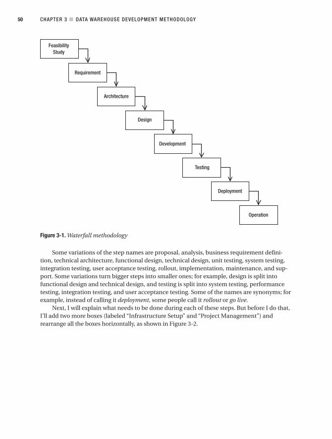
Figure 3-1. Waterfall methodology
Some variations of the step names are proposal, analysis, business requirement defini-tion, technical architecture, functional design, technical design, unit testing, system testing,integration testing, user acceptance testing, rollout, implementation, maintenance, and sup-port. Some variations turn bigger steps into smaller ones; for example, design is split intofunctional design and technical design, and testing is split into system testing, performancetesting, integration testing, and user acceptance testing. Some of the names are synonyms; forexample, instead of calling it deployment, some people call it rollout or go live.
Next, I will explain what needs to be done during each of these steps. But before I do that,I’ll add two more boxes (labeled “Infrastructure Setup” and “Project Management”) andrearrange all the boxes horizontally, as shown in Figure 3-2.
CHAPTER 3 ■ DATA WAREHOUSE DEVELOPMENT METHODOLOGY50
9314ch03final.qxd 11/15/07 10:20 AM Page 50

Figure 3-2. Waterfall methodology with infrastructure setup and project management
I’ll now discuss the boxes in the figures one by one, detailing what you need to do whenbuilding a data warehouse:
Feasibility study: You gather the requirements at a high level (for example, determiningwhy you need a data warehouse and whether data warehousing is the right solution), youhave a quick look at the source systems to find out whether it is possible to get the datayou need, you get sample data to assess the data quality, and you write a proposal (somepeople prefer to call this document the business case). The important things to mention inthe proposal are the benefits, how long it will take, how much it will cost, and the businessjustifications. Other things that you probably need to put in the proposal are the require-ments (just the summary), the project organization (including external resources such asconsultants and contractors), and the project plan (it’s very important to know who willbe doing what when).
As you can see, in order to produce a decent proposal, you have to know everything inadvance: the requirements, the solution, the architecture, the design, the infrastructure,the data quality, what tasks are required, and how you would resource it (external or inter-nal). All these are required to find out how long it will take to build the data warehouseand how much will it cost. This step requires experience. It can really be done only bythose people who have built data warehouse systems several times. For example, at thisearly stage, how would you know the specification of the servers and how long it wouldtake to build the ETL system?
CHAPTER 3 ■ DATA WAREHOUSE DEVELOPMENT METHODOLOGY 51
9314ch03final.qxd 11/15/07 10:20 AM Page 51

I find that it is best to set the feasibility study step as its own project on separate budget.In this phase, the work is to analyze the requirements and data volume at a high level anddetermine a suitable architecture and toolset so you can produce a rough estimate. Forthis work, you need a business analyst to analyze the requirements, a data warehousearchitect to determine the architecture, and a project manager to produce the estimateand high-level project plan. The number of resources varies from project to project; forexample, you may need more than one business analyst if several distinct business areasare involved. Other types of resources that may be required during the feasibility studyphase are a hardware and infrastructure person (to verify the details of the proposedarchitecture), a business owner (such as a customer service manager), and the sourcesystem DBA (to get information about the data volume).
Requirements: You talk to the users to understand the details of the processes, thebusiness, the data, and the issues. Arrange site visits to get firsthand experience. Dis-cuss the meaning of the data, the user interface, and so on, and document them. Youalso list the nonfunctional requirements such as performance and security. I will gothrough the requirements in more detail in the next chapter.
Architecture: I discussed this in the previous chapter. Basically, you need to determinewhich data flow architecture you are going to use and what system architecture you aregoing to use, in detail, including the specification for database servers, the type of net-work, the storage solution, and so on. It is important to have somebody who has done thismany times; if you don’t have anybody in the organization with these skills, then hirefrom outside. It is not common to find data warehousing and infrastructure skills in oneperson. This is a critical step, meaning that if the architecture is wrong, you may have toredesign everything from scratch or restart the project from the beginning.
Design: You need to design three main parts of the data warehouse system: the datastores, the ETL system, and the front-end applications. These require different skill sets sopotentially it could require different people. I will go through the data stores in Chapters 5and 6, the ETL system in Chapters 7 and 8, and the front-end applications in Chapters 11to 15. In addition, you need to design two other parts: data quality systems and metadata,which I will discuss in Chapters 9 and 10. Some people consider data quality and meta-data as part of the ETL system.
Development: You need to build the three parts that you design: the data stores, the ETLsystem (including data quality system and metadata), and the front-end application. I’lldiscuss these topics in the relevant chapters mentioned in the previous paragraph. Withsome caution and consideration, these three parts can be built in parallel. The mostimportant consideration when building in parallel is to define accurate interfacesbetween the parts.
Testing: Basically, you need to test the data stores, the ETL, and the front-end applica-tions. This is potentially the weakest point in the whole project. In many projects I’veworked on that used the waterfall approach, testing has always been the problematicpart. Everything is quiet until the development finishes and testing begins. Why? Well, thisis the first time all the components are put together and the first time the whole architec-ture runs as a system. This is the first time the users see the data warehouse. This is the
CHAPTER 3 ■ DATA WAREHOUSE DEVELOPMENT METHODOLOGY52
9314ch03final.qxd 11/15/07 10:20 AM Page 52

first time the test environment and the production environment are used. This is the firsttime you try to run the system at maximum capacity (for performance testing). Thego-live date is approaching fast, and you cannot risk any errors in the productionenvironment. There are so many “first-time” happenings at the time of testing, it’s nowonder there are many surprises. As a result, you spend a lot of time and money fixing theproblems. (I will discuss data warehouse testing in Chapter 16.) You can mitigate theseproblems by putting together these components and running the whole architectureseveral times during development. Another way to mitigate these problems is by doingprototyping to discover problems early.
Deployment: Once the system is ready, you put all the components in the productionboxes: the ETL system, the data stores, and the front-end applications. You do the initialload; that is, you load the data from the source system for the first time. You do a few testsin the production environment to make sure the data warehouse is populated correctlyand the front-end applications are producing the correct figures. You produce the userguide, the operation guide, and the troubleshooting guide for the operations team. Youtrain the users and the operations team. You support the system, the users, and the opera-tions team for a few weeks. You hand over the system to the operations team, and youclose the project. I will discuss deployment in Chapter 16 when I discuss testing.
Operation: The users continue to use the data warehouse and the application. The opera-tions team continues to administer the data warehouse and to support the users. Thereare basically three types of support: solving errors or problems that happen when usingthe system, administering new users and their access rights (and of existing users), andhelping new and existing users using the system (kind of “how do I…?” questions). Userswill also have enhancement requests: to add more data to the data warehouse (or changeexisting data), to add a feature to the front-end applications, or to create a new report ora new cube. The operations team will then pass these requests to you in the developmentteam. You prioritize the requests, and then either you reject them or you do them andinclude them in the next release.
Infrastructure setup: One of the biggest tasks when you build an application is to preparethe production environment where you are going to run the application and to build thedevelopment and testing environment. This task consists of creating system architecture,doing technical design, procuring goods (buying the hardware and software), installinghardware, installing and configuring software, connecting networks (including firewallchanges), testing the infrastructure, producing infrastructure documentation, and hand-ing it all over to the operations team. It is a project in itself and needs to be managed assuch. At the very least it should be managed as a subproject. In my experience, manypeople underestimate the scale of this task, which usually results in the data warehouseproject being delayed because the infrastructure is not ready.
Project management: This is when you maintain the project plan (that means at any timeyou have to know the status of each task and who will be doing what and when), maintaingood communication with all stakeholders (project sponsors, users, and developers)including status reports and meetings, and attack the risks aggressively (rather thanresolving them when they become issues).
CHAPTER 3 ■ DATA WAREHOUSE DEVELOPMENT METHODOLOGY 53
9314ch03final.qxd 11/15/07 10:20 AM Page 53

Iterative MethodologyThe basic principle of the iterative methodology is to release bigger and bigger portions ofthe complete project to discover problems early and make necessary adjustments when therequirements cannot be adequately defined by users. In the waterfall methodology, you go liveonce, and prior to that you have a period of testing when you try to fix errors. In the iterativemethodology, you release a version of the system several times into production to be used byselected users. For example, say it will take eight months to build a data warehouse system;using the waterfall methodology, it is going live in month 8. If you use the iterative methodol-ogy, you will be releasing a version in months 3, 6, and 8 (three times) into production.
You build the data warehouse in pieces horizontally. In each iteration, you build a piecefrom end to end. In other words, in each iteration you do the requirements, design, build, test,put it into production, and have the users use it. And you build all the necessary componentsto support that piece in production. For example, if you want to deliver a data mart, you buildthe ETL, the data stores, and the front-end application. Figure 3-3 shows this concept.
Figure 3-3. Building a data warehouse in multiple iterations
You can also picture the iterative methodology as a circle or spiral where each cycle con-sists of design, development, testing, and deployment. The architecture needs to be done onlyin the first iteration. Figure 3-4 describes this.
When working on the sections labeled as “Design” in Figure 3-4, you need to define therequirements too. Also, you need to do a feasibility study before the section labeled as “Arch”in Figure 3-4. To be completely thorough, after the last “Deploy” section, you can add the“Operation” segment too.
CHAPTER 3 ■ DATA WAREHOUSE DEVELOPMENT METHODOLOGY54
9314ch03final.qxd 11/15/07 10:20 AM Page 54
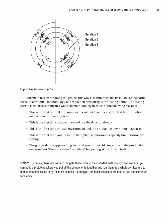
Figure 3-4. Iterative cycles
The main reason for doing the project this way is to minimize the risks. One of the bottle-necks in a waterfall methodology, as I explained previously, is the testing period. The testingperiod is the riskiest time in a waterfall methodology because of the following reasons:
• This is the first time all the components are put together and the first time the wholearchitecture runs as a system.
• This is the first time the users see and use the data warehouse.
• This is the first time the test environment and the production environment are used.
• This is the first time you try to run the system at maximum capacity (for performancetesting).
• The go-live date is approaching fast, and you cannot risk any errors in the productionenvironment. There are many “first-time” happening at the time of testing.
■Note To be fair, there are ways to mitigate these risks in the waterfall methodology. For example, youcan build a prototype where you put all the components together and run them as a whole architecture todetect potential issues early. Also, by building a prototype, the business users are able to see the user inter-face early.
CHAPTER 3 ■ DATA WAREHOUSE DEVELOPMENT METHODOLOGY 55
9314ch03final.qxd 11/15/07 10:20 AM Page 55

The iterative methodology eliminates all five risks and problems mentioned earlier! Allfive of them have been done since iteration 1 so that at the final go-live date (iteration 3), thesystem will run a lot more smoothly. Let’s go through this process step by step:
1. In the first iteration, you run the whole architecture as a system.
2. In the first iteration, the users see and use the data warehouse.
3. In the first iteration, the test and production environments are used.
4. In the first iteration, you run the system at maximum capacity for performance testing.
5. In the first iteration, you deploy to production (go live).
And by the time you reach the last iteration, there are no “first times” left! This eliminatesthose risks and problems.
Perhaps it is easier to explain with an example. Let’s use the Amadeus Entertainment casestudy that I described in Chapter 2. Say, for example, the solution for this particular project isto build four data marts: sales, purchasing, inventory, and CRM. Let’s say for argument’s sakethat CRM is the most complex data mart and purchasing is the easiest data mart. You will seethe detailed design of these data marts in Chapter 5 when I discuss dimensional modeling,but for now let’s concentrate on how to use the iterative methodology. Let’s also say that thesystem architecture that you are going to use is similar to Figure 2-11. You will be using theNDS + DDS data architecture (please refer to Chapter 2). There will be five full-time peopleworking on the project: a project manager (PM), a data warehouse architect (DWA), a businessanalyst (BA), and two developers.
In this particular project, you will go live three times. The focus of the first iteration is thearchitecture. This doesn’t mean you don’t deliver any functionality. You do deliver functional-ity by building the easiest data mart (purchasing). In fact, you are building the entire system,from ETL to data stores to reports to cubes. But the focus in the first iteration is on architec-ture, which is why you don’t want to take the most difficult data mart to build during the firstiteration. In the Rational Unified Process (RUP) methodology, this type of iteration is calledelaboration, where you focus on the architecture. RUP is one of the methodologies that usesan iterative approach.
The focus of the second iteration is the functionality. Therefore, in the second iteration,you pick the most complex data mart (CRM). Because it is the most difficult data mart, if youcan do this mart, all other marts should not be a problem. In RUP, the type of iteration whereyou focus on functionality is also an elaboration phase.
Now that you have made sure the architecture works and that you can build the mostdemanding functionality, in the third iteration you just need to work like a factory to producecode as efficiently as possible. In RUP, this type of iteration is called construction, where youdo mass production to complete the system. In RUP, there is one more type of iteration calledinception (which is the first iteration), where you focus on getting the stakeholders to agreeon the objectives, the rough architecture, and the high-level schedule.
In the Amadeus Entertainment case study, iteration 1 will run for three months, produc-ing a live system in the production environment. The system is not necessarily ready for useby all users, because not all functionality is built yet. The main goal of this iteration is to prove
CHAPTER 3 ■ DATA WAREHOUSE DEVELOPMENT METHODOLOGY56
9314ch03final.qxd 11/15/07 10:20 AM Page 56

that the system architecture and data architecture work. You do this by getting the easiest datamart (purchasing) up and running in the production system. The DWA will specify the systemarchitecture technically (as in Figure 3-5), and the PM will coordinate with infrastructure peo-ple to get it purchased, installed, and set up, including the necessary connectivity to and fromdifferent parts of the network to build the architecture. The DWA will supervise the installationtechnically, for example, the disk carving of the SAN and the configuration of SQL Server. Theinfrastructure team (internal or external contractors) will get production, quality assurance(QA), and development environment set up and ready. The result is an up-and-running sys-tem architecture and infrastructure, as shown in Figure 3-5.
Figure 3-5. System architecture built in iteration 1
The BA and DWA will work together to design and create part of the NDS and DDS data-bases required by the purchasing data mart, as shown in Figure 3-6. They will also specify thefront-end application for three reports and one OLAP cube. The two developers will build theETL and the report and set up the OLAP cube. The system will extract the purchase order tablefrom the Jupiter, Jade, and WebTower9 systems every day and load the data into the NDS data-base. The DDS ETL will get the data into the DDS database, as shown in Figure 3-6.
CHAPTER 3 ■ DATA WAREHOUSE DEVELOPMENT METHODOLOGY 57
9314ch03final.qxd 11/15/07 10:20 AM Page 57
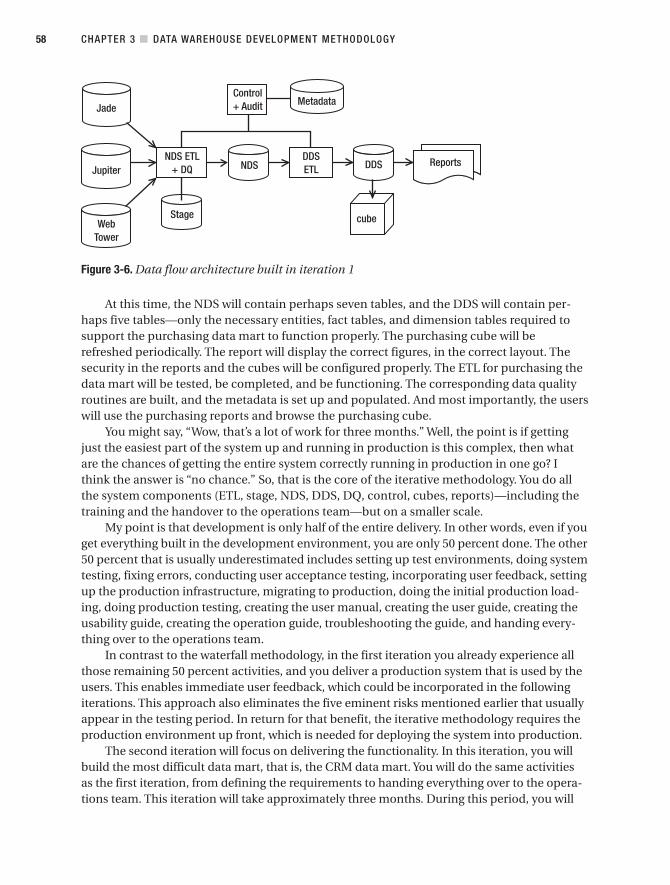
Figure 3-6. Data flow architecture built in iteration 1
At this time, the NDS will contain perhaps seven tables, and the DDS will contain per-haps five tables—only the necessary entities, fact tables, and dimension tables required tosupport the purchasing data mart to function properly. The purchasing cube will berefreshed periodically. The report will display the correct figures, in the correct layout. Thesecurity in the reports and the cubes will be configured properly. The ETL for purchasing thedata mart will be tested, be completed, and be functioning. The corresponding data qualityroutines are built, and the metadata is set up and populated. And most importantly, the userswill use the purchasing reports and browse the purchasing cube.
You might say, “Wow, that’s a lot of work for three months.” Well, the point is if gettingjust the easiest part of the system up and running in production is this complex, then whatare the chances of getting the entire system correctly running in production in one go? Ithink the answer is “no chance.” So, that is the core of the iterative methodology. You do allthe system components (ETL, stage, NDS, DDS, DQ, control, cubes, reports)—including thetraining and the handover to the operations team—but on a smaller scale.
My point is that development is only half of the entire delivery. In other words, even if youget everything built in the development environment, you are only 50 percent done. The other50 percent that is usually underestimated includes setting up test environments, doing systemtesting, fixing errors, conducting user acceptance testing, incorporating user feedback, settingup the production infrastructure, migrating to production, doing the initial production load-ing, doing production testing, creating the user manual, creating the user guide, creating theusability guide, creating the operation guide, troubleshooting the guide, and handing every-thing over to the operations team.
In contrast to the waterfall methodology, in the first iteration you already experience allthose remaining 50 percent activities, and you deliver a production system that is used by theusers. This enables immediate user feedback, which could be incorporated in the followingiterations. This approach also eliminates the five eminent risks mentioned earlier that usuallyappear in the testing period. In return for that benefit, the iterative methodology requires theproduction environment up front, which is needed for deploying the system into production.
The second iteration will focus on delivering the functionality. In this iteration, you willbuild the most difficult data mart, that is, the CRM data mart. You will do the same activitiesas the first iteration, from defining the requirements to handing everything over to the opera-tions team. This iteration will take approximately three months. During this period, you will
CHAPTER 3 ■ DATA WAREHOUSE DEVELOPMENT METHODOLOGY58
9314ch03final.qxd 11/15/07 10:20 AM Page 58

build all the components required to support the CRM mart: the ETL, the data stores, theapplication, the data quality, and the metadata. This second iteration is usually easier than thefirst iteration because the people now have the experience to develop, test, and deploy to pro-duction. In addition, the development, quality assurance (QA), and production environmentsare already set up and configured properly, and the users know what to expect, so there are nosurprises there.
The last iteration will deliver the remaining functionality, the sales and inventory datamarts. In this iteration, you can accommodate change requests based on the user feedbackon the first two iterations. You will do the same activities as the previous two iterations: fromgathering the requirement to handing everything over to the production team. You will buildthe same components: the ETL system, metadata system, data quality system, data stores,and front-end applications.
The advantage of using this iteration methodology is obvious: it minimizes the risks. Inother words, the project has more of a chance to be successful, and the delivered system willhave a better quality. The main disadvantage is that the infrastructure needs to be deliveredup front.
SummaryThe waterfall methodology is commonly used in software development including in datawarehousing. There are three main streams of work: ETL, data stores, and front-end applica-tions. In the waterfall methodology, you go live once, while in the iterative methodology you golive many times. With waterfall, the riskiest period is during testing. This is because it is the firsttime the whole architecture runs as a system, the first time the users see the data warehouse,and the first time the production environment is used. It’s also risky because the go-live date isapproaching fast, and you cannot risk any errors in the production environment.
The iterative methodology overcomes those problems by bringing deployment to produc-tion up front. By doing this, you do all the critical things in the first iteration. You minimize therisks because you go live with only one piece of the system.
CHAPTER 3 ■ DATA WAREHOUSE DEVELOPMENT METHODOLOGY 59
9314ch03final.qxd 11/15/07 10:20 AM Page 59

9314ch03final.qxd 11/15/07 10:20 AM Page 60

Functional and NonfunctionalRequirements
It is important to define functional and nonfunctional requirements when building a datawarehouse system to make sure that the system we build will help users achieve the businessobjectives. Functional requirements define what the system does. They contain the featuresthat the data warehouse system should have. Nonfunctional requirements guide and constrainthe architecture.
Sometimes the best way to learn something is by doing it. In this chapter, I will use theAmadeus Entertainment case study described in Chapter 2 to show how to gather functionaland nonfunctional requirements. First, we will find out about Amadeus Entertainment’sbusiness issues and challenges. Then we will identify the business areas that would benefitfrom a data warehouse system. We will then dive into each of these areas and learn aboutthe business operations within that area. By that I mean the purpose, the processes, theroles, the exceptions, and the issues. We will need this understanding later when we do datamodeling in the next chapter.
After we understand the business operations, we will define the functional requirements,that is, the things that define what the data warehouse system does, such as the questions orissues that a data warehouse system will be able to answer, the data that will be stored in thedata warehouse, and the analysis the users will be performing. We will also define the non-functional requirements, such as security, availability, and performance. An example of anonfunctional requirement (in this case, availability) is that the data warehouse is expectedto be up and running with downtime of less than one hour a month.
We will then investigate the operational systems (Jupiter, WebTower9, and Jade) and con-duct a data feasibility study to find out whether the data that we need is available in the sourcesystems and whether it is accessible. We will research the amount of data, the condition of thedata, and the quality of the data and try to identify any potential risks in the project that couldprevent us from delivering a data warehouse system that satisfies those functional and non-functional requirements.
Identifying Business AreasIn the case study, Amadeus Entertainment is a worldwide online and offline retailer specializ-ing in music, films, and audio books, with outlets in eight countries. Let’s name the key peoplein this case study: the business project manager is Grace, the data warehouse architect is
61
C H A P T E R 4
9314ch04final.qxd 11/15/07 10:19 AM Page 61

David, and the project manager is Natalie. They met with various managers and directors fromvarious parts of the business and talked about the business operations and the business issuesthat the managers were facing. They then visited several physical stores, talked to the storemanagers and employees, and studied the details of how the business works in the stores.
They also visited the online stores and looked at the product categories and the salesorder process. They also created a few orders in WebTower9 (the online store system) and fol-lowed up these orders into the back end of the system. Let’s say that from these activities theyfound the following business challenges and issues:
• Because Amadeus Entertainment spans several countries and operates on three differ-ent systems, it has difficulty aggregating worldwide sales (including returns) at anytime. The company also needs to analyze sales by product and geographic area.
• The company needs to evaluate supplier performance based on delivery lead time andpromptness, order volume and quantity, trading and payment history, and store stockfluctuation records, regardless of brand, country, and transaction system. Historically,this activity has also been laborious.
• The company wants to be able to select certain customers based on demographicattributes, order history, and communication permissions and send them newslettersvia e-mails containing promotional offers, regardless of which systems they are on, andrecord the customer responses, such as opening the e-mails and visiting the companyweb sites.
They then grouped these issues and challenges into three business areas: sales, purchas-ing, and CRM.
Understanding Business OperationsGrace (the business project manager) and David (the data warehouse architect) then wentback to the business users and drilled down into each area to understand the business opera-tions in each area. They tried to understand the processes, the roles, and the issues in eacharea. In particular, they were looking for business events, status, levels, and roles.
• An event is an activity that happens repeatedly every few seconds or minutes. Or itcould be every few hours or days. For example, in the purchasing area, we have adocument called a purchase order. This document contains a request to the supplier(a music record company, for example) to supply the company with some products(CDs or MP3 songs, for example). Every week Amadeus Entertainment creates hun-dreds of these documents and sends them to various suppliers. This purchase ordercreation is an event. Another example of an event is when a customer buys a recordor downloads a song from the online stores.
• A status is a condition of an object at a particular point in time. For example, a song canhave a status of active or obsolete. A customer subscription can have a status of sub-scribed, unsubscribed, or does not exist.
CHAPTER 4 ■ FUNCTIONAL AND NONFUNCTIONAL REQUIREMENTS62
9314ch04final.qxd 11/15/07 10:19 AM Page 62

• A level is a quantitative measurement of an object at a particular point in time, such asaccount balance, inventory level, and number of customers. These quantitative meas-urements change from time to time.
• Roles are the who, whom, and what involved in the event. For example, the roles in thepurchase order event are supplier, account manager, and product. The account man-ager raises a purchase order for a supplier for a particular product. The roles in the sub-scriber event are customer, package, and store; in other words, a customer subscribesto a package in a store.
After talking to business users about these three areas, Grace and David found out thatthe events, status, and levels in Amadeus Entertainment were as follows: sales event, browsingevent, subscribe event, customer class, customer band, purchase order event, campaign sentevent, campaign opened event, campaign click-through event, inventory level, package rev-enues, and package costs. They then worked with the business people to get all the roles andattributes associated with each event and process. In this activity, they tried to understand thebusiness terminology and the business principles in the corporation.
David and Grace spent some time again exploring the WebTower9, Jupiter, and Jade sys-tems. They examined in detail how these processes happen and how these events are capturedin these systems. David then sat down with the SQL Server, DB/2, and Informix DBAs for a fewhours and conducted a brief walk-through of the database of each system.
Defining Functional RequirementsAfter understanding the business operations in each area, the business project manager(Grace) discussed with the business users the functional requirements, that is, the featuresand functions of the data warehouse. In other words, what does the system do? In the end,they agreed that the Amadeus Entertainment data warehouse system has the functionalrequirements shown in Table 4-1. The users collectively agreed that the business prioritiesof the requirements are as per the Priority column in Table 4-1.
Table 4-1. Amadeus Entertainment Data Warehouse System Functional Requirements
No. Requirement Priority
1 The business users need to be able to analyze “product sales” (that’s when a Highcustomer is buying a product rather than subscribing to a package) over time by geographic area, by customer demographic, by stores and sales territory, and by product hierarchy. The users also need to know the revenues, the costs, and the margin in U.S. dollars. Local currencies will be converted to U.S. dollars.
2 The business users need to be able to analyze “subscription sales” (that’s Highwhen a customer is subscribing to a package rather than purchasing a product) over time by geographic area, by customer demographic, by stores and sales territory, and by product hierarchy. In addition, the users also need to analyze subscription sales by subscription duration and lead source (in other words, where the customers are coming from). The users need to know the revenues, costs, and margins, evaluated every day for a period of one month.
Continued
CHAPTER 4 ■ FUNCTIONAL AND NONFUNCTIONAL REQUIREMENTS 63
9314ch04final.qxd 11/15/07 10:19 AM Page 63

Table 4-1. Continued
No. Requirement Priority
3 The business users will be able to analyze “subscriber profitability,” which is Highdefined as the projected annual revenue of the subscribing customer minus the annualized costs (including proportional indirect costs), expressed as a percentage of the projected annual revenue. This is analyzed over time, by geographic area, by customer demographic attributes, by stores and sales territory, and by product package.
4 The business users need to be able to allocate subscribers to specific “classes” Mediumbased on the customer’s projected annual revenue and allocate them to certain “bands” based on the profitability. The classes and bands are used in the loyalty programs. These two attributes are updated daily.
5 The business users will be able to analyze “supplier performance,” which is the Lowweighted average of the totals spent, costs, value of returns, value of rejects, title and format availability, stock outages, lead time, and promptness.
6 The system will enable CRM users to select customers based on communica- Hightion permissions (subscribed/unsubscribed, e-mail/phone/post, and so on), geographic attributes (address, city, and so on), demographic attributes (age, gender, occupation, income, hobby, and so on), interests (music taste, book topic interests, favorite film types, and so on), purchase history (order values, order dates, number of items, store locations, and so on), subscription details (details of packages, subscription dates, durations, store locations, and so on), and the attributes of the products purchased (for example, music genre, artist, film type, and so on) for the purpose of sending CRM campaigns.
7 The system will enable CRM users to analyze campaign results by viewing the Mediumfollowing measures for each campaign sent to customers: the number of mes-sages sent by communication channels (mobile phone text message, e-mail, or post), the number of messages delivered successfully, and the number of messages failed to be delivered (including the reason). For e-mail messages, the users need to analyze the following additional information: open rate, click-through rate, complaint rate, spam verdict, and trap hit rate.
8 For CRM analysis purposes, the data warehouse will store the customers’ old Lowoccupations, incomes, addresses, e-mail addresses, and telephone numbers, especially the subscribers (as opposed to the purchasers).
9 The data warehouse will store the previous region and division of each store. LowThere is a plan to reorganize the store hierarchy; that is, currently there are only five regions in the United States, but in a few months’ time there will be eight regions. Online stores are currently in a separate division, but in the future they will be in the same division as their offline colleagues. Reorganiza-tion like this rarely happens. This is the first time it has happened in the six-year history of Amadeus Entertainment. You can expect the new structure to last at least three years.
10 For requirements 1 to 7, when the data warehouse goes live, two years of Mediumhistorical transactional data needs to be loaded into the warehouse, except requirement 5, which should be one year.
11 The data warehouse will store the data up to five years online and five years Lowoffline. The offline data should be able to be accessed online with two days of notice.
12 The system will enable the store managers to view the data of just their own Highstores. This is because each store manager is responsible for different stores. This is applicable for both offline and online store managers.
CHAPTER 4 ■ FUNCTIONAL AND NONFUNCTIONAL REQUIREMENTS64
9314ch04final.qxd 11/15/07 10:19 AM Page 64

No. Requirement Priority
13 At the store level, the ability to view the daily data in the past few weeks is Highimportant. The system should enable the store managers to see the ups and downs of sales, costs, and profitability, and they need to be able to drill down to any particular day to understand the causes of low sales or low profitability, that is, which products, titles, media, or customers caused the issue.
14 The data warehouse system will enable the global managers to understand Mediumthe global trends and break them down by country. They do not need store-level data or daily data. If a certain store or country is having a problem with a particular media, title, or product (for example when they are experiencing negative trends), then the managers needs to be able to communicate this to all stores as early as possible.
15 The report and OLAP will have an easy-to-use user interface. As long as the user Lowinterface enables the company to perform the analysis in this table and it is easy to use, the users do not really care about the details of the user interface. The numbers are much more important to the users than the layout. The data ware-house users understand that their job is to deliver business performance, and these numbers are the enabler.
16 The system will be able to display the figures and charts and will be able to print. LowThe users collectively agree that they will need charts and graphs, but if this fea-ture is not available, they can export to Excel and do the graphs there. They will need an export to Excel (or to CSV) feature.
David, Grace, and Natalie reviewed these functional requirements, documented them,and obtained the necessary sign-off. They reviewed the requirements in terms of complete-ness, feasibility, and data availability. They documented them in the form of use cases. Thebusiness users reviewed the use cases and signed off on them.
Defining Nonfunctional RequirementsMeetings with the IT architecture and operations teams and discussions with the businessusers revealed the nonfunctional requirements described in Table 4-2. Functional require-ments determine what the system does (the features), whereas nonfunctional requirementsdo not specify the features. Instead, nonfunctional requirements provide guides and con-straints to the system architecture. Some of them are from the company IT standards, someare from the IT architecture team, some are from source system restrictions (requests fromthe source system DBAs and operations manager), and some are from the user needs (require-ments from the business users). There are also nonfunctional requirements related to projectmanagement or how the project should run, such as requirements related to the time, resources,locations, and budgets.
CHAPTER 4 ■ FUNCTIONAL AND NONFUNCTIONAL REQUIREMENTS 65
9314ch04final.qxd 11/15/07 10:19 AM Page 65

Table 4-2. Amadeus Entertainment Data Warehouse System Nonfunctional Requirements
No. Requirement
1 All data warehouse users must be able to access the data warehouse front-end applications(reports and OLAP) without logging in again. They just need to log in once to Windows ontheir PC or laptop.
2 The data warehouse front-end applications must not be accessible from outside thecompany network.
3 All front-end applications are ideally web-based, accessible from anywhere within thecompany network.
4 All users access the front-end applications from a central portal. The user interface layoutand design need to follow company standards and guidelines.
5 Some users are allowed to access data from their own country only, but some users areallowed to access data from any country.
6 Some “power” users are given access to the dimensional store to perform direct SQLqueries.
7 Certain sensitive data is viewable by certain people only.
8 The maximum response time for any report, query, or OLAP view is 30 seconds.
9 The standard minimum specification for the client is Internet Explorer 6 on Windows XPrunning on a PC or laptop with Intel Pentium D 820 (or mobile/AMD equivalent) with512MB memory and SVGA resolution (1024✕768 pixel).
10 The data warehouse must be available for 24 hours a day, 7 days a week. The downtime isexpected to be no more than one hour a month.
11 The downloads from Jupiter can occur only from 4 a.m. to 5 a.m. U.S. Eastern standardtime.
12 It is preferred that no application or database changes are made in the WebTower9, Jupiter,and Jade systems, including trigger or schema changes.
13 The data warehouse system must notify the appropriate data owner within 24 hours when adata quality issue arises.
14 The company preference is to use Microsoft SQL Server to build the data warehouse fromend to end, including the ETL tool, reporting, and OLAP. Specific front-end BI applicationsmay be used if required. The data warehouse should be upgradable to SQL Server futureversions.
15 We need to utilize this project to satisfy data integration needs too. As you know, AmadeusEntertainment has disparate front-end applications. In particular, it would be ideal if thisproject could create a stepping-stone for master data management.
16 The data warehouse needs to be flexible so we can enhance it easily and adapt to changesthat happen in the transaction systems. In particular, it needs to include enhancementssuch as bringing new pieces of data into the warehouse, adding new reports/cubes/dataquality rules, or modifying existing ones.
17 “Who accessed what and when” must be auditable.
18 All servers must be rack mountable, preferably from the Amadeus Entertainment’s favoredhardware supplier.
19 The data warehouse must be backed up to offline media daily, and the backup must betested every six months by restoring it from the media. Fairly recent media must be storedoff-site.
CHAPTER 4 ■ FUNCTIONAL AND NONFUNCTIONAL REQUIREMENTS66
9314ch04final.qxd 11/15/07 10:19 AM Page 66

No. Requirement
20 If the ETL failed because of power failure in the data center, the data in the data warehouseshould not be corrupted or compromised; it must be recoverable, and there should not beany data loss.
21 The number of users is estimated to be between 300 and 500. About 20 percent of theseusers are estimated to be heavy and frequent users; the rest are occasional.
22 To protect investments, we need to use the same storage area network (SAN) as the file ande-mail servers rather than creating a new, separate SAN.
David, Grace, and Natalie reviewed these requirements, documented them, and obtainedthe necessary sign-off. They reviewed the requirements in terms of completeness, feasibility,and effect on the system architecture. They documented these requirements in supplementaryspecification format, with the following sections: usability, reliability, performance, supporta-bility, design constraints, user documentation and help, interfaces, and applicable standards.The business users, IT architecture group, and operations team reviewed the documents andsigned off on them.
Conducting a Data Feasibility StudyAfter defining the functional and nonfunctional requirements, now it is time to understandthe data and the source system in detail. A data feasibility study is a process to explore thesource system, to understand the data by listing the main data risks and verifying them, and todetermine whether it is possible to deliver the project as per the requirements. Exploring thesource system means examining the database platform, examining the database structure,and querying the tables. Understanding the data means finding out where the data is locatedfor each functional requirement and understanding the meaning and the quality of the data.The risks are identified by finding out whether there are gaps between the requirements andthe data, that is, whether for each requirement the data is available and accessible.
The purpose of doing a data feasibility study is to get an idea about whether there areany data risks that could fail the project. Data risks are project risks associated with dataavailability and data accessibility. Data availability risks are risks of not being able to satisfya requirement because the data is not available. For example, a requirement could specifytwo years of historical data, but you have only six months worth of data. Data accessibilityrisks are project risks of not being able to satisfy a requirement because the ETL system can-not extract the data and bring it into the warehouse. For example, we may not be able toidentify updates in a table because there is no “last updated” timestamp, because we are notallowed to install a trigger in the source table, and because the table is too big to extract thewhole table every time.
For the Amadeus Entertainment case study, Table 4-3 lists a few examples of the datarisks.
CHAPTER 4 ■ FUNCTIONAL AND NONFUNCTIONAL REQUIREMENTS 67
9314ch04final.qxd 11/15/07 10:19 AM Page 67
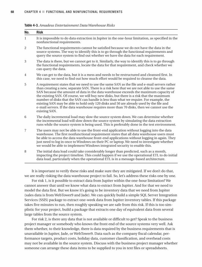
Table 4-3. Amadeus Entertainment Data Warehouse Risks
No. Risk
1 It is impossible to do data extraction in Jupiter in the one-hour limitation, as specified in thenonfunctional requirements.
2 The functional requirements cannot be satisfied because we do not have the data in thesource systems. The way to identify this is to go through the functional requirements andquery the source system to find out whether we have the data for each requirement.
3 The data is there, but we cannot get to it. Similarly, the way to identify this is to go throughthe functional requirements, locate the data for that requirement, and check whether wecan query the data.
4 We can get to the data, but it is a mess and needs to be restructured and cleansed first. Inthis case, we need to find out how much effort would be required to cleanse the data.
5 A requirement states that we need to use the same SAN as the file and e-mail servers ratherthan creating a new, separate SAN. There is a risk here that we are not able to use the sameSAN because the amount of data in the data warehouse exceeds the maximum capacity ofthe existing SAN. Of course, we will buy new disks, but there is a risk that the maximumnumber of disks that the SAN can handle is less than what we require. For example, theexisting SAN may be able to hold only 120 disks and 50 are already used by the file ande-mail servers. If the data warehouse requires more than 70 disks, then we cannot use theexisting SAN.
6 The daily incremental load may slow the source system down. We can determine whetherthe incremental load will slow down the source system by simulating the data extractionruns while the source system is being used. This is preferably done in the test environment.
7 The users may not be able to use the front-end application without logging into the datawarehouse. The first nonfunctional requirement states that all data warehouse users mustbe able to access the data warehouse front-end applications without logging in again. Theyjust need to log in once to Windows on their PC or laptop. We need to investigate whetherwe would be able to implement Windows integrated security to enable this.
8 The initial data load could take considerably longer than predicted, such as a month,impacting the project timeline. This could happen if we use the operational ETL to do initialdata load, particularly when the operational ETL is in a message-based architecture.
It is important to verify these risks and make sure they are mitigated. If we don’t do that,we are really risking the data warehouse project to fail. So, let’s address these risks one by one.
For risk 1, is it possible to extract data from Jupiter within the one-hour limitation? Wecannot answer that until we know what data to extract from Jupiter. And for that we need tomodel the data first. But we know it’s going to be inventory data that we need from Jupiter(sales data is from WebTower9 and Jade). We can quickly build a simple SQL Server IntegrationServices (SSIS) package to extract one-week data from Jupiter inventory tables. If this packagetakes five minutes to run, then roughly speaking we are safe from this risk. If this is too sim-plistic for your project, build a package that extracts one day of equivalent data from severallarge tables from the source system.
For risk 2, is there any data that is not available or difficult to get? Speak to the businessproject manager or somebody who knows the front end of the source systems very well. Askthem whether, to their knowledge, there is data required by the business requirements that isunavailable in Jupiter, Jade, or WebTower9. Data such as the company fiscal calendar, per-formance targets, product costs, holiday data, customer classification, and overhead costsmay not be available in the source system. Discuss with the business project manager whethersomeone can arrange these data items to be supplied to you in text files or spreadsheets.
CHAPTER 4 ■ FUNCTIONAL AND NONFUNCTIONAL REQUIREMENTS68
9314ch04final.qxd 11/15/07 10:19 AM Page 68

For risk 3, we need to find out whether we can get to the data. We need to understandwhat RDBMS the source systems are running on. Most companies uses popular RDBMSs fortheir OLTP systems, such as Oracle, Informix, DB/2, Ingress, Progress, mysql, Sybase, or SQLServer, and these RDBMSs supports ADO.NET, ODBC, JDBC, or OLEDB, so we can get to thedata using SSIS, assuming we have cleared the security permission. But if we hear that one ofthe source systems is on a proprietary system, not on an RDBMS, then we need to find outwhether we can get to the data. If we can’t find any ODBC or JDBC drivers for this proprietarysystem, we need to speak to the DBA about whether it is possible to arrange for the data to beexported periodically to text files.
Connectivity is another obstacle that could prevent us from getting to the data. For exam-ple, the production database server may sit behind a firewall. We may need to open a firewallhole, that is, raise a network request allowing database traffic through the firewall to and froma particular database server.
For risk 4, some data in the source system may require cleansing. We can find this out byquerying the source system. Some of the data quality issues are incomplete data, incorrect/inaccurate data, duplicate records (because no hard database constraints are applied, such asprimary keys or unique constraints), data is in free text format, a column is available but mostvalues are null, orphan records, and so on.
For risk 5, unfortunately, without designing the DDS and NDS, we would not be able tounderstand the size of the data stores. If we try to estimate the storage at this stage, it could beinaccurate. I don’t suggest we shouldn’t estimate it, though. We should. The earlier we do theestimate, the better. But we need to be aware of how accurate the estimate is. When we com-plete data modeling (discussed in the next chapter), then we will be able to estimate thestorage much more accurately.
Here is how we can estimate the data storage at this stage, without having the data modelin hand:
• For each point in business requirements 1 to 7, assume there will be a fact table and asummary table. At this stage, we do not know the data structure of our dimensionalmodel, so we need to make a lot of assumptions. Estimate the width of the fact table byassuming the number of key columns and fact columns. For a rough estimate, assume5 key columns for a simple fact table and 15 for a complex one.
• Estimate the width of dimension tables by assuming the number of columns. For arough estimate, assume 10 columns for a simple dimension and 50 columns for a com-plex dimension. Most columns are 4 to 8 characters, but some are 100 to 200 characters,so for an estimate assume that on average each column is 50 characters.
• Assume that the size of the summary table is 10 to 20 percent of the fact tables.
• The depth of the fact table depends on volume. For transactional fact tables, look at thesource system to figure out how many transactions there are a day. For daily snapshotfact tables, look at the source system to figure out how many records there are per snap-shot. Multiply this by the period—how long you plan to use the storage (take two tothree years if you have no idea). For example, if on average there are 500,000 purchasesa day, the size of the Product Sales fact table would be 500,000 ✕ 365 ✕ 2 ✕ the width offact table as estimated earlier.
CHAPTER 4 ■ FUNCTIONAL AND NONFUNCTIONAL REQUIREMENTS 69
9314ch04final.qxd 11/15/07 10:19 AM Page 69

• Query the source system to estimate the number of records for each dimension. Forexample, for the product dimension, we query the inventory master table in Jupiter.
• Estimating the size of the NDS or ODS could vary widely. We cannot estimate it basedon the size of the DDS. We can query the source system tables to estimate the size ofeach of the NDS or ODS tables.
Risk 6, the risk that the daily incremental load may slow the source system down, alsodepends on the data model and source system mapping, which we will do in the next chapter.But it is possible to mitigate this risk by building some simple SSIS packages that extract thedata specified in the business requirements. The SSIS packages simulate the daily incrementalload, extracting data from the main tables on the source systems. When this package is run-ning, we use the source systems as normal for OLTP activities and measure whether there isany degradation in performance. For example, entering an order that usually takes a split sec-ond when saving to a database now takes three to four seconds. If this is the case, we shouldschedule the daily incremental load to run after-hours, such as from 2 a.m. to 4 a.m. I will gothrough how to build an ETL package using SSIS in Chapters 7 and 8.
For risk 7, the single login requirement can be mitigated by building a simple report anda simple OLAP cube and then applying the security. To enable the single login requirement(the customer doesn’t need to log in again to the data warehouse system once they log in toWindows), we need to apply Windows integrated security, both on SQL Server Reporting Ser-vices (SSRS) and on SQL Server Analysis Services (SSAS). I will go through the steps of build-ing reports in Chapter 11 and building OLAP cubes in Chapter 12.
Risk 8, initial data load, can be estimated by querying the source system according to thecriteria specified in functional requirement 10. We can query the main transaction tables inthe source system to find out how many records you have to load to the data warehouse tosatisfy the historical data requirement. In the case of Amadeus Entertainment, functionalrequirement 10 specifies that we need to load two years of historical data for sales and CRMand one year for purchasing. We can then go to the source system and query the sales ordertable with something like select count(*) where sales order date >= [2 years ago] to findout how many historical rows we need on the initial data load for sales data. We then do thesame for the CRM subscription data and purchase order data.
SummaryIn this chapter, we defined the functional requirements for the case study. We also definedthe nonfunctional requirements and verified that the data and the source systems supportthe requirements, meaning that, up to this point, we don’t see anything that poses a seriousrisk to the project or prevents us from delivering the data warehouse.
In the next chapter, I will show how to design a data model that satisfies these require-ments. The discussion about events, levels, status, and roles in this chapter will be useful inthe next chapter.
CHAPTER 4 ■ FUNCTIONAL AND NONFUNCTIONAL REQUIREMENTS70
9314ch04final.qxd 11/15/07 10:19 AM Page 70
Data Modeling
In this chapter, we will design the data stores for the Amadeus Entertainment case study. Wewill use the NDS + DDS architecture. Apart from the benefits outlined in Chapter 2, the pur-pose of choosing this architecture for this case study is so that you can have the experienceof designing a normalized store and a dimensional store.
We will begin by looking at the business requirements and then design the dimensionaldata store (DDS) accordingly. We will define the meaning of the facts and dimensional attrib-utes. We will also define the data hierarchy.
Then we will map the data in the DDS with the source systems; that is, we will definethe source of the columns in the fact and dimension tables. Sometimes one column in theDDS is populated from several tables in the source system (for example, from column 1 oftable A and column 1 of table B) and sometimes from more than one source system. We willdefine the transformations (formula, calculation logic, or lookups) required to populate thetarget columns.
Then we will design the normalized data store (NDS) by normalizing the dimensionaldata store and by examining the data from the source systems we have mapped. The normal-ization rules and the first, second, and third normal forms are described in the appendix. Wewill use these rules to design the NDS.
Designing the Dimensional Data StoreSo, let’s start by designing the DDS. The users will be using the data warehouse to do analysisin six business areas: product sales, subscription sales, subscriber profitability, supplier per-formance, CRM campaign segmentation, and CRM campaign results. So, we need to analyzeeach business area one by one to model the business process in order to create the datamodel. Let’s do the first business area: product sales. An order-item data mart in the retailindustry is a classic example of data warehousing.
A product sales event happens when a customer is buying a product, rather than sub-scribing to a package. The roles (the who, where, and what) in this event are the customer,product, and store. The levels (or in dimensional modeling terms, the measures) are the quan-tity, unit price, value, direct unit cost, and indirect unit cost. We get these levels from thebusiness requirements in Chapter 4; in other words, they’re what users need to perform theirtasks. We put the measures in the fact table and the roles (plus dates) in the dimension tables.The business events become the fact table row. Figure 5-1 describes the result.
71
C H A P T E R 5
9314ch05final.qxd 11/15/07 10:16 AM Page 71

Figure 5-1. Product Sales fact table and its dimensions
quantity, unit_price, and unit_cost measures are derived from the source system, butthe other three measures (sales_value, sales_cost, and margin) are calculated. They aredefined as follows:
• sales_value = unit_price ✕ quantity
• sales_cost = unit_cost ✕ quantity
• margin = sales_value – sales_cost
The four keys in the Product Sales fact table link the fact table with the four dimensions.According to Ralph Kimball, it is important to declare the grain of the fact table. Grain is thesmallest unit of occurrence of the business event in which the event is measured. In otherwords, grain is completing this sentence: “One row in the fact table corresponds to. . . .” In thiscase, the grain is each item sold—one row in the Product Sales fact table corresponds to eachitem sold.
It is easy to define simple measures for our case study such as sales value, sales cost, andmargin, but in practice when doing data modeling we have to deal with complex events, fea-tures, exceptions, and logic that are industry specific, such as discounts, taxes, promotionalitems (for example, “three for the price of two,” “buy one get one free,” and so on), bundles,and returns.
The general rule for dealing with complex events and exceptions is to always look at thesource system. We have to replicate or mimic the source system logic. This is because the out-put of the data warehouse application must agree with the source system. If the source systemincludes the discount in the unit price, we should not implement discounts as line itemsbecause if we aggregated the discount, it would not match the source system. In any case,always talk to the businesspeople first about the business logic because they know the busi-ness rules. Then it is wise to always confirm the data model and business logic with the sourcesystem. It is important to get the data model and business logic correct to ensure that the out-put of the data warehouse reflects the correct business conditions.
CHAPTER 5 ■ DATA MODELING72
9314ch05final.qxd 11/15/07 10:16 AM Page 72

Some of the business logic is quite complex, such as cost allocations and customer prof-itability calculations. Cost allocation is where you need to allocate a total cost to each businessevent. Usually, it is an overhead or indirect cost occurring periodically, such as the cost of rent-ing a building. Customer profitability is where you calculate the profit you are making for eachcustomer for a certain period. For complex business logic such as this, you could have a dis-agreement between the businesspeople and the source system code, meaning that the busi-nesspeople want the data warehouse business logic to be different from the one implementedin the source system. In this case, advise the business project manager of the discrepancy youfound and ask her to decide which one to implement in the data warehouse. This happens inpractice, and I have experienced it myself several times: “I know that the source system calcu-lates the annual revenue with that logic, but in the data warehouse I want to calculate theannual revenue differently.” In this case, my belief is that you should implement as per therequirement from the businesspeople; however, it is essential to always let the business proj-ect manager facilitate this. It should be documented and should require sign-off. The reasonfor this is it is perfectly valid for the data warehouse users to have a requirement (about busi-ness logic) that is different from the source system. For instance, perhaps there have beensome changes in the business situation, or perhaps they want to analyze the data differently.
In retail, alongside sales transactions, you also have sales tax (value-added tax [VAT]) thatvaries depending on country, state, and product. VAT can be implemented in several ways. Insome implementations, VAT is not included in the sales fact table because the business wantsto analyze product sales only (to them, taxes obscure the real transaction value). In otherimplementations, they build a sales tax fact table, with the granularity at one row per orderline. In this fact table, they analyze the taxes. In still other implementations, discounts areincluded in the unit price (rather than as a transaction line). In other words, if the normalprice is $5 and there is a 20 percent discount, the unit price is reduced to $4.
Let’s now return to the fact table and continue our dimensional design. In Figure 5-1,you can see there are two columns in the fact table: order_id and line_number. They arecalled degenerate dimensions. A degenerate dimension is a dimension with only one attrib-ute, and therefore the attribute is put in the fact table. order_id and line_number are theidentifiers of the order line in the source system. We need to always bear in mind that we maybe dealing with more than one source system, so it is possible that two source systems havethe same order ID. Because of this, we want to include a source system ID column to differ-entiate them. Also, it is a good idea to always put a timestamp column in the fact table, thatis, the time when the record was loaded into the fact table. This column enables us to deter-mine when the fact row (or dimension row) was loaded into the data warehouse data store.In many cases, we need a second timestamp column to store the time the record was lastupdated. This column enables us to determine when the fact row (or dimension row) was lastmodified. These two columns are in addition to the transactional date/timestamp column.The transaction timestamp explains when the order (or order line) was created, shipped,canceled, or returned, but it does not explain when the record was loaded into the data ware-house and when it was last modified.
The next step in the fact table design is to determine which column combinationuniquely identifies a fact table row. This is important because it is required for both logicaland physical database design in order to determine the primary key(s). We ordinarily would beable to uniquely identify a fact table row by using the combination of all dimensional columnsin the fact table. However, it is still possible to have duplicate rows. Sometimes we need to usethe degenerate dimension to make it unique. In our Amadeus Entertainment case study, the
CHAPTER 5 ■ DATA MODELING 73
9314ch05final.qxd 11/15/07 10:16 AM Page 73

fact table contains one row for each item sold. So, it seems that the combination of the cus-tomer, date, product, and store dimensions will be enough to uniquely identify a fact tablerow. What if customer A bought song B in online store C on date D at 10 a.m. and then shecame back at 7 p.m. on the same day to the same store and bought the same song again? Ah,we have two rows with those four dimensional columns having identical values. But the orderID and line number are different. So, to differentiate these two fact rows, we use the order IDand line number. Therefore, we can use order_id and line_number for the primary key candi-dates. Or we can create a new fact table key column and use it as the primary key candidate.
■Note I will discuss the primary keys and cluster indexes in the next chapter because determining primarykeys and cluster indexes are part of the physical database design process.
This collection of a fact table and its dimension tables is called a data mart. There aremore complex forms of data marts, such as when you have more than one fact table, but fornow let’s consider only one fact table. Bear in mind that this concept of a data mart is applica-ble only if the data warehouse is in a dimensional model. If the data warehouse is not in adimensional model—that is, when we are talking about a normalized data store—there is nodata mart. A data mart is a group of related fact tables and their corresponding dimensiontables containing the measurements of business events, categorized by their dimensions. Datamarts exist in dimensional data stores.
With the timestamp columns, the Product Sales fact table (and its dimensions) now lookslike Figure 5-2.
Figure 5-2. Product Sales table (and its dimensions) with timestamp columns
CHAPTER 5 ■ DATA MODELING74
9314ch05final.qxd 11/15/07 10:16 AM Page 74

We then define the data type for each column. All key columns have integer data typesbecause they are surrogate keys, that is, simple integer values with one increment. The meas-ure columns are usually numeric or currency, so in SQL Server, their data types are decimal ormoney. The three timestamp columns have datetime data types. The source system code is aninteger because it contains only the code, and the description is stored in the source systemtable in the metadata database.
Then we add the description for each column. We also provide a sample value so we areclear about the data we are going to store in each column. We can get a sample value by query-ing the source system. Table 5-1 describes the final form of the Product Sales fact table.
Table 5-1. Product Sales Fact Table
Column Name Data Type Description Sample Value
sales_date_key int The key of the date the customer pur- 108chased the product
customer_key int The key of the customer who purchased 345the product
product_key int The key of the product purchased by the 67customer
store_key int The key of the store where the customer 48made the purchase
order_id int WebTower9 or Jade order ID 7852299
line_number int WebTower9 or Jade order line number 2
quantity decimal(9,2) How many units of the product the 2customer purchased
unit_price money Price of one unit of the product pur- 6.10chased in the original currency
unit_cost money Direct and indirect costs for one unit of 5.20the product in the original currency
sales_value money quantity ✕ unit_price 12.20
sales_cost money quantity ✕ unit_cost 10.40
margin money sales_value – sales_cost 1.80
sales_timestamp datetime When the customer purchased the 02/17/2008 product 18:08:22.768
source_system_code int The key of the source system from which 2this record was coming from
create_timestamp datetime When the record was created in DDS 02/17/200804:19:16.638
update_timestamp datetime When the record was last updated 02/17/200804:19:16.638
In multinational companies, you may need to define additional columns to store themeasures in the “global enterprise currency,” along with the currency rate. When a businesshas branches in many countries, the business transactions occur in different local currencies.These transactions are stored in the fact table columns listed in Table 5-1. Usually, there arealso requirements to analyze transaction data globally. To do this analysis, the transactions
CHAPTER 5 ■ DATA MODELING 75
9314ch05final.qxd 11/15/07 10:16 AM Page 75

need to be converted and stored in a single global currency. The currency rates that were usedto convert the transaction values from the local currencies to the global currency are alsostored in the fact table. In addition, we need to have a currency key column in the ProductSales fact table, containing the currency in which the transaction occurred. This key column islinked to the currency dimension where the name of the currency is stored. To accommodatethese multicurrency requirements in the fact table, we can create the additional columnsshown in Table 5-2.
Table 5-2. Additional Columns on the Product Sales Fact Table
Column Name Data Type Description Sample Value
currency_key int The key of the currency in which the trans- 3action occurred
unit_price_usd money Price of one unit of the product purchased 6.10in U.S. dollars
unit_cost_usd money Direct and indirect costs for one unit of the 5.20product in U.S. dollars
sales_value_usd money quantity ✕ unit_price, in U.S. dollars 12.20
sales_cost_usd money quantity ✕ unit_cost, in U.S. dollars 10.40
margin_usd money sales_value – sales_cost, in U.S. dollars 1.80
currency_rate money Conversion rate between the local currency 1.97and U.S. dollars
Dimension TablesNow that we have discussed the fact table, let’s discuss the dimension tables. A dimensiontable is a table that contains various attributes explaining the dimension key in the facttable. As mentioned earlier in this chapter, the fact table stores business events. The attrib-utes explain the conditions of the entity at the time the business event happened. Forexample, in the fact table in Figure 5-1, we have a dimension key called customer_key.Table 5-1 says that this column contains the key (or the ID) of the customer purchasing theproduct. In Figure 5-1, you can see that the customer dimension table is “linked” to the facttable using the customer_key column. The customer_key column is a primary key in the cus-tomer dimension table, and it is a foreign key on the fact table. This is known in the databaseworld as referential integrity.
Referential integrity is a concept of establishing a parent-child relationship between twotables, with the purpose of ensuring that every row in the child table has a corresponding par-ent entry in the parent table. The referential integrity can be “hardened” or “enforced” physi-cally as a physical database constraint (data warehouse people call this hard RI). A databaseconstraint is a rule governing the permissible values on a certain column. Alternatively, thereferential integrity can managed by the ETL and not enforced as a physical data constraint(data warehouse people call this soft RI). The ETL checks that the values on the fact tabledimensional keys exist in the dimension tables.
The dimension tables contain various attributes explaining the conditions of the entitiesinvolved in the business event stored in the fact table. The attributes are stored as columns inthe dimension tables. They are known as dimensional attributes. The customer dimension
CHAPTER 5 ■ DATA MODELING76
9314ch05final.qxd 11/15/07 10:16 AM Page 76

contains columns that describe the condition of the customer who made the purchase,including the data about customer name, address, telephone number, date of birth, e-mailaddress, gender, interest, occupation, and so on. The product dimension contains columnsthat describe conditions of the product purchased, including the data about product name,product type, product category, media, SKU, minimum order level, product code, unit cost,and unit price.
Now that you understand what a dimension is, let’s go through the four dimensions inFigure 5-1—date, customer, product, and store—to complete the design of the product salesdata mart. We will define each dimension one by one. We will begin with the date dimensionfirst and then discuss the other three dimensions. We will also talk about the concept of slowlychanging dimension (SCD). SCD is a data modeling technique to store historical values ofdimensional attributes. It is important to discuss it in the context of dimensions because of itscapability to preserve historical attribute values. OK, let’s start with the date dimension.
Date DimensionAlmost every single data mart has the date dimension in it. This reflects the nature of adimensional data mart in that the fact table rows are business events that happened on cer-tain dates. Because the date dimension is used in almost every data mart in the data ware-house, it is important to model the date dimension correctly. It is important for the datedimension to contain the attributes required by all fact tables in all data marts.
Why don’t we have a time dimension instead of a date dimension? Well, it is not practical.A date dimension with 10 years of data has 3,650 rows. If it were a time dimension with preci-sion to the second, it would have 315 million rows and would impact the data warehouseperformance because it’s used everywhere. Instead, we use either the timestamp column inthe fact table (99 percent of the cases) or a time of day dimension (1 percent of the cases). Atimestamp column in the fact table stores the date and time the business event happenedand, therefore, eliminates the need to have a time dimension. A time of day dimension con-tains all the possible minutes (or seconds) in one day. A time of day dimension is used whena different period in a day has a different meaning or label, such as “happy hour,” “off-peakperiod,” “night shift,” and “migration slot.” If labels such as these are not required, the time-stamp column is easier (for calculation) and better (for performance).
The columns or attributes in a date dimension can be categorized into four groups:
Date formats: The date format columns contain dates in various formats.
Calendar date attributes: The calendar date attributes contain various elements of a date,such as day, month name, and year.
Fiscal attributes: The fiscal attribute columns contain elements related to the fiscal calen-dar, such as fiscal week, fiscal period, and fiscal year.
Indicator columns: The indicator columns contain Boolean values used to determinewhether a particular date satisfies a certain condition, such as whether it is a nationalholiday.
CHAPTER 5 ■ DATA MODELING 77
9314ch05final.qxd 11/15/07 10:16 AM Page 77

Typically used date format columns in the date dimension are as follows (with examplesfor February 17, 2008):
• date such as “02/17/2008”
• sql_date such as “02/17/2008 00:00:00.000”
• ansi_date such as “2008-02-17”
The sql_date column contains the date in the SQL Server datetime data type, whereas thedate and ansi_date columns contain the date in the varchar data type. The date column canbe formatted according to the custom in the local geography; for example, mm/dd/yyyy isusually used in the United States. We can also create a column for other places; for example,the dd/mm/yyyy format is usually used in the United Kingdom.
The calendar date attribute columns contain the parts or elements of a date. Table 5-3shows typically used calendar date attributes in the date dimension, with examples for Febru-ary 17, 2008. The columns are listed from the smallest unit of measure.
Table 5-3. Calendar Date Attributes Columns
Column Sample Values Notes
week_day 7 Monday = 1, Tuesday = 2, …, Sunday = 7.
week_day_name Sunday
day 17 You can call it day_of_the_month, but most users prefer theshort version.
day_of_the_year 48
week_number 7 The week starts on Monday.
month 2
short_month_name Feb
long_month_name February
quarter Q1
year 2008
The columns that end with the word name (such as short_month_name and week_day_name)probably need to be in several languages if you are a multinational organization. If we use sev-eral languages, we also need to correctly set the SQL collation of the database according to thecharacter set used by the languages.
It is true that we can derive the attributes in the date dimension (such as month name,week number, day name, and so on) by using Transact SQL functions such as datepart. Thereason for providing those attributes in the date dimension is because when we are in the facttable, all we have is the date key, so in the date dimension rather than going to the sql_datecolumn and then deriving the month, we can go directly to the month column.
After the calendar date attribute columns, the next group of columns in the date dimen-sion is the fiscal attribute columns. These columns contain the fiscal property of a date, suchas the fiscal year and fiscal week. The values of fiscal attributes are dependent upon when thefiscal year starts and when it ends. Those values are also affected by how many fiscal periods
CHAPTER 5 ■ DATA MODELING78
9314ch05final.qxd 11/15/07 10:16 AM Page 78
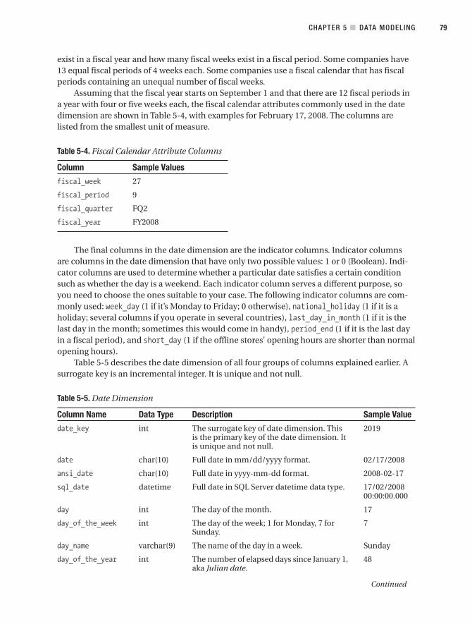
exist in a fiscal year and how many fiscal weeks exist in a fiscal period. Some companies have13 equal fiscal periods of 4 weeks each. Some companies use a fiscal calendar that has fiscalperiods containing an unequal number of fiscal weeks.
Assuming that the fiscal year starts on September 1 and that there are 12 fiscal periods ina year with four or five weeks each, the fiscal calendar attributes commonly used in the datedimension are shown in Table 5-4, with examples for February 17, 2008. The columns arelisted from the smallest unit of measure.
Table 5-4. Fiscal Calendar Attribute Columns
Column Sample Values
fiscal_week 27
fiscal_period 9
fiscal_quarter FQ2
fiscal_year FY2008
The final columns in the date dimension are the indicator columns. Indicator columnsare columns in the date dimension that have only two possible values: 1 or 0 (Boolean). Indi-cator columns are used to determine whether a particular date satisfies a certain conditionsuch as whether the day is a weekend. Each indicator column serves a different purpose, soyou need to choose the ones suitable to your case. The following indicator columns are com-monly used: week_day (1 if it’s Monday to Friday; 0 otherwise), national_holiday (1 if it is aholiday; several columns if you operate in several countries), last_day_in_month (1 if it is thelast day in the month; sometimes this would come in handy), period_end (1 if it is the last dayin a fiscal period), and short_day (1 if the offline stores’ opening hours are shorter than normalopening hours).
Table 5-5 describes the date dimension of all four groups of columns explained earlier. Asurrogate key is an incremental integer. It is unique and not null.
Table 5-5. Date Dimension
Column Name Data Type Description Sample Value
date_key int The surrogate key of date dimension. This 2019is the primary key of the date dimension. It is unique and not null.
date char(10) Full date in mm/dd/yyyy format. 02/17/2008
ansi_date char(10) Full date in yyyy-mm-dd format. 2008-02-17
sql_date datetime Full date in SQL Server datetime data type. 17/02/200800:00:00.000
day int The day of the month. 17
day_of_the_week int The day of the week; 1 for Monday, 7 for 7Sunday.
day_name varchar(9) The name of the day in a week. Sunday
day_of_the_year int The number of elapsed days since January 1, 48aka Julian date.
Continued
CHAPTER 5 ■ DATA MODELING 79
9314ch05final.qxd 11/15/07 10:16 AM Page 79

Table 5-5. Continued
Column Name Data Type Description Sample Value
week_number int The number of elapsed weeks since Jan- 7uary 1; weeks start on Monday.
month int The number of the month. 2
month_name varchar(9) The full name of the month in English. February
short_month_name char(3) The short name of the month in English. Feb
quarter char(2) Three-month period in calendar year, Qn Q1format.
year int The calendar year of the date. 2008
fiscal_week int The number of elapsed weeks since Sep- 27tember 1.
fiscal_period char(4) A period consists of four or five weeks FP9depending on the fiscal calendar. Usually, the pattern used in this company is 454, 544, or 445, in FPn format. A fiscal year always consists of 12 periods.
fiscal_quarter char(3) A fiscal quarter is three fiscal periods, from FQ2September 1, FQn format.
fiscal_year char(6) Fiscal year begins on September 1, in FY2008FYnnnn format.
week_day tinyint 1 if it is Monday to Friday; 0 otherwise. 0
us_holiday tinyint 1 if it is a national holiday in the United 0States; 0 otherwise.
uk_holiday tinyint 1 if it is a statutory holiday in the United 0Kingdom; 0 otherwise.
month_end tinyint 1 if it is the last day in the month; 0 otherwise. 0
period_end tinyint 1 if it is the last day in a fiscal period; 0 0otherwise.
short_day tinyint 1 if on that day the offline stores’ opening 0hours are shorter than normal opening hours; 0 otherwise. This is applicable only for off-line stores.
The date_key column is the primary key of the date dimension. In SQL Server implemen-tations, it is also the cluster index.
Slowly Changing DimensionNow that I have discussed the date dimension, before I discuss the other three dimensions,I’ll cover something called SCD, which is a technique used to store the historical value ofdimension attributes. The values of dimensional attributes change as time goes by. Whenthese attribute values change, you can overwrite the old values with the new ones, or you canpreserve the old value. There are two methods of preserving the old attribute values: you canstore the old values as rows, or you can store them as columns. For example, say that store 7
CHAPTER 5 ■ DATA MODELING80
9314ch05final.qxd 11/15/07 10:16 AM Page 80

was in region 1, but it is now in region 2. You want to store the historical information—thefact that it was in region 1. You can do this in two ways: by storing it as a row or by storing itas a column. Table 5-6 shows an example of historical information stored as a row.
Table 5-6. Storing Historical Information As a Row
key store region status
1 7 1 expired
2 7 2 active
In Table 5-6, you can see that the active row is row 2, but you still have the previous region(region 1) stored in the first row. To understand when row 1 became expired and when row 2became active, you can add two columns in Table 5-6: effective_date and expiry_date.
You can also store the historical information (the old attribute values) as columns insteadof rows. Table 5-7 shows how historical information is stored as a column. In Table 5-7, thecurrent region of store 7 is region 2, and previously store 7 was in region 1.
Table 5-7. Storing Historical Information As a Column
key store current_region old_region effective_date
1 7 2 1 11/18/2007
In Table 5-7, you can see that there is a column called old_region that stores the previousvalue of the region (region 1). To record the date when store 7 moved from region 1 to region 2,you can add a column called effective_date, such as the one shown in Table 5-7.
Of course, the question now is, what if store 7 moves region again, to region 3, for exam-ple? Well, because you have only two columns, the oldest value is not stored. You can storeonly the last two values. If you want to store three values, you need to have three columns:current_region, old_region, and old_region2. What if you want to store ten values? Well, youneed to have ten columns. This is the distinct disadvantage of storing the historical value ascolumns, compared to storing them as rows.
Now that you understand how historical values are stored in the dimension table (that is,as rows or columns), I’ll talk about three types of SCD:
• SCD type 1 overwrites the old values of the attributes so the old values are not kept.
• SCD type 2 keeps the old values by creating a new row for each change, just like Table 5-6.
• SCD type 3 keeps the old values by putting them in another column, just like Table 5-7.
Generally, SCD type 2 is more flexible for storing the historical value of dimensionalattributes, because you can store as many old versions as you want without altering the tablestructure. SCD type 3 is using columns to store old values, which is why it is not flexible. It isideal for situations where you don’t have many old versions (five or fewer) and you know therewill be only a certain number of versions. Type 3 is also ideal when the changes in this attrib-ute affect a large number of rows. In other words, a lot of dimension rows change the value ofthis attribute at the same time (simultaneously). For a detailed explanation of SCD, please
CHAPTER 5 ■ DATA MODELING 81
9314ch05final.qxd 11/15/07 10:16 AM Page 81
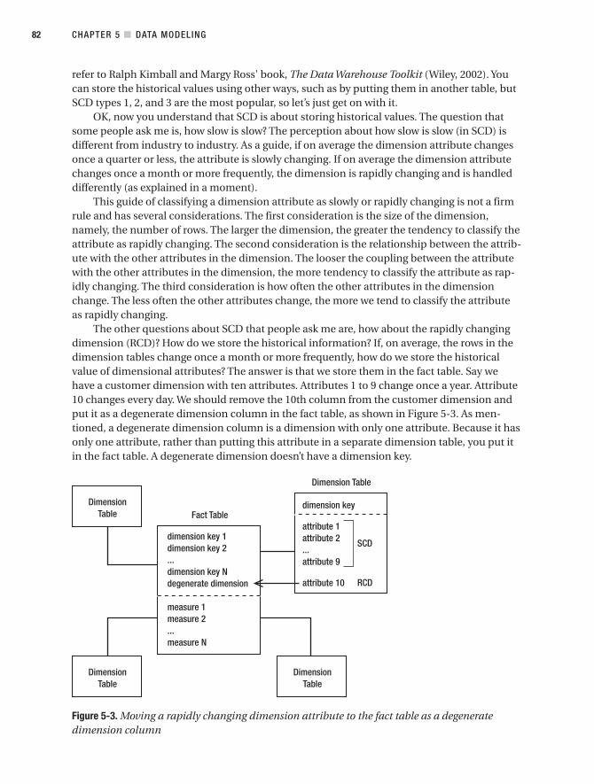
refer to Ralph Kimball and Margy Ross' book, The Data Warehouse Toolkit (Wiley, 2002). Youcan store the historical values using other ways, such as by putting them in another table, butSCD types 1, 2, and 3 are the most popular, so let’s just get on with it.
OK, now you understand that SCD is about storing historical values. The question thatsome people ask me is, how slow is slow? The perception about how slow is slow (in SCD) isdifferent from industry to industry. As a guide, if on average the dimension attribute changesonce a quarter or less, the attribute is slowly changing. If on average the dimension attributechanges once a month or more frequently, the dimension is rapidly changing and is handleddifferently (as explained in a moment).
This guide of classifying a dimension attribute as slowly or rapidly changing is not a firmrule and has several considerations. The first consideration is the size of the dimension,namely, the number of rows. The larger the dimension, the greater the tendency to classify theattribute as rapidly changing. The second consideration is the relationship between the attrib-ute with the other attributes in the dimension. The looser the coupling between the attributewith the other attributes in the dimension, the more tendency to classify the attribute as rap-idly changing. The third consideration is how often the other attributes in the dimensionchange. The less often the other attributes change, the more we tend to classify the attributeas rapidly changing.
The other questions about SCD that people ask me are, how about the rapidly changingdimension (RCD)? How do we store the historical information? If, on average, the rows in thedimension tables change once a month or more frequently, how do we store the historicalvalue of dimensional attributes? The answer is that we store them in the fact table. Say wehave a customer dimension with ten attributes. Attributes 1 to 9 change once a year. Attribute10 changes every day. We should remove the 10th column from the customer dimension andput it as a degenerate dimension column in the fact table, as shown in Figure 5-3. As men-tioned, a degenerate dimension column is a dimension with only one attribute. Because it hasonly one attribute, rather than putting this attribute in a separate dimension table, you put itin the fact table. A degenerate dimension doesn’t have a dimension key.
Figure 5-3. Moving a rapidly changing dimension attribute to the fact table as a degeneratedimension column
CHAPTER 5 ■ DATA MODELING82
9314ch05final.qxd 11/15/07 10:16 AM Page 82

Product, Customer, and Store DimensionsNow that we have discussed the concept of SCD, let’s discuss the other three dimensions:the product dimension, the customer dimension, and the store dimension. Unlike the datedimension that we just discussed, product attributes vary widely from industry to industry.Hence, when you model data in a different industry, keep in mind that the product attributescan be totally different from the ones discussed in this section. This is where industry experi-ence becomes useful. For Amadeus Entertainment, the product attributes are product ID (justa number to identify the product, which is maintained by Jupiter), name, description, title (thetitle of the song/film/book), artist (the singer, cast, or author), product type (music, film, orbook), product group (which is a large grouping; that is, for film, it is thriller, comedy, action,documentary, children, Asian, and so on), product category (a smaller grouping; that is, for anAsian film it is Indian, Chinese, and martial arts), media (WMA, MP3, and so on), unit price,and unit cost.
Business requirements 8 and 9 in Chapter 4 mentioned that we need to store the oldattribute values of the customer and store dimensions, but nothing was mentioned about theproduct dimension. Because we don’t have a requirement to store historical values of theproduct attribute, we will use SCD type 1, meaning we will overwrite the old attribute values.
To create the product dimension, we look at the source system. The case study in Chapter2 specifies that the inventory and products in Amadeus Entertainment are managed in theJupiter system, not in the Jade or WebTower9 system. So, we get the product dimensioncolumns from the product tables in the Jupiter system. In the operational source system, theproduct tables may be normalized, and we need to denormalize them to get a flat structure forthe product dimension. We do this by joining the product tables in the source system on theirprimary and foreign key columns. We then get data types and the length for each column fromthe source system. We write a description for each column and provide a sample value. Table5-8 describes the complete structure of the product dimension. As we discussed, a surrogatekey is simply an incremental integer. It is unique and not null.
Table 5-8. Product Dimension
Column Name Data Type Description Sample Value
product_key int The surrogate key of the product dimen- 3746sion. It is unique, is not null, and is the primary key of product dimension.
product_code varchar(10) Natural key. Product code is the identifier FGA334288and primary key of the product table in Jupiter. It is in AAA999999 format.
name varchar(30) Product name. The PanamaStory DVD
description varchar(100) Product description. Panama Storymovie in DVDformat
title varchar(100) The song/film/book title. The PanamaStory
artist varchar(100) The singer, star, or author. Mark Danube
Continued
CHAPTER 5 ■ DATA MODELING 83
9314ch05final.qxd 11/15/07 10:16 AM Page 83

Table 5-8. Continued
Column Name Data Type Description Sample Value
product_type varchar(20) Level 1 of the product hierarchy, such as Filmmusic, film, book.
product_category varchar(30) Level 2 of the product hierarchy; for film, Actionit could be thriller, western, comedy, action, documentary, children, Asian, and so on.
media varchar(25) Format of the media, such as MP3, MPG, DVDCD, or DVD.
unit_price money Price for one item. 4.75
unit_cost money Allocated direct and indirect costs. 3.62
status varchar(15) Upcoming if we have signed contract Activewith the supplier, Active if it is still being offered to the customer, and Expired if it is no longer being offered.
source_system_code int The key of the source system where this 2record was coming from.
create_timestamp datetime When the record was created in DDS. 02/05/2008
update_timestamp datetime When the record was last updated. 02/05/2008
The product_key column is the primary key of the product dimension, and it is also thecluster index. product_code is the primary key of the product table in the Jupiter system. Wecall product_code the natural key, which is a column in the source system that we can use toidentify the record. It must be unique and not null, and it is usually a primary key in thesource system table.
Now let’s look at the customer dimension with SCD type 2. A customer dimension tablelooks like the one described in Table 5-9.
Table 5-9. Customer Dimension
Column Name Data Type Description Sample Value
customer_key int The surrogate key of customer 84743dimension.
customer_id varchar(10) Natural key. The primary key of the DH029383customer tables in WebTower9 and Jade. WebTower9 customer_id format is AA999999. and Jade is AAA99999.
account_number int The account number for subscription 342165customers. 0 for nonsubscription customers.
customer_type char(1) Subscriber, purchaser, or member. S
name varchar(100) Customer’s full name. CharlotteThompson
gender char(1) M for male; F for female. F
CHAPTER 5 ■ DATA MODELING84
9314ch05final.qxd 11/15/07 10:16 AM Page 84

Column Name Data Type Description Sample Value
email_address varchar(200) Customer’s e-mail address. [email protected]
date_of_birth smalldatetime Customer’s date of birth. 04/18/1973
address1 varchar(50) First line of address. 570GreenfieldBoulevard
address2 varchar(50) Second line of address. Suite 2100
address3 varchar(50) Third line of address.
address4 varchar(50) Fourth line of address.
city varchar(50) Village, town, or city of customer’s Jacksonvilleresidence.
state varchar(40) For non-U.S. address, it’s county or Floridaregion.
zipcode varchar(10) Postal code. 32228
country varchar(50) Country. USA
phone_number varchar(20) Telephone number including area code. (904) 402-8294
occupation varchar(50) Customer’s job/profession. DBA
household_income varchar(20) Range of household income in U.S. 50–60kdollars.
date_registered smalldatetime The date when the customer first pur- 11/23/2007chased or subscribed.
status varchar(10) Active if the customer is currently a Activemember or made a purchase in the last 12 months.
subscriber_class varchar(3) Classification of subscribers based on R1projected annual revenue.
subscriber_band varchar(3) Classification of subscribers based on Aprofitability.
effective_timestamp datetime For SCD type 2, when the data in the 1/1/1900row becomes effective; this defaults to 1/1/1900.
expiry_timestamp datetime For SCD type 2, when the data in the 12/31/2999row is no longer valid; this defaults to 12/31/2999.
is_current int For SCD type 2, 1 if this is the current 1record; 0 otherwise.
source_system_code int The key of the source system where 2this record was coming from.
create_timestamp datetime When the record was created in DDS. 02/05/2008
update_timestamp datetime When the record was last updated. 02/05/2008
CHAPTER 5 ■ DATA MODELING 85
9314ch05final.qxd 11/15/07 10:16 AM Page 85

According to business requirement 8 in Chapter 4, the columns that we need to pre-serve the history are occupation, household_income, address1, address2, address3, address4,city, state, zipcode, country, phone_number, and email_address. In Chapter 8, we’ll discusshow to monitor and maintain the changes in these columns. The is_current column,effective_timestamp column, and expiry_timestamp column are for accommodatingSCD type 2. I will discuss how to maintain these columns in Chapter 8.
To accommodate multiple e-mail/postal addresses and landline/cell phone numbers fora customer, we can have multiple sets of addresses, telephones, and e-mail addresses in thecustomer dimension if we use a star schema. If we use a snowflake schema, we normalize thecustomer dimension by putting the e-mail/postal address and phone numbers in subtablesbranching out from the customer dimension.
In Table 5-9, we have the subscriber_class and subscriber_band columns. The purpose ofthese two columns is to satisfy business requirement 4 from Chapter 4. The requirement wasto allocate each subscriber to a specific “class” based on their projected annual revenue. Thebusiness requirement also expected us to allocate each customer to a certain “band” based onthe profit that the customer generated. The class and band are used in the loyalty program.
Now let’s design the final dimension: store. Business requirement 9 in Chapter 4 indicatesthat there could be a reorganization of the stores. That is, currently there are only five regionsin the United States, but in a few months there will be eight regions. Online stores are cur-rently in one division, but in the future they will be in the same division as their offline col-leagues. It is said that a reorganization like this rarely happens. This will be the first time insix years, and we can expect the new structure to last at least three years.
This store dimension is an ideal case for SCD type 3 because, as we discussed earlier,type 3 is suitable if we don’t have many changes in the attributes (five or fewer) and if weknow that there will be only a certain number of old versions. We also discussed that type 3 issuitable when the change involves a large number of rows in the dimension. In other words,a lot of rows are updated simultaneously. We will have a column for the current region, a col-umn for the old region (and the date), and a similar one for the division. Table 5-10 describesthe structure.
Table 5-10. Store Dimension
Column Name Data Type Description Sample Value
store_key int The surrogate key of the store dimension. 12
store_number int Natural key. The common store identi- 56fier used in Jupiter, WebTower9, and Jade.
store_name varchar(40) Name of the store, usually based on Los Angeleslocation.
store_type varchar(20) Store size, in terms of product variety. Large
store_address1 varchar(50) First line of store address. 725 SouthPacificAvenue
CHAPTER 5 ■ DATA MODELING86
9314ch05final.qxd 11/15/07 10:16 AM Page 86

Column Name Data Type Description Sample Value
store_address2 varchar(50) Second line of store address. Suite 800
store_address3 varchar(50) Third line of store address.
store_address4 varchar(50) Fourth line of store address.
city varchar(50) Town or city where the store is located. Los Angeles
state varchar(40) For non-U.S. address, it’s county or Californiaregion.
zipcode varchar(10) Postal code. 90017
country varchar(50) Country. USA
phone_number varchar(20) Store’s main/public telephone number. (213) 454-5555
web_site varchar(100) Direct URL to store website. http://www.amadeus.com/LA
region varchar(30) Current allocated region. West
prior_region varchar(30)
prior_region_date datetime
division varchar(30) Current allocated division. USA
prior_division varchar(30)
prior_division_date datetime
source_system_code int The key of the source system where 2this record was coming from.
create_timestamp datetime When the record was created in DDS. 02/05/2007
update_timestamp datetime When the record was last updated. 02/05/2007
When the new store organization is announced, the current region will be moved to theprior_region column, and the new region will be placed in the region column. The date themove happens will be recorded in the prior_region_date column. We will also do similarthings for division. This way, after the new organizational structure has been implemented,the business users use both the old store organizational structure and the new structure.
To do a sales analysis of different periods by comparing the old organization structureand the new structure, we query the product sales data mart by joining the fact table with thedate and store dimensions. We pick region, prior_region, division, and prior_divisioncolumns from the store dimension and use this information to organize the data from the facttable in a report or a BI application.
Figure 5-4 shows the final diagram of the data mart. It is a good idea to write the fact tablegrain just underneath the fact table name to remind us what facts can and cannot go into thefact table.
CHAPTER 5 ■ DATA MODELING 87
9314ch05final.qxd 11/15/07 10:16 AM Page 87

Figure 5-4. Dimensional star schema for product sales data mart
CHAPTER 5 ■ DATA MODELING88
9314ch05final.qxd 11/15/07 10:16 AM Page 88

Subscription Sales Data MartNow that we have done the product sales data mart, we can do the other data marts thesame way. In other words, we start with the fact table, determine the dimensional key col-umn in the fact table, set the fact table grain, and then create the dimension tables, takinginto account the SCD. If the dimension table in this new data mart already exists in the pre-vious mart, we don’t create a new one. Instead, we reuse the existing dimension. If this newmart needs an attribute that does not exist in the dimension yet, we add that attribute to theexisting dimension.
The other requirements that we have from the case study are subscription sales, sub-scriber profitability, supplier performance, CRM campaign segmentation, and CRM campaignresults. Generally, the steps to design these marts are the same; they just require differentbusiness knowledge to design them. A data mart (the fact table and its dimensions) stores acollection of business events in a certain business area. To design the fact tables and dimen-sions, we need to have business knowledge in that business area. For example, to determinewhat columns we need to have in the Campaign Results fact table, we need to have a certainlevel of business knowledge in CRM.
There are a few things that I want to mention at this point. First, for performance rea-sons as well as design simplicity and consistency, it is better to stick to a star schema ratherthan a snowflake, at least as much as we can. As I discussed in Chapter 1, a star schema issimpler and is more consistent than a snowflake schema because it has only one level in alldimensions. Because a star schema is simpler, it is easier for the ETL processes to load thedata into it. A snowflake schema is when you normalize a dimension into several smallertables with a hierarchy structure. It is used when you want to benefit from less data redun-dancy. The benefit of a snowflake schema is that some analytics applications work betterwith a snowflake schema than a star schema. The other benefit of a snowflake schema is thatless disk space is required. A snowflake schema can decrease query performance, but it canalso increase query performance. It decreases the fact table query performance because wehave to join more tables to the fact table. It increases the query performance when we wantto get the distinct value of a particular dimension attribute. If this attribute is normalizedinto its own subdimension table, the select distinct query runs more quickly.
Second, if the dimension already exists, we use the existing one instead of creatinganother version. For example, do not create another customer dimension. If we need moreattributes, extend the dimension columns. We need to be careful when doing this so we don’trepeat columns with the same meaning. Also, we need be careful not to make the dimensiontable too wide (more than 40 columns). Also, we should not put nonrelated attributes intothe same dimension table; they need to go to their own dimension tables linked separately tothe fact table. If we need a higher level of granularity (such as a week dimension), we create aview on top of it. This means we create a view that takes the data solely from the dimensionphysical table. When creating the view, we filter irrelevant rows on the where clause and selectonly required columns on the select clause of the view definition.
Third, we have to be consistent with our data definitions. The definition for each meas-ure and each dimension attribute must be accurate and unique. The same term used as ameasure or attribute should not be used anywhere else in the data warehouse with a differ-ent meaning. For example, if date_registered is defined as “the date when the customerfirst purchased or subscribed,” we should use this term consistently with the same meaning
CHAPTER 5 ■ DATA MODELING 89
9314ch05final.qxd 11/15/07 10:16 AM Page 89

throughout the data warehouse. We should not use this term elsewhere in the data ware-house to mean something else.
Now, let’s do the other data marts one by one. Subscription sales analysis (that is when acustomer subscribes to a package rather than buying a product) and subscriber profitabilityanalysis can be satisfied with one data mart, as mentioned in business requirements 2 and 3in Chapter 4. Business requirement 4 is also relevant to this fact table. Let’s repeat those threerequirements here:
Requirement 2: The system will be able to analyze subscription sales over time by geo-graphic area, by customer demographic, by stores and sales territory, and by productpackage. In addition, the users need to analyze by subscription duration and lead source(where the customers are coming from). They need to know the revenues, costs, andmargins, evaluated every day for a period of one month. So, they have monthly revenue,monthly direct costs, monthly indirect costs, and monthly margin.
Requirement 3: The system will be able to analyze the subscriber profitability, which isdefined as the projected annual revenue of the subscribing customer minus the annu-alized costs (including proportional indirect costs), expressed as a percentage of theprojected annual revenue. This is analyzed over time by geographic area, by customerdemographic attributes, by stores and sales territory, and by product package.
Requirement 4: The system will be able to allocate subscribers to a specific “class” basedon their projected annual revenue and allocated to a certain “band” based on the prof-itability. The class and band are used in the loyalty program. These two attributes areupdated daily.
For this, we will need to create a periodic snapshot fact table. A periodic snapshot facttable captures the state or condition of the business at a particular point in time. A periodicsnapshot fact table is different from the one we did for the Product Sales fact table, whereeach row in the fact table corresponds to a certain business event. A fact table that containsa collection of business events is called a transaction fact table.
To design a period snapshot fact table that satisfies these three requirements, the firstthing we need to do is determine the period, that is, how often we need to capture the busi-ness condition or state and put the snapshot in the fact table. Requirement 2 states that “therevenues, costs, and margins need to be evaluated every day,” so the period is daily.
The next step is to determine the measures. The measures are determined based onwhat data the user needs to analyze. Requirement 2 mentioned that the users need to ana-lyze monthly revenue, monthly direct costs, monthly indirect costs, and month margin.These are the measures. These measures are calculated from quantity and unit costs, so weneed to include them as measures.
CHAPTER 5 ■ DATA MODELING90
9314ch05final.qxd 11/15/07 10:16 AM Page 90

Then we need to determine the dimensions for this fact table. To do this, we need to findout by what the users need to analyze the measure. Requirement 2 mentioned that the usersneed to analyze the data by geographic area, by customer demographic, by stores and salesterritory, by product package, by subscription duration, and by lead source. The geographicarea and customer demographic are covered by the customer dimension. Stores and salesterritory are covered by the store dimension. So, we need to have customer, store, productpackage, start + end subscription dates, and lead time as the dimensions of this fact table.
Next, we need to determine the fact table grain, that is, what constitutes a row in the facttable. The lowest level that we can capture the monthly revenue, monthly direct costs,monthly indirect costs, and monthly margin is per individual subscription. We can capture itper customer, but subscription is a lower level. So, the grain of this fact table is one row persubscription, and the period is daily.
If Amadeus Entertainment has 500,000 customer subscriptions, every day we will create500,000 rows in this fact table. Each row will contain the revenues and costs of each subscrip-tion. This enables us to analyze the profitability of each customer by the hierarchical attrib-utes, for example, by city, by state, by country, by occupation, by gender, and by householdincome, on a daily basis and compare them with other days.
The business requirement states that we need to evaluate the subscription sales everyday. This is described in functional requirement 2 in Chapter 4 (and earlier in this chapter).The revenues and costs are dynamic, and they change every day. If the customer downloadsmore songs this week, the cost increases. If the customer downloads fewer films, the costgoes down. If the title unit cost increases, the cost incurred by Amadeus Entertainment forthat customer increases. If the customer gets some single titles, the revenue increases.
It is important to be clear about the grain of the fact table. The grain of this fact table isone row for each subscription per day, not one row for each subscriber (customer) per day. Itis possible for a customer to have more than one subscription, for example, when a customersubscribes to two different packages.
When drawing the dimensional star schema, I like to write the fact table grain under-neath the fact table name to remind me what fact can and cannot go into the fact table. Thisfact table has six dimensional key columns: three of them already exist (we created themwhen we did the product sales data mart), and three of them are new dimensions. The threeexisting dimensions are date, customer, and store. The three new dimensions are package(for example, with a basic package, you can download x quantity of film, music, and audiobooks), format (as in type of media), and lead (the source where the subscription sales wereoriginated from).
Figure 5-5 describes the Subscription Sales fact table and its dimensions. The three exist-ing dimensions were mentioned in Figure 5-4, so the column names are not shown here.
CHAPTER 5 ■ DATA MODELING 91
9314ch05final.qxd 11/15/07 10:16 AM Page 91

Figure 5-5. Dimensional star schema for subscription sales data mart
Let’s go through the measures in the fact table one by one. You need to understand thedefinition of the measures in order to populate them correctly. These descriptions will be usedto drive the ETL processes. Table 5-11 describes each measure in the Subscription Sales facttable, along with the data type, description, and sample value.
Table 5-11. Subscription Sales Fact Table
Column Name Data Type Description Sample Value
subscription_revenue money Last four weeks of income from mem- 25.00bership payments.
single_title_revenue money Last four weeks of income from addi- 7.50tional single-item downloads (some items are outside the subscription coverage and are billed separately).
monthly_revenue money subscription_revenue + single_ 32.50title_revenue.
CHAPTER 5 ■ DATA MODELING92
9314ch05final.qxd 11/15/07 10:16 AM Page 92

Column Name Data Type Description Sample Value
music_quantity int Number of music products down- 18loaded by the subscriber in the last four weeks.
music_unit_cost money Weighted average of the unit cost of all 0.65music items, regardless of subscriber, in the last four weeks.
monthly_music_cost money music_quantity ✕ music_unit_cost. 11.70
film_quantity int Number of films downloaded by the 5subscriber in the last four weeks.
film_unit_cost money Weighted average of the unit cost of all 1.25films, regardless of subscriber, in the last four weeks.
monthly_film_cost money film_quantity ✕ film_unit_cost. 6.25
book_quantity int Number of audio books downloaded by 2the subscriber in the last four weeks.
book_unit_cost money Weighted average of the unit cost of all 3.65audio books, regardless of subscriber, in the last four weeks.
monthly_book_cost money book_quantity ✕ book_unit_cost. 7.30
monthly_indirect_cost money Last four weeks of store, head office, 2.14infrastructure, and technology costs, allocated to each subscriber. The allo-cation is weighted on price and quan-tity of the items downloaded by the customers.
monthly_cost money monthly_music_cost + monthly_film_ 27.39cost + monthly_book_cost + monthly_indirect_cost.
monthly_margin money monthly_revenue – monthly_cost. 5.11
annual_revenue money One-year projection of monthly_revenue, 131.47using the last three months of data. Ifthe subscriber was registered within the last three months, we use all data that we have about that subscriber.
annual_cost money One-year projection of monthly_cost, 103.25using the last three months of data.
annual_profit money annual_revenue – annual_cost. 28.21
subscriber_ money annual_profit calculated as a 21.46profitability percentage of annual revenue.
For the subscription sales data mart shown in Figure 5-5, every day we need to take asnapshot of all subscription data and put it in the fact table. If we have 1 million subscriptions,we will add 1 million new records every day. This way we can analyze the revenue, cost, andprofitability of each customer and can roll it up by any of the criteria defined in the require-ment, that is, by geographic area, by customer demographic, by stores and sales territory, byproduct package, by subscription duration, and by lead source. We can analyze the data by allthese criteria because they are defined as dimensions.
CHAPTER 5 ■ DATA MODELING 93
9314ch05final.qxd 11/15/07 10:16 AM Page 93

We created this fact table as a periodic snapshot because we need to capture the revenues,costs, and margins at a regular interval. We cannot create this fact table as a transaction facttable because unlike the Product Sales fact table, the Subscription Sales fact table does not cap-ture business events.
Business requirement 4 mentioned that we need to calculate the subscriber class andband based on annual revenue and annual profitability daily. This means we need to updatethe value of the subscriber_class and subscriber_band columns in the customer dimensionbased on today’s set of customer subscription data. For this purpose, it is best to keep today’sset of data in a separate table. It is faster to calculate today’s value of the subscribers’ classesand bands on a table that contains today’s data only rather than on a table that containsmonths or years of subscription data. It is also faster than querying the source system becausetoday’s subscription data is stored locally on the DDS and because the annual revenue andannual profitability have been calculated.
Supplier Performance Data MartFigure 5-6 shows the dimensional star schema for the supplier performance data mart.
Figure 5-6. Dimensional star schema for the supplier performance data mart
CHAPTER 5 ■ DATA MODELING94
9314ch05final.qxd 11/15/07 10:16 AM Page 94

The grain of the fact table is one row per product supplied per week. It is not one row persupplier per week. This enables us to drill down to the product level and to roll up to the sup-plier level. The type of the fact table is a periodic snapshot.
It has a week dimension in addition to the date dimension. The week dimension isreferred to by the week_key, which is the week when the supplier performance was evaluated.The date dimension is referred to by the start_date_key, which is the date the supplier startedsupplying that product to Amadeus Entertainment. The week dimension is a view created ontop of the date dimension, filtering columns that are not relevant at week level, by constrain-ing on a particular day. It has the same key as the date dimension.
The supplier performance data mart has four dimensions: date, week, supplier, and prod-uct. The supplier dimension supports SCD type 2, indicated by the effective and expiry time-stamp and the is_current column. The address columns in the supplier dimension are similarto the columns in the customer dimension, except contact_name and contact_title, whichindicate the contact person in the supplier’s organization.
The purpose of this data mart is to support the user to analyze “supplier performance,”which is the weighted average of the total spent, costs, value of returns, value of rejects, titleand format availability, stock outages, lead time, and promptness. To define the measure onthe fact table, we need to determine the period on which we want to evaluate the perform-ance. This can be done by discussing the requirement with the business. In this example, wewill assume that the cost is calculated based on the last three months.
Table 5-12 contains the column names of the measures on the fact table, as well as thedescription, data type, and sample values. These definitions will be required to populate thefact table. These descriptions will be used to drive the ETL processes.
Table 5-12. Supplier Performance Fact Table
Column Name Data Type Description Sample Value
order_quantity int How many units of that product were 44ordered from that supplier in the last three months.
unit_cost money The average price that Amadeus 2.15Entertainment paid to its supplier for this product in the last three months.
ordered_value money order_quantity ✕ unit_cost. 94.6
returns_quantity int How many units of this product 1Amadeus Entertainment received back from the customer and subsequently returned to the supplier in the last three months.
returns_value money returns_quantity ✕ unit_cost. 2.15
rejects_quantity int How many units were returned to the 1supplier without it being supplied to a customer first, in the last three months.
rejects_value money rejects_quantity ✕ unit_cost. 2.15
total_spend money ordered_value – returns_value –rejects_value. 90.3
Continued
CHAPTER 5 ■ DATA MODELING 95
9314ch05final.qxd 11/15/07 10:16 AM Page 95
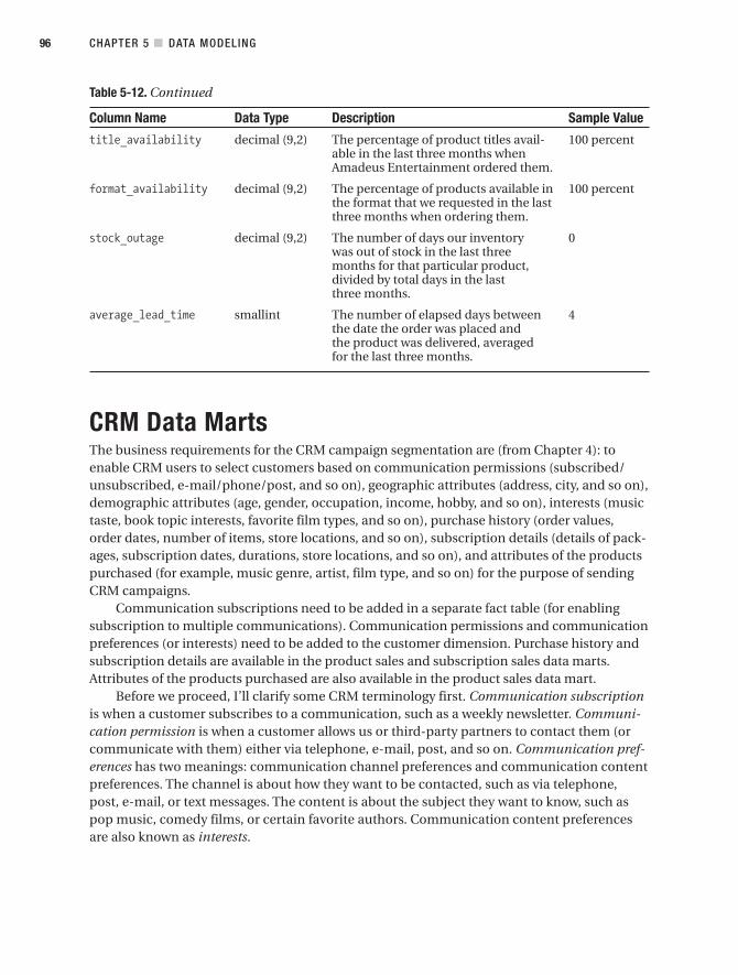
Table 5-12. Continued
Column Name Data Type Description Sample Value
title_availability decimal (9,2) The percentage of product titles avail- 100 percentable in the last three months when Amadeus Entertainment ordered them.
format_availability decimal (9,2) The percentage of products available in 100 percentthe format that we requested in the last three months when ordering them.
stock_outage decimal (9,2) The number of days our inventory 0was out of stock in the last three months for that particular product, divided by total days in the last three months.
average_lead_time smallint The number of elapsed days between 4the date the order was placed and the product was delivered, averaged for the last three months.
CRM Data MartsThe business requirements for the CRM campaign segmentation are (from Chapter 4): toenable CRM users to select customers based on communication permissions (subscribed/unsubscribed, e-mail/phone/post, and so on), geographic attributes (address, city, and so on),demographic attributes (age, gender, occupation, income, hobby, and so on), interests (musictaste, book topic interests, favorite film types, and so on), purchase history (order values,order dates, number of items, store locations, and so on), subscription details (details of pack-ages, subscription dates, durations, store locations, and so on), and attributes of the productspurchased (for example, music genre, artist, film type, and so on) for the purpose of sendingCRM campaigns.
Communication subscriptions need to be added in a separate fact table (for enablingsubscription to multiple communications). Communication permissions and communicationpreferences (or interests) need to be added to the customer dimension. Purchase history andsubscription details are available in the product sales and subscription sales data marts.Attributes of the products purchased are also available in the product sales data mart.
Before we proceed, I’ll clarify some CRM terminology first. Communication subscriptionis when a customer subscribes to a communication, such as a weekly newsletter. Communi-cation permission is when a customer allows us or third-party partners to contact them (orcommunicate with them) either via telephone, e-mail, post, and so on. Communication pref-erences has two meanings: communication channel preferences and communication contentpreferences. The channel is about how they want to be contacted, such as via telephone,post, e-mail, or text messages. The content is about the subject they want to know, such aspop music, comedy films, or certain favorite authors. Communication content preferencesare also known as interests.
CHAPTER 5 ■ DATA MODELING96
9314ch05final.qxd 11/15/07 10:16 AM Page 96

Let’s put the communication subscription in a fact table, and let’s put the communicationpermission and communication preferences in the customer dimension. Figure 5-7 shows thecommunication subscription fact table and its dimensions.
Figure 5-7. Dimensional star schema for communication subscription data mart
For simplicity in this case study, a customer has only one e-mail address, one telephonenumber, and one postal address. But in a real CRM data warehouse, of course this is not thecase. A customer can have multiple e-mail/postal addresses and landline/cell phone num-bers. If this is the case, in the subscription fact table in Figure 5-7 we need to have contact_address_key, and we need to have a “contact address” dimension. This dimension storeswhich e-mail address is subscribed to the newsletter. This dimension also stores which cellphone number is subscribed to the SMS feed and which postal address is subscribed to pro-motional mailings. This enables the same customer to be subscribed to a newsletter usingdifferent e-mail addresses, which is not the case when we have only one e-mail address fora customer. When we design the normalized data store later in this chapter, we will accom-modate having multiple postal/e-mail addresses and phone numbers for each customer bynormalizing the data.
Now let’s add communication permission and preferences in the customer dimension.Table 5-13 shows the additional attributes in the customer dimensions to incorporate permis-sion and preferences. Content preferences or interests are usually obtained via customersurveys, and the questionnaire can be based on the product hierarchy.
CHAPTER 5 ■ DATA MODELING 97
9314ch05final.qxd 11/15/07 10:16 AM Page 97
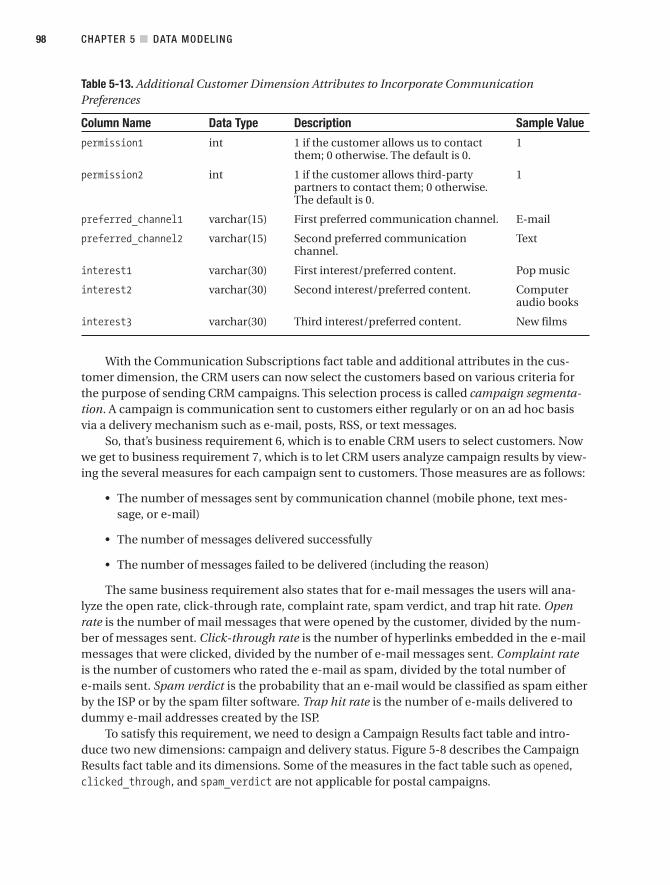
Table 5-13. Additional Customer Dimension Attributes to Incorporate CommunicationPreferences
Column Name Data Type Description Sample Value
permission1 int 1 if the customer allows us to contact 1them; 0 otherwise. The default is 0.
permission2 int 1 if the customer allows third-party 1partners to contact them; 0 otherwise. The default is 0.
preferred_channel1 varchar(15) First preferred communication channel. E-mail
preferred_channel2 varchar(15) Second preferred communication Textchannel.
interest1 varchar(30) First interest/preferred content. Pop music
interest2 varchar(30) Second interest/preferred content. Computeraudio books
interest3 varchar(30) Third interest/preferred content. New films
With the Communication Subscriptions fact table and additional attributes in the cus-tomer dimension, the CRM users can now select the customers based on various criteria forthe purpose of sending CRM campaigns. This selection process is called campaign segmenta-tion. A campaign is communication sent to customers either regularly or on an ad hoc basisvia a delivery mechanism such as e-mail, posts, RSS, or text messages.
So, that’s business requirement 6, which is to enable CRM users to select customers. Nowwe get to business requirement 7, which is to let CRM users analyze campaign results by view-ing the several measures for each campaign sent to customers. Those measures are as follows:
• The number of messages sent by communication channel (mobile phone, text mes-sage, or e-mail)
• The number of messages delivered successfully
• The number of messages failed to be delivered (including the reason)
The same business requirement also states that for e-mail messages the users will ana-lyze the open rate, click-through rate, complaint rate, spam verdict, and trap hit rate. Openrate is the number of mail messages that were opened by the customer, divided by the num-ber of messages sent. Click-through rate is the number of hyperlinks embedded in the e-mailmessages that were clicked, divided by the number of e-mail messages sent. Complaint rateis the number of customers who rated the e-mail as spam, divided by the total number ofe-mails sent. Spam verdict is the probability that an e-mail would be classified as spam eitherby the ISP or by the spam filter software. Trap hit rate is the number of e-mails delivered todummy e-mail addresses created by the ISP.
To satisfy this requirement, we need to design a Campaign Results fact table and intro-duce two new dimensions: campaign and delivery status. Figure 5-8 describes the CampaignResults fact table and its dimensions. Some of the measures in the fact table such as opened,clicked_through, and spam_verdict are not applicable for postal campaigns.
CHAPTER 5 ■ DATA MODELING98
9314ch05final.qxd 11/15/07 10:16 AM Page 98

Figure 5-8. Dimensional star schema for campaign results data mart
Now let’s discuss the data mart shown in Figure 5-8. The grain of the Campaign Resultsfact table is one row for each intended campaign recipient. If a campaign is planned to besent to 200,000 recipients, then there will be 200,000 rows in this table for that campaign,even though the campaign was actually sent to 199,970 recipients because (for example) 10had invalid e-mail addresses and 20 customers explicitly asked not to be contacted for anymarketing purposes.
Table 5-14 defines the fact table columns.
Table 5-14. Campaign Results Fact Table
Column Name Data Type Description Sample Value
campaign_key int The key of the campaign that was sent to 1456customers.
customer_key int The key of the customer who was 25433intended to receive this campaign.
communication_key int The key of the communication to which 5the campaign belongs. For example, this campaign is an instance of a communica-tion called “Amadeus music weekly news-letter” dated 02/18/2008.
Continued
CHAPTER 5 ■ DATA MODELING 99
9314ch05final.qxd 11/15/07 10:16 AM Page 99
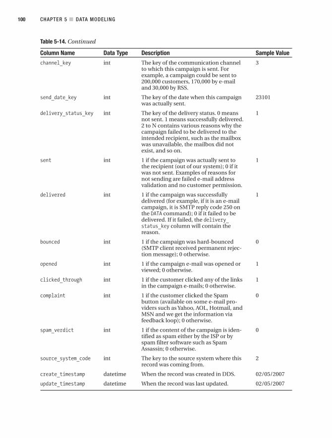
Table 5-14. Continued
Column Name Data Type Description Sample Value
channel_key int The key of the communication channel 3to which this campaign is sent. For example, a campaign could be sent to 200,000 customers, 170,000 by e-mail and 30,000 by RSS.
send_date_key int The key of the date when this campaign 23101was actually sent.
delivery_status_key int The key of the delivery status. 0 means 1not sent. 1 means successfully delivered. 2 to N contains various reasons why the campaign failed to be delivered to the intended recipient, such as the mailbox was unavailable, the mailbox did not exist, and so on.
sent int 1 if the campaign was actually sent to 1the recipient (out of our system); 0 if it was not sent. Examples of reasons for not sending are failed e-mail address validation and no customer permission.
delivered int 1 if the campaign was successfully 1delivered (for example, if it is an e-mail campaign, it is SMTP reply code 250 on the DATA command); 0 if it failed to be delivered. If it failed, the delivery_status_key column will contain the reason.
bounced int 1 if the campaign was hard-bounced 0(SMTP client received permanent rejec-tion message); 0 otherwise.
opened int 1 if the campaign e-mail was opened or 1viewed; 0 otherwise.
clicked_through int 1 if the customer clicked any of the links 1in the campaign e-mails; 0 otherwise.
complaint int 1 if the customer clicked the Spam 0button (available on some e-mail pro-viders such as Yahoo, AOL, Hotmail, and MSN and we get the information via feedback loop); 0 otherwise.
spam_verdict int 1 if the content of the campaign is iden- 0tified as spam either by the ISP or byspam filter software such as Spam Assassin; 0 otherwise.
source_system_code int The key to the source system where this 2record was coming from.
create_timestamp datetime When the record was created in DDS. 02/05/2007
update_timestamp datetime When the record was last updated. 02/05/2007
CHAPTER 5 ■ DATA MODELING100
9314ch05final.qxd 11/15/07 10:16 AM Page 100

The Delivery Status dimension contains the failure reason codes if the delivered factis 0. If the delivered fact is 1, then delivery_status_key is 1, which means OK. delivery_status_key being 0 means that the campaign was not sent out to the particular customer.The category column in this dimension contains, for example, a severity level based onSMTP reply codes. If the reply code is 550 (mailbox unavailable), then we can categorize itas severe.
Data HierarchyIn dimension tables, there is a certain structure called hierarchy. Hierarchy is importantbecause it provides you with paths that you can use to roll up and drill down when analyzingthe data. In this section, I will discuss data hierarchy in the dimension tables and how it canbe used for rolling up the data.
In the dimension tables, sometimes an attribute (column) is a subset of another attribute,meaning that the attribute values can be grouped by the other attribute. The attribute that canbe used to group is said to be on a higher level than the attribute that is being grouped. That is,if A is a subset of B, then A is on a higher level than B. These levels in the dimensions tables arecalled dimensional hierarchy. For example, a year consists of four quarters, and a quarter con-sists of three months. In this case, the highest level is year and then quarter, and the bottomlevel is month. You can roll up a fact from a lower level to a higher level. For example, if youknow the sales value of each month in the quarter, you know the sales value of that quarter.
All four dimensions of the Product Sales fact table have hierarchies. The hierarchies of thedate, store, customer, and product dimensions are shown in Figure 5-9 and Figure 5-10.
Figure 5-9 shows that fiscal week rolls up to fiscal period, but week does not roll up tomonth. The sqldate, system_date, julian_date, day, day_of_the_week, day_name, and so onare at the same level as date, so they can also roll up to week, month, and fiscal week.
Figure 5-10 shows that store can roll up to regional structure and geographical structure.Customers roll up to their geographical locations.
Figure 5-9. Hierarchy of the date dimension
CHAPTER 5 ■ DATA MODELING 101
9314ch05final.qxd 11/15/07 10:16 AM Page 101

Figure 5-10. Hierarchies of the store, customer, and product dimensions
To apply hierarchy in your own situation, first look at the columns (attributes) in thedimension tables to find whether there are any groupings or subsets. Arrange the attributesin the appropriate levels, meaning that you need to put the higher-level attribute on top ofthe lower-level attribute. Test the data to prove that all the members of the lower-level attrib-ute can be grouped by the higher-level attribute. Identify whether there are multiple paths(branches) in the hierarchy structure; for example, store in Figure 5-10 can be grouped byboth city and region. You can do all this by using the data profiling tool. Hierarchy is anintegrated part of dimension design.
Source System MappingIn this section, I will discuss why and how to do source system mapping. Source system map-ping is an exercise in mapping the dimensional data store to the source systems.
After we complete the DDS design, the next step is to map every column in the DDS tothe source systems so that we know where to get the data from when populating thosecolumns. When doing this, we also need to determine the transformations or calculationsrequired to get the source columns into the target column. This is necessary to understandthe functionality that the ETL logic must perform when populating each column on the DDStables. Bear in mind that a DDS column may come from more than one table in the sourcesystem or even from more than one source system, because the ODS integrates data frommultiple sources. This is where the source_system_code column becomes useful because itenables us to understand from which system the data is coming. I’ll give an example usingthe Product Sales data mart.
Refer to Table 5-1 again, which shows the Product Sales fact table. The first step is to findout from which tables the columns are coming. When we designed the DDS, we created theDDS columns (fact table measures and dimensional attributes) to fulfill the business require-ments. Now we need to find out where we can get the data from by looking at the sourcesystem tables. We write the source tables and their abbreviations in brackets so we can usethem later in the mapping table. Then we write the join conditions between these sourcetables so that we know how to write the query later when we develop the ETL.
The following list specifies the target table, the source tables, and the join conditions.It shows where the Product Sales fact table is populated from and how the source tablesare joined.
CHAPTER 5 ■ DATA MODELING102
9314ch05final.qxd 11/15/07 10:16 AM Page 102

Target table in DDS: Product Sales fact table
Source: WebTower9 sales_order_header [woh], WebTower9 sales_order_detail [wod],Jade order_header [joh], Jade order_detail [jod], Jupiter item_master [jim], Jupitercurrency_rate table [jcr]
Join condition: woh.order_id = wod.order_id, joh.order_id = jod.order_id,wod.product_code = jim.product_code, jod.product_code = jim.product_code
In this case study, the inventory is managed in Jupiter, and the sales transaction is storedin the two front-office systems, WebTower9 and Jade, which is why we have the link betweenthe Jupiter inventory master table and the order detail tables in WebTower9 and Jade. If youneed to recall the Amadeus Entertainment case study, see Chapter 2.
Then we add two columns to Table 5-1: source and transformation. In the source column,we refer to the source table abbreviations that we wrote earlier—woh, wod, joh, jod, and jim.We can determine which table we sourced the column from by understanding the data in thesource system. So, Table 5-1 becomes like Table 5-15. I removed the data types and sample val-ues so there’s enough space, but I kept the Description column to remind us of what thosecolumns are.
CHAPTER 5 ■ DATA MODELING 103
Table 5-15. Product Sales Fact Table Source System Mapping
Column Name Description Source Transformation
sales_date_key The date the customer pur- woh.order_date, Key lookup on date chased the product joh.order_date dimension based on
date column.
customer_key The customer who purchased woh.customer_id, Key lookup on customerthe product joh.customer_number dimension based on
customer_id column.
product_key The product purchased by wod.product_code, Key lookup on product the customer jod,product_code dimension based on
product_code column.
store_key The store where the customer woh.store_number, Key lookup on store made the purchase joh.store_number dimension based on
store_number column.
order_id WebTower9 or Jade order ID woh.order_id, Trim and convert to joh.order_id uppercase character if
required.
line_number WebTower9 or Jade order line wod.line_no, Remove leading zeros.number jod.line_no
quantity How many units of the product wod.qty, jod.qty None.were purchased by the customer
unit_price Price of one unit of the product wod.price, jod.price Divided by jcr.rate for purchased in U.S. dollars that date. Round to four
decimal digits.
unit_cost Direct and indirect costs for one jim.unit_cost Divided by jcr.rate for unit of the product in U.S. dollars that date. Round to four
decimal digits.
Continued
9314ch05final.qxd 11/15/07 10:16 AM Page 103

Table 5-15. Continued
Column Name Description Source Transformation
sales_value quantity ✕ unit_price This fact table quantity column ✕unit_price column.Round to four decimaldigits.
sales_cost quantity ✕ unit_cost This fact table quantity column ✕unit_cost column.Round to four decimaldigits.
margin sales_value – sales_cost This fact table sales_value – sales_cost column. Round tofour decimal digits.
sales_timestamp When the customer pur- woh.timestamp, Convert to mm/dd/yyyy chased the product joh.timestamp hh:mm:ss.sss format.
source_system_code The source system from which 1 for WebTower9, Lookup in source sys-this record is coming from 2 for Jade, 3 for Jupiter tem table in metadata
database.
create_timestamp When the record was created Current system time None.in DDS
update_timestamp When the record was last Current system time None.updated
CHAPTER 5 ■ DATA MODELING104
We don’t need to map the time dimension because it does not come from any source sys-tem. Instead, it is calculated internally in the data warehouse. I recommend spending a fewhours writing a SQL script that generates the values for calendar columns, with beginning andend dates as input parameters. You can do this by looping from the start date to the end dateand inserting a record at a time containing various date attributes. You can find an example ofsuch a script in the dim_date.sql file in the /Scripts/DDS folder on the book’s website. I preferthat approach than calculating them in a spreadsheet because we can rerun the script repeat-edly. This comes in handy when developing, testing, and migrating to production.
Fiscal and holiday columns are usually imported from the source system or spread-sheets by loading them into a temporary table using SSIS and then imported into the DDSby the previous script. These sources need to be mapped to a date dimension, as shown inTable 5-16, by comparing the source system columns with the DDS columns. The purpose ofdoing this mapping is to enable us to write the date dimension population script that I men-tioned earlier.
Source: Jupiter fiscal_calendar table [jfc], holidays.xls [xh],Jade store_hours [jsh]
9314ch05final.qxd 11/15/07 10:16 AM Page 104

Table 5-16. Date Dimension Source System Mapping
Column Name Description Source Transformation
fiscal_week The number of elapsed weeks since jfc.week NoneSeptember 1.
fiscal_period A period consists of four or five weeks jfc.period Remove lead-depending on the fiscal calendar. ing zero, prefix Usually, the pattern used in this com- with FPpany is 454, 544, or 445, in FPn format. A fiscal year always consists of 12 periods.
fiscal_quarter A fiscal quarter is three fiscal periods, jfc.quarter Add FQ prefixfrom September 1, in FQn format.
fiscal_year Fiscal year begins on September 1, in jfc.year Add FY prefixFYnnnn format.
us_holiday 1 if it is a national holiday in the US; 0 xh.us.date Lookup to con-otherwise. vert to 1 and 0
uk_holiday 1 if it is a statutory holiday in the UK; 0 xh.uk.date Lookup to con-otherwise. vert to 1 and 0
period_end 1 if it is the last day in a fiscal period; 0 Calculated based select maxotherwise. on fiscal period (date) group
column by fiscal period
short_day 1 if the offline stores’ opening hours is jsh.start, 1 if (start-end) shorter than normal opening hours; jsh.end < 12, else 00 otherwise.
As usual, we write the source tables with abbreviations in square brackets. We also writethe join criteria between the source tables, as follows:
Source: Jupiter item_master [jim], Jupiter product_type [jpt],Jupiter category table [jc], Jupiter media table [jm],Jupiter currency rate [jcr], Jupiter product_status [jps]Join criteria: jim.type = jpt.id, jim.category = jc.id,jim.media = jm.id, jim.status = jps.id
Table 5-17 shows the source system mapping for the product dimension.
Table 5-17. Product Dimension Source System Mapping
Column Name Description Source Transformation
product_key The surrogate key of product dimen- Identity column Nonesion. It is unique, is not null, and is with seed 1 and the primary key of product dimension. increment 1.
product_code Natural key. Product code is the jim.product_code Convert to identifier and primary key of the uppercaseproduct table in Jupiter. It is in AAA999999 format.
name The product name. jim.product_name None
description The product description. jim.description None
Continued
CHAPTER 5 ■ DATA MODELING 105
9314ch05final.qxd 11/15/07 10:16 AM Page 105

Table 5-17. Continued
Column Name Description Source Transformation
title The song/film/book title. jim.title None
artist The singer, star, or author. jim.artist None
product_type Level 1 of product hierarchy, such as jpt.description Nonemusic, film, or book.
product_category Level 2 of product hierarchy; for film, jc.name Noneit could be thriller, western, comedy, action, documentary, children, Asian, and so on.
media Format of the media, such as MP3, jm.name NoneMPG, CD, or DVD.
unit_price Price for one item. jim.unit_price Divide byjcr.rate forthat date
unit_cost Allocated direct and indirect costs. jim.unit_cost Divide byjcr.rate forthat date
status Upcoming if we have signed contract jps.description Nonewith the supplier, Active if it is still being offered to customer, Expired if it is no longer being offered.
Now we need to complete similar exercises with the customer and store dimensions, thatis, write down the source system tables with abbreviations in square brackets, write the joincriteria between the source system tables, map the dimension columns to the source systemtables and columns, and write the transformations. Then we do the same thing with all theother fact and dimension tables in other data marts.
The end result is that the dimensional data store that we designed in the previous sectionwill be completely mapped to the source systems. Therefore, we know where every single col-umn will be sourced from, including the transformations.
Designing the Normalized Data StoreNow that we have designed the dimensional data store and mapped every column in everytable to the source systems, we are ready to design the normalized data store, which is a nor-malized database that sits between the stage and the DDS. Please refer to the data flow archi-tecture diagram in Figure 2-5 in Chapter 2. The NDS is a master data store containing thecomplete data sets, including all historical transaction data and all historical versions of mas-ter data. The NDS contains master tables and transaction tables. A transaction table is a tablethat contains a business transaction or business event. A master table is a table that containsthe persons or objects involved in the business event. In this section, you will learn how todesign the data model for NDS.
First, we list all the entities based on the source tables and based on the fact and dimen-sion attributes in the DDS. We list all the tables in the source system that we have identifiedduring the source system mapping exercise in the previous section. We then normalize DDS
CHAPTER 5 ■ DATA MODELING106
9314ch05final.qxd 11/15/07 10:16 AM Page 106

fact and dimension tables into a list of separated normalized tables. We then combine thetwo lists by eliminating the same tables and separating them into different subject areas.Figure 5-11 shows the results; it contains several groups of tables that have been categorizedinto business areas. Related tables are put into the same group.
Figure 5-11. Listing the entities
We then arrange the entities according to their relationships to enable us to establishthe referential integrity between the entities. We do this by connecting the parent table tothe child table. A child table has a column containing the primary key of the parent table.Figure 5-12 shows the result; it shows the tables listed in Figure 5-11, but the parent andchild tables have been connected. The DDS fact tables become child (transaction) tablesin NDS. The DDS dimension tables become parent (master) tables in the NDS.
As an example, let’s take the Subscription Sales fact table. This fact table in the DDS hassix dimensions: lead, package, format, store, customer, and date. So, the subscription salestransaction table in the NDS in Figure 5-12 is connected to lead, package, format, store, andcustomer. We don’t model the DDS date dimension in the NDS because we put the date inthe transaction tables. We normalize the package type column in the package table into aseparate table. We normalize the media column in the format table into a separate table.
CHAPTER 5 ■ DATA MODELING 107
9314ch05final.qxd 11/15/07 10:16 AM Page 107

Figure 5-12. Arranging the entities
Ideally, the NDS diagram includes the cardinality in “crow’s feet” format to reflect the rela-tionship between entities such as one-to-many. The crow’s feet format consists of the symbolsof circle (zero), line (one), or fork (many) near a table, as shown in Figure 5-13.
Figure 5-13. Crow’s feet symbols
CHAPTER 5 ■ DATA MODELING108
9314ch05final.qxd 11/15/07 10:16 AM Page 108

The J boxes are junction tables to enable many-to-many relationships. Some people callthem bridge tables. For example, the customer_address junction table links between thecustomer table and the address table. This junction table has three main columns: customer_address_id, customer_id, and address_id. The first column is the primary key of this table. Thelast two columns are the primary key of the customer table and the address table. Some peopleprefer to make the customer_id and address_id columns a composite primary key and not usecustomer_address_id at all. This junction table also has the standard supporting columns suchas create_timestamp and update_timestamp.
To support multiple DDSs consistently, all data warehouse keys need to be defined andmaintained in the NDS so that all DDSs have consistent keys. In addition to the natural keysfrom the source system, all the NDS tables in Figure 5-12 need to have a data warehouse key.I will discuss NDS key maintenance in Chapter 8 when I discuss ETL. Some people disagreewith this approach and say it is better to generate the DW keys in DDS because surrogate keysare used in the DDS. If you have only one DDS or if you source the secondary DDSs from onemain DDS, I agree this is the best approach because you don’t have to have a surrogate key intwo places (the NDS and the DDS). But if you have more than one DDS and you intend to gen-erate the DDSs from NDS, it is better to maintain the data warehouse keys in the NDS becauseit will maintain surrogate key’s consistency between multiple DDSs.
From a data integration point of view, we need to have a DW key for every table in theNDS. We need it for mapping the reference data from several source systems. To create themapping, we identify the primary key of the table in the source system and match it with theDW key in the NDS table. When populating the NDS tables, we build ETL according to thismapping. For example, if Jade has 30,000 artists and WebTower9 has 60,000 artists, we need tohave an artist_key in the NDS artist table and map Jade artist_id and WebTower9 artist_idto it. Not only does this make the DDS population easier (because it deals only with one sys-tem), but also makes the data integration from many source systems easier in the NDS.
The date table is maintained in the NDS too. As we defined in the previous section,the date table is sourced from the fiscal_calendar table, holiday table, and opening_hourstables. But most columns of the date table are generated internally using a populationscript. This includes the week number, last day flag, system date, Julian date, week dayname, month name, and so on.
When designing the NDS, we need to follow the normalization rules. The purpose of nor-malization is to remove redundant data and make it easier to maintain the data. We need tobear in mind that normalization could impact the performance. There is no definitive rulethat we need to design the NDS to the third normal form. In some cases, it makes more senseto design some tables to the second normal form. In other cases, we need to implement othernormal forms such as the Boyce-Codd normal form (BCNF) or the fourth normal form.
■Note Please refer to the appendix for normalization rules and a quick summary of the first, second, third,Boyce-Codd, fourth, and fifth normal forms.
When doing normalization, we need to be careful when reaching 3NF and BCNF. They arebest practice, but there are cases when they are not practical. For example, if we want to bringthe customer table to 3NF, we need to break some columns into their own table. Gender and
CHAPTER 5 ■ DATA MODELING 109
9314ch05final.qxd 11/15/07 10:16 AM Page 109

status, which probably have only two or three possible values, according to 3NF rules, need togo into their own tables, linked by a foreign key to the customer table.
The next step is to list the columns. We base this on the DDS columns and on the sourcesystem columns. We don’t want to bring all source system columns into the NDS. We want tobring only the relevant ones. We get the data types from the source systems. If a particular col-umn is sourced from two different source systems, take the longest one. For example, perhapsemail in Jade is varchar(100) and in WebTower9 it is varchar(255). If one is an integer and theother is a varchar (in the case of the order ID, for example), make it a varchar. Be careful whendefining decimal and float, because different RDBMSs have different precision. Also, we needto be careful when dealing with date and timestamp data types; again, different RDBMSs havedifferent formats and behaviors.
As in many cases, an example is the best way to understand. Let’s do a customer table foran example, as shown in Table 5-18.
Table 5-18. NDS Customer Table
Column Name Data Type Description Sample Value
customer_key int The surrogate data warehouse key of 84743customer table.
customer_id varchar(10) Natural key. The primary key of the DH029383customer tables in WebTower9 and Jade. The WebTower9 customer_id for-mat is AA999999, and Jade is AAA99999.
account_number int For subscription customer; blank 342165otherwise.
customer_type_id int Foreign key (FK) to customer_type 2table where the customer type is stored.
name varchar(100) Customer’s full name. CharlotteThompson
gender char(1) M for male; F for female. F
date_of_birth smalldatetime Customer’s date of birth. 04/18/1973
occupation_id int FK to occupation ID where the cus- 439tomer occupation is stored.
household_income_id int FK to household income table where 732the customer household income is stored.
date_registered smalldatetime The date when the customer first pur- 11/23/2007chased or subscribed.
status int FK to customer_status table where the Activecustomer status is stored (active if the customer is currently a member or made a purchase in the last 12 months).
subscriber_class_id int FK to subscriber_class table where 3the subscriber class is stored. It is a classification of subscribers based on projected annual revenue.
CHAPTER 5 ■ DATA MODELING110
9314ch05final.qxd 11/15/07 10:16 AM Page 110

Column Name Data Type Description Sample Value
subscriber_band_id int FK to subscriber_band table where the 5subscriber band is stored. It is a classifi-cation of subscribers based on profitability.
effective_timestamp datetime For SCD type 2, when the data in the row 1/1/1900becomes effective; defaults to 1/1/1900.
expiry_timestamp datetime For SCD type 2, when the data in the row 12/31/2999is no longer valid; defaults to 12/31/2999.
is_current int For SCD type 2, 1 if this is the current 1record; 0 otherwise.
source_system_code int The key to the source system where this 2record was coming from.
create_timestamp datetime When the record was created in NDS. 02/05/2008
update_timestamp datetime When the record was last updated. 02/05/2008
Then we do the same thing with all the NDS tables; in other words, we list their columns.The next step is to write down the source and transformation. This should not be difficultbecause we defined them when we did the source system mapping in the DDS.
Now the NDS is complete. It has all the tables necessary to create the DDS. It is highlynormalized. We have defined all columns in all tables, along with the source and transforma-tion for each column. We can now return to the DDS and redefine the source for each DDScolumn in the NDS. This is required for building the ETL between NDS and DDS. We can dothis by identifying the source table in the NDS for each DDS table. Then we identify the cor-responding NDS column that contains the source data for each DDS column.
SummaryIn this chapter, we designed the dimensional data store and the normalized data store of theAmadeus Entertainment case study. We started from the business requirements and modeledthe DDS. We defined the fact tables and the dimension tables. We did the source system map-ping where we identified the source for each column and the required transformation.
Then we designed the NDS. We listed all the entities and then defined the relationships.Next, we listed the required columns, and we defined their sources and transformations. Wewent back to the DDS and redefined the source of each column in the NDS.
In the next chapter, you’ll see how to physically implement these databases on the SQLServer platform.
CHAPTER 5 ■ DATA MODELING 111
9314ch05final.qxd 11/15/07 10:16 AM Page 111

9314ch05final.qxd 11/15/07 10:16 AM Page 112

Physical Database Design
Having designed the logical model of the dimensional data store and normalized datastore in the previous chapter, this chapter will cover how we implement those data storesphysically as SQL Server databases. For an experienced DBA, this should not be a problem.In the previous chapter, we defined all the columns, all the data types, and the relationshipsbetween tables. It should be quite straightforward to now create those tables, right?
Although this is partially true, we need to consider a few details before taking the plungeand creating those tables. For example, we need to deal with issues such as the hardwareplatform, storage considerations, partitioning, and indexes. I will cover these topics in thischapter.
Hardware PlatformIn Chapter 2, we drafted the system architecture for Amadeus Entertainment. Figure 6-1shows the system architecture diagram for your convenience.
In the system architecture shown in Figure 6-1, we have one ETL server, two databaseservers (clustered), two report servers (load balanced), and two OLAP servers. We have 12TBraw disk space in the SAN consisting of 85 disks, each with 146GB capacity and 15,000 RPM.All the network connections to the SAN are via a fiber network, and for high availability wehave two Fibre Channel switches. We estimated that the number of client PCs that will beusing the data warehouse is between 300 and 500.
■Note In this chapter, we will be doing the physical database design. To do the physical database design,it is important to understand the physical system architecture on which the database will be operating. Phys-ical database design is a fundamental part of data warehouse design. The performance of a data warehouseis largely affected by the physical design of the underlying databases and the environment where the data-bases are running.
113
C H A P T E R 6
9314ch06final.qxd 11/15/07 10:12 AM Page 113

Figure 6-1. System architecture for the Amadeus Entertainment data warehouse
Now let’s look once again at the nonfunctional requirements from Chapter 4. Nonfunc-tional requirement 10 mentioned that the data warehouse must be available for 24 hoursa day, 7 days a week, and the downtime is expected to be no more than one hour a month.The Amadeus Entertainment data warehouse is used to support CRM activities, both cus-tomer analytics and campaign management operations. This means the campaign responsedata needs to be loaded into the data warehouse many times a day, and the campaign seg-mentation needs to query the data warehouse many times a day. Users need to run purchaseanalyses against the order data in the data warehouse several times a day. As such, it is impor-tant for the data warehouse to be available 24 hours a day, because it supports the revenuegeneration from CRM activities.
The previous high-availability requirement means we cannot implement the SQL Serverdatabase engine on a single server, because the data warehouse must be available all the time.As we know, it must not be down more than one hour a month. Therefore, we need to imple-ment it in a failover cluster. A failover cluster is a configuration of SQL Server installations onseveral identical servers (nodes). The SQL Server database instances are running on an activenode, but when the active node is not available, the database instances automatically switchesover to a secondary node.
SQL Server Reporting Services (the web or Windows service part) also needs to bedeployed in a network load balanced (NLB) cluster, and the Reporting Services database isinstalled in the failover cluster described in the previous paragraph. NLB is a configuration ofservers where the incoming traffic is distributed to several identical servers. SQL ServerReporting Services (SSRS) has two components: a web service and a database. To make SSRS
CHAPTER 6 ■ PHYSICAL DATABASE DESIGN114
9314ch06final.qxd 11/15/07 10:13 AM Page 114

available all the time, the SSRS web service needs to be installed on NLB servers. The SSRSdatabase needs to be running on a failover cluster so that when one server is not available, thedatabase will still be operational because the system automatically switches to another server.
To support this high availability requirement, Analysis Services also needs to be installedin a failover cluster, either in the same cluster as the database engine or in a separate cluster.In SQL Server 2005 and 2008, unlike SQL Server 2000, Analysis Services is cluster-aware. Ifyour budget permits, I recommend installing Analysis Services in a separate cluster, becauseyou can optimize and tune the memory and CPU usage separately. This means you need tocreate another failover cluster (separate from the failover cluster that we use for the databaseengine) specifically for running Analysis Services. This is shown in Figure 6-1, where AnalysisServices is installed in a two-node failover cluster.
The allocated disk space on the SAN for Analysis Service should ideally be separated fromthe database server for the same reason—so that you can optimize and tune the disk usageseparately. This is done by configuring the disks on the storage area network (SAN) into twoseparate sets of logical drives. One is attached to the database engine to store the databases,and the other one is attached to the Analysis Services server to store the multidimensionaldatabases (cubes).
Unfortunately, SQL Server Integration Services is not a cluster-aware application. Thismeans we cannot put SSIS in a failover cluster, which means that if the SSIS server is unavail-able, there is no secondary server to take over. This also means that (unlike other ETL softwaresuch as Informatica), we cannot distribute the ETL load to several SSIS servers in the NLB con-figuration. But SSIS does not impact the 24✕7 availability requirement to the end users. Thedata warehouse data stores are still available to the applications and to the end users to query.But if SSIS is down for a period of time, it will impact the data currency. The system architec-ture diagram in Figure 6-1 shows SSIS installed on a single server.
Some considerations in the network that you may want to consider are as follows. Betweenthe SSIS server and the database server, and between the database server and the OLAP server,try to put in a Gigabit network (capable of performing at 1Gbps throughput), rather than thenormal 100Mbps Ethernet. This will help Analysis Services performance, especially when youuse relational OLAP (ROLAP), where the aggregates are stored on the relational database server.It also improves SSIS performance because it increases the data-loading rate from the SSIS intothe data stores on the database server.
In many organizations, the SAN is typically used not only for data warehousing but forother systems too, such as Microsoft Exchange and a file server, so it’s probably worth puttingin a fiber network (2Gbps or 4Gbps), depending on the network traffic to the SAN. If manyother applications are utilizing the SAN, you need to put in a fiber network. To match the highavailability of the SAN’s RAID disks and the OLAP and database server failover cluster, youneed to use two redundant Fibre Channel switches. There is no point in having a high-speednetwork but a single point of failure.
The next questions that your hardware and network department will be asking you areabout the server technical specifications. Typical questions involve how much memory, howmany CPUs, how much disk space, which version of Windows Server, and which version ofSQL Server to license. I will explain several considerations here, but the answers depend onmany factors and vary from project to project. I will also discuss the SSRS server, SSIS/ETLserver, SSAS server, and database server.
The Reporting Services web farm (also known as a scale-out deployment) does not requirea high server specification. For a situation like Amadeus Entertainment, with 300–500 users,
CHAPTER 6 ■ PHYSICAL DATABASE DESIGN 115
9314ch06final.qxd 11/15/07 10:13 AM Page 115

two or three nodes with two CPUs and 2GB or 4GB RAM on each node would probably beenough, depending on the report complexity. If you have 1,000 users, consider adding one ortwo other nodes, depending on light or heavy usage. Sizing a Reporting Services web farm issimilar to sizing the web servers for a web site. It all depends on the amount of traffic servedby the servers. If the performance statistics show a lot of contention in the WWW service, con-sider adding another web server.
Several factors determine the specification of the ETL server. The ETL server typically per-forms intense calculations and therefore will benefit from CPU power. This is determinedfrom the complexity of transformation logic in the ETL processes. The amount of memoryrequired depends on the size of the online lookup in the transformations. For the AmadeusEntertainment case study, based on the data model we did in Chapter 5 and based on thebusiness requirements and data feasibility study we did in Chapter 4, four CPUs with 8GB to16GB memory will be more than enough for its current condition, and this will also guaranteefuture growth. In other words, it will be safe for the next two to three years. If the CPUs arehyperthreaded and/or dual-core, we need to adjust the number of CPUs accordingly. A dual-core CPU practically halves the number of CPUs (minus overhead), while a hyperthreadedCPU performs better than single-threaded ones. So, for the Amadeus Entertainment casestudy, if we use a dual-core hyperthreaded CPU, we use two CPUs instead of four. For an ETLserver, you need to take into account the future growth by estimating new data warehouse/ETL projects and enhancement requests that may happen in the future. You may have onlyten SSIS packages on the first day to start with, but after a year you may have 100 packagesrunning on it, some of which might not be data warehousing packages but other projects/systems.
Some considerations for OLAP server cluster hardware are the number of large cubes thatwill be running on Analysis Services, the number of partitions (the more partitions we have,the more memory we need), whether there will be OLAP queries running while the partitionsare being processed (if there are, we need more memory), the requirements of a large file sys-tem cache (the larger the cache, the more memory we need), the requirements of a largeprocess buffer (the larger this is, the more memory we need), the number of large replicasrequired (a replica is a subset of a dimension to accommodate dynamic security), and thenumber of heavy relational database queries and OLAP queries running simultaneously (lotsof parallel queries require more memory). All of these factors affect the memory requirement.The number of CPUs affects the aggregate calculations and cube-processing times. For cur-rent requirements and the amount of data in the Amadeus Entertainment case study, fourCPUs with 8GB RAM on each node will be enough, including accommodating the futuregrowth of more cubes and data. The best guide for sizing Analysis Services is the SQL Server2005 Analysis Services Performance Guide document, available on the Microsoft web site athttp://www.microsoft.com/technet/prodtechnol/sql/2005/ssas2005perfguide.mspx.
The database server is probably the most difficult one to size, because it is largelydependent on how heavily and frequently applications access the databases, but we can’treally determine how heavy the queries are until the applications are built. We are doingactive/passive failover clustering, so it’s only the performance of each server that matters.Active/passive failover means that only one node is working at a time. So, even though wehave two servers, only the performance of one server matters, because only one server isworking. The second server is not working. Some considerations for sizing the databaseserver of a data warehouse are as follows:
CHAPTER 6 ■ PHYSICAL DATABASE DESIGN116
9314ch06final.qxd 11/15/07 10:13 AM Page 116

The number and complexity of reports, applications, and direct queries hitting the DDS:The main factor that determines the specification of the database server is the work-load from application queries. As I discussed in Chapter 2, the DDS is the user-facingdatabase. So, it is the one that the users and BI/CRM applications will be querying. Adatabase server used for data warehousing is predominantly used for queries. It isprobably 10 to 20 percent of the time used for loading the data (such as one to threehours a day), and the rest (80 to 90 percent of the time) is used to satisfy user andapplication queries. The heavier the queries, the more memory and CPU we need inthe database server.
Whether we’re taking an ELT or ETL approach in populating the NDS/ODS: An ELTapproach loads the data into the database server in raw format (in other words, the sameas the source system format) and then uses the power of the database server to transformthe data into the NDS or ODS format in a set-based operation via stored procedures,whereas the ETL approach transforms the data using the power of the ETL server. If weuse the ELT approach in loading the data, we need a more powerful database server thanthe ETL approach.
Calculation from the stage to the NDS/ODS and the complexity of firewall rules: If theseprocesses run on a separate ETL server, then they don’t affect the database server sizing.But if they run on the database server (as stored procedure or triggers), then they impactthe performance of the database server. The more complex the calculation and the fire-wall rules, the more CPU we need.
The number and size of data stores: The more user-facing data stores we have, the morememory and CPUs we need because we would have more connections from the users.The size of the data stores affects the number of records involved in the ETL processes.The larger the size of the data store, the more records inserted/updated/selected/deletedby the ETL processes. To complete a larger ETL process in the same amount of time, weneed more powerful hardware for the database server (faster disk, larger memory, andbetter CPU).
How the data stores are physically designed (indexing, partitions, and so on): Physical data-base design affects database server configuration because if we utilize certain physicaldatabase features, we can improve loading and query performance without significantchanges to the server hardware. For example, we can load data into the data warehousefaster if we partition the table physically and if we put the tables in databases on differentdisks.
The number of other databases hosted in the same server and future growth: For cost rea-sons, the database server may be utilized to host other databases, not just the datawarehouse. This will affect the number of CPUs, the cache size, and the amount of mem-ory we need on the database server. We also need to take into account two to three yearsof projected growth.
For a system like Amadeus Entertainment, four CPUs with 8GB to 16GB RAM will besuitable for the database server considering the data warehouse workload and its futuregrowth. This is determined based on the business requirements in Chapter 4, the datamodel in Chapter 5, the architecture in Chapter 2, and all the considerations I described
CHAPTER 6 ■ PHYSICAL DATABASE DESIGN 117
9314ch06final.qxd 11/15/07 10:13 AM Page 117

previously, as well as from Microsoft’s RDBMS Performance Tuning Guide for Data Ware-housing at http://www.microsoft.com/technet/prodtechnol/sql/2000/maintain/rdbmspft.mspx. It is on SQL Server 2000, but the principles are highly applicable for SQLServer 2005. Microsoft’s Project REAL (http://www.microsoft.com/sql/solutions/bi/projectreal.mspx) is also a good reference.
Once we have determined the server configurations for the SSIS, SSAS, SSRS, and data-base servers, we need to determine which operating system and SQL Server editions we needand which licensing model best suits the architecture. I’ll discuss the operating system first,then the SQL Server hardware levels (32-bit or 64-bit), then the SQL Server editions (StandardEdition or Enterprise Edition), and finally the licenses.
Regarding the operating system, Windows 2003 R2 Enterprise Edition (EE) supports upto eight processors and 64GB RAM, so it is suitable for the Amadeus Entertainment databaseserver mentioned previously (four CPUs with 8GB to 16GB RAM). The next level up is Win-dows 2003 R2 Datacenter Edition, which supports up to 64 processors and 128GB RAM, butin the Amadeus Entertainment case study, there is no need to use this.
We need to determine whether we need the SQL Server 32-bit or 64-bit edition for theAmadeus Entertainment case study. On the 32-bit platform, even though the SQL Server data-base engine can use all the RAM available in the server (limited only by the operating system),Analysis Services can use only 3GB RAM. So if we use the 32-bit edition for the SSAS server, itwon’t be able to use the entire 8GB RAM that we have in the server. Because of this, we needthe 64-bit edition.
Regarding the database server, on the 32-bit edition some SQL Server database engineresources such as sort space, join hash tables, aggregate hash tables, and index creation do notuse RAM more than 3GB. For these reasons, in the Amadeus Entertainment case study, weneed to use the 64-bit version.
SQL Server is available in six editions: Express, Evaluation, Developer, Workgroup, Stan-dard, and Enterprise. The first four are for trial, development, and small applications. Forenterprise-class data warehousing solutions in a production environment like in the AmadeusEntertainment case study, practically speaking we can use only the last two, the Standard Edi-tion or Enterprise Edition. SQL Server Standard Edition supports four CPUs and unlimitedRAM. These capabilities suit the Amadeus Entertainment case study. But because of the high-availability and performance requirements, for the Amadeus Entertainment case study weneed SQL Server Enterprise Edition. The primary reason is that the following features are notavailable in the Standard Edition:
Table and index partitioning: These features enable us to physically divide a table intosmaller chunks that we can load and query separately. When dealing with a fact table con-taining billions of rows, this feature is a must-have if we need to have good performance.
Report server scale-out deployment: This means we can run Reporting Services on multi-ple web servers, all accessing the same reporting services database in the same SQLServer instance. This enables us to serve hundreds or thousands of users simultaneouslyand achieve high availability. Both are requirements in the Amadeus Entertainment casestudy: 300–500 client PCs/laptops and 24✕7 availability, with only one hour of downtimeper month (99.86 percent uptime).
CHAPTER 6 ■ PHYSICAL DATABASE DESIGN118
9314ch06final.qxd 11/15/07 10:13 AM Page 118

Analysis Services partitioned cubes: This feature enables us to divide a cube into smallerchunks that we can load and query separately. This is important because it means lesscube-processing time and higher query performance.
Semiadditive aggregate functions: These are functions that work with measures that canbe summed up in some dimensions but not in other dimensions. This is importantbecause it enables us to deal with semiadditive measures such as account balances.
Parallel index operations: This feature enables us to create or rebuild an index using mul-tiple processors simultaneously. It is useful in data warehousing when we deal with largefact tables.
Online index operation: This enables us to create or rebuild an index when users arequerying or updating data on the table being indexed. This is important in data ware-housing to maximize data store availability.
Number of nodes for failover clustering: In Standard Edition, the maximum number ofnodes is two, which limits future growth because we cannot add more active nodes whenwe need more capacity or performance. In Enterprise Edition, we don’t have a limitationon the number of nodes.
Now that I have discussed the editions, we need to deal with the licenses. Generallyspeaking, there are two SQL Server licensing models:
Per-processor license: We buy a license for each processor in the server. It does not matterhow many users we have. Prices vary between countries, but in the United States theretail price of Enterprise Edition for a per-processor license is about $25,000.1
Server + CAL license: We buy a license for the server and a client access license (CAL) foreach client accessing the server. A client can be per user or per computer. For EnterpriseEdition in the United States, the retail price for one server license is about $14,000 (whichincludes 25 CALs). Each additional client license is about $162.
The way SQL Server is licensed means that for every single component we need to buy aseparate license. Because for the Amadeus Entertainment case study we are installing SSIS,SSRS, SSAS, and the database engine on separate servers, this means we need to buy SQLServer licenses separately for each of those servers.
For the Amadeus Entertainment case study, if we license it per processor, we will need 16per-processor licenses: four for the database cluster (the passive node does not require alicense), four for the Analysis Services cluster, four for the report server farm (two servers ✕two CPUs each, because each node requires a license), and four for the SSIS server. The costwould be 16 ✕ $25,000 = $400,000. If we use Server + CAL licenses, for 500 users we need fiveserver licenses (one for the database cluster, one for the Analysis Services cluster, two for thereport server farm, and one for the SSIS server) and 375 additional CALs (from the five serverlicenses we get 5 ✕ 25 CALs). So, the cost would be (5 ✕ $14,000) + (375 ✕ $162) = $130,750.In this case, the server + CAL licensing model is better.
CHAPTER 6 ■ PHYSICAL DATABASE DESIGN 119
1. http://www.microsoft.com/sql/howtobuy/default.mspx
9314ch06final.qxd 11/15/07 10:13 AM Page 119
Storage ConsiderationsThe next thing we need to purchase for the infrastructure is the disk space. In Chapter 4, I saidit was not possible to estimate the amount of storage properly at that stage, because we hadnot completed the DDS and NDS design. Now that we have completed the database design,we can do the estimation.
This is done by calculating the size of the fact and dimension tables to get the size of theDDS. Then we estimate the size of the NDS based on the row size and the number of rows foreach table. Then we estimate the size of the stage database based on the source system tablesand data extraction method. Let’s start with the DDS, then the NDS, then the stage database,then the metadata database, and finally the disk configuration.
Let’s examine the Product Sales fact table illustrated in Table 5-1 in Chapter 5. It haseight int columns, one decimal column, ten money columns, and three datetime columns.Integers are 4 bytes, decimals are 5 bytes, and money and datetime are 8 bytes, so the rowsize is 8 ✕ 4 + 1 ✕ 5 + (10 + 3) ✕ 8 = 141 bytes. Allow 50 percent to accommodate extra col-umns in the future, which makes it 212 bytes. The percentage is determined based on howmany columns we will add in the future. If the source system shows that on average thereare 500,000 sales per day (make it 600,000 to allow for growth—or more, based on projectedgrowth) and we are planning to purchase storage capacity for two years (see Chapter 4),then the size of the fact table is 600,000 ✕ 365 ✕ 2 ✕ 212 bytes = 86GB. We will add fill factorand overhead later for the whole database, not per table.
The Subscription Sales fact table has 12 int columns, 16 money columns, and 4 datetimecolumns, so the row size is 208 bytes. Some people call row size record length, which is theterm inherited from the sequential file era. Allowing 50 percent for extra columns makes it312 bytes. If the store system shows that Amadeus Entertainment has 800,000 subscribers(make it 1 million to allow for growth) and we store daily data for the last four weeks andweekly data for the last two years (refer to Chapter 5), the size of the fact table is 1 million ✕(4 ✕ 7 + 2 ✕ 52) ✕ 312 bytes = 38GB.
We do the same exercise for all fact and dimension tables, and we will get the size of alltables in the DDS. It’s the same principle in the NDS. We calculate the row size by multiplyingthe number of columns of each data type with the bytes for that data type. We estimate thenumber of rows by querying the source system. The number of rows in the NDS table wouldbe roughly the same as the number of rows in the source system. We need to keep in mind thatif we have several source systems, the number of rows in the NDS depends on how much over-lap we have between the source systems. For example, if the product table in source system Acontains 600,000 rows and the product table in source system B contains 400,000 rows, ofwhich 250,000 exist in source system A, then the number of rows in the NDS product tablewould be 600,000 + 150,000 = 750,000.
To estimate the size of the stage database, we need to list all the source tables that we didin Chapter 5 when we did the source system mapping. For each table, query the source systemto determine the row size and the number of rows. If the extraction method to the stage isincremental, count how many rows are inserted or updated per day in the source system. Forexample, say there are 300 million rows in the sales order item table but there are only 900,000rows updated or inserted for each day. If the extraction method to the stage is “truncate andreload,” use the number of rows in the whole table. We will go through data extraction fromthe source system in Chapter 7.
Remember that you may need to get only some columns from the source system tableinto the data warehouse, not all columns in the table. Let’s say the width of the sales order
CHAPTER 6 ■ PHYSICAL DATABASE DESIGN120
9314ch06final.qxd 11/15/07 10:13 AM Page 120

table in WebTower9 is 2,000 bytes but the total bytes of the columns that you download is onlyhalf of this. This affects the sizing of the stage database. Another factor that affects the stagedatabase sizing is that you may want to store three or five days’ worth (or more, depending onbackup strategy) of data in the stage before purging it in case you need to reload it to the NDSfor some reason. So in this case, the size of the order item stage table would be 1.1 million ✕ 5✕ 1000 bytes = 5GB. We adjust the daily rows from 900,000 to 1.1 million to allow for two yearsof growth.
The other database that we will create is metadata. It is not big, probably 10–20GB. Allo-cating 50GB will be sufficient. This is estimated based on the content of the metadatadatabase. The metadata database stores seven kinds of metadata: data definition and map-ping metadata, data structure metadata, source system metadata, ETL processes metadata,data quality metadata, audit metadata, and usage metadata.
You may also want to allocate some space for two or three smaller DDSs, such as for datamining purposes or specific analysis projects. The reason for having a separate DDS for theseprojects and activities is because they may need to update the data to reflect certain businessscenarios.
Say, for argument’s sake, the result of the previous calculation is as follows: the DDS is400GB, the NDS is 300GB, the stage is 100GB, the metadata database is 50GB, so the total is850GB. To get the size of the data files (MDB), we need to allow some space for indexes andfor RDBMS overhead such as the table header, row ID, block header and trailer, fill factor,page splits, and other SQL Server internal DBMS mechanisms. Take 30 percent for indexesand 15 percent for internal mechanisms, which makes it 1233GB. Allow 20 percent for esti-mation tolerance, which makes it 1479GB. The percentages for indexes vary depending onhow heavily we index the tables; in other words, it can be 50 percent for some tables, and itcan be 10 percent for other tables. My general estimate of 30 percent for index space is just ahigh-level estimate. If you need a more precise estimation, use the Microsoft guide at http://msdn2.microsoft.com/en-us/library/ms190620.aspx (this page is also available in BooksOnline). The 20 percent estimation tolerance is to cover unknown factors—those things weare not aware of at the time we do the estimating.
TERMINOLOGY
Let’s clear up some terminology commonly used in data storage, especially disk and volume, before we con-tinue. We will use the terminology later in this chapter. A disk is a single SCSI drive (we tend not to use IDEdrives for database servers because the IDE is perceived more for home use rather than for industrial usebecause of their reliability and durability). The capacity of a SCSI drive varies from 36GB to 73GB to 146GB to300GB. The speed varies from 10,000 RPM to 15,000 RPM. Some people use the term spindle to refer to adisk. A volume is several disks arranged together according to a certain RAID configuration. Redundant Arrayof Inexpensive Disks (RAID) is a method to configure several disks as one unit to make them more resilient bycreating some physical data redundancy.
The popular RAID configurations (some people say RAID level) are RAID 0, RAID 1, RAID 5, and RAID1+0 (some people say RAID 10). If you have four 146GB SCSI disks and arrange them in RAID 0 configura-tion, the resulting volume is 146 ✕ 4 = 584GB. If you arrange them in RAID 5, the resulting volume is 146 ✕3 = 438GB. If you arrange them in RAID 1+0, the resulting volume is 146GB. RAID 1 can be made only withtwo disks. If you have two 146GB disks, the resulting RAID 1 volume is 146GB. We will use these four RAIDlevels in this example.
CHAPTER 6 ■ PHYSICAL DATABASE DESIGN 121
9314ch06final.qxd 11/15/07 10:13 AM Page 121
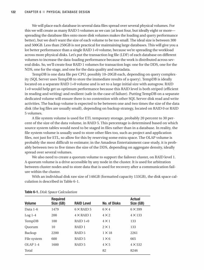
We will place each database in several data files spread over several physical volumes. Forthis we will create as many RAID 5 volumes as we can (at least four, but ideally eight or more—spreading the database files onto more disk volumes makes the loading and query performancebetter), but we don’t want the size of each volume to be too small. The ideal size is between 300and 500GB. Less than 250GB is not practical for maintaining large databases. This will give you alot better performance than a single RAID 1+0 volume, because we’re spreading the workloadacross more physical disks. Let’s put the transaction log file (LDF) of each database on differentvolumes to increase the data-loading performance because the work is distributed across sev-eral disks. So, we’ll create four RAID 1 volumes for transaction logs: one for the DDS, one for theNDS, one for the stage, and one for the data quality and metadata.
TempDB is one data file per CPU, possibly 10–20GB each, depending on query complex-ity (SQL Server uses TempDB to store the immediate results of a query). TempDB is ideallylocated on a separate RAID 1+0 volume and is set to a large initial size with autogrow. RAID1+0 would help get us optimum performance because this RAID level is both striped (efficientin reading and writing) and resilient (safe in the case of failure). Putting TempDB on a separatededicated volume will ensure there is no contention with other SQL Server disk read and writeactivities. The backup volume is expected to be between one and two times the size of the datadisk (the log files are usually small), depending on backup strategy, located on RAID 0 or RAID5 volumes.
A file system volume is used for ETL temporary storage, probably 20 percent to 30 per-cent of the size of the data volume, in RAID 5. This percentage is determined based on whichsource system tables would need to be staged in files rather than in a database. In reality, thefile system volume is usually used to store other files too, such as project and applicationfiles, not just for ETL, so allow for this by reserving some extra space. The OLAP volume isprobably the most difficult to estimate; in the Amadeus Entertainment case study, it is prob-ably between two to five times the size of the DDS, depending on aggregate density, ideallyspread over several volumes.
We also need to create a quorum volume to support the failover cluster, on RAID level 1.A quorum volume is a drive accessible by any node in the cluster. It is used for arbitrationbetween cluster nodes and to store data that is used for recovery after a communication fail-ure within the cluster.
With an individual disk raw size of 146GB (formatted capacity 133GB), the disk space cal-culation is described in Table 6-1.
Table 6-1. Disk Space Calculation
Required Actual Volume Size (GB) RAID Level No. of Disks Size (GB)
Data 1-6 1479 6 ✕ RAID 5 6 ✕ 4 6 ✕ 399
Log 1-4 200 4 ✕ RAID 1 4 ✕ 2 4 ✕ 133
TempDB 100 RAID 1+0 4 ✕ 1 133
Quorum 10 RAID 1 2 ✕ 1 133
Backup 2200 RAID 5 1 ✕ 18 2261
File system 600 RAID 5 1 ✕ 6 665
OLAP 1-4 1600 RAID 5 4 ✕ 5 4 ✕ 532
Total 82 8246
CHAPTER 6 ■ PHYSICAL DATABASE DESIGN122
9314ch06final.qxd 11/15/07 10:13 AM Page 122

Eighty-two disks are required, and the total usable space is 8.2TB. The previous exercise isknown as logical unit number design. With 85 disks in the cabinet, we have three disks for SANhot spare. Hot spare is a standby disk used automatically to replace a failed disk. It is best touse disks with the same capacity and RPM throughout the SAN. If you use disks with a differ-ent capacity or RPM, you must remember that they require different hot spare disks. A RAIDvolume is built from several disks. If one of these disks fails, the SAN controller automaticallyassigns the hot spare disk to temporarily replace the failed one. For this to happen, the hotspare disk must have the same capacity as the one being replaced.
If you can afford it, a large quantity of smaller disks (such as 73GB) is better than fewerbigger disks (such as 146GB). This is because the workload is distributed to more disks. A highRPM (such as 15,000) is absolutely essential in any case, because it gives better performancethan a lower RPM (such as 10,000). Hewlett-Packard has reported that the I/O throughput per-formance of a 15,000 RPM disk can be as much as 25 percent higher than the equivalent10,000 RPM,2 whereas IBM has reported 50 percent.3 TempDB is ideally in a RAID 1+0 volume,as explained earlier. It is faster than RAID 5 or RAID 1, both at reading and writing. For datawarehousing, a very large TempDB (10–20GB per CPU, depending on the query complexity)on a good-performance RAID 1+0 volume is crucial. The default is 8MB, which is way toosmall for DW.
I’ve heard suggestions to partition the RAID 1 quorum volume and allocate a little portion(say 10GB) for the quorum and the remainder (say 123GB) for the log files. I am against thisidea because the quorum is the core of a cluster build; I prefer not to risk it. Get a smaller diskif you want for the quorum (36GB, for example), but dedicate it just for the quorum alone.Microsoft recommends assigning a dedicated LUN for quorum resources and not storing userdata on any volume on the quorum LUN.4
Bear in mind that you need to allocate some amount of disk space for your QA environ-ment. Ideally, the QA environment has the same capacity as production. This enables us tounload production data into the QA environment to test a modification or enhancement toensure that the modifications will run OK in production. Having a QA environment with thesame capacity as the production environment is also useful for performance testing, when weload the QA environment with the same amount of data (if not more) as the production envi-ronment. With some calculation, we also can get a reasonable idea about how a productionenvironment will perform based on tests in a smaller QA environment.
Configuring DatabasesNow that we have designed the databases, let’s create them in SQL Server. Here are somepoints you may want to consider when creating the databases. Let’s take the Amadeus Enter-tainment case study as an example in these points:
CHAPTER 6 ■ PHYSICAL DATABASE DESIGN 123
2. http://h20223.www2.hp.com/NonStopComputing/cache/117086-0-0-225-121.html
3. http://www-01.ibm.com/common/ssi/cgi-bin/ssialias?subtype=ca&infotype=an&appname=iSource&supplier=897&letternum=ENUS105-324
4. http://technet2.microsoft.com/windowsserver/en/library/dba487bf-61b9-45af-b927-e2333ec810b61033.mspx?mfr=true
9314ch06final.qxd 11/15/07 10:13 AM Page 123

• Keep database names short and concise. DDS, NDS, Stage, and Meta will do. We need tokeep them short because they will be used as prefixes to ETL process names and storedprocedure names.
• Remember to keep the collation of all data warehouse databases the same, preferablyas per the company’s SQL Server installation standard defined by the SQL Server DBA.Database collation defines how SQL Server handles character and Unicode data, suchas case-sensitivity, sort order, and code page. If they are different, there will be conver-sion problems when populating the NDS from the stage and populating the DDS fromthe NDS; for example, when trying to do column comparisons for UPSERT, set the servercollation as well in case you need to create a new DDS in the future.
• Consider case sensitivity very carefully. Query results will be different depending on thecase sensitivity. We need to set case according to the user requirements for sortingorder. For the Amadeus Entertainment case study, we will use SQL Server default colla-tion, SQL_Latin1_General_CP1_CI_AS, so it will be case-insensitive.
• For each database we will create six filegroups, located on six different physical disks onRAID 5, with one transaction log file located in the designated log disk of RAID 1. File-groups are a collection of database files. Set the database default location in the serverproperty to match this. This is necessary so that when we create a new database (forexample, a new DDS), SQL Server will put the database data and log files in the correctlocations. This is done by right-clicking the SQL Server name in Management Studioand choosing Properties. Click Database Settings, and modify the default databaselocations.
• Arrange the data files to support the previous filegroup arrangement, meaning thatwhen creating the database, place data files as per the filegroup locations. We have sixphysical disks for data, so use them well by spreading the filegroups into different phys-ical disks. Put the log files of each database on different log disks, as specified in theprevious section. Set the initial size of the data files for six to twelve months of growthby specifying the initial size correctly when creating the database. Maintain the dataand log files manually; do not rely on autogrowth. If there is a data load operation thatrequires more log space than what’s available, the operation will take a long time tocomplete because it has to wait until the grow operation completes. Growing a data-base by little increments causes a performance problem because of file and diskfragmentation. We still need to turn on autogrow (with a large increment) but use itonly for emergency measures.
• Based on the estimated database size in the previous section (400 and 300 over twoyears), aiming for six months I would set the initial size of the DDS to 100GB with agrowth increment of 25GB and the initial size of the NDS to 75GB with a 15GB growthincrement. The initial sizes for the DDS and the NDS (100 and 75GB) are calculated bytaking the linear proportion of the two-year projection (400GB and 300GB) for sixmonths. If you have initial load, then add this amount to the initial sizes. For example,if the initial load is 30GB, then the initial sizes for the DDS and the NDS become 130GB
CHAPTER 6 ■ PHYSICAL DATABASE DESIGN124
9314ch06final.qxd 11/15/07 10:13 AM Page 124
and 105GB. We need to remember that these initial sizes are collective overall figures, sowe need to divide them among the six files. Set the growth increment to 20 to 25 per-cent of the initial sizes to minimize the SQL Server grow operation. Remember that weneed to maintain the size of the data and log files manually (say every six months, withmonitoring every month); we should use autogrowth only for emergencies.
• If the expected daily load is 5GB to 10GB and we keep five days of data on the stage, setthe stage database’s initial size to 50GB with a growth increment of 10GB. For themetadata database, we expect it would be about 10GB in a year and to be 20GB in twoyears, so let’s set the initial size to 10GB with a 5GB increment. The principle to settingthe increment is that it is only for emergencies; we should never have to use auto-growth because we increase the file size manually. The increment for the earlier stagedatabase was set to 20 percent to 25 percent as per the DDS and the NDS. This largepercentage is selected to minimize fragmentation if the database file did become full.The increment for the metadata database is set to 50 percent (5GB) because the meta-data database contains audit and usage metadata that could fluctuate by significantamounts depending on ETL processes.
• The log file size depends on the size of the daily load, recovery model, and the loadingmethod (ETL or ELT, stage or not stage; I’ll discuss this in the next chapter) as well asindex operations. Let’s set it to a 1GB initial size with a 512MB increment for both theDDS and the NDS. For the stage, set a 2GB initial size with a 512MB increment. Formetadata, set it to 100MB with a 25MB increment. The transaction log contains data-base changes. The transaction log space required depends on how much data we loadinto the database. One way to estimate how much log space is required is to use theETL processes to load one day’s data into the stage and then into the NDS and then intothe DDS. If we set the initial size and the increment of these three databases to a smallamount (say 1MB to 2MB), during this process the log file will grow so that after the ETLprocesses are completed, the transaction log sizes of these three databases will indicatethe required log sizes.
• For the recovery model, choose simple rather than bulk. All the changes in the datawarehouse are from the ETL processes. When recovering from failure, we can roll for-ward using ETL by reapplying the extracted source system data for the particular day.We don’t require the bulk recovery model to roll forward to a certain point in time usingdifferential backup or transaction log backup. We fully control the data upload on theETL, and the ETL process is the only process that updates the data warehouse. For thestage, the NDS, and the DDS, the full recovery model is not necessary and causes over-head. The full recovery model requires log backup, whereas the simple recovery modeldoesn’t. The simple recovery model reclaims the log space automatically. The full recov-ery model is suitable for OLTP systems where inserts and updates happen frequently allday from many users and we want to be able to recover the database to a certain pointin time. In data warehousing, we can recover the data store by restoring the last fullbackup followed by applying differential backups and then applying the daily ETLloads.
CHAPTER 6 ■ PHYSICAL DATABASE DESIGN 125
9314ch06final.qxd 11/15/07 10:13 AM Page 125

• If you use the ODS + DDS architecture, you may want to consider the full recoverymodel in the ODS especially if ETL is not the only process that updates the ODS. Unlikethe NDS, the ODS is updatable. End-user applications can retrieve data from the ODS,but they can also update the ODS (please refer to Chapter 2 where ODS + DDS architec-ture is explained). Because the ODS is continuously updated by the users, it is useful toimplement the full recovery model so we can recover the ODS to any point in time.
• For a metadata database, we need to set the recovery mode to full. The data quality andfront-end application will also write to metadata, in addition to the daily ETL process,mainly for audit purposes such as report stored procedures, data quality stored proce-dures, and the administration of ETL processes. Because the metadata database iscontinuously updated, it is useful to implement the full recovery model so we canrecover the metadata database to any point in time.
• Leave the maximum degree of parallelism at 0 to utilize all processors. The degree ofparallelism is the number of processors used to execute a single SQL statement in par-allel. If we leave it set to 0 (which is the default), SQL Server will utilize all the availableprocessors.
• Disable full-text indexing if you are not using it. Full-text indexing enables us to searchfor patterns in character columns a lot faster than the LIKE predicate in SELECT state-ments. The Microsoft Search service uses system memory for the full-text indexingprocess.
• It is different from DBA to DBA, but you may want to disable autoshrink and enableautomatic statistics update, especially in the DDS. A database with autoshrink may leadto fragmentation and cause performance issues. Automatic statistics updating is neces-sary for the SQL Server query optimizer to know the best path to execute the query. SQLServer collects the statistics of the indexes and column data in the database. The queryoptimizer uses these database statistics to estimate the selectivity of a column or indexand to estimate the costs of different query plans.
For an example, let’s create the DDS database. Say we want to make the total size of thedata files 100GB. Because we will have six files located on six different physical files, we allo-cate 100GB / 6 = 17GB for each file. A few months later, these files will not be the same size.A few months later, file 1 could be 18GB, file 2 could be 30GB, and file 3 could be 20GB. Toallow for this natural possibility of uneven growth, we will set the initial size for each file to30GB—the maximum growth. The size of each disk is 399GB, so you can set the max size ofeach file to 150GB or 170GB if you want, which is 40 percent of the disk size, not 100 percent,because other databases will reside on the same disk too.
The growth increment for the DDS, as mentioned previously, is 25GB. Spread over sixdisks, that’s 4.2GB each, roughly. A growth increment is a figure that tells SQL Server howmuch we want to expand the file when it’s full. It doesn’t have the uneven growth problemmentioned previously, so we will allocate 5GB in each file. As I said previously, we should notrely on autogrowth, because the DWA should have a script monitoring this allocated dataspace. This script shows the percentage of data files used for each data warehouse data store.
The database creation script for the DDS is as follows. It shows that the initial size is 30GB,as mentioned previously, and the file growth is 5GB. It uses six data files. The log file is 1GBwith a 512MB increment, as discussed previously. This script is included in the /script folder
CHAPTER 6 ■ PHYSICAL DATABASE DESIGN126
9314ch06final.qxd 11/15/07 10:13 AM Page 126

at the book's web site (http://www.apress.com/). To execute this script on a stand-alone lap-top or desktop, you just need to replace the drive letter (h) with a local drive such as c or d.
use mastergo
if db_id ('DDS') is not nulldrop database DDS;
go
create database DDS on primary (name = 'dds_fg1', filename = 'h:\disk\data1\dds_fg1.mdf', size = 30 GB, filegrowth = 5 GB), filegroup dds_fg2 (name = 'dds_fg2', filename = 'h:\disk\data2\dds_fg2.ndf', size = 30 GB, filegrowth = 5 GB), filegroup dds_fg3 (name = 'dds_fg3', filename = 'h:\disk\data3\dds_fg3.ndf', size = 30 GB, filegrowth = 5 GB), filegroup dds_fg4 (name = 'dds_fg4', filename = 'h:\disk\data4\dds_fg4.ndf', size = 30 GB, filegrowth = 5 GB), filegroup dds_fg5 (name = 'dds_fg5', filename = 'h:\disk\data5\dds_fg5.ndf', size = 30 GB, filegrowth = 5 GB), filegroup dds_fg6 (name = 'dds_fg6', filename = 'h:\disk\data6\dds_fg6.ndf', size = 30 GB, filegrowth = 5 GB)log on (name = 'dds_log', filename = 'h:\disk\log1\dds_log.ldf', size = 1 GB, filegrowth = 512 MB)collate SQL_Latin1_General_CP1_CI_ASgo
alter database DDS set recovery simple goalter database DDS set auto_shrink offgoalter database DDS set auto_create_statistics ongoalter database DDS set auto_update_statistics ongo
h:\disk\data1 to h:\disk\data6 and h:\disk\log1 to h:\disk\log4 are the mount pointsof the six data volumes and four log volumes that we built in the SAN (please refer to the previ-ous section). A mount point is the drive letter assigned to a volume created from severalphysical disks in a RAID configuration. This drive letter is used by the operating system to
CHAPTER 6 ■ PHYSICAL DATABASE DESIGN 127
9314ch06final.qxd 11/15/07 10:13 AM Page 127

access the data in that volume. For other databases, the scripts are similar, apart from the filelocations and sizes. Put the NDS log file on h:\disk\log2, the stage on h:\disk\log3, and themetadata on h:\disk\log4.
For the stage database, we don’t need automatic statistic updating because we don’t usu-ally index tables. We still want the simple recovery model, and we still don’t need autoshrinkfor the stage database. Remember to put the stage log file on a different disk from the NDSand DDS logs; this is important for ETL performance because it minimizes the contention oflog traffic between data stores. Because of the size and the nature of loading, we don’t need tosplit the stage database over six disks. Three of four would be more than enough because wecan allocate different stage tables in three to four different disks that can be loaded simultane-ously. We can use data disks 1–4 for the stage.
Remember to set the recovery mode to full for the metadata database. Because the sizeof the metadata database is small and because the way we use the metadata database ismore like an OLTP type query than a data warehouse query (in other words, it is frequentlyupdated), we don’t need to spread it across six disks. Two disks are good enough because thesize is only 10–20GB, as discussed previously. We can use data disks 5 and 6 for metadata.We still need to put the metadata log file on a separate disk, though, not for the benefit ofthe metadata database itself but so that we don’t affect the performance the NDS, the DDS,and the stage log files.
■Note Because you will be creating the databases in your development environment, which in the case ofa stand-alone desktop or laptop probably doesn’t have multiple disks or drivers and a large amount of diskspace, you can reduce the figures from gigabytes to megabytes so the databases will be enough for yourdisk space. Just create a folder called disk and create ten folders called data1 to data6 and log1 to log4under this disk folder. This simulates the six data disks and four log disks discussed earlier. You can put thedatabase data files and log files in these ten folders.
Now that we have created all four databases, we are ready to create the database struc-ture—the tables.
Creating DDS Database StructureAfter we created the databases, we can now create the tables based on the logical design thatwe created in the previous chapter. Let’s start with the DDS. It has five fact tables and fourteendimensions. Let’s do the Product Sales fact table first. We’ll do the four dimensions that it usesfirst and then the fact table. We defined these four dimension tables in the previous chapter.So, open SQL Server 2005 Management Studio, connect to your development SQL Serverinstance, and start creating the tables. You can use Management Studio’s point-and-click func-tionality if you want, or you can script it.
Either way, create the date dimension table as follows:
CHAPTER 6 ■ PHYSICAL DATABASE DESIGN128
9314ch06final.qxd 11/15/07 10:13 AM Page 128

use DDSgo
if exists (select * from sys.tables where name = 'dim_date')
drop table dim_datego
create table dim_date( date_key int not null , date char(10) not null, system_date char(10) not null, sql_date datetime not null, julian_date int not null, day tinyint not null, day_of_the_week tinyint not null, day_name varchar(9) not null, day_of_the_year smallint not null, week_number tinyint not null, month tinyint not null, month_name varchar(9) not null, short_month_name char(3) not null, quarter char(2) not null, year smallint not null, fiscal_week tinyint , fiscal_period char(4), fiscal_quarter char(3), fiscal_year char(6), week_day tinyint not null, us_holiday tinyint, uk_holiday tinyint, month_end tinyint not null, period_end tinyint, short_day tinyint, source_system_code tinyint not null, create_timestamp datetime not null, update_timestamp datetime not null, constraint pk_dim_date primary key clustered (date_key) on dds_fg6
) on dds_fg6go
CHAPTER 6 ■ PHYSICAL DATABASE DESIGN 129
9314ch06final.qxd 11/15/07 10:13 AM Page 129

if exists (select * from sys.indexes where name = 'sql_date'and object_id = object_id('dim_date'))
drop index dim_date.sql_datego
create unique index sql_dateon dim_date(sql_date)on dds_fg6
go
In SQL Server 2005 and 2008, the sys.tables catalog view replaces sysobjects used inSQL Server 2000. You can use sys.objects if you want (notice the dot there), but you need tospecify where type = 'U'. The sys.objects catalog view contains all the database objects suchas tables, views, triggers, primary keys, and stored procedures. By specifying type = 'U', wefilter the rows for user-defined tables only. Catalog views contain information used by the SQLServer database engine, such as tables, columns, and primary keys.
The dimension key needs to be assigned as the primary key of the table and as the clus-tered index. This means that the table will be physically ordered on the date_key column. Thiswill be useful for query performance. We don’t need to make the dimensional key column anidentity column because all keying will be done in the NDS. Columns that should not containNULL such as weekdays and month ends should have the NOT NULL constraint.
I don’t advise putting a check constraint in the DDS dimensions because it will negativelyaffect the loading performance. Instead, it would be better to put it in the data quality (DQ)routine inside the ETL because the check will be processed in a set-based statement ratherthan row by row, so it’s faster. I’ll talk about DQ in Chapter 9. Don’t put default gettime() inthe create_timestamp or update_timestamp column, because we want all rows inserted orupdated during the same batch to have the same timestamp, so we will set this timestamp inthe ETL.
You may want to put in a bit of code that checks and drops the foreign key constraintsbefore dropping and creating the table, like in the following code. This prevents orphan orinvalid foreign keys on the related tables.
if exists(select * from sys.foreign_keyswhere name = 'fk_fact_campaign_result_dim_date'and parent_object_id = object_id('fact_campaign_result'))
alter table fact_campaign_resultdrop constraint fk_fact_campaign_result_dim_date
go
And after creating the table, re-create the foreign key that you dropped, like this:
CHAPTER 6 ■ PHYSICAL DATABASE DESIGN130
9314ch06final.qxd 11/15/07 10:13 AM Page 130

if exists(select * from sys.tableswhere name = 'fact_campaign_result')
alter table fact_campaign_resultadd constraint fk_fact_campaign_result_dim_dateforeign key (send_date_key)references dim_date(date_key)
go
This way, the individual script can be executed independently of the other scripts. Don’tforget to use Unicode (nchar and nvarchar) if you operate in countries with non-Latin char-acters. If the width is fixed, such as date, use char rather than varchar; char is slightly fasterbecause it has a fixed position and is slightly smaller because it doesn’t have the 2 bytes off-set. If you have three varchar(10) columns, the storage is 2 + (3 ✕ 2) + (3 ✕ 10 bytes) = 38bytes. If you use three char(10) columns, the storage is 30 bytes. To get the row size, you needto add 4 bytes for the row header and 3 bytes for the null bitmap (this is the total for the row,not for each column). The null bitmap is an indicator whether a column may contain null.So, if we use varchar, the row size is 45 bytes, and if we use char, the row size is 37 bytes. If,however, you know that on average the varchar column will be only 60 percent full, use var-char, because the storage is 2 + (3 ✕ 2) + (3 ✕ 10 bytes ✕ 60 percent) = 26 bytes.
Every time you use int, ask yourself whether the value of that column will ever reach2 billion. In many cases, you can use tinyint (up to 255) and smallint (up to 32k). If you usedecimal or number, always specify the precision, 9 or lower if possible. Precision 9 uses 5bytes, whereas precisions 10 to 19 use 9 bytes. The default precision is 18. For dimensiontables, you can just set all columns to Unicode and int because they are small (probably afew thousand rows except for the customer dimension, which could be millions). But for afact table with billions of rows, you may want to consider the right data type to save the diskspace and maximize data loading and query performance.
Every time you use money (8 bytes), ask yourself whether the value will ever reach214,000. If not, use smallmoney, which is only 4 bytes. Also, ask yourself whether you needmore than four digits after the decimal point, for example, for the currency rate. If you do, usedecimal rather than money. Some people use smalldatetime rather than datetime when theyneed only the date and don’t need the time element. You probably want to reconsider thisbecause smalldatetime is only up to year 2079, and it starts from 1900.
Perhaps you also noticed there are two dds_fg6 on the create table statement previouslymentioned. They are the filegroups. Filegroups are collections of database files. You need tospecify the filegroup; otherwise, it will be stored in the primary filegroup, which is on disk 1.The first one is where the primary key’s clustered index is physically stored. The second one iswhere the table is physically stored. To keep track of what table goes to which filegroup, it isuseful if you make a filegroup allocation table, as shown in Table 6-2. As we discussed earlier, itis important to spread the tables in the data store on different disks, using filegroups, to maxi-mize query performance and data-loading performance.
CHAPTER 6 ■ PHYSICAL DATABASE DESIGN 131
9314ch06final.qxd 11/15/07 10:13 AM Page 131

Table 6-2. Filegroup Allocation Table for the DDS
Table Name Table Type Filegroup
dim_week Dimension 6
dim_store Dimension 6
dim_campaign Dimension 6
dim_channel Dimension 6
dim_communication Dimension 6
dim_customer Dimension 6
dim_date Dimension 6
dim_delivery_status Dimension 6
dim_format Dimension 6
dim_lead Dimension 6
dim_package Dimension 6
dim_product Dimension 6
dim_subscription_status Dimension 6
dim_supplier Dimension 6
fact_product_sales Fact 2
fact_subscription_sales Fact 3
fact_supplier_performance Fact 3
fact_communication_subscription Fact 5
fact_campaign_result Fact 5
Fact tables’ PKs and indexes 4
Dimension tables’ PKs and indexes 6
To maximize query performance and data-loading performance on the DDS database,in Table 6-2 we allocate all dimension tables to filegroup 6, the Product Sales fact table tofilegroup 2, the Subscription Sales and Supplier Performance fact tables to filegroup 3, thetwo CRM fact tables to filegroup 5, and the fact table indexes to filegroup 4. We won’t use theprimary filegroup yet. We will use this for the summary fact table later.
If we put a fact table and dimension table on different disks, we reduce the disk con-tention and therefore increase the query performance. The performance increase depends onhow large the dimension tables being joined to the fact table in the query are. We reduce thecontention further by putting the fact indexes on a separate disk from the fact tables. Ideally,the dimension table and index should also be separated, but because they are a lot smallerthan fact tables, I prefer to put the dimension indexes in filegroup 6 together with dimensiontables rather than, for example, putting them in filegroup 2 with the large Product Sales facttable.
OK, let’s continue creating the product dimension as follows:
CHAPTER 6 ■ PHYSICAL DATABASE DESIGN132
9314ch06final.qxd 11/15/07 10:13 AM Page 132

use DDSgo
if exists(select * from sys.objects where name = 'dim_product')
drop table dim_productgo
create table dim_product( product_key int not null, product_code varchar(10), name varchar(30), description varchar(100), title varchar(100), artist varchar(100), product_type varchar(20), product_category varchar(30), media varchar(25), unit_price money, unit_cost money, status varchar(15), source_system_code tinyint , create_timestamp datetime, update_timestamp datetime, constraint pk_dim_product primary key clustered (product_key)on dds_fg6
) on dds_fg6go
And then let’s create the customer dimension:
use DDSgo
if exists (select * from sys.tables where name = 'dim_customer')
drop table dim_customergo
CHAPTER 6 ■ PHYSICAL DATABASE DESIGN 133
9314ch06final.qxd 11/15/07 10:13 AM Page 133

create table dim_customer( customer_key int not null, customer_id varchar(10), account_number int, customer_type char(1), name varchar(100), gender char(1), email_address varchar(200), date_of_birth datetime, address1 varchar(50), address2 varchar(50), address3 varchar(50), address4 varchar(50), city varchar(50), state varchar(40), zipcode varchar(10), country varchar(50), phone_number varchar(20), occupation varchar(50), household_income varchar(20), date_registered datetime, status varchar(10), subscriber_class varchar(3), subscriber_band varchar(3), permission tinyint, preferred_channel1 varchar(15), preferred_channel2 varchar(15), interest1 varchar(30), interest2 varchar(30), interest3 varchar(30), effective_timestamp datetime, expiry_timestamp datetime, is_current tinyint, source_system_code tinyint, create_timestamp datetime, update_timestamp datetime , constraint pk_dim_customer primary key clustered (customer_key)on dds_fg6
) on dds_fg6go
CHAPTER 6 ■ PHYSICAL DATABASE DESIGN134
9314ch06final.qxd 11/15/07 10:13 AM Page 134

And then let’s create the store dimension:
use DDSgo
if exists (select * from sys.tables where name = 'dim_store')
drop table dim_storego
create table dim_store( store_key int not null, store_number smallint, store_name varchar(40), store_type varchar(20), store_address1 varchar(50), store_address2 varchar(50), store_address3 varchar(50), store_address4 varchar(50), city varchar(50), state varchar(40), zipcode varchar(10), country varchar(50), phone_number varchar(20), web_site varchar(100), region varchar(30), prior_region varchar(30), prior_region_date datetime, division varchar(30), prior_division varchar(30), prior_division_date datetime, source_system_code tinyint, create_timestamp datetime, update_timestamp datetime, constraint pk_dim_storeprimary key clustered (store_key)on dds_fg6
) on dds_fg6go
And finally, we’ll create the Product Sales fact table:
CHAPTER 6 ■ PHYSICAL DATABASE DESIGN 135
9314ch06final.qxd 11/15/07 10:13 AM Page 135

use DDSgo
if exists (select * from sys.objects where name = 'fact_product_sales' and type = 'U')
drop table fact_product_salesgo
create table fact_product_sales( sales_date_key int not null, customer_key int not null, product_key int not null, store_key int not null, order_id int not null, line_number int not null, quantity int, unit_price smallmoney, unit_cost smallmoney, sales_value money, sales_cost money, margin money, sales_timestamp datetime, source_system_code tinyint not null, create_timestamp datetime not null, update_timestamp datetime not null, constraint pk_fact_product_sales primary key clustered (order_id, line_number)on dds_fg4
, constraint fk_fact_product_sales_dim_dateforeign key (sales_date_key)references dim_date(date_key)
, constraint fk_fact_product_sales_dim_customerforeign key (customer_key)references dim_customer(customer_key)
, constraint fk_fact_product_sales_dim_productforeign key (product_key)references dim_product(product_key)
, constraint fk_fact_product_sales_dim_storeforeign key (store_key)references dim_store(store_key)
) on dds_fg2go
CHAPTER 6 ■ PHYSICAL DATABASE DESIGN136
9314ch06final.qxd 11/15/07 10:13 AM Page 136

create index fact_product_sales_sales_date_keyon fact_product_sales(sales_date_key)on dds_fg4
go
create index fact_product_sales_customer_keyon fact_product_sales(customer_key)on dds_fg4
go
create index fact_product_sales_product_keyon fact_product_sales(product_key)on dds_fg4
go
create index fact_product_sales_store_keyon fact_product_sales(store_key)on dds_fg4
go
I’ll discuss the indexes and how to choose primary keys in more detail when I talk aboutindexing later in this chapter because it is closely related with how to choose a cluster index.For now let’s suffice it to say that for the primary key we need to choose a column or columnsthat make the row unique. There could be several candidates for the primary key.
Some people prefer not to put referential integrity (foreign keys) in a data warehouse.They say that data integrity is controlled in the ETL so we don’t need a foreign key. The sec-ond argument is that a foreign key slows down the loading. But on the other hand, the queryoptimizer uses constraint definitions such as the primary key and the foreign key to build ahigh-performance query execution plan. If you have a primary key - foreign key relationshipbetween two tables, it indicates to SQL Server that the two tables have been optimized to becombined in a query that uses the key as its criteria. This is particularly useful on optimizingqueries that join several tables, the choice is yours. I prefer putting the foreign key on first andseeing how the loading performs. If loading is slow at a particular table, consider taking thatparticular foreign key off (not all of them) before the loading begins and put it back afterward.
About the column names, some people prefer to abbreviate the column name such assh_mon_nm. I think it is better to use the full words because they are easier to understand.
■Note Regarding table naming, some people prefix table names with dim_ and fact_, some prefix themwith d and f, some put the word dim or fact at the end as in order_fact, and some people don’t useunderscores as in PurchaseOrderFact (this is what Microsoft recommends in MSDN, but many SQL Server2005 system views use underscores, as in sys.foreign_key). Again, the choice is yours, but please beconsistent.
CHAPTER 6 ■ PHYSICAL DATABASE DESIGN 137
9314ch06final.qxd 11/15/07 10:13 AM Page 137

We do the same thing with all other tables in DDS. For the complete DDS table creationscripts, please refer to the web site accompanying this book at http://www.apress.com/; thescripts are in the /script folder.
When you have completed all five fact tables and fourteen dimension tables, create abatch file using sqlcmd, as shown next, and call those scripts one by one. sqlcmd is a SQL Serverutility that enables you to enter Transact SQL statements and script files at the commandprompt. Start with the database creation, then the dimensions, and finally the facts. Theyneed to be in this order because of the foreign key in the fact tables.
h:cd "h:\dw\scripts\dds"sqlcmd -i db_dds.sql >> ddsout.txtsqlcmd -i dim_campaign.sql >> ddsout.txtsqlcmd -i dim_channel.sql >> ddsout.txtsqlcmd -i dim_communication.sql >> ddsout.txtsqlcmd -i dim_customer.sql >> ddsout.txtsqlcmd -i dim_date.sql >> ddsout.txtsqlcmd -i dim_delivery_status.sql >> ddsout.txtsqlcmd -i dim_format.sql >> ddsout.txtsqlcmd -i dim_lead.sql >> ddsout.txtsqlcmd -i dim_package.sql >> ddsout.txtsqlcmd -i dim_product.sql >> ddsout.txtsqlcmd -i dim_store.sql >> ddsout.txtsqlcmd -i dim_subscription_status.sql >> ddsout.txtsqlcmd -i dim_supplier.sql >> ddsout.txtsqlcmd -i dim_week.sql >> ddsout.txtsqlcmd -i fact_product_sales.sql >> ddsout.txtsqlcmd -i fact_subscription_sales.sql >> ddsout.txtsqlcmd -i fact_supplier_performance.sql >> ddsout.txtsqlcmd -i fact_communication_subscription.sql >> ddsout.txtsqlcmd -i fact_campaign_result.sql >> ddsout.txt
The parameter –i [filename] means “input file.” Instead of >> [filename], you use –o [filename] or > [filename] to create the output file, but it will replace the content of theoutput file. If your development SQL Server environment is not local, you need to specify –S followed by the server name: sqlcmd –S server1. You may also need to specify the user-name and password using the –U and –P parameters: sqlcmd –S server1 –U user1 –Ppassword1. You can specify the password just once in the environment variable using setsqlcmdpassword=. If you don’t specify –U and –P, the default is –E, which means use a trustedconnection. You can also string all the script file names together in one line: sqlcmd –i file1,file2, file3, ....
Here are two examples:
sqlcmd –i file1.sql –S server1 –U user1 –P password1sqlcmd –i file1.sql file2.sql –S server1 –E
The first example connects to server1 using user1 and password1 credentials and thenexecutes the statements in file1.sql.
The second example connects to server1 using a trusted connection (Windows inte-grated security) and executes the statements in file1.sql and file2.sql.
CHAPTER 6 ■ PHYSICAL DATABASE DESIGN138
9314ch06final.qxd 11/15/07 10:13 AM Page 138

Creating the Normalized Data StoreThe NDS is a little bit different from the DDS. The main difference is the normalization. In thenext few pages, I will discuss the tables in Figure 6-2 and how to create them physically. I willalso discuss how to arrange the tables in different filegroups located on different disks.
Figure 6-2. Schema of Amadeus Entertainment normalized data store
The tables in the NDS can be categorized into three groups: transaction tables, mastertables, and attribute tables. Transaction tables contain business events and are derived fromthe DDS fact tables. Master tables contain business entities and are derived from the DDS
CHAPTER 6 ■ PHYSICAL DATABASE DESIGN 139
9314ch06final.qxd 11/15/07 10:13 AM Page 139
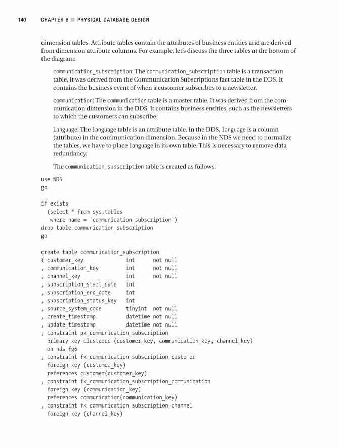
dimension tables. Attribute tables contain the attributes of business entities and are derivedfrom dimension attribute columns. For example, let’s discuss the three tables at the bottom ofthe diagram:
communication_subscription: The communication_subscription table is a transactiontable. It was derived from the Communication Subscriptions fact table in the DDS. Itcontains the business event of when a customer subscribes to a newsletter.
communication: The communication table is a master table. It was derived from the com-munication dimension in the DDS. It contains business entities, such as the newslettersto which the customers can subscribe.
language: The language table is an attribute table. In the DDS, language is a column(attribute) in the communication dimension. Because in the NDS we need to normalizethe tables, we have to place language in its own table. This is necessary to remove dataredundancy.
The communication_subscription table is created as follows:
use NDSgo
if exists (select * from sys.tables where name = 'communication_subscription')
drop table communication_subscriptiongo
create table communication_subscription( customer_key int not null , communication_key int not null, channel_key int not null, subscription_start_date int, subscription_end_date int, subscription_status_key int, source_system_code tinyint not null, create_timestamp datetime not null, update_timestamp datetime not null, constraint pk_communication_subscriptionprimary key clustered (customer_key, communication_key, channel_key)on nds_fg6
, constraint fk_communication_subscription_customerforeign key (customer_key)references customer(customer_key)
, constraint fk_communication_subscription_communicationforeign key (communication_key)references communication(communication_key)
, constraint fk_communication_subscription_channelforeign key (channel_key)
CHAPTER 6 ■ PHYSICAL DATABASE DESIGN140
9314ch06final.qxd 11/15/07 10:13 AM Page 140

references channel(channel_key), constraint fk_communication_subscription_subscription_statusforeign key (subscription_status_key)references subscription_status(subscription_status_key)
) on nds_fg4go
The primary key of the communication_subscription table has the same granularity as thefact table—one row per subscription. If the customer unsubscribes, we will just mark it in thesame row, subscription_end_date. If the customer resubscribes to the same newsletter, wewill mark the subscription_start_date column and clear the unsubscribe date. We don’t cre-ate a new row. We need to include a channel in the primary key because it is possible that acustomer subscribes to (for example) the Amadeus Entertainment Music weekly newslettervia two channels: e-mail and RSS feed.
Just as we did in the DDS, we need to place the tables in different filegroups located on adifferent physical disk. The main principle here is to avoid putting large transaction tables onthe same disk. For the NDS, I usually split them according to the subject areas, as follows(please refer to Figure 6-2):
• Subject area 1 is sales, physically located on the primary filegroup.
• Subject area 2 is customer, physically located on filegroup 2.
• Subject area 3 is geographic, physically located on filegroup 3.
• Subject area 4 is CRM, physically located on filegroup 4.
• Subject area 5 is supplier, physically located on filegroup 5.
Table 6-3 lists all the NDS tables, along with the table type (master, transaction, or attrib-ute), the subject area (one of the five mentioned previously), and the filegroup where they arelocated.
Table 6-3. Filegroup Allocation Table for NDS
Table Name Table Type Subject Area Filegroup
supplier Master Supplier 5
contact Attribute Supplier 5
supplier_performance Transaction Supplier 5
product Master Product 5
format Master Product 5
media Attribute Product 5
product_status Attribute Product 5
product_type Attribute Product 5
product_category Attribute Product 5
package Master Sales Primary
package_type Attribute Sales Primary
Continued
CHAPTER 6 ■ PHYSICAL DATABASE DESIGN 141
9314ch06final.qxd 11/15/07 10:13 AM Page 141

Table 6-3. Continued
Table Name Table Type Subject Area Filegroup
lead Master Sales Primary
subscription_sales Transaction Sales 3
order_header Transaction Sales Primary
order_item Transaction Sales Primary
currency Master Sales Primary
currency_rate Attribute Sales Primary
store_type Attribute Geographic 3
store Master Geographic 3
region Attribute Geographic 3
division Attribute Geographic 3
city Attribute Geographic 3
state Attribute Geographic 3
country Attribute Geographic 3
customer Master Customer 2
occupation Attribute Customer 2
interest Attribute Customer 2
interest_junction Junction Customer 2
permission Attribute Customer 2
subscriber_band Attribute Customer 2
subscriber_class Attribute Customer 2
customer_status Attribute Customer 2
customer_type Attribute Customer 2
address Attribute Geographic 3
address_type Attribute Geographic 3
address_junction Junction Geographic 3
phone_number Attribute Customer 2
phone_number_type Attribute Customer 2
phone_number_junction Junction Customer 2
email_address Attribute Customer 2
email_address_type Attribute Customer 2
email_address_junction Junction Customer 2
communication_subscription Transaction CRM 4
subscription_status Master CRM 4
campaign Master CRM 4
channel Master CRM 4
channel_junction Junction CRM 2
CHAPTER 6 ■ PHYSICAL DATABASE DESIGN142
9314ch06final.qxd 11/15/07 10:13 AM Page 142

Table Name Table Type Subject Area Filegroup
communication Master CRM 4
campaign_result Transaction CRM 4
business_unit Attribute CRM 4
communication_category Attribute CRM 4
language Attribute CRM 4
delivery_status Master CRM 4
delivery_status_category Attribute CRM 4
We then put indexes in filegroup 6 to separate them from the tables. For performance rea-sons, we generally want to have indexes and tables on separate disks. The Primary filegrouphas three transaction tables, so to balance everything, we can put the Subscription Sales tablein filegroup 3. Filegroup 2 doesn’t have a transaction table, but the customer master andattribute tables are generally larger than other subject areas.
The communication table contains (amongst other things) the newsletter that we send tocustomers. It is created as follows:
use NDSgo
-- Remove FK if exists (otherwise you can't drop the table):if exists(select * from sys.foreign_keyswhere name = 'fk_communication_subscription_communication'and parent_object_id = object_id('communication_subscription'))
alter table communication_subscriptiondrop constraint fk_communication_subscription_communication
go
if exists(select * from sys.foreign_keyswhere name = 'fk_campaign_result_communication'and parent_object_id = object_id('campaign_result'))
alter table campaign_resultdrop constraint fk_campaign_result_communication
go
-- Drop the table if exists:if exists (select * from sys.tables where name = 'communication')
drop table communicationgo
CHAPTER 6 ■ PHYSICAL DATABASE DESIGN 143
9314ch06final.qxd 11/15/07 10:13 AM Page 143

-- Create the table:create table communication( communication_key int not null identity(1,1), title varchar(50) not null, description varchar(200), format varchar(20), language_key int, category_key int, issuing_unit_key int, start_date smalldatetime, end_date smalldatetime, status varchar(10), source_system_code tinyint not null, create_timestamp datetime not null, update_timestamp datetime not null, constraint pk_communicationprimary key clustered (communication_key)on nds_fg6
, constraint fk_communication_languageforeign key (language_key)references language(language_key)
, constraint fk_communication_communication_categoryforeign key (category_key)references communication_category(communication_category_key)
, constraint fk_communication_business_unitforeign key (issuing_unit_key)references business_unit(business_unit_key)
) on nds_fg4go
-- Create FK:alter table communication_subscriptionadd constraint fk_communication_subscription_communicationforeign key (communication_key)references communication(communication_key)
go
alter table campaign_resultadd constraint fk_campaign_result_communicationforeign key (communication_key)references communication(communication_key)
CHAPTER 6 ■ PHYSICAL DATABASE DESIGN144
9314ch06final.qxd 11/15/07 10:13 AM Page 144
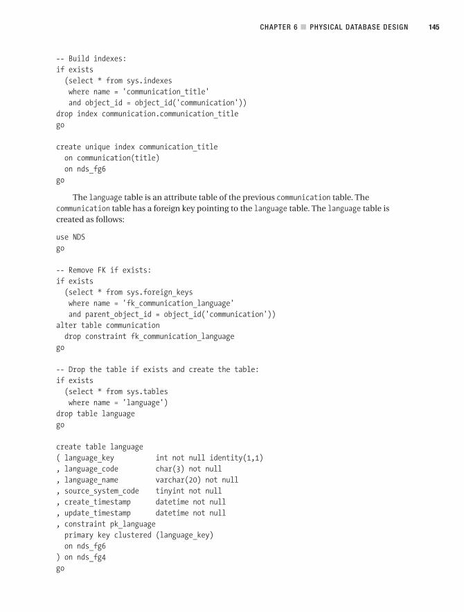
-- Build indexes:if exists(select * from sys.indexeswhere name = 'communication_title'and object_id = object_id('communication'))
drop index communication.communication_titlego
create unique index communication_titleon communication(title)on nds_fg6
go
The language table is an attribute table of the previous communication table. Thecommunication table has a foreign key pointing to the language table. The language table iscreated as follows:
use NDSgo
-- Remove FK if exists:if exists(select * from sys.foreign_keyswhere name = 'fk_communication_language'and parent_object_id = object_id('communication'))
alter table communicationdrop constraint fk_communication_language
go
-- Drop the table if exists and create the table:if exists (select * from sys.tables where name = 'language')
drop table languagego
create table language( language_key int not null identity(1,1), language_code char(3) not null, language_name varchar(20) not null, source_system_code tinyint not null, create_timestamp datetime not null, update_timestamp datetime not null, constraint pk_languageprimary key clustered (language_key)on nds_fg6
) on nds_fg4go
CHAPTER 6 ■ PHYSICAL DATABASE DESIGN 145
9314ch06final.qxd 11/15/07 10:13 AM Page 145
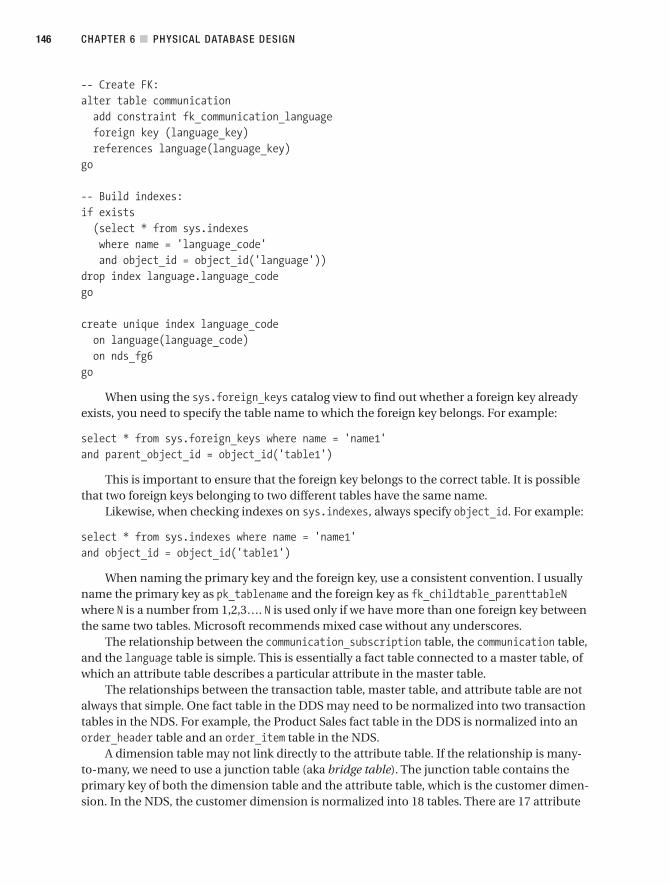
-- Create FK:alter table communicationadd constraint fk_communication_languageforeign key (language_key)references language(language_key)
go
-- Build indexes:if exists(select * from sys.indexes where name = 'language_code' and object_id = object_id('language'))
drop index language.language_codego
create unique index language_codeon language(language_code)on nds_fg6
go
When using the sys.foreign_keys catalog view to find out whether a foreign key alreadyexists, you need to specify the table name to which the foreign key belongs. For example:
select * from sys.foreign_keys where name = 'name1'and parent_object_id = object_id('table1')
This is important to ensure that the foreign key belongs to the correct table. It is possiblethat two foreign keys belonging to two different tables have the same name.
Likewise, when checking indexes on sys.indexes, always specify object_id. For example:
select * from sys.indexes where name = 'name1'and object_id = object_id('table1')
When naming the primary key and the foreign key, use a consistent convention. I usuallyname the primary key as pk_tablename and the foreign key as fk_childtable_parenttableNwhere N is a number from 1,2,3…. N is used only if we have more than one foreign key betweenthe same two tables. Microsoft recommends mixed case without any underscores.
The relationship between the communication_subscription table, the communication table,and the language table is simple. This is essentially a fact table connected to a master table, ofwhich an attribute table describes a particular attribute in the master table.
The relationships between the transaction table, master table, and attribute table are notalways that simple. One fact table in the DDS may need to be normalized into two transactiontables in the NDS. For example, the Product Sales fact table in the DDS is normalized into anorder_header table and an order_item table in the NDS.
A dimension table may not link directly to the attribute table. If the relationship is many-to-many, we need to use a junction table (aka bridge table). The junction table contains theprimary key of both the dimension table and the attribute table, which is the customer dimen-sion. In the NDS, the customer dimension is normalized into 18 tables. There are 17 attribute
CHAPTER 6 ■ PHYSICAL DATABASE DESIGN146
9314ch06final.qxd 11/15/07 10:13 AM Page 146

tables. Attribute tables that are one-to-many, such as the occupation table, are connecteddirectly to the customer table. Attribute tables that are many-to-many, such as theemail_address table, are connected to the customer table using a junction table.
The customer table is the most complex table in the NDS. It has 17 attribute tables. It ref-erences six other tables and is being referenced by eight other tables. This table is the coretable in this system. We will create it in filegroup 2, with the index in filegroup 6. The customertable is created as follows:
use NDSgo
-- Remove FK if exists:if exists(select * from sys.foreign_keyswhere name = 'fk_address_junction_customer'and parent_object_id = object_id('address_junction'))
alter table address_junctiondrop constraint fk_address_junction_customer
go
if exists(select * from sys.foreign_keyswhere name = 'fk_phone_number_junction_customer'and parent_object_id = object_id('phone_number_junction'))
alter table phone_number_junctiondrop constraint fk_phone_number_junction_customer
go
if exists(select * from sys.foreign_keyswhere name = 'fk_email_address_junction_customer'and parent_object_id = object_id('email_address_junction'))
alter table email_address_junctiondrop constraint fk_email_address_junction_customer
go
if exists(select * from sys.foreign_keyswhere name = 'fk_interest_junction_customer'and parent_object_id = object_id('interest_junction'))
alter table interest_junctiondrop constraint fk_interest_junction_customer
go
CHAPTER 6 ■ PHYSICAL DATABASE DESIGN 147
9314ch06final.qxd 11/15/07 10:13 AM Page 147

if exists(select * from sys.foreign_keyswhere name = 'fk_subscription_sales_customer'and parent_object_id = object_id('subscription_sales'))
alter table subscription_salesdrop constraint fk_subscription_sales_customer
go
if exists(select * from sys.foreign_keyswhere name = 'fk_communication_subscription_customer'and parent_object_id = object_id('communication_subscription'))
alter table communication_subscriptiondrop constraint fk_communication_subscription_customer
go
if exists(select * from sys.foreign_keyswhere name = 'fk_campaign_result_customer'and parent_object_id = object_id('campaign_result'))
alter table campaign_resultdrop constraint fk_campaign_result_customer
go
if exists(select * from sys.foreign_keyswhere name = 'fk_channel_junction_customer'and parent_object_id = object_id('channel_junction'))
alter table channel_junctiondrop constraint fk_channel_junction_customer
go
-- Create customer table (drop it first if exists):if exists (select * from sys.tables where name = 'customer')
drop table customergo
create table customer( customer_key int not null identity(1,1), customer_id varchar(10) not null, account_number int, customer_type_key int, name varchar(100) not null, gender char(1)
CHAPTER 6 ■ PHYSICAL DATABASE DESIGN148
9314ch06final.qxd 11/15/07 10:13 AM Page 148

, date_of_birth datetime, occupation_key int, household_income_key int, date_registered datetime, customer_status_key int, subscriber_class_key int, subscriber_band_key int, permission_key int, effective_timestamp datetime not null, expiry_timestamp datetime not null, is_current tinyint not null, source_system_code tinyint not null, create_timestamp datetime not null, update_timestamp datetime not null, constraint pk_customer primary key clustered (customer_key)on nds_fg6
, constraint fk_customer_occupationforeign key (occupation_key)references occupation(occupation_key)
, constraint fk_customer_household_incomeforeign key (household_income_key)references household_income(household_income_key)
, constraint fk_customer_customer_statusforeign key (customer_status_key)references customer_status(customer_status_key)
, constraint fk_customer_subscriber_classforeign key (subscriber_class_key)references subscriber_class(subscriber_class_key)
, constraint fk_customer_subscriber_bandforeign key (subscriber_band_key)references subscriber_band(subscriber_band_key)
, constraint fk_customer_permissionforeign key (permission_key)references permission(permission_key)
) on nds_fg2go
-- Create FK from other tables to this table:alter table address_junctionadd constraint fk_address_junction_customerforeign key (customer_key)references customer(customer_key)
go
CHAPTER 6 ■ PHYSICAL DATABASE DESIGN 149
9314ch06final.qxd 11/15/07 10:13 AM Page 149

alter table phone_number_junctionadd constraint fk_phone_number_junction_customerforeign key (customer_key)references customer(customer_key)
go
alter table email_address_junctionadd constraint fk_email_address_junction_customerforeign key (customer_key)references customer(customer_key)
go
alter table interest_junctionadd constraint fk_interest_junction_customerforeign key (customer_key)references customer(customer_key)
go
alter table subscription_salesadd constraint fk_subscription_sales_customerforeign key (customer_key)references customer(customer_key)
go
alter table communication_subscriptionadd constraint fk_communication_subscription_customerforeign key (customer_key)references customer(customer_key)
go
alter table campaign_resultadd constraint fk_campaign_result_customerforeign key (customer_key)references customer(customer_key)
go
alter table channel_junctionadd constraint fk_channel_junction_customerforeign key (customer_key)references customer(customer_key)
go
CHAPTER 6 ■ PHYSICAL DATABASE DESIGN150
9314ch06final.qxd 11/15/07 10:13 AM Page 150

-- Build indexes:if exists(select * from sys.indexes where name = 'customer_id' and object_id = object_id('customer'))
drop index customer.customer_idgo
create unique index customer_idon customer(customer_id)on nds_fg6
go
As you can see, it has its own data warehouse key called customer_key. The DDS willbe using this key too. We do key management in the NDS. The NDS is where the key isassigned and maintained. If you notice, there is no address_key, email_address_key, orphone_number_key in the Customer table. This is because we are using junction tables toimplement a many-to-many relationship for these three entities. The customer table hasoccupation_key, household_income_key, customer_status_key, subscriber_class_key,subscriber_band_key, and permission_key, because they have a many-to-one relationship.
For key columns, to avoid confusion and maintain consistency, I prefer to use int ratherthan tiny or small int, even though it takes up more space. This is because if you have a foreignkey on a key column, the data type must match exactly. If one table uses tinyint and the othertable uses smallint, SQL Server won’t create the foreign key. With so many tables to link, 14 inthis customer table, remembering which one is smallint, which one is tinyint, and which one isint causes a headache.
The additional space is not that much anyway; in other words, using 2 or 3 bytes extra andthe dimensions that can use tinyint as their dimension keys means that they have less than255 rows anyway. Remember that key columns are identity (1,1), meaning that even thoughthe number of rows is currently 200, it is possible that the max(key) is 300, because the other100 rows have been deleted over time. If we set the key column as tinyint, we would have aproblem.
Here is the order_header table:
use NDSgo
-- Remove FK if exists:if exists(select * from sys.foreign_keyswhere name = 'fk_order_detail_order_header'and parent_object_id = object_id('order_detail'))
alter table order_detaildrop constraint fk_order_detail_order_header
go
CHAPTER 6 ■ PHYSICAL DATABASE DESIGN 151
9314ch06final.qxd 11/15/07 10:13 AM Page 151
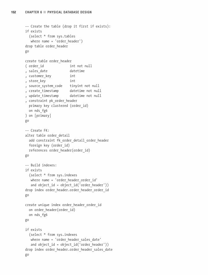
-- Create the table (drop it first if exists):if exists (select * from sys.tables where name = 'order_header')
drop table order_headergo
create table order_header( order_id int not null, sales_date datetime, customer_key int, store_key int, source_system_code tinyint not null, create_timestamp datetime not null, update_timestamp datetime not null, constraint pk_order_headerprimary key clustered (order_id)on nds_fg6
) on [primary]go
-- Create FK:alter table order_detailadd constraint fk_order_detail_order_headerforeign key (order_id)references order_header(order_id)
go
-- Build indexes:if exists(select * from sys.indexeswhere name = 'order_header_order_id'and object_id = object_id('order_header'))
drop index order_header.order_header_order_idgo
create unique index order_header_order_idon order_header(order_id)on nds_fg6
go
if exists(select * from sys.indexeswhere name = 'order_header_sales_date'and object_id = object_id('order_header'))
drop index order_header.order_header_sales_datego
CHAPTER 6 ■ PHYSICAL DATABASE DESIGN152
9314ch06final.qxd 11/15/07 10:13 AM Page 152

create unique index order_header_sales_dateon order_header(sales_date)on nds_fg6
go
if exists(select * from sys.indexeswhere name = 'order_header_customer_key'and object_id = object_id('order_header'))
drop index order_header.order_header_customer_keygo
create unique index order_header_customer_keyon order_header(customer_key)on nds_fg6
go
if exists(select * from sys.indexeswhere name = 'order_header_store_key'and object_id = object_id('order_header'))
drop index order_header.order_header_store_keygo
create unique index order_header_store_keyon order_header(store_key)on nds_fg6
go
Notice that we created four indexes for the order_header table, because the query trafficcould come from those four possible directions. The order_header table references customerand store tables and is being referenced by the order_detail table.
Here is the email_address_table, with the email_address_junction and email_address_type tables:
use NDSgo
if exists(select * from sys.foreign_keyswhere name = 'fk_email_address_junction_email_address'and parent_object_id = object_id('email_address_junction'))
alter table email_address_junctiondrop constraint fk_email_address_junction_email_address
go
CHAPTER 6 ■ PHYSICAL DATABASE DESIGN 153
9314ch06final.qxd 11/15/07 10:13 AM Page 153
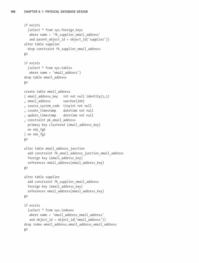
if exists(select * from sys.foreign_keyswhere name = 'fk_supplier_email_address'and parent_object_id = object_id('supplier'))
alter table supplierdrop constraint fk_supplier_email_address
go
if exists (select * from sys.tables where name = 'email_address')
drop table email_addressgo
create table email_address( email_address_key int not null identity(1,1), email_address varchar(200), source_system_code tinyint not null, create_timestamp datetime not null, update_timestamp datetime not null, constraint pk_email_address primary key clustered (email_address_key)on nds_fg6
) on nds_fg2go
alter table email_address_junctionadd constraint fk_email_address_junction_email_addressforeign key (email_address_key)references email_address(email_address_key)
go
alter table supplieradd constraint fk_supplier_email_addressforeign key (email_address_key)references email_address(email_address_key)
go
if exists(select * from sys.indexeswhere name = 'email_address_email_address'and object_id = object_id('email_address'))
drop index email_address.email_address_email_addressgo
CHAPTER 6 ■ PHYSICAL DATABASE DESIGN154
9314ch06final.qxd 11/15/07 10:13 AM Page 154

create unique index email_address_email_addresson email_address(email_address)on nds_fg6
go
Here is the email_address_junction table:
use NDSgo
if exists (select * from sys.tables where name = 'email_address_junction')
drop table email_address_junctiongo
create table email_address_junction( email_address_junction_key int not null, customer_key int not null, email_address_key int not null, email_address_type_key int, source_system_code tinyint not null, create_timestamp datetime not null, update_timestamp datetime not null, constraint pk_email_address_junctionprimary key clustered (email_address_junction_key)on nds_fg6
, constraint fk_email_address_junction_customerforeign key (customer_key)references customer(customer_key)
, constraint fk_email_address_junction_email_addressforeign key (email_address_key)references email_address(email_address_key)
, constraint fk_email_address_junction_email_address_typeforeign key (email_address_type_key)references email_address_type(email_address_type_key)
) on nds_fg2go
if exists(select * from sys.indexeswhere name = 'email_address_junction_customer_key_email_address_key'and object_id = object_id('email_address_junction'))
drop indexemail_address_junction.email_address_junction_customer_key_email_address_key
go
CHAPTER 6 ■ PHYSICAL DATABASE DESIGN 155
9314ch06final.qxd 11/15/07 10:13 AM Page 155

create unique index email_address_junction_customer_key_email_address_keyon email_address_junction(customer_key, email_address_key)on nds_fg6
go
Here’s the email_address_type table:
use NDSgo
-- Remove FK if exists:if exists(select * from sys.foreign_keyswhere name = 'fk_email_address_junction_email_address_type'and parent_object_id = object_id('email_address_junction'))
alter table email_address_junctiondrop constraint fk_email_address_junction_email_address_type
go
-- Create the table (drop it first if exists):if exists (select * from sys.tables where name = 'email_address_type')
drop table email_address_typego
create table email_address_type( email_address_type_key int not null identity(1,1), email_address_type_code char(2), email_address_type varchar(10), description varchar(30), source_system_code tinyint not null, create_timestamp datetime not null, update_timestamp datetime not null, constraint pk_email_address_typeprimary key clustered (email_address_type_key)on nds_fg6
) on nds_fg2go
-- Create FK:alter table email_address_junctionadd constraint fk_email_address_junction_email_address_typeforeign key (email_address_type_key)references email_address_type(email_address_type_key)
go
CHAPTER 6 ■ PHYSICAL DATABASE DESIGN156
9314ch06final.qxd 11/15/07 10:13 AM Page 156

The email_address_type table is used to determine, for example, which e-mail addressis the home e-mail address and which e-mail address is an office e-mail address. Similarly,address_type and phone_number_type are used for the same purpose. If you use a junctiontable, you don’t have key columns on both child and parent tables. Both child and parentkey columns are in the junction table. Remember to set all primary key columns in all tablesto identity (1,1).
■Tip It is useful to name the foreign key as fk_childtable_parenttable. If, for example, you makea small change in the email_address table and want to run the script and it says “Cannot drop the emailaddress table because it is being used in FK relationship with other table,” then you need to find out whichtable referenced to it. But with this naming, you can query with select * from sys.foreign_keys
where name like '%email_address'.
With that, we have finished creating the NDS. Just like we did in the DDS, you just needto create a batch file that contains sqlcmd to call all these scripts. Be careful with the sequenceof how you build the tables. Because of the referential integrity (foreign keys), you need tobuild them in a particular order. And the script may need several passes to build successfullybecause the foreign key creation is put on the table creation script (if we create all tables firstand then create all the foreign keys afterward, we need only one pass). For a complete list ofscripts for all the tables in the NDS, please refer to http://www.apress.com/. The NDS tablecreation scripts are located in the /script folder.
Using ViewsA view is a database object with columns and rows like a table but not persisted on disks. Aview is created using a SELECT statement that filters columns and rows from a table or a com-bination of several tables using a JOIN clause. In a data warehouse, views are used for threepurposes:
To create conform dimensions in dimensional data stores: Conformed dimensions meanthey are either the same dimension table or one is the subset of the other. As I discussedin Chapter 1, dimension A is said to be a subset of dimension B when all columns ofdimension A exist in dimension B and all rows of dimension A exist in dimension B.
To shield users from physical tables, making it simpler for the users as well as to restrictaccess: A view creates a virtual layer on the top of physical tables. Users do not access thephysical tables anymore. Instead, they are accessing the views. This additional layerenables us to create a virtual table that gets data from several tables. The additional layeralso enables us to restrict users from accessing certain columns or certain rows.
To increase the availability, particularly to make the data warehouse up and runningwhen we are populating it: This is used in user-facing data stores such as the DDS. Forevery dimension table and every fact table, we create two physical tables and one viewthat selects from one of these two tables. When table 1 is being populated, the view selectsfrom table 2. Conversely, when table 2 is being populated, the view selects from table 1.
CHAPTER 6 ■ PHYSICAL DATABASE DESIGN 157
9314ch06final.qxd 11/15/07 10:13 AM Page 157

Let’s discuss these three uses of views one by one. The first one is to create a conform dimension. Sometimes when creating a data mart,
the dimension that we need in that mart already exists. But we can use the existing dimensionbecause the granularity is different. We need a dimension with higher granularity, and there-fore only certain columns are applicable. In this case, we create a view from that existingdimension to select only certain rows and certain columns. We make this view a new dimen-sion with a higher grain for that data mart.
The new dimension conforms to the existing dimension. When we have conformeddimensions between two data marts, we can drill across from one mart to another mart. Thebenefit of using views to create conform dimensions is that we don’t have to populate thehigher-grain dimension. When the data in the underlying dimension changes, the data in thehigher-grain dimension automatically changes.
For example, in the supplier performance data mart, there is a dimension called week.The week dimension contains one row for each week in the year. This dimension is not a phys-ical table but a view created from the date dimension. It is created by filtering only certaindays (this can be any day of the week) and selecting only relevant columns, as follows:
use DDSgo
if exists (select * from sys.objectswhere name = 'dim_week' and type = 'V')
drop view dim_weekgo
create view dim_week as selectdate_key, date, system_date, sql_date, julian_date, day, day_of_the_year, week_number, month, month_name, short_month_name, quarter, year, fiscal_week, fiscal_period, fiscal_quarter, fiscal_year,source_system_code, create_timestamp, update_timestampfrom dim_date where day_of_the_week = 1go
The week dimension and date dimension are conformed. This is an example of con-formed dimensions that consist of two entities. Two dimensions are said to be conformed ifthey are identical or one is a subset of the other.
The second usage is to create a virtual layer on top of the physical tables to make it sim-pler for the users. Three typical uses are the data mart view, last month view, and specificstore view. Two other uses are for SCD type 2 and SCD type 3 current view. A slowly changingdimension contains both the current values and the historical values. We use a current viewto select only the current values.
A data mart view is where we create a view on top of a fact table and its dimension tables,giving the end users who have direct DDS access a single virtual table sourced from manyphysical tables. For example, in the Amadeus Entertainment case study to analyze productsales by date, customer, product, and store, the SQL query is as follows:
CHAPTER 6 ■ PHYSICAL DATABASE DESIGN158
9314ch06final.qxd 11/15/07 10:13 AM Page 158

select f.quantity, f.price, f.value, f.cost, f.margind.date, d.day_name, d.fiscal_week, d.fiscal_period,c. name, c.email_address, c.city, c.country, c.subscriber_class,p.name, p.title, p.artist, p.product_type, p.product_category,s.city, s.country, s.store_type, s.region, s.divisionfrom fact_product_salesleft join dim_date t on f.date_key = d.date_keyleft join dim_customer c on f.customer_key = c.customer_keyleft join dim_product p on f.product_key = p.product_keyleft join dim_store s on f.store_key = s.store_key
These key columns from the main dimension tables are accessed over and over again,and every time users have to type those long left-joins. In certain cases, the column nameson the tables are not short and nice like previously shown but rather long and confusing,such as wk_rev_sub_sgl_ttl, fs_prd_nm, and tot_rgn_div. To avoid this problem in the firstplace, we should use descriptive names for all database objects including columns, tables,views, indexes, primary keys, and foreign keys. For these users, a view like the followingwould make it a single table with the necessary columns:
create view sales asselect f.quantity, f.price, f.value, f.cost, f.margind.date, d.day_name, d.fiscal_week, d.fiscal_period,c. name, c.email_address, c.city, c.country, c.subscriber_class,p.name, p.title, p.artist, p.product_type, p.product_category,s.city, s.country, s.store_type, s.region, s.divisionfrom fact_product_salesjoin dim_date t on f.date_key = d.date_keyjoin dim_customer c on f.customer_key = c.customer_keyjoin dim_product p on f.product_key = p.product_keyjoin dim_store s on f.store_key = s.store_key
I have experienced this myself: some users are so used to writing these queries that theyknow the date_key value for yesterday and the store_key value for their stores, as in select *from fact_sales where date_key = 12201 and store_key = 324. In the first few weeks, theywrite this:
select * from sales_fact f join dim_date d on f.date_key = d.date_key join dim_store s on f.store_key = s.store_keywhere d.sql_date = 'mm/dd/yyyy' and s.name = 'Paris'
but because they get so used to it (also to make it shorter), in the end they type date_key andstore_key directly. My point is, if they use the views, it would be much easier for them.
Another example where a view is used to create a virtual layer to make it simpler for theusers is the last month view. The last month view is a view with the where clause where d.month= datepart(m,getdate())-1. This is frequently used because last month was a completemonth, and it was recent. This month is not complete yet, so you can’t really compare it.
CHAPTER 6 ■ PHYSICAL DATABASE DESIGN 159
9314ch06final.qxd 11/15/07 10:13 AM Page 159

A specific store (or country, or branch, or locale, or region) is another view that is fre-quently used, as shown previously but with a where clause to limit to a certain store, branch,or region. This is because the users are responsible only for that store or region.
When you have a slowly changing dimension, most of the time the users just want thecurrent view. So, a view with a where clause such as where is_current = 1 is greatly welcomedby the users. That’s for SCD type 2. For type 3, the view is something like create view asselect store_id, address, city, region2 as region, division2 as division, ignoring theprior region and prior division. This is especially useful when your current region is calledregion2, but last year it was region1.
The last usage of view is to increase availability. When you populate a fact table, chancesare, you will be locking this table from access. There are two purposes of locking the tablewhen loading data: to speed up loading and to avoid data volatility, such as in ever-changingvalues, which could cause user confusion. So, your infrastructure is excellent, is clustered, andhas a web farm with dual fiber switches, but still the data warehouse will be inaccessible forthree hours every day. If the data warehouse is used worldwide, there is no “nighttime.” Night-time in the United States is daytime in Asia. You can’t schedule the batch-loading process for3 a.m. EST because Singapore and London are using the data warehouse.
A common technique is to use a view. We have two physical tables and one view thatpoint to one of these two tables. For example, say we have two physical tables: fact_product_sales_1 and fact_product_sales_2. We create a view called fact_product_sales as createview fact_product_sales as select * from fact_product_sales_N, with N = 1 or 2, depend-ing on which day. Monday it is 1, Tuesday it is 2, Wednesday it is 1, Thursday it is 2, and so on.Assume that today is Monday. Your active fact table is fact_product_sales_2. On the stage, youhave a table containing today’s data. So, you load this data (Monday data) into fact_product_sales_1. After you load it, you drop the fact_product_sales view and do this: create viewfact_product_sales as select from fact_product_sales_1. Notice that now fact_product_sales_2 is out-of-date because it contains Sunday data.
Tomorrow, your stage table contains Monday data and Tuesday data. You load theMonday and Tuesday data from the stage into fact_product_sales_2. Then you drop thefact_product_sales view and do this: create view fact_product_sales as select fromfact_product_sales_2. Notice that now fact_product_sales_1 is out-of-date because itcontains Monday data. The BI or CRM applications are shielded from what’s happening.From an application point of view, they only access a fact table called fact_product_sales,which is always available, and the data is always up-to-date. In reality, the fact table is actu-ally a view sourced alternately from two different physical tables.
This technique is not only for loading fact tables but also for loading dimension tables.Rather than a multiday implementation as described previously, you can also use this tech-nique for an intraday implementation, as follows:
1. Set the view to point to table 2.
2. Load today’s data into table 1.
3. Set the view to point to table 1.
4. Load today’s data into table 2.
CHAPTER 6 ■ PHYSICAL DATABASE DESIGN160
9314ch06final.qxd 11/15/07 10:13 AM Page 160

By using this technique, your data warehouse will be up all the time. Dropping andre-creating a view takes only a few seconds. This technique is commonly used to increase thedata warehouse availability, both in packaged applications running on a normalized datawarehouse as well in custom-developed data warehouses.
Summary TablesOut of the many things that can improve data warehouse performance, the summary tableis at the top of the list. (The second one is table partitioning, and the third one is indexing.)This is because the data that the users need is already precalculated. We will discuss thesethree things one by one in the next three main sections.
Say you have a report that displays a graph of the summary of weekly sales data for thelast 12 weeks by product group or by stores. Let’s say that within a week you have 1 millionrows. So the stored procedure behind that report must process 1 million rows and display thedata on the screen as a graph, while the user waits. Let’s say that this takes 45 seconds.
If you produce a table called weekly_sales_summary, which runs the same query, and putthe result in this summary table, when the user accesses the report, the stored procedure orthe SQL statement behind the report needs to access only this summary table. The responsetime of the report is greatly improved; it’s probably only one or two seconds now.
The summary table needs to be at least 10 times smaller (in terms of the number of rows),ideally 100 times smaller or more. Otherwise, there is no point creating a summary table. Ifyou wonder where 10 and 100 come from, the guideline to determine whether it is worth cre-ating the summary table is to compare the performance improvement with the time requiredto build it. What I meant by “performance improvement” is how much faster querying thesummary table compared to querying the underlying table directly is. If the performanceimprovement is insignificant (say less than 10 percent), if it takes a long time to build the table(say one hour), and if the query is not used frequently, then it’s not worth building a summarytable. Remember that a summary table needs to be updated every time the underlying facttable is updated. If the number of rows in the summary table is much less than the underlyingtable, such as 10 or 100 times smaller, usually the performance improvement is significant.The ideal time to refresh the summary tables is immediately after the population of the under-lying fact table.
As we discussed in Chapter 5, we have three types of fact table: the transactional facttable, the periodic snapshot fact table, and the accumulative snapshot fact table. A summaryfact table is suitable for a transaction fact table. For a periodic snapshot fact table, we have the“latest summary table.” A latest summary table contains only today’s version of the snapshot.For example, the Subscription Sales fact table contains a daily snapshot of all the membershipsubscriptions. If we have 1 million customer subscriptions, the table would contain 1 millionrecords every day. Over two years, there would be 730 million rows in the fact table. In thiscase, we can create a table called fact_subscription_sales_latest that contains only today’srows so it contains only 1 million rows and is therefore faster. This latest summary table is use-ful if you need information that depends on the today value only.
CHAPTER 6 ■ PHYSICAL DATABASE DESIGN 161
9314ch06final.qxd 11/15/07 10:13 AM Page 161

PartitioningOut of many things that can improve the performance of a data warehouse, I would say parti-tioning is the second most important. In SQL Server 2005 and 2008, we have a new feature forpartitioning for a physical table. Previously, in SQL Server 2000, we could partition only a view;we could not partition a table.
There are two types of partitioning: vertical partitioning and horizontal partitioning.Vertical partitioning is splitting a table vertically into several smaller tables, with each tablecontaining some columns of the original table. Horizontal partitioning is splitting a table hori-zontally into several smaller tables, with each table containing some rows of the original table.In this section, I’m talking about horizontal partitioning, not vertical partitioning.
Imagine if the Subscription Sales fact table were horizontally partitioned like the one inFigure 6-3.
Figure 6-3. Partitioned and nonpartitioned Subscription Sales fact table
The nature of the fact tables in dimensional data warehouses is that their content ischronological according to time. If it is a transactional fact table, such as Product Sales, therows coming into the fact table are the sales records from the previous day. If it is a periodicsnapshot fact table, such as Subscription Sales, the rows coming into the fact table are thesnapshot of all subscriber records as they were on that day.
Because of this natural characteristic, it is best to physically organize the table by date. Itmakes the loading a lot quicker. It makes the query faster if the information you need is fromthe same month or the same year. The left part of Figure 6-4 shows the loading and query of anonpartitioned Subscription Sales fact table, physically clustered on store_key. The recordsare loaded to various parts of the table. The queries fetch the data also from various differentplaces within the table.
CHAPTER 6 ■ PHYSICAL DATABASE DESIGN162
9314ch06final.qxd 11/15/07 10:13 AM Page 162

Figure 6-4. Loading and query of partitioned and nonpartitioned table
The right part of Figure 6-4 shows a partitioned Subscription Sales fact table. The loadingof today’s data hits only a particular partition, which is faster because the data is loaded intoone place (physically clustered sectors on disk), rather than scattered over different sectorsand disks. Queries are faster too. The response time of a query with where column1 = value1 isbetter if run on a partitioned table with column1 as the partitioning key, compared to runningit on a nonpartitioned table because it encourages SQL Server to execute the query in parallel.A test on SQL Server 2005 running on Unisys ES7000 with EMC Clarion SAN managed to load2.5 billion rows into a partitioned fact table in about one hour.5
Let’s partition our Subscription Sales table. In this example, we have a fact table storingcustomer subscriptions. We will partition the table into monthly partitions; in other words,each month will go into its own partition. In this example, we will use January until December2008. Here is the table creation script:
use ddsgo
if exists (select * from sys.tables where name = 'fact_subscription_sales')
drop table fact_subscription_salesgo
if exists(select * from sys.partition_schemeswhere name = 'ps_subscription_sales')
drop partition scheme ps_subscription_salesgo
CHAPTER 6 ■ PHYSICAL DATABASE DESIGN 163
5. http://www.microsoft.com/technet/prodtechnol/sql/2005/spdw.mspx#ESGAC
9314ch06final.qxd 11/15/07 10:13 AM Page 163

if exists(select * from sys.partition_functionswhere name = 'pf_subscription_sales')
drop partition function pf_subscription_salesgo
create partition function pf_subscription_sales (int)as range left for values (10365, 10396, 10425, 10456, 10486, 10517, 10547, 10578, 10609, 10639, 10670, 10700, 10731)go
create partition scheme ps_subscription_salesas partition pf_subscription_sales to (dds_fg2, dds_fg3, dds_fg5, dds_fg2, dds_fg3, dds_fg5, dds_fg2, dds_fg3, dds_fg5, dds_fg2, dds_fg3, dds_fg5, dds_fg2, dds_fg3)go
create table fact_subscription_sales( date_key int not null, customer_key int not null, package_key int not null, format_key int not null, store_key int not null, start_date_key int not null, end_date_key int not null, lead_key int not null, subscription_id int not null, subscription_revenue money, single_titles_revenue money , monthly_revenue money, music_quantity int, music_unit_cost money, monthly_music_cost money, film_quantity int, film_unit_cost money, monthly_film_cost money, book_quantity int, book_unit_cost money, monthly_book_cost money, monthly_indirect_cost money, monthly_cost money, monthly_margin money, annual_revenue money, annual_cost money, annual_profit money
CHAPTER 6 ■ PHYSICAL DATABASE DESIGN164
9314ch06final.qxd 11/15/07 10:13 AM Page 164

, subscriber_profitability decimal(9,2), subscribe_timestamp datetime, unsubscribe_timestamp datetime, source_system_code tinyint, create_timestamp datetime, update_timestamp datetime, constraint pk_fact_subscription_sales primary key clustered( date_key, customer_key, subscription_id ) on ps_subscription_sales(date_key)
, constraint fk_fact_subscription_sales_dim_date1foreign key (date_key)references dim_date(date_key)
, constraint fk_fact_subscription_sales_dim_customerforeign key (customer_key)references dim_customer(customer_key)
, constraint fk_fact_subscription_sales_dim_packageforeign key (package_key)references dim_package(package_key)
, constraint fk_fact_subscription_sales_dim_storeforeign key (store_key)references dim_store(store_key)
, constraint fk_fact_subscription_sales_dim_date2foreign key (start_date_key)references dim_date(date_key)
, constraint fk_fact_subscription_sales_dim_date3foreign key (end_date_key)references dim_date(date_key)
, constraint fk_fact_subscription_sales_dim_leadforeign key (lead_key)references dim_lead(lead_key)
) on ps_subscription_sales(date_key)go
First we drop the table, the partition function, and the partition scheme, if they exist.Then we create a partition function called pf_subscription_sales. We specify the boundaryvalues. Because we will partition the table based on the date_key column, we need to specifythe boundary values of each partition. Partition 1 is for records before 1/1/2008, partition 2 isfor January 2008, partition 3 is for February 2008, partition 4 is for March 2008, partition 5 isfor April 2008, …, partition 13 is for December 2008, and partition 14 is for records on or after1/1/2009.
In the data warehouse, we’ll set date_key for 1/1/2007 as 10,000. This enables us to go back10,000 days if necessary; in other words, if we need to create 2006 records (which we do need atsome point before we go live to load the history), it would be assigned date_key 9635 to 9999.You don’t have to set it to 10,000. You can customize it to your needs. Setting the date_key of thefirst operational day of the data warehouse to 10,000 enables us to go back 27 years. If you needonly three years, then you can start the date key with 1100 (3 ✕ 365).
CHAPTER 6 ■ PHYSICAL DATABASE DESIGN 165
9314ch06final.qxd 11/15/07 10:13 AM Page 165

The date keys for 2008 records are 10365 to 10730. So in the partition function, we specifythat the boundary values are 1/1/2008 (date_key 10365), 2/1/2008 (date_key 10396), and soon. We then create the partition scheme by assigning the partitions to filegroups.
After creating the partition scheme, we then create the table by specifying the partitionscheme with the partitioned column in brackets at the end of the DDL. This is to inform SQLServer that we want to partition the table using that partition scheme. A common mistake is tospecify a filegroup for the clustered primary key as follows: constraint pk_tablename primarykey clustered(PK columns) on dds_fg4. This will produce the following message:
The filegroup 'dds_fg4' specified for the clustered index'pk_fact_subscription_sales' was used for table 'fact_subscription_sales' even though partition scheme 'ps_subscription_sales' is specified for it.
What happened was that SQL Server put the table and the clustered index on dds_fg4,rather than on dds_fg2, dds_fg3, and dds_fg5 as we specified in the partition scheme. This isbecause the leaf nodes of the clustered index are the physical table pages. When creating apartition table, if the constraint filegroup is different from the table filegroup, SQL Server willdo whatever is specified in the constraint filegroup and ignore the table filegroup.
The partition index is best placed in the same filegroup as the partition table because itenables SQL Server to switch the partitions efficiently. In this case, we say that the index isaligned with the table. Aligning the partition index with the partition table helps when weimplement a sliding window for archiving partitions and when we add new partitions to thetable. To enable us to switch or move partitions, the index must be aligned with the table.When we move or transfer a partition, we don’t actually move the data. Instead, we changethe metadata only around where the data is.
Partition maintenance is the activity of administering a partitioned table so that it is readyfor data loading and query. If we implement partitioning using monthly sliding windows, wecan do partition maintenance monthly or annually. Every month we can drop the oldest parti-tion (and archive it) and add this month’s partition. Or we can do this every December: drop12 partitions for the oldest year and add 12 new partitions for the coming year.
IndexesIndexing can significantly improve the query and loading performance of data warehousing.In this section, I will discuss how to implement indexing in a data warehouse. I will discusschoosing the primary key and clustered index and indexing small tables, including indexesand partitioned indexes.
In the DDS, we have fact tables and we have dimension tables. They require differentindexing and primary keys. I will discuss dimension tables first and then the fact tables. Eachdimension table has a surrogate key column. This is an identity (1,1) column, and the valuesare unique. We make this surrogate key column the primary key of the dimension table. Wealso make this surrogate key column the clustered index of the dimension table. The reasonfor doing this is because in the DDS, the dimension tables are joined to the fact table on thesurrogate key column. By making the surrogate key a clustered primary key, we will get goodquery performance because in SQL Server a clustered index determines the order of how the
CHAPTER 6 ■ PHYSICAL DATABASE DESIGN166
9314ch06final.qxd 11/15/07 10:13 AM Page 166

rows are physically stored on disk. Because of this, we can have only one clustered index oneach table.
Dimension tables contain attribute columns, typically having a character data type.Attribute columns that are often used in the where clause of the queries need to be set as anonclustered index—but only if the selectivity is high. If the attribute column has manyduplicate values, it may not be worth indexing.
For the fact table in SQL Server data warehousing, we have two approaches in terms ofdetermining the primary key and the clustered index. Note that this is specifically for SQLServer; it does not apply to other database engines such as Oracle or Teradata.
• The first approach is to create a fact table surrogate key column. This is an identity (1,1)column that functions as a single-column unique identifier of the fact table row. We setthis column as the primary key and the clustered index of the fact table.
• The second approach is not to have a fact table surrogate key column. Instead, weselect the minimum combination of columns that make a row unique as the primarykey. In some cases, the combination of all dimensional surrogate key columns makesa row unique. In other cases, they don’t, and we have to identify other columns thatmake a row unique, such as the degenerate dimension columns.
If you want to implement the first approach, create a new column for every single facttable. Call this column fact_key. It is an identity (1,1) column. The data type is bigint. It is notworth taking the risk of using the int data type to save 4 bytes, unless you are certain you arenot going to hit 9 billion. Remember that the max(key) can be higher than the number ofrows, as I explained earlier. The bigint data type is 9 quintillion (18 zeros), so it should beenough. Create a clustered primary key in this column. The advantages of this approach arethat the loading can be twice as fast (because the clustered index key is an identity column,so there is no need to reorganize the fact table rows when loading new data), and the non-clustered indexes can be four to five times smaller than the second approach (because theclustered index key is 8 bytes).
If you want to implement the second approach, find out what makes the fact table rowunique. For example, in our Subscription Sales fact table, the grain is one row for each cus-tomer subscription per day. So, date_key and customer_key must be part of the primary key.What if the customer subscribes to two packages? We need to include the subscription_idin the primary key to make it unique, so the primary key is date_key, customer_key, andsubscription_id. We cluster the table in these primary key columns, so the table will physi-cally be organized/sorted according to date, customer, and then subscription ID.
This will make the query fast if the where clause contains the date and customer, becausethe table is physically sorted by the date and then the customer. This could be 10 times fasterthan if the date and customer are not indexed. That’s the advantage of the second approach.The loading speed of the second approach could be twice as slow as the first approach (as dis-cussed previously), but we have fewer indexes to maintain. Overall, on the SQL Serverplatform, the fact table surrogate key approach is preferred because there is no need to reor-ganize the clustered index when loading, which results in better loading performance, whilethe query performance can be supported by a nonclustered index. The second reason is func-tionality: we can uniquely identify a fact table row using a single column, which is useful whenwe need to refer to a fact table row either from another fact table (drilling across) or from thesame fact table itself (self-join).
CHAPTER 6 ■ PHYSICAL DATABASE DESIGN 167
9314ch06final.qxd 11/15/07 10:13 AM Page 167

For the Communication Subscriptions fact table, the grain is one row for each subscrip-tion, so the columns that make a row unique are customer_key, communication_key, andstart_date_key. So, we make these three columns the clustered primary key. For the SupplierPerformance fact table, the grain is one row per week for each product supplied. The columnsthat make a row unique are week_key, supplier_key, and product_key, so we make these threecolumns the clustered primary key. For the Campaign Results fact table, the grain is one rowfor each intended recipient. The columns that make a row unique are campaign_key, customer_key, and send_date_key, so we make them the clustered primary key.
For the Product Sales fact table, the grain is one row for each item sold. The columnsthat make a row unique are order_id and line_number, so we make them the clustered pri-mary key. The disadvantage of the second approach is that, potentially, the nonclusteredindexes are three to four times larger, because the clustered index may consist of three orfour columns. The disadvantage of the first approach (the fact table surrogate key) is thatthere are more indexes to maintain, which could impact query performance. How much itimpacts the query performance depends on whether the index covers the column on thewhere clause of the query.
The Subscription Sales fact table has eight dimensional key columns and one degeneratedimension column (subscription_id). If you create the fact table clustered primary key basedon the combination of eight dimension keys plus subscription_id, all nonclustered indexeswould become very large, in other words, nine columns (which is as big as the table itself).This is not a good idea because in SQL Server the clustered index key is used by all nonclus-tered indexes. The loading performance could be two times slower (or worse) as SQL Serverand must physically reorganize the fact table based on these nine columns as the data isloaded into the fact table.
It is not worth indexing the small tables, such as some dimension tables and some attrib-ute tables on the NDS. The overhead (index maintenance at loading) outweighs the benefit(query performance). The guideline I usually use is 1,000 rows (this is determined by queryingtwo tables with and without an index). If it is less than 1,000 rows, I generally don’t index.Dimension tables between 1,000 and 10,000 rows I rarely index; I think twice or even threetimes before indexing them, probably examining the execution plan first. For example, in theAmadeus Entertainment store table, the query where city = value1 takes 0 milliseconds,whether we have a nonclustered index on city or not. The loading is impacted, though. Aninsert select into the table (empty) takes 0 milliseconds without an index, 93 millisecondswith an index only on the city column, and 2560 milliseconds with indexes on 17 columns.
Indexing is a two-step process. The first step is to determine what column to index basedon application and business knowledge. If the column will be used when analyzing the data,we consider that column for indexing. This is done when doing data modeling and physicaldatabase design. For example, on the customer dimension, we think we need to put a non-clustered index on the occupation column because the business user needs to analyze theproduct and subscription sales by income. We also need to index on the permission column,because the CRM segmentation process will need to get a list of customers who have giventheir permissions.
The second step is to fine-tune the indexes based on the query workload using the QueryExecution Plan and the Database Engine Tuning Advisor. This is done after we load the datainto the NDS and DDS, still in the development environment. We can identify slow-runningqueries by measuring how many milliseconds each query runs. This is done using SQL Server
CHAPTER 6 ■ PHYSICAL DATABASE DESIGN168
9314ch06final.qxd 11/15/07 10:13 AM Page 168

Profiler to capture the SQL statement execution duration into a table that we can analyze.After we identify the slow-running queries, we examine the execution plan of those queries.For example, we may find some SQL queries use columns that we have not indexed in theirwhere clause. We can improve these queries by creating a nonclustered index on thosecolumns.
OK, let’s move on with our indexing. In the dimension table, let’s create the indexes incolumns that are used in the queries. For example, the day of the week column is used ondim_week, so we index on that column, like this:
if exists (select * from sys.indexes where name = 'dim_date_day_of_the_week'and object_id = object_id('dim_date'))
drop index dim_date.dim_date_day_of_the_weekgo
create index dim_date_day_of_the_weekon dim_date(day_of_the_week)on dds_fg6
go
Which dimension column do we index? In the first step of indexing, during data modelingand physical database design, we create the indexes based on our application and businessknowledge. In the second step, we fine-tune the indexes based on the result of query execu-tion results that we capture using SQL Server Profiler.
For a fact table, it generally helps the performance of queries that join the fact table andthe dimension tables if we create one column nonunique nonclustered index for each dimen-sional surrogate key column in the fact table. The SQL Server query optimizer can then use thecombination of these one-column indexes when executing the query with where dim_key1 =... and dim_key2 = ... and dim_key3 = .... Some people call this type of indexing indexintersection, and some people call it index bitmapping. Here is an example of index inter-section that creates an index for each dimensional surrogate key column in the fact table:
create index fact_product_sales_sales_date_keyon fact_product_sales(sales_date_key)on dds_fg4
go
create index fact_product_sales_customer_keyon fact_product_sales(customer_key)on dds_fg4
go
create index fact_product_sales_product_keyon fact_product_sales(product_key)on dds_fg4
go
CHAPTER 6 ■ PHYSICAL DATABASE DESIGN 169
9314ch06final.qxd 11/15/07 10:13 AM Page 169

create index fact_product_sales_store_keyon fact_product_sales(store_key)on dds_fg4
go
To help index intersection and speed up certain queries, sometimes it is better to createa covering index. A covering index is an index that contains all the columns referenced in thequery. The benefit of using a covering index is that the SQL Server query engine doesn’t haveto go to the table itself to get any data. It can find all the data it needs on the index. For exam-ple, if the where clause in the SQL statement is where column1 = value1, column2 = value2,then the covering index needs to contain column1 and column2.
The order of columns in the where clause does not matter, but the order of columns in thecovering index does matter. So, be careful when specifying the order of columns in the cover-ing index. For the first column, we need to choose the most used dimension key. For thesecond column, choose the second most-used dimension key. For the Product Sales fact table,I’ll set the three covering indexes as follows:
• Date, customer, store, product
• Date, store, product, customer
• Date, product, store, customer
We may have to swap the third and fourth columns depending on the queries. Note thateven if you have all columns covered, the SQL Server query optimizer may not use the index ifthe selectivity is low. Selectivity is the ratio between the number of rows that satisfy the criteriaand the total rows. If this ratio is high, the selectivity is low, and the index is not useful andmay not be useful. A unique index has the highest selectivity because it returns only one row.
To create indexes in a partitioned table, we just have to mention the partition schemainstead of the normal filegroup. Here are some of examples for the Subscription Sales facttable we partitioned earlier:
create index date_keyon fact_subscription_sales(date_key)on ps_subscription_sales(date_key)go
create index package_keyon fact_subscription_sales(package_key)on ps_subscription_sales(package_key)go
create index customer_keyon fact_subscription_sales(customer_key)on ps_subscription_sales(customer_key)go
The indexed column must be of the same data type as the partitioning function. This isanother reason why we need to keep all the dimension key column data types as int (notsmallint or tinyint), in addition to the foreign key reason we discussed earlier.
CHAPTER 6 ■ PHYSICAL DATABASE DESIGN170
9314ch06final.qxd 11/15/07 10:13 AM Page 170

SummaryWell, this was quite a long chapter. Database design is the cornerstone of data warehousing.We will build the ETL and applications on this foundation, so we must get it right. In thischapter, we discussed the details of the hardware platform and system architecture, the diskspace calculation, database creation, and table and view creation.
We also covered the top three factors that can improve data warehouse performance:summary table, partitioning, and indexing. We need to make sure they are set correctly fromthe beginning—in other words, when we create the databases, not later when we have per-formance problems.
Now that we have built the databases, in the next two chapters you will learn how toextract the data from the source systems and populate our NDS and DDS databases, widelyknown as ETL, which stands for Extract, Transform, and Load.
CHAPTER 6 ■ PHYSICAL DATABASE DESIGN 171
9314ch06final.qxd 11/15/07 10:13 AM Page 171

9314ch06final.qxd 11/15/07 10:13 AM Page 172
Data Extraction
Now that we have created the tables in the NDS and the DDS, it is time to populate them.Before we can populate them, though, we need to retrieve the data from the source system.This is what data extraction is all about.
First I’ll discuss the general principles of data extraction, different kinds of source sys-tems, and several data extraction techniques. Then I’ll introduce the tool that we will be using,SQL Server Integration Services. After introducing the tool, I’ll then show how to use it toextract the data from the source systems in our case study: Jade, WebTower, and Jupiter.
Introduction to ETLETL stands for Extract, Transform, and Load. It is the process of retrieving and transformingdata from the source system and putting it into the data warehouse. It has been around fordecades, and it has developed and improved a lot since its inception.
There are several basic principles to understand when extracting data from a source sys-tem for the purpose of populating a data warehouse. First, the volume of data being retrieved islarge, probably hundreds of megabytes or tens of gigabytes. An OLTP system is designed so thatthe data is retrieved in little pieces, not in large amounts like this, so you have to be careful notto slow the source system down too much. We want the extraction to be as fast as possible, suchas five minutes if we can, not three hours (this depends on the extraction method, which I’llcover later in this chapter). We also want it to be as small as possible, such as 10MB per day ifwe can, not 1GB per day. In addition, we want it to be as infrequent as possible, such as once aday if we can, not every five minutes. We want the change in the source systems to be as mini-mal as possible, such as no change at all if we can, not creating triggers for capturing datachanges in every single table.
The previous paragraph talks about a fundamental principle in data extraction. If thereis only thing that you will take away from this chapter, I hope it is this: when extracting datafrom a source system, you have to be careful not to disturb the source system too much.
After we extract the data, we want to put it into the data warehouse as soon as possible,ideally straightaway, without touching the disk at all (meaning without storing it temporarilyin a database or in files). We need to apply some transformations to the data from the sourcesystem so that it suits the format and structure of the data in the NDS and the DDS. Some-times the data transformation is just formatting and standardization, converting to a certainnumber or date format, trimming trailing spaces or leading zeros, and conforming into stan-dards. Other times the modification is a lookup, such as translating customer status 2 toActive or translating the product category “Pop music” to 54. Another transformation that is
173
C H A P T E R 7
9314ch07final.qxd 11/15/07 10:10 AM Page 173

frequently used in data warehousing is aggregation, which means summarizing data athigher levels.
We also want the data we put into the warehouse to be clean and of good quality. Forexample, we don’t want invalid telephone numbers, an e-mail address without the character @in it, a product code that does not exist, a DVD with a capacity of 54GB, an address with a cityof Amsterdam but a state of California, or a unit price of $0 for a particular audio book. Forthis purpose, we need to do various checks before putting the data into the warehouse.
Two other important principles are leakage and recoverability. Leakage happens whenthe ETL process thinks it has downloaded all the data completely from the source system butin reality has missed some records. A good ETL process should not have any leakage. Recov-erability means that the ETL process should be robust so that in the event of a failure, it canrecover without data loss or damage. I will discuss all this in this chapter.
ETL Approaches and ArchitectureThere are several approaches of implementing ETL. A traditional approach is to pull thedata from the source systems, put it in a staging area, and then transform it and load it intothe warehouse, as per the top diagram of Figure 7-1. Alternatively, instead of putting thedata in a staging area, sometimes the ETL server does the transformation in memory andthen updates the data warehouse directly (no staging), as shown in the bottom diagram ofFigure 7-1. The staging area is a physical database or files. Putting the data into the stagingarea means inserting it into the database or writing it in files.
Figure 7-1. To stage on disks or do transformation in memory
CHAPTER 7 ■ DATA EXTRACTION174
9314ch07final.qxd 11/15/07 10:10 AM Page 174

Transforming the data in memory is faster than putting it on disk first. If the data issmall enough, you can transform in memory, but if the data is big, you need to put it on diskfirst. Whether you can put the data into memory depends on how much memory the ETLserver has.
The alternative to the two ETL approaches shown in Figure 7-1 is called Extract, Load, andTransform (ELT), as shown in the bottom half of Figure 7-2. In the ELT approach, we pull thedata from the source systems, load it into the data warehouse, and then apply the transforma-tion by updating the data in the warehouse. In the ELT approach, essentially we copy thesource system (OLTP) data into the data warehouse and transform it there. People usually takethe ETL approach if they have a strong ETL server and strong software that is rich with allkinds of transformation and data quality processes.
Figure 7-2. ETL and ELT: choices of where to perform the transformations
People usually take the ELT approach if they have a strong data warehouse database sys-tem, usually MPP database systems. Massively parallel processing (MPP) is a group of servers(called nodes), and each node has its own memory, processor, and disk. Examples of MPPdatabase systems are Teradata, Netezza, and Neoview. When you cluster two or more SQLServers, you get high availability and each node has its own memory and processor, but youstill share the disks. In MPP database systems, each node has its own memory, processor, anddisk. It is known as a share nothing architecture. An MPP database system is more powerfulthan systems with shared disks because data loading is happening in parallel across multiplenodes that have their own disks.
The main advantage of MPP database systems is that the performance increase is linear.If you put ten SQL Servers in an active-active cluster, the performance increases, but not 10✕ asingle SQL Server. In MPP database systems, if you put in ten nodes, the performance isalmost ten times the performance of a single node.
CHAPTER 7 ■ DATA EXTRACTION 175
9314ch07final.qxd 11/15/07 10:10 AM Page 175

In terms of who moves the data out of the source system, we can categorize ETL methodsinto four approaches (see Figure 7-3):
• An ETL process pulls the data out by querying the source system database regularly.This is the most common approach. The ETL connects to the source system database,queries the data, and brings the data out.
• Triggers in the source system database push the data changes out. A database trigger isa collection of SQL statements that executes every time there is an insert, update, ordelete on a table. By using triggers, we can store the changed rows in another table.
• A scheduled process within the source system exports the data regularly. This is similarto the first approach, but the program that queries the database is not an external ETLprogram. Instead, it is an internal exporter program that runs in the source systemserver.
• A log reader reads the database log files to identify data changes. A database log filecontains a record of the transactions made to that database. A log reader is a programthat understands the format of the data in the log file. It reads the log files, gets the dataout, and stores the data somewhere else.
Figure 7-3. Four ETL approaches based on who moves the data out of the source system
In terms of where the processes that move the data out are executed, we can categorizeETL into three approaches (see Figure 7-4):
• Execute the ETL processes in a separate ETL server that sits between the source systemand the data warehouse server. This approach provides the highest performance. TheETL runs on its own server, so it does not use the resources of the data warehouseserver or the source system server at all. It is more expensive than the next two optionsbecause you have to purchase additional server and software licenses.
• Execute the ETL processes in the data warehouse server. This approach can be used ifwe have spare capacity in the data warehouse server or if we have a time slot when thedata warehouse is not used (at night for example). It is cheaper than the first approachbecause we don’t need to provide additional servers.
CHAPTER 7 ■ DATA EXTRACTION176
9314ch07final.qxd 11/15/07 10:10 AM Page 176

• Execute the ETL processes in the server that hosts the source system. This approach isimplemented when we need real-time data warehousing. In other words, the momentthe data in the source system changes, the change is propagated to the data warehouse.This is can be achieved using database triggers in the source system. In practice, thisapproach is implemented in conjunction with either of the previous approaches. Thatis, this approach is used only for a few tables, and the remaining tables are populatedusing the first two approaches.
Figure 7-4. Choices of where to put ETL processes
General ConsiderationsThe system we are extracting from may not be a database. It could be a file system, a queue,a service, or e-mails. If the data is in a database, usually we retrieve the data using ADO.NET,ODBC, OLEDB, JDBC, or proprietary database connectivity. These days, most databases arerelational, but occasionally we come across hierarchical databases, such as Adabas and ISM,or sequential file storage, such as ISAM. To extract the data from them, we need to have theright database driver or write a data export script using the database-specific language.
If the data is in a file or files, it could be structured, semistructured, or unstructured.A structured file is like this:
ID Date Store Product Quantity2893 2/1/08 32 A160 1502897 2/4/08 29 B120 240
which is a fixed position file, meaning that the fields are in certain column positions. Or itcould be like this:
CHAPTER 7 ■ DATA EXTRACTION 177
9314ch07final.qxd 11/15/07 10:10 AM Page 177

ID|Date|Store|Product|Quantity2893|2/1/08|32|A160|1502897|2/4/08|29|B120|240
which is a delimited file. In this case, it is pipe delimited.A structure file contains tabular (table) data, meaning that the data is essentially in
columns and rows format. A semistructured file contains tabular data and nontabular data.A semistructured file looks like this XML file:
<order ID="2893"><date>2/1/08</date><store>32</stores><product>A160</product><quantity>150</quantity>
</order>
<order ID="2897"><date>2/4/08</date><store>29</stores><product>B120</product><quantity>240</quantity>
</order>
<customer ID="83"><name>John Smith</name><email>[email protected]</email>
</order>
The first two sections (order data) are tabular, but the third one (customer data) is nottabular.
Unstructured data is like this: “On 2/1/2008 we received order ID 2893 from store 32,requiring 150 units of product A160. Three days later store 29 asked for 240 pieces of B120.”It is the typical content of e-mails. We extract the information in unstructured data using textmining.
Sometimes, the data extraction can be done only during certain times, such as after abatch, or it cannot be done at certain times, such as at backup times or during month-endprocessing. Sometimes, if we are lucky, we can access the source data at any time, such aswhen there is a secondary read-only server specifically provided for ad hoc queries and ETL.Table 7-1 lists the potential problems in data extraction, the scenarios, and the common tech-niques in those scenarios.
CHAPTER 7 ■ DATA EXTRACTION178
9314ch07final.qxd 11/15/07 10:10 AM Page 178

Table 7-1. Potential Problems in Data Extraction
Common Technique to Potential Problem Scenario Overcome
Data is available only at A long batch schedule runs Negotiate a time slot with the certain times. overnight followed by a big OLTP DBA. Break the
database backup. Extracting extraction into smaller data during the day would chunks.slow the OLTP.
The OLTP database is not On the first day of every month, Skip extraction on that day. available on certain days. OLTP runs a month-end batch Tell users the reasons for this
for the whole day. limitation.
The OLTP DBA is concerned The project team consists of Ask the DBA to give “read-that our ETL could “mess up” external consultants who are only” access. Ask the OLTP their system. just learning the OLTP internals. DBA to export data for you.
There is a concern that ETL will There are no “quiet times” Read from the secondary strain/overload the OLTP because the OLTP is a global OLTP database. Use a less database. database. frequent extract for large
tables, such as only Sundays.
The OLTP DBA is concerned There is an emergency situa- Tell the DBA they may ter-that they can’t stop ETL pro- tion in OLTP that requires server minate you at any time (tell cesses in an emergency. restart. them how) but rerun
afterward (manual invoke).
They can’t start ETL processes. There is an OLTP backup Program the ETL to rerun overrun. automatically later.
One of the most important things at this stage of the project (the beginning of ETL) is toget to the data, that is, to be able to connect to the source data. Sometimes it takes time to bein a position where we can query the source system (if it is a database) or read the files (if it afile system). Sometimes the source database server is physically located on another continentand there is no connectivity to that server. I’ve worked on several projects where we had toarrange for the network connectivity to be opened, that is, to allow certain TCP traffic to flowthrough the firewall so that we could get to the data. Table 7-2 lists the common reasons fornot being able to get to the source data, as well as their common solutions.
Table 7-2. Reasons for Not Being Able to Get the Source Data
Reason Common Solution
There is no connectivity to the target database, Ask the network engineer to open the firewall. probably because of no routing or the traffic is Provide the source IP address, the destination blocked on the firewall. IP address, and the port number to open. Use
the NATed IP address if required.
The target database requires a specific driver. Obtain or purchase the driver and install it on We cannot use ODBC, ADO.NET, or OLEDB. the ETL server.
The target server name is not recognized. Try it with IP first. If this works, ask the networkteam to add the name on the DNS. Some data-base systems such as Teradata add a suffix tothe name.
Continued
CHAPTER 7 ■ DATA EXTRACTION 179
9314ch07final.qxd 11/15/07 10:10 AM Page 179

Table 7-2. Continued
Reason Common Solution
We can reach the database but cannot query Ask the OLTP DBA to create two accounts: a because we have no access to the tables or views. personal account for development and a
functional account for production. Always askfor read-only access.
The database version of the OLTP is newer than Upgrade the driver.the driver on the ETL server.
The RDBMS requires a specific language or tool, Either obtain the ODBC version of the driver such as Progress 4GL. (which accepts normal SQL queries) or ask the
DBA to write a script to export the data.
In the next three sections, I’ll discuss extracting data from databases, file systems, andother source types.
Extracting Relational DatabasesAfter we connect to the source data, we can then extract the data. When extracting data from arelational database that consists of tables, we can use one of four main methods:
• Whole table every time
• Incremental extract
• Fixed range
• Push approach
Whole Table Every TimeWe use the whole table every time when the table is small, such as with a table with three inte-ger or varchar(10) columns consisting of a few rows. A more common reason is because thereis no timestamp or identity column that we can use for knowing which rows were updatedsince the last extract. For example, a general decode table like Table 7-3 could be extractedusing the “whole table every time” method.
Table 7-3. A General Decode Table
Table Code Description
PMT 1 Direct debit
PMT 2 Monthly invoice
PMT 3 Annual in advance
STS AC Active
STS SU Suspended
STS BO Balance outstanding
SUB S Subscribed
SUB U Unsubscribed
…
CHAPTER 7 ■ DATA EXTRACTION180
9314ch07final.qxd 11/15/07 10:10 AM Page 180

This code-decode table is used throughout the system. Rather than creating a separatetable for the payment code, customer status, subscription status, and so on, some businesssystems use a common table, that is, a single decode table serving the whole system. Ofcourse, this is less flexible, but I’ve seen this implemented in a source system. Because therewas no timestamp, no transaction date (it’s not a transaction table), and no identity columneither, there was no way we could possibly download the data incrementally, because wecouldn’t identify which rows were new, updated, or deleted. Luckily, the table was only about15,000 rows and took about a minute to extract to the stage.
In my experience, a table that contains 1,000 to 5,000 rows (say 10 to 30 columns, or upto 500 bytes in width) on a 100Mbps LAN normally takes one to five seconds to downloadfrom DB/2 on an AS/400 using an iSeries OLE DB driver, or from Informix on Unix using anInformix native OLE DB driver into a staging table with no index in SQL Server 2005 or 2000on a Windows 2000 or 2003 server, configured with RAID 5 for MDF and RAID 1 for LDF using15,000 RPM disks, running on Dell 2850 with 8MB memory, performed using SSIS or DTS,with no transformation or scripting (just plain column-to-column mapping with data con-version). I cannot give you the formula of how to calculate the time it would take in yourenvironment because different hardware and software configurations have different results,but I can give you a guide: you can estimate the time it would take in your production envi-ronment by measuring how long it takes to run the ETL routine on your development or testenvironment against the test OLTP system.
If the table is small enough, say up to 10,000 rows (this number is based on my experi-ence; it may be different in your environment), it is usually quicker to download the wholetable than to constrain the query with a certain where clause in the query. If we specify, forexample, select * from stores where (createtimestamp > 'yyyy-mm-dd hh:mm:ss' andcreatetimestamp <= 'yyyy-mm-dd hh:mm:ss') or (updatetimestamp > 'yyyy-mm-ddhh:mm:ss' and updatetimestamp <= 'yyyy-mm-dd hh:mm:ss'), it will take the source databaseengine a few seconds to do the previous four comparisons with every row to identify the rowsthat we are looking for. This is especially true if the table is not indexed in any of those fourcolumns (and most tables are not indexed in timestamp columns). It would be faster to putjust select * from stores so that the source database engine can start returning the rowsstraightaway, without doing any preprocess calculation first.
For tables with fewer than 10,000 rows, I recommend you measure the time it takes todownload the whole table and compare it with the time to download it incrementally withsome constraints on. We can measure the time it takes to download by using SQL Profiler, bystoring “before” and “after” timestamps into a table/file, or by looking at the SSIS log.
Incremental ExtractThe transaction tables in major organizations are large tables, containing hundreds of thou-sands of rows or even hundreds of millions of rows (or more). It could take days to extract thewhole table, which is a very disk-intensive operation, decreasing the transactional perform-ance on the front-end application because of a database bottleneck. It is not a viable option(because of the time required to extract), so we need to find a way to extract the data incre-mentally.
Incremental extraction is a technique to download only the changed rows from the sourcesystem, not the whole table. We can use several things to extract incrementally. We can use
CHAPTER 7 ■ DATA EXTRACTION 181
9314ch07final.qxd 11/15/07 10:10 AM Page 181

timestamp columns, identity columns, transaction dates, triggers, or a combination of them.Let’s explore and study these methods one by one.
Imagine that the order header table in Jade is like the one in Table 7-4.
Table 7-4. Jade Order Header Table
Order ID Order Date Some Columns Order Status Created Last Updated
45433 10/10/2007 Some Data Dispatched 10/11/2007 10/12/2007 10:05:44 11:23:41
45434 10/15/2007 Some Data Open 10/16/2007 10/17/2007 14:10:00 15:29:02
45435 10/16/2007 Some Data Canceled 10/16/2007 10/17/2007 11:23:55 16:19:03
…
This table is ideal for incremental extract. It has a “created” timestamp column and a “lastupdated” timestamp column. It has an incremental order ID column. It has an order date thatshows when the order was received.
First we need to check whether the timestamp columns are reliable. A reliable timestampmeans that every time the row in the table changes, the timestamp is updated. This can bedone by examining the value in both timestamp columns and comparing them with the orderdate. If they contain dummy values such as 1900-01-01, blank, or null, or if they differ from theorder date significantly (say by five months), or if the “last updated” date is less than the “cre-ated” date, it’s an indication that we may not be able to rely on them.
We can also do further checks by comparing the timestamp columns to the order ID col-umn; that is, the created date of an order between order ID 1 and order ID 2 should be betweentheir created dates. Note that this does not apply in situations where IDs are assigned in blocksto multiple DB servers. If the timestamp columns are in a good order, we can then use them forincremental extraction in SSIS as follows (see Figure 7-5).
Figure 7-5. Incremental extraction logic using LSET and CET
Here’s how to extract incrementally using the current extraction time (CET) and the lastsuccessful extraction time (LSET):
CHAPTER 7 ■ DATA EXTRACTION182
9314ch07final.qxd 11/15/07 10:10 AM Page 182

1. Retrieve the LSET from the metadata database. LSET acts like a watermark. It memo-rizes the time when data was last extracted.
2. Get the CET, which is passed in by the top-level ETL package. CET is the time the ETLpackage started, not when the current task started. The purpose of using the start timeof the ETL package rather than the task start time is so that all ETL tasks in the packagehave the same CET so it’s easier to restart if the package failed.
3. Extract the data using select * from order_header where (created >= LSET andcreated < CET) or (last_updated >= LSET and last_update < CET).
4. If the extract is successful, update the metadata database by writing CET as the newLSET value.
This logic is fault tolerant, meaning that if it doesn’t run or it failed to run, we could justrerun it with no risk of missing the data or loading data that we loaded earlier. For example,if the ETL has not been running for two days because of a connection problem to the sourcesystem (or the extraction failed for other reasons), it will pick up two days of data becausethe LSET would still be two days ago.
The purpose of restricting the upper limit with the CET is to exclude orders that were cre-ated after the ETL process started. This way, the next time the ETL process runs, it will pick upthe orders created after the ETL process started. If we don’t put CET as the upper limit, theorders created after the extract begins will be extracted twice.
If the timestamp is not in good order, we can use the order date column. It is a transactiondate that reflects when the event happened. But we need to be careful when using the orderdate column. Although the two timestamp columns are system generated, the order date col-umn is input. Therefore, it is possible that the operative set it to last week’s data instead oftoday, because the order happened last week but just entered into the system today (past-dated orders).
If we apply the previous logic to the order_date column, we will miss past-dated orders.To pick up the past-dated orders, we need to add a grace period, as follows: select * fromorder_header where order_date >= (LSET – 28 days) and created < CET. The grace periodis obtained from the business rule implemented in the source system application as a restric-tion or validation; for example, if you try to put the order date as 29 days ago, Jade wouldn’tallow it and would generate an error message. This is not ideal, compared to a reliable last-updated date column, so use it as the last resort and test for data leakage (which I’ll discussin a moment).
If there is no source application restriction on the order date, another way of doing incre-mental extract is to use the order ID as follows (see Figure 7-5, where the logic is the same):
1. Retrieve the Last Successfully Extracted ID (LSEI) from the metadata database.
2. Select max(order_id) from order_header, and put this in CEI variable as the currentextraction ID.
3. Extract the rows between the LSEI and CEI as follows: select * from order_headerwhere order_id >= LSEI and order_id < CEI.
4. If the extract is successful, store the CEI in the metadata database as the LSEI.
CHAPTER 7 ■ DATA EXTRACTION 183
9314ch07final.qxd 11/15/07 10:10 AM Page 183

The previous discussion of fault-tolerant and missed orders still applies; that is, the LSEIprovides a fault-tolerant mechanism, and the CEI prevents the orders created after the extractbegins from being missed. The past-dated orders and the grace period are also applicable.
How about deletion? How do we know which orders have been deleted? The source sys-tems don’t delete the order header records from the previous table. Instead, the orders thathave been canceled are marked as canceled in the order status column. This is the ideal con-dition for ETL, which is known as a soft delete, meaning that they don’t physically delete therecord in the table but mark them only in certain columns.
If for some reason the rows are physically deleted, then there are two ways we can detectthe deletion:
By comparing the primary key between the source table and the warehouse table: If we finda primary key that exists in the warehouse table but not in the source table, it means thatthe row was deleted from the source system. We can then mark the data warehouse row asdeleted.
Using deletion trigger; that is, when a record is deleted, the trigger inserts a row into anaudit or event table containing the primary key of the deleted row: The ETL then reads theaudit table incrementally to find out which rows were deleted from the source system,and we mark the data warehouse rows as deleted.
In addition to detecting deletion, we can use triggers to detect updates and inserts too,which benefits us because it provides a means of capturing the data changes in the source sys-tem so we can extract incrementally. We can create separate triggers for delete, update, andinsert. A trigger is the most reliable approach in ETL. It is the best way to detect the changeshappening in the source systems. The drawback of installing triggers in the source system isan overhead of about 20 to 100 ms per trigger depending on the complexity (these are typicalvalues; I’ve seen 16 and 400 ms too). This may or may not be a problem depending on yourOLTP application, that is, whether it can wait that long or not for a database transaction tocomplete.
There is one thing we need to be careful of when installing triggers that insert the primarykey of the deleted row into an event table: multiple updates. If we write the primary key onlyof the updated row, we may not be able to get the changed value if there is another updatebefore we read the row. Here is the scenario: in the customer table, row 37 contains the nameJohn. That row was updated at 10:47, changing the name to Alex. The update trigger fired andinserted the primary key of row 37 into the event table. At 10:48, row 37 was updated again,changing the name to David. The trigger fired again and inserted the primary key of row 37into the event table again. When we read the event table, there were two rows there, bothpointing at row 37. When we read the customer table, the name is now David. There is no waywe can get the intermediate value (Alex) because it has been overwritten.
In some situations, it is acceptable not to get the intermediate value, but in certain casesit is not acceptable. If it is not acceptable, we can create an audit table that contains all thecolumns of the source table. When the update trigger fires, it inserts a row into the audit tablecontaining the values of all columns of the updated row, as well as inserting a row into theevent table containing just the primary key and a timestamp. Compared with implementingan event table, it takes more overhead to implement an audit table, but we can see the full his-tory of data changes.
CHAPTER 7 ■ DATA EXTRACTION184
9314ch07final.qxd 11/15/07 10:10 AM Page 184

Fixed RangeIf it is not possible to extract the whole table because the table is too large—and it is not possi-ble to do incremental extraction, for example, because there are no timestamp columns or thetimestamp columns are not reliable, because there is no reliable incremental identity column,and because it is not possible to install triggers in the source system—there is one moreapproach we can do. We can use the “fixed range” method.
Basically, we extract a certain number of records or a certain period of time. For example,say we extract the last six months of data, based on the transaction date. As before, we get theduration of the period from the source application if there is a restriction on the front-endapplication. For example, once the month-end processing is done, the rows can’t be changed.In this case, we can download the last five weeks of data every time the ETL process runs orwhere the transaction date is after the month-end date.
If there is no transaction date column in the table and we cannot extract the whole tablebecause it is a huge table, we can use the system-assigned row ID to extract a fixed range, suchas the last 100,000 rows. What I meant by row ID is a hidden column in every table containingsystem-assigned sequential values. Not all database systems have row IDs; for example, Oracleand Informix have row IDs, but SQL Server and DB/2 don’t. (In DB/2, the row ID is a data type,not a hidden column.) When using the row ID, we have no restrictions on the front-end appli-cation, so we need to monitor the source system and find out how many we need to extractevery time. Download the primary key column(s) every day, and compare between each dailydownload to detect the changes. Identifying new rows and deleted rows by comparing pri-mary keys is quite straightforward. Let’s have a look at Table 7-5.
Table 7-5. Comparing Daily Download to Detect New and Deleted Rows
10/1 10/2 10/3 10/4 10/5
5467 5467 5467 5467 5467
8765 8765 3422 3422 3422
3422 6771 6771 6771
1129 1129
In this table, 8765 was deleted on 10/3, 6771 was created on 10/3, and 1129 was createdon 10/4. But identifying updates is more difficult. For example, it seems that there are no newor deleted rows on 10/5, but in fact there is an update on row 3422. Updates can be detectedusing checksum, but we need to download the columns that we want to compare to the stagefirst, and this will be time-consuming if the table is large. Assuming table1 contains yester-day’s data and table2 contains today’s data, we can do the checksum comparison asillustrated here:
create table table1 (col1 int, col2 int, col3 int)insert into table1 values(3434, 4565, 2342)insert into table1 values(2345, 3465, 6321)insert into table1 values(9845, 9583, 8543)go
CHAPTER 7 ■ DATA EXTRACTION 185
9314ch07final.qxd 11/15/07 10:10 AM Page 185
create table table2 (col1 int, col2 int, col3 int)insert into table2 values(3434, 4565, 2342)insert into table2 values(2345, 8888, 8888)insert into table2 values(9845, 9583, 8543)go
alter table table1 add col4 as checksum(col1, col2, col3)alter table table2 add col4 as checksum(col1, col2, col3)go
select * from table1select * from table2select * from table1 t1where not exists( select * from table2 t2where t1.col4 = t2.col4 )
go
After we are able to identify the changed rows, we can now define how far back we needto download the data every time the ETL process runs, that is, the last 10,000 rows, the last100,000 rows, the last three weeks, the last two months, and so on.
Related TablesIf a row in the source table is updated, we need to extract the corresponding row in the relatedtable too. For example, if order ID 34552 in the order header table is updated and extracted tothe data warehouse, the rows for order ID 34552 in the order detail table need to be extractedto the data warehouse too, and vice versa. For example, if a row in the order detail is updatedand that row is extracted into the data warehouse, the corresponding row in the order headerneeds to be extracted too.
This is also the case for inserts and deletes. If a new row (a new order) is inserted into theorder header in the source system, the corresponding order detail rows need to be insertedinto the data warehouse order detail table too. If a row is marked as canceled (soft delete) inthe order header in the source system, the corresponding order detail rows need to be can-celed too. We can do this in the data warehouse application too, but ideally it is done in thedata warehouse database. If a row is physically deleted in the order header, it needs to bemarked as deleted in the data warehouse order detail.
To do this, we identify the changed rows in the first table, and then using the primarykey and foreign key relationship, we identify the rows in the second table, and vice versa.For example, in the case of the order header and order detail tables, we find the changedrows on the order header first, then we identify the changed rows in the order detail, andfinally we extract both sets of rows from both tables into the data warehouse.
CHAPTER 7 ■ DATA EXTRACTION186
9314ch07final.qxd 11/15/07 10:10 AM Page 186
Testing Data LeaksIf we do either incremental extraction or period range extraction, it is essential that we test fordata leaks. Say we think we have extracted all changes in the source system into our data ware-house. Now let’s test it. We need to build the incremental or fixed-range ETL and run it everyday (or four times a day or any other frequency). After a few weeks, we compare the numberof rows between the source system and the data warehouse. Then we identify whether thereare any missing rows or missing updates by comparing the checksum. That is, table1 containsthe data from the ETL that has been running for two weeks, and table2 contains the data fromthe source system as it is today, so we compare the checksum columns from both tables:
select * from table2 where not exists( select * from table1where table1.checksum_column = table2.checksum_column )
The reverse is also true. For rows that exist in table1 but do not exist in table2, use this:
select * from table1 where not exists( select * from table2where table1.checksum_column = table2.checksum_column )
If we don’t have any missing rows or any missing updates, then our incremental ETLprocess is reliable. Let it run for a few more weeks while you develop other parts of the DWsystem, and then do the previous test again. If you find missing rows, check your ETL logic,the LSET, the CET, and so on. If the ETL logic is correct, then consider another approach; forexample, use a trigger to capture data changes or use a fixed-period extract if there is no reli-able timestamp column.
If we extract from a relational database, it is very important to always test for data leaks.If we missed some rows or some updates, it means that the data in our data warehouse is notreliable. Remember that no matter how good the data warehouse functionality is, if the datain our warehouse is wrong, then it is unusable.
Extracting File SystemsThe most common type of files acting as sources in the ETL process are flat files. Two exam-ples of flat files, fixed-position files and pipe-delimited files, were shown earlier in the chapter.Flat files are common because they provide the best performance. Importing or exportingfrom a flat file is probably the fastest, compared to importing from other types of files (XML,for example). SQL Server’s bulk insert and bulk copy utility (bcp) work with flat files.
bulk insert is a SQL command to load data from a file into a SQL Server table. bulkinsert is executed from within the SQL Server query editor like a regular Transact SQL com-mand. A typical usage of bulk insert is to load a pipe-delimited file into a table:
bulk insert table1 from 'file1' with (fieldterminator = '|')
CHAPTER 7 ■ DATA EXTRACTION 187
9314ch07final.qxd 11/15/07 10:10 AM Page 187

The bulk copy utility is executed from a command prompt. To use the bulk copy utility toload data from a pipe-delimited file into a table, a typical usage is as follows:
bcp db1.schema1.table1 in file1 –c –t "|" –S server1 –U user1 –P password1
It is quite a common practice in data warehousing for the source system to export thedata into flat files, and then an ETL process picks them up and imports them into the datawarehouse. Here are some of the things you need to consider when importing from flat files:
• Agree with the source system administrator about the structure of the file system.This includes the file naming convention (fixed file name such as order_header.dat ordynamic file names such as order_header_20071003.dat), the directory structure (onedirectory per day), and so on. Guidelines: In my experience, it is more useful to usedynamic file names so we can leave the last n days of extract files on disk before delet-ing them.
• Make sure you have access to the agreed-upon location. It could be a shared networkfolder. It could be an FTP server. Whatever and wherever the location is, you need tohave access to it. You may need permissions to delete files as well as read the files. Findout what user ID you must use to connect to the file server or FTP server. Do not under-estimate this, because it can take a long time. Guidelines: Start raising the changerequests for having read-write access to the file location as soon as possible. Do this forthe development, QA, and production environments.
• Agree on the process; for example, after processing each file, do you need to delete thefiles or move them to an archive directory? If you move them to an archive directory,who will be deleting them from there later? How long will the files be stored in thearchive directory? Will it be a year, six months, and so on? Guidelines: Determine thearchive period based on backup procedure. That is, don’t delete from disk before it’sbacked up to tape. Modify the extraction routine to include the movement of extractedfiles to the archive directory and to delete archived files older than the archive period.
• Agree on failure handling. For example, if for some reason the source systems areunable to produce the files yesterday, when their export process works again today,will the files be placed in the yesterday directory or the today directory? If both theyesterday and today data goes into the today directory, will it be two files or one file?Guidelines: I’d put them in the today directory. The main principle of failure handlingis that the ETL process must be able to be rerun (or miss a run) without causing anyproblems.
• Agree on the frequency that the source systems run their export. Is it once a day, fourtimes a day, and so on? Guidelines: This loading frequency depends on how often theyexport and on how often the business needs to see the data. The ideal loading fre-quency is the same as the export frequency (loading: put the data into the DW;exporting: retrieve the data from the source system).
CHAPTER 7 ■ DATA EXTRACTION188
9314ch07final.qxd 11/15/07 10:10 AM Page 188
• Agree on the file format. Will it contain a column heading, is it going to be a delimitedfile or a fixed-position file (delimiter is better, because the file sizes are smaller), what isthe delimiter (don’t use commas because the data can contain a comma; a pipe is agood choice), are you enabling Unicode (the 2-byte characters), what’s the maximumline length, and what’s the maximum file size? Guidelines: In my experience, it is notgood to use tabs, commas, colons, backslashes, or semicolons. I usually test the OLTPdata for pipes (|). If the data does not contain a pipe, then I use a pipe as the delimiter.Otherwise, I use a tilde (~) or this character: ¬. Both are rarely used/found in the data.Also test for newline characters, and if you find any, replace them when exporting.
• Agree on which columns are going to be exported by the source system and in whatorder. This is so that you can prepare column-to-column mapping for your import rou-tine, whether you are using SSIS or bcp. Guidelines: For simplicity, consider leaving theorder as is but choose and export only required columns. Refrain from exporting allcolumns. This is useful to minimize incremental extract size, especially if the table isvery large (more than 1 million rows) and the data changes frequently.
If you are importing spreadsheet files such as Excel files, the guidelines are more or lessthe same as the previous ones. The main difference is that you don’t need to worry about thedelimiter. You can’t use bcp or bulk insert for importing Excel files. In SQL Server we use SSISfor importing Excel files. Spreadsheets are quite commonly used for source files because theyare widely used by the business users. For example, annual budgets or targets may be stored inExcel files.
Web logs are the log files of a web site, located within the web servers. Each web log is atext file containing the HTTP requests from the web browsers to the servers. It contains theclient IP address, the date and time of the request, which page was requested, the HTTP codereflecting the status of the request, the number of bytes served, the user agent (such as thetype of web browser or search engine crawlers), and the HTTP referrer (the page this requestcame from, that is, the previous page from which the link was followed).
People are interested in web logs because they can give useful browsing and shoppinginformation in an e-commerce web site, that is, who browsed for what and when. The purposeof extracting from web logs into a data warehouse (instead of using web analysis software) isto integrate the web traffic data with the data already in the warehouse, such as to monitor theresults of a CRM campaign, because the page requests in the campaign have additional querystrings identifying the particular e-mail campaign from which they originated.
Web logs come in different formats. Apache HTTP Server 1.3 uses Common Log Formatand Combined Log Format. IIS 6.0 uses W3C Extended Log Format. Once we know the format,we can parse each line of the log files into a separate entry/field, including the client IPaddress, username, date, time, service, server name, and so on. We can then map each fieldinto a column in the data warehouse target table and load the data.
Although they’re not as common as flat files and spreadsheets, database transaction logfiles and binary files can also be used as a source of ETL processes. Database transactionlog files (in Oracle this is known as redo logs) are utilized by applying the transactions inthe log files into a secondary copy of the database by using log shipping or by reading the files
CHAPTER 7 ■ DATA EXTRACTION 189
9314ch07final.qxd 11/15/07 10:10 AM Page 189

and processing them using specialized software (a different tool is used for each RDBMS).Transaction logs are very useful because we do not touch the primary database at all. Theycome at no cost to us. The transaction logs are produced and backed up for the purpose ofrecovering the database in the event of a failure. They are there doing nothing if you like. Byreading them and extracting the transactions into our data warehouse, we avoid touching thesource database. And the logs are quite timely too; for example, they contain a constantstream of data from the database. This is probably the only extraction method that does nottouch the source relational database.
To do this, you need a specific tool or software that can read the transaction log files ofyour source system database. Different database systems have different log file formats andtransaction log architecture. An example of such a tool or software is DataMirror. If the sourcesystem is a SQL Server, we can apply the transaction log files into a secondary server using logshipping. Then we read the data from the secondary server.
Binary files containing images, music samples, film trailers, and documents can also beimported into a data warehouse by using tools such as ADO.NET (or other data access tech-nologies) and storing them as binary or varbinary data types in SQL Server tables.
These days, XML files are becoming more and more commonly used as source data inthe ETL. We can use SSIS to read, merge, validate, transform, and extract XML documentsinto SQL Server databases. To do this, we use the XML task in the SSIS control flow and spec-ify the operation type. Validation can be done using the XML schema definition (XSD) ordocument type definition (DTD). To do this, we specify the operation type as Validate in theSSIS XML task. Note that the DTD is now superseded by XSD. We can also use XML bulk loadCOM objects or OpenXML Transact SQL statements to read and extract XML documents. Touse OpenXML, we call sp_xml_preparedocument first to get the document handle. We can thendo select * from openxml (doc handle, row pattern, mapping flag) with (schemadeclaration) to read the content of the XML document.
Extracting Other Source TypesRelational database and flat files are the most common types of source data for the ETLprocesses of a data warehouse system. I have also briefly mentioned spreadsheet files, weblogs, hierarchical databases, binary files, database transaction logs, and XML files. Other typesof source data are web services, message queues, and e-mails. I’ll discuss these types in thissection so you can understand what they are, how they are normally used, and how to extractthem in our ETL processes into a data warehouse.
A web service is a collection of functions that perform certain tasks or retrieve certaindata, exposed by a web interface to receive requests from web clients. Well, we don’t reallyextract a web service, but we use a web service to get the data. In a service-oriented architec-ture (SOA) environment, we don’t access the database directly. Instead, the data is “published”using a collection of web services. We can, for example, request a list of products (with theirattributes) that were updated in the last 24 hours.
The benefit of using a web service to get the data is that the source system can have a sin-gle, uniform mechanism to publish its data. All the consumers of this data are sure that thedata they receive is consistent. I have been on a data warehouse project where the sourcesystem had already published its data using a web service so the data consumers (the datawarehouse is one of them) can just tap into this service. Although this is fine for operational
CHAPTER 7 ■ DATA EXTRACTION190
9314ch07final.qxd 11/15/07 10:10 AM Page 190

purposes where the data is a trickle feed (in other words, a small amount), the web serviceapproach cannot be used for initial bulk loading where we need to load large volumes of data.The performance would be poor. For example, if each transaction takes tens or hundreds ofmilliseconds, it would take weeks or months to load millions of rows of initial data. We needto use another mechanism for initial data loading.
A message queue is a system that provides an asynchronous communication protocol,meaning that the sender does not have to wait until the receiver gets the message. System Asends messages to the queue, and system B reads the messages from the queue. A queuemanager starts and stops the queue, cleans up unprocessed messages, sets threshold limits(maximum number of messages in the queue), logs the events, performs security functionssuch as authentications, deals with errors and warnings such as when the queue is full, gov-erns the order of the queue, manages multicasting, and so on. To put a message queue intoETL context and to understand the implementation of message queues for ETL systems, let’sgo through an example from a project.
A source system captures the changes using insert, update, and delete triggers. Thesystem has several event log tables to record the changes that happened in the system. Atcertain periods (typically between one and four hours, which is determined based on thebusiness requirement, that is, how recent we need the DW data to be), the ETL routines readthe event logs incrementally and retrieve the changed data from the source database usingweb services that return the data in XML format. The ETL routines then wrap the XML inouter envelopes (also in XML format) and send them as XML messages to message queuesover a VPN. These message queues are located in the global data warehouse, so other sub-sidiary companies also use the same message queues for sending their data. The global datawarehouse then reads the messages in the message queues in a multicast mode; that is, therewere two redundant ETL routines reading each message from the same queue into tworedundant relational stores within the data warehouse. In this case, the global data ware-house reads the MQ as an ETL source.
E-mails are stored in e-mail servers such as Microsoft Exchange and Java Email Server(JES). E-mails are accessed using application programming interfaces (APIs), CollaborationData Objects (CDO), ADO.NET, or an OLEDB provider. For example, OLE DB for ExchangeServer enables us to set up an Exchange Server as a linked server in SQL Server so that the e-mails stored in Exchange Server are exposed in a tabular form and so we can use a normal SQLselect statement within SSIS to retrieve the data.
Extracting Data Using SSISNow let’s try to extract data from Jade into the stage database using SSIS. Before we start, let’sgo through an overview of what we are going to do. To extract data from Jade into the stagedatabase, in the next few pages we will be doing the following steps:
1. Create the source system database and a user login.
2. Create a new SSIS project.
3. Create data sources for Jade and the stage.
4. Create a Data Flow task.
CHAPTER 7 ■ DATA EXTRACTION 191
9314ch07final.qxd 11/15/07 10:10 AM Page 191

5. Probe the source system data.
6. Create a data flow source.
7. Create a data flow destination.
8. Map the source columns to the destination.
9. Execute the SSIS package.
Before we open Business Intelligence Development Studio and start creating SSIS pack-ages to extract data from Jade, we need to create a Jade database first. To simulate a Jadedatabase, which in the Amadeus Entertainment case study is an Informix database, we willcreate a database called Jade in SQL Server. To create this database, we will restore it from abackup available on the Apress web site using the following steps:
1. Download the file called Jade.zip (about 6MB) from this book’s page on the Apressweb site at http://www.apress.com/.
2. Uncompress it to get Jade.bak from that file.
3. Put Jade.bak in your development SQL Server, say on c:\. This file is a backup of a SQLServer database named Jade, which we will use to simulate Jade as the source system.
4. Open SQL Server Management Studio, and restore the Jade database from Jade.bak,either by using SQL Server Management Studio or by typing the following in a querywindow, replacing [sqldir] with the SQL Server data directory:
restore database Jade from disk = 'c:\Jade.bak'with move 'Jade_fg1' to '[sqldir]\Jade_fg1.mdf',move 'Jade_log' to '[sqldir]\Jade_log.ldf'
We need a stage database for the target, and we created a stage database in Chapter 6. Wealso need to create a login to access Jade and the stage databases. To create a login called ETLwith db_owner permission in both the stage and Jade databases, and with the default databaseset to the stage, do the following:
create login ETL with password = '[pwd]', default_database = stagegouse Jadegocreate user ETL for login ETLgosp_addrolemember 'db_owner', 'ETL'gouse Stagegocreate user ETL for login ETLgosp_addrolemember 'db_owner', 'ETL'
CHAPTER 7 ■ DATA EXTRACTION192
9314ch07final.qxd 11/15/07 10:10 AM Page 192

gouse Metagocreate user ETL for login ETLgosp_addrolemember 'db_owner', 'ETL'go
Replace [pwd] with a complex password that meets SQL Server security standards, or useWindows integrated security (Windows authentication mode). In the previous script, we alsocreate a user for that login in the metadata database. This is to enable the ETL login to retrieveand store the extraction timestamp in the metadata database, which we will do in the nextsection.
Open Business Intelligence Development Studio. Click File ➤ New ➤ Project, select Inte-grated Services Project, and name the project Amadeus ETL. Click OK to create the project.The screen will look like Figure 7-6.
Figure 7-6. Business Intelligence Development Studio initial project screen
CHAPTER 7 ■ DATA EXTRACTION 193
9314ch07final.qxd 11/15/07 10:10 AM Page 193

Now let’s set up a data source for Jade:
1. In the top-right corner, right click Data Sources, and choose New Data Source. In theData Source Wizard, click New.
2. In the Provider drop-down list, you would select IBM OLE DB Provider for Informix,but for this case study we will choose Microsoft OLE DB Provider for SQL Server inorder to simulate the connection to Informix (in practice, if your source system is SQLServer, choose SQL Native Client).
3. Enter your development server name, select Use SQL Server Authentication, type ETLas the username along with the password, check “Save my password,” and select Jadefor the database name. If you use Windows integrated security, choose Use WindowsAuthentication.
4. The screen should look like Figure 7-7. Click Test Connection, and click OK.
5. Ensure that servername.Jade.ETL in the Data Connections box is selected, and clickNext. Name it Jade, and click Finish. You will see now that under Data Sources we haveJade.ds.
Figure 7-7. Using the Connection Manager dialog box to set up a connection to Jade
CHAPTER 7 ■ DATA EXTRACTION194
9314ch07final.qxd 11/15/07 10:10 AM Page 194

Repeat the same process to set up another data source for the stage, as follows:
1. Choose SQL Native Client as the provider.
2. Type the server name, username, and password the same as before.
3. Enter the database name as Stage.
4. Click Test Connection, and click OK if succeeds.
5. Make sure servername.Stage.ETL in the Data Connections box is selected, and clickNext.
6. Name it Stage, and click Finish. Notice that you now have two data sources in the top-right corner.
Double-click the Data Flow task in the Toolbox on the left side. A Data Flow task willappear in the top-left corner of the design surface. Double-click that Data Flow task in thedesign surface, and the design surface will change from Control Flow to Data Flow. Double-click OLE DB Source under Data Flow Sources in the Toolbox on the left side. The OLE DBSource box will appear in the design surface, as shown in Figure 7-8.
Figure 7-8. Creating the OLE DB source in the Data Flow task
When we are facing an unknown source system, we need to be careful. It could be a hugetable containing 500 million rows. It could contain strange characters in Extended BinaryCoded Decimal Interchange Code (EBCDIC). Perhaps we are not even familiar with the tablenames and column names. Perhaps we are even not familiar with the syntax of the SQL lan-guage in that platform. The last thing we want is to cripple that source system with ourqueries. Here I will illustrate how we can “probe” an unknown source system carefully.
First we need to know how many rows are in the source table. In practice, the source sys-tem may not be an SQL Server, so we can’t query it directly. Therefore, we use SSIS to count therows as follows:
1. Click the OLE DB Source box on the design surface.
2. Hit F2, and rename it to Jade order_header.
CHAPTER 7 ■ DATA EXTRACTION 195
9314ch07final.qxd 11/15/07 10:10 AM Page 195

3. Double-click the “Jade order_header” box.
4. In the OLE DB Connection Manager, click New.
5. Select servername.Jade.ETL, and click OK.
6. In the Data Access Mode drop-down list, choose SQL Command.
7. Click Build Query, and Query Builder window opens.
8. Click the rightmost icon, Add Table. This is so that we know what the tables are in thesource system.
9. Click Close.
10. In the SELECT FROM section of the window, type select count(*) from order_header,and click OK.
11. Click Preview. If it takes a long time and it shows a big number (such as a few millionor more), we need to be careful not to extract the whole table.
12. Click Close to close the table list.
Modify the SQL Command Text box to say select top 10 * from order_header, and clickPreview. Every RDBMS has a different syntax, as follows:
Informix: select first 10 * from order_headerOracle: select * from order_header where rownum() <= 10DB/2: select * from order_header fetch first 10 rows onlyMysql and Postgres: select * from order_header limit 10Sybase: set rowcount 10; select * from order_header;Teradata: select * from order_header sample 10
Figure 7-9 shows the result.
Figure 7-9. Previewing the first ten rows
CHAPTER 7 ■ DATA EXTRACTION196
9314ch07final.qxd 11/15/07 10:10 AM Page 196

This selection of the first ten rows has three purposes:
• To know the column names. We need these names for further queries. If the source sys-tem DBA provides us with the data dictionary, that’s great. If not, here the names are. Ifyou are familiar with the system tables of your source system and your user account hasadministrative privileges, you can query the source system metadata to get the columnnames. For example, in SQL Server it’s catalog views, in Teradata it’s DBC, and in Oracleit’s system tables.
• To understand the content of the data for each column, scroll the window to the right.In particular, look for columns containing nonstandard characters (usually shown aslittle blank rectangles) and the date format.
• If count(*) is large, this “ten rows” query enables us to understand whether the sourcesystem has good response time or is very slow. If the table is huge but it is partitionedand indexed well, we should expect the first “ten rows” query to return in less than twoseconds. Bear in mind that the response time is also affected by other factors such assystem load, hardware and software configuration, throttling, and so on.
Then select the changed data by typing this in the SQL Command Text window:
select * from order_headerwhere (created > '2007-12-01 03:00:00'and created <= '2007-12-02 03:00:00')or (last_updated > '2007-12-01 03:00:00'and last_updated <= '2007-12-02 03:00:00')
Change the dates to yesterday’s date and today’s date, and click Preview. Don’t worryabout the dates being hard-coded; later in this chapter you’ll learn how to make this dynamicby retrieving and storing into the metadata database. Don’t worry about the risk that it willreturn 400 million rows in 4 hours; SSIS will return only the first 200 rows because SSIS limitsthe output when previewing data. Scroll down and scroll to the right to examine the data. Ifeverything looks all right, change the data access mode to Table or View, choose order_headeras the name of table, click Preview, click Close, and then click OK.
Scroll down in the Toolbox. Under Data Flow Destination, double-click SQL Server Desti-nation. The SQL Server Destination box will appear in the design surface. Click that box, pressF2, and rename it to Stage order header. Resize the box if necessary. Click the “Jade orderheader” box, and pull the green arrow to the “Stage order header” box. Double-click the “Stageorder header” box. In the “OLE DB connection manager” drop-down list, click New. In theData Connection box, select servername.Stage.ETL, and click OK.
You can create the destination table in the stage manually, based on the source systemcolumn data types. You can also create it on the fly using the New button to the right of thetable or the View drop-down list. I prefer to create it manually so I can be sure of the datatypes, table name, column name, constraints, and physical location/filegroup, as follows (ofcourse you can use SQL Server Management Studio rather than typing the SQL statement):
CHAPTER 7 ■ DATA EXTRACTION 197
9314ch07final.qxd 11/15/07 10:10 AM Page 197

create table order_header( order_id int, order_date datetime, customer_number int, store_number int, created datetime, last_updated datetime) on stage_fg2go
Click OK in Create Table window to create the order_header table in the stage database.In the table or view, choose order_header that we just created. Click Preview, and it shows anempty table. Click Close, and then click Mapping on the left side. Figure 7-10 shows theoutcome.
Figure 7-10. Mapping source columns to the stage table columns
If the column names are different, you need to map them manually. If the column namesare the same, they are mapped automatically. Click OK to close this window. Press F5 or thegreen triangle icon in the toolbar to run the package. It will fail with a “Stage order_header”box marked in red, as shown in Figure 7-11.
CHAPTER 7 ■ DATA EXTRACTION198
9314ch07final.qxd 11/15/07 10:10 AM Page 198
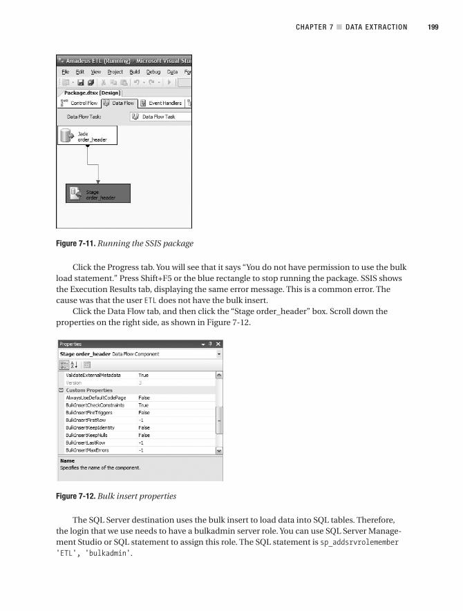
Figure 7-11. Running the SSIS package
Click the Progress tab. You will see that it says “You do not have permission to use the bulkload statement.” Press Shift+F5 or the blue rectangle to stop running the package. SSIS showsthe Execution Results tab, displaying the same error message. This is a common error. Thecause was that the user ETL does not have the bulk insert.
Click the Data Flow tab, and then click the “Stage order_header” box. Scroll down theproperties on the right side, as shown in Figure 7-12.
Figure 7-12. Bulk insert properties
The SQL Server destination uses the bulk insert to load data into SQL tables. Therefore,the login that we use needs to have a bulkadmin server role. You can use SQL Server Manage-ment Studio or SQL statement to assign this role. The SQL statement is sp_addsrvrolemember'ETL', 'bulkadmin'.
CHAPTER 7 ■ DATA EXTRACTION 199
9314ch07final.qxd 11/15/07 10:10 AM Page 199

Rerun the package. Now both boxes in the Data Flow tab should be green, meaning thatSSIS has successfully imported those rows from the source table to the stage table. Click Stop,or press Shift+F5. Click the blue disk button (or select File ➤ Save) to save your SSIS package.Go to SQL Server Management Studio, and query the order_header table in the stage databaseto verify that you have the rows in the stage.
Memorizing the Last Extraction TimestampMemorizing the last extraction timestamp means that we memorize the last timestamp of thedata we extracted so that on the next extraction we can start from that point. We have just suc-cessfully extracted the order header records from Jade into the stage. But we used fixed valuesfor the date range. Now let’s store the last extraction timestamp in the metadata database sothat every time the ETL process runs it will extract different records. The ETL process willextract only those records that were added after the last extract.
Before we begin, let’s go through an overview of what we are going to do. In the next fewpages, we will use the last extraction timestamp to control the next extraction. This enables usto extract the source table incrementally. To do that, in the next few pages we will be doing thefollowing steps:
1. Create a table in the metadata database to store the timestamps.
2. Create a data source for the metadata database.
3. Modify the data flow as follows:
a. Store the current time.
b. Get the last extraction timestamp from the table.
c. Add timestamps to the extraction query as parameters.
d. Update the timestamps in the table.
4. Clear the target table in the stage database.
5. Set the initial timestamps in the metadata table.
6. Execute the package to populate the target table.
So first, let’s create the data_flow table as follows:
use metago
if exists( select * from sys.tableswhere name = 'data_flow' )
drop table data_flowgo
CHAPTER 7 ■ DATA EXTRACTION200
9314ch07final.qxd 11/15/07 10:10 AM Page 200

create table data_flow( id int not null identity(1,1), name varchar(20) not null, LSET datetime, CET datetime, constraint pk_data_flowprimary key clustered (id)
)go
create index data_flow_nameon data_flow(name)go
declare @LSET datetime, @CET datetimeset @LSET = '2007-12-01 03:00:00'set @CET = '2007-12-02 03:00:00'insert into data_flow (name, status, LSET, CET)values ('order_header', 0, @LSET, @CET)
insert into data_flow (name, status, LSET, CET)values ('order_detail', 0, @LSET, @CET)
insert into data_flow (name, status, LSET, CET)values ('customer', 0, @LSET, @CET)
insert into data_flow (name, status, LSET, CET)values ('product', 0, @LSET, @CET)
go
■Note LSET stands for Last Successful Extraction Timestamp, and CET means Current ExtractionTimestamp.
Verify that we have that order_header row in the data_flow table: select * fromdata_flow. You should see four rows, as shown in Table 7-6.
Table 7-6. data_flow Table
id name LSET CET
1 order_header 2007-12-01 03:00:00.000 2007-12-02 03:00:00.000
2 order_detail 2007-12-01 03:00:00.000 2007-12-02 03:00:00.000
3 customer 2007-12-01 03:00:00.000 2007-12-02 03:00:00.000
4 product 2007-12-01 03:00:00.000 2007-12-02 03:00:00.000
CHAPTER 7 ■ DATA EXTRACTION 201
9314ch07final.qxd 11/15/07 10:10 AM Page 201

OK, now let’s modify our order_header Data Flow task in our Amadeus ETL package sothat it first sets the CET to the current time and then reads the LSET. If the data flow is success-fully executed, we update the LSET and status for that data flow. If it fails, we set the status tofail, and we don’t update the LSET. This way, the next time the data flow is run, it will pick upthe records from the same LSET.
So, let’s create a new data source called Meta that connects to the metadata databaseusing the ETL user. The procedure is the same as the last time. This is why in the previoussection, when we created the Jade database, we also assigned the user ETL as db_owner in themetadata database. Now we will set the CET to the current time for all rows.
1. In the Toolbox on the left side, double-click the Execute SQL task. There will be a newbox on the design surface labeled Execute SQL Task. Right-click, and rename this boxas Set CET.
2. Double-click this box. In the SQL Statement section, click the Connection drop-downlist, and select <New connection…>, as shown in Figure 7-13.
Figure 7-13. Configuring the connection for the Execute SQL Task
3. Choose the servername.Meta.ETL data connection, and click OK.
4. In the SQL Statement field, type update data_flow set CET = getdate() where name ='order_header'. Click OK to close the Execute SQL Task Editor dialog box.
In steps 5 to 7 we are going to retrieve the last successful extraction time and the cur-rent extraction time from the data flow metadata table.
CHAPTER 7 ■ DATA EXTRACTION202
9314ch07final.qxd 11/15/07 10:10 AM Page 202

5. In the Toolbox, double-click the Execute SQL task again to create a new task in thedesign surface. Rename this box to Get LSET.
6. Double-click the box to edit it. Set the connection to servername.Meta.ETL. Set Result-Set to Single Row.
7. In the SQL Statement field, type select LSET, CET from data_flow where name =‘order_header’. Click Parse Query to verify.
In steps 8 to 12, we are going to store the query result in variables. They will be usedlater to limit the order header query.
8. In the left column, click Result Set. Click Add. Change NewResultName to LSET.
9. Click the Variable Name cell, expand the drop-down list, and choose <New vari-able…>. Leave the container set to Package, which means that the scope of thevariable is the SSIS package, not just the Get LSET task, which means we can use thevariable in other tasks.
10. Change the name to dtLSET. Leave Namespace set to User.
11. Change Value Type to DateTime. Set the value as 2007-10-01 00:00:00 (or any date youlike), and click OK.
12. Click Add again to add another variable. Set Result Name as CET and Variable Name asa new variable called dtCET of type DateTime. The result will look like Figure 7-14.
Figure 7-14. Storing the result set in variables
CHAPTER 7 ■ DATA EXTRACTION 203
9314ch07final.qxd 11/15/07 10:10 AM Page 203

13. Click OK to close the Execute SQL Task Editor dialog box.
In steps 14 to 16 we will connect the tasks on the design surface and tidy up the layout.
14. Connect the green success arrow from the Set CET box to the Get LSET box. Renamethe Data Flow task to Extract Order Header, and connect the green arrow from theGet LSET box to this box.
15. In the Toolbox, double-click the Execute SQL task to create a new box, and rename it toSet LSET. Connect the green arrow from Extract Order Header box to this Set LSET box.
16. Let’s tidy up the layout a little bit. In the menu bar, select Format ➤ Auto Layout ➤Diagram. The result looks like Figure 7-15.
Figure 7-15. Arranging the layout after connecting the task boxes
In steps 17 to 20, we will modify to extract order header task to include the timestampas parameters to limit the query.
17. Double-click the Extract Order Header box, and in the Data Flow design surface dou-ble-click the Jade Order Header box to edit it.
18. Update the SQL command text by changing all the fixed dates to question marks, asfollows:
select * from order_headerwhere (created > ? and created <= ?)or (last_updated > ? and last_updated <= ?)
19. Click the Parameter button, and set parameter 0 to User::dtLSET, parameter 1 toUser:dtCET, parameter 2 to User::dtLSET, and parameter 3 to User::dtCET, as shown inFigure 7-16.
CHAPTER 7 ■ DATA EXTRACTION204
9314ch07final.qxd 11/15/07 10:10 AM Page 204
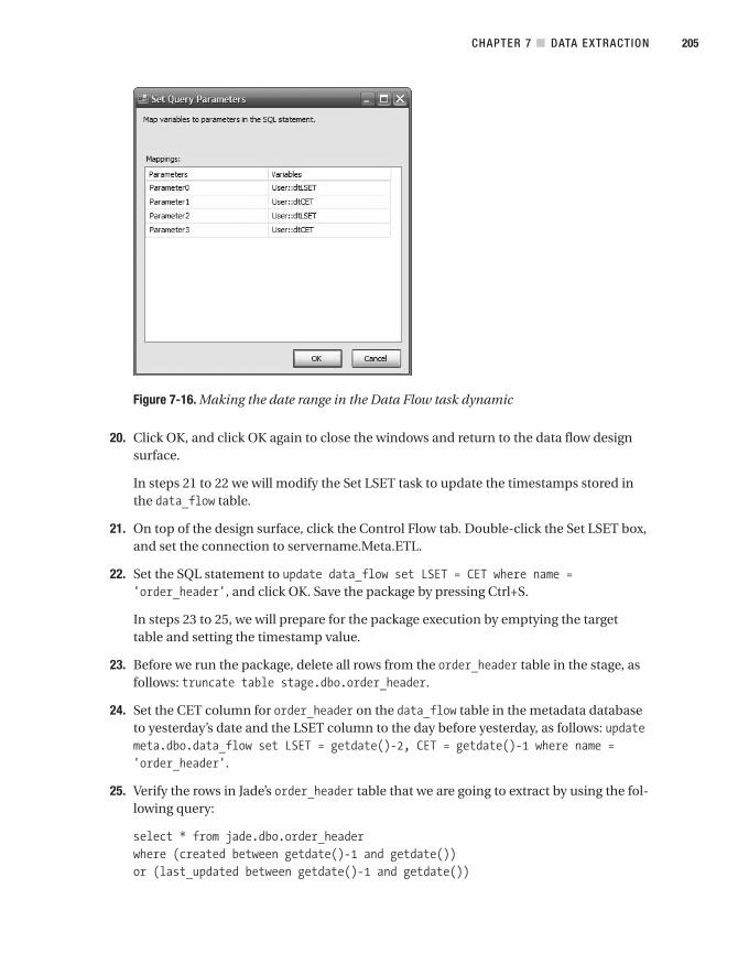
Figure 7-16. Making the date range in the Data Flow task dynamic
20. Click OK, and click OK again to close the windows and return to the data flow designsurface.
In steps 21 to 22 we will modify the Set LSET task to update the timestamps stored inthe data_flow table.
21. On top of the design surface, click the Control Flow tab. Double-click the Set LSET box,and set the connection to servername.Meta.ETL.
22. Set the SQL statement to update data_flow set LSET = CET where name ='order_header', and click OK. Save the package by pressing Ctrl+S.
In steps 23 to 25, we will prepare for the package execution by emptying the targettable and setting the timestamp value.
23. Before we run the package, delete all rows from the order_header table in the stage, asfollows: truncate table stage.dbo.order_header.
24. Set the CET column for order_header on the data_flow table in the metadata databaseto yesterday’s date and the LSET column to the day before yesterday, as follows: updatemeta.dbo.data_flow set LSET = getdate()-2, CET = getdate()-1 where name ='order_header'.
25. Verify the rows in Jade’s order_header table that we are going to extract by using the fol-lowing query:
select * from jade.dbo.order_headerwhere (created between getdate()-1 and getdate())or (last_updated between getdate()-1 and getdate())
CHAPTER 7 ■ DATA EXTRACTION 205
9314ch07final.qxd 11/15/07 10:10 AM Page 205

Note how many rows this query returns.
In steps 26 to 29, we will execute the package and check the execution results.
26. Go back to Business Intelligence Development Studio, and press F5 (or click the greentriangle button in the toolbar) to run the package. All four boxes become yellow andthen green one by one, as shown in Figure 7-17.
Figure 7-17. Running SSIS package that memorizes the last extraction time
27. If one of them becomes red, don’t panic. Click the last tab (Progress) and see the errormessage. You can debug by right-clicking the boxes on the control flow and choosingEdit Breakpoints. The Set Breakpoints dialog box will pop up, as shown in Figure 7-18,and you can choose when you want the breakpoint to occur. You can also specifywhether the breakpoint always happens or only at a certain count, that is, how manytimes the breakpoint is ignored before the execution is stopped.
You can also see the value of the variable by clicking the Watch 1 or Locals tabs in thebottom-left corner of the screen. Figure 7-19 shows that we can observe the value ofthe local variables when the execution is suspended at a breakpoint. For example, thevalue of user variable dtCET_OH is 06/10/2007 21:47:22 and the data type is DateTime.
28. Press Shift+F5 to stop the package running. Click the Execution Results tab, and verifythat all tasks were executed successfully.
29. Open SQL Server Management Studio, and check that the LSET and CET columns fororder_header in the data_flow table in the metadata database are updated correctly tocurrent time. Also check that order_header in the stage database contains the correctnumber of rows from the Jade order_header table, as noted earlier.
CHAPTER 7 ■ DATA EXTRACTION206
9314ch07final.qxd 11/15/07 10:10 AM Page 206

Figure 7-18. Setting up a breakpoint
Figure 7-19. The Locals window showing the variable value and data type
30. At the moment, the name of the SSIS package in Solution Explorer is Package.dtsx.Rename it to order_header.dtsx by right-clicking it. When asked “Do you want torename the package object as well,” click Yes. By default SSIS renames only the packagefile, but internally the object name is not changed (you can see the object name byclicking the View menu and choosing Properties Window). By answering yes, werename the package object as well as the package file.
31. Click the File menu, and choose Save All to save the entire solution. Click the Filemenu, and choose Close Project to close the package.
With that, we’re finished going through the basics of extracting data incrementally from arelational database. Before we close this chapter, let’s do a data extract from a file because inreal data warehouse projects this happens a lot.
CHAPTER 7 ■ DATA EXTRACTION 207
9314ch07final.qxd 11/15/07 10:10 AM Page 207

Extracting from FilesNow that we have extracted data from a database, let’s try to extract data from files. In the nextfew pages, we will extract data from a flat file. For the purpose of this exercise, we have ISOcountry data supplied to us in pipe-delimited files. We will import this file to the stage data-base. The file will be supplied once a week, from an external data provider.
In the following pages we will create an SSIS package to import the flat file into the stagedatabase. After importing successfully to the stage, we will archive the file by moving it toanother directory. We will accomplish this by doing the following steps:
1. Download the flat file containing the ISO country data.
2. Open the flat file to see the content.
3. Create the target table in the stage database.
4. Create a new SSIS package.
5. Create an Execute SQL task to truncate the target table.
6. Create a Data Flow task to load the flat file to the stage database.
7. Create a File System task to archive the file.
8. Execute the package.
The SSIS package that we are building looks like Figure 7-20. It truncates the target table,extracts data from the country flat file, and then archives the file.
Figure 7-20. SSIS package to extract data from file
OK, so let’s get started. First download the flat file from the book’s web site athttp://www.apress.com/. It is located in the folder /data/external. The file name iscountry.dat (8KB). Put this file in your local drive, for example: c:\.
Let’s open the country.dat file using Notepad to see the content. It looks like this:
CHAPTER 7 ■ DATA EXTRACTION208
9314ch07final.qxd 11/15/07 10:10 AM Page 208

Code|Countryad|Andorraae|United Arab Emiratesaf|Afghanistanag|Antigua and Barbudaai|Anguillaal|Albania
This consists of two columns, and it is pipe delimited. The first column is a two-characterISO country code, and the second column is the country name. The first line contains the col-umn header: Code for the first column and Country for the second column.
Now that we know the content and format of the file, let’s create the SSIS package toload this file into the stage. But before that, we need to create the stage table first. If we lookat the data file, the longest country name is 34 characters (Saint Tome (Sao Tome) andPrincipe), so for this exercise we will set the width of the country name column to 50 char-acters. Let’s open Management Studio and create the target table called country on the stagedatabase as follows:
create table country( country_code char(2), country_name varchar(50))
Now we can create the SSIS package:
1. Open Business Intelligence Development Studio, and open the Amadeus ETL project(select File ➤ Open ➤ Project, navigate to Amadeus ETL.sln, and double-click it).
2. In Solution Explorer, right-click SSIS Packages, and choose New SSIS Package. A blankdesign surface opens.
3. To be able to run the package many times, we need to truncate the target table beforewe load the data. Click the Control Flow tab, and double-click the Execute SQL task inthe Toolbox.
4. Rename the box Truncate Country Table, and double-click the box to edit it. Set theconnection to servername.Stage.ETL.
5. Set the SQL statement to truncate table country, and click OK. Click OK again toclose the Execute SQL Task Editor dialog box.
6. Now let’s create a Data Flow task to load the flat file to the stage database. Double-click Data Flow Task in the Toolbox, and rename the new box Load Country Flat File.Connect the green arrow from Truncate Country Table to Load Country Flat File.
7. Double-click Load Country Flat File to edit it. Let’s add the country flat file as asource. Double-click Flat File Source in the Toolbox, and rename the new boxCountry Flat File.
8. Double-click the Country Flat File box, and click the New button.
CHAPTER 7 ■ DATA EXTRACTION 209
9314ch07final.qxd 11/15/07 10:10 AM Page 209
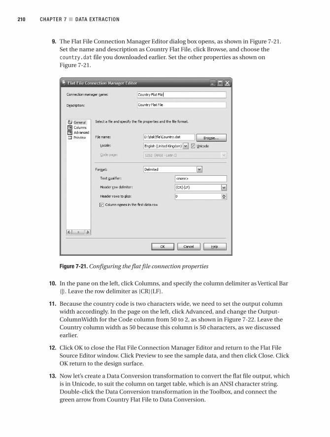
9. The Flat File Connection Manager Editor dialog box opens, as shown in Figure 7-21.Set the name and description as Country Flat File, click Browse, and choose thecountry.dat file you downloaded earlier. Set the other properties as shown onFigure 7-21.
Figure 7-21. Configuring the flat file connection properties
10. In the pane on the left, click Columns, and specify the column delimiter as Vertical Bar{|}. Leave the row delimiter as {CR}{LF}.
11. Because the country code is two characters wide, we need to set the output columnwidth accordingly. In the page on the left, click Advanced, and change the Output-ColumnWidth for the Code column from 50 to 2, as shown in Figure 7-22. Leave theCountry column width as 50 because this column is 50 characters, as we discussedearlier.
12. Click OK to close the Flat File Connection Manager Editor and return to the Flat FileSource Editor window. Click Preview to see the sample data, and then click Close. ClickOK return to the design surface.
13. Now let’s create a Data Conversion transformation to convert the flat file output, whichis in Unicode, to suit the column on target table, which is an ANSI character string.Double-click the Data Conversion transformation in the Toolbox, and connect thegreen arrow from Country Flat File to Data Conversion.
CHAPTER 7 ■ DATA EXTRACTION210
9314ch07final.qxd 11/15/07 10:10 AM Page 210

Figure 7-22. Configuring the properties of each column
14. Double-click Data Conversion to edit it, and check both the Code and Countrycolumns under Available Input Columns. In the Data Type column, choose string[DT_STR] for both the Code and Country columns, as shown in Figure 7-23.
Figure 7-23. Data Conversion Transformation Editor
CHAPTER 7 ■ DATA EXTRACTION 211
9314ch07final.qxd 11/15/07 10:10 AM Page 211

15. In the Toolbox, double-click SQL Server Destination, and rename the new box toCountry Stage. Connect the green arrow on the Data Conversion box to the CountryStage box. Double-click the Country Stage box, and set the OLE DB connection man-ager to servername.Stage.ETL.
16. Set “Use table or view” to country, which we created earlier. In the panel on the left,click Mappings. Click and drag the Copy of Code column on the left to thecountry_code column on the right. Click and drag Copy of Country column on the leftto the country_name column on the right, as shown in Figure 7-24.
Figure 7-24. Mapping the source columns to the target columns
17. Click OK to return to the design surface. Click the Control Flow tab on the top of thedesign surface. We need to add one more task here, which is to archive the country flatfile by moving it to another directory.
18. Double-click the File System task in the Toolbox, and rename the newly created boxArchive Country Flat File.
19. Double-click the Archive Country Flat File box to edit it. Set Source Connection topoint to the country flat file. Set Destination Connection to point to an empty folder.Set Operation to Move File, as shown on Figure 7-25.
20. Click OK to return to the design surface. Let’s tidy up the layout a little bit. Click theEdit menu, and choose Select All. Click the Format menu, choose Auto Layout, andchoose Diagram. The three boxes are now aligned and evenly spaced.
21. Click the File menu, and choose Save All to save the entire solution. Hit F5 to run thepackage. It should now run OK. Each box should turn yellow and then turn green, asshown in Figure 7-26.
CHAPTER 7 ■ DATA EXTRACTION212
9314ch07final.qxd 11/15/07 10:10 AM Page 212

Figure 7-25. Configuring the File System task to archive the file
Figure 7-26. Importing country data from flat files into the stage
Even though we are not extracting incrementally here, we still have to add the metadatabit as we did previously when extracting the order header. This means we need to store the lastsuccessful run timestamp in the data_flow table. Recording the result of every single ETL dataflow is important so that when the ETL fails and we want to restart from failure, we knowwhere to restart from because we know which tasks were successful and which tasks failed torun. We do this by storing the execution result in the same data_flow metadata table as shownin Figure 7-27. (I will be discussing metadata in Chapter 10.)
Figure 7-27. The data_flow metadata table stores execution status, the LSET, and the CET
CHAPTER 7 ■ DATA EXTRACTION 213
9314ch07final.qxd 11/15/07 10:10 AM Page 213

SummaryThis chapter started with the approaches and architectures for ETL systems, that is, ETL, ELT,using a dedicated ETL server or not, push vs. pull, choices of which server to place the ETLprocesses, and so on. Then it went through different kinds of source systems, such as rela-tional databases, spreadsheets, flat files, XML files, web logs, database log files, images, webservices, message queues, and e-mails. It also discussed how to extract incrementally a wholetable every time using fixed ranges and how to detect data leaks.
Then I showed how to extract order header data from Jade to the stage using SSIS. We putsome processes in place to memorize the last extract so we could extract incrementally. Wealso extracted the country flat file into the stage database using SSIS.
This chapter gave you a good foundation of data extraction principles, as well as a clearunderstanding of how to do it using SSIS. In the next chapter, we will bring the data that wehave imported to the stage into the NDS and the DDS.
CHAPTER 7 ■ DATA EXTRACTION214
9314ch07final.qxd 11/15/07 10:10 AM Page 214

Populating the Data Warehouse
Now that we have extracted the data from the source system, we’ll populate the normalizeddata store and dimensional data store with the data we have extracted. In this chapter, I willdiscuss five main subjects regarding data warehouse population in the sequence they occurin a data warehouse system:
1. Loading the stage: We load the source system data into the stage. Usually, the focus isto extract the data as soon as possible without doing too much transformation. Inother words, the structure of the stage tables is similar to the source system tables. Inthe previous chapter, we discussed the extraction, and in this chapter, we will focuson the loading.
2. Creating the data firewall: We check the data quality when the data is loaded from thestage into the NDS or ODS. The check is done using predefined rules that define whataction to take: reject the data, allow the data, or fix the data.
3. Populating a normalized data store: This is when we load the data from the stage intothe NDS or ODS, after the data passes through the data firewall. Both are normalizeddata stores consisting of entities with minimal data redundancy. Here we deal withdata normalization and key management.
4. Populating dimension tables: This is when we load the NDS or ODS data into the DDSdimension tables. This is done after we populate the normalized data store. DDS is adimensional store where the data is denormalized, so when populating dimensiontables, we deal with issues such as denormalization and slowly changing dimension.
5. Populating fact tables: This is the last step in populating the data warehouse. It is doneafter we populate the dimension tables in the DDS. The data from the NDS or ODS (orfrom the stage, depending on the architecture; see Chapter 2) is loaded into DDS facttables. In this process, we deal with surrogate key lookup and late-arriving fact rows.
In this chapter, I will also discuss and compare batches, mini-batches, and the near real-time approach, because the latter two approaches are becoming more and more popularthese days. I will close the chapter by discussing real-time ETL, which means that the data ispushed into the warehouse rather than being pulled.
I will also cover how to use SSIS for populating the NDS and managing data warehousekeys and how to use SSIS to populate the dimension tables and fact tables in the DDS. I willalso show how to use related SSIS tasks and transformations (such as the Slowly ChangingDimension transformation, the Lookup transformation, and the Execute SQL task) to popu-late NDS and DDS. 215
C H A P T E R 8
9314ch08final.qxd 11/15/07 10:09 AM Page 215
Stage LoadingIn the previous chapter, we extracted the data from the source system into a stage. The stagecan be a file system or a database.
When using files as a data warehouse stage, it is necessary to plan the file naming anddirectory structure carefully, in particular when incorporating the dates into the file names ordirectory names. We need to have access rights and permission to the stage folders. We needto define the deletion and archiving process, the failure handling, and the loading frequency.Most important, we need to define the details of the file format. Capacity on the allocateddisk is also important at the planning stage. This is a simple point but has caused problems,so ensure that you won’t run out of disk space, and ensure that your ETL process will be ableto handle this situation gracefully rather than abruptly. The disk space for the stage area isplanned based on the maximum daily data extraction volume from the source system andhow long we will be archiving the data for.
If your stage is a database, which is common, it is better not to put any indexes or con-straints (such as not null, primary keys, or check constraints) in the stage database. The mainreason for this is not because of performance but because we want to capture and report the“bad data” in the data quality process. We want to allow bad data such as null and duplicateprimary keys into the stage table so we can report it. If we restrict our stage table to rejectnull and duplicate primary keys, then the data quality process that sits between the stage andthe NDS would not be able capture these DQ issues and report them for correction in thesource system. For example, if we restrict the stage table with a unique constraint on the pri-mary key column, when we have two duplicate rows, the second row will not be inserted intothe stage. It is better to allow them into the stage. This way, when we populate the NDS, wecan implement a set of comprehensive and stringent rules that filter out bad data into thedata quality quarantine area for reporting and further processing such as cleansing, fixing,reimporting, or archiving.
Indexing stage tables is generally not necessary. This is because of the way the stage tablesare structured and selected. The best way to do this is to load the data into empty stage tableswithout any indexes and then select all records from those tables for loading into the NDS. Ifyou plan to keep, say, five days of stage data, in case you need them in the event of failures, itis better not to keep the previous day’s data in the same table. The first reason why we can’t goback to the source system and restage is because the source system data may have changed.The second reason is performance. In other words, it is quicker to reload the NDS from thestage than to retrieve data from the source system again.
Figure 8-1 shows three different approaches of how stage tables are structured:
CHAPTER 8 ■ POPULATING THE DATA WAREHOUSE216
9314ch08final.qxd 11/15/07 10:09 AM Page 216

Approach 1 keeps the previous day’s data in the same table: This approach is simple toimplement because you have only one table. You store the time each record was loadedinto the stage table by having a column called loaded_timestamp in the stage table. Theloaded_timestamp column is a datetime column that indicates when the record wasloaded into the stage.
Approach 2 keeps each day in a separate table: Even though it is more complex thanapproach 1, approach 2 gives better performance because you load into an empty tableand select all records when retrieving the data. When implementing approach 2, you cre-ate the Today table before the loading begins and drop the Day 1 table after the loadinghas completed successfully.
Approach 3 is to have just one table and truncate the table every time before loading: Thisapproach is even simpler than approach 1. We don’t keep the previous day’s data in thestage database. If we need to restore the stage data retrieved a few days ago, we have torestore from database backup. Well, the number of days of the stage database backup tokeep is different for each company. It is determined based on the extraction frequency(from the source system into the stage) and the loading frequency (from the stage to theNDS, ODS, or DDS).
Figure 8-1. Different approaches for stage loading
I said earlier that indexing the stage table is generally not necessary. So, when is it neces-sary to index the stage table? It may be necessary to index a stage table when you implementapproach 1 (keeping the previous day’s data in the same table) and the stage table is used bymultiple applications, not just the data warehouse. It depends on the data volume. In otherwords, indexing is useful only if the volume is large enough. In this case, indexing the stagetable on the loaded_timestamp column will assist the application’s ETL in selecting the rowsrelevant to a particular day when loading from the stage into the application’s data store.
CHAPTER 8 ■ POPULATING THE DATA WAREHOUSE 217
9314ch08final.qxd 11/15/07 10:09 AM Page 217
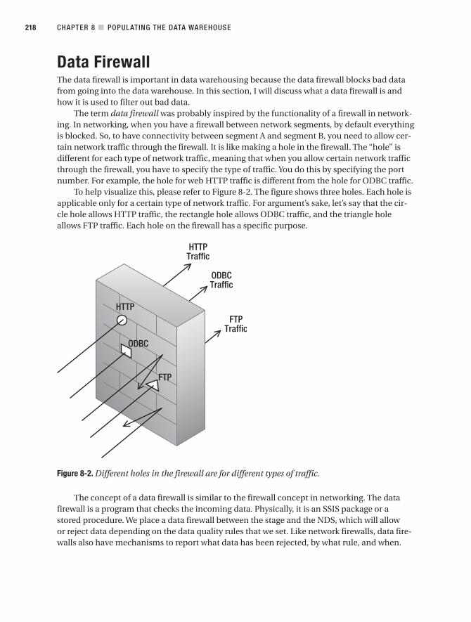
Data FirewallThe data firewall is important in data warehousing because the data firewall blocks bad datafrom going into the data warehouse. In this section, I will discuss what a data firewall is andhow it is used to filter out bad data.
The term data firewall was probably inspired by the functionality of a firewall in network-ing. In networking, when you have a firewall between network segments, by default everythingis blocked. So, to have connectivity between segment A and segment B, you need to allow cer-tain network traffic through the firewall. It is like making a hole in the firewall. The “hole” isdifferent for each type of network traffic, meaning that when you allow certain network trafficthrough the firewall, you have to specify the type of traffic. You do this by specifying the portnumber. For example, the hole for web HTTP traffic is different from the hole for ODBC traffic.
To help visualize this, please refer to Figure 8-2. The figure shows three holes. Each hole isapplicable only for a certain type of network traffic. For argument’s sake, let’s say that the cir-cle hole allows HTTP traffic, the rectangle hole allows ODBC traffic, and the triangle holeallows FTP traffic. Each hole on the firewall has a specific purpose.
Figure 8-2. Different holes in the firewall are for different types of traffic.
The concept of a data firewall is similar to the firewall concept in networking. The datafirewall is a program that checks the incoming data. Physically, it is an SSIS package or astored procedure. We place a data firewall between the stage and the NDS, which will allowor reject data depending on the data quality rules that we set. Like network firewalls, data fire-walls also have mechanisms to report what data has been rejected, by what rule, and when.
CHAPTER 8 ■ POPULATING THE DATA WAREHOUSE218
9314ch08final.qxd 11/15/07 10:09 AM Page 218

This is because every time the data firewall captures or finds bad data (as defined by the dataquality rule), the bad data is stored in the data quality database, along with which rule wasused to capture the bad data, what action was taken, and when it happened. We can thenreport from this data quality database. We can also set the data quality system to notify theappropriate people when certain data quality rules are violated.
Unlike a network firewall, a data firewall can also fix or correct bad data. When the datafirewall detects bad data, we can set it to do one of these three actions: reject the data (notload it into the data warehouse), allow the data (load it into the data warehouse), or fix thedata (correct the data before loading it into the data warehouse).
A data firewall is an important part of data warehouse loading because it ensures dataquality. Before we load the data into the normalized data store (or into a DDS if we use DDS-only architecture), we check the data by passing the data through firewall rules.
Populating NDSIn the NDS + DDS architecture, we need to populate the tables in the NDS before we popu-late the dimension and fact tables in the DDS. This is because we populate the DDS basedon the NDS data. Populating a normalized data store is quite different from populating thestage. This is because when populating the NDS, we need to normalize the data, while whenpopulating the stage, we don’t need to normalize the data. We extract some data from thestage table or straight from the source system and then load it into the NDS database. If therecord does not exist in the NDS, we insert it. If the record already exists, we update it.
When populating the NDS, we need to consider several issues:
Normalization: In the NDS, the tables are normalized, so when loading the data from thestage, we need to normalize it to fit the NDS structure. This means we need to populatecertain tables first before we can populate the main table.
External data: It is possible that the data from external sources does not match the datafrom the source system. This means that when we load data into the NDS, we may needto do some data conversion.
Key management: In the NDS, we need to create and maintain internal data warehousekeys, which will also be used in the DDS. When loading data into the NDS, we need tomanage these keys.
Junction tables: The junction tables enable us to implement many-to-many relationships.When populating junction tables, we need to follow a certain sequence.
We will discuss each of these four topics one by one in the following pages. Let’s beginwith the first one, normalization. The NDS is a normalized store. But the source systems maynot be normalized, so we have to normalize the data to fit the NDS normalized structure. Forexample, consider the store table in the source system, shown in Table 8-1.
CHAPTER 8 ■ POPULATING THE DATA WAREHOUSE 219
9314ch08final.qxd 11/15/07 10:09 AM Page 219

Table 8-1. Non-normalized store Table in the Source System
store_number store_name store_type
1805 Perth Online
3409 Frankfurt Full Outlet
1014 Strasbourg Mini Outlet
2236 Leeds Full Outlet
1808 Los Angeles Full Outlet
2903 Delhi Online
We need transform it into the table shown in Table 8-2.
Table 8-2. A Normalized store Table in the NDS
store_number store_name store_type_key
1805 Perth 1
3409 Frankfurt 2
1014 Strasbourg 3
2236 Leeds 2
1808 Los Angeles 2
2903 Delhi 1
The store_type column in the source system in Table 8-1 is normalized into its own table,as shown in Table 8-3.
Table 8-3. store_type Table in the NDS
store_type_key store_type
1 Online
2 Full Outlet
3 Mini Outlet
Figure 8-3 shows the entity relationship diagram of the store and store_type tables in thesource system and in the NDS. The diagram on the right shows that the store table is normal-ized in the NDS. Each store has one store type. Each store type relates to zero or many stores.
CHAPTER 8 ■ POPULATING THE DATA WAREHOUSE220
9314ch08final.qxd 11/15/07 10:09 AM Page 220

Figure 8-3. Entity relationship diagram of the store table in the source system and the NDS
If in the source system we have the store_type table, we just need to bring it to the NDS.But if we don’t have a store_type table in the source system, we need to populate the NDSstore_type table using the data in the store table. If the store table contains a new store type,we need to insert it into the store_type table. In practice, whether you use an ODS or NDS inyour data warehouse architecture, many of the reference entities are available in the sourcesystem.
But there are always a few entities that are not available in the source system, so youneed to create them based on the data in the main entities. You can do this by inserting newdata from the main entity into the subentity. In the store example, the source system doesn’thave a store_type table. So in the NDS, you need to create and populate the store_type tablebased on the data available in the store table. Suppose we get the three rows from the sourcesystem, as shown in Table 8-4.
Table 8-4. Incoming Data from the Source System
store_number store_name store_type
2009 Dallas Online
2237 London Full Outlet
2014 San Francisco Distribution Center
The first and second rows (Dallas and London) are fine because their store typesalready exist in the NDS store_type table (shown earlier in Table 8-3). But the third row(San Francisco) has a store type of Distribution Center. We don’t have this store type in theNDS store_type table. So, we insert this new Distribution Center store type into the NDSstore_type table, as shown in Table 8-5.
Table 8-5. Adding a New Store Type
store_type_key store_type
1 Online
2 Full Outlet
3 Mini Outlet
4 Distribution Center
CHAPTER 8 ■ POPULATING THE DATA WAREHOUSE 221
9314ch08final.qxd 11/15/07 10:09 AM Page 221
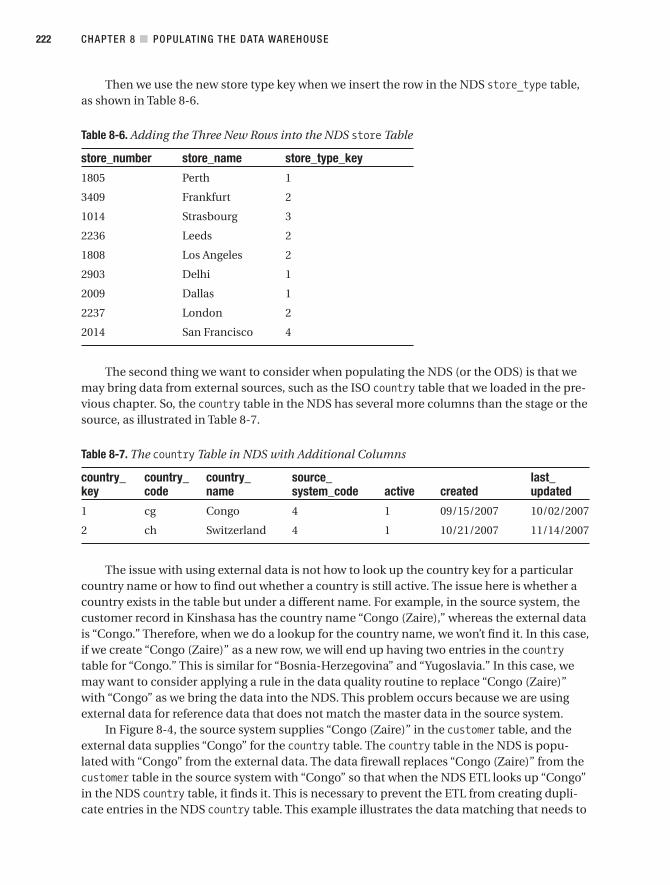
Then we use the new store type key when we insert the row in the NDS store_type table,as shown in Table 8-6.
Table 8-6. Adding the Three New Rows into the NDS store Table
store_number store_name store_type_key
1805 Perth 1
3409 Frankfurt 2
1014 Strasbourg 3
2236 Leeds 2
1808 Los Angeles 2
2903 Delhi 1
2009 Dallas 1
2237 London 2
2014 San Francisco 4
The second thing we want to consider when populating the NDS (or the ODS) is that wemay bring data from external sources, such as the ISO country table that we loaded in the pre-vious chapter. So, the country table in the NDS has several more columns than the stage or thesource, as illustrated in Table 8-7.
Table 8-7. The country Table in NDS with Additional Columns
country_ country_ country_ source_ last_key code name system_code active created updated
1 cg Congo 4 1 09/15/2007 10/02/2007
2 ch Switzerland 4 1 10/21/2007 11/14/2007
The issue with using external data is not how to look up the country key for a particularcountry name or how to find out whether a country is still active. The issue here is whether acountry exists in the table but under a different name. For example, in the source system, thecustomer record in Kinshasa has the country name “Congo (Zaire),” whereas the external datais “Congo.” Therefore, when we do a lookup for the country name, we won’t find it. In this case,if we create “Congo (Zaire)” as a new row, we will end up having two entries in the countrytable for “Congo.” This is similar for “Bosnia-Herzegovina” and “Yugoslavia.” In this case, wemay want to consider applying a rule in the data quality routine to replace “Congo (Zaire)”with “Congo” as we bring the data into the NDS. This problem occurs because we are usingexternal data for reference data that does not match the master data in the source system.
In Figure 8-4, the source system supplies “Congo (Zaire)” in the customer table, and theexternal data supplies “Congo” for the country table. The country table in the NDS is popu-lated with “Congo” from the external data. The data firewall replaces “Congo (Zaire)” from thecustomer table in the source system with “Congo” so that when the NDS ETL looks up “Congo”in the NDS country table, it finds it. This is necessary to prevent the ETL from creating dupli-cate entries in the NDS country table. This example illustrates the data matching that needs to
CHAPTER 8 ■ POPULATING THE DATA WAREHOUSE222
9314ch08final.qxd 11/15/07 10:09 AM Page 222

be done when we have more than one data source. When populating the NDS, matching is thebase activity for integrating the data.
Figure 8-4. Using the DQ rule to correct incoming data to prevent duplicate data in the NDS
The third consideration is key management. We want to implement key managementwhen doing NDS population. Consider a simple table in Jade like the one shown in Table 8-8.
Table 8-8. product_status Table in Jade
status_code description
AC Active
QC Quality Control
IN Inactive
WD Withdrawn
The product_status table in the NDS has a surrogate key column and an unknown row, asshown in Table 8-9.
Table 8-9. product_status Table in NDS
product_status_key product_status_code product_status other columns
0 UN Unknown
1 AC Active
2 QC Quality Control
3 IN Inactive
4 WD Withdrawn
The purpose of having our own keying system in the data warehouse is twofold. First, itenables integration with the second source system, and second, we want to be able to adaptthe key changes in the source system(s). Data warehouse keying is in the form of simple incre-mental integers (1, 2, 3, 4, and so on). The data warehouse key is known as a surrogate key(SK). The source system key is known as a natural key (NK). The SK enables the integration
CHAPTER 8 ■ POPULATING THE DATA WAREHOUSE 223
9314ch08final.qxd 11/15/07 10:09 AM Page 223

of several source systems because we can map or associate the NK with the SK. For example,say Jupiter has the product status shown in Table 8-10.
Table 8-10. product_status Table in Jupiter
status_code description
N Normal
OH On Hold
SR Supplier Reject
C Closed
The SK in the data warehouse enables us to arrange in the ETL to have Normal in Jupiterassociated with Active in Jade. In addition, both should be mapped to SK 1, both Inactive andClosed should be mapped to SK 3, and the remaining two codes from both systems are main-tained so that the resulting product_status table looks like Table 8-11. Figure 8-5 shows themapping.
Table 8-11. product_status Table in NDS Combining Jade and Jupiter
product_status_key product_status_code product_status control columns
0 UN Unknown …
1 AC Active …
2 QC Quality Control …
3 IN Inactive …
4 WD Withdrawn …
5 OH On Hold …
6 SR Supplier Reject …
What I meant by “control columns” in Table 8-11 are active flag, source system code,created, and last updated. In the NDS, we have a source_system table that contains a listof source systems feeding the NDS. In this source system table, we define 1 for Jade, 2 forWebTower, 3 for Jupiter, and 0 for unknown or not applicable, as shown in Figure 8-5. We setthe source system code for On Hold and Supplier Reject to 3, Unknown to 0, and the remain-ing four rows to 1. Figure 8-5 shows the mapping between the source system tables and theNDS. It also shows the source_system table.
CHAPTER 8 ■ POPULATING THE DATA WAREHOUSE224
9314ch08final.qxd 11/15/07 10:09 AM Page 224

Figure 8-5. The mapping for the product_status table between the source systems and the NDS
If Quality Control was deleted later from Jade, we would change the active flag forQuality Control from T to F (please see the active column on the NDS product_status tablein Figure 8-5). It is better to apply soft deletion in the NDS, rather than hard deletion. Someregulations in certain countries may require hard deletion on certain data; for example,French and UK customers may request that their e-mail addresses be physically deleted froma marketing-related database.
Junction tables are the fourth and last consideration. In Chapter 5 when we did the datamodeling, we created five junction tables in the NDS: address_junction, phone_number_junction, email_address_junction, channel_junction, and interest_junction. The purposeof these tables is to implement many-to-many relationships between the customer table andaddress, phone_number, email_address, channel, and interest tables. Now we need to popu-late these junction tables. Let’s take one junction table for this example: the phone_number_junction. Table 8-12 shows the customer table in the source system. It has three customerswith their phone numbers. Some are home phone numbers, some are office phone num-bers, and some are cell phone numbers.
CHAPTER 8 ■ POPULATING THE DATA WAREHOUSE 225
9314ch08final.qxd 11/15/07 10:09 AM Page 225

Table 8-12. customer Table in Source System
home_phone_ office_phone_ cell_phone_customer_id customer_name number number number
56 Brian Cable (904) 402-8294 (682) 605-8463 N/A
57 Valerie Arindra (572) 312-2048 N/A (843) 874-1029
58 Albert Amadeus N/A (948) 493-7472 (690) 557-3382
The target tables in the NDS are the customer table, the phone_number table, thephone_number_junction table, and the phone_number_type table. Figure 8-6 shows the entityrelationship diagram, and Tables 8-13 to 8-16 shows the NDS tables.
Figure 8-6. Entity relationship diagram for NDS phone number tables
Table 8-13. NDS customer Table
customer_key customer_id customer_name
801 56 Brian Cable
802 57 Valerie Arindra
803 58 Albert Amadeus
CHAPTER 8 ■ POPULATING THE DATA WAREHOUSE226
9314ch08final.qxd 11/15/07 10:09 AM Page 226

Table 8-14. NDS phone_number_junction Table
phone_number_ phone_number_junction_key customer_key phone_number_key type_key
101 801 501 1
102 801 502 2
103 802 503 1
104 802 504 3
105 803 505 2
106 803 506 3
Table 8-15. NDS phone_number Table
phone_number_key phone_number
0 unknown
501 (904) 402-8294
502 (682) 605-8463
503 (572) 312-2048
504 (843) 874-1029
505 (948) 493-7472
506 (690) 557-3382
Table 8-16. NDS phone_number_type Table
phone_number_type_key phone_number_type
0 Unknown
1 Home phone
2 Office phone
3 Cell phone
In the previous case, we remove all three phone columns in the customer table and putthem in the junction table, with the customer_key, phone_key, and phone_type_key columnseach referring to their own table. Alternatively, rather than linking the phone_number_type tableto the phone_number_junction table, we can link the phone_number_type table to the phonenumber table, as shown in Figure 8-7.
CHAPTER 8 ■ POPULATING THE DATA WAREHOUSE 227
9314ch08final.qxd 11/15/07 10:09 AM Page 227

Figure 8-7. Alternate ERD for NDS phone number tables
The NDS tables are normalized, which is good in terms of no data redundancy. Thismeans there is only one place to update if you have a data change. It’s just that this transfor-mation is a little bit tricky to do in the ETL. In the ETL, we need to populate the customer tableand phone_number table first, and then we populate the junction table by looking up the cus-tomer key and phone number key. The phone_number_type table is static; we populate it whenwe initiate the data warehouse.
Using SSIS to Populate NDSIn this section, you will learn how to populate a table in the NDS using the Slowly ChangingDimension Wizard in SSIS. The best way to learn about data warehouse population is by doingit. It is good to know the theory, but if you haven’t actually done it, then you won’t encounterany problems (or their solutions). So, let’s populate the NDS using SSIS. Open BIDS, and openthe Amadeus ETL SSIS package that we created in the previous chapter.
In the previous chapter, we created SSIS packages that populate the stage tables from thesource systems. In this chapter, we will create packages for populating the NDS and DDS tables.All the packages that populate the stage tables are available on this book’s web page at http://www.apress.com/. In the /ETL folder, there is an SSIS solution file called Amadeus ETL.sln. Thestage packages are named according to the frequency they are run and the extraction method,as follows:
[destination data store] [frequency] [extraction method]
The first element is the target data store, such as the stage, the NDS, or the DDS. The sec-ond element is the frequency that the ETL package is executed, such as daily, weekly, monthly,or ad hoc. The third element is the extraction method, such as incremental, full reload, orexternal data. There are five stage packages in the Amadeus ETL SSIS solution:
• Stage daily incremental.dtsx contains the order header, order detail, customer, prod-uct, and store.
• Stage monthly incremental.dtsx contains the currency rate.
CHAPTER 8 ■ POPULATING THE DATA WAREHOUSE228
9314ch08final.qxd 11/15/07 10:09 AM Page 228

• Stage daily full reload.dtsx contains the product status, customer status, producttype, household income, product category, interest, currency, package, and packagetype.
• Stage weekly external data.dtsx contains the country and language.
• Stage adhoc full reload.dtsx contains the region, division, and state.
In the previous chapter, we loaded country data from an external source into the stage.Now let’s create a package to load the country data from the stage to the NDS. We will do thisusing the Slowly Changing Dimension Wizard. If the country already exists in the NDS countrytable, the Slowly Changing Dimension Wizard will update the target row. But if the country codedoesn’t exist in the NDS country table, the Slowly Changing Dimension Wizard will insert it asa new row. The stage country table contains only the country_code and country_name columns,but the NDS country table contains three additional columns: source_system_code, create_timestamp, and update_timestamp. In this exercise, we will also populate these three additionalcolumns.
1. Create a new package in SSIS. In Solution Explorer, right-click SSIS Packages, andchoose New SSIS Package to create a new SSIS package.
2. We want to load the data from the stage to the NDS. The task suitable for this job isthe Data Flow task, so let’s create a Data Flow task on the design surface and renameit to Country.
3. Double-click it to edit the data flow and create an OLE DB source. Call this OLE DBsource Stage Country, and point the connection to the servername.Stage.ETL OLEDB connection. Set the data access mode to Table or View and the table name tocountry.
4. Click Preview to see the data, and click Close. Click OK to close the OLE DB source edi-tor window.
5. In the Toolbox, find a transformation called Derived Column, and drag it onto thedesign surface. Connect the green arrow from the stage’s Country column to theDerived Column. Double-click Derived Column to edit it.
6. Click the cell under Derived Column Name, and type source_system_code. Thenset Expression to 2 and Data Type to a single-byte unsigned integer, as shown inFigure 8-8. The source_system_code data type is defined as a single-byte unsignedinteger because the destination data type in the NDS is tinyint. The source_system_code value is defined as 2 because the data originated from Jupiter (Jade = 1, Jupiter = 2, WebTower = 3).
7. Create two more columns called create_timestamp and update_timstamp, setExpression to getdate() for both columns, and set Data Type to database time-stamp, as shown in Figure 8-8. Click OK to close the Derived Column Transfor-mation Editor dialog box.
CHAPTER 8 ■ POPULATING THE DATA WAREHOUSE 229
9314ch08final.qxd 11/15/07 10:09 AM Page 229

Figure 8-8. Setting the constants in the Derived Column transformation
8. In the Toolbox, scroll down and find Slowly Changing Dimension. Drag it onto thedesign surface, and put it under the Derived Column box. Connect the green arrowfrom the Derived Column box to this new Slowly Changing Dimension box.
9. Double-click the Slowly Changing Dimension box, and the Slowly Changing Dimen-sion Wizard will open. Click Next. Set the connection manager to servername.NDS.ETLby clicking the New button. Set the “Table or view” drop-down list to country. Click“Not a key column” for country_code, and change it to “Business key.” Figure 8-9 dis-plays the result.
10. Click Next. On the next page, click the blank cell under Dimension Columns, and selectcountry_name. Set Change Type to “Changing attribute.” Do the same for source_system_code and update_timestamp. We don’t want to update the create_timestampcolumn for existing records because it is set once at record creation only. Figure 8-10shows the result. We set the three columns shown in Figure 8-10 to “Changing attrib-ute” because we want them to be updated when the stage data changes. But we wantthe create_timestamp column to be static because it shows when the row was created.
11. The “Changing attribute” option is for SCD type 1 (overwriting existing values), and“Historical attribute” is for SCD type 2 (preserving history by writing the new valuesinto new records). Click Next. Leave the Changing Attribute check box uncheckedbecause we don’t have outdated records in the country dimension.
12. Click Next. Uncheck “Enable inferred member support.” Inferred dimension memberhappens when a fact table references a dimension row that has not been loaded yet.We will map the unknown dimensional value in the fact table to the unknown dimen-sion record later in this chapter.
CHAPTER 8 ■ POPULATING THE DATA WAREHOUSE230
9314ch08final.qxd 11/15/07 10:09 AM Page 230
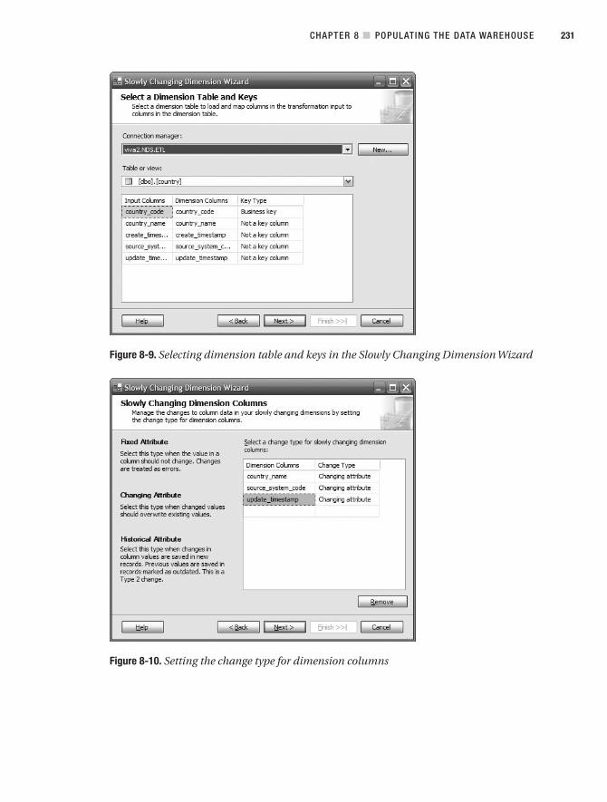
Figure 8-9. Selecting dimension table and keys in the Slowly Changing Dimension Wizard
Figure 8-10. Setting the change type for dimension columns
CHAPTER 8 ■ POPULATING THE DATA WAREHOUSE 231
9314ch08final.qxd 11/15/07 10:09 AM Page 231
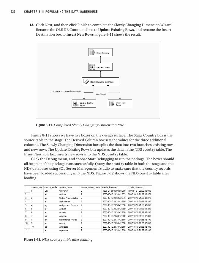
13. Click Next, and then click Finish to complete the Slowly Changing Dimension Wizard.Rename the OLE DB Command box to Update Existing Rows, and rename the InsertDestination box to Insert New Rows. Figure 8-11 shows the result.
Figure 8-11. Completed Slowly Changing Dimension task
Figure 8-11 shows we have five boxes on the design surface. The Stage Country box is thesource table in the stage. The Derived Column box sets the values for the three additionalcolumns. The Slowly Changing Dimension box splits the data into two branches: existing rowsand new rows. The Update Existing Rows box updates the data in the NDS country table. TheInsert New Row box inserts new rows into the NDS country table.
Click the Debug menu, and choose Start Debugging to run the package. The boxes shouldall be green if the package runs successfully. Query the country table in both the stage and theNDS databases using SQL Server Management Studio to make sure that the country recordshave been loaded successfully into the NDS. Figure 8-12 shows the NDS country table afterloading.
Figure 8-12. NDS country table after loading
CHAPTER 8 ■ POPULATING THE DATA WAREHOUSE232
9314ch08final.qxd 11/15/07 10:09 AM Page 232

Figure 8-12 showed that there is a row with country_key set to 0. This row is called theunknown record. On every master table in the NDS, we need to add the unknown record withthe data warehouse key equal to 0. An unknown record is a row with all the columns set todummy values, used when we have an unknown value in the main table. We can create theunknown record using the following Transact SQL:
set identity_insert country oninsert into country( country_key, country_code, country_name, source_system_code,create_timestamp, update_timestamp )
values( 0, 'UN', 'Unknown', 0,'1900-01-01', '1900-01-01' )
set identity_insert country off
We need to set identity_insert to ON because the country_key column is an identity col-umn and we are inserting a specific value in this column. Some people prefer to set the keyvalue to 0 for the unknown records, and others prefer to set it to –1. I have seen some imple-mentations with the key value equal to 1 for unknown records; 0 or –1 is better than 1 becauseyou can have your surrogate key as a positive integer. Whatever the value is, you need to beconsistent; for example, once you have defined it as 0, use 0 throughout (in the DDS too).
Generally, the value of an unknown record is 0 for numeric columns; Unknown or ablank string for char or varchar columns; and a low-value date for the date columns, such as1900-01-01 for smalldatetime, 1753-01-01 for datetime, and 0001-01-01 for the new SQL 2008datetime2 data type. We should not use NULL in the unknown record to differentiate from arow that doesn’t actually have a value. The purpose of having an unknown record is so thatthe referential integrity in the NDS is maintained, even if the code value in the transactiontable is not known.
Now that we have populated the country table, let’s do the state table using the sameprocess. The SQL command for the OLE DB source is as follows:
select state_code, state_name, formal_name,admission_to_statehood, population,capital, largest_city,cast(2 as tinyint) as source_system_code,getdate() as create_timestamp,getdate() as update_timestamp
from state
The unknown record initialization is comprised of the following SQL statements:
set identity_insert state oninsert into state( state_key, state_code, state_name, formal_name,admission_to_statehood, population,capital, largest_city, source_system_code,create_timestamp, update_timestamp )
CHAPTER 8 ■ POPULATING THE DATA WAREHOUSE 233
9314ch08final.qxd 11/15/07 10:09 AM Page 233

values( 0, 'UN', 'Unknown', 'Unknown','1900-01-01', 0,'Unknown', 'Unknown', 0,'1900-01-01', '1900-01-01' )
set identity_insert state off
When you execute the package for the first time, it should insert records into the destina-tion, but when you run it for the second time, it should update the records in the destination,as shown in Figure 8-13.
Figure 8-13. Using SCD transformation for loading the state table
Figure 8-14 shows the NDS state table. It consists of all the columns in the stage statetable from state_code to largest_city, plus three control columns (source_system_code,create_timestamp, and update_timestamp). It has an unknown record with state_key equalto 0.
Figure 8-14. NDS state table after loading
CHAPTER 8 ■ POPULATING THE DATA WAREHOUSE234
9314ch08final.qxd 11/15/07 10:09 AM Page 234

As before, we query both the stage and the NDS state table to make sure that all data hasbeen correctly loaded into the NDS. We can do this using the following query, which tests theexistence of each stage row in the NDS. If no row is returned, it means all the rows in the stagehave been loaded into the NDS.
select * from stage.dbo.state awhere not exists( select * from nds.dbo.state bwhere a.state_code = b.state_code )
Now that the “initial loading” is done, let’s test whether a change in the stage data will becorrectly loaded into the NDS by the previous SCD transformation. For that purpose, let’supdate the population of Arizona in the stage database. Issue the following SQL statementsone by one against the stage database in SQL Server Management Studio:
use stageselect population from state where state_code = 'AZ' --6166318update state set population = 6167318 where state_code = 'AZ'
Notice that the population was 6,166,318 and we updated it to 6,167,318. Before we runthe SSIS package, run this query to check the value of the Arizona population in the NDS:
select population from nds.dbo.state where state_code = 'AZ'
Notice that in the NDS the population is 6,166,318. Now let’s run the SSIS package andthen run the previous NDS query. The population in the NDS should now be 6,167,318 asexpected. Set the stage back to 6,166,318, and rerun the SSIS package to put it back as it was.
Upsert Using SQL and LookupWhat the previous SCD transformation does is commonly known as upsert—in other words,update if exist, insert if not exist. It is a basic operation in data warehousing, and you willcome across this operation many times when building a data warehouse ETL system. Thereare two other methods that are commonly used in practice to do upsert using SSIS. The firstone is using a SQL statement. The second one is using the Lookup transformation.
The following Transact SQL shows how to do an UPSERT operation using a SQL statement.I’ll use the same example as mentioned previously: country, which is simpler than the stateexample. The first statement (update ...) updates the rows in the NDS table that have coun-try names different from the ones on the stage table. The second statement (insert ...) loadsthe rows on the stage table that do not exist in the NDS.
update nds.dbo.countryset country_name = s.country_name,source_system_code = 2,update_timestamp = getdate()
from the stage.dbo.country sinner join nds.dbo.country non n.country_code = s.country_code
where n.country_name <> s.country_nameand n.country_key <> 0
CHAPTER 8 ■ POPULATING THE DATA WAREHOUSE 235
9314ch08final.qxd 11/15/07 10:09 AM Page 235

insert into nds.dbo.country( country_code, country_name, source_system_code,create_timestamp, update_timestamp )
select s.country_code, s.country_name,2 as source_system_code,getdate() as create_timestamp,getdate() as update_timestamp
from the stage.dbo.country sleft join nds.dbo.country non s.country_code = n.country_code
where n.country_key is null
To implement the previous SQL statement approach in SSIS, create a new SSIS package,and rename it to NDS country using SQL. In the Toolbox, drag the Execute SQL task onto thedesign surface, and rename it to Update NDS Country. Drag another Execute SQL task ontothe design surface, and rename it to Insert NDS Country. Set the connection to servername.NDS.ETL for both of them. Set the SQL statement to the previous statements, and leave SQL-SourceType as direct input. Connect the green arrow from the Update NDS Country box to theInsert NDS Country box. Figure 8-15 describes the package execution result. The resultingdata is the same as in Figure 8-12.
Figure 8-15. Using Execute SQL tasks to do an upsert operation
The second method is to use a Lookup transformation. Let’s use the same example asmentioned previously (country) so it is easy to understand the differences between the two:
1. In Solution Explorer, right-click SSIS Packages, and choose New SSIS Package to createa new SSIS package.
2. Drag a Data Flow task from the Toolbox onto the design surface, and double-click thebox to edit it.
3. To set the country table in the stage as a source, drag an OLE DB source from theToolbox onto the design surface, and rename it to Stage Country. Configure the con-nection to point to the stage. To retrieve both columns from the source table and addthe three additional columns, set the data access mode to SQL Command, and set theSQL command to the following:
CHAPTER 8 ■ POPULATING THE DATA WAREHOUSE236
9314ch08final.qxd 11/15/07 10:09 AM Page 236

select country_code, country_name,cast(2 as tinyint) as source_system_code,getdate() as create_timestamp,getdate() as update_timestamp
from country
4. Click Preview to make sure the SQL statement is correct and the data is there, and thenclick OK.
5. Let’s create a Lookup transformation to check whether the row already exists in theNDS. In the Toolbox, under the Data Flow Transformation section, find an icon calledLookup, and drag it onto the design surface. Name this box Lookup Country Code.Connect the green arrow from Stage Country to the Lookup Country Code box.Double-click the box to edit it.
6. Now we need to configure the Lookup transformation to check whether the countrycode exists in the NDS country table. To do that, set the connection to NDS. Select “Usethe results of an SQL query,” and set the query as select country_code from country.This is so that only one column is retrieved from disk into memory. If you select “Usetable or view,” all columns will be retrieved into memory. Click Preview to make surethe data is there. Figure 8-16 shows the settings.
Figure 8-16. Configuring the data source and SQL query for the Lookup transformation
CHAPTER 8 ■ POPULATING THE DATA WAREHOUSE 237
9314ch08final.qxd 11/15/07 10:09 AM Page 237

7. Click the Columns tab. There should be a line connecting country_code from AvailableInput Columns on the left to the country_code from Available Lookup Columns on theright, as shown in Figure 8-17. If there isn’t, drag country_code from the left to the rightto map it. You don’t need to check the box on country_code; in fact, leave it unchecked.We are not using any output column from this Lookup transformation. We use theLookup transformation only for checking whether all the country codes on the stagetable exist on the NDS table.
Figure 8-17. Specifying the join column
8. Click the Advanced tab. On this tab, we can tune the memory usage by setting thecache size closer to the byte size of the lookup column(s). Tuning the memory usagemeans we allocate how much memory we want to use for caching the lookup table.The lookup table is the output of the lookup SQL statement. If the lookup table issmall, we don’t want to waste memory by allocating too much memory to contain theoutput. If the lookup table is large and we allocate too little memory, SSIS will put thelookup table on disk, and it will slow down the lookup process. Check the “Enablememory restriction” box, and set the cache size to 1MB to minimize memory usage.The country code is only two characters wide, and there are fewer than 250 countriesin the stage table. Change the SQL statement to select country_code from countrywhere country_code = ?, as shown in Figure 8-18.
9. Click OK to close the Lookup Transformation Editor dialog box.
CHAPTER 8 ■ POPULATING THE DATA WAREHOUSE238
9314ch08final.qxd 11/15/07 10:09 AM Page 238

Figure 8-18. Configuring the cache memory size and SQL statement
10. Next, we need to update the countries that already exist in the NDS, setting the coun-try names to be the same as the ones in the stage table. In the Toolbox, find the OLE DBcommand, and drag it onto the design surface. Name it Update Existing Row. Connectthe green arrow from Lookup Country Code to the Update Existing Row box. Double-click the box to edit it.
11. To set the country name of the row in the NDS table to be the same as the countryname in the stage table, under the Connection Manager column set the Connectiondrop-down list to servername.NDS.ETL. Click the Component Properties tab, and setSqlCommand to this:
update countryset country_name = ?,source_system_code = 2,create_timestamp = getdate(),update_timestamp = getdate()
where country_code = ?
12. In the previous Transact SQL, we have two question marks. They are parameters. Thefirst question mark is Param_0, and the second question mark is Param_1. To feed theinput columns coming from the Lookup Country Code box to these parameters, clickthe Column Mappings tab, and connect country_code to Param_1 and country_name toParam_0, as shown in Figure 8-19. Click OK to close this editor.
CHAPTER 8 ■ POPULATING THE DATA WAREHOUSE 239
9314ch08final.qxd 11/15/07 10:09 AM Page 239

Figure 8-19. Configuring column mappings in the OLE DB command
13. Next, we need to insert rows in the stage table that do not exist in the NDS table. In theToolbox, find SQL Server Destination, and drag it onto the design surface. Name itInsert New Rows. Connect the red arrow from the Lookup Country Code box to thisbox. Click OK in the dialog box.
14. Double-click the Insert New Rows box to edit it. Set the connection to NDS. Set Tableto country, and click Preview to verify that it is country table that we selected.
15. Click Mappings, and configure the mappings between the input columns and destina-tion columns, as shown in Figure 8-20.
16. Click OK to close the SQL Server Destination Editor dialog box.
17. To test the package, we can prepare the data by issuing the following SQL statementsagainst the NDS database. The first statement updates Andorra’s country name in theNDS to Andorra1 and is, therefore, not the same as the country name in the stage. Thesecond statement deletes Turks and Caicos Island from the NDS.
update nds.dbo.country set country_name = 'Andorra1'where country_code = 'ad'
delete from nds.dbo.country where country_code = 'tc'
18. Query the NDS country table to check that the data changes were successfully made.To execute the package, click the Debug menu, and choose Start Debugging (F5). Fig-ure 8-21 shows how the final package looks.
CHAPTER 8 ■ POPULATING THE DATA WAREHOUSE240
9314ch08final.qxd 11/15/07 10:09 AM Page 240

Figure 8-20. Mapping the columns on the SQL Server destination
Figure 8-21. Upsert using the Lookup transformation
19. Check the NDS country table to see whether Andorra was corrected and whetherTurks and Caicos Island was reinserted into the table. Also, check that both thecreate_timestamp and update_timestamp columns for these two records are set totoday.
The question that many people ask is, which one is the best method, or which one givesthe best performance? The SQL method is simpler and easier to use. Which method gives thebest performance depends on the size of data, the complexity of the lookup, and the specifi-cation of the ETL server, in particular the memory. If the lookup table can be cached into the
CHAPTER 8 ■ POPULATING THE DATA WAREHOUSE 241
9314ch08final.qxd 11/15/07 10:09 AM Page 241

memory of the ETL server, then the lookup and SCD methods are faster than the SQL state-ment method. But if the lookup table cannot be cached into memory, the SQL statementmethod is faster. The performance of the SQL statement method also depends on the indexesand partitions. If performance is really critical in your data warehouse project, the best thingto do is to test both methods and compare the performance.
NormalizationNormalization is a key part of NDS population. Earlier in this chapter, we discussed how tonormalize stage tables in NDS. In this section, we will discuss how to load the stage data(which is not normalized) into the normalized NDS tables. We will use the store table as anexample. In the NDS, we normalized the stage store table into four tables: store, store_type,address, and phone_number. In this section, you will learn that to populate the NDS store table,you need to load the address, store_type, and phone_number tables first. We will also learn howuse SSIS to load the store table.
Consider the store table in the stage database, as shown in Table 8-17.
Table 8-17. store Table in the Stage Database
store_number store_name store_type other columns
1010 Paris Mini Outlet …
1011 Lyon Full Outlet …
1012 Toulouse Full Outlet …
1013 Nice Full Outlet …
1014 Strasbourg Distribution Center …
1015 Nantes Mini Outlet …
We can see that the store_type column is not normalized. Let’s now refer to the targettable in the NDS, as shown in Table 8-18.
Table 8-18. store Table in the NDS
store_key store_number store_name store_type_key other columns
0 0 Unknown 0 …
562 1010 Paris 19 …
607 1011 Lyon 18 …
576 1012 Toulouse 18 …
531 1013 Nice 18 …
585 1014 Strasbourg 17 …
547 1015 Nantes 19 …
515 2703 Osaka 18 …
CHAPTER 8 ■ POPULATING THE DATA WAREHOUSE242
9314ch08final.qxd 11/15/07 10:09 AM Page 242

In the previous table, we can see that to load the NDS store table we need store_type_key. We get this store_type_key from the store_type table. This is also the case with theaddress and phone_number columns. To insert a record into the store table, we need store_type_key, address_key, and phone_number_key, so we need to do a lookup on those threetables. But before we can do a lookup, if there is any new store type, address, or phone num-ber, we need to load them first. So, diagrammatically, the process is like the one described inFigure 8-22.
Figure 8-22. Loading the NDS store table
When populating the address table, we need to check whether there are any new citiesbecause we need the city key to populate the address table. If there are new cities, we need toinsert them into the city table. The state and country tables have their own data feed fromthe source system, so we do not need to normalize them. We only need to do a lookup to gettheir key values.
So, let’s create the SSIS package for loading the store table:
1. Open BIDS, create a new package, and call it NDS store. Drag the Execute SQL taskfrom the Toolbox onto the design surface, and call it Insert New Store Types.
2. Double-click it to edit it, and set the connection to NDS. Set the SQL statement asfollows:
insert into nds.dbo.store_type( store_type, source_system_code,create_timestamp, update_timestamp )
selectdistinct store_type as store_type,1 as source_system_code,getdate() as create_timestamp,getdate() as update_timestamp
from stage.dbo.store swhere not exists( select * from nds.dbo.store_type twhere t.store_type = s.store_type )
CHAPTER 8 ■ POPULATING THE DATA WAREHOUSE 243
9314ch08final.qxd 11/15/07 10:09 AM Page 243

The earlier SQL statement looks for new store types—those that exist in the stage storetable but do not exist in the NDS store_type table. It then inserts the new store typesinto the NDS store_type table.
You can also build the SQL statement by clicking the Query Builder button in theSSMS. This will open the Query Builder, which is shown in Figure 8-23.
Figure 8-23. Using Query Builder to build the SQL statement
3. Similarly, create an Execute SQL task, call it Insert New Phone Number pointing to theNDS database, and set the SQL statements as follows. The following SQL statementlooks for new phone numbers that exist in the stage but not in the NDS and theninserts these new phone numbers into the NDS phone_number table.
insert into nds.dbo.phone_number( phone_number, source_system_code,create_timestamp, update_timestamp )
selectdistinct s.phone_number as phone_number,1 as source_system_code,getdate() as create_timestamp,getdate() as update_timestamp
from stage.dbo.store swhere not exists( select * from nds.dbo.phone_number pwhere p.phone_number = s.phone_number )
CHAPTER 8 ■ POPULATING THE DATA WAREHOUSE244
9314ch08final.qxd 11/15/07 10:09 AM Page 244

4. We then insert new cities and addresses, using the Execute SQL task, with the SQLstatements as follows. The first statement inserts the new cities into the NDS citytable, and the second statement inserts the new addresses into the NDS address table.
insert into city( city_name, source_system_code,create_timestamp, update_timestamp )
selectdistinct s.city as city_name,1 as source_system_code,getdate() as create_timestamp,getdate() as update_timestamp
from stage.dbo.store swhere not exists( select * from nds.dbo.city cwhere c.city_name = s.city )
insert into nds.dbo.address( address1, address2, address3, address4,city_key, post_code, state_key, country_key,source_system_code, create_timestamp, update_timestamp)
selectdistinct s.address1, s.address2, s.address3, s.address4,c.city_key, s.zipcode, st.state_key, co.country_key,1 as source_system_code,getdate() as create_timestamp,getdate() as update_timestamp
from stage.dbo.store sleft join nds.dbo.city con s.city = c.city_name
left join nds.dbo.state ston case when s.state = 'N/A' then 'Unknown'
else s.state end = st.state_nameleft join nds.dbo.country coon s.country = co.country_code
where not exists( select * from nds.dbo.address awhere coalesce(a.address1,'') = coalesce(s.address1,'')and coalesce(a.address2,'') = coalesce(s.address2,'')and coalesce(a.address3,'') = coalesce(s.address3,'')and coalesce(a.address4,'') = coalesce(s.address4,'')and coalesce(a.city_key,0) = coalesce(c.city_key,0)and coalesce(a.post_code,'') = coalesce(s.zipcode,'')and coalesce(a.state_key,0) = coalesce(st.state_key,0)and coalesce(a.country_key,0) = coalesce(co.country_key,0) )
CHAPTER 8 ■ POPULATING THE DATA WAREHOUSE 245
9314ch08final.qxd 11/15/07 10:09 AM Page 245
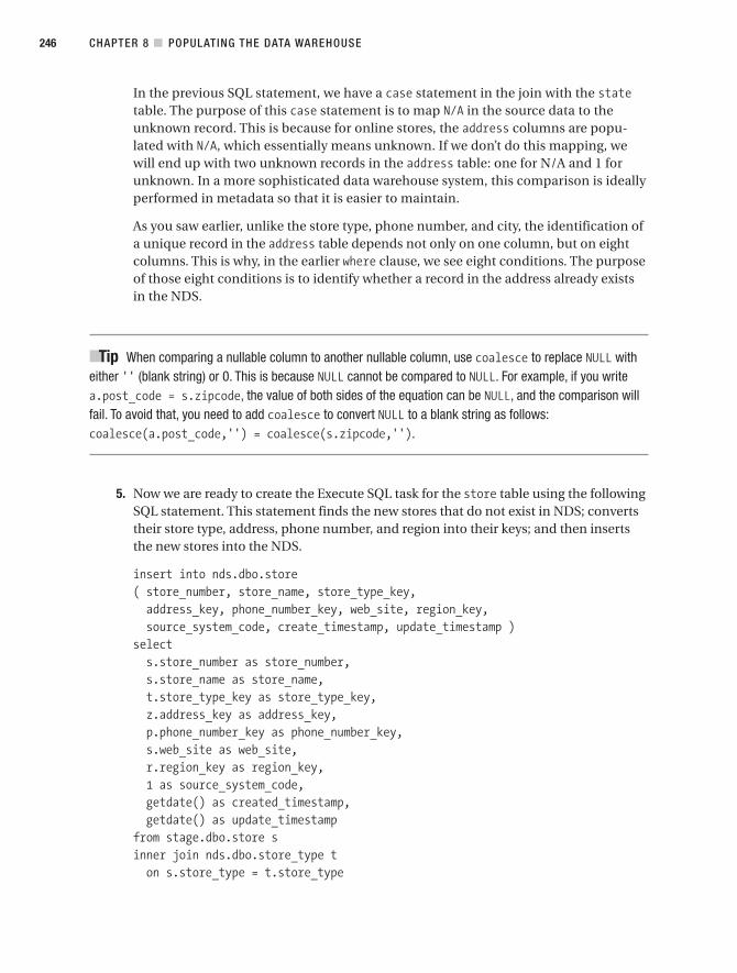
In the previous SQL statement, we have a case statement in the join with the statetable. The purpose of this case statement is to map N/A in the source data to theunknown record. This is because for online stores, the address columns are popu-lated with N/A, which essentially means unknown. If we don’t do this mapping, wewill end up with two unknown records in the address table: one for N/A and 1 forunknown. In a more sophisticated data warehouse system, this comparison is ideallyperformed in metadata so that it is easier to maintain.
As you saw earlier, unlike the store type, phone number, and city, the identification ofa unique record in the address table depends not only on one column, but on eightcolumns. This is why, in the earlier where clause, we see eight conditions. The purposeof those eight conditions is to identify whether a record in the address already existsin the NDS.
■Tip When comparing a nullable column to another nullable column, use coalesce to replace NULL witheither '' (blank string) or 0. This is because NULL cannot be compared to NULL. For example, if you writea.post_code = s.zipcode, the value of both sides of the equation can be NULL, and the comparison willfail. To avoid that, you need to add coalesce to convert NULL to a blank string as follows:coalesce(a.post_code,'') = coalesce(s.zipcode,'').
5. Now we are ready to create the Execute SQL task for the store table using the followingSQL statement. This statement finds the new stores that do not exist in NDS; convertstheir store type, address, phone number, and region into their keys; and then insertsthe new stores into the NDS.
insert into nds.dbo.store( store_number, store_name, store_type_key,address_key, phone_number_key, web_site, region_key,source_system_code, create_timestamp, update_timestamp )
selects.store_number as store_number,s.store_name as store_name,t.store_type_key as store_type_key,z.address_key as address_key,p.phone_number_key as phone_number_key,s.web_site as web_site,r.region_key as region_key,1 as source_system_code,getdate() as created_timestamp,getdate() as update_timestamp
from stage.dbo.store sinner join nds.dbo.store_type ton s.store_type = t.store_type
CHAPTER 8 ■ POPULATING THE DATA WAREHOUSE246
9314ch08final.qxd 11/15/07 10:09 AM Page 246
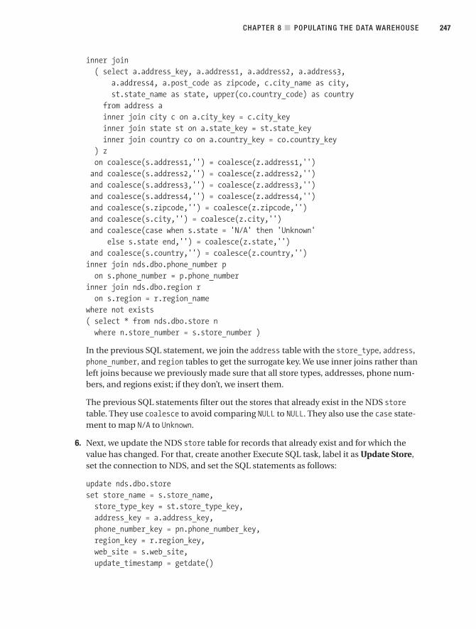
inner join( select a.address_key, a.address1, a.address2, a.address3,
a.address4, a.post_code as zipcode, c.city_name as city,st.state_name as state, upper(co.country_code) as country
from address ainner join city c on a.city_key = c.city_keyinner join state st on a.state_key = st.state_keyinner join country co on a.country_key = co.country_key
) zon coalesce(s.address1,'') = coalesce(z.address1,'')and coalesce(s.address2,'') = coalesce(z.address2,'')and coalesce(s.address3,'') = coalesce(z.address3,'')and coalesce(s.address4,'') = coalesce(z.address4,'')and coalesce(s.zipcode,'') = coalesce(z.zipcode,'')and coalesce(s.city,'') = coalesce(z.city,'')and coalesce(case when s.state = 'N/A' then 'Unknown'
else s.state end,'') = coalesce(z.state,'')and coalesce(s.country,'') = coalesce(z.country,'')inner join nds.dbo.phone_number pon s.phone_number = p.phone_number
inner join nds.dbo.region ron s.region = r.region_name
where not exists( select * from nds.dbo.store nwhere n.store_number = s.store_number )
In the previous SQL statement, we join the address table with the store_type, address,phone_number, and region tables to get the surrogate key. We use inner joins rather thanleft joins because we previously made sure that all store types, addresses, phone num-bers, and regions exist; if they don’t, we insert them.
The previous SQL statements filter out the stores that already exist in the NDS storetable. They use coalesce to avoid comparing NULL to NULL. They also use the case state-ment to map N/A to Unknown.
6. Next, we update the NDS store table for records that already exist and for which thevalue has changed. For that, create another Execute SQL task, label it as Update Store,set the connection to NDS, and set the SQL statements as follows:
update nds.dbo.storeset store_name = s.store_name,store_type_key = st.store_type_key,address_key = a.address_key,phone_number_key = pn.phone_number_key,region_key = r.region_key,web_site = s.web_site,update_timestamp = getdate()
CHAPTER 8 ■ POPULATING THE DATA WAREHOUSE 247
9314ch08final.qxd 11/15/07 10:09 AM Page 247

from stage.dbo.store sinner join nds.dbo.store non s.store_number = n.store_number
inner join nds.dbo.store_type ston n.store_type_key = st.store_type_key
inner join nds.dbo.address aon n.address_key = a.address_key
inner join nds.dbo.phone_number pnon n.phone_number_key = pn.phone_number_key
inner join nds.dbo.region ron n.region_key = r.region_key
inner join nds.dbo.city con a.city_key = c.city_key
inner join nds.dbo.state staon a.state_key = sta.state_key
inner join nds.dbo.country coon a.country_key = co.country_key
where coalesce(s.store_name,'') <> coalesce(n.store_name,'')or coalesce(s.store_type,'') <> coalesce(st.store_type,'')or coalesce(s.address1,'') <> coalesce(a.address1,'')or coalesce(s.address2,'') <> coalesce(a.address2,'')or coalesce(s.address3,'') <> coalesce(a.address3,'')or coalesce(s.address4,'') <> coalesce(a.address4,'')or coalesce(a.city_key,0) <> coalesce(c.city_key,0)or coalesce(a.post_code,'') <> coalesce(s.zipcode,'')or coalesce(a.state_key,0) <> coalesce(sta.state_key,0)or coalesce(a.country_key,0) <> coalesce(co.country_key,0)or coalesce(s.phone_number,'') <> coalesce(pn.phone_number,'')or coalesce(s.web_site,'') <> coalesce(n.web_site,'')
This SQL statement updates the NDS stores that have a different store name, storetype, address, phone number, or web site from the ones in the stage. Just like theinsert statement, in the previous SQL statement we join the address table with thecity, state, and country tables to compare the address. We also use coalesce to avoidthe NULL-against-NULL comparison.
7. The control flow of the package now looks like Figure 8-22, which we discussed earlier.Save and run the package.
8. Query the five NDS tables (city, address, phone number, store type, and store) toensure that they are populated properly by comparing them to the source system.Figure 8-24 shows the result (the NDS store table).
CHAPTER 8 ■ POPULATING THE DATA WAREHOUSE248
9314ch08final.qxd 11/15/07 10:09 AM Page 248
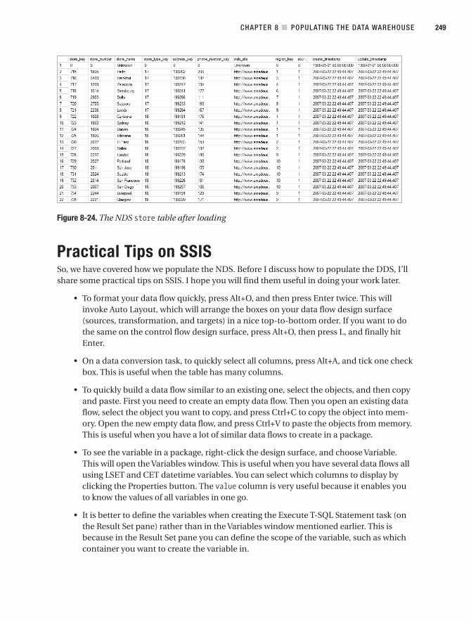
Figure 8-24. The NDS store table after loading
Practical Tips on SSISSo, we have covered how we populate the NDS. Before I discuss how to populate the DDS, I’llshare some practical tips on SSIS. I hope you will find them useful in doing your work later.
• To format your data flow quickly, press Alt+O, and then press Enter twice. This willinvoke Auto Layout, which will arrange the boxes on your data flow design surface(sources, transformation, and targets) in a nice top-to-bottom order. If you want to dothe same on the control flow design surface, press Alt+O, then press L, and finally hitEnter.
• On a data conversion task, to quickly select all columns, press Alt+A, and tick one checkbox. This is useful when the table has many columns.
• To quickly build a data flow similar to an existing one, select the objects, and then copyand paste. First you need to create an empty data flow. Then you open an existing dataflow, select the object you want to copy, and press Ctrl+C to copy the object into mem-ory. Open the new empty data flow, and press Ctrl+V to paste the objects from memory.This is useful when you have a lot of similar data flows to create in a package.
• To see the variable in a package, right-click the design surface, and choose Variable.This will open the Variables window. This is useful when you have several data flows allusing LSET and CET datetime variables. You can select which columns to display byclicking the Properties button. The value column is very useful because it enables youto know the values of all variables in one go.
• It is better to define the variables when creating the Execute T-SQL Statement task (onthe Result Set pane) rather than in the Variables window mentioned earlier. This isbecause in the Result Set pane you can define the scope of the variable, such as whichcontainer you want to create the variable in.
CHAPTER 8 ■ POPULATING THE DATA WAREHOUSE 249
9314ch08final.qxd 11/15/07 10:09 AM Page 249

• If your SSIS package is big and doesn’t fit into one screen, click the four arrow icons atthe bottom-right corner of the design surface to navigate around the design surface. It’smuch better and quicker to move around the workflow to control flow objects thanusing scroll bars.
• In the Lookup transformation, on the Columns tab, to delete all lines between the lefttable and the right table, click the background, press Ctrl+A, and then press Delete.
• On the Data Conversion transformation, set the output data type according to the tar-get column (see Table 8-19); otherwise, SSIS will produce a data conversion error whenyou run the package. In Table 8-19, I list some of the most popular used data types (inthe target column) and what the data conversion output should be.
Table 8-19. Data Conversion Output for Popular Data Types
Target Column Conversion Output Notes
int 4-byte signed integer [DT_I4]
tinyint Single-byte unsigned integer [DT_UI1]
datetime Database timestamp [DT_DBTIMESTAMP]
decimal Numeric [DT_NUMERIC] Don’t choose decimal because you canspecify only the scale and cannot specify theprecision.
money Currency [DT_CURRENCY] There is only one data type for currency.
char, varchar String [DT_STR] Don’t forget to specify the correct length;otherwise, a data conversion warning or erroroccurs.
Populating DDS Dimension TablesNow that I have discussed how to populate the NDS, I’ll discuss how to populate the DDS.The DDS is a dimensional store. The tables in the DDS are denormalized. Just like when load-ing data into the NDS, when loading data into the DDS, we also do an UPSERT operation toupdate or insert the source row depending on whether it exists in the target.
We have two main types of DDS tables: fact tables and dimension tables. In this section,I will discuss how to load data into dimension tables. In the next section, I will discuss howto load data into the fact tables. I will show how to use SSIS to load the data. I will show howto use the Slowly Changing Dimension Wizard to load the data into dimension tables. Whenloading data into dimensional tables in the DDS, you need to consider several issues: incre-mental loading, key management, denormalization, and slowly changing dimension. I’lldiscuss these four topics first, and then we will create an SSIS package to load the data intocustomer dimension.
CHAPTER 8 ■ POPULATING THE DATA WAREHOUSE250
9314ch08final.qxd 11/15/07 10:09 AM Page 250

Incremental loading: When populating the dimension tables in the DDS, we have the lux-ury of incremental loading. We don’t have to worry about how to extract the data incre-mentally from the NDS because in the NDS everything is timestamped. When loading thestage data into the NDS, we always put the current time on the last-updated timestampcolumn. So, we know when each record was last updated. This enables us to load the NDSdata into the DDS incrementally. In other words, we load only the NDS rows that changedsince the last ETL run.
Key management: In the DDS, we don’t have to maintain the surrogate keys. Surrogatekeys are managed in the NDS. This makes the UPSERT operation simpler, because everyrow in the dimension table has a surrogate key. The surrogate keys that we use in the DDSare the same as the surrogate key that we use in the NDS. Bear in mind that in the NDS +DDS architecture we can have multiple DDS data stores. Because we define and managethe data warehouse surrogate key in the NDS, we can guarantee that all DDSs use thesame surrogate key.
ODS, on the contrary, does not have surrogate keys, and we need to create and managethe surrogate keys in the DDS. In the ODS + DDS architecture, we can have only oneDDS, so we don’t have an issue of synchronizing the surrogate keys between DDSs. Ear-lier in this chapter when I discussed populating the NDS, I talked about surrogate keymanagement. If you use the ODS + DDS architecture, you need to apply this method tomanage the surrogate key in the DDS.
Denormalization: The dimension tables in the DDS are denormalized, whereas in theNDS they are normalized. Therefore, to load a single dimension table in the DDS, weneed to get data from several tables in the NDS by joining them. For example, to loadthe store dimension in the DDS, in the NDS we need to join the store table with thestore_type table. This is because the NDS store table has only the store type keys.Please refer to Figure 8-3 and Tables 8-1 to 8-3. To get the store type, we need to jointhe store table with the store_type table.
Slowly changing dimension (SCD): The dimension tables in DDS have either SCD type 1(overwrite), SCD type 2 (rows), or SCD type 3 (column). Please refer to Chapter 5 formore information about SCD. In the Amadeus Entertainment case study, the productdimension is SCD type 1, the customer dimension is SCD type 2, and the store dimen-sion is SCD type 3. If the dimension is SCD type 1, we just overwrite the old attributevalues with the new values. If the dimension is SCD type 2, we need to create a new rowcontaining the new attribute values and expire the old row. If the dimension is SCD type3, we need to put the old values into another column and put the new values in themain attribute column.
A good way to learn more about these four topics in SQL Server data warehousing is byimplementing them using SSIS. So, let’s populate our customer dimension using SSIS, and I’llexplain these topics as we go along:
1. Open BIDS. Create a new SSIS package, and name it DDS Customer.
2. Drop an Execute SQL task onto the design surface, name it Set Customer CET, set theconnection to the metadata database, and set the SQL statement as follows:
CHAPTER 8 ■ POPULATING THE DATA WAREHOUSE 251
9314ch08final.qxd 11/15/07 10:09 AM Page 251
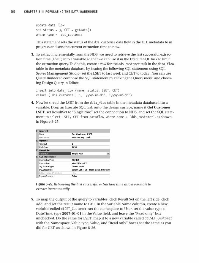
update data_flowset status = 3, CET = getdate()where name = 'dds_customer'
This statement sets the status of the dds_customer data flow in the ETL metadata to inprogress and sets the current extraction time to now.
3. To extract incrementally from the NDS, we need to retrieve the last successful extrac-tion time (LSET) into a variable so that we can use it in the Execute SQL task to limitthe extraction query. To do this, create a row for the dds_customer task in the data_flowtable in the metadata database by issuing the following SQL statement using SQLServer Management Studio (set the LSET to last week and CET to today). You can useQuery Builder to compose the SQL statement by clicking the Query menu and choos-ing Design Query in Editor.
insert into data_flow (name, status, LSET, CET)values ('dds_customer', 0, 'yyyy-mm-dd', 'yyyy-mm-dd')
4. Now let’s read the LSET from the data_flow table in the metadata database into avariable. Drop an Execute SQL task onto the design surface, name it Get CustomerLSET, set ResultSet to “Single row,” set the connection to NDS, and set the SQL state-ment to select LSET, CET from dataflow where name = 'dds_customer', as shownin Figure 8-25.
Figure 8-25. Retrieving the last successful extraction time into a variable to extract incrementally
5. To map the output of the query to variables, click Result Set on the left side, clickAdd, and set the result name to CET. In the Variable Name column, create a newvariable called dtCET_Customer, set the namespace to User, set the value type toDateTime, type 2007-01-01 in the Value field, and leave the “Read only” boxunchecked. Do the same for LSET; map it to a new variable called dtLSET_Customerwith the Namespace, Value type, Value, and “Read only” boxes set the same as youdid for CET, as shown in Figure 8-26.
CHAPTER 8 ■ POPULATING THE DATA WAREHOUSE252
9314ch08final.qxd 11/15/07 10:09 AM Page 252

Figure 8-26. Mapping the result set to variables
6. Now we can create a task to retrieve the data from NDS incrementally using the CETand LSET that we have put into variables. To do this, drop a Data Flow task (some peo-ple call it DFT) onto the design surface, and name it Populate Customer Dimension.Double-click it to edit it. Add an OLE DB source, name it Customer NDS, set the con-nection to NDS, set the data access mode to SQL Command, and set the command textas follows:
select * from customerwhere (create_timestamp >= ? and create_timestamp < ?)or (update_timestamp >= ? and update_timestamp < ?)
The previous SQL statement gets customer records from the NDS that were created orupdated within a certain date range.
7. The previous SQL statement has four parameters (indicated by four question marks).We need to map these parameters to the CET and LSET variables so that the whereclause in the previous SQL statement is limited by the variables. Click the Parametersbutton, and specify the variables for each parameter, as shown in Figure 8-27. Thenclick OK.
CHAPTER 8 ■ POPULATING THE DATA WAREHOUSE 253
9314ch08final.qxd 11/15/07 10:09 AM Page 253
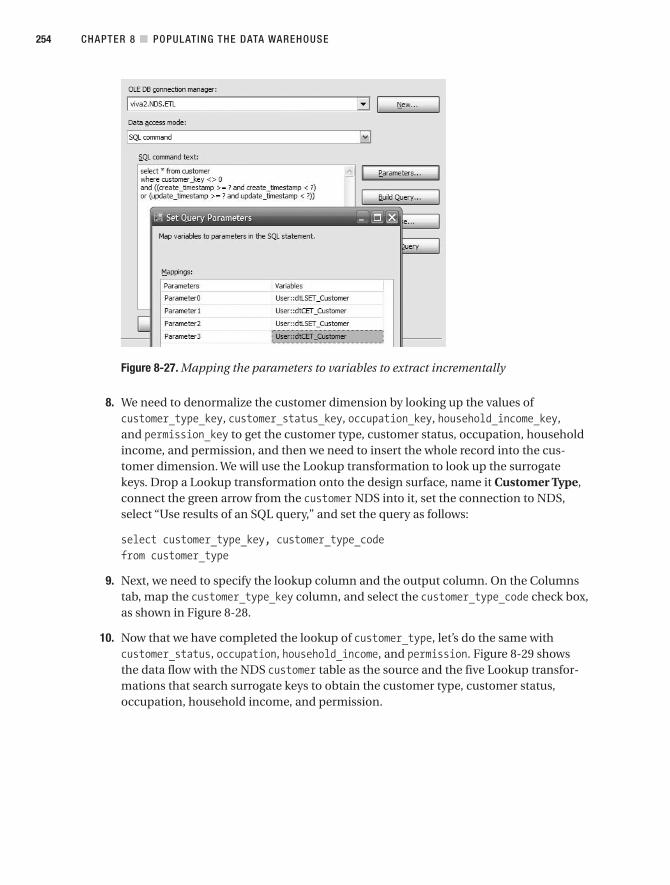
Figure 8-27. Mapping the parameters to variables to extract incrementally
8. We need to denormalize the customer dimension by looking up the values ofcustomer_type_key, customer_status_key, occupation_key, household_income_key,and permission_key to get the customer type, customer status, occupation, householdincome, and permission, and then we need to insert the whole record into the cus-tomer dimension. We will use the Lookup transformation to look up the surrogatekeys. Drop a Lookup transformation onto the design surface, name it Customer Type,connect the green arrow from the customer NDS into it, set the connection to NDS,select “Use results of an SQL query,” and set the query as follows:
select customer_type_key, customer_type_codefrom customer_type
9. Next, we need to specify the lookup column and the output column. On the Columnstab, map the customer_type_key column, and select the customer_type_code check box,as shown in Figure 8-28.
10. Now that we have completed the lookup of customer_type, let’s do the same withcustomer_status, occupation, household_income, and permission. Figure 8-29 showsthe data flow with the NDS customer table as the source and the five Lookup transfor-mations that search surrogate keys to obtain the customer type, customer status,occupation, household income, and permission.
CHAPTER 8 ■ POPULATING THE DATA WAREHOUSE254
9314ch08final.qxd 11/15/07 10:09 AM Page 254
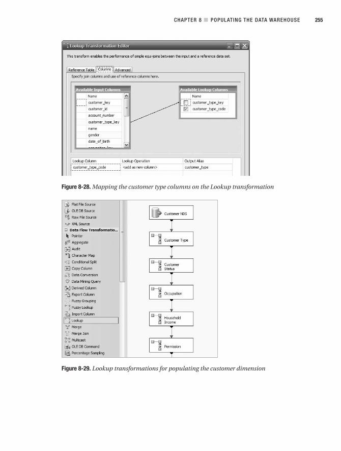
Figure 8-28. Mapping the customer type columns on the Lookup transformation
Figure 8-29. Lookup transformations for populating the customer dimension
CHAPTER 8 ■ POPULATING THE DATA WAREHOUSE 255
9314ch08final.qxd 11/15/07 10:09 AM Page 255

11. The five attributes we did in the previous step link directly to the NDS customer table.But there are some attributes that are linked to the customer table using junctiontables, such as email_address, phone_number, and address. So, we need to look up thecustomer surrogate keys in the junction tables to get this data. To do this, drop aLookup transformation on the design surface, name it Email Address, and double-click it to edit it. Point the connection to NDS, and set the SQL query as follows:
select j.customer_key, e.email_addressfrom email_address_junction jjoin email_address e on j.email_address_key = e.email_address_keyjoin customer c on j.customer_key = c.customer_key
This SQL statement gets email_address_key in the email_address_junction table andthen goes to the email_address table to get the email address.
12. We need to define the lookup column and the output column for the Lookup transfor-mation. On the Columns tab, map customer_key on the input side to customer_key onthe lookup side, as shown in Figure 8-30. Also select the email_address check box tooutput that column.
Figure 8-30. Configuring the junction table lookup
13. The lookup for phone_number_junction is similar to email_address_junction becauseboth have one lookup column. The SQL query for phone number lookup is as follows.This SQL statement finds phone_number_key for the customer and then gets the phonenumber:
select j.customer_key, p.phone_numberfrom phone_number_junction jjoin phone_number p on j.phone_number_key = p.phone_number_keyjoin customer c on j.customer_key = c.customer_key
CHAPTER 8 ■ POPULATING THE DATA WAREHOUSE256
9314ch08final.qxd 11/15/07 10:09 AM Page 256

14. The lookup for the address junction is a little bit different because we need to join withthree other tables and because it has multiple output columns. The SQL query for theaddress lookup is as follows. This SQL statement gets the address key from the junctiontable and then gets the customer address, including the city name, state name, andcountry name.
select j.customer_key, a.address1, a.address2,a.address3, a.address4, ci.city_name as city,a.post_code, st.state_name as state,co.country_name as country
from address_junction jjoin address a on j.address_key = a.address_keyjoin customer c on j.customer_key = c.customer_keyjoin city ci on a.city_key = ci.city_keyjoin state st on a.state_key = st.state_keyjoin country co on a.country_key = co.country_key
The purpose of naming the previous output columns (city, state, and country) is tomatch the column names in the dimension table so that the SCD transformation can auto-matically map the columns. Figure 8-31 shows the key mapping and output columns.
Figure 8-31. Key mapping and output columns for address lookup
In this data flow, so far we have looked up all the customer attributes from the correspon-ding tables: customer_type, customer_status, occupation, household_income, permission,email_address, phone_number, and address. We now have a full customer record from the NDS,ready to be loaded into the customer dimension in the DDS. Remember that the customerdimension has SCD type 2 (see Chapter 5 for more information). We are going to load the cus-tomer data into the DDS using the Slowly Changing Dimension Wizard. The Slowly ChangingDimension Wizard will produce a data flow that will do the UPSERT operation into the DDS cus-tomer dimension table. This means loading new customers and updating existing customers.
CHAPTER 8 ■ POPULATING THE DATA WAREHOUSE 257
9314ch08final.qxd 11/15/07 10:09 AM Page 257

1. Open the Slowly Changing Dimension Wizard. Drop the Slowly Changing Dimensionfrom the toolbar onto the design surface. Double-click it to edit.
2. Define a new connection to the DDS database. Choose dim_customer as the targettable. Immediately after choosing the table name, you should see that most columnsare automatically mapped because they have the same names and the same datatypes, as shown in Figure 8-32.
Figure 8-32. Mapping the columns of customer table on the Slowly ChangingDimension Wizard
3. Select customer_key as the business key, as shown in Figure 8-32. Some columns arenot mapped automatically because they have different names. For these columns,choose the right input columns. In the case study, we need to map the post_code col-umn to zipcode. Leave effective_date, expiry_date, and is_current unmapped. Wewill be using them for SCD later. After you have mapped all the columns, click Nextto move to the next step.
4. The next screen is Slowly Changing Dimension Columns, shown in Figure 8-33. On thisscreen, we define the change type for each column such as “Fixed attributes,” “Chang-ing attributes,” or “Historical attributes.” Let’s go through what these three changetypes mean.
CHAPTER 8 ■ POPULATING THE DATA WAREHOUSE258
9314ch08final.qxd 11/15/07 10:09 AM Page 258

Fixed attributes means that the value should not change; changes are treated aserrors (by processing the error output). For example, you may want to considercreate_timestamp, date_of_birth, date_registered, and gender columns to be fixedattributes.
Changing attributes means that the new values will overwrite existing values.Select this type when you don’t need to store the history, such as when you needonly the latest version. For example, you may want to consider source_system_code,update_timestamp, subscriber_band, subscriber_class, interest, and preferred_channels columns as changing attributes because you don’t need to store their pre-vious values.
Figure 8-33. Assigning the change type for each dimension attribute
Historical attributes means SCD type 2; in other words, SSIS will create a new row con-taining the new attribute values. The existing row will be marked as outdated. The newrow will be marked as current, meaning that it is the active row containing the validattribute values. Most columns in the customer dimension would be in this category.For example, you may want to make the address columns (including city, state,country, and post_code), phone_number, email_address, customer_type, customer_id,status, name, occupation, and household_income historical attributes, if you need tostore the previous values either for analysis purposes or for data traceability. When youhave assigned the correct change type to every column, click Next to go to the nextscreen.
CHAPTER 8 ■ POPULATING THE DATA WAREHOUSE 259
9314ch08final.qxd 11/15/07 10:09 AM Page 259
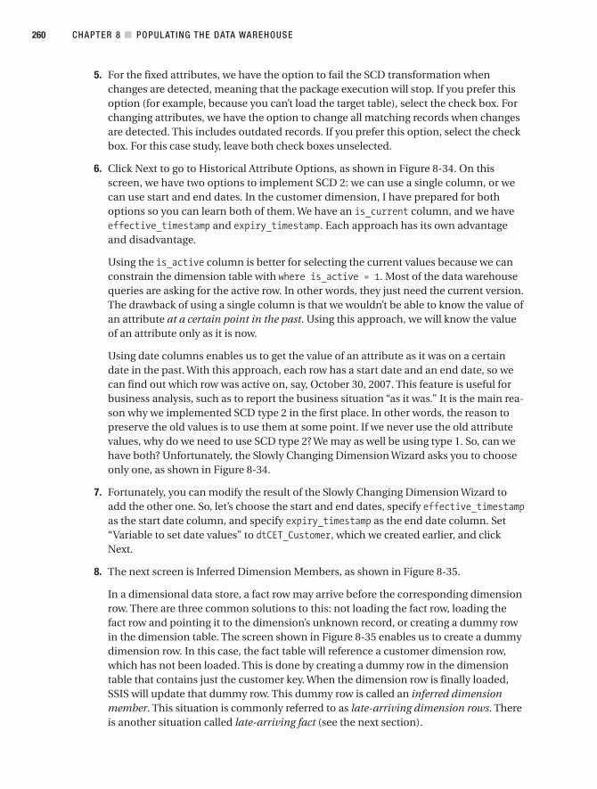
5. For the fixed attributes, we have the option to fail the SCD transformation whenchanges are detected, meaning that the package execution will stop. If you prefer thisoption (for example, because you can’t load the target table), select the check box. Forchanging attributes, we have the option to change all matching records when changesare detected. This includes outdated records. If you prefer this option, select the checkbox. For this case study, leave both check boxes unselected.
6. Click Next to go to Historical Attribute Options, as shown in Figure 8-34. On thisscreen, we have two options to implement SCD 2: we can use a single column, or wecan use start and end dates. In the customer dimension, I have prepared for bothoptions so you can learn both of them. We have an is_current column, and we haveeffective_timestamp and expiry_timestamp. Each approach has its own advantageand disadvantage.
Using the is_active column is better for selecting the current values because we canconstrain the dimension table with where is_active = 1. Most of the data warehousequeries are asking for the active row. In other words, they just need the current version.The drawback of using a single column is that we wouldn’t be able to know the value ofan attribute at a certain point in the past. Using this approach, we will know the valueof an attribute only as it is now.
Using date columns enables us to get the value of an attribute as it was on a certaindate in the past. With this approach, each row has a start date and an end date, so wecan find out which row was active on, say, October 30, 2007. This feature is useful forbusiness analysis, such as to report the business situation “as it was.” It is the main rea-son why we implemented SCD type 2 in the first place. In other words, the reason topreserve the old values is to use them at some point. If we never use the old attributevalues, why do we need to use SCD type 2? We may as well be using type 1. So, can wehave both? Unfortunately, the Slowly Changing Dimension Wizard asks you to chooseonly one, as shown in Figure 8-34.
7. Fortunately, you can modify the result of the Slowly Changing Dimension Wizard toadd the other one. So, let’s choose the start and end dates, specify effective_timestampas the start date column, and specify expiry_timestamp as the end date column. Set“Variable to set date values” to dtCET_Customer, which we created earlier, and clickNext.
8. The next screen is Inferred Dimension Members, as shown in Figure 8-35.
In a dimensional data store, a fact row may arrive before the corresponding dimensionrow. There are three common solutions to this: not loading the fact row, loading thefact row and pointing it to the dimension’s unknown record, or creating a dummy rowin the dimension table. The screen shown in Figure 8-35 enables us to create a dummydimension row. In this case, the fact table will reference a customer dimension row,which has not been loaded. This is done by creating a dummy row in the dimensiontable that contains just the customer key. When the dimension row is finally loaded,SSIS will update that dummy row. This dummy row is called an inferred dimensionmember. This situation is commonly referred to as late-arriving dimension rows. Thereis another situation called late-arriving fact (see the next section).
CHAPTER 8 ■ POPULATING THE DATA WAREHOUSE260
9314ch08final.qxd 11/15/07 10:09 AM Page 260

Figure 8-34. Historical attribute options in the Slowly Changing Dimension Wizard
Figure 8-35. Inferred Dimension Members screen
There are two ways to tell SSIS that a row is an inferred member: when an indicatorcolumn is true or when all columns are null (except the key column). Let’s enable theinferred member support and leave the option as “all columns with a change type arenull.”
CHAPTER 8 ■ POPULATING THE DATA WAREHOUSE 261
9314ch08final.qxd 11/15/07 10:09 AM Page 261

9. Click Next, and then click Finish. Rename the boxes as shown in Figure 8-36.
Figure 8-36. Result of the Slowly Changing Dimension Wizard
I’ll discuss the resulting boxes one by one so you know what they are. The SlowlyChanging Dimension box splits the data flow into three output flows. The left outputis the historical attributes/old rows, the middle output is the new rows, and the rightoutput is the changing attributes. So, the rows on the left output need to be marked asexpired, the rows on the middle output need to be marked as effective, and for therows on the right output the values need to be updated.
10. The “Update DDS Customer” box updates the customer dimension with the new val-ues for columns that we marked earlier in the Slowly Changing Dimension Wizard aschanging attributes using the following SQL statement. The ten parameters (the ques-tion marks) are mapped to the corresponding input columns with the matchingnames.
UPDATE dim_customerSET interest1 = ?, interest2 = ?, interest3 = ?,preferred_channel1 = ?, preferred_channel2 = ?,source_system_code = ?, subscriber_band = ?,subscriber_class = ?, update_timestamp = ?
WHERE customer_key = ? AND expiry_timestamp IS NULL
CHAPTER 8 ■ POPULATING THE DATA WAREHOUSE262
9314ch08final.qxd 11/15/07 10:09 AM Page 262

11. The “Set old row’s expiry date” box assigns the dtCET_Customer variable to theexpiry_timestamp column so that the expiry date of the old row is updated with thecurrent extraction time. The “Expire the old row” box updates the expiry_timestampcolumn of the old row, using the following SQL statement, to the dtCET_Customer vari-able set previously. The purpose of doing this is to expire the old row because we aregoing to insert a new row containing the current attribute values.
UPDATE dim_customer SET expiry_timestamp = ?WHERE customer_key = ? AND expiry_timestamp IS NULL
12. The Union All box (shown in Figure 8-37) combines the output of the previous “Expirethe old row” box with the middle output of the SCD box (the new rows to be inserted).This prepares the new customer rows containing the current, valid attribute values.Double-click the Union All box to see the properties in Figure 8-37.
Figure 8-37. Union All transformation to combine two outputs
CHAPTER 8 ■ POPULATING THE DATA WAREHOUSE 263
9314ch08final.qxd 11/15/07 10:09 AM Page 263

13. The “Set new row’s effective date” box assigns the dtCET_Customer variable to theeffective_timestamp column so that the new rows that will be inserted have the cor-rect start dates.
14. The last box, which is marked as “Insert rows to DDS customer,” inserts the new rowsinto the customer dimension in the DDS. You can double-click this box to see the col-umn mapping, which is shown in Figure 8-38.
Figure 8-38. Final mapping of the columns before inserting into dimension table
Sometimes you get a warning saying truncation may happen on column X, such as if thesubscriber class lookup is varchar(30) but on the customer dimension it is varchar(20). Tosolve this error, you can adjust the column width on the customer dimension table.
If there is no warning or error, save the package and run it. Check that the customerdimension is populated properly by comparing it to the NDS tables. Change some values invarious columns in the customer table in the source system (the Jade database), and run thestage and NDS package to bring the data to the NDS. Do this by opening the SSIS package andthen clicking the Debug menu and choosing Start Debugging (or pressing F5 for short). Then
CHAPTER 8 ■ POPULATING THE DATA WAREHOUSE264
9314ch08final.qxd 11/15/07 10:09 AM Page 264
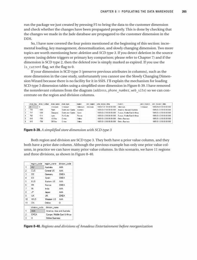
run the package we just created by pressing F5 to bring the data to the customer dimensionand check whether the changes have been propagated properly. This is done by checking thatthe changes we made in the Jade database are propagated to the customer dimension in theDDS.
So, I have now covered the four points mentioned at the beginning of this section: incre-mental loading, key management, denormalization, and slowly changing dimension. Two moretopics are worth mentioning here: deletion and SCD type 3. If you detect deletion in the sourcesystem (using delete triggers or primary key comparison; please refer to Chapter 7) and if thedimension is SCD type 2, then the deleted row is simply marked as expired. If you use theis_current flag, set the flag to 0.
If your dimension is SCD type 3 (preserve previous attributes in columns), such as thestore dimension in the case study, unfortunately you cannot use the Slowly Changing Dimen-sion Wizard because there is no facility for it in SSIS. I’ll explain the mechanism for loadingSCD type 3 dimension tables using a simplified store dimension in Figure 8-39. I have removedthe nonrelevant columns from the diagram (address, phone_number, web_site) so we can con-centrate on the region and division columns.
Figure 8-39. A simplified store dimension with SCD type 3
Both region and division are SCD type 3. They both have a prior value column, and theyboth have a prior date column. Although the previous example has only one prior value col-umn, in practice we can have many prior value columns. In this scenario, we have 11 regionsand three divisions, as shown in Figure 8-40.
Figure 8-40. Regions and divisions of Amadeus Entertainment before reorganization
CHAPTER 8 ■ POPULATING THE DATA WAREHOUSE 265
9314ch08final.qxd 11/15/07 10:09 AM Page 265
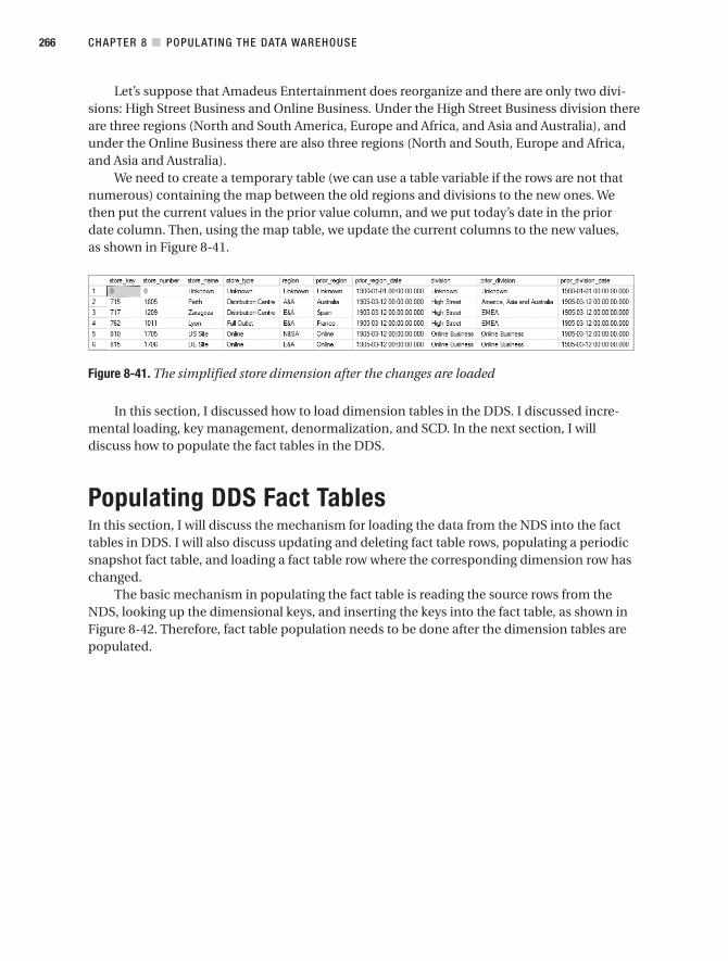
Let’s suppose that Amadeus Entertainment does reorganize and there are only two divi-sions: High Street Business and Online Business. Under the High Street Business division thereare three regions (North and South America, Europe and Africa, and Asia and Australia), andunder the Online Business there are also three regions (North and South, Europe and Africa,and Asia and Australia).
We need to create a temporary table (we can use a table variable if the rows are not thatnumerous) containing the map between the old regions and divisions to the new ones. Wethen put the current values in the prior value column, and we put today’s date in the priordate column. Then, using the map table, we update the current columns to the new values,as shown in Figure 8-41.
Figure 8-41. The simplified store dimension after the changes are loaded
In this section, I discussed how to load dimension tables in the DDS. I discussed incre-mental loading, key management, denormalization, and SCD. In the next section, I willdiscuss how to populate the fact tables in the DDS.
Populating DDS Fact TablesIn this section, I will discuss the mechanism for loading the data from the NDS into the facttables in DDS. I will also discuss updating and deleting fact table rows, populating a periodicsnapshot fact table, and loading a fact table row where the corresponding dimension row haschanged.
The basic mechanism in populating the fact table is reading the source rows from theNDS, looking up the dimensional keys, and inserting the keys into the fact table, as shown inFigure 8-42. Therefore, fact table population needs to be done after the dimension tables arepopulated.
CHAPTER 8 ■ POPULATING THE DATA WAREHOUSE266
9314ch08final.qxd 11/15/07 10:09 AM Page 266

Figure 8-42. Data flow in fact table population
The data flow in SSIS is similar to the one shown in Figure 8-29. In other words, one OLEDB source is followed by a series of Lookup transformations. We can also use the Execute SQLapproach, similar to the one I discussed earlier in this chapter when populating the NDS. Forexample, the SQL statement for inserting into the Product Sales fact table is as follows:
insert into fact_product_sales( sales_date_key, customer_key, product_key,store_key, order_id, line_number, quantity,unit_price, unit_cost, sales_value,sales_cost, margin, sales_timestamp,source_system_code,create_timestamp, update_timestamp )
select oh.order_date, oh.customer_number, od.product_code,oh.store_number, oh.order_id, od.line_no, od.qty,od.price, od.unit_cost, od.qty * od.price as sales_value,od.qty * od.unit_cost as sales_cost,od.qty * (od.price - od.unit_cost) as margin,oh.order_date as sales_timestamp,1 as source_system_code,getdate() as create_timestamp,getdate() as update_timestamp
from nds.dbo.order_header ohleft join nds.dbo.order_detail odon oh.order_id = od.order_id
CHAPTER 8 ■ POPULATING THE DATA WAREHOUSE 267
9314ch08final.qxd 11/15/07 10:09 AM Page 267

The previous SQL statement selects the rows from the order_header and order_detailtables in the NDS and inserts them into the Product Sales fact table in the DDS. In the facttable, we don’t store the natural keys such as customer number, product code, and storenumber; instead, we store the surrogate keys. So, we need to get the surrogate key from thedimension tables. The SQL statement to do that is as follows:
select coalesce(dd.date_key, 0) as date_key,coalesce(dc.customer_key, 0) as customer_key,coalesce(dp.product_key, 0) as product_key,coalesce(ds.store_key, 0) as store_key,oh.order_id, od.line_no, od.qty,od.price, od.unit_cost, od.qty * od.price as sales_value,od.qty * od.unit_cost as sales_cost,od.qty * (od.price - od.unit_cost) as margin,oh.order_date as sales_timestamp,1 as source_system_code,getdate() as create_timestamp,getdate() as update_timestamp
from nds.dbo.order_header ohleft join nds.dbo.order_detail odon oh.order_id = od.order_idleft join dim_date ddon dd.sql_date = oh.order_dateleft join dim_customer dcon dc.customer_number = oh.customer_numberleft join dim_product dpon dp.product_code = od.product_codeleft join dim_store dson ds.store_number = oh.store_number
The previous SQL statement selects rows from the NDS order_header and order_detailtables and then gets the surrogate keys from the relevant DDS dimension tables. It theninserts the fact rows into the Product Sales fact table in the DDS.
In some data warehouses, we only do INSERTs on the fact tables. In other systems, we doboth INSERTs and UPDATEs. If we need to update the fact table as well, we use the UPSERT tech-nique. We can use either the SQL statement method or the Lookup transformation method.Fact tables are normally large tables (in terms of the number of rows). Table partitioning canspeed up the update operation significantly when correctly applied to a fact table.
Whether it is better to drop the indexes before updating the fact table depends on whatportion of the fact table we are updating and whether the fact table is partitioned. If we areupdating a large number of rows, then it is probably worth it to drop the indexes. I’m talkingabout the index on the measure columns, not the dimensional key indexes. The dimensionalkey index is required to find the row that we want to update, so we should not drop them.
To determine whether it is beneficial to drop the measure column indexes, compare thetime required to update the rows (without dropping the index) with the time required to dropthe index first, update the rows, and then re-create the index. In most cases, I have found thatdropping fact table indexes is not necessary. If the table is partitioned, there is no need to drop
CHAPTER 8 ■ POPULATING THE DATA WAREHOUSE268
9314ch08final.qxd 11/15/07 10:09 AM Page 268

the indexes and re-create them afterward. Indexes do not slow down insert operations toomuch (depending on how many indexes exist on the table); it is the update operation that ismore affected by indexes.
We don’t usually delete from the fact table (except when purging). Cancellations orreturns are implemented as inserts with negative quantities or with different transactiontypes. For example, in our case study, if a customer returns a product, we can insert a row inthe Product Sales fact table with the quantity set to –1.
A periodic snapshot fact table requires a different loading method because it does notcontain incremental transactional data. A periodic snapshot fact table is a fact table that cap-tures the state or condition of the business at a particular point in time at a certain interval.An example of a periodic snapshot fact table is the Subscription Sales fact table in ourAmadeus Entertainment case study (see Figure 5-5).
The source of this fact table is not from the order header and order detail in the NDS butfrom the customer dimension where customer type = subscriber. We read all active customersfrom the customer dimension; then join (or look up) with the store, lead, date, package, andformat dimensions to get the dimensional keys; and then we load the rows into the fact table.
One interesting phenomenon in fact table population is a late-arriving fact. This is dif-ferent from a late-arriving dimension row, which I discussed earlier. A late-arriving facthappens when we receive fact table rows with transaction dates in the past (say, a few weeksago or a few months ago). As usual, we do a lookup in the dimension tables to get the dimen-sional keys and then load the row into the fact table.
But, when the transaction is a few months old, the dimension row may have changed. Ifthe dimension table is using SCD type 2, we will have several rows in the dimension table. Weneed to find which row corresponds to the transaction that we load into the fact table. To dothis, we use the effective date and expiry date columns in the dimension table. The correctdimension row for this transaction is the one where the fact table transaction date is betweenthe effective date and expiry date.
For example, the customer dimension we populated in the previous section uses SCDtype 2. The customer dimension row for this late-arriving fact row may have changed; forexample, there may be four rows for this customer. Three of them are marked as inactive, andone of them is marked as active. Because we have the effective date and the expiry date, wecan find which one of those three inactive rows is the correct one to apply for this late-arrivingfact table transaction.
Batches, Mini-batches, and Near Real-Time ETLMost of the data warehouse ETL processes run daily, weekly, or monthly. Many people refer tothese ETL processes as batches. When people say daily batch, for example, they are referringto the ETL processes that run daily.
In recent years (the past two to three years), I have heard the term mini-batch more andmore often. When people talk about a mini-batch, what they mean is a group of ETL processes(that brings data into the data warehouse) that runs hourly, typically between one to six hours.Only some of the ETL processes are included in the mini-batch. The rest still run in batches,such as daily, weekly, monthly, and so on.
In the Amadeus Entertainment case study, there is no business benefit in populating theSubscription Sales fact table hourly. The business requirement indicates that the revenues,
CHAPTER 8 ■ POPULATING THE DATA WAREHOUSE 269
9314ch08final.qxd 11/15/07 10:09 AM Page 269

costs, and margin associated with the subscription sales, subscription duration, and leadsources need to be evaluated every day (please refer to Chapter 4). There is also no businessbenefit for the Supplier Performance fact table to be loaded hourly. But it could be beneficialto run the Product Sales mart hourly in order to manage the inventory better, for example. TheCampaign Results fact table could benefit from a mini-batch too. For example, it would enablethe marketing department to know within an hour which customers clicked which links in thecampaign e-mails so marketing can respond accordingly.
Because of this latest development (in other words, the mini-batch), data warehousesnow have a new function. Ten years ago, data warehouses were intended for analysis purposesand not as operational systems. Now they can have an operational role.
Near real-time ETL is the term people use when the time lag between the data in the datawarehouse and the data in the source systems is less than one hour, typically between 10 and30 minutes. Again, in near real-time ETL, only some tables are set in that fashion. In the Ama-deus Entertainment case study, not only could the Campaign Results fact table benefit frommini-batch, but also it would benefit from near real-time ETL. For example, to enable themarketing department to know within ten minutes which customers are interested in whichproducts, they can react accordingly by using automated response rules.
Just like batch processes, both the mini-batch and near real-time ETL are based on pullapproaches. The ETL processes pull the data from the source system into the data warehouse.The main difference between the three of them is the frequency they run. The batch ETL runsdaily, weekly, or monthly; the mini-batch runs hourly; and the near real-time ETL typicallyruns every 10 to 30 minutes. The near real-time ETL is also known as a micro-batch.
To apply a micro-batch or near real-time ETL, you need to analyze the DDS fact tablesand determine which one would benefit if they were loaded every few hours (or less). Ideally,you need to pick only one or two fact tables to minimize the negative impact on performance.The next step is to determine which dimensions associated with these fact tables need to beloaded at the same frequency. Then you can change the execution interval of the ETLprocesses.
Pushing the Data InData warehouse population has traditionally been done using ETL. The ETL processes pull thedata from the source system and then load it into the data warehouse. In recent years, becauseof their operational functions, some data warehouses need to be updated as soon as thesource system changes. In this case, the source systems push the data into the warehouse. Inthis approach, the source systems have triggers. They typically contain insert and update trig-gers but sometimes delete triggers too. Please refer to Figure 8-43.
Figure 8-43. Push approach for loading data
CHAPTER 8 ■ POPULATING THE DATA WAREHOUSE270
9314ch08final.qxd 11/15/07 10:09 AM Page 270

As the application inserts or updates or deletes data from the source system database,these triggers are invoked, and they insert the changed data into the ODS. The tables in theODS also have triggers that send the data changes to a message queuing (MQ) system in theform of XML messages. On the other end of the MQ, an ETL application constantly polls andprocesses the XML messages from the MQ, unwraps them, shreds them, assigns or looks upthe data warehouse keys, and inserts them into appropriate dimensions and fact tables in thedata warehouse. Or, leaving the MQ out, in the case of a DDS-only architecture (please refer toChapter 2), the triggers in the source system update the DDS directly. A DDS-only architectureis more suitable for the push approach because there is no intermediary data store such as anNDS or an ODS. The typical lead time is between 5 and 30 seconds, happening in real time.
Three years ago, we heard this approach implemented only for enterprise applicationintegration (EAI). Today, it is implemented for data warehouse population. Some people referto this push approach as real-time data integration.
Let’s understand how we can benefit from this technology. If we can push the datachanges into the warehouse within 30 seconds, then in the case of Amadeus Entertainment,the marketing department can respond to customer shopping behavior. When an online cus-tomer is currently browsing the site looking for products or subscriptions but then abandonsthe shopping process and leaves the site, marketing can respond accordingly using the CRMsystem in almost real time.
One important consideration when loading large fact tables in real time is that we need toarrange the ETL so that we can insert into the fact table only. We can’t possibly do an update ora delete, because this will take a few seconds and we don’t have a few seconds. We have only afew milliseconds. When the daily batch runs, along with flipping the fact table views (seeChapter 6), we can process today’s inserted data and do the updates in batches.
SummaryThis chapter started with a brief discussion on stage loading, including the three approachesof stage tables. Then I talked a little bit about the data firewall, followed by several points thatyou need to consider when loading the NDS: normalization, external data, key management,and the many-to-many relationship. Then I showed how to load the data into the NDS usingSSIS.
I showed how to use three different methods in SSIS to load the data: SQL statements,Slowly Changing Dimension transformations, and Lookup transformations. Then we popu-lated the dimension tables and fact tables in the DDS, including SCD. And finally I discussedthe batch, mini-batch, and near real-time (or micro-batch) ETL approaches, followed by thepush approach.
CHAPTER 8 ■ POPULATING THE DATA WAREHOUSE 271
9314ch08final.qxd 11/15/07 10:09 AM Page 271

9314ch08final.qxd 11/15/07 10:09 AM Page 272

Assuring Data Quality
In this chapter, we’ll explore why data quality is important, and I’ll explain why there is nopoint having a data warehouse if we cannot trust the data in the warehouse. Then I will dis-cuss the data quality process and explore the architecture elements that are involved in theprocess.
In addition, I will discuss data cleansing and explore the three types of matching logic:exact, fuzzy (approximate), and rule based. I’ll show how to do a Fuzzy Lookup transformationin SSIS to identify duplication in artist names based on the similarity scores. I will also discusscross-checking with external sources. Then I’ll talk about the three categories of data qualityrules: incoming data, cross-references, and internal rules.
I’ll discuss the three choices of what to do with the data when a data quality rule is vio-lated: we can reject it, allow it into the warehouse, or fix/correct it. I’ll also talk about logging,which is basically storing the failed rows in the data quality (DQ) database, along with addi-tional audit information, such as the time it happened, which rule was violated, and thecorrection status; this is for the purpose of auditing and reporting later. We will then end thechapter with reporting and notification so that someone can correct the data.
So, why is data quality important? It is easy to answer this simple question. Say you can’ttrust the data in your data warehouse, perhaps because some data is incorrect (accuracy),because some data is missing (completeness), because some data is not in sync with otherdata (consistency), because some data is only a rough estimate (precision), or because somedata is out-of-date (timeliness). In these cases, would it still be possible for you to use the datawarehouse? If you use the data for making important decisions and the data is incorrect, howmuch will the mistake cost the company? And how bad will it be for your career?
Further, if you cannot trust the data in your data warehouse, what is the point of havinga data warehouse? To prevent this disaster, when building a data warehouse, it is importantto think about data quality as early as possible, preferably at the beginning of the project. Theessence of maintaining data quality is to prevent bad data from getting into the data ware-house and to fix the bad data as early as possible in the process chain (ideally at the sourcesystem). To implement this, we need to set up rules that define what “bad data” is and putadditional components in the architecture to filter the bad data out and to enable reporting,monitoring, and cleaning mechanisms.
273
C H A P T E R 9
9314ch09final.qxd 11/15/07 10:06 AM Page 273

Data Quality ProcessThe data quality process includes the activities to make sure the data in the data warehouseis correct and complete. This is usually done by checking the data on its way into the datawarehouse. The data quality process also includes the mechanism to report the bad data andto correct it. So, there are three aspects of the data quality process: checking, reporting, andcorrecting.
For example, in the Amadeus Entertainment case study, customers can purchase a prod-uct, or they can subscribe to a package. The date a customer subscribes to a package for thefirst time is called the first subscription date, and the most recent date they canceled their sub-scriptions is called the last cancellation date. Suppose one day the ETL process extracted acustomer record with the last cancellation date earlier than the first subscription date. This isnot a valid condition. Either the last cancellation date is wrong or the first subscription date iswrong, or both. The data quality process detects this condition and reports it to the peopleresponsible for the subscription data. They then correct the data in the source system, and thedata is loaded into the data warehouse.
To understand the mechanism of how the data quality process works, look at Figure 9-1.It shows the ODS + DDS architecture discussed in Chapter 2, with the data quality compo-nents added.
Figure 9-1. Data quality components in the data warehouse architecture
The DQ components in Figure 9-1 are shaded and are as follows:
• The data firewall is a program that checks the incoming data. Physically it is an SSISpackage or a stored procedure.
• Metadata is a database that stores the data quality rules, such as “The last cancellationdate must be greater than the first subscription date.”
• The DQ database stores the bad data detected by the data firewall.
• DQ reports and notifications read the DQ database and inform the people responsiblefor data quality.
• Correction is a process to correct the data in the source system.
CHAPTER 9 ■ ASSURING DATA QUALITY274
9314ch09final.qxd 11/15/07 10:07 AM Page 274

In Figure 9-1, the stage ETL extracts the data from the source system and loads it into thestage database. The data firewall then checks the data according to the data quality rules fromthe metadata database, such as “The first subscription date is greater than or equal to the lastcancellation date.” If the data satisfies the DQ rule, the data is passed to the ODS ETL, whichwill then put the data into the ODS. If the data fails the DQ rule, it is put in the DQ database.
When the data is placed in the DQ database, certain auditing information is recorded too,such as which source system the data is coming from, which table in the source system it isfrom, what time (and date) this happened, which rule(s) failed the data, and what table/mart/area this data is for.
DQ reports and notifications read the DQ database at regular intervals, such as daily. Inthe DQ database, we have many records from different DQ rules. For example, we could have2,000 records from 100 different DQ rules, or an average of 20 for each rule. The DQ databasealso contains information about who is responsible for each rule; for example, the customerservice department is responsible for rules 1 to 10, which are about customer data, and thefinance department is responsible for rules 11 to 20, which are about financial data.
DQ reports and notifications read the records in the DQ database rule by rule and reportthem to the appropriate people at a regular interval. The people fix the data in the source sys-tem so that the next time that data is extracted by the stage ETL, it is already correct. Thepurpose of these reports and notifications is to notify the users to get the data corrected.They contain the previous day’s (or previous week’s) errors.
There is another group of data quality reports whose purpose is to analyze the data qual-ity in the data warehouse. One indicator of the quality of the data in the data warehouse is thenumber of times each rule was violated. The reports contain the number of DQ rule violationsfor a certain period.
This analysis can also be done using data quality dashboards. Dashboards are businessintelligence applications that give a quick summary of the data quality in graphical gadgets,typically gauges, charts, and indicators. By clicking these gadgets, we can drill down to lower-level details. We will discuss more about data quality dashboards later in this chapter.
■Tip If you implement a data warehouse for the purpose of business intelligence, you may think it is agood idea to use the same notification mechanism for alerting certain managers about time-dependantbusiness warnings such as a period of low sales. This idea is usually inspired by the fact that this is theearliest point in the system where the data is coming into the warehouse. The earlier the managers knowabout this alert, the better, right? Well, no. The data coming into the data firewall is not a complete setwhere you can examine it in a true business sense. For business alerts like this, your notification serviceneeds to operate off the ODS (or the DDS) after it is fully loaded, not in the middle of the loading process;for example, we can put it at the end of the ETL batch.
In the box marked as Correction in Figure 9-1, the people responsible for the appropriateareas (product sales, subscriptions, customers, products, currency, and so on) then fix the datain the source system so that when the data is loaded again the next day (or whenever), the data isalready correct. We can fix the data automatically on its way into the data warehouse, but gener-ally this is not a good practice because it is still wrong in the source system. Other applicationsthat may be using the same data (or the source system itself) will publish incorrect data.
CHAPTER 9 ■ ASSURING DATA QUALITY 275
9314ch09final.qxd 11/15/07 10:07 AM Page 275

Can the correction in the source system be automated? The simple answer is yes. But weneed to be careful when doing this. First, the rule for automatic correction must be checkedand double-checked to make sure it is 100 percent correct. Second, it is generally better tounderstand how the bad data is created in the source system and why this happens. If it iswithin our control, let’s fix it so it doesn’t happen again. That is better than automaticallycorrecting it every day.
In reality, the boundary between good data and bad data is not always clear. For exam-ple, if the data value is 5,000 or more, it is good. If the value is 3,000 or less, it is bad. But if thevalue is between 3,000 and 5,000, it is not good but not too bad. So, in practice, we need to sethow we want to react accordingly. For example, we may have a different treatment for eachrange. Or, a certain range qualifies as a “warning,” and a certain range qualifies as an “error,”and so on. In this example, if the data value is between 3,000 and 5,000, we want to classify itas a warning, but if the value is lower than 3,000, it is an error.
In Figure 9-1, instead of putting the data firewall before the ODS ETL, we can put itbefore the stage ETL. The data quality checks the data as the data is being loaded into thestage tables. If the data satisfies the DQ rule, it is loaded into the stage tables. If it fails theDQ rules, the data is placed in the DQ database for reporting and correction. The extractionprocess is slower, but this means the bad data does not touch any area of the data ware-house at all, not even the stage.
We can also check the data on the source system and not extract bad data; in otherwords, the where clause is dynamically set. For example, we can use select product_code,product_name, description, status, … etc… where product_code <> 19331. The data fromthe source is clean, but the extraction is slower. The other disadvantage is that we can’t reportthe bad data comprehensively because that data is not extracted.
The problem in data quality is usually not about a particular record but about a collectionof records. For example, usually in a medium-sized branch there are about 20,000 to 60,000transactions a day, with total sales of $0.6 million to $6 million (for small or large branches, themetrics are different). If the number of transactions is less than 10,000 or the total sales is $0.5million, it is probably an indication of extraction or loading failure, so we want this conditionto be reported.
One way to do this is to have what we call an ODS firewall, in Figure 9-2. The ODS firewallis a program that runs after the data has been loaded into the ODS but before it is loaded intothe DDS. The ODS firewall reads the ODS database and checks the data according to the DQrules from the metadata database.
Figure 9-2. The ODS firewall (bottom right) checks the data against the DQ rules.
CHAPTER 9 ■ ASSURING DATA QUALITY276
9314ch09final.qxd 11/15/07 10:07 AM Page 276

If the collection of data fails the DQ rules, we put the data on the DQ database, along withthe auditing information such as which table in the source system it is from, what time (anddate) this happened, which rule(s) failed the data, and what table/mart/area this data is for.We could let the data remain in the ODS (and be subsequently loaded into the DDS), or wecan remove the data from the ODS (and not be loaded into the DDS) until the problem is fixed.The approach we need to take depends on the nature of the data. If it is more important forthe data to be present in the data warehouse even though it is not complete, then we load thedata into the DDS. But if the incompleteness causes problems in the business analysis or deci-sion making, then we remove the data from the ODS.
If we allow the data to stay in the ODS (and load it into the DDS), we need to mark thedata quality. We do this by adding up to five data quality keys on each row of data: accuracy,precision, timeliness, completeness, and consistency. These keys refer to the five data qualitydimensions. We don’t have to use all five keys. We can just use two of them (such as accuracyand precision), depending on which ones we need.
Alternatively, we can just have a single DQ key on each row. This single DQ key is calledreliability, which is calculated based on the scores of the five DQ base dimensions. For exam-ple, the calculation can simply be a weighted average such as reliability = A * accuracy + B *precision + C * timeliness + D *completeness + E * consistency, where A, B, C, D, and E are per-centages that add up to 100 percent. This reliability “stamp” on each row enables the users toknow how much they can trust the data. The disadvantage of this approach is that the calcula-tion could become a little bit tricky. For example, if an aggregate is calculated by averagingfifty rows all with an accuracy of 5 but there are two rows with an accuracy of 1, how wouldyou score the accuracy of the aggregate?
Now that you understand the mechanism of data quality in the data warehouse, how dataquality is implemented in the architecture, which components are affected, and the alterna-tive approaches, I’ll discuss the details of each component, such as the rules, the actions, thelogging and auditing, and the reporting. But before I do that, I’ll talk about two other areas indata quality, namely, data cleansing and external data.
Data Cleansing and MatchingWhat is data cleansing? Why is it important in data quality? Put simply, data cleansing, ordata scrubbing, is the process of identifying and correcting dirty data. Dirty data meansincomplete, wrong, duplicate, or out-of-date data. I’m not sure why, but people in the datawarehousing community prefer to use the words cleanse and scrub rather than clean, whichis simpler and more descriptive. An example of data cleansing is checking stores’ tables tomake sure the store names, store numbers, store types, and store addresses are all correct.Other examples are making sure that there are no duplicate customer records, that the pricelists are correct, that obsolete products are flagged accordingly, that all subscriptions refer toexisting packages, and that the song and film titles are correctly spelled.
In data cleansing, it is important to be able to determine that one data item is the sameas another data item. This is called data matching. Data matching is used to identify dupli-cate records when doing a lookup on reference data. Matching is particularly relevant forcharacter-based data types, including large value data types, such as varchar(max), becausefor numerical or datetime data types, we can simply use the equal sign. For character-baseddata types, it may not be that clear. For example, when loading the address table in the NDS,
CHAPTER 9 ■ ASSURING DATA QUALITY 277
9314ch09final.qxd 11/15/07 10:07 AM Page 277

we may find that the city name is “Los Angles,” which does not exist in the city table. In thiscase, we need to match “Los Angles” to “Los Angeles.” Another example is the customer name“Robert Peterson.” We need to match/recognize that “Robert Peterson” is the same as “BobPeterson.”
Numeric data is not as tricky as character data. We can just use the equal sign; 5 is 5whatever way we look at it, and 5 is different from 6. So, we can just use = for matchingnumeric data. For example, “if A = B, then….” The only possible problem is rounding; forexample, is 5.029 the same as 5.03? If the precision is two decimal digits, they are the same,but if the precision is three decimal digits, then they are different.
For date and time data, if the data is stored as a datetime data type, it’s not a problem.We can just use the equal sign like the numeric data. But if it is stored as a character datatype, it could be a little bit tricky because of the date format and time zone. For example, is03/01/2008 the same as 01/03/2008? Is it the same as 2007-03-01T00:00:00Z+06? We need alittle bit of logic here to match them, such as by comparing the components or by compar-ing the date, month, and year.
In SQL Server we have three types of matching logic: exact, fuzzy (approximate), andrule based. Exact matching is where all characters are the same, for example “Los Angeles”and “Los Angeles.” In SSIS this is done using a Lookup transformation. Fuzzy logic matchingfinds how similar a set of data is to another set of data. For example, using the Fuzzy Lookuptransformation in SSIS, “You can’t hurry love” and “You cannot hurry love” have a similarityscore of 0.81666672 and a confidence level of 0.59414238. You can then decide for examplethat if the similarity score is greater than 0.75 and the confidence level is greater than 0.5,then it’s a match.
To determine the threshold for the similarity score and confidence level (0.75 and 0.5 inthe previous case), we need to run the data through a Fuzzy Lookup transformation with thesimilarity threshold set to zero. This will output the similarity scores for all the rows in thesource data. We then manually examine the score to find the appropriate threshold. We willdo this (finding the threshold) later in this section.
Rule-based logic is where we use certain rules and data to identify a match. For example,we can define (in a table) that for name data the string “Bill” is the same as “William” or inproduct names “movie” is the same as “film.” In SSIS this is implemented with databaselookup. We can also define a rule, such as “For product code, omit the spaces when compar-ing” so that “KL 7923 M” is the same as “KL7923M.” Here’s another example: “Omit prefix9000 in the supplier number” so that “900089123” and “89123” are the same. SSIS logic likethe previous can be implemented with Script Component.
Let’s open Business Intelligence Development Studio (BIDS) and construct a fuzzy logicand a rule-based logic solution. As they say, the devil is in the details. And without trying it, wewouldn’t know the details. In this scenario, we have a table in Jade called artist2. The tablecontains 20 artists that we are going to load into NDS. The artist2 table also contains cityand country, as shown in Table 9-1.
CHAPTER 9 ■ ASSURING DATA QUALITY278
9314ch09final.qxd 11/15/07 10:07 AM Page 278

Table 9-1. artist2 Table in the Jade Source System
artist_code artist_name genre country city
CAT011 Catherine Jarrette CJ Poland Warsaw
NIC003 Nicoleta Jadyn BF Andorra Andorra la Vella
ADE006 Adellais Clarinda BX Zambia Lusaka
CHE019 Cheyanne Chantelle BA Australia Canberra
HUG005 Hughie Violet BE Norway Oslo
PAL002 Palmira Charlie BE Israel Jerusalem
LUC003 Luciana Chrysanta CC Nigeria Abuja
CEL008 Celeste Vitolia AH Nicaragua Managua
EVE002 Evete Mona CH Mauritius Port Louis
ALI004 Alienor Hambert CG Kazakhstan Astana
CHL003 Chloe Ignatius AJ United States Washington DC
HUG005 Hugh Clarity AW Taiwan Taipei
SUS002 Susan Johansen BN Belgium Brussels
TAN001 Tania Balumbi AW Pakistan Islamabad
VIC001 Victor Robinson CE Luxembourg Luxembourg
THO001 Thomas Clark AJ Japan Tokyo
TIM001 Tim Lewis AJ Germany Berlin
LAU002 Laura Scott AN Congo Kinshasa
PET001 Peter Hernandez AP Spain Madrid
ADA001 Adam Baxter BQ Egypt Cairo
Out of these twenty artists, nine are new artists. Eleven of those twenty, however, actuallyalready exist in the NDS, but their names are slightly different. For example, one that alreadyexists in the NDS is “Catherine Jarrett,” but the incoming data is “Catherine Jarrette.”
We are going to use a Fuzzy Lookup transformation with certain similarity levels to deter-mine whether the artists already exist in the NDS. If they exist, we update the NDS. If theydon’t exist, we will insert them into the NDS. In this case, we will find first what the confidencelevel should be by pointing the output of the Fuzzy Lookup transformation to a file and settingup a data viewer. The city and country need be translated into keys using normal lookup(exact match). As with every NDS table, we also need to populate the source_system_code,create_timestamp, and update_timestamp columns. We’ll use a Derived Column transforma-tion to populate these three columns. Using a Derived Column transformation, we can createnew columns containing constant values or calculations based on the input columns.
In Chapters 7 and 8 I discussed how to extract and load data using SSIS and gave quite alot of detailed exercises, so you should be quite familiar with it by now. Let’s get started:
1. Define a new SSIS package, and call it NDS Artist.
2. Create a Data Flow task on the design surface, and call it Load Artist.
3. Double-click it to edit it.
CHAPTER 9 ■ ASSURING DATA QUALITY 279
9314ch09final.qxd 11/15/07 10:07 AM Page 279
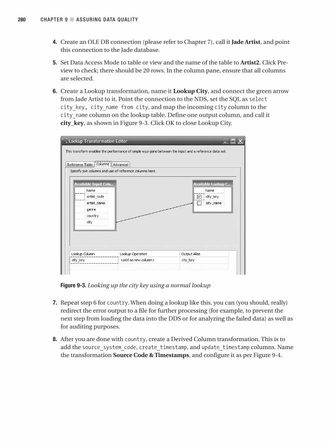
4. Create an OLE DB connection (please refer to Chapter 7), call it Jade Artist, and pointthis connection to the Jade database.
5. Set Data Access Mode to table or view and the name of the table to Artist2. Click Pre-view to check; there should be 20 rows. In the column pane, ensure that all columnsare selected.
6. Create a Lookup transformation, name it Lookup City, and connect the green arrowfrom Jade Artist to it. Point the connection to the NDS, set the SQL as selectcity_key, city_name from city, and map the incoming city column to thecity_name column on the lookup table. Define one output column, and call itcity_key, as shown in Figure 9-3. Click OK to close Lookup City.
Figure 9-3. Looking up the city key using a normal lookup
7. Repeat step 6 for country. When doing a lookup like this, you can (you should, really)redirect the error output to a file for further processing (for example, to prevent thenext step from loading the data into the DDS or for analyzing the failed data) as well asfor auditing purposes.
8. After you are done with country, create a Derived Column transformation. This is toadd the source_system_code, create_timestamp, and update_timestamp columns. Namethe transformation Source Code & Timestamps, and configure it as per Figure 9-4.
CHAPTER 9 ■ ASSURING DATA QUALITY280
9314ch09final.qxd 11/15/07 10:07 AM Page 280

Figure 9-4. Using derived column to define source system code and timestamps
9. The resulting data flow will be similar to the one in Figure 9-5. The last two boxes inFigure 9-5 (Lookup Artist Names and Flat File Destination) are not done yet. We’ll dothem next.
Figure 9-5. Data flow for loading the artist2 table using fuzzy lookup
CHAPTER 9 ■ ASSURING DATA QUALITY 281
9314ch09final.qxd 11/15/07 10:07 AM Page 281

10. In the Toolbox, find the Fuzzy Lookup transformation, and drag it to the design sur-face. Connect the green arrow from Source Code & Timestamp to it, and call it LookupArtist Names. Double-click it to edit it, set the connection to NDS, and choose artist asthe reference table, as shown in Figure 9-6.
Figure 9-6. Setting the reference table on the Fuzzy Lookup transformation
11. Now we want to look up the artist record in the NDS (target) based on the artistname on the stage (source). For that, click the Columns tab. Ensure that all the PassThrough check boxes are checked so that the input columns are included in the out-put. Delete the artist_code and genre mappings, leaving only artist_name. This isbecause we want to do the lookup based only on the artist name. Check artist_namein the Available Lookup Columns list, and set Output Alias to artist_name1, as shownin Figure 9-7.
12. Click the Advanced tab. Leave the maximum number of matches at 1. Leave the simi-larity threshold at 0, and leave the token delimiters as they are, as shown in Figure 9-8.The purpose of doing this is so that we get the similarity score for all the rows in thetable. Click OK to close the Fuzzy Lookup Transformation Editor dialog box.
CHAPTER 9 ■ ASSURING DATA QUALITY282
9314ch09final.qxd 11/15/07 10:07 AM Page 282

Figure 9-7. Configuring the lookup columns on the Fuzzy Lookup transformation
Figure 9-8. Advanced tab of the Fuzzy Lookup transformation
13. Now let’s add a file destination and a data viewer so we can see and examine thedata, along with the similarity score and confidence level. Create a flat-file destina-tion. Point it to a new folder called Output in your ETL directory. Set the format toDelimited. In the column pane, set the column delimiter to a vertical bar (|). Leaveeverything else as is, and click OK. Right-click the green connector between theFuzzy Lookup and the Flat File destination, and select Data Viewers. Click Add, andchoose Grid. Click the Grid tab, and select all columns. Click OK twice to return tothe Data Flow transformation.
CHAPTER 9 ■ ASSURING DATA QUALITY 283
9314ch09final.qxd 11/15/07 10:07 AM Page 283

14. Run the package, and it will stop at the data viewer. The data viewer shows the similar-ity and confidence columns, as shown in Figure 9-9.
Figure 9-9. Data viewer showing the similarity and confidence columns
15. The data viewer shows that the similarity figures for the first 11 rows are all greaterthan 87 percent. This means the source data is similar to the target data in the NDS. Inother words, we found a match for these 11 rows. You can compare the artist_nameand artist_name1 columns to see the slight differences. artist_name is the incomingdata, and artist_name1 is the data in the NDS artist table. However, the similarity forHugh Clarity (NDS record Hue Clarity) is only 65 percent, about the same as SusanJohansen (NDS record Susana Johnnie), which gets 69 percent. Four gets 0 (nonematching), two gets between 20 percent and 30 percent, and 1 gets 40 percent. Thismeans that the Fuzzy Lookup transformation did not find similar records in the NDS.In other words, there are no matches for these records. Based on this, we can decide toset the similarity level to about 85 percent because this threshold will allow goodrecords to be loaded onto NDS, yet it will prevent the bad data from going through.
16. Click the green arrow in the top-left corner of the data viewer to continue executingthe package. The package completes, and the flat file is populated. The first ten lines ofthe flat file are shown here:
artist_code|artist_name|genre|country|city|city_key|country_key|source_system_code|create_timestamp|update_timestamp|artist_name1|_Similarity|_Confidence
CHAPTER 9 ■ ASSURING DATA QUALITY284
9314ch09final.qxd 11/15/07 10:07 AM Page 284

CAT011 |Catherine Jarrette|CJ|Poland|Warsaw|380|173|1|2007-04-06 22:30:42.546000000|2007-04-06 22:30:42.546000000|Catherine Jarrett|0.93352449|0.5|0.93352449NIC003 |Nicoleta Jadyn|BF|Andorra|Andorra la Vella|413|1|1|2007-04-06 22:30:42.546000000|2007-04-06 22:30:42.546000000|Nicoletta Jadyn|0.94442153|0.5|0.94442153ADE006 |Adellais Clarinda|BX|Zambia|Lusaka|300|241|1|2007-04-06 22:30:42.546000000|2007-04-06 22:30:42.546000000|Adelais Clarinda|0.93737274|0.5|0.93737274CHE019 |Cheyanne Chantelle|BA|Australia|Canberra|111|14|1|2007-04-06 22:30:42.546000000|2007-04-06 22:30:42.546000000|Cheyanne Chantel|0.88881922|0.5|0.88881922HUG005 |Hughie Violet|BE|Norway|Oslo|421|160|1|2007-04-06 22:30:42.546000000|2007-04-06 22:30:42.546000000|Hughie Violetta|0.87504929|0.5|0.87504929PAL002 |Palmira Charlie|BE|Israel|Jerusalem|317|100|1|2007-04-06 22:30:42.546000000|2007-04-06 22:30:42.546000000|Palmira Carlie|0.92811567|0.5|0.92811567LUC003 |Luciana Chrysanta|CC|Nigeria|Abuja|405|157|1|2007-04-06 22:30:42.546000000|2007-04-06 22:30:42.546000000|Luciana Chrysanta|1|1|1CEL008 |Celeste Vitolia|AH|Nicaragua|Managua|293|158|1|2007-04-06 22:30:42.546000000|2007-04-06 22:30:42.546000000|Celeste Vitalia|0.92354828|0.5|0.92354828EVE002 |Evete Mona|CH|Mauritius|Port Louis|260|147|1|2007-04-06 22:30:42.546000000|2007-04-06 22:30:42.546000000|Evette Mona|0.91588253|0.5|0.91588253ALI004 |Alienor Hambert|CG|Kazakhstan|Astana|204|120|1|2007-04-06 22:30:42.546000000|2007-04-06 22:30:42.546000000|Alienor Humbert|0.92823803|0.5|0.92823803
17. Press Shift+F5 to stop the package and return to the designer. Now let’s delete the FlatFile destination because we want to direct the output of the Fuzzy Lookup transforma-tion to the NDS. To load the output into the NDS, we need to split the output into twodepending on whether the artist record already exists in the NDS. If the record alreadyexists, we update it. If it does not exist, we insert it. For that let’s add a Conditional Splittransformation and connect the green arrow from Fuzzy Lookup to it. Name the boxSplit Based on Similarity, and double-click it to edit it. Under Output Name, type Sim-ilar, and under Condition, type [_Similarity]>=0.85, as shown in Figure 9-10.
CHAPTER 9 ■ ASSURING DATA QUALITY 285
9314ch09final.qxd 11/15/07 10:07 AM Page 285

Figure 9-10. Splitting the output of the Fuzzy Lookup transformation based on similarity
18. Now that we have split the output into two branches, we need to feed both branchesinto two separate destinations. The first destination is for insert, and the second one isfor update. If the artist name is the same or similar to the ones in the target (the NDS),we want to update the target. On the other hand, if the artist name does not exist (NotSimilar), we want to insert (create) that artist into the NDS. For that, let’s set DefaultOutput Name to Not Similar and click OK. Now we need to configure the insert andupdate. Let’s do the insert first. Drag an SQL Server destination onto the design sur-face, and name it Insert to NDS Artist. Connect the green arrow from the Split Basedon Similarity box, and the Input Output Selection will pop up. In the Output drop-down list, select Not Similar, and click OK. Double-click the SQL Server destination,and set the connection to NDS. Point it to the artist table, and configure the columnmappings as per Figure 9-11.
CHAPTER 9 ■ ASSURING DATA QUALITY286
9314ch09final.qxd 11/15/07 10:07 AM Page 286

Figure 9-11. Column mappings for inserting nonsimilar rows
19. From the Toolbox, drag an OLE DB Command transformation onto the design surface,and call it Update NDS Artist. Connect the green arrow from the Split box onto it; thistime the Input Output Select doesn’t pop up. It will just choose Similar because Similaris the only output left from the Split box without connection. Double-click the UpdateNDS Artist box to edit it. Set Connection Manager to NDS.
20. Click the Component Properties tab to display the common and custom properties, asshown in Figure 9-12. On this tab we need to set the SQL statement that updates theartist record in the NDS.
CHAPTER 9 ■ ASSURING DATA QUALITY 287
9314ch09final.qxd 11/15/07 10:07 AM Page 287

Figure 9-12. Common properties and custom properties in the Advanced Editor
21. Set the SQL statement on the SqlCommand property, as shown in Figure 9-12. Please notethat SqlCommand here is a property of the OLE DB Command SSIS transformation, not the.NET Framework class on the System.Data.SqlClient namespace. We need to set theSqlCommand property as follows:
update artist set artist_code = ?,artist_name = ?, genre = ?,city_key = ?, country_key = ?, source_system_code = ?,update_timestamp = ?where artist_name = ?
Notice that we don’t update create_timestamp in the previous SQL because we are updat-ing the row, not creating the row. On the Column Mappings tab, configure the mappings asshown in Figure 9-13, and click OK to close the Update NDS Artist OLE DB command.
CHAPTER 9 ■ ASSURING DATA QUALITY288
9314ch09final.qxd 11/15/07 10:07 AM Page 288
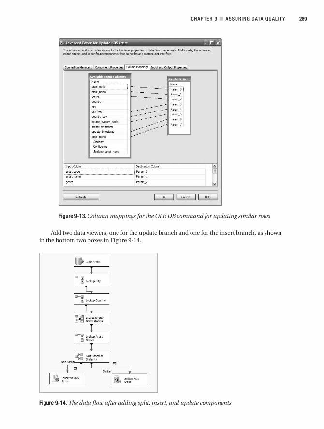
Figure 9-13. Column mappings for the OLE DB command for updating similar rows
Add two data viewers, one for the update branch and one for the insert branch, as shownin the bottom two boxes in Figure 9-14.
Figure 9-14. The data flow after adding split, insert, and update components
CHAPTER 9 ■ ASSURING DATA QUALITY 289
9314ch09final.qxd 11/15/07 10:07 AM Page 289

The bottom part of Figure 9-14 is basically an UPSERT operation (insert if it does not existand update if it exists), but it uses fuzzy lookup to determine approximate matches. In Fig-ure 9-14, the Lookup Artist Names box checks whether the incoming artist names match theNDS artist table using fuzzy lookup. The Split Based on Similarity box splits the flow basedon the fuzzy lookup similarity score. The flow is split into an “insert branch” that inserts theincoming data into the artist table and an “update branch” that updates the existing rows inthe artist table.
Save and execute the package, and notice that the first data row (the insert one) shows theeleven rows with similarity greater than 85 percent. Click Continue (the green arrow). The sec-ond data viewer then shows the nine rows that don’t exist in the NDS with similarity less than70 percent. Check the NDS artist table to make sure that eleven rows in the destination artistNDS table are updated and nine are inserted.
So, we have created a SSIS package that imports the artist data from the stage table andloads it into the NDS database, using the Fuzzy Lookup transformation instead of using anexact match. If the artist name on the stage table is “similar” to the one in the NDS, we updatethe NDS record. Otherwise, we insert it into the NDS. We defined the “similarity” criteria bydetermining the similarity threshold by allowing all records from the stage to flow through theFuzzy Logic transformation to score them. Once we determined the similarity threshold, weset the Fuzzy Logic transformation to split the data from the source into two branches. For the“similar” branch, we update the NDS based on the source data, and for the “nonsimilar”branch we insert the source data into NDS.
Cross-checking with External SourcesSome data-cleansing activities are done internally, such as checking 100 stores includingtheir store types, locations, phone numbers, web sites, store numbers, regions, and divisions.In this case, we manually verify that the store details in the system are accurate and correctthem if they are wrong.
Some data cleansing is done by cross-referencing with external data sources, such aschecking and fixing names and addresses in the customer table, identifying duplicate cus-tomer records (individual level, household level, or company level), and flagging deceasedcustomers. We can also use external sources for enriching our data, such as by adding tele-phone numbers to the customer data.
Cross-referencing with external data can be done by using data from post office organiza-tions such as Address Information Systems (AIS) and NCOA Link from the U.S. Postal Service.Or, in the United Kingdom, this can be done using the Royal Mail Postcode Address File (PAF).In some countries, other possible data sources are voter registration and the electoral roll.Another example of external data is reference data from the International Standard Organiza-tion, such as country names and languages, as we discussed in Chapter 7.
External data sources are delivered in various formats and in various ways. This affectsthe way we integrate the external data with our data warehouse. Some are delivered as files onCD-ROMs, some are delivered as a system (you need to install the system to use it, with auto-matic weekly updates via the Internet, for example), some are using EDI, and some aredelivered online using web services.
We need to work with the providers to be able to use their data or services appropriatelyin our data warehouse. Looking at how the external data is integrated into the data warehouse,
CHAPTER 9 ■ ASSURING DATA QUALITY290
9314ch09final.qxd 11/15/07 10:07 AM Page 290

we can classify these different delivery mechanisms into two big approaches. With the firstapproach, we bring the external data into the data warehouse. The provider gives us the data,and we store it in the data warehouse. With the second approach, we don’t bring the externaldata into our data warehouse. Instead, we leave the data with the provider, and we “tap” thedata as and when we need it. This “tapping” is done, for example, using web services.
Data Quality RulesData quality rules are essentially filters to prevent dirty data from getting into the warehouse.Based on the data location, there are three kinds of data quality rules:
• Incoming data validation
• Cross-reference validation
• Data warehouse internal validation
Incoming data validation is where we check the incoming data only on its own, withoutreferring to the data already in the warehouse (the ODS, NDS, or DDS). Incoming data valida-tion is performed on the fly when the data is being loaded into the warehouse. These rulesverify that the data from the source systems is valid, in other words, within the expected rangeand in the right format. Examples are that the product code is in AAA999AA format, the pricesfor a certain product range are greater than $1, the song duration is between one and ten min-utes, and the subscription duration is greater than or equal to one month. Here are three realexamples from my projects:
• ∑(col1, col2, col3) > 0 where col4 > 0 and col5 > 0
• Value of data limited to list: value1, value2, value3, value4
• Fiscal period <= 13
Cross-reference validation is where we check the incoming data against the data in thewarehouse. The objective is to make sure that the value of the incoming data is within a cer-tain range that is calculated based on the data already in the warehouse: the incoming data isexpected to be within a 25 percent range of the average of col1, the number of downloadedsongs per week is less than 50 times the registered devices (the number of registered devices isdata already in the warehouse, while the number of downloaded songs is incoming data fromthe source systems), and the incoming unit cost is within 15 percent of the average of the lastthree months of supplier costs. Like incoming data validation, cross-reference validation isperformed on the fly when the data is being loaded into the warehouse.
Data warehouse internal validation is where we check the data already in the warehouse.We don’t check the incoming data. The purpose of doing this is to verify the quality of the datain the warehouse at the aggregate level. In other words, the details data (record level) might becorrect, but the totals might be incorrect. This can be done by comparing the totals over aperiod of time against a known standard value. Examples of data warehouse internal valida-tion are that the number of new subscriptions last week is less than or equal to 5,000; theaverage number of copies for each title in the last three weeks is between 10 and 20; and theaverage unit cost of last week’s title is within 10 percent of the average of the last three months.
CHAPTER 9 ■ ASSURING DATA QUALITY 291
9314ch09final.qxd 11/15/07 10:07 AM Page 291

Unlike the previous two, data warehouse internal validation is performed after the incomingdata is fully loaded into the warehouse.
The DQ rules for internal data warehouse validation have different running frequencies.That is, some are run every few hours, some are daily, and some are weekly or monthly. The fre-quency depends on how critical the data is and how quickly the business needs to be informedif some inaccuracies happen. If the data is critical (such as data that has direct impact on therevenue or has potential risks of breaking government regulations), the business may need toknow quickly, so we need to set up the DQ rules at short frequencies such as every four hours ortwice a day. The frequency also depends on the volume and seasonality of data. For example, ifthe number of subscriptions varies widely every day, we may want to compare it weekly ratherthan daily.
We need to be careful with the last two categories (cross-reference validation and datawarehouse internal validation), because it can potentially impact the ETL performance.Here’s why. When the DQ rules involve a statistical calculation, such as “within 15 percent ofthe average of the last three months of supplier costs,” it could take a long time to calculatethe statistics. So if we tried to calculate the statistics on the fly, we would face a bottleneck,and the ETL process would be very slow. One common technique is to calculate the statisti-cal figures beforehand, such as the day before. This way, when the DQ rule runs, the statisticsare already calculated and stored in the warehouse as constant numbers. So, the validationwill be fast because we are comparing against constant numbers rather than a formula.
Not all DQ rules are errors. Some DQ rules are only warnings. For warnings, we still wantthe occurrence to be reported, but we are not rejecting the data. We allow the data to beloaded into the warehouse. For example, if the data is more than 35, it is good, and if it is lessthan 30, it is an error. But if it is between 30 and 35, it is a warning. Even though we load thedata into the warehouse, the data still needs to be reported to the business users and subse-quently corrected in the source systems so that the next time that data is loaded into thewarehouse, it is already correct.
Some DQ rules are neither an error nor a warning but are informational only. In otherwords, there is no issue whatsoever with the data. An example of this kind of DQ rule is if thenational sales amount on a weekday is more than $3 million, we need to inform the nationalsales manager. This is neither an error nor a warning, but is informational only. On the con-trary, the reverse (too little rather than too much) might be an error or a warning; for example,if the national sales amount on a weekday is less than $300,000, then there may be a problemwith the ETL, perhaps because not all source sales data is loaded properly into the data ware-house for that day.
I have found that it is good practice in a data warehouse project for the business user towrite a document called Data Quality Business Rules. It essentially describes all the businessrules, what type they are, which data warehouse attributes they are applicable to, what is theappropriate course of action (for example, reject, allow, or fix; see the next section), and whoshould be notified when a violation to a rule occurs. The document is written in pure Englishwith no SQL code or pseudocode. For example, rather than where (prd_type = 'FL' andunit_cost < 2.25) or (prd_type = 'AB' and unit_cost < 1.43), we should describe it as“The incoming unit cost should be less than 2.25 for films and less than 1.43 for audio books.”The developer can then translate this to SQL when implementing the rules in SSIS. I havefound that throughout the development process we kept referring to this handy document.
CHAPTER 9 ■ ASSURING DATA QUALITY292
9314ch09final.qxd 11/15/07 10:07 AM Page 292

■Tip When defining DQ rules, define them based on the risk, in other words, the impact or damage. It isuseful to know that if rule #34 is violated, all the marts will be totally inaccurate and useless, whereas if rule#17 is violated, the impact is almost negligible, and we have nothing to worry about. It is very useful to havethis attribute in the previously mentioned document and on the DQ reports (see the DQ report section later inthis chapter). We can then define the urgency and service-level agreement (SLA) based on the risk level. Forexample, risk level 5 rules need to be solved next day, whereas risk level 1 has a four-week period.
The DQ rules are described in a table called dq_rules. The purpose of this table is todescribe the details of each data quality rule including the following:
• The objective of the rule (including the calculation if any, in English)
• Whether it is an error, is a warning, or is informational
• What type of validation it is (whether it is an incoming data validation, cross-referencevalidation, or internal validation)
• How critical the rule is (measured by the risk), from level 1 (low risk) to level 5 (highrisk)
• What actions to take, such as reject the data, allow the data into the warehouse, or fix it
• The status of the rule (whether it is active or disabled)
• Who to notify when there is a violation to this rule
This table is used by the data firewall to check the incoming data before loading it into theNDS or ODS. In some implementations, the DQ rule table is placed in the metadata database;in other implementations, the DQ rule table is placed in the DQ database. For performancereasons, in my opinion, it is better to put it in the DQ database because it is referenced by theDQ tables, even though technically it is a metadata table (I’ll discuss metadata in the nextchapter). Essentially the DQ rule table contains the same columns as the Data Quality BusinessRules document, in other words, rule_id, rule_name, rule_description, rule_type (error orwarning), category (incoming data, cross-reference, or internal), risk_level (1 to 5), status,action, notification, create_timestamp, and update_timestamp. This table will be cross-referenced by the DQ audit tables. DQ audit tables store the records that fail the DQ rulevalidation. We’ll discuss DQ rules table in more detail in the next chapter.
Action: Reject, Allow, FixWhen a data quality rule is violated, we have three choices of what to do with the data: we canreject the data, allow the data into the warehouse, or fix/correct the data. These are known asactions. Which action is appropriate for a particular piece of data depends on the situation,the risk level, the rule type (error or warning), and so on.
CHAPTER 9 ■ ASSURING DATA QUALITY 293
9314ch09final.qxd 11/15/07 10:07 AM Page 293

The reject action means that we do not allow the data into the warehouse. We put it in anaudit table in the DQ database. The data will then be reported to the business users and cor-rected before it is loaded into the data warehouse. Typically, the structure of the audit table isthe same as the structure of the source system table, but with five additional columns: dq_id,rule_id, dq_timestamp, dq_action, and dq_status. If on the source system we have 60 tables,then there will be 60 audit tables in the DQ database. If these are your 60 tables in your sourcesystem:
artistchannelcustomercustomer_statuscustomer_typeformat…product_typestore
then these are the audit tables in the DQ database:
artistchannelcustomercustomer_statuscustomer_typeformat…product_typestore
Yes, the table names are the same, and they have all the columns in the original table,plus five additional columns: dq_key, rule_key, dq_timestamp, dq_action, and dq_status.dq_key contains a sequential identity(1,1) column. rule_key is the identifier of the DQ rulethat causes this row to be rejected by the data firewall and put in the quarantine table (seethe previous section for the dq_rule table). dq_timestamp is the time when this row wasrejected by the data firewall. dq_action is the action taken to the incoming data (reject,allow, or fix). dq_status is the correction status (fixed or not fixed).
So, if we reject a row of address data, instead of going into the address table in the NDS (orthe ODS or the DDS, depending on your DW architecture), the row goes to the address audittable in the DQ database. The row will be reported (see the section “Data Quality Reports andNotifications” later in this chapter) to the relevant people, fixed in the source system, andreloaded into the NDS (or the ODS or the DDS). If the address table is extracted using “thewhole table every time” approach, it’s not a problem. In other words, the row will be loadedautomatically in the data warehouse on the next ETL batch that occurs after the row is cor-rected. If the address table is extracted incrementally, we need to “memorize” the failed row,and we need to keep extracting the row on the ETL batch until it is corrected. One way to dothis is by modifying the extraction SQL, adding something like this: … union select [columns]from source.dbo.address src join dq.dbo.address d on src.address_id = dq.address_id
CHAPTER 9 ■ ASSURING DATA QUALITY294
9314ch09final.qxd 11/15/07 10:07 AM Page 294

and dq_status <> 'C'. And when the row has been loaded successfully, we mark the row onthe audit table as C (or closed). In SSIS, as an alternative to the Execute SQL task, we can alsouse a merged join or a Lookup transformation for this purpose.
Instead of fixing it in the source system, we can also take the approach of correctingthe failed row stored in the DQ database and reloading it to the data warehouse. Althoughthis is less favorable because we leave the source system incorrect, at times it is more prac-tical, because it has a quicker turnaround time, resulting in the row being loaded into thewarehouse sooner. The drawback of choosing this approach is that the source system isstill incorrect so that the next time the data is retrieved from the source system, we willstill face the same problem. That’s why it is usually used for data that does not change fre-quently, such as reference data. This approach is usually used as a temporary measure,while waiting for the data change request to be implemented in production (which couldtake, say, two to three weeks).
Instead of rejecting the dirty data, we can allow it into our warehouse. Wait a minute,why do we want to do this? Well, there are several reasons. One reason is because perhaps itis only a warning, not an error; for example, the rule may say that single-title revenue shouldbe between $1 and $4. If it is between 0 and 1 or between 4 and 10, allow it in. But if it is lessthan 0 or greater than 10, reject it. This is because (for example) the majority of the products(say, 99 percent) are priced between $1 and $4. Sometimes (the 1 percent) products arepriced very low for sale or promotional reasons (between 0 and $1) and very high for sea-sonal reasons (between $4 and $10). That is why these two ranges are only a warning, not anerror. But a negative price or prices more than $10 never happens in the business for thatproduct type, so that is why in this example the “< 0” and “> 10” are classified as errors.
The second reason for allowing the data into the warehouse is that other data in the samerow is required for data integrity. Each fact table row is essentially a business transaction. If wedon’t load some rows, the total of that day would not be correct because there is some missingdata. For example, a Subscription Sales fact table contains eight dimension keys and nineteenfacts. Say one column does not satisfy a DQ rule; for example, the subscribe_timestamp col-umn contains an invalid date. All the other facts are OK; subscription_revenue, single_title_revenue, monthly_revenue, music_quantity, music_unit_cost, monthly_music_cost, film_quan-tity, film_unit_cost, monthly_film_cost, book_quantity, book_unit_cost, monthly_book_cost,monthly_indirect_cost, monthly_cost, monthly_margin, annual_revenue, annual_cost,annual_profit, and subscriber_profitability are all correct. We have two choices: if we rejectthe fact row, the total of all these facts will be incorrect. If we allow the row in, the total of allthese facts will be correct, and the subscribe_timestamp will be set to unknown. The invaliddate will still be logged, reported, fixed, and reloaded next time.
The third possible action is to automatically fix the data based on certain rules. In thiscase, when the data firewall detects a certain value, it automatically replaces it with anothervalue, based on certain criteria. For example, say in the source system we have “NA,” “ N/A,”“N.A.,” and “Not Applicable.” We create a DQ rule to replace “NA,” “N/A,” and “N.A.” with“Not Applicable.” This way, the data in the data warehouse is clean, even though the data inthe source system is not. Here’s another example: in the source system store 17 is in region 1.This is incorrect. Store 17 should be in region 2. We create a DQ rule to update the regionautomatically. Here’s another example: when the total customer purchase is between $500and $1,000 in the source system, it is classified as band C. In the data warehouse, this range isclassified as band D. We create a DQ rule to update the customer band from C to D. Note thatin a way, this is like an ETL transformation, because we update the data as we load it into the
CHAPTER 9 ■ ASSURING DATA QUALITY 295
9314ch09final.qxd 11/15/07 10:07 AM Page 295
data warehouse. We need to be careful when implementing autofix actions like this, becausethe data in the source system is still wrong. It is (always) better to fix the data in the sourcesystem than to fix it in the data warehouse. But if we cannot change it in the source system,this could be an alternative solution. Or perhaps it’s possible to fix the data in the source sys-tem, but it will take a long time. In that case, we could implement this temporarily.
One example of a good use of a DQ rule with autofix action is formatting, for example, toconvert to mixed case or to remove spaces. For example, in the format column of the producttable in the source system, we have the following entries: “DVD 5,” “DVD-5,” and “DVD5,” andin the ODS or NDS the entry is “DVD-5.” When loading the product table from the source sys-tem, we can create a DQ rule with an action to convert them to “DVD-5.” Some people arguethat this should be implemented as a normal “transformation” in the ETL logic, so why wouldwe want to put it as a DQ rule? Well, the main difference between an ETL transformation and aDQ rule is the reporting aspect. We know that this inconsistency between “DVD 5,” “DVD-5,”and “DVD5” is an issue in the source system. In other words, there is no referential integrityfrom the product table to the format table. We have reported this to the source system ownerand the data will be fixed in the next few weeks, but in the meantime we need to keep the datawarehouse up and running, so we put this rule in. Because it is a DQ rule with an autofixaction, it is reported to the appropriate people regularly, so we know when it is fixed. If it isimplemented as an ETL transformation, it won’t be reported and monitored. Well, actually youcan report and monitor ETL transformation, but it will slow the ETL processes down if youneed to report and monitor all the transformations. Also, an ETL transformation is not as richas a DQ rule; for example, it doesn’t have the following:
• The objective of the rule (including the calculation if any)
• Whether it is an error, is a warning, or is informational
• What type of validation it is (whether it is an incoming data validation, cross-referencevalidation, or internal validation)
• How critical the rule is (measured by the risk), for example from level 1 (low risk) tolevel 5 (high risk)
• What actions to take, such as reject the data, allow the data into the warehouse, or fix it
• The status of the rule (whether it is active or disabled)
• Who to notify when there is a violation to this rule
Logging and AuditingWhen a DQ rule is violated, we store that event in the data quality database. We store the timethat violation happened, which rule was violated, what action was taken, and the correctionstatus. We store all of this information in a table called the data quality log, or DQ log for short.We also need to store the rows that failed the DQ rule. This process of recording the DQ ruleviolation events, along with the rows that failed the DQ rules, is called data quality logging.
CHAPTER 9 ■ ASSURING DATA QUALITY296
9314ch09final.qxd 11/15/07 10:07 AM Page 296

The failed rows are also stored in the DQ database, but not in the DQ log table. They arestored in a number of tables called data quality audit tables. The structures of the audit tablesare the same as the target data warehouse tables. So if the target table has ten columns, theaudit table also has ten columns, with each column having the same name and the same datatypes as the target tables. This process of analyzing the data quality rules violation by queryingthe DQ log table and DQ audit tables is called data quality audit.
We store the failed rows in the corresponding audit table; for example, if the failed rowswere for the customer table, we store them in the customer audit table. If the failed rows werefor the subscription table, we store them in the subscription audit table. Whether the action ofthe DQ rule is to reject, allow, or fix, we still need to put the failed rows in the audit tables.
One additional column in the audit tables makes them different from the target datawarehouse table: the primary key. The primary key of an audit table is a surrogate integer col-umn. This primary key is stored in the DQ log table as a foreign key. This is how the audittables are linked to the DQ log table, as shown in Figure 9-15.
Figure 9-15. The DQ log table and the DQ audit tables
As we can see in Figure 9-15, the DQ log table stores four pieces of information related tothe violation event: which rule was violated (rule_key), when it happened (dq_timestamp),what action was taken (dq_action), and the correction status (dq_status). In Figure 9-15,log_key is the primary key of the dq_log table.
Figure 9-15 shows that the DQ log tables contain three other key columns: table_key,dq_key, and row_key. These three key columns point to the failed rows stored in the DQ audittables.
CHAPTER 9 ■ ASSURING DATA QUALITY 297
9314ch09final.qxd 11/15/07 10:07 AM Page 297
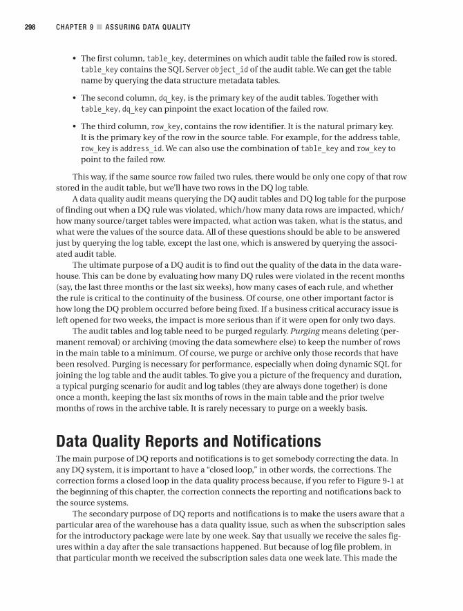
• The first column, table_key, determines on which audit table the failed row is stored.table_key contains the SQL Server object_id of the audit table. We can get the tablename by querying the data structure metadata tables.
• The second column, dq_key, is the primary key of the audit tables. Together withtable_key, dq_key can pinpoint the exact location of the failed row.
• The third column, row_key, contains the row identifier. It is the natural primary key.It is the primary key of the row in the source table. For example, for the address table,row_key is address_id. We can also use the combination of table_key and row_key topoint to the failed row.
This way, if the same source row failed two rules, there would be only one copy of that rowstored in the audit table, but we’ll have two rows in the DQ log table.
A data quality audit means querying the DQ audit tables and DQ log table for the purposeof finding out when a DQ rule was violated, which/how many data rows are impacted, which/how many source/target tables were impacted, what action was taken, what is the status, andwhat were the values of the source data. All of these questions should be able to be answeredjust by querying the log table, except the last one, which is answered by querying the associ-ated audit table.
The ultimate purpose of a DQ audit is to find out the quality of the data in the data ware-house. This can be done by evaluating how many DQ rules were violated in the recent months(say, the last three months or the last six weeks), how many cases of each rule, and whetherthe rule is critical to the continuity of the business. Of course, one other important factor ishow long the DQ problem occurred before being fixed. If a business critical accuracy issue isleft opened for two weeks, the impact is more serious than if it were open for only two days.
The audit tables and log table need to be purged regularly. Purging means deleting (per-manent removal) or archiving (moving the data somewhere else) to keep the number of rowsin the main table to a minimum. Of course, we purge or archive only those records that havebeen resolved. Purging is necessary for performance, especially when doing dynamic SQL forjoining the log table and the audit tables. To give you a picture of the frequency and duration,a typical purging scenario for audit and log tables (they are always done together) is doneonce a month, keeping the last six months of rows in the main table and the prior twelvemonths of rows in the archive table. It is rarely necessary to purge on a weekly basis.
Data Quality Reports and NotificationsThe main purpose of DQ reports and notifications is to get somebody correcting the data. Inany DQ system, it is important to have a “closed loop,” in other words, the corrections. Thecorrection forms a closed loop in the data quality process because, if you refer to Figure 9-1 atthe beginning of this chapter, the correction connects the reporting and notifications back tothe source systems.
The secondary purpose of DQ reports and notifications is to make the users aware that aparticular area of the warehouse has a data quality issue, such as when the subscription salesfor the introductory package were late by one week. Say that usually we receive the sales fig-ures within a day after the sale transactions happened. But because of log file problem, inthat particular month we received the subscription sales data one week late. This made the
CHAPTER 9 ■ ASSURING DATA QUALITY298
9314ch09final.qxd 11/15/07 10:07 AM Page 298
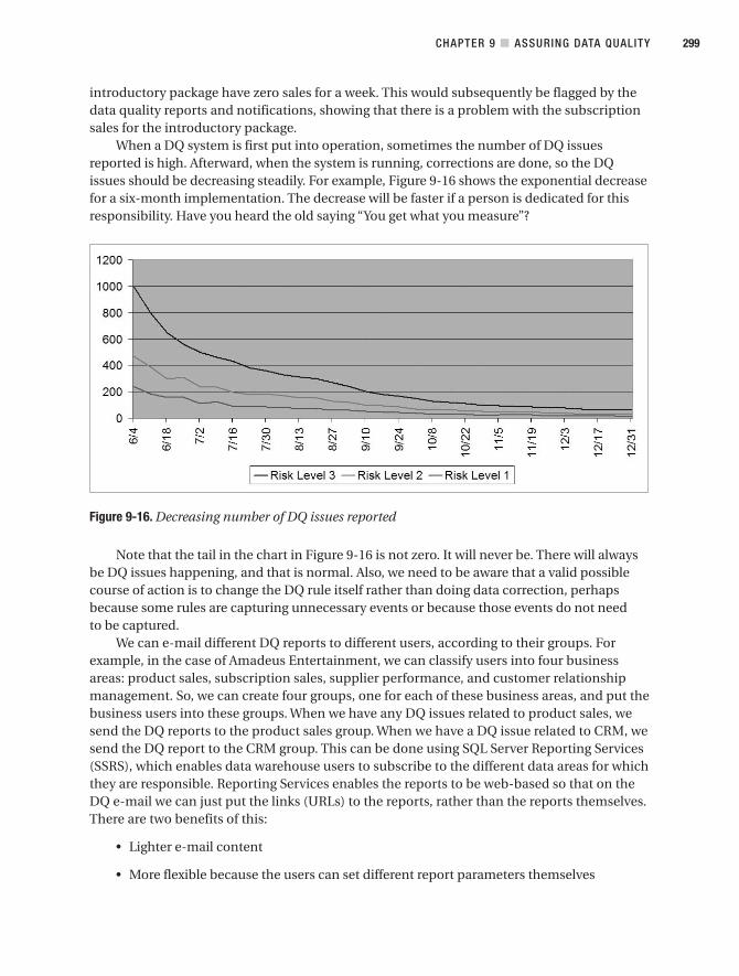
introductory package have zero sales for a week. This would subsequently be flagged by thedata quality reports and notifications, showing that there is a problem with the subscriptionsales for the introductory package.
When a DQ system is first put into operation, sometimes the number of DQ issuesreported is high. Afterward, when the system is running, corrections are done, so the DQissues should be decreasing steadily. For example, Figure 9-16 shows the exponential decreasefor a six-month implementation. The decrease will be faster if a person is dedicated for thisresponsibility. Have you heard the old saying “You get what you measure”?
Figure 9-16. Decreasing number of DQ issues reported
Note that the tail in the chart in Figure 9-16 is not zero. It will never be. There will alwaysbe DQ issues happening, and that is normal. Also, we need to be aware that a valid possiblecourse of action is to change the DQ rule itself rather than doing data correction, perhapsbecause some rules are capturing unnecessary events or because those events do not needto be captured.
We can e-mail different DQ reports to different users, according to their groups. Forexample, in the case of Amadeus Entertainment, we can classify users into four businessareas: product sales, subscription sales, supplier performance, and customer relationshipmanagement. So, we can create four groups, one for each of these business areas, and put thebusiness users into these groups. When we have any DQ issues related to product sales, wesend the DQ reports to the product sales group. When we have a DQ issue related to CRM, wesend the DQ report to the CRM group. This can be done using SQL Server Reporting Services(SSRS), which enables data warehouse users to subscribe to the different data areas for whichthey are responsible. Reporting Services enables the reports to be web-based so that on theDQ e-mail we can just put the links (URLs) to the reports, rather than the reports themselves.There are two benefits of this:
• Lighter e-mail content
• More flexible because the users can set different report parameters themselves
CHAPTER 9 ■ ASSURING DATA QUALITY 299
9314ch09final.qxd 11/15/07 10:07 AM Page 299

The DQ rule violations can also be sent to the users using notifications. For this we canuse SQL Server Notification Services. For example, we can set the Notification Services to readthe DQ log table and DQ audit tables and deliver the newest records to the users.
We can also create a dashboard application to display the overall data quality status forthe whole warehouse, along with the key data quality indicator of each business area. Thedashboard can also contain some data quality reports and selected data quality charts, suchas the one shown in Figure 9-17.
Figure 9-17. Data quality dashboard
SummaryIn this chapter, I discussed what data quality is and why it is so important. I discussed the dataquality process and the components involved in the process. I talked about data cleansing anddata matching, and I showed how to do a Fuzzy Lookup transformation in SSIS.
I discussed the categories of data quality rules in terms of validation and the choices ofwhat to do with the data when a data quality rule is violated: reject, allow, or fix. I talked aboutlogging and auditing, and I finished the chapter by talking about reporting and notification inorder to get somebody correcting the data.
Of all the various aspects of data warehousing, data quality is probably the most impor-tant one. Simply speaking, this is because if the data is wrong, we cannot use the datawarehouse.
CHAPTER 9 ■ ASSURING DATA QUALITY300
9314ch09final.qxd 11/15/07 10:07 AM Page 300

Metadata
In general, metadata means data that describes data. For example, in photography, we storeour photographs as RAW or JPG files. That is the data. But we also store the following infor-mation: which camera we used to take the photographs, the aperture and ISO settings of thecamera, the resolution of each photograph, where it was taken, when it was taken, and a fewwords describing the content of the photo. That is all metadata.
Metadata in data warehousing is different from photography, though. In this chapter,I will discuss what metadata is in a data warehousing context, why metadata is important indata warehousing, what it is used for, how to store it, and how to maintain it.
Metadata in Data WarehousingIn data warehousing, metadata contains the definitions of data (the meaning and sourceof each column), the definition of the data warehouse itself (in other words, the data storestructure, the ETL processes, and the data quality), the definition of the related systems (forexample, the source systems), the audit information (what processes ran and when they ran),and the usage (which reports and cubes are used by whom and when). So, we have sevenkinds of metadata:
• Data definition and mapping metadata contains the meaning of each fact and dimen-sion column and where the data is coming from.
• Data structure metadata describes the structure of the tables in each data store.
• Source system metadata describes the data structure of source system databases.
• ETL process metadata describes each data flow in the ETL processes.
• Data quality metadata describes data quality rules, their risk levels, and their actions.
• Audit metadata contains a record of processes and activities in the data warehouse.
• Usage metadata contains an event log of application usage.
I’ll discuss these briefly here, and in the subsequent sections I will discuss them in moredepth.
The data definition metadata contains the meaning of each fact, dimension key, anddimension attribute within the data warehouse. “Meaning” is the business description of thedata in the context of the organization where the data warehouse is implemented or used.
301
C H A P T E R 1 0
9314ch10final.qxd 11/15/07 10:05 AM Page 301

This is necessary so that all users have a common understanding about what the facts andattributes mean. For example, in Chapter 5, we defined title availability as the percentageof the product titles being available in the last three months when Amadeus Entertainmentordered them. Having a definitive meaning of title availability stored in a metadata databaseand viewable by the users is useful to avoid confusion and misperception. The users can viewthe data definitions either via reports created using SSRS or via direct query using EnterpriseManager. Data definition metadata also contains the business description of each column inthe NDS or ODS.
Data mapping metadata (sometimes called data lineage metadata) is about where eachpiece of data is coming from. For example, the music_unit_cost fact in the Subscription Salesfact table in the DDS is from the unit_cost column in the product table in the NDS. Theunit_cost column in the product table in the NDS is from the unit_cost column in theproduct table in the stage database. And the unit_cost column in the product table in thestage database is from the unit_cost column in the product table in the Jade source system.The data lineage metadata makes it easier to perform the impact analysis. Impact analysis isan activity to understand the effect of a particular change to different elements of the datawarehouse. For example, when the source system DBA says that the unit_cost column in theJupiter product table will not contain intercompany trading figures, we can understand whatcolumns on the ODS, NDS, and DDS will be impacted.
Data structure metadata describes the structure of the DDS, NDS, ODS, and stage data-bases. It contains an entry for every table in the data warehouse. It contains the data types foreach column in every table, including the collation, whether the column is a primary or a for-eign key, and whether the column is an identity column or can contain null. For the DDS, italso contains the dimensional hierarchy and SCD details and the index, view, and partitioninformation. Why don’t we just use SQL Server object catalog views directly instead of buildingdata structure metadata? The reason is that we need to reference the database objects in theETL metadata, DQ metadata, and data description metadata in order to understand theirstructure.
Source system metadata describes the data structure of all the source systems feedinginto the data warehouse. It contains the data type, collation, primary key, foreign key, view,index, and partition. It also contains volumetric data and data profiling information. Sourcesystem metadata is used to help users understand the source of the data.
Audit metadata contains the results of all processes and activities in the data warehouse,such as ETL processes, data modification, DQ rule validation, security log, system patches,purging, indexing, and partitioning activities. Audit metadata is used for administering thedata warehouse such as to verify whether the ETL processes ran successfully.
Usage metadata contains a log that records which reports and cubes are used by whomand when. Usage metadata is used to understand the access and usage pattern of the datawarehouse applications. For example, how many times is a particular report accessed andby which users or departments?
ETL metadata contains the description of each data flow, where they extract from, whatthe destination is, what transformation is applied, the parent process, and the schedule whenit is supposed to run. Along with the data mapping metadata, ETL metadata is useful tounderstand the data flow and transformation. ETL metadata is also used to determine thesequence each task is run in an ETL batch.
Data quality metadata describes each data quality rule, along with the rule types, whichtable and column they are applicable for, their risk level, and their actions. Data quality meta-data is used to determine what action to take when “bad data” is detected.
CHAPTER 10 ■ METADATA302
9314ch10final.qxd 11/15/07 10:05 AM Page 302

Why do we need metadata? The primary reason is to describe and explain the data andthe data warehouse (the structure and processes) to the users. This explanation enables theusers to use the data warehouse better. This explanation also makes it easier to enhance andmaintain the data warehouse. For example, data definition metadata helps new users under-stand the meaning of each fact and dimension attribute, along with its sample values. Datadefinition metadata also helps avoid misunderstanding among existing users about the mean-ing of certain columns. Data mapping metadata helps us understand the impact if a columnin the source system is deprecated or if we want to add a new column in the data warehouse.This is possible because data mapping metadata explains the source of each piece of data.
The secondary reason is for audit purposes to understand what happened, where it hap-pened, and when it happened. For example, when an ETL process stopped unexpectedly, theaudit metadata helps us understand which steps have been executed, what the results of thosesteps are, and which steps have not been executed so we can pinpoint the exact point in theETL process where it failed. This is because audit metadata contains the results of all pro-cesses and activities in the data warehouse, including ETL processes, data modification, andDQ rule validation. That will make it easier to find out the cause of failure, and it enables theETL processes to recover from the point of failure the next time it runs.
Metadata is also used by the system to run operational tasks, such as determining therequired action when “bad data” is detected by a data quality rule and the order the ETL tasksneed to be executed.
For maintainability, we use normalized forms in the metadata database; in other words,the table names and column names are stored in data structure metadata. Data definition,data mapping, ETL metadata, and audit metadata refer to the data structure metadata by stor-ing the table keys and column keys. By using normalized forms, we need to modify only oneplace when we want to change something in the metadata database.
Data Definition and Mapping MetadataData definition metadata is a list of all columns from every table in the DDS, ODS, and NDS(depending on which architecture we chose; see Chapter 2), along with their meanings andsample values. Instead of mentioning the data store names, table names, and column names,data definition metadata uses the table key and column key defined in the data structuremetadata.
Mapping metadata describes where each piece of data comes from in the source system.Mapping metadata is also known as data lineage metadata. If the mapping metadata containsonly the source system column name, it can be put on the same table as the data definitionmetadata. But if the mapping metadata contains the complete data lineage between the DDS,the NDS/ODS, the stage, and the source systems, then it is usually placed in a separate table.The benefit of putting the mapping metadata in the same table as the data definition meta-data is that the structure is simpler. The benefit of putting mapping metadata in separatetables is that the structure is more flexible and has less data redundancy.
Table 10-1 contains an example of data definition and mapping metadata. Table 56 is theproduct table, and table 68 is the campaign result fact table. The source column is located onthe database one step earlier in the process; in other words, if it is a DDS column, we put theNDS column as the source. If it is an NDS column, we put the stage column as the source. Ifit is stage column, we put the source system column as the source.
CHAPTER 10 ■ METADATA 303
9314ch10final.qxd 11/15/07 10:05 AM Page 303

Table 10-1. Data Definition Metadata
table_key column_key description sample_value source_column_key
56 112 The surrogate key of the product 3746 88dimension. It is unique, is not null, and is the primary key of the product dimension.
56 113 Natural key. Product code is the FGA334288 89identifier and primary key of the product table in Jupiter. It is in AAA999999 format.
56 114 The product name. The Panama 90Story DVD
56 115 The product description. The Panama 91Story movie on DVD format
56 116 The song/film/book title. The Panama 92Story
56 117 The singer, star, or author. Mark Danube 93
56 118 Level 1 of product hierarchy; in other Film 94words, music, film, or book.
56 119 Level 2 of product hierarchy; in other Action 95words, for film, it could be thriller, western, comedy, action, documen-tary, children, Asian, and so on.
56 120 Format of the media; in other words, DVD 96MP3, MPG, CD, or DVD.
56 121 Price for one item. 4.75 97
56 122 Allocated direct and indirect costs. 3.62 98
56 123 Upcoming if we have signed contract Active 99with the supplier, active if it is still being offered to the customer, expired if it is no longer being offered.
68 251 The key of the campaign that was 1456 124sent to customers.
68 252 The key of the customer who was 25433 145intended to receive this campaign.
68 253 The key of the communication to 5 165which the campaign belongs. For example, this campaign is an instance of a communication called “Amadeus music weekly newsletter” dated 02/18/2008.
68 254 The key of the communication 3 178channel to which this campaign is sent. For example, a campaign could be sent to 200,000 customers, 170,000 by e-mail and 30,000 by RSS.
68 255 The key of the date when this 23101 189campaign was actually sent.
CHAPTER 10 ■ METADATA304
9314ch10final.qxd 11/15/07 10:05 AM Page 304

table_key column_key description sample_value source_column_key
68 256 The key of the delivery status. 0 means 1 193not sent. 1 means successfully delivered. 1 to N contains various dif-ferent reasons why the campaign failed to be delivered to the intended recipient, such as the mailbox was unavailable, the mailbox does not exist, and so on.
68 257 1 if the campaign was actually sent to 1 204the recipient (out our door); 0 if it was not sent. Examples of reasons for not sending are failed e-mail address validation and no customer permission.
CHAPTER 10 ■ METADATA 305
The Data Definition Language (DDL) of the data definition table in Table 10-1 is as followsso you can create the table for the case study:
use metago
create table data_definition( column_key int not null, table_key int not null, column_type_key int not null, description varchar(200), sample_values varchar(50), source_column_key int not null, create_timestamp datetime not null, update_timestamp datetime not null, constraint pk_data_definitionprimary key clustered (column_key)
)go
create index data_definition_descriptionon data_definition(description)go
The table_key column is optional, because the column key links to the data structuremetadata column table that also has a table key. The index on the description column helpsquerying a column with a particular meaning. To enable sophisticated word searches, youmay want to build a full-text index on the description column instead, as follows:
create fulltext catalog data_definition_fulltext_catalogin path 'd:\disk\data6'as defaultgo
9314ch10final.qxd 11/15/07 10:05 AM Page 305

create fulltext indexon data_definition (description)key index pk_data_definitiongo
Columns in data warehouse tables serve different purposes. A column type indicatesthese purposes. A column type helps differentiate, for example, dimensional attributes fromthe fact column. Table 10-2 lists various column types and their descriptions. Column typescan be put on data structure metadata or on data definition metadata.
Table 10-2. Column Types
Column Type Location Description
Surrogate key DDS dimension tables A single not null column that uniquely identifies arow in a dimension table.
Natural key DDS dimension tables Uniquely identifies a dimension row in the sourcesystem.
Dimensional DDS dimension tables Describes a particular property of a dimension.attribute
Degenerate DDS fact tables Identifies a transaction in the source system. A dimension natural key of a dimension without any attributes.
SCD support DDS dimension tables Columns that support slowly changing dimensionsuch as is_active, effective_date, and expiry_date.
Measure DDS fact tables Columns in the fact table that contain businessmeasurements or transaction values.
Fact key DDS fact tables A single not null column that uniquely identifies arow on a fact table.
System All data stores Auxiliary columns created by the system for systemusage such as create_timestamp and update_timestamp.
Transaction ODS and NDS tables Column in normalized tables containing businesstransaction values, such as order tables.
Master ODS and NDS tables Columns in normalized tables that contain masterdata such as stores, products, and campaigns.
Stage Stage tables Columns in stage tables containing business data.
In addition to table columns, we can also include report columns in data definition meta-data. We do this by adding the report columns in the metadata_definition table. This way, themeaning of every column in every report is explained properly. This helps avoid confusionamong the users about the meaning of particular columns in a report. For example, a columncalled profitability can have many different meanings.
As I described earlier, if we want to describe full data lineage, we need to put data map-ping metadata in a separate table. If we put the source column in the data definition tableshown in Table 10-1, we can refer to only one level of data source, in other words, only thesource system. But if we put the source column on data mapping metadata, we can refer tomultiple levels of data stores, not only the source system but also the DDS, NDS, and stage.
CHAPTER 10 ■ METADATA306
9314ch10final.qxd 11/15/07 10:05 AM Page 306
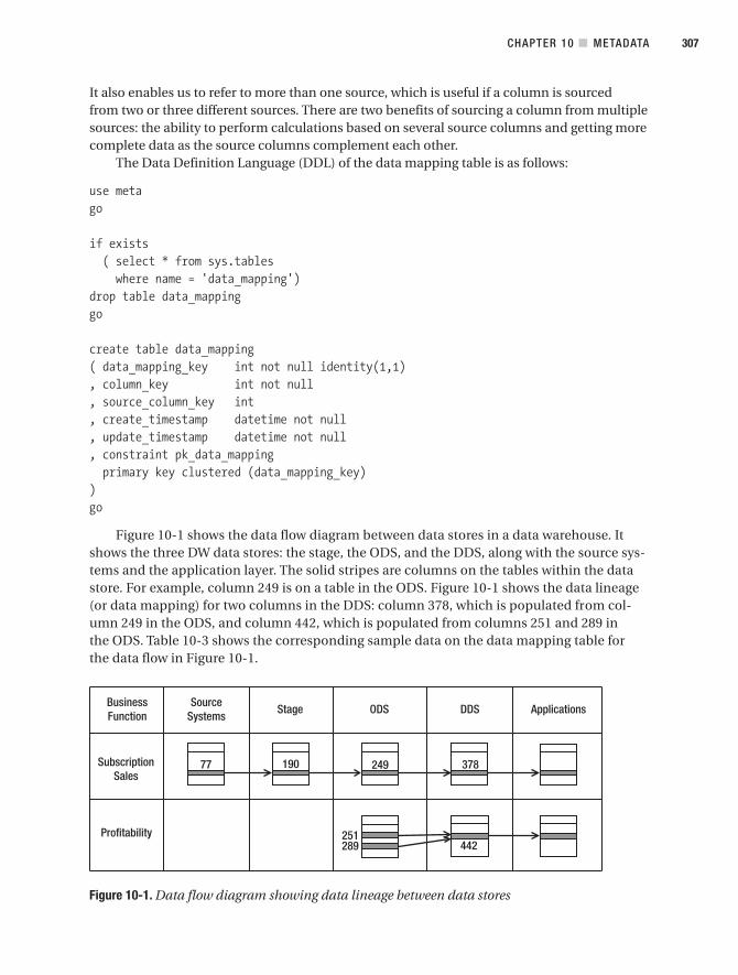
It also enables us to refer to more than one source, which is useful if a column is sourcedfrom two or three different sources. There are two benefits of sourcing a column from multiplesources: the ability to perform calculations based on several source columns and getting morecomplete data as the source columns complement each other.
The Data Definition Language (DDL) of the data mapping table is as follows:
use metago
if exists( select * from sys.tableswhere name = 'data_mapping')
drop table data_mappinggo
create table data_mapping( data_mapping_key int not null identity(1,1), column_key int not null, source_column_key int, create_timestamp datetime not null, update_timestamp datetime not null, constraint pk_data_mappingprimary key clustered (data_mapping_key)
)go
Figure 10-1 shows the data flow diagram between data stores in a data warehouse. Itshows the three DW data stores: the stage, the ODS, and the DDS, along with the source sys-tems and the application layer. The solid stripes are columns on the tables within the datastore. For example, column 249 is on a table in the ODS. Figure 10-1 shows the data lineage(or data mapping) for two columns in the DDS: column 378, which is populated from col-umn 249 in the ODS, and column 442, which is populated from columns 251 and 289 inthe ODS. Table 10-3 shows the corresponding sample data on the data mapping table forthe data flow in Figure 10-1.
Figure 10-1. Data flow diagram showing data lineage between data stores
CHAPTER 10 ■ METADATA 307
9314ch10final.qxd 11/15/07 10:05 AM Page 307
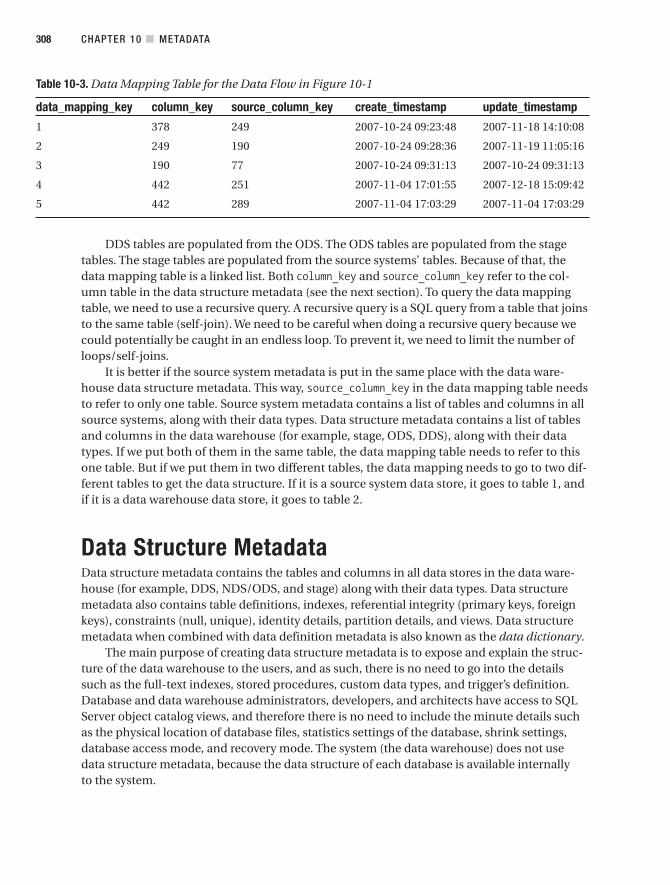
Table 10-3. Data Mapping Table for the Data Flow in Figure 10-1
data_mapping_key column_key source_column_key create_timestamp update_timestamp
1 378 249 2007-10-24 09:23:48 2007-11-18 14:10:08
2 249 190 2007-10-24 09:28:36 2007-11-19 11:05:16
3 190 77 2007-10-24 09:31:13 2007-10-24 09:31:13
4 442 251 2007-11-04 17:01:55 2007-12-18 15:09:42
5 442 289 2007-11-04 17:03:29 2007-11-04 17:03:29
CHAPTER 10 ■ METADATA308
DDS tables are populated from the ODS. The ODS tables are populated from the stagetables. The stage tables are populated from the source systems’ tables. Because of that, thedata mapping table is a linked list. Both column_key and source_column_key refer to the col-umn table in the data structure metadata (see the next section). To query the data mappingtable, we need to use a recursive query. A recursive query is a SQL query from a table that joinsto the same table (self-join). We need to be careful when doing a recursive query because wecould potentially be caught in an endless loop. To prevent it, we need to limit the number ofloops/self-joins.
It is better if the source system metadata is put in the same place with the data ware-house data structure metadata. This way, source_column_key in the data mapping table needsto refer to only one table. Source system metadata contains a list of tables and columns in allsource systems, along with their data types. Data structure metadata contains a list of tablesand columns in the data warehouse (for example, stage, ODS, DDS), along with their datatypes. If we put both of them in the same table, the data mapping table needs to refer to thisone table. But if we put them in two different tables, the data mapping needs to go to two dif-ferent tables to get the data structure. If it is a source system data store, it goes to table 1, andif it is a data warehouse data store, it goes to table 2.
Data Structure MetadataData structure metadata contains the tables and columns in all data stores in the data ware-house (for example, DDS, NDS/ODS, and stage) along with their data types. Data structuremetadata also contains table definitions, indexes, referential integrity (primary keys, foreignkeys), constraints (null, unique), identity details, partition details, and views. Data structuremetadata when combined with data definition metadata is also known as the data dictionary.
The main purpose of creating data structure metadata is to expose and explain the struc-ture of the data warehouse to the users, and as such, there is no need to go into the detailssuch as the full-text indexes, stored procedures, custom data types, and trigger’s definition.Database and data warehouse administrators, developers, and architects have access to SQLServer object catalog views, and therefore there is no need to include the minute details suchas the physical location of database files, statistics settings of the database, shrink settings,database access mode, and recovery mode. The system (the data warehouse) does not usedata structure metadata, because the data structure of each database is available internallyto the system.
9314ch10final.qxd 11/15/07 10:05 AM Page 308

We do need to describe, however, at the very least, the data store, tables, and columns. Inother words, we need to describe—with good business descriptions—how many data storesthere are in the data warehouse; how many tables are in the DDS, NDS, and stage; and howmany columns there are in each table. It is absolutely useless for the business users if wedescribe dim_communication as communication dimension and dim_channel as channel dimen-sion. What the business users need, especially those who are new to CRM, is an explanation ofwhat communication and channel are. So, descriptions such as these are much more useful:“A communication is printed or electronic media issued at a regular or irregular interval thatcustomers can subscribe to, such as a newsletter or an RSS feed” and “A channel is a mediumto deliver communications to customers, such as an e-mail, an RSS feed, a cell/mobile phonetext message, and a telephone call.”
The second purpose of creating data structure metadata is for a reference to other meta-data. Data structure metadata contains the name, data type, and description of all the tablesand columns in all data stores. Other metadata needs to refer to data structure metadata to getthis information. As listed earlier, these are seven types of metadata. Many of them refer todata structure metadata. For example, as you learned in the previous section, data definitionand mapping metadata refer quite frequently to the data structure metadata. Rather thanrewriting the column names and data types, they simply refer to the column table in the datastructure metadata.
Data structure metadata consists of five tables: ds_data_store, ds_table, ds_table_type,ds_column, and ds_column_type. (DS stands for data structure.) Table 10-4 lists the tables fordata structure metadata.
Table 10-4. Data Structure Metadata Tables
Table Name Description
ds_data_store Lists all data stores in the data warehouse
ds_table Lists tables in each data store
ds_table_type Lists table types such as dimension table, fact table, and so on
ds_column Lists all columns in each table
ds_column_type Lists column types such as the surrogate key column, measure, and so on
Tables 10-5 to 10-8 describe an example of the data structure metadata tables.
CHAPTER 10 ■ METADATA 309
Table 10-5. Data Structure Metadata: ds_data_store Table
current_key data_store description collation size growth
1 Stage Staging area SQL_Latin1_General_CP1_CI_AS 70 10
2 NDS Normalized data store SQL_Latin1_General_CP1_CI_AS 125 25
3 DDS Dimensional data store SQL_Latin1_General_CP1_CI_AS 150 25
4 Meta Metadata SQL_Latin1_General_CP1_CI_AS 10 5
9314ch10final.qxd 11/15/07 10:05 AM Page 309

Table 10-6. Data Structure Metadata: ds_table Table
key name entity_type data_store description
1 dim_campaign 1 3 DDS campaign dimension. Acampaign is an instance of acommunication, such as“Amadeus weekly musicnewsletter dated 19 December2007.”
2 dim_channel 1 3 DDS channel dimension. Achannel is a medium to delivera communication to cus-tomers, such as e-mail, RSSfeed, mobile phone text, andtelephone calls.
3 dim_communication 1 3 DDS communicationdimension. A communicationis printed or electronic mediathat issues at a regular orirregular interval that cus-tomers can subscribe to, suchas a newsletter or an RSS feed.
4 dim_customer 1 3 DDS customer dimension. Acustomer is an individual ororganization that purchaseda product, subscribed to acommunication, subscribed toa package, or registered on aweb site.
11 fact_product_sales 2 3 DDS Product Sales fact table.Contains purchases made bycustomers.
12 fact_subscription_sales 2 3 DDS Subscription Sales facttable. Contains subscriptionsmade by customers topackages.
13 fact_campaign_result 2 3 DDS Campaign Result facttable. Contains the send anddelivery status of the campaignto each intended recipient.
28 product 3 2 NDS product master table.Contains active productsoffered to customers for pur-chase including artist, format,and unit cost, as well asinactive products.
29 order_detail 4 2 NDS order detail transactiontable. Contains order linerecords for each purchaseincluding product code,quantity, and price.
…
CHAPTER 10 ■ METADATA310
9314ch10final.qxd 11/15/07 10:05 AM Page 310

Table 10-7. Data Structure Metadata: ds_table_type Table
key table_type description
1 dimension Dimension table
2 fact Fact table
3 master Master table
4 transaction Transaction table
5 stage Stage table
6 metadata Metadata table
CHAPTER 10 ■ METADATA 311
Table 10-8. Data Structure Metadata: ds_column Table
is_column_key table_key column_name data_type is_PK is_FK is_null identity
…
126 21 customer_key int Y Y N N
127 21 communication_key int Y Y N N
128 21 channel_key int N Y N N
129 21 subscription_start_date_key int Y Y N N
130 21 subscription_end_date_key int N Y N N
131 21 subscription_status_key int N Y N N
132 21 source_system_code tinyint N N N N
133 21 create_datetime datetime N N N N
134 21 update_datetime datetime N N N N
…
Some data structure metadata can be populated from SQL Server object catalog views, asfollows (other tables are populated manually):
use ddsgo
select coalesce(t2.table_key, 0) as table_key, c.name as column_name, case when ty.name in ('char', 'varchar')then ty.name + '(' + convert(varchar, c.max_length) + ')'elsecase when ty.name in ('decimal', 'float')then ty.name + '(' + convert(varchar, c.precision)+ ',' + convert(varchar,c.scale) + ')'
else ty.nameend
9314ch10final.qxd 11/15/07 10:05 AM Page 311

end as data_type, case coalesce(a.index_column_id, 0) when 0 then 'N' else 'Y' end as is_PK, case coalesce(fkc.parent_column_id, 0) when 0 then 'N' else 'Y' end as is_FK, case c.is_nullable when 0 then 'N' else 'Y' end as is_null, case c.is_identity when 0 then 'N' else 'Y' end as is_identityfrom sys.tables tinner join sys.columns con t.object_id = c.object_id
inner join sys.types tyon c.system_type_id = ty.system_type_id
left join( select i.object_id, ic.index_column_idfrom sys.indexes iinner join sys.index_columns icon i.object_id = ic.object_idand i.index_id = ic.index_idand i.is_primary_key = 1) aon t.object_id = a.object_idand c.column_id = a.index_column_idleft join sys.foreign_key_columns fkcon t.object_id = fkc.parent_object_idand c.column_id = fkc.parent_column_idleft join meta.dbo.ds_table t2on t.name = t2.table_name
order by table_key, c.column_idgo
Table 10-9 shows the output of the previous script.
CHAPTER 10 ■ METADATA312
Table 10-9. Output of the Script to Populate Data Structure Metadata
table_key column_name data_type is_PK is_FK is_null is_identity
…
11 customer_key int Y Y N N
11 communication_key int Y Y N N
11 channel_key int Y Y N N
11 subscription_start_date_key int N Y N N
11 subscription_end_date_key int N Y N N
11 subscription_status_key int N Y N N
11 source_system_code tinyint N N N N
11 create_timestamp datetime N N N N
11 update_timestamp datetime N N N N
…
9314ch10final.qxd 11/15/07 10:05 AM Page 312

The core of the previous query is interrogating the sys.tables and sys.columns objectcatalog views to list all the columns in the data store, including getting the null and identityattributes of the column. The query then goes to sys.index_columns and sys.foreign_key_columns to identify whether the column is a primary key or a foreign key. The output columnsare converted into Y and N using a case statement. The data_type column is then formattedusing a case statement as follows:
• If the column is char or varchar, it includes the maximum length.
• If the column is a decimal or float, it includes the precision and scale.
Finally, the table names are converted into table keys.It is, of course, possible to populate the data structure metadata manually, but it is handy
to be able to populate it automatically using scripts like the previous one for consistency andaccuracy. The output of the previous script needs to be “upserted” into the column table, inother words, updated when it exists and inserted when it does not exist. But, regardless of thescript, the table description columns still need to be filled in manually with meaningful anduseful business descriptions. There are tools that can produce data structure information ofa database, such as table and column names, data types, and data length, but we still have totype the business description of each column and table manually.
Source System MetadataSource system metadata is similar to data structure metadata. In other words, it contains thedata structure of the source system. Like data structure metadata, at the least it needs to con-tain the database level, table level, and column level. This information is required becausedata mapping metadata stores only the column key. When the application needs to display thecolumn names and data types, it gets this information from the source system metadata.Additionally, source system metadata can also contain other information such as the refreshfrequency for particular tables. The refresh frequency is useful when we try to optimize theETL process. Other information that is useful on source system metadata is a data profile,such as minimum and maximum values, row count, and the number of NULLs.
The main purpose of creating the source system metadata is to expose and explain thestructure of the source systems to the data warehouse users. This, in a way, acts as an exten-sion to the data warehouse structure exposed by the data structure metadata. As such, there isno need to go down to the technical details of the source systems, such as the indexes, backupinterval, triggers, and detailed database properties.
The second purpose of creating source system metadata is to serve as a reference for theother metadata. For example, the source column on the data mapping metadata refers to thecolumns on the source systems, which exist in the source system metadata. ETL processesmetadata and data quality metadata also contain the source system columns, and thereforethey need to refer to the source system metadata. This other metadata stores only the columnkey. When the application needs to display the column name and data types, it gets this infor-mation from the source system metadata.
As I explained earlier, it is best to place the source system metadata in the same place asthe data structure metadata, rather than creating it on its own set of tables. They have thesame structure, so they can be put in the same set of tables. This way, it is easier to query
CHAPTER 10 ■ METADATA 313
9314ch10final.qxd 11/15/07 10:05 AM Page 313

because we don’t have to conditionally join two different set of tables, which will make thequery slower. For example, on the full data lineage/mapping table, if we place the source sys-tem metadata columns in the data structure metadata column table, we have only the tableto link to, regardless of whether it is a stage, NDS, or source system column.
Tables 10-10, 10-11, 10-12, and 10-13 show the data structure metadata tables. Datastructure metadata consists of three core tables: ds_data_store contains a list of data stores,ds_table contains a list of tables, and ds_column contains a list of columns. In these tables weput the data stores, tables, and columns of both the data warehouse and the source systems.Table 10-10 shows the ds_data_store table, which contains both the data warehouse datastores and the source system data stores. Table 10-11 shows the ds_tables table, which con-tains both the data warehouse tables and the source system tables. Table 10-12 shows theds_table_type table, which describes the types of tables, such as dimension table or fact table.Table 10-13 shows the ds_column table, which contains both the data warehouse columns andthe source system columns.
CHAPTER 10 ■ METADATA314
Table 10-10. Data Structure + Source System Metadata: ds_data_store Table
data_ data_ current_store_key store_name description DBMS collation size growth
1 Stage Staging area. SQL Server 2005 SQL_Latin1_ 70 10General_CP1_CI_AS
2 ODS Operational data store. SQL Server 2005 SQL_Latin1_ 225 25General_CP1_CI_AS
3 DDS Dimensional data store. SQL Server 2005 SQL_Latin1_ 350 25General_CP1_CI_AS
4 Meta Metadata database. SQL Server 2005 SQL_Latin1_ 10 5General_CP1_CI_AS
5 Jade A custom Java-based system Informix Dynamic Unicode 430 30running on Informix. This Server 10includes sales, customer service, subscriptions, and front-office functions.
6 WebTower A custom-developed .NET- Oracle 10g R2 ANSI 845 65based system for dynamic web sites, multimedia trading, broadcasting, sales order pro-cessing, and subscription management, running on Oracle Database.
7 Jupiter The back-end enterprise DB2 Enterprise 9 EBCDIC 800 50resource planning (ERP) sys-tem. An off-the-shelf AS/400-based business system run-ning on DB2.
9314ch10final.qxd 11/15/07 10:05 AM Page 314
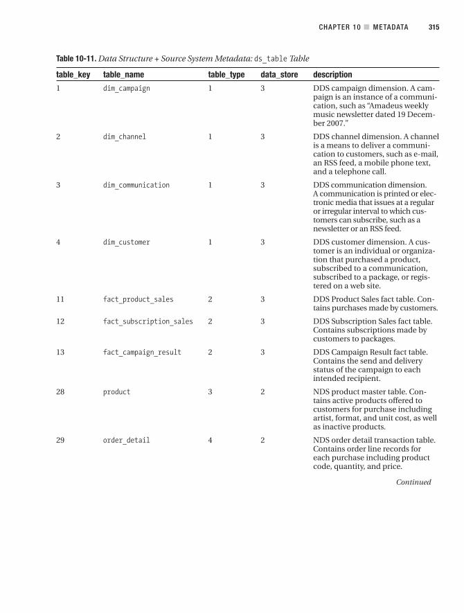
Table 10-11. Data Structure + Source System Metadata: ds_table Table
table_key table_name table_type data_store description
1 dim_campaign 1 3 DDS campaign dimension. A cam-paign is an instance of a communi-cation, such as “Amadeus weeklymusic newsletter dated 19 Decem-ber 2007.”
2 dim_channel 1 3 DDS channel dimension. A channelis a means to deliver a communi-cation to customers, such as e-mail,an RSS feed, a mobile phone text,and a telephone call.
3 dim_communication 1 3 DDS communication dimension.A communication is printed or elec-tronic media that issues at a regularor irregular interval to which cus-tomers can subscribe, such as anewsletter or an RSS feed.
4 dim_customer 1 3 DDS customer dimension. A cus-tomer is an individual or organiza-tion that purchased a product,subscribed to a communication,subscribed to a package, or regis-tered on a web site.
11 fact_product_sales 2 3 DDS Product Sales fact table. Con-tains purchases made by customers.
12 fact_subscription_sales 2 3 DDS Subscription Sales fact table.Contains subscriptions made bycustomers to packages.
13 fact_campaign_result 2 3 DDS Campaign Result fact table.Contains the send and deliverystatus of the campaign to eachintended recipient.
28 product 3 2 NDS product master table. Con-tains active products offered tocustomers for purchase includingartist, format, and unit cost, as wellas inactive products.
29 order_detail 4 2 NDS order detail transaction table.Contains order line records foreach purchase including productcode, quantity, and price.
Continued
CHAPTER 10 ■ METADATA 315
9314ch10final.qxd 11/15/07 10:05 AM Page 315
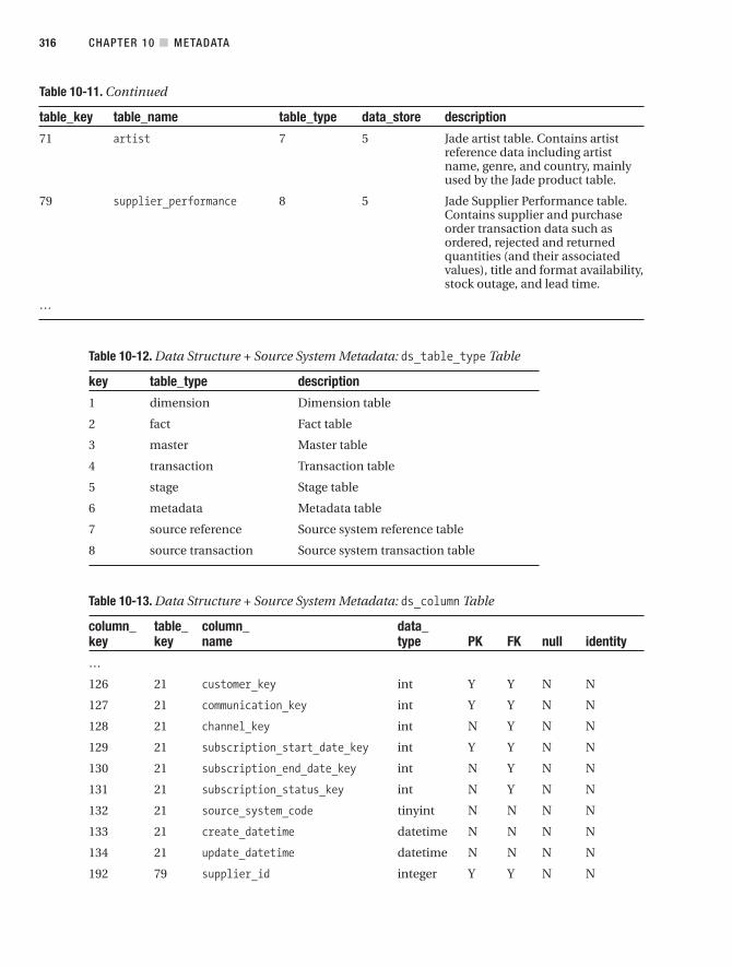
Table 10-11. Continued
table_key table_name table_type data_store description
71 artist 7 5 Jade artist table. Contains artistreference data including artistname, genre, and country, mainlyused by the Jade product table.
79 supplier_performance 8 5 Jade Supplier Performance table.Contains supplier and purchaseorder transaction data such asordered, rejected and returnedquantities (and their associatedvalues), title and format availability,stock outage, and lead time.
…
CHAPTER 10 ■ METADATA316
Table 10-12. Data Structure + Source System Metadata: ds_table_type Table
key table_type description
1 dimension Dimension table
2 fact Fact table
3 master Master table
4 transaction Transaction table
5 stage Stage table
6 metadata Metadata table
7 source reference Source system reference table
8 source transaction Source system transaction table
Table 10-13. Data Structure + Source System Metadata: ds_column Table
column_ table_ column_ data_key key name type PK FK null identity
…
126 21 customer_key int Y Y N N
127 21 communication_key int Y Y N N
128 21 channel_key int N Y N N
129 21 subscription_start_date_key int Y Y N N
130 21 subscription_end_date_key int N Y N N
131 21 subscription_status_key int N Y N N
132 21 source_system_code tinyint N N N N
133 21 create_datetime datetime N N N N
134 21 update_datetime datetime N N N N
192 79 supplier_id integer Y Y N N
9314ch10final.qxd 11/15/07 10:05 AM Page 316

column_ table_ column_ data_key key name type PK FK null identity
193 79 product_id integer Y Y N N
194 79 start_date date N N Y N
195 79 ordered_quantity integer N N Y N
…
How do we populate source system metadata? Unlike data structure metadata, which canbe obtained automatically (well, semiautomatically to be precise, because we still have to putin the description), in most cases we are not able to populate the source system metadataautomatically, because it is not under our control. We need administrative rights to the sourcesystem databases, and this kind of access is usually possessed only by the DBA. So, we need topopulate the source system metadata manually. We usually get the information that we needto populate the source system metadata when we do source system analysis (also known asthe data feasibility study; please refer to Chapter 4). For some of us who are lucky enough (orunlucky, depending on how you look at it) to be the DBA of the source systems, we will be ableto automate the population by accessing the system information schema or table definitionsand be able to create a script in the source system to export its structure into a text file, whichwe can then import into metadata tables.
There is one thing that source system metadata has but that does not exist in data struc-ture metadata: a source data profile. A source data profile contains statistics and volumetricinformation describing the source data such as minimum value, maximum value, averagevalue, and number of distinct values for each column. It also contains the number of rows,row size, and number of columns for each table. A source data profile is useful when creatingETL processes to extract the data out of the source system. It is also useful when we need tomodify the ETL processes after the data warehouse has been deployed in production.
We get the information required for populating the source data profile usually when doingsource system analysis. Tables 10-14 and 10-15 show an example of a source data profile. To putit into context, in the following example, table 71 is the artist table, 72 is the customer table, and79 is a supplier performance table, all from the Jade source system.
Table 10-14. Source System Metadata: Source Table Data Profile
table_key rows row size columns has_timestamp
…
71 5768 240 5 N
72 2415832 877 28 Y
79 4103841 85 15 N
…
CHAPTER 10 ■ METADATA 317
9314ch10final.qxd 11/15/07 10:05 AM Page 317

Table 10-15. Source System Metadata: Source Column Data Profile
column_key table_key unique_values minimum maximum average max length null
…
192 79 12894 110921 219032 159281 0
193 79 45120 3 50394 27291 0
194 79 1609 03/19/1998 12/19/2007 05/07/2002 120
195 79 78 0 134 2 0
…
CHAPTER 10 ■ METADATA318
In Table 10-14, we can see the number of rows, row size, and number of columns for eachtable. Table 10-15 lists the number of unique/distinct values, the minimum value, the maxi-mum value, and the average value for each column. Table 10-15 also shows the number ofrows with nulls in that column. For char or varchar columns, we can have minimum length,maximum length, and average length. We can also have other useful statistics such as thecount of the most and least frequent values for each column.
ETL Process MetadataETL process metadata consists of a data flow table, a package table, and a status table. Thedata flow table describes the name and description of each SSIS data flow, what table theyextract from, the destination table, what transformations are applied (only a descriptive text,not the exact formula), the parent package, their current status, the last successful extractiontime (LSET), and the current extraction time (CET). This information is used by the ETL pro-cesses to determine which records to extract from the source system. Sometimes on the dataflow table, we have a column called order. This column contains the sequential order whenthe data flow needs to run, in relative position to other data flow. When using SSIS, we don’tactually need this column, because we have precedence constraints defining the workflowbetween data flows. We need it when we use stored procedures for ETL.
The package table contains the name and description of each SSIS package, their sched-ule (only descriptive text; the actual schedule is set when creating the SQL Server Agent Job toexecute the SSIS package), their status, and the last time they ran. The status table containsthe status code and description. To be able to restart an ETL batch from the point of failure(not from the beginning), we need to know exactly where it failed, what was executed, andwhat was not executed. The status column on both the data flow table and the package tableenables this. In its simplest form, the status values are success, failed, and in progress. In amore sophisticated implementation, other status values are “about to run” and “canceled.”These two additional statuses enable us to understand the more precise state of each ETLprocess, which helps us troubleshoot when there is a problem with the ETL.
Tables 10-16 to 10-18 show the tables that form the ETL processes metadata. There arethree tables: data_flow, package, and status. The data_flow table contains a list of ETL pro-cesses. An ETL process contains several ETL tasks, such as transformations. The package tablecontains a collection of ETL processes. The status table contains the state of each data flow.
9314ch10final.qxd 11/15/07 10:05 AM Page 318

Table 10-16. ETL Processes Metadata: data_flow Table
key name description source target transformation package status LSET CET
…
8 stage_product Extracts Jade and Jade. stage. Adds 9000 on 4 1 11/27/2007 11/27/2007
Jupiter product product, product Jupiter product 04:06:09 04:06:09
tables incre- Jade. code; dedupe
mentally based product_ two source
on the last- detail, systems
updated date Jupiter. based on
and puts them prod_hd, product
in the product Jupiter. group and
stage table. prod_dt product code.
9 nds_product Loads product state. stage. Upsert 11 1 11/27/2007 11/27/2007
data from the product product and key- 04:07:11 04:07:11
stage to the NDS. ing; DQ
unit_cost
with rule 29
…
Table 10-17. ETL Processes Metadata: package Table
key name description schedule
…
4 Stage daily This SSIS package extracts the following data from the source Runs every day incremental system incrementally and loads it onto the stage: customer, including weekends
permission, product, store, product purchases, package sub- at 3 a.m.scription, and communication subscription.
5 Stage daily This SSIS package extracts the following data from the source Runs every day at full reload system by downloading the whole table: customer type, cus- 3 a.m.
tomer status, interest, household income, occupation, cur-rency, artist, product status, product type, product category, package, and package type.
11 NDS This loads product-related tables from the stage to the NDS, Runs daily at 3 a.m.product in other words, the ones with product, product status, product
type, product category, package, and package type data.
12 NDS This loads customer-related tables from the stage to the NDS, Runs daily at 3 a.m.customer in other words, the ones with customer, customer status, cus-
tomer type, address, address type, e-mail address, e-mail address type, permission, phone number, phone number type, household income, occupation, and interest data.
…
CHAPTER 10 ■ METADATA 319
9314ch10final.qxd 11/15/07 10:05 AM Page 319

Table 10-18. ETL Processes Metadata: status Table
key status
…
0 Unknown
1 Success
2 Failed
3 In progress
…
Table 10-17 shows that the stage ETL packages are grouped into packages according tothe frequency they run (daily, weekly, monthly, ad hoc, and so on) and the extraction method(full reload, incremental, or fixed period). Table 10-17 also shows that the NDS ETL packagesare grouped into packages according to the subject area, such as product, customer, productpurchase, package subscription, CRM subscription, and so on.
The main purpose of having ETL metadata is to control the ETL packages in SSIS. Forexample, as we did in Chapter 7, the LSET and CET columns enable us to extract incremen-tally by memorizing the last time a successful extract was run. The status columns enable theSSIS packages or the whole ETL batch to restart from the point of failure. When we restart anETL package, we can use the status column to determine which ETL processes have not beenexecuted, and we can restart from that process onward, rather than from the beginning. To beable to restart from failure, the ETL processes need to be re-runnable. In other words, we needto be able to run the same process over and over without causing any problem.
The second purpose of having ETL metadata is to describe the ETL processes. It describeswhat the ETL process or package does, such as “Stage daily incremental: this SSIS packageextracts the following data from the source system incrementally and loads it into the stage:customer, permission, product, store, product purchases, package subscription, and commu-nication subscription. Runs every day including weekend at 3 a.m.” Being able to query suchdescriptive text for every package and data flow is very useful to most data warehouse admin-istrators, provided that the descriptions are kept up-to-date. We can automate it a little bit,such as by querying sysjobs, sysjobsteps, sysjobschedules, and sysschedules tables in themsdb database to determine the SQL Server Agent job steps and schedule. We can also querysysjobhistory to determine what jobs have been executed.
Data Quality MetadataData quality metadata contains the data quality rules that we discussed in the previous chap-ter, including the rule name and description, rule type (for example, error or warning), rulecategory (for example, incoming data validation, cross reference validation, or internal datawarehouse validation; see Chapter 9), risk level (for example, business or financial risk if thisrule is violated, on the scale of 1 to 5), status (active or not), action (reject, allow, or fix; seeChapter 9), notification, create timestamp, and update timestamp. The notification columncontains a link to the DQ notification table that contains who to notify and how to notify them(for example, an e-mail or a cell/mobile phone text message). We can have other features suchas how many times to notify, at what interval, acknowledgment status, escalation timeframe,
CHAPTER 10 ■ METADATA320
9314ch10final.qxd 11/15/07 10:05 AM Page 320

escalation person/second level, and so on. We also need to have a third table containing theuser details, in other words, name, department/business area, role/position, e-mail address,cell phone number, group number, and so on. And potentially we need a fourth table fordescribing the user groups when we have a lot of users and we want to assign the data qualitytasks to a group of users rather than to individual users. It is usually better to start with some-thing simple, such as without escalation/second level. If it is proven to be successful, we canenhance it further.
Tables 10-19 to 10-21 contain data quality metadata. There are three main tables: DQrules, DQ notification, and DW user. The DQ rules table contains the data quality rules. TheDQ notification table specifies which DW users to notify for each rule. The DW user tabledescribes the data warehouse users including their e-mail addresses.
CHAPTER 10 ■ METADATA 321
Table 10-19. Data Quality Metadata: DQ Rules Table
rule_ rule_ rule_ rule_ risk_ create_ update_key name description type category level status action timestamp timestamp
…
7 The product Product code needs to be in E I 3 A R 10/21/2007 11/27/2007 code format AAA999AA format. Reject if 11:41:33 14:07:11
it is not in this format, and notify product manager bye-mail.
8 The unit Within 25% of last three W C 1 A A 09/18/2007 10/12/2007price months’ average. 12:04:33 09:27:55
…
Table 10-20. Data Quality Metadata: DQ Notification Table
key rule_key recipient_type recipient method
…
11 7 I 3 E
12 8 G 9 E
…
Table 10-21. Data Quality Metadata: Data Warehouse User Table
key name department role email_address phone_number group
…
3 Brian Hill Merchandising Product brian.hill@ 0983475052 9Manager amadeus.com
4 Sarah Finance Costing sarah.fairbank@Fairbank Assistant amadeus.com 9
…
9314ch10final.qxd 11/15/07 10:05 AM Page 321

In Table 10-19, the rule_type column is linked to the rule_type table, which has twoentries: E for errors and W for warnings. This enables us to determine whether it is an erroror warning. The rule_category column is linked to the rule_category table, which has threeentries: I for incoming data validation rules, C for cross-reference validation rules, and D forinternal data warehouse validation rules (see Chapter 9). This enables us to determine thetype of data quality issue we are facing.
The risk_level column is linked to the rule_risk_level table, which has five entries:level 1 for no business impact to level 5 for severe damage to business financial positions. Thisenables us to determine how big the impact of the data quality issue is. The status column islinked to the rule_status table, which has two entries: A for active and D for decommissioned.This enables us to add new rules and deactivate obsolete rules. The action column is linked tothe rule_action table, which contains R for reject, A for allow, and F for fix. This enables us todetermine what kind of action was taken against each data quality issue.
■Tip rule is a SQL Server keyword, which specifies the acceptable values that can be inserted intoa column. In SQL Server 2008, it is replaced by check constraints. So, be careful when you want to userule as a table name, because you need to use brackets ([rule]) every time you use the table name. Apractical approach is to change the table name to dq_rule, which is more descriptive. For consistency,you need to name the rule type, rule category, and rule status tables as dq_rule_type, dq_rule_category, and dq_rule_status. Underscores are used for naming SQL Server system views, suchas sys.foreign_keys, sys.default_constraint, sys.service_queues, sys.sql_modules, andsys.backup_devices. I prefer to use underscores because it gives better readability compared tojoined words with no underscore.
In Table 10-20, the recipient type column is linked to the recipient_type table, whichhas two entries: I for individual and G for group. This enables us to send the notification toa group of users, rather than to an individual user. The recipient column contains the key ofthe individual or the group on the user table, depending on the value of the recipient_typecolumn. Table 10-21 contains the user details, with the last column (group) being the groupkey of each user to enable sending a DQ notification for a particular rule to several peoplesimultaneously.
This is only one design. Of course, you could and should alter or enhance it accordingthe needs of your projects and situations. The purpose of giving the previous example is justfor illustration to help you understand the practical implementation. For instance, in someprojects, it is required to extend the DQ rule table by creating a parameter column. This col-umn contains a value that is used in the rule. For example, if the rule is “the unit cost ofproduct family AG9 needs to be greater than 1.25,” then the number 1.25 is actually storedas a value in the parameter column, not hard-coded in SSIS data flow logic. This makes iteasier to update the value later. To accommodate more than one parameter, the parametersare placed in a separate parameter table and linked to the DQ rule table on the rule key col-umn. You can add “data type” column in the parameter table to handle the issue ofparameters being of different data types.
CHAPTER 10 ■ METADATA322
9314ch10final.qxd 11/15/07 10:05 AM Page 322

Audit MetadataAudit metadata contains the results of every process and activity in the data warehouse,including data loading process (ETL), creation of specific purpose DDS (mart), manual datamodification (for example, updating DQ user table), DQ rule validation, security log/breach(for example, web portal login), system enhancements and modifications (for example,patches, schema changes and upgrades), data purging and archiving, database tuning, andmaintenance (indexing and partitioning activities).
Audit metadata is used for administering the data warehouse, including monitoring ETLprocesses, monitoring data quality, enhancements requests, installation patches, and moni-toring security access. For example, the purpose of one of the daily operation reports (ormanual query using SQL script) is to verify whether the ETL processes ran successfully. Thisreport or script accesses the audit metadata to get the number of rows loaded for each table.It is used to see when the last purging, indexing, or partitioning was done on a particulartable. Another example of administrative usage is to support enhancement requests. Byexamining or querying the audit metadata, we know what patch was applied and when. Wewill go though these administrative tasks in Chapter 17 when we discuss data warehouseadministration.
The secondary usage of audit metadata is for troubleshooting. When there is a problemor issue, you can query audit metadata to know what happened in the last few hours. Sayyou got a call from a user saying that a package subscription report or cube is missing somedata. You know that this cube is fed from the Subscription Sales fact table in the DDS, and itturns out that today this fact table was not loaded. In this case, you can query how manyrecords were loaded into the stage, how many into NDS, and how many into DDS. It helpsyou to pinpoint where the cause of the problem lies.
In its simplest form, audit metadata is an event log table containing every single eventthat happened in the data warehouse populated by every single process and activity in thedata warehouse. The processes use insert SQL statements to add rows into the event logtable. It contains the event type, event category, which data warehouse object is involved inthe event (linked to data structure metadata), the data flow initiating the event (linked tothe data flow table), the number of rows involved, the timestamp when the event occurred,and a note. Table 10-22 gives an example of this event log table.
In the event_type table described in Table 10-22, the key column is an identity (1,1)containing a sequential number for identifying the log entry. The type column contains theevent type, linked to the event_type table shown in Table 10-23. The category column con-tains the event category, linked to the event_category table shown in Table 10-24. Theobject column contains the table key, linked to the ds_table table in the data structuremetadata. For ETL processes, the data_flow column contains the SSIS data flow, linked tothe data_flow table in the ETL processes metadata. For ETL processes, the rows columncontains the number of rows affected. The event_log table is purged regularly, such asevery month, leaving only the last 12 months of data. This enables us to maintain queryand reporting performance. The purge frequency and number of months to keep dependson the administrative requirements, performance requirements, regulatory issues, andcompany standards.
CHAPTER 10 ■ METADATA 323
9314ch10final.qxd 11/15/07 10:05 AM Page 323
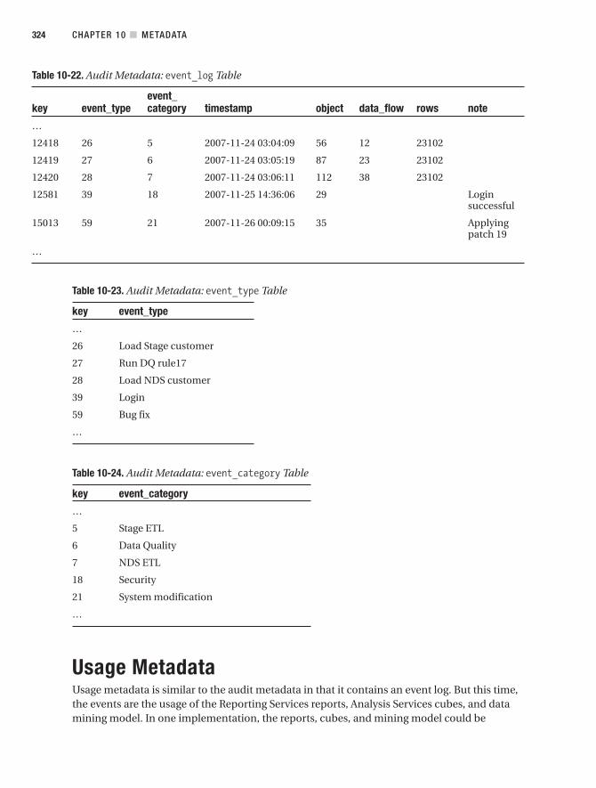
Table 10-22. Audit Metadata: event_log Table
event_key event_type category timestamp object data_flow rows note
…
12418 26 5 2007-11-24 03:04:09 56 12 23102
12419 27 6 2007-11-24 03:05:19 87 23 23102
12420 28 7 2007-11-24 03:06:11 112 38 23102
12581 39 18 2007-11-25 14:36:06 29 Login successful
15013 59 21 2007-11-26 00:09:15 35 Applyingpatch 19
…
CHAPTER 10 ■ METADATA324
Table 10-23. Audit Metadata: event_type Table
key event_type
…
26 Load Stage customer
27 Run DQ rule17
28 Load NDS customer
39 Login
59 Bug fix
…
Table 10-24. Audit Metadata: event_category Table
key event_category
…
5 Stage ETL
6 Data Quality
7 NDS ETL
18 Security
21 System modification
…
Usage MetadataUsage metadata is similar to the audit metadata in that it contains an event log. But this time,the events are the usage of the Reporting Services reports, Analysis Services cubes, and datamining model. In one implementation, the reports, cubes, and mining model could be
9314ch10final.qxd 11/15/07 10:05 AM Page 324

accessed via a web portal. Before the link on the portal redirects to the report (or cubes ormining model), it inserts a record into this usage metadata first. So, we know which reports orcubes were accessed and when they were accessed. The access patterns are useful for doingperformance tuning and capacity planning. For example, they enable us to avoid the busytimes when processing the cubes.
Another implementation is to populate the usage metadata from the SQL Server storedprocedures, which are invoked by the Reporting Services reports. For this, the reports mustnot contain direct SQL statements; instead, they must call the stored procedures.
Usage metadata is used to understand (for example) how many times a particularreport is accessed and by which users or departments. We can use an IIS log to record thenumber of hits on the links on the data warehouse portal page, but usage metadata is moreflexible. It could be reported using SSRS, so it would have a more consistent look with otherdata warehouse reports. An IIS log, on the other hand, requires some kind of web log analy-sis software in order for us to understand how many times a report is accessed and by whichusers. Each entry on the IIS log contains the date and time the activity occurred, the clientIP address, the username of the authenticated user who accessed the server, the target pageor report, the Universal Resource Identifier (URI) query, the bytes sent, and the length oftime that the action took (in milliseconds). Each hit on the report produced an IIS log entrywith all the previous information. This way, a full collection of IIS log entries enables us todetermine the usage or access pattern of the report.
One simple implementation of usage metadata is a usage_log table. The log table con-tains the user, the object, and the timestamp, and if applicable, it also contains theparameters. Table 10-25 shows an example of this usage_log table.
Table 10-25. Usage Metadata: usage_log Table
key user object timestamp parameters note
…
7834 12 56 2007/11/03 16:09:33 FG45
7892 20 114 2007/12/05 11:39:05
…
The user column on Table 10-25 is linked to the data warehouse user table shown inTable 10-21. The object column is linked to the ds_table table in the data structure meta-data shown in Table 10-6. The timestamp column shows when the object is accessed.
When the authentication method in SSRS is Windows integrated security, the user ID canbe obtained using system_user. system_user is a SQL Server internal system variable that con-tains the login name (if using SQL authentication) or the Windows login identification name(if using Windows authentication).
Maintaining MetadataIt is important to keep the metadata up-to-date. An out-of-date data structure or outdateddata mapping metadata, for example, may lead the users to the wrong understanding of thedata warehouse. Also, the system may take an incorrect action if the metadata is incorrect.
CHAPTER 10 ■ METADATA 325
9314ch10final.qxd 11/15/07 10:05 AM Page 325

Conducting a change request impact analysis based on out-of-date data mapping metadatacould lead to ETL problems, such as because we misinterpreted where a piece of data is com-ing from or because the data type was not correct.
Data definition and mapping metadata is usually defined and created at an early phase ofa data warehousing project. Once created, they are then maintained through change requestprocedures. Rather than changing it directly on the metadata tables, the change needs to beimplemented using a data change script. The data change script is a Transact SQL script con-taining the rollback section, the change request details (which go to the event log table), andthe roll forward.
The DW administrator needs to prepare a script to change the metadata and submit thisscript to be executed under a change request process. The script contains three sections: log,rollback, and implementation.
• The log section records the change request details into the event log table. The reasonfor doing this is for traceability and troubleshooting if something goes wrong.
• The rollback section tries to “undo” the change. This is necessary to prove that we canrevert the changes.
• The implementation section applies the change to the metadata database.
The following is an example of a metadata change request. This example updates the risklevel of rule 8 in Table 10-19 from level 1 to level 2.
/* Change request number: CR023Date created: 12/14/2007Created by: Vincent RainardiDescription of change: Change the risk level for rule 8 from 1 to 2Schedule for production implementation: 12/18/2007*/
use meta -- switch to metadata database
-- Event Log sectioninsert into event_log (event_type, event_category,event_timestamp, object, dataflow, rows, note)values (7, 3, getdate(), 371, 0, 8,'update risk level from 1 to 2')
-- Rollback sectionupdate dq_rules set risk_level = 1 where rule_key = 8
-- Implementation sectionupdate dq_rules set risk_level = 2 where rule_key = 8
Some data structure metadata can be maintained automatically using SQL Server objectcatalog views. A query gets the data from the object catalog views and inserts or updates theappropriate metadata tables. For example, we can use the query shown earlier in this chapter.Some data structure metadata still needs to be maintained manually, such as object business
CHAPTER 10 ■ METADATA326
9314ch10final.qxd 11/15/07 10:05 AM Page 326

descriptions, dimensional hierarchy, and SCD details. Source system metadata is usually cre-ated and populated during the source system analysis phase and then maintained during thedevelopment phase by using a data change script to update the metadata tables (illustratedearlier), according to the change request process. After the data warehouse is released, thesource system metadata is maintained using data change scripts, governed by a change requestprocedure.
ETL process metadata is created and populated during the development of the SSIS pack-ages. We need to update the ETL process metadata every time we modify the SSIS packages.Similarly, data quality metadata (DQ rule table, and so on) needs to be updated every time wemodify the SSIS packages. Ideally, we need to use a standardized data change script to updatethe metadata tables, rather than using direct SQL statements to update the tables. All updatesto metadata need to be recorded on the audit metadata event log table. So, this needs to beincluded in the data change scripts.
Audit metadata and usage metadata are maintained as the data warehouse is used. Auditmetadata is populated by the ETL processes, patch release processes, and security processes.Usage metadata is populated by the stored procedure or the web portal.
SummaryThis chapter defined what metadata in a data warehouse is and what it contains. It listedseven kinds of metadata: data definition and mapping metadata, data structure metadata,source system metadata, ETL processes metadata, data quality metadata, audit metadata,and usage metadata. I discussed them one by one so you can understand what they are usedfor, how to create them, and how to populate/maintain them.
Metadata helps us understand the structure and definition/meaning of the data in thedata warehouse. It also helps us understand the structure and definition of the data ware-house itself. Metadata is also used for auditing and troubleshooting purposes, in other words,to understand what happened (and what is happening) in the data warehouse, where it hap-pened, and when it happened.
In the next few chapters, I will discuss how to get the data out of the data warehouse. Iwill discuss how to use SQL Server Reporting Services and SQL Server Analysis Services tocreate reports and cubes to bring the data from the data warehouse to the users.
CHAPTER 10 ■ METADATA 327
9314ch10final.qxd 11/15/07 10:05 AM Page 327

9314ch10final.qxd 11/15/07 10:05 AM Page 328

Building Reports
Earlier in this book, you learned how to build a data warehouse, including defining thearchitecture, selecting the methodology, gathering the requirements, designing the datamodels, and creating the databases. In the past few chapters, I discussed how to populatethe data warehouse, including extracting from the source system, loading the data stores,maintaining the data quality, and utilizing the metadata.
Now that we have loaded the data into the warehouse, in this chapter and the next fewchapters, I will discuss how to get the data out to the users and how to use the data in thewarehouse. Two of the most popular ways to present the data to the users are using reportsand using multidimensional databases. So in this chapter, I will discuss reports, and in thenext chapter, I will talk about multidimensional databases.
Two of the most popular uses of data warehouses are for business intelligence (BI)and customer relationship management (CRM). In Chapters 13 and 14, I will discuss thesetwo uses, and in Chapter 15, I will discuss other uses such as customer data integrationand unstructured data. Reporting and multidimensional databases are used quite inten-sively in BI.
In this chapter, you will learn how to use SQL Server 2005 Reporting Services to createreports to bring the data from the data warehouse to the users. I’ll first explain what datawarehouse reports are, and then I will show how to use Reporting Services to actually build areport. When building the report, you will learn some key features in reporting such as query-ing the data, arranging the report layout, using parameters, sorting the data, and filtering thedata. I will also discuss how to create a pivot table report, how to follow the principle of sim-plicity, and how to report from a multidimensional database. I will close this chapter bydiscussing how to deploy and administer the reports.
This chapter will give you enough knowledge to start building the reports for your datawarehouse. There is no doubt that you will need to refer to Books Online along the way formore detailed instructions, but this chapter will provide you with a good starting point.
Data Warehouse ReportsIn the data warehousing context, a report is a program that retrieves data from the data ware-house and presents it to the users on the screen or on paper. Users also can subscribe to thesereports so that they can receive them automatically by e-mail at certain times (daily or weekly,for example) or in response to events.
Which data stores do data warehouse reports usually retrieve data from? Data warehousereports usually retrieve data from a dimensional data store (DDS), an operational data store
329
C H A P T E R 1 1
9314ch11final.qxd 11/15/07 10:03 AM Page 329
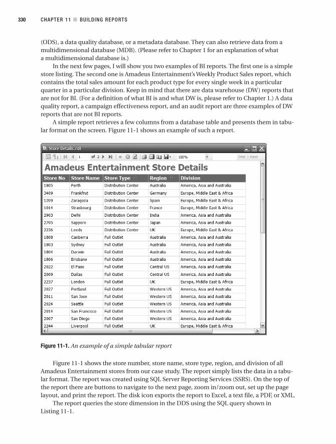
(ODS), a data quality database, or a metadata database. They can also retrieve data from amultidimensional database (MDB). (Please refer to Chapter 1 for an explanation of whata multidimensional database is.)
In the next few pages, I will show you two examples of BI reports. The first one is a simplestore listing. The second one is Amadeus Entertainment’s Weekly Product Sales report, whichcontains the total sales amount for each product type for every single week in a particularquarter in a particular division. Keep in mind that there are data warehouse (DW) reports thatare not for BI. (For a definition of what BI is and what DW is, please refer to Chapter 1.) A dataquality report, a campaign effectiveness report, and an audit report are three examples of DWreports that are not BI reports.
A simple report retrieves a few columns from a database table and presents them in tabu-lar format on the screen. Figure 11-1 shows an example of such a report.
Figure 11-1. An example of a simple tabular report
Figure 11-1 shows the store number, store name, store type, region, and division of allAmadeus Entertainment stores from our case study. The report simply lists the data in a tabu-lar format. The report was created using SQL Server Reporting Services (SSRS). On the top ofthe report there are buttons to navigate to the next page, zoom in/zoom out, set up the pagelayout, and print the report. The disk icon exports the report to Excel, a text file, a PDF, or XML.
The report queries the store dimension in the DDS using the SQL query shown inListing 11-1.
CHAPTER 11 ■ BUILDING REPORTS330
9314ch11final.qxd 11/15/07 10:03 AM Page 330
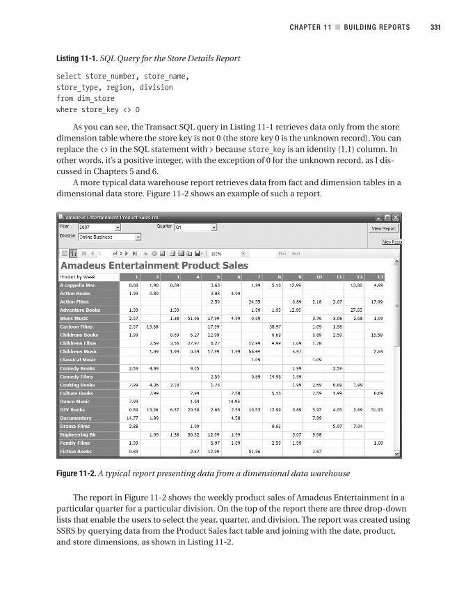
Listing 11-1. SQL Query for the Store Details Report
select store_number, store_name,store_type, region, divisionfrom dim_storewhere store_key <> 0
As you can see, the Transact SQL query in Listing 11-1 retrieves data only from the storedimension table where the store key is not 0 (the store key 0 is the unknown record). You canreplace the <> in the SQL statement with > because store_key is an identity (1,1) column. Inother words, it’s a positive integer, with the exception of 0 for the unknown record, as I dis-cussed in Chapters 5 and 6.
A more typical data warehouse report retrieves data from fact and dimension tables in adimensional data store. Figure 11-2 shows an example of such a report.
Figure 11-2. A typical report presenting data from a dimensional data warehouse
The report in Figure 11-2 shows the weekly product sales of Amadeus Entertainment in aparticular quarter for a particular division. On the top of the report there are three drop-downlists that enable the users to select the year, quarter, and division. The report was created usingSSRS by querying data from the Product Sales fact table and joining with the date, product,and store dimensions, as shown in Listing 11-2.
CHAPTER 11 ■ BUILDING REPORTS 331
9314ch11final.qxd 11/15/07 10:03 AM Page 331

Listing 11-2. SQL Query for Weekly Product Sales Report
select d.week_number, p.product_type, sum(f.sales_value) as [Sales Value]from fact_product_sales finner join dim_date don f.sales_date_key = d.date_key
inner join dim_product pon f.product_key = p.product_key
inner join dim_store son f.store_key = s.store_key
where d.quarter = @pQuarterand d.year = @pYearand (s.division = @pDivisionor @pDivision = ' All')
group by d.week_number, p.product_type
The output columns of this query (week number, product type, and sales value) are thenarranged into a cross-tab table. The columns of the cross-tab table are the week numbers, therows are the product types, and the cells are the sales values.
When to Use Reports and When Not to Use ThemData warehouse reports are used to present the business data to users, but they are also usedfor data warehouse administration purposes. Reports such as the one shown in Figure 11-2are called dimensional reports. Their main purpose is to present DDS data to the users in across-tab format. Other data warehouse reports have different purposes or different ways ofoperating:
Data quality reports: These report the statistics of data quality rule violation events. Theyprimarily query a metadata database. I discussed them in Chapter 9.
Audit reports: These reports read the event log table in a metadata database to get theresults and status of data warehouse processes and activities, such as ETL processes, martcreation, security logs, system enhancements, data purging, database maintenance, andso on.
Usage reports: These reports read the usage log table to retrieve which reports, cubes, andmining models were used/ran, when, and by whom.
ODS reports: In the ODS + DDS architecture, the ODS acts as an integration point frommultiple source systems, as well as acts as the data store for an operation application suchas a customer service center application. ODS reports read the ODS to check that the datafrom various source systems is integrated correctly, as well as check that the dimensionhierarchies are correct, including the customer and product hierarchies.
CHAPTER 11 ■ BUILDING REPORTS332
9314ch11final.qxd 11/15/07 10:03 AM Page 332
DDS single dimension reports: Some DDS reports do not join a fact table to several dimen-sions but report only from a single dimension for a specific business purpose, such as tocheck the store/region/division structure.
DDS drill-across dimensional reports: Some DDS reports drill across from a fact table toanother fact table, such as combining the Subscription Sales fact table, the Communica-tion Subscriptions fact table, and the Campaign Results fact table to understand theeffectiveness of particular campaigns and their impact on revenue streams.
The previous are examples of where and when data warehouse reports are used. Butnot all cases are suitable for reports. Sometimes it is not appropriate to use data warehousereports:
• Some operational reporting such as “when was order X dispatched?” and “what is theaddress of customer X?” are best performed using the reports in the source system,such as OLTP, rather than using data warehouse reports. Source system reports containmore up-to-date data than data warehousing reports. The data in the source systemreports is up-to-the-minute, whereas the data in the data warehouse reports could beone day old or one week old depending on how frequently the ETL updates the datawarehouse.
• In some cases, it is more suitable to use OLAP tools to explore the data in the ware-house (particularly the DDS) than using reports. Reports are more rigid. For example,it is difficult for the users to change the dimensions and the attributes they want toview. We can use drop-down lists to make them a little bit more flexible, but that’sabout it. OLAP tools such as Analysis Services enable the users to choose the dimen-sions and attributes they require. Well, we also have some degree of flexibility in SSRS.For example, we have other methods of entering parameters and the ability to toggleviews including charts, and so on, but it’s less flexible than OLAP tools.
On the other hand, you need to be aware of the following in regard to the previous twocases:
• Regarding the first point, sometimes we need to report not just from one source systembut from several source systems. In this case, it may be more appropriate to report fromthe data warehouse because it integrates several operational source systems.
• Regarding the second point, in certain cases reports are preferred over OLAP tools:
• To use OLAP tools, the users need to understand how the data is structured andorganized, while to use reports we don’t, so it is easier for the users.
• If we use OLAP tools, we need to populate and process the OLAP cubes every dayto refresh the data in the cubes, but when using reports, we don’t need to populateand process. So, reports are simpler to maintain.
• OLAP tools are suitable to report from the DDS because the DDS is in dimensionalformat. It is easy and natural to create OLAP cubes from the DDS. Creating OLAPcubes from the ODS is not that easy, because the ODS is in normalized format, notin dimensional format. So if you need to report from the ODS, it is easier to usereporting tools than to use OLAP tools.
CHAPTER 11 ■ BUILDING REPORTS 333
9314ch11final.qxd 11/15/07 10:03 AM Page 333

Now that you understand what data warehouse reports are and when to use them, let’screate a report. I’ve found that “learning by doing” is the fastest way to learn data warehousingreports, so like Chapter 7 when you learned ETL and SSIS, you’ll complete a hands-on exercisein this chapter. We’ll create the report shown in Figure 11-2. We’ll build it gradually. In the nextsection, we’ll build the query. In the section after that, we will define the report layout, andthen we will add the parameters, and so on. At the end of each section, I will add some otherpoints that are useful to know but are not covered by the exercise. By the end of the wholeexercise, you should have practical knowledge to build a data warehouse report that you canthen expand upon.
If you are new to data warehousing and also new to SSRS, following the exercise in thenext few sections is probably the fastest way to get you into the heart of the matter. This exer-cise will take a only few hours to do, yet you will get first-hand experience in dimensionalreporting, which is used quite a lot for BI, as well as basic and advanced topics in ReportingServices such as data sets, queries, matrixes, layout, parameters, grouping, subtotals, filtering,and sorting.
In choosing and explaining the exercise, I will focus on the core functionalities that arerelevant for data warehousing reports. Out of hundreds of features that SSRS has, I will prob-ably cover only 30 percent of them. But those 30 percent are the ones you need to build thesimple report and dimensional report illustrated in the previous section. After finishing thischapter, you will have enough knowledge to build simple data warehouse reports and com-plex dimensional reports, using SSRS, for your own data warehouse project. If you want tomaster the remaining 70 percent functionality, you need to complete your knowledge byreading a book that specifically explains every aspect of SSRS from cover to cover. The mostcomplete source of documentation for SSRS is, of course, Books Online.
OK, enough about the approach. Let’s start building the dimensional report shown inFigure 11-2 by using SSRS. The first step is to use the Report Wizard to create the reportincluding defining the SQL query.
Report WizardFollow these steps to start creating the report:
1. Let’s begin by restoring the DDS database on your development SQL Server. Thebackup file of the DDS database that you need to restore is dds.bak, located in the/data folder on the book’s page on the Apress web site at http://www.apress.com/.Ensure that you have a login called ETL, and create a user with db_owner permissionon the DDS database. (Please refer to Chapter 7 for information on how to restore adatabase and create the user.)
2. After restoring the DDS database, open Business Intelligence Development Studio,and start a new project (File ➤ New ➤ Project). Choose the Business Intelligence Pro-jects project type, choose the Report Server Project Wizard template, enter AmadeusReports as the project name, set the location to a working directory on your com-puter, keep the solution name as Amadeus Reports, and ensure that “Create directoryfor solution” is ticked. Verify that it looks similar to Figure 11-3, and click OK.
CHAPTER 11 ■ BUILDING REPORTS334
9314ch11final.qxd 11/15/07 10:03 AM Page 334

Figure 11-3. Creating a new report server project
3. Click Next on the welcome page. On the Select the Data Source page, set the name toDDS, keep the type as Microsoft SQL Server, and click Edit. The Connection Propertiesdialog box will open. Set the server name as your development SQL server. Choose UseWindows Authentication, or use the username ETL and the password (we created thislogin in Chapter 7). Under “Select or enter a database name,” choose DDS from thedrop-down list. The dialog box should look like Figure 11-4.
4. Click Test Connection. Microsoft Visual Studio should respond with “Test connectionsucceeded.” Click OK to close the response window. Click OK to close the ConnectionProperties dialog box. If you want to reuse this data source for other reports, check the“Make this a shared data source” box. The Select the Data Source page should look likeFigure 11-5.
CHAPTER 11 ■ BUILDING REPORTS 335
9314ch11final.qxd 11/15/07 10:03 AM Page 335

Figure 11-4. Setting the database connection in the Report Wizard
Figure 11-5. Select the Data Source page in the Report Wizard
CHAPTER 11 ■ BUILDING REPORTS336
9314ch11final.qxd 11/15/07 10:03 AM Page 336

5. Click Next on the Select the Data Source page. You should now see the Design theQuery page. Click the Query Builder button. Click the Generic Query Designer button(the leftmost button). The Query Builder page pops up. Maximize the Query Builderdialog box so you can see it better. On the toolbar on the top of the page, click AddTable (the rightmost icon with a yellow + on it). Using the Control button, select thesethree tables: dim_date, dim_product, and fact_product_sales. Then click Add to addthese tables to Query Builder. Click Close. Query Builder now looks like Figure 11-6.Please notice that Query Builder automatically adds the relationship between the threetables because we have defined the relationship on the database using foreign keys.
Figure 11-6. Building the query
In Query Builder, the top pane is called the diagram pane. The middle pane is calledthe grid pane. The bottom pane is called the SQL pane. In the diagram pane, we definewhich tables we want to query from, the relationship between tables, and whichcolumns we want to use.
We use the grid pane to define which column we want to display on the report, the fil-ter criteria (the where clause), the summary values (the group by clause), and the sortorder (the order by clause). The SQL pane displays the SQL statement of the query,which we can edit if we need to do so.
CHAPTER 11 ■ BUILDING REPORTS 337
9314ch11final.qxd 11/15/07 10:03 AM Page 337

6. Scroll down on the date dimension (the dim_date table in the diagram pane), and findthe week_number column. Select this column by ticking its check box. Selecting a col-umn in the diagram pane brings the column to the grid pane so we can use it latereither for displaying the column on the report or for applying a filter, grouping, orsorting order.
Select the product_type column from the product dimension and the sales_valuecolumn from the Product Sales fact table.
7. Click the Use Group By icon on the grid pane (the second one from the right). In thegrid pane, look at the Group By column. Keep week_number and product_type as GroupBy, but change sales_value to Sum. In the Alias column, set the alias of sales_value to[Sales Value]. The Alias column is used to label the column that we select so that it canhave a nice name. The Alias column is particularly useful for aggregate columns (suchas SUM) because, by default, aggregate columns have no column name. Query Buildernow looks like Figure 11-7.
Figure 11-7. Selecting the columns and creating a grouping
8. Click OK to close Query Builder, and click Next on the Design the Query page. On theSelect the Report Type page, choose Matrix, and click Next. On the Design the Tablepage, put week_number as Columns, product_type as Rows, and sales_value as Details,as shown in Figure 11-8.
CHAPTER 11 ■ BUILDING REPORTS338
9314ch11final.qxd 11/15/07 10:03 AM Page 338
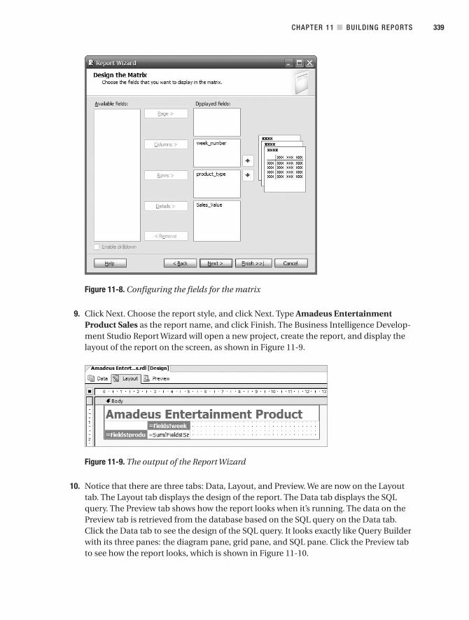
Figure 11-8. Configuring the fields for the matrix
9. Click Next. Choose the report style, and click Next. Type Amadeus EntertainmentProduct Sales as the report name, and click Finish. The Business Intelligence Develop-ment Studio Report Wizard will open a new project, create the report, and display thelayout of the report on the screen, as shown in Figure 11-9.
Figure 11-9. The output of the Report Wizard
10. Notice that there are three tabs: Data, Layout, and Preview. We are now on the Layouttab. The Layout tab displays the design of the report. The Data tab displays the SQLquery. The Preview tab shows how the report looks when it’s running. The data on thePreview tab is retrieved from the database based on the SQL query on the Data tab.Click the Data tab to see the design of the SQL query. It looks exactly like Query Builderwith its three panes: the diagram pane, grid pane, and SQL pane. Click the Preview tabto see how the report looks, which is shown in Figure 11-10.
CHAPTER 11 ■ BUILDING REPORTS 339
9314ch11final.qxd 11/15/07 10:03 AM Page 339

Figure 11-10. Preview of the report after finishing the Report Wizard
The query we just built is quite simple, but it reflects the most popular type of query usedin dimensional reporting. We joined a fact table with two dimension tables. We group on twocolumns and sum a column from the fact table. In a real project when querying a dimensionaldata store, it is likely that you will be dealing with more dimensions and more numbers offacts or measures. But the principles are the same. Now let’s continue with perfecting thereport layout. By that I mean enhancing the report appearance such as fixing the report title,formatting the numbers, adding column headings, and adjusting the column size. We willthen add some parameters to the report.
Report LayoutIn Figure 11-10, the word Sales in the title falls on the second row. The figures on the cells con-tain four decimal points, but the third and fourth ones are all zero. They need to be changed totwo decimal points. The first column has no title, and the product types are wrapped onto twolines. So, let’s tidy up the layout.
CHAPTER 11 ■ BUILDING REPORTS340
9314ch11final.qxd 11/15/07 10:03 AM Page 340

1. First, let’s fix the word Sales in the report title. Click the Layout tab. Click the title.Notice that now there are eight little white boxes around the title. Click the right-centerbox, and drag it to the right until the word Sales appears on the title line. Click the Pre-view tab to verify that the title is now on one line.
2. Now let’s change the figures on the report cells to two decimal points. Click the Layouttab. Right-click the report cell, the one that contains =Sum(Fields!Sa…, and select Prop-erties. The Textbox Properties dialog box appears. Click the Format tab. Click the …button next to the “Format code” text box. Underneath Standard, select Number, andclick 1,234.00, as illustrated in Figure 11-11. Click OK to close the Choose Format dia-log box. Then click OK again to close the Textbox Properties dialog box.
Figure 11-11. Setting the format of the report cells
3. Click the Preview tab to check that the figures on the report cells have been formattedcorrectly to two decimal points.
4. Now let’s fix the width of the first column. Click the Layout tab. Click the first column.Notice on the ruler that the width of the first column is 2.5 centimeters. Click the verti-cal line between the first and second columns, and drag it to the right to make thecolumn width 4 centimeters. Click the Preview tab to verify that the product types arenot wrapped onto two lines.
5. Now let’s give the first column a heading. Click the Layout tab. Double-click the firstcell of the first column. Type Product by Week, and click the Preview tab to verify thatthe first column now has a heading.
6. Last, let’s resize the columns containing the weekly sales figure. Click the Layout col-umn. Click the second column. Click the line on the right of the second column, anddrag the line to the left to make the column width 1.5 centimeters; for example, on theruler it should be from 4.0 to 5.5 centimeters. Click Preview to verify.
CHAPTER 11 ■ BUILDING REPORTS 341
9314ch11final.qxd 11/15/07 10:03 AM Page 341

Now that we have completed fixing the layout, let’s run the report by pressing F5. BusinessIntelligence Development Studio should say, “The project cannot be debugged because nostarting report is specified.” This is because we have not specified the starting point of theproject, so we need to specify which report to execute when we run the project. So, click theProject menu, and select Amadeus Reports Properties. On the StartItem, select AmadeusEntertainment Product Sales. Click OK. Press F5 again to run the report. Figure 11-12 showshow the report looks.
Figure 11-12. How the report looks after tidying up the layout
We can tweak the layout in many other ways, including adding columns, adding a pageheader and footer, changing the font, setting the alignment, and setting the spacing as well asspecifying all the text box properties shown in Figure 11-11. You can also create a report in tab-ular form instead of matrix form. I encourage you to explore those Reporting Services layoutfeatures and use them in your reports.
Report ParametersReport parameters are an important feature in a data warehouse dimensional report. Ina dimensional model, the core data is stored in a fact table, which has links to dimensiontables so that we can filter and group by the dimensional attributes. Refer to the SQL queryin Listing 11-2. In this query, we can choose any fact columns from the Product Sales facttable—grouped by any columns from the date, product, customer, or store dimensiontable, as well as filtered by any conditions in any dimension columns. That is a verypowerful query!
CHAPTER 11 ■ BUILDING REPORTS342
9314ch11final.qxd 11/15/07 10:03 AM Page 342

In the report we just created in the previous two sections, we have not put any conditionson the query. There is no where clause in the query (refer to Figure 11-6). We have select, from,and group by clauses, but we don’t have a where clause. In this section, you will learn how toadd some conditions to the query, such as the where clause, using parameters.
We’ll add three parameters to the report (Year, Quarter, and Division) as three drop-downlists. The values of these parameters will then be passed to the SQL query. These parameterswill be passed to the where clause of the SQL query, as shown in Listing 11-3.
Listing 11-3. The where Clause of Weekly Product Sales Query
where d.quarter = @pQuarterand d.year = @pYearand (s.division = @pDivisionor @pDivision = ' All')
A parameter name always begins with @. I usually name the parameter the same as thecolumn but add a p prefix. For example, for the quarter column, I name the parameter@pQuarter. This is so that I can find out quickly which parameter is for which column. But youcan name your parameters differently; there are no restrictions for this. OK, let’s start.
1. Let’s return to our report in Business Intelligence Development Studio. If the report isstill running, close it. Click the Layout tab. Click the Report menu, and choose ReportParameters. Click Add. Set the name to pYear, the data type to String, and the promptto Year. Leave everything else as is, and click OK.
The reason why I add the p prefix in the parameter name is because in the ReportParameters dialog box (see the later Figure 11-14), we don’t have the @ sign on theparameter names. So if we name the table column Year, the parameter Year, and thedata set Year, it’s difficult for us to know which one is which. If we name the columnYear, the parameter pYear, and the data set dsYear, it is easier to differentiate them. I’llexplain about data sets in the next paragraph. This is not really a Hungarian namingconvention because the prefix does not indicate the data type. In Hungarian namingconventions (such as sSupplierName, nQuantity, and dOrderDate), the prefix indicatesthe data type (s = string, n = numeric, and d = date).
2. When the user clicks the Year drop-down list, we want the list to display all the yearsthat exist in the orders in the Product Sales fact table. For that, we need to create a datasource for the drop-down list. So, click the Data tab. Click the DDS data set drop-downlist, and choose <New Dataset…>. Set the name to dsYear, the data source to DDS, andthe command type to Text, as shown in Figure 11-13.
CHAPTER 11 ■ BUILDING REPORTS 343
9314ch11final.qxd 11/15/07 10:03 AM Page 343

Figure 11-13. Setting up the data source for the Year parameter
3. Set the query string as shown in Listing 11-4, and click OK to close the Dataset dialogbox.
Listing 11-4. SQL Query for dsYear Data Set
select distinct d.yearfrom fact_product_sales finner join dim_date don f.sales_date_key = d.date_key
I need to mention here that populating the Year drop-down list by selecting from a facttable like this is quite an expensive query to run, especially on large databases. If theperformance is not satisfactory, consider creating a little parameter table containingthe distinct year values of the sales date column on the fact table. You can then use thislittle parameter table to populate the Year drop-down list. The year values on this littletable need to be maintained by the ETL process to keep them up-to-date.
4. Click the exclamation mark (!) to run the query. It displays 2006 and 2007 on the out-put grid.
5. Click the Report menu, and choose Report Parameters. Click the pYear parameter toselect it. Under Available Values, click From Query. Set the data set to dsYear, the Valuefield to Year, and the Label field to Year, as shown in Figure 11-14.
CHAPTER 11 ■ BUILDING REPORTS344
9314ch11final.qxd 11/15/07 10:03 AM Page 344
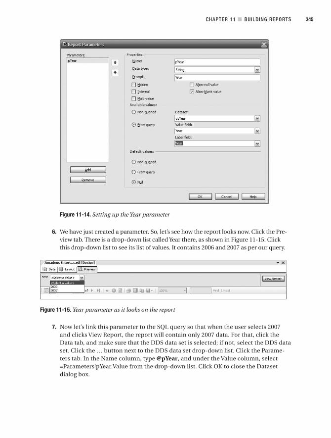
Figure 11-14. Setting up the Year parameter
6. We have just created a parameter. So, let’s see how the report looks now. Click the Pre-view tab. There is a drop-down list called Year there, as shown in Figure 11-15. Clickthis drop-down list to see its list of values. It contains 2006 and 2007 as per our query.
Figure 11-15. Year parameter as it looks on the report
7. Now let’s link this parameter to the SQL query so that when the user selects 2007and clicks View Report, the report will contain only 2007 data. For that, click theData tab, and make sure that the DDS data set is selected; if not, select the DDS dataset. Click the … button next to the DDS data set drop-down list. Click the Parame-ters tab. In the Name column, type @pYear, and under the Value column, select=Parameters!pYear.Value from the drop-down list. Click OK to close the Datasetdialog box.
CHAPTER 11 ■ BUILDING REPORTS 345
9314ch11final.qxd 11/15/07 10:03 AM Page 345

8. For the dim_date table, scroll down to find the year column, and tick the check box.Notice that the year column now appears on the grid pane (the middle pane). On thegrid pane, clear the Output check box for year. Change the Group By column fromGroup By to Where. In the Filter column, type =@pYear, and press Enter. The data setnow looks like Figure 11-16.
Figure 11-16. Adding the Year parameter to the where clause of the data set query
9. Notice that there is a where clause in the query now. Also notice there is a funnel iconon the dim_date’s year column.
10. Now that we have added the Year parameter to the data set query (on the where clause),let’s test the report. Click Preview. In the Year drop-down list, select 2006, and clickView Report. Memorize the value of the data in a few cells. Now select 2007, and clickView Report again. Notice that the values on those cells are different.
11. Now let’s add the second parameter: Quarter. This second parameter (Quarter) isdependent on the first parameter (Year). For 2006, we have four quarters of data in theProduct Sales fact table. But for 2007, we have only Q1 and Q2 data. So, when wechoose 2006 on the Year parameter, the Quarter parameter should show four quarters.But when we choose 2007 on the Year parameter, the Quarter parameter should showonly Q1 and Q2. The same technique can be implemented on the Division and Regionparameters on the store dimension hierarchy.
CHAPTER 11 ■ BUILDING REPORTS346
9314ch11final.qxd 11/15/07 10:03 AM Page 346
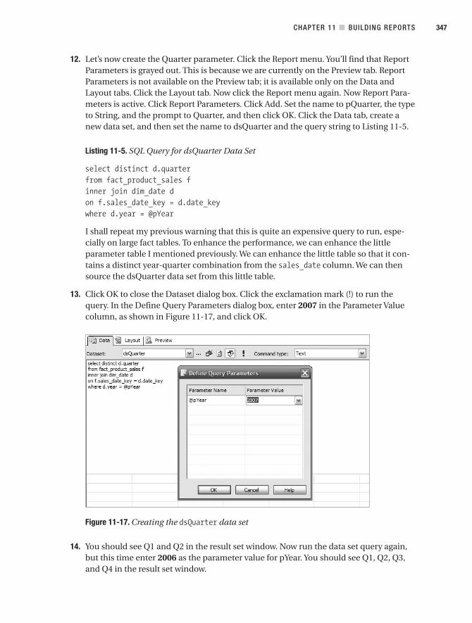
12. Let’s now create the Quarter parameter. Click the Report menu. You’ll find that ReportParameters is grayed out. This is because we are currently on the Preview tab. ReportParameters is not available on the Preview tab; it is available only on the Data andLayout tabs. Click the Layout tab. Now click the Report menu again. Now Report Para-meters is active. Click Report Parameters. Click Add. Set the name to pQuarter, the typeto String, and the prompt to Quarter, and then click OK. Click the Data tab, create anew data set, and then set the name to dsQuarter and the query string to Listing 11-5.
Listing 11-5. SQL Query for dsQuarter Data Set
select distinct d.quarterfrom fact_product_sales finner join dim_date don f.sales_date_key = d.date_keywhere d.year = @pYear
I shall repeat my previous warning that this is quite an expensive query to run, espe-cially on large fact tables. To enhance the performance, we can enhance the littleparameter table I mentioned previously. We can enhance the little table so that it con-tains a distinct year-quarter combination from the sales_date column. We can thensource the dsQuarter data set from this little table.
13. Click OK to close the Dataset dialog box. Click the exclamation mark (!) to run thequery. In the Define Query Parameters dialog box, enter 2007 in the Parameter Valuecolumn, as shown in Figure 11-17, and click OK.
Figure 11-17. Creating the dsQuarter data set
14. You should see Q1 and Q2 in the result set window. Now run the data set query again,but this time enter 2006 as the parameter value for pYear. You should see Q1, Q2, Q3,and Q4 in the result set window.
CHAPTER 11 ■ BUILDING REPORTS 347
9314ch11final.qxd 11/15/07 10:03 AM Page 347

15. Now that the data set for Quarter is created, let’s use it on the parameter. Click theReport menu, and select Report Parameters. Click pQuarter. Under Available Values,click From Query. Set the data set to dsQuarter, and select quarter for both Value Fieldand Label Field. Click OK to close the Report Parameters dialog box.
Please notice that you don’t have to click the Parameters tab of the data set to definethe pQuarter parameter. This is an optional step. Reporting Services will automaticallycreate it for you if you don’t define it.
16. Click the Preview tab to see the report. Notice that the Quarter parameter is there butis grayed out. This is because it is dependent on the value of the Year parameter. Select2006 for Year. Notice that now the Quarter parameter is active, and it contains Q1, Q2,Q3, and Q4. Select 2007 for Year, and notice that the Quarter parameter contains Q1and Q2 only, as shown in Figure 11-18.
Figure 11-18. A parameter that is dependent on the value of another parameter
17. Select Q1, and click View Report. Notice that it still contains data from week 1 untilweek 17, which means the Quarter parameter is not working. In Q1, we have week 1 toweek 13 only. Change the quarter to Q2, and click View Report. Notice that the data onthe report is the same, and it also contains week 1 to week 17. This is because we havenot put the Quarter parameter on the where clause of the main data set.
18. Let’s add the Quarter parameter to the main data set query. Click the Data tab. Ensurethat the DDS data set is selected, and if not, select it. Scroll down on the dim_date tableto find the quarter column. Tick the check box on this column to select it. Notice thatthe quarter column has now been added to the grid pane. Clear the Output check boxfor the quarter column, and change the Group By column from Group By to Where. Inthe Filter column, type =@pQuarter, and press Enter.
19. Now that we have added Quarter parameter to the main data set, if we select 2007 Q1on the parameters, the report should display only 2007 Q1 data. Let’s try it. Click thePreview tab. Select 2007 for Year, select Q1 for Quarter, and click View Report. Now itcontains only weeks 1 to 13. Press F5 to run the report. Figure 11-19 shows the result.
CHAPTER 11 ■ BUILDING REPORTS348
9314ch11final.qxd 11/15/07 10:03 AM Page 348

Figure 11-19. Product Sales report with the Year and Quarter parameters
20. Now that we have added two parameters to the report, let’s add the third one. This timeit is not from the date dimension but from the store dimension. This third parameter isDivision. This time it has one additional value in the drop-down list, which is All. So,the users will be able to select a division, but they can also select all divisions.
21. Because we have already done it twice, this time I’ll skip the details. Add a parametercalled pDivision with a label called Division. Define a data set called dsDivision, withthe query string as shown in Listing 11-6.
Listing 11-6. SQL Query for dsDivision Data Set
select distinct s.divisionfrom fact_product_sales finner join dim_store son f.store_key = s.store_keyunionselect 'All' as division
The query retrieves the distinct values on the division column from the Product Salesfact table. It adds one more value, which is ‘All,’ using the union operation.
CHAPTER 11 ■ BUILDING REPORTS 349
9314ch11final.qxd 11/15/07 10:03 AM Page 349

■Tip If you want to ensure that ‘All’ is on the top of the list, you can add a space in front of it.
Perhaps you’re wondering why we want to restrict the values on the drop-down listonly to the items that have records in the fact table. In other words, in the previousexample, why do we want to restrict the Year, the Quarter, and the Division parame-ters to only the ones that have sales? Doesn’t it make the query more expensive? Theanswer is that there is no point displaying divisions, years, or quarters that have nosales. About a year ago I had a UAT in a SQL Server data warehousing project wherewe used SSRS for reporting. The users were not happy having drop-down lists con-taining many values when only a few of them actually had sales. For example, out of50 branches, only 5 of them had sales for that particular product type on that day.Why couldn’t the report be intelligent enough to filter them for us, they asked? If inyour project you have only three divisions and 99 percent of the time all three alwayshave sales, then of course you want to populate the Division drop-down list from thedivision table and display all three divisions all the time.
22. Click the Report menu, and select Report Parameters again. Click the pDivision, andget the values from dsDivision data set. Set both Value Field and Label Field to division.
23. On the DDS data set, click the Add Table icon (the rightmost icon), and add thedim_store table. Click Close. Scroll down in the dim_store table until you find the Divi-sion column, and select it. On the grid pane, clear the Output check box, and changethe Group By column to Where. In the Filter column, enter =@pDivision.
24. Click the Preview tab, and you should see three parameters now: Year, Quarter, andDivision. Select 2007 for Year, Q1 for Quarter, and Online Business for Division, andthen click View Report. Notice that the report is now sparser than before; that is,there are some blank cells. This is because it displays only the Online Business divi-sion. Change the Division parameter to All, and click View Report. The report isblank. Why is the report blank? Well, there is no division called All. So, the queryreturns no results.
25. To fix this, click the Data tab. Click the Generic Query Designer icon (the one with ayellow pencil). Update the where clause from WHERE (dim_date.year = @pYear) AND(dim_date.quarter = @pQuarter) AND (dim_store.division = @pDivision) to what’sshown in Listing 11-7.
Listing 11-7. Updating Main Data Set’s where Clause to Include All
WHERE dim_date.year = @pYearAND dim_date.quarter = @pQuarterAND (dim_store.division = @pDivision or @pDivision = 'All')
So now if you select All on the Division parameter, the @pDivision = 'All' will evalu-ate to true so the expression in parentheses will also evaluate to true.
CHAPTER 11 ■ BUILDING REPORTS350
9314ch11final.qxd 11/15/07 10:03 AM Page 350
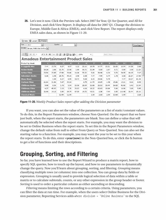
26. Let’s test it now. Click the Preview tab. Select 2007 for Year, Q1 for Quarter, and All forDivision, and click View Report. It displays all data for 2007 Q1. Change the division toEurope, Middle East & Africa (EMEA), and click View Report. The report displays onlyEMEA sales data, as shown in Figure 11-20.
Figure 11-20. Weekly Product Sales report after adding the Division parameter
If you want, you can also set the value of the parameters as a list of static/constant values.To do this, in the Report Parameters window, choose Non-Queried. On the report that we havejust built, when the report starts, the parameters are blank. You can define a value that willautomatically be selected when the report starts. For example, you may want the division tobe set to Online Business when the report starts. To set this in the Report Parameters window,change the default value from null to either From Query or Non-Queried. You can also set thestarting value to a function. For example, you may want the year to be set to this year whenthe report starts. To do this, enter =year(now) in the Non-Queried box, or click the fx buttonto get a list of functions and their descriptions.
Grouping, Sorting, and FilteringSo far, you have learned how to use the Report Wizard to produce a matrix report, how tospecify SQL queries, how to touch up the layout, and how to use parameters to dynamicallychange the query. Now you’ll learn about grouping, sorting, and filtering. Grouping meansclassifying multiple rows (or columns) into one collection. You can group data by fields orexpression. Grouping is usually used to provide logical selection of data within a table ormatrix or to calculate subtotals, counts, or any other expression in the group header or footer.Sorting is used to order a particular column as either ascending or descending.
Filtering means limiting the rows according to a certain criteria. Using parameters, youcan filter the data at run time. For example, when the users select Online Business for the Divi-sion parameter, Reporting Services adds where division = 'Online Business' to the SQL
CHAPTER 11 ■ BUILDING REPORTS 351
9314ch11final.qxd 11/15/07 10:03 AM Page 351

query. This will then filter the data that is displayed on the report. There is another way to filterthe data that we display on the report—by adding a where clause to the main data set query atdesign time. This type of filtering cannot be changed by the users at run time. The purpose ofdoing this is to limit the rows returned by the query according to certain criteria. For example,you may want to have a report that specifically deals with business customers. In this case, wefilter the query with where customer_type = 'Business' or something similar. In this section,we will be doing the type of filtering that uses the where clause at design time.
First, we’ll include the product category column on the SQL query, and then we’ll add it asa group to the Weekly Product Sales report that we built. Then, we will change the order of thecolumn, add a sorting order, and, finally, apply a filter.
1. To start, click the Data tab. Add dim_product.product_category on both the selectclause and group by clause, and reformat the query a little bit, as shown in Listing 11-8.
Listing 11-8. Adding the Product Category on the SQL Query
select dim_date.week_number, dim_product.product_type,sum(fact_product_sales.sales_value) AS [Sales Value],dim_product.product_category
from dim_dateinner join fact_product_saleson dim_date.date_key = fact_product_sales.sales_date_key
inner join dim_producton fact_product_sales.product_key = dim_product.product_key
inner join dim_storeon fact_product_sales.store_key = dim_store.store_key
where dim_date.year = @pYearand dim_date.quarter = @pQuarterand (dim_store.division = @pDivision or @pDivision = 'All')
group by dim_product.product_type, dim_date.week_number,dim_product.product_category
In SSRS, we have two tools to build queries. One is called Query Builder, and the otheris Generic Query Designer. Query Builder is the graphical tool that we used with theReport Wizard. Generic Query Designer is the plain-text editor that we used to add@pDivision or @pDivision = 'All' to the report query.
A lot of SQL developers find that SQL query formatting is sometimes annoying if it isnot up to their standards or their style. For example, where to break to a new line, theabbreviation of table names, the number of spaces for indentation, the choice ofuppercase or lowercase, whether to put the comma at the beginning or at the end ofthe line, and where to put brackets…all these are little things that sometimes make usuncomfortable if the formatting is different from our own style.
Other than the ability to control the details such as the join syntax, style is another rea-son (but not the primary one) why some SQL developers choose to not use QueryBuilder and instead use the plain-text Generic Query Designer.
CHAPTER 11 ■ BUILDING REPORTS352
9314ch11final.qxd 11/15/07 10:03 AM Page 352

2. We want to add the product category to the report to understand how the sales figuresplits between music, film, and audio books. For that, let’s now add the product cate-gory as a new group to the report. Click the Layout tab. Click the heading of column 1(Product by Week). Right-click the cell above Product by Week, and choose Add RowGroup. The Grouping and Sorting Properties dialog box will pop up. Set the name toProductCategory, and set Expression to '=Fields!product_category.Value, as shownin Figure 11-21. Next, click OK.
Figure 11-21. Setting the properties of the product category group
3. Click the Preview tab, fill in the parameters (such as 2007, Q1, and All Divisions), andclick View Report. The product category is positioned as the second column in thereport, as shown in Figure 11-22.
4. There are only three product categories (music, films, and audio books), but there aremany product types. The product category is on a higher level than the product type.One product category contains many product types. So in Figure 11-22, the productcategory should be located to the left of the product type. Let’s now swap the productcategory column and the product type column. Click the Layout tab. Click the productcategory cell. Click the line surrounding the product category cell, and drag it to theleft of the product type column, as shown in Figure 11-23.
5. Click the Preview tab, and view the report again. It now looks like Figure 11-24.
CHAPTER 11 ■ BUILDING REPORTS 353
9314ch11final.qxd 11/15/07 10:03 AM Page 353

Figure 11-22. Product Sales report with product category column added
Figure 11-23. Swapping product category and product types
Figure 11-24. Product Sales report after swapping the product category and product type columns
I’ll now discuss the sorting order for groups. Let’s put the sorting order on the productcategory column so that Music is at the top, Films is second, and Audio Books is at the bot-tom. Click the Layout tab. Right-click the product category cell, and choose Edit Group. TheGrouping and Sorting Properties dialog box appears. Click the Sorting tab, set Expression to=Fields!product_category.Value, and set Direction to Descending. Click OK. Click the Pre-view tab to view the report.
CHAPTER 11 ■ BUILDING REPORTS354
9314ch11final.qxd 11/15/07 10:03 AM Page 354

The sorting order on the product category column is now what we wanted; that is, Musicis at the top, Films is in the middle, and Audio Book is at the bottom. But at the very top,before Music, we have Unknown. This is because we have an unknown record on both theproduct category dimension and the product type dimension in the DDS. So, let’s filter out theunknown record.
1. Click the Layout tab. Right-click the Product Category cell, and choose Edit Group.
2. Click the Filter tab, set Expression to =Fields!product_category.Value, Operator to !=,and Value to Unknown. Click OK.
3. Click the Preview tab to view the report again. The unknown record is no longer there,and the report now looks like Figure 11-25.
Figure 11-25. Sorting on the product category and filtering the unknown record
Grouping is usually used to provide a logical grouping of data within a table or matrix orfor calculating subtotals, counts, or any other expression on the group header or footer. As thelast task in this section, let’s now add a subtotal in the product category column and a grandtotal.
1. Click the Layout tab. To add the subtotal to the product category column, right-clickthe Product Type cell, and choose Subtotal. You will see a new row with Total in the sec-ond column with a little green triangle in the corner of the cell.
2. To add the grand total, right-click the product category cell, and choose Subtotal.
3. Click the Preview tab to view the report. Scroll down to see the subtotal for the Musiccategory and the Films category.
4. On the toolbar, click the Next Page icon (the blue triangle) to go to page 2. Verify thatyou can see the subtotal for the Audio Books category as well as the grand total on thelast row, as shown in Figure 11-26.
CHAPTER 11 ■ BUILDING REPORTS 355
9314ch11final.qxd 11/15/07 10:03 AM Page 355
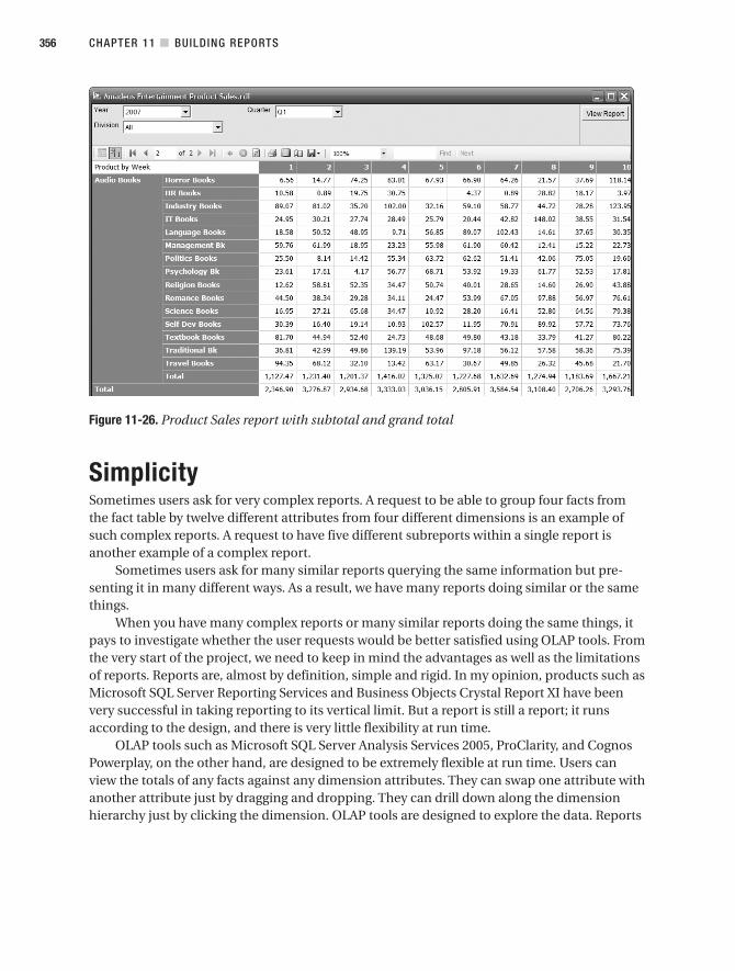
Figure 11-26. Product Sales report with subtotal and grand total
SimplicitySometimes users ask for very complex reports. A request to be able to group four facts fromthe fact table by twelve different attributes from four different dimensions is an example ofsuch complex reports. A request to have five different subreports within a single report isanother example of a complex report.
Sometimes users ask for many similar reports querying the same information but pre-senting it in many different ways. As a result, we have many reports doing similar or the samethings.
When you have many complex reports or many similar reports doing the same things, itpays to investigate whether the user requests would be better satisfied using OLAP tools. Fromthe very start of the project, we need to keep in mind the advantages as well as the limitationsof reports. Reports are, almost by definition, simple and rigid. In my opinion, products such asMicrosoft SQL Server Reporting Services and Business Objects Crystal Report XI have beenvery successful in taking reporting to its vertical limit. But a report is still a report; it runsaccording to the design, and there is very little flexibility at run time.
OLAP tools such as Microsoft SQL Server Analysis Services 2005, ProClarity, and CognosPowerplay, on the other hand, are designed to be extremely flexible at run time. Users canview the totals of any facts against any dimension attributes. They can swap one attribute withanother attribute just by dragging and dropping. They can drill down along the dimensionhierarchy just by clicking the dimension. OLAP tools are designed to explore the data. Reports
CHAPTER 11 ■ BUILDING REPORTS356
9314ch11final.qxd 11/15/07 10:03 AM Page 356

are not. So if you get very complex reporting requests, it’s worth finding out whether the usersneed to explore the data. If so, OLAP tools would satisfy their needs better than reports.
Another means of exploring the data is using SQL queries. I have found that if the busi-ness user understands a little bit about SELECT statements, it takes only a day or two to explainthe structure of the dimensional data store and how to use a join to query the structure. If theydon’t understand how to use SELECT statements, many tools help build SQL queries through aGUI. Reporting Services has Query Builder, which does this. Excel has Query Wizard, which isa query design tool with a GUI interface. A lot of other BI applications also have reportingtools with GUI interfaces for designing queries.
The business users understand the data and the meaning of each fact and attribute, andthat’s why it’s quicker for them to query the fact and dimension tables. This is especially true ifyou consistently use a star schema, because once you spend a day explaining how to queryone data mart, the other marts have the same structure. Querying can be done from Manage-ment Studio or from Excel via an ODBC or OLEDB connection (or SQL Server native if youinstall the driver on the client’s PC).
Different users have different needs. Some users need to use a static report only to viewthe facts related to their area of responsibility. Some users need to explore and analyze thedata to find out the root cause of a particular problem such as a period of low sales. Someusers need to run “what if?” scenarios. Some users need to investigate whether the data hascertain consistent patterns.
SSRS is a sophisticated reporting tool with a lot of capabilities and features. But we needto keep in mind that there are better ways and tools to satisfy exploration needs. Reports aredesigned for something simple and fixed. So, we need to keep reporting simple. That’s theprinciple of simplicity in reporting.
SpreadsheetsIt is also possible to present or report the data in the data warehouse to the users usingspreadsheets such as Excel. Many data warehouse business users are familiar with spread-sheets, and spreadsheets are the perfect compromise between SSRS reports, which are static,and OLAP tools, which are very flexible. Using spreadsheets, users can query the data in thedata warehouse and present it either in a simple tabular format or in a pivot table.
I’ll show some examples of how it looks if we use spreadsheets to present the data.In these examples, I will use Excel as the spreadsheet. Figure 11-27 shows the AmadeusEntertainment Store Details report, which is in tabular format. It is essentially the same asFigure 11-1, but this one was created in Excel. I’ll explain how to create and populate thisExcel spreadsheet after the next paragraph.
Figure 11-28 shows the Amadeus Entertainment Weekly Product Sales report that we cre-ated earlier in this chapter. It also has the year, quarter, and division parameters like the onesshown earlier in Figure 11-2. Of course, we can also enhance the layout, such as adding areport title, tidying up the column headers, and fixing the column width.
CHAPTER 11 ■ BUILDING REPORTS 357
9314ch11final.qxd 11/15/07 10:03 AM Page 357
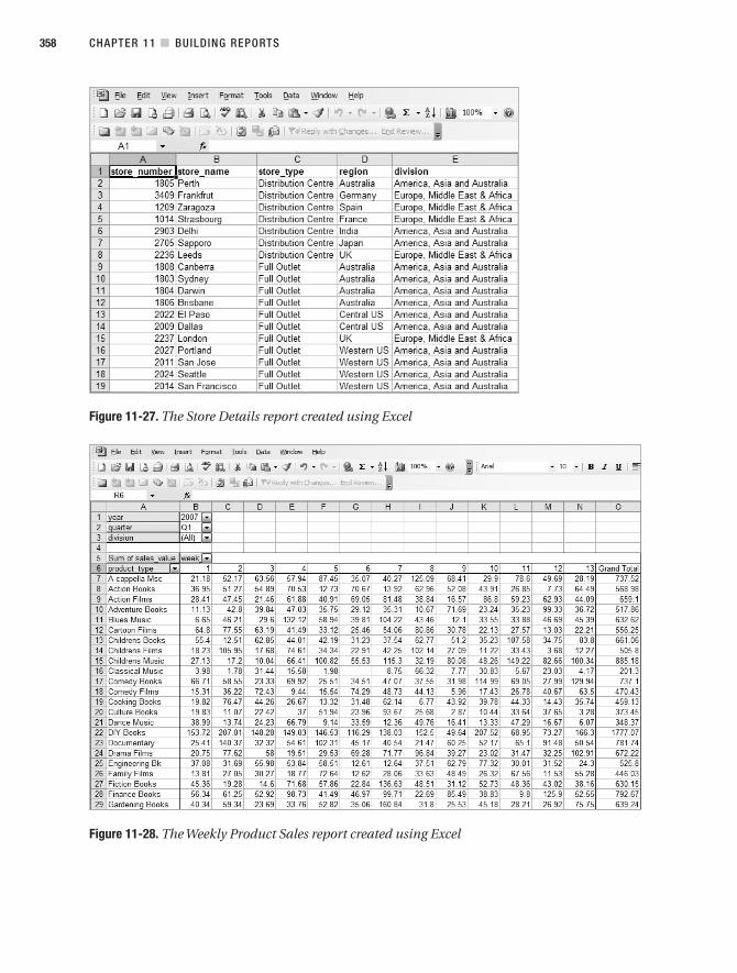
Figure 11-27. The Store Details report created using Excel
Figure 11-28. The Weekly Product Sales report created using Excel
CHAPTER 11 ■ BUILDING REPORTS358
9314ch11final.qxd 11/15/07 10:03 AM Page 358

Creating these reports is easy. Let’s start.
1. Open Excel, and click Data ➤ Import External Data ➤ New Database Query. Define anew data source, and connect to the data source as follows: select <New Data Source>on the Databases tab, as shown in Figure 11-29, and click OK.
Figure 11-29. Creating a new data source
2. In the Create New Data Source dialog box (see Figure 11-30), name the data sourceDDS. Select SQL Server as the driver, and click Connect.
Figure 11-30. Filling in the details in the Create New Data Source dialog box
3. The SQL Server Login dialog box will open, as shown in Figure 11-31. Select your SQLServer, uncheck Use Trusted Connection, and supply the login details (we discussedthis in Chapter 7). Click the Options button, and select the DDS database. Click OK togo back to the Create New Data Source dialog box in Figure 11-30. Optionally, you canselect dim_store as the default table. Click OK.
CHAPTER 11 ■ BUILDING REPORTS 359
9314ch11final.qxd 11/15/07 10:03 AM Page 359
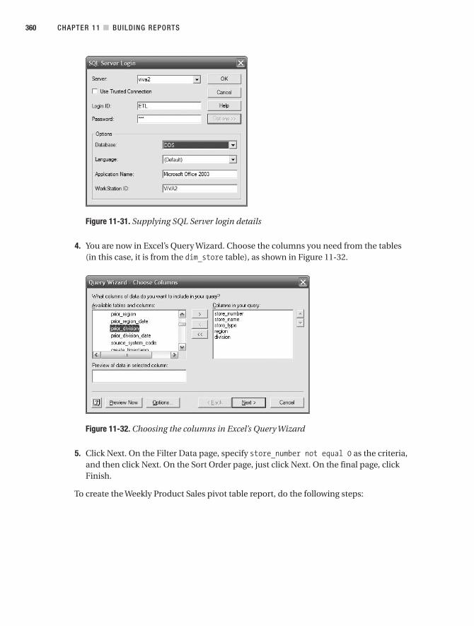
Figure 11-31. Supplying SQL Server login details
4. You are now in Excel’s Query Wizard. Choose the columns you need from the tables(in this case, it is from the dim_store table), as shown in Figure 11-32.
Figure 11-32. Choosing the columns in Excel’s Query Wizard
5. Click Next. On the Filter Data page, specify store_number not equal 0 as the criteria,and then click Next. On the Sort Order page, just click Next. On the final page, clickFinish.
To create the Weekly Product Sales pivot table report, do the following steps:
CHAPTER 11 ■ BUILDING REPORTS360
9314ch11final.qxd 11/15/07 10:03 AM Page 360

1. Click the Data menu, and select Pivot Table. Choose External Data Source, and clickNext.
2. Click Get Data, and select DDS as the data source. Choose the columns (week_number,quarter, and year from dim_date; product_code from dim_product; division fromdim_store; and sales_value from fact_product_sales). Excel’s Query Wizard will saythat you can’t continue because of the join criteria. This is because it cannot find thedate_key column in the fact_product_sales table to join it with the dim_date table. Justclick Yes in the dialog box and join date_key on dim_date to sales_date_key onfact_product_sales manually, as shown in Figure 11-33.
Figure 11-33. Joining the tables
3. Click the Return Data icon, and click Next in the dialog box.
4. Click Layout, and specify the layout, including the week number in the column, theproduct code in the row, the sales value in the cells and year, and the quarter anddivision on the page, as shown in Figure 11-34.
5. Click OK, and then click Finish. You will get the pivot table shown in Figure 11-28.You can then tidy up the layout by adding a report title, setting the column width,and so on.
CHAPTER 11 ■ BUILDING REPORTS 361
9314ch11final.qxd 11/15/07 10:03 AM Page 361

Figure 11-34. Setting up the layout of the pivot table
The problem with Excel reporting is the distribution. We practically need to distributethe Excel file to all users and set up the data source on every PC that needs to run the report(unless you put it on a server with the web-based Excel viewer). It can be made easier by uti-lizing a file data source name (DSN), which is located on a common network drive, but thedeployment overhead is still there. And security is a nightmare. Simply speaking, we need tocreate views in the data warehouse to restrict user access. For example, say you have a tablecalled payment containing a column called credit_card_number. We can create a view calledpayment_v containing all payment table columns except the credit card number column. Wegrant SELECT permission to the user on this view, but we revoke SELECT permission from theuser on the base table (payment table). If we simply grant the db_datareader role to the users,they will be able to access all columns on all tables.
SSRS, on the other hand, is deployment friendly. The reports are web-based, so we don’thave to install anything on any of the users’ PCs. Setting up security is very simple. We caneven utilize the Windows accounts to authenticate the users so the users don’t have to log inagain. We’ll discuss more about deployment later in this chapter. But, reports are more orless static.
Access to DDS using Excel would suit a handful of business analysts who can write a SQLquery, can understand the DDS structure, are very familiar with Excel, are happy to set upDSN themselves, and are able to create the Excel reports. They can manipulate the data in anyway they like in their Excel files. They can turn the pivot tables in any way they like. They canformat the reports in any way they like, and they can also create some charts.
Multidimensional Database ReportsSo far in this chapter, you have learned that from SSRS you can access relational data storeswithin the data warehouse, such as the DDS database. But a data warehouse may also con-tain multidimensional databases or cubes. (Please refer to Chapter 1 for an explanation ofwhat a multidimensional database or cube is.) From SSRS, we can also access multidimen-sional databases.
CHAPTER 11 ■ BUILDING REPORTS362
9314ch11final.qxd 11/15/07 10:03 AM Page 362

By their very nature, cubes are meant to be accessed using OLAP tools or cube browsersor by using an application framework such as ADOMD.NET. In most cases, cube data isaccessed independently of relational data, but occasionally we need to combine the data froma relational store and from a cube in one report or in one set of reports.
Let’s learn how to create a report that retrieves data from a cube. The fastest and bestway to learn this is by doing it. So, let’s get started. This time we will not use the Report Wiz-ard. Instead, we will create it manually, including the query and the layout. In the nextchapter, we will learn how to create a cube, but for now we will use an existing cube. For that,please restore the Amadeus Entertainment.abf cube backup from the /data folder on thisbook’s web site (http://www.apress.com). You can use SQL Server Management Studio torestore the cube backup. You just need to connect to your Analysis Services server, right-clickDatabases in Object Explorer, and choose Restore.
1. In Solution Explorer of BIDS, define a new data source. To do this, right-click SharedData Sources, and choose Add New Data Source. Set the name to Cubes, and set thetype to Microsoft SQL Server Analysis Services, as shown in Figure 11-35.
2. Click the Edit button. Set the server name to your development SQL Server, and in thedatabase name drop-down list choose the Analysis Services database where the cube islocated. Click OK. Leave the Credential tab as Use Windows Authentication (IntegratedSecurity), and click OK.
Figure 11-35. Creating a shared data source for accessing Analysis Services cubes
3. In the Solution Explorer pane, right-click the Reports, and choose Add ➤ New Item.Choose Report (not Report Wizard). Give it a name, such as Cube Report.rdl, andclick Add.
CHAPTER 11 ■ BUILDING REPORTS 363
9314ch11final.qxd 11/15/07 10:03 AM Page 363

4. In the Dataset drop-down list, choose <New Dataset…>. Give it a name (such asdsCube), choose the Data Source to Cubes (shared), leave the command type set totext, and leave the query string empty. Click OK. MDX Query Designer, similar to theone shown in Figure 11-36, will be displayed.
Figure 11-36. MDX Query Designer
5. Drag the following fact and attributes from the Metadata pane to the center pane:Product Type from Dim Product, week_number from Dim Date, and Sales Value meas-ure from Fact Product Sales, as shown in Figure 11-36 previously.
6. Drag Year and Quarter from Dim Date to the <Select dimension> area. Tick the Para-meters check boxes for both Year and Quarter, as shown in Figure 11-36. ReportingServices automatically creates those two parameters.
7. To verify, click the Report menu, and choose Report Parameters.
8. Click the Layout tab. In the left pane, click the Toolbox tab, and drag Matrix from theToolbox to the canvas, as shown in Figure 11-37.
9. Click the Datasets tab in the left pane, and drag product_type, week_number, andsales_value from dsCube to the matrix. Specifically, drag product_type to the Rowscell, week_number to the Columns cell, and sales_value to the Data cell.
10. Save the report, and click the Preview tab. Select Year to 2007, Quarter to Q1, and clickView Report. The report looks similar to Figure 11-38.
CHAPTER 11 ■ BUILDING REPORTS364
9314ch11final.qxd 11/15/07 10:03 AM Page 364

Figure 11-37. Creating the report layout
Figure 11-38. Report that retrieves data from a cube
11. If the product type column is not wide enough, you can adjust it on the Layout tab, aswell as the 13 columns containing the sales values. You can also add a report title.
And with that, we have finished created our report that retrieves data from a cube!If you notice, we did not write any Multidimensional Expressions (MDX) at all. This is
because we were using the MDX Query Designer. If you want to see what the MDX looks like,click the Data tab, and click the … button next to the dsCube Dataset drop-down list. You willsee that the MDX query is like the one in Listing 11-9.
Listing 11-9. The MDX Query for the Cube Report
SELECT NON EMPTY { [Measures].[Sales Value] }ON COLUMNS, NON EMPTY{ ([Dim Product].[Product Type].[Product Type].ALLMEMBERS
* [Dim Date].[week_number].[week_number].ALLMEMBERS ) }
CHAPTER 11 ■ BUILDING REPORTS 365
9314ch11final.qxd 11/15/07 10:03 AM Page 365

DIMENSION PROPERTIES MEMBER_CAPTION, MEMBER_UNIQUE_NAME ON ROWSFROM( SELECT ( STRTOSET(@DimDateQuarter, CONSTRAINED) ) ON COLUMNSFROM ( SELECT ( STRTOSET(@DimDateYear, CONSTRAINED) ) ON COLUMNS
FROM [DDS]))WHERE ( IIF( STRTOSET(@DimDateYear, CONSTRAINED).Count = 1,STRTOSET(@DimDateYear, CONSTRAINED),[Dim Date].[Year].currentmember ),IIF( STRTOSET(@DimDateQuarter, CONSTRAINED).Count = 1,STRTOSET(@DimDateQuarter, CONSTRAINED),[Dim Date].[Quarter].currentmember ) )
CELL PROPERTIES VALUE, BACK_COLOR, FORE_COLOR,FORMATTED_VALUE, FORMAT_STRING,FONT_NAME, FONT_SIZE, FONT_FLAGS
It is handy that Reporting Services uses MDX Query Designer to help us create the MDXquery. It makes reporting from cubes so much easier.
Deploying ReportsAfter we have built the reports, we want to publish them in a web server so the business userscan access them through their web browsers. This action is commonly known as deployingreports. Reports are deployed to a place called Report Manager on the web server. Let’s take astep back for a moment and try to understand what a Report Manager is.
When we install Reporting Services on a web server, it creates a web site called ReportManager. Report Manager is usually located at http://servername/reports (that’s the defaultlocation). We use Report Manager to upload reports, view reports, create data sources, organ-ize reports in folders, subscribe users to a report, configure site properties, and manage reportsecurity (which users can access which reports). Figure 11-39 shows how Report Managerlooks on the web browser.
Figure 11-39. Report Manager
CHAPTER 11 ■ BUILDING REPORTS366
9314ch11final.qxd 11/15/07 10:03 AM Page 366

Now that you understand what deploying a report means and what Report Manager is, I’llexplain how to deploy a report. First, we need to make sure that Reporting Services is up andrunning. Check the SQL Server Configuration Manager, and start it if it’s not running. Figure11-40 shows how to start Reporting Services in Configuration Manager.
Figure 11-40. Starting Reporting Services in Configuration Manager
After starting Reporting Services, we need to configure our report project in BIDS to pointto the target server. Click the Project menu, choose Properties, and set the Target Data SourceFolder, Target Report Folder, and Target Server URL options, as shown in Figure 11-41. KeepOverwrite Data Source as false, because we don’t want to overwrite data source informationon the production server. Usually, the data source details on the production server are differ-ent from the development server. Target Data Source Folder is the folder name on the ReportManager where we want the data sources to be deployed. Target Report Folder is the foldername on the Report Manager where we want the reports to be deployed. Target Server URL isthe web server where Reporting Services is installed.
Now after Reporting Services is started and the report project is configured, we candeploy the reports. To deploy all the reports in our project, as well as the data sources, in Solu-tion Explorer right-click the root folder of the report project, as shown in Figure 11-42, andchoose Deploy.
CHAPTER 11 ■ BUILDING REPORTS 367
9314ch11final.qxd 11/15/07 10:03 AM Page 367

Figure 11-41. Configuring project properties for report deployment
Figure 11-42. Deploying reports
Listing 11-10 shows the output log of this deployment.
Listing 11-10. Deployment Output
------ Build started: Project: Amadeus Reports, Configuration: Debug ------Build complete -- 0 errors, 0 warnings------ Deploy started: Project: Amadeus Reports, Configuration: Debug ------Deploying to http://localhost/ReportServerDeploying data source '/Data Sources/Cubes'.Deploying data source '/Data Sources/DDS'.
CHAPTER 11 ■ BUILDING REPORTS368
9314ch11final.qxd 11/15/07 10:03 AM Page 368

Deploying report '/Amadeus Reports/Amadeus Entertainment Product Sales'.Deploying report '/Amadeus Reports/Cube Report'.Deploying report '/Amadeus Reports/Store Details'.Deploy complete -- 0 errors, 0 warnings========== Build: 1 succeeded or up-to-date, 0 failed, 0 skipped ==================== Deploy: 1 succeeded, 0 failed, 0 skipped ==========
Instead of deploying all reports and data sources as discussed earlier, you can also deployonly a particular report or a particular data source. To do so, in Solution Explorer, right-clickthe report or data source you want to deploy, and choose Deploy.
Now that the reports are deployed, you can view them in Report Manager. To do that,open your web browser (Internet Explorer, Firefox, Opera, Safari, or whatever), and go to theReport Manager URL at http://servername/reports, where servername is the name of the webserver (IIS) where Reporting Services is installed. Report Manager will display two folders:Amadeus Reports and Data Sources, as shown previously in Figure 11-39.
Let’s view the Product Sales report we created earlier in this chapter. Click the AmadeusReport link. It shows the three reports we have in BIDS: Amadeus Entertainment ProductSales, Store Details, and Cube Report. Click Amadeus Entertainment Product Sales to view it.Figure 11-43 shows the result.
Figure 11-43. How the Product Sales report looks when deployed
To increase the scalability, we can also deploy the report on a web farm. Reporting Ser-vices also supports the report server database to be installed on a SQL Server cluster.Clustering increases the availability of the reports.
Now that we have deployed the reports, the next thing to do is manage them, which wewill discuss next.
CHAPTER 11 ■ BUILDING REPORTS 369
9314ch11final.qxd 11/15/07 10:03 AM Page 369

Managing ReportsAfter we deploy the reports to the Reporting Services server, we need to manage them. In par-ticular, we need to manage three areas: security, subscriptions, and execution:
• Security is about authentication and authorization. Authentication is verifying theuser’s identity, for example, by checking the user ID and password. Authorization isabout allowing certain users to access certain objects (such as reports) and keepingeverybody else out.
• A subscription is a request to deliver a particular report to a particular user using a par-ticular method (such as e-mail or a file share) at a particular time in a particular format.
• Execution is about the process of running the reports. We can execute a report in threeways: on demand, on demand from the cache, or from a snapshot. A snapshot is a staticcopy of the report output, produced at a specific time. We can schedule certain reportsto run at certain frequencies or for the snapshots to be created at a certain interval.
Managing Report SecurityIn some data warehouse implementations, all users can access all reports. But that is rare. Inmost implementations, certain users may access only certain reports, or at least there are cer-tain reports that some users are not allowed to access. This is usually done by configuring thereport security. A good way to configure report security is to create groups of users and assignthose groups to security roles in Reporting Services. The groups are ideally created in ActiveDirectory on the domain, the same place where all the Windows user accounts are.
The benefit of using groups rather than adding individual users is easier maintenance.If you have a new data warehouse user, all you have to do is add her to the appropriategroups. If a user leaves the company, all you have to do is remove her from the groups.You could arrange the groups by individual report, such as Report1_Readers, Report1_Writers, Report2_Readers, and Report2_Writers. Users who can view report1 are placed onlyin the Report1_Readers group, and users who can edit report1 are placed in the Report1_Writers group.
In Reporting Services, you can create a folder and put several reports into that folder.You can then arrange the groups by folders (instead of arranging them by reports), such asFolder1_Readers, Folder1_Writers, Folder2_Readers, and Folder2_Writers. Users who canview only those reports in folder1 will be in Folder1_Readers, and users who can create andedit all reports in folder1 will be in Folder1_Writers. You can always go down to the reportlevel if needed. For example, if a particular user needs to view all ten reports in folder1,except report5 that she needs to edit, you still add her to the Folder1_Readers group buton top of that you will add her as an individual user in report5 with write access.
Now that I have discussed the approach, let’s configure the security for the reports in ourcase study. We’ll give a group called Group1 read access to all reports in the Amadeus Reportfolder. In the Report Manager, to assign a user or a group to a folder, we click the Property taband click the Security link in the menu on the left. OK, open Report Manager by going tohttp://servername/reports in your web browser. Navigate to the Amadeus Report folder,and then click the Properties tab, as shown in Figure 11-44.
CHAPTER 11 ■ BUILDING REPORTS370
9314ch11final.qxd 11/15/07 10:03 AM Page 370
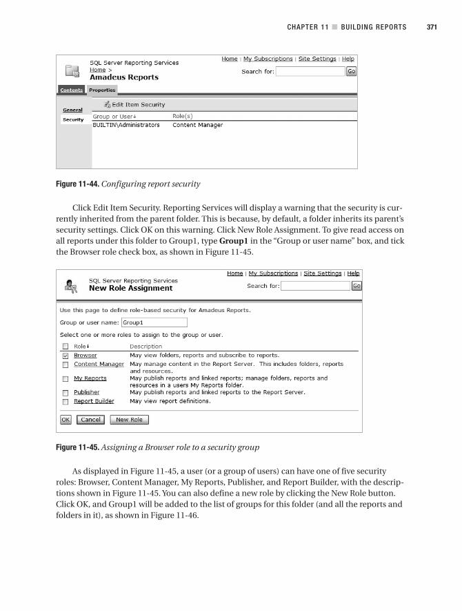
Figure 11-44. Configuring report security
Click Edit Item Security. Reporting Services will display a warning that the security is cur-rently inherited from the parent folder. This is because, by default, a folder inherits its parent’ssecurity settings. Click OK on this warning. Click New Role Assignment. To give read access onall reports under this folder to Group1, type Group1 in the “Group or user name” box, and tickthe Browser role check box, as shown in Figure 11-45.
Figure 11-45. Assigning a Browser role to a security group
As displayed in Figure 11-45, a user (or a group of users) can have one of five securityroles: Browser, Content Manager, My Reports, Publisher, and Report Builder, with the descrip-tions shown in Figure 11-45. You can also define a new role by clicking the New Role button.Click OK, and Group1 will be added to the list of groups for this folder (and all the reports andfolders in it), as shown in Figure 11-46.
CHAPTER 11 ■ BUILDING REPORTS 371
9314ch11final.qxd 11/15/07 10:03 AM Page 371

Figure 11-46. Adding a group with browser role to report security
Now, if a user who does not belong to Group1 tries to access the Amadeus Report, he willnot see any report in the folder. Instead, the folder will be empty, so he cannot access thereports.
Managing Report SubscriptionsAs I said earlier, a subscription is a request to deliver a particular report to a particular userusing a particular method at a particular time in a particular format. For example, users cansubscribe to the Product Sales report, requesting the report to be delivered to them at 8 a.m.every Tuesday morning in Excel format via e-mail as an attachment. This way, they don’t haveto open Report Manager, navigate to the report, and run it. Instead, it would be ready for themin their e-mail inbox when they arrive in the office at 9 a.m. every Tuesday.
To subscribe to a report, open the report you want to subscribe to, and click the New Sub-scription button. The New Subscription page looks like Figure 11-47.
CHAPTER 11 ■ BUILDING REPORTS372
9314ch11final.qxd 11/15/07 10:03 AM Page 372

Figure 11-47. Creating a new subscription
Then choose the report delivery option, such as e-mail or file share. If you choose e-mail,fill in the To text box with the recipient’s e-mail address, and choose the delivery option, eitherInclude Report or Include Link. Include Report means the e-mail will contain the report,whereas Include Link means the e-mail will contain only the URL of the report. For IncludeReport, if you choose Web Archive as the render format, the report will be embedded in thebody of the e-mail. If you choose any other render format (CSV, Excel, PDF, HTM, XML, orTIFF), the report will be sent as an attachment to the e-mail.
If you choose the report delivery option of File Share, specify the file name and folderwhere you want the file to be created, the format (CSV, Excel, PDF, HTM, XML, or TIFF), thecredential to access the file, and whether you want to overwrite the existing file.
Next, you can set the schedule when you want the report to run, such as every Tuesdayat 8 a.m. Finally, you can set the parameters. Figure 11-48 shows the result.
CHAPTER 11 ■ BUILDING REPORTS 373
9314ch11final.qxd 11/15/07 10:03 AM Page 373
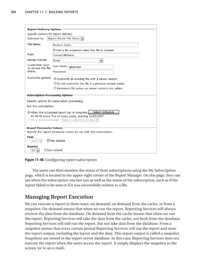
Figure 11-48. Configuring report subscription
The users can then monitor the status of their subscriptions using the My Subscriptionpage, which is located in the upper-right corner of the Report Manager. On this page, they cansee when the subscription was last run as well as the status of the subscription, such as if thereport failed to be sent or if it was successfully written to a file.
Managing Report ExecutionWe can execute a report in three ways: on demand, on demand from the cache, or from asnapshot. On demand means that when we run the report, Reporting Services will alwaysretrieve the data from the database. On demand from the cache means that when we runthe report, Reporting Services will take the data from the cache, not fresh from the database.Reporting Services will still run the report, but not take data from the database. From asnapshot means that every certain period Reporting Services will run the report and storethe report output, including the layout and the data. This report output is called a snapshot.Snapshots are stored in the report server database. In this case, Reporting Services does notexecute the report when the users access the report. It simply displays the snapshot to thescreen (or in an e-mail).
CHAPTER 11 ■ BUILDING REPORTS374
9314ch11final.qxd 11/15/07 10:03 AM Page 374

To configure the execution method, navigate to the report you want to configure, andthen click the Properties tab. Then click the Execution link in the left pane. Figure 11-49 showsthe Execution page.
Figure 11-49. Configuring report execution
To set the report to be run on demand, choose “Always run this report with the mostrecent data” and “Do not cache temporary copies of this report.” To set the report to be run ondemand from the cache, choose “Always run this report with the most recent data” and one ofthe “Cache a temporary copy of the report. Expire copy of report…” options. To set the reportto be run from a snapshot, choose “Render this report from a report execution snapshot.”
With that, we’ve finished going through the three things about reports that we need tomanage after we have developed them: security, subscription, and execution. Data warehouseusers usually access the reports via a web portal rather than using the Report Manager.
SummaryReports are one of the two primary means of getting the data out of the data warehouse (theother one is using an OLAP/BI tool). Because of this key role, reports are important in datawarehousing. Reports can retrieve data from a relational database as well as from a multidi-mensional database.
Reports are used by both the business users as well as data warehouse administrators inthe form of data quality reports, audit reports, and usage reports. For business purposes,reports are mostly used for business intelligence.
In the next chapter, I will discuss the other way of presenting the data from the data ware-house to the business users: using OLAP tools.
CHAPTER 11 ■ BUILDING REPORTS 375
9314ch11final.qxd 11/15/07 10:03 AM Page 375

9314ch11final.qxd 11/15/07 10:03 AM Page 376
Multidimensional Database
In the previous chapter, I discussed reporting, which is one of the most popular ways ofgetting the data out of the data warehouse and presenting it to the users. In this chapter, Iwill discuss another popular way of getting the data out—using multidimensional databases(MDBs). Multidimensional databases are mainly used for analytics and data mining appli-cations. While you are learning in this chapter what multidimensional databases are, whatthey are for, how to design them, how to populate them, and how to query them, you needto remember that the final purpose of data warehousing is to get the data to the users, not toget the data into the warehouse.
There is no point in collecting data from various source systems throughout the enter-prise into one central place if you are not going to retrieve the data and present it to theusers. If you remember only one thing from this book, I hope it is this one: we can spend amillion dollars and two years setting up the servers, architecting the data warehouse, design-ing the databases, building the ETL systems, and populating the data stores, but if the data isnot retrieved and presented to the users, then the data warehouse is useless. It is very impor-tant to get the data out and presented in such a way that gives good business value to theusers. In fact, the entire data warehouse should be designed to support this.
In this chapter, I’ll cover, step by step, what MDBs are, what they are for, how to designthem, how to populate them, how to query them, and how to administer them.
What a Multidimensional Database IsIn this section, I’ll discuss what multidimensional databases are, what they look like, whatthey are used for, their advantages and disadvantages, how they are different from OLAP, andthe system to manage them.
A multidimensional database is a form of database where the data is stored in cells andthe position of each cell is defined by a number of hierarchical called dimensions. Each cellrepresents a business event, and the value of the dimensions shows when and where thisevent happened.
The structure stores the aggregate values as well as the base values, typically in com-pressed multidimensional array format, rather than in RDBMS tables. Aggregate values areprecomputed summaries of the base values.
Examples of multidimensional databases are Microsoft Analysis Services, HyperionEssbase, and Cognos PowerCube. The other terms that people use for a multidimensionaldatabase are hypercube, cube, OLAP cube, multidimensional database (abbreviated as MDB,MDD, or MDDB), and multidimensional data store (MDDS).
377
C H A P T E R 1 2
9314ch12final.qxd 11/15/07 10:01 AM Page 377

Physically, an MDB is a file. To help you understand how an MDB file is internally struc-tured, you can visualize it as a matrix or a cube, as shown in Figure 12-1 and Figure 12-2.Figure 12-1 shows an MDB with two dimensions; it looks like a matrix. The two dimensionsare customer and product. The combination of these two dimensions points to a cell in thematrix. The cell contains one or more measurement values (or none/empty). A cell representsa business event. The value of the dimensions shows when and where this event happened.Event A is created by customer C1 and product P1.
Figure 12-1. Visualization of a multidimensional database with two dimensions
Figure 12-2 shows an MDB with three dimensions; it looks like a cube. An MDB with fouror more dimensions is called a hypercube. Although logically an MDB looks like a cube (forthree dimensions) or a hypercube (for four or more dimensions), physically it is stored ascompressed multidimensional arrays with offset positioning. The cube in Figure 12-2 hasthree dimensions: customer, product, and time. The combination of these three dimensionspoints to a cell in the cube. Each cell represents a business event. The value of the dimensionsshows when and where this event happened. In Figure 12-2, the business event is “A customerbuys a product.” Business event A is a transaction where customer C1 buys product P1 at timeT1. In Figure 12-2, the cell contains three measure values: the revenue, the cost, and the profit.
Multidimensional databases are typically used for business intelligence (BI), especiallyfor online analytical processing (OLAP) and data mining (DM). The advantages of usingmultidimensional databases for OLAP and DM rather than a relational database such as adimensional data store (DSS) are that they use less disk space and have better performance.A multidimensional database occupies less disk space compared to a relational dimensionaldatabase (like DDS) because it is compressed and because it does not use indexing like aDDS. Instead, it uses multidimensional offsetting to locate the data. A multidimensionaldatabase performs better on OLAP operations because the aggregates are precalculated andbecause the way the data is physically stored (compressed multidimensional array formatwith offset positioning) minimizes the number of IO operations (disk reads), compared tostoring tables in an RDBMS.
CHAPTER 12 ■ MULTIDIMENSIONAL DATABASE378
9314ch12final.qxd 11/15/07 10:01 AM Page 378

Figure 12-2. Visualization of a multidimensional database with three dimensions
On the other hand, the drawback of using a multidimensional database compared tousing a relational database is the processing time required for loading the database and calcu-lating the aggregate values. Whenever the relational source is updated, the MDB needs to beupdated or reprocessed; in other words, the aggregate cells need to be recalculated (it doesn’thave to be done in real time). The second drawback is the scalability: an MDB may not scalewell for a very large database (multiple terabytes) or a large number of dimensions.
■Note The term multidimensional database is often confused with the term online analytical processing,but these terms have different meanings. An MDB is the database, and OLAP is the activity used to analyzethe database. The confusion is caused by the word OLAP cube. An OLAP cube has the same meaning as anMDB; it means a multidimensional database. We’ll talk about OLAP in the next section.
Most people in the database world know that an RDBMS is the system that manages arelational database. What do we use to manage multidimensional databases? The system thatmanages and operates multidimensional databases is called a multidimensional database sys-tem (MDBMS). Multidimensional database systems are also known as OLAP servers or cubeengines. Examples of an MDBMS are Microsoft SQL Server Analysis Services, Hyperion Ess-base, and Cognos PowerCube. Business Objects and MicroStrategy don’t have an MDBMS;they use ROLAP (I’ll talk about ROLAP in the next section).
The standard interface to connect to an MDBMS is XML for Analysis (http://www.xmlforanalysis.com/), which is known as XMLA. For example, using SQL Server ReportingServices, we can connect not only to Analysis Services cubes but also to Hyperion Essbasecubes using XMLA. Microsoft, Hyperion (now owned by Oracle), SAP, and SAS support XMLA.ADOMD.NET is a .NET data provider that uses XMLA to communicate the analytical datasources.
CHAPTER 12 ■ MULTIDIMENSIONAL DATABASE 379
9314ch12final.qxd 11/15/07 10:01 AM Page 379

Online Analytical ProcessingOnline analytical processing is the activity of interactively analyzing business transactiondata stored in the dimensional data warehouse to make tactical and strategic business deci-sions. Typically, people who do OLAP work are business analysts, business managers, andexecutives. An example of OLAP is analyzing the effectiveness of a marketing campaign bymeasuring sales growth over a certain period. Another example is analyzing the impact of aprice increase on the product sales in different regions and product groups during the sameperiod of time.
OLAP helps solve these types of problems by summing up the measure values withinthe MDB according to certain criteria that reflect the business conditions. OLAP alsoenables the business users to drill down to a particular area of the MDB to view the data at a more detailed level.
How about analyzing business transactions data stored in operational systems such asenterprise resource planning (ERP) systems or an operational data store (ODS)? Is that classi-fied as OLAP? No, it is not OLAP. It is business analysis, but it is not OLAP. For the analysis to beOLAP, it needs to be performed against a dimensional data warehouse, either stored in rela-tional format or stored in multidimensional format.
What if it is not interactive, but only a one-way interaction such as reading and analyz-ing reports? Is that OLAP? No, that is reporting, not OLAP. OLAP is interactive; in otherwords, the business analyst queries, and the system responds, repeatedly, as illustrated inFigure 12-3. The response time is typically within seconds, not hours (although certainOLAP scenarios take hours).
Figure 12-3. OLAP is interactive.
OLAP activities are part of BI. There are three widely used BI activities: reporting, OLAP,and data mining. OLAP tools are the interactive tools that business analysts use to query adata warehouse to perform business analysis. Examples of OLAP tools are SSAS, Cognos BI 8Analysis, Business Objects XI Release 2 Voyager, and ProClarity Analytics 6.
OLAP functionalities can be delivered using a relational database or using a multidimen-sional database. OLAP that uses a relational database is known as relational online analyticalprocessing (ROLAP). ROLAP leaves the data in tables and relies on SQL select statements withsum and group clauses to summarize the detail-level data. The precalculated summary data(called aggregates) is stored in summary tables. When receiving queries, ROLAP chooses thebest summary tables to be used to satisfy the query and then supplements the results withselect statements to the base tables.
CHAPTER 12 ■ MULTIDIMENSIONAL DATABASE380
9314ch12final.qxd 11/15/07 10:01 AM Page 380

OLAP that uses a multidimensional database is known as multidimensional onlineanalytical processing (MOLAP). MOLAP precalculates the summary of measure values inthe MDB and stores the aggregates within the MDB structure. An example of ROLAP isMicroStrategy OLAP Services. Examples of MOLAP are Cognos BI 8 Analysis and ProClarityAnalytics 6. Microsoft SQL Server Analysis Services (SSAS) supports both ROLAP andMOLAP, plus it supports Hybrid Online Analytical Processing (HOLAP). HOLAP uses bothrelational and multidimensional databases. SSAS databases can store the data in a rela-tional database, a multidimensional database, or both. When we set SSAS to store the datain HOLAP mode, the base data (leaf level) is stored in SQL Server relational database tables,and the aggregate data is stored in an MDB.
Creating a Multidimensional DatabaseLet’s create a multidimensional database from the DDS database in the Amadeus Entertain-ment case study. In this exercise, we will create the Product Sales multidimensionaldatabase that was used for reporting in the previous chapter. For that, open BIDS, and fol-low these steps:
1. Click the File menu, and select New ➤ Project.
2. Choose Business Intelligence Projects for the project type, choose Analysis ServicesProject as the template, and name it Amadeus Analysis Services, as shown in Fig-ure 12-4. Then click OK.
Figure 12-4. Creating a new Analysis Services project
CHAPTER 12 ■ MULTIDIMENSIONAL DATABASE 381
9314ch12final.qxd 11/15/07 10:01 AM Page 381

3. We need to connect to the DDS database. The scripts mentioned in Chapter 6 createdthe DDS database and the tables within it. The steps in Chapters 7 and 8 populated theDDS tables. You can also download the completed DDS at the Apress website (http://www.apress.com/). It is in the /data folder, and the file name is dds.zip (7MB). Uncom-press this file, and restore the database on your development SQL Server.
4. Let’s create a data source pointing to the DDS database so we can use the DDS as adata source for our MDB. In Solution Explorer, right-click Data Sources, and chooseNew Data Source. Click Next on the welcome page.
5. On the Data Source wizard page, click New to create a new connection. Because theDDS is a SQL Server database, choose SQL Native Client as the provider.
6. Select your development SQL Server in the Server Name drop-down box, and selectUse Windows Authentication (or supply the credential if you use SQL Server authenti-cation). Choose DDS for the database to connect to, as shown in Figure 12-5.
Figure 12-5. Creating the data connection to the DDS database
7. Choose servername.DDS.ETL as the data connection, and click Next.
CHAPTER 12 ■ MULTIDIMENSIONAL DATABASE382
9314ch12final.qxd 11/15/07 10:01 AM Page 382

8. On the Impersonation Information page, choose “Use the service account” (or supplythe credential if you use SQL Server authentication), and then click Next.
9. Name the data source DDS, and click Finish. Now in Solution Explorer, there is a newdata source called DDS.
Now let’s create a data source view, which is the relational model for this data source. Inthis data source view, we will put in only the dimension and fact table that we need to createthe product sales cube, which are: date dimension, product dimension, store dimension, andProduct Sales fact table. For that, follow these steps:
1. Right-click Data Source Views in Solution Explorer, and choose New Data Source View.
2. Click Next on the welcome page.
3. Select DDS for Relational Data Sources, and click Next.
4. Double-click the date, product, and store dimensions, as well as the Product Salesfact table, and bring them to the Included Objects box on the right side, as shown inFigure 12-6. Then click Next.
5. Click Finish to complete the wizard.
Figure 12-6. Selecting tables for the data source view
The result is a new data source view with one fact table and three dimensions, as shownin Figure 12-7.
CHAPTER 12 ■ MULTIDIMENSIONAL DATABASE 383
9314ch12final.qxd 11/15/07 10:01 AM Page 383

Figure 12-7. Creating a new data source view for the product sales data mart
Now let’s create the multidimensional database (cube):
1. Right-click Cubes in Solution Explorer, and choose New Cube.
2. Click Next on the welcome page.
3. Choose “Build Cube using a data source,” and ensure that the Auto Build box ischecked. In the drop-down list, you’ll see two options: “Create attributes and hierar-chies” or “Create attributes.” Selecting the former will make SSAS build the hierarchies(levels) for the dimensions, whereas the latter does not create the dimensional hierar-chies. Choose the former, and click Next.
CHAPTER 12 ■ MULTIDIMENSIONAL DATABASE384
9314ch12final.qxd 11/15/07 10:01 AM Page 384

4. Auto Build makes recommendations based on the data source view structure. Whenbuilding a cube in SSAS, we have two choices: we can either build it manually or selectAuto Build. When building the cube manually, we specify the measures in the facttables, the data types, the dimensions, and the hierarchies. With Auto Build, the CubeWizard will detect the cube structure based on the tables in the data source view. SelectDDS for the data source view, and click Next.
5. The wizard analyzes the relationship between tables in the data source view, as shownin Figure 12-8. The wizard identifies which tables are the fact tables and which tablesare the dimension tables. Click Next.
Figure 12-8. Detecting fact and dimension tables
6. The wizard correctly identifies dim_product and dim_store as dimension tables, butit incorrectly identifies dim_date as both a fact and dimension table. To correct this,uncheck the fact check box for dim_date so that date, product, and store are set asdimensions and Product Sales is set as a fact table. The wizard does not identify thetime dimension, so in the “Time dimension table” drop-down list, choose dim_date,as shown in Figure 12-9.
CHAPTER 12 ■ MULTIDIMENSIONAL DATABASE 385
9314ch12final.qxd 11/15/07 10:01 AM Page 385

Figure 12-9. Selecting the fact and dimension tables when creating the cube
7. The next page is Select Time Periods. On this page, we need to specify the hierarchy ofthe time dimension. Set the Year, Quarter, and Week time properties by selecting theappropriate columns from the date dimension table, as shown in Figure 12-10. Thenclick Next.
Figure 12-10. Selecting time periods
CHAPTER 12 ■ MULTIDIMENSIONAL DATABASE386
9314ch12final.qxd 11/15/07 10:01 AM Page 386
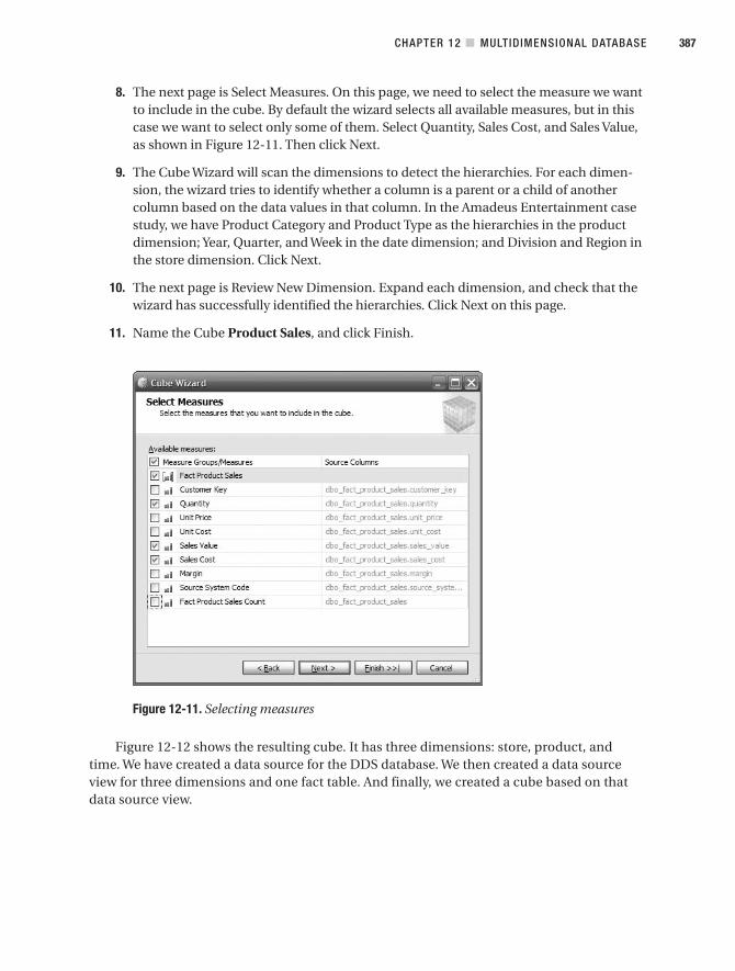
8. The next page is Select Measures. On this page, we need to select the measure we wantto include in the cube. By default the wizard selects all available measures, but in thiscase we want to select only some of them. Select Quantity, Sales Cost, and Sales Value,as shown in Figure 12-11. Then click Next.
9. The Cube Wizard will scan the dimensions to detect the hierarchies. For each dimen-sion, the wizard tries to identify whether a column is a parent or a child of anothercolumn based on the data values in that column. In the Amadeus Entertainment casestudy, we have Product Category and Product Type as the hierarchies in the productdimension; Year, Quarter, and Week in the date dimension; and Division and Region inthe store dimension. Click Next.
10. The next page is Review New Dimension. Expand each dimension, and check that thewizard has successfully identified the hierarchies. Click Next on this page.
11. Name the Cube Product Sales, and click Finish.
Figure 12-11. Selecting measures
Figure 12-12 shows the resulting cube. It has three dimensions: store, product, andtime. We have created a data source for the DDS database. We then created a data sourceview for three dimensions and one fact table. And finally, we created a cube based on thatdata source view.
CHAPTER 12 ■ MULTIDIMENSIONAL DATABASE 387
9314ch12final.qxd 11/15/07 10:01 AM Page 387

Figure 12-12. Product Sales cube structure
Processing a Multidimensional DatabaseAs you have just seen, if you have a dimensional relational data warehouse (also known as adimensional data store), you can easily create the multidimensional database or cube. Beforeyou can browse this cube or query this cube for reporting, though, you need to process thecube first. Processing a cube means calculating the aggregates from the cube cells.
And before you can process the cube, you need to build it and deploy it first:
• Building a cube means checking the internal structure of the cube including the facts,dimensions, hierarchy, and connections to the data source to make sure the structurewe created is valid.
• Deploying a cube means creating the cube structure that we have designed in a multi-dimensional database engine (aka OLAP server or cube engine), which, in this case, isan Analysis Services server.
CHAPTER 12 ■ MULTIDIMENSIONAL DATABASE388
9314ch12final.qxd 11/15/07 10:01 AM Page 388

Let’s build and deploy the cube we just created:
1. Click the Build menu, and choose Build Amadeus Analysis Services. In the bottom-leftcorner you’ll see “Build started,” followed by “Build succeeded.”
2. Ensure that the Analysis Services server is up and running. Click Start ➤ All Programs➤ Microsoft SQL Server 2005 or 2008 ➤ Configuration Tools ➤ SQL Server Configura-tion Manager. Right-click the SQL Server Analysis Services, and choose Start, as shownin Figure 12-13.
Figure 12-13. Starting Analysis Services
3. Now let’s deploy the cube. In the Solution Configuration drop-down list on the toolbar(the one next to the green Play button), choose Development. Click the Build menu,and choose Deploy Amadeus Analysis Services.
4. When the project has been successfully deployed to the Analysis Services instance, thedeployment progress will be like the one in Figure 12-14, and the output script will belike Listing 12-1. Figure 12-14 tells us that SSAS has successfully created the cube struc-ture in the MDB and populated it with the data from the DDS tables. When it says“Processing Measure Group Fact Product Sales completed successfully,” it means thatSSAS has loaded all the values on the measure columns in the fact_product_salestable in the DDS into the cube structure. When it says “Processing Dimensiondim_store completed successfully,” it means that SSAS has loaded the distinct valuesfor each column in the store dimension in the DDS into the cube structure, includingthe hierarchy structure.
CHAPTER 12 ■ MULTIDIMENSIONAL DATABASE 389
9314ch12final.qxd 11/15/07 10:01 AM Page 389

Figure 12-14. Progress script of a successful deployment
Listing 12-1. Successful Output Script
------ Build started: Project: Amadeus Analysis Services, Configuration: Development ------Started Building Analysis Services project: Incremental ....Build complete -- 0 errors, 0 warnings------ Deploy started: Project: Amadeus Analysis Services, Configuration: Development ------Performing an incremental deployment of the 'Amadeus Analysis Services' database to the 'localhost' server.Generating deployment script...
Add RelationalDataSource DDSProcess Database Amadeus Analysis Services
DoneSending deployment script to the server...DoneDeploy complete -- 0 errors, 0 warnings========== Build: 1 succeeded or up-to-date, 0 failed, 0 skipped ==================== Deploy: 1 succeeded, 0 failed, 0 skipped ==========
5. What we just did was deploy the cube design into a physical structure. In other words,we were creating the cube in SSAS based on what we designed in BIDS. So, let’s see thecube we just created. Open SQL Server Management Studio, and connect to the Analy-sis Services instance. The Object Explorer shows the measure groups of the cube alongwith the three dimensions, as shown in Figure 12-15.
CHAPTER 12 ■ MULTIDIMENSIONAL DATABASE390
9314ch12final.qxd 11/15/07 10:01 AM Page 390

Figure 12-15. Object Explorer of the deployed Analysis Services project
6. Now that we have built and deployed the project, we are ready to process the cube.In BIDS, click the Database menu, and choose Process. The Process Database pageopens, as shown in Figure 12-16. The Impact Analysis button lists which other SSASobjects are affected by the processing task. There are three main types of SSAS objects:server objects (such as data sources and data source views), dimension objects (suchas attributes and hierarchies), and cube objects (such as measures and partitions).
The Change Settings button enables us to change the processing order (whether theobjects are processed sequentially, which means one object at a time, or in parallel,which means all objects simultaneously) and the transaction mode if we processsequentially (process in one transaction or in separate transactions); it also enablesus to handle dimensional errors (whether to convert to an unknown record or discardthe record, how to handle invalid keys, null keys and duplicate keys, and so on) and(whether or not to) process affected objects.
CHAPTER 12 ■ MULTIDIMENSIONAL DATABASE 391
9314ch12final.qxd 11/15/07 10:01 AM Page 391

Figure 12-16. Process Database dialog box
7. In our case, we are quite happy to go with the default settings, so just click Run. Analy-sis Services will process the cube and display the progress as it goes along, as shown inFigure 12-17. It will end with a message “Process succeeded.” Click Close to close theProcess Progress dialog box. Click Close again to close the Process Database dialogbox.
CHAPTER 12 ■ MULTIDIMENSIONAL DATABASE392
9314ch12final.qxd 11/15/07 10:01 AM Page 392

Figure 12-17. Processing the cube
So, we have built, deployed, and processed a cube: product sales with its dimensions. Thecube is populated from the Product Sales fact table. We have not included all the dimensionsand measures from this fact table. We included only three dimensions (date, product, andstore) and three measures (quantity, sales value, and sales cost). A typical scenario in a simpledata warehouse project is to include most of the dimensions and measures. I prefer to buildthe cube bit by bit. For example, if the mart has six dimensions and ten measures, I wouldprobably start the cube with three dimensions and three to five measures; add member for-mulas, additional aggregations, and dimension intelligence; build and deploy the cube; makesure it’s working fine before adding the remaining dimensions and measures; and then buildand deploy it again. This makes it easier to troubleshoot if we have problems.
CHAPTER 12 ■ MULTIDIMENSIONAL DATABASE 393
9314ch12final.qxd 11/15/07 10:01 AM Page 393

When building a cube, we do not have to include all the dimensions and measures in thefact table. It is normal to not include some measures or dimensions in the cube. It is a per-fectly valid scenario to have multiple cubes from the same fact table with different sets ofdimensions and measures.
Then we move on, building the cubes for the other fact tables. In the case study, we havefour other fact tables to build the cubes from: Subscription Sales, Supplier Performance, Com-munication Subscriptions, and Campaign Results fact tables. Not all fact tables need cubes.Some fact tables are accessed only in their relational format. We build the cubes only if weneed to browse them in multidimensional format.
Some BI tools don’t require cubes to be built because they are ROLAP or reporting tools.These tools read from relational databases such as the ODS or the DDS. Some tools such asProClarity and data mining tools work better with cubes.
We don’t have to build a cube from just one fact table. We can build a cube from two (ormore) fact tables. When doing this, we need to bear in mind dimensional conformity. Con-formed dimensions mean they are either the same dimension table or one is the subset of theother. Dimension A is said to be a subset of dimension B when all columns of dimension Aexist in dimension B and all rows of dimension A exist in dimension B. In doing this, we aredrilling across, in other words, joining two (or more) fact tables that have conformed dimen-sions between them.
Querying a Multidimensional DatabaseNow that the cube has been processed, we can query the cube. The easiest way to query acube is by browsing it. Browsing a cube means querying the cube and displaying the cube dataon the screen in a particular format and order. Let’s try to re-create the Weekly Product Salesreport that we did in the previous chapter. But in the previous chapter it was a report, and thistime it will be a cube browser.
1. Click the Browser tab, as shown in Figure 12-18.
Figure 12-18. Selecting the row and column to browse a cube
2. Expand the date dimension by clicking the + sign next to it. Click week_number, anddrop it onto the Drop Column Fields Here area, also shown in Figure 12-18.
CHAPTER 12 ■ MULTIDIMENSIONAL DATABASE394
9314ch12final.qxd 11/15/07 10:01 AM Page 394
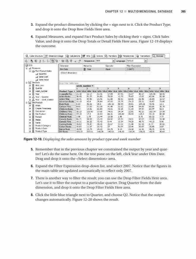
3. Expand the product dimension by clicking the + sign next to it. Click the Product Type,and drop it onto the Drop Row Fields Here area.
4. Expand Measures, and expand Fact Product Sales by clicking their + signs. Click SalesValue, and drop it onto the Drop Totals or Detail Fields Here area. Figure 12-19 displaysthe outcome.
Figure 12-19. Displaying the sales amount by product type and week number
5. Remember that in the previous chapter we constrained the output by year and quar-ter? Let’s do the same here. On the tree pane on the left, click Year under Dim Date.Drag and drop it onto the <Select dimension> area.
6. Expand the Filter Expression drop-down list, and select 2007. Notice that the figures inthe main table are updated automatically to reflect only 2007.
7. There is another way to filter the result; you can use the Drop Filter Fields Here area.Let’s use it to filter the output to a particular quarter. Drag Quarter from the datedimension, and drop it onto the Drop Filter Fields Here area.
8. Click the little blue triangle next to Quarter, and choose Q2. Notice that the outputchanges automatically. Figure 12-20 shows the result.
CHAPTER 12 ■ MULTIDIMENSIONAL DATABASE 395
9314ch12final.qxd 11/15/07 10:01 AM Page 395

Figure 12-20. Adding filters to the cube output
As you can see in Figure 12-20, there are two ways of putting a filter on the cube out-put: using filter expression (as we did with the year) or using filter fields (as we did withthe quarter).
You have just seen that you can query the cube using the Analysis Services cube browser.There are other ways to query an Analysis Services cube to get the data out and present it tothe users:
• You can query the Analysis Services cube from Reporting Services using MDX queries,as we did in the previous chapter when I discussed reporting.
• You can browse Analysis Services cubes using a third-party BI tool such as ProClarity.
• You can use data mining to analyze an Analysis Services cube.
• You can use ADOMD or XMLA to query the cube.
Administering a Multidimensional DatabaseOnce we have built, deployed, processed, and queried the cubes, we need to administer them.There are three common administrative tasks with regard to Analysis Services cubes. The firstone is to secure the cube; for example, only people who are authorized to access the cubesshould be able to access them. The second one is to keep the data within the cubes up-to-date. For this we need to process the cube regularly, such as once a day or a few times a day,depending on the following:
CHAPTER 12 ■ MULTIDIMENSIONAL DATABASE396
9314ch12final.qxd 11/15/07 10:01 AM Page 396

• How frequently the source DDS is updated
• How up-to-date the users need the data to be
The third one is to make sure we can restore the cubes if they are out of order, for exam-ple, taking backups regularly.
■Note Before we go through these three items, I’d like to clarify two Analysis Services terms that are oftenmisunderstood and used incorrectly. In the multidimensional world, the term cube has the same meaning asthe term multidimensional database. In Analysis Services, they are different. In Analysis Services, a cube is asingle n dimensional structure consisting of n dimensions and m measures, whereas a multidimensionaldatabase (or a database for short) is a collection of cubes.
Multidimensional Database SecurityTo secure the cubes, we need to understand Analysis Services security architecture. Unlike aSQL Server database engine, Analysis Services doesn’t have SQL Authentication mode. It hasWindows Authentication mode only. So, a user needs to be created in Windows before we cangive the user access to Analysis Services cubes. Analysis Services has two different roles: theserver role and the database role. Users with server roles have access to everything. They canaccess all multidimensional databases and the cubes within them, create and delete multi-dimensional databases, create and delete database users, and perform administrative tasks.Users with database roles can access only a specific multidimensional database and the cubeswithin them.
To grant a server role to a user, in Management Studio right-click the Analysis Servicesserver instance, and choose Properties. Click Security, and then click Add. Type the username,and click Check Names, as shown in Figure 12-21. Click OK. Alternatively, you can also clickthe Advanced button and then click Find Now to get a list of users.
CHAPTER 12 ■ MULTIDIMENSIONAL DATABASE 397
9314ch12final.qxd 11/15/07 10:01 AM Page 397

Figure 12-21. Analysis Services server role
To give a user access to a particular multidimensional database, in Management Studiogo to the multidimensional database that you want to give access to, right-click Roles, andchoose New Role. The Create Role dialog box will be displayed, as shown in Figure 12-22.
You’ll see the following tabs:
• On the General tab (shown in Figure 12-22), we can give the role a name and adescription. We can also choose the database permissions: Full Control has access toeverything in the database, Process Database can process a cube or a dimension, andRead Definition can access the definition of the database.
• On the Membership tab, we can add the users to the role.
• On the Data Sources tab, we can give access to the data source (this is mainly used fordata mining).
• On the Cubes tab, we can give the user read or write access to the individual cubeswithin the database and specify whether the user can drill through, create local cubes,or process the cube, as shown in Figure 12-23.
CHAPTER 12 ■ MULTIDIMENSIONAL DATABASE398
9314ch12final.qxd 11/15/07 10:01 AM Page 398

Figure 12-22. Analysis Services database role
Figure 12-23. Setting up cube permissions
• On the Cell Data tab, we can give the user read or write access to the cell data. Notethat the cell data is limited by the cube permission. For example, if a role has writeaccess on a cell but the role has only read access on the cube, then the role can onlyread on that cell.
• On the Dimensions tab, we can give the user read or write access to the individualdimension, read the dimension definition, and process the dimension.
• On the Dimension Data tab, we can specify the access to an individual member andhierarchy within each dimension.
Processing CubesEarlier in this chapter, you learned how to process a cube manually using BIDS. In practice,once we have built and deployed the cube in the production server, we need to schedule it tobe processed regularly to keep the data up-to-date with the DDS. For this we use SSIS. OpenBIDS, and go through the process:
CHAPTER 12 ■ MULTIDIMENSIONAL DATABASE 399
9314ch12final.qxd 11/15/07 10:01 AM Page 399

1. Create a new Integrated Services project by clicking File ➤ New ➤ Project. ChooseBusiness Intelligence Projects for the process types and the Analysis Services projectfor the templates.
2. Create a new package: in Solution Explorer, right-click SSIS Packages, and chooseNew SSIS Package. A blank design surface opens.
3. Drag the Analysis Services processing task from the Toolbox onto the design surface.
4. Let’s name the task. Double-click the task to edit it. On the General tab, type ProcessProduct Sales Cube for the name and description.
5. Ensure that Analysis Services is running. In Server Configuration Manager, right-clickthe SQL Server Analysis Services, and choose Start, as shown previously in Figure 12-13.
6. We need to establish a connection to the Analysis Services cube. Click the AnalysisServices tab, and click New in the Connection Manager drop-down list. Click Edit todefine a new connection, and enter the details of your Analysis Services server, asshown in Figure 12-24.
Figure 12-24. Setting the connection to the Analysis Services database
CHAPTER 12 ■ MULTIDIMENSIONAL DATABASE400
9314ch12final.qxd 11/15/07 10:01 AM Page 400

7. Click Add in the object list, and select the database, cubes, measure groups, partitions,and dimensions to process, as shown in Figure 12-25. In this case, we need to selectonly the Product Sales cube; there’s no need to select any of the dimensions. SSAS willautomatically process the measure groups and dimensions for that cube.
Figure 12-25. Selecting the Analysis Services object to process
8. You can also specify the processing order, transaction mode, dimension errors, dimen-sion key error log path, and whether to process affected objects by clicking the ChangeSettings button, as shown in Figure 12-26.
The parallel processing order makes the tasks run simultaneously in a single transac-tion. To do this, click Change Settings, and select Parallel. Sequential processing ordermeans Analysis Services will execute the processes one by one, either in a single trans-action or in a separate transaction. If it is a single transaction, when a single processfails, the whole job is rolled back, and the entire job fails. If it is a separate transaction,when a single process fails, only the failed process is rolled back, and the otherprocesses in the job continue.
Processing affected objects means processing all objects that have a dependency onthe object that we selected. It is normally used when processing dimensions; for exam-ple, when we process a dimension, we may want to process all the cubes that use thatdimension.
CHAPTER 12 ■ MULTIDIMENSIONAL DATABASE 401
9314ch12final.qxd 11/15/07 10:01 AM Page 401
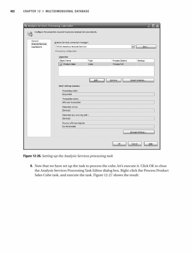
Figure 12-26. Setting up the Analysis Services processing task
9. Now that we have set up the task to process the cube, let’s execute it. Click OK to closethe Analysis Services Processing Task Editor dialog box. Right-click the Process ProductSales Cube task, and execute the task. Figure 12-27 shows the result.
CHAPTER 12 ■ MULTIDIMENSIONAL DATABASE402
9314ch12final.qxd 11/15/07 10:01 AM Page 402
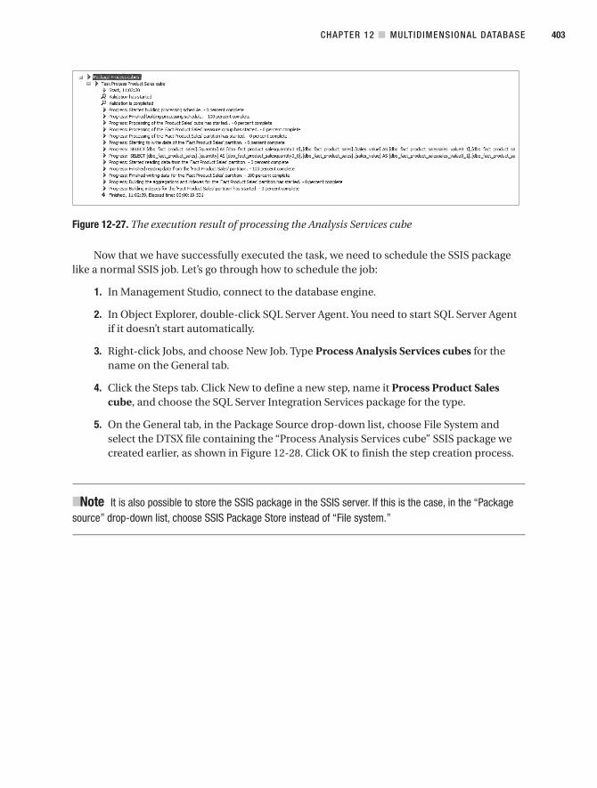
Figure 12-27. The execution result of processing the Analysis Services cube
Now that we have successfully executed the task, we need to schedule the SSIS packagelike a normal SSIS job. Let’s go through how to schedule the job:
1. In Management Studio, connect to the database engine.
2. In Object Explorer, double-click SQL Server Agent. You need to start SQL Server Agentif it doesn’t start automatically.
3. Right-click Jobs, and choose New Job. Type Process Analysis Services cubes for thename on the General tab.
4. Click the Steps tab. Click New to define a new step, name it Process Product Salescube, and choose the SQL Server Integration Services package for the type.
5. On the General tab, in the Package Source drop-down list, choose File System andselect the DTSX file containing the “Process Analysis Services cube” SSIS package wecreated earlier, as shown in Figure 12-28. Click OK to finish the step creation process.
■Note It is also possible to store the SSIS package in the SSIS server. If this is the case, in the “Packagesource” drop-down list, choose SSIS Package Store instead of “File system.”
CHAPTER 12 ■ MULTIDIMENSIONAL DATABASE 403
9314ch12final.qxd 11/15/07 10:01 AM Page 403

Figure 12-28. Setting up a job to process the cube regularly
6. Click the Schedule tab, and click New to create a new schedule to set the regular timewhen you want the cube to be processed, as shown in Figure 12-29, just like when cre-ating a regular SQL job. Click OK twice to create the scheduled job.
7. In Management Studio Object Explorer, right-click the job you just created, and chooseStart Job to execute the job to make sure it runs OK.
CHAPTER 12 ■ MULTIDIMENSIONAL DATABASE404
9314ch12final.qxd 11/15/07 10:01 AM Page 404

Figure 12-29. Setting up the schedule to process the cube
Backup and RestoreNow that we have created the multidimensional database, set up the security access, andarranged for it to be processed regularly, we need to back up the multidimensional databaseregularly. The backup frequency is determined based on how often the cube is processed.One important thing that some people forget is that when we have backed up the multi-dimensional database, we need to restore the backup. If we don’t prove that the backup canbe restored successfully, we still have a great risk. It is necessary to schedule the backup regu-larly (say, every day), but it is also necessary to schedule the restore regularly (say, everyquarter). This is not a real restore, but only a test restore. So, let’s go through the process ofbacking up and restoring an Analysis Services multidimensional database.
Before we get down to the details, let’s understand an important concept first when back-ing up a multidimensional database (MDB). If the MDB storage is in ROLAP mode, the data isnot stored in the MDB. The data (both the base data and the aggregates) is stored in the tablesin a normal relational database. Therefore, the backup of the MDB contains only the meta-data. The backup does not contain the data.
CHAPTER 12 ■ MULTIDIMENSIONAL DATABASE 405
9314ch12final.qxd 11/15/07 10:01 AM Page 405

If the MDB is in MOLAP mode, then the data (base data and aggregates) is stored in theMDB. Therefore, the backup of the MDB contains the data, the aggregates, and the metadata.The metadata contains the structure of the multidimensional database (the hierarchy, dimen-sion, measures, partition, and so on) and the aggregate navigations (which aggregates to usefor certain conditions).
If the MDB is in HOLAP mode, the base data is stored in tables in a relational database,but the aggregates are stored in the MDB. Therefore, the backup file contains only the meta-data and the aggregations. It does not contain the base data.
So if we use SSAS for the cube engine and SQL Server for the relational engine and if weset the SSAS database in ROLAP mode in addition to backing up the SSAS database, then wealso need to back up the SQL Server database (the DDS tables) because the base data is storedthere. In the cube designer in BIDS, on the Partitions tab, we can specify the store mode(MOLAP, ROLAP, or HOLAP) by clicking the … button in the Aggregations column and select-ing the storage and caching options, as shown in Figure 12-30.
Figure 12-30. Specifying the storage mode for the partition
Now that you understand what will be stored and what will not be stored in the backupfile, let’s go through the backup and restore process. The easiest way to regularly back up theAnalysis Services database is to create an XMLA script using Management Studio and executethat script using SSIS. XMLA is the de facto standard for accessing multidimensional data-bases (MDBs). We then use SQL Server Agent to execute the script.
CHAPTER 12 ■ MULTIDIMENSIONAL DATABASE406
9314ch12final.qxd 11/15/07 10:01 AM Page 406

Let’s create the XMLA script for backing up the MDB:
1. In Management Studio’s Object Browser, connect to the Analysis Services instance.Right-click the database you want to back up, and select Backup.
2. Set the path and name of the backup file, and set the options to allow overwritingan existing backup file and to compress or encrypt the backup file, as shown inFigure 12-31.
Figure 12-31. Creating XMLA script for backing up the database
3. To create the XMLA script, click Script at the top. The result is similar to Listing 12-2.
Listing 12-2. XMLA for Backing Up a Multidimensional Database
<Backup xmlns="http://schemas.microsoft.com/analysisservices/2003/engine"><Object><DatabaseID>Amadeus Analysis Services</DatabaseID>
</Object><File>h:\data\backup\MDB\Amadeus.abf</File><AllowOverwrite>true</AllowOverwrite>
</Backup>
CHAPTER 12 ■ MULTIDIMENSIONAL DATABASE 407
9314ch12final.qxd 11/15/07 10:01 AM Page 407

4. Now we need to run this script in SSIS. So, open BIDS, create a new SSIS project, andcreate a new package.
5. Drag the Analysis Services Execute DDL task from the palette onto the design surface.Double-click it to edit it.
6. On the General tab, we can give the task a name and description.
7. On the DDL tab, we set the connection to our Analysis Services instance. We can leavethe SourceType as Direct Input and paste the XMLA script in Listing 12-2 directly. Or,we can set the SourceType as File and specify the file path to the XMLA script, asshown in Figure 12-32.
Figure 12-32. Configuring an SSIS task to execute the XMLA script
8. Click OK to close the task editor and execute the task.
9. Check that the backup file is produced at the specified location.
10. Using SQL Server Agent, we can then schedule the SSIS package to run at a specifiedtime, such as after the cube is processed successfully.
To test restoring the backup regularly, we create an XMLA file using the same process asearlier. To restore into a new database with a different name, just modify the <DatabaseName>element in the XMLA file. Then execute it using the SSIS task as done earlier. Alternatively, if itis one time only, we can just use Management Studio to restore the backup.
CHAPTER 12 ■ MULTIDIMENSIONAL DATABASE408
9314ch12final.qxd 11/15/07 10:01 AM Page 408

SummaryIn this chapter, you learned about MDBs, OLAP, and the difference between them. I also dis-cussed the differences between ROLAP, MOLAP, and HOLAP. We created a multidimensionaldatabase for our Product Sales fact table, and you learned how to process, query, secure, andback up the multidimensional database.
As I emphasized in the beginning of this chapter, the main purpose of having a datawarehouse is to get the data out and present it to the user community. In the previous twochapters, I discussed how to get the data out of the data warehouse using reports and analyti-cal tools. In the next three chapters, I’ll discuss how to use data warehouses for BI and CRM,as well as for other purposes.
CHAPTER 12 ■ MULTIDIMENSIONAL DATABASE 409
9314ch12final.qxd 11/15/07 10:01 AM Page 409

9314ch12final.qxd 11/15/07 10:01 AM Page 410

Using Data Warehouse forBusiness Intelligence
In this chapter and the next two chapters, I will discuss the applications of data warehouses.In this chapter, I will discuss business intelligence (BI), which is by far the most widely useddata warehouse application. The next chapter describes customer relationship management(CRM), and in Chapter 15, I will discuss customer data integration (CDI), unstructured data,and search.
BI is a collection of activities to get an understanding and insights about a business byperforming various types of analysis on the company data as well as on external data fromthird parties to help make strategic, tactical, and operational business decisions and take thenecessary actions to improve business performance. The key words here are “improve busi-ness performance.” The purpose of any BI activity is to improve business performance. Someof the most popular examples of BI implementations are analyzing customer profitability,studying product profitability, evaluating sales figures across different products and regions,exploring accounts profitability, examining supplier performance, and discovering customerrisk patterns.
It is important to bear in mind that business intelligence activities are not limited to thedata in the data warehouse. Business intelligence applications can query the ODS or ERP orany other systems in the enterprise to perform the necessary analysis for improving busi-ness performance. But in this chapter, I’ll discuss only BI applications that query the datawarehouse.
You can classify the various BI applications into six categories: reporting applications,analytic applications, data mining applications, dashboards, alerts, and portal. Reportingapplications query the data warehouse and present the data in static tabular or pivot format.Analytic applications query the data warehouse repeatedly and interactively and present thedata in flexible formats that users can slice and dice. Data mining applications explore thedata warehouse to find patterns and relationships that describe the data. Reporting applica-tions are usually used to perform lightweight analysis. Analytic applications are used toperform deeper analysis. Data mining applications are used for pattern finding.
Dashboards are a category of business intelligence applications that give a quick high-level summary of business performance in graphical gadgets, typically gauges, charts,indicators, and color-coded maps. By clicking these gadgets, we can drill down to lower-leveldetails. Alerts are notifications to the users when certain events or conditions happen. A BI
411
C H A P T E R 1 3
9314ch13final.qxd 11/15/07 9:49 AM Page 411

portal is an application that functions as a gateway to access and manage business intelligencereports, analytics, data mining, and dashboard applications as well as alert subscriptions.
In the rest of the chapter, I will discuss these six categories of BI applications. I’ll discusswhat they are, why we use them (why are they important), and their advantages and disadvan-tages, and I will provide some examples of each.
Business Intelligence ReportsAs discussed in Chapter 11, reports query the data warehouse and present the data in tabularformat or pivot format. We can also produce various types of charts. We can add parameterson the reports to make them dynamic. In a data warehousing context, a report retrieves datafrom the data warehouse and presents it to the users on the screen or on paper. Users also cansubscribe to these reports so that the reports can be sent to the users automatically by email atcertain times (daily or weekly, for example). In Chapter 11, we discussed reports in great detail,including when to use reports (and when not to), how to create them, how to deploy them,and how to administer them. So in this section, I’ll be brief so as not to repeat the topics Ialready discussed in Chapter 11.
The main advantage of using reports in BI is their simplicity. Reports are simple to cre-ate, simple to manage, and simple to use. We usually use reports (instead of analytics ordata mining applications) in BI when the presentation format requirements are fairly sim-ple and static. The disadvantages of using reports are that they are not flexible or inter-active. If users want to swap a piece of data with another piece or want to view the data ata higher or lower level, we need to redesign the report. By comparison, the other types ofbusiness intelligence applications such as analytic applications are more flexible. We don’thave to redesign the application if the user wants to present another piece of information.We just “plug” the analytic application on top of some cubes, and the user can explore allthe data in those cubes.
With SSRS we can do charting (line chart, bar chart, pie chart, and so on) or present thedata in simple tables or pivot table format. We can group, sort, and filter the data. We can drivethe content of the report using parameters and make the report a little bit dynamic. Users canalso change the sort order of the report at run time. Users can subscribe to a report to receiveit via e-mail automatically at certain intervals. The report can be attached to the e-mail, or thee-mail can just contain the link to the report. We can also create a subreport within a report.We can store or cache the report output for quick retrieval later. We can add a link to anotherreport by passing certain parameters to tailor the content.
BI reports are not limited to just the data warehouse. BI reports can query other datasources within the enterprise. Most relational databases (SQL Server, Oracle, Teradata, DB/2,mySQL, Informix, Sybase, and many others) can be accessed using ADO.NET, OLE DB, OpenDatabase Connectivity (ODBC), and Java Database Connectivity (JDBC). Instead of usingODBC to access SQL Server, we can also use the SQL Native Client driver. Most multidimen-sional databases can be accessed using XML for Analysis (XMLA) and ADOMD.NET. We canaccess, for example, data stored in the ERP systems (production, HR, sales, and purchasinginformation), the call center application (customer applications, complaints, and new con-tacts), the ODS (integrated master data, reference codes, account and policy information,up-to-date prices, and currency conversion rates), or even Windows Active Directory (securityinformation and usernames). Using reports we can combine the stored results of a saved
CHAPTER 13 ■ USING DATA WAREHOUSE FOR BUSINESS INTELLIGENCE412
9314ch13final.qxd 11/15/07 9:49 AM Page 412

query and the fresh output of an online query. We can combine the data from ERP systems,the ODS, and the data warehouse in a single report or in a set of reports.
BI reports are usually managed and published in one central place, such as an intranet.Using SSRS we can secure the reports, allowing only the people who should be able to accessthe reports and keeping everybody else out. We can set the security access so that differentpeople or departments can administer the content of different reports. We can also integratethe report security with Windows Active Directory so the users don’t have to login again toaccess the reports.
Business Intelligence AnalyticsHenry Morris coined the term analytic applications in 1997. He defined analytic applicationsas applications that “provide guidance in the decision-making process by accessing time-based data from multiple sources.”1 Users use analytic applications to access a dimensionaldata warehouse interactively. Analytic applications, or analytics for short, are also known asOLAP applications. Users can slice and dice the data, drilling up and drilling down.
I’d like to clarify the terminology that people use in analytics (such as slicing, dicing,drilling up, and drilling down) to make sure we have a common understanding. Slicing is theprocess of retrieving a block of data from a cube by filtering on one dimension, as shown inFigure 13-1. Dicing is the process of retrieving a block of data from a cube by filtering on alldimensions, as shown in Figure 13-2.
Figure 13-1. Slicing
CHAPTER 13 ■ USING DATA WAREHOUSE FOR BUSINESS INTELLIGENCE 413
1. Power, D., “Henry Morris Interview: Decision support and analytic applications,” DSSResources.com.December 3, 2006.
9314ch13final.qxd 11/15/07 9:49 AM Page 413

Figure 13-2. Dicing
In Figure 13-1, we are filtering only on dimension 1; in other words, dimension 1 = [val-ues]. We do not constrain or filter dimensions 2 and 3. In Figure 13-2, we filter on all threedimensions; in other words, dimension 1 = [values], dimension 2 = [values], and dimension 3= [values].
Now let’s discuss drilling up and drilling down. Figure 13-3 displays the store hierarchy ofAmadeus Entertainment. On the bottom level we have stores. Moving up the hierarchy wehave regions, then divisions, and finally the whole Amadeus Entertainment group.
Figure 13-3. Dimension hierarchy, drilling up and drilling down
Drilling up means presenting the data at a higher level on the dimension hierarchy (fromdetail level to summary level), such as going from the store level to the region level. Drillingdown means presenting the data at a lower level on the dimension hierarchy (from summarylevel to detail level), such as going from the region level to the store level.
To illustrate the process of drilling up, please look at the subscription revenue of AmadeusEntertainment stores for a particular week in Table 13-1.
CHAPTER 13 ■ USING DATA WAREHOUSE FOR BUSINESS INTELLIGENCE414
9314ch13final.qxd 11/15/07 9:49 AM Page 414

Table 13-1. Subscription Revenue for a Particular Week at Store Level
Store Subscription Revenue
Store 1 72,663
Store 2 61,899
Store 3 36,409
Store 4 61,994
Store 5 75,786
Store 6 34,049
Store 7 34,937
Store 8 41,012
When we drill up from store level to region level, we will get the subscription revenue foreach region, as displayed in Table 13-2.
Table 13-2. Subscription Revenue for a Particular Week at Region Level
Region Subscription Revenue
Region 1 134,562
Region 2 98,403
Region 3 109,835
Region 4 75,949
We can then drill up further to division level and to group level. Drilling down is thereverse, going from a higher level to a lower level. When drilling down, we get more detailinformation.
Analytics are what most people mean when they say BI applications. Depending onwhich industry you are in, you can use analytic applications to evaluate business perform-ance, analyze product and customer profitability, and study how to lower inventory costs.Some analytic applications have their own multidimensional database management system(MDBMS) such as SQL Server Analysis Services, Cognos 8 BI Analysis, Hyperion System 9 BIEssbase Analytics, and SAP Business Warehouse. Some analytic applications can use othervendors’ MDBMSs; for example, Business Objects OLAP Intelligence can read MicrosoftAnalysis Services, Hyperion Essbase, SAP BW, and DB2 OLAP cubes,2 while ProClarity readsMicrosoft Analysis Services cubes.
All these applications are called MOLAP applications; they’re analytic applications thatread from multidimensional databases. Some analytic applications do not read from multidi-mensional databases. They read from relational databases instead, such as MicroStrategyOLAP. These are called ROLAP applications. To be able to respond quickly to a query such as“What is the total revenue for fiscal week 4 in 2008 from all stores in region 4?”, ROLAP appli-cations store the totals (known as aggregates) in summary tables. These aggregates arecalculated and stored in summary tables when the ROLAP structure is processed. This way,
CHAPTER 13 ■ USING DATA WAREHOUSE FOR BUSINESS INTELLIGENCE 415
2. http://www.businessobjects.com/global/pdf/products/queryanalysis/olap_intelligence.pdf
9314ch13final.qxd 11/15/07 9:49 AM Page 415

when end users submit their queries, the ROLAP application doesn’t need to access a lot ofrecords on the fact table. The ROLAP application can just access the summary table to get theprecomputed total.
Some applications can read from both relational and multidimensional sources and com-bine the data internally before presenting the data to the end users. Whether the applicationsread from a relational or multidimensional data source, the data source ideally needs to be indimensional data warehouse (Kimball) form, consisting of fact and dimension tables thatmake conformed data marts. Some analytic applications can supplement this dimensionaldata with data from a normalized database; for example, to get more accurate descriptions(product descriptions, account descriptions, and so on).
Using analytic applications, we can get an overview of the current business performance,such as sales, production, purchasing, or profitability (probably by region) and compare itwith the budget or targets. We can then drill down into specific areas that have problems andtry to find out the cause of the problems. That is a typical scenario of BI analysis. But thereare also other scenarios; for example, in the telecommunications industry we can analyze theline usage patterns (by weekly time slots) against the bandwidth cost. Or in the waste man-agement industry we can weigh the revenue stream (which is by volume) vs. the disposal cost(which is by weight). Using analytic applications in monetary and technical organizations,such as combustion engine laboratories, nationwide economic management, and weathermeasurement stations, are totally different from the “normal” business organizations (com-panies) mentioned earlier.
We can also do charting, “what if?” analysis, planning exercises, and key performanceindicator monitoring from analytic applications. We can swap any dimension with anotherdimension to get a different business perspective, going up and down the dimensional hier-archy to get different levels of summary, and we can pick certain dimension members andfocus our attention on them. Using analytic applications, we can perform ad hoc queries, drillacross to another cube, analyze data from several cubes, find and locate certain data, and per-form various kinds of formatting and manipulation with regard to the results, such as addingor removing columns and performing calculations.
The main advantage of using analytic applications is the flexibility. If the users don’tknow what they are trying to find in advance, then this is the right tool for them. Using ana-lytic applications, we have the whole data warehouse at our fingertips. This is especiallyuseful for companies and organizations that make business decisions based on data ratherthan instincts, such as performing quantitative analysis to justify the decisions. The maindisadvantage of analytic applications is the complexity. It takes some time for the users toget familiar with the tools. Also, the multidimensional databases’ data sources need to bemaintained properly. But once everything is set and ready, then it’s easy to keep the opera-tion going.
In analytic applications, a multidimensional database (cube) is fundamental, becausethat’s where the data is stored. In the previous chapter, I discussed how to create, process, andbrowse cubes using SSAS. I also discussed how to query the cubes and how to administerthem. Hence, I’m not going to repeat those topics here, so let’s continue with data mining.
Business Intelligence Data MiningData mining is the process of exploring data to find the patterns and relationships thatdescribe the data and to predict the unknown or future values of the data. The key value of
CHAPTER 13 ■ USING DATA WAREHOUSE FOR BUSINESS INTELLIGENCE416
9314ch13final.qxd 11/15/07 9:49 AM Page 416

data mining is the ability to understand why some things happened in the past and the abilityto predict what will happen in the future. To refer to predicting the future with regard to datamining, some people use the term forecasting, and some call it predictive analytics. On theother hand, when data mining is used to explain the current or past situation, it is called des-criptive modeling, descriptive analytics, or knowledge discovery.
Implementing data mining in the business is growing by the day, both through descrip-tive and predictive analytics. Using data mining, we can find the correlation between purchasepatterns and customer demographics. For example, in our Amadeus Entertainment case study,we can find whether there is a relation between the sales of a music product type and the cus-tomer interest or occupation. In the financial services industry, data mining is traditionallyused for credit scoring, for example, to predict the ability and willingness to pay the loanbased on (each country has different factors) payment behavior, past delinquency, current debt,credit history, number of inquiries, address, bankruptcies filed, and customer demography.
There are many examples of data mining implementation for CRM, which we will discussin the next chapter. In business intelligence, popular applications of data mining are for frauddetection (credit card industry), forecasting and budgeting (finance), cellular/mobile packagedevelopment by analyzing call patterns (telecommunication industry), market basket analysis(retail industry), customer risk profiling (insurance industry), usage monitoring (energy andutilities), and machine service times (manufacturing industry).
We need to do four steps to implement data mining in SQL Server 2005 Analysis Services:
1. Define what we want to achieve: In this step, we formulate the question that we will tryto answer. For example, in our Amadeus Entertainment case study, the question is this:“Is there a correlation between the sales of music, film, and audio book product typesand the customer interest or occupation?”
2. Prepare the data: In this step, we make sure we have the relevant data and check thedata quality. In our case study, the data is already cleansed and ready in the data ware-house, but to answer the previous question, we need to prepare the data in a separatetable that records whether the customers have purchased music, film, or audio bookproducts.
3. Build the mining models: We then create a mining structure that consists of one ormore data mining models. The mining models can use different mining algorithms.Mining models can be built from relational sources or from OLAP cubes. We thenprocess the models and test how they perform.
4. Deploy and maintain the models in production: We can then use the models to createpredictions, either using the SQL Server data mining language (DMX) or using Predic-tion Query Builder. A prediction is a forecast or a guess about the future value of acertain variable. For example, in the Amadeus Entertainment case study, we can usethe model to forecast the sales of music products in the next quarter. We can also cre-ate reports that query the mining models by creating an Analysis Services data set. Wemay need to process the models regularly to keep them up-to-date, either using XMLfor Analysis (XMLA) or using Analysis Management Objects (AMO).
Let’s go through the process of creating and processing the mining models in SQL Serverfor the Amadeus Entertainment case study. Open Management Studio, and create the follow-ing table in the DDS database. We will use this table to build mining models to find the
CHAPTER 13 ■ USING DATA WAREHOUSE FOR BUSINESS INTELLIGENCE 417
9314ch13final.qxd 11/15/07 9:49 AM Page 417

correlation between the music purchases and demographic attributes. We will also group therows on this table into ten clusters with similar characteristics to enable us to analyze and pre-dict the behavior of each cluster.
create table dm_purchase_pattern( customer_key int, gender char(1), interest varchar(30), occupation varchar(50), music char(1), film char(1), audio_books char(1), constraint pk_dm_purchase_patternprimary key clustered (customer_key)
)go
Now let’s store music, film, and audio book purchases in this table, along with the cus-tomer demographic attributes such as interest, gender, and occupation.
Listing 13-1 inserts customer demographic information into the dm_purchase_patterntable, along with indicators whether they have purchased music, film, or audio book products.
Listing 13-1. Creating and Populating Purchase Pattern Table for Data Mining
insert into dm_purchase_pattern(customer_key, gender, interest, occupation, music, film, audio_books)select c.customer_key, c.gender, c.interest1, c.occupation, case sum(case p.product_category when 'Music' then 1 else 0 end)when 0 then 'N' else 'Y' end as music
, case sum(case p.product_category when 'Films' then 1 else 0 end)when 0 then 'N' else 'Y' end as films
, case sum(case p.product_category when 'Audio Books' then 1 else 0 end)when 0 then 'N' else 'Y' end as audio_books
from fact_product_sales fjoin dim_product p on f.product_key = p.product_keyjoin dim_customer c on f.customer_key = c.customer_keygroup by c.customer_key, c.gender, c.interest1, c.occupationgo
Now open BIDS, and open the Analysis Services project we created in Chapter 12.(You can also create a new project if you want.) Edit the DDS data source view by double-clicking it in Solution Explorer. Right-click the canvas, and choose Add/Remove Tables.Add the dm_purchase_pattern table we just created to the data source view.
Right-click Mining Structures in Solution Explorer, and choose New Mining Structure.Click Next on the welcome page, and choose “From existing relational database or data ware-house” on the next page. Choose “Microsoft Decision Trees” for Data Mining Technique, andthen choose DDS for the data source view. On the Specify Table Types page, choosedm_purchase_pattern as the case table. The case table is a table that contains the training datathat we want to use to train the mining model.
CHAPTER 13 ■ USING DATA WAREHOUSE FOR BUSINESS INTELLIGENCE418
9314ch13final.qxd 11/15/07 9:49 AM Page 418
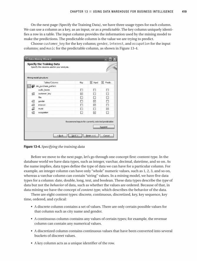
On the next page (Specify the Training Data), we have three usage types for each column.We can use a column as a key, as an input, or as a predictable. The key column uniquely identi-fies a row in a table. The input column provides the information used by the mining model tomake the predictions. The predictable column is the value we are trying to predict.
Choose customer_key for the key column; gender, interest, and occupation for the inputcolumns; and music for the predictable column, as shown in Figure 13-4.
Figure 13-4. Specifying the training data
Before we move to the next page, let’s go through one concept first: content type. In thedatabase world we have data types, such as integer, varchar, decimal, datetime, and so on. Asthe name implies, data types define the type of data we can have for a particular column. Forexample, an integer column can have only “whole” numeric values, such as 1, 2, 3, and so on,whereas a varchar column can contain “string” values. In a mining model, we have five datatypes for a column: date, double, long, text, and boolean. These data types describe the type ofdata but not the behavior of data, such as whether the values are ordered. Because of that, indata mining we have the concept of content type, which describes the behavior of the data.
There are eight content types: discrete, continuous, discretized, key, key sequence, keytime, ordered, and cyclical:
• A discrete column contains a set of values. There are only certain possible values forthat column such as city name and gender.
• A continuous column contains any values of certain types; for example, the revenuecolumn can contain any numerical values.
• A discretized column contains continuous values that have been converted into severalbuckets of discreet values.
• A key column acts as a unique identifier of the row.
CHAPTER 13 ■ USING DATA WAREHOUSE FOR BUSINESS INTELLIGENCE 419
9314ch13final.qxd 11/15/07 9:49 AM Page 419

• A key sequence column is a key column, but the values represent a sequence of events.The values are ordered, as in 1, 2, 3, 4, 5, …. They don’t have to have the same distancebetween them. For example, 1, 3, 4, 6, … are valid key sequence values.
• A key time column is a key column, but the values are datetime values. The values areordered, as in 2007-10-22 00:00:00, 2007-10-23 00:00:00, 2007-10-24 00:00:00, and so on.
• An ordered column is a discreet column, but the values are ordered. For example, thecustomer class column may contain discreet values of A, B, C, and D.
• A cyclical column is an ordered column, but the values are repeating. For example, themonth number goes from 1 to 12 and then repeats from 1 again.
Only certain data types are valid for certain content types. For example, for a continuouscolumn we can have only date, double, and long; we cannot have text or boolean data types.Table 13-3 shows the valid data types for each content type.
Table 13-3. Valid Data Types for Mining Structure Content Types
Content Types Date Double Long Text Boolean
Discrete Yes Yes Yes Yes Yes
Continuous Yes Yes Yes No No
Discretized Yes Yes Yes No No
Key Yes Yes Yes Yes No
Key Sequence Yes Yes Yes Yes No
Key Time Yes Yes Yes No No
Ordered Yes Yes Yes Yes Yes
Cyclical Yes Yes Yes Yes Yes
Now that you understand the concepts of content types and data types, let’s continuewith the Data Mining Wizard. The next page is Specify Columns’ Content and Data Type,where we specify the content type and the data type for each column, as shown in Figure 13-5.On this page, we can ask Analysis Services to detect the content types and data types, or wecan specify them manually. In this case, click Next because they are already correct.
On the next page, specify the mining structure name as Purchase Pattern and the miningmodel name as Decision Trees, and check the “Allow drill through” box. This option allows usto explore the source data. The Mining Structure designer opens, showing thedm_purchase_pattern table, as shown in Figure 13-6.
CHAPTER 13 ■ USING DATA WAREHOUSE FOR BUSINESS INTELLIGENCE420
9314ch13final.qxd 11/15/07 9:49 AM Page 420

Figure 13-5. Specifying content types and data types
Figure 13-6. Mining Structure designer
Before we move on, let’s go through the five tabs on the Mining Structure designer:
• The Mining Structure tab (displayed in Figure 13-6) contains the columns in the miningstructure and the table that the data source view contains. We can use this tab to mod-ify the mining structure and explore the underlying source data.
• The Mining Models tab contains the mining models we created using the Data MiningWizard, based on the mining structure displayed on the Mining Structure tab. We usethis tab to manage existing models and to create new models.
CHAPTER 13 ■ USING DATA WAREHOUSE FOR BUSINESS INTELLIGENCE 421
9314ch13final.qxd 11/15/07 9:49 AM Page 421

• The Mining Model Viewer tab is used to visually explore the mining models.
• The Mining Accuracy Chart tab is used to test the accuracy of the mining model’s pre-diction. This tab contains tools to filter the data and to display the accuracy results.
• On the last tab, Mining Model Prediction tab, we can specify the mining model andinput tables, map the columns, add functions to the query, and specify the criteria foreach column.
Next, click the Mining Models tab. The Decision Trees mining model is displayed there.We’ll create another mining model using a different clustering algorithm so we can comparedifferent data mining algorithms. A clustering algorithm, also known as a segmentation algo-rithm, divides data into groups with similar properties, whereas the decision trees algorithm(also known as the classification algorithm), on the other hand, predicts a variable (or more)based on the other variables in the data set.
Right-click anywhere on the table, and choose New Mining Model. Name the model Clus-tering, and choose Microsoft Clustering. The Mining Models tab now looks like Figure 13-7.
Figure 13-7. Creating the second mining model
Now that we have created the models, we need to build, deploy, and process the models.This is to create the mining structure in SQL Server Analysis Services, populate the structurewith raw data, and calculate the result using the correct data mining algorithms. Right-clickanywhere on the table shown in Figure 13-7, and choose Process Mining Structure and AllModels. BIDS will ask whether we want to build and deploy the model first. Click Yes. Afterbuilding and deploying the model, BIDS displays the Process Mining Structure dialog box, asshown in Figure 13-8.
CHAPTER 13 ■ USING DATA WAREHOUSE FOR BUSINESS INTELLIGENCE422
9314ch13final.qxd 11/15/07 9:49 AM Page 422
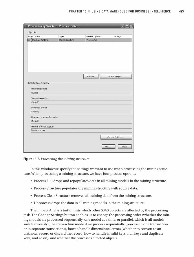
Figure 13-8. Processing the mining structure
In this window we specify the settings we want to use when processing the mining struc-ture. When processing a mining structure, we have four process options:
• Process Full drops and repopulates data in all mining models in the mining structure.
• Process Structure populates the mining structure with source data.
• Process Clear Structure removes all training data from the mining structure.
• Unprocess drops the data in all mining models in the mining structure.
The Impact Analysis button lists which other SSAS objects are affected by the processingtask. The Change Settings button enables us to change the processing order (whether the min-ing models are processed sequentially, one model at a time, or parallel, which is all modelssimultaneously), the transaction mode if we process sequentially (process in one transactionor in separate transactions), how to handle dimensional errors (whether to convert to anunknown record or discard the record, how to handle invalid keys, null keys and duplicatekeys, and so on), and whether the processes affected objects.
CHAPTER 13 ■ USING DATA WAREHOUSE FOR BUSINESS INTELLIGENCE 423
9314ch13final.qxd 11/15/07 9:49 AM Page 423

In this case, we are happy to go with the default settings, so just click Run. BIDS will dis-play the progress as we go along, as shown in Figure 13-9.
Figure 13-9. The progress of processing a mining structure
After the processing is completed, click Close. Click Close again to close the Process Min-ing Structure dialog box. Click the Mining Model Viewer tab. The viewer displays the DecisionTrees model using Microsoft Tree Viewer. As shown in Figure 13-10, there are 298 customerswith interest = ‘Pop Music’, and 264 of them (88 percent) purchased music products fromAmadeus Entertainment. The Y and N equates to purchasing music because when populatingthe case table (dm_purchase_pattern), we store music purchases in the music column (seeFigure 13-4), and when creating the mining model, we set music as the predictable column(as shown earlier in Listing 13-1).
In the figure, the shaded part shows how many customers in that segment purchasedmusic products, and the unshaded part shows how many didn’t. The group of customers whoare interested in romance, management, and business are all unshaded, meaning that none ofthem purchased the music products. Classic and Asian Music, on the other hand, have long
CHAPTER 13 ■ USING DATA WAREHOUSE FOR BUSINESS INTELLIGENCE424
9314ch13final.qxd 11/15/07 9:49 AM Page 424

shaded lines, meaning that the majority of them purchased music products. You can displaythe numeric details of each box by placing the cursor on those boxes. We can show more levelsby moving the slider. We can move and navigate around the canvas easier by clicking the +sign on the bottom-right corner of the canvas.
Figure 13-10. Examining the correlation between interest and music purchase
Click the Dependency Network tab to see the relationship between the demographic fac-tors (gender, interest, and occupation) and music purchases, as shown in Figure 13-11. Youcan understand the strength of the relationship using the slider on the left. When we move theslider down, the arrow with the weak relationship will disappear.
A dependency network diagram shows the relationship or dependency between theinput columns and the predictable columns (please refer to Figure 13-4 when we specifiedthe columns in our mining model). These columns are called nodes (represented as ellipsesin Figure 13-11). When we select a node (by clicking it), the nodes are color-coded; theselected node is in light blue, the input columns are in red, the predictable columns are in
CHAPTER 13 ■ USING DATA WAREHOUSE FOR BUSINESS INTELLIGENCE 425
9314ch13final.qxd 11/15/07 9:49 AM Page 425

dark blue, and if a column is used for both input and predictable, it is in purple. For exam-ple, although the colors aren’t shown in Figure 13-11, Music is the selected node, andInterest and Occupation are the input columns.
Figure 13-11. Relationships between nodes
In the dependency network diagram, only input columns that affect the predictable col-umn are shown. Figure 13-11 shows that only interest and occupation affects music purchase;gender doesn’t.
CHAPTER 13 ■ USING DATA WAREHOUSE FOR BUSINESS INTELLIGENCE426
9314ch13final.qxd 11/15/07 9:49 AM Page 426

We can move the slider downward to find out which demographic factor has strongerinfluence on the music purchase: occupation or interest. Figure 13-12 shows what happenswhen we move the slider downward to the bottom. It shows that occupation has strongerinfluence because it is the only node with an arrow pointing to music. The arrow on the inter-est node has disappeared.
Figure 13-12. Moving the slider downward shows the strongest link.
CHAPTER 13 ■ USING DATA WAREHOUSE FOR BUSINESS INTELLIGENCE 427
9314ch13final.qxd 11/15/07 9:49 AM Page 427

We can also view the other model that we built using the clustering algorithm by choosingthe model in the drop-down list. BIDS will ask whether we want to build and deploy the modelfirst. Say Yes to this offer. Figure 13-13 shows the result.
Figure 13-13. The mining model using the Microsoft clustering algorithm
The Microsoft clustering algorithm uses iterative techniques to group the rows in ourdm_purchase_pattern table into ten clusters that contain similar characteristics. Figure 13-13shows how the ten clusters are similar to each other; in other words, the darker the linebetween two clusters, the more similar those clusters are. By default, the graph displays thepopulation size; in other words, the bluer the cluster box, the more customers in that cluster.
CHAPTER 13 ■ USING DATA WAREHOUSE FOR BUSINESS INTELLIGENCE428
9314ch13final.qxd 11/15/07 9:49 AM Page 428

In Figure 13-13, we can change what data the shading color is showing. For example, wecan show interest in gardening by changing the Shading Variable drop-down list to Interestand the State drop-down list to Gardening, as shown in Figure 13-14.
Figure 13-14. Changing the shading variable on the cluster diagram
We can see the profile of each cluster by clicking the Cluster Profile tab, as shown inFigure 13-15.
Figure 13-15. The profile of each cluster
CHAPTER 13 ■ USING DATA WAREHOUSE FOR BUSINESS INTELLIGENCE 429
9314ch13final.qxd 11/15/07 9:49 AM Page 429
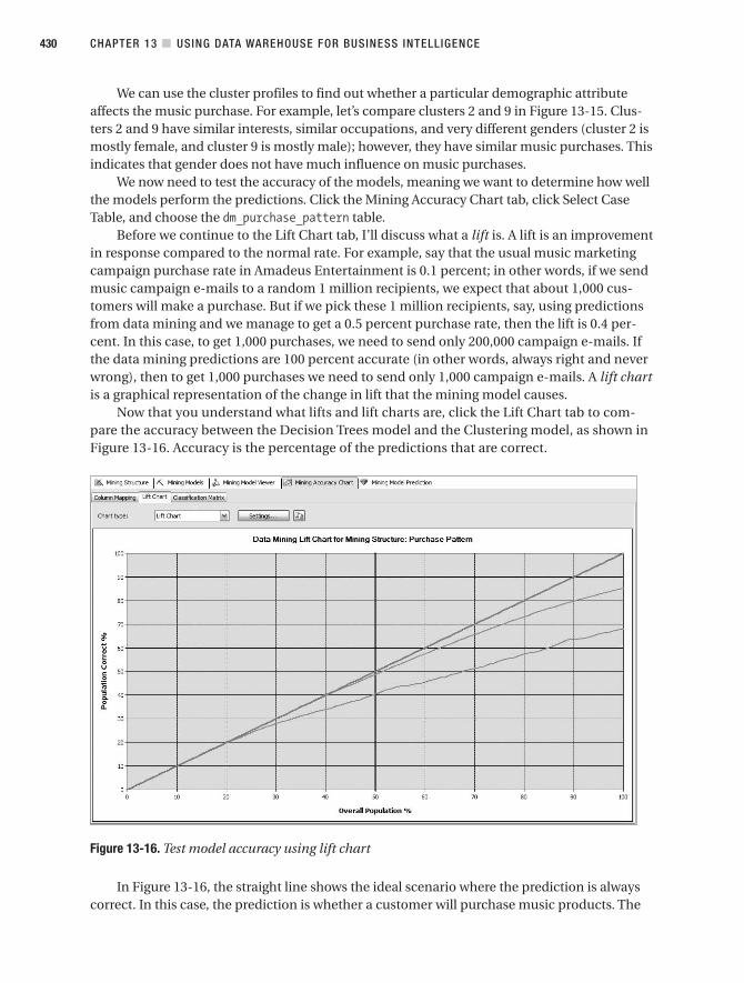
We can use the cluster profiles to find out whether a particular demographic attributeaffects the music purchase. For example, let’s compare clusters 2 and 9 in Figure 13-15. Clus-ters 2 and 9 have similar interests, similar occupations, and very different genders (cluster 2 ismostly female, and cluster 9 is mostly male); however, they have similar music purchases. Thisindicates that gender does not have much influence on music purchases.
We now need to test the accuracy of the models, meaning we want to determine how wellthe models perform the predictions. Click the Mining Accuracy Chart tab, click Select CaseTable, and choose the dm_purchase_pattern table.
Before we continue to the Lift Chart tab, I’ll discuss what a lift is. A lift is an improvementin response compared to the normal rate. For example, say that the usual music marketingcampaign purchase rate in Amadeus Entertainment is 0.1 percent; in other words, if we sendmusic campaign e-mails to a random 1 million recipients, we expect that about 1,000 cus-tomers will make a purchase. But if we pick these 1 million recipients, say, using predictionsfrom data mining and we manage to get a 0.5 percent purchase rate, then the lift is 0.4 per-cent. In this case, to get 1,000 purchases, we need to send only 200,000 campaign e-mails. Ifthe data mining predictions are 100 percent accurate (in other words, always right and neverwrong), then to get 1,000 purchases we need to send only 1,000 campaign e-mails. A lift chartis a graphical representation of the change in lift that the mining model causes.
Now that you understand what lifts and lift charts are, click the Lift Chart tab to com-pare the accuracy between the Decision Trees model and the Clustering model, as shown inFigure 13-16. Accuracy is the percentage of the predictions that are correct.
Figure 13-16. Test model accuracy using lift chart
In Figure 13-16, the straight line shows the ideal scenario where the prediction is alwayscorrect. In this case, the prediction is whether a customer will purchase music products. The
CHAPTER 13 ■ USING DATA WAREHOUSE FOR BUSINESS INTELLIGENCE430
9314ch13final.qxd 11/15/07 9:49 AM Page 430
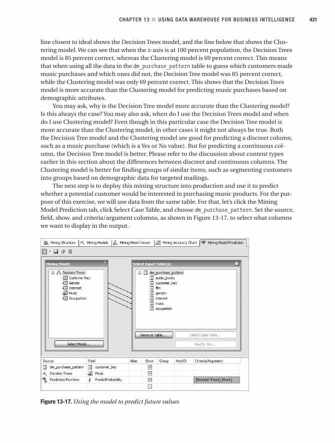
line closest to ideal shows the Decision Trees model, and the line below that shows the Clus-tering model. We can see that when the x-axis is at 100 percent population, the Decision Treesmodel is 85 percent correct, whereas the Clustering model is 69 percent correct. This meansthat when using all the data in the dm_purchase_pattern table to guess which customers mademusic purchases and which ones did not, the Decision Tree model was 85 percent correct,while the Clustering model was only 69 percent correct. This shows that the Decision Treesmodel is more accurate than the Clustering model for predicting music purchases based ondemographic attributes.
You may ask, why is the Decision Tree model more accurate than the Clustering model?Is this always the case? You may also ask, when do I use the Decision Trees model and whendo I use Clustering model? Even though in this particular case the Decision Tree model ismore accurate than the Clustering model, in other cases it might not always be true. Boththe Decision Tree model and the Clustering model are good for predicting a discreet column,such as a music purchase (which is a Yes or No value). But for predicting a continuous col-umn, the Decision Tree model is better. Please refer to the discussion about content typesearlier in this section about the differences between discreet and continuous columns. TheClustering model is better for finding groups of similar items, such as segmenting customersinto groups based on demographic data for targeted mailings.
The next step is to deploy this mining structure into production and use it to predictwhether a potential customer would be interested in purchasing music products. For the pur-pose of this exercise, we will use data from the same table. For that, let’s click the MiningModel Prediction tab, click Select Case Table, and choose dm_purchase_pattern. Set the source,field, show, and criteria/argument columns, as shown in Figure 13-17, to select what columnswe want to display in the output.
Figure 13-17. Using the model to predict future values
CHAPTER 13 ■ USING DATA WAREHOUSE FOR BUSINESS INTELLIGENCE 431
9314ch13final.qxd 11/15/07 9:49 AM Page 431

The rows on the table at the bottom of Figure 13-17 correspond to the columns we wantto display in the prediction output in Figure 13-18. In this case, we want to display threecolumns in the prediction output: customer key, music, and prediction probability. The firstrow means we want to display the customer_key column from the dm_purchase_pattern tablein the output. The second row means we want to display music purchases from the DecisionTrees model. The third row means we want to display the probability of the music purchaseprediction using the PredictProbability function, in other words, how certain we are about theresult. The probability level is expressed as a decimal number between 0 and 1; 0 means notsure at all, and 1 means 100 percent certain. PredictProbability is a Data Mining Extensions(DMX) function that users cannot configure. It returns the probability of a given value in adiscreet column.
To view the prediction results, click the first icon in the toolbar. Figure 13-18 shows theresult.
Figure 13-18. The prediction output
In Figure 13-18, customers 6, 7, and 8 are likely to purchase music products, with theprobability levels of 0.78, 0.57, and 0.87. This means the prediction for customers 6 and 8 aremore certain than the prediction for customer 7. Customers 1, 2, 9, 11, and 12 almost certainlywon’t purchase music products. The model predicts that customer 10 won’t purchase musiceither, but it’s not so certain.
Business Intelligence DashboardsDashboards are a category of business intelligence applications that give a quick high-levelsummary of business performance in graphical gadgets, typically gauges, charts, indicators,and color-coded maps. By clicking these gadgets, we can drill down to lower-level details.Dashboard applications that are based on a data warehouse are typically updated daily, butsometimes weekly or monthly, depending on how frequently business performance measure-ments are required. Real-time dashboards are becoming increasingly popular, querying datafrom operational systems rather than from a data warehouse.
Figure 13-19 shows an example of a dashboard for Amadeus Entertainment. It shows thetop-level key performance indicators (KPIs) in four key areas: product sales (actual sales year-to-date vs. target), subscription sales (the number of subscriptions compared to the target),
CHAPTER 13 ■ USING DATA WAREHOUSE FOR BUSINESS INTELLIGENCE432
9314ch13final.qxd 11/15/07 9:49 AM Page 432

supplier performance (one for each product category plus streaming media), and customerrelationship management (bounce rate, open rate, click-through rate, and CRM revenue).
Figure 13-19. Amadeus Entertainment BI dashboard
Dashboard applications were initially used by upper-level management (senior managersand C-level executives) to analyze business performance. Today all levels of management usedashboards as the applications become increasingly closer to operational level rather than foranalysis. Dashboard applications have become important and useful tools for managing busi-ness operations and driving business performance. If there are problems in achieving businesstargets and budgets, operation managers and directors need to know as early as possible sothey have the time to take action to rectify the problems; in other words, if the target ismonthly, they want the data daily. The critical factor for the successful implementation ofdashboard applications is to determine the correct KPIs and regularly update these indica-tors with the correct data. The old saying is true: we get what we measure.
Key performance indicators are metrics that reflect business objectives. Different busi-ness areas have different KPIs. For sales departments, weekly or monthly sales revenue andprofit margin, by region or store, are important KPIs, especially if they are compared againstthe target figures. For finance, debtor days, operating profit, and return on equity are someKPIs. KPIs are different from organization to organization. Other examples of popular KPIs arecustomer churns, market share, employee turnover, customer satisfaction rating, and productprofitability.
Dashboard applications incorporate these KPIs into visual gadgets that are very clear andeasy to understand and keep up-to-date. It can also show the trend or progress (in otherwords, down or up) of the KPI by comparing the current value to a previous period. The mainadvantages of dashboard applications are the ability to understand the overall status of the
CHAPTER 13 ■ USING DATA WAREHOUSE FOR BUSINESS INTELLIGENCE 433
9314ch13final.qxd 11/15/07 9:49 AM Page 433
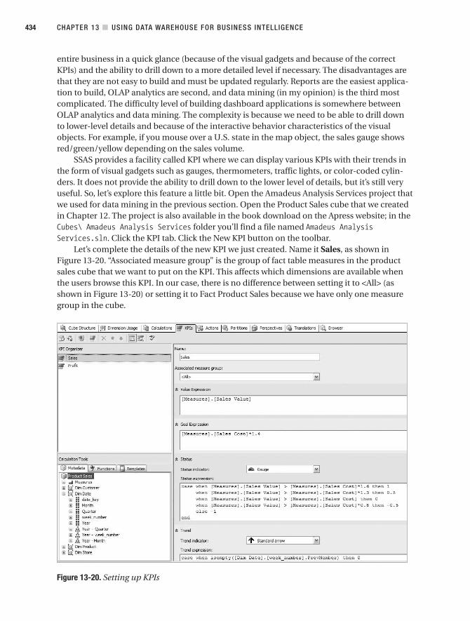
entire business in a quick glance (because of the visual gadgets and because of the correctKPIs) and the ability to drill down to a more detailed level if necessary. The disadvantages arethat they are not easy to build and must be updated regularly. Reports are the easiest applica-tion to build, OLAP analytics are second, and data mining (in my opinion) is the third mostcomplicated. The difficulty level of building dashboard applications is somewhere betweenOLAP analytics and data mining. The complexity is because we need to be able to drill downto lower-level details and because of the interactive behavior characteristics of the visualobjects. For example, if you mouse over a U.S. state in the map object, the sales gauge showsred/green/yellow depending on the sales volume.
SSAS provides a facility called KPI where we can display various KPIs with their trends inthe form of visual gadgets such as gauges, thermometers, traffic lights, or color-coded cylin-ders. It does not provide the ability to drill down to the lower level of details, but it’s still veryuseful. So, let’s explore this feature a little bit. Open the Amadeus Analysis Services project thatwe used for data mining in the previous section. Open the Product Sales cube that we createdin Chapter 12. The project is also available in the book download on the Apress website; in theCubes\ Amadeus Analysis Services folder you’ll find a file named Amadeus AnalysisServices.sln. Click the KPI tab. Click the New KPI button on the toolbar.
Let’s complete the details of the new KPI we just created. Name it Sales, as shown inFigure 13-20. “Associated measure group” is the group of fact table measures in the productsales cube that we want to put on the KPI. This affects which dimensions are available whenthe users browse this KPI. In our case, there is no difference between setting it to <All> (asshown in Figure 13-20) or setting it to Fact Product Sales because we have only one measuregroup in the cube.
Figure 13-20. Setting up KPIs
CHAPTER 13 ■ USING DATA WAREHOUSE FOR BUSINESS INTELLIGENCE434
9314ch13final.qxd 11/15/07 9:49 AM Page 434
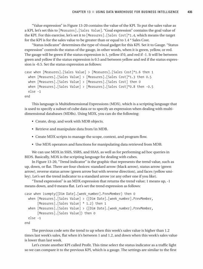
“Value expression” in Figure 13-20 contains the value of the KPI. To put the sales value asa KPI, let’s set this to [Measures].[Sales Value]. “Goal expression” contains the goal value ofthe KPI. For this exercise, let’s set it to [Measures].[Sales Cost]*1.4, which means the targetfor the KPI is for the sales value to be greater than or equal to 1.4 * Sales Cost.
“Status indicator” determines the type of visual gadget for this KPI. Set it to Gauge. “Statusexpression” controls the status of the gauge, in other words, when it is green, yellow, or red.The gauge will be green if the status expression is 1, yellow if 0, and red if -1. It will be betweengreen and yellow if the status expression is 0.5 and between yellow and red if the status expres-sion is -0.5. Set the status expression as follows:
case when [Measures].[Sales Value] > [Measures].[Sales Cost]*1.6 then 1when [Measures].[Sales Value] > [Measures].[Sales Cost]*1.3 then 0.5when [Measures].[Sales Value] > [Measures].[Sales Cost] then 0when [Measures].[Sales Value] > [Measures].[Sales Cost]*0.8 then -0.5else -1
end
This language is Multidimensional Expressions (MDX), which is a scripting language thatis used to specify a subset of cube data or to specify an expression when dealing with multi-dimensional databases (MDBs). Using MDX, you can do the following:
• Create, drop, and work with MDB objects.
• Retrieve and manipulate data from/in MDB.
• Create MDX scripts to manage the scope, context, and program flow.
• Use MDX operators and functions for manipulating data retrieved from MDB.
We can use MDX in SSIS, SSRS, and SSAS, as well as for performing ad hoc queries inBIDS. Basically, MDX is the scripting language for dealing with cubes.
In Figure 13-20, “Trend indicator” is the graphic that represents the trend value, such asup, down, or flat. There are four choices: standard arrow (black arrow), status arrow (greenarrow), reverse status arrow (green arrow but with reverse direction), and faces (yellow smi-ley). Let’s set the trend indicator to a standard arrow (or any other one if you like).
“Trend expression” is an MDX expression that returns the trend value; 1 means up, -1means down, and 0 means flat. Let’s set the trend expression as follows:
case when isempty([Dim Date].[week_number].PrevMember) then 0when [Measures].[Sales Value] > ([Dim Date].[week_number].PrevMember,
[Measures].[Sales Value] * 1.2) then 1when [Measures].[Sales Value] > ([Dim Date].[week_number].PrevMember,
[Measures].[Sales Value]) then 0else -1
end
The previous code sets the trend to up when this week’s sales value is higher than 1.2times last week’s sales, flat when it’s between 1 and 1.2, and down when this week’s sales valueis lower than last week.
Let’s create another KPI called Profit. This time select the status indicator as a traffic lightso we can compare it to the previous KPI, which is a gauge. The settings are similar to the first
CHAPTER 13 ■ USING DATA WAREHOUSE FOR BUSINESS INTELLIGENCE 435
9314ch13final.qxd 11/15/07 9:49 AM Page 435

KPI that we just set. Set “Associated measure group” to <All>, because we have only onemeasure group in the cube. Set the value expression to [Measures].[Sales Value]-[Measures].[Sales Cost] to describe that Profit = Sales – Cost. Set the goal expression to[Measures].[Sales Value]*0.5, meaning that the goal is to have a profit equal to half of thesales value. Set the status indicator to a traffic light; in other words, the status is green, yellow,or red. Set the status expression as follows:
case when ([Measures].[Sales Value]-[Measures].[Sales Cost]) >[Measures].[Sales Value]*0.5 then 1when ([Measures].[Sales Value]-[Measures].[Sales Cost]) > 0 then 0else -1
end
The previous code sets the Profit KPI to green when the profit is greater than 0.5 * sales,yellow when the profit is greater than 0 but less than 0.5 * sales, and red when the profit isnegative. Set the trend indicator as a standard arrow and the trend expression as follows:
case when isempty([Dim Date].[week_number].PrevMember) then 1when ([Measures].[Sales Value]-[Measures].[Sales Cost]) >1.2 * ([Dim Date].[week_number].PrevMember,([Measures].[Sales Value]-[Measures].[Sales Cost])) then 1
when ([Measures].[Sales Value]-[Measures].[Sales Cost]) >1.1 * ([Dim Date].[week_number].PrevMember,([Measures].[Sales Value]-[Measures].[Sales Cost])) then 0.5
when ([Measures].[Sales Value]-[Measures].[Sales Cost]) >([Dim Date].[week_number].PrevMember,([Measures].[Sales Value]-[Measures].[Sales Cost])) then 0
when ([Measures].[Sales Value]-[Measures].[Sales Cost]) >([Dim Date].[week_number].PrevMember,0.9 * ([Measures].[Sales Value]-[Measures].[Sales Cost])) then -0.5
else -1end
The previous code sets the profit trend to up when the profit is greater than 1.2 of lastweek’s profit, half up (pointing to 2 o’clock direction) when the profit is between 1.1 and 1.2of last week’s profit, flat (pointing to the right) when the profit is between 1 and 1.1, halfdown (pointing to 4 o’clock direction) when the profit is between 0.9 and 1, and down whenthe profit is less than 0.9.
After everything is set up, click the ABC button to check that the syntax is correct. Clickthe Build menu, and choose Deploy. After deployment is completed successfully, click theReconnect icon (it’s the third icon from the left). This is necessary to reconnect to the AnalysisServices cube after the KPIs have been added to the cube to pick up the changes we just made.To see the KPIs, with their values, goals, status, and trends, click the Browser View button (it’sthe second icon from the right). Let’s pick up a certain product category and certain week tocheck whether the values, goals, status, and trends are correct for that week. Set the productcategory to Music and the date dimension to week 10 (you can pick other product categoriesand other weeks if you want), as shown in Figure 13-21.
CHAPTER 13 ■ USING DATA WAREHOUSE FOR BUSINESS INTELLIGENCE436
9314ch13final.qxd 11/15/07 9:49 AM Page 436
Figure 13-21. Viewing the KPIs
The condition of the visual gadgets depends on the criteria that we specify in the MDX.Figure 13-21 shows that the status of Profit is yellow, meaning it is between 0 and 0.5 of thesales value. The trend for Profit is up, meaning it is more than 1.2 times the value in the previ-ous period. The sales status is between yellow and green, which means it is between 1.3 and1.6 times the sales cost. The sales trend is flat, meaning it’s between 1 and 1.2 times the previ-ous period.
In SQL Server, we can deliver a dashboard using SSAS and KPIs, as discussed. We can thenput the KPIs that we built in SSAS as web parts and host them in SharePoint to create dash-board applications. ProClarity (now part of Microsoft), Microsoft Office Performance Point,and Business Scorecards Manager also have the ability to deliver dashboard applications.
Business Intelligence AlertsAlerts are notifications to the users that a certain event or condition has happened. Examplesof such events or conditions are the following:
• When a daily sales figure in any particular store falls under a certain percentage of thetarget
• When the number of account closures across the whole country is beyond a certainfigure
• When the profit margins for certain product types across the whole region are lowerthan a preset limit
Again, remember that BI covers a wider area than just the data warehouse. A BI tool suchas alert system can access the ODS and operational systems as well as the data warehouse.Therefore, we can distinctly differentiate BI alerts into two categories according to which sys-tem they get the data from: data warehouse alerts and operational system alerts. The maindifference between these two is that the scope of operational system alerts is per transaction,whereas data warehouse alerts are at an aggregate level; for example, they can be weeklyacross product types or daily across regions. Examples of operational system alerts are ane-mail, pager, or SMS notification in the event that the stock level falls below a certain markor when a booking order value is more than the customer credit limit.
CHAPTER 13 ■ USING DATA WAREHOUSE FOR BUSINESS INTELLIGENCE 437
9314ch13final.qxd 11/15/07 9:49 AM Page 437

The main purpose of having BI alerts is to be able to react early in order to prevent some-thing that is about to happen or to rectify something before it gets worse. The main advantageof delivering BI information using alerts as opposed to the other four methods (reports, analyt-ics, data mining, and dashboards) is the timing. An alert proactively notifies the user when thesituation occurs or when the event happens, whereas with the other methods, the user needsto actively run or invoke reports, analytics, data mining, or dashboard applications (with theexception of subscription-based reports). The main disadvantage is that alerts usually containonly simple data, as opposed to the rich data delivered by data mining or dashboard applica-tions. But, alerts can contain links or URLs to the web pages that contain rich information.
So, how do we deliver alerts in SQL Server? The answer is SQL Server Notification Ser-vices. Notification Services is a platform for developing and deploying applications thatgenerate and send notifications to subscribers. Notification Services has four components:Subscription Management, Event Collection, Subscription Processing, and NotificationDelivery. The Subscription Management component stores the subscribers, the informationto be delivered, and the preferred delivery channels. The Event Collection component gath-ers the events from databases, file systems, or applications and sends these events to anotification application. Standard event providers are SQL Server (T-SQL queries), AnalysisServices (MDX queries), and file system watcher (XML files). The Subscription Processingcomponent evaluates the subscriptions to find a match against the collected events and thengenerates the notifications. The Notification Distribution component transforms the notifi-cation data into a readable message (web, file, or e-mail), formats the message, and sends itto the subscribers via the correct delivery channels.
Business Intelligence PortalA BI portal is an application that functions as a gateway to access and manage businessintelligence reports, analytics, data mining, and dashboard applications as well as alert sub-scriptions. It can be developed as a custom-built application (using Visual Studio .NET, forexample) or using an off-the-shelf solution. Some BI vendors have products to construct aBI portal that put various reports, OLAP, scorecards, and dashboards (usually their own BIapplications) into one place for easier and simpler access, including MicroStrategy 8Dynamic Enterprise Dashboards, Hyperion 9 Interactive Reporting Dashboard Studio, andCognos Portlets for IBM WebSphere Portal. Microsoft Office Business Scorecard Manager2005 and Microsoft Office SharePoint Server 2007 also have a BI portal as a built-in sampleapplication.
The main benefit of using a BI portal is that all BI applications are available in one centralplace. The second benefit is centralized security management. In other words, users need tolog in only once to the portal, and they don’t need to log in again to access each application.So, it is simpler for the administrator to manage the security. These days most BI portals areweb-based so that users across different geographical regions can access them via the com-pany intranet, extranet, or other platform. It is also common to place the BI documentationand user guides, as well as the support phone numbers and the link to the help desk applica-tion, on the BI portal for easy access by the users. You can also put BI and data warehousenews and announcements such as when you have new dashboards or when a particular salesreport shows good results. Figure 13-22 shows an example of a BI portal.
CHAPTER 13 ■ USING DATA WAREHOUSE FOR BUSINESS INTELLIGENCE438
9314ch13final.qxd 11/15/07 9:49 AM Page 438

Figure 13-22. Example of a BI portal
So, how do we build a BI portal? Well, in its simplest form, it is a web page containingmany links to various reports and BI applications. So, we can use ASP.NET to build it. Withsome documentation, a user guide, and other useful information added, it would become agood starting point for the BI users. For the implementation of business intelligence on theSQL Server platform, some people build the BI portal using SharePoint to take advantage ofintegrating Reporting Services web parts with SharePoint. (Reporting Services provides Share-Point components that we can include in the SharePoint portal. These components are calledweb parts.) Examples of Reporting Services SharePoint web parts are RsReportInfo,RsReportView, RsReportParameters, and RsReportExport. You can use RsReportInfo to get thereport details. RsReportView is used for viewing the reports, so it’s probably the most usefulweb part. RsReportParameters is for setting up reporting parameters. RsReportExport is forexporting reports to PDF, XML, Excel, or text files. On the SharePoint portal, you can also pro-vide the link to the Reporting Services main page, where all the reports are kept in folders.
SummaryThere are several types of BI applications such as reporting, analytics, data mining, dash-boards, and alerts. In this chapter, I discussed each of these types one by one. I went throughthe detailed steps of creating key performance indicators in SQL Server Analysis Services 2005.I also discussed BI portals, which unify all the previous applications in one central place andsimplify the security administration.
CHAPTER 13 ■ USING DATA WAREHOUSE FOR BUSINESS INTELLIGENCE 439
9314ch13final.qxd 11/15/07 9:49 AM Page 439

All these BI applications give you information about the condition of your business. Youneed to implement the correct actions to improve your business performance and verify thatthese actions are correct by looking at these BI applications again. If the performance isimproving, your actions are correct. If not, it’s wrong, and you need try another action. With-out doing anything, there is no point having the BI applications. If there is only one point thatyou take from this chapter, I hope it is this one: take action!
CHAPTER 13 ■ USING DATA WAREHOUSE FOR BUSINESS INTELLIGENCE440
9314ch13final.qxd 11/15/07 9:49 AM Page 440
Using Data Warehouse forCustomer RelationshipManagement
Customer Relationship Management (CRM) is the activity of establishing contact and man-aging communications with customers, analyzing information about customers, campaigningto attract new customers, performing business transactions with customers, servicing cus-tomers, and providing support to customers. Customers are the people (or parties) who acompany or an organization serves; they’re the ones who consume its products or services.If the organization is not a company or business (for example, a school or university, govern-ment agency, nonprofit organization, social club, political party, and so on), you can replacethe word customers in the earlier definition with students, constituents, citizens, taxpayers,users, applications, stakeholders, and so on, whichever is most appropriate.
A CRM application is a system that a company or organization uses to create and sendcampaigns, analyze customers’ personal and demographic information, analyze and predictcustomer behavior including purchases, perform customer scoring, manage customer per-missions, manage customer support/service, integrate customer data, manage customerloyalty programs, and manage customer contacts (including complaints and resolutions).Some CRM applications cover only some of the functionalities listed here. CRM applicationscan be hosted internally in-house or hosted externally with an application support provider(ASP), meaning the application and data is hosted outside the company and the users accessit remotely, usually via the Internet. An example of a hosted CRM solution is Salesforce.com,which offers customer data management, customer analysis, customer response manage-ment, and customer relationship history hosted on its servers over the Internet. CRMapplications can be sold as part of an Enterprise Resource Planning (ERP) product suite, suchas in the case of Siebel, SAP, and PeopleSoft, or it can be a stand-alone product such as Infor(Epiphany), Microsoft Dynamics CRM, and Teradata CRM.
Customer data can be stored centrally in a data warehouse or in an operational data store,where the customer data is integrated to produce a single-customer view (SCV). An SCV is anintegrated collection of customer data from various data sources in one central place so youcan have a holistic view of your customers. An SCV is important because it gives you a betterunderstanding of your customers. I will discuss SCVs in more detail in the next section. Theother major benefit of storing integrated customer data in the data warehouse is to performcustomer analytics and data mining—both descriptive analytics (discovering the patterns in
441
C H A P T E R 1 4
9314ch14final.qxd 11/15/07 9:45 AM Page 441

customer data) and predictive analytics (forecasting customer behaviors). Also, a dimensionaldata warehouse is an ideal platform to perform customer scoring (calculating the value of acustomer using a particular formula, for example, based on their purchases), especially whenthe algorithm for scoring involves demographics and purchase analysis.
In this chapter, I will discuss how to use a data warehouse to perform CRM activities,including creating a single customer view, performing campaign segmentation, managingpermissions, monitoring deliverability, performing customer analysis, managing customersupport, managing personalization, and administering loyalty schemes.
Single Customer ViewOrganizations make contacts with their customers at various points. This results in variousviews or definitions of customers. If we asked our order-processing department about whoour customers are, they would probably say, “Individuals who have purchased a product orservice from us.” If we asked our CRM department, they would probably have a different view.Their concept of a customer might be “Individuals who have purchased something from us,plus anybody who is currently subscribed to our newsletters.” Another department, such ascustomer service, could have a different view of a customer. Their concept of a customer maybe “Individuals who have put something in a shopping basket, even though they don’t con-tinue to the checkout.” Finance may have a different view of a customer: “A customer isanybody who has paid us or owes us money.”
The previous paragraph illustrates a common situation where different parts of the enter-prise have their own view, or definition, of customers. Because of these different views, “thenumber of customers” is different from department to department. If we ask the order-processing department, they may say that the number of customers is 25 million, whereasthe marketing department may say that the number of customers is 60 million.
This situation may be even worse if different departments are using different systems orapplications. Marketing may be using Omniture, finance may be using SAP, and CRM may beusing Siebel. In this situation, the customer data is scattered across several different systems,and each system has a different list of customers. Therefore, it is very difficult to compose asingle definitive list of customers.
The concept of an SCV is to have a single definition about who a customer is. Only whenwe have a single common definition across all departments can we have a definitive list ofcustomers. An SCV is an integrated collection of customer data from various data sources inone central place so we can have a holistic view of our customers.
Let’s illustrate this with our case study, Amadeus Entertainment. A customer in AmadeusEntertainment can be a purchaser, subscriber, registered user, or various other definitions,depending on the department. Say that we have the following definitions of customers. Thesequantities are just some examples to show the effect of overlaps on the total (they don’t comefrom our DDS sample database).
• Twenty-five million individuals have purchased Amadeus Entertainment’s products.
• Thirty-five million individuals subscribe to its communications.
• Twenty million individuals have registered on the web sites.
CHAPTER 14 ■ USING DATA WAREHOUSE FOR CUSTOMER RELATIONSHIP MANAGEMENT442
9314ch14final.qxd 11/15/07 9:45 AM Page 442

• Forty-four million individuals have asked for quotes.
• Fifty-five million individuals have browsed its web sites.
• Thirty-one million individuals have downloaded something from the web sites.
• Twelve million individuals have participated in one of its online competitions.
• Seven million individuals have sent the company e-mails or called.
• Twenty-four million individuals have made payments to Amadeus Entertainment.
• Seventeen million individuals have accounts with Amadeus Entertainment.
This situation can be drawn in the Venn diagram shown in Figure 14-1. The circles on thediagram show the different customer definitions. The sizes of the circles reflect the quantities.Each circle intersects with other circles, meaning that the same customers can be included inseveral definitions. If the common definition of a customer of Amadeus Entertainmentincludes all of the previous (purchaser, subscriber, registered user, and so on), then the totalnumber of customers that the company has is identified by the total area of the Venn diagram.
Figure 14-1. Intersections between different customer definitions
Because of the overlap, the total number of customers that Amadeus Entertainmenthas is not 25 million + 35 million + 20 million + 44 million + 55 million + 31 million +12 million + 7 million + 24 million + 17 million = 270 million, but probably much less thanthat. In Figure 14-1, the total area is probably 1.5 of the largest circle (B/S, 55 million), giv-ing us only 82.5 million. This situation is illustrated in the customer table shown inTable 14-1.
CHAPTER 14 ■ USING DATA WAREHOUSE FOR CUSTOMER RELATIONSHIP MANAGEMENT 443
9314ch14final.qxd 11/15/07 9:45 AM Page 443

CHAPTER 14 ■ USING DATA WAREHOUSE FOR CUSTOMER RELATIONSHIP MANAGEMENT444
Table 14-1 shows the simplified concept of an SCV, without any customer attributes orlinks to other areas. When we want to know how many customers we have, all we need to dois use select count (*).
Table 14-1 probably looks simple, but in practice there are two things that we need toconsider when creating an SCV. First, how do we identify, match, and deduplicate a cus-tomer? This is fundamental to SCV. If we have a new customer registered on the web sitetoday, say her name is Orsola Velia and her e-mail address is [email protected], is she thesame person as the customer on the last row in Table 14-1? Maybe not. What if we know onlyher e-mail address but not her name? Then it’s even more difficult for us to identify or matchthe customer. Some applications have user IDs or account IDs (for example, when the useris registered) that uniquely identify each customer. But some applications may not have userIDs or account IDs (for example, when a user subscribes to a newsletter). So, we need toagree on the business rules for identifying, matching, and deduplicating customers; forexample, we could agree that a customer can be identified by an account ID if available and,if not, by an e-mail address and the source system. Matching (to determine whether two cus-tomers are the same customer) is quite a risky business, so we want to get it right the firsttime. If we are not careful, orders from customer A could be under customer B’s name. Surelywe don’t want that to happen.
The second issue to consider when creating an SCV is the customer attributes. Becausethe definition of a customer is different across different departments in an organization (asdescribed earlier), the customer attributes have different levels of richness (the number ofattributes). For example, if it is a subscriber, we know only the name and e-mail address. If it isa purchaser, we know their name, e-mail address, address, and phone number. If it is a com-petition participant (they filled in a customer survey), we know their name, e-mail address,address, phone number, date of birth, occupation, and interests. So when using the SCV data,we need to be aware that we don’t have all the attributes for all the customers. For example,perhaps we have addresses only for 60 percent of our customers, we have names for 80 per-cent of our customers, and for email address we have 95 percent coverage.
Table 14-1. Customer Table Containing Different Customer Definitions
Name Email Address P S RU QP B/S CP E/C B/P AH
Chloe Nicoletta [email protected] Y Y Y Y Y
Nicolina Luigia [email protected] Y Y
Deni Hudd [email protected] Y Y
Bernardine Avril [email protected] Y Y
Jojo Emilie [email protected] Y Y Y
Serafina Hodge [email protected] Y Y Y Y
Orsola Velia [email protected] Y Y
P stands for Purchaser, S stands for Subscriber, RU stands for Registered User, QP stands for Quoted Person, B/S standsfor Browser/Shopper, CP stands for Competitor Participant, E/C stands for E-mailed/Called, B/P stands forBilling/Payment, and AH stands for Account Holder.
9314ch14final.qxd 11/15/07 9:45 AM Page 444

In many organizations, customer data is scattered across different systems. The systemsmay have different applications (ERP systems) between the stores and the e-commerce websites or between marketing contacts and promotions. They may use different agencies fore-mail promotions (which means that the data is even more scattered). For example, an inter-national business group consists of different individual legal entities (companies or agencies),which are composed of many brands that may be located in many countries. Some occurredby acquisitions; in other words, the group purchased a subsidiary company. Some happenedvia merger; in other words, two big business groups joined together. We could be talking about30 to 100 individual legal entities (worldwide). There is no way that all these companies areusing the same application to manage their business. But if you are talking about a smallbusiness with three offices all under one legal entity, it is possible that they have a singleapplication to manage their business, at least with regard to where the customer data isstored. But for an international business that exists in 50 countries, it is unlikely. This meansthe customer data is likely to be scattered all over the place.
So, is it possible to have a centralized customer database containing personal informa-tion, their orders, their preferences, their quotes, their e-mail promotions, their downloads,their contact details, their interests, their subscriptions, their complaints, their queries, theircredit score, their loyalty score, their browsing/shopping history, their account details, theircompetition participations, their payments, their registration details, and their security detailsall in one central place? Luckily, the answer is yes. It’s hard work, but it is possible. Many CRMinitiatives started by integrating customer data. Projects such as Customer Data Integration(CDI) hubs and Operational Data Stores (ODS) centralize customer data into one place; theyprobably also publish this data for other applications to consume via a software as a service(SaaS) scheme in a Service Oriented Architecture (SOA). Sometimes, in less than ideal situa-tions, they don’t have CDI hubs or an ODS, and the only place where customer data isintegrated is in the data warehouse, in other words, in the customer dimension.
An SCV is important because it gives us a better understanding of our customers; basi-cally, it gives us a more complete view. We get different attributes from different sources. Forexample, from the registration database, we get their user IDs, names, and addresses. Fromthe order-processing system, we get contact telephone numbers, e-mail addresses, billingaddresses (which may be different from the registered address), and perhaps the credit carddetails. From the promotion and competition system, we could get their occupation, marriagestatus, number of children, salary range, interests/communication preferences, and permis-sions (for us to send them marketing-related material), and perhaps they can even subscribeto one or two newsletters. From customer service systems, perhaps we can get informationabout which products they don’t like or which service they like best. Perhaps from customerloyalty programs, we can get their input about what products and services need to beimproved, which benefits are valuable or not valuable to them, and what we can do to helpthem more. When we combine the data from various systems, we get a more complete viewabout the customers. The more we know about our customers, the more we can tailor ourproducts and services to meet their interests and needs, and the business becomes more suc-cessful. So, an SCV is about an integrated view of our customers from various sources.
What are the advantages of having an SCV in the data warehouse, compared to having itin the ODS or CDI, for example? The first advantage is a slowly changing dimension (SCD),particularly type 2. SCD is a technique used in dimensional modeling for preserving histori-cal information about dimensional data. In SCD type 2, we keep the historical information inrows, while in SCD type 3, we keep the historical information in columns. In SCD type 1, we
CHAPTER 14 ■ USING DATA WAREHOUSE FOR CUSTOMER RELATIONSHIP MANAGEMENT 445
9314ch14final.qxd 11/15/07 9:45 AM Page 445

don’t keep the historical information. (Please refer to Chapter 5 for more information aboutSCD.) The advantage of having historical information is the data richness. With an SCD, wehave richer customer data in the data warehouse, because of historical information. Forexample, in the case of the customer dimension, we can use SCD type 2 to store the previousaddress, the previous occupation, or, more important, the previous loyalty scores and sub-scriber bands. The last two are calculated based on their purchases and subscriptions andbased on the revenue and/or profit the customer produced. So for customers who were pre-viously on higher bands, we may want to tailor our offerings a little bit by presenting themwith more suitable products or services, thus potentially resulting in more revenue fromcustomers.
The second advantage of using a data warehouse for an SCV is the analytical nature of adimensional data warehouse, enabling us to perform better customer analysis, which resultsin a better understanding of the customers. This can potentially drive the business to be moresuccessful. A dimensional data warehouse is an ideal place for performing analysis, such asanalyzing customer purchase behavior or subscription dynamics to get the customer scoreand subscription band, which can then be persisted as a customer attribute. I’m not sayingthat we can’t do this in the ODS, CDI, or ERP; I’m saying that data warehouse is a better placeto perform that analysis. In terms of performance, this analysis is better performed on adimensional database than on a normalized database, particularly on a star schema. This isbecause in a normalized database we need to do a lot of joins between tables. Analyzing fiveyears of order data against 20 million customers (with SCD type 2) using data mining algo-rithms will probably affect the operational performance of our normalized ERP, CDI, or ODS.Say it is 30 million order lines per year. Say that SCD type 2 on average creates one historicalrow for each customer, so we are talking 40 million rows on customer data. Say we use threealgorithms: Decision Trees, Clustering, and Naive Bayes. So, we are talking about runninganalysis on the ODS or ERP for 150 million order data items against 40 million customer dataitems and say 10,000 product data items using three algorithms. How long would it take torun? It could take from a few hours to a few days. I’m sure the internal front-end users won’tbe happy that the system performance is so slow during the hours the analysis runs. Can youimagine the impact on revenue if customers can’t add an item to a shopping basket or if thecheckout system is affected in any way? No, I don’t think anybody would run this kind ofanalysis on anything that affects the front-end systems. By having SCV customer data on thedata warehouse, the customer purchase and subscription analysis results will be better interms of performance.
The third advantage of using a data warehouse for an SCV is the computational powerof a data warehouse system. A data warehouse system is designed and built to be able tohandle large data-processing requirements. A data warehouse system is designed to be ableto process queries involving large data sets efficiently such as by having physical table parti-tions. If the data is 10MB to 20MB, it probably won’t matter on which platform we performthe SCV, for example doing deduplication and customer matching, but for large data (saygreater than 1TB), it matters. You can analyze your situation by running analytical querieson your current platform. Extracting information from marketing data, registration data,order data, competition data, and subscription data and then updating the customer dataincluding matching and deduplication for upsert (update and insert) is best performed onplatforms specifically designed for large queries.
The fourth advantage of using a data warehouse for SCV is that the customer data in thedata warehouse is already integrated from various source systems, so it enables us to combine
CHAPTER 14 ■ USING DATA WAREHOUSE FOR CUSTOMER RELATIONSHIP MANAGEMENT446
9314ch14final.qxd 11/15/07 9:45 AM Page 446

customer attributes from different sources. If we have an ODS or a CDI hub, then we could doSCV there, subject to the earlier considerations. But in many cases where there is no ODS orCDI, the data warehouse can be the only integration point of customer data in the organiza-tion. So when we do an SCV in the data warehouse, we will work with complete customer datathat has been integrated from various source systems.
Campaign SegmentationA campaign is a communication sent to customers regularly or on an ad hoc basis via e-mail,post, RSS, or text messages and containing marketing promotions (cross-sale, up sale, and soon) or notifications. Weekly newsletters, new product tactical promotions, and price increasenotifications are examples of campaigns. An order confirmation e-mail is an example of acommunication sent to customers that is not a campaign. It is considered to be a trans-actional communication.
Before we move on, let me introduce some of the campaign terminology normally usedin CRM. A campaign is a communication sent to customers. A delivery channel is the mediaused to send the campaign, such as post, e-mail, text message, or RSS. RSS is a web feedused to publish frequently updated content. Some delivery channels have several contentformats. For example, in e-mail messages, there are two content formats: HTML format andtext format.
Open rate and click-through rate are terms used in e-mail campaigns. Open rate is thenumber of e-mail messages that were opened by the customer divided by the number of mes-sages sent. For example, if we sent 100,000 e-mail messages and 20,000 of them were opened,the open rate is 20 percent. The click-through rate, commonly abbreviated as CTR, is the num-ber of customers who clicked the hyperlink embedded in the e-mail messages to go to the website divided by the number of e-mail messages sent. For example, if we sent 100,000 e-mailmessages and 4,000 of them were clicked, then the CTR was 4 percent.
The delivery rate is the number of e-mail messages that are delivered successfully dividedby the number of e-mail messages sent. The bounce rate is the number of e-mail messagesthat are not delivered successfully to the intended recipient divided by the number of e-mailmessages sent. For example, if we sent 100,000 e-mail messages and 98,000 were deliveredsuccessfully, then the delivery rate is 98 percent, and the bounce rate is 2 percent.
Now let’s continue our discussion about campaigns. A campaign is a fundamental corner-stone of CRM activity. Put simply, the process of creating a CRM campaign is roughly asfollows (bear in mind that this is different from company to company):
1. Based on the business need, we decide which customers we want to target (andquantify roughly how many), what message we want to deliver to them (just a briefparagraph describing the idea), the frequency of the campaign (for example, everyweek or one time only), the batch sizes (for example, in chunks of 150,000/day), thedelivery channel (for example, 10 percent by RSS and 90 percent by HTML e-mail), andthe expected results (for example, 15 percent open rate, 5 percent click-through rate,and $200,000 additional revenue/month). For example, we want to offer service Y tocustomers who purchased product X in the last six months.
2. Create a selection query that selects from a database a list of customers who satisfycertain criteria, such as customers who purchased product X in the last six months.
CHAPTER 14 ■ USING DATA WAREHOUSE FOR CUSTOMER RELATIONSHIP MANAGEMENT 447
9314ch14final.qxd 11/15/07 9:45 AM Page 447

3. Compose the content of the campaign, one for each delivery channel and format.We check all the links in the content and test the campaign appearance/cosmetics onevery major e-mail and RSS client to ensure that our customers will see the campaignas it was designed to be.
4. Set up the campaign in the campaign management system, paste the selection query,load the content file, add the control group, execute it, send it to testers, obtain finalapproval, execute it, and send it out to customers.
5. Monitor the delivery rate, bounce rate, open rate, click-through rate, and the revenueincrease resulting from the campaign.
A campaign targets a list of customers. This list, as illustrated in step 2, is called a seg-ment. The simplest form of a campaign is where we have only one segment. This is called anunsegmented campaign. It is rather strange that it is called unsegmented even though it hasone segment, but that’s the term used in CRM. A more complex campaign contains morethan one segment. For example, we can divide the list based on where the customer lives; inother words, we send different offers for different areas. Or we can divide the list based ontheir preferred communication channel and format. We need to prepare separate contentfiles for each campaign format, for example, one for HTML e-mail and one for text-only e-mail. When a campaign is segmented, each segment receives different campaign content,because the content is tailored to each segment. For example, we could have a campaign tar-geting two different segments: male and female, each with different content. It’s not only thecontent that is different for each segment, but the actions could be different too, specificallythe sending times, the number of send retries, the bounce treatments, and the further selec-tions, to suit the segment we are targeting. For example, for segment 1 the best sending timeis at lunchtime, and for segment 2 the best sending time is in the morning. The combinationof content and actions that we apply to a particular segment is called treatment.
Whether the campaign is segmented (several lists of customers each receiving differentcampaign treatments) or unsegmented (one list of customers receiving one campaign treat-ment), we need to query the customer data to get lists of customers. This process iscommonly known as the list selection process, and the SQL query is known as the selectionquery. Some tools do the segmentation first and then perform the selection query for eachsegment, and some tools combine the selection queries for different segments together inone query. To give you an idea, Listing 14-1 shows the simplest form of selection query foran unsegmented campaign.
Listing 14-1. Example of a Selection Query
select c1.email_addressfrom fact_subscription finner join dim_customer c1on f.customer_key = c1.customer_key
inner join dim_campaign c2on f.campaign_key = c2.campaign_key
where c2.campaign_name = 'Music Newsletter'
CHAPTER 14 ■ USING DATA WAREHOUSE FOR CUSTOMER RELATIONSHIP MANAGEMENT448
9314ch14final.qxd 11/15/07 9:45 AM Page 448
The selection query in Listing 14-1 retrieves the customer e-mail addresses for an e-mailcampaign called Music Newsletter. There is no further selection on the query, which is why itis called an unsegmented campaign.
In my experience, there are four types of selection queries: permission, demographicdata, customer activities, and campaign response:
Permission: Permission is basically the consent from a customer that we can send themthis communication, such as a subscription to a newsletter on our web site. A permissionselection query is basically a query selecting a list of customers from whom we have con-sent to send this communication. For any campaign we must always have a permissionselection query. Listing 14-1 is an example of a selection query for permission.
Demographic data: Demographic data is a customer’s personal attributes, such as age,gender, location, occupation, income, interest, and number of children. A demographicdata selection query retrieves a list of customers based on these customer attributes, suchas where calculate_age(date_of_birth) between 20 and 30 or where occupation ='Student'.
Customer behavior: Every business or organization conducts transactions or activitieswith their customers. Customer behaviors are the actions that the customers do or don’tdo within these activities or transactions. Each industry has different customer behavior.For the retail and e-commerce industry, it is browsing and purchasing behavior; for tele-communications and utilities, it is usage behavior; and for financial services it is accountactivities. Examples of customer behavior selection queries are a list of customers whomade an order more than 12 months ago (known as sleeping customers) or customers whouse their cell phone less than 10 times a month.
Campaign response: When a customer receives an e-mail campaign from us, the cus-tomer can have three responses: delete the e-mail (or do nothing), open the e-mail, orclick a link on that e-mail. These three possible actions are called campaign responses.So, we can have a selection query producing a list of customers who have opened theprevious three campaigns but have not made any purchase in the last three months andthen target them specifically in the next campaign.
What is the benefit of using a data warehouse for campaign selection and segmentation?Well, it is easier and faster. Producing a list of customers who made an order more than 12months ago is more easily done on a data warehouse than in an operational system. Con-sider a query to get a list of customers who have purchased certain product types in the last12 months but did not purchase other product types, who have not been sent a campaign inthe last three days, who have given permission for us to send them promotional campaigns,who live in certain cities, and whose customer status is active. This query runs faster (min-utes rather than hours) in a dimensional data warehouse than in an OLTP system becausethe data model in an operational system is not specifically designed to support an analyticalquery like this. The main difference between an OLTP query and an analytical query is thatan OLTP query retrieves a few records (in other words, where order_id = X), whereas an ana-lytical query summarizes millions of records (such as the query I mentioned earlier). AnOLTP system is primary designed to insert or update a particular record(s) with split-secondperformance. It is not designed to summarize millions of records. Hence, it could take hours
CHAPTER 14 ■ USING DATA WAREHOUSE FOR CUSTOMER RELATIONSHIP MANAGEMENT 449
9314ch14final.qxd 11/15/07 9:45 AM Page 449

to run analytical-type queries, not because of the hardware but because of the way the data-base is designed.
A regular campaign’s segmentation queries may run once a week when it is operational.But when designing the campaign, the business user needs to run the segmentation queriesmany times to get the counts of intended recipients. This is a repetitive process, and if it takeshours to complete the counts, then it slows down the business process and decreases the userfriendliness.
The other benefit is capacity. Campaign delivery and response data are large. A data ware-house can naturally cope with such demand using the Campaign Results fact table describedin Figure 5-6 in Chapter 5. In that structure, various statuses are easily loaded into the facttable: sent, delivered, bounced, opened, clicked through, and so on. This campaign responsedata can then be used for the selection query on future campaigns, as described earlier.
Permission ManagementWe must send campaigns only to those customers from which we have consent. This consentis known as permission. Maintaining permissions is the most important thing in CRM opera-tions because sending a campaign without a customer’s permission means we are spamming.In some countries, the laws are very strict and include heavy penalties for spammers, includ-ing the Spam Bill in Australia, Penal Code Article 226-18 in France, and the CAN-SPAM Act inthe United States.
There are four types of customer permission:
General permission: In this type of permission, the customer gives consent for us to sendthem any marketing-related communications. Sometimes the consent is extended to“affiliates” or “carefully selected partners” as well. This is usually done via a little checkbox when the customer registers, accompanied with very small print, or on a marketingpreferences web page. This is generally known as opt-in. In CRM, it is common practice todo double opt-in. In other words, we send an e-mail to the customer’s e-mail address, andthe customer needs to click a link in that e-mail to confirm their consent. There are twomajor benefits of double opt-in:
• Customers can submit only their own e-mail address.
• The list contains only valid and tested e-mail addresses.
Specific permission: In this case, the customer allows us to send a specific type of commu-nication, for example only transaction-related communications such as order confirma-tion e-mails, payment receipts, and e-tickets. Or they want to receive only e-mails relatedto products that they have purchased, such as a flight reminder, destination guide (forgifts), download link (for computer products), or product withdrawal notice. We cannotuse specific permissions to send any other e-mails such as new products announce-ments. Specific permission also can be channel specific, such as “you can e-mail me,but you cannot call me.”
CHAPTER 14 ■ USING DATA WAREHOUSE FOR CUSTOMER RELATIONSHIP MANAGEMENT450
9314ch14final.qxd 11/15/07 9:45 AM Page 450
Subscription: This type of permission is very specific. In this case, the customer sub-scribes to a specific campaign, such as subscribing to a weekly newsletter or music news(as in the case study Amadeus Entertainment). We can send them only the campaignsthat the customer asked for in the format and delivery channel that the customer askedfor. The permission cannot be used to send them anything else in any format.
Negative permission: Sometimes customers ask us not to send them anything. Theydon’t want to receive any marketing material, news, announcements, product support,customer support, and transaction-related e-mails including order confirmation e-mails or payment receipts. For this kind of request where the customer revokes theirconsent, we could list them in a “banned e-mail addresses” table, and in every cam-paign we add the selection criteria like: where e-mail_address not in (select e-mail_address from banned_e-mail_addresses). Alternatively, we could use where not exist.This table or list is also known as a block list or black list. Many CRM campaign man-agement and e-mail delivery systems have this functionality; for example, we just needto configure them to point to the right table, and the system will filter it out when exe-cuting or sending campaigns.
Now that you know what permission is, what is the benefit of using a data warehouse forimplementing permission? Permission is used in the selection query, and a dimensional datawarehouse gives good performance when performing selection queries.
Subscription management is a transactional process and captured by the front-end appli-cations, such as on the web site and customer service systems. General permission is alsotransactional in nature; that is, it is usually captured when customers register on the web siteor when they become customers.
So, permission usually happens in the front-end applications, and it is used as aselection query when composing a list of customers for campaign recipients. Therefore,permission data needs to be transported from the front-end applications to the CRM datawarehouse. This can be done via a daily ETL incremental feed, based on the created and lastupdated timestamps. The structure of the data warehouse to store the permission variesdepending on which type of permission it is. For general permission, we can put it on thecustomer dimension, as follows: alter table dim_customer add permission bit. We thenset the ETL to populate it with “True” or “False” based on the front-end permission data.Specific permission is also usually incorporated on the customer dimension as severalTrue/False columns. Each column represents one specific permission. For example:
alter table dim_customeradd transaction_permission bit,promotion_permission bit,newsletter_permission bit
The implementation of subscriptions in the data warehouse is very different from thegeneric and specific permission. Subscriptions are usually implemented as a fact table, asshown in Figure 14-2, as we discussed in Chapter 5 when doing dimensional modeling.
CHAPTER 14 ■ USING DATA WAREHOUSE FOR CUSTOMER RELATIONSHIP MANAGEMENT 451
9314ch14final.qxd 11/15/07 9:45 AM Page 451
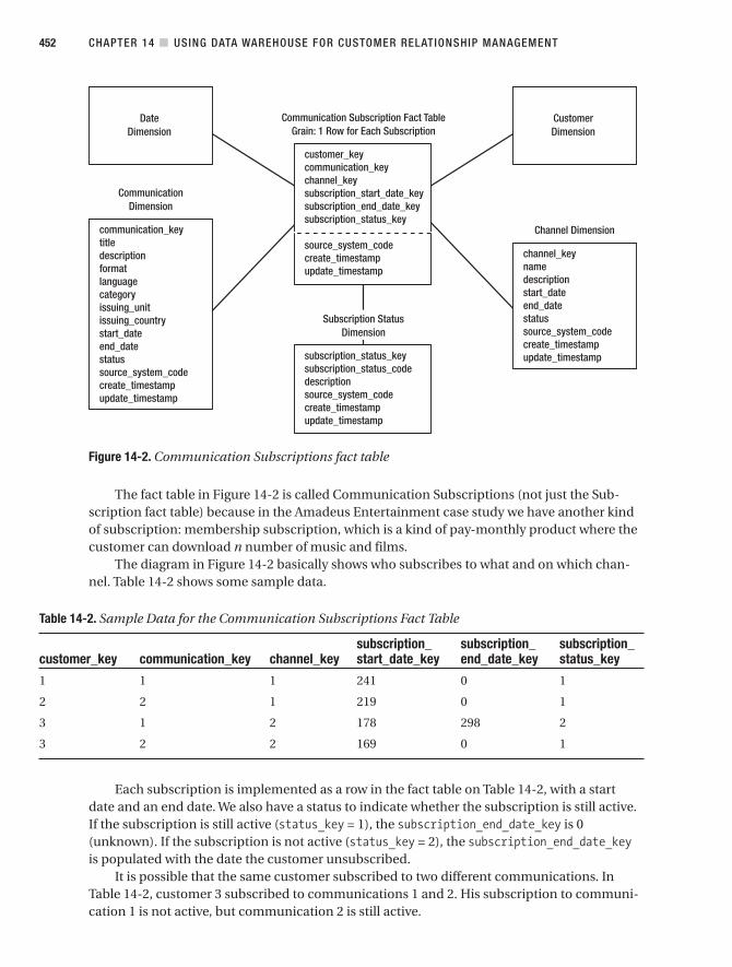
Figure 14-2. Communication Subscriptions fact table
The fact table in Figure 14-2 is called Communication Subscriptions (not just the Sub-scription fact table) because in the Amadeus Entertainment case study we have another kindof subscription: membership subscription, which is a kind of pay-monthly product where thecustomer can download n number of music and films.
The diagram in Figure 14-2 basically shows who subscribes to what and on which chan-nel. Table 14-2 shows some sample data.
CHAPTER 14 ■ USING DATA WAREHOUSE FOR CUSTOMER RELATIONSHIP MANAGEMENT452
Table 14-2. Sample Data for the Communication Subscriptions Fact Table
subscription_ subscription_ subscription_customer_key communication_key channel_key start_date_key end_date_key status_key
1 1 1 241 0 1
2 2 1 219 0 1
3 1 2 178 298 2
3 2 2 169 0 1
Each subscription is implemented as a row in the fact table on Table 14-2, with a startdate and an end date. We also have a status to indicate whether the subscription is still active.If the subscription is still active (status_key = 1), the subscription_end_date_key is 0(unknown). If the subscription is not active (status_key = 2), the subscription_end_date_keyis populated with the date the customer unsubscribed.
It is possible that the same customer subscribed to two different communications. InTable 14-2, customer 3 subscribed to communications 1 and 2. His subscription to communi-cation 1 is not active, but communication 2 is still active.
9314ch14final.qxd 11/15/07 9:45 AM Page 452
The channel key column in the fact table shown in Table 14-2 indicates how the campaignwill be delivered, such as by e-mail, text message, or RSS. The campaign format, however (text,HTML, and so on), is not in the fact table; but it is in the communication dimension instead,because the format is an attribute of a communication. A communication is something thatwe deliver to the subscribing customer on a regular or semiregular basis (many times, not onetime only), such as a weekly newsletter or news alert. As you can see in Figure 14-2, a commu-nication has a start date, end date, and status to indicate whether a communication is active.The category attribute groups common communications together and acts as a hierarchy, suchas weekly or ad hoc tactical. A channel also has a start date, end date, and status to indicatewhether it is active. In some implementations, particularly in multibrand and multinationalorganizations, we may want to add a brand and locale or country attribute in the communica-tion dimension to indicate which company owns that communication.
Listing 14-2 shows the Data Definition Language (DDL) for Figure 14-2.
Listing 14-2. DDL for Implementing Subscription in a Data Warehouse
create table fact_communication_subscription( customer_key int not null, communication_key int not null, channel_key int not null, subscription_start_date_key int not null, subscription_end_date_key int not null, subscription_status_key int not null, source_system_code tinyint not null, create_timestamp datetime not null, update_timestamp datetime not null, constraint pk_fact_communication_subscriptionprimary key clustered( communication_key, customer_key, subscription_start_date_key )
)
create table dim_communication( communication_key int not null, title varchar(50), description varchar(200), format varchar(20), language varchar(50), category varchar(20), issuing_unit varchar(30), issuing_country char(3), start_date datetime, end_date datetime, status varchar(10), source_system_code tinyint not null, create_timestamp datetime not null, update_timestamp datetime not null, constraint pk_dim_communicationprimary key clustered (communication_key)
)
CHAPTER 14 ■ USING DATA WAREHOUSE FOR CUSTOMER RELATIONSHIP MANAGEMENT 453
9314ch14final.qxd 11/15/07 9:45 AM Page 453

create table dim_subscription_status( subscription_status_key int not null, subscription_status_code char(2), description varchar(50), source_system_code tinyint, create_timestamp datetime, update_timestamp datetime, constraint pk_dim_subscription_statusprimary key clustered (subscription_status_key)
)
create table dim_channel( channel_key int not null, name varchar(20), description varchar(50), start_date smalldatetime, end_date smalldatetime, status varchar(10), source_system_code tinyint not null, create_timestamp datetime not null, update_timestamp datetime not null, constraint pk_dim_channelprimary key clustered (channel_key)
)
While we are on the permission management topic, it is relevant to talk about optingout, or revoking the permission. It is mandatory that the customer is able to unsubscribe orrevoke their permission at any time from any campaign. If it is an e-mail campaign, we needto have a link on every campaign pointing to an unsubscribe page. This page will update thefront-end database that will then be propagated to the data warehouse. As a result, the sub-scription will be deactivated, in other words, by updating the subscription end date andstatus. It is important that the propagation of unsubscription information to the CRM datawarehouse is frequent, ideally intraday or at least once a day, so that we can make sure cus-tomers who have revoked their permissions do not get subsequent campaigns. If it is ageneral or specific permission, the ETL will update the corresponding permission columnon the customer dimension from Y to N.
Delivery and Response DataCampaign delivery data is about whether the campaign that we sent is delivered to theintended recipient. For example, if the campaign is delivered using an e-mail message, it maynot get into the target mailbox because the mailbox is full. Campaign response data is aboutthe reaction from the customer after receiving our campaign. For example, they may be inter-ested in a particular offer in the e-mail and click it to purchase the product.
To understand campaign delivery and response data, let’s go through the process of cam-paign delivery. Take the Amadeus Entertainment Music Weekly Newsletter, which has 100,000recipients, as an example. After the campaign is created, it is executed and sent to the target
CHAPTER 14 ■ USING DATA WAREHOUSE FOR CUSTOMER RELATIONSHIP MANAGEMENT454
9314ch14final.qxd 11/15/07 9:45 AM Page 454

recipients. Let’s say that when the campaign was executed, there were 100,000 target recipi-ents. Let’s say 1,000 of these target recipients were filtered out because of the banned list table(refer to the earlier discussion of negative permissions), and 2,000 were filtered out becausethe recipient e-mail addresses have bounced four times. So, 97,000 actually went out: 90,000by e-mail; 4,000 by post; 2,000 by RSS; and 1,000 by text message. Out of the 90,000 e-mailmessages, say 86,000 reached the intended recipients, and 4,000 were undelivered (becausethe e-mail domain did not exist, because of an invalid mailbox name, because the mailboxwas full, and so on). Out of the 86,000 e-mail messages that were delivered, 25,000 wereopened/read, and 5,000 were clicked through; that is, the customers went to the web pagesspecified in the e-mail campaign. Out of these 5,000 customers, 500 made an order (pur-chased some products). Figure 14-3 illustrates the figures in this process.
Figure 14-3. Number of customers involved in each step of campaign delivery process
The number of e-mail messages sent out, the number of messages delivered, the numberof messages not delivered (bounced), and the number of e-mail messages not sent out (eitherbecause of banned list or bounce list) are called campaign delivery data, and the number ofe-mail messages opened/read, the number of messages clicked by the customers, and thenumber of customers purchased some products are called campaign response data. Bothcampaign delivery data and campaign response data are important because they indicate thesuccess or failure of the campaign; for example, if the open rate and click-through rate (CTR)are high, the campaign is successful.
The open and click-through rates vary from industry to industry. Amongst other things,they depend on whether we implement double opt-in (cleaner list), they depend on who thetarget audience is (business to business or business to consumer), and they depend onwhether the segmentation is specific or general. If you still want a rough indicator, for busi-ness to consumer with double opt-in and specific segmentation, you can expect an open ratefrom 5 percent to 15 percent.
It would be useful to understand how campaign delivery and response data can be col-lected by the CRM system. In other words, how do we know that an e-mail has been opened
CHAPTER 14 ■ USING DATA WAREHOUSE FOR CUSTOMER RELATIONSHIP MANAGEMENT 455
9314ch14final.qxd 11/15/07 9:45 AM Page 455

or read? How do we know that the customer has clicked certain links in the e-mail? How do wedetect which customer purchased which products and identify which campaign initiated thepurchase? The techniques and methods of obtaining delivery and response data within theCRM systems vary greatly from application to application. If it is an e-mail campaign, the deliv-ery status can be obtained from SMTP response codes, which is the number sent back by thetarget e-mail server, such as 250 for delivered, 530 for access denied, 552 for exceeding themailbox limit, 521 for a domain that does not except e-mail, 421 for a domain that’s not valid/available, and so on. Sometimes the interpretation of the response codes is not so straightfor-ward; for example, code 250 can mean several things, because it actually means that therequested action is done OK, so the meaning depends on what the requested action was. Fora text message, we need to use the appropriate protocol instead of SMTP, such as an SMSdelivery report that indicates whether the text message has reached the target cell phone orcannot be delivered.
Now that you have an understanding of campaign delivery and response data, I’ll coverthe pros and cons of implementing them in a data warehouse. The benefit of using a datawarehouse (as opposed to an operational system such as an ERP, CDI, or ODS) is that we canuse the delivery and response data for campaign segmentation. This is because the deliveryand response data will be located on the same platform as the other data used for a selectionquery (for example, customer data, shopping/purchase/activity data, and permission data)during the campaign selection and segmentation process. For example, we might select cus-tomers who have received a campaign e-mail about certain music product types but did notopen the e-mail or opened the e-mail but did not click any offer in the e-mail. We can then tar-get these groups with specific follow-up campaigns encouraging them to go to our web site tolook at the products.
The second benefit of implementing campaign delivery and response data in the datawarehouse is that we have better performance when loading data and performing analysis.The amount of campaign delivery and response data can be billions of rows within a fewyears. For example, we could have 35 campaigns that send e-mails to 20 million target sub-scribers every week, which equates to 1 billion a year. The grain of campaign delivery andresponse data is the number of target recipients. That means that for every message createdby the campaign, we will have a row, whether the message is sent or not. Because of the vol-ume, we can take advantage of a data warehouse platform, which handles a large volume ofdata better than operational systems. This is especially true when querying the campaignresponse data for customer analysis and purchase analysis, such as when analyzing cus-tomers who have clicked but not purchased or when performing demographic analysisagainst customers who have received certain types of campaigns in the last six months.
So, those are two benefits of implementing campaign delivery and response data in adimensional data warehouse. But sometimes we are not able to do that if our CRM applicationis a packaged application. For example, the CRM application may not work with a dimen-sional data warehouse; it may work only with a highly normalized operational database. Inthis case, we could load the campaign delivery and response data from the normalized CRMdatabase into a dimensional data warehouse for analysis.
Figure 14-4 shows the design of an implementation of CRM campaign delivery andresponse data in a data warehouse. It consists of a campaign delivery and response fact tablewith six dimensions.
CHAPTER 14 ■ USING DATA WAREHOUSE FOR CUSTOMER RELATIONSHIP MANAGEMENT456
9314ch14final.qxd 11/15/07 9:45 AM Page 456

Figure 14-4. Schema design for implementing campaign delivery and response data in a datawarehouse
Let’s go through the schema in Figure 14-4. It has one fact table and six dimension tables:date, communication, campaign, customer, channel, and delivery status. The grain of the facttable is one row for each intended recipient in the campaign. For example, say we have 10campaigns that were sent last week, each containing 20,000 customers. In this case, we have200,000 rows in this fact table.
I discussed this schema in Chapter 5. But to refresh, let’s go through each key column onthe fact table. The campaign key identifies which campaign was sent, for example: WeeklyFrance Music Newsletter 01/14/2008. The customer key identifies to which customer the cam-paign was sent. The communication key identifies the communication to which the campaignbelongs. For example, the Weekly France Music Newsletter 01/14/2008 campaign is aninstance of the Weekly France Music Newsletter communication. The channel key indicateshow the campaign was sent, such as via e-mail. The send date indicates when the campaignwas sent. The delivery status indicates whether the campaign was delivered successfully to theintended recipient.
Listing 14-3 shows the DDL of Figure 14-4.
CHAPTER 14 ■ USING DATA WAREHOUSE FOR CUSTOMER RELATIONSHIP MANAGEMENT 457
9314ch14final.qxd 11/15/07 9:45 AM Page 457
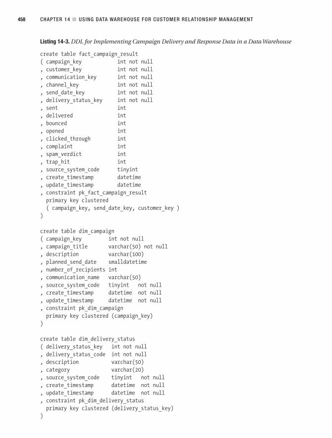
Listing 14-3. DDL for Implementing Campaign Delivery and Response Data in a Data Warehouse
create table fact_campaign_result( campaign_key int not null, customer_key int not null, communication_key int not null, channel_key int not null, send_date_key int not null, delivery_status_key int not null, sent int, delivered int, bounced int, opened int, clicked_through int, complaint int, spam_verdict int, trap_hit int, source_system_code tinyint, create_timestamp datetime, update_timestamp datetime, constraint pk_fact_campaign_resultprimary key clustered( campaign_key, send_date_key, customer_key )
)
create table dim_campaign( campaign_key int not null, campaign_title varchar(50) not null, description varchar(100), planned_send_date smalldatetime, number_of_recipients int, communication_name varchar(50), source_system_code tinyint not null, create_timestamp datetime not null, update_timestamp datetime not null, constraint pk_dim_campaignprimary key clustered (campaign_key)
)
create table dim_delivery_status( delivery_status_key int not null, delivery_status_code int not null, description varchar(50), category varchar(20), source_system_code tinyint not null, create_timestamp datetime not null, update_timestamp datetime not null, constraint pk_dim_delivery_statusprimary key clustered (delivery_status_key)
)
CHAPTER 14 ■ USING DATA WAREHOUSE FOR CUSTOMER RELATIONSHIP MANAGEMENT458
9314ch14final.qxd 11/15/07 9:45 AM Page 458
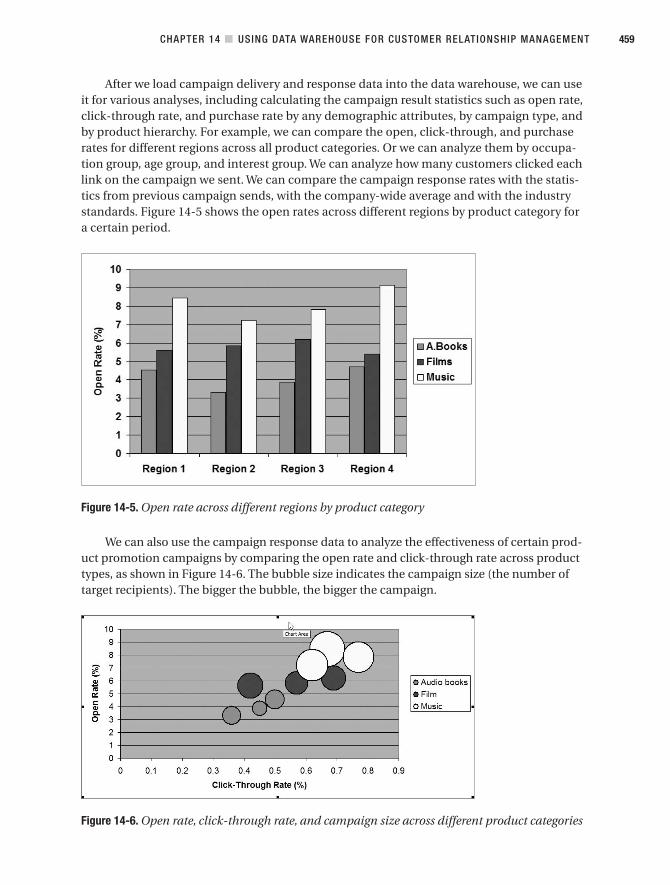
After we load campaign delivery and response data into the data warehouse, we can useit for various analyses, including calculating the campaign result statistics such as open rate,click-through rate, and purchase rate by any demographic attributes, by campaign type, andby product hierarchy. For example, we can compare the open, click-through, and purchaserates for different regions across all product categories. Or we can analyze them by occupa-tion group, age group, and interest group. We can analyze how many customers clicked eachlink on the campaign we sent. We can compare the campaign response rates with the statis-tics from previous campaign sends, with the company-wide average and with the industrystandards. Figure 14-5 shows the open rates across different regions by product category fora certain period.
Figure 14-5. Open rate across different regions by product category
We can also use the campaign response data to analyze the effectiveness of certain prod-uct promotion campaigns by comparing the open rate and click-through rate across producttypes, as shown in Figure 14-6. The bubble size indicates the campaign size (the number oftarget recipients). The bigger the bubble, the bigger the campaign.
Figure 14-6. Open rate, click-through rate, and campaign size across different product categories
CHAPTER 14 ■ USING DATA WAREHOUSE FOR CUSTOMER RELATIONSHIP MANAGEMENT 459
9314ch14final.qxd 11/15/07 9:45 AM Page 459

Campaign delivery data enables us to analyze the bounce rate across different e-maildomains and understand the reasons for the rate. The bounce rate is the number of e-mailmessages not delivered divided by the number of e-mail messages sent. E-mail domains arethe domain name of the customer e-mail address. For example, Figure 14-7 shows AmadeusEntertainment’s average bounce rate for the top six e-mail domains in a particular week.
Figure 14-7. Bounce rate across different e-mail domains
Customer AnalysisIn addition to the campaign response analysis discussed earlier, we can use CRM data in thedata warehouse for analyzing customer activities and behavior. This analysis of customeractivities and behavior is what we call customer analysis. There are two main categories of cus-tomer analysis: descriptive analysis and predictive analysis. In descriptive analysis, we try tounderstand or describe customer behavior and activities. In predictive analysis, we try to pre-dict or forecast customer behavior and activities. The following are examples of descriptiveanalysis:
E-commerce industry: Purchase pattern by demographic, where we try to understand thepurchase and browsing behavior of our customer group by demographic attributes, suchas age, occupation, income, location, family, and interest.
Telecommunication industry: Usage analysis against products, such as analyzing a cus-tomer’s cell phone usage to see whether the calling plan they are on now is the mostappropriate one. We could then use the CRM campaign to encourage switching to thecorrect calling plan to increase customer service satisfaction.
Insurance industry: Risk pattern identification, where we calculate customer risk factorsand insurance premiums according to customer activities. For example, for car insurance,the risk groups could be determined according to the base location, driving area, type ofcars, vehicle usage, and traveling time.
Utility industry: Customer profitability analysis, where we find out which customers weare making money on and which ones we are losing money from and by how much.
CHAPTER 14 ■ USING DATA WAREHOUSE FOR CUSTOMER RELATIONSHIP MANAGEMENT460
9314ch14final.qxd 11/15/07 9:45 AM Page 460

As we can see, all these analyses describe, analyze, or explain the current situation aboutcustomer activities and behavior. Predictive analysis is different. It tries to predict or forecastcustomer activities and behavior. Examples of predictive analysis are as follows:
Utilities industry: Price sensitivity analysis, where we try to find out which customerswould be likely to close their accounts when we do the annual price increase next monthand what the financial implications are of losing them. This enables us to approach thecustomers to prevent the account closure from happening.
E-commerce industry: Sales forecasting, where we predict the quantity sold for each prod-uct type in the coming months and calculate the sale amount accordingly. We can thentailor the CRM campaigns accordingly to make the forecast inline with the sales targets.
Travel industry: Predicting which customers are likely to be interested in certain types ofholiday, flight, or lifestyle product offers, based on the demographic data, previous book-ing data, and campaign response data. Another example is predicting which subscribersare likely to make a purchase when we send them promotional campaigns on certainproduct types.
Waste management: Forecasting which days are “heavy” days and which days are “light”days based on weight measurement data and customer business types, and arrange thepickup truck routing accordingly to increase fleet efficiency.
A CRM data warehouse contains customer data, permission data, campaign responsedata, customer activity data (purchase, shopping, subscription, gain, and loss), billing data,payments data, and marketing data (including promotions and campaigns). Because of itsrich content, a CRM data warehouse is naturally helpful for customer analysis, be it descrip-tive or predictive. The methods to do customer analysis are similar to those of BI, such asreporting, analytics, and data mining. Descriptive customer analysis can be delivered usingall of these three methods, while predictive customer analysis is usually delivered using datamining.
As an example of descriptive customer analysis, let’s use SSAS to analyze film purchasesby customer interests. For that, let’s create a product sales cube, shown in Figure 14-8, usingthe same process we discussed in Chapter 12. This cube is similar to the one we created inChapter 12. The only difference is that we have one more dimension here: customer.
We process this cube as we discussed in Chapter 12 and then browse it. Now let’s set thecube browser to display the customer interest against the product type. For this, we put theInterest1 attribute from the customer dimension as the row field and the Product Type attrib-ute from the product dimension as the column field. Put the Sales Value measure as the detailfield, and filter the cube on product category = ‘Films’. Figure 14-9 shows the result. I dis-cussed how to do all this in Chapter 12, so you should be familiar with this.
CHAPTER 14 ■ USING DATA WAREHOUSE FOR CUSTOMER RELATIONSHIP MANAGEMENT 461
9314ch14final.qxd 11/15/07 9:45 AM Page 461

Figure 14-8. Product sales cube with customer dimension
Figure 14-9. Analyzing film purchases by customer interests
CHAPTER 14 ■ USING DATA WAREHOUSE FOR CUSTOMER RELATIONSHIP MANAGEMENT462
9314ch14final.qxd 11/15/07 9:45 AM Page 462

In Figure 14-9 you can see that, for example, customers with a DIY interest purchasedmany more comedy films than those with a cooking interest. Customers with a cartoon inter-est purchased many more drama films than those with a church interest. We can also analyzethe film purchases by other demographic factors such as age, gender, and income. For this wejust need to swap the interest on the row field with other customer attributes.
This is an example of descriptive customer analysis. We did some predictive customeranalysis in Chapter 13, when we predicted the purchase of music products using gender,interest, and occupation demographic factors using the Decision Trees mining model.
Customer SupportMost customer support activities are done on the operational systems, both the call centersystems and ERPs. The customer service agents usually use these two types of systems to sup-port and service the customers. Operational data stores are increasingly used for customersupport too.
But sometimes a data warehouse is useful for customer support, especially utilizing datawarehouse analytical nature and prediction capability. The following are examples of datawarehouse usage for customer support.
Travel industry: Predeparture campaigns, where we send a campaign one week beforethe travel starts, to inform the customers about the weather forecast in the destinationcity, general information about the flight check-in time and security restriction, map ofthe area around the hotel, and destination information such as recommended restau-rants. We can also use this opportunity to remind them to bring their passports if thedestination is overseas and to ask whether they need a taxi to go to/from the airport,a car hire, attraction tickets, or a wireless Internet connection.
Telecommunication industry: To help individual customers get the right billing plan byanalyzing all the calls made by the customer in the last three months (time, destination,duration, cost) and comparing it with all available plans to see whether there are anyplans that have lower prices than the plan the customer currently has. The campaign canbe set up to run once a month to advise all customers who have not been advised in thelast six months (this would require campaign response data).
Utilities industry: To analyze individual customer’s electricity and gas usage and advisethe customers whether there is a better tariff plan in terms of costs, as well as giving themgeneral energy-saving advice.
Financial industry: To analyze the overdraft and withdrawal activities for each customer(across all accounts) and advise them accordingly. For example, you could ask whetherthey want to increase their overdraft limit. The bank can calculate the limit they are pre-pared to give, based on the account activity information in the data warehouse.
CHAPTER 14 ■ USING DATA WAREHOUSE FOR CUSTOMER RELATIONSHIP MANAGEMENT 463
9314ch14final.qxd 11/15/07 9:45 AM Page 463

E-commerce industry: A price alert, where you automatically advise the registered cus-tomer if certain products are now discounted below certain levels, for example, becausenew product lines will be replacing them soon. The campaign can run once a day match-ing the product prices and the customer interest and buying history and then advise thecustomers via e-mail, RSS, or text message.
Entertainment industry (like Amadeus Entertainment): Customized new title film/musicannouncements, where we advise the customers if his favorite artist or author has a newsingle, album, film, or book, as well as give information about the artist such as biography,web site, fans club, and coming shows.
The primary methods used to deliver this functionality are analytics and data mining.Some functionality would also require notification and subscription.
PersonalizationPersonalization is the customization of web sites, campaigns, offers, products, and servicesto a particular customer. For example, if John Smith browses the Amadeus Entertainmentweb site, the content he gets is different from the one Stella Sanchez gets. Customization isusually used on e-commerce web sites to make the products and offers more specific to par-ticular customers.
Personalization is important because it increases the chances of the customers pur-chasing the products, which could increase sales revenue. The source data for personaliza-tion can be taken from shopping data (the pages that the customer looked at on previousvisits), interest register (the interest text boxes/drop-down lists on the registration pages), or past purchases of similar customers (the similarity can be determined from demographicattributes). The source data can be analyzed using data mining models (decision trees, clus-tering, and other algorithms) to score a list of offers and products against individual cus-tomers. The output can then be wrapped as XML and fed to the personalized home pageson the web site. The output can also be displayed as “my store” or “my travel” or “My Ama-deus,” in other words, a page customized specifically to a particular customer, based on thepersonalization output.
The personalization output can also be fed into a personalized campaign that is then sentvia e-mails to customers. Depending on the degree of personalization and the segmentationof the campaign (which could be a segment of one), the campaign can take days to execute orjust a few hours (to just produce the raw XML files, not send out the e-mails).
The output of this analysis can also be stored in a dimensional mart, with time, cus-tomer, and product as the dimensions. The measure in the fact table itself is the likelihoodscore that the customer would be interested in those products. The data on this mart canthen be used for recommendations, which are similar to personalized offer e-mails but areusually applied when the customers are still shopping on the web site. The recommendationcan be as simple as “People who bought this item also bought …” or can be as complex asanalyzing the customer’s demographics and then going to the likelihood mart to find themost likely product range.
The key to site content personalization and recommendation is identifying the customer,because we have to be able to tailor the site while the customer is still on it. Two approachesare commonly used for identification: logins and cookies. The best way to identify a customer
CHAPTER 14 ■ USING DATA WAREHOUSE FOR CUSTOMER RELATIONSHIP MANAGEMENT464
9314ch14final.qxd 11/15/07 9:45 AM Page 464

is by self-authentication, in other words, asking the customer to log in. Although this may beinconvenient to customers (it’s an additional step), it is a reliable and accurate method.
Cookies, on the other hand, are tiny files on the customer’s computer that store a uniqueweb site visitor ID to identify the customer the next time they visit the web site. This is moreconvenient to customers because they don’t have to log in, but it is not as reliable as self-authentication. Some people delete their cookies or disable them, making the identificationfail. The customers may even be using a public computer, which means the cookie could iden-tify a different user.
Cookies on their own cannot identify customers. They simply act as a client-side mecha-nism for storing information. We still need to get a form of identification from the customerand then store this information as a cookie. Whether we use cookies or logins or both, we needto be able to identify the customer to be able to tailor the site content for personalization.
Customer Loyalty SchemeIn many organizations, especially commercial ones, a customer loyalty scheme is an impor-tant CRM activity. A customer loyalty scheme is a program to reward customers based on theircontribution to the business. The contribution is measured in loyalty scores, usually calcu-lated based on the revenue or profit generated by the customers. The main purpose of aloyalty scheme is usually to encourage customers to stay with us and eventually to increasecompany revenue or profit. A customer loyalty scheme can be implemented to all customersor just the top n customers based on the loyalty scores.
An example of a customer loyalty scheme is a frequent-flier program where customerscollect air miles by flying with the airline or by using services from its partners. Customers canthen use their air miles for booking a flight. A frequent-flier program could also have statustiers, where customers with more air miles get to higher tiers and can enjoy additional bene-fits such as executive airport lounge and priority check-in.
The calculated loyalty scores can then be stored as an attribute on the customer dimen-sion. This makes it easier for the scores to be used in campaign segmentation for sendingmessages to customers as well as for analysis. In some loyalty scheme implementations, thescores are converted into bands (or classes). For example, 0.4 to 0.6 is band C, 0.6 to 0.8 isband B, and 0.8 to 1.0 is band A. The classes will then determine the rewards and benefitsthe customer gets, as well as drive the communication plan.
Customer loyalty schemes require some periodic reporting and analysis such as churnanalysis and revenue analysis in order to measure the success of the program. Churn analysisbasically analyzes how many new customers we are getting every period (week, month, and soon) and how many customers we are losing. Revenue analysis indicates how much additionalrevenue is generated by each customer band or class, compared to the control group. A con-trol group contains customers who do not receive any rewards from the loyalty scheme. Forexample, if we have 100,000 customers in the program, we may want to allocate the top 25,000as band A; the second 25,000 as band B; the third 25,000 as band C; and the bottom 25,000 ascontrol group. Bands A, B, and C receive the good rewards (rewards for band A are higher thanB, and B rewards are higher than C), but the control group gets nothing. After a few months,we compare their purchases. In theory, bands A, B, and C should produce more revenue thanthe control group.
New customers need to be added to the scheme periodically, and the loyalty scores needto be updated regularly across all customers. We also need to keep the permission for loyalty
CHAPTER 14 ■ USING DATA WAREHOUSE FOR CUSTOMER RELATIONSHIP MANAGEMENT 465
9314ch14final.qxd 11/15/07 9:45 AM Page 465
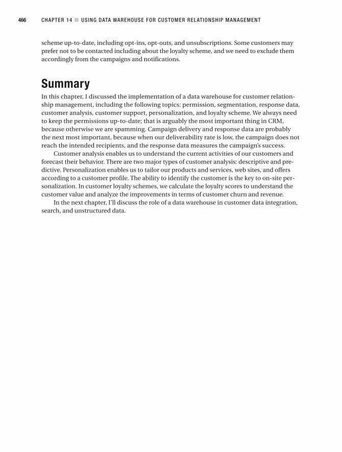
scheme up-to-date, including opt-ins, opt-outs, and unsubscriptions. Some customers mayprefer not to be contacted including about the loyalty scheme, and we need to exclude themaccordingly from the campaigns and notifications.
SummaryIn this chapter, I discussed the implementation of a data warehouse for customer relation-ship management, including the following topics: permission, segmentation, response data,customer analysis, customer support, personalization, and loyalty scheme. We always needto keep the permissions up-to-date; that is arguably the most important thing in CRM,because otherwise we are spamming. Campaign delivery and response data are probablythe next most important, because when our deliverability rate is low, the campaign does notreach the intended recipients, and the response data measures the campaign’s success.
Customer analysis enables us to understand the current activities of our customers andforecast their behavior. There are two major types of customer analysis: descriptive and pre-dictive. Personalization enables us to tailor our products and services, web sites, and offersaccording to a customer profile. The ability to identify the customer is the key to on-site per-sonalization. In customer loyalty schemes, we calculate the loyalty scores to understand thecustomer value and analyze the improvements in terms of customer churn and revenue.
In the next chapter, I’ll discuss the role of a data warehouse in customer data integration,search, and unstructured data.
CHAPTER 14 ■ USING DATA WAREHOUSE FOR CUSTOMER RELATIONSHIP MANAGEMENT466
9314ch14final.qxd 11/15/07 9:45 AM Page 466

Other Data Warehouse Usage
In the previous two chapters, I discussed the implementation of data warehousing for busi-ness intelligence (BI) and customer relationship management (CRM). In this chapter, I willdiscuss data warehousing within the context of customer data integration (CDI) and unstruc-tured data. I will also discuss the role of search in data warehousing.
Unlike BI and CRM, it would be incorrect to say “implementing data warehousing forCDI” because a data warehouse is a consumer of CDI. Data warehouses utilize the output orresults of CDI. In most data warehousing systems these days, the customer dimension in thedata warehouse is where customer data is integrated. But in the past few years, there has beena growing trend to integrate customer data in a normalized store outside the data warehouse,with the main argument being that the consumer of customer data is not just the data ware-house but probably other systems and applications as well.
Since 2005, CDI, unstructured data, and search have increasingly become more and morepopular in data warehousing. Customer data integration (and master data management ingeneral) offers high value to organizations by providing a single, valid, authoritative customerview for downstream applications such as data warehouses. The amount of unstructured datais probably five to ten times more than structured data; therefore, you can potentially gainmore information from unstructured data than structured data. With the help of text analyticsand digital image processing, you can extract useful information from unstructured data.Search as a user interface is useful in finding information in the data warehouse and present-ing it to the end user.
These three elements (CDI, unstructured data, and search) could potentially fulfill thefuture of data warehousing because of the benefits they bring; hence, I’ll discuss them indetail in this chapter.
Customer Data IntegrationIn this section, I will discuss what CDI is, what the benefits are, and how to implement it. Inmany organizations, customer data is scattered across different systems or applications. Forexample, in retail banking, the credit card division may be using a different system than theone used for savings accounts or loan management. The systems for life insurance and mort-gages may also be different. Also, customer service or call centers may be using a differentsystem. Because of this, the customer data is scattered across several systems. CDI is anongoing process of retrieving, cleaning, storing, updating, and distributing customer data.This includes customer names, customer addresses, dates of birth, telephone numbers, e-mail
467
C H A P T E R 1 5
9314ch15final.qxd 11/15/07 9:43 AM Page 467

addresses, occupations, communication preferences, interests, and subscriptions. Let’s gothrough the five processes mentioned earlier:
• Retrieving means extracting the customer data from the source system.
• Cleaning means correcting incorrect data and removing duplicate records.
• Storing means putting the customer data in a central customer data store.
• Updating means modifying the customer data in the customer data store, accordingto the new values from the source system.
• Distributing means publishing the customer data so that other systems can use thiscustomer data.
CDI enables you to have a cleaner, single, reliable version of customer data that theapplications in the enterprise can use. This in turn can deliver business benefits such asthe following:
• Increased customer satisfaction
• Better business analysis
• Reduced complexity of the processes that use customer data
CDI is implemented using a service-oriented architecture, as shown in Figure 15-1. In thisfigure, the customer data is in a central customer data store, with services built around thedata store. No applications touch the customer data store directly. Instead, all applicationsmust use the services to put the data in and to get the data out.
Figure 15-1. Implementation of CDI
CHAPTER 15 ■ OTHER DATA WAREHOUSE USAGE468
9314ch15final.qxd 11/15/07 9:43 AM Page 468

In Figure 15-1, you can see that some source systems put the customer data into the cus-tomer data store by directly calling the services, like in source system A. But some sourcesystems store the customer data only in their own databases, like in source systems B and C.For these source systems, you can build an ETL that retrieves and cleanses the customer datafrom the source system and calls the services to store the data into the customer data store.
The metadata database shown in Figure 15-1 contains the data definition, data structuremetadata, and data integration rules. The data definition contains the meaning of each cus-tomer attribute in the customer data store. The data structure describes the database struc-ture of the customer data store. It contains the data types and lengths of every column inevery table in the customer data store, including the collation, constraints (such as null andunique), and whether the column is a primary key or a foreign key. It also contains the datahierarchy. The data integration rules contain the data mapping and transformations; forexample, customer group code X in source system A is mapped to customer group code Yin the customer data store.
The customer data store is in normalized relational model. This model gives betterperformance over the dimensional model when used to retrieve, create, or update a singlecustomer record or part of a customer record. Figure 15-2 shows an example of a customerdata store schema.
Figure 15-2. An example of customer data store schema
In Figure 15-2, the customer data store is designed so that a customer can have severaltypes of addresses, telephone numbers, and e-mail addresses, such as for the home and office.This is implemented by using junction tables, marked as J in Figure 15-2.
In some cases in the customer data store, you’ll need to store the historical values of cus-tomer attributes. This is required when some applications need to get the previous value, such
CHAPTER 15 ■ OTHER DATA WAREHOUSE USAGE 469
9314ch15final.qxd 11/15/07 9:43 AM Page 469

as to explain an old transaction. You can do this by using a series of audit tables. Before chang-ing the customer attributes, you store the original record with the old attribute values in anaudit table, along with a timestamp when the change happened.
Unstructured DataGenerally, you can classify data into two big groups. The first group is essentially numbers,characters, and dates, such as 32, “John Smith,” and 05/21/2008. You usually store this kindof data in a database. It can be a relational database, dimensional database or hierarchicaldatabase, or even a multidimensional database. This data is usually stored in tables, as rowsand columns, where you can sort and query. This kind of data is called structured data.
The second group of data is not as discreet as the structured data. Instead, it is differentkinds of multimedia, such as images, videos, web pages, presentations, telephone conversa-tions, e-mails, documents, and music. This kind of data is called unstructured data. This datais usually stored in file servers, database servers, FTP servers, e-mail servers, content manage-ment systems (CMSs), and document management systems (DMSs).
The amount of unstructured data is a lot more than the structured data, but most of it isuntouched by data warehousing. To give an illustration, say the sizes of all databases in threemultinational groups of companies (9,000; 12,000; and 20,000 employees) are about 50TB,30TB, and 5TB, respectively. The sizes of all documents, text files, presentation, working files,web pages, web site objects, video, audio, and e-mails in the file server, web server, FTP server,e-mail server, and database server are estimated to be about 200TB, 300TB, and 100TB,respectively, roughly from 4 to 20 times the size of the databases. These three groups are indifferent lines of business: e-commerce, manufacturing, and utilities. The e-commerce grouphas a 20TB group-wide data warehouse and a 5TB local data warehouse, which is the reasonfor the large database size. The manufacturing group produces a lot of artwork and multime-dia designs (5MB to 50MB each set), which is the reason for the large amount of unstructureddata, but almost each company in the group has its own systems (grown by acquisition). Theutility group has centralized several mini/mainframe-based systems across the group and a1TB data warehouse, which is the reason for the compact database size.
In the last 15 years of data warehousing and probably almost in the whole history of data-bases, we have been focusing on structured data. But since the amount of unstructured data ismuch larger than the structured data, it is understandable that people are now looking at theunstructured data.
So, how do you store unstructured data in the data warehouse? Traditionally, you store itas files in the file system and store the attributes and the links in the data warehouse. It is eas-ier to understand this using an example. Let’s say you have 1 million documents in variousformats. Some are Microsoft Word documents, some are Microsoft PowerPoint presentations,some are PDFs, some are e-mail messages, some are text documents, and some are scannedinvoices, signed contracts, and purchased orders. Each document has various attributes, suchas the name or title of the document, the subject, an abstract or summary of the document,the type of the document, the version, the document number or ID, the classification, the datethe document was created, the date the document was last edited/modified, the date the doc-ument was last printed, the size of the file, the number of characters, the words in the documents,the sentences and pages in the documents, the name of the author and author’s company, thesecurity settings (read-only, whether copying or printing is allowed, the password to edit the
CHAPTER 15 ■ OTHER DATA WAREHOUSE USAGE470
9314ch15final.qxd 11/15/07 9:43 AM Page 470

document, and so on), the fonts used in the document, the name and path to the related doc-uments…and the list goes on.
You can store all these attributes in the data warehouse, that is, in relational tables. Youthen store the path to the files (or the URL of the web page) in a column in the same table sothe application can get to the file to access it. You can also store these attributes and the linksto the files/objects in dimensional format for analysis purposes. Or you can store the docu-ments as binary objects or character large objects inside the database. The same method isapplicable for storing different types of unstructured data such as video, audio, e-mails, andimages. All kinds of unstructured data have their specific attributes by which they could becategorically and systematically stored. CMSs and DMSs can also often be used to store andmanage unstructured data.
The previous methods have been on the market for many years and are considered“traditional” methods. There is a newer method for storing unstructured data in a datawarehouse—well, it’s not really a method to store documents in a data warehouse but moreof a method to extract structured data from unstructured data and then store the extractedstructured data in the data warehouse.
For documents, this method is known as text analytics. Text analytics is the process oftransforming unstructured documents into structured, analyzable data by analyzing the lin-guistic structure of the text within the documents, parsing the text, extracting phrases, andidentifying associations using techniques such as statistical analysis and categorization(combining phrases using predefined rules).
Let’s go through the details of how text analytics works for documents. The first step is toconvert the documents to text. Whether they are in Microsoft Word format, StarOffice format,scanned invoices, or PDF, the first step is to convert them all to text files. You may need to useoptical character recognition (OCR) to convert them, such as in the case of scanned invoicesor purchase orders. Once they are in text format, you can feed them all to text analytics soft-ware, which will parse the text files and extract the words and phrases from them.
The result is a list of words and phrases with their association scores reflecting the rela-tions to other words or phrases. An association score is a decimal number ranging from 0 to 1calculated for each phrase in relevance to another phrase. The higher the scores, the closer therelations. The association scores are important because they reflect how close two phrases are.You can use association scores to then group related entities and find relationships betweenentities. There are various factors affecting the scores, such as the relative “distance” to theother words, the words located in the same files, the synonyms or meaning of those words,and the number of occurrences. Within the text analytics application, various less meaningfulprepositions such as (this is language specific) an, on, and the are weighted much less thanmore meaningful words such as downtime, revenue, and Boston. The same thing happens forpast tenses, such as sat and opened; they are converted to the present tense. Similarly, for syn-onyms such as big and large, gigantic, and huge, they are also converted.
The text analytics application may also process the files in the context of a certain indus-try; for example, they could all be trading invoices, or they could be pharmaceutical patents,contracts, or candidate résumés/CVs. To understand the context, let’s take the résumé exam-ple. The parser would recognize that words such as SQL Server 2005, CRM, and Data Ware-housing are the candidate’s skills, whereas Oracle DBA, Data Architect, and Web Developer arethe candidate’s past roles or titles. Informatica, Teradata, and WebSphere are the software thatthe candidate has used in the past. Dallas, Los Angeles, and New York are cities where the can-didate lived or worked. Citibank, The Home Depot, and T-Mobile are company names where
CHAPTER 15 ■ OTHER DATA WAREHOUSE USAGE 471
9314ch15final.qxd 11/15/07 9:43 AM Page 471

the candidate worked. The software can then use this understanding of the parsed text. Thewords are then processed using a data mining clustering algorithm to get the relationships.My point here is that a text analytics application that is developed specifically for the recruit-ment industry understands the context of the industry and is able to identify that certainphrases are skills, titles, software, cities, and company names, whereas a pharmaceutical textanalytics application would be able to recognize the symptoms, research, diagnoses, chemicalcontent, cure, and treatment phrases within hundreds of medicine patent files. The applica-tion understands the relationship between phrases, such as how skills are related to softwareand how symptoms are related to treatments. Because of this, when selecting a text analyticsapplication, you need to ensure that it has the right “dictionary” for your industry. A text ana-lytics application, which works well for pharmaceuticals, may not be good for processingclaim documents within the insurance industry.
The scored lists describe which words have strong relations to other words. A pictorialrepresentative of the result is probably easier to understand. Figure 15-3 shows the result ofthe résumé example.
Figure 15-3. Pictorial representation of the result of text analytics
The line thickness reflects the strength of association between the phrases. For example,in Figure 15-3, city A is more related to role B than to software A, and software B is more closelyassociated to skill B than to city D. City C is related only to software A, and company A has norelation with any skill, software, or company. The other output of the analytics is grouping orclassification according to the taxonomy of the phrases, that is, the list of cities, list of jobs, listof roles, list of software, and so on. It is often industry specific. In other words, text analytics ormining software that works well for car insurance claims may not have the vocabulary requiredto analyze food and beverage patents.
Once you have the lists and the association scores, you can store them in the data ware-house for further analysis. For example, you can ask questions such as, “What are the top five
CHAPTER 15 ■ OTHER DATA WAREHOUSE USAGE472
9314ch15final.qxd 11/15/07 9:43 AM Page 472

cities for software X?”, and “Which software do you need to master if you want to be a goodcandidate for role C?”, and “Which companies have the most of role A?”
The method you can apply for documents is also applicable for other types of unstruc-tured data, such as images or audio. Of course, in this case, it is not text analytics but perhapsdigital image processing or audio analysis, depending on the media type. For example, speechaudio files could be parsed and categorized into questions, statements, and short commentsbased on the intonations, rhythms, and voice intensity (pattern recognition). Just like OCR,technology can convert scanned documents into text files, and speech audio files can also beconverted into text files using voice recognition software. And from there, the same text ana-lytics follow. A stream of outgoing e-mails can also be scanned, classified, and stored usingtext analytics. Common implementations of e-mail analysis are a junk mail filter and a cus-tomer service center’s incoming e-mails (automatic categorization and routing).
One example of a scanned document application is invoices, which could be linked to aworkflow system. Say there are 29 major suppliers in a company. Each supplier has a differentinvoice format. You could set up the software so it knows that for invoices from supplier A, thepurchase order number is located in the upper-right corner of the document (in certain coor-dinates) in AAA99A format, the invoice amount is in the lower right, and the number is pre-fixed by a $, €, or £ symbol. The document archiving system then processes the documentsfrom various suppliers; extracts the structured data such as the invoice number, purchaseorder number, supplier name, and order amount; and stores them all in a database, whichcould then be fed into the ERP system for invoice matching and payment processes and alsobe fed into a data warehouse for analysis purposes.
The metadata aspect of unstructured data conversion is also significant. All the attributesI mentioned can be stored, in addition to the output of the text analytics or mining. Theseattributes (subject/title, dates, author, and so on) are stored as metadata in the data warehouse.The metadata would then be retrieved by the client applications using a search facility (see thenext section). Because of this, it is important to keep the metadata correct and up-to-date. Youcan do this by consistently updating the metadata every time you add or change the unstruc-tured data. The metadata update should be an automated process that is executed every timeyou load or change the unstructured data.
Text analytics and unstructured data are particularly useful in the legal industry, thepharmaceutical industry, police departments, TV stations, political parties, national parlia-ments, and any other industries that deal with a lot of documents or images. They enable youto search a lot of information in a shorter period of time. The text analytics extract the termsand phrases from the unstructured data and categorizes them so the search engine doesn’thave to read the unstructured data again. The search could be a lot quicker, probably lessthan 10 percent of the time required to browse the original unstructured data.
Another application is the e-mail store, which stores outgoing and incoming e-mails asunstructured data. The e-mails are then processed, and the resulting metadata, content lists,and association scores can be stored in a data warehouse. The users would be able to searchthe content and metadata later. The e-mail store application is particularly relevant for regu-latory compliance (such as the Sarbanes-Oxley Act) and for CRM (such as customer queriesand correspondence). Sarbanes-Oxley section 802 requires firms that audit or review anissuer’s financial statements to retain relevant records including correspondence and com-munications sent or received in connection with the audit or review. Sometimes a courtorder requires the preservation of all e-mails containing information potentially relevant to
CHAPTER 15 ■ OTHER DATA WAREHOUSE USAGE 473
9314ch15final.qxd 11/15/07 9:43 AM Page 473

a subject of litigation. If your e-mail system is set to delete e-mails more than n months old,you can use the e-mail store application to retain the relevant e-mails.
Search in Data WarehousingWhen your data warehouse has grown to several terabytes and you have hundreds of storedreports, cubes, and many BI data models, it can help if you have a search facility that canassist the users in locating the right reports, cubes, and data models. A search facility is a toolthat indexes data warehouse reports, analytics, or data models (both the metadata and thecontent) to enable the users to find information by typing the search criteria in a search textbox. A search facility is capable of prioritizing the search results by relevance. Some vendors,such as SAS, search the business views and data structure in the metadata server in order tolink the relevant information in the search results. Other vendors, such as Information Builder,search the structured data within corporate databases. Some vendors, such as Clarabridge,also search unstructured data along with the structured reports.
A typical search application consists of an indexer, retriever, and scoring routines. Theindexer browses the folders for all of the file types (unstructured data files, and so on), thenopens and crawls each file, and then stores the locations of those words in the repository.The indexer also collects the information about the reports, cubes, and data models andstores this information in the repository. It also stores previous searches and queries. Theretriever accepts a value from the search text box, searches its repository and metadata, anddisplays the results to the end users. Before it is displayed to the end user, the scoring rou-tine sorts the results according to a preset logic/algorithm. The scoring routine may alsopartition the result into more than one section to be displayed separately on the screen.
Within the search text box, you can type sales and it would list, say, nine sales reports,two BI models, and three Analysis Services cubes that are related to sales. Similarly, you canalso search for things such as customers and subscriptions. The search would go throughthe report metadata (such as titles, columns, and so on), multidimensional metadata, datawarehouse metadata, and BI data model metadata to find the relevant reports, cubes, andmodels. It could also search the content of the stored reports and previous searches. Forexample, there might be 12 variations of a product sales report for 2007 that are physicallystored as snapshots in the report server database, all with different stores, customers, andproduct attributes. The search facility can find the relevant reports and highlight them forthe BI users. Previous searches are what the users typed into the search box, which mayspeed things up a little bit.
Rather than trying to build our own data warehouse search facility in this book, I think itis better if I show how to implement one of the off-the-shelf search products from BI vendors.At the beginning of 2006, it was difficult to find search products in the market. But currently(the second half of 2007), almost every single BI vendor is working with Google to deliver asearch product (some of them have already delivered, such as Cognos, SAS, InformationBuilder, and Clarabridge). BI or data warehouse search is quite a specialized area. A rankingalgorithm to prioritize search results by their relevance, for example, is not straightforward todevelop. And even if you manage to develop it, would it be better than the Google search algo-rithm? Indexing a pile of unstructured data, crawling structured databases, searching OLAPcubes, and correctly interpreting metadata are all challenging tasks within DW/BI search.
CHAPTER 15 ■ OTHER DATA WAREHOUSE USAGE474
9314ch15final.qxd 11/15/07 9:43 AM Page 474

Searching the report’s content, column titles, data values, and practically any text appearingon the report is better left to a search specialist company working with the BI vendors.
Three areas in data warehousing would benefit from a search facility. The first one issimplifying the user interface. In this application, search is used for querying structureddata in the dimensional data store. I’m not talking only about long varchar data types butalso about numeric, date, and short character data types. You can supplement the queryinterface with a search interface. A typical implementation is a simple text box where thedata warehouse user can type anything. The application then searches the data warehousefor the relevant content. The following query is a typical data warehouse query to under-stand the sales amount per store:
select s.store, sum(f.sale_amount)from fact_purchase fjoin dim_date d on f.date_key = d.dim_keyjoin dim_store s on s.store_key = d.store_keywhere d.month = 10and d.year = 2007and s.region = 'Midwest'group by s.store
Rather than typing that query, the users can just type October 2007 sales in Midwestregion. Or they can just type Sales; the search application will display the sales reportsfrom all regions, and the user can then pick the Midwest region for October 2007. Yes, itis true that a BI application has made data warehouse querying and browsing very userfriendly by providing an excellent user interface for data warehouse users. But search takesthe user friendliness further. What can be easier than just typing whatever you want into atext box? You need to understand that the search facility does not replace the query func-tion and BI tool function; instead, it just supplements them to make them more completeand easier to use.
The key here is that the search application needs to be aware that certain words aremetadata while other words are data. For example, subscription sales and subscription bandare facts/measures and dimensional attributes, so the search application can find them inthe metadata. On the other hand, Los Angeles and Classical Music are data values, so thesearch application cannot find them in the metadata store; instead, they can be found in thedata itself. The search results can be partitioned between the results found in the metadataarea and the results that are found in the actual data. You need to bear in mind that in orderfor the search application to have this capability, the metadata behind the application mustbe excellent.
The second area to benefit from the search is the reports search, which I talked about ear-lier. The third area that benefits from the search is unstructured data such as documents, webpages, text files, images, videos, and audio files. In the previous section, I discussed howunstructured data can be processed by text analytics applications (or digital image processingfor images) and provided a correlation diagram between related words or phrases. The sourcefiles can also be browsed and indexed by a search application, so it would be a lot easier tofind information.
CHAPTER 15 ■ OTHER DATA WAREHOUSE USAGE 475
9314ch15final.qxd 11/15/07 9:43 AM Page 475

SummaryIn this chapter and the previous two chapters, I discussed the implementation of a data ware-house for business intelligence and customer relationship management within the context ofcustomer data integration, unstructured data, and search. There are other implementations ofdata warehouse for other industries such as for research/science/labs, geology, topology, earthsciences, astronomy, and particle physics.
Now that you have implemented a data warehouse for good uses, in the next two chaptersof this book I will discuss the testing and administration aspects.
CHAPTER 15 ■ OTHER DATA WAREHOUSE USAGE476
9314ch15final.qxd 11/15/07 9:43 AM Page 476

Testing Your Data Warehouse
As with any other IT system, after you build the data warehouse with its ETL and applications,you need to test it thoroughly. You need to go through six types of testing. I’ll introduce themhere with a brief description, and in the rest of the chapter I will discuss them one by one:
ETL testing: In the ETL testing stage, you make sure that appropriate changes in thesource system are captured properly and propagated correctly into the data warehouse.You also need to verify that the bulk load solution works as it was intended so it can dothe initial data loading.
Functional testing: In the functional testing stage, you make sure all the business require-ments are fulfilled.
Performance testing: In the performance testing stage, you verify that the data warehousecan handle the required load and volume.
Security testing: In the security testing stage, you make sure only the users who should beable to access the resources can actually access them.
User acceptance testing: In the user acceptance testing stage, the end users use the datawarehouse system to verify the usability.
End-to-end testing: In the end-to-end testing stage, you let the system run for a few daysto simulate production situations.
In this chapter, I will focus on the mechanism and procedure of how each type of test isconducted specifically within the data warehousing context. I will not discuss the general soft-ware testing methodology. The software testing methodology is the systematic arrangementand management of testing tasks to produce high-quality software. These testing tasks includecreating a test plan, creating test cases, producing test data, performing unit testing, doingsystem tests and integration tests, doing system fixes, writing test results, conducting useracceptance tests, and writing test reports. The methodology explains how each task relates toeach other in the project plan. The methodology specifies how to log errors, how to pass errorsto the development team, how to get the fix back into the main release, how to judge howmany passes of the test will be performed, how to log the test results, how to report the num-ber of errors found and fixed to management, and so on and so forth. These are the items inthe software testing methodology.
Instead, I will focus on the content of those tests specific to data warehousing. For exam-ple, when doing functionality testing, what part of the data warehouse do you need to verify?How does it differ from the functionality testing for an ERP system? How do you test the ETL?
477
C H A P T E R 1 6
9314ch16final.qxd 11/15/07 9:41 AM Page 477

How do you conduct a user acceptance test for a data warehouse? Do you test data quality?Those kinds of questions are the ones I will discuss in this chapter. So, let’s discuss the six testareas one by one. In each area, I will discuss what the test is about, the purpose of doing thetest, and how to perform the test.
Data Warehouse ETL TestingETL testing is important because ETL brings the data from the source systems into the datawarehouse. If the ETL is incorrect, the data in the data warehouse will be incorrect. If the datain the warehouse is wrong, no matter how good the data model is and no matter how goodthe application is, you can’t use the data warehouse. On the other hand, if the data is rightbut the data model is not perfect (it’s missing some attributes here and there, for example) orthe application is not right (it’s not user-friendly enough, for example), then you can still usethe data warehouse system. At least you can still query the data store directly by using a SQLquery tool instead of the applications.
Essentially, a data warehouse system has three primary components: ETL, data stores,and applications. Of these three, ETL development takes the largest portion of data warehousedevelopment effort. A general view in the data warehouse community is that ETL takes 60–80percent of development effort, but in my experience ETL takes about 50 percent of the devel-opment effort, while data stores take 25 percent and front-end applications take 25 percent.The percentages vary depending on how complex your application is. The hardware and soft-ware platform is probably 10 to 25 percent of the combined three. Figure 16-1 shows this pro-portion. Because ETL is the largest portion, it requires a larger effort in testing than those ofdata stores, applications, and platform.
Figure 16-1. Three major components of a data warehouse
Figure 16-1 also shows that the ETL is the process that brings the data into the data stores,while applications deliver the data to the users. Users can also query the data warehousedirectly without using applications.
The main objectives of ETL testing are the following:
• To make sure you get all the data you need, in other words, that you don’t miss somedata updates in the source systems.
• To make sure the data is correctly loaded into the data warehouse, that is, loaded inthe right tables, on the right columns, in the right formats, at the right time.
CHAPTER 16 ■ TESTING YOUR DATA WAREHOUSE 478
9314ch16final.qxd 11/15/07 9:41 AM Page 478

• To make sure the incremental ETL is working according to the design, regardlessof whether it is a batch architecture, a push architecture, or a service-orientedarchitecture.
• To make sure the bulk load script (if you have one) correctly loads the data into thedata warehouse.
Now let’s discuss the how. You start from the ETL architecture diagram and the ETLprocesses. You need to test that both the overall ETL process and the individual ETL tasksdeliver the data correctly to the data stores. Say you have a daily batch consisting of 30 tasks,a weekly batch consisting of 3 tasks, and an hourly batch of 2 tasks. To test the ETL processes,you run the daily ETL workflow, making sure the tasks within the daily batch are executed inthe correct order. Then you do the same thing with the hourly and weekly batches. You thencheck the data in the target, comparing it to the source system.
If you have any “push approach” or SOA-based ETL, you switch them on and make sometransactions in the source systems, making sure the changes are captured and propagatedproperly into the data warehouse. You need to test whether there is any “data leakage” duringthe ETL run. Please refer to Chapter 7 for an explanation of what data leakage is.
One important feature to test is recoverability. Recoverability means that the ETLprocesses should be robust enough that in the event of failure the system can recover withoutdata loss or damage. The ETL process needs to be built so that if the process is stopped at anypoint and rerun, there is no data loss. You test recoverability by listing the event types you wantto be covered against, such as loss of electricity and disk failure. You then list the process typeswithin the ETL system where the failures possibly occur, such as extraction process, DDS pop-ulation process, and cube-building process. You then simulate the combination between eachevent type and each process type, followed by a rerun of the ETL processes. You then checkthat the process can continue as normal and there is no data loss.
For an SOA architecture doing trickle feed, you need to simulate message queue (MQ)failure or network failure where the messages sent by the source system don’t reach the targetsystem and need to be resent. You can simulate MQ failure by disabling the queue and the net-work failure by changing the IP address. If you build a notification or alert feature in the ETL,you need to test that the correct people are notified when certain events happen.
In some projects, you can use the incremental ETL architecture to do the initial bulk load-ing of the data warehouse. In other projects, you need to use a separate ETL architecture forbulk loading, because the incremental ETL is not designed to handle a big load, such as load-ing 200 million rows of historical transactions, for example. This is particularly true when youuse real-time message-based ETL (SOA) for the incremental ETL that was designed to pick up,say, 10 to 100 rows every time. To determine whether the incremental ETL is capable of doingbulk initial data load, you need to test it. If the projected execution time is beyond what youcan tolerate, you need to develop a separate ETL architecture for bulk loading. In either case,you need to verify that the bulk load script works, that is, that it loads the initial data com-pletely and correctly into the target tables. It is essential to test that you don’t miss any dataaround the cutoff date, because there is a potential gap between the bulk load cutoff date andthe start date of the incremental load.
CHAPTER 16 ■ TESTING YOUR DATA WAREHOUSE 479
9314ch16final.qxd 11/15/07 9:41 AM Page 479

Functional TestingFunctional testing is about making sure that all business requirements are satisfied. Businessrequirements are data and capabilities that the users need from the data warehouse in orderto perform their business tasks, such as the ability to analyze a particular customer activity bycertain criteria, the ability to view certain data for a specific period, and the ability to drilldown the data into a certain level to identify business problems.
Business requirements are identified at the beginning of a data warehousing project,which will then drive the design and development. Simply speaking, functional testing isjust verifying that the data warehouse that you built satisfies all those requirements. In thecase of the Amadeus Entertainment Group case study, you identified the business require-ments in Chapter 4. The following are two of those requirements:
• The data warehouse should enable Amadeus Entertainment to analyze subscriptionsales (that’s when a customer is subscribing to a package rather than to a product) overtime by geographical area, by customer demographic, by stores and sales territory, andby product hierarchy. In addition, they also need to analyze by subscription durationand lead source (where the customers are coming from). They need to know the rev-enues, the costs, and the margins, which are evaluated every day for a period of onemonth in U.S. currency.
• At the store level, the ability to view the daily data in the last few weeks is important.The stores need to see the ups and downs of sales, costs, and profitability, and thestores need to be able to drill down to any particular day to understand the causesof low sales or low profitability problems, such as specific products, titles, media, orcustomers.
In functional testing, you test all these business requirements that you defined in thebeginning of the project, as discussed in Chapter 4. For example, you analyze the cost of sub-scription sales for each month by stores and sales territory. You check that the data warehousefigures are correct. You do this by comparing it to the source systems. The figures on the datawarehouse must match the figures from the source systems. Of course, it is not possible tocheck every single number. One testing technique is to verify the total, then drill down onelevel (verify all members), and finally drill down to the bottom level by picking n members.For example, in the case of the first requirement mentioned earlier, you need to get the totalrevenue, cost, and margin for a particular day and verify that these three figures are correct.Then you drill down one level. For geographical area, the highest level is country, so you checkthe total revenue, cost, and margin for each country for that particular day. Then you do thecustomer demographic, such as occupation or age group, that is, the total revenue, cost, andmargin for each occupation or age group. Then you do other areas such as sales territory,product hierarchy, and subscription duration. Finally, after you finish testing the top level, youtest the bottom level by selecting a few members. For example, for the product hierarchy, thebottom (base) level is the product code. You can pick a few product codes and check their rev-enue, cost, and margin for that particular day.
The product codes are not selected randomly but are based on the boundary values, suchas the minimum and maximum values, for example product codes that are never purchasedby the customers (minimum values) or product codes that are very active/popular (maximumvalues). You can also determine the boundary values based on product age, such as the newestproduct code and the oldest product code.
CHAPTER 16 ■ TESTING YOUR DATA WAREHOUSE 480
9314ch16final.qxd 11/15/07 9:41 AM Page 480

After checking the totals, you also need to verify the count of the dimension members atall levels. For example, if you have 12 product categories, 438 product types, and 25,034 prod-ucts in the source systems, then the data warehouse needs to have the same numbers. In thecase of the first requirement (subscription sales), the fact table type is a snapshot. If the facttable is incremental, like the Product Sales fact table in the Amadeus Entertainment casestudy, it is important to verify the total of the individual additive measures in the fact tablewithin different time periods, such as a week, month, quarter, or year. For example, in theProduct Sales fact table, you need to verify the total revenue, cost, and margin within variouslevels of time periods.
It is imperative that the tester understands how to verify the data warehouse figures.They do this by comparing the data warehouse figures to the source systems, either byquerying the source system database or by running some reports on the source systemapplications. The testers need to know how to use the source systems to get the data ware-house figure that is being tested. In the earlier example, say that according to the datawarehouse the total revenue for France on October 21, 2007, is $21,351.64. The tester needsto know how to use the source system to get the revenue for France for that day, includingwhether returns and cancellations are included, whether intercompany sales are excluded,and whether voucher codes are counted as face value or cost value. He needs to know whatcurrency rate to use to convert from euros to U.S. dollars. To perform this test, you needsomebody whose job involves calculating all this. It is likely that for different business areasyou will need a different tester.
Functionality testing is not just about calculating the totals and comparing countsbetween the source system and the data warehouse. You also need to test things such as aslowly changing dimension, whether it is type 1, 2, or 3. You need to test the surrogate keys,including whether they link the fact tables and the dimensions properly. You need to test thereferential integrity in the ODS. You need to test the date dimension, making sure that all theattributes are correct for all dates, such as for the fiscal week, fiscal year, week day indicator,last day of the month indicator, and week number. You need to check the dimension hierar-chies, such as whether product code X belongs to product type Y. You need to test all customerattributes, such as whether all the demographic attributes of customer X are correctly inte-grated from two different source systems, according to the survivorship criteria. You need toverify all degenerate dimensions in all fact tables, such as order line number and purchaseorder ID. You need to test all control columns such as the loaded timestamp, source systemcode, and active flag. You need to test that all data quality filters work properly. And last butnot least, you need to check the metadata, all seven types: data definition and mapping meta-data, data structure metadata, source system metadata, ETL processes metadata, data qualitymetadata, audit metadata, and usage metadata. (I explained these types of metadata inChapter 10.) During the testing, you need to verify that they are populated correctly.
Numerous business scenarios and business conditions need to be tested in functionalitytesting. First you identify a business event that you want to test (examples will follow). Thenyou prepare a test data in the test environment of the source system to simulate this event.You then run the ETL processes to bring the simulated data into the data warehouse and verifythe data has been loaded into each data store correctly. This verification is done by comparingthe data in the data warehouse to the source systems. Examples of the business events arewhen a branch closes and all its customers are reallocated to another branch, when you havea price increase, when you have a month-end or year-end process, and when a new fiscal cal-endar begins. There are also business events that are more day-to-day routine, such as interest
CHAPTER 16 ■ TESTING YOUR DATA WAREHOUSE 481
9314ch16final.qxd 11/15/07 9:41 AM Page 481

rate changes, currency rate updates, supplier changes, stock audits, a new newsletter, returnsand refunds, new calling plans, and customer re-sign-ups. These are real business events thatwould affect the data warehouse. Of course, different industries have different events; forexample, a new calling plan is specific to the telecommunications industry, a customer re-sign-up is specific to finance and utilities, and a stock audit is specific to the retail or supplychain industry. You need to verify that the data in the data warehouse is still correct on allthese occasions.
Test data is important in performing functionality testing. It takes a lot of effort to cre-ate the test data for a particular test condition. Unlike other application testing, in datawarehouse functional testing you need to create the test data in the source systems, not inthe data warehouse. You need to work with the source system DBA to create the test data.Sometimes it is rather difficult to simulate certain conditions in the source systems, and itis easier to use real events from production, such as a price increase. If the price increasepercentages are different for each customer and they have been accumulated over a fewyears, it is difficult to create test data to simulate the increase. It may be easier to use the lastannual price increase data from production and copy the data to the QA environment soyou can search it to find the data you need for testing. Sometimes it is the reverse; that is, itis quite difficult to find a specific event in the production source system, and it is easier tocreate the event yourself, such as for a new product. You may find it difficult to find a certainproduct or customer with certain criteria that you need. In this case, it is easier to create theproduct or customer in the test environment.
Performance TestingPerformance testing verifies that all technical requirements related to the platform, capacity,latency, and response times are satisfied. In particular, you need to prove that the data ware-house system is capable of completing the data loading process in a particular amount oftime. Performance testing is important because when developing the ETL processes, you use asmall amount of data. You often focus on making sure the functionality of the ETL processes iscorrect. Now that it is developed, you need to run it in operational conditions in terms of workload, timing, amount of data loaded, and amount of data already existing in the target tables,hardware, indexes, partitions, number of users, type and amount of queries, cube-processingtimes, number of variables in data mining and predictive analysis, and so on. The data stores,the ETL, and the applications need to be tested in operational production conditions toensure that they satisfy the performance requirements. For example, when developing theworkflow to populate a fact table, you load hundreds of rows into a fact table that is nearlyempty, and you run each workflow in isolation. In contrast, you know that when it is opera-tional, the fact table would have hundreds of millions of rows and each load could be roughlymillions rows, so many different workflows will run simultaneously. It is hardly surprising thata few months after the data warehouse is operational, this ETL workflow would run slowly inproduction, even though it ran smoothly on the development server. This is because the oper-ational production conditions are different from the development conditions. The purpose ofperformance testing is to eliminate these types of risk.
There are two main areas to test the performance in a data warehouse. The first area isabout the ETL, and the second one concerns the applications. In the ETL area, you need toverify that both the bulk load performance and the incremental load performance satisfythe required performance criteria. The bulk load is used to populate the data warehouse for
CHAPTER 16 ■ TESTING YOUR DATA WAREHOUSE 482
9314ch16final.qxd 11/15/07 9:41 AM Page 482
the first time. The incremental load is used to populate the warehouse when it is operational.On the application side, the performance criteria are generally about the response times.
The purpose of doing performance testing is to satisfy the performance requirements.Some requirements are applicable to the whole data warehouse system (let’s call these gen-eral performance requirements), while other requirements are applicable only to specificelements of the system (let’s call these specific performance requirements). General per-formance requirements require the whole system to perform based on certain conditions,such as the availability of the data warehouse. Specific performance requirements requireonly those elements (such as certain ETL processes or certain tables in the data stores) toperform at certain levels. For example, the ETL process that extracts data from a particularsource system needs to be completed within a certain time window. You need to ensure thatboth the ETL and the applications satisfy both the general and specific performancerequirements.
So, what are the tasks you need to do to perform data warehouse performance testing?There are essentially three steps to carry out performance testing on the ETL processes: con-figure the test environment, run the bulk load processes, and run the incremental processes.Let’s go through these three steps one by one:
1. First you need to configure the data warehouse test servers as per the production con-figuration. You create the data stores and set up the ETL processes; that is, you migratethe SSIS packages from development to test server. Then you need to connect the testserver to the test version of the source system (sometimes known as QA) and set up allnecessary connectivity and access. You load the test data into the QA environment. Yourun the whole ETL processes end to end using a small load to verify that the test envi-ronment has been configured properly.
2. You run the initial load ETL processes (be it T-SQL scripts or SSIS packages) to pop-ulate the warehouse and measure their performance, that is, when each task in theinitial/bulk load ETL processes started and when each one completed. One way tomeasure the performance is by utilizing the ETL log and the timestamp column of theloaded table. Let me explain what I mean by the ETL log and the timestamp column.The ETL log is a table or file where the ETL system writes to. It is sometimes known asthe audit table or file. In each ETL task or process, after each major step the ETL rou-tine writes a row (if it is a table) or a line (if it is a file) in this ETL log, containing theessential statistics of the task, such as the data volume (number of records affected bythe operation), the task name, and the current time. The timestamp column containsthe time the row was loaded or modified.
Both the ETL log and the timestamp columns are useful to measure the performanceof the incremental ETL and bulk load because you can determine the duration of eachETL task. They are also useful for troubleshooting the root cause or finding the bottle-neck of the performance problem as well as for doing fine-tuning in the data ware-house performance. You can do this by finding out the long-running/long-performingtasks, and then you try to make these tasks more efficient. Both take a little bit of timeto implement (probably 30 minutes to an hour for each task) because you need to pro-gram each ETL task to write into the log, but they are extremely useful because theyhelp identify slow-running tasks (I have seen a 50 percent increase in performance),so they are worth the effort.
CHAPTER 16 ■ TESTING YOUR DATA WAREHOUSE 483
9314ch16final.qxd 11/15/07 9:41 AM Page 483
Another way to measure the performance is using SQL Server Profiler. You set up SQLServer Profiler to log the time each SQL statement is executed. You can also utilize SSISlogging. SSIS logs runtime events as they are executed in SSIS. For this you need toenable logging on each task in all SSIS packages in the bulk load processes.
3. Then you run the ETL batches—whether it is daily, hourly, or weekly—in a particularsequence according to the prepared test scenario and measure their performance(speed). In incremental ETL, you can also use the same methods/instruments as thebulk load to measure the performance: ETL log, timestamp, SQL Server Profiler, andSSIS logging. For real-time ETL, you need to measure the time lag as well; that is, howmany minutes after the transaction was made in the source system did the data arrivein the data warehouse?
The previous steps are about performance testing for ETL. For applications, to measureperformance you can script the actions, or you can measure them manually. Scripting theactions means you use software to record the actions that a user does when using the appli-cations. You then play the recording back to simulate many people using the system simul-taneously while recording the system performance. Measuring them manually means youuse the system interactively.
In application performance testing, you use the applications, whether they’re reports,mining models cubes, or BI applications, using both normal scenarios and exception scenar-ios. Normal scenarios are steps that the users perform in regular daily activities. Exceptionscenarios are steps the users perform that result in errors.
As discussed in Chapter 6 when I talked about physical database design, you can do sev-eral things to improve application performance, such as indexing, partitioning tables, andcreating summary tables. The one with the biggest results is creating summary tables (alsoknown as aggregates), whether they are in the relational database (DDS) or in the cubes. Thisis because results have been calculated in advance, so all the application needs to do is to dis-play them on the screen. But too many summary tables (or cube aggregates) could decreasethe performance of the ETL, because populating them takes time. So, you need to be carefuland strike a delicate balance between them. As I discussed in Chapter 6, summary tablesneeds to be at least 10 times smaller in terms of the number of rows, ideally 100 times smalleror more. Otherwise, there is no point in creating a summary table. Remember that a summarytable needs to be updated every time the underlying fact table is updated. The ideal time torefresh the summary tables is immediately after the population of the underlying fact table. Tobe sure about the benefit, you need to measure both the time required to update the summarytable and the improvement in application queries.
As discussed in Chapters 5–8, you need to think about the performance when you designthe data warehouse, not tweak it when you finish building the data warehouse. You shouldstart taking the performance into account when you design the architecture and again whenyou physically build the architecture (that is, server, network, SAN, and so on). Then youincorporate performance requirements when you design the data stores, both when you dothe logical design (data modeling) as well as physical design (database creation). After thatyou design the ETL, also with performance considerations in mind. Then when you design thereports, cubes, mining models, and other types of applications, you need to design by keepingan eye on the performance factor. The whole thing should be designed for performance atevery single step from the start of the project, not after the data warehouse system is built.
CHAPTER 16 ■ TESTING YOUR DATA WAREHOUSE 484
9314ch16final.qxd 11/15/07 9:41 AM Page 484

Security TestingSecurity testing is about making sure that only the people and applications that are allowedto access the data warehouse can actually access it. In addition, you also need to test howpeople are accessing the data in the data warehouse, such as the tools used to access thedata warehouse and the way the user supplies the security credentials.
As discussed in Chapter 4, these are the security requirements for the Amadeus Entertain-ment case study:
• All data warehouse users must be able to access the data warehouse front-end appli-cations (report and OLAP) without logging in again. They just need to log in once toWindows on their PC or laptop.
• The data warehouse front-end applications must not be accessible from outside thecompany network.
• All front-end applications need to be web based, accessible from anywhere in thecompany network.
• All users should access the front-end applications from a central portal.
• Some users are allowed to access data from their own country only, but some usersare allowed to access data from any country.
• Some “power users” are given access to the dimensional store to perform direct SQLqueries.
• Certain sensitive data is viewable only by certain people. In other words, users mustbe authorized to access the data.
• “Who accessed what and when” must be auditable, meaning the user access activityneeds to be recorded or logged.
A data warehouse consists of several data stores, and within each data store you haveseveral data objects, such as tables, views, and stored procedures. The security requirementsstate which users should be able to access which objects. You verify these requirements byconnecting to the data warehouse as those users and accessing those objects and by con-necting as other users and trying to access the same objects.
You test the data warehouse security by accessing the data warehouse from the applica-tions (such as reports and BI tools) and by issuing direct SQL queries to the data stores. Ifthere is encrypted data such as credit card numbers, you should test accessing them as well.You also verify that the security audit table is populated properly and correctly, containing theusername and the time they access the warehouse. You do this by comparing the actions youdid on the applications and the security logs.
You need to test the security access from different network points according to the secu-rity requirements. Sometimes the requirement is that the data warehouse needs to be accessi-ble from anywhere within the company network. Sometimes the requirement is to restrict theaccess to certain network segments only. And sometimes you need to enable external access(from outside the company), such as from the Internet. For this purpose, you need to workwith the network engineer to identify all possible segments that need to have access to ensureyour coverage. Once you’ve identified the network segments from which you need to test the
CHAPTER 16 ■ TESTING YOUR DATA WAREHOUSE 485
9314ch16final.qxd 11/15/07 9:41 AM Page 485

connectivity, you need the network team to put your test clients into those segments. You cando this either by assigning a fixed IP to the client or by rerouting the client to the target seg-ment. If the corporation consists of several legally separated entities (a situation such as thisis common in large enterprises with a lot of acquisitions), you may need some firewall holesto be opened between the company’s firewalls to allow the traffic between the entities. Oneway to test the connectivity is by asking the representative of the user population (for exam-ple, one from each region or office) to access the warehouse portal (from their computer)and access the applications from there.
User Acceptance TestingThe three tests mentioned earlier (functionality, performance, and security) are conducted bythe data warehouse development project team. Once these three tests are completed, it is theend users’ turn to test the data warehouse. This test is called the user acceptance test (UAT).This is where some key users use the data warehouse and its applications to find out whetherit fulfills their needs. The users also test the user friendliness.
Before they start, you explain all the functionality of the data warehouse and its applica-tions to the users. You walk them through the systems, explaining the components and the dataflow architecture, to make sure they understand their way in, out, and around the system. Yougive the users with proper security access by creating user accounts in the applications forthem. You populate the data warehouse with test data that satisfies the UAT scenarios, whichcan be from production or QA source systems. The test data may need to be tailored accordingto specific scenarios. You then ask the users to perform certain scenarios using the applicationsand ask them to record the results. You then let the users use the system to test the functional-ity, the user friendliness, and the appearance and have them write down their comments.
I want to point out here that UAT is done after you have conducted the ETL test, the func-tional test, the performance test, and the security test. This means that when users test thedata warehouse and its applications, all the functionality written in the use cases is there, asper the functional specification.
The purpose of conducting a UAT is twofold. The primary purpose is to confirm that thesystem is capable of performing the tasks for which it was designed. The secondary purposeis to get user feedback, especially about user friendliness.
In the UAT, you confirm the system capability to perform the daily business tasks andfulfill the user needs. The test cases in the functionality testing are designed to cover all possi-bilities, based on the functional and nonfunctional specification that was derived from thebusiness requirements. In a user acceptance test, ideally the test cases are designed to reflectday-to-day activities of different roles within the user base. It is not about how easy it is toadminister the data warehouse,1 but it’s about how easy it is for the business users from eachrole to use the data warehouse and its applications to perform their tasks.
User friendliness of the same application is different from user to user because each hasdifferent responsibilities. For example, a particular user could be a regional manager who isnot responsible for a particular store. Unlike a store manager, she does not need daily salesand cost reports. She doesn’t need a breakdown by product type. She needs a regional
CHAPTER 16 ■ TESTING YOUR DATA WAREHOUSE 486
1. Unless you’ve created or deployed tools to accomplish this.
9314ch16final.qxd 11/15/07 9:41 AM Page 486

overview to see which branches are performing poorly and which ones are right on target. Thesame application could be more user friendly to a store manager than to a regional manager.
End-to-End TestingAt this stage, the data warehouse is almost ready to go to production. The ETL tasks have beenverified in the ETL test. All the functionalities has been tested in the functionality test. Theperformance issues have been sorted out in the performance test. The security has beenchecked in the security test. The users have reviewed the data warehouse, and all theirrequests have been processed. Before deploying the data warehouse into production, there isjust one more test to do: end-to-end testing where you verify the whole system from end toend.
To do end-to-end testing, you let the data warehouse ETL processes run for a few days tosimulate operational conditions. The ETL batches are running automatically. A tester is query-ing the data warehouse every now and then and using some front-end applications. You checkthat there are no missing transactions, customers, or other data. You check that the data qual-ity works fine. You check that the audit tables are populated. You check that the ODS tables arepopulated properly. You check that all the fact tables and dimension tables in the DDS arepopulated properly. You check that staging is correctly used and purged. You check the appli-cations, reports, cubes, and mining models. It’s like doing a final check of everything, but thistime the ETL runs automatically, feeding the data into the data warehouse every now and thenaccording to its schedule (daily, hourly, weekly, and so on).
Some people call this end-to-end testing integration testing. You can perform the end-to-end testing before the UAT. You can perform it after ETL and functionality testing.
When you do this test, you document everything: all the details regarding the configura-tion; all the details about the initial data; information about which code base you deployed,how to deploy them, and which cutoff date you loaded the data from; details of the security/functional account that you use to set up; and so on. You make note of anything and every-thing, because you need to repeat this deployment in production. The note is ideally in theform of a deployment procedure, which is a step-by-step list for deploying the data warehousesystem to any environment.
After completing the end-to-end testing satisfactorily, you are now ready to migrate toproduction. So with that note, you approach the production system with care.
Migrating to ProductionYou are now ready to deploy the data warehouse to production. You will do the same thing asfor end-to-end testing, except this time you are doing it in the production environment. Youwill execute the same scripts, copy the same executables/files, set the same configurations,load the same initial data, and activate the same ETL processes. You will do every single stepin the deployment procedure that you created earlier.
But wait, before you do that, let’s go through this “go live” checklist. This list is not specificto data warehouses. In fact, any system can use this “go live” checklist. This checklist coversthe technical aspects of production deployment, such as environment, help desk, handover,user training, and documentation. It does not cover management aspects such as corporatecommunication, benefit realization, and project management.
CHAPTER 16 ■ TESTING YOUR DATA WAREHOUSE 487
9314ch16final.qxd 11/15/07 9:41 AM Page 487

1. Prepare the production environment: You make sure that the production environmentis ready. This is necessary so the deployment of data stores and ETL process into pro-duction goes well.
You may tend to just assume that the production environment is ready. You should notassume that. Instead, you need to check that the production SQL servers are built andconfigured properly and that all the application servers (report and analysis services)are configured correctly. All the things you went through in Chapter 6 need to happento the production hardware, including disk carving/LUN masking, database configura-tion, storage allocation, and so on. The firewall between the network segment wherethe users are and the data warehouse SQL server needs to be opened. This may be alengthy procedure, so allow plenty of time. If external access to the data warehouseapplications is required, it may even take longer to open the firewall. Also, you needto check the licenses for all software used in production including SQL Server, Win-dows, BI applications, ETL software, and any e-mail clients.
2. Coordinate with the help desk for first-line support: Make sure that the help desk per-sonnel can support the data warehouse and its applications. This is necessary toensure that the data warehouse users will get proper support from the help desk.
Just like what you did at UAT to the users, you need to go through the data warehousewith the help desk personnel. You explain all the functionality to them so that theyknow what the users are talking about when receiving call from the users. You set upuser accounts with proper security for them to use. You agree with them who to con-tact for data problems, who to contact for access and security, who to contact fortechnical issues, and who to contact for business issues.
3. Hand over the data warehouse system to the operation team: You transfer the knowl-edge and responsibility from the development team (project team) to the operationteam. This is necessary to ensure that when the project team is dissolved (after theproject is closed), the users will get proper support for solving operational issues andenhancement requests.
Just like what you did with help desk team, you go through the data warehouse with theoperation team. You explain all the functionality to them, but in a more detailed levelthan the help desk. Ideally there should be a dedicated data warehouse administrator(DWA) within the support team who will support the data warehouse and all its applica-tions. You explain everything to this DWA, including how the system works and thedetails of ETL tasks, DDS and ODS schemas, and practically anything he needs to knowin order to be able to solve any problems that may arise. You give him all data ware-house design documents including architecture design, ETL design, schema design(ERD), cube design, report design, business requirements, functional requirements,and all testing documents. Ideally, the DWA joined the team at least three months inadvance and is involved in the later phase of the development. The earlier the DWA isinvolved in the data warehouse development, the better. The DWA definitely needs tobe involved in the end-to-end testing and in the production deployment. For a fewweeks (say, two to three weeks), both the development/project team and the operationteam support the data warehouse operation, and then after that, both parties sign thehandover document to formally mark that the project has ended, the project team isdismissed, and the operation team is in charge to support the data warehouse.
CHAPTER 16 ■ TESTING YOUR DATA WAREHOUSE 488
9314ch16final.qxd 11/15/07 9:41 AM Page 488

4. Train users and create documentation: You train the end users and create a user man-ual. This is necessary to ensure that the users have proper knowledge to use the appli-cations and query the data warehouse.
For the users to be able to use the data warehouse system properly, you need to explainall the functionality. You need to walk the users through the system. You explain whatdata is stored in the data warehouse and how the data is organized. You go through allthe applications one by one—every single report, every single cube, every single min-ing model, and every single BI application. You put all this information in a nice andcompact user guide and put it in the data warehouse portal so that all the users canread it.
5. Liaise with the DBA: You discuss the database administrative requirements with theDBA. This is necessary to ensure that the data warehouse databases will be supportedproperly by the DBA.
In some companies, the DWA is also the database administrator (DBA). But in somecompanies, they are two (or more) different people. You need to discuss the capacityplanning and projected growth with the DBA, especially with regard to the disk spacein the SAN. You also need to discuss the backup and test restore requirements with theDBA. In the case where the backup to tape is administered by a central person from anetwork department or data center, you arrange the backup to tape with them. Thetest restore needs to be performed regularly at least every six months. Also, discussthe disaster recovery (DR) plan with the data center people.
6. Create the data warehouse portal: This is necessary to ensure that the users havesingle access points to the data warehouse reports and applications, as well as theuser guide and help desk numbers. Configure and set up the data warehouse portalcorrectly according to the structure that the users need. Don’t forget to set the secu-rity arrangements as well.
Now that you have prepared everything, you are ready to deploy the data warehouse intoproduction environment. When you migrate into production, there is no more testing.
SummaryIn this chapter, I discussed testing the data warehouse: ETL testing, functional testing, per-formance testing, security testing, user acceptance testing, and finally end-to-end testing.I also discussed a short “go live” checklist that you need to follow when deploying the datawarehouse to production.
You should not underestimate testing. It usually requires quite a significant amount oftime. If you count, there are six types of data warehouse testing. Essentially, in testing you doanything necessary to verify that the data warehouse is working properly. A good data ware-house consists of hundreds if not thousands of data elements and application parts, and eachof them needs to be verified. And you should always remember that testing involves fixing.You need to include the time required to fix the errors or accommodate the change requests.
In the next chapter, which is the last chapter of the book, I will discuss the operationalaspects of a data warehouse—that is, how to administer a data warehouse as well as how tomaintain it.
CHAPTER 16 ■ TESTING YOUR DATA WAREHOUSE 489
9314ch16final.qxd 11/15/07 9:41 AM Page 489

9314ch16final.qxd 11/15/07 9:41 AM Page 490
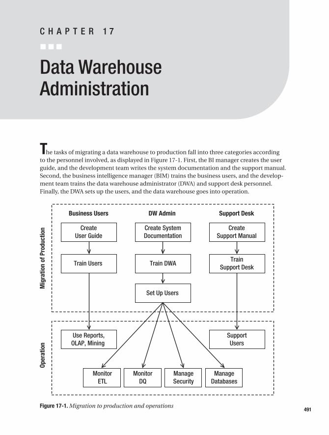
Data Warehouse Administration
The tasks of migrating a data warehouse to production fall into three categories accordingto the personnel involved, as displayed in Figure 17-1. First, the BI manager creates the userguide, and the development team writes the system documentation and the support manual.Second, the business intelligence manager (BIM) trains the business users, and the develop-ment team trains the data warehouse administrator (DWA) and support desk personnel.Finally, the DWA sets up the users, and the data warehouse goes into operation.
Figure 17-1. Migration to production and operations491
C H A P T E R 1 7
9314ch17final.qxd 11/15/07 9:39 AM Page 491

This chapter is about the second half of the diagram in Figure 17-1: operation. In particu-lar, I will discuss the DW administrator tasks, including monitoring ETL, monitoring dataquality, managing security, and managing databases. I will also discuss system enhancementssuch as bringing a new piece of data into the warehouse and updating the applications.
Monitoring Data Warehouse ETLOne of the most important things in data warehouse administration is monitoring the ETLprocesses. The ETL processes feed the data warehouse with data. If the ETL is not running atall for that day, it’s not that bad, because it means the data in the warehouse is old, that’s all.But if the ETL is running halfway on that day, that’s bad, because the data could be in anincomplete state. It’s not necessarily wrong, but it’s incomplete.
For example, say the ETL batch starts with extracting data from the source systems intothe stage and then loading the data into the ODS. The ETL then loads the data from the ODSinto the DDS, starting with the dimension tables first and then moving on to the fact tables.When loading the second fact table, the process stops halfway because of an error. Let’s sayout of 46 branches, data from 20 branches was loaded completely, the 21st branch was half-way done, and the remaining branches were not touched. The regional totals would be incor-rect because the data was not complete. The data warehouse was not ready to be consumedby the users because it was halfway through the loading process. To avoid this situation(because you are risking serving incomplete or incorrect data to the end user), in some imple-mentations you can block end users from accessing the data warehouse (so only the DWA canaccess it) until the data warehouse is 100 percent ready for consumption.
This is why it is important to monitor the ETL, checking whether the ETL process exe-cutes successfully. I cannot emphasize enough that this should be an automated process, andif any task fails, you should be notified automatically. Again, this should not be a manual pro-cess. This is so important that I’m going to repeat it one more time: you must automate ETLmonitoring. Why? There are four reasons:
• First, if it is a manual process (meaning that somebody must check it before you knowthat the ETL ran OK), you may not know that the ETL has not been working correctlyfor a week!
• Second, you need to automate the ETL monitoring to make it simpler and quicker to dothe monitoring. The ETL processes may have hundreds of tasks, and it could take hoursto check them. To make it simpler and quicker, you could have exception-based report-ing, meaning you get a report only if there is something wrong. This way, you need tocheck only a few tasks that did not work correctly.
CHAPTER 17 ■ DATA WAREHOUSE ADMINISTRATION492
9314ch17final.qxd 11/15/07 9:39 AM Page 492

• Third, you need to automate the ETL monitoring process because it could fail in themiddle of the night (say at 1 a.m.), and nobody would notice anything until 9 a.m.when everybody comes to the office. Then it’s too late to do anything to get the datawarehouse ready for that day. If you notice earlier (say it got reported automatically tothe on-duty operations team, which may be outsourced offshore because of the hoursof operation), then they could check and fix it so the warehouse is available in themorning. This is especially important if the data warehouse is used for CRM ratherthan for BI, because the campaign must go out on a certain day of the week (maybeevery day). If CRM campaigns don’t run for that day, the revenue would be directlyaffected.
• Finally, you need to automate the ETL monitoring process because of consistency. Inan automated process, the same queries and the same steps are executed every singletime, so you can guarantee the consistency. Manual checks are more prone to error,and they are also tedious.
Ideally, the ETL batch should not fail because of bad data, but in practice this happens.Bad data should go to the data quality quarantine area and not be loaded into the data ware-house. Alternatively, it could be automatically corrected according to the business rules andloaded into the warehouse. Either way, the ETL should not fail because of bad data. Pleaserefer to Chapter 9 for more information. If your ETL uses service-oriented architecture andthe data validation is using XSD, when bad data fails the XSD validation, the ETL should notfail. If your ETL is batch-oriented, when your data firewall encounters bad data, the ETLbatch should not stop with an error. It should continue working until the end of the batch.
You can do two things to monitor ETL processes:
• Notification
• Reconciliation
Notification means the system needs to let you know whether the ETL is working OK orfailed. Reconciliation means you compare the source and target data to find out whether thedata in the data warehouse is correct.
More specifically, notification is a process of monitoring the data warehouse ETL tasksand informing the operations personnel of the status of those tasks. There are two approachesgenerally used for notification: either the ETL tasks themselves internally log their statuses oran external monitoring system checks the ETL tasks periodically. The internal approach isusually cheaper to set up, and it gets more information about the status of ETL tasks (becauseit’s done from the inside), but when a certain task hangs in memory, it would not be able tosend the notification. The external approach is potentially more expensive (you need to getmonitoring software such as GFI, Nagios, MOM 2005, or Microsoft SCOM 2007), and the infor-mation about the ETL task is more limited (because it’s done from the outside); however, it ismore reliable. In other words, you still get notification even if an ETL task crashes.
For the internal approach, you can set up e-mail and text message notification at the endof the ETL batch. In SSIS, you do this by adding a Send Mail task to the SSIS package, as shownin Figure 17-2.
CHAPTER 17 ■ DATA WAREHOUSE ADMINISTRATION 493
9314ch17final.qxd 11/15/07 9:39 AM Page 493
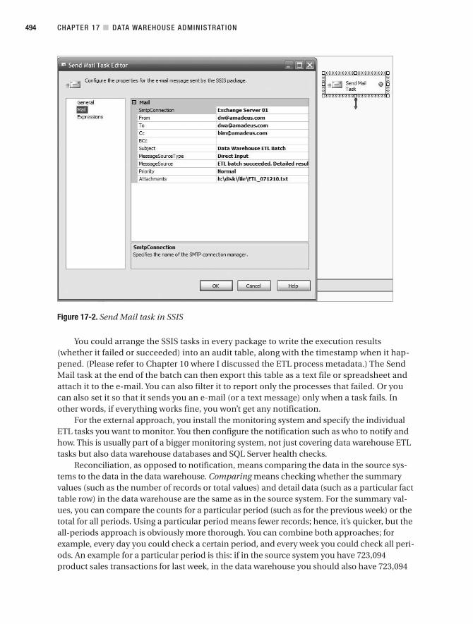
Figure 17-2. Send Mail task in SSIS
You could arrange the SSIS tasks in every package to write the execution results(whether it failed or succeeded) into an audit table, along with the timestamp when it hap-pened. (Please refer to Chapter 10 where I discussed the ETL process metadata.) The SendMail task at the end of the batch can then export this table as a text file or spreadsheet andattach it to the e-mail. You can also filter it to report only the processes that failed. Or youcan also set it so that it sends you an e-mail (or a text message) only when a task fails. Inother words, if everything works fine, you won’t get any notification.
For the external approach, you install the monitoring system and specify the individualETL tasks you want to monitor. You then configure the notification such as who to notify andhow. This is usually part of a bigger monitoring system, not just covering data warehouse ETLtasks but also data warehouse databases and SQL Server health checks.
Reconciliation, as opposed to notification, means comparing the data in the source sys-tems to the data in the data warehouse. Comparing means checking whether the summaryvalues (such as the number of records or total values) and detail data (such as a particular facttable row) in the data warehouse are the same as in the source system. For the summary val-ues, you can compare the counts for a particular period (such as for the previous week) or thetotal for all periods. Using a particular period means fewer records; hence, it’s quicker, but theall-periods approach is obviously more thorough. You can combine both approaches; forexample, every day you could check a certain period, and every week you could check all peri-ods. An example for a particular period is this: if in the source system you have 723,094product sales transactions for last week, in the data warehouse you should also have 723,094
CHAPTER 17 ■ DATA WAREHOUSE ADMINISTRATION494
9314ch17final.qxd 11/15/07 9:39 AM Page 494

transactions for last week. An example of the all-periods approach is comparing the totalnumber of active customers.
The reconciliation process is a systematic comparison between the data in the data ware-house and the data in the source system. Systematic comparison means checking a series ofpredefined summary values and detail data periodically. You can do this using a program thatlaunches SQL queries to both the source system and the data warehouse database to get thetotals. The reconciliation process can send a report to the DWA that contains the total countsfrom both the source system and the data warehouse. The report can be filtered to report onlythe discrepancies; that is, if there are 100 summary values to check and three of them don’tmatch, then the report contains only three items. If all of them match, it is better to still senda report saying that everything is OK. Otherwise, the DWA could wonder whether there is aproblem with the report generation.
When comparing the detail data, the reconciliation process can select some samples totest some values, comparing between the source systems and the data warehouse. The samplecan be selected carefully based on the business value. The other consideration of selecting thesample is the coverage; that is, you need to ensure that all dimensions and facts are covered.For example, you can check the measures on the last fact table row loaded into the warehouseto ensure that they match the values in the source systems. Similarly, you can pick up the lastrow updated in each dimension to compare them with the source systems.
You need to be careful when the ETL combines data from several different source sys-tems using a certain formula. When reconciling this measure with the source system, youneed to apply the same formula that was used to calculate the measure. If the formula ischanged in the ETL, you also need to update the formula in the reconciliation process.
The reconciliation process needs to be executed regularly as an ongoing process to ensurethat the quality of the data that you load into the data warehouse is good all the time.
Monitoring Data QualityNow I’ll quickly recap the data quality (DQ) processes discussed in Chapter 9. Bad data fromthe source system is picked up by one of the ETL tasks and will be loaded into the data ware-house. The data quality rule within the ETL workflow picks up the bad data and decides whichaction to take: reject the data (if it’s outside the tolerance limits), allow the data into the ware-house (within the tolerance limits), or fix the data automatically (according to predefinedrules and values). The failed data is stored in the DQ audit tables, along with additional auditinformation such as the time it happened, which rule was violated, and the correction status.
A series of DQ reports queries the DQ audit tables for the purpose of finding out when aDQ rule was violated, which/how many data rows are impacted, which/how many source/tar-get tables were impacted, what action was taken, what the status is, and what the values of thesource data were. These reports are sent out (usually by e-mail) to various users according totheir functional groups. Different people are responsible for different data quality rules/areas.The reports can be web-based so that in the DQ e-mail you can just put the links (URLs) to thereports, rather than the whole reports.
The users review the data quality reports and take actions to correct the data in the sourcesystem. Every day (or every week, depending on the report frequency), these users read theDQ report associated with their area of responsibility, such as CRM, subscriber sales, product
CHAPTER 17 ■ DATA WAREHOUSE ADMINISTRATION 495
9314ch17final.qxd 11/15/07 9:39 AM Page 495

sales, supplier/purchasing, inventory, and so on. They check the data in the warehouse andask the source system users to correct the bad data so that the next time the ETL runs, the datais correct.
Bear in mind that the solution is not always correcting the data. The solution can alsobe adjusting the data quality rule. This is because sometimes the DQ rule can be out-of-date, perhaps because the current condition is different from the condition when the rulewas created. What was considered bad data years ago could be OK for today. For example,you could have a DQ rule that says if the number of customers who unsubscribed was notwithin 35 percent of the last three months’ moving average, then raise this as a warning. Itmay be that the customer subscription behavior was so dynamically up and down that thebusiness user responsible for the CRM DQ area decided to change the DQ rule to “within65 percent of the last one month’s average.”
Although the business users are responsible for checking the violation of DQ rules withintheir own business areas, the BIM needs to monitor the overall trends, such as the following:
The number of DQ rules violation over time: This is to find out whether the number of dataquality rules violations generally tends to decrease over time, as shown in Figure 17-3. Thenumber of data quality rules violations generally reflects the quality of the data in the datawarehouse because the rules are designed to capture bad data. It is also useful to find outwhether there are any rules with an increasing number of occurrences, such as rule 7 inFigure 17-3. From week 11 to week 20, while the violations of other rules went down, theviolation of rule 7 went up. You need to find out whether the bad data for rule 7 is cor-rected in the source system.
Figure 17-3. Number of data quality rules violations over time
The geographic dispersion of rule violations: This is to find out the number of rules viola-tions per geographical unit, such as branches or stores, regions, and divisions, as shownin Figure 17-4. This chart is per rule; that is, each rule has its own chart.
CHAPTER 17 ■ DATA WAREHOUSE ADMINISTRATION496
9314ch17final.qxd 11/15/07 9:39 AM Page 496

Figure 17-4. Geographical dispersion of rule violations
The other overall data quality analysis: To find other data quality analysis that you can dofor your own particular situation, you can have a look at your DQ rules. If the DQ rule isabout a dimension, then you can analyze the data by the attribute of that dimension. If theDQ rule is about a measure of a fact table, then you can analyze the data by any dimensionof that fact table. For example, if the DQ rule is about the product dimension, then the DQviolation can be analyzed by product type and product category.
From data quality analysis, sometimes you’ll find problems, such as the increasingnumber of rule violations shown in Figure 17-3. Common DQ problems are a high quantityof violations (either persistently high, steadily increasing, or spikes) and uneven distribu-tion of violations (high only for a specific product type, store, or other item). The causes ofthe problems are different in each organization. A systematic approach to understandingthe causes of these problems in your situation is to analyze the corresponding rows on theaudit table to study each rule violation, look at the rule formula in the metadata database,and examine the source values in the source systems. This enables you to find the root ofthe problem. These are several common causes:
• There is no proper validation in the front-end application. In this case, you need to addor fix the validation in the front-end application.
• A one-off event was happening in the source system, such as a large data load. In thiscase, you need to do a manual one-off data correction in the source system by askingthe source system DBA to execute a data change script.
• The DQ rule is out-of-date. In this case, you need to update, fix, or deactivate the rule.
• There’s no specific rule covering a particular DQ area or issue. In this case, you need tocreate a new rule to cover that area.
The data quality trends need to be monitored continuously. It is possible that the numberof violations for a particular rule could decrease and reach a steady plateau and then suddenlyincrease again. Sometimes the increase could happen across many rules. The possible causes
CHAPTER 17 ■ DATA WAREHOUSE ADMINISTRATION 497
9314ch17final.qxd 11/15/07 9:39 AM Page 497

of this kind of event are activities with a wide impact affecting the whole company or organi-zation and therefore affecting many areas of the data warehouse. These events are usuallyknown in advance, so you can plan and prepare for them, such as a company-wide annualprice increase, a merger with another company, or a new source system feeding data into thedata warehouse.
Managing SecurityIn this section, I will discuss what data warehouse security is, why it is important, and how tomanage it. Data warehouse security is the process of enabling people who need to access thedata warehouse and preventing those who should not access it. Data warehouse security cov-ers authentication and authorization.
Authentication is identifying that the data warehouse users are really who they said theyare. This includes verifying that the user who asks for access to the data warehouse shouldgenuinely have access. You can do this by checking with the user’s superior or the BIM. Afterverifying the user, you can create the user. You also need to remove leavers or movers from thelist of data warehouse users. Movers are people who moved departments and are no longerdoing their data warehouse roles. Leavers are people who left the company and don’t needaccess to the data warehouse anymore.
Authorization is verifying that the user has access to a data warehouse object beforeallowing the user to access it. This includes giving or blocking access to the data stores, data-bases, reports, cubes, mining models, portals, and dashboards. This is done using securitygroups and security roles.
A security group is a collection of users with the same access rights. The purpose of cre-ating security groups is to make the security administration simpler and to make the accessrights consistent across the group. A security role is a functional position with the ability todo certain tasks. A user or a group can then be assigned to that role, making the user or groupcapable of doing the tasks that the role is capable of doing.
Other security tasks are checking security logs and applying security patches. The DWAneeds to check Windows and the SQL Server security log, as well as the front-end applicationsuch as SSRS and BI applications. Applying SQL Server and Windows security patches to SQLServer installations and Windows servers used by the data warehouse is required to minimizethe possibility of people exploiting known SQL Server and Windows vulnerabilities.
Managing data warehouse security is important because a data warehouse usuallycontains a lot of data from different source systems. It is used as a foundation to makeimportant business decisions and to run applications such as CRM. If you don’t protectthis data, unauthorized people will be able to read the data. Or worse, they may be ableto modify the data, resulting in inaccurate decisions being made or some problems in theCRM operations.
Now let’s talk about the how—how to manage data warehouse security. Ideally, you needto put a process in place that covers capturing the security request, verifying the user, grantingthe necessary access, and removing inactive users. For example, new users need to fill in aform stating who they are, which department they’re in, which part of the data warehouse
CHAPTER 17 ■ DATA WAREHOUSE ADMINISTRATION498
9314ch17final.qxd 11/15/07 9:39 AM Page 498

they need to access, the purpose (short-term project, daily operation, regulatory audit, andso on), which environment (dev, QA, or production), and how they would like to access it(via SSRS, SSAS, BI application, or ODBC).
It is important to state for how long the user needs the access. For example, a member ofa customer loyalty project may need access to the DDS via ODBC for three months to analyzethe customer data. The request is then approved or authorized by either the manager of therequesting user or the BIM.
The DWA can then grant the access to the new user. If a security group for similar usersalready exists, the DWA adds the new user to the existing security group. If such a groupdoesn’t exist, the DWA creates a new security group. Even if there is only one member to thesecurity group, the DWA would still need to grant the access to a security group, not directlyto the user account. This is necessary so that when people change positions, they don’t carrythe security access with them.
You need to be careful with leavers and movers. As I explained earlier, leavers are peoplewho have left the company, and movers are people who have moved to other departmentsand have new roles. The problem here is that usually HR is aware of the leaver, but they don’tinform the DWA. You need to set up a process where HR notifies the BIM or DWA when peopleleave their jobs.
The other thing you need to be careful about is a request for a short-term project. Moreoften than not, after the project is finished, the access is still active. This provides a securitythreat and needs to be fixed urgently. To minimize the chances of this situation recurring, youneed to establish a process where all accounts are made to expire after a certain period. Ontop of that, you need to set up a routine security audit to remove all inactive accounts.
Managing DatabasesData warehouse database management is the process of maintaining the databases used bythe data warehouse. Maintaining a database means ensuring that enough disk space is alwaysavailable, backups are performed regularly, indexes are maintained and optimized, and data-base statistics are up-to-date. In this section, I’ll explain what databases are involved. In a SQLServer–based data warehouse system, you have the stage database, ODS or NDS database,DDS database(s), and Analysis Services databases (cubes). You may also have a metadatadatabase, a data quality database, and archived databases.
Why is it important to maintain the databases in a data warehouse? Well, almost all datain the data warehouse is stored within the databases, and the data in the databases is used tosupport making business decisions.
The scope of data warehouse database management includes the following. I created thislist based on my experience. There may be other activities that are specific to your situation.
CHAPTER 17 ■ DATA WAREHOUSE ADMINISTRATION 499
9314ch17final.qxd 11/15/07 9:39 AM Page 499
Maintaining capacity: One of the most important aspects of managing a SQL Server data-base is to make sure there is always enough disk space. You don’t want tomorrow’s ETLload failing because there is not enough space. If you use SAN, you need to make sure thedata warehouse has enough space allocation. As the data warehouse size grows, you alsoneed to evaluate whether you need to increase the memory of the server, whether it is theSSIS server, the SSAS server, the SSRS server, or the database server.
Backing up databases: As with any databases, backups need to be scheduled, executed,and monitored. As I explained in Chapter 6, full recovery model is not required for thestage, NDS, and DDS databases. Simple recovery is more suitable for them. Full recoverymodel is suitable for an ODS database. A good time to back up the databases is after thedaily ETL batch is run successfully. In many organizations, backing up to hard media iscentralized across servers. If this is the case, you need to back up the databases to disk,ready for the centralized tape backup process to pull it to tapes. You also need to arrangeoff-site backups.
Testing database restore: It is important to restore the database backup regularly. A data-base backup is useful only when it is in good condition, and the best way to test that it isin good condition is to restore it. At the very least, you need to test restoring the stage,DDS, NDS, ODS, and Analysis Services databases every three to six months. These fre-quencies are from my own experience as well as from other DWAs’ experience. For yourown environment, you may want to use different frequencies. I have found that mostpeople back up, but a disciplined, periodic test restore is something that is still rare.
Maintaining indexes: Depending on the fragmentation levels and the performance ofthe ETL loading the table, you need to defrag the index or re-create the index. From myexperience, you need to consider maintaining the index when the fragmentation isgreater than 15–25 percent. I recommend creating a SQL query for each fact table tobenchmark the index performance. Once the response time of this query is less thanthe benchmark, then you need to reindex. In SQL Server 2005 and newer, re-creatingindexes is an online operation; that is, users can still access the table being indexed.The exception for this is the clustered index. You can find out the fragmentation usingthe sys.dm_db_index_physical_stats dynamic management function. This functionreturns the size and fragmentation information for the data and indexes of the speci-fied table or view. You also need to find out whether certain queries require additionalindexes to be created. You can do this by comparing the response times of thosequeries against the benchmark.
Maintaining table partitions: This includes adding new partitions and removing theold ones (and archiving them) to maintain data warehouse performance, as discussedin Chapter 6. Also, as the fact tables become larger and larger, you may want to converta fact table from a nonpartitioned table to a partitioned table to improve query per-formance. It is important to place the partition on the correct filegroup so that youneed to back up only the latest partitions (provided that you arrange the partitionscheme by date). Please refer to Chapter 6 about implementing table partitioning fordata warehousing.
CHAPTER 17 ■ DATA WAREHOUSE ADMINISTRATION500
9314ch17final.qxd 11/15/07 9:39 AM Page 500

Changing the schema: Occasionally after the data warehouse is in production, you need toupdate the database schema. What I mean by schema is the database structure, table def-inition, triggers, views, and stored procedures. This is usually because of development/enhancement requests (see the next section).
Changing the data: In contrast to the schema changes, sometimes you have a request toload data directly into the data warehouse. One possible cause is integration with anotherdata warehouse or because you have a new source system.
Creating a DDS database: Part of the database maintenance is to create a new database.Sometimes you receive a request from a project team to create a DDS database for thepurpose of thorough data analysis specifically for that project. This DDS is a subset ofthe main DDS containing a certain data mart and for a certain time period. For example,Amadeus Entertainment, for the purpose of issuing a new product range, requires thelast six months of data of the product sales data mart.
Making Schema ChangesAfter the data warehouse goes live and operational, sometimes there are changes in thebusiness processes that generate new data or change or reduce data. For example, installinga new human resources system adds a new data source for the employee dimension in thedata warehouse. A new call center system generates a new data source for the customerdimension in the data warehouse. The new piece of data can also come from existing sys-tems. It can be a new attribute, a new measure, a new dimension, or even a new data mart.This requires schema changes in the data warehouse.
Because the data warehouse is now operational, such requests should be regarded andtreated as change requests. As with any IT systems, you need to establish a formal procedureto deal with data warehouse change requests. The business user needs to fill in a form describ-ing the request and the reasons or justifications to support it. In the request, the business userneeds to mention what data changes are required, where the data is coming from, what theformat is, and what information it contains, as well as a sample of the real data. This is neces-sary so you can understand what schema changes are required to support this change. Therequests are then analyzed and prioritized by the BIM and forwarded to the DWA for esti-mates, and so on, before they are approved for implementation.
As an illustration, please look at the example shown in Figure 17-5. The data warehouse isoperational in production, and you have a change request from the business to bring in twonew attributes from the source systems. One attribute is from the subscription sales area, andthe other one is from the fulfillment operation.
The solid stripes indicate new columns or impacted columns in the databases. As you cansee in Figure 17-5, the two attributes flow from the source system to the stage, then to theODS, and then to the DDS. In my experience, this kind of quick diagram really helps thedesign, planning, and implementation. It also helps the testing. The diagram gives an overallview of the changes so you know which areas in the data warehouse are impacted. You maywant to consider using the diagram in Figure 17-5 when you need to change the data ware-house schema. The diagram is also useful for understanding the overall data flow in your datawarehouse, even when you don’t have any schema changes.
CHAPTER 17 ■ DATA WAREHOUSE ADMINISTRATION 501
9314ch17final.qxd 11/15/07 9:39 AM Page 501

Figure 17-5. Updating the data warehouse schema
To create the diagram in Figure 17-5 for your own situation, you can start by drawing thesix column headings. Then in the Area column, list your fact tables that are affected by thischange. In each cell under Source Systems, Stage, ODS, and DDS, list the tables affected by thechange, and mark the columns that will need to be updated or created. Connect those tableswith arrows to show how the data flows between tables.
You should not underestimate the size or complexity of the work. It may sound simplewhen you first hear it: “Two new attributes…ah, that’s easy; it’s probably going to take me aweek.” If you count all the arrows in Figure 17-5, you’ll see that 21 ETL tasks are involved. Ifyou count all the solid stripes in the stage, ODS, and DDS databases, you’ll see that 18 col-umns are impacted in 10 different tables. That’s excluding the impact to modify the appli-cations, such as report and OLAP cubes, which I will discuss in the next section.
Bringing a new piece of data into the data warehouse requires data modeling, schemachanges, ETL modifications, new data quality rules, ETL testing, integration testing, and a lotof regression testing. It is not as simple as it looks. You need to define the business require-ments and then translate this into a functional specification, as discussed in Chapter 4. Thenyou update the data model and create the schema change diagram as shown in Figure 17-5.Based on this diagram, you specify the changes required in ETL processes, along with the dataquality rules updates. You then code the enhancements and test the changes. You run the sys-tem from end to end to ensure that the new data flows through the warehouse correctly. Youthen rerun the same system test that you did before the data warehouse went into productionto make sure this change does not affect any existing functionality.
CHAPTER 17 ■ DATA WAREHOUSE ADMINISTRATION502
9314ch17final.qxd 11/15/07 9:39 AM Page 502

Updating ApplicationsAfter the data warehouse is in production, there will be requests from the users to enhance theapplications, such as to add columns in a report, to add a new attribute in the cube, or toupdate a calculation in the BI application. If you look at Figure 17-5 earlier in the chapter, afterthe data has been modified, the applications need to be updated too.
Just like when you bring a new piece of data into the warehouse, you also need to have aprocess for updating the application. The procedure is similar to the one mentioned earlier.In other words, the business user needs to fill in a form describing the request and the rea-sons or justifications supporting it. In the request, the user needs to specify which area of thedata warehouse application needs changing, what changes are required, a summary of thenew functionality, and the screen/page mock-up if it requires user interface changes. If it isreport changes, the request needs to mention what data changes are required, as well as anychanges to the report layout. This is necessary so that you understand the impact of thechange to the data warehouse applications. The requests are then analyzed and prioritizedby the BIM by determining the change’s impact to the business and the financial value gener-ated by the request. The BIM then forwards the request to the DWA for estimates, and so on,before they are approved for implementation.
Once the change is approved for implementation, you then translate the businessrequirements to functional specifications, and at the same time you write a high-level testplan to verify the use cases in the functional specifications. You then determine the impactof the request to the data warehouse application. It helps to draw the impacts in a diagramlike Figure 17-5 so you know exactly which page and applications are affected and how thedata will be flowing across applications. You then specify the changes required in each page,cube, or report in the form of technical specification documents. You then code the changesrequired in each application and test the changes by running the application using test dataspecifically prepared for testing each change. You then run the data warehouse from end toend, including the ETL processes to make sure that the changes have no negative impact onall the other areas of the data warehouse. Once the technical test is completed, the updatedapplication needs to be tested and verified by the business users before it is implementedin production.
A request to change the application does not necessarily require a schema change. Thedata may already be in the data warehouse but not be delivered to the application, such asadding a column in a report to display an existing dimension attribute.
SummaryIn this chapter, I discussed data warehouse administration, including monitoring the ETL,administering databases, managing security, bringing new data, and updating applications.This is the end of the book. I hope this book has served its purpose—to provide you with apractical explanation of the essential topics in data warehousing that you need to understandin order to build your first data warehouse.
CHAPTER 17 ■ DATA WAREHOUSE ADMINISTRATION 503
9314ch17final.qxd 11/15/07 9:39 AM Page 503

Throughout this book, I used Amadeus Entertainment as the case study. I discussed thearchitecture and methodology, gathered the requirements, designed the data model, createdthe physical databases, built the ETL, and developed the reports, cubes, and mining modelsfor that project. I hope it has been a useful experience for you as your first project. Now it’stime to go out there and implement all these concepts in real projects. I wish you great successin your data warehousing journey.
CHAPTER 17 ■ DATA WAREHOUSE ADMINISTRATION504
9314ch17final.qxd 11/15/07 9:39 AM Page 504

Normalization Rules
Normalization is the process of removing data redundancy by implementing normalizationrules. There are five degrees of normal forms, from the first normal form through the fifthnormal form, as described in this appendix.
First Normal FormThe following are the characteristics of first normal form (1NF):
• There must not be any repeating columns or groups of columns. An example of arepeating column is a customer table with Phone Number 1 and Phone Number 2columns. Using “table (column, column)” notation, an example of a repeating group ofcolumns is Order Table (Order ID, Order Date, Product ID, Price, Quantity, Product ID,Price, Quantity). Product ID, Price, and Quantity are the repeating group of columns.
• Each table must have a primary key (PK) that uniquely identifies each row. The PKcan be a composite, that is, can consist of several columns, for example, Order Table(Order ID, Order Date, Customer ID, Product ID, Product Name, Price, Quantity). Inthis notation, the underlined columns are the PKs; in this case, Order ID and ProductID are a composite PK.
Second Normal FormThe following are the characteristics of second normal form (2NF):
• It must be in 1NF.
• When each value in column 1 is associated with a value in column 2, we say thatcolumn 2 is dependant on column 1, for example, Customer (Customer ID, CustomerName). Customer Name is dependant on Customer ID, noted as Customer ID ➤Customer Name.
505
A P P E N D I X
9314appfinal.qxd 11/15/07 10:26 AM Page 505

• In 2NF, all non-PK columns must be dependent on the entire PK, not just on part ofit, for example, Order Table (Order ID, Order Date, Product ID, Price, Quantity). Theunderlined columns are a composite PK. Order Date is dependent on Order ID butnot on Product ID. This violates 2NF.
• To make it 2NF, we need to break it into two tables: Order Header (Order ID, OrderDate) and Order Item (Order ID, Product ID, Price, Quantity). Now all non-PK columnsare dependent on the entire PK. In the Order Header table, Order Date is dependent onOrder ID. In the Order Item table, Price and Quantity are dependent on Order ID andProduct ID. Order ID in the Order Item table is a foreign key.
Third Normal FormThe following are the characteristics of third normal form (3NF):
• It must be in 2NF.
• If column 1 is dependent on column 2 and column 2 is dependent on column 3, wesay that column 3 is transitively dependent on column 1. In 3NF, no column is tran-sitively dependent on the PK, for example, Product (Product ID, Product Name,Category ID, Category Name). Category Name is dependant on Category ID, andCategory ID is dependant on Product ID. Category Name is transitively dependenton the PK (Product ID). This violates 3NF.
• To make it 3NF, we need to break it into two tables: Product (Product ID, Product Name,Category ID) and Category (Category ID, Category Name). Now no column is transi-tively dependent on the PK. Category ID in the Product table is a foreign key.
Boyce-Codd Normal FormBoyce-Codd Normal Form (BCNF) is between 3NF and 4NF. The following are the characteris-tics of BCNF:
• It must be in 3NF.
• In Customer ID ➤ Customer Name, we say that Customer ID is a determinant. InBCNF, every determinant must be a candidate PK. A candidate PK means capable ofbeing a PK; that is, it uniquely identifies each row.
• BCNF is applicable to situations where you have two or more candidate compositePKs, such as with a cable TV service engineer visiting customers: Visit (Date, Route ID,Shift ID, Customer ID, Engineer ID, Vehicle ID). A visit to a customer can be identifiedusing Date, Route ID, and Customer ID as the composite PK. Alternatively, the PK canbe Shift ID and Customer ID. Shift ID is the determinant of Date and Route ID.
APPENDIX ■ NORMALIZATION RULES506
9314appfinal.qxd 11/15/07 10:26 AM Page 506

Higher Normal FormsThe following are the characteristics of other normal forms:
• A table is in fourth normal form (4NF) when it is in BCNF and there are no multivalueddependencies.
• A table is in fifth normal form (5NF) when it is in 4NF and there are no cyclicdependencies.
It is a good practice to apply 4NF or 5NF when it is applicable.
■Note A sixth normal form (6NF) has been suggested, but it’s not widely accepted or implemented yet.
APPENDIX ■ NORMALIZATION RULES 507
9314appfinal.qxd 11/15/07 10:26 AM Page 507

9314appfinal.qxd 11/15/07 10:26 AM Page 508

■Numbers and Symbols@ for naming report parameters, 3431NF (first normal form), 5062NF (second normal form), 5053NF (third normal form), 5064NF (fourth normal form), 5075NF (fifth normal form), 507
■Aaccounts, security audits of, 499action column, 322actions, data quality, 293–296administration functions
data quality monitoring, 495–498database management, 499–501ETL monitoring, 492–495schema changes, 501–502security management, 498–499updating applications, 503
ADOMD.NET, 412aggregates. See also summary tables
defined, 415alerts (BI), 437–438aligning partition indexes, 166allow action (DQ rules), 295Amadeus Entertainment case study. See case
study (Amadeus Entertainment)AMO (Analysis Management Objects), 417Analysis Services (OLAP)
authentication and, 397cubes in, 397failover clusters and, 115partitioned cubes, 119tools vs. reports, 333
analytics applications (BI), 413–416applications, updating by DWA, 503architectures
data flow. See data flow architecturedetermining, 52system. See system architecture design
association scores, 471attributes, customer, 444audio processing, text analytics and, 473audit metadata
components of, 323event tables, 323maintaining, 327
overview, 302purposes of, 323
auditsDQ auditing, 296–298ETL, defined, 31reports, 332
authentication of users, 498authorization of user access, 498Auto Build, 385Auto Layout, 249autofix action (DQ rules), 296automating ETL monitoring, 492–493
■Bbacking up
databases, 500MDBs, 405–408
band attribute (Amadeus), 64batch files
creating, 138, 157ETL, 269updating, 15–16
BCNF (Boyce-Codd Normal Form), 506BI (Business Intelligence)
alerts, 437–438analytics applications, 413–416application categories, 411Business Intelligence Development Studio
Report Wizard, 339dashboard applications, 432–437data mining applications. See data mining
applications (BI)examples of, 12–13portal applications, 438–439reports, 34, 412–413search product vendors, 474systems, applications for, 17–18
binary files, importing, 190bitmapping, index, 169block lists (black lists), 451boolean data type (data mining), 419, 420bounce rate (e-mail), defined, 447bridge tables, defined, 109bulk copy utility (bcp) SQL command,
188–189bulk insert SQL command, 187, 189business areas, identifying (Amadeus), 61–62business case document, 51–52
Index
509
9314idxfinal.qxd 11/15/07 1:39 PM Page 509

business Intelligence (BI). See BI (BusinessIntelligence)
Business Objects Crystal Report XI, 356Business Objects XI Release 2 Voyager, 380business operations, evaluating (Amadeus),
62–63business performance management, 13business requirements
CRM data marts (Amadeus), 96subscription sales data mart (Amadeus),
90verifying with functional testing, 480
■Ccalendar date attributes column (date
dimension), 77–78campaigns
creating CRM, 447–448defined, 447delivery/response data (CRM), 454–460response selection queries, 449results fact table, 99, 450segmentation (CRM), 18, 98, 447–450
candidate PK, 506case sensitivity in database configuration,
124case study (Amadeus Entertainment)
data feasibility study, 67–70data warehouse risks, 67defining functional requirements, 63–65defining nonfunctional requirements,
65–67evaluating business operations, 62–63extracting Jade data with SSIS, 191–200functional testing of data warehouse, 480identifying business areas, 61–62iterative methodology example, 56–58overview of, 44–46product sales. See product sales data mart
(Amadeus)product sales reports, 349, 353, 355, 359,
369query for product sales report, 331security testing, 485server licenses and, 119
case table, defined (data mining), 418CDI (Customer Data Integration)
customer data store schema, 469fundamentals, 23–24, 467–468implementation of, 469
CET (current extraction time), 182change requests, procedures for, 501character-based data types, 277charting. See also analytics applications (BI),
440churn analysis, 465
class attribute (Amadeus), 64classification algorithm, 422cleaning (CDI), defined, 468cleansing, data, 277–290click-through rate (email), 98, 447clustered configuration, defined, 43clustering algorithm, 422Clustering model, 431Cognos
BI 8 Analysis, 380PowerCube, 377, 379Powerplay, 356
collation, database, 124columns
continuous (data mining), 419cyclical (data mining), 420description (data definition table), 305discrete (data mining), 419discretized (data mining), 419ordered (data mining), 420repeating, 505risk_level column, 322status, 320, 322storing historical data as, 81types in DW tables, 306
communicationCommunication Subscriptions Fact Table
(example), 452communication_subscription transaction
table (NDS database), 140–143master table (NDS physical database), 143permission, defined, 96preferences, defined, 96subscription, defined, 96
comparing data (ETL monitoring), 494–495complaint rate (email), 98conformed dimensions
creating (views), 158defined, 7
consolidation of data, 5–6construction iteration, 56content types (data mining), 419–420continuous columns (data mining), 419control system, ETL, 31converting data for consolidation, 6cookies vs. self-authentication, 464covering index, 170CRM (customer relationship management)
basics, 14campaign analysis (Amadeus), 64campaign delivery/response data,
454–460campaign segmentation, 447–450customer analysis, 460–463customer loyalty schemes, 465–466customer support, 463–464
■INDEX510
9314idxfinal.qxd 11/15/07 1:39 PM Page 510

data marts (Amadeus), 96–101fundamentals, 441permission management, 450–454personalization, 464–465single customer view, 442–447systems, applications for, 18–19
cross-referencingdata validation and, 291–292data with external sources, 290–291
cross tab reports, 13cubes (multidimensional data stores)
in Analysis Services, 397building/deploying, 388–394Cube Wizard, 385defined, 3engines, 379reports from, 362–366scheduling processing with SSIS, 399–404
current extraction time (CET), 318customer relationship management (CRM).
See CRM (customer relationshipmanagement)
customersanalysis (CRM), 18, 460–463attributes, 444behavior selection queries, 449customer table (NDS physical database),
147–151Customer Data Integration (CDI). See CDI
(Customer Data Integration)data store schema (CDI), 469dimension, creating, 133dimension, designing, 84–86defined, 18loyalty schemes (CRM), 18, 465–466permissions (CRM). See permissions,
management (CRM)profitability analysis, 13services/support (CRM), 18, 463-464
cyclical columns (data mining), 420
■Ddaily batches, 269dashboards
applications (BI), 432–437data quality, 275
dataarchitecture vs. data flow architecture, 29availability, 5cleansing, 69, 277–290comparing (ETL monitoring), 494consolidation of, 5–6conversion of, 6defining, 6dictionary, defined, 308hierarchy in dimension tables, 101–102
history, storing, 10–11integration, defined, 36leakage, ETL testing and, 187, 479lineage metadata. See data mapping
metadatamatching, 6, 277–290vs. metadata (example), 475querying basics, 11reconciliation of (ETL monitoring),
493–495retrieval of, 4–5risks, examples of (Amadeus), 67–69scrubbing, 277storage, estimating, 69transformation, defined, 36update frequency, 6
data definition metadataoverview, 301report columns, 306table, 303table DDL, 305
data extractionconnecting to source data, 179–180ETL. See ETL (Extract, Transform, and
Load)extracting e-mails, 191extracting file systems, 187–190extracting message queues, 191extracting relational databases. See
extracting relational databasesextracting web services, 190from flat files, 208–213memorizing last extraction timestamp,
200–207potential problems in, 178with SSIS, 191–200from structured files, 177from unstructured files, 178
data feasibility studiesAmadeus example of, 67–70populating source system metadata, 317purpose of, 67
data firewallcreating, 215, 218–219defined, 32
data flowformatting, 249table (ETL process metadata), 318–320
data flow architecturevs. data architecture, 29data stores. See data storesdefined, 29federated data warehouse (FDW), 39–42fundamentals, 29–33NDS+DDS example, 35–37
■INDEX 511
9314idxfinal.qxd 11/15/07 1:39 PM Page 511
ODS+DDS example, 38–39single DDS example, 33–35
data mapping metadatadata flow table, 307overview, 302source column and, 306
data martfact tables and, 74view, 158–159
data miningapplications for, 19–20fundamentals, 14, 19
data mining applications (BI)column data types, 419–420creating/processing models, 417–422demographic analysis example, 424–431implementation steps, 417processing mining structure, 423–424uses for, 416
data modelingCRM data marts (Amadeus), 96–101data hierarchy (dimension tables),
101–102date dimension, 77–80defined, 29designing DDS (Amadeus), 71–76designing NDS (Amadeus), 106–111dimension tables, 76–77product sales data mart. See product sales
data mart (Amadeus)SCD, 80–82source system mapping, 102–106subscription sales data mart (Amadeus),
89–94supplier performance data mart
(Amadeus), 94–95data quality (DQ)
actions, 293–296auditing, 296-298components in DW architecture, 274cross-referencing with external sources,
290–291data cleansing and matching, 277–290Data Quality Business Rules document,
292database, defined, 32importance of, 273logging, 296–298monitoring by DWA, 495–498process, 274–277processes, defined, 32reports, 32, 332reports and notifications, 298–300
data quality metadatacomponents of, 320DQ notification table, 321–322
DQ rules table, 321–322DW user table, 321–322overview, 302
data quality rulesdata quality metadata and, 320defined, 32fundamentals, 291-293violations, 496-497
data storesdata lineage between, 307defined, 30delivering data with ETL testing, 478overview, 31–32types of, 30
data structure metadatamaintaining, 326overview, 302populating from SQL Server, 311–313purposes of, 308–309tables, 309–311tables with source system metadata,
314–317data types
conversion output for (SSIS), 250in data mining, 419
data warehouses (DW)advantages for SCV, 445–447alerts, 437building in multiple iterations, 54The Data Warehouse Toolkit (Wiley), 82defined, 1, 16–17deploying, 53designing, 52development methodology. See system
development methodologydevelopment of, 52DW keys, 109vs. front-office transactional system, 5internal validation, 291major components of, 478MDM relationship to, 23migrating to production, 491non-business analytical uses for, 14operation of, 53populating. See populating data
warehousesreal-time, 27system components, 4updating data in, 15–16uses for, 17
databasescollation of, 124configuring, 123–128design, data stores and, 7extracting relational. See extracting
relational databases
■INDEX512
9314idxfinal.qxd 11/15/07 1:39 PM Page 512

management by DWA, 499–501MPP systems, 175multidimensional. See MDB
(multidimensional database)naming, 124restoring backup of, 500servers, sizing, 116–118SQL Server. See physical database designtransaction log files, 189
DataMirror software, 190date dimension
fundamentals, 77–80source system mapping, 104
datesdata type (data mining), 419–420date/time data types, 278dimension table, creating, 128–132excluding in MDM systems, 21format columns (date dimension), 77
DBA (Database Administrator), liaising with,489
DDL (Data Definition Language)of data definition table, 303of data mapping table, 307for subscription implementation
(example), 453DDS (dimensional data store)
database, creating new, 501defined, 2, 30designing (Amadeus), 71–76dimension tables, populating, 215,
250–266drill-across dimensional reports, 333fact tables, populating, 215, 266–269fundamentals, 7vs. NDS, 9NDS+DDS example, 35–37ODS+DDS example, 38–39single DDS example, 33–35single dimension reports, 333sizing, 124, 126–128
DDS database structurebatch file, creating, 138customer dimension, creating, 133date dimension table, creating, 128–132product dimension, creating, 132Product Sales fact table, 135store dimension, creating, 135
decision treesalgorithm, 422model, 431
decode table (example), 180defragmenting database indexes, 500degenerate dimensions, defined, 73deletion trigger, 184
deliverycampaign delivery/response data,
454–460channel, defined (CRM), 447rate (e-mail), defined, 447
demographic data selection queries(campaigns), 449
denormalization (DDS dimension tables),251
denormalized databases, defined, 30dependency network diagrams, 425deploying
data warehouses, 53reports, 366–369
description column (data definition table),305
descriptive analysisin data mining, 417defined, 14examples of, 460–463
determinants, 506diagram pane (Query Builder), 337dicing, defined (analytics), 413dimension tables (DDS)
fundamentals, 76–77loading data into, 250–266
dimensional attributes, defined, 76dimensional data marts, defined, 33dimensional data store (DDS). See DDS
(dimensional data store)dimensional databases, defined, 30dimensional hierarchy, defined, 101dimensional reports, 332dimensions, defined, 3, 377discrete columns (data mining), 419discretized columns (data mining), 419disk, defined, 121distributing (CDI), defined, 468Division parameter example, 349–351DMX (Data Mining Extensions), 432DMX SQL Server data mining language, 417documentation, creating, 489documents
transforming with text analytics, 471–473unstructured into structured, 471
double data type (data mining), 419, 420DQ (data quality). See data quality (DQ)drilling
across, 394up, 414–415
DW (data warehouse). See data warehouses(DW)
DWA (data warehouse administrator)functions of, 56, 488–489. See also
administration functionsmetadata scripts and, 326
dynamic file names, 188
■INDEX 513
9314idxfinal.qxd 11/15/07 1:39 PM Page 513

■Ee-commerce industry
customer analysis and, 460–461customer support in, 464
e-mailsemail_address_junction table (NDS
physical database), 155–156email_address_table (NDS physical
database), 153email_address_type table (NDS physical
database), 156–157extracting, 191store application, 473
EII (enterprise information integration), 40elaboration iteration, defined, 56ELT (Extract, Load, and Transform)
defined, 5ETL and, 117fundamentals, 175
end-to-end testingdefined, 477fundamentals, 487
enterprise data warehouse, illustrated, 10Enterprise Edition, SQL Server, 118–119enterprise information integration (EII). See
EII (enterprise informationintegration)
entertainment industry, customer supportin, 464
ETL (Extract, Transform, and Load)batches, 269CPU power of server, 116defined, 2, 4ELT and, 175extraction from source system, 176–177fundamentals, 32, 173–174log, 483monitoring by DWA, 492–495near real-time ETL, 270performance testing and, 482pulling data from source system, 270testing, defined, 477–479
ETL process metadatacomponents of, 318overview, 302purposes of, 320tables, 318–320updating, 327
eventsdefined, 62Event Collection (Notification Services),
438event tables (audit metadata), 323
exact matching, 278Excel, Microsoft, creating reports with,
359–362
exception-based reporting, 492exception scenarios (performance testing),
484execution, report, 374–375external data, NDS populating and, 219,
222–223external notification (ETL monitoring),
493–494external sources, cross-referencing data with,
290–291Extract, Transform, and Load (ETL). See ETL
(Extract, Transform, and Load)extracting relational databases
fixed range method, 186incremental extract method, 181–184related tables, 186testing data leaks, 187whole table every time method, 180–181
■Ffact constellation schema, 7fact tables
campaign results, 99loading data into (DDS), 250, 266–269populating DDS, 215, 266–269product sales (Amadeus), 71, 75, 102subscription sales (Amadeus), 90supplier performance (Amadeus), 90
failover clustersdefined, 114number of nodes for, 119
FDW (federated data warehouse), 39–42feasibility studies, 51–52federated data warehouse (FDW). See FDW
(federated data warehouse)fibre networks, 115fifth normal form (5NF), 507file names, dynamic, 188file systems, extracting, 187–190filegroups, 131–132filtering reports, 351financial industry, customer support in, 463firewalls
creating data, 215, 218–219ODS, 276
first normal form (1NF), 505first subscription date, 274fiscal attribute columns (date dimension),
77, 78fix action (DQ rules), 295fixed position files, 177fixed range extraction method, 185–186flat files, extracting, 187, 208–213forecasting (data mining), 416
■INDEX514
9314idxfinal.qxd 11/15/07 1:39 PM Page 514

foreign keysnaming, 146, 157necessity of, 137
fourth normal form (4NF), 507fragmentation of database indexes, 500frequent-flier programs, 465full-text indexing, 126functional requirements
defined, 61establishing (Amadeus), 63–65
functional testingdefined, 477fundamentals, 480
fuzzy logic matching, 278Fuzzy Lookup transformation (example),
279–290
■Ggalaxy schemas, 7general performance requirements, 483general permissions (CRM), 450Generic Query Designer, 352geographic dispersion of rule violations, 496global enterprise currency, 75Google search products, 474grain, table, 72granularity, FDW data and, 39grid pane (Query Builder), 337grouping reports, 351–355groups, security, 498–499
■Hhard RI, defined, 76hardware platform (physical database
design), 113–119help desk support, 488hierarchy
data, 101–102dimensional, 101MDM, 23
historical data, storing, 10–11HOLAP (Hybrid Online Analytical
Processing), 381horizontal/vertical partitioning, 162hot spare disks, 123hubs, MDM, 23Hungarian naming conventions, 343hybrid data store, defined, 30hypercubes, 378Hyperion Essbase, 377, 379
■IIIS logs, 325image processing, text analytics and, 473impact analysis, defined, 302inactive accounts, security audits of, 499
inception iteration, 56incoming data validation, 291incremental extraction method, 181–184incremental loading (DDS dimension tables),
251incremental methodology. See iterative
methodologyindexes
covering index, 170creating in partitioned tables, 170index intersection, 169Index Wizard, 168indexer in search applications, 474maintaining database, 500
indexingfull-text, 126implementing, 166–170online index operation, 119parallel index operations, 119stage tables, 217
indicator columns (date dimension), 77, 79inferred dimension members, 260infrastructure setup overview, 53Inmon, Bill, 16insert SQL statements, 323insurance industry, customer analysis and,
460integration testing. See end-to-end testinginternal data store, defined, 30internal notification (ETL monitoring), 493internal validation, data warehouse, 291–292intersection, index, 169invoices, text analytics and, 473iterative methodology, 54–59
■JJade system, 45junction tables
defined, 109NDS populating and, 219, 225–228
Jupiter ERP system, 44
■Kkey columns (data mining), 419key management
DDS dimension tables and, 251in NDS, 151NDS populating and, 219, 223–225
key sequence columns (data mining), 420key time columns (data mining), 420keys, DW, 109Kimball dimensional modeling, 41Kimball, Ralph, 16, 82knowledge discovery, 416. See also data
mining
■INDEX 515
9314idxfinal.qxd 11/15/07 1:39 PM Page 515

■Llanguage attribute table (NDS physical
database), 145–146last cancellation date, 274last month view, 159last successful extraction time (LSET), 318late-arriving dimension rows, 260late-arriving facts, 269latest summary table, 161layouts, report, 340–342leakage, defined, 174leavers
defined, 498updating, 499
levels of objects, defined, 63licensing models, SQL Server, 119lift charts, defined (data mining), 430list selection process (campaigns), 448loading/query of partitioned tables, 163log files
database transaction, 189size of, 125
loggingdata quality, 296–298ETL log, 483log reader, database, 176–177SSIS logging, 484web logs, 189
logical unit number design, 123logins for customer ID, 464long data type (data mining), 419, 420Lookup transformations, upsert using,
236–242loyalty schemes, customer (CRM), 465–466LSET (last successful extraction time), 182
■Mmassively parallel processing (MPP)
database system. See MPP (massivelyparallel processing) database system
master datafundamentals, 21management (MDM). See MDM (master
data management)store, defined, 30storing history of, 11
master tables, defined, 36, 106matching, data, 6, 277–290matching rules (metadata storage), 22matrix form (reports), 13, 338, 342MDB (multidimensional database)
backing up and restoring, 405–408building/deploying cube, 388–394creating (Amadeus), 381–387defined, 3, 31fundamentals, 377–379
online analytical processing (OLAP),380–381
querying, 394–396vs. relational databases, 378scheduling cube processing with SSIS,
399–404security of, 397–399
MDBMS (multidimensional databasemanagement systems), 379, 415
MDDS (multidimensional data store), 377MDM (master data management)
examples of, 20–21fundamentals, 21–23OLTP systems and, 22relationship to data warehouses, 23
MDX (Multidimensional Expressions)fundamentals, 435MDX Query Designer, 365
membership subscriptions, 452memory maintenance (database
management), 500message queue (MQ). See MQ (message
queue)messaging, defined, 16metadata
change request (example), 326vs. data (example), 475database, configuring, 126, 128defined, 31maintaining, 325–327overview, 301–303reasons for using, 303storage, 22types of, 301–302unstructured data and, 473
methodology, system development. Seesystem development methodology
MicrosoftAnalysis Services, 377, 379clustering algorithm, 428Office SharePoint Server, 438–439
MicroStrategy OLAP Services, 381migrating data warehouse to production,
487–489, 491mini-batches, defined, 15, 269Mining Structure designer, 421–422MOLAP (multidimensional online analytical
processing)applications, 415defined, 14, 381
monitoringdata quality, 495–498ETL processes, 492–495
Morris, Henry, 413
■INDEX516
9314idxfinal.qxd 11/15/07 1:39 PM Page 516

moversdefined, 498updating, 499
MPP (massively parallel processing)database system
defined, 43fundamentals, 175
MQ (message queue)basics, 16extracting, 191failure, simulating, 479
multidimensional data stores (cubes). Seecubes (multidimensional data stores)
multidimensional database (MDB). See MDB(multidimensional database)
multidimensional online analyticalprocessing (MOLAP). See MOLAP(multidimensional online analyticalprocessing)
multiple iterations, building in, 54
■Nnaming
database, 124dynamic file names, 188foreign keys, 146primary keys, 146report parameters, 343tables, 137
natural keysdefined, 37, 223example, 84
NDS (normalized data store)customer table (Amadeus), 110defined, 30designing (Amadeus), 106–111fundamentals, 8–10NDS+DDS example, 35–37populating, 215, 219–228populating with SSIS, 228–235population, normalization and, 242–248sizing, 124store table example (populating), 242
NDS physical database, creatingbatch file, 157communication master table, 143communication_subscription transaction
table, 140–143customer table, 147–151email_address_junction table, 155–156email_address_table, 153email_address_type table, 156–157language attribute table, 145–146order_header table, 151–153overview, 139
near real-time ETL, 270
networks, testing security access, 485NK (natural key). See natural keysNLB (network load balanced) servers, 114nodes
columns, defined, 425defined, 43
nonfunctional requirementsdefined, 61establishing, 65–67
normal scenarios (performance testing), 484normalization
defined, 8NDS population and, 219, 242–248normalized databases, defined, 30normalized data store (NDS). See NDS
(normalized data store)rules, 109, 505–507
notificationcolumn, 320data quality, 275, 298–300to monitor ETL processes, 493Notification Delivery (Notification
Services), 438Notification Services, SQL Server, 438
numerical data types, 278
■OOCR (Optical Character Recognition), 471ODBC (Open Database Connectivity), 412ODS (operational data store )
CRM systems and, 18defined, 30firewall, 276ODS+DDS architecture, configuring, 126ODS+DDS architecture (example), 38–39reports, 332
OLAP (Online Analytical Processing)applications. See analytics applications
(BI)basics, 14fundamentals, 380–381server cluster hardware, 116servers, 379tools, 333, 356, 380
OLTP (Online Transaction Processing)vs. data warehouse reports, 333defined, 2
Online Analytical Processing (OLAP). SeeOLAP (Online Analytical Processing)
online index operation, 119Online Transaction Processing (OLTP). See
OLTP (Online TransactionProcessing)
open rate (e-mail), defined, 98, 447operation, data warehouse (overview), 53operation team, user support and, 488
■INDEX 517
9314idxfinal.qxd 11/15/07 1:39 PM Page 517

operational data store (ODS). See ODS(operational data store )
operational system alerts, 437opting out (permissions), 454order column, defined, 318order header table
example, 182NDS physical database, 151–153
ordered columns (data mining), 420
■Ppackage, ETL, defined, 31package table (ETL process metadata),
318–320parallel database system. See MPP (massively
parallel processing) database systemparallel index operations, 119parallel query, defined, 10parameters, report
Division parameter example, 349–351naming, 343overview, 342Quarter parameter example, 346–348Year parameter example, 345–346
partition indexes, aligning, 166partitioned cubes, 119partitioned tables (databases)
administering, 166creating indexes in, 170loading/query of partitioned tables, 163maintenance of, 500Subscription Sales fact table example, 162,
163–166vertical/horizontal partitioning, 162
partitioning, table and index, 118patches, security, 498per-processor licenses (SQL Server), 119performance
requirements, 483testing, defined, 477testing, fundamentals, 482–484
periodic snapshotsdefined, 11fact table, 90, 269
periodic updating of data, 6permissions
management (CRM), 18, 450–454selection queries, 449
personalization (CRM), 18, 464–465physical database design
configuring databases, 123–128DDS database structure, creating. See DDS
database structurehardware platform, 113–119indexing, 166–170
NDS, creating physically. See NDS physicaldatabase, creating
partitioning tables. See partitioned tables(databases)
sizing database server, 116–118SQL Server, editions of, 118–119SQL Server, licensing of, 119storage requirements, calculating,
120–123summary tables, 161views. See views (database object)
PIM (product information management), 22PM (project manager), function of (example),
56populating data warehouses
data firewall, creating, 215, 218–219DDS dimension tables, 215, 250–266DDS fact tables, 266–269ETL batches, 269NDS, 215, 219–228NDS with SSIS, 228–235near real-time ETL, 270normalization, 242–248overview, 215pushing data approach, 270–271SSIS practical tips, 249–250stage loading, 215, 216–217upsert using Lookup transformation, 236upsert using SQL statements, 235–236
portalsapplications (BI), 438–439creating data warehouse, 489
post office organizations, 290Prediction Query Builder, 417predictive analysis
basics, 13customer analysis (example), 461in data mining, 416defined, 14
PredictProbability function, 432primary keys, naming, 146processes
data quality, 274–277ETL, 31mining structure (data mining), 423–424
ProClarity Analytics 6, 380product data, MDM systems and, 21–22product dimension
creating, 83–84, 132source system mapping, 105
product information management (PIM). SeePIM (product informationmanagement)
product sales data mart (Amadeus)analysis of product sales, 63customer dimension, 84–86
■INDEX518
9314idxfinal.qxd 11/15/07 1:39 PM Page 518

date dimension, 77–80fact tables, 71, 75product dimension, 83–84sales taxes, 73source system logic, 73source system mapping, 103store dimension, 86–87
production environment, migrating DW to,487–489
profitability band attribute (Amadeus), 64project management, 53pull approach (updating), 16, 22purchase orders, 62purchase pattern table (data mining), 418pushing data approach
for populating DW, 270–271updating with, 16, 22
■QQA (Quality Assurance) in DW, 46Quarter parameter example, 346–348querying
data, 11MDBs, 394–396Query Builder, 244, 337Query Execution Plan, 168recursive queries, defined, 308
■RRAID (Redundant Array of Inexpensive
Disks)definition and configurations, 121RAID 5 volumes, 122
ranking algorithms, 474RCD (rapidly changing dimension), 82real-time data integration, 271real-time data warehouse
fundamentals, 27updates from key tables, 15
recipient_type table, 322reconciliation, to monitor ETL processes,
493–495recoverability
defined, 174ETL testing and, 479
recovery model, 125recursive queries, 308referential integrity, 75refresh frequency, 313reject action (DQ rules), 294–295relational databases
analytics and, 415defined, 30extracting. See extracting relational
databases
relational online analytical processing(ROLAP). See ROLAP (relationalonline analytical processing )
reliability DQ key, 277repeating columns, 505reports
BI, 412–413creating with Excel, 359–362creating with report wizard, 334–340data quality, 275, 298–300deploying, 366–369dimensional, 332execution, managing, 374–375filtering, 351formatting cells, 341fundamentals, 13grouping, 351–355layout of, 340–342from multidimensional data stores,
362–366OLAP tools vs. data warehouse, 333OLTP vs. data warehouse, 333overview, 329–332parameters. See parameters, reportreport columns (data definition table), 306Report Manager, 366–367report server scale-out deployment, 118Reporting Services SharePoint web parts,
439search, 475security, managing, 370–372simplicity vs. complexity of, 356–357sorting, 351, 354spreadsheets, 357–362subscriptions, managing, 372–374types of, 332–333
requests, change, 501requirements, determining user, 52response data. See campaigns,
delivery/response data (CRM)restoring MDBs, 405–408retrieval of data, 4–5retriever (search applications), 474retrieving (CDI), defined, 468revenue analysis, 465revoking permissions, 454risk_level column, 322ROLAP (relational online analytical
processing )applications, 415defined, 14, 380
rolesdefined, 63security, 498
Ross, Margy, 82rows, storing historical data as, 80
■INDEX 519
9314idxfinal.qxd 11/15/07 1:39 PM Page 519

rulesdata quality, 291–293DQ, adjusting, 496–497normalization, 109, 505–507rule-based logic, 278rule category table, 322rule risk level table, 322rule (SQL Server keyword), 322rule type table, 322
RUP (Rational Unified Process) methodology,56
■Ssales taxes, 73SAN (storage area network), 115scale-out deployment, 115scanned documents, text analytics and, 473SCD (slowly changing dimension)
DDS dimension tables and, 251–265defined, 11fundamentals, 80–82Slowly Changing Dimension Wizard
(SSIS), 228–230schemas, database
design for campaign delivery/responsedata, 457–459
managing changes to, 501–502snowflake, 7, 89updating, 501
scoring routines (search applications), 474scripts, metadata, 326scrubbing, data, 277SCV (single customer view), 442–447SDLC (system development life cycle). See
system development methodologysearching
fundamentals, 25–26search facilities, 474search interface, 475
second normal form (2NF), 505security
groups, defined, 498management by DWA, 498–499of MDBs, 397–399report, managing, 370–372testing, defined, 477testing, fundamentals, 485-486
segmentationalgorithm, 422campaign (CRM), 447–450
selection queries (campaigns), 448self-authentication vs. cookies, 464semiadditive aggregate functions, 119semistructured files, defined, 178Send Mail tasks (SSIS), 493
sequential methodology. See waterfallmethodology
server+CAL licenses (SQL Server), 119servers, sizing database, 116–118service-oriented architecture (SOA). See SOA
(service-oriented architecture)share nothing architecture, 175SharePoint Server, Microsoft Office, 438–439Simon, Alan, 17single customer view, 18, 442–447single DDS architecture example, 33–35single login requirement, 70sizing database servers, 116–118SK (surrogate key), defined, 223slicing, defined (analytics), 413slowly changing dimension (SCD). See SCD
(slowly changing dimension)smalldatetime, 131SMP (symmetric multiprocessing) database
system, 43snapshots
defined, 11report output, 374
snowflake schemasbasics, 7benefits of, 89
SOA (service-oriented architecture), 26–27soft deletes (records), 184sorting reports, 351, 354source data
connecting to, 179–180profiles, 317–318
source system metadataoverview, 302populating, 317purposes of, 313source data profiles, 317–318table components of, 314–317
source systemsanalysis. See data feasibility studiesfunctional testing and, 481–482logic, replicating, 72mapping, 102–106moving data out of, 176pushing data from, 270–271querying, 12
spam verdict (e-mail), defined, 98specific performance requirements, 483specific permissions (CRM), 450specific store view, 160spiral methodology. See iterative
methodologyspreadsheets (reports), 357–362SQL (Structured Query Language)
Native Client driver, 412queries, exploring data with, 357
■INDEX520
9314idxfinal.qxd 11/15/07 1:40 PM Page 520

query formatting, 352statements, upsert using, 235–236
SQL ServerAnalysis Services 2005, 356Configuration Manager, 367databases, design of. See physical
database designEnterprise Edition, 118–119licensing, 119Management Studio, 232, 363Notification Services, 438object catalog views, 311–313, 326Profiler, performance testing and, 484Reporting Services. See SSRS (SQL Server
Reporting Services)system views, naming, 322
SSAS (SQL Server Analysis Services)data mining in, 20KPIs and, 434–437as OLAP tool, 380
SSIS (SQL Server Integration Services)data extraction with, 191–200failover clusters and, 115logging, 484packages, simulating incremental load
with, 70populating dimension table with, 251–265populating NDS with, 228–235practical tips, 249–250scheduling cube processing with, 399–404Send Mail tasks in, 493
SSRS (SQL Server Reporting Services)building reports with, 329–330charts and tables with, 412DQ reports and, 299NLB servers and, 114report security and, 370–371scheduling package (example), 403–404
stage data storedefined, 30fundamentals, 33
stage loading (populating DW), 215–217star schemas, 7, 89statistical analysis, 13status columns, 320, 322status of objects, defined, 62status table (ETL process metadata),
318–320steps, ETL, defined, 31storage of data
calculating database requirements, 120,123
customer data, 468estimating, 69unstructured data, 470
store dimensioncreating, 135designing (Amadeus), 86–87
structured data, defined, 470structured files, extracting, 177subscribers
subscriber class attribute (Amadeus), 64subscriber profitability, analyzing
(Amadeus), 64subscriptions
Communication Subscriptions Fact Table(example), 452
managing report, 372–374membership, 452permissions (CRM), 451sales, analyzing (Amadeus), 63sales data mart (Amadeus), 89–94sales fact table (partitioning), 163–166Subscription Management (Notification
Services), 438Subscription Processing (Notification
Services), 438Subscription Sales fact table
(partitioning), 162summary tables
application performance and, 484fundamentals, 161
supplier performanceanalyzing (Amadeus), 64data mart (Amadeus), 94–95
SupplyNet system, 44support, types of user, 53surrogate keys, defined, 37survivorship rules (metadata storage), 22symmetric multiprocessing (SMP) database
system. See SMP (symmetricmultiprocessing) database system
sys.dm_db_index_physical_stats dynamicmanagement function, 500
system architecture design, 42–44system development methodology
defined, 49iterative methodology, 54–59waterfall methodology, 49–53
systematic comparisons (ETL monitoring),495
system_user SQL variable, 325
■Ttable grain, defined, 72table partitioning
defined, 10maintenance of, 500
tablescolumn types in DW, 306data definition metadata, 303
■INDEX 521
9314idxfinal.qxd 11/15/07 1:40 PM Page 521

data mapping, 307data quality audit. See audits, DQ auditingdata quality metadata, 321–322data structure metadata, 309–311, 314–317DDL of data definition, 305DDL of data mapping, 306ETL process metadata, 318–320loading DDS fact, 215, 250, 266–269log, data quality. See loggingnaming, 137normalization rules and, 505–507populating DDS dimension, 215,
250–266source system metadata, 314–317structure of stage, 216updating related, 186usage log (usage metadata), 325whole table every time extraction method,
180–181tabular data, defined, 178tabular report (example), 330telecommunications industry
customer analysis and, 460customer support in, 463
testingdata leaks, 187database restore, 500end-to-end testing, 487ETL testing, 478–479functional testing, 480performance testing, 482–484security testing, 485–486types of, 477–478user acceptance testing (UAT), 477,
486–487waterfall methodology and, 52
text analyticsfor recruitment industry, 471transforming documents with, 471–473
text data type (data mining), 419, 420third normal form (3NF), 506time
consolidating data with different ranges,5
excluding in MDM systems, 21timestamps
memorizing last extraction, 200–207reliable, 182
transactionsdatabase transaction log files, 189Transact SQL script, 326transactional systems, 5, 12transaction fact table, defined, 90transaction tables, defined, 36, 106
transition iteration, 56trap hit rate (email), 98
travel industrycustomer analysis and, 461customer support in, 463
treatment, defined (campaigns), 448Trend expression (MDX), 435triggers
database, 176detecting updates and inserts with, 184update, 184
■UUnicode, 131unknown records, defined, 233unsegmented campaigns, 448unstructured data
defined, 470fundamentals, 24–25metadata and, 473search facilities and, 475storing, 470text analytics and, 471–473
unstructured files, extracting, 178update triggers, 184updating
applications, 503batch data, 15–16customer data store, 468data warehouse schemas, 501–502ETL process metadata, 327periodic data, 6
upsertusing Lookup transformation, 236–242using SQL statements, 235–236
usage metadatamaintaining, 327overview, 302purposes of, 324–325usage log table, 325
usage reports, 332user acceptance testing (UAT)
defined, 477fundamentals, 486–487
user-facing data store, defined, 30users
authentication of, 498authorizing access of, 498interface, search facility and, 475training, 489
utilities industrycustomer analysis and, 460customer support in, 463
■Vvalidations, types of, 291VAT (value-added tax), 73vertical/horizontal partitioning, 162
■INDEX522
9314idxfinal.qxd 11/15/07 1:40 PM Page 522

views (database object)conform dimensions, creating, 158data mart view, 158–159defined, 157increasing availability with, 160–161last month view, 159purposes of, 157specific store view, 160virtual layers, creating, 158
virtual layers, creating (views), 158volume, disk, 121
■Wwaste management, customer analysis and,
461waterfall methodology, 49–53web analytics, 15web logs, 189web parts (SharePoint), defined, 438
web services, extracting, 190WebTower9 system, 44whole table every time extraction method,
180–181Windows 2003 R2 Datacenter Edition, 118Windows 2003 R2 Enterprise Edition (EE),
118
■XXML files as source data, 190XMLA (XML for Analysis )
accessing MDBs with, 412connecting to MDBMS with, 379processing mining models with, 417scripts, backing up MDBs with, 406–408
■YYear parameter example, 345–346
■INDEX 523
9314idxfinal.qxd 11/15/07 1:40 PM Page 523
Copyright © 2022 FDOKUMEN