Measurement of the cross-section and charge asymmetry of W ...
Upload
khangminh22Category
view
0download
0
The measurement of W± boson chargeasymmetry at
√s = 13 TeV with the CMS
detector using the 2015 data set and aglobal QCD analysis on this asymmetry.
Dissertation
zur Erlangung des Doktorgradesdes Department Physik
der Universität Hamburg
vorgelegt von
Vladyslav Danilov
Hamburg2020

Gutachter/in der Dissertation: Prof. Dr. Elisabetta GalloDr. Katarzyna Wichman
Gutachter/in der Disputation: Prof. Dr. Elisabetta GalloProf. Dr. Johannes HallerDr. Hannes JungProf. Dr. Berndt KniehlDr. Katarzyna Wichman
Vorsitzender des Prüfungsausschusses: Prof. Dr. Berndt Kniehl
Datum der Disputation: 29.05.2020
Vorsitzender des Promotionsausschusses: Prof. Dr. Günter Hans Walter Sigl
Dekan des Fachbereichs Physik: Prof. Dr. Wolfgang Hansen
Dekan der Fakultät MIN: Prof. Dr. Heinrich Graener
AbstractThis thesis presents physics results accomplished during the 2017-2019 years in the
CMS experiment. Three main contributions are discussed: a measurement of diamondsensors for the BCM1F luminometer and monitoring of its performance during thewhole Run 2; a measurement of differential cross-sections of W± boson production inthe muon channel as a function of pseudorapidity at
√s = 13 TeV using 2015 data set,
and extraction of W± boson charge asymmetry values; a global QCD analysis with theobtained asymmetry results.
During 2016-2017 in DESY-Zeuthen laboratories, twelve poly-crystalline Chemi-cal Vapour Deposited (pCVD), and five single-crystalline Chemical Vapour Deposited(sCVD) diamonds were tested to select the most suitable sensors for the BCM1F up-grade, scheduled during a short technical stop at the end of 2017. In these studies,each sensor was tested for the leakage current durability, current over time stability,and charge collection distance constancy. During Run 2, the stability of diamond sen-sors performance was monitored and analyzed. These results allowed to broaden ourknowledge about technical aspects of luminosity measurement with diamond sensors insevere conditions of radiation damage and were considered in the next design generationof luminometers.
The extraction of W± boson charge asymmetry was performed starting from theanalysis of the "Measurement of inclusive W± and Z0 boson production cross-sectionsin pp collisions and luminosity calibration at
√s = 13 TeV" using a data sample col-
lected with the CMS detector in 2015 with a corresponding integrated luminosity of2.2± 0.05 fb–1. The asymmetry was calculated by measuring differential cross-sectionsof W± boson production in the muon channel as a function of pseudorapidity. The ob-tained results of differential cross-sections and asymmetry values were compared withtheoretical predictions at NNLO, produced using different PDF sets. The final resultsare presented with the full set of systematic uncertainties, showing good agreement withtheoretical predictions, within the uncertainty range.
The final part is dedicated to two global QCD analyses made using the measuredasymmetry. Studies were performed using a global QCD fit approach, implemented inthe xFitter framework. In the first analysis, the measured asymmetry was tested onits sensitivity to proton structure using combined DIS results from the H1 and ZEUSexperiments. The inclusion of the asymmetry values showed a good improvement ofvalence quark distributions in a range of 10–3 ≤ x ≤ 10–1. The second analysis wasperformed with DIS data and CMS results of previous measurements of W± bosoncharge asymmetry and W± boson + charm quark production. The impact of theW± boson charge asymmetry, measured in this thesis, is presented with the full set ofexperimental, model, and parameterization systematic uncertainties. The final resultsshowed an improvement in the distribution of the up valence quark distribution.
ZusammenfassungIn dieser Arbeit werden Ergebnisse des CMS Experiments aus den Jahren 2017-
2019 präsentiert. Es werden drei Beiträge vorgestellt: Messungen, die durch Diamant-Sensoren innerhalb des BCM1F Luminometers aufgezeichnet wurden und die Überwa-chung dieser Komponenten während des gesamten Run 2; die Bestimmung des diffe-rentiellen Wirkungsquerschnitts von W± Bosonen im Myon-Zerfallskanal, als Funktionder Pseudorapidität, bei einer Schwerpunktsenergie von
√s = 13 TeV, sowie die Bestim-
mung der Ladungsassymmetrie-Werte von W±; die anschließende globale QCD Analyse,in der die zuvor gemessenen W± Ergebnisse verwendet werden.
In den Jahren 2016 bis 2017 wurden in den DESY-Laboratorien in Zeuthen zwölfpoly-crystalline Chemical Vapour Deposited (pCVD) und fünf single-crystalline Chemi-cal Vapour Deposited (sCVD) Diamanten getestet, um die am besten passenden Sen-soren für das BCM1F Upgrade zu finden, welches während eines kurzen Shut-Downs2017 stattfinden sollte. In diesen Studien wurde jeder Sensor einzeln auf seine LeakageCurrent Durability, Current Over Time Stability und Charge Collection Distance Con-stancy getestet. Diese Ergebnisse liefern Erkenntnisse über die technischen Aspekte vonLuminositätsmessungen mit Diamant-Sensoren unter extremen Bedingungen, wie hoherStrahlenbelastung, und werden einen Einfluss auf das Design zukünftiger Generationenvon Luminometern haben.
Die Bestimmung der Ladungsasymmetrie von W±-Bosonen wurde als Beitrag zurAnalyse “Measurement of inclusive W± and Z0 boson production cross-sections in ppcollisions and luminosity calibration at
√s = 13 TeV” durchgeführt, welche von einer
Gruppe am MIT geleitet wurde. Für die Messung wurden Daten verwendet, welchedurch den CMS-Detektor im Jahr 2015 aufgezeichnet wurden und einer integriertenLuminosität von 2.2±0.05 fb–1 entsprechen. Die Asymmetrie wurde durch die Messungdes differentiellen Wirkungsquerschnitts von W±-Bosonen im Myon-Zerfallskanal, als ei-ne Funktion der Pseudorapidität, berechnet. Die Ergebnisse dieser Messungen wurdenmit theoretischen Vorhersagen in Next-to-Next-to-Leading Order (NNLO) verglichen,bei denen verschiedene Sets an Parton-Verteilungsfunktionen, eng. parton distributi-on functions (PDF) verwendet werden. Die Ergebnisse werden zusammen mit einemvollständigen Satz an systematischen Unsicherheiten präsentiert, und zeigen eine guteÜbereinstimmung mit den theoretischen Vorhersagen innerhalb der Unsicherheiten.
Der letzte Teil der Arbeit ist den beiden globalen QCD Analysen gewidmet, in derdie zuvor gemessene Asymmetrie verwendet werden. Für die Studien wurde ein globalerQCD-Fit Ansatz verwendet, wie er innerhalb des xFitter Frameworks implementiert ist.In der ersten Analyse wurde der Grad der Sensitivität der gemessenen Asymmetrie aufdie Protonstruktur, durch einen Vergleich mit den kombinierten DIS-Ergebnissen der H1und Zeus Experimente, getestet. Durch das Einbeziehen der Asymmetrie-Werte in dieQCD Analyse kann eine Verbesserung bezüglich der Unsicherheiten in der ValenzquarkVerteilung im Bereich 10–3 ≤ x ≤ 10–1 beobachtet werden. In der zweiten Analyse wur-den die DIS-Daten, sowie die Ergebnisse früherer Messungen der W± Ladungsasymme-trie und W±+charm Produktion verwendet. Der Einfluss der W± Ladungsasymmetrie,welche in dieser Arbeit gemessen wurde, wird mit allen Unsicherheiten bezüglich desexperimentellen Aufbaus, des gewählten Modells und der verwendeten Parametrisie-rung präsentiert. Die Ergebnisse zeigen, dass die Einbeziehung der Messung zu einerVerbesserung in der Up-Quark Verteilung führt.
5
Contents
Introduction 1
1 Theoretical overview 31.1 Standard Model . . . . . . . . . . . . . . . . . . . . . . . . . . . . . . . . 3
1.1.1 Strong interaction . . . . . . . . . . . . . . . . . . . . . . . . . . 51.1.2 Electroweak interaction . . . . . . . . . . . . . . . . . . . . . . . 7
1.2 Proton structure . . . . . . . . . . . . . . . . . . . . . . . . . . . . . . . 101.2.1 Parton Distribution Functions . . . . . . . . . . . . . . . . . . . . 101.2.2 Factorization theorem and PDF evolution equations . . . . . . . 141.2.3 PDF extraction using a global QCD fit . . . . . . . . . . . . . . . 16
1.3 W± boson production at LHC . . . . . . . . . . . . . . . . . . . . . . . . 171.3.1 W± boson charge asymmetry . . . . . . . . . . . . . . . . . . . . 19
2 LHC and CMS experiment 232.1 Large Hadron Collider . . . . . . . . . . . . . . . . . . . . . . . . . . . . 232.2 Compact Muon Solenoid . . . . . . . . . . . . . . . . . . . . . . . . . . . 26
2.2.1 CMS coordinate system . . . . . . . . . . . . . . . . . . . . . . . 272.2.2 Physical processes behind detection techniques . . . . . . . . . . 292.2.3 Tracker Detector . . . . . . . . . . . . . . . . . . . . . . . . . . . 292.2.4 Calorimeters . . . . . . . . . . . . . . . . . . . . . . . . . . . . . 302.2.5 Superconducting Magnet . . . . . . . . . . . . . . . . . . . . . . . 332.2.6 Muon Detectors . . . . . . . . . . . . . . . . . . . . . . . . . . . . 342.2.7 Triggering and Data Acquisition . . . . . . . . . . . . . . . . . . 362.2.8 Acceptance . . . . . . . . . . . . . . . . . . . . . . . . . . . . . . 37
3 Event reconstruction 393.1 Particle Flow algorithm . . . . . . . . . . . . . . . . . . . . . . . . . . . 393.2 Vertex reconstruction . . . . . . . . . . . . . . . . . . . . . . . . . . . . . 403.3 Pile-up Per Particle Identification . . . . . . . . . . . . . . . . . . . . . . 413.4 Reconstruction of muons . . . . . . . . . . . . . . . . . . . . . . . . . . . 42
3.4.1 Hit and segment reconstruction . . . . . . . . . . . . . . . . . . . 433.4.2 Muon track reconstruction . . . . . . . . . . . . . . . . . . . . . . 433.4.3 Muon identification types . . . . . . . . . . . . . . . . . . . . . . 443.4.4 Momentum determination . . . . . . . . . . . . . . . . . . . . . . 453.4.5 Muon isolation . . . . . . . . . . . . . . . . . . . . . . . . . . . . 453.4.6 Reconstruction, identification and isolation efficiencies . . . . . . 46
3.5 Reconstruction of missing transverse energy . . . . . . . . . . . . . . . . 48
6 Contents
4 Luminosity measurement at CMS 514.1 Luminosity measurement using BCM1F . . . . . . . . . . . . . . . . . . 524.2 Fast Beam Condition Monitor Detector Upgrade during the Run 2 . . . 55
4.2.1 Diamond sensors measurements . . . . . . . . . . . . . . . . . . . 564.3 BCM1F status monitoring using VME ADC . . . . . . . . . . . . . . . . 68
4.3.1 VME ADC data processing . . . . . . . . . . . . . . . . . . . . . 684.3.2 Baseline position . . . . . . . . . . . . . . . . . . . . . . . . . . . 694.3.3 Test pulse spectra characteristics . . . . . . . . . . . . . . . . . . 704.3.4 Signal spectra characteristics . . . . . . . . . . . . . . . . . . . . 71
4.4 BCM1F performance . . . . . . . . . . . . . . . . . . . . . . . . . . . . . 714.4.1 BCM1F monitoring upgrades . . . . . . . . . . . . . . . . . . . . 714.4.2 BCM1F performance during the Run 2 . . . . . . . . . . . . . . . 744.4.3 Conclusions . . . . . . . . . . . . . . . . . . . . . . . . . . . . . . 79
5 Measurement of the W± boson charge asymmetry in the muon channelusing the 2015 data set 815.1 Analysis strategy . . . . . . . . . . . . . . . . . . . . . . . . . . . . . . . 825.2 Data sample . . . . . . . . . . . . . . . . . . . . . . . . . . . . . . . . . . 825.3 Muon selection . . . . . . . . . . . . . . . . . . . . . . . . . . . . . . . . 835.4 Muon energy scale and resolution corrections . . . . . . . . . . . . . . . 84
5.4.1 Muon charge misidentification correction . . . . . . . . . . . . . . 855.4.2 Estimation of muon efficiencies . . . . . . . . . . . . . . . . . . . 855.4.3 Muon tracking, identification and isolation efficiency . . . . . . . 875.4.4 Standalone muon efficiency . . . . . . . . . . . . . . . . . . . . . 885.4.5 Muon trigger efficiency . . . . . . . . . . . . . . . . . . . . . . . . 885.4.6 Total muon efficiency . . . . . . . . . . . . . . . . . . . . . . . . . 89
5.5 Missing transverse energy . . . . . . . . . . . . . . . . . . . . . . . . . . 905.6 W± boson signal extraction . . . . . . . . . . . . . . . . . . . . . . . . . 92
5.6.1 Electroweak background . . . . . . . . . . . . . . . . . . . . . . . 925.6.2 Background from quantum chromodynamics processes . . . . . . 945.6.3 Simultaneous fit . . . . . . . . . . . . . . . . . . . . . . . . . . . 955.6.4 Fit results . . . . . . . . . . . . . . . . . . . . . . . . . . . . . . . 96
5.7 Acceptance . . . . . . . . . . . . . . . . . . . . . . . . . . . . . . . . . . 995.8 Systematic uncertainties . . . . . . . . . . . . . . . . . . . . . . . . . . . 100
5.8.1 Muon efficiencies . . . . . . . . . . . . . . . . . . . . . . . . . . . 1015.8.2 Muon momentum scale and resolution correction . . . . . . . . . 1015.8.3 Missing transverse energy . . . . . . . . . . . . . . . . . . . . . . 1015.8.4 W± boson signal extraction fit . . . . . . . . . . . . . . . . . . . 1025.8.5 Luminosity uncertainties . . . . . . . . . . . . . . . . . . . . . . . 102
5.9 W± boson charge asymmetry measurement . . . . . . . . . . . . . . . . 1035.9.1 Differential cross-sections . . . . . . . . . . . . . . . . . . . . . . 1035.9.2 Asymmetry . . . . . . . . . . . . . . . . . . . . . . . . . . . . . . 1045.9.3 Total uncertainties . . . . . . . . . . . . . . . . . . . . . . . . . . 105
5.10 Results . . . . . . . . . . . . . . . . . . . . . . . . . . . . . . . . . . . . . 108
Contents 7
6 QCD analysis of W± boson charge asymmetry 1116.1 Previous results . . . . . . . . . . . . . . . . . . . . . . . . . . . . . . . . 1116.2 xFitter . . . . . . . . . . . . . . . . . . . . . . . . . . . . . . . . . . . . . 1126.3 QCD analysis . . . . . . . . . . . . . . . . . . . . . . . . . . . . . . . . . 113
6.3.1 Estimation of PDF uncertainties . . . . . . . . . . . . . . . . . . 1166.3.2 QCD analysis with the new W± boson charge asymmetry and
HERA data. . . . . . . . . . . . . . . . . . . . . . . . . . . . . . . 1166.3.3 QCD analysis with the new W± boson charge asymmetry and
other sensitive processes. . . . . . . . . . . . . . . . . . . . . . . . 119
7 Summary and conclusions 127
Acknowledgements 131
List of Figures 133
List of Tables 143
Bibliography 145
A BCM1F sensor measurement results 157A.1 Poly-crystalline Chemical Vapor Deposited (pCVD) diamonds . . . . . . 157
A.1.1 pCVD 07B10412 . . . . . . . . . . . . . . . . . . . . . . . . . . . 157A.1.2 pCVD 07B10415 . . . . . . . . . . . . . . . . . . . . . . . . . . . 158A.1.3 pCVD 07B10417 . . . . . . . . . . . . . . . . . . . . . . . . . . . 159A.1.4 pCVD 07B10421 . . . . . . . . . . . . . . . . . . . . . . . . . . . 160A.1.5 pCVD 07B10422 . . . . . . . . . . . . . . . . . . . . . . . . . . . 161A.1.6 pCVD 07B10423 . . . . . . . . . . . . . . . . . . . . . . . . . . . 162A.1.7 pCVD 07B10430 . . . . . . . . . . . . . . . . . . . . . . . . . . . 163A.1.8 pCVD 07B10431 . . . . . . . . . . . . . . . . . . . . . . . . . . . 164A.1.9 pCVD 07B10433 . . . . . . . . . . . . . . . . . . . . . . . . . . . 165A.1.10 pCVD 07B10434 . . . . . . . . . . . . . . . . . . . . . . . . . . . 166A.1.11 pCVD 07B10435 . . . . . . . . . . . . . . . . . . . . . . . . . . . 167A.1.12 pCVD 07B10436 . . . . . . . . . . . . . . . . . . . . . . . . . . . 168
A.2 Single-crystalline Chemical Vapor Deposited (sCVD) diamonds . . . . . 169A.2.1 sCVD PLT S55(2-1-2) . . . . . . . . . . . . . . . . . . . . . . . . 169A.2.2 sCVD PLT S115(2-1-6) . . . . . . . . . . . . . . . . . . . . . . . 170A.2.3 sCVD PLT S119(2-1-3) . . . . . . . . . . . . . . . . . . . . . . . 171A.2.4 sCVD Batch390 2499089-1 (3-3-4) . . . . . . . . . . . . . . . . . 172A.2.5 sCVD 2713547-5 "Number 5" . . . . . . . . . . . . . . . . . . . . 173
B Measurement of the W± charge asymmetry 175
C APPLgrid upgrade 183C.1 The APPLgrid project . . . . . . . . . . . . . . . . . . . . . . . . . . . . 183
C.1.1 PDF representation on a grid . . . . . . . . . . . . . . . . . . . . 184C.1.2 Weights representation in the case of two incoming hadrons . . . 184C.1.3 A Monte Carlo for femtobarn processes (MCFM) . . . . . . . . . 186C.1.4 Technical implementation . . . . . . . . . . . . . . . . . . . . . . 186
C.2 MCFM-interface upgrade . . . . . . . . . . . . . . . . . . . . . . . . . . 188

8 Contents
C.2.1 Processes mapping . . . . . . . . . . . . . . . . . . . . . . . . . . 188C.2.2 Steering file implementation . . . . . . . . . . . . . . . . . . . . . 190

9
In memory of my parents and grandparents.

1
Introduction
In the era of hadron-hadron collisions, the factorization theorem became a benefi-cial concept of cross-sections calculation. Due to the hard work of many theorists, adescription of the non-perturbative nature of proton structure became available withthe introduction of the Parton Distribution Functions (PDFs) concept. Various fieldsof precision measurements, as well as searches, contain PDF uncertainty as main con-tribution to the total uncertainty. For that reason, various groups continuously workon the improvement of PDF precision by studying effects sensitive to proton structure.
In proton-proton collisions at the LHC the CMS collaboration has studied variousprocesses, sensitive to proton structure. One of such processes is the W± boson chargeasymmetry. W± bosons can be produced in u + d → W+ and d + u → W– processes.As it is known, a proton consists of two up and one down valence quarks. Thus, theincreased production of W+ compared to W– arises from the higher up valence quarkdensity, compared to down valence quark.
In this thesis, the W± boson charge asymmetry is measured in a data sample col-lected at
√s = 13 TeV with the CMS detector corresponding to an integrated luminosity
of up to 2.2± 0.05 fb–1. The analysis is performed by selecting W± bosons decaying inthe muon channel, W± → μ±νμ. Since neutrino cannot be directly observed in the de-tector, a certain amount of undetected, missing transverse energy, carried by a neutrinois always present in each event. The muon can be reconstructed in the CMS detectorwith high efficiency, which allows to use it as an event selection criterion. The eventselection procedure is organized in a way that allows to significantly reduce the numberof selected events with the same signature but different origin. Nevertheless, back-ground events cannot be fully avoided. For that reason, the extraction of the numberof produced W± bosons is performed using a fit to the reconstructed missing transverseenergy. The W± boson charge asymmetry is calculated differentially as a function ofpseudorapidity. This requires extraction of W± boson yields in bins of pseudorapid-ity. The final results are presented as differential distributions for W+ and W– bosons,asymmetry values, and full sets of systematic uncertainties for each measurement.
The second part of the dissertation is dedicated to the QCD analysis, an estimationof PDF improvement using the obtained asymmetry values. The analysis is performedusing a global QCD fit approach in the open-source QCD framework xFitter [1]. Inthis approach, the PDF for each parton is defined as parameterization as a function ofBjorken x. The exact parameterization scheme is determined using a parameterizationscan procedure. To estimate the sensitivity of the obtained asymmetry values to theproton structure, in the first step, the QCD analysis is performed using combined DISresults from H1 [2] and ZEUS [3] experiments, measured at HERA during phase I andII. At this stage two fits are performed, the first one is obtained using only HERA I+II[4] data, the second fit is produced using HERA data with W± boson charge asymmetryvalues. A comparison of relative uncertainties of both PDFs allowed to estimate thesensitivity of the measured asymmetry values to the proton structure. In the secondstage the QCD analysis is done using HERA data and previous CMS measurements of
2 Contents
W± boson charge asymmetry at√s = 7 TeV and
√s = 8 TeV. Also, due to the poor
sensitivity of W± boson charge asymmetry to the strange quark content of proton,previous CMS measurements of W+charm quark at
√s = 7 TeV,
√s = 13 TeV are also
used. The improvement of PDFs uncertainty after including new values of W± bosoncharge asymmetry is estimated comparing PDF results obtained with and without newasymmetry values.
The thesis is organized as follows. The first chapter is dedicated to an introductionto the theoretical background of the Standard Model, proton structure, and W± bosoncharge asymmetry. A short description of the LHC and CMS experiments are givenin the second chapter. In particular, the CMS detector is described with a specialemphasis on the detection of muons and missing energy. The interpretation of detectorsignals in terms of reconstructed physics objects is given in Chapter 3. The main focusof this chapter is dedicated to muon and missing energy reconstruction algorithms.Chapter 4 describes the author’s contribution to luminosity measurements in CMS asa part of his responsibilities as a member of the CMS collaboration. The chapterdescribes diamond sensor measurements that were done in preparation for the BCM1Fluminometer upgrade in 2017, and BCM1F sensor monitoring during the Run 2 period.The description of differential cross-sections measurement of W± boson production aswell as W± boson charge asymmetry extraction, and systematic uncertainties evaluationis given in Chapter 5. The QCD analysis of extracted W± boson charge asymmetryvalues is given in Chapter 6. The outlook and conclusions are given in Chapter 7.
3
Chapter 1
Theoretical overview
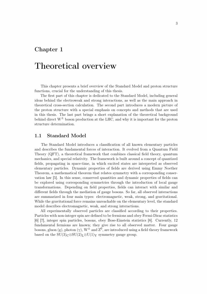
This chapter presents a brief overview of the Standard Model and proton structurefunctions, crucial for the understanding of this thesis.
The first part of this chapter is dedicated to the Standard Model, including generalideas behind the electroweak and strong interactions, as well as the main approach intheoretical cross-section calculation. The second part introduces a modern picture ofthe proton structure with a special emphasis on concepts and methods that are usedin this thesis. The last part brings a short explanation of the theoretical backgroundbehind direct W± boson production at the LHC, and why it is important for the protonstructure determination.
1.1 Standard Model
The Standard Model introduces a classification of all known elementary particlesand describes the fundamental forces of interaction. It evolved from a Quantum FieldTheory (QFT), a theoretical framework that combines classical field theory, quantummechanics, and special relativity. The framework is built around a concept of quantizedfields, propagating in space-time, in which excited states are interpreted as observedelementary particles. Dynamic properties of fields are derived using Emmy NoetherTheorem, a mathematical theorem that relates symmetry with a corresponding conser-vation law [5]. In this sense, conserved quantities and dynamic properties of fields canbe explored using corresponding symmetries through the introduction of local gaugetransformations. Depending on field properties, fields can interact with similar anddifferent fields through the mediation of gauge bosons. So far, all observed interactionsare summarized in four main types: electromagnetic, weak, strong, and gravitational.While the gravitational force remains unreachable on the elementary level, the standardmodel describes electromagnetic, weak, and strong interactions.
All experimentally observed particles are classified according to their properties.Particles with non-integer spin are defined to be fermions and obey Fermi-Dirac statistics[6] [7], integer spin particles, bosons, obey Bose-Einstein statistics [8]. Currently, 12fundamental fermions are known; they give rise to all observed matter. Four gaugebosons, gluon (g), photon (γ), W± and Z0, are introduced using a field theory frameworkbased on the SU(3)C⊗SU(2)L⊗U(1)Y symmetry gauge group.
4 Chapter 1. Theoretical overview
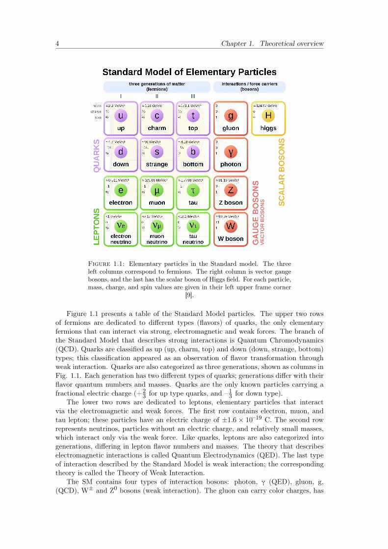
Figure 1.1: Elementary particles in the Standard model. The threeleft columns correspond to fermions. The right column is vector gaugebosons, and the last has the scalar boson of Higgs field. For each particle,mass, charge, and spin values are given in their left upper frame corner
[9].
Figure 1.1 presents a table of the Standard Model particles. The upper two rowsof fermions are dedicated to different types (flavors) of quarks, the only elementaryfermions that can interact via strong, electromagnetic and weak forces. The branch ofthe Standard Model that describes strong interactions is Quantum Chromodynamics(QCD). Quarks are classified as up (up, charm, top) and down (down, strange, bottom)types; this classification appeared as an observation of flavor transformation throughweak interaction. Quarks are also categorized as three generations, shown as columns inFig. 1.1. Each generation has two different types of quarks; generations differ with theirflavor quantum numbers and masses. Quarks are the only known particles carrying afractional electric charge (+2
3 for up type quarks, and – 13 for down type).The lower two rows are dedicated to leptons, elementary particles that interact
via the electromagnetic and weak forces. The first row contains electron, muon, andtau lepton; these particles have an electric charge of ±1.6 × 10⁻¹⁹ C. The second rowrepresents neutrinos, particles without an electric charge, and relatively small masses,which interact only via the weak force. Like quarks, leptons are also categorized intogenerations, differing in lepton flavor numbers and masses. The theory that describeselectromagnetic interactions is called Quantum Electrodynamics (QED). The last typeof interaction described by the Standard Model is weak interaction; the correspondingtheory is called the Theory of Weak Interaction.
The SM contains four types of interaction bosons: photon, γ (QED), gluon, g,(QCD), W± and Z0 bosons (weak interaction). The gluon can carry color charges, has
1.1. Standard Model 5
zero mass, and is being a self-interacting boson. W±, Z0, and photon are combinationsof electroweak gauge bosons. Unlike the rest of the bosons, W± and Z0 have a very highmass, shown in the upper left corner. Each of the bosons has a spin of 1. More detailson each of them will be given in a description of the corresponding type of interaction.The last but not least part of this table is a Higgs boson, a quantum excitation of theHiggs fields, responsible for the spontaneous symmetry breaking and mass generation[10], [11]. The observation was announced on 4th of July 2012 by CERN using dataanalysis results from two independent experiments ATLAS [12] and CMS [13].
The Standard Model still has unsolved questions, including the origin of dark matter,matter-antimatter asymmetry, dark energy interpretation, and others.
1.1.1 Strong interaction
Quantum Chromodynamics
QCD describes the interaction between hadrons, particles that interact via the strongforce. The hadrons consist of quarks, depending on a number of quarks, two or three,hadrons are called mesons or baryons, respectively. Each quark carries a specific type ofcharge called "color-charge", schematically denoted as red (r), blue (b), and green (g).Hadronic wave-function states can be derived introducing a concept of isospin quantumnumber, with the SU(2), ud, and SU(3)1, uds, flavor symmetries. The color states arederived using a non-abelian gauge theory, with a color symmetry group SU(3)C, whereC is denoted as "color".
The Lagrangian density of QCD is given by
LQCD =∑fψif(iγμD
μ – mf)ijψjf –
14Fμνa Faμν, (1.1)
here the f corresponds to a quark flavor, ψ is the field of a quark. ψ = ψ†γ0 is the Diracadjoint, γμ represent the Dirac matrices, mf is the quark mass, and Dμ is the covariantderivative given by the
Dμij = δij∂μ + ig(ta)ijA
μ
a, (1.2)
where taij are 3× 3 hermitian matrices, with elements (λa)ij/2 and λa are the Gell-Mannmatrices. The gluon field strength tensor Fμνa is given by
Fμνa = ∂μAνa – ∂νAμa + gfabcAμbA
νc, (1.3)
where Aa (a = 1...8) are the gluon fields, the last term corresponds to the interactionof the gluons with themselves as they also carry a color-charge. One of the uniqueproperties of QCD is the so-called color confinement, which means that colored quarkcannot exist in a free state. Another QCD property is asymptotic freedom, a reductionof the interaction coupling αs at small distances, and high values of the interaction scale.
Perturbative QCD and renormalization
Calculations of some interaction processes in QFT originate from the Fermi’s GoldenRule and perturbation expansion of the Transition Matrix Element. The QCD part,which is used in the perturbative regime, is called pQCD. This regime is based on
1Not exact symmetry due to difference in quark masses.
6 Chapter 1. Theoretical overview
perturbation series calculation of considered process. At higher-order correction calcu-lations, various mathematical obstacles lead to divergences in integration. Some of themare called infrared and collinear divergences and are common for QCD and QED. Theyappear from the multiple emission of particles with very low energy, or from consid-ered very small angles between the particle and its radiation. For example, a simplifiedcross-section expression for the process where a soft photon emerges from an electronafter some scattering process (e–(p + k)→ γ(k) + e–(p)) is given by:
dσ ∼∣∣∣∣ α
(p + k)2
∣∣∣∣2 d3kEk∼ α
2
E2p(1 – cosθeγ)
dEkEk
dΩ, (1.4)
where EP, Ek, are the energies of the final electron and photon, the angle between themis given by θeγ. From this expression, infrared singularity arises after integration of thedEk/Ek spectrum down to zero energy. Collinear singularity appears when θeγ → 0.Calculation of a finite result requires the usage of the approach called "renormalization".Various techniques were proposed over the years, some of them are Pauli and Villarsapproach, the minimal subtraction scheme of t’Hoft and Veltman (MS), and the modi-fied minimal subtraction scheme (MS). Usage of these techniques leads to dependenceon the artificially included parameter, renormalization scale, μr.
Strong coupling
Considering processes at higher energies, a contribution from virtual pairs, causedby the uncertainty principle, cannot be neglected. This makes a coupling constant tobe dependent on the scale at which observation is performed. This effect is known as a"running of the coupling", in QFT it is expressed through a beta-function, β(g), definedby:
β(g) ≡ μ∂g∂μ
=∂g
∂ln(μ), (1.5)
here μ corresponds to the energy scale of the given process. In QCD, the beta-functioncan be calculated as an expansion in αs
β(αs) = –b0α2s – b1α3s – b2α4s +O(α5s ), (1.6)
which depends on the number of active flavors, nf :
b0 =33 – 2nf12π
,
b1 =153 – 19nf
24π2,
b2 =77139 – 15099nf + 325n2f
3445π3. (1.7)
The QCD beta-function takes negative values, which finds its reflection in asymptoticfreedom, meaning the interaction intensity decreases as the process scale increases. The
1.1. Standard Model 7
equation for the running coupling at leading order can be written as:
α(Q2) =α(μ2)
1 + α(μ2)b0ln(Q2
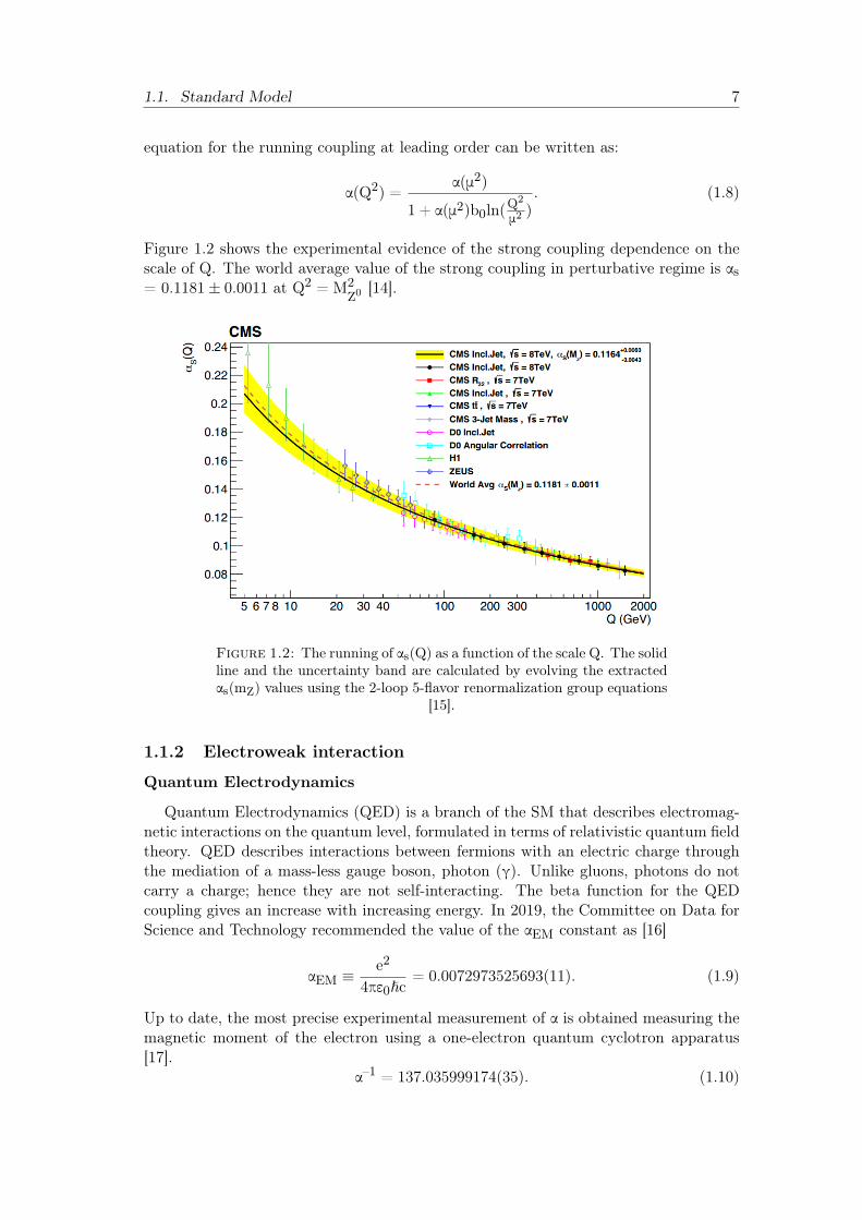
μ2). (1.8)
Figure 1.2 shows the experimental evidence of the strong coupling dependence on thescale of Q. The world average value of the strong coupling in perturbative regime is αs= 0.1181± 0.0011 at Q2 = M2
Z0 [14].
Figure 1.2: The running of αs(Q) as a function of the scale Q. The solidline and the uncertainty band are calculated by evolving the extractedαs(mZ) values using the 2-loop 5-flavor renormalization group equations
[15].
1.1.2 Electroweak interaction
Quantum Electrodynamics
Quantum Electrodynamics (QED) is a branch of the SM that describes electromag-netic interactions on the quantum level, formulated in terms of relativistic quantum fieldtheory. QED describes interactions between fermions with an electric charge throughthe mediation of a mass-less gauge boson, photon (γ). Unlike gluons, photons do notcarry a charge; hence they are not self-interacting. The beta function for the QEDcoupling gives an increase with increasing energy. In 2019, the Committee on Data forScience and Technology recommended the value of the αEM constant as [16]
αEM ≡e2
4πε0}c= 0.0072973525693(11). (1.9)
Up to date, the most precise experimental measurement of α is obtained measuring themagnetic moment of the electron using a one-electron quantum cyclotron apparatus[17].
α–1 = 137.035999174(35). (1.10)
8 Chapter 1. Theoretical overview
The running of the coupling is also inherited to αEM, but unlike αs, at higher energies,Q2 = m2
W, the value of the coupling is higher [14]:
α–1EM ∼ 128. (1.11)
The mathematical formulation of QED is built using the abelian gauge field with thesymmetry group U(1)em. The QED Lagrangian density is given by:
LQED = ψ(iγμDμ – m)ψ –14FμνFμν. (1.12)
Here ψ is a bi-spinor field of a charged lepton, Dμ is the QED gauge covariant derivativedefined by:
Dμ = ∂μ + ieAμ, (1.13)
where e is a coupling constant, m is a mass of a charged lepton, Aμ is the covariant four-potential of the electromagnetic field generated by the charged lepton, Fμν = ∂μAν –∂νAμ is the electromagnetic field tensor.
Weak interaction
All known fermions can interact via the weak force, exchanging three types ofbosons, W+, W–, and Z0. Unlike for QED and QCD, these bosons have a very highmass, mW± = 80.379± 0.012 GeV, mZ0 = 91.1876± 0.0021 GeV [14], which limits thedistance of interaction to 10–17 – 10–16 m.
In 1956, in the Wu experiment it was discovered that P-parity is violated by theweak interaction [18]. The explanation was proposed in 1957 in the "universal theory ofweak interactions", or "V-A theory" by Feynman, Lee, and Yang introducing projectionoperators that can transform a four-component spinor into a two-component left orright-handed spinor:
PR ≡1 + γ5
2, PL ≡
1 – γ5
2, (1.14)
where γ5 = iγ0γ1γ2γ3, and γi are the gamma matrices. This quantity is introduced aschirality, in which mathematical representation reflects whether the particle transformsin a left- or right-handed representation of the Poincare group. The weak symmetryis introduced through the weak isospin quantum number, usually marked as T or I.In quark flavor transformation the absolute value of the third component of the weakisospin, |T3| is conserved. In this process, a quark can change its flavor only into oneof the flavors of the opposite type. Figure 1.3 shows interaction relation between all sixquarks, grouped into doublets of up and down with T3 = +1
2 and T3 = – 12 , respectively.Up and down types of quarks and leptons are shown in Fig. 1.1.
1.1. Standard Model 9
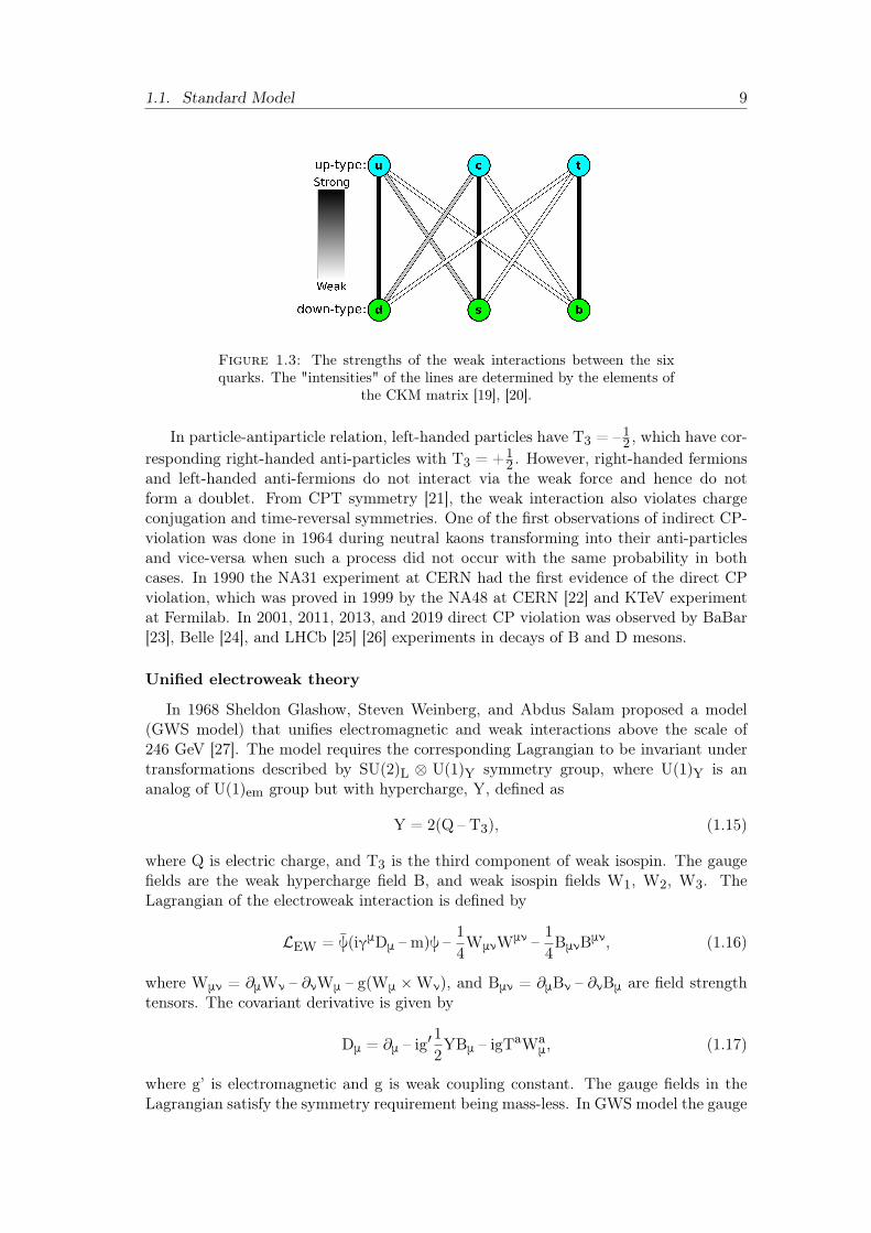
Figure 1.3: The strengths of the weak interactions between the sixquarks. The "intensities" of the lines are determined by the elements of
the CKM matrix [19], [20].
In particle-antiparticle relation, left-handed particles have T3 = – 12 , which have cor-responding right-handed anti-particles with T3 = +1
2 . However, right-handed fermionsand left-handed anti-fermions do not interact via the weak force and hence do notform a doublet. From CPT symmetry [21], the weak interaction also violates chargeconjugation and time-reversal symmetries. One of the first observations of indirect CP-violation was done in 1964 during neutral kaons transforming into their anti-particlesand vice-versa when such a process did not occur with the same probability in bothcases. In 1990 the NA31 experiment at CERN had the first evidence of the direct CPviolation, which was proved in 1999 by the NA48 at CERN [22] and KTeV experimentat Fermilab. In 2001, 2011, 2013, and 2019 direct CP violation was observed by BaBar[23], Belle [24], and LHCb [25] [26] experiments in decays of B and D mesons.
Unified electroweak theory
In 1968 Sheldon Glashow, Steven Weinberg, and Abdus Salam proposed a model(GWS model) that unifies electromagnetic and weak interactions above the scale of246 GeV [27]. The model requires the corresponding Lagrangian to be invariant undertransformations described by SU(2)L ⊗ U(1)Y symmetry group, where U(1)Y is ananalog of U(1)em group but with hypercharge, Y, defined as
Y = 2(Q – T3), (1.15)
where Q is electric charge, and T3 is the third component of weak isospin. The gaugefields are the weak hypercharge field B, and weak isospin fields W1, W2, W3. TheLagrangian of the electroweak interaction is defined by
LEW = ψ(iγμDμ – m)ψ –14WμνWμν –
14BμνBμν, (1.16)
where Wμν = ∂μWν – ∂νWμ – g(Wμ ×Wν), and Bμν = ∂μBν – ∂νBμ are field strengthtensors. The covariant derivative is given by
Dμ = ∂μ – ig′12YBμ – igTaWa
μ, (1.17)
where g’ is electromagnetic and g is weak coupling constant. The gauge fields in theLagrangian satisfy the symmetry requirement being mass-less. In GWS model the gauge
10 Chapter 1. Theoretical overview
fields W3 and B transform into γ and Z0 through a weak mixing angle, Weinberg angle,θW: (
γ
Z0
)=(
cosθW sinθW– sinθW cosθW
)(BW3
), (1.18)
while W+ and W– are a superposition of W1 and W2
W± =1√2W1 ∓W2. (1.19)
The interaction of the Higgs field with W± and Z0 generates the mass of these particles,making weak interaction weak and different from the electromagnetic force.
1.2 Proton structure
One of the first experiments on probing the proton structure was made in 1956 byE.E. Chambers and R. Hofstadter [28]. In this experiment, the proton structure (chargedistribution) was studied analyzing scattered high-energy electrons from protons inpolyethylene at the energies in the laboratory system of 200, 300, 400, 500, 550 MeV.Results showed a strong deviation from a point-like proton model. Since that time,many various experiments have proved the non-triviality of proton structure.
Nowadays, proton is classified as the lightest baryon in the baryon octet with themass mp = 938.27 MeV, a lower bound on its half-life is estimated to be >5.8×1029years [14]. In 2018 two independent groups measured a proton charge radius to benear rp = 0.833 ± 0.01 fm [29] and rp = 0.831 ± 0.007 ± 0.012 fm [30]. It is knownthat proton consists of partons, three so-called "valence quarks" (uud), gluons and seaquarks (fluctuating g ↔ qq states). It has a charge of +1, isospin I3 = 1
2 , and parityP = +1. The spin of a proton is S = 1
2 , but its nature is still a topic for debates dueto experimental results, which showed that the valence quark spin contribution into thetotal proton spin is at the level of 4% – 24% [31]. Despite various experimental resultsin this area, a theoretical model that would provide a prediction for proton structuredynamics is not reachable due to non-perturbative QCD phenomena and the absenceof valid mathematical methods. So far, the Parton Distribution Functions (PDF) areestimated using experimental data and phenomenological assumptions.
1.2.1 Parton Distribution Functions
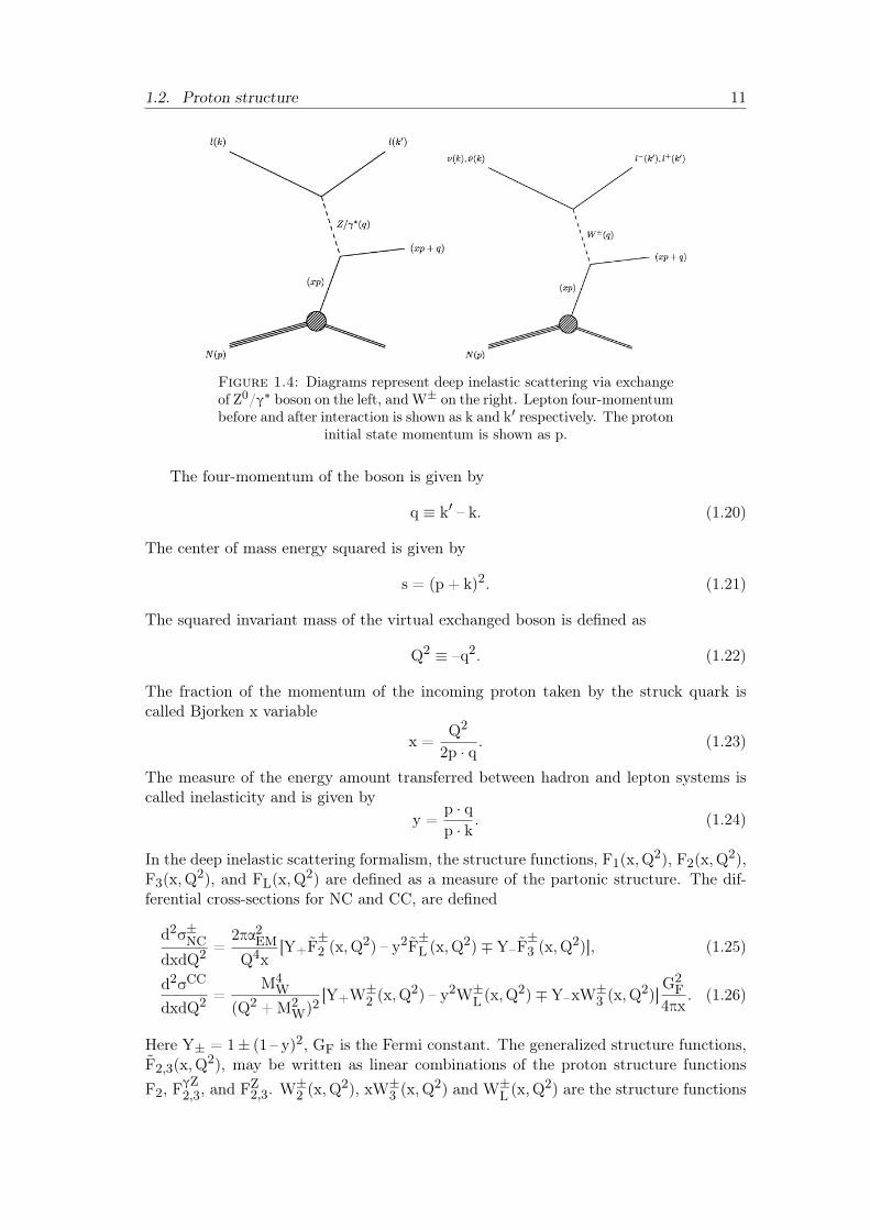
Significant progress in understanding of the proton structure was achieved after thebeginning of "Deep Inelastic Scattering" (DIS) experiments. In these experiments, highenergetic leptons (e±, μ–, ν) were scattering on hadrons. Early experiments with thefixed target and lepton (e–, μ–, ν) beams were performed in SLAC and CERN. Later,e±p scattering was performed at the HERA accelerator at DESY. The experiments wereable to reach the level of quark and gluon resolution, probing the hadron state. Thelepton-proton scattering diagrams are shown in Fig. 1.4. The interaction is performedthrough a vector boson exchange (W±, Z0, or γ). Depending on the boson charge,processes are defined as Neutral Current (NC) and Charged Current (CC).
1.2. Proton structure 11
Figure 1.4: Diagrams represent deep inelastic scattering via exchangeof Z0/γ∗ boson on the left, andW± on the right. Lepton four-momentumbefore and after interaction is shown as k and k′ respectively. The proton
initial state momentum is shown as p.
The four-momentum of the boson is given by
q ≡ k′ – k. (1.20)
The center of mass energy squared is given by
s = (p + k)2. (1.21)
The squared invariant mass of the virtual exchanged boson is defined as
Q2 ≡ –q2. (1.22)
The fraction of the momentum of the incoming proton taken by the struck quark iscalled Bjorken x variable
x =Q2
2p · q. (1.23)
The measure of the energy amount transferred between hadron and lepton systems iscalled inelasticity and is given by
y =p · qp · k
. (1.24)
In the deep inelastic scattering formalism, the structure functions, F1(x,Q2), F2(x,Q2),F3(x,Q2), and FL(x,Q2) are defined as a measure of the partonic structure. The dif-ferential cross-sections for NC and CC, are defined
d2σ±NCdxdQ2 =
2πα2EMQ4x
[Y+F±2 (x,Q
2) – y2F±L (x,Q
2)∓Y–F±3 (x,Q
2)], (1.25)
d2σCC
dxdQ2 =M4
W(Q2 +M2
W)2[Y+W±2 (x,Q
2) – y2W±L (x,Q2)∓Y–xW±3 (x,Q
2)]G2F
4πx. (1.26)
Here Y± = 1± (1 – y)2, GF is the Fermi constant. The generalized structure functions,F2,3(x,Q2), may be written as linear combinations of the proton structure functionsF2, F
γZ2,3, and FZ2,3. W
±2 (x,Q
2), xW±3 (x,Q2) and W±L (x,Q
2) are the structure functions
12 Chapter 1. Theoretical overview
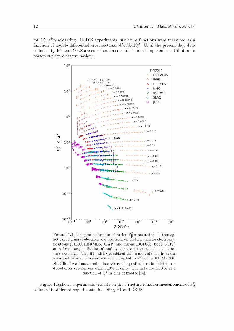
for CC e±p scattering. In DIS experiments, structure functions were measured as afunction of double differential cross-sections, d2σ/dxdQ2. Until the present day, datacollected by H1 and ZEUS are considered as one of the most important contributors toparton structure determinations.
Figure 1.5: The proton structure function F2p measured in electromag-netic scattering of electrons and positrons on protons, and for electrons/-positrons (SLAC, HERMES, JLAB) and muons (BCDMS, E665, NMC)on a fixed target. Statistical and systematic errors added in quadra-ture are shown. The H1+ZEUS combined values are obtained from themeasured reduced cross-section and converted to F2p with a HERA-PDFNLO fit, for all measured points where the predicted ratio of F2p to re-duced cross-section was within 10% of unity. The data are plotted as a
function of Q2 in bins of fixed x [14].
Figure 1.5 shows experimental results on the structure function measurement of Fp2collected in different experiments, including H1 and ZEUS.
1.2. Proton structure 13
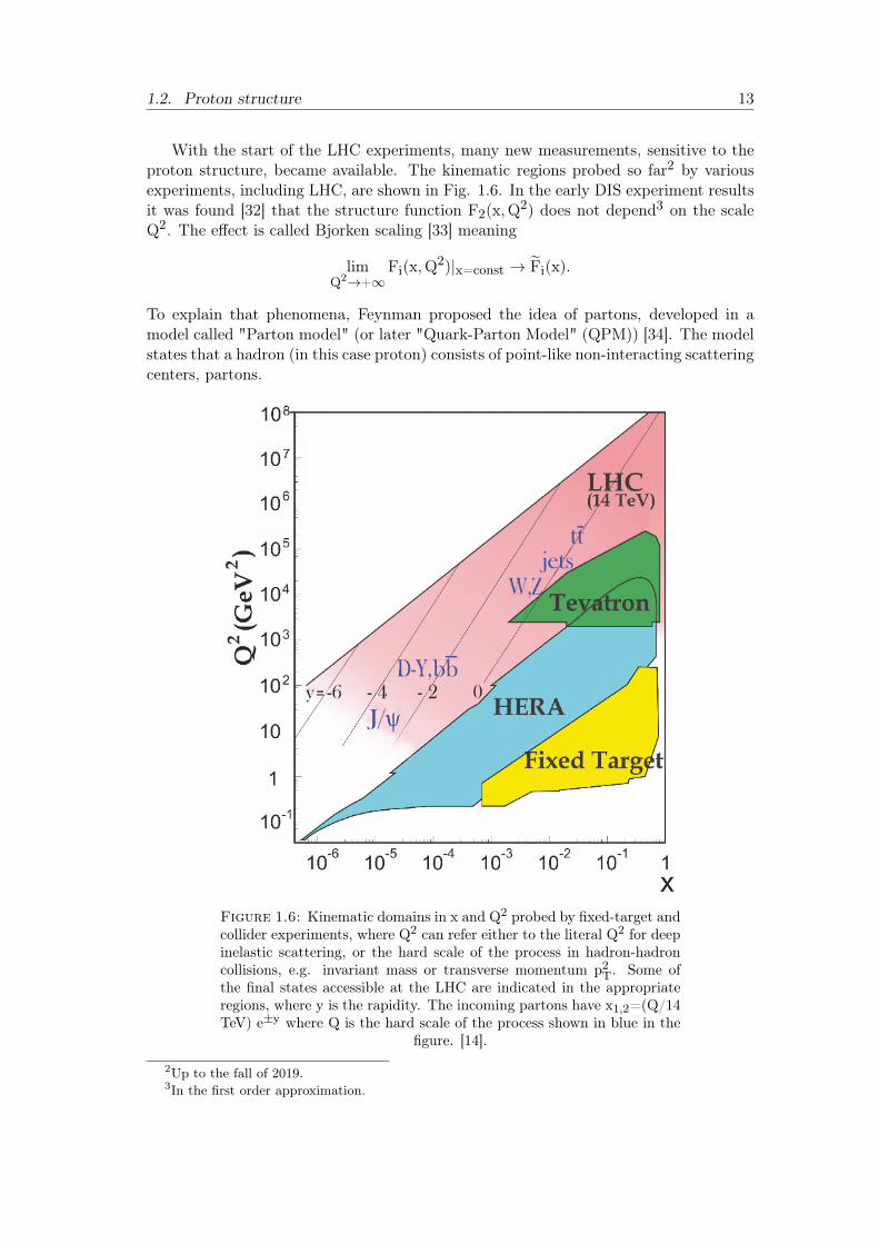
With the start of the LHC experiments, many new measurements, sensitive to theproton structure, became available. The kinematic regions probed so far2 by variousexperiments, including LHC, are shown in Fig. 1.6. In the early DIS experiment resultsit was found [32] that the structure function F2(x,Q2) does not depend3 on the scaleQ2. The effect is called Bjorken scaling [33] meaning
limQ2→+∞
Fi(x,Q2)|x=const → Fi(x).
To explain that phenomena, Feynman proposed the idea of partons, developed in amodel called "Parton model" (or later "Quark-Parton Model" (QPM)) [34]. The modelstates that a hadron (in this case proton) consists of point-like non-interacting scatteringcenters, partons.
Figure 1.6: Kinematic domains in x and Q2 probed by fixed-target andcollider experiments, where Q2 can refer either to the literal Q2 for deepinelastic scattering, or the hard scale of the process in hadron-hadroncollisions, e.g. invariant mass or transverse momentum p2T. Some ofthe final states accessible at the LHC are indicated in the appropriateregions, where y is the rapidity. The incoming partons have x1,2=(Q/14TeV) e±y where Q is the hard scale of the process shown in blue in the
figure. [14].
2Up to the fall of 2019.3In the first order approximation.
14 Chapter 1. Theoretical overview
In the QPM frame, the transverse structure function can be re-written as
F2(x) =∑i
e2i xf i(x), (1.27)
where the sum over partons with a given charge ei and function f i(x) is unknown,however, the f i(x) is interpreted as a probability that the i-th parton is carrying xfraction of the proton momentum, parton momentum density.
Various quark-parton model tests have shown that the proton consists not only ofthe valence quarks but also has sea-quarks, which consists of quark-antiquark pairs withno overall flavor. Taking this into account
Fi(x) =∑i
e2i [xqi(x) + xqi(x)]. (1.28)
Knowing the number of valence quarks allows to define some additional constraints, theso-called "sum rules" ∫ 1
0uv(x)dx = 2,
∫ 1
0dv(x)dx = 1, (1.29)
where uv and dv are distributions for valence up and down quarks, respectively. A veryimportant momentum sum rule defines the sum over all quark and antiquark types inthe proton ∫ 1
0xΣ(x)dx = 1, (1.30)
where Σ(x) = u(x) + u(x) + d(x) + d(x) + s(x) + s(x) + c(x) + c(x) + b(x) + b(x)4.Neutrino-nucleus and anti-neutrino-nucleus scattering experiments have shown [35]
that only 50% of proton momentum is coming from quarks, the rest was contributedby particles that interact only via strong force - gluons. The gluon was discovered in1979 with the PETRA collider at DESY [36]. To account for gluon contribution, themomentum sum rule is given by
∑i
∫ 1
0xf i(x)dx +
∫ 1
0xg(x)dx = 1 (1.31)
1.2.2 Factorization theorem and PDF evolution equations
Cross-section calculations of the hard interactions, calculable in pQCD, rely on theassumption that the time scale of the hard scatter is relatively much shorter than thefinal state hadronization [37]. The approach is formulated as a Factorization theorem,which allows factorizing the cross-section into the probability of the hard scatteringand a probability density for finding a parton that carries a certain amount of hadronmomentum [38]. In this scheme, the parton-parton interaction cross-section can becalculated in the pQCD regime using a general approach at LO, NLO, NNLO, etc. withthe corresponding strong coupling defined at renormalization scale μr and order p. Thenon-perturbative part of the process, the PDF, is separated from the pQCD, introducinga factorization scale, μf , which is not necessarily equivalent to μr. Infrared singularitiesare handled by renormalization at the factorization scale; collinear singularities are
4The top quark may be also included.
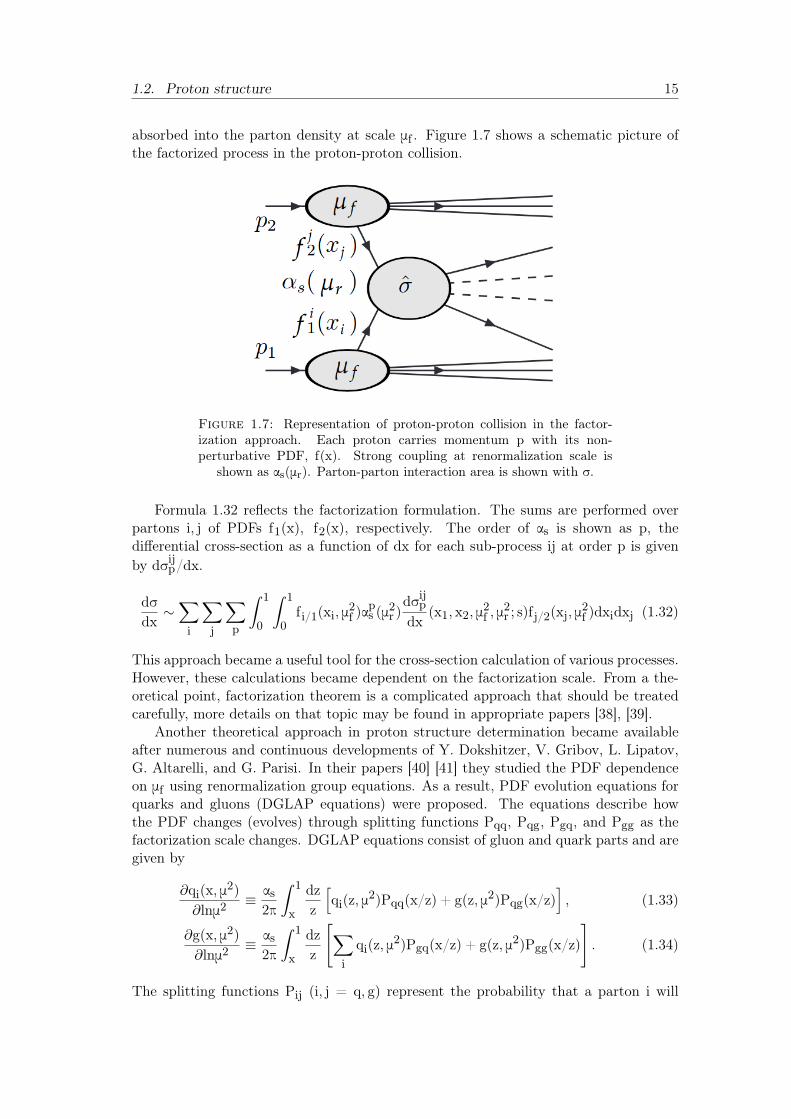
1.2. Proton structure 15
absorbed into the parton density at scale μf . Figure 1.7 shows a schematic picture ofthe factorized process in the proton-proton collision.
Figure 1.7: Representation of proton-proton collision in the factor-ization approach. Each proton carries momentum p with its non-perturbative PDF, f(x). Strong coupling at renormalization scale is
shown as αs(μr). Parton-parton interaction area is shown with σ.
Formula 1.32 reflects the factorization formulation. The sums are performed overpartons i, j of PDFs f1(x), f2(x), respectively. The order of αs is shown as p, thedifferential cross-section as a function of dx for each sub-process ij at order p is givenby dσijp/dx.
dσdx∼∑i
∑j
∑p
∫ 1
0
∫ 1
0f i/1(xi, μ
2f )α
ps (μ2r )
dσijpdx
(x1, x2, μ2f , μ2r ; s)fj/2(xj, μ
2f )dxidxj (1.32)
This approach became a useful tool for the cross-section calculation of various processes.However, these calculations became dependent on the factorization scale. From a the-oretical point, factorization theorem is a complicated approach that should be treatedcarefully, more details on that topic may be found in appropriate papers [38], [39].
Another theoretical approach in proton structure determination became availableafter numerous and continuous developments of Y. Dokshitzer, V. Gribov, L. Lipatov,G. Altarelli, and G. Parisi. In their papers [40] [41] they studied the PDF dependenceon μf using renormalization group equations. As a result, PDF evolution equations forquarks and gluons (DGLAP equations) were proposed. The equations describe howthe PDF changes (evolves) through splitting functions Pqq, Pqg, Pgq, and Pgg as thefactorization scale changes. DGLAP equations consist of gluon and quark parts and aregiven by
∂qi(x, μ2)∂lnμ2
≡ αs2π
∫ 1
x
dzz
[qi(z, μ
2)Pqq(x/z) + g(z, μ2)Pqg(x/z)], (1.33)
∂g(x, μ2)∂lnμ2
≡ αs2π
∫ 1
x
dzz
[∑i
qi(z, μ2)Pgq(x/z) + g(z, μ2)Pgg(x/z)
]. (1.34)
The splitting functions Pij (i, j = q, g) represent the probability that a parton i will
16 Chapter 1. Theoretical overview
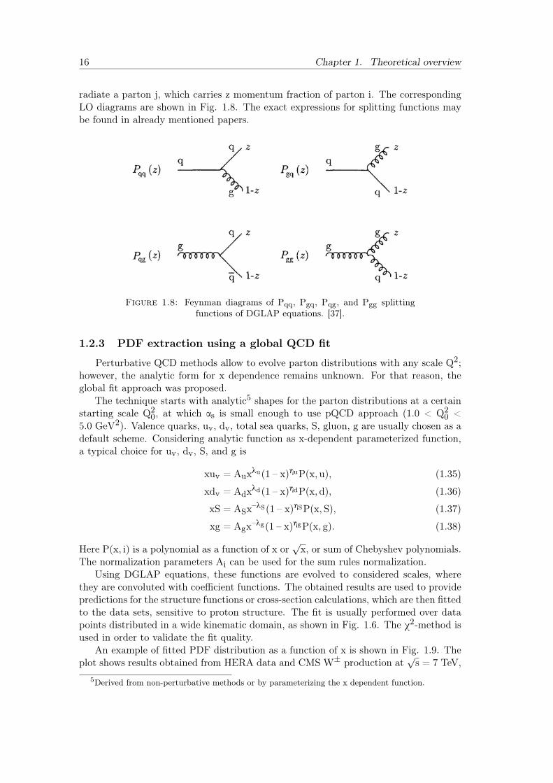
radiate a parton j, which carries z momentum fraction of parton i. The correspondingLO diagrams are shown in Fig. 1.8. The exact expressions for splitting functions maybe found in already mentioned papers.
Figure 1.8: Feynman diagrams of Pqq, Pgq, Pqg, and Pgg splittingfunctions of DGLAP equations. [37].
1.2.3 PDF extraction using a global QCD fit
Perturbative QCD methods allow to evolve parton distributions with any scale Q2;however, the analytic form for x dependence remains unknown. For that reason, theglobal fit approach was proposed.
The technique starts with analytic5 shapes for the parton distributions at a certainstarting scale Q2
0, at which αs is small enough to use pQCD approach (1.0 < Q20 <
5.0 GeV2). Valence quarks, uv, dv, total sea quarks, S, gluon, g are usually chosen as adefault scheme. Considering analytic function as x-dependent parameterized function,a typical choice for uv, dv, S, and g is
xuv = Auxλu(1 – x)ηuP(x, u), (1.35)
xdv = Adxλd(1 – x)ηdP(x, d), (1.36)
xS = ASx–λS(1 – x)ηSP(x, S), (1.37)
xg = Agx–λg(1 – x)ηgP(x, g). (1.38)
Here P(x, i) is a polynomial as a function of x or√x, or sum of Chebyshev polynomials.
The normalization parameters Ai can be used for the sum rules normalization.Using DGLAP equations, these functions are evolved to considered scales, where
they are convoluted with coefficient functions. The obtained results are used to providepredictions for the structure functions or cross-section calculations, which are then fittedto the data sets, sensitive to proton structure. The fit is usually performed over datapoints distributed in a wide kinematic domain, as shown in Fig. 1.6. The χ2-method isused in order to validate the fit quality.
An example of fitted PDF distribution as a function of x is shown in Fig. 1.9. Theplot shows results obtained from HERA data and CMS W± production at
√s = 7 TeV,
5Derived from non-perturbative methods or by parameterizing the x dependent function.
1.3. W± boson production at LHC 17
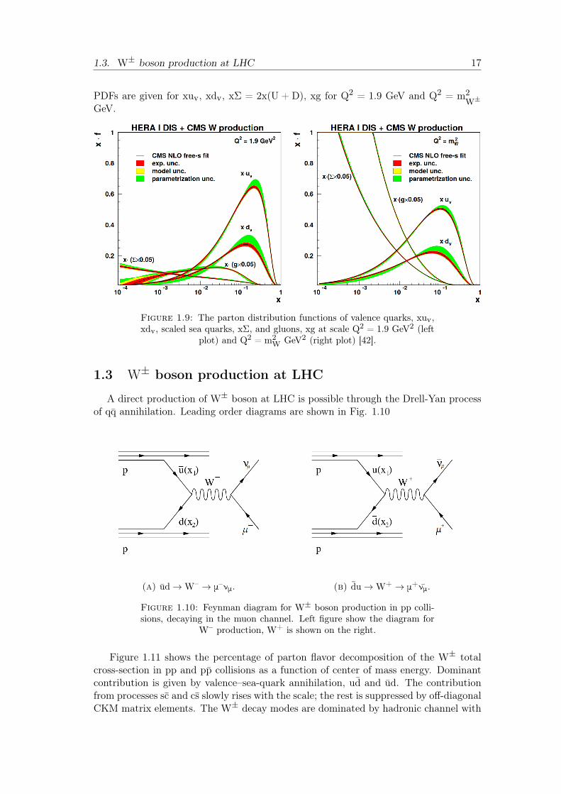
PDFs are given for xuv, xdv, xΣ = 2x(U + D), xg for Q2 = 1.9 GeV and Q2 = m2W±
GeV.
Figure 1.9: The parton distribution functions of valence quarks, xuv,xdv, scaled sea quarks, xΣ, and gluons, xg at scale Q2 = 1.9 GeV2 (left
plot) and Q2 = m2W GeV2 (right plot) [42].
1.3 W± boson production at LHC
A direct production of W± boson at LHC is possible through the Drell-Yan processof qq annihilation. Leading order diagrams are shown in Fig. 1.10
(a) ud→W– → μ–νμ. (b) du→W+ → μ+νμ.
Figure 1.10: Feynman diagram for W± boson production in pp colli-sions, decaying in the muon channel. Left figure show the diagram for
W– production, W+ is shown on the right.
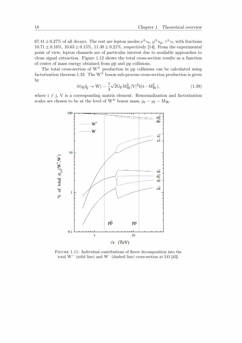
Figure 1.11 shows the percentage of parton flavor decomposition of the W± totalcross-section in pp and pp collisions as a function of center of mass energy. Dominantcontribution is given by valence–sea-quark annihilation, ud and ud. The contributionfrom processes sc and cs slowly rises with the scale; the rest is suppressed by off-diagonalCKM matrix elements. The W± decay modes are dominated by hadronic channel with
18 Chapter 1. Theoretical overview
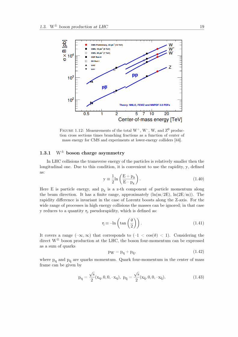
67.41± 0.27% of all decays. The rest are lepton modes e±νe, μ±νμ, τ±ντ with fractions10.71± 0.16%, 10.63± 0.15%, 11.38± 0.21%, respectively [14]. From the experimentalpoint of view, lepton channels are of particular interest due to available approaches toclean signal extraction. Figure 1.12 shows the total cross-section results as a functionof center of mass energy obtained from pp and pp collisions.
The total cross-section of W± production in pp collisions can be calculated usingfactorization theorem 1.32. The W± boson sub-process cross-section production is givenby
σ(qiqj →W) =π
3√2GFM
2W|V|2δ(s – M2
W), (1.39)
where i 6= j, V is a corresponding matrix element. Renormalization and factorizationscales are chosen to be at the level of W± boson mass, μr = μf = MW.
Figure 1.11: Individual contributions of flavor decomposition into thetotal W+ (solid line) and W– (dashed line) cross-section at LO [43].
1.3. W± boson production at LHC 19
Figure 1.12: Measurements of the total W+, W–, W, and Z0 produc-tion cross sections times branching fractions as a function of center ofmass energy for CMS and experiments at lower-energy colliders [44].
1.3.1 W± boson charge asymmetry
In LHC collisions the transverse energy of the particles is relatively smaller then thelongitudinal one. Due to this condition, it is convenient to use the rapidity, y, definedas:
y ≡ 12ln(E + pzE – pz
). (1.40)
Here E is particle energy, and pz is a z-th component of particle momentum alongthe beam direction. It has a finite range, approximately (ln(m/2E), ln(2E/m)). Therapidity difference is invariant in the case of Lorentz boosts along the Z-axis. For thewide range of processes in high energy collisions the masses can be ignored; in that casey reduces to a quantity η, pseudorapidity, which is defined as:
η ≡ –ln(tan
(θ
2
)). (1.41)
It covers a range (–∞,∞) that corresponds to (–1 < cos(θ) < 1). Considering thedirect W± boson production at the LHC, the boson four-momentum can be expressedas a sum of quarks
pW = pq + pq, (1.42)
where pq and pq are quarks momentum. Quark four-momentum in the center of massframe can be given by
pq =√s2(xq, 0, 0, –xq), pq =
√s2(xq, 0, 0, –xq). (1.43)
20 Chapter 1. Theoretical overview
Using these equations together with Eq. 1.40, it can be shown how the boson rapiditydepends on quarks momentum
yW =12ln(xqxq
). (1.44)
The scale of interaction is usually taken as the boson mass, q2 = m2W±
, combiningthis relation with s = 4E2 it can be shown how the boson mass is connected with themomentum fraction of quarks
m2W± = xqxqs. (1.45)
The final expression for quark momentum fraction as a function of the boson mass,rapidity, and the proton center of mass energy can be derived combining Eq. 1.45 andEq. 1.44
xq =mW±√
seyW± , xq =
mW±√s
e–yW± . (1.46)
Taking into account individual contributions of flavor decomposition shown in Fig.1.11, the attention is focused on ud and ud production mechanism. W+ bosons arepredominantly produced in the direction of up quark, while W– are produced in thedirection of a down quark. The differential cross-section as a function of rapidity (orpseudorapidity) can be studied to explore the proton structure. It can be derivedusing the Cabibbo mixing approximation [45] together with an SU(3) symmetric seaapproximation [46]
dσdy∼ 2πGF
3√2xaxb[u(xa)d(xb) + d(xa)u(xb)]. (1.47)
Since proton has two up and one down quark, up quark has higher chances to befound in the proton than the down quark (see Fig. 1.9), that leads to quantitativelyasymmetric production of W+ bosons over W–. The asymmetry can be defined throughthe W± boson production as a function rapidity by
AW±(y) ≡dσW+/dy – dσW–/dydσW+/dy + dσW–/dy
, (1.48)
where dσW±/dy is a differential cross-section value as a function of boson rapidity. Thisequation can be re-written in terms of the production mechanism
AW±(y) ≈u(x)d(x) – d(x)u(x)u(x)d(x) + d(x)u(x)
, (1.49)
where u(x) and d(x) are PDFs of valence up and down quarks, while u and d are anti-up and anti-down PDFs of sea quarks. The sensitivity to valence quarks can only beobtained for a region of low x of sea quarks, when approximation d ∼ u ∼ q is valid
AW±(y) ∼u(x) – d(x)u(x) + d(x)
. (1.50)
1.3. W± boson production at LHC 21
W± boson charge asymmetry is usually studied using the lepton channel of W± decay.Lepton asymmetry can be defined by
Al±(η) ≡dσ/dηl+ – dσ/dηl–dσ/dηl+ + dσ/dηl–
. (1.51)
Due to the vector-axial nature of the leptonic W± decay, the lepton asymmetry has morecomplicated explanation. The laws of weak interaction impose limitations on W± bosonand fermion mechanism of coupling. The W– boson can interact only with left-handedfermions or right-handed anti-fermions and vice-versa. This makes the dependence ofW± matrix element on the angle between lepton and the boson, sensitive to differentboson polarization.
|M–|2 = g2Wm2W
14(1 + cosθ)2, (1.52)
|ML|2 = g2Wm2
W12sin2 θ, (1.53)
|M+|2 = g2Wm2W
14(1 – cosθ)2. (1.54)
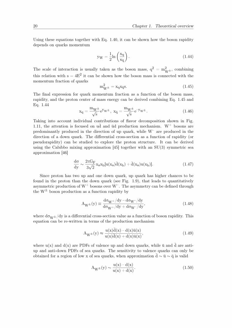
Figure 1.13: W± boson in different helicity states decaying into elec-tron channel in a rest frame. The first row corresponds to three differenthelicity states, left-handed (negative), longitudinal, and right-handed(positive). Blue arrows are momentum; red arrows are helicity states ofdaughter particles, while the yellow arrow shows the boson spin projec-tion on the z-axis. The second row shows the matrix element dependence
on the theta angle for each helicity state [47].
Figure 1.13 in the first row illustrates different helicity states of W– boson in therest frame. The incoming quark is left-handed, while anti-quark is right-handed, due toangular momentum conservation, the helicity of the W± must be left-handed, especiallyfor high rapidity. In some cases, anti-quark might have a higher fraction of protonmomentum than the valence quark, making the W± boson polarization right-handed.As a result, angular momentum conservation law, V-A formalism, and matrix elementdependence on helicity state cause the difference in dσ/dη distributions for W+ andW–. When ud annihilates into W+, the dominant part of bosons has left-handed
22 Chapter 1. Theoretical overview
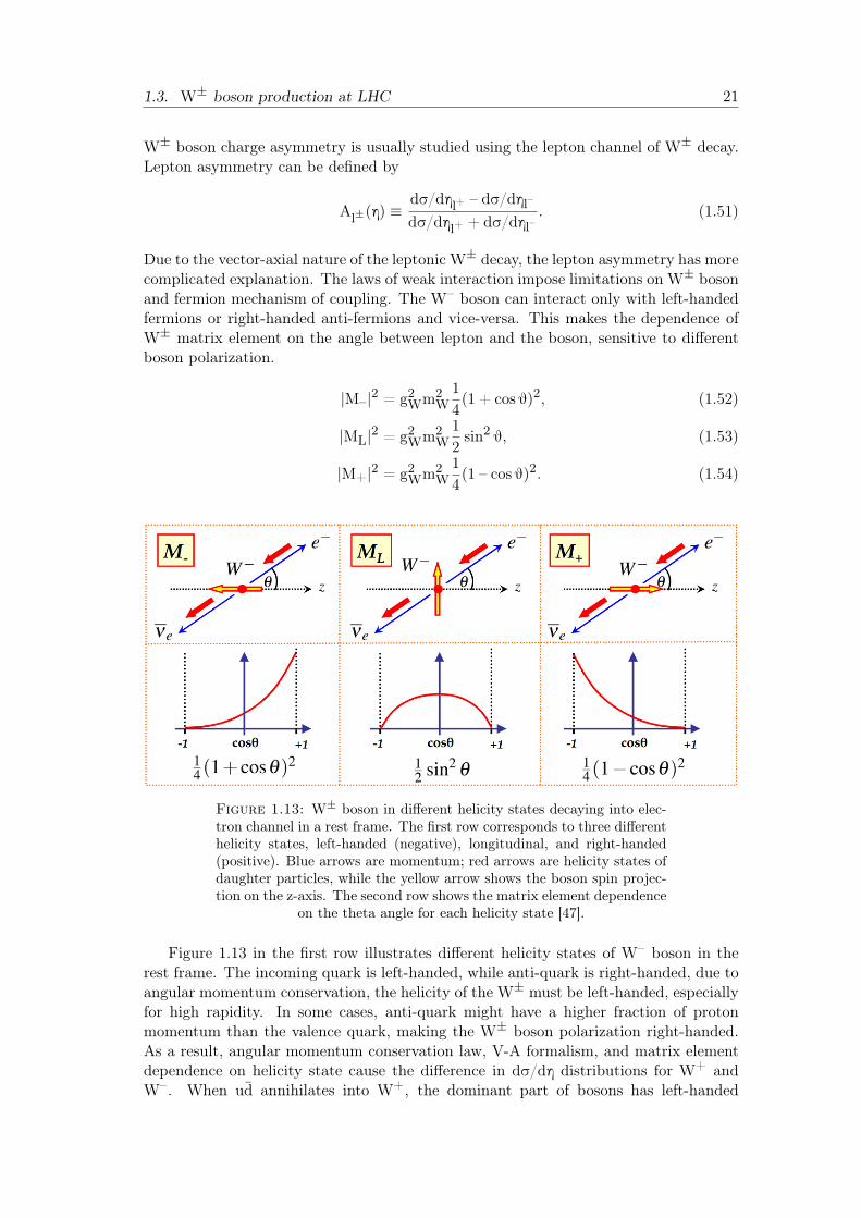
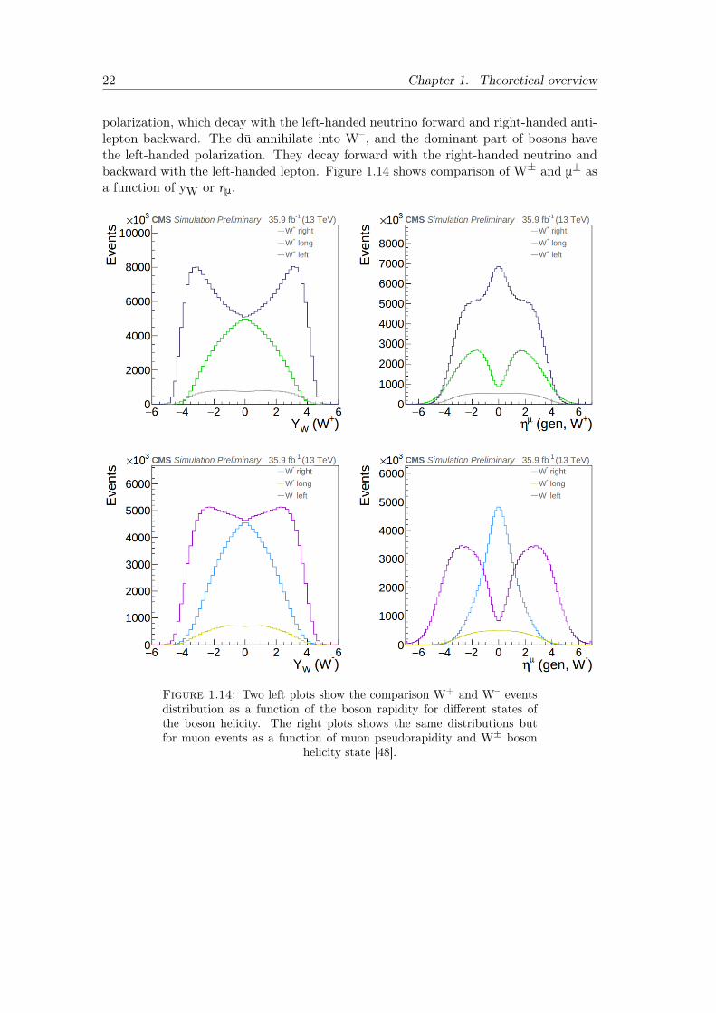
polarization, which decay with the left-handed neutrino forward and right-handed anti-lepton backward. The du annihilate into W–, and the dominant part of bosons havethe left-handed polarization. They decay forward with the right-handed neutrino andbackward with the left-handed lepton. Figure 1.14 shows comparison of W± and μ± asa function of yW or ημ.
Figure 1.14: Two left plots show the comparison W+ and W– eventsdistribution as a function of the boson rapidity for different states ofthe boson helicity. The right plots shows the same distributions butfor muon events as a function of muon pseudorapidity and W± boson
helicity state [48].
23
Chapter 2
LHC and CMS experiment
The leading player on the experimental high energy field today is the Large HadronCollider (LHC), together with its four main experiments: A Large Ion Collider Experi-ment (ALICE), A Toroidal LHC Apparatus (ATLAS), Compact Muon Solenoid (CMS),and LHC-beauty (LHCb). Four years after the LHC launch, in July 2012, CMS andATLAS, independently, reported on the observation of the boson that was predicted tobe responsible for the mass generation mechanism. [12], [13]. The observation of theHiggs boson became a great success and a triumph of modern particle physics.
Studies and results presented in this thesis are achieved performing an analysis ofdata collected with the CMS detector at the LHC. The next section describes the LHCpurpose and design. After that, a section is dedicated to the CMS detector and its maincomponents.
2.1 Large Hadron Collider
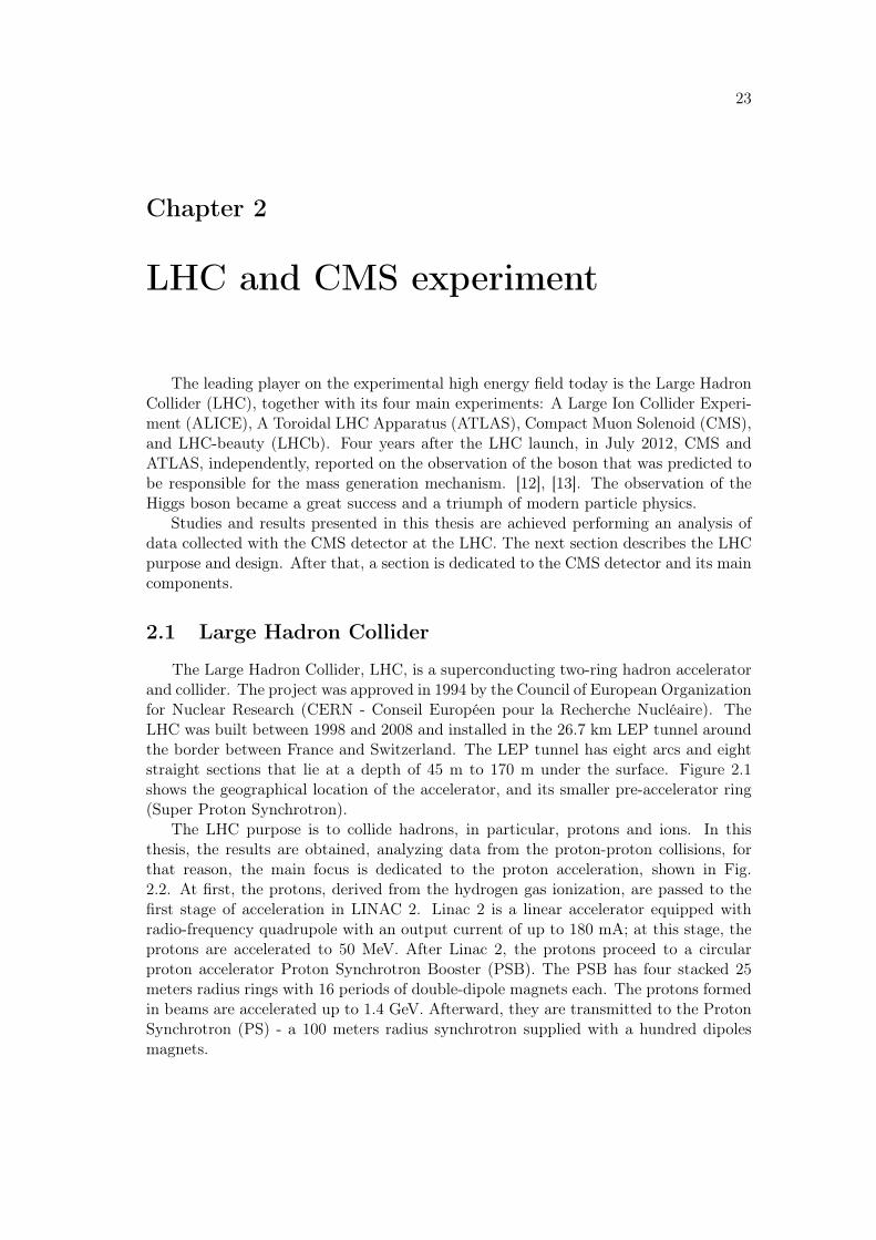
The Large Hadron Collider, LHC, is a superconducting two-ring hadron acceleratorand collider. The project was approved in 1994 by the Council of European Organizationfor Nuclear Research (CERN - Conseil Européen pour la Recherche Nucléaire). TheLHC was built between 1998 and 2008 and installed in the 26.7 km LEP tunnel aroundthe border between France and Switzerland. The LEP tunnel has eight arcs and eightstraight sections that lie at a depth of 45 m to 170 m under the surface. Figure 2.1shows the geographical location of the accelerator, and its smaller pre-accelerator ring(Super Proton Synchrotron).
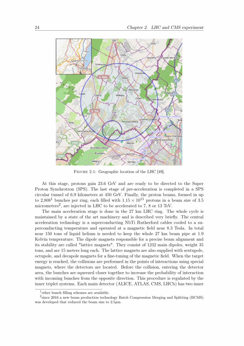
The LHC purpose is to collide hadrons, in particular, protons and ions. In thisthesis, the results are obtained, analyzing data from the proton-proton collisions, forthat reason, the main focus is dedicated to the proton acceleration, shown in Fig.2.2. At first, the protons, derived from the hydrogen gas ionization, are passed to thefirst stage of acceleration in LINAC 2. Linac 2 is a linear accelerator equipped withradio-frequency quadrupole with an output current of up to 180 mA; at this stage, theprotons are accelerated to 50 MeV. After Linac 2, the protons proceed to a circularproton accelerator Proton Synchrotron Booster (PSB). The PSB has four stacked 25meters radius rings with 16 periods of double-dipole magnets each. The protons formedin beams are accelerated up to 1.4 GeV. Afterward, they are transmitted to the ProtonSynchrotron (PS) - a 100 meters radius synchrotron supplied with a hundred dipolesmagnets.
24 Chapter 2. LHC and CMS experiment
Figure 2.1: Geographic location of the LHC [49].
At this stage, protons gain 23.6 GeV and are ready to be directed to the SuperProton Synchrotron (SPS). The last stage of pre-acceleration is completed in a SPScircular tunnel of 6.9 kilometers at 450 GeV. Finally, the proton beams, formed in upto 2,8081 bunches per ring, each filled with 1.15 × 10¹¹ protons in a beam size of 3.5micrometers2, are injected in LHC to be accelerated to 7, 8 or 13 TeV.
The main acceleration stage is done in the 27 km LHC ring. The whole cycle ismaintained by a state of the art machinery and is described very briefly. The centralacceleration technology is a superconducting NbTi Rutherford cables cooled to a su-perconducting temperature and operated at a magnetic field near 8.3 Tesla. In totalnear 150 tons of liquid helium is needed to keep the whole 27 km beam pipe at 1.9Kelvin temperature. The dipole magnets responsible for a precise beam alignment andits stability are called "lattice magnets". They consist of 1232 main dipoles, weight 35tons, and are 15 meters long each. The lattice magnets are also supplied with sextupole,octupole, and decapole magnets for a fine-tuning of the magnetic field. When the targetenergy is reached, the collisions are performed in the points of interactions using specialmagnets, where the detectors are located. Before the collision, entering the detectorarea, the bunches are squeezed closer together to increase the probability of interactionwith incoming bunches from the opposite direction. This procedure is regulated by theinner triplet systems. Each main detector (ALICE, ATLAS, CMS, LHCb) has two inner
1other bunch filling schemes are available.2since 2016 a new beam production technology Batch Compression Merging and Splitting (BCMS)
was developed that reduced the beam size to 2.5μm.
2.1. Large Hadron Collider 25
triplet systems from both sides to squeeze the beams right before the interaction from0.2 millimeters to 16 micrometers across.
Figure 2.2: Acceleration scheme [50].
A tight packaging of bunches results in a small interval between the bunches colli-sions. Twenty-five nanosecond gap between the interactions forms a 40 MHz collisionrate that creates a significant challenge to the detecting technologies and readout sys-tems. After a collision, using dipole magnets, the beams are split back to be used infurther collisions. At a certain point, the sufficient amount of protons diminishes to thethreshold value, and the bunches are deflected from the LHC through the beam dumpprocedure.
The LHC goal is to provide a good quality interaction for the main experiments withthe center of mass collision energy up to 14 TeV. Run 1 took place in 2009-2013; duringthat period, LHC maintained collisions at 7 and 8 TeV center of mass energy. Theamount of data recorded during that period was sufficient to report the observationof the Higgs boson. A long shut down in 2013-2015 was necessary for acceleratorand detectors to upgrade. The second operational run (Run 2) started in 2015 withthe first-ever reached center of mass energy of 13 TeV and ended in late 2018. Theresults presented in this thesis are obtained after analyzing data collected with theCMS detector during the first period (2015) of Run 2. Since December 2018 and until2021, the LHC and all detectors are on a long shutdown to replace few components.One of the goals of this period is to prepare for the High Luminosity LHC (HL-LHC),which is supposed to increase luminosity by a factor of 5-7. The next Run 3 is plannedto start in 2021 and to last until 2024, while HL-LHC will start in 2027, in the presentschedule.
A straightforward characteristic of the collisions is the number of collision eventsgenerated per second, R, given by the expression:
R = L× σevent, (2.1)
26 Chapter 2. LHC and CMS experiment
where L is the machine luminosity and σ is the cross-section. The luminosity variabledepends on the parameters of the beams and can be defined as:
L =N2bnbfrevγr4πεnβ∗
F, (2.2)
where εn is the normalized transverse beam emittance, β∗ is the beta function at thecollision point, and F corresponds to the geometric luminosity reduction factor due tothe crossing angle at the interaction point. Nb is the number of particles in a bunch,γr the relativistic gamma factor, nb is the number of bunches per beam, frev is therevolution frequency [51]. More details on luminosity measurements is given in chapter4.
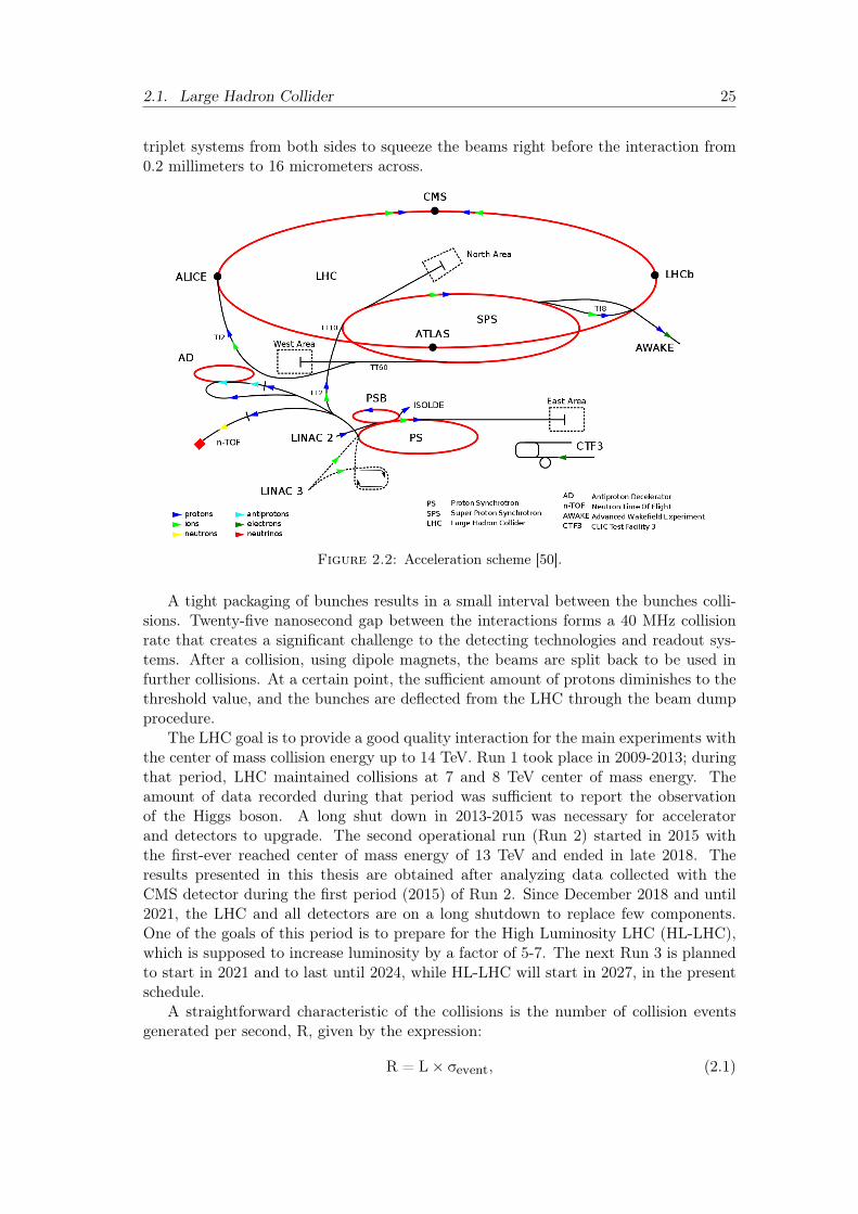
One of the main goals of the LHC is to deliver the designed luminosity L =1034cm–2s–1 for the high luminosity experiments ATLAS and CMS. In September 2018,the LHC has reported in "The final days of Run 2" the successful delivery of designedluminosity for CMS and ATLAS [52]. The report was given a week before the shutdown,but already then it was clear that the machine achieved one of its main tasks. Figure2.3 shows the integrated luminosity during Run 1 and Run 2.
Figure 2.3: LHC report on the delivered luminosityduring RUN 1 and RUN 2.
2.2 Compact Muon Solenoid
The CMS project approval in 1993 initiated a formation of the CMS collaborationthat consists of over 4000 particle physicists, computer scientists, technicians, engineers,and students from near 200 universities and institutes from more than 40 countries. Theobjectives of the physics program are:
• Study for the excited state of the Higgs field (the Higgs Boson) discovered in 2012.The limit on the Higgs mass, derived from the Tevatron data analysis, predictedhigh branching ratio for the hadronic final state. The LHC has a high QCDbackground which reduces the quality of the results in hadronic channels. A goodlepton detection system was a key point for this search.
2.2. Compact Muon Solenoid 27
• Search of supersymmetric particles like gluinos and squarks.
• New vector boson search (Z’) involves identification of very high mass bosons thatdecay leptonically. Different models are expected to be probed using forward-backward asymmetry measurement that depends on good momentum resolutionat high pT and pseudorapidity coverage up to |η| < 2.4.
• Extra dimensions searches include different scenarios that could allow to determinethe Hawking radiation temperature, number of extra dimensions, etc. Some ofthe models predict a graviton emission that escapes into extra dimension meaninga presence of missing transverse energy.
• The observation of standard model processes with higher precision level might leadto an indication of deviations from the predictions or reduce uncertainty level.
• Heavy-ion physics studies allow to shed a light on the mysterious and poorlyunderstood quark-gluon matter.
The CMS detector is located in a cavern near Cessy in France, across the border fromGeneva. It has a cylinder shape and weighs about 14,000 tonnes with sizes 21 meterslong, and 15 m in diameter (Fig. 2.4). The detecting sub-systems are designed in a five-layer structure. The inner layer surrounds an interaction region located at the cylinderaxis where the beam pipe is placed. This layer holds the CMS inner tracking detector.The second and third layers are electromagnetic and hadronic calorimeters. Layer fourcorresponds to a large solenoid magnet, and the muon system forms the fifth layer.
2.2.1 CMS coordinate system
The CMS coordinate system is a right-handed Cartesian coordinate system. Thezero coordinates are placed in the center of the detector, which is considered as thenominal interaction point. The basis vector of the X-axis points towards the center ofthe LHC ring, the basis vector of the Y-axis is placed perpendicular to the LHC ring,and as the Z-axis basis vector the counterclockwise direction of the beams is used. TheX-Y axes form a transverse plane where the measure of an angle is defined by the φnotation, and the radial component is denoted by r. The angle in Y-Z plane from theZ axis is defined as Θ. The measure of distance between objects in the η – φ space isdefined by the variable ΔR as:
ΔR ≡√
(Δη)2 + (Δφ)2, (2.3)
where η is pseudorapidity, defined in Eq.1.41, Δη = ηi – ηj and Δφ = φi – φj correspondto the difference between the η and φ coordinates of the objects. This variable is usedin this thesis as a discriminant variable for the isolation of the muons (see, for example,section 5.3).
The particle transverse momentum, pT, is defined as:
pT ≡√
p2x + p2y, (2.4)
where px and py are the particle momentum components in X and Y planes.
28 Chapter 2. LHC and CMS experiment
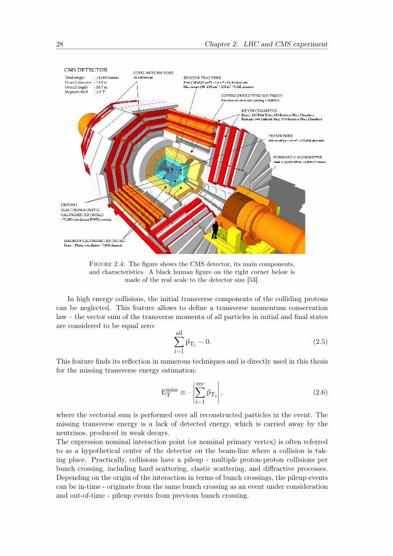
Figure 2.4: The figure shows the CMS detector, its main components,and characteristics. A black human figure on the right corner below is
made of the real scale to the detector size [53].
In high energy collisions, the initial transverse components of the colliding protonscan be neglected. This feature allows to define a transverse momentum conservationlaw – the vector sum of the transverse momenta of all particles in initial and final statesare considered to be equal zero:
all∑i=1
~pTi = 0. (2.5)
This feature finds its reflection in numerous techniques and is directly used in this thesisfor the missing transverse energy estimation:
EmissT ≡ –
∣∣∣∣∣rec∑i=1
~pTi
∣∣∣∣∣ , (2.6)
where the vectorial sum is performed over all reconstructed particles in the event. Themissing transverse energy is a lack of detected energy, which is carried away by theneutrinos, produced in weak decays.The expression nominal interaction point (or nominal primary vertex) is often referredto as a hypothetical center of the detector on the beam-line where a collision is tak-ing place. Practically, collisions have a pileup - multiple proton-proton collisions perbunch crossing, including hard scattering, elastic scattering, and diffractive processes.Depending on the origin of the interaction in terms of bunch crossings, the pileup eventscan be in-time - originate from the same bunch crossing as an event under considerationand out-of-time - pileup events from previous bunch crossing.
2.2. Compact Muon Solenoid 29
2.2.2 Physical processes behind detection techniques
The next sections present an overview of the CMS layers and its main components.Each of them has its own goals and unique, custom design and technology. However,physics processes and detection principles are conventional for each of them. All3 parti-cles created in pp collisions lose their energy moving through the detector materials. Forcharged particles, these processes are caused by the interaction of the charged particleelectromagnetic field with the EM fields of electrons and nucleus in the matter. Theenergy loss may happen through atoms excitement, which returns to the ground stateemitting a photon with characteristic energy. This process is called scintillation, anddetectors that use this effect as a detecting principle are called scintillation detectors.Some detector uses bremsstrahlung as a detection principle. In bremsstrahlung, the de-celerated charged particle loses its kinetic energy emitting photons. Deceleration mainlyhappens due to a charged particle (usually electron) deflection in the electric field of anucleus. Another way4 of energy loss is ionization. When the energy, transmitted toan electron, is high enough to overcome (or penetrate through) a potential barrier ofan atom, a free electron and ion can appear. These processes are of a subatomic scale,and hence are being invariant from a phase state of a detecting matter. High energyphotons interact with matter creating e+e– pairs. The general idea behind particleregistration is to collect products of interaction as effective as possible. The producedelectric charge signal is assembled with a readout electronics.
2.2.3 Tracker Detector
The Tracker Detector (TD) can be called the heart of the CMS since it is placedclosest to the interaction point, where the charged particle flux has its highest value(≈ 107 per second). One of the main objectives of this detector includes detection ofdecay vertices and particle path (track). According to the Lorentz force, a chargedparticle moving perpendicular to the magnetic field will have a curved trajectory. Theinformation about the trajectory is used to calculate transverse momentum and the signof the particle. Particles with a high curvature of a track have a small momentum andvice-versa. A high granularity of the TD allows track reconstruction with a high levelof precision and efficiency.
The TD detector has a total length of 5.8 m and 2.5 m in diameter [54]. A detailedsketch of the TD is shown in Figure 2.5. Depending on the distance from the interactionpoint (hence - particle flux), the detector is divided into three parts.The first part is a pixel detector. It has a radius of 10 cm and is made of pixel sensorswith a size ≈ 100 × 150 μm2 each. During pixel sensor ionization, charged particlecreates electron-hole pairs; then the electrons are collected with an electric current fromeach pixel. Pixel sensors are mounted on three barrel layers with 768 sensors in totaland two endcap disks on each side of them. The radii of the barrel layers are of 4.4 cm,7.3 cm, and 10.2 cm, the length of each is 53 cm [55]. Both endcap disks with inner,and outer radii 6 cm and 15 cm, respectively, are located at a distance |z| = 34.5 cmand 46.5 cm, respectively, containing 672 pixel sensors in total. The spatial resolutionis near 10 μm in the r-φ plane and 20 μm in the z plane. The pixel read-out systemconsists of almost 16,000 chips.
3Except hypothetical particles and neutrinos.4Cherenkov radiation is not reviewed.
30 Chapter 2. LHC and CMS experiment
The second part of TD is an intermediate region with radius 20 < r < 55 cm. TheTracker Inner Barrel (TIB) consists of four layers of silicon and strip pitch sensors withtotal length |z| < 65 cm [55]. The first two layers are made with stereo modules (shownin blue Fig. 2.5) allowing measurements in the r-φ and the r-z planes. The TrackerInner Disks (TID) are located at each side of the detector. They are arranged in threerings, two of which are supplied with stereo modules.
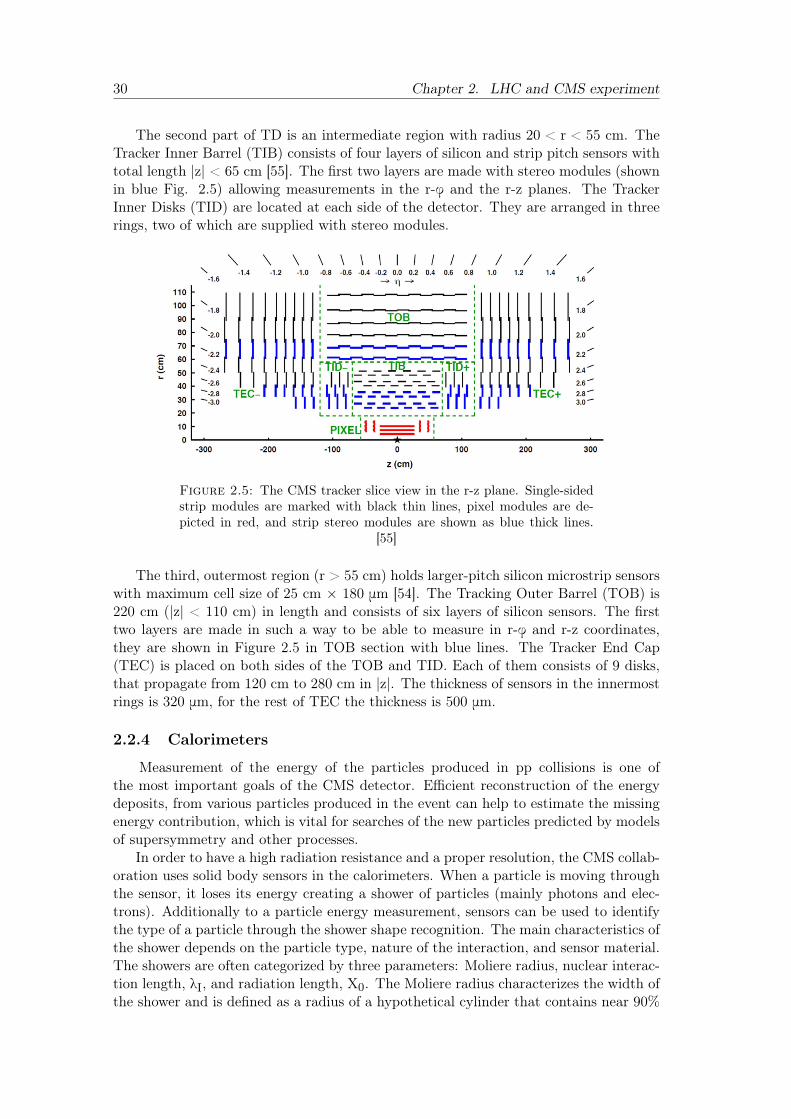
Figure 2.5: The CMS tracker slice view in the r-z plane. Single-sidedstrip modules are marked with black thin lines, pixel modules are de-picted in red, and strip stereo modules are shown as blue thick lines.
[55]
The third, outermost region (r > 55 cm) holds larger-pitch silicon microstrip sensorswith maximum cell size of 25 cm × 180 μm [54]. The Tracking Outer Barrel (TOB) is220 cm (|z| < 110 cm) in length and consists of six layers of silicon sensors. The firsttwo layers are made in such a way to be able to measure in r-φ and r-z coordinates,they are shown in Figure 2.5 in TOB section with blue lines. The Tracker End Cap(TEC) is placed on both sides of the TOB and TID. Each of them consists of 9 disks,that propagate from 120 cm to 280 cm in |z|. The thickness of sensors in the innermostrings is 320 μm, for the rest of TEC the thickness is 500 μm.
2.2.4 Calorimeters
Measurement of the energy of the particles produced in pp collisions is one ofthe most important goals of the CMS detector. Efficient reconstruction of the energydeposits, from various particles produced in the event can help to estimate the missingenergy contribution, which is vital for searches of the new particles predicted by modelsof supersymmetry and other processes.
In order to have a high radiation resistance and a proper resolution, the CMS collab-oration uses solid body sensors in the calorimeters. When a particle is moving throughthe sensor, it loses its energy creating a shower of particles (mainly photons and elec-trons). Additionally to a particle energy measurement, sensors can be used to identifythe type of a particle through the shower shape recognition. The main characteristics ofthe shower depends on the particle type, nature of the interaction, and sensor material.The showers are often categorized by three parameters: Moliere radius, nuclear interac-tion length, λI, and radiation length, X0. The Moliere radius characterizes the width ofthe shower and is defined as a radius of a hypothetical cylinder that contains near 90%
2.2. Compact Muon Solenoid 31
of the shower’s energy. The nuclear interaction length, λI, describes the mean distancethat hadron travels before an inelastic nuclear interaction occurs. The radiation lengthcharacterizes electromagnetic showers and represents an average distance during whichthe moving electron loses energy, by a factor of 1
e .For the purpose of high resolution and detector efficiency the calorimeter system is
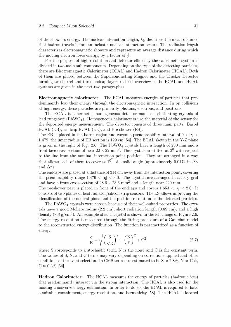
divided in two main sub-components. Depending on the type of the detecting particles,there are Electromagnetic Calorimeter (ECAL) and Hadron Calorimeter (HCAL). Bothof them are placed between the Superconducting Magnet and the Tracker Detectorforming two barrel and three endcap layers (a brief overview of the ECAL and HCALsystems are given in the next two paragraphs).
Electromagnetic calorimeter. The ECAL measures energies of particles that pre-dominantly lose their energy through the electromagnetic interaction. In pp collisionsat high energy, these particles are primarily photons, electrons, and positrons.
The ECAL is a hermetic, homogeneous detector made of scintillating crystals oflead tungstate (PbWO4). Homogeneous calorimeters use the material of the sensor forthe deposited energy measurement. The detector consists of three main parts: BarrelECAL (EB), Endcap ECAL (EE), and Pre shower (ES).The EB is placed in the barrel region and covers a pseudorapidity interval of 0 < |η| <1.479, the inner radius of EB section is 129 cm [54]. The ECAL sketch in the Y-Z planeis given in the right of Fig. 2.6. The PbWO4 crystals have a length of 230 mm and afront face cross-section of near 22× 22 mm2. The crystals are tilted at 30 with respectto the line from the nominal interaction point position. They are arranged in a waythat allows each of them to cover ≈ 10
2of a solid angle (approximately 0.0174 in Δφ
and Δη).The endcaps are placed at a distance of 314 cm away from the interaction point, coveringthe pseudorapidity range 1.479 < |η| < 3.0. The crystals are arranged in an x-y gridand have a front cross-section of 28.6× 28.6 mm2 and a length near 220 mm.The preshower part is placed in front of the endcaps and covers 1.653 < |η| < 2.6. Itconsists of two planes of lead radiator/silicon strip sensors. The ES allows improving theidentification of the neutral pions and the position resolution of the detected particles.
The PbWO4 crystals were chosen because of their well-suited properties. The crys-tals have a good Moliere radius (2.2 cm), short radiation length (0.89 cm), and a highdensity (8.3 g/cm3). An example of such crystal is shown in the left image of Figure 2.6.The energy resolution is measured through the fitting procedure of a Gaussian modelto the reconstructed energy distribution. The function is parametrized as a function ofenergy:
σ
E=
√(S√E
)2+(NE
)2+C2, (2.7)
where S corresponds to a stochastic term, N is the noise and C is the constant term.The values of S, N, and C terms may vary depending on corrections applied and otherconditions of the event selection. In CMS terms are estimated to be S ≈ 2.8%, N ≈ 12%,C ≈ 0.3% [54].
Hadron Calorimeter. The HCAL measures the energy of particles (hadronic jets)that predominantly interact via the strong interaction. The HCAL is also used for themissing transverse energy estimation. In order to do so, the HCAL is required to havea suitable containment, energy resolution, and hermeticity [58]. The HCAL is located
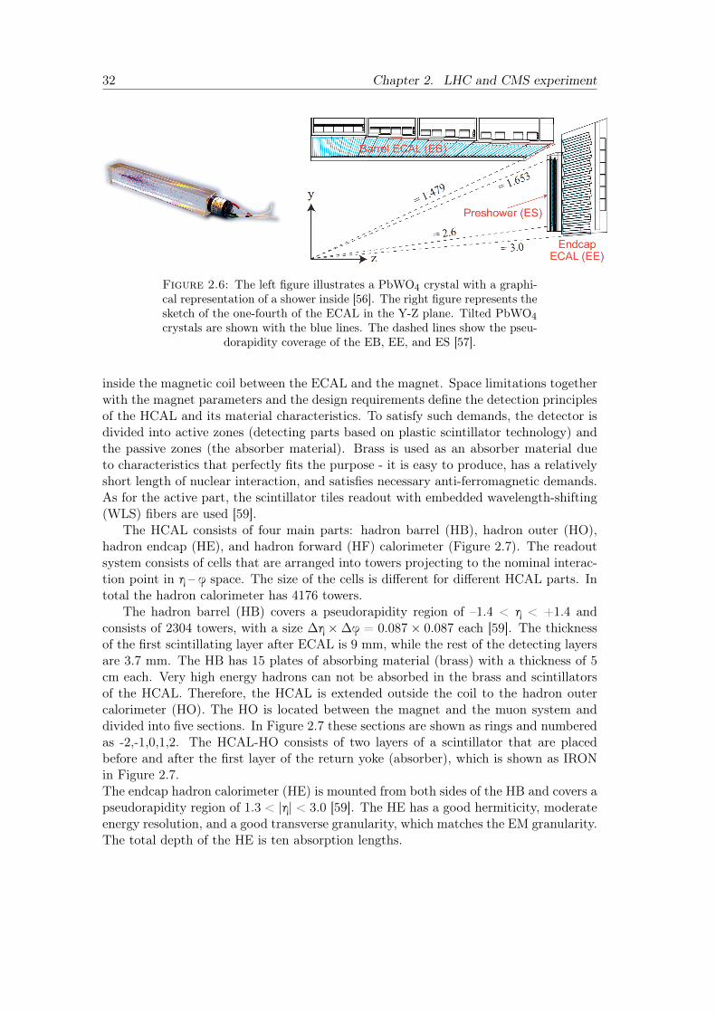
32 Chapter 2. LHC and CMS experiment
Figure 2.6: The left figure illustrates a PbWO4 crystal with a graphi-cal representation of a shower inside [56]. The right figure represents thesketch of the one-fourth of the ECAL in the Y-Z plane. Tilted PbWO4crystals are shown with the blue lines. The dashed lines show the pseu-
dorapidity coverage of the EB, EE, and ES [57].
inside the magnetic coil between the ECAL and the magnet. Space limitations togetherwith the magnet parameters and the design requirements define the detection principlesof the HCAL and its material characteristics. To satisfy such demands, the detector isdivided into active zones (detecting parts based on plastic scintillator technology) andthe passive zones (the absorber material). Brass is used as an absorber material dueto characteristics that perfectly fits the purpose - it is easy to produce, has a relativelyshort length of nuclear interaction, and satisfies necessary anti-ferromagnetic demands.As for the active part, the scintillator tiles readout with embedded wavelength-shifting(WLS) fibers are used [59].
The HCAL consists of four main parts: hadron barrel (HB), hadron outer (HO),hadron endcap (HE), and hadron forward (HF) calorimeter (Figure 2.7). The readoutsystem consists of cells that are arranged into towers projecting to the nominal interac-tion point in η – φ space. The size of the cells is different for different HCAL parts. Intotal the hadron calorimeter has 4176 towers.
The hadron barrel (HB) covers a pseudorapidity region of –1.4 < η < +1.4 andconsists of 2304 towers, with a size Δη ×Δφ = 0.087 × 0.087 each [59]. The thicknessof the first scintillating layer after ECAL is 9 mm, while the rest of the detecting layersare 3.7 mm. The HB has 15 plates of absorbing material (brass) with a thickness of 5cm each. Very high energy hadrons can not be absorbed in the brass and scintillatorsof the HCAL. Therefore, the HCAL is extended outside the coil to the hadron outercalorimeter (HO). The HO is located between the magnet and the muon system anddivided into five sections. In Figure 2.7 these sections are shown as rings and numberedas -2,-1,0,1,2. The HCAL-HO consists of two layers of a scintillator that are placedbefore and after the first layer of the return yoke (absorber), which is shown as IRONin Figure 2.7.The endcap hadron calorimeter (HE) is mounted from both sides of the HB and covers apseudorapidity region of 1.3 < |η| < 3.0 [59]. The HE has a good hermiticity, moderateenergy resolution, and a good transverse granularity, which matches the EM granularity.The total depth of the HE is ten absorption lengths.
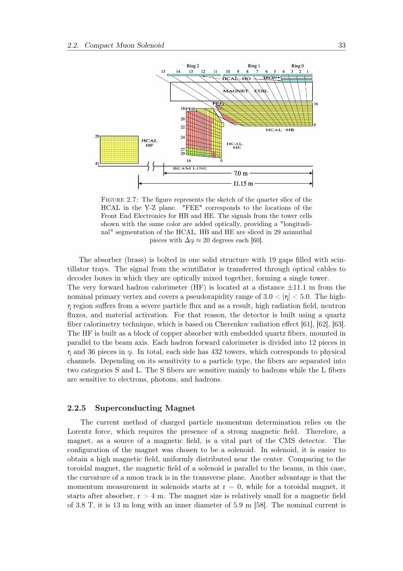
2.2. Compact Muon Solenoid 33
Figure 2.7: The figure represents the sketch of the quarter slice of theHCAL in the Y-Z plane. "FEE" corresponds to the locations of theFront End Electronics for HB and HE. The signals from the tower cellsshown with the same color are added optically, providing a "longitudi-nal" segmentation of the HCAL. HB and HE are sliced in 29 azimuthal
pieces with Δφ ≈ 20 degrees each [60].
The absorber (brass) is bolted in one solid structure with 19 gaps filled with scin-tillator trays. The signal from the scintillator is transferred through optical cables todecoder boxes in which they are optically mixed together, forming a single tower.The very forward hadron calorimeter (HF) is located at a distance ±11.1 m from thenominal primary vertex and covers a pseudorapidity range of 3.0 < |η| < 5.0. The high-η region suffers from a severe particle flux and as a result, high radiation field, neutronfluxes, and material activation. For that reason, the detector is built using a quartzfiber calorimetry technique, which is based on Cherenkov radiation effect [61], [62], [63].The HF is built as a block of copper absorber with embedded quartz fibers, mounted inparallel to the beam axis. Each hadron forward calorimeter is divided into 12 pieces inη and 36 pieces in φ. In total, each side has 432 towers, which corresponds to physicalchannels. Depending on its sensitivity to a particle type, the fibers are separated intotwo categories S and L. The S fibers are sensitive mainly to hadrons while the L fibersare sensitive to electrons, photons, and hadrons.
2.2.5 Superconducting Magnet
The current method of charged particle momentum determination relies on theLorentz force, which requires the presence of a strong magnetic field. Therefore, amagnet, as a source of a magnetic field, is a vital part of the CMS detector. Theconfiguration of the magnet was chosen to be a solenoid. In solenoid, it is easier toobtain a high magnetic field, uniformly distributed near the center. Comparing to thetoroidal magnet, the magnetic field of a solenoid is parallel to the beams, in this case,the curvature of a muon track is in the transverse plane. Another advantage is that themomentum measurement in solenoids starts at r = 0, while for a toroidal magnet, itstarts after absorber, r > 4 m. The magnet size is relatively small for a magnetic fieldof 3.8 T, it is 13 m long with an inner diameter of 5.9 m [58]. The nominal current is
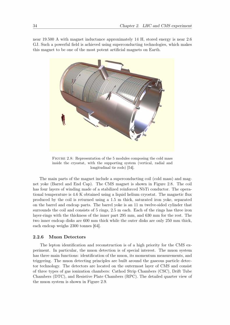
34 Chapter 2. LHC and CMS experiment
near 19.500 A with magnet inductance approximately 14 H, stored energy is near 2.6GJ. Such a powerful field is achieved using superconducting technologies, which makesthis magnet to be one of the most potent artificial magnets on Earth.
Figure 2.8: Representation of the 5 modules composing the cold massinside the cryostat, with the supporting system (vertical, radial and
longitudinal tie rods) [54].
The main parts of the magnet include a superconducting coil (cold mass) and mag-net yoke (Barrel and End Cap). The CMS magnet is shown in Figure 2.8. The coilhas four layers of winding made of a stabilized reinforced NbTi conductor. The opera-tional temperature is 4.6 K obtained using a liquid helium cryostat. The magnetic fluxproduced by the coil is returned using a 1.5 m thick, saturated iron yoke, separatedon the barrel and endcap parts. The barrel yoke is an 11 m twelve-sided cylinder thatsurrounds the coil and consists of 5 rings, 2.5 m each. Each of the rings has three ironlayer-rings with the thickness of the inner part 295 mm, and 630 mm for the rest. Thetwo inner endcap disks are 600 mm thick while the outer disks are only 250 mm thick,each endcap weighs 2300 tonnes [64].
2.2.6 Muon Detectors
The lepton identification and reconstruction is of a high priority for the CMS ex-periment. In particular, the muon detection is of special interest. The muon systemhas three main functions: identification of the muon, its momentum measurements, andtriggering. The muon detecting principles are built around the gaseous particle detec-tor technology. The detectors are located on the outermost layer of CMS and consistof three types of gas ionization chambers: Cathod Strip Chambers (CSC), Drift TubeChambers (DTC), and Resistive Plate Chambers (RPC). The detailed quarter view ofthe muon system is shown in Figure 2.9.
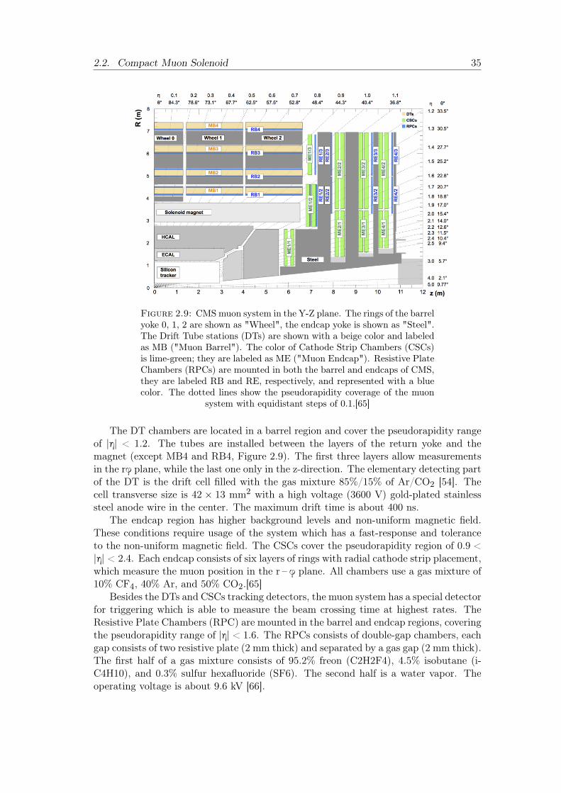
2.2. Compact Muon Solenoid 35
Figure 2.9: CMSmuon system in the Y-Z plane. The rings of the barrelyoke 0, 1, 2 are shown as "Wheel", the endcap yoke is shown as "Steel".The Drift Tube stations (DTs) are shown with a beige color and labeledas MB ("Muon Barrel"). The color of Cathode Strip Chambers (CSCs)is lime-green; they are labeled as ME ("Muon Endcap"). Resistive PlateChambers (RPCs) are mounted in both the barrel and endcaps of CMS,they are labeled RB and RE, respectively, and represented with a bluecolor. The dotted lines show the pseudorapidity coverage of the muon
system with equidistant steps of 0.1.[65]
The DT chambers are located in a barrel region and cover the pseudorapidity rangeof |η| < 1.2. The tubes are installed between the layers of the return yoke and themagnet (except MB4 and RB4, Figure 2.9). The first three layers allow measurementsin the rφ plane, while the last one only in the z-direction. The elementary detecting partof the DT is the drift cell filled with the gas mixture 85%/15% of Ar/CO2 [54]. Thecell transverse size is 42 × 13 mm2 with a high voltage (3600 V) gold-plated stainlesssteel anode wire in the center. The maximum drift time is about 400 ns.
The endcap region has higher background levels and non-uniform magnetic field.These conditions require usage of the system which has a fast-response and toleranceto the non-uniform magnetic field. The CSCs cover the pseudorapidity region of 0.9 <|η| < 2.4. Each endcap consists of six layers of rings with radial cathode strip placement,which measure the muon position in the r – φ plane. All chambers use a gas mixture of10% CF4, 40% Ar, and 50% CO2.[65]
Besides the DTs and CSCs tracking detectors, the muon system has a special detectorfor triggering which is able to measure the beam crossing time at highest rates. TheResistive Plate Chambers (RPC) are mounted in the barrel and endcap regions, coveringthe pseudorapidity range of |η| < 1.6. The RPCs consists of double-gap chambers, eachgap consists of two resistive plate (2 mm thick) and separated by a gas gap (2 mm thick).The first half of a gas mixture consists of 95.2% freon (C2H2F4), 4.5% isobutane (i-C4H10), and 0.3% sulfur hexafluoride (SF6). The second half is a water vapor. Theoperating voltage is about 9.6 kV [66].
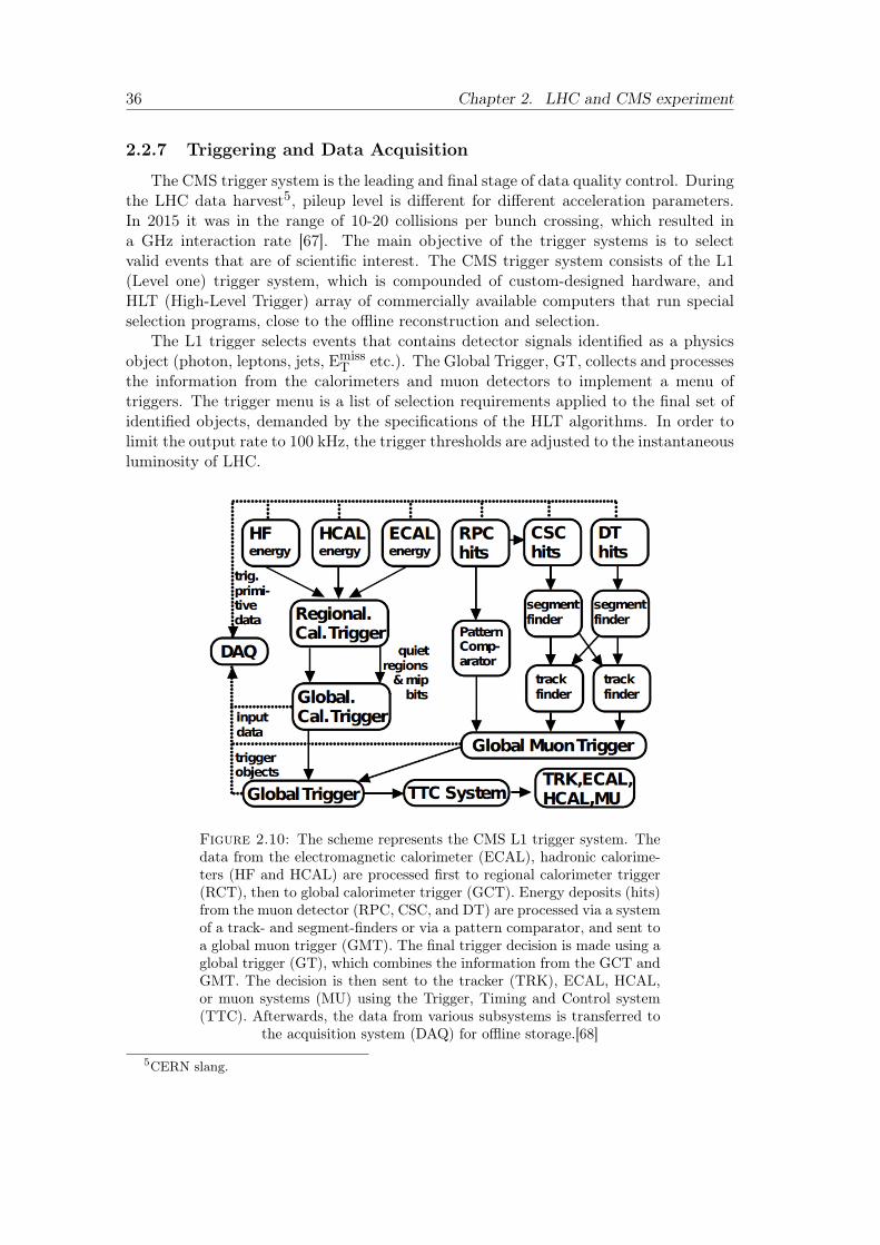
36 Chapter 2. LHC and CMS experiment
2.2.7 Triggering and Data Acquisition
The CMS trigger system is the leading and final stage of data quality control. Duringthe LHC data harvest5, pileup level is different for different acceleration parameters.In 2015 it was in the range of 10-20 collisions per bunch crossing, which resulted ina GHz interaction rate [67]. The main objective of the trigger systems is to selectvalid events that are of scientific interest. The CMS trigger system consists of the L1(Level one) trigger system, which is compounded of custom-designed hardware, andHLT (High-Level Trigger) array of commercially available computers that run specialselection programs, close to the offline reconstruction and selection.
The L1 trigger selects events that contains detector signals identified as a physicsobject (photon, leptons, jets, Emiss
T etc.). The Global Trigger, GT, collects and processesthe information from the calorimeters and muon detectors to implement a menu oftriggers. The trigger menu is a list of selection requirements applied to the final set ofidentified objects, demanded by the specifications of the HLT algorithms. In order tolimit the output rate to 100 kHz, the trigger thresholds are adjusted to the instantaneousluminosity of LHC.
Figure 2.10: The scheme represents the CMS L1 trigger system. Thedata from the electromagnetic calorimeter (ECAL), hadronic calorime-ters (HF and HCAL) are processed first to regional calorimeter trigger(RCT), then to global calorimeter trigger (GCT). Energy deposits (hits)from the muon detector (RPC, CSC, and DT) are processed via a systemof a track- and segment-finders or via a pattern comparator, and sent toa global muon trigger (GMT). The final trigger decision is made using aglobal trigger (GT), which combines the information from the GCT andGMT. The decision is then sent to the tracker (TRK), ECAL, HCAL,or muon systems (MU) using the Trigger, Timing and Control system(TTC). Afterwards, the data from various subsystems is transferred to
the acquisition system (DAQ) for offline storage.[68]
5CERN slang.
2.2. Compact Muon Solenoid 37
The general scheme of the L1 trigger stages is represented in Figure 2.10. TheHLT hardware consists of a processor farm that consists of commodity computers. Thetrigger algorithms are implemented in software, that reduces an output stream to anaverage rate of 100 Hz for offline event storage. The HLT algorithms sort out theevents, applying reconstruction and identification criteria to each object. The analogof the trigger menu in the HLT trigger is called HLT path. It has more sophisticatedalgorithms that simultaneously perform physics object reconstruction and selection ofthese objects. The selection criteria include various kinematic thresholds (pT, η, E
missT )
as much as a specific detection condition (quality of a fit, number of matched stations,etc.). Depending on the signatures of a specific process of interest, different HLT pathschemes may be used. To reduce the amount of data to be stored, trigger paths withhigh event rates may be prescaled by an individual factor X. This factor means thatonly one event out of X will be recorded.
2.2.8 Acceptance
The detector acceptance, A - is a measure of the detector’s performance, definedas the fraction of events that are detected, reconstructed, and passed selection require-ments, Npass, to a total number of all generated events, Ntotal, Formula 2.8. Theacceptance depends on the detector phase space.
A =Npass
Ntotal (2.8)
The detector phase space embodies characteristics of the detector (solid angle of thedetector coverage, detecting volume, etc.), detector efficiency, reconstruction algorithmsefficiencies, features of sub-detector alignment, and many others. The full phase spacemay be defined6 as the full solid angle of events production within a corresponding vol-ume. The detector acceptance in full phase space is estimated using theory predictions.The acceptance is calculated as the fraction of generated events in the detector phasespace that pass the selection requirements, Npass
det , over the number of generated eventsin the full phase space, Ngen
full, Formula 2.9.
A =Npassdet
Ngenfull
. (2.9)
CMS experiment has an extensive physics program so that the detector phase spacemay be different for different studies. In other words, depending on the properties ofstudied physics objects, the detector phase space can be customized, becoming a fiducialphase space. The fiducial phase space may be defined as a phase-space with a set ofspecific requirements of geometric, kinematic, and reconstruction nature. For example,the calculation of differential cross-section values in W± asymmetry studies requiresestimation of the fiducial acceptance in each pseudorapidity bin. Here, the additionalconstraints are the pseudorapidity cuts, which define the geometric boundaries of thedetector phase space for each η bin. More details on acceptance definition for the W±
boson charge asymmetry studies is given in section 5.7.
6In the context of CMS experiment.

39
Chapter 3
Event reconstruction
The reconstruction of W± boson candidate events includes recognition and inter-pretation of the detector signals in terms of physics objects. The products of W±
boson decay in lepton channel are highly energetic muon and muon neutrino, which isindirectly detected as missing energy, Emiss
T . The muon reconstruction procedure com-bines information from several detector systems and processes it via specific algorithms.The Emiss
T reconstruction procedure relies on sophisticated methods that combine theinformation of all reconstructed particles in the event.
The next chapter describes methods that were used to reconstruct the event can-didates. First, an introduction to the algorithms that were used to identify physicsobjects is given. The next part briefly explains the vertex reconstruction algorithms.Afterward, the main steps in muon and missing transverse energy reconstruction ispresented.
3.1 Particle Flow algorithm
The Particle Flow algorithm, (PF) [69] is a "link" between detector signals andphysics objects used in the analysis. The main goal of PF is to reconstruct and identifyall particles in an event. In this sense, particles are referred to as photons, electrons,muons, charged, and neutral hadrons. In particular, PF aims to determine a particletype of each PF candidate, the direction of its propagation, and its energy. To do that,it combines all information of the event from all CMS sub-detectors.
The general PF algorithm has three main stages. In the first stage, informationfrom sub-detectors is analyzed to create elementary objects of the algorithm, so-called"elements". They typically include charged-particle tracks, muon tracks, and calorime-ter clusters. The tracks are reconstructed during five iterations of iterative-trackingstrategy [70]. Calorimeter clusters are identified using the "Clustering Algorithm" [71].This algorithm is performed individually in ECAL barrel, ECAL endcap, HCAL barrel,HCAL endcap, first PS layer, and second PS layer. The algorithm reconstructs thedirection and energy of stable neutral particles, separates neutral particles energy de-posits from charged hadron deposits, measures the energy of charged hadrons, identifiesand reconstructs electron energy deposits [69].
The second stage is a link algorithm. Reconstructed "elements" are linked to eachother, forming "blocks". An essential part of this stage is to avoid double-counting.Depending on a variety of elements in the event, the linking schemes may be different.
In the last stage, the blocks are used to reconstruct and identify the particle typeand its properties. In each block, the algorithm is executed in a particular order. First,the algorithm reconstructs the muon candidates. After reconstruction, a correspondingPF element is removed from the block. Next, the electron reconstruction is done; it also
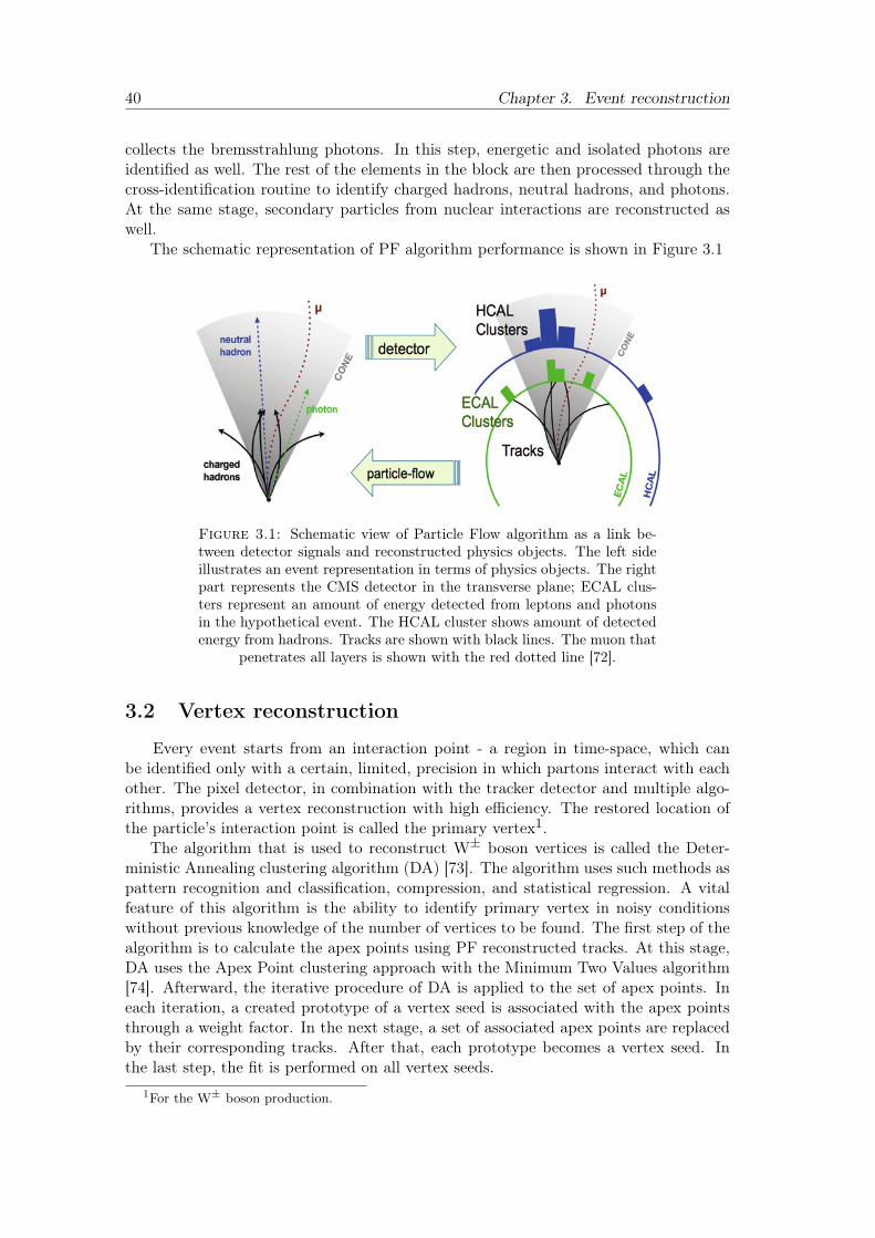
40 Chapter 3. Event reconstruction
collects the bremsstrahlung photons. In this step, energetic and isolated photons areidentified as well. The rest of the elements in the block are then processed through thecross-identification routine to identify charged hadrons, neutral hadrons, and photons.At the same stage, secondary particles from nuclear interactions are reconstructed aswell.
The schematic representation of PF algorithm performance is shown in Figure 3.1
Figure 3.1: Schematic view of Particle Flow algorithm as a link be-tween detector signals and reconstructed physics objects. The left sideillustrates an event representation in terms of physics objects. The rightpart represents the CMS detector in the transverse plane; ECAL clus-ters represent an amount of energy detected from leptons and photonsin the hypothetical event. The HCAL cluster shows amount of detectedenergy from hadrons. Tracks are shown with black lines. The muon that
penetrates all layers is shown with the red dotted line [72].
3.2 Vertex reconstruction
Every event starts from an interaction point - a region in time-space, which canbe identified only with a certain, limited, precision in which partons interact with eachother. The pixel detector, in combination with the tracker detector and multiple algo-rithms, provides a vertex reconstruction with high efficiency. The restored location ofthe particle’s interaction point is called the primary vertex1.
The algorithm that is used to reconstruct W± boson vertices is called the Deter-ministic Annealing clustering algorithm (DA) [73]. The algorithm uses such methods aspattern recognition and classification, compression, and statistical regression. A vitalfeature of this algorithm is the ability to identify primary vertex in noisy conditionswithout previous knowledge of the number of vertices to be found. The first step of thealgorithm is to calculate the apex points using PF reconstructed tracks. At this stage,DA uses the Apex Point clustering approach with the Minimum Two Values algorithm[74]. Afterward, the iterative procedure of DA is applied to the set of apex points. Ineach iteration, a created prototype of a vertex seed is associated with the apex pointsthrough a weight factor. In the next stage, a set of associated apex points are replacedby their corresponding tracks. After that, each prototype becomes a vertex seed. Inthe last step, the fit is performed on all vertex seeds.
1For the W± boson production.
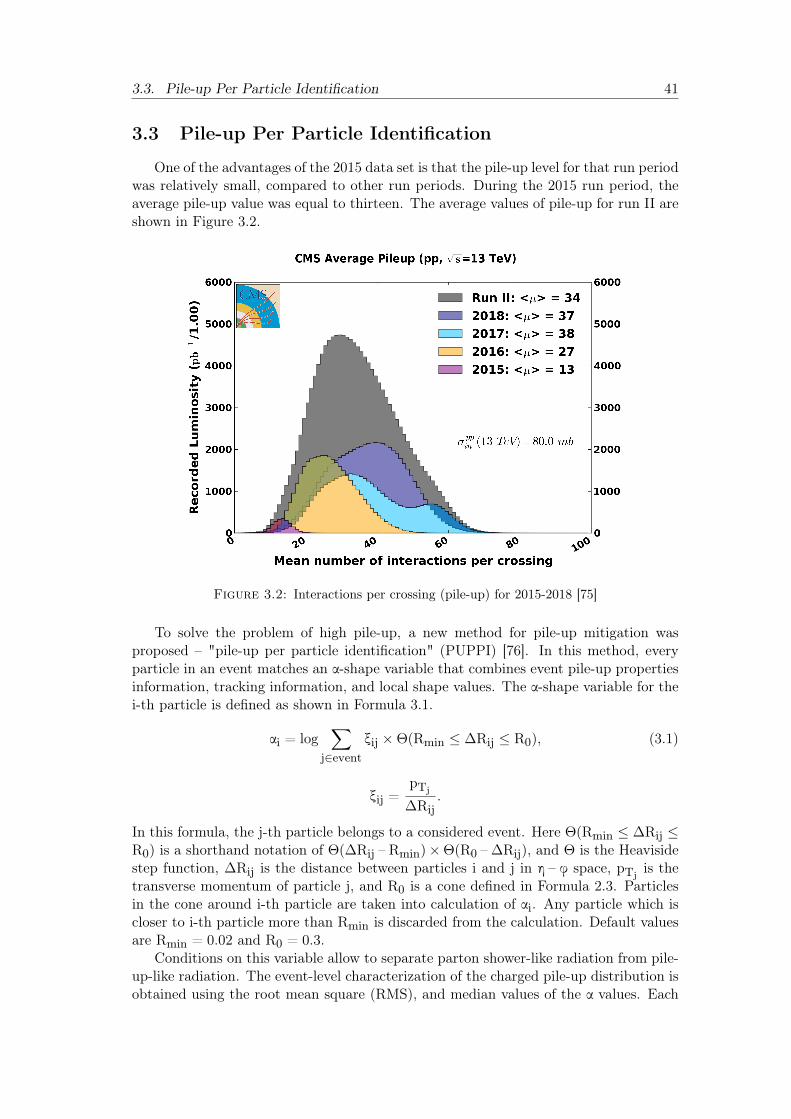
3.3. Pile-up Per Particle Identification 41
3.3 Pile-up Per Particle Identification
One of the advantages of the 2015 data set is that the pile-up level for that run periodwas relatively small, compared to other run periods. During the 2015 run period, theaverage pile-up value was equal to thirteen. The average values of pile-up for run II areshown in Figure 3.2.
Figure 3.2: Interactions per crossing (pile-up) for 2015-2018 [75]
To solve the problem of high pile-up, a new method for pile-up mitigation wasproposed – "pile-up per particle identification" (PUPPI) [76]. In this method, everyparticle in an event matches an α-shape variable that combines event pile-up propertiesinformation, tracking information, and local shape values. The α-shape variable for thei-th particle is defined as shown in Formula 3.1.
αi = log∑
j∈eventξij ×Θ(Rmin ≤ ΔRij ≤ R0), (3.1)
ξij =pTj
ΔRij.
In this formula, the j-th particle belongs to a considered event. Here Θ(Rmin ≤ ΔRij ≤R0) is a shorthand notation of Θ(ΔRij – Rmin)×Θ(R0 –ΔRij), and Θ is the Heavisidestep function, ΔRij is the distance between particles i and j in η – φ space, pTj is thetransverse momentum of particle j, and R0 is a cone defined in Formula 2.3. Particlesin the cone around i-th particle are taken into calculation of αi. Any particle which iscloser to i-th particle more than Rmin is discarded from the calculation. Default valuesare Rmin = 0.02 and R0 = 0.3.
Conditions on this variable allow to separate parton shower-like radiation from pile-up-like radiation. The event-level characterization of the charged pile-up distribution isobtained using the root mean square (RMS), and median values of the α values. Each
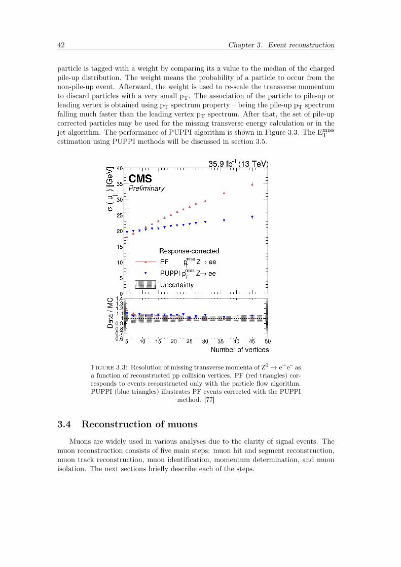
42 Chapter 3. Event reconstruction
particle is tagged with a weight by comparing its α value to the median of the chargedpile-up distribution. The weight means the probability of a particle to occur from thenon-pile-up event. Afterward, the weight is used to re-scale the transverse momentumto discard particles with a very small pT. The association of the particle to pile-up orleading vertex is obtained using pT spectrum property – being the pile-up pT spectrumfalling much faster than the leading vertex pT spectrum. After that, the set of pile-upcorrected particles may be used for the missing transverse energy calculation or in thejet algorithm. The performance of PUPPI algorithm is shown in Figure 3.3. The Emiss
Testimation using PUPPI methods will be discussed in section 3.5.
Figure 3.3: Resolution of missing transverse momenta of Z0 → e+e– asa function of reconstructed pp collision vertices. PF (red triangles) cor-responds to events reconstructed only with the particle flow algorithm.PUPPI (blue triangles) illustrates PF events corrected with the PUPPI
method. [77]
3.4 Reconstruction of muons
Muons are widely used in various analyses due to the clarity of signal events. Themuon reconstruction consists of five main steps: muon hit and segment reconstruction,muon track reconstruction, muon identification, momentum determination, and muonisolation. The next sections briefly describe each of the steps.
3.4. Reconstruction of muons 43
3.4.1 Hit and segment reconstruction
Muon reconstruction starts with a collection of "hits" - electric signals producedon the wires and strips after muon gas ionization. So-called "local" algorithms collectinformation from the drift tubes (DT), residual plate chambers (RPC) and cathodestrip chambers (CSC) [78].
In DT, the charge from the gas ionization is collected using anode wire under avoltage. The arrival time is obtained using a time-to-digital converter (TDC). Thistime, TTDC, is corrected by the pedestal time, Tped, and multiplied by the drift velocity(v). The DT hit position calculation is calculated as
HitDT = (TTDC – Tped)× v. (3.2)
The CSC detector measures the hit position by combining the information from theanode wires and cathode strips. The radial location of the strips allows measuring theφ angle precisely. Traveling through the gap between two plates of RPC, the muonproduces an electron shower, that is collected on an external strip readout plane as acharge. That charge produces a signal on a readout plate of an external strip allowingto identify muons with a precision of a few ns. The charge from ionization can be dis-tributed among a few strips. For that reason, neighboring strips are clustered together[54]. Such configuration allows reconstructing hits more accurately.
3.4.2 Muon track reconstruction
In the standard CMS track reconstruction scheme, the tracks are reconstructedindependently in the tracker system and muon system. After that, the informationabout reconstructed tracks proceeds for muon track reconstruction, which consists ofthree different types [79].
• Standalone-muon tracks are created using the information about the position ofthe hits in the muon detector. In particular, it combines the data from DT, RPC,and CSC. In this reconstruction scheme, the Kalman-filter technique is widelyused [80]. The reconstruction starts with reconstructed seeds in DT groups andCSC segments.
• Tracker-muon tracks are reconstructed using a chain of slightly different trackingalgorithms in an iterative approach. The tracks are built "inside-out" by extrap-olating tracker tracks with pT > 0.5 GeV and total momentum p > 2.5 GeV tothe muon system to match tracks reconstructed in DT or CSC parts. The trackertrack is determined as a tracker-muon track if at least one muon segment matchesthe extrapolated track and if the absolute value of the difference between positionsof the tracks in the x coordinate is smaller than 3 cm.
• Global muon tracks, unlike the tracker muon tracks, are built in the oppositedirection - “outside-in”. Using Kalman filter and information about the standalonemuon track and tracker track, the algorithm matches the tracks through the fit.At large transverse momenta, pT > 200 GeV, the resolution can be improved withthe information from the global muon fit. The hadron shower remnants can punchthrough the innermost muon station (punch-through effect) [55]. Such events maybe a source of misidentification for those muons, which match only one segment
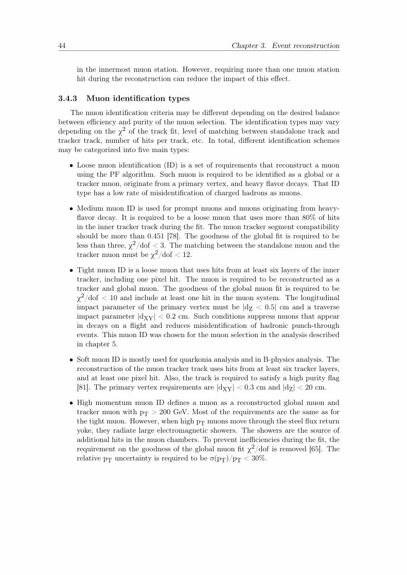
44 Chapter 3. Event reconstruction
in the innermost muon station. However, requiring more than one muon stationhit during the reconstruction can reduce the impact of this effect.
3.4.3 Muon identification types
The muon identification criteria may be different depending on the desired balancebetween efficiency and purity of the muon selection. The identification types may varydepending on the χ2 of the track fit, level of matching between standalone track andtracker track, number of hits per track, etc. In total, different identification schemesmay be categorized into five main types:
• Loose muon identification (ID) is a set of requirements that reconstruct a muonusing the PF algorithm. Such muon is required to be identified as a global or atracker muon, originate from a primary vertex, and heavy flavor decays. That IDtype has a low rate of misidentification of charged hadrons as muons.
• Medium muon ID is used for prompt muons and muons originating from heavy-flavor decay. It is required to be a loose muon that uses more than 80% of hitsin the inner tracker track during the fit. The muon tracker segment compatibilityshould be more than 0.451 [78]. The goodness of the global fit is required to beless than three, χ2/dof < 3. The matching between the standalone muon and thetracker muon must be χ2/dof < 12.
• Tight muon ID is a loose muon that uses hits from at least six layers of the innertracker, including one pixel hit. The muon is required to be reconstructed as atracker and global muon. The goodness of the global muon fit is required to beχ2/dof < 10 and include at least one hit in the muon system. The longitudinal
impact parameter of the primary vertex must be |dZ < 0.5| cm and a traverseimpact parameter |dXY| < 0.2 cm. Such conditions suppress muons that appearin decays on a flight and reduces misidentification of hadronic punch-throughevents. This muon ID was chosen for the muon selection in the analysis describedin chapter 5.
• Soft muon ID is mostly used for quarkonia analysis and in B-physics analysis. Thereconstruction of the muon tracker track uses hits from at least six tracker layers,and at least one pixel hit. Also, the track is required to satisfy a high purity flag[81]. The primary vertex requirements are |dXY| < 0.3 cm and |dZ| < 20 cm.
• High momentum muon ID defines a muon as a reconstructed global muon andtracker muon with pT > 200 GeV. Most of the requirements are the same as forthe tight muon. However, when high pT muons move through the steel flux returnyoke, they radiate large electromagnetic showers. The showers are the source ofadditional hits in the muon chambers. To prevent inefficiencies during the fit, therequirement on the goodness of the global muon fit χ2/dof is removed [65]. Therelative pT uncertainty is required to be σ(pT)/pT < 30%.
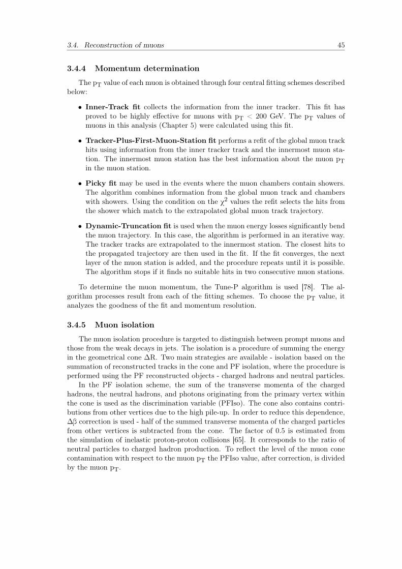
3.4. Reconstruction of muons 45
3.4.4 Momentum determination
The pT value of each muon is obtained through four central fitting schemes describedbelow:
• Inner-Track fit collects the information from the inner tracker. This fit hasproved to be highly effective for muons with pT < 200 GeV. The pT values ofmuons in this analysis (Chapter 5) were calculated using this fit.
• Tracker-Plus-First-Muon-Station fit performs a refit of the global muon trackhits using information from the inner tracker track and the innermost muon sta-tion. The innermost muon station has the best information about the muon pTin the muon station.
• Picky fit may be used in the events where the muon chambers contain showers.The algorithm combines information from the global muon track and chamberswith showers. Using the condition on the χ2 values the refit selects the hits fromthe shower which match to the extrapolated global muon track trajectory.
• Dynamic-Truncation fit is used when the muon energy losses significantly bendthe muon trajectory. In this case, the algorithm is performed in an iterative way.The tracker tracks are extrapolated to the innermost station. The closest hits tothe propagated trajectory are then used in the fit. If the fit converges, the nextlayer of the muon station is added, and the procedure repeats until it is possible.The algorithm stops if it finds no suitable hits in two consecutive muon stations.
To determine the muon momentum, the Tune-P algorithm is used [78]. The al-gorithm processes result from each of the fitting schemes. To choose the pT value, itanalyzes the goodness of the fit and momentum resolution.
3.4.5 Muon isolation
The muon isolation procedure is targeted to distinguish between prompt muons andthose from the weak decays in jets. The isolation is a procedure of summing the energyin the geometrical cone ΔR. Two main strategies are available - isolation based on thesummation of reconstructed tracks in the cone and PF isolation, where the procedure isperformed using the PF reconstructed objects - charged hadrons and neutral particles.
In the PF isolation scheme, the sum of the transverse momenta of the chargedhadrons, the neutral hadrons, and photons originating from the primary vertex withinthe cone is used as the discrimination variable (PFIso). The cone also contains contri-butions from other vertices due to the high pile-up. In order to reduce this dependence,Δβ correction is used - half of the summed transverse momenta of the charged particlesfrom other vertices is subtracted from the cone. The factor of 0.5 is estimated fromthe simulation of inelastic proton-proton collisions [65]. It corresponds to the ratio ofneutral particles to charged hadron production. To reflect the level of the muon conecontamination with respect to the muon pT the PFIso value, after correction, is dividedby the muon pT.
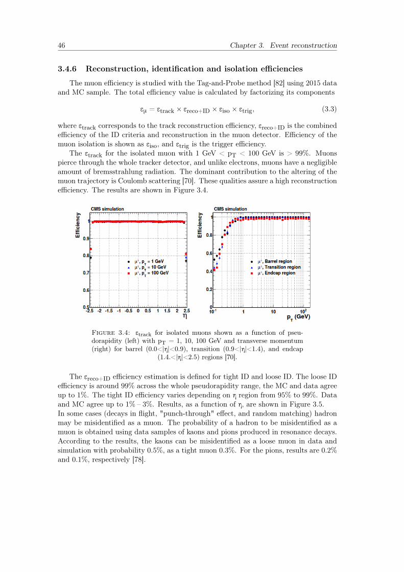
46 Chapter 3. Event reconstruction
3.4.6 Reconstruction, identification and isolation efficiencies
The muon efficiency is studied with the Tag-and-Probe method [82] using 2015 dataand MC sample. The total efficiency value is calculated by factorizing its components
εμ = εtrack × εreco+ID × εiso × εtrig, (3.3)
where εtrack corresponds to the track reconstruction efficiency, εreco+ID is the combinedefficiency of the ID criteria and reconstruction in the muon detector. Efficiency of themuon isolation is shown as εiso, and εtrig is the trigger efficiency.
The εtrack for the isolated muon with 1 GeV < pT < 100 GeV is > 99%. Muonspierce through the whole tracker detector, and unlike electrons, muons have a negligibleamount of bremsstrahlung radiation. The dominant contribution to the altering of themuon trajectory is Coulomb scattering [70]. These qualities assure a high reconstructionefficiency. The results are shown in Figure 3.4.
Figure 3.4: εtrack for isolated muons shown as a function of pseu-dorapidity (left) with pT = 1, 10, 100 GeV and transverse momentum(right) for barrel (0.0<|η|<0.9), transition (0.9<|η|<1.4), and endcap
(1.4.<|η|<2.5) regions [70].
The εreco+ID efficiency estimation is defined for tight ID and loose ID. The loose IDefficiency is around 99% across the whole pseudorapidity range, the MC and data agreeup to 1%. The tight ID efficiency varies depending on η region from 95% to 99%. Dataand MC agree up to 1% – 3%. Results, as a function of η, are shown in Figure 3.5.In some cases (decays in flight, "punch-through" effect, and random matching) hadronmay be misidentified as a muon. The probability of a hadron to be misidentified as amuon is obtained using data samples of kaons and pions produced in resonance decays.According to the results, the kaons can be misidentified as a loose muon in data andsimulation with probability 0.5%, as a tight muon 0.3%. For the pions, results are 0.2%and 0.1%, respectively [78].
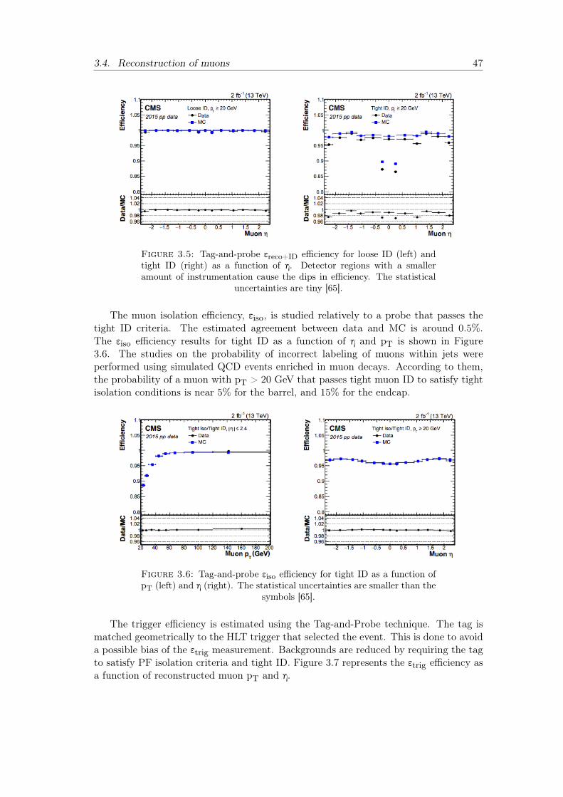
3.4. Reconstruction of muons 47
Figure 3.5: Tag-and-probe εreco+ID efficiency for loose ID (left) andtight ID (right) as a function of η. Detector regions with a smalleramount of instrumentation cause the dips in efficiency. The statistical
uncertainties are tiny [65].
The muon isolation efficiency, εiso, is studied relatively to a probe that passes thetight ID criteria. The estimated agreement between data and MC is around 0.5%.The εiso efficiency results for tight ID as a function of η and pT is shown in Figure3.6. The studies on the probability of incorrect labeling of muons within jets wereperformed using simulated QCD events enriched in muon decays. According to them,the probability of a muon with pT > 20 GeV that passes tight muon ID to satisfy tightisolation conditions is near 5% for the barrel, and 15% for the endcap.
Figure 3.6: Tag-and-probe εiso efficiency for tight ID as a function ofpT (left) and η (right). The statistical uncertainties are smaller than the
symbols [65].
The trigger efficiency is estimated using the Tag-and-Probe technique. The tag ismatched geometrically to the HLT trigger that selected the event. This is done to avoida possible bias of the εtrig measurement. Backgrounds are reduced by requiring the tagto satisfy PF isolation criteria and tight ID. Figure 3.7 represents the εtrig efficiency asa function of reconstructed muon pT and η.
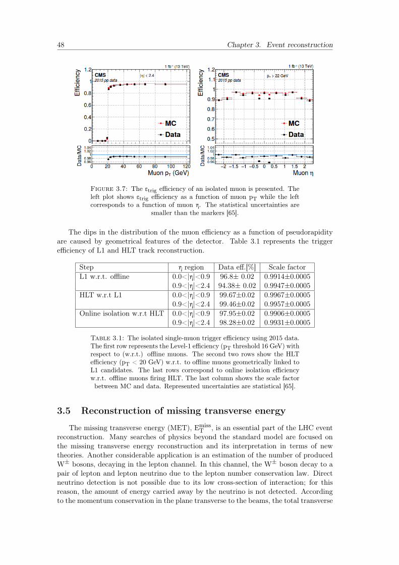
48 Chapter 3. Event reconstruction
Figure 3.7: The εtrig efficiency of an isolated muon is presented. Theleft plot shows εtrig efficiency as a function of muon pT while the leftcorresponds to a function of muon η. The statistical uncertainties are
smaller than the markers [65].
The dips in the distribution of the muon efficiency as a function of pseudorapidityare caused by geometrical features of the detector. Table 3.1 represents the triggerefficiency of L1 and HLT track reconstruction.
Step η region Data eff.[%] Scale factorL1 w.r.t. offline 0.0<|η|<0.9 96.8± 0.02 0.9914±0.0005
0.9<|η|<2.4 94.38± 0.02 0.9947±0.0005HLT w.r.t L1 0.0<|η|<0.9 99.67±0.02 0.9967±0.0005
0.9<|η|<2.4 99.46±0.02 0.9957±0.0005Online isolation w.r.t HLT 0.0<|η|<0.9 97.95±0.02 0.9906±0.0005
0.9<|η|<2.4 98.28±0.02 0.9931±0.0005
Table 3.1: The isolated single-muon trigger efficiency using 2015 data.The first row represents the Level-1 efficiency (pT threshold 16 GeV) withrespect to (w.r.t.) offline muons. The second two rows show the HLTefficiency (pT < 20 GeV) w.r.t. to offline muons geometrically linked toL1 candidates. The last rows correspond to online isolation efficiencyw.r.t. offline muons firing HLT. The last column shows the scale factorbetween MC and data. Represented uncertainties are statistical [65].
3.5 Reconstruction of missing transverse energy
The missing transverse energy (MET), EmissT , is an essential part of the LHC event
reconstruction. Many searches of physics beyond the standard model are focused onthe missing transverse energy reconstruction and its interpretation in terms of newtheories. Another considerable application is an estimation of the number of producedW± bosons, decaying in the lepton channel. In this channel, the W± boson decay to apair of lepton and lepton neutrino due to the lepton number conservation law. Directneutrino detection is not possible due to its low cross-section of interaction; for thisreason, the amount of energy carried away by the neutrino is not detected. Accordingto the momentum conservation in the plane transverse to the beams, the total transverse
3.5. Reconstruction of missing transverse energy 49
momentum of all particles produced in the event is equal to zero. Precise measurementof all available particles in the event allows to construct the transverse momentumdistribution and spot the imbalance that corresponds to undetected particles. The ~E
missT
is computed as a negative of the vectorial sum of particles momenta, and is defined by
~EmissT = –
all∑i=1
~pTi , (3.4)
where ~pTi corresponds to the transverse momenta of all reconstructed particles in the
event. The modulus of ~EmissT value is referred to as Emiss
T and is used in the analysis(Chapter 5) as the main variable for the signal yields extraction. CMS has four mainalgorithms to estimate Emiss
T : Particle Flow MET [69], PUPPI EmissT [76], Calo MET
method [83], and Track-Corrected EmissT (TC) algorithm [84].
The Particle Flow MET uses pT values of all particles reconstructed with the PFalgorithm [69]. The values of MET are obtained using formula 3.4. The correctionsthat are applied to the MET values are briefly described later in this section.
PUPPI EmissT calculation applies PUPPI corrections to the PF objects [76]. The
definition of local shape variable α is redefined for PF objects. The α variable of i-thPF object is defined as
αi = log∑
j6=,ΔRij<0.4
( pTj
ΔRij
)2{ for |ηi| < 2.5, j are charged PF candidates from PV,for |ηi| > 2.5, j are all kinds of PF candidates.
(3.5)Here j represents charged PF candidates that originate from the primary vertex (PV)in a cone of radius R in η – φ space around PF candidate i, ΔRij is a distance betweeni and j in η – φ space. If a charged PF candidate is not associated with the PV, but thedistance between the track and PV is less then 0.3 cm, dZ < 0.3 cm, the candidate isused in the calculation [85]. The χ2 approximation is used to determine the likelihoodthat the PF candidate is originating from the pile-up:
χ2i =
(αi – αPU)2
RMS2PU. (3.6)
Here αPU is a median value of the αi distribution for pile-up particles of the event. Theroot mean square of the αi distribution is shown as RMSPU. The χ2 values are usedto calculate the weight w, which means a probability of the PF candidate to originatefrom the PV. The expression for the weight is given as:
wi = Fχ2,NDF=1(χ
2i ). (3.7)
The Fχ2,NDF=1 is the cumulative distribution function that approximates the χ2 dis-
tribution with one degree of freedom of all PF candidates in the event [85]. After theweight is defined for every PF candidate, the Emiss
T can be calculated using formula 3.4.Calo MET method is based on calorimeter tower geometry and calorimeter energies.
The MET is calculated using the same formula 3.4, but the information about thetransverse energy is taken from the energy deposits in calorimetry towers [71].
The TC EmissT algorithm is based on the Calo MET method and includes recon-
structed tracks from the inner tracker [55]. For the tracks that are not identified as
50 Chapter 3. Event reconstruction
electron or muon, the simulation of energy deposit from charged pion is used [84].Nonlinearities in detector response, inefficiencies of the tracker, and minimum energy
thresholds in the calorimeters can lead to overestimated or underestimated values of theEmissT . For that reason, CMS uses a few types of MET corrections:
• Type-0 correction aims to consider the impact of the degraded MET reconstruc-tion, which appears from the pile-up interaction. The MET reconstruction de-grades as the pile-up increases. Type-0 correction applies Charged Hadron Sub-traction (CHS) scheme to the MET. The scheme removes contributions fromcharged hadrons that originate from the pile-up events [83]. The correction isdeveloped for the PF MET and cannot be used for the Calo MET.
• Type-I correction corresponds to the propagation of jet energy correction (JEC[86]) to MET. In few words, this correction replaces the four-vectors of jets withthe JEC four-vectors.
• Type-II correction corrects the ~pT of unprescaled particles by uniformly scalingit with a constant factor. The correction was originally made for the Calo METand is not recommended for PF MET.
• The XY-Shift correction aims to reduce the MET φmodulation. The experimentaldistribution of MET shows that it has a non-uniform distribution in φ. At the sametime, due to the axial symmetry of events production, MET values are expectedto have uniform distribution across the φ coordinate. The observed φ modulationcan be explained by the presence of the anisotropic detector response, inactivecalorimeter cells, the detector misalignment, and the displacement of the beamspot. The modulation can be reduced by shifting the origin of the coordinate inthe transverse plane.
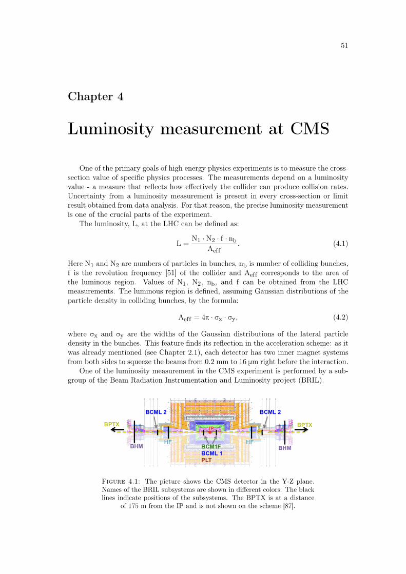
51
Chapter 4
Luminosity measurement at CMS
One of the primary goals of high energy physics experiments is to measure the cross-section value of specific physics processes. The measurements depend on a luminosityvalue - a measure that reflects how effectively the collider can produce collision rates.Uncertainty from a luminosity measurement is present in every cross-section or limitresult obtained from data analysis. For that reason, the precise luminosity measurementis one of the crucial parts of the experiment.
The luminosity, L, at the LHC can be defined as:
L =N1 ·N2 · f · nb
Aeff. (4.1)
Here N1 and N2 are numbers of particles in bunches, nb is number of colliding bunches,f is the revolution frequency [51] of the collider and Aeff corresponds to the area ofthe luminous region. Values of N1, N2, nb, and f can be obtained from the LHCmeasurements. The luminous region is defined, assuming Gaussian distributions of theparticle density in colliding bunches, by the formula:
Aeff = 4π · σx · σy, (4.2)
where σx and σy are the widths of the Gaussian distributions of the lateral particledensity in the bunches. This feature finds its reflection in the acceleration scheme: as itwas already mentioned (see Chapter 2.1), each detector has two inner magnet systemsfrom both sides to squeeze the beams from 0.2 mm to 16 μm right before the interaction.
One of the luminosity measurement in the CMS experiment is performed by a sub-group of the Beam Radiation Instrumentation and Luminosity project (BRIL).
Figure 4.1: The picture shows the CMS detector in the Y-Z plane.Names of the BRIL subsystems are shown in different colors. The blacklines indicate positions of the subsystems. The BPTX is at a distance
of 175 m from the IP and is not shown on the scheme [87].
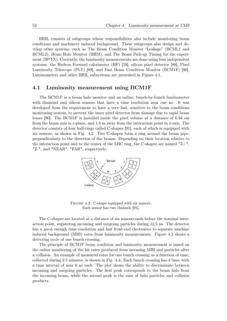
52 Chapter 4. Luminosity measurement at CMS
BRIL consists of subgroups whose responsibilities also include monitoring beamconditions and machinery induced background. These subgroups also design and de-velop other systems, such as The Beam Condition Monitor “Leakage” (BCML1 andBCML2), Beam Halo Monitor (BHM), and The Beam Pick-up Timing for the experi-ment (BPTX). Currently, the luminosity measurements are done using four independentsystems: the Hadron Forward calorimeter (HF) [59], silicon pixel detector [88], PixelLuminosity Telescope (PLT) [89], and Fast Beam Condition Monitor (BCM1F) [90].Luminometers and other BRIL subsystems are presented in Figure 4.1.
4.1 Luminosity measurement using BCM1F
The BCM1F is a beam halo monitor and an online, bunch-by-bunch luminometerwith diamond and silicon sensors that have a time resolution near one ns. It wasdeveloped from the requirement to have a very fast, sensitive to the beam conditionsmonitoring system, to prevent the inner pixel detector from damage due to rapid beamlosses [90]. The BCM1F is installed inside the pixel volume at a distance of 6.94 cmfrom the beam axis in r-plane, and 1.8 m away from the interaction point in z-axis. Thedetector consists of four half-rings called C-shapes [91], each of which is equipped withsix sensors, as shown in Fig. 4.2. Two C-shapes form a ring around the beam pipe,perpendicularly to the direction of the beams. Depending on their location relative tothe interaction point and to the center of the LHC ring, the C-shapes are named "Z+","Z-", and "NEAR", "FAR", respectively.
Figure 4.2: C-shape equipped with six sensors.Each sensor has two channels [91].
The C-shapes are located at a distance of six nanoseconds before the nominal inter-action point, registering incoming and outgoing particles during 12.5 ns. The detectorhas a good enough time resolution and fast front-end electronics to separate machineinduced background (MIB) rates from luminosity measurements. Figure 4.3 shows adetecting cycle of one bunch crossing.
The principle of BCM1F beam condition and luminosity measurement is based onthe online monitoring of the hit rates produced from incoming MIB and particles aftera collision. An example of measured rates for one bunch crossing as a function of time,collected during 2.5 minutes, is shown in Fig. 4.4. Each bunch crossing has 4 bins, witha time interval of near 6 ns each. The plot shows the ability to discriminate betweenincoming and outgoing particles. The first peak corresponds to the beam halo fromthe incoming beam, while the second peak is the sum of halo particles and collisionproducts.
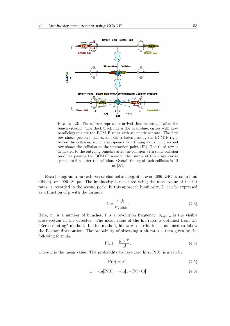
4.1. Luminosity measurement using BCM1F 53
Figure 4.3: The scheme represents arrival time before and after thebunch crossing. The thick black line is the beam-line, circles with grayparallelograms are the BCM1F rings with schematic sensors. The firstrow shows proton bunches, and theirs halos passing the BCM1F rightbefore the collision, which corresponds to a timing -6 ns. The secondrow shows the collision at the interaction point (IP). The third row isdedicated to the outgoing bunches after the collision with some collisionproducts passing the BCM1F sensors, the timing of this stage corre-sponds to 6 ns after the collision. Overall timing of each collision is 12
ns [87].
Each histogram from each sensor channel is integrated over 4096 LHC turns (a luminibble), or 4096×89 μs. The luminosity is measured using the mean value of the hitrates, μ, recorded in the second peak. In this approach luminosity, L, can be expressedas a function of μ with the formula:
L =nbfμσvisible
. (4.3)
Here, nb is a number of bunches, f is a revolution frequency, σvisible is the visiblecross-section in the detector. The mean value of the hit rates is obtained from the"Zero counting" method. In this method, hit rates distribution is assumed to followthe Poisson distribution. The probability of observing n hit rates is then given by thefollowing formula:
P(n) =μne–μ
n!, (4.4)
where μ is the mean value. The probability to have zero hits, P(0), is given by:
P(0) = e–μ (4.5)
μ = –ln[P(0)] = –ln[1 – P(> 0)] (4.6)
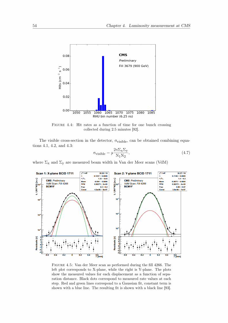
54 Chapter 4. Luminosity measurement at CMS
Figure 4.4: Hit rates as a function of time for one bunch crossingcollected during 2.5 minutes [92].
The visible cross-section in the detector, σvisible, can be obtained combining equa-tions 4.1, 4.2, and 4.3:
σvisible = μ2πΣxΣyN1N2
, (4.7)
where Σx and Σy are measured beam width in Van der Meer scans (VdM)
Figure 4.5: Van der Meer scan as performed during the fill 4266. Theleft plot corresponds to X-plane, while the right is Y-plane. The plotsshow the measured values for each displacement as a function of sepa-ration distance. Black dots correspond to measured rate values at eachstep. Red and green lines correspond to a Gaussian fit, constant term isshown with a blue line. The resulting fit is shown with a black line [93].
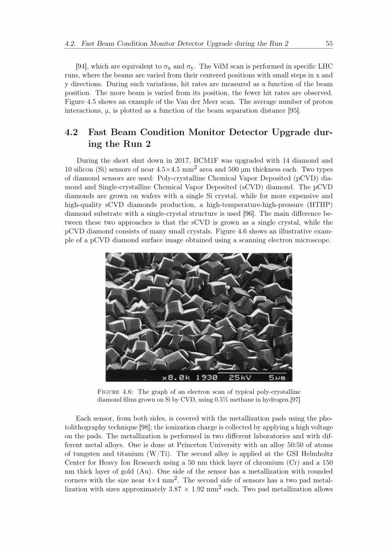
4.2. Fast Beam Condition Monitor Detector Upgrade during the Run 2 55
[94], which are equivalent to σx and σy. The VdM scan is performed in specific LHCruns, where the beams are varied from their centered positions with small steps in x andy directions. During such variations, hit rates are measured as a function of the beamposition. The more beam is varied from its position, the fewer hit rates are observed.Figure 4.5 shows an example of the Van der Meer scan. The average number of protoninteractions, μ, is plotted as a function of the beam separation distance [95].
4.2 Fast Beam Condition Monitor Detector Upgrade dur-ing the Run 2
During the short shut down in 2017, BCM1F was upgraded with 14 diamond and10 silicon (Si) sensors of near 4.5×4.5 mm2 area and 500 μm thickness each. Two typesof diamond sensors are used: Poly-crystalline Chemical Vapor Deposited (pCVD) dia-mond and Single-crystalline Chemical Vapor Deposited (sCVD) diamond. The pCVDdiamonds are grown on wafers with a single Si crystal, while for more expensive andhigh-quality sCVD diamonds production, a high-temperature-high-pressure (HTHP)diamond substrate with a single-crystal structure is used [96]. The main difference be-tween these two approaches is that the sCVD is grown as a single crystal, while thepCVD diamond consists of many small crystals. Figure 4.6 shows an illustrative exam-ple of a pCVD diamond surface image obtained using a scanning electron microscope.
Figure 4.6: The graph of an electron scan of typical poly-crystallinediamond films grown on Si by CVD, using 0.5% methane in hydrogen.[97]
Each sensor, from both sides, is covered with the metallization pads using the pho-tolithography technique [98]; the ionization charge is collected by applying a high voltageon the pads. The metallization is performed in two different laboratories and with dif-ferent metal alloys. One is done at Princeton University with an alloy 50:50 of atomsof tungsten and titanium (W/Ti). The second alloy is applied at the GSI HelmholtzCenter for Heavy Ion Research using a 50 nm thick layer of chromium (Cr) and a 150nm thick layer of gold (Au). One side of the sensor has a metallization with roundedcorners with the size near 4×4 mm2. The second side of sensors has a two pad metal-lization with sizes approximately 3.87 × 1.92 mm2 each. Two pad metallization allows
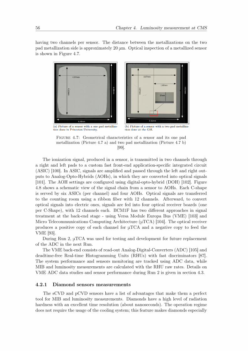
56 Chapter 4. Luminosity measurement at CMS
having two channels per sensor. The distance between the metallizations on the twopad metallization side is approximately 20 μm. Optical inspection of a metallized sensoris shown in Figure 4.7.
Figure 4.7: Geometrical characteristics of a sensor and its one padmetallization (Picture 4.7 a) and two pad metallization (Picture 4.7 b)
[99].
The ionization signal, produced in a sensor, is transmitted in two channels througha right and left pads to a custom fast front-end application-specific integrated circuit(ASIC) [100]. In ASIC, signals are amplified and passed through the left and right out-puts to Analog-Opto-Hybrids (AOHs), in which they are converted into optical signals[101]. The AOH settings are configured using digital-opto-hybrid (DOH) [102]. Figure4.8 shows a schematic view of the signal chain from a sensor to AOHs. Each C-shapeis served by six ASICs (per channel) and four AOHs. Optical signals are transferredto the counting room using a ribbon fiber with 12 channels. Afterward, to convertoptical signals into electric ones, signals are fed into four optical receiver boards (oneper C-Shape), with 12 channels each. BCM1F has two different approaches in signaltreatment at the back-end stage - using Versa Module Europa Bus (VME) [103] andMicro Telecommunications Computing Architecture (μTCA) [104]. The optical receiverproduces a positive copy of each channel for μTCA and a negative copy to feed theVME [93].
During Run 2, μTCA was used for testing and development for future replacementof the ADC in the next Run.
The VME back-end consists of read-out Analog-Digital-Converters (ADC) [105] anddeadtime-free Real-time Histogramming Units (RHUs) with fast discriminators [87].The system performance and sensors monitoring are tracked using ADC data, whileMIB and luminosity measurements are calculated with the RHU raw rates. Details onVME ADC data studies and sensor performance during Run 2 is given in section 4.3.
4.2.1 Diamond sensors measurements
The sCVD and pCVD sensors have a list of advantages that make them a perfecttool for MIB and luminosity measurements. Diamonds have a high level of radiationhardness with an excellent time resolution (about nanoseconds). The operation regimedoes not require the usage of the cooling system; this feature makes diamonds especially
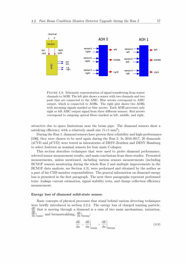
4.2. Fast Beam Condition Monitor Detector Upgrade during the Run 2 57
Figure 4.8: Schematic representation of signal transferring from sensorchannels to AOH. The left plot shows a sensor with two channels and twopads that are connected to the ASIC. Blue arrows correspond to ASICoutput, which is connected to AOHs. The right plot shows two AOHswith incoming signals marked as blue arrows. Each AOH processes onlyright or left ASIC output signal from three different sensors. Red arrowscorrespond to outgoing optical fibers marked as left, middle, and right.
attractive due to space limitations near the beam pipe. The diamond sensors show asatisfying efficiency with a relatively small size (5×5 mm2).
During the Run 1, diamond sensors have proven their reliability and high-performance[106], they were chosen to be used again during the Run 2. In 2016-2017, 20 diamonds(sCVD and pCVD) were tested in laboratories of DESY-Zeuthen and DESY Hamburgto select fourteen as nominal sensors for four main C-shapes.
This section describes techniques that were used to probe diamond performance,selected sensor measurement results, and main conclusions from these studies. Presentedmeasurements, unless mentioned, including various sensors measurements (includingBCM1F sensors monitoring during the whole Run 2 and multiple improvements in theBCM1F data analysis, see Section 4.3), were performed and obtained by the author asa part of his CMS member responsibilities. The general information on diamond energyloss is presented in the first paragraph. The next three paragraphs represent performedtests: leakage current estimation, signal stability tests, and charge collection efficiencymeasurement.
Energy loss of diamond solid-state sensor.
Basic concepts of physical processes that stand behind various detecting techniqueswere briefly introduced in section 2.2.2. The energy loss of charged ionizing particle,dEdx that is moving through a diamond is a sum of two main mechanisms, ionization,dEdx∣∣ioniz, and bremsstrahlung, dE
dx∣∣brems:
dEdx
=dEdx
∣∣∣∣ioniz
+dEdx
∣∣∣∣brems
. (4.8)
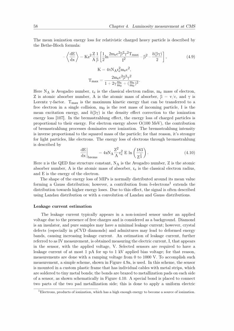
58 Chapter 4. Luminosity measurement at CMS
The mean ionization energy loss for relativistic charged heavy particle is described bythe Bethe-Bloch formula:
–⟨dEdx
⟩= Kz2
ZA1β
[12ln2mec2β2γ2Tmax
I2– β2 –
δ(βγ)2
], (4.9)
K = 4πNAr2emec2,
Tmax =2mec2β2γ2
1 + 2γmem0
+ (mem0
)2.
Here NA is Avogadro number, re is the classical electron radius, me mass of electron,Z is atomic absorber number, A is the atomic mass of absorber, β = v/c, and γ isLorentz γ-factor. Tmax is the maximum kinetic energy that can be transferred to afree electron in a single collision, m0 is the rest mass of incoming particle, I is themean excitation energy, and δ(βγ) is the density effect correction to the ionizationenergy loss [107]. In the bremsstrahlung effect, the energy loss of charged particles isproportional to their energy. For electron energy above O(100 MeV), the contributionof bremsstrahlung processes dominates over ionization. The bremsstrahlung intensityis inverse proportional to the squared mass of the particle; for that reason, it’s strongerfor light particles, like electrons. The energy loss of electrons through bremsstrahlungis described by
dEdx
∣∣∣∣brems
= 4αNAZ2
Ar2e E ln
(183
Z13
). (4.10)
Here α is the QED fine structure constant, NA is the Avogadro number, Z is the atomicabsorber number, A is the atomic mass of absorber, re is the classical electron radius,and E is the energy of the electron.
The shape of the energy loss of MIPs is normally distributed around its mean valueforming a Gauss distribution; however, a contribution from δ-electrons1 extends thedistribution towards higher energy loses. Due to this effect, the signal is often describedusing Landau distribution or with a convolution of Landau and Gauss distributions.
Leakage current estimation
The leakage current typically appears in a non-ionized sensor under an appliedvoltage due to the presence of free charges and is considered as a background. Diamondis an insulator, and pure samples may have a minimal leakage current; however, crystaldefects (especially in pCVD diamonds) and admixtures may lead to deformed energybands, causing increasing leakage current. An estimation of leakage current, furtherreferred to as IV measurement, is obtained measuring the electric current, I, that appearsin the sensor, with the applied voltage, V. Selected sensors are required to have aleakage current of at most 1 pA for up to 1 kV applied bias voltage; for that reason,measurements are done with a ramping voltage from 0 to 1000 V. To accomplish suchmeasurement, a simple scheme, shown in Figure 4.9a, is used. In this scheme, the sensoris mounted in a custom plastic frame that has individual cables with metal strips, whichare soldered to tiny metal bonds; the bonds are brazed to metallization pads on each sideof a sensor, as shown schematically in Figure 4.10. A special bond is placed to connecttwo parts of the two pad metallization side; this is done to apply a uniform electric
1Electrons, products of ionization, which has a high enough energy to become a source of ionization.
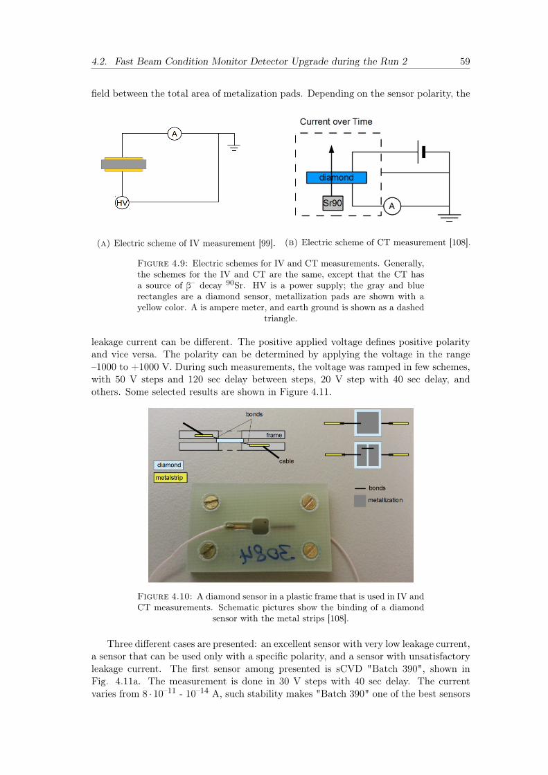
4.2. Fast Beam Condition Monitor Detector Upgrade during the Run 2 59
field between the total area of metalization pads. Depending on the sensor polarity, the
(a) Electric scheme of IV measurement [99]. (b) Electric scheme of CT measurement [108].
Figure 4.9: Electric schemes for IV and CT measurements. Generally,the schemes for the IV and CT are the same, except that the CT hasa source of β– decay 90Sr. HV is a power supply; the gray and bluerectangles are a diamond sensor, metallization pads are shown with ayellow color. A is ampere meter, and earth ground is shown as a dashed
triangle.
leakage current can be different. The positive applied voltage defines positive polarityand vice versa. The polarity can be determined by applying the voltage in the range–1000 to +1000 V. During such measurements, the voltage was ramped in few schemes,with 50 V steps and 120 sec delay between steps, 20 V step with 40 sec delay, andothers. Some selected results are shown in Figure 4.11.
Figure 4.10: A diamond sensor in a plastic frame that is used in IV andCT measurements. Schematic pictures show the binding of a diamond
sensor with the metal strips [108].
Three different cases are presented: an excellent sensor with very low leakage current,a sensor that can be used only with a specific polarity, and a sensor with unsatisfactoryleakage current. The first sensor among presented is sCVD "Batch 390", shown inFig. 4.11a. The measurement is done in 30 V steps with 40 sec delay. The currentvaries from 8 · 10–11 - 10–14 A, such stability makes "Batch 390" one of the best sensors
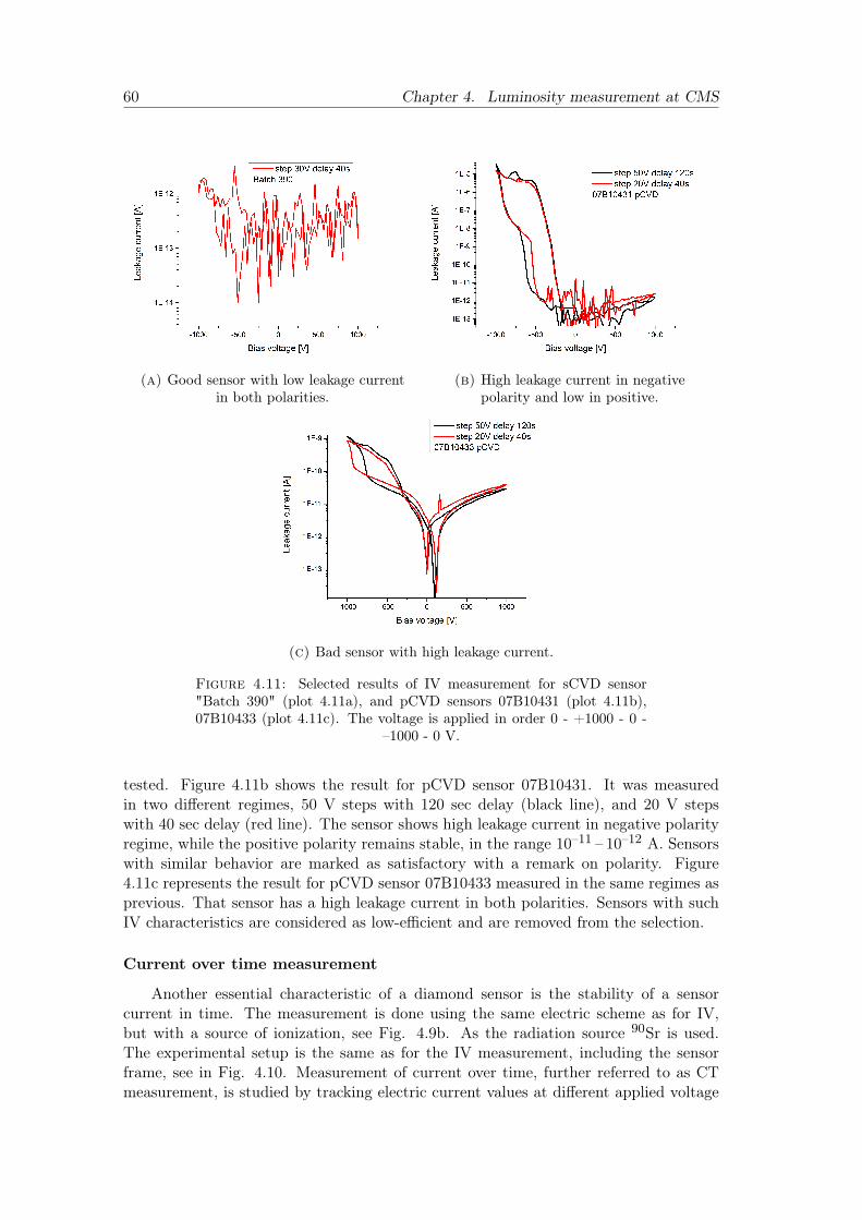
60 Chapter 4. Luminosity measurement at CMS
(a) Good sensor with low leakage currentin both polarities.
(b) High leakage current in negativepolarity and low in positive.
(c) Bad sensor with high leakage current.
Figure 4.11: Selected results of IV measurement for sCVD sensor"Batch 390" (plot 4.11a), and pCVD sensors 07B10431 (plot 4.11b),07B10433 (plot 4.11c). The voltage is applied in order 0 - +1000 - 0 -
–1000 - 0 V.
tested. Figure 4.11b shows the result for pCVD sensor 07B10431. It was measuredin two different regimes, 50 V steps with 120 sec delay (black line), and 20 V stepswith 40 sec delay (red line). The sensor shows high leakage current in negative polarityregime, while the positive polarity remains stable, in the range 10–11 – 10–12 A. Sensorswith similar behavior are marked as satisfactory with a remark on polarity. Figure4.11c represents the result for pCVD sensor 07B10433 measured in the same regimes asprevious. That sensor has a high leakage current in both polarities. Sensors with suchIV characteristics are considered as low-efficient and are removed from the selection.
Current over time measurement
Another essential characteristic of a diamond sensor is the stability of a sensorcurrent in time. The measurement is done using the same electric scheme as for IV,but with a source of ionization, see Fig. 4.9b. As the radiation source 90Sr is used.The experimental setup is the same as for the IV measurement, including the sensorframe, see in Fig. 4.10. Measurement of current over time, further referred to as CTmeasurement, is studied by tracking electric current values at different applied voltage
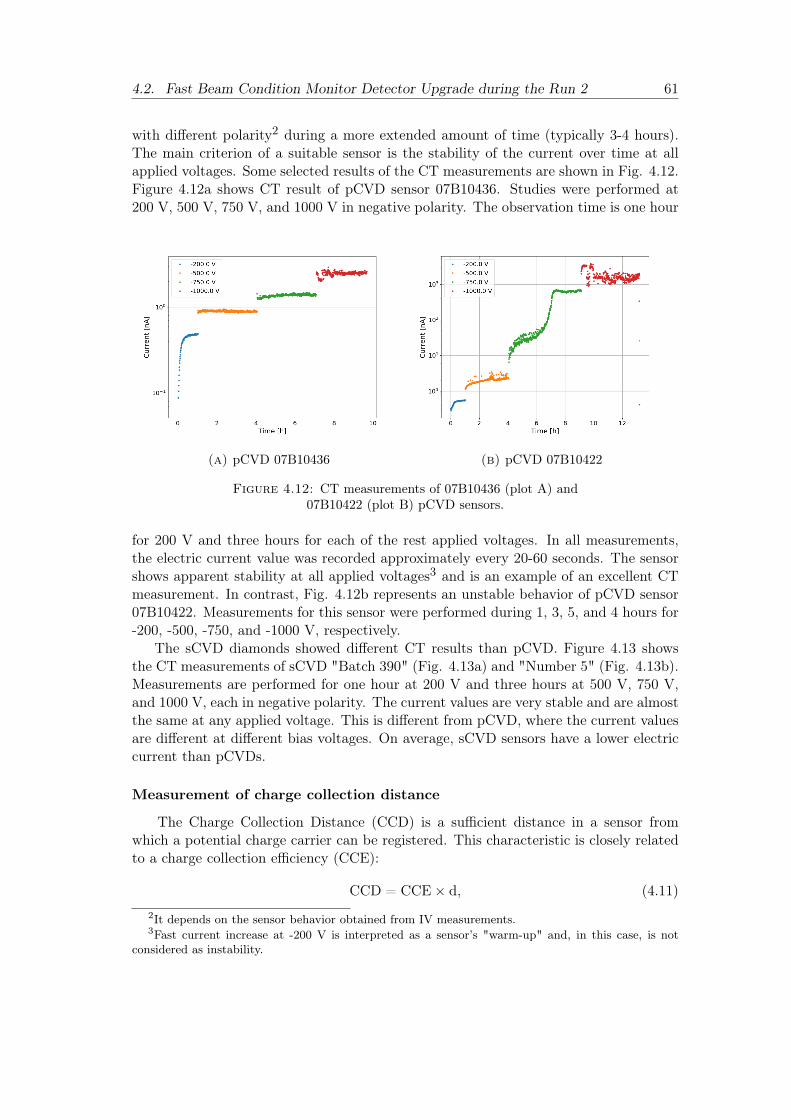
4.2. Fast Beam Condition Monitor Detector Upgrade during the Run 2 61
with different polarity2 during a more extended amount of time (typically 3-4 hours).The main criterion of a suitable sensor is the stability of the current over time at allapplied voltages. Some selected results of the CT measurements are shown in Fig. 4.12.Figure 4.12a shows CT result of pCVD sensor 07B10436. Studies were performed at200 V, 500 V, 750 V, and 1000 V in negative polarity. The observation time is one hour
(a) pCVD 07B10436 (b) pCVD 07B10422
Figure 4.12: CT measurements of 07B10436 (plot A) and07B10422 (plot B) pCVD sensors.
for 200 V and three hours for each of the rest applied voltages. In all measurements,the electric current value was recorded approximately every 20-60 seconds. The sensorshows apparent stability at all applied voltages3 and is an example of an excellent CTmeasurement. In contrast, Fig. 4.12b represents an unstable behavior of pCVD sensor07B10422. Measurements for this sensor were performed during 1, 3, 5, and 4 hours for-200, -500, -750, and -1000 V, respectively.
The sCVD diamonds showed different CT results than pCVD. Figure 4.13 showsthe CT measurements of sCVD "Batch 390" (Fig. 4.13a) and "Number 5" (Fig. 4.13b).Measurements are performed for one hour at 200 V and three hours at 500 V, 750 V,and 1000 V, each in negative polarity. The current values are very stable and are almostthe same at any applied voltage. This is different from pCVD, where the current valuesare different at different bias voltages. On average, sCVD sensors have a lower electriccurrent than pCVDs.
Measurement of charge collection distance
The Charge Collection Distance (CCD) is a sufficient distance in a sensor fromwhich a potential charge carrier can be registered. This characteristic is closely relatedto a charge collection efficiency (CCE):
CCD = CCE× d, (4.11)2It depends on the sensor behavior obtained from IV measurements.3Fast current increase at -200 V is interpreted as a sensor’s "warm-up" and, in this case, is not
considered as instability.
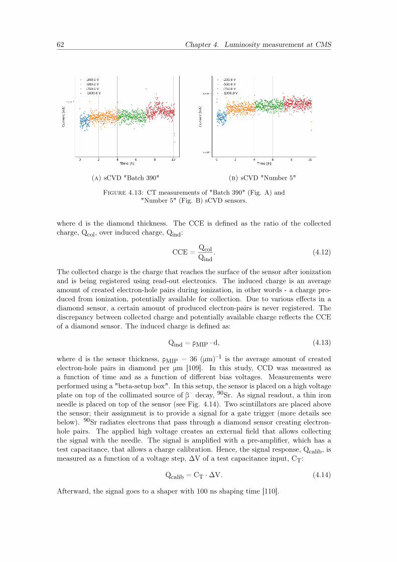
62 Chapter 4. Luminosity measurement at CMS
(a) sCVD "Batch 390" (b) sCVD "Number 5"
Figure 4.13: CT measurements of "Batch 390" (Fig. A) and"Number 5" (Fig. B) sCVD sensors.
where d is the diamond thickness. The CCE is defined as the ratio of the collectedcharge, Qcol, over induced charge, Qind:
CCE =QcolQind
. (4.12)
The collected charge is the charge that reaches the surface of the sensor after ionizationand is being registered using read-out electronics. The induced charge is an averageamount of created electron-hole pairs during ionization, in other words - a charge pro-duced from ionization, potentially available for collection. Due to various effects in adiamond sensor, a certain amount of produced electron-pairs is never registered. Thediscrepancy between collected charge and potentially available charge reflects the CCEof a diamond sensor. The induced charge is defined as:
Qind = ρMIP · d, (4.13)
where d is the sensor thickness, ρMIP = 36 (μm)–1 is the average amount of createdelectron-hole pairs in diamond per μm [109]. In this study, CCD was measured asa function of time and as a function of different bias voltages. Measurements wereperformed using a "beta-setup box". In this setup, the sensor is placed on a high voltageplate on top of the collimated source of β– decay, 90Sr. As signal readout, a thin ironneedle is placed on top of the sensor (see Fig. 4.14). Two scintillators are placed abovethe sensor; their assignment is to provide a signal for a gate trigger (more details seebelow). 90Sr radiates electrons that pass through a diamond sensor creating electron-hole pairs. The applied high voltage creates an external field that allows collectingthe signal with the needle. The signal is amplified with a pre-amplifier, which has atest capacitance, that allows a charge calibration. Hence, the signal response, Qcalib, ismeasured as a function of a voltage step, ΔV of a test capacitance input, CT:
Qcalib = CT ·ΔV. (4.14)
Afterward, the signal goes to a shaper with 100 ns shaping time [110].
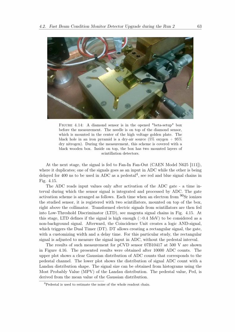
4.2. Fast Beam Condition Monitor Detector Upgrade during the Run 2 63
Figure 4.14: A diamond sensor is in the opened "beta-setup" boxbefore the measurement. The needle is on top of the diamond sensor,which is mounted in the center of the high voltage golden plate. Theblack hole in an iron pyramid is a dry-air source (5% oxygen + 95%dry nitrogen). During the measurement, this scheme is covered with ablack wooden box. Inside on top, the box has two mounted layers of
scintillation detectors.
At the next stage, the signal is fed to Fan-In Fan-Out (CAEN Model N625 [111]),where it duplicates; one of the signals goes as an input in ADC while the other is beingdelayed for 400 ns to be used in ADC as a pedestal4, see red and blue signal chains inFig. 4.15.
The ADC reads input values only after activation of the ADC gate - a time in-terval during which the sensor signal is integrated and processed by ADC. The gateactivation scheme is arranged as follows. Each time when an electron from 90Sr ionizesthe studied sensor, it is registered with two scintillators, mounted on top of the box,right above the collimator. Transformed electric signals from scintillators are then fedinto Low-Threshold Discriminator (LTD), see magenta signal chains in Fig. 4.15. Atthis stage, LTD defines if the signal is high enough (>0.4 MeV) to be considered as anon-background signal. Afterward, the Coincidence Unit creates a logic AND-signal,which triggers the Dual Timer (DT). DT allows creating a rectangular signal, the gate,with a customizing width and a delay time. For this particular study, the rectangularsignal is adjusted to measure the signal input in ADC, without the pedestal interval.
The results of such measurement for pCVD sensor 07B10417 at 500 V are shownin Figure 4.16. The presented results were obtained after 10000 ADC counts. Theupper plot shows a clear Gaussian distribution of ADC counts that corresponds to thepedestal channel. The lower plot shows the distribution of signal ADC count with aLandau distribution shape. The signal size can be obtained from histograms using theMost Probably Value (MPV) of the Landau distribution. The pedestal value, Ped, isderived from the mean value of the Gaussian distribution.
4Pedestal is used to estimate the noise of the whole readout chain.
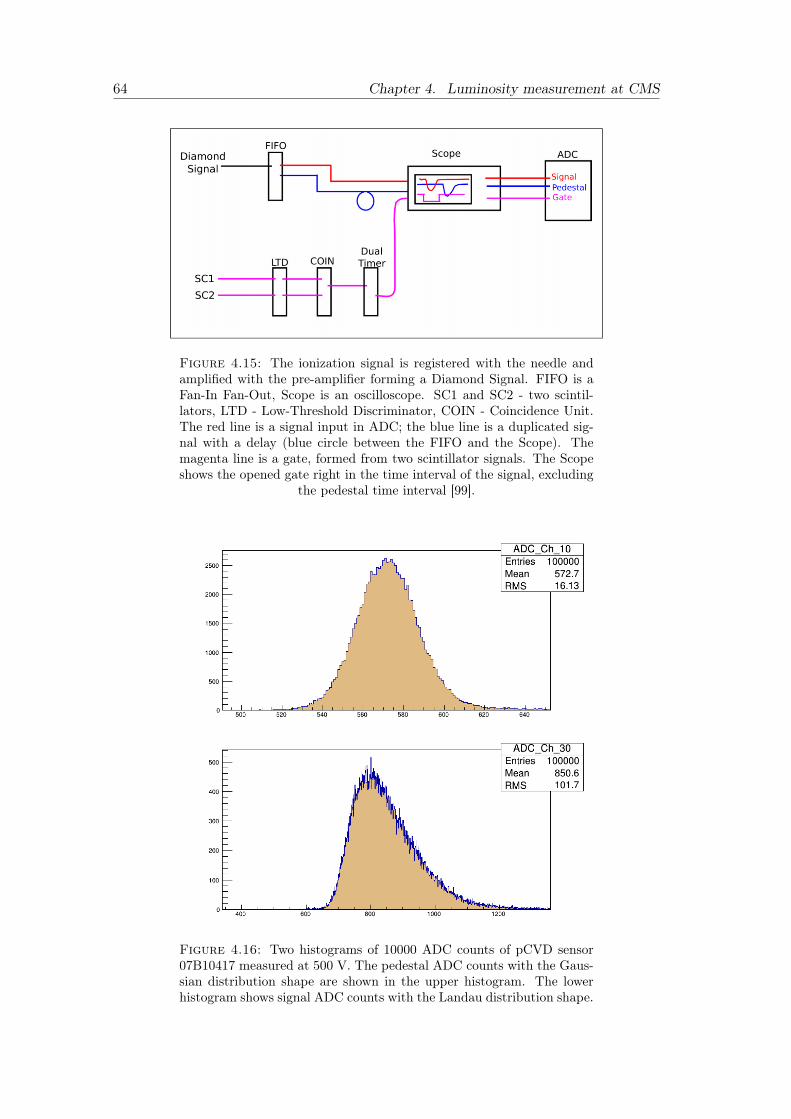
64 Chapter 4. Luminosity measurement at CMS
Figure 4.15: The ionization signal is registered with the needle andamplified with the pre-amplifier forming a Diamond Signal. FIFO is aFan-In Fan-Out, Scope is an oscilloscope. SC1 and SC2 - two scintil-lators, LTD - Low-Threshold Discriminator, COIN - Coincidence Unit.The red line is a signal input in ADC; the blue line is a duplicated sig-nal with a delay (blue circle between the FIFO and the Scope). Themagenta line is a gate, formed from two scintillator signals. The Scopeshows the opened gate right in the time interval of the signal, excluding
the pedestal time interval [99].
Figure 4.16: Two histograms of 10000 ADC counts of pCVD sensor07B10417 measured at 500 V. The pedestal ADC counts with the Gaus-sian distribution shape are shown in the upper histogram. The lowerhistogram shows signal ADC counts with the Landau distribution shape.
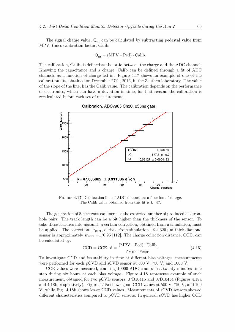
4.2. Fast Beam Condition Monitor Detector Upgrade during the Run 2 65
The signal charge value, Qm can be calculated by subtracting pedestal value fromMPV, times calibration factor, Calib:
Qm = (MPV – Ped) · Calib.
The calibration, Calib, is defined as the ratio between the charge and the ADC channel.Knowing the capacitance and a charge, Calib can be defined through a fit of ADCchannels as a function of charge fed in. Figure 4.17 shows an example of one of thecalibration fits, obtained on December 27th, 2016, in the Zeuthen laboratory. The valueof the slope of the line, k is the Calib value. The calibration depends on the performanceof electronics, which can have a deviation in time; for that reason, the calibration isrecalculated before each set of measurements.
Figure 4.17: Calibration line of ADC channels as a function of charge.The Calib value obtained from this fit is k=47.
The generation of δ-electrons can increase the expected number of produced electron-hole pairs. The track length can be a bit higher than the thickness of the sensor. Totake these features into account, a certain correction, obtained from a simulation, mustbe applied. The correction, srcorr, derived from simulations, for 320 μm thick diamondsensor is approximately srcorr =1/0.95 [112]. The charge collection distance, CCD, canbe calculated by:
CCD = CCE · d =(MPV – Ped) · CalibρMIP · srcorr
. (4.15)
To investigate CCD and its stability in time at different bias voltages, measurementswere performed for each pCVD and sCVD sensor at 500 V, 750 V, and 1000 V.
CCE values were measured, counting 10000 ADC counts in a twenty minutes timestep during six hours at each bias voltage. Figure 4.18 represents example of suchmeasurement, obtained for two pCVD sensors, 07B10415 and 07B10434 (Figures 4.18aand 4.18b, respectively). Figure 4.18a shows good CCD values at 500 V, 750 V, and 100V, while Fig. 4.18b shows lower CCD values. Measurements of sCVD sensors showeddifferent characteristics compared to pCVD sensors. In general, sCVD has higher CCD
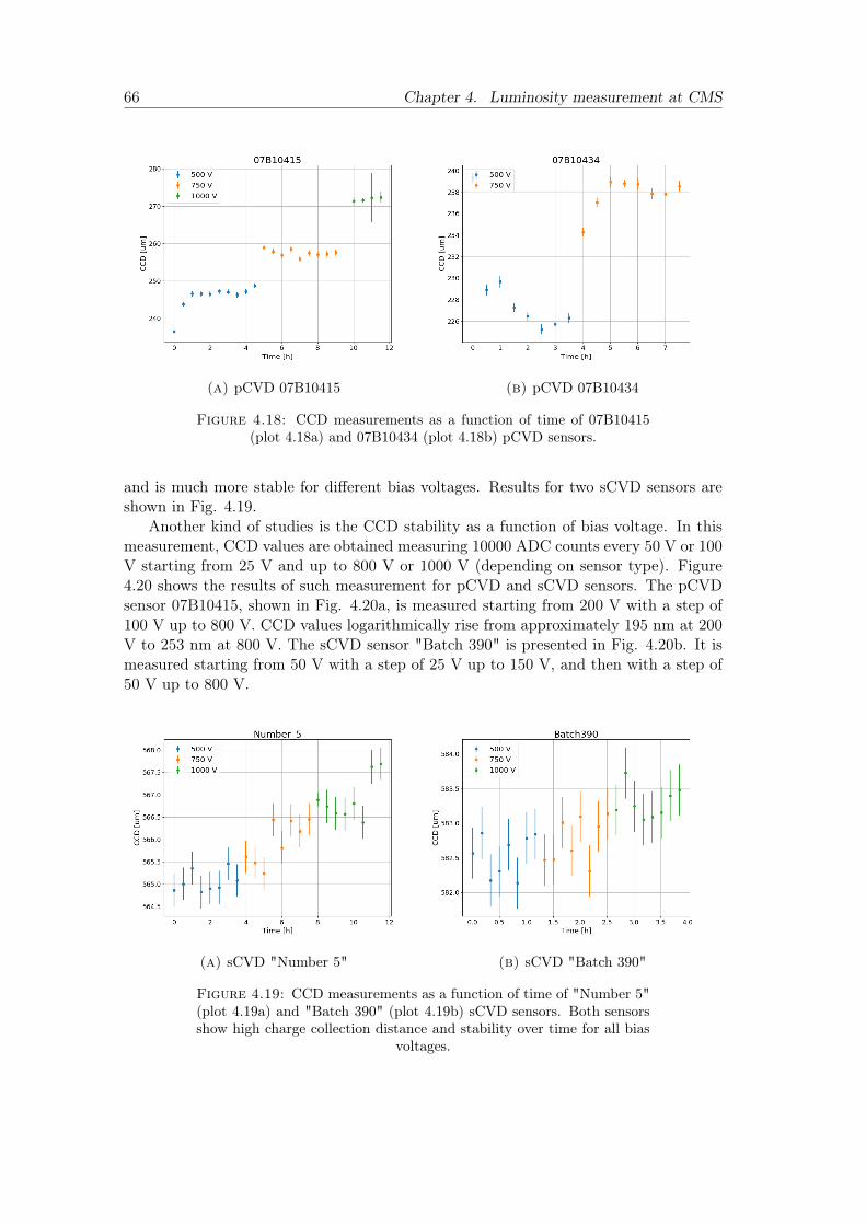
66 Chapter 4. Luminosity measurement at CMS
(a) pCVD 07B10415 (b) pCVD 07B10434
Figure 4.18: CCD measurements as a function of time of 07B10415(plot 4.18a) and 07B10434 (plot 4.18b) pCVD sensors.
and is much more stable for different bias voltages. Results for two sCVD sensors areshown in Fig. 4.19.
Another kind of studies is the CCD stability as a function of bias voltage. In thismeasurement, CCD values are obtained measuring 10000 ADC counts every 50 V or 100V starting from 25 V and up to 800 V or 1000 V (depending on sensor type). Figure4.20 shows the results of such measurement for pCVD and sCVD sensors. The pCVDsensor 07B10415, shown in Fig. 4.20a, is measured starting from 200 V with a step of100 V up to 800 V. CCD values logarithmically rise from approximately 195 nm at 200V to 253 nm at 800 V. The sCVD sensor "Batch 390" is presented in Fig. 4.20b. It ismeasured starting from 50 V with a step of 25 V up to 150 V, and then with a step of50 V up to 800 V.
(a) sCVD "Number 5" (b) sCVD "Batch 390"
Figure 4.19: CCD measurements as a function of time of "Number 5"(plot 4.19a) and "Batch 390" (plot 4.19b) sCVD sensors. Both sensorsshow high charge collection distance and stability over time for all bias
voltages.
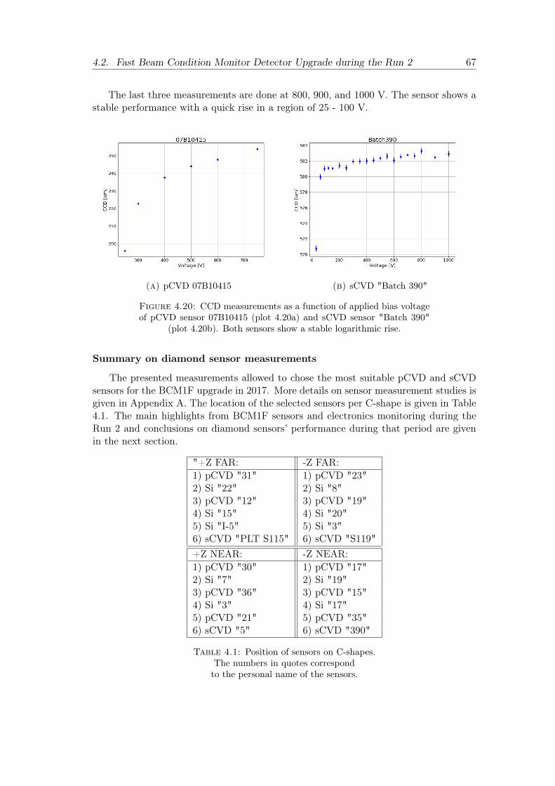
4.2. Fast Beam Condition Monitor Detector Upgrade during the Run 2 67
The last three measurements are done at 800, 900, and 1000 V. The sensor shows astable performance with a quick rise in a region of 25 - 100 V.
(a) pCVD 07B10415 (b) sCVD "Batch 390"
Figure 4.20: CCD measurements as a function of applied bias voltageof pCVD sensor 07B10415 (plot 4.20a) and sCVD sensor "Batch 390"
(plot 4.20b). Both sensors show a stable logarithmic rise.
Summary on diamond sensor measurements
The presented measurements allowed to chose the most suitable pCVD and sCVDsensors for the BCM1F upgrade in 2017. More details on sensor measurement studies isgiven in Appendix A. The location of the selected sensors per C-shape is given in Table4.1. The main highlights from BCM1F sensors and electronics monitoring during theRun 2 and conclusions on diamond sensors’ performance during that period are givenin the next section.
"+Z FAR: -Z FAR:1) pCVD "31" 1) pCVD "23"2) Si "22" 2) Si "8"3) pCVD "12" 3) pCVD "19"4) Si "15" 4) Si "20"5) Si "I-5" 5) Si "3"6) sCVD "PLT S115" 6) sCVD "S119"+Z NEAR: -Z NEAR:1) pCVD "30" 1) pCVD "17"2) Si "7" 2) Si "19"3) pCVD "36" 3) pCVD "15"4) Si "3" 4) Si "17"5) pCVD "21" 5) pCVD "35"6) sCVD "5" 6) sCVD "390"
Table 4.1: Position of sensors on C-shapes.The numbers in quotes correspondto the personal name of the sensors.

68 Chapter 4. Luminosity measurement at CMS
4.3 BCM1F status monitoring using VME ADC
BCM1F performance control exists to give a clear picture of how reliable the de-tector results are. The detector efficiency is expected to decrease due to sensors andelectronics degradation from the radiation damage. Also, uncertainties may arise fromelectronics productivity due to the changes in CMS magnetic field, temperature fluctu-ation, etc. While the RHU unit is called to calculate online luminosity, the goal of VMEADC readout is to provide the data for the monitor sensor performance and electronicsstability. Sensor efficiency is studied in each channel, analyzing the amplitude spectraof particle hits. Such measurements allow to track spectra degradation in time and,when it’s possible, to take actions to improve sensor performance. Electronics behavioris observed separately from the sensors’ response, using a Test Pulse (TP).
4.3.1 VME ADC data processing
The BCM1F status monitoring starts from the VME ADC raw data processing,which is a record of ADC counts as a function of time. The timeline ends when a bunchmakes a full circle in LHC, approximately in 90 · 10–6 seconds. Such data, recordedper one ring, is called "orbit". Figure 4.21 shows an example of recorded orbit. Thefirst signal belongs to a TP, and the rest are bunches of the fill. Bunches are gatheredin groups called "trains". The so-called "pilot" bunch train follows the test pulse andconsists of 12 bunches. The rest are twelve trains with 70 bunches in each.
Figure 4.21: Recorded orbit from the LHC Fill 4364 with 852 collidingbunches [87]. The baseline is set on 140 ADC counts, signals are shownas dips in a baseline position. Red ellipse shows a TP, green rectanglecorresponds to the "pilot" train, and each magenta circle is a train of
bunches.
The arrival time is obtained by applying a 3 ADC counts threshold to the orbit.An example of acquired arrival time distribution is shown in Figure 4.22, where the TPsignal is cut out, the "pilot" train is first, and the rest are twelve bunches grouped intwo.
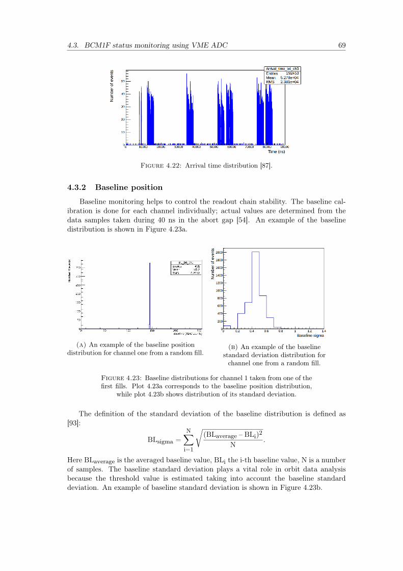
4.3. BCM1F status monitoring using VME ADC 69
Figure 4.22: Arrival time distribution [87].
4.3.2 Baseline position
Baseline monitoring helps to control the readout chain stability. The baseline cal-ibration is done for each channel individually; actual values are determined from thedata samples taken during 40 ns in the abort gap [54]. An example of the baselinedistribution is shown in Figure 4.23a.
(a) An example of the baseline positiondistribution for channel one from a random fill.
(b) An example of the baselinestandard deviation distribution forchannel one from a random fill.
Figure 4.23: Baseline distributions for channel 1 taken from one of thefirst fills. Plot 4.23a corresponds to the baseline position distribution,
while plot 4.23b shows distribution of its standard deviation.
The definition of the standard deviation of the baseline distribution is defined as[93]:
BLsigma =N∑i=1
√(BLaverage – BLi)2
N.
Here BLaverage is the averaged baseline value, BLi the i-th baseline value, N is a numberof samples. The baseline standard deviation plays a vital role in orbit data analysisbecause the threshold value is estimated taking into account the baseline standarddeviation. An example of baseline standard deviation is shown in Figure 4.23b.
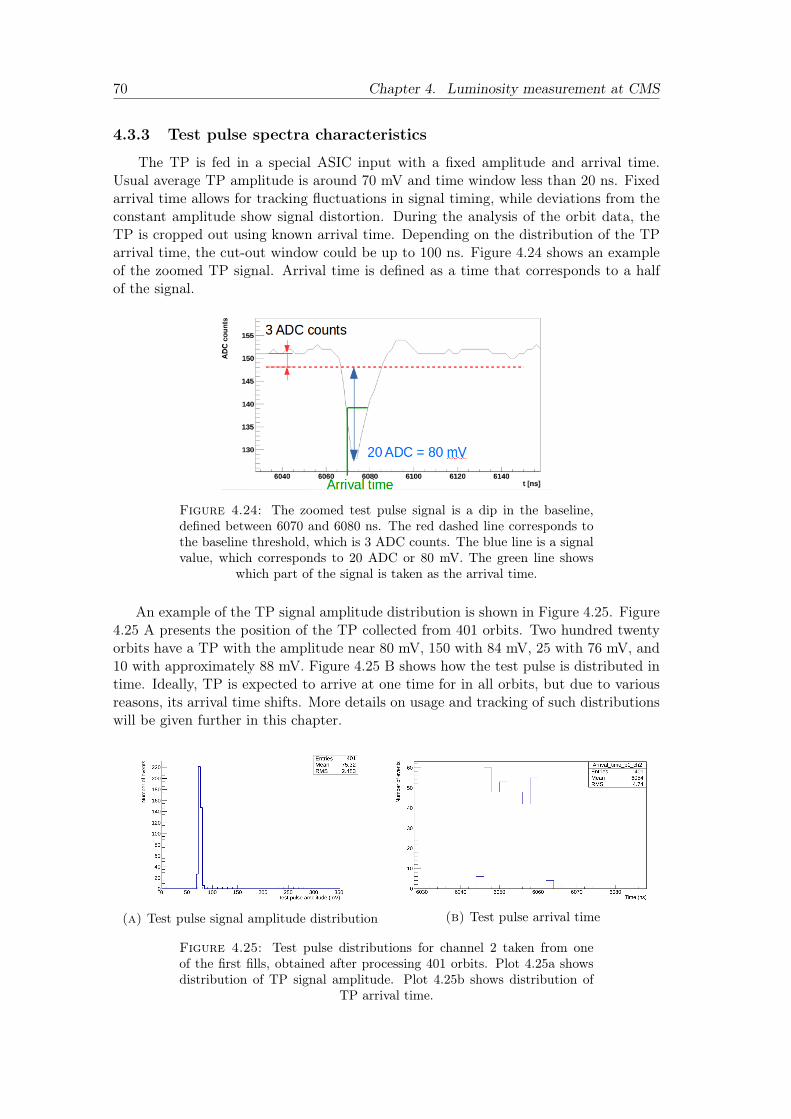
70 Chapter 4. Luminosity measurement at CMS
4.3.3 Test pulse spectra characteristics
The TP is fed in a special ASIC input with a fixed amplitude and arrival time.Usual average TP amplitude is around 70 mV and time window less than 20 ns. Fixedarrival time allows for tracking fluctuations in signal timing, while deviations from theconstant amplitude show signal distortion. During the analysis of the orbit data, theTP is cropped out using known arrival time. Depending on the distribution of the TParrival time, the cut-out window could be up to 100 ns. Figure 4.24 shows an exampleof the zoomed TP signal. Arrival time is defined as a time that corresponds to a halfof the signal.
Figure 4.24: The zoomed test pulse signal is a dip in the baseline,defined between 6070 and 6080 ns. The red dashed line corresponds tothe baseline threshold, which is 3 ADC counts. The blue line is a signalvalue, which corresponds to 20 ADC or 80 mV. The green line shows
which part of the signal is taken as the arrival time.
An example of the TP signal amplitude distribution is shown in Figure 4.25. Figure4.25 A presents the position of the TP collected from 401 orbits. Two hundred twentyorbits have a TP with the amplitude near 80 mV, 150 with 84 mV, 25 with 76 mV, and10 with approximately 88 mV. Figure 4.25 B shows how the test pulse is distributed intime. Ideally, TP is expected to arrive at one time for in all orbits, but due to variousreasons, its arrival time shifts. More details on usage and tracking of such distributionswill be given further in this chapter.
(a) Test pulse signal amplitude distribution (b) Test pulse arrival time
Figure 4.25: Test pulse distributions for channel 2 taken from oneof the first fills, obtained after processing 401 orbits. Plot 4.25a showsdistribution of TP signal amplitude. Plot 4.25b shows distribution of
TP arrival time.
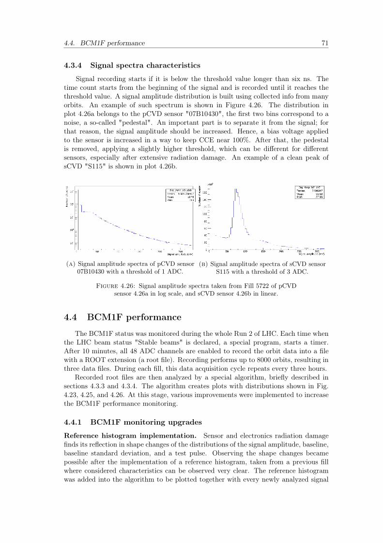
4.4. BCM1F performance 71
4.3.4 Signal spectra characteristics
Signal recording starts if it is below the threshold value longer than six ns. Thetime count starts from the beginning of the signal and is recorded until it reaches thethreshold value. A signal amplitude distribution is built using collected info from manyorbits. An example of such spectrum is shown in Figure 4.26. The distribution inplot 4.26a belongs to the pCVD sensor "07B10430", the first two bins correspond to anoise, a so-called "pedestal". An important part is to separate it from the signal; forthat reason, the signal amplitude should be increased. Hence, a bias voltage appliedto the sensor is increased in a way to keep CCE near 100%. After that, the pedestalis removed, applying a slightly higher threshold, which can be different for differentsensors, especially after extensive radiation damage. An example of a clean peak ofsCVD "S115" is shown in plot 4.26b.
(a) Signal amplitude spectra of pCVD sensor07B10430 with a threshold of 1 ADC.
(b) Signal amplitude spectra of sCVD sensorS115 with a threshold of 3 ADC.
Figure 4.26: Signal amplitude spectra taken from Fill 5722 of pCVDsensor 4.26a in log scale, and sCVD sensor 4.26b in linear.
4.4 BCM1F performance
The BCM1F status was monitored during the whole Run 2 of LHC. Each time whenthe LHC beam status "Stable beams" is declared, a special program, starts a timer.After 10 minutes, all 48 ADC channels are enabled to record the orbit data into a filewith a ROOT extension (a root file). Recording performs up to 8000 orbits, resulting inthree data files. During each fill, this data acquisition cycle repeats every three hours.
Recorded root files are then analyzed by a special algorithm, briefly described insections 4.3.3 and 4.3.4. The algorithm creates plots with distributions shown in Fig.4.23, 4.25, and 4.26. At this stage, various improvements were implemented to increasethe BCM1F performance monitoring.
4.4.1 BCM1F monitoring upgrades
Reference histogram implementation. Sensor and electronics radiation damagefinds its reflection in shape changes of the distributions of the signal amplitude, baseline,baseline standard deviation, and a test pulse. Observing the shape changes becamepossible after the implementation of a reference histogram, taken from a previous fillwhere considered characteristics can be observed very clear. The reference histogramwas added into the algorithm to be plotted together with every newly analyzed signal
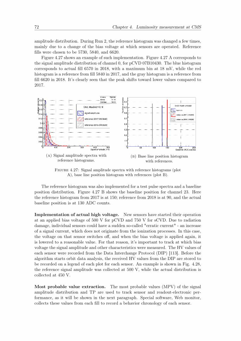
72 Chapter 4. Luminosity measurement at CMS
amplitude distribution. During Run 2, the reference histogram was changed a few times,mainly due to a change of the bias voltage at which sensors are operated. Referencefills were chosen to be 5730, 5840, and 6620.
Figure 4.27 shows an example of such implementation. Figure 4.27 A corresponds tothe signal amplitude distribution of channel 0, for pCVD 07B10430. The blue histogramcorresponds to actual fill 6570 in 2018, with a maximum bin at 18 mV, while the redhistogram is a reference from fill 5840 in 2017, and the gray histogram is a reference fromfill 6620 in 2018. It’s clearly seen that the peak shifts toward lower values compared to2017.
(a) Signal amplitude spectra withreference histograms.
(b) Base line position histogramwith references.
Figure 4.27: Signal amplitude spectra with reference histograms (plotA), base line position histogram with references (plot B).
The reference histogram was also implemented for a test pulse spectra and a baselineposition distribution. Figure 4.27 B shows the baseline position for channel 23. Herethe reference histogram from 2017 is at 150; reference from 2018 is at 90, and the actualbaseline position is at 130 ADC counts.
Implementation of actual high voltage. New sensors have started their operationat an applied bias voltage of 500 V for pCVD and 750 V for sCVD. Due to radiationdamage, individual sensors could have a sudden so-called "erratic current" - an increaseof a signal current, which does not originate from the ionization processes. In this case,the voltage on that sensor switches off, and when the bias voltage is applied again, itis lowered to a reasonable value. For that reason, it’s important to track at which biasvoltage the signal amplitude and other characteristics were measured. The HV values ofeach sensor were recorded from the Data Interchange Protocol (DIP) [113]. Before thealgorithm starts orbit data analysis, the received HV values from the DIP are stored tobe recorded on a legend of each plot for each sensor. An example is shown in Fig. 4.28,the reference signal amplitude was collected at 500 V, while the actual distribution iscollected at 450 V.
Most probable value extraction. The most probable values (MPV) of the signalamplitude distribution and TP are used to track sensor and readout-electronic per-formance, as it will be shown in the next paragraph. Special software, Web monitor,collects these values from each fill to record a behavior chronology of each sensor.
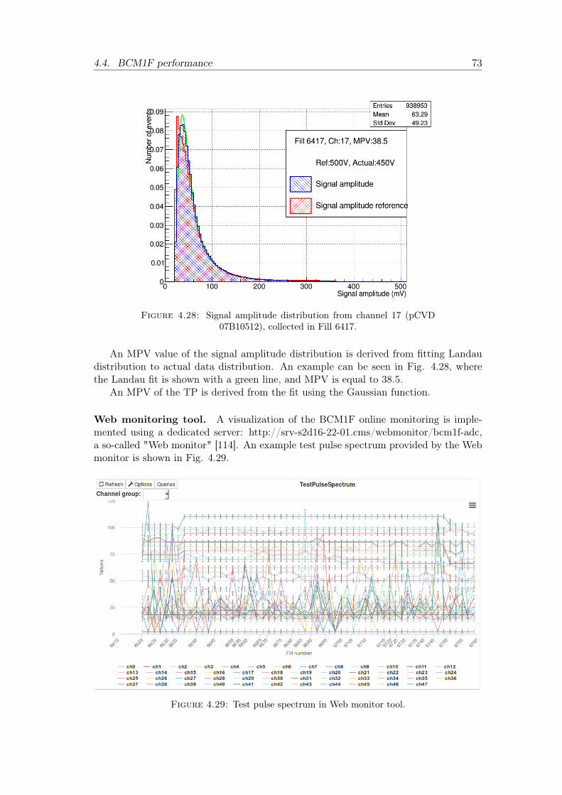
4.4. BCM1F performance 73
Figure 4.28: Signal amplitude distribution from channel 17 (pCVD07B10512), collected in Fill 6417.
An MPV value of the signal amplitude distribution is derived from fitting Landaudistribution to actual data distribution. An example can be seen in Fig. 4.28, wherethe Landau fit is shown with a green line, and MPV is equal to 38.5.
An MPV of the TP is derived from the fit using the Gaussian function.
Web monitoring tool. A visualization of the BCM1F online monitoring is imple-mented using a dedicated server: http://srv-s2d16-22-01.cms/webmonitor/bcm1f-adc,a so-called "Web monitor" [114]. An example test pulse spectrum provided by the Webmonitor is shown in Fig. 4.29.
Figure 4.29: Test pulse spectrum in Web monitor tool.
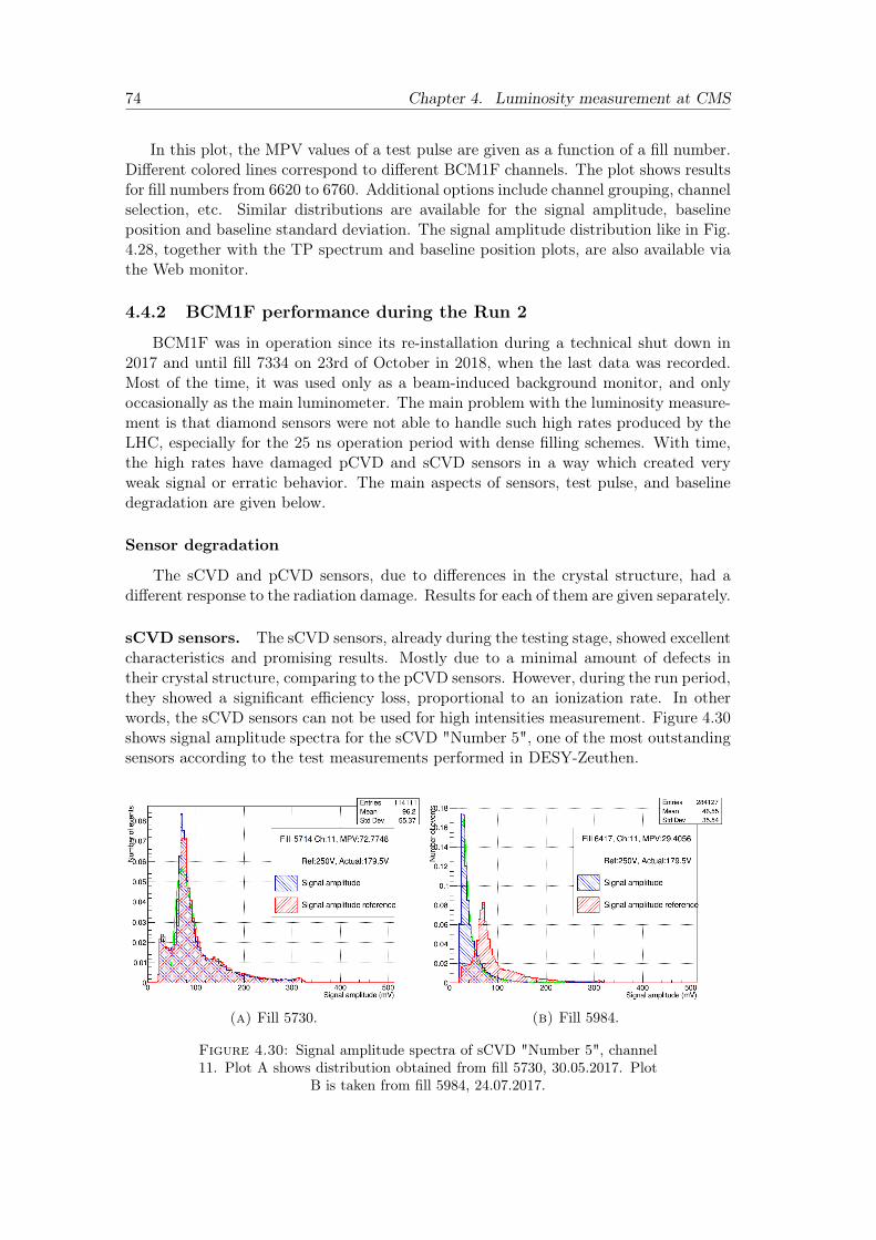
74 Chapter 4. Luminosity measurement at CMS
In this plot, the MPV values of a test pulse are given as a function of a fill number.Different colored lines correspond to different BCM1F channels. The plot shows resultsfor fill numbers from 6620 to 6760. Additional options include channel grouping, channelselection, etc. Similar distributions are available for the signal amplitude, baselineposition and baseline standard deviation. The signal amplitude distribution like in Fig.4.28, together with the TP spectrum and baseline position plots, are also available viathe Web monitor.
4.4.2 BCM1F performance during the Run 2
BCM1F was in operation since its re-installation during a technical shut down in2017 and until fill 7334 on 23rd of October in 2018, when the last data was recorded.Most of the time, it was used only as a beam-induced background monitor, and onlyoccasionally as the main luminometer. The main problem with the luminosity measure-ment is that diamond sensors were not able to handle such high rates produced by theLHC, especially for the 25 ns operation period with dense filling schemes. With time,the high rates have damaged pCVD and sCVD sensors in a way which created veryweak signal or erratic behavior. The main aspects of sensors, test pulse, and baselinedegradation are given below.
Sensor degradation
The sCVD and pCVD sensors, due to differences in the crystal structure, had adifferent response to the radiation damage. Results for each of them are given separately.
sCVD sensors. The sCVD sensors, already during the testing stage, showed excellentcharacteristics and promising results. Mostly due to a minimal amount of defects intheir crystal structure, comparing to the pCVD sensors. However, during the run period,they showed a significant efficiency loss, proportional to an ionization rate. In otherwords, the sCVD sensors can not be used for high intensities measurement. Figure 4.30shows signal amplitude spectra for the sCVD "Number 5", one of the most outstandingsensors according to the test measurements performed in DESY-Zeuthen.
(a) Fill 5730. (b) Fill 5984.
Figure 4.30: Signal amplitude spectra of sCVD "Number 5", channel11. Plot A shows distribution obtained from fill 5730, 30.05.2017. Plot
B is taken from fill 5984, 24.07.2017.
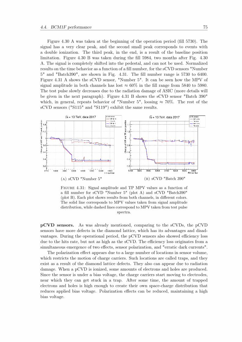
4.4. BCM1F performance 75
Figure 4.30 A was taken at the beginning of the operation period (fill 5730). Thesignal has a very clear peak, and the second small peak corresponds to events witha double ionization. The third peak, in the end, is a result of the baseline positionlimitation. Figure 4.30 B was taken during the fill 5984, two months after Fig. 4.30A. The signal is completely shifted into the pedestal, and can not be used. Normalizedresults on the time behavior as a function of a fill number, for the sCVD sensors "Number5" and "Batch390", are shown in Fig. 4.31. The fill number range is 5730 to 6400.Figure 4.31 A shows the sCVD sensor, "Number 5". It can be seen how the MPV ofsignal amplitude in both channels has lost ≈ 60% in the fill range from 5840 to 5980.The test pulse slowly decreases due to the radiation damage of ASIC (more details willbe given in the next paragraph). Figure 4.31 B shows the sCVD sensor "Batch 390"which, in general, repeats behavior of "Number 5", loosing ≈ 70%. The rest of thesCVD sensors ("S115" and "S119") exhibit the same results.
(a) sCVD "Number 5" (b) sCVD "Batch 390"
Figure 4.31: Signal amplitude and TP MPV values as a function ofa fill number for sCVD "Number 5" (plot A) and sCVD "Batch390"(plot B). Each plot shows results from both channels, in different colors.The solid line corresponds to MPV values taken from signal amplitudedistribution, while dashed lines correspond to MPV taken from test pulse
spectra.
pCVD sensors. As was already mentioned, comparing to the sCVDs, the pCVDsensors have more defects in the diamond lattice, which has its advantages and disad-vantages. During the operational period, the pCVD sensors also showed efficiency lossdue to the hits rate, but not as high as the sCVD. The efficiency loss originates from asimultaneous emergence of two effects, sensor polarization, and "erratic dark currents".
The polarization effect appears due to a large number of locations in sensor volume,which restricts the motion of charge carriers. Such locations are called traps, and theyexist as a result of the diamond lattice defects. They also can appear due to radiationdamage. When a pCVD is ionized, some amounts of electrons and holes are produced.Since the sensor is under a bias voltage, the charge carriers start moving to electrodes,near which they can get stuck in a trap. After some time, the amount of trappedelectrons and holes is high enough to create their own space-charge distribution thatreduces applied bias voltage. Polarization effects can be reduced, maintaining a highbias voltage.
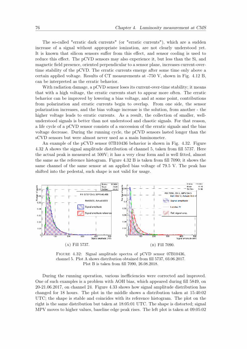
76 Chapter 4. Luminosity measurement at CMS
The so-called "erratic dark currents" (or "erratic currents"), which are a suddenincrease of a signal without appropriate ionization, are not clearly understood yet.It is known that silicon sensors suffer from this effect, and sensor cooling is used toreduce this effect. The pCVD sensors may also experience it, but less than the Si, andmagnetic field presence, oriented perpendicular to a sensor plane, increases current-over-time stability of the pCVD. The erratic currents emerge after some time only above acertain applied voltage. Results of CT measurements at -750 V, shown in Fig. 4.12 B,can be interpreted as the erratic behavior.
With radiation damage, a pCVD sensor loses its current-over-time stability; it meansthat with a high voltage, the erratic currents start to appear more often. The erraticbehavior can be improved by lowering a bias voltage, and at some point, contributionsfrom polarization and erratic currents begin to overlap. From one side, the sensorpolarization increases, and the bias voltage increase is the solution, from another - thehigher voltage leads to erratic currents. As a result, the collection of smaller, well-understood signals is better than not understood and chaotic signals. For that reason,a life cycle of a pCVD sensor consists of a succession of the erratic signals and the biasvoltage decrease. During the running cycle, the pCVD sensors lasted longer than thesCVD sensors but were almost never used as a main luminometer.
An example of the pCVD sensor 07B10436 behavior is shown in Fig. 4.32. Figure4.32 A shows the signal amplitude distribution of channel 5, taken from fill 5737. Herethe actual peak is measured at 500V; it has a very clear form and is well fitted, almostthe same as the reference histogram. Figure 4.32 B is taken from fill 7090; it shows thesame channel of the same sensor at an applied bias voltage of 79.5 V. The peak hasshifted into the pedestal, such shape is not valid for usage.
(a) Fill 5737. (b) Fill 7090.
Figure 4.32: Signal amplitude spectra of pCVD sensor 07B10436,channel 5. Plot A shows distribution obtained from fill 5737, 03.06.2017.
Plot B is taken from fill 7090, 26.08.2018.
During the running operation, various inefficiencies were corrected and improved.One of such examples is a problem with AOH bias, which appeared during fill 5849, on20-21.06.2017, on channel 24. Figure 4.33 shows how signal amplitude distribution haschanged for 18 hours. The plot in the middle shows a distribution taken at 15:40:02UTC; the shape is stable and coincides with its reference histogram. The plot on theright is the same distribution but taken at 18:05:01 UTC. The shape is distorted; signalMPV moves to higher values, baseline edge peak rises. The left plot is taken at 09:05:02
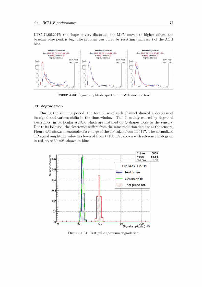
4.4. BCM1F performance 77
UTC 21.06.2017; the shape is very distorted, the MPV moved to higher values, thebaseline edge peak is big. The problem was cured by resetting (increase ) of the AOHbias.
Figure 4.33: Signal amplitude spectrum in Web monitor tool.
TP degradation
During the running period, the test pulse of each channel showed a decrease ofits signal and various shifts in the time window. This is mainly caused by degradedelectronics, in particular ASICs, which are installed on C-shapes close to the sensors.Due to its location, the electronics suffers from the same radiation damage as the sensors.Figure 4.34 shows an example of a change of the TP taken from fill 6417. The normalizedTP signal amplitude value has lowered from ≈ 100 mV, shown with reference histogramin red, to ≈ 60 mV, shown in blue.
Figure 4.34: Test pulse spectrum degradation.
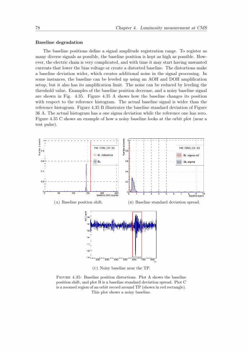
78 Chapter 4. Luminosity measurement at CMS
Baseline degradation
The baseline positions define a signal amplitude registration range. To register asmany diverse signals as possible, the baseline position is kept as high as possible. How-ever, the electric chain is very complicated, and with time it may start having unwantedcurrents that lower the bias voltage or create a distorted baseline. The distortions makea baseline deviation wider, which creates additional noise in the signal processing. Insome instances, the baseline can be leveled up using an AOH and DOH amplificationsetup, but it also has its amplification limit. The noise can be reduced by leveling thethreshold value. Examples of the baseline position decrease, and a noisy baseline signalare shown in Fig. 4.35. Figure 4.35 A shows how the baseline changes its positionwith respect to the reference histogram. The actual baseline signal is wider than thereference histogram. Figure 4.35 B illustrates the baseline standard deviation of Figure36 A. The actual histogram has a one sigma deviation while the reference one has zero.Figure 4.35 C shows an example of how a noisy baseline looks at the orbit plot (near atest pulse).
(a) Baseline position shift. (b) Baseline standard deviation spread.
(c) Noisy baseline near the TP.
Figure 4.35: Baseline position distortions. Plot A shows the baselineposition shift, and plot B is a baseline standard deviation spread. Plot Cis a zoomed region of an orbit record around TP (shown in red rectangle).
This plot shows a noisy baseline.

4.4. BCM1F performance 79
4.4.3 Conclusions
The studied diamond sensors have shown a great performance for the severe condi-tions in which they were operated. The diamond sensors are a very reliable detectingmaterial; however, only when the ionization rate is lower than during Run 2. Duringthe running period, each C-shape was equipped with one silicon sensor. Despite the factthat those silicon sensors didn’t have a proper cooling system, they were mounted in acold place. They showed a good performance on the same level as the sCVD sensors(at their best) and lasted longer. This is one of the reasons why, for the next upgrade,silicon sensors with a cooling system will be used.

81
Chapter 5
Measurement of the W± bosoncharge asymmetry in the muonchannel using the 2015 data set
This chapter describes the W± boson charge asymmetry measurement using W±
bosons decaying to a muon, μ±, and a muon neutrino, νμ. The studied decay is charac-terized by an isolated, prompt, energetic muon and a neutrino that carries a significantamount of undetectable or missing transverse energy, Emiss
T . The asymmetry, A(η), isextracted using the differential W± boson cross-section as a function of pseudorapidity,dσ±dη . The pseudorapidity, η, is chosen as observable due to its sensitivity to the protonmomentum fraction. The definition of differential W± boson cross-section is shown inFormula 5.1.
dσ±
dη=
12Δη
N(η)±
ε(η)±ε(η)±FSRA(η)±Lint
, (5.1)
where the factor of two appears due to pseudorapidity representation in absolutevalues, Δη is the η bin width, muon efficiency corrections as a function of the pseudora-pidity are marked as ε(η)±, ε(η)±FSR corresponds to a ratio of number of events withinthe η and pT acceptance before and after the final state radiation, Lint is the integratedluminosity. The detector acceptance, estimated for W+ or W– boson production in eachη bin, is shown as A(η)±. Finally, the number of estimated W+ or W– bosons in eachpseudorapidity bin is represented as N(η)±.
The W± boson charge asymmetry is defined in Formula 5.2.
A(η) =dσdη (W
+ → μ+νμ) – dσdη (W
– → μ–νμ)dσdη (W
+ → μ+νμ) + dσdη (W
– → μ–νμ). (5.2)
The W± boson lifetime is 10–25 seconds, such a short-lived particle cannot bedirectly observed using existing technologies. However, good theoretical understandingand state of the art detecting techniques allow to reconstruct the events up to theW± boson production and investigate its properties through observation of its decayproducts.
The next sections present the concrete steps of W± boson charge asymmetry mea-surement. The analysis strategy is explained in section 5.1. The data set and the maintriggers are introduced in section 5.2. The event selection strategy and the correspond-ing corrections with efficiency calculations are described in section 5.3. Muon energyscale and resolution corrections are given in section 5.4. Missing energy estimation and
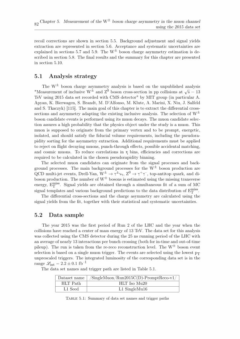
82Chapter 5. Measurement of the W± boson charge asymmetry in the muon channelusing the 2015 data set
recoil corrections are shown in section 5.5. Background adjustment and signal yieldsextraction are represented in section 5.6. Acceptance and systematic uncertainties areexplained in sections 5.7 and 5.9. The W± boson charge asymmetry estimation is de-scribed in section 5.8. The final results and the summary for this chapter are presentedin section 5.10.
5.1 Analysis strategy
The W± boson charge asymmetry analysis is based on the unpublished analysis"Measurement of inclusive W± and Z0 boson cross-section in pp collisions at
√s = 13
TeV using 2015 data set recorded with CMS detector" by MIT group (in particular A.Apyan, K. Bierwagen, S. Brandt, M. D’Alfonso, M. Klute, A. Marini, X. Niu, J. Salfeldand S. Tkaczyk) [115]. The main goal of this chapter is to extract the differential cross-sections and asymmetry adapting the existing inclusive analysis. The selection of W±
boson candidate events is performed using its muon decays. The muon candidate selec-tion assures a high probability that the physics object under the study is a muon. Thismuon is supposed to originate from the primary vertex and to be prompt, energetic,isolated, and should satisfy the fiducial volume requirements, including the pseudora-pidity sorting for the asymmetry extraction. Additional requirements must be appliedto reject on flight decaying muons, punch-through effects, possible accidental matching,and cosmic muons. To reduce correlations in η bins, efficiencies and corrections arerequired to be calculated in the chosen pseudorapidity binning.
The selected muon candidates can originate from the signal processes and back-ground processes. The main background processes for the W± boson production areQCD multi-jet events, Drell-Yan, W± → τ±ντ, Z0 → τ+τ–, top-antitop quark, and di-boson production. The number of W± bosons is estimated using the missing transverseenergy, Emiss
T . Signal yields are obtained through a simultaneous fit of a sum of MCsignal templates and various background predictions to the data distribution of Emiss
T .The differential cross-sections and the charge asymmetry are calculated using the
signal yields from the fit, together with their statistical and systematic uncertainties.
5.2 Data sample
The year 2015 was the first period of Run 2 of the LHC and the year when thecollisions have reached a center of mass energy of 13 TeV. The data set for this analysiswas collected using the CMS detector during the 25 ns running period of the LHC withan average of nearly 13 interactions per bunch crossing (both for in-time and out-of-timepileup). The run is taken from the re-reco reconstruction level. The W± boson eventselection is based on a single muon trigger. The events are selected using the lowest pTunprescaled triggers. The integrated luminosity of the corresponding data set is in therange Lint = 2.2± 0.1 fb–1
The data set names and trigger path are listed in Table 5.1.
Dataset name /SingleMuon/Run2015C(D)-PromptReco-v1/HLT Path HLT Iso Mu20L1 Seed L1 SingleMu16
Table 5.1: Summary of data set names and trigger paths
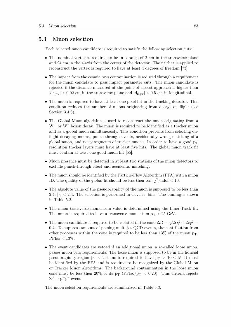
5.3. Muon selection 83
5.3 Muon selection
Each selected muon candidate is required to satisfy the following selection cuts:
• The nominal vertex is required to be in a range of 2 cm in the transverse planeand 24 cm in the z-axis from the center of the detector. The fit that is applied toreconstruct the vertex is required to have at least 4 degrees of freedom [73].
• The impact from the cosmic rays contamination is reduced through a requirementfor the muon candidate to pass impact parameter cuts. The muon candidate isrejected if the distance measured at the point of closest approach is higher than|d0,pv| > 0.02 cm in the transverse plane and |dz,pv| > 0.5 cm in longitudinal.
• The muon is required to have at least one pixel hit in the tracking detector. Thiscondition reduces the number of muons originating from decays on flight (seeSection 3.4.3).
• The Global Muon algorithm is used to reconstruct the muon originating from aW+ or W– boson decay. The muon is required to be identified as a tracker muonand as a global muon simultaneously. This condition prevents from selecting on-flight-decaying muons, punch-through events, accidentally wrong-matching of aglobal muon, and noisy segments of tracker muons. In order to have a good pTresolution tracker layers must have at least five hits. The global muon track fitmust contain at least one good muon hit [55].
• Muon presence must be detected in at least two stations of the muon detectors toexclude punch-through effect and accidental matching.
• The muon should be identified by the Particle-Flow Algorithm (PFA) with a muonID. The quality of the global fit should be less then ten, χ2/ndof < 10.
• The absolute value of the pseudorapidity of the muon is supposed to be less than2.4, |η| < 2.4. The selection is performed in eleven η bins. The binning is shownin Table 5.2.
• The muon transverse momentum value is determined using the Inner-Track fit.The muon is required to have a transverse momentum pT > 25 GeV.
• The muon candidate is required to be isolated in the cone ΔR =√Δη2 +Δφ2 =
0.4. To suppress amount of passing multi-jet QCD events, the contribution fromother processes within the cone is required to be less than 13% of the muon pT,PFIso < 13%.
• The event candidates are vetoed if an additional muon, a so-called loose muon,passes muon veto requirements. The loose muon is supposed to be in the fiducialpseudorapidity region |η| < 2.4 and is required to have pT > 10 GeV. It mustbe identified by the PFA and is required to be recognized by the Global Muonor Tracker Muon algorithms. The background contamination in the loose muoncone must be less then 20% of its pT (PFIso/pT < 0.20). This criteria rejectsZ0 → μ+μ– events.
The muon selection requirements are summarized in Table 5.3.
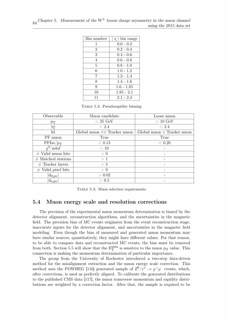
84Chapter 5. Measurement of the W± boson charge asymmetry in the muon channelusing the 2015 data set
Bin number | η | bin range1 0.0 - 0.22 0.2 - 0.43 0.4 - 0.64 0.6 - 0.85 0.8 - 1.06 1.0 - 1.27 1.2 - 1.48 1.4 - 1.69 1.6 - 1.8510 1.85 - 2.111 2.1 - 2.4
Table 5.2: Pseudorapidity binning
Observable Muon candidate Loose muonpT > 25 GeV > 10 GeV|η| < 2.4 < 2.4Id Global muon ∧∨ Tracker muon Global muon ∨ Tracker muon
PF muon True TruePFIso/pT < 0.13 < 0.20χ2/ndof < 10 -
# Valid muon hits > 0 -# Matched stations > 1 -# Tracker layers > 5 -# Valid pixel hits > 0 -
|d0,pv| > 0.02 -|dz,pv| > 0.5 -
Table 5.3: Muon selection requirements
5.4 Muon energy scale and resolution corrections
The precision of the experimental muon momentum determination is biased by thedetector alignment, reconstruction algorithms, and the uncertainties in the magneticfield. The precision bias of MC events originates from the event reconstruction stage,inaccurate inputs for the detector alignment, and uncertainties in the magnetic fieldmodeling. Even though the bias of measured and generated muon momentum mayhave similar sources, quantitatively, they might have different values. For that reason,to be able to compare data and reconstructed MC events, the bias must be removedfrom both. Section 5.5 will show that the Emiss
T is sensitive to the muon pT value. Thisconnection is making the momentum determination of particular importance.
The group from the University of Rochester introduced a two-step data-drivenmethod for the misalignment extraction and the muon energy scale correction. Thismethod uses the POWHEG [116] generated sample of Z0/γ∗ → μ+μ– events, which,after corrections, is used as perfectly aligned. To calibrate the generated distributionsto the published CMS data [117], the muon transverse momentum and rapidity distri-butions are weighted by a correction factor. After that, the sample is required to be
5.4. Muon energy scale and resolution corrections 85
modified to have perfectly aligned detector by smearing generated muon momentumwith an experimental resolution function that depends on pseudorapidity.
In the first step, to obtain initial momentum scale corrections, data and simulationare re-scaled in a way that the average value of 1/pμT exactly matches the perfectlyaligned sample. In the second step, the reconstructed Z0 masses from data and MC arerequired to be the same as for the perfectly aligned sample. This correction removesdependencies on the assumptions that were made during the production of Z0/γ∗ →μ+μ– events and in the detector efficiencies modeling. The corrections are calculated in
terms of η–φ bins, separately for positive and negative charges of the muon candidates.More details on the exact methodology may be found in the appropriate source [118].
The Rochester corrections are implemented as a package of a few C++ classes tobe applied directly during the event’s selection. For this analysis, the "2015 RochesterCorrection" package is used.
5.4.1 Muon charge misidentification correction
Charge identification is essential for the W± boson charge asymmetry measurement.The muon charge identification is performed through its track curvature reconstruction,hence the primary source of possible charge misidentification is related to the curvaturemeasurement. Studies with cosmic rays have shown that the CMS tracker detectorhas a high charge identification efficiency. In the pT range of this study, the rate ofmisidentification is negligible, < 10–5, which gives insignificant impact on the asymme-try measurement, < 0.01% [119].
5.4.2 Estimation of muon efficiencies
A variety of physical processes like pileup, the precision level of the reconstructionalgorithms, and many other issues do not allow to have a perfect detection system.This is taken into account by introducing the detector efficiency variable, defined asthe ratio of the number of detected objects over the total amount of produced objects.In practice, it is more convenient to use the efficiency of physics object detection andreconstruction.
The muon efficiency is estimated in data and simulation using the Tag and ProbeMethod [82]. The idea of Tag and Probe is simple – find a good source of l+l– simultane-ous pair production and require one of the leptons (the tag) to pass harsh identificationand isolation requirements. Afterwards, find a way to check if the second lepton (theprobe) has passed the studied conditions. The efficiency is calculated using formula 5.3.
ε =Npass
Npass +Nfail, (5.3)
where Npass and Nfail are the numbers of passing and failing probes, respectively.This method usually is performed using Z0 bosons decaying in muon channel (Z0 →μ+μ–), which are characterized by pure, high pT muon pair production. Having a well-
reconstructed one muon from the pair and taking into consideration a constraint on theZ0 boson mass (60 GeV < MZ0 < 120 GeV), it is possible to determine if the secondhigh pT muon was reconstructed using unbiased conditions. During the check, twocategories are considered: muons that passed or failed the probe. The usage of twoindependent categories makes their statistical uncertainty uncorrelated and simplifies
86Chapter 5. Measurement of the W± boson charge asymmetry in the muon channelusing the 2015 data set
the uncertainty calculation. The background contribution is estimated performing a fiton the dilepton signal invariant mass spectrum.
The difference in Z0 and W± boson production kinematics is taken into account byrepresenting kinematic efficiencies in two dimensional bins of pT (Table 5.4) and η (Table5.2). The charge-dependent difference is taken into account by separate measurementfor positively and negatively charged leptons.
pT bins [GeV] 25 30 35 40 45 50 55 13000
Table 5.4: Transverse momentum binning
The signal of the passing and failing probe distributions can be extracted in eachbin by using fitting techniques with an appropriate signal model. Two different signalmodels are considered:
1. A two-parameter convolution of a Gaussian spectrum with the reconstructed MCmass spectrum. The Gaussian distribution is used to account for energy scaleshifts and resolution degradation in data relative to the simulation.
2. A four-parameter convolution of a Breit-Wigner line shape with the Crystal Ballfunction (BW*CB).
For the nominal fit the first model is used while the second model is used as an al-ternative model for the estimation of systematic uncertainties (more details in section"Systematic uncertainties" 5.8.1). Muons, which fail the required conditions, might pro-duce a distorted signal shape. Distortions are caused mainly by an excessive amount offinal-state radiation (FSR) or bremsstrahlung.
The background contributions are extracted using various fitting functions:
1. A one-parameter exponential model is used when the background is significantlysmaller than the signal.
2. A one-parameter power law model is an alternative to the exponential model.
3. A three parameter quadratic model is a polynomial model.
Background for the pass and fail samples is modeled mostly using the exponential model.Systematic uncertainties are estimated using the Power law model (see section 5.8.1).
The measured efficiencies are used to determine the scaling corrections on simulationto account for difference between data and simulation (Formula 5.4).
εW±,data(η, pT) = εW±,MC(η, pT)εT&P,data(η, pT)εT&P,MC(η, pT)
. (5.4)
Here εW±,data(η, pT) corresponds to the reconstruction efficiency of muons estimatedfrom W± boson decays using data events, same values but from MC events are shownas εW±,MC(η, pT). Efficiencies measured using Tag and Probe technique in data andMC samples are εT&P,data(η, pT) and εT&P,MC(η, pT), respectively.
The full muon reconstruction relies on multiple detection systems and reconstructionalgorithms. Each of them has its efficiency that can be estimated using the Tag andProbe technique. Different efficiencies might be correlated with each other, and these
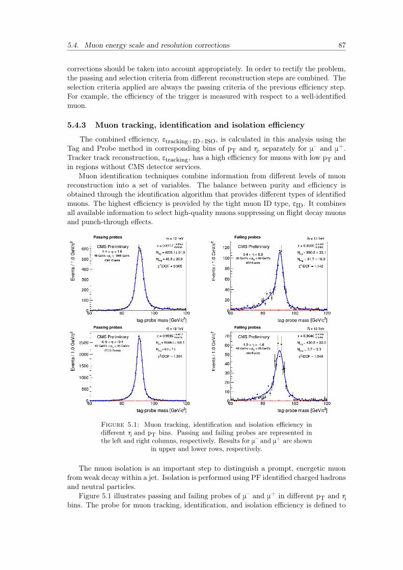
5.4. Muon energy scale and resolution corrections 87
corrections should be taken into account appropriately. In order to rectify the problem,the passing and selection criteria from different reconstruction steps are combined. Theselection criteria applied are always the passing criteria of the previous efficiency step.For example, the efficiency of the trigger is measured with respect to a well-identifiedmuon.
5.4.3 Muon tracking, identification and isolation efficiency
The combined efficiency, εtracking+ID+ISO, is calculated in this analysis using theTag and Probe method in corresponding bins of pT and η, separately for μ– and μ+.Tracker track reconstruction, εtracking, has a high efficiency for muons with low pT andin regions without CMS detector services.
Muon identification techniques combine information from different levels of muonreconstruction into a set of variables. The balance between purity and efficiency isobtained through the identification algorithm that provides different types of identifiedmuons. The highest efficiency is provided by the tight muon ID type, εID. It combinesall available information to select high-quality muons suppressing on flight decay muonsand punch-through effects.
Figure 5.1: Muon tracking, identification and isolation efficiency indifferent η and pT bins. Passing and failing probes are represented inthe left and right columns, respectively. Results for μ– and μ+ are shown
in upper and lower rows, respectively.
The muon isolation is an important step to distinguish a prompt, energetic muonfrom weak decay within a jet. Isolation is performed using PF identified charged hadronsand neutral particles.
Figure 5.1 illustrates passing and failing probes of μ– and μ+ in different pT and ηbins. The probe for muon tracking, identification, and isolation efficiency is defined to
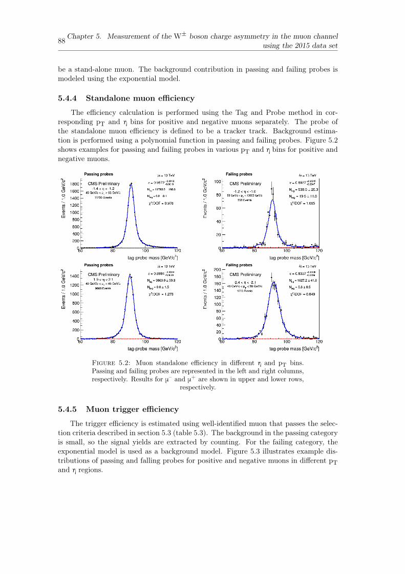
88Chapter 5. Measurement of the W± boson charge asymmetry in the muon channelusing the 2015 data set
be a stand-alone muon. The background contribution in passing and failing probes ismodeled using the exponential model.
5.4.4 Standalone muon efficiency
The efficiency calculation is performed using the Tag and Probe method in cor-responding pT and η bins for positive and negative muons separately. The probe ofthe standalone muon efficiency is defined to be a tracker track. Background estima-tion is performed using a polynomial function in passing and failing probes. Figure 5.2shows examples for passing and failing probes in various pT and η bins for positive andnegative muons.
Figure 5.2: Muon standalone efficiency in different η and pT bins.Passing and failing probes are represented in the left and right columns,respectively. Results for μ– and μ+ are shown in upper and lower rows,
respectively.
5.4.5 Muon trigger efficiency
The trigger efficiency is estimated using well-identified muon that passes the selec-tion criteria described in section 5.3 (table 5.3). The background in the passing categoryis small, so the signal yields are extracted by counting. For the failing category, theexponential model is used as a background model. Figure 5.3 illustrates example dis-tributions of passing and falling probes for positive and negative muons in different pTand η regions.
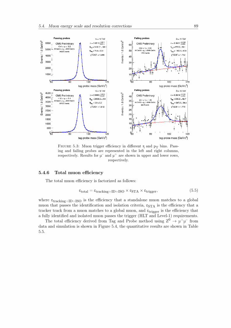
5.4. Muon energy scale and resolution corrections 89
Figure 5.3: Muon trigger efficiency in different η and pT bins. Pass-ing and failing probes are represented in the left and right columns,respectively. Results for μ– and μ+ are shown in upper and lower rows,
respectively.
5.4.6 Total muon efficiency
The total muon efficiency is factorized as follows:
εtotal = εtracking+ID+ISO × εSTA × εtrigger, (5.5)
where εtracking+ID+ISO is the efficiency that a standalone muon matches to a globalmuon that passes the identification and isolation criteria, εSTA is the efficiency that atracker track from a muon matches to a global muon, and εtrigger is the efficiency thata fully identified and isolated muon passes the trigger (HLT and Level-1) requirements.
The total efficiency derived from Tag and Probe method using Z0 → μ+μ– fromdata and simulation is shown in Figure 5.4, the quantitative results are shown in Table5.5.
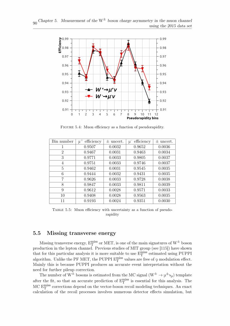
90Chapter 5. Measurement of the W± boson charge asymmetry in the muon channelusing the 2015 data set
Effi
cie
ncy
0.91
0.92
0.93
0.94
0.95
0.96
0.97
0.98
0.99
0.91
0.92
0.93
0.94
0.95
0.96
0.97
0.98
0.99
Pseudorapidity bins0 1 2 3 4 5 6 7 8 9 10 11 12
W +→μ+νW -→μ-ν
Figure 5.4: Muon efficiency as a function of pseudorapidity.
Bin number μ+ efficiency ± uncert. μ
– efficiency ± uncert.1 0.9507 0.0032 0.9652 0.00362 0.9467 0.0031 0.9463 0.00343 0.9771 0.0033 0.9805 0.00374 0.9751 0.0033 0.9746 0.00375 0.9462 0.0031 0.9545 0.00356 0.9444 0.0032 0.9431 0.00357 0.9626 0.0033 0.9728 0.00388 0.9847 0.0033 0.9811 0.00399 0.9612 0.0028 0.9571 0.003310 0.9408 0.0028 0.9563 0.003511 0.9193 0.0024 0.9351 0.0030
Table 5.5: Muon efficiency with uncertainty as a function of pseudo-rapidity
5.5 Missing transverse energy
Missing transverse energy, EmissT or MET, is one of the main signatures of W± boson
production in the lepton channel. Previous studies of MIT group (see [115]) have shownthat for this particular analysis it is more suitable to use Emiss
T estimated using PUPPIalgorithm. Unlike the PF MET, the PUPPI Emiss
T values are free of φ modulation effect.Mainly this is because PUPPI produces an accurate event interpretation without theneed for further pileup correction.
The number of W± bosons is estimated from the MC signal (W± → μ±νμ) templateafter the fit, so that an accurate prediction of Emiss
T is essential for this analysis. TheMC Emiss
T corrections depend on the vector-boson recoil modeling techniques. An exactcalculation of the recoil processes involves numerous detector effects simulation, but
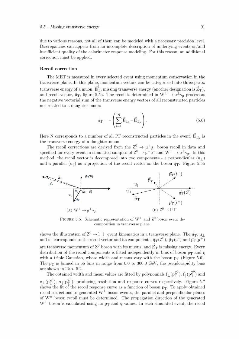
5.5. Missing transverse energy 91
due to various reasons, not all of them can be modeled with a necessary precision level.Discrepancies can appear from an incomplete description of underlying events or/andinsufficient quality of the calorimeter response modeling. For this reason, an additionalcorrection must be applied.
Recoil correction
The MET is measured in every selected event using momentum conservation in thetransverse plane. In this plane, momentum vectors can be categorized into three parts:transverse energy of a muon, ~E
lT, missing transverse energy (another designation is ~�ET),
and recoil vector, ~uT, figure 5.5a. The recoil is determined in W± → μ±νμ process asthe negative vectorial sum of the transverse energy vectors of all reconstructed particlesnot related to a daughter muon:
~uT = –
N∑i=1
~ETi – ~ETμ
. (5.6)
Here N corresponds to a number of all PF reconstructed particles in the event, ~ETμ isthe transverse energy of a daughter muon.
The recoil corrections are derived from the Z0 → μ+μ– boson recoil in data andspecified for every event in simulated samples of Z0 → μ+μ– and W± → μ±νμ. In thismethod, the recoil vector is decomposed into two components - a perpendicular (u⊥)and a parallel (u‖) as a projection of the recoil vector on the boson qT. Figure 5.5b
(a) W± → μ±νμ (b) Z0 → l+l–
Figure 5.5: Schematic representation of W± and Z0 boson event de-composition in transverse plane.
shows the illustration of Z0 → l+l– event kinematics in a transverse plane. The ~uT, u⊥and u‖ corresponds to the recoil vector and its components, ~qT(Z
0), ~pT(μ–) and ~pT(μ+)
are transverse momentum of Z0 boson with its muons, and ~�ET is missing energy. Every
distribution of the recoil components is fitted independently in bins of boson pT and ηwith a triple Gaussian, whose width and means vary with the boson pT (Figure 5.6).The pT is binned in 56 bins in range from 0.0 to 300.0 GeV, the pseudorapidity binsare shown in Tab. 5.2.
The obtained width and mean values are fitted by polynomials f⊥(pZ0
T ), f‖(pZ0T ) and
σ⊥(pZ0
T ), σ‖(pZ0T ), producing resolution and response curves respectively. Figure 5.7
shows the fit of the recoil response curve as a function of boson pT. To apply obtainedrecoil corrections to generated W± boson events, the parallel and perpendicular planesof W± boson recoil must be determined. The propagation direction of the generatedW± boson is calculated using its pT and φ values. In each simulated event, the recoil
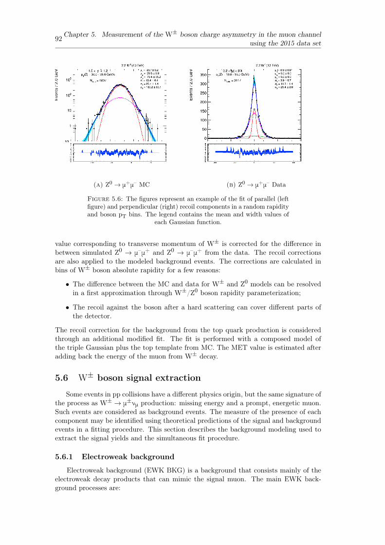
92Chapter 5. Measurement of the W± boson charge asymmetry in the muon channelusing the 2015 data set
(a) Z0 → μ+μ– MC (b) Z0 → μ+μ– Data
Figure 5.6: The figures represent an example of the fit of parallel (leftfigure) and perpendicular (right) recoil components in a random rapidityand boson pT bins. The legend contains the mean and width values of
each Gaussian function.
value corresponding to transverse momentum of W± is corrected for the difference inbetween simulated Z0 → μ–μ+ and Z0 → μ–μ+ from the data. The recoil correctionsare also applied to the modeled background events. The corrections are calculated inbins of W± boson absolute rapidity for a few reasons:
• The difference between the MC and data for W± and Z0 models can be resolvedin a first approximation through W±/Z0 boson rapidity parameterization;
• The recoil against the boson after a hard scattering can cover different parts ofthe detector.
The recoil correction for the background from the top quark production is consideredthrough an additional modified fit. The fit is performed with a composed model ofthe triple Gaussian plus the top template from MC. The MET value is estimated afteradding back the energy of the muon from W± decay.
5.6 W± boson signal extraction
Some events in pp collisions have a different physics origin, but the same signature ofthe process as W± → μ±νμ production: missing energy and a prompt, energetic muon.Such events are considered as background events. The measure of the presence of eachcomponent may be identified using theoretical predictions of the signal and backgroundevents in a fitting procedure. This section describes the background modeling used toextract the signal yields and the simultaneous fit procedure.
5.6.1 Electroweak background
Electroweak background (EWK BKG) is a background that consists mainly of theelectroweak decay products that can mimic the signal muon. The main EWK back-ground processes are:
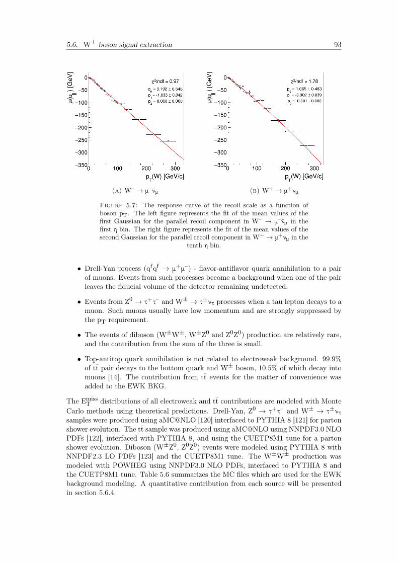
5.6. W± boson signal extraction 93
(a) W– → μ– νμ (b) W+ → μ+νμ
Figure 5.7: The response curve of the recoil scale as a function ofboson pT. The left figure represents the fit of the mean values of thefirst Gaussian for the parallel recoil component in W– → μ– νμ in thefirst η bin. The right figure represents the fit of the mean values of thesecond Gaussian for the parallel recoil component in W+ → μ+νμ in the
tenth η bin.
• Drell-Yan process (qfqf → μ+μ–) - flavor-antiflavor quark annihilation to a pairof muons. Events from such processes become a background when one of the pairleaves the fiducial volume of the detector remaining undetected.
• Events from Z0 → τ+τ– and W± → τ±ντ processes when a tau lepton decays to amuon. Such muons usually have low momentum and are strongly suppressed bythe pT requirement.
• The events of diboson (W±W±, W±Z0 and Z0Z0) production are relatively rare,and the contribution from the sum of the three is small.
• Top-antitop quark annihilation is not related to electroweak background. 99.9%of tt pair decays to the bottom quark and W± boson, 10.5% of which decay intomuons [14]. The contribution from tt events for the matter of convenience wasadded to the EWK BKG.
The EmissT distributions of all electroweak and tt contributions are modeled with Monte
Carlo methods using theoretical predictions. Drell-Yan, Z0 → τ+τ– and W± → τ±ντsamples were produced using aMC@NLO [120] interfaced to PYTHIA 8 [121] for partonshower evolution. The tt sample was produced using aMC@NLO using NNPDF3.0 NLOPDFs [122], interfaced with PYTHIA 8, and using the CUETP8M1 tune for a partonshower evolution. Diboson (W±Z0, Z0Z0) events were modeled using PYTHIA 8 withNNPDF2.3 LO PDFs [123] and the CUETP8M1 tune. The W±W± production wasmodeled with POWHEG using NNPDF3.0 NLO PDFs, interfaced to PYTHIA 8 andthe CUETP8M1 tune. Table 5.6 summarizes the MC files which are used for the EWKbackground modeling. A quantitative contribution from each source will be presentedin section 5.6.4.
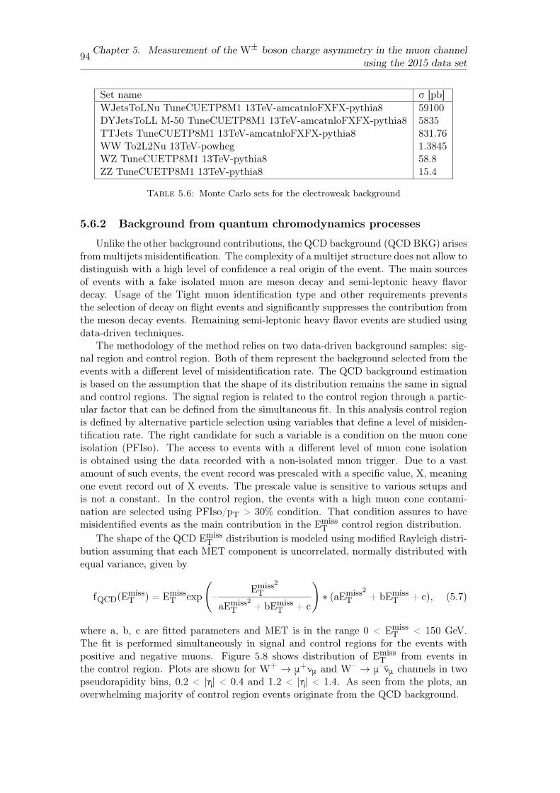
94Chapter 5. Measurement of the W± boson charge asymmetry in the muon channelusing the 2015 data set
Set name σ [pb]WJetsToLNu TuneCUETP8M1 13TeV-amcatnloFXFX-pythia8 59100DYJetsToLL M-50 TuneCUETP8M1 13TeV-amcatnloFXFX-pythia8 5835TTJets TuneCUETP8M1 13TeV-amcatnloFXFX-pythia8 831.76WW To2L2Nu 13TeV-powheg 1.3845WZ TuneCUETP8M1 13TeV-pythia8 58.8ZZ TuneCUETP8M1 13TeV-pythia8 15.4
Table 5.6: Monte Carlo sets for the electroweak background
5.6.2 Background from quantum chromodynamics processes
Unlike the other background contributions, the QCD background (QCD BKG) arisesfrom multijets misidentification. The complexity of a multijet structure does not allow todistinguish with a high level of confidence a real origin of the event. The main sourcesof events with a fake isolated muon are meson decay and semi-leptonic heavy flavordecay. Usage of the Tight muon identification type and other requirements preventsthe selection of decay on flight events and significantly suppresses the contribution fromthe meson decay events. Remaining semi-leptonic heavy flavor events are studied usingdata-driven techniques.
The methodology of the method relies on two data-driven background samples: sig-nal region and control region. Both of them represent the background selected from theevents with a different level of misidentification rate. The QCD background estimationis based on the assumption that the shape of its distribution remains the same in signaland control regions. The signal region is related to the control region through a partic-ular factor that can be defined from the simultaneous fit. In this analysis control regionis defined by alternative particle selection using variables that define a level of misiden-tification rate. The right candidate for such a variable is a condition on the muon coneisolation (PFIso). The access to events with a different level of muon cone isolationis obtained using the data recorded with a non-isolated muon trigger. Due to a vastamount of such events, the event record was prescaled with a specific value, X, meaningone event record out of X events. The prescale value is sensitive to various setups andis not a constant. In the control region, the events with a high muon cone contami-nation are selected using PFIso/pT > 30% condition. That condition assures to havemisidentified events as the main contribution in the Emiss
T control region distribution.The shape of the QCD Emiss
T distribution is modeled using modified Rayleigh distri-bution assuming that each MET component is uncorrelated, normally distributed withequal variance, given by
fQCD(EmissT ) = Emiss
T exp
(–
Emiss2T
aEmiss2T + bEmiss
T + c
)∗ (aEmiss2
T + bEmissT + c), (5.7)
where a, b, c are fitted parameters and MET is in the range 0 < EmissT < 150 GeV.
The fit is performed simultaneously in signal and control regions for the events withpositive and negative muons. Figure 5.8 shows distribution of Emiss
T from events inthe control region. Plots are shown for W+ → μ+νμ and W– → μ–νμ channels in twopseudorapidity bins, 0.2 < |η| < 0.4 and 1.2 < |η| < 1.4. As seen from the plots, anoverwhelming majority of control region events originate from the QCD background.
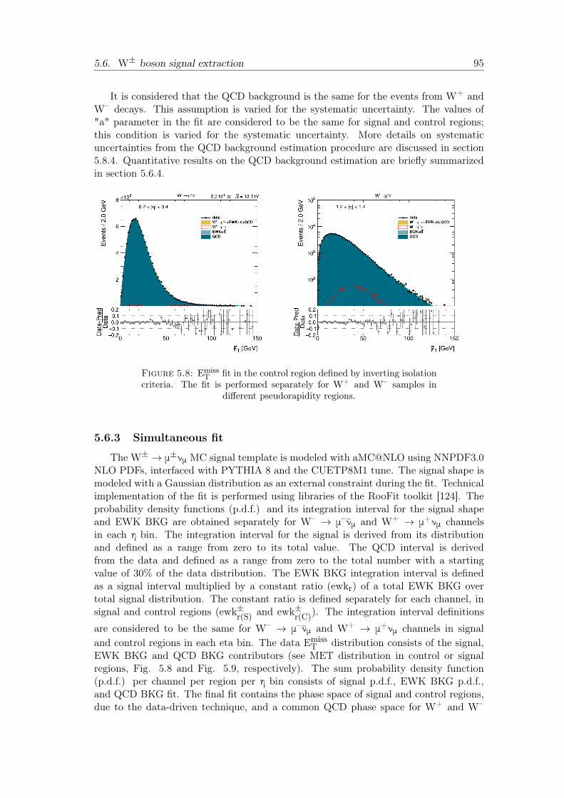
5.6. W± boson signal extraction 95
It is considered that the QCD background is the same for the events from W+ andW– decays. This assumption is varied for the systematic uncertainty. The values of"a" parameter in the fit are considered to be the same for signal and control regions;this condition is varied for the systematic uncertainty. More details on systematicuncertainties from the QCD background estimation procedure are discussed in section5.8.4. Quantitative results on the QCD background estimation are briefly summarizedin section 5.6.4.
Figure 5.8: EmissT fit in the control region defined by inverting isolation
criteria. The fit is performed separately for W+ and W– samples indifferent pseudorapidity regions.
5.6.3 Simultaneous fit
The W± → μ±νμ MC signal template is modeled with aMC@NLO using NNPDF3.0NLO PDFs, interfaced with PYTHIA 8 and the CUETP8M1 tune. The signal shape ismodeled with a Gaussian distribution as an external constraint during the fit. Technicalimplementation of the fit is performed using libraries of the RooFit toolkit [124]. Theprobability density functions (p.d.f.) and its integration interval for the signal shapeand EWK BKG are obtained separately for W– → μ–νμ and W+ → μ+νμ channelsin each η bin. The integration interval for the signal is derived from its distributionand defined as a range from zero to its total value. The QCD interval is derivedfrom the data and defined as a range from zero to the total number with a startingvalue of 30% of the data distribution. The EWK BKG integration interval is definedas a signal interval multiplied by a constant ratio (ewkr) of a total EWK BKG overtotal signal distribution. The constant ratio is defined separately for each channel, insignal and control regions (ewk±r(S) and ewk±r(C)). The integration interval definitions
are considered to be the same for W– → μ–νμ and W+ → μ+νμ channels in signaland control regions in each eta bin. The data Emiss
T distribution consists of the signal,EWK BKG and QCD BKG contributors (see MET distribution in control or signalregions, Fig. 5.8 and Fig. 5.9, respectively). The sum probability density function(p.d.f.) per channel per region per η bin consists of signal p.d.f., EWK BKG p.d.f.,and QCD BKG fit. The final fit contains the phase space of signal and control regions,due to the data-driven technique, and a common QCD phase space for W+ and W–
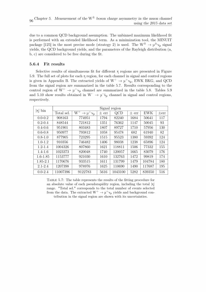
96Chapter 5. Measurement of the W± boson charge asymmetry in the muon channelusing the 2015 data set
due to a common QCD background assumption. The unbinned maximum likelihood fitis performed with an extended likelihood term. As a minimization tool, the MINUITpackage [125] in the most precise mode (strategy 2) is used. The W± → μ±νμ signalyields, the QCD background yields, and the parameters of the Rayleigh distribution (a,b, c) are considered to be free during the fit.
5.6.4 Fit results
Selective results of simultaneous fit for different η regions are presented in Figure5.9. The full set of plots for each η region, for each channel in signal and control regionsis given in Appendix B. The extracted yields of W+ → μ+νμ, EWK BKG, and QCDfrom the signal region are summarized in the table 5.7. Results corresponding to thecontrol region of W+ → μ+νμ channel are summarized in the table 5.8. Tables 5.9and 5.10 show results obtained in W– → μ–νμ channel in signal and control regions,respectively.
|η| bin Signal regionTotal sel. W+ → μ+νμ ± err QCD ± err EWK ±err
0.0-0.2 908163 774951 1794 82240 1684 50641 1170.2-0.4 848544 721812 1351 76362 1147 50045 930.4-0.6 951901 803483 1807 89727 1710 57956 1300.6-0.8 950977 793812 1058 95478 682 61940 820.8-1.0 877905 723295 1515 95523 1380 59392 1241.0-1.2 910356 746482 1406 98038 1238 65896 1241.2-1.4 1004326 807860 1621 118811 1506 77332 1551.4-1.6 1023373 820048 1740 120057 1665 83079 1761.6-1.85 1153777 921030 1610 132763 1472 99819 1741.85-2.1 1170676 933515 1611 131799 1479 104784 1802.1-2.4 1207398 978976 1625 110690 1490 117687 1950.0-2.4 11007396 9122783 5616 1043100 5282 839350 516
Table 5.7: The table represents the results of the fitting procedure foran absolute value of each pseudorapidity region, including the total |η|range. "Total sel." corresponds to the total number of events selectedfrom the data. The extracted W+ → μ+νμ yields and background con-
tribution in the signal region are shown with its uncertainties.
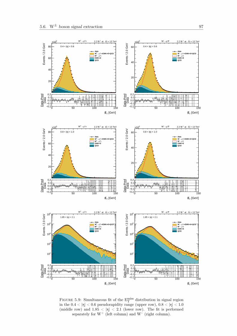
5.6. W± boson signal extraction 97
Eve
nts
/ 2.0
GeV
20
40
60
80
310×
data+QCDt+EWK+tν+µ→+W
ν+µ→+WtEWK+t
QCD
| < 0.6η0.4 < |
ν+µ→+W = 13 TeVs at -12.2 fb
[GeV]TE
0 50 100 150
Dat
aD
ata-
Pre
d
0.2−0.1−0.00.10.2
Eve
nts
/ 2.0
GeV
20
40
60
310×
data+QCDt+EWK+tν-µ→-W
ν-µ→-WtEWK+t
QCD
| < 0.6η0.4 < |
ν-µ→-W = 13 TeVs at -12.2 fb
[GeV]TE
0 50 100 150
Dat
aD
ata-
Pre
d
0.2−0.1−0.00.10.2
Eve
nts
/ 2.0
GeV
20
40
60
80
310×
data+QCDt+EWK+tν+µ→+W
ν+µ→+WtEWK+t
QCD
| < 1.0η0.8 < |
ν+µ→+W = 13 TeVs at -12.2 fb
[GeV]TE
0 50 100 150
Dat
aD
ata-
Pre
d
0.2−0.1−0.00.10.2
Eve
nts
/ 2.0
GeV
20
40
60
310×
data+QCDt+EWK+tν-µ→-W
ν-µ→-WtEWK+t
QCD
| < 1.0η0.8 < |
ν-µ→-W = 13 TeVs at -12.2 fb
[GeV]TE
0 50 100 150
Dat
aD
ata-
Pre
d
0.2−0.1−0.00.10.2
Eve
nts
/ 2.0
GeV
210
310
410
510
610
data+QCDt+EWK+tν+µ→+W
ν+µ→+WtEWK+t
QCD
| < 2.1η1.85 < |
ν+µ→+W = 13 TeVs at -12.2 fb
[GeV]TE
0 50 100 150
Dat
aD
ata-
Pre
d
0.2−0.1−0.00.10.2
Eve
nts
/ 2.0
GeV
210
310
410
510
610
data+QCDt+EWK+tν-µ→-W
ν-µ→-WtEWK+t
QCD
| < 2.1η1.85 < |
ν-µ→-W = 13 TeVs at -12.2 fb
[GeV]TE
0 50 100 150
Dat
aD
ata-
Pre
d
0.2−0.1−0.00.10.2
Figure 5.9: Simultaneous fit of the EmissT distribution in signal region
in the 0.4 < |η| < 0.6 pseudorapidity range (upper row), 0.8 < |η| < 1.0(middle row) and 1.85 < |η| < 2.1 (lower row). The fit is performed
separately for W+ (left column) and W– (right column).
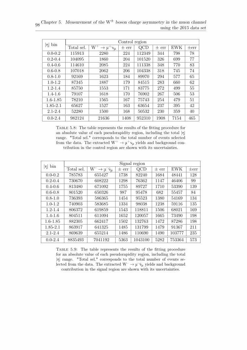
98Chapter 5. Measurement of the W± boson charge asymmetry in the muon channelusing the 2015 data set
|η| bin Control regionTotal sel. W+ → μ+νμ ± err QCD ± err EWK ±err
0.0-0.2 115913 2280 224 112349 344 798 780.2-0.4 104095 1860 204 101520 326 699 770.4-0.6 114610 2085 224 111338 348 770 830.6-0.8 107018 2062 206 104338 318 745 740.8-1.0 92169 1623 184 89970 294 577 651.0-1.2 87345 1887 179 84515 283 660 621.2-1.4 85750 1553 171 83775 272 499 551.4-1.6 79107 1618 170 76902 267 506 531.6-1.85 78210 1565 167 75743 254 479 511.85-2.1 65627 1527 163 63654 237 395 422.1-2.4 52280 1500 168 50532 230 359 400.0-2.4 982124 21636 1408 952310 1908 7154 465
Table 5.8: The table represents the results of the fitting procedure foran absolute value of each pseudorapidity region, including the total |η|range. "Total sel." corresponds to the total number of events selectedfrom the data. The extracted W+ → μ+νμ yields and background con-
tribution in the control region are shown with its uncertainties.
|η| bin Signal regionTotal sel. W– → μ–νμ ± err QCD ± err EWK ±err
0.0-0.2 785783 655427 1738 82240 1684 48441 1280.2-0.4 730670 608222 1298 76362 1147 46406 990.4-0.6 813480 671092 1755 89727 1710 53390 1390.6-0.8 801520 650326 987 95478 682 55457 840.8-1.0 736393 586365 1454 95523 1380 54169 1341.0-1.2 740903 583685 1334 98038 1238 59116 1351.2-1.4 806372 619859 1543 118811 1506 68021 1691.4-1.6 804511 611094 1652 120057 1665 73490 1981.6-1.85 882305 662417 1502 132763 1472 87286 1981.85-2.1 863917 641325 1485 131799 1479 91367 2112.1-2.4 869639 655214 1486 110690 1490 103777 2350.0-2.4 8835493 7041192 5363 1043100 5282 753364 573
Table 5.9: The table represents the results of the fitting procedurefor an absolute value of each pseudorapidity region, including the total|η| range. "Total sel." corresponds to the total number of events se-lected from the data. The extracted W– → μ– νμ yields and background
contribution in the signal region are shown with its uncertainties.
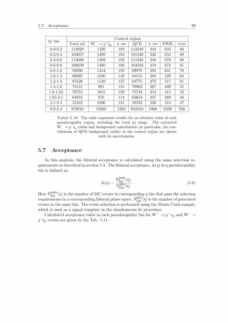
5.7. Acceptance 99
|η| bin Control regionTotal sel. W– → μ–νμ ± err QCD ± err EWK ±err
0.0-0.2 113920 1420 193 112349 344 633 860.2-0.4 103657 1499 183 101520 326 653 800.4-0.6 113088 1489 193 111338 348 676 880.6-0.8 106639 1480 180 104338 318 672 810.8-1.0 92090 1454 158 89970 294 641 701.0-1.2 86005 1230 149 84515 283 529 641.2-1.4 85526 1149 137 83775 272 517 611.4-1.6 78121 991 135 76902 267 409 551.6-1.85 76755 1015 129 75743 254 415 521.85-2.1 64853 876 114 63654 237 369 482.1-2.4 52162 1096 125 50532 230 418 470.0-2.4 972816 15005 1283 952310 1908 6508 556
Table 5.10: The table represents results for an absolute value of eachpseudorapidity region, including the total |η| range. The extractedW– → μ– νμ yields and background contribution (in particular, the con-tribution of QCD background yields) in the control region are shown
with its uncertainties.
5.7 Acceptance
In this analysis, the fiducial acceptance is calculated using the same selection re-quirements as described in section 5.3. The fiducial acceptance, A(η) in η pseudorapiditybin is defined as:
A(η) =Npassfid (η)
Ngenfid (η)
. (5.8)
Here Npassfid (η) is the number of MC events in corresponding η bin that pass the selection
requirements in a corresponding fiducial phase space, Ngenfid (η) is the number of generated
events in the same bin. The event selection is performed using the Monte Carlo sample,which is used as a signal template in the simultaneous fit procedure.
Calculated acceptance value in each pseudorapidity bin for W+ → μ+νμ and W– →μ–νμ events are given in the Tab. 5.11.
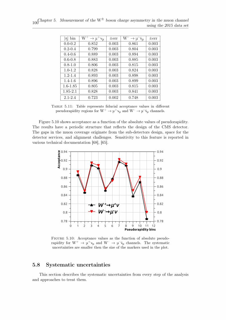
100Chapter 5. Measurement of the W± boson charge asymmetry in the muon channelusing the 2015 data set
|η| bin W+ → μ+νμ ±err W– → μ–νμ ±err0.0-0.2 0.852 0.003 0.861 0.0030.2-0.4 0.799 0.003 0.804 0.0030.4-0.6 0.889 0.003 0.894 0.0030.6-0.8 0.883 0.003 0.885 0.0030.8-1.0 0.806 0.003 0.815 0.0031.0-1.2 0.828 0.003 0.824 0.0031.2-1.4 0.893 0.003 0.898 0.0031.4-1.6 0.896 0.003 0.899 0.0031.6-1.85 0.805 0.003 0.815 0.0031.85-2.1 0.828 0.003 0.841 0.0032.1-2.4 0.723 0.002 0.748 0.003
Table 5.11: Table represents fiducial acceptance values in differentpseudorapidity regions for W+ → μ+νμ and W– → μ– νμ channels.
Figure 5.10 shows acceptance as a function of the absolute values of pseudorapidity.The results have a periodic structure that reflects the design of the CMS detector.The gaps in the muon coverage originate from the sub-detectors design, space for thedetector services, and alignment challenges. Sensitivity to this feature is reported invarious technical documentation [68], [65].
Acc
ep
tan
ce
0.78
0.8
0.82
0.84
0.86
0.88
0.9
0.92
0.94
0.78
0.8
0.82
0.84
0.86
0.88
0.9
0.92
0.94
Pseudorapidity bins0 1 2 3 4 5 6 7 8 9 10 11 12
W +→μ+νW -→μ-ν
Figure 5.10: Acceptance values as the function of absolute pseudo-rapidity for W+ → μ+νμ and W– → μ– νμ channels. The systematicuncertainties are smaller then the size of the markers used in the plot.
5.8 Systematic uncertainties
This section describes the systematic uncertainties from every step of the analysisand approaches to treat them.
5.8. Systematic uncertainties 101
5.8.1 Muon efficiencies
Lepton efficiency estimation is a complicated procedure that uses various assump-tions in its methodology. The main sources of systematic uncertainties originate fromthe signal and background shape modeling, variations in uncertainty range, and alter-native binning.
Breit-Wigner * Crystal Ball signal model. For the nominal signal model, a con-volution of the Gaussian spectrum with reconstructed MC mass spectrum is used. Asan alternative model the four-parameter convolution of Breit-Wigner [126] line shapewith the Crystal Ball function [127] is used. The Breit-Wigner shape is fixed to thePDG values of the Z0 width and mass. The Crystal Ball function has free parametersintended to account for energy scale shifts, mass resolution, and low mass tails from FSRand bremsstrahlung. The deviation from the nominal differential cross-section valuesacross the pseudorapidity bins varies between 1 – 1.5% for W+ and W– channels.
Power law background model. The power-law model is used as an alternativebackground model due to its wide usage for background estimation. It does a good de-scription of protracted energy tails after energy loss events. The power-law distributionis defined as:
f(x) = A · x–r, (5.9)
where A is a constant, -r is a power-law index. The systematic uncertainty from usingthis model is below 1%.
Variation in estimated uncertainty range. Another considered systematic uncer-tainty is a variation of lepton efficiencies in uncertainty range of its η – φ bins. Thecorrelation among the η bins is reduced due to a representation of η part of 2D bins inasymmetry pseudorapidity binning (Table 5.2). The uncertainty from the variation liesin the range of 0.6 – 1.1% for both channels.
5.8.2 Muon momentum scale and resolution correction
The systematic uncertainty estimation of the muon energy scale and resolution isbased on the smearing of the correction using one sigma of the statistical error in ηand φ bins following Gaussian distribution. The actual smearing is implemented in theRochester C++ class and can be calculated through a generation of a toy run with arandom seed number. Systematic uncertainty is calculated running a hundred of toyruns with different seeds, and taking an RMS value of all toy runs. The uncertaintyvalue in each channel varies from bin to bin in a range of 0.5 – 1.2%.
5.8.3 Missing transverse energy
The primary sources of systematic uncertainties for the EmissT calculation come
from an alternative recoil binning, the pileup variation, and usage of alternative fittingfunctions.
102Chapter 5. Measurement of the W± boson charge asymmetry in the muon channelusing the 2015 data set
Inclusive recoil. To produce the systematic uncertainty from the recoil fit, analternative, inclusive (0.0 < η < 2.4) binning of rapidity is performed. The resultsvaries in a range from 1.0– 3.5% in W– → μ–νμ and 0.9– 3.5% in W+ → μ+νμ channels.
Pileup variation. Additional systematic uncertainty is coming from the varia-tions in the pileup uncertainty range. The systematic uncertainty is derived using recoilcorrections calculated using an alternative simulation, which was produced with variedpileup in its uncertainty range. Obtained results are varying in range 0.6 – 2.9% inW+ → μ+νμ channel and 0.8 – 3.4% in W– → μ–νμ channel.
Alternative fitting function of the recoil component. The systematic un-certainty coming from the fitting function choice is estimated using an alternative ap-proach. The fit is performed using the non-parametric function in the RooFit toolkit.In this approach, the p.d.f. of the recoil components is represented as a superposition ofGaussians with the same surface but different dynamic width, which varies dependingon event density [124]. The obtained uncertainty is varying in the range of 0.7%–1.04%and 0.7% – 1.2% for W+ → μ+νμ and W– → μ–νμ channels, respectively. For theasymmetry, the uncertainty is in the range of 0.1% – 0.4%.
5.8.4 W± boson signal extraction fit
Separate "a" parameter for the QCD shape functions. As an alternativeapproach in QCD background estimation, the fit is performed without binding the "a"parameter between signal and control regions. The new fit is performed for each η binin each channel. The systematic uncertainty varies from bin to bin in a range 0.5– 3.0%in W+ → μ+νμ channel and 0.6 – 3.6% in W– → μ–νμ.
Separate QCD shape functions. Additional fits are performed with a separateQCD shape functions for W+ → μ+νμ and W– → μ–νμ. The systematic uncertainty inW+ → μ+νμ and W– → μ–νμ channels varies for different η bins in a range 0.5 – 1.7%and 0.5 – 1.5% respectively.
5.8.5 Luminosity uncertainties
The total uncertainty of luminosity is 2.3% [128]; it is fully correlated betweendifferent channels and pseudorapidity bins. The source of each uncertainty componentis summarized in the table 5.12.
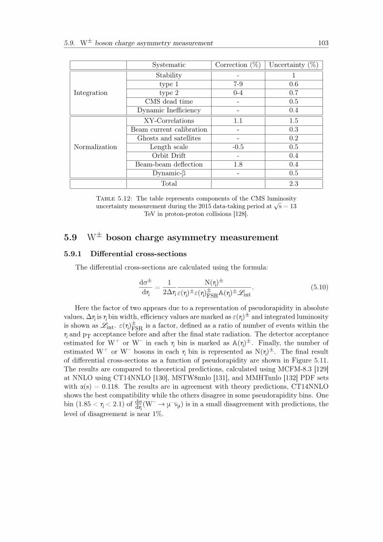
5.9. W± boson charge asymmetry measurement 103
Systematic Correction (%) Uncertainty (%)
Integration
Stability - 1type 1 7-9 0.6type 2 0-4 0.7
CMS dead time - 0.5Dynamic Inefficiency - 0.4
Normalization
XY-Correlations 1.1 1.5Beam current calibration - 0.3Ghosts and satellites - 0.2
Length scale -0.5 0.5Orbit Drift - 0.4
Beam-beam deflection 1.8 0.4Dynamic-β - 0.5
Total 2.3
Table 5.12: The table represents components of the CMS luminosityuncertainty measurement during the 2015 data-taking period at
√s = 13
TeV in proton-proton collisions [128].
5.9 W± boson charge asymmetry measurement
5.9.1 Differential cross-sections
The differential cross-sections are calculated using the formula:
dσ±
dη=
12Δη
N(η)±
ε(η)±ε(η)±FSRA(η)±Lint
. (5.10)
Here the factor of two appears due to a representation of pseudorapidity in absolutevalues,Δη is η bin width, efficiency values are marked as ε(η)± and integrated luminosityis shown as Lint. ε(η)±FSR is a factor, defined as a ratio of number of events within theη and pT acceptance before and after the final state radiation. The detector acceptanceestimated for W+ or W– in each η bin is marked as A(η)±. Finally, the number ofestimated W+ or W– bosons in each η bin is represented as N(η)±. The final resultof differential cross-sections as a function of pseudorapidity are shown in Figure 5.11.The results are compared to theoretical predictions, calculated using MCFM-8.3 [129]at NNLO using CT14NNLO [130], MSTW8nnlo [131], and MMHTnnlo [132] PDF setswith α(s) = 0.118. The results are in agreement with theory predictions, CT14NNLOshows the best compatibility while the others disagree in some pseudorapidity bins. Onebin (1.85 < η < 2.1) of dσ
dη (W– → μ–νμ) is in a small disagreement with predictions, the
level of disagreement is near 1%.
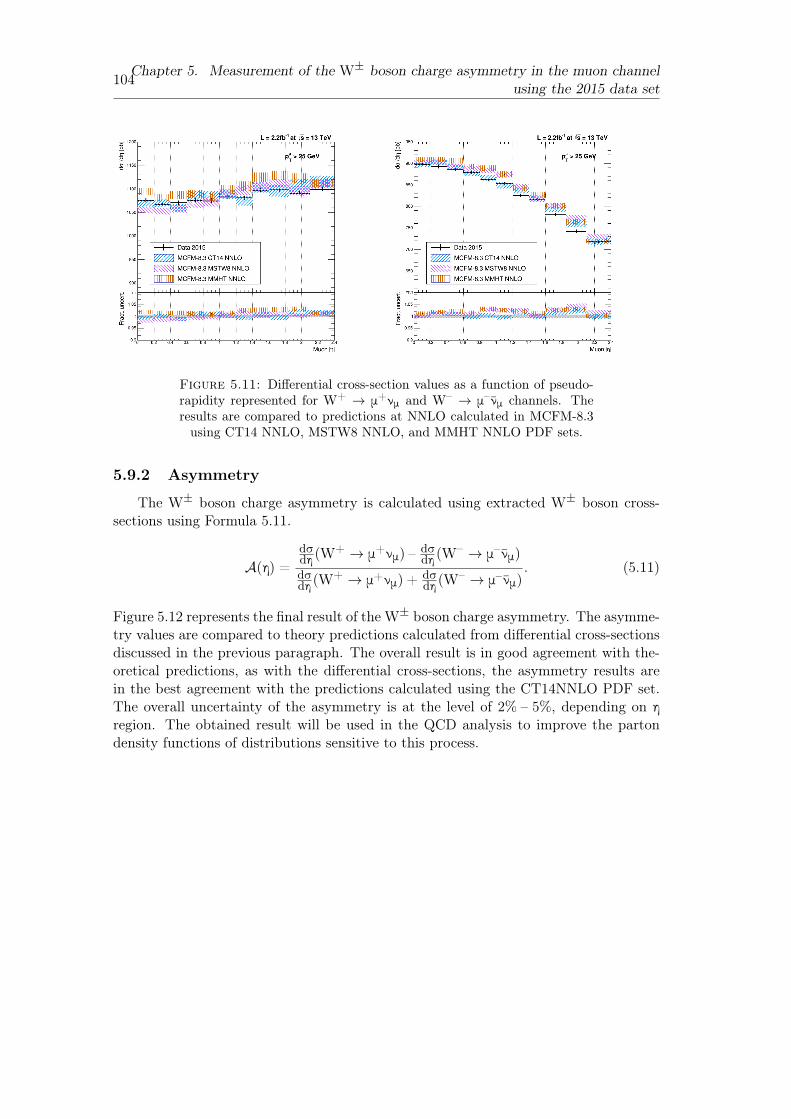
104Chapter 5. Measurement of the W± boson charge asymmetry in the muon channelusing the 2015 data set
Figure 5.11: Differential cross-section values as a function of pseudo-rapidity represented for W+ → μ+νμ and W– → μ– νμ channels. Theresults are compared to predictions at NNLO calculated in MCFM-8.3using CT14 NNLO, MSTW8 NNLO, and MMHT NNLO PDF sets.
5.9.2 Asymmetry
The W± boson charge asymmetry is calculated using extracted W± boson cross-sections using Formula 5.11.
A(η) =dσdη (W
+ → μ+νμ) – dσdη (W
– → μ–νμ)dσdη (W
+ → μ+νμ) + dσdη (W
– → μ–νμ). (5.11)
Figure 5.12 represents the final result of the W± boson charge asymmetry. The asymme-try values are compared to theory predictions calculated from differential cross-sectionsdiscussed in the previous paragraph. The overall result is in good agreement with the-oretical predictions, as with the differential cross-sections, the asymmetry results arein the best agreement with the predictions calculated using the CT14NNLO PDF set.The overall uncertainty of the asymmetry is at the level of 2% – 5%, depending on ηregion. The obtained result will be used in the QCD analysis to improve the partondensity functions of distributions sensitive to this process.
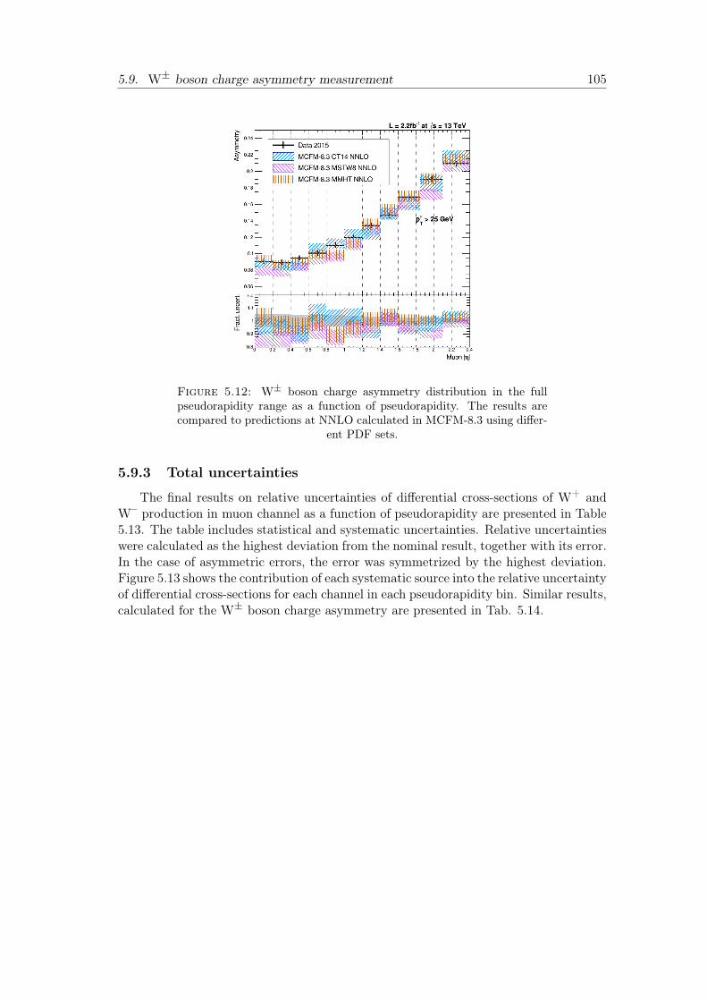
5.9. W± boson charge asymmetry measurement 105
Figure 5.12: W± boson charge asymmetry distribution in the fullpseudorapidity range as a function of pseudorapidity. The results arecompared to predictions at NNLO calculated in MCFM-8.3 using differ-
ent PDF sets.
5.9.3 Total uncertainties
The final results on relative uncertainties of differential cross-sections of W+ andW– production in muon channel as a function of pseudorapidity are presented in Table5.13. The table includes statistical and systematic uncertainties. Relative uncertaintieswere calculated as the highest deviation from the nominal result, together with its error.In the case of asymmetric errors, the error was symmetrized by the highest deviation.Figure 5.13 shows the contribution of each systematic source into the relative uncertaintyof differential cross-sections for each channel in each pseudorapidity bin. Similar results,calculated for the W± boson charge asymmetry are presented in Tab. 5.14.
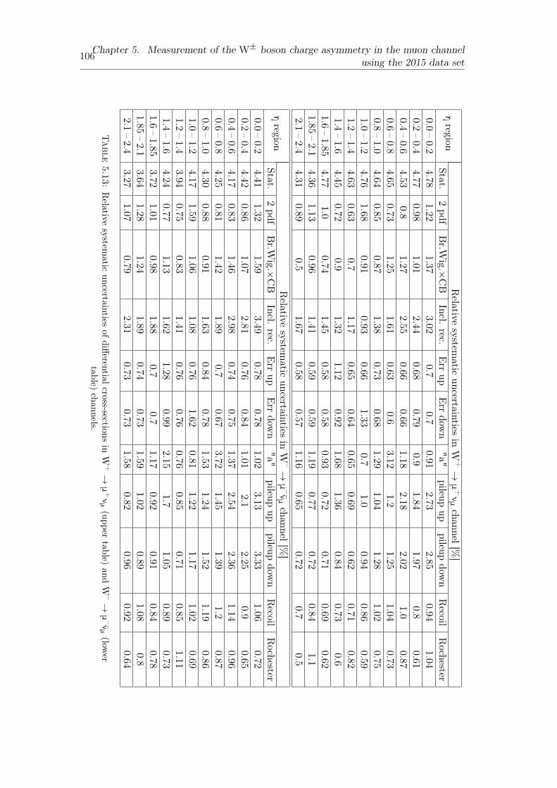
106Chapter 5. Measurement of the W± boson charge asymmetry in the muon channelusing the 2015 data set
ηregion
Relative
systematic
uncertaintiesin
W+→μ +νμchannel[%
]Stat.
2pdf
Br.W
ig.×CB
Incl.rec.
Err
upErr
down
"a"pileup
uppileup
down
Recoil
Rochester
0.0–0.2
4.781.22
1.373.02
0.70.7
0.912.73
2.850.94
1.040.2
–0.4
4.770.98
1.012.44
0.680.79
0.91.84
1.970.8
0.610.4
–0.6
4.530.8
1.272.55
0.660.66
1.182.18
2.021.0
0.870.6
–0.8
4.650.73
1.251.61
0.630.6
3.121.2
1.251.04
0.730.8
–1.0
4.640.85
0.871.38
0.730.68
1.291.04
1.281.02
0.751.0
–1.2
4.761.68
0.910.93
0.661.33
0.71.0
0.940.86
0.591.2
–1.4
4.630.63
0.71.17
0.650.64
0.650.69
0.620.71
0.821.4
–1.6
4.450.72
0.91.32
1.120.92
1.681.36
0.840.73
0.61.6
–1.85
4.771.0
0.741.45
0.580.58
0.930.72
0.710.69
0.621.85
–2.1
4.361.13
0.961.41
0.590.59
1.190.77
0.720.84
1.12.1
–2.4
4.310.89
0.51.67
0.580.57
1.160.65
0.720.7
0.5
ηregion
Relative
systematic
uncertaintiesin
W–→μ –νμchannel[%
]Stat.
2pdf
Br.W
ig.×CB
Incl.rec.
Err
upErr
down
"a"pileup
uppileup
down
Recoil
Rochester
0.0–0.2
4.411.32
1.593.49
0.780.78
1.023.13
3.331.06
0.720.2
–0.4
4.420.86
1.072.81
0.760.84
1.012.1
2.250.9
0.650.4
–0.6
4.170.83
1.462.98
0.740.75
1.372.54
2.361.14
0.960.6
–0.8
4.250.81
1.421.89
0.70.67
3.721.45
1.391.2
0.870.8
–1.0
4.300.88
0.911.63
0.840.78
1.531.24
1.521.19
0.861.0
–1.2
4.171.59
1.061.08
0.761.62
0.811.22
1.171.02
0.691.2
–1.4
3.940.75
0.831.41
0.760.76
0.760.85
0.710.85
1.111.4
–1.6
4.240.77
1.131.62
1.280.99
2.151.7
1.050.89
0.731.6
–1.85
3.721.01
0.981.88
0.70.7
1.170.92
0.910.84
0.781.85
–2.1
3.641.28
1.241.89
0.740.73
1.591.02
0.891.08
0.82.1
–2.4
3.271.07
0.792.31
0.730.73
1.580.82
0.960.92
0.64
Table
5.13:Relative
systematic
uncertaintiesof
differentialcross-sectionsin
W+→μ+νμ(upper
table)and
W–→μ–νμ(low
ertable)
channels.
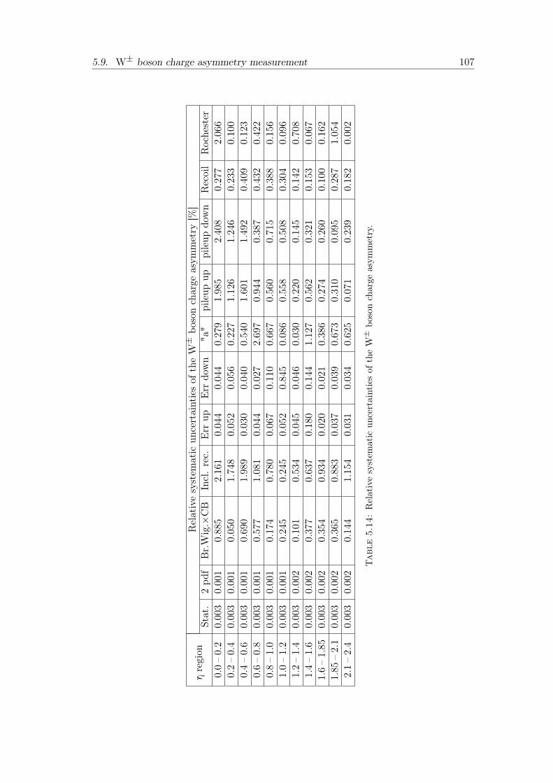
5.9. W± boson charge asymmetry measurement 107
ηregion
Relativesystem
atic
uncertaintiesof
theW±
bosoncharge
asym
metry
[%]
Stat.
2pd
fBr.W
ig.×
CB
Incl.rec.
Err
upErr
down
"a"
pileup
uppileup
down
Recoil
Roche
ster
0.0–0.2
0.00
30.00
10.88
52.16
10.04
40.04
40.27
91.98
52.40
80.27
72.06
60.2–0.4
0.00
30.00
10.05
01.74
80.05
20.05
60.22
71.12
61.24
60.23
30.10
00.4–0.6
0.00
30.00
10.69
01.98
90.03
00.04
00.54
01.60
11.49
20.40
90.12
30.6–0.8
0.00
30.00
10.57
71.08
10.04
40.02
72.69
70.94
40.38
70.43
20.42
20.8–1.0
0.00
30.00
10.17
40.78
00.06
70.11
00.66
70.56
00.71
50.38
80.15
61.0–1.2
0.00
30.00
10.24
50.24
50.05
20.84
50.08
60.55
80.50
80.30
40.09
61.2–1.4
0.00
30.00
20.10
10.53
40.04
50.04
60.03
00.22
00.14
50.14
20.70
81.4–1.6
0.00
30.00
20.37
70.63
70.18
00.14
41.12
70.56
20.32
10.15
30.06
71.6–1.85
0.00
30.00
20.35
40.93
40.02
00.02
10.38
60.27
40.26
00.10
00.16
21.85
–2.1
0.00
30.00
20.36
50.88
30.03
70.03
90.67
30.31
00.09
50.28
71.05
42.1–2.4
0.00
30.00
20.14
41.15
40.03
10.03
40.62
50.07
10.23
90.18
20.00
2
Tabl
e5.
14:Relativesystem
atic
uncertaintiesof
theW±
bosoncharge
asym
metry.
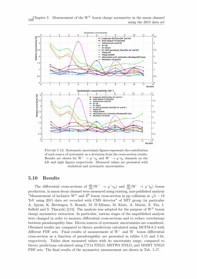
108Chapter 5. Measurement of the W± boson charge asymmetry in the muon channelusing the 2015 data set
Systematic uncertaintiesR
elat
ive
unce
reta
inty
[%]
0
0.5
1
1.5
2
2.5
3
3.5
0
0.5
1
1.5
2
2.5
3
3.5
Eta bins0 1 2 3 4 5 6 7 8 9 10 11 12
0 1 2 3 4 5 6 7 8 9 10 11 12
2 separate QCD func(W+ and W-) Breit-Wigner*Cristal Ball Inklusive eta recoil fit Err Up Err Down'a1' QCD parameter fixed (for W+ and W-) Pileup UP Pileup DOWN Alternative p.d.f. estimation (RooKeysPdf class) Rochester correction
Systematic uncertainties (W - )
Rel
ativ
e un
cert
aint
y [%
]
0
0.5
1
1.5
2
2.5
3
3.5
4
0
0.5
1
1.5
2
2.5
3
3.5
4
Eta bins0 1 2 3 4 5 6 7 8 9 10 11 12
0 1 2 3 4 5 6 7 8 9 10 11 12
2 separate QCD func(for W + and W - ) Breit-Wigner*Cristal Ball Inklusive eta recoil fit Err Up Err Down'a1' QCD parameter fixed (for W + and W - ) Pileup UP Pileup DOWN Alternative p.d.f. estimation (RooKeysPdf class) Rochester correction
Figure 5.13: Systematic uncertainty figures represents the contributionof each source of systematic as a deviation from the cross-section results.Results are shown for W+ → μ+νμ and W– → μ– νμ channels on theleft and right figures respectively. Measured values are presented with
statistical and systematic uncertainties.
5.10 Results
The differential cross-sections of dσdη (W
+ → μ+νμ) and dσ
dη (W– → μ
–νμ) boson
production, in muon decay channel were measured using existing, non-published analysis"Measurement of inclusive W± and Z0 boson cross-section in pp collisions at
√s = 13
TeV using 2015 data set recorded with CMS detector" of MIT group (in particularA. Apyan, K. Bierwagen, S. Brandt, M. D’Alfonso, M. Klute, A. Marini, X. Niu, J.Salfeld and S. Tkaczyk) [115]. The analysis was adopted for the purpose of W± bosoncharge asymmetry extraction. In particular, various stages of the unpublished analysiswere changed in order to measure differential cross-sections and to reduce correlationsbetween pseudorapidity bins. Eleven sources of systematic uncertainties are considered.Obtained results are compared to theory predictions calculated using MCFM-8.3 withdifferent PDF sets. Final results of measurement of W+ and W– boson differentialcross-section as a function of pseudorapidity are presented in tables 5.15 and 5.16,respectively. Tables show measured values with its uncertainty range, compared totheory predictions calculated using CT14 NNLO, MSTW8 NNLO, and MMHT NNLOPDF sets. The final results of the asymmetry measurement are shown in Tab. 5.17.
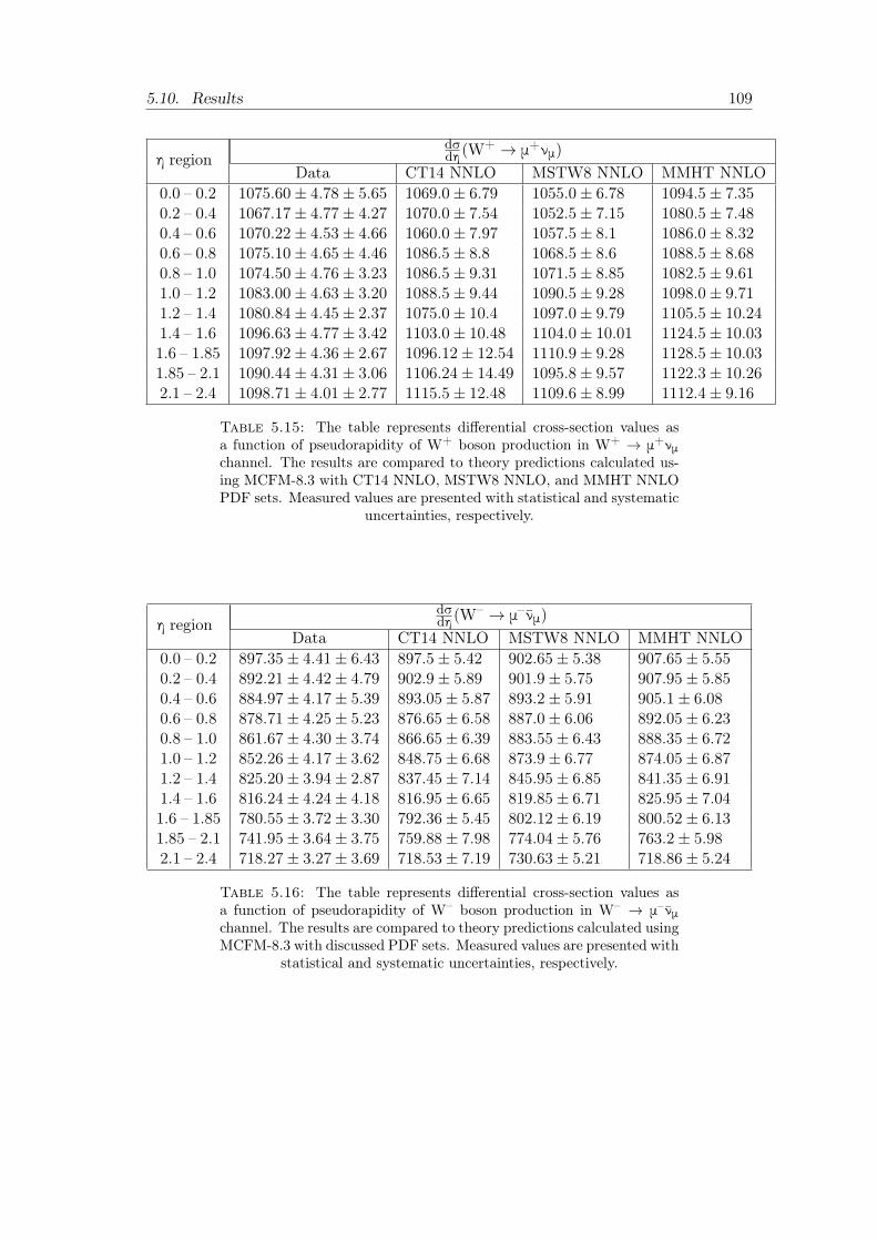
5.10. Results 109
η regiondσdη (W
+ → μ+νμ)Data CT14 NNLO MSTW8 NNLO MMHT NNLO
0.0 – 0.2 1075.60± 4.78± 5.65 1069.0± 6.79 1055.0± 6.78 1094.5± 7.350.2 – 0.4 1067.17± 4.77± 4.27 1070.0± 7.54 1052.5± 7.15 1080.5± 7.480.4 – 0.6 1070.22± 4.53± 4.66 1060.0± 7.97 1057.5± 8.1 1086.0± 8.320.6 – 0.8 1075.10± 4.65± 4.46 1086.5± 8.8 1068.5± 8.6 1088.5± 8.680.8 – 1.0 1074.50± 4.76± 3.23 1086.5± 9.31 1071.5± 8.85 1082.5± 9.611.0 – 1.2 1083.00± 4.63± 3.20 1088.5± 9.44 1090.5± 9.28 1098.0± 9.711.2 – 1.4 1080.84± 4.45± 2.37 1075.0± 10.4 1097.0± 9.79 1105.5± 10.241.4 – 1.6 1096.63± 4.77± 3.42 1103.0± 10.48 1104.0± 10.01 1124.5± 10.031.6 – 1.85 1097.92± 4.36± 2.67 1096.12± 12.54 1110.9± 9.28 1128.5± 10.031.85 – 2.1 1090.44± 4.31± 3.06 1106.24± 14.49 1095.8± 9.57 1122.3± 10.262.1 – 2.4 1098.71± 4.01± 2.77 1115.5± 12.48 1109.6± 8.99 1112.4± 9.16
Table 5.15: The table represents differential cross-section values asa function of pseudorapidity of W+ boson production in W+ → μ+νμchannel. The results are compared to theory predictions calculated us-ing MCFM-8.3 with CT14 NNLO, MSTW8 NNLO, and MMHT NNLOPDF sets. Measured values are presented with statistical and systematic
uncertainties, respectively.
η regiondσdη (W
– → μ–νμ)Data CT14 NNLO MSTW8 NNLO MMHT NNLO
0.0 – 0.2 897.35± 4.41± 6.43 897.5± 5.42 902.65± 5.38 907.65± 5.550.2 – 0.4 892.21± 4.42± 4.79 902.9± 5.89 901.9± 5.75 907.95± 5.850.4 – 0.6 884.97± 4.17± 5.39 893.05± 5.87 893.2± 5.91 905.1± 6.080.6 – 0.8 878.71± 4.25± 5.23 876.65± 6.58 887.0± 6.06 892.05± 6.230.8 – 1.0 861.67± 4.30± 3.74 866.65± 6.39 883.55± 6.43 888.35± 6.721.0 – 1.2 852.26± 4.17± 3.62 848.75± 6.68 873.9± 6.77 874.05± 6.871.2 – 1.4 825.20± 3.94± 2.87 837.45± 7.14 845.95± 6.85 841.35± 6.911.4 – 1.6 816.24± 4.24± 4.18 816.95± 6.65 819.85± 6.71 825.95± 7.041.6 – 1.85 780.55± 3.72± 3.30 792.36± 5.45 802.12± 6.19 800.52± 6.131.85 – 2.1 741.95± 3.64± 3.75 759.88± 7.98 774.04± 5.76 763.2± 5.982.1 – 2.4 718.27± 3.27± 3.69 718.53± 7.19 730.63± 5.21 718.86± 5.24
Table 5.16: The table represents differential cross-section values asa function of pseudorapidity of W– boson production in W– → μ– νμchannel. The results are compared to theory predictions calculated usingMCFM-8.3 with discussed PDF sets. Measured values are presented with
statistical and systematic uncertainties, respectively.
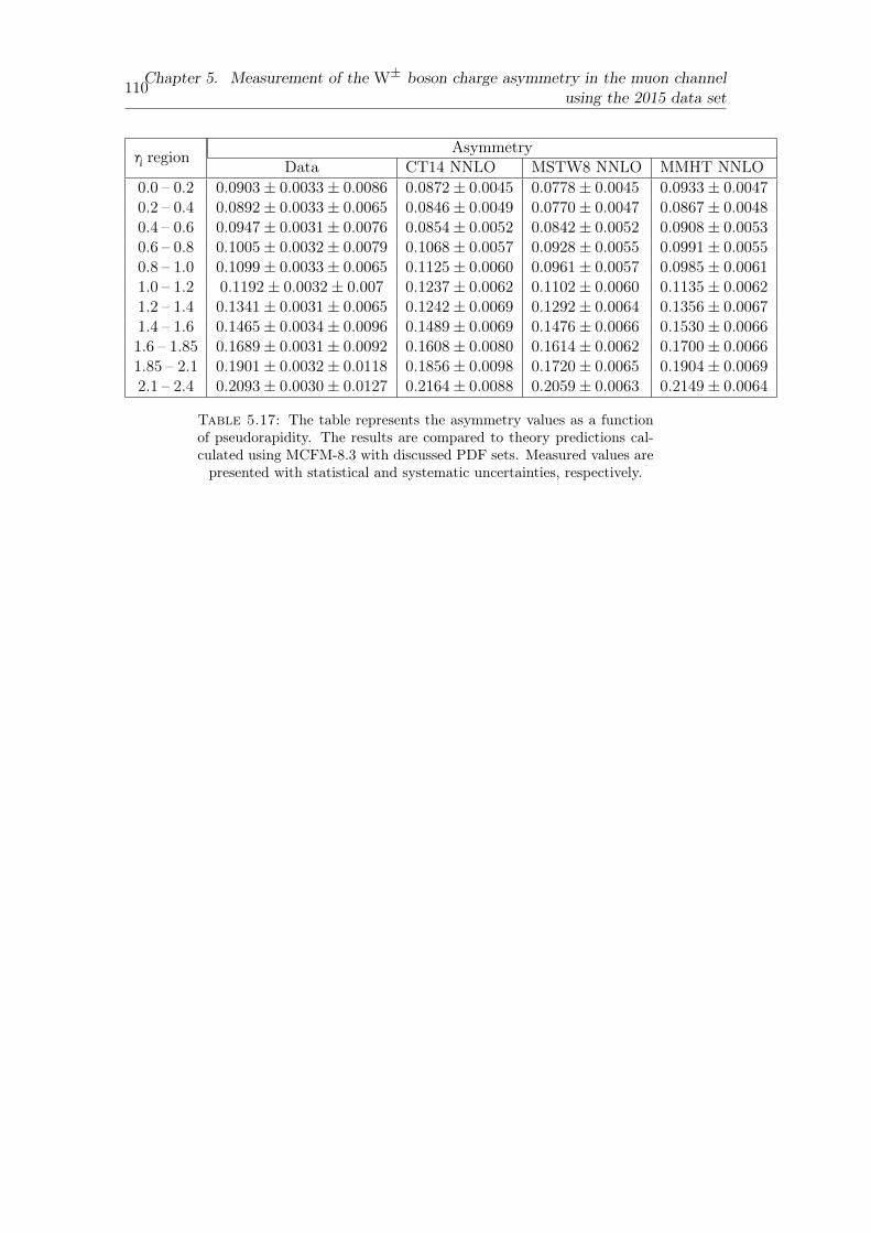
110Chapter 5. Measurement of the W± boson charge asymmetry in the muon channelusing the 2015 data set
η region AsymmetryData CT14 NNLO MSTW8 NNLO MMHT NNLO
0.0 – 0.2 0.0903± 0.0033± 0.0086 0.0872± 0.0045 0.0778± 0.0045 0.0933± 0.00470.2 – 0.4 0.0892± 0.0033± 0.0065 0.0846± 0.0049 0.0770± 0.0047 0.0867± 0.00480.4 – 0.6 0.0947± 0.0031± 0.0076 0.0854± 0.0052 0.0842± 0.0052 0.0908± 0.00530.6 – 0.8 0.1005± 0.0032± 0.0079 0.1068± 0.0057 0.0928± 0.0055 0.0991± 0.00550.8 – 1.0 0.1099± 0.0033± 0.0065 0.1125± 0.0060 0.0961± 0.0057 0.0985± 0.00611.0 – 1.2 0.1192± 0.0032± 0.007 0.1237± 0.0062 0.1102± 0.0060 0.1135± 0.00621.2 – 1.4 0.1341± 0.0031± 0.0065 0.1242± 0.0069 0.1292± 0.0064 0.1356± 0.00671.4 – 1.6 0.1465± 0.0034± 0.0096 0.1489± 0.0069 0.1476± 0.0066 0.1530± 0.00661.6 – 1.85 0.1689± 0.0031± 0.0092 0.1608± 0.0080 0.1614± 0.0062 0.1700± 0.00661.85 – 2.1 0.1901± 0.0032± 0.0118 0.1856± 0.0098 0.1720± 0.0065 0.1904± 0.00692.1 – 2.4 0.2093± 0.0030± 0.0127 0.2164± 0.0088 0.2059± 0.0063 0.2149± 0.0064
Table 5.17: The table represents the asymmetry values as a functionof pseudorapidity. The results are compared to theory predictions cal-culated using MCFM-8.3 with discussed PDF sets. Measured values arepresented with statistical and systematic uncertainties, respectively.
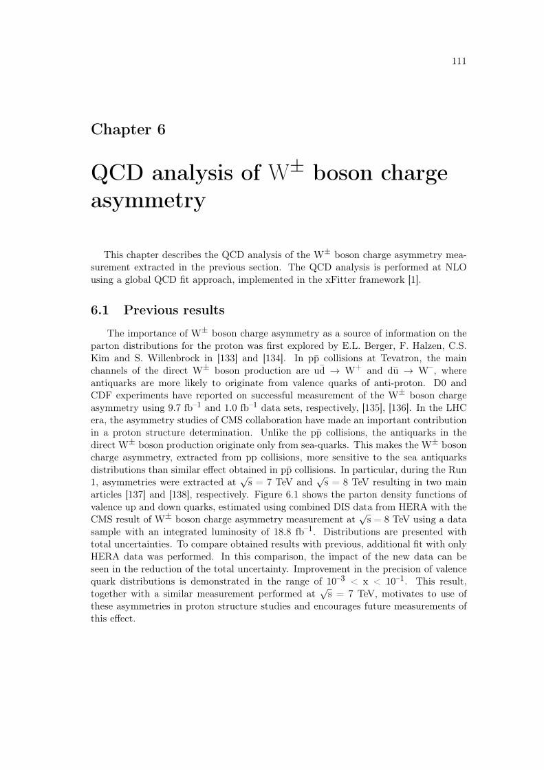
111
Chapter 6
QCD analysis of W± boson chargeasymmetry
This chapter describes the QCD analysis of the W± boson charge asymmetry mea-surement extracted in the previous section. The QCD analysis is performed at NLOusing a global QCD fit approach, implemented in the xFitter framework [1].
6.1 Previous results
The importance of W± boson charge asymmetry as a source of information on theparton distributions for the proton was first explored by E.L. Berger, F. Halzen, C.S.Kim and S. Willenbrock in [133] and [134]. In pp collisions at Tevatron, the mainchannels of the direct W± boson production are ud → W+ and du → W–, whereantiquarks are more likely to originate from valence quarks of anti-proton. D0 andCDF experiments have reported on successful measurement of the W± boson chargeasymmetry using 9.7 fb–1 and 1.0 fb–1 data sets, respectively, [135], [136]. In the LHCera, the asymmetry studies of CMS collaboration have made an important contributionin a proton structure determination. Unlike the pp collisions, the antiquarks in thedirect W± boson production originate only from sea-quarks. This makes the W± bosoncharge asymmetry, extracted from pp collisions, more sensitive to the sea antiquarksdistributions than similar effect obtained in pp collisions. In particular, during the Run1, asymmetries were extracted at
√s = 7 TeV and
√s = 8 TeV resulting in two main
articles [137] and [138], respectively. Figure 6.1 shows the parton density functions ofvalence up and down quarks, estimated using combined DIS data from HERA with theCMS result of W± boson charge asymmetry measurement at
√s = 8 TeV using a data
sample with an integrated luminosity of 18.8 fb–1. Distributions are presented withtotal uncertainties. To compare obtained results with previous, additional fit with onlyHERA data was performed. In this comparison, the impact of the new data can beseen in the reduction of the total uncertainty. Improvement in the precision of valencequark distributions is demonstrated in the range of 10–3 < x < 10–1. This result,together with a similar measurement performed at
√s = 7 TeV, motivates to use of
these asymmetries in proton structure studies and encourages future measurements ofthis effect.
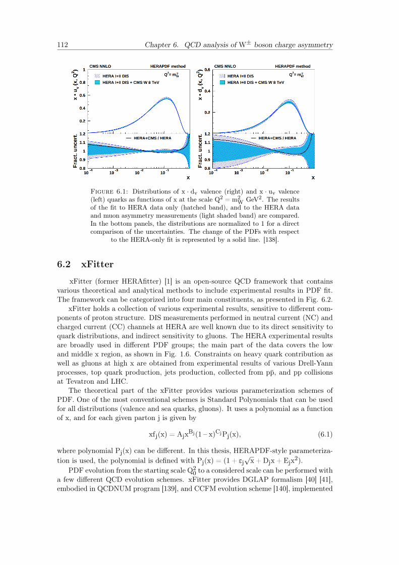
112 Chapter 6. QCD analysis of W± boson charge asymmetry
Figure 6.1: Distributions of x · dv valence (right) and x · uv valence(left) quarks as functions of x at the scale Q2 = m2
W GeV2. The resultsof the fit to HERA data only (hatched band), and to the HERA dataand muon asymmetry measurements (light shaded band) are compared.In the bottom panels, the distributions are normalized to 1 for a directcomparison of the uncertainties. The change of the PDFs with respect
to the HERA-only fit is represented by a solid line. [138].
6.2 xFitter
xFitter (former HERAfitter) [1] is an open-source QCD framework that containsvarious theoretical and analytical methods to include experimental results in PDF fit.The framework can be categorized into four main constituents, as presented in Fig. 6.2.
xFitter holds a collection of various experimental results, sensitive to different com-ponents of proton structure. DIS measurements performed in neutral current (NC) andcharged current (CC) channels at HERA are well known due to its direct sensitivity toquark distributions, and indirect sensitivity to gluons. The HERA experimental resultsare broadly used in different PDF groups; the main part of the data covers the lowand middle x region, as shown in Fig. 1.6. Constraints on heavy quark contribution aswell as gluons at high x are obtained from experimental results of various Drell-Yannprocesses, top quark production, jets production, collected from pp, and pp collisionsat Tevatron and LHC.
The theoretical part of the xFitter provides various parameterization schemes ofPDF. One of the most conventional schemes is Standard Polynomials that can be usedfor all distributions (valence and sea quarks, gluons). It uses a polynomial as a functionof x, and for each given parton j is given by
xfj(x) = AjxBj(1 – x)CjPj(x), (6.1)
where polynomial Pj(x) can be different. In this thesis, HERAPDF-style parameteriza-tion is used, the polynomial is defined with Pj(x) = (1 + εj
√x + Djx + Ejx2).
PDF evolution from the starting scale Q20 to a considered scale can be performed with
a few different QCD evolution schemes. xFitter provides DGLAP formalism [40] [41],embodied in QCDNUM program [139], and CCFM evolution scheme [140], implemented
6.3. QCD analysis 113
in uPDFevolv [141]. Theoretical predictions of cross-sections can be used from varioustools, including MCFM [142].
Figure 6.2: Schematic representation of the xFitter constituents [1].
Parameters of PDFs are estimated through the χ2 function minimization using theMINUIT program [125]. The xFitter provides a list of options for the account of corre-lated statistical and systematic uncertainties in various forms of the χ2 representation.The list includes the Full Covariance Matrix approach, use of Nuisance Parameters,and Mixed Form. In particular, the treatment of nuisance parameters can be performedusing Offset or Hessian methods. More details on these methods can be found in [1].
Theoretical uncertainties from renormalization and factorization scale variations, in-cluding strong coupling variation and predictions with different PDF sets, are time/re-source consuming. For that reason, fast techniques like k-factor and fast grid (APPLgrid[143] and fastNLO [144]) are used. In particular, a certain contribution to the APPLgridmodernization was performed by the author in order to prepare it for the NNLO up-grade. More details on that study may be found in Appendix C.
6.3 QCD analysis
Two separate QCD analyses are presented. The main difference is the data sets usedin these analyses and some of the settings. In both analyses the parton distributionfunctions are defined for valence quarks, xuv(x), xdv(x), anti-up, xu(x), and anti-down,xd(x), quarks, anti-strange quark1, xs(x), and gluon, xg(x) using standard polynomialsparameterization scheme (Eq.6.1).
The impact of W± boson charge asymmetry measurement at√s = 13 TeV on
the proton structure determination is performed in combination with other data sets,1Parameterization is done only in one analysis.
114 Chapter 6. QCD analysis of W± boson charge asymmetry
sensitive to the proton structure. The list of selected data sets includes DIS processesof neutral and charged current scattering, collected at HERA [4]. This data representscombined results from H1 [2] and ZEUS [3] experiments, obtained in e±p collisions atproton beam energies of 920, 820, 575, 460 GeV and an electron/positron beam energyof 27.5 GeV. This data is a core of any QCD analysis due to its high sensitivity tovalence and sea quark distributions in a wide kinematic range. The neutral current(NC) cross-sections are sensitive to valence and sea quark distributions in a range of6 · 10–7 ≤ x ≤ 0.65. The charged current (CC) cross-sections provide access to probemainly valence quark distributions in a range of 1.3 · 10–2 ≤ x ≤ 0.4.
Previous results of W± boson charge asymmetry measurements with the CMS de-tector at
√s = 7 TeV [145] and
√s = 8 TeV [138] are also used. In these measurements,
muons were selected with the transverse momentum higher than 25 GeV, pT > 25 GeV,in eleven bins of absolute values of pseudorapidity using the same η binning that wasused in the W± boson charge asymmetry measurement, described in this thesis. In ad-dition to the valence quarks sensitivity, W± asymmetry is sensitive to the strange quarkparton density function through suppressed processes uv + s → W+ and u + s → W–.Therefore, an additional result, sensitive to proton strange quark content is importantto include. The W± + charm quark processes provide information on strange–anti-strange proton content in a range of 10–3 ≤ x ≤ 10–1. The contribution of the seaquarks into the proton structure is usually expressed through a strangeness suppressionfactor, defined as
ks(Q2) =∫ 10 [s(Q
2, x) + s(Q2, x)]dx∫ 10 [u(Q
2, x) + d(Q2, x)]dx. (6.2)
The strangeness suppression rs is defined as an integrand of eq. 6.2. The list of selecteddata sets includes measurements of associated W± + charm production with the CMSdetector at
√s = 7 TeV [146] and
√s = 13 TeV [147]. Each measurement was performed
in five bins of absolute values of pseudorapidity. Results of extracted W± boson chargeasymmetry at
√s = 7 TeV,
√s = 8 TeV, and measurements of differential cross-sections
of associated W± + charm production at√s = 7 TeV,
√s = 13 TeV, used in this
analysis are shown in Fig. 6.3.The nuisance parameter representation is used in the fit for the treatment of sys-
tematic uncertainties from data. The χ2 is defined as
χ2(m, s) =
∑i
[mi –
∑j γ
ijm
isj – μi)]2
δ2i,statμimi + δ2i,uncor(m
i)2+∑j
s2j +∑i
lnδ2i,statμ
imi + (δi,uncormi)2
(δ2i,stat + δ2i,uncor)(μ
i)2.
(6.3)Here μi is the measured value at the point i,
∑j γ
ij are the relative correlated systematic
uncertainties, δi,stat and δi,uncor are relative statistical and uncorrelated systematicuncertainties. Vector m corresponds to a vector of results of the averaging for thecross-sections [148]. Summation over i is performed overall points on the (x,Q2) grid.Summation over j runs overall correlated systematic uncertainties. Vector s representscorrelated shifts of the cross-sections in units of sigma of the corresponding correlatedsystematic uncertainties. Logarithmic term is used to minimize biases [149].
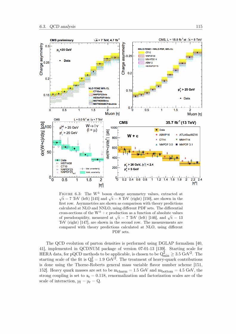
6.3. QCD analysis 115
Figure 6.3: The W± boson charge asymmetry values, extracted at√s = 7 TeV (left) [145] and
√s = 8 TeV (right) [150], are shown in the
first row. Asymmetries are shown as comparison with theory predictionscalculated at NLO and NNLO, using different PDF sets. The differentialcross-sections of the W±+c production as a function of absolute valuesof pseudorapidity, measured at
√s = 7 TeV (left) [146], and
√s = 13
TeV (right) [147], are shown in the second row. The measurements arecompared with theory predictions calculated at NLO, using different
PDF sets.
The QCD evolution of parton densities is performed using DGLAP formalism [40,41], implemented in QCDNUM package of version 07-01-13 [139]. Starting scale forHERA data, for pQCD methods to be applicable, is chosen to be Q2
min ≥ 3.5 GeV2. Thestarting scale of the fit is Q2
0 = 1.9 GeV2. The treatment of heavy-quark contributionsis done using the Thorne-Roberts general mass variable flavor number scheme [151,152]. Heavy quark masses are set to be mcharm = 1.5 GeV and mbottom = 4.5 GeV, thestrong coupling is set to αs = 0.118, renormalization and factorization scales are of thescale of interaction, μf = μr = Q.
116 Chapter 6. QCD analysis of W± boson charge asymmetry
6.3.1 Estimation of PDF uncertainties
The PDF uncertainties are evaluated in accordance with the HERAPDF 2.0 strat-egy [4]. Three types of uncertainties are considered: experimental, model, and param-eterization uncertainties. Propagation of experimental uncertainties to PDF, with thetolerance criterion of Δχ2 = 1, which corresponds to 68% confidence level, is performedusing the Hessian method [153].
Model uncertainty is evaluated from fit results, performed with a different charm andbottom quark masses. Variation of charm quark mass was performed in two separatefits with mcharm = 1.45 GeV and mcharm = 1.55 GeV. Variation of the bottom quarkmass was obtained in a similar way with mbottom = 4.25 GeV and mbottom = 4.75 GeV.In addition Q2
min is set to 2.5 GeV and 5 GeV. All model uncertainties are added inquadrature.
Parameterization uncertainty in each analysis is calculated as an envelope of a setof fits obtained with the inclusion of an additional D and E parameters. An additionalsystematic includes a variation of the starting scale, Q2
0 = 1.6 GeV2, and Q20 = 2.2
GeV2.In the first QCD analysis, model uncertainty of strange quark content originates
from varying values of strange fraction, fs. Details are given in the next subsection.The second QCD analysis uses the parameterization of strange quarks. Details of pa-rameterization and systematic uncertainty evaluation are given in 6.3.3. The totaluncertainty for each of the QCD analyses is calculated, adding in quadrature all threeuncertainty types.
6.3.2 QCD analysis with the new W± boson charge asymmetry andHERA data.
The first analysis is done to estimate the sensitivity of the new W± boson chargeasymmetry result to the proton structure. For that reason, the global fit is performedusing only the HERA data. The sensitivity can be shown comparing total relativeuncertainties of two fits, with and without the W± boson charge asymmetry obtainedin this thesis. Parameters of the standard polynomials and hence their form, are definedusing a so-called "parameterization scan". In this procedure, suitable parameters aredefined in an iterative approach, through the χ2 monitoring. The first fit starts onlywith ten parameters, with all D, E, and A
′g being set to zero. Each next fit is modified
with one new parameter until no more further χ2 improvement is observed. After thisprocedure is done, the resulting fit with thirteen parameters is given by:
xg(x) = AgxBg(1 – x)Cg , (6.4)
xuv(x) = AuvxBuv (1 – x)Cuv (1 + Duvx + Euvx
2), (6.5)
xdv(x) = AdvxBdv (1 – x)Cdv , (6.6)
xu(x) = AuxBu(1 – x)Cu(1 – Dux), (6.7)
xd(x) = AdxBd(1 – x)Cd . (6.8)
Here the normalization parameters Auv , Adv , and Ag are determined from the QCDsum rules. The B parameter describes PDF behavior at small x values with additionalconstraints Au = Ad, Bu = Bd. The C parameter corresponds to a shape of a distribu-tion at x→ 1. The asymmetry itself does not provide strong constraints on the strange
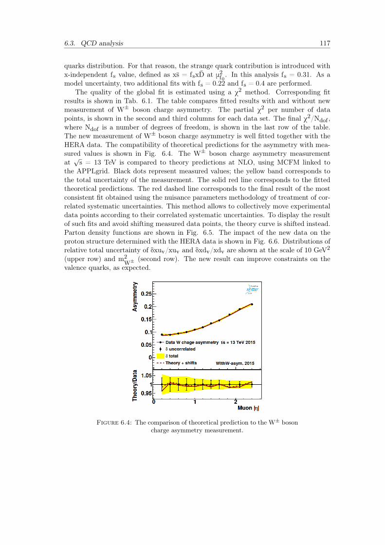
6.3. QCD analysis 117
quarks distribution. For that reason, the strange quark contribution is introduced withx-independent fs value, defined as xs = fsxD at μ2f0 . In this analysis fs = 0.31. As amodel uncertainty, two additional fits with fs = 0.22 and fs = 0.4 are performed.
The quality of the global fit is estimated using a χ2 method. Corresponding fitresults is shown in Tab. 6.1. The table compares fitted results with and without newmeasurement of W± boson charge asymmetry. The partial χ2 per number of datapoints, is shown in the second and third columns for each data set. The final χ2/Ndof ,where Ndof is a number of degrees of freedom, is shown in the last row of the table.The new measurement of W± boson charge asymmetry is well fitted together with theHERA data. The compatibility of theoretical predictions for the asymmetry with mea-sured values is shown in Fig. 6.4. The W± boson charge asymmetry measurementat√s = 13 TeV is compared to theory predictions at NLO, using MCFM linked to
the APPLgrid. Black dots represent measured values; the yellow band corresponds tothe total uncertainty of the measurement. The solid red line corresponds to the fittedtheoretical predictions. The red dashed line corresponds to the final result of the mostconsistent fit obtained using the nuisance parameters methodology of treatment of cor-related systematic uncertainties. This method allows to collectively move experimentaldata points according to their correlated systematic uncertainties. To display the resultof such fits and avoid shifting measured data points, the theory curve is shifted instead.Parton density functions are shown in Fig. 6.5. The impact of the new data on theproton structure determined with the HERA data is shown in Fig. 6.6. Distributions ofrelative total uncertainty of δxuv/xuv and δxdv/xdv are shown at the scale of 10 GeV2
(upper row) and m2W±
(second row). The new result can improve constraints on thevalence quarks, as expected.
Figure 6.4: The comparison of theoretical prediction to the W± bosoncharge asymmetry measurement.
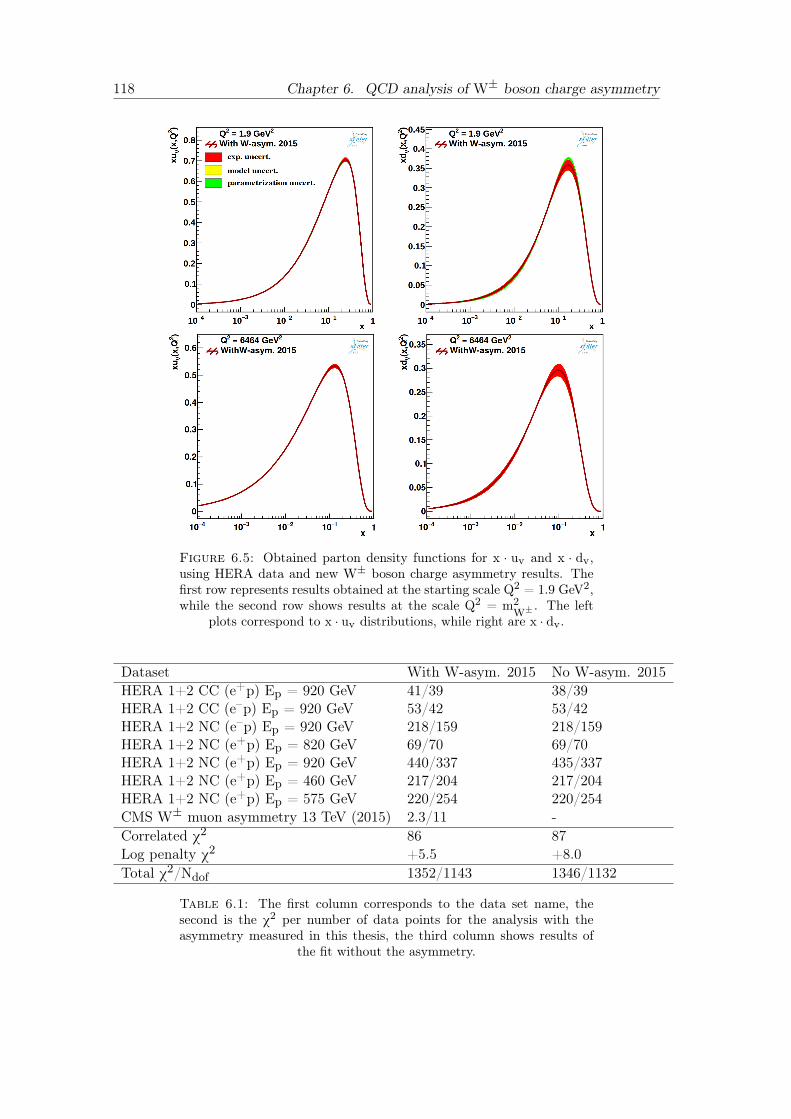
118 Chapter 6. QCD analysis of W± boson charge asymmetry
Figure 6.5: Obtained parton density functions for x · uv and x · dv,using HERA data and new W± boson charge asymmetry results. Thefirst row represents results obtained at the starting scale Q2 = 1.9 GeV2,while the second row shows results at the scale Q2 = m2
W± . The leftplots correspond to x · uv distributions, while right are x · dv.
Dataset With W-asym. 2015 No W-asym. 2015HERA 1+2 CC (e+p) Ep = 920 GeV 41/39 38/39HERA 1+2 CC (e–p) Ep = 920 GeV 53/42 53/42HERA 1+2 NC (e–p) Ep = 920 GeV 218/159 218/159HERA 1+2 NC (e+p) Ep = 820 GeV 69/70 69/70HERA 1+2 NC (e+p) Ep = 920 GeV 440/337 435/337HERA 1+2 NC (e+p) Ep = 460 GeV 217/204 217/204HERA 1+2 NC (e+p) Ep = 575 GeV 220/254 220/254CMS W± muon asymmetry 13 TeV (2015) 2.3/11 -Correlated χ2 86 87Log penalty χ2 +5.5 +8.0Total χ2/Ndof 1352/1143 1346/1132
Table 6.1: The first column corresponds to the data set name, thesecond is the χ2 per number of data points for the analysis with theasymmetry measured in this thesis, the third column shows results of
the fit without the asymmetry.
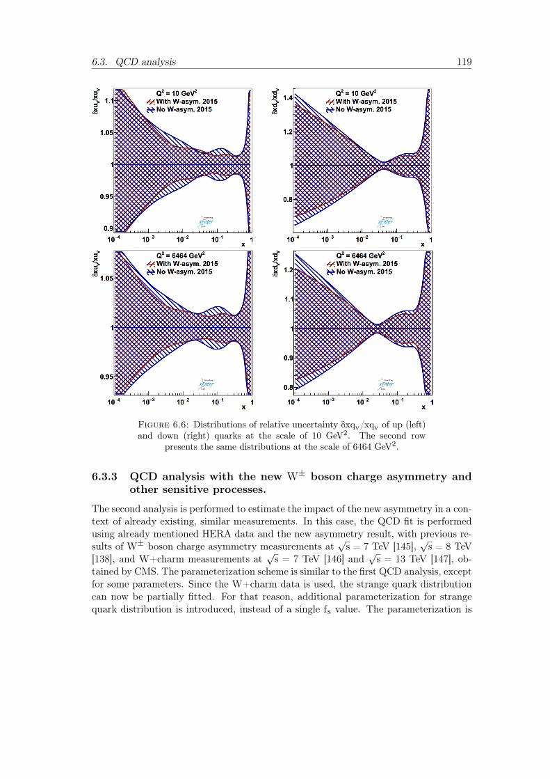
6.3. QCD analysis 119
Figure 6.6: Distributions of relative uncertainty δxqv/xqv of up (left)and down (right) quarks at the scale of 10 GeV2. The second row
presents the same distributions at the scale of 6464 GeV2.
6.3.3 QCD analysis with the new W± boson charge asymmetry andother sensitive processes.
The second analysis is performed to estimate the impact of the new asymmetry in a con-text of already existing, similar measurements. In this case, the QCD fit is performedusing already mentioned HERA data and the new asymmetry result, with previous re-sults of W± boson charge asymmetry measurements at
√s = 7 TeV [145],
√s = 8 TeV
[138], and W+charm measurements at√s = 7 TeV [146] and
√s = 13 TeV [147], ob-
tained by CMS. The parameterization scheme is similar to the first QCD analysis, exceptfor some parameters. Since the W+charm data is used, the strange quark distributioncan now be partially fitted. For that reason, additional parameterization for strangequark distribution is introduced, instead of a single fs value. The parameterization is
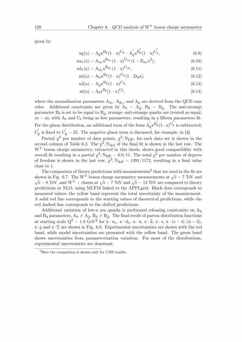
120 Chapter 6. QCD analysis of W± boson charge asymmetry
given by
xg(x) = AgxBg(1 – x)Cg – A′gx
B′g(1 – x)C
′g , (6.9)
xuv(x) = AuvxBuv (1 – x)Cuv (1 + Euvx
2), (6.10)
xdv(x) = AdvxBdv (1 – x)Cdv , (6.11)
xu(x) = AuxBu(1 – x)Cu(1 – Dux), (6.12)
xd(x) = AdxBd(1 – x)Cd , (6.13)
xs(x) = AsxBs(1 – x)Cs , (6.14)
where the normalization parameters Auv , Adv , and Ag are derived from the QCD sumrules. Additional constraints are given by Au = Ad, Bu = Bd. The anti-strangeparameter Bs is set to be equal to Bd, strange–anti-strange quarks are treated as equal,xs = xs, with As and Cs being as free parameters, resulting in a fifteen parameters fit.
For the gluon distribution, an additional term of the form A′gxB
′g(1– x)C
′g is subtracted;
C′g is fixed to C
′g = 25. The negative gluon term is discussed, for example, in [4].
Partial χ2 per number of data points, χ2/NDP, for each data set is shown in thesecond column of Table 6.2. The χ2/Ndof of the final fit is shown in the last row. TheW± boson charge asymmetry, extracted in this thesis, shows good compatibility withoverall fit resulting in a partial χ2/NDP = 6.0/11. The total χ2 per number of degreesof freedom is shown in the last row, χ2/Ndof = 1391/1172, resulting in a final valueclose to 1.
The comparison of theory predictions with measurements2 that are used in the fit areshown in Fig. 6.7. The W± boson charge asymmetry measurements at
√s = 7 TeV and√
s = 8 TeV, and W± + charm at√s = 7 TeV and
√s = 13 TeV are compared to theory
predictions at NLO, using MCFM linked to the APPLgrid. Black dots corresponds tomeasured values; the yellow band represent the total uncertainty of the measurement.A solid red line corresponds to the starting values of theoretical predictions, while thered dashed line corresponds to the shifted predictions.
Additional variation of low-x sea quarks is performed releasing constraints on Aqand Bq parameters, Au 6= Ad, Bu 6= Bd. The final result of parton distribution functionsat starting scale Q2 = 1.9 GeV2 for x · uv, x · dv, x · u, x · d, x · s, x · (s + s)/(u + d),x · g and x ·Σ are shown in Fig. 6.8. Experimental uncertainties are shown with the redband, while model uncertainties are presented with the yellow band. The green bandshows uncertainties from parameterization variation. For most of the distributions,experimental uncertainties are dominant.
2Here the comparison is shown only for CMS results.
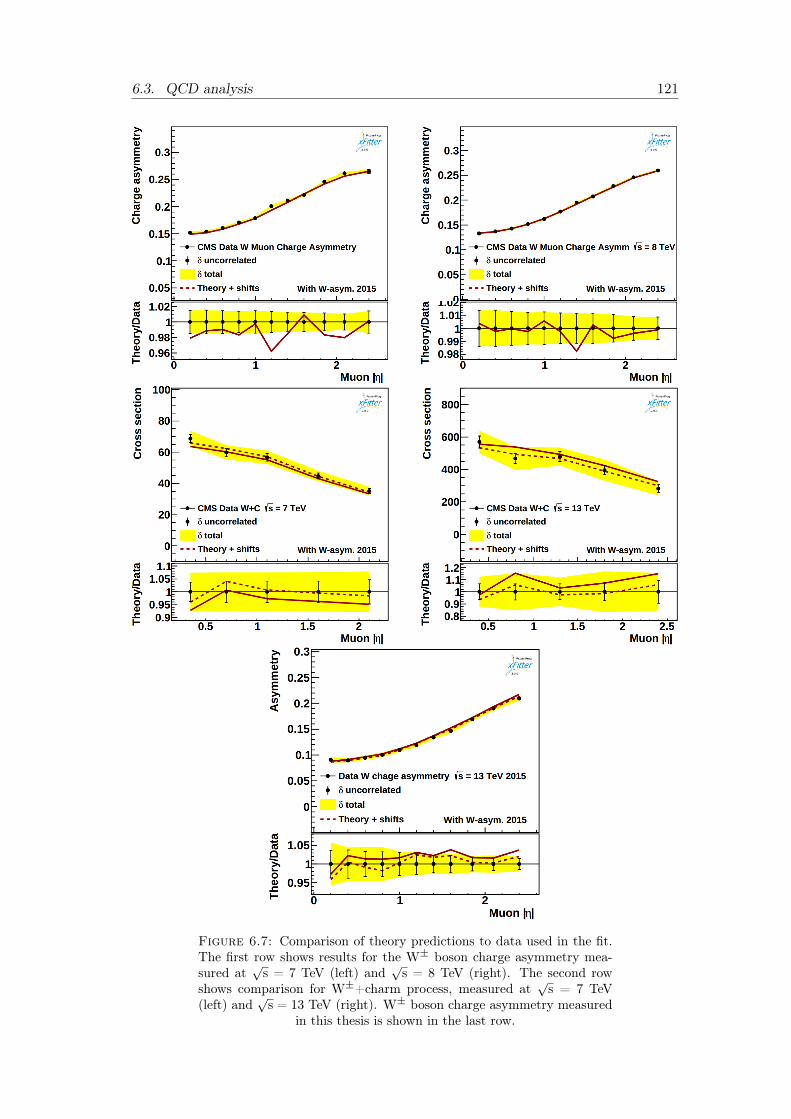
6.3. QCD analysis 121
Figure 6.7: Comparison of theory predictions to data used in the fit.The first row shows results for the W± boson charge asymmetry mea-sured at
√s = 7 TeV (left) and
√s = 8 TeV (right). The second row
shows comparison for W±+charm process, measured at√s = 7 TeV
(left) and√s = 13 TeV (right). W± boson charge asymmetry measured
in this thesis is shown in the last row.
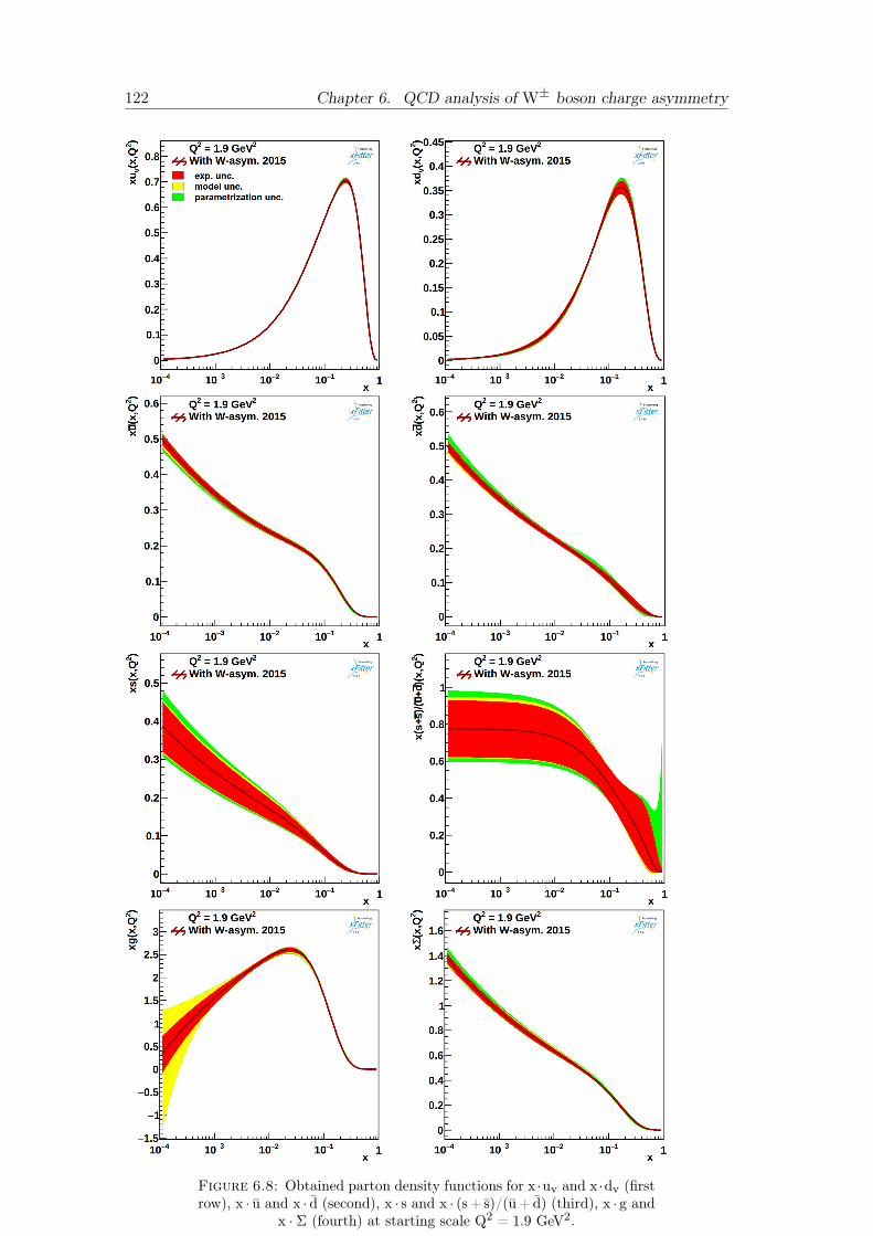
122 Chapter 6. QCD analysis of W± boson charge asymmetry
Figure 6.8: Obtained parton density functions for x ·uv and x ·dv (firstrow), x · u and x · d (second), x · s and x · (s+ s)/(u + d) (third), x · g and
x · Σ (fourth) at starting scale Q2 = 1.9 GeV2.
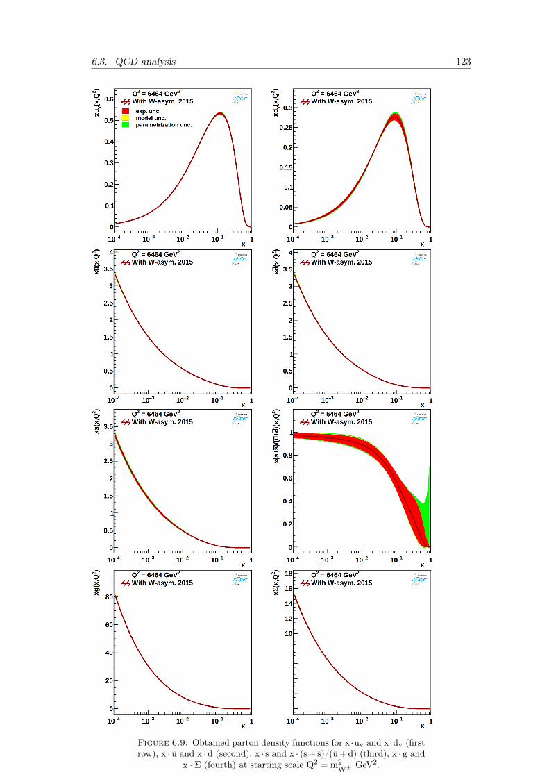
6.3. QCD analysis 123
Figure 6.9: Obtained parton density functions for x ·uv and x ·dv (firstrow), x · u and x · d (second), x · s and x · (s+ s)/(u + d) (third), x · g and
x · Σ (fourth) at starting scale Q2 = m2W± GeV2.
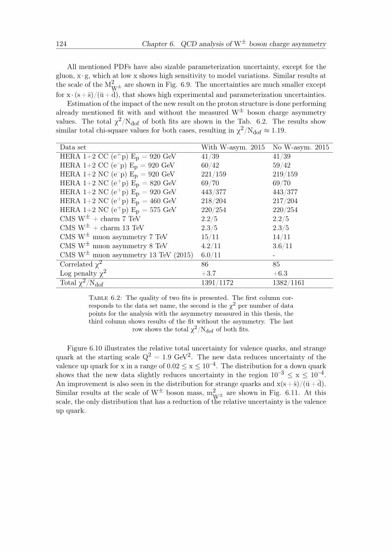
124 Chapter 6. QCD analysis of W± boson charge asymmetry
All mentioned PDFs have also sizable parameterization uncertainty, except for thegluon, x ·g, which at low x shows high sensitivity to model variations. Similar results atthe scale of the M2
W± are shown in Fig. 6.9. The uncertainties are much smaller exceptfor x · (s+ s)/(u+ d), that shows high experimental and parameterization uncertainties.
Estimation of the impact of the new result on the proton structure is done performingalready mentioned fit with and without the measured W± boson charge asymmetryvalues. The total χ2/Ndof of both fits are shown in the Tab. 6.2. The results showsimilar total chi-square values for both cases, resulting in χ2/Ndof ≈ 1.19.
Data set With W-asym. 2015 No W-asym. 2015HERA 1+2 CC (e+p) Ep = 920 GeV 41/39 41/39HERA 1+2 CC (e–p) Ep = 920 GeV 60/42 59/42HERA 1+2 NC (e–p) Ep = 920 GeV 221/159 219/159HERA 1+2 NC (e+p) Ep = 820 GeV 69/70 69/70HERA 1+2 NC (e+p) Ep = 920 GeV 443/377 443/377HERA 1+2 NC (e+p) Ep = 460 GeV 218/204 217/204HERA 1+2 NC (e+p) Ep = 575 GeV 220/254 220/254CMS W± + charm 7 TeV 2.2/5 2.2/5CMS W± + charm 13 TeV 2.3/5 2.3/5CMS W± muon asymmetry 7 TeV 15/11 14/11CMS W± muon asymmetry 8 TeV 4.2/11 3.6/11CMS W± muon asymmetry 13 TeV (2015) 6.0/11 -Correlated χ2 86 85Log penalty χ2 +3.7 +6.3Total χ2/Ndof 1391/1172 1382/1161
Table 6.2: The quality of two fits is presented. The first column cor-responds to the data set name, the second is the χ2 per number of datapoints for the analysis with the asymmetry measured in this thesis, thethird column shows results of the fit without the asymmetry. The last
row shows the total χ2/Ndof of both fits.
Figure 6.10 illustrates the relative total uncertainty for valence quarks, and strangequark at the starting scale Q2 = 1.9 GeV2. The new data reduces uncertainty of thevalence up quark for x in a range of 0.02 ≤ x ≤ 10–4. The distribution for a down quarkshows that the new data slightly reduces uncertainty in the region 10–3 ≤ x ≤ 10–4.An improvement is also seen in the distribution for strange quarks and x(s+ s)/(u+ d).Similar results at the scale of W± boson mass, m2
W±are shown in Fig. 6.11. At this
scale, the only distribution that has a reduction of the relative uncertainty is the valenceup quark.
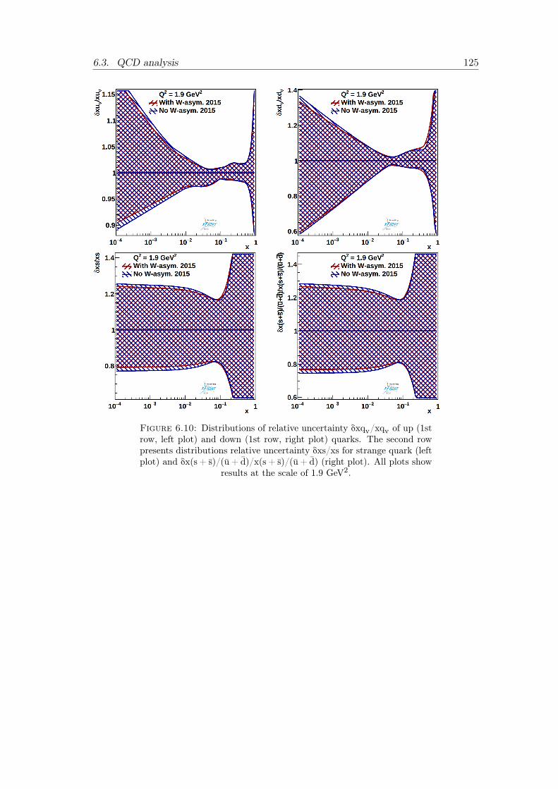
6.3. QCD analysis 125
Figure 6.10: Distributions of relative uncertainty δxqv/xqv of up (1strow, left plot) and down (1st row, right plot) quarks. The second rowpresents distributions relative uncertainty δxs/xs for strange quark (leftplot) and δx(s + s)/(u + d)/x(s + s)/(u + d) (right plot). All plots show
results at the scale of 1.9 GeV2.
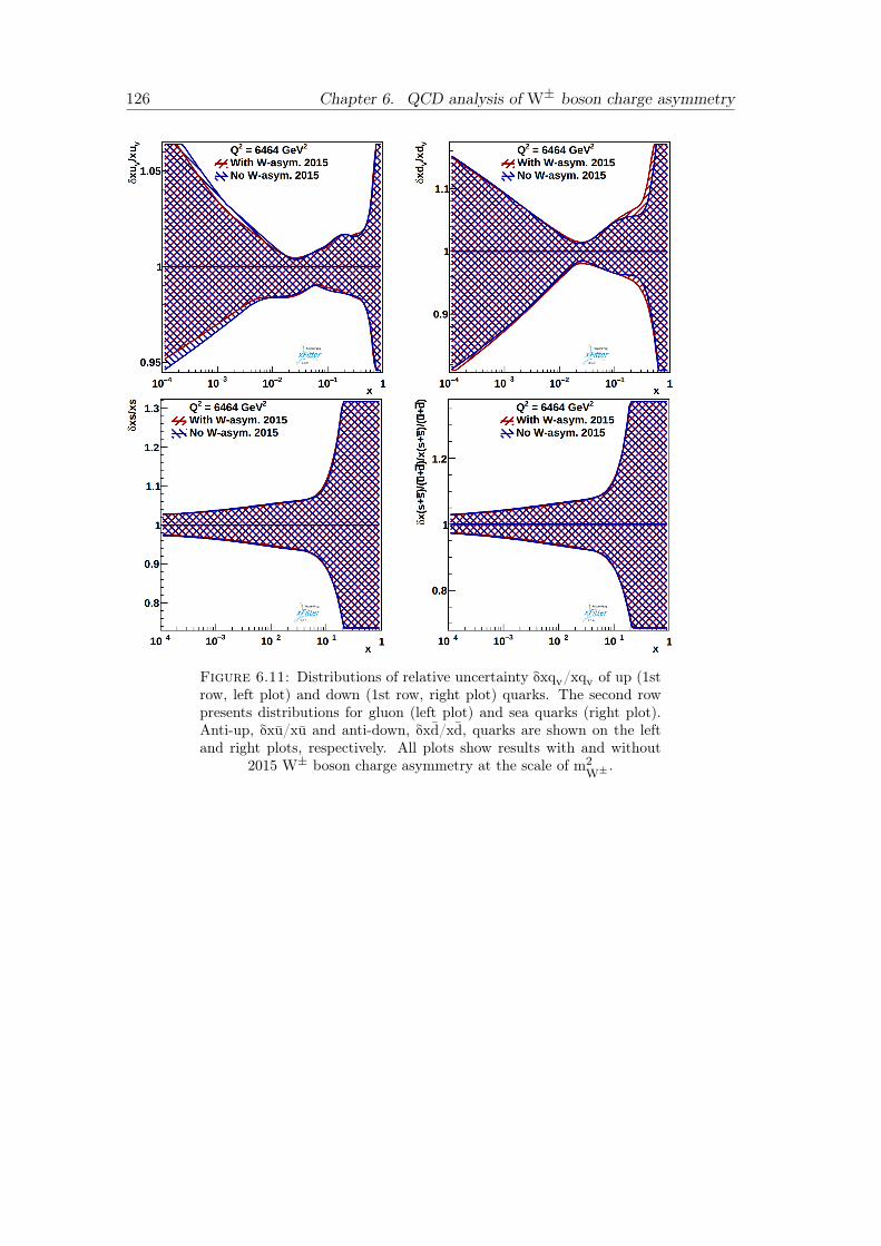
126 Chapter 6. QCD analysis of W± boson charge asymmetry
Figure 6.11: Distributions of relative uncertainty δxqv/xqv of up (1strow, left plot) and down (1st row, right plot) quarks. The second rowpresents distributions for gluon (left plot) and sea quarks (right plot).Anti-up, δxu/xu and anti-down, δxd/xd, quarks are shown on the leftand right plots, respectively. All plots show results with and without
2015 W± boson charge asymmetry at the scale of m2W± .
127
Chapter 7
Summary and conclusions
A measurement of W± boson charge asymmetry in the data sample collected at√s = 13 TeV with the CMS detector corresponding to an integrated luminosity of up
to 2.2± 0.05 fb–1 and the QCD analysis with measured values are presented.Differential cross-sections are measured using W± bosons events decaying in the
muon channel. The event selection is performed selecting muons that satisfy kine-matic and fiducial requirements. The estimation of W± boson yields is obtained fromthe missing transverse energy distributions using an unbinned maximum-likelihood fit.Calculation of systematic uncertainties of differential cross-sections showed high sen-sitivity to inclusive W± boson recoil correction and pileup. The obtained values arecompared to theoretical predictions calculated at NNLO using MCFM-8.3 package withCT14 NNLO, MSTW8 NNLO, MMHT NNLO PDF sets. A comparison of differentialcross-sections showed good agreement with prediction calculated using the CT14 NNLOPDF set. Asymmetry values are in good agreement with predictions produced usingCT14 NNLO and MMHT NNLO PDF sets. The sensitivity of W± boson charge asym-metry to valence and sea content of proton in the range of 10–3 ≤ x ≤ 10–1 was testedby performing a QCD analysis to probe the improvement on the PDF determination.The analysis is done using the open-source QCD framework xFitter. Quantitative es-timation of the measured asymmetry sensitivity to proton structure is obtained usingHERA I+II data. Experimental uncertainties associated with the input data sets arepropagated to PDF uncertainties with the Hessian method, with the tolerance criterionof Δχ2 = 1. The results show that the measured asymmetry values can improve PDFuncertainties for valence quarks at different scales. After this result is obtained, themeasured asymmetry is used in combination with previous CMS measurements of W±
boson charge asymmetry at√s = 7 TeV and
√s = 8 TeV, measurements of W+charm
quark production at√s = 7 TeV,
√s = 13 TeV, and HERA I+II data. The inclusion
of similar data sets into the global fit significantly constrains the phase space of valencequark distributions.


129
Eidesstatliche Versicherung
Hiermit versichere ich an Eides statt, die vorliegende Dissertationsschrift selbstverfasst und keine anderen als die angegebenen Hilfsmittel und Quellen benutzt zuhaben.
Die eingereichte schriftliche Fassung entspricht der auf dem elektronischen Speichr-mendium.
Die Dissertation wurde in der vorgelegten oder einer ähnlichen Form nicht schoneinmal in einem früheren Promotionsverfahren angenommen oder als ungenügend be-urteilt.
Hamburg den 29.05.2020 Vladyslav Danilov

131
AcknowledgementsFirst of all, I would like to thank my supervisors Elisabetta Gallo and Katarzyna
Wichmann, for giving me the opportunity to do this wonderful research and gain alot of experience. I am very grateful for all that support and experience that theygave me and their help in my aspiration to be better. I also would like to thankall CMS DESY group members who were always open to questions, discussions, andchats. Much helpful advice I received from Katerina Lipka, Svenja Pflitsch, AkshanshSingh, Pavel Starovoitov, Oleksi Turkot, and many others. Also, I’m very thankfulto Stephanie Brandt, who was always ready to answer my questions and share heropinion in various discussions. I was glad to participate in the APPLgrid upgrade withPavel Starovoitov. During that time, I have learned a lot. Many thanks to MoritzGuethoff, Olena Karacheban, and Anastasia Velyka for being great teachers in mytechnical responsibilities.
I would like to thank my aunt, Valentyna Harnaga, and cousin, Yaroslav Tyshenko,for all support they gave me. Finally, I would like to thank my girlfriend, Valeria, whomade my life better than it was before.
I thank you all.

133
List of Figures
1.1 Elementary particles in the Standard model. The three left columnscorrespond to fermions. The right column is vector gauge bosons, andthe last has the scalar boson of Higgs field. For each particle, mass,charge, and spin values are given in their left upper frame corner [9]. . . 4
1.2 The running of αs(Q) as a function of the scale Q. The solid line and theuncertainty band are calculated by evolving the extracted αs(mZ) valuesusing the 2-loop 5-flavor renormalization group equations [15]. . . . . . 7
1.3 The strengths of the weak interactions between the six quarks. The"intensities" of the lines are determined by the elements of the CKMmatrix [19], [20]. . . . . . . . . . . . . . . . . . . . . . . . . . . . . . . . 9
1.4 Diagrams represent deep inelastic scattering via exchange of Z0/γ∗ bosonon the left, and W± on the right. Lepton four-momentum before andafter interaction is shown as k and k′ respectively. The proton initialstate momentum is shown as p. . . . . . . . . . . . . . . . . . . . . . . . 11
1.5 The proton structure function F2p measured in electromagnetic scatter-ing of electrons and positrons on protons, and for electrons/positrons(SLAC, HERMES, JLAB) and muons (BCDMS, E665, NMC) on a fixedtarget. Statistical and systematic errors added in quadrature are shown.The H1+ZEUS combined values are obtained from the measured reducedcross-section and converted to F2p with a HERA-PDF NLO fit, for allmeasured points where the predicted ratio of F2p to reduced cross-sectionwas within 10% of unity. The data are plotted as a function of Q2 inbins of fixed x [14]. . . . . . . . . . . . . . . . . . . . . . . . . . . . . . . 12
1.6 Kinematic domains in x and Q2 probed by fixed-target and collider ex-periments, where Q2 can refer either to the literal Q2 for deep inelasticscattering, or the hard scale of the process in hadron-hadron collisions,e.g. invariant mass or transverse momentum p2T. Some of the final statesaccessible at the LHC are indicated in the appropriate regions, where yis the rapidity. The incoming partons have x1,2=(Q/14 TeV) e±y whereQ is the hard scale of the process shown in blue in the figure. [14]. . . . 13
1.7 Representation of proton-proton collision in the factorization approach.Each proton carries momentum p with its non-perturbative PDF, f(x).Strong coupling at renormalization scale is shown as αs(μr). Parton-parton interaction area is shown with σ. . . . . . . . . . . . . . . . . . . 15
1.8 Feynman diagrams of Pqq, Pgq, Pqg, and Pgg splitting functions ofDGLAP equations. [37]. . . . . . . . . . . . . . . . . . . . . . . . . . . . 16
1.9 The parton distribution functions of valence quarks, xuv, xdv, scaledsea quarks, xΣ, and gluons, xg at scale Q2 = 1.9 GeV2 (left plot) andQ2 = m2
W GeV2 (right plot) [42]. . . . . . . . . . . . . . . . . . . . . . . 17
134 List of Figures
1.10 Feynman diagram for W± boson production in pp collisions, decaying inthe muon channel. Left figure show the diagram for W– production, W+
is shown on the right. . . . . . . . . . . . . . . . . . . . . . . . . . . . . 171.11 Individual contributions of flavor decomposition into the total W+ (solid
line) and W– (dashed line) cross-section at LO [43]. . . . . . . . . . . . . 181.12 Measurements of the total W+, W–, W, and Z0 production cross sections
times branching fractions as a function of center of mass energy for CMSand experiments at lower-energy colliders [44]. . . . . . . . . . . . . . . . 19
1.13 W± boson in different helicity states decaying into electron channel in arest frame. The first row corresponds to three different helicity states,left-handed (negative), longitudinal, and right-handed (positive). Bluearrows are momentum; red arrows are helicity states of daughter particles,while the yellow arrow shows the boson spin projection on the z-axis. Thesecond row shows the matrix element dependence on the theta angle foreach helicity state [47]. . . . . . . . . . . . . . . . . . . . . . . . . . . . 21
1.14 Two left plots show the comparison W+ and W– events distribution asa function of the boson rapidity for different states of the boson helicity.The right plots shows the same distributions but for muon events as afunction of muon pseudorapidity and W± boson helicity state [48]. . . . 22
2.1 Geographic location of the LHC [49]. . . . . . . . . . . . . . . . . . . . . 242.2 Acceleration scheme [50]. . . . . . . . . . . . . . . . . . . . . . . . . . . . 252.3 LHC report on the delivered luminosity during RUN 1 and RUN 2. . . . 262.4 The figure shows the CMS detector, its main components, and charac-
teristics. A black human figure on the right corner below is made of thereal scale to the detector size [53]. . . . . . . . . . . . . . . . . . . . . . . 28
2.5 The CMS tracker slice view in the r-z plane. Single-sided strip modulesare marked with black thin lines, pixel modules are depicted in red, andstrip stereo modules are shown as blue thick lines. [55] . . . . . . . . . . 30
2.6 The left figure illustrates a PbWO4 crystal with a graphical represen-tation of a shower inside [56]. The right figure represents the sketch ofthe one-fourth of the ECAL in the Y-Z plane. Tilted PbWO4 crystalsare shown with the blue lines. The dashed lines show the pseudorapiditycoverage of the EB, EE, and ES [57]. . . . . . . . . . . . . . . . . . . . . 32
2.7 The figure represents the sketch of the quarter slice of the HCAL in the Y-Z plane. "FEE" corresponds to the locations of the Front End Electronicsfor HB and HE. The signals from the tower cells shown with the samecolor are added optically, providing a "longitudinal" segmentation of theHCAL. HB and HE are sliced in 29 azimuthal pieces with Δφ ≈ 20degrees each [60]. . . . . . . . . . . . . . . . . . . . . . . . . . . . . . . . 33
2.8 Representation of the 5 modules composing the cold mass inside thecryostat, with the supporting system (vertical, radial and longitudinaltie rods) [54]. . . . . . . . . . . . . . . . . . . . . . . . . . . . . . . . . . 34
List of Figures 135
2.9 CMS muon system in the Y-Z plane. The rings of the barrel yoke 0,1, 2 are shown as "Wheel", the endcap yoke is shown as "Steel". TheDrift Tube stations (DTs) are shown with a beige color and labeled asMB ("Muon Barrel"). The color of Cathode Strip Chambers (CSCs) islime-green; they are labeled as ME ("Muon Endcap"). Resistive PlateChambers (RPCs) are mounted in both the barrel and endcaps of CMS,they are labeled RB and RE, respectively, and represented with a bluecolor. The dotted lines show the pseudorapidity coverage of the muonsystem with equidistant steps of 0.1.[65] . . . . . . . . . . . . . . . . . . 35
2.10 The scheme represents the CMS L1 trigger system. The data fromthe electromagnetic calorimeter (ECAL), hadronic calorimeters (HF andHCAL) are processed first to regional calorimeter trigger (RCT), then toglobal calorimeter trigger (GCT). Energy deposits (hits) from the muondetector (RPC, CSC, and DT) are processed via a system of a track- andsegment-finders or via a pattern comparator, and sent to a global muontrigger (GMT). The final trigger decision is made using a global trigger(GT), which combines the information from the GCT and GMT. The de-cision is then sent to the tracker (TRK), ECAL, HCAL, or muon systems(MU) using the Trigger, Timing and Control system (TTC). Afterwards,the data from various subsystems is transferred to the acquisition system(DAQ) for offline storage.[68] . . . . . . . . . . . . . . . . . . . . . . . . 36
3.1 Schematic view of Particle Flow algorithm as a link between detectorsignals and reconstructed physics objects. The left side illustrates anevent representation in terms of physics objects. The right part representsthe CMS detector in the transverse plane; ECAL clusters represent anamount of energy detected from leptons and photons in the hypotheticalevent. The HCAL cluster shows amount of detected energy from hadrons.Tracks are shown with black lines. The muon that penetrates all layersis shown with the red dotted line [72]. . . . . . . . . . . . . . . . . . . . 40
3.2 Interactions per crossing (pile-up) for 2015-2018 [75] . . . . . . . . . . . 413.3 Resolution of missing transverse momenta of Z0 → e+e– as a function
of reconstructed pp collision vertices. PF (red triangles) corresponds toevents reconstructed only with the particle flow algorithm. PUPPI (bluetriangles) illustrates PF events corrected with the PUPPI method. [77] . 42
3.4 εtrack for isolated muons shown as a function of pseudorapidity (left)with pT = 1, 10, 100 GeV and transverse momentum (right) for bar-rel (0.0<|η|<0.9), transition (0.9<|η|<1.4), and endcap (1.4.<|η|<2.5)regions [70]. . . . . . . . . . . . . . . . . . . . . . . . . . . . . . . . . . . 46
3.5 Tag-and-probe εreco+ID efficiency for loose ID (left) and tight ID (right)as a function of η. Detector regions with a smaller amount of instrumen-tation cause the dips in efficiency. The statistical uncertainties are tiny[65]. . . . . . . . . . . . . . . . . . . . . . . . . . . . . . . . . . . . . . . 47
3.6 Tag-and-probe εiso efficiency for tight ID as a function of pT (left) and η(right). The statistical uncertainties are smaller than the symbols [65]. 47
3.7 The εtrig efficiency of an isolated muon is presented. The left plot showsεtrig efficiency as a function of muon pT while the left corresponds to afunction of muon η. The statistical uncertainties are smaller than themarkers [65]. . . . . . . . . . . . . . . . . . . . . . . . . . . . . . . . . . 48
136 List of Figures
4.1 The picture shows the CMS detector in the Y-Z plane. Names of theBRIL subsystems are shown in different colors. The black lines indicatepositions of the subsystems. The BPTX is at a distance of 175 m fromthe IP and is not shown on the scheme [87]. . . . . . . . . . . . . . . . . 51
4.2 C-shape equipped with six sensors. Each sensor has two channels [91]. . 524.3 The scheme represents arrival time before and after the bunch crossing.
The thick black line is the beam-line, circles with gray parallelograms arethe BCM1F rings with schematic sensors. The first row shows protonbunches, and theirs halos passing the BCM1F right before the collision,which corresponds to a timing -6 ns. The second row shows the collisionat the interaction point (IP). The third row is dedicated to the outgo-ing bunches after the collision with some collision products passing theBCM1F sensors, the timing of this stage corresponds to 6 ns after thecollision. Overall timing of each collision is 12 ns [87]. . . . . . . . . . . 53
4.4 Hit rates as a function of time for one bunch crossing collected during2.5 minutes [92]. . . . . . . . . . . . . . . . . . . . . . . . . . . . . . . . 54
4.5 Van der Meer scan as performed during the fill 4266. The left plot cor-responds to X-plane, while the right is Y-plane. The plots show themeasured values for each displacement as a function of separation dis-tance. Black dots correspond to measured rate values at each step. Redand green lines correspond to a Gaussian fit, constant term is shown witha blue line. The resulting fit is shown with a black line [93]. . . . . . . . 54
4.6 The graph of an electron scan of typical poly-crystalline diamond filmsgrown on Si by CVD, using 0.5% methane in hydrogen.[97] . . . . . . . 55
4.7 Geometrical characteristics of a sensor and its one pad metallization (Pic-ture 4.7 a) and two pad metallization (Picture 4.7 b) [99]. . . . . . . . . 56
4.8 Schematic representation of signal transferring from sensor channels toAOH. The left plot shows a sensor with two channels and two pads thatare connected to the ASIC. Blue arrows correspond to ASIC output,which is connected to AOHs. The right plot shows two AOHs with in-coming signals marked as blue arrows. Each AOH processes only rightor left ASIC output signal from three different sensors. Red arrows cor-respond to outgoing optical fibers marked as left, middle, and right. . . . 57
4.9 Electric schemes for IV and CT measurements. Generally, the schemesfor the IV and CT are the same, except that the CT has a source of β–
decay 90Sr. HV is a power supply; the gray and blue rectangles are adiamond sensor, metallization pads are shown with a yellow color. A isampere meter, and earth ground is shown as a dashed triangle. . . . . . 59
4.10 A diamond sensor in a plastic frame that is used in IV and CT measure-ments. Schematic pictures show the binding of a diamond sensor withthe metal strips [108]. . . . . . . . . . . . . . . . . . . . . . . . . . . . . 59
4.11 Selected results of IV measurement for sCVD sensor "Batch 390" (plot4.11a), and pCVD sensors 07B10431 (plot 4.11b), 07B10433 (plot 4.11c).The voltage is applied in order 0 - +1000 - 0 - –1000 - 0 V. . . . . . . . 60
4.12 CT measurements of 07B10436 (plot A) and 07B10422 (plot B) pCVDsensors. . . . . . . . . . . . . . . . . . . . . . . . . . . . . . . . . . . . . 61
4.13 CT measurements of "Batch 390" (Fig. A) and "Number 5" (Fig. B)sCVD sensors. . . . . . . . . . . . . . . . . . . . . . . . . . . . . . . . . . 62
List of Figures 137
4.14 A diamond sensor is in the opened "beta-setup" box before the measure-ment. The needle is on top of the diamond sensor, which is mounted inthe center of the high voltage golden plate. The black hole in an ironpyramid is a dry-air source (5% oxygen + 95% dry nitrogen). During themeasurement, this scheme is covered with a black wooden box. Inside ontop, the box has two mounted layers of scintillation detectors. . . . . . . 63
4.15 The ionization signal is registered with the needle and amplified withthe pre-amplifier forming a Diamond Signal. FIFO is a Fan-In Fan-Out,Scope is an oscilloscope. SC1 and SC2 - two scintillators, LTD - Low-Threshold Discriminator, COIN - Coincidence Unit. The red line is asignal input in ADC; the blue line is a duplicated signal with a delay(blue circle between the FIFO and the Scope). The magenta line is agate, formed from two scintillator signals. The Scope shows the openedgate right in the time interval of the signal, excluding the pedestal timeinterval [99]. . . . . . . . . . . . . . . . . . . . . . . . . . . . . . . . . . . 64
4.16 Two histograms of 10000 ADC counts of pCVD sensor 07B10417 mea-sured at 500 V. The pedestal ADC counts with the Gaussian distributionshape are shown in the upper histogram. The lower histogram shows sig-nal ADC counts with the Landau distribution shape. . . . . . . . . . . . 64
4.17 Calibration line of ADC channels as a function of charge. The Calibvalue obtained from this fit is k=47. . . . . . . . . . . . . . . . . . . . . 65
4.18 CCD measurements as a function of time of 07B10415 (plot 4.18a) and07B10434 (plot 4.18b) pCVD sensors. . . . . . . . . . . . . . . . . . . . 66
4.19 CCD measurements as a function of time of "Number 5" (plot 4.19a) and"Batch 390" (plot 4.19b) sCVD sensors. Both sensors show high chargecollection distance and stability over time for all bias voltages. . . . . . . 66
4.20 CCD measurements as a function of applied bias voltage of pCVD sensor07B10415 (plot 4.20a) and sCVD sensor "Batch 390" (plot 4.20b). Bothsensors show a stable logarithmic rise. . . . . . . . . . . . . . . . . . . . 67
4.21 Recorded orbit from the LHC Fill 4364 with 852 colliding bunches [87].The baseline is set on 140 ADC counts, signals are shown as dips in abaseline position. Red ellipse shows a TP, green rectangle correspondsto the "pilot" train, and each magenta circle is a train of bunches. . . . 68
4.22 Arrival time distribution [87]. . . . . . . . . . . . . . . . . . . . . . . . . 694.23 Baseline distributions for channel 1 taken from one of the first fills. Plot
4.23a corresponds to the baseline position distribution, while plot 4.23bshows distribution of its standard deviation. . . . . . . . . . . . . . . . . 69
4.24 The zoomed test pulse signal is a dip in the baseline, defined between 6070and 6080 ns. The red dashed line corresponds to the baseline threshold,which is 3 ADC counts. The blue line is a signal value, which correspondsto 20 ADC or 80 mV. The green line shows which part of the signal istaken as the arrival time. . . . . . . . . . . . . . . . . . . . . . . . . . . . 70
4.25 Test pulse distributions for channel 2 taken from one of the first fills,obtained after processing 401 orbits. Plot 4.25a shows distribution of TPsignal amplitude. Plot 4.25b shows distribution of TP arrival time. . . . 70
4.26 Signal amplitude spectra taken from Fill 5722 of pCVD sensor 4.26a inlog scale, and sCVD sensor 4.26b in linear. . . . . . . . . . . . . . . . . . 71
4.27 Signal amplitude spectra with reference histograms (plot A), base lineposition histogram with references (plot B). . . . . . . . . . . . . . . . . 72
138 List of Figures
4.28 Signal amplitude distribution from channel 17 (pCVD 07B10512), col-lected in Fill 6417. . . . . . . . . . . . . . . . . . . . . . . . . . . . . . . 73
4.29 Test pulse spectrum in Web monitor tool. . . . . . . . . . . . . . . . . . 734.30 Signal amplitude spectra of sCVD "Number 5", channel 11. Plot A shows
distribution obtained from fill 5730, 30.05.2017. Plot B is taken from fill5984, 24.07.2017. . . . . . . . . . . . . . . . . . . . . . . . . . . . . . . . 74
4.31 Signal amplitude and TP MPV values as a function of a fill numberfor sCVD "Number 5" (plot A) and sCVD "Batch390" (plot B). Eachplot shows results from both channels, in different colors. The solid linecorresponds to MPV values taken from signal amplitude distribution,while dashed lines correspond to MPV taken from test pulse spectra. . . 75
4.32 Signal amplitude spectra of pCVD sensor 07B10436, channel 5. Plot Ashows distribution obtained from fill 5737, 03.06.2017. Plot B is takenfrom fill 7090, 26.08.2018. . . . . . . . . . . . . . . . . . . . . . . . . . . 76
4.33 Signal amplitude spectrum in Web monitor tool. . . . . . . . . . . . . . 774.34 Test pulse spectrum degradation. . . . . . . . . . . . . . . . . . . . . . . 774.35 Baseline position distortions. Plot A shows the baseline position shift,
and plot B is a baseline standard deviation spread. Plot C is a zoomedregion of an orbit record around TP (shown in red rectangle). This plotshows a noisy baseline. . . . . . . . . . . . . . . . . . . . . . . . . . . . 78
5.1 Muon tracking, identification and isolation efficiency in different η andpT bins. Passing and failing probes are represented in the left and rightcolumns, respectively. Results for μ– and μ+ are shown in upper andlower rows, respectively. . . . . . . . . . . . . . . . . . . . . . . . . . . . 87
5.2 Muon standalone efficiency in different η and pT bins. Passing and failingprobes are represented in the left and right columns, respectively. Resultsfor μ– and μ+ are shown in upper and lower rows, respectively. . . . . . 88
5.3 Muon trigger efficiency in different η and pT bins. Passing and failingprobes are represented in the left and right columns, respectively. Resultsfor μ– and μ+ are shown in upper and lower rows, respectively. . . . . . 89
5.4 Muon efficiency as a function of pseudorapidity. . . . . . . . . . . . . . . 905.5 Schematic representation of W± and Z0 boson event decomposition in
transverse plane. . . . . . . . . . . . . . . . . . . . . . . . . . . . . . . . 915.6 The figures represent an example of the fit of parallel (left figure) and
perpendicular (right) recoil components in a random rapidity and bosonpT bins. The legend contains the mean and width values of each Gaussianfunction. . . . . . . . . . . . . . . . . . . . . . . . . . . . . . . . . . . . . 92
5.7 The response curve of the recoil scale as a function of boson pT. Theleft figure represents the fit of the mean values of the first Gaussian forthe parallel recoil component in W– → μ–νμ in the first η bin. The rightfigure represents the fit of the mean values of the second Gaussian forthe parallel recoil component in W+ → μ+νμ in the tenth η bin. . . . . . 93
5.8 EmissT fit in the control region defined by inverting isolation criteria. The
fit is performed separately for W+ and W– samples in different pseudo-rapidity regions. . . . . . . . . . . . . . . . . . . . . . . . . . . . . . . . . 95
List of Figures 139
5.9 Simultaneous fit of the EmissT distribution in signal region in the 0.4 <
|η| < 0.6 pseudorapidity range (upper row), 0.8 < |η| < 1.0 (middle row)and 1.85 < |η| < 2.1 (lower row). The fit is performed separately for W+
(left column) and W– (right column). . . . . . . . . . . . . . . . . . . . . 975.10 Acceptance values as the function of absolute pseudorapidity for W+ →
μ+νμ and W– → μ–νμ channels. The systematic uncertainties are smaller
then the size of the markers used in the plot. . . . . . . . . . . . . . . . 1005.11 Differential cross-section values as a function of pseudorapidity repre-
sented for W+ → μ+νμ and W– → μ
–νμ channels. The results are
compared to predictions at NNLO calculated in MCFM-8.3 using CT14NNLO, MSTW8 NNLO, and MMHT NNLO PDF sets. . . . . . . . . . . 104
5.12 W± boson charge asymmetry distribution in the full pseudorapidity rangeas a function of pseudorapidity. The results are compared to predictionsat NNLO calculated in MCFM-8.3 using different PDF sets. . . . . . . . 105
5.13 Systematic uncertainty figures represents the contribution of each sourceof systematic as a deviation from the cross-section results. Results areshown for W+ → μ+νμ and W– → μ–νμ channels on the left and rightfigures respectively. Measured values are presented with statistical andsystematic uncertainties. . . . . . . . . . . . . . . . . . . . . . . . . . . . 108
6.1 Distributions of x · dv valence (right) and x · uv valence (left) quarks asfunctions of x at the scale Q2 = m2
W GeV2. The results of the fit to HERAdata only (hatched band), and to the HERA data and muon asymmetrymeasurements (light shaded band) are compared. In the bottom panels,the distributions are normalized to 1 for a direct comparison of the un-certainties. The change of the PDFs with respect to the HERA-only fitis represented by a solid line. [138]. . . . . . . . . . . . . . . . . . . . . . 112
6.2 Schematic representation of the xFitter constituents [1]. . . . . . . . . . 1136.3 The W± boson charge asymmetry values, extracted at
√s = 7 TeV (left)
[145] and√s = 8 TeV (right) [150], are shown in the first row. Asymme-
tries are shown as comparison with theory predictions calculated at NLOand NNLO, using different PDF sets. The differential cross-sections ofthe W±+c production as a function of absolute values of pseudorapidity,measured at
√s = 7 TeV (left) [146], and
√s = 13 TeV (right) [147], are
shown in the second row. The measurements are compared with theorypredictions calculated at NLO, using different PDF sets. . . . . . . . . . 115
6.4 The comparison of theoretical prediction to the W± boson charge asym-metry measurement. . . . . . . . . . . . . . . . . . . . . . . . . . . . . . 117
6.5 Obtained parton density functions for x ·uv and x ·dv, using HERA dataand new W± boson charge asymmetry results. The first row representsresults obtained at the starting scale Q2 = 1.9 GeV2, while the secondrow shows results at the scale Q2 = m2
W±. The left plots correspond to
x · uv distributions, while right are x · dv. . . . . . . . . . . . . . . . . . . 1186.6 Distributions of relative uncertainty δxqv/xqv of up (left) and down
(right) quarks at the scale of 10 GeV2. The second row presents thesame distributions at the scale of 6464 GeV2. . . . . . . . . . . . . . . . 119
140 List of Figures
6.7 Comparison of theory predictions to data used in the fit. The first rowshows results for the W± boson charge asymmetry measured at
√s = 7
TeV (left) and√s = 8 TeV (right). The second row shows comparison
for W±+charm process, measured at√s = 7 TeV (left) and
√s = 13 TeV
(right). W± boson charge asymmetry measured in this thesis is shownin the last row. . . . . . . . . . . . . . . . . . . . . . . . . . . . . . . . . 121
6.8 Obtained parton density functions for x · uv and x · dv (first row), x · uand x · d (second), x ·s and x ·(s+s)/(u+d) (third), x ·g and x ·Σ (fourth)at starting scale Q2 = 1.9 GeV2. . . . . . . . . . . . . . . . . . . . . . . 122
6.9 Obtained parton density functions for x · uv and x · dv (first row), x · uand x · d (second), x ·s and x ·(s+s)/(u+d) (third), x ·g and x ·Σ (fourth)at starting scale Q2 = m2
W±GeV2. . . . . . . . . . . . . . . . . . . . . . 123
6.10 Distributions of relative uncertainty δxqv/xqv of up (1st row, left plot)and down (1st row, right plot) quarks. The second row presents dis-tributions relative uncertainty δxs/xs for strange quark (left plot) andδx(s + s)/(u + d)/x(s + s)/(u + d) (right plot). All plots show results atthe scale of 1.9 GeV2. . . . . . . . . . . . . . . . . . . . . . . . . . . . . 125
6.11 Distributions of relative uncertainty δxqv/xqv of up (1st row, left plot)and down (1st row, right plot) quarks. The second row presents distri-butions for gluon (left plot) and sea quarks (right plot). Anti-up, δxu/xuand anti-down, δxd/xd, quarks are shown on the left and right plots,respectively. All plots show results with and without 2015 W± bosoncharge asymmetry at the scale of m2
W±. . . . . . . . . . . . . . . . . . . 126
A.1 CT at 200V 400V (negative attenuated) . . . . . . . . . . . . . . . . . . 157A.2 CT at 500V 750V 1000V (positive attenuated) . . . . . . . . . . . . . . 157A.3 CCD at 500V . . . . . . . . . . . . . . . . . . . . . . . . . . . . . . . . . 157A.4 CCD at 500V 750V 1000V . . . . . . . . . . . . . . . . . . . . . . . . . . 158A.5 CCD vs HV . . . . . . . . . . . . . . . . . . . . . . . . . . . . . . . . . . 158A.6 CT at 200V 400V 600V (negative attenuated) . . . . . . . . . . . . . . . 158A.7 CT at 500V 750V (negative attenuated) . . . . . . . . . . . . . . . . . . 158A.8 CT at 1000V (negative attenuated) . . . . . . . . . . . . . . . . . . . . . 158A.9 CT at 200V 400V 600V (negative attenuated) . . . . . . . . . . . . . . . 159A.10 CT at 500V 750V 1000V(negative attenuated) . . . . . . . . . . . . . . . 159A.11 CCD at 500V 750V 1000V . . . . . . . . . . . . . . . . . . . . . . . . . . 159A.12 CT at 200V 500V 750V 1000V (negative attenuated) . . . . . . . . . . . 160A.13 CCD at 500V 750V . . . . . . . . . . . . . . . . . . . . . . . . . . . . . . 160A.14 CT at 200V 500V 750V 1000V (negative attenuated) . . . . . . . . . . . 161A.15 CT at 500V 750V 1000V(positive attenuated) . . . . . . . . . . . . . . . 161A.16 CCD at 500V 750V 1000V . . . . . . . . . . . . . . . . . . . . . . . . . . 161A.17 CT at 200V 400V 600V 750V 1000V (negative attenuated) . . . . . . . . 162A.18 CCD at 500V 750V . . . . . . . . . . . . . . . . . . . . . . . . . . . . . . 162A.19 CT at 200V 500V 750V 1000V (negative attenuated) . . . . . . . . . . . 163A.20 IV . . . . . . . . . . . . . . . . . . . . . . . . . . . . . . . . . . . . . . . 163A.21 CCD at 500V 750V 1000V . . . . . . . . . . . . . . . . . . . . . . . . . . 163A.22 CCD 500V 4h check . . . . . . . . . . . . . . . . . . . . . . . . . . . . . 163A.23 CT at 200V 500V 750V 1000V . . . . . . . . . . . . . . . . . . . . . . . 164A.24 IV . . . . . . . . . . . . . . . . . . . . . . . . . . . . . . . . . . . . . . . 164A.25 CCD at 500V . . . . . . . . . . . . . . . . . . . . . . . . . . . . . . . . . 164
List of Figures 141
A.26 CT at 200V 500V 750V 1000V . . . . . . . . . . . . . . . . . . . . . . . 165A.27 IV . . . . . . . . . . . . . . . . . . . . . . . . . . . . . . . . . . . . . . . 165A.28 CCD at 500V . . . . . . . . . . . . . . . . . . . . . . . . . . . . . . . . . 165A.29 CT at 200V 500V 750V 1000V . . . . . . . . . . . . . . . . . . . . . . . 166A.30 IV . . . . . . . . . . . . . . . . . . . . . . . . . . . . . . . . . . . . . . . 166A.31 CCD at 500V 750V . . . . . . . . . . . . . . . . . . . . . . . . . . . . . . 166A.32 CT at 200V 500V 750V 1000V . . . . . . . . . . . . . . . . . . . . . . . 167A.33 IV . . . . . . . . . . . . . . . . . . . . . . . . . . . . . . . . . . . . . . . 167A.34 CCD at 500V 750V 1000V . . . . . . . . . . . . . . . . . . . . . . . . . . 167A.35 CT at 200V 500V 750V 1000V . . . . . . . . . . . . . . . . . . . . . . . 168A.36 IV . . . . . . . . . . . . . . . . . . . . . . . . . . . . . . . . . . . . . . . 168A.37 CCD at 500V 750V 1000V . . . . . . . . . . . . . . . . . . . . . . . . . . 168A.38 CCD vs HV Hysteresis . . . . . . . . . . . . . . . . . . . . . . . . . . . . 168A.39 CT at 200V 500V 750V 1000V . . . . . . . . . . . . . . . . . . . . . . . 169A.40 IV . . . . . . . . . . . . . . . . . . . . . . . . . . . . . . . . . . . . . . . 169A.41 CCD at 500V 750V . . . . . . . . . . . . . . . . . . . . . . . . . . . . . . 169A.42 CCD vs HV . . . . . . . . . . . . . . . . . . . . . . . . . . . . . . . . . . 169A.43 CT at 200V 500V 750V 1000V . . . . . . . . . . . . . . . . . . . . . . . 170A.44 IV . . . . . . . . . . . . . . . . . . . . . . . . . . . . . . . . . . . . . . . 170A.45 CCD at 500V 750V 1000V . . . . . . . . . . . . . . . . . . . . . . . . . . 170A.46 remeasured HV at 500V . . . . . . . . . . . . . . . . . . . . . . . . . . . 170A.47 CCD vs HV . . . . . . . . . . . . . . . . . . . . . . . . . . . . . . . . . . 170A.48 CT at 200V 500V 750V 1000V . . . . . . . . . . . . . . . . . . . . . . . 171A.49 IV . . . . . . . . . . . . . . . . . . . . . . . . . . . . . . . . . . . . . . . 171A.50 CCD at 500V 750V 1000V . . . . . . . . . . . . . . . . . . . . . . . . . . 171A.51 CCD vs HV . . . . . . . . . . . . . . . . . . . . . . . . . . . . . . . . . . 171A.52 CT at 200V 500V 750V 1000V . . . . . . . . . . . . . . . . . . . . . . . 172A.53 IV . . . . . . . . . . . . . . . . . . . . . . . . . . . . . . . . . . . . . . . 172A.54 CCD at 500V 750V 1000V . . . . . . . . . . . . . . . . . . . . . . . . . . 172A.55 CCD vs HV . . . . . . . . . . . . . . . . . . . . . . . . . . . . . . . . . . 172A.56 CT at 200V 500V 750V 1000V . . . . . . . . . . . . . . . . . . . . . . . 173A.57 IV . . . . . . . . . . . . . . . . . . . . . . . . . . . . . . . . . . . . . . . 173A.58 CCD at 500V 750V 1000V . . . . . . . . . . . . . . . . . . . . . . . . . . 173A.59 CCD vs HV . . . . . . . . . . . . . . . . . . . . . . . . . . . . . . . . . . 173
B.1 Results of simultaneous fit of the EmissT distribution in signal (left) and
control (right) regions for W+ → μ+νμ. The upper row corresponds to0.0 < |η| < 0.2 region and the last row to 0.2 < |η| < 0.4. . . . . . . . . . 175
B.2 Results of simultaneous fit of the EmissT distribution in signal (left) and
control (right) regions for W+ → μ+νμ. The upper row corresponds to0.4 < |η| < 0.6 region, middle row to 0.6 < |η| < 0.8 , and the last rowto 0.8 < |η| < 1.0. . . . . . . . . . . . . . . . . . . . . . . . . . . . . . . . 176
B.3 Results of simultaneous fit of the EmissT distribution in signal (left) and
control (right) regions for W+ → μ+νμ. The upper row corresponds to1.0 < |η| < 1.2 region, middle row to 1.2 < |η| < 1.4, and the last row to1.4 < |η| < 1.6. . . . . . . . . . . . . . . . . . . . . . . . . . . . . . . . . 177
142 List of Figures
B.4 Results of simultaneous fit of the EmissT distribution in signal (left) and
control (right) regions for W+ → μ+νμ. The upper row corresponds to1.6 < |η| < 1.85 region, middle row to 1.85 < |η| < 2.1, and the last rowto 2.1 < |η| < 2.4. . . . . . . . . . . . . . . . . . . . . . . . . . . . . . . . 178
B.5 Results of simultaneous fit of the EmissT distribution in signal (left) and
control (right) regions for W– → μ–νμ. The upper row corresponds to0.0 < |η| < 0.2 region, middle row to 0.2 < |η| < 0.4, and the last row to0.4 < |η| < 0.6. . . . . . . . . . . . . . . . . . . . . . . . . . . . . . . . . 179
B.6 Results of simultaneous fit of the EmissT distribution in signal (left) and
control (right) regions for W– → μ–νμ. The upper row corresponds to0.6 < |η| < 0.8 region, middle row to 0.8 < |η| < 1.0, and the last row to1.0 < |η| < 1.2. . . . . . . . . . . . . . . . . . . . . . . . . . . . . . . . . 180
B.7 Results of simultaneous fit of the EmissT distribution in signal (left) and
control (right) regions for W– → μ–νμ. The upper row corresponds to1.2 < |η| < 1.4 region, middle row to 1.4 < |η| < 1.6, and the last row to1.6 < |η| < 1.85. . . . . . . . . . . . . . . . . . . . . . . . . . . . . . . . . 181
B.8 Results of simultaneous fit of the EmissT distribution in signal (left) and
control (right) regions for W– → μ–νμ. The upper row corresponds to1.85 < |η| < 2.1 region, the last row to 2.1 < |η| < 2.4. . . . . . . . . . . 182
143
List of Tables
3.1 The isolated single-muon trigger efficiency using 2015 data. The first rowrepresents the Level-1 efficiency (pT threshold 16 GeV) with respect to(w.r.t.) offline muons. The second two rows show the HLT efficiency (pT< 20 GeV) w.r.t. to offline muons geometrically linked to L1 candidates.The last rows correspond to online isolation efficiency w.r.t. offline muonsfiring HLT. The last column shows the scale factor between MC and data.Represented uncertainties are statistical [65]. . . . . . . . . . . . . . . . 48
4.1 Positions of sensors on C-shapes . . . . . . . . . . . . . . . . . . . . . . . 67
5.1 Summary of data set names and trigger paths . . . . . . . . . . . . . . . 825.2 Pseudorapidity binning . . . . . . . . . . . . . . . . . . . . . . . . . . . . 845.3 Muon selection requirements . . . . . . . . . . . . . . . . . . . . . . . . . 845.4 Transverse momentum binning . . . . . . . . . . . . . . . . . . . . . . . 865.5 Muon efficiency . . . . . . . . . . . . . . . . . . . . . . . . . . . . . . . . 905.6 Electroweak background Monte Carlo sets . . . . . . . . . . . . . . . . . 945.7 Extracted W+ → μ+νμ yields in signal region . . . . . . . . . . . . . . . 965.8 Extracted W+ → μ+νμ yields in control region . . . . . . . . . . . . . . 985.9 Extracted W– → μ–νμ yields in signal region . . . . . . . . . . . . . . . . 985.10 Extracted W– → μ–νμ yields in control region . . . . . . . . . . . . . . . 995.11 Acceptance . . . . . . . . . . . . . . . . . . . . . . . . . . . . . . . . . . 1005.12 Luminosity uncertainty table . . . . . . . . . . . . . . . . . . . . . . . . 1035.13 Table of differential cross-section systematic uncertainties . . . . . . . . 1065.14 Table of the asymmetry systematic uncertainties . . . . . . . . . . . . . 1075.15 Differential cross-sections of W+ boson production . . . . . . . . . . . . 1095.16 Differential cross-sections of W– boson production . . . . . . . . . . . . 1095.17 Measured asymmetry results . . . . . . . . . . . . . . . . . . . . . . . . . 110
6.1 Comparison of the fit quality of the first QCD analysis . . . . . . . . . . 1186.2 Comparison of the fit quality . . . . . . . . . . . . . . . . . . . . . . . . 124
144 List of Tables
C.1 Table of MCFM-8.0 processes available in the APPLgrid. The MCFMnumber of the process is given in the first column. Process channel, aswell as numbering of outgoing 4-vectors of particles (p3 – p8), is shown inthe second column. A maximum available computational perturbationorder is given in the third column. [rad.in.dk] - processes includes onlythe corrections in the semileptonic decay of the top quark. (uncorr)- no spin correlations in the decay of the top quarks. [rad.in.top.dk]- include only the radiative corrections in the decay of the top quarkwithout including the radiative corrections in the hadronic decay of theW-boson. [rad.in.W.dk] - includes only the radiative corrections in thehadronic decay of the W-boson coming from the anti-top(top). NLO+Fsignifies that the calculation can be performed at NLO including theeffects of experimental isolation and photon fragmentation. . . . . . . . 189
145
Bibliography
[1] V. Bertone et al. xFitter 2.0.0: An Open Source QCD Fit Framework. 2017.arXiv: 1709.01151 [hep-ph].
[2] The H1 experiment main page. url: https://h1.desy.de/.
[3] ZEUS experiment main page. url: https://www-zeus.desy.de/.
[4] H1 and ZEUS Collaborations. “Combination of Measurements of Inclusive DeepInelastic e±p Scattering Cross Sections and QCD Analysis of HERA Data”. In:(2015). arXiv: 1506.06042 [hep-ex].
[5] Emmy Noether. “Invariante Variationsprobleme”. In:Machrichten von der KoniglichenGesellschaft der Wissenschaften (July 1918), pp. 17, 235.
[6] Alberto Zannoni. On the Quantization of the Monoatomic Ideal Gas. 1999. arXiv:cond-mat/9912229 [cond-mat.stat-mech].
[7] P. A. M. Dirac. “On the Theory of Quantum Mechanics”. In: Proceedings ofthe Royal Society of London Series A 112.762 (Oct. 1926), pp. 661–677. doi:10.1098/rspa.1926.0133.
[8] Bose. “Plancks Gesetz und Lichtquantenhypothese”. In: Zeitschrift fur Physik26.1 (Dec. 1924), pp. 178–181. doi: 10.1007/BF01327326.
[9] Cush MissMJ. Standard Model of Elementary Particles. 2019. url: https:/ / commons . wikimedia . org / wiki / File : Standard _ Model _ of _Elementary_Particles.svg.
[10] Peter W. Higgs. “Broken Symmetries and the Masses of Gauge Bosons”. In: Phys.Rev. Lett. 13 (16 Oct. 1964), pp. 508–509. doi: 10.1103/PhysRevLett.13.508. url: https://link.aps.org/doi/10.1103/PhysRevLett.13.508.
[11] F. Englert and R. Brout. “Broken Symmetry and the Mass of Gauge VectorMesons”. In: Phys. Rev. Lett. 13 (9 Aug. 1964), pp. 321–323. doi: 10.1103/PhysRevLett.13.321. url: https://link.aps.org/doi/10.1103/PhysRevLett.13.321.
[12] G. Aad et al. “Observation of a new particle in the search for the Standard ModelHiggs boson with the ATLAS detector at the LHC”. In: Physics Letters B 716.1(Sept. 2012), pp. 1–29. issn: 0370-2693. doi: 10.1016/j.physletb.2012.08.020. url: http://dx.doi.org/10.1016/j.physletb.2012.08.020.
[13] S. Chatrchyan et al. “Observation of a new boson at a mass of 125 GeV withthe CMS experiment at the LHC”. In: Physics Letters B 716.1 (Sept. 2012),pp. 30–61. issn: 0370-2693. doi: 10.1016/j.physletb.2012.08.021.url: http://dx.doi.org/10.1016/j.physletb.2012.08.021.
146 BIBLIOGRAPHY
[14] M. Tanabashi et al. “Review of Particle Physics”. In: Phys. Rev. D 98 (3 Aug.2018), p. 030001. doi: 10.1103/PhysRevD.98.030001. url: https://link.aps.org/doi/10.1103/PhysRevD.98.030001.
[15] V. Khachatryan et al. “Measurement and QCD analysis of double-differentialinclusive jet cross sections in pp collisions at s=8
√s = 8 TeV and cross section
ratios to 2.76 and 7 TeV”. In: Journal of High Energy Physics 2017.3 (Mar. 2017).issn: 1029-8479. doi: 10.1007/jhep03(2017)156. url: http://dx.doi.org/10.1007/JHEP03(2017)156.
[16] Fine structure constant. 2019. url: https://physics.nist.gov/cgi-bin/cuu/Value?alph.
[17] Rym Bouchendira et al. “New Determination of the Fine Structure Constant andTest of the Quantum Electrodynamics”. In: Physical Review Letters 106.8 (Feb.2011). issn: 1079-7114. doi: 10.1103/physrevlett.106.080801. url:http://dx.doi.org/10.1103/PhysRevLett.106.080801.
[18] C. S. Wu et al. “Experimental Test of Parity Conservation in Beta Decay”. In:Physical Review 105.4 (Feb. 1957), pp. 1413–1415. doi: 10.1103/PhysRev.105.1413.
[19] Nicola Cabibbo. “Unitary Symmetry and Leptonic Decays”. In: 10.12 (June1963), pp. 531–533. doi: 10.1103/PhysRevLett.10.531.
[20] KJBurns TimothyRias.Quark weak interactions. 2009. url: https://commons.wikimedia.org/wiki/File:Quark_weak_interactions.svg.
[21] Julian Schwinger. “The Theory of Quantized Fields. I”. In: Phys. Rev. 82 (6June 1951), pp. 914–927. doi: 10.1103/PhysRev.82.914. url: https://link.aps.org/doi/10.1103/PhysRev.82.914.
[22] Heinrich Wahl. “First observation and measurement of direct CP violation by theNA31 and NA48 experiments at CERN”. In: Subnucl. Ser. 37 (2001), pp. 378–386. doi: 10.1142/9789812811585_0013.
[23] B. Aubert et al. “Measurement ofCP-Violating Asymmetries inB0Decays toCPEigen-states”. In: Physical Review Letters 86.12 (Mar. 2001), pp. 2515–2522. issn: 1079-7114. doi: 10.1103/physrevlett.86.2515. url: http://dx.doi.org/10.1103/PhysRevLett.86.2515.
[24] K. Abe et al. “Observation of LargeCPViolation in the NeutralBMeson Sys-tem”. In: Physical Review Letters 87.9 (Aug. 2001). issn: 1079-7114. doi: 10.1103/physrevlett.87.091802. url: http://dx.doi.org/10.1103/PhysRevLett.87.091802.
[25] R. Aaij et al. “First Observation of CP Violation in the Decays of Bs0 Mesons”. In:Physical Review Letters 110.22 (May 2013). issn: 1079-7114. doi: 10.1103/physrevlett.110.221601. url: http://dx.doi.org/10.1103/PhysRevLett.110.221601.
[26] R. Aaij et al. “Observation of CP Violation in Charm Decays”. In: Phys. Rev. Lett.122 (21 May 2019), p. 211803. doi: 10.1103/PhysRevLett.122.211803.url: https://link.aps.org/doi/10.1103/PhysRevLett.122.211803.
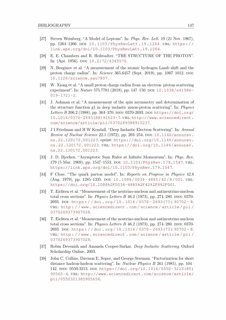
BIBLIOGRAPHY 147
[27] Steven Weinberg. “A Model of Leptons”. In: Phys. Rev. Lett. 19 (21 Nov. 1967),pp. 1264–1266. doi: 10.1103/PhysRevLett.19.1264. url: https://link.aps.org/doi/10.1103/PhysRevLett.19.1264.
[28] E. E. Chambers and R. Hofstadter. “THE STRUCTURE OF THE PROTON”.In: (Apr. 1956). doi: 10.2172/4345570.
[29] N. Bezginov et al. “A measurement of the atomic hydrogen Lamb shift and theproton charge radius”. In: Science 365.6457 (Sept. 2019), pp. 1007–1012. doi:10.1126/science.aau7807.
[30] W. Xiong et al. “A small proton charge radius from an electron–proton scatteringexperiment”. In: Nature 575.7781 (2019), pp. 147–150. doi: 10.1038/s41586-019-1721-2.
[31] J. Ashman et al. “A measurement of the spin asymmetry and determination ofthe structure function g1 in deep inelastic muon-proton scattering”. In: PhysicsLetters B 206.2 (1988), pp. 364–370. issn: 0370-2693. doi: https://doi.org/10.1016/0370-2693(88)91523-7. url: http://www.sciencedirect.com/science/article/pii/0370269388915237.
[32] J I Friedman and H W Kendall. “Deep Inelastic Electron Scattering”. In: AnnualReview of Nuclear Science 22.1 (1972), pp. 203–254. doi: 10.1146/annurev.ns.22.120172.001223. eprint: https://doi.org/10.1146/annurev.ns.22.120172.001223. url: https://doi.org/10.1146/annurev.ns.22.120172.001223.
[33] J. D. Bjorken. “Asymptotic Sum Rules at Infinite Momentum”. In: Phys. Rev.179 (5 Mar. 1969), pp. 1547–1553. doi: 10.1103/PhysRev.179.1547. url:https://link.aps.org/doi/10.1103/PhysRev.179.1547.
[34] F Close. “The quark parton model”. In: Reports on Progress in Physics 42.8(Aug. 1979), pp. 1285–1335. doi: 10.1088/0034-4885/42/8/001. url:https://doi.org/10.1088%2F0034-4885%2F42%2F8%2F001.
[35] T. Eichten et al. “Measurement of the neutrino-nucleon and antineutrino-nucleontotal cross sections”. In: Physics Letters B 46.2 (1973), pp. 274–280. issn: 0370-2693. doi: https://doi.org/10.1016/0370- 2693(73)90702- 8.url: http://www.sciencedirect.com/science/article/pii/0370269373907028.
[36] T. Eichten et al. “Measurement of the neutrino-nucleon and antineutrino-nucleontotal cross sections”. In: Physics Letters B 46.2 (1973), pp. 274–280. issn: 0370-2693. doi: https://doi.org/10.1016/0370- 2693(73)90702- 8.url: http://www.sciencedirect.com/science/article/pii/0370269373907028.
[37] Robin Devenish and Amanda Cooper-Sarkar. Deep Inelastic Scattering. OxfordScholarship Online, 2003.
[38] John C. Collins, Davison E. Soper, and George Sterman. “Factorization for shortdistance hadron-hadron scattering”. In: Nuclear Physics B 261 (1985), pp. 104–142. issn: 0550-3213. doi: https://doi.org/10.1016/0550-3213(85)90565-6. url: http://www.sciencedirect.com/science/article/pii/0550321385905656.
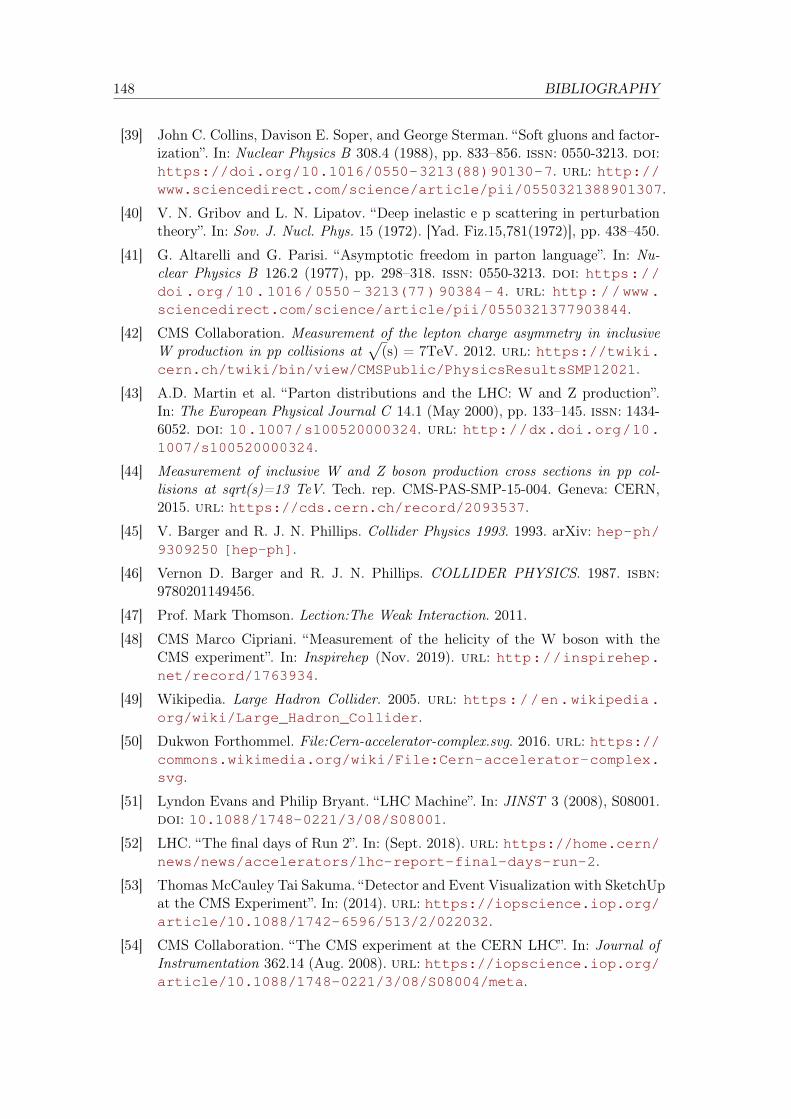
148 BIBLIOGRAPHY
[39] John C. Collins, Davison E. Soper, and George Sterman. “Soft gluons and factor-ization”. In: Nuclear Physics B 308.4 (1988), pp. 833–856. issn: 0550-3213. doi:https://doi.org/10.1016/0550-3213(88)90130-7. url: http://www.sciencedirect.com/science/article/pii/0550321388901307.
[40] V. N. Gribov and L. N. Lipatov. “Deep inelastic e p scattering in perturbationtheory”. In: Sov. J. Nucl. Phys. 15 (1972). [Yad. Fiz.15,781(1972)], pp. 438–450.
[41] G. Altarelli and G. Parisi. “Asymptotic freedom in parton language”. In: Nu-clear Physics B 126.2 (1977), pp. 298–318. issn: 0550-3213. doi: https://doi.org/10.1016/0550- 3213(77)90384- 4. url: http://www.sciencedirect.com/science/article/pii/0550321377903844.
[42] CMS Collaboration. Measurement of the lepton charge asymmetry in inclusiveW production in pp collisions at
√(s) = 7TeV. 2012. url: https://twiki.
cern.ch/twiki/bin/view/CMSPublic/PhysicsResultsSMP12021.
[43] A.D. Martin et al. “Parton distributions and the LHC: W and Z production”.In: The European Physical Journal C 14.1 (May 2000), pp. 133–145. issn: 1434-6052. doi: 10.1007/s100520000324. url: http://dx.doi.org/10.1007/s100520000324.
[44] Measurement of inclusive W and Z boson production cross sections in pp col-lisions at sqrt(s)=13 TeV. Tech. rep. CMS-PAS-SMP-15-004. Geneva: CERN,2015. url: https://cds.cern.ch/record/2093537.
[45] V. Barger and R. J. N. Phillips. Collider Physics 1993. 1993. arXiv: hep-ph/9309250 [hep-ph].
[46] Vernon D. Barger and R. J. N. Phillips. COLLIDER PHYSICS. 1987. isbn:9780201149456.
[47] Prof. Mark Thomson. Lection:The Weak Interaction. 2011.
[48] CMS Marco Cipriani. “Measurement of the helicity of the W boson with theCMS experiment”. In: Inspirehep (Nov. 2019). url: http://inspirehep.net/record/1763934.
[49] Wikipedia. Large Hadron Collider. 2005. url: https://en.wikipedia.org/wiki/Large_Hadron_Collider.
[50] Dukwon Forthommel. File:Cern-accelerator-complex.svg. 2016. url: https://commons.wikimedia.org/wiki/File:Cern-accelerator-complex.svg.
[51] Lyndon Evans and Philip Bryant. “LHC Machine”. In: JINST 3 (2008), S08001.doi: 10.1088/1748-0221/3/08/S08001.
[52] LHC. “The final days of Run 2”. In: (Sept. 2018). url: https://home.cern/news/news/accelerators/lhc-report-final-days-run-2.
[53] Thomas McCauley Tai Sakuma. “Detector and Event Visualization with SketchUpat the CMS Experiment”. In: (2014). url: https://iopscience.iop.org/article/10.1088/1742-6596/513/2/022032.
[54] CMS Collaboration. “The CMS experiment at the CERN LHC”. In: Journal ofInstrumentation 362.14 (Aug. 2008). url: https://iopscience.iop.org/article/10.1088/1748-0221/3/08/S08004/meta.
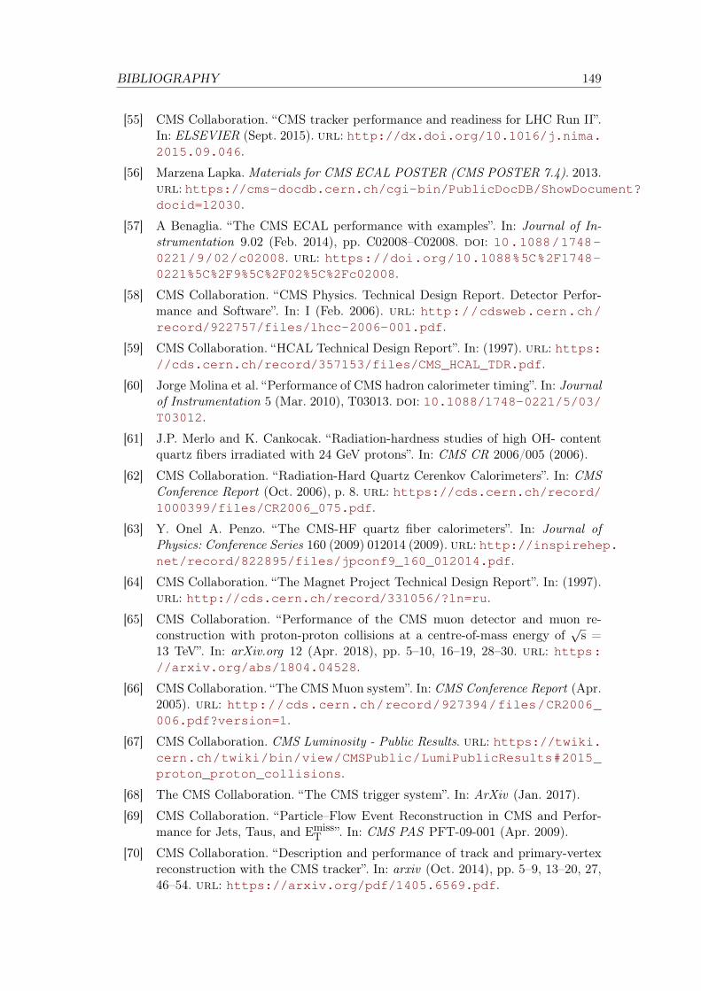
BIBLIOGRAPHY 149
[55] CMS Collaboration. “CMS tracker performance and readiness for LHC Run II”.In: ELSEVIER (Sept. 2015). url: http://dx.doi.org/10.1016/j.nima.2015.09.046.
[56] Marzena Lapka. Materials for CMS ECAL POSTER (CMS POSTER 7.4). 2013.url: https://cms-docdb.cern.ch/cgi-bin/PublicDocDB/ShowDocument?docid=12030.
[57] A Benaglia. “The CMS ECAL performance with examples”. In: Journal of In-strumentation 9.02 (Feb. 2014), pp. C02008–C02008. doi: 10.1088/1748-0221/9/02/c02008. url: https://doi.org/10.1088%5C%2F1748-0221%5C%2F9%5C%2F02%5C%2Fc02008.
[58] CMS Collaboration. “CMS Physics. Technical Design Report. Detector Perfor-mance and Software”. In: I (Feb. 2006). url: http://cdsweb.cern.ch/record/922757/files/lhcc-2006-001.pdf.
[59] CMS Collaboration. “HCAL Technical Design Report”. In: (1997). url: https://cds.cern.ch/record/357153/files/CMS_HCAL_TDR.pdf.
[60] Jorge Molina et al. “Performance of CMS hadron calorimeter timing”. In: Journalof Instrumentation 5 (Mar. 2010), T03013. doi: 10.1088/1748-0221/5/03/T03012.
[61] J.P. Merlo and K. Cankocak. “Radiation-hardness studies of high OH- contentquartz fibers irradiated with 24 GeV protons”. In: CMS CR 2006/005 (2006).
[62] CMS Collaboration. “Radiation-Hard Quartz Cerenkov Calorimeters”. In: CMSConference Report (Oct. 2006), p. 8. url: https://cds.cern.ch/record/1000399/files/CR2006_075.pdf.
[63] Y. Onel A. Penzo. “The CMS-HF quartz fiber calorimeters”. In: Journal ofPhysics: Conference Series 160 (2009) 012014 (2009). url: http://inspirehep.net/record/822895/files/jpconf9_160_012014.pdf.
[64] CMS Collaboration. “The Magnet Project Technical Design Report”. In: (1997).url: http://cds.cern.ch/record/331056/?ln=ru.
[65] CMS Collaboration. “Performance of the CMS muon detector and muon re-construction with proton-proton collisions at a centre-of-mass energy of
√s =
13 TeV”. In: arXiv.org 12 (Apr. 2018), pp. 5–10, 16–19, 28–30. url: https://arxiv.org/abs/1804.04528.
[66] CMS Collaboration. “The CMS Muon system”. In: CMS Conference Report (Apr.2005). url: http://cds.cern.ch/record/927394/files/CR2006_006.pdf?version=1.
[67] CMS Collaboration. CMS Luminosity - Public Results. url: https://twiki.cern.ch/twiki/bin/view/CMSPublic/LumiPublicResults#2015_proton_proton_collisions.
[68] The CMS Collaboration. “The CMS trigger system”. In: ArXiv (Jan. 2017).
[69] CMS Collaboration. “Particle–Flow Event Reconstruction in CMS and Perfor-mance for Jets, Taus, and Emiss
T ”. In: CMS PAS PFT-09-001 (Apr. 2009).
[70] CMS Collaboration. “Description and performance of track and primary-vertexreconstruction with the CMS tracker”. In: arxiv (Oct. 2014), pp. 5–9, 13–20, 27,46–54. url: https://arxiv.org/pdf/1405.6569.pdf.
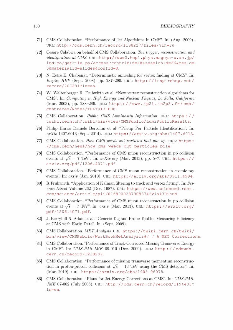
150 BIBLIOGRAPHY
[71] CMS Collaboration. “Performance of Jet Algorithms in CMS”. In: (Aug. 2009).url: http://cds.cern.ch/record/1198227/files/?ln=ru.
[72] Cesare Calabria on behalf of CMS Collaboration. Tau trigger, reconstruction andidentification at CMS. url: http://www2.hepl.phys.nagoya-u.ac.jp/indico/getFile.py/access?contribId=48&sessionId=26&resId=0&materialId=slides&confId=0.
[73] N. Estre E. Chabanat. “Deterministic annealing for vertex finding at CMS”. In:Inspire HEP (Sept. 2008), pp. 287–290. url: http://inspirehep.net/record/707291?ln=en.
[74] W. Waltenberger R. Fruhwirth et al. “New vertex reconstruction algorithms forCMS”. In: Computing in High Energy and Nuclear Physics, La Jolla, California(Mar. 2003), pp. 288–289. url: https://www.ip2i.in2p3.fr/cms/cmstraces/Notes/TULT013.PDF.
[75] CMS Collaboration. Public CMS Luminosity Information. url: https : / /twiki.cern.ch/twiki/bin/view/CMSPublic/LumiPublicResults.
[76] Philip Harris Daniele Bertolini et al. “Pileup Per Particle Identification”. In:arXiv 1407.6013 (Sept. 2014). url: https://arxiv.org/abs/1407.6013.
[77] CMS Collaboration. How CMS weeds out particles that pile up. url: https://cms.cern/news/how-cms-weeds-out-particles-pile.
[78] CMS Collaboration. “Performance of CMS muon reconstruction in pp collisionevents at
√s = 7 TeV”. In: arXiv.org (Mar. 2013), pp. 5–7. url: https://
arxiv.org/pdf/1206.4071.pdf.
[79] CMS Collaboration. “Performance of CMS muon reconstruction in cosmic-rayevents”. In: arxiv (Jan. 2010). url: https://arxiv.org/abs/0911.4994.
[80] R.Frühwirth. “Application of Kalman filtering to track and vertex fitting”. In: Sci-ence Direct Volume 262 (Dec. 1987). url: https://www.sciencedirect.com/science/article/pii/0168900287908874?via%3Dihub.
[81] CMS Collaboration. “Performance of CMS muon reconstruction in pp collisionevents at
√s = 7 TeV”. In: arxiv (Mar. 2013). url: https://arxiv.org/
pdf/1206.4071.pdf.
[82] J. Berryhill N. Adam et al. “Generic Tag and Probe Tool for Measuring Efficiencyat CMS with Early Data”. In: (Sept. 2009).
[83] CMS Collaboration.MET Analysis. url: https://twiki.cern.ch/twiki/bin/view/CMSPublic/WorkBookMetAnalysis#7_7_6_MET_Corrections.
[84] CMS Collaboration. “Performance of Track-Corrected Missing Transverse Energyin CMS”. In: CMS-PAS-JME 09-010 (Dec. 2009). url: http://cdsweb.cern.ch/record/1228297.
[85] CMS Collaboration. “Performance of missing transverse momentum reconstruc-tion in proton-proton collisions at
√s = 13 TeV using the CMS detector”. In:
(Mar. 2019). url: https://arxiv.org/abs/1903.06078.
[86] CMS Collaboration. “Plans for Jet Energy Corrections at CMS”. In: CMS-PAS-JME 07-002 (July 2008). url: http://cds.cern.ch/record/1194485?ln=en.
BIBLIOGRAPHY 151
[87] Olena Karacheban. “Luminosity Measurement at the Compact Muon SolenoidExperiment of the LHC”. PhD thesis. Cham: Brandenburg Tech. U., 2017. doi:10.3204/PUBDB-2017-11439,10.1007/978-3-319-93139-5.
[88] CMS Collaboration. “CMS luminosity measurement for the 2015 data-takingperiod”. In: CERN CDS (Feb. 2017).
[89] Andreas Kornmayer. The CMS Pixel Luminosity Telescope. Tech. rep. CMS-CR-2015-121. Geneva: CERN, June 2015. doi: 10.1016/j.nima.2015.09.104.url: https://cds.cern.ch/record/2039978.
[90] E. Castro A. Bell et al. “Fast Beam Conditions Monitor BCM1F for the CMSExperiment”. In: (Dec. 2009). url: https://arxiv.org/pdf/0911.2480.pdf.
[91] CMS Collaboration. THE BCM1F DOCUMENTATION. url: https://twiki.cern.ch/twiki/bin/viewauth/CMS/BcmDocumentation.
[92] CMS Collaboration. BCM1F performance plots 2015. url: https://twiki.cern.ch/twiki/bin/view/CMSPublic/BCM1FforEPS2015.
[93] Olena Karacheban. Luminosity Measurement at the Compact Muon SolenoidExperiment of the LHC. Springer International Publishing, 2018. url: https://link.springer.com/book/10.1007%2F978-3-319-93139-5#toc.
[94] S van der Meer. Calibration of the effective beam height in the ISR. Tech. rep.CERN-ISR-PO-68-31. ISR-PO-68-31. Geneva: CERN, 1968. url: http : / /cds.cern.ch/record/296752.
[95] CMS Collaboration. “Fast Beam Condition Monitor for CMS: performance andupgrade”. In: Nuclear Instruments and Methods in Physics Research Section Ac-celerators Spectrometers Detectors and Associated Equipment 765 (May 2014).doi: 10.1016/j.nima.2014.05.008.
[96] Moritz Guthoff. “Radiation Damage to the diamond-based Beam Condition Mon-itor of the CMS Detector at the LHC”. Doctoral thesis. Karlsruher Insituts furTechnologie, 2014.
[97] M. Ashfold, C.A Rego, and N. Everitt. “Thin Film Diamond by Chemical VaporDeposition Methods”. In: Chemical Society Reviews - CHEM SOC REV 23 (Feb.1994). doi: 10.1039/cs9942300021.
[98] Robert Visinka Carmen Simons. “Microstructuring of diamonds with laser lithog-raphy”. 2nd ADAMAS Workshop @GSI. 2013. url: http://www-adamas.gsi.de/ADAMAS02/talks/simons_ADAMAS02.pdf.
[99] Maria Hempel. “Development of a novel diamond based detector for machineinduced background and luminosity measurements”. Master thesis. BTU Cottbus- Senftenberg, 2017.
[100] D. Przyborowski. “Development of Front-End Electronics for Beam-ConditionMonitor at CMS.” Contribution at the 1st ADAMAS Workshop, GSI, Darm-stadt, 2012. url: http://www- adamas.gsi.de/ADAMAS01/talks/przyborowski.pdf.
[101] Bheesette Srinidhi. “Characterisation of the BCM1F Analog Opto Hybrids forthe CMS experiment. BCM1F-Fast Beam Condition Monitoring ”. In: (Aug.2013). url: https://cds.cern.ch/record/1596774.
152 BIBLIOGRAPHY
[102] Optical Links for CMS webpage. url: http://cms-tk-opto.web.cern.ch/cms-tk-opto/.
[103] Richard Grigonis. Versa Module Europa (VME) Bus. url: https://www.globalspec.com/reference/41898/203279/chapter- v- versa-module-europa-vme-bus-vpim.
[104] PICMG.MicroTCA Overview. url: https://www.picmg.org/openstandards/microtca/.
[105] http://www.onmyphd.com. Analog-Digital Converters. url: http://www.onmyphd.com/?p=analog.digital.converter.
[106] R S Schmidt et al. “Performance of the Fast Beam Conditions Monitor BCM1Fof CMS in the first running periods of LHC”. In: Journal of Instrumentation6.01 (Jan. 2011), pp. C01004–C01004. issn: 1748-0221. doi: 10.1088/1748-0221/6/01/c01004. url: http://dx.doi.org/10.1088/1748-0221/6/01/C01004.
[107] PDG Collaboration. “Review of Particle Physics”. In: Phys. Rev. D 86 (1 July2012), p. 010001. doi: 10.1103/PhysRevD.86.010001. url: https://link.aps.org/doi/10.1103/PhysRevD.86.010001.
[108] Martin Stegler. “Characterisation of non-irradiated and irradiated diamond sen-sors before and after application at LHC”. Master thesis. Brandenburg Universityof Technology, 2015.
[109] C. Canali et al. “Electrical properties and performances of natural diamond nu-clear radiation detectors”. In: Nuclear Instruments and Methods 160.1 (1979),pp. 73–77. issn: 0029-554X. doi: https://doi.org/10.1016/0029-554X(79)90167-8. url: http://www.sciencedirect.com/science/article/pii/0029554X79901678.
[110] Circuit Cellar. Pulse-Shaping Basics. url: https://circuitcellar.com/cc-blog/pulse-shaping-basics/.
[111] CAEN. DIP Description. 2004. url: https://edms.cern.ch/file/457113/2/DIPDescription.doc.
[112] Alexander Sinclair Howard. Diamond detectors for particle physics. Universityof London, 1998.
[113] W. Salter et al. CAEN N625. url: https://www.caen.it/products/n625/.
[114] William Badgett et al. “Web Based Monitoring in the CMS Experiment atCERN”. In: (2014). arXiv: 1409.1133 [physics.ins-det].
[115] CMS Collaboration. “Measurement of inclusive W and Z boson cross section inpp collisions at
√s = 13 TeV”. In: CMS AN - unpublished 2016/250 (2016).
url: http://cms.cern.ch/iCMS/jsp/db_notes/noteInfo.jsp?cmsnoteid=CMS%20AN-2016/250.
[116] C. Oleari. “The POWHEG BOX”. In: Nuclear Physics B - Proceedings Supple-ments 205-206 (Aug. 2010), pp. 36–41. issn: 0920-5632. doi: 10.1016/j.nuclphysbps.2010.08.016. url: http://dx.doi.org/10.1016/j.nuclphysbps.2010.08.016.
BIBLIOGRAPHY 153
[117] CMS Collaboration. “Measurement of the Rapidity and Transverse MomentumDistributions of Z Bosons in pp Collisions at sqrt(s)=7 TeV”. In: arXiv:1110.4973(22 Oct 2011). url: https://arxiv.org/abs/1110.4973.
[118] A. van Dyne A. Bodek et al. “Extracting Muon Momentum Scale Corrections”.In: ArXiv:1208.3710v3 (Sept. 2012), p. 6.
[119] CMS Collaboration. “Measurement of the charge ratio of atmospheric muonswith the CMS detector”. In: ArXiv (May 2010). url: https://arxiv.org/pdf/1005.5332.pdf.
[120] Roberto Pittau. Status of MadLoop/aMC@NLO. 2012. arXiv: 1202.5781 [hep-ph].
[121] Torbjörn Sjöstrand. PYTHIA 8 Status Report. 2008. arXiv: 0809.0303 [hep-ph].
[122] Richard D. Ball et al. “Parton distributions for the LHC run II”. In: Journalof High Energy Physics 2015.4 (Apr. 2015). issn: 1029-8479. doi: 10.1007/jhep04(2015)040. url: http://dx.doi.org/10.1007/JHEP04(2015)040.
[123] Richard D. Ball et al. “Parton distributions with LHC data”. In: Nuclear PhysicsB 867.2 (Feb. 2013), pp. 244–289. issn: 0550-3213. doi: 10.1016/j.nuclphysb.2012.10.003. url: http://dx.doi.org/10.1016/j.nuclphysb.2012.10.003.
[124] Wouter Verkerke and David Kirkby. The RooFit toolkit for data modeling. 2003.arXiv: physics/0306116 [physics.data-an].
[125] MINUIT homepage. url: https://seal.web.cern.ch/seal/snapshot/work-packages/mathlibs/minuit/.
[126] G. Breit and E. Wigner. “Capture of Slow Neutrons”. In: Phys. Rev. 49 (7 Apr.1936), pp. 106–109. doi: 10.1103/PhysRev.49.519. url: https://link.aps.org/doi/10.1103/PhysRev.49.519.
[127] T. Skwarnicki. A study of the radiative CASCADE transitions between the Upsilon-Prime and Upsilon resonances. 1986. DESY F31-86-02: PhDThesis (physics.data-an).
[128] CMS luminosity measurement for the 2015 data-taking period. Tech. rep. CMS-PAS-LUM-15-001. Geneva: CERN, 2017. url: http : / / cds . cern . ch /record/2138682.
[129] Radja Boughezal et al. “Color-singlet production at NNLO in MCFM”. In: TheEuropean Physical Journal C 77.1 (Dec. 2016). issn: 1434-6052. doi: 10.1140/epjc/s10052-016-4558-y. url: http://dx.doi.org/10.1140/epjc/s10052-016-4558-y.
[130] Sayipjamal Dulat et al. “New parton distribution functions from a global analysisof quantum chromodynamics”. In: Physical Review D 93.3 (Feb. 2016). issn:2470-0029. doi: 10.1103/physrevd.93.033006. url: http://dx.doi.org/10.1103/PhysRevD.93.033006.
[131] A. D. Martin et al. “Extended parameterisations for MSTW PDFs and theireffect on lepton charge asymmetry from W decays”. In: The European PhysicalJournal C 73.2 (Feb. 2013). issn: 1434-6052. doi: 10.1140/epjc/s10052-013-2318-9. url: http://dx.doi.org/10.1140/epjc/s10052-013-2318-9.
154 BIBLIOGRAPHY
[132] L. A. Harland-Lang et al. “Parton distributions in the LHC era: MMHT 2014PDFs”. In: The European Physical Journal C 75.5 (May 2015). issn: 1434-6052.doi: 10.1140/epjc/s10052-015-3397-6. url: http://dx.doi.org/10.1140/epjc/s10052-015-3397-6.
[133] E.L. Berger et al. In: Madison preprint University of Wisconsin.MAD/PH/400(1988).
[134] E. L. Berger et al. “Weak-boson production at Fermilab Tevatron energies”. In:Phys. Rev. D 40 (1 July 1989), pp. 83–91. doi: 10.1103/PhysRevD.40.83.url: https://link.aps.org/doi/10.1103/PhysRevD.40.83.
[135] J. L. Holzbauer. Measurements of W charge asymmetry. 2015. arXiv: 1510.01716 [hep-ex].
[136] T. Aaltonen et al. “Direct Measurement of theWProduction Charge Asymmetryin pp Collisions at
√s = 1.96 TeV”. In: Physical Review Letters 102.18 (May
2009). issn: 1079-7114. doi: 10.1103/physrevlett.102.181801. url:http://dx.doi.org/10.1103/PhysRevLett.102.181801.
[137] S. Chatrchyan et al. “Measurement of the muon charge asymmetry in inclusivepp → W +Xproduction at
√s = 7TeV and an improved determination of light
parton distribution functions”. In: Physical Review D 90.3 (Aug. 2014). issn:1550-2368. doi: 10.1103/physrevd.90.032004. url: http://dx.doi.org/10.1103/PhysRevD.90.032004.
[138] V. Khachatryan et al. “Measurement of the differential cross section and chargeasymmetry for inclusive pp→W±+X
√s = 8 TeV”. In: The European Physical
Journal C 76.8 (Aug. 2016). issn: 1434-6052. doi: 10.1140/epjc/s10052-016-4293-4. url: http://dx.doi.org/10.1140/epjc/s10052-016-4293-4.
[139] M. Botje. “QCDNUM: Fast QCD evolution and convolution”. In: ComputerPhysics Communications 182.2 (Feb. 2011), pp. 490–532. issn: 0010-4655. doi:10.1016/j.cpc.2010.10.020. url: http://dx.doi.org/10.1016/j.cpc.2010.10.020.
[140] Emil Avsar and Edmond Iancu. “CCFM evolution with unitarity corrections”.In: Nuclear Physics A 829.1-2 (Oct. 2009), pp. 31–75. issn: 0375-9474. doi:10.1016/j.nuclphysa.2009.08.001. url: http://dx.doi.org/10.1016/j.nuclphysa.2009.08.001.
[141] F. Hautmann, H. Jung, and S. Taheri Monfared. “The CCFM uPDF evolutionuPDFevolv Version 1.0.00”. In: The European Physical Journal C 74.10 (Oct.2014). issn: 1434-6052. doi: 10.1140/epjc/s10052-014-3082-1. url:http://dx.doi.org/10.1140/epjc/s10052-014-3082-1.
[142] John Campbell et al. MCFM - Monte Carlo for FeMtobarn processes. 2001. url:https://mcfm.fnal.gov/.
[143] Tancredi Carli et al. “A posteriori inclusion of parton density functions in NLOQCD final-state calculations at hadron colliders: the APPLGRID project”. In:The European Physical Journal C 66.3-4 (Feb. 2010), pp. 503–524. issn: 1434-6052. doi: 10.1140/epjc/s10052-010-1255-0. url: http://dx.doi.org/10.1140/epjc/s10052-010-1255-0.
BIBLIOGRAPHY 155
[144] Michal Czakon, David Heymes, and Alexander Mitov. fastNLO tables for NNLOtop-quark pair differential distributions. 2017. arXiv: 1704.08551 [hep-ph].
[145] CMS Collaboration. “Measurement of the lepton charge asymmetry in inclusiveW production in pp collisions at
√(s) = 7TeV”. In: ArXive (2011). url: https:
//arxiv.org/abs/1103.3470.
[146] S. Chatrchyan et al. “Measurement of associated W + charm production in ppcollisions at
√s=7 TeV”. In: Journal of High Energy Physics 2014.2 (Feb. 2014).
issn: 1029-8479. doi: 10.1007/jhep02(2014)013. url: http://dx.doi.org/10.1007/JHEP02(2014)013.
[147] A. M. Sirunyan et al. “Measurement of associated production of a W boson anda charm quark in proton–proton collisions at
√s = 13 TeV”. In: The European
Physical Journal C 79.3 (Mar. 2019). issn: 1434-6052. doi: 10.1140/epjc/s10052-019-6752-1. url: http://dx.doi.org/10.1140/epjc/s10052-019-6752-1.
[148] F. D. Aaron et al. “Measurement of the inclusive ep scattering cross section atlow Q 2 and x at HERA”. In: The European Physical Journal C 63.4 (Sept. 2009),pp. 625–678. issn: 1434-6052. doi: 10.1140/epjc/s10052-009-1128-6.url: http://dx.doi.org/10.1140/epjc/s10052-009-1128-6.
[149] H1 Collaboration. Inclusive Deep Inelastic Scattering at High Q2 with Longitudi-nally Polarised Lepton Beams at HERA. 2012. arXiv: 1206.7007 [hep-ex].
[150] CMS Collaboration. “Measurement of the differential cross section and chargeasymmetry for inclusive pp to W + X production at
√(s) = 8TeV”. In: ArXive
(2016). url: https://arxiv.org/abs/1603.01803.
[151] A. D. Martin et al. “Parton distributions for the LHC”. In: The European PhysicalJournal C 63.2 (July 2009), pp. 189–285. issn: 1434-6052. doi: 10.1140/epjc/s10052-009-1072-5. url: http://dx.doi.org/10.1140/epjc/s10052-009-1072-5.
[152] R. S. Thorne. “Effect of changes of variable flavor number scheme on partondistribution functions and predicted cross sections”. In: Physical Review D 86.7(Oct. 2012). issn: 1550-2368. doi: 10.1103/physrevd.86.074017. url:http://dx.doi.org/10.1103/PhysRevD.86.074017.
[153] M Botje. “Error estimates on parton density distributions”. In: Journal of PhysicsG: Nuclear and Particle Physics 28.5 (Apr. 2002), pp. 779–789. issn: 0954-3899.doi: 10.1088/0954-3899/28/5/305. url: http://dx.doi.org/10.1088/0954-3899/28/5/305.
[154] Mark Sutton et al. The APPLgrid project. 2010. url: https://applgrid.hepforge.org/index.htm.
[155] Zoltan Nagy. NLOJET++. 2011. url: http://www.desy.de/~znagy/Site/NLOJet++.html.
[156] Andy Buckley et al. Les Houches Approach. 2019. url: https://lhapdf.hepforge.org/.
[157] Andy Buckley et al. “LHAPDF6: parton density access in the LHC precisionera”. In: The European Physical Journal C 75.3 (Mar. 2015). issn: 1434-6052.doi: 10.1140/epjc/s10052-015-3318-8. url: http://dx.doi.org/10.1140/epjc/s10052-015-3318-8.
156 BIBLIOGRAPHY
[158] Particle Data Group. MONTE CARLO PARTICLE NUMBERING SCHEME.url: http://pdg.lbl.gov/2007/reviews/montecarlorpp.pdf.
[159] John M. Campbell, R. Keith Ellis, and Ciaran Williams. MCFM - Monte Carlofor FeMtobarn processes. 2020. url: https://mcfm.fnal.gov/.
[160] J. M. Campbell and R. K. Ellis. “Update on vector boson pair production athadron colliders”. In: Physical Review D 60.11 (Nov. 1999). issn: 1089-4918.doi: 10.1103/physrevd.60.113006. url: http://dx.doi.org/10.1103/PhysRevD.60.113006.
[161] John M. Campbell, R. Keith Ellis, and Ciaran Williams. “Vector boson pairproduction at the LHC”. In: Journal of High Energy Physics 2011.7 (July 2011).issn: 1029-8479. doi: 10.1007/jhep07(2011)018. url: http://dx.doi.org/10.1007/JHEP07(2011)018.
[162] Iain W. Stewart, Frank J. Tackmann, and Wouter J. Waalewijn. “NJettiness:An Inclusive Event Shape to Veto Jets”. In: Physical Review Letters 105.9 (Aug.2010). issn: 1079-7114. doi: 10.1103/physrevlett.105.092002. url:http://dx.doi.org/10.1103/PhysRevLett.105.092002.
[163] G.P. Salam and J. Rojo. “A Higher Order Perturbative Parton Evolution Toolkit(HOPPET)”. In: Computer Physics Communications 180.1 (Jan. 2009), pp. 120–156. issn: 0010-4655. doi: 10.1016/j.cpc.2008.08.010. url: http://dx.doi.org/10.1016/j.cpc.2008.08.010.
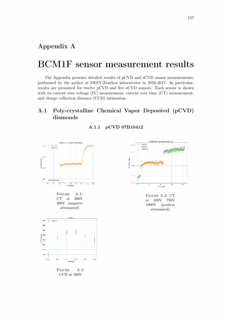
157
Appendix A
BCM1F sensor measurement resultsThe Appendix presents detailed results of pCVD and sCVD sensor measurements,
performed by the author at DESY-Zeuthen laboratories in 2016-2017. In particular,results are presented for twelve pCVD and five sCVD sensors. Each sensor is shownwith its current over voltage (IV) measurement, current over time (CT) measurement,and charge collection distance (CCD) estimation.
A.1 Poly-crystalline Chemical Vapor Deposited (pCVD)diamonds
A.1.1 pCVD 07B10412
Figure A.1:CT at 200V400V (negativeattenuated)
Figure A.2: CTat 500V 750V1000V (positive
attenuated)
Figure A.3:CCD at 500V
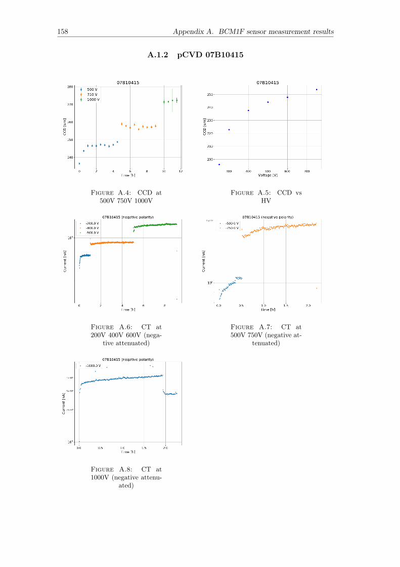
158 Appendix A. BCM1F sensor measurement results
A.1.2 pCVD 07B10415
Figure A.4: CCD at500V 750V 1000V
Figure A.5: CCD vsHV
Figure A.6: CT at200V 400V 600V (nega-
tive attenuated)
Figure A.7: CT at500V 750V (negative at-
tenuated)
Figure A.8: CT at1000V (negative attenu-
ated)
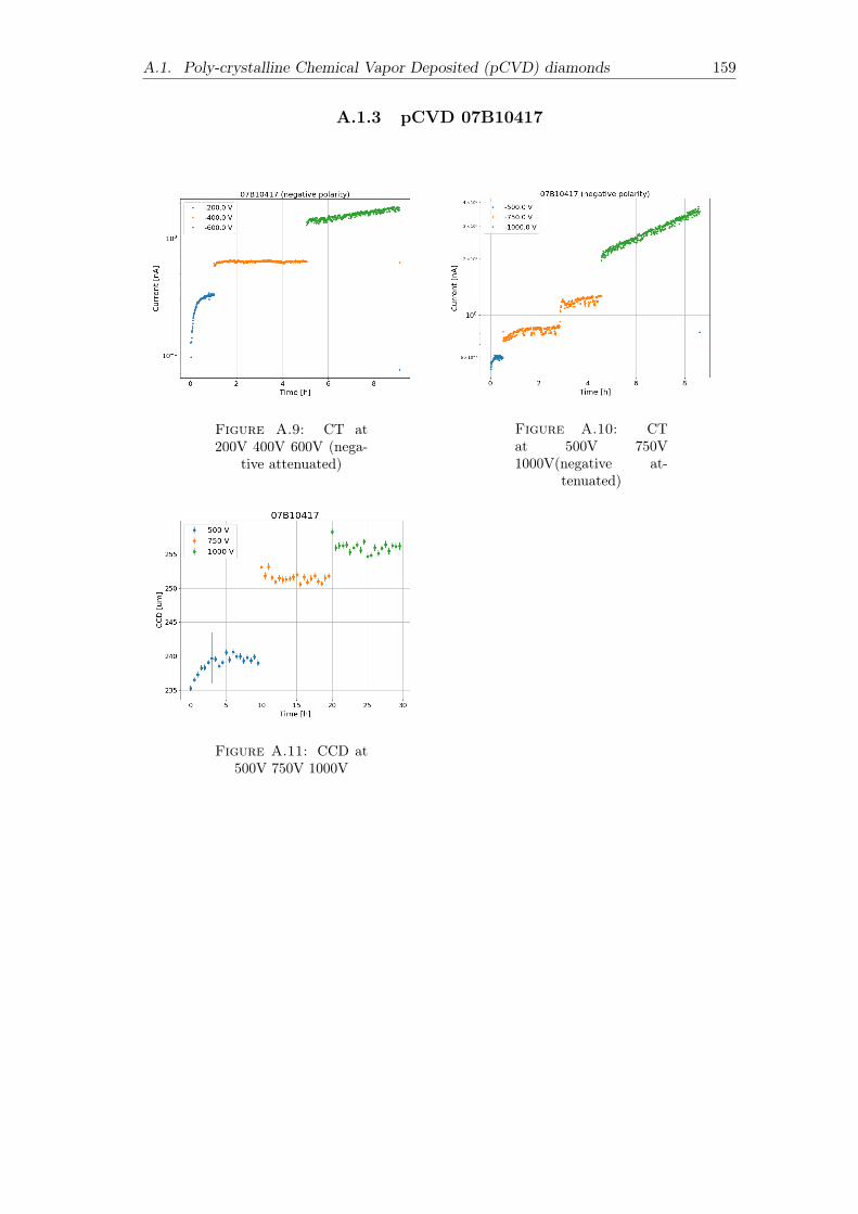
A.1. Poly-crystalline Chemical Vapor Deposited (pCVD) diamonds 159
A.1.3 pCVD 07B10417
Figure A.9: CT at200V 400V 600V (nega-
tive attenuated)
Figure A.10: CTat 500V 750V1000V(negative at-
tenuated)
Figure A.11: CCD at500V 750V 1000V
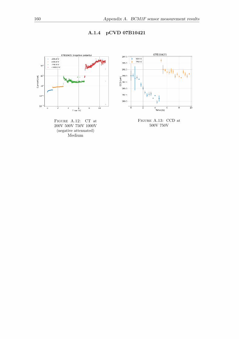
160 Appendix A. BCM1F sensor measurement results
A.1.4 pCVD 07B10421
Figure A.12: CT at200V 500V 750V 1000V(negative attenuated)
Figure A.13: CCD at500V 750V
Medium
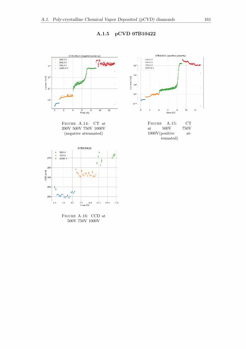
A.1. Poly-crystalline Chemical Vapor Deposited (pCVD) diamonds 161
A.1.5 pCVD 07B10422
Figure A.14: CT at200V 500V 750V 1000V(negative attenuated)
Figure A.15: CTat 500V 750V1000V(positive at-
tenuated)
Figure A.16: CCD at500V 750V 1000V
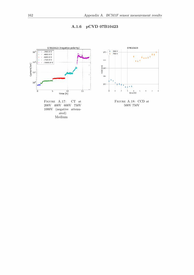
162 Appendix A. BCM1F sensor measurement results
A.1.6 pCVD 07B10423
Figure A.17: CT at200V 400V 600V 750V1000V (negative attenu-
ated)
Figure A.18: CCD at500V 750V
Medium
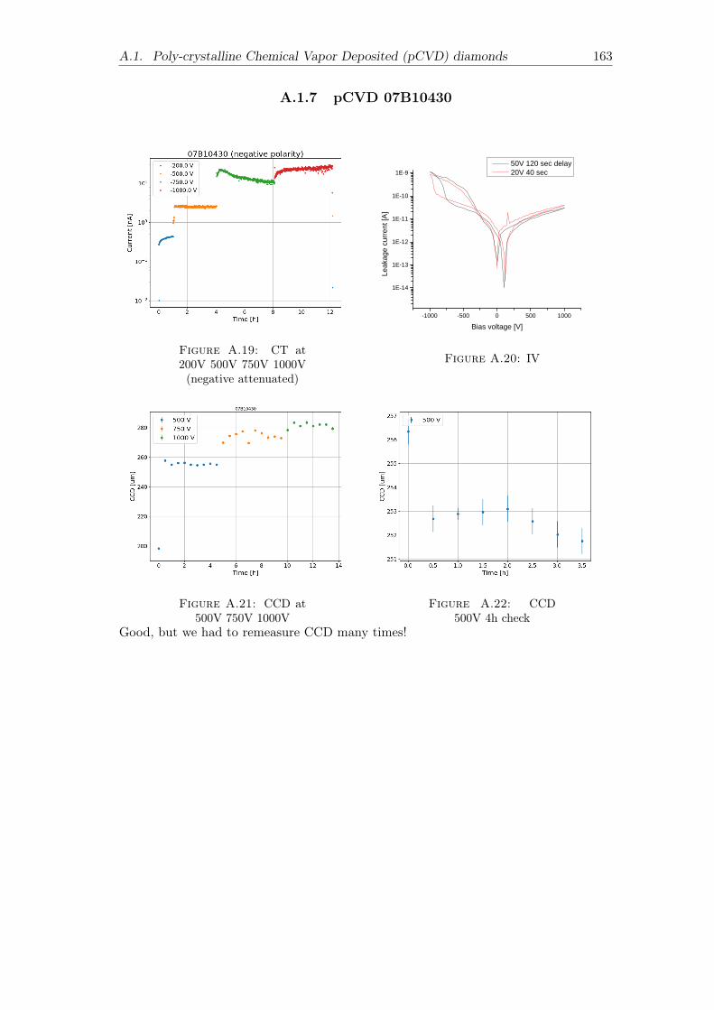
A.1. Poly-crystalline Chemical Vapor Deposited (pCVD) diamonds 163
A.1.7 pCVD 07B10430
Figure A.19: CT at200V 500V 750V 1000V(negative attenuated)
- 1 0 0 0 - 5 0 0 0 5 0 0 1 0 0 0
1 E - 1 4
1 E - 1 3
1 E - 1 2
1 E - 1 1
1 E - 1 0
1 E - 9
Leak
age c
urren
t [A]
B i a s v o l t a g e [ V ]
5 0 V 1 2 0 s e c d e l a y 2 0 V 4 0 s e c
Figure A.20: IV
Figure A.21: CCD at500V 750V 1000V
Figure A.22: CCD500V 4h check
Good, but we had to remeasure CCD many times!
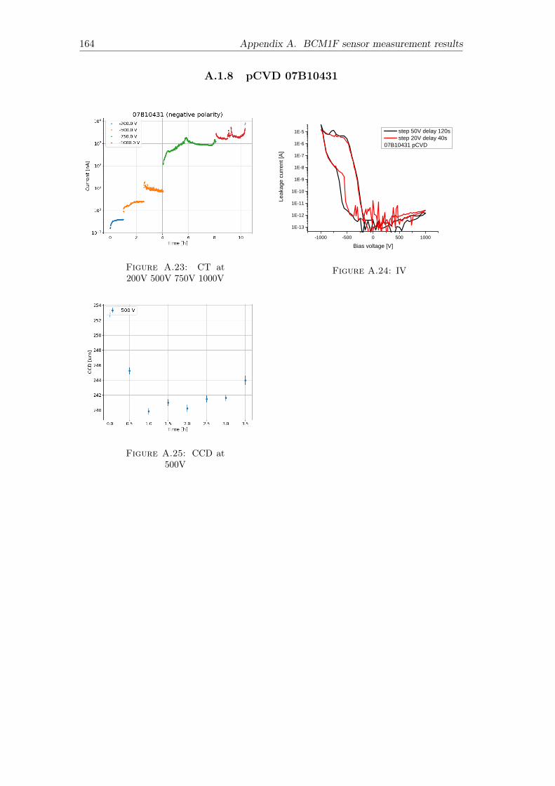
164 Appendix A. BCM1F sensor measurement results
A.1.8 pCVD 07B10431
Figure A.23: CT at200V 500V 750V 1000V
- 1 0 0 0 - 5 0 0 0 5 0 0 1 0 0 01 E - 1 31 E - 1 21 E - 1 11 E - 1 0
1 E - 91 E - 81 E - 71 E - 61 E - 5
Leak
age c
urren
t [A]
B i a s v o l t a g e [ V ]
s t e p 5 0 V d e l a y 1 2 0 s s t e p 2 0 V d e l a y 4 0 s
0 7 B 1 0 4 3 1 p C V D
Figure A.24: IV
Figure A.25: CCD at500V
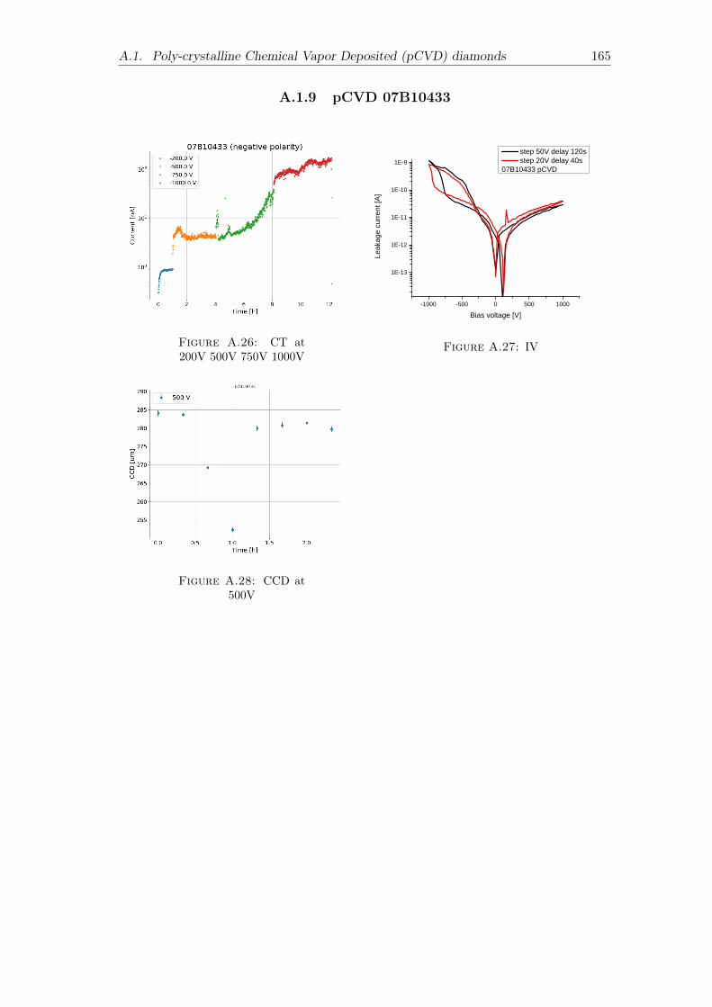
A.1. Poly-crystalline Chemical Vapor Deposited (pCVD) diamonds 165
A.1.9 pCVD 07B10433
Figure A.26: CT at200V 500V 750V 1000V
- 1 0 0 0 - 5 0 0 0 5 0 0 1 0 0 0
1 E - 1 3
1 E - 1 2
1 E - 1 1
1 E - 1 0
1 E - 9
Leak
age c
urren
t [A]
B i a s v o l t a g e [ V ]
s t e p 5 0 V d e l a y 1 2 0 s s t e p 2 0 V d e l a y 4 0 s
0 7 B 1 0 4 3 3 p C V D
Figure A.27: IV
Figure A.28: CCD at500V
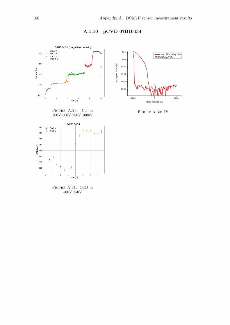
166 Appendix A. BCM1F sensor measurement results
A.1.10 pCVD 07B10434
Figure A.29: CT at200V 500V 750V 1000V
- 1 0 0 0 0 1 0 0 0
1 E - 1 3
1 E - 1 2
1 E - 1 1
1 E - 1 0
1 E - 9
1 E - 8
Leak
age c
urren
t [A]
B i a s v o l t a g e [ V ]
s t e p 3 0 V d e l a y 4 0 s0 7 B 1 0 4 3 4 p C V D
Figure A.30: IV
Figure A.31: CCD at500V 750V
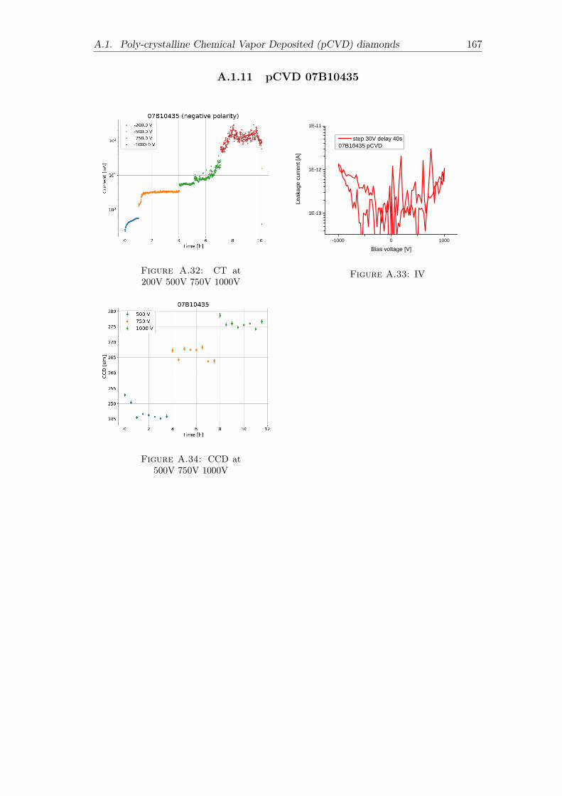
A.1. Poly-crystalline Chemical Vapor Deposited (pCVD) diamonds 167
A.1.11 pCVD 07B10435
Figure A.32: CT at200V 500V 750V 1000V
- 1 0 0 0 0 1 0 0 0
1 E - 1 3
1 E - 1 2
1 E - 1 1
Leak
age c
urren
t [A]
B i a s v o l t a g e [ V ]
s t e p 3 0 V d e l a y 4 0 s0 7 B 1 0 4 3 5 p C V D
Figure A.33: IV
Figure A.34: CCD at500V 750V 1000V
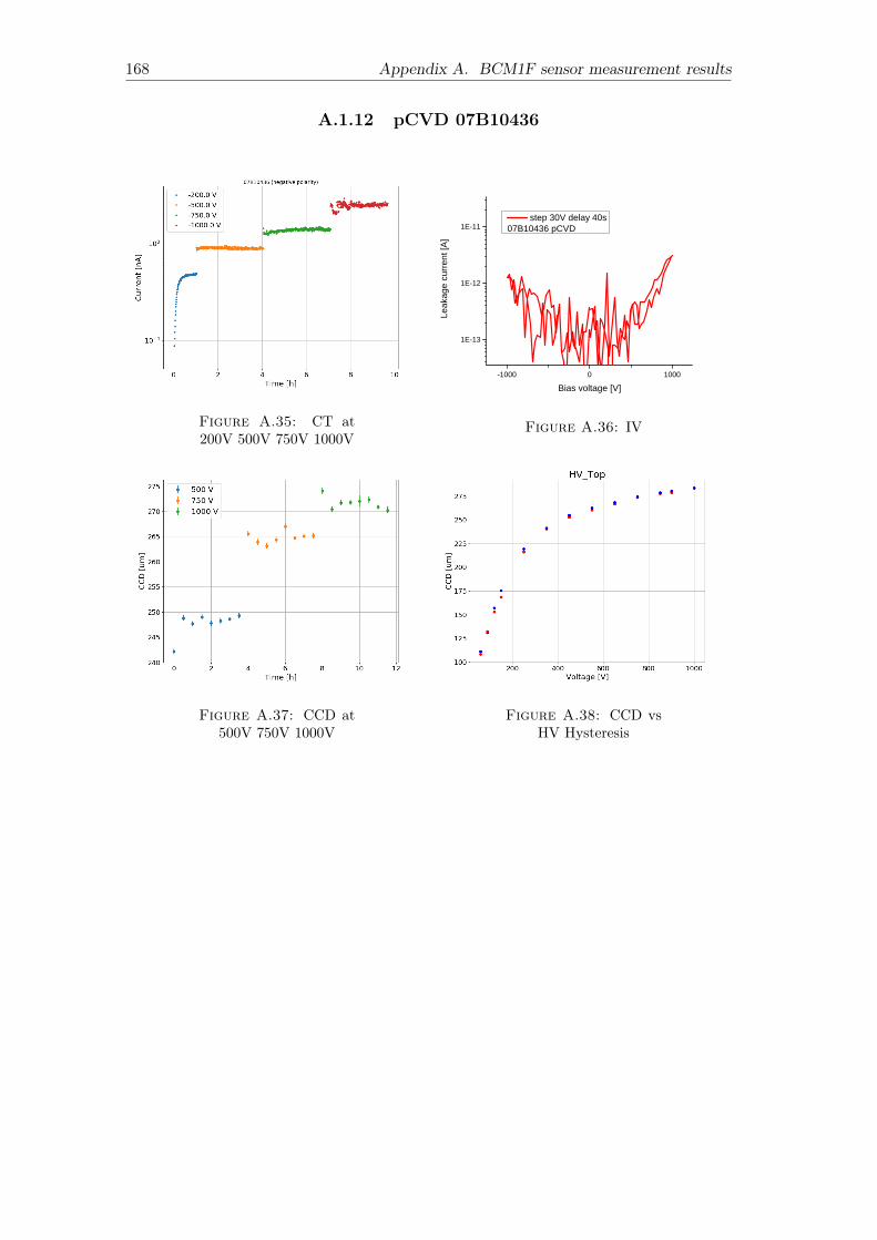
168 Appendix A. BCM1F sensor measurement results
A.1.12 pCVD 07B10436
Figure A.35: CT at200V 500V 750V 1000V
- 1 0 0 0 0 1 0 0 0
1 E - 1 3
1 E - 1 2
1 E - 1 1
Leak
age c
urren
t [A]
B i a s v o l t a g e [ V ]
s t e p 3 0 V d e l a y 4 0 s0 7 B 1 0 4 3 6 p C V D
Figure A.36: IV
Figure A.37: CCD at500V 750V 1000V
Figure A.38: CCD vsHV Hysteresis
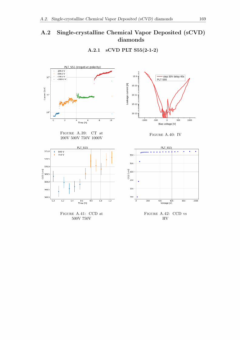
A.2. Single-crystalline Chemical Vapor Deposited (sCVD) diamonds 169
A.2 Single-crystalline Chemical Vapor Deposited (sCVD)diamonds
A.2.1 sCVD PLT S55(2-1-2)
Figure A.39: CT at200V 500V 750V 1000V
- 1 0 0 0 - 5 0 0 0 5 0 0 1 0 0 0
1 E - 1 3
1 E - 1 2
1 E - 1 1
1 E - 1 0
1 E - 9
Leak
age c
urren
t [A]
B i a s v o l t a g e [ V ]
s t e p 3 0 V d e l a y 4 0 sP L T S 5 5
Figure A.40: IV
Figure A.41: CCD at500V 750V
Figure A.42: CCD vsHV
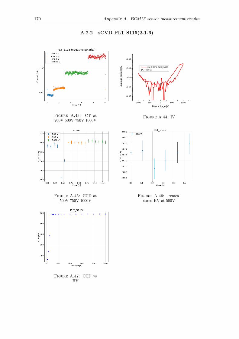
170 Appendix A. BCM1F sensor measurement results
A.2.2 sCVD PLT S115(2-1-6)
Figure A.43: CT at200V 500V 750V 1000V
- 1 0 0 0 - 5 0 0 0 5 0 0 1 0 0 0
1 E - 1 4
1 E - 1 3
1 E - 1 2
1 E - 1 1
1 E - 1 0
Leak
age c
urren
t [A]
B i a s v o l t a g e [ V ]
s t e p 3 0 V d e l a y 4 0 sP L T S 1 1 5
Figure A.44: IV
Figure A.45: CCD at500V 750V 1000V
Figure A.46: remea-sured HV at 500V
Figure A.47: CCD vsHV
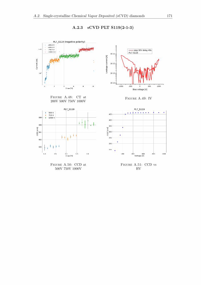
A.2. Single-crystalline Chemical Vapor Deposited (sCVD) diamonds 171
A.2.3 sCVD PLT S119(2-1-3)
Figure A.48: CT at200V 500V 750V 1000V
- 1 0 0 0 - 5 0 0 0 5 0 0 1 0 0 01 E - 1 4
1 E - 1 3
1 E - 1 2
1 E - 1 1
Leak
age c
urren
t [A]
B i a s v o l t a g e [ V ]
s t e p 3 0 V d e l a y 4 0 sP L T S 1 1 9
Figure A.49: IV
Figure A.50: CCD at500V 750V 1000V
Figure A.51: CCD vsHV
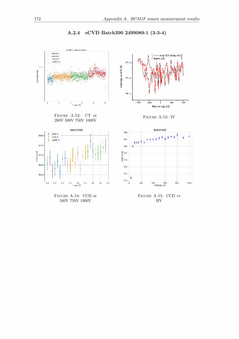
172 Appendix A. BCM1F sensor measurement results
A.2.4 sCVD Batch390 2499089-1 (3-3-4)
Figure A.52: CT at200V 500V 750V 1000V
Figure A.53: IV
Figure A.54: CCD at500V 750V 1000V
Figure A.55: CCD vsHV
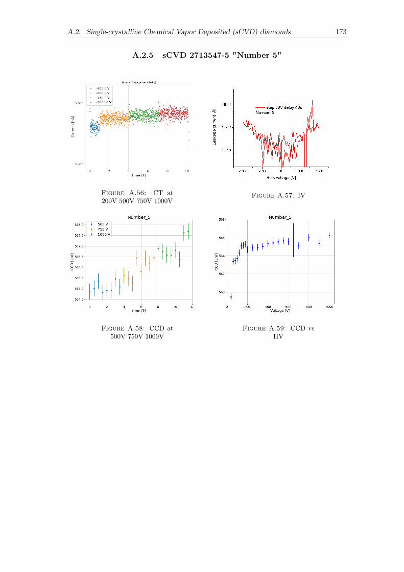
A.2. Single-crystalline Chemical Vapor Deposited (sCVD) diamonds 173
A.2.5 sCVD 2713547-5 "Number 5"
Figure A.56: CT at200V 500V 750V 1000V
Figure A.57: IV
Figure A.58: CCD at500V 750V 1000V
Figure A.59: CCD vsHV

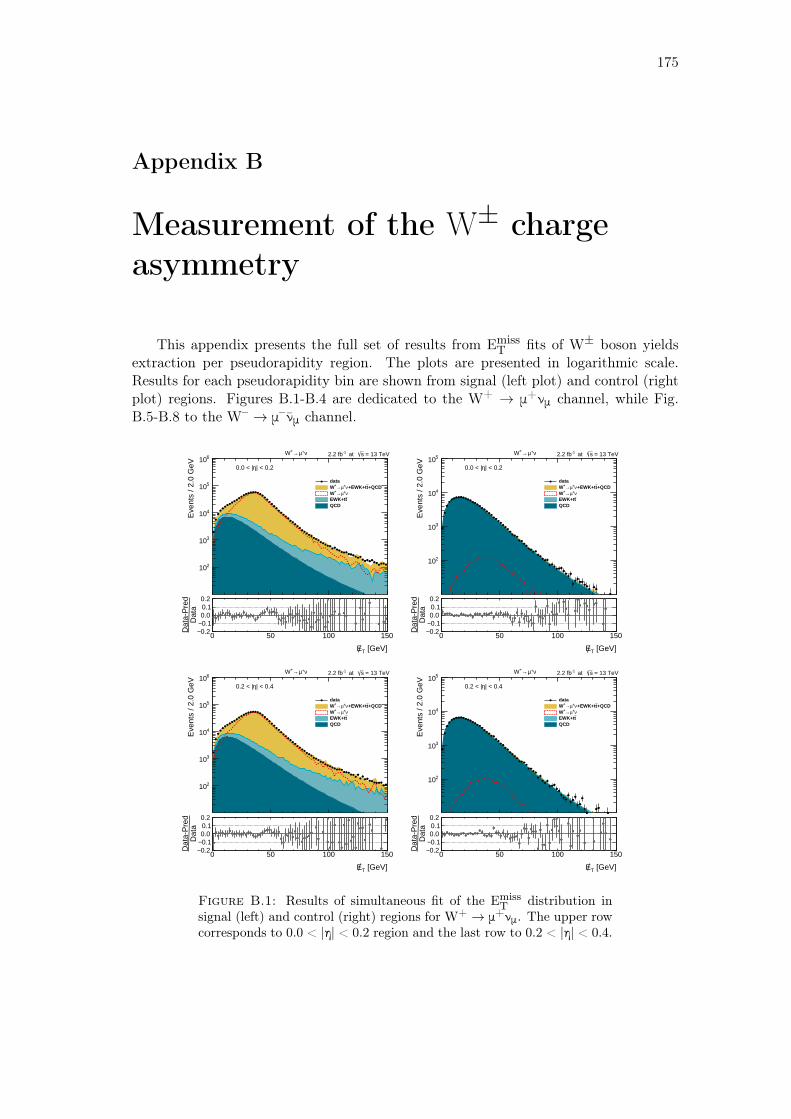
175
Appendix B
Measurement of the W± chargeasymmetry
This appendix presents the full set of results from EmissT fits of W± boson yields
extraction per pseudorapidity region. The plots are presented in logarithmic scale.Results for each pseudorapidity bin are shown from signal (left plot) and control (rightplot) regions. Figures B.1-B.4 are dedicated to the W+ → μ+νμ channel, while Fig.B.5-B.8 to the W– → μ–νμ channel.
Eve
nts
/ 2.0
GeV
210
310
410
510
610
data+QCDt+EWK+tν+µ→+W
ν+µ→+WtEWK+t
QCD
| < 0.2η0.0 < |
ν+µ→+W = 13 TeVs at -12.2 fb
[GeV]TE
0 50 100 150
Dat
aD
ata-
Pre
d
0.2−0.1−0.00.10.2
Eve
nts
/ 2.0
GeV
210
310
410
510
data+QCDt+EWK+tν+µ→+W
ν+µ→+WtEWK+t
QCD
| < 0.2η0.0 < |
ν+µ→+W = 13 TeVs at -12.2 fb
[GeV]TE
0 50 100 150
Dat
aD
ata-
Pre
d
0.2−0.1−0.00.10.2
Eve
nts
/ 2.0
GeV
210
310
410
510
610
data+QCDt+EWK+tν+µ→+W
ν+µ→+WtEWK+t
QCD
| < 0.4η0.2 < |
ν+µ→+W = 13 TeVs at -12.2 fb
[GeV]TE
0 50 100 150
Dat
aD
ata-
Pre
d
0.2−0.1−0.00.10.2
Eve
nts
/ 2.0
GeV
210
310
410
510
data+QCDt+EWK+tν+µ→+W
ν+µ→+WtEWK+t
QCD
| < 0.4η0.2 < |
ν+µ→+W = 13 TeVs at -12.2 fb
[GeV]TE
0 50 100 150
Dat
aD
ata-
Pre
d
0.2−0.1−0.00.10.2
Figure B.1: Results of simultaneous fit of the EmissT distribution in
signal (left) and control (right) regions for W+ → μ+νμ. The upper rowcorresponds to 0.0 < |η| < 0.2 region and the last row to 0.2 < |η| < 0.4.
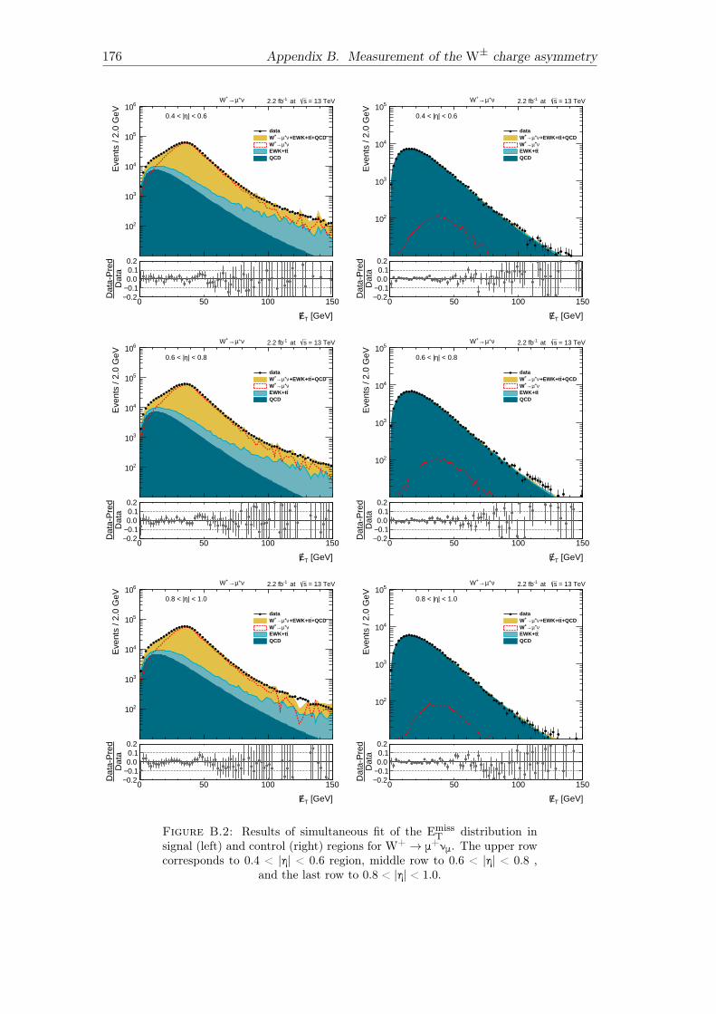
176 Appendix B. Measurement of the W± charge asymmetry
Eve
nts
/ 2.0
GeV
210
310
410
510
610
data+QCDt+EWK+tν+µ→+W
ν+µ→+WtEWK+t
QCD
| < 0.6η0.4 < |
ν+µ→+W = 13 TeVs at -12.2 fb
[GeV]TE
0 50 100 150
Dat
aD
ata-
Pre
d
0.2−0.1−0.00.10.2
Eve
nts
/ 2.0
GeV
210
310
410
510
data+QCDt+EWK+tν+µ→+W
ν+µ→+WtEWK+t
QCD
| < 0.6η0.4 < |
ν+µ→+W = 13 TeVs at -12.2 fb
[GeV]TE
0 50 100 150
Dat
aD
ata-
Pre
d
0.2−0.1−0.00.10.2
Eve
nts
/ 2.0
GeV
210
310
410
510
610
data+QCDt+EWK+tν+µ→+W
ν+µ→+WtEWK+t
QCD
| < 0.8η0.6 < |
ν+µ→+W = 13 TeVs at -12.2 fb
[GeV]TE
0 50 100 150
Dat
aD
ata-
Pre
d
0.2−0.1−0.00.10.2
Eve
nts
/ 2.0
GeV
210
310
410
510
data+QCDt+EWK+tν+µ→+W
ν+µ→+WtEWK+t
QCD
| < 0.8η0.6 < |
ν+µ→+W = 13 TeVs at -12.2 fb
[GeV]TE
0 50 100 150
Dat
aD
ata-
Pre
d
0.2−0.1−0.00.10.2
Eve
nts
/ 2.0
GeV
210
310
410
510
610
data+QCDt+EWK+tν+µ→+W
ν+µ→+WtEWK+t
QCD
| < 1.0η0.8 < |
ν+µ→+W = 13 TeVs at -12.2 fb
[GeV]TE
0 50 100 150
Dat
aD
ata-
Pre
d
0.2−0.1−0.00.10.2
Eve
nts
/ 2.0
GeV
210
310
410
510
data+QCDt+EWK+tν+µ→+W
ν+µ→+WtEWK+t
QCD
| < 1.0η0.8 < |
ν+µ→+W = 13 TeVs at -12.2 fb
[GeV]TE
0 50 100 150
Dat
aD
ata-
Pre
d
0.2−0.1−0.00.10.2
Figure B.2: Results of simultaneous fit of the EmissT distribution in
signal (left) and control (right) regions for W+ → μ+νμ. The upper rowcorresponds to 0.4 < |η| < 0.6 region, middle row to 0.6 < |η| < 0.8 ,
and the last row to 0.8 < |η| < 1.0.
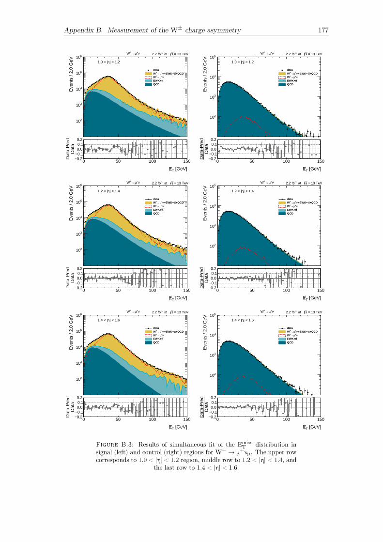
Appendix B. Measurement of the W± charge asymmetry 177
Eve
nts
/ 2.0
GeV
210
310
410
510
610
data+QCDt+EWK+tν+µ→+W
ν+µ→+WtEWK+t
QCD
| < 1.2η1.0 < |
ν+µ→+W = 13 TeVs at -12.2 fb
[GeV]TE
0 50 100 150
Dat
aD
ata-
Pre
d
0.2−0.1−0.00.10.2
Eve
nts
/ 2.0
GeV
210
310
410
510
data+QCDt+EWK+tν+µ→+W
ν+µ→+WtEWK+t
QCD
| < 1.2η1.0 < |
ν+µ→+W = 13 TeVs at -12.2 fb
[GeV]TE
0 50 100 150
Dat
aD
ata-
Pre
d
0.2−0.1−0.00.10.2
Eve
nts
/ 2.0
GeV
210
310
410
510
610
data+QCDt+EWK+tν+µ→+W
ν+µ→+WtEWK+t
QCD
| < 1.4η1.2 < |
ν+µ→+W = 13 TeVs at -12.2 fb
[GeV]TE
0 50 100 150
Dat
aD
ata-
Pre
d
0.2−0.1−0.00.10.2
Eve
nts
/ 2.0
GeV
210
310
410
510
data+QCDt+EWK+tν+µ→+W
ν+µ→+WtEWK+t
QCD
| < 1.4η1.2 < |
ν+µ→+W = 13 TeVs at -12.2 fb
[GeV]TE
0 50 100 150
Dat
aD
ata-
Pre
d
0.2−0.1−0.00.10.2
Eve
nts
/ 2.0
GeV
210
310
410
510
610
data+QCDt+EWK+tν+µ→+W
ν+µ→+WtEWK+t
QCD
| < 1.6η1.4 < |
ν+µ→+W = 13 TeVs at -12.2 fb
[GeV]TE
0 50 100 150
Dat
aD
ata-
Pre
d
0.2−0.1−0.00.10.2
Eve
nts
/ 2.0
GeV
210
310
410
510
data+QCDt+EWK+tν+µ→+W
ν+µ→+WtEWK+t
QCD
| < 1.6η1.4 < |
ν+µ→+W = 13 TeVs at -12.2 fb
[GeV]TE
0 50 100 150
Dat
aD
ata-
Pre
d
0.2−0.1−0.00.10.2
Figure B.3: Results of simultaneous fit of the EmissT distribution in
signal (left) and control (right) regions for W+ → μ+νμ. The upper rowcorresponds to 1.0 < |η| < 1.2 region, middle row to 1.2 < |η| < 1.4, and
the last row to 1.4 < |η| < 1.6.
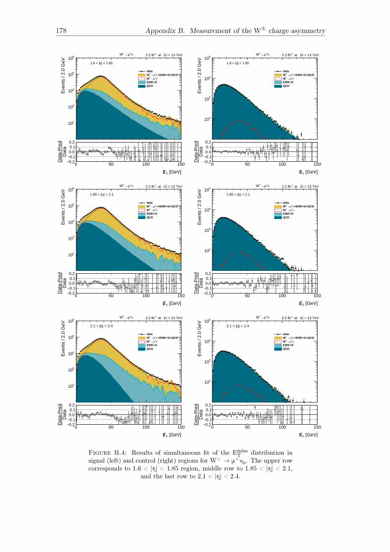
178 Appendix B. Measurement of the W± charge asymmetry
Eve
nts
/ 2.0
GeV
210
310
410
510
610
data+QCDt+EWK+tν+µ→+W
ν+µ→+WtEWK+t
QCD
| < 1.85η1.6 < |
ν+µ→+W = 13 TeVs at -12.2 fb
[GeV]TE
0 50 100 150
Dat
aD
ata-
Pre
d
0.2−0.1−0.00.10.2
Eve
nts
/ 2.0
GeV
210
310
410
510
data+QCDt+EWK+tν+µ→+W
ν+µ→+WtEWK+t
QCD
| < 1.85η1.6 < |
ν+µ→+W = 13 TeVs at -12.2 fb
[GeV]TE
0 50 100 150
Dat
aD
ata-
Pre
d
0.2−0.1−0.00.10.2
Eve
nts
/ 2.0
GeV
210
310
410
510
610
data+QCDt+EWK+tν+µ→+W
ν+µ→+WtEWK+t
QCD
| < 2.1η1.85 < |
ν+µ→+W = 13 TeVs at -12.2 fb
[GeV]TE
0 50 100 150
Dat
aD
ata-
Pre
d
0.2−0.1−0.00.10.2
Eve
nts
/ 2.0
GeV
210
310
410
510
data+QCDt+EWK+tν+µ→+W
ν+µ→+WtEWK+t
QCD
| < 2.1η1.85 < |
ν+µ→+W = 13 TeVs at -12.2 fb
[GeV]TE
0 50 100 150
Dat
aD
ata-
Pre
d
0.2−0.1−0.00.10.2
Eve
nts
/ 2.0
GeV
210
310
410
510
610
data+QCDt+EWK+tν+µ→+W
ν+µ→+WtEWK+t
QCD
| < 2.4η2.1 < |
ν+µ→+W = 13 TeVs at -12.2 fb
[GeV]TE
0 50 100 150
Dat
aD
ata-
Pre
d
0.2−0.1−0.00.10.2
Eve
nts
/ 2.0
GeV
210
310
410
510
data+QCDt+EWK+tν+µ→+W
ν+µ→+WtEWK+t
QCD
| < 2.4η2.1 < |
ν+µ→+W = 13 TeVs at -12.2 fb
[GeV]TE
0 50 100 150
Dat
aD
ata-
Pre
d
0.2−0.1−0.00.10.2
Figure B.4: Results of simultaneous fit of the EmissT distribution in
signal (left) and control (right) regions for W+ → μ+νμ. The upper rowcorresponds to 1.6 < |η| < 1.85 region, middle row to 1.85 < |η| < 2.1,
and the last row to 2.1 < |η| < 2.4.
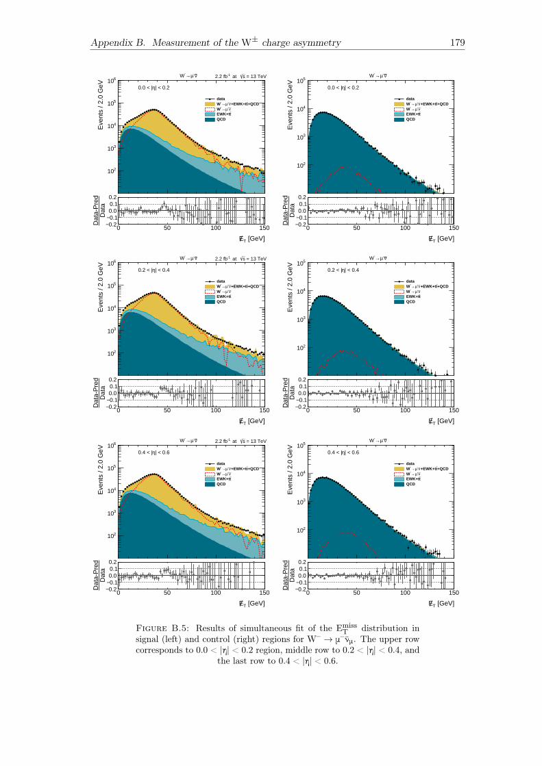
Appendix B. Measurement of the W± charge asymmetry 179
Eve
nts
/ 2.0
GeV
210
310
410
510
610
data+QCDt+EWK+tν-µ→-W
ν-µ→-WtEWK+t
QCD
| < 0.2η0.0 < |
ν-µ→-W = 13 TeVs at -12.2 fb
[GeV]TE
0 50 100 150
Dat
aD
ata-
Pre
d
0.2−0.1−0.00.10.2
Eve
nts
/ 2.0
GeV
210
310
410
510
data+QCDt+EWK+tν-µ→-W
ν-µ→-WtEWK+t
QCD
ν-µ→-W
| < 0.2η0.0 < |
[GeV]TE
0 50 100 150
Dat
aD
ata-
Pre
d
0.2−0.1−0.00.10.2
Eve
nts
/ 2.0
GeV
210
310
410
510
610
data+QCDt+EWK+tν-µ→-W
ν-µ→-WtEWK+t
QCD
| < 0.4η0.2 < |
ν-µ→-W = 13 TeVs at -12.2 fb
[GeV]TE
0 50 100 150
Dat
aD
ata-
Pre
d
0.2−0.1−0.00.10.2
Eve
nts
/ 2.0
GeV
210
310
410
510
data+QCDt+EWK+tν-µ→-W
ν-µ→-WtEWK+t
QCD
ν-µ→-W
| < 0.4η0.2 < |
[GeV]TE
0 50 100 150
Dat
aD
ata-
Pre
d
0.2−0.1−0.00.10.2
Eve
nts
/ 2.0
GeV
210
310
410
510
610
data+QCDt+EWK+tν-µ→-W
ν-µ→-WtEWK+t
QCD
| < 0.6η0.4 < |
ν-µ→-W = 13 TeVs at -12.2 fb
[GeV]TE
0 50 100 150
Dat
aD
ata-
Pre
d
0.2−0.1−0.00.10.2
Eve
nts
/ 2.0
GeV
210
310
410
510
data+QCDt+EWK+tν-µ→-W
ν-µ→-WtEWK+t
QCD
ν-µ→-W
| < 0.6η0.4 < |
[GeV]TE
0 50 100 150
Dat
aD
ata-
Pre
d
0.2−0.1−0.00.10.2
Figure B.5: Results of simultaneous fit of the EmissT distribution in
signal (left) and control (right) regions for W– → μ– νμ. The upper rowcorresponds to 0.0 < |η| < 0.2 region, middle row to 0.2 < |η| < 0.4, and
the last row to 0.4 < |η| < 0.6.
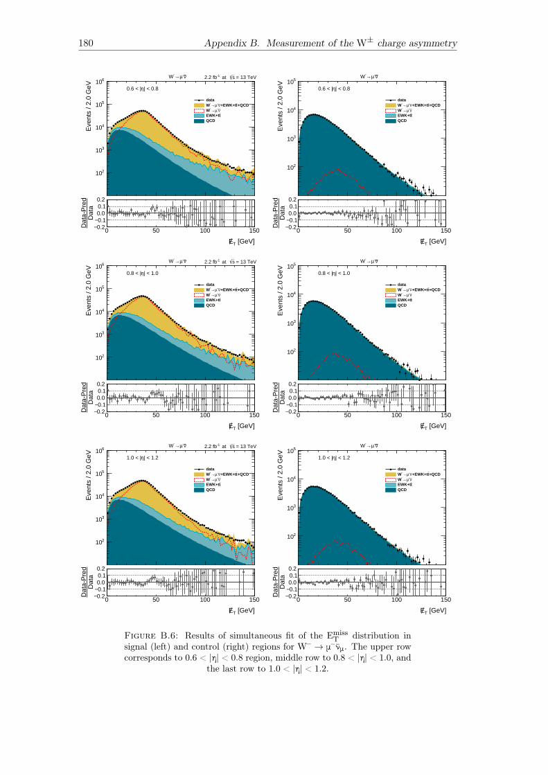
180 Appendix B. Measurement of the W± charge asymmetry
Eve
nts
/ 2.0
GeV
210
310
410
510
610
data+QCDt+EWK+tν-µ→-W
ν-µ→-WtEWK+t
QCD
| < 0.8η0.6 < |
ν-µ→-W = 13 TeVs at -12.2 fb
[GeV]TE
0 50 100 150
Dat
aD
ata-
Pre
d
0.2−0.1−0.00.10.2
Eve
nts
/ 2.0
GeV
210
310
410
510
data+QCDt+EWK+tν-µ→-W
ν-µ→-WtEWK+t
QCD
ν-µ→-W
| < 0.8η0.6 < |
[GeV]TE
0 50 100 150
Dat
aD
ata-
Pre
d
0.2−0.1−0.00.10.2
Eve
nts
/ 2.0
GeV
210
310
410
510
610
data+QCDt+EWK+tν-µ→-W
ν-µ→-WtEWK+t
QCD
| < 1.0η0.8 < |
ν-µ→-W = 13 TeVs at -12.2 fb
[GeV]TE
0 50 100 150
Dat
aD
ata-
Pre
d
0.2−0.1−0.00.10.2
Eve
nts
/ 2.0
GeV
210
310
410
510
data+QCDt+EWK+tν-µ→-W
ν-µ→-WtEWK+t
QCD
ν-µ→-W
| < 1.0η0.8 < |
[GeV]TE
0 50 100 150
Dat
aD
ata-
Pre
d
0.2−0.1−0.00.10.2
Eve
nts
/ 2.0
GeV
210
310
410
510
610
data+QCDt+EWK+tν-µ→-W
ν-µ→-WtEWK+t
QCD
| < 1.2η1.0 < |
ν-µ→-W = 13 TeVs at -12.2 fb
[GeV]TE
0 50 100 150
Dat
aD
ata-
Pre
d
0.2−0.1−0.00.10.2
Eve
nts
/ 2.0
GeV
210
310
410
510
data+QCDt+EWK+tν-µ→-W
ν-µ→-WtEWK+t
QCD
ν-µ→-W
| < 1.2η1.0 < |
[GeV]TE
0 50 100 150
Dat
aD
ata-
Pre
d
0.2−0.1−0.00.10.2
Figure B.6: Results of simultaneous fit of the EmissT distribution in
signal (left) and control (right) regions for W– → μ– νμ. The upper rowcorresponds to 0.6 < |η| < 0.8 region, middle row to 0.8 < |η| < 1.0, and
the last row to 1.0 < |η| < 1.2.
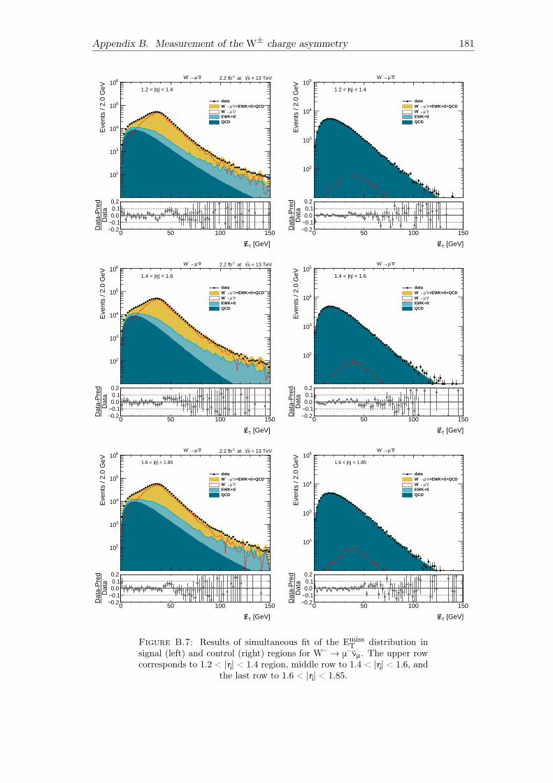
Appendix B. Measurement of the W± charge asymmetry 181
Eve
nts
/ 2.0
GeV
210
310
410
510
610
data+QCDt+EWK+tν-µ→-W
ν-µ→-WtEWK+t
QCD
| < 1.4η1.2 < |
ν-µ→-W = 13 TeVs at -12.2 fb
[GeV]TE
0 50 100 150
Dat
aD
ata-
Pre
d
0.2−0.1−0.00.10.2
Eve
nts
/ 2.0
GeV
210
310
410
510
data+QCDt+EWK+tν-µ→-W
ν-µ→-WtEWK+t
QCD
ν-µ→-W
| < 1.4η1.2 < |
[GeV]TE
0 50 100 150
Dat
aD
ata-
Pre
d
0.2−0.1−0.00.10.2
Eve
nts
/ 2.0
GeV
210
310
410
510
610
data+QCDt+EWK+tν-µ→-W
ν-µ→-WtEWK+t
QCD
| < 1.6η1.4 < |
ν-µ→-W = 13 TeVs at -12.2 fb
[GeV]TE
0 50 100 150
Dat
aD
ata-
Pre
d
0.2−0.1−0.00.10.2
Eve
nts
/ 2.0
GeV
210
310
410
510
data+QCDt+EWK+tν-µ→-W
ν-µ→-WtEWK+t
QCD
ν-µ→-W
| < 1.6η1.4 < |
[GeV]TE
0 50 100 150
Dat
aD
ata-
Pre
d
0.2−0.1−0.00.10.2
Eve
nts
/ 2.0
GeV
210
310
410
510
610
data+QCDt+EWK+tν-µ→-W
ν-µ→-WtEWK+t
QCD
| < 1.85η1.6 < |
ν-µ→-W = 13 TeVs at -12.2 fb
[GeV]TE
0 50 100 150
Dat
aD
ata-
Pre
d
0.2−0.1−0.00.10.2
Eve
nts
/ 2.0
GeV
210
310
410
510
data+QCDt+EWK+tν-µ→-W
ν-µ→-WtEWK+t
QCD
ν-µ→-W
| < 1.85η1.6 < |
[GeV]TE
0 50 100 150
Dat
aD
ata-
Pre
d
0.2−0.1−0.00.10.2
Figure B.7: Results of simultaneous fit of the EmissT distribution in
signal (left) and control (right) regions for W– → μ– νμ. The upper rowcorresponds to 1.2 < |η| < 1.4 region, middle row to 1.4 < |η| < 1.6, and
the last row to 1.6 < |η| < 1.85.
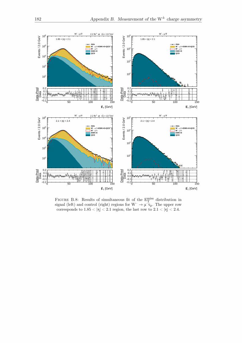
182 Appendix B. Measurement of the W± charge asymmetry
Eve
nts
/ 2.0
GeV
210
310
410
510
610
data+QCDt+EWK+tν-µ→-W
ν-µ→-WtEWK+t
QCD
| < 2.1η1.85 < |
ν-µ→-W = 13 TeVs at -12.2 fb
[GeV]TE
0 50 100 150
Dat
aD
ata-
Pre
d
0.2−0.1−0.00.10.2
Eve
nts
/ 2.0
GeV
210
310
410
510
data+QCDt+EWK+tν-µ→-W
ν-µ→-WtEWK+t
QCD
ν-µ→-W
| < 2.1η1.85 < |
[GeV]TE
0 50 100 150
Dat
aD
ata-
Pre
d
0.2−0.1−0.00.10.2
Eve
nts
/ 2.0
GeV
210
310
410
510
610
data+QCDt+EWK+tν-µ→-W
ν-µ→-WtEWK+t
QCD
| < 2.4η2.1 < |
ν-µ→-W = 13 TeVs at -12.2 fb
[GeV]TE
0 50 100 150
Dat
aD
ata-
Pre
d
0.2−0.1−0.00.10.2
Eve
nts
/ 2.0
GeV
210
310
410
510
data+QCDt+EWK+tν-µ→-W
ν-µ→-WtEWK+t
QCD
ν-µ→-W
| < 2.4η2.1 < |
[GeV]TE
0 50 100 150
Dat
aD
ata-
Pre
d
0.2−0.1−0.00.10.2
Figure B.8: Results of simultaneous fit of the EmissT distribution in
signal (left) and control (right) regions for W– → μ– νμ. The upper rowcorresponds to 1.85 < |η| < 2.1 region, the last row to 2.1 < |η| < 2.4.
183
Appendix C
APPLgrid upgrade
An intense development of theoretical approaches, numerical methods, and compu-tational hardware allow calculations of many different physical processes up to NNLO.Computation of processes from proton collisions (like deep inelastic scattering or proton-proton collisions) depends on errors from PDF uncertainties. The calculation of finalstate observables using a particular PDF set, and estimation of theoretical uncertaintiesfrom a variation of the strong coupling, αs, renormalization, μr, and factorization, μf ,scales becomes very time-consuming. Different approaches to PDF determination raisea necessity to compare cross sections obtained using various PDF sets, which requiresrecalculation of the whole process using different PDF sets. On average, depending ona process, the CPU time to produce a precise result can take from days to weeks. Forthat reason, less resource-demanding methods are being developed.
The APPLgrid project [154] emerged as one of proposed solutions and proved to bea reliable algorithm allowing to handle such problems. APPLgrid is library that allowto collect cross-section weights from Monte Carlo generators1 though additional soft-ware interfaces. The weights are stored on a 3D look-up table (in momentum transfer,Q, and momentum fraction, x), which can be afterwards combined with an arbitraryPDF, stored in an APPLgrid format. In this approach, PDF values are stored in atwo-dimensional grid of points. PDF-independent cross-section weights representationallows the implementation of renormalization and factorization scale variations. Usingthe APPLgrid methods, a total cross section is calculated convoluting the PDF valueswith weights from the look-up table.
The APPLgrid package is widely used not only as a package interfaced into MCtools but also as a part of complex computational frameworks like xFitter [1]. In thatcontext, APPLgrid became an important part of modern numerical tools of particlephysics.
This chapter is dedicated to the APPLgrid modification for its upgrade to NNLO.The first part covers a brief introduction to the APPLgrid methodology, while thesecond is focused on implemented improvements.
C.1 The APPLgrid project
The APPLgrid project appeared as a result of the collaboration between TancrediCarli, Dan Clements, Amanda Cooper-Sarkar, Claire Gwenlan, Gavin P. Salam, FrankSiegert, Pavel Starovoitov, and Mark Sutton [143]. Detailed instructions on installa-tion and execution, as well as various produced grids together with convolution andcalculation codes, can be found on its official web-page https://mcfm.fnal.gov.
1MCFM [142] or NLOJET++ [155].
184 Appendix C. APPLgrid upgrade
C.1.1 PDF representation on a grid
In the APPLgrid approach, parton density function values for different x and Q2 arestored on a two-dimensional grid of points with an n-th order of interpolation betweenthem. The parton momentum fraction x and the factorization scale Q2 are re-writtenin more convenient terms, y(x) and τ(Q2) to provide a uniform distribution of pointson the grid:
y(x) = ln1x+ a(1 – x), (C.1)
τ(Q2) = ln
(lnQ2
Λ2
). (C.2)
The Λ parameter may be chosen as of the order of ΛQCD, but not mandatory identical,the parameter a regulates a uniform distribution of points increasing density of pointsin the large x region. Using these notations, the PDF2, f(x,Q2), can be re-written intwo-dimensional grid (iy δy, iτδτ), where iy and iτ correspond to PDF values on thegrid, and δy with δτ are the grid spacing, obtained by interpolation:
f(x,Q2) =n∑i=0
n′∑j=0
fh+i,l+jI(n)i
(y(x)δy
– h(x))I(n′)
j
(τ(Q2)δτ
– l(Q2)
). (C.3)
Here n and n′ are the interpolation order, I(n)i (u) is interpolation function equal to 1for case u = i and for the rest is given by:
I(n)i (u) =(–1)n–i
i!(n – i)!u(u – 1)...(u – n)
u – i. (C.4)
Definitions of h(x) and l(Q2) are given by:
h(x) = int(y(x)δy
–n – 12
), (C.5)
l(Q2) = int
(τ(Q2)δτ
–n′ – 12
). (C.6)
C.1.2 Weights representation in the case of two incoming hadrons
The APPLgrid method of storing cross-section weights in a look-up table allowsthe convolution of a chosen PDF set with a given weight, including μr, μf , and αs scalevariation. Let’s consider an NLO MC software that produces N events m = 1...N fromtwo incoming hadrons, with a weight wb
m of a particular b-th sub-process, at a scaleQ2, as a Q2
m, and a certain momentum fraction from two protons x1 and x2, as x1m ,and x2m . Defining pm as the number of powers of αs in event m, one would expect thefinal result of the MC integration for one sub-process to be:
W =N∑
m=1
nsub∑b=1
w(b)m
(αs(Q2
m)2π
)pmF(b)(x1m , x2m , Q
2), (C.7)
2Les Houches Aprroach is used as the main PDF format [156], [157].
C.1. The APPLgrid project 185
where nsub is a number of sub-processes contributing to the considered event, F(b)(x1m , x2m , Q2)
are PDF combinations of sub-processes defined later. In the APPLgrid approach, aweight grid W(p)(b)
iy1 ,iy2 ,iτupdates with each event by a portion of the grid with:
W(p)(b)h+i,l+j →W(p)(b)
h+i,l+j +w(b)m I(n)(b)i
(y(xm)δy
– h(x))I(n′)(b)
j
(τ(Q2
m)δτ
– l(Q2m)
), (C.8)
i = 0...n, j = 0...n′.A general expression for W, for any PDF and any αs can be expressed by:
W =∑p
nsub∑b=0
∑iy1
∑iy2
∑iτ
W(p)(b)iy1,iy2,iτ
(αs(Q2(iτ))
2π
)p
F(b)(x(iy1)1 , x(iy2)2 , Q2(iτ)). (C.9)
Depending on considered processes, combinations of the incoming parton densities canbe different. Here, the case of W+ sub-processes is presented, details on some othercases, as well as more details on the APPLgrid project can be found in appropriate paper[143]. Sub-processes of the W-boson production are defined from the assumptions ofmass-less quarks, using CKM matrix elements. At NLO, six initial states are given by
DU : F(0)(x1, x2, Q2) = S12(x1, x2),
UD : F(1)(x1, x2, Q2) = S21(x1, x2),
Dg : F(2)(x1, x2, Q2) = D1(x1)G2(x2),
Ug : F(3)(x1, x2, Q2) = U1(x1)G2(x2), (C.10)
gD : F(4)(x1, x2, Q2) = G1(x1)D2(x2),
gU : F(5)(x1, x2, Q2) = G1(x1)U2(x2).
Generalized PDFs are defined as:
GH(x) = f0/H(x,Q2),
UH(x) = f2/H(x,Q2)(V2
ud +V2us) + f4/H(x,Q
2)(V2cd +V2
cs),
DH(x) = f–1/H(x,Q2)(V2
ud +V2cd) + f–3/H(x,Q
2)(V2us +V2
cs),
S12(x1, x2) = f–3/H1(x1, Q2)f2/H2(x2, Q
2)V2us+
f–3/H1(x1, Q2)f4/H2(x2, Q
2)V2cs+
f–1/H1(x1, Q2)f2/H2(x2, Q
2)V2ud+
f–1/H1(x1, Q2)f4/H2(x2, Q
2)V2cd,
S21(x1, x2) = f2/H1(x1, Q2)f–3/H2(x2, Q
2)V2us+
f4/H1(x1, Q2)f–3/H2(x2, Q
2)V2cs+
f2/H1(x1, Q2)f–1/H2(x2, Q
2)V2ud+
f4/H1(x1, Q2)f–1/H2(x2, Q
2)V2cd.
186 Appendix C. APPLgrid upgrade
Here Vij are the CKM matrix elements. The PDF of a particular parton with corre-sponding PDG Id [158] of incoming k-th hadron (proton) is given as fId/Hk
. In thatsense, numbers 1...5 correspond to quarks from up to bottom, and anti-quarks withthe opposite sign, zero is dedicated to gluon, the contribution from the top quark isneglected. Details on scale dependence as well as re-weighting to a different center ofmass can be found in the paper [143].
C.1.3 A Monte Carlo for femtobarn processes (MCFM)
MCFM-6.8 [159] is a parton-level Monte Carlo program, that produces predictionsup to next-to-leading-order for various processes at hadron colliders [160], [161]. Theprogram has a wide range of various setups as input parameters. A user can definedifferent modes of MCFM, producing an output of a specific format. MCFM allowssetting heavy quark masses, as well as PDF set, jet definition, event cuts, settings forphoton processes, and anomalous couplings of the W± and Z0 bosons. The programprovides calculation of renormalization and factorization scales on an event-by-eventbasis, with different possible schemes of scales treatment. Besides that, it has manydifferent setups dedicated to particular processes. More details can be found on theofficial web-page [154].
Since version 8.0, MCFM can calculate NNLO predictions for color-singlet processes[129]. The NNLO corrections are calculated using the non-local N-jettiness subtractionapproach [162]. This upgrade, together with APPLgrid compatibility, makes the latestversions of MCFM (8.3-present) even more attractive in terms of a variety of its usage.Representation of NNLO weights on the APPLgrid grid can find its application onvarious areas of particle physics, from a great computation time reduction in theoryuncertainties calculation, to NNLO weights usage in xFitter [1] PDF fits. For thatreason, the APPLgrid upgrade to NNLO weights processing is a crucial task.
C.1.4 Technical implementation
Studies described in the second half of this chapter are performed for the APPLgridpart, which is linked to the MCFM Monte Carlo program. For that reason, an exampleof APPLgrid technical implementation is given in the frame of MCFM.
An important element of the APPLgrid is a so-called "mcfm-bridge", in this de-scription, version 0.0.35 is used. It is a package of C++ codes that contains a library,libmcfmbridge.a, with instructions for weights extraction from MCFM and settings fora grid constructor. The bridge also includes a utility called "mcfmbridge-config"; thisutility provides options required to link APPLgrid with MCFM. A user access to specifyall available parameters for grid production is provided by a C++ file called "mcfm-bridge-0.0.35/src/mcfm_interface.cxx". The setting list includes:
• A number of grids and the binning information for the grid constructor:
– lower and upper limits of x and Q2;– number of x and Q2 bins;– order of interpolation for x and Q2;
Default values for each process are also available.
• Derived observables from 4-vectors of available final state particles, provided byMCFM, in particular:
C.1. The APPLgrid project 187
– number of observables;
– binning information (flexibility in binning definition);
– kinematic cuts.
• A type of PDF decomposition and some other technical details.
When the grid parameters are set and ready, the mcfm-bridge-0.0.35 package, as wellas MCFM-6.8 has to be recompiled for changes to be applied3.
The software implementation of a grid structure is fulfilled as a multidimensionalarray (for x1, x2, Q2) of the TH3D-class of the ROOT analysis framework. Each suchthree-dimensional grid is stored for each sub-process per αs order (see eq. C.9). Theweight grid W(p)(b)
h+i,l+j is filled for each cross-section bin during the MCFM-6.8 run.To reduce a memory usage and to increase a grid readability time, the MCFM-6.8 isrequired to run twice. The first run is needed for APPLgrid to estimate and allocate aproper amount of required weight space, while the second is to fill the actual grid(s).
The master class for a given cross-section is called appl::grid and contains instancesof an internal class for each order of αs. The internal class appl::igrid contains allnecessary tools to calculate the cross-section for one particular bin at a specific order.The class also contains x-to-y, y-to-x, and Q2-to-τ, τ-to-Q2 transformations, and others.A produced grid(s) is saved to a ROOT file with all necessary information required forthe cross-section calculation:
• The center of mass energy at which the weight grid has been produced,
• The choice of coordinate transformation functions, with the default definitiongiven by eq. C.1 and C.2,
• The order of interpolation given in eq. C.4,
• The number of grid points to be used in each dimension of x1, x2, and Q2,
• The definition of the sub-processes in a 13 x 13 matrix,
• The CKM matrix elements and others.
Calculation of a considered cross section is possible using a convolution procedure,built in a dedicated sub-class of the master class. Members of this sub-class fulfill aconvolution procedure over a given x1, x2, and Q2 for each sub-process. The final cross-section value in each bin is then computed by the master class collecting and summingall cross-section values from the sub-classes for each order. To perform a convolution,as an input information, user has to specify a PDF set and αs. Example of such aprocedure may look as shown in Listing C.1.
Listing C.1: APPLgrid commands to perform convolution.
12 // read the g r id3 appl : : g r i d grid_eta1 ( " gr id – i n c l j e t s 0 6 – eta1 . root " ) ;45 // perform the convo lut ion6 std : : vector<double> xsec_eta1 = grid_eta1 . vconvolute ( evolvepdf_ , alphasqcd_ ) ;
3This issue is successfully removed by the author, discussed in detail in the second section of thischapter.
188 Appendix C. APPLgrid upgrade
Where "grid-incljets06-eta1.root" is a grid file, "vconvolute" is a convolution function,"evolvepdf_" is a PDF set under consideration, and "alphasqcd_" is a strong couplingparameter [154]. DGLAP splitting functions are calculated using the HOPPET program[163].
C.2 MCFM-interface upgrade
The mcfm-bridge upgrade is a necessary part of the APPLgrid modification. Tech-nically, the APPLgrid modification to MCFM NNLO weights processing will requirevarious studies, accuracy checks, etc. natural for any development process. The mcfm-bridge upgrade, discussed in this section, includes modifications that will allow savingtime and simplifying the development process. The upgrade was performed in cooper-ation with Pavel Starovoitov, one of the authors of APPLgrid and xFitter.
C.2.1 Processes mapping
The first step is dedicated to an improvement of APPLgrid grid default setups forvarious processes. The list of processes with default grid setups is shown in Table C.1.Each of the processes has recommended grid setup that consists of following parameters:
• Name of the processes,
• Type of a PDF decomposition,
• String label in a grid name ,
• Lower and upper limits of Q2,
• Number of the bins in Q2 range,
• Order of interpolation for the Q2 dimension,
• Lowest αs order,
• Lower and upper limits of x,
• Number of the bins in x range,
• Order of interpolation for the x dimension,
• Number of loops.
To re-arrange the default grid settings, the table is taken out from mcfm_interface.cxxinto separate files. The parameter list for each process is implemented into a specialstructure "info", described in a header file "mcfm-bridge-0.0.35/src/mcfm_procmap.h".The file contains a standard C++ associative container object "map", which returnsprocess parameters through a corresponding key (MCFM process number, see the firstcolumn in Tab. C.1). Access to the process parameter can be provided directly througha structure member name. The C++ structure syntax together with the definition of"info" is given in the Listing C.2.
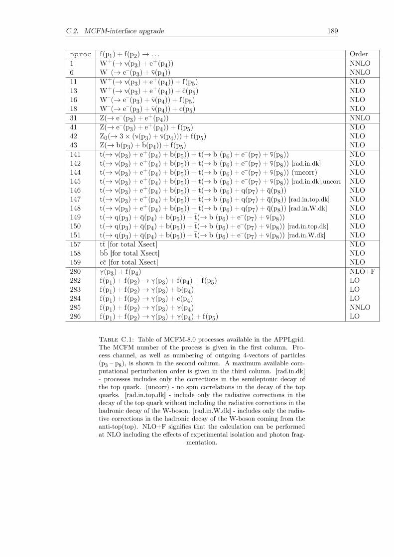
C.2. MCFM-interface upgrade 189
nproc f(p1) + f(p2)→ . . . Order1 W+(→ ν(p3) + e+(p4)) NNLO6 W–(→ e–(p3) + ν(p4)) NNLO11 W+(→ ν(p3) + e+(p4)) + f(p5) NLO13 W+(→ ν(p3) + e+(p4)) + c(p5) NLO16 W–(→ e–(p3) + ν(p4)) + f(p5) NLO18 W–(→ e–(p3) + ν(p4)) + c(p5) NLO31 Z(→ e–(p3) + e+(p4)) NNLO41 Z(→ e–(p3) + e+(p4)) + f(p5) NLO42 Z0(→ 3× (ν(p3) + ν(p4))) + f(p5) NLO43 Z(→ b(p3) + b(p4)) + f(p5) NLO141 t(→ ν(p3) + e+(p4) + b(p5)) + t(→ b (p6) + e–(p7) + ν(p8)) NLO142 t(→ ν(p3) + e+(p4) + b(p5)) + t(→ b (p6) + e–(p7) + ν(p8)) [rad.in.dk] NLO144 t(→ ν(p3) + e+(p4) + b(p5)) + t(→ b (p6) + e–(p7) + ν(p8)) (uncorr) NLO145 t(→ ν(p3) + e+(p4) + b(p5)) + t(→ b (p6) + e–(p7) + ν(p8)) [rad.in.dk],uncorr NLO146 t(→ ν(p3) + e+(p4) + b(p5)) + t(→ b (p6) + q(p7) + q(p8)) NLO147 t(→ ν(p3) + e+(p4) + b(p5)) + t(→ b (p6) + q(p7) + q(p8)) [rad.in.top.dk] NLO148 t(→ ν(p3) + e+(p4) + b(p5)) + t(→ b (p6) + q(p7) + q(p8)) [rad.in.W.dk] NLO149 t(→ q(p3) + q(p4) + b(p5)) + t(→ b (p6) + e–(p7) + ν(p8)) NLO150 t(→ q(p3) + q(p4) + b(p5)) + t(→ b (p6) + e–(p7) + ν(p8)) [rad.in.top.dk] NLO151 t(→ q(p3) + q(p4) + b(p5)) + t(→ b (p6) + e–(p7) + ν(p8)) [rad.in.W.dk] NLO157 tt [for total Xsect] NLO158 bb [for total Xsect] NLO159 cc [for total Xsect] NLO280 γ(p3) + f(p4) NLO+F282 f(p1) + f(p2)→ γ(p3) + f(p4) + f(p5) LO283 f(p1) + f(p2)→ γ(p3) + b(p4) LO284 f(p1) + f(p2)→ γ(p3) + c(p4) LO285 f(p1) + f(p2)→ γ(p3) + γ(p4) NNLO286 f(p1) + f(p2)→ γ(p3) + γ(p4) + f(p5) LO
Table C.1: Table of MCFM-8.0 processes available in the APPLgrid.The MCFM number of the process is given in the first column. Pro-cess channel, as well as numbering of outgoing 4-vectors of particles(p3 – p8), is shown in the second column. A maximum available com-putational perturbation order is given in the third column. [rad.in.dk]- processes includes only the corrections in the semileptonic decay ofthe top quark. (uncorr) - no spin correlations in the decay of the topquarks. [rad.in.top.dk] - include only the radiative corrections in thedecay of the top quark without including the radiative corrections in thehadronic decay of the W-boson. [rad.in.W.dk] - includes only the radia-tive corrections in the hadronic decay of the W-boson coming from theanti-top(top). NLO+F signifies that the calculation can be performedat NLO including the effects of experimental isolation and photon frag-
mentation.
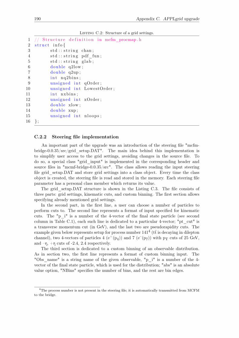
190 Appendix C. APPLgrid upgrade
Listing C.2: Structure of a grid settings.
1 // St ruc ture d e f i n i t i o n in mcfm_procmap . h2 s t r u c t i n f o {3 std : : s t r i n g chan ;4 std : : s t r i n g pdf_fun ;5 std : : s t r i n g glab ;6 double q2low ;7 double q2up ;8 i n t nq2bins ;9 unsigned i n t qOrder ;10 unsigned i n t LowestOrder ;11 i n t nxbins ;12 unsigned i n t xOrder ;13 double xlow ;14 double xup ;15 unsigned i n t n loops ;16 } ;
C.2.2 Steering file implementation
An important part of the upgrade was an introduction of the steering file "mcfm-bridge-0.0.35/src/grid_setup.DAT". The main idea behind this implementation isto simplify user access to the grid settings, avoiding changes in the source file. Todo so, a special class "grid_input" is implemented in the corresponding header andsource files in "mcmf-bridge-0.0.35/src". The class allows reading the input steeringfile grid_setup.DAT and store grid settings into a class object. Every time the classobject is created, the steering file is read and stored in the memory. Each steering fileparameter has a personal class member which returns its value.
The grid_setup.DAT structure is shown in the Listing C.3. The file consists ofthree parts: grid settings, kinematic cuts, and custom binning. The first section allowsspecifying already mentioned grid settings.
In the second part, in the first line, a user can choose a number of particles toperform cuts to. The second line represents a format of input specified for kinematiccuts. The "p_i" is a number of the 4-vector of the final state particle (see secondcolumn in Table C.1), each such line is dedicated to a particular 4-vector; "pt_cut" isa transverse momentum cut (in GeV), and the last two are pseudorapidity cuts. Theexample given below represents setup for process number 1414 (tt is decaying in dileptonchannel), two 4-vectors of particles 4 (e+(p4)) and 7 (e–(p7)) with pT cuts of 25 GeV,and –η, +η cuts of -2.4, 2.4 respectively.
The third section is dedicated to a custom binning of an observable distribution.As in section two, the first line represents a format of custom binning input. The"Obs_name" is a string name of the given observable, "p_i" is a number of the 4-vector of the final state particle, which is used for the distribution; "abs" is an absolutevalue option, "NBins" specifies the number of bins, and the rest are bin edges.
4The process number is not present in the steering file; it is automatically transmitted from MCFMto the bridge.
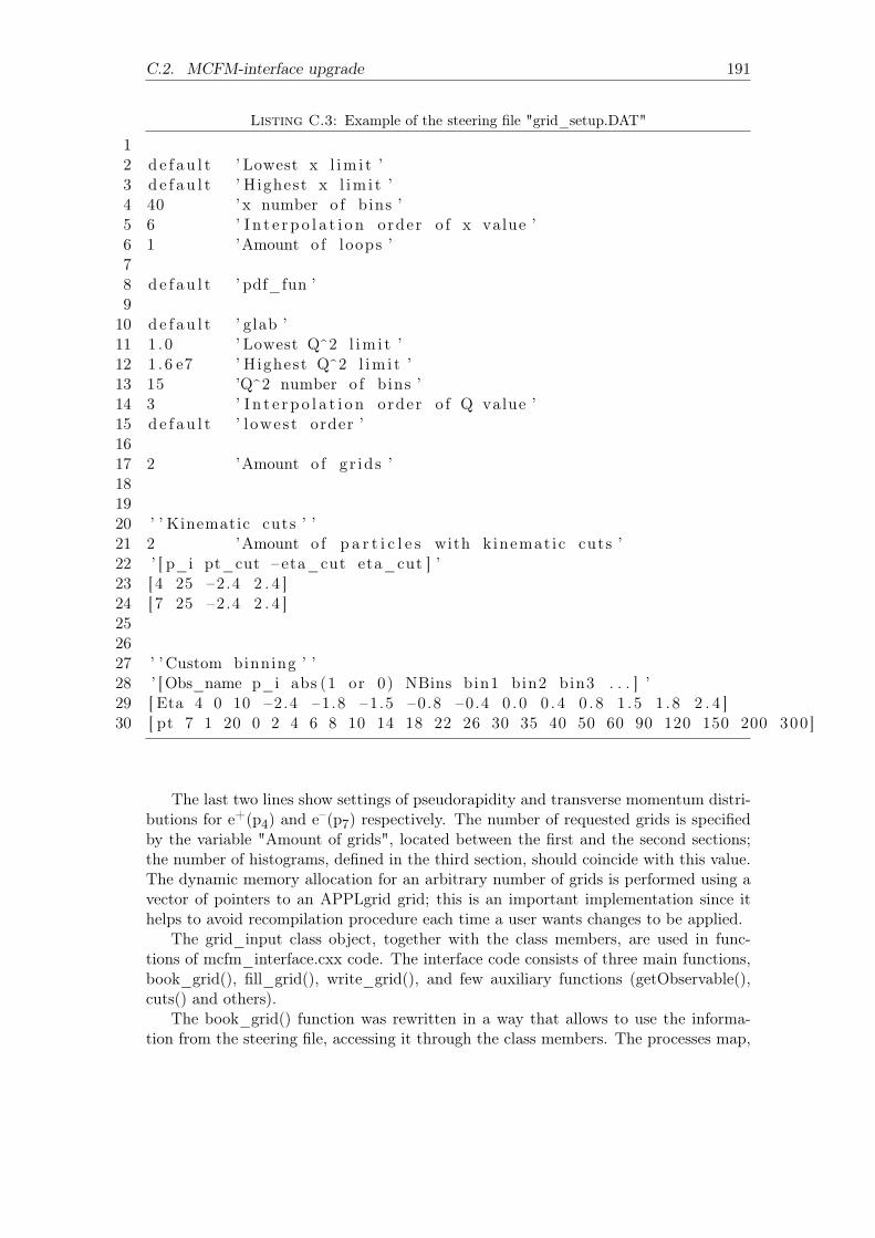
C.2. MCFM-interface upgrade 191
Listing C.3: Example of the steering file "grid_setup.DAT"
12 d e f au l t ’ Lowest x l im i t ’3 d e f au l t ’ Highest x l im i t ’4 40 ’ x number o f bins ’5 6 ’ I n t e r p o l a t i o n order o f x value ’6 1 ’Amount o f loops ’78 d e f au l t ’ pdf_fun ’910 d e f au l t ’ glab ’11 1 .0 ’ Lowest Q^2 l im i t ’12 1 .6 e7 ’ Highest Q^2 l im i t ’13 15 ’Q^2 number o f bins ’14 3 ’ I n t e r p o l a t i o n order o f Q value ’15 d e f au l t ’ l owest order ’1617 2 ’Amount o f g r ids ’181920 ’ ’ Kinematic cuts ’ ’21 2 ’Amount o f p a r t i c l e s with kinemat ic cuts ’22 ’ [ p_i pt_cut – eta_cut eta_cut ] ’23 [ 4 25 –2.4 2 . 4 ]24 [ 7 25 –2.4 2 . 4 ]252627 ’ ’ Custom binning ’ ’28 ’ [Obs_name p_i abs (1 or 0) NBins bin1 bin2 bin3 . . . ] ’29 [ Eta 4 0 10 –2.4 –1.8 –1.5 –0.8 –0.4 0 .0 0 .4 0 .8 1 .5 1 .8 2 . 4 ]30 [ pt 7 1 20 0 2 4 6 8 10 14 18 22 26 30 35 40 50 60 90 120 150 200 300 ]
The last two lines show settings of pseudorapidity and transverse momentum distri-butions for e+(p4) and e–(p7) respectively. The number of requested grids is specifiedby the variable "Amount of grids", located between the first and the second sections;the number of histograms, defined in the third section, should coincide with this value.The dynamic memory allocation for an arbitrary number of grids is performed using avector of pointers to an APPLgrid grid; this is an important implementation since ithelps to avoid recompilation procedure each time a user wants changes to be applied.
The grid_input class object, together with the class members, are used in func-tions of mcfm_interface.cxx code. The interface code consists of three main functions,book_grid(), fill_grid(), write_grid(), and few auxiliary functions (getObservable(),cuts() and others).
The book_grid() function was rewritten in a way that allows to use the informa-tion from the steering file, accessing it through the class members. The processes map,
192 Appendix C. APPLgrid upgrade
described in section C.2.1, is combined with the steering file through additionally im-plemented flag "default"5. In this case, parameters tagged as "default" are taken fromthe processes map.
Function fill_grid() selects valid weights and fills them in previously created grid us-ing functions getObservable() and cuts(). Particles, selected for kinematic selection, aswell as observables, are determined in getObservable() function using the customKine-matics(p, c) and customGrid(k, t) class members. Kinematic selection is performedin function cuts(); the function is modified to use customKinematics(p,c) and nK-inPar() members to provide information from the "Kinematic cuts" section of thegrid_setup.DAT. Selected events are then filled in a grid using fill_grid() function.
Additionally, to mentioned improvements, various checks and minor optimizationswere also performed.
5The steering file example (List.C.3) contains variables replaced with the word "default".
Copyright © 2022 FDOKUMEN