Born to Export:

Understanding Export Growth in Bangladesh’s Apparel and

Textiles Industry∗

Bernardo Dıaz de Astarloa† Jonathan Eaton‡ Kala Krishna†

Bee Aw Roberts† Andres Rodrıguez-Clare§ James Tybout†

Preliminary versionJanuary 2015

Abstract

Trade economists usually think about new exporters as previously established domestic firms

that diversify into foreign markets, starting with low export volumes and gradually increasing the

share of output they ship abroad. Using data on the universe of exporters in Bangladesh we show

that the experience of Bangladeshi exporters is diametrically opposed to this standard description.

Exporters are fully committed to foreign markets, exporting most of their output abroad; they start

big, not small, and show high survival rates once they start exporting. They are born to export firms

who operate in orphan industries, with essentially missing domestic demand for their products. In

addition to the usual fixed and sunk costs of exporting, they must face presumably higher costs of

starting up new businesses. We compare these patterns with those of China, Colombia and Taiwan,

and find similar but less-striking patterns for China. These features seem to be missing in Taiwan

and Colombia, which accord with other typical cases described in the literature. We adapt the search

and learning model of Eaton et al. (2014) to show how the presence of high sunk costs of establishing

a new business and the absence of a domestic market can generate export dynamics similar to the

ones we observe in Bangladesh.

1 Introduction

Standard thinking about firms entering export markets is that they have already developed a strong

position at home. Both static and dynamic models of trade with heterogeneous firms imply that exporters

will always produce for and sell in the domestic market. Conditional on a firm’s productivity, variable

profits in the domestic market are always positive and fixed production costs have already been incurred

upon making the decision to export. Hence, exporters will always sell in the domestic market. These

∗This project was partially supported by the International Growth Centre. Eaton and Tybout acknowledge support fromthe National Science Foundation (Grant SES-0922358). For helpful comments and suggestions we would like to thank WahidMahmud, Mustazur Rahman, Fahmida Khatun and participants at the BRAC-iiG-IGC Conference on Entrepreneurshipand Development (March 2011) and the IGC Trade Program Meeting at Penn State (April 2011). We thank Anik Ashraf,Ravid Chowdhury and Ummul Ruthbah for invaluable help and guidance in accessing and collecting data in Bangladesh.Bibhuti Sarker provided excellent research assistance.†Pennsylvania State University.‡Brown University.§University of California, Berkeley.

1

types of models also imply that firms export a relatively low share of output and that changes in total

exports arise either through the expansion of exports by incumbent exporters or by entry into exporting

by established domestic firms.1

Evidence from Bangladesh suggests that these patterns do not apply to the rapid expansion of its

apparel and textiles exports during the period 1983-2010: exporting firms emerged de novo and sold

considerable amounts to new foreign markets without selling much or anything at home. To exploit the

combination of cheap labour and non-binding MFA quotas, most Bangladeshi apparel and textiles pro-

ducers were established to export. Foreign sales by these firms far exceeded what they sold domestically

(Mostafa and Klepper, 2009). As a consequence, firms that sold substantial amounts in foreign markets

were not particularly large sellers at home, if they had any presence there at all. They were “born to

export”.

The Bangladeshi experience with apparel and textiles is not an isolated case of an export-oriented

emerging industry. Rather, this seems to be a common feature of expanding exporting sectors in many

developing countries. During their industrialization stage, by the end of the 1970s, Taiwan and Korea

exported 80% and 70% of their electronics production, respectively (Matthews, 2006). In Malaysia, export

oriented firms were responsible for the first wave of electronics growth (Rasiah, 2006).2 The Colombian

fresh cut-flower industry was conceived for export markets and, consequently, has exported the majority

of its production (from 70% to 95%) since its inception (Mendez, 1991; Arbelaez et al., 2012), as did the

same industry in Ethiopia (Gebreeyesus and Iizuka, 2010). Lu (2010) has documented that around 40%

of Chinese exporters sell more than 90% of their production abroad.3 McWilliams and Verma (2012),

using the World Bank’s Business Environment and Enterprise Performance Survey (BEEPS), find that

28% of firms in a sample of 95 low and middle-income countries were pure (and direct) exporters.

These observations are in contrast with what has been observed in developed countries, where, typi-

cally, firms export a small share of their production.4Since export-oriented industrialization has been key

for productivity growth in developing countries, understanding born to export phenomena is important

to shed light on the behavior of firms as they enter foreign markets.

A common feature among the cases of export emergence cited above is that born to export (BTE)

firms have emerged in industries for which there is little or no domestic demand in the exporting country.

We will refer to such industries as “orphan industries.” The presence of orphan industries means that

few incumbent firms exist, and, in the event that entrepreneurs become aware of exporting opportunities,

they must create new establishments to exploit them. When they do, most of their production will be

dedicated to foreign sales. The importance of sunk and fixed costs of foreign market entry has been well

documented in the international trade literature (Roberts and Tybout, 1997; Das et al., 2007; Cherkashin

et al., forthcoming). We should expect these costs to be specially binding in orphan industries since, in

addition to the costs of establishing products in a foreign market, entrepreneurs face the presumably much

1The standard static framework is essentially developed in Melitz (2003). Impullitti et al. (2013) provide an extensionto a dynamic setting, allowing for time-varying productivity and sunk costs of creating firms and exporting. In general,firms enter foreign markets only after surpassing a given size (productivity) threshold. Even if this occurs at birth, firmswill also sell in the domestic market.

2Multinational firms in export processing zones were key in generating this pattern in Malaysia. While the governmentdiscouraged multinationals from selling in the domestic market, Rasiah (2006) notes that “the domestic market was toosmall to affect most of the firms.” We address the importance of export processing zones in Bangladesh below.

3Dai et al. (2012) have noted that firms engaged in processing trade are pervasive in China. We address the issue ofprocessing trade below and still find that a significant fraction of non-processing exporters exports most of its output.

4See Bernard and Jensen (1995) and Bernard et al. (2003) for the U.S.; Bernard and Wagner (1997) for Germany; andEaton et al. (2011, 2004) for France. Most firms in these studies usually ship less than 15% of the value of their output toforeign countries.

2

larger costs of creating new establishments and training managers and workers.5 These extra costs are

likely to generate export dynamics quite distinct from those generated by firms that are created initially

to serve domestic consumers. For one thing, since these much larger start-up costs must be amortized

over a relatively lengthy period, the current period pay-offs of exporting will matter relatively less than

expectations about future payoffs in driving exporting decisions. Moreover, a large sunk cost creates a

large option value of remaining in an export market once this cost is incurred. Thus, BTE firms are more

likely than other firms to remain in foreign markets once they enter.

In this paper we use novel firm-level data sets from Bangladesh to assess the importance of BTE

firms there and compare it to export dynamics in other countries for which we have the necessary data:

China, Colombia, and Taiwan. Using micro data from these four countries we first document different

patterns of export growth. In particular, we explore whether entrants represent a major dimension of

export growth, how they behave over time and whether they can be characterized as BTE. Since export

processing zones (EPZs) have been suggested to generate BTE-like patterns by design, we also discuss

their role in generating the patterns we observe in Bangladesh. Finally, we employ a simpler version of

the search and learning model of export dynamics developed in Eaton et al. (2014) (henceforth EEJKKT)

to show it can characterize the distinctive features of export dynamics when firms are born to export.

The rest of the paper is organized as follows. In the next section we present our empirical exercises and

show that Bangladesh exporters are starkly different in key dimensions of the data. Section 3 contains a

discussion of the role of EPZs in Bangladesh. Section 4 develops a model of BTE dynamics. Section 5

concludes.

2 Patterns of export participation and growth

We first discuss some features of export growth in the individual countries we examine and then turn to

a description of our firm-level datasets. Since textiles and apparel represent more than 90% of exports

in Bangladesh, we concentrate on this industry for all countries, commenting on other industries where

appropriate. Our findings can be summarized as follows: exports from Colombia and Taiwan adhere

to patterns of export dynamics implied by standard models: (1) export growth is primarily driven by

expansion of exports on the part of incumbent exporters; (2) new exporters sell much less than incumbents

and are much more likely to exit foreign markets; (3) the average age of a firm when it starts to export

is over ten years. Bangladesh is the opposite in each dimension: (1) looking over a six-year horizon, net

entry accounts for over half of export expansion; (2) firms that start exporting sell almost as much as

incumbents and are more likely to survive than their Colombian and Taiwanese counterparts; (3) the

mean age of an exporting firm is under two years and the median new exporter has never sold before.

The picture for China is mixed: (1) entry makes an even more important contribution to growth than in

Bangladesh; (2) new exporters sell only negligibly less than incumbents and are more likely to survive;

but (3) the average new exporter is nearly seven years old.

2.1 Countries studied: main aggregate trends

We study apparel and textiles producers in four countries: Bangladesh, China, Colombia, and Taiwan.

Figures 1 and 2 summarize the main features about total and apparel and textiles exports over the

5Artopoulos et al. (2013) have recently emphasized that firms in developing countries intending to export differentiatedproducts to developed countries must adopt business practices significantly different from those implemented at home.

3

last three decades.6 All have gained market share in world manufacturing exports, although none as

spectacularly as China, and most manufacturing exports have gone to high income countries. For all

countries except Taiwan from the 1990s on, apparel and textiles exports have continued growing. Apparel

and textiles were a significant share of exports in the mid 1970s (above 30%), more even so for Bangladesh,

which was almost completely specialized in these industries. As China, Colombia and Taiwan developed

a wider manufacturing base, the share of apparel and textiles has declined in general and, even for China,

stands at below 20% of total manufacturing exports. Bangladesh, on the other hand, has not been able to

diversify into other industries and apparel and textiles have remained at 90% or more of total exports.7

Before turning to firm-level data, we briefly describe each country’s background.

Bangladesh The emergence of the Bangladeshi apparel exporting sector is well known in development

policy circles (Rhee and Belot, 1990; Hausmann and Rodrik, 2003; Mostafa and Klepper, 2009). It

began in 1979 when Daewoo Corporation of South Korea, a company with considerable experience in

apparel exports, signed a collaborative agreement with a Bangladeshi firm (Desh) with the intention

of circumventing import quotas to the United States and European markets imposed by the Multi-

Fiber Agreement (MFA). At that time, Bangladesh was not restricted by quotas. Bangladeshi apparel

producers had so far produced garments for the local market, such as sarees and lungis, and had very low

exports of Western-style apparel covered under the MFA. As part of the Daewoo-Desh agreement, about a

130 Bangladeshi workers were sent to Korea for training in technology, quality control, and management.

Daewoo also helped Desh absorb key management and marketing techniques for garment exporting. Once

Desh succeeded, many of its workers left to start up other firms, spurring the growth of the industry. As

was mentioned above, apparel remains the overwhelmingly dominant export of Bangladesh. Interestingly,

at least to our knowledge, the government does not seem to have played a major role in stimulating this

particular industry in its early phase.8

China Like Bangladesh, China experienced a dramatic growth in apparel exports. However, the indus-

try already served a relatively large domestic market and several policy reforms did play a major role.

First, China initiated key market-oriented reforms in 1992 which improved the efficiency of the apparel

sector (China Textile University and Harvard Center of Textile and Apparel Research, 1999). Second,

after fifteen years of negotiations, China joined the World Trade Organization (WTO) in 2001. In doing

so it benefitted from the phase-out of the MFA product- and country-specific quotas on textiles, yarn,

and apparel, which was completed by 2005.9 As a member of the WTO, China also obtained Most Fa-

vored Nation (MFN) status (so that Chinese exporters to any WTO-member destination faced the lowest

6Aggregate merchandise exports are from The World Bank (Bangladesh, China and Colombia) and Feenstra et al. (2005)(Taiwan). Apparel and textiles exports are from Feenstra et al. (2005) and include exports in the following SITC two-digitindustries: 26 (Textile fibers and their wastes), 61 (Leather and dressed furskins), 65 (Textile yarn, fabrics, and relatedproducts), 84 (Articles of apparel and clothing) and 85 (Footwear). We thank Robert Feenstra for providing us with morerecent data.

7The composition of exports in Bangladesh at a more disaggregate level has, however, changed significantly since the1970s. When looking at the four-digit SITC level, for example, those sub-industries included in “Articles of apparel andclothing” (SITC84) started to dominate the list of top-20 selling sub-industries in the mid 1980s. These tend to includemore sophisticated products (shirts, jerseys, pullovers, undergarments) than were produced by Bangladesh in the 1970s(jute, textile fabrics).

8There was only one EPZ established in the 1980s, and, as we show below, EPZs have not been substantial contributorsto apparel export growth.

9See Brambilla et al. (2010) for a historical discussion of the MFA and its precursor, the Agreement on Textiles andClothing (ATC). These authors argue that China was more constrained by such quotas than other suppliers, resulting in thesurge in Chinese exports post MFA. Khandelwal et al. (2013) estimate that removal of inefficient licensing among exportersof textiles and clothing accounted for almost three quarters of the productivity gain experienced by China after quotas wereremoved.

4

tariff applied to any exporter there).10 Finally, under the terms of its accession to the WTO, China

agreed to remove domestic restrictions on direct exporting. These restrictions, which were lifted in a

series of reforms between 1999 and 2004, prevented firms (other than large producers and intermediaries,

state-owned enterprises, and foreign firms) from exporting directly; they had to go through other firms

or intermediaries who were permitted to export.11

Apparel exports have grown extremely rapidly, especially since 1992, and China now has the largest

apparel sector in the world. Furthermore, most apparel exporters are strongly oriented toward foreign

markets and ship well over half of their output abroad (Lu, 2010). China’s apparel boom would have been

even larger if the China Containment Agreements (CCAs) had not been implemented under China’s WTO

accession agreements of 2001. Under the CCAs, China agreed to constrain import surges voluntarily until

2013. The U.S. invoked the CCAs in mid 2005, after the phase-out of the MFA triggered a surge in its

Chinese apparel imports. The E.U. followed suit in the fall of 2005 and since then a host of other countries

have done so as well, including Canada, Mexico, Turkey, and some lower income countries.12

Colombia Colombia has managed to expand its apparel exports over the past 30 years successfully,

albeit much more gradually than China and Bangladesh. Also, unlike Bangladesh, its export growth was

largely driven by the re-orientation of its established apparel sector toward foreign markets. Colombia is,

after Mexico, one of the largest employers of apparel and textiles in Latin America and enjoys the highest

average unit values of apparel exports to the U.S. among Central and Latin American countries. This

reflects Colombia’s advantages in design and adoption of ISO quality standards over other countries in

the region (Condo et al., 2004). The sector has, like all Colombian manufacturing sectors, been influenced

by government trade-induced policies to soften the cycles in world demand. After a first wave of tariff

reductions in the 1970s, policy became increasingly protectionist in the beginning of the 1980s and turned

more liberal again in the mid 1980s. For the 1977-1985 period, Roberts (1996) reports that apparel and

textiles producers’ entry rates were among the highest of Colombian manufacturing industries. Differently

from other textiles-exporting countries in the region (Nicaragua, Mexico, Dominican Republic), Colombia

hasn’t been so dependent on preferential access to the U.S. market. However, it did benefit from the

implementation of the Andean Trade Promotion and Drug Eradication Act of 2002, as it allowed it to

increase value added of apparel and textiles exports to the U.S. (Condo et al., 2004).

Taiwan Finally, Taiwan combined elements of Chinese and Colombian experiences. After implementing

export subsidies and other industrial policies in the early 1960s, this country enjoyed a period of rapid

growth in apparel exports. However, these exports peaked at 9.5% of total Taiwanese exports in 1986, and

by 2004 their share had declined to less than 0.8%. Like their Colombian counterparts, most Taiwanese

apparel producers who continue to export derive the majority of their revenue from domestic sales.13

10However, most Chinese exports already had de facto MFN status.11Bai and Krishna (2013) use the variation in time and space of these reforms to argue that these reforms were responsible

for a good part of the surge in exports. Bai et al. (2013) suggest (based on estimates from a dynamic structural model)that the inability to export directly adversely affected such firms.

12The growth rate of the CCA quotas is higher than that of MFA quotas they replaced, though the coverage is similar oreven greater in some cases. See Dayarathna-Banda and Whalley (2007) for more on this matter.

13Establishment-level data from 2000-2004 show that, among Taiwanese apparel exporters, roughly 80% of productionhas been directed to the domestic market.

5

2.2 Firm-level analysis

We base our empirical analysis on several firm-level data sets. To document producer-level patterns of

export market participation, we rely on transactions-level data for the universe of exporting producers

in Bangladesh, Colombia, and China (no such data are available for Taiwan). These data are collected

from customs declarations in each country. For each shipment, we observe an exporter’s ID, date of

the customs declaration, product code of the item being shipped, values and quantities shipped, and

destination country.

To study the relationship between firms’ birth and their participation in export markets we augment

customs records with additional information. For Bangladesh these extra data come from tax registries,

which provide tax IDs and a tax registration date. Since tax IDs also appear in the customs declarations,

the registration date allows us to construct a measure of exporter’s age. Additionally, tax registries allow

us to distinguish firms by activity. For each exporter in the tax registries we observe whether it belongs

to any combination of the following five activities: manufacturer, exporter, importer, trader, or service

renderer.

For Colombia, China and Taiwan, comprehensive tax registries are unavailable. However, we have

access to annual manufacturing survey data that cover essentially all establishments with at least 10

workers and provide standard information on age of the plant or firm inputs, production and value of

sales by destination (home versus foreign markets). Confidentiality constraints prevent us from linking

these establishment data with customs data. Nonetheless, since industrial survey data include information

on foreign sales and year of birth, we are able to infer firms’ age when they enter export markets.

Importantly, while the data from Colombia and China are for firms, for Bangladesh and Taiwan are

for establishments. We use the term firm to apply to all countries, but this distinction should be kept in

mind. Appendix A contains additional information on the sources of data.

2.2.1 Margins of growth

We begin our descriptive analysis by using transactions-level data from Bangladesh, China, and Colombia

to study the margins of export growth. Specifically, following Eaton et al. (2008) (henceforth EEKT), we

decompose the growth of total exports into the contribution of pairwise continuing, entering, and exiting

firms. Letting Xt denote aggregate exports in period t and xjt denote exports by firm j in period t, we

use the following decomposition:

Xt −Xt−1

(Xt +Xt−1)/2=

∑j∈Ct−1,t

(xjt−1 + xjt)/2

(Xt +Xt−1)/2×∑j∈Ct−1,t

(xjt − xjt−1)/2∑j∈Ct−1,t

(xjt + xjt−1)/2

+NENt−1,txt−1

(Xt +Xt−1)/2+

∑j∈ENt−1,t

[xjt − xt−1]

(Xt +Xt−1)/2(1)

−NEXt−1,txt−1

(Xt +Xt−1)/2−∑j∈EXt−1,t

(xjt − xt−1)

(Xt +Xt−1)/2,

where the set Ct−1,t includes all firms hat exported in t− 1, and t (pairwise continuing), the set ENt−1,t

those that exported in t but not t − 1 (pairwise entering), and the set EXt−1,t those that exported

in t − 1 and not in t (pairwise exiting). The term NYt represents the number of firms in set Y ∈

{Ct−1,t, ENt−1,t, EXt−1,t} in period t. The term xt−1 indicates average firm export sales in period t− 1.

The decomposition works as follows. The left-hand side measures the growth in the value of total

exports between year t − 1 and t. The first line of the right-hand side represents the contribution to

6

growth of pairwise continuing firms, decomposed into the share of those firms in total sales in t− 1 and

the growth in their sales. The second line decomposes the contribution of entrants as the sum of two

terms: the increase in exports by entering firms if entering firms had sold the same as the average firm in

period t− 1, and the sum of the differences between exports of entrants and that of the average exporter

in t − 1. The final line computes the contribution of exiting firms in a similar way, as the sum of the

decrease in exports if exiting firms had exported the same as the average firm in period t− 1 and a term

that adjusts for the differences in sales between exiting firms and the average firm. The decompositions

thus separate the contribution of entry and exit purely through the number of different firm categories

from differences in the mean size of categories.

Table 1 applies the growth decomposition to apparel and textiles exports for Bangladesh (2004-2009),

Colombia (2000-2012) and China (2000-2006). It reports cross-year averages of year-to-year growth rates,

and cumulative growth rates between the first and last years of the sample. For example, in the case

of Bangladesh, our cumulative growth figures take t − 1 = 2004 and t = 2009. The column labeled

“Contribution” reports the figures for each line in the right-hand side of equation (1) for each country. In

all countries data limitations force us to miss the early years of rapid export growth. Nonetheless, since

differences in domestic markets persisted within each country, patterns of apparel exports presumably

continued to reflect each country’s distinctive circumstances.

The results in Table 1 highlight the role of entrants in explaining growth patterns in Bangladesh and

China relative to Colombia. Net foreign market entry, given by the sum of columns 8 and 10, accounted

for 38.6− 11.4 = 27.2% of export growth per year on average in Bangladesh, and 56.8− 15.4 = 41.4% of

net export growth in China. In Colombia, in contrast, this margin was only 47.7 − 29.0 = 18.7%. New

exporter arrival, on the other hand, had a lower relative importance in Bangladesh when compared to

Colombia and China: new exporters accounted for approximately 40% of all exporters in Colombia and

China, but only 25% in Bangladesh (see column 5). The large role of entry in driving Bangladeshi export

growth reflected two facts: entrants’ shipments relative to incumbents’ shipments were much larger in

Bangladesh than in Colombia and to a lesser extent China (column 6), and the exporter exit rate was

much lower in Bangladesh than in Colombia (column 8). The Chinese exit rate was actually lower than

Bangladesh’s. These effects were only partly offset by the fact that exiting firms were relatively small in

Colombia (refer to column 9 and recall that this figure is the negative of relative size).

A clearer picture emerges when we look at the contribution of continuing, entering and exiting firms

to overall growth between the first and last years of our samples. While in Colombia almost all net growth

is explained by continuing firms (the positive contribution of entering firms is almost exactly offset by

the negative contribution of exiting firms), in Bangladesh and China the largest contribution is that of

net entry (56% and 89.7%, respectively).

2.2.2 Export intensity and specialization

Why are shipments of new entrants relatively larger in Bangladesh? Part of the answer lies in the fact

that, like incumbents, new exporters devote most or all of their productive capacity to foreign sales. In

Bangladesh, not only exports are concentrated in a few products, but firms also specialize in serving

either the domestic or the foreign market.

Using industrial survey data for Bangladesh in 2005 we can compute export intensity patterns at the

product level. Table 2 lists top-10 products according to their share in Bangladesh’s total foreign sales

and total domestic sales. Garment producers reaped more than 99% of total sales revenues from exports

in 2005, and this sector alone accounted for 63% of total exports. In contrast, domestic demand for this

7

sector was almost inexistent: garments represented only 0.4% of total domestic sales, less than one third

the share of newspapers. Similar comments apply to producers of woolen jumpers, who were entirely

oriented to foreign markets and accounted for an additional 4% of exports. Dhoties and sarees, traditional

apparel products in Bangladesh, were among the top selling products in the domestic market (2.3% of

total sales) but producers were entirely domestically-oriented. Only cotton yarn and fabrics producers

sold a significant share of output in the domestic and foreign markets, but their combined share in total

exports was less than 3%. Thus, as argued above, apparel exporters in Bangladesh can be characterized

as operating in orphan industries for which domestic demand is essentially missing.

Now turning to firm patterns, Figure 3 contrasts the cross-firm distribution of export intensities in

Bangladesh with export intensity distributions in other countries. All graphs are based on industrial

survey data and exclude non-exporters. Clearly, the dominance of pure exporting firms in Bangladesh

is extraordinary, with more than 90% of exporters selling more than 90% of their sales abroad. China

also shows an unusual concentration of firms that specialize in exports, as previously noted by Lu (2010),

although not as high as in Bangladesh.14 On the other hand, Taiwan, and especially Colombia, show a

pattern similar to developed countries, where exporting firms generate most of their sales from domestic

markets. Iacovone and Javorcik (2010) also show that Mexican exporters sell around 12% of their sales

abroad during their first year of exporting, increasing to near 20% after five years.

One concern with Figure 3 is that the export intensities we observe for Bangladesh could be the

result of the prevalence of trading houses or intermediaries that are not actually manufacturers.15 This

is unlikely since the data comes from an industrial survey that reports on manufacturing establishments.

Still, to have a sense of how prevalent trading is in Bangladesh, we use customs data to look at the

composition of exporters by activity. For each exporter that we can match to a tax registry we observe

whether it also performs any combination of the following four activities: manufacturer, importer, trader

or service renderer. As Table 3 shows, although the number of traders and/or non-manufacturer exporters

increases throughout the period, their share in apparel and textiles exports remains less than 2%. The

export intensities that we see in Bangladesh, therefore, can hardly be explained by the presence of traders

and intermediaries.

2.2.3 Cohort survival

The high cumulative contribution of entrants to export growth in Bangladesh and China suggests that

new exporters managed to survive at a relatively high rate in these countries. Further details on survival

patterns are clearer when we organize exporting firms according to the number of years they have been

exporting and examine their survival rates in export markets as they age.

Following EEKT, we can chronicle the progress of different cohorts of exporters from Bangladesh,

China and Colombia (Tables 4-6). They are arranged with the year of entry in the column and the year

of participation in the row. The top panel reports the number of firms from that cohort in that year,

the second panel total exports of that cohort in that year, and the third panel exports per firm (i.e. the

14Dai et al. (2012) have noted that not distinguishing exporters engaged in processing trade can lead to a misleadinginterpretation of the data. Hence, we exclude Chinese firms that are engaged in processing trade. Including these firmsincreases, but not significantly, the share of firms that specialize in exports.

15Manufacturers in Bangladesh can sell to foreign buyers directly, to local offices of foreign brands or to local buyinghouses (intermediaries), which are usually owned by foreign entrepreneurs (Indian, Thai, etc.). In a personal interviewwith one of the authors in Dhaka in 2011, the director of a large manufacturing group owning three plants in Bangladesh(around 650 workers) stated that it was not the case that administrative costs of selling through intermediaries were lowerthan exporting directly. Rather, he stressed diversification (selling to one brand only can be risky) and access to a largerpool of contacts.

8

second panel divided by the first). Since we do not have data before the first year, the first “cohort” is

simply all firms exporting in the first year regardless of when they entered.16

The top panels of Tables 4-6 show that, on average for apparel and textiles, Bangladeshi firms had a

68% chance of lasting past their first year as exporters and new Chinese exporters had a 79% chance of

surviving their first year in foreign markets. In contrast, Colombian firms had only a 39% chance. The

gap in survival rates between Bangladesh and China narrows considerably for firms with at least two

years of exporting experience, but that between these and Colombia is still significant even for firms with

five years in foreign markets. It seems that the early shakedown period typical of firms after their first

year of selling abroad is simply missing in Bangladesh and China.

The lower rows of the second panel reveal an equally remarkable difference between Bangladesh and

China, on the one hand, and Colombia, on the other. If we consider total exports five years into our

samples, for Colombia 80% of total exports (in the last column) were from firms that were there at the

beginning of the period (the first column). The figure for Bangladesh is 62% and for China 30%. This

means, in line with the findings above, that in Bangladesh and China new cohorts quickly gain market

over incumbent exporters, while in Colombia it is established exporters who dominate foreign sales.

The third panel reveals another striking difference between new exporters in the two sets of countries.

Not surprisingly, in all cases younger firms are usually smaller than older ones, and exports per firm tend

to grow as a cohort ages (through a combination of firm growth and the exit of smaller firms). But in

Colombia the size disadvantage of new exporters is enormous. In 2006, for example, those firms that had

always exported remained more than four times larger than those firms that entered in 2001, and almost

twenty times larger than firms that entered in 2005, the previous year. For Bangladesh and China, on

the other hand, new firms are not nearly as small relative to older ones, even in the first or second year

of exporting.

To summarize, apparel export growth in Bangladesh and China was derived largely from firms that

entered foreign markets on a large scale and, once in, tended to survive. These patterns contrast with

those found in Colombia, where entry into export markets was frequent but mostly done on a small scale

and relatively unimportant for cumulative export growth. Our findings for Bangladesh and China also

contrast with what Amador and Opromolla (2013) report for Portugal. Using transactions data similar

to those that we use here, their reported figures imply Portuguese manufacturing exporters had a 53%

chance of surviving their first year between 1997 and 2005. Also, new exporters showed a significant size

disadvantage vis a vis continuing exporters: in 2005, for example, firms that had always exported were

eight times larger than those that entered in 2004.

The findings in this section together with the growth decomposition presented above suggest that,

in orphan industries, a substantial portion of export growth comes from firms that are immediately

committed to export markets, while firms that simply “test the waters” abroad are relatively less common.

Firms in Bangladesh (and China) start big, not small, and their relationships with foreign buyers are

long-lived. Viewed through the lens of theories that stress the importance of uncertainty in buyer-seller

partnerships as determinants of international trade flows (Rauch and Watson, 2003), born to export firms

seem to operate in environments where, from the buyers’ side, some informational asymmetries have been

resolved since exporters in orphan industries are specialized in adapting products for foreign markets.

16A cohort is defined by the first year of a foreign sale in our data; firms that quit exporting and re-enter foreign marketslater switch cohorts. Changing the definition so that firms do not switch cohort does not alter the results significantly (withthe disadvantage that it can generate survival rates above one).

9

2.2.4 Are firms born to export?

One explanation for the large role of entry in Bangladesh and China relative to Colombia is that, in the

first two countries, entry into exporting was by newly-created, export-oriented firms, while in Colombia

new exporters were existing, domestically-oriented firms testing out foreign markets. This interpretation

seems to accord with Bangladeshi experiences. The domestic market for western apparel was limited

in this country, and most entrepreneurs who started to export apparel could not do so by re-orienting

production capacity in existing varieties toward foreign consumers. They needed to create new establish-

ments, train workers and adapt to business practices not implemented at home.17 As we show in this

section, the BTE explanation fits the Bangladeshi experience very well. For China, however, the evidence

is mixed.

To explore the prevalence of BTE firms, we turn to firms’ ages at the time they begin exporting.

For Bangladesh, we compute each exporter’s age by using the date at which it registered its tax ID

and we identify its entry into export markets using our shipment-level data. All firms at least 20 years

old are assigned an age of 19 years since the tax registration date in our data is truncated at July 1st

1991. To calculate age in Colombia and China we use annual establishment survey data which show

both the foundation date for the plant and the value of exports, year by year.18 Finally, since we also

have establishment survey data for Taiwan, we include figures for this country to broaden the basis for

comparison.

Table 7 shows the main patterns. Note that in Colombia and Taiwan, the median age of an estab-

lishment in the apparel and textiles industry at the time of its first sale abroad is 8 years or more. In

Bangladesh, however, the median age does not exceed one year. China is in between, with a median age

of 3. Figure 4 provides more details on the distribution of exporters’ ages in Bangladesh. It shows the

histogram of the across-year average firm age the year of entry into export markets. We classify firms

into ten age groups, with the first group being composed of firms one year old or less.19 If exporters are

born to export, we should expect to see that entrants are young. Indeed, Figure 4 shows that the age

distribution at entry is remarkably skewed for Bangladesh. This pattern contrasts sharply with those

observed in China, Colombia, and Taiwan, where the distribution of firm age at entry is far less skewed,

if at all.

The fact that young Bangladeshi exporters are numerous and export substantial volumes suggests that

a large fraction of total sales is supplied by newly created firms. Figure 5, which shows total exports by

age group of the exporting firm, confirms this. Most exports in Bangladesh originate from firms less than

five years old. But in China, Colombia and Taiwan, the older, established exporters are the dominant

source of foreign sales.

3 Export Processing Zones in Bangladesh

One possible explanation is that Bangladesh’s distinctive exporting dynamics, and in particular the

prevalence of BTE firms and the finding that exporters tend to sell very little in the domestic market, is

an artifact of the Export Processing Zone (EPZ) regime: if this regime provides large benefits to exporters

17Mostafa and Klepper (2009) report that, in 1978, there were only “a handful of garment producers,” while the numberin 2009 was over 4,000. Their Figure 1 shows how the number of garment factories in Bangladesh closely tracked totalexports, suggesting that these factories weren’t producing much for the domestic market.

18It should be noted that the establishment survey data only cover plants with at least 10 workers, so they miss verysmall exporters, which are also likely to be very young.

19The rest of the groups are as follows: (1,3] years old, (3,5], (5,7], (7,10], (10,15], (15,20], (20,30], (30,50] and more than50 years old.

10

but prevents them by law from selling a significant share of their output in the domestic market, then

the BTE phenomenon is bound to arise for EPZ firms. We examine this possibility in this section.

Bangladesh has eight operating export processing zones located in different districts in four divisions:

Dhaka, Chittagong, Khulna and Rajshahi. Only one of them, the Chittagong EPZ, has been in operation

since the 1980s. The Dhaka EPZ was opened in 1993 and the remaining 6 were opened between 2001

and 2007. There are fiscal benefits of opening a plant in an EPZ, as well as benefits in access to water,

gas and electricity, together with warehouses and dormitories for workers.20

Exports from EPZs grew 172% between 2000 and 2010. But their overall role in Bangladesh’s export

boom is surprisingly small. Their share in total exports was 18% in 2010, down from a peak of 21% in

2005. Employment in EPZs remains low, at 0.7% of total manufacturing employment in 2005.21

Both our customs and survey data sets give further evidence on the role of EPZ’s. Customs data

provide more accurate information on the location of plants in EPZs, while survey data allow us to

investigate employment, export intensity and other characteristics of plants located in EPZ districts.

Table 8 summarizes what the customs data indicate about where total exports and apparel exports

originated during 2004-2009. Overall, foreign sales from EPZs averaged only 10.9% of total exports during

this period. Moreover, the share didn’t change much: both exports from EPZ’s and from outside EPZ’s

slightly more than doubled over the five year period. Inside EPZ’s export growth was much more at the

extensive rather than the intensive margin. While the number of plants increased from 146 in 2004 to 238

in 2009, exports per firm rose only 26%, from US$5.3 million to US$6.7 million. Outside EPZ’s growth

was more evenly balanced between the two margins. We also see little difference between exports from

plants in and out of EPZs in terms of the representation of apparel. Table 8 indicates an apparel share

of EPZ exports hovering between 90% and 95%, in line with apparel’s share in overall exports shown in

Figure 2.

The most notable difference between plants inside and outside EPZ’s is their size. Exports per EPZ

plant were about three times higher than from plants outside EPZs. Apparel and textiles producers in

EPZs were also larger than other producers in EPZs, as measured by exports per plant. This is not

surprising, as the fixed and sunk costs of establishing a plant in an EPZ are probably higher than those

of opening up a plant outside an EPZ.22

Finally, we look at plant age to investigate whether EPZs have a distinctive role in explaining the BTE

phenomenon. Table 9 shows that there are no significant differences in plant age in and out of EPZs.

In 2009 plants in EPZs were around one year older than their counterparts not in EPZs, irrespective

of whether they belonged to the apparel and textiles sector.23 Table 9 also shows that there were no

significant age differences on average between plants in and out of EPZs at the moment of entering export

markets in 2009.24 That the median plant age in EPZs was one year is not surprising, however, given

that firms who want to operate in an EPZ must open a new plant there, usually registering a new plant

20See Aggarwal (2005) for a thorough description of the development of EPZs in Bangladesh, and how it compares withthose in India and Sri Lanka. He argues that plants located in EPZs are at a huge advantage both in terms of fiscal andnon-fiscal incentives compared to units outside them. Also, Bangladesh seems to offer greater fiscal incentives relative toIndia and Sri Lanka. See the Appendix B for an extended description of EPZs in Bangladesh and data sources.

21We take total manufacturing employment from the Survey of Manufacturing Industries 2005-06 (Bangladesh Bureau ofStatistics, undated).

22Firms in EPZs also tend to be foreign owned, or joint ventures between Bangladeshi and foreign firms. As of 2009, 75%of firms in EPZs were in either of these ownership categories. See the appendix.

23A t-test for the difference in means cannot reject the hypothesis that plants in EPZs were older than plants outsideEPZs, but the difference in mean age is less than a year. This result holds even if we control for apparel and textilesproducers in EPZs.

24When we pool all years, a t-test for the difference in mean age rejects the hypothesis that mean plant age is differentin and out of EPZs.

11

ID.

This evidence strongly suggests that BTE plants are not something exclusive of EPZs. In fact, if we

define a BTE plant as one that entered the foreign market within one year of start-up, Table 10 shows

that, if anything, the share of born to export plants is higher outside EPZs. Moreover, the share of total

exports accounted for by BTE plants is lower in EPZs than in non-EPZs (23% compared to 31% in 2009),

and the percentage of exports by BTE plants that are apparel and textiles is roughly similar for EPZ

and non-EPZ plants.

In summary, while EPZ’s have played some role in Bangladesh’s export boom, they were not the

central factor.25 They account for a relatively small share of total exports, which has remained fairly

constant over the period we look at. Moreover, we cannot find significant differences in their role in the

born-to-export phenomenon. In Appendix B we present some evidence that exporters located in districts

where there is an EPZ (not necessarily within an EPZ) seem to be younger than those located outside

EPZ districts (although this difference is absent for non-exporters). Since the quality of the data is not

as good as the customs data, we do not consider this piece of evidence as conclusive.

Given the apparent benefits of locating in an EPZ, a puzzle is why more plants haven’t located in

them. We speculate that, for many plants, the administrative fees or price of land in EPZ’s offset these

benefits. The one significant difference that we do observe, that plants in EPZ’s are about four times

larger, is consistent with a fixed cost of locating in one that only larger plants can recover.

4 Export dynamics with born to export firms

Among the four countries we have examined, new exporters account for a large part of export growth in

Bangladesh and China, and in Bangladesh these new exporters tend to be BTE firms. In this section we

suggest a model that captures key features of BTE firms, namely the absence of a domestic market and

the existence of large sunk costs associated with the decision to start exporting.

As discussed in the introduction, an entrepreneur who starts up a BTE firm must not only incur the

fixed and sunk costs of exporting, but the presumably much larger start-up costs of the establishing a

new business. This much higher cost has several implications for export dynamics. Relatively larger

start-up costs make firms’ exporting decisions relatively more forward-looking, given that a significant

fraction of these costs are sunk and must be covered in expected value by a substantial stream of future

export profits. Furthermore, when entrepreneurs lack experience in their home market, they face more

uncertainty about their prospects for profits abroad. This uncertainty makes their entry decisions and

subsequent efforts to meet foreign clients strongly depend upon whatever signals are available about

foreign market conditions. Also, once they have created a firm, they are relatively more committed to

remaining in foreign markets.

To numerically explore these distinctive features of born to export firms, we now adapt the search and

learning model of export dynamics developed in EEJKKT.26 The EEJKKT model assumes that firms

experience ongoing, serially-correlated shocks to their own productivity which are independent across

firms. Moreover, firms experience common shocks to aggregate demand at home and abroad, exchange

rate shocks being incorporated in the foreign demand shock. In order to search for buyers in their

25Kee (2015) studies the effect of FDI (mostly located in EPZs) on Bangladeshi garment firms’ performance throughshared supplier spillovers. She finds that the expansion of FDI firms led to better performance of domestic firms thatshared suppliers with them.

26Nguyen (2012) and Albornoz et al. (2012) also look at the implications of learning about markets for the pattern ofexports.

12

domestic and foreign markets, firms pay a per-period fixed cost. While a firm knows the popularity of its

product in the home country, it is initially uncertain about its popularity abroad. Taking stock of their

acceptance rates among home market buyers and foreign buyers they have met (if any), firms formulate

beliefs about their products’ popularity abroad. As they update their beliefs, firms adjust their search

intensity for foreign clients, and drop foreign clients when the expected operating profits from the match

fall below the fixed costs of maintaining the relationship.

We modify these assumptions in two ways. First, we eliminate the home market and thus force

entrepreneurs to make their initial exporting decisions without any prior information about the appeal

of their products. Second, we assume that, before an entrepreneur can begin exporting, she must incur

a fixed cost of setting up a firm, and this investment is only partially recoverable if the firm shuts down.

Firms choose how intensively to search for potential clients in each market where they wish to generate

sales. If they wish to meet a client with probability λ ∈ [0, 1] during the next time interval, they must

incur costs c(λ), where c(0) = 0 and c(·) is increasing and convex in λ. Depending on search intensity,

these costs might include the expenses of maintaining a web site in a foreign language, attending trade

fairs, researching and contacting potential buyers on the internet, and/or maintaining a foreign sales

office.

Simplifying EEJKKT, we assume that some fraction θj ∈ [0, 1] of the buyers in foreign markets are

willing to do business with firm j, where θj is distributed beta with parameters (α, β) across potential

exporters. Firms that have not yet exported know only the distribution from which their θj values are

drawn, but they learn about their particular θj types as they meet new clients abroad and update their

beliefs according to Bayes’ rule.27 Updating yields a posterior distribution for θj that depends upon

the number of potential clients firm j has met (nj), and the number of these meetings that resulted in

successful business relationships (aj), as well as the parameters (α, β). Specifically, firm j’s perceived

success count after having met nj clients and established aj successful business relationship is given by

a draw from the conditional binomial distribution:

q(aj |nj , θj) =

(nj

aj

)θajj (1− θj)nj−aj . (2)

Correspondingly, the posterior beliefs about the firm’s product appeal θj are distributed according to

p(θj |nj , aj) =q(aj |nj , θj) · h(θj |α, β)∫ 1

0q(aj |nj , θj) · h(θj |α, β)dθj

, (3)

where h(θj |α, β) is the density of θj (derived from the beta distribution). The mean of this posterior

distribution, which the firm uses to assess the value of continuing to search, is given by

θj(nj , aj) =

∫ 1

0

θjp(θj |nj , θj)dθj . (4)

If firm j chooses search intensity λjt during period t, the probability it will establish a new successful

business relationship abroad is λjtθj . Supposing this relationship is with client i, it generates period t

profits of:

π(xt, ϕjt, yijt) = xtϕσ−1jt yijt, (5)

27In EEJKKT, a firm j also faces a fraction θhj of domestic buyers that will be willing to do business with it, and it is

assumed that firms have learned their θhj .

13

where xt captures market wide demand shocks (inclusive of exchange rate effects), ϕjt is a firm-specific

productivity shock, and yijt is a shock specific to the match between buyer i and seller j. Here σ > 1 is

the elasticity of substitution, and we assume that the seller sets a price equal to the Dixit-Stiglitz markup

σ/(σ − 1) over its unit cost.

Successful matches endure until the buyer and seller are separated by an exogenous shock or until the

seller determines it is not worth the fixed cost of maintaining the business relationship. Accordingly, the

expected value of the profit stream associated with client i is:

π(xt, ϕjt, yijt) = xtϕσ−1jt yijt +

1− δ1 + r

max

{∫x′

∫ϕ′

∫y′π(x′, ϕ′, y′)dG(x′, ϕ′, y′|xt, ϕjt, yijt)− F, 0

}, (6)

where δ is a per-period probability that a successful match will break up for exogenous reasons, r is

the rate of time preference and F is the fixed cost incurred by a firm to maintain the relationship, and

G(x′, ϕ′, y′|xt, ϕjt, yijt) is the joint transition distribution for the model’s exogenous stochastic variables.

Of course, firms don’t know ex ante with whom they will match next, so when choosing its search intensity

in period t, firm j considers the expected payoff to a successful match to be:

π0(xt, ϕjt) =

∫y

π(xt, ϕjt, y)dG0(y|xt), (7)

where G0(y|xt) is the distribution of buyer types when market-wide conditions are xt.

We are now ready to characterize a firm’s exporting decisions when it has no experience in its domestic

market. Suppose an up-front investment of K is required to create a firm, and upon shutting a firm down

one can recoup some fraction ψ ∈ [0, 1) of the initial investment. Then, suppressing firm and time

subscripts, the value of an incumbent firm that has had n encounters, a of which were successful, is:

VI(ϕ, x, a, n) = maxλ−c(λ) + λθ(a, n)

[π0(ϕ,X) + ρEmax{VI(ϕ′, x′, a+ 1, n+ 1), ψK}

]+ λ[1− θ(a, n)

]ρEmax{VI(ϕ′, x′, a, n+ 1), ψK} (8)

+ (1− λ) ρEmax{VI(ϕ′, x′, a, n), ψK},

where ρ ≡ 1/(1 + r) is the discount factor and expectations are taken over next period’s realizations of

(ϕ′, x′) given (ϕ, x). The first line of equation (8) computes the expected value of a successful match, the

second line computes the expected value of an unsuccessful match, and the third line the expected value

value of not finding a buyer, all net of search costs. We specify the cost function c(λ) as

c(λ) =γλ

1− λ+ Fλ · 1{λ>0}, (9)

where γ is a parameter and Fλ represents fixed costs of searching. Solving the maximization problem in

(8) determines the optimal search and exit policies of incumbent firms.28

Given that potential entrepreneurs know the macro state x and their initial productivity ϕ0, they will

view the value of an entry opportunity as:

VE(ϕ0, x) = max {VI(ϕ0, x, 0, 0)−K, 0} . (10)

28Note that we require that exiting firms are able to “sell” their current business relationships to other firms at full value.Relaxing this assumption would have little effect on the behavior of the model but would require us to keep track of ongoingbusiness relationships when the exit decision is characterized.

14

Equation (10) determines the entry policy of potential exporters.

4.1 Calibration

To explore the role of firm entry costs in driving export dynamics, we now implement a quantitative version

of the model. To do so we follow EEJKKT in assuming that dG(x′, ϕ′, y′|xt, ϕjt, yijt) is characterized by

a first-order vector autoregression with mutually independent variables, and we take the estimated values

for this VAR from that paper. Given that our data is very limited, we adopt the EEJKKT calibration of

the remaining model parameters. This calibration is based on various cross-sectional and dynamic features

of the micro data on Colombian-U.S. trade relationships. Parameters that govern search intensity are

identified by the relative frequency of firms with one foreign buyer, two foreign buyers, etc., and by the

rates at which firms transit across numbers of buyers in foreign markets. The exogenous match failure

rate δ and the fixed costs of maintaining a match F are identified by the rates at which buyer-seller

relationships fail as a function of the age of the relationship. Parameters of the beta distribution for

θj are identified by dispersions in log export volumes, conditioning on firm-level productivity, as well as

cross-firm correlations in log sales. Table 16 summarizes our calibrated parametrization.

For our base-case simulations, we choose the start-up capital investment to be K = 3, 000. This

figure implies a capital-output ratio of three for the average firm, which is similar to what one finds

in establishment level survey data. For comparison we also generate results under the assumption that

K = 0, implicitly assuming that all potential exporters have already established their productive capacity.

Finally, we experiment with several values of ψ to explore the role of scrap values. The smaller is ψ,

the less entrepreneurs recover by liquidating their firms, and the more incentive they have to remain in

export markets once they have entered.

4.2 Experiments

Our primary interest is in the effect of K and ψ on export dynamics. When K is large and ψ is small,

we expect that firms will abstain from casual explorations of export markets, entering only when the

expected long run profit stream more than covers the sunk costs of creating a firm. Also, once firms

have committed to export markets, we expect them to stay in with high probability, since exiting and

re-entering is costly.

To quantify these effects we look at search, entry and exit decisions for different specifications of

(K,ψ). We do this first assuming that K = 0, then we introduce sunk start-up costs by assuming

K = 3, 000 and ψ = 0.3, and, finally, we examine the case of K = 3, 000 and ψ = 0, which further

discourages entry but also eliminates any incentive firms have to leave export markets once they have

entered.

4.2.1 Policy functions

Incumbent search intensity We begin by looking at the effects of sunk start-up costs on firms’

optimal search intensity, taking as given that they are already in the export market. Figure 6 presents

the change in the search policy function λ(ϕ, x, a, n) when we go from K = 0 to K = 3, 000 and ψ = 0.3.

The left panel takes expectations over all (ϕ, x) realizations, whereas the right panels characterizes λ(·)for an average value of x and a high value of ϕ, since high-productivity firms account for most exports.

All panels take the cumulative number of successful matches (a) and cumulative number of unsuccessful

matches (n− a) as horizontal axes.

15

Figure 6 confirms that sunk entry costs increase the sensitivity of firms’ search intensities to the arrival

of information, especially among high-productivity firms. In particular, firms that receive negative signals

about the fraction of potential buyers who like their product react more dramatically when scrap values

are present. This result reflects the fact that meeting potential clients generates information about θj ,

and information is particularly valuable when sunk costs create an option value to sticking around. Note

that the biggest effects of sunk costs obtain for high productivity firms that have not yet acquired much

experience in foreign markets.

Sunk costs and entry Let χe(ϕ0, x;K,ψ) = 1{VI(ϕ0,x,0,0)−K>0} be the entry policy function associated

to equation (10). Figure 7 presents the change in χe when start-up costs and scrap values change, i.e.

∆χe = χe( · ;K ′, ψ′)−χe( · ;K,ψ). Since potential entrants have not yet experienced successes or failures

in foreign markets (n = a = 0), we focus here on the relationship between initial profit determinants

(ϕ0, x) and entry decisions. Panel (a) plots ∆χe when sunk costs increase from K = 0 to K ′ = 3, 000,

keeping fixed ψ = 0.3. If sunk costs deter entry, we should expect to see ∆χe = −1; ∆χe = 0 results

if entry decisions are not affected. In fact, figure 7 (a) shows that, when K increases to 3,000, only the

highest productivity firms keep entering. Further, sufficiently poor market-wide conditions (low values

of x) keep even these firms out. Figure 7 (b) confirms that reducing the scrap value of firms to zero

(ψ′ = 0) further discourages entry of high productivity firms by reducing the expected value of creating

a new firm.29

Sunk costs and continuation A similar graph can be constructed to demonstrate the effect of sunk

costs on persistence in export markets. Define the continuation policy function implicit in equation (8)

to be χc(ϕ, x, a, n;K,ψ) = 1{VI(ϕ,x,a,n)>ψK}. Figure 8 shows how this function changes when we go from

an environment in which K = 0 to an environment in which K = 3, 000 and ψ = 0.3. Like in Figure 7,

productivity ϕ and market-wide demand x are on the horizontal axes. However, since a different surface

obtains for each a, n combination, we focus here on firms with products that are not well-loved in foreign

markets: a = 1, n − a = 10. The message is simple. Firms with unpopular products have a reason to

stop searching altogether and exit when their scrap value is positive. Only those with exceptionally high

productivity find it worth their while to slog onward. Of course, even when K is large, this exit incentive

goes away if ψ = 0. Thus orphan industry firms that face thin secondary markets for their capital stocks

are likely to soldier onward in foreign markets, even when their profits are small.

Another way to visualize the effect of entry costs on export market participation is to ask: over what

range of (ϕ, x) values would non-exporters refrain from entering, yet incumbent exporters refrain from

exiting? This is the hysteresis band discussed in Dixit (1989) and Baldwin and Krugman (1989). This

question can be answered by graphing the difference between the continuation policy function and the

entry policy function: ∆χ(ϕ, x;K,ψ) ≡ χc(ϕ, x, 0, 0;K,ψ) − χe(ϕ, x;K,ψ). Note that, in this exercise,

sunk costs and scrap values remained unchanged. Figure 9 presents the case ∆χ(ϕ, x; 3000, 0.3). It shows

that, while very favorable conditions are required to induce entrepreneurs to create firms (recall Figure 7),

incumbent exporters may experience large deteriorations in their productivity or in market-wide demand

before they are induced to liquidate them.30

29Figure 7 (b) plots ∆χe = 2χe( · ; 3000, 0.3)− χe( · ; 3000, 0). A value of ∆χe = 2 indicates firms that are discouragedwhen there are no scrap values. ∆χe = 1 and ∆χe = 0 represent, respectively, firms that enter under both cases and firmsthat never enter with K = 3000 (irrespective of ψ).

30Here we consider only firms that have yet to meet any potential buyers. Learning will of course change the shape ofthe hysteresis band.

16

4.2.2 Export trajectories

Having characterized policy functions, we are ready to explore the effects of sunk entry costs on aggregate

export trajectories. To do so we simulate aggregate matching patterns (successful and unsuccessful),

aggregate export trajectories, and the aggregate number of exporters for a hypothetical population of

2,000 potential exporters over a 50 year period. In the first set of simulations (case 1) we set sunk entry

costs and scrap values to zero. In the second set (case 2) we assume K = 3, 000 and ψ = 0.3, so that sunk

entry costs are important, but relatively unprofitable exporters have an incentive to liquidate their firms.

Finally, in the third set (case 3) we assume K = 3, 000 and ψ = 0, thereby eliminating any incentive to

exit foreign markets, once in.

All three sets of trajectories are constructed using the same set of simulated realizations on {xt, ϕjt, yijt},which in turn is generated using the estimated transition distribution G(x′, ϕ′, y′|xt, ϕjt, yijt) from EE-

JKKT. Time-invariant θjs are also common to the two sets of trajectories. These are drawn from the

calibrated beta distributions discussed above and randomly assigned to entrepreneurs. Thus, comparing

cases, the only sources of difference in outcomes are differences in K and/or in ψ.

By assumption, entrepreneurs always know their current-period ϕ realization and the current macro

state, x, regardless of whether they are currently operating a firm. But entrepreneurs do not know

their θj draws ex ante; these they learn about through their foreign market experiences. Further, to

highlight the role of learning, all entrepreneurs are assumed to hold pessimistic priors about the foreign

market. Specifically although the θjs are drawn from a beta distribution with expected value of α/(α+

β), entrepreneurs with no experience in export markets assume that the θj ’s are drawn from a beta

distribution with mean 0.5α/(α+ β).

Period 0 is the first period in which exporting opportunities arise, either because of policy reforms

(as in China) or because new technologies become known to domestic entrepreneurs (as in Bangladesh).

Our simulations therefore begin from zero exports and characterize the emerge of a new exporting sector.

Period by period, each entrepreneur endogenously creates or shuts down exporting firms as innovations

in the {xt, ϕjt, yijt} process arrive, choosing optimal search intensities and updating her beliefs about her

success rate (θj) as matches occur.

Selection and search intensity Figure 10 shows the aggregate number of successful and unsuccessful

matches,∑j ajt and

∑j (njt − ajt), through time, for the three cases described above. Not surprisingly,

experience accumulates in the foreign market much more slowly in cases 2 and 3, when start-up costs are

present (note the units on the vertical axes in these graphs.) But more interestingly, the gap between

unsuccessful (green line) and successful (blue line) matches is much smaller in case 2 (K = 3, 000, ψ = 0.3)

than in case 1 (K = 0). The reason is that entry costs generate selection effects. That is, as exporters with

low success rates (modest θj values) learn their type through experience, they discover it is best to drop

out and collect ψK. For this reason, as learning takes place, the population of exporters is increasingly

dominated by high productivity firms that export relatively large volumes. Case 3 (K = 3, 000, ψ = 0) is

different still because no exporter ever liquidates her firm when scrap values are 0. Thus although there

is strong selection on productivity when entry occurs, there is no selection on product appeal (θj) once

new firms are created. This means the gap between failure rates and success rates evolves in a manner

similar to case 1.

The fact that the trajectories for cases 2 and 3 are concave upward implies that aggregate experiences

accumulate at an increasing rate when sunk costs are present. In turn, this reflects the fact that the

number of exporters ramps up gradually when sunk costs are present.

17

Total number of exporters Figure 11 shows the associated trajectories for total number of exporters.

It also shows the simulated time series for market-wide shocks, x, which happens to start below its long

run expected value and evolve upward over the early sample years. Notice that without sunk start-

up costs (case 1), the number of exporters is immediately close to its long-run average of around 150.

However, sunk entry costs cause far fewer firms to participate initially (recall the difference in entry

policies discussed above). And rapid entry takes place as market-wide demand improves, especially in

case 3, where no one enters at all until period 15.

Here, then, is one sense in which the need to create productive capacity can affect export dynamics

and entry. When incumbent producers already exist (case 1), they participate in foreign markets even

when foreign demand is limited. But when sunk entry costs are important, and productive capacity has

not been created, such participation is limited (case 2) or missing altogether (case 3).

Aggregate exports Figure 12 brings the margins of response discussed above together, and shows

how they translate into aggregate export trajectories for our three cases. The simulated trajectory for

our market-wide demand index x is also presented.

Focussing on the first 20 years of simulated exports, note that when K = 0 (case 1), total exports

are substantial from the beginning and they grow by about 250% by over the next 20 years. But when

K = 3, 000 and ψ = 0.3 (case 2), exports don’t really take off until year 3, and thereafter grow about

200% over a 17 year period. The boom phase is even more dramatic when K = 3, 000 and ψ = 0, since

exports begin from 0 in year 16, and reach the same aggregate levels attained in cases 1 and 2 over a 4

year period. The simple message is that start-up costs can lead to export booms driven by born-to-export

firms, especially when scrap values are low.

A number of forces lie behind these patterns. As seen in Figure 11, when K = 0 the number of

exporters is immediately near its long run average. Accordingly, the only reasons exports grow during

the early years are that x is improving and new exporters are building up their client bases. In contrast,

when K = 3, 000 and ψ = 0.3 low values of x during the early years discourage participation. As x

improves, firms are drawn in, and those that come in are firms with relatively high productivity, so each

contributes significantly to export volumes. Further, those exporters whose productivity deteriorates

after entry continue to participate in foreign markets, reflecting the hysteresis effects summarized by

Figure 9. Finally, sunk entry costs make the value of information relatively high, and thus induce new

exporters to search for clients relatively intensively (Figure 6). All of these effects are stronger when scrap

values are negligible (case 3 versus case 2) because the lack of an exit payoff makes selection on initial

productivity stronger, eliminates incentives to liquidate firms, and increases the role of information by

increasing the option value of staying in foreign markets.

5 Concluding remarks

Trade economists usually think about growth in manufactured exports as coming from established firms

that diversify into foreign markets, starting with low export volumes and gradually increasing the share of

output they ship abroad. But this pattern does not describe Bangladeshi and other developing countries’

experiences, where new exporters have typically been new firms that were born to export. In Bangladesh

these firms have entered big, not small, and survived in export markets at relatively high rates. Most of

them sold all of their output abroad. We document these patterns using data on the universe of exporting

firms in Bangladesh and a smaller sample of manufacturing establishments. We also show that similar

18

but less-striking patterns appear in Chinese data, and that these features seem to be missing in Taiwan

and Colombia, which accord with other typical cases of established exporters described in the literature.

We interpret these dynamics as being explained by the fact that exports come from “orphan industries”

with very limited domestic markets. Thus, when profitable exporting opportunities arise, entrepreneurs

are unable to exploit them by simply re-directing existing productive capacity toward foreign customers.

Rather, they need to create whole new businesses. Furthermore, we argue that this phenomenon is not

a consequence of the fact that export processing zones require firms to specialize in foreign sales (most

Bangladeshi exports do not originate in EPZs).

Using a variant of the model in Eaton et al. (2014), we show precisely how start-up costs can influence

exporting patterns. First, when entrepreneurs must create productive capacity in order to export, only

those producers who expect to sustain large export volumes are likely to enter. That is, sunk entry costs

make Melitz-type selection effects relatively strong. Second, new exporters are relatively likely to survive

in foreign markets. This hysteresis effect obtains because firms in orphan industries cannot reorient

their production to domestic consumers when they experience negative shocks to their export profits,

nor can they completely recoup their investment in productive capacity by shutting down. Third, it can

take an exceptionally large market-wide shock to expected exporting profits before there is much of an

export response. But once such a shock has occurred, rapid export growth may follow. This last result

obtains partly because potential exporters face similar entry hurdles and, without any domestic market

experience, they hold similar expectations about the scope of the market for their products. Thus they

are likely to enter in large numbers, if at all. It also reflects the fact that once orphan industry exporters

appear, they tend to survive, devoting their entire productive capacity to foreign sales.

A limitation of our approach is that we have not tried to link patterns of firm export participation

to firm-level productivity. Although the model developed in section 4 relies on productivity differences

across firms to generate entry and exit, the quality of our data prevents us from estimating a measure

of productivity for Bangladeshi exporters.31 We leave for future research a complete description of the

channels between firm-productivity, orphan industries and born to export firms.

Throughout the paper we have been silent about policy issues. By itself, the BTE phenomenon

that we document in Bangladesh is not indicative of a market failure in need of a particular policy

response. However, in what follows we venture into three dimensions along which policy implications

could be assessed: lack of existing manufacturing capacity, uncertainty about profitability of new business

opportunities and homogeneity of beliefs among entrepreneurs.

The lack of a domestic market, and, more generally, the absence of a developed manufacturing base,

makes orphan industry exporting a particularly risky enterprise. First, entrepreneurs must sink substan-

tial investments in productive capacity in order to export, rather than simply experiment by re-directing

existing production toward foreign markets. Second, they must commit these resources without the ben-

efit of production experience or feedback from domestic consumers about the appeal of their products.

Thus, efforts to promote risk-pooling or venture capital markets may encourage this type of exporting.

Lacking idiosyncratic experiences in domestic markets, all potential orphan industry entrepreneurs

are likely to hold similar beliefs about their prospects in export markets. Thus they are likely to move as

a herd –or not at all– in response to market-wide shocks, be they informational (e.g. signals generated

by pioneer firms) or economic (e.g. changes in trade barriers). When they do move, orphan industry

entrants commit their entire capacity to foreign sales. These industries can generate dramatic export

surges, but they can also be stubbornly unresponsive to modest export stimuli.

31Recall that we are not able to merge customs data with industrial survey data.

19

Finally, the fact that potential entrants are uniformly inexperienced makes them particularly sensitive

to signals about market potential and best practices. As Hausmann and Rodrik (2003) have argued, this

can create a coordination failure in which no entrepreneur wishes to generate information spillovers by

being the pioneer entrant in an orphan industry. In the case of Bangladeshi apparel, this problem was

surmounted by a joint venture between the Korean multinational Daewoo and the Bangladeshi firm

Desh, which demonstrated the viability of exports and familiarized many Bangladeshi managers with

production techniques and business practices. But the fact that Bangladesh has failed to diversify away

from apparel suggests that it is difficult to replicate these conditions in other industries. It should be kept

in mind that the single most successful story of industrial development in Bangladesh emerged not from

a particular policy of industrial or export promotion, but from private agents that exploited a business

opportunity.

20

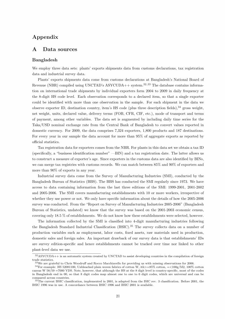
Appendix

A Data sources

Bangladesh

We employ three data sets: plants’ exports shipments data from customs declarations, tax registration

data and industrial survey data.

Plants’ exports shipments data come from customs declarations at Bangladesh’s National Board of

Revenue (NBR) compiled using UNCTAD’s ASYCUDA++ system.32,33 The database contains informa-

tion on international trade shipments by individual exporters form 2004 to 2009 in daily frequency at

the 8-digit HS code level. Each observation corresponds to a declared item, so that a single exporter

could be identified with more than one observation in the sample. For each shipment in the data we

observe exporter ID, destination country, item’s HS code (plus three description fields),34 gross weight,

net weight, units, declared value, delivery terms (FOB, CFR, CIF, etc.), mode of transport and terms

of payment, among other variables. The data set is augmented by including daily time series for the

Taka/USD nominal exchange rate from the Central Bank of Bangladesh to convert values reported in

domestic currency. For 2009, the data comprises 7,324 exporters, 1,800 products and 187 destinations.

For every year in our sample the data account for more than 95% of aggregate exports as reported by

official statistics.

Tax registration data for exporters comes from the NBR. For plants in this data set we obtain a tax ID

(specifically, a “business identification number” —BIN) and a tax registration date. The latter allows us

to construct a measure of exporter’s age. Since exporters in the customs data are also identified by BINs,

we can merge tax registries with customs records. We can match between 85% and 90% of exporters and

more than 90% of exports in any year.

Industrial survey data come from the Survey of Manufacturing Industries (SMI), conducted by the

Bangladesh Bureau of Statistics (BBS). The BBS has conducted the SMI regularly since 1973. We have

access to data containing information from the last three editions of the SMI: 1999-2001, 2001-2002

and 2005-2006. The SMI covers manufacturing establishments with 10 or more workers, irrespective of

whether they use power or not. We only have specific information about the details of how the 2005-2006

survey was conducted. From the “Report on Survey of Manufacturing Industries 2005-2006” (Bangladesh

Bureau of Statistics, undated) we know that the survey was based on the 2001-2003 economic census,

covering only 18.5 % of establishments. We do not know how these establishments were selected, however.

The information collected by the SMI is classified into 4-digit manufacturing industries following

the Bangladesh Standard Industrial Classification (BSIC).35 The survey collects data on a number of

production variables such as employment, labor costs, fixed assets, raw materials used in production,

domestic sales and foreign sales. An important drawback of our survey data is that establishments’ IDs

are survey edition-specific and hence establishments cannot be tracked over time nor linked to other

plant-level data we use.

32ASYCUDA++ is an automatic system created by UNCTAD to assist developing countries in the compilation of foreigntrade statistics.

33We are grateful to Chris Woodruff and Rocco Macchiavello for providing us with missing observations for 2006.34For example: HS 52081100, Unbleached plain woven fabrics of cotton W, ith>=85% cotton, =<100g/M2, 100% cotton

canvas W 58/59 =7000 YDS. Note, however, that although the HS at the 8 digit level is country-specific, most of the codesin Bangladesh end in 00, so that 8 digit codes map almost one to one to 6 digit codes, which are universal and can becompared across countries.

35The current BSIC classification, implemented in 2001, is adapted from the ISIC rev. 3 classification. Before 2001, theBSIC 1996 was in use. A concordance between BSIC 1996 and BSIC 2001 is available.

21

China, Colombia and Taiwan

For both China and Colombia we are able to employ export shipments from customs and industrial survey

data (although for confidentiality reasons we are not allowed to use merged datasets). For China, export

shipments data were collected by the Chinese Custom’s Office and cover the 2000-2006 period.36 For

Colombia, our data set includes all export transactions by Colombian firms between 2000 and 2012 and

comes from the Colombian Bureau of Statistics (Departamento Administrativo Nacional de Estadıstica,

DANE). See Eaton et al. (2008) for details.37

The Chinese industrial survey data we use are firm-level data from Annual Surveys of Industrial

Production from 1998 to 2007. These surveys are made by the Chinese National Bureau of Statistics and

include all of the state-owned enterprises (SOE) and non-SOEs with sales over 5 million RMB (USD0.6

million in 2000). See Bai et al. (2013) for additional details. The Colombian industrial data are annual

plant-level data originally collected by DANE, covering all plants with 10 or more employees. (Roberts

and Tybout, eds, 1996, Ch. 10) provide a detailed description of the data set.

Finally, the Taiwanese data was collected by the Ministry of Economic Affairs (MOEA) in Taiwan for

the years 2000 and 2002-2004.38 The data set is an unbalanced panel of plants that were in operation in

all four sample years and that reported information on domestic and export sales, capital stocks and R&D

expenditure. While the survey is conducted at the plant level, the distinction between plant and firm is

not important as the bulk of firms in the Taiwanese manufacturing sector own only a single plant.39

B Export processing zones

Fiscal incentives provided to firms locating in EPZs consist of a 10-year holiday for firms established

before January 1, 2012, while for firms established after December 31, 2011 the tax holiday schedule is

100% for the first 2 years, 50% for the next 2 years and 25% for the following (fifth) year. Additional

fiscal incentives include duty free import of construction materials, machineries, office equipment, raw

materials and finished goods, and exemption from dividend, municipal and regional taxes. Further non-

fiscal incentives include allowance of 100% foreign ownership, full repatriation of capital and dividends

and off-shore banking for foreign owned and joint-venture firms. Plants in EPZs also enjoy higher quality

of governance relative to plants outside EPZs in terms of issue of trade licenses, security and access to

utilities. Moreover, specific labor regulations apply in EPZs. Minimum wages and benefits for workers

are established by law, formation of labor unions is forbidden and strikes are prohibited. This is a big

deal in Bangladesh where strikes are common and costly.40

Bangladesh’s tax registration data allow us to observe exporter plants’ addresses, which indicate when

a plant is located in an EPZ.41 Looking at plants’ addresses we are able to identify which plants were in

an EPZ at the moment of entering the tax registration database. Given the nature of tax registration

36See Bai et al. (2013) for details. We are grateful to Jiandong Ju and Hong Ma for allowing us access to the Chinesedata.

37We thank Marcela Eslava for providing access to a more recent version of these data.38The survey was not conducted in 2001. In that year a manufacturing sector census was conducted by the Directorate

General of Budget, Accounting, and Statistics. This cannot be merged at the plant level with the MOEA survey data forthe other years.

39Over the period 2000-2004, 92.8 percent of the manufacturing plants were owned by single-plant firms.40The government has allowed the formation of Workers Welfare Committees (WWC), however. In a WWC, workers and

management representatives meet to discuss workplace related issues. In a survey of manufacturing plants, Rahman et al.(2008) found that 21 out of 38 EPZ factories had WWC in 2006.

41This is indicated directly, so we do not have to infer an EPZ location by the plant’s zip code, say. For example, considerthe following address of a plant located in the Adamjee EPZ: “Plot-38 & 55 Aadamjee EPZ.”

22

data, however, we cannot identify exporters moving in and out of EPZs over time. The number of plants

in EPZs changes in our data as firms enter or exit from exporting altogether.42

The 2008-2009 report of the Bangladesh Export Processing Zones Authority (BEPZA) identifies 305

firms operating in EPZs, of which 185 (60%) were 100% foreign owned, 48 (15%) were joint ventures and

74 (25%) were 100% local ventures. The number of exporters whose address is in an EPZ in our tax

records is 460. When we merge these records with customs data we are left with 287 firms that were in

an EPZ in at least one year. We are able to account for between 50% and 85% of total EPZ exports.43

Survey data prevent us from identifying exactly which firms are located in an EPZ. However, since we

see the zip code for each manufacturing establishment in the survey, we can identify which plants are in

districts where an EPZ is located. Table 11 presents some summary statistics. By 2005, 45% of surveyed

plants (2,367) were located in EPZ districts, and they accounted for 67% of total employment. Of these,

628 were exporters and accounted for 74% of total exports. In contrast, in non-EPZ districts there were

only 154 exporters out of 2,850 plants in 2005. Plants in EPZ districts tend to be larger, as total sales

per plant were US$2.0 million compared to US$1.2 million for plants located in non-EPZ districts.

To further compare producers in EPZ districts with those in non-EPZ districts, we compute differences

in plant characteristics within the same four-digit BSIC industry pooling all years. Table 12 reports that,

on average, establishments in EPZ districts pay higher wages, sell more and employ more workers. Being

located in an EPZ district does not appear to be significantly associated with differences in variable

cost and labor productivity.44 However, exporters located in an EPZ district do show higher labor

productivity.

Since in our EPZ districts we include two main industrial regions, Dhaka and Chittagong, where

factors other than proximity to an EPZ can affect plant characteristics, we compute differences in plant

characteristics excluding plants located in these two districts. The results are presented in the last three

columns of Table 12. The results do not differ qualitatively, but now being an exporter in an EPZ district

is more strongly associated to a lower age.

Table 11 also shows that EPZ districts export 77% of what is sold, compared to 58% for non-EPZ

districts. Table 13 further shows that individual exporters in EPZ districts are almost fully devoted to

exporting. Mean export intensity in EPZ districts is greater than 95% in any year of the survey. Export

intensity in districts with no EPZs is lower, but still high, with plants selling 87% of their sales abroad

in 2005. Moreover, around 95% of plants in EPZ districts sold more than 95% of their sales abroad in

2005, while 75% of plants in other districts did so in 2005.

The age profile of establishments in EPZ and non-EPZ districts for 2005 is described in Table 14.45

Non-exporting establishments in EPZ districts do not seem to be significantly younger than their coun-

terparts in non-EPZ districts. This is also the case if we focus on apparel and textiles producers, although

these are 6 year older on average than establishments producing other products. However, exporters in

EPZ districts are 7 and 8 years younger on average than exporters in non-EPZ districts, respectively. A

simple regression of age on EPZ districts location and exporter indicators confirms that being in an EPZ

district and exporting is strongly associated to a lower establishment age (see Table 15).

42As an example, consider a firm that was set up in 2000, then applied for a VAT in 2005 and started exporting thatsame year, but was not in an EPZ. Then its address in the VAT registration data would indicate the firm is not in an EPZ.We have no way of telling whether the firm moved to an EPZ in 2007, say, and continued to export.

43We take total EPZ exports from BEPZA official data as of 2010. Reports and data from BEPZA are available athttp://www.epzbangladesh.org.bd.

44We define variable cost as expenditures in raw materials, energy use and employment cost divided by gross output.Labor productivity is defined as gross output over number of workers. Both variables are constructed only for 1999 and2005 since we do not have data on gross output for 2001.

452005 is the only survey year for which we have the year of start-up, from which we compute establishment age.

23

References

Aggarwal, Aradhna, “Performance of Export Processing Zones: A Comparative Analysis of India, Sri

Lanka and Bangladesh,” ICRIER Working Paper, 2005, (155).

Albornoz, Facundo, Hector Calvo-Pardo, Gregory Corcos, and Emmanuel Ornelas, “Sequen-

tial Exporting,” Journal of International Economics, 2012, 88 (1), 17–31.

Amador, Joao and Luca David Opromolla, “Product and destination mix in export markets,”

Weltwirtschaftliches Archiv, 2013, 149 (1), 23–53.

Arbelaez, Marıa Angelica, Marcela Melendez, and Nicolas Leon, “The Emergence f Fresh Cut-

Flower Exports in Colombia,” in Charles Sabel, Eduardo Fernandez-Arias, Eduardo Hausmann, Andres

Rodrıguez-Clare, and Ernesto Stein, eds., Export Pioneers in Latin America, Cambridge, MA: Harvard

University, 2012, pp. 69–100.

Artopoulos, Alejando, Daniel Friel, and Juan Carlos Hallak, “Export emergence of differentiated

goods from developing countries: Export pioneers and business practices in Argentina,” Journal of

Development Economics, 2013, 105, 19–35.

Bai, Xue and Kala Krishna, “Self Inflicted Wounds? China’s Restrictions on Direct Exporting,”

2013. Unpublished manuscript.

, , and Hong Ma, “How You Export Matters: Export Mode, Learning and Productivity in China,”

2013. Unpublished manuscript.

Baldwin, Richard E. and Paul Krugman, “Persistent Trade Effects of Large Exchange Rate

Changes,” Quarterly Journal of Economics, 1989, 104 (4), 635–654.

Bangladesh Bureau of Statistics, “Report on Survey of Manufacturing Industries 2005-06,” Technical

Report undated.

Bernard, Andrew and J. Bradford Jensen, “Exporters, Jobs, and Wages in U.S. Manufacturing:

1976-1987,” Brooking Papers on Economic Activity. Microeconomics, 1995, 1995, 67–112.

and Joachim Wagner, “Export and Success in German Manufacturing,” Weltwirtschaftliches Archiv,

1997, 133 (1), 134–157.

, Jonathan Eaton, J. Bradford Jensen, and Samuel Kortum, “Plants and Productivity in

International Trade,” American Economic Review, 2003, 93 (4), 1268–1290.

Brambilla, Irene, Amit Khandelwal, and Peter Schott, “China’s Experience under the Multi-

Fiber Arrangement (MFA) and the Agreement on Textile and Clothing (ATC),” in Robert C. Feenstra

and Shang-Jin Wei, eds., China’s Growing Role in World Trade, Cambridge, MA: NBER Books, 2010.

Cherkashin, Ivan, Svetlana Demidova, Hiau Looi Kee, and Kala Krishna, “Firm Heterogeneity

and Costly Trade: A New Estimation Strategy and Policy Experiments,” Journal of International

Economics, forthcoming.

Condo, Arturo, Mauricio Jenkins, Luis Figueroa, Luis Obando, Luis Morales, and Luis

Reyes, “El Sector Textil Exportador Latinoamericano Ante la Liberalizacion del Comercio,” Technical

Report 1605, CLADS/INCAE 2004.

24

Dai, Mi, Madhura Maitra, and Miaojie Yu, “Unexceptional Exporter Performance in China? The

Role of Processing Trade,” 2012. Mimeo, Peking University - China Center for Economic Research.

Das, Sanghamitra, Mark J. Roberts, and James R. Tybout, “Market entry costs, producer

heterogeneity, and export dynamics,” Econometrica, 2007, 75 (3), 837–873.

Dayarathna-Banda, O. G. and John Whalley, “After the MFA, the CCAs,” CIGI Working Paper,

2007, (24).

Dixit, Avinash, “Hysteresis, Import Penetration, and Exchange Rate Pass-Through,” Quarterly Journal

of Economics, 1989, 104 (2), 205–228.

Eaton, Jonathan, Marcela Eslava, David Jinkins, C. J. Krizan, Maurice Kugler, and

James R. Tybout, “A Search and Learning Model of Export Dynamics,” 2014. Unpublished

manuscript.

, , Maurice Kugler, and James Tybout, “The Margins of Entry into Export Markets: Evidence

from Colombia,” in Elhanan Helpman, Dalia Marin, and Thiery Verdier, eds., The Organization of

Firms in a Global Economy, Cambridge, MA: Harvard University Press, 2008.

, Samuel Kortum, and Francis Kramarz, “Dissecting Trade: Firms, Industries, and Export

Destinations,” The American Economic Review, 2004, 94 (2, Papers and Proceedings of the 116th

Annual Meeting of the AEA.), 150–154.

, , and , “An Anatomy of International Trade: Evidence from French Firms,” Econometrica,

2011, 79 (5), 1453–1498.

Feenstra, Robert C., Robret E. Lipsey, Haiyan Deng, Alyson C. Ma, and Hengyong Mo,

“World Trade Flows: 1962-2000,” NBER Working Paper, 2005, (11040).

Gebreeyesus, Mulu and Michiko Iizuka, “Discovery of the Flower Industry in Ethiopia: Experi-

mentation and Coordination,” UNU-MERIT Working Paper, 2010, (25).

Hausmann, Ricardo and Dani Rodrik, “Economic Development as Self-Discovery,” Journal of De-

velopment Economics, 2003, 72 (2), 603–633.

Iacovone, Leonardo and Beata S. Javorcik, “Multi-product exporters: Product churning, uncer-

tainty, and export discoveries,” Economic Journal, 2010, 120 (May), 481–499.

Impullitti, Giammario, Alfonso Irarrazabal, and Luca David Opromolla, “A Theory of Entry

into and Exit from Export Markets,” Journal of International Economics, 2013, 90 (1), 75–90.

Kee, Hiau Looi, “Local intermediate inputs and the shared supplier spillovers of foreign direct invest-

ment,” Journal of Development Economics, January 2015, 112, 56–71.

Khandelwal, Amit K., Peter K. Schott, and Shang-Jin Wei, “Trade Liberalization and Embedded

Institutional Reform: Evidence from Chinese Exporters,” American Economic Review, 2013, 103 (6),

2169–2195.

Lu, Dan, “Exceptional Exporter Performance? Evidence from Chinese Manufacturing Firms,” 2010.

Unpublished.

25

Matthews, John A., “Electronics in Taiwan: A Case of Technological Learning,” in Vandana Chandra,

ed., Technology, Adaptation and Exports. How Some Developing Countries Got It Right, Washington,

DC: The World Bank, 2006.

McWilliams, Bruce and Rubina Verma, “Exporters, Export Intensity and Productivity,” 2012.

Unpublished manuscript.

Melitz, Marc J., “The Impact of Trade on Intra-Industry Reallocations and Aggregate Industry Pro-

ductivity,” Econometrica, 2003, 71 (6), 1695–1725.

Mendez, Jose, “The Development of the Colombian Cut Flower Industry,” World Bank Policy Research

Working Paper Series, 1991, (660).

Mostafa, Romel and Steven Klepper, “Industrial Development Through Tacit Knowledge Seeding:

Evidence from the Bangladesh Garment Industry,” Working Paper, Department of Social and Decision

Science, Carnegie Mellon University, 2009.

Nguyen, Daniel X., “Demand Uncertainty: Exporting Delays and Exporting Failures,” Journal of

International Economics, 2012, 86 (2), 336–344.

Rahman, Mustafizur, Debapriya Bhattacharya, and Khondaker Golam Moazzem, Bangladesh

Apparel Sector in Post-MFA Era: A Study on the Ongoing Restructuring Process, Dhaka: Centre for

Policy Dialogue, 2008.

Rasiah, Rajah, “Electronics in Malaysia: Export Expansion but Slow Technical Change,” in Vandana

Chandra, ed., Technology, Adaptation and Exports. How Some Developing Countries Got It Right,

Washington, DC: The World Bank, 2006.

Rauch, James E. and Joel Watson, “Starting small in an unfamiliar environment,” International

Journal of Industrial Organization, 2003, 21 (7), 1021–1042.

Rhee, Yung Whee and Therese Belot, “Export Catalysts in Low-Income Countries: A Review of

Eleven Success Stories,” World Bank Discussion Paper, 1990, (72).

Roberts, Mark and James Tybout, eds, Industrial Evolution in Developing Countries, New York:

Oxford University Press, 1996.

Roberts, Mark J., “Colombia, 1977-1983: Producer Turnover, Margins and Trade Exposure,” in

Mark J. Roberts and James R. Tybout, eds., Industrial Evolution in Developing Countries, Oxford

University Press, 1996, pp. 227–259.

and James R. Tybout, “The decision to export in Colombia: an empirical model of entry with

sunk costs,” The American Economic Review, 1997, 87 (4), 545–564.

26

Tab

le1:

Con

trib

uti

onof

pair

wis

een

try

an

dex

itto

the

gro

wth

of

exp

ort

sb

etw

eent

an

dt−

1.

Pair

wis

eco

nti

nu

ing

Pair

wis

een

teri

ng

Pair

wis

eex

itin

g

Yea

r(t

)G

row

thS

hare

int−

1G

row

thC

ontr

ibu

tion

Ad

ded

firm

sR

el.

exp

ort

sC

ontr

ibu

tion

Dro

pp

edfi

rms

Rel

.ex

port

sC

ontr

ibu

tion

(1)

(2)

(3)

(2)×

(3)/

(1)

(5)

(6)

[(5)

+(6

)]/(1

)(8

)(9

)[(

8)

+(9

)]/(1

)

Ban

gla

des

h

An

nu

al

Aver

age

15.0

96.6

11.1

72.8

25.4

-19.8

38.6

-16.4

15.1

-11.4

2004-2

009

71.9

70.8

44.7

44.7

63.5

-14.2

68.6

-25.9

16.8

-12.6

Colo

mb

ia

An

nu

al

Aver

age

3.1

94.2

3.6

81.3

38.9

-33.4

47.7

-38.8

33.5

-29.0

2000-2

012

36.4

66.5

55.4

101.2

65.5

-32.2

91.6

-66.6

32.8

-92.7

Ch

ina

An

nu

al

aver

age

25.8

91.8

16.6

58.5

38.7

-25.2

56.8

-15.1

12.2

-15.4

2000-2

006

130.4

30.1

44.5

10.3

131.4

-3.0

98.5

-19.2

7.8

-8.8

Note

:P

air

wis

eco

nti

nu

ing

firm

sin

yea

rt

are

those

that

exp

ort

edint−

1an

dt.

Pair

wis

een

teri

ng

firm

sint

are

those

that

exp

ort

edint

bu

tn

ot

int−

1.

Pair

wis

eex

itin

gfi

rms

int

are

those

that

exp

ort

edint−

1b

ut

not

int.

Per

centa

ge

contr

ibu

tion

of

each

gro

up

toth

egro

wth

of

tota

lex

port

sis

rep

ort

edin

colu

mn

s4,

7an

d10.

All

com

pu

tati

on

su

sevalu

esin

US

D.

27

Table 2: Product specialization (selected products), Bangladesh (2005).

Product description Export intensity Share of exports Share of domestic sales

Top-10 products by share of exports

Garments, all types 99.40 62.83 0.41Woolen jumpers 100.00 3.67 0.00Jute yarn and twist 94.22 1.93 0.13Cloth and cotton fabrics 40.67 1.42 2.21Cotton yarn (all counts) 30.82 0.94 2.26Finished leather 95.08 0.85 0.05Leather and cow hides 97.91 0.72 0.02Woven fabrics (nec) 100.00 0.72 0.00Silk fabrics 67.88 0.66 0.33Cotton yarn (up to 10 counts) 43.45 0.42 0.58

Top-10 products by share of domestic sales

Iron and steel rods and bars 0.00 0.00 9.13Motorcycles 0.00 0.00 8.63Brick (ordinary) 0.01 0.00 6.54Cigarettes 1.69 0.10 6.24Cement 0.58 0.03 5.06Leather boots and shoes (gents) 8.32 0.23 2.68Dhoties and sarees 0.00 0.00 2.28Cotton yarn (all counts) 30.82 0.94 2.26Cloth and cotton fabrics 40.67 1.42 2.21Iron and steel sheets (nec) 2.23 0.04 1.73Newspapers (Bengali) 0.05 0 1.51

Note: based on survey data from the Bangladesh Bureau of Statistics, applying firms sample weightsto construct aggregate figures. Export intensity is defined as the share of exports in total sales fora particular product. Products are 6-digit Bangladesh Standard Industrial Classification (BSIC)codes. Food commodities are excluded (frozen fish, rice, etc.).

Table 3: Exports and exporters by activity of the plant, Bangladesh(apparel and textiles).

2004 2005 2006 2007 2008 2009

A. Exports as % of total apparel and textiles exports

Manufacturer and exporter 98.0 97.9 98.1 97.5 97.7 97.3Traders and other activity 0.9 1.0 1.1 1.3 1.1 1.3Other exporters 1.2 1.1 0.9 1.2 1.2 1.4

B. Number of exporters

Manufacturer and exporter 2,595 2,723 2,926 3,272 3,509 3,548Traders and other activity 217 295 347 537 569 664Other exporters 385 466 505 715 802 864

Note: only plants in the apparel and textiles sector are included. Based oncustoms and tax data from Bangladesh’s National Board of Revenue.

28

Table 4: Firms by initial export year cohorts. Appareland textiles, Bangladesh.

YearCohort

Total2004 2005 2006 2007 2008 2009

A. Number of firms

2004 3,197 3,1972005 2,654 830 3,4842006 2,334 563 881 3,7782007 2,098 446 639 1,341 4,5242008 1,903 359 508 921 1,189 4,8802009 1,705 301 420 699 757 1194 5,076

B. Value of exports (US$ million)

2004 6,660 6,6602005 7,797 999 8,7962006 8,510 865 402 9,7772007 8,997 1,030 1,052 474 11,5532008 9,322 1,108 1,281 1,236 433 13,3802009 8,800 1,102 1,373 1,498 949 413 14,135

C. Exports per firm (US$ million)

2004 2.1 2.12005 2.9 1.2 2.52006 3.6 1.5 0.5 2.62007 4.3 2.3 1.6 0.4 2.62008 4.9 3.1 2.5 1.3 0.4 2.72009 5.2 3.7 3.3 2.1 1.3 0.3 2.8

Note: a firm is classified as belonging to cohort x if the firm firstreported exporting in year x. If a cohort x firm exits in a givenyear t and re-enters in some future period x + n, it is treated asbelonging to cohort x+ n (i.e. it switches cohorts).

29

Table 5: Firms by initial export year cohorts. Apparel and textiles,China.

YearCohort

Total2000 2001 2002 2003 2004 2005 2006

A. Number of firms

2000 13,644 13,6442001 11,040 4,177 15,2172002 9,475 3,195 6,393 19,0632003 8,507 2,804 5,299 8,790 25,4002004 7,630 2,462 4,649 7,154 13,539 35,4342005 6,852 2,242 4,183 6,090 10,368 14,981 44,7162006 6,114 1,991 3,803 5,334 8,745 11,566 20,063 57,616

B. Value of exports (US$ million)

2000 25,672 25,6722001 26,128 2,103 28,2312002 25,490 4,807 3,842 34,1392003 26,611 5,831 9,238 6,059 47,7392004 27,172 6,159 10,634 13,398 9,012 66,3752005 26,919 6,385 11,972 15,844 18,508 9,501 89,1292006 27,095 6,822 13,005 16,529 20,357 20,061 17,923 121,791

C. Exports per firm (US$ million)

2000 1.9 1.92001 2.4 0.5 1.92002 2.7 1.5 0.6 1.82003 3.1 2.1 1.7 0.7 1.92004 3.6 2.5 2.3 1.9 0.7 1.92005 3.9 2.8 2.9 2.6 1.8 0.6 2.02006 4.4 3.4 3.4 3.1 2.3 1.7 0.9 2.1

Note: a firm is classified as belonging to cohort x if the firm first reported exportingin year x. If a cohort x firm exits in a given year t and re-enters in some futureperiod x+ n, it is treated as belonging to cohort x+ n (i.e. it switches cohorts).

30

Table 6: Firms by initial export year cohorts. Apparel and textiles, Colombia.

YearCohort

Total2000 2001 2002 2003 2004 2005 2006 2007 2008 2009 2010 2011 2012

A. Number of firms

2000 2,079 2,0792001 1,331 1,147 2,4782002 1,035 474 1,080 2,5892003 863 297 433 1,362 2,9552004 768 222 290 463 1,917 3,6602005 591 133 160 227 417 1,388 2,9162006 530 111 126 170 273 715 927 2,8522007 487 96 105 131 210 475 417 1,067 2,9882008 448 82 85 101 164 332 239 478 975 2,9042009 396 68 60 71 127 235 147 253 407 971 2,7352010 352 56 51 55 92 173 93 138 167 266 678 2,1212011 320 49 45 47 76 139 62 100 105 137 288 723 2,0912012 291 44 38 39 62 109 53 76 72 98 194 297 679 2,052

B. Value of exports (US$ million)

2000 893 8932001 894 54 9482002 750 40 27 8172003 843 39 36 36 9542004 1,024 70 49 57 97 1,2972005 1,117 67 51 62 56 51 1,4042006 1,150 55 51 43 78 79 35 1,4912007 1,415 122 50 65 129 162 114 183 2,2402008 1,337 118 42 58 109 198 93 200 233 2,3882009 797 61 24 25 33 103 48 63 131 116 1,4012010 810 43 28 33 33 44 40 22 31 24 81 1,1892011 908 51 21 22 24 39 49 26 24 36 25 46 1,2712012 891 53 15 21 20 34 56 25 21 38 29 55 33 1,291

C. Exports per firm (US$ million)

2000 0.43 0.432001 0.67 0.05 0.382002 0.72 0.08 0.03 0.322003 0.98 0.13 0.08 0.03 0.322004 1.33 0.32 0.17 0.12 0.05 0.352005 1.89 0.50 0.32 0.27 0.13 0.04 0.482006 2.17 0.50 0.40 0.25 0.29 0.11 0.04 0.522007 2.91 1.27 0.48 0.50 0.61 0.34 0.27 0.17 0.752008 2.98 1.44 0.49 0.57 0.66 0.60 0.39 0.42 0.24 0.822009 2.01 0.90 0.40 0.35 0.26 0.44 0.33 0.25 0.32 0.12 0.512010 2.30 0.77 0.55 0.60 0.36 0.25 0.43 0.16 0.19 0.09 0.12 0.562011 2.84 1.04 0.47 0.47 0.32 0.28 0.79 0.26 0.23 0.26 0.09 0.06 0.612012 3.06 1.20 0.39 0.54 0.32 0.31 1.06 0.33 0.29 0.39 0.15 0.19 0.05 0.63

Note: a firm is classified as belonging to cohort x if the firm first reported exporting in year x. If a cohort x firm exitsin a given year t and re-enters in some future period x + n, it is treated as belonging to cohort x + n (i.e. it switchescohorts).

Table 7: Age when entering foreign markets.

Apparel and textiles Other sectors

Mean Median Mean Median

Bangladesh 2.0 0.4 2.6 0.8China 5.0 3.0 6.1 3.7Colombia 11.5 8.1 14.6 10.5Taiwan 11.9 10.7 7.2 4.7

Note: figures are annual averages as follows: Bangladesh (2005-2009), China (2001-2006), Colombia (1983-1989) and Taiwan (2002-2004). Age at entry for an exporteris determined by the year it entered an export cohort and the date of tax registration(for Bangladesh) or firm start up (for Colombia, China and Taiwan).

31

Table 8: Exporters in export processing zones (EPZ), Bangladesh, 2004-2009.

2004 2005 2006 2007 2008 2009

Plants in EPZs

Exports (US$ million) 775 1,551 1,099 1,277 1,422 1,594Apparel and textiles 698 1,466 1,009 1,182 1,340 1,500

Number of plants 146 169 168 210 213 238Apparel and textiles 94 110 122 151 153 163

Number of products 338 340 360 378 389 418Number of destinations 88 82 93 87 98 96Exports per plant (US$ million) 5.3 9.2 6.5 6.1 6.7 6.7

Apparel and textiles 7.4 13.3 8.3 7.8 8.8 9.2

Plants outside EPZs

Exports (US$ million) 6,865 8,329 9,839 11,832 13,360 14,035Number of plants 4,542 4,960 5,034 5,827 6,257 6,469Number of products 1,334 1,425 1,459 1,400 1,449 1,532Number of destinations 172 171 178 186 182 185Exports per plant (US$ million) 1.5 1.7 2.0 2.0 2.1 2.2

EPZ exports (% of total) 10.1 15.7 10.0 9.7 9.6 10.2Data as % of BEPZA 50.0 84.5 53.3 52.6 55.1 56.5

Notes: source is Bangladesh customs and tax registration data. Location in an EPZ is determined by theaddress of the plant. Last row computes EPZ exports in our data (the one to last row) as a percentage oftotal EPZ exports as reported by BEPZA.

Table 9: Plant age by EPZ status, Bangladesh, 2009.

Age Age at entry

Mean Median Mean Median

Apparel and textiles

Non-EPZ 6.74 5.09 2.00 1(0.08) (0.13)

EPZ 7.41 6.03 1.92 1(0.37) (0.57)

Other

Non-EPZ 6.39 4.81 1.94 0(0.13) (0.17)

EPZ 7.29 6.50 2.00 1(0.47) (0.75)

Notes: source is Bangladesh customs and tax registration data. Lo-cation in an EPZ is determined by the address of the firm. Appareland textiles sector are HS 2-digit codes 42, 43 and 50-65. Standarderrors between parenthesis.

32

Table 10: Born to export plants by EPZ status, 2004-2009.

2004 2005 2006 2007 2008 2009

Plants in EPZs

No. of BTE plants 39 54 52 80 81 98% of total 26.7 32.0 31.0 38.1 38.0 41.2

Exports (US$ million) 37.4 725.1 114.7 196.8 311.3 370.0% of total 4.8 46.8 10.4 15.4 21.9 23.2% apparel and textiles 55.2 97.8 90.2 88.7 92.7 94.4

Plants outside EPZs

No. of BTE plants 1,093 1,601 1,907 2,542 2,922 3,179% of total 24.1 32.3 37.9 43.6 46.7 49.1

Exports (US$ million) 601.5 1,295.1 2,078.8 2,895.5 3,684.6 4,311.2% of total 8.8 15.5 21.1 24.5 27.6 30.7% apparel and textiles 84.3 86.4 91.1 90.0 93.0 91.2

Notes: source is Bangladesh customs and tax registration data. Location in an EPZ is determinedby the address of the firm. Born to export (BTE) plants are defined as plants that began to exportwithin 1 year or less from start-up. Apparel and textiles sector are HS 2-digit codes 42, 43 and50-65.

Table 11: Characteristics of EPZ districts, by survey year.

1999 2001 2005

Plants in EPZs districts

Number of plants 1,247 1,583 2,367Number of exporters 750 824 628Exports (US$ million) 1,833.8 1,688.2 2,402.6Total sales 3,021.3 2,843.0 4,790.0Employment 514,345 470,185 600,917Exports/Total sales (%) 60.7 59.4 50.2Sales per plant (US$ million) 2.4 1.8 2.0

Plants outside EPZs districts

Number of plants 2,464 2,864 2,850Number of exporters 90 128 154Exports (US$ million) 298.5 461.9 1,688.3Total sales (US$ million) 976.9 1,228.8 3,357.2Employment 232,449 222,188 300,171Exports/Total sales (%) 30.6 37.6 50.3Sales per plant (US$ million) 0.4 0.4 1.2

EPZ exports (% of total) 91.0 86.0 73.9EPZ employment (% of total) 68.9 67.9 66.7

Notes: EPZ districts are those districts in which there is an EPZ. It isnot necessarily the case that all establishments in these districts are in factlocated in an EPZ.

33

Table 12: Establishment characteristics among EPZ and non-EPZ districts.

All districts Dhaka & Chittagong excluded

Plant characteristic EPZ Exporter and EPZ Observations EPZ Exporter and EPZ Observations

Variable cost −0.011 0.033 8, 906 0.019 −0.012 6, 095(−0.023) (−0.037) (−0.034) (−0.098)

Labor productivity −0.023 0.437∗ 8, 904 −0.212∗ 0.696∗ 6, 094(−0.035) (−0.057) (−0.049) (−0.138)

Employment 0.119∗ 0.660∗ 13, 371 −0.012 0.641∗ 9, 141(−0.024) (−0.039) (−0.034) (−0.085)

Total sales 0.163∗ 0.923∗ 12, 650 −0.072 1.149∗ 8, 659(−0.040) (−0.066) (−0.053) (−0.133)

Wage 0.081∗ −0.002 13, 330 0.024 0.045 9, 101(−0.018) (−0.028) (−0.024) (−0.060)

Fixed assets −0.136∗ 0.901∗ 13, 356 −0.304∗ 1.221∗ 9, 136(−0.042) (−0.067) (−0.056) (−0.141)

Notes: standard errors in parenthesis. Differences are obtained from a regression of the form lnYij = β0 + β1EPZij +β2EXEPZ

ij + Ij + εij , where i indexes plants, j indexes four-digit BSIC industries; EPZ are plants in EPZ districts, and

EXEPZ are exporters in EPZ districts; I are industry dummies and Y is the plant characteristic. ∗,∗∗ and + indicatesignificance at the 1%, 5% and 10% level, respectively.

Table 13: Export intensity (X/Y ) for exporters in EPZ districts.

Mean X/Y % with X/Y ≥ 95%

1999 2001 2005 1999 2001 2005

Non-EPZ 82.3 75.9 87.1 66.7 58.6 75.3EPZ 97.0 97.0 96.4 94.1 94.1 94.8

Note: Export intensity is defined as exports as a share of total sales.

Table 14: Age of establishments in and out of EPZ districtsand by export status.

Non-exporters Exporters

Mean Median Mean Median

Apparel and textiles producers

Non-EPZ 19.3 13 17.1 10.5EPZ 18.9 18 9.1 8

Non-apparel and textiles producers

Non-EPZ 13.2 10 19.5 14.5EPZ 13.1 9 12.5 6

Note: Age is computed using the year of start of operations.

34

Table 15: Establishment age differences between EPZ and non-EPZdistricts.

All districts Dhaka & Chittagong excluded

Located in EPZ district 0.236 0.905(−0.670) (−0.876)

Exporter 5.563∗ 5.794∗

(−1.765) (−1.983)Exporter in an EPZ district −5.173∗∗ −14.207∗

(−2.080) (−4.368)Constant 27.764∗∗ 27.095∗∗

(−12.99) (−13.348)Observations 3, 086 2, 592

Notes: standard errors in parenthesis. Age differences are obtained from aregression of the form Aij = β0 + β1EPZij + β2EXij + β3EXEPZ

ij + Ij +εij , where i indexes plants, j indexes four-digit BSIC industries; EPZ areplants in EPZ districts, EX are exporters, and EXEPZ are exporters in EPZdistricts; I are industry dummies and A is establishment age. ∗,∗∗ and +

indicate significance at the 1%, 5% and 10% level, respectively.

Table 16: Calibrated parameter values.

Parameter Description Value

Model

α Beta distribution parameter 3β Beta distribution parameter 6σ Elasticity of substitution 5r Rate of time preference 0.05δ Exogenous match separation rate 0.3298γ Cost function parameter 38.5289F Fixed cost of maintaining a relationship 34.1008Fλ Fixed cost of searching 0.1891

Stochastic processes

ϕ Mean of productivity process 0ρϕ Root of productivity process 0.7724σεϕ Std. dev. of innovation, productivity process 0.4344x Mean of foreign shock process 0ρϕ Root of foreign shock process 0.953σεx Std. dev. of innovation, foreign shock process 0.052y Mean of match-specific shock process 0ρϕ Root of match-specific shock process 0.6033σεy Std. dev. of innovation, match-specific shock process 0.8913

Discretization

#(θ) Number of discretized values, product appeal 100#(ϕ) Number of discretized values, productivity shock 30#(x) Number of discretized values, foreign shock 15#(y) Number of discretized values, match-specific shock 30#(n) Max. number of signals per firm 50

35

Aggregate trends: share in world exports

0.00

2.00

4.00

6.00

8.00

10.00

12.00

0.00

0.05

0.10

0.15

0.20

0.25

0.30

0.35

1978 1981 1984 1987 1990 1993 1996 1999 2002 2005 2008 2011

BGD (left)

COL (left)

CHN (right)

TWN (right)

(a) Share in world merchandise exports (%).

40.0

50.0

60.0

70.0

80.0

90.0

100.0

1978 1981 1984 1987 1990 1993 1996 1999 2002 2005 2008 2011

BGD

CHN

COL

(b) Share exported to high income economies (% of total mer-chandise exports).

Figure 1. Aggregate exports: Bangladesh, China, Colombia and Taiwan, 1978-2011.

36

10

100

1000

10000

100000

1000000

1972 1975 1978 1981 1984 1987 1990 1993 1996 1999 2002 2005

BGD

CHN

COL

TWN

(a) Log of total exports (US$ million).

0.0

10.0

20.0

30.0

40.0

50.0

60.0

70.0

80.0

90.0

100.0

1972 1975 1978 1981 1984 1987 1990 1993 1996 1999 2002 2005

BGD

CHN

COL

TWN

(b) Share in manufacturing exports (%).

Figure 2. Apparel and textile exports: Bangladesh, China, Colombia and Taiwan, 1972-2007.

37

0.1

.2.3

.4.5

.6.7

.8.9

1Fr

actio

n

0 20 40 60 80 100Export intensity

(a) Bangladesh (2005).

0.1

.2.3

.4.5

.6.7

.8.9

1Fr

actio

n

0 20 40 60 80 100Export intensity

(b) China (2006).

0.1

.2.3

.4.5

.6.7

.8.9

1Fr

actio

n

0 20 40 60 80 100Export intensity

(c) Colombia (1989).

0.1

.2.3

.4.5

.6.7

.8.9

1Fr

actio

n

0 20 40 60 80 100Export intensity

(d) Taiwan (2004).

Figure 3. Histograms of exporters’ export intensities.

38

0.00

0.10

0.20

0.30

0.40

0.50

0.60

1 2 3 4 5 6 7 8 9 10

Shar

e of

firm

s

Age group

BGD

Apparel and textiles Other sectors

0.00 0.10 0.20 0.30 0.40 0.50 0.60 0.70

1 2 3 4 5 6 7 8 9 10

Shar

e of

firm

s

Age group

CHN

Apparel and textiles Other sectors

0.00 0.10 0.20 0.30 0.40 0.50 0.60 0.70

1 2 3 4 5 6 7 8 9 10

Shar

e of

firm

s

Age group

COL

Apparel and textiles Other sectors

0.00 0.10 0.20 0.30 0.40 0.50 0.60 0.70

1 2 3 4 5 6 7 8 9 10

Shar

e of

firm

s

Age group

TWN

Apparel and textiles Other sectors

Figure 4. Fraction of total firms in an entering cohort by firm age group .

0.00

0.10

0.20

0.30

0.40

0.50

0.60

1 2 3 4 5 6 7 8 9 10

Shar

e of

firm

s

Age group

BGD

Apparel and textiles Other sectors

0.00 0.10 0.20 0.30 0.40 0.50 0.60 0.70

1 2 3 4 5 6 7 8 9 10

Shar

e of

firm

s

Age group

CHN

Apparel and textiles Other sectors

0.00 0.10 0.20 0.30 0.40 0.50 0.60 0.70

1 2 3 4 5 6 7 8 9 10

Shar

e of

firm

s

Age group

COL

Apparel and textiles Other sectors

0.00 0.10 0.20 0.30 0.40 0.50 0.60 0.70

1 2 3 4 5 6 7 8 9 10

Shar

e of

firm

s

Age group

TWN

Apparel and textiles Other sectors

Figure 5. Share of total exports in an entering cohort by firm-age group.

39

010

2030

4050

010

2030

4050

−0.04

−0.02

0

0.02

0.04

0.06

Failures

Search intensity (average)

Successes

(a)

010

2030

4050

010

2030

4050

−0.04

−0.02

0

0.02

0.04

0.06

Failures

Search intensity (high productivity)

Successes

(b)

Figure 6. Differences in search policies, ∆λ(·).

0

5

10

15

0

10

20

30−1

−0.8

−0.6

−0.4

−0.2

0

Foreign shock

Entry policy

Productivity

(a) χe(ϕ0, x; 3000, 0.3)− χe(ϕ0, x; 0, 0.3)

0

5

10

15

0

10

20

300

0.5

1

1.5

2

Foreign shock

Entry policy

Productivity

(b) χe(ϕ0, x; 3000, 0.3)− χe(ϕ0, x; 3000, 0)

Figure 7. Market entry with and without sunk costs and scrap values.

40

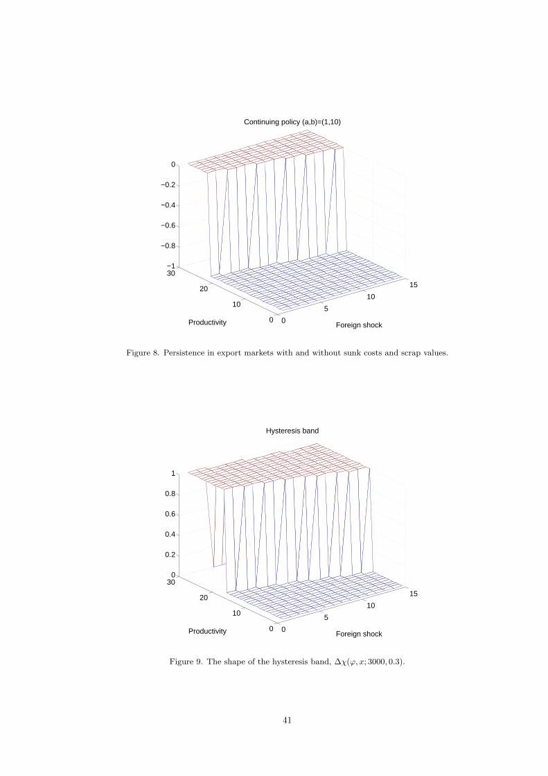
0

5

10

15

0

10

20

30−1

−0.8

−0.6

−0.4

−0.2

0

Foreign shock

Continuing policy (a,b)=(1,10)

Productivity

Figure 8. Persistence in export markets with and without sunk costs and scrap values.

0

5

10

15

0

10

20

300

0.2

0.4

0.6

0.8

1

Foreign shock

Hysteresis band

Productivity

Figure 9. The shape of the hysteresis band, ∆χ(ϕ, x; 3000, 0.3).

41

0 10 20 30 40 500

1

2

3

4

5

6

7x 10

4 Evolution of succesful and failed matches (K=0,psi=0)

Period

Suc

cess

es a

nd fa

ilure

s

SuccessesFailures

(a) K = 0, ψ = 0

0 10 20 30 40 500

500

1000

1500Evolution of succesful and failed matches (K>0,psi>0)

Period

Suc

cess

es a

nd fa

ilure

s

SuccessesFailures

(b) K = 3000, ψ = 0.3

0 10 20 30 40 500

1000

2000

3000

4000

5000

6000

Period

Suc

cess

es a

nd fa

ilure

s

SuccessesFailures

(c) K = 3000, ψ = 0

Figure 10. Aggregate successes and failures.

0 10 20 30 40 500

2

4

6

8

10Number of exporters and foreign shock trajectories

Exp

orte

rs (

log)

Period

−0.5

0

0.5

For

eign

sho

ck (

log)

K=0,psi=0K>0,psi=0K>0,psi>0

Figure 11. (Log of) Total exporters and foreign shock trajectories.

42

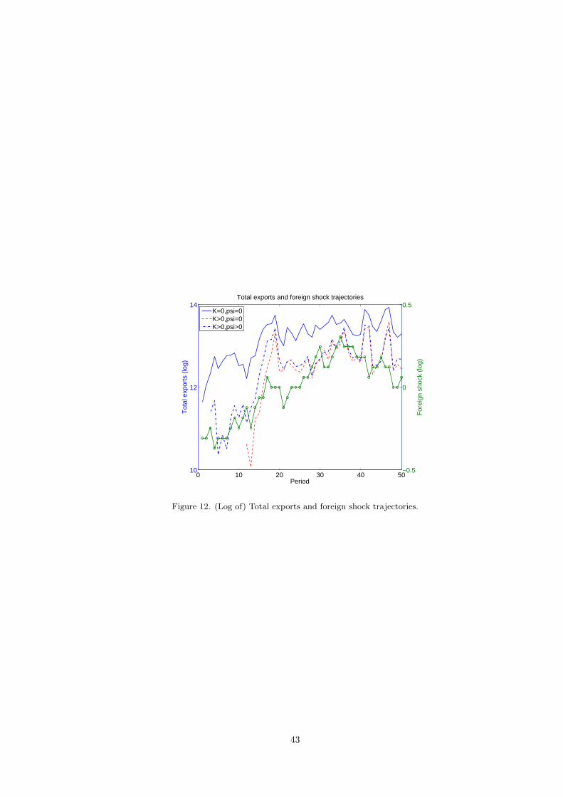
0 10 20 30 40 5010

12

14Total exports and foreign shock trajectories

Tot

al e

xpor

ts (

log)

Period

−0.5

0

0.5

For

eign

sho

ck (

log)

K=0,psi=0K>0,psi=0K>0,psi>0

Figure 12. (Log of) Total exports and foreign shock trajectories.

43