Biometric Face Skintone Data Augmentation Using A ...

Biometric Face Skintone DataAugmentation Using A Generative

Adversarial Network

byRosalin Dash

Bachelor Of TechnologyElectronics and Communication Engineering

Gandhi Institute of Engineering and Technology2012

A thesissubmitted to the College of Engineering and Science at

Florida Institute of Technologyin partial fulfillment of the requirements

for the degree of

Master of Sciencein

Computer Science

Melbourne, FloridaDecember, 2020

We, the undersigned committee, hereby approve the attached thesis.

Biometric Face Skintone Data Augmentation Using A GenerativeAdversarial Network

byRosalin Dash

Michael King, Ph.D.Major AdvisorAssociate ProfessorComputer Engineering and Sciences

Kevin Bowyer, Ph.D.Committee MemberHonorary ProfessorBiomedical Technologies

Munevver Mine Subasi, Ph.D.Outside Committee MemberAssociate Professor and Department HeadMathematical Sciences

Philip Bernhard, Ph.D.Associate Professor and Department HeadAssociate ProfessorComputer Engineering and Sciences

Abstract

Title:

Biometric Face Skintone Data Augmentation Using A Generative Adversarial

Network

Author:

Rosalin Dash

Thesis Advisor:

Michael King, Ph.D.

Researchers seek methods to increase the accuracy and efficiency in identifying an

individual using facial biometric systems. Factors like skin color, which may affect

the accuracy of facial recognition, need to be investigated further. To analyze

the impact of race with respect to skin color of face on biometric systems, we

focused on generating a dataset with uniformly distributed images of different skin

tones while preserving identities. Deep learning neural network architectures like

the generative adversarial network (GAN) focus on modifying only certain features

of the face like the color of the skin. In our experimental approach, we implemented

iii

a cycle GAN to synthesize multiple images of individuals with varying color of their

skin based on the Fitzpatrick scale. The Fitzpatrick scale defines six levels of skin

tone, with FP-1 representing a lighter and FP-6 a darker shade of color. The

resulting GAN receives an image of a person with a skin tone labeled FP-1 as its

input and synthesizes five additional images to show what that person would look

like with skin-tone ratings of FP-2 to FP-6. A GAN was trained to receive an image

of a person with a skin-tone rating of FP-6 and subsequently to produce images

corresponding to skin-tone ratings of FP-5 to FP-1. The Arcface matcher was

used to measure the similarity between the original images of a person and those

produced by the GAN. The results of the analysis indicate a drop in the similarity

scores when skin tones change from light to dark and vice versa. In future work, we

intend to train a facial recognition algorithm to evaluate the impact of bias relative

to skin tone with uniformly generated improved version of skin color images of the

same individual.

iv

Table of Contents

List of Figures viii

List of Tables xi

Acknowledgments xii

1 Introduction 1

2 Background 4

2.1 Biometrics . . . . . . . . . . . . . . . . . . . . . . . . . . . . . . . 4

2.1.1 Categorization of Biometrics Authentication System . . . . 4

2.1.2 Applications of Biometrics System . . . . . . . . . . . . . . 5

2.1.3 Process Involved in Biometric Detail Extraction . . . . . . . 7

2.1.4 Multimodal Biometric Systems . . . . . . . . . . . . . . . . 8

2.1.5 Necessity Of Soft Biometrics . . . . . . . . . . . . . . . . . 9

v

2.2 Deep Learning . . . . . . . . . . . . . . . . . . . . . . . . . . . . . 9

2.2.1 Application of Neural Network in Image Processing . . . . . 10

2.2.2 Generative Adversarial Network . . . . . . . . . . . . . . . 11

2.3 Literature Review . . . . . . . . . . . . . . . . . . . . . . . . . . . 12

2.3.1 Style GAN . . . . . . . . . . . . . . . . . . . . . . . . . . . 13

2.3.2 Beauty GAN . . . . . . . . . . . . . . . . . . . . . . . . . 13

2.3.3 Exploring Racial Bias within Face Recognition . . . . . . . . 14

2.3.4 Automated Skin Tone Extraction for Visagism Applications 14

2.3.5 Fitzpatrick Skin Typing: Applications in Dermatology . . . . 15

3 Experiment Design 17

3.1 Datasets . . . . . . . . . . . . . . . . . . . . . . . . . . . . . . . . 17

3.2 Beauty GAN: A Generative Adversarial Network . . . . . . . . . . . 19

3.3 Cycle GAN: A Generative Adversarial Network . . . . . . . . . . . . 22

3.4 Arc Face: An Open Source Face Matcher . . . . . . . . . . . . . . 25

4 Implementation 28

4.1 Workstation Description . . . . . . . . . . . . . . . . . . . . . . . 28

4.2 Software and Libraries . . . . . . . . . . . . . . . . . . . . . . . . . 29

vi

4.3 Experimental Procedure . . . . . . . . . . . . . . . . . . . . . . . . 30

4.3.1 Proposed Approach . . . . . . . . . . . . . . . . . . . . . . 31

4.3.2 Modified Approach . . . . . . . . . . . . . . . . . . . . . . 33

4.4 Significance of Box Plots . . . . . . . . . . . . . . . . . . . . . . . 42

4.5 Significance of Cosine Similarity . . . . . . . . . . . . . . . . . . . 43

5 Results 44

5.1 Analysis on PPB Dataset . . . . . . . . . . . . . . . . . . . . . . . 44

5.2 Analysis of Morph Caucasian . . . . . . . . . . . . . . . . . . . . . 50

5.3 Analysis for Morph African American . . . . . . . . . . . . . . . . . 55

6 Conclusion 61

vii

List of Figures

2.1 Biometric Systems Classification . . . . . . . . . . . . . . . . . . . 5

2.2 Applications of Biometric Systems . . . . . . . . . . . . . . . . . . 6

2.3 Overview of a Biometric Authentication System . . . . . . . . . . . 7

2.4 Simple Neural Network Architecture . . . . . . . . . . . . . . . . . 10

2.5 Generative Adversarial Network Architecture . . . . . . . . . . . . . 12

3.1 Fitzpatrick Skin Images as Source Input . . . . . . . . . . . . . . . 20

3.2 Modified Beauty GAN architecture . . . . . . . . . . . . . . . . . . 21

3.3 Cycle GAN Architecture. . . . . . . . . . . . . . . . . . . . . . . . 22

3.4 Fitzpatrick GAN Architecture for Type I to Type VI. . . . . . . . . 23

3.5 Application of Arcface Block Diagram . . . . . . . . . . . . . . . . 26

4.1 Proposed Approach Block Diagram Using Beauty GAN . . . . . . . 31

4.2 Sample Generated Images . . . . . . . . . . . . . . . . . . . . . . 32

viii

4.3 Average RGB Value For All Classes of PPB Dataset . . . . . . . . 32

4.4 Median RGB Value For All Classes of PPB Dataset . . . . . . . . . 33

4.5 Process Block Diagram of Modified Approach . . . . . . . . . . . . 34

4.6 Folder Structure Along with Two Sample Images Per Type. . . . . . 36

4.7 PPB Dataset Sample Images . . . . . . . . . . . . . . . . . . . . . 37

4.8 Morph Dataset Sample Images . . . . . . . . . . . . . . . . . . . . 38

4.9 Modified Approach Testing and Training Phase Block Diagram . . . 39

4.10 Checkpoint Directory Structure . . . . . . . . . . . . . . . . . . . . 41

4.11 Different Parts of a Box Plot . . . . . . . . . . . . . . . . . . . . . 42

5.1 First 10 Subject Scores from PPB Dataset categorized as Type I . 45

5.2 Sample Generated Images Categories as FP-1 . . . . . . . . . . . . 45

5.3 Box Plot for PPB Dataset Categorized as Type I . . . . . . . . . . 46

5.4 Low Score Outlier Samples from PPB FP-1 . . . . . . . . . . . . . 47

5.5 Mean and Standard Deviation Distribution for PPB Type I . . . . . 47

5.6 First 10 Subject Scores from PPB Dataset Categorized as Type VI 48


5.8 Box Plot for PPB Datasets Categorized as Type VI . . . . . . . . . 49

5.9 Low Score Outlier Samples from PPB FP-6 . . . . . . . . . . . . . 49

ix

5.10 Mean and Standard Deviation Distribution for PPB Type VI . . . . 50

5.11 First 10 Subject Scores from Morph CM Categorized as Type I . . . 51

5.12 Mean and Standard Deviation Distribution for CM Type I . . . . . . 51


5.14 Box Plot for CM Genuine Intra Subject . . . . . . . . . . . . . . . . 53

5.15 Box Plot for CM Genuine Cross Intra Subject . . . . . . . . . . . . 54

5.16 High scoring sample . . . . . . . . . . . . . . . . . . . . . . . . . . 54

5.17 Low scoring sample . . . . . . . . . . . . . . . . . . . . . . . . . . 55

5.18 First 10 Subject Scores from Morph AAM Categorized as Type VI . 56


5.20 Mean and Standard Deviation Distribution for AAM Type VI . . . . 57

5.21 Box Plot for AAM Genuine Intra Subject . . . . . . . . . . . . . . . 58

5.22 Box Plot for AAM Genuine Cross Intra Subject . . . . . . . . . . . 59

5.23 High scoring sample . . . . . . . . . . . . . . . . . . . . . . . . . . 59

5.24 Low scoring sample . . . . . . . . . . . . . . . . . . . . . . . . . . 60

x

List of Tables

2.1 Overview of Biometrics Uni-modal Characteristics . . . . . . . . . . 8

2.2 Dermatologist Skin Tone Reading . . . . . . . . . . . . . . . . . . 15

2.3 Fitzpatrick Skin Characteristics for Type I to Type VI . . . . . . . . 16

3.1 Details about Dataset Being Used . . . . . . . . . . . . . . . . . . 18

3.2 GAN Training Model Combination . . . . . . . . . . . . . . . . . . 24

4.1 Workstation Details . . . . . . . . . . . . . . . . . . . . . . . . . . 29

4.2 Total Number of Images in Morph Dataset . . . . . . . . . . . . . 37

4.3 Hyper-Parameter Details for Training Model . . . . . . . . . . . . . 40

xi

Acknowledgments

I take this opportunity to express my profound gratitude and deep regard to my

advisor and mentor Dr. Michael King for his guidance, regular monitoring, and

constant encouragement throughout the course of this thesis.

I also take this opportunity to express a deep sense of gratitude to my parents Dr.

Rama Chandra Dash and Dr. Sabitri Satapathy; I owe thanks to a very special

person, my late husband Gopal Satpathy, for always having the confidence in me

which motivated me to aspire more in life, along with my brother and sisters, for

being there and supporting me in every decision of life.

I am obliged to identity lab team members and my committee members for the

esteemed information provided by them in their respective fields. I am grateful for

their cooperation during the period of my assignment.

Lastly, I would like to thank Manas Bhattacharya and Tapas Joshi for their assis-

tance in proofreading the thesis document and have given it a dynamic way by their

information and feedback. I am glad to thank my friends Ravi Pandhi and Adolf

D’Costa for being a constant support during this two-year journey.

xii

Chapter 1

Introduction

Rapid advances in science include the exploration of biometric technology for iden-

tification purposes. Because humans are complex organisms, establishing identity

is essential for recognizing people to understand if they are who they claim to be.

Researchers find that developing systems for identifying individuals with different be-

havioral and physical characteristics is challenging when establishing identity. They

invest much time focusing on other aspects of human behavior and physiological

factors that affect the performance measurements of biometric systems.

The evolution of the facial recognition systems (FRS) has made its way to many

fields covering airports, border security, law enforcement, and even software for

banking transactions. Due to the diverse use of FRS, it is essential to identify a

person appropriately. A recent study by NIST evaluates the effects of demographics

and highlights other soft biometric traits on facial recognition software, such as

age and sex [6]. As one of our previous work characterizes the variability of two

different cohorts, the African American and the Caucasian, with different threshold

accuracy [21], eradication of bias involvement becomes crucial. The necessity of

facial recognition algorithms (FRA) to operate at a uniform threshold across cohorts

1

is indispensable. Top performing algorithm identified faces at 99.64% accuracy for

true positive or same person comparisons and 99.999% accuracy for false positive

or different person comparisons. Another 50 different algorithms benchmarks that

identified faces with at least an accuracy of 98.75% for same person comparisons

and 99.999% accuracy for different person comparisons [13].

Due to rapid advancement in deep learning technology, a convolutional neural net-

work (CNN), approaches how skin tone can be extracted and classified into three

categories: light, medium, and dark [1]. The further classification of skin as cool,

warm, and neutral originated from the idea of the skin’s undertone, irrespective of

tanning effect. As dermatologists classify skin into six Fitzpatrick classes [22]. The

CNN approach thus lacks intermediate skin tones. Prior work of understanding the

unequal gender classification accuracy for face images; eradicates skin tone as a

factor for discrepancy in dark-skinned females [19]. Their approach focus on train-

ing and understanding bias by using IBM Watson [20] and other customized neural

network with a ResNet-50 [9] architecture. The luminance mode shift and optimal

transport procedures are used to analyse the impact of skin tone.

Our experimental approach focuses on establishing the more complex and finer clas-

sification schemes by utilizing the widely popular deep learning generative adversarial

network (GAN). GAN is a powerful approach to machine learning (ML). At a high

level, a GAN is a combination of two neural networks that feed into each other, one

producing increasingly accurate data with the other improving the ability to classify

such data. The neural network architecture gradually learns the details about the

entire dataset and eventually tries to superimpose the training model into the test

image. GAN architecture improves neural network ability to learn more about the

images that are visually indistinguishable. The GAN generator module helps to

generate images close to the train input set, thereby making them difficult to be

2

identified. Thus, benefits of the neural network include the generation of a new

dataset from the pre-existing one with different skin types. The newly generated

dataset can help eradicate the bias caused in the FRA by uniformly distributing the

skin color of an individual and preserving the identity, regardless of the variation in

skin tone.

This thesis proposal introduces the GAN approach that considers images manually

rated according to the Fitzpatrick Type I (FP-1) category and uses GAN neural

network architecture to hallucinate face skin tone and generate the subsequent FP-

2 to FP-6 of the same image. Similarly, the GAN analyzes images rated as FP-6 and

generates copies that alter the skin tone from FP-1 to FP-5. In the initial approach,

we considered performing the experiment using beauty GAN architecture, but due

to the lack of clear demarcation in the Fitzpatrick scale images, we modified the

approach by changing the architecture to cycle GAN. The generated sample images

of both the approaches were observed, and analysis were carried out on the cycle

GAN architecture using the Arcface matcher.

3

Chapter 2

Background

2.1 Biometrics

In the current world of digitization, security can be maintained primarily using either

password-based systems or biometric security systems [15]. Password systems are

susceptible to hackers, while biometric-based systems are less susceptible to change,

and unique to each individual. Biometric is defined as a measurement of certain

biological features of a human body [10], which acts as biometric traits for defining a

biometric authentication system. These biometric traits can be unique, permanent,

and are less susceptible to change because of its existential nature.

2.1.1 Categorization of Biometrics Authentication System

A biometric authentication system is defined as a system that uses certain biometric

traits for verification and authentication. The biometric traits defined by these

systems can be broadly classified into three major characteristics: the physiological,

which deals with the physical existence of human body features like eyes, ears,

4

feet, and fingerprints; the behavioral which is defined by the way humans project

themselves or acquires certain behavior over time and the chemical or biological

which characterizes the internal biological factors that define the existence of human

bodies like DNA, veins, melanin (skin color), etc [27]. Figure 2.1 represents various

biometric traits and their categorization on the basis of the above classification

technique.

Figure 2.1: Biometric Systems Classificationkulkarni2018, [16], [29], [25], [28], [11],

2.1.2 Applications of Biometrics System

The use of a biometric authentication system has shown constant growth across the

globe for myriad reasons but most applications of these systems have three primary

purposes i.e verification, identification, and duplicate checking [7]. Looking at the

top five uses of these systems worldwide we can define places where these systems

are used on a daily basis for more security, and convenience. Biometric system is

used to cover airport security, in the identification of passengers for seamless entries,

5

time and attendance of employees in organizations for establishing their identities,

law enforcement for verification of an individual against the evidence collected,

access control and single sign-on(SSO) for verifying if the individual requesting for

access is the same person i.e comparing with “what they are” to “what we know”

and “what we have” and bank transaction authentication for verification of the

persons identify with the details of its own to grant access to their own accounts

[m2sys_2020]. We can also use biometric traits for fraud detection and check for

the existence of multiple records for social benefit programs.

Figure 2.2: Applications of Biometric Systems

Figure 2.2 above classifies the applications of Biometric Systems into three major

types. Verification is classified as a 1:1 match, as a single biometric trait is obtained

from an individual and is checked one by one to obtain the highest-scoring match

where the threshold of the comparison is kept high to know “Are you who you say

you are”. On the other hand, identification performs a check on the entire gallery

of images in the database to establish “Are you someone who is known to the

system”. Duplication is also a kind of identification establishment in the search of

finding duplicates of the person in the gallery of a single existence to prevent fraud.

6

Figure 2.3: Overview of a Biometric Authentication System

2.1.3 Process Involved in Biometric Detail Extraction

To establish a biometric authentication system for verification or identification, the

system is categorized into different modules where each module performs a specific

set of tasks. Figure 2.3 below represents the block diagram and the flow of a

generic biometric system. The various building blocks or modules used to define

these systems are sensor module, preprocessing, feature extraction, database, and

matcher module. Each module captures and processes details about individual

identity. The process of this capture is divided into two categories; enrollment, and

recognition [10]. During the enrollment phase, the biometric traits as decided by

7

the design of the system are captured and are stored in the database as templates.

During the recognition or authentication phase, the biometric trait is again captured

and is compared to the templates already present in the existing database. Once the

matcher compares the templates against the existing templates, it either generates

a match or a non-match to establish the identity of the individual.

2.1.4 Multimodal Biometric Systems

Multimodal biometric systems capture more than two biometric traits and fuses

it into a single template file for matching against the authenticator. The various

biometric recognition solutions comparison as stated in 2.1 [26] gives a gist of

how the unimodal biometric solution doesn’t provide enough level of security which

makes them vulnerable for spoofing and hacking attempts.

Table 2.1: Overview of Biometrics Uni-modal Characteristics

MeasurementParameters

Facial Recog-nition

Iris Scan-ning

FingerprintIdentification

Voice Veri-fication

Accuracy Medium-low High High MediumSensors Camera Camera Scanner Microphone

Resistance

Lightening,Glasses,hair,motion,age,skin-tone

Lightening,eye move-ment,lenses

Dryness,dirt,injury, age

Noise, cold

Attack Pre-cautions Average Very high High AverageVerificationDelay

3 secondsless than 5seconds

less than 3 sec-onds

5 seconds

Other reasons for the increasing demands of the multimodal biometric system in-

clude strong liveness detection of the individual, option to consider other biometric

8

traits in case of disabilities, inclusion of multi modalities that ensures high accuracy

for identification and can neglect the input traits coming from faulty sensors by still

maintaining the accuracy [23]. The efficiency of biometric systems is determined

using image acquisition errors and the matching errors [30]. Image acquisition

error can be further classified into failure-to-acquire (FTA) and failure-to-enroll

(FTE); and matching error into false-non-match rates (FNMR) and false match

rate (FMR). FNMR is the error caused when a legitimate person is rejected where

FMR is due to an imposter gaining access to the system. In the case of a mul-

timodal biometric system, FTA, FTE, and FMR are almost zero leading to open

areas for research.

2.1.5 Necessity Of Soft Biometrics

Due to the increased use of multimodal biometrics to enhance security, additional

biometric traits called soft biometrics like the gait, gender, periocular, color of the

skin, etc improves the overall performance of the system. Soft biometric can also

play a significant role in identifying individuals when the primary biometric traits

are either corrupted or unavailable. This has proved to be of major importance in

identifying subjects for crime scenes by providing extra details about the suspect

like tattoos, marks, shoe size, and, the ethnicity of the suspects.

2.2 Deep Learning

Due to the increased need for automation in various industries, artificial intelligence

(AI) is often relied upon to assist in making complex decisions. The subset of AI

i.e machine learning (ML) helps in identifying and categorizing images over a set

9

of known or unknown images. Deep learning, a fragment of ML, carries out the

ML process using neural networks. These networks learn features of the phase

of the image by phase in each layer and come to certain probabilistic conclusions

of identifying the images. The arrangement of weights and biases of the neural

network to achieve the desired outcome is defined as deep learning.

Figure 2.4: Simple Neural Network Architecture[24]

2.2.1 Application of Neural Network in Image Processing

The biometric traits when captured from the sensors are in the form of images.

Image processing helps to extract minute details of these biometric traits and vali-

dates the identity of an individual. Figure 2.4 below defines a simple neural network

architecture in which the first layer acts as the input layers which reads the image

and the hidden layers consecutively filter certain necessary details about the image

and pass it onto the next layers. In the last layers, the output layer identifies the

probability of the image being identified as a defined category. The adjustment

of these weights and biases at each layer of the neural network to improve the

10

efficiency of identification of an image is called image processing. When the same

set of identification is done over a similar category of images, neural networks, like

the brain, learn a particular pattern of the image and improve its output probability

when subject to any random image. As biometric a field of extracting and process-

ing biological traits from the finger, face, and, iris images, images processing, and

neural network acts as the backbone for learning features from a source Image.

2.2.2 Generative Adversarial Network

A GAN is a special type of neural network architecture where two neural networks

compete with each other to generate the desired output, matching the input dataset

of images. The two neural networks fight with each other, a convolutional neural

network (CNN) which is termed as a generator, and a classification neural network

which is the discriminator. Adversarial refers to the system improving itself by the

focus on its own weakness. The output generated by the generator is classified by

the discriminator and if the discriminator fails to identify by throwing a probability

of 0.5, then the output is really close to the probability distribution of the input

dataset. On the other hand, if the discriminator is rightly able to identify the

fakeness of the image, then the generator is trained with error thereby adjusting its

weight and biases by back-propagation. The adversarial technique helps generate an

image as close to the input dataset probability distribution where the discriminator

fails to identify.

Figure 2.5 illustrates a GAN architecture with a generator and a discriminator

network, and the random noise is the latent space which acts as the source input

images to the GAN architecture whose probability distribution should be made

11

Figure 2.5: Generative Adversarial Network Architecture[14]

similar to that of the real face images thereby trapping the discriminator to wrongly

identify the target generated image. The ability of GAN to generate visually realistic

images is achieved by training the generator with the gradient of its discriminator

model.

2.3 Literature Review

This section of the chapter gives a thorough background of all the related works

which are beneficial and motivated me towards the contribution of this thesis work.

The Section Beauty GAN, Style GAN below throws light on different GAN archi-

tecture and other skin tone related works in the field of neural networks. It also

gives certain details about the dermatologist skin classification approach.

12

2.3.1 Style GAN

A style based generator architecture for GAN talks about a new generator archi-

tecture where they have introduced an additional intermediate latent space that

uses affine transformation [12], adds gaussian noise, and performs an adaptive in-

stance normalization (AdaIN) to each convolution layer in the introduced generator

architecture. This paper gives a detailed analysis of the performance of the new

architecture at each introduced step and how it differs from traditional generator

architecture. It also offers a new Flickr-Faces-HQ (FFHQ) dataset with 1024*1024

resolution images with more variations with respect to age, ethnicity, image back-

ground, and other facial accessories.

2.3.2 Beauty GAN

The beauty GAN paper talks about instance-level facial makeup transfer with deep

GAN [17]. Considering source A as a makeup image and source B as the non-

makeup image, they have tried to superimpose the makeup source A onto the face

in source B without changing the face structure and the texture of the face image.

They have tried to achieve the makeup transfer at a domain-level by introducing

perpetual loss and cycle consistency loss to maintain the background information of

the image. To extract details further at instance-level like extracting color transfer

features like eyeliner, lipstick, or foundation they have introduced histogram loss

over the particular region of interest. It also introduced a facial makeup dataset

comprising no-makeup images and 2719 makeup images.

13

2.3.3 Exploring Racial Bias within Face Recognition

This research paper talks about the facial recognition bias which causes the im-

balance in the dataset of varied ethnicity [32]. It generates a new dataset from a

predefined base dataset using cycle GAN. The dataset generated contains equally

distributed four categories of individuals Caucasian, African, Indian, and Asian. The

primary objective of this paper is to transform a source image of a particular cat-

egory into the other three categories by preserving the identity of the individual.

In conjunction with the cycle GAN, the images are subjected to three varied loss

functions: the Softmax, CosFace, and the Arcface loss as the last layer of the fully

connected layer of the neural network.

2.3.4 Automated Skin Tone Extraction for Visagism Applica-

tions

This paper states skin tone as a soft biometric component and is generally classified

using three skin colors: light, medium, and dark [1]. They have compared the

principal component analysis for determining the skin color of a particular region

with respect to that of the CNN approach to automatically extract chromatic

features from facial images. Upon their evaluation, they have found that the CNN

approach obtains an accuracy of 91.29% while the PCA has 86.67%. Since the skin

tone is always classified in 3 classes which is not a widely accepted classification

scheme my work focuses on classifying it according to Fitzpatrick, which is worldly

accepted by various dermatologists across the world.

14

2.3.5 Fitzpatrick Skin Typing: Applications in Dermatology

Table 2.2: Dermatologist Skin Tone Reading

Fitzpatrick Skin Types Dermatone Skin Analyzer ReadingType I 35-50Type II 50-60Type III 60-75Type IV 70-85Type V 80-100Type VI 95-127

This paper gives a detailed understanding of the origin of the Fitzpatrick scale and

how it has evolved over time [22]. Thomas B. Fitzpatrick developed the Fitzpatrick

Scale as a skin classification system for human skin color in 1975. Dermatologists

categorizes skin into six Fitzpatrick classes. This classification scheme is used by

dermatologists and can be recorded using a device called dermatone skin analyzer

[31]. It talks about the effect of sunburn, tanning history, and a genetic disposition

with respect to its classes. Table 2.2 gives an idea about how dermatone skin

tone readings are labeled under the Fitzpatrick scale and how the scale can help

identify six classes of variation with respect to skin color. It also indicates the

division of the world population using the six defined classes of skin variations. The

Fitzpatrick scale has proven to be effective in diagnosing the patient’s level of risk

in having a skin disease, sun damage, and skin cancer. Table 2.3 gives the detailed

characteristics of Fitzpatrick skin types.

15

Table 2.3: Fitzpatrick Skin Characteristics for Type I to Type VI

FitzpatrickSkin TypeI

FitzpatrickSkin TypeII

FitzpatrickSkin TypeIII

FitzpatrickSkin TypeIV

FitzpatrickSkin TypeV

FitzpatrickSkin TypeVI

Alwaysburnsnever tan

Usuallyburns,minimaltanning

Mild burnsat times,uniformtanning

Burnsminimallyalwaystans well

Very rarelyburns, tansvery easi-ly/rapidly

Nevertans neverburns

The skincolor ofpale orivory

Skin colorof fair

Skin colorof creamywhite orfair

Skin colorof lightbrown orolive

Skin colorof darkbrown toblack

Skin colorof black

The eyecolor ofblue

Eye colorof blue,green, orhazel

Eye colorof hazel orlight brown

Eye colorof brown

Eye colorof darkbrown toblack

Eyecolor ofbrownish-black

Hair colorof blond orred

Hair colorof blondeor red

Hair colorof darkblonde tolight brown

Hair colorof darkbrown

Hair colorof darkbrown toblack

Hair colorof black

Moderateto severefrecklesalong theskin

Light tomoderatefrecklesalong theskin

Minimalfreck-ling afterexposure

Skindoesn’treallyfreckle



16

Chapter 3

Experiment Design

This chapter covers details about the dataset being used to carry out the experiment

design along with the Deep learning neural network architecture which helps in

generating the desirable dataset. The results obtained are verified using a widely

used open-source facial recognition algorithm “Arcface”.

3.1 Datasets

Data augmentation is defined as a process of adding data to a pre-existing dataset.

We have enhanced the Pilot Parliament Benchmark (PPB), IARPA Janus Bench-

mark–C (IJB-C), and a part of the Morph dataset as the reference point for carrying

out the below experiment procedures. PPB dataset [2] gives images of around 1270

individuals with minor variations in the pose. The individuals being public parliamen-

tarians hence justifies the name given. It consists of individuals with both genders

from six different countries targeting populations with diversified skin colors. The

images in this dataset consist of an average bounding box size of 63 pixels and

17

the IM width and height being 160-590 and 213-886 respectively. The subjects

captured in this dataset consists of both African and European countries covering

the diversified skin color variations from lighter to dark individuals. Comparing to

datasets such as Adience or IJB-A, the PPB dataset gives a uniform distribution of

females and males with lighter and darker skin types. 21.3% being darker females,

25% darker males, 23.3% lighter females, and 30.3% lighter males. Subjects in

this dataset originate from countries like South-African, Senegal, Rwanda covering

darker individuals and lighter from European countries like Sweden, Finland, and

Iceland. The metadata which comes along with the dataset has six-points Fitz-

patrick classification systems i.e Type I to Type VI as required for the experiment

setup thereby giving the ability to pick up an average skin color value for all six-point

classes as rated by the dermatologist manually.

Table 3.1: Details about Dataset Being Used

Original Dataset Total number of Images Skin labelingPPB 1270 Available and DermatologistIJB-C 31,334 Available and People

The other dataset used is the IJB-C [18] dataset which is the extension of IJB-B

with the addition of 1667 new subjects. The total number of subjects included in

the dataset is now 3531 with an average of six images per subject a total of 31,334

images out of which 21,294 faces and 10,040 non-faces images. Our enhancement

on this dataset is subject to only images and not videos. The images in the dataset

consist of diversified populations with full variation in poses. The geographic regions

targeted in this dataset include North and South America, Western Europe, South

West Africa, East Europe, East Africa, Middle East, Southeast Asia, Indian, China,

and East Asia thereby providing images with a vast difference in skin tone color.

As the experiment is only focused on the hallucinating skin color of an individual,

18

we only focused on images with skin tone labeled in the metadata. The skin color

labeled in the metadata is also subject to the Fitzpatrick classification system which

makes it convenient to use. The skin label rating in the metadata is subject to an

average rating as rated manually by at least a minimum of nine human raters.

3.2 Beauty GAN: A Generative Adversarial Network

Beauty GAN architecture leverages instance-level facial makeup transfer with deep

GAN. It operates on 2 source images: source A and source B. Source A takes

the makeup image and source B as the non-make image. The makeup of source

A is replicated on the image of source B without changing the facial features.

They have tried to achieve the makeup transfer at a domain-level by introducing

perpetual loss and cycle consistency loss to maintain the background information.

To further extract details at instance-level like extracting color transfer features

like eyeliner, lipstick, or foundation they have introduced histogram loss over the

particular region of interest. This approach considered the style transfer approach

as used by beauty GAN for generating images with 6 different classes of skin tone

variation. Here in this experiment the source A images consist of the Fitzpatrick

image variation reference templates and source B is the original image whose skin

tone variation needs to be achieved. The source A image being the primary factor

for analysis, we have considered Figure 3.1 as an input image set.

As stated below in Figure 3.2 the architecture of beauty GAN consists of a gen-

erator model that takes Source A Fitzpatrick scale rating template and source B

as the input image which has to be transformed. The discriminator accepts the

translated image generated by the generator and trains the network with the loss

19

Figure 3.1: Fitzpatrick Skin Images as Source Input

function to distinguish between a real and fake image. The generator G contains

4 types of losses i.e the adversarial loss, cycle consistency loss, skin constrain loss

and perceptual loss. Unlike beauty GAN instead of taking makeup attribute as a

loss, our project focuses only on the aspect of skin variation of the image thereby

considering skin tone loss for training the generator model. The adversarial loss is

the summation of the loss of the two discriminators being used to identify the fake

and real image differences.

Lg = αLad v + βLc y c + Ls k i n (3.1)

Equation 3.1 refers to the GAN loss equation, where Lg: GAN loss, Ladv: adversarial

loss which is backpropagated to train the neural network, Lcyc: consistency loss,

Lskin: perpetual loss with respect to skin mask, and α, β represents the weighting

factor for each term. The Perpetual loss calculates the high-level feature extracted

utilizing the 16-layer VGG network which is pertained on the imagenet dataset. The

cyclic consistency loss helps in preserving the image background. The instance-level

20

Figure 3.2: Modified Beauty GAN architecture

skin transfer is achieved using histogram loss over the entire image and free parsing

is done over the skin region of the entire image.

21

3.3 Cycle GAN: A Generative Adversarial Network

Cycle GAN as the deep learning neural network is used for designing the experiment

plan for generating face images with hallucinating six different variations of skin

color starting from light to dark. This architecture addresses the image-to-image

translation as it falls into the problem category of computer vision and graphics.

Image-to-image transfer approach focuses on the mapping of input image to that

of output target image sets. The introduction of cycle consistency loss and back-

propagation of these losses to the network architecture drives the performance

of cycle GAN architecture to generate more realistic images with respect to two

domain classes.

Figure 3.3: Cycle GAN Architecture.[33]

Figure 3.3 represents the cycle GAN architecture which is used to translate images

of one class to another and vice versa [33]. The below mentioned elements provides

details about figure implementation of cycle GAN architecture 3.3.

22

Figure 3.4: Fitzpatrick GAN Architecture for Type I to Type VI.

• G and F indicates the Generator modules.

• DX and DY represents the discriminator modules.

• X and Y are probability distribution of the input domains.

• X and Y are probability distribution of the generated dataset.

• x and y are single instances from X and Y domain.

• x and y are single instances of the generated data-sets.

The Generator(G) is used to translate images of Domain X → Y and F from Y →

X. Dx and Dy are respective discriminators for class X and Y respectively. We can

map this functionality of each generator as G: X → Y and F: Y → X respectively.

The output generated by the Generator G i.e G(X) = y falls in the same probability

distribution as the domain Y and F(Y) = x and x generated fall into the class X. The

23

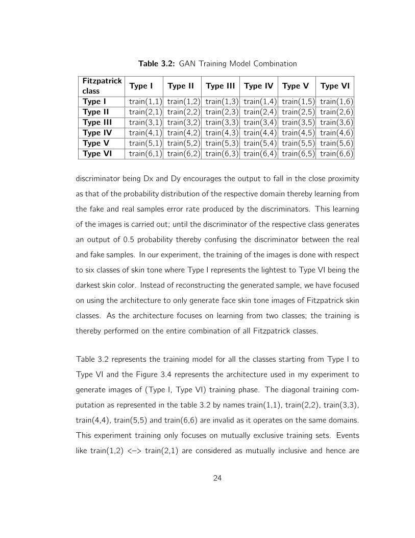
Table 3.2: GAN Training Model Combination

Fitzpatrickclass Type I Type II Type III Type IV Type V Type VI

Type I train(1,1) train(1,2) train(1,3) train(1,4) train(1,5) train(1,6)Type II train(2,1) train(2,2) train(2,3) train(2,4) train(2,5) train(2,6)Type III train(3,1) train(3,2) train(3,3) train(3,4) train(3,5) train(3,6)Type IV train(4,1) train(4,2) train(4,3) train(4,4) train(4,5) train(4,6)Type V train(5,1) train(5,2) train(5,3) train(5,4) train(5,5) train(5,6)Type VI train(6,1) train(6,2) train(6,3) train(6,4) train(6,5) train(6,6)

discriminator being Dx and Dy encourages the output to fall in the close proximity

as that of the probability distribution of the respective domain thereby learning from

the fake and real samples error rate produced by the discriminators. This learning

of the images is carried out; until the discriminator of the respective class generates

an output of 0.5 probability thereby confusing the discriminator between the real

and fake samples. In our experiment, the training of the images is done with respect

to six classes of skin tone where Type I represents the lightest to Type VI being the

darkest skin color. Instead of reconstructing the generated sample, we have focused

on using the architecture to only generate face skin tone images of Fitzpatrick skin

classes. As the architecture focuses on learning from two classes; the training is

thereby performed on the entire combination of all Fitzpatrick classes.

Table 3.2 represents the training model for all the classes starting from Type I to

Type VI and the Figure 3.4 represents the architecture used in my experiment to

generate images of (Type I, Type VI) training phase. The diagonal training com-

putation as represented in the table 3.2 by names train(1,1), train(2,2), train(3,3),

train(4,4), train(5,5) and train(6,6) are invalid as it operates on the same domains.

This experiment training only focuses on mutually exclusive training sets. Events

like train(1,2) <–> train(2,1) are considered as mutually inclusive and hence are

24

treated as the same training sample. Therefore the training phase is carried out 15

times over all the mutually exclusive combinations of six classes of Fitzpatrick type

thereby generating 15 cycle GAN training models to be tested on. To obtain, the

skin hallucinated images of the PPB dataset, the testing is carried on each image

and the respective skin tone is transferred for the generated model onto the test

sets.

3.4 Arc Face: An Open Source Face Matcher

The implementation of biometric systems for security and safety expands the use of

FRAs, which are algorithms that extract the facial features of individual captured

images and cross-verifies facial features across a predefined template stored in a

database. FRAs are predominately used for identification and verification. Arc-

face [3] which is one of the mostly widely used open-source face matchers has an

accuracy of 98%, therefore it was used for analysing the similarity score on the gen-

erated images. This helps to understand the impact of bias involved with respect

to the skin tone of an individual.

Arcface is a deep convolutional neural network FRA developed in 2018. The pri-

mary role of this algorithm is to develop a loss function that extracts discriminative

features from images and videos for facial recognition. The proposed approach

introduces an additive angular margin penalty to compel intra-class compactness

and inter-class discrepancy. Ease of implementation and use, avoidance of com-

plexity for improved performance, and negligible computational complexity are few

advantages for choosing Arcface matcher for analyzing the impact of skin tone.

The training of this loss function is implemented using various CNN architectures;

25

our experiment focuses on the pre-trained model of ResNet100 [8]. The training

model named MS1M-Arcface alias for ResNet100 is downloaded from the Arcface

GitHub [4] repository and is utilized on pre-processed images cropped with a scaling

factor of (112 X 112) as per the necessity of this matcher.

Figure 3.5: Application of Arcface Block Diagram

The accuracy of the ResNet100 architecture has outperformed other CNN archi-

tecture used by Arcface matcher. The ResNet module defines the neural network

arrangement as a stack which consists of a number of convolution and pooling

layers to reduce computational memory usage as well as gaining deep insight about

the features in the image samples. The architecture consists of a 100 layer deep

arrangement of a pyramidal bottleneck layer of (3 X 3) convolution sandwiched

with (1 X 1) convolutions for improved accuracy. The name ResNet refers to the

residual units being used and carried over for activation to the next layer of the neu-

ral network for detailed feature extraction. The application of ResNet architecture

26

combined with the additive angular loss function of the Arc Face matcher helps in

generating templates for each image sample from the dataset. As represented in

Figure 3.5 their templates then are used to evaluate the match score of individual

identity. If the distance between the match score falls on the higher side of the score

ranging from 0-100; it’s considered as the same individual. In this experiment, an

analysis of the generated match score is then performed to check the involvement

of bias with skin tone when the identity of the individual is still being preserved with

its facial features.

27

Chapter 4

Implementation

This chapter covers the necessary experimental procedures, the approach taken and

the system requirements utilized to conduct the study.

4.1 Workstation Description

System specifications that drive the experiment requires high computational power

due to the use of deep learning neural network architectures. To handle a large

amount of image data, we have concurrently utilized multiple resources with Graph-

ics Processing Units (GPU) functionalities. Table 4.1 describes the hardware specifi-

cations of these high-end GPUs which are used to train these 15 models as described

in Chapter 3. The training is thus performed with the described workstation.

28

Table 4.1: Workstation Details

OperatingSystem Memory Processor Graphics Disk

Capacity

Ubuntu 15.5 GiB Intel Core i7GeForceRTX 2060

1.3 TB

Ubuntu 125.6 GiB Intel Core i7GeForceRTX 2080

216.5GB

4.2 Software and Libraries

Our experiment setup consists of multiple neural network architectures, one being

a GAN for generating skin hallucination images, and other a facial recognition

matcher for calculating the authenticity. To access deep learning frameworks for our

conducted study, we have used high-end GPU resources for training purpose. Both

the architecture uses different configurations for execution and implementation. To

manage these cross-platform variations in libraries we have utilized the anaconda

cloud virtual environment. Each virtual environment is configured with the below

specific requirements.

1. GAN utilizes the below set of libraries and software:

• python 3.7

• pytorch 1.3.1

• cudatoolkit 10.0

• tourchvision 0.4.2

2. Face Recognition Matcher uses

• python 3.5.6

• cudatoolkit 10.2

29

• mxnet-cu102

• pandas 0.25

• opencv-python 4.2.0

Other generic specifications used for the analysis of results include matplotlib and

scipy libraries. The overall end to end coding is developed on a c©PyChram Inte-

grated Development Environment(IDE).

4.3 Experimental Procedure

Changing the skin color of a face image can be performed using various online tools

and mobile apps, the manual implementation of this approach to image dataset

of more than 1000 images takes an ample amount of time and computational re-

sources. Thereby, automation of this approach by effective utilization of resources

available can help us to analyze the impact of skin color variation on the Facial

Recognition algorithm. The generated dataset thus created using the automation

approach can provide us a platform to mitigate challenges of these open-source

algorithms and improve the accuracy, if the images are exposed to the varied con-

trolled environments. These controlled environments can be defined as improper

access to light sources; image captured during the night with low resolution etc. An

improper capture of the images can result in an increasing number of true negatives

thereby denying access to a valid individual. Below are the proposed approaches

that we have taken with two different GAN architectures and the modified approach

using the cycle GAN architecture, has given us remarkable results for the gener-

ated dataset, and has provided key insights when analyzed on the open-source face

matcher algorithm.

30

4.3.1 Proposed Approach

This approach leverages the Beauty GAN architecture for instance-level facial makeup

transfer [17] where source A is the make-up image and source B is the non-makeup

image on to which the makeup has to be replicated. The idea of this makeup

transfer inspired the use of the above architecture on the skin superimposition to

the target images. Figure 4.1 is the experimental block diagram designed for this

approach.

Figure 4.1: Proposed Approach Block Diagram Using Beauty GAN

The beauty GAN architecture for this proposed approach has failed to generate

distinguishable skin tone variation images for all six FP classes. Figure 4.2 shows a

sample generated image using this approach. By looking at the last image of the

generated sample we can conclude that this approach fails to replicate skin color

to the target images and thereby showing a change in the background of the image

too which was not expected to alter as per the beauty GAN paper.

31

Figure 4.2: Sample Generated Images

Figure 4.3: Average RGB Value For All Classes of PPB Dataset

As the paper [17] focuses on instant level makeup transfer only i.e. makeup fo-

cusing only on lips, eyes, and cheeks; the change of the background didn’t carry

a proper explanation. The skin masks RGB (red, blue, and green channel) value

generated using the average pixel value of face skin images of each separated fold-

ers is represented in Figure 4.3. The median of the RGB value with the separated

32

images categorized into six Fitzpatrick classes is illustrated in Figure 4.4. Both the

average and median didn’t give a clear separation of the first three classes of the

Fitzpatrick scale thereby impacting the target generated images.

Figure 4.4: Median RGB Value For All Classes of PPB Dataset

4.3.2 Modified Approach

Due to the advancement in deep learning architectures, we have come across vari-

ous Generative Adversarial Networks. Each advancement to the GANs architecture

demonstrated a new way of model generation by changing the basic building block

of a GAN architecture. In our modified approach we have considered utilizing the

capabilities of cycle GAN architecture, with two generators and two discrimina-

tors for transforming images of one class variant into the other [33]. Figure 4.5

represents the process block diagram for the modified approach.

33

Figure 4.5: Process Block Diagram of Modified Approach

Data acquisition, preprocessing and data transformation can be collectively termed

as data-processing. Model training and hyper-parameter decision fall into the cat-

egory of in-process. Finally, the generated model is tested on a part of the data or

an entirely different set of data. In our modified approach, the training and testing

are done on different datasets. Evaluation of the generated dataset is done using a

Face Recognition Algorithm; the authenticity of the generated images is analyzed

by the match scores obtained from the matcher. Each building block as defined by

the workflow as in Figure 4.5 carries out a certain specific task as stated below.

• Data Acquisition: A collection of raw data for training and testing

• Pre-processing: Handling the missing data and segregation.

34

• Data Transformation: Making the raw data training ready i.e. converting it

into specific formats as required by the training algorithms.

• Model Training: Training the model with the training dataset

• Hyper-parameter tuning: Find and adjust the training parameters of the

model.

• Batch Inference: Testing the trained model with the test dataset.

• Model Evaluation: Analyse model performance by evaluating the images with

Face Recognition Algorithm.

Data Pre-processing

Pre-processing of data is referred to as preparing the dataset for training and test-

ing the neural network architectures. These pre-processing steps can be further

subcategorized as data acquisition, data handling, and data transformation. Data

acquisition refers to the collection of data; this can be achieved by manually down-

loading images from different internet sources or a predefined set of data that

can be downloaded along with the metadata information from a legitimate data

repository. Our training and the testing data acquisition is stated below.

• The training data consists of manual downloaded data of almost 336 images

each categorized and placed into six Fitzpatrick classes starting from Type

I being the lightest to Type VI the darkest skin tone. Each data folder FP

class consists of 56 images with one image per subject, randomly picked, and

chosen manually by us to fall into the six categories. Few sample images on

35

which the training data is executed along with the folder structure is defined

in Figure 4.6.

Figure 4.6: Folder Structure Along with Two Sample Images Per Type.

• The test data consists of pre-defined accumulated data as stated in Chapter

3 section 3.1. PPB dataset contains around 1270 images, with a single

image per individual. The other dataset used for testing purposes of intra-

subject score variation is done on the Morph dataset. This dataset comprises

two categories of individuals i.e African Americans with darker skin tone and

Caucasians with lighter skin tones. Each subcategory has a combination of

males and females subsets. The total number of images in each subset of

the Morph group is stated in table 4.2.

Our experiment considers a subset of Morph image manually rated across three

human raters. We have considered only the male subset of both groups. As this

36

Table 4.2: Total Number of Images in Morph Dataset

Group Number of ImagesAfrican American Female (AAF ) 5782African American Male (AAM) 36838

Caucasian Female (CF ) 2606Caucasian Male (CM) 8005

dataset doesn’t have metadata information with skin color rating, we have taken a

subset of individuals in both the groups which were manually labeled as category 1

and category 6 across 3 human raters. With this data approach, we have selected

417 unique subjects from the AAM group and 944 subjects from CM. Each group

has a total number of 2435 and 4398 images. Hence, giving rise to more than one

image per subject for intra-subject score analysis. Figure 4.7 are few image sample

of the PPB datasets on which data augmentation is performed using our modified

approach and figure 4.8 represents the images for intrasubject score variations

analysis from the Morph dataset.

Figure 4.7: PPB Dataset Sample Images

Before the execution of the training phase using deep learning architecture, the

training and the testing data are pre-processed with face image being loosely

cropped. Other pre-processing steps include image resizing to a uniform variant

37

Figure 4.8: Morph Dataset Sample Images

of (112 X 112) dimension as accepted by both neural networks as well as the face

matcher algorithm. The entire image cannot be subjected to training purposes as

the neural network would learn details about the background of the image which is

not relevant for our study. Segregation of images into six Fitzpatrick categories,

neglecting downloaded images that fail to detect a face, and handling other outliers

are a part of data handling and transformations.

In-processing

In-process is referred to as the training phase of a deep learning neural network

architecture. This phase is usually computationally expensive as it utilizes the

software and hardware capabilities of the system to learn details about images.

Image processing and feature extraction are carried out on all the pre-processed

images using the deep adversarial architecture. In the presented experimental setup,

we focused on training the neural network with 15 combinations as stated in Chapter

3 section 3.2. Figure 4.9 represents the in-process block diagram of the cycle GAN

architecture. The left side of the figure 4.9 describes the training phase, where the

cycle GAN takes two class inputs and generates checkpoints for each combination.

38

After running the experiment with different epochs ranging from 100 to 600, we

have finalized the below hyper-parameters configuration. Table 4.3 gives a key

insight into the tuning details.

Figure 4.9: Modified Approach Testing and Training Phase Block Diagram

The 15 checkpoints thus generated after training cycle GAN model are located in

the folder structure as represented below. Each file named “latest.ckpt” as stated

in Figure 4.10 defines the weights and biases learned by training on the six dataset

folders of different skin shades. These generated checkpoints are used to transform

images on the test datasets. On the right of figure 4.9, describes the testing

phase of the generation process where a checkpoint is used to transform skin tone

belonging to two different classes. Our approach focuses on only FP-1 and FP-6

combinations thereby generating a total of 9 checkpoints on which transformation

is carried out.

39

Table 4.3: Hyper-Parameter Details for Training Model

Hyper-parameters Name DetailEpochs 600Decay Epoch 100Batch Size 1Learning Rate 0.002Load Height 286Load Width 286Crop Height 256Crop Width 256Load Height 286lambda 10IDT co-efficient 0.5Load Width 286Normalization BatchDrop Out No drop out for GeneratorNumber of Generator filter in 1stConvolution

64

Number of Discriminator filter in 1stConvolution

64

Post-processing

Post-processing of data in machine learning algorithms refers to cleaning and re-

moving noisy data from the generated dataset. This step is usually carried out after

the training phase of the model generation. In our experiment post-processing fo-

cuses on applying the generated GANs model on the dataset like PPB dataset with

1270 images and Morph subcategories of AAM and CM of 417 and 944 unique

subjects. A test script to run on the entire folders of the test data is executed

and the respective skin variation images of each individual are placed in the folder

categorized as [1, 2, 3, 4, 5, 6]. If the original image is marked as class 1 image,

then the respective 2, 3, 4, 5 and 6 Fitzpatrick skin color image is obtained by

40

Figure 4.10: Checkpoint Directory Structure

utilizing the class1_2, class1_3, class1_4, class1_5, and class1_6 checkpoints

respectively. This entire set of execution is performed on all the images, categorized

into different Fitzpatrick types.

After the generation of the two new datasets, cleansing of noisy data before per-

forming a facial recognition analysis is carried out. This cleansing includes removing

images from all the datasets which are a failure to detect cases with the Arcface

matcher. Hence, giving us a refined dataset for evaluation and analysis. As stated

in chapter 3 section 3.3 the generated dataset is then compared with the original

dataset using the Arcface matcher to check if the skin color plays a significant role

to increase the true negatives in Facial Recognition Algorithms. Since the PPB

dataset only comprises one image per subject, an intra-subject score analysis can’t

be performed on this particular dataset. Morph dataset thus plays a significant role

in giving us the necessary takeaway with intrasubject score analysis. The imple-

41

mentation procedure thus gives us a clear idea of the benefit of GAN architecture,

thereby giving us the flexibility to augment data to a pre existing dataset and draw

analysis on the impact of the skin tone affecting facial recognition algorithms.

4.4 Significance of Box Plots

The box plot provides a means of representing the distribution of data across a

common axis. This can be summarized using 5 points: minimum, maximum, first

quartile (Q1), third quartile (Q3), and median [5]. Figure 4.11 shows the different

parts of a box plot.

Figure 4.11: Different Parts of a Box Plot

• First Quartile/Q1: Represents the numbers between the smallest number and

the median value or in other words the 25th percentile.

• Median/Q2: Represents the middle value of the dataset or in other words the

50th percentile.

42

• Third Quartile/Q3: Represents the numbers between the largest number and

the median value or in other words the 75th percentile.

• Interquartile Range(IQR): Highlights the maximum distribution of points in

the dataset which is from 25th to 75th percentile.

• Maximum and Minimum: Represent the outlier of the entire distribution and

is calculated with the formula as shown in figure 4.11.

This plot has been a boon to analyze the score distribution generated by the compar-

ison of two images, the original when being compared with the other five generated

Fitzpatrick class images. Plotting probability distribution plots for all classes would

be of more beneficial to visualize the impact of skin tone when changed from light

to dark. This plot gives us the flexibility to plot all the class variation in a single

locality. Matplotlib python is used to generate the plots.

4.5 Significance of Cosine Similarity

Images are represented in three-dimensional vectors. FRAs use the vectors to

generate a template for each image with facial features. Cosine similarity is generally

used to measure the correlation between templates generated using CNNs. A

match score, computed after the template comparison, is the euclidean distance

for checking authenticity. Image-to-image comparison requires cosine similarity in

order to find the smallest angular difference between two image templates. The

higher the score generated using this comparison technique, the more similar are the

two feature vectors of the images. Python libraries like scipy are used to compute

the cosine similarity scores of two feature vectors.

43

Chapter 5

Results

This chapter gives a detailed analysis of the key points of the conducted study. The

training set for the FRAs typically contains images of mostly Caucasians. This bias

results in higher false match rates with respect to darker skin tones. To eradicate

the impact of skin color bias, our experiment focused on generating datasets with

diversified skin tones. The evaluation of the generated dataset includes analyzing

the impact of skin colors on the open-source matcher algorithm. An explanation

of the important box plots is generated to evaluate the results.

5.1 Analysis on PPB Dataset

Figure 5.1 represents the cosine similarity match scores generated in text files

using the Arcface matcher. Column 1 represents the ID of the image template.

Column 2 indicates the match score of the probe, which is the original image, with

itself, resulting in a similarity score of 100.0. Columns 3 to 7, named “gen_2,”

“gen_3,” “gen_4,” “gen_5,” and “gen_6,” show the probe comparison scores of

44

the generated cycle GAN skin hallucinated images. From the metadata, the probe

is rated as FP-1. Sample images as in figure 5.2 are generated using our modified

approach.

Figure 5.1: First 10 Subject Scores from PPB Dataset categorized as Type I

Figure 5.2: Sample Generated Images Categories as FP-1

The generated text file represented in figure 5.1 is plotted in figure 5.3, which

summarizes the scores in a single locality. A huge drop in score distribution occurs

45

when an original image is compared with the darkest skin color of the same image

even after preserving facial features across the skin hallucinated images. The plot

in figure 5.3 has some outliers (indicated with circles), "gen_2," "gen_4," and

"gen_5" with scores below the usual distribution. A sample of the low-scoring

images is represented in figure 5.4 along with the scores. The few low-scoring

images are failed cases that indicate the induced factors from the training datasets.

Unwanted effects can be improved with proper uniform distribution of the images

in the training phase.

Figure 5.3: Box Plot for PPB Dataset Categorized as Type I

Figure 5.5 represents the mean and standard deviation of the original and generated

images. The first row is preserved in the table to give a detailed comparison.

46

Figure 5.4: Low Score Outlier Samples from PPB FP-1

Figure 5.5: Mean and Standard Deviation Distribution for PPB Type I

Images rated FP-6 as per PPB metadata, which are the probes with image IDs

listed in column 1 of the figure 5.6, are plotted against the match scores when

compared to the generated images that fall in category 1 to 5. Figure 5.7 shows a

few image samples on which the comparison is performed. Original_6 of figure 5.7

represents the probe comparison to itself and column 2 to 1 represents the score

for generated images.

47

Figure 5.6: First 10 Subject Scores from PPB Dataset Categorized as Type VI


The box plot for Type VI PPB data distribution is shown in figure 5.8. A drop in the

scores of the testing samples is noted when images with darker skin are converted

to ones with lighter, but the drop may not be consistent due to the impact of the

training models.

48

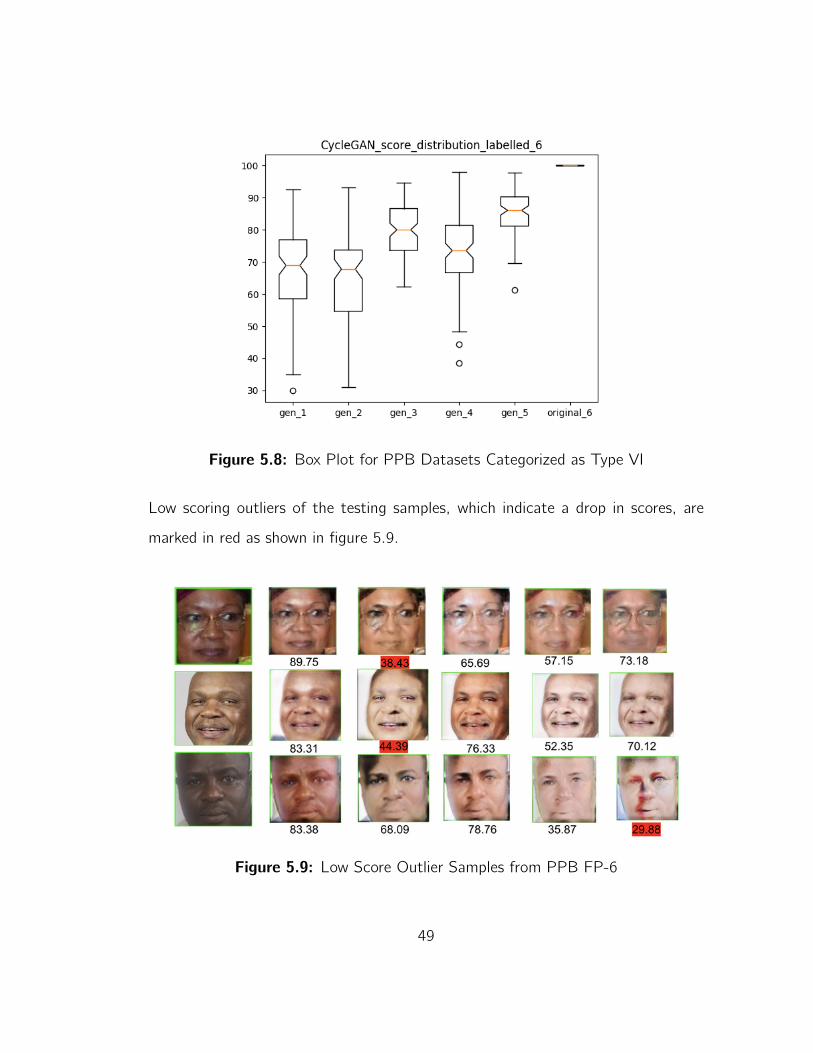
Figure 5.8: Box Plot for PPB Datasets Categorized as Type VI

Low scoring outliers of the testing samples, which indicate a drop in scores, are

marked in red as shown in figure 5.9.

Figure 5.9: Low Score Outlier Samples from PPB FP-6

49

The mean and standard deviation of PPB Type VI score distribution is displayed in

figure 5.10.

Figure 5.10: Mean and Standard Deviation Distribution for PPB Type VI

5.2 Analysis of Morph Caucasian

The morph Caucasian dataset consists of at least two images per subject, allowing

the flexibility to analyze the impact of skin color when modified across all the images

of the same subject.

Figure 5.11 displays the scores generated in a comparison of the probe with each

generated image in the morph dataset. “subject1image1” from the original set is

compared with “subject1image1” of the generated classes 2, 3, 4, 5, and 6. The

“original_1” column reveals the probe comparisons with themselves that produce a

similarity score of 100.0.

The mean and standard deviations are shown in figure 5.12. The standard devia-

tions indicate a consistent increase in score distribution across class Types IV, V,

and VI whereas Types I, II, and III have less variation.

50

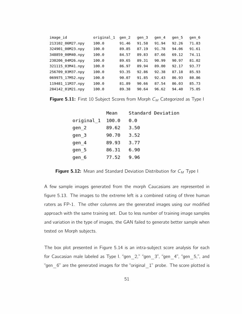
Figure 5.11: First 10 Subject Scores from Morph CM Categorized as Type I

Figure 5.12: Mean and Standard Deviation Distribution for CM Type I

A few sample images generated from the morph Caucasians are represented in

figure 5.13. The images to the extreme left is a combined rating of three human

raters as FP-1. The other columns are the generated images using our modified

approach with the same training set. Due to less number of training image samples

and variation in the type of images, the GAN failed to generate better sample when

tested on Morph subjects.

The box plot presented in Figure 5.14 is an intra-subject score analysis for each

for Caucasian male labeled as Type I. “gen_2,” “gen_3”, “gen_4”, “gen_5,”, and

“gen_6” are the generated images for the “original_1” probe. The score plotted is

51


a comparison between multiple samples of the same subjects. Assuming subject1

has three images taken with different intervals of controller environment at different

time intervals. Match score is generated with a different sample of the same subject

within each generated category of classes 2, 3, 4, 5, and 6. An example comparison

is stated as (subject1Image1, subject1Image2), (subject1Image1, subject1Image3)

and (subject1Image2, subject1Image3) of the same type class. The original_1

box plot sample represents the intra-subject score comparison of each subject.

Analyzing the box plot for morph Caucasian we see a uniform distribution drop in

scores for every class which signifies that the generated images are less affected

by the GAN architecture. On the other hand, the drop in score in the “gen_6”

might signify the effect of skin tone as a crucial factor for non-uniformity. But any

conclusive statement would need further investigation with improved dataset.

52

Figure 5.14: Box Plot for CM Genuine Intra Subject

Figure 5.15 plots a cross intra-subject analysis. Assuming subject1 with three

images per subject at different intervals of time and environment; the match scores

are generated with a cross image comparison of original intra subjects with that of

the generated ones. The sample comparisons of subject 1 with three images are:

• (subject1Image1_original1, subject1Image2_gen2)




• (subject1Image3_original1, subject1Image1_gen2),


53

The “original_1” plot represents same probe with different images.

Figure 5.15: Box Plot for CM Genuine Cross Intra Subject

Figure 5.16: High scoring sample

54

Figure 5.16 is an image from the morph Caucasian dataset which scores high with

the intrasubject analysis. The scores observed are consistently high.A low scoring

subject is shown figure 5.17 . Scores are uniformly under the threshold with an

original and generated comparison. Factors like other facial features which include

the length of beard, no mustache affect the similarity score and eliminates the idea

of GAN causing the drop in score.

Figure 5.17: Low scoring sample

5.3 Analysis for Morph African American

Subjects chosen for the plot are African American subset from morph dataset,

categorized as skin tone Type VI when rated with 3 human raters. The original_6

probe are matched against generated 1, 2, 3, 4, and 5 as shown in figure 5.18.

Sample images for this generated dataset can be seen in figure 5.19. The impact

55

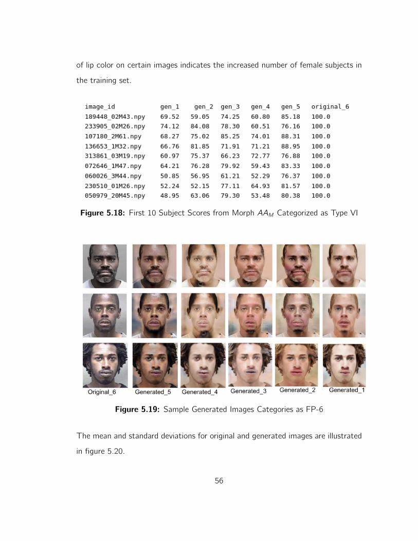
of lip color on certain images indicates the increased number of female subjects in

the training set.

Figure 5.18: First 10 Subject Scores from Morph AAM Categorized as Type VI


The mean and standard deviations for original and generated images are illustrated

in figure 5.20.

56

Figure 5.20: Mean and Standard Deviation Distribution for AAM Type VI

The genuine intra-subject score analysis for morph African American group is shown

in figure 5.21. The images categorized as Type VI is compared with the generated

images of types I to V. Considering the three images of subject 1, the comparison

is as follows.

• (subject1Image1, subject1Image2)



“original_6” in X-axis of the box plot in figure 5.22 gives the idea of match score

distribution for probe intra-subject feature matching. “gen_1,” “gen_2,” “gen_3,”

“gen_4,” and “gen_5” are intra-subject scores of each categories respectively.

The box plot shown in figure 5.22 is the intra-subject genuine comparison between

original and the generated type classes. The combinations of two types of classes,

with same subject different images, are as follows:


57

Figure 5.21: Box Plot for AAM Genuine Intra Subject






The score generated from each intra-subject comparison combination is represented

in “gen_2” of the X-axis label.

A high scoring morph subject with intra-subject genuine comparison is shown in

5.23. The scores in this figure consistently high, on the other hand, we can see a

58

Figure 5.22: Box Plot for AAM Genuine Cross Intra Subject

Figure 5.23: High scoring sample

gradual drop in the score when the color of the skin is manipulated with different

class types.

59

Figure 5.24: Low scoring sample

The low scoring subject in figure 5.24 is a special case scenario where we can see the

original to original comparison has a low score of -13.03 whereas the images subse-

quently generated using our approach tend to have a high score. The faulty images

with a constant increase and decrease in scores have to be further investigated to

come up with certain conclusions.

The generated images and figures thus gives us an indication of skin affecting the

facial recognition system, but drawing any concrete statement requires improve-

ment in the training dataset, isolating female and male subjects, increasing the

images per Fitzpatrick class, and other hyper-parameter tunning on the training

sets.

60

Chapter 6

Conclusion

Analyzing the plots and scores generated by our experimental approach we come

to the conclusion that altering the skin color of an individual by preserving identity

has a significant impact on the facial recognition algorithm. However, the impact

seems to be persistent in either direction, whether a darker skin is changed to light

or vice versa. As GANs are subject to introduction noise at each training epochs

any conclusive statement can not be inferred about skin tone being the only driving

for FRAs. Other facial factors like the presence of makeup in the female subject

and facial hairs in male sunset can induce the effects on the testing set. However,

due to the consistency in low scores and high scores of the intra-subject comparison

can of the original and generated dataset, we can conclude that GANs can be used

to alter the skin color of an image without affecting the facial features.

Future Work

The experimental approach and literature review highlights the lack of a proper skin

tone color classification system defined in cohesion with dermatologists. The upper

61

and lower bound for the classification system can be inferred by applying a k-mean

clustering algorithm with six cluster centers to better understand the separation of

each skin type class. Our experiment did not focus on generates the intermediate

training models as it only converts Type I and Type 6 images. Training and model

generation for FP-2 to FP-5 should be conducted for a better understanding of the

impact of skin tone. The training set can be improved by increasing the number of

images in each Fitzpatrick Types and conduction training as well as testing on the

female and male subset separately.

62

Bibliography

[1] Diana Borza, Adrian Sergiu Darabant, and Radu Danescu. “Automatic Skin

Tone Extraction for Visagism Applications.” In: VISIGRAPP (4: VISAPP).

2018, pp. 466–473.

[2] Joy Buolamwini and Timnit Gebru. “Gender shades: Intersectional accuracy

disparities in commercial gender classification”. In: Conference on fairness,

accountability and transparency. 2018, pp. 77–91.

[3] Jiankang Deng et al. “Arcface: Additive angular margin loss for deep face

recognition”. In: Proceedings of the IEEE Conference on Computer Vision

and Pattern Recognition. 2019, pp. 4690–4699.

[4] Jiankang Deng et al. “Lightweight face recognition challenge”. In: Proceedings

of the IEEE International Conference on Computer Vision Workshops. 2019,

pp. 0–0.

[5] Michael Galarnyk. Understanding Boxplots. https://towardsdatascience.

com/understanding-boxplots-5e2df7bcbd51. July 2020.

[6] P. Grother, M. Ngan, and K. Hanaoka. NISTIR 8280: Ongoing Face Recogni-

tion Vendor Test (FRVT) Part 3: Demographic Effects. https://nvlpubs.

nist.gov/nistpubs/ir/2019/NIST.IR.8280.pdf.

[7] Souhail Guennouni, Anass Mansouri, and Ali Ahaitouf. Biometric Systems and

Their Applications. https://www.intechopen.com/online-first/biometric-sys-

tems-and-their-applications. Mar. 2019.

63

[8] Dongyoon Han, Jiwhan Kim, and Junmo Kim. “Deep Pyramidal Residual

Networks”. In: Proceedings of the IEEE Conference on Computer Vision and

Pattern Recognition (CVPR). July 2017.

[9] Kaiming He et al. “Deep Residual Learning for Image Recognition”. In: Pro-

ceedings of the IEEE Conference on Computer Vision and Pattern Recogni-

tion (CVPR). June 2016.

[10] Anil K Jain, Arun A Ross, and Karthik Nandakumar. Introduction to biomet-

rics. Springer Science & Business Media, 2011.

[11] 2019 Jocelyn KaiserNov. 7 et al. A judge said police can search the DNA of 1

million Americans without their consent. What’s next? https://www.science-

mag.org/news/2019/11/judge-said-police-can-search-dna-millions-americans-

without-their-consent-what-s-next. Nov. 2019.

[12] Tero Karras, Samuli Laine, and Timo Aila. “A Style-Based Generator Archi-

tecture for Generative Adversarial Networks”. In: The IEEE Conference on

Computer Vision and Pattern Recognition (CVPR). June 2019.

[13] Brendan Klare. Race and Face Recognition Accuracy: Common Misconcep-

tions. https://blog.rankone.io/2019/09/12/race-and-face-recognition-accu-

racy-common-misconceptions/. Dec. 2019.

[14] Sarvasv Kulpati. A Brief Introduction To GANs (and how to code them).

https://medium.com/sigmoid/a-brief-introduction-to-gans-and-how-to-code-

them-2620ee465c30. May 2019.

[15] Chien Le and R Jain. “A survey of biometrics security systems”. In: EEUU.

Washington University in St. Louis (2009).

[16] Abigail Klein Leichman. 6 futuristic Israeli biometric techs that will transform

our lives. https://www.israel21c.org/6-futuristic-israeli-biometric-techs-that-

will-transform-our-lives/. Oct. 2016.

[17] Tingting Li et al. “Beautygan: Instance-level facial makeup transfer with deep

generative adversarial network”. In: Proceedings of the 26th ACM interna-

tional conference on Multimedia. 2018, pp. 645–653.

64

[18] Brianna Maze et al. “ Iarpa janus benchmark-c: Face dataset and protocol”. In:

2018 International Conference on Biometrics (ICB). IEEE. 2018, pp. 158–

165.

[19] Vidya Muthukumar et al. “Understanding Unequal Gender Classification Ac-

curacy from Face Images”. In: ArXiv abs/1812.00099 (2018).

[20] S. Pankanti, R. M. Bolle, and A. Jain. “Biometrics: The future of identifi-

cation [Guest Eeditors’ Introduction]”. In: Computer 33.2 (2000), pp. 46–

49.

[21] Krishnapriya K. S et al. “Characterizing the Variability in Face Recognition

Accuracy Relative to Race”. In: Proceedings of the IEEE/CVF Conference on

Computer Vision and Pattern Recognition (CVPR) Workshops. June 2019.

[22] Silonie Sachdeva et al. “Fitzpatrick skin typing: Applications in dermatology”.

In: Indian Journal of Dermatology, Venereology, and Leprology 75.1 (2009),

p. 93.

[23] Shahnewaz.Multimodal biometric System for human identification. https://w-

ww.m2sys.com/blog/important-biometric-terms-to-know/the-advantages-of-

multimodal-biometric-system-for-human-identification/. Jan. 2019.

[24] Lavanya Shukla. Fundamentals of Neural Networks on Weights & Biases.

https://www.wandb.com/articles/fundamentals-of-neural-networks/ . Aug.

2019.

[25] Skorzewiak. Hands typing on laptop keyboard with watching eye on hologram

screen. https://www.shutterstock.com/image-photo/hands-typing-on-laptop-

keyboard-watching-1361794664.

[26] Aleksandr Solonskyi. Why you should use multimodal biometric verification

for security systems. https://towardsdatascience.com/why-you-should-use-

multimodal-biometric-verification-for-security-systems-f345134ffd05 . Apr.

2020.

65

[27] Dr. Meka James Stephen and P.V.G.D. Reddy. “Implementation of Easy Fin-

gerprint Image Authentication with Traditional Euclidean and Singular Value

Decomposition Algorithms”. In: International Journal of Advances in Soft

Computing and Its Applications Vol. 3 (July 2011), pp. 1–19.

[28] Jiande SUn, Yufei Wang, and Jing Li. Gait Recognition. https://www.intech-

open.com/books/motion-tracking-and-gesture-recognition/gait-recognition.

July 2017.

[29] Danny Thakkar. Retinal vs. Iris Recognition: Your Eyes Can Get You Identi-

fied? https://www.bayometric.com/retinal-vs-iris-recognition/. Aug. 2018.

[30] John Trader. The Top 5 Uses of Biometrics Applications across the Globe.

https://www.m2sys.com/blog/biometric-hardware/top-5-uses-biometrics-a-

cross-globe/. June 2020.

[31] Kambiz Youabian. Dermatone skin analyzer. US Patent App. 11/183,572.

Jan. 2007.

[32] Seyma Yucer et al. “Exploring Racial Bias within Face Recognition via per-

subject Adversarially-Enabled Data Augmentation”. In: Proceedings of the

IEEE/CVF Conference on Computer Vision and Pattern Recognition Work-

shops. 2020, pp. 18–19.

[33] Jun-Yan Zhu et al. “Unpaired Image-To-Image Translation Using Cycle-Con-

sistent Adversarial Networks”. In: The IEEE International Conference on Com-

puter Vision (ICCV). Oct. 2017.

66

Biometric Face Skintone Data Augmentation Using A ...

Documents

Transcript of Biometric Face Skintone Data Augmentation Using A ...