©D

IGIT

AL

VIS

ION

, AR

TV

ILLE

& S

TO

CK

BY

TE

IEEE SIGNAL PROCESSING MAGAZINE [26] MAY 2007 1053-5888/07/$25.00©2007IEEE

The goal of this article is to show how a simple self-synchronization mechanism,borrowed from biological systems, can form the basic tool for achieving globallyoptimal distributed decisions in a wireless sensor network with no need for afusion center. After describing the basic interaction mechanism among the net-work nodes, we will illustrate the conditions guaranteeing the convergence of

each node to a global (or local) consensus coinciding with the globally (locally) optimaldecision statistics. The interaction mechanism takes into account the physical channelparameters, such as fading coefficients and propagation delays. We then illustrate ourresults through examples of distributed estimation and multiple hypothesis testing. We alsoaddress energy consumption issues and discuss some possible implementations.

[Sergio Barbarossa and Gesualdo Scutari]

Bio-Inspired SensorNetwork Design

[Distributed decisions through self-synchronization]

Authorized licensed use limited to: Universita degli Studi di Roma La Sapienza. Downloaded on November 29, 2008 at 06:40 from IEEE Xplore. Restrictions apply.

IEEE SIGNAL PROCESSING MAGAZINE [27] MAY 2007

OVERVIEWThe design of sensor networks faces a number of challengesresulting from very demanding requirements on one side, suchas high reliability of the decision taken by the network androbustness to node failure, and very limited resources on theother side, such as energy, bandwidth, and node complexity. Forthis reason, many recent works on sensor networks have con-centrated on the efficient use of the available resources, mainlyenergy, necessary to achieve the users’ requirements [1]. Giventhe considerable amount of knowledge accumulated in thetelecommunication networks field, it is not surprising that mostworks on sensor networks fall within the conceptual frameworkof telecommunication networks, with a special emphasis onenergy-efficient design, node simplicity, and scalability.However, while the goal of a telecommunication network is tocarry information packets from each source to the relative desti-nation, irrespective of the packet content, a sensor network is,fundamentally, an event-driven system: in a sensor network, it isevents that are carried and not packets. If a fire starts, what isimportant is that the remote control or actuator node gets thisinformation as soon as possible, not that all the temperaturemeasurements taken by the sensors reach the fusion center.

A critical aspect of a sensor network is its vulnerability totemporary node sleeping, due to duty-cycling for batteryrecharge, permanent failures, or even intentional attacks.Clearly, the vulnerability increases if there are just a few deci-sion (sink) nodes, as the failure of a sink node could jeopardizethe whole system. To improve resilience against node failures, itis necessary to devise decentralized decision strategies that areable to quickly react to unpredictable topology changes.

Decentralizing the decisions is also strategic to reducing thecongestion probability. A congestion around a sink node is anevent that is most likely to occur precisely when a hazard situa-tion occurs, in which case many nodes send their warning packetsto the control nodes at about the same time. This could make thenetwork less reliable just when the monitoring system is expectedto be as reliable as possible. Decentralizing the decisions is usefulalso in this case, as it would prevent the bottleneck situation inwhich all the nodes try to access a single sink node.

Of course, the network resilience to node failures increasesas the number of nodes increases. However, this raises thescalability issue. From an information theoretic point of view,it was shown in [2] that the transport capacity of a sensor net-work composed of N nodes sending data to a sink node scalesas 1/N. While intuitive, this result is a somewhat discourag-ing, as it implies that we cannot do any better than just divid-ing the resources (e.g., bandwidth) by the number of nodes.Nevertheless, as shown by Giridhar and Kumar [3], [4] this isnot necessarily the case if the specificity of the sensing prob-lem is properly taken into account. A sensor network can be infact seen as a sort of distributed computer that, on the basis ofthe data collected by N sensors, let us say y1, y2, . . . , yN , hasto compute a function f(y1, y2, . . . , yN). This function maybe, for example, a sufficient statistic of the data. From this per-spective, a sensor network could be designed using the power-

ful tools of parallel and distributed optimization [5], [6].Moreover, the objective function f(y1, y2, ldots, yN) may haveproperties that can be exploited to improve scalability. In manyapplications, for example, f(y1, y2, . . . , yN) is a symmetricfunction of the measurements; i.e., it is invariant to any per-mutation of the observed variables. In such a case, it wasshown in [4] that the transport capacity scales as 1/ log N, asopposed to 1/N. Interestingly, this permutation invarianceassumption is not at all artificial, as, conversely, it reflects thedata-centric nature of some sensor networks, where what isimportant is the whole set of measurements and not theknowledge of which node has taken which measurement.Examples of networks designed according to the data-centricperspective include the type-based multiple access, where theidentification of the data type at the sensor decides whatorthogonal channel the sensor is going to use over a multipleaccess channel [7]. A sensor network can be seen indeed as amultiterminal inference machine, where multiple nodes sendtheir information to a control node, subject to a rate con-straint imposed by the communication channel [1]. Thisinduces an interplay between signal processing and network-ing that should be properly taken into account [1].

Besides deriving scaling laws pertinent to sensor networks,Giridhar and Kumar [4] showed also that better scalability lawscan be achieved by endowing the network with in-network pro-cessing capabilities and structuring the network in a hierarchi-cal structure, with different roles assigned to different nodes.

Following [4], we share the view that the network should beorganized in hierarchical levels, where the lower level nodes,simple but vulnerable, cooperate to achieve local consensus witha reliability greater than the single node, whereas intermediatenodes are responsible for conveying the local consensusachieved by the lower level nodes to the control centers. In thisarticle, we concentrate on the lower level nodes and our goal isto illustrate a strategy of interaction among the nodes thatallows them to reach globally optimal decisions with a totallydecentralized approach, exploiting a consensus mechanismbased on the self-synchronization of first-order coupled dynami-cal systems. The basic idea is borrowed from biological systemswhere self-synchronization occurs in a variety of circumstances,from the heart beating to neuron cell firing, and forms the basisof their robustness and reliability. Our goal is to bring the math-ematical models describing self-synchronization into a signalprocessing perspective to derive a novel approach to distributedhypothesis testing or estimation.

Distributed consensus algorithms are indeed techniqueslargely studied in distributed computing (see, e.g., [6]) and theirapplication to statistical consensus theory has a long history(see, e.g., [8]). Average consensus techniques have receivedgreat attention in recent years (see, e.g., [9]–[13] and referencestherein). In particular, the conditions for achieving a consensusover a common specified value, like a linear combination of theobservations, was solved for networked dynamic systems byOlfati-Saber and Murray, under a variety of network topologies,also allowing for topology variations during the time necessary

Authorized licensed use limited to: Universita degli Studi di Roma La Sapienza. Downloaded on November 29, 2008 at 06:40 from IEEE Xplore. Restrictions apply.

to achieve consensus [9], [10], [13]. Belief propagation is anotherpowerful distributed technique capable of achieving globallyoptimal decisions in a totally decentralized way (see, e.g.,[14]–[16] and the references therein). A special form of consen-sus, known as the alignment problem, where all network agentseventually reach an agreement, but without specifying the finalvalue, was also thoroughly studied by Jadbabaie et al. in [17]. Arecent excellent tutorial on distributed consensus techniques isgiven in [13].

MOTIVATING EXAMPLESIn this section we will illustrate some basic statistical signal pro-cessing problems, whose centralized solution is well known. Thegoal of the ensuing sections will be to show how to solve themin a totally decentralized way.

PROBLEM 1: ESTIMATION OF A COMMON SET OF PARAMETERSLet us consider a network composed of N sensors, whose goal isto estimate a set of L parameters, given by vector ξ . We assumethat each sensor collects a vector yi of M measurements, relatedto the unknown vector ξ through the linear observation model

yi = Ai ξ + vi ; (1)

where vi is additive noise, with zero mean and covariance matrixRi. The noises on different sensors are statistically independentof each other but each vector vi may be colored. If the noiseprobability density function (pdf) is Gaussian, the globally opti-mal maximum likelihood (ML) estimator is [18]

ξ =(

N∑i =1

ATi R−1

i Ai

)−1 (N∑

i =1

ATi R−1

i yi

). (2)

If the noise pdf is unknown, (2) still represents a meaningfulestimator, as it is the best linear unbiased estimator (BLUE)[18]. If this estimation is to be taken by a fusion center, everysensor is required to transmit to the fusion center not only itsmeasurement vector yi but also its own mixing matrix Ai andnoise covariance matrix Ri.

PROBLEM 2: MULTIPLE HYPOTHESIS TESTINGLet us consider now the case where the goal of the network is todistinguish between M alternative hypotheses, with M ≥ 2, ingeneral. The M hypotheses may be spatial patterns, for example.We suppose that each hypothesis Hk occurs with a known a prioriprobability Pk and we denote by pi(yi/Hk) the conditional pdfrelated to the observation of vector yi, conditioned to the hypoth-esis Hk. We also assume that the measurements taken by differ-ent sensors are conditionally independent from each other sothat, if we group the vector of measurements yi into a vectory = (y1, y2, . . . , yN)T , we have p(y/Hk) = �N

i =1 pi(yi/Hk) . Ifthe decision criterion consists of minimizing the error probabili-ty, the optimal decision test is the one that chooses the hypothesisHm that maximizes the a posteriori probability P(Hk/y), or [18]

Hm = arg maxk

{p(y/Hk)P(Hk)}

= arg maxk

{N�

i =1pi(yi/Hk)P(Hk)

}. (3)

Hence, the fusion center needs to know every single pdfpi(yi/Hk) to take a decision.

DECENTRALIZED DECISION THROUGH SELF-SYNCHRONIZATIONIn this section we will briefly review the self-synchronizationconcept, as observed in nature, and then we will show how touse a self-synchronization mechanism to force every singlenode of the network to reach the globally optimal decision testsspecified in the previous section, without the need of any afusion center.

A BRIEF HISTORY OF THE SELF-SYNCHRONIZATION IDEASelf-synchronization is a phenomenon first observed betweenpendulum clocks (hooked to the same wooden beam) byChristian Huygens in 1658 [19]. Since then, self-synchroniza-tion has been observed in a myriad of natural phenomena,from flashing fireflies in South East Asia to singing crickets,from cardiac pacemaker or neuron cells to menstrual cycles ofwomen living in strict contact with each other [19]. Readersinterested in the self-synchronization phenomena as observedin nature should refer to [19] for an in-depth treatment of thisfascinating and pervasive subject. A simple example may beuseful to illustrate how some basic biological mechanismscould be exploited to devise robust sensor networks with built-in consensus capabilities. In the so-called pacemaker cellspresent in the human heart, a chemical reaction takes placethat generates positive ions. This reaction induces an electricalpotential difference, between the interior and exterior of thecell, that increases with time. Above a certain potential differ-ence, however, the cell membrane becomes transparent so thatthe internal ions are fired to the exterior, thus periodicallyresetting the potential to zero. This behavior makes the singlecell work as a pulse oscillator. At the same time, the cell mem-brane lets outer ions, fired by neighbor cells, enter into thecell. This induces an interaction about the firing times so that,from the outside, the overall population of pacemaker cells canbe seen as a set of pulse-coupled oscillators. The situation isactually more complicated, as this population is also affectedby pulsed commands arriving from the brain, which reacts toexternal and internal stimuli to insure the proper functioningof the whole body. From an engineering point of view, themain question is whether this system is sufficiently stable toguarantee a proper functioning, in spite of the simplicity andpotential unreliability of the single cell. Interestingly, Mirolloand Strogatz provided a rigorous answer to this question prov-ing that, under mild assumptions on the coupling function, ifthe network of nodes is fully connected, there exists only onestable equilibrium represented by the situation where all cellsfire at the same time [20]. Hence, the interaction among the

IEEE SIGNAL PROCESSING MAGAZINE [28] MAY 2007

Authorized licensed use limited to: Universita degli Studi di Roma La Sapienza. Downloaded on November 29, 2008 at 06:40 from IEEE Xplore. Restrictions apply.

IEEE SIGNAL PROCESSING MAGAZINE [29] MAY 2007

cells is what insures the desired robustness. Actually, full con-nectivity is not even necessary, as what is really needed is onlyglobal connectivity (i.e., the presence of a path between everypair of cells). The previous mechanism is very robust, as it cantolerate the death of many cells without any permanent impacton the cell firing rate, provided that the number of dead cellsdoes not affect the network connectivity. Hoppensteadt andIzhikevich went even further, proving that two pulse-coupledoscillators really interact with each only if their rates are in aresonant ratio. This led them to conjecture that simultaneousexchanges of information can take place in the human brainusing a sort of frequency multiplexing: Classes of neuronstuned on the same (or resonant) firing rate interact with eachother, but they do not interact with other classes of neuronsfiring at nonresonant rates [21].

The previous mechanism is just an example of an algo-rithm inspired by biological systems that could have animpact in the design of robust, self-organizing, systems. Forexample, Izhikevich proposed the use of a pulse-coupled oscil-lator as an associative memory [22]. As an example related tosensor networks, Hong et al. proposed the use of pulse-cou-pled oscillators to achieve a detection consensus in a fullyconnected sensor network [23], building on the results ofMirollo and Strogatz [20]. Later, Lucarelli et al. [24] provedthat full connectivity is not necessary, as what is strictlyrequired is global connectivity (i.e., the existence of a pathbetween each pair of nodes, possibly composed of severalhops). The approach suggested in [23], [24] is a form of con-sensus achieved through self-synchronization, but the finalconsensus value is a priori unpredictable. Also, timing syn-chronization, as proposed in [23], [24], may be critical inwide-area networks, where propagation delays might inducean ambiguity problem. In general, self-synchronization maybe extended to include the situation where a consensus isachieved over a physical parameter of interest, not necessarilythe initial time of phase. In this broader sense, self-synchro-nization was proposed as the way to achieve globally optimalestimation or detection [25]–[29]. In the next sections we willconcentrate on these approaches.

OPTIMAL DISTRIBUTED DECISION THROUGH SELF-SYNCHRONIZATION The idea of sensor networks proposed in [25]–[29] is the fol-lowing. The network is composed of N nodes, each equippedwith four basic components: 1) a transducer that senses thephysical parameter of interest yi (e.g., temperature, concen-tration of contaminants, radiation, etc.); 2) a local processingunit that provides a function gi(yi) of the measurement; 3) adynamical system, initialized with the local measurements,whose state xi(t) evolves as a function of its own measure-ment gi(yi) and of the state of nearby sensors; 4) a radiointerface that makes possible the interaction among the sen-sors. In the scalar observation case, the state of the dynamicalsystem present at node i evolves according to the followingdifferential equation [25]–[29]:

xi(t) = gi (yi) + Kci

N∑j=1

aij h[xj (t − τi j) − xi(t)] + wi(t),

i = 1, 2, . . . , N, (4)

where h(x) is a scalar coupling function, typically dependenton the radio interface (if h(x) = sin(x), (4) coincides withKuramoto’s model [30]), K is a global control loop gain, ci is alocal positive coefficient whose choice determines the finalconsensus form, the coefficients aij account for the couplingamong the nodes, τi j is the propagation delay from node j tonode i, and wi (t) is coupling noise. The only assumption wemake on the coefficients aij is that they are non-negative. Theymay depend, for example, on the channel parameters accord-ing to the law aij =

√pj|hij|2/d 2

i j , where pj is the power trans-mitted by node j, hij is the fading coefficient of the channelbetween nodes i and j, and dij is the distance between nodes iand j. In general, the coefficients aij are not symmetric, toaccommodate, as an example, for different transmit powers.The evolution of the state equation (4), for example, for t > 0,requires the specification of the states xi(t),∀i, for a timeinterval [−τmax, 0], where τmax is the maximum propagationdelay [for unretarded systems, it is only necessary to specifyxi(0)]. In the vector case, each node observes a vector yi andthe state equation becomes

xi(t) = gi(yi) + K C−1i

N∑j=1

aij h[x j (t − τi j) − xi(t)] + wi(t),

i = 1, 2, . . . , N, (5)

where Ci is a positive definite matrix. The important questionnow is how to choose the free parameters of (4) or (5) and todetermine the conditions guaranteeing that each node is able toreach the globally optimal decision statistic. But, before proceed-ing it is necessary to clarify what we mean by consensus. We saythat the system (4) synchronizes if all the state derivatives xi (t)converge asymptotically toward a common value ω∗, for any setof initial conditions. A global consensus is achieved when thewhole system synchronizes in the sense specified above.

This definition is different from the commonly used defini-tion in which what is required is convergence on the state (see,e.g., [12]), rather than on its derivative. The main motivationunderlying our choice is the better resilience against couplingnoise. In fact, in the presence of coupling noise [wi (t) in (4)],the states xi (t), at least in the simple linear coupling case, areaffected by a random walk process whose variance increases lin-early with time. This makes the final consensus a strong func-tion of the coupling noise. In our case, instead, the statederivative is affected by a noise that is the derivative of a randomwalk and then it has a constant variance. Furthermore, asshown in [28], system (4) is able to converge, for any set of(bounded) propagation delays, to a prescribed function of theobservations. Conversely, classical consensus techniques [10],[13], studied under a homogeneous delay assumption (i.e.,

Authorized licensed use limited to: Universita degli Studi di Roma La Sapienza. Downloaded on November 29, 2008 at 06:40 from IEEE Xplore. Restrictions apply.

τi j = τ ), converge if the (undirected) graph is connected, and ifand only if the delay is less than a topology-dependent value.

It is now useful to recall some basic properties of directedgraphs, as they represent the basic analytical tool for studyingthe interaction among the nodes.

DIRECTED GRAPHS: THE BASIC MATHEMATICAL TOOL TO DESCRIBE INTERACTIONSA weighted directed graph (or digraph, for short) G = {V, E} isdefined as a set of nodes (or vertices) V and a set of edges E(i.e., ordered pairs of nodes), with the convention thateij � (vi, vj) ∈ E (i.e., vi and vj are the head and the tail of theedge eij, respectively) means that the information flows fromvj to vi. A digraph is weighted if a positive weight aij is associ-ated to each edge. In our case, there are no loops, so thataii = 0. If (vi, vj) ∈ E ⇔ (vj, vi) ∈ E , then the graph is said tobe undirected. For any node vi,Ni is the set of neighbors ofnode vi (i.e., the set of nodes sending data to node vi). Astrong path in a digraph G is a sequence of distinct nodesv1, v2, . . . , vq ∈ V such that (vi−1, vi) ∈ E, for i = 2, . . . , q. Ifv1 ≡ vq , the path is said to be closed. A weak path is asequence of distinct nodes v1, v2, . . . , vq ∈ V such that either(vi−1, vi) ∈ E or (vi, vi−1) ∈ E , for i = 2, . . . , q. A strong cycle(or circuit) is a closed strong path. A digraph with N nodes is adirected tree if it has N − 1 edges and there exists a distin-guished node, called the root node, which can reach all theother nodes through a (unique) strong path. Hence, a directedtree cannot have cycles and every node, except the root, hasone and only one incoming edge. A digraph is a (directed) for-est if it consists of one or more directed trees. A subgraphGs = {Vs, Es} of a digraph G , with Vs ⊆ V and Es ⊆ E , is adirected spanning tree (or a spanning forest) if it is a directedtree (or a directed forest) and it has the same node set as G;i.e., Vs ≡ V . We say that a digraph G contains a spanning tree(or a spanning forest) if there exists a subgraph of G that is adirected spanning tree (or a spanning forest).

In a digraph there are many degrees of connectedness: 1) adigraph is strongly connected (SC) if any ordered pair of dis-tinct nodes can be joined by a strong path; 2) a digraph isquasi strongly connected (QSC) if, for every ordered pair ofnodes vi and vj, there exists a node r that can reach either vi

or vj via a strong path; 3) a digraph is weakly connected (WC)if any ordered pair of distinct nodes can be joined by a weakpath; 4) a digraph is disconnected if it is not weakly connect-ed. According to the above definitions, it is straightforward tosee that strong connectivity implies quasi strong connectivityand that quasi strong connectivity implies weak connectivity,but the converse, in general, does not hold. For undirectedgraphs, instead, the above notions of connectivity are equiva-lent: An undirected graph is connected if any two distinctnodes can be joined by a path. Moreover, it is easy to checkthat the quasi strong connectivity of a digraph is equivalent tothe existence of a directed spanning tree in the graph. When adigraph G is WC, it may still contain strongly connected sub-graphs. A maximal subgraph of G, which is also SC, is called a

strongly connected component (SCC) of G [31]. Since a nodeis SC, it follows that every node lies in an SCC. Using thisconcept, any digraph G can be partitioned into SCCs, let ussay G1 = {V1, E1}, . . . ,GK = {VK, EK} , where Vk ⊆ V andEk ⊆ E, k = 1, . . . , K , denote the set of nodes and edges lyingin the k th SCC, respectively.

The connectivity properties of a digraph may be betterunderstood by referring to its corresponding condensationdigraph. We may reduce the original digraph G to the conden-sation digraph G∗ = {V∗, E∗} by associating the node set Vk ofeach SCC Gk of G to a single distinct node v∗

k ∈ V∗k of G∗ and

introducing an edge in G∗ from v∗i to v∗

j if and only if thereexists some edges from the SCC Gi and the SCC G j of the origi-nal graph [31, Ch. 3.2]. An SCC that is reduced to the root of adirected spanning tree of the condensation digraph is calledroot SCC (RSCC). Looking at the condensation graph, we maysingle out the following topologies of the original graph: 1) Gis SC if and only if G∗ is composed by a single node; 2) G isQSC if and only if G∗ contains a directed spanning tree; 3) if Gis WC, then G∗ contains either a spanning tree or a (weakly)connected forest.

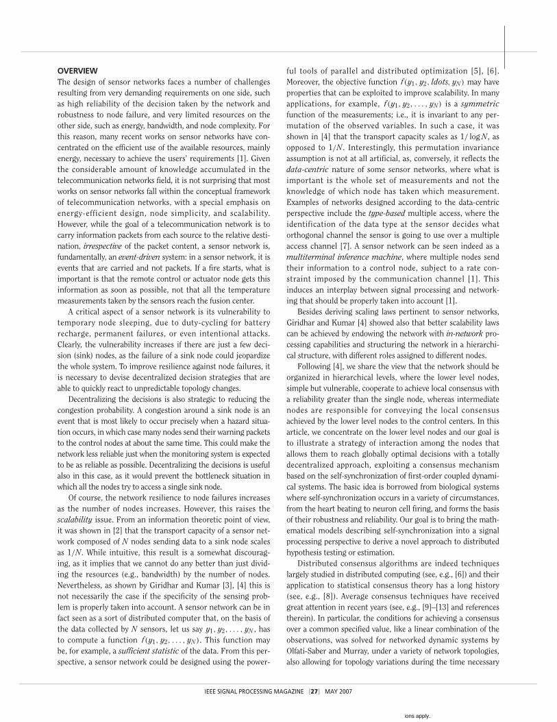
Some examples of graph topologies are shown in the top rowof Figure 1, where we report three topologies (top row), namely:(a) an SC digraph, (b) a QSC digraph with three SCCs, and (c) aWC (not QSC) digraph with a two-tree forest. For each digraph,we also sketch its decomposition into SCCs and RSCCs.

We recall now the basic properties of the matrices associ-ated to a digraph, as they play a fundamental role in the sta-bility analysis of the system illustrated in this article. Given adigraph G , we introduce the following matrices associatedwith G : 1) The N × N adjacency matrix A, which is com-posed of entries aij equal to the weight associated to the edgeeij, if eij ∈ E , or equal to zero, otherwise; 2) the degreematrix D, which is a diagonal matrix with diagonal entriesDii = ∑N

j=1 aij ; 3) the weighted Laplacian L, defined asL = D − A.

If we denote by 1 and 0 the vectors of all ones or zeros,respectively, it is straightforward to verify that L 1 = 0; i.e.,zero is an eigenvalue of L corresponding to the right eigen-vector 1. The multiplicity of the zero eigenvalue of L is equalto the minimum number of directed trees contained in adirected spanning forest of G. Moreover, the zero eigenvalueof L is simple if and only if G contains a spanning directedtree or, equivalently, G is QSC.

FORMS OF CONSENSUSWe can now illustrate the achievable forms of consensus. Wewill consider the linear coupling case first, with or withoutpropagation delays, and then we will consider the nonlinearcoupling case, with no delays.

Linear CouplingIn the linear coupling case, i.e., when h(x ) = x, system (4) hasbeen proved to synchronize if and only if the digraph is QSC andthe consensus value is [28]

IEEE SIGNAL PROCESSING MAGAZINE [30] MAY 2007

Authorized licensed use limited to: Universita degli Studi di Roma La Sapienza. Downloaded on November 29, 2008 at 06:40 from IEEE Xplore. Restrictions apply.

IEEE SIGNAL PROCESSING MAGAZINE [31] MAY 2007

[FIG1] Examples of graphs: (a) Strongly connected graph. (b) Quasi strongly connected graph with one root strongly connectedcomponent and two strongly connected components. (c) WC graph containing a two-tree forest (top row) and evolution of the statederivatives of (4) (bottom row).

1

2

3

4

5

6

9

7810

11

60

55

50

45

40

35

30

25

20

15

100 0.1 0.2 0.3 0.4 0.5 0.6 0.7 0.8 0.9 1

Time(a)

RSCC

SCC2

1

2

3

45

6

9

7810

11

SCC1

60

55

50

45

40

35

30

25

20

15

100 0.1 0.2 0.3 0.4 0.5 0.6 0.7 0.8 0.9 1

Time(b)

RSCC1

1

2

3

45

6

9

7810

11

SCC2

RSCC2

010

20

30

40

50

60

70

80

90

0.1 0.2 0.3 0.4 0.5 0.6 0.7 0.8 0.9 1Time(c)

RSCC2

RSCC1

x i (

t)•x i (

t)•

x i (

t)•

Authorized licensed use limited to: Universita degli Studi di Roma La Sapienza. Downloaded on November 29, 2008 at 06:40 from IEEE Xplore. Restrictions apply.

limt→∞

xq(t) = ω∗

=∑N

i =1 γi ci gi(yi)∑Ni =1 γi ci + K

∑Ni =1

∑Nj=1 γiaijτi j

, ∀q,(6)

where γi are the entries of the left eingenvector associated tothe null eigenvalue of the graph Laplacian. The coefficient γi ispositive if and only if node i can reach every other node througha strong path, otherwise γi = 0. This means that the only nodesthat have an impact on the final consensus are those that canreach every other node in the network, even if this occursthrough several hops. As an extreme case, the final consensuscoincides with the decision taken by a single node, let us saynode r, if the graph contains only one directed tree whose rootnode is node i. More generally, if the graph is not even QSC butit contains a forest with K strongly connected root components,the system evolution gives rise to K clusters, where the nodesbelonging to each cluster achieve a local (within the cluster)consensus [28]

limt→∞

xq(t) = ω∗q =

∑i ∈Ni

γi ci gi(yi)∑i ∈Ni

γi ci + K∑

i ∈Ni

∑Nj=1 γiaijτi j

,

∀q ∈ Ck, k = 1, . . . , K, (7)

where Ck indicates the k th cluster. Hence, the same mechanismleading to a global consensus, as in (6), is also able to produceclusters, as in (7), depending on the network connectivity prop-erties. In practice, we may force one behavior or the other, act-ing on the transmit powers pj; i.e., on the coefficients aij, asthey ultimately determine the graph topology.

The consensus forms described before are appealing becausethey can be achieved under very broad conditions. However,they present also a drawback due to their dependence on thenetwork topology, through the weights γi, and the channel sta-tus, through the coefficients aij and the delays τi j. It was provedin [28] that the dependence of the final consensus on thetopology disappears (in the sense that γi = 1) if and only if thegraph is balanced; i.e.,

∑Nj=1 aij = ∑N

j=1 aji,∀i.Note that for undirected strongly connected graphs, this

condition is always true. Then, a topology-independent consen-sus is achievable by changing the channel coefficients in orderto get a balanced graph. Recalling, from (4), thataij =

√pj |hij |2/d 2

i j , in time division duplexing systems, wherehij = hji, a balanced graph is obtained by using the same trans-mit power on each node, so that pj = p,∀ j, and thusaij = aji,∀ i and j.

Even if we are able to get rid of the topology dependence,the final consensus values, as given in (6) or (7), still dependon the channel parameters. Actually, this is true only in thedelayed case, because for τi j = 0 the channel dependence dis-appears. But in the delayed case, this dependence preventsexpressions (6) or (7) from becoming optimal decision statis-tics, as these should depend only on the gathered data.Nevertheless, also in the delayed case, we can easily eliminate

the channel-dependent term, in the denominator of both (6) or(7), using the following two-step procedure. We run the evolu-tion equation first with the right functions gi(yi), thus obtain-ing the consensus value ω∗(y). Then, we run the algorithmagain, this time setting gi(yi) = 1, thus obtaining a secondconsensus, let us say ω∗(1). It is easy to verify, from (6) or (7),that the ratio ω∗(y)/ω∗(1) assumes a value independent of thechannel coefficients. If we also insure that the graph is bal-anced, the previous procedure allows each node to reach,asymptotically through its state derivative, any form of con-sensus that can be expressed in the form [28]

f(y1, y2, . . . , yN) = u

(

N∑i =1

ci

)−1 N∑i =1

ci gi(yi)

, (8)

where u (·) is a function that each node can apply to the ratioachieved through (6) or (7).

Similarly, in the vector case (5), the final consensus, in theabsence of delays, assumes the form [28]

f(y1, y2, . . . , yN) = u

(

N∑i =1

Ci

)−1 N∑i =1

Cigi(yi)

. (9)

The forms of consensus, (8) or (9), although apparently very spe-cific, incorporate several cases of practical interest in statisticalsignal processing. For example, the vector form (9) may be usedto solve Problem 1 as formulated in the Motivating Examplessection above; i.e., to achieve the globally optimal ML estimate,given by (2), simply by running (5), after setting Ci = AT

i R−1i Ai

and gi(yi) � (ATi R−1

i Ai)−1 AT

i R−1i yi .

Similarly, we may also solve Problem 2, using (8). TheMAP test may in fact be constructed by evolving (4) withci = 1 and gi(yi/Hk) = log(pi(yi/Hk)P(Hk)) for K times(i.e., as many time as the number of hypotheses). At conver-gence, each node applies the function u(ω∗

k) = exp(ω∗k) to the

consensus achieved under hypothesis k. It is easy to verifythat each final value u(ω∗

k) is proportional to the argument ofthe MAP detector in (3).

Nonlinear Coupling CaseThe nonlinear coupling case is of course more difficult to analyzemathematically. Nevertheless, in [27], it was shown that, in thecase of undirected graphs, if the coupling function h(·) in (4) or(5) is an odd, monotonically increasing function, then the net-work achieves a global consensus, still in the form of (8) or (9), ifthe global coupling coefficient K is greater than a critical value.This value was upper-bounded by the following expression [27]:

KU = 2‖Dc�ω‖2

hmax λ2(LA),

where Dc = diag (c1, . . . , cN) , �ω = [g1(y1), g2(y2), . . . ,

gN(yN)]T − ω∗1, hmax is the maximum of h(x); λ2(LA) is the

IEEE SIGNAL PROCESSING MAGAZINE [32] MAY 2007

Authorized licensed use limited to: Universita degli Studi di Roma La Sapienza. Downloaded on November 29, 2008 at 06:40 from IEEE Xplore. Restrictions apply.

IEEE SIGNAL PROCESSING MAGAZINE [33] MAY 2007

so called algebraic connectivity of the graph; i.e., the secondsmallest eigenvalue of the graph Laplacian LA. The same condi-tion applies to the vector observation case. Hence, at least in theabsence of delays and for symmetric links, a global consensustoward the optimal decision statistics is still achievable, pro-vided that the nonlinear coupling function is an antisymmetricincreasing function and that the coupling is sufficiently strong.Interestingly, the nonlinear case has a greater variety of behav-iors than the linear case as the network may be designed toavoid the convergence toward a unique common value simplychoosing K smaller than a critical value [27]. This propertymight be used, for example, to achieve some forms of clustering.

NUMERICAL EXAMPLESWe now present some numerical examples to validate the theo-retical findings described in the previous sections.

EXAMPLE 1In the bottom row of Figure 1, we plot the dynamical evolutionsof the state derivatives of (7) versus time for the three networktopologies sketched in the top row. Each curve shows also thetheoretical asymptotic values of (6) or (7) (dashed line witharrows). As predicted by the theory, the dynamical system ofFigure 1(a) achieves a global consensus, since the underlyingdigraph is SC. The network of Figure 1(b), instead, is not SC,but it is QSC and the system is still able to globally synchronize,since there is a set of nodes in the RSCC component able toreach all the other nodes. However, the final consensus in sucha case contains only the contributions from the nodes in theRSCC, since no other node belongs to the root of a spanning-directed tree of the condensation digraph. Finally, the system ofFigure 1(c) cannot reach a global consensus since there is nonode that can reach all the others, but it does admit two disjointclusters, corresponding to the two RSCCs; namely, RSCC1 andRSCC2. The middle lines of Figure 1(c) refer to the nodes of theSCC component that do not belong to either RSCC1 or RSCC2.These nodes are affected by the consensus achieved by the twoRSCC components, but they cannot affect them. Observe that,in all the cases, the state derivatives of the (global or local) clus-ters converge to the values predicted by the closed-form expres-sion given in (6) or (7), depending on the network topology andthe channel parameters.

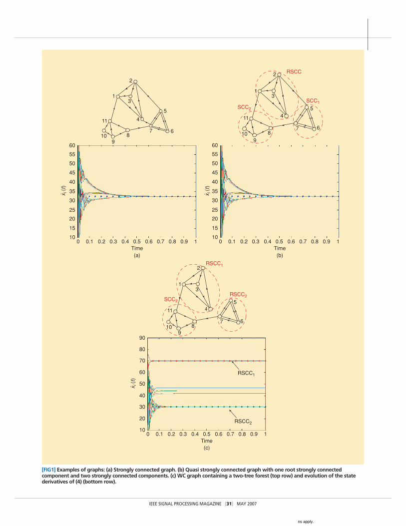
EXAMPLE 2The behaviors shown in the previous example refer to a givenrealization of the topology, with given link coefficients andobservations. In this example, we report the performanceobtained in the estimation of a scalar variable, averaged over100 independent realizations of network topology, channelcoefficients, and noise terms. Each sensor observes a variableyi = Ai ξ + vi , where vi is additive zero mean Gaussian noise,with variance σ 2

i . The goal is to estimate ξ . The estimate isperformed through the interaction system (4), settinggi(yi) = yi/Ai and ci = A2

i /σ2i , in order to achieve the global-

ly optimal ML estimate. The network is composed of 40

nodes, randomly spaced over a square of size D. The analogsystem (4) is implemented in discrete time, with samplingtime Ts = 10−3 s. The size of the square occupied by the net-work is chosen in order to have a maximum delayτmax = 100 Ts. To simulate a practical scenario, the channelcoefficients aij are generated as independent and identicallydistributed Rayleigh random variables, to accommodate forchannel fading. Each variable aij has a variance depending onthe distance dij between nodes i and j, equal toσ 2

i j = pj/(1 + d 2i j). We set the threshold on the amplitude of

the minimum useful signal to zero, so that, at least in princi-ple, each node hears each other node. The correspondinggraph is then SC. Figure 2 shows the estimated average ofthe state derivative (plus and minus the estimation standarddeviation), as a function of the iteration time. The resultsrefer to following cases of interest: 1) ML estimate achievedwith a centralized system, with no communication errorsbetween nodes and fusion center (parallel dotted lines); 2)estimate achieved with the proposed method, with no propa-gation delays, as a benchmark term (dashed and dotted linesplus x marks for the average value); 3) estimate achieved withthe proposed method, with propagation delays (dashed linesplus * for the average value); 4) estimate achieved with thetwo-step estimation method leading to the ratio ω∗(y)/ω∗(1)

(solid lines plus circles for the average value). From Figure 2,we can see that, in the absence of delays, the (decentralized)iterative algorithm based on (4) behaves, asymptotically, asthe (centralized) globally optimal ML estimator. In the pres-ence of delays, we observe a clear bias (dashed lines), due tothe large delay values but still with a final estimation vari-ance close to the ML estimators. Interestingly, the two-stepprocedure provides results very close to the optimal ML esti-mator, with no apparent bias, in spite of the large delays andthe random channel fading coefficients.

[FIG2] Estimated value standard deviation.

0 0.1 0.2 0.3 0.4 0.580

85

90

95

100

105

110

Time

mθ

± σ θ

∧∧

Authorized licensed use limited to: Universita degli Studi di Roma La Sapienza. Downloaded on November 29, 2008 at 06:40 from IEEE Xplore. Restrictions apply.

NETWORK TOPOLOGY AND ENERGY EXPENDITUREThe totally distributed approach used to achieve a distributedconsensus is appealing because it does not need a fusion center.However, there is penalty to be paid due to the iterative processnecessary to achieve the consensus. The overall energy neces-sary to achieve the final decision is the sum of the powers trans-mitted by each sensor multiplied by the convergence time. Asshown in [26], the convergence rate of the proposed algorithmis proportional to Kλ2(LA), where λ2(LA) is the algebraic con-nectivity. In the simple case in which all nodes transmit withthe same power pT, the total energy consumption is [32]

E(pT) = αNpT

λ2(LA(pT)), (10)

where with λ2(LA(pT)) we make explicit the dependence of thealgebraic connectivity on the single node transmit power pT,through the Laplacian; α is a multiplicative factor determinedby the requirement on the final accuracy. Interestingly, we mayobserve that the higher the transmit power, the higher is λ2(LA)

and hence the faster is the convergence. However, at the sametime, the higher is also the numerator of (10). Hence, thereexists, in general, an optimal pT resulting in the best trade-offbetween the local transmit power and the convergence time, asshown in [32].

IMPLEMENTATION ISSUESAn example of implementation based on a phase-locked loop(PLL) is illustrated in Figure 3. The received signal isr(t) = ∑n

j=1 aij cos(2π f0 t + xj(t)) , where f0 is the nominalcarrier frequency. The received signal is beaten with the refer-ence signal u(t) = sin(2π f0 t + xi(t)) obtained as a 90-degreephase-shifted version of the output of the voltage-controlledoscillator (VCO), q(t) = cos(2π f0 t + xi(t)), which is also thetransmitted signal. The low-pass filter removes the componentswith spectrum centered around 2 f0 and its output isz(t) = K

ci

∑nj=1 aij sin(xj(t) − xi(t)) . It is easy to check that

the input of the VCO is a special case of (4), corresponding toh(x) = sin(x). Hence, a single PLL scheme, plus the associatedsensing device, is sufficient for implementing the whole nodeevolving according to the interaction model (4). What is alsoimportant to observe is that it is not necessary for the receiverto discriminate the signals transmitted by different sensors, as

opposed to the conventional average consensus techniques:What is really necessary is that the receiver be able to get thesummation given by z (t). As a consequence, the mediumaccess control may be implemented in a very simple way.

An alternative implementation may be based on impulseradio technology. In such a case, every node transmits a periodicsequence of pulses, with rate 1/ T. If we take the discrete versionof (4), sampled at a rate 1/ Ts, with Ts � T, that is,

xi[n + 1] = xi[n] + Tsgi(yi) + KTs

ci

N∑j=1

aij h(xj[n − nij ]

− xi[n]) + wi[n], i = 1, 2, . . . , N,

we can associate the pulse position ti[n] of the i th oscillator,within the n th period, to the state variable xi[n]. In this case,consensus, as used in this article, refers to the situation in whichall nodes reach the same interpulse time ti[n + 1] − ti[n].

KEY CHALLENGES FOR FUTURE RESEARCHIn conclusion, the use of self-synchronization mechanismsappears to possess great potential for devising simple and effec-tive schemes for implementing globally optimal decentralizeddecision systems. One nice feature of the proposed approach isthe possibility to make the network converge either to a global,common set of parameters or to form clusters of consensus byproperly devising the network connectivity. The approach isuseful also for self-synchronization of wide area networks,where the propagation delays cannot be neglected. The self-syn-chronization capability might be especially useful if merged withtype-based multiple access schemes to get coherent transmis-sions. A key parameter affecting the performance of decentralizedalgorithms is the algebraic connectivity, as this influences boththe energy spent by the network to achieve consensus and theconvergence time. The latter parameter determines the maxi-mum rate of change of the monitored phenomenon that the net-work may be able to track. An especially important contributionto this area would be the incorporation of the properties of ran-dom graphs, possibly with a clear physical motivation, into theanalysis of the convergence capabilities. Moreover, more compli-cated tasks than just estimation of a set of parameters or multi-ple hypothesis testing should be addressed with, probably, moresophisticated interaction mechanisms. Finally, we note that fur-ther cross fertilization between mathematical biology and dis-tributed signal processing, an example of which has beenpresented in this article, has great potential for future emergingapplications in distributed systems.

ACKNOWLEDGMENTSThis work has been partially funded by the WINSOC Project, aSpecific Targeted Research Project (contract number 0033914)co-funded by the INFSO DG of the European Commission with-in the RTD activities of the Thematic Priority InformationSociety Technologies, and by ARL/ERO, contract numberN62558-05-P-0458.

IEEE SIGNAL PROCESSING MAGAZINE [34] MAY 2007

[FIG3] Implementation of (4) as a phase-locked loop.

r (t )

VCO

LPF

gi (yi)

xi (t )

u(t )

z(t )

Sensor

π/2

Tx Antenna

Rx Antenna

q(t )?

Authorized licensed use limited to: Universita degli Studi di Roma La Sapienza. Downloaded on November 29, 2008 at 06:40 from IEEE Xplore. Restrictions apply.

IEEE SIGNAL PROCESSING MAGAZINE [35] MAY 2007

AUTHORSSergio Barbarossa (sergio@infocom.uniroma1.it) received theM.Sc. in 1984 and the Ph.D. in electrical engineering in 1988,both from the University of Rome “La Sapienza,” Rome, Italy.He joined the Radar System Division of Selenia in 1985 as aRadar System Designer. In 1987, he was a research engineer atthe Environmental Research Institute of Michigan (ERIM), AnnArbor, Michigan. From 1988 until 1991, he was an assistantprofessor at the University of Perugia. In November 1991, hejoined the University of Rome “La Sapienza,” where he is now afull professor and director of graduate studies. He has heldpositions as visiting scientist and visiting professor at theUniversity of Virginia (1995 and 1997), the University ofMinnesota (1999), and the Polytechnic University of Catalonia(2001). He has participated in international projects on syn-thetic aperture radar systems, flown on the space shuttle, andhe has been the primary investigator in four European projectson multiantenna systems and multihop systems. He is current-ly the scientific responsible of the European project WINSOC(on wireless sensor networks), and he is one of the primaryinvestigators of the European project SURFACE (on reconfig-urable air interfaces for wideband multiantenna communica-tion systems). From 1998 to 2004, he was a member of theIEEE Signal Processing for Communications TechnicalCommittee. He served as an associate editor of the IEEETransactions on Signal Processing from 1998 to 2001 andfrom 2004 to 2006. He has co-edited a special issue of theEURASIP Journal of Applied Signal Processing on MIMOCommunications and Signal Processing and a special issue ofthe IEEE Journal on Selected Areas in Communications onOptimization of MIMO Transceivers for Realistic Communi-cation Networks: Challenges and Opportunities. He receivedthe 2000 IEEE Best Paper Award from the IEEE Signal Pro-cessing Society for a co-authored paper in the area of signal pro-cessing for communications. He is the author of a researchmonograph titled “Multiantenna Wireless CommunicationSystems.” His current research interests lie in the areas of sensornetworks, cooperative communications, and distributed decision.

Gesualdo Scutari (scutari@infocom.uniroma1.it) receivedthe electrical engineering and Ph.D. degrees from the Universityof Rome “La Sapienza,” Rome, Italy, in 2001 and 2004, respec-tively. During 2003, he held a visiting research appointment atthe Department of Electrical Engineering and ComputerSciences at the University of California at Berkeley. He currentlyholds a post-doc position at the INFOCOM Department at theUniversity of Rome “La Sapienza.” He has participated in twoEuropean projects on multiantenna systems and multihop sys-tems (IST SATURN and IST-ROMANTIK) and he is currentlyinvolved in the European projects WINSOC, on wireless sensornetworks, and SURFACE, on reconfigurable air interfaces forwideband multiantenna communication systems. His primaryresearch interests include sensor networks and communicationaspects of wireless multiple-input multiple-output (MIMO)channels, with special emphasis on convex optimization theoryand game theory applied to communications systems.

REFERENCES[1] Z.-Q. Luo, M. Gastpar, J.J. Liu, and A. Swami, Eds., “Special issue on distributedsignal processing in sensor networks,” IEEE Signal Processing Mag., vol. 23, no. 4,July 2006.[2] E.J. Duarte-Melo and M. Liu, “Data-gathering wireless sensor networks:Organization and capacity,” Comput. Netw., vol. 43, pp. 519–537, Apr. 2003.[3] A. Giridhar and P.R. Kumar, “Computing and communicating functions over sen-sor networks,” IEEE J. Selected Areas Commun., vol. 23, pp. 755–764, Apr. 2005.[4] A. Giridhar and P.R. Kumar, “Toward a theory of in-network computation inwireless sensor networks,” IEEE Commun. Mag., vol. 44, pp. 98–107, Apr. 2006. [5] D.P. Bertsekas and J.N. Tsitsiklis, Parallel and Distributed Computation:Numerical Methods, 2nd ed. Nashua, NH: Athena Scientific, 1989.[6] N.A. Lynch, Distributed Algorithms. San Mateo, CA: Morgan-Kaufmann, 1997.[7] G. Mergen and L. Tong, “Type based estimation over multiaccess channels,”IEEE Trans. Signal Processing, vol. 54, pp. 613–626, Feb. 2006.[8] E. Eisenberg and D. Gale, “Consensus of subjective probabilities: The pari-mutuel method,” Ann. Mathemat. Stat., vol. 30, pp. 165–168, Mar. 1959.[9] R. Olfati-Saber and R.M. Murray, “Consensus protocols for networks of dynamicagents,” in Proc. 2003 American Control Conf., June 2003, pp. 951–956.[10] R. Olfati-Saber and R.M. Murray, “Consensus problems in networks of agentswith switching topology and time-delays,” IEEE Trans. Automat. Contr., vol. 49,pp. 1520–1533, Sept., 2004.[11] C.W. Wu, “Agreement and consensus problems in groups of autonomousagents with linear dynamic,” in Proc. ISCAS 2005, May 2005, pp. 292–295.[12] L. Xiao, S. Boyd, and S. Lall, “A scheme for robust distributed sensor fusionbased on average consensus,” in Proc. IPSN 2005, Apr. 2005, pp. 63–70.[13] R. Olfati-Saber, J.A. Fax, and R.M. Murray, “Consensus and cooperation in net-worked multi-agent systems,” Proc. IEEE, to be published.[14] V. Saligrama, M. Alanyali, and O. Savas, “Distributed detection in sensor net-works with packet losses and finite capacity links,” IEEE Trans. Signal Processing,vol. 54, pp. 4118–4132, Nov. 2006.[15] R. Olfati-Saber, E. Franco, E. Frazzoli, and J.S. Shamma, “Belief consensusand distributed hypothesis testing in sensor networks,” in Workshop NetworkEmbedded Sensing and Control, South Bend, IN, Oct. 2005, pp. 169-182. [16] M. Alanyali, V. Saligrama, O. Savas, and S. Aeron, “Distributed Bayesianhypothesis testing in sensor networks,” in Proc. American Control Conf., Boston,MA, June 2004, pp. 5369–5374.[17] A. Jadbabaie, J. Lin, and A.S. Morse, “Coordination of groups of mobileautonomous agents using nearest neighbour rules,” IEEE Trans. Automat. Contr.,vol. 48, pp. 988–1001, June 2003.[18] S.M. Kay, Fundamentals of Statistical Signal Processing. Upper Saddle River,NJ: Prentice Hall, 1998.[19] A. Pikovsky, M. Rosenblum, and J. Kurths, Synchronization—A UniversalConcept in Nonlinear Sciences. Cambridge, UK: Cambridge Univ. Press, 2001.[20] R. Mirollo and S.H. Strogatz, “Synchronization of pulse-coupled biologicaloscillators,” SIAM J. Appl. Math., vol. 50, pp. 1645–1662, 1990.[21] F.C. Hoppensteadt and E.M. Izhikevich, “Thalamo-cortical interactions mod-eled by weakly connected oscillators: Could brain use FM radio principles?”BioSystems, vol. 48, pp. 85–94, 1998.[22] E.M. Izhikevich, “Weakly pulse-coupled oscillators, FM interactions, syn-chronization, and oscillatory associative memory,” IEEE Trans. NeuralNetworks, pp. 508–526, May 1999.[23] Y.-W. Hong, L.F. Cheow, and A. Scaglione, “A simple method to reach detec-tion consensus in massively distributed sensor networks,” in Proc. ISIT 2004, June2004, p. 250.

[24] D. Lucarelli and I.J. Wang, “Decentralized synchronization protocols with near-est neighbor communication,” in SenSys 2004, Baltimore, MD, Nov. 2004, pp. 62-68.

[25] S. Barbarossa, “Self-organizing sensor networks with information propagationbased on mutual coupling of dynamic systems,” IWWAN 2005, London, UK, May 2005.

[26] S. Barbarossa and G. Scutari, “Decentralized maximum likelihood estimationfor sensor networks composed of nonlinearly coupled dynamical systems,” IEEETrans. Signal Processing, to be published.

[27] S. Barbarossa, G. Scutari, and L. Pescosolido, “Global stability of a populationof mutually coupled oscillators reaching global maximum likelihood estimatethrough a decentralized approach,” ICASSP 2006, Toulouse, France, May 2006, pp.IV-385-388.

[28] G. Scutari, S. Barbarossa, and L. Pescosolido, “Distributed decision throughself-synchronizing sensor networks in the presence of propagation delays and non-reciprocal channels,” IEEE Trans. Signal Processing, submitted for publication.

[29] G. Scutari, S. Barbarossa, and L. Pescosolido, “Optimal decentralized estima-tion through self-synchronizing networks in the presence of propagation delays,”SPAWC 2006, Cannes, France, July 2006.

[30] Y. Kuramoto, Chemical Oscillations, Waves, and Turbulence. Berlin:Springer-Verlag, 1984.

[31] R.A. Brualdi and H.J. Ryser, Combinatorial Matrix Theory. Cambridge, UK:Cambridge Univ. Press, 1991.

[32] S. Barbarossa, G. Scutari, and A. Swami, “Achieving consensus in self-organiz-ing wireless sensor networks: The impact of network topology on energy consump-tion,” in Proc. ICASSP 2007, Honolulu, HI, Apr. 2007, to be published. [SP]

Authorized licensed use limited to: Universita degli Studi di Roma La Sapienza. Downloaded on November 29, 2008 at 06:40 from IEEE Xplore. Restrictions apply.