Bilateral Trade and Similarity of Income Distributions: The Role of Second Moments

Peter S. Eppinger Gabriel J. Felbermayr

Ifo Working Paper No. 184

July 2014

An electronic version of the paper may be downloaded from the Ifo website www.cesifo-group.de.

Ifo Institute – Leibniz Institute for Economic Research at the University of Munich

Ifo Working Paper No. 184

Bilateral Trade and Similarity of Income Distributions: The Role of Second Moments

Abstract

We use an augmented gravity model to revisit the effect of similarity in income distribu-

tions on bilateral trade flows. Disentangling supply-side and demand-side mechanisms,

we document a robust new regularity: while differences in average incomes between

two countries increase trade, differences in income dispersion reduce it. Our result sheds

new light on the Linder hypothesis and strengthens the role of non-homothetic prefer-

ences in trade theory.

JEL Code: F10, D31.

Keywords: International trade, income distribution, gravity model, Linder hypothesis,

nonhomothetic preferences.

Peter S. Eppinger Institute for Applied Economic Research,

University of Tübingen International Economics

Mohlstr. 36 72074 Tübingen, Germany

Phone: +49(0)7071/29-76014 peter.eppinger@uni-tuebingen.de

Gabriel J. Felbermayr* University of Munich, CESifo

Ifo Institute– Leibniz Institute for Economic Research

at the University of Munich, Poschingerstr. 5

81679 Munich, Germany Phone: +49(0)89/9224-1428

felbermayr@ifo.de

* Corresponding author. We thank participants at the Tübingen Hohenheim Economics Workshop and the Annual Congress of the European Economic Association in Gothenburg for helpful discussions and suggestions.

1 Introduction

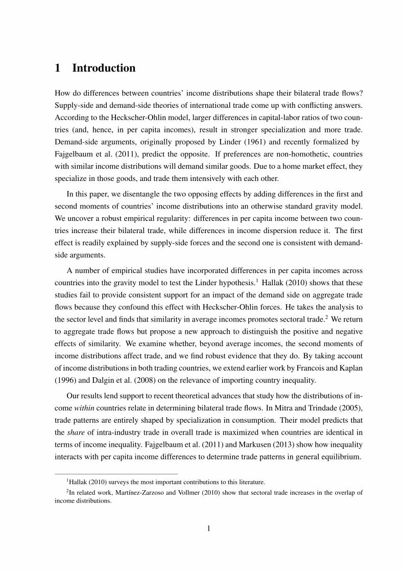
How do differences between countries’ income distributions shape their bilateral trade flows?Supply-side and demand-side theories of international trade come up with conflicting answers.According to the Heckscher-Ohlin model, larger differences in capital-labor ratios of two coun-tries (and, hence, in per capita incomes), result in stronger specialization and more trade.Demand-side arguments, originally proposed by Linder (1961) and recently formalized byFajgelbaum et al. (2011), predict the opposite. If preferences are non-homothetic, countrieswith similar income distributions will demand similar goods. Due to a home market effect, theyspecialize in those goods, and trade them intensively with each other.

In this paper, we disentangle the two opposing effects by adding differences in the first andsecond moments of countries’ income distributions into an otherwise standard gravity model.We uncover a robust empirical regularity: differences in per capita income between two coun-tries increase their bilateral trade, while differences in income dispersion reduce it. The firsteffect is readily explained by supply-side forces and the second one is consistent with demand-side arguments.

A number of empirical studies have incorporated differences in per capita incomes acrosscountries into the gravity model to test the Linder hypothesis.1 Hallak (2010) shows that thesestudies fail to provide consistent support for an impact of the demand side on aggregate tradeflows because they confound this effect with Heckscher-Ohlin forces. He takes the analysis tothe sector level and finds that similarity in average incomes promotes sectoral trade.2 We returnto aggregate trade flows but propose a new approach to distinguish the positive and negativeeffects of similarity. We examine whether, beyond average incomes, the second moments ofincome distributions affect trade, and we find robust evidence that they do. By taking accountof income distributions in both trading countries, we extend earlier work by Francois and Kaplan(1996) and Dalgin et al. (2008) on the relevance of importing country inequality.

Our results lend support to recent theoretical advances that study how the distributions of in-come within countries relate in determining bilateral trade flows. In Mitra and Trindade (2005),trade patterns are entirely shaped by specialization in consumption. Their model predicts thatthe share of intra-industry trade in overall trade is maximized when countries are identical interms of income inequality. Fajgelbaum et al. (2011) and Markusen (2013) show how inequalityinteracts with per capita income differences to determine trade patterns in general equilibrium.

1Hallak (2010) surveys the most important contributions to this literature.2In related work, Martínez-Zarzoso and Vollmer (2010) show that sectoral trade increases in the overlap of

income distributions.

1

2 Gravity Model

The starting point of our empirical analysis is a standard gravity model,3 which we augmentby two terms capturing the similarity of the trading partners’ income distributions. The mainequation to be estimated explains the value of differentiated goods exports Xij shipped fromcountry i to country j:

lnXij = βy∆yij + βσ∆σij + γTij + δi + δj + εij, (1)

by the difference in average incomes y : ∆yij ≡ (ln yi − ln yj)2 (2)

and the difference in within-country income dispersion σ : ∆σij ≡ (lnσi − lnσj)2 . (3)

Tij is a vector that collects the usual gravity covariates approximating trade costs: the log ofbilateral distance, dummy variables for a common border, language, colonial link or colonizer,as well as lagged dummies indicating joint membership in a Free Trade Agreement (FTA), orin the World Trade Organization (WTO). To deal with unobserved multilateral resistance, weinclude importer and exporter fixed effects δi and δj. They make inclusion of purely monadicvariables such as the level of GDP, yi, or σj redundant and also absorb all monadic variation ofvariables contained in Tij .4

We are interested in estimates of βy and βσ. Clean identification of these parameters requiresthat the following identifying assumption on the conditional covariances holds: cov (∆zij, εij|δi, δj,Tij) = 0, z ∈ {y, σ}. Given the definition of ∆zij , these requirements translate into

cov (zizj, εij| δi, δj,Tij) = 0 (4)

under the standard assumption that εij has zero conditional mean. If zi and zj are independent,this identifying assumption is met. It requires that any trade shock εij must be orthogonal tothe joint realization of z in both countries. In other words, we need that aggregate conditions incountry i are independent of aggregate conditions in country j. Clearly, this condition can beviolated if i is an important trade partner for j or vice versa. We thus run robustness checks thateliminate each importer’s five largest trading partners from the sample.

3See Head and Mayer (2014) for an excellent introduction into gravity modeling.4When estimating (1) on panel data, we employ time-specific dummies δit and δjt and add a pair fixed-

effect δij . Note that we do not normalize the dispersion measures in (3) by the mean income in order to captureunconfounded variation in σ; the bilateral difference in average incomes is controlled for by ∆yij . We providerobustness checks using alternative dispersion measures in the Appendix.

2

A positive estimate of βy can be interpreted as evidence of Heckscher-Ohlin forces, while anegative sign favors the traditional Linder hypothesis. If the second moments capture similarityin demand, and if this promotes trade, we should observe βσ < 0.

3 Data

We obtain the shares of total net income received by deciles of the population from the WorldBank’s World Development Indicators (WDI), complemented by Eurostat and the nationalstatistics offices of the U.S. and Canada. Due to limited data availability, we take averages over5-year periods: 1995-1999, 2000-2004, and 2005-2009. Dispersion measures are computedfrom all available quantiles within a given period. The resulting unbalanced panel includes 145countries, of which 114 are available in the middle period.5

Disaggregate trade flows are obtained from the BACI dataset.6 Since the arguments inthe theoretical literature mostly relate to trade in differentiated goods, we select only thoseproducts (at the SITC 4 level) for which neither an organized exchange nor a reference priceexists according to Rauch’s (1999) ‘liberal’ classification and aggregate them up to obtain onetrade flow per exporter, importer, and time period. We use data on population and GDP fromthe WDI and gravity controls are taken from CEPII and the WTO website.

4 Results

4.1 Main findings

The first three columns of Table 1 display our main results for the cross-section of 2000-2004.7

The ‘traditional’ Linder test in column 1 suggests that differences in per capita incomes en-courage trade rather than discourage it. Heckscher-Ohlin factors appear to outweigh the Lindermechanism. The alternative Linder test referring to second moments is reported in column 2.Differences in standard deviations between countries do not seem to affect trade in any way.

5The Appendix provides details on our selection and treatment of the data on income distributions and lists thecountries and sectors in the dataset.

6The Base pour l’Analyse du Commerce International (BACI) of the Centre d’Etudes Prospectives etd’Informations Internationales (CEPII) is based on the UN Comtrade database and documented in Gaulier andZignago (2010).

7Very similar results obtain in each period of our panel; see the Appendix, which also provides summarystatistics.

3

Only if both terms ∆yij and ∆σij are included, a clear pattern emerges (column 3): differences

in average incomes across countries promote trade as does the similarity of income distribu-tion within countries. This finding suggests an amended, ‘distributional’ Linder mechanism:similarity in second moments of countries’ income distributions fosters bilateral trade.

«TABLE 1 HERE»

Next, we exploit time variation in bilateral trade relationships to identify the effects of incomedistribution on trade. We eliminate all pair-specific effects by within-transformation. The esti-mates displayed in column 6 of Table 1 confirm our earlier findings. For example, they implythat trade between France and Hong Kong would increase by 2.5% if income in Hong Kongwere redistributed such that its level of inequality were reduced to the level of France.8 Interest-ingly, in contrast to the cross-sectional results, including either the difference in first or secondmoments individually yields negative coefficients on both (dis)similarity measures.

4.2 Robustness analysis

Table 2 explores the robustness of our results.9 We start by addressing the obvious endogene-ity concern. We first run robustness checks that eliminate each importer’s five largest tradingpartners from the sample. Second, we substitute ∆y and ∆σ by one-period lags, and third, weuse these lags as instrumental variables (IV) for their contemporaneous values in 2SLS regres-sions. As displayed in Panel A of Table 2, our main results are robust to these modifications:the coefficients βy and βσ in columns 3, 6, and 9 preserve their signs and significance levels.

«TABLE 2 HERE»

The presence of zeros in bilateral trade data constitutes a well-known problem in estimatinggravity models. Furthermore, Santos Silva and Tenreyro (2006) have shown that heteroskedas-ticity may introduce a bias in log-linear models such as equation (1). Therefore, following theguidance of Head and Mayer (2014), we apply Pseudo Maximum Likelihood estimators of thePoisson (PPML) and Gamma (ΓPML) types as well as Tobit regressions. Panel B of Table 2shows that our results appear even stronger if these non-linear models are applied.

8These numbers refer to the second period of our sample (2000-2004), in which France and HongKong have approximately the same GDP per capita. The difference in standard deviations ∆σ =[ln(24, 453)− ln(13, 555)]

2 ≈ 0.348 thus reduces trade by the factor exp(−0.071 × 0.212) ≈ 0.976. Elimi-nating this difference would boost trade by roughly 1/0.976− 1 ≈ 2.5%.

9In the Appendix, we provide a wide range of additional robustness checks.

4

Panel C divides the sample by the development status of trading partners and examinestotal aggregate trade flows. Confining the analysis to the sample of “northern” (industrialized)countries,10 our benchmark results continue to hold despite the small number of observations.Similarly, when focusing on North-South trade (including flows in both directions), our mainresults remain intact. However, the North-North sample admits much larger coefficients on the(dis)similarity measures, which may be due to stronger forces of specialization and of demandsimilarities or due to lower measurement error in the dependent and independent variables.11

The last group of regressions in Panel C shows that our results continue to hold if we considertotal trade rather than trade in differentiated goods as the dependent variable.

The Appendix provides further robustness checks. To highlight a few of them, we con-firm that our cross-sectional results carry through for different time periods, and that our panelregressions are qualitatively robust to using first differences or a balanced panel. We also ex-periment with alternative measures of (dis)similarity in income distributions (e.g. differencesin Gini, Theil, and Atkinson indices as well as decile and quintile ratios) and find that signpatterns are robust. Finally, we show that our results cannot be explained by (dis)similarity ininstitutions (democratic orientation and economic freedom).

5 Interpretation of results and conclusion

We uncover a very robust stylized fact that has not been documented in the economics literatureso far: differences in first and second moments of countries’ income distributions matter forthe volume of bilateral trade, but with opposite signs. While the two measures are positivelycorrelated in the data, they do proxy different dimensions of (dis)similarity. Besides the Linderchannel stressed by Hallak (2010), differences in mean incomes may capture the role of differ-ent endowment structures or development status. The positive trade effect of similarity in thedispersion of income is also reminiscent of Linder’s argument, but it may alternatively reflectthe impact of affinity in countries’ societal structures determining the distribution of assets orthe taste for fiscal redistribution. The observed pattern calls for further research to distinguishexplanations based on non-homothetic preferences from other mechanisms.

10We distinguish high-income countries by their income per capita in 2011 according to the World Bank defi-nition.

11Results for South-South trade (not shown) turn out insignificant, likely for similar reasons.

5

References

Dalgin, Muhammed, Vitor Trindade, and Devashish Mitra, “Inequality, NonhomotheticPreferences, and Trade: A Gravity Approach,” Southern Economic Journal, January 2008,74 (3), 747–774.

Fajgelbaum, Pablo, Gene M. Grossman, and Elhanan Helpman, “Income Distribution,Product Quality, and International Trade,” Journal of Political Economy, 2011, 119 (4), 721– 765.

Francois, Joseph F. and Seth Kaplan, “Aggregate Demand Shifts, Income Distribution, andthe Linder Hypothesis,” The Review of Economics and Statistics, May 1996, 78 (2), 244–50.

Gaulier, Guillaume and Soledad Zignago, “BACI: International Trade Database at theProduct-Level. The 1994-2007 Version,” Working Papers 2010-23, CEPII research centerOct 2010.

Hallak, Juan Carlos, “A Product-Quality View of the Linder Hypothesis,” The Review of Eco-

nomics and Statistics, September 2010, 92 (3), 453–466.

Head, Keith and Thierry Mayer, “Gravity Equations: Workhorse, Toolkit, and Cookbook,”in Gita Gopinath, Elhanan Helpman, and Kenneth Rogoff, eds., Handbook of International

Economics, Vol. 4 2014, chapter 3, pp. 131–195.

Linder, Staffan Burenstam, An Essay on Trade and Transformation, Stockholm: Almqvist &Wiksell, 1961.

Markusen, James R., “Putting Per-Capita Income Back into Trade Theory,” Journal of Inter-

national Economics, 2013, 90 (2), 255–265.

Martínez-Zarzoso, Inmaculada and Sebastian Vollmer, “Bilateral trade flows and income-distribution similarity,” Working Papers 10-06, Asociación Española de Economía y FinanzasInternacionales Sep 2010.

Mitra, Devashish and Vitor Trindade, “Inequality and trade,” Canadian Journal of Eco-

nomics, November 2005, 38 (4), 1253–1271.

Rauch, James E., “Networks versus markets in international trade,” Journal of International

Economics, June 1999, 48 (1), 7–35.

Santos Silva, João M. C. and Silvana Tenreyro, “The Log of Gravity,” The Review of Eco-

nomics and Statistics, 09 2006, 88 (4), 641–658.

6

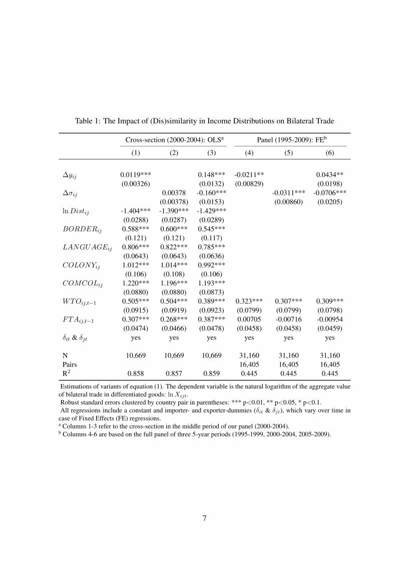
Table 1: The Impact of (Dis)similarity in Income Distributions on Bilateral Trade

Cross-section (2000-2004): OLSa Panel (1995-2009): FEb

(1) (2) (3) (4) (5) (6)

∆yij 0.0119*** 0.148*** -0.0211** 0.0434**(0.00326) (0.0132) (0.00829) (0.0198)

∆σij 0.00378 -0.160*** -0.0311*** -0.0706***(0.00378) (0.0153) (0.00860) (0.0205)

lnDistij -1.404*** -1.390*** -1.429***(0.0288) (0.0287) (0.0289)

BORDERij 0.588*** 0.600*** 0.545***(0.121) (0.121) (0.117)

LANGUAGEij 0.806*** 0.822*** 0.785***(0.0643) (0.0643) (0.0636)

COLONYij 1.012*** 1.014*** 0.992***(0.106) (0.108) (0.106)

COMCOLij 1.220*** 1.196*** 1.193***(0.0880) (0.0880) (0.0873)

WTOij,t−1 0.505*** 0.504*** 0.389*** 0.323*** 0.307*** 0.309***(0.0915) (0.0919) (0.0923) (0.0799) (0.0799) (0.0798)

FTAij,t−1 0.307*** 0.268*** 0.387*** 0.00705 -0.00716 -0.00954(0.0474) (0.0466) (0.0478) (0.0458) (0.0458) (0.0459)

δit & δjt yes yes yes yes yes yes

N 10,669 10,669 10,669 31,160 31,160 31,160Pairs 16,405 16,405 16,405R2 0.858 0.857 0.859 0.445 0.445 0.445

Estimations of variants of equation (1). The dependent variable is the natural logarithm of the aggregate valueof bilateral trade in differentiated goods: lnXijt.Robust standard errors clustered by country pair in parentheses: *** p<0.01, ** p<0.05, * p<0.1.All regressions include a constant and importer- and exporter-dummies (δit & δjt), which vary over time in

case of Fixed Effects (FE) regressions.a Columns 1-3 refer to the cross-section in the middle period of our panel (2000-2004).b Columns 4-6 are based on the full panel of three 5-year periods (1995-1999, 2000-2004, 2005-2009).

7

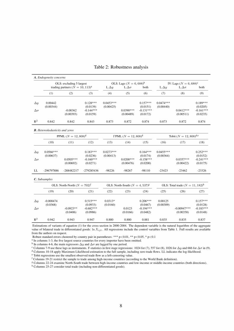
Table 2: Robustness analysis

A. Endogeneity concerns

OLS: excluding 5 largest OLS: Lags (N = 6, 688)b IV: Lags (N = 6, 688)c

trading partners (N = 10, 113)a L.∆y L.∆σ both L.∆y L.∆σ both

(1) (2) (3) (4) (5) (6) (7) (8) (9)

∆y 0.00442 0.128*** 0.0453*** 0.157*** 0.0474*** 0.189***(0.00344) (0.0139) (0.00425) (0.0151) (0.00440) (0.0205)

∆σ -0.00362 -0.144*** 0.0390*** -0.131*** 0.0412*** -0.161***(0.00393) (0.0159) (0.00489) (0.0172) (0.00511) (0.0235)

R2 0.842 0.842 0.843 0.873 0.872 0.874 0.873 0.872 0.874

B. Heteroskedasticity and zeros

PPML (N = 12, 808)d ΓPML (N = 12, 808)d Tobit (N = 12, 808)d,e

(10) (11) (12) (13) (14) (15) (16) (17) (18)

∆y 0.0566*** 0.183*** 0.0273*** 0.164*** 0.0455*** 0.252***(0.00637) (0.0236) (0.00413) (0.0174) (0.00364) (0.0152)

∆σ 0.0505*** -0.160*** 0.0200*** -0.158*** 0.0357*** -0.241***(0.00692) (0.0271) (0.00476) (0.0200) (0.00422) (0.0175)

LL -296797886 -288482217 -279285436 -98226 -98267 -98110 -23423 -23462 -23326

C. Subsamples

OLS: North-North (N = 702)f OLS: North-South (N = 4, 537)g OLS: Total trade (N = 11, 182)h

(19) (20) (21) (22) (23) (24) (25) (26) (27)

∆y -0.000474 0.515*** 0.0313* 0.206*** 0.00125 0.157***(0.0368) (0.0933) (0.0160) (0.0467) (0.00309) (0.0128)

∆σ -0.0923** -0.682*** 0.0123 -0.194*** -0.00947*** -0.183***(0.0406) (0.0986) (0.0166) (0.0482) (0.00358) (0.0148)

R2 0.942 0.943 0.947 0.880 0.880 0.881 0.835 0.835 0.837

Estimations of variants of equation (1) for the cross-section in 2000-2004. The dependent variable is the natural logarithm of the aggregatevalue of bilateral trade in differentiated goods: lnXijt. All regressions include the control variables from Table 1. Full results are availablefrom the authors on request.Robust standard errors clustered by country pair in parentheses: *** p<0.01, ** p<0.05, * p<0.1

a In columns 1-3, the five largest source countries for every importer have been omitted.b In columns 4-6, the main regressors ∆y and ∆σ are lagged by one period.c Columns 7-9 use these lags as instruments. F-statistics in first stage regressions: 1024 for (7), 557 for (8), 1026 for ∆y and 666 for ∆σ in (9).d Columns 10-18 apply Maximum Likelihood estimation to the full sample, including zero trade flows. LL indicates the log-likelihood.e Tobit regressions use the smallest observed trade flow as a left-censoring value.f Columns 19-21 restrict the sample to trade among high-income countries (according to the World Bank definition).g Columns 22-24 examine North-South trade between high-income countries and low-income or middle-income countries (both directions).h Columns 25-27 consider total trade (including non-differentiated goods).

8

APPENDIX TO

EPPINGER & FELBERMAYR

“Bilateral Trade and Similarity of Income Distributions: The Role of Second Moments”

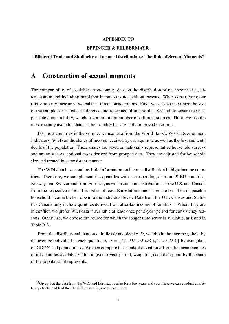
A Construction of second moments

The comparability of available cross-country data on the distribution of net income (i.e., af-ter taxation and including non-labor incomes) is not without caveats. When constructing our(dis)similarity measures, we balance three considerations. First, we seek to maximize the sizeof the sample for statistical inference and relevance of our results. Second, to ensure the bestpossible comparability, we choose a minimum number of different sources. Third, we use themost recently available data, as their quality has arguably improved over time.

For most countries in the sample, we use data from the World Bank’s World DevelopmentIndicators (WDI) on the shares of income received by each quintile as well as the first and tenthdecile of the population. These shares are based on nationally representative household surveysand are only in exceptional cases derived from grouped data. They are adjusted for householdsize and treated in a consistent manner.

The WDI data base contains little information on income distribution in high-income coun-tries. Therefore, we complement the quantiles with corresponding data on 19 EU countries,Norway, and Switzerland from Eurostat, as well as income distributions of the U.S. and Canadafrom the respective national statistics offices. Eurostat income shares are based on disposablehousehold income broken down to the individual level. Data from the U.S. Census and Statis-tics Canada only include quintiles derived from after-tax income of families.12 Where they arein conflict, we prefer WDI data if available at least once per 5-year period for consistency rea-sons. Otherwise, we choose the source for which the longer time series is available, as listed inTable B.3.

From the distributional data on quintiles Q and deciles D, we obtain the income yi held bythe average individual in each quantile qi, i = {D1, D2, Q2, Q3, Q4, D9, D10} by using dataon GDP Y and population L. We then compute the standard deviation σ from the mean incomesof all quantiles available within a given 5-year period, weighting each data point by the shareof the population it represents.

12Given that the data from the WDI and Eurostat overlap for a few years and countries, we can conduct consis-tency checks and find that the differences in general are small.

i

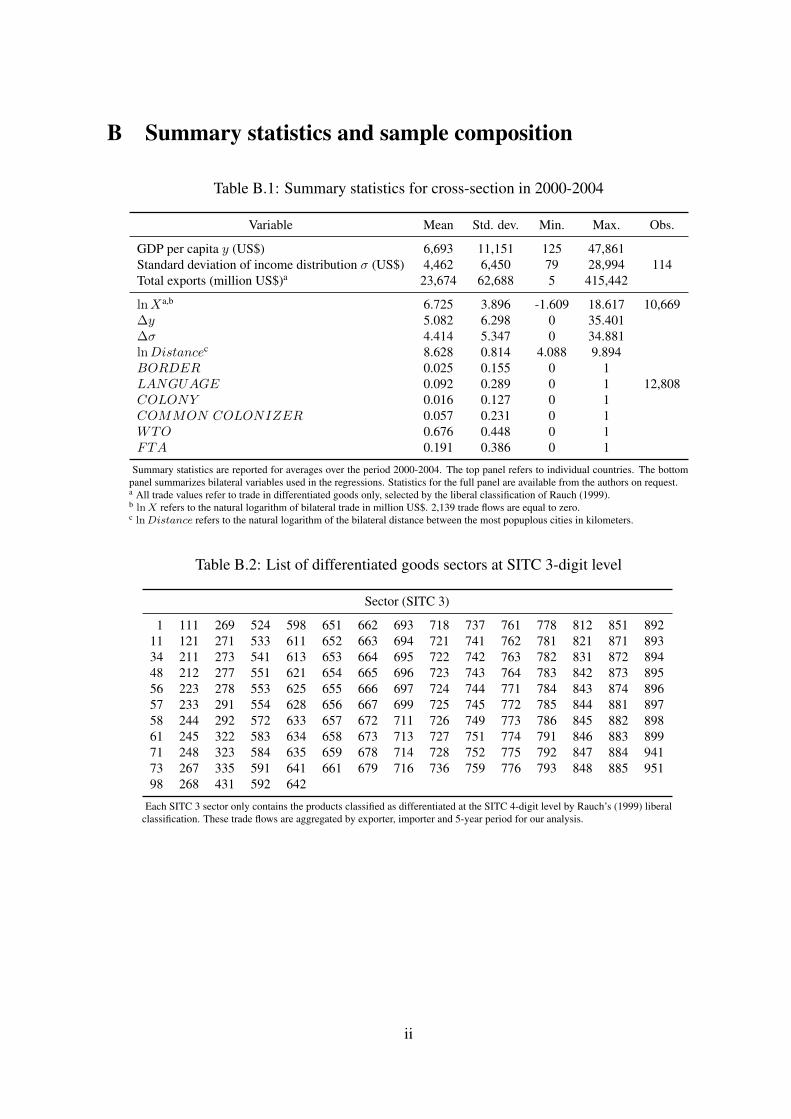
B Summary statistics and sample composition

Table B.1: Summary statistics for cross-section in 2000-2004

Variable Mean Std. dev. Min. Max. Obs.

GDP per capita y (US$) 6,693 11,151 125 47,861114Standard deviation of income distribution σ (US$) 4,462 6,450 79 28,994

Total exports (million US$)a 23,674 62,688 5 415,442

lnXa,b 6.725 3.896 -1.609 18.617 10,669∆y 5.082 6.298 0 35.401

12,808

∆σ 4.414 5.347 0 34.881lnDistancec 8.628 0.814 4.088 9.894BORDER 0.025 0.155 0 1LANGUAGE 0.092 0.289 0 1COLONY 0.016 0.127 0 1COMMON COLONIZER 0.057 0.231 0 1WTO 0.676 0.448 0 1FTA 0.191 0.386 0 1

Summary statistics are reported for averages over the period 2000-2004. The top panel refers to individual countries. The bottompanel summarizes bilateral variables used in the regressions. Statistics for the full panel are available from the authors on request.a All trade values refer to trade in differentiated goods only, selected by the liberal classification of Rauch (1999).b lnX refers to the natural logarithm of bilateral trade in million US$. 2,139 trade flows are equal to zero.c lnDistance refers to the natural logarithm of the bilateral distance between the most popuplous cities in kilometers.

Table B.2: List of differentiated goods sectors at SITC 3-digit level

Sector (SITC 3)

1 111 269 524 598 651 662 693 718 737 761 778 812 851 89211 121 271 533 611 652 663 694 721 741 762 781 821 871 89334 211 273 541 613 653 664 695 722 742 763 782 831 872 89448 212 277 551 621 654 665 696 723 743 764 783 842 873 89556 223 278 553 625 655 666 697 724 744 771 784 843 874 89657 233 291 554 628 656 667 699 725 745 772 785 844 881 89758 244 292 572 633 657 672 711 726 749 773 786 845 882 89861 245 322 583 634 658 673 713 727 751 774 791 846 883 89971 248 323 584 635 659 678 714 728 752 775 792 847 884 94173 267 335 591 641 661 679 716 736 759 776 793 848 885 95198 268 431 592 642

Each SITC 3 sector only contains the products classified as differentiated at the SITC 4-digit level by Rauch’s (1999) liberalclassification. These trade flows are aggregated by exporter, importer and 5-year period for our analysis.

ii

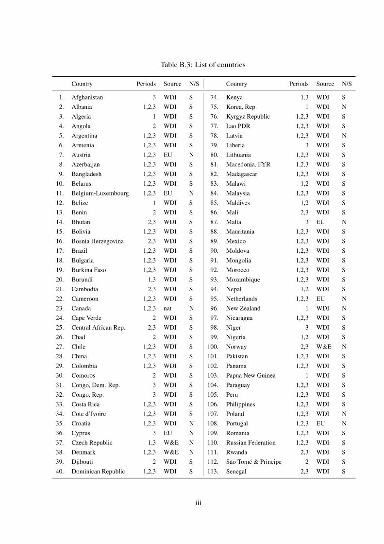
Table B.3: List of countries

Country Periods Source N/S Country Periods Source N/S

1. Afghanistan 3 WDI S 74. Kenya 1,3 WDI S2. Albania 1,2,3 WDI S 75. Korea, Rep. 1 WDI N3. Algeria 1 WDI S 76. Kyrgyz Republic 1,2,3 WDI S4. Angola 2 WDI S 77. Lao PDR 1,2,3 WDI S5. Argentina 1,2,3 WDI S 78. Latvia 1,2,3 WDI N6. Armenia 1,2,3 WDI S 79. Liberia 3 WDI S7. Austria 1,2,3 EU N 80. Lithuania 1,2,3 WDI S8. Azerbaijan 1,2,3 WDI S 81. Macedonia, FYR 1,2,3 WDI S9. Bangladesh 1,2,3 WDI S 82. Madagascar 1,2,3 WDI S

10. Belarus 1,2,3 WDI S 83. Malawi 1,2 WDI S11. Belgium-Luxembourg 1,2,3 EU N 84. Malaysia 1,2,3 WDI S12. Belize 1 WDI S 85. Maldives 1,2 WDI S13. Benin 2 WDI S 86. Mali 2,3 WDI S14. Bhutan 2,3 WDI S 87. Malta 3 EU N15. Bolivia 1,2,3 WDI S 88. Mauritania 1,2,3 WDI S16. Bosnia Herzegovina 2,3 WDI S 89. Mexico 1,2,3 WDI S17. Brazil 1,2,3 WDI S 90. Moldova 1,2,3 WDI S18. Bulgaria 1,2,3 WDI S 91. Mongolia 1,2,3 WDI S19. Burkina Faso 1,2,3 WDI S 92. Morocco 1,2,3 WDI S20. Burundi 1,3 WDI S 93. Mozambique 1,2,3 WDI S21. Cambodia 2,3 WDI S 94. Nepal 1,2 WDI S22. Cameroon 1,2,3 WDI S 95. Netherlands 1,2,3 EU N23. Canada 1,2,3 nat N 96. New Zealand 1 WDI N24. Cape Verde 2 WDI S 97. Nicaragua 1,2,3 WDI S25. Central African Rep. 2,3 WDI S 98. Niger 3 WDI S26. Chad 2 WDI S 99. Nigeria 1,2 WDI S27. Chile 1,2,3 WDI S 100. Norway 2,3 W&E N28. China 1,2,3 WDI S 101. Pakistan 1,2,3 WDI S29. Colombia 1,2,3 WDI S 102. Panama 1,2,3 WDI S30. Comoros 2 WDI S 103. Papua New Guinea 1 WDI S31. Congo, Dem. Rep. 3 WDI S 104. Paraguay 1,2,3 WDI S32. Congo, Rep. 3 WDI S 105. Peru 1,2,3 WDI S33. Costa Rica 1,2,3 WDI S 106. Philippines 1,2,3 WDI S34. Cote d’Ivoire 1,2,3 WDI S 107. Poland 1,2,3 WDI N35. Croatia 1,2,3 WDI N 108. Portugal 1,2,3 EU N36. Cyprus 3 EU N 109. Romania 1,2,3 WDI S37. Czech Republic 1,3 W&E N 110. Russian Federation 1,2,3 WDI S38. Denmark 1,2,3 W&E N 111. Rwanda 2,3 WDI S39. Djibouti 2 WDI S 112. São Tomé & Principe 2 WDI S40. Dominican Republic 1,2,3 WDI S 113. Senegal 2,3 WDI S

iii

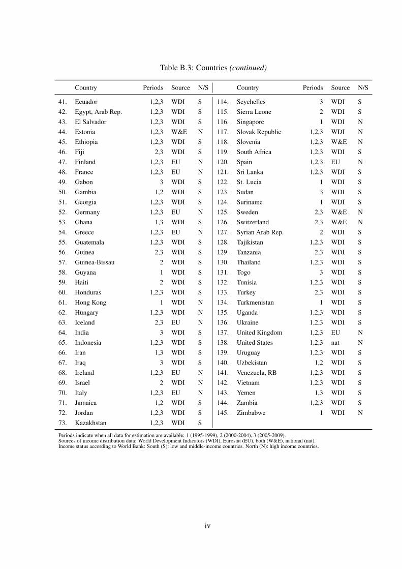
Table B.3: Countries (continued)

Country Periods Source N/S Country Periods Source N/S

41. Ecuador 1,2,3 WDI S 114. Seychelles 3 WDI S42. Egypt, Arab Rep. 1,2,3 WDI S 115. Sierra Leone 2 WDI S43. El Salvador 1,2,3 WDI S 116. Singapore 1 WDI N44. Estonia 1,2,3 W&E N 117. Slovak Republic 1,2,3 WDI N45. Ethiopia 1,2,3 WDI S 118. Slovenia 1,2,3 W&E N46. Fiji 2,3 WDI S 119. South Africa 1,2,3 WDI S47. Finland 1,2,3 EU N 120. Spain 1,2,3 EU N48. France 1,2,3 EU N 121. Sri Lanka 1,2,3 WDI S49. Gabon 3 WDI S 122. St. Lucia 1 WDI S50. Gambia 1,2 WDI S 123. Sudan 3 WDI S51. Georgia 1,2,3 WDI S 124. Suriname 1 WDI S52. Germany 1,2,3 EU N 125. Sweden 2,3 W&E N53. Ghana 1,3 WDI S 126. Switzerland 2,3 W&E N54. Greece 1,2,3 EU N 127. Syrian Arab Rep. 2 WDI S55. Guatemala 1,2,3 WDI S 128. Tajikistan 1,2,3 WDI S56. Guinea 2,3 WDI S 129. Tanzania 2,3 WDI S57. Guinea-Bissau 2 WDI S 130. Thailand 1,2,3 WDI S58. Guyana 1 WDI S 131. Togo 3 WDI S59. Haiti 2 WDI S 132. Tunisia 1,2,3 WDI S60. Honduras 1,2,3 WDI S 133. Turkey 2,3 WDI S61. Hong Kong 1 WDI N 134. Turkmenistan 1 WDI S62. Hungary 1,2,3 WDI N 135. Uganda 1,2,3 WDI S63. Iceland 2,3 EU N 136. Ukraine 1,2,3 WDI S64. India 3 WDI S 137. United Kingdom 1,2,3 EU N65. Indonesia 1,2,3 WDI S 138. United States 1,2,3 nat N66. Iran 1,3 WDI S 139. Uruguay 1,2,3 WDI S67. Iraq 3 WDI S 140. Uzbekistan 1,2 WDI S68. Ireland 1,2,3 EU N 141. Venezuela, RB 1,2,3 WDI S69. Israel 2 WDI N 142. Vietnam 1,2,3 WDI S70. Italy 1,2,3 EU N 143. Yemen 1,3 WDI S71. Jamaica 1,2 WDI S 144. Zambia 1,2,3 WDI S72. Jordan 1,2,3 WDI S 145. Zimbabwe 1 WDI N73. Kazakhstan 1,2,3 WDI S

Periods indicate when all data for estimation are available: 1 (1995-1999), 2 (2000-2004), 3 (2005-2009).Sources of income distribution data: World Development Indicators (WDI), Eurostat (EU), both (W&E), national (nat).Income status according to World Bank: South (S): low and middle-income countries. North (N): high income countries.

iv

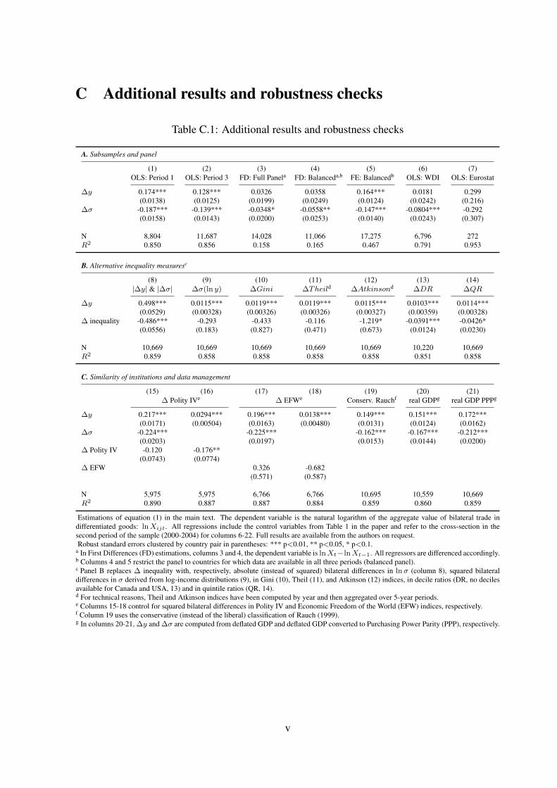
C Additional results and robustness checks

Table C.1: Additional results and robustness checks

A. Subsamples and panel

(1) (2) (3) (4) (5) (6) (7)OLS: Period 1 OLS: Period 3 FD: Full Panela FD: Balanceda,b FE: Balancedb OLS: WDI OLS: Eurostat

∆y 0.174*** 0.128*** 0.0326 0.0358 0.164*** 0.0181 0.299(0.0138) (0.0125) (0.0199) (0.0249) (0.0124) (0.0242) (0.216)

∆σ -0.187*** -0.139*** -0.0348* -0.0558** -0.147*** -0.0804*** -0.292(0.0158) (0.0143) (0.0200) (0.0253) (0.0140) (0.0243) (0.307)

N 8,804 11,687 14,028 11,066 17,275 6,796 272R2 0.850 0.856 0.158 0.165 0.467 0.791 0.953

B. Alternative inequality measuresc

(8) (9) (10) (11) (12) (13) (14)|∆y| & |∆σ| ∆σ(ln y) ∆Gini ∆Theild ∆Atkinsond ∆DR ∆QR

∆y 0.498*** 0.0115*** 0.0119*** 0.0119*** 0.0115*** 0.0103*** 0.0114***(0.0529) (0.00328) (0.00326) (0.00326) (0.00327) (0.00359) (0.00328)

∆ inequality -0.486*** -0.293 -0.433 -0.116 -1.219* -0.0391*** -0.0426*(0.0556) (0.183) (0.827) (0.471) (0.673) (0.0124) (0.0230)

N 10,669 10,669 10,669 10,669 10,669 10,220 10,669R2 0.859 0.858 0.858 0.858 0.858 0.851 0.858

C. Similarity of institutions and data management

(15) (16) (17) (18) (19) (20) (21)∆ Polity IVe ∆ EFWe Conserv. Rauchf real GDPg real GDP PPPg

∆y 0.217*** 0.0294*** 0.196*** 0.0138*** 0.149*** 0.151*** 0.172***(0.0171) (0.00504) (0.0163) (0.00480) (0.0131) (0.0124) (0.0162)

∆σ -0.224*** -0.225*** -0.162*** -0.167*** -0.212***(0.0203) (0.0197) (0.0153) (0.0144) (0.0200)

∆ Polity IV -0.120 -0.176**(0.0743) (0.0774)

∆ EFW 0.326 -0.682(0.571) (0.587)

N 5,975 5,975 6,766 6,766 10,695 10,559 10,669R2 0.890 0.887 0.887 0.884 0.859 0.860 0.859

Estimations of equation (1) in the main text. The dependent variable is the natural logarithm of the aggregate value of bilateral trade indifferentiated goods: lnXijt. All regressions include the control variables from Table 1 in the paper and refer to the cross-section in thesecond period of the sample (2000-2004) for columns 6-22. Full results are available from the authors on request.Robust standard errors clustered by country pair in parentheses: *** p<0.01, ** p<0.05, * p<0.1.

a In First Differences (FD) estimations, columns 3 and 4, the dependent variable is lnXt−lnXt−1. All regressors are differenced accordingly.b Columns 4 and 5 restrict the panel to countries for which data are available in all three periods (balanced panel).c Panel B replaces ∆ inequality with, respectively, absolute (instead of squared) bilateral differences in lnσ (column 8), squared bilateraldifferences in σ derived from log-income distributions (9), in Gini (10), Theil (11), and Atkinson (12) indices, in decile ratios (DR, no decilesavailable for Canada and USA, 13) and in quintile ratios (QR, 14).d For technical reasons, Theil and Atkinson indices have been computed by year and then aggregated over 5-year periods.e Columns 15-18 control for squared bilateral differences in Polity IV and Economic Freedom of the World (EFW) indices, respectively.f Column 19 uses the conservative (instead of the liberal) classification of Rauch (1999).g In columns 20-21, ∆y and ∆σ are computed from deflated GDP and deflated GDP converted to Purchasing Power Parity (PPP), respectively.

v

Ifo Working Papers

No. 183 Wohlrabe, K., Das FAZ-Ökonomenranking 2013: Eine kritische Betrachtung, Juli 2014.

No. 182 Lehmann, R. and A. Weyh, Forecasting employment in Europe: Are survey result help-

ful?, June 2014.

No. 181 Schinke, C., Government Ideology, Globalization, and Top Income Shares in OECD

Countries, June 2014.

No. 180 Benz, S., M. Larch and M. Zimmer, The Structure of the German Economy, May 2014.

No. 179 Meier, V. and H. Rainer, Pigou Meets Ramsey: Gender-Based Taxation with Non-

Cooperative Couples, May 2014.

No. 178 Kugler, F., G. Schwerdt und L. Wößmann, Ökonometrische Methoden zur Evaluierung

kausaler Effeke der Wirtschaftspolitik, April 2014.

No. 177 Angerer, S., D. Glätzle-Rützler, P. Lergetporer and M. Sutter, Donations, risk attitudes

and time preferences: A study on altruism in primary school children, March 2014.

No. 176 Breuer, C., On the Rationality of Medium-Term Tax Revenue Forecasts: Evidence from

Germany, March 2014.

No. 175 Reischmann, M., Staatsverschuldung in Extrahaushalten: Historischer Überblick und

Implikationen für die Schuldenbremse in Deutschland, März 2014.

No. 174 Eberl, J. and C. Weber, ECB Collateral Criteria: A Narrative Database 2001–2013,

February 2014.

No. 173 Benz, S., M. Larch and M. Zimmer, Trade in Ideas: Outsourcing and Knowledge Spillovers,

February 2014.

No. 172 Kauder, B., B. Larin und N. Potrafke, Was bringt uns die große Koalition? Perspektiven

der Wirtschaftspolitik, Januar 2014.

No. 171 Lehmann, R. and K. Wohlrabe, Forecasting gross value-added at the regional level: Are

sectoral disaggregated predictions superior to direct ones?, December 2013.

No. 170 Meier, V. and I. Schiopu, Optimal higher education enrollment and productivity externalities

in a two-sector-model, November 2013.

No. 169 Danzer, N., Job Satisfaction and Self-Selection into the Public or Private Sector: Evidence

from a Natural Experiment, November 2013.

No. 168 Battisti, M., High Wage Workers and High Wage Peers, October 2013.

No. 167 Henzel, S.R. and M. Rengel, Dimensions of Macroeconomic Uncertainty: A Common

Factor Analysis, August 2013.

No. 166 Fabritz, N., The Impact of Broadband on Economic Activity in Rural Areas: Evidence

from German Municipalities, July 2013.

No. 165 Reinkowski, J., Should We Care that They Care? Grandchild Care and Its Impact on

Grandparent Health, July 2013.

No. 164 Potrafke, N., Evidence on the Political Principal-Agent Problem from Voting on Public

Finance for Concert Halls, June 2013.

No. 163 Hener, T., Labeling Effects of Child Benefits on Family Savings, May 2013.

No. 162 Bjørnskov, C. and N. Potrafke, The Size and Scope of Government in the US States:

Does Party Ideology Matter?, May 2013.

No. 161 Benz, S., M. Larch and M. Zimmer, The Structure of Europe: International Input-Output

Analysis with Trade in Intermediate Inputs and Capital Flows, May 2013.

No. 160 Potrafke, N., Minority Positions in the German Council of Economic Experts: A Political

Economic Analysis, April 2013.

No. 159 Kauder, B. and N. Potrafke, Government Ideology and Tuition Fee Policy: Evidence

from the German States, April 2013.

No. 158 Hener, T., S. Bauernschuster and H. Rainer, Does the Expansion of Public Child Care

Increase Birth Rates? Evidence from a Low-Fertility Country, April 2013.