Bidirectional propagation of

Action potentials

Jorin Diemer

Supervisor: Alfredo Gonzalez-PerezStudent Project

Niels Bohr InstituteUniversity of Copenhagen

March 27, 2014

Acknowledgements

Firstly I want to thank Prof. Thomas Heimburg for giving me the opportunity to work in hisgroup and for instructive conversations. Special thanks go to my supervisor Alfredo Gonzalez-Perez for taking a great deal of his time to give me a sufficient amount of knowledge and helpedme in the lab as well as with the writting. Also I want to thank Alfredo for being patient andinteresting talks about the topic as well as about non-scientific-related topics. Additionally Iwant to thank Tian Wang and Rima Budvytyte, with whom I spent the most time in the lab.

3

4

Abstract

In this project we invectigated bidirectional propagation of action potentials in giant axonof lobster Homarus americanus. We found an asymetrical propagation in the giant axonsfrom the first two walking legs, which have claws. The backpropagating antidromic actionpotential decreases the conduction velocity when we increase the stimulation voltage, while theforward propagating (orthodromic) action potential conduction velocity remains constant. Thebidirectional propagation in giant axons from the third and fourth walking legs was found to beapproximately symetrical. Furthermor an analogy to backpropagation in dendrites was found.

5

6

Contents

Abstract 5

1 Introduction 91.1 The nervous system . . . . . . . . . . . . . . . . . . . . . . . . . . . . . . . . . . 91.2 Types of neurons . . . . . . . . . . . . . . . . . . . . . . . . . . . . . . . . . . . . 101.3 Glial cells . . . . . . . . . . . . . . . . . . . . . . . . . . . . . . . . . . . . . . . . 101.4 Action potential propagation . . . . . . . . . . . . . . . . . . . . . . . . . . . . . 111.5 Backpropagation of Action potentials . . . . . . . . . . . . . . . . . . . . . . . . . 121.6 Conduction velocity . . . . . . . . . . . . . . . . . . . . . . . . . . . . . . . . . . 131.7 Theories of nerve pulse propagation . . . . . . . . . . . . . . . . . . . . . . . . . 13

1.7.1 The Hodgkin-Huxley theory . . . . . . . . . . . . . . . . . . . . . . . . . . 131.7.2 The soliton theory . . . . . . . . . . . . . . . . . . . . . . . . . . . . . . . 151.7.3 Comparison of H-H and the soliton theory . . . . . . . . . . . . . . . . . . 16

2 Materials and methods 172.1 Sample preparation . . . . . . . . . . . . . . . . . . . . . . . . . . . . . . . . . . . 172.2 Nerve sensory bundle extraction . . . . . . . . . . . . . . . . . . . . . . . . . . . 182.3 Instrumentation . . . . . . . . . . . . . . . . . . . . . . . . . . . . . . . . . . . . . 20

3 Results and discussion 23

4 Conclusion 39

A Appendix 41

7

8

Chapter 1

Introduction

1.1 The nervous system

The nervous system is responsible for sending and collecting informations through the body ofboth vertebrates and invertebrates, e.g. for pain detection or muscle contraction. It containstwo classes of Cells, the nerve cells or ”neurons” and the glial cells or ”glia”. They both havedifferent functions to make the nervous system work.

We can classify neurons in three functional categories: sensory neurons, motor neurons andinterneurons. While sensory neurons convey signals from the body’s periphery to the nervoussystem, motor neurons communicate commands and decisions form the brain to muscles andglands. [9]

These neurons interact with each other via contacts called synapses. We have two main kindsof synaptic connections, an electronic, where a protein channel connects the cells or a chemicalone. In a chemical connection the siganl between two neurons is conveyed via neurotransmittersthrough the synaptic cleft. The network of these interactions of neurons is known as thenervous system. In the nervous system one distinguish the central nervous system (CNS) andthe peripheral nervous system (PNS). The aggregation of neuronal components organized innerve cords along the midline of the animal is called CNS. The CNS contains dendrites andsomata from motor neurons and all interneurons. In vertebrates the CNS runs along the backand is enclosed in bone, whereas in invertebrates the CNS runs along the abdomial side (seeFig.1.1).[10]

The CNS also contains the output branches of the sensory neurons. The PNS contains thesensory neurons and transmitts signals from the periphery to the CNS, where the processing ofthe signal is done. The processing is located in regions with a density of interaction betweenneurons, consequently in regions with an high amount of synapses, the ganglia.[10]

Figure 1.1: CNS of invertebrates and vertebrates [4]

9

1.2 Types of neurons

Neurons are the signaling units of the nervous system. They consist of a cell membrane, in whichthe cell organelles are embedded, like in other cells. Having several protrusions nerve cells differin shape. Beside the cell body, called soma, the neuron has dendrites and an axon. The somais the metabolic center of the cell, where all the organelles are located. While the dendrites areresponsible for receiving incoming signals from other neurons, the axon carries the signal overdistances from 0.1 mm to 2 m. The signals, called action potential, are inherently electrical andtravel with a speed of 1 to 100 m/s. The action potentials are uniform in shape and therefore theinformation of a signal is determined by its pathway in the nervous system. One distinguishesbetween four groups of neurons: unipolar, bipolar, pseudo-unipolar and multipolar neurons(Figure 1.2).

Figure 1.2: Types of neurons: 1) unipolar, 2) bipolar, 3) multipolar, 4) pseudo-unipolar [?]

Unipolar neurons have the simpliest structure. They have one single branch , which splitsinto one branch serving as axon and several branches receiving signals, the dendrite. In abipolar neuron has two seperated branches originated in the soma. One dendritic structurereceives the signals from the peripheric PNS and one axon conveying the signal to the CNS.Many sensory neurons are bipolar. In pseudo-unipolar neurons these two branches fuse close tothe soma. Multipolar neurons possess many dendritic structures emerging from variuos pointsof the soma and an axon. Multipolar neurons generally act as motor neurons or interneurons.[9]

1.3 Glial cells

While neurons represent the active part of signal propagation, glial cells have a supporting role.In the nervous system exist four types of glial cells. Microglia and the macroglia astrocytes,oligodendrocytes and Schwann cells. Astrocytes the most present glia in the CNS. They supplyneurons with needed nutrients, while connecting them with the blood vessels and acting ascellular ”pipelines”. Additionally Astrocytes prevent postsynaptic neurons from overexcitation,which could be deadly. Oligodendrocytes and Schwann cells insulate the axons by wrappingthin myelin layers around it. Oligodendrocytes are located in the CNS while Schwann cellssupport neurons the PNS. The insulation process is called myelination and allows sending signalsvery fast and over long distances. The myelin insulation has gaps, called Nodes of Ranvier.Microglia destroy invading microbes or leftovers of dead cells. In resting state microglia have

10

many branches, but after responding to invading microbes or dying cells the change in shapeand start to travel to the origin of threat. They are the only motile glial cells and annihilateproblems using phagocytose. [11]

1.4 Action potential propagation

Signal propagation can be described uniform for neurons, regardsless of different neuron shapesand functions, in a model neuron. A signal travelling through the neuron can be seen as alinkage between four components. A input component, a trigger component, a long-distancecomponent and a secretory output component. Each cell possess a resting membrane potentialdue to unequal distribution of ions. Ion pumps actively keep the K+ concentration in the cellhigh and the Na+ concentration low. The membrane is selectively permeable to K+ ions due toporebuilding proteins called ion channels. Consequently K+ ions diffuse down the ion gradientand leed to a negative charge inside the cell, consequently maintain the resting potential.

If it is possible to change the membrane potential rapidly, the cell is excitable, such as nervesand muscles. A reduction of the potential leeds, dependent on a varying threshold, to an actionpotential due to changes in membrane permeability, such that the membrane is more permeablefor Na+ than K+ [9]. This action potential travels through the axon, which connects the somawith the axon’s terminal.

A signal can be induced by a physical stimulus (receptor Potential) or due to a registration ofneurotransmitters (synaptic potential). This refers to the input component of the signal. Thesesignals could leed to both depolarization and hyperpolarization. As mentioned depolarizationcould leed to an action potential, thus hyperpolarization has an inhibitory effect. Receptor andsynaptic potential are graded, e.g. the amplitude and duration depends on the intensity of thephysical signal respectively on the amount of neurotransmitter. The signals propagate passivelyand doesn’t travel much farther than 2 mm. If an action potential is initiated, is verified in thetrigger zone in the initial segment of the axon, more precise in the axon Hillock (figure 1.3) .This segment has the highest density of Na+ channels, therefore the lowest treshold to generatean action potential, because a depolarization increases the percentage of open Na+ channels. Inthe trigger zone all activities of synaptic and receptor potentials is summed up and the actionpotential is initiated, if the treshold is reached.

Figure 1.3: Schematic diagram of a neuron from reference [14]

The generated action potential is uniform in amplitude and shape, therefore the informationis conveyed in the number of action potentials and their distribution in time. Once initiatedthe action potential travels without decay in amplitude along the axon until it reaches theneuronal terminal. There, each action potential leeds to a release of neurotransmitter and theinformation is conveyed in the amount of neurotransmitter. After diffusion across the synaptic

11

cleft the transmitter leeds to a synaptic potential in the postsynaptic neuron. This transmissionis dependent on the type of receptor this potential is inhibitory (hyperpolarization) or exhibitory(depolarization).

1.5 Backpropagation of Action potentials

Talking about backpropagation one first has to remember the receptor and the synaptic po-tential, discussed in section 1.4. These potentials will in the following be called dendriticspikes, having their origin in the dendrites. Dentritic spikes occasionally pass the soma success-fully and initiate an action potential. Both, the dendritic spike and the action potential canbackpropagate in the dendrite and through the soma, respectively. Backpropagating signalsdiminish the chance of excitation in a time dependent manner and reduce the amplitude offollowing dendritic spikes. In case that the dendritic spike does not initiate an action poten-tial, it backpropagates in its original dendrite (local backpropagation, Fig.1.4 A). If a dendriticspike successfully propagates through the soma and generates an action potential, this initiatedaction potential backpropagates through the soma and all dendrites, thus initiation of actionpotentials leeds to global attenuation of dendritic spikes(Fig.1.4 B). [2]

Figure 1.4: Local and Global Resets of Dendritic Excitability by Dendritic Spikes and Back-propagating Action Potentials. (A) Activation of a local dendritic spike that does not propagateeffectively beyond its own branch reduces the ability of inputs to the same branch to triggersubsequent dendritic spikes. (B) When an action potential is triggered in the axon (either bya dendritic spike or by distributed input), its backpropagation into the dendritic tree causesa widespread reduction in the probability of dendritic spike generation. Figure obtained fromreference [2]

.

Generally backpropagation controls the dendritic input. Waters er al. [16] determined thebackpropagation after action potential generation in different neurons. They detected differentintensity in the attenuation of the backpropagating signal. They normalized the dendritic spiketo the somatis Action potential amplitude, so that they could compare the neuron’s behaviourwith increasing distance from the soma(Fig.1.5).

12

Figure 1.5: Dendritic Action Potential amplitude normalized to the somatic Action Potentialamplitude and plotted as a function of the distance from the soma for different neurons. Figureobtained from reference [16]

In case of local backpropagation, the attenuation of dendritic spikes, which can be consideredas a form of refractoriness or short-term plasticity can take almost 5 s to fully recover. Thephenomenon of backpropagation can be exploited for computation and plasticity [2]. The timedependence of the spike attenuation and the differences in neuronal properties (Fig. 1.5) allowa various and diverse amount of signal proccessing. In this study I investige if backpropagationis also possible, if the action potential is generated ectonic, i.e. not in the axon Hillock.

1.6 Conduction velocity

Two basic systems have been evolved for increasing nerve pulse velocities: Axional giantism andMyelination. The axon can be represented by an equivalent circuit with the interior resistance(ri), the transverse resistance (rs) and the transverse capacity (cs) (Fig. 1.6).

The conduction velocity increases, if the memebrane can be charged faster. The charging isdependent of the longitudinal resistance (ri +ro) and the transverse capacity (cm in Fig. 1.6A).The faster the charging, the smaller the product (ro + ri) ∗ cm [6].

The interior resistance decrease quadratically with the axon diameter, therefore axonalgiantism leeds to faster conduction velocities. The myelination increase the transverse resistance(rs in Fig. 1.6 B) and reduces the transverse capacitance (cs).

The increase in transverse resistance increases the ratio of current along the axon to thecurrent across the membrane, while the reduce in transverse capacitance decreases the amountof charge needed to generate a certain membrane potential. Due to less current across the mem-brane, the current in myelinated memebranes is less attenuated over distance. This, addtionallyto the faster voltage change (due to decreases cs), leeds to an increase in action potential ve-locity. Anyway, increases in axon diameter and myelination increase the conduction velocity.[6]

1.7 Theories of nerve pulse propagation

In this section we will shortly introduce two different theories about nerve pulse propagation.The widely accepted Hodgkin-Huxley theory and the more recent soliton theory by Heimburgand Jackson [7].

1.7.1 The Hodgkin-Huxley theory

The Hodgkin-Huxley theory is based on ion current through voltage dependent ion channels.More precise the action potential is the result of a fast inward current of Na+ and a more slowlyactivated outward current of K+. Additionally they assumed a leak current that consist mainly

13

Figure 1.6: Axon as equivalent circuit. (A) non-myelinated (B) myelinated. Figure obtainedfrom reference [6]

of Cl−. The membrane potential is generated by different ion concentrations inside and outsideof the cell. The channels can be represented as their conductances (Fig. 1.7).

Figure 1.7: Equivalent circuit of H-H model. Figure obtained from refernce [8].

While the leakage channel is voltage independent, the conductances gNa and gK representthe maximal channel conductances, correlating with an open state. The opening of the channelsdepends on gating particles, whose behavoiur is not discussed here. The current through themembrane is described with

Cdu

dt= gNam

3h(u− ENa) + gKn4(u− EK) + gL(u− EL) + I(t)

The parameters m, h and n represent the probabilty of an gating particle to be in an openstate. ENa, EK and EL potentials generated by different ion concentrations inside and outsideof the axon.

14

1.7.2 The soliton theory

The soliton theory treats the nerve pulse as a density wave propagating along the axon. Havingits melting point slightly below body tremperature, the membrane in resting state is fluid.During the nerve pulse it passes the transition point into a gel state. In transition heat capacity,lateral density and lateral compressibility changes in a non-linear manner, furthermore thelateral sound velocity depends on frequency (Fig. 1.8), this effect is called dispersion.

Figure 1.8: Behaviour of membrane properties in transition and frequency dependence of soundvelocity. Figure is taken from reference [7].

The non-linearity and the dispersion are required for solitons. A solitary wave propagateswith constant velocity and maintaining shape, therefore it is enabled to travel over long dis-tances without a loss of energy. Mathematically a density wave with dispersion in one dimensionis described by

∂2

∂t2∆ρA =

∂

∂x

[c2∂

∂x∆ρA

]− h

∂4

∂x4∆ρA

.

Where ρA is lateral membrane density, c is sound velocity in fluid phase of membrane, h isthe linear parameter to set the linear scale of propagating pulse and the diminishing term rep-resents dispersion.

Taking into account, that the sound velocity is frequency dependent one maintains, aftercoordinate transformation

ν2∂2

∂z2∆ρA =

∂

∂z

[(c20 + p∆ρA + q(∆ρA)2 + ...)

∂

∂z∆ρA

]− h

∂4

∂z4∆ρA

Where ν is propagation velocity, p and q are the parameters determined from sound veloc-ity and density dependence.

The voltage change during the nerve pulse is associated with changes in area and thicknessof the membrane, which affect the capacitance. During the nerve pulse a reversible heat ex-change is obtained and is proposed to be a result of lipid melting enthalpy. This heat flow iscorrelated with the voltage change and the density change during the pulse. Additionally thenerve pulse is adiabatic, because no energy is lost to the environment.

15

1.7.3 Comparison of H-H and the soliton theory

Appali et al.[1] listed the major differences of these two neural theories, which we show in thefollowing paragraph.

Hodgkin-Huxley theory Soliton theoryH-H The action potential is due to theelectric current con- ducted across themembrane by ion channels that act asresistors.

S The nerve pulse is a solitary wavegenerated by the lipid transition in themembrane.

H-H Nerve pulse propagation is thenexplained as a mov- ing self regenerat-ing pulse of local capacitive dischargesthrough the resistors followed by capac-itor recharging.

S The propagation is due to the com-bined effect of non- linearity and dis-persion.

H-H The theory is pure electrical withionic hypothesis.

S The theory is physical/ mechanicali.e. based on ther- modynamics.

H-H The nerve signal or action poten-tial is electrical pulse.

S The nerve signal is propagating adia-batic electrome- chanical pulse.

H-H The pulse propagation dissipatesenergy in the form of heat.

S The propagating pulse does not dissi-pate heat energy.

H-H The nerves physical changes arenot explained.

S The nerve changes dimensions andgets thicker during nerve pulse. Thevoltage pulse accompanies the prop-agating signal, as a result of these tran-sient geometric changes of the mem-brane.

Both theories explain the electrical properties of a nerve pulse, but only in the Solitonmechanical changes and reversible heat exchange are predicted. [1]

16

Chapter 2

Materials and methods

2.1 Sample preparation

For the experiments nerve bundles from the walking legs of lobster Homarus americanus havebeen used. The lobster has four pairs of walking legs, which are different sized. The first andsecond legs have claws and are larger than the third and fourth legs (Fig.2.1).

Figure 2.1: Walking legs of lobster Homarus americanus. Blue line represents approximatedprogression of the nervebundles.

In the legs of a lobster, sensory neurons and motorneurons are gathered in three nervebundles. A big, primary sensory bundle as well as a medium and a small bundle, which containmotor neurons. The soma is located in the ganglia of the thorax, while the axon strech alongthe legs. In the big bundle giant axons with diameter of 65-150 µm are found. These giantaxons are divided into two groups. One group contains 20-30 smaller giant axon with diameterbetweeen 65 µm and 80 µm and is located in the bundle’s periphery. Another group, onlypresent in the first and second legs, contains only five to six giant fibres with an diameter of100-150µm. These giant axons are located even more peripheric than the small giant axons.These giant axons are individually wrapped by thick (4-8 µm) layers. [15]. Besides the giantaxons a large number of medium sized fibers with a diameter from 20 to 30 µm. The remainingprocesses consist of small axons, with an diameter less than 5 µm and organized in fascicles. [3]Figure 2.2 shows a corner of a nerve bundle. A nerve bundle contains hundreds of axons groupedtogether in sheat encased fascicles. Consequently there exist three extrcellular compartments.

17

The space between the axons inside the fascicles is calles peri-axonal (PA). The room betweenthe fascicles is called peri-fascicular (PF) and the outside of the bundle is the solution bath. [?]

Figure 2.2: Axon distribution in a nerve bundle of a lobster nerve. Fascicluar and outer sheatare highlighted and the three extracellular compartments are shown (PA, PF and Bath). TheGiant Axons are located in the bundles periphery as suggested. Figure obtained from refernce[5]

2.2 Nerve sensory bundle extraction

The lobster Humarus americanus was bought from a local fish dealer (Fiskerikajen, Frederiks-borggade 21, 1360 København). Over night it was stored in a fridge. First the legs were choppedat the Ischiopodite. The legs could be stored for two days in cooled solution, without a loss innerve activity. The used solution was composed of: 465 mM NaCL, 2 mM KCl, 25 mM CaCl2 , 8 mM MgCl2, 4 mM Kl2 Sol4 and 3 mM Glucose in 1 l of distilled water. The pH wasadjusted to 7,4 with NaOH.

The entire dissection process was performed in solution. The carapace was cutted with ascissor on both sides of the leg from the Ischiopodite to the Carpopodite (Fig.2.3), so thatthe upper carapace could be gently removed, by carefully lifting the cutted carapace with a

18

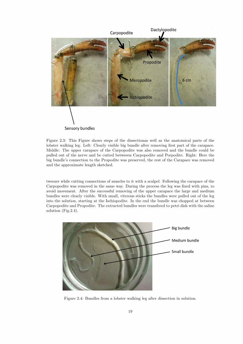
Figure 2.3: This Figure shows steps of the dissectionas well as the anatomical parts of thelobster walking leg. Left: Clearly visible big bundle after removing first part of the carapace.Middle: The upper carapace of the Carpopodite was also removed and the bundle could bepulled out of the nerve and be cutted betweeen Carpopodite and Porpodite. Right: Here thebig bundle’s connection to the Propodite was preserved, the rest of the Carapace was removedand the approximate length sketched.

tweezer while cutting connections of muscles to it with a scalpel. Following the carapace of theCarpopodite was removed in the same way. During the process the leg was fixed with pins, toavoid movement. After the successful removing of the upper carapace the large and mediumbundles were clearly visible. With small, vitreous sticks the bundles were pulled out of the leginto the solution, starting at the Ischiopodite. In the end the bundle was chopped at betweenCarpopodite and Propodite. The extracted bundles were transfered to petri dish with the salinesolution (Fig.2.4).

Figure 2.4: Bundles from a lobster walking leg after dissection in solution.

19

To run the experiment the big bundle was transferred to a nerve chamber (next section) assoon as possible.

2.3 Instrumentation

The nerve chamber as used in the experiment is shown in figure 2.5. The chamber consistsof plexiglass , wherein pins were fixed. The nerve bundle was placed on the pins and wasstimulated from outside of the bundle (external stimulation). The distance between two pinswas 0,25 cm, therefore the used nerve chamber had a pin array of 5,25 cm. The diameter of apin was 0,6 mm, made of stainless. At the ends of the chamber were pockets filled with solutionto prevent the bundle from drying. The chamber was covered with a glass lid to avoid drying.

Figure 2.5: Nerve chamber with large bundle. The bundle has its ends in the solution chambers.

For recording and stimulation we used a PowerLab 26T from AD instruments, as in shown infigure 2.6, with an integrated Bio-amplifier. Further information can be found on the companywebpage [13]. This instrument is able to record with two channels at a time.

Figure 2.6: PowerLab 26T. In the left the output connection, used for the generation of thestimulation signal, while in the right the Bio-amplifier is connected to the recording channels.

To meassure the bidirectional propagation the bundle was excited through the stimulation

20

channel. On both sides of the stimulation a recording channel was positioned. Each channel, thestimulation channel as well as the recording channel has an anode and a cathode. Additionallyan earth was placed between the stimulation channel and the recordning channels, respectively.The anode of the recording channels had to be closer to the stimulation as the cathode to getan uninverted signal. One possible configuration is shown in figure 2.7. Figure 2.8 shows asketch of the experimental setting.

Figure 2.7: Likely electrode configuration during a meassurement.

Figure 2.8: Sketched experimental setting. R1 and R2 are recording channels, while S refers tothe stimulation. Propagation of action potentials in antidromic and orthodromic direction.

The signal was proccessed with the software LabChart7pro. It images the stimulationchannel and the recordning channels as in figure 2.9. The distance betweeen the channels wascalculated out of the number of pins between the anode of the recording channels and thenext electrode of the stimulation channel. The stimulation took place after a time of 0,003 s.The first peaks in the recording channels refer to a stimulation artefact and not to an actionpotential. This stimulus-artefact could be minimized by placing the earths as close as possibleto the recording channels. The second peaks refer to an action potential meassured in the

21

bundle. The nerve bundle was placed with its ends in the solution. With this setup it waspossible to easily change distance and postion from all channels, therefore it was simple to findconfigurations with a clear signal as shown in figure 2.9.

Figure 2.9: LabChart data 19.3.02Blue: Stimulation Channel, Green: First Recording Channel, Red: Second Recording Channel

The data were exported from Labchart7pro in a text file and imported to OriginPro 9.1. Fromthe location of a peak we determined the propagation velocity of an action potential, by dividingthe distance between stimulation and recording channel by the calculated time from stimulationto the first peak of the action potential signal. Note that the ”stimulation” (”stimulus”) atrefactcan change in intensity (height) depending on their proximity to the recording electrodes aswell as the position of the ground. Because the ground of the stimulation cables have to be inone of the propagating sides generally the stimulus artefact appearing forr the antidromic andorthodromic signals are different.

22

Chapter 3

Results and discussion

It is generally known that the action potential (AP) is generated in the axon Hillock (Fig. 1.3)and propagates away from the soma to the neuron’s terminus or synaptic area. Nervertheless,backpropagation of APs through the soma into the dendrites was observed [16] [14] [12]. Back-propagation is believed to be important for neuronal signal control, hence for neuronal functionand plays a key role in synaptic plasticity and neuronal computation [2]. It is generally known,that an AP can be artificially generated in ectopic sites of a neuron. We intend to investigatethe bidirectional propagation of Action potentials in giant axons in order to explore possibleasymetries in the AP propagation, as a function of the stimulation Voltage. As a experimentalmodel we chose the large sensory bundle of the walking legs from a lobster, since it contains alimited number of giant axons. The preparation and execution of the experiment was performedas described in ”Materials and Methods”.

As a first step we had to identify the generation of the APs, corresponding in the giant ax-ons. We assorted the walking legs in two categories. The first and second walking legs haveclaws and build the first category (Category ”Claw”). The second category represents thirdand fourth walking legs, since they don’t have a claw (Category ”NoClaw”). The grouping wasperformed, since differences in neuronal arrangements are present in both groups. In figureswe show 3.1 to 3.4 we show the results of measurements with one bundle of each category.They show AP propagation in orthodromic and antidromic direction for different stimulationVoltages, respectively. Figures 3.1 and 3.2 correspond to the measurement 19.1.01. Since everymeasurement took place in february 2014 the ”19” defines the date of it. The single ”1” means,that it was the first bundle used on this day and ”01” signifies, that it was the first measure-ment, which was done with the bundle. Figures 3.3 and 3.4 correspond to measurement 14.1.01.

23

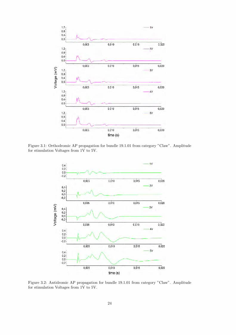
Figure 3.1: Orthodromic AP propagation for bundle 19.1.01 from category ”Claw”. Amplitudefor stimulation Voltages from 1V to 5V.

Figure 3.2: Antidromic AP propagation for bundle 19.1.01 from category ”Claw”. Amplitudefor stimulation Voltages from 1V to 5V.

24

Figure 3.3: Orthodromic AP propagation for bundle 14.1.01 from category ”NoClaw”. Ampli-tude for stimulation Voltages from 1V to 5V.

Figure 3.4: Antidromic AP propagation for bundle 14.1.01 from category ”NoClaw”. Amplitudefor stimulation Voltages from 1V to 5V.

25

The number of peaks depends on the polydispersity of the axonal diameter, since severalaxons with identical diameter would lead to one peak. Axons with a larger diameter lead to anearlier peak in the spike histomgram, since APs propagate faster with larger diameter[6]. Thisvaries depending on the preparation (animal).

In attempt to compare the results of different measurements, we had to be sure, that all giantneurons were excited. So that the peaks, which correspond to similar axons are compareable.The stimulation voltage was delivered for a duration of 0,05 ms and the intensity was increasedin steps of ≤ 0, 2V . At lower stimulation voltages not all giant neurons are excited, so that thenumber of peaks varies. After reaching a treshold the number of peaks stays constant (Fig. 3.5- Fig. 3.8). However, the shape and position of the peaks can change also at stimulation volt-ages higher than the treshold. It was found that at stimulation voltages about 2V all neuronswere excited and consequently the number of peaks didn’t change at higher stimulation voltages.

Figure 3.5: Antidromic AP propagation for the bundle 19.3.01 from category ”Claw” at differentstimulation voltages. Number of peaks after stimulation with 2 V and 3 V constant, while itvaries between 1 V , 1.2 V and 1.4 V, respectively.

26

Figure 3.6: Orthodromic AP propagation for the bundle 19.3.01 from category ”Claw” atdifferent stimulation voltages. Number of peaks after stimulation with 2 V and 3 V constant,while it varies between 1.4 V and 2 V.

Figure 3.7: Antidromic AP propagation for the bundle 20.2.01 from category ”NoClaw” atdifferent stimulation voltages. Number of peaks after stimulation with 2 V and 3 V constant,while it varies between 1 V , 1.2 V and 1.4 V, respectively.

27

Figure 3.8: Orthodromic AP propagation for the bundle 20.2.01 from category ”NoClaw” atdifferent stimulation voltages. Number of peaks after stimulation with 2 V and 3 V constant,while it varies between 1 V and 1.2 V.

Due to this observations a stimulation voltage of 2V had been chosen as the treshold, atwhich all neurons in a bundle are excited (Vt = 2V ). More reasons for the chosen treshold willbe presented later. However, in some rare cases even at stimulation voltages above the treshold,the number of peaks changed (e.g. Fig. 3.4). These cases haven’t been regarded in calculations.An explanation for that behaviour could be, that the stimulation took place on the outside ofthe bundle, so that the distance to the neurons was not uniform. It is well known, that thedistance between the stimulation electrode and the neuron influences the treshold voltage nec-essary to generate an AP (Figure 3.9).

Figure 3.9: The neuron close to the stimulation needs less voltage to be excited, if the neuronshave the same diameter. S represents the stimulation site

28

The giant axons are located in the periphery of the bundle (Figure 2.2), what makes it dif-ficult to always get the spikes correlated with the diameter to stimulation voltage. In neuronswith larger diameter the AP propagates with higher velocity and generally the neurons areexcited at lower voltages. We took the first and second peaks as corespondence to the giantaxons, because they are the fatest axon present in the bundle.

After we performed all the experiments at different stimulation voltages we had to calculatedifferent parameters associated with the APs for the first and second peak, corresponding tothe giant axons. We determined the propagtion velocity, the intensity and the width of eachAP. The velocity was calculated by taking the time from stimulation to the peak of the APand the distance to the recording channel. The intensity was estimated by the peak-to-peakdistance and the width by the extension of the AP. Figures 3.10 and 3.11 show examples of APvelocities in giant axons for the two categories of legs, respectively.

Figure 3.10: AP velocities from 19.1.01 (”Claw”), corresponding to giant axons in orthodomicand antidromic direction.

29

Figure 3.11: AP velocities from 14.1.05(”NoClaw”), corresponding to giant axons in orthodomicand antidromic direction.

Figure 3.12: Behaviour of width, propagation velocity and intensity (peak-to-peak) 19.1.01 forthe second peak orthodromic

30

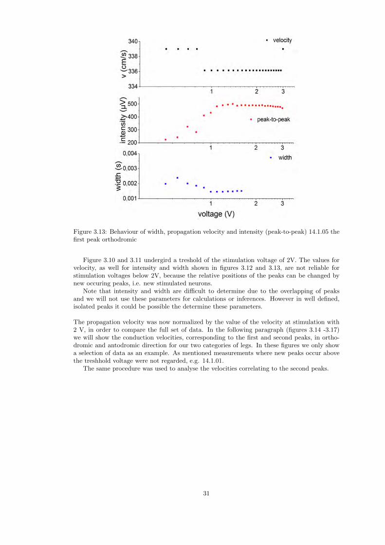
Figure 3.13: Behaviour of width, propagation velocity and intensity (peak-to-peak) 14.1.05 thefirst peak orthodromic

Figure 3.10 and 3.11 undergird a treshold of the stimulation voltage of 2V. The values forvelocity, as well for intensity and width shown in figures 3.12 and 3.13, are not reliable forstimulation voltages below 2V, because the relative positions of the peaks can be changed bynew occuring peaks, i.e. new stimulated neurons.

Note that intensity and width are difficult to determine due to the overlapping of peaksand we will not use these parameters for calculations or inferences. However in well defined,isolated peaks it could be possible the determine these parameters.

The propagation velocity was now normalized by the value of the velocity at stimulation with2 V, in order to compare the full set of data. In the following paragraph (figures 3.14 -3.17)we will show the conduction velocities, corresponding to the first and second peaks, in ortho-dromic and antodromic direction for our two categories of legs. In these figures we only showa selection of data as an example. As mentioned measurements where new peaks occur abovethe treshhold voltage were not regarded, e.g. 14.1.01.

The same procedure was used to analyse the velocities correlating to the second peaks.

31

Figure 3.14: In the treshold (Vt) normalized conduction velocities of first peaks in orthodromicdirection in leg category ”Claw” as function of the stimulation voltage.

Figure 3.15: In the treshold (Vt) normalized conduction velocities of first peaks in antidromicdirection in leg category ”Claw”, as a function of the stimulation voltage.

32

Figure 3.16: In the treshold (Vt) normalized conduction velocities of first peaks in orthodromicdirection in leg category ”NoClaw”, as a function of the stimulation voltage.

Figure 3.17: In the treshold (Vt) normalized conduction velocities of first peaks in antidromicdirection in leg category ”NoClaw”, as a function of the stimulation voltage.

33

In order to summarize our results we averaged the values of the normalized velocities inorthodromic and antidromic direction for each stimulation voltage and the two categories oflegs, repectively. The results were fitted with a linear polynome in order to compare the gen-eral trends of each respresented peak. In figures 3.18 - 3.21 we show the averaged velocities inantidromic and orthodromic direction for the first and second peaks of the legs with (”Claw”)and without claw (”NoClaw”).

Figure 3.18: Normalized and averaged conduction velocities corresponding to the first peaksin orthodromic and antidromic direction for legs of ”Claw”. Vt is the treshold voltage used forthe normalization. Red line shows the linear fit and error bars the standard deviation of theaveraged values.

34

Figure 3.19: Normalized and averaged conduction velocities corresponding to the second peaksin orthodromic and antidromic direction for legs of ”Claw”. Vt is the treshold voltage used forthe normalization. Red line shows the linear fit and error bars the standard deviation of theaveraged values.

Figure 3.20: Normalized and averaged conduction velocities corresponding to the first peaksin orthodromic and antidromic direction for legs of ”NoClaw”. Vt is the treshold voltage usedfor the normalization. Red line shows the linear fit and error bars the standard deviation ofthe averaged values.

35

Figure 3.21: Normalized and averaged conduction velocities corresponding to the second peaksin orthodromic and antidromic direction for legs of ”NoClaw”. Vt is the treshold voltage usedfor the normalization. Red line shows the linear fit and error bars the standard deviation ofthe averaged values.

From the figures it is evident, that the propagation in the first two legs (”Claw”) is asymet-rical as function of the stimulation voltage for the first and second peak, while in the third andfourth walking legs (”NoClaw”) the propagation is almost perfectly symetrical. In the followingtable, the slopes from the first two peaks for orthodromically and antidromically propagationis shown, for the to categories (”Claw”, ”NoClaw”), respectively.

Table 3.1: Slopes from figures 3.18 to 3.21 to comparison.”Claw” ”NoClaw”

First peak Second peak First peak Second peakorthodromic 0 -0,001 0,008 0,001antidromic -0,025 -0,041 -0,008 -0,005

It is important to note that the large giant axon (diameter ≤ 100µm) are only presentin the first and second walking leg. Controlling the claw they are absent in the third andfourth leg. Additionally it is expected that the axonal diameter is more uniform in the thirdand fourth legs, due to there smaller diameter. The differences in propagation velocity couldbe related with the changes in axonal diameter for the giant axons. The diameter gets largerclose to the body or rather close to the soma, while it decreases in the bodies periphery, theclaws. To point out: The axons diameter decreases with distance in the orthodromic directionand increases with distance in the antidromic direction. The stimulation voltage respresentthe energy necessary to depolarize a precise membrane area in the sensory bundle. The decayin propagation velocity in antidromic direction could be due to an incresing membrane area(increasing diameter) and a constant energy - or rather a decrease in the energy per unit ofmembrane area, expressed in the decreased velocity.According this idea the propagation velocity should increase in orthodromic direction, if thediameter decrease. It is plausible to assume, that the diameter change in antidromic direc-

36

tion is bigger than in orthodromic direction. The antidromically propagating AP is travellingin direction of the soma, which has a significantly larger diameter than the axon, while theorthodromically propagating AP stays in the axon, so that the changes in diameter are notsignificant. Additionally the result indicates that the higher the energy supply the membrane(higher stimulation voltage) the higher is the decrease in antidromically conduction velocity.Note that the assumption, that the diameter of the giant axons present in third and fourthwalking legs is plausible, because the error bars of those preparations are noticeable smallerthan those for the first and second walking legs. This indicates, that anatomically the neuronsare more uniform between different animals for the third and fourth walking legs. The largeerror bars present on the first and second walking legs, are an indication of large polydispersityin the axons between different animals. It is also plausible, that small giant axons could havean asymetrical AP propagation. However, the extension of this asymetry is in any case lowerthan in the case of first and second walking legs. It will be interesting in future to investigatein more details the large bundles of the third and fourth legs as well as the medium and smallbundles present in all walking legs, in order to examine possible asymetries in bidirectional APpropagation.

37

38

Chapter 4

Conclusion

We investigated the effect of changing stimulation voltage on the bidirectional propagation ofaction potentials in the giant axons of lobster walking legs. The treshold stimulation voltageto generate action potentials propagating bidirectionally was found to be ≤ 2V for all nervepreparations. The treshold was approximately the same for orthodromic and antidromic prop-agating signals. The propagation velocity shows an asymetric behaviour in bundles from legswith claw. The antidromic propagation velocity decreases with increasing stimulation volt-age, probably due to the increase axon diameter in direction of the soma. The orthodromicpropagation stays constant with increasing stimulation voltage. In the legs without claws theaction potential propagation was found to propagate nearly symetrical, i.e. antidromic andorthodromic propagation velocities didn’t change with increasing stimulation voltage. Becauseaxonal membrane-area changes in the large giant axon in first and second walking legs are moresignificant as in third and fourth walking legs, it is suggested that changes in surface area affectthe propagation velocity of an action potential. With larger surface area the energy per areaunit decreases. This decrease in energy per area unit is expressed in a decay of the conductionvelocity.

Furthermore the propagation in antidromic direction shows an analogy ( a decrease in energyper unit) with the backpropagation in neurons as reported by Stuart et al., that shows a decayin intensity of the backpropagating action potential with the distance from the soma.[14].

39

40

Appendix A

Appendix

41

Figure A.1: Normalized and averaged conduction velocities corresponding to the first peaks inorthodromic direction for legs of ”Claw”.

42

Figure A.2: Normalized and averaged conduction velocities corresponding to the first peaks inantidromic direction for legs of ”Claw”.

43

Figure A.3: Normalized and averaged conduction velocities corresponding to the second peaksin orthodromic direction for legs of ”Claw”.

44

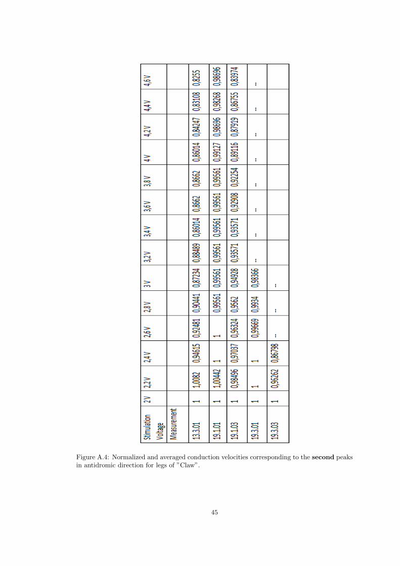
Figure A.4: Normalized and averaged conduction velocities corresponding to the second peaksin antidromic direction for legs of ”Claw”.

45

Figure A.5: Normalized and averaged conduction velocities corresponding to the first peaks inorthodromic direction for legs of ”NoClaw”.

46

Figure A.6: Normalized and averaged conduction velocities corresponding to the first peaks inantidromic direction for legs of ”NoClaw”.

47

Figure A.7: Normalized and averaged conduction velocities corresponding to the second peaksin orthodromic direction for legs of ”NoClaw”.

48

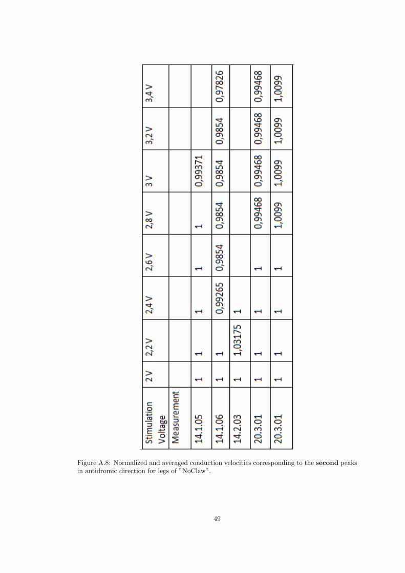
Figure A.8: Normalized and averaged conduction velocities corresponding to the second peaksin antidromic direction for legs of ”NoClaw”.

49

50

Bibliography

[1] R. Appali, S. Petersen, and U. van Rienen. A comparision of Hodgkin-Huxley and solitonneural theories. Advances in Radio Science, 8:75–79, Sept. 2010.

[2] T. Branco and M. Hausser. The selfish spike: local and global resets of dendritic excitability.Neuron, 61(6):815–7, Mar. 2009.

[3] A. J. Darin De Lorenzo, M. Brzin, and W. D. Dettbarn. Fine structure and organizationof nerve fibers and giant axons in Homarus americanus. Journal of ultrastructure research,24(5):367–84, Sept. 1968.

[4] DericBownds. http://dericbownds.net/bom99/Ch02/Ch02.html March 27th, 2014 1 pm.

[5] A. J. Foust and D. M. Rector. Optically teasing apart neural swelling and depolarization.Neuroscience, 145(3):887–99, Mar. 2007.

[6] D. K. Hartline and D. R. Colman. Rapid conduction and the evolution of giant axons andmyelinated fibers. Current biology : CB, 17(1):R29–35, Jan. 2007.

[7] T. Heimburg and A. D. Jackson. On soliton propagation in biomembranes and nerves.Proceedings of the National Academy of Sciences of the United States of America,102(28):9790–5, July 2005.

[8] A. L. Hodgkin and A. F. Huxley. A quantitative description of membrane current and itsapplication to conduction and excitation in nerve. The Journal of physiology, 117(4):500–44, Aug. 1952.

[9] E. R. Kandel. Principle of neural Science. 2012.

[10] T. Matheson. Invertebrate Nervous Systems. pages 1–6, 2002.

[11] J. R. Morgan and O. Bloom. Cells of the nervous system. 2005.

[12] D. Pinault. Backpropagation of action potentials generated at ectopic axonal loci: hy-pothesis that axon terminals integrate local environmental signals. Brain research. Brainresearch reviews, 21(1):42–92, July 1995.

[13] PowerLab. http://cdn.adinstruments.com/adi-web/manuals/PowerLab Teaching 15 26 OG.pdfMarch 27th, 2014 1 pm.

[14] G. Stuart, N. Spruston, B. Sakmann, and M. Hausser. Action potential initiation andbackpropagation in neurons of the mammalian CNS. Trends in neurosciences, 20(3):125–31, Mar. 1997.

[15] G. M. Villegas and F. Sanchez. Periaxonal ensheathment of lobster giant nerve fibres as re-vealed by freeze-fracture and lanthanum penetration. Journal of neurocytology, 20(6):504–17, June 1991.

[16] J. Waters, A. Schaefer, and B. Sakmann. Backpropagating action potentials in neurones:measurement, mechanisms and potential functions. Progress in biophysics and molecularbiology, 87(1):145–70, Jan. 2005.

51