University of Bath

PHD

Bearings only tracking using a set of range parameterised extended Kalman filters

Peach, Nigel G.

Award date:1997

Awarding institution:University of Bath

Link to publication

Alternative formatsIf you require this document in an alternative format, please contact:openaccess@bath.ac.uk

Copyright of this thesis rests with the author. Access is subject to the above licence, if given. If no licence is specified above,original content in this thesis is licensed under the terms of the Creative Commons Attribution-NonCommercial 4.0International (CC BY-NC-ND 4.0) Licence (https://creativecommons.org/licenses/by-nc-nd/4.0/). Any third-party copyrightmaterial present remains the property of its respective owner(s) and is licensed under its existing terms.

Take down policyIf you consider content within Bath's Research Portal to be in breach of UK law, please contact: openaccess@bath.ac.uk with the details.Your claim will be investigated and, where appropriate, the item will be removed from public view as soon as possible.

Download date: 24. Jul. 2022

Bearings Only Tracking Using a Set of Range Parameterised Extended Kalman Filters

Submitted by

Nigel G. Peach

for the degree of PhX>. of the

University of Bath

1997

COPYRIGHT

Attention is drawn to the fact that the copyright of this thesis rests with its author. This copy of the thesis has been supplied on condition that anyone who consults it is understood to recognise that its copyright rests with the author and that no quotation from the thesis and no information derived from it may be published without the prior written consent of the author.

This thesis may be made available for consultation within the University Library and may be photocopied or lent to other libraries for the purposes of consultation.

Page 1

UMI Number: U60153B

All rights reserved

INFORMATION TO ALL USERS The quality of this reproduction is dependent upon the quality of the copy submitted.

In the unlikely event that the author did not send a complete manuscript and there are missing pages, these will be noted. Also, if material had to be removed,

a note will indicate the deletion.

Dissertation Publishing

UMI U601533Published by ProQuest LLC 2013. Copyright in the Dissertation held by the Author.

Microform Edition © ProQuest LLC.All rights reserved. This work is protected against

unauthorized copying under Title 17, United States Code.

ProQuest LLC 789 East Eisenhower Parkway

P.O. Box 1346 Ann Arbor, Ml 48106-1346

UNIVERSITY OF BATH S LIBRARY

51)5211

ABSTRACT

Bearings only tracking using the Extended Kalman Filter (EKF) configured in Cartesian and modified polar coordinate systems is reviewed. A new tracking approach is proposed which consists of a set of weighted EKFs each with a different initial range estimate and this is referred to as the Range Parameterised (RP) tracker. This new approach overcomes the problems exhibited with existing EKF trackers when the bearing rate is very high or near zero. In addition, it allows a more natural implementation for the prior knowledge of the target velocity, which can allow the range to be inferred even before the first observer manoeuvre.

Results are presented for a typical tracking scenario, involving a manoeuvring observer and a constant velocity target. The results show that the RP tracker gives stable, consistent and unbiased estimates in all the cases considered, whereas the same is not true for the Cartesian and Modified Polar EKF trackers.

The RP tracker has been extended to allow for manoeuvring targets by adding a manoeuvre detection and correction procedure based on a Generalised Likelihood Ratio (GLR) test The GLR threshold has been set to 3.0 as this gives a good compromise between a reasonably low false alarm rate (3.7 x 10“3 per update) and a short detection delay for typical target manoeuvres. However, the selection of a particular threshold is not critical as the proposed procedure is robust to false alarms, since it only results in increased computation without long term loss in tracking accuracy.

The tracking performance of the GLR procedure has been compared with the standard technique of adding plant noise to allow for unmodelled target dynamics. This comparison has illustrated that the GLR procedure provides better tracking performance before and after a target manoeuvre and, in particular, the track estimates for the GLR procedure are consistent with the estimated covariance matrix.

The tracking performance of the RP tracker has been shown to approach the Cramer Rao Lower Bound (CRLB) for the special case of symmetric observer manoeuvres. A range error lower limit associated with a manoeuvre has been derived for more general scenarios, and this has been shown to give a good prediction of the RP tracker RMS range error. The simplicity of the expression for the range error lower limit allows it to be used to specify criteria for the time and magnitude of observer manoeuvres to give optimum range observability.

Page 2

ACKNOWLEDGEMENTS

The work described in this thesis has been carried out at the University of Bath under the supervision of Mr M E Brigden (School of Mathematical Sciences) and with the support of GEC-Marconi Naval Systems, Sonar Systems Division, Templecombe.

Page 3

CONTENTS

1. Introduction1.1 Description of the Problem1.2 The Extended Kalman Filter1.3 System Observability1.4 Review of Bearings only Tracking using an EKF

1.4.1 Cartesian Coordinates1.4.2 Modified Polar Coordinates

2. Literature Review2.1 Review of Bearings only Tracking

2.1.1 Early Bearings only Tracking2.1.2 Cartesian EKF Stability and Adhoc Solutions2.1.3 Modified Polar EKF2.1.4 Non-Kalman Techniques2.1.5 Range Observability

2.2 Review of Tracking Manoeuvring Targets2.2.1 Multiple Model Techniques2.2.2 Manoeuvre Estimation and Correction Techniques2.2.3 Manoeuvre Following Techniques

2.3 Summary2.3.1 Bearings only Tracking2.3.2 Manoeuvring Targets2.3.3 Range Observability

3. Bearings only Tracking using a Range Parameterised Tracker3.1 Derivation of the RP Tracker

3.1.1 Choice of Coordinate System3.1.2 Motivation for Range Parameterisation3.1.3 Updating the Weights3.1.4 Thresholding

3.2 Initialisation Assumptions3.2.1 Cartesian EKF3.2.2 Modified Polar EKF3.2.3 Range Parameterised Tracker

3.3 Monte Carlo Performance of RP Tracker3.3.1 Scenario Definition3.3.2 RMS Range Errors3.3.3 Typical Track Output3.3.4 RMS Normalised Range Errors

Page 4

4. Tracking Target Manoeuvres using a GLR Procedure4.1 Derivation of GLR Procedure

4.1.1 Manoeuvre Detection4.1.2 Manoeuvre Correction

4.2 Derivation of Plant Noise4.3 Monte Carlo Performance of GLR Procedure

4.3.1 Scenario Definition4.3.2 Operating Characteristics4.3.3 Contingency Tables4.3.4 RMS Range Errors

4.3.4.1 Choice of Plant Noise Manoeuvre Factor (y)4.3.4.2 Effect of Target Manoeuvre Time4.3.4.3 Multiple Target Manoeuvres

4.3.5 Normalised Range Errors4.3.6 Typical Track Plot

5. Optimum Observer Manoeuvres5.1 Cramer-Rao Lower Bound for Bearings Only Tracking5.2 Geometric Derivation of the Range Error Lower Limit5.3 Monte Carlo Analysis

5.3.1 Scenario Definition5.3.2 Comparison with CRLB5.3.3 Comparison with Range Error Lower Limit

6. Conclusions6.1 Range Parameterised Tracker6.2 GLR Manoeuvre Detection / Correction Procedure6.3 Optimum Observer Manoeuvres

7. References Figures AppendicesA. Improved Initialisation Procedure

A.1 Cartesian CoordinatesA.2 Modified Polar Coordinates

B. Derivation of GLR ProcedureB.l Effect of Manoeuvre on System Model B.2 Likelihood Ratio TestB.3 Generalised Likelihood Ratio TestB.4 Alternative Derivation of the Decision StatisticB.5 Manoeuvre Correction

Page 5

SYNOPSIS OF NOTATION

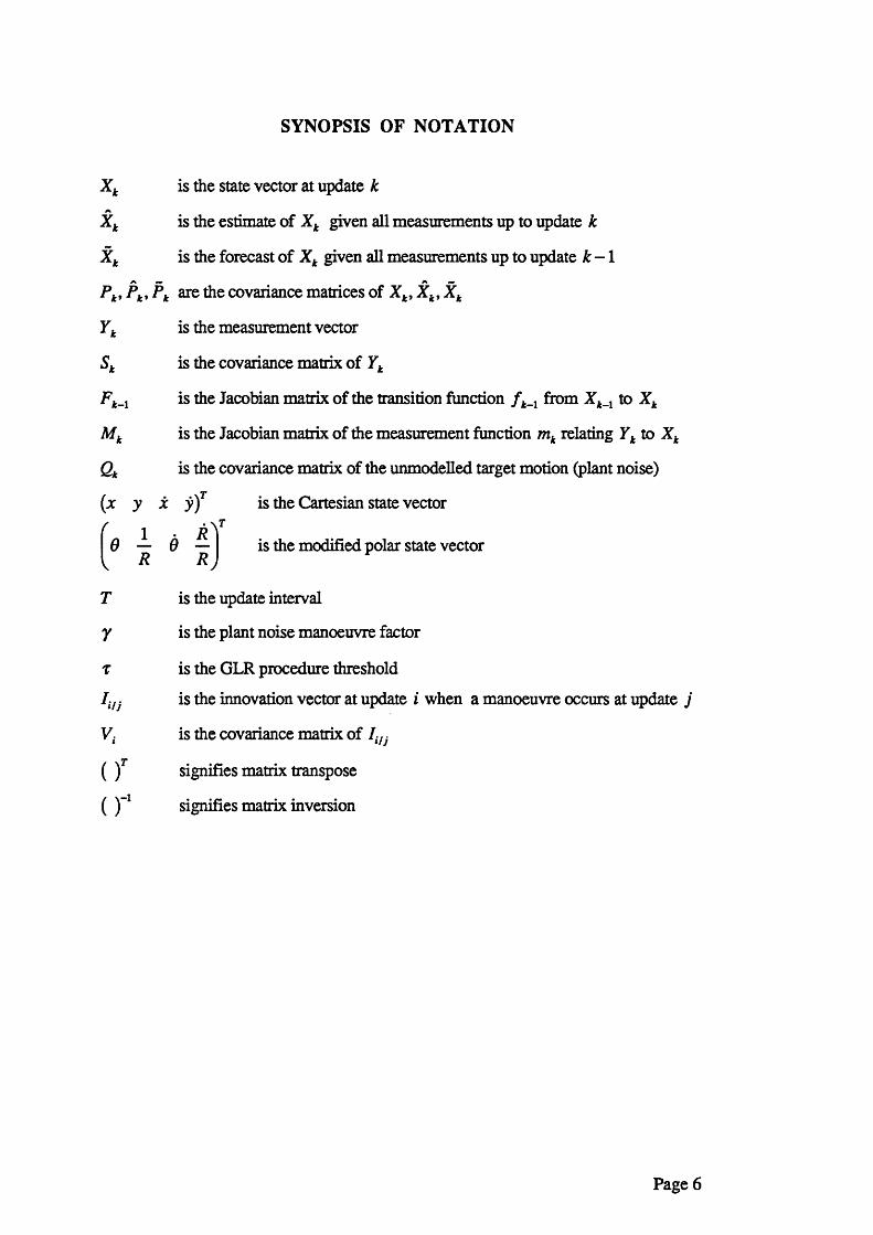
is the state vector at update k

is the estimate of Xk given all measurements up to update k

is the forecast of Xk given all measurements up to update k - 1A w

are the covariance matrices of Xk, Xk, Xk

is the measurement vector

is the covariance matrix of Yk

is the Jacobian matrix of the transition function f k_x from Xk_ to Xk

is the Jacobian matrix of the measurement function mk relating Yk to Xk

is the covariance matrix of the unmodelled target motion (plant noise)

y)T is the Cartesian state vector

is the modified polar state vectoreR y

is the update interval

is the plant noise manoeuvre factor

is the GLR procedure threshold

is the innovation vector at update i when a manoeuvre occurs at update j

is the covariance matrix of IiU

signifies matrix transpose

signifies matrix inversion

LIST OF ABBREVIATIONS

c CartesianCEP Circular Error ProbableCPDF Conditional Probability Density FunctionCRLB Cramer Rao Lower BoundDDL Double Decision LogicEKF Extended Kalman FilterGLR Generalised Likelihood RatioGPB Generalised Pseudo BayesIMM Interacting Multiple ModelsLOS Line of SightLSE Least Squares EstimateMGEKF Modified Gain Extended Kalman FilterMIV Modified Instrumental VariableMLE Maximum Likelihood EstimateMP Modified PolarOC Operating Characteristicspdf Probability Density FunctionPLE Pseudo Linear EstimatePMF Pseudo Measurement FilterRMS Root Mean SquaredRP Range ParameterisedRSS Reduced Sufficient Statisticsd Standard DeviationSOS Sum of SquaresTMA Target Motion Analysis

1234567

89101112131415161718192021222324252627282930313233

LIST OF FIGURES

RMS Range Error for an Initial Target Range of 1 kmRMS Range Error for an Initial Target Range of 2.2 kmRMS Range Error for an Initial Target Range of 10 kmRMS Range Error for an Initial Target Range of 22 kmRMS Range Error for an Initial Target Range of 100 kmOperating Characteristics for Various Target Manoeuvres at Update 32Operating Characteristics for a 15 Degree Target Manoeuvre at VariousUpdatesRMS Range Error for a Non-Manoeuvring TargetRMS Range Error for a 5 Degree Target Manoeuvre at Update 32RMS Range Error for a 15 Degree Target Manoeuvre at Update 32RMS Range Error for a 45 Degree Target Manoeuvre at Update 32RMS Range Error for a 15 Degree Target Manoeuvre at Update 8RMS Range Error for a 15 Degree Target Manoeuvre at Update 16RMS Range Error for a 15 Degree Target Manoeuvre at Update 24RMS Range Error for a 15 Degree Target Manoeuvre at Update 32RMS Range Error for a 15 Degree Target Manoeuvre at Update 40RMS Range Error for 15 Degree Target Manoeuvre at Update 48RMS Range Error for 15 Degree Target Manoeuvres at Updates 32 and 48RMS Normalised Range Error for a Non-Manoeuvring TargetRMS Normalised Range Error for a for a 5 Degree Manoeuvre at Update 32RMS Normalised Range Error for a for a 15 Degree Manoeuvre at Update 32RMS Normalised Range Error for a for a 45 Degree Manoeuvre at Update 32Normalised Bearing Error for a 15 Degree Manoeuvre at Update 32RMS Bearing Error for an Initial Target Range of 10 kmRMS Range Error for an Initial Target Range of 10 kmRMS Bearing Rate Error for an Initial Target Range of 10 kmRMS Range Rate / Range Error for an Initial Target Range of 10 kmRMS Range Error for an Initial Target Range of 22 kmRMS Range Error for an Initial Target Range of 2.2 kmRMS Range Error for an 15 Degree Heading OffsetRMS Range Error for an 30 Degree Heading OffsetRMS Range Error for an 45 Degree Heading OffsetRMS Range Error for an 60 Degree Heading Offset

Page 8

1 . INTRODUCTION

Hassab (1987, 1989) [12, 39] presented a perspective on Target Motion Analysis (TMA) in the ocean environment. He defined various classes of problem ranging from Class A (linear problem with the target state observable at each observation), to Class F (non-linear problem with the target state observable only after multiple observations, and only with motion constraints placed on the target and observer). Bearings only tracking from a single observer is a class F problem and is one of the most difficult tracking problems encountered.

Bearings only tracking is inherently non-linear since the target motion is assumed linear in Cartesian co-ordinates (straight line motion) and the measurements are in polar co-ordinates. Only three of the states are observable directly from the measurements prior to an observer manoeuvre. The range state only becomes observable through synthetic triangulation between the current observer position and where the observer would have been had it not manoeuvred, as shown in Section 5.2 of this thesis.

There have been many previous techniques proposed for bearings only tracking, as identified in the literature review in Section 2.1. However, many of these techniques are heuristic and are sensitive to the initialisation assumptions for the state and covariance matrix and can yield erratic results. The aim of this research has been to develop an efficient solution to the bearings only tracking problem, which produces stable, consistent and unbiased estimates in the general case of a manoeuvring target and a manoeuvring observer, without unrealistic limitations on the initialisation assumptions.

1 .1 Description of the Problem

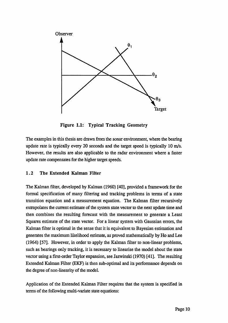
The aim of bearings only tracking is to determine the trajectory of the target based on a time series of bearing measurements from a single observer. In this thesis it is assumed that the motion of the target is constrained to straight line, constant speed segments separated infrequently by manoeuvres in course and speed. The geometry of a typical straight line segment is illustrated in Figure 1.1:

Page 9

Observer

Target

Figure 1.1: Typical Tracking Geometry

The examples in this thesis are drawn from the sonar environment, where the bearing update rate is typically every 20 seconds and the target speed is typically 10 m/s. However, the results are also applicable to the radar environment where a faster update rate compensates for the higher target speeds.

1.2 The Extended Kalman Filter

The Kalman filter, developed by Kalman (1960) [40], provided a framework for the formal specification of many filtering and tracking problems in terms of a state transition equation and a measurement equation. The Kalman filter recursively extrapolates the current estimate of the system state vector to the next update time and then combines the resulting forecast with the measurement to generate a Least Squares estimate of the state vector. For a linear system with Gaussian errors, the Kalman filter is optimal in the sense that it is equivalent to Bayesian estimation and generates the maximum likelihood estimate, as proved mathematically by Ho and Lee (1964) [57]. However, in order to apply the Kalman filter to non-linear problems, such as bearings only tracking, it is necessary to linearise the model about the state vector using a first-order Taylor expansion, see Jazwinski (1970) [41]. The resulting Extended Kalman Filter (EKF) is then sub-optimal and its performance depends on the degree of non-linearity of the model.

Application of the Extended Kalman Filter requires that the system is specified in terms of the following multi-variate state equations:

Page 10

- State Transition Equation

Yk - mk (X* ) + Nk - Measurement Equation

where Xk is the state vector at update kf k_x( ) is a state transition function which transforms Xk_x to XkUk_x is the stochastic element of the target dynamics, not included

within f k_x, with zero mean and covariance matrix Qk_x Yk is the measurement vector at update kmk( ) is the measurement function which relates Xk to YkNk is the measurement noise with zero mean and covariance

matrix Sk

Linearisation of the state transition function around the state estimate, and linearisation of the measurement function around the state forecast, allows the system to be approximated by the following piecewise linear state transition and measurement equations.

Xk = f k_x J + Fk_x - Xk_x j + Uk_x - State Transition Equation

Yk - mk(x* j + Mk (xk - X k + Nk - Measurement Equation

or Z*= Yl+ Mk Xk - m t (x t ) = Mk Xl+ Nk

where Xk_x is the estimate of the state vector at update k — 1Xk is the forecast of the state vector at update k

a

Fk_x is the Jacobian matrix of f k_x evaluated at Xk- 1

Mk is the Jacobian matrix of mk evaluated at Xk

The system state veaor and associated covariance matrix can be estimated recursively using the following state transition and updating equations, which form the extended Kalman filter

Xk = f t. i ( i M )

= 1 ^*-1 ^ t- i Qk-1State Transition Equations

Page 11

where Pk_: is the covariance matrix for the estimate at update k — 1 Pk is the covariance matrix for the forecast at update k

Xt = Xk+Kt (zk- M kXk) h = h ~ K t MkPk Kk = Pt M Tk {Mk Pk M Tk +Sk)‘

Updating Equations

where Kk is the smoothing parameter at update k.

The only requirement is that the Kalman Filter is seeded with a prior estimate of the state X Q, with associated covariance Po .

1 .3 System Observability

A system is defined as observable if all the states can be estimated directly from the measurements. The system defining the bearings only tracking problem is only partially observable, since the range state only becomes observable after an observer manoeuvre. Prior to this manoeuvre the estimate of the range state is highly dependent on the initialisation assumptions for the other states, as shown in Appendix A.

For a linear system an observability criterion can be defined by recasting the estimation problem in terms of the estimation of the initial state vector X0, since this

is linearly related to the current state by the state transition equation. The set of measurement equations for the initial state vector are given by:

Zq = Mq X q + Nq

Z l =Ml Xl +Nl = Ml F l0 X0 + Nl

2* ~ X k + Nk = Mk Fq X0 + Nk

where F0* is the matrix describing the state transition from update 0 to update k .

These equations can be combined into the single composite measurement equation:

Z(k) = M(k)X0 + N(k)

Page 12

where Z(k), M{k) and N(k) have the form:

Z(fc) = [Z0>Zp- , Z i f

N(k) = [N0,N t, - , N t]T

Rearranging the measurement equation gives the initial state as:

X0 = M'(k) Z(k)-M*(k) N(k)

where M*(k) is the pseudo inverse of M(k) given by:

Af'(fc) = [MT(k) M{k)\ lM r(k)

MT(k) M(k) is defined as the information matrix and if this is full rank the system is defined as observable, since the initial state can be estimated as:

X0= M \ k ) Z(k)

This requirement for full rank is satisfied if there are at least as many measurements as states and, in addition, for bearings only tracking Nardone and Aidala (1981) [11] proved mathematically that there has to be an observer manoeuvre.

1.4 Review of Bearings only Tracking using an EKF

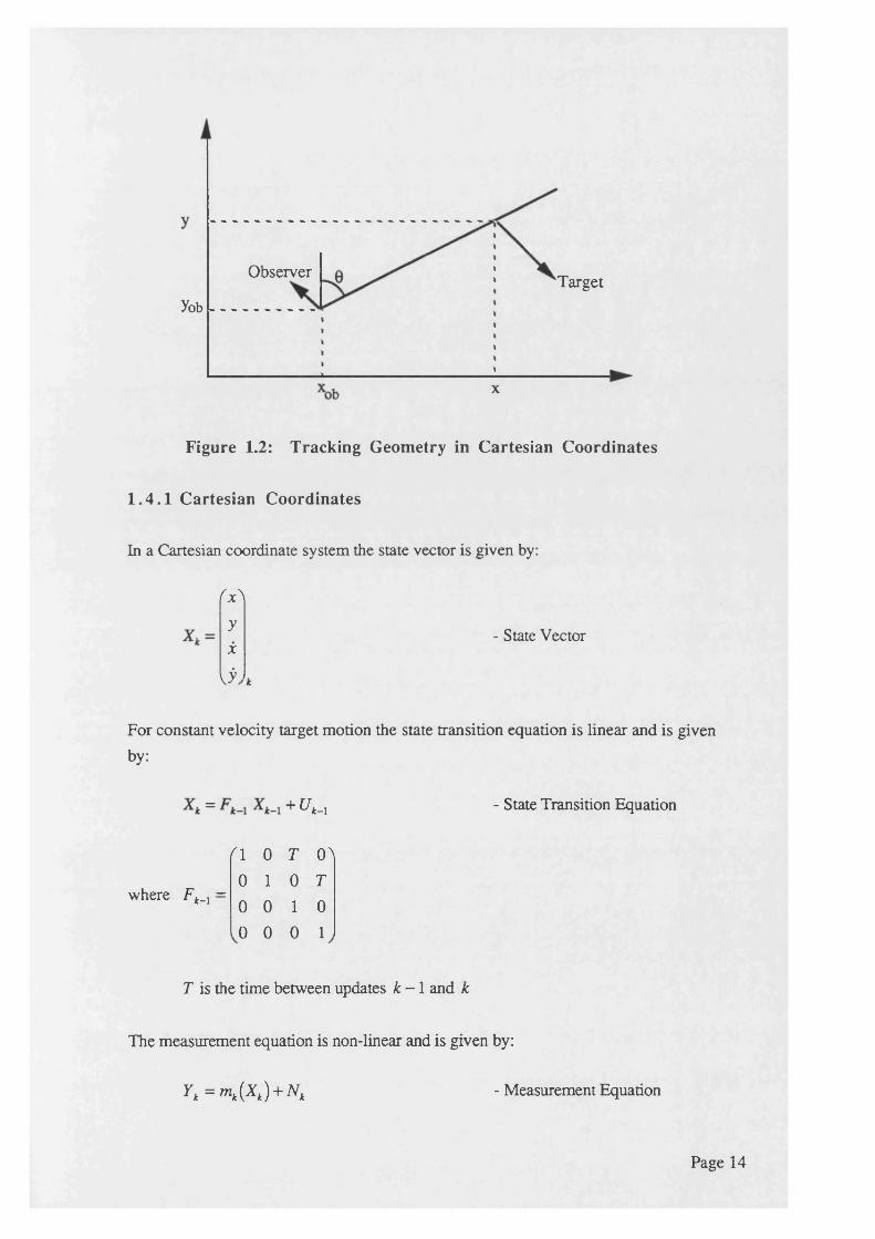
Bearings only tracking is a highly non-linear problem and the performance of an EKF is heavily dependent on the choice of coordinate system. The two most popular coordinate systems are Cartesian, due to the ease of application, and modified polar, due to the improved stability of the tracker, as demonstrated by Hoelzer, Johnson and Cohen (1978) [49]. This section reviews the implementation of an EKF in Cartesian and modified polar coordinate systems, based on the tracking geometry shown in Figure 1.2. The EKF in modified polar coordinates is fundamental to this research, since it forms the basis of the Range Parameterised tracker derived in Section 3.

Page 1"

Observer TargetYob

x

Figure 1.2: Tracking Geometry in Cartesian Coordinates

1 .4 .1 Cartesian Coordinates

In a Cartesian coordinate system the state vector is given by:

'x 'yX

{y.

- State Vector

For constant velocity target motion the state transition equation is linear and is given by:

= + u „ - State Transition Equation

where Fk_x =

' I 0 T 0^ 0 1 0 T 0 0 1 0 0 0 0 1

T is the time between updates k - 1 and k

The measurement equation is non-linear and is given by:

Yk = mk (Xk ) + Nk - Measurement Equation

Page 14

where mk(Xk) = tan-1r \ x xob

\ ? ~ yob)

xob9 yob 316 ^ artes an coordinates of the observer

Linearising the measurement equation around the forecast Xk gives:

Zk ~ Y k + Mk Xk - tan-i ' h - xohI h - yob)

= Mk Xk + N k

where Mk is the Jacobian matrix of mk evaluated at Xk given by:

Mk =yic-yob (xk xob)

[h-xob?+{h-yobY {h-xobt+{h-y0b), 0 , 0

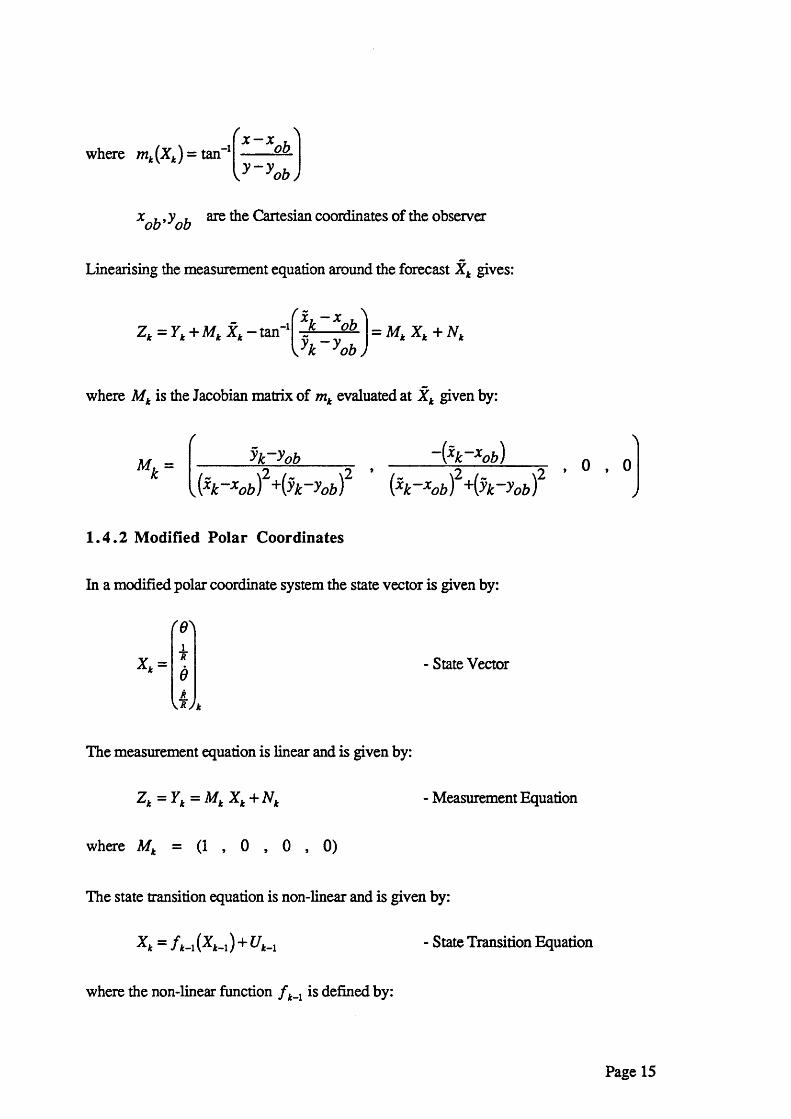
1 .4 .2 Modified Polar Coordinates

In a modified polar coordinate system the state vector is given by:

(&\xR

e

\ R J k

- State Vector

The measurement equation is linear and is given by:

Zt =Yt = Mk Xk+ Nk - Measurement Equation

where Mk = (1 , 0 , 0 , 0)

The state transition equation is non-linear and is given by:

- State Transition Equation

where the non-linear function / jk_1 is defined by:

Page 15

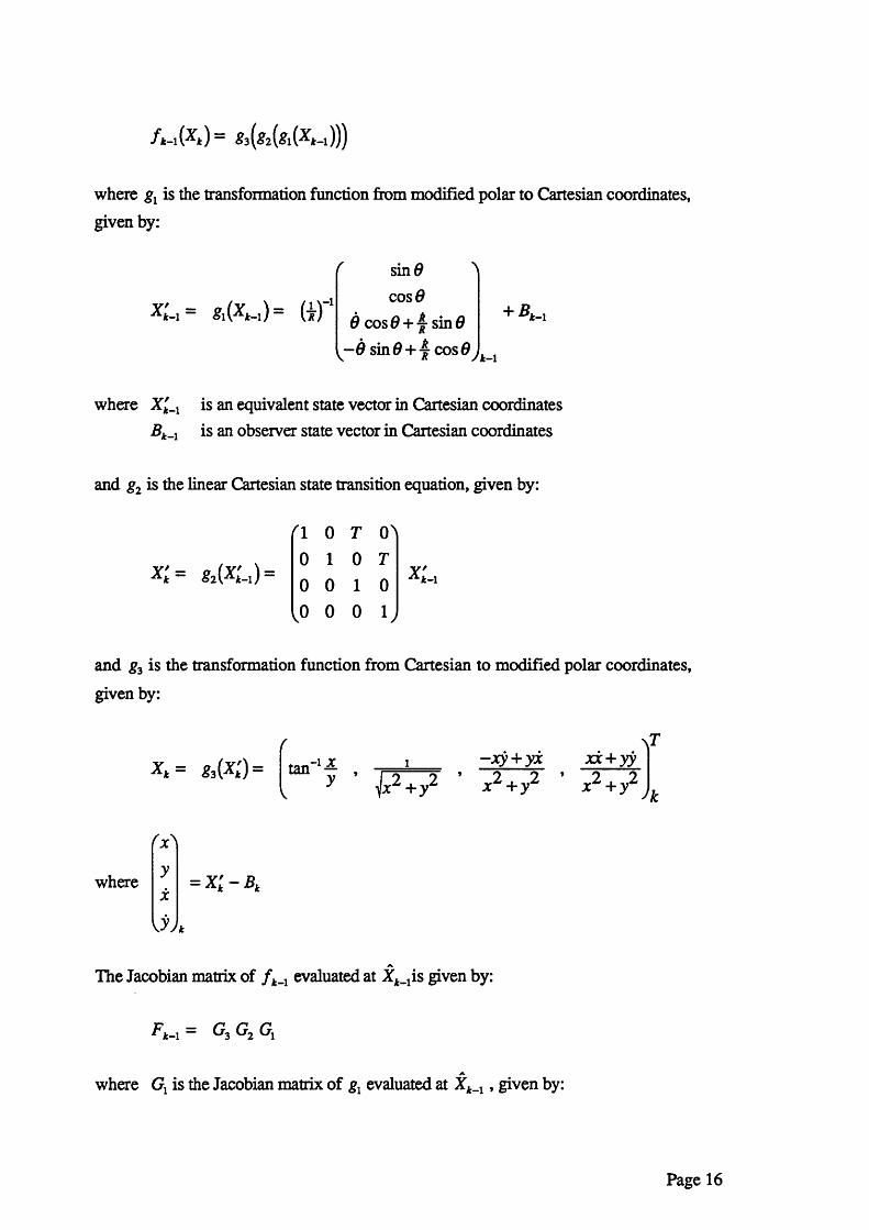
fk-l {%k ) “ S3 {Si (#1 fak-l)))

where gl is the transformation function from modified polar to Cartesian coordinates, given by:

sin 6 cosd

6 cos0 + j sin# - 0 sin 0 + 4 cos 0j

+ Bk-\

where X'k_x is an equivalent state vector in Cartesian coordinates Bk_x is an observer state vector in Cartesian coordinates

and g2 is the linear Cartesian state transition equation, given by:

1 0 T 00 1 0 T0 0 1 00 0 0 1

Y'k-l

and g3 is the transformation function from Cartesian to modified polar coordinates, given by:

* » = & (* ;)= tan"1 — - xy + yx xx+yy

y ’2 2 x +y

where yX

= X'k - B k

\T

2 2 x r + y L

The Jacobian matrix of f h_x evaluated at X ^ i s given by:

Ft_ 1 = 0 , 0 , 0 ,

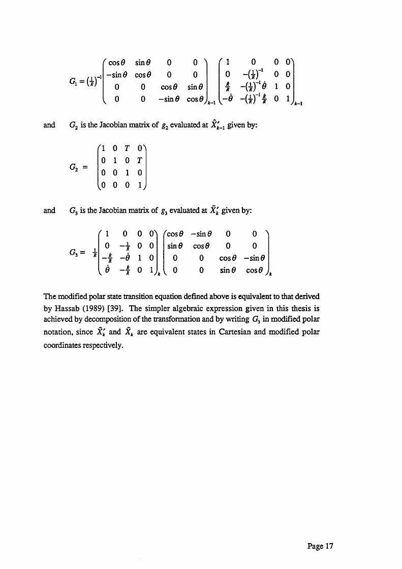
where Gl is the Jacobian matrix of gl evaluated at Xk_x, given by:

Page 16

' cos # sin# 0 0 ' f 1 0 0 0 "-s in # cos# 0 0 0 -ar 0 0

0 0 cos# sin# AR -ar* 1 0

, 0 0 -s in # cos#. k - l [ - # 04

A

and G2 is the Jacobian matrix of g2 evaluated at given by:

'1 0 T O'0 1 0 T

Go =2 0 0 1 0^0 0 0 1,

and G3 is the Jacobian matrix of g3 evaluated at X'k given by:

' 1 0 0 O' 'cos# -s in # 0 0 '1 0 1

R 0 0 sin# cos# 0 0R R

R - # 1 0 0 0 cos# —sin#

I dRR 0 h k , 0 0 sin# cos# ,

The modified polar state transition equation defined above is equivalent to that derived by Hassab (1989) [39]. The simpler algebraic expression given in this thesis is achieved by decomposition of the transformation and by writing G3 in modified polarnotation, since Xk and Xk are equivalent states in Cartesian and modified polar

coordinates respectively.

Page 17

2 . LITERATURE REVIEW

Sections 2.1 and 2.2 review the relevant papers from the extensive literature on the subjects of bearings only tracking and the tracking of manoeuvring targets. Section2.3 summarises those considered to be the most important papers from the literature review and identifies how this thesis builds upon the previously published work.

2 .1 Review of Bearings Only Tracking

2.1.1 Early Bearings Only Tracking

Initial solutions to the bearings only tracking problem relied on geometric constructions to obtain an estimate of the target range by triangulation. This technique works reasonably well provided that the bearing errors are small and that there is a significant speed advantage for the observer, such that there is a long triangulation baseline before the target has moved significantly.

With the introduction of the computer, it became possible for an operator to batch test various estimates of the range, speed and course of the target against the observed bearings until there was approximate agreement, using a Least Squares Error test. This method relies on the skill of the operator to select the state estimates, since there may not be a unique solution. It also does not give an estimate of the likely errors in the state estimates.

The development of the Kalman filter by Kalman (1960) [40], provided a framework for the formal specification of the tracking problem in terms of a system dynamics model and the track update equation. The Kalman filter has found widespread application, since it generates the Least Squares Estimate and accommodates non- stationary process noise and more general types of target and observer motion. In addition, for a linear system with Gaussian errors, it is optimal in the sense that it equivalent to Bayesian estimation and generates the maximum likelihood estimate, as proved mathematically by Ho and Lee (1964) [57].

However, in order to apply the Kalman filter to the bearings only problem it is necessary to linearise the model about the forecast state using a first order Taylor expansion, see Jazwinski (1970) [41]. The resulting Extended Kalman filter is then sub-optimal and its performance will depend on the degree of non-linearity of the system.

Page 18

2.1.2 Cartesian EKF Instability and Adhoc Solutions

Initially, the bearings only tracking problem was formulated as an EKF in a Cartesian state space, since this leads to relatively simple expressions for the state transition and measurement equations. However, unlike for linear filters, an appropriate choice of coordinate system and initial state estimate is fundamental to the good performance of non-linear filters. Kolb and Hollister (1967) [43] found experimentally that in a Cartesian coordinate system the state estimates become severely biased, leading to premature covariance collapse and tracker divergence.

Remedies for the divergence problem were initially heuristic and called for rotation of the covariance matrix to align with the estimated bearing, or gating of the range estimate, see Muiphy (1969) [42]. Such techniques are sensitive to the initialisation assumptions for the state vector and covariance matrix and yield erratic results.

Lingren and Gong (1978) [21] developed the ‘Pseudo linear’ filter which is an EKF configured in relative Cartesian coordinates with linearisation around the measured bearing. The initial relative velocity estimate is initialised to zero so that the range estimate during the first unobservable leg is scaled by the initial range estimate, which can be set to zero. The covariance matrix is initialised to the identity matrix scaled by a constant multiplier, in order to keep the range estimates stable during the first leg. The drawback with this approach is that stable estimates require a small constant, but this in turn leads to bias in these estimates. A method of reducing the bias associated with linearisation around the noisy measured bearings is proposed, based on the instrumented variable method of Wong and Polak (1967) [44].

Aidala (1979) [9] gave a detailed analysis of the behaviour of the EKF in a bearings only tracking application. It is proved mathematically that the instability problem, characterised by large range changes, premature covariance collapse and divergence, is a result of the normal initialisation procedures. In particular, the initialisation of the covariance matrix with a large range variance and a small velocity variance leads to a covariance matrix which is ill conditioned. In addition, it leads to the initial range estimate being discarded after two updates, and subsequently being replaced by an estimate based on the initial velocity estimate and the measured bearings. Since the Kalman weighting is dependent on the range estimate, the weighting between the forecast and the measured bearings is inappropriate. If the range estimate is small, the measured bearing will appear to be ‘error free’ and the tracker will match this bearing at the expense of all previous measurements. After a number of ‘error free’ updates the covariance matrix will have collapsed and tracker divergence will result. Aidala

Page 19

advocated overcoming these problems by use of the ‘Pseudo linear* filter, initialised with the covariance matrix set to the identity multiplied by the range variance and with the relative Cartesian state set to the null vector. He states that in all the tests conducted this algorithm behaved in a predictable manner.

Weiss and Moore (1980) [45] generated an indirect stability measure based on the decay rate of a Lyapunov function. Bearings only tracking using a Cartesian EKF yields the worst possible value for the stability criterion.

Petridis (1981) [18] developed a bearings only tracking method which is shown to give better performance than the ‘Pseudo linear’ filter in the adverse conditions of a low speed target at long range with noisy bearing measurements. The technique involves partitioning the x component of the initial target position and velocity estimates into a number of sub-areas. An independent Cartesian EKF is applied to each sub-area to generate estimates of the y component of the initial target position and velocity estimate. The likelihood of each sub-area is calculated based on a Gaussian assumption for the residuals, and the mean position and velocity estimates are generated by calculating the weighted sum over all the sub-areas. It is stated that a large number of observations are required for the convergence to a single sub-area, particularly if there is a small mesh size. It is not clear in the Petridis paper how convergence is specified. The drawbacks with this method are there is no premature estimate prior to convergence and that the accuracy is dependent on having a large number of sub-areas, which makes the level of numerical computation daunting. The underlying philosophy of this method has similarities with the Range Parameterised (RP) tracker proposed in section 3, however, there are a number of important differences. The RP tracker only partitions the initial range estimate, which greatly reduces the number of sub-areas required, the subsequent estimates of range are not constrained by the initial partitioning, which improves the tracking accuracy, and estimates of the states are available at all times, not just after convergence.

Aidala and Nardone (1982) [13] derived approximate expressions for the range bias associated with the ‘Pseudo linear* filter. They show experimentally that the bias is dependent on the tracking geometry, in terms of the number and angular deviation of observer manoeuvres, and the bearing error variance. The results presented show that for a typical tracking scenario with a 1.34 degree RMS bearing error, the range bias is negligible for a range of 2700 yd and is approximately 12.5% for a range of 27000 yd. The other states are shown to be unbiased.

Page 20

Song and Speyer (1985) [26] developed a Modified Gain Extended Kalman Filter (MGEKF) for bearings only tracking. It is derived using a similar approach to the pseudo linear filter, or pseudo measurement filter (PMF), but unlike the PMF the gain is only a function of the past measurements. It is stated that dependence of the gain on the current measurement is a cause of bias in the PMF. The performance of the MGEKF is presented in a three dimensional bearings only tracking scenario. Comparison with that for the PMF and the Cartesian EKF shows that the MGEKF produces stable and unbiased estimates, where as the PMF produces biased estimates and the Cartesian EKF only produces stable estimates when the initial errors in the estimates are small. The application of the MGEKF to the more general problem of non-linear dynamics as well as non-linear measurement are discussed in Song and Speyer (1986) [29]. The 'Universal Linearisation' concept of this paper is generalised in Pachter and Chandler (1993) [1].

Balakrishman and Speyer (1986) [28] proposed a different polar coordinate system for the update equation in the EKF, based on the cube of range for a three dimensional tracking scenario and the square of range for tracking scenarios in a single plane. The approach utilises the linear transition of the state vector in Cartesian coordinates and the linear update in polar coordinates, which had been used previously by Mehra (1971) [47], Sammons, Balakrishman, Speyer and Hull (1979) [48] and Aidala and Hammel (1983) [10]. It is shown experimentally in a two dimensional scenario, that the use of a range squared state leads to less range bias than the use of the range state, as used in Sammons, Balakrishman, Speyer and Hull (1979) [48], which in turn is less biased than the standard Cartesian EKF. The range squared state was selected since the maximum likelihood estimates are preserved by the non-linear transformation from Cartesian to the polar coordinates and the conditional probability density function (CPDF) remains Gaussian. No comparison is made with the modified polar coordinate system, proposed in Aidala and Hammel (1983) [10], which uses a reciprocal of range state.

Spingam (1987) [23] compared the performance of the EKF, the iterated EKF (local iteration around the current estimate) and the method of non-linear least squares (Gauss-Newton batch method) for determining the location of a stationary target by triangulation of bearing measurements from a moving observer. All three methods are shown to be equivalent after sufficient updates have been received such that the effects of the prior covariance matrix for the EKF methods have diminished. The number of updates to reach equivalence is small if the prior variance is large. Poirot and McWilliams (1974) [50] stated that, against a stationary target, measurement bias can be handled by adding an additional state to the state vector to allow the unknown

Page 21

bias to be estimated. Gavish and Fogel (1990) [15] developed observability criteria for this case and showed that observability is achieved if the observer trajectory is not on a circle passing through the target. This criteria degenerates into a requirement that the trajectory is not on the Line of Sight (LOS) to the target in the zero bias case. Gavish and Fogel also established the Cramer-Rao lower bound (CRLB) for the case of biased measurements, and approximate expressions for the circular error probable (CEP). However, it should be noted that the problem of triangulation of a stationary target is very much more observable than the more general case of a moving target and observer, where the target velocity is unknown and non-zero.

Gray (1993) [5] developed a pure Cartesian formulation for angle only and angle plus range tracking filters in three dimensions. This approach implements a Cartesian EKF in a Cartesian coordinate system that is rotated to the expected LOS of the target This ensures that the components of the sensor measurements are statistically uncoupled, leading to a diagonal covariance matrix. It is claimed that the filter is simple, efficient, flexible, and it avoids the polar singularity associated with bearing and elevation measurements, however, no absolute or comparative performance figures are presented for the filter. In addition, it is unclear how the formulation is different from that proposed by Murphy (1969) [42].

2.1.3 Modified Polar EKF

A significant contribution to bearings only tracking was the development of an EKF using a Modified Polar (MP) coordinates system, by Hoelzer, Johnson and Cohen (1978) [49], since it yields stable and unbiased estimates. The state vector consists of bearing, the reciprocal of range, bearing rate and range rate divided by range. Decoupling the three observable states from the reciprocal of range, which remains unobservable until an observer manoeuvre, prevents covariance matrix becoming ill conditioned and the associated filter instability.

Aidala and Hammel (1983) [10] compared the performance of the MP filter with the Cartesian filter, the Pseudo linear filter and an idealised MP filter based on linearisation about the true state vector. The latter provides a measure of optimal performance since the error covariance matrix coincides with the Cramer-Rao lower bound, as specified by Taylor (1979) [46]. The MP filter gave similar performance to the idealised filter. The pseudo linear filter performed well in scenarios with high bearing rates and low measurement noise, but generated biased range estimates in long range scenarios. The Cartesian filter was poor and erratic at best. In the long range scenario the Cartesian filter converged on the wrong solution after erratic

Page 22

transient behaviour. It is concluded that MP coordinates are ideally suited for bearings only TMA. It should be noted that Kerr (1989) [22] questioned the validity of generating the Cramer-Rao lower bound using the Taylor method, since the parameters are not constant.

Stallard (1987) [6, 52] extended the use of the modified polar coordinate system to the problem of bearings only tracking in a three dimensional scenario. The modified spherical coordinate (MSC) system used has the additional states of elevation and elevation rate.

Balakrishman (1989) [17] extended the use of modified polar coordinates to the tracking of target acceleration. The acceleration is introduced in two dimensions as two additional states of bearing acceleration and range acceleration divided by range. In three dimensions elevation acceleration is also included as a state. The performance of the Modified Polar EKF is shown experimentally to be superior to the Cartesian EKF for tracking an accelerating target.

Allen and Blackman (1991) [31] presented the results of an implementation of an angle and angle rate tracker in Modified Spherical Coordinates (MSC), based on the approach of Stallard (1987) [6, 52]. The Kalman filter extrapolation equations are formulated by transformation from MSC to Cartesian coordinates and back to MSC, since this allows straightforward compensation for observer and target accelerations.

Peach (1995) [30] developed the Range Parameterised (RP) tracker, which consisted of running in parallel a number of independent EKF configured in modified polar coordinates, as described in section 3 of this thesis. This approach is similar to the Gaussian sum filter of Sorenson and Alspach (1971) [54] and Alspach (1974) [60], which approximated a non-Gaussian prior region by the weighted sum of a mixture of Gaussians, each centred on a different point in the state space. Peach showed that the number of Gaussians to adequately cover the state space in the bearings only tracking application need not be prohibitively large e.g. 8 filters. In addition, after a number of updates the likelihood of some of the filters will fall below a threshold and these will no longer be processed.

Aderson and litis (1996) [32] developed a distributed bearings only tracking algorithm, to combine local estimates from two spatially separated sensors into a single global estimate, for the cases of unidirectional transmission (independent local estimates) and bi-directional transmission (estimates are transferred between sensors). The algorithm is based on the Reduced Sufficient Statistic (RSS) method for

Page 23

representing the local sensor densities, introduced by Kulhavy (1990) [55, 56], which corresponds to fitting the true posterior density by a parameterised density e.g. point mass, Gaussian sum or piecewise constant densities. This leads to a simple fusion rule for the local estimates requiring only the addition of the RSS vectors. In the distributed bearings only tracking application the posterior density is approximated by a Gaussian sum, with fixed mean and covariance matrices, judiciously distributed over the four dimensional parameter space. The performance of the RSS method is compared with an alternative algorithm, based on an EKF implemented in modified polar coordinates, for the cases of unidirectional and bi-directional transmission. It is shown experimentally that the RSS algorithm out performs the EKF in both cases and, in addition, the EKF estimates diverge when unidirectional transmission is used. The reported divergence is probably due to the method of linearisation of the EKF for the second sensor which is not located at the origin. A better method would have been to generate an alternative modified polar coordinate system for this sensor, which would ensure linear measurement equations for both sensors. For bi­directional transmission, it is not clear whether the additional complexity of the RSS method is justified.

2.1.4 Non-Kalman Techniques

Broman and Shensa (1986) [8] developed the 'polygon' tracker for bearings only tracking with unobservable states. It is based on a geometric construction of the containment regions using a sub-optimal Bayesian approach. The containment region for a single measurement is defined by a uniform distribution over bearing and range limits, based on prior knowledge of the bearing accuracy and detection range of the sensor. As additional measurements are received the containment region for a stationary target is revised to the intersection of the containment regions for each measurement. Two approaches are proposed for dealing with moving targets. The first uses a pessimistic assumption that the containment region should be enlarged between updates based on the maximum speed of the target. The second uses the assumption that the target velocity is constant between the first and latest containment regions, which allows a new polygon prior containment region to be generated. The first method allows for unlimited target manoeuvres within the model at the expense of poor convergence, whereas the second may result in a sharp decrease in the size of the containment region if the target manoeuvres. The main drawbacks with the 'polygon' tracker are that it makes very little use of the cross correlation between position and velocity errors, the assumption of uniform bearing errors between arbitrary limits is inappropriate and the method is intolerant to outliers.

Page 24

Custance-Baker (1989) [38] developed a Bayesian method of combining bearing and doppler velocity information from at least two sonobuoys into estimates of the position and velocity, based on numerical integration over many sub-areas. Unlike a normal Bayesian implementation, the posterior distribution is not propagated forward to form the next prior based on a model of the target dynamics. Instead, the prior is defined by a uniform distribution over the region enclosed by 4 standard deviation limits either side of the bearing measurements. This improves the manoeuvre following capability of the tracker, but results in very noisy estimates. An adhoc method of smoothing these estimates is proposed. Tracking performance for the Bayesian method is presented in terms of the predicted and achieved containment percentages, however no comparison is made with an EKF. An EKF operating in this constrained scenario, with combined bearing and doppler information, could be expected to give good performance.

Gordon, Salmond and Smith (1993) [7] developed a Bootstrap filter for bearings only tracking, based on the result of Smith and Gelfand (1992) [61], which proved mathematically that Bayes' theorem can be implemented as a weighted Bootstrap. This is a sampling technique for performing numerical integration similar to the Monte Carlo method proposed by Muller (1991) [62]. The prior is defined in terms of a large number of samples of the prior pdf, where the samples are naturally concentrated in the regions of high probability. On receipt of a measurement the posterior probability of each sample is evaluated. Re-sampling, based on the posterior probabilities, generates a new sample set with a pdf that asymptotically tends to the posterior pdf as the number of samples tends to infinity. The samples are finally propagated forward using the transition equation (which may be non-linear) to generate the next prior. In order to reduce the number of samples required for acceptable performance the prior samples are initially clustered in the vicinity of the likelihood. In addition, the posterior samples are 'roughened' by adding independent jitter, based on a Gaussian distribution with a diagonal covariance matrix, so that the distribution does not collapse to a single sample. The Bootstrap filter is shown experimentally to give superior performance to a Cartesian EKF in a bearings only tracking application, based on a sample size of 4000. However, no performance comparison is made with the Modified Polar EKF.

Re-sampling methods, where the samples are naturally clustered in the high probability regions, will in general be more efficient than the point mass techniques of Bucy (1969) [58] and Bucy and Senne (1971) [59], which used a fixed grid. In the latter, the choice of an efficient grid is non-trivial, and a large number of grid points are required to cover the multi-dimensional state space. An alternative approach is to

Page 25

divide the distributions into piecewise constant regions to make the convolution integral tractable, and this is the approach used by Kitagawa (1987) [25] and Kramer and Sorenson (1988) [33]. Kramer and Sorenson showed experimentally that the estimation accuracy of the piecewise constant method is superior to the point mass technique, and for moderately dense grids the computation is also faster. Kitagawa considered the use of third order splines to approximate the distributions, and states that in one dimension the number of nodes can be reduced by a factor of 1 0 . However, the use of third order splines leads to numerical stability problems with higher order dimensions.

2.1.5 Range Observability

Lingren and Gong (1978) [90] examined the observability of the bearings only tracking problem where the observer motion is constrained to constant velocity segments. Under such conditions it was demonstrated that the state covariance varies inversely proportional to the number of observer manoeuvres.

Nardone and Aidala (1981) [11] derived an expression for the required observer manoeuvre to achieve range observability in bearings only target motion analysis (TMA), based on consideration of the observability criteria for the system measurement equation. The expression equates to a requirement to ensure that the observer manoeuvre results in a change in the bearing rate, so that the bearing measurements associated with the manoeuvre are distinguishable from those had the manoeuvre not occurred. An example of a manoeuvre not leading to range observability is acceleration of the observer in a radial direction, directly towards the target. Hammel and Aidala (1985) [27] extended the observability criteria to the three dimensional tracking problem based on the angle measurements of bearing and elevation. This problem has the interesting special cases that range observability can be achieved if the observer maintains a non-zero depth velocity, or if the target depth is a known non-zero constant, without the requirement for an observer manoeuvre.

Nardone, Lindgren and Gong (1984) [16] analysed the performance of filters based on the maximum likelihood estimate (MLE), the modified instrumental variable estimate (MIV), the pseudo linear estimate (PLE) and the Cramer-Rao lower bound (CRLB). The properties of the Eigen values of the CRLB filter are analysed for the special case of a long range target and a symmetric manoeuvre strategy. In the long range scenarios expressions are given for the variances of each of the states. Monte Carlo runs produce results which are consistent with the analysis. In particular, at low measurement error variance all three filters provide nearly identical performance

Page 26

to that of the CRLB. As the measurement error variance increases beyond a specified breakpoint the bias of the PLE deteriorates significantly. The non-linear processing of the MLE and MTV provides a more gradual departure from the CRLB as the measurement error variance is increased. Finally, the effect of adding a speed constraint is analysed. It is shown experimentally that a speed constraint is of most benefit in long range scenarios where it helps to filter the very large position errors.

Balakrishman (1989) [17] derived the observability criteria for the case of an accelerating target.

Payne (1989) [14] used an alternative approach to that used by Nardone and Aidala(1981) [11] for the derivation of the observability criteria in two dimensional bearings only tracking. This approach establishes conditions for the elements of the measurement matrix to be independent, so that the gramian is positive definite, which is a necessary and sufficient condition for observability. The conditions on the position changes required by the observer manoeuvre are as found previously, however, it also establishes conditions in terms of the acceleration direcdy. It is proved mathematically that the observability criteria is not very restrictive on the type of observer manoeuvres to achieve range observability, but no attempt is made to specify manoeuvres which give optimum observability.

Allen and Blackman (1991) [31] discussed the effect of sampling rate, measurement accuracy, and observer and target manoeuvres on the range estimation accuracy. It is stated that optimum passive ranging is achieved if the observer manoeuvres to give maximum displacement perpendicular to the line of sight, since this improves the triangulation baseline. The dependence of the ranging accuracy on the sampling rate is not as heavy as anticipated, since the accuracy is dominated by the dependence on geometry.

2.2 Review of Tracking Manoeuvring Targets

2.2.1 Multiple Model Techniques

Magill (1965) [64] was one of the first to address the problem of manoeuvring targets, and proposed running N parallel Kalman filters, each with a different target trajectory. The ‘correct1 filter is identified by a Bayesian approach to evaluate the posterior weights for each filter. Alternatively, Magill proposed taking a weighted average over all N filters as the estimate. Harrison and Stevens (1976) [36] referred to this as a Class I problem, since it is assumed that a single trajectory is appropriate

Page 27

for all times, and the problem is to determine which trajectory is ’correct’ from a set of discrete alternatives. This technique was used by Ricker and Williams (1978) [71] to generate the state estimate of a manoeuvring target, as the weighted sum of Kalman filters, each conditioned on a particular manoeuvre value. Tenney, Herbert and Sandell (1977) [19] and Peach (1995) [30] used related techniques to determine a target trajectory, which have been parameterised in terms of target heading and range, respectively.

Ackerson and Fu (1970) [6 6 ] produced the first treatment of estimation in a switching environment, where the mean and covariance of the process and measurement noise experience jumps. Their solution to this problem was to merge the Gaussian mixture generated by forecasting using multiple models, into a single Gaussian prior with identical first and second moments. This is equivalent to a Generalised Pseudo Bayes algorithm of order one, which is generally shortened to GPB(l).

Jaffer and Gupta (1971) [67] introduced the idea of fixed depth hypothesis merging for estimation in a switching environment, known as the Generalised Pseudo Bayes approach. A GPB filter of order k processes Kalman filters simultaneously, where N is the number of models, in order to cater for all the possible permutations of model switching over the last k updates. A merge operation is carried out to prune the branching process to a fixed history of k updates. Harrison and Stevens (1976) [34] referred to this as a Class II problem, since it is assumed that no single model adequately describes the trajectory, and the problem is to determine which model from a set of discrete alternatives is operating at each update.

Moose (1973, 1975) [6 8 , 69] developed a method of modelling major changes in target trajectories by a semi-Markov process. The general approach is to discretise the range of possible vehicle accelerations or velocities. The estimation algorithm then views the manoeuvring vehicle as input commands which are modelled by a semi- Markov process, i.e. a random process with a finite number of states. The duration of time in one state prior to switching to another state is a random process, based on the transition probabilities, which were assumed fixed by Moose. Moose, VanLandingham and McCabe (1979) [70] implemented the semi-Markov concept and the Singer model of auto correlated acceleration into a Bayesian estimator for the tracking of manoeuvring targets.

Chang and Athans (1978) [81] indicated that the optimum state estimation in a multi­model environment is obtained by estimators tuned to all possible model histories. However, this optimum is unachievable in practical tracking scenarios, since it

Page 28

requires an exponentially increasing number of model histories to be retained. Chang and Athans overcame this problem by merging the Gaussian mixture into an equivalent Gaussian at each update, in a similar manner to the GPB(2) algorithm. This is equivalent to the method proposed by Harrison and Stevens (1976) [34] to collapse the posterior distributions, produced by the N models of a class II multi­model process, down to N priors for the next update.

Tugnait et al (1979 - 1983) [72 - 75] solved the problem of exponential growth in hypotheses by retaining only the N most likely hypotheses, based on residual testing, and by merging hypotheses where the states are close together, based on the Bhattacharya distance.

Blom (1984) [76] developed the interacting multiple model (IMM) algorithm, which yields similar performance to the GPB(2) algorithm, but at the complexity of the GPB(l) algorithm. The main saving of the IMM algorithm is a reduction in the number of Kalman filters required to retain the various track hypotheses, and a reorganisation of the processing steps of the GPB(2) algorithm, for greater computational efficiency. Blom (1986) [77] extended the IMM algorithm so that the model dynamics is a function of the Markov switching level at the previous time step, in addition to being a function of the current level. Blom and Bar-Shalom (1988) [78] compared the performance of the IMM algorithm with the GPB(l) and GPB(2) algorithms in 19 scenarios. The IMM algorithm is shown to be one of the most computationally effective schemes for the estimation of hybrid systems.

Campo, Mookeijee and Bar-Shalom (1991) [79] applied the IMM algorithm to a system which has discrete models that randomly vary with time and experience switching between models after a random sojourn time. In a system where the switching probabilities depend on the sojourn time, knowledge of the sojourn time is needed for the computation of the conditional transition probabilities. Campo et al show how to infer the transition probabilities via the evaluation of the conditional distribution of the sojourn time.

Rong Li and Bar-Shalom (1993) [80] developed an analytic performance prediction method for the IMM algorithm. The performance measure is the conditional expectation of the error covariance, which is determined without recourse to Monte Carlo simulation.

Page 29

2.2.2 Manoeuvre Estimation and Correction Techniques

The methods for dealing with manoeuvring targets so far described have characterised various manoeuvres by a set of discrete models, and the problem has been to choose the correct model for a particular update. The disadvantages with the multi-model approach are that they require a detailed prior knowledge on the types of target manoeuvres and they have a high computational requirement An alternative method is based on the assumption that the target motion is adequately described by a single non-manoeuvring model for the majority of the time separated by infrequent manoeuvres. This is particularly the case with passive bearings only tracking in a sonar environment, where the number of updates during a target manoeuvre is small, and the target motion can then be viewed as a series of straight legs, separated by step changes in velocity.

Willsky and Jones (1976) [87] developed a generalised likelihood ratio approach for the detection and estimation of jumps (manoeuvres) in a linear system, in a completely recursive form. The algorithm proposes the use of a hypothesis test, to test a manoeuvre hypothesis against the null hypothesis of no manoeuvre. When the log likelihood ratio of this test is above a threshold, a manoeuvre is detected and the states of the system are corrected. The algorithm needs a bank of matched correlators in order to detect the manoeuvre onset time. Kom, Gully and Willsky (1982) [35] extended the approach to incorporate system model non-linearities, which yields the 'extended* GLR. The performance of the extended GLR is presented in a missile/target engagement scenario. Caglayan and Lancroft (1983) [91] investigated alternative updating schemes after manoeuvre detection. Further discussion of the application of the GLR approach to change detection problems is given in Basseville and Nikiforov (1993) [37] and Lai (1994) [36].

Chan, Hu and Plant (1979) [83] used a generalised least squares approach to estimate the acceleration inputs for a standard Kalman filter to maintain the innovation sequence as a zero mean white sequence. The state estimates are updated, based on the derived acceleration values if a manoeuvre is deemed to have occurred. A manoeuvre is detected, based on a chi-squared test of the innovation sequence. Bogler (1987) [84] extended the work of Chan, Hu and Plant (1979) [83] so that the acceleration correction is not applied immediately after a detection, but is delayed for a period to wait for the manoeuvre estimate to converge. An advantage of this technique is that it is less likely to trigger a second erroneous detection, due to transient filter response, or when the manoeuvre is of long duration.

Page 30

Bar-Shalom and Birmiwai (1982) [85] developed a variable dimension (VD) filter, consisting of a standard four state Kalman filter, for the non-manoeuvring periods, and a filter with the addition of an acceleration state during manoeuvres. The onset of a manoeuvre is detected based on a 'fading memory' average (exponential smoothing) of the innovations for the lower order system model. When the manoeuvre ends the Kalman filter returns to the lower order system model.

Spall (1984,1985) [8 6 ,20] presented a method for testing whether a dynamic model in a linear state space accurately describes the system under consideration. Three test statistics for the normalised residuals are proposed depending on the type of misspecification of the model and the degree of prior knowledge. The proposed test statistics do not require that all the random terms in the system and measurement models are Gaussian.

Cloutier, Lin and Yang (1993) [3] extended the work of Bar-Shalom and Birmiwai(1982) [85], and developed an enhanced variable dimension (EVD) filter. The EVD filter introduces double decision logic (DDL) to improve the switching between non­manoeuvring and manoeuvring models. The first decision uses the input estimation manoeuvre detection scheme of Chan, Hu and Plant (1979) [83], based on a sliding window of 5 updates, to determine that a manoeuvre has occurred and that a manoeuvre filter should be initialised to run in parallel with the existing non­manoeuvring filter. The second decision is a likelihood ratio test of these two filters until either the manoeuvre or non-manoeuvre hypothesis is accepted. The advantage of this DDL is that the first decision threshold can be set relatively low to increase the probability of detection, since the second decision threshold will reduce the probability of false alarm. A similar DDL approach is applied to the detection of the end of a manoeuvre and the switch from a manoeuvring to a non-manoeuvring filter. Cloutier, Lin and Yang also developed a measurement concatenation technique for tracking applications where the measurement sampling rate is much higher than can handled by the estimation processing. This technique enables the measurements to be batch processed prior to the filter update. In a sonar environment, this technique is not applicable since the actual measurement rate is relatively low.

Wang and Varshney (1993) [2] developed a manoeuvre detection and estimation method for tracking a manoeuvring target. It is based on a Neyman-Pearson test of the summation of the innovation sequence over a finite window, which is optimised to give minimum detection delay for a given manoeuvre magnitude. Wang and Varshney also developed a recursive method for estimating the manoeuvre magnitude,

Page 31

which is shown to lead to a smaller RMS errors than the recursive method of Chan, Hu and Plant (1979) [83].

2.2.3 Manoeuvre Following Techniques

Jazwinski (1968) [63] developed a limited memory filter where the filter gains were prevented from decaying to zero, so that the filter could adapt to a new target trajectory, by filtering over a finite track history. A similar result can be achieved by adding plant noise to the state transition equation so that the posterior estimate is weighted more heavily towards the measurement than the prior forecast, see Jazwinski (1970) [41]. The plant noise models the unknown acceleration as a Weiner process, with zero mean and fixed covariance. Singer (1970) [65] assumed that the target acceleration is modelled as a random process with known exponential autocorrelation. McAulay and Denlinger (1973) [82] extended this approach by using two filters based on different levels of target acceleration autocorrelation. The ’correct’ filter is chosen by monitoring the innovation sequence. All these techniques work by reducing the smoothing time constant of the Kalman filter, such that they adapt to a target manoeuvre. However, the estimation is degraded when tracking a non-manoeuvring target.

Thorp (1972) [8 8 ] modelled a manoeuvre as an increase in the driving noise, assumed to be a white Gaussian sequence. In the absence of a manoeuvre the standard non- manoeuvring Kalman filter is used. If it is decided that a manoeuvre exists, the best state estimate is a weighted sum of the results of several Kalman filters with different levels of driving noise. The manoeuvre decision is triggered by the likelihood ratio for the hypotheses corresponding to the presence or absence of a manoeuvre. Hampton and Cooke (1973) [89] developed a similar adaptive technique for tracking manoeuvring targets.

Kitagawa (1987) [25] and Meinhold and Singpurwalla (1989) [24] proposed the use of heavy tailed distributions for the system noise in order to cater for unknown jumps in the system states. In addition, the use of heavy tailed distributions for the observation noise helps to make the filter robust to observation outliers. Kitagawa proposed the use of the Pearson family of distributions, which naturally links the Gaussian and Cauchy distributions. However, his approach was to perform the Bayesian update by numerical integration, which requires considerable computation. Meinhold and Singpurwalla (1989) [24] used the Student-t distribution, with the weight of the tails dependent on the number of degrees of freedom. Their approach was to generate an approximate closed form solution for the Bayesian update, based

Page 32

on the approximation of the posterior distribution by the sum of two Student-t distributions. Where there is a large discrepancy between the prior and the measurement, the use of heavy tailed prior and likelihood distributions results in a multi-modal posterior distribution. A Kalman filter, based on Gaussian assumptions, would generate an unrealistic compromise estimate for the same situation.

Allen and Blackman (1991) [31] handled target manoeuvres by adding process noise to the state transition equations, based on the manoeuvre capabilities of the target. The target manoeuvre model assumes that the acceleration is exponentially correlated with a given time constant, using the approach of Singer (1970) [51]. Two levels of process noise are used (xlO and xO.l) depending on a statistical test of the variance normalised sum of squared (SOS) of residuals, to determine the likelihood that the target is manoeuvring. The first test is a conventional manoeuvre detection method, which performs a chi-squared test of the residuals at a single update or exponentially smoothed over several updates. The second is a batch process over 10 updates, based on the approach of Beard (1984) [53], which is also a chi-squared test of the SOS of residuals. The latter method also generates estimates of the state following detection of an observer manoeuvre and these replace the Kalman state estimates. It is shown experimentally that the batch process is effective even when the target and observer manoeuvre simultaneously.

2 .3 Summary

This section identifies the key references from the literature review and summarises their relevance to this particular research. In addition, it identifies the contribution of this research to the previously published literature.

2.3.1 Bearings Only Tracking

Initially, the bearings only tracking problem was formulated as an EKF in a Cartesian state space, since this leads to relatively simple expressions for the state transition and measurement equations. However, Kolb and Hollister (1967) [43] and many other authors since, found that in a Cartesian coordinate system the state estimates can become severely biased leading to premature covariance collapse and filter divergence. Various adhoc solutions have been proposed including the ’Pseudo linear1 filter developed by Lingren and Gong (1978) [21], with varying degrees of success. The major contribution to the bearings only tracking problem was the development of an EKF using a modified polar coordinate system, by Hoelzer, Johnson and Cohen (1978) [49]. The state vector consists of bearing, the reciprocal

Page 33

of range, bearing rate and range rate divided by range. Aidala and Hammel (1983) [ 1 0 ] stated that this naturally decouples the three observable states from the unobservable range, which prevents covariance matrix becoming ill conditioned and the associated filter instability.

Section 3 of this thesis, previously published as Peach (1995) [30], shows experimentally that the performance of the Modified Polar tracker degrades when there is a significant difference between the true range and the initial range estimate, which can lead to filter instability and inconsistent estimates. The Range Parameterised (RP) tracker has been developed to overcome this problem, by running a number of Modified Polar EKFs in parallel, each with a different initial range estimate. The resulting tracker gives stable, consistent and unbiased estimates for all initial range values. In addition, if low likelihood filters are removed, the tracker is no more computationally intensive that the original MP tracker.

Several authors have proposed non-Kalman techniques for bearings only tracking. The techniques use various numerical methods to calculate the convolution integral between the measurement and the prior in a Bayesian framework. These methods include using piecewise constant sub-areas, using a fixed grid point mass technique and sampling of the distributions. The most efficient is the sampling method, since the samples are naturally clustered in the high probability regions. However, even for the sampling method there is a high computational requirement, particularly when applied to all four dimensions and, therefore, these techniques have not been considered in this thesis.

2.3.2 Manoeuvring Targets

The three primary techniques for tracking manoeuvring targets are:

a) Multiple Model Process

The multiple model process assumes that the trajectory of the target can be described by a set of models and the problem is to determine which model is operating at each update. Chang and Athans (1978) [81] indicated that the optimum state estimation in a multi-model environment is obtained by estimators tuned to all possible model histories. However, this optimum is unachievable in practical tracking scenarios, since it requires an exponentially growing number of model histories to be retained. Various hypotheses pruning and merging techniques have been proposed, the most

Page 34

computationally efficient is the IMM algorithm developed by Blom (1984) [76].

b) Manoeuvre Detection / Correction Techniques

The manoeuvre detection / correction technique assumes that the target motion is adequately described by a single non-manoeuvring model, with the infrequent manoeuvres characterised by step changes to the velocity state. The aim of the technique is to detect and subsequently correct for the changes in velocity. Willsky and Jones (1976) [87] developed a generalised likelihood ratio approach for the detection and estimation of jumps in a linear system, which has been extended by Korn, Gully and Willsky (1982) [35] to non­linear systems.

c) Manoeuvre Following Techniques

The manoeuvre following techniques allow a filter to adapt to a change in the target trajectory by increasing the weighting applied to the latest measurements compared with the track history, thereby reducing the smoothing period of the tracker. Jazwinski (1968) [63] proposed the limited memory filter and Jazwinski (1970) [41] detailed how the same effect could be achieved by adding plant noise to the covariance matrix in order to weight the posterior more heavily towards the measurement than the prior. Singer (1970) [65] based the plant noise on the known acceleration autocorrelation of the target manoeuvre and McAulay and Denlinger (1973) [82] proposed using multiple filters with different levels of acceleration autocorrelation. Allen and Blackman (1991) [31] have more recently used a single filter, but switch between plant noise levels depending on a statistical test of the residuals. Kitagawa (1987) [25] and Meinhold and Singpurwalla (1989) [24] achieved the same effect in a Bayesian framework by using heavy tailed distributions.

Section 4 of this thesis applies the GLR manoeuvre detection / correction procedure of Korn, Gully and Willsky (1982) [35] to the bearings only tracking problem. A new method is proposed for correcting the state estimate, which allows for the uncertainty in the manoeuvre time. The results for the GLR procedure are compared with a manoeuvre following technique based on a fixed plant noise level. A multiple model process has not been considered, since in a sonar environment the number of updates during a target manoeuvre is small, and the target motion can then be viewed as a series of straight legs separated by step changes in velocity.

Page 35

2.3.3 Range Observability

The observability of the bearings only tracking problem has been previously examined by many authors. Lingren and Gong (1978) [90] demonstrated that, if the observer motion is constrained to constant velocity segments, the state covariance varies inversely proportional to the number of observer manoeuvres. Nardone, Lingren and Gong (1984) [16] derived expressions for the CRLB in the special case of a long range target and a symmetric manoeuvre strategy. Nardone and Aidala (1981) [11] established an observability criteria for the two dimensional bearings only problem based on the solution of a third order non-linear differential equation. The criteria equates to a requirement that the bearing measurements associated with the manoeuvre are distinguishable from those which would have existed had the manoeuvre not occurred. Hammel and Aidala (1985) [27] extended the observability criteria to the three dimensional problem and Balakrishman (1989) [17] derived the observability criteria for an accelerating target Payne (1989) [14] used an alternative approach to establish the observability criteria for the two dimensional problem in terms of a requirement on the observer acceleration. Payne proved mathematically that the observability criteria is satisfied for a wide range of observer manoeuvres, although he made no attempt to specify the time and magnitude of manoeuvres to give optimum observability. Allen and Blackman (1991) [31] stated that optimum passive ranging is achieved if the observer manoeuvre gives maximum displacement perpendicular to the line of sight, however, this is not quantified.

Section 5 of this thesis shows that the RP tracker approaches the CRLB derived by Nardone, Lingren and Gong (1984) [16] for the special case of a long range scenario and symmetric observer manoeuvres. However, it is not possible to use the CRLB to derive the expected tracker performance for more general scenarios, or to investigate the time and magnitude of observer manoeuvres to give optimum observability. Section 5 derives expressions for the lower limit on the RMS range error resulting from an observer manoeuvre in an arbitrary scenario, and provides an estimate of the time taken to approach this limit. This enables the specification of a criterion for the time and magnitude of an observer manoeuvre to give optimum range observability. The criterion states that the observer should manoeuvre to achieve the maximum change in the bearing rate, which requires it to turn perpendicular to the line of sight to the target. After a given time the range error will reach a lower limit and further manoeuvres are required if the range error is to be reduced. Thus, this criterion is an extension of the general statement by Allen and Blackman (1991) [31] that the observer manoeuvre should give maximum displacement perpendicular to the line of sight.

Page 36

3 . BEARINGS ONLY TRACKING USING A RANGE PARAMETERISED TRACKER

The new tracking approach proposed in this thesis is to commence tracking with a number of independent EKFs, each with a different initial range estimate. At each update the filters are weighted for their consistency with the measured bearing. After a number of updates the likelihood of some of the filters will fall below a threshold and will no longer be processed. How quickly this happens depends on the scenario geometry, the observer and target trajectories and the number and type of observer manoeuvres. In good tracking conditions, the correct filter will dominate very quickly and within a short time it will be the only filter being processed. In these circumstances the RP tracker becomes no more computationally intensive than a single EKF tracker.

3 .1 Derivation of the RP Tracker

3 .1 .1 Choice of Coordinate System

The RP tracker detailed in this thesis is configured in a modified polar coordinate system as described in Section 1.4.2. This coordinate system has been selected since it has been previously demonstrated by Aidala and Hammel (1983) [10] to give stable tracking performance in the majority of conditions. In principle the methodology of the RP tracker could be applied to any coordinate system (Cartesian, polar and variants of modified polar). However, the number of filters into which the range has to be parameterised in order to give acceptable tracking performance varies according to the coordinate system in which it is implemented. Alternative coordinate systems are not considered in this thesis.

3 .1 .2 Motivation for Range Parameterisation

The tracking performance of an EKF in a modified polar coordinate system is highly dependent on the stability of the i state. The stability is defined as the relativechange in the j state, between forecast and estimate, for a given change in the bearing state. The change in the ^ state (A-^) for a given change in the bearing state

(Ad) is given by the following correlation equation:

where <J l is the forecast covariance of the reciprocal of range and bearing errors

o j is the forecast variance of the bearing errors

Therefore, the relative change in the reciprocal of range state is given by:

= Afl ° 4~R ~R G'q <7,K

is the forecast coefficient of variation of the reciprocal of range

is the ratio of the change in the bearing state to the forecast s.d.

is the forecast correlation coefficient of the reciprocal of range and

bearing errors

Since the magnitude of the correlation coefficient will be less than unity and the ratio of the change in the bearing estimate to the standard deviation will be a small, the relative change in the 1 state, and therefore the stability of the EKF tracker, is dependent on the coefficient of variation of the \ state.

Ideally the coefficient of variation should be as small as possible in order to minimise the relative change in the -J- state, since large changes will cause significant

linearisation errors in the state transition equation. These linearisation errors can lead to premature covariance collapse and divergence as previously reported by Aidala (1979) [9]. If the coefficient of variation is very large the relative change in the ^

state can be sufficient to give a negative estimate, which is usually fatal for the tracker. A 20% coefficient of variation has been selected in this thesis since it results in a tracker which is relatively stable and the relative change in the range estimate is small even when there is a large change in the bearing estimate and high correlation of range and bearing errors.

At tracker initialisation, however, the range of the target is not usually known very accurately. In the example in this thesis the best estimate is that the true range lies

where -p-R

Ad° 9

Ge

Page 38

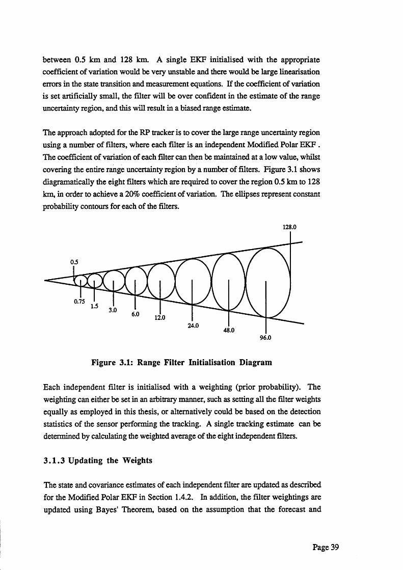
between 0.5 km and 128 km. A single EKF initialised with the appropriate coefficient of variation would be very unstable and there would be large linearisation errors in the state transition and measurement equations. If the coefficient of variation is set artificially small, the filter will be over confident in the estimate of the range uncertainty region, and this will result in a biased range estimate.

The approach adopted for the RP tracker is to cover the large range uncertainty region using a number of filters, where each filter is an independent Modified Polar EKF . The coefficient of variation of each filter can then be maintained at a low value, whilst covering the entire range uncertainty region by a number of filters. Figure 3.1 shows diagramatically the eight filters which are required to cover the region 0.5 km to 128 km, in order to achieve a 20% coefficient of variation. The ellipses represent constant probability contours for each of the filters.

128.0

0.751.5 3.0 6.0 12.0

24.048.0

96.0

Figure 3.1: Range Filter Initialisation Diagram

Each independent filter is initialised with a weighting (prior probability). The weighting can either be set in an arbitrary manner, such as setting all the filter weights equally as employed in this thesis, or alternatively could be based on the detection statistics of the sensor performing the tracking. A single tracking estimate can be determined by calculating the weighted average of the eight independent filters.

3 .1 .3 Updating the Weights

The state and covariance estimates of each independent filter are updated as described for the Modified Polar EKF in Section 1.4.2. In addition, the filter weightings are updated using Bayes' Theorem, based on the assumption that the forecast and

Page 39

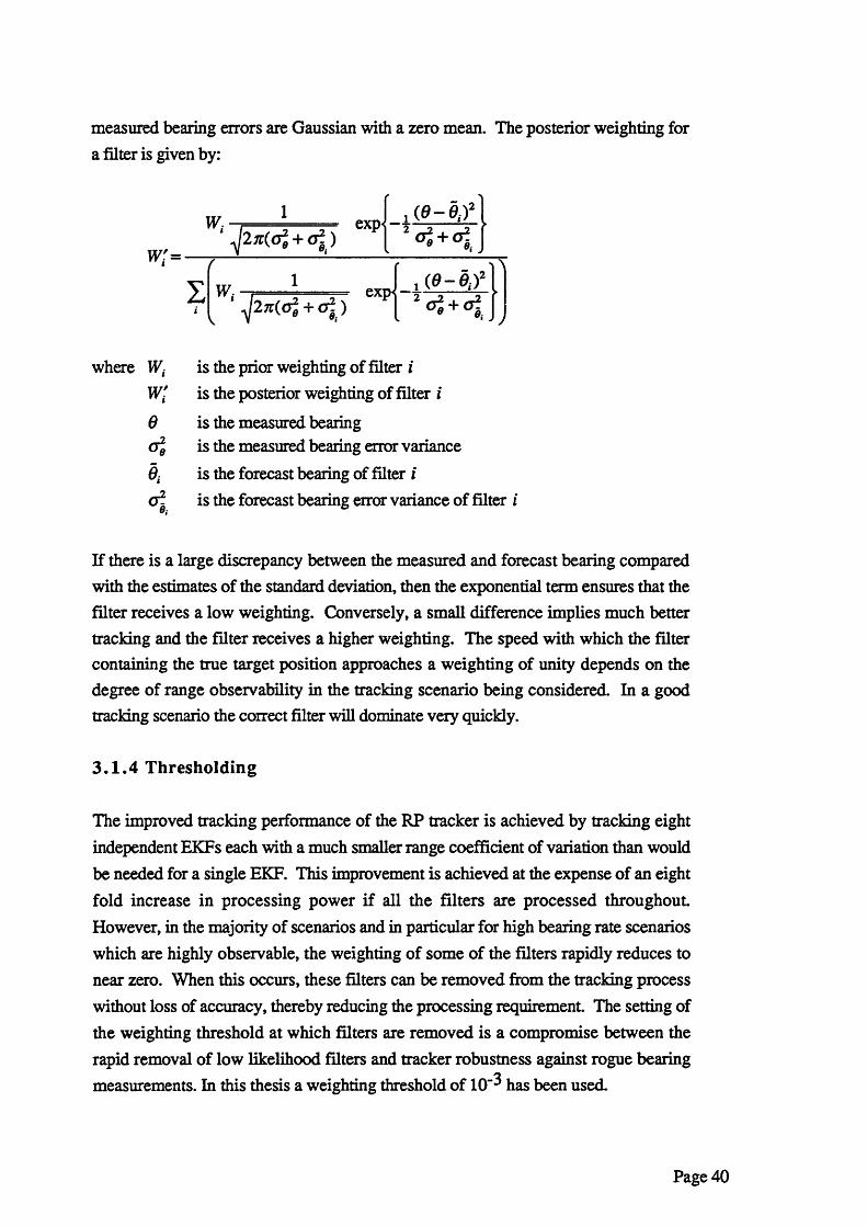
measured bearing errors are Gaussian with a zero mean. The posterior weighting for a filter is given by:

W,1

‘ ^2*r(of+of~jexp ■ ( g - o .) 2]

0

W:‘ ^ 2 rc (o f+ o |)

exp , ( M l 0 0 ,

where Wi is the prior weighting of filter iw; is the posterior weighting of filter i6 is the measured bearing

is the measured bearing error variance

$ is the forecast bearing of filter i< is the forecast bearing error variance of filter i

If there is a large discrepancy between the measured and forecast bearing compared with the estimates of the standard deviation, then the exponential term ensures that the filter receives a low weighting. Conversely, a small difference implies much better tracking and the filter receives a higher weighting. The speed with which the filter containing the true target position approaches a weighting of unity depends on the degree of range observability in the tracking scenario being considered. In a good tracking scenario the correct filter will dominate very quickly.

3 .1 .4 Thresholding

The improved tracking performance of the RP tracker is achieved by tracking eight independent EKFs each with a much smaller range coefficient of variation than would be needed for a single EKF. This improvement is achieved at the expense of an eight fold increase in processing power if all the filters are processed throughout. However, in the majority of scenarios and in particular for high bearing rate scenarios which are highly observable, the weighting of some of the filters rapidly reduces to near zero. When this occurs, these filters can be removed from the tracking process without loss of accuracy, thereby reducing the processing requirement. The setting of the weighting threshold at which filters are removed is a compromise between the rapid removal of low likelihood filters and tracker robustness against rogue bearing measurements. In this thesis a weighting threshold of 10"^ has been used.

Page 40

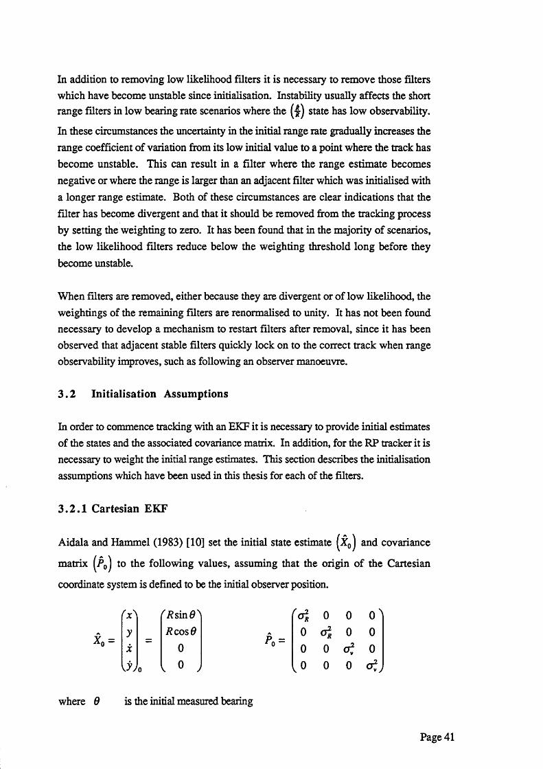
In addition to removing low likelihood filters it is necessary to remove those filters which have become unstable since initialisation. Instability usually affects the short range filters in low bearing rate scenarios where the (4) state has low observability.

In these circumstances the uncertainty in the initial range rate gradually increases the range coefficient of variation from its low initial value to a point where the track has become unstable. This can result in a filter where the range estimate becomes negative or where the range is larger than an adjacent filter which was initialised with a longer range estimate. Both of these circumstances are clear indications that the filter has become divergent and that it should be removed from the tracking process by setting the weighting to zero. It has been found that in the majority of scenarios, the low likelihood filters reduce below the weighting threshold long before they become unstable.

When filters are removed, either because they are divergent or of low likelihood, the weightings of the remaining filters are renormalised to unity. It has not been found necessary to develop a mechanism to restart filters after removal, since it has been observed that adjacent stable filters quickly lock on to the correct track when range observability improves, such as following an observer manoeuvre.

3 .2 Initialisation Assumptions

In order to commence tracking with an EKF it is necessary to provide initial estimates of the states and the associated covariance matrix. In addition, for the RP tracker it is necessary to weight the initial range estimates. This section describes the initialisation assumptions which have been used in this thesis for each of the filters.

3 .2 .1 Cartesian EKF

Aidala and Hammel (1983) [10] set the initial state estimate and covariance

matrix to the following values, assuming that the origin of the Cartesian

coordinate system is defined to be the initial observer position.

( x )rRsin9' foi 0 0 0

y RcosO A 0 ° R 0 0X 0 Po = 0 0 of 0

0 , 0 , ,0 0 0

where 9 is the initial measured bearing

Page 41

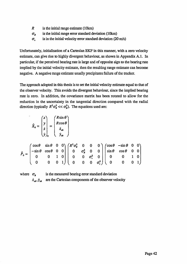
R is the initial range estimate (10km)<jR is the initial range error standard deviation (1 0 km)crv is in the initial velocity error standard deviation ( 2 0 m/s)

Unfortunately, initialisation of a Cartesian EKF in this manner, with a zero velocity estimate, can give rise to highly divergent behaviour, as shown in Appendix A.l. In particular, if the perceived bearing rate is large and of opposite sign to the bearing rate implied by the initial velocity estimate, then the resulting range estimate can become negative. A negative range estimate usually precipitates failure of the tracker.

The approach adopted in this thesis is to set the initial velocity estimate equal to that of the observer velocity. This avoids the divergent behaviour, since the implied bearing rate is zero. In addition, the covariance matrix has been rotated to allow for thereduction in the uncertainty in the tangential direction compared with the radial direction (typically R2ol « a j). The equations used are:

(X) 'AsinG^A

* 0 =y RcosO

=X

0 < j

f cos0 sin 0 0 0> rR2c?e 0 0 o ' 'cos0 -sin 0 0 0>-sin 0 cos 0 0 0 0 o i 0 0 sin0 COS0 0 0

0 0 1 0 0 0 0 0 0 1 0

, 0 0 0 1> , 0 0 0 , 0 0 0 K

where <J9 is the measured bearing error standard deviationxob, yob are the Cartesian components of the observer velocity

Page 42

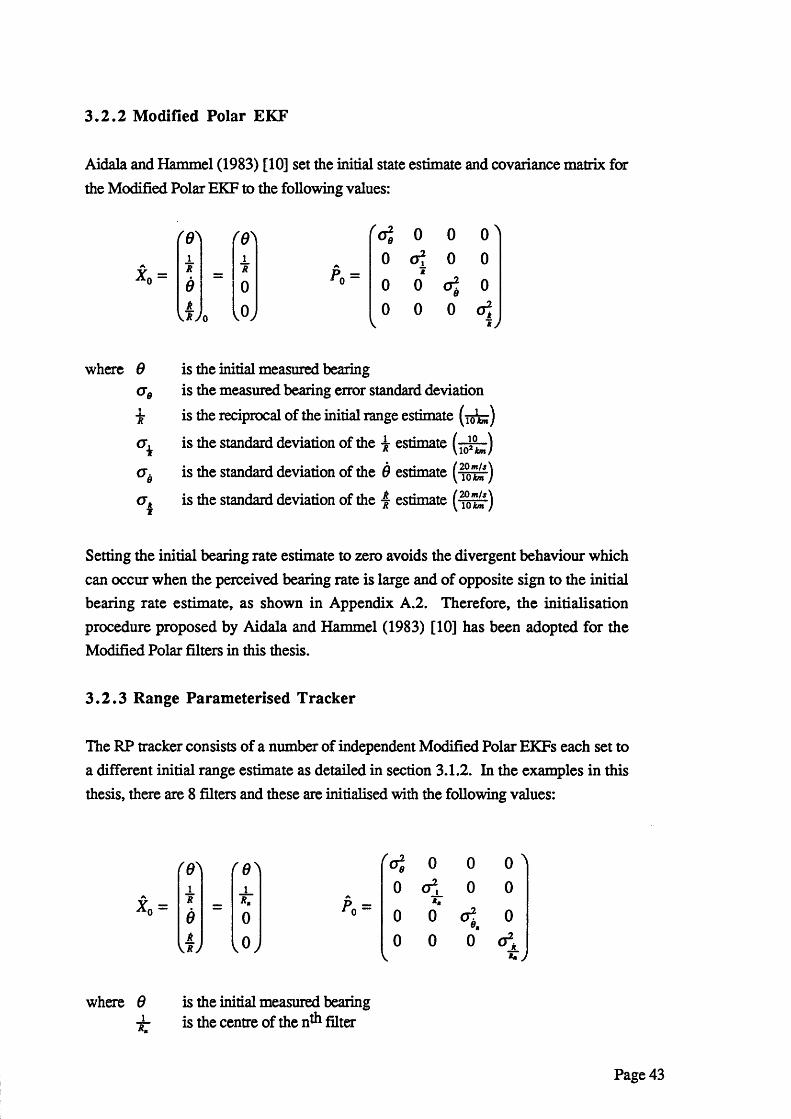
3 .2 .2 Modified Polar EKF

Aidala and Hammel (1983) [10] set the initial state estimate and covariance matrix for the Modified Polar EKF to the following values:

(0>iRei

o

(0}R0

vOy

P« =

oi 0 0 0

0 0 0

0

Jt0 0

0 0 0 o]* /

where 0 is the initial measured bearingis the measured bearing error standard deviation

iR is the reciprocal of the initial range estimate (iotr

is the standard deviation of the 4 estimate (' 10 ' JO2 fen;

is the standard deviation of the 0 estimate ('20 m/i' k 10 fen t

o ,T is the standard deviation of the 4 estimate (' 20 m/sy t 10 fen t

Setting the initial bearing rate estimate to zero avoids the divergent behaviour which can occur when the perceived bearing rate is large and of opposite sign to the initial bearing rate estimate, as shown in Appendix A.2. Therefore, the initialisation procedure proposed by Aidala and Hammel (1983) [10] has been adopted for the Modified Polar filters in this thesis.

3 .2 .3 Range Parameterised Tracker

The RP tracker consists of a number of independent Modified Polar EKFs each set to a different initial range estimate as detailed in section 3.1.2. In the examples in this thesis, there are 8 filters and these are initialised with the following values:

1 iR *.e 0a

where 0 is the initial measured bearing is the centre of the n^ 1 filter

0 0 00 °i 0 00 0 < 00 0 0

Page 43

o e is the measured bearing error standard deviation

is the standard deviation of the 4 estimate ^-jrj

<7 is the standard deviation of the 9 estimate

(Tj is the standard deviation of the 4 estimate ( n ^ )

Rh = (0.75,1.5,3.0,6.0,12.0, 24.0,48.0,96.0 km)re — ( 0 5 10 2 0 4 0 8.0 16.0 32.0 64.0

“ (>/l2» -m* Vl2’ Vl2» Vl2» Vl2» V l2 ’ Vl2 Km)

By choosing a constant value of velocity error standard deviation (20 m/s) for each range filter, the standard deviation of the bearing rate reduces at longer range. This is a useful feature for identifying the target range prior to observer manoeuvres, as will be shown in Section 3.3.3.

In this thesis, each filter is equally weighted at initialisation. However, in practice the weightings could be set based on the detection statistics of the sensor performing the tracking.

3 .3 Monte Carlo Performance of RP Tracker

The scenario defined in Section 3.3.1 has been Monte Carlo run for the Cartesian (C), Modified Polar (MP) and Range Parameterised (RP) trackers. The runs consist of 100 replications with identical pseudo random number seeds. The bearing errors have been drawn from a Gaussian distribution with a fixed standard deviation and zero mean.

The mean and RMS of the range errors averaged across the 100 replications have been calculated for each update. Outliers exceeding 3 standard deviations from the mean have been monitored, however, neither the number nor magnitude of the outliers have influenced these statistical measures.

Only the range error statistics are presented in this thesis as the other states (bearing, bearing rate and range rate/range) are well behaved except when the filters become divergent. Also, the range error following an observer manoeuvre is highly dependent on the accuracy of the other states and, thus, the size of the range error is indicative of the overall tracking performance.

Page 44

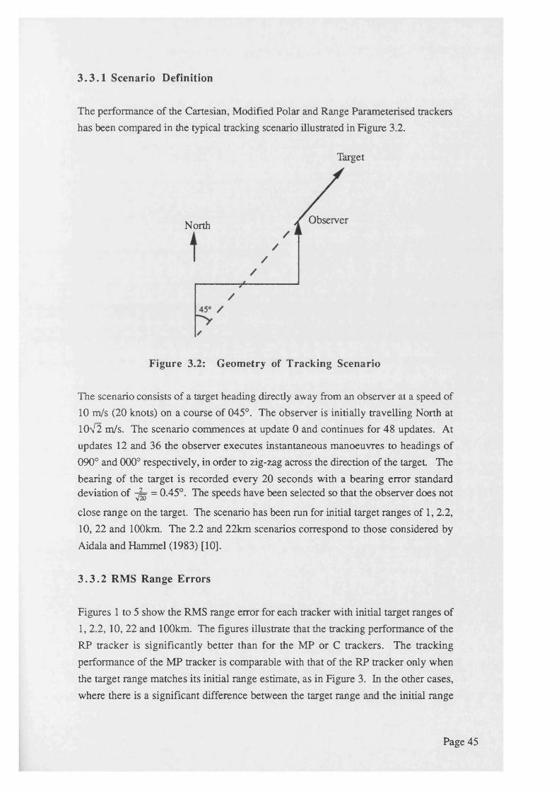
3 .3 .1 Scenario Definition

The performance of the Cartesian, Modified Polar and Range Parameterised trackers has been compared in the typical tracking scenario illustrated in Figure 3.2.

Target

ObserverNorth

Figure 3.2: Geometry of Tracking Scenario

The scenario consists of a target heading directly away from an observer at a speed of10 m/s (20 knots) on a course of 045°. The observer is initially travelling North at10V2 m/s. The scenario commences at update 0 and continues for 48 updates. Atupdates 12 and 36 the observer executes instantaneous manoeuvres to headings of090° and 000° respectively, in order to zig-zag across the direction of the target Thebearing of the target is recorded every 20 seconds with a bearing error standard deviation of ^ = 0.45°. The speeds have been selected so that the observer does not

close range on the target. The scenario has been run for initial target ranges of 1,2.2, 10, 22 and 100km. The 2.2 and 22km scenarios correspond to those considered by Aidala and Hammel (1983) [10].

3 .3 .2 RMS Range Errors

Figures 1 to 5 show the RMS range error for each tracker with initial target ranges of 1, 2.2, 10, 22 and 100km. The figures illustrate that the tracking performance of the RP tracker is significantly better than for the MP or C trackers. The tracking performance of the MP tracker is comparable with that of the RP tracker only when the target range matches its initial range estimate, as in Figure 3. In the other cases, where there is a significant difference between the target range and the initial range

Page 45

estimate, the RMS range error for the MP tracker is typically a factor of 5 to 10 times worse than for the RP tracker in the equivalent conditions. The tracking performance of the MP tracker is generally better than that for the C tracker, and this is particularly apparent in Figure 3 and 4. However, it should be noted that in order to prevent the MP tracker becoming divergent when the target is at long range, the x state had to be limited to above 3 ^ . Without this limit the x state became negative, which usually

resulted in failure of the tracker.

It was not found necessary to place artificial limits on the state estimates for the RP or C trackers. This is due mainly to the small range variance in each filter for the RP tracker and to the new initialisation criteria proposed in Section 3.2.1 for the C tracker. Experimentation using the previous initialisation recommendations for the C tracker as used by Aidala and Hammel (1983) [10], required a limit on the range state in order to prevent negative values and the resultant tracker failure.

3 .3 .3 Typical Track Output

The track output (range estimate only) for a typical replication with the target at an initial range of 2.2km is tabulated in Table 3.1 below.

Page 46

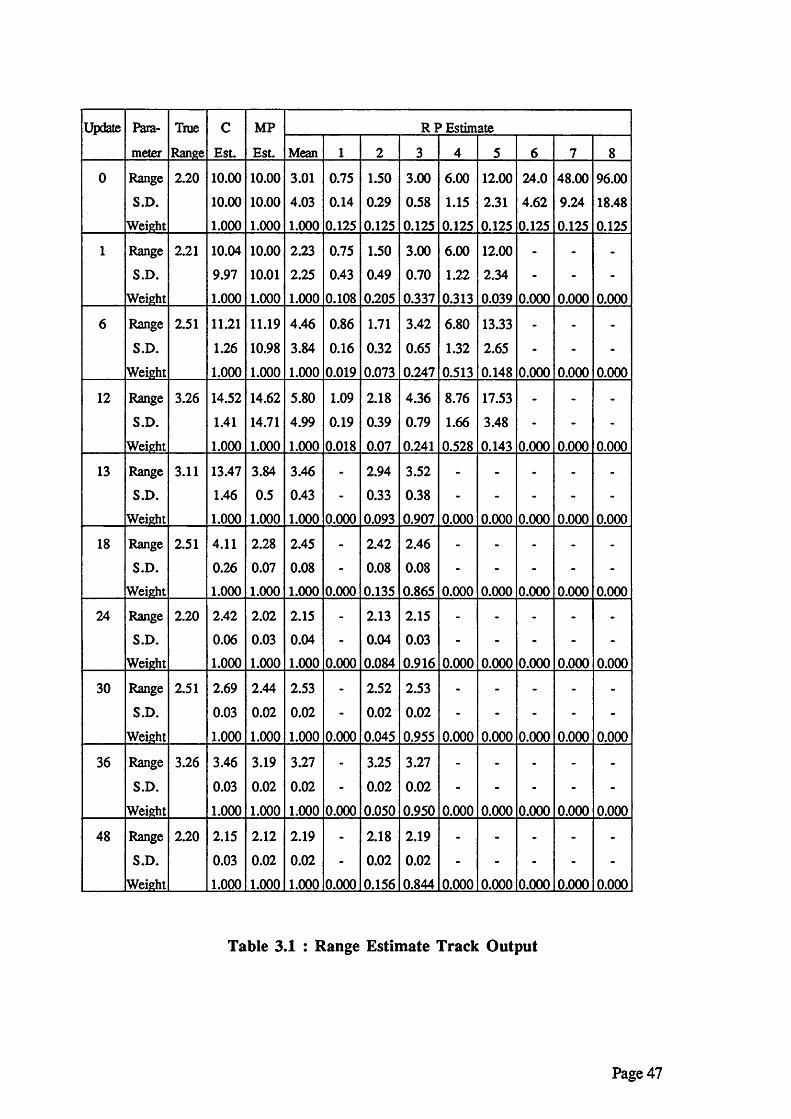
Update Para­

meter

True

Range

C

Est.

MP

Est.

R P Estimate

Mean 1 2 3 4 5 6 7 8

0 RangeS.D.

Weight

2.20 10.0010.001.000

10.0010.001.000

3.014.031.000

0.750.14

0.125

1.500.290.125

3.000.580.125

6.001.150.125

12.002.310.125

24.04.620.125

48.009.24

0.125

96.0018.480.125

1 RangeS.D.

Weight

2.21 10.04

9.971.000

10.0010.011.000

2.232.251.000

0.750.43

0.108

1.500.490.205

3.000.700.337

6.001.22

0.313

12.002.34

0.039 0.000 0.000 0.000

6 Range

S.D.

Weight

2.51 11.21

1.26

1.000

11.19

10.981.000

4.463.84

1.000

0.86

0.160.019

1.71

0.32

0.073

3.42

0.650.247

6.801.32

0.513

13.33

2.650.148 0.000 0.000 0.000

12 RangeS.D.

Weight

3.26 14.521.41

1.000

14.6214.71

1.000

5.804.991.000

1.09

0.190.018

2.180.390.07

4.360.790.241

8.76

1.660.528

17.533.480.143 0.000 0.000 0.000

13 RangeS.D.

Weight

3.11 13.471.461.000

3.84

0.51.000

3.460.431.000 0.000

2.94

0.330.093

3.520.380.907 0.000 0.000 0.000 0.000 0.000

18 RangeS.D.

Weight

2.51 4.11

0.261.000

2.280.071.000

2.450.081.000 0.000

2.420.080.135

2.460.080.865 0.000 0.000 0.000 0.000 0.000

24 RangeS.D.

Weight

2.20 2.42

0.061.000

2.02

0.031.000

2.150.041.000 0.000

2.130.040.084

2.150.030.916 0.000 0.000 0.000 0.000 0.000

30 RangeS.D.

Weight

2.51 2.69

0.03

1.000

2.44

0.02

1.000

2.530.02

1.000 0.000

2.52

0.02

0.045

2.530.02

0.955 0.000 0.000 0.000 0.000 0.000

36 Range

S.D.

Weight

3.26 3.46

0.03

1.000

3.190.02

1.000

3.27

0.02

1.000 0.000

3.250.02

0.050

3.27

0.02

0.950 0.000 0.000 0.000 0.000 0.000

48 RangeS.D.

Weight

2.20 2.150.031.000

2.12

0.02

1.000

2.190.02

1.000 0.000

2.180.02

0.156

2.190.020.844 0.000 0.000 0.000 0.000 0.000

Table 3.1 : Range Estimate Track Output

Page 47

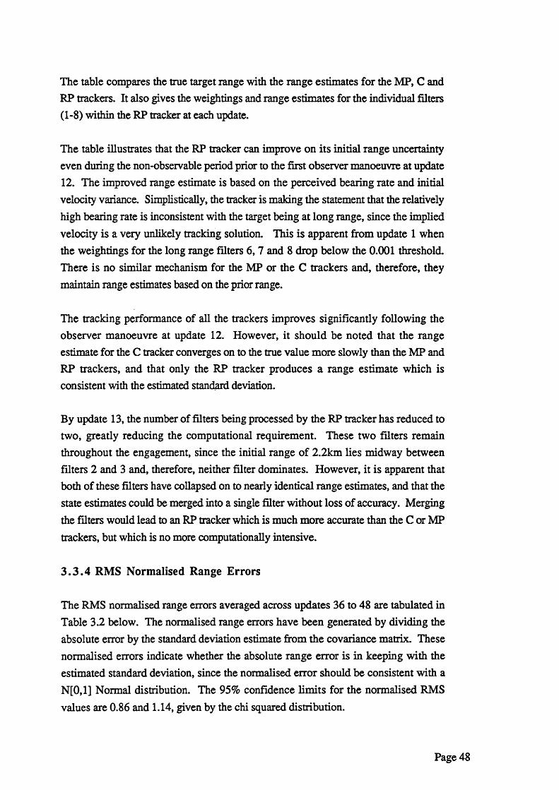
The table compares the true target range with the range estimates for the MP, C and RP trackers. It also gives the weightings and range estimates for the individual filters (1-8) within the RP tracker at each update.

The table illustrates that the RP tracker can improve on its initial range uncertainty even during the non-observable period prior to the first observer manoeuvre at update 12. The improved range estimate is based on the perceived bearing rate and initial velocity variance. Simplistically, the tracker is making the statement that the relatively high bearing rate is inconsistent with the target being at long range, since the implied velocity is a very unlikely tracking solution. This is apparent from update 1 when the weightings for the long range filters 6 ,7 and 8 drop below the 0 . 0 0 1 threshold. There is no similar mechanism for the MP or the C trackers and, therefore, they maintain range estimates based on the prior range.

The tracking performance of all the trackers improves significantly following the observer manoeuvre at update 12. However, it should be noted that the range estimate for the C tracker converges on to the true value more slowly than the MP and RP trackers, and that only the RP tracker produces a range estimate which is consistent with the estimated standard deviation.

By update 13, the number of filters being processed by the RP tracker has reduced to two, greatly reducing the computational requirement. These two filters remain throughout the engagement, since the initial range of 2 .2 km lies midway between filters 2 and 3 and, therefore, neither filter dominates. However, it is apparent that both of these filters have collapsed on to nearly identical range estimates, and that the state estimates could be merged into a single filter without loss of accuracy. Merging the filters would lead to an RP tracker which is much more accurate than the C or MP trackers, but which is no more computationally intensive.

3 .3 .4 RMS Normalised Range Errors

The RMS normalised range errors averaged across updates 36 to 48 are tabulated in Table 3.2 below. The normalised range errors have been generated by dividing the absolute error by the standard deviation estimate from the covariance matrix. These normalised errors indicate whether the absolute range error is in keeping with the estimated standard deviation, since the normalised error should be consistent with a N[0,1] Normal distribution. The 95% confidence limits for the normalised RMS values are 0.86 and 1.14, given by the chi squared distribution.

Page 48

1 km 2 .2 km 1 0 km 2 2 km 1 0 0 kmc 18.2 4.0 7.9 4.2 13.4MP 120.7 5.2 1 . 2 1 . 6 2.3RP 4.3 1 . 2 1 . 1 1 . 0 0 . 8

Table 3.2 - RMS Normalised Range Errors

The table illustrates that the range errors for the RP tracker with 8 filters are consistent with the estimated standard deviation, for target ranges of 2 .2 , 1 0 , 2 2 and 1 0 0 km. More consistent estimates can also be generated for a target range of 1 km by increasing the number of filters operating in the RP tracker from 8 to 32, resulting in a RMS normalised range error of 1.5. The improved normalised range error with 32 filters is accompanied by a factor of 3 reduction in the RMS range error from, typically, 0.03km to 0.01km. Therefore, increasing the number of filters not only makes the RP tracker more consistent, but also leads to smaller range error as well.

In contrast, the absolute range errors for the MP tracker are only consistent with the standard deviation estimate when the target range is close to the initial range estimate. The C tracker never produces consistent range estimates.

Page 49

4 . TRA CK IN G TARGET M ANOEUVRES USING A GLR PROCEDURE

The manoeuvre detection procedure proposed in this thesis uses the Generalised Likelihood Ratio (GLR) test to detect a change in the innovation sequence associated with a manoeuvre. The innovation is defined as the difference between the measured and forecast bearings (Basseville and Nikiforov (1993) [37]), and in the case of no manoeuvre this will have zero mean and covariance Vi given by:

V| = M i Pi M j + S,

where Mi is the measurement matrixPi is the covariance matrix for the forecastSi is the covariance matrix for the measurement

After a target manoeuvre the mean of the innovation sequence will be non-zero, with a dynamic profile, or signature, characteristic of a particular manoeuvre. The purpose of the GLR procedure is to detect this manoeuvre signature and to correct the system states, such that the innovation sequence is restored to zero mean. In the bearings only tracking application a manoeuvre is characterised by a step change in the target velocity, which approximates to a ramp change in the observed bearings. This results in a non-linear signature for the innovation as the Kalman filter attempts to adapt to this change using a non-manoeuvring model.

The manoeuvre is detected by a GLR test, which is applied at each update over a history of up to 16 updates. A large manoeuvre will be detected with a small track history, whereas a small manoeuvre will be detected only after many updates. After detection, a new independent Kalman filter is initialised based on the corrected state estimates using the estimates of the time and magnitude of the manoeuvre derived from the GLR test. The original filter is retained to cater for the possibility of a false alarm. The likelihoods of the new filter and the original non-manoeuvring filter are reset according to the likelihood ratio for the manoeuvre. The GLR procedure therefore represents the multi-modal posterior distribution, associated with a manoeuvring and non-manoeuvring target, as a mixture of Gaussians using independent Kalman filters. After a short time one of these filters will dominate and the other will no longer be processed, depending on whether the detected manoeuvre actually occurred or was only a false alarm.

Page 50

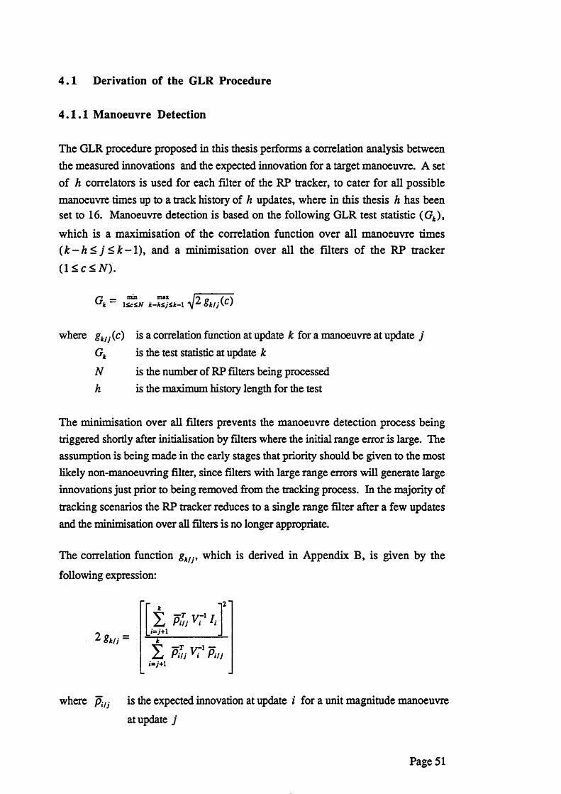
4 .1 Derivation of the GLR Procedure

4 .1 .1 Manoeuvre Detection

The GLR procedure proposed in this thesis performs a correlation analysis between the measured innovations and the expected innovation for a target manoeuvre. A set of h correlators is used for each filter of the RP tracker, to cater for all possible manoeuvre times up to a track history of h updates, where in this thesis h has been set to 16. Manoeuvre detection is based on the following GLR test statistic (Gk),

which is a maximisation of the correlation function over all manoeuvre times ( k - h < j < k - l ) , and a minimisation over all the filters of the RP tracker (1 < c< N ).

/-» min max /9 oUk “ IZcZN \ Sk/j\C)

where gk/j (c) is a correlation function at update k for a manoeuvre at update j Gk is the test statistic at update k

N is the number of RP filters being processedh is the maximum history length for the test

The minimisation over all filters prevents the manoeuvre detection process being triggered shortly after initialisation by filters where the initial range error is large. The assumption is being made in the early stages that priority should be given to the most likely non-manoeuvring filter, since filters with large range errors will generate large innovations just prior to being removed from the tracking process. In the majority of tracking scenarios the RP tracker reduces to a single range filter after a few updates and the minimisation over all filters is no longer appropriate.

The correlation function gk/j, which is derived in Appendix B, is given by the

following expression:

t Phi V? /,]

E Pin v-1 Pi,j«= ;+ i

where pUj is the expected innovation at update i for a unit magnitude manoeuvre

at update j

8klj —

Page 51

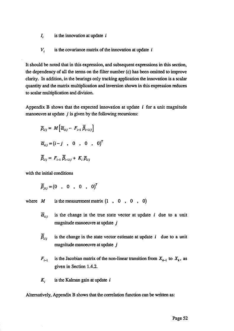
is the innovation at update i

Vi is the covariance matrix of the innovation at update i

It should be noted that in this expression, and subsequent expressions in this section, the dependency of all the terms on the filter number (c) has been omitted to improve clarity. In addition, in the bearings only tracking application the innovation is a scalar quantity and the matrix multiplication and inversion shown in this expression reduces to scalar multiplication and division.

Appendix B shows that the expected innovation at update i for a unit magnitude manoeuvre at update j is given by the following recursions:

Pit j = M \cCnj - Fw A-l/y]

V i l , 0 , 0 , 0 /

Avj — A-l A-l/y + Kl Pin

with the initial conditions

pm = ( 0 , 0 , 0 , 0 /

where M is the measurement matrix (1 , 0 , 0 , 0)

aiU is the change in the true state vector at update i due to a unit

magnitude manoeuvre at update j

PUj is the change in the state vector estimate at update i due to a unit

magnitude manoeuvre at update j

Fm is the Jacobian matrix of the non-linear transition from X k_: to Xk, as

given in Section 1.4.2.

Ki is the Kalman gain at update i

Alternatively, Appendix B shows that the correlation function can be written as:

Page 52

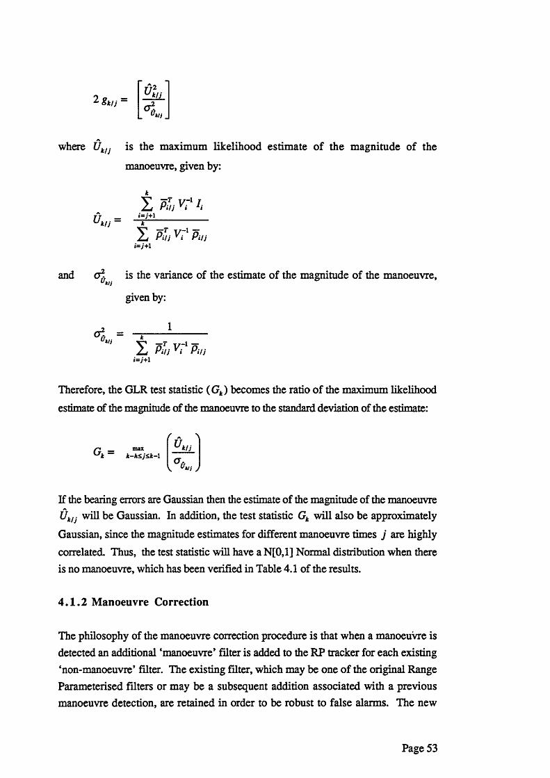
2 8k i j “U2k / j

a iutl!Uj J

where Uk/J is the maximum likelihood estimate of the magnitude of the

manoeuvre, given by:

I pin r11,U =U kl j - *

I Pin V? Pm•=y+1

and is the variance of the estimate of the magnitude of the manoeuvre,Ukisgiven by:

i

X pin vr‘ p,/‘ = 7+1

Therefore, the GLR test statistic (Gk) becomes the ratio of the maximum likelihood

estimate of the magnitude of the manoeuvre to the standard deviation of the estimate:

/-i max* ~ ' k-hZiZk-1

k/ j

If the bearing errors are Gaussian then the estimate of the magnitude of the manoeuvreA

Uklj will be Gaussian. In addition, the test statistic Gk will also be approximately

Gaussian, since the magnitude estimates for different manoeuvre times j are highly correlated. Thus, the test statistic will have a N[0,1] Normal distribution when there is no manoeuvre, which has been verified in Table 4.1 of the results.

4 .1 .2 Manoeuvre Correction

The philosophy of the manoeuvre correction procedure is that when a manoeuvre is detected an additional ‘manoeuvre’ filter is added to the RP tracker for each existing ‘non-manoeuvre’ filter. The existing filter, which may be one of the original Range Parameterised filters or may be a subsequent addition associated with a previous manoeuvre detection, are retained in order to be robust to false alarms. The new

Page 53

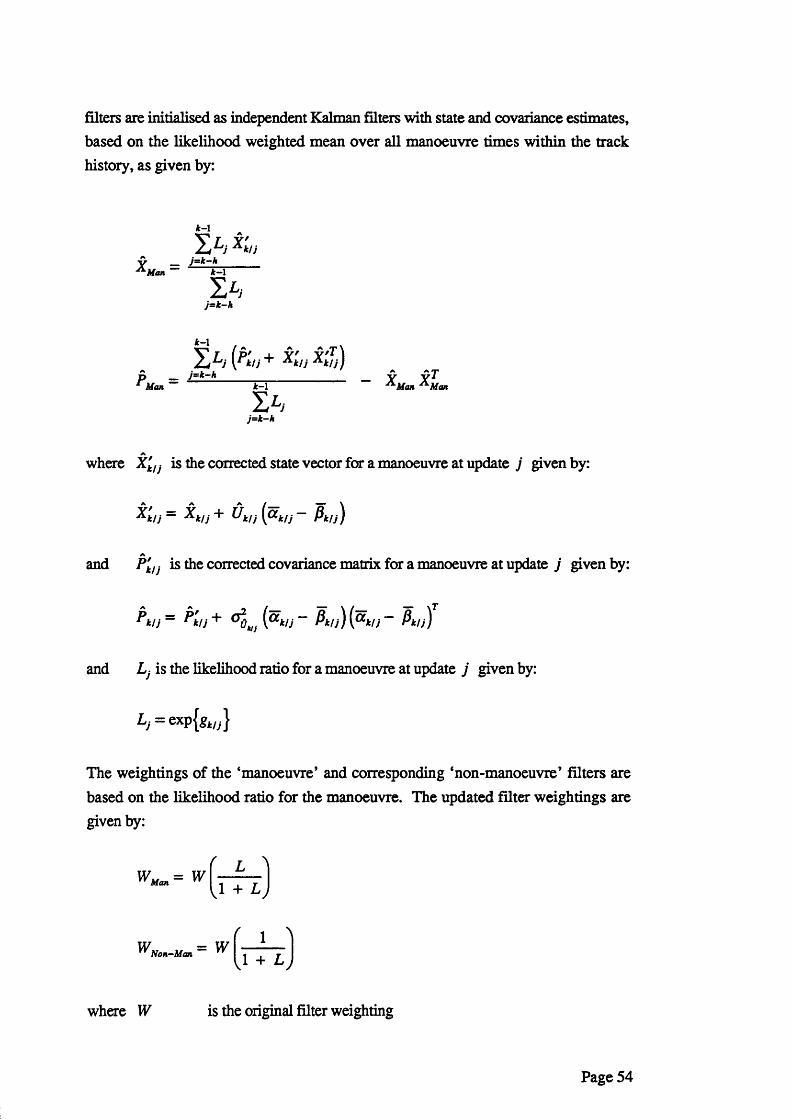
filters are initialised as independent Kalman filters with state and covariance estimates, based on the likelihood weighted mean over all manoeuvre times within the track history, as given by:

k-i

^ M a n j=k—h

k- 1

j=k—h

P — Man

j=k-hk- 1

J=k—k

A A T’

Y Y 1Man Man

A

where X'klJ is the corrected state vector for a manoeuvre at update j given by:

Xk/J = %k/ j + U k l j [ a k/ j — P k f j )

A

and P'k/j is the corrected covariance matrix for a manoeuvre at update j given by:

— \T^ k / j ~ H , J + ° 0 kj. ( a k/j P k / j ) { a k/ j P k l j )

and Lj is the likelihood ratio for a manoeuvre at update j given by:

Lj = txp{gklj}

The weightings of the ‘manoeuvre* and corresponding ‘non-manoeuvre* filters are based on the likelihood ratio for the manoeuvre. The updated filter weightings are given by:

1 + L

1 V 1 + L j

where W is the original filter weighting

Page 54

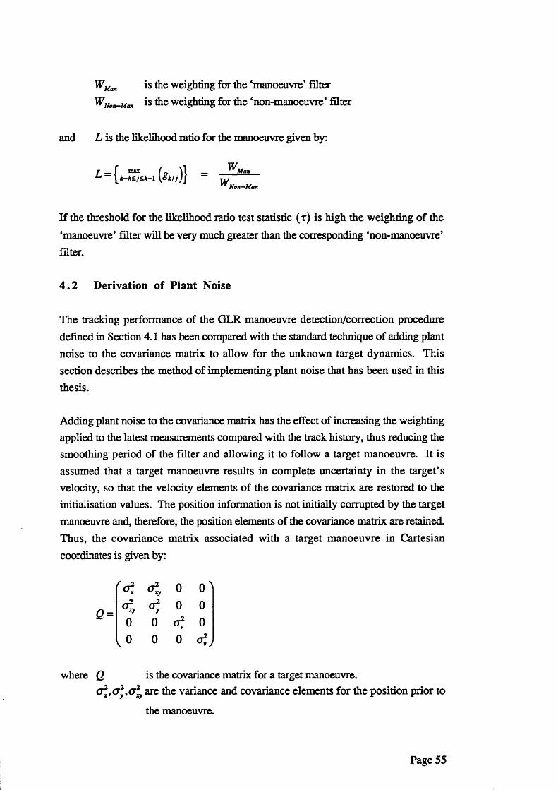
WMan is the weighting for the ‘manoeuvre* filter WNon_Mm is the weighting for the ‘non-manoeuvre’ filter

and L is the likelihood ratio for the manoeuvre given by:

^ = { k-htjzk-i (gk/j) } “WVV Man

^ Non—Man

If the threshold for the likelihood ratio test statistic (t) is high the weighting of the ‘manoeuvre’ filter will be very much greater than the corresponding ‘non-manoeuvre’ filter.

4 .2 Derivation of Plant Noise

The tracking performance of the GLR manoeuvre detection/correction procedure defined in Section 4.1 has been compared with the standard technique of adding plant noise to the covariance matrix to allow for the unknown target dynamics. This section describes the method of implementing plant noise that has been used in this thesis.

Adding plant noise to the covariance matrix has the effect of increasing the weighting applied to the latest measurements compared with the track history, thus reducing the smoothing period of the filter and allowing it to follow a target manoeuvre. It is assumed that a target manoeuvre results in complete uncertainty in the target’s velocity, so that the velocity elements of the covariance matrix are restored to the initialisation values. The position information is not initially corrupted by the target manoeuvre and, therefore, the position elements of the covariance matrix are retained. Thus, the covariance matrix associated with a target manoeuvre in Cartesian coordinates is given by:

2 = oo

0 0

0 0

0 of 0 0 0

where Q is the covariance matrix for a target manoeuvre.are the variance and covariance elements for the position prior to

the manoeuvre.

Page 55

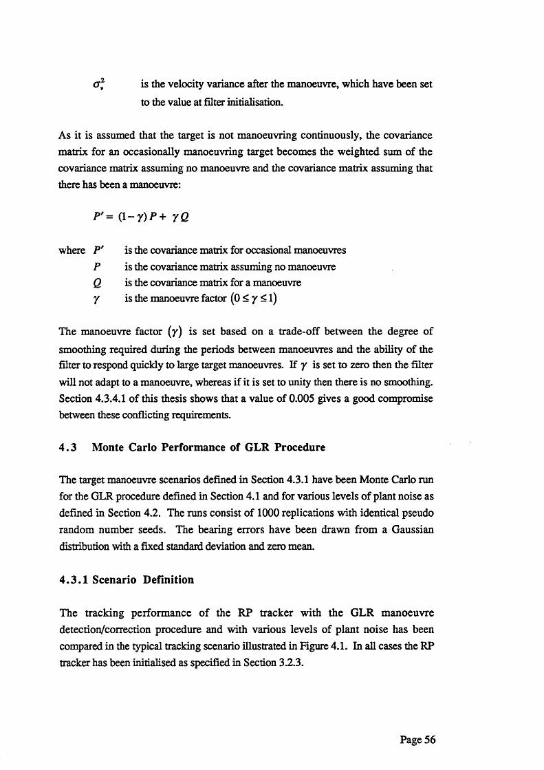
o] is the velocity variance after the manoeuvre, which have been set

to the value at filter initialisation.

As it is assumed that the target is not manoeuvring continuously, the covariance matrix for an occasionally manoeuvring target becomes the weighted sum of the covariance matrix assuming no manoeuvre and the covariance matrix assuming that there has been a manoeuvre:

p'= a- y ) P + rQ

where P' is the covariance matrix for occasional manoeuvresP is the covariance matrix assuming no manoeuvreQ is the covariance matrix for a manoeuvrey is the manoeuvre factor ( 0 < y < 1 )

The manoeuvre factor (y) is set based on a trade-off between the degree of

smoothing required during the periods between manoeuvres and the ability of the filter to respond quickly to large target manoeuvres. If y is set to zero then the filter will not adapt to a manoeuvre, whereas if it is set to unity then there is no smoothing. Section 4.3.4.1 of this thesis shows that a value of 0.005 gives a good compromise between these conflicting requirements.

4 .3 Monte Carlo Performance of GLR Procedure

The target manoeuvre scenarios defined in Section 4.3.1 have been Monte Carlo run for the GLR procedure defined in Section 4.1 and for various levels of plant noise as defined in Section 4.2. The runs consist of 1000 replications with identical pseudo random number seeds. The bearing errors have been drawn from a Gaussian distribution with a fixed standard deviation and zero mean.

4 .3 .1 Scenario Definition

The tracking performance of the RP tracker with the GLR manoeuvre detection/correction procedure and with various levels of plant noise has been compared in the typical tracking scenario illustrated in Figure 4.1. In all cases the RP tracker has been initialised as specified in Section 3.2.3.

Page 56

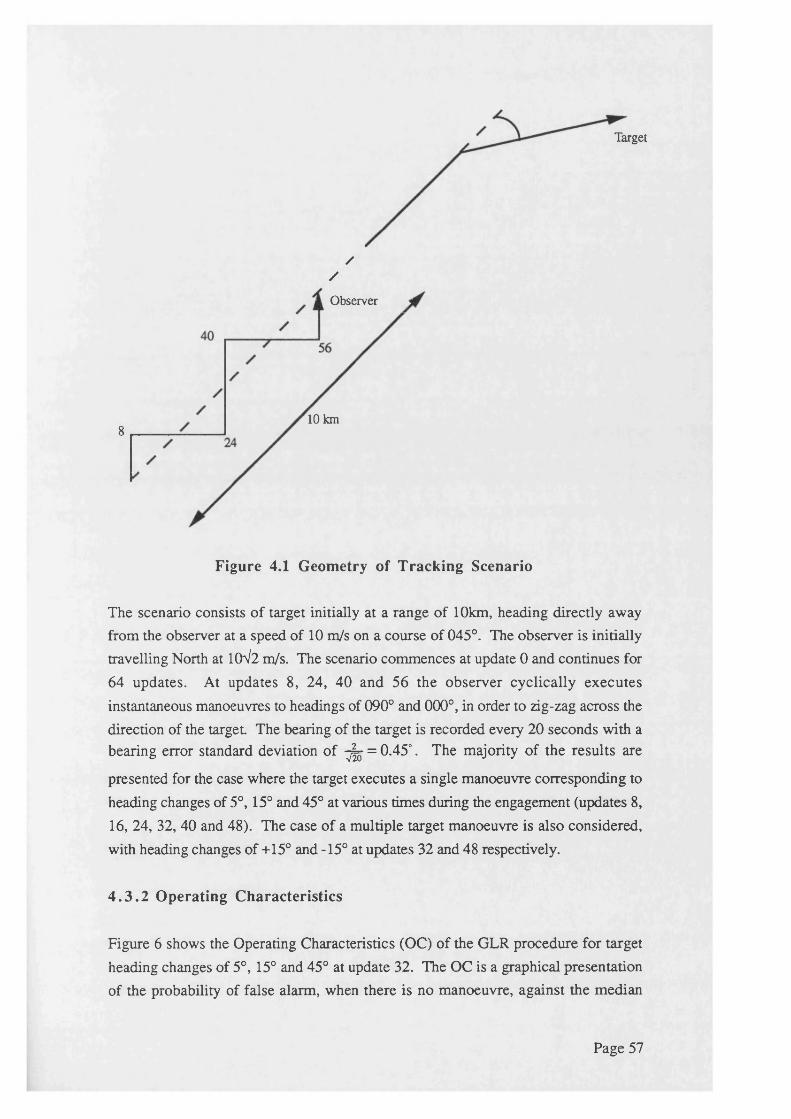
Target

//

Observer

10 km8

Figure 4.1 Geometry of Tracking Scenario

The scenario consists of target initially at a range of 10km, heading directly away from the observer at a speed of 10 m/s on a course of 045°. The observer is initially travelling North at 10^2 m/s. The scenario commences at update 0 and continues for 64 updates. At updates 8, 24, 40 and 56 the observer cyclically executes instantaneous manoeuvres to headings of 090° and 000°, in order to zig-zag across the direction of the target The bearing of the target is recorded every 20 seconds with a bearing error standard deviation of ^ = 0.45°. The majority of the results are

presented for the case where the target executes a single manoeuvre corresponding to heading changes of 5°, 15° and 45° at various times during the engagement (updates 8, 16, 24, 32, 40 and 48). The case of a multiple target manoeuvre is also considered, with heading changes of +15° and -15° at updates 32 and 48 respectively.

4 .3 .2 Operating Characteristics

Figure 6 shows the Operating Characteristics (OC) of the GLR procedure for target heading changes of 5°, 15° and 45° at update 32. The OC is a graphical presentation of the probability of false alarm, when there is no manoeuvre, against the median

Page 57

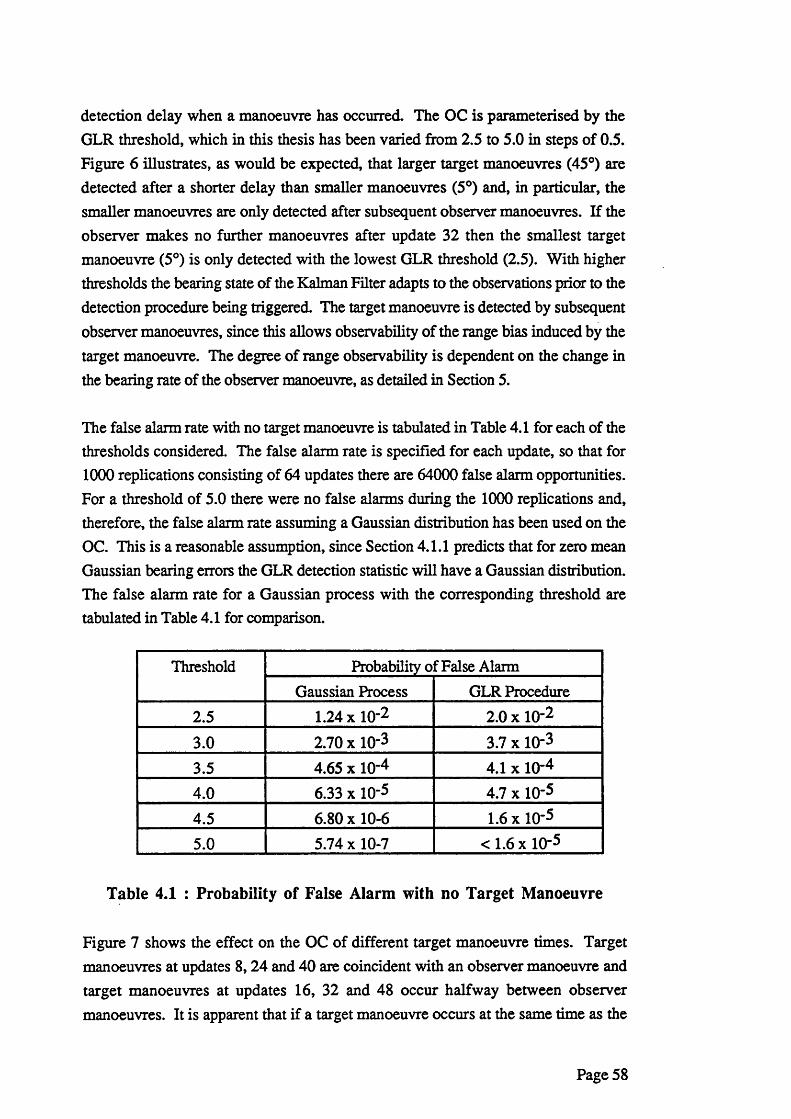
detection delay when a manoeuvre has occurred. The OC is parameterised by the GLR threshold, which in this thesis has been varied from 2.5 to 5.0 in steps of 0.5. Figure 6 illustrates, as would be expected, that larger target manoeuvres (45°) are detected after a shorter delay than smaller manoeuvres (5°) and, in particular, the smaller manoeuvres are only detected after subsequent observer manoeuvres. If the observer makes no further manoeuvres after update 32 then the smallest target manoeuvre (5°) is only detected with the lowest GLR threshold (2.5). With higher thresholds the bearing state of the Kalman Filter adapts to the observations prior to the detection procedure being triggered. The target manoeuvre is detected by subsequent observer manoeuvres, since this allows observability of the range bias induced by the target manoeuvre. The degree of range observability is dependent on the change in the bearing rate of the observer manoeuvre, as detailed in Section 5.

The false alarm rate with no target manoeuvre is tabulated in Table 4.1 for each of the thresholds considered. The false alarm rate is specified for each update, so that for 1000 replications consisting of 64 updates there are 64000 false alarm opportunities. For a threshold of 5.0 there were no false alarms during the 1000 replications and, therefore, the false alarm rate assuming a Gaussian distribution has been used on the OC. This is a reasonable assumption, since Section 4.1.1 predicts that for zero mean Gaussian bearing errors the GLR detection statistic will have a Gaussian distribution. The false alarm rate for a Gaussian process with the corresponding threshold are tabulated in Table 4.1 for comparison.

Threshold Probability of False AlarmGaussian Process GLR Procedure

2.5 1.24 x lO- 2 2 . 0 x lO" 2

3.0 2.70 x 10-3 3.7 x 10-3

3.5 4.65 x 10- 4 4.1 x 10- 4

4.0 6.33 x 10-5 4.7 x 10-5

4.5 6.80 x 1 0 - 6 1.6x10-5

5.0 5.74 x 10-7 < 1 . 6 x 10-5

Table 4.1 : Probability of False Alarm with no Target Manoeuvre

Figure 7 shows the effect on the OC of different target manoeuvre times. Target manoeuvres at updates 8,24 and 40 are coincident with an observer manoeuvre and target manoeuvres at updates 16, 32 and 48 occur halfway between observer manoeuvres. It is apparent that if a target manoeuvre occurs at the same time as the

Page 58

first observer manoeuvre (update 8 ), there is a very long detection delay. After the first observer manoeuvre the detection delay becomes less sensitive to the time of the target manoeuvre, however, it should be noted that the detection delay is significandy smaller when the target manoeuvre is coincident with the observer manoeuvre. The detection delay is dependent on the degree of adaptation of the Kalman filter to the manoeuvre, which is related to the bearing rate error variance at the time of the manoeuvre. In addition, there is a lower limit on the magnitude of target manoeuvre that can be detected, since the manoeuvre must result in a change in the bearing rate which is greater than the GLR threshold multiplied by the bearing rate standard deviation.

Analysis of the OC for the various target manoeuvres has lead to the selection of a threshold of 3.0 for the GLR procedure. This value was chosen as a compromise between the conflicting requirements of a low probability of false alarm and a short detection delay. The probability of false alarm of 3.7 x 1 0 '3 ( 1 in 270 updates) was judged to be acceptable, since the occurrence of a false alarm is not critical, as will be shown in Section 4.3.6. The threshold value of t=3 has been used in all subsequent runs analysed in this thesis.

4 .3 .3 Contingency Tables

Table 4.2 shows the contingency table for the GLR procedure for a target heading change of 15° at update 32.

Page 59

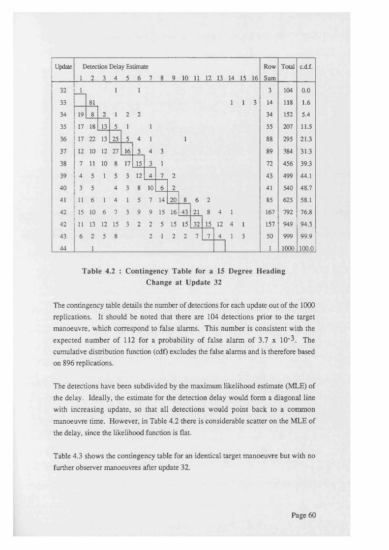
Update Detection Delay Estimate

1 2 3 4 5 6 7 8 9 10 11 12 13 14 15 16

Row

Sum

Total c.d.f.

32 1 1 1 3 104 0.0

33 81 1 1 3 14 118 1.6

34 19 8 2 1 2 2 34 152 5.4

35 17 18 13 5 1 1 55 207 11.5

36 17 22 13 25 5 4 1 1 88 295 21.3

37 12 10 12 27 161! 5 4 3 89 384 31.3

38 7 11 10 8 171! 15 3 1 72 456 39.3

39 4 5 1 5 3 12 4 7 2 43 499 44.1

40 3 5 4 3 8 10 6 2 41 540 48.7

41 11 6 1 4 1 5 7 14 20 8 6 2 85 625 58.1

42 15 10 6 7 3 9 9 15 16 43 21 8 4 1 167 792 76.8

42 11 13 12 15 3 2 2 5 15 15 32 15 12 4 1 157 949 94.3

43 6 2 5 8 2 1 2 2 7 7 4 1 3 50 999 99.9

44 1 | 1 1000 100.0

Table 4.2 : Contingency Table for a 15 Degree Heading Change at Update 32

The contingency table details the number of detections for each update out of the 1000 replications. It should be noted that there are 104 detections prior to the target manoeuvre, which correspond to false alarms. This number is consistent with the expected number of 112 for a probability of false alarm of 3.7 x 10"3. The cumulative distribution function (cdf) excludes the false alarms and is therefore based on 896 replications.

The detections have been subdivided by the maximum likelihood estimate (MLE) of the delay. Ideally, the estimate for the detection delay would form a diagonal line with increasing update, so that all detections would point back to a common manoeuvre time. However, in Table 4.2 there is considerable scatter on the MLE of the delay, since the likelihood function is flat.

Table 4.3 shows the contingency table for an identical target manoeuvre but with no further observer manoeuvres after update 32.

Page 60

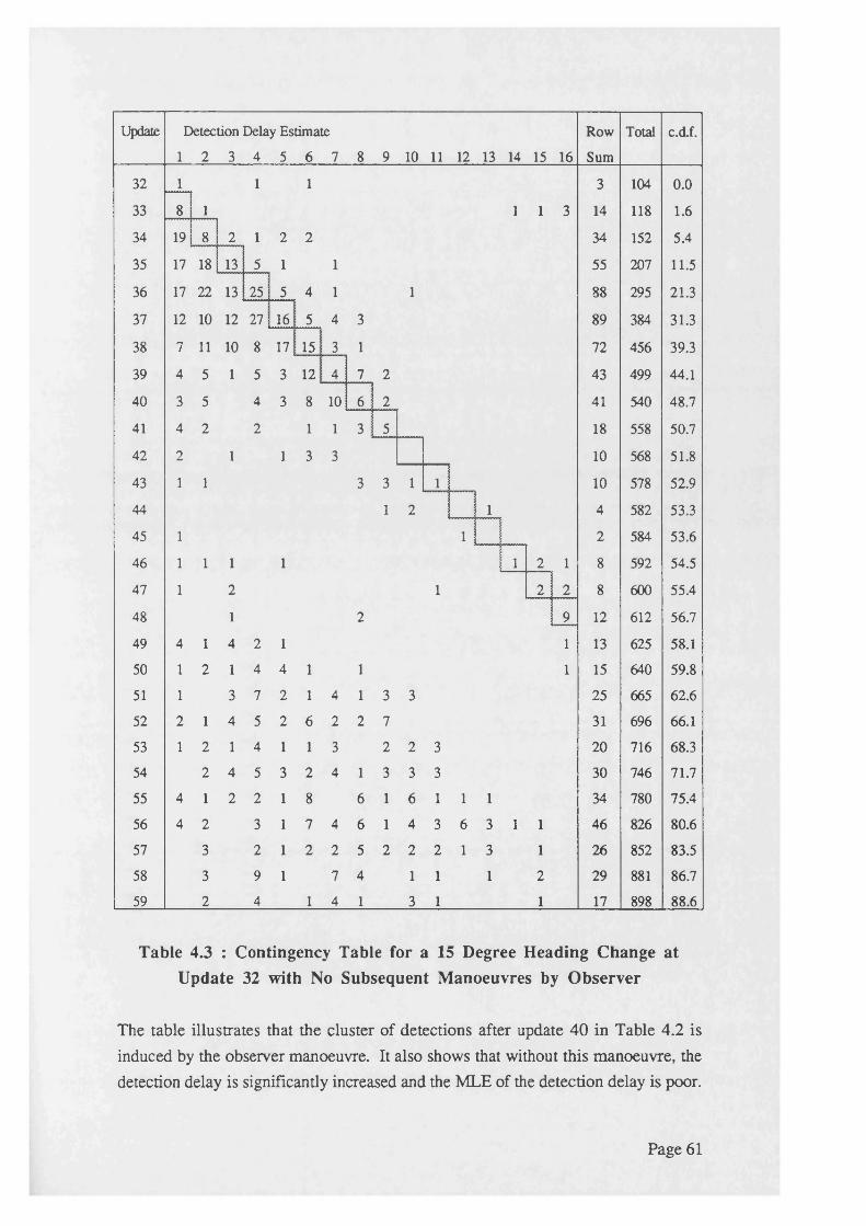
Update Detection Delay Estimate Row Total c.d.f.

1 2 3 4 5 6 7 8 9 10 11 12 13 14 15 16 Sum

32 1 1 1 3 104 0.0

33 8 1 1 1 3 14 118 1.6

34 19 8 2 1 2 2 34 152 5.4

35 17 18 13 5 1 1 55 207 11.5

36 17 22 13 25 5 4 1 1 88 295 21.3

37 12 10 12 27 16 5 4 3 89 384 31.3

38 7 11 10 8 17 15 3 1 72 456 39.3

39 4 5 1 5 3 12 4 7 2 43 499 44.1

40 3 5 4 3 8 10 6 2 41 540 48.7

41 4 2 2 1 1 3 5 18 558 50.7

42 2 1 1 3 3 10 568 51.8

43 1 1 3 3 1 1 10 578 52.9

44 1 2 1 4 582 53.3

45 1 1 2 584 53.6

46 1 1 1 1 1 2 1 8 592 54.5

47 1 2 1 2 2 8 600 55.4

48 1 2 9 12 612 56.7

49 4 1 4 2 1 1 13 625 58.1

50 1 2 1 4 4 1 1 1 15 640 59.8

51 1 3 7 2 1 4 1 3 3 25 665 62.6

52 2 1 4 5 2 6 2 2 7 31 696 66.1

53 1 2 1 4 1 1 3 2 2 3 20 716 68.3

54 2 4 5 3 2 4 1 3 3 3 30 746 71.7

55 4 1 2 2 1 8 6 1 6 1 1 1 34 780 75.4

56 4 2 3 1 7 4 6 1 4 3 6 3 1 1 46 826 80.6

57 3 2 1 2 2 5 2 2 2 1 3 1 26 852 83.5

58 3 9 1 7 4 1 1 1 2 29 881 86.7

59 2 4 1 4 1 3 1 1 17 898 88.6

Table 4.3 : Contingency Table for a 15 Degree Heading Change at Update 32 with No Subsequent Manoeuvres by Observer

The table illustrates that the cluster of detections after update 40 in Table 4.2 is induced by the observer manoeuvre. It also shows that without this manoeuvre, the detection delay is significantly increased and the MLE of the detection delay is poor.

Page 61

In particular, there are a significant number of replications where no detection is achieved.

4 .3 .4 RMS Range Errors

The RMS range error has been used as the primary measure of tracking effectiveness as the range error is highly dependent on the accuracy of the other states (bearing, bearing rate and range rate/range) and, therefore, the RMS range error is indicative of the overall tracking performance.

The mean and RMS of the range errors averaged across the 1000 replications have been calculated for each update. Outliers exceeding 3 standard deviations from the mean have been monitored, however, neither the number nor magnitude of the outliers have influenced these statistical measures.

4.3.4.1 Choice of plant noise manoeuvre factor (y)

Figure 8 compares the RMS range eiror for the GLR procedure with that for various levels of plant noise, when the target is non-manoeuvring. The optimum performance in this scenario is given by a plant noise manoeuvre factor (y) of 0.0. Increasing the y up to 0.05, significantly increases the RMS range error, particularly after observer manoeuvres. The plant noise places a limit of the steady state RMS range error that will be achieved after an observer manoeuvre. In contrast, the RMS range error for the GLR procedure is not significantly worse than for y=0.0. The slightly higher RMS range error is associated with a small number of false alarm which start new filters, since this inflates the RMS range error when calculated over all filters. It should be noted that the original non-manoeuvre filter will remain even after a false alarm, and the RMS range enror for this filter will be identical to that for y=0.0.

Figures 9 to 11 compare the RMS range error for the GLR procedure with that for various values of y, when the target undertakes heading changes of 5°, 15° and 45°. Figure 9 shows that even for a very small heading change (5°), a non-zero plant noise is required if the RMS range error is not to be divergent after the target manoeuvre at update 32. In this scenario the best RMS range error is given by a y of 0.0005. The RMS range error for the GLR procedure initially diverges after the target manoeuvre, however, after a median delay of 13 updates the manoeuvre detection procedure is triggered and the RMS range error reduces to the level for a y of 0.0005. The RMS range error for y of 0.005 and 0.05 are unaffected by such a small heading change.

Page 62

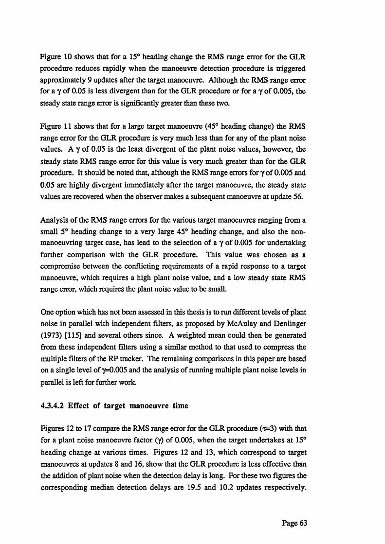
Figure 10 shows that for a 15° heading change the RMS range error for the GLR procedure reduces rapidly when the manoeuvre detection procedure is triggered approximately 9 updates after the target manoeuvre. Although the RMS range error for a y of 0.05 is less divergent than for the GLR procedure or for a y of 0.005, the steady state range error is significantly greater than these two.

Figure 11 shows that for a large target manoeuvre (45° heading change) the RMS range error for the GLR procedure is very much less than for any of the plant noise values. A y of 0.05 is the least divergent of the plant noise values, however, the steady state RMS range error for this value is very much greater than for the GLR procedure. It should be noted that, although the RMS range errors for y of 0.005 and 0.05 are highly divergent immediately after the target manoeuvre, the steady state values are recovered when the observer makes a subsequent manoeuvre at update 56.

Analysis of the RMS range errors for the various target manoeuvres ranging from a small 5° heading change to a very large 45° heading change, and also the non­manoeuvring target case, has lead to the selection of a y of 0.005 for undertaking further comparison with the GLR procedure. This value was chosen as a compromise between the conflicting requirements of a rapid response to a target manoeuvre, which requires a high plant noise value, and a low steady state RMS range error, which requires the plant noise value to be small.

One option which has not been assessed in this thesis is to run different levels of plant noise in parallel with independent filters, as proposed by McAulay and Denlinger (1973) [115] and several others since. A weighted mean could then be generated from these independent filters using a similar method to that used to compress the multiple filters of the RP tracker. The remaining comparisons in this paper are based on a single level of y=0.005 and the analysis of running multiple plant noise levels in parallel is left for further work.

4.3.4.2 Effect of target manoeuvre time

Figures 12 to 17 compare the RMS range error for the GLR procedure (t=3) with that for a plant noise manoeuvre factor (y) of 0.005, when the target undertakes at 15° heading change at various times. Figures 12 and 13, which correspond to target manoeuvres at updates 8 and 16, show that the GLR procedure is less effective than the addition of plant noise when the detection delay is long. For these two figures the corresponding median detection delays are 19.5 and 10.2 updates respectively.

Page 63

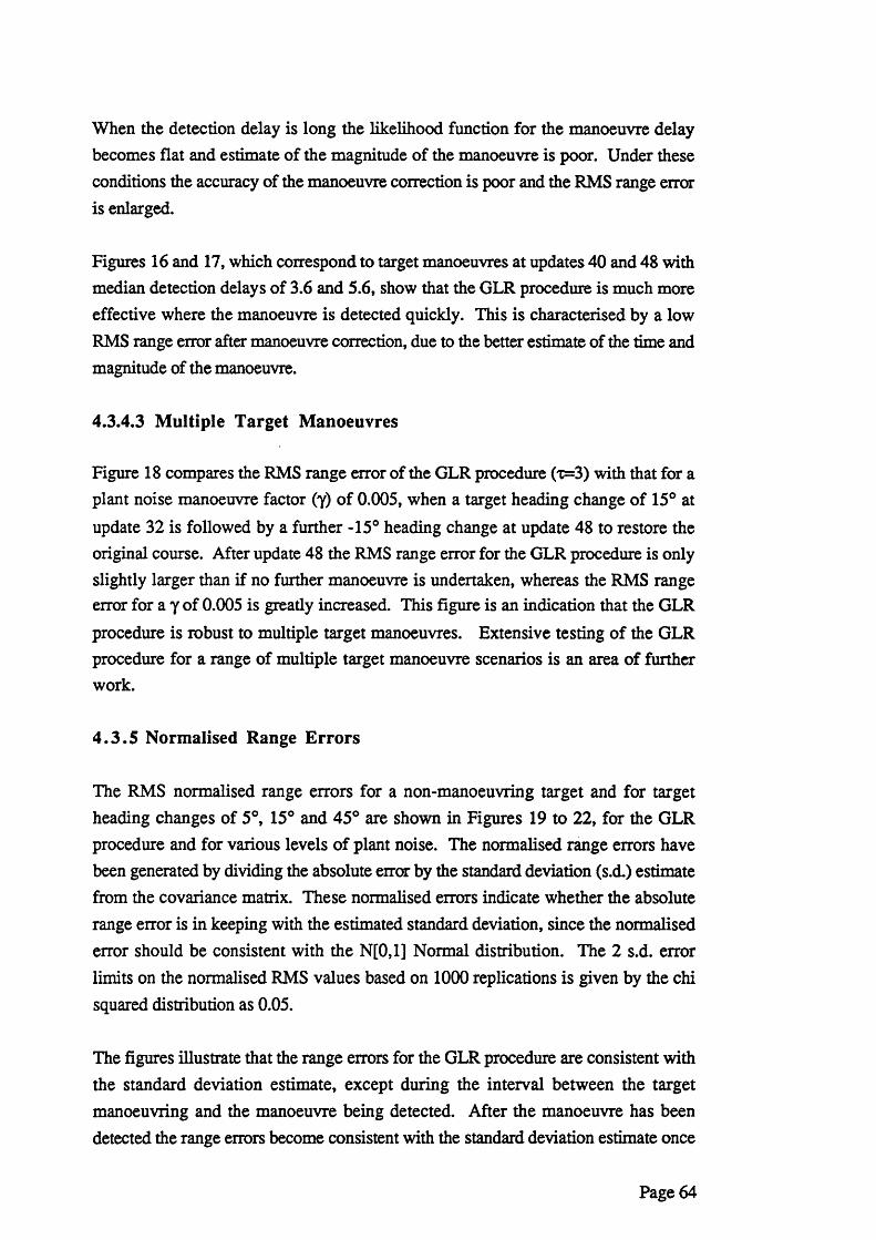
When the detection delay is long the likelihood function for the manoeuvre delay becomes flat and estimate of the magnitude of the manoeuvre is poor. Under these conditions the accuracy of the manoeuvre correction is poor and the RMS range error is enlarged.

Figures 16 and 17, which correspond to target manoeuvres at updates 40 and 48 with median detection delays of 3.6 and 5.6, show that the GLR procedure is much more effective where the manoeuvre is detected quickly. This is characterised by a low RMS range error after manoeuvre correction, due to the better estimate of the time and magnitude of the manoeuvre.

4.3.4.3 Multiple Target Manoeuvres

Figure 18 compares the RMS range error of the GLR procedure (t=3) with that for a plant noise manoeuvre factor (y) of 0.005, when a target heading change of 15° at update 32 is followed by a further -15° heading change at update 48 to restore the original course. After update 48 the RMS range error for the GLR procedure is only slightly larger than if no further manoeuvre is undertaken, whereas the RMS range error for a y of 0.005 is gready increased. This figure is an indication that the GLR procedure is robust to multiple target manoeuvres. Extensive testing of the GLR procedure for a range of multiple target manoeuvre scenarios is an area of further work.

4.3 .5 Normalised Range Errors

The RMS normalised range errors for a non-manoeuvring target and for target heading changes of 5°, 15° and 45° are shown in Figures 19 to 22, for the GLR procedure and for various levels of plant noise. The normalised range errors have been generated by dividing the absolute error by the standard deviation (s.d.) estimate from the covariance matrix. These normalised errors indicate whether the absolute range error is in keeping with the estimated standard deviation, since the normalised error should be consistent with the N[0,1] Normal distribution. The 2 s.d. error limits on the normalised RMS values based on 1000 replications is given by the chi squared distribution as 0.05.

The figures illustrate that the range errors for the GLR procedure are consistent with the standard deviation estimate, except during the interval between the target manoeuvring and the manoeuvre being detected. After the manoeuvre has been detected the range errors become consistent with the standard deviation estimate once

Page 64

again. In contrast the range errors for the various levels of plant noise are generally inconsistent with the standard deviation estimate. During non-manoeuvring periods the covariance matrix is being artificially inflated to allow the filter to response to a manoeuvring target, resulting in a RMS normalised range error which is considerably less than 1.0. However, when the target makes a large manoeuvre the RMS normalised range error may become considerably greater than 1 .0 .

Thus, the standard deviation estimate for the GLR procedure provides reliable information for defining a confidence region for the target The same is not true when plant noise is added, since the standard deviation estimate may be over or under confident depending on the relative magnitude of a target manoeuvre.

4 .3 .6 Typical Track Output

Table 4.4 shows a typical track output for the GLR procedure when the target makes a 15° heading change at update 32.

Page 65

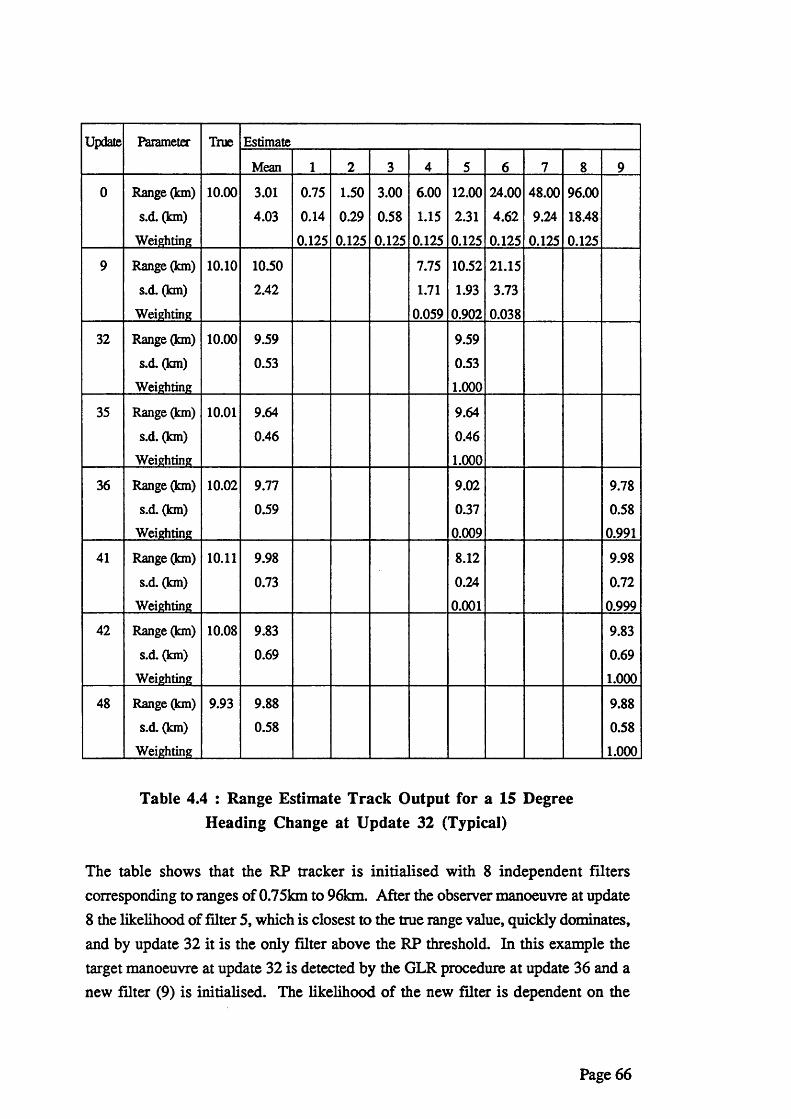
Update Parameter True Estimate

Mean 1 2 3 4 5 6 7 8 9

0 Range (km)

s.d.(km)

Weighting

10.00 3.01

4.03

0.750.14

0.125

1.50

0.29

0.125

3.00

0.580.125

6.00

1.150.125

12.00

2.31

0.125

24.004.62

0.125

48.009.24

0.125

96.0018.48

0.125

9 Range (km)

s.d. (km) Weighting

10.10 10.502.42

7.751.71

0.059

10.52

1.930.902

21.153.73

0.038

32 Range (km) s.d. (km)

Weighting

10.00 9.590.53

9.590.531.000

35 Range (km)

s.d. (km) Weighting

10.01 9.64

0.46

9.64

0.461.000

36 Range (km)

s.d. (km) Weighting

10.02 9.770.59

9.020.37

0.009

9.780.58

0.991

41 Range (km)

s.d. (km) Weighting

10.11 9.98

0.73

8.120.24

0.001

9.980.72

0.999

42 Range (km)

s.d. (km) Weighting

10.08 9.830.69

9.830.691.000

48 Range (km) s.d. (km)

Weighting

9.93 9.880.58

9.880.581.000

Table 4.4 : Range Estimate Track Output for a 15 Degree Heading Change at Update 32 (Typical)

The table shows that the RP tracker is initialised with 8 independent filters corresponding to ranges of 0.75km to 96km. After the observer manoeuvre at update 8 the likelihood of filter 5, which is closest to the true range value, quickly dominates, and by update 32 it is the only filter above the RP threshold. In this example the target manoeuvre at update 32 is detected by the GLR procedure at update 36 and a new filter (9) is initialised. The likelihood of the new filter is dependent on the

Page 66

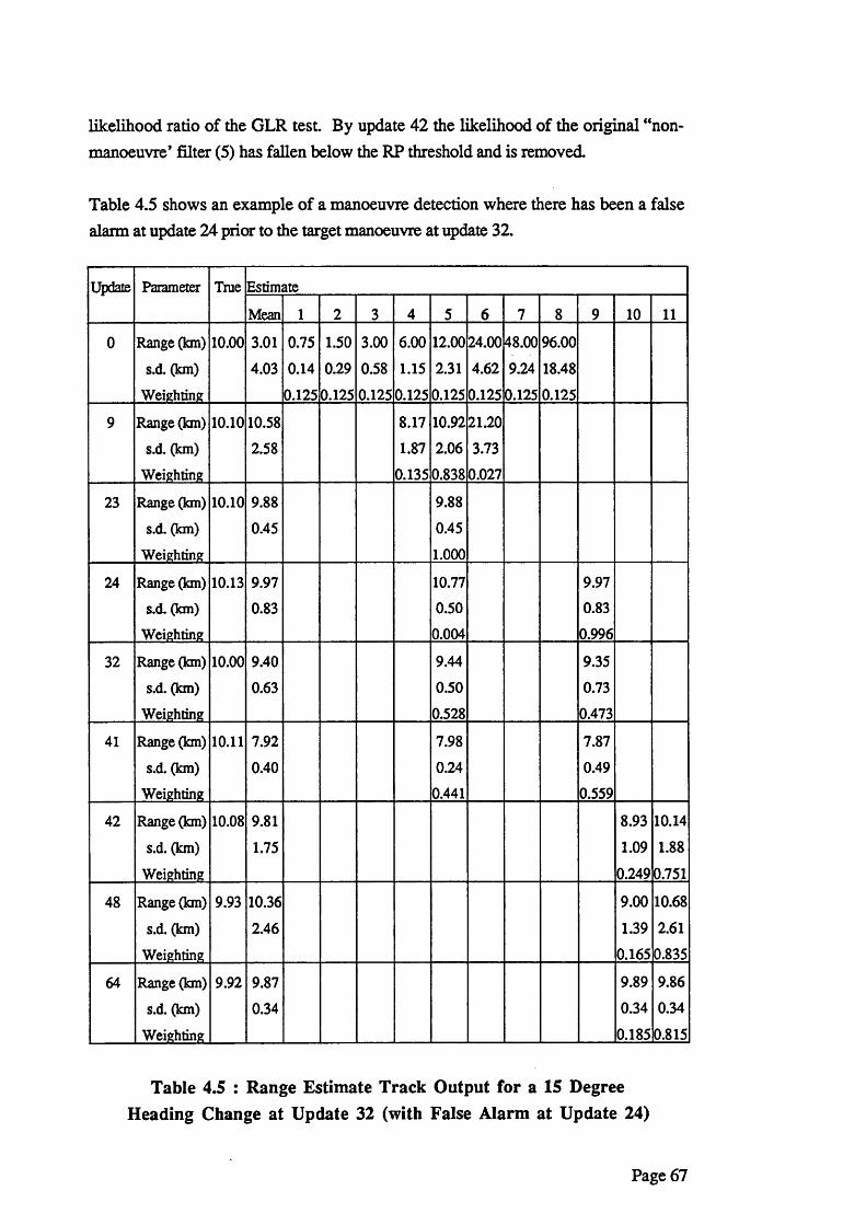
likelihood ratio of the GLR test. By update 42 the likelihood of the original “non- manoeuvre* filter (5) has fallen below the RP threshold and is removed.

Table 4.5 shows an example of a manoeuvre detection where there has been a false alarm at update 24 prior to the target manoeuvre at update 32.

Update Parameter Tme Estimate

Mean 1 2 3 4 5 6 7 8 9 10 11

0 Range (km)

s.d. (km) Weighting

10.00 3.014.03

0.750.14

0.125

1.500.29

0.125

3.000.58

0.125

6.001.15

0.125

12.002.31

0.125

24.004.62

0.125

48.009.24

0.125

96.00

18.480.125

9 Range (km) s.d. (km)

Weighting

10.10 10.582.58

8.171.87

0.135

10.922.060.838

21.203.73

0.027

23 Range (km)

s.d. (km) Weighting

10.10 9.880.45

9.880.451.000

24 Range (km) s.d. (km)

Weighting

10.13 9.970.83

10.770.50

0.004

9.970.83

0.996

32 Range (km) s.d. (km)

Weighting

10.00 9.400.63

9.44

0.500.528

9.350.730.473

41 Range (km)

s.d. (km) Weighting

10.11 7.92

0.407.980.24

0.441

7.870.49

0.559

42 Range (km)

s.d. (km) Weighting

10.08 9.81

1.75

8.931.09

0.249

10.14

1.88

0.751

48 Range (km)

s.d. (km) Weighting

9.93 10.36

2.46

9.00

1.390.165

10.68

2.610.835

64 Range (km) s.d. (km)

Weighting

9.92 9.870.34

9.890.34

0.185

9.860.34

0.815

Table 4.5 : Range Estimate Track Output for a 15 Degree Heading Change at Update 32 (with False Alarm at Update 24)

Page 67

The likelihood of the false alarm filter (9) does not quickly dominate the original filter (5), but instead the likelihood of the original filter is restored. The effect of the false alarm is to delay the correct detection of the target manoeuvre until update 42. At this time, two further ‘manoeuvre* filters ( 1 0 and 1 1 ) are added, with likelihoods sufficiently large that the original filters fall below the RP threshold and are removed. Both of these filters converge on the true range value and either could be removed without loss of accuracy. The rationalisation of multiple similar filters was proposed in Peach (1995) [30] and remains an area of future work. However, this is not an urgent problem since it only results in an increase in the processing requirement

Figure 23 shows the normalised bearing error for a single replication with a 15° target heading change at update 32. The bearing error is normalised by the bearing measurement standard deviation (0.45°). In this replication the manoeuvre is detected at update 36 and the bearing estimate is corrected so that it is close to the measured bearing. It should be noted that the detection delay in this replication is significantly less than the median for this scenario ( 8 updates).

Page 68

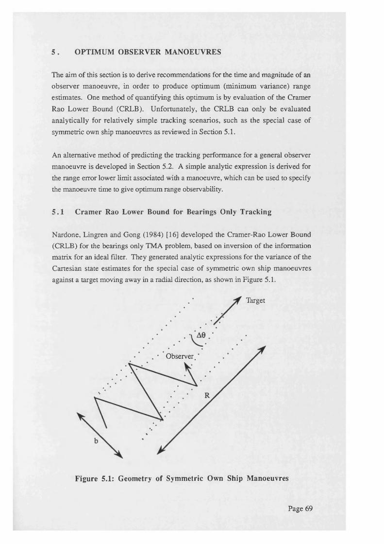
5 . OPTIMUM OBSERVER MANOEUVRES

The aim of this section is to derive recommendations for the time and magnitude of an observer manoeuvre, in order to produce optimum (minimum variance) range estimates. One method of quantifying this optimum is by evaluation of the Cramer Rao Lower Bound (CRLB). Unfortunately, the CRLB can only be evaluated analytically for relatively simple tracking scenarios, such as the special case of symmetric own ship manoeuvres as reviewed in Section 5.1.

An alternative method of predicting the tracking performance for a general observer manoeuvre is developed in Section 5.2. A simple analytic expression is derived for the range error lower limit associated with a manoeuvre, which can be used to specify the manoeuvre time to give optimum range observability.

5 .1 Cramer Rao Lower Bound for Bearings Only Tracking

Nardone, Lingren and Gong (1984) [16] developed the Cramer-Rao Lower Bound (CRLB) for the bearings only TMA problem, based on inversion of the information matrix for an ideal filter. They generated analytic expressions for the variance of the Cartesian state estimates for the special case of symmetric own ship manoeuvres against a target moving away in a radial direction, as shown in Figure 5.1.

Target

Observer.

Figure 5.1: Geometry of Symmetric Own Ship Manoeuvres

Page 69

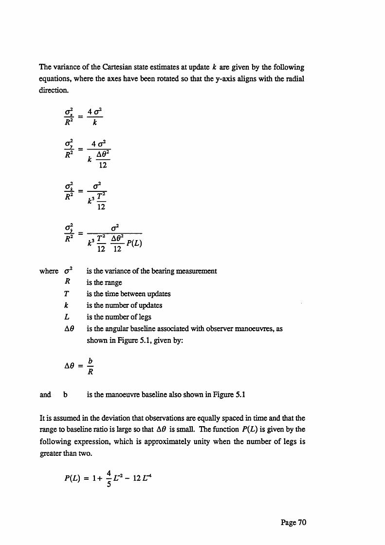
The variance of the Cartesian state estimates at update k are given by the following equations, where the axes have been rotated so that the y-axis aligns with the radial direction.

of 4 a 2

R2 ” k

°y _R2 , Ad2k -----

12

o i o 2

" p H 12

<7?y _e T- ^ P{L)

12 12 v '

where a 2 is the variance of the bearing measurementR is the rangeT is the time between updatesk is the number of updatesL is the number of legsA 9 is the angular baseline associated with observer manoeuvres, as

shown in Figure 5.1, given by:

A0 = iLR

and b is the manoeuvre baseline also shown in Figure 5.1

It is assumed in the deviation that observations are equally spaced in time and that the range to baseline ratio is large so that A6 is small. The function P(L) is given by the following expression, which is approximately unity when the number of legs is greater than two.

P(L) = 1+ - I S 2 - 12 IT*

Page 70

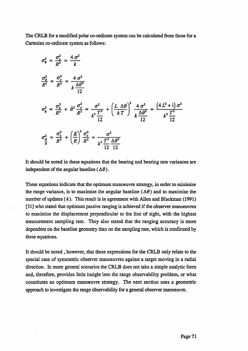
The CRLB for a modified polar co-ordinate system can be calculated from those for a Cartesian co-ordinate system as follows:

It should be noted in these equations that the bearing and bearing rate variances are independent of the angular baseline (AO).

These equations indicate that the optimum manoeuvre strategy, in order to minimise

the range variance, is to maximise the angular baseline (AO) and to maximise the number of updates (k). This result is in agreement with Allen and Blackman (1991) [31] who stated that optimum passive ranging is achieved if the observer manoeuvres to maximise the displacement perpendicular to the line of sight, with the highest measurement sampling rate. They also stated that the ranging accuracy is more dependent on the baseline geometry than on the sampling rate, which is confirmed by these equations.

It should be noted, however, that these expressions for the CRLB only relate to the special case of symmetric observer manoeuvres against a target moving in a radial direction. In more general scenarios the CRLB does not take a simple analytic form and, therefore, provides little insight into the range observability problem, or what constitutes an optimum manoeuvre strategy. The next section uses a geometric approach to investigate the range observability for a general observer manoeuvre.

R2 R2

Page 71

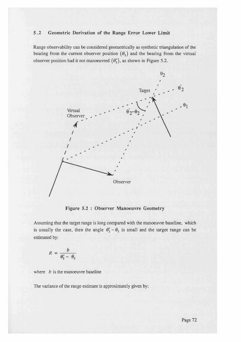
5.2 Geometric Derivation of the Range E rror Lower Limit

Range observability can be considered geometrically as synthetic triangulation of the bearing from the current observer position (02) and the bearing from the virtual observer position had it not manoeuvred (02), as shown in Figure 5.2.

0 2

VirtualObserver

Taiget *

Observer

Figure 5.2 : Observer Manoeuvre Geometry

Assuming that the target range is long compared with the manoeuvre baseline, which is usually the case, then the angle 62 - 02 is small and the target range can be estimated by:

R = ----------e' - e2

where b is the manoeuvre baseline

The variance of the range estimate is approximately given by:

Page 72

where it is assumed that the bearing estimates are independent with zero mean error. The assumption of independence is valid provided that there are sufficient updates after the observer manoeuvre.

For a long range target the bearing rate during the observer straight legs before and after a manoeuvre can be considered constant, such that:

e'2 = 0,+Te,@2 = + ^ 2

and

where T is the time since the manoeuvreis the bearing at the time of the manoeuvre

0 j is the bearing rate prior to the manoeuvre G2 is the bearing rate after the manoeuvre

The variance of the range estimate is then given by:

It is apparent in this equation that as the time since the manoeuvre (T) increases the range variance will initially reduce. However, eventually a plateau is reached, for (t 2g 2 » Ggt + g\2 j , when the variance of the range estimate is given by:

This expression provides a lower limit on the range variance for a given change in the bearing rate. To reduce the range variance below this limit the observer must perform

Page 73

additional manoeuvres. The time taken for the range standard deviation to reduce to within 1 0 % of this limit is given by:

where it has been assumed that the bearing variance before and after the manoeuvre are approximately equal.

The expressions for the range error lower limit and the time to approach this limit allow the observer to develop optimum manoeuvre strategies. An optimum manoeuvre strategy would require the observer to manoeuvre after a time T10qb in a

direction which maximises the change in the bearing rate (perpendicular to the line of sight). It has been found that the optimum period between manoeuvres is initially small, but increases as the range variance reduces.

It is important to note that the expressions derived in this section for the range error lower limit and the optimum time between manoeuvres are not dependent on the geometry being the special case of symmetric own ship manoeuvres with the target moving in a radial direction. Therefore, they are more general than the CRLB given in Section 5.1.

5 .3 Monte Carlo Analysis

The scenario defined in Section 5.3.1 has been Monte Carlo run for various observer manoeuvres, using the RP tracker as defined in Section 3.2.3. The runs consist of 1000 replications with identical pseudo random number seeds. The bearing errors have been drawn from a Gaussian distribution with a fixed standard deviation and zero mean.

The mean and RMS of the range errors averaged across the 1000 replications have been calculated for each update. Outliers exceeding 3 standard deviations from the mean have been monitored, however, neither the number nor magnitude of the outliers have influenced these statistical measures.

Page 74

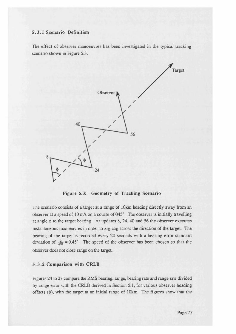
5 .3 .1 Scenario Definition

The effect of observer manoeuvres has been investigated in the typical tracking scenario shown in Figure 5.3.

Target

Observer

Figure 5.3: Geometry of Tracking Scenario

The scenario consists of a target at a range of 10km heading directly away from an observer at a speed of 10 m/s on a course of 045°. The observer is initially travelling at angle <j> to the target bearing. At updates 8, 24, 40 and 56 the observer executes instantaneous manoeuvres in order to zig-zag across the direction of the target. The bearing of the target is recorded every 20 seconds with a bearing error standard deviation of = 0.45°. The speed of the observer has been chosen so that the

observer does not close range on the target.

5 .3 .2 Comparison with CRLB

Figures 24 to 27 compare the RMS bearing, range, bearing rate and range rate divided by range error with the CRLB derived in Section 5.1, for various observer heading offsets (<{>), with the target at an initial range of 10km. The figures show that the

Page 75

RMS error for the RP tracker approaches the CRLB in all the scenarios considered. The oscillations in the RMS levels are due to cross-correlation effects between the states, associated with the target being at finite range. The reference curve for the CRLB does not contain these oscillations, since it has been derived assuming that the target is at long range (A0 is small) such that these cross-correlation effects are minimised.

Figures 24 and 26 illustrate that the bearing and bearing rate error are independent of the magnitude of the observer manoeuvre and are only a function of the number of updates, as predicted by the CRLB. The range and range rate divided by range error (Figures 25 and 27) are sensitive to the magnitude of the observer manoeuvre, also as predicted by the CRLB.

Figures 28 and 29 compare the RMS range error with the CRLB for initial target ranges of 22 km and 2.2 km, and show that the RMS range error asymptotically approaches the CRLB in both scenarios. The oscillations in RMS levels noted above are even more apparent for the 2 . 2 km scenario, due to the violation of the long range assumption.

5.3.3. Comparison with Range Error Lower Limit

Figures 30 to 33 compare the RMS range error with the range error lower limit, derived in Section 5.2, for various observer manoeuvres and with various initial target ranges. The results show that the range error lower limit provides a good prediction of the range accuracy that will be achieved during an observer leg. It is apparent that the range accuracy improves for larger magnitude observer manoeuvres and with the target at close range. The improvement is dependent solely on the change in the bearing rate associated with the observer manoeuvre, since the bearing rate variance is independent of the magnitude of the observer manoeuvre, and is only a function of the number of updates, as shown in Section 5.3.2.

The RMS range error is below the range error lower limit for the second leg (updates 8 to 24), since the initial range rate estimate for the tracker is equal to the true value of zero. Thus, the range error is artificially low during the second leg, since this would be inflated by the initial range rate error. During subsequent legs the range rate becomes independent of the initial estimate and the range error approaches the lower limit

Page 76

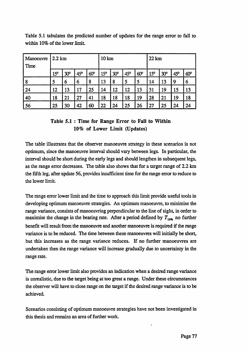
Table 5.1 tabulates the predicted number of updates for the range error to fall to within 1 0 % of the lower limit.

ManoeuvreTime

2 . 2 km 1 0 km 2 2 km

15° 30P 45° eop 15° 30P 45° 6 (P 15° 30° 45° 60P8 5 6 6 8 13 8 5 5 14 13 9 6

24 1 2 13 17 25 14 1 2 1 2 13 31 19 15 1340 18 2 1 27 41 18 18 18 19 28 2 1 19 1856 25 30 42 60 2 2 24 25 26 27 25 24 24

Table 5.1 : Time for Range Error to Fall to Within 10% of Lower Limit (Updates)

The table illustrates that the observer manoeuvre strategy in these scenarios is not optimum, since the manoeuvre interval should vary between legs. In particular, the interval should be short during the early legs and should lengthen in subsequent legs, as the range error decreases. The table also shows that for a target range of 2.2 km the fifth leg, after update 56, provides insufficient time for the range error to reduce to the lower limit.

The range error lower limit and the time to approach this limit provide useful tools in developing optimum manoeuvre strategies. An optimum manoeuvre, to minimise the range variance, consists of manoeuvring perpendicular to the line of sight, in order to maximise the change in the bearing rate. After a period defined by r 10* no further

benefit will result from the manoeuvre and another manoeuvre is required if the range variance is to be reduced. The time between these manoeuvres will initially be short, but this increases as the range variance reduces. If no further manoeuvres are undertaken then the range variance will increase gradually due to uncertainty in the range rate.

The range error lower limit also provides an indication when a desired range variance is unrealistic, due to the target being at too great a range. Under these circumstances the observer will have to close range on the target if the desired range variance is to be achieved.

Scenarios consisting of optimum manoeuvre strategies have not been investigated in this thesis and remains an area of further work.

Page 77

6 CONCLUSIONS

6 .1 Range Parameterised Tracker

The new tracking approach, referred to in this paper as the Range Parameterised (RP) tracker, has been shown to give considerably better tracking performance in a typical scenario than the Modified Polar (MP) or Cartesian (C) trackers. In particular, the RP tracker gives significandy lower range errors than the other trackers, and the range errors are consistent with the standard deviation estimate derived from the covariance matrix. The RP tracker is stable even under adverse tracking conditions, such as when the bearing rate is very high or near zero, and there is no requirement for limits on the state estimates in order to prevent divergent behaviour. In addition, if the low likelihood filters are removed, the tracker is no more computationally intensive than the MP tracker.

The major advantage of the RP tracker over the MP or C trackers is that it divides the large prior range uncertainty region into a small number of filters, each with a low coefficient of variation. This allows a more natural implementation for the prior knowledge of the target velocity, which prevents filter instability and can allow the range to be inferred even before the first observer manoeuvre. It should be noted, however, that much of the instability previously reported for the C tracker can be prevented by setting appropriate initialisation conditions as proposed in Appendix A.

6.2 GLR Manoeuvre Detection / Correction Procedure

The RP tracker has been extended to allow for manoeuvring targets by adding a manoeuvre detection and correction procedure based on a Generalised Likelihood Ratio (GLR) test. The tracking performance of the GLR procedure has been compared with the standard technique of adding plant noise to allow for unmodelled target dynamics. This comparison has illustrated that the GLR procedure provides better tracking performance before and after a target manoeuvre and, in particular, the track estimates for the GLR procedure are consistent with the estimated covariance matrix. The GLR procedure also generates a Maximum Likelihood estimate of the time and magnitude of the manoeuvre.

A GLR threshold of 3.0 has been found to give a good compromise between a reasonably low false alarm rate (3.7 x 10"4 per update) and a short detection delay for typical target manoeuvres. The selection of a particular threshold is not critical as the GLR procedure is robust to false alarms, since the weighting for an additional filter

Page 78

representing an erroneous target manoeuvre will be rapidly reduced to close to zero and the filter will be discarded. Therefore, the penalty of a false alarm is only an increase in computation and not a long term reduction in tracking performance.

6.3 Optimum Observer Manoeuvres

The tracking performance of the RP tracker has been shown to approach the Cramer Rao Lower Bound (CRLB) for the special case of symmetric observer manoeuvres. A range error lower limit associated with a manoeuvre has been derived for more general scenarios, and this has been shown to give a good prediction of the RP tracker RMS range error. The simplicity of the expression for the range error lower limit allows it to the used to specify criteria for the time and magnitude of observer manoeuvres to give optimum range observability.

Page 79

7 .

1

2

3

4

5

6

7

8

9

10

11

12

13

REFERENCES

M. Pachter and P. R. Chandler,Universal Linearization Concept for Extended Kalman Filters,IEEE Trans. Aerosp. and Electron. Systems, 29(3), 946 - 961, July 1993.

T. C. Wang and P. K. Varshney,A Tracking Algorithm for Maneuvering Targets,IEEE Trans. Aerosp. and Electron. Systems, 29(3), 910 - 924, July 1993.

J. R. Cloutier, C.-F. Lin and C. Yang,Enhanced Variable Dimension Filter for Manoeuvring Target Tracking,IEEE Trans. Aerosp. and Electron. Systems, 29(3), 786 - 796, July 1993.

D. Lerro and Y. Bar-Shalom,Tracking with Debiased Consistent Converted Measurements Versus EKF, IEEE Trans. Aerosp. and Electron. Systems, 29(3), 1015 - 1022, July 1993.

R. L. Gray,A Pure Cartesian Formulation for Tracking Filters,IEEE Trans. Aerosp. and Electron. Systems, 29(3), 749 - 754, July 1993

D. V. Stallard,An Angle Only Tracking Filter in Modified Spherical Coordinates,AIAA Paper No. 87-2380,1987.

N. J. Gordon, D. J. Salmond and A. F. Smith,A Novel Approach to Non-linear/Non-Gaussian Bayesian State Estimation, IEE Proceedings, Vol. 140, Part F, No. 2, 1993.

V. P. Broman and M. J. Shensa,Bearings Tracking of Targets with Unobservable States.Proc. Amer. Contr. Conf, Seattle, Wa, June 1986.

V. J. Aidala,Kalman Filter Behavior in Bearings only Tracking Applications.IEEE Trans. Aerosp. and Electronics Systems, AES-15(1), 29 - 39, January 1979.

V. J. Aidala and S. E. Hammel,Utilization of Modified Polar Coordinates for Bearings only Tracking.IEEE Trans. Automatic. Control, AC-28(3), 283 - 294, March 1983.

S. C. Nardone and V. J. Aidala,Observability Criteria for Bearings only Target Motion Analysis.IEEE Trans. Aerosp. and Electronics Systems, AES-17(2), 162 - 166, March1981.

J. C. Hassab,Contact Localization and Motion Analysis in the Ocean Environment: A Perspective.IEEE J. Oceanic Engng., OE-8(3), 136 - 147, July 1987.

V. J. Aidala and S. C. Nardone,Biased Estimation Properties of the Pseudolinear Tracking Filter.IEEE Trans. Aerosp. and Electronics Systems, AES-18(4), 432 - 441, July1982.

Page 80

14

15

16

17

18

19

20

21

22

23

24

25

26

A. N. Payne,Observability Problem for Bearings only Tracking Int. J. Control, 49(3), 761 - 768, 1989.

M. Gavish and E. Fogel,Effect of Bias on Bearing Only Target Location,IEEE Trans. Aerosp. and Electronics Systems, AES-26(1), 22 - 25, January 1990.

S. C. Nardone, A. G. Lindgren, and K. F. Gong,Fundamental Properties and Performance of Conventional Bearings only Target Motion analysis,IEEE Trans. Automatic Control, AC-29(9), 775 - 787, January 1990.

S. N. Balakrishnan,Extension to Modified Polar Coordinates and Applications with Passive Measurements,J. Guidance, 12(2), 906 - 912, December 1989.

V. Petridis,A Method for Bearings only Velocity and Position Estimation,IEEE Trans. Automatic Control, AC-26(2), 488 - 493, April 1981.

R. R. Tenney, R. S. Hebbert, and N. R. Sandell,A Tracking Filter for Maneuvering Sources,IEEE Trans. Automatic Control, 246 - 251, April 1977.

J. C. Spall,Validation of State Space Models from a Single realization of Non-Gaussian Measurements,IEEE Trans. Automatic Control, AC-30(12), 1212 -1214, December 1985.

A. G. Lindgren and K. F. Gong,Position and Velocity Estimation via Bearing Observations,IEEE Trans. Aerosp. and Electron. Systems, AES-14(4), 564 - 577, July 1978.

T. H. Kerr,Status of CR Like Lower Bounds for Nonlinear Filtering,IEEE Trans. Aerosp and Electron. Systems, 25(5), 590 - 600, September 1989.

K. Spingam,Passive Position Location Estimation using the Extended Kalman Filter,IEEE Trans. Aerosp. and Electron. Systems, AES-23(4), 558 - 567, July 1987.

R. J. Meinhold and N. D. Singpurwalla,Robustification of Kalman Filter ModelsJ. Amer. Statistical Assoc., 84(406), 479 - 486, June 1989.

G. Kitagawa,Non-Gaussian State-Space Modeling of Non-stationary Time Series,J. Amer. Statistical Assoc., 82(400), 1032 -1063, December 1987.

T. L. Song and J. L. Speyer,A Stochastic Analysis of a Modified Gain Extended Kalman Filter with applications to Estimation with Bearings Only Measurements,IEEE Trans. Automatic Control, AC-30(10), 940 - 949, October 1985.

Page 81

27

28

29

30

31

32

33

34

35

36

37

38

39

S. E. Hammel and V. J. Aidala,Observability Requirements for Three-Dimensional Tracking via Angle Measurements,IEEE Trans. Aerosp. and Electron. Systems, AES-21(2), 200 - 207, March 1985.

S. N. Balakrishnan and J. L. Speyer,Coordinate Transformation Based Filter for Improved Target Tracking,J. Guidance, 9(3), 704 - 709, Nov - Dec 1986.

T. L. Song and J. L. Speyer,The Modified Gain Extended Kalman Filter and Parameter identification in Linear Systems,Automatica, 22(1), 59 - 75,1986.

N. G. Peach,Bearings only tracking using a set of range parameterised extended Kalman filters,IEE Proc. Control Theory Appl., 142(1), 73 - 80, January 1995.

R. R. Allen and S. S. Blackman,Angle only tracking with a Modified Spherical Coordinates Filter,Proc IEEE/AIAA 10th Digital Avionics Syst. Conf., 561 - 566,1991.

K. L. Anderson and R. A. Iltis,A Distributed Bearings only Tracking Algorithm Using Reduced Sufficient S tati stiesIEEE Trans. Aero, and Elec. Sys., Vol. 32, No. 1, 339 - 349, Jan. 1996.

S. C. Kramer and H. W. Sorenson,Recursive Bayesian Estimation using Piecewise Constant Approximations, Automatica, Vol. 24, No. 6,789 - 801, 1988.

P. J. Harrison and C. F. Stevens,Bayesian ForecastingJ. Roy. Stat. Soc., B, 38, 205 - 247, 1976.

J. Korn, S. W. Gully and A. S. Willsky,Application of the Generalised Likelihood Ratio Algorithm to Manoeuvre Detection and EstimationProc. American Control Conf., Arlington, VA, 792 - 798,1982.

T. L. Lai,Sequential Changepoint Detection in Quality Control and Dynamical Systems, J. R. Statist. Soc. B, No. 3, 1995.

M. Basseville and I. V. Nikiforov,Detection of Abrupt Changes: Theory and Applications,Englewood Cliffs: Prentice Hall, 1993.

S. Custance Baker,A Bayesian Method of Tracking Submarines with Data from Passive Sonobuoys,PhD Thesis, Plymouth Polytechnic, 1989.

J. C. Hassab,Underwater Signal and Data Processing,ISBN 0-8493-6800-6, 230 - 240, 1989.

Page 82

40

41

42

43

44

45

46

47

48

49

50

51

52

R. E. Kalman,A new approach to linear filtering and prediction problems,ASME Journal of Basic Engineering, 82, March 1960.

A. H. Jazwinski,Stochastic processes and filtering theory,Academic Press, 1970.

D. J. Murphy,Noisy bearings only target motion analysis,Ph.D Thesis, Northeastern University, Boston, 1969.

R.C. Kolb and F. H. Hollister,Bearings only target estimation,Proc. 1st Asfiomer Conf. Circuits and Systems, pp. 935-946,1967.

K. Y. Wong and E. Polak,Identification of linear discrete time systems using the instrumental variable method,IEEE Trans. Automat. Contr., vol. AC-12, Dec. 1967.

H. Weiss and J. B. Moore,Improved extended Kalman filter design for passive tracking,IEEE Trans. Automat. Cont, vol. AC-25, pp. 807-811, Aug. 1980.

J. H. Taylor,The Cramer-Rao estimation error lower bound computation for deterministic non-linear systems,IEEE Trans. Automat. Contr., vol. AC-24, pp. 343-344, Apr. 1979.

R. K. Mehra,A comparison of several non-linear filters for re-entry vehicle tracking,IEEE Trans. Automat. Contr., Vol. AC-6 , No. 4, Aug. 1971.

J. M. Sammons, S. Balakrishman, J. L. Speyer and D. G. Hull,Development and comparison of optimal filters,Rep. AFATL-TR-79-87, Air Force Armament Laboratory, Air Force Systems Command, U.S. Air Force, Eglin Air Force Base, FI., Oct .1979.

H. D. Hoelzer, G. W. Johnson and A. O. Cohen,Modified polar coordinates - The key to well behaved bearings only ranging, IBM Shipboard and Defense Systems, Manassas, VA., IRD Rep. 78-M19- 0001A, Aug. 1978.

J. L. Poirot and G. V. McWilliams,Application of linear statistical models to radar location techniques,IEEE Trans. Aero, and Elec. Sys., AES-10, 6 , Nov. 1974.

R. A. Singer,Estimating optimal tracking filter performance for manned manoeuvring targets,IEEE Trans, on Aero, and Elec. Sys., Vol. AES-6 , No. 4, pp. 473-483, July 1970.

D. V. Stallard,An angle only tracking filter in modified spherical coordinates,Proc. of AIAA Guidance, Navigation and Contol Conf., pp. 542-550,1987.

Page 83

53

54

55

56

57

58

59

60

61

62

63

64

65

66

J. K. Beard,An efficient, reliable approach for hydroacoustical bearings only target motion analysis,Proc. of 23rd IEEE Conf. on Decision and Control, Dec. 1984.

H. Sorenson and D. Alspach,Recursive Bayesian estimation using Gaussian sums,Automatica, 7, pp. 465-478,1971.

R. Kulhavy,A Bayes-closed approximation of recursive non-linear estimation, International Journal of Adaptive Control and Signal Processing, 4, pp. 271- 285, 1990.

R. Kulhavy,Recursive non-linear estimation: A geometric approach,Automatic, 26, pp. 545-555,1990.

Y. C. Ho and R. C. K. Lee,A Bayesian approach to problems in stochastic estimation and control.IEEE Trans, on Automatic Control, Vol. AC-9, October 1964.

R. S. Bucy,Bayes' theorem and digital realisation for nonlinear filters,J. Astronaut. Sci., 17, pp. 80-94, 1969.

R. S. Bucy and K. D. Senne,Digital synthesis of nonlinear filters,Automatica, 7, pp. 287-298,1971.

D. L. Alspach,Gaussian sum approximations in nonlinear filtering and control,Inf. Sci., 7, pp. 271-290, 1974.

A. F. M. Smith and A. E. Gelfand,Bayesian statistics without tears: a sampling-resampling perspective,The American Statistician, 46, pp. 84-88,1992.

P. Muller,Monte Carlo integration in general dynamic models,Contempary Mathematics, 115, pp. 145-163,1991.

A. H. Jazwinski,Limited memory optimal filtering,IEEE Trans. Automat. Contr., Vol. AC-13, Oct 1968.

D. T. Magil,Optimal adaptive estimation of sampled stochastic processes,IEEE Trans, on Auto. Contr., AC-10, pp. 434-439, Oct 1965.

R. A. Singer,Estimating optimal tracking filter performance for manned manoeuvring targets,IEEE Trans, on Aero, and Elec. Sys., AES-6 , pp. 473-483, July 1970.

G. A. Ackerson and K. S. Fu,On state estimation in switching environments,IEEE Trans, Automat Control., Vol. AC-15, pp. 10-17, Feb. 1970.

Page 84

67

68

69

70

71

72

73

74

75

76

77

78

79

A. G. Jaffer and S. C. Gupta,On estimation of discrete processes under multiplicative and additive noise conditions,Information Sciences, 3, pp. 267-276, 1971.

R. L. Moose and P.P. Wang,An adaptive estimator with learning for a plant containing semi-Markov switching parameters,IEEE Trans. Sys., Man., Cybem., Vol. SMC-3, pp. 277-281, May 1973.

R. L. Moose,An adaptive state estimation solution to the manoeuvring target problem,IEEE Trans. Auto. Contr., pp. 359-362, June 1975.

R. L. Moose, H. F. VanLandingham and D. H. McCabe,Modelling and estimation for tracking manoeuvring targets,IEEE Trans. Aerosp. Elect. Sys., Vol. AES-15, pp. 448-456, May 1979.

G. C. Ricker and J. R. Williams,Adaptive tracking filter for manoeuvring targets,IEEE Trans, on Aero, and Elec. Sys., AES-14, pp. 185-193, Jan. 1978.

J. K. Tugnait and A. H. Haddad,A detection estimation scheme for state estimation in switching environments, Automatica, Vol. 15, pp. 471-481,1979.

J. K. Tugnait,State estimation for discrete systems with switching parameters,IEEE Trans. Aero, and Elect. Sys., Vol. AES-15, pp. 464,1979.

J. K.. Tugnait,Detection and estimation for abruptly changing systems,Automatica, Vol. 18, No. 5, pp. 607-615,1982.

V. J. Mathews and J. K. Tugnait,Detection and estimation with fixed lag for abruptly changing systems,IEEE Trans. Aero. Elect. Sys., Vol. AES-19, No.5, Sept 1983.

H. A. P Blom,An efficient filter for abruptly changing systems,Proc. 23rd IEEE Conf. on Decision and Control, pp. 656-658,1984.

H. A. P. Blom,Overlooked potential of systems with Markovian coefficients,Proc. 25th IEEE Conf. on Decision and Control, pp. 1758-1764,1986.

H. A. P. Blom and Y. Bar-Shalom,The interacting multiple model algorithm for systems with Markovian switching parameters,IEEE Trans, Automat. Contr., Vol. 33, No. 8 , pp. 780-783,1988.

L. Campo, P. Mookeijee and Y. Bar-Shalom,State estimation for systems with Sojourn time dependent Markov model switching,IEEE Trans. Automat. Contr., Vol. 36, No. 2, pp. 238-243,1991.

Page 85

80

81

82

83

84

85

86

87

88

89

90

91

X. Rong Li and Y. Bar-Shalom,Performance prediction of the interacting multiple model algorithm,IEEE Trans. Aero, and Elect. Sys., Vol. 29, No. 3, July 1993.

C. B. Chang and M. Athans,State estimation for discrete systems with switching parameters,IEEE Trans. Aero, and Elec. Sys., Vol. AES-14, No. 3, pp. 418-425, May 1978.

R. J. McAulay and E. J. Denlinger,A decision-directed adaptive tracker,IEEE Trans. Aero. Elect Sys., AES-9, pp. 229-236, Mar. 1973.

Y. T. Chan A. G. C. Hu and J. B. Plant,A Kalman filter based tracking scheme with input estimation,IEEE Trans. Aero. Elect Sys., AES-15,2, pp. 237-244, Mar. 1979.

P. L. Bogler,Tracking a manoeuvring target with input estimation,IEEE Trans. Aero. Elect Sys., AES-23, 3, pp. 298-310, May 1987.

Y. Bar-Shalom and K. Birmiwai,Variable dimension filter for manoeuvring target tracking,IEEE Trans. Aero. Elect. Sys., AES-18, 5, pp. 621-629, Sept 1982.

J. C. Spall,Validation of state space models in non-Gaussian systems,Proc. Amer. Contr. Conf., pp. 1072-1076, 1984.

A. S. Willsky and H. L. Jones,A generalised likelihood ratio approach to the detection and estimation of jumps in linear systems,IEEE Trans. Auto. Contr., Vol. AC-21, pp. 108-112,1976.

J. S. Thorp,Optimal tracking of manoeuvring targets,IEEE Trans. Aero. Elec. Sys., AES-9, pp. 800-810, Nov. 1972.

R. L. Hampton and J. R. Cooke,Unsupervised tracking of manoeuvring vehicles,IEEE Trans. Aero. Elec. Sys., AES-9, pp. 197-207, Mar. 1973.

A. G. Lingren and K. F. Gong,Properties of a bearings only motion analysis estimator: An interesting case study in system observability,Proc. 12th Asilomar Conf. Circuits, Systems and Computers, Western Periodicals, North Hollywood, CA, pp. 50-58, Nov. 1978.

A. K. Caglayan and R. E. Lancroft,Reinitialisation issues in fault tolerant systems,Proc. American Control Conf., pp. 952-955,1983.

Page 86

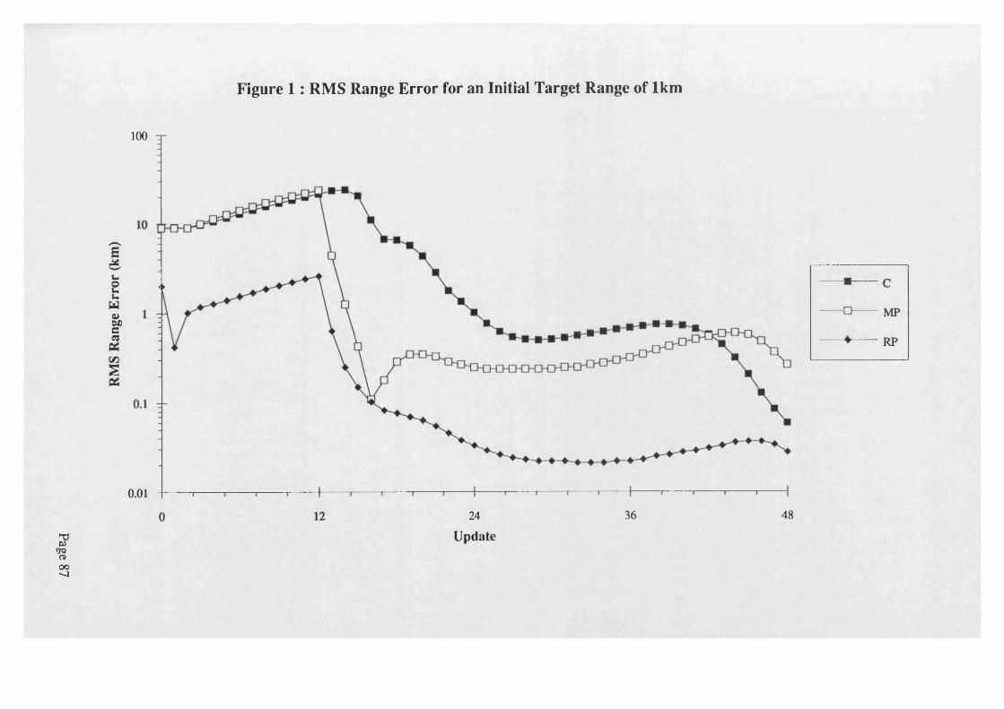
RMS

Rang

e Er

ror

(km

)

Figure 1: RMS Range Error for an Initial Target Range of 1km

100

* >

0.01

36 4824

MP

RP

gJ Updatem(V00-J

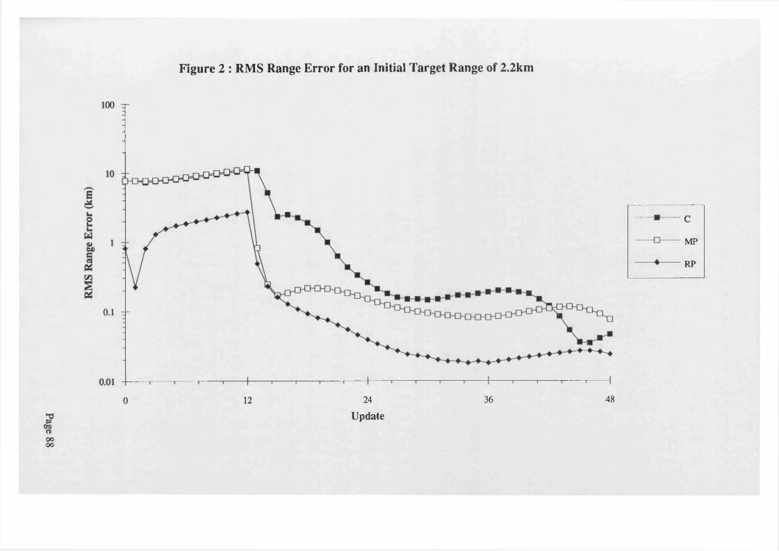
Figure 2 : RMS Range Error for an Initial Target Range of 2.2km

36 4824120

- MP

RP

Update

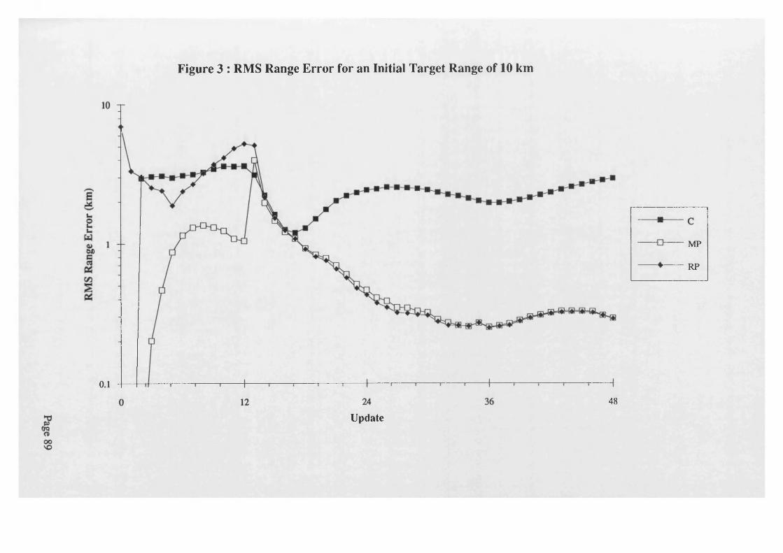
Figure 3 : RMS Range Error for an Initial Target Range of 10 km

o.i48

MP

RP

Update

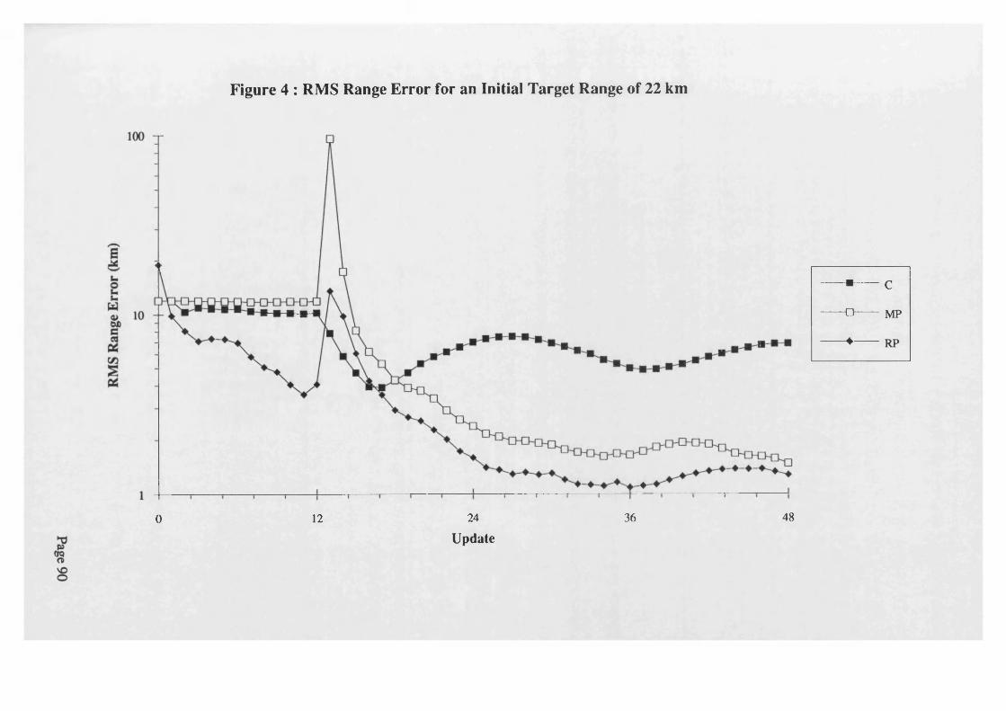
Figure 4 : RMS Range Error for an Initial Target Range of 22 km

36 4824120

------ ■— c------ □— MP

-------♦ — RP

Update

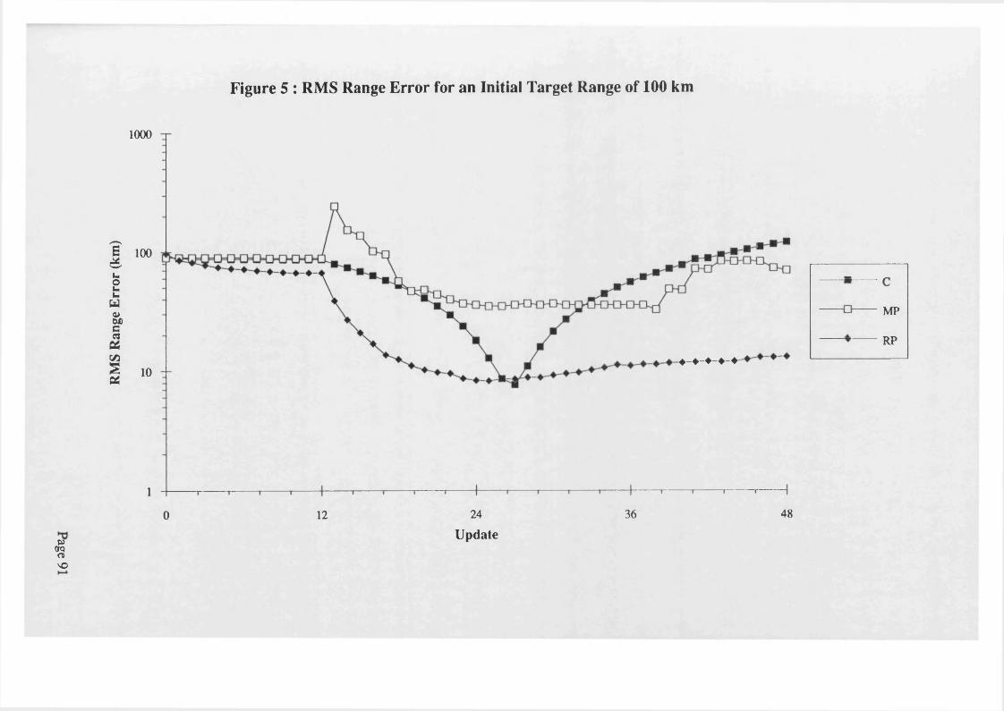
RMS

Rang

e Er

ror

(km

)

Figure 5 : RMS Range Error for an Initial Target Range of 100 km

p(rqo>VO

1000

100

MP

RP

10

1

483624120

Update

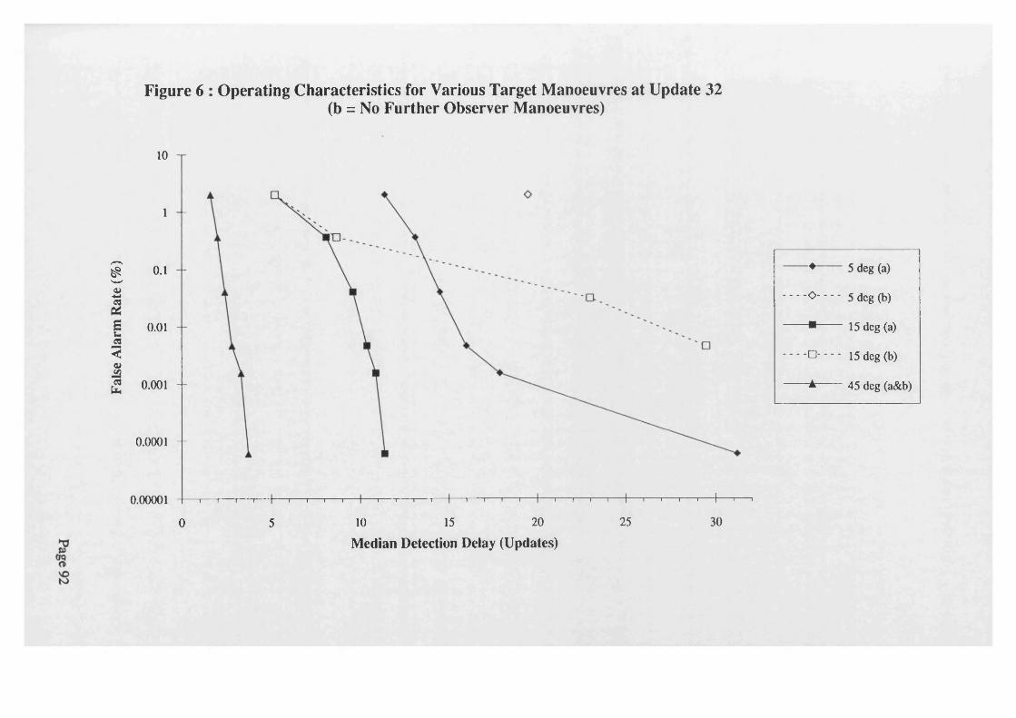
False

Al

arm

Rate

(%)

Figure 6 : Operating Characteristics for Various Target Manoeuvres at Update 32 (b = No Further Observer Manoeuvres)

10 -r

1 -

o . i - -

o . o i - -

0 . 0 0 1 - -

0 . 0 0 0 1 - -

------ ♦ ------ 5 deg (a)

----- O------ 5 deg (b)

------■------ 15 deg (a)

— □ — 15 deg (b)

------ ▲------ 45 deg (a&b)

0.00001 H 1 1---- 1---- '----1----1----1----1----r 1 T-— I 1 1 1 1----r 1----1---- (---- 1----<---- 1---- 1----1----1--- -1---- r 1 1 1---- 1

0 5 10 15 20 25 30

Median Detection Delay (Updates)

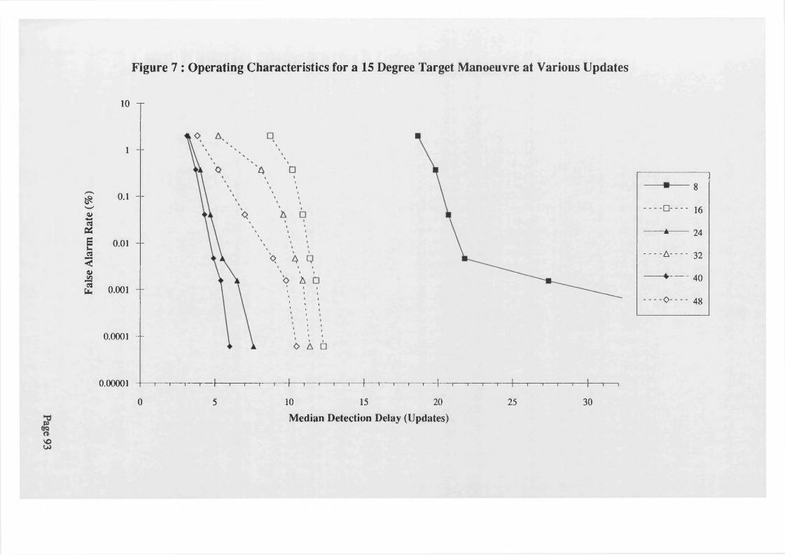
False

Al

arm

Rate

(%)

Figure 7 : Operating Characteristics for a 15 Degree Target Manoeuvre at Various Updates

10 -T

1 --

o . i - -

0.01 - -

0 . 0 0 1 - -

0 . 0 0 0 1 - -

8■

— □ — 16

24Jk "

------A------ 32

40▼

----- 0 ------ 48

0.00001 ~i— i— i— i— i— i— i— i— i— i— i— i— i— i— i— i— i— i— i— i— i— i— i— i— i— |— i— i— i— r

0 5 10 15 20 25 3010 15 20

Median Detection Delay (Updates)

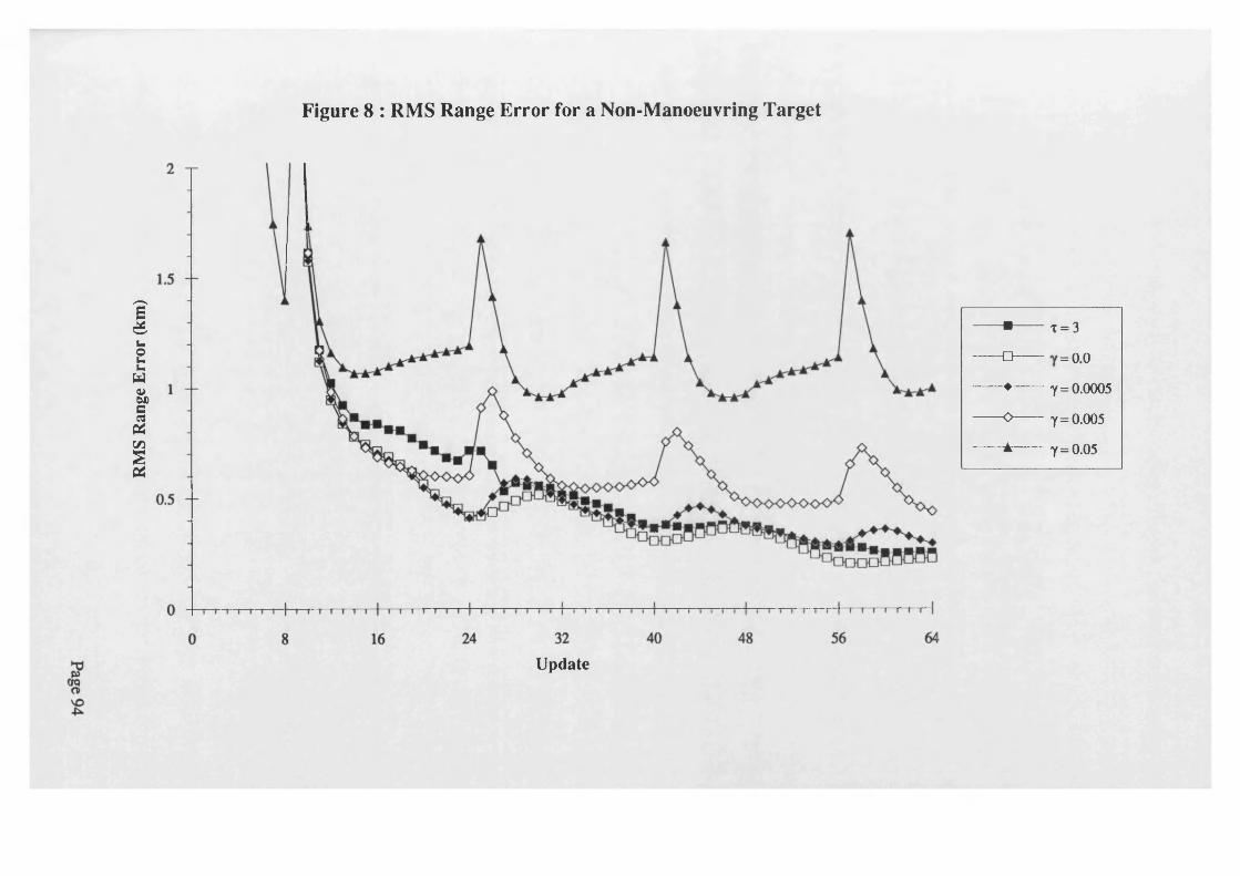
RMS

Rang

e Er

ror

(km

)Figure 8 : RMS Range Error for a Non-Manoeuvring Target

Update

------ ■— t = 3

------□ — II o o

------ ♦— Y = 0.0005

------ 0 — Y =0.005

— ▲— y = 0.05

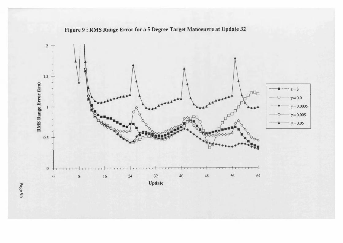
Figure 9 : RMS Range Error for a 5 Degree Target Manoeuvre at Update 32

645640 4832241680

------ ■— II

— □— 1 II o ©

-------♦— 7=0.0005

------ 0 — 7=0.005

------ A— 7=0.05

Update

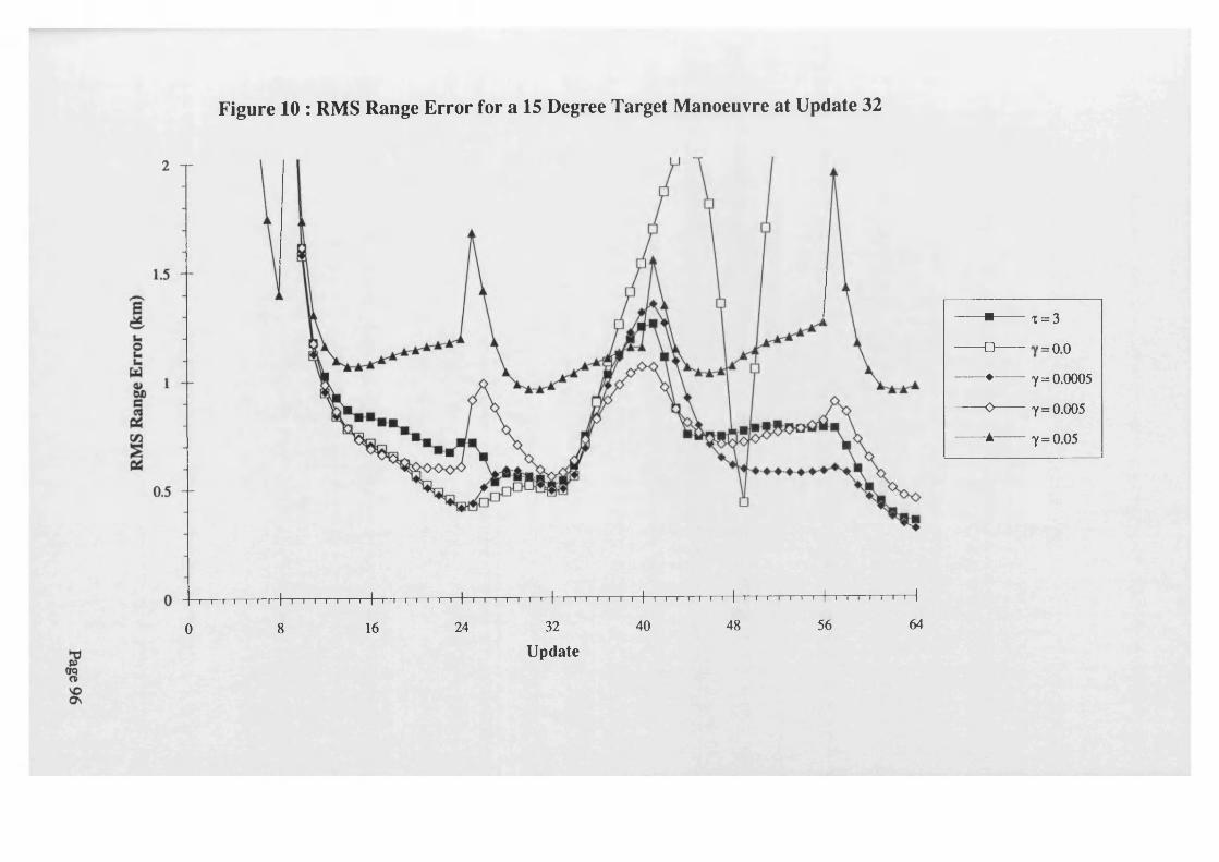
Figure 10 : RMS Range Error for a 15 Degree Target Manoeuvre at Update 32

------ ■— T = 3

------□ — o©II

------ ♦— Y = 0.0005

------ 0 — 7=0.005

------ ▲— 7=0.05

- t | | | | 1 1 " t T I I I I I I | I I T I I I I I ' ' 1 ' I ' ' I ' ' ' ' 1 ' 1 I ' ' 1 1 1 1 1 I ' 1 1 1 1 1 •' I 1 ' I

o 8 16 24 32 40 48 56 64

Update

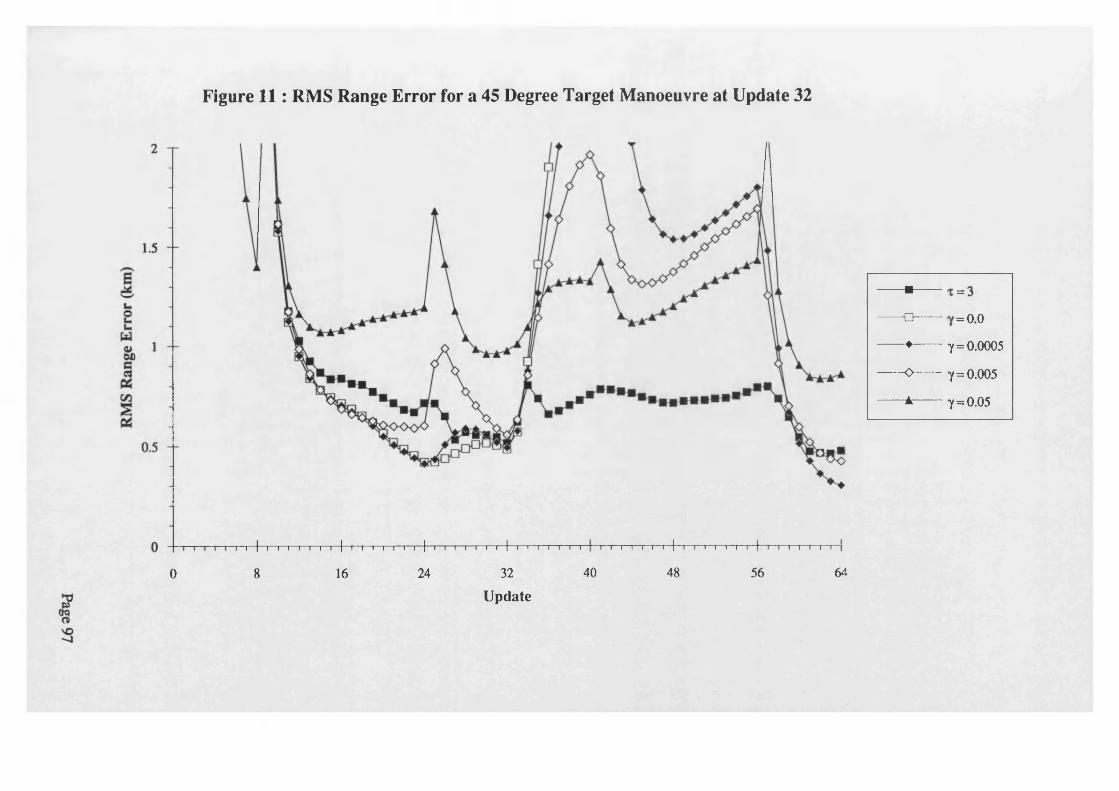
Figure 11: RMS Range Error for a 45 Degree Target Manoeuvre at Update 32

l++ + + + i i i i i i i t i i i i i r t—i—i—i—i—i—ri i i—i—i—i—r i—i—i—i—i—i—rT—T t—i—i—i—i—i—r t—i—i—i—i—i—r

------ ■— 1 II

------ □— II o ©

------ ♦— 7=0.0005

------0 — 7=0.005

— * — 7=0.05

0 8 16 24 32 40 48 56 64

Update

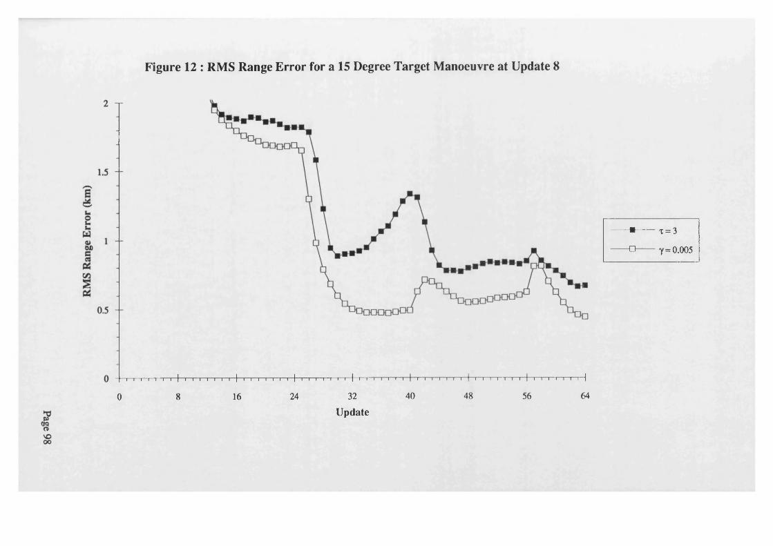
Figure 12 : RMS Range Error for a 15 Degree Target Manoeuvre at Update 8

------ ■ - T = 3

------ □ — Y = 0.005

1 i i i i i i | i i i i i i i } - t ~ i i i i i i | i i i i i i i | i i i i i i i I i i i i i i ' I i t i i i i ' I i i i ' i r - i \0 8 16 24 32 40 48 56 64

Update

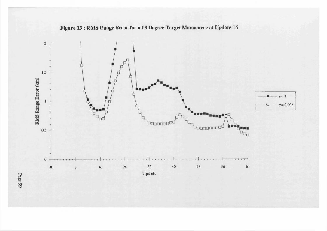
Figure 13 : RMS Range Error for a 15 Degree Target Manoeuvre at Update 16

645632 40 4816 240 8

------ ■— 1 c* II

------ □ — Y =0.005

Update

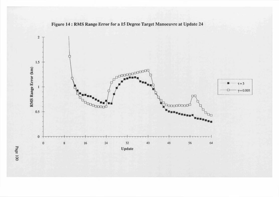
Figure 14 : RMS Range Error for a 15 Degree Target Manoeuvre at Update 24

7=0.005

— i—i—i—i—i—i—i—|—i—i—i—i—i—i—i—|—i—i—i—i—i—i—i—|—i—i—i—i—i—i—i—|—i—i—i—i—i—i—i—|—i—i—i—i—i—i—i—|—i—i—i—i—i—i—i—|—i—i—r~i—i—i—i—|

0 8 16 24 32 40 48 56 64

Update

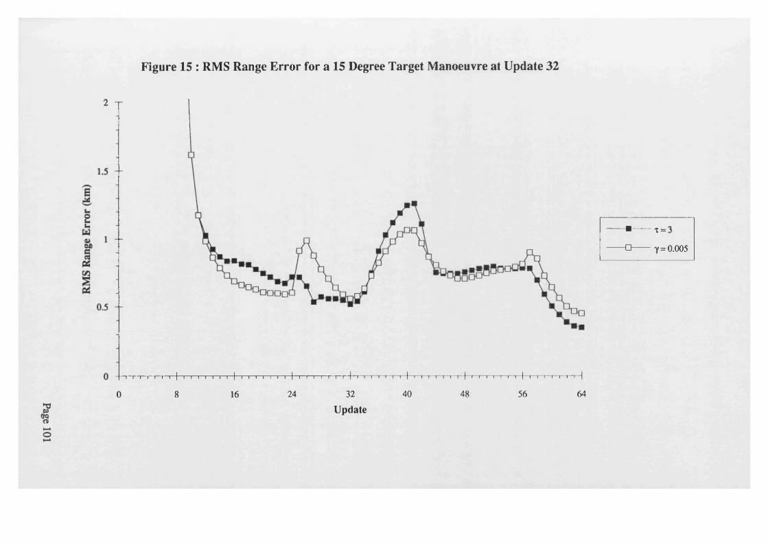
Figure 15 : RMS Range Error for a 15 Degree Target Manoeuvre at Update 32

------ ■— 1•4 II

------ □— 7=0.005

— i - r i r i i r ~ { — i— i i i i i i | f i i i i i i 1 i i i i i i i | r i i' i i i i | i i i i i t t | i i i i i i i | i i i— i i i i \

0 8 16 24 32 40 48 56 64

Update

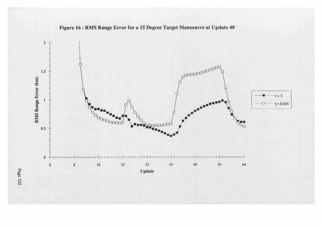
Figure 16 : RMS Range Error for a 15 Degree Target Manoeuvre at Update 40

------ ■— t = 3

— □ — Y =0.005

— i i i i i i r j - n i i i i i | i i i i i n ' h r i i i i t |~~r~r~i—r~i—r i | - r r r i i i i ( i r i i i i i -f —i—r n—i—i—i—i—|

0 8 16 24 32 40 48 56 64

Update

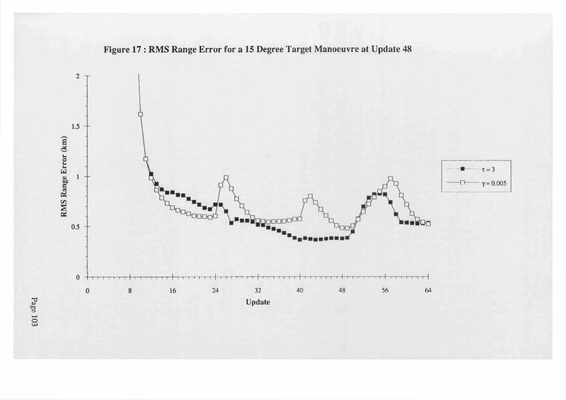
RMS

Rang

e Er

ror

(km

)

Figure 17 : RMS Range Error for a 15 Degree Target Manoeuvre at Update 48

------ ■— T = 3

------ n — 7 = 0.005

0 1—i—i—i—i—r—i—|—i—i—i—i—r—i—i—(—i—i—i—r—i—i—\—|—i—i—i—i—i—i—i ( r • i—i—r i i t |—i—r i—i—i—i—r~|—1—r—n —i i—r~|—i—i—r r i—i—i—|

16 24 32 40 48 56 64

Update* 0

£CrqCD

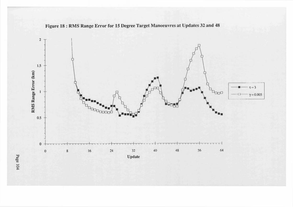
Figure 18 : RMS Range Error for 15 Degree Target Manoeuvres at Updates 32 and 48

■ ~ a■

------ □—

T = 3

y = 0.005

1—i—i—i—i—i—i—|—i—r—i—i—rn—i—|—i—i—i—i—i—i—r }—i—i—i—i—i i i | i i—i i i n | i r~i i i i i f- 1 i r~i i i r-1 i i i i i i i |

0 8 16 24 32 40 48 56 64

Update

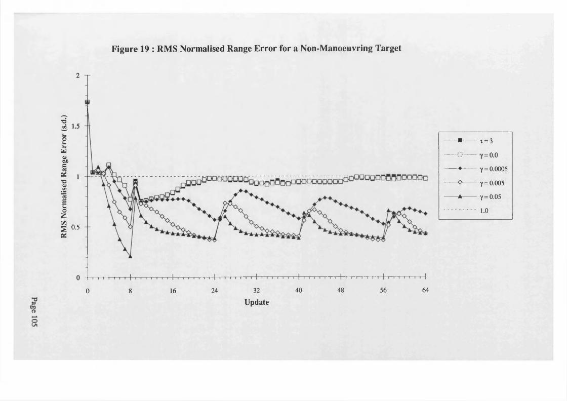
RMS

Nor

mal

ised

Rang

e Er

ror

(s.d

.)

Figure 19 : RMS Normalised Range Error for a Non-Manoeuvring Target

0.5

6448 5632 40248 160

------ ■— T = 3

— o — ii o o

------ ♦— 7=0.0005

------ 0 — 7=0.005

------ A— 7=0.05

- 1.0

Update

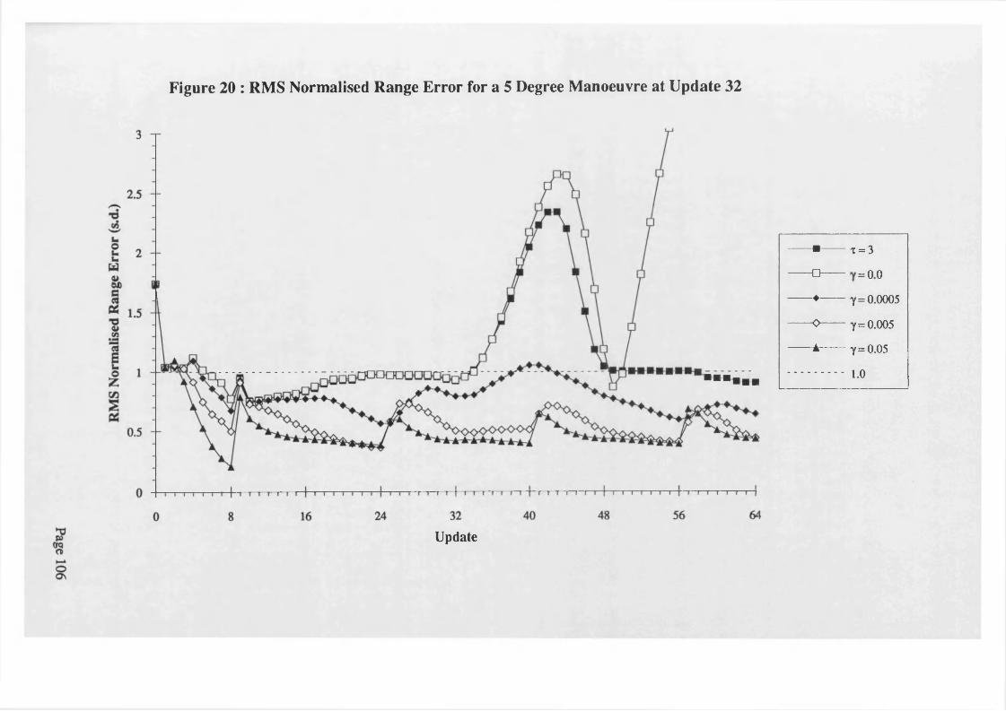
Figure 20 : RMS Normalised Range Error for a 5 Degree Manoeuvre at Update 32

Update

----- ■----- t = 3

□ ii o o

♦ 7=0.0005

----- 0----- 7=0.005

----- ±----- 7=0.05

■■■■■■ .................1.0

Figure 21: RMS Normalised Range Error for a 15 Degree Manoeuvre at Update 32

40 48 56 6416 24 320 8

- O

A

T = 3

y= 0 .0A AAATw

A

7 = 0.0005

. _ . A AA r7=0.005

« 7 = u.ud

. . . . . . . . . 4 A1.0

Update

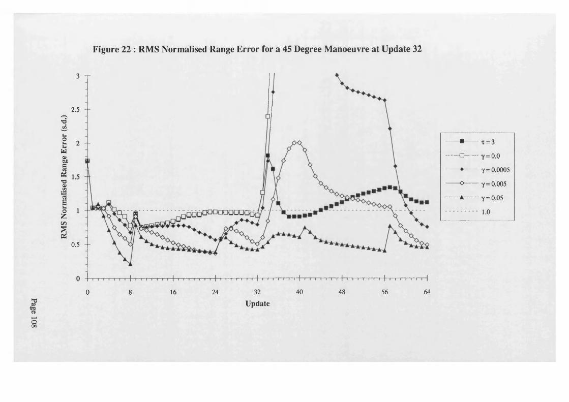
RMS

Nor

mal

ised

Rang

e Er

ror

(s.d

.)

Figure 22 : RMS Normalised Range Error for a 45 Degree Manoeuvre at Update 32

2.5

0.5

40 4816 24 32 56 640 8

Update

------ ■— 1 ll

------ □— 1 ii o ©

------ ♦— 7=0.0005

------ 0 — 7 = 0.005

------ A— 7=0.05

-- 1.0

ooo

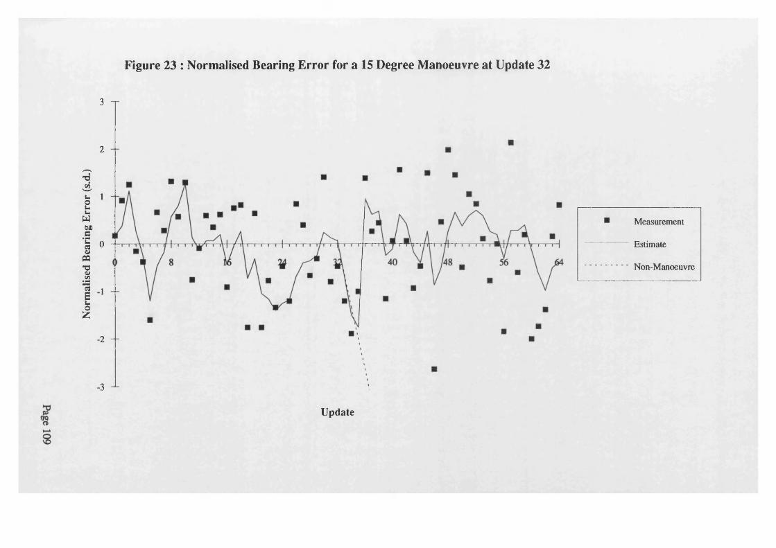
Nor

mal

ised

Bear

ing

Erro

r (s

.d.)

Figure 23 : Normalised Bearing Error for a 15 Degree Manoeuvre at Update 32

3

2

1

0

1

-2

■3

■ Measurement

Estimate

Non-Manoeuvre

Update

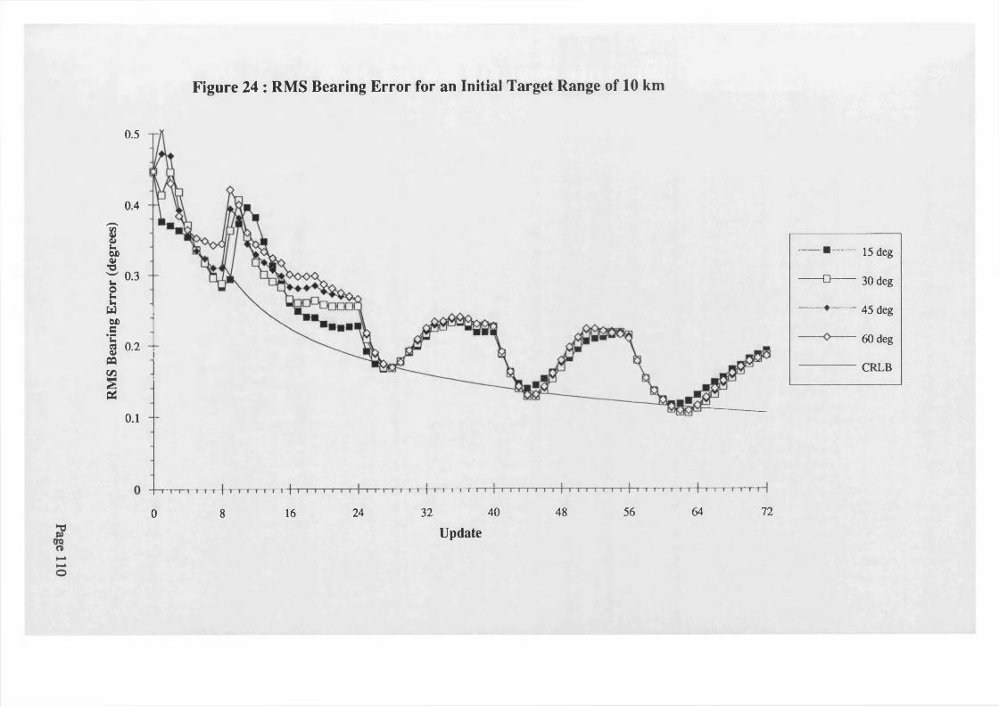
RMS

Bear

ing

Erro

r (d

egre

es)

Figure 24 : RMS Bearing Error for an Initial Target Range of 10 km

0.5

0.4

0.3

0.2

0.1

7256 6440 483216 240 8

------ ■—

------ □—

▲

15 deg

30 deg

45 deg

____ /'A J _ _60 deg

CRLB

Update

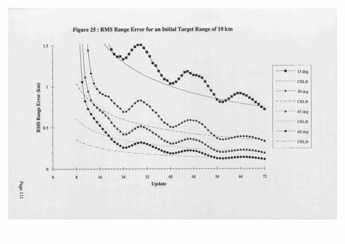
15 deg

CRLB

30 deg

CRLB

45 deg

CRLB

60 deg

CRLB

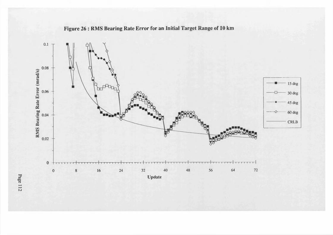
RMS

Bear

ing

Rate

Erro

r (m

rad/

s)

Figure 26 : RMS Bearing Rate Error for an Initial Target Range of 10 km

o.i

0.08 - -

0.06 -

0.04 - -

0.02 -

7248 56 6432 40240 8 16

"■------- 15 deg

-O 30 deg

"♦------ 45 deg

-0-------60 deg

CRLB

Update

to

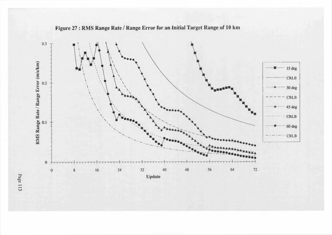
RMS

Rang

e Ra

te / R

ange

Er

ror

(m/s

/km

)

Figure 27 : RMS Range Rate / Range Error for an Initial Target Range of 10 km

0.3 -r

0.2 -

7256 6440 483224160 8

CRLB

CRLB

CRLB

2

< 8

Update

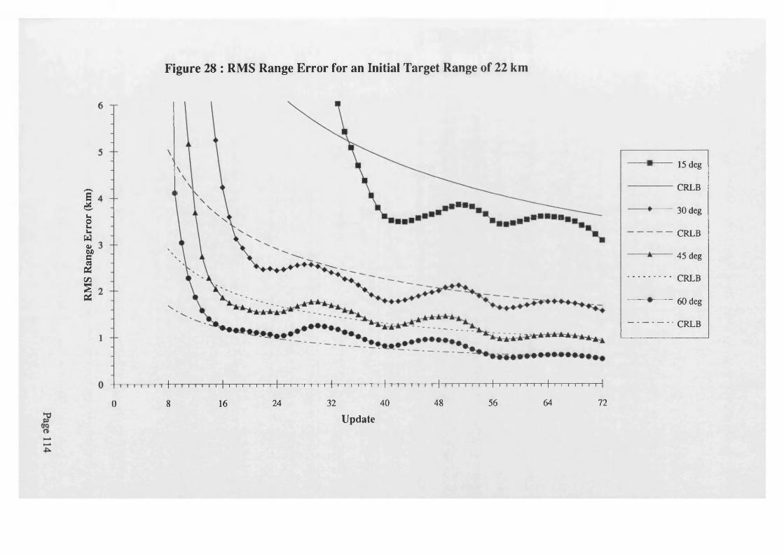
RMS

Rang

e Er

ror

(km

)

Figure 28 : RMS Range Error for an Initial Target Range of 22 km

+ + + +++ i i i i i 'l l' i t i r r r ir r TTTTT I I I I I I Ii r i—i i i r

0 8 16 24 32 40 48 56 64 72

Update

■ 15 deg

- CRLB

- 30 deg

CRLB

" 45 deg

CRLB

■ 60 deg

CRLB

RMS

Rang

e Er

ror

(km

)Figure 29 : RMS Range Error for an Initial Target Range of 2.2 km

o.i

0.09

0.08

0.07

0.06

0.05

0.04

0.03

0.02

0.01

64 7224 32 40 48 560 8 16

CRLB

CRLB

CRLB

CRLB

-apergCDUpdate

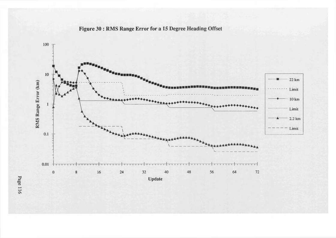
RMS

Rang

e Er

ror

(km

)

Figure 30 : RMS Range Error for a 15 Degree Heading Offset

100

■■■■■■■■■■■

40 48 56 64 728 16 24 320

Update

*------ 22 km

Limit

-♦------ 10 km

Limit

*------ 2.2 km

Limit

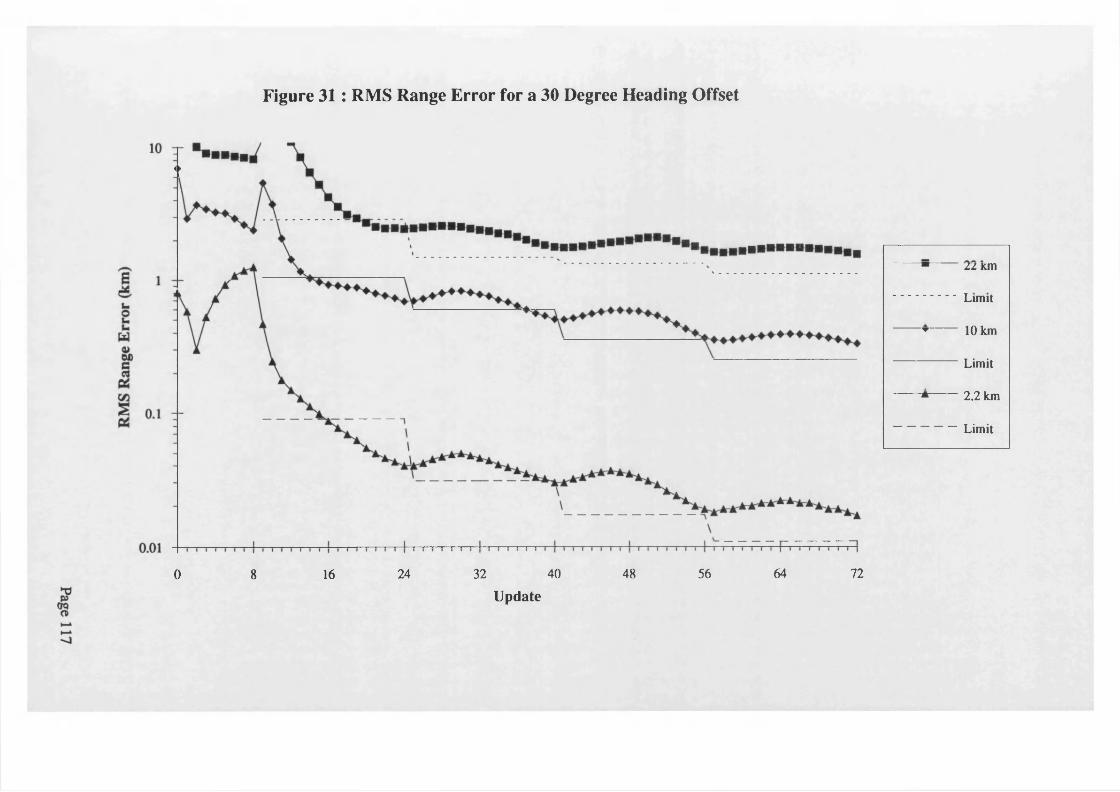
Figure 31: RMS Range Error for a 30 Degree Heading Offset

< >

7232 40 48 56 6416 240 8

m L i Km

. — * -

Limit

1 a 1w 10 km

Limit

A 2.2 km

Limit

Update

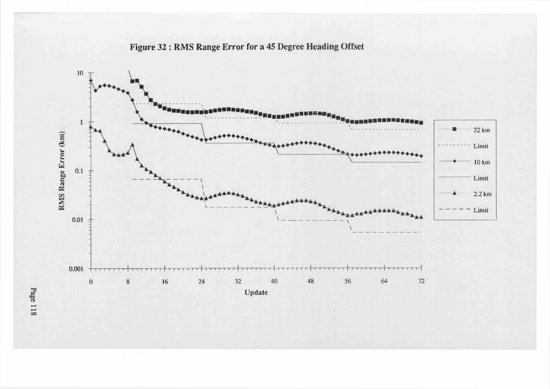
RMS

Rang

e Er

ror

(km

)

Figure 32 : RMS Range Error for a 45 Degree Heading Offset

10

!■■■!

0.1

7240 48 56 64328 16 240

■1 zz Km

▲

Limit

W 10 km

A

Limit

m 2.2 km

Limit

Update

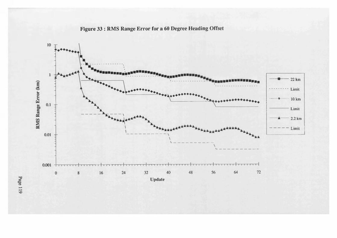
Figure 33 : RMS Range Error for a 60 Degree Heading Offset

..............................

* * * .

7256 6440 483224160 8

LL Km

L i m a

▼ i u Km

A

Limit

A 2.2 km

Limit

Update

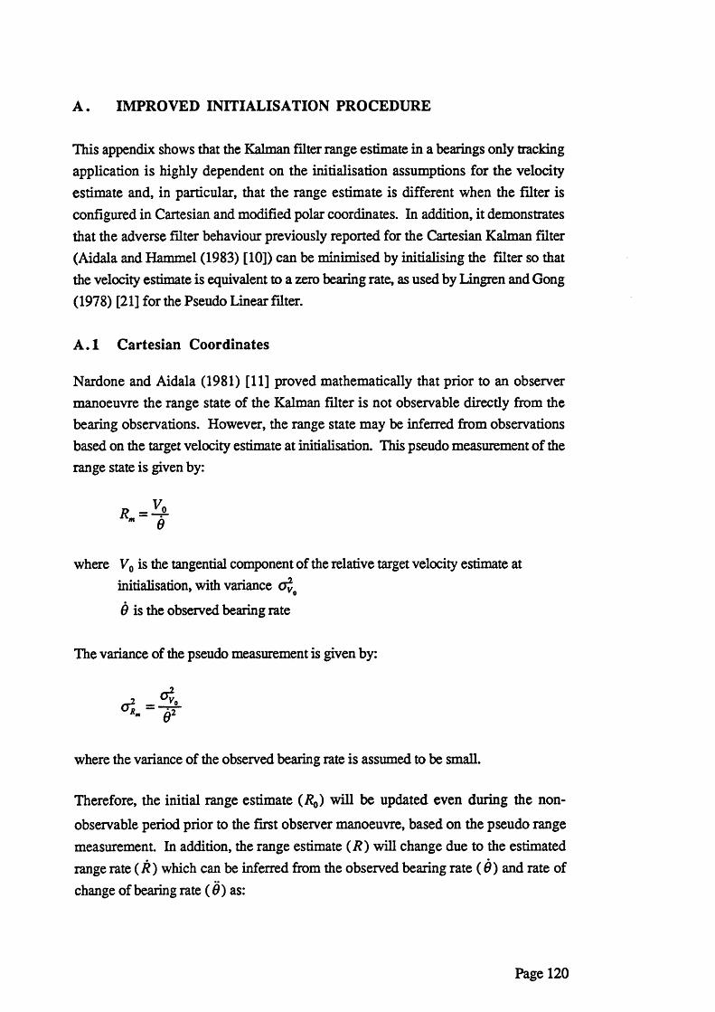
A . IMPROVED INITIALISATION PROCEDURE

This appendix shows that the Kalman filter range estimate in a bearings only tracking application is highly dependent on the initialisation assumptions for the velocity estimate and, in particular, that the range estimate is different when the filter is configured in Cartesian and modified polar coordinates. In addition, it demonstrates that the adverse filter behaviour previously reported for the Cartesian Kalman filter (Aidala and Hammel (1983) [10]) can be minimised by initialising the filter so that the velocity estimate is equivalent to a zero bearing rate, as used by lingren and Gong (1978) [21] for the Pseudo Linear filter.

A . l Cartesian Coordinates

Nardone and Aidala (1981) [11] proved mathematically that prior to an observer manoeuvre the range state of the Kalman filter is not observable directly from the bearing observations. However, the range state may be inferred from observations based on the target velocity estimate at initialisation. This pseudo measurement of the range state is given by:

where V0 is the tangential component of the relative target velocity estimate at initialisation, with variance cj}g

0 is the observed bearing rate

The variance of the pseudo measurement is given by:

where the variance of the observed bearing rate is assumed to be small.

Therefore, the initial range estimate (Rq) will be updated even during the non-

observable period prior to the first observer manoeuvre, based on the pseudo range measurement. In addition, the range estimate (R) will change due to the estimated range rate (R) which can be inferred from the observed bearing rate (0 ) and rate of change of bearing rate ( 0 ) as:

Page 120

However, in this section it is assumed that the range rate is zero, in order to simplify the analysis. Thus the range estimate generated by the Kalman filter is only a combination of the initial range estimate ( R q ) and the pseudo range measurement.

Ho and Lee (1964) [57] proved mathematically that the Kalman filter, with independent Gaussian noise, generates a Least Squares Estimate (LSE) as the variance weighted sum of the prior estimate and observation, such that:

— = * 0 +0 *

i _ i i<4 ~ < + < 4

where Rq is the initial range estimate with variance cr o

Substituting for Rm and <7 ^ leads to the following expressions for the range estimate

and variance of a Cartesian Kalman filter:

R = *o Gy0 + <6 2 a t + o i

c 2 = —6 2 o i + a t

In order to give satisfactory operation of the Kalman filter during the non-observable period prior to the first observer manoeuvre, the range estimate should remain positive and should be of the same order of magnitude as the initial range estimate. It is apparent in the above expression that if the tangential velocity estimate at initialisation (V0) is large and is of opposite sign to the observed bearing rate, such

that:

then the range estimate will become negative, and this usually precipitates failure of the tracker.

The approach adopted in this thesis is to set the initial velocity estimate equal to the observer velocity, such that V0 is zero, since this prevents the range estimate

becoming negative regardless of the sign or magnitude of the observed bearing rate. The range estimate is then given by:

R = -------& -------□2 *01 + & —

a t

2 Ojla i = -------^i + e > * L

%

The reduction in the range estimate from the initialisation value will be small provided that the coefficient of variation for the range estimate is small compared with the coefficient of variation for the tangential velocity estimate:

O’,«R |fl0|

A .2 Modified Polar Coordinates

Applying the analysis of the previous section to a Kalman filter configured in modified polar coordinates leads to pseudo measurement of the j state as:

-L = AV,

where V0 is the tangential component of the relative target velocity estimate at initialisation, with variance o jo

6 is the observed bearing rate

The variance of this pseudo measurement is given by:

Page 122

where again it is assumed that the variance of the observed bearing rate is small.

The Kalman filter estimate is given by the variance weighted sum of the prior estimate and pseudo measurement derived from the observations, such that:

j_ _L _ L... ft , — R° , 4. ..

R Rq Rm

° i ~ ° 1 + ° 1R Rq Rm

where is the initial estimate with variance

Substituting for and <j \_ leads to the following expressions for the j estimate and

variance of a Modified Polar Kalman filter

As in the case of the Cartesian Kalman filter, if the tangential velocity estimate at initialisation ( V0) is large and is of opposite sign to the observed bearing rate, such

that:

V 3yoe

- 1

RnRn

then the range estimate for the Modified Polar Kalman filter will become negative, and again this usually precipitates failure of the tracker.

The approach adopted in this thesis is to set the initial velocity estimate equal to the observer velocity, such that V0 is zero, since this prevents the range estimate

Page 123

becoming negative regardless of the sign or magnitude of the observed bearing rate. The range estimate for the Modified Polar Kalman filter is then given by:

R ~ R o

° i =g r0

This initialisation procedure for the Modified Polar Kalman filter is the same as used by Aidala andHammel (1983) [10].

Page 124

B . DERIVATION OF GLR PROCEDURE

This appendix derives the Generalised Likelihood Ratio (GLR) procedure which has been used in Section 4 of this thesis to detect a target manoeuvre and, subsequently, to correct the state vector for the manoeuvre. The derivation uses a similar approach to Korn, Gully and Willsky (1982) [35] for the detection statistic. However, the method of correction proposed in this thesis is slightly different, and has proved to be more robust for the detection of small manoeuvres where the peak in the likelihood function for the estimate of the time of the manoeuvre is small.

B . l Effect of Manoeuvre on System Model

A target manoeuvre at update j is characterised by an additive change a klj to the

state vector at time k given by:

where Xk/0 is the true state vector at update k when there is no manoeuvre Xu, is the true state vector at update k for a manoeuvre at update j a klj is the additive change at update k for a manoeuvre at update j

The measurement vector associated with the manoeuvre is given by:

where Xu, is the measurement vector at update k for a manoeuvre at update j Mk is the measurement matrixNk is the measurement noise with zero mean and covariance matrix S* k

The innovation vector (Ik/j) associated with the manoeuvre is defined by:

where Xk/j is the forecast state vector at update k for a manoeuvre at update j

%-k/j — Xm + ocklj (* > j )

Xu, = Xkl! +Equation B.l

Equation B.2

The Kalman filter update equations will adapt the estimated state vector (Xklj) to the

manoeuvre so that, at update k , it is given by:

Page 125

^ k / j ~ * k,0 "*■ P kf j

Awhere X*,o is the estimated state vector at update k for no manoeuvre

pklJ is the change in the state vector estimate, as defined by this equation

The state vector forecast is related to the previous state vector estimate by the following non-linear state transition equation:

Xk/j — fk-l (- k-l/j) = /* -l(* * -l/0 + Pk-llj)

where f k_: is the non-linear state transition function.

The state transition function can be linearised around the estimated state using a first order Taylor expansion, since it is assumed that the change in the state vector estimate prior to manoeuvre detection is small. The linearised state transition equation is given by:

X ku ~ fk-i(Xk-w) Fk-i Pk-ifj = Xk,o+ Fk-\ Pk-iij EquationB.3

where Fk_x is the Jacobian matrix of f k_x.

Combining Equations B.l, B.2 and B.3 gives the innovation vector associated with the manoeuvre as:

^ktj = M k (Xk/0 + cck/j) + N k — M k (Xk/0 + Fk_x Pk_uj)

= M k X k/0 + N k — M k X k/0 + M k ( cck/j — Fk_x P k-u j)

= ^k/0 + ( & k/ j ~ F k_! P t - l f j )

where Ik/0 is the innovation vector for no manoeuvre.

The difference between the innovation vectors when there has been a manoeuvre and when there has been no manoeuvre is given by:

Pk/j = ^kij ~Ik/o = (cckfj — Fk_i py-uj) Equation B.4

This parameter is also the expected innovation for a target manoeuvre, since the expected innovation for no manoeuvre is zero.

Page 126

The parameter Pklj» which is the difference between the state vector estimates with

and without a manoeuvre, can be calculated recursively using the Kalman updating equations, given in Section 1.2:

where Kk is the Kalman smoothing parameter

At the time of the manoeuvre the recursion is initialised with Pj/j - o and pJ+l/J is set using Equation B.4.

B .2 Likelihood Ratio Test

The likelihood ratio test, performs a test of the hypothesis that a manoeuvre occurred at update j (Y,. = YUJ} against the null hypothesis that no manoeuvre occurred atupdate j (Yi = Yi/0). The log-likelihood ratio (sk) associated with this test being

earned out at update k is given by:-

where Yi is the measurement vector at update i

It is assumed in the log-likelihood ratio that the measurements are independent If, in addition, it is assumed that the process is Gaussian, then the log-likelihood ratio can be recast in terms of the likelihood of the innovation sequence:

The Gaussian assumption is a reasonable provided that the bearing measurement errors are Gaussian and that the EKF linearisation errors are small.

where /, is the innovation vector at update i

Page 127

The probability density function for the innovation sequence is given by:

when there is no manoeuvre and by:

P^ ‘ = = 1/(2 ^d e t(V j) eXPl “ ^ ~ Pu') V‘ '

when a manoeuvre occurs at update j .

where r is the dimension of the innovation vectorVt- is the covariance matrix for the innovation vector given by:

V, = M. P: M j + S:

Thus, the log-likelihood ratio becomes:

* = - \ i [b-pujfvfb-puj)-*!v-'i,2 i=j+1

s>= i p I , v-1 /, - \ t p !,j vr1 pi/ji- j+ l «=j+1

Equation B.5

B .3 Generalised Likelihood Ratio Test

The Generalised Likelihood Ratio (GLR) test extends the applicability of the likelihood ratio test, by replacing unknown parameters with their Maximum Likelihood Estimates (MLE). In the case of a manoeuvring target the unknown parameters are the manoeuvre magnitude and the time of the manoeuvre. The MLE for the manoeuvre time is determined by calculating the log-likelihood ratio for all manoeuvre times (k - h < j < k - 1 ) and choosing the maximising value.

The MLE for the manoeuvring magnitude is determined by expressing the log- likelihood ratio in terms of the known dynamic profile for a unit manoeuvre ( ocUj)

scaled by the unknown manoeuvre magnitude (U ). In the case of the bearings only tracking problem this corresponds to stating the dynamic profile of the manoeuvre is a

Page 128

ramp change in the bearing observations, which is caused by a step change in the bearing rate of unknown magnitude U .

Decomposing the change parameters into unitised parameters scaled by the unknown magnitude U , allows the log-likelihood ratio in Equation B.5 to be rewritten as:

2 *= - - ^ r l PZj VT'Pvj

i=y+l ^ i=/'+lEquation B . 6

where the unitised parameters a ilJ9 PUj and pUJ are given by:

«/« = u a ui A It ~ U A /;Hi Pi/j ~ U Pilj

The MLE of the manoeuvre magnitude (Uklj) can be determined by differentiation of

the log-likelihood ratio and equating to zero:

- u £ phj V,- piU = 0

i-y+i

I Pin hu = ,‘=-y+1

X PuiV?PiUi=y+1

Substitution of into Equation B. 6 leads to the generalised log-likelihood ratio

given by:

max sup r l6 k k-hZj&k-l U \ r k l j \

8k =X Pin vr11.*=;+i

X A/; A' 1 A,Equation B.7

B .4 Alternative Derivation of Decision Statistic

The variance of MLE of manoeuvre magnitude (Uklj) is given by:

Page 129

= £K ] - (4 M J

where E is the expectation operator

Since it has been assumed that the innovation vector is Gaussian then Ukfj will alsoA

be Gaussian with mean U . Substituting for Uklj in this expression and replacing I. by hlQ + U pUJ gives:

r ± K v i ' i u + u p J

2 Puj Pm\ *=;+i

- U7

c I = E' t Puj V71 A/o + ^ 2 P u j V P u 'i=j+ 1________________ i=;+l_________

t PSj V- 1 puj»=y+i

Since the innovation for no manoeuvre Iil0 is independent with zero mean then

4 /</o]=° E [/.VO = 0 £ [/.vo 4 ] = V,

and hence:

2 A« v r 1 V,. V-' pma t = !=& ---------------------

2 Puj *7* Puj»•=;+!

_2 _ 1______^k,j —7 T/_i —

X Puj v i Puji=j+ 1

The decision statistic for the GLR test given by Equation B.7 can therefore be written as:

Page 130

2 Sk/j “‘•=7+1

i/0

I AL V f piU*=7+1

2 Sk/j —u 2

*/y j

The decision statistic which has been used in this thesis is:

Gt = [ 2 gt ]Vi

Since this will have approximately a N [0,1] Normal distribution in the case of no

Umanoeuvre, and a N * , 1 Normal distribution in the case of manoeuvre.

B . 5 Manoeuvre Correction

Following manoeuvre detection the state vector estimate is corrected based on the estimate of the time and the magnitude of the manoeuvre.

k/j ~ Jfc/0 + U k / j a k/ j

- % k i j + & ki j ( a k/ j P k / j )

Hu - Pk/j + gqu. {ak/j Pk/j) (ak/j Pk/j)

where XklJ and Pklj are the state vector and covariance matrix prior to manoeuvre

correction.

Since the time of the manoeuvre is described by a discrete distribution for the likelihood of all possible manoeuvre times over a track history of h, then the corrected state vector is then given by:

Page 131

% lj K jY — j - k-h

Man ~~ k- 1

I L,j=k—h

I h [hr, + Kj *5)D j - k-h__________________________ _ y- y ir Man ~ k- 1 ^Man

Z L jj - k-h

where L} is the likelihood ratio for a manoeuvre at update j given by:

Lj = exp{ gtlj }

This is different to the approach used by Korn, Gully and Willsky (1982) [35], since they use only the single MLE of the manoeuvre time to update the state and covariance matrix instead of using the likelihood weighted sum over all manoeuvre times. The later approach used in this thesis has proved to be more robust for the detection of small manoeuvres where the peak in the likelihood function for the estimate of the manoeuvre time is small. The updated state and covariance matrix is sensitive to errors in the estimate of the manoeuvre time and this can lead to significant bias, which may result in multiple triggers of the manoeuvre detection procedure.

Page 132